Figure 7.13
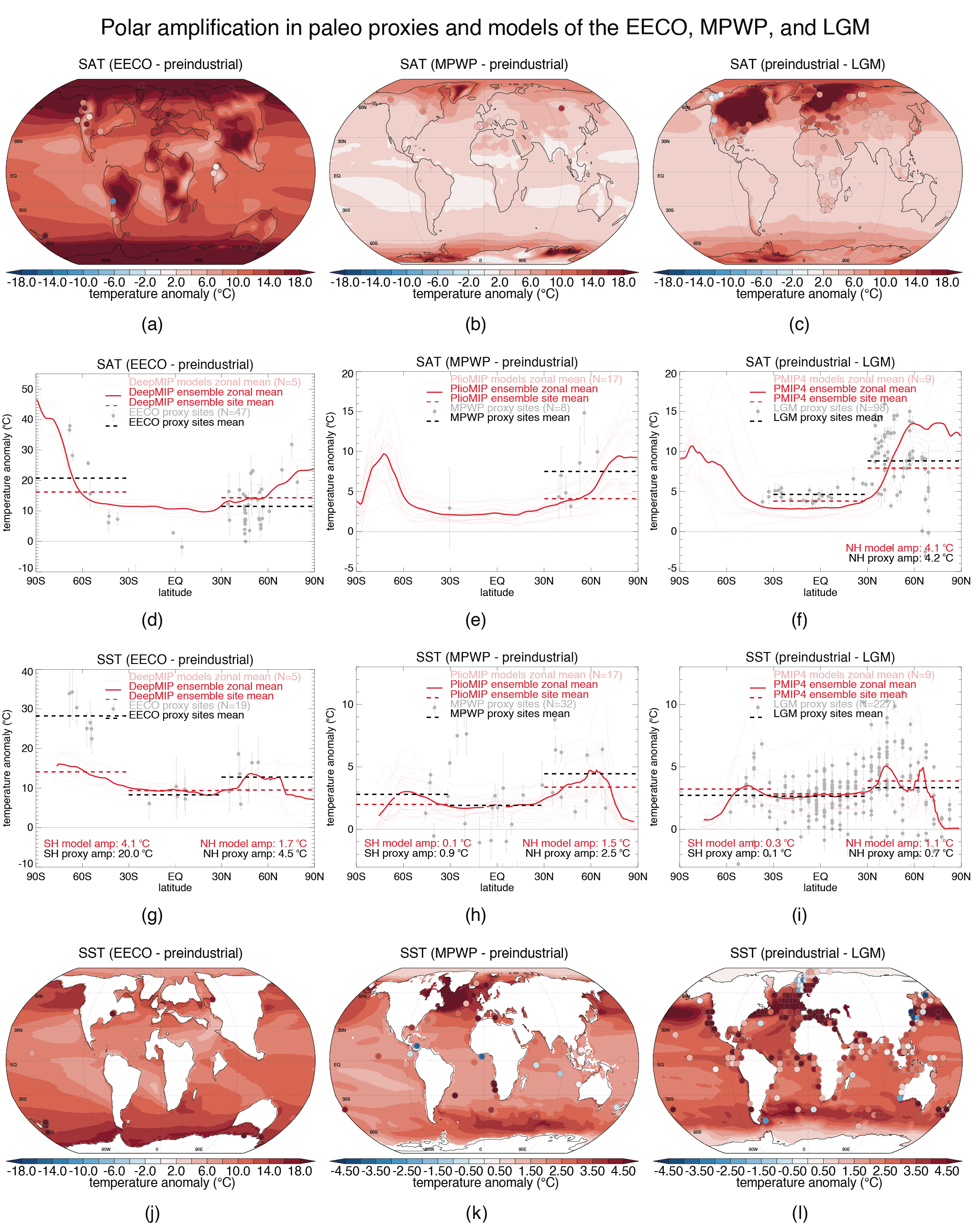
Figure caption
Temperature anomalies compared with pre-industrial (equivalent to CMIP6 simulation ‘piControl’) are shown for the high-CO2 EECO and MPWP time periods, and for the low-CO2 LGM (expressed as pre-industrial minus LGM). (a), (b) and (c) Modelled near-surface air temperature anomalies for ensemble-mean simulations of the (a) EECO (Lunt et al., 2021); (b) MPWP (Haywood et al., 2020; Zhang et al., 2021); and (c) LGM (Kageyama et al., 2021; Zhu et al., 2021). Also shown are proxy near-surface air temperature anomalies (coloured circles). (d), (e) and (f) Proxy near-surface air temperature anomalies (grey circles), including published uncertainties (grey vertical bars), model ensemble mean zonal mean anomaly (solid red line) for the same model ensembles as in (a–c), light-red lines show the modelled temperature anomaly for the individual models that make up each ensemble (LGM, N=9; MPWP, N=17; EECO, N=5). Black dashed lines show the average of the proxy values in each latitude band: 90°S–30°S, 30°S–30°N, and 30°N–90°N. Red dashed lines show the same banded average in the model ensemble mean, calculated from the same locations as the proxies. Black and red dashed lines are only shown if there are five or more proxy points in that band. Mean differences between the 90°S/N to 30°S/N and 30°S to 30°N bands are quantified for the models and proxies in each plot. Panels (g), (h) and (i) are like panels (d–f) but for sea surface temperature (SST) instead of near-surface air temperature. Panels (j), (k) and (l) are like panels (a–c) but for SST instead of near-surface air temperature. For the EECO maps – (a) and (j) – the anomalies are relative to the zonal mean of the pre-industrial, due to the different continental configuration. Proxy datasets are: (a) and (d) Hollis et al. (2019); (b) and (e) Salzmann et al. (2013); Vieira et al. (2018), (c) and (f) Cleator et al. (2020) at the sites defined in Bartlein et al. (2011); (g) and (j) Hollis et al. (2019); (h) and (k) McClymont et al. (2020); (i) and (l) Tierney et al. (2020b). Where there are multiple proxy estimations at a single site, a mean is taken. Model ensembles are (a), (d), (g) and (j) DeepMIP (only model simulations carried out with a mantle-frame paleogeography, and carried out under CO2 concentrations within the range assessed in Table 2.2, are shown); (b), (e), (h) and (k) PlioMIP; and (c), (f), (i) and (l) PMIP4. Further details on data sources and processing are available in the chapter data table (Table 7.SM.14).