Figure 1.17

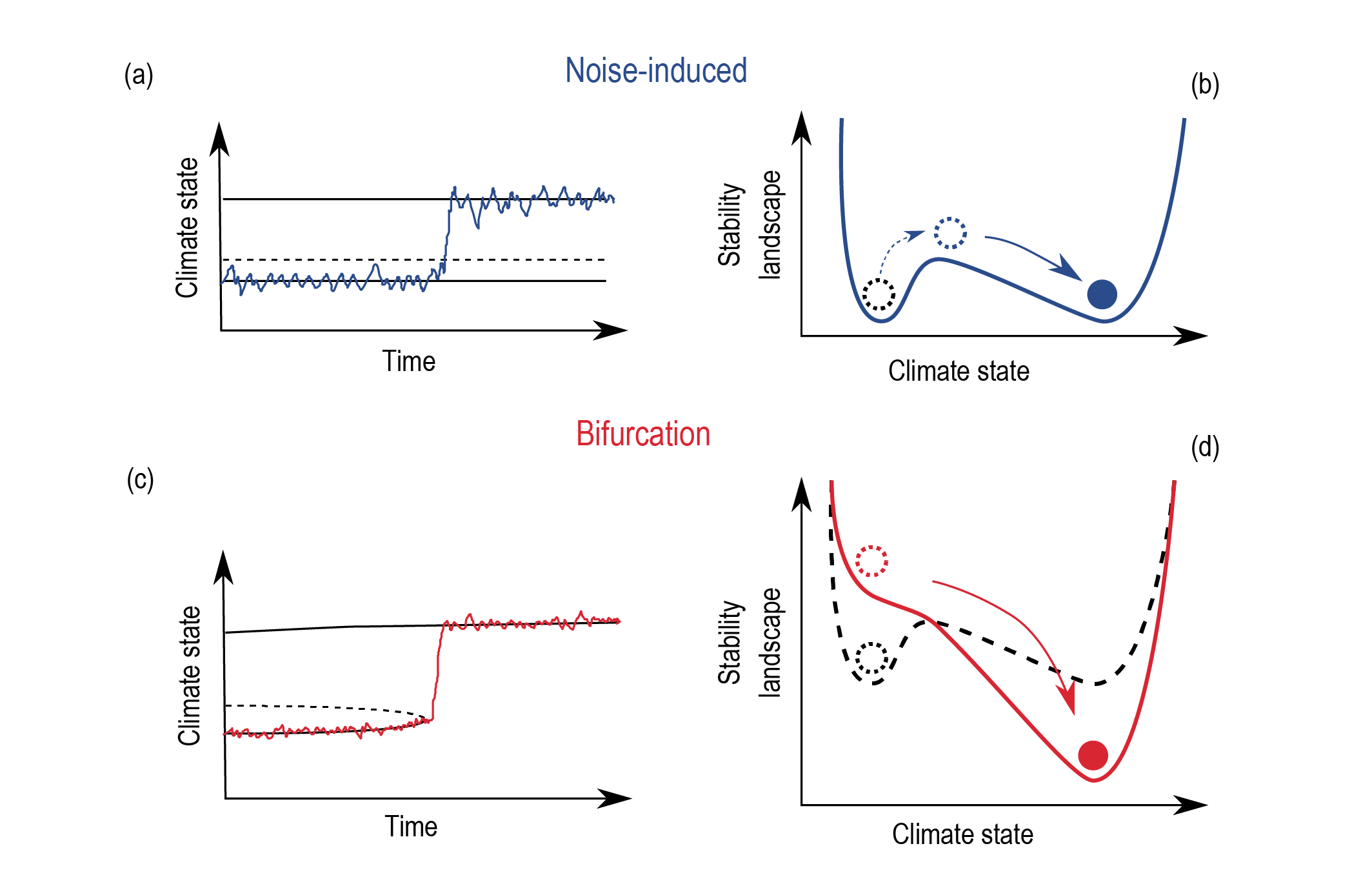
Figure caption

Figure 1.17 | Illustration of two types of tipping points: noise-induced (a, b) and bifurcation (c, d). (a) and (c) are example time-series (coloured lines) through the tipping point, with solid-black lines indicating stable climate states (e.g., low or high rainfall) and dashed lines representing the boundary between stable states. (b) and (d) are stability landscapes, which provide an intuitive understanding of the different types of tipping point. The ‘valleys’ represent different climate states the system can occupy, with ‘hilltops’ separating the stable states. The resilience of a climate state is implied by the depth of the valley. The current state of the system is represented by a ball. Both scenarios assume that the ball starts in the left-hand valley (dashed-black lines) and then through different mechanisms dependent on the type of tipping transitions to the right-hand valley (coloured lines). Noise-induced tipping events (a, b), for instance drought events causing sudden dieback of the Amazon rainforest, develop from fluctuations within the system. The stability landscape in this scenario remains fixed and stationary. A series of perturbations in the same direction, or one large perturbation, are required to force the system over the hilltop and into the alternative stable state. Bifurcation tipping events (c, d), such as a collapse of the thermohaline circulation in the Atlantic Ocean under climate change, occur when a critical level in the forcing is reached. Here the stability landscape is subjected to a change in shape. Under gradual anthropogenic forcing the left-hand valley begins to shallow and eventually vanishes at the tipping point, forcing the system to transition to the right-hand valley.