Figure 10.19

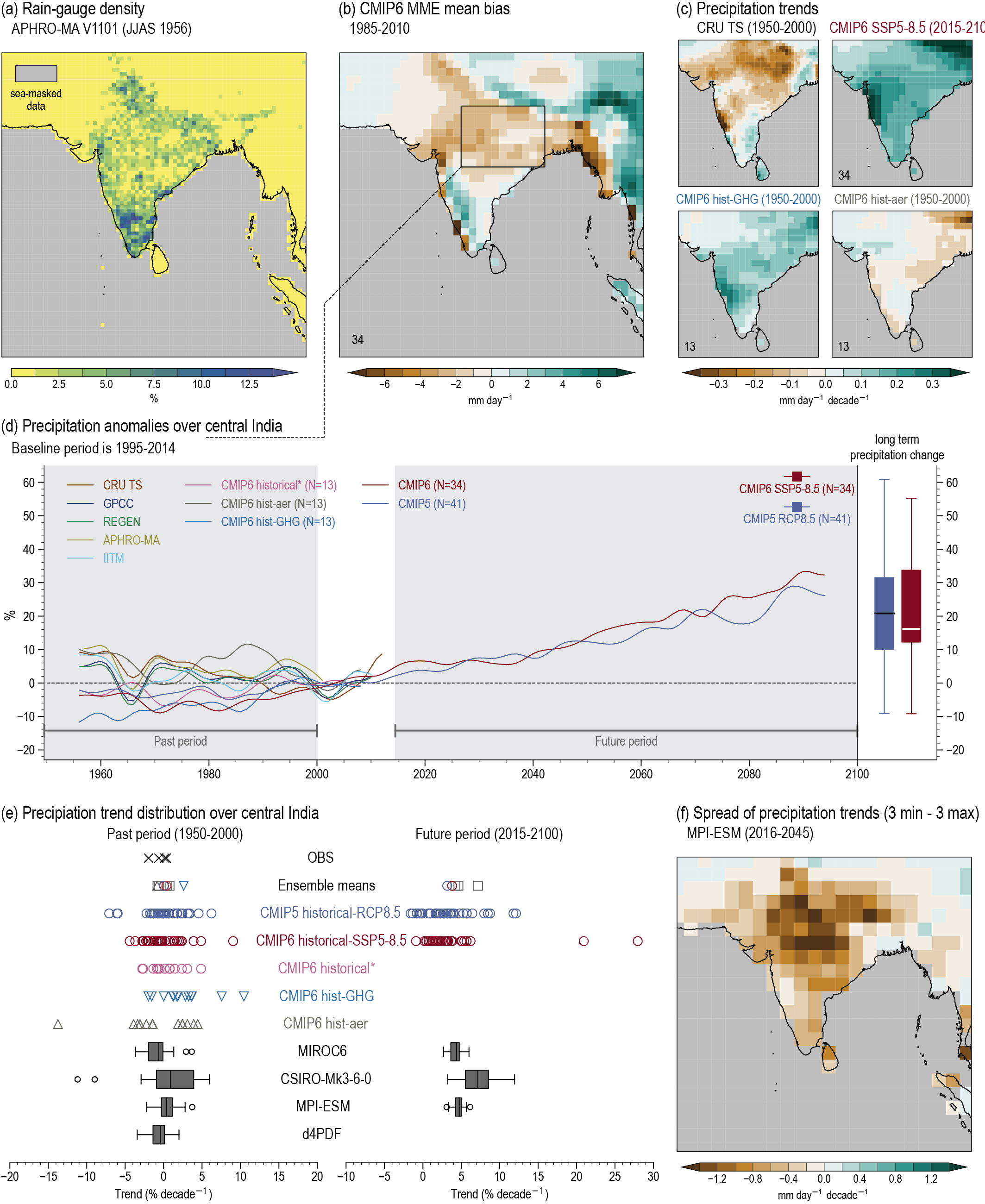
Figure caption

Figure 10. 19 | Changes in the Indian summer monsoon in the historical and future periods. Observational uncertainty demonstrated by a snapshot of rain-gauge density (% of 0.05° subgrid boxes containing at least one gauge) in the APHRO-MA 0.5° daily precipitation dataset for June to September 1956. (b) Multi-model ensemble (MME) mean bias of 34 CMIP6 models for June to September precipitation (mm day^–1) compared to CRU TS observations for the 1985–2010 period. (c) Maps of rainfall trends (mm day^–1 per decade) in CRU TS observations (1950–2000), the CMIP6 MME-mean of SSP5-8.5 future projections for 2015–2100 (34 models), the CMIP6 hist-GHG and hist-aer runs, both measured over 1950 to 2000. (d) Low-pass filtered time series of June to September precipitation anomalies (%, relative to 1995–2014 baseline) averaged over the central India box shown in panel (b). The averaging region (20°N–28°N, 76°E–87°E) follows other works (Bollasina et al., 2011; Jin and Wang, 2017; Huang et al., 2020b). Time series are shown for CRU TS (brown), GPCC (dark blue), REGEN (green), APHRO-MA (light brown) observational estimates and the IITM all-India rainfall product (light blue) in comparison with the CMIP6 mean of 13 models for the all-forcings historical (pink) the aerosol-only (hist-aer, grey) and greenhouse gas-only (hist-GHG, blue). Dark red and blue lines show low-pass filtered MME-mean change in the CMIP6 historical/SSP5-8.5 (34 models) and CMIP5 historical/RCP8.5 (41 models) experiments for future projections to 2100. The filter is the same as that used in Figure 10.11 (d). To the right, box-and-whisker plots show the 2081–2100 change averaged over the CMIP5 (blue) and CMIP6 (dark red) ensembles. Note that some models exceed the plotting range (CMIP5: GISS-E2-R-CC, GISS-E2-R, IPSL-CM5B-LRl and CMIP6: CanESM5-CanOE, CanESM5 and GISS-E2-1-G). (e) Precipitation linear trend (% per decade) over Central India for historical 1950–2000 (left) and future 2015–2100 (right) periods in Indian Monsoon rainfall in observed estimates (black crosses), the CMIP5 historical-RCP8.5 simulations (blue), the CMIP6 ensemble (dark red) for historical all-forcings experiment and SSP5-8.5 future projection, the CMIP6 hist-GHG (light blue triangles), hist-aer (grey triangles) and historical all-forcings (same sample as for hist-aer and hist-GHG, pink circles). Ensemble means are also shown. Box-and-whisker plots show the trend distribution of the three coupled and the d4PDF atmosphere-only (for past period only) SMILEs used throughout Chapter 10 and follow the methodology used in Figure 10.6. (f) Example spread of trends (mm day^–1 per decade) for the period 2016–2045 in RCP8.5 SMILE experiments of the MPI-ESM model, showing the difference between the three driest and three wettest trends among ensemble members over central India. All trends are estimated using ordinary least-squares regression. Further details on data sources and processing are available in the chapter data table (Table 10.SM.11).