Figure 4.38

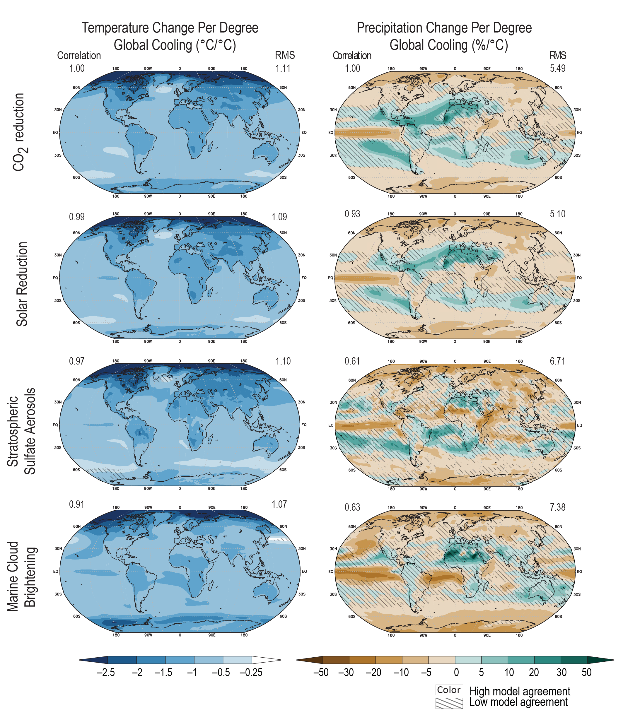
Figure caption

Figure 4.38 | Multi-model response per degree global mean cooling in temperature and precipitation in response to CO₂ forcing and SRM forcing. Top row shows the response to a CO₂ decrease, calculated as the difference between pre-industrial control simulation and abrupt4xCO2 simulations where the CO₂ concentration is quadrupled abruptly from the pre-industrial level (11-model average); second row shows the response to a globally uniform solar reduction, calculated as the difference between GeoMIP experiment G1 and abrupt4xCO2 (11-model average); third row shows the response to stratospheric sulphate aerosol injection, calculated as the difference between GeoMIP experiment G4 (a continuous injection of 5 Tg SO₂ year^–1 at one point on the equator into the lower stratosphere against the RCP4.5 background scenario) and RCP4.5 (six-model average); and The bottom row shows the response to marine cloud brightening, calculated as the difference between GeoMIP experiment G4cdnc (increase cloud droplet concentration number in marine low cloud by 50% over the global ocean against RCP4.5 background scenario) and RCP4.5 (eight-model average). All differences (average of years 11–50 of simulation) are normalized by the global mean cooling in each scenario, averaged over years 11–50. Diagonal lines represent regions where fewer than 80% of the models agree on the sign of change. The values of correlation represent the spatial correlation of each SRM-induced temperature and precipitation change pattern with the pattern of change caused by a reduction of atmospheric CO₂. RMS (root mean square) is calculated based on the fields shown in the maps (normalized by global mean cooling). Further details on data sources and processing are available in the chapter data table (Table 4.SM.1).