Figure 5.28

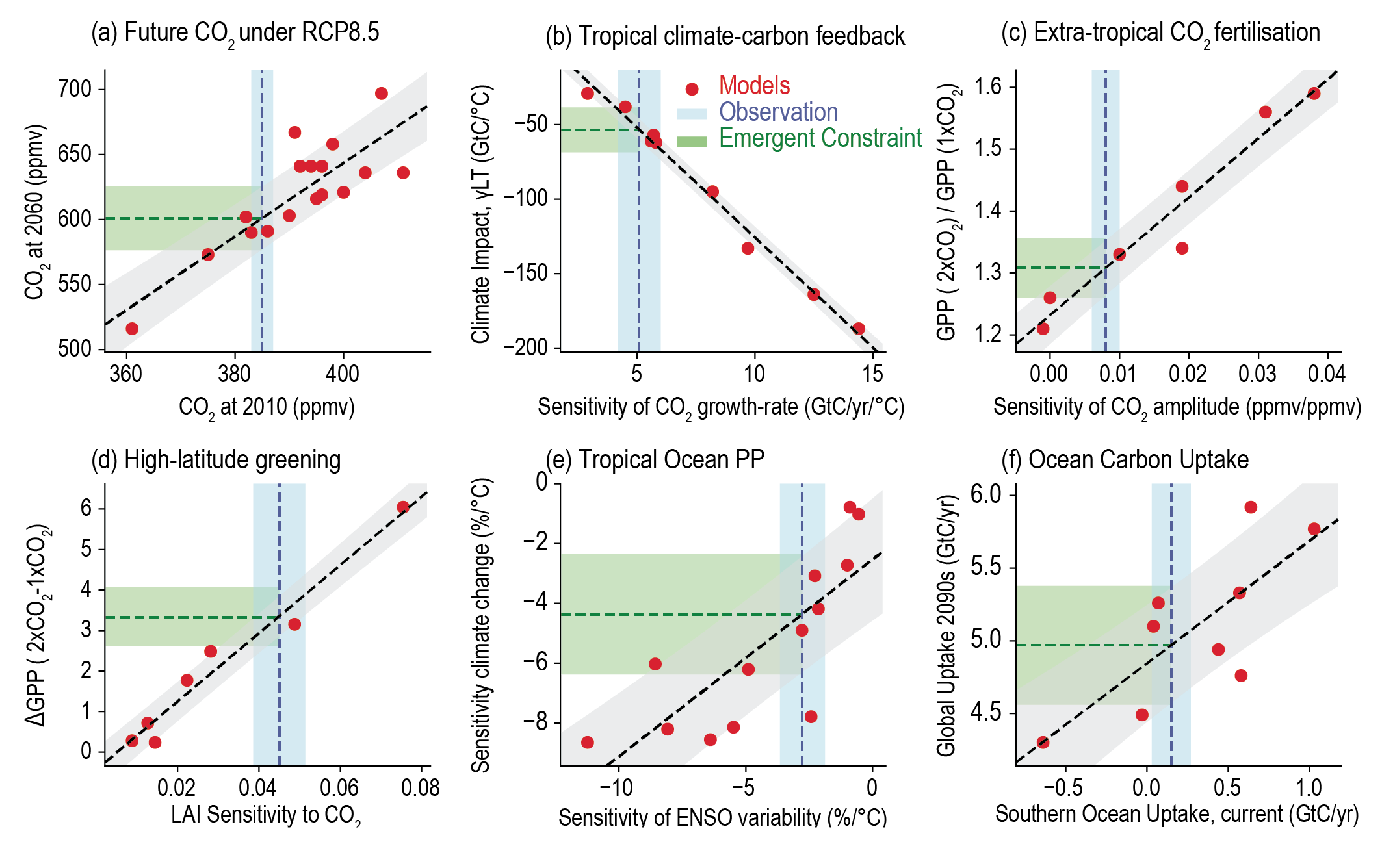
Figure caption

Figure 5.28 | Examples of emergent constraints on the carbon cycle in Earth system models (ESMs), reproduced from previously published studies: (a) projected global mean atmospheric carbon dioxide (CO₂) concentration by 2060 under the RCP8. 5 emissions scenario against the simulated CO₂ in 2010 (Friedlingstein et al., 2014b; Hoffman et al., 2014); (b) sensitivity of tropical land carbon to warming (γ _LT) against the sensitivity of the atmospheric CO₂ growth-rate to tropical temperature variability (Cox et al., 2013; Wenzel et al., 2014); (c) sensitivity of extratropical (30°N–90°N) gross primary production to a doubling of atmospheric CO₂ against the sensitivity of the amplitude of the CO₂ seasonal cycle at Kumkahi, Hawaii to global atmospheric CO₂ concentration (Wenzel et al., 2016); (d) change in high-latitude (30°N–90°N) gross primary production versus trend in high-latitude leaf area index or ‘greenness’ (Winkler et al., 2019); (e) sensitivity of the primary production of the Tropical Ocean to climate change versus its sensitivity to El Niño–Southern Oscillation (ENSO)-driven temperature variability (Kwiatkowski et al., 2017); (f) global ocean carbon sink in the 2090s versus the current-day carbon sink in the Southern Ocean. In each case, a red dot represents a single ESM projection, the grey bar represents the emergent relationship between the y-variable and the x-variable, the blue bar represents the observational estimate of the x-axis variable, and the green bar represents the resulting emergent constraint on the y-axis variable. The thicknesses represent ± one standard error in each case. Figure after Cox (2019). Further details on data sources and processing are available in the chapter data table (Table 5.SM.6).