Chapter 3: Oceans and Coastal Ecosystems and their Services


This chapter should be cited as:
Cooley, S., D. Schoeman, L. Bopp, P. Boyd, S. Donner, D.Y. Ghebrehiwet, S.-I. Ito, W. Kiessling, P. Martinetto, E. Ojea, M.-F. Racault, B. Rost, and M. Skern-Mauritzen, 2022: Oceans and Coastal Ecosystems and Their Services. In: Climate Change 2022: Impacts, Adaptation and Vulnerability. Contribution of Working Group II to the Sixth Assessment Report of the Intergovernmental Panel on Climate Change [H.-O. Pörtner, D.C. Roberts, M. Tignor, E.S. Poloczanska, K. Mintenbeck, A. Alegría, M. Craig, S. Langsdorf, S. Löschke, V. Möller, A. Okem, B. Rama (eds.)]. Cambridge University Press, Cambridge, UK and New York, NY, USA, pp. 379–550, doi:10.1017/9781009325844.005.
Executive Summary 
Ocean and coastal ecosystems support life on Earth and many aspects of human well-being. Covering two-thirds of the planet, the ocean hosts vast biodiversity and modulates the global climate system by regulating cycles of heat, water and elements, including carbon. Marine systems are central to many cultures, and they also provide food, minerals, energy and employment to people. Since previous assessments 1 , new laboratory studies, field observations and process studies, a wider range of model simulations, Indigenous knowledge, and local knowledge have provided increasing evidence on the impacts of climate change on ocean and coastal systems, how human communities are experiencing these impacts, and the potential solutions for ecological and human adaptation.
Observations: vulnerabilities and impacts
Anthropogenic climate change has exposed ocean and coastal ecosystems to conditions that are unprecedented over millennia (high confidence2 ), and this has greatly impacted life in the ocean and along its coasts (very high confidence). Fundamental changes in the physical and chemical characteristics of the ocean acting individually and together are changing the timing of seasonal activities (very high confidence), distribution (very high confidence) and abundance (very high confidence) of oceanic and coastal organisms, from microbes to mammals and from individuals to ecosystems, in every region. Evidence of these changes is apparent from multi-decadal observations, laboratory studies and mesocosms, as well as meta-analyses of published data. Geographic range shifts of marine species generally follow the pace and direction of climate warming (high confidence): surface warming since the 1950s has shifted marine taxa and communities poleward at an average (mean ±very likely 3 range) of 59.2 ± 15.5 km per decade (high confidence), with substantial variation in responses among taxa and regions. Seasonal events occur 4.3 ± 1.8 d to 7.5 ± 1.5 d earlier per decade among planktonic organisms (very high confidence) and on average 3 ± 2.1 d earlier per decade for fish (very high confidence). Warming, acidification and deoxygenation are altering ecological communities by increasing the spread of physiologically suboptimal conditions for many marine fish and invertebrates (medium confidence). These and other responses have subsequently driven habitat loss (very high confidence), population declines (high confidence), increased risks of species extirpations and extinctions (medium confidence) and rearrangement of marine food webs (medium to high confidence, depending on ecosystem). {3.2, 3.3, 3.3.2, 3.3.3, 3.3.3.2, 3.4.2.1, 3.4.2.3–3.4.2.8, 3.4.2.10, 3.4.3.1, 3.4.3.2, 3.4.3.3, Box 3.2}
Marine heatwaves lasting weeks to several months are exposing species and ecosystems to environmental conditions beyond their tolerance and acclimation limits (very high confidence). WGI AR6 concluded that marine heatwaves are more frequent (high confidence), more intense and longer (medium confidence) since the 1980s, and since at least 2006very likely attributable to anthropogenic climate change. Open-ocean, coastal and shelf-sea ecosystems, including coral reefs, rocky shores, kelp forests, seagrasses, mangroves, the Arctic Ocean and semi-enclosed seas, have recently undergone mass mortalities from marine heatwaves (very high confidence). Marine heatwaves, including well-documented events along the west coast of North America (2013–2016) and east coast of Australia (2015–2016, 2016–2017 and 2020), drive abrupt shifts in community composition that may persist for years (very high confidence), with associated biodiversity loss (very high confidence), collapse of regional fisheries and aquaculture (high confidence) and reduced capacity of habitat-forming species to protect shorelines (high confidence). {WGI AR6 Chapter 9, 3.2.2.1, 3.4.2.1–3.4.2.5, 3.4.2.7, 3.4.2.10, 3.4.2.3, 3.4.3.3.3, 3.5.3}
At local to regional scales, climate change worsens the impacts on marine life of non-climate anthropogenic drivers, such as habitat degradation, marine pollution, overfishing and overharvesting, nutrient enrichment and introduction of non-indigenous species (very high confidence). Although impacts of multiple climate and non-climate drivers can be beneficial or neutral to marine life, most are detrimental (high confidence). Warming exacerbates coastal eutrophication and associated hypoxia, causing ‘dead zones’ (very high confidence), which drive severe impacts on coastal and shelf-sea ecosystems (very high confidence), including mass mortalities, habitat reduction and fisheries disruptions (medium confidence). Overfishing exacerbates effects of multiple climate-induced drivers on predators at the top of the marine food chain (medium confidence). Urbanisation and associated changes in freshwater and sediment dynamics increase the vulnerability of coastal ecosystems like sandy beaches, salt marshes and mangrove forests to sea level rise and changes in wave energy (very high confidence). Although these non-climate drivers confound attribution of impacts to climate change, adaptive, inclusive and evidence-based management reduces the cumulative pressure on ocean and coastal ecosystems, which will decrease their vulnerability to climate change (high confidence). {3.3, 3.3.3, 3.4.2.4–3.4.2.8, 3.4.3.4, 3.5.3, 3.6.2, Cross-Chapter Box SLR in Chapter 3}
Climate-driven impacts on ocean and coastal environments have caused measurable changes in specific industries, economic losses, emotional harm and altered cultural and recreational activities around the world (high confidence). Climate-driven movement of fish stocks is causing commercial, small-scale, artisanal and recreational fishing activities to shift poleward and diversify harvests (high confidence). Climate change is increasing the geographic spread and risk of marine-borne pathogens like Vibrio sp. (very high confidence), which endanger human health and decrease provisioning and cultural ecosystem services (high confidence). Interacting climate-induced drivers and non-climate drivers are enhancing movement and bioaccumulation of toxins and contaminants into marine food webs (medium evidence, high agreement ), and increasing salinity of coastal waters, aquifers and soils (very high confidence), which endangers human health (very high confidence). Combined climate-induced drivers and non-climate drivers also expose densely populated coastal zones to flooding (high confidence) and decrease physical protection of people, property and culturally important sites (very high confidence). {3.4.2.10, 3.5.3, 3.5.5, 3.5.5.3, 3.5.6, Cross-Chapter Box SLR in Chapter 3}
Projections: vulnerabilities, risks and impacts
Ocean conditions are projected to continue diverging from a pre-industrial state (virtually certain), with the magnitude of warming, acidification, deoxygenation, sea level rise and other climate-induced drivers depending on the emission scenario (very high confidence), and to increase risk of regional extirpations and global extinctions of marine species (medium confidence). Marine species richness near the equator and in the Arctic is projected to continue declining, even with less than 2°C warming by the end of the century (medium confidence). In the deep ocean, all global warming levels will cause faster movements of temperature niches by 2100 than those that have driven extensive reorganisation of marine biodiversity at the ocean surface over the past 50 years (medium confidence). At warming levels beyond 2°C by 2100, risks of extirpation, extinction and ecosystem collapse escalate rapidly (high confidence). Paleorecords indicate that at extreme global warming levels (>5.2°C), mass extinction of marine species may occur (medium confidence). {Box 3.2, 3.2.2.1, 3.4.2.5, 3.4.2.10, 3.4.3.3, Cross-Chapter Box PALEO in Chapter 1}
Climate impacts on ocean and coastal ecosystems will be exacerbated by increases in intensity, reoccurrence and duration of marine heatwaves (high confidence), in some cases, leading to species extirpation, habitat collapse or surpassing ecological tipping points (very high confidence). Some habitat-forming coastal ecosystems including many coral reefs, kelp forests and seagrass meadows, will undergo irreversible phase shifts due to marine heatwaves with global warming levels >1.5°C and are at high risk this century even in <1.5°C scenarios that include periods of temperature overshoot beyond 1.5°C (high confidence). Under SSP1-2.6, coral reefs are at risk of widespread decline, loss of structural integrity and transitioning to net erosion by mid-century due to increasing intensity and frequency of marine heatwaves (very high confidence). Due to these impacts, the rate of sea level rise is very likely to exceed that of reef growth by 2050, absent adaptation. Other coastal ecosystems, including kelp forests, mangroves and seagrasses, are vulnerable to phase shifts towards alternate states as marine heatwaves intensify (high confidence). Loss of kelp forests are expected to be greatest at the low-latitude warm edge of species’ ranges (high confidence). {3.4.2.1, 3.4.2.3, 3.4.2.5, 3.4.4}
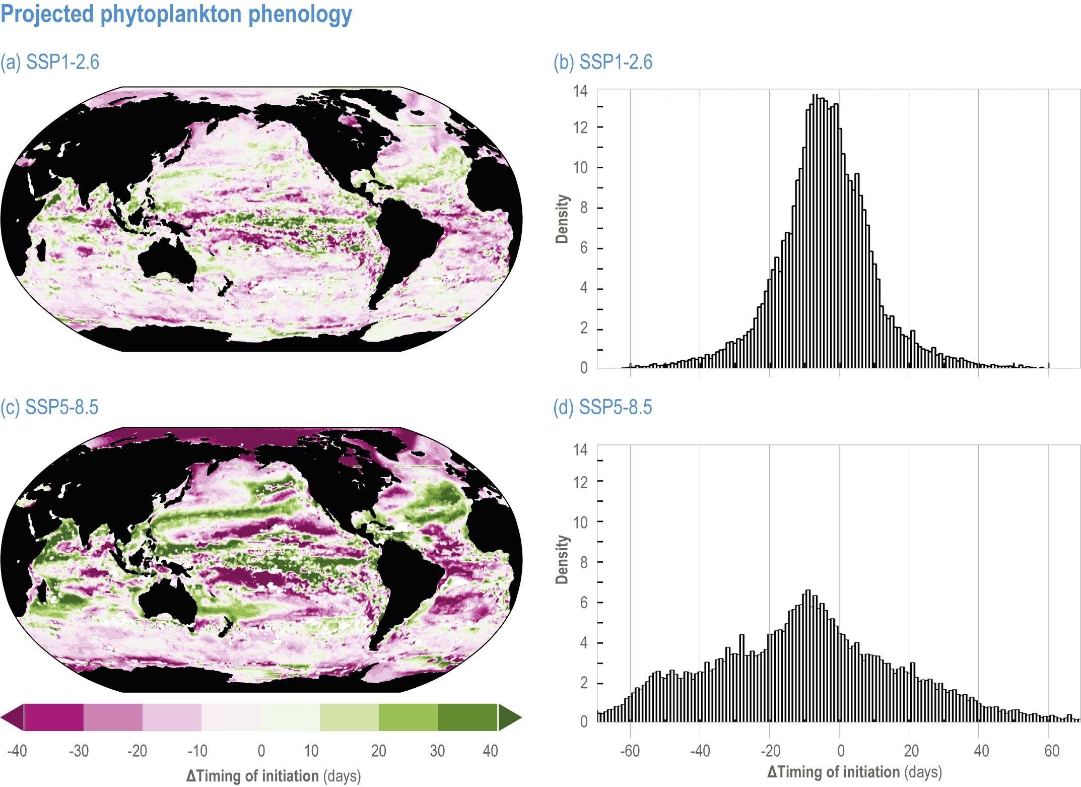
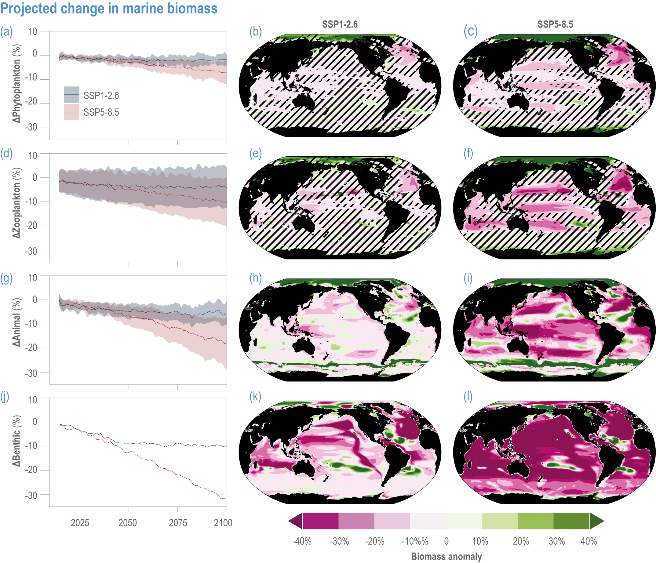
Escalating impacts of climate change on marine life will further alter biomass of marine animals (medium confidence), the timing of seasonal ecological events (medium confidence) and the geographic ranges of coastal and ocean taxa (medium confidence), disrupting life cycles (medium confidence), food webs (medium confidence) and ecological connectivity throughout the water column (medium confidence). Multiple lines of evidence suggest that climate-change responses are very likely to amplify up marine food webs over large regions of the ocean. Modest projected declines in global phytoplankton biomass translate into larger declines of total animal biomass (by 2080–2099 relative to 1995–2014) ranging from (mean ±very likely range) −5.7 ± 4.1% to −15.5 ± 8.5% under SSP1-2.6 and SSP5-8.5, respectively (medium confidence). Projected declines in upper-ocean nutrient concentrations, likely associated with increases in stratification, will reduce carbon export flux to the mesopelagic and deep-sea ecosystems (medium confidence). This will lead to a decline in the biomass of abyssal meio- and macrofauna (by 2081–2100 relative to 1995–2014) by −9.8% and −13.0% under SSP1-2.6 and SSP5-8.5, respectively (limited evidence). By 2100, 18.8 ± 19.0% to 38.9 ± 9.4% of the ocean will very likely undergo a change of more than 20 d (advances and delays) in the start of the phytoplankton growth period under SSP1-2.6 and SSP5-8.5, respectively (low confidence). This altered timing increases the risk of temporal mismatches between plankton blooms and fish spawning seasons (medium to high confidence) and increases the risk of fish-recruitment failure for species with restricted spawning locations, especially in mid-to-high latitudes of the Northern Hemisphere (low confidence). Projected range shifts among marine species (medium confidence) suggest extirpations and strongly decreasing tropical biodiversity. At higher latitudes, range expansions will drive increased homogenisation of biodiversity. The projected loss of biodiversity ultimately threatens marine ecosystem resilience (medium to high confidence), with subsequent effects on service provisioning (medium to high confidence). {3.2.2.3, 3.4.2.10, 3.4.3.1–3.4.3.5, 3.5, WGI AR6 <a class='section-link' data-title='Hazards and Exposure' href='/report/ar6/wg2/chapter/chapter-2#2.3'>Section 2.3.4.2.3</a>}
Risks from sea level rise for coastal ecosystems and people arevery likely to increase tenfold well before 2100 without adaptation and mitigation action as agreed by Parties to the Paris Agreement (very high confidence). Sea level rise under emission scenarios that do not limit warming to 1.5°C will increase the risk of coastal erosion and submergence of coastal land (high confidence), loss of coastal habitat and ecosystems (high confidence) and worsen salinisation of groundwater (high confidence), compromising coastal ecosystems and livelihoods (high confidence). Under SSP1-2.6, most coral reefs (very high confidence), mangroves (likely , medium confidence) and salt marshes (likely , medium confidence) will be unable to keep up with sea level rise by 2050, with ecological impacts escalating rapidly beyond 2050, especially for scenarios coupling high emissions with aggressive coastal development (very high confidence). Resultant decreases in natural shoreline protection will place increasing numbers of people at risk (very high confidence). The ability to adapt to current coastal impacts, cope with future coastal risks and prevent further acceleration of sea level rise beyond 2050 depends on immediate implementation of mitigation and adaptation actions (very high confidence). {3.4.2.1, 3.4.2.4, 3.4.2.5, 3.4.2.6, 3.5.5.3, Cross-Chapter Box SLR in Chapter 3}
Climate change will alter many ecosystem services provided by marine systems (high confidence), but impacts to human communities will depend on people’s overall vulnerability, which is strongly influenced by local context and development pathways (very high confidence). Catch composition and diversity of regional fisheries will change (high confidence), and fishers who are able to move, diversify and leverage technology to sustain harvests decrease their own vulnerability (medium confidence). Management that eliminates overfishing facilitates successful future adaptation of fisheries to climate change (very high confidence). Marine-dependent communities, including Indigenous Peoples and local peoples, will be at increased risk of losing cultural heritage and traditional seafood-sourced nutrition (medium confidence). Without adaptation, seafood-dependent people face increased risk of exposure to toxins, pathogens and contaminants (high confidence), and coastal communities face increasing risk from salinisation of groundwater and soil (high confidence). Early-warning systems and public education about environmental change, developed and implemented within the local and cultural context, can decrease those risks (high confidence). Coastal development and management informed by sea level rise projections will reduce the number of people and amount of property at risk (high confidence), but historical coastal development and policies impede change (high confidence). Current financial flows are globally uneven and overall insufficient to meet the projected costs of climate impacts on coastal and marine social–ecological systems (very high confidence). Inclusive governance that (a) accommodates geographically shifting marine life, (b) financially supports needed human transformations, (c) provides effective public education and (d) incorporates scientific evidence, Indigenous knowledge and local knowledge to manage resources sustainably shows greatest promise for decreasing human vulnerability to all of these projected changes in ocean and coastal ecosystem services (very high confidence). {3.5.3, 3.5.5, 3.5.6, 3.6.3, Box 3.4, Cross-Chapter Box ILLNESS in Chapter 2, Cross-Chapter Box SLR in Chapter 3}
Solutions, trade-offs, residual risk, decisions and governance
Humans are already adapting to climate-driven changes in marine systems, and while further adaptations are required even under low-emission scenarios (high confidence), transformative adaptation will be essential under high-emission scenarios (high confidence). Low-emission scenarios permit a wider array of feasible, effective and low-risk nature-based adaptation options (e.g., restoration, revegetation, conservation, early-warning systems for extreme events and public education) (high confidence). Under high-emission scenarios, adaptation options (e.g., hard infrastructure for coastal protection, assisted migration or evolution, livelihood diversification, migration and relocation of people) are more uncertain and require transformative governance changes (high confidence). Transformative climate adaptation will reinvent institutions to overcome obstacles arising from historical precedents, reducing current barriers to climate adaptation in cultural, financial and governance sectors (high confidence). Without transformation, global inequities will likely increase between regions (high confidence) and conflicts between jurisdictions may emerge and escalate. {3.5, 3.5.2, 3.5.5.3, 3.6, 3.6.2.1, 3.6.3.1, 3.6.3.2, 3.6.3.3, 3.6.4.1, 3.6.4.2, 3.6.5, Cross-Chapter Box SLR in Chapter 3, Cross-Chapter Box ILLNESS in Chapter 2}
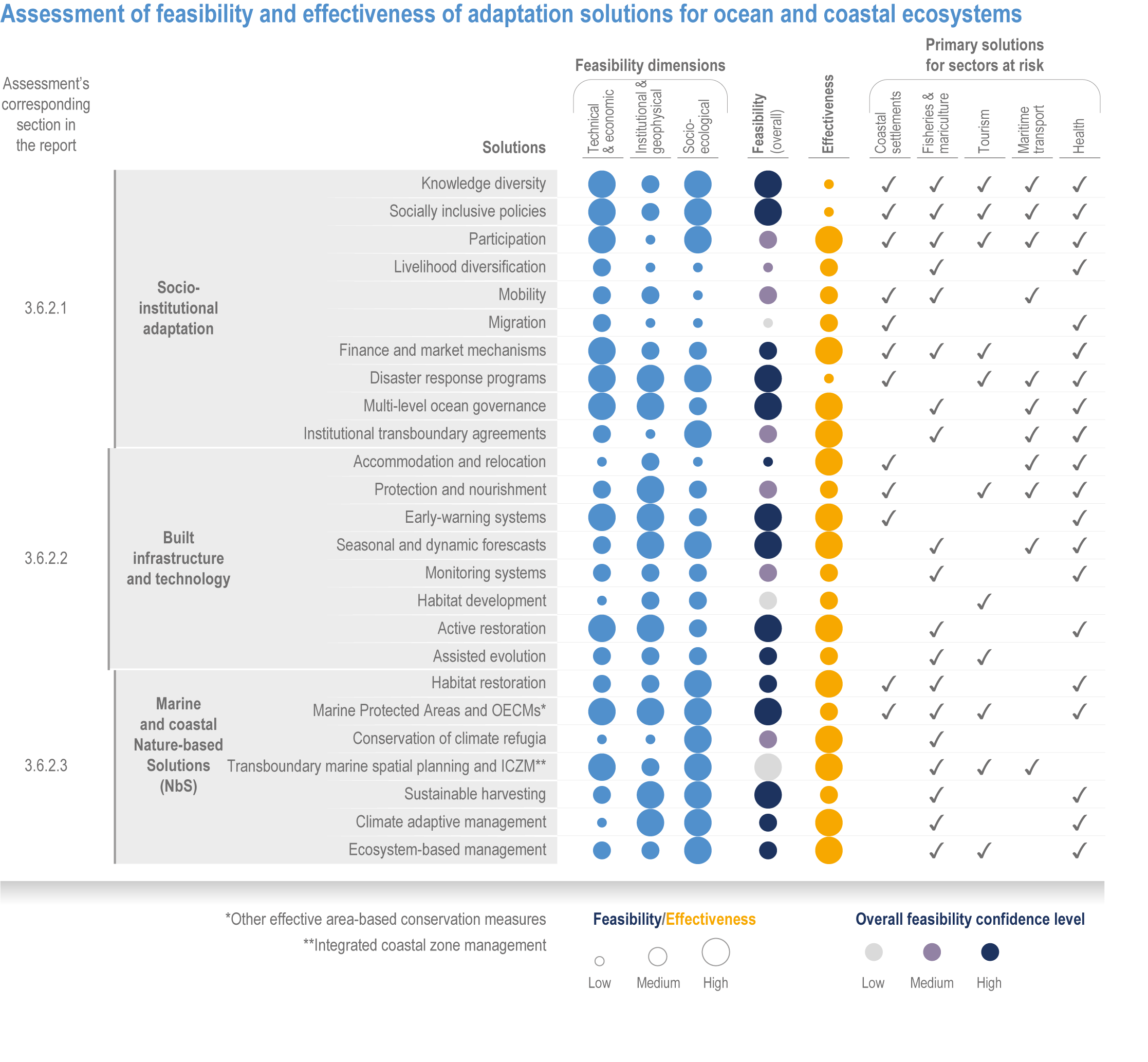
Available adaptation options are unable to offset climate-change impacts on marine ecosystems and the services they provide (high confidence). Adaptation solutions implemented at appropriate scales, when combined with ambitious and urgent mitigation measures, can meaningfully reduce impacts (high confidence). Increasing evidence from implemented adaptations indicates that multi-level governance, early-warning systems for climate-associated marine hazards, seasonal and dynamic forecasts, habitat restoration, ecosystem-based management, climate-adaptive management and sustainable harvesting tend to be both feasible and effective (high confidence). Marine protected areas (MPAs), as currently implemented, do not confer resilience against warming and heatwaves (medium confidence) and are not expected to provide substantial protection against climate impacts past 2050 (high confidence). However, MPAs can contribute substantially to adaptation and mitigation if they are designed to address climate change, strategically implemented and well governed (high confidence). Habitat restoration limits climate-change-related loss of ecosystem services, including biodiversity, coastal protection, recreational use and tourism (medium confidence), provides mitigation benefits on local to regional scales (e.g., via carbon-storing ‘blue carbon’ ecosystems) (high confidence) and may safeguard fish-stock production in a warmer climate (limited evidence). Ambitious and swift global mitigation offers more adaptation options and pathways to sustain ecosystems and their services (high confidence). {3.4.2, 3.4.3.3, 3.5, 3.5.2, 3.5.3, 3.5.5.4, 3.5.5.5, 3.6.2.1, 3.6.2.2, 3.6.2.3, 3.6.3.1, 3.6.3.2, 3.6.3.3, 3.6.5, Figure 3.24, Figure 3.25}
Nature-based solutions for adaptation of ocean and coastal ecosystems can achieve multiple benefits when well designed and implemented (high confidence), but their effectiveness declines without ambitious and urgent mitigation (high confidence). Nature-based solutions, such as ecosystem-based management, climate-smart conservation approaches (i.e., climate-adaptive fisheries and conservation) and coastal habitat restoration, can be cost-effective and generate social, economic and cultural co-benefits while contributing to the conservation of marine biodiversity and reducing cumulative anthropogenic drivers (high confidence). The effectiveness of nature-based solutions declines with warming; conservation and restoration alone will be insufficient to protect coral reefs beyond 2030 (high confidence) and to protect mangroves beyond the 2040s (high confidence). The multidimensionality of climate-change impacts and their interactions with other anthropogenic stressors calls for integrated approaches that identify trade-offs and synergies across sectors and scales in space and time to build resilience of ocean and coastal ecosystems and the services they deliver (high confidence). {3.4.2, 3.5.2, 3.5.3, 3.5.5.3, 3.5.5.4, 3.5.5.5, 3.6.2.2, 3.6.3.2, 3.6.5, Figure 3.25, Table 3.SM.6}
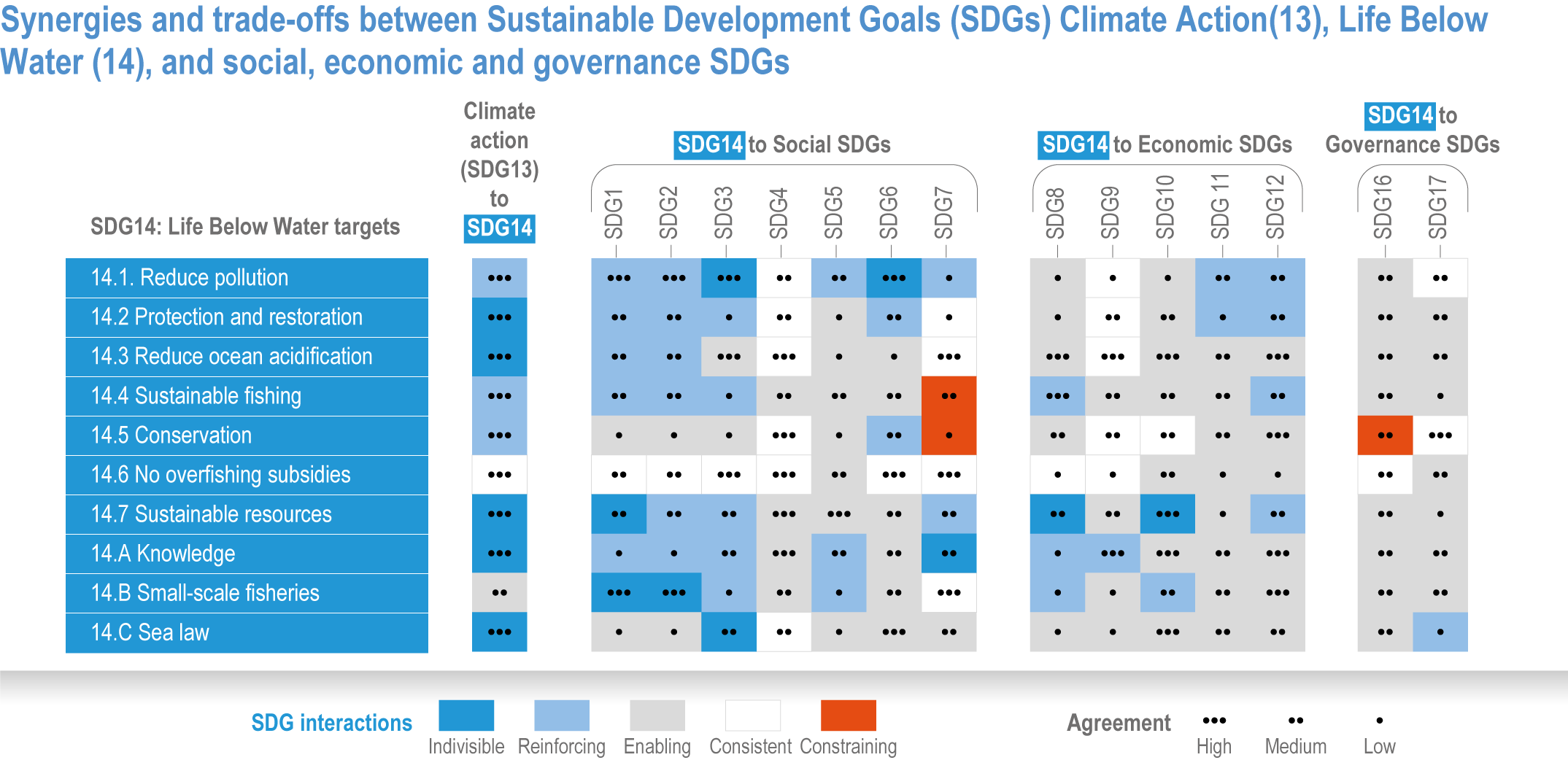
Ocean-focused adaptations, especially those that employ nature-based solutions, address existing inequalities, and incorporate just and inclusive decision-making and implementation processes, support the UN Sustainable Development Goals (SDGs) (high confidence). There are predominantly positive synergies between adaptation options for Life Below Water (SDG14), Climate Action (SDG13) and social, economic and governance SDGs (SDG1–12, 16–17) (high confidence), but the ability of ocean adaptation to contribute to the SDGs is constrained by the degree of mitigation action (high confidence). Furthermore, existing inequalities and entrenched practices limit effective and just responses to climate change in coastal communities (high confidence). Momentum is growing towards transformative international and regional governance that will support comprehensive, equitable ocean and coastal adaptation while also achieving SDG14 (robust evidence), without compromising achievement of other SDGs. {3.6.4.0, 3.6.4.2, 3.6.4.3, Figure 3.26}.
3.1 Point of Departure
The ocean contains approximately 97% of Earth’s water within a system of interconnected basins that cover 71% of its surface. Coastal systems mostly extend seaward from the high-water mark, or just beyond, to the edge of the continental shelf and include shores of soft sediments, rocky shores and reefs, embayments, estuaries, deltas and shelf systems. Oceanic systems comprise waters beyond the shelf edge, from ~200 m to nearly 11,000 m deep (Stewart and Jamieson, 2019), with an average depth of approximately 3700 m. The epipelagic zone, or upper 200 m of the ocean, is illuminated by sufficient sunlight to sustain photosynthesis that supports the rich marine food web. Below the epipelagic zone lies the barely lit mesopelagic zone (200–1000 m), the perpetually dark bathypelagic zone (depth >1000 m) and the deep seafloor (benthic ecosystems at depths >200 m), which spans rocky and sedimentary habitats on seamounts, mid-ocean ridges and canyons, abyssal plains and sedimented margins. Semi-enclosed seas (SES) include both coastal and oceanic systems.
The ocean sustains life on Earth by providing essential resources and modulating planetary flows of energy and materials. Together, harvests from the ocean and inland waters provide more than 20% of dietary animal protein for more than 3.3 billion people worldwide and livelihoods for about 60 million people (FAO, 2020b). The global ocean is centrally involved in sequestering anthropogenic atmospheric CO2 and recycling many elements, and it regulates the global climate system by redistributing heat and water (WGI AR6 Chapter 9; Fox-Kemper et al., 2021). The ocean also provides a wealth of aesthetic and cultural resources (Barbier et al., 2011), contains vast biodiversity (Appeltans et al., 2012), supports more animal biomass than on land (Bar-On et al., 2018) and produces at least half the world’s photosynthetic oxygen (Field et al., 1998). Ecosystem services (Annex II: Glossary) delivered by ocean and coastal ecosystems support humanity by protecting coastlines, providing nutrition and economic opportunities (Figure 3.1; Selig et al., 2019) and providing many intangible benefits. Even though ecosystem services and biodiversity underpin human well-being and support climate mitigation and adaptation (Pörtner et al., 2021b), there are also ethical arguments for preserving biodiversity and ecosystem functions regardless of the beneficiary (e.g., Taylor et al., 2020). This chapter assesses the impact of climate change on the full spectrum of ocean and coastal ecosystems, on their services and on related human activities, and it assesses marine-related opportunities within both ecological and social systems to adapt to climate change.
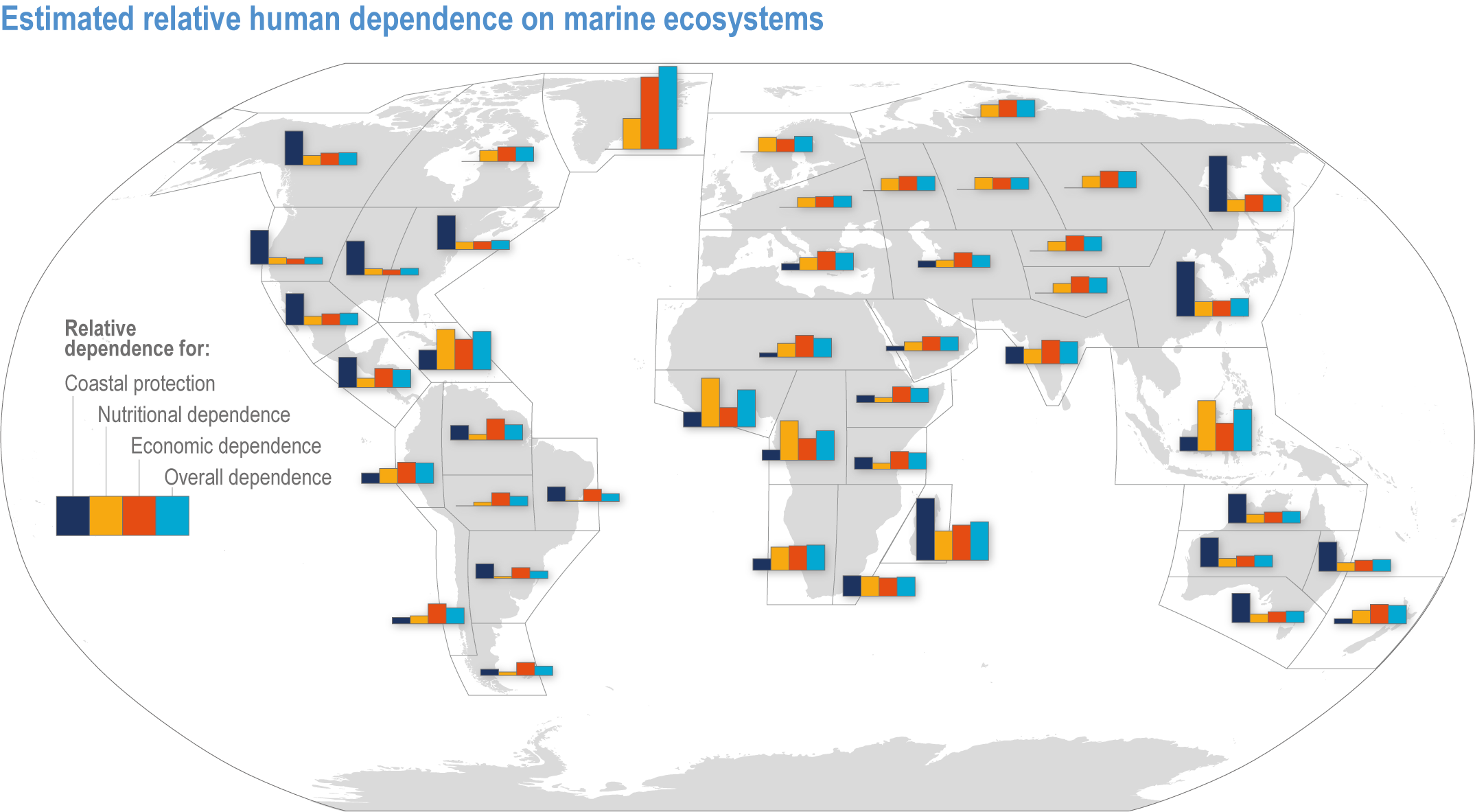
Figure 3.1 | Estimated relative human dependence on marine ecosystems for coastal protection, nutrition, fisheries economic benefits and overall. Each bar represents an index value that semi-quantitatively integrates the magnitude, vulnerability to loss and substitutability of the benefit. Indices synthesize information on people’s consumption of marine protein and nutritional status, gross domestic product, fishing revenues, unemployment, education, governance and coastal characteristics. Overall dependence is the mean of the three index values after standardisation from 0–1. (Details regarding component indices are found in Table 1 and Supplementary Material of Selig et al., 2019.) The overall index does not include the economic benefits from tourism or other ocean industries, and data limitations prevented including artisanal or recreational fisheries or the protective impact of salt marshes (Selig et al., 2019). Values for reference regions established in the WGI AR6 Atlas (Gutiérrez et al., 2021) were computed as area-weighted means from original country-level data (Table S6 in Selig et al., 2019).
Previous IPCC Assessment Reports (IPCC, 2014b; IPCC, 2014c; IPCC, 2018; IPCC, 2019b) have expressed growing confidence in the detection of climate-change impacts in the ocean and their attribution to anthropogenic greenhouse gas emissions. Heat and CO2 taken up by the ocean (high to very high confidence) (IPCC, 2021b) directly affect marine systems, and the resultant “climatic impact-drivers (CIDs) (e.g., ocean temperature and heatwaves, sea level, dissolved oxygen levels, acidification; Annex II: Glossary, WGI Figure SPM.9; IPCC, 2021b) also influence ocean and coastal systems (Section 3.2; Cross-Chapter Box SLR in Chapter 3; Cross-Chapter Box EXTREMES in Chapter 2; Figure 3.SM.1), from individual biophysical processes to dependent human activities. Several marine outcomes of CIDs are themselves drivers of ecological change (e.g., climate velocities, stratification, sea ice changes). This chapter updates and extends the assessment of SROCC (IPCC, 2019b) and WGI AR6 by assessing the ecosystem effects of the CIDs in WGI AR6 Figure SPM.9 (IPCC, 2021b) and their biologically relevant marine outcomes (detailed in Section 3.2), which are referred to collectively hereafter as ‘climate-induced drivers’4 .
Detrimental human impacts on ocean and coastal ecosystems are not only caused by climate. Other anthropogenic activities are increasingly affecting the physical, chemical and biological conditions of the ocean (Doney, 2010; Halpern et al., 2019), and these ‘non-climate drivers 5 ’ also alter marine ecosystems and their services. Fishing and other extractive activities are major non-climate drivers in many ocean and coastal systems (Steneck and Pauly, 2019). Many activities, such as coastal development, shoreline hardening and habitat destruction, physically alter marine spaces (Suchley and Alvarez-Filip, 2018; Ducrotoy et al., 2019; Leo et al., 2019; Newton et al., 2020; Raw et al., 2020). Other human activities decrease water quality by overloading coastal water with terrestrial nutrients (eutrophication) and by releasing runoff containing chemical, biological and physical pollutants, toxins, and pathogens (Jambeck et al., 2015; Luek et al., 2017; Breitburg et al., 2018; Froelich and Daines, 2020). Some human activities disturb marine organisms by generating excess noise and light (Davies et al., 2014; Duarte et al., 2021), while others decrease natural light penetration into the ocean (Wollschläger et al., 2021). Several anthropogenic activities alter processes that span the land–sea interface by changing coastal hydrology or causing coastal subsidence (Michael et al., 2017; Phlips et al., 2020; Bagheri-Gavkosh et al., 2021). Atmospheric pollutants can harm marine systems or unbalance natural marine processes (Doney et al., 2007; Hagens et al., 2014; Lamborg et al., 2014; Ito et al., 2016). Organisms frequently experience non-climate drivers simultaneously with climate-induced drivers (Section 3.4), and feedbacks may exist between climate-induced drivers and non-climate drivers that enhance the effects of climate change (Rocha et al., 2015; Ortiz et al., 2018; Wolff et al., 2018; Cabral et al., 2019; Bowler et al., 2020; Gissi et al., 2021). SROCC assessed with high confidence that reduction of pollution and other stressors, along with protection, restoration and precautionary management, supports ocean and coastal ecosystems and their services (IPCC, 2019b). This chapter examines the combined influence of climate-induced drivers and primary non-climate drivers on many ecosystems assessed.
Detecting changes and attributing them to specific drivers has been especially difficult in ocean and coastal ecosystems because drivers, responses and scales (temporal, spatial, organisational) often overlap and interact (IPCC, 2014b; IPCC, 2014c; Abram et al., 2019; Gissi et al., 2021). In addition, some marine systems have short, heterogeneous or geographically biased observational records, which exacerbate the interpretation challenge (Beaulieu et al., 2013; Christian, 2014; Huggel et al., 2016; Benway et al., 2019). It is even more challenging to detect and attribute climate impacts on marine-dependent human systems, where culture, governance and society also strongly influence observed outcomes. To assess climate-driven change in natural and social systems robustly, IPCC reports rely on multiple lines of evidence, and the available types of evidence differ depending on the system under study (Section 1.3.2.1, Cross-Working Group Box ATTRIB). Lines of evidence used for ocean and coastal ecosystems for this and previous assessments include observed phenomena, laboratory and field experiments, long-term monitoring, empirical and dynamical model analyses, Indigenous knowledge (IK) and local knowledge (LK), and paleorecords (IPCC, 2014b; IPCC, 2014c; IPCC, 2019b). The growing body of climate research for ocean and coastal ecosystems and their services increasingly provides multiple independent lines of evidence whose conclusions support each other, raising the overall confidence in detection and attribution of impacts over time (Section 1.3.2.1, Cross-Working Group Box ATTRIB in Chapter 3).
Natural adaptation to climate change in ocean and coastal systems includes an array of responses taking place at scales from cells to ecosystems. Previous IPCC assessments have established that many marine species ‘have shifted their geographic ranges, seasonal activities, migration patterns, abundances and species interactions in response to climate change’ (high confidence) (IPCC, 2014b; IPCC, 2014c), which has had global impacts on species composition, abundance and biomass, and on ecosystem structure and function (medium confidence) (IPCC, 2019b). Warming and acidification have affected coastal ecosystems in concert with non-climate drivers (high confidence), which have affected habitat area, biodiversity, ecosystem function and services (high confidence) (IPCC, 2019b). Confidence has grown in these assessments over time as observational datasets have lengthened and other lines of evidence have corroborated observations. AR5 and SROCC assessed how physiological sensitivity to climate-induced drivers is the underlying cause of most marine organisms’ vulnerability to climate (high confidence) (Pörtner et al., 2014; Bindoff et al., 2019a). Since those assessments, more evidence supports the empirical physiological models of tolerance and plasticity (Sections 3.3.2, 3.3.4) and of interactions among multiple (climate and non-climate) drivers at individual to ecosystem scales (Sections 3.3.3, 3.4.5). New experimental evidence about evolutionary adaptation (Section 3.3.4) bolsters previous assessments that adaptation options to climate change are limited for eukaryotic organisms. Tools such as ecosystem models can now constrain probable ecosystem states (Sections 3.3.4, 3.3.5, 3.4). Observations have increased understanding of how extreme events affect individuals, populations and ecosystems, helping refine understanding of both ecological tolerance to climate impacts and ecological transformations (Section 3.4).
Human adaptation to climate impacts on ocean and coastal systems spans a variety of actions that change human activity to maintain marine ecosystem services. After AR5 concluded that coastal adaptation could reduce the effects of climate impacts on coastal human communities (high agreement , limited evidence) (Wong et al., 2014), SROCC confirmed that mostly risk-reducing ocean and coastal adaptation responses were underway (Bindoff et al., 2019a). However, overlapping climate-induced drivers and non-climate drivers confound implementation and assessment of the success of marine adaptation, revealing the complexity of attempting to maintain marine ecosystems and services through adaptation. SROCC assessed with high confidence that while the benefits of many locally implemented adaptations exceed their disadvantages, others are marginally effective and have large disadvantages, and overall, adaptation has a limited ability to reduce the probable risks from climate change, being at best a temporary solution (Bindoff et al., 2019a). SROCC also concluded that a portfolio of many different types of adaptation actions, effective and inclusive governance, and mitigation must be combined for successful adaptation (Bindoff et al., 2019a). The portfolio of adaptation measures has now been defined (Section 3.6.2), and individual and combined adaptation solutions have been implemented in several marine sectors (Section 3.6.3). Delays in marine adaptation have been partly attributed to the complexity of ocean governance (Section 3.6.4; Cross-Chapter Box 3 and Figure CB3.1 in Abram et al., 2019) and to the low priority accorded the ocean in international development goals (Nash et al., 2020), but in recent years the ocean is being increasingly incorporated in international climate policy and multilateral environmental agreements (Section 3.6.4).
This chapter assesses the current understanding of climate-induced drivers, ecological vulnerability and adaptability, risks to coastal and ocean ecosystems, and human vulnerability and adaptation to resulting changes in ocean benefits, now and in the future (Figure 3.2). It starts by assessing the biologically relevant outcomes of anthropogenic climate-induced drivers (Section 3.2). Next, it sets out the mechanisms that determine the responses of ocean and coastal organisms to individual and combined drivers from the genetic to the ecosystem level (Section 3.3). This supports a detailed assessment of the observed and projected responses of coastal and ocean ecosystems to these hazards, placing them in context using the paleorecord (Section 3.4). These observed and projected impacts are used to quantify consequent risks to delivery of ecosystem services and the socioeconomic sectors that depend on them, with attention to the vulnerability, resilience and adaptive capacity of social–ecological systems (Section 3.5). The chapter concludes by assessing the state of adaptation and governance actions available to address these emerging threats while also advancing human development (Section 3.6). Abbreviations used repeatedly in the chapter are defined in Table 3.1.

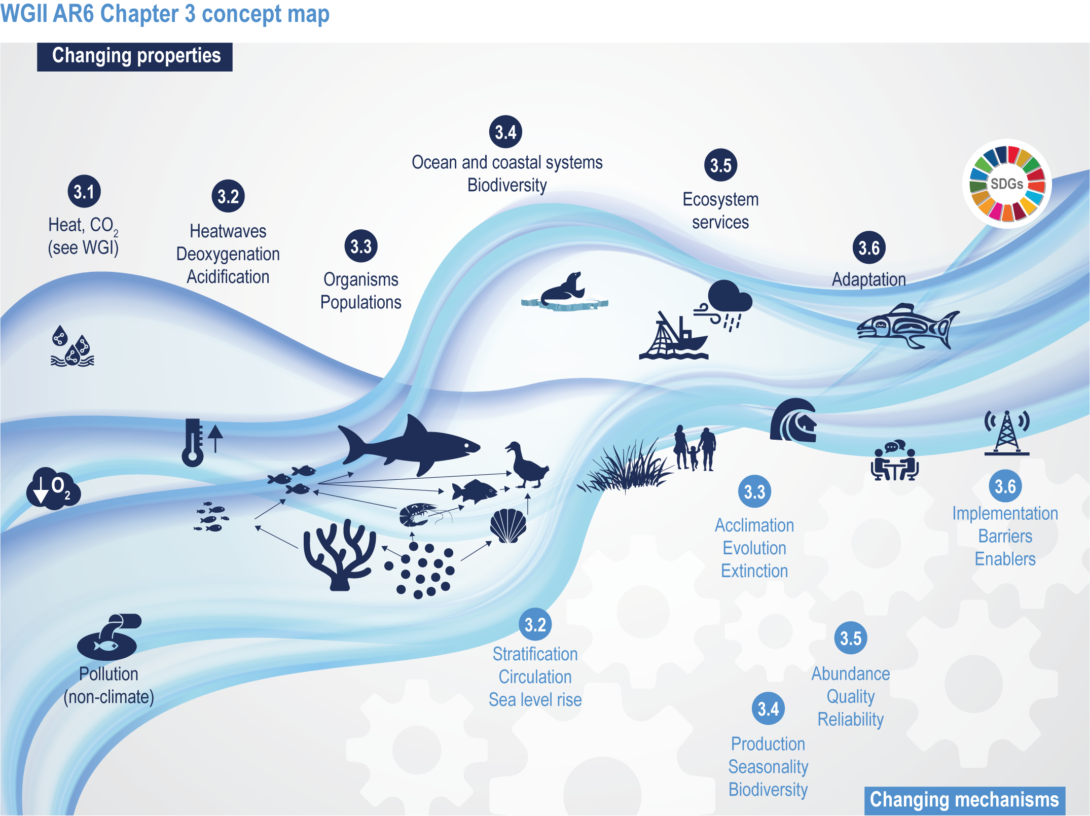
Figure 3.2 | WGII AR6 Chapter 3 concept map. Climate changes both the properties (top of wave; Sections 3.1–3.6) and the mechanisms (below wave; Sections 3.2–3.6) that influence the ocean and coastal social–ecological system. The Sustainable Development Goals (top right) represent ideal outcomes and achievement of equitable, healthy and sustainable ocean and coastal social–ecological systems.
Table 3.1 | Abbreviations frequently used in this chapter, with brief definitions
Abbreviation | Definition |
ABNJ | Areas beyond national jurisdiction: the water column beyond the exclusive economic zone called the high seas and the seabed beyond the limits of the continental shelf; established in conformity with United Nations Convention on the Law of the Sea |
AMOC | Atlantic meridional overturning circulation (WGI AR6 Glossary, IPCC, 2021a) |
AR5 | The IPCC Fifth Assessment Report (IPCC, 2013; IPCC, 2014b; IPCC, 2014c; IPCC, 2014d) |
CBD | Convention on Biological Diversity: an international legal instrument that has been ratified by 196 nations to conserve biological diversity, sustainably use its components and share its benefits fairly and equitably |
CE | Common era |
CID | Climatic impact-driver (WGI AR6 Glossary, IPCC, 2021a) |
CMIP5, CMIP6 | The Coupled Model Intercomparison Project, Phase 5 or 6 (WGI AR6 Glossary, IPCC, 2021a) |
EbA | Ecosystem-based adaptation: the use of ecosystem management activities to increase the resilience and reduce the vulnerability of people and ecosystems to climate change |
EBUS | Eastern boundary upwelling system (WGI AR6 Glossary, IPCC, 2021a) |
EEZ | Exclusive economic zone: the area from the coast to 200 nautical miles (370 km) off the coast, where a nation exercises its sovereign rights and exclusive management authority |
ESM | Earth system model: a coupled atmosphere–ocean general circulation model (AOGCM, WGI AR6 Glossary, IPCC, 2021a) in which a representation of the carbon cycle is included, allowing for interactive calculation of atmospheric CO2 or compatible emissions |
Fish-MIP | The Fisheries and Marine Ecosystem Model Intercomparison Project: a component of the Inter-Sectoral Impact Model Intercomparison Project (ISIMIP) that explores the long-term impacts of climate change on fisheries and marine ecosystems using scenarios from CMIP models |
GMSL/GMSLR | Global mean sea level/global mean sea level rise (sea level change, WGI AR6 Glossary, IPCC, 2021a) |
HAB | Harmful algal bloom: an algal bloom composed of phytoplankton known to naturally produce biotoxins that are harmful to the resident population as well as humans |
ICZM | Integrated coastal zone management: a dynamic, multidisciplinary and iterative process to promote sustainable management of coastal zones (European Environmental Agency) |
IKLK | Indigenous knowledge and local knowledge (SROCC Glossary, IPCC, 2019a) |
MHW | Marine heatwaves (WGI AR6 Glossary, IPCC, 2021a) |
MPA | Marine protected area: an area-based management approach, commonly intended to conserve, preserve or restore biodiversity and habitat, protect species or manage resources (especially fisheries) |
NbS | Nature-based Solution: actions to protect, sustainably manage and restore natural or modified ecosystems that address societal challenges effectively and adaptively, simultaneously providing human well-being and biodiversity benefits (IUCN, 2016) |
NDC | Nationally determined contribution by parties to the Paris Agreement |
NPP | Net primary production: the difference between how much CO2 vegetation takes in during photosynthesis (gross primary production) and how much CO2 the plants release during respiration |
OECM | Other effective area-based conservation measures: a conservation designation for areas that are achieving the effective in situ conservation of biodiversity outside of protected areas |
OMZ | Oxygen minimum zone (WGI AR6 Glossary, IPCC, 2021a) |
pCO2 | Partial pressure of carbon dioxide. For seawater, pCO2 is used to measure the amount of carbon dioxide dissolved in seawater. |
pH | Potential of hydrogen (WGI AR6 Glossary, IPCC, 2021a) |
POC | Particulate organic carbon: a fraction of total organic carbon operationally defined as that which does not pass through a filter pore size ≥ 0.2 µm |
SDG | Sustainable Development Goals: the 17 global goals for development for all countries established by the United Nations through a participatory process and elaborated in the 2030 Agenda for Sustainable Development |
SES | Semi-enclosed sea: a gulf, basin or sea surrounded by land and connected to another sea by a narrow outlet |
SIDS | Small Island Developing States (WGI AR6 Glossary, IPCC, 2021a) |
SLR/RSLR/RSL | Sea level rise/relative sea level rise/relative sea level (sea level change, WGI AR6 Glossary, IPCC, 2021a) |
SR15 | The IPCC Special Report on 1.5°C (IPCC, 2018) |
SROCC | The IPCC Special Report on the Ocean and Cryosphere in a Changing Climate (IPCC, 2019b) |
SSP/RCP | Shared Socioeconomic Pathway/Representative Concentration Pathway (Pathways; IPCC, 2021a) |
SST | Sea surface temperature (WGI AR6 Glossary, IPCC, 2021a) |
Ωaragonite | Saturation state of seawater with respect to the calcium carbonate mineral aragonite, used as a proxy measurement for ocean acidification |
FAQ 3.1 | How do we know which changes to marine ecosystems are specifically caused by climate change?
To attribute changes in marine ecosystems to human-induced climate change, scientists use paleorecords (reconstructing the links between climate, evolutionary and ecological changes in the geological past), contemporary observations (assessing current climate and ecological responses in the field and through experiments) and models. We refer to these as multiple lines of evidence, meaning that the evidence comes from diverse approaches, as described below.
Emissions of greenhouse gases like carbon dioxide from human activity cause ocean warming, acidification, oxygen loss, and other physical and chemical changes that are affecting marine ecosystems around the world. At the same time, natural climate variability and direct human impacts, such as overfishing and pollution, also affect marine ecosystems locally, regionally and globally. These climate and non-climate impact drivers counteract each other, add up or multiply to produce smaller or larger changes than expected from individual drivers. Attribution of changes in marine ecosystems requires evaluating the often-interacting roles of natural climate variability, non-climate drivers, and human-induced climate change. To do this work, scientists use
- paleorecords: reconstructing the links between climate and evolutionary and ecological changes of the past;
- contemporary observations: assessing current climate and ecological responses;
- manipulation experiments: measuring responses of organisms and ecosystems to different climate conditions; and
- models: testing whether we understand how organisms and ecosystems are impacted by different stressors, and quantifying the relative importance of different stressors.
Paleorecords can be used to trace the correlation between past changes in climate and marine life. Paleoclimate is reconstructed from the chemical composition of shells and teeth or from sediments and ice cores. Changes to sea life signalled by changing biodiversity, extinction or distributional shifts are reconstructed from fossils. Using large datasets, we can infer the effects of climate change on sea life over relatively long time scales ⎯ usually hundreds to millions of years. The advantage of paleorecords is that they provide insights into how climate change affects life from organisms to ecosystems, without the complicating influence of direct human impacts. A key drawback is that the paleo and modern worlds do not have fully comparable paleoclimate regimes, dominant marine species and rates of climate change. Nevertheless, the paleorecord can be used to derive fundamental rules by which organisms, ecosystems, environments and regions are typically most affected by climate change. For example, the paleorecord shows that coral reefs repeatedly underwent declines during past warming events, supporting the inference that corals may not be able to adapt to current climate warming.
Contemporary observations over recent decades allow scientists to relate the status of marine species and ecosystems to changes in climate or other factors. For example, scientists compile large datasets to determine whether species usually associated with warm water are appearing in traditionally cool-water areas that are rapidly warming. A similar pattern observed in multiple regions and over several decades (i.e., longer than time scales of natural variability) provides confidence that climate change is altering community structure. This evidence is weighed against findings from other approaches, such as manipulation experiments, to provide a robust picture of climate-change impacts in the modern ocean.
In manipulation experiments, scientists expose organisms or communities of organisms to multiple stressors, for example, elevated CO2, high temperature, or both, based on values drawn from future climate projections. Such experiments will involve multiple treatments (e.g., in different aquarium tanks) in which organisms are exposed to different combinations of the stressors. This approach enables scientists to understand the effects of individual stressors as well as their interactions to explore physiological thresholds of marine organisms and communities. The scale of manipulation experiments can range from small tabletop tanks to large installations or natural ocean experiments involving tens of thousands of litres of water.
Ecological effects of climate change are also explored within models developed from fundamental scientific principles and observations. Using these numerical representations of marine ecosystems, scientists can explore how different levels of climate change and non-climate stressors influence species and ecosystems at scales not possible with experiments. Models are commonly used to simulate the ecological response to climate change over recent decades and centuries. Convergence between the model results and the observations suggests that our understanding of the key processes is sufficient to attribute the observed ecological changes to climate change, and to use the models to project future ecological changes. Differences between model results and observations indicate gaps in knowledge to be filled in order to better detect and attribute the impacts of climate change on marine life.
Using peer-reviewed research spanning the full range of scientific approaches (paleorecords, observations, experiments and models), we can assess the level of confidence in the impact of climate change on observed modifications in marine ecosystems. We refer to this as multiple lines of evidence, meaning that the evidence comes from the diverse approaches described above. This allows policymakers and managers to address the specific actions needed to reduce climate change and other impacts.
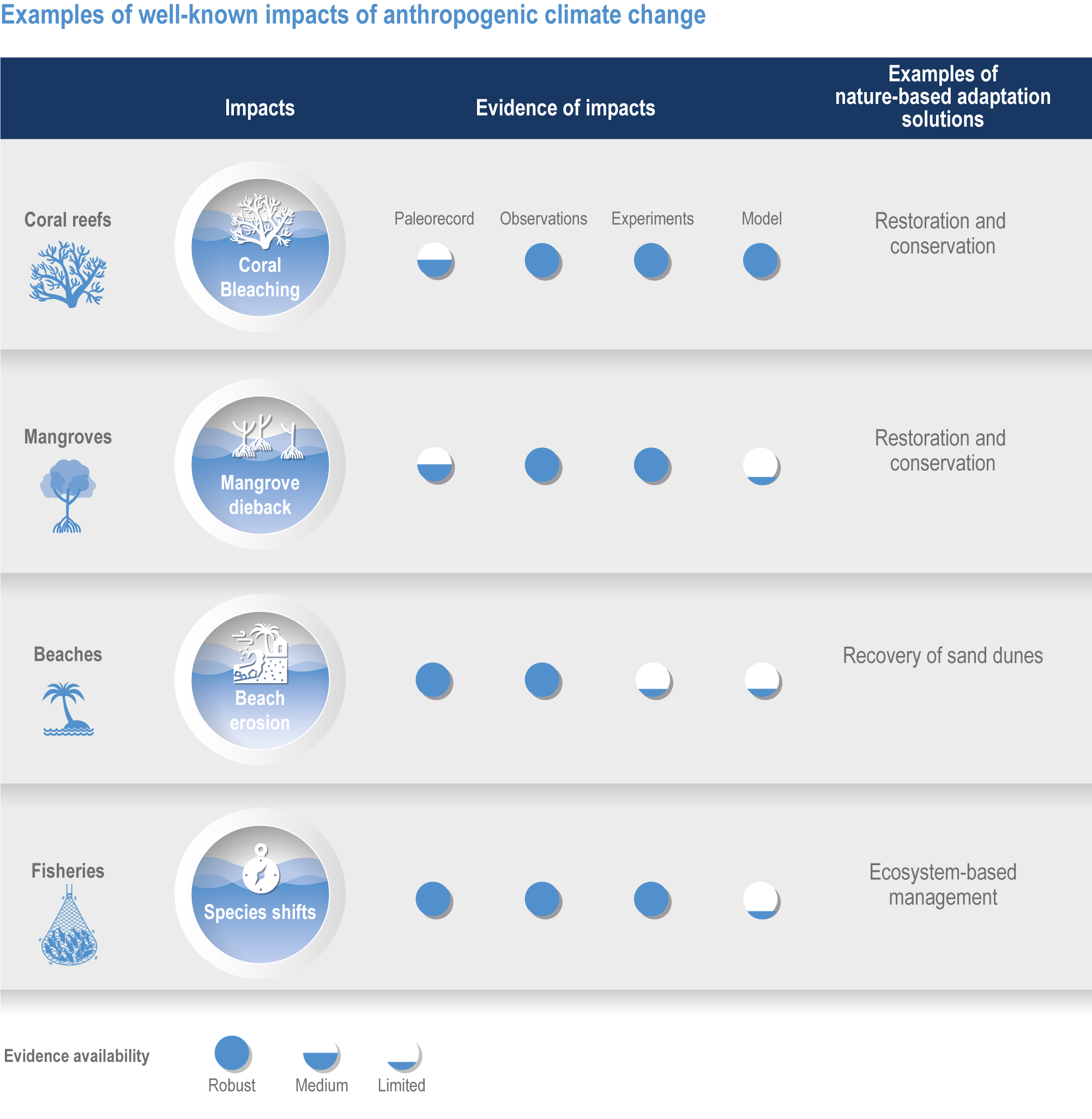
Figure FAQ3.1.1 | Examples of well-known impacts of anthropogenic climate change and associated nature-based adaptation. To attribute changes in marine ecosystems to anthropogenic climate change, scientists use multiple lines of evidence including paleorecords, contemporary observations, manipulation experiments and models.
3.2 Observed Trends and Projections of Climatic Impact-Drivers in the Global Ocean
3.2.1 Introduction
Climate change exposes ocean and coastal ecosystems to changing environmental conditions, including ocean warming, SLR, acidification, deoxygenation and other climatic impact-drivers (CIDs), which have distinct regional and temporal characteristics (Gruber, 2011; IPCC, 2018). This section aims to build on the WGI AR6 assessment (Table 3.2) to provide an ecosystem-oriented framing of CIDs. Updating SROCC, projected trends assessed here are based on a new range of scenarios (Shared Socioeconomic Pathways, SSPs), as used in the Coupled Model Intercomparison Project Phase 6 (CMIP6; Section 1.2.2).
Table 3.2 | Overview of the main global ocean climatic impact-drivers and their observed and projected trends from WGI AR6, with corresponding confidence levels and links to WGI chapters where these trends are assessed in detail
Climatic impact-drivers (hazards) | Observed trends over the historical period | WGI section | Projected trends over the 21st century | WGI section |
Ocean temperature | ||||
Ocean warming | ‘At the ocean surface, temperature has on average increased by 0.88 [0.68–1.01] °C from 1850–1900 to 2011–2020.’ | 2.3.3.1, 9.2.1 | Ocean warming will continue over the 21st century (virtually certain), with the rate of global ocean warming starting to be scenario-dependent from about the mid-21st century (medium confidence). | 9.2.1 (Fox-Kemper et al., 2021) |
Marine heatwaves (MHWs) | MHWs became more frequent (high confidence), more intense and longer (medium confidence) over the 20th and early 21st centuries. | Box 9.2 (Fox-Kemper et al., 2021) | MHWs will become ‘4 [2–9, likely range] times more frequent in 2081–2100 compared with 1995–2014 under SSP1-2.6, and 8 [3–15, likely range] times more frequent under SSP5-8.5.’ | Box 9.2 (Fox-Kemper et al., 2021) |
Climate velocities | Not assessed in WGI | Not assessed in WGI | ||
Sea level | ||||
Global mean sea level (GMSL) | ‘Since 1901, GMSL has risen by 0.20 [0.15–0.25] m’, and the rate of rise is accelerating. | 2.3.3, 9.6.1 (Fox-Kemper et al., 2021; Gulev et al., 2021) | There will be continued rise in GMSL throughout the 21st century under all assessed SSPs (virtually certain). | 4.3.2.2, 9.6.3 (Fox-Kemper et al., 2021; Lee et al., 2021) |
Extreme sea levels | Relative sea level rise is driving a global increase in the frequency of extreme sea levels (high confidence). | 9.6.4 (Fox-Kemper et al., 2021) | Rising mean relative sea level will continue to drive an increase in the frequency of extreme sea levels (high confidence). | 9.6.4 (Fox-Kemper et al., 2021) |
Ocean circulation | ||||
Ocean stratification | ‘The upper ocean has become more stably stratified since at least 1970 […] (virtually certain). ’ | 9.2.1.3 (Fox-Kemper et al., 2021) | ‘Upper-ocean stratification will continue to increase throughout the 21st century (virtually certain). ’ | 9.2.1.3 (Fox-Kemper et al., 2021) |
Eastern boundary upwelling systems | ‘Only the California current system has experienced some large-scale upwelling-favourable wind intensification since the 1980s (medium confidence). ’ | 9.2.5 (Fox-Kemper et al., 2021) | ‘Eastern boundary upwelling systems will change, with a dipole spatial pattern within each system of reduction at low latitude and enhancement at high latitude (high confidence). ’ | 9.2.5 (Fox-Kemper et al., 2021) |
Atlantic overturning circulation (AMOC) | There is low confidence in reconstructed and modelled AMOC changes for the 20th century. | 2.3.3.4, 9.2.3 (Fox-Kemper et al., 2021; Gulev et al., 2021) | The AMOC will decline over the 21st century (high confidence, but low confidence for quantitative projections). | 4.3.2.3, 9.2.3 (Fox-Kemper et al., 2021; Lee et al., 2021) |
Sea ice | ||||
Arctic sea ice changes | ‘Current Arctic sea ice coverage levels are the lowest since at least 1850 for both annual mean and late-summer values (high confidence).’ | 2.3.2.1, 9.3.1 (Fox-Kemper et al., 2021; Gulev et al., 2021) | ‘The Arctic will become practically ice-free in September by the end of the 21st century under SSP2-4.5, SSP3-7.0 and SSP5-8.5[…](high confidence).’ | 4.3.2.1, 9.3.1 (Fox-Kemper et al., 2021; Lee et al., 2021) |
Antarctic sea ice changes | There is no global significant trend in Antarctic sea ice area from 1979 to 2020 (high confidence). | 2.3.2.1, 9.3.2 (Fox-Kemper et al., 2021; Gulev et al., 2021) | There is low confidence in model simulations of future Antarctic sea ice. | 9.3.2 (Fox-Kemper et al., 2021) |
Ocean chemistry | ||||
Changes in salinity | The ‘large-scale, near-surface salinity contrasts have intensified since at least 1950 […] (virtually certain).’ | 2.3.3.2, 9.2.2.2 (Fox-Kemper et al., 2021; Gulev et al., 2021) | ‘Fresh ocean regions will continue to get fresher and salty ocean regions will continue to get saltier in the 21st century (medium confidence).’ | 9.2.2.2 (Fox-Kemper et al., 2021) |
Ocean acidification | Ocean surface pH has declined globally over the past four decades (virtually certain). | 2.3.3.5, 5.3.2.2 (Canadell et al., 2021; Gulev et al., 2021) | Ocean surface pH will continue to decrease ‘through the 21st century, except for the lower-emission scenarios SSP1-1.9 and SSP1-2.6 […] (high confidence).’ | 4.3.2.5, 4.5.2.2, 5.3.4.1 (Lee et al., 2021; Canadell et al., 2021) |
Ocean deoxygenation | Deoxygenation has occurred in most open ocean regions since the mid-20th century (high confidence). | 2.3.3.6, 5.3.3.2 (Canadell et al., 2021; Gulev et al., 2021) | Subsurface oxygen content ‘is projected to transition to historically unprecedented condition with decline over the 21st century (medium confidence).’ | 5.3.3.2 (Canadell et al., 2021) |
Changes in nutrient concentrations | Not assessed in WGI | Not assessed in WGI |
3.2.2 Physical Changes
3.2.2.1 Ocean Warming, Climate Velocities and Marine Heatwaves
Global mean SST has increased since the beginning of the 20th century by 0.88°C (very likely range: 0.68–1.01°C), and it is virtually certain that the global ocean has warmed since at least 1971 (WGI AR6 Section 9.2; Fox-Kemper et al., 2021). A key characteristic of ocean temperature change relevant for ecosystems is climate velocity, a measure of the speed and direction at which isotherms move under climate change (Burrows et al., 2011), which gives the rate at which species must migrate to maintain constant climate conditions. It has been shown to be a useful and simple predictor of species distribution shifts in marine ecosystems (Chen et al., 2011; Pinsky et al., 2013; Lenoir et al., 2020). Median climate velocity in the surface ocean has been 21.7 km per decade since 1960, with higher values in the Arctic/sub-Arctic and within 15° of the Equator (Figure 3.3; Burrows et al., 2011). While climate velocity has been slower in the mesopelagic layer (200–1000 m) than in the epipelagic layer (0–200 m) over the past 50 years, it has been shown to be faster in the bathypelagic (1000–4000 m) and abyssopelagic (>4000 m) layers (Figure 3.4; Brito-Morales et al., 2020), suggesting that deep-ocean species could be as exposed to effects of warming as species in the surface ocean (Brito-Morales et al., 2020).
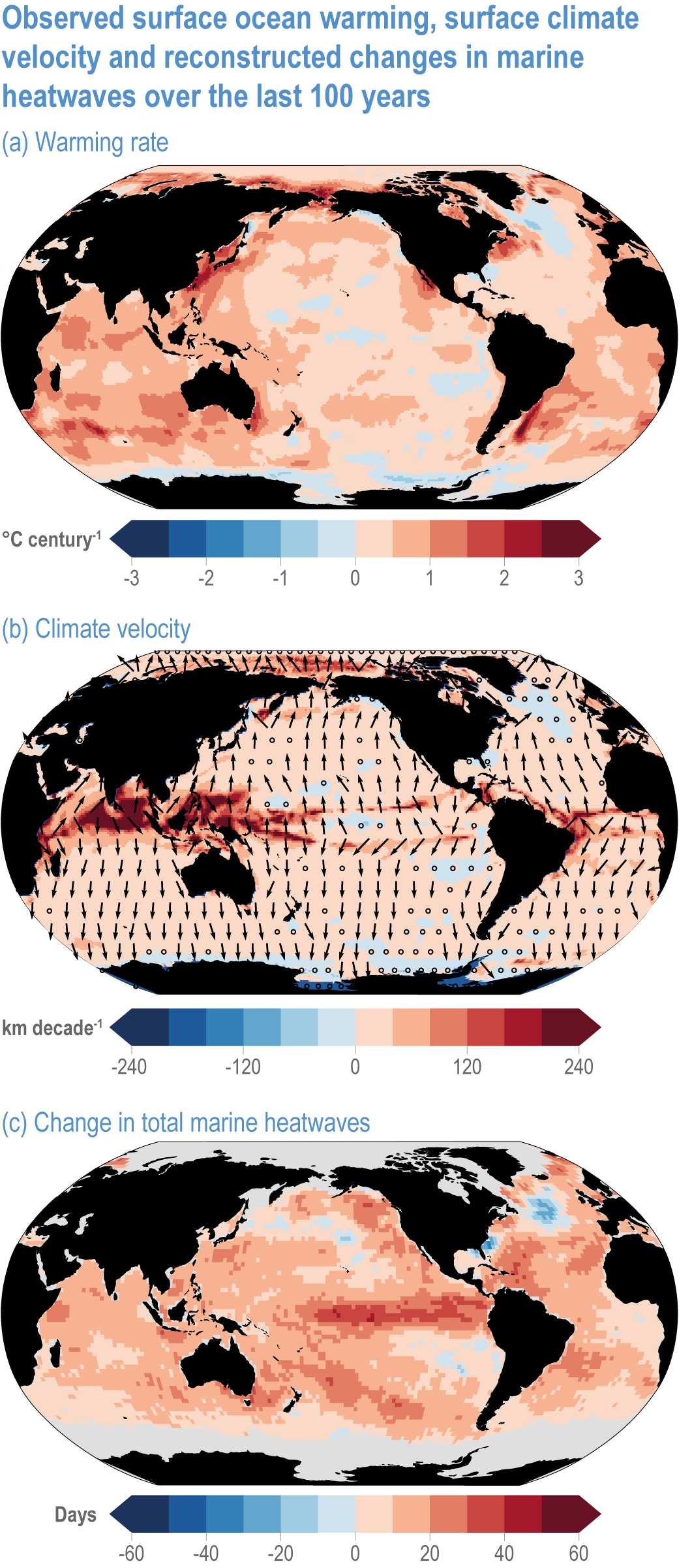
Figure 3.3 | Observed surface ocean warming, surface climate velocity and reconstructed changes in marine heatwaves (MHWs) over the past 100 years. (a) Sea surface temperature trend (degrees Celsius per century) over 1925–2016 from Hadley Centre Sea Ice and Sea Surface Temperature 1.1 (HadISST1.1; (b) surface climate velocity (kilometres per decade) over 1925–2016 computed from HadISST1.1 and (c) change in total MHW days for the surface ocean over 1925–1954 to 1987–2016 based on monthly proxies. (Data from Oliver et al., 2018).
Marine heatwaves (MHWs) are periods of extreme seawater temperature relative to the long-term mean seasonal cycle, that persist for days to months, and that may carry severe consequences for marine ecosystems and their services (WGI AR6 Box 9.2; Hobday et al., 2016a; Smale et al., 2019; Fox-Kemper et al., 2021). MHWs became more frequent over the 20th century (high confidence) and into the beginning of the 21st century, approximately doubling in frequency (high confidence) and becoming more intense and longer since the 1980s (medium confidence) (WGI AR6 Box 9.2; Fox-Kemper et al., 2021). These trends in MHWs are explained by an increase in ocean mean temperatures (Oliver et al., 2018), and human influence has very likely contributed to 84–90% of them since at least 2006 (WGI AR6 Box 9.2; Fox-Kemper et al., 2021). The probability of occurrence (as well as duration and intensity) of the largest and most impactful MHWs that have occurred in the past 30 years has increased more than 20-fold due to anthropogenic climate change (Laufkötter et al., 2020).
Ocean warming will continue over the 21st century (virtually certain), with the rate of global ocean warming starting to be scenario-dependent from about the mid-21st century (medium confidence). At the ocean surface, it is virtually certain that SST will continue to increase throughout the 21st century, with increasing hazards to many marine ecosystems (WGI AR6 Box 9.2; Fox-Kemper et al., 2021). The future global mean SST increase projected by CMIP6 models for the period 1995–2014 to 2081–2100 is 0.86°C (very likely range: 0.43–1.47°C) under SSP1-2.6, 1.51°C (1.02–2.19°C) under SSP2-4.5, 2.19°C (1.56–3.30°C) under SSP3-7.0 and 2.89°C (2.01–4.07°C) under SSP5-8.5 (WGI AR6 Section 9.2.1; Fox-Kemper et al., 2021). Stronger surface warming occurs in parts of the tropics, in the North Pacific, and in the Arctic Ocean, where SST increases by >4°C in 2080–2099 under SSP5-8.5 (Kwiatkowski et al., 2020). The CMIP6 climate models also project ocean warming at the seafloor, with the magnitude of projected changes being less than that of surface waters but having larger uncertainties (Kwiatkowski et al., 2020). The projected end-of-the-century warming in CMIP6 as reported here is greater than assessed with Coupled Model Intercomparison Project 5 (CMIP5) models in AR5 and in SROCC for similar radiative forcing scenarios (Figure 3.5; Kwiatkowski et al., 2020), because of greater climate sensitivity in the CMIP6 model ensemble than in CMIP5 (WGI AR6 Chapter 4; Forster et al., 2020; Lee et al., 2021).
Marine heatwaves will continue to increase in frequency, with a likely global increase of 2–9 times in 2081–2100 compared with 1995–2014 under SSP1-2.6, and 3–15 times under SSP5-8.5, with the largest increases in tropical and Arctic oceans (WGI AR6 Box 9.2; Frölicher et al., 2018; Fox-Kemper et al., 2021).
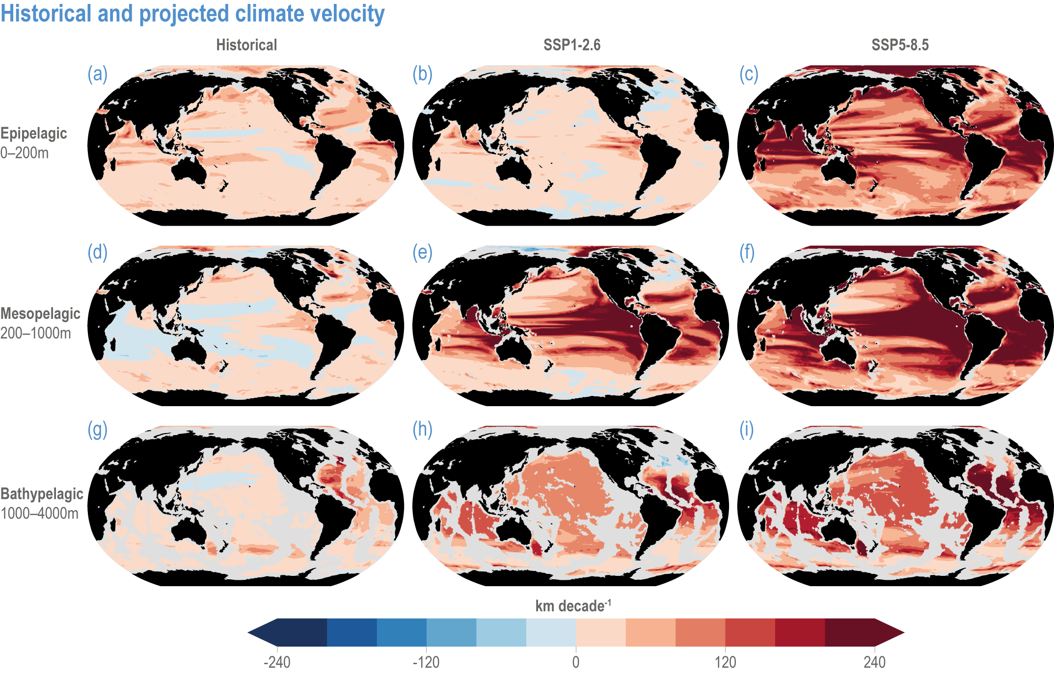
Figure 3.4 | Historical and projected climate velocity. Climate velocities (in kilometres per decade) are shown for the (a,d,g) historical period (1965–2014), and the last 50 years of the 21st century (2051–2100), under (b,e,h) SSP1-2.6 and (c,f,i) SSP5-8.5. Also shown are the epipelagic (0–200 m), mesopelagic (200–1000 m) and bathypelagic (1000–4000 m) domains. Updated figure from Brito-Morales et al. (2020), with Coupled Model Intercomparison Project 6 models used in Kwiatkowski et al. (2020).
3.2.2.2 Sea Level Rise and Extreme Sea Levels
Global mean sea level (GMSL) (Cross-Chapter Box SLR in Chapter 3) has risen by about 0.20 m since 1901 and continues to accelerate (WGI AR6 Section 2.3.3.3; Church and White, 2011; Jevrejeva et al., 2014; Hay et al., 2015; Kopp et al., 2016; Dangendorf et al., 2017; WCRP Global Sea Level Budget Group, 2018; Kemp et al., 2018; Ablain et al., 2019; Gulev et al., 2021).
Most coastal ecosystems (mangroves, seagrasses, salt marshes, shallow coral reefs, rocky shores and sandy beaches) are affected by changes in relative sea level (RSL, the change in the mean sea level relative to the land; Section 3.4.2). Regional rates of RSL rise differ from the global mean due to a range of factors, including local subsidence driven by anthropogenic activities such as groundwater and hydrocarbon extraction (WGI AR6 Box 9.1; Fox-Kemper et al., 2021). In many deltaic regions, anthropogenic subsidence is currently the dominant driver of RSL rise (WGI AR6 Section 9.6.3.2; Tessler et al., 2018; Fox-Kemper et al., 2021). RSL rise is driving a global increase in the frequency of extreme sea levels (high confidence) (WGI AR6 Section 9.6.4.1; Fox-Kemper et al., 2021).
GMSL rise through the middle of the 21st century exhibits limited dependence on emissions scenario; between 1995–2014 and 2050, GMSL is likely to rise by 0.15–0.23 m under SSP1-1.9 and 0.20–0.30 m under SSP5-8.5 (WGI AR6 Section 9.6.3; Fox-Kemper et al., 2021). Beyond 2050, GMSL and RSL projections are increasingly sensitive to the differences among emission scenarios. Considering only processes in which there is at least medium confidence (e.g., thermal expansion, land-water storage, land-ice surface mass balance and some ice-sheet dynamic processes), GMSL between 1995–2014 and 2100 is likely to rise by 0.28–0.55 m under SSP1-1.9, 0.33–0.61 m under SSP1-2.6, 0.44–0.76 m under SSP2-4.5, 0.55–0.90 m under SSP3-7.0 and 0.63–1.02 m under SSP5-8.5 (Figure 3.5). Under high-emission scenarios, ice-sheet processes in which there is low confidence and deep uncertainty might contribute more than one additional metre to GMSL rise by 2100 (WGI AR6 Chapter 9; Fox-Kemper et al., 2021).
Rising mean RSL will continue to drive an increase in the frequency of extreme sea levels (high confidence). The expected frequency of the current 1-in-100-year extreme sea level is projected to increase by a median of 20–30 times across tide-gauge sites by 2050, regardless of emission scenario (medium confidence). In addition, extreme-sea-level frequency may be affected by changes in tropical cyclone climatology (low confidence), wave climatology (low confidence) and tides (high confidence) associated with climate change and sea level change (WGI AR6 Section 9.6.4.2; Fox-Kemper et al., 2021).
3.2.2.3 Changes in Ocean Circulation, Stratification and Coastal Upwelling
Ocean circulation and its variations are key to the evolution of the physical, chemical and biological properties of the ocean. Vertical mixing and upwelling are critical factors affecting the supply of nutrients to the sunlit ocean and hence the magnitude of primary productivity. Ocean currents not only transport heat, salt, carbon and nutrients, but they also control the dispersion of many organisms and the connectivity between distant populations.
Ocean stratification is an important factor controlling biogeochemical cycles and affecting marine ecosystems. WGI AR6 Section 9.2.1.3 (Fox-Kemper et al., 2021) assessed that it is virtually certain that stratification in the upper 200 m of the ocean has been increasing since 1970. Recent evidence has strengthened estimates of the rate of change (Yamaguchi and Suga, 2019; Li et al., 2020a; Sallée et al., 2021), with an estimated increase of 1.0 ± 0.3% (very likely range) per decade over the period 1970–2018 (high confidence) (WGI AR6 Section 9.2.1.3; Fox-Kemper et al., 2021), higher than assessed in SROCC. It is very likely that stratification in the upper few hundred metres of the ocean will increase substantially in the 21st century in all ocean basins, driven by intensified surface warming and near-surface freshening at high latitudes (WGI AR6 Section 9.2.1.3; Capotondi et al., 2012; Fu et al., 2016; Bindoff et al., 2019a; Kwiatkowski et al., 2020; Fox-Kemper et al., 2021).
Contrasting changes among the major eastern boundary coastal upwelling systems (EBUS) were identified in AR5 (Hoegh-Guldberg et al., 2014). While SROCC assessed with high confidence that three (Benguela, Peru-Humboldt, California) out of the four major EBUS have experienced upwelling-favourable wind intensification in the past 60 years (Sydeman et al., 2014; Bindoff et al., 2019a), WGI AR6 revisited this assessment based on evidence showing low agreement between studies that have investigated trends over past decades (Varela et al., 2015). WGI AR6 assessed that only the California Current system has undergone large-scale upwelling-favourable wind intensification since the 1980s (medium confidence) (WGI AR6 Section 9.2.1.5; García-Reyes and Largier, 2010; Seo et al., 2012; Fox-Kemper et al., 2021).
While no consistent pattern of contemporary changes in upwelling-favourable winds emerges from observation-based studies, numerical and theoretical work projects that summertime winds near poleward boundaries of upwelling zones will intensify, while winds near equatorward boundaries will weaken (high confidence) (WGI AR6 Section 9.2.3.5; García-Reyes et al., 2015; Rykaczewski et al., 2015; Wang et al., 2015; Aguirre et al., 2019; Fox-Kemper et al., 2021). Nevertheless, projected future annual cumulative upwelling wind changes at most locations and seasons remain within ±10–20% of present-day values (medium confidence) (WGI AR6 Section 9.2.3.5; Fox-Kemper et al., 2021).
Continuous observation of the Atlantic meridional overturning circulation (AMOC) has improved the understanding of its variability (Frajka-Williams et al., 2019), but there is low confidence in the quantification of AMOC changes in the 20th century because of low agreement in quantitative reconstructed and simulated trends (WGI AR6 Sections 2.3.3, 9.2.3.1; Fox-Kemper et al., 2021; Gulev et al., 2021). Direct observational records since the mid-2000s remain too short to determine the relative contributions of internal variability, natural forcing and anthropogenic forcing to AMOC change (high confidence) (WGI AR6 Sections 2.3.3, 9.2.3.1; Fox-Kemper et al., 2021; Gulev et al., 2021). Over the 21st century, AMOC will very likely decline for all SSP scenarios but will not involve an abrupt collapse before 2100 (WGI AR6 Sections 4.3.2, 9.2.3.1; Fox-Kemper et al., 2021; Lee et al., 2021).
3.2.2.4 Sea Ice Changes
Sea ice is a key driver of polar marine life, hosting unique ecosystems and affecting diverse marine organisms and food webs through its impact on light penetration and supplies of nutrients and organic matter (Arrigo, 2014). Since the late 1970s, Arctic sea ice area has decreased for all months, with an estimated decrease of 2 million km 2 (or 25%) for summer sea ice (averaged for August, September and October) in 2010–2019 as compared with 1979–1988 (WGI AR6 Section 9.3.1.1; Fox-Kemper et al., 2021). For Antarctic sea ice there is no significant global trend in satellite-observed sea ice area from 1979 to 2020 in either winter or summer, due to regionally opposing trends and large internal variability (WGI AR6 Section 9.3.2.1; Maksym, 2019; Fox-Kemper et al., 2021).
CMIP6 simulations project that the Arctic Ocean will likely become practically sea ice free (area below 1 million km 2) for the first time before 2050 and in the seasonal sea ice minimum in each of the four emission scenarios SSP1-1.9, SSP1-2.6, SSP2-4.5 and SSP5-8.5 (Figure 3.7; WGI AR6 Section 9.3.2.2; Notze and SIMIP Community, 2020; Fox-Kemper et al., 2021). Antarctic sea ice area is also projected to decrease during the 21st century, but due to mismatches between model simulations and observations, combined with a lack of understanding of reasons for substantial inter-model spread, there is low confidence in model projections of future Antarctic sea ice changes, particularly at the regional level (WGI AR6 Section 9.3.2.2; Roach et al., 2020; Fox-Kemper et al., 2021).
3.2.3 Chemical Changes
3.2.3.1 Ocean Acidification
The ocean’s uptake of anthropogenic carbon affects its chemistry in a process referred to as ocean acidification, which increases the concentrations of aqueous CO2, bicarbonate and hydrogen ions, and decreases pH, carbonate ion concentrations and calcium carbonate mineral saturation states (Doney et al., 2009). Ocean acidification affects a variety of biological processes with, for example, lower calcium carbonate saturation states reducing net calcification rates for some shell-forming organisms and higher CO2 concentrations increasing photosynthesis for some phytoplankton and macroalgal species (Section 3.3.2).
Direct measurements of ocean acidity from ocean time series, as well as pH changes determined from other shipboard studies, show consistent decreases in ocean surface pH over the past few decades (virtually certain) (WGI AR6 Section 5.3.2.2; Takahashi et al., 2014; Bindoff et al., 2019a; Sutton et al., 2019; Canadell et al., 2021).
Since the 1980s, surface ocean pH has declined by a very likely rate of 0.016–0.020 per decade in the subtropics and 0.002–0.026 per decade in the subpolar and polar zones (WGI AR6 Section 5.3.2.2; Canadell et al., 2021). Typically, the pH of global surface waters has decreased from 8.2 to 8.1 since the pre-industrial era (1750 CE), a trend attributable to rising atmospheric CO2 (virtually certain) (Orr et al., 2005; Jiang et al., 2019).
Ocean acidification is also developing in the ocean interior (very high confidence) due to the transport of anthropogenic CO2 to depth by ocean currents and mixing (WGI AR6 Section 5.3.3.1; Canadell et al., 2021). There, it leads to the shoaling of saturation horizons of aragonite and calcite (high confidence) (WGI AR6 Section 5.3.3.1; Canadell et al., 2021), below which dissolution of these calcium carbonate minerals is thermodynamically favoured. The calcite or aragonite saturation horizons have migrated upwards in the North Pacific (1–2 m yr –1 over 1991–2006) (Feely et al., 2012) and in the Irminger Sea (10–15 m yr –1 for the aragonite saturation horizon over 1991–2016) (Perez et al., 2018). In some locations of the western Atlantic Ocean, calcite saturation depth has risen by ~300 m since the pre-industrial era due to increasing concentrations of deep-ocean dissolved inorganic carbon (Sulpis et al., 2018). In the Arctic, where some coastal surface waters are already undersaturated with respect to aragonite due to the degradation of terrestrial organic matter (Mathis et al., 2015; Semiletov et al., 2016), the deep aragonite saturation horizon shoaled on average 270 ± 60 m during 1765–2005 (Terhaar et al., 2020).
Detection and attribution of ocean acidification in coastal environments are more difficult than in the open ocean due to larger spatio-temporal variability of carbonate chemistry (Duarte et al., 2013; Laruelle et al., 2017; Torres et al., 2021) and to the influence of other natural acidification drivers such as freshwater and high-nutrient riverine inputs (Cai et al., 2011; Laurent et al., 2017; Fennel et al., 2019; Cai et al., 2020) or anthropogenic acidification drivers (Section 3.1) like atmospherically deposited nitrogen and sulphur (Doney et al., 2007; Hagens et al., 2014). Since AR5, the observing network in coastal oceans has expanded substantially, improving understanding of both the drivers and amplitude of observed variability (Sutton et al., 2016). Recent studies indicate that two more decades of observations may be required before anthropogenic ocean acidification emerges over natural variability in some coastal sites and regions (WGI AR6 Section 5.3.5.2; Sutton et al., 2019; Turk et al., 2019; Canadell et al., 2021).
Mean open-ocean surface pH is projected to decline by 0.08 ± 0.003 (very likely range), 0.17 ± 0.003, 0.27 ± 0.005 and 0.37 ± 0.007 pH units in 2081–2100 relative to 1995–2014, for SSP1-2.6, SSP2-4.5, SSP3-7.0 and SSP5-8.5, respectively (Figure 3.5; WGI AR6 Section 4.3.2; Kwiatkowski et al., 2020; Lee et al., 2021). Projected changes in surface pH are relatively uniform in contrast with those of other surface-ocean variables, but they are largest in the Arctic Ocean (Figure 3.6; WGI AR6 Section 5.3.4.1; Canadell et al., 2021). Similar declines in the concentration of carbonate ions are projected by Earth system models (ESMs; Bopp et al., 2013; Gattuso et al., 2015; Kwiatkowski et al., 2020). The North Pacific, the Southern Ocean and Arctic Ocean regions will become undersaturated for calcium carbonate minerals first (Orr et al., 2005; Pörtner et al., 2014). Concurrent impacts on the seasonal amplitude of carbonate chemistry variables are anticipated (i.e., increased amplitude for pCO2 and hydrogen ions, decreased amplitude for carbonate ions; McNeil and Sasse, 2016; Kwiatkowski and Orr, 2018; Kwiatkowski et al., 2020).

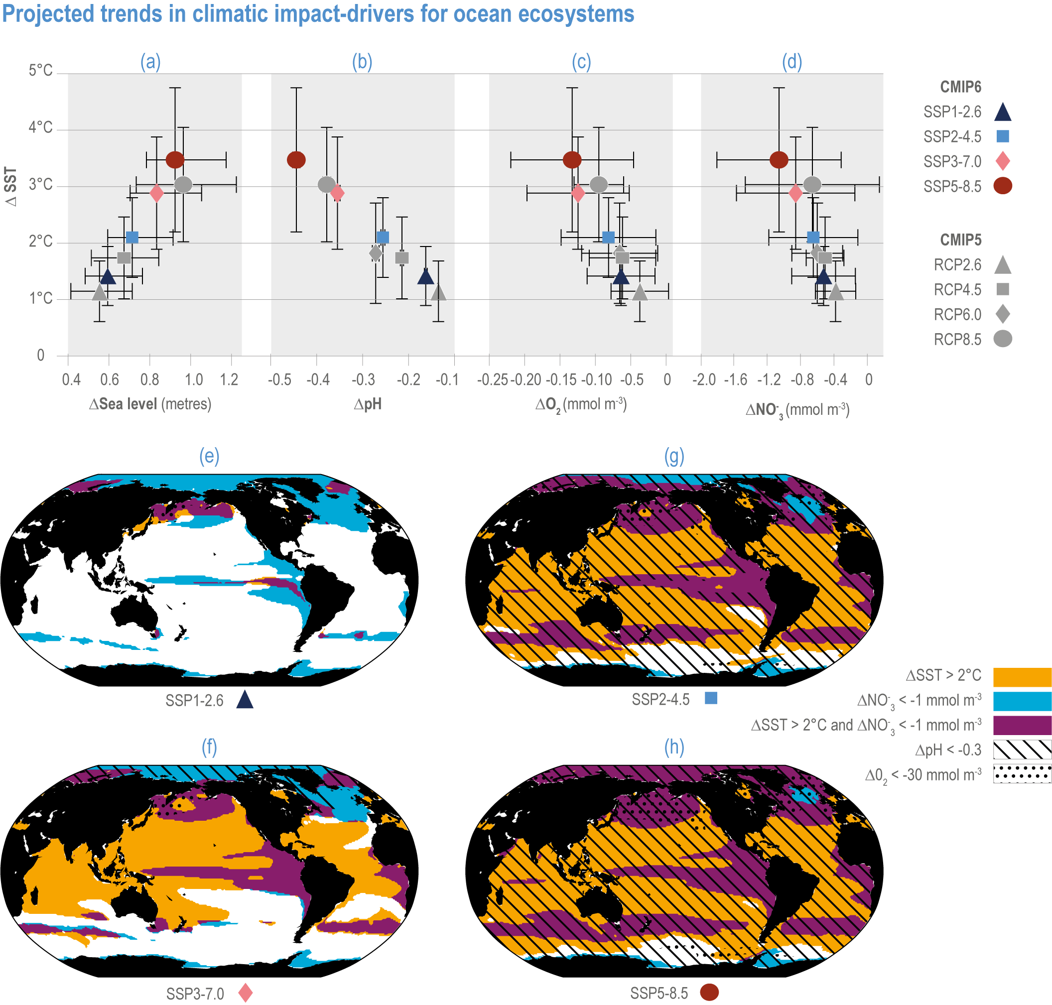
Figure 3.5 | Projected trends in climatic impact-drivers for ocean ecosystems. Panels (a,b,c,d) represent Coupled Model Intercomparison Project 5 (CMIP5) Representative Concentration Pathway (RCP) and CMIP6 Shared Socioeconomic Pathway (SSP) end-of-century changes in (a) global sea level; (b) average surface pH, (c) subsurface (100–600 m) dissolved oxygen concentration and (d) euphotic-zone (0–100 m) nitrate (NO3) concentration against anomalies in sea surface temperature. All anomalies are model-ensemble averages over 2080–2099 relative to the 1870–1899 baseline period (from Kwiatkowski et al., 2020), except for sea level, which shows model-ensemble median in 2100 relative to 1901 (from AR6 WGI Chapter 9). Error bars represent very likely ranges, except for SLR where they represent likely ranges. Very likely ranges for pH changes are too narrow to appear in the figure (see text). Panels (e,f,g,h) show regions where end-of-century projected CMIP6 surface warming exceeds 2°C, where surface ocean pH decline exceeds 0.3, where subsurface dissolved oxygen decline exceeds 30 mmol m -3 and where euphotic-zone (0–100 m) nitrate decline exceeds 1 mmol m -3 in (e) SSP1-2.6, (f) SSP2-4.5, (g) SSP3-7.0 and (h) SSP5-8.5. All anomalies are 2080–2099 relative to the 1870–1899 baseline period. (Modified from Kwiatkowski et al., 2020).
Future declines in subsurface pH (Figure 3.6) will be modulated by changes in ocean overturning and water-mass subduction (Resplandy et al., 2013), and in organic matter remineralisation (Chen et al., 2017). In particular, decreases in pH will be less consistent at the seafloor than at the surface and will be linked to the transport of surface anomalies to depth. For example, >20% of the North Atlantic seafloor deeper than 500 m, including canyons and seamounts designated as marine protected areas (MPAs), will experience pH reductions >0.2 by 2100 under RCP8.5 (Gehlen et al., 2014). Changes in pH in the abyssal ocean (>3000 m deep) are greatest in the Atlantic and Arctic Oceans, with lesser impacts in the Southern and Pacific Oceans by 2100, mainly due to ventilation time scales (Sweetman et al., 2017).
3.2.3.2 Ocean Deoxygenation
Ocean deoxygenation, the loss of oxygen in the ocean, results from ocean warming, through a reduction in oxygen saturation, increased oxygen consumption, increased ocean stratification and ventilation changes (Keeling et al., 2010; IPCC, 2019a). In recent decades, anthropogenic inputs of nutrients and organic matter (Section 3.1) have increased the extent, duration and intensity of coastal hypoxia events worldwide (Diaz and Rosenberg, 2008; Rabalais et al., 2010; Breitburg et al., 2018), while pollution-induced atmospheric deposition of soluble iron over the ocean has accelerated open-ocean deoxygenation (Ito et al., 2016). Deoxygenation and acidification often coincide because biological consumption of oxygen produces CO2. Deoxygenation can have a range of detrimental effects on marine organisms and reduce the extent of marine habitats (Sections 3.3.2, 3.4.3.1; Vaquer-Sunyer and Duarte, 2008; Chu and Tunnicliffe, 2015).
Changes in ocean oxygen concentrations have been analysed from compilations of in situ data dating back to the 1960s (Helm et al., 2011; Ito et al., 2017; Schmidtko et al., 2017). SROCC concluded that a loss of oxygen had occurred in the upper 1000 m of the ocean (medium confidence), with a global mean decrease of 0.5–3.3% (very likely range) over 1970–2010 (Bindoff et al., 2019a). Based on new regional assessments (Queste et al., 2018; Bronselaer et al., 2020; Cummins and Ross, 2020; Stramma et al., 2020), WGI AR6 assesses that ocean deoxygenation has occurred in most regions of the open ocean since the mid-20th century (high confidence), but it is modified by climate variability on interannual and inter-decadal time scales (medium confidence) (WGI AR6 Sections 2.3.3.6, 5.3.3.2; Canadell et al., 2021; Gulev et al., 2021). New findings since SROCC also confirm that the volume of oxygen minimum zones (OMZs) are expanding at many locations (high confidence) (WGI AR6 Section 5.3.3.2; Canadell et al., 2021).
The most recent estimates of future oxygen loss in the subsurface ocean (100–600 m), using CMIP6 models, amount to −4.1 ± 4.2 (very likely range), −6.6 ± 5.7, −10.1 ± 6.7 and −11.2 ± 7.7% in 2081–2100 relative to 1995–2014 for SSP1-2.6, SSP2-4.5, SSP3-7.0 and SSP5-8.5, respectively (Figure 3.5; Kwiatkowski et al., 2020). Based on these CMIP6 projections, WGI AR6 concludes that the oxygen content of the subsurface ocean is projected to decline to historically unprecedented conditions over the 21st century (medium confidence) (WGI AR6 Section 5.3.3.2; Canadell et al., 2021). These declines are greater (by 31–72%) than simulated by the CMIP5 models in their Representative Concentration Pathway (RCP) analogues, a likely consequence of enhanced surface warming and stratification in CMIP6 models (Figure 3.5; Kwiatkowski et al., 2020). At the regional scale and for subsurface waters, projected changes are not spatially uniform, and there is lower agreement among models than they show for the global mean trend (Bopp et al., 2013; Kwiatkowski et al., 2020). In particular, large uncertainties remain for these future projections of ocean deoxygenation in the subsurface tropical oceans, where the major OMZs are located (Cabré et al., 2015; Bopp et al., 2017).
3.2.3.3 Changes in Nutrient Availability
The availability of nutrients in the surface ocean often limits primary productivity, with implications for marine food webs and the biological carbon pump. Nitrogen availability tends to limit phytoplankton productivity throughout most of the low-latitude ocean, whereas dissolved iron availability limits productivity in high-nutrient, low-chlorophyll regions, such as in the main upwelling region of the Southern Ocean and the Eastern Equatorial Pacific (high confidence) (Moore et al., 2013; IPCC, 2019b). Phosphorus, silicon, other micronutrients such as zinc, and vitamins can also co-limit marine phytoplankton productivity in some ocean regions (Moore et al., 2013). Whereas some studies have shown coupling between climate variability and nutrient trends in specific regions, such as in the North Atlantic (Hátún et al., 2016), North Pacific (Di Lorenzo et al., 2009; Yasunaka et al., 2014) and tropical (Stramma and Schmidtko, 2021) Oceans, very few studies have been able to detect long-term changes in ocean nutrient concentrations (but see Yasunaka et al., 2016).
Future changes in nutrient concentrations have been estimated using ESMs, with future increases in stratification generally leading to decreased nutrient levels in surface waters (IPCC, 2019b). CMIP6 models project a decline in the nitrate concentration of the upper 100 m in 2080–2099 relative to 1995–2014 of −0.46 ± 0.45 (very likely range), −0.60 ± 0.58, −0.80 ± 0.77 and −1.00 ± 0.78 mmol m –3 under SSP1-2.6, SSP2-4.5 and SSP5-8.5, respectively (Figure 3.5; Kwiatkowski et al., 2020). These declines in nitrate concentration are greater than simulated by the CMIP5 models in their RCP analogues, a likely consequence of enhanced surface warming and stratification in CMIP6 models (Figure 3.5; Kwiatkowski et al., 2020). It is concluded that the surface ocean will encounter reduced nitrate concentrations in the 21st century (medium confidence).
3.2.4 Global Synthesis on Multiple Climate-induced Drivers
In the 21st century, ocean and coastal ecosystems are projected to face conditions unprecedented over past centuries to millennia (high confidence) (Section 3.2; WGI AR6 Chapters 4, 9; Fox-Kemper et al., 2021; Lee et al., 2021), with increased temperatures (virtually certain) and frequency and severity of MHWs (very high confidence), stronger upper-ocean stratification (high confidence), continued rise in GMSL throughout the 21st century (high confidence) and increased frequency of extreme sea levels (high confidence), further acidification (virtually certain), oxygen decline (high confidence) and decreased surface nitrate inventories (medium confidence).
The rates and magnitudes of these changes largely depend on the extent of future emissions (very high confidence), with surface ocean warming and acidification (very likely range) at +3.47°C ± 1.28°C and −0.44 pH units ± 0.008 pH units in 2080–2099 (relative to 1870–1899) for SSP5-8.5 compared with +1.42°C ± 0.53°C and −0.16 pH units ± 0.003 pH units for SSP1-2.6 (Figure 3.5; Kwiatkowski et al., 2020).
3.2.4.1 Compound Changes in the 21st century
Earth system models project distinct regional evolutions of the different CIDs over the 21st century (very high confidence) (Figures 3.5, 3.6, 3.7; Kwiatkowski et al., 2020). Tropical and subtropical oceans are characterised by projected warming and acidification, accompanied by declining nitrate concentrations in equatorial upwelling regions. The North Atlantic is characterised by a high exposure to acidification and declining nitrate concentrations. The North Pacific is characterised by high sensitivity to compound changes, with high rates of warming, acidification, deoxygenation and nutrient depletion. In contrast, the development of compound hazards is limited in the Southern Ocean, where rates of warming and nutrient depletion are lower. The Arctic Ocean is characterised by the highest rates of acidification and warming, strong nutrient depletion, and it will likely become practically sea ice free in the September mean for the first time before the year 2050 in all SSP scenarios (high confidence) (Figures 3.5, 3.6, 3.7; Sections 3.2.2, 3.2.3).
In general, the projected changes in climate-induced drivers are less in absolute terms in the deep-sea (mesopelagic and bathypelagic domains and deep-sea habitats) than in the surface ocean and in shallow-water habitats (e.g., kelp ecosystems, warm-water corals) (very high confidence) (Figures 3.6, 3.7; Mora et al., 2013; Sweetman et al., 2017). The mesopelagic domain will be nevertheless exposed to high rates of deoxygenation (Figure 3.6) and high climate velocities (Figure 3.4; Section 3.2.2.1), as well as impacted by the shoaling of aragonite or calcite saturation horizon (Section 3.2.3.2). Significant differences in projected trends between the SSPs show that mitigation strategies will limit exposure of deep-sea ecosystems to potential warming, acidification and deoxygenation during the 21st century (very high confidence) (Figure 3.6; Kwiatkowski et al., 2020).
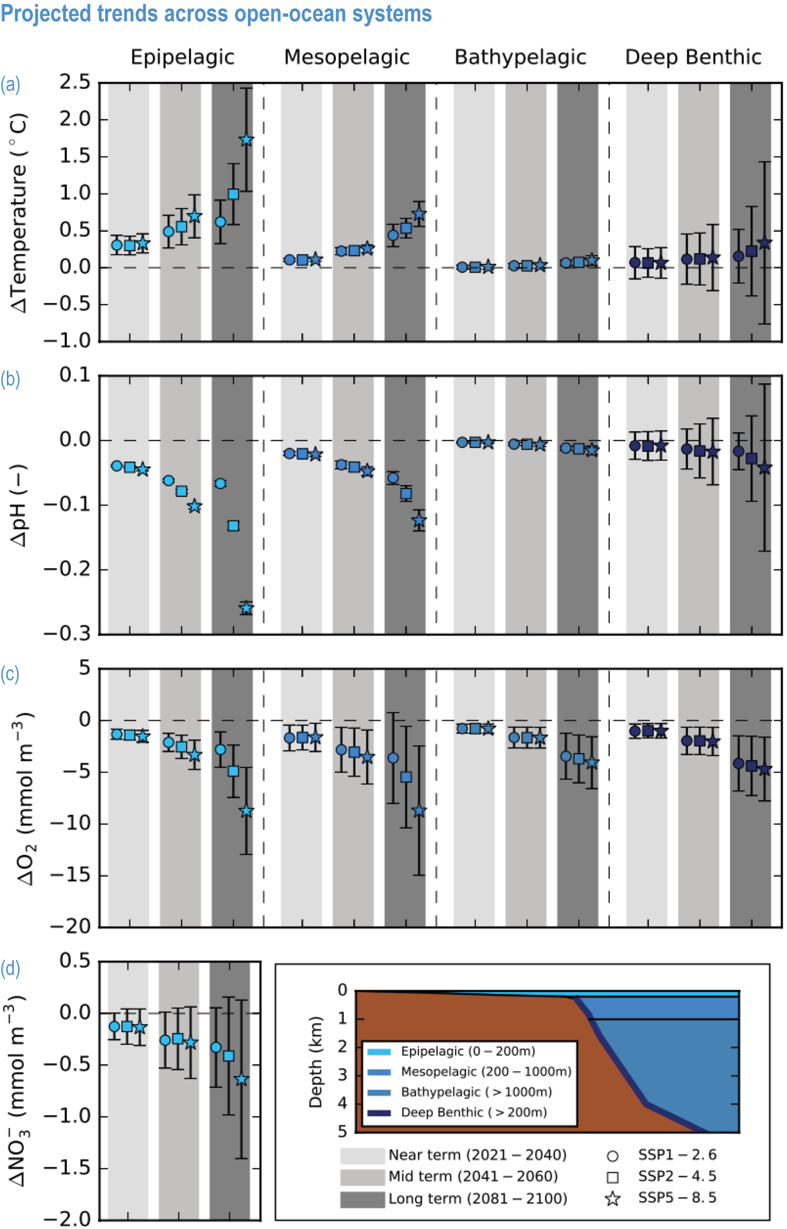
Figure 3.6 | Projected trends across open-ocean systems. Projected annual and global (a) average warming, (b) acidification, (c) changes in dissolved oxygen concentrations and (d) changes in nitrate (NO3) concentrations for four open-ocean systems, including the epipelagic (0–200 m depth), mesopelagic (200–1000 m), bathypelagic (>1000 m) domains and deep benthic waters (>200 m). All projections are based on Coupled Model Intercomparison Project 6 models and for three Shared Socioeconomic Pathways (SSPs): SSP1-2.6, SSP2-4.5 and SSP5-8.5 (Kwiatkowski et al., 2020). Anomalies in the near-term (2020–2041), mid-term (2041–2060) and long-term (2081–2100) are all relative to 1985–2014. Error bars represent very likely ranges.

Figure 3.7 | Projected trends across coastal-ocean ecosystems. Projected (a) warming, (b) acidification, (c) changes in dissolved oxygen concentrations, (d) changes in nitrate (NO3) concentrations and (e) changes in summer sea ice cover fraction (September and north of 66°N for the Northern Polar Oceans, and March and south of 66°S for the Southern Polar Ocean) for five coastal-ocean ecosystems. All projected trends are for the surface ocean, except oxygen concentration changes that are computed for the subsurface ocean (100–600 m depth) for the upwelling ecosystems and the polar seas. All projections are based on Coupled Model Intercomparison Project 6 (CMIP6) models and for three Shared Socioeconomic Pathways (SSPs): SSP1-2.6, SSP2-4.5 and SSP5-8.5 (Kwiatkowski et al., 2020). Anomalies in the near term (2020–2041), mid term (2041–2060) and long term (2081–2100) are all relative to 1985–2014. Error bars represent very likely ranges. Coastal seas are defined on a 1° × 1° grid when bathymetry is less than 200 m deep. Distribution of warm-water corals is from UNEP-WCMC et al. (2018). Distribution of kelp ecosystems is from OBIS (2020). Upwelling areas are defined according to Rykaczewski et al. (2015).
3.2.4.2 Time of Emergence
Anthropogenic changes in climate-induced drivers assessed here exhibit vastly distinct times of emergence, which is the time scale over which an anthropogenic signal related to climate change is statistically detected to emerge from the background noise of natural climate for a specific region (Christensen et al., 2007; Hawkins and Sutton, 2012). SROCC concluded that for ocean properties, the time of emergence ranges from under a decade (e.g., surface ocean pH) to over a century (e.g., net primary production; see Section 3.4.3.3.4 for time of emergence of biological properties; Bindoff et al., 2019a).
The literature assessed in SROCC mainly focused on surface ocean properties and gradual mean changes. Since then, the time of emergence has also been investigated for subsurface properties, ocean extreme events and particularly vulnerable regions, such as the Arctic Ocean (Hameau et al., 2019; Oliver et al., 2019; Burger et al., 2020; Landrum and Holland, 2020; Schlunegger et al., 2020), but subsequent assessments are low confidence due to limited evidence. Below the surface, changes in temperature typically emerge from internal variability prior to changes in oxygen; however, in about a third of the global thermocline, deoxygenation emerges prior to warming (Hameau et al., 2019). Permanent MHW states, defined as when SST exceeds the MHW threshold continuously over a full calendar year, will emerge during the 21st century in many parts of the surface ocean (Oliver et al., 2019). Ocean acidification extremes have already emerged from background natural internal variability during the 20th century in most of the surface ocean (Burger et al., 2020). In the Arctic, anthropogenic sea ice changes have already emerged from the background internal variability, and anthropogenic alteration of air temperatures will emerge in the early- to mid-21st century (Landrum and Holland, 2020).
3.2.4.4 Perspectives from Paleoclimatology Data
Paleoclimatology observations are useful to assess multiple hazards of environmental change while excluding direct anthropogenic impacts (Section 3.4.3.3). Ancient intervals of rapid climate warming that occurred between 300 and 50 million years ago (Ma) were triggered by the release of greenhouse gases (high confidence). The sources of greenhouse gases varied but include volcanic degassing from continental flood basalts and methane hydrates stored in marine sediments and soils (Foster et al., 2018). Six extreme ancient hyperthermal events are known from the last 300 Ma, when tropical SSTs reached 1.5°C–10°C warmer than pre-industrial conditions, and with substantial impacts on ancient life (Cross-Chapter Box PALEO in Chapter 1). Warming and deoxygenation in the oceans were closely associated in hyperthermal events (high confidence), with anoxia reaching the photic zone and abyssal depths (Kaiho et al., 2014; Müller et al., 2017; Penn et al., 2018; Weissert, 2019), whereas ocean acidification has not been demonstrated consistently (medium confidence) (Hönisch et al., 2012; Penman et al., 2014; Clarkson et al., 2015; Harper et al., 2020a; Jurikova et al., 2020; Müller et al., 2020).
Greenhouse gases also contributed substantially to shaping the longer-term climate trends over the past 50 million years, although changes in continental configuration and ocean circulation as well as planetary orbital cycles were equally important (WGI AR6 Cross-Chapter Box 2.1 in Chapter 2; Westerhold et al., 2020; Gulev et al., 2021). There is little evidence for ocean acidification in the past 2.6 Ma (low confidence) (Hönisch et al., 2012), but ocean ventilation was highly sensitive to even modest warming such as observed in the past 10,000 years (medium confidence) (Jaccard and Galbraith, 2012; Lembke-Jene et al., 2018).
3.3 Linking Biological Responses to Climate-induced Drivers
3.3.1 Introduction
This section assesses new evidence since AR5 (Pörtner et al., 2014) and SROCC (Bindoff et al., 2019a) regarding biotic responses to multiple environmental drivers. It assesses differential sensitivities among life stages within individual organisms, changing responses across scales of biological organisation and the potential for evolutionary adaptation to climate change (e.g., Przeslawski et al., 2015; Boyd et al., 2018; Reddin et al., 2020), providing examples and identifying key gaps and uncertainties that limit our ability to project the ecological impact of multiple climate-induced drivers (Figure 3.8a). The assessment includes physiological responses to single environmental drivers and their underlying mechanisms (Section 3.3.2), the characteristics of multiple drivers and organisms’ responses to them (Section 3.3.3), short-term acclimation and longer-term evolutionary adaptation of populations (Section 3.3.4), and it concludes with an assessment of progress in upscaling laboratory findings to ecosystems within in situ settings (Figure 3.8b; Section 3.3.5).
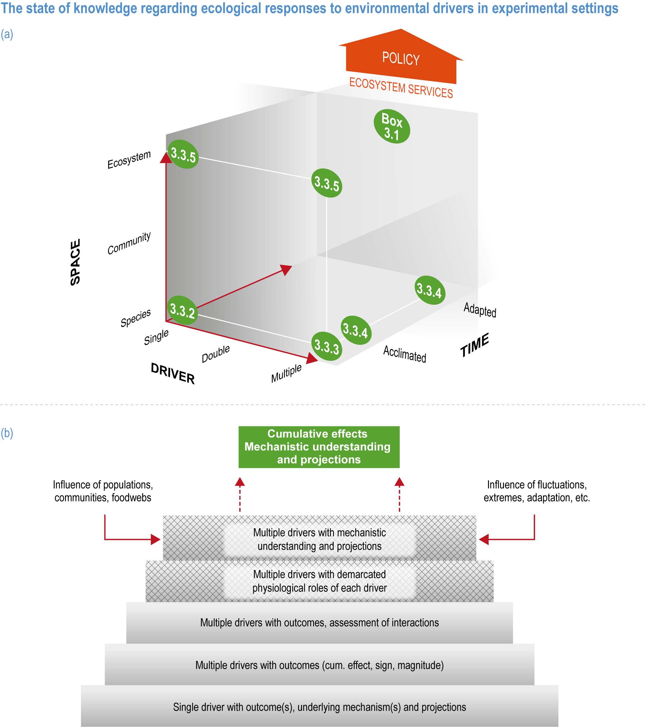
Figure 3.8 | The state of knowledge regarding ecological responses to environmental drivers in experimental settings.
(a) Schematic indicates where themes are discussed within Section 3.3, and how they jointly inform policy. (Adapted from Riebesell and Gattuso, 2014).
(b) The hierarchy of accumulating physiological knowledge (grey layers), from single (e.g., Pörtner et al., 2012) to multiple drivers, and from simple outcomes (e.g., Sciandra et al., 2003), interactions among drivers (e.g., Crain et al., 2008) and identification of physiological roles of drivers (e.g., Bach et al., 2015) to mechanistic understanding of drivers (e.g., Thomas et al., 2017). At present, the upper grey layer has been achieved, in full, for two drivers (e.g., temperature and nutrient concentrations), with validation of dual controls on phytoplankton growth rate (Thomas et al., 2017). Hatched layers denote major advances since WGII AR5 Chapter 6 (Pörtner et al., 2014). The green layer indicates the level of understanding potentially needed to project the response of marine life subjected to multiple drivers. Red horizontal arrows indicate the influence of confounding factors on our current understanding, including population genetics, fluctuating oceanic conditions or extreme events.
3.3.2 Responses to Single Drivers
Anthropogenic CO2 emissions trigger a suite of changes that alter ocean temperature, pH and CO2 concentration, oxygen concentration and nutrient supply at global scales (Section 3.2). The response pathways of these climate-induced drivers have been investigated primarily as single variables.
Temperature affects the movement and transport of molecules and, thereby, the rates of all biochemical reactions; thus, ongoing and projected warming (Section 3.2.2.1) that remains below an organism’s physiological optimum will generally raise metabolic rates (very high confidence) (Pörtner et al., 2014). Beyond this optimum (Topt ; Figure 3.9), metabolism typically decreases sharply, finally reaching a critical threshold (Tcrit ) beyond which enzymes become thermally inactivated and cells undergo oxidative stress. Local and regional adaptation affect the heat tolerance thresholds of organisms. For example, organisms adapted to thermally stable environments (e.g., tropical, polar, deep sea) are often more sensitive to warming than those from thermally variable environments (e.g., estuaries) (very high confidence) (Section 3.4; Sunday et al., 2019; Collins et al., 2020). Heat tolerance also decreases with increasing organisational complexity (Storch et al., 2014; Pörtner and Gutt, 2016) and is lower in eggs, embryos and spawning fish than for their larval stages or adults outside the spawning season (high confidence) (Dahlke et al., 2020b). By altering physiological responses, projected changes in ocean warming (Section 3.2.2.1) will modify growth, migration, distribution, competition, survival and reproduction (very high confidence) (Messmer et al., 2017; Dahlke et al., 2018; Andrews et al., 2019; Pinsky et al., 2019; Anton et al., 2020).

Figure 3.9 | Organismal responses to single and multiple drivers.
(a) The generic temperature–response curve shows physiological process rates as a nonlinear function of a particular driver (e.g., temperature) with maximum rates (Rmax) and temperature optima (Topt ). The driver range that keeps physiological rates above a certain threshold represents the organism’s range of phenotypic plasticity, while below that threshold, the critical temperature (Tcrit ), physiological performance is so low as to constitute stressful conditions.
(b) The response curve for one driver can depend on other drivers, here exemplified for temperature and pH in the central panel. This interaction causes rates as well as optima to change with pH (left) and temperature (right), indicated by the coloured lines. (c) Impacts of multiple drivers on processes can be additive (blue), synergistic (red) or antagonistic (green), that is, the cumulative effects of two (or more) drivers are equal to, larger than or smaller than the sum of their individual effects, respectively. Potential experimental outcomes affected by additive, synergistic and antagonistic interactions are shown for scenarios where drivers increase rates (left), decrease rates (centre) or cause opposite responses (right), showing how experimental outcomes can mask these mechanistic interactions. (For a quantitative analysis of effects of driver pairs on animals, see Figure 3.SM.2.) (Adapted from Crain et al., 2008 and Piggott et al., 2015).
Altered seawater carbonate chemistry (Section 3.2.3.1) affects specific processes to varying degrees. For example, higher CO2 concentrations can increase photosynthesis and growth in some phytoplankton, macroalgal and seagrass species (high confidence) (Pörtner et al., 2014; Seifert et al., 2020; Zimmerman, 2021), while lower pH levels decrease calcification (high confidence) (Pörtner et al., 2014; Falkenberg et al., 2018; Doney et al., 2020; Fox et al., 2020; Reddin et al., 2020) or silicification (low confidence) (Petrou et al., 2019). Organisms’ capacity to compensate for or resist acidification of internal fluids depends on their capacity for acid–base regulation, which differs due to organisms’ wide-ranging biological complexity and adaptive abilities (low to medium confidence) (Vargas et al., 2017; Melzner et al., 2020). Detrimental impacts of acidification include decreased growth and survival, and altered development, especially in early life stages (high confidence) (Dahlke et al., 2018; Onitsuka et al., 2018; Hancock et al., 2020), along with lowered recruitment and altered behaviour in animals (Kroeker et al., 2013a; Wittmann and Pörtner, 2013; Clements and Hunt, 2015; Cattano et al., 2018; Esbaugh, 2018; Bednaršek et al., 2019; Reddin et al., 2020). For finfish, laboratory studies of behavioural and sensory consequences of ocean acidification showed mixed results (Rossi et al., 2018; Nagelkerken et al., 2019; Stiasny et al., 2019; Velez et al., 2019; Clark et al., 2020; Munday et al., 2020). Calcifiers are generally more sensitive to acidification (e.g., for growth and survival) than non-calcifying groups (high confidence) (Kroeker et al., 2013a; Wittmann and Pörtner, 2013; Clements and Hunt, 2015; Cattano et al., 2018; Bednaršek et al., 2019; Reddin et al., 2020; Seifert et al., 2020). For calcifying primary producers, including phytoplankton and coralline algae, ocean acidification has different, often opposing effects, for example, decreasing calcification while photosynthetic rates increase (high confidence) (Riebesell et al., 2000; Van de Waal et al., 2013; Bach et al., 2015; Cornwall et al., 2017b; Gafar et al., 2019).
Oxygen concentrations affect aerobic and anaerobic processes, including energy metabolism and denitrification. Projected decreases in dissolved oxygen concentration (Section 3.2.3.2) will thus impact organisms and their biogeography in ways dependent upon their oxygen requirements (Deutsch et al., 2020), which are highest for large, multicellular organisms (Pörtner et al., 2014). The upper ocean generally contains high dissolved-oxygen concentrations due to air–sea exchange and photosynthesis, but in subsurface waters, deoxygenation may impair aerobic organisms in multiple ways (Oschlies et al., 2018; Galic et al., 2019; Thomas et al., 2019; Sampaio et al., 2021). Many processes contribute to lowered oxygen levels: altered ventilation and stratification; microbial respiration enhanced by nearshore eutrophication; and less oxygen solubility in warmer waters. For example, deoxygenation in highly eutrophic estuarine and coastal marine ecosystems (Section 3.4.2) can result from accelerated microbial activity, leading to acute organismal responses. Under hypoxia (oxygen concentrations ≤2 mg l –1; Limburg et al., 2020), physiological and ecological processes are impaired and communities undergo species migration, replacement and loss, transforming community composition (very high confidence) (Chu and Tunnicliffe, 2015; Gobler and Baumann, 2016; Sampaio et al., 2021). Hypoxia can lead to expanding OMZs, which will favour specialised microbes and hypoxia-tolerant organisms (medium confidence) (Breitburg et al., 2018; Ramírez-Flandes et al., 2019). As respiration consumes oxygen and produces CO2, lowered oxygen levels are often interlinked with acidification in coastal and tropical habitats (Rosa et al., 2013; Gobler and Baumann, 2016; Feely et al., 2018) and is an example of a compound hazard (Sections 3.2.4.1, 3.4.2.4).
Increased density stratification and mixed-layer shallowing, caused by warming, freshening and sea ice decline, can alter light climate and nutrient availability within the surface mixed layer (high confidence) (Section 3.2.2.3). As light and nutrient levels drive photosynthesis, changes in these drivers directly affect primary producers, often in different directions (Matsumoto et al., 2014; Deppeler and Davidson, 2017). Decreased upward nutrient supply is expected to decrease primary production in the low-latitude ocean (medium confidence) (Section 3.4.4.2.1; Moore et al., 2018a; Kwiatkowski et al., 2019). Alternatively, higher mean underwater light levels resulting from changes in sea ice and/or mixed layer shallowing can increase primary production in high-latitude offshore regions, provided nutrient levels remain sufficiently high (medium confidence) (Section 3.4.4.2.1; Cross-Chapter Paper 6; Vancoppenolle et al., 2013; Deppeler and Davidson, 2017; Tedesco et al., 2019; Ardyna and Arrigo, 2020; Lannuzel et al., 2020). In some parts of the open Southern Ocean, where iron limitation largely controls primary productivity (Tagliabue et al., 2017), changes in wind fields will deepen the summer mixed-layer depth (Panassa et al., 2018), entrain more nutrients, and raise primary productivity in the future (medium confidence) (Cross-Chapter Paper 6; Hauck et al., 2015; Leung et al., 2015; Moore et al., 2018a; Kwiatkowski et al., 2020).
Climate-induced drivers fluctuate on time scales ranging from diurnal to annual, with potential consequences for organismal responses (Figure 3.10), but these fluctuations are commonly not incorporated experimentally. Experiments that simulate natural fluctuations in drivers, especially beyond tidal or diel cycles, can result in more detrimental impacts than those based on quasi-constant conditions (Eriander et al., 2015; Sunday et al., 2019), but can also ameliorate effects (Comeau et al., 2014; Laubenstein et al., 2020; Cabrerizo et al., 2021), confirming that the influence of environmental variability requires evaluation (Dowd et al., 2015). Marine heatwaves exacerbate the impacts of rising mean temperatures, with major ecological consequences (very high confidence) (Frölicher et al., 2018; IPCC, 2018; Arafeh-Dalmau et al., 2020; Laufkötter et al., 2020). Higher temperature variability decreased phytoplankton growth and calcification in Emiliania huxleyi relative to a stable warming regime (Wang et al., 2019b). Diel fluctuations (i.e., over 24 h) in carbonate chemistry superimposed on current and future pCO2 levels influenced diatom species differently, depending on their habitat (Li et al., 2016). CO2 fluctuations overlaid on changing mean values also altered phenotypic evolutionary outcomes of picoeukaryotic algae (Schaum et al., 2016). In the bivalve Mytilus edulis, fluctuating pH regimes exerted higher metabolic costs (Mangan et al., 2017), while salinity fluctuations might be more influential than pH fluctuations in other bivalves (Velez et al., 2016). The amplitude of diel and seasonal pH and CO2 changes are projected to increase in the future due to lowered CO2 seawater buffering capacity (very high confidence) (Section 3.2.3.1; Burger et al., 2020), which can impose additional stress on organisms.
3.3.3 Responses to Multiple Drivers
Each organism encounters a unique combination of local and climate-induced drivers, which vary in space and time. The contribution of these drivers to an organism’s overall biological response, and thereby also potential risks for the organism, depends on the intensity and duration of its exposure to these drivers and associated sensitivities. Both geographic location (e.g., polar, tropical) and marine habitat (e.g., benthic, pelagic) strongly affect the combination of climate and non-climate drivers to which organisms are exposed. Non-climate drivers (Section 3.1) can dominate outcomes or amplify vulnerability to climate-induced drivers, with mostly detrimental effects such as extirpation (very high confidence) (Section 3.4; Boyd et al., 2018; Gissi et al., 2021), and unique feedbacks may exist between climate change and drivers like habitat loss or invasive species that further confound climate-change effects (Ortiz et al., 2018; Wolff et al., 2018; Gissi et al., 2021). Individual responses are further influenced by an organism’s behaviour, trophic level and life-history strategy (Figure 3.10; Przeslawski et al., 2015; Boyd et al., 2018). Evidence is increasing that some life-history stages are more sensitive to specific drivers than others (Dahlke et al., 2020b). To identify the most influential drivers for an organism requires targeting key traits (e.g., calcification, reproduction). The trophic level of the organism must also be considered, because autotrophs directly depend on light and nutrients while invertebrates are often more sensitive to changes in oxygen or altered prey, but temperature plays a key role for both groups (Figure 3.10b).
Co-occurring environmental drivers often cause complex organismal responses (high confidence) (Pörtner et al., 2014). Individual drivers can have detrimental, neutral or beneficial effects, depending on the relationship between driver and physiological process (Section 3.3.2; Figure 3.9a). Multiple drivers can have interactive effects, where the response to one driver alters the sensitivity to another, and outcomes cannot be deduced from individual drivers’ effects (Figure 3.9b). Impacts of multiple drivers can be additive, synergistic or antagonistic (Figure 3.9c; Crain et al., 2008; Piggott et al., 2015; Boyd et al., 2018; Bindoff et al., 2019a). Well-controlled laboratory studies on multiple-driver effects have revealed insights into the mode of action of individual drivers and their interdependence (Kroeker et al., 2017; Gao et al., 2019; Reddin et al., 2020; Seifert et al., 2020; Green et al., 2021b; Sampaio et al., 2021). Understanding the outcomes of interactive drivers is important for robustly assessing risks to organisms under different climate-change scenarios.

Figure 3.10 | The effect of environmental drivers differs depending upon organisms’ life history, and trophic strategy or habitat.
(a) pH variability differs for benthic invertebrates, such as sea urchins (in blue), and their pelagic larvae (in green); pH fluctuations over the annual cycle can be much larger in the water column (due to primary production) relative to the seafloor. Variability associated with behaviour and life stage strongly defines organisms’ niches and sensitivities to present and future conditions.
(b) Examples of organisms that are influenced by different suites of drivers that are set jointly by their habitat (e.g., benthic versus epipelagic settings) and trophic strategy (e.g., nutrients for phytoplankton, prey characteristics for grazers).
3.3.3.1 Effects of Multiple Drivers on Primary Producers
Warming and rising CO2 concentrations enhance growth and/or photosynthetic rates in many species of cyanobacteria, picoeukaryotes, coccolithophores, dinoflagellates and diatoms (high confidence) (Fu et al., 2007; Sett et al., 2014; Hoppe et al., 2018a; Wolf et al., 2018; Brandenburg et al., 2019), and the optimum pCO2 for growth and/or primary production shifts upward under warming (medium confidence) (Sett et al., 2014; Hoppe et al., 2018a). Warming and ocean acidification appear to jointly favour the proliferation and toxicity of harmful algal bloom (HAB) species (limited evidence, high agreement ) (Section 3.5.5.3; Bindoff et al., 2019a; Brandenburg et al., 2019; Griffith et al., 2019a; Wells et al., 2020), but a 2021 analysis found no uniform global trend in HABs or their distribution over 1985–2018 once field data were adjusted for regional variations in monitoring effort (Hallegraeff et al., 2021). The predominantly detrimental impacts of ocean acidification on coccolithophores can partly be offset by warming (Seifert et al., 2020) but also be exacerbated, depending on the magnitudes of drivers (D’Amario et al., 2020). For non-calcifying macroalgae, responses are highly species specific and often indicate synergistic interactions between warming and acidification (Kram et al., 2016; Falkenberg et al., 2018). Ocean acidification poses a large risk for coralline algae that is further amplified by warming (medium confidence) (Section 3.4.2.2; Cornwall et al., 2019). However, temperatures up to 5°C above ambient do not decrease calcification (Cornwall et al., 2019), and there is limited evidence that some species have the physiological capacity to resist acidification via pH upregulation at the calcification site (Cornwall et al., 2017a). For seagrass, warming beyond a species’ thermal tolerance will limit growth and impact germination, but ocean acidification appears to increase thermal tolerance of some eelgrass species by increasing the photosynthesis-to-respiration ratio (medium confidence) (Egea et al., 2018; Scalpone et al., 2020; Zimmerman, 2021).
Thermal sensitivity of pelagic primary producers changes with nutrient supply (high confidence) (Thomas et al., 2017; Marañón et al., 2018; Fernández et al., 2020). Phosphorus limitation lowers the temperature optimum for growth of phytoplankton, making these organisms more prone to heat stress (Thomas et al., 2017; Bestion et al., 2018). This trend may hold for open-ocean phytoplankton, which are often iron-limited (medium confidence) (Boyd, 2019). Such temperature-nutrient interactions might be especially relevant during summer MHWs (Section 3.2.2.1; Cross-Chapter Box EXTREMES in Chapter 2; IPCC, 2018; Holbrook et al., 2019; DeCarlo et al., 2020; Hayashida et al., 2020), when primary producers are often nutrient-limited and near their thermal limits. Increasingly frequent and intense MHWs along with projected decreases in nutrient availability (Section 3.2.3.3) may push some primary producers beyond tolerance thresholds. Temperature–nutrient interactions can also alter the photosynthesis-to-respiration ratio in phytoplankton (Marañón et al., 2018). Overall, rising metabolic rates due to warming will be restricted to primary producers in high-nutrient regions (medium confidence) (Thomas et al., 2017; Marañón et al., 2018). For zooxanthellae-containing corals, nutrient supply from upwelling or from runoff can increase coral susceptibility to bleaching during warm-season MHWs (DeCarlo et al., 2020; Wooldridge, 2020).
The effects of ocean acidification on growth, metabolic rates or elemental composition of primary producers changes with nutrient availability and light conditions (high confidence) (Gao et al., 2019; Seifert et al., 2020). While interactions with nutrients are often additive in phytoplankton, diatoms revealed predominantly synergistic interactions (Seifert et al., 2020). Growth or photosynthesis of some diatom and HAB species, for instance, are stimulated by ocean acidification only if nutrients are replete (Hoppe et al., 2013; Boyd et al., 2015b; Eberlein et al., 2016; Griffith et al., 2019a). Interactions with light are more complex because relative effects of ocean acidification are larger under limiting irradiances, while saturating light levels decrease beneficial or detrimental effects on these processes (Kranz et al., 2010; Garcia et al., 2011; Rokitta and Rost, 2012; Heiden et al., 2016). For the coccolithophore Emiliania huxleyi, for example, the impacts of ocean acidification are less detrimental under high light availability, which could partly explain why this species is moving poleward (Winter et al., 2014; Kondrik et al., 2017; Neukermans et al., 2018), although acidification is more pronounced in polar waters (Section 3.2.3.1; Cross-Chapter Paper 6). Under excess light, however, the detrimental impacts of ocean acidification are amplified for many species (high confidence) (Gao et al., 2012; Li and Campbell, 2013; Zhang et al., 2015; Kottmeier et al., 2016; Gafar et al., 2019). Lowered photo-physiological capacity to cope with high-light stress and avoid photodamage (Gao et al., 2012; Li and Campbell, 2013; Hoppe et al., 2015; Kvernvik et al., 2020) is also consistent with observations that dynamic light regimes can become more stressful under ocean acidification (Jin et al., 2013; Hoppe et al., 2015). Given the expected mixed-layer shallowing in some regions (Section 3.2.2.3), the exposure to overall higher mean irradiances could shift the effects of acidification from beneficial to detrimental for some primary producers, depending on species and organismal traits (medium confidence) (Gao et al., 2019; Seifert et al., 2020).
Studies investigating two drivers provide most of the information on the wide range of interactive effects of drivers on phytoplankton (Gao et al., 2019; Seifert et al., 2020), although climate change alters several oceanic drivers concurrently (Section 3.2). The few experimental studies that have addressed three or more drivers (Xu et al., 2014; Boyd et al., 2015b; Brennan and Collins, 2015; Brennan et al., 2017; Hoppe et al., 2018b; Moreno-Marín et al., 2018) indicate that one or two drivers generally dominate the cumulative outcome, with others playing a subordinate role (medium confidence). In these studies, temperature had a disproportionately large influence, while other drivers differed in importance, depending on the type of primary producer, ecosystem characteristics and selected driver values.
3.3.3.2 Effects of Multiple Drivers on Animals
When changing CO2 concentrations affect marine ectotherms, they typically combine additively or synergistically with warming (medium confidence) (e.g., Lefevre, 2016; Reddin et al., 2020; Sampaio et al., 2021), and their cumulative effects can lead to detrimental, neutral or beneficial effects (high confidence) (Figure 3.9a; Bennett et al., 2017; Büscher et al., 2017; Dahlke et al., 2017; Foo and Byrne, 2017; Johnson et al., 2017b; Cominassi et al., 2019). Higher ocean CO2 influences the thermal tolerance of species adapted to extreme but stable habitats in tropical and polar regions, more than that of thermally tolerant generalists (high confidence) (Byrne et al., 2013; Schiffer et al., 2014; Flynn et al., 2015; Kunz et al., 2016; Pörtner et al., 2017; Kunz et al., 2018; Bindoff et al., 2019a; but see Ern et al., 2017), especially in early life stages (Dahlke et al., 2020a). In thermal generalists from temperate and subtropical species, warming and ocean acidification generally have detrimental effects on growth and survival (e.g., Gao et al., 2020), but warming can also alleviate the detrimental effects of ocean acidification by increasing metabolic rate and/or growth (Garzke et al., 2020), provided that other conditions (e.g., thermal niche, food availability) are beneficial. For example, larval growth and survival of Australasian snapper (Pagrus auratus) appear to benefit from combined acidification and warming (but see Watson et al., 2018; McMahon et al., 2020), introducing major uncertainties to population modelling (Section 3.3.4; Parsons et al., 2020).
As with ocean acidification, reduced oxygen availability further alters the influence of warming on metabolic rates (high confidence). Acidification and hypoxia can contribute to a decrease or shift in thermal tolerance, while the magnitude of this effect depends on the duration of exposure (Tripp-Valdez et al., 2017; Cattano et al., 2018; Calderón-Liévanos et al., 2019; Schwieterman et al., 2019). Warming and hypoxia are mostly positively correlated and tolerances to both phenomena are often linked after long-term acclimation (e.g., Bouyoucos et al., 2020). Acute short-term heat shocks can impair hypoxia tolerance, for instance, in intertidal fish (McArley et al., 2020). This is relevant for shallow waters, specifically for MHWs (Section 3.2.2.1; Hobday et al., 2016a; IPCC, 2018; Collins et al., 2019a). Ocean acidification can increase hypoxia tolerance in some cases, possibly by downregulating activity (Faleiro et al., 2015) and/or changing blood oxygenation (Montgomery et al., 2019). Other studies, however, reported additive negative effects of acidification and warming on hypoxia tolerance (Schwieterman et al., 2019; Götze et al., 2020), in line with the oxygen- and capacity-limited thermal tolerance (OCLTT) hypothesis presented in AR5 (Pörtner et al., 2014): Warming causes increased metabolic rates and oxygen demand in ectotherms, which at some point exceed supply capacities (which also depend on environmental oxygen availability) and reduce aerobic scope. In consequence, expansion of OMZs and other regions where warming, hypoxia and acidification combine will further reduce habitat for many fish and invertebrates (high confidence) (Sections 3.4.3.2, 3.4.3.3).
Food availability modulates, and may be more influential than, other driver responses by affecting the energetic and nutritional status of animals (Cole et al., 2016; Stiasny et al., 2019; Cominassi et al., 2020). Laboratory studies conducted under an excess of food risk underestimating the ecological effects of climate-induced drivers, because increased feeding rates may help mitigate adverse effects (Nowicki et al., 2012; Towle et al., 2015; Cominassi et al., 2020). Lowered food availability from reduced open-ocean primary production (Sections 3.2.3.3, 3.4.4.2.1) will act as an additional driver, amplifying the detrimental effects of other drivers. However, warming and higher CO2 availability may increase primary productivity in some coastal areas (Section 3.4.4.1), ameliorating the adverse direct effects on animals (e.g., Sswat et al., 2018). Due to the few studies addressing food availability under multiple-driver scenarios (Thomsen et al., 2013; Pistevos et al., 2015; Towle et al., 2015; Ramajo et al., 2016; Brown et al., 2018a; Cominassi et al., 2020), there is medium confidence in its modulating effect on climate-induced driver responses.
Animal behaviour can be affected by ocean acidification, warming and hypoxia. While warming and hypoxia mostly induce avoidance behaviour, potentially leading to migration and habitat compression (Section 3.4; McCormick and Levin, 2017; Limburg et al., 2020), the effects of acidification appear more complex. Some studies reported that acidification dominates behavioural effects (Schmidt et al., 2017), although outcomes vary with experimental design and duration of exposure (low confidence, low agreement ) (Maximino and de Brito, 2010; Munday et al., 2016; Laubenstein et al., 2018; Munday et al., 2019; Sundin et al., 2019; Clark et al., 2020; Munday et al., 2020; Williamson et al., 2021). Behaviour represents an integrated phenomenon that can be influenced both directly and indirectly by multiple drivers. For instance, increased pCO2 can directly act on neuronal signalling pathways (e.g., Gamma-aminobutyric acid hypothesis; Nilsson et al., 2012; Thomas et al., 2020) and influence learning (Chivers et al., 2014), vision (Chung et al., 2014), and choice and escape behaviour (Watson et al., 2014; Wang et al., 2017b). There is further evidence that observed alterations in fish olfactory behaviour under ocean acidification may result from physiological and molecular changes of the olfactory epithelium, influencing olfactory receptors (Roggatz et al., 2016; Porteus et al., 2018; Velez et al., 2019; Mazurais et al., 2020). Temperature mainly drives metabolic processes and thus energetic requirements, which can indirectly influence behaviour, including increased risk-taking during feeding (Marangon et al., 2020). Ocean warming also accelerates the biochemical reactions and metabolic processes that are primarily influenced by acidification. It is therefore difficult to generalise to what extent co-occurring ocean warming ameliorates or exacerbates effects of acidification on behaviour (Laubenstein et al., 2019); outcomes depend upon species and life stage (Faleiro et al., 2015; Chan et al., 2016; Tills et al., 2016; Wang et al., 2018b; Jarrold et al., 2020), interactions between species (e.g., Paula et al., 2019) along with confounding factors including food availability and salinity (medium confidence) (Ferrari et al., 2015; Pistevos et al., 2015; Pimentel et al., 2016; Pistevos et al., 2017; Horwitz et al., 2020).
While hypoxia can dominate multiple-driver responses locally (Sampaio et al., 2021), warming is the fundamental physiological driver for most marine ectotherms, globally, as it directly affects their entire biochemistry and energy metabolism. Other influential drivers include ocean acidification, salinity (high confidence) (Lefevre, 2016; Whiteley et al., 2018; Reddin et al., 2020) or food availability/quality (medium confidence) (Nagelkerken and Munday, 2016; Gao et al., 2020). Fluctuating and decreasing salinity may aggravate the detrimental effects of warming and elevated CO2, because dilution with freshwater lowers acid–base buffering capacity, resulting in lower pH and calcium carbonate saturation state (Dickinson et al., 2012; Shrivastava et al., 2019; Melzner et al., 2020).
3.3.4 Acclimation and Evolutionary Adaptation
Climate change is and will continue to be a major driver of natural selection, causing important changes in fitness-related (e.g., growth, reproduction, survival) and functional (e.g., body/cell size, morphology, physiology) traits, and in the genetic diversity of natural populations (medium confidence) (Pauls et al., 2013; Merilä and Hendry, 2014). Climate-change impacts will continue to be exacerbated by interactions with non-climate drivers such as habitat fragmentation or loss, pollution or resource overexploitation, which limit the adaptive potential of populations to future conditions (Trathan et al., 2015; Gaitán-Espitia and Hobday, 2021). However the ultimate responses to complex change are conditioned by the rate and magnitude of environmental change, organisms’ capacity for acclimation, the degree of local adaptation of natural populations and populations’ potential for adaptive evolution (Figure 3.11; Pespeni et al., 2013; Calosi et al., 2017; Vargas et al., 2017). These controlling factors are mainly determined by local environmental conditions encountered by populations across their geographic distribution (Boyd et al., 2016). In highly fluctuating environments (e.g., upwelling regions, coastal zones), multiple drivers can change and interact across temporal and spatial scales, generating geographic mosaics of tolerances and sensitivities to environmental and climate change in marine organisms (medium confidence) (Pespeni et al., 2013; Boyd et al., 2016; Vargas et al., 2017; Li et al., 2018a). A further challenge for marine life lies in its ability to cope with extreme events such as MHWs (Cross-Chapter Box EXTREMES in Chapter 2). The interplay between the abruptness, intensity, duration, magnitude and reoccurrence of extreme events may alter or prevent evolutionary responses (e.g., adaptation) to climate change and the potential for acclimation to extreme conditions such as MHWs (Cheung and Frölicher, 2020; Coleman et al., 2020a; Gurgel et al., 2020; Gruber et al., 2021).
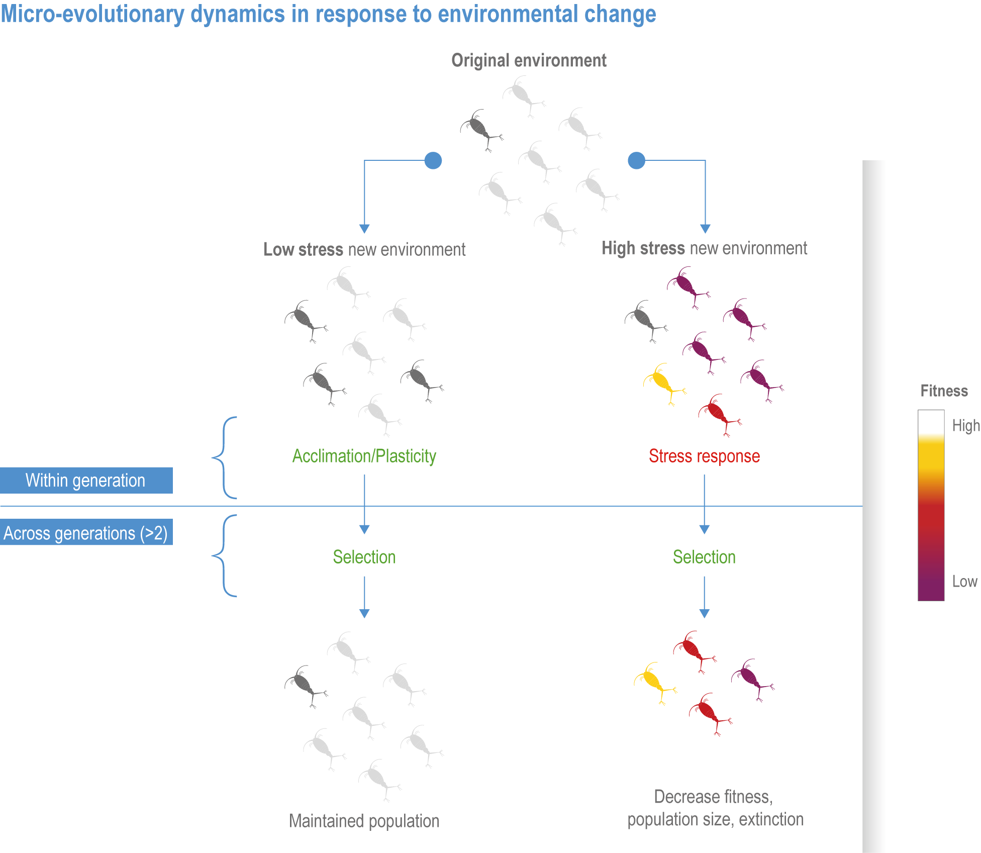
Figure 3.11 | Micro-evolutionary dynamics in response to environmental change. Simplified conceptual framework shows two main eco-evolutionary trajectories for natural populations over time (vertical axis from top to bottom). If environmental stress is low, rapid responses (within a generation) through plastic phenotypic adjustments and selection (across generations) sustain fitness, enhancing maintenance of viable populations across generations. In contrast, if environmental stress is high, ongoing phenotypic plasticity and acclimation may be insufficient to buffer the negative effects, exacerbating the loss of fitness (change of colour to orange/yellow/red). Ultimately, very high stress conditions accelerate population decline, enhancing the risk of species extinction.
Some studies have documented higher phenotypic plasticity and tolerance to ocean warming and acidification in marine invertebrates (Dam, 2013; Kelly et al., 2013; Pespeni et al., 2013; Gaitán-Espitia et al., 2017a; Vargas et al., 2017; Li et al., 2018a), seaweeds (Noisette et al., 2013; Padilla-Gamiño et al., 2016; Machado Monteiro et al., 2019) and fish (medium confidence) (Sandoval-Castillo et al., 2020; Enbody et al., 2021) living in coastal zones characterised by strong temporal fluctuations in temperature, pH, pCO2, light and nutrients. For these populations, strong directional selection with intense and highly fluctuating conditions may have favoured local adaptation and increased tolerance to environmental stress (low confidence, low evidence) (Hong and Shurin, 2015; Gaitán-Espitia et al., 2017b; Li et al., 2018a).
Other mechanisms acting within and across generations can influence selection and inter-population tolerances to environmental and climate-induced drivers. For instance, transgenerational effects and/or developmental acclimation, both ‘carry-over effects’ (where the early-life environment affects the expression of traits in later life stages or generations), can influence within- and cross-generational changes in the tolerances of marine organisms (medium confidence) to ocean warming (Balogh and Byrne, 2020) and acidification (Parker et al., 2012). Over longer time scales, increasing tolerance to these drivers may be mediated by mechanisms such as transgenerational plasticity (Murray et al., 2014), leading to locally adapted genotypes as seen in bivalves (Thomsen et al., 2017), annelids (Rodríguez-Romero et al., 2016; Thibault et al., 2020), corals (Putnam et al., 2020) and coralline algae (Cornwall et al., 2020). However, transgenerational plasticity is species specific (Byrne et al., 2020; Thibault et al., 2020) and, depending on the rate and magnitude of environmental change, it may either be insufficient for evolutionary rescue (Morgan et al., 2020) or could induce maladaptive responses (i.e., reduced fitness) in marine organisms exposed to multiple drivers (medium confidence, low evidence) (Figure 3.11; Griffith and Gobler, 2017; Parker et al., 2017; Byrne et al., 2020).
Acclimation to environmental pressures and climate change via phenotypic plasticity (Section 3.3.3; Collins et al., 2020) enables species to undergo niche shifts such that their present-day climatic niche is altered to incorporate new or shifted conditions (Fox et al., 2019). Although plasticity provides an adaptive mechanism, it is unlikely to provide a long-term solution for species undergoing sustained directional environmental change (e.g., global warming) (medium confidence) (Fox et al., 2019; Gaitán-Espitia and Hobday, 2021). Beyond the limits for plastic responses (Figure 3.9; DeWitt et al., 1998; Valladares et al., 2007), genetic adjustments are required to persist in a changing world (Figure 3.11; Fox et al., 2019). The ability of species and populations to undergo these adjustments (i.e., adaptive evolution) depends on extrinsic factors including the rate and magnitude of environmental change (important determinants of the strength and form of selection; Hoffmann and Sgrò, 2011; Munday et al., 2013), along with intrinsic factors such as generation times and standing genetic variation (Mitchell-Olds et al., 2007; Lohbeck et al., 2012). Accurately assessing the degree of acclimation and/or adaptation across space and time is difficult and constrains studying adaptive evolution in natural populations. There is a major gap in climate-change biology related to the study of evolutionary responses in complex and long-lived multicellular organisms. Insights on organismal acclimation, adaptation and evolution rely on studies of small, short-lived marine organisms, such as phytoplankton, which divide rapidly and contain high genetic variation in large populations. (Schaum et al., 2016; Cavicchioli et al., 2019; Collins et al., 2020).
Experimental evolution suggests that microbial populations can rapidly adapt (i.e., over 1–2 years) to environmental changes mimicking projected effects of climate change (medium confidence). Phytoplankton adaptive mechanisms include intraspecific strain sorting and genetic changes (Bach et al., 2018; Hoppe et al., 2018b; Wolf et al., 2019). The evolutionary responses of microbes are conditioned by the number and characteristics of interacting drivers (low confidence) (Brennan et al., 2017). For example, in a high-salinity adapted strain of the phytoplankton Chlamydomonas reinhardtii, the selection intensity and the adaptation rate increased with the number of environmental drivers, accelerating the adaptive evolutionary response (Brennan et al., 2017). For this and other phytoplankton species, a few dominant drivers explain most of the phenotypic and evolutionary changes observed (Boyd et al., 2015a; Brennan and Collins, 2015; Brennan et al., 2017).
Adaptation can be impeded, delayed or constrained in eukaryotic microbial populations as a result of reduced genetic diversity and/or the presence of functional and evolutionary trade-offs (Aranguren-Gassis et al., 2019; Lindberg and Collins, 2020; Walworth et al., 2020). In the marine diatom Chaetoceros simplex, a functional trade-off between high-temperature tolerance and increased nitrogen requirements underlies inhibited thermal adaptation under nitrogen-limited conditions (low confidence) (Aranguren-Gassis et al., 2019). When selection is strong due to unfavourable environmental conditions, microbial populations can encounter functional and evolutionary trade-offs evidenced by reducing growth rates while increasing tolerance and metabolism of reactive oxygen species (Lindberg and Collins, 2020). Other trade-offs can be observed in offspring quality and number (Lindberg and Collins, 2020). These findings contribute towards a mechanistic framework describing the range of evolutionary strategies in response to multiple drivers (Collins et al., 2020), but other hazards, such as extreme events (e.g., MHWs), still need to be included because their characteristics may alter the potential for adaptation of species and populations to climate change (Gruber et al., 2021).
3.3.5 Ecological Response to Multiple Drivers
Assessing ecological responses to multiple climate-induced drivers requires a combination of approaches, including laboratory- and field-based experiments, field observations (e.g., natural gradients, climate analogues), study of paleo-analogues and the development of mechanistic and empirical models (Clapham, 2019; Gissi et al., 2021). Experimental studies of food-web responses are often limited to an individual driver, although recent manipulations have used a matrix of >1000-l mesocosms to explore ecological responses to both warming and acidification (see Box 3.1; Nagelkerken et al., 2020). Hence, complementary approaches are needed to indirectly explore the mechanisms underlying ecosystem responses to global climate change (Parmesan et al., 2013). Observations from time series longer than modes of natural variability (i.e., decades) are essential for revealing and attributing ecological responses to climate change (e.g., Section 3.4; Barton et al., 2015b; Brun et al., 2019). Also, paleorecords provide insights into the influence of multiple drivers on marine biota (Cross-Chapter Box PALEO in Chapter 1; Reddin et al., 2020). Specifically, associations between vulnerabilities and traits of marine ectotherms in laboratory experiments correspond with organismal responses to ancient hyperthermal events (medium confidence) (Reddin et al., 2020). This corroboration suggests that responses to multiple drivers inferred from the fossil record can help provide insights into the future status of functional groups, and hence food webs, under rapid climate change.
Multi-species and integrated end-to-end ecosystem models are powerful tools to explore and project outcomes to the often-interacting cumulative effects of climate change and other anthropogenic drivers (Section 3.1; Kaplan and Marshall, 2016; Koenigstein et al., 2016; Peck and Pinnegar, 2018; Tittensor et al., 2018; Gissi et al., 2021). These models can integrate some aspects of the knowledge accrued from manipulation experiments, paleo- and contemporary observations, help test the relative importance of specific drivers and driver combinations, and identify synergistic or antagonistic responses (Koenigstein et al., 2016; Payne et al., 2016; Skogen et al., 2018; Tittensor et al., 2018). As these models are associated with wide-ranging uncertainties (SM3.2.2; Payne et al., 2016; Trolle et al., 2019; Heneghan et al., 2021), they cannot be expected to accurately project the trajectories of complex marine ecosystems under climate change; hence, they are most useful for assessing overall trends and in particular for providing a plausible envelope of trajectories across a range of assumptions (Fulton et al., 2018; Peck et al., 2018 ; Tittensor et al., 2018). On a global scale, ecosystem models project a −5.7 ± 4.1% (very likely range) to −15.5 ± 8.5% decline in marine animal biomass with warming under SSP1-2.6 and SSP5-8.5, respectively, by 2080–2099 relative to 1995–2014, albeit with significant regional variation in both trends and uncertainties (medium confidence) (Section 3.4.3.4; Tittensor et al., 2021). Biological interactions may exacerbate or buffer the projected impacts. For instance, trophic amplification (strengthening of responses to climate-induced drivers at higher trophic levels) may result from combined direct and indirect food-web-mediated effects (medium confidence) (Section 3.4.3.4; Lotze et al., 2019). Alternatively, compensatory species interactions can dampen strong impacts on species from ocean acidification, resulting in weaker responses at functional-group or community level than at species level (medium confidence) (Marshall et al., 2017; Hoppe et al., 2018b; Olsen et al., 2018; Gissi et al., 2021). Globally, the projected reduction of biomass due to climate-induced drivers is relatively unaffected by fishing pressure, indicating additive responses of fisheries and climate change (low confidence) (Lotze et al., 2019). Regionally, projected interactions of climate-induced drivers, fisheries and other regional non-climate drivers can be both synergistic and antagonistic, varying across regions, functional groups and species, and can cause nonlinear dynamics with counterintuitive outcomes, underlining the importance of adaptations and associated trade-offs (high confidence) (Sections 3.5.3, 3.6.3.1.2, 4.5, 4.6; Weijerman et al., 2015; Fulton et al., 2018; Hansen et al., 2019; Trolle et al., 2019; Zeng et al., 2019; Holsman et al., 2020; Pethybridge et al., 2020; Gissi et al., 2021).
Given the limitations of individual ecological models discussed above, model intercomparisons, such as the Fisheries and Marine Ecosystem Model Intercomparison Project (Fish-MIP; Tittensor et al., 2018) show promise in increasing the robustness of projected ecological outcomes (Tittensor et al., 2018). Model ensembles include a greater number of relevant processes and functional groups than any single model and thus capture a wider range of plausible responses. Among the global Fish-MIP models, there is high (temperate and tropical areas) to medium agreement (coastal and polar regions) on the direction of change, but medium (temperate and tropical regions) to low agreement (coastal and polar regions) on magnitude of change (Lotze et al., 2019; Heneghan et al., 2021). Although model outputs are validated relative to observations to assess model skills (Payne et al., 2016; Tittensor et al., 2018), the Fish-MIP models under-represent some sources of uncertainty, as they often do not include parameter uncertainties and do not usually include impacts of ocean acidification, oxygen loss or evolutionary responses because there remains high uncertainty regarding the influences of these processes across functional groups. Ensemble model investigations like Fish-MIP have also identified gaps in our mechanistic understanding of ecosystems and their responses to anthropogenic forcing, leading to model improvement and more rigorous benchmarking. These investigations could inspire future targeted observational and experimental research to test the validity of model assumptions (Payne et al., 2016; Lotze et al., 2019; Heneghan et al., 2021). The state of the art in such experimental research is presented in Box 3.1.
Box 3.1 | Challenges for Multiple-Driver Research in Ecology and Evolution
The majority of the examples in Section 3.3 are from studies mimicking projected conditions in the year 2100 that report the responses of an individual species or strain to multiple drivers. This powerful generic experimental approach has largely been restricted to single species because it is logistically complex to conduct experiments that straddle multiple trophic levels, and that also include more than two drivers (see Figure Box 3.1.1b); the need for multiple replicates, drivers and treatment levels greatly increase the work required (Parmesan et al., 2013; Boyd et al., 2018). It is challenging to apply this experimental approach to communities or ecosystems (see Figure Box 3.1.1). To date, most research on community or ecosystem response to climate-induced drivers has been in large-volume (>10,000 l) mesocosms (Riebesell and Gattuso, 2014), or at natural analogues such as CO2 seeps, in which only one driver (ocean acidification) is altered (see (4) in Figure Box 3.1.1). Only very recently have two drivers been incorporated into climate-change manipulation studies examining responses of primary producers to secondary consumers (see (5) in Figure Box 3.1.1a; Nagelkerken et al., 2020). Therefore, ‘natural experiments’ from the geological past (Reddin et al., 2020) provide insights into how food webs and their constituents respond to complex change involving multiple drivers. Contemporary observations are occasionally long enough (>50 years) to capture community responses to complex climate change. For example, Brun et al. (2019) reported a shift in zooplankton community structure in the North Atlantic (1960–2014), with major biogeochemical ramifications.
Conducting sufficiently long manipulation experiments to study the effect of adaptation on organisms is equally difficult (see Figure Box 3.1.1b), with much research restricted to multi-year studies of the microevolution of fast-growing (more than one division per day) phytoplankton species responding to single drivers (Lohbeck et al., 2012; Schaum et al., 2016). In a few experimental evolution studies (see (7) in Figure Box 3.1.1a; Brennan et al., 2017), multiple drivers have been used, but none have used communities or ecosystems (see Figure Box 3.1.1b). Nevertheless, the fossil record provides limited evidence of adaptations to less rapid (relative to present day) climate change (Jackson et al., 2018). Despite the need to explore ecological or biogeochemical responses to projected future ocean conditions, logistical challenges require that assessments of climate-change impacts at scales larger than mesocosms use large-scale, long-term in situ observational studies (as documented in Section 3.4).
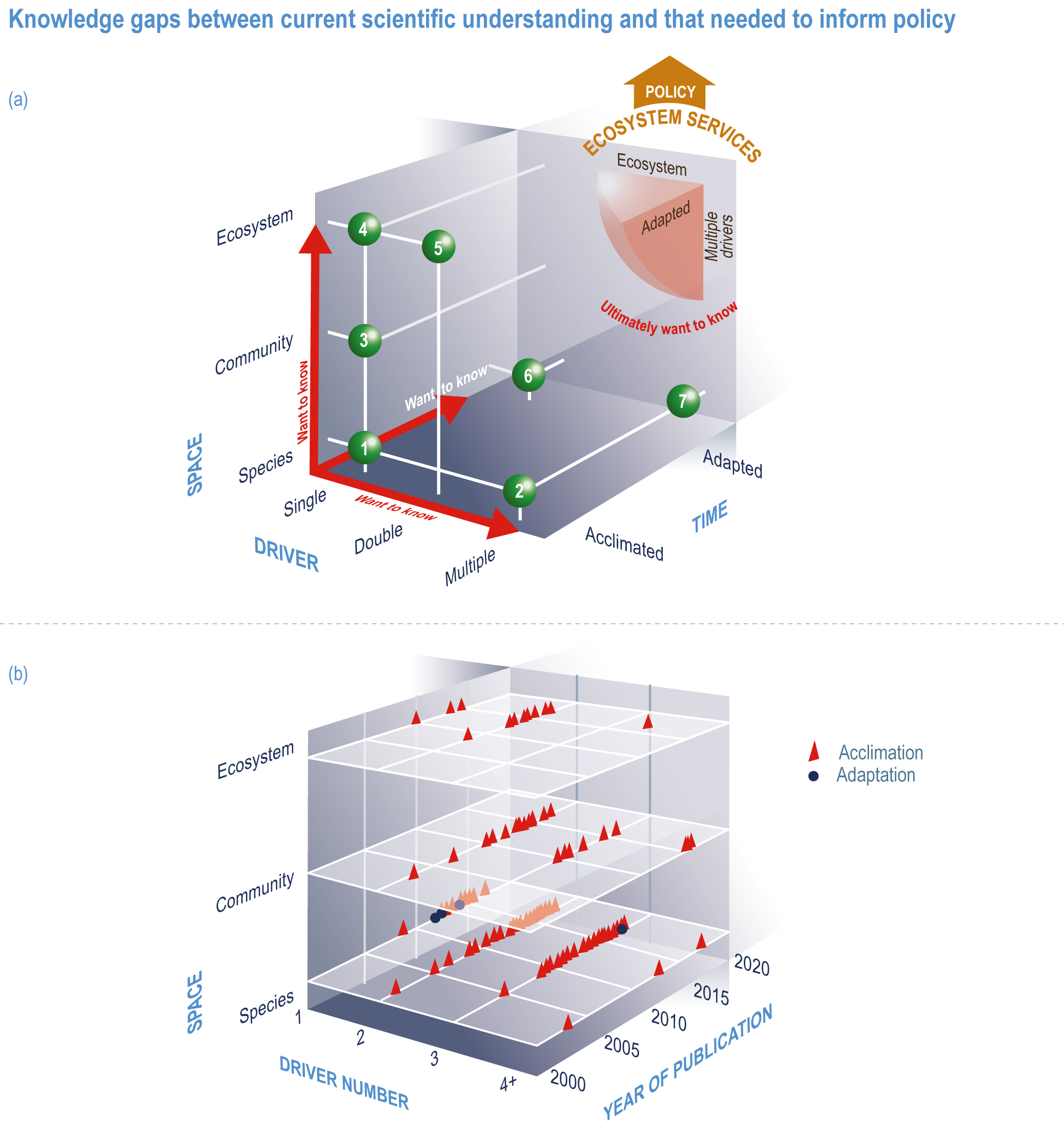
Figure Box 3.1.1 | Knowledge gaps between current scientific understanding and that needed to inform policy. The conceptual space relating driver number, (Driver axis), ecological organisation (Space axis) and evolutionary acclimation state (Time axis), modified from Riebesell and Gattuso (2014).
(a) Spheres indicate suites of studies that illustrate the progress of research, including multiple drivers: (1) one species and one driver (Hutchins et al., 2013); (2) one species and multiple drivers (five; Boyd et al., 2015a). Ecology: (1) one driver, one species; (3) one driver, planktonic community (Moustaka-Gouni et al., 2016); (4) one driver (high-CO2 seep) and (benthic) ecosystem (Fabricius et al., 2014); (5) two drivers and nearshore ecosystem (Nagelkerken et al., 2020). Evolution: (1) acclimated organism and one driver; (6) adapted organisms and one driver (Listmann et al., 2016); (7) adapted organism and multiple drivers (Brennan et al., 2017).
(b) Trends in research trajectories since 2000 from a survey of 171 studies (Boyd et al., 2018). Note the dominance of multiple-driver experiments at the species level (lower left cluster); the focus on acclimation (red triangle) rather than adaptation (blue dot); and the focus of investigation on three or fewer drivers. (Redrawn from Boyd et al., 2018).
3.4 Observed and Projected Impacts of Climate Change on Marine Systems
3.4.1 Introduction
Ocean and coastal ecosystems and their resident species are under increasing pressure from a multitude of climate-induced drivers and non-climate drivers (Section 3.1; Figure 3.12; Bindoff et al., 2019a). This section builds from the assessment of biological responses to climate-impact drivers (Section 3.3) to examine the new evidence about climate-change impacts at the level of marine ecosystems. It focuses on detection and attribution of observed changes to marine ecosystems and the projected changes under different future climate scenarios. This assessment considers emerging evidence on the effects of multiple non-climate drivers and physiological acclimation and/or evolutionary adaptation on these observations and projections.
The section focuses first on coastal ecosystems and seas (Section 3.4.2), which have high spatial variability in physical and chemical characteristics, are affected by many non-climate drivers (Section 3.1; Figure 3.12) and support rich fisheries, high biodiversity and high levels of species endemism. The assessment begins with warm-water coral reefs (Section 3.4.2.1) because these highly threatened systems are at the vanguard of research on acclimation and evolutionary adaptation among coastal ecosystems. It follows with the other shallow, nearshore ecosystems dominated by habitat-forming species (e.g., rocky shores, kelp systems) and then nearshore sedimentary systems (estuaries, deltas, coastal wetlands and sandy beaches), before moving on to semi-enclosed seas, shelf seas, upwelling zones and polar seas.
The section continues on to oceanic and cross-cutting changes (Section 3.4.3), which influence large areas of the epipelagic zone (<200 m depth) while also affecting the mesopelagic (200–1000 m), the perpetually dark bathypelagic (depth >1000 m) and the deep seafloor (benthic ecosystems at depths >200 m) zones. Assessed in this section are species range shifts (Section 3.4.3.1), phenological shifts and trophic mismatches (Section 3.4.3.2), changes in communities and biodiversity (Section 3.4.3.3.2), time of emergence of climate-impact signals in ecological systems from background natural variability (Section 3.4.3.3.4) and changes in biomass, primary productivity and carbon export (Sections 3.4.3.4–3.4.3.6).
3.4.2 Coastal Ecosystems and Seas
3.4.2.1 Warm-Water Coral Reefs
Warm-water coral reef ecosystems house one-quarter of the marine biodiversity and provide services in the form of food, income and shoreline protection to coastal communities around the world. These ecosystems are threatened by climate-induced and non-climate drivers, especially ocean warming, MHWs, ocean acidification, SLR, tropical cyclones, fisheries/overharvesting, land-based pollution, disease spread and destructive shoreline practices (Hoegh-Guldberg et al., 2018a; Bindoff et al., 2019a; Hughes et al., 2020). Warm-water coral reefs face near-term threats to their survival (Table 3.3), but research on observed and projected impacts is very advanced.
Table 3.3 | Summary of previous IPCC assessments of coral reefs
Observations | Projections |
Coral reefs are one of the most vulnerable marine ecosystems (high confidence), and more than half of the world’s reefs are under medium or high risk of degradation. Mass coral bleaching and mortality, triggered by positive temperature anomalies (high confidence), is the most widespread and conspicuous impact of climate change. Ocean acidification reduces biodiversity and the calcification rate of corals (high confidence) while at the same time increasing the rate of dissolution of the reef framework (medium confidence). ‘In summary, ocean warming is the primary cause of mass coral bleaching and mortality (very high confidence), which, together with ocean acidification, deteriorates the balance between coral reef construction and erosion (high confidence).’ | ‘Coral bleaching and mortality will increase in frequency and magnitude over the next decades (very high confidence).’ Analysis of the Coupled Model Intercomparison Project 5 ensemble projects the loss of coral reefs from most sites globally by 2050 under mid to high rates of warming (very likely ). ‘Under the A1B CO2 emission scenario, 99% of the reef locations will experience at least one severe bleaching event between 2090 and 2099, with limited evidence and low agreement that coral acclimation and/or adaptation will limit this trend.’ ‘The onset of global dissolution [of coral reefs] is at an atmospheric CO2[concentration] of 560 ppm (medium confidence) and dissolution will be widespread in 2100’ (Representative Concentration Pathway, RCP8.5, medium confidence). ‘A number of coral reefs could therefore keep up with the maximum rate of sea level rise (SLR) of 15.1 mm yr –1 projected for the end of the century [...], but lower net accretion [...] and increased turbidity will weaken this capability (very high confidence).’ |
‘Climate change [...] has emerged as the greatest threat to coral reefs, with temperatures of just 1°C above the long-term summer maximum for an area (reference period 1985–1993) over 4–6 weeks being enough to cause mass coral bleaching [...] and mortality (very high confidence).’ Predictions of back-to-back bleaching events have become reality over 2015–2017 as have projections of declining coral abundance (high confidence). | ‘Multiple lines of evidence indicate that the majority (70–90%) of warm water (tropical) coral reefs that exist today will disappear even if global warming is constrained to 1.5°C (very high confidence).’ Coral reefs, for example, are projected to decline by a further 70–90% at 1.5°C (high confidence) with larger losses (>99%) at 2°C (very high confidence). |
SROCC (Bindoff et al., 2019a) | |
‘New evidence since AR5 and SR15 confirms the impacts of ocean warming and acidification on coral reefs (high confidence), enhancing reef dissolution and bioerosion (high confidence), affecting coral species distribution and leading to community changes (high confidence). The rate of SLR (primarily noticed in small reef islands) may outpace the growth of reefs to keep up, although there is low agreement in the literature (low confidence).’ ‘Reefs are further exposed to other increased impacts, such as enhanced storm intensity, turbidity and increased runoff from the land (high confidence). Recovery of coral reefs resulting from repeated disturbance events is slow (high confidence). Only few coral reef areas show some resilience to global change drivers (low confidence).’ | ‘Coral reefs will face very high risk at temperatures 1.5°C of global sea surface warming (very high confidence).’ ‘Almost all coral reefs will degrade from their current state, even if global warming remains below 2°C (very high confidence), and the remaining shallow coral reef communities will differ in species composition and diversity from present reefs (very high confidence). This will greatly diminish the services they provide to society, such as food provision (high confidence), coastal protection (high confidence) and tourism (medium confidence).’ ‘The very high vulnerability of coral reefs to warming, ocean acidification, increasing storm intensity and SLR under climate change, including enhanced bioerosion (high confidence), points to the importance of considering both mitigation and adaptation.’ |
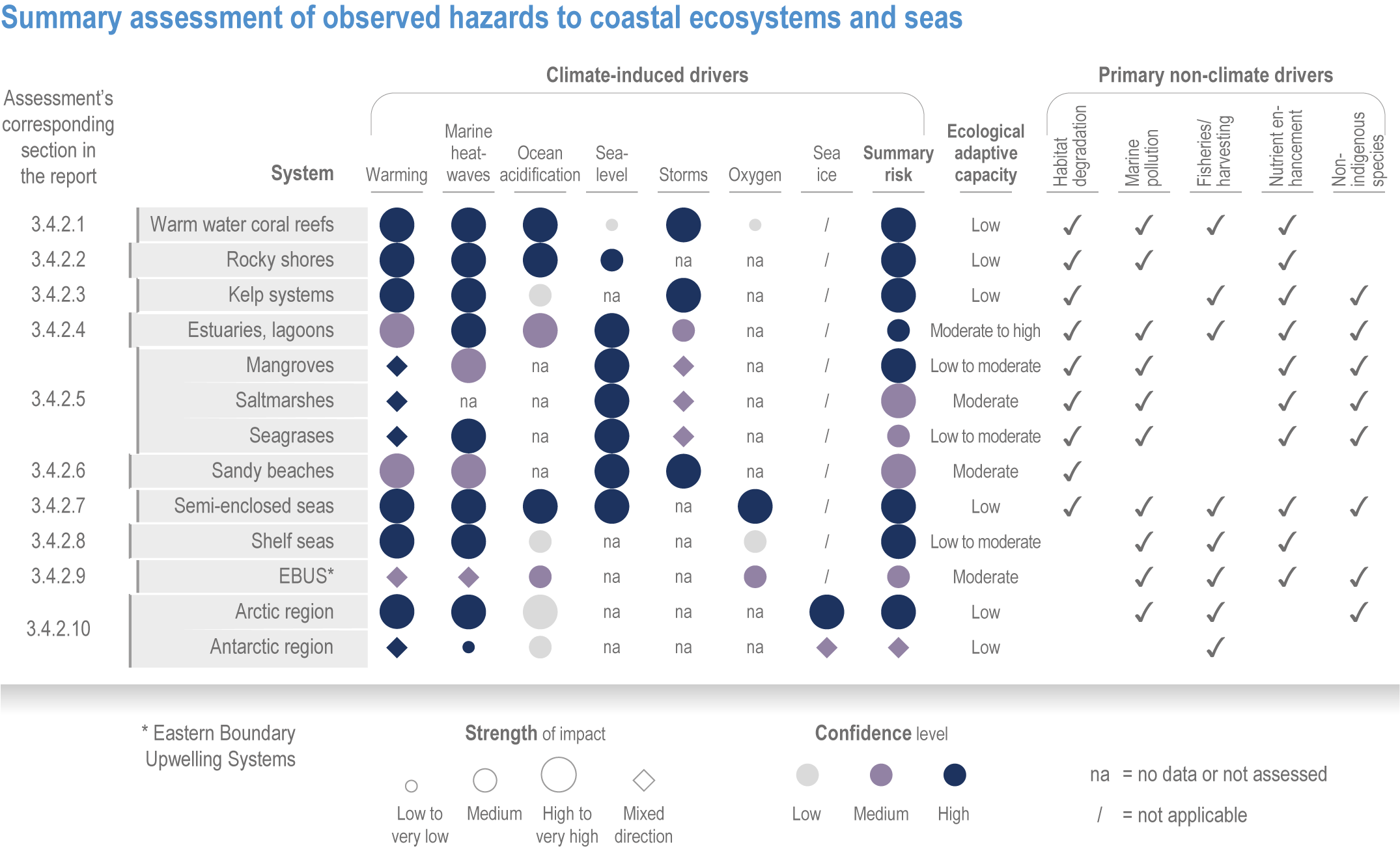
Figure 3.12 | Summary assessment of observed hazards to coastal ecosystems and seas as assessed in Section 3. 4.2.
Global analyses published since AR5 show that mass coral bleaching events and disease outbreaks have increased due to more frequent and severe heat stress associated with ocean warming (very high confidence, virtually certain) (Donner et al., 2017; Hughes et al., 2018a; DeCarlo et al., 2019; Sully et al., 2019; Tracy et al., 2019). The mass coral bleaching, which occurred continuously across different parts of the tropics from 2014 to 2016, is considered the longest and most severe global coral bleaching event on record (Section 10.4.3; see Box 15.2; Eakin et al., 2019). The Great Barrier Reef underwent mass bleaching three times between 2016 and 2020 (see Box 11.2; Pratchett et al., 2021), validating past model projections that some warm-water coral reefs would encounter bleaching-level heat stress multiple times per decade by the 2020s (Hoegh-Guldberg, 1999; Donner, 2009).
Heat stress and mass bleaching events caused decreases in live coral cover (virtually certain) (Graham et al., 2014; Hughes et al., 2018b), loss of sensitive species (extremely likely ) (Donner and Carilli, 2019; Lange and Perry, 2019; Toth et al., 2019; Courtney et al., 2020), vulnerability to disease (extremely likely ) (van Woesik and Randall, 2017; Hadaidi et al., 2018; Brodnicke et al., 2019; Howells et al., 2020) and declines in coral recruitment in the tropics (medium confidence) (Hughes et al., 2019; Price et al., 2019). Recent observations also suggest that excess nutrients can increase the susceptibility of corals to heat stress (DeCarlo et al., 2020). Changes in coral community structure due to bleaching have caused declines in reef carbonate production (high confidence) (Perry and Morgan, 2017; Lange and Perry, 2019; Perry and Alvarez-Filip, 2019; Courtney et al., 2020; van Woesik and Cacciapaglia, 2021) and in reef structural complexity (high confidence, very likely ) (Couch et al., 2017; Leggat et al., 2019; Magel et al., 2019), which increases water depth, reduces wave attenuation and increases coastal flood risk (Yates et al., 2017; Beck et al., 2018). Corals may also lose reproductive synchrony through climate change (Shlesinger and Loya, 2019), adding to their vulnerability. Bleaching and other drivers promote phase shifts to ecosystems dominated by macroalgae or other stress-tolerant species (very high confidence) (Graham et al., 2015; Stuart-Smith et al., 2018), leading to changes in reef-fish species assemblages (high confidence) (Richardson et al., 2018; Robinson et al., 2019a; Stuart-Smith et al., 2021).
Ocean acidification and associated declines in aragonite saturation state (Ωaragonite) decrease rates of calcification by corals and other calcifying reef organisms (very high confidence), reduce coral settlement (medium confidence) and increase bioerosion and dissolution of reef substrates (high confidence) (Hoegh-Guldberg et al., 2018a; Bindoff et al., 2019a; Kline et al., 2019; Pitts et al., 2020). Warming can exacerbate the coral response to ocean acidification (Kornder et al., 2018) and accelerate the decrease in coral skeletal density (Guo et al., 2020). In addition, reefs with lower coral cover and a higher proportion of slow-growing species, because of bleaching, are more sensitive to acidification (net dissolution occurs Ωaragonite= 2.3 for 100% coral cover, and Ωaragonite>3.5 for 30% coral cover; Kline et al., 2019). However, experimental evidence suggests that coral responses to ocean acidification are species specific (medium confidence) (Fabricius et al., 2011; DeCarlo et al., 2018; Comeau et al., 2019). Evidence from experiments suggests that crustose coralline algae, which contribute to reef structure and integrity and may be resistant to warming at the RCP8.5 level by 2100 (Cornwall et al., 2019), are also sensitive to declines in Ωaragonite (high confidence) (Section 3.4.2.3; Fabricius et al., 2015; Smith et al., 2020). The integrated effect of acidification, bleaching, storms and other non-climate drivers on corals, coralline algae and other calcifiers can further compromise reef integrity and ecosystem services (Rivest et al., 2017; Cornwall et al., 2018; Perry and Alvarez-Filip, 2019).
Since SROCC, there have been advances in experimental, field and modelling research on the projected response of coral cover and reef growth to bleaching and ocean acidification (Cziesielski et al., 2019; Morikawa and Palumbi, 2019; Cornwall et al., 2021; Klein et al., 2021; Logan et al., 2021; McManus et al., 2021), and on the effect of possible human interventions like assisted evolution on coral resilience (Section 3.6.3.2.2; Condie et al., 2021; Hafezi et al., 2021; Kleypas et al., 2021). New model projections incorporating physiological acclimation, larval dispersal and evolutionary processes find limited ability to adapt this century at rates of warming at or exceeding that in RCP4.5 (high confidence, very likely ) (Bay et al., 2017; Kubicek et al., 2019; Matz et al., 2020; McManus et al., 2020; Logan et al., 2021; McManus et al., 2021). For example, a global analysis (Logan et al., 2021) finds that increased thermal tolerance via evolution or switching to more stress-tolerant algal symbionts enable most (73–81%) coral to survive through 2100 under RCP2.6, but coral-dominated communities with a historical mix of coral taxa still disappear (0–8% coral survival) under RCP6.0 in simulations with adaptive mechanisms (Figure 3.13). Due to the impacts of warming, and to a lesser extent ocean acidification, global reef carbonate production is estimated to decline 71% by 2050 in SSP1-2.6, and the rate of SLR is estimated to exceed that of reef growth for 97% of reefs assessed, without adaptation by corals and their symbionts (WGI AR6 Table 9.9; Cornwall et al., 2021; Fox-Kemper et al., 2021). The increased water depth due to coral loss and reef erosion, as well as reduced structural complexity, will limit wave attenuation and exacerbate the risk of flooding from SLR on reef-fringed shorelines and reef islands (Yates et al., 2017; Beck et al., 2018; Harris et al., 2018). Local coral reef fish species richness is projected to decline due to the impacts of warming on coral cover and diversity (high confidence), with declines up to 40% by 2060 in SSP5-8.5 (Strona et al., 2021).
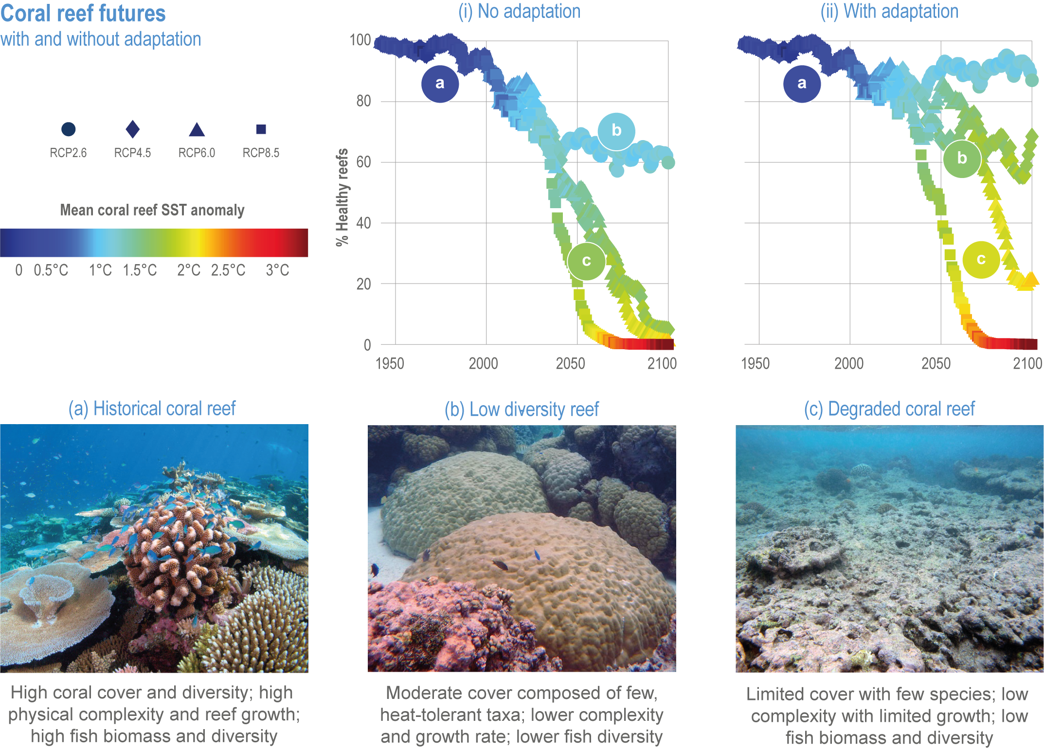
Figure 3.13 | Coral reef futures, with and without adaptation. Graphs are based on a model of coral-symbiont evolutionary dynamics from Logan et al. (2021), which simulates two coral types and symbiont populations for 1925 reef cells worldwide, from 1950 to 2100 drawn from simulations with National Oceanic and Atmospheric Administration–Geophysical Fluid Dynamics Laboratory Earth System Model (ESM2M) under four RCPs. Top panels show the simulated fraction of cells with healthy reefs, when both coral types are not in a state of severe bleaching or mortality, (i) without adaptive responses and (ii) with adaptive responses (symbiont evolution). Colours indicate maximum monthly sea surface temperature increase across all reef cells, versus a 1861–2010 baseline. Panels (a,b,c) depict snapshots of coral reef conditions at time points in the future, each with different levels of warming, drawn from the model-projected cover of the two coral types and from a literature assessment (Section 3.4.2.1; Hughes et al., 2018b; Bindoff et al., 2019a; Darling et al., 2019; Leggat et al., 2019; Cornwall et al., 2021).
These observed and projected impacts are supported by geological and paleo-ecological evidence showing a decline in coral reef extent and species richness under previous episodes of climate change and ocean acidification (Kiessling and Simpson, 2011; Pandolfi et al., 2011; Kiessling et al., 2012; Pandolfi and Kiessling, 2014; Kiessling and Kocsis, 2015). Major reef crises in the past 300 million years were governed by hyperthermal events (medium confidence) (Section 3.2.4.4; Cross-Chapter Box PALEO in Chapter 1) longer in time scale than anthropogenic climate change, during which net coral reef accretion was more strongly affected than biodiversity (medium confidence).
In response to the global-scale decline in coral reefs and high future risk, recent literature focuses on finding thermal refuges and identifying uniquely resilient species, populations or reefs for targeted restoration and management (Hoegh-Guldberg et al., 2018b). Reefs exposed to internal waves (Storlazzi et al., 2020), turbidity (Sully and van Woesik, 2020) or warm-season cloudiness (Gonzalez-Espinosa and Donner, 2021) are expected to be less sensitive to thermal stress. Mesophotic reefs (30–150 m) have also been proposed as thermal refugia (Bongaerts et al., 2010), although evidence from recent bleaching events, subsurface temperature records and species overlap is mixed (Frade et al., 2018; Rocha et al., 2018b; Eakin et al., 2019; Venegas et al., 2019; Wyatt et al., 2020). A study of 2584 reef sites across the Indian and Pacific oceans estimated that 17% had sufficient cover of framework-building corals to warrant protection, 54% required recovery efforts and 28% were on a path to net erosion (Darling et al., 2019). There is medium evidence for greater bleaching resistance among reefs subject to temperature variability or frequent heat stress (Barkley et al., 2018; Gintert et al., 2018; Hughes et al., 2018a; Morikawa and Palumbi, 2019), but with trade-offs in terms of diversity and structural complexity (Donner and Carilli, 2019; Magel et al., 2019). There is limited agreement about the persistence of thermal tolerance in response to severe heat stress (Le Nohaïc et al., 2017; DeCarlo et al., 2019; Fordyce et al., 2019; Leggat et al., 2019; Schoepf et al., 2020). Recovery and restoration efforts that target heat-resistant coral populations and culture heat-tolerant algal symbionts have the greatest potential of effectiveness under future warming (high confidence) (see Box 5.5 in SROCC Chapter 5; Bay et al., 2017; Darling and Côté, 2018; Baums et al., 2019; Bindoff et al., 2019a; Howells et al., 2021); however, there is low confidence that enhanced thermal tolerance can be sustained over time (Section 3.6.3.3.2; Buerger et al., 2020). The effectiveness of active restoration and other specific interventions (e.g., reef shading) are further assessed in Section 3.6.3.3.2.
In summary, additional evidence since SROCC and SR15 (Table 3.3) finds that living coral and reef growth are declining due to warming and MHWs (very high confidence). Coral reefs are under threat of transitioning to net erosion with >1.5°C of global warming (high confidence), with impacts expected to occur fastest in the Atlantic Ocean. The effectiveness of conservation efforts to sustain living coral area, coral diversity and reef growth is limited for the majority of the world’s reefs with >1.5°C of global warming (high confidence) (Section 3.6.3.3.2; Hoegh-Guldberg et al., 2018b; Bruno et al., 2019; Darling et al., 2019).
3.4.2.2 Rocky Shores
Rocky shore ecosystems refer to a range of temperate intertidal and shallow coastal ecosystems that are dominated by different foundational organisms, including mussels, oysters, fleshy macroalgae, hard and soft corals, coralline algae, bryozoans and sponges, which create habitat for species-rich assemblages of invertebrates, fish, marine mammals and other organisms. Rocky shores provide services including wave attenuation, habitat provision and food resources, and these support commercial, recreational and Indigenous fisheries and shellfish aquaculture.
Table 3.4 | Summary of previous IPCC assessments of rocky shores
Observations | Projections |
AR5 (Wong et al., 2014) | |
‘Rocky shores are among the better-understood coastal ecosystems in terms of potential impacts of climate variability and change. The most prominent effects are range shifts of species in response to ocean warming (high confidence) and changes in species distribution and abundance (high confidence) mostly in relation to ocean warming and acidification.’ ‘The dramatic decline of biodiversity in mussel beds of the Californian coast has been attributed to large-scale processes associated with climate-related drivers [...] (high confidence).’ | ‘The abundance and distribution of rocky shore species will continue to change in a warming world (high confidence). For example, the long-term consequences of ocean warming on mussel beds of the northeast Pacific are both positive (increased growth) and negative (increased susceptibility to stress and of exposure to predation) (medium confidence).’ ‘Observations performed near natural CO2 vents in the Mediterranean Sea show that diversity, biomass and trophic complexity of rocky shore communities will decrease at future pH levels (high confidence).’ |
SR15 (Hoegh-Guldberg et al., 2018a) | |
‘Changes in ocean circulation can have profound impacts on [temperate] marine ecosystems by connecting regions and facilitating the entry and establishment of species in areas where they were unknown before (‘tropicalization’ ...) as well as the arrival of novel disease agents (medium agreement, limited evidence).’ | ‘In the transition to 1.5°C, changes to water temperatures are expected to drive some species (e.g., plankton, fish) to relocate to higher latitudes and cause novel ecosystems to assemble (high confidence). Other ecosystems (e.g., kelp forests, coral reefs) are relatively less able to move, however, and are projected to experience high rates of mortality and loss (very high confidence).’ ‘In the case of ‘less mobile’ ecosystems (e.g., coral reefs, kelp forests, intertidal communities), shifts in biogeographic ranges may be limited, with mass mortalities and disease outbreaks increasing in frequency as the exposure to extreme temperatures increases’ (high agreement, robust evidence). |
SROCC (Bindoff et al., 2019a) | |
Intertidal rocky shores ecosystems are highly sensitive to ocean warming, acidification and extreme heat exposure during low tide emersion (high confidence). ‘Sessile calcified organisms (e.g., barnacles and mussels) in intertidal rocky shores are highly sensitive to extreme temperature events and acidification (high confidence), a reduction in their biodiversity and abundance have been observed in naturally acidified rocky reef ecosystems (medium confidence).’ | ‘Intertidal rocky shores are also expected to be at very high risk (transition above 3°C) under the RCP8.5 scenario (medium confidence). These ecosystems have low to moderate adaptive capacity, as they are highly sensitive to ocean temperatures and acidification.’ ‘Benthic species will continue to relocate in the intertidal zones and experience mass mortality events due to warming (high confidence). Interactive effects between acidification and warming will exacerbate the negative impacts on rocky shore communities, causing a shift towards a less diverse ecosystem in terms of species richness and complexity, increasingly dominated by macroalgae (high confidence).’ |
Observations since AR5 and SROCC (Table 3.4) find increased impacts of ocean warming on rocky shores. This includes extirpation of species at the warm edge of their ranges (Yeruham et al., 2015; Martínez et al., 2018), extension of poleward range boundaries (Sanford et al., 2019), mortality from climate extremes (Seuront et al., 2019), reduction in survival at shallower depths (Sorte et al., 2019; Wallingford and Sorte, 2019) and reorganisation of communities (Wilson et al., 2019; Mulders and Wernberg, 2020; Albano et al., 2021). Data collected after MHWs find ecological phase shifts (moderate evidence, high agreement ) (e.g., California; Rogers-Bennett and Catton, 2019; McPherson et al., 2021) and homogenisation of communities (limited evidence) (e.g., Alaska; Weitzman et al., 2021). For example, the collapse of sea star populations in the Northeast Pacific due to a MHW-related disease outbreak (Hewson et al., 2014; Menge et al., 2016; Miner et al., 2018; Schiebelhut et al., 2018), including 80–100% loss of the common predatory sunflower star, Pycnopodia helianthoides (very high confidence) (Harvell et al., 2019), triggered shifts from kelp- to urchin-dominated ecosystems (Schultz et al., 2016; Gravem and Morgan, 2017; McPherson et al., 2021).
Multiple lines of evidence find that foundational calcifying organisms such as mussels are at high risk of decline due to both the individual and synergistic effects of warming, acidification and hypoxia (high confidence) (Sunday et al., 2016; Sorte et al., 2017; Sorte et al., 2019; Newcomb et al., 2020). Warmer temperatures reduce mussel and barnacle recruitment (e.g., northwest Atlantic; Petraitis and Dudgeon, 2020) and the upper vertical limit of mussels (e.g., northeast Pacific, Harley, 2011; and southwest Pacific, Sorte et al., 2019). Experiments show that ocean acidification negatively impacts mussel physiology (very high confidence), with evidence of reduced growth (Gazeau et al., 2010), attachment (Newcomb et al., 2020), biomineralisation (Fitzer et al., 2014) and shell thickness (Pfister et al., 2016; McCoy et al., 2018). Net calcification and abundance of mussels and other foundational species, including oysters, are expected to decline due to ocean acidification (very high confidence) (Kwiatkowski et al., 2016; Sunday et al., 2016; McCoy et al., 2018; Meng et al., 2018), causing the reorganisation of communities (high confidence) (Kroeker et al., 2013b; Linares et al., 2015; Brown et al., 2016; Sunday et al., 2016; Agostini et al., 2018; Teixidó et al., 2018). Experiments indicate that acidification can interact with warming and hypoxia to increase the detrimental effects on mussels (Gu et al., 2019; Newcomb et al., 2020). In regions where food is readily available to mussels, detrimental effects of ocean acidification may be dampened (Kroeker et al., 2016); however, recent findings are inconclusive (Brown et al., 2018a).
Coralline algae, foundational taxa that create habitat for sea urchins and abalone, form rhodolith beds in temperate to Arctic habitats and bind together substrates, are expected to be highly susceptible to ocean acidification because they precipitate soluble magnesium calcite (Kuffner et al., 2008; Williams et al., 2021). Damage from acidification varies among species and regions, and can be due to direct physiological stress (Marchini et al., 2019) or interactions with non-calcifying competitors such as fleshy macroalgae (Smith et al., 2020). Experiments indicate that warming reduces calcification by coralline algae (high confidence) (Cornwall et al., 2019) and exacerbates the effect of acidification (Kim et al., 2020; Williams et al., 2021).
In contrast to warm-water coral reefs, there are no regional or global numerical models of rocky shore ecosystem response to projected climate change and acidification. Experiments suggest that existing genetic variation could be sufficient for some mussels (Bitter et al., 2019) and coralline algae (Cornwall et al., 2020) to adapt over generations to ocean acidification. Populations exposed to variable environments often have a greater capacity for phenotypic plasticity and resilience to environmental change [e.g., urchins (Gaitan-Espitia et al., 2017b) and coralline algae (Section 3.3.2; Rivest et al., 2017; Cornwall et al., 2018)]. Although parental conditioning within and across generations is an acclimatisation mechanism to global change, there is limited evidence from experimental studies that this is applicable for marine invertebrates on rocky shores (Byrne et al., 2020).
This assessment concludes that MHWs attributable to climate change (Section 3.2.2.1) can cause fatal disease outbreaks or mass mortality among some key foundational species (high confidence) and contribute to ecological phase shifts (medium confidence). The upper vertical limits of some species will also be constrained by climate change (high confidence). Experimental evidence since previous assessments further indicates that acidification decreases abundance and richness of calcifying species (high confidence), although there is limited evidence for acclimation in some species. Synergistic effects of warming and acidification will promote shifts towards macroalgal dominance in some ecosystems (medium confidence) and lead to reorganisation of communities (medium confidence).
3.4.2.3 Kelp Ecosystems
Kelp are temperate, habitat-forming marine macroalgae or seaweeds, mostly of the order Laminariales, which extend across one-quarter of the world’s coastlines (Assis et al., 2020; Jayathilake and Costello, 2020). The perennial species form dense underwater forest canopies and three-dimensional habitat that provides refuge for fish, crustaceans, invertebrates and marine mammals (Filbee-Dexter et al., 2016; Wernberg et al., 2019). Kelp ecosystems support fisheries, aquaculture, fertiliser and food provision, including for local and Indigenous Peoples, along with regulating services in the form of wave attenuation and habitat provision. Kelp aquaculture can also buffer against local acidification (Xiao et al., 2021) and contribute to carbon storage (Froehlich et al., 2019).
Recent research (Straub et al., 2019; Butler et al., 2020; Filbee-Dexter et al., 2020b; Tait et al., 2021) supports the findings of previous assessments (Table 3.5) that kelp and other seaweeds in most regions are undergoing mass mortalities from high temperature extremes and range shifts from warming (very high confidence). Kelp are highly sensitive to the direct effect of high temperature on survival (Nepper-Davidsen et al., 2019) and indirect impact of temperature on herbivorous species (Ling, 2008; Vergés et al., 2016), upwelling and nutrient availability (Carr and Reed, 2015; Schiel and Foster, 2015). Synergies between warming, storms, pollution and intensified herbivory (due to removal or loss of predators including sea stars and otters that constrain herbivory by fish and urchin populations) can also cause physiological stress and physical damage in kelp, reducing productivity and reproduction (Rogers-Bennett and Catton, 2019; Beas-Luna et al., 2020; McPherson et al., 2021).
Table 3.5 | Summary of previous IPCC assessments of kelp ecosystems
Observations | Projections |
AR5 (Wong et al., 2014) | |
‘Kelp forests have been reported to decline in temperate areas in both hemispheres, a loss involving climate change (high confidence). Decline in kelp populations attributed to ocean warming has been reported in southern Australia and the north coast of Spain.’ | ‘Kelp ecosystems will decline with the increased frequency of heatwaves and sea temperature extremes as well as through the impact of invasive subtropical species (high confidence).’ ‘Climate change will contribute to the continued decline in the extent of [...] kelps in the temperate zone (medium confidence) and the range of [...] kelps in the Northern Hemisphere will expand poleward (high confidence). ’ |
SR15 (Hoegh-Guldberg et al., 2018a) Observed movement of kelp ecosystems not assessed. | ‘In the transition to 1.5°C of warming, changes to water temperatures will drive some species (e.g., plankton, fish) to relocate to higher latitudes and cause novel ecosystems to assemble (high confidence). Other ecosystems (e.g., kelp forests, coral reefs) are relatively less able to move, however, and are projected to experience high rates of mortality and loss (very high confidence).’ |
SROCC (Bindoff et al., 2019a) | |
‘Kelp forests have experienced large-scale habitat loss and degradation of ecosystem structure and functioning over the past half century, implying a moderate to high level of risk at present conditions of global warming (high confidence).’ ‘The abundance of kelp forests has decreased at a rate of ~2% per year over the past half century, mainly due to ocean warming and marine heat waves [...], as well as from other human stressors (high confidence).’ ‘Changes in ocean currents have facilitated the entry of tropical herbivorous fish into temperate kelp forests decreasing their distribution and abundance (medium confidence).’ ‘The loss of kelp forests is followed by the colonisation of turfs, which contributes to the reduction in habitat complexity, carbon storage and diversity (high confidence).’ | Kelp forests will face moderate to high risk at temperatures above 1.5°C global sea surface warming (high confidence). ‘Due to their low capacity to relocate and high sensitivity to warming, kelp forests are projected to experience higher frequency of mass mortality events as the exposure to extreme temperature rises (very high confidence).’ ‘Changes in ocean currents have facilitated the entry of tropical herbivorous fish into temperate kelp forests decreasing their distribution and abundance (medium confidence).’ ‘Kelp forests at low latitudes [...] will continue to retreat as a result of intensified extreme temperatures, and their low dispersal ability will elevate the risk of local extinction under RCP8.5 (high confidence).’ |
Trends in kelp abundance since 1950 are uneven globally (Krumhansl et al., 2016; Wernberg et al., 2019), with population declines (e.g., giant kelp Macrocystis pyrifera in Tasmania, Butler et al., 2020; and sugar kelp Saccharina latissima in the North Atlantic, Filbee-Dexter et al., 2020b) more common than increases or no change (e.g., giant kelp Macrocystis pyrifera in southern Chile; Friedlander et al., 2020). Warming is driving range contraction and extirpation at the warm edge of species’ ranges and expansions at the cold range edge (very high confidence) (Smale, 2019; Filbee-Dexter et al., 2020b). Local declines in populations of kelp and other canopy-forming seaweeds driven by MHWs and other stressors have caused irreversible shifts to turf- or urchin-dominated ecosystems, with lower productivity and biodiversity (high confidence) (Filbee-Dexter and Scheibling, 2014; Filbee-Dexter and Wernberg, 2018; Rogers-Bennett and Catton, 2019; Beas-Luna et al., 2020; Stuart-Smith et al., 2021), ecosystems dominated by warm-affinity seaweeds or coral (high confidence) (Vergés et al., 2019), and loss of genetic diversity (Coleman et al., 2020a; Gurgel et al., 2020).
Species distribution models of kelp project range shifts and local extirpations with increasing levels of warming (Japan: Takao et al., 2015, Sudo et al., 2020; Australia: see Table 11.6, and Assis et al., 2018, Martínez et al., 2018, Castro et al., 2020; Europe: de la Hoz et al., 2019; North America: Wilson et al., 2019; South America: see Figure 12.3). There is high agreement on the direction but not the magnitude of change (Martínez et al., 2018; Castro et al., 2020), but effects of MHWs are not simulated. Where the length of higher-latitude coastlines is limited, range contractions are projected to occur, even with 2°C of global warming (i.e., SSP1-2.6) due to loss of habitat at the warm edge of species’ ranges (Martínez et al., 2018). Poleward expansion of warm-affinity herbivores, including urchins, could further reduce warm-edge kelp populations (Castro et al., 2020; Mulders and Wernberg, 2020). Evidence from natural temperate CO2 seeps suggests that ocean acidification at levels above those in RCP4.5 in 2100 could offset the increase in urchin abundance (Coni et al., 2021). Genetic analyses suggest that kelp populations at the midpoint of species’ ranges will have lower tolerance of warming than that implied by species distribution models, without assisted gene flow from warm-edge populations (King et al., 2019; Wood et al., 2021).
While reducing non-climate drivers can help prevent kelp loss from warming and MHWs, there is limited potential for restoration of kelp ecosystems after transition to urchin-dominant ecosystems (high confidence). Current restoration efforts are generally small scale (<0.1 km 2) and less advanced than those in ecosystems like coral reefs (Coleman et al., 2020b; Eger et al., 2020; Layton et al., 2020). Although abundance of herbivores limits kelp populations, there is limited evidence that restoring predators of herbivores by creating marine reserves, or directly removing grazing species, will increase kelp forest resilience to warming and extremes (Vergés et al., 2019; Wernberg et al., 2019). Active reseeding of wild kelp populations through transplantation and propagation of warm-tolerant genotypes (Coleman et al., 2020b; Alsuwaiyan et al., 2021) can overcome low dispersal rates of many kelp species and facilitate effective restoration (medium confidence) (Morris et al., 2020c).
Building on the conclusions of SROCC, this assessment finds that kelp ecosystems are expected to decline and undergo changes in community structure in the future due to warming and increasing frequency and intensity of MHWs (high confidence). Risk of loss of kelp ecosystems and shifts to turf- or urchin-dominated ecosystems are highest at the warm edge of species’ ranges (high confidence) and risks increase under RCP6.0 and RCP8.5 by the end of the century (high confidence).
3.4.2.4 Estuaries, Deltas and Coastal Lagoons
Estuaries, deltas and lagoons encounter environmental gradients over small spatial scales, generating diverse habitats that support myriad ecosystem services, including food provision, regulation of erosion, nutrient recycling, carbon sequestration, recreation and tourism, and cultural significance (D’Alelio et al., 2021; Keyes et al., 2021). Although these coastal ecosystems have historically been sensitive to erosion-accretion cycles driven by sea level, drought and storms (high confidence) (Peteet et al., 2018; Wang et al., 2018c; Jones et al., 2019b; Urrego et al., 2019; Hapsari et al., 2020; Zhao et al., 2020b), they were impacted for much of the 20th century primarily by non-climate drivers (very high confidence) (Brown et al., 2018b; Ducrotoy et al., 2019; Elliott et al., 2019; He and Silliman, 2019; Andersen et al., 2020; Newton et al., 2020; Stein et al., 2020). Nevertheless, the influence of climate-induced drivers has become more apparent over recent decades (medium confidence) (Table 3.6).
Table 3.6 | Summary of previous IPCC assessments of estuaries, deltas and coastal lagoons
Observations | Projections |
AR5 (Wong et al., 2014) | |
Humans have impacted lagoons, estuaries and deltas (high to very high confidence), but non-climate drivers have been the primary agents of change (veryhigh confidence). In estuaries and lagoons, nutrient inputs have driven eutrophication, which has modified food-web structures (high confidence) and caused more-intense and longer-lasting hypoxia, more-frequent occurrence of harmful algal blooms and enhanced emissions of nitrous oxide (high confidence). In deltas, land-use changes and associated disruption of sediment dynamics and land subsidence have driven changes that have been exacerbated by relative SLR and episodic events, including river floods and oceanic storm surges (very high confidence). Increased coastal flooding, erosion and saltwater intrusions have led to degradation of ecosystems (very high confidence). | Future changes in climate impact-drivers such as warming, acidification, waves, storms, sea level rise (SLR) and runoff will have consequences for ecosystem function and services in lagoons and estuaries (high confidence), but with regional differences in magnitude of change in impact drivers and ecosystem response. Warming, changes in precipitation and changes in wind strength can interact to alter water-column salinity and stratification (medium confidence), which could impact water column oxygen content (medium confidence). Land-use change, SLR and intensifying storms will alter deposition-erosion dynamics, impacting shoreline vegetation and altering turbidity (medium confidence). Together with warming, these drivers will alter the seasonal pattern of primary production and the distribution of biota throughout the ecosystems (medium to high confidence), impacting associated ecosystem services. The projected impacts of climate change on deltas are associated mainly with pluvial floods and SLR, which will amplify observed impacts of interacting climate and non-climate drivers (high confidence). |
SR15 (Hoegh-Guldberg et al., 2018a) | |
Estuaries, deltas and lagoons were not assessed in this report. | Under both a 1.5°C and 2°C of warming, relative to the pre-industrial era, deltas are expected to be highly threatened by SLR and localised subsidence (high confidence). The slower rate of SLR associated with 1.5°C of warming poses smaller risks of flooding and salinisation (high confidence), and facilitates greater opportunities for adaptation, including managing and restoring natural coastal ecosystems and infrastructure reinforcement (medium confidence). [Intact coastal ecosystems] ‘may be effective in reducing the adverse impacts of rising sea levels and intensifying storms by protecting coastal and deltaic regions (medium confidence).’ ‘Natural sedimentation rates are expected to be able to offset the effect of rising sea levels, given the slower rates of SLR associated with 1.5°C of warming (medium confidence). Other feedbacks, such as landward migration of wetlands and the adaptation of infrastructure, remain important (medium confidence).’ |
SROCC (Bindoff et al., 2019a) | |
Increased seawater intrusion caused by SLR has driven upstream redistribution of marine biotic communities in estuaries (medium confidence) where physical barriers, such as the availability of benthic substrates, do not limit availability of suitable habitats (medium confidence). Warming has driven poleward range shifts in species’ distributions among estuaries (medium confidence). Interactions between warming, eutrophication and hypoxia have increased the incidence of harmful algal blooms (high confidence), pathogenic bacteria, such as Vibrio species, (low confidence) and mortalities of invertebrates and fish communities (medium confidence). | ‘Salinisation and expansion of hypoxic conditions will intensify in eutrophic estuaries, especially in mid and high latitudes with microtidal regimes (high confidence).’ ‘The effects of warming will be more pronounced in high-latitude and temperate shallow estuaries with limited exchange with the open ocean [...] and seasonality that already leads to dead zone development [...] (medium confidence).’ Interaction between SLR and changes in precipitation will have greater impacts on shallow than deep estuaries (medium confidence). Estuaries characterised by large tidal exchanges and associated well-developed sediments will be more resilient to projected SLR and changes in river flow (medium confidence). Human activities that inhibit sediment dynamics in coastal deltas increase their vulnerability to SLR (medium confidence). |
Estuarine biota are sensitive to warming (high confidence), with recent responses including changes in abundance of some fish stocks (Erickson et al., 2021; Woodland et al., 2021), poleward shifts in distributions of fish species, communities and associated biogeographic transition zones (Table 12.3; Franco et al., 2020; Troast et al., 2020), recruits of warm-affinity species persisting into winter (Kimball et al., 2020) and changes in seasonal timing of peaks in species abundance (Kimball et al., 2020). MHWs can be more severe in estuaries than in adjacent coastal seas (Lonhart et al., 2019), causing conspicuous impacts (very high confidence), including mass mortality of intertidal vegetation (Section 3.4.2.5), range shifts in algae and animals (Lonhart et al., 2019) and reduced spawning success among invertebrates (Shanks et al., 2020).
Relative SLR extends the upstream limit of saline waters (high confidence) (Harvey et al., 2020; Jiang et al., 2020) and alters tidal ranges (high confidence) (Idier et al., 2019; Talke et al., 2020). Elevated water levels also alter submergence patterns for intertidal habitat (high confidence) (Andres et al., 2019), moving high-water levels inland (high confidence) (Peteet et al., 2018; Appeaning Addo et al., 2020; Liu et al., 2020e) and increasing the salinity of coastal water tables and soils (high confidence) (Eswar et al., 2021). These processes favour inland and/or upstream migration of intertidal habitat, where it is unconstrained by infrastructure, topography or other environmental features (high confidence) (Kirwan and Gedan, 2019; Parker and Boyer, 2019; Langston et al., 2020; Magolan and Halls, 2020; Saintilan et al., 2020). The spread of ‘ghost forests’ along the North American east coast (Kirwan and Gedan, 2019) and elsewhere (Grieger et al., 2020) illustrates this phenomenon. Along estuarine shorelines, changing submergence patterns and upstream penetration of saline waters interact synergistically to stress intertidal plants, changing species composition and reducing above-ground biomass, in some cases favouring invasive species (Xue et al., 2018; Buffington et al., 2020; Gallego-Tévar et al., 2020). Overall, changing salinity and submergence patterns decrease the ability of shoreline vegetation to trap sediment (Xue et al., 2018), reducing accretion rates and increasing the vulnerability of estuarine shorelines to submergence by SLR and erosion by wave action (medium confidence) (Zhu et al., 2020b).
Drought and freshwater abstraction can reduce freshwater inflows to estuaries and lagoons, increasing salinity, reducing water quality (Brooker and Scharler, 2020) and depleting resident macrophyte communities (Scanes et al., 2020b). Changes in freshwater input and SLR, combined with land-use change, can alter inputs of land-based sediments, causing expansion (Suyadi et al., 2019; Magolan and Halls, 2020) or contraction (Andres et al., 2019; Appeaning Addo et al., 2020; Li et al., 2020b) of intertidal habitats. The same phenomena alter salinity gradients, which are the primary drivers of estuarine species distributions (high confidence) (Douglass et al., 2020; Lauchlan and Nagelkerken, 2020). Extreme reduction of freshwater input can extend residence time of estuarine water, leading to persistent HABs (Lehman et al., 2020) and converting estuaries to lagoons if the mouth clogs with sediment (Thom et al., 2020).
Acidification of estuarine water is a growing hazard (medium confidence) (Doney et al., 2020; Scanes et al., 2020a; Cai et al., 2021), and resident organisms display sensitivity to altered pH in laboratory settings (medium confidence) (Young et al., 2019a; Morrell and Gobler, 2020; Pardo and Costa, 2021). However, attribution of the biological effects of acidification is difficult because many biogeochemical processes affect estuarine carbon chemistry (Sections 3.2.3.1, 3.3.2). Warming can exacerbate the impacts of both acidification and hypoxia on estuarine organisms (Baumann and Smith, 2018; Collins et al., 2019b; Ni et al., 2020). These effects are further complicated by eutrophication, with high nitrogen loads associated with lower pH (Rheuban et al., 2019). Warming (including MHWs) and eutrophication interact to decrease estuarine oxygen content and pH, increasing the vulnerability of animals to MHWs (Brauko et al., 2020) and exacerbating the incidence and impact of dead zones (medium confidence) (Altieri and Gedan, 2015). The impacts of storms on estuaries are variable and are described in SM3.3.1.
All these impacts are projected to escalate under future climate change, but their magnitude depends on the amount of warming, the socioeconomic development pathway and implementation of adaptation strategies (medium confidence). Modelling studies (Lopes et al., 2019; Rodrigues et al., 2019; White et al., 2019; Zhang and Li, 2019; Hong et al., 2020; Krvavica and Ružić, 2020; Liu et al., 2020e; Shalby et al., 2020) suggest that responses of estuaries to SLR will be complex and context dependent (Khojasteh et al., 2021), but project that salinity, tidal range, storm-surge amplitude, depth and stratification will increase with SLR (medium confidence), and that marine-dominated waters will penetrate farther upstream (high confidence). Without careful management of freshwater inputs, sediment augmentation and/or the restoration of shorelines to more natural states, transformation and loss of intertidal areas and wetland vegetation will increase with SLR (high confidence) (Doughty et al., 2019; Leuven et al., 2019; Yu et al., 2019; Raw et al., 2020; Shih, 2020; Stein et al., 2020), with small, shallow microtidal estuaries being more vulnerable to impacts than deeper estuaries with well-developed sediments (medium confidence) (Leuven et al., 2019; Williamson and Guinder, 2021). Warming and MHWs will enhance stratification and deoxygenation in shallow lagoons (medium confidence) (Derolez et al., 2020) and will continue to drive range shifts among estuarine biota (medium confidence) (Veldkornet and Rajkaran, 2019; Zhang et al., 2020c), resulting in extirpations where thermal habitat is lost and potentially generating new habitat for warm-affinity species (limited evidence, medium agreement ) (Veldkornet and Rajkaran, 2019).
3.4.2.5 Vegetated Blue Carbon Ecosystems
Mangroves, salt marshes and seagrass beds (wetland ecosystems) are considered ‘blue carbon’ ecosystems due to their capacity to accumulate and store organic-carbon rich sediments (see Box 3.4; Macreadie et al., 2019; Rogers et al., 2019) and provide an extensive range of other ecosystem services (see Box 3.4). Because these ecosystems are often found within estuaries and along sheltered coastlines, they share vulnerabilities, climate-induced drivers (Table 3.7) and non-climate drivers with estuaries and coastal lagoons (Section 3.4.2.4).
Table 3.7 | Summary of previous IPCC assessments of mangroves, salt marshes and seagrass beds
Observations | Projections |
AR5 (Wong et al., 2014) | |
Seagrasses occurring close to their upper thermal limits are already stressed by climate change (high confidence). ‘Increased CO2 concentrations have increased seagrass photosynthetic rates by 20% (limited evidence, high agreement ).’ | Climate change will drive ongoing declines in the extent of seagrasses in temperate waters (medium confidence) as well as poleward range expansions of seagrasses and mangroves, especially in the Northern Hemisphere (high confidence). Beneficial effects of elevated CO2 will increase seagrass productivity and carbon burial rates in salt marshes during the first half of the 21st century, but there is limited evidence that this will improve their survival or resistance to warming. As a result, interactions between climate change and non-climate drivers will continue to cause declines in estuarine vegetated systems (very high confidence). |
SR15 (Hoegh-Guldberg et al., 2018a) | |
Vegetated blue carbon systems were not assessed in this report. | Intact wetland ecosystems can reduce the adverse impacts of rising sea levels and intensifying storms by protecting shorelines (medium confidence), and their degradation could reduce remaining carbon budgets by up to 100 GtCO2. Under 1.5°C of warming, natural sedimentation rates are projected to outpace SLR (medium confidence), but ‘other feedbacks, such as landward migration of wetlands and the adaptation of infrastructure, remain important (medium confidence).’ |
Coastal ecosystems, including salt marshes, mangroves, vegetated dunes and sandy beaches, can build vertically and expand laterally in response to SLR, though this capacity varies across sites (high confidence). These ecosystems provide important services that include coastal protection and habitat for diverse biota. However, as a consequence of human actions that fragment wetland habitats and restrict landward migration, coastal ecosystems progressively lose their ability to adapt to climate-induced changes and provide ecosystem services, including acting as protective barriers (high confidence).’ Warming and SLR-driven salinisation of wetlands are causing shifts in the distribution of plant species inland and poleward. Examples include mangrove encroachment into subtropical salt marshes (high confidence) and contraction in extent of low-latitude seagrass meadows (high confidence). Plants with low tolerance to flooding and extreme temperatures are particularly vulnerable, increasing the risk of extirpation (medium confidence). Extreme-weather events, including heatwaves, droughts and storms, are causing mass mortalities and changes in community composition in coastal wetlands (high confidence). Severe disturbance of wetlands or transitions among wetland community types can favour invasive species (medium confidence). The degradation or loss of vegetated coastal ecosystems reduces carbon storage, with positive feedbacks to the climate system (high confidence). | ‘Seagrass meadows (high confidence) [...] will face moderate to high risk at temperature above 1.5°C global sea surface warming.’ ‘The transition from undetectable to moderate risk in salt marshes [...] takes place between 0.7°C–1.2°C of global sea surface warming (medium/high confidence), and between 0.9°C–1.8°C (medium confidence) in sandy beaches, estuaries and mangrove forests.’ ‘The ecosystems at moderate to high risk under future emission scenarios are mangrove forests (transition from moderate to high risk at 2.5°C–2.7°C of global sea surface warming), estuaries and sandy beaches (2.3°C–3.0°C) and salt marshes (transition from moderate to high risk at 1.8°C–2.7°C and from high to very high risk at 3.0°C–3.4°C) (medium confidence).’ ‘Global coastal wetlands will lose between 20–90% of their area depending on emissions scenario with impacts on their contributions to carbon sequestration and coastal protection (high confidence).’ Estuarine wetlands will remain resilient to modest rates of SLR where their sediment dynamics are unconstrained. But SLR and warming are projected to drive global loss of up to 90% of vegetated wetlands by the end of the century under the RCP8.5 (medium confidence), especially if landward migration and sediment supply are limited by human modification of shorelines and river flows (medium confidence). ‘Moreover, pervasive coastal squeeze and human-driven habitat deterioration will reduce the natural capacity of these ecosystems to adapt to climate impacts (high confidence).’ |
Since AR5 and SROCC, syntheses have emphasised that the vulnerability of rooted wetland ecosystems to climate-induced drivers is exacerbated by non-climate drivers (high confidence) (Elliott et al., 2019; Ostrowski et al., 2021; Williamson and Guinder, 2021) and climate variability (high confidence) (Day and Rybczyk, 2019; Kendrick et al., 2019; Shields et al., 2019). Global rates of mangrove loss have been extensive but are slowing (high confidence) at least partially due to management interventions (Friess et al., 2020b; Goldberg et al., 2020). From 2000 to 2010 mangrove loss averaged 0.16% yr –1, globally, but with greatest loss in Southeast Asia (high confidence) (Hamilton and Casey, 2016; Friess et al., 2019; Goldberg et al., 2020) and ubiquitous fragmentation leaving few mangroves intact (Bryan-Brown et al., 2020). Salt-marsh ecosystems have also suffered extensive losses (up to 60% in places since the 1980s), especially in developed and rapidly developing countries (medium confidence) (Table 12.3; Gu et al., 2018; Stein et al., 2020). Similarly, 29% of seagrass meadows were lost from 1879–to 2006 due primarily to coastal development and degradation of water quality, with climate-change impacts escalating since 1990 (medium confidence) (Waycott et al., 2009; Sousa et al., 2019; Derolez et al., 2020; Green et al., 2021a). Local examples of habitat stability or growth (e.g., de los Santos et al., 2019; Laengner et al., 2019; Sousa et al., 2019; Suyadi et al., 2019; Derolez et al., 2020; Goldberg et al., 2020; McKenzie and Yoshida, 2020) indicate some resilience to climate change in the absence of non-climate drivers (high confidence). Nevertheless, previous declines have left wetland ecosystems more vulnerable to impacts from climate-induced drivers and non-climate drivers (high confidence) (Friess et al., 2019; Williamson and Guinder, 2021).
Warming and MHWs have affected the range, species composition and survival of some wetland ecosystems. Warming is allowing some, but not all (Rogers and Krauss, 2018; Saintilan et al., 2018), mangrove species to expand their ranges poleward (high confidence) (Friess et al., 2019; Whitt et al., 2020). This expansion can affect species interactions (Guo et al., 2017; Friess et al., 2019), and enhance sediment accretion and carbon storage rates in some instances (medium confidence) (Guo et al., 2017; Kelleway et al., 2017; Chen et al., 2018b; Coldren et al., 2019; Raw et al., 2019). Drought, low sea levels and MHWs can cause significant die-offs among mangroves (medium confidence) (Lovelock et al., 2017b; Duke et al., 2021). Seagrasses are similarly vulnerable to warming (high confidence) (Repolho et al., 2017; Duarte et al., 2018; Jayathilake and Costello, 2018; Savva et al., 2018), which has been attributed as one cause of observed changes in distribution and community structure (medium confidence) (Hyndes et al., 2016; Nowicki et al., 2017). MHWs, together with storm-driven turbidity and structural damage, can cause seagrass die-offs (high confidence) (Arias-Ortiz et al., 2018 ; Kendrick et al., 2019; Smale et al., 2019; Strydom et al., 2020), shifts to small, fast-growing species (high confidence) (Kendrick et al., 2019; Shields et al., 2019; Strydom et al., 2020) and ecosystem collapse (Serrano et al., 2021).
The sensitivity of salt marshes and mangroves to RSLR depends on whether they accrete inorganic sediment and/or organic material at rates equivalent to rising water levels (very high confidence) (Peteet et al., 2018; FitzGerald and Hughes, 2019; Friess et al., 2019; Gonneea et al., 2019; Leo et al., 2019; Marx et al., 2020; Saintilan et al., 2020). Otherwise, wetland ecosystems must migrate either inland or upstream, or face gradual submergence in deeper, increasingly saline water (very high confidence) (Section 3.4.2.4; Andres et al., 2019; Jones et al., 2019b; Cohen et al., 2020; Mafi-Gholami et al., 2020; Magolan and Halls, 2020; Sklar et al., 2021). Ability to migrate depends on local topography, the positioning of anthropogenic infrastructure and structures placed to defend such infrastructure (Schuerch et al., 2018; Fagherazzi et al., 2020; Cahoon et al., 2021). Submergence drives changes in community structure (high confidence) (Jones et al., 2019b; Yu et al., 2019; Douglass et al., 2020; Langston et al., 2020) and functioning (high confidence) (Charles et al., 2019; Buffington et al., 2020; Stein et al., 2020), and will eventually lead to extirpation of the most sensitive vegetation (medium confidence) (Schepers et al., 2017; Scalpone et al., 2020) and associated animals (low confidence) (Rosencranz et al., 2018). The impacts of storms on wetlands are variable and described in SM3.3.1.
Table 3.8 | Estimates of vulnerability of coastal wetlands to sea level rise (SLR) on the basis of sediment cores
Region | Habitat | Reference | Rates of SLR at which habitat loss is | WGI AR6 Table 9.9 median estimate (and likely range) of SLR (Fox-Kemper et al., 2021) | ||
Likely | Very likely | 2040–2060 | 2080–2100 | |||
Global | Mangrove | 4.2a | 6.1 | SSP1-1.9: 4.2 (2.9–6.1) mm yr –1 | 4.3 (2.5–6.6) mm yr –1 | |
Southeastern USA | Salt marsh | 3.5b | 4.2b | SSP5-8.5: 7.3 (5.7–9.8) mm yr –1 | 12.2 (8.8–17.7) mm yr –1 | |
UK | Salt marsh | 4.6a | 7.1a | |||
Notes:
(a) Estimate digitised from published figure
(b) Published figure digitised and remodelled as binomial generalised linear model (number drowned as compared with not drowned)
As noted in SROCC, given the diversity of coastal wetlands as well as the dependence of their future vulnerability to climate change on adaptation pathways (Krauss, 2021; Rogers, 2021), projections of future impacts based on shoreline elevation estimated from satellite data and CMIP5 projections (Spencer et al., 2016; Schuerch et al., 2018) vary greatly. Although all approaches have individual strengths and weaknesses (Törnqvist et al., 2021), paleorecords provide some clarity because they yield estimates of wetland responses to changes in climate in the absence of other anthropogenic drivers and are therefore inherently conservative. On the basis of paleorecords (Table 3.8), we assess that mangroves and salt marshes are likely at high risk from future SLR, even under SSP1-1.9, with impacts manifesting in the mid-term (medium confidence). Under SSP5-8.5, wetlands are very likely at high risk from SLR, with larger impacts manifesting before 2040 (medium confidence). By 2100, these ecosystems are at high risk of impacts under all scenarios except SSP1-1.9 (high confidence), with impacts most severe along coastlines with gently sloping shorelines, limited sediment inputs, small tidal ranges and limited space for inland migration (very high confidence) (Cross-Chapter Box SLR in Chapter 3; Schuerch et al., 2018; FitzGerald and Hughes, 2019; Leo et al., 2019; Schuerch et al., 2019; Raw et al., 2020; Saintilan et al., 2020).
For seagrasses, recent projections for climate-change impacts vary by species and region. Warming is projected to increase the habitat available to Zostera marina on the east coast of the USA by 2100 but contract its southern range edge by 150–650 km under RCP2.6 and RCP8.5, respectively (Wilson and Lotze, 2019 ). Other species, such as Posidonia oceanica in the Mediterranean, might lose as much as 75% of their habitat by 2050 under RCP8.5 and become functionally extinct (low confidence) by 2100 (Chefaoui et al., 2018). Observed impacts of MHWs (Kendrick et al., 2019; Strydom et al., 2020; Serrano et al., 2021) indicate that increasing intensity and frequency of MHWs (Section 3.2.2.1) will have escalating impacts on seagrass ecosystems (high confidence). Habitat suitability can also be reduced by moderate RSLR, due to its impact on light attenuation (medium confidence) (Aoki et al., 2020; Ondiviela et al., 2020; Scalpone et al., 2020).
Overall, warming will drive range shifts in wetland species (medium to high confidence), but SLR poses the greatest risk for mangroves and salt marshes, with significant losses projected under all future scenarios by mid-century (medium confidence) and substantially greater losses by 2100 under all scenarios except SSP1-1.9 (high confidence). MHWs pose the greatest risk to seagrasses (high confidence). In all cases, losses will be greatest where accommodation space is constrained or where other non-climate drivers exacerbate risk from climate-induced drivers (very high confidence).
3.4.2.6 Sandy Beaches
Table 3.9 | Summary of previous IPCC assessments of sandy beaches.
Observations | Projections |
AR5 (Wong et al., 2014) | |
‘Globally, beaches and dunes have in general undergone net erosion over the past century or longer.’ ‘Attributing shoreline changes to climate change is still difficult owing to the multiple natural and anthropogenic drivers contributing to coastal erosion.’ | ‘In the absence of adaptation, beaches, sand dunes and cliffs currently eroding will continue to do so under increasing sea level (high confidence).’ ‘Coastal squeeze is expected to accelerate with a rising sea level. In many locations, finding sufficient sand to rebuild beaches and dunes artificially will become increasingly difficult and expensive as present supplies near project sites are depleted (high confidence).’ ‘In the absence of adaptation measures, beaches and sand dunes currently affected by erosion will continue to be affected under increasing sea levels (high confidence).’ |
SROCC (Bindoff et al., 2019a) | |
Coastal ecosystems are already impacted by the combination of SLR, other climate-related ocean changes and adverse effects from human activities on ocean and land (high confidence). Attributing such impacts to SLR, however, remains challenging due to the influence of other climate-related and non-climate drivers such as infrastructure development and human-induced habitat degradation (high confidence). Coastal ecosystems, including salt marshes, mangroves, vegetated dunes and sandy beaches, can build vertically and expand laterally in response to SLR, though this capacity varies across sites (high confidence) as a consequence of human actions that fragment wetland habitats and restrict landward migration. Coastal ecosystems also progressively lose their ability to adapt to climate-induced changes and provide ecosystem services, including acting as protective barriers (high confidence). ‘Loss of breeding substrate, including mostly coastal habitats such as sandy beaches, can reduce the available nesting or pupping habitat for land-breeding marine turtles, lizards, seabirds and pinnipeds (high confidence).’ ‘Overall, changes in sandy beach morphology have been observed from climate-related events, such as storm surges, intensified offshore winds and from coastal degradation caused by humans (high confidence), with impacts on beach habitats (e.g., benthic megafauna) (medium confidence).’ | ‘Sandy beach ecosystems will increasingly be at risk of eroding, reducing the habitable area for dependent organisms (high confidence).’ ‘Sandy shorelines are expected to continue to reduce their area and change their topography due to SLR and increased extreme climatic erosive events. This will be especially important in low-lying coastal areas with high population and building densities (medium confidence).’ ‘Assuming that the physiological underpinning of the relationship between body size and temperature can be applied to warming (medium confidence), the body size of sandy beach crustaceans is expected to decrease under warming (low evidence, medium agreemen t).’ Sandy beaches transition from undetectable to moderate risk between 0.9°C and 1.8°C (medium confidence) of global sea surface warming and from moderate to high risk at 2.3°C–3.0°C of global sea surface warming (medium confidence). ‘Projected changes in mean and extreme sea levels and warming under RCP8.5 are expected to result in high risk of impacts on sandy beach ecosystems by the end of the 21st century (medium confidence), taking account of the slow recovery rate of sandy-beach vegetation, the direct loss of habitats and the high climatic sensitivity of some fauna.’ ‘Under RCP2.6, the risk of impacts on sandy beaches is expected to be only slightly higher than the present-day level (low confidence). However, pervasive coastal urbanisation lowers the buffering capacity and recovery potential of sandy beach ecosystems to impacts from SLR and warming, and thus is expected to limit their resilience to climate change (high confidence).’ ‘Coastal squeeze and human-driven habitat deterioration will reduce the natural capacity of these ecosystems to adapt to climate impacts (high confidence).’ |
Sandy beaches comprise unvegetated, fine- to medium-grained sediments in the intertidal zones that line roughly one-third of the length of the world’s ice-free coastlines (Luijendijk et al., 2018). The amenity value of beaches as cultural, recreational and residential destinations has driven extensive urbanisation of beach-associated coastlines (Todd et al., 2019). Beaches also provide habitat for many resident species, nesting habitat for marine vertebrates, filtration of coastal waters and protection of the coastline from erosion (McLachlan and Defeo, 2018). These soft-sediment coastal ecosystems are particularly vulnerable to habitat loss caused by erosion, especially where landward transgression is inhibited by infrastructure (Table 3.9).
Since SROCC, observed trends in coastal erosion continue to be obscured by beach nourishment that replaces eroded sediment or by coastal protection of areas at risk of erosion (Section 3.6.3.1.1; Cross-Chapter Box SLR in Chapter 3). Nevertheless, RSLR, increases in wave energy and/or changes in wave direction, disruptions to sediment supplies (including sand mining) and other anthropogenic modifications of the coast have driven localised beach erosion (very high confidence) at rates up to 0.5–3 m yr –1 (Vitousek et al., 2017a; Vitousek et al., 2017b; Cambers and Wynne, 2019; Enríquez-de-Salamanca, 2020; Sharples et al., 2020). Corresponding analyses of coarse-scale (30-m resolution) global data estimate that 15% of tidal flats (including beaches) have been lost since 1984 (medium confidence) (Mentaschi et al., 2018; Murray et al., 2019) but with a corresponding number of the world’s beaches accreting (28%) as eroding (24%) (medium confidence) (Luijendijk et al., 2018).
Progress is being made towards models that can project beach erosion under future scenarios despite inherent uncertainties and the presence of multiple confounding drivers in the coastal zone (Vitousek et al., 2017b; Le Cozannet et al., 2019; Cooper et al., 2020a; Vousdoukas et al., 2020b; Vousdoukas et al., 2020a). In the interim, models with varying levels of complexity estimate local loss of beach area to SLR by 2100 under RCP8.5-like scenarios, assuming minimal human intervention, ranging 30–70% (low confidence) (Vitousek et al., 2017b; Mori et al., 2018; Ritphring et al., 2018; Hallin et al., 2019; Kasmi et al., 2020). Within regions, projected impacts scale negatively with beach width and positively with the magnitude of projected SLR. None of these local studies, however, considered high-energy storm events, which are known to also impact sandy coasts (high confidence) (e.g., Burvingt et al., 2018; Garrote et al., 2018; Duvat et al., 2019; Sharples et al., 2020), and model structure often had more influence on projected shoreline responses than did physical drivers (Le Cozannet et al., 2019). Nevertheless, the most-advanced available models, which incorporate multiple coastal processes, including SLR, project that without anthropogenic barriers to erosion, 13.6–15.2% and 35.7–49.5% of the world’s beaches likely risk undergoing at least 100 m of shoreline retreat (relative to 2010) by 2050 and 2100, respectively (low confidence) (Vousdoukas et al., 2020b). Aggregating these trends regionally suggests that relative rates of shoreline change under RCP4.5 and RCP8.5 diverge strongly after mid-century, with trends towards erosion escalating under RCP8.5 by 2100 (medium confidence) (Figure 3.14; Vousdoukas et al., 2020b). This trend supports the WGI AR6 assessment that projected SLR will contribute to erosion of sandy beaches, especially under high-emissions futures (high confidence) (WGI AR6 Technical Summary; Arias et al., 2021).

Figure 3.14 | Relative trends in projected regional shoreline change (advance/retreat relative to 2010). Frequency distributions of median projected change by (a,c) 2050 and (b,d) 2100 under (a,b) RCP4.5 and (c,d) RCP8.5. Projections account for both long-term shoreline dynamics and sea level rise and assume no impediment to inland transgression of sandy beaches. Data for small island states are aggregated and plotted in the Caribbean. (Data are from Vousdoukas et al., 2020b.) Values for reference regions established in the WGI AR6 Atlas (Gutiérrez et al., 2021) were computed as area-weighted means from original country-level data. (For model assumptions and associated debate, see Vousdoukas et al., 2020a and Cooper et al., 2020a.)
For beach fauna, emerging evidence links range shifts, increasing representation by warm-affinity species and mass mortalities to ocean warming (limited evidence, high agreement ) (McLachlan and Defeo, 2018; Martin et al., 2019). But even amongst the best-studied taxa, such as turtles, vulnerability to warming (high confidence) and SLR (medium confidence) anticipated on the basis of theory (Poloczanska et al., 2009; Saba et al., 2012; Pike, 2013; Laloë et al., 2017; Tilley et al., 2019) yields only a few detected impacts in the field associated mainly with feminisation (female-skewed sex ratios driven by warmer nest temperatures) (Jensen et al., 2018; Colman et al., 2019; Tilley et al., 2019), phenology (Monsinjon et al., 2019), reproductive success (Bladow and Milton, 2019) and inter-nesting period (Valverde-Cantillo et al., 2019). Moreover, although established vulnerabilities imply high projected future risk for turtles (high confidence) (e.g., Almpanidou et al., 2019; Monsinjon et al., 2019; Patrício et al., 2019; Varela et al., 2019; Santidrián Tomillo et al., 2020), many populations remain resilient to change (Fuentes et al., 2019; Valverde-Cantillo et al., 2019; Laloë et al., 2020; Lamont et al., 2020), perhaps because variation in sand temperatures at nesting depth among beaches very likely exceeds the magnitude of warming anticipated by 2100, even under RCP8.5 (medium confidence) (Bentley et al., 2020a). As expected for a taxon with a long evolutionary history, turtles display natural adaptation, not only by virtue of broad geographic distributions that include natural climate-change refugia (Boissin et al., 2019; Jensen et al., 2019), but also because some initial responses to warming might counteract anticipated impacts. For example, although feminisation poses a significant long-term risk to turtle populations (high confidence), it might contribute to population growth in the near to mid-term (medium confidence) (Patrício et al., 2019). Resilience to climate change might be further enhanced by range extensions, alterations in nesting phenology and fine-scale nest-site selection (medium confidence) (Abella Perez et al., 2016; Santos et al., 2017; Almpanidou et al., 2018; Rivas et al., 2019; Laloë et al., 2020).
New literature since SROCC on climate impacts and risks has been scarce for most beach taxa besides turtles. (The impacts of storms on beach fauna are variable and are described in SM3.3.1.) Nevertheless, theoretical sensitivity to warming (Section 3.3.2), together with the projected loss of habitat under future climate scenarios, suggest substantial impacts for populations and communities of beach fauna into the future (high confidence). These impacts will be exacerbated by coastal squeeze along urbanised coastlines (high confidence), albeit with magnitudes that cannot yet be accurately projected (McLachlan and Defeo, 2018; Le Cozannet et al., 2019; Leo et al., 2019).
3.4.2.7 Semi-Enclosed Seas
This section assesses impacts on five SES, or seas larger than 200,000 km 2 with single entrances <120 km wide, including the Persian Gulf, the Red Sea, the Black Sea, the Baltic Sea and the Mediterranean Sea. These SES are largely landlocked and are thus heavily influenced by surrounding landscapes, local and global climate-induced drivers, as well as non-climate drivers (Section 3.1), making them highly vulnerable to cumulative threats. Key climate-induced drivers in SES are warming, increasing frequency and duration of MHWs, acidification and the increasing in size and number of OMZs (Figure 3.12; Hoegh-Guldberg et al., 2014). In AR5, SES were recognised as regionally significant for fisheries and tourism but highly exposed to both local and global stressors, offering limited options for organisms to migrate in response to climate change (Table 3.10).
Table 3.10 | Summary of past IPCC assessments of semi-enclosed seas (SES)
Observations | Projections |
‘The surface waters of the SES exhibit significant warming from 1982, and most CBS [coastal boundary systems] show significant warming since 1950. Warming of the Mediterranean has led to the recent spread of tropical species invading from the Atlantic and Indian oceans.’ ‘SES are highly vulnerable to changes in global temperature on account of their small [seawater] volume and landlocked nature. Consequently, SES will respond faster than most other parts of the ocean (high confidence).’ ‘The impact of rising temperatures on SES is exacerbated by their vulnerability to other human influences such as over-exploitation, pollution and enhanced runoff from modified coastlines. Due to a mixture of global and local human stressors, key fisheries have undergone fundamental changes in their abundance and distribution over the past 50 years (medium confidence).’ | ‘Projected warming increases the risk of greater thermal stratification in some regions, which can lead to reduced O2 ventilation [of underlying waters] and the formation of additional hypoxic zones, especially in the Baltic and Black seas (medium confidence).’ ‘Changing rainfall intensity can exert a strong influence on the physical and chemical conditions within SES, and in some cases will combine with other climatic changes to transform these areas. These changes are likely to increase the risk of reduced bottom-water O2 levels to Baltic and Black Sea ecosystems (due to reduced solubility, increased stratification, and microbial respiration), which is very likely to affect fisheries.’ Persian Gulf, Red Sea: ‘Extreme temperature events, such as heat waves, are projected to increase (high confidence) [... and] temperatures are very likely to increase above established thresholds for mass coral bleaching and mortality (very high confidence).’ |
SROCC (Bindoff et al., 2019a) | |
Semi-enclosed seas were not assessed in this report. | ‘Projections from multiple fish species distribution models for multiple fish species show hotspots of decrease in species richness in the Indo-Pacific region, and semi-enclosed seas such as the Red Sea and Persian Gulf (medium evidence, high agreement ). In addition, geographic barriers, such as land boundaries [...] or lower oxygen water in deeper waters, are projected to limit species range shifts in SES, resulting in a larger relative decrease in species richness (medium confidence).’ |
Since AR5, there is evidence for increasing frequency and duration of MHWs, extreme-weather events and a diversity of threats across depth strata causing mass-mortality events, local extirpations and coral reef decline (high confidence) (Section 3.4.2.1; SM3.3.2; Buchanan et al., 2016a; Shlesinger et al., 2018; Wabnitz et al., 2018b; Garrabou et al., 2019). In most SES, non-climate drivers, including pollution, habitat destruction and especially overfishing, are decreasing the local adaptive capacity of organisms and the ability of ecosystems to cope with climate-change impacts (high confidence) (Cramer et al., 2018; Hidalgo et al., 2018; Ben-Hasan and Christensen, 2019). The SLR is accelerating faster than expected (high confidence) (Kulp and Strauss, 2019), posing a key risk to SES’ coastal ecosystems and the services they provide in urban areas, including drinking water provision, housing and recreational activities, among others (Hérivaux et al., 2018; Reimann et al., 2018).
The size and number of OMZs are increasing worldwide and in most SES (high confidence) (Global Ocean Oxygen Network, 2018), with growing impacts on fish species diversity and ecosystem functioning. In the Persian Gulf and Red Sea, increasing nutrient loads associated with coastal activities and warming has increased the size of OMZs (high confidence) (Al-Said et al., 2018; Lachkar et al., 2019). OMZs represent an even greater problem in the Black and Baltic seas, with broad implications for ecosystem function and services (Levin et al., 2009), especially where actions to reduce nutrient loading from land have been unable to reduce the OMZ coverage (high confidence) (Carstensen et al., 2014; Miladinova et al., 2017; Global Ocean Oxygen Network, 2018). In the Baltic Sea, OMZs are affecting the extent of suitable spawning areas of cod, Gadus morhua (high confidence) (Hinrichsen et al., 2016), while in the Black Sea, the combined effect of OMZs and warming is influencing the distribution and physiology of fish species, and their migration and schooling behaviour in their overwintering grounds (medium confidence) (Güraslan et al., 2017). Cascading effects on food webs have been reported in the Baltic, where detrimental effects of changing oxygen levels on zooplankton production, pelagic and piscivorous fish are influencing seasonal succession and species composition of phytoplankton (high confidence) (Viitasalo et al., 2015).
In the Mediterranean Sea (Cross-Chapter Paper 4), the increase in climate extremes and mass-mortality events reported in AR5 has continued (very high confidence) (Gómez-Gras et al., 2021). Extreme-weather events (including deep convection; González-Alemán et al., 2019) and MHWs have become more frequent (Darmaraki et al., 2019) and are associated with mass mortality of benthic sessile species across the basin (high confidence) (Garrabou et al., 2019; Gómez-Gras et al., 2021). Since AR5, in the Persian Gulf and Red Sea, extreme temperatures, together with disease and predation, have continued to cause bleaching-induced mortality of corals, along with declines in the average coral-colony size (high confidence) (Burt et al., 2019). Poleward migration and tropicalisation of species (Section 3.4.2.3) has also continued in the Mediterranean, and these phenomena have also become an issue in the Black Sea (high confidence) (Boltachev and Karpova, 2014; Hidalgo et al., 2018). Climate impacts on phytoplankton production and phenology show high spatial heterogeneity across the Mediterranean Sea (medium evidence) (Marbà et al., 2015b; Salgado-Hernanz et al., 2019), with consequent effects on the diversity and abundance of zooplankton and fish species (medium confidence) (Peristeraki et al., 2019). Changes in primary production and a decrease in river runoff have also altered the optimum habitats for small pelagic fish in the Mediterranean, from the local to the basin scale (Piroddi et al., 2017). Evidence of impacts from ocean acidification is increasing, with the rates of coral calcification showing major decline in the Red Sea (medium confidence) (Section 3.4.2.1; Steiner et al., 2018; Bindoff et al., 2019a). In the Mediterranean Sea, evidence of acidification events have been reported at the local scale (Hassoun et al., 2015), with impacts on bivalves and coralligenous species (medium confidence) (Lacoue-Labarthe et al., 2016).
Climate models project increasing frequency and intensity of MHWs (high confidence) (Section 3.2.2.1), which will exacerbate warming-driven impacts in the Red Sea and Persian Gulf regions, and erode the resilience of Red Sea coral reefs (high confidence) (Osman et al., 2018; Genevier et al., 2019; Kleinhaus et al., 2020). In the Persian Gulf region, extreme temperatures, >35°C (Pal and Eltahir, 2016), have been linked with high rates of extirpation and a decrease in fisheries catch potential (medium confidence) (Wabnitz et al., 2018b). In the Mediterranean Sea, east–west gradients in rates of warming are projected to trigger spatially different changes in primary production, which combined with the increasing arrival of non-indigenous species, may trigger biogeographic changes in fish diversity, increasing in the eastern and decreasing in the western Mediterranean (medium to high confidence) (Albouy et al., 2013; Macias et al., 2015). Projections also show greater impacts from SLR than originally expected in the Mediterranean and Baltic (e.g., Dieterich et al., 2019; Thiéblemont et al., 2019). In the Baltic Sea, under high nutrient load and warming climate scenarios, eutrophication is projected to increase in the future (2069–2098) compared with historical (1976–2005) periods. In contrast, under continued nutrient load reductions following present management regulations, environmental conditions and ecological state will continue to improve independently of the climate-warming scenarios (low to medium confidence) (Saraiva et al., 2019).
3.4.2.8 Shelf Seas
Shelf seas overlie the continental margin, often with maximum depths of <200 m, and represent 7% of the global ocean by area (Simpson and Sharples, 2012). These ecosystems are found offshore of every continent, generate 10–30% (Mackenzie et al., 2000; Andersson and Mackenzie, 2004) of global marine net primary production and play a key role in global biogeochemical cycling, including the export of land-borne carbon and nutrients (Johnson et al., 1999; Nishioka et al., 2011; Li et al., 2019) to the deep ocean and recycling of fixed nitrogen back to the atmosphere via denitrification (Devol, 2015). The shelf seas are home to several of the world’s major industrial capture fisheries, such as those of the mid-Atlantic Bight, Scotian Shelf, Eastern Bering Sea Shelf and North Brazil Shelf (Barange et al., 2018), and support other marine industries, including aquaculture, extractive industries (oil, gas and mining), shipping and renewable energy installations.
Table 3.11 | Summary of past IPCC assessments of shelf seas
Observations | Projections |
‘Primary productivity, biomass yields and fish capture rates have undergone large changes within the ECS [East China Sea] over the past decades (limited evidence, medium agreement, low confidence).’ ‘Changing sea temperatures have influenced the abundance of phytoplankton, benthic biomass, cephalopod fisheries and the size of demersal trawl catches in the northern SCS [South China Sea] observed over the period 1976–2004 (limited evidence, medium agreement ).’ ‘Concurrent with the retreat of the ‘cold pool’ [...] on the northern Bering Sea shelf, [...] bottom trawl surveys of fish and invertebrates show a significant community-wide northward distributional shift and a colonisation of the former cold pool areas by sub-Arctic fauna (high confidence).’ ‘Observed changes in the phenology of plankton groups in the North Sea over the past 50 years are driven by climate forcing, in particular regional warming (high confidence).’ | ‘Global warming will result in more frequent extreme events and greater associated risks to ocean ecosystems (high confidence). In some cases, [...] projected increases will eliminate ecosystems, and increase the risks and vulnerabilities to coastal livelihoods [and the vulnerabilities for food security including that of Southeast Asia] (medium to high confidence). Reducing stressors not related to climate change represents an opportunity to strengthen the ecological resilience within these regions, which may help them [biota] survive some projected changes in ocean temperature and chemistry.’ Changes in eutrophication and hypoxia are likely to influence shelf seas, but there is low confidence in the understanding of the magnitude of potential changes and impacts on ecosystem functioning, fisheries and other industries. |
SROCC (Bindoff et al., 2019a) | |
‘Species composition of fisheries catches since the 1970s in many shelf seas ecosystems of the world is increasingly dominated by warm-water species (medium confidence).’ ‘Estuaries, shelf seas and a wide range of other intertidal and shallow-water habitats play an important role in the global carbon cycle through their primary production by rooted plants, seaweeds (macroalgae) and phytoplankton, and also by processing riverine organic carbon. However, the natural carbon dynamics of these systems have been greatly changed by human activities (high confidence).’ | ‘Direct anthropogenic impacts include coastal land-use change; indirect effects include increased nutrient delivery and other changes in river catchments, and marine resource exploitation in shelf seas. There is high confidence that these human-driven changes will continue, reflecting coastal settlement trends and global population growth.’ |
Similar to other coastal ecosystems, evidence since SROCC (Table 3.11) suggests that shelf-sea ecosystems and the fisheries and aquaculture they support are sensitive to the interactive effects of climate-induced drivers, as well as non-climate drivers, including nutrient pollution, sedimentation, fishing pressure and resource extraction (Table 3.12; Figure 3.12). Changes in freshwater, nutrient and sediment inputs from rivers due to both climate-induced and non-climate drivers can influence productivity and nutrient limitation, ecosystem structure, carbon export and species diversity and abundance (Balch et al., 2012; Picado et al., 2014), and can result in reduced water clarity and light penetration (Dupont and Aksnes, 2013; McGovern et al., 2019). Seasonal bottom-water hypoxia occurs in some shelf seas (e.g., northern Gulf of Mexico, Bohai Sea, East China Sea) due to riverine inputs of freshwater and nutrients, promoting stratification, enhanced primary production and organic carbon export to bottom waters (high confidence) (Zhao et al., 2017; Wei et al., 2019; Del Giudice et al., 2020; Große et al., 2020; Jarvis et al., 2020; Rabalais and Baustian, 2020; Song et al., 2020a; Xiong et al., 2020; Zhang et al., 2020a).
Table 3.12 | Synthesis of interactive effects and their influence on shelf-sea ecosystems and the fisheries and aquaculture they support
Factor | Example of effect | Example references |
Temperature | Altered habitats for species, change in plankton, fish and macrofauna community structure, influence on species growth, thermal stress, altered diversity, altered productivity and altered phenology | Liang et al. (2018); Maharaj et al. (2018); Ma et al. (2019); Meyer and Kröncke (2019); Yan et al. (2019); Bargahi et al. (2020); Bedford et al. (2020); Denechaud et al. (2020); Friedland et al. (2020b); Mérillet et al. (2020); Nohe et al. (2020) |
pH | Acidification with hypoxia | |
Salinity | Change in species distribution due to altered salinity front distribution | |
Oxygen concentration | Deoxygenation | Wei et al. (2019); Del Giudice et al. (2020) |
River discharge | Change in plankton community structure | |
Nutrient pollution | Enhanced primary production, change in plankton community structure | Kong et al. (2019); Nohe et al. (2020) |
Sedimentation | Modified ocean chemistry | |
Fishing pressure | Increased vulnerability leading to changes in community structure | Maharaj et al. (2018); Wang et al. (2019c); Hernvann and Gascuel (2020) |
Resource extraction | Contamination, change in benthic community structure |
Key risks to shelf seas include shifts or declines in marine micro- and macro-organism abundance and diversity driven by eutrophication, HABs and extreme events (storms and MHWs), and consequent effects on fisheries, resource extraction, transportation, tourism and marine renewable energy (Figure 3.12). The combined effects of deoxygenation and warming can affect the metabolism, growth, feeding behaviour and mobility of fish species (Section 3.3.3). The increasing availability of observations mean that ecosystem changes in shelf seas can be increasingly attributed to climate change (high confidence) (Liang et al., 2018; Maharaj et al., 2018; Ma et al., 2019; Meyer and Kröncke, 2019; Bargahi et al., 2020; Bedford et al., 2020; Friedland et al., 2020b; Mérillet et al., 2020). Eutrophication and seasonal bottom-water hypoxia in some shelf seas have been linked to warming (high confidence) (Wei et al., 2019; Del Giudice et al., 2020) and increased riverine nutrient loading (high confidence) (Wei et al., 2019; Del Giudice et al., 2020). Since SROCC, some severe HABs have been attributed to extreme events, such as MHWs (Section 14.4.2; Roberts et al., 2019; Trainer et al., 2019); however, a recent worldwide assessment of HABs attributed the increase in observed HABs to intensified monitoring associated with increased aquaculture production (high confidence) (Hallegraeff et al., 2021).
Since SROCC, changes in the community structure and diversity of plankton, macrofauna and infauna have been detected in some shelf seas, although attribution has been regionally specific (e.g . , bottom-water warming or hypoxia) (Meyer and Kröncke, 2019; Rabalais and Baustian, 2020). Detection of the picoplankton Synechococcus spp. in the North Sea is potentially linked to a summer decrease in copepod stocks and declining food-web efficiency (low confidence) (Schmidt et al., 2020). The seasonally distinct phytoplankton assemblages in the North Sea have begun to appear concurrently and homogenise (Nohe et al., 2020). Changes in abundance, species composition and size of zooplankton have been detected in some shelf seas (Yellow Sea, North Sea, Celtic Sea and Tasman Sea), including a decline in stocks of larger copepods, increased abundances of gelatinous and meroplankton, and a shift to smaller species due to warming, increased river discharge, circulation change and/or extreme events (high confidence) (Wang et al., 2018a; Bedford et al., 2020; Evans et al., 2020; Shi et al., 2020; Edwards et al., 2021).
Ocean warming has shifted distributions of fish (Free et al., 2019; Franco et al., 2020; Pinsky et al., 2020b; Fredston et al., 2021) and marine mammal species (Salvadeo et al., 2010; García-Aguilar et al., 2018; Davis et al., 2020) poleward (high confidence) or deeper (low to medium confidence) (Section 3.4.3.1; Nye et al., 2009; Pinsky et al., 2013; Pinsky et al., 2020b). Warming has also tropicalised the pelagic and demersal fish assemblages of mid- and high-latitude shelves (high confidence) (Montero-Serra et al., 2015; Liang et al., 2018; Maharaj et al., 2018; Ma et al., 2019; Friedland et al., 2020a; Kakehi et al., 2021; Punzón et al., 2021). Fisheries catch composition in many shelf-sea ecosystems has become increasingly dominated by warm-water species since the 1970s (high confidence) (Cheung et al., 2013; Leitão et al., 2018; Maharaj et al., 2018; McLean et al., 2019). Warming has taxonomically diversified fish communities along a latitudinal gradient in the North Sea but has homogenised functional diversity (McLean et al., 2019). However, in some regions, changing predator or prey distributions, temperature-dependent hypoxia, population changes, evolutionary adaptation and other biotic or abiotic processes, including species’ exploitation, confound responses to climate-induced drivers, which must therefore be interpreted with caution (Frank et al., 2018). For example, although, most species’ range edges are tracking temperature change on the northeast shelf of the USA (medium confidence) (Fredston-Hermann et al., 2020; Fredston et al., 2021), range edges of others are not.
A wide range of responses by fish and invertebrate populations to warming have been observed. The majority of responses have been detrimental, with the direction and magnitude of the response depending on ecoregion, taxonomy, life history and exploitation history (Free et al., 2019; Yati et al., 2020). For example, fisheries productivity has strongly decreased in the North Sea (Free et al., 2019), and fisheries yields have also decreased in the Celtic Sea, attributed primarily to warming and secondarily to long-term exploitation (Hernvann and Gascuel, 2020; Mérillet et al., 2020). Conversely, fish species diversity and overall productivity have increased in the Gulf of Maine, even with warming (Le Bris et al., 2018; Friedland et al., 2020a; Friedland et al., 2020b). Fisheries yields have decreased in the Yellow Sea, East China Sea and South China Sea partially due to overexploitation (Ma et al., 2019; Wang et al., 2019c), with warming exerting more influence on the yield of cold-water species than on temperate- and warm-water groups (Ma et al., 2019). The combined effects of exploitation and multi-decadal climate fluctuations make it difficult to assess global climate-change impacts on fisheries yields (Chapter 5; Ma et al., 2019; Bentley et al., 2020b; Johnson et al., 2020).
Since AR5, increasing spatio-temporal extent of hypoxia has been projected due to enhanced benthic respiration and reduced oxygen solubility from warming (Del Giudice et al., 2020). Similar to the open ocean, large shifts in the phenology of phytoplankton blooms have been projected for shelf seas throughout subpolar and polar waters (medium confidence) (Henson et al., 2018a; Asch et al., 2019). Zooplankton, which are important prey for many fish species and sea birds, are expected to decrease in abundance on the northeast shelf of the USA (Grieve et al., 2017); however, responses vary by shelf ecosystem (Chust et al., 2014b). Trends towards tropicalisation will continue in the future (high confidence) (Cheung et al., 2015; Stortini et al., 2015; Allyn et al., 2020; Maltby et al., 2020; Costa et al., 2021), but uncertainty of future projections of fisheries production increases substantially beyond 2040 (Maltby et al., 2020). Nevertheless, shelf-sea fisheries at lower latitudes are most vulnerable to climate change (Monnereau et al., 2017). Under future climate change marked by more frequent and intense extreme events and the influences of multiple drivers, more flexible and adaptive management approaches could reduce climate impacts on species while also supporting industry adaptation (high confidence) (Section 3.6.3.1.2; Shackell et al., 2014; Stortini et al., 2015; Hare et al., 2016; Stortini et al., 2017; Greenan et al., 2019; Ocaña et al., 2019; Maltby et al., 2020).
3.4.2.9 Upwelling Zones
Eastern boundary upwelling systems (EBUS) comprise four important social–ecological systems in the Pacific (California and Peru-Humboldt) and Atlantic (Canary and Benguela) ocean basins. Each is characterised by high primary production, sustained by wind-driven upwelling that draws cold, nutrient-rich, generally low-pH and low-oxygen water to the surface (Bindoff et al., 2019a). Despite their small relative size, the primary productivity in EBUS supports a vast biomass of marine consumers, including some of the world’s most productive fisheries (Pauly and Zeller, 2016), along with many species of conservation significance (Bakun et al., 2015).
Although upwelling is important in many other oceanic regions, we focus here on the most documented examples provided by the EBUS. Yet even here, observed changes in upwelling, temperature, acidification and loss of oxygen (Seabra et al., 2019; Abrahams et al., 2021; Gallego et al., 2021; Varela et al., 2021) cannot be robustly attributed to anthropogenic climate change, and projected future changes in upwelling are expected to be relatively small and variable among and within EBUS (Section 3.2.2.3; WGI AR6 Chapter 9; Fox-Kemper et al., 2021). We therefore have few updates to assessments provided by AR5 and SROCC (Table 3.13) and restrict our brief assessment to the limited amount of new evidence (Figure 3.12).
Table 3.13 | Summary of previous IPCC assessments of eastern boundary upwelling systems (EBUS)
Observations | Projections |
‘[EBUS] are vulnerable to changes that influence the intensity of currents, upwelling and mixing (and hence changes in sea surface temperature, wind strength and direction), as well as O2 content, carbonate chemistry, nutrient content and the supply of organic carbon to deep offshore locations (high confidence).’ Climate-change-induced intensification of ocean upwelling in some EBUS, as observed in past decades, may lead to regional cooling, rather than warming, of surface waters and cause enhanced productivity (medium confidence), but also enhanced hypoxia, acidification and associated biomass reduction in fish and invertebrate stocks. Owing to contradictory observations, there is currently uncertainty about the future trends of major upwelling systems and how their drivers will shape ecosystem characteristics (low confidence). ‘Declining O2 and shoaling of the aragonite saturation horizon through ocean acidification increase the risk of upwelling water being low in pH and O2, with impacts on coastal ecosystems and fisheries [...]. These risks and uncertainties are likely to involve significant challenges for fisheries and associated livelihoods along the west coasts of South America, Africa and North America (low to medium confidence).’ ‘There is robust evidence and medium agreement that the California Current has experienced [...] an increase of the overall magnitude of upwelling events from 1967 to 2010 (high confidence). This is consistent with changes expected under climate change yet remains complicated by the influence of decadal-scale variability (low confidence).’ Declining oxygen concentrations and shoaling of the hypoxic boundary layer likely ‘reduced the available habitat for key benthic communities as well as fish and other mobile species. Together with the shoaling of the saturation horizon, these changes have increased the incidence of low O2 and low pH water flowing onto the continental shelf (high confidence; 40 to 120 m), causing problems for industries such as the shellfish aquaculture industry.’ Despite its apparent sensitivity to environmental variability, there is limited evidence of ecological changes in the Benguela Current EBUS due to climate change. | ‘Like other ocean sub-regions, [EBUS] are projected to warm under climate change, with increased stratification and intensified winds as westerly winds shift poleward (likely ). However, cooling has also been predicted for some [EBUS], resulting from the intensification of wind-driven upwelling.’ ‘There is medium agreement , despite limited evidence, that upwelling intensity and associated variables (e.g., temperature, nutrient and O2 concentrations) from the Benguela system will change as a result of climate change.’ Any projected increase in upwelling intensity has potential disadvantages. ‘Elevated primary productivity may lead to decreasing trophic transfer efficiency, thus increasing the amount of organic carbon exported to the seabed, where it is virtually certain to increase microbial respiration and hence increase low O2 stress.’ |
SROCC (Bindoff et al., 2019a; IPCC, 2019c; IPCC, 2019d) | |
‘Increasing ocean acidification and oxygen loss are negatively impacting two of the four major upwelling systems: the California Current and Humboldt Current (high confidence). Ocean acidification and decrease in oxygen level in the California Current upwelling system have altered ecosystem structure, with direct negative impacts on biomass production and species composition (medium confidence).’ ‘Three out of the four major Eastern Boundary Upwelling Systems (EBUS) have shown large-scale wind intensification in the past 60 years (high confidence). However, the interaction of coastal warming and local winds may have affected upwelling strength, with the direction of changes [varying] between and within EBUS (low confidence). Increasing trends in ocean acidification in the California Current EBUS and deoxygenation in California Current and Humboldt Current EBUS are observed in the last few decades (high confidence), although there is low confidence to distinguish anthropogenic forcing from internal climate variability. The expanding California EBUS OMZ [oxygen minimum zone] has altered ecosystem structure and fisheries catches (medium confidence).’ ‘Overall, EBUS have been changing with intensification of winds that drives the upwelling, leading to changes in water temperature and other ocean biogeochemistry (medium confidence).’ ‘The direction and magnitude of observed changes vary among and within EBUS, with uncertainties regarding the driving mechanisms behind this variability. Moreover, the high natural variability of EBUS and their insufficient representation by global ESMs [Earth system models] gives low confidence that these observed changes can be attributed to anthropogenic causes.’ | ‘Anthropogenic changes in EBUS will emerge primarily in the second half of the 21st century (medium confidence). EBUS will be impacted by climate change in different ways, with strong regional variability with consequences for fisheries, recreation and climate regulation (medium confidence). The Pacific EBUS are projected to have calcium carbonate undersaturation in surface waters within a few decades RCP8.5 (high confidence); combined with warming and decreasing oxygen levels, this will increase the impacts on shellfish larvae, benthic invertebrates, and demersal fishes (high confidence) and related fisheries and aquaculture (medium confidence).’ ‘The inherent natural variability of EBUS, together with uncertainties in present and future trends in the intensity and seasonality of upwelling, coastal warming and stratification, primary production and biogeochemistry of source waters poses large challenges in projecting the response of EBUS to climate change and to the adaptation of governance of biodiversity conservation and living marine resources in EBUS (high confidence).’ ‘Given the high sensitivity of the coupled human–natural EBUS to oceanographic changes, the future sustainable delivery of key ecosystem services from EBUS is at risk under climate change; those that are most at risk in the 21st century include fisheries (high confidence), aquaculture (medium confidence), coastal tourism (low confidence) and climate regulation (low confidence).’ ‘For vulnerable human communities with a strong dependence on EBUS services and low adaptive capacity, such as those along the Canary Current system, unmitigated climate-change effects on EBUS (complicated by other non-climatic stresses such as social unrest) have a high risk of altering their development pathways (high confidence).’ |
The California EBUS is arguably the best-studied of the four ecosystems in terms of robust projections of climate change, although even here, there is limited evidence and low agreement among projections. For example, trends in outputs from high-resolution, downscaled models in the California EBUS generally reflect those from underlying coarser-scale ESMs, but projections for physical variables are more convergent among modelling approaches than are those for biogeochemical variables (high confidence) (Howard et al., 2020a; Pozo Buil et al., 2021). Models agree on general warming in the California EBUS, with concomitant declines in oxygen content (medium confidence) (Howard et al., 2020b; Fiechter et al., 2021; Pozo Buil et al., 2021). But implications for the future spatial distribution of species, including for some fisheries resources (Howard et al., 2020b; Fiechter et al., 2021), are confounded by local-scale oceanographic processes (Siedlecki et al., 2021) and by lateral input of anthropogenic land-based nutrients (Kessouri et al., 2021), suggesting that such projections should be accorded low confidence.
More generally, changes in upwelling intensity are observed to affect organismal metabolism, population productivity and recruitment, and food-web structure (medium confidence) (van der Sleen et al., 2018; Brodeur et al., 2019; Ramajo et al., 2020). But low confidence in projected trends in upwelling make it difficult to extrapolate these results to understand potential changes in the ecology of EBUS. Projected changes in fish biomass within EBUS (Carozza et al., 2019) are therefore accorded low confidence. Finally, although MHWs are an important emerging hazard in the global ocean, with intensity, frequency and duration increasing strongly (Section 3.2.2.1), the number of MHW days yr –1 within EBUS has been increasing more slowly (or decreasing faster, in the case of the Peru-Humboldt system) than in surrounding waters (Varela et al., 2021). Notwithstanding these trends, EBUS remain vulnerable both to MHWs (high confidence) (Sen Gupta et al., 2020) and to their long-lasting impacts (high confidence) (Arafeh-Dalmau et al., 2019; Harvell et al., 2019; McPherson et al., 2021). On this basis, the suggestion that EBUS may represent refugia from MHWs is accorded low confidence.
Despite low confidence in detailed projections for ecological changes in EBUS, the WGI assessment (WGI AR6 Chapter 9; Fox-Kemper et al., 2021) that upwelling-favourable winds will weaken (or be present for shorter durations) at low latitude but intensify at high latitude (high confidence), albeit by no more than 20% in either case (medium confidence), presents some key risks to associated EBUS ecosystems. These risks include potential decreases in provisioning services, including fisheries and marine aquaculture (Bertrand et al., 2018; Kifani et al., 2018; Lluch-Cota et al., 2018; van der Lingen and Hampton, 2018), and cultural services such as nature-based tourism (Section 3.5).
3.4.2.10 Polar Seas
The polar seas cover ~20% of the global ocean and include the deep Arctic Ocean and surrounding shelf seas as well as the Southern Ocean south of the polar front. They play a significant role in ocean circulation and absorption of anthropogenic CO2 (Meredith et al., 2019). The Arctic is characterised by polar seas surrounded by land, while the Antarctic comprises continental Antarctica surrounded by the Southern Ocean. These high-latitude ecosystems share key properties, including strong seasonality in solar radiation and sea ice coverage. Sea ice regulates water-column physics, chemistry and biology, air–sea exchange and is a critical habitat for many species. In spring, when solar radiation returns and sea ice melts, intense phytoplankton blooms fuel food webs that include rich communities of both resident and summer-migrant species, with typically high dependency on a few key species for trophic transfer (Meredith et al., 2019; Rogers et al., 2020). Over the past two decades, Arctic Ocean surface temperature has increased in line with the global average, while there has been no uniform warming across the Antarctic (high confidence) (WGI AR6 Chapter 9; Fox-Kemper et al., 2021). Thus, the rate of change due to warming, and associated sea ice loss, is greater in the Arctic than in the Antarctic (high confidence) (Section 3.2; Table 3.14; WGI AR6 Chapter 9; Fox-Kemper et al., 2021). Both Arctic and Antarctic regions have a long history of living resource extraction, including some of the largest fisheries on the globe in terms of catches. However, only the Arctic hosts human populations, holding a rich Indigenous knowledge and local knowledge (IKLK) on these social–ecological systems (Cross-Chapter Paper 6; Meredith et al., 2019).
Previous assessments of polar seas (Table 3.14) concluded that climate change has already profoundly influenced polar ecosystems, through changing species distributions and abundances from primary producers to top predators, including both ecologically and economically important species (high confidence), and that it will continue to do so (Table 3.14).
Table 3.14 | Summary of previous IPCC assessments for polar seas
Observations | Projections |
AR5 (Wong et al., 2014) | |
Poleward species distributional shifts are due to climate warming (medium to high confidence). Impacts of shifts in ocean conditions affect fish and shellfish abundances in the Arctic (high confidence). Changes in sea ice and the physical environment to the west of the Antarctic Peninsula are altering phytoplankton stocks and productivity, and krill (high confidence). | Some marine species will shift their ranges in response to changing ocean and sea ice conditions in the polar regions (medium confidence). Loss of sea ice in summer and increased ocean temperatures are expected to impact secondary pelagic production in some regions of the Arctic Ocean, with associated changes in the energy pathways within the marine ecosystem (medium confidence). Ocean acidification has the potential to inhibit embryo development and shell formation of some zooplankton and krill in the polar regions, with potentially far-reaching consequences to food webs in these regions (medium confidence). Shifts in the timing and magnitude of seasonal biomass production could disrupt coupled phenologies in the food webs, leading to decreased survival of dependent species (medium confidence). |
SR15 (Hoegh-Guldberg et al., 2018a) | |
‘A fundamental transformation is occurring in polar organisms and ecosystems, driven by climate change (high confidence).’ | ‘The losses in sea ice at 1.5°C and 2°C of warming will result in habitat losses for organisms such as seals, polar bears, whales and seabirds. There is high agreement and robust evidence that phytoplankton species will change because of sea ice retreat and related changes in temperature and radiation, and this is very likely to benefit fisheries productivity [in the Arctic spring bloom system].’ ‘‘Unique and threatened systems’ (RFC1), [including Arctic and coral reefs], display a transition from high to very high risk of transition at temperatures between 1.5°C and 2°C of global warming, as opposed to at 2.6°C of global warming in AR5 (high confidence).’ |
SROCC (Bindoff et al., 2019a) | |
Climate-induced changes in seasonal sea ice extent and thickness as well as ocean stratification are altering marine primary production (high confidence), with impacts on ecosystems (medium confidence). Changes in the timing, duration and magnitude of primary production have occurred in both polar oceans, with marked regional or local variability (high confidence). In both polar regions, climate-induced changes in ocean and sea ice conditions have expanded the range of temperate species and contracted the range of polar fish and ice-associated species (high confidence). Ocean acidification will affect several key Arctic species (medium confidence). | Future climate-induced changes in the polar oceans, sea ice, snow and permafrost will drive habitat and biome shifts, with associated changes in the ranges and abundance of ecologically important species (medium confidence). Projected range expansion of sub-Arctic marine species will increase pressure for high-Arctic species (medium confidence), with regionally variable impacts. Both polar oceans will be increasingly affected by CO2 uptake, causing corrosive conditions for calcium carbonate shell-producing organisms (high confidence), with associated impacts on marine organisms and ecosystems (medium confidence). The projected effects of climate-induced stressors on polar marine ecosystems present risks for commercial and subsistence fisheries, with implications for regional economies, cultures and the global supply of fish, shellfish, and Antarctic krill (high confidence). |
Since SROCC, evidence demonstrates that warmer oceans, less sea ice and increased advection results in increasing primary production in the Arctic, albeit with regional variation (high confidence), while trends remain spatially heterogeneous and less clear in the Antarctic (medium confidence) (Cross-Chapter Paper 6; Del Castillo et al., 2019; Lewis et al., 2020; Pinkerton et al., 2021; Song et al., 2021a). Furthermore, climate warming influences key mechanisms determining energy transfer between trophic levels including (a) altered size spectra, (b) shifts in trophic pathways, (c) phenological mismatches and (d) increased top-down trophic regulation (Table 3.15); however, the scale of impacts from changes in these mechanisms on ecosystem productivity in warming polar oceans remains unresolved and is hence assigned low confidence.
Table 3.15 | Examples of mechanisms influencing the transfer of energy between lower trophic levels in warmer polar oceans
Mechanism | Examples | References |
Altered size spectra | Shifts towards smaller algal cells and zooplankton in warmer and more stratified oceans results in longer and less-efficient food chains, with lower lipid content. | Aarflot et al. (2018); Kimmel et al. (2018); Weydmann et al. (2018); Hop et al. (2019); Møller and Nielsen (2020); Spear et al. (2020); but see Dong et al. (2021) and Vernet et al. (2017) for opposite trends. |
Shifts in trophic pathways | Changes in microbial food-web interactions, including strengthening of the microbial loop, may reduce overall productivity. Transitions from sea ice algae to open-water phytoplankton production may reduce benthic–pelagic coupling and benthic production; transition from autotroph to heterotroph benthic production with increased water turbidity; shifts from krill-dominated to salp-dominated ecosystems in the Antarctic may have negative impacts on higher trophic levels. | Cross-Chapter Paper 6; Fujiwara et al. (2016); Onda et al. (2017); Vernet et al. (2017); Grebmeier et al. (2018); Moore et al. (2018b); Cavan et al. (2019); Vaqué et al. (2019); Yurkowski et al. (2020); Braekcman et al. (2021) |
Phenological mismatches | Mismatches in timing arise between spring phytoplankton blooms and zooplankton recruits. | Søreide et al. (2010); Renaud et al. (2018); Dezutter et al. (2019) |
Increased top-down trophic regulation | Increased predation efficiency and top-down regulation of zooplankton by zooplanktivorous fish (due to more light with less sea ice) disconnects zooplankton and phytoplankton production. | Langbehn and Varpe (2017); Kaartvedt and Titelman (2018); Hobbs et al. (2021) |
Major community shifts, both gradual and abrupt, are observed in polar oceans in response to warming trends and MHWs (Arctic only) (high confidence) (Figure 3.12; Cross-Chapter Paper 6; Beaugrand et al., 2019; Meredith et al., 2019; Huntington et al., 2020). In general, abundances and ranges of Arctic fish species are declining and contracting, while ranges of boreal fish species are expanding, both geographically and in terms of feeding interactions and ecological roles (high confidence) (Huserbråten et al., 2019; Meredith et al., 2019; Huntington et al., 2020; Pecuchet et al., 2020a), with variable outcomes for large commercial fish stocks (Cross-Chapter Paper 6; Kjesbu et al., 2014; Holsman et al., 2018; Free et al., 2019). The extreme seasonal solar radiation cycles of these high latitudes may both act as a barrier for species immigration and change predator–prey dynamics in previously ice-covered areas, factors not currently considered in projections (limited evidence) (Kaartvedt and Titelman, 2018; Ljungström et al., 2021). Responses by marine mammals and birds to the ongoing changes in polar ecosystems are both positive and negative (Meredith et al., 2019; Bestley et al., 2020). Phenological, behavioural, physiological and distributional changes are observed in marine mammals and birds in response to altered ecological interactions and habitat degradation, especially to loss of sea ice (high confidence) (see Box 3.2; Cross-Chapter Paper 6; Beltran et al., 2019; Cusset et al., 2019; Descamps et al., 2019; Meredith et al., 2019; Huntington et al., 2020). Reproductive failures and declining abundances attributed to warmer polar oceans and less sea ice cover are observed in populations of polar bears, Ursus maritimus, seals, whales and marine birds (high confidence) (see Box 3.2; Duffy-Anderson et al., 2019; Ropert-Coudert et al., 2019; Bestley et al., 2020; Chambault et al., 2020; Molnár et al., 2020; Stenson et al., 2020). The ongoing changes in polar marine ecosystems can lead to temporary increases in biodiversity and functional diversity (e.g., due to immigration of boreal species in the Arctic, high confidence), but reduced trophic-transfer efficiencies and functional redundancy, with uncertain consequences for ecosystem resilience and vulnerability (limited evidence, low agreement ) (Griffith et al., 2019b; Alabia et al., 2020; du Pontavice et al., 2020; Alabia et al., 2021; Frainer et al., 2021).
Calcareous polar organisms are among the groups most sensitive to ocean acidification (high confidence) (Section 3.3.2). Niemi et al. (2021) reports that >80% of sampled sea snail, Limacina helicina, a key species in pelagic food webs, displayed signs of shell dissolution in the Amundsen Gulf. However, bacteria, phytoplankton, zooplankton and benthic communities are found to be detrimentally impacted, resilient or even positively influenced by ocean acidification in observational and experimental studies (Section 3.3; Hildebrandt et al., 2016; Thor et al., 2018; Ericson et al., 2019; McLaskey et al., 2019; Meredith et al., 2019; Petrou et al., 2019; Renaud et al., 2019; Brown et al., 2020; Hancock et al., 2020; Henley et al., 2020; Johnson and Hofmann, 2020; Torstensson et al., 2021). While fish larval stages may be sensitive, adult fish are expected to have low vulnerability to projected acidification levels (Section 3.3.3; Hancock et al., 2020), although reduced swimming capacity in polar cod in an ocean acidification experiment has been observed (Kunz et al., 2018). Polar organisms’ sensitivity to ocean acidification may increase with increasing light levels due to the loss of sea ice (algae; Donahue et al., 2019; Kvernvik et al., 2020), temperature stress (pteropods; Johnson and Hofmann, 2020) or indirectly via increased heterotrophic bacterial productivity (limited evidence) (Vaqué et al., 2019). Due to limited mechanistic understanding of observed effects, and mixed responses among Arctic species, future impacts of ocean acidification are assigned medium confidence for polar species and low confidence for outcomes for polar ecosystems (Meredith et al., 2019; Green et al., 2021b).
While levels of pollutants in biota (e.g., persistent organic pollutants, mercury) have generally declined over the past decades, recent increasing levels are associated with release from reservoirs in ice, snow and permafrost, and through changing food webs and pathways for trophic amplification (medium confidence) (see Box 3.2; Ma et al., 2016; Amélineau et al., 2019; Foster et al., 2019; Bourque et al., 2020; Kobusińska et al., 2020). Also, a warmer climate, altered ocean currents and increased human activities elevate the risk of invasive species in the Arctic (medium confidence), potentially changing ecosystems in this region (high confidence) (Chan et al., 2019; Goldsmit et al., 2020). In the remote Antarctic, there is a lower risk of invasive species (limited evidence) (McCarthy et al., 2019; Holland et al., 2021).
Fisheries are largely sustainably managed yet are expanding polewards following sea ice melt in the Arctic (high confidence) (Fauchald et al., 2021) and possibly in the Antarctic (limited evidence) (Santa Cruz et al., 2018). Tourism is increasing and expanding in both polar regions, while shipping and hydrocarbon exploration are growing in the Arctic, increasing the risks of compound effects on vulnerable and already stressed populations and ecosystems (high confidence) (Sections 3.6.3.1.3, 3.6.3.1.4; Cross-Chapter Paper 6; Hauser et al., 2018; Meredith et al., 2019; Helle et al., 2020; Rogers et al., 2020; Cavanagh et al., 2021).
Ensemble global model projections indicate future increases in primary production and total animal biomass towards 2100 under RCP2.6 (~5 and 50%, respectively) and RCP8.5 (~10 and 70%, respectively), in the Arctic (Bryndum-Buchholz et al., 2019; Lotze et al., 2019; Nakamura and Oka, 2019), highlighting opportunities for, and possibly conflicts over, new ecosystem services (Section 3.5). For the Southern Ocean, no overall trends are apparent, but greater variability in both primary production and total animal biomass are projected under RCP2.6, with an ~5 and 15% increase in primary production and total animal biomass under RCP8.5, respectively (Bryndum-Buchholz et al., 2019; Lotze et al., 2019; Nakamura and Oka, 2019). All projections presented exhibit high inter-model variability and hence uncertainty (Heneghan et al., 2021). Furthermore, regional models project significant distributional shifts and wide-ranging trends (i.e., relatively stable, increasing and declining) in productivity for key ecological and commercial species, and functional groups, with weak to strong dependence on emission scenarios, indicating low confidence in future outcomes for polar marine ecosystems and associated ecosystem services (Section 3.5; Piñones and Fedorov, 2016; Griffiths et al., 2017; Klein et al., 2018; Hansen et al., 2019; Meredith et al., 2019; Steiner et al., 2019; Tai et al., 2019; Alabia et al., 2020; Holsman et al., 2020; Reum et al., 2020; Veytia et al., 2020; Sandø et al., 2021). Potentially highly influential tipping points associated with Arctic sea ice melt and Antarctic ocean circulation change adds to this uncertainty (Cross-Chapter Paper 6; Heinze et al., 2021). Nevertheless, increasing evidence supports that sustainable and adaptive ecosystem-based fisheries practices can reduce detrimental impacts of climate change on harvested populations (medium confidence) (Section 3.6.3.1.2; Klein et al., 2018; Free et al., 2019; Hansen et al., 2019; Holsman et al., 2020).
FAQ 3.2 | How are marine heatwaves affecting marine life and human communities?
Heatwaves happen in the ocean as well as in the atmosphere. Marine heatwaves (MHWs) are extended periods of unusually warm ocean temperatures relative to the typical temperatures for that location and time of year. Due to climate change, the number of days with MHWs has increased by 54% over the past century. These MHWs cause mortalities in a wide variety of marine species, from corals to kelp to seagrasses to fish to seabirds, and have consequent effects on ecosystems and industries like aquaculture and fisheries.
Extreme events in the ocean can have damaging effects on marine ecosystems and the human communities that depend on them. The most common form of ocean extremes are MHWs, which are becoming more frequent and intense due to global warming. Because seawater absorbs and releases heat more slowly than air, temperature extremes in the ocean are not as pronounced as over land, but they can persist for much longer, often for weeks to months over areas covering hundreds of thousands of square kilometres. These MHWs can be more detrimental for marine species, in comparison with land species, because marine species are usually adapted to relatively stable temperatures.
A commonly used definition of MHWs is a period of at least 5 days whose temperatures are warmer than 90% of the historical records for that location and time of year. Marine heatwaves are described by their abruptness, magnitude, duration, intensity and other metrics. In addition, targeted methods are used to characterize MHWs that threaten particular ecosystems; for example, the accumulated heat stress above typical summer temperatures, described by ‘degree heating weeks’, is used to estimate the likelihood of coral bleaching.
Over the past century, MHWs have doubled in frequency, become more intense, lasted for longer and extended over larger areas. Marine heatwaves have occurred in every ocean region over the past few decades, most markedly in association with regional climate phenomena such as the El Niño/Southern Oscillation. During the 2015–2016 El Niño event, 70% of the world’s ocean surface encountered MHWs.
Such MHWs cause mortality of a wide variety of marine species, from corals to kelp to seagrasses to fish to seabirds, and they have consequent effects on ecosystems and industries such as mariculture and fisheries. Warm-water coral reefs, estuarine seagrass meadows and cold-temperate kelp forests are among the ecosystems most threatened by MHWs since they are attached to the seafloor (see FAQ 3.2). Unusually warm temperatures cause bleaching and associated death of warm-water corals, which can lead to shifts to low-diversity or algae-dominated reefs, changes in fish communities and deterioration of the physical reef structure, which causes habitat loss and increases the vulnerability of nearby shorelines to large-wave events and SLR. Since the early 1980s, the frequency and severity of mass coral bleaching events have increased sharply worldwide. For example, from 2016 through 2020, the Great Barrier Reef experienced mass coral bleaching three times in 5 years.
Mass loss of kelp from MHWs effects on the canopy-forming species has occurred across ocean basins, including the coasts of Japan, Canada, Mexico, Australia and New Zealand. In southern Norway and the northeast USA, mortality from MHWs contributed to the decline of sugar kelp over the past two decades and the spread of turf algal ecosystems that prevent recolonisation by the original canopy-forming species.
One of the largest and longest-duration MHWs, nicknamed the ‘Blob’, occurred in the Northeast Pacific Ocean, extending from California north towards the Bering Sea, from 2013 through 2015. Warming from the MHW persisted into 2016 off the West Coast of the USA and into 2018 in the deeper waters of a Canadian fjord. The consequent effects of this expansive MHW included widespread shifts in abundance, distribution and nutritional value of invertebrates and fish, a bloom of toxic algae off the West Coast of the USA that impacted fisheries, the decline of California kelp forests that contributed to the collapse of the abalone fishery, and mass mortality of seabirds.
The projected increase in the frequency, severity, duration and areal extent of MHWs threaten many marine species and ecosystems. These MHWs may exceed the thermal limits of species, and they may occur too frequently for the species to acclimate or for populations to recover. The majority of the world’s coral reefs are projected to decline and begin eroding due to more frequent bleaching-level MHWs if the world warms by more than 1.5°C. Recent research suggests possible shifts to more heat-tolerant coral communities but at the expense of species and habitat diversity. Other systems, including kelp forests, are most threatened near the edges of their ranges, although more research is needed into the effect of re-occurring MHWs on kelp forests and other vulnerable systems.
The projected ecological impacts of MHWs threaten local communities and Indigenous Peoples, incomes, fisheries, tourism and, in the case of coral reefs, shoreline protection from waves. High-resolution forecasts and early-warning systems, currently most advanced for coral reefs, can help people and industries prepare for MHWs and also collect data on their effects. Identifying and protecting locations and habitats with reduced exposure to MHWs is a key scientific endeavour. For example, corals may be protected from MHWs in tidally stirred waters or in reefs where cooler water upwells from subsurface. Marine protected areas and no-take zones, in addition to terrestrial protection surrounding vulnerable coastal ecosystems, cannot prevent MHWs from occurring. But, depending on the location and adherence by people to restrictions on certain activities, the cumulative effect of other stressors on vulnerable ecosystems can be reduced, potentially helping to enhance the rate of recovery of marine life.
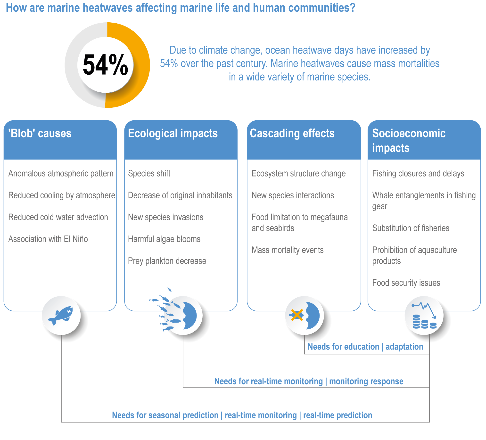
Figure FAQ3.2.1 | Impact pathway of a massive extreme marine heatwave, the northwest Pacific ‘Blob’, from causal mechanisms to initial effects, resulting nonlinear effects and the consequent impacts for humans. Lessons learnt from the Blob include the need to advance seasonal forecasts, real-time predictions, monitoring responses, education, possible fisheries impacts and adaptation.
3.4.3 Oceanic Systems and Cross-Cutting Changes
The oceanic zone, comprising >99% of the ocean’s volume, is highly exposed to climate-induced drivers because of its proximity to the atmosphere (Section 3.2; Pörtner et al., 2014; Bindoff et al., 2019a), while its relative distance from human settlements and coastal ecosystems decreases variability and interactions, and permits many phenomena to be detected clearly and attributed to climate change. This section assesses how climate-driven changes influence oceanic biological systems over very large spatial scales and notes how impacts on the epipelagic zone affect the mesopelagic, bathypelagic and deep seafloor ecosystems.
3.4.3.1 Biogeography and Species Range Shifts
3.4.3.1.1 Observed species range shifts
Since previous assessments (Table 3.16), poleward range shifts have remained a ubiquitous response to climate change (high confidence), moving species from warmer regions into higher-latitude ecosystems (Fossheim et al., 2015; Kumagai et al., 2018; Burrows et al., 2019; Lenoir et al., 2020).
Table 3.16 | Summary of previous IPCC assessments of biogeography and species range shifts
Observations | Projections |
The distribution and abundance of many fishes and invertebrates have shifted poleward and/or to deeper, cooler waters (high confidence). On average, species’ distributions have shifted poleward by 72.0 ± 0.35 km per decade (high confidence). | Spatial shifts of marine species due to projected warming will cause high-latitude invasions and high local-extinction rates in the tropics and semi-enclosed seas (medium confidence). |
SROCC (Bindoff et al., 2019a) | |
‘Ocean warming has contributed to observed changes in biogeography of organisms ranging from phytoplankton to marine mammals (high confidence).’ ‘The direction of the majority of the shifts of epipelagic organisms are consistent with a response to warming (high confidence)’ but are also shaped by oxygen concentrations and ocean currents across depth, latitudinal and longitudinal gradients (high confidence). Geographic ranges have shifted since the 1950s by 51.5 ± 33.3 km per decade (mean and very likely range) and 29.0 ± 15.5 km per decade for organisms in the epipelagic and seafloor ecosystems, respectively. | ‘Recent model projections since AR5 and SR15 continue to support global-scale range shifts of marine fishes at rates of tens to hundreds of km per decade in the 21st century, with rate of shifts being substantially higher under RCP8.5 than RCP2.6.’ |
Thermal tolerances of epipelagic populations drive biogeographic change (Figures 3.10, 3.15), but the strength and direction of range shifts tend to be modulated by both climate-induced and non-climate drivers (Pinsky et al., 2020b), including: (a) interactive effects of hypoxia and ocean acidification (Sampaio et al., 2021); (b) oceanic dispersal barriers (Choo et al., 2021), food and critical habitat availability (Alabia et al., 2020; Tanaka et al., 2021); (c) geographic position, including depth (Mardones et al., 2021); and (d) ocean currents (Sunday et al., 2015; Chapman et al., 2020; Fuchs et al., 2020). The difference between physiological thermal tolerances (Section 3.3.2) and local environmental conditions determines safety margins against future climate warming in ectotherms (Pinsky et al., 2019). Acclimation and evolution (Section 3.3.4) and life-history stage (Section 3.3.3) also alter species’ thermal tolerances. Biogeographic responses are further modulated by other interacting factors (Table 3.17).
Table 3.17 | Synthesis of selected processes conditioned by multiple environmental drivers that interact with warming to ultimately define range-shift responses
Factor | Effect | Example references |
Evolution and acclimation | Evolution of thermal tolerances and acclimation under local climatic conditions can increase resilience to future climate warming, slowing the loss of species at trailing (warm) range edges. | |
Marine heatwaves (MHWs) | MHWs can influence the evolution of thermal tolerances by eliminating genotypes that are intolerant of elevated temperatures. | |
MHWs can produce widespread die-offs of shallow-water benthic organisms triggering extensive contractions of their ranges. | ||
MHWs can facilitate range expansions by opening niches and/or enhancing recruitment of warm-affiliated species. | Leriorato and Nakamura (2019); Thomsen et al. (2019); Monaco et al. (2021) | |
Cold waves can halt or even reverse range expansions at leading edges. | ||
Ocean currents | Ocean currents can influence range dynamics through their effect on dispersal, depending on their magnitude, direction and seasonal patterns. | Hunt et al. (2016); Kumagai et al. (2018); Fuchs et al. (2020) |
Where currents align with spatial gradients of warming, range expansions track thermal changes more closely. Conversely, directional mismatches result in consistently slower expansion rates and larger response lags, an effect more acute for benthic organisms relying on passive dispersion of larvae and propagules. | García Molinos et al. (2017) | |
Rates of range contraction across taxa decreased (increased) under directional agreement (mismatch) with ocean currents, possibly associated with enhanced (reduced) flows of adaptive genes to warming in downstream (upstream) populations within the distributional range. | García Molinos et al. (2017) | |
Climatic refugia | Areas of locally stable climatic conditions, such as deeper waters or regions with internal tides or localised upwelling, can buffer the effects of regional warming, facilitating species persistence and conserving genetic diversity at rear-edge populations. | Smith et al. (2014); Assis et al. (2016); Lourenço et al. (2016); Wyatt et al. (2020) |
Distributional shifts into deeper, cooler habitats can offer an effective alternative response to latitudinal shifts, because sharper thermal gradients mean that vertical displacements, needed to compensate for the same amount of warming, are several orders of magnitude smaller than planar displacements. | Smith et al. (2014); Assis et al. (2016); Lourenço et al. (2016) | |
Oxygen availability | Oxygen supersaturation may extend ectotherm survival to extreme temperatures and increase thermal tolerances by compensating for the increasing metabolic demand at high temperatures. | |
Oxygen deprivation increases metabolic demand and respiration rates. Shallowing of oxygen-dead zones and subsequent hypoxic avoidance can render deep thermal refuges unsuitable for organisms. | Brown and Thatje (2015); Roman et al. (2019); Hughes et al. (2020) | |
Habitat availability and quality | The availability and quality of habitat (underwater light conditions, adequate substrate, nutrient and food supply) set limits to the distribution of organisms and range-shift dynamics (e.g., resilience of populations to climate warming and the consolidation of range expansions). | |
Biotic interactions, including food availability | Species interactions can confer resilience to warming by retarding habitat degradation and buffering the impacts of warming on organisms. | |
Changes in biotic interactions (e.g., altered predation rates, food availability, competition or trophic mismatches) induced by climate warming can modify range-shift dynamics. | Selden et al. (2018); Westerbom et al. (2018); Figueira et al. (2019); Pinsky et al. (2020b); Monaco et al. (2021) |
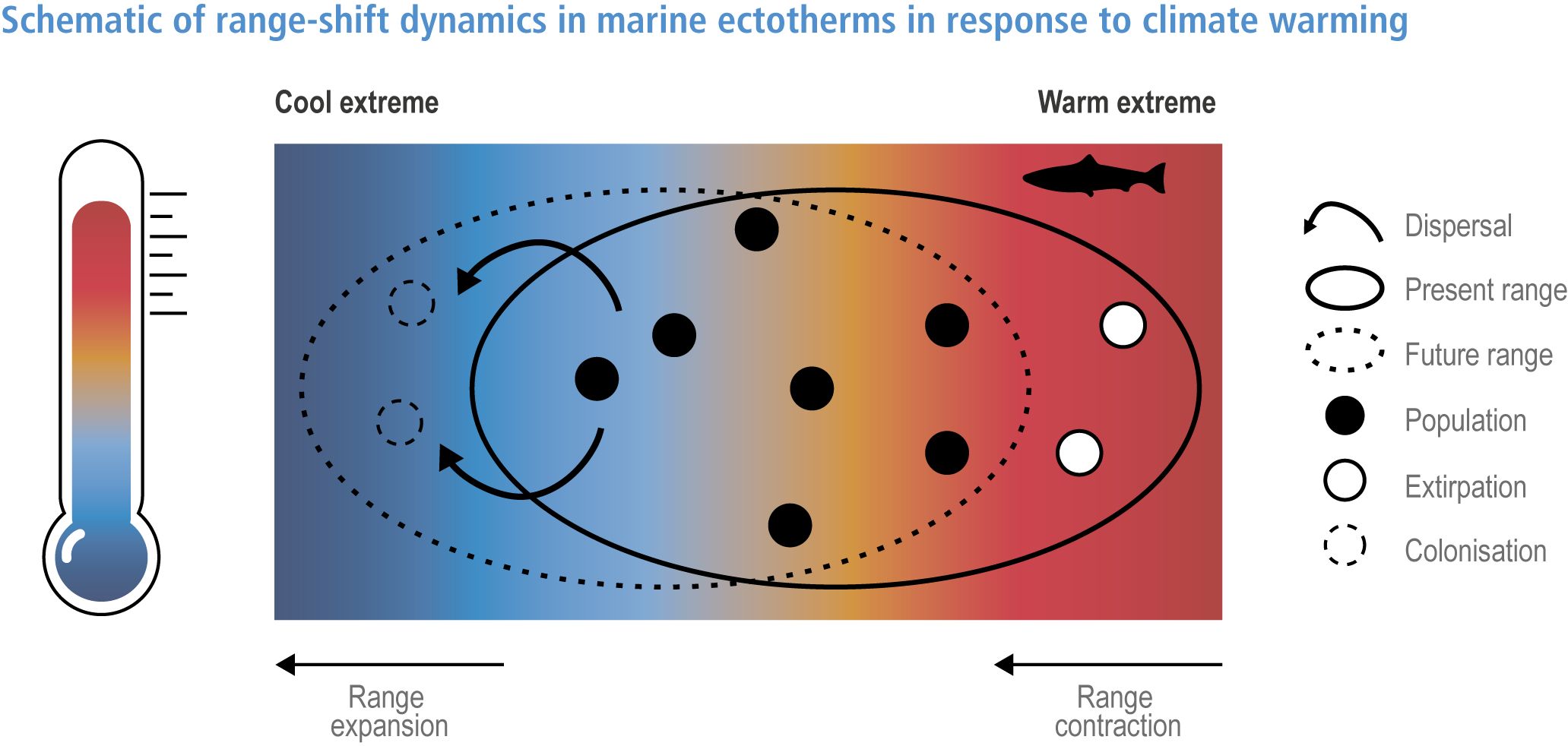
Figure 3.15 | Range-shift dynamics in marine ectotherms in response to climate warming. As the ocean warms, conditions at the edge of the species’ distribution may become warmer than the maximum thermal tolerance of the species (Figure 3.9), causing local populations to undergo a gradual decline in performance, a decreasing population size and ultimately their extirpation, resulting in a range contraction. Conversely, at the cool extreme of the distribution, habitats beyond the current range of the species will become thermally suitable in the future (i.e., within the species’ thermal tolerance range) and, providing the species can disperse to those locations, allow for the colonisation and consolidation of new populations and subsequent range expansion. These are processes conditioned by multiple drivers that interact with warming to ultimately define range-shift responses, some of which are described in Table 3.17. Note that physiological thermal tolerances relate to body temperatures of the organism rather than ambient temperatures.
A global meta-analysis of range shifts (Lenoir et al., 2020) that included data from 951 species (over half of which exhibited median range shifts consistent with climate change) estimates that marine species are moving poleward at a rate of 59.2 km per decade (very likely range: 43.7–74.7 km per decade), closely matching the local climate velocity (high confidence). In some cases, warming-related distribution shifts were followed by density-dependent use of these areas, influencing associated fisheries (Baudron et al., 2020), and in others, warming influenced competitive interactions: in the Arctic-Boreal Barents Sea, warming-induced increases in cod (Gadus morhua) abundance reduces haddock (Melanogrammus aeglefinus) abundance (Durant et al., 2020).
Biogeographic shifts lead to novel communities and biotic interactions (high confidence) (Zarco-Perello et al., 2017; Pecuchet et al., 2020b), with concomitant changes in ecosystem functioning and servicing (high confidence) (Vergés et al., 2019; Nagelkerken et al., 2020; Peleg et al., 2020). For instance, temperature-driven changes in distribution and abundance of copepods, the dominant zooplankton, were observed between 1960 and 2014 in the North Atlantic. These changes subsequently affect biogenic carbon cycling through alteration of microbial remineralisation and carbon sequestration in deep water (medium confidence) (Section 3.4.3.6; Pitois and Fox, 2006; Brun et al., 2019).
3.4.3.1.2 Observed vertical redistributions
Epipelagic isotherms have recently (1980–2015) deepened at an average of 6.6 ± 18.8 m per decade (Pinsky et al., 2019), but there is low agreement on whether species move deeper in pursuit of thermal refuge. Prior studies suggested range shifts to depth (Dulvy et al., 2008; Pinsky et al., 2013; Yemane et al., 2014), but increasing evidence suggests that fish and planktonic communities across large parts of the North Atlantic, sub-Arctic and northeast Pacific Ocean redistribute horizontally with horizontal climate velocity, except where vertical temperature gradients are particularly steep. There is low confidence for temperature-driven depth shifts in the epipelagic zone (Burrows et al., 2019; Campana et al., 2020; Caves and Johnsen, 2021). At the same time, decreasing oxygen concentrations and the vertical expansion of OMZs have already decreased suitable habitat of pelagic fishes, including tuna and billfishes, by ~15% primarily due to vertical compression of environmental niches (Stramma et al., 2012; Deutsch et al., 2015).
3.4.3.1.3 Projected changes in species range shifts
Continued changes in the biogeography of marine predators and prey are anticipated under future climate change, with climate velocity in the epipelagic zone during 2050–2100 under RCP8.5 projected to be sevenfold faster than that during 1955–2005 (medium confidence) (Figure 3.4; Brito-Morales et al., 2020). This has substantial ecological implications, as projections suggest near elimination of overlaps between the distributions of certain predator–prey pairs in the northeast Atlantic Ocean when their current joint distributions (1989–2014) are compared with those projected (2037–2062) under RCP8.5 (Sadykova et al., 2020).
Deepening of epipelagic isotherms is projected to accelerate over 2006–2100 to rates of 8.5 m per decade under RCP4.5 and 32 m per decade under RCP8.5 (Jorda et al., 2020). Although vertical redistribution of thermal niches is three to four orders of magnitude slower than horizontal displacement, maximum depth limits imposed by the seafloor and photic layer (both of which are projected to be reached in this century) will likely vertically compress suitable habitat for most marine organisms (medium confidence) (Dueri et al., 2014; Jorda et al., 2020).
Projections from coupled biogeochemical and ecosystem models suggest a general decline in mesopelagic biomass (Lefort et al., 2015), although this may vary among ocean basins. The volume of OMZs have been expanding at many locations (high confidence), and the oxygen content of the subsurface ocean is projected to decline to historically unprecedented conditions over the 21st century (medium confidence) (Section 3.2.3.2; WGI AR6 Section 5.3.3.2; Canadell et al., 2021) at a rate of 10–15 µM per decade in OMZs (Section 3.2.3.2; Breitburg et al., 2018). Oxygen availability and the effects of ocean acidification (Sections 3.3, 3.4.2) on zooplankton might become a dominant constraint in the upper ocean’s metabolic index, which is projected to decrease globally by 20% by 2100 (Deutsch et al., 2015; Steinberg and Landry, 2017). In addition, extremely rapid acceleration of climate velocities projected in the mesopelagic under all emissions scenarios suggest that species in this ocean stratum will be even more exposed to future warming than species in the epipelagic (Figure 3.4; Brito-Morales et al., 2020). But projections also suggest that warming-related increases in trophic efficiency lead to a 17% increase in the biomass of the deep-scattering layer (zooplankton and fish in the mesopelagic) by 2100 (low confidence) (Bindoff et al., 2019a). Observational studies appear to show that mesopelagic fishes adapted to warm water increased in abundance and distribution in the California Current associated with warming and the expansion of OMZ (Koslow et al., 2019), suggesting that some mesopelagic fish stocks might be resilient to a changing climate (medium confidence).
3.4.3.2 Phenological Shifts and Trophic Mismatches
3.4.3.2.1 Observed changes
SROCC reported high confidence in phenological shifts towards earlier onset of biological events (Table 3.18), with phenological shifts among epipelagic species attributed to ocean warming (high confidence).
Table 3.18 | Summary of previous IPCC assessments of phenological shifts and trophic mismatches
Observations | Projections |
AR5 WGII (Hoegh-Guldberg et al., 2014; Larsen et al., 2014) | |
‘Changes to sea temperature have altered the phenology, or timing of key life-history events such as plankton blooms, and migratory patterns, and spawning in fish and invertebrates, over recent decades (medium confidence). There is medium to high agreement that these changes pose significant uncertainties and risks to fisheries, aquaculture and other coastal activities.’ The highly productive high-latitude spring bloom systems in the northeast Atlantic are responding to warming (medium evidence, high agreement ), with the greatest changes being observed since the late 1970s in the phenology, distribution and abundance of plankton assemblages, and the reorganisation of fish assemblages, with a range of consequences for fisheries (high confidence). ‘Observed changes in the phenology of plankton groups in the North Sea over the past 50 years are driven by climate forcing, in particular regional warming (high confidence).’ ‘On average, spring events in the ocean have advanced by 4.4 ± 0.7 days per decade (mean ± SE).’ ‘Shifts in the timing and magnitude of seasonal biomass production could disrupt matched phenologies in the food webs, leading to decreased survival of dependent species (medium confidence). If the timing of primary and secondary production is no longer matched to the timing of spawning or egg release, survival could be impacted, with cascading implications to higher trophic levels. This impact would be exacerbated if shifts in timing occur rapidly (medium confidence).’ ‘There is medium to high confidence that climate-induced disruptions in the synchrony between timing of spawning and hatching of some fish and shellfish and the seasonal increases in prey availability can result in increased larval or juvenile mortality or changes in the condition factor of fish and shellfish species in the Arctic marine ecosystems.’ | Projections of phenological shifts and trophic mismatches were not assessed in this report. |
SROCC (Bindoff et al., 2019a) | |
‘Phenology of marine ectotherms in the epipelagic systems related to ocean warming (high confidence) and the timing of biological events has shifted earlier (high confidence).’ ‘Timing of spring phenology of marine organisms is shifting to earlier in the year under warming, at an average rate of 4.4 ± 1.1 days per decade, although it is variable among taxonomic groups and among ocean regions.’ | Projections of phenological shifts and trophic mismatches were not assessed in this report. |
WGI AR6 Chapter 2 (Gulev et al., 2021) | |
‘Phenological metrics for many species of marine organisms have changed in the last half century (high confidence), though many regions and many species of marine organisms remain under-sampled or even unsampled. The changes vary with location and with species (high confidence). There is a strong dependence of survival in higher trophic-level organisms (fish, exploited invertebrates, birds) on the availability of food at various stages in their life cycle, which in turn depends on the phenologies of both (high confidence). There is a gap in our understanding of how the varied responses of marine organisms to climate change, from a phenological perspective, might threaten the stability and integrity of entire ecosystems.’ | Projections of phenological shifts and trophic mismatches were not assessed in this report. |
Table 3.19 | Assessment of phenological shifts by taxon based on time series from field observations spanning at least 19 years published over the past 25 years
Taxon | Rate of consistency of observations with climate change | Estimated mean rate of change in seasonal timing | Confidence | Notes |
Phytoplankton | 78.41% (n= 85) | −7.5 d per decade (n= 83) | Very high confidence | Evidence most robust for changes in timing of blooms in the North Atlantic (e.g., Chivers et al., 2020) and Baltic (e.g., Scharfe and Wiltshire, 2019; Wasmund et al., 2019), with limited evidence from the Southern Hemisphere. |
Holozooplankton | 79.74% (n= 77) | −4.27 d per decade (n= 58) | Very high confidence | Evidence most robust in the northeast Atlantic (e.g., Chevillot et al., 2017), but sparse elsewhere. |
Meroplankton (taxa that are only temporarily in the plankton) | 81.06% (n= 72) | −4.34 d per decade (n= 64) | Very high confidence | Includes earlier peak abundance of fish larvae in upwelling systems (e.g., Asch, 2015). |
Benthic invertebrates | 72.34% (n= 5) | −8.5 d per decade (n= 5) | Low confidence (limited evidence, medium agreement ) | Evidence is limited, uncertainty levels are high. Rate of consistency of responses with climate change is not significantly different from random chance. |
Plants | 100% (n= 1) | No estimate available | Very low confidence | Just a single study for seagrasses, and only for consistency (Diaz-Almela et al., 2007). |
Fish | 65.48% (n= 109) | −3.02 d per decade (n= 43) | Very high confidence | Includes earlier appearance of migratory fish in estuaries (e.g., Chevillot et al., 2017), earlier spawning migrations for anadromous fish such as salmon (e.g., Rubenstein et al., 2019), earlier migrations for sole (e.g., Fincham et al., 2013) and tuna (e.g., Dufour et al., 2010), and earlier spawning of key commercial demersal (bottom-dwelling) species such as cod (e.g., McQueen and Marshall, 2017). |
Marine reptiles | 100.0% (n= 4) | −2.89 d per decade (n= 4) | Low confidence (limited evidence, low agreement ) | Evidence is limited, uncertainty levels are high. Mean phenological shift is not significantly different from zero. |
Seabirds | 42.36% (n= 56) | +0.77 d per decade (n= 51) | Very low confidence (limited evidence, low agreement ) | Neither the rate of consistency with climate change nor the phenological shift differ significantly from null expectations (50% consistency and no shift). Many seabirds are breeding earlier (Byrd et al., 2008; Sydeman et al., 2009), while breeding among others in temperate and polar regions has been delayed, which has been linked to later sea ice breakup or limited prey resources (Barbraud and Weimerskirch, 2006; Wanless et al., 2009; Chambers et al., 2014). Although the response of lifecycle events for many seabird species is variable in direction, there has usually been a more complex driver associated with climate that has been considered to be responsible (Sydeman et al., 2015). For many species, seasonal timing is moving earlier, especially in the Arctic (e.g., Byrd et al., 2008; Descamps et al., 2019), but for many species in the Southern Ocean, it is not (Barbraud and Weimerskirch, 2006; Chambers et al., 2014). This could be because of a much slower rate of warming in most of the Southern Ocean than in the Arctic. |
Marine mammals | 100.0% (n= 4) | −0.34 d per decade (n= 4) | Very low confidence (limited evidence, low agreement ) | All studies of phenological changes for marine mammals have focused on whales (e.g., Ramp et al., 2015; Hauser et al., 2017; Loseto et al., 2018) or polar bears (e.g., Cherry et al., 2013; Atwood et al., 2016; Escajeda et al., 2018) and have related timing to aspects of sea ice dynamics, highlighting the complexity of such processes. Mean phenological shift is not significantly different from zero at the global scale. |
Since SROCC, field data have continued to show that the phenology of biological events in the ocean is very likely (high to very high confidence) advancing in response to climate change, with 71.9% of published observations consistent with these anticipated effects (Figure 3.16a,b; Table 3.19), although most reports (95.6%) were from the Northern Hemisphere (Figure 3.16a). Biological events that are shifting earlier in response to climate change include phytoplankton blooms (Scharfe and Wiltshire, 2019; Chivers et al., 2020) such as: (a) those of HAB species (Forsblom et al., 2019; Bucci et al., 2020); (b) peaks in zooplankton abundance (Chevillot et al., 2017; Forsblom et al., 2019); (c) the migration (Otero et al., 2014; Kovach et al., 2015; Chust et al., 2019) and spawning of commercial fish (McQueen and Marshall, 2017; Kanamori et al., 2019), including crabs and squid (Henderson et al., 2017); and (d) breeding of marine reptiles (Mazaris et al., 2008; Cherkiss et al., 2020). Moreover, different trophic levels within epipelagic food webs are responding at different rates (very high confidence) (Table 3.19; Figure 3.16b,c), with greater and more consistent responses by lower trophic levels (phytoplankton, holozooplankton and meroplankton) but less consistent, weaker and more varied responses by higher trophic levels. There were too few independent time series to make robust estimates for benthic invertebrates, plants, marine reptiles and mammals. This differential response across trophic levels could lead to trophic mismatches (Neuheimer et al., 2018), where predators and their prey respond asynchronously to climate change (Edwards and Richardson, 2004; Rogers and Dougherty, 2019; Rubenstein et al., 2019; Émond et al., 2020), with potential population-level consequences, including declines in fish recruitment (Burthe et al., 2012; Chevillot et al., 2017; McQueen and Marshall, 2017; Asch et al., 2019; Durant et al., 2019; Régnier et al., 2019). Available evidence also suggests that feeding relationships could modulate species responses to climate change, as seen in breeding of surface-feeding and deeper-diving seabirds (Descamps et al., 2019). These differential responses could determine ‘winners’ and ‘losers’ under future climate change (Lindén, 2018).
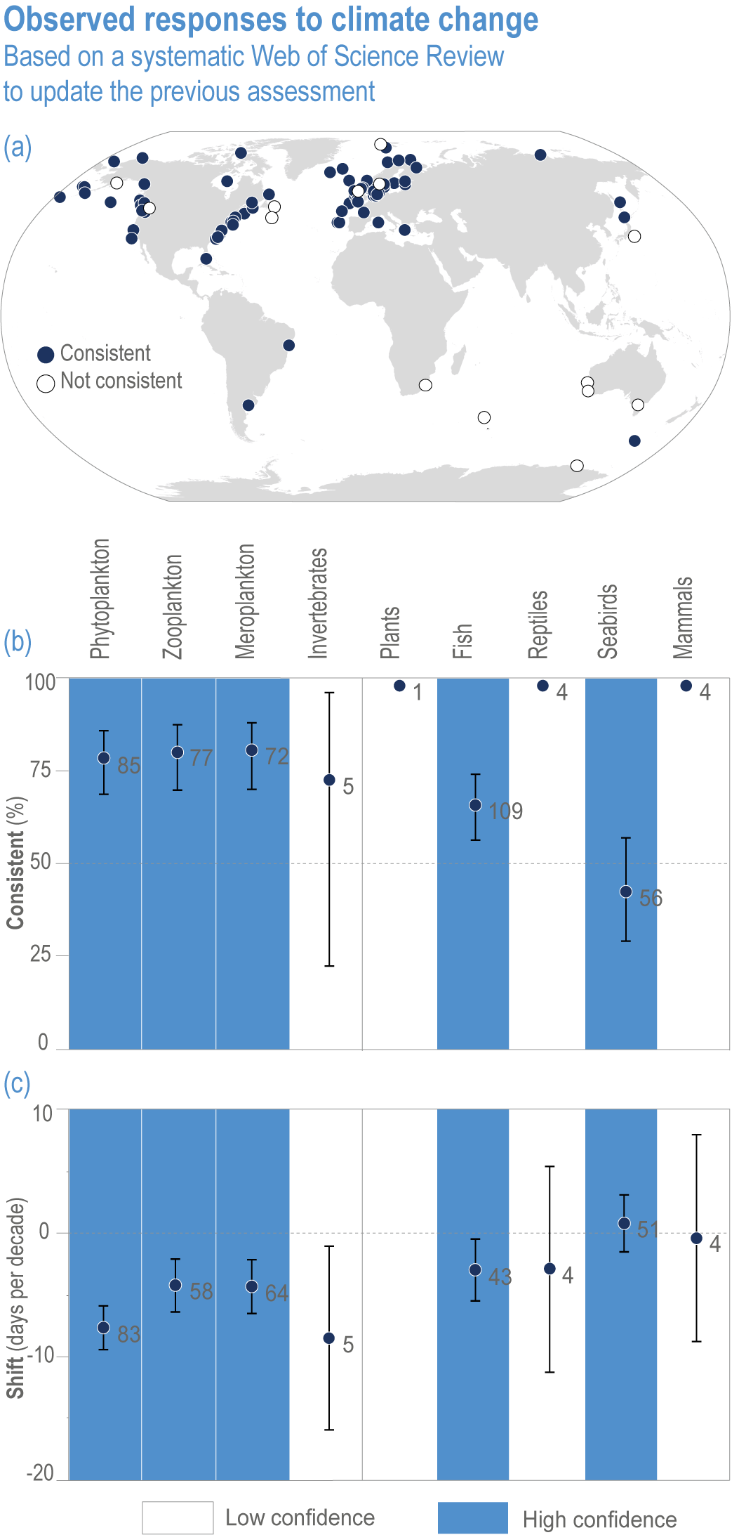
Figure 3.16 | Observed responses to climate change based on a systematic Web of Science review of marine phenology studies exceeding 19 years in length to update the assessment in WGII AR5 Chapter 30 (Hoegh-Guldberg et al. , 2014). Error bars indicate 95% confidence limits (i.e., the extremely likely range).
(a) Global data shows changes in seasonal cycles of biota that are attributed (at least partly) to climate change (blue, n= 297 observations), and changes that are inconsistent with climate change (white, n= 116 observations). Each circle represents the centre of a study area.
(b) The proportion of phenological observations (showing means and extremely likely ranges) that are attributed to climate change (i.e., generally showing earlier timing) by taxonomic group.
(c) Observed shifts in timing (days per decade, showing means and extremely likely ranges), by taxonomic group, that are attributed to climate change. Negative shifts are earlier, positive shifts are later. (Details and additional plots are presented in 3.SM.3.3, Figure 3.SM.3 and Table 3.SM.1.)
3.4.3.2.2 Projected changes
The CMIP6 ESM ensembles project that, by 2100, 18.8 ± 19.0% (mean ±very likely range) and 38.9 ± 9.4% of the ocean surface will very likely undergo a change of 20 d or more (advance or delay) in the start of the phytoplankton growth period under SSP1-2.6 and SSP5-8.5, respectively (Figure 3.17a,b) (low confidence due to the dependence with the projected changes in phytoplankton biomass, the trends of which are reported with low confidence) (Section 3.4.3.4; SROCC Section 5.2.3; Bindoff et al., 2019a). Phytoplankton growth is projected to begin later in the Northern Hemisphere subtropics, and earlier at high latitudes in some regions around the Antarctic Peninsula, and over large areas in the Northern Hemisphere (low to medium confidence as there are improved constraints from historical variability in this region and consistency with CMIP5-based-studies results) (Henson et al., 2018b; Asch et al., 2019). There is high agreement in model projections that the start of the phytoplankton growth period will very likely advance in the Arctic Ocean under a high-emission scenario for CMIP5 and CMIP6 (Figure 3.17b; Henson et al., 2018b; Asch et al., 2019; Tedesco et al., 2019; Lannuzel et al., 2020). The CMIP6 ensemble projections further show limited changes in phenology across most of the Southern Ocean but large regional variations in the tropics (Figure 3.17). Overall, the regional patterns are qualitatively similar under SSP1-2.6 and SSP5-8.5 but with greater magnitude and larger areas under SSP5-8.5 (low confidence).

Figure 3.17 | Projected phytoplankton phenology. (a,c) Spatial patterns and (b,d) density distributions of projected change in phytoplankton phenology by 2100 under Shared Socioeconomic Pathway (SSP)1-2.6 and SSP5-8.5, respectively. Difference in the start of the phytoplankton growth period is calculated as 2090–2099 minus 1996–2013. Negative (positive) values indicate earlier (later) start of the phytoplankton growth period by 2100. The ensemble projections of global changes in phytoplankton phenology include, under SSP1-2.6 and SSP5-8.5, respectively, a total of five Coupled Model Intercomparison Project 6 Earth system models containing coupled ocean biogeochemical models that cover a wide range of complexity (Kwiatkowski et al., 2019). (The phenology calculations are based on Racault et al., 2017, using updated data.)
At latitudes >40°N, temperature-linked phenology of fish reproduction with high geographic fidelity to spawning grounds (geographic spawners) is projected to change at double the rate of that for phytoplankton, which will likely cause phenological mismatches resulting in increased risk of starvation for fish larvae (medium to high confidence) (WGI AR6 Section 2.3.4.2.3; Asch et al., 2019; Durant et al., 2019; Régnier et al., 2019; Gulev et al., 2021; Laurel et al., 2021). Furthermore, under RCP8.5, trophic mismatch events exceeding ±30 days (Asch et al., 2019) leading to fish-recruitment failure are expected to increase tenfold for geographic spawners across much of the North Atlantic, North Pacific and Arctic Ocean basins (low confidence) (Neuheimer et al., 2018). In contrast, temporal mismatches between fish that relocate spawning grounds in response to environmental variations (environmental spawners) and phytoplankton blooms are projected to remain shorter and less varied, suggesting that across ocean basins, range shifts by environmental spawners may increase their resilience. Nevertheless, this compensation mechanism might fail at locations where phytoplankton bloom phenology is not controlled by temperature-driven water-column stratification, leading to a possible sixfold local increase in extreme mismatches under climate change (Asch et al., 2019).
3.4.3.3 Changes in Community Composition and Biodiversity
3.4.3.3.1 Evidence of natural adaptive capacity based on species’ responses to past climate variability
Responses to abrupt climate change in the geological past suggest that adaptive capacity is limited for marine animals (Cross-Chapter Box PALEO in Chapter 1). Temperatures during the last Interglacial (~125 ka), which were warmer than today, led to poleward range shifts of reef corals (medium confidence) (Kiessling et al., 2012; Jones et al., 2019a). Temperature has also driven marine range shifts over multi-million-year time scales (medium confidence) (Gibbs et al., 2016; Reddin et al., 2018). Warming climates, even with low ocean-warming rates, inevitably decreased tropical marine biodiversity compared with middle latitudes (high confidence) (Mannion et al., 2014; Crame, 2020; Yasuhara et al., 2020; Raja and Kiessling, 2021).
The paleorecord confirms that marine biodiversity has been vulnerable to climate warming both globally and regionally (very high confidence) (Cross-Chapter Box PALEO in Chapter 1; Stanley, 2016). In extreme cases of warming (e.g., >5.2°C), marine mass extinctions occurred in the geological past, and there may be a relationship between warming magnitude and extinction toll (medium confidence) (Song et al., 2021b). A combination of warming and spreading anoxia caused marine extinctions in ancient episodes of rapid climate warming (high confidence) (Bond and Grasby, 2017; Benton, 2018; Penn et al., 2018; Them II et al., 2018; Chen and Xu, 2019). The role of ocean acidification in ancient extinctions is yet to be resolved (low confidence) (Clapham and Payne, 2011; Clarkson et al., 2015; Jurikova et al., 2020; Müller et al., 2020).
3.4.3.3.2 Observed and projected changes in contemporary community structure and biodiversity
Ocean temperature is a major driver of species richness in the global ocean at evolutionary time scales (Tittensor et al., 2010; Chaudhary et al., 2021). This, together with temperature-driven range and phenology shifts evident across taxa and ocean ecosystems (Sections 3.4.3.1, 3.4.3.2), suggests that recent ocean warming (Section 3.2.2.1) should alter biodiversity at regional to global scales. Since previous assessments (Table 3.20), the most common evidence supporting these expected changes is replacement of cold-adapted species by warm-adapted species within an ecosystem as waters warm (Worm and Lotze, 2021). Known as tropicalisation (Section 3.4.2.3), this phenomenon has been attributed to ocean warming (medium to high confidence) in communities as diverse as kelp, invertebrates, plankton and fish (Burrows et al., 2019; Flanagan et al., 2019; Ajani et al., 2020; Villarino et al., 2020; Punzón et al., 2021; Smith et al., 2021).
Table 3.20 | Summary of previous IPCC assessments of community composition and biodiversity
Observations | Projections |
The paleoecological record shows that global climate changes comparable in magnitudes to those projected for the 21st century under all scenarios resulted in large-scale biome shifts and changes in community composition, and that for rates projected under RCP6 and 8.5 those changes were associated with species extinctions in some groups (high confidence). Loss of corals due to bleaching has a potentially critical influence on the maintenance of marine biodiversity in the tropics (high confidence). | Spatial shifts of marine species due to projected warming will cause high-latitude invasions and high local-extinction rates in the tropics and semi-enclosed seas (medium confidence). Species richness and fisheries catch potential are projected to increase, on average, at mid and high latitudes (high confidence) and decrease at tropical latitudes (medium confidence). ‘Shifts in the geographical distributions of marine species [...] cause changes in community composition and interactions [...]. Thereby, climate change will reassemble communities and affect biodiversity, with differences over time and between biomes and latitudes (high confidence).’ ‘Models are currently useful for developing scenarios of directional changes in net primary productivity, species distributions, community structure, and trophic dynamics of marine ecosystems, as well as their implications for ecosystem goods and services under climate change. However, specific quantitative projections by these models remain imprecise (low confidence).’ |
SROCC (Bindoff et al., 2019a) | |
‘Ocean warming has contributed to observed changes in biogeography of organisms ranging from phytoplankton to marine mammals (high confidence), consequently changing community composition (high confidence), and in some cases altering interactions between organisms and ecosystem function (medium confidence).’ | Poleward range shifts are projected to decrease species richness in tropical oceans, counterbalanced by increases in mid- to high-latitude regions, leading to global-scale species turnover (medium confidence on trends, low confidence on magnitude because of model uncertainties and the limited number of published model simulations). ‘The projected intensity of species turnover is lower under low-emission scenarios (high confidence).’ ‘Projections from multiple fish species distribution models show hotspots of decrease in species richness in the Indo-Pacific region, and semi-enclosed seas such as the Red Sea and Persian Gulf (medium evidence, high agreement ). In addition, geographic barriers, such as land, [bounding the] poleward species range edge in semi-enclosed seas or low-oxygen water in deeper waters are projected to limit range shifts, resulting in a larger relative decrease in species richness (medium confidence).’ ‘The large variation in sensitivity between different zooplankton taxa to future conditions of warming and ocean acidification suggests elevated risk on community structure and inter-specific interactions of zooplankton in the 21st century (medium confidence).’ |
At local to regional scales, tropicalisation often increases species richness where warm-water species extend their ranges to overlap with existing communities and decreases species richness where warming waters extirpate species (medium to high confidence) (Friedland et al., 2020a; Chaudhary et al., 2021; Worm and Lotze, 2021). Latitudinal estimates from catalogued observations show declining species richness in equatorial waters over the past 50 years, with concomitant increases in species richness at mid-latitudes; the pattern is especially prominent in free-swimming pelagic species (Figure 3.18; Chaudhary et al., 2021). Similar patterns among marine animals have been described previously for historical warming events (Song et al., 2020b). Tropicalisation is associated with increased representation of herbivorous species (Vergés et al., 2016; Zarco-Perello et al., 2020; Smith et al., 2021), although observations and theory suggest that dietary generalism can also favour range-shifting species (Monaco et al., 2020; Wallingford et al., 2020).
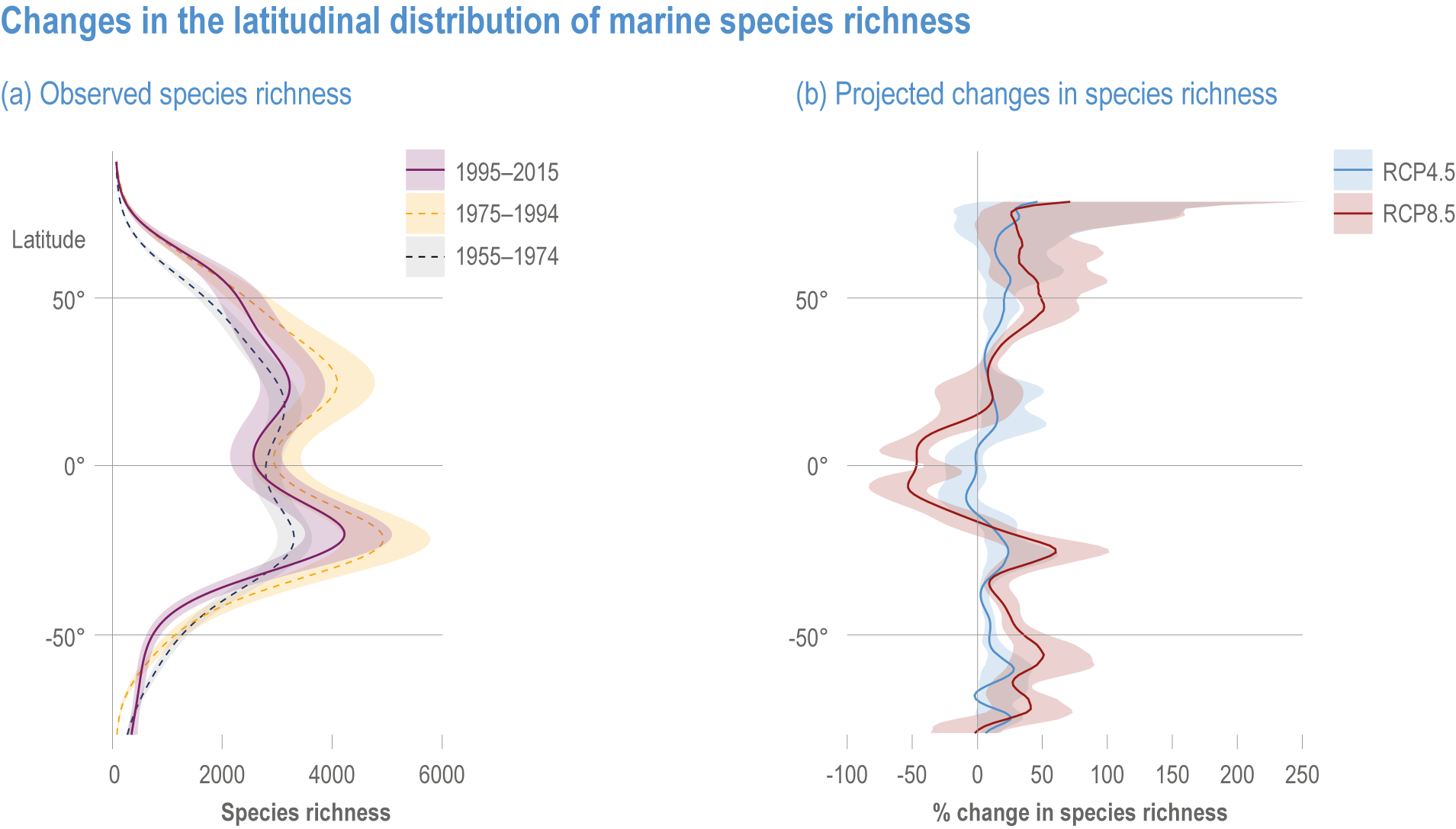
Figure 3.18 | Changes in the latitudinal distribution of marine species richness.
(a) Observed species richness for three historical periods. The observed latitudinal patterns in species richness are for a suite of taxonomic groups based on 48,661 marine species (Chaudhary et al., 2021).
(b) Projected changes in species richness under RCP4.5 and RCP8.5 are calculated as differences by grid cell by 2100 relative to 2006. Latitudinal global median (5° moving average). (Based on Figure 1b,c in García Molinos et al., 2016.) The projected latitudinal patterns in changes in species richness under climate change are based on a numerical model that includes species-specific information across a suite of taxonomic groups, based on 12,796 marine species (García Molinos et al., 2016).
At the community level, the magnitude and shape of projected future biodiversity changes differ depending on which groups are considered (medium confidence) (Chaudhary et al., 2021). Molecular-based richness measures indicate that the most dramatic increases in diversity relative to current conditions are expected for photosynthetic eukaryotes and copepods in the Arctic Ocean (Ibarbalz et al., 2019). However, component eukaryotic taxa, for example diatoms (Busseni et al., 2020), are projected to lose diversity by 2100 under RCP8.5. Ecosystem models project a decline in nutrient supply that drives the disappearance of less-competitive and larger phytoplankton types, leading to extinction of up to 30% of diatom types, particularly in the Northern Hemisphere, by 2100 under RCP8.5 (Henson et al., 2021). Models further suggest that high latitudes are likely to encounter entirely novel phytoplankton communities by 2100 under RCP8.5 (100% change in community composition; Dutkiewicz et al., 2019; Reygondeau et al., 2020). At the polar edges, the increased richness is projected to coincide with high species turnover and increasing dominance of smaller phytoplankton types (Henson et al., 2021). These imply pronounced changes to both the oceans’ ecological and biogeochemical function, as regions dominated by small phytoplankton typically support less-productive food webs (Section 3.4.3.4; Stock et al., 2017; Armengol et al., 2019) and sequester less particulate organic carbon (POC) in the deep ocean (Section 3.4.3.5; Mouw et al., 2016; Cram et al., 2018) than areas dominated by larger size classes (high confidence).
The profound climatic and environmental changes projected for the Arctic region by 2100 (Cross-Chapter Paper 6) are also anticipated to alter the composition of apex assemblages like marine mammals (see Box 3.2; Albouy et al., 2020). Under both RCP2.6 and 8.5 scenarios the most vulnerable marine mammal species will be the North Pacific right whale (Eubalaena japonica, listed as an endangered species; IUCN, 2020) and the grey whale (Eschrichtius robustus, which has critically endangered subpopulations; IUCN, 2020). The extinction of the most-vulnerable species will disproportionately eliminate unique and important evolutionary lineages as well as functional diversity, with consequent impacts throughout the entire marine ecosystem (Section 3.3.4). More generally, future warming and acidification simulated in mesocosm experiments support projections of a substantial increase in biomass and productivity of primary producers and secondary consumers, but a decrease by >40% of primary consumers (Nagelkerken et al., 2020). On longer time scales, alteration of energy flow through marine food webs may lead to ecological tipping points (Wernberg et al., 2016; Harley et al., 2017) after which the food web collapses into shorter, bottom-heavy trophic pyramids (medium confidence).
Global projections anticipate a likely future reorganisation of marine life of variable magnitude, contingent on emission scenario (Beaugrand et al., 2015; Jones and Cheung, 2015; Barton et al., 2016; García Molinos et al., 2016; Nagelkerken et al., 2020; Henson et al., 2021). Marine organism redistributions projected under RCP4.5 and RCP8.5 include extirpations and range contractions in the tropics, strongly decreasing tropical biodiversity, and range expansions at higher latitudes, associated with increased diversity and homogenisation of marine communities (Figure 3.18b). Under continuing climate change, the projected loss of biodiversity may ultimately threaten marine ecosystem stability (medium confidence) (Albouy et al., 2020; Nagelkerken et al., 2020; Henson et al., 2021), altering both the functioning and structure of marine ecosystems and thus affecting service provisioning (medium confidence) (Section 3.5; Ibarbalz et al., 2019; Righetti et al., 2019).
However, biodiversity observations remain sparse, and statistical and modelling tools can provide conflicting diversity information (e.g., Righetti et al., 2019; Dutkiewicz et al., 2020) because correlative approaches assume that the modern-day relationship between marine species distribution and environmental conditions remains the same into the future, whereas mechanistic models permit marine species to respond dynamically to changing environmental forcing. Moreover, existing global projections of future biodiversity disproportionately focus on the effects sea surface temperature (Thomas et al., 2012), typically overlooking other factors such as ocean acidification, deoxygenation and nutrient availability (Section 3.2.3), and often failing to account for natural adaptation (e.g., Section 3.3.4; see Box 3.1; Barton et al., 2016; Henson et al., 2021).
3.4.3.3.3 Abrupt ecosystem shifts and extreme events
Climate-change-driven changes in ocean characteristics and the frequency and intensity of extreme events (Section 3.2) increase the risk of persistent, rapid and abrupt ecosystem change (very high confidence), often referred to as ecosystem collapses or regime shifts (AR6 WGI Chapter 9; Collins et al., 2019a; Canadell and Jackson, 2021; Ma et al., 2021). Such abrupt changes include altering ecosystem structure, function and biodiversity outside the range of natural fluctuations (Collins et al., 2019a; Canadell and Jackson, 2021). They can involve mass-mortality events and ‘tipping points’ or ‘critical transitions’, where strong positive feedbacks within an ecosystem lead to self-sustaining change (Figure 3.19a; Scheffer et al., 2012; Möllmann et al., 2015; Biggs et al., 2018). Abrupt ecosystem shifts have been observed in both large open-ocean ecosystems and coastal ecosystems (Section 3.4.2), with dramatic social consequences through significant loss of diverse ecosystem services (high confidence) (Section 3.5; Biggs et al., 2018; Pinsky et al., 2018; Beaugrand et al., 2019; Collins et al., 2019a; Filbee-Dexter et al., 2020b; Huntington et al., 2020; Trisos et al., 2020; Turner et al., 2020b; Canadell and Jackson, 2021; Ma et al., 2021; Ruthrof et al., 2021). A summary of previous assessments of abrupt ecosystem shifts and extreme events is provided in Table 3.21.
Table 3.21 | Summary of previous IPCC assessments of observed and projected abrupt ecosystem shifts and extreme events
Observations | Projections |
AR5 (Wong et al., 2014) | |
Observations of abrupt ecosystem shifts and extreme events were not assessed in this report. | ‘Warming and acidification will lead to coral bleaching, mortality, and decreased constructional ability (high confidence), making coral reefs the most vulnerable marine ecosystem with little scope for adaptation. Temperate seagrass and kelp ecosystems will decline with the increased frequency of heatwaves and sea temperature extremes as well as through the impact of invasive subtropical species (high confidence).’ |
SROCC (Collins et al., 2019a) | |
‘Marine heatwaves (MHWs), periods of extremely high ocean temperatures, have negatively impacted marine organisms and ecosystems in all ocean basins over the last two decades, including critical foundation species such as corals, seagrasses and kelps (very high confidence).’ | ‘Marine heatwaves are projected to further increase in frequency, duration, spatial extent and intensity (maximum temperature) (very high confidence). Climate models project increases in the frequency of marine heatwaves by 2081–2100, relative to 1850–1900, by approximately 50 times under RCP8.5 and 20 times under RCP2.6 (medium confidence).’ ‘Extreme El Niño and La Niña events are projected to likely increase in frequency in the 21st century and to likely intensify existing hazards, with drier or wetter responses in several regions across the globe. Extreme El Niño events are projected to occur about twice as often under both RCP2.6 and RCP8.5 in the 21st century when compared to the 20th century (medium confidence).’ ‘Limiting global warming would reduce the risk of impacts of MHWs, but critical thresholds for some ecosystems (e.g., kelp forests, coral reefs) will be reached at relatively low levels of future global warming (high confidence).’ |

Figure 3.19 | Observed ecological regime shifts and their drivers in the oceans.
(a) A conceptual representation of ecosystem resilience and regime shifts. Shift from Regime 1 to Regime 2 can be triggered by either a large shock (i.e., an abrupt environmental transition) or gradual internal or external change that erodes the dominant balancing feedbacks, reducing ecosystem resilience (indicated by the shallower dotted line, relative to the deeper ‘valley’ reflecting higher resilience). (Based on Biggs et al., 2018).
(b) The sum of the magnitude and extent of the abrupt community shifts that has been estimated at each geographic cell in the global ocean during 1960–2014, calculated as the ratio of the amplitude of the change in a particular year to the average magnitude of the change over the entire time series (thus, is dimensionless). (Based on Beaugrand et al., 2019).
Abrupt ecosystem shifts are associated with large-scale patterns of climate variability (Alheit et al., 2019; Beaugrand et al., 2019; Lehodey et al., 2020), some of which are projected to intensify with climate change (medium confidence) (WGI AR6 Chapter 1; Wang et al., 2017a; Collins et al., 2019a; Chen et al., 2021). Over the past 60 years, abrupt ecosystem shifts have generally followed El Niño/Southern Oscillation events of any strength, but some periods had geographically limited ecological shifts (~0.25% of the global ocean in 1984–1987) and others more extensive shifts (14% of the global ocean in 2012–2015) (medium confidence) (Figure 3.19b; Beaugrand et al., 2019). Typically, interacting drivers, such as eutrophication and overharvest, reduce ecosystem resilience to climate extremes (e.g., MHWs, cyclones) or gradual warming, and hence promote ecosystem shifts (high confidence) (Figure 3.19a; Rocha et al., 2015; Biggs et al., 2018; Babcock et al., 2019; Turner et al., 2020b; Bergstrom et al., 2021; Canadell and Jackson, 2021; Tait et al., 2021). Also, shifts in different ecosystems may be connected through common drivers or through cascading effects (medium confidence) (Rocha et al., 2018a).
Recent MHWs (Section 3.2.2.1) have caused major ecosystem shifts and mass mortality in oceanic and coastal ecosystems, including corals, kelp forests and seagrass meadows (Sections 3.4.2.1, 3.4.2.3, 3.4.2.5, 3.4.2.6, 3.4.2.10; Cross-Chapter Box MOVING SPECIES in Chapter 5; Cross-Chapter Box EXTREMES in Chapter 2), with dramatic declines in species foundational for habitat formation or trophic flow, biodiversity declines, and biogeographic shifts in fish stocks (very high confidence) (Table 3.15; Cross-Chapter Box MOVING SPECIES in Chapter 5; Canadell and Jackson, 2021). Three major bleaching episodes on Australia’s Great Barrier Reef in 5 years corresponded with extreme temperatures in 2016, 2017 and 2020 (Pratchett et al., 2021). Between 1981 and 2017, MHWs have increased more than 20-fold due to anthropogenic climate change (Section 3.2.2.1; WGI AR6 Chapter 9; Laufkötter et al., 2020; Fox-Kemper et al., 2021), increasing the risk of abrupt ecosystem shifts (high confidence) (Figure 3.19a; Cross-Chapter Box EXTREMES in Chapter 2; van der Bolt et al., 2018; Garrabou et al., 2021; Wernberg, 2021).
Ecosystems can recover from abrupt shifts (e.g., Babcock et al., 2019; Christie et al., 2019; Medrano et al., 2020). However, where climate change is a dominant driver, ecosystem collapses increasingly cause permanent transitions (high confidence), although the extents of such transitions depend on the emission scenario (Trisos et al., 2020; Garrabou et al., 2021; Klein et al., 2021; Pratchett et al., 2021; Wernberg, 2021). Over the coming decades, MHWs are projected to very likely become more frequent under all emission scenarios (Section 3.2; WGI AR6 Chapter 9; Fox-Kemper et al., 2021), with intensities and rates too high for recovery of degraded foundational species, habitats or biodiversity (medium confidence) (Babcock et al., 2019; Garrabou et al., 2021; Klein et al., 2021; Serrano et al., 2021; Wernberg, 2021). Emission pathways that result in temperature overshoot above 1.5oC will increase the risks of abrupt and irreversible shifts in coral reefs and other vulnerable ecosystems (Section 3.4.4).
3.4.3.3.4 Time of emergence: species exposure to altered environments
Since SROCC, more studies have assessed the time of emergence for climate-induced drivers (Section 3.2.3) and the ecosystem attributes through which the impacts manifest. However, as in previous assessments (Table 3.22), the time of emergence for a given driver or ecosystem attribute depends on the reference period, the definition of the signal emergence threshold and the spatio-temporal scales considered (see Box 5.1 in SROCC; Kirtman et al., 2013; Bindoff et al., 2019a).
Table 3.22 | Conclusions from previous IPCC assessments about projected time of emergence on coastal, ocean and deep-sea systems
Oceanic systems and chapter subsection | Projections |
Coastal (Section 3.4.2) | ‘Multiple [climate-impact drivers] will emerge [...] in the 21st century under RCP8.5, while the time of emergence will be later and with less [climatic hazards] under RCP2.6. [Non-climate] impacts such as eutrophication add to, and in some cases, exacerbate these large-scale slow climate drivers beyond biological thresholds at local scale (e.g., deoxygenation)’ (Section 5.3.7 in SROCC; Bindoff et al., 2019a). |
Epipelagic (Section 3.4.3) | ‘Observed range shifts in response to climate change in some regions such as the north Atlantic are strongly influenced by warming due to both multi-decadal [climate change and] variability, suggesting that there is a longer time of emergence of range shifts from natural variability and a need for longer biological time series for robust attribution’ (Section 5.2.3.1.1 in SROCC; Bindoff et al., 2019a). |
Open ocean (Section 3.4.3) | ‘[The timing] for five primary drivers of marine ecosystem change (surface warming and acidification, oxygen loss, nitrate concentration and net primary production change) are all prior to 2100 for over 60% of the ocean area under RCP8.5 and over 30% under RCP2.6 (very likely )’ (Figure 1 in Box 5.1 in SROCC, Box 5.1 in SROCC, Executive Summary in SROCC Chapter 5; Bindoff et al., 2019a). ‘Anthropogenic signals are expected to remain detectable over large parts of the ocean, even for the RCP2.6 scenario for pH and SST, but are likely [to be less conspicuous] for nutrients and NPP [net primary production] in the 21st century. For example, for the open ocean, the anthropogenic pH signal in Earth System Models’ (ESM) historical simulations is very likely to have emerged for three-quarters of the ocean prior to 1950, and it is very likely over 95% of the ocean has already been affected, with little discernible difference between scenarios’ (Executive Summary in SROCC Chapter 5, Box 5.1 in SROCC; Bindoff et al., 2019a). ‘The climate signal of oxygen loss will very likely emerge by 2050 with a very likely range of 59–80% by 2031–2050 and rising with a very likely range of 79–91% of the ocean area by 2081–2100 (RCP8.5 emissions scenario). The emergence of oxygen loss is smaller in area for the RCP2.6 scenario in the 21st century and by 2090 the [area where emergence is evident is declining].’ It has also been shown that signatures of altered oxygen solubility or utilisation may emerge earlier than for oxygen levels (Executive Summary in SROCC Chapter 5, Box 5.1 in SROCC; Bindoff et al., 2019a). |
Deep sea (Box 3.3) | ‘Emergence of risk is expected to occur later at around the mid-21st century under RCP8.5 for abyssal plain and chemosynthetic ecosystems (vents and seeps)’ (Section 5.2.5 in SROCC; Bindoff et al., 2019a). ‘All deep seafloor ecosystems are expected to be subject to at least moderate risk under RCP8.5 by the end of the 21st century, with cold water corals undergoing a transition from moderate to high risk below 3°C’ (SM5.2 in SROCC; Bindoff et al., 2019b). |
Anthropogenically driven changes in chlorophyll-a concentrations across an ensemble of 30 ESMs are expected to exceed natural variability under RCP8.5 by 2100 in ~65–80% of the global oceans, when the natural variability is calculated using the ensemble’s standard deviation (Schlunegger et al., 2020); however, if two standard deviations are used, then significant trends in chlorophyll-a concentration are expected under RCP8.5 across ~31% of the global oceans by 2100 (Dutkiewicz et al., 2019). In contrast, the anthropogenic signal in phytoplankton community structure, which has a lower natural variability, will emerge under RCP8.5 across 63% of the ocean by 2100 when two standard deviations are used (limited evidence) (Dutkiewicz et al., 2019).
The time of emergence of climate impacts on ecosystems will be modulated jointly by species-specific adaptation potential (Section 3.3.4; Jones and Cheung, 2018; Collins et al., 2020; Gamliel et al., 2020; Miller et al., 2020a), speed of range shifts and spatial reorganisation (high confidence) (Sections 3.3, 3.4.2, 3.4.3). These ecosystem responses complicate projections of the time of emergence of environmental properties that impact biogeochemical cycling (Schlunegger et al., 2019; Schlunegger et al., 2020; Wrightson and Tagliabue, 2020), ecosystem structure and biodiversity (Figure 3.20a,c; Dutkiewicz et al., 2019; Trisos et al., 2020), and higher trophic levels, including fisheries targets (Cheung and Frölicher, 2020). Better accounting for multiple interacting factors in ESMs (see Box 3.1) will provide insight into how marine ecosystems will respond to future climate (high confidence).
The time of emergence of ecosystem responses supports planning for specific time-bound actions to reduce risks to ecosystems (Section 3.6.3.2.1; Bruno et al., 2018; Trisos et al., 2020). Although under RCP8.5, climate refugia from SST after 2050 are primarily in the Southern Ocean in tropical waters, these refugia are mainly from deoxygenation (Bruno et al., 2018). Marine assemblages in these places will be exposed to unprecedented temperatures after 2050, peaking in 2075 (Figure 3.20a,b; Trisos et al., 2020). In contrast, changes in phytoplankton community structure will emerge earlier, primarily in the Pacific Ocean subtropics and through much of the North Atlantic Ocean (Figure 3.20c,d; Dutkiewicz et al., 2019). Under RCP8.5, changes in phytoplankton community structure and, to a lesser extent, exposure of marine species to unprecedented temperatures, will emerge earlier in marine protected areas (MPAs), covering ~7.7% of the global oceans (Section 3.6.2.3.2.1; UNEP-WCMC and IUCN, 2020; UNEP-WCMC and IUCN, 2021) as compared with non-MPAs (Figure 3.20b,d). Such assessment can support planning for future MPA placement and extent. Because MPAs can serve as refugia from non-climate drivers (Sections 3.6.2.3, 3.6.3.2.1), they facilitate opportunities for adaptation among marine species and communities in coastal oceans (Section 3.4.2).
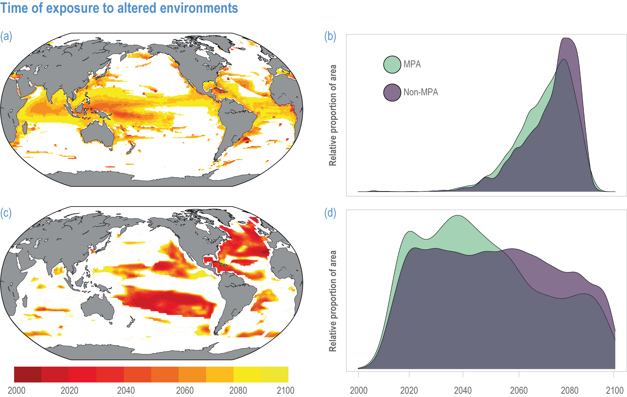
Figure 3.20 | Time of exposure to altered environments.
(a) Simulated spatial variation in the time of exposure of marine species to unprecedented temperatures under RCP8.5. Time of exposure is quantified as the median year after which local species are projected to encounter temperatures warmer than the historical maximum within their full geographic range for a period of at least 5 years. This estimate is based on 22 Coupled Model Intercomparison Project 5 (CMIP5) models, and is drawn from data presented by Trisos et al. (2020). Only regions that have times of emergence by 2100 are shown.
(b) The distribution in the time of exposure to unprecedented temperatures within marine assemblages (Trisos et al., 2020) under RCP8.5 in marine protected areas (in turquoise) and in non-marine protected areas (in purple). Values were calculated after regridding to equal-area 0.5° hexagons.
(c) Time of emergence for phytoplankton community-structure changes (based on a proxy–ecosystem-model reflectance at 500 nm) under RCP8.5. Only regions with statistically significant (p< 0.05) trends that are presently largely ice free and have times of emergence by 2100 are shown. (Based on the results of one numerical model from Dutkiewicz et al., 2019).
(d) The distribution in the time of emergence for changes in phytoplankton community structure (same proxy as in panel c) (Dutkiewicz et al., 2019) under RCP8.5 in marine protected areas (in turquoise) and in non-marine protected areas (in purple). Values were calculated after regridding to equal-area 0.5° hexagons.
3.4.3.4 Biomass
3.4.3.4.1 Observed changes
Observed changes in biomass in the global ocean, beyond those for phytoplankton (Table 3.23), have not routinely been attributed to climate-induced drivers, but rather to the compound effects of multiple drivers, especially fishing (Christensen et al., 2014; Palomares et al., 2020). We therefore do not assess observed changes in ocean biomass here.
Table 3.23 | Summary of previous IPCC assessments of changes in open ocean and deep-sea biomass
Measure | Observations | Projections |
AR5 WGII (Hoegh-Guldberg et al., 2014; Pörtner et al., 2014) | ||
Chlorophyll-a/phytoplankton biomass | ‘Phytoplankton biomass: the approximately 15-year archived time series of satellite-chlorophyll (as a proxy of phytoplankton biomass) is too short to reveal trends over time and their causes’ (WGII AR5 Section 6.1.2; Pörtner et al., 2014). ‘Chlorophyll concentrations measured by satellites have decreased in the subtropical gyres of the North Pacific, Indian and North Atlantic oceans by 9, 12 and 11%, respectively, over and above the inherent seasonal and interannual variability from 1998 to 2010 (high confidence; p≤ 0.05). Significant warming over this period has resulted in increased water-column stratification, reduced mixed-layer depth and possibly decreases in nutrient availability and ecosystem productivity (limited evidence, medium agreement ). The short time frame of these studies against well-established patterns of long-term variability leads to the conclusion that these changes are about as likely as not due to climate change’ (WGII AR5 Chapter 30; Hoegh-Guldberg et al., 2014). | ‘Owing to contradictory observations there is currently uncertainty about the future trends of major upwelling systems and how their drivers (enhanced productivity, acidification and hypoxia) will shape ecosystem characteristics (low confidence)’ (WGII AR5 Chapter 6 Executive Summary; Pörtner et al., 2014). |
Animal biomass | Observed changes in animal biomass were not assessed in this report. | ‘The climate-change-induced intensification of ocean upwelling in some eastern boundary systems, as observed in the last decades, may lead to regional cooling, rather than warming, of surface waters and cause enhanced productivity (medium confidence), but also enhanced hypoxia, acidification and associated biomass reduction in fish and invertebrate stocks’ (WGII AR5 Chapter 6 Executive Summary; Pörtner et al., 2014). |
SROCC (Bindoff et al., 2019a) | ||
Chlorophyll-a/phytoplankton biomass | ‘[Changes reported] in overall open-ocean chlorophyll levels (a proxy of phytoplankton biomass) of less than ±1% yr –1 for individual time periods. Regionally, trends of ±4% between 2002 and 2015 for different regions are found when different satellite products are merged, with increases at high latitudes and moderate decreases at low latitudes’ (SROCC Section 5.2.2.6; Bindoff et al., 2019a). | Projected changes in chlorophyll-a/phytoplankton biomass were not assessed in this report. |
Animal biomass | Observed changes in open-ocean and deep-sea biomass were not assessed in this report. | ‘There is high agreement in model projections that global zooplankton biomass will very likely reduce in the 21st century, with projected decline under RCP8.5 almost doubled that of RCP2.6 (very likely ). However, the strong dependence of the projected declines on phytoplankton production (low confidence) and simplification in representation of the zooplankton communities and food web render their projections having low confidence.’ The global biomass of marine animals, including those that contribute to fisheries, is projected to decrease by 4.3 ± 2.0% (95% confidence interval) and 15.0 ± 5.9% under RCP2.6 and RCP8.5, respectively, by 2080–2099 relative to 1986–2005, while the decrease is around 4.9% by 2031–2050 across all RCP2.6 and RCP8.5 (very likely ). Regionally, total animal biomass decreases largely in tropical and mid-latitude oceans (very likely ). ‘Projected decrease in upper-ocean export of organic carbon to the deep seafloor is expected to result in a loss of animal biomass on the deep seafloor by 5.2–17.6% by 2090–2100 compared to the present (2006–2015) under RCP8.5 with regional variations (medium confidence). Some increases are projected in the polar regions, due to enhanced stratification in the surface ocean, reduced primary production and shifts towards small phytoplankton (medium confidence). The projected impacts on biomass in the abyssal seafloor are larger under RCP8.5 than RCP4.5 (very likely ).’ |
WGI AR6 Chapter 2 (Gulev et al., 2021) | ||
Chlorophyll-a/phytoplankton biomass | The multi-sensor time series of chlorophyll-a concentration has been updated to cover two decades (1998–2018). ‘Global trends in chlorophyll-a for the last two decades are insignificant over large areas of the global oceans, but some regions exhibit significant trends, with positive trends in parts of the Arctic and the Antarctic waters (>3% yr –1), and both negative and positive trends (within ±3% yr –1) in parts of the tropics, subtropics and temperate waters.’ ‘In the last two decades, the concentration of phytoplankton at the base of the marine food web, as indexed by chlorophyll concentration, has shown weak and variable trends in low and mid-latitudes and an increase in high latitudes (medium confidence).’ | Projected changes in open-ocean and deep-sea biomass were not assessed in this report. |
3.4.3.4.2 Projected changes
Based on an ensemble of CMIP5 ESMs, SROCC projected declines in global zooplankton biomass by 2100 dependent on emission scenario (low confidence) (Table 3.23). The new CMIP6 ESM ensemble projects a decline in global zooplankton biomass by −3.9 ± 8.2% (very likely range) and −9.0 ± 8.9% in the period 2081–2100 relative to 1995–2014 under SSP1-2.6 and SSP5-8.5, respectively (Figure 3.21d; Kwiatkowski et al., 2020), thus reinforcing the SROCC assessment albeit with greater inter-model uncertainties.

Figure 3.21 | Projected change in marine biomass. Simulated global biomass changes of (a,b,c) surface phytoplankton, (d,e,f) zooplankton, (g,h,i) animals and (j,k,l) seafloor benthos. In (a,d,g,j), the multi-model mean (solid lines) and very likely range (envelope) over 2000–2100 relative to 1995–2014, for SSP1-2.6 and SSP5-8.5. Spatial patterns of simulated change by 2090–2099 are calculated relative to 1995–2014 for (b,e,h,k) SSP1-2.6 and (c,f,i,l) SSP5-8.5. Confidence intervals can be affected by the number of models available for the Coupled Model Intercomparison Project 6 (CMIP6) scenarios and for different variables. Only one model was available for panel (j), so no confidence interval is calculated. For panels (a–f), the ensemble projections of global changes in phytoplankton and zooplankton biomasses updated based on Kwiatkowski et al. (2019) include, under SSP1-2.6 and SSP5-8.5, respectively, a total of nine and ten CMIP6 Earth system models (ESMs). For panels (b,c,e,f), unhatched areas represent regions where at least 80% of models agree on the sign of biomass anomaly. For panels (g,h,i), the ensemble projections of global changes in total animal biomass updated based on Tittensor et al. (2021) include six to nine published global fisheries and marine ecosystem models from the Fisheries and Marine Ecosystem Model Intercomparison Project (Tittensor et al., 2018; Tittensor et al., 2021), forced with standardised outputs from two CMIP6 ESMs. For panels (j,k,l), globally integrated changes in total seafloor biomass have been updated based on Yool et al. (2017) with one benthic model (Kelly-Gerreyn et al., 2014) forced with the CMIP6 ESM UKESM-1.
Using an ensemble of global-scale marine ecosystem and fisheries models (Fish-MIP) (Tittensor et al., 2018) with the CMIP5 ESM ensemble, SROCC concludes that projected ocean warming and decreased phytoplankton production and biomass will reduce global marine animal biomass during the 21st century (medium confidence). The simulated declines (with very likely range) are −3.5 ± 4.8% and −14.0 ± 14.6% under RCP2.6 and RCP8.5, respectively, by 2080–2099 relative to 1995–2014 (SROCC Section 5.2.3; Bindoff et al., 2019a; Lotze et al., 2019)6 . Updated Fish-MIP simulations with CMIP6 (Figure 3.21g,h,i) confirm the projected decline in total marine animal biomass in the 21st century (Tittensor et al., 2021). The simulated declines (with very likely range) are −5.7 ± 4.1% and −15.5 ± 8.5% under SSP1-2.6 and SSP5-8.5, respectively, by 2080–2099 relative to 1995–2014 (Figure 3.21g), showing greater declines and lower inter-model uncertainties (Tittensor et al., 2021). These declines result from combined warming and decreased primary production (with low confidence in future changes in primary production; Section 3.4.3.5) and are amplified at each trophic level within all ESM and marine ecosystem model projections across all scenarios (medium confidence) (Kwiatkowski et al., 2019; Lotze et al., 2019; Tittensor et al., 2021). However, there is limited evidence about how underlying food-web mechanisms amplify the climate signal from primary producers to higher trophic levels, and several putative mechanisms have been proposed (Section 3.4.4.2.2; Chust et al., 2014a; Stock et al., 2014; Kwiatkowski et al., 2019; Lotze et al., 2019; Heneghan et al., 2021). As assessed in SROCC, the biomass projections contain considerable regional variation with declines in tropical to temperate regions and strong increases in total animal biomass are projected in polar regions under high-emission scenarios, with climate-change effects that are spatially similar but less pronounced under lower-emission scenarios (Figure 3.21b,c,e,f,h,i; Tai et al., 2019; Tittensor et al., 2021).
SROCC assessed that reduced food supply to the deep sea will drive a reduction in abyssal seafloor biota by 2100 for RCP8.5 (Table 3.23). Simulations from one size-resolved benthic biomass model coupled to an ocean-biogeochemistry model forced with the CMIP5 ESM HadGEM2-ES (Yool et al., 2017) project a decline in the globally integrated total seafloor biomass of −1.1 and −17.6% by 2100 under RCP2.6 and RCP8.5, respectively (limited evidence, high agreement ). In waters shallower than 100 m, total benthic biomass is projected to increase by 3.2% on average by 2100 under RCP8.5, primarily driven by warming-increased growth rates (Yool et al., 2013), while at depths >2000 m (representing 83% of the ocean seafloor), declines of −32% arise from climate-driven decreases in surface primary production and POC flux to the seafloor (Yool et al., 2013; Kelly-Gerreyn et al., 2014; Yool et al., 2015; Yool et al., 2017). These patterns are qualitatively similar under RCP2.6, except in the Pacific and Indian Ocean basins, where some increased total seafloor biomass is projected (Yool et al., 2013). Updated simulations with the same benthic biomass model (Kelly-Gerreyn et al., 2014) forced with the CMIP6 ESM UKESM-1 project declines in total seafloor biomass of −9.8 and −13.0% by 2081–2100 relative to 1995–2014 for SSP1-2.6 and SSP5-8.5, respectively (Figure 3.21j,k,l). These projected changes in benthic biomass are based on limited evidence. Development of ensemble projections forced with a range of ESMs and a benthic model that considers the ecological roles of temperature (Hunt and Roy, 2006; Reuman et al., 2014), oxygen (Mosch et al., 2012) and ocean acidification (Andersson et al., 2011) will provide opportunities to better quantify uncertainty in projected declines in total seafloor biomass under climate change.
Overall, ocean warming and decreased phytoplankton production and biomass will drive a global decline in biomass for zooplankton (low confidence), marine animals (medium confidence) and seafloor benthos (low confidence), with regional differences in the direction and magnitude of changes (high confidence). There is increasing evidence that responses will amplify throughout the food web and at ocean depths, with relatively modest changes in surface primary producers translating into substantial changes at higher trophic levels and for deep-water benthic communities (medium confidence).
3.4.3.5 Changes in Primary Production and Biological Carbon Export Flux
3.4.3.5.1 Observed changes in primary production
Analyses of satellite-derived primary production over the past two decades (1998–2018) showed generally weak and negative trends (up to −3.0%) at low and mid latitudes (Kulk et al., 2020). In contrast, positive trends occurred in large areas of the South Atlantic and South Pacific Oceans, as well as in polar and coastal (upwelling) regions (up to +4.5%; Cross-Chapter Paper 6; Kulk et al., 2020). Data-assimilating ocean biogeochemical models estimate a global decline in primary production of 2.1% per decade in the period 1998–2015, driven by the shoaling mixed layer and decreasing nitrate concentrations (Gregg and Rousseaux, 2019). This is consistent with previous assessments that identified ocean warming and increased stratification as the main drivers (high confidence) affecting the regional variability in primary production Bindoff et al. (2019). However, as noted in SROCC and WGI AR6 Chapter 2 (Table 3.24; Gulev et al., 2021), observed interannual changes in primary production on global and regional scales are nonlinear and largely influenced by natural temporal variability, providing low confidence in the trends.
Table 3.24 | Summary of previous IPCC assessments of ocean primary production and carbon export flux
Process | Observed impacts | Projected impacts |
SROCC (Bindoff et al., 2019a) | ||
Open-ocean primary production | ‘Past open-ocean productivity trends, including those determined by satellites, [are appraised with low confidence] due to newly identified region-specific drivers of microbial growth and the lack of corroborating in situ time series datasets.’ | ‘Net primary productivity (NPP) is very likely to decline by 4–11% by 2081–2100, relative to 2006–2015, across CMIP5 models for RCP8.5, but there is low confidence for this estimate due to the medium agreement among models and the limited evidence from observations. The tropical ocean NPP will very likely to decline by 7–16% for RCP8.5, with medium confidence as there are improved constraints from historical variability in this region.’ |
Open-ocean carbon export | ‘Analyses of long-term trends in primary production and particle export production, as well as model simulations, reveal that increasing temperatures, leading to enhanced stratification and nutrient limitation, will have the greatest influence on decreasing the flux of particulate organic carbon (POC) to the deep ocean. However, different lines of evidence (including observation, modelling and experimental studies) provide low confidence on the mechanistic understanding of how climate drivers affect different components of the biological pump in the epipelagic ocean, as well as changes in the efficiency and magnitude of carbon export in the deep ocean.’ | ‘The projected changes in export production can be larger than global primary production because they are affected by both, the NPP changes, but also how shifts in food-web structure modulates the ‘transfer efficiency’ of particulate organic material, which then affects the sinking speed and lability of exported particles through the ocean interior to the sea floor.’ ‘As export production is a much better understood net integral of changing net nutrient supply and can be constrained by interior ocean nutrient and oxygen levels, there is medium confidence in projections for global [export production] changes [based on CMIP5 model runs].’ |
WGI AR6 Chapters 2, 5 (Canadell et al., 2021; Gulev et al., 2021) | ||
Open-ocean primary production | Global ocean marine primary production is estimated to be 47 ± 7.8 PgC yr –1 with low confidence because of the small number of recent studies and the insufficient length of the time series analysed. A small decrease in productivity is evident globally for the period 1998–2015, but regional changes are larger and of opposing signs (low confidence) (WGI AR6 Section 2.3.4.2.2; Gulev et al., 2021). | ‘In CMIP5 models run under RCP8.5, [POC] export flux is projected to decline by 1–12% by 2100 (Taucher and Oschlies, 2011; Laufkötter et al., 2015). Similar values are predicted in 18 CMIP6 models, with declines of 2.5–21.5% (median: −14%) [...] between 1900 and 2100 under the SSP5-8.5 scenario. The mechanisms driving these changes vary widely between models due to differences in parameterisation of particle formation, remineralisation and plankton community structure’ (WGI AR6 Section 5.4.4.2; Canadell et al., 2021). |
3.4.3.5.2 Projected changes in primary production
Across 10 CMIP5 and 13 CMIP6 ESM ensembles, global mean NPP is projected to decline by 2080–2099 relative to 2006–2015, under all RCPs and SSPs (Kwiatkowski et al., 2020). However, under comparable radiative forcing, the CMIP6 multi-model mean projections of primary production declines (mean ± SD: −0.56 ± 4.12% under SSP1-2.6, and −3.00 ± 9.10% under SSP5-8.5) are less than those of previous CMIP5 models (3.42 ± 2.47% under RCP2.6, and 8.54 ± 5.88% under RCP8.5) (WGI AR6 Section 5.4.4.2; Kwiatkowski et al., 2020; Canadell et al., 2021). The inter-model uncertainty associated with CMIP6 NPP projections is larger than in CMIP5, and it is consistently larger than the scenario uncertainty. For each SSP across the CMIP6 ensemble, individual models project both increases and decreases in global primary production, reflecting a diverse suite of bottom-up and top-down ecological processes, which are variously parameterised across models (Laufkötter et al., 2015; Bindoff et al., 2019a). Furthermore, accurate simulation of many of the biogeochemical tracers upon which NPP depends (e.g., the distribution of iron; Tagliabue et al., 2016; Bindoff et al., 2019a) remains a significant and ongoing challenge to ESMs (high confidence) (Séférian et al., 2020).
Regionally, multi-model mean changes in primary production show generally similar patterns of large declines in the North Atlantic and the western equatorial Pacific, while in the high latitudes, primary production consistently increases in CMIP5 and CMIP6 by 2100 (Cross-Chapter Paper 6; Kwiatkowski et al., 2020). In the Indian Ocean and subtropical North Pacific, which were regions of consistent NPP decline in CMIP5 projections (Bopp et al., 2013), the regional declines are reduced in magnitude, less spatially extensive and are typically less robust in CMIP6. Further assessment of simultaneous changes in processes such as nutrient advection, nitrogen fixation, the microbial loop and top-down grazing pressure (WGI AR6 Section 5.4.4.2; Laufkötter et al., 2015; Bindoff et al., 2019a; Canadell et al., 2021) are required to fully understand the regional primary production response in CMIP6 (Kwiatkowski et al., 2020). Given the regional variations in the estimates of primary production changes and the uncertainty in the representation of the dominant drivers, there remains low confidence in the projected global decline in NPP.
3.4.3.5.3 Observed processes driving changes in global export flux
The SROCCmedium confidence assessment that warming, stratification, declines in productivity and changes in plankton community in the epipelagic zone result in reduced export of primary production to deeper layers (Table 3.24) is supported by subsequent literature (Bach et al., 2019; Leung et al., 2021). Particulate organic carbon export efficiency is constrained by altered mixing and nutrient availability (Boyd et al., 2019; Lundgreen et al., 2019), particle fragmentation (Briggs et al., 2020) as well as viral, microbial and planktonic community structure (Fu et al., 2016; Guidi et al., 2016; Flombaum et al., 2020; Kaneko et al., 2021) and metabolic rates (Cavan et al., 2019). These processes are strongly interlinked, and their net effect on primary production export from the upper ocean remains difficult to quantify observationally (Boyd et al., 2019). Since SROCC, there is increasing evidence that ocean deoxygenation can alter zooplankton community structure (Wishner et al., 2018), zooplankton respiration rates (Cass and Daly, 2014; Cavan et al., 2017) and patterns of diel vertical migration (Aumont et al., 2018), which may focus remineralisation of organic carbon at the upper margins of OMZs (Section 3.4.3.4 on depth shifts due to OMZ; Bianchi et al., 2013; Archibald et al., 2019).
Data on export flux from the upper ocean are limited either in coverage and consistency (ship-board sampling) or duration (sediment traps), and are subject to considerable spatial variability (as shown in satellite observations (Boyd et al., 2019). As a result, trends are weak, inconsistent and often not statistically significant (Lomas et al., 2010; Cael et al., 2017; Muller-Karger et al., 2019; Xie et al., 2019). Deep-ocean fluxes are similarly equivocal (Smith et al., 2018; Fischer et al., 2019; Fischer et al., 2020). In coming years, an increasing number of Argo floats equipped with bio-optical sensors should help improve estimates of particle flux spatio-temporal variability (e.g., Dall’Olmo et al., 2016).
Projected changes
SROCC and WGI AR6 reported global declines in POC export flux, from −8.9 to −15.8% by 2100 relative to 2000 under RCP8.5 in CMIP5 models, and −2.5 to −21.5% (median value: −14%) between 1900 and 2100 under SSP5-8.5 in CMIP6 models (Table 3.24; WGI AR6 5.4.4.2; Bindoff et al., 2019a; Canadell et al., 2021). In CMIP5 model runs, the decrease in the sinking flux of organic matter from the upper ocean into the ocean interior was strongly related to the changes in stratification that reduce net nutrient supply (Fu et al., 2016; Bindoff et al., 2019a), especially in tropical regions, and the projections for global export production changes are reported with medium confidence. Increasing model complexity with more widespread representation of ocean biogeochemical processes between CMIP5 and CMIP6, and inclusion of more than one or two classes of phyto- and zooplankton, will provide opportunities to improve assessments of how climate-induced drivers affect different components of biological carbon pump in the epipelagic ocean, as well as changes in the efficiency and magnitude of carbon export in the deep ocean (high confidence) (see Box 3.3; Le Quéré et al., 2016; Séférian et al., 2020; Wright et al., 2021).
Box 3.2 | Marine Birds and Mammals
Marine birds (seabirds and shorebirds) and mammals include charismatic species and species that are economically, culturally and ecologically important (Sydeman et al., 2015; Albouy et al., 2020; Pimiento et al., 2020). Their long generation times and slow population growth suggests limited evolutionary resilience to rapid climate change (Section 3.3.4; Sydeman et al., 2015; Miller et al., 2018). According to the Red List Species Assessments of the International Union for Conservation of Nature (IUCN, 2020), the greatest current hazards to these groups include human use of biological resources and areas, invasive species and pollution (see Figure Box 3.2.1; Dias et al., 2019; Lusseau et al., 2021). Impacts of climate change and severe weather are ranked among the five most-important hazards influencing 131 and 45 bird and mammal species, respectively (see Figure Box 3.2.1 for selection of species), including 24 bird and 7 mammal species that are currently listed as endangered, critically endangered or threatened. Furthermore, according to these IUCN assessments, climate change and severe weather are expected to impact an additional 122 and 18 marine bird and mammal species over the next 50–100 years, respectively (see Figure Box 3.2.1; Dias et al., 2019).
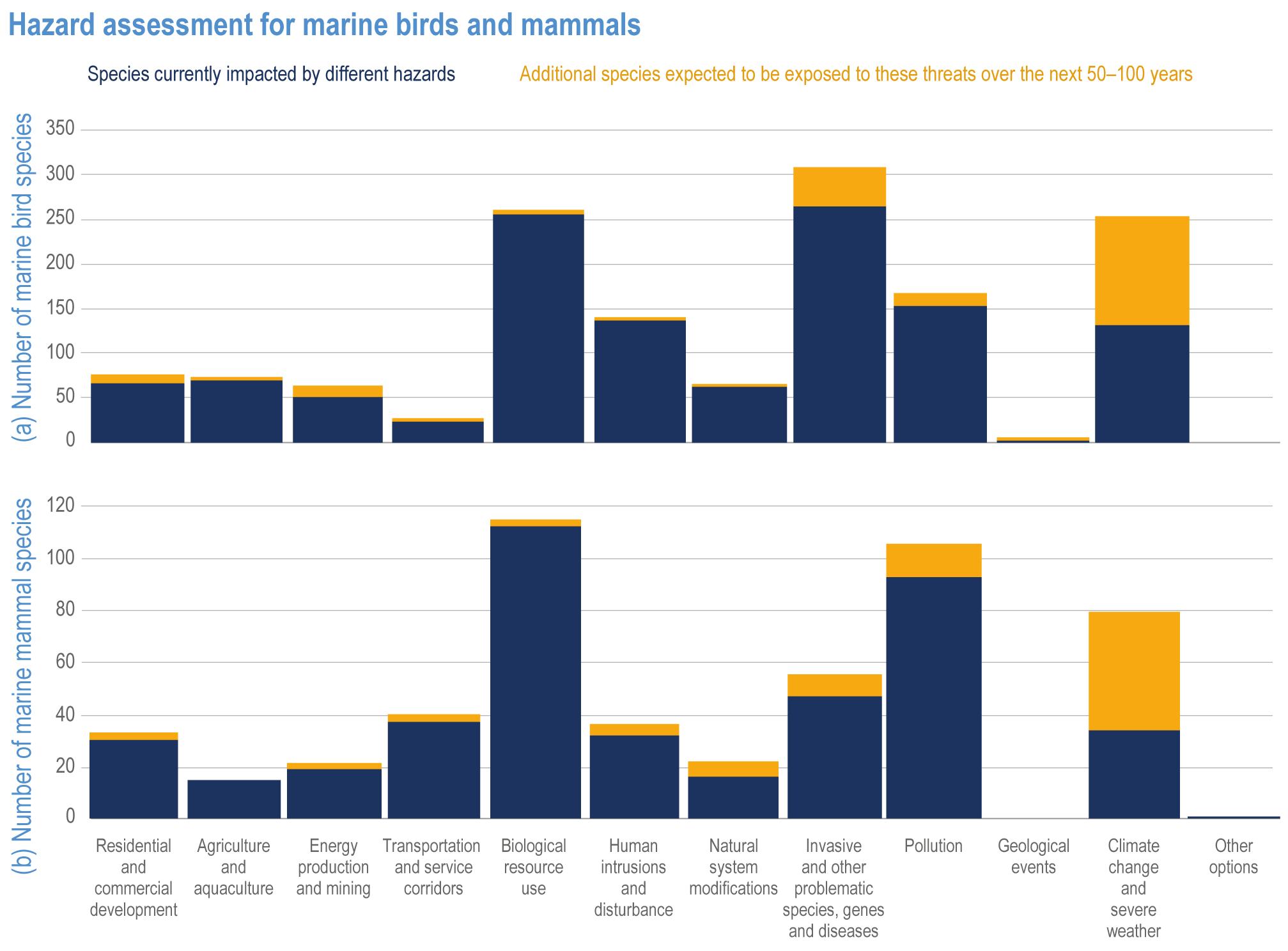
Figure Box 3.2.1 | Hazard assessment for marine birds and mammals. Number of (a) marine birds and (b) mammals currently impacted by different hazards (blue), and numbers of additional species expected to be exposed to these threats over the next 50–100 years (red), as assessed in the International Union for Conservation of Nature Red List (IUCN, 2020). Seabird species include species in the key orders Sphenisciformes, Pelecaniformes, Suliformes, Anseriformes, Procellariiformes and Charadriiformes categorised as inhabitants of marine ecosystems (n= 483 species, assessed in the period 2016–2019). Marine mammal species include the species reviewed by Lusseau et al. (2021) (n= 136 species, assessed in the period 2008–2019).
Marine birds and mammals are vulnerable to climate-induced loss of breeding and foraging habitats such as sea ice (Section 3.4.2.1 2), sandy beaches (Section 3.4.2.6), salt marshes (Section 3.4.2.5) and seagrass beds (high confidence) (Section 3.4.2.5; Sydeman et al., 2015; Bindoff et al., 2019a; Ropert-Coudert et al., 2019; Von Holle et al., 2019; Albouy et al., 2020; Amano et al., 2020; Bestley et al., 2020; Grose et al., 2020). With warming, shorebird population abundances decline in the tropics, likely due to heat stress and habitat loss, and increase at higher latitudes (Amano et al., 2020). Marine mammals dependent on sea ice habitat are particularly vulnerable to warming (medium confidence) (Albouy et al., 2020; Bestley et al., 2020; Lefort et al., 2020), yet vulnerability can differ between populations. Ongoing sea ice loss is decreasing some polar bear populations while others remain stable, likely related to past harvesting history, regional differences in sea ice phenology and ecosystem productivity (Hamilton and Derocher, 2019; Molnár et al., 2020). Nevertheless, even under an intermediate emission scenario RCP4.5, increasing ice-free periods will likely reduce both recruitment and adult survival across most polar bear populations over the next four decades, threatening their existence (medium confidence) (see Figure Box 3.2.2; Molnár et al., 2020).
Climate change is affecting marine food-web dynamics (high confidence) (Sections 3.4.2, 3.4.3), and the vulnerability and adaptive capacity of marine birds and mammals to such changes is linked to the species’ breeding and feeding ecology. Higher-vulnerability species include central-place foragers (confined to, for example, breeding colonies fixed in space), diet and habitat specialists, and species with restricted distributions such as marine mammal populations in SES (medium confidence) (McMahon et al., 2019; Ropert-Coudert et al., 2019; Albouy et al., 2020; Grose et al., 2020; Sydeman et al., 2021). Surface-feeding and piscivorous marine birds appear to be more vulnerable to food-web changes than diving seabirds and planktivorous seabirds (medium confidence) (Sydeman et al., 2021). During the 2014–2015 Pacific heatwave, around 1 million piscivorous common murres died along a 1500 km coastal stretch in the Pacific USA due to reduced prey availability (Jones et al., 2018b; Piatt et al., 2020). Marine birds are vulnerable to phenological shifts in food-web dynamics, as they have limited phenotypic plasticity of reproductive timing, with potentially little scope for evolutionary adaptation (medium confidence) (Keogan et al., 2018), although changes in reproduction timing are observed in several species (Section 3.4.4.1; Sydeman et al., 2015; Descamps et al., 2019; Sauve et al., 2019). There is limited evidence of marine mammals’ capacity to adapt to shifting phenologies, but observed responses include changes in the onset of migrations, moulting and breeding (Section 3.4.4.1; Ramp et al., 2015; Hauser et al., 2017; Beltran et al., 2019; Bowen et al., 2020; Szesciorka et al., 2020).

Figure Box 3.2.2 | Modelled risk timelines for demographic impacts on circumpolar polar bear subpopulations, and associated confidence assessments, due to extended fasting periods with loss of sea ice. Years of first impact on cub recruitment (yellow), adult male survival (blue) and adult female survival (red) are shown for the (left) RCP4.5 and (right) RCP8.5. (Data from Molnár et al., 2020).
Increased emergence of infectious disease in mammals and birds is expected with ocean warming, due to new transmission pathways from changing species distributions, higher species densities caused by habitat loss and increased vulnerability due to environmental stress on individuals (limited evidence) (Sydeman et al., 2015; VanWormer et al., 2019; Sanderson and Alexander, 2020). Marine birds and mammals are likely to suffer from increased mortalities due to increasing frequencies of HABs, and of extreme weather, at sea, on sea ice, and in terrestrial breeding habitats (Broadwater et al., 2018; Gibble and Hoover, 2018; Ropert-Coudert et al., 2019; Grose et al., 2020). Also, climate-change driven distributional shifts have strengthened interactions with other anthropogenic impacts, through, for example, increasing risks of ship strikes and bycatch (medium confidence) (e.g., Hauser et al., 2018; Krüger et al., 2018; Record et al., 2019; Santora et al., 2020).
FAQ 3.3 | Are we approaching so-called tipping points in the ocean and what can we do about it?
A tipping point is a threshold beyond which an abrupt or rapid change in a system occurs. Tipping points that have already been reached in ocean systems include the melting of sea ice in the Arctic, thermal bleaching of tropical coral reefs and the loss of kelp forests. Human-induced climate change will continue to force ecosystems into abrupt and often irreversible change, without strong mitigation and adaptation action.

Figure FAQ3.3.1 | Global map with examples of tipping points that have been passed in ocean systems around the world. Tipping points in ecological systems are linked to increasing impacts and vulnerability of dependent human communities. SES: semi-enclosed sea; EBUS: eastern boundary upwelling system; CBC; coastal boundary current.
A gradual change in water temperature or oxygen concentration can lead to a fundamental shift in the structure and/or composition of an ecosystem when a tipping point is exceeded. For example, all species have upper temperature limits below which they can thrive. In the tropics, prolonged warm temperatures can cause fatal ‘bleaching’ of tropical corals, leading reef ecosystems to degrade and become dominated by algae. In temperate regions, MHWs can kill or reduce the growth of kelp, threatening the other species that depend on the tall, canopy-forming marine plants for habitat. In the Arctic, rising temperatures are melting sea ice and reducing the available habitat for communities of ice-dependent species.
Once a tipping point is passed, the effects can be long-lasting and/or irreversible over time scales of decades or longer. An ecosystem or a population can remain in the new state, even if the driver of the change returns to previous levels. For example, once a coral reef has been affected by bleaching, it can take decades for corals to grow back, even if temperatures remain below the bleaching threshold. Crossing a tipping point can cause entire populations to collapse, causing local extinctions.
Tipping points are widespread across oceanic provinces and their ecosystems for climate variables like water temperature, oxygen concentration and acidification. Evidence suggests that ocean tipping points are being surpassed more frequently as the climate changes; scientists have estimated that abrupt shifts in communities of marine species occurred over 14% of the ocean in 2015, up from 0.25% of the ocean in the 1980s. Other human stressors to the ocean, including habitat destruction, overfishing, pollution and the spread of diseases, combine with climate change to push marine systems beyond tipping points. As an example, nutrient pollution from land together with climate change can lead to low-oxygen coastal areas referred to as ‘dead zones’.
Box FAQ 3.3
Human communities can also experience tipping points that alter people’s relationships with marine ecosystem services. Indigenous Peoples and local communities may be forced to move from a particular location due to SLR, erosion or loss of marine resources. Current activities that help sustain Indigenous Peoples and their cultures may no longer be possible in the coming decades, and traditional diets or territories may have to be abandoned. These tipping points have implications for physical and mental health of marine-dependent human communities.
Adaptation solutions to the effects of ecological tipping points are rarely able to reverse their environmental impacts, and instead often require human communities to transform their livelihoods in different ways. Examples include diversifying income by shifting from fishing to tourism and relocating communities threatened by flooding to other areas to continue their livelihoods. Tipping points are being passed already in coral reefs and polar systems, and more will probably be reached in the near future given climate-change projections. Nevertheless, the chances of moving beyond additional tipping points in the future will be minimised if we reduce greenhouse gas emissions and we also act to limit other human impacts on the ocean, such as overfishing and nutrient pollution.
3.4.4 Reversibility and Impacts of Temporary Overshoot of 1.5°C or 2°C Warming
Scenarios limiting warming to the 1.5°C and 2°C limits in the Paris Agreement can involve temporarily exceeding those warming levels before declining again (WGI AR6 Section 4.6.2.1; Lee et al., 2021). The effect of such ‘overshoot’ on marine and coastal ecosystems depends on the reversibility of both the response of climate-induced drivers and the response of organisms and ecosystems to the climate impact-drivers during the overshoot period. WGI AR6 assessed that temporary overshoot of a 2°C warming threshold has irreversible effects on global mean sea level and also effects on ocean heat content that persist beyond 2100 (WGI AR6 Section 4.6.2.1; Lee et al., 2021). Model results indicate that sea surface temperatures (high confidence), Arctic sea ice (high confidence), surface ocean acidification (very high confidence) and surface ocean deoxygenation (very high confidence) are reversible within years to decades if net emissions reach zero or below (WGI AR6 Table 4.10; Lee et al., 2021). Although changes in these surface ocean variables are reversible, habitat-forming ecosystems, including coral reefs and kelp forests, may undergo irreversible phase shifts with >1.5°C warming (Sections 3.4.2.1, 3.4.2.3), and are thus at high risk this century in 1.5°C or 2°C scenarios involving overshoot (Tachiiri et al., 2019). In an overshoot scenario in which CO2 returns to 2040 levels by 2100 (SSP5-3.4-OS; O’Neill et al., 2016), SST and Arctic sea ice do not fully return by 2100 to levels prior to the CO2 peak (medium confidence) (WGI AR6 Section 4.6.2.1; Lee et al., 2021), suggesting that reversal of marine ecological impacts from 21st century climate impacts would extend into the 22nd century or beyond (McManus et al., 2021). Models also indicate that global sea level rise, as well as warming, ocean acidification and deoxygenation at depth, are irreversible for centuries or longer (very high confidence) (WGI AR6 Section 4.6.2.1 and Table 4.10; Palter et al., 2018; Li et al., 2020c; Lee et al., 2021).
Box 3.3 | Deep-Sea Ecosystems
Deep-sea ecosystems include all waters below the 200-m isobath as well as the underlying benthos, and they provide habitats for highly diversified and specialised biota, which play a key role in the cycling of carbon and other nutrients (see Figure Box 3.3.1; Thurber et al., 2014; Middelburg, 2018; Snelgrove et al., 2018). The deep sea covers >63% of Earth’s surface (Costello and Cheung, 2010) and is exposed to climate-driven changes in abyssal, intermediate and surface waters that influence sinking fluxes of particulate organic matter (high confidence) (see Figure Box 3.3.1; Sections 3.1, 3.2.1, 3.2.2, 3.4.3.4; WGII AR5 Section 30.5.7; SROCC Sections 5.2.3, 5.2.4; Hoegh-Guldberg et al., 2014; Bindoff et al., 2019a). These ecosystems are also influenced by non-climate drivers, especially fisheries, oil and gas extraction (Thurber et al., 2014; Cordes et al., 2016; Zhang et al., 2019a); cable laying (United Nations, 2021); and mineral resource exploration (Hein et al., 2021); with proposed large-scale deep-sea mining a potential future source of impacts (Danovaro, 2018; Levin et al., 2020).
Ocean warming alters biological processes in deep-sea ecosystems in ways that affect deep-sea habitat, biodiversity and material processing. Enhancement of microbial respiration by warming attenuates sinking POC, which has been associated with the globally projected declines in total seafloor biomass of −9.8 and −13.0% by 2081–2100 relative to 1995–2014 under SSP1-2.6 and SSP5-8.5, respectively (limited evidence) (Section 3.4.3.4). Additionally, climate-change-driven oxygen loss (Section 3.2.3.2; Luna et al., 2012; Belley et al., 2016) and geographic shifts in predator distributions (Section 3.4.3.1) are anticipated to affect deep-sea biodiversity (limited evidence, high agreement ) (Smith et al., 2012; Morato et al., 2020). Complex responses of some bathyal crustacean assemblages to environmental change suggest an increase in phylogenetic diversity but limited decreases in abundances with temperature (Ashford et al., 2019). Acute mortality of some reef-forming cold-water corals to laboratory-simulated warming (Lunden et al., 2014) suggests that both long-term warming and the increase of MHWs in intermediate and deep waters (Elzahaby and Schaeffer, 2019) could pose significant risk to associated ecosystems (high confidenc e). Thermal tolerance thresholds (lethal and sub-lethal) of scleractinians in laboratory settings depend on their geographic position and capacity for thermal adaptation, as well as other factors including food, oxygen and pH (medium to high confidence) (Naumann et al., 2013; Hennige et al., 2014; Lunden et al., 2014; Naumann et al., 2014; Georgian et al., 2016; Gori et al., 2016; Maier et al., 2016; Büscher et al., 2017).
The extension and intensification of deep-water acidification (Section 3.2.3.1) has been identified as a further key risk to deep-water coral ecosystems (medium confidence) (Bindoff et al., 2019a). Literature since SROCC supports this assessment (Morato et al., 2020; Puerta et al., 2020), although scleractinians and gorgonians are found in regions undersaturated with respect to aragonite (Thresher et al., 2011; Fillinger and Richter, 2013; Baco et al., 2017). Laboratory experiments on reef-forming scleractinians show variable results, with regional acclimation potential and population-genetic adaptations (Georgian et al., 2016; Kurman et al., 2017). Desmophyllum pertusum71 and Madrepora oculata maintain calcification in moderately low pH (7.75) and near-saturation of aragonite (Hennige et al., 2014; Maier et al., 2016; Büscher et al., 2017), but lower pH (7.6) and corrosive conditions lead to net dissolution of D. pertusum skeletons (high confidence) (Lunden et al., 2014; Kurman et al., 2017; Gómez et al., 2018). Experiments suggest that D. dianthus is more sensitive to warming than acidification and when both are high, as projected under climate change. Warming appears to compensate for declines in calcification, with fitness also sensitive to food availability (Bramanti et al., 2013; Movilla et al., 2014; Gori et al., 2016; Baussant et al., 2017; Büscher et al., 2017; Schönberg et al., 2017; Höfer et al., 2018; Maier et al., 2019).
In OMZ regions (Section 3.2.3.2), benthic species distributions (Sperling et al., 2016; Levin, 2018; Gallo et al., 2020), abundance and composition of demersal fishes in canyons (De Leo et al., 2012) and deep-pelagic zooplankton (Wishner et al., 2018) follow oxygen gradients, indicating that deep-sea biodiversity and ecosystem structure will be impacted by extension of hypoxic areas (medium confidence). Fossil records show benthic population collapse and turnover when oxygen ranged from oxic to mildly or severely hypoxic (Cross-Chapter Box PALEO in Chapter 1; Moffitt et al., 2015). Regional extirpations among cold-water corals in the paleorecord were associated with substantial declines in oxygen, coincident with abrupt warming and altered properties of intermediate water-masses (Wienberg et al., 2018; Hebbeln et al., 2019). Despite mortality and functional impacts from low oxygen concentrations observed in aquaria (Lunden et al., 2014), recent observations of the deep-water coral D. pertusum suggest adaptive capacity to hypoxia among specimens from OMZ regions that are highly productive (low confidence) (Hanz et al., 2019; Hebbeln et al., 2020).
Chemosynthetic ecosystems could be particularly prone to oxygen decline (low to medium confidence). Projected OMZ expansion in the vicinity of seep communities could favour sulphide-tolerant species, as suggested from fossil records (Moffitt et al., 2015), but this will exclude large symbiont-bearing foundation species of methane-seep ecosystems (Fischer et al., 2012; Sweetman et al., 2017). Projected warming, or shifts in warm-current circulation along continental margins, could enhance dissociation of buried methane hydrates (Phrampus and Hornbach, 2012; Phrampus et al., 2014), either increasing anaerobic methane oxidation (Boetius and Wenzhöfer, 2013), which benefits seep communities, or increasing gas fluxes, which would decrease anaerobic methane oxidation rates and exclude chemosynthetic fauna.
Environmental niche models (FAO, 2019; Morato et al., 2020; Puerta et al., 2020) project that under RCP8.5, >50% of present-day scleractinian habitats in the North Atlantic Ocean will become unsuitable by 2100, with greater impacts on D. pertusum than on D. dianthus or M. oculata. For gorgonians, corresponding habitat loss is likely >80%. Much less is known about the environmental niches of deep-sea sponges, preventing a similar assessment (Kazanidis et al., 2019; Puerta et al., 2020).
Climate-driven impacts further limit the resilience of deep-sea ecosystems to impacts from human activities (high confidence) (Levin and Le Bris, 2015; Rogers, 2015; Sweetman et al., 2017). However, assessing cumulative climatic and non-climatic impacts is challenging for these data-poor environments (Ashford et al., 2018; Levin, 2018; Armstrong et al., 2019; Heffernan, 2019; Kazanidis et al., 2020; Orejas et al., 2020), where lack of knowledge increases the possibility of overlooking ecosystem vulnerabilities and risks (Levin, 2021). A paucity of information about the natural variability and historical trends of these habitats prevents robust assessment of adaptive capacities and potential vulnerabilities to extreme events (Aguzzi et al., 2019; Levin et al., 2019; Chapron et al., 2020; Danovaro et al., 2020; Le Bris and Levin, 2020; Levin, 2021). The spatial resolution of CMIP5 models is too coarse to robustly project changes in mesoscale circulation at the seafloor (Sulpis et al., 2019), on which deep-sea ecosystems depend for organic material supplies and dispersal of planktonic and planktotrophic larvae (high confidence) (Fox et al., 2016; Mitarai et al., 2016; Dunn et al., 2018). Higher-resolution modelling from CMIP6 (Orr et al., 2017), multi-annual and high-frequency records of ocean bottom-water properties (Meinen et al., 2020), and better understanding and accounting of biogeochemical mechanisms of organic carbon transport to the ocean interior is expected to improve this capacity (Boyd et al., 2019; Séférian et al., 2020).
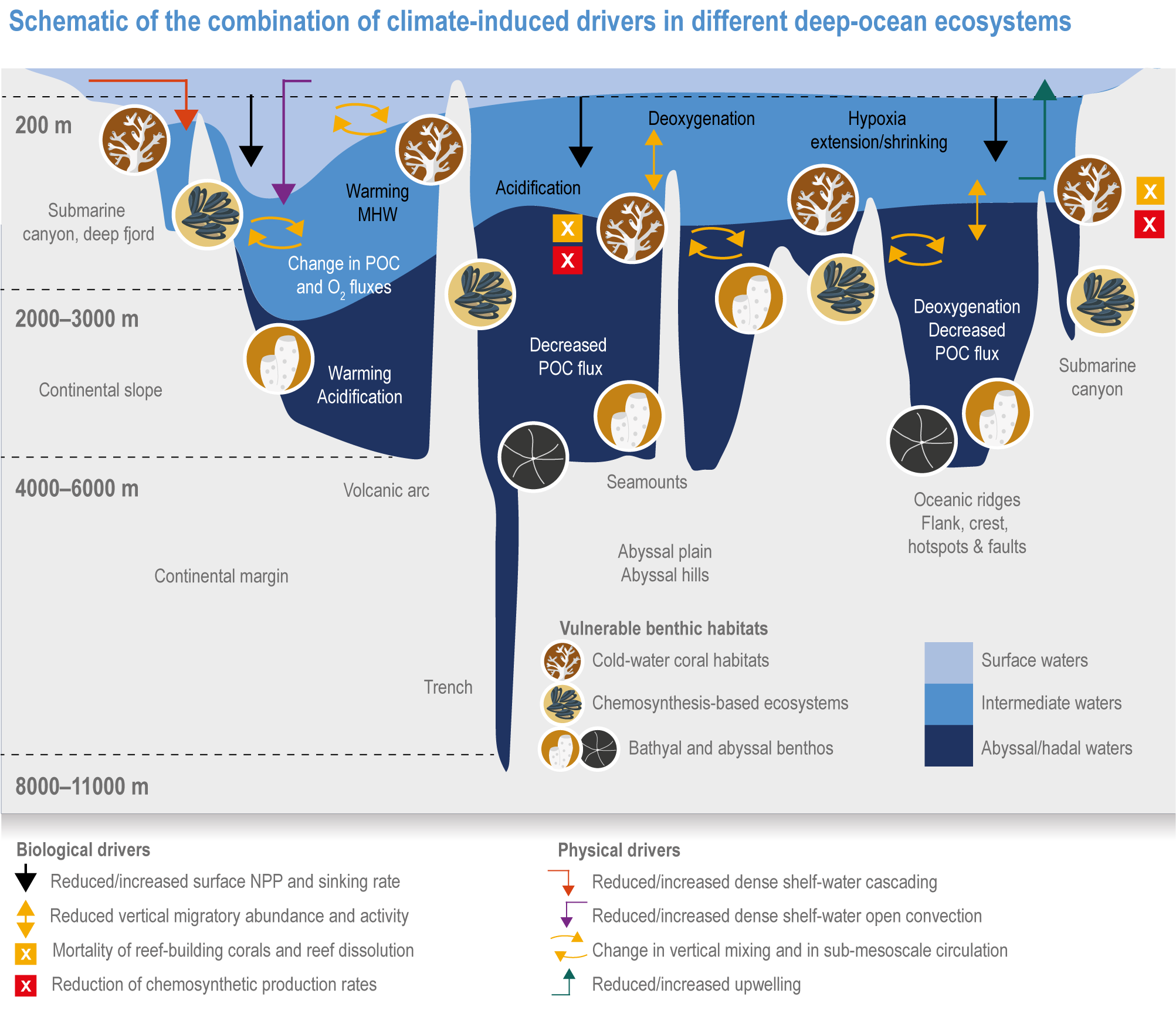
Figure Box 3.3.1 | The combination of climate-induced drivers in different deep-ocean ecosystems. (Key physical and biological drivers of change in the deep-sea and benthic habitats with specific vulnerabilities are discussed in Section 3.4.3.3.)
1 7 Previously named Lophelia pertusa
3.5 Vulnerability, Resilience, and Adaptive Capacity in Marine Social–Ecological Systems, Including Impacts on Ecosystem Services
3.5.1 Introduction
This section assesses the impacts of climate change on ecosystem services (Table 3.25; Chapter 1) and the outcomes on social–ecological systems, building on previous assessments (Table 3.26). Section 3.5.2 assesses how changes in biodiversity influence ecosystem services. Then Sections 3.5.3 and 3.5.4 assess provisioning services (food and non-food), Section 3.5.5 assesses supporting and regulating services, and Section 3.5.6, cultural services. Where evidence exists, the section evaluates how the vulnerability and adaptive capacity of social–ecological systems govern the manifestation of impacts on each ecosystem service.
Table 3.25 | Ocean and coastal ecosystem services a
Ecosystem service category | Components | Ocean and coastal examples |
Provisioning | Food and feed | Status of harvested marine fish, invertebrates, mammals and plants. |
Medicinal, biochemical and genetic resources | Existence of, and access to, biological resources that could offer future prospects for development, including marine fish, invertebrates, mammals, plants, microbes and viruses. | |
Materials and assistance | Existence of, and access to, minerals, shells, stones, coral branches and dyes used to create other goods; availability of marine organisms to exhibit in zoos, aquariums and as pets. | |
Energy | Existence of, and access to, sources of energy, including oil and gas reserves; solar, tidal and thermal ocean energy; and biofuels from marine plants. | |
Supporting and regulating | Habitat creation and maintenance | Status of nesting, feeding, nursery and mating sites for birds, mammals and other marine life, and of resting and overwintering places for migratory marine life or insects. Connectivity of ocean habitats. |
Dispersal and other propagules | Ability of marine life to spread gametes and larvae successfully by broadcast spawning reproduction, and ability of adults to disperse widely. | |
Regulation of climate | Status of carbon storage and sequestration, methane cycling in wetlands, and dimethyl sulphide creation and destruction. | |
Regulation of air quality | Status of aquatic processes that maintain and balance CO2, oxygen, nitrogen oxides, sulphur oxides, volatile organic compounds, particulates and aerosols. | |
Regulation of ocean acidification (Section 3.2.3.1) | Status of chemical and biological aquatic processes that maintain and balance CO2 and other acids/bases. | |
Regulation of freshwater quantity, location and timing | Status of water storage by coastal systems, including groundwater flow, aquifer recharge and flooding responses of wetlands, coastal water bodies and developed spaces. | |
Regulation of freshwater and coastal water quality | Status of chemical and biological aquatic processes that retain and filter coastal waters, capture pollutants and particles, and oxygenate water (e.g., natural filtration by sediments including adsorbent minerals and microbes). | |
Regulation of organisms detrimental to humans and marine life | Status of grazing that controls harmful algal blooms and algal overgrowth of key ecosystems. Environmental conditions that suppress marine pathogens. | |
Formation, protection and decontamination of soils and sediments | Status of chemical and biological aquatic processes that capture pollutants and particles (e.g., adsorption by minerals, microbial breakdown of pollutants). | |
Regulation of hazards and extreme events | Ability of coastal environments to serve as wave-energy dissipators, barriers and wave breaks. | |
Regulation of key elements | Status of aquatic processes that maintain and balance stocks of carbon, nitrogen, phosphorus and other elements critical for life. | |
Cultural | Physical and psychological experiences | Existence of, and access to, recreational opportunities including visiting beaches and coastal environments; and aquatic activities such as fishing, boating, swimming and diving. |
Supporting identities | Existence of, and access to, cultural, heritage and religious activities, and opportunities for intergenerational knowledge transfer; sense of place. | |
Learning and inspiration | Existence of educational opportunities and characteristics to be emulated, as in biomimicry. | |
Maintenance of options | Existence of opportunities to develop new medicines, materials, foods, and resources, or to adapt to a warmer climate and emergent diseases. |
Notes:
(a) Adapted from IPBES (2017), with examples made specific to ocean and coastal ecosystems by the authors of Chapter 3
Table 3.26 | Conclusions from previous IPCC assessments about observed and projected climate impacts on ocean and coastal biodiversity and ecosystem services
Ecosystem service and chapter subsection | Observed impacts | Projected impacts |
All (Section 3.5) | Climate change has affected marine ‘ecosystem services with regionally diverse outcomes, challenging their governance (high confidence). Both positive and negative impacts result for food security through fisheries (medium confidence), local cultures and livelihoods (medium confidence), and tourism and recreation (medium confidence). The impacts on ecosystem services have negative consequences for health and well-being (medium confidence), and for Indigenous Peoples and local communities dependent on fisheries (high confidence) (1.1, 1.5, 3.2.1, 5.4.1, 5.4.2, Figure SPM.2)’ (SROCC SPM A.8; IPCC, 2019c). | ‘Long-term loss and degradation of marine ecosystems compromises the ocean’s role in cultural, recreational, and intrinsic values important for human identity and well-being (medium confidence) (3.2.4, 3.4.3, 5.4.1, 5.4.2, 6.4)’ (SROCC SPM B.8; IPCC, 2019c). |
Biodiversity (Section 3.5.2) | ‘[Climate] Impacts are already observed on [coastal ecosystem] habitat area and biodiversity, as well as ecosystem functioning and services (high confidence) (4.3.2, 4.3.3, 5.3, 5.4.1, 6.4.2, Figure SPM.2)’ (SROCC SPM A.6; IPCC, 2019c). | ‘Risks of severe impacts on biodiversity, structure and function of coastal ecosystems are projected to be higher for elevated temperatures under high compared to low emissions scenarios in the 21st century and beyond’ (SROCC SPM B.6; IPCC, 2019c). |
Food provision (Section 3.5.3) | ‘Warming-induced changes in the spatial distribution and abundance of some fish and shellfish stocks have had positive and negative impacts on catches, economic benefits, livelihoods, and local culture (high confidence). There are negative consequences for Indigenous Peoples and local communities that are dependent on fisheries (high confidence). Shifts in species distributions and abundance has challenged international and national ocean and fisheries governance, including in the Arctic, North Atlantic and Pacific, in terms of regulating fishing to secure ecosystem integrity and sharing of resources between fishing entities (high confidence) (3.2.4, 3.5.3, 5.4.2, 5.5.2, Figure SPM.2)’ (SROCC SPM A.8.1; IPCC, 2019c). | ‘Future shifts in fish distribution and decreases in their abundance and fisheries catch potential due to climate change are projected to affect income, livelihoods, and food security of marine resource-dependent communities (medium confidence). Long-term loss and degradation of marine ecosystems compromises the ocean’s role in cultural, recreational, and intrinsic values important for human identity and well-being (medium confidence) (3.2.4, 3.4.3, 5.4.1, 5.4.2, 6.4)’ (SROCC SPM B.8; IPCC, 2019c). |
Non-food consumable provisioning services (Section 3.5.4.1) | Observed impacts on non-food provisioning services not previously assessed. | ‘Reductions in marine biodiversity due to climate change and other anthropogenic stressors (Tittensor et al., 2010), such as ocean acidification (CBD, 2009) and pollution, might reduce the discovery of genetic resources from marine species useful in pharmaceutical, aquaculture, agriculture, and other industries (Arrieta et al., 2010), leading to a loss of option value from marine ecosystems’ (WGII AR5 Section 6.4.1.2; Pörtner et al., 2014) |
Renewable energy (Section 3.5.4.2) | Observed impacts on ocean renewable energy not previously assessed. | ‘Ocean renewable energy can support climate change mitigation, and can comprise energy extraction from offshore winds, tides, waves, thermal and salinity gradient and algal biofuels. The emerging demand for alternative energy sources is expected to generate economic opportunities for the ocean renewable energy sector (high confidence), although their potential may also be affected by climate change (low confidence) (5.4.2, 5.5.1, Figure 5.23)’ (SROCC SPM C.2.5; IPCC, 2019c). |
Habitat creation and maintenance | ‘[Climate] Impacts are already observed on [coastal ecosystem] habitat area and biodiversity, as well as ecosystem functioning and services (high confidence) (4.3.2, 4.3.3, 5.3, 5.4.1, 6.4.2, Figure SPM.2)’ (SROCC SPM A.6; IPCC, 2019c). ‘In polar regions, ice associated marine mammals and seabirds have experienced habitat contraction linked to sea ice changes (high confidence)’ (SROCC SPM A.5.2; IPCC, 2019c). | ‘In the Southern Ocean, the habitat of Antarctic krill, a key prey species for penguins, seals and whales, is projected to contract southwards under both RCP2.6 and RCP8.5 (medium confidence) (3.2.2, 3.2.3, 5.2.3)’ (SROCC SPM B5.3; IPCC, 2019c). ‘Ocean warming, oxygen loss, acidification and a decrease in flux of organic carbon from the surface to the deep ocean are projected to harm habitat-forming cold-water corals, which support high biodiversity, partly through decreased calcification, increased dissolution of skeletons, and bioerosion (medium confidence)’ (SROCC SPM B5.4; IPCC, 2019c). |
Climate regulation and air quality | ‘Global ocean heat content continued to increase throughout [the 1951 to present] period, indicating continuous warming of the entire climate system (very high confidence)’ (WGI AR6 TS1.2.3; Arias et al., 2021). | ‘The increase in global ocean heat content (TS2.4) will likely continue until at least 2300 even for low-emission scenarios’ (WGI AR6 Box TS.9; Arias et al., 2021). |
‘Land and ocean have taken up a near-constant proportion (globally about 56% yr –1) of CO2 emissions from human activities over the past six decades, with regional differences (high confidence)’ (WGI AR6 SPM A1.1; IPCC, 2021b). | ‘While natural land and ocean carbon sinks are projected to take up, in absolute terms, a progressively larger amount of CO2 under higher compared to lower CO2 emissions scenarios, they become less effective, that is, the proportion of emissions taken up by land and ocean decrease with increasing cumulative CO2 emissions. This is projected to result in a higher proportion of emitted CO2 remaining in the atmosphere (high confidence)’ (WGI AR6 SPM B4.1; IPCC, 2021b). | |
Observed impacts on marine organisms’ contribution to climate regulation not previously assessed. | ‘The effect of climate change on marine biota will alter their contribution to climate regulation, that is, the maintenance of the chemical composition and physical processes in the atmosphere and oceans (high confidence) (Beaumont et al., 2007)’ (WGII AR5 Section 6.4.1.3; Pörtner et al., 2014). | |
Provision of freshwater, maintenance of water quality, regulation of pathogens (Section 3.5.5.3) | Observed climate impacts on salinisation of coastal soil and groundwater not previously assessed. | ‘In the absence of more ambitious adaptation efforts compared to today, and under current trends of increasing exposure and vulnerability of coastal communities, risks, such as erosion and land loss, flooding, salinisation, and cascading impacts due to mean sea level rise and extreme events are projected to significantly increase throughout this century under all greenhouse gas emissions scenarios (very high confidence)’ (SROCC SPM B9.1; IPCC, 2019c). |
‘Global warming compromises seafood safety (medium confidence) through human exposure to elevated bioaccumulation of persistent organic pollutants and mercury in marine plants and animals (medium confidence), increasing prevalence of waterborne Vibrio sp. pathogens (medium confidence), and heightened likelihood of harmful algal blooms (medium confidence)’ (SROCC SPM B.8.3; IPCC, 2019c). | ‘[Risks from marine-borne pollutants and pathogens] are projected to be particularly large for human communities with high consumption of seafood, including coastal Indigenous communities (medium confidence), and for economic sectors such as fisheries, aquaculture, and tourism (high confidence) (3.4.3, 5.4.2, Box 5.3)’ (SROCC SPM B.8.3; IPCC, 2019c). | |
‘Since the early 1980s, the occurrence of harmful algal blooms (HABs) and pathogenic organisms (e.g., Vibrio) has increased in coastal areas in response to warming, deoxygenation and eutrophication, with negative impacts on food provisioning, tourism, the economy and human health (high confidence)’ (SROCC Chapter 5 Executive Summary; Bindoff et al., 2019a). | ‘Overall, the occurrence of HABs, their toxicity and risk on natural and human systems are projected to continue to increase with warming and rising CO2 in the 21st century (Glibert et al., 2014; Martín-García et al., 2014; McCabe et al., 2016; Paerl et al., 2016; Gobler et al., 2017; McKibben et al.; 2017; Rodríguez et al., 2017; Paerl et al., 2018; Riebesell et al., 2018) (high confidence)’ (SROCC Box 5.4; Bindoff et al., 2019a). | |
Regulation of physical hazards | ‘Coastal ecosystems are already impacted by the combination of sea level rise, other climate-related ocean changes, and adverse effects from human activities on ocean and land (high confidence)... Coastal and near-shore ecosystems including saltmarshes, mangroves, and vegetated dunes in sandy beaches,...provide important services including coastal protection...(high confidence)’ (SROCC Chapter 4 Executive Summary; Oppenheimer et al., 2019). | ‘The decline in warm water coral reefs is projected to greatly compromise the services they provide to society, such as...coastal protection (high confidence)...’ (SROCC SPM B.8.2; IPCC, 2019c). |
Ocean and coastal carbon storage | ‘Recent observations show that ocean carbon processes are starting to change in response to the growing ocean sink, and these changes are expected to contribute significantly to future weakening of the ocean sink under medium- to high-emission scenarios. However, the effect of these changes is not yet reflected in a weakening trend of the contemporary (1960–2019) ocean sink (high confidence)’ (WGI AR6 Chapter 5 Executive Summary; Canadell et al., 2021). | ‘Emission scenarios SSP4-6.0 and SSP5-8.5 lead to warming of the surface ocean and large reductions of the buffering capacity, which will slow the growth of the ocean sink after 2050. Scenario SSP1-2.6 limits further reductions in buffering capacity and warming, and the ocean sink weakens in response to the declining rate of increasing atmospheric CO2. There is low confidence in how changes in the biological pump will influence the magnitude and direction of the ocean carbon feedback’ (WGI AR6 Chapter 5 Executive Summary; Canadell et al., 2021). |
‘Mangrove, seagrass, and salt marsh ecosystems offer important carbon storage and sequestration opportunities (limited evidence, medium agreement ), in addition to ecosystem goods and services such as protection against coastal erosion and storm damage and maintenance of habitats for fisheries species’ (WGII AR5 Technical Summary). | ‘…under high emission scenarios, sea level rise and warming are expected to reduce carbon sequestration by vegetated coastal ecosystems (medium confidence); however, under conditions of slow sea level rise, there may be net increase in carbon uptake by some coastal wetlands (medium confidence)’ (SROCC Chapter 5; Bindoff et al., 2019a). | |
Cultural services (Section 3.5.6) | ‘Climate change impacts on marine ecosystems and their services put key cultural dimensions of lives and livelihoods at risk (medium confidence), including through shifts in the distribution or abundance of harvested species and diminished access to fishing or hunting areas. This includes potentially rapid and irreversible loss of culture and local knowledge and Indigenous knowledge, and negative impacts on traditional diets and food security, aesthetic aspects, and marine recreational activities (medium confidence)’ (SROCC SPM B.8.4; IPCC, 2019c). | ‘Future shifts in fish distribution and decreases in their abundance and fisheries catch potential due to climate change are projected to affect income, livelihoods, and food security of marine resource-dependent communities (medium confidence). Long-term loss and degradation of marine ecosystems compromises the ocean’s role in cultural, recreational, and intrinsic values important for human identity and well-being (medium confidence)’ (SROCC SPM B.8; IPCC, 2019c). |
3.5.2 Biodiversity
Climate change is a key agent of biodiversity change in numerous ocean and coastal ecosystems (very high confidence) (Table 3.26; Worm and Lotze, 2021), and climate change and biodiversity loss reinforce each other (Pörtner et al., 2021b). Biodiversity has changed in association with ocean warming and loss of sea ice (Sections 3.4.2.10, 3.4.3.3.3; Section CCP6 2.4.2), SLR (Section 3.4.2; Cross-Chapter Box SLR in Chapter 3), coral bleaching (Section 3.4.2.1), MHWs (Sections 3.4.2.1–3.4.2.5) and upwelling changes (high confidence) (Section 3.4.2.9). Overlapping non-climate drivers (Section 3.1) also decrease ocean and coastal ecosystem biodiversity (very high confidence) (O’Hara et al., 2021; Pörtner et al., 2021b). There is medium confidence that local and regional marine biodiversity losses from climate disrupt ecosystem services provided by specific ocean and coastal species or places (Sections 3.5.3–3.5.6; Figure 3.23; Table 3.26; see Box 3.3; Dee et al., 2019a; Hossain, 2019; Smale et al., 2019; Teixeira et al., 2019; Martin et al., 2020; Pathak, 2020; Weiskopf et al., 2020; Zunino et al., 2020; Archer et al., 2021). However, adaptive capacity varies greatly among ecosystems, and ecological functions sometimes remain, despite changes in species assemblages, as in certain coral reef communities (Richardson et al., 2020). Projected changes in biodiversity due to climate change (Section 3.4.3.3.3) are expected to alter the flow and array of ocean and coastal ecosystem services (high confidence) (Smale et al., 2019; Cavanagh et al., 2021; Ruthrof et al., 2021; Worm and Lotze, 2021), but data gaps hinder developing projections of ecosystem service changes detailed enough to support decision making (Rosa et al., 2020).
Non-indigenous marine species are major agents of ocean and coastal biodiversity change, and climate and non-climate drivers interact to support their movement and success (high confidence) (Iacarella et al., 2020). At times, non-indigenous species act invasively and outcompete indigenous species, causing regional biodiversity shifts and altering ecosystem function, as seen in the Mediterranean region (high confidence) (e.g., Mannino et al., 2017; Bianchi et al., 2019; Hall-Spencer and Harvey, 2019; Verdura et al., 2019; García-Gómez et al., 2020; Dimitriadis et al., 2021). Warming-related range expansions of non-indigenous species have directly or indirectly decreased commercially important fishery species and nursery habitat (Booth et al., 2018). Non-indigenous species outperform indigenous species in coastal zones experiencing warming and freshening (McKnight et al., 2021). Non-climate drivers, especially marine shipping in newly ice-free locations (Chan et al., 2019), fishing pressure (Last et al., 2011), aquaculture of non-indigenous species (Mach et al., 2017; Ruby and Ahilan, 2018) and marine pollution and debris (Gall and Thompson, 2015; Carlton et al., 2018; Carlton and Fowler, 2018; Lasut et al., 2018; Miralles et al., 2018; Rech et al., 2018; Therriault et al., 2018), promote range shifts and movement of non-indigenous species (high confidence). Non-climate drivers can also intensify the ecological effects of non-indigenous species (Geraldi et al., 2020). Invasive marine species can alter species behaviour, reduce indigenous species abundance, reduce water clarity, bioaccumulate more heavy metals than indigenous species and inhibit ecosystem resilience in the face of extreme events (medium confidence) (McDowell et al., 2017; Geburzi and McCarthy, 2018; Anton et al., 2019; Ruthrof et al., 2021). Risks from invasive species to the sources of other ecosystem services or aquatic goods, including valuable materials, mining activities, shipping or ocean energy installations, have not been evaluated.
Reducing risk to ecosystem functions and services that depend on biodiversity requires an integrated approach that acknowledges the close linkages between the climate and biodiversity crises and common governance challenges (Pörtner et al., 2021b). Climate-focused solutions that employ nature-based solutions (NbS), technological interventions and socio-institutional interventions (Section 3.6.2) can also safeguard biodiversity (Pörtner et al., 2021b), which in turn will help ocean and coastal ecosystems adapt to climate impacts as well as help sustain the services they provide to people (Sections 3.5.3–3.5.6).
3.5.3 Food Provision
Globally, about 17% of humans’ average per capita intake of animal protein in 2017 came from marine and freshwater wild-caught and aquacultured aquatic animals (Costello et al., 2020; FAO, 2020a). Per capita intake of seafood is 50% or more in some Small Island Developing States (SIDS) (Vannuccini et al., 2018), and consumption per capita is 15 times higher in Indigenous Peoples than non-Indigenous Peoples (Cisneros-Montemayor et al., 2016). Fishery products also supply critical dietary micronutrients worldwide (Section 3.5.4.1; Hicks et al., 2019; Vianna et al., 2020). Marine and freshwater fisheries and aquaculture provide livelihoods for an estimated 10–12% of the world’s population (Barange et al., 2018). Fishing and aquaculture provide women and their families with substantial amounts of food and income (Harper et al., 2020b), because at least 11% of small-scale fishers (Harper et al., 2020b) and up to half of all fishery and aquaculture workers (FAO, 2018) are women. This section assesses how climate-driven alterations of the abundance or nutritional quality of food from the sea could affect humans. Aquaculture, catch potential changes and human adaptations to changes in wild and cultured harvests are assessed in Section 5.9.
Ocean and coastal fauna are moving towards higher latitudes globally due to warming (high confidence) (Section 3.4.3.1; Table 3.26), challenging fishers and fisheries management (high confidence) as fishers also move poleward and diversify harvests (medium evidence, high agreement ) (Sections 3.4.3.3.3, 5.8.4; Table 3.26; Leitão et al., 2018; Liang et al., 2018; Ottosen et al., 2018; Peck and Pinnegar, 2018; Pinsky et al., 2018; Erauskin-Extramiana et al., 2019; Free et al., 2019; Gianelli et al., 2019; Scott et al., 2019; Smith et al., 2019; Gervais et al., 2021). Model hindcasts have identified temperature-associated fisheries reductions worldwide (Free et al., 2019), and they have implicated overfishing as the primary non-climate driver increasing fishery vulnerability (Section 5.8.4; Peck and Pinnegar, 2018; Das et al., 2020). Catch composition is changing in many locations fished by smaller-scale, less-mobile commercial, artisanal and recreational fisheries (high confidence) (Booth et al., 2018; Townhill et al., 2019; Young et al., 2019b; Robinson et al., 2020; Champion et al., 2021). Limited exceptions have been noted, with wild harvests in some places remaining stable or increasing (e.g., Arreguín-Sánchez, 2019; Robinson et al., 2019b; Kainge et al., 2020). Where possible, fishers are maintaining harvests by broadening catch diversity, traveling poleward and changing gear and strategies (high confidence) (Section 3.6.3.1.2; Barange et al., 2018; Dubik et al., 2019; Townhill et al., 2019). Fisheries and aquaculture adaptations, including management, are comprehensively assessed in Sections 3.6.3.1.2, 5.8.4 and 5.9.4.
Ocean acidification and deoxygenation caused by climate change are thought to influence fishing and aquaculture harvests, but limited evidence prevents assessing their present global impact on harvests. Substantial economic losses in the North American Pacific Coast shellfish aquaculture industry in the 2000s assessed in SROCC (Bindoff et al., 2019a) and WGII AR5 (Pörtner et al., 2014) remain the clearest example of human harm from ocean acidification. Technology-based adaptations (Section 3.6.3) have minimised aquaculture losses from ocean acidification, including early-warning systems to guide hatchery operations and culturing resilient shellfish strains (Section 5.9.4; Barton et al., 2015a). Laboratory studies show that ocean acidification decreases the fitness, growth or survival of many economically and culturally important larval or juvenile shelled mollusks (high confidence) (Cao et al., 2018; Onitsuka et al., 2018; Stevens and Gobler, 2018; Griffith et al., 2019a; Mellado et al., 2019) and of several valuable wild-harvest crab species (Barton et al., 2015a; Punt et al., 2015; Miller et al., 2016; Swiney et al., 2017; Gravinese et al., 2018; Tomasetti et al., 2018; Long et al., 2019; Trigg et al., 2019). Ocean acidification alters larval settlement and metamorphosis of fish in laboratory studies (high confidence) (Cattano et al., 2018; Espinel-Velasco et al., 2018), suggesting possible changes in fish survival and thus fishery characteristics. Deoxygenation can decrease size and abundance of marine species and suppress trophic interactions (Levin, 2003), decrease the diversity within marine ecosystems (Sperling et al., 2016) while temporarily increasing catchability and increasing the risk of overfishing (Breitburg et al., 2018) and decrease the ecosystem services provided by specific fisheries (Orio et al., 2021). The chronic effects of deoxygenation on wild fisheries are complex and highly interactive with co-occurring drivers and overall ecosystem responses (medium evidence, high agreement ) (Townhill et al., 2017; Rose et al., 2019). Detecting and attributing marine ecosystem responses to ocean acidification and deoxygenation outside of laboratory studies remains challenging because of the strong influence of co-occurring environmental changes on natural systems (Section 3.3.5; Rose et al., 2019; Doo et al., 2020).
Ocean and coastal organisms will continue moving poleward under RCP8.5 (high confidence) (Section 3.4.3.1.3; Figure 3.18), and this is expected to decrease fisheries harvests in low latitudes and alter species composition and abundance in higher latitudes (high confidence) (Table 3.26; Figure 3.23; Asch et al., 2018; Morley et al., 2018; Tai et al., 2019; Erauskin-Extramiana et al., 2020; Shelton et al., 2021). Species that succeed in new ranges or conditions may offer opportunities to diversify regional fisheries or aquaculture (Sections 3.6.3.1.2, 5.8.4, 5.9.4; Bindoff et al., 2019a), or they may outcompete indigenous species and act as invasive species (Sections 3.4.2.10, 3.5.2).
Temperature will continue to be a major driver of fisheries changes globally, but other non-climate factors like organism physiology and ecosystem response (Section 3.3) and fishing pressure (Chapter 5), as well as other climate-induced drivers like acidification, deoxygenation and sea ice loss (Section 3.2), will play critical roles in future global and local fisheries changes (high confidence). Warming, acidification and business-as-usual fishing policy under RCP8.5 are projected to place around 60% of global fisheries at very high risk (medium confidence) (Cheung et al., 2018). Model intercomparison showed that ocean acidification and protection affect ecosystems more than fishing pressure, and ecological adaptation will significantly determine impacts on fishery biomass, catch and value until approximately 2050 (medium confidence) (Olsen et al., 2018). Ecosystem responses to warming water, fishing pressure, food-web changes, MHWs and sea ice algal populations have been responsible for highly variable or collapsing populations of Northern Hemisphere high-latitude forage fish species including sand lances (Ammodytes spp . ), Arctic cod (Boreogadus saida), capelin (Mallotus catervarius) and herring (Clupea spp . ) (Lindegren et al., 2018; Steiner et al., 2019; Arimitsu et al., 2021; Suca et al., 2021). Declining stocks of forage fish are expected to have detrimental effects on seabirds, pelagic fish and marine mammals (medium confidence) (Lindegren et al., 2018; Steiner et al., 2019), which may harm dependent human communities, including Arctic Indigenous Peoples (low confidence) (Arctic Monitoring and Assessment Programme, 2018; Steiner et al., 2019). Modelled fishery futures and revenue depend on environmental scenario, fishing-fleet composition and management, and ocean acidification and temperature responses of harvested species (high confidence) (Punt et al., 2014; Punt et al., 2015; Seung et al., 2015; Fernandes et al., 2017; Rheuban et al., 2018; Tai et al., 2019; Punt et al., 2020). Detrimental effects of ocean acidification are projected to begin emerging in specific fisheries by 2030 (limited evidence, high agreement ) [(southern Tanner crab (Chionoecetes bairdi) (Punt et al., 2015); sea scallop (Placopecten magellanicus) (Rheuban et al., 2018); Northeast Arctic cod (Gadus morhua) (Hänsel et al., 2020); Arctic fisheries (Lam et al., 2016)]. At the same time, projected hypoxic conditions of ~2 mg l –1 of oxygen will be consistently detrimental across taxonomic groups, developmental stages and climate regions (high confidence) (Sampaio et al., 2021). Ecosystem-based management (Section 3.6.3.1.2) shows promise for decreasing risk from interacting climate and non-climate drivers to forage species and fished species.
3.5.4 Other Provisioning Services
3.5.4.1 Non-Food Consumable Products
The interaction of climate and non-climate drivers endangers the supply of non-food consumable products developed from marine organisms (limited evidence, high agreement ). This broad class includes nutraceuticals (derived from fish, krill, shellfish, seaweeds and microbes), food preservatives or additives (derived from crustaceans, fish, microalgae and seaweeds, and cyanobacteria), pharmaceuticals (derived from fish, shellfish, microbes, cyanobacteria, corals and sponges) or cosmetic products (derived from sponges, phytoplankton and seaweeds, fish etc.) (Freitas et al., 2012; Dewapriya and Kim, 2014; Leal and Calado, 2015; Stengel and Connan, 2015; Greene et al., 2016; Ciavatta et al., 2017; Gutiérrez-Rodríguez et al., 2018). But biodiversity changes, warming, acidification and non-climate drivers (especially fishing pressure) may decrease the availability of these organisms or the potency of the compounds they produce (Section 5.7.5.1; Figure 3.23; Table 3.26; Webster and Taylor, 2012; Mehbub et al., 2014; Kotta et al., 2018; Martins et al., 2018; Conrad et al., 2021). Observed and projected declines and movement of fish stocks due to fishing pressure and climate change impacts (IPCC, 2019b) have generated concerns that the supply and safety of fish and krill oil for human dietary supplements may decline (Section 5.7.5.1; Gribble et al., 2016; Lloret et al., 2016). This risk can be lowered by technological adaptations (Section 3.6.2.2), such as increasing the use of alternative sources like marine phytoplankton, macroalgae, marine microbes (Dewapriya and Kim, 2014; Greene et al., 2016; Dave and Routray, 2018; Nguyen et al., 2020) and underutilised resources such as fish, seal, crab and shrimp byproducts (Dave and Routray, 2018), and by improving extraction and processing efficiency (Cashion et al., 2017). Climate effects on non-food consumable products could be widespread yet poorly detected, complicating assessment of impacts, risks and vulnerability reduction.
There is insufficient evidence to develop global projections of future climate impacts on humans through changes in non-food consumable marine products, but specific local examples have been investigated, such as the Arctic ooligan (eulachon; Thaleichthys pacificus), a small smelt fish. Ooligan grease has been used by Indigenous Peoples of the North Pacific coast (Phinney et al., 2009) for at least 5000 years to treat stomach aches, colds and skin conditions, and as a traditional food source high in omega-3 fatty acids (Byram and Lewis, 2001; Cranmer, 2016; Patton et al., 2019). Analysis of remains have shown that ooligan could comprise up to 67% of traditional historical fisheries catches (Patton et al., 2019). Because ooligan spawning relies on the timing of the spring freshet, and because the species has declined in the past 25 years due to fishing pressure and predation, the species may be at risk from combined climate-induced and non-climate drivers (medium confidence) (Talloni-Álvarez et al., 2019). Projections under RCP2.6 or RCP8.5 estimate reductions by 21 or 31% by 2050 in essential nutrients from traditional seafood for Indigenous Peoples in Canada, relative to 2000, with a modelled nutritional deficit that includes non-traditional dietary substitutions (Marushka et al., 2019).
3.5.4.2 Non-Consumable Goods
Limited evidence about climate impacts exists for valuable non-food aquatic materials. Ocean warming and acidification harm red coral (Corallium rubrum) (Bramanti et al., 2013) and communities hosting black coral (Antipatharian spp.), both used for jewellery (Ross et al., 2020). While no-take MPAs (Section 3.6.3.2) enhance red-coral structural complexity, they only weakly compensate for warming effects (Cerrano et al., 2013; Montero-Serra et al., 2019). Antipatharian spp. are not well studied or monitored (Gress and Andradi-Brown, 2018). Acidification and warming negatively impact pearl oysters (Welladsen et al., 2010; Liu and He, 2012; Liu et al., 2012; Hoegh-Guldberg et al., 2014; Zhang et al., 2019b). For example, projected climate impacts for 2035 would decrease the average net present value of French Polynesia’s pearl aquaculture industry by 29.1% compared with the present (Hilsenroth et al., 2021). Climate impacts on ornamental species sought by aquarists have not been well studied (Dee et al., 2019b).
Decreasing the vulnerability of renewable-energy installations, particularly wind turbines, to climate risks (Table 3.26; Bindoff et al., 2019a) could include technological adaptations (Section 3.6.2.2) such as storm ‘survival mode’ settings (Penalba et al., 2018); preparation for hazards such as icing, SLR, drifting sea ice and wave activity (Neill et al., 2018; Goodale and Milman, 2019; Solaun and Cerdá, 2019); and biofouling (medium confidence) (Want and Porter, 2018; Joyce et al., 2019; Vinagre et al., 2020), which is expected to increase in response to warming and acidification (medium confidence) (Dobretsov et al., 2019; Khosravi et al., 2019; Liu et al., 2020d; Lamim and Procópio, 2021). Macroalgae and fish-processing byproducts are being tested for biofuel use (Greene et al., 2016; Alamsjah et al., 2017; Saifuddin and Boyce, 2017; Sakthivel et al., 2018; Sudhakar et al., 2019; Nguyen et al., 2020; Ramachandra and Hebbale, 2020; Tan et al., 2020), but weather variability could pose financial risk to this sector (Kleiman et al., 2021).
3.5.5 Supporting and Regulating Services
Ocean and coastal regulating services are detailed in Table 3.25. The economic value of all regulating ecosystem services in 2015 was estimated at 29.1 trillion USD, with water- and climate-regulating services contributing the most (Balasubramanian, 2019).
3.5.5.1 Habitat Creation and Maintenance, and Larval Dispersal
Climate impacts have already altered ocean and coastal habitats (Section 3.4.2; Table 3.26; Gissi et al., 2021) in ways that have led to species range shifts, biodiversity changes, phenology changes and regime shifts (Section 3.4.3) from the surface ocean to the seafloor (very high confidence) (see Box 3.3; Figure 3.22). Continued ocean and coastal habitat impacts are projected, and their severities will depend on emissions scenario and co-occurring drivers (Section 3.4.3; Qiu et al., 2019) or extremes (e.g., Babcock et al., 2019). Warming and physical circulation are projected to change larval dispersal, a habitat-related service (Bashevkin et al., 2020), but identifying probable outcomes remains challenging owing to the high variability among species, locations and recruitment (Schilling et al., 2020; King et al., 2021; Le Corre et al., 2021; Raventos et al., 2021). Climate risks to habitat can be decreased by reducing non-climate drivers, preserving ecosystems or restoring habitat (Sections 3.6.2, 3.6.3.2). Risk to larval dispersal cannot be meaningfully addressed at scale by human-implemented adaptations; instead, declines in this service will pressure natural systems to adapt via physiological plasticity or evolution (Section 3.3; Bashevkin et al., 2020).

Figure 3.22 | Observed global influence of climate-induced drivers on ecosystem services. Symbols show whether the observed impact of the climate-induced drivers on a group of ecosystem services is positive (beneficial), negative (detrimental) or mixed (usually resulting from location, the presence of interacting drivers or changing effects over time). The ‘observed impact’ indicates the total effect of all climate-induced drivers on a specific ecosystem service, using expert judgement based on summary statements throughout Section 3.5. Tick marks represent the presence of co-occurring drivers non-climate drivers that affect the service. No assessment indicates that not enough evidence is available to assess the direction of impact.
3.5.5.2 Climate Regulation and Air Quality
Climate regulation by the ocean depends on physical and biogeochemical processes (Sections 3.2–3.4) that create, move, and store heat, water vapour and other climate-active compounds including CO2, methane and dimethyl sulphide (WGI AR6 Chapter 6; Szopa et al., 2021). Over the 21st century, ocean heat and CO2 uptake will continue (WGI AR6 SPMB4.1, B5.1; IPCC, 2021b) and sea ice loss from warming will allow some additional CO2 uptake (Armstrong et al., 2019), but the ocean will take up a smaller fraction of CO2 emissions as atmospheric CO2 concentrations rise (high confidence) (Table 3.26; WGI AR6 SPM B4.1; IPCC, 2021b).
There is very limited evidence on climate-driven air-quality changes in the coastal zone. Increased humidity decreases the lifetime of ozone and increases particulate matter and indoor mould levels (USGCRP, 2016), potentially affecting near-shore air quality. However, coastal-zone air pollution can enhance coastal-climate impacts by increasing the risk of acid rain, which worsens ocean acidification (nitrogen oxides, sulphur oxides and mercury; Doney, 2010; Northcott et al., 2019).
3.5.5.3 Provision of Freshwater, Maintenance of Water Quality and Regulation of Pathogens
The salinities of many estuaries, deltas, coastal freshwater aquifers and soils around the world are increasing, and this decrease in water quality is endangering human health and agricultural yields (very high confidence) (Section 3.4.2.4; Table 3.26; Bindoff et al., 2019a; Bouderbala, 2019; Rahman et al., 2019; Naser et al., 2020; Rakib et al., 2020; Mastrocicco and Colombani, 2021). Coastal salinisation is attributed to regionally varying combinations of climate-induced drivers, like SLR and storm-related flooding by seawater, and non-climate drivers, like water withdrawal and land-use changes (very high confidence) (Islam et al., 2019; Rahman et al., 2019; Paldor and Michael, 2021). Monitoring-related adaptations (Section 3.6.2.2.2), including advances in modelling and monitoring, are providing decision-relevant, regional-scale information (Colombani et al., 2016; Mukhopadhyay et al., 2019; Slama et al., 2020; Corwin, 2021). For example, new projections indicate which drinking-water intake stations on China’s Pearl River Estuary will be unable to meet demands by 2100 due to SLR and drought (Wang and Hong, 2021), while others show that SLR effects on seawater intrusion into the coastal aquifer in Kerala, India, under both RCP4.5 and RCP8.5 scenarios are negligible (Sithara et al., 2020). Salinisation-associated changes may disproportionately burden women responsible for securing drinking water and fuel, such as in the Indian Sundarbans (Mukhopadhyay et al., 2019). Salinisation will continue to endanger coastal water and soil quality in the future (high confidence) (Islam et al., 2019; Paldor and Michael, 2021), but the evidence assessed above shows that subsequent impacts to human health and agriculture will depend heavily on regional variations in environment and human behaviour (medium confidence).
Together, climate-induced and non-climate drivers can mobilise toxins and contaminants in ways that harm human and marine species health (very high confidence) (see Box 3.2), and climate change is altering these relationships (high confidence) (Table 3.26; Bindoff et al., 2019a). Under warming or ocean acidification, marine molluscs exposed to pharmaceuticals via wastewater experience more detrimental biological consequences or greater bioaccumulation (limited evidence, high agreement ) (Costa et al., 2020a; Costa et al., 2020b; Dionísio et al., 2020; Freitas et al., 2020; Kibria et al., 2021). Physical circulation, temperature and biogeochemical characteristics (Bowman et al., 2020; Liu et al., 2020a; Liu et al., 2020b; Sun et al., 2020; Zhang et al., 2020b) control the ubiquitous oceanic distribution of methylmercury, and ocean acidification- and warming-driven changes in planktonic speciation and interactions can promote additional food-web bioaccumulation of methylmercury (Tada and Marumoto, 2020; Wu et al., 2020b; Zhang et al., 2020b; Zhang et al., 2021a). Interactions among drivers also matter: temperature plus overfishing increased tissue methylmercury concentrations in Atlantic bluefin tuna from the 1970s to the 2000s more than the decreases in the late 1990s and 2000s from lower environmental mercury levels (Schartup et al., 2019). This appears true for persistent organic pollutants as well, but their bioaccumulation is related more to temperature effects on animal behaviour than on pollutant dynamics (Houde et al., 2019; Wagner et al., 2019; Kalia et al., 2021). By 2100 under RCP8.5, productivity changes and community structure shifts are expected to increase methylmercury concentrations in polar oceans and high-latitude phytoplankton and decrease it in low latitudes (Zhang et al., 2021a). The estimated average global cost of mercury-related health effects by 2050, mainly from seafood consumption during 2010–2050, will be 19 trillion USD (2020), assuming a 3% discount rate, if methylmercury emissions are not reduced (Zhang et al., 2021b).
Since previous assessments, evidence has increased that climate impacts, such as warming, extreme weather and SLR, are increasing the geographic spread and risk of marine-borne human pathogen outbreaks, including Vibrio spp. (very high confidence) (Table 3.26; Bindoff et al., 2019a; Logar-Henderson et al., 2019; Froelich and Daines, 2020; Montánchez and Kaberdin, 2020; Semenza, 2020; Ferchichi et al., 2021). Climate change affects at least 30 human pathogens with aquatic-system infection routes (e.g., ingestion of contaminated water or seafood, or contact with wounds; Table 3.SM.2; Cross-Chapter Box ILLNESS in Chapter 2; Nichols et al., 2018). Conditions favourable for Vibrio cholerae are increasing globally, which raises the risk to humans (Cross-Chapter Box ILLNESS in Chapter 2). Increased storm-related flooding and SLR further increase human encounters with Vibrio spp. (Froelich and Daines, 2020). Aquatic diseases, particularly Vibrio spp., have caused large economic losses in aquaculture by decreasing the quality or survival of cultured species (Lafferty et al., 2015; Novriadi, 2016). Temperature-based model projections show that all Canadian shellfish beds will experience conditions that promote high risk of Vibrio spp. growth by 2100 for both RCP4.5 and RCP8.5 scenarios (Ferchichi et al., 2021). Climate-induced drivers may increase Vibrio spp. loads in seafood species: laboratory-simulated heatwaves increase Vibrio spp. abundance in Pacific oyster (Crassostrea gigas) (Green et al., 2019) and simulated ocean acidification increases hard clam (Mercenaria mercenaria) susceptibility to Vibrio spp. infection (Schwaner et al., 2020). Projected increases in temperature, extreme and variable rainfall conditions, coastal flooding and SLR (Section 3.2; Cross-Chapter Box SLR in Chapter 3) strongly increase the risk of frequent and severe aquatic human pathogen outbreaks in ocean and coastal areas that will continue to harm human health and cause economic losses (high confidence) (Cross-Chapter Box ILLNESS in Chapter 2; Froelich and Daines, 2020; Semenza, 2020; Ferchichi et al., 2021). Section 3.6.3.1.5 assesses human adaptations to increasing risk of marine-borne pathogens.
Climate-driven changes in temperature, salinity (from ice melt and precipitation changes), deoxygenation and ocean acidification can alter dynamics of infectious diseases that target ocean and coastal species by increasing hosts’ susceptibility or pathogens’ abundance or virulence (high confidence) (Burge and Hershberger, 2020; Byers, 2021). Coral and urchin diseases have increased over time driven by warming-related declines in organism recovery and survival or immunity (medium confidence) (Cohen et al., 2018; Tracy et al., 2019). Seagrass and sea star wasting disease outbreaks have occurred under combinations of ocean warming or MHWs and non-climate drivers (e.g., eutrophication, bottom trawling), but attribution of these outbreaks to specific drivers is still not resolved (Harvell et al., 2019; Jakobsson-Thor et al., 2020; Krause-Jensen et al., 2021). Disease outbreaks threaten marine biodiversity, species that create habitat or dampen wave action, and keystone species (Harvell and Lamb, 2020). Attributing observed changes in marine disease patterns to climate remains extremely difficult owing to interacting climate and non-climate drivers (Burge and Hershberger, 2020) and lack of baseline data (Tracy et al., 2019). Projected increases in the frequency, duration and intensity of warming events would reduce survival and recovery of some species from hot events, reduce immunity of other species to pathogens, extend poleward ranges of some pathogens and increase infection risk when host species congregate in scarce habitat (Cohen et al., 2018). Pathogens that target ocean and coastal organisms may themselves be sensitive to future climate conditions or subsequent ecosystem changes, which challenges development of projections (Cohen et al., 2018; Burge and Hershberger, 2020).
New examples have illustrated how toxic HABs interfere with regulating, provisioning (Section 3.5.3) and cultural ecosystem services (Section 3.5.6) in interconnected ways (limited evidence, high agreement ). A massive toxic Pseudo-nitzschia spp. bloom in 2013–2016 along the USA West Coast triggered Dungeness crab, rock crab and razor clam fishery closures to protect human consumers (Sections 3.6.2, 3.6.3.1.5; McCabe et al., 2016), and this disproportionately harmed fishers, especially small-vessel owners, and fishing-support service industries, primarily through lost revenue (Ritzman et al., 2018; Moore et al., 2019; Trainer et al., 2019; Jardine et al., 2020; Moore et al., 2020a). Toxic Alexandrium spp. blooms promoted by climate-driven coastal extremes (e.g., MHWs, stratification, runoff) in Tasmania, Australia, in 2012 and Chile in 2016 caused fish kills, shellfish product recalls, substantial economic losses, and human sickness and death (Trainer et al., 2019). The Chile event caused an estimated loss of 800 million USD in the farmed salmon industry (Díaz et al., 2019) and resulted in a series of large, long-lasting regional protests calling for national aid (Delgado et al., 2019). New evidence, however, suggests that the perceived global increase in harmful algal blooms results from better monitoring and more detrimental bloom impacts, rather than a climate-linked mechanism (Hallegraeff et al., 2021).
Natural and engineered systems have long been used effectively to manage precipitation and wastewater safely (see Box 4.5), and maintaining and enhancing them is a key nature-based adaptation strategy for coastal communities (Section 3.6.2.3; Cross-Chapter Paper 2). Estimated values of water purification and stormwater management provided by coastal ecosystems are in the hundreds to thousands of USD per hectare [e.g., 272 Euro per 0.01 km 2 yr –1 from the Mediterranean’s sandy coastline (Hérivaux et al., 2018); 1100–2800 USD per 0.01 km 2 yr –1 from the state of Maryland, USA (Campbell et al., 2020b); 600 USD per 0.01 km 2 yr –1 in Zhuzhou City, China (Zhan et al., 2020)]. Both wild and cultured organisms also provide filtration services. Seagrasses’ ability to purify water is well recognised by coastal residents and ocean resource users in tropical and temperate locations (Ambo-Rappe et al., 2019; Quevedo et al., 2020; Heckwolf et al., 2021; McKenzie et al., 2021a). Globally, aquacultured shellfish remove an estimated 49,000 tonnes of nitrogen and 6000 tonnes of phosphorus from coastal waters, worth a potential 1.20 billion USD, and they may help improve existing engineered wastewater treatment systems (van der Schatte Olivier et al., 2020). Climate change, especially episodic extreme rains and RSLR (Romero-Lankao et al., 2014), is challenging management and design of wastewater and stormwater systems (high confidence) (Flood and Cahoon, 2011; Trtanj et al., 2016; Hummel et al., 2018; Kirshen et al., 2018; Nazarnia et al., 2020; Reznik et al., 2020; McKenzie et al., 2021b) and the integrity of coastal landfills (Beaven et al., 2020). Without substantial adaptation that addresses projected wastewater management challenges and community needs (Section 4.2.6.1; Kirshen et al., 2018; Kirchhoff and Watson, 2019; Kool et al., 2020; Nazarnia et al., 2020; Hughes et al., 2021), coastal water quality in many areas will decrease because of more frequent or severe releases of untreated wastes (high confidence) (Flood and Cahoon, 2011; Hummel et al., 2018; Hughes et al., 2021; McKenzie et al., 2021b), and this will have harmful consequences for human and coastal ecosystem health (high confidence) (Section 4.2.6.1; Cross-Chapter Box ILLNESS in Chapter 2; Bindoff et al., 2019a).
3.5.5.4 Regulation of Physical Hazards
Coastal ecosystems physically protect people and property from storms and flooding, and climate change threatens this protection function (Figure 3.22; Table 3.26). Increasingly detailed models show how warm-water coral reefs (Reguero et al., 2019; Storlazzi et al., 2019; Reguero et al., 2021) mangroves (Blankespoor et al., 2017; Menéndez et al., 2020; Trégarot et al., 2021) and wetlands (Sun and Carson, 2020) prevent billions of US dollars of direct and indirect damage to private and public property and shield millions of people from flooding each year. Protection by mangroves provides more economic benefits in higher-income nations and shields more people in lower-income nations (Menéndez et al., 2020). Seagrasses (James et al., 2020; James et al., 2021), kelp (Morris et al., 2020b; Zhu, 2020), suspended shellfish aquaculture (Gentry et al., 2020; Zhu et al., 2020a), oyster reefs (Chowdhury et al., 2019), coastal wetlands (Möller, 2019; Keimer et al., 2021) and sandy coastlines (Section 3.4.2.6) Hérivaux et al., 2018) also measurably decrease wave energy. Non-climate drivers [e.g., invasive species (James et al., 2020), sediment-supply changes (Ganju, 2019; Ladd et al., 2019; Ilia, 2020), erosion and storm damage (Mehvar et al., 2019; Bacopoulos and Clark, 2021)], acting together with climate-induced drivers and associated impacts [e.g., SLR (Cross-Chapter Box SLR in Chapter 3), changes in plant biodiversity (Section 3.5.2; Lee Smee, 2019; Silliman et al., 2019; Schoutens et al., 2020), MHWs (Section 3.4.3.7) and acidification (Section 3.4.2.1)], compromise physical protection by coastal ecosystems (very high confidence). (See Cross-Chapter Box SLR in Chapter 3 and Sections 3.6.3.1 and 3.6.3.2.2 for assessment of adaptations that address this ecosystem service.)
3.5.5.5 Regulation of Carbon Cycling in Ocean and Coastal Ecosystems
Current and future total carbon storage and cycling in the ocean are governed by past and future CO2 emissions trajectories (Table 3.26), but regional ocean and coastal carbon stocks and cycling vary over time and space due to processes being altered by climate, including ocean circulation, sea ice cover, coastal upwelling and thermal stratification (Section 3.2.2.3); ocean primary production and export (Sections 3.2.3, 3.4.4); and marine ecosystem biodiversity (high confidence) (Section 3.5.2; Figure 3.22). Quantifying regional carbon fluxes and stocks is still challenging and relies on indirect measures (e.g., Fennel et al., 2019; Clay et al., 2020), especially in coastal ecosystems where drivers interact. Carbon cycling and storage co-occurs with other regulating services such as habitat provision, water-quality maintenance and coastal protection (Ouyang et al., 2018), particularly in vegetated coastal ecosystems (see Box 3.4). Adaptations to support regional carbon cycling and storage generally focus on area-based management and conservation (Section 3.6.3.2), but interventions to enhance ocean carbon storage are being explored for mitigation (WGIII AR6 Chapter 7).
Box 3.4 | Blue Carbon Ecosystems
Climate change and other anthropogenic drivers, including eutrophication, land-use changes and overexploitation, directly and indirectly threaten blue carbon ecosystems (Annex II: Glossary). Commonly considered blue carbon ecosystems include vegetated coastal ecosystems (Sections 3.4.2.3–3.4.2.5), whose mangroves, salt marshes and seagrass beds host rooted, vascular plants known to store large amounts of carbon for long periods and to be amenable to management (Lovelock and Duarte, 2019). Other ocean and coastal taxa, including rooted or floating macroalgae (e.g., non-vascular multicellular kelp or seaweed genera such as Macrocystis spp., Sargassum spp. or Laminaria spp. (Filbee-Dexter and Wernberg, 2020), phytoplankton and even pelagic fauna (e.g., finfish or whales; Chami et al., 2019), have also been proposed as blue carbon ecosystems. Terrestrial vascular-plant-derived material can also carry and store significant amounts of carbon in marine environments (Cragg et al., 2020). There is increasing evidence about the coverage and carbon content of macroalgal, planktonic and faunal taxa, but low agreement about their long-term carbon-storage potential and manageability (Alongi, 2018b; Wernberg and Filbee-Dexter, 2018; Lovelock and Duarte, 2019; Ortega et al., 2019; Pfister et al., 2019; Queirós et al., 2019; Filbee-Dexter et al., 2020a; Gallagher, 2020; Mariani et al., 2020; Thorhaug et al., 2020; van Son et al., 2020; Bach et al., 2021; Bayley et al., 2021; Cavanagh et al., 2021; Frontier et al., 2021; Martin et al., 2021; Pedersen et al., 2021; Weigel and Pfister, 2021). This section focuses on the array of ecosystem services and adaptation opportunities provided by vegetated coastal blue carbon ecosystems, where consensus and evidence are most abundant. Mitigation potential of blue carbon ecosystems is assessed with land-based mitigation options in WGIII AR6 Section 7.4.
Carbon storage and burial in mangroves, salt marshes and seagrass meadows (see Table Box 3.4.1) help regulate ocean and coastal carbon cycling and may contribute to nature-based mitigation, although regional estimates vary widely based on climatic and edaphic conditions (WGIII AR6 Section 7.4). In addition, coastal vegetated ecosystems provide substantial and interdependent regulating, provisioning and cultural ecosystem services. These services include: (a) disproportionately high biodiversity per unit area (Pörtner et al., 2021a); (b) abundant habitat (Section 3.5.5.1) and nurseries for aquatic, terrestrial, aerial and microbial species; (c) natural filtration of waste and stormwater runoff into the coastal ocean (Sections 3.5.5.3, 4.2.7; Cross-Chapter Box ILLNESS in Chapter 2); (d) coastal protection (Section 3.5.5.4; Ouyang et al., 2018; Quevedo et al., 2020); (e) food and natural materials (Sections 3.5.3, 3.5.4); and (f) support for tourism, livelihoods and cultural activities (Section 3.5.6). Global estimates of services provided by coastal blue carbon ecosystems depend on the quality of available mapping, which is currently best developed for mangroves (Macreadie et al., 2019), and improving for salt marshes and seagrasses (McOwen et al., 2017; McKenzie et al., 2020; Young et al., 2021).
Table Box 3.4.1 | Estimates of organic carbon storage and burial rates in mangroves, salt marshes and seagrass meadows a
Mangroves | Salt marshes | Seagrass meadows | |
Carbon stocks (MgC ha –1) | 856 ± 64.2 [79–2208] (Kauffman et al., 2020) | 317.2 ± 38.2 [27–1900] (Alongi, 2018c) | 139.7 [9.1–628] (Fourqurean et al., 2012; Alongi, 2018d) |
Carbon burial rate (g C m –2 yr –1) | 194 ± 30 [6.2–1722] (Wang et al., 2020) | 168 ± 14 [1.2–1167.5] (Wang et al., 2020) | 220.7 ± 40.2 [–2094 to 2124] (Alongi, 2018d) |
Global carbon burial rate (TgC yr –1) | 41 (Wang et al., 2020) | 12.63 (Wang et al., 2020) | 35.31 (Alongi, 2020) |
Global areal coverage (Mha) | 13.7 (Richards et al., 2020) | 5.5 (McOwen et al., 2017) |
(a) Estimates are the mean ± 95% confidence interval, where available (indicating the extremely likely range) and range. Carbon stocks for mangroves include above- and below-ground storage up to 3 m depth (sampling period 2007–2017). The estimates for salt-marsh and seagrass stocks are soil stocks up to 1 m depth (observations spanning 1983–2016 for salt marshes and until 2016 for seagrass meadows). Date ranges for the burial rates are: 1989–2020, 1975–2020 and 1956–2016 for mangroves, salt marshes and seagrass meadows, respectively.
Coastal vegetated ecosystems are vulnerable to harm from multiple climate-induced and non-climate drivers, and together these have reduced wetland area globally (high confidence) (Section 3.4.2.5) and endangered the services provided by these ecosystems (high confidence). Loss of coastal vegetated ecosystems changes biodiversity (Sections 3.5.2, 3.4.2.3–3.4.2.5; Numbere, 2019; Parreira et al., 2021), increases risk of damage and erosion from SLR and storms (Sections 3.4.2.3–3.4.2.5; Cross-Chapter Box SLR in Chapter 3; Galeano et al., 2017) and impacts provisioning (Sections 3.5.3–3.5.4; Li et al., 2018b; Maina et al., 2021). These changes also strongly determine the quantity and longevity of blue carbon storage (high confidence) (Macreadie et al., 2019; Lovelock and Reef, 2020). Specific site characteristics and ecosystem responses to climate change will determine future local blue carbon storage or loss (high confidence) (see Table Box 3.4.2). For instance, poleward migration of mangroves to areas dominated by salt marshes is expected to increase carbon storage (Kelleway et al., 2016); however, this change in the dominant vegetation and associated faunal changes can modify carbon stocks and sequestration, as well as other ecosystem services (Martinetto et al., 2016; Kelleway et al., 2017; Smee et al., 2017; Macreadie et al., 2019; Macy et al., 2019). Landward range expansion of mangroves, marshes and seagrass in response to gradual RSLR can enhance carbon sequestration (Section 3.4.2.5; Cross-Chapter Box SLR in Chapter 3; Macreadie et al., 2019), but coastal squeeze can limit this (Phan et al., 2015; Schuerch et al., 2018) and RSLR can either submerge and bury or erode and release stored blue carbon (Section 3.4.2.5; Macreadie et al., 2019; Lovelock and Reef, 2020). Gains and losses of mangrove habitat area (and therefore carbon storage) projected for nations under RCP4.5 and RCP8.5 depend primarily on the combination of SLR rate, adaptation scenario (including coastal development) and island or continental status (Lovelock and Reef, 2020). The influence of warming, MHWs and acidification on seagrass meadows (Kendrick et al., 2019; Strydom et al., 2020), and associated coralligenous reefs (Zunino et al., 2019), suggests that future warming and especially MHWs will cause more widespread loss of services from these ecosystems (Section 3.4.2.5). Loss of blue carbon ecosystems will not only halt carbon storage but also release stored carbon: emissions after 2000 due to global mangrove deforestation have been estimated at 23.5–38.7 Tg Cyr –1 (Ouyang and Lee, 2020). Mitigation estimates for avoided conversion and restoration of coastal wetlands and the implications of the impacts of climate change are assessed in WGIII AR6 Section 7.4.
Box 3.4
To date, initiatives aiming to restore coastal wetland ecosystems primarily address ecosystem characteristics other than carbon storage (Herr et al., 2017; de los Santos et al., 2019; Lovelock and Duarte, 2019; Friess et al., 2020a). But recovery of coastal vegetated ecosystems is expected to bring back the full suite of ecosystem services they provide, not just carbon storage (medium confidence) (Marbà et al., 2015a; Burden et al., 2019; Friess et al., 2020a), making coastal restoration a low-risk action that offers both adaptation and mitigation benefits (Steven et al., 2020; Gattuso et al., 2021). Successful restoration requires using appropriate plant species in suitable environmental settings (Wodehouse and Rayment, 2019; Friess et al., 2020a) with favourable geomorphology and biophysical conditions (Cameron et al., 2019; Ochoa-Gómez et al., 2019) and considering social, economic, policy and operational constraints (Section 3.6.3.2.2; Cross-Chapter Box NATURAL in Chapter 2), now and in the future (high confidence) (Duarte et al., 2020; Lovelock and Reef, 2020). Nevertheless, restored spaces may not store carbon at rates equal to those of undisturbed spaces (Yang et al., 2020), and it may take decades to determine or achieve carbon-storage outcomes of restoration (Sasmito et al., 2019; Duarte et al., 2020; Oreska et al., 2020). Integration improves efforts to restore or conserve coastal wetland ecosystems to accomplish both adaptation and mitigation outcomes (Steven et al., 2020). Government-led conservation of blue carbon ecosystems as part of national and subnational climate strategies (e.g., Friess et al., 2020a; Kelleway et al., 2020; Wedding et al., 2021) benefits from coordination with private activities, such as incentivising conservation with payments for ecosystem services (Muenzel and Martino, 2018; Friess et al., 2020a). Moreover, successful area-based protection measures consider both environmental and social issues (Section 3.6.3.2). Continued integration and alignment of policies at international to local levels (Section 3.6.5) will also support achieving the adaptation and mitigation benefit of blue carbon spaces (Friess et al., 2020a; Steven et al., 2020; Wu et al., 2020a).
Table Box 3.4.2 | Examples of vegetated blue carbon ecosystem carbon-storage gains and losses in response to climate-induced drivers, and key actions contributing to maintained and/or increased carbon storage a
Mangroves | Salt marshes | Seagrasses | |
Sea level rise | |||
Landward expansion by vegetation | +C | +C | +C |
Coastal squeeze | −C | −C | −C |
Loss of low-lying or submerged land or vegetation | −C | −C | −C |
Human adaptation to increase accommodation space | +C | +C | |
Extreme storms | |||
Erosion, loss of area, subsidence | −C | −C | 0 to −C |
Enhanced sedimentation | +C | +C | +C |
Vegetation damage and mortality | −C to +C | −C | |
Warming | |||
Increased productivity | +C | +C | |
Vegetation mortality | −C | ||
Increased decomposition of soil | −C | −C to +C | |
Poleward expansion of mangroves | +C | −C | |
Poleward expansion of seagrasses | +C | ||
Poleward expansion of bioturbators | ∆C | ||
Change in dominant species | ∆C | ||
Rising concentrations of atmospheric CO2 | |||
Increased productivity of some species | ∆C | ∆C | +C |
Biodiversity loss | −C | ||
Altered precipitation | |||
Vegetation mortality | −C | ||
Reduced productivity | −C | −C | |
Increased productivity | +C | +C | |
Increased remineralisation | −C | −C | |
Low-salinity events | 0 to −C | ||
Key actions to sustain blue carbon storage | |||
Protect ecosystems | X | X | X |
Develop alternative livelihoods | X | ||
Provide space for landward migration | X | X | |
Restore hydrological connections | X | X | |
Maintain or restore sediment supply | X | X | |
Restore ecosystems | X | X | |
Plant indigenous species | X | ||
Reduce nutrient inputs | X |
(a) ‘+C’ indicates potential positive effects on blue carbon stocks, ‘−C’ indicates potential negative effects, ‘0’ indicates no effects and ‘∆C’ indicates positive potential or negative effects. Effects on carbon stocks are from Section 3.4.2.5, Macreadie et al. (2019), Lovelock and Reef (2020) and Wang et al. (2020). Key actions to sustain blue carbon storage are from Duarte et al. (2020) and Wedding et al. (2021).
Box 3.4
3.5.6 Cultural Services
Cultural services provided by ocean and coastal ecosystems help maintain psychological well-being, cultural development, human identities, educational opportunities and reserves that could support development of future goods or activities (Table 3.25). Most recent studies of ocean and coastal cultural services simply detail local benefits using replicable methods (e.g., Drakou et al., 2018; Folkersen, 2018; Förster et al., 2019; Lau et al., 2019; Pouso et al., 2019; Weitzman, 2019; Yang et al., 2019), focusing on diverse ocean and coastal environments and ecosystems (Jobstvogt et al., 2014; Balzan et al., 2018; Drakou et al., 2018; Ingram et al., 2018; Pouso et al., 2018; Zapata et al., 2018; Ghermandi et al., 2019; Pouso et al., 2019; Tanner et al., 2019; Turner et al., 2019; Ortíz Liñán and Vázquez Solís, 2021). Cultural ecosystem services may directly benefit from marine development activities, such as marine aquaculture (e.g., Alleway et al., 2018), and indirectly benefit from marine activities that increase biodiversity (e.g., Causon and Gill, 2018). Cultural services are generally quantified using interviews and revealed-preference or stated-preference valuation (National Research Council, 2005; Sangha et al., 2019), but people often are especially reluctant to evaluate cultural ecosystem services in monetary terms, given the spiritual and community linkages to these services (Oleson et al., 2018).
Additional evidence since previous assessments (Table 3.26) confirms that climate-change impacts on ocean and coastal cultural ecosystem services have already disrupted people’s place-based emotional attachments and cultural activities (limited evidence, high agreement ) (Figure 3.22). Bleaching and mortality of corals in the Great Barrier Reef have induced measurable ‘reef grief’, a type of solastalgia, among reef visitors and researchers (Conroy, 2019; Curnock et al., 2019; Marshall et al., 2019). The mental health of people in Tuvalu (Gibson et al., 2020), Alaska (Allen, 2020) and Honduras (Kent and Brondo, 2020) have suffered from both the experience of climate impacts on ocean and coastal ecosystems (e.g., SLR and changes in fisheries and wildlife), and the anticipation of more in the future. The climate-associated MHWs and harmful algal bloom events in 2014–2016 in the US Pacific Northwest (Moore et al., 2019) prevented seasonal razor clam harvests culturally important to Indigenous Peoples and the local community (Section 3.5.5.3; Crosman et al., 2019). Sea level rise and storm-driven coastal erosion endanger coastal archaeological and heritage sites around the world (very high confidence) (Hoque and Hoque, 2008; Carmichael et al., 2018; Reimann et al., 2018; Elliott and Williams, 2019; Ravanelli et al., 2019; Anzidei et al., 2020; Chemeli et al., 2020; García Sánchez et al., 2020; Harkin et al., 2020; Hil, 2020; Rivera-Collazo, 2020).
Disruptions in ocean and coastal ecosystem services partly attributable to climate change have also caused economic losses (limited evidence, high agreement ). Water-quality deterioration over 24 years in a temperate bay in the USA due to nutrient enrichment and warming caused 0.08–0.67 million USD per decade in lost recreational shellfish revenues (Luk et al., 2019). In southwestern Florida, where nutrient enrichment, lake hydrology, and rainfall conditions control cyanobacterial HAB formation (Havens et al., 2019), toxic HAB events deterred visitors and recreation, leading to lodging and restaurant revenue losses (Bechard, 2020), decreased domestic and international arrivals and overall visitor spending (a 99 million USD loss from August to October 2018; Scanlon, 2019), and lost recreational spending from loss of boat-ramp access (a 3 million USD economic loss from June to September 2018; Alvarez et al., 2019). In Cornwall, England, HABs from 2009 to 2016 disrupted residents’ sense of place, identity and well-being by interrupting recreational and economic activities, and by creating feelings of uncertainty and unease around the safety or dependability of future ocean-related activities (Willis et al., 2018). Increasingly abundant Sargassum spp. floating macroalgae from the central Atlantic Ocean and Caribbean Sea, whose proliferation has been attributed to high sea surface temperatures and nutrient enrichment (Wang et al., 2019a), has substantially disrupted beach tourism in the Caribbean and Mexico and imposes millions of dollars of clean-up costs annually on affected beaches (Milledge and Harvey, 2016).
Observed disruption of ocean and coastal cultural services by climate impacts, plus increasingly severe and widespread projected climate-change impacts on ocean and coastal ecosystems, imply that the risk to cultural ecosystem services will remain constant or even increase (medium confidence) (Figure 3.22; Table 3.26). Recent studies assert that cultural ecosystem services are at risk from climate change (high confidence) (Singh et al., 2019a; Koenigstein, 2020). However, limited evidence and complex social–ecological interactions (e.g., Ingram et al., 2018) challenge development of specific projections. For instance, the little auk (Alle alle) in the North Water Polynya is traditionally harvested by Indigenous Inughuit for food and community-wide celebrations and seasonal activities, but harvests are threatened to an undetermined degree as the seabird competes for food with recovering bowhead whale (Balaena mysticetus) populations and northward range shifts of capelin (Mallotus villosus) due to warming (Mosbech et al., 2018). Section 3.6 assesses the cultural implications of implemented human adaptations.
3.6 Planned Adaptation and Governance to Achieve the Sustainable Development Goals
3.6.1 Introduction
Human adaptation comprises an array of measures (adaptation options; IPCC, 2014a) that modulate harm or exploit opportunities from climate change (Section 1.2.1.3). Adaptation options that respond to key ocean and coastal risks (Section 3.4) focus on individuals, livelihoods and economic sectors that benefit from ocean and coastal ecosystem services (Section 3.5). AR5 concluded that local adaptation measures would not alone be enough to offset global effects of increased climate change on marine and coastal ecosystems, and that mitigation of emissions would also be necessary (high confidence) (Table 3.27; Pörtner et al., 2014; Oppenheimer et al., 2019). SROCC assessed that ecosystem-based adaptation, including MPAs (high confidence) (Bindoff et al., 2019a) and adaptive management, are effective to reduce climate-change impacts (IPCC, 2018; IPCC, 2019b), but that existing marine governance is insufficient to provide an effective adaptation response in the marine ecosystem (high confidence) (IPCC, 2019c).
Table 3.27 | Conclusions from previous IPCC assessments about implemented adaptation, enablers and limits, and contribution to Sustainable Development Goals (SDGs)
AR5 | SR15 | SROCC | |
Degree of implementation (Section 3.6.3.1) | ‘The analysis and implementation of coastal adaptation towards climate-resilient and sustainable coasts has progressed more significantly in developed countries than in developing countries (high confidenc e)’ | ‘Adaptation (to SLR) is already happening (high confidence) and will remain important over multi-centennial time scales’ | ‘A diversity of adaptation responses to coastal impacts and risks have been implemented around the world, but mostly as a reaction to current coastal risk or experienced disasters (high confidence)’ |
Conservation and restoration | ‘With continuing climate change, local adaptation measures (such as conservation) or a reduction in human activities (such as fishing) may not sufficiently offset global-scale effects on marine ecosystems (high confidence)’ | ‘Existing and restored natural coastal ecosystems may be effective in reducing the adverse impacts of rising sea levels and intensifying storms by protecting coastal and deltaic regions (medium confidence)’ | ‘Ecosystem restoration may be able to locally reduce climate risks (medium confidence) but at relatively high cost and effectiveness limited to low-emissions scenarios and to less-sensitive ecosystems (high confidence)’ |
Enablers, barriers and limits of adaptation (Section 3.6.3.3) | ‘Adaptation strategies for ocean regions beyond coastal waters are generally poorly developed but will benefit from international legislation and expert networks, as well as marine spatial planning (high agreement )’ | ‘Lower rates of change [associated with a 1.5°C temperature increase] enhance the ability of natural and human systems to adapt, with substantial benefits for a wide range of terrestrial, freshwater, wetland, coastal and ocean ecosystems (including coral reefs) (high confidence)’ | ‘There are a broad range of identified barriers and limits for adaptation to climate change in ecosystems and human systems (high confidence). Limitations include [...] availability of technology, knowledge and financial support, and existing governance structures (medium confidence) Existing ocean-governance structures are already facing multi-dimensional, scale-related challenges because of climate change [...] (high confidence)’ |
SDGs and other policy frameworks (Section 3.6.4) | ‘Overall, there is a strong need to develop ecosystem-based monitoring and adaptation strategies to mitigate rapidly growing risks and uncertainties to the coastal and oceanic industries, communities and nations (high agreement )’ | ‘Adaptation strategies can result in trade-offs with and among the SDGs (medium evidence, high agreement )’ | ‘Achieving [the SDGs] and charting Climate Resilient Development Pathways depends in part on ambitious and sustained mitigation efforts to contain SLR coupled with effective adaptation actions to reduce SLR impacts and risk (medium evidence, high agreement )’ |
This section builds on the SROCC assessment of the portfolio of available solutions, their applicability and their effectiveness in reducing climate-change-induced risks to ocean and coastal ecosystems. Section 3.6.2 assesses the set of planned adaptation measures. Section 3.6.3 assesses implementation of adaptation solutions and the enablers, barriers and limitations that affect their feasibility. Section 3.6.4 evaluates the contribution of planned adaptation to the Sustainable Development Goals (SDGs) and other policy-relevant frameworks, and Section 3.6.5 synthesises emerging evidence about best practices.
3.6.2 Adaptation Solutions
Adaptation in ocean and coastal ecosystems continues to be informed primarily by theory, as there is still limited evidence about implemented solutions (high agreement ) (Seddon et al., 2020) and their success across regions, especially in low-income nations (Chausson et al., 2020). Adapting to climate change depends on society’s ability and willingness to anticipate the change, recognise its effects, plan to accommodate its consequences (Ling and Hobday, 2019; Wilson et al., 2020b) and implement a coordinated portfolio of informed solutions. Here, the complete portfolio of adaptation solutions is assessed using the taxonomy of Abram et al. (2019): (1) socio-institutional adaptation, (2) built infrastructure and technology, and (3) marine and coastal nature-based solutions (NbS) (Figure 3.23).

Figure 3.23 | Adaptation solutions for ocean and coastal ecosystems that address climate-change risk in different ocean ecosystems, communities and economic sectors. Box colour indicates confidence in the solution’s potential to reduce mid-term risks (based on the amount of evidence and agreement supporting the solutions; see SM3.5.1 for full assessment). The feasibility and effectiveness of each solution (low, medium or high) indicates its ability to support ecosystems and societies as they adapt to climate change impacts, based on Table 3.SM.3.
3.6.2.1 Socio-Institutional Adaptation
Increasing evidence shows that an effective solution portfolio includes social and institutional adaptation (Figure 3.23, top; Table 3.28). Social adaptation to climate change is already occurring, as people use strategies ranging from accommodating change, to coping, adapting and transforming their livelihoods (Béné and Doyen, 2018; Fedele et al., 2019; Galappaththi et al., 2019; Barnes et al., 2020; Ojea et al., 2020; Green et al., 2021c). Although management and institutions have major roles in adaptation (Gaines et al., 2018; Barange, 2019), marine governance is impeded by increasing numbers of often-competing users and uses (Boyes and Elliott, 2014); sector-led, fragmented efforts (Nunan et al., 2020); and a legal framework less clear than those on land (Crespo et al., 2019; Guggisberg, 2019). Future social responses depend on warming levels and on the institutional, socioeconomic and cultural constructs that allow or limit livelihood changes (medium confidence) (Chapter 18; Galappaththi et al., 2019; Ford et al., 2020; Green et al., 2021c). Both social and institutional transformations are needed to change the structures of power, culture, politics and/or identity associated with marine ecosystems (Section 1.5.2; Wilson et al., 2020b). Ideally, institutional and social adaptation will work together to sustain knowledge systems and education, enhance participation and social inclusion, facilitate livelihood support and transformational change of dependent coastal communities, provide economic and financial instruments, and include polycentric and multi-level governance of transboundary management (Fedele et al., 2019; Fulton et al., 2019).
Table 3.28 | Assessment of socio-institutional adaptation solutions to reduce mid-term climate impacts in oceans and coastal ecosystems a
Solution | Confidence in solution (mid-term potential) | Contribution to adaptation | Selected references | Examples of implementation |
Knowledge diversity | High confidence | Consideration of IK and LK systems is beneficial to communities, increases their resilience and is relevant and transferable beyond the local scale. | Norström et al. (2020); Petzold et al. (2020); Gianelli et al. (2021); Schlingmann et al. (2021) | Ecotourism (Section 3.6.3.1.3), conservation (Section 3.6.3.2.1) |
Socially inclusive policies | High confidence | Policies that promote participation of a diversity of groups are able to address existing vulnerabilities in coastal communities and promote adaptation and transformational change. | Brodie Rudolph et al. (2020); Ford et al. (2020); Friedman et al. (2020) | Finance (Section 3.6.3.4.2) |
Participation | Medium confidence | Participation in decision making and adaptation processes is recommended across a range of different hazards and contexts, and has the potential to improve adaptation outcomes. | Brodie Rudolph et al. (2020); Claudet et al. (2020a); Hügel and Davies, 2020); Sumaila et al. (2021) | Fisheries and mariculture (Section 3.6.3.1.2), Indigenous Peoples (Section 3.6.3.4.1) |
Livelihood diversification | Medium confidence | Livelihood diversification in communities dependent on marine and coastal ecosystems reduces climate risks and confers flexibility to individuals, which is key to adaptive capacity. | Blanchard et al. (2017); Cinner and Barnes (2019); Shaffril et al. (2020); Owen (2020); Pinsky (2021); Taylor et al. (2021) | Fisheries and mariculture (Section 3.6.3.1.2), coastal communities (Cross-Chapter Box SLR in Chapter 3), tourism (Section 3.6.3.1.3) |
Mobility | Medium confidence | When individuals are given the choice about mobility, they may elect to use this response to minimise climate risks and benefit their livelihoods. | Fisheries and mariculture (Section 3.6.3.1.2) | |
Migration | Low confidence | Migration often involves different spatial and temporal scales than mobility. Migration could be considered an adaptation solution for some coastal and island populations in the cases of extreme events, but also as a response to more gradual changes (e.g., coastal erosion from sea level rise). | Maharjan et al. (2020); Biswas and Mallick (2021); Zickgraf (2021) | Coastal livelihoods (Section 3.6.3.1.1) |
Finance and market mechanisms | High confidence | Financial mechanisms and credit provision for marine-dependent livelihoods are effective for overcoming impacts from SLR, extreme events and other climate-induced drivers. | Shaffril et al. (2017); Dunstan et al. (2018); Hinkel et al. (2018); Moser et al. (2019); Sainz et al. (2019); Woodruff et al. (2020) | Economic dimensions (Section 3.6.3.4.2) |
Disaster response programmes | High confidence | Disaster response programmes confer resilience to communities and contribute to adaptation, when designed to be inclusive, participatory and adaptive. | Climate services (Section 3.6.3.4.3), tourism cruise-ship sector (Section 3.6.3.1.3) | |
Multi-level ocean governance | High confidence | The multi-scale nature of ocean and coastal climate-change risk demands adaptation solutions at multiple levels of governance that consider the objectives and perceptions of all stakeholders to support local implementation of broad strategies. | Miller et al. (2018); Gilfillan (2019); Holsman et al. (2019); Obura et al. (2021) | Policy frameworks (Section 3.6.4.3) |
Institutional transboundary agreements | Medium confidence | Institutional agreements for the management of transboundary marine resources are key for a sustainable future given current impacts on marine species distribution due to climate change. | Engler (2020); Mason et al. (2020); Oremus et al. (2020); Melbourne-Thomas et al. (2021) | Fisheries (Section 3.6.3.1.2; Cross-Chapter Box MOVING SPECIES in Chapter 5) |
(a) Confidence is assessed in SM3.5.1. Feasibility and effectiveness are assessed in Figure 3.24.
3.6.2.2 Built Infrastructure and Technology
Engineering and technology support marine and coastal adaptation (Table 3.29). Built infrastructure includes engineered solutions that protect, accommodate or relocate coastal assets using hard engineering, like seawalls, and soft engineering, such as beach and shore nourishment (Cross-Chapter Box SLR in Chapter 3). Technological tools include early-warning systems for extreme events (Bindoff et al., 2019a; Collins et al., 2019a), improved forecast and hindcast models (Winter et al., 2020; Davidson et al., 2021; Spillman and Smith, 2021) and environmental monitoring (Claudet et al., 2020a; Wilson et al., 2020a; Melbourne-Thomas et al., 2021) that support informed decision making (Tommasi et al., 2017; Rilov et al., 2020; A. Maureaud et al., 2021). Emerging adaptation technologies, such as habitat development, active restoration and assisted evolution (Boström-Einarsson et al., 2020; Kleypas et al., 2021), intend to accelerate recovery of damaged ecosystems and promote ecological adaptation to climate change (Jones et al., 2018a; Boström-Einarsson et al., 2020; Kleypas et al., 2021).
Table 3.29 | Assessment of built infrastructure and technology solutions to reduce mid-term climate impacts in oceans and coastal ecosystems a
Solution | Confidence in solution (mid-term potential) | Contribution to adaptation | Selected references | Examples of implementation |
Accommodation and relocation | High confidence | Asset modification and relocation of livelihoods to adapt to sea level rise, extreme events and coastal erosion. | Hanson and Nicholls (2020); Monios and Wilmsmeier (2020); Zickgraf (2021) | Cross-Chapter Box SLR in Chapter 3, coastal development (Section 3.6.3.1.1) |
Protection and beach and shore nourishment | Medium confidence | Protection of coastal ecosystems with interventions, such as beach and shore nourishment, is a common response to beach erosion around the world, and an alternative to hard protection structures such as seawalls. | Pinto et al. (2020); de Schipper et al. (2021); Elko et al. (2021) | Cross-Chapter Box SLR in Chapter 3, coastal development (Section 3.6.3.1.1) |
Early-warning systems | High confidence | Early-warning systems can support decision making, limit economic losses from extreme events and aid in the enterprise and development of adaptive management systems. | Bindoff et al. (2019); Collins et al. (2019a); Winter et al. (2020); Neußner (2021) | Coastal development (Section 3.6.3.1.1), human health (Section 3.6.3.1.5) |
Seasonal and dynamic forecasts | High confidence | The proliferation of real-time and seasonal forecasts of temperature extremes, marine heatwaves, storm surges, harmful algal blooms and the distribution of living marine resources greatly contribute to adaptation through monitoring, early-warning systems, adaptive management and ecosystem-based management. | Payne et al. (2017); Hazen et al. (2018); Fernández-Montblanc et al. (2019); Holbrook et al. (2020); Winter et al. (2020); Bever et al. (2021); Davidson et al. (2021); Spillman and Smith (2021) | Fisheries and mariculture (Section 3.6.3.1.2), marine protected areas (MPAs) (Section 3.6.3.2.1), climate services (Section 3.6.3.2.4) |
Monitoring systems | Medium confidence | Monitoring systems that address climate-induced drivers, ecosystem impacts and social vulnerabilities in marine social–ecological systems are key for adaptation. | Nichols et al. (2019); Claudet et al. (2020a); Wilson et al. (2020a) | MPAs (Section 3.6.3.2.1), climate services (Section 3.6.3.2.4), fisheries (Section 3.6.3.1.2) |
Habitat development | Low confidence | Accelerates the recovery of damaged ecosystems and promotes ecological or biological adaptation to future climate change. | Jones et al. (2018a); Boström-Einarsson et al. (2020); Kleypas et al. (2021) | Restoration (Section 3.6.3.2.2) |
Active restoration | High confidence | Reintroduces species or augments existing populations, for example, propagating and transplanting heat-tolerant coral species. | Restoration (3.6.3.2.2) | |
Assisted evolution | High confidence | Manipulates species’ genes to accelerate natural selection. | Bulleri et al. (2018); National Academies of Sciences (2019); Morris et al. (2020c) | Restoration (Section 3.6.3.2.2) |
(a) Confidence is assessed in SM3.5.1. Feasibility and effectiveness are assessed in Figure 3.24.
3.6.2.3 Marine and Coastal Nature-Based Solutions
The ocean and coastal adaptation portfolio (Figure 3.23) also includes marine and coastal NbS (Table 3.30). NbS that contribute to climate adaptation, also known as ecosystem-based adaptations (EBA), are cross-cutting actions that harness ecosystem functions to restore, protect and sustainably manage marine ecosystems facing climate-change impacts, while also benefiting social systems and human security (Abelson et al., 2015; Barkdull and Harris, 2019) and supporting biodiversity (high confidence) (Annex II: Glossary; Cross-Chapter Box NATURAL in Chapter 2; Seddon et al., 2021). NbS are expected to contribute to global adaptation and mitigation goals (high confidence) (Beck et al., 2018; Cooley et al., 2019; Hoegh-Guldberg et al., 2019b; Menéndez et al., 2020; Morris et al., 2020a) by protecting coastal environments from SLR and storms (Cross-Chapter Box SLR; Reguero et al., 2018), and by storing substantial quantities of carbon (Sections 3.4.2.5, 3.6.3.1.5; WGIII AR6 Chapter 7; Howard et al., 2017; Chow, 2018; Smale et al., 2018; Singh et al., 2019b; Soper et al., 2019). Marine NbS are cost-effective, can generate social, economic and cultural co-benefits, and can contribute to the conservation of biodiversity in the near- to mid-term (high confidence) (Secretariat of the Convention on Biological Diversity, 2009; Gattuso et al., 2018; Barkdull and Harris, 2019; McLeod et al., 2019).
FAQ 3.4 | Which industries and jobs are most vulnerable to the impacts of climate change in the oceans?
The global ocean underpins human well-being through the provision of resources that directly and indirectly feed and employ many millions of people. In many regions, climate change is degrading ocean health and altering stocks of marine resources. Together with over-harvesting, climate change is threatening the future of the sustenance provided to Indigenous Peoples, the livelihoods of artisanal fisheries, and marine-based industries including tourism, shipping and transportation.
The ocean is the lifeblood of the planet. In addition to regulating planetary cycles of carbon, water and heat, the ocean and its vast resources support human livelihoods, cultural practices, jobs and industries. The impacts of climate change on the ocean can influence human activities and employment by altering resource availability, spreading pathogens, flooding shorelines and degrading ocean ecosystems. Fishing and mariculture are highly exposed to change. The global ocean and inland waters together provide more than 3.3 billion people at least 20% of the protein they eat and provide livelihoods for 60 million people. Changes in the nutritional quality or abundance of food from the oceans could influence billions of people.
Substantial economic losses for fisheries resulting from recent climate-driven harmful algal blooms and marine pathogen outbreaks have been recorded in Asia, North America and South America. A 2016 event in Chile caused an estimated loss of 800 million USD in the farmed-salmon industry and led to regional government protests. The recent closure of the Dungeness crab and razor clam fishery in the USA due to a climate-driven algal bloom harmed 84% of surveyed residents from 16 California coastal communities. Fishers and service industries that support commercial and recreational fishing experienced the most substantial economic losses, and fishers were the least able to recover their losses. This same event also disrupted subsistence and recreational fishing for razor clams, important activities for Indigenous Peoples and local communities in the Pacific Northwest of the USA.
Other goods from the ocean, including non-food products like dietary supplements, food preservatives, pharmaceuticals, biofuels, sponges and cosmetic products, as well as luxury products like jewellery coral, cultured pearls and aquarium species, will change in abundance or quality due to climate change. For instance, ocean warming is endangering the ‘candlefish’ ooligan (Thaleichthys pacificus), whose oil is a traditional food source and medicine of Indigenous Peoples of the Pacific Northwest of North America. Declines in tourism and real estate values, associated with climate-driven harmful algal blooms, have also been recorded in the USA, France and England.
Small-scale fisheries livelihoods and jobs are the most vulnerable to climate-driven changes in marine resources and ecosystem services. The abundance and composition of their harvest depend on suitable environmental conditions and on IKLK developed over generations. Large-scale fisheries, though still vulnerable, are more able to adapt to climate change due to greater mobility and greater resources for changing technologies. These fisheries are already adapting by broadening catch diversity, increasing their mobility to follow shifting species, and changing gear, technology and strategies. Adaptation in large-scale fisheries, however, is at times constrained by regulations and governance challenges.
Jobs, industries and livelihoods which depend on particular species or are tied to the coast can also be at risk from climate change. Species-dependent livelihoods (e.g., a lobster fishery or oyster farm) are vulnerable due to a lack of substitutes if the fished species are declining, biodiversity is reduced, or mariculture is threatened by climate change or ocean acidification. Coastal activities and industries ranging from fishing (e.g., gleaning on a tidal flat) to tourism to shipping and transportation are also vulnerable to sea level rise and other climate-change impacts on the coastal environment. The ability of coastal systems to protect the shoreline will decline due to sea level rise and simultaneous degradation of nearshore systems, including coral reefs, kelp forests and coastal wetlands.
The vulnerability of communities to losses in marine ecosystem services varies within and among communities. Tourists seeking to replace lost cultural services can adapt by engaging in the activity elsewhere. But communities who depend on tourism for income or who have strong cultural identity linked to the ocean have a more difficult time. Furthermore, climate-change impacts exacerbate existing inequalities already experienced by some communities, including Indigenous Peoples, Pacific Island countries and territories and marginalised peoples, such as migrants and women in fisheries and mariculture. These inequities increase the risk to their fundamental human rights by disrupting livelihoods and food security, while leading to loss of social, economic and cultural rights. These maladaptive outcomes can be avoided by securing tenure and access rights to resources and territories for all people depending on the ocean, and by supporting decision-making processes that are just, participatory and equitable.

Figure FAQ3.4.1 | Illustration of vulnerable ocean and coastal groups, the climate-induced hazards they experience, and anticipated outcomes for human systems.
A key adaptation solution is improving access to credit and insurance in order to buffer against variability in resource access and abundance. Further actions that decrease social and institutional vulnerability are also important, such as inclusive decision-making processes, access to resources and land for Indigenous Peoples, and participatory approaches in management. For the fishing industry, international fisheries agreements and investing in sustainable mariculture and fisheries reforms is often recommended. Immediate adaptations to other challenges, such as harmful algal blooms, frequently include fishing-area closures; these can be informed by early-warning forecasts, public communications; and education. These types of adaptations are more effective when built on trusted relationships and effective coordination among involved parties, and are inclusive of the diversity of actors in a coastal community.
Table 3.30 | Assessment of marine and coastal nature-based solutions to reduce mid-term climate impacts in oceans and coastal ecosystems a
Solution | Confidence in solution (mid-term potential) | Contribution to adaptation | Selected references | Examples of implementation |
Habitat restoration | High confidence | Marine habitat restoration increases biodiversity and protects shorelines and coastal livelihoods from climate oceanic hazards. | Colls et al. (2009); Arkema et al. (2017); Espeland and Kettenring (2018); McLeod et al. (2019) | Restoration (Section 3.6.3.2.2) |
Marine protected areas (MPAs) and other effective area-based conservation measures (OECMs) | High confidence | MPAs and MPA networks that are carefully designed to address climate change, strategically placed and well enforced, hold great potential to deliver adaptation outcomes. OECMs can confer climate resilience to dependent communities outside of MPAs. | Section 3.4.3.3.4; Queirós et al. (2016); Roberts et al. (2017); Maxwell et al. (2020a); Arafeh-Dalmau et al. (2021); Gurney et al. (2021); Sala et al. (2021) | Conservation (Section 3.6.3.2.1) |
Conservation of climate refugia | Medium confidence | Protecting areas that retain climate and biodiversity conditions for longer durations under climate change can increase the resilience of marine ecosystems to warming and marine heatwaves (MHWs), and facilitate marine species range shifts. | Section 3.4.3.3.4; Cross-Chapter Box MOVING SPECIES in Chapter 5; Rilov et al. (2020); Wilson et al. (2020a); Arafeh-Dalmau et al. (2021) | Conservation (Section 3.6.3.2.1) |
Transboundary marine spatial planning (MSP) and integrated coastal zone management (ICZM) | Low confidence | Transboundary MSP and ICZM that incorporate climate-change impacts and adaptation in their design can support climate adaptation and foster international ocean cooperation. | Rosendo et al. (2018); Tittensor et al. (2019); Frazão Santos et al. (2020); Rilov et al. (2020); Pinsky et al. (2021) | Tourism (Section 3.6.3.1.3), conservation, (Section 3.6.3.2.1.) |
Sustainable harvesting | High confidence | Sustainable harvesting is a nature-based solution that contributes to adaptation by safeguarding the provision of marine food and cultural services while reducing the ecological vulnerability of marine ecosystems. | Gattuso et al. (2018); Burden and Fujita (2019); Duarte et al. (2020) | Fisheries and mariculture (Section 3.6.3.1.2) |
Climate-adaptive management | High confidence | Incorporating climate-adaptive management allows climate knowledge and information available for the system to be iteratively updated in the management plan. It also facilitates consideration of species distribution shifts and other climate-change responses. | Cross-Chapter Box MOVING SPECIES in Chapter 5; Rilov et al. (2019); Free et al. (2020); Wilson et al. (2020a); Melbourne-Thomas et al. (2021) | Fisheries and mariculture (Section 3.6.3.1.2), conservation, (Section 3.6.3.2.1), restoration (Section 3.6.3.2.2) |
Ecosystem-based management (EbM) | High confidence | EbM focuses on ecosystems. By incorporating many of the above tools, ecosystem-based adaptation benefits adaptation of marine ecosystems and supports provision of ecosystem services to people. | Fernandino et al. (2018); Lowerre-Barbieri et al. (2019) | Fisheries and mariculture (Section 3.6.3.1.2) |
(a) Confidence is assessed in SM3.5.1. Feasibility and effectiveness are assessed in Figure 3.24.
3.6.3 Implementation and Effectiveness of Adaptation and Mitigation Measures
This section assesses implemented adaptations introduced in Section 3.6.2 for selected marine sectors (Section 3.6.3.1) and ecosystems (Section 3.6.3.2), using case studies to emphasise characteristics that enable or inhibit adaptation (Section 3.6.3.3). The feasibility and effectiveness of these adaptations are assessed in Figure 3.24.

Figure 3.24 | Assessment of feasibility and effectiveness of adaptation solutions for ocean and coastal ecosystems. Feasibility dimensions assessed include: technical and economic capacity to deliver and implement the solution; the institutional and geophysical capacity to implement a solution; and associated social and ecological implications that make a solution more feasible. The general feasibility level is obtained from assessment of the three dimensions together. Note that feasibility is assessed for marine and coastal ecosystems as a whole and not by ecosystem type or region. Feasibility dimensions and assessment are updated and adapted from IPCC (2018) and Singh et al. (2020). Effectiveness: ability of the adaptation solution to reduce climate-change mid-term risks. The main solutions are assessed per sector. (Underlying data are available in Table 3.SM.3.)
3.6.3.1 Degree of Implementation and Evidence of Effectiveness Across Sectors
3.6.3.1.1 Coastal community development and settlement
Coastal adaptation often addresses the risk of flooding and erosion from SLR, changes in storm activity and degradation of coastal ecosystems and their services (high confidence) (Sections 3.4.2, 3.5; Oppenheimer et al., 2019). Without coastal protection, people and property will be increasingly exposed to coastal flooding after 2050, especially under RCP8.5 (Cross-Chapter Box SLR in Chapter 3; Bevacqua et al., 2020; Kirezci et al., 2020). This section assesses adaptation responses for coastal ecosystems, addressing loss of natural coastal protection (Sections 3.4.2.1, 3.4.2.4–3.4.2.6), and the need for relocation (Section 3.6.2.1.2). Adaptation responses specific to SLR are assessed in detail in Cross-Chapter Box SLR in Chapter 3, while adaptation in coastal cities and settlements is assessed in Chapter 6.
Coastal conservation tends to involve cost-effective, low-impact actions that aim to support both adaptation and mitigation by conserving a wide array of ecosystem functions and services (Gattuso et al., 2018; Gattuso et al., 2021), and that are achievable by nations with extensive coastlines or low-income status (Herr et al., 2017; Taillardat et al., 2018). Where coastlines are undeveloped, the lowest-risk option is to avoid new development, but elsewhere, coastal conservation includes protection of key assets, accommodation of SLR, advancing defences seawards or upwards, or planned retreat from the coast (Cross-Chapter Box SLR in Chapter 3).
Hard-engineered structures like seawalls are generally more costly than nature-based adaptations (high confidence) (Hérivaux et al., 2018; Haasnoot et al., 2019; Nicholls et al., 2019; Oppenheimer et al., 2019) and can lock communities into engineered responses in the future (Cross-Chapter Box SLR in Chapter 3), creating trade-offs with mitigation goals, which constitutes maladaptation (Nunn et al., 2021) that carries ecological and cultural costs (Sections 3.4.2.4, 3.4.2.6, 3.5.6). As a result, there is high agreement on the importance of shifting from hard infrastructure to soft infrastructure for coastal defence (Toimil et al., 2020; Nunn et al., 2021). The common remedy for beach erosion is beach nourishment (Oppenheimer et al., 2019; Pinto et al., 2020; Elko et al., 2021), which provides rapid results but poorly quantified trade-offs between efficacy, long-term cost, utility to beach users and ecological damage (de Schipper et al., 2021).
Since SROCC, coastal adaptation using NbS, like restoration of coastal vegetation, has advanced substantially (Cohen-Shacham et al., 2019; Kuhl et al., 2020; Kumar et al., 2020; Morris et al., 2020a). Field and modelling studies confirm that wetland restoration and preservation are key actions to restore coastal protection and reduce community vulnerability to flooding (very high confidenc e) (see also Section 3.6; Chapter 15; Cross-Chapter Box SLR in Chapter 3; Jones et al., 2020; Menéndez et al., 2020; Van Coppenolle and Temmerman, 2020), while maintaining coastal ecosystem services (Section 3.5). Restoring coral reefs, oyster reefs and mangroves (Section 3.6.2.1) and protecting macrophyte meadows dissipates wave energy (Section 3.4.2.1; Yates et al., 2017; Beck et al., 2018; Wiberg et al., 2019; Menéndez et al., 2020), accretes sediment and elevate shorelines, which reduces exposure to waves and storm surges, and offsets erosional losses (medium confidence) (Kench and Mann, 2017; Pomeroy et al., 2018; Dasgupta et al., 2019; James et al., 2019; Morris et al., 2019; David and Schlurmann, 2020; Masselink et al., 2020). However, irreversible regime shifts in ocean ecosystems due to SLR and extreme events, such as MHWs, can limit or compromise restoration in the long term (high confidence) (Section 3.4.3.3.3; Cross-Chapter Box SLR in Chapter 3; Marzloff et al., 2016; Johnson et al., 2017a). Under all warming scenarios, coastal wetlands will be impacted by warming and MHWs (Sections 3.2.2.1, 3.2.4.5; Cross-Chapter Box 9.1 in WGI Chapter 9; Fox-Kemper et al., 2021), while also being pressed inland by RSLR (Section 3.4.2.5; Cross-Chapter Box SLR in Chapter 3). Therefore, restoration and conservation are more successful when non-climate drivers are also minimised (high confidence) (Brodie et al., 2020; Duarte et al., 2020; Liu et al., 2021).
For highly exposed human settlements, migration is an adaptation option (e.g., for some island populations under extreme circumstances), but there are important uncertainties (Section 15.3.4.6), as international regimes develop around human rights, migration (Scobie, 2019a), displacement (George Puthucherril, 2012) and the implications for national sovereignty (Yamamoto and Esteban, 2014) of disappearing land spaces caused by climate change. Colonial power dynamics can influence climate-change responses (Chapter 18), for example, when external funders favour migration over local desires to adapt in place to preserve national identity and sovereignty (Bordner et al., 2020). Examples of relocation within livelihoods’ customary land show some successes (Section 15.3.4.6).
Evidence since SROCC (Section, 5.5.2.3.3; Bindoff et al., 2019a) continues to show that built infrastructure cannot address all of the adaptation challenges that coastal communities face. Coastal squeeze creates tensions between coastal development, armouring and habitat management (Sections 3.4.2.4–3.4.2.6). Managed realignment is the best option to reduce risks from SLR (high confidence) (Cross-Chapter Box SLR in Chapter 3) but requires transformative changes in coastal development and settlement (Felipe Pérez and Tomaselli, 2021; Fitton et al., 2021; Mach and Siders, 2021; Siders et al., 2021). Implementation of protective measures varies among nations and lack of financial resources limits the options available (very high confidence) (Cross-Chapter Box SLR in Chapter 3; Hinkel et al., 2018; Klöck and Nunn, 2019).
3.6.3.1.2 Fisheries and mariculture
SROCC (Bindoff et al., 2019a) assessed adaptation in fisheries and mariculture (marine aquaculture), and socioeconomically focused updates are provided in Section 5.8.4 and Cross-Chapter Box MOVING SPECIES in Chapter 5. Here, we present a brief synthesis of how fisheries and mariculture adaptations interact with the natural environment, with further detail and supporting material in SM3.5.2.
Mobility allows fishing fleets and fishers to adapt to shifts in marine species distributions (high agreement ) (Sections 3.4.3.1, 3.5.3; Peck and Pinnegar, 2018; Pinsky et al., 2018; Frazão Santos et al., 2020) but with limits and unintended consequences (Pinsky and Fogarty, 2012; Bell et al., 2021). Diversification of target species, harvest tactics and employment sectors, including transitions from fisheries to mariculture and ecotourism, allows some fishers to accommodate some impacts on their livelihoods (Miller et al., 2018; Robinson et al., 2020; Gonzalez-Mon et al., 2021). Technology and infrastructure adaptations can improve marine harvest efficiency, reduce risk and support resource management goals (Friedman et al., 2020; Bell et al., 2021; Melbourne-Thomas et al., 2021), but their ability to overcome climate-change impacts remains uncertain (Bell et al., 2020). Improving capacity to predict anomalous conditions in coastal and marine ecosystems (Jacox et al., 2019; Holbrook et al., 2020; Jacox et al., 2020), storm-driven flooding in reef-lined coasts (Scott et al., 2020; Winter et al., 2020) and fisheries stocks (Payne et al., 2017; Tommasi et al., 2017; Muhling et al., 2018) can improve forecasts of coastal and marine resources; these can enhance sustainability of wild-capture fisheries under climate change (high confidence) (Blanchard et al., 2017; Tommasi et al., 2017; Pinsky et al., 2020a; Bell et al., 2021). Limiting overexploitation is the central goal of fishery management, and it very likely benefits fisheries adaptation to climate change (Burden and Fujita, 2019; Free et al., 2019; Sumaila and Tai, 2020). Conventional tools include catch and size limits, spatial management and adaptive management. Ecosystem-based fisheries management outperforms single-species management (Fulton et al., 2019), is widely legislated (Bryndum-Buchholz et al., 2021) and can reduce climate impacts in fisheries in the near-term, especially under low-emission scenarios (Karp et al., 2019; Holsman et al., 2020). Transboundary agreements on shifting fisheries will reduce the risk of overharvesting (medium confidence) (Gaines et al., 2018). Permits tradable across political boundaries could also address this challenge, but limited evidence is available regarding their efficacy (Cross-Chapter Box MOVING SPECIES in Chapter 5; Pinsky et al., 2018). Climate-smart conservation (Section 3.6.3 2.1) under the negotiations on areas beyond national jurisdiction (ABNJ) (Pinsky et al., 2018; Tittensor et al., 2019; Frazão Santos et al., 2020), and in the Convention on Biological Diversity (CBD) areas designed as other effective area-based conservation measures (OECMs) (Tittensor et al., 2019), provide further benefits. Despite the potential for adaptive management to achieve sustainable fisheries, outcomes will very likely be inequitable (Gaines et al., 2018; Lam et al., 2020), with lower-income countries suffering the greater biomass and economic losses, increasing inequalities, especially under higher-emission scenarios (high confidence) (Boyce et al., 2020). Flexible and polycentric governance approaches have facilitated some short-term successes in achieving equitable, sustainable fisheries practices, but these may be challenging to implement where other governance systems, especially hierarchical systems, are well established (Cvitanovic et al., 2018; Bell et al., 2020).
3.6.3.1.3 Tourism
Coastal areas, coastal infrastructure and beaches, sustaining tourism that contributes significantly to local economies (James et al., 2019; Ruiz-Ramírez et al., 2019), are under threat from development, SLR and increased wave energy during storms (high confidence) (Sections 3.4.2.4–3.4.2.6, 3.5.6, SM3.3.1; Lithgow et al., 2019; Ruiz-Ramírez et al., 2019). Engineered solutions, such as seawalls and revetments, have traditionally been used to address coastal erosion (Section 3.6.3.1.1), but soft infrastructure approaches, including beach nourishment, submerged breakwaters and groins, and NbS (Section 3.6.2.1), are becoming more common, partly due to demand from the tourism industry (medium confidence) (Pranzini, 2018; Pranzini et al., 2018).
Elsewhere, interactions between tourism and climate impacts worsen outcomes for coastal and ocean environments (Section 3.6.3.1.4). Climate change is opening up new cruise-ship routes in the Arctic (Sun et al., 2018), increasing the number of visitors and associated stressors, such as litter, to previously undisturbed areas (Anfuso et al., 2020; Hovelsrud et al., 2020; Suaria et al., 2020). Risk reduction for cruise-ship tourism includes disaster response management, improved mapping and passenger codes of conduct ensuring social, cultural and ecological sustainability (Stewart et al., 2015; Dawson et al., 2016).
Marine ecotourism, integrating conservation, education and provision of benefits to local communities (Donohoe and Needham, 2006) can provide significant economic benefits (Wabnitz, 2019) and is among the most common livelihood alternatives to support both marine conservation and climate-change adaptation (Kutzner, 2019; Pham, 2020; Prasetyo et al., 2020). Ecotourism can enhance social and political will for marine conservation (Cisneros-Montemayor and Sumaila, 2014) and facilitates integration of local and Indigenous Peoples in employment, ownership and industry governance. The community of Cabo Pulmo, Mexico, self-imposed an MPA and replaced fishing with ecotourism, which now generates millions of USD yr –1, sustains locally owned and operated tour companies and has increased some fish populations tenfold (Knowlton, 2020). In Misool, Indonesia, local ecotourism incorporates IK by including local communities’ preferences and sustainable resource use (Prasetyo et al., 2020).
Unintended consequences of ecotourism, such as detrimental ecological impacts on reefs (Giglio et al., 2020), sharks, marine birds (Monti et al., 2018) and whales (Higham et al., 2016; Barra et al., 2020; Hoarau et al., 2020), can be minimised by relying on evidence-based management of associated activities (Blumstein et al., 2017). Public perception of climate-change connections to tourism can create obstacles (Meynecke et al., 2017; Atzori et al., 2018) such as deterring long-term investment in SIDS tourism initiatives (Santos-Lacueva et al., 2017), or benefits like inclining tourists to participate in conservation projects (Curnock et al., 2019; Miller et al., 2020b; Ziegler et al., 2021). Social and cultural networks may decrease climate vulnerability, as with Indigenous tourism operators in SIDS (Parsons et al., 2018). Tourism-based adaptation can also be improved by equitable access to resources as well as recognition and inclusion of all stakeholders during policy planning and implementation. The principles of marine spatial planning (Papageorgiou, 2016) provide for effectively incorporating stakeholders and could inform development of activities to assess climate-associated risks (e.g., Tzoraki et al., 2018; Loehr, 2020). The recent decrease in global tourism due to the COVID-19 pandemic may offer opportunities to transform existing practices to more sustainable approaches (Cross-Chapter Box COVID in Chapter 7; Gössling et al., 2021).
3.6.3.1.4 Maritime transport
Increased maritime transport and cruise-ship tourism in the Arctic are already impacting local and Indigenous Peoples, revealing conflicts over the uses of the ocean and the governance needed to support local people and a sustainable blue economy (high confidence) (Debortoli et al., 2019; Palma et al., 2019; Berman et al., 2020; Dundas et al., 2020). While shipping and its associated environmental impacts are projected to grow (Palma et al., 2019; Dawson et al., 2020), adaptation efforts are only at the planning stage (Debortoli et al., 2019). Increased Arctic traffic due to ice loss can benefit trade, transportation and tourism (medium confidence), but will also affect Arctic marine ecosystems and livelihoods (high confidence) (Palma et al., 2019; Dawson et al., 2020). Increasing search-and-rescue activities (Ford and Clark, 2019) reveal capacity gaps to support future demands (Ford and Clark, 2019; Palma et al., 2019). The Low-Impact Shipping Corridors initiative has been developed as an adaptation strategy in the Arctic, although with limited inclusion of IKLK (Dawson et al., 2020).
Relative SLR and the increased frequency and severity of storms are already affecting port activity, infrastructure and supply chains, sometimes disrupting trade and transport (Monios and Wilmsmeier, 2020), but these hazards are not systematically incorporated into adaptation planning (medium evidence) (Monios and Wilmsmeier, 2020; O’Keeffe et al., 2020). Climate-change impacts that increase food insecurity, income loss and poverty can exacerbate maritime criminal activity, including illegal fishing, drug trafficking or piracy (medium evidence) (Germond and Mazaris, 2019). A transformational adaptation approach to address climate impacts on maritime activities and increase security (Germond and Mazaris, 2019) would relocate ports, change centres of demand, reduce shipping distances or shorten supply chains (medium agreement ) (Walsh et al., 2019; Monios and Wilmsmeier, 2020) as well as decrease marginalisation of vulnerable groups, develop polycentric governance systems and eliminate maladaptive environmental policies and resource loss (Belhabib et al., 2020; O’Keeffe et al., 2020).
3.6.3.1.5 Human health
Health-focused adaptations to climate-driven changes in ocean and coastal water quality (Section 3.5.5.3) leverage mainly technology and infrastructure (Section 3.6.2.2) to improve water-quality monitoring and forecasting to inform socio-institutional adaptation (Section 3.6.2.1) and NbS (Section 3.6.2.3). Seafood quality and safety are decreasing due to climate-driven increases in marine-borne diseases (Cross-Chapter Box ILLNESS in Chapter 2), toxic HABs or toxin bioaccumulation (high agreement ) (Karagas et al., 2012; Krabbenhoft and Sunderland, 2013; Rafaj et al., 2013; Curtis et al., 2019; Schartup et al., 2019; Thackray and Sunderland, 2019). Future exposure to seafood-borne contaminants also depends partly on consumers’ seafood preferences (Elsayed et al., 2020) and seafood supply (Sunderland et al., 2018). Reducing this risk by decreasing seafood consumption increases the risk of eating less nutritious foods, and loss of cultural practices (Chapter 5; Cross-Chapter Box MOVING SPECIES in Chapter 5; Donatuto et al., 2011; Bindoff et al., 2019a). Models incorporating high-resolution satellite images, field survey data, meteorological observations and historical records can provide early-warning forecasts of HABs or conditions that favour microbial pathogen outbreaks (Cross-Chapter Box ILLNESS in Chapter 2; Semenza et al., 2017; Franks, 2018; Hattenrath-Lehmann et al., 2018; Borbor-Cordova et al., 2019; Davis et al., 2019; Campbell et al., 2020a; Davidson et al., 2021). Forecasts facilitate preventive public health measures (World Health Organisation and United Nations Children’s Fund, 2017), or seafood harvest guidance (Maguire et al., 2016; Leadbetter et al., 2018; Anderson et al., 2019; Bolin et al., 2021), reducing risks of disease outbreaks, waste and contaminated seafood entering the market (medium confidence) (Cross-Chapter Box ILLNESS in Chapter 2; Nichols et al., 2018). Monitoring of water quality and seafood safety (Cross-Chapter Box ILLNESS in Chapter 2), paired with effective public communication and education (Ekstrom et al., 2020), inform individual and local adaptations, including use of (a) personal protective equipment, (b) seafood selection and preparation (Elsayed et al., 2020; Froelich and Daines, 2020; Fielding et al., 2021), (c) income diversification (Section 3.6.2.1; Moore et al., 2020b), (d) public education (Borbor-Cordova et al., 2019) or (e) community-level actions to decrease risk from coastal aquifer and soil salinisation (Slama et al., 2020; Mastrocicco and Colombani, 2021), HAB toxins (Ekstrom et al., 2020) and other contaminants (e.g., methylmercury, metals, persistent organic pollutants) in seafood (Chan et al., 2021). A full assessment of climate-change impacts on human health is found in Chapter 7 and Cross-Chapter Box ILLNESS in Chapter 2.
3.6.3.2 Cross-Cutting Solutions for Coastal and Ocean Ecosystems
SROCC concluded that protection, restoration and pollution reduction can support ocean and coastal ecosystems (high confidence), and that EbA lowers climate risks locally and provides multiple societal benefits (high confidence) (IPCC, 2019c). This section updates the assessment of the effectiveness of these strategies for addressing climate impacts.
3.6.3.2.1 Area-based protection: MPAs for adapting to climate change
Marine protected areas are the most widely implemented area-based management approach (Section 3.6.2.3.2), commonly intended to conserve, preserve or restore biodiversity and habitats, protect species or manage resources (especially fisheries) (National Research Council, 2001). By August 2021, 7.74% of the ocean was protected (in both MPAs and OECMs) (UNEP-WCMC and IUCN, 2021), primarily within nations’ exclusive economic zones (EEZs). These MPAs support adaptation by sustaining nearshore ecosystems that provide natural erosion barriers (Sections 3.4.2.1–3.4.2.5; Cross-Chapter Box SLR in Chapter 3), ecosystem function (Cheng et al., 2019), habitat, natural filtration, carbon storage, livelihoods and cultural opportunities (Sections 3.5.5, 3.5.6; Erskine et al., 2021), and help ecosystems and livelihoods recover after extreme events (Roberts et al., 2017; Aalto et al., 2019; Wilson et al., 2020a). However, in 2021 only 2.7% of the ocean was in fully or highly protected MPAs (Marine Conservation Institute, 2021), the hard-to-achieve states that most effectively rebuild biomass and fish community structure (Sala and Giakoumi, 2017; Bergseth, 2018; Zupan et al., 2018; Ohayon et al., 2021). Only 1.18% of ABNJ is protected (UNEP-WCMC and IUCN, 2021), mostly due to governance limitations (O’Leary and Roberts, 2017; Vijayaraghavan, 2021), but calls to protect more ABNJ emphasise the need to protect the habitats of long-range pelagic fish and marine mammals, maintain the ocean’s regulating functions and minimise impacts from uses such as maritime shipping or deep-sea mining (Table 3.30).
Marine protected areas are theorised to facilitate ecological climate adaptation and contribute to SDG14 (Life Below Water) (Table 3.30; Figure 3.26; Bates et al., 2014; Lubchenco and Grorud-Colvert, 2015; Gattuso et al., 2018) because they alleviate non-climate drivers and promote biodiversity (i.e., ‘managed resilience hypothesis’) (Bruno et al., 2019; Maestro et al., 2019; Cinner et al., 2020). Current MPAs offer conservation benefits such as increases in biomass and diversity of habitats, populations and communities (high confidence) (Pendleton et al., 2018; Bates et al., 2019; Stevenson et al., 2020; Lenihan et al., 2021; Ohayon et al., 2021), and these benefits may last after some (possibly climate-enhanced) disturbances (e.g., tropical cyclones) (McClure et al., 2020). But current MPAs do not provide resilience against observed warming and heatwaves in tropical-to-temperate ecosystems (medium confidence) (Bates et al., 2019; Bruno et al., 2019; Freedman et al., 2020; Graham et al., 2020; Rilov et al., 2020). There is robust evidence that processes around MPA design and implementation strongly influence whether outcomes are beneficial or harmful for adjacent human communities (McNeill et al., 2018; Zupan et al., 2018; Ban et al., 2019).
Current placement and extent of MPAs will not provide substantial protections against projected climate change past 2050 (high confidence), as the placement of MPAs has been driven more often by political expediency (e.g., Leenhardt et al., 2013) than by managing key drivers of biodiversity loss (Cockerell et al., 2020; Stevenson et al., 2020) or climate-induced drivers (Bruno et al., 2018). Only 3.5% of the area currently protected will provide refuges from both SST and deoxygenation by 2050 under both RCP4.5 and RCP8.5 (Bruno et al., 2018), and MPAs are more exposed to climate change under RCP8.5 than non-MPAs (Section 3.4.3.3.4; Figure 3.20d). Community thermal tolerances will be exceeded by 2050 in the tropics and by 2150 for many higher-latitude MPAs (Bruno et al., 2018). Most MPA design has focused on the surface ocean, but MPAs are assumed to protect the entire water column and benthos. Climate-induced drivers (Section 3.2) throughout the water column and rapidly accelerating climate velocities at depths below 200 m (Johnson et al., 2018; Brito-Morales et al., 2020) are projected to affect virtually all North Atlantic deep-water and open-ocean area-based management zones in the next 20–50 years (Johnson et al., 2018), and the conservation goals of benthic MPAs in the North Sea are not expected to be fulfilled (Weinert et al., 2021). Heightened risk of non-indigenous species immigration from vessel traffic plus climate change further endangers MPA success (Iacarella et al., 2020), a particular concern in the Mediterranean (D’Amen and Azzurro, 2020; Mannino and Balistreri, 2021), where the current MPA network is already highly vulnerable to climate change (Kyprioti et al., 2021). This new evidence supports SROCC’s high confidence assessment that present governance arrangements, including MPAs, are too fragmented to provide integrated responses to the increasing and cascading risks from climate change in the ocean (SROCC SPMC1.2; IPCC, 2019c).
Strategic conservation planning can yield future MPA networks substantially more ready for climate change (e.g., Section 3.6.3.1.5; SROCC SPM C2.1; IPCC, 2019c; Frazão Santos et al., 2020; Rassweiler et al., 2020). Global protection is increasing (Worm, 2017; Claudet et al., 2020b) as nations pursue international targets (e.g., SDG14, Life Below Water aimed to conserve 10% of the ocean by 2020), and the UN CBD proposes to protect 30% by 2030 (Section 3.6.4; SM3.5.3; CBD, 2020). A growing body of evidence (Tittensor et al., 2019; Zhao et al., 2020a; Pörtner et al., 2021b; Sala et al., 2021) underscores the urgent need to pursue biodiversity, ecosystem-service provision and climate-adaptation goals simultaneously, while acknowledging inherent trade-offs (Claudet et al., 2020a; Sala et al., 2021). Frameworks to create ‘climate-smart’ MPAs (Tittensor et al., 2019) generally include: (a) defining conservation goals that embrace resource vulnerabilities and co-occurring hazards; (b) carefully selecting adaptation strategies that include IKLK while respecting Indigenous rights and accommodating human behaviour (Kikiloi et al., 2017; Thomas, 2018; Yates et al., 2019; Failler et al., 2020; Wilson et al., 2020a; Croke, 2021; Reimer et al., 2021; Vijayaraghavan, 2021); (c) developing protection that is appropriate for all ocean depths (Brito-Morales et al., 2018; Frazão Santos et al., 2020; Wilson et al., 2020a), especially considering climate velocity (Arafeh-Dalmau et al., 2021); (d) using dynamic national and international management tools to accommodate extreme events or species distribution shifts (Gaines et al., 2018; Pinsky et al., 2018; Bindoff et al., 2019a; Scheffers and Pecl, 2019; Tittensor et al., 2019; Cashion et al., 2020; Crespo et al., 2020; Frazão Santos et al., 2020; Maxwell et al., 2020b), which could build on dynamic regulations already in place for fishing or ship strikes (Maxwell et al., 2020b); and (e) seeking to increase connectivity (Wilson et al., 2020a), using genomic or multi-species model insights (Xuereb et al., 2020; Friesen et al., 2021; Lima et al., 2021).
There is growing international support for a 30% conservation target for 2030 (Gurney et al., 2021), which will need efforts beyond protected areas. For example, OECMs recognise management interventions that sustain biodiversity, irrespective of their main objective (Maxwell et al., 2020b; Gurney et al., 2021). There is high agreement on the potential of OECMs to contribute to conservation and equity, for example, by recognising Indigenous territories as OECMs (Maxwell et al., 2020b; Gurney et al., 2021); however, the capacity of these conservation tools to provide adaptation outcomes remains unexplored.
In summary, MPAs and other marine spatial-planning tools have great potential to address climate-change mitigation and adaptation in ocean and coastal ecosystems, if they are designed and implemented in a coordinated way that takes into account ecosystem vulnerability and responses to projected climate conditions, considers existing and future ecosystem uses and non-climate drivers, and supports effective governance (high confidence).
3.6.3.2.2 Ecological restoration, interventions and their limitations
Restoration of degraded ecosystems is a common NbS increasingly deployed at local scales in response to climate change (Cross-Chapter Box NATURAL in Chapter 2; Duarte et al., 2020; Bertolini and da Mosto, 2021; Braun de Torrez et al., 2021). Despite covering limited areas and having uncertain efficacy under future climate change (Gordon et al., 2020), these actions have successfully restored marine populations and ecosystems at regional to global scales (Duarte et al., 2020), and enhanced livelihoods and the well-being of coastal peoples as well as the biodiversity and resilience of ecological communities (Silver et al., 2019; Gordon et al., 2020; Braun de Torrez et al., 2021). Technology-based approaches, such as active restoration, assisted evolution and ecological forecasting, can aid in moving beyond restoring ecosystems (Section 3.6.2.3) towards enhancing resilience, reviving biodiversity and guarding against loss of foundational, ornamental or iconic species (Bulleri et al., 2018; Collins et al., 2019a; da Silva et al., 2019; National Academies of Sciences, 2019; Boström-Einarsson et al., 2020; Fredriksen et al., 2020; Morris et al., 2020c; Kleypas et al., 2021).
Local restoration projects often target vegetated ecosystems like mangroves, seagrasses and salt marshes that are valued and used by coastal communities (Veettil et al., 2019; Duarte et al., 2020; Wu et al., 2020a; Bertolini and da Mosto, 2021). Detail on mangroves and corals as EbA and protection/restoration hotspots is provided in SM3.8. Common and effective actions (Sasmito et al., 2019; Duarte et al., 2020; Oreska et al., 2020) include securing accommodation space (Sections 3.4.2.4–3.4.2.5), restoring hydrological (Kroeger et al., 2017; Al-Haj and Fulweiler, 2020) and sediment dynamics; managing harvesting (particularly in mangroves); reducing pollution (especially in seagrasses) (de los Santos et al., 2019); and replanting appropriate species in suitable environmental settings (Wodehouse and Rayment, 2019; Friess et al., 2020a). Although efficacy is context dependent (Zeng et al., 2020; Krause-Jensen et al., 2021) and implementation is most often local (Alongi, 2018a), such projects facilitate tangible community engagement in climate action. Moreover, because these ecosystems sequester disproportionate amounts of carbon (blue carbon) (Annex II: Glossary; see Box 3.4), restoration supports climate-change mitigation (Lovelock and Reef, 2020; Gattuso et al., 2021). Yet, constraints remain. For instance, Southeast Asia has 1.21 million km 2 of terrestrial, freshwater and mangrove area biophysically suitable for reforestation, which could mitigate 3.43 ± 1.29 Pg CO2 e yr −1 through 2030; however, reforestation is only feasible in a small fraction of this area (0.3–18%) given financial, land-use and operational constraints (Zeng et al., 2020). Nevertheless, the multiple benefits offered by ecosystem restoration will likely outweigh competing costs and increase its relevance as part of adaptation-strategy portfolios (Silver et al., 2019; Wedding et al., 2021), national carbon-accounting systems and nationally determined contributions by parties to the Paris Agreement (Friess et al., 2020a; Wu et al., 2020a).
Restoration efficacy of coral reefs, kelp forests and other habitat-forming coastal ecosystems (Sections 3.4.2.2–3.4.2.6) are jeopardised by the near-term nature of climate-driven risks (McLeod et al., 2019; National Academies of Sciences, 2019; Coleman et al., 2020b). Modelling studies indicate that available practices will not prevent degradation of coral reefs from >1.5°C of global average surface warming (Figure 3.25; National Academies of Sciences Engineering and Medicine, 2019; Condie et al., 2021; Hafezi et al., 2021). Proposed interventions include assisted migration (Boström-Einarsson et al., 2020; Fredriksen et al., 2020; Morris et al., 2020c), assisted evolution (Bay et al., 2019; National Academies of Sciences, 2019) and other engineering solutions like artificial shading and enhanced upwelling (Condie et al., 2021; Kleypas et al., 2021).
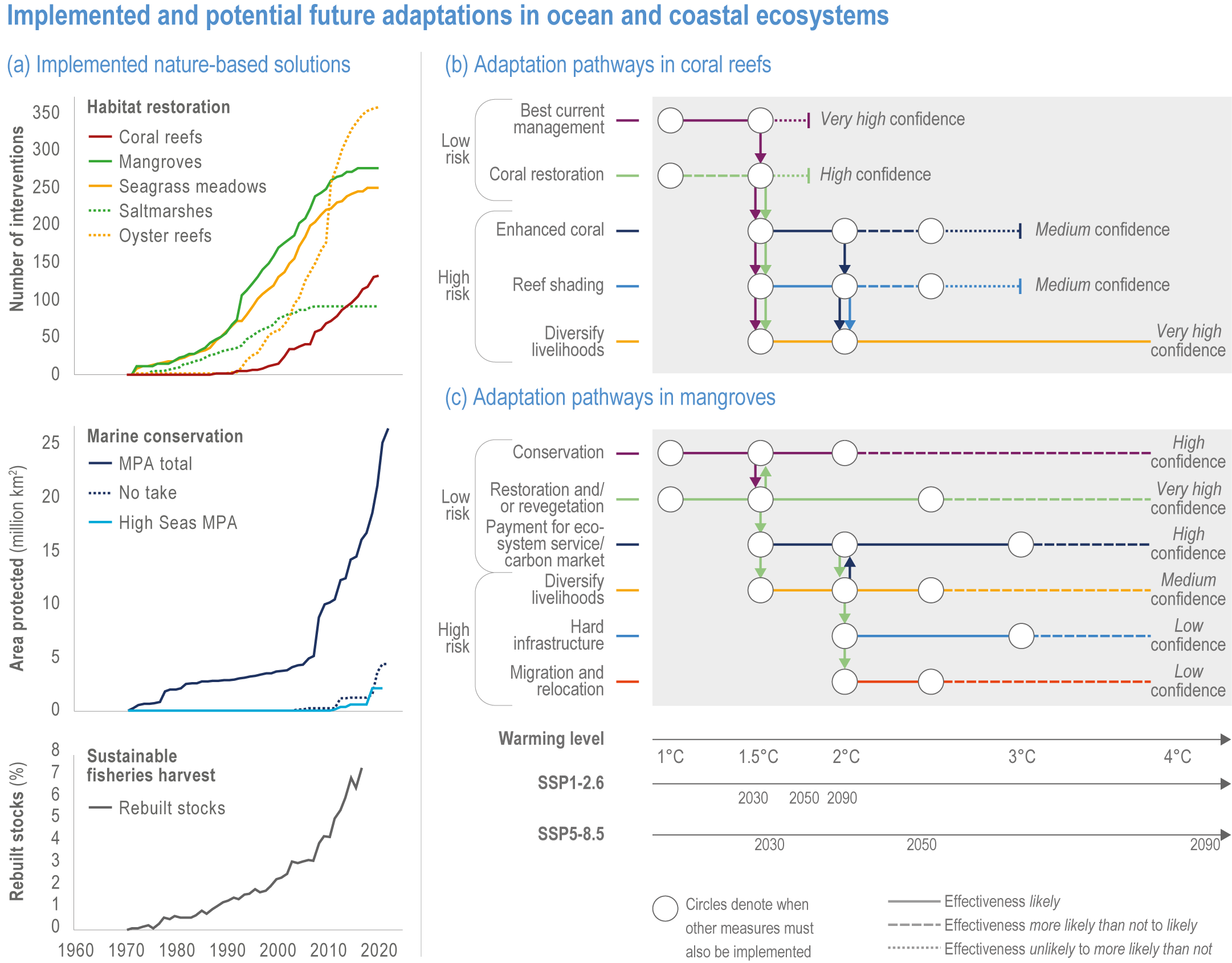
Figure 3.25 | Implemented and potential future adaptations in ocean and coastal ecosystems.
(a) Global implementation since 1970 of (top) cumulative habitat-restoration projects (Duarte et al., 2020), (middle) cumulative area-based conservation protected area (MPA total) (Boonzaier and Pauly, 2016), no-take areas (UN Environment World Conservation Monitoring Centre et al., 2018; UNEP-WCMC, 2019) and (bottom) percentage of total fish stocks rebuilt (Kleisner et al., 2013).
(b) Adaptation pathways for coral reefs to maintain healthy cover (line weight: solid lines, likely effectiveness; dashed lines, more likely than not to likely ; dotted lines =unlikely to more likely than not ), with confidence noted for each intervention (Section 3.4.2.1, 3.6.3.2; Anthony et al., 2019; National Academies of Sciences, 2019)
(c) As in (b), but for mangrove ecosystems. (Underlying data are available in Tables SM3.4–3.6.)
Transplanting heat-tolerant coral colonies can increase reef resistance to bleaching (Morikawa and Palumbi, 2019; Howells et al., 2021) but potentially lower species diversity and alter ecosystem function (Section 3.4.2.1). Genetic manipulation or assisted evolution that propagates genes from heat-tolerant populations could enhance restoration of corals (Anthony et al., 2017; Epstein et al., 2019) and kelp (medium agreement, limited evidence) (Coleman and Goold, 2019; Coleman et al., 2020b; Fredriksen et al., 2020; Wade et al., 2020). Managed breeding of corals has also had limited success in the laboratory and at small local scales (National Academies of Sciences, 2019). There is also limited evidence that physiological interventions, such as algal-symbiont or microbiome manipulation, could increase coral thermal tolerance in the field (National Academies of Sciences, 2019). Employing the natural adaptive capacity of species or individuals in active restoration for corals and kelps with current technology involves fewer risks than assisted evolution or long-distance relocation (high confidence) (Filbee-Dexter and Smajdor, 2019; National Academies of Sciences, 2019). More ambitious engineered interventions like reef shading remain theoretical and not scalable to the reef level (Condie et al., 2021). Debate continues on how to apply planned adaptation in cost-effective ways that will accomplish the intended goals (National Academies of Sciences, 2019; Duarte et al., 2020; Kleypas et al., 2021).
Models show that a combination of available management approaches (restoration, reducing non-climate drivers) and speculative interventions (e.g., enhanced corals, reef shading) can contribute to sustaining some coral reefs beyond 1.5°C of global warming with declining effectiveness beyond 2°C of global warming (medium confidence) (Figure 3.25; WGII Chapter 17). These proposed interventions are also currently theoretical and impractical over large scales; for example, engineered solutions like reef shading are untested and not scalable at the reef level (Condie et al., 2021). Existing projects suggest that restoration and ecological interventions to habitat-forming ecosystems have the additional benefits of raising local awareness, promoting tourism, and creating jobs and economic benefits (Fadli et al., 2012; Boström-Einarsson et al., 2020; Hafezi et al., 2021), provided communities are involved in planning, operation and monitoring (Boström-Einarsson et al., 2020).
3.6.3.3 Enablers, Barriers and Limitations of Adaptation and Mitigation
Not only is mitigation necessary to support ocean and coastal adaptation (Pörtner et al., 2014; Oppenheimer et al., 2019), but the global emission pathways also impose limits to ocean and coastal adaptation, with lower warming levels enabling greater effectiveness of adaptations (high confidence) (Figure 3.25). Chapter 17 broadly assesses the limits to adaptation, while this section focuses on barriers and limits to adaptation imposed by cultural (Section 3.6.3.3.1), economic (Section 3.6.3.3.2) and governance (Section 3.6.3.3.3) dimensions (Hinkel et al., 2018). Globally, these factors more strongly influence ocean development than does local natural resource availability (Cisneros-Montemayor et al., 2021), and are key to avoiding maladaptation. This section also assesses enablers and limits to mitigation (Section 3.6.3.3.4).
3.6.3.3.1 Sociocultural dimensions (culture, ethics, identity, behaviour)
Every coastal community values marine ecosystems for more than the material and intangible resources they deliver, or the physical protection they offer (Díaz et al., 2018). Cultural services that provide identity, spiritual and cultural continuity, religious meaning or options for the future (e.g., genetic or mineral resources) (Bindoff et al., 2019a) are not substitutable. Furthermore, interactions between climate impacts and existing inequalities can threaten the human rights of already-marginalised peoples by disrupting livelihoods and food security, which further erodes people’s social, economic and cultural rights (Finkbeiner et al., 2018). For instance, European colonisation and ongoing development blocked the Cucapá Indigenous People’s access and rights to resources in the Colorado River Delta, USA, over the 20th century. Recent reallocation of water rights and fishing access is allowing the Cucapá people to reconstruct their cultural identity (Sangha et al., 2019), but future climate-change impacts could reverse the community’s recovery of their cultural heritage. Adaptations that consider local needs may help sustain cultural services (Ortíz Liñán and Vázquez Solís, 2021).
Interactions with oceans are fundamental to the identities of many coastal Indigenous Peoples (Norman, 2017), and this influences Indigenous responses to climate hazards and adaptation. Around 30 million Indigenous Peoples live along coasts (Cisneros-Montemayor et al., 2016). Seafood consumption among Indigenous Peoples is much higher than for non-Indigenous populations, and marine species support many cultural, medicinal and traditional activities contributing to public health (Section 3.5.3.1; Kenny et al., 2018). Perpetuation of Indigenous cultures depends on protecting marine ecosystems and on adapting to changes in self-led ways (Section 3.5.6; Sangha et al., 2019) that promote self-determination (von der Porten et al., 2019). Indigenous resurgence, or reinvigorating Indigenous ways of life and traditional management, can include marine resource protection and ocean-sector development founded on culturally appropriate strategies and partnerships that are consistent with traditional norms and beneficial to local communities (von der Porten et al., 2019). Successful adaptation would simultaneously improve ecosystem health and address current and historical inequities (Bennett, 2018). Examples include practicing traditional resource management, protecting traditional territories, engaging with monitoring, collaborations with non-Indigenous partners and reinvesting benefits into capacity-building within communities (von der Porten et al., 2019; Equator Initiative, 2020). The legitimacy of different adaptation strategies depends on local and Indigenous Peoples’ acceptance, which is based on cultural values (Adger et al., 2017); financial gain cannot compensate for loss of IK or LK (Wilson et al., 2020b). Palau’s recent goal of shifting seafood consumption away from reef fishes (Remengesau Jr., 2019) as well as limiting and closely monitoring the expansion of ecotourism was prompted by the cultural importance of protecting these reefs and associated traditional fisheries for local consumption, a recognition of the importance of tourism and the hazard of climate change (Wabnitz et al., 2018a).
Adaptations implemented at the local level that consider IKLK systems are beneficial (high confidence) (Nalau et al., 2018; Sultana et al., 2019). Studies in SIDS and the Arctic have shown how IKLK facilitate the success of EbA (Nalau et al., 2018; Peñaherrera-Palma et al., 2018; Raymond-Yakoubian and Daniel, 2018), reinforce and improve institutional approaches and enhance the provision of ecosystem services (Ross et al., 2019; Terra Stori et al., 2019). Perspectives on adaptation also vary among groups of age, race, (dis)ability, class, caste and gender (Wilson et al., 2020b), so engaging different groups results in more robust and equitable adaptation to climate change (Cross-Chapter Box GENDER in Chapter 18; McLeod et al., 2018). Some coastal communities have developed substantial social capital and dense local networks based on trust and reciprocity (Petzold and Ratter, 2015), with individual and community flexibility to learn, adapt and organise themselves to help local adaptation governance (Silva et al., 2020). Recent evidence suggests that policies supporting local institutions can improve adaptation outcomes (medium confidence) (Berman et al., 2020). Coastal communities can be engaged using novel approaches to co-generate adaptation solutions (van der Voorn et al., 2017; Flood et al., 2018) that benefit education (Koenigstein et al., 2020) and engagement in adaptation processes (Rumore et al., 2016). Successful adaptation implementation in line with climate resilient development pathways (WGII Chapter 18) depends on bottom-up, participatory and inclusive processes (Section 3.6.1.2.1) that engage diverse stakeholders (Basel et al., 2020; McNamara et al., 2020; Ogier et al., 2020; Williams et al., 2020) and protect Indigenous customary rights (Farbotko and McMichael, 2019; Ford et al., 2020), empower women and give rights to climate refugees (McLeod et al., 2018).
3.6.3.3.2 Economic dimensions (planning, finance, costs)
Finance is a key barrier globally for ocean health, governance and adaptation to climate change (high agreement ) (Annex II: Glossary; Cross-Chapter Box FINANCE in Chapter 17; Hinkel et al., 2018; Miller et al., 2018; Wabnitz and Blasiak, 2019; Woodruff et al., 2020; Sumaila et al., 2021). Global adaptation finance was estimated to total 30 billion USD yr –1 in 2017–2018, or 5% of all climate finance (CPI, 2019), with no tracking specifically for coastal or marine adaptation in low- to middle-income countries. Marine-focused adaptation finance is difficult to trace and label due to the cross-sectoral nature of many projects (Blasiak and Wabnitz, 2018) and the lack of clear definitions about what qualifies as adaptation or as new and additional finance (Donner et al., 2016; Weikmans and Roberts, 2019). Finance for marine conservation from Overseas Development Assistance doubled between 2003 and 2016, reaching 634 million USD in 2016, similar to the level provided by philanthropic foundations (Berger et al., 2019). Yet coastal adaptation to SLR alone is projected to cost hundreds of billions of USD yr –1, depending on the model and emission scenario (e.g., Wong et al., 2014; Nicholls et al., 2019). Economic and financing barriers to marine adaptation are often higher in low- to middle-income countries, where resources influence governance and constrain options for implementation and maintenance (high confidence) (Hinkel et al., 2018; Klöck and Nunn, 2019; Tompkins et al., 2020), and impacts on their coastal and marine ecosystems could total several percentage points of their gross domestic product (Wong et al., 2014). Current financial flows are insufficient to meet the costs of coastal and marine impacts of climate change (very high confidence) and ocean-focused finance is unevenly distributed, with higher flows within, and to, developed countries (very high confidence).
Development assistance can help resolve resource constraints, but additional governance and coordination challenges can arise from short-term, project-based funding, shifting the priorities of donor institutions and the pressures placed on human resources in the receiving nation (Parsons and Nalau, 2019; Nunn et al., 2020). Innovative policy instruments, such as concessional loans, tax-policy reforms, climate bonds and public-debt forgiveness, can supplement traditional financial instruments (Bisaro and Hinkel, 2018; McGowan et al., 2020). Mechanisms for solving the persistent problem of securing upfront investments for coastal protection and other adaptation measures (Bisaro and Hinkel, 2018; Moser et al., 2019; Kok et al., 2021) include integrating adaptation investments into insurance schemes (Reguero et al., 2020) and using debt financing to bridge the time until benefits are realised (Ware and Banhalmi-Zakar, 2020). Insurance mechanisms that link payments to losses from a trigger event (e.g., MHW) can confer resilience to marine-dependent communities (Sumaila et al., 2021). All innovative financial instruments are most effective when they are inclusive and reach vulnerable groups and marginalised communities (low evidence, high agreement ) (Claudet et al., 2020a; Sumaila et al., 2021).
Countries with large ocean areas within their EEZs have opportunities to develop ‘blue–green economies’ to reduce emissions and finance adaptation pathways (Chen et al., 2018a; Lee et al., 2020). Shifting from grants to results-based financing can help attract more private capital to ocean adaptation (Lubchenco et al., 2016; Claudet et al., 2020a). Public–private partnerships can also increase ocean adaptation finance (Goldstein et al., 2019; Sumaila et al., 2021). For example, the financial benefits that biodiversity conservation confers to seafood harvest resilience could be used to leverage industry participation in adaptation and conservation finance (Barbier et al., 2018). Connecting restoration of blue carbon ecosystems with offset markets (e.g., Vanderklift et al., 2019) shows potential, but uncertainties remain about the international emissions trading under the UN Framework Convention on Climate Change and climate impacts on blue carbon ecosystems (Section 3.6.3.1.6; Lovelock et al., 2017a; Macreadie et al., 2019).
Transparency, coherence between different actors and initiatives, and project monitoring and evaluation enhance success in adapting and achieving SDG14 (Life Below Water) (Blasiak et al., 2019). Maladaptation (WGII Chapter 16; Magnan et al., 2016) is a common risk of current project-based funding due to the pressure to produce concrete results (medium confidence) (Parsons and Nalau, 2019; Nunn et al., 2020; Nunn et al., 2021). Maladaptation can be avoided through a focus on building adaptive capacity, community-based management, drivers of vulnerability and site-specific measures (low confidence) (Magnan and Duvat, 2018; Piggott-McKellar et al., 2020; Schipper, 2020). More research is needed to identify ways that governance and financing agreements can help overcome financial barriers and sociocultural constraints to avoid maladaptation in coastal ecosystems (high confidence) (Hinkel et al., 2018; Miller et al., 2018; Piggott-McKellar et al., 2020; Schipper, 2020).
3.6.3.3.3 Governance dimension (institutional settings, decision making)
Ocean governance has become increasingly complex as new initiatives, new international agreements, institutions and scientific evidence arise at global, national and subnational scales (high agreement ) (Bindoff et al., 2019a; Scobie, 2019b), limiting the present effectiveness of adaptation (IPCC, 2019c). Marine climate governance is within the normatively contested marine governance space (Frazão Santos et al., 2020), which is influenced by geopolitics (Gray et al., 2020) and profit maximisation (Flannery et al., 2016; Haas et al., 2021) in ways that can entrench exclusionary processes in decision making, science management and funding (Levin et al., 2018). This limits just and inclusive ocean governance (Bennett, 2018), perpetuates historical and cultural extractive practices and climate inaction, and leaves little space for Indigenous-led adaptation frameworks and approaches (Nursey-Bray et al., 2019). At the national level, ocean governance for climate-change adaptation is often transversal, requiring consideration of biophysical and environmental conditions (Furlan et al., 2020) while fitting into existing economic (Kim, 2020) and political processes. Adaptation governance that couples existing top-down structures with decentralised and participatory approaches generates shared goals and unlocks required resources and monitoring (Gupta et al., 2016; Haas et al., 2021).
Communities and governments at all levels increasingly use decision-making frameworks (e.g., structured decision making) or decision-analysis tools to evaluate trade-offs between different responses, rather than applying generic best practices to different physical, technical or cultural contexts (high confidence) (Watkiss et al., 2015; Haasnoot et al., 2019; Palutikof et al., 2019). Increased effort has also been devoted to developing climate services (actionable information and data products) that bridge the gap between climate prediction and decision making (Hewitt et al., 2020). Climate services have the potential to inform decision making related to disaster-risk reduction, adaptation responses, marine environmental management (e.g., fisheries management and MPA management) and ocean-based climate mitigation (e.g., renewable-energy installations) (Le Cozannet et al., 2017; Gattuso et al., 2019; Gattuso et al., 2021). Although improving observational and modelling capacity is important to developing ocean-focused services, particularly in high-risk regions like SIDS where regional climate projections are scarce (WGI AR6 Chapter 9; Morim et al., 2019; Fox-Kemper et al., 2021), data are not the only limiting factor in decision making (Weichselgartner and Arheimer, 2019). Focusing on user engagement, relationship building and the decision-making context ensures that climate services are useful to, and used by, different stakeholders (high confidence) (Soares et al., 2018; Mackenzie et al., 2019; Weichselgartner and Arheimer, 2019; Findlater et al., 2021; West et al., 2021).
3.6.3.3.4 Mitigation
Ocean and coastal NbS can contribute to global mitigation efforts, especially with ocean renewable energy and restoration and preservation of carbon ecosystems (see Box 3.4; Section 3.6.2.3). Technological, economic and financing barriers presently hamper development of renewable ocean energy (AR6 WGIII Chapter 6). Such development could help small nations reliant on imported fuel meet their climate-mitigation goals and decrease risk from global fuel-supply dynamics (Millar et al., 2017; Chen et al., 2018a), but progress is limited by lack of investment (Millar et al., 2017; Lee et al., 2020) or equipment (Aderinto and Li, 2018; Rusu and Onea, 2018). Wave-energy installations, possibly co-located with wind turbines (Perez-Collazo et al., 2018), are promising for both low- to middle-income nations and areas with significant island or remote coastal geographies (Lavidas and Venugopal, 2016; Bergillos et al., 2018; Jakimavičius et al., 2018; Kompor et al., 2018; Penalba et al., 2018; Saprykina and Kuznetsov, 2018; Lavidas, 2019). Wave-energy capture may also diminish storm-induced coastal erosion (Abanades et al., 2018; Bergillos et al., 2018). Tidal energy is a relatively new technology (Haslett et al., 2018; Liu et al., 2018; Neill et al., 2018) with limiting siting requirements (Mofor et al., 2013). Ocean renewable-energy expansion faces other technological obstacles including lack of implementable or scalable energy-capture devices, access to offshore sites, competing coastal uses, potential environmental impacts and lack of power-grid infrastructure at the coast (Aderinto and Li, 2018; Neill et al., 2018).
Cross-Chapter Box SLR | Sea Level Rise
Authors: Gonéri Le Cozannet (France, Chapter 13, CCP4), Judy Lawrence (New Zealand, Chapter 11), David S. Schoeman (Australia, Chapter 3), Ibidun Adelekan (Nigeria, Chapter 9), Sarah R. Cooley (USA, Chapter 3), Bruce Glavovic (New Zealand/South Africa, Chapter 18, CCP2), Marjolijn Haasnoot (The Netherlands, Chapter 13, CCP2), Rebecca Harris (Australia, Chapter 2), Wolfgang Kiessling (Germany, Chapter 3), Robert E. Kopp (USA, WGI), Aditi Mukherji (Nepal, Chapter 4), Patrick Nunn (Australia, Chapter 15), Dieter Piepenburg (Germany, Chapter 13), Daniela Schmidt (UK/Germany, Chapter 13), Craig T. Simmons (Australia), Chandni Singh (India, Chapter 10, CCP2), Aimée Slangen (The Netherlands, WGI), Seree Supratid (Thailand, Chapter 4).
Sea level rise is already impacting ecosystems, human livelihoods, infrastructure, food security and climate mitigation at the coast and beyond. Ultimately, it threatens the existence of cities and settlements in low-lying areas, and some island nations and their cultural heritage (Chapters 9–15; Cross-Chapter Papers 2, 4; Oppenheimer et al., 2019). The challenge can be addressed by mitigation of climate change and coastal adaptation.
Current impacts of sea level rise
The rate of global mean SLR was 1.35 mm yr –1 (0.78–1.92 mm yr –1, very likely range) during 1901–1990, faster than during any century in at least 3000 years (high confidence) (WGI AR6 Chapter 9; Stanley and Warne, 1994; Woodroffe et al., 2016; Fox-Kemper et al., 2021). Global mean SLR has accelerated to 3.25 mm yr –1 (2.88–3.61 mm yr –1, very likely range) during 1993–2018 (high confidence). Extreme sea levels have increased consistently across most regions (WGI AR6 Chapter 9; Fox-Kemper et al., 2021). The largest observed changes in coastal ecosystems are being caused by the concurrence of human activities, waves, current-induced sediment transport and extreme storm events (medium confidence) (Chapters 3, 15, 16; Takayabu et al., 2015; Mentaschi et al., 2018; Duvat, 2019; Murray et al., 2019; Oppenheimer et al., 2019). Early impacts of accelerating SLR detected at sheltered or subsiding coasts include chronic flooding at high tides, wetland salinisation and ecosystem transitions, increased erosion and coastal flood damage (Chapters 3, 11, 13–16; WGI AR6 Chapter 9; Sweet and Park, 2014; Moftakhari et al., 2015; Nunn et al., 2017; Oppenheimer et al., 2019; Sharples et al., 2020; Fox-Kemper et al., 2021; Strauss et al., 2021). The exposure of many coastal populations and ecosystems to SLR is high: economic development is disproportionately concentrated in and around coastal cities and settlements (virtually certain) (Chapters 3, 9–15; Cross-Chapter Papers 2, 4).
Projected risks to coastal communities, infrastructure and ecosystems
Risks from SLR are very likely to increase by one order of magnitude well before 2100 without adaptation and mitigation action as agreed by parties to the Paris Agreement (very high confidence). Global mean SLR is likely to continue accelerating under SSP1-2.6 and more strongly forced scenarios (Figure BoxSLR1; WGI AR6 Chapter 9; Oppenheimer et al., 2019; Fox-Kemper et al., 2021), increasing the risk of chronic coastal flooding at high tide, serious flooding during extreme events such as swells, storms and hurricanes, and erosion, and coastal ecosystem losses across many low-lying and erodible coasts (very high confidence) (Chapters 3, 9–15; Cross-Chapter Paper 2; Hinkel et al., 2014; McLachlan and Defeo, 2018; Kulp and Strauss, 2019; Vousdoukas et al., 2020b). The compounding of rainfall, river flooding, rising water tables, coastal surges and waves are projected to exacerbate SLR impacts on low-lying areas and rivers further inland (Chapters 4, 11–15; Bevacqua et al., 2020).
There is high confidence that coastal risks will increase by at least one order of magnitude over the 21st century due to committed SLR (Hinkel et al., 2013; Hinkel et al., 2014; IPCC, 2019b). Exposure of population and economic assets to coastal hazards is projected to increase over the next decades, particularly in coastal regions with fast-growing populations in Africa, Southeast Asia and Small Islands (medium evidence) (Chapters 9–15; Cross-Chapter Papers 2, 4; Neumann et al., 2015; Jones and O’Neill, 2016; Merkens et al., 2016; Merkens et al., 2018; Rasmussen et al., 2020). For RCP8.5, 2.5–9% of the global population and 12–20% of the global gross domestic product is projected to be exposed to coastal flooding by 2100 (Kulp and Strauss, 2019; Kirezci et al., 2020; Rohmer et al., 2021). Above 3°C global warming levels (GWL) and with low adaptation, SLR may cause disruptions to ports and coastal infrastructure (Camus et al., 2019; Christodoulou et al., 2019; Verschuur et al., 2020; Yesudian and Dawson, 2021), which in turn may cascade and amplify across sectors and regions, generating impacts to financial systems (Chapters 11, 13; Mandel et al., 2021). Depending on the hydrogeological context, SLR causes salinisation of groundwater, estuaries, wetlands and soils, adding constraints to water management and livelihoods in agriculture sectors, for example, in deltas (Chapters 9, 15; Cross-Chapter Paper 4; Oppenheimer et al., 2019; Nicholls et al., 2020).
Coastal ecosystems can migrate landward or grow vertically in response to SLR, but their resilience and capacity to keep up with SLR will be compromised by ocean warming and other drivers, depending on regions and species, for example, above 1.5°C for coral reefs (high confidence) (Chapters 3, 16; IPCC, 2018; Melbourne et al., 2018; Perry et al., 2018; IPCC, 2019b; Cornwall et al., 2021). Sediments and space for landward retreat are crucial for mangroves, salt marshes and beach ecosystems (high confidence) (Chapter 3; Peteet et al., 2018; Schuerch et al., 2018; FitzGerald and Hughes, 2019; Friess et al., 2019; Leo et al., 2019; Schuerch et al., 2019). Loss of habitat is accompanied by loss of associated ecosystem services, including wave-energy attenuation, habitat provision for biodiversity, food production and carbon storage (Chapter 3; Cross-Chapter Box NATURAL in Chapter 2).
Under a high-emissions, low-likelihood/high-impact scenario, where low confidence ice-sheet mass loss occurs, global mean SLR could exceed the likely range by more than one additional metre in 2100 (Figure BoxSLR1b; Cross-Chapter Box DEEP in Chapter 17; WGI AR6 Technical Summary and Chapter 9; Arias et al., 2021; Fox-Kemper et al., 2021). This is a reason for concern given that rapid SLR after the last glacial–interglacial transition caused a drowning of coral reefs (high confidence) (Camoin and Webster, 2015; Sanborn et al., 2017; Webster et al., 2018), extensive loss of coastal land and islands, habitats and associated biodiversity (high confidence) (AR6 WGI Chapter 9; Fruergaard et al., 2015; Fernández-Palacios et al., 2016; Hamilton et al., 2019; Helfensdorfer et al., 2019; Kane and Fletcher, 2020; Fox-Kemper et al., 2021), and triggered Neolithic migrations in Europe and Australia (medium confidence) (Cross-Chapter Box PALEO in Chapter 1; Turney and Brown, 2007; Brisset et al., 2018; Williams et al., 2018).
Cross-Chapter Box SLR
At centennial time scales, projected SLR represents an existential threat for island nations, low-lying coastal zones and the communities, infrastructure, and cultural heritage therein (Chapters 9–15; Cross-Chapter Paper 4). Even if climate warming is stabilised at 2°C to 2.5°C GWL, coastlines will continue to reshape over millennia, affecting at least 25 megacities and drowning low-lying areas where 0.6–1.3 billion people lived in 2010 (medium confidence) (WGI AR6 Chapter 9; Marzeion and Levermann, 2014; Clark et al., 2016; Kulp and Strauss, 2019; Fox-Kemper et al., 2021; Strauss et al., 2021).
Solutions, opportunities and limits to adaptation
The ability to adapt to current coastal impacts, to cope with future coastal risks and to prevent further acceleration of SLR beyond 2050 depends on immediate mitigation and adaptation actions (very high confidence). The most urgent adaptation challenge is chronic flooding at high tide (Chapters 10, 11, 13–15). Reducing the acceleration of SLR beyond 2050 will only be achieved with fast and profound mitigation of climate change (Nicholls et al., 2018; Oppenheimer et al., 2019). Until 2050, adaptation planning and implementation needs are projected to increase significantly in most inhabited coastal regions (see Figure BoxSLR1; WGI AR6 Chapter 9; IPCC, 2019b; Fox-Kemper et al., 2021). For SSP1-2.6 and more strongly forced scenarios, SLR rates continue to increase (WGI AR6 Chapter 9; Fox-Kemper et al., 2021), and so do the scale and frequency of adaptation interventions needed in coastal zones (Figure BoxSLR1; Haasnoot et al., 2020).
Risks can be anticipated, planned and decided upon, and adaptation interventions can be implemented over the coming decades considering their often long lead- and lifetimes, irrespective of the large uncertainty about SLR beyond 2050 (high confidence) (Figure BoxSLR1; Cross-Chapter Box DEEP in Chapter 17; Cross-Chapter Paper 2; Chapters 11, 13; Haasnoot et al., 2018; Stephens et al., 2018; Stammer et al., 2019). Adaptation capacity and governance to manage risks from projected SLR typically require decades to implement and institutionalise (high confidence) (Chapters 11, 13; Haasnoot et al., 2021). Without considering both short- and long-term adaptation needs, including beyond 2100, communities are increasingly confronted with a shrinking solution space, and adverse consequences are disproportionately borne by exposed and socially vulnerable people (Chapters 1, 8). Sea level rise is likely to compound social conflict in some settings (high confidence) (Oppenheimer et al., 2019).
Coastal impacts of SLR can be avoided by preventing new development in exposed coastal locations (Chapters 3, 9–15; Cross-Chapter Paper 2; Doberstein et al., 2019; Oppenheimer et al., 2019). For existing developments, a range of near-term adaptation options exists, including: (a) engineered, sediment- or ecosystem-based protection; (b) accommodation and land-use planning, to reduce the vulnerability of people and infrastructure; (c) advance through, for example, land reclamation; and (d) retreat through planned relocation or displacements and migrations due to SLR (Chapters 9–15; Cross-Chapter Paper 2; Oppenheimer et al., 2019). Only avoidance and relocation can remove coastal risks for the coming decades, while other measures only delay impacts for a time, have increasing residual risk or perpetuate risk and create ongoing legacy effects and virtually certain property and ecosystem losses (high confidence) (Cross-Chapter Paper 2; Siders et al., 2019). Large-scale relocation has immense cultural, political, social and economic costs, and equity implications, which can be reduced by fast implementation of climate mitigation and adaptation policies (Chapter 8; Cross-Chapter Paper 2; Gibbs, 2015; Haasnoot et al., 2021). While relocation may currently appear socially unacceptable, economically inefficient or technically infeasible today (Lincke and Hinkel, 2021), it becomes the only feasible option as protection costs become unaffordable and the limits to accommodation become obvious (Chapters 11, 13, 15; Hino et al., 2017; Siders et al., 2019; Strauss et al., 2021). Effective responses to rising sea level involve locally applicable combinations of decision analysis, land-use planning, public participation and conflict resolution approaches; together these can anticipate change and help to chart adaptation pathways, over time addressing the governance challenges due to rising sea level (high confidence) (Oppenheimer et al., 2019).
Ecosystem-based adaptation can reduce impacts on human settlements and bring substantial co-benefits, such as ecosystem services restoration and carbon storage, but they require space for sediment and ecosystems and have site-specific physical limits, at least above 1.5°C GWL (high confidence) (Cross-Chapter Box NATURAL in Chapter 2; Chapters 3, 9, 11, 15; Herbert et al., 2015; Brown et al., 2019; Van Coppenolle and Temmerman, 2019; Watanabe et al., 2019; Neijnens et al., 2021). For example, planting and conserving vegetation helps sediment accumulation by dissipating wave energy and reducing impacts of storms, at least at present-day sea levels (high confidence) (Temmerman et al., 2013; Narayan et al., 2016; Romañach et al., 2018; Laengner et al., 2019; Leo et al., 2019). Coastal wetlands and ecosystems can be preserved by landward migration (Schuerch et al., 2018; Schuerch et al., 2019) or sediment supply (VanZomeren et al., 2018), but they can be seriously damaged by coastal defences designed to protect infrastructure (Chapters 3, 13; Cooper et al., 2020b). Sediment nourishment can prevent erosion, but it can also negatively impact beach amenities and ecosystems through ongoing dredging, pumping and deposition of sand and silts (VanZomeren et al., 2018; de Schipper et al., 2021; Harris et al., 2021).
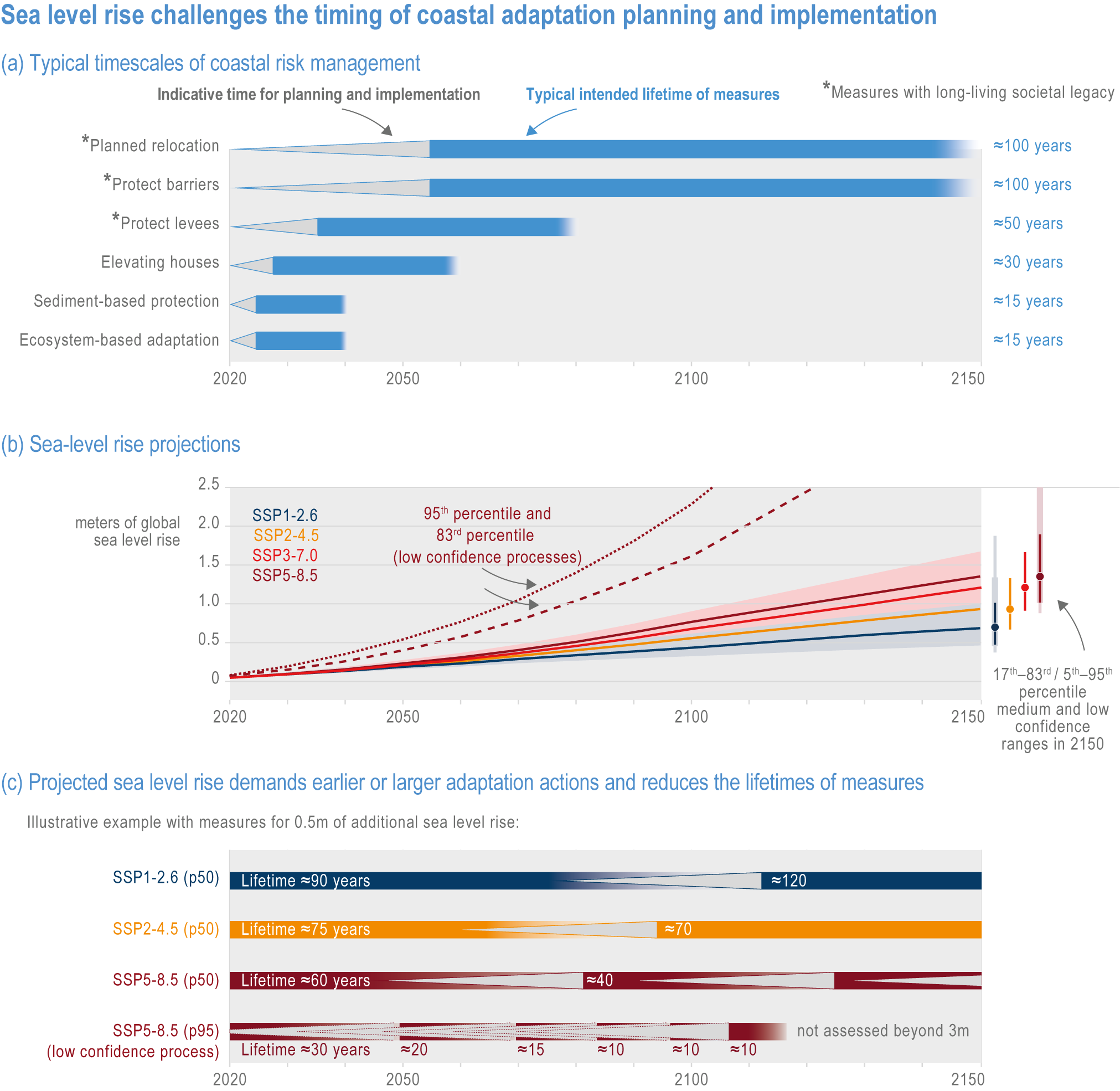
Figure Cross-Chapter BoxSLR.1 | The challenge of coastal adaptation in the era of sea level rise (SLR): (a) typical time scales for the planning, implementation (grey triangles) and operational lifetime of current coastal risk-management measures (blue bars); (b) global sea level projections, which are representative of relative SLR projected for 60–70% of global shorelines, within ±20% errors (WGI AR6 Chapter 9; Fox-Kemper et al. , 2021); (c) frequency of illustrative adaptation decisions to +0.5 m of SLR under different SSP-RCP scenarios. In response to accelerated SLR, adaptation either occurs earlier and faster, or accounts for higher amounts of SLR (e.g., to +1 m instead of to +0.5 m). Adaptation to +0.5 m from today’s sea levels have a lifetime of 90 years for SSP1-2.6, but lifetime is reduced to 60 years for SSP5-8.5 and 30 years for a high-end scenario involving low confidence processes. Adaptations to +0.5 m are comparable to, for example, the Thames Barrier in the United Kingdom or the Delta Works in the Netherlands, which primarily had an intended lifetime of 100–200 years. Adaptation measures to +0.2 m may include nourishment or wetland or setback zones.
There is increasing evidence that current governance and institutional arrangements are unable to address the escalating risks in low-lying coastal areas worldwide (high confidence). Barriers to adaptation, such as decision making driven by short-term thinking or vested interests, funding limitations and inadequate financial policies and insurance, can be addressed equitably and sustainably through implementation of suites of adaptation options and pathways (Chapters 11, 13, 17–18; Cross-Chapter Paper 2). Improved coastal adaptation governance can be supported by approaches that consider changing risks over time, such as ‘dynamic adaptation pathways’ planning (Chapters 11, 13, 18; Cross-Chapter Box DEEP in Chapter 17). Integrated coastal zone management and land-use and infrastructure planning are starting to consider SLR by, for example, monitoring early signals (Haasnoot et al., 2018; Stephens et al., 2018; Kool et al., 2020), updating sea level projections (Stephens et al., 2017; Hinkel et al., 2019; Kopp et al., 2019; Stammer et al., 2019), considering uncertainties of sea level projections and coastal impacts (e.g., Stephens et al., 2017; Jevrejeva et al., 2019; Rohmer et al., 2019), as well as engaging with communities, practitioners and scientists, recognising the values of current and future generations (e.g., Nicholls et al., 2014; Buchanan et al., 2016b). While there is high agreement that the majority of adaptation needs are not met yet, there is robust evidence of SLR increasingly being considered in coastal adaptation decision making and being embedded in national and local guidance and regulations (Nicholls et al., 2014; Le Cozannet et al., 2017; Lawrence et al., 2018; Kopp et al., 2019; McEvoy et al., 2021).
Cross-Chapter Box SLR
FAQ 3.5 | How can nature-based solutions, including marine protected areas, help us to adapt to climate-driven changes in the oceans?
Coastal habitats, such as mangroves or vegetated dunes, protect coastal communities from sea level rise and storm surges while supporting fisheries, sequestering carbon and providing other ecosystem services as well. Efforts to restore, conserve and/or recover these natural habitats help people confront the impacts of climate change. These marine nature-based solutions (NbS), such as Marine protected areas (MPAs), habitat restoration and sustainable fisheries, are cost-effective and provide myriad benefits to society.
In the oceans, NbS comprise attempts to recover, restore or conserve coastal and marine habitats to reduce the impacts of climate change on nature and society. Marine habitats, such as seagrasses and coral reefs, provide services like food and flood regulation in the same way as forests do on land. Coastal habitats, such as mangroves or vegetated dunes, protect coastal communities from sea level rise and storm surges while supporting fisheries as well as recreational and aesthetic services. Seagrasses, coral reefs and kelp forests also provide important benefits that help humans adapt to climate change, including sustainable fishing, recreation and shoreline protection services. By recognising these services and benefits of the ocean, NbS can improve the quality and integrity of the marine ecosystems.
Nature-based solutions offer a wide range of potential benefits, including protecting ecosystem services, supporting biodiversity and mitigating climate change. Coastal and marine examples include MPAs, habitat restoration, habitat development and maintaining sustainable fisheries. While local communities with limited resources might find NbS challenging to implement, they are generally ‘no-regret’ options, which bring societal and ecological benefits regardless of the level of climate change.
Carefully designed and placed MPAs, especially when they exclude fishing, can increase resilience to climate change by removing additional stressors on ecosystems. While MPAs do not prevent extreme events, such as marine heatwaves (FAQ3.2), they can provide marine plants and animals with a better chance to adapt to a changing climate. Current MPAs, however, are often too small, too poorly connected and too static to account for climate-induced shifts in the range of marine species. MPA networks that are large, connected, have adaptable boundaries and are designed following systematic analysis of future climate projections can better support climate resilience.
Habitat restoration and development in coastal systems can support biodiversity, protect communities from flooding and erosion, support the local economy and enhance the livelihoods and well-being of coastal peoples. Restoration of mangroves, salt marshes and seagrass meadows provide effective ways to remove carbon dioxide from the atmosphere and at the same time protect coasts from the impacts of storms and SLR. Active restoration techniques that target heat-resistant individuals or species are increasingly recommended for coral reefs and kelp forests, which are highly vulnerable to marine heatwaves and climate change.
Sustainable fishing is also seen as an NbS because managing marine commercial species within sustainable limits maximises the catch and food production, thus contributing to the UN’s Sustainable Development Goal 2 (Zero Hunger). Currently, the oceans provide 17% of the animal protein eaten by the global population, but the contribution could be larger if fisheries were managed sustainably. Aquaculture, such as oyster farming, can be an efficient and sustainable means of food production and also provide additional benefits like shoreline protection. Through NbS that conserve and restore marine habitats and species, we can sustain marine biodiversity, respond to climate change and provide benefits to society.
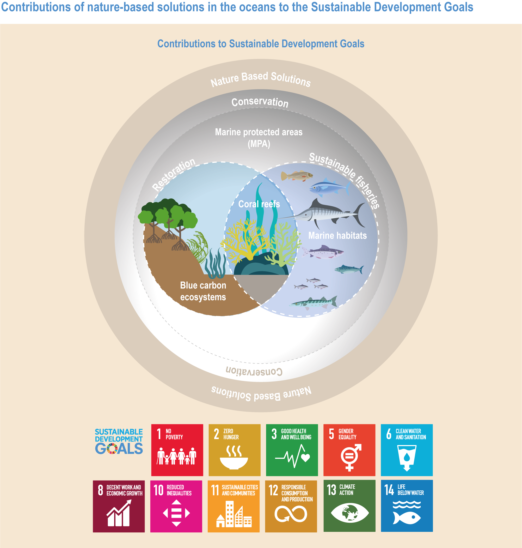
Figure FAQ3.5.1 | Contributions of nature-based solutions (NbS) in the oceans to the Sustainable Development Goals. The icons at the bottom show the Sustainable Development Goals to which NbS in the ocean possibly contribute.
3.6.4 Contribution to the Sustainable Development Goals and Other Relevant Policy Frameworks
The impacts of climate change on ocean and coastal ecosystems and their services threaten achievement of the UN SDGs by 2030 (high confidence), particularly ocean targets (Table 3.31; Nilsson et al., 2016; Pecl et al., 2017; IPCC, 2018; Singh et al., 2019a; Claudet et al., 2020a). Nevertheless, local to international decision-making bodies have assigned the lowest priority to SDG14, Life Below Water (Nash et al., 2020).
3.6.4.1 Climate Mitigation Effects on Ocean-Related SDGs
SROCC underscored the need for ambitious mitigation to control climate hazards in the ocean to achieve SDGs (medium evidence, high agreement ) (Bindoff et al., 2019a; Oppenheimer et al., 2019). Delays in achieving ocean-dependent SDGs observed in SROCC and SR15 can be addressed with ambitious planned adaptation and mitigation action (high agreement ) (Hoegh-Guldberg et al., 2019b). Since the ocean can contribute substantially to the attainment of mitigation targets aiming to limit warming to 1.5°C above pre-industrial levels (Hoegh-Guldberg et al., 2019b), and to adaptation solutions facilitating attainment of social and economic SDGs, climate policy is treating the ocean less as a victim of climate change and more as a central participant in solving the global climate challenge (Cooley et al., 2019; Hoegh-Guldberg et al., 2019a; Dundas et al., 2020).
Relationships between Climate Action (SDG13) targets and SDG14 targets are mostly synergistic (Figure 3.26; Fuso Nerini et al., 2019). Responding to climate-change impacts requires transformative governance (high confidence) (Chapters 1, 18; Collins et al., 2019a; Brodie Rudolph et al., 2020; Claudet et al., 2020a), especially for extreme events and higher-impact scenarios (e.g., higher emissions) (Fedele et al., 2019), and for achieving SDGs through one of the global ecosystems transitions (Chapter 18; Sachs et al., 2019; Brodie Rudolph et al., 2020). Opportunities to transform ocean governance exist in developing new international and local agreements, regulations and policies that reduce the risks of relocating ocean and coastal activities (Section 3.6.3.1.1) or in reinventing established practices (Section 3.6.3.3.3). Policy transformations improving ocean sustainability under SDG14 also help address SDG13 (Brodie Rudolph et al., 2020; Dundas et al., 2020; Claudet, 2021; Sumaila et al., 2021). Emergent situations, such as the COVID-19 pandemic, may provide opportunities to implement transformative ‘green recovery plans’ that support achievement of the SDGs and NDCs (Cross-Chapter Box COVID in Chapter 7).

Figure 3.26 | Synergies and trade-offs between SDG13 Climate Action, SDG14 Life Below Water and social, economic and governance SDGs. Achieving SDG13 provides positive outcomes and supports the achievement of all SDG14 targets. In turn, meeting SDG14 drives mostly positive interactions with social, economic and governance SDGs. The interaction types, ‘Indivisible’ (inextricably linked to the achievement of another goal), ‘Reinforcing’ (aids the achievement of another goal), ‘Enabling’ (creates conditions that further another goal), ‘Consistent’ (no significant positive or negative interactions) and ‘Constraining’ (limits options on another goal), follow Nilsson et al.’s (2016) scoring system based on the authors’ assessment, and agreement denotes consistency across author ratings. (Full data are available in Table 3.SM.7.)
3.6.4.2 Contribution of Ocean Adaptation to SDGs
Marine-focused adaptations show promise in helping achieve social SDGs, especially when they are designed to achieve multiple benefits (medium confidence) (Figure 3.26; Ntona and Morgera, 2018; Claudet et al., 2020a). Technology- and infrastructure-focused adaptations (Section 3.6.2.2) can help relieve coastal communities from risks associated with poverty (SDG1), hunger (SDG2), health and water sanitation (SDG3 and SDG6), and inequality (SDG10) by supporting aquaculture (Sections 3.5.3, 3.6.3.1), alerting the public about poor water quality (Sections 3.5.5.3, 3.6.3.1) and empowering marginalised groups, such as women and Indigenous Peoples, with decision-relevant information (medium evidence, high agreement ) (Sections 3.5.5.3, 3.6.3.1). Effectively implemented and managed marine NbS (Section 3.6.2.3) contribute to attainment of social SDGs by: (a) preserving biodiversity (Carlton and Fowler, 2018; Warner, 2018; Scheffers and Pecl, 2019), which benefits most ocean and coastal ecosystem services (Section 3.5.3; Figure 3.22); (b) increasing marine fishery and aquaculture sustainability (Section 3.6.3); (c) including vulnerable people and communities in management (Section 3.6.3.2.1); (d) lowering risk of flooding from storms and SLR (Cross-Chapter Box SLR in Chapter 3; Sections 3.6.3.1.1); and (e) implementing spatial-management tools that make room for new uses like renewable-energy development (Section 3.6.3.3.4). Nature-based solutions can therefore help support achievement of No Poverty (SDG1) (Ntona and Morgera, 2018), Zero Hunger (SDG2), Good Health and Well-Being (SDG3) (Duarte et al., 2020), Affordable and Clean Energy (SDG7) (Fuso Nerini et al., 2019; Levin et al., 2020) and Reduced Inequality (SDG10). Socio-institutional marine adaptations (Section 3.6.2.2) that support current livelihoods and help develop alternatives can contribute to attainment of social SDGs by enhancing social equity and supporting societal transformation (medium confidence) (Cisneros-Montemayor et al., 2019; Pelling and Garschagen, 2019; Nash et al., 2021). Even societal changes that are not directly marine related can decrease human vulnerability to ocean and coastal climate risks by improving overall human adaptive capacity (Section 1.2).
Marine adaptation also shows promise for helping support achievement of economic SDGs (medium confidence) (Figure 3.26). Marine NbS could help blue-economy frameworks achieve Decent Work and Economic Growth (SDG8) (Lee et al., 2020) by sustainably and equitably incorporating ecosystem-based fisheries management, restoration or conservation (Sections 3.6.3.1.2, 3.6.3.2.1, 3.6.3.2.2; Voyer et al., 2018; Cisneros-Montemayor et al., 2019; Cohen et al., 2019; Okafor-Yarwood et al., 2020). Nature-based solutions that involve active restoration or accommodation can contribute to Sustainable Cities and Communities (SDG11) and Infrastructure (SDG9) (Section 3.6.3.1.1). Newly developed marine industries and livelihoods associated with NbS might support attainment of Sustainable Communities (SDG11) (Cisneros-Montemayor et al., 2019). Finance and market mechanisms to support disaster relief or ocean ecosystem services, such as blue carbon or food provisioning, and innovations (SDG9) including new technologies like vessel-monitoring systems (Kroodsma et al., 2018), can contribute to Responsible Consumption and Production (SDG12) (Sumaila and Tai, 2020). Blue-economy growth that includes sustainable shipping, tourism, renewable ocean energy and transboundary fisheries management (Pinsky et al., 2018) have the potential to contribute to Economic Development (SDG8), affordable and clean energy (SDG7) as well as global mitigation efforts (SDG13) (Hoegh-Guldberg et al., 2019b; Duarte et al., 2020). Participatory approaches and co-management systems (Section 3.6.2.1) in many maritime sectors can contribute to SDG11 and SDG12 while helping align the blue economy and the SDGs (high agreement ) (Lee et al., 2020; Okafor-Yarwood et al., 2020).
Developing marine adaptation pathways that offer multiple benefits requires transformational adaptation (high confidence) (Claudet et al., 2020a; Friedman et al., 2020; Wilson et al., 2020b; Nash et al., 2021) that avoids risky and maladaptive actions (Magnan and Duvat, 2018; Ojea et al., 2020). Ocean and coastal extreme events and other hazards disproportionately harm the most vulnerable communities in SIDS, tropical and Arctic regions, and Indigenous Peoples (Chapter 8.2.1.2). Presently implemented adaptation activity, at the aggregate level, adversely affects multiple gender targets under SDG5 (high confidence) (Cross-Chapter Box GENDER in Chapter 18). Although women make up over half of the global seafood production workforce (fishing and processing sectors), provide more than half the artisanal landings in the Pacific region (Harper et al., 2013), dominate some seafood sectors such as seaweed (Howard and Pecl, 2019) and shellfish harvesting (Turner et al., 2020a) and account for 11% of global artisanal fisheries participants (Harper et al., 2020b), they are often not specifically counted in datasets and excluded from decision making and support programmes (Cross-Chapter Box GENDER in Chapter 18; Harper et al., 2020b; Michalena et al., 2020). Targeted efforts to incorporate knowledge diversity, and include artisanal fishers, women and Indigenous Peoples within international, regional and local policy planning, promote marine adaptation that supports achievement of gender equality (SDG5) and reduces inequalities (SDG10) (limited evidence, high agreement ) (FAO, 2015). Integrated planning, financing and implementation can help overcome these limitations (Section 3.6.3.3.2; Cross-Chapter Box FINANCE in Chapter 17), ensuring that marine adaptations do not compromise overall human equity or specific SDGs (Österblom et al., 2020; Nash et al., 2021), but are in fact fully synergistic with these goals (Bennett et al., 2021).
3.6.4.3 Relevant Policy Frameworks for Ocean Adaptation
The intricacy, scope, time scales and uncertainties associated with climate change challenge ocean governance, which already is extremely complex because it encompasses a variety of overlapping spatial scales, concerns and governance structures (see Figure CB3.1 in SROCC Chapter 1; Prakash et al., 2019). Assessment of how established global agreements and regional, sectoral or scientific bodies address climate adaptation and resilience, and how current practices can be improved, is found in SM3.5.3.
There is growing momentum to include the ocean in international climate policy (robust evidence), paving the way for a more integrated approach to both mitigation and adaptation. Following adoption of the Paris Agreement in 2015, the UN SDGs (Table 3.31) came into force in 2016, including SDG14 specifically dedicated to Life Below Water (Table 3.31). In 2017, the first UN Ocean Conference was held (United Nations, 2017), the UNFCCC adopted the Ocean Pathway to increase ocean-targeted multilateral climate action (COP23, 2017) and the UN Assembly declared 2021–2030 the Decade for Ocean Science for Sustainable Development (Visbeck, 2018; Lee et al., 2020). Next, 14 world leaders formed the High-Level Panel for a Sustainable Ocean Economy to produce the New Ocean Action Agenda, founded on 100% sustainable management of national ocean spaces by 2025 (Ocean Panel, 2020). All of these initiatives position oceans centrally within the climate-policy and biodiversity-conservation landscapes and seek to develop a coherent effort and common frameworks to achieve marine sustainability (Visbeck, 2018; Lee et al., 2020), new economic opportunities (Konar and Ding, 2020; Lee et al., 2020), more equitable outcomes (Österblom et al., 2020) and decisive climate mitigation and adaptation (Hoegh-Guldberg et al., 2019a), to achieve truly transformative change (Claudet et al., 2020a).
Table 3.31 | Sustainable Development Goals, grouped into broader categories as discussed in this section a
Category | Goal |
Society | SDG1: No Poverty SDG2: Zero Hunger SDG3: Good Health and Well-Being SDG4: Quality Education SDG5: Gender Equality SDG6: Clean Water and Sanitation SDG7: Affordable and Clean Energy |
Economy | SDG8: Decent Work and Economic Growth SDG9: Industry, Innovation and Infrastructure SDG10: Reduced Inequality SDG11: Sustainable Cities and Communities SDG12: Responsible Consumption and Production |
Environment | SDG13: Climate Action SDG14: Life Below Water SDG15: Life on Land |
Governance | SDG16: Peace and Justice Strong Institutions SDG17: Partnerships to Achieve the Goals |
(a) See http://sdgs.un.org/goals
There is high confidence in the literature that multilateral environmental agreements need better alignment and integration to support achievement of ambitious international development, climate mitigation and adaptation goals (Swilling et al., 202; Duarte et al., 2020; Friedman et al., 2020; Conservation International and IUCN, 2021; Pörtner et al., 2021b; Sumaila et al., 2021). The ocean targets of the CBD (e.g., the Post-2020 Global Biodiversity Framework), the SDGs (Agenda 2030) and the Paris Agreement are already inclusive and synergistic (Duarte et al., 2020). However, specific policy instruments and sectors within them could be additionally integrated, especially to address such cross-cutting impacts as ocean acidification and deoxygenation (Gallo et al., 2017; Bindoff et al., 2019a), increasing plastic pollution (Ostle et al., 2019; Duarte et al., 2020), high-seas governance (Johnson et al., 2019; Leary, 2019) or deep-sea uses (Wright et al., 2019; Levin et al., 2020; Orejas et al., 2020). National adaptation plans present opportunities to synergistically build on mitigation to support equitable development (Morioka et al., 2020), economic planning (Dundas et al., 2020; Lee et al., 2020) and ocean stewardship (von Schuckmann et al., 2020). Alignment of multilateral agreements is expected to increase mitigation impact as well as increase adaptation options (Section 3.6.3; Figure 3.25; Roberts et al., 2020). Opportunities to improve multilateral environmental agreements and policies beyond UNFCCC and CBD processes are discussed in SM3.5.3, and an assessment of commercial species-management initiatives and needs is in Chapter 5.
3.6.5 Emerging Best Practices for Ocean and Coastal Climate Adaptation
There is robust evidence that a combination of global and local solutions offers the greatest benefit in reducing climate risk (Gattuso et al., 2018; Hoegh-Guldberg et al., 2019a; Hoegh-Guldberg et al., 2019b). Ambitious and swift global mitigation offers more adaptation options and pathways to sustain ecosystems and their services (Figure 3.25). Some solutions target both mitigation and adaptation (e.g., blue carbon conservation; Cross-Chapter Box NATURAL in Chapter 2; see Box 3.4), and cross-cutting solutions simultaneously support several ocean-related sectors (e.g., area-based measures support fishing, tourism; Section 3.6.3.2.1) or ecosystem functions (e.g., NbS support coastal protection, biodiversity, habitat, etc.; Section 3.6.3.2.2; Sala et al., 2021). Combined solutions also leverage a variety of existing policies and governance systems (Section 3.6.4.3; Duarte et al., 2020) to advance climate mitigation and adaptation. Even communities that face the limits of adaptation, like those who must relocate to cope with rising seas (McMichael et al., 2019; Bronen et al., 2020), urgently require solutions that combine scientific projections, IKLK, cultural and community values, and ways to preserve cultural identity to support planning and implementation of relocation (McMichael and Katonivualiku, 2020).
Nature-based solutions are showing promising results in achieving adaptation and mitigation outcomes across marine and coastal ecosystems (Sections 3.6.3.2.1–3.6.3.2.2), but NbS have different degrees of readiness in marine ecosystems (Duarte et al., 2020). Habitat restoration and recovery are highly effective in specific settings and conditions (McLeod et al., 2019). Restoring and conserving vegetated coastal habitats (Sections 3.4.2.4–3.4.2.5) represent robust NbS, especially in the tropics, and particularly when paired with restoration and conservation of terrestrial ecosystems (robust evidence) (e.g., peatlands and forests; WGIII AR6 Chapter 7; Hoegh-Guldberg et al., 2019b; Duarte et al., 2020; Griscom et al., 2020). Although most of the focus on NbS efficacy has been on coastal and shelf ecosystems (Section 3.6.3.2), recent advances point to an emerging role of NbS beyond coastal waters in the form of area-based management tools in marine areas beyond national jurisdiction (Section 3.6.2.3; Gaines et al., 2018; Pinsky et al., 2018; Crespo et al., 2020; O’Leary et al., 2020; Visalli et al., 2020; Wagner et al., 2020), because sustainable fisheries and aquaculture and climate-responsive MPAs have high potential to adapt (Tittensor et al., 2019).
Adaptation efforts (Sections 3.6.3.1–3.6.3.2) have three common characteristics that facilitate implementation and success, and contribute to climate resilient development pathways (Chapter 18). First, availability of multiple types of information (e.g., monitoring, models, climate services; Section 3.6.3.3) exposes the magnitude and nature of the adaptation challenge. Well-developed observation and modelling capabilities (Reusch et al., 2018) offer insights on climate-associated risks at different time scales (Cvitanovic et al., 2018; Hobday et al., 2018), and this facilitates adaptation within multiple areas (e.g., industries over shorter time scales, societies over longer scales) (Hobday et al., 2018). Environmental data have supported building societal and political (socio-institutional) will to adopt national and subnational adaptive management principles (Hobday et al., 2016b; Champion et al., 2018; McDonald et al., 2019). However, incorporating IKLK at the same time provides more diverse social–environmental insight (Section 3.6.3.4.1; Goeldner-Gianella et al., 2019; Petzold and Magnan, 2019; Wilson et al., 2020b). This can help align adaptation solutions with cultural values and increase their legitimacy with Indigenous and local communities (Chapter 1.3.2.3), achieving climate resilient development pathways (Chapter 18; Adger et al., 2017; Nalau et al., 2018; Peñaherrera-Palma et al., 2018; Raymond-Yakoubian and Daniel, 2018; Wamsler and Brink, 2018). Second, implementation of multiple low-risk options (Hoegh-Guldberg et al., 2019a; Gattuso et al., 2021) such as economic diversification (Section 3.6.2.1) can provide culturally acceptable livelihood alternatives and food supplies (e.g., fishing to ecotourism and mariculture) (Froehlich et al., 2019) while also providing environmental benefits (e.g., seaweed mariculture’s potential carbon storage co-benefits) (WGIII AR6 Chapter 7; Hoegh-Guldberg et al., 2019a; Gattuso et al., 2021). Third, inclusive governance that is well aligned to the systems at risk from climate change is fundamental for effective adaptation (Barange et al., 2018). Solutions implemented within polycentric governance systems (Section 3.6.3; Bellanger et al., 2020) benefit from synergies between knowledge, action and social–ecological contexts and stimulate governance responses at appropriate spatio-temporal scales (Cvitanovic and Hobday, 2018). Governance aligned with Indigenous structures and local structures supports successful outcomes that prioritise the concerns and rights of involved communities (Section 3.6.3; Mawyer and Jacka, 2018) and better leverages existing social organisation (i.e., network structures), learning processes and power dynamics (Barnes et al., 2020).
There is an opportunity to improve current practices when developing new ocean and coastal adaptation efforts so that they routinely contain these successful characteristics and resolve technical, economic, institutional, geophysical, ecological and social constraints (Figure 3.25; Section 3.6.3.3; IPCC, 2018; Singh et al., 2020). Enhancements are needed in human, technical and financial resources; regulatory frameworks (Ojwang et al., 2017); political support (Rosendo et al., 2018); institutional conditions and resources for fair governance (Gupta et al., 2016; Scobie, 2018); political leadership; stakeholder engagement; multidisciplinary data availability (Gopalakrishnan et al., 2018); funding and public support for adaptation (Cross-Chapter Box FINANCE in Chapter 17; Ford and King, 2015); and incorporating IKLK in decision making (Nalau et al., 2018; Jabali et al., 2020; Petzold et al., 2020). As climate change continues to challenge ocean and coastal regions, there is high confidence associated with the benefits of developing robust, equitable adaptation strategies that incorporate scientific projections, employ portfolios of low-risk options, internalise IKLK and address social aspects of governance from international to local scales (Finkbeiner et al., 2018; Gattuso et al., 2018; Miller et al., 2018; Raymond-Yakoubian and Daniel, 2018; Cheung et al., 2019; Gattuso et al., 2021).
Acknowledgements
We acknowledge the kind contributions of Rita Erven (GEOMAR Helmholtz Centre for Ocean Research Kiel, Germany), Miriam Seifert (Alfred Wegener Institute for Polar and Marine Research, Germany), Sebastian Rokitta (Alfred Wegener Institute for Polar and Marine Research, Germany), Amy Marie Campbell (National Oceanography Centre, Southampton/Centre for Environment, Fisheries and Aquaculture Science, UK), Mariana Castaneda-Guzman (Virginia Polytechnic Institute and State University, USA), Stephen Goult (Plymouth Marine Laboratory/National Centre for Earth Observation, UK), Josh Douglas (Plymouth Marine Laboratory, UK), Carl Reddin (Museum für Naturkunde, Berlin, Germany) and the PML Communications and Graphics Team (Plymouth Marine Laboratory, UK) who assisted in drafting figures and tables.
References
Aalto, E.A., et al., 2019: Catastrophic mortality, allee effects, and marine protected areas. Am. Nat. , 193 (3), 391–408, doi:10.1086/701781.
Aarflot, J.M., H.R. Skjoldal, P. Dalpadado and M. Skern-Mauritzen, 2018: Contribution of Calanus species to the mesozooplankton biomass in the Barents Sea. ICES J. Mar. Sci. , 75 (7), 2342–2354, doi:10.1093/icesjms/fsx221.
Abanades, J., G. Flor-Blanco, G. Flor and G. Iglesias, 2018: Dual wave farms for energy production and coastal protection. Ocean Coast. Manag. , 160, 18–29, doi:10.1016/j.ocecoaman.2018.03.038.
Abella Perez, E., A. Marco, S. Martins and L.A. Hawkes, 2016: Is this what a climate change-resilient population of marine turtles looks like?Biol. Conserv. , 193, 124–132, doi:10.1016/j.biocon.2015.11.023.
Abelson, A., et al., 2015: Upgrading marine ecosystem restoration using ecological–social concepts. BioScience, 66 (2), 156–163, doi:10.1093/biosci/biv171.
Ablain, M., et al., 2019: Uncertainty in satellite estimates of global mean sea-level changes, trend and acceleration. Earth Syst. Sci. Data, 11 (3), 1189–1202, doi:10.5194/essd-11-1189-2019.
Abrahams, A., R.W. Schlegel and A.J. Smit, 2021: Variation and change of upwelling dynamics detected in the world’s eastern boundary upwelling systems. Front. Mar. Sci. , 8, 626411, doi:10.3389/fmars.2021.626411.
Abram, N., et al., 2019: Framing and Context of the Report. In: IPCC Special Report on the Ocean and Cryosphere in a Changing Climate. [Pörtner, H.-O., D. C. Roberts, V. Masson-Delmotte, P. Zhai, M. Tignor, E. S. Poloczanska, K. Mintenbeck, M. Nicolai, A. Okem, J. Petzold, B. Rama and N. Weyer (eds.)](pp. In press).
Aderinto, T. and H. Li, 2018: Ocean wave energy converters: status and challenges. Energies, 11 (5), 1250, doi:10.3390/en11051250.
Adger, W.N., C. Butler and K. Walker-Springett, 2017: Moral reasoning in adaptation to climate change. Environ. Polit. , 26 (3), 371–390, doi:10.1080/09644016.2017.1287624.
Agostini, S., et al., 2018: Ocean acidification drives community shifts towards simplified non-calcified habitats in a subtropical-temperate transition zone. Sci. Rep. , 8 (1), 11354, doi:10.1038/s41598-018-29251-7.
Aguirre, C., M. Rojas, R.D. Garreaud and D.A. Rahn, 2019: Role of synoptic activity on projected changes in upwelling-favourable winds at the ocean’s eastern boundaries. NPJ Clim. Atmos. Sci. , 2 (1), 44, doi:10.1038/s41612-019-0101-9.
Aguzzi, J., et al., 2019: New high-tech flexible networks for the monitoring of deep-sea ecosystems. Environ. Sci. Technol. , 53 (12), 6616–6631, doi:10.1021/acs.est.9b00409.
Ajani, P.A., C.H. Davies, R.S. Eriksen and A.J. Richardson, 2020: Global warming impacts micro-phytoplankton at a long-term Pacific ocean coastal station. Front. Mar. Sci. , 7 (878), doi:10.3389/fmars.2020.576011.
Al-Haj, A.N. and R.W. Fulweiler, 2020: A synthesis of methane emissions from shallow vegetated coastal ecosystems. Glob. Change Biol. , 26 (5), 2988–3005, doi:10.1111/gcb.15046.
Al-Said, T., et al., 2018: High total organic carbon in surface waters of the northern Arabian Gulf: implications for the oxygen minimum zone of the Arabian Sea. Mar. Pollut. Bull. , 129 (1), 35–42, doi:10.1016/j.marpolbul.2018.02.013.
Alabia, I.D., et al., 2021: Marine biodiversity refugia in a climate-sensitive subarctic shelf. Glob. Change Biol. , 27 (14), 3299–3311, doi:10.1111/gcb.15632.
Alabia, I.D., et al., 2020: Multiple facets of marine biodiversity in the Pacific Arctic under future climate. Sci. Total Environ. , 744, 140913, doi:10.1016/j.scitotenv.2020.140913.
Alamsjah, M. A., A.A. Abdillah, H. Mustikawati and S.D.P. Atari (eds.), 2017: Screening of biodiesel production from waste tuna oil (Thunnus sp.), seaweed Kappaphycus alvarezii and Gracilaria sp. AIP Conference Proceedings. 6th International Conference and Workshops on Basic and Applied Sciences, 1888, 020009.
Albano, P.G., et al., 2021: Native biodiversity collapse in the eastern Mediterranean. Proc. R. Soc. B. , 288 (1942), 20202469, doi:10.1098/rspb.2020.2469.
Albouy, C., et al., 2020: Global vulnerability of marine mammals to global warming. Sci. Rep. , 10 (1), 548, doi:10.1038/s41598-019-57280-3.
Albouy, C., et al., 2013: Projected climate change and the changing biogeography of coastal Mediterranean fishes. J. Biogeogr. , 40 (3), 534–547, doi:10.1111/jbi.12013.
Alheit, J., et al., 2019: What happened in the mid-1990s? The coupled ocean-atmosphere processes behind climate-induced ecosystem changes in the Northeast Atlantic and the Mediterranean. Deep. Res. Part II Top. Stud. Oceanogr. , 159, 130–142, doi:10.1016/j.dsr2.2018.11.011.
Allen, M.D., 2020: Climate change in Alaska: social workers’ attitudes, beliefs, and experiences. Int. J. Soc. Welf. , 29 (4), 310–320, doi:10.1111/ijsw.12443.
Alleway, H.K., et al., 2018: The ecosystem services of marine aquaculture: valuing benefits to people and nature. BioScience, 69 (1), 59–68, doi:10.1093/biosci/biy137.
Allyn, A.J., et al., 2020: Comparing and synthesizing quantitative distribution models and qualitative vulnerability assessments to project marine species distributions under climate change. PLoS ONE, 15 (4), e231595, doi:10.1371/journal.pone.0231595.
Almpanidou, V., E. Katragkou and A.D. Mazaris, 2018: The efficiency of phenological shifts as an adaptive response against climate change: a case study of loggerhead sea turtles (Caretta caretta) in the Mediterranean. Mitig. Adapt. Strateg. Glob. Change, 23 (7), 1143–1158, doi:10.1007/s11027-017-9777-5.
Almpanidou, V., V. Markantonatou and A.D. Mazaris, 2019: Thermal heterogeneity along the migration corridors of sea turtles: Implications for climate change ecology. J. Exp. Mar. Biol. Ecol. , 520, 151223, doi:10.1016/j.jembe.2019.151223.
Alongi, D.M., 2018a: The blue economy: mitigation and adaptation. In: Blue Carbon: Coastal Sequestration for Climate Change Mitigation[Alongi, D.M.(ed.)]. Springer International Publishing, Cham, pp. 59–84. ISBN 978-3319916989.
Alongi, D.M., 2018b: Kelp forests. In: Blue Carbon: Coastal Sequestration for Climate Change Mitigation[Alongi, D.M.(ed.)]. Springer International Publishing, Cham, pp. 53–57. ISBN 978-3319916989.
Alongi, D.M., 2018c: Salt marshes. In: Blue Carbon: Coastal Sequestration for Climate Change Mitigation[Alongi, D.M.(ed.)]. Springer International Publishing, Cham, pp. 9–22. ISBN 978-3319916989.
Alongi, D.M., 2018d: Seagrass meadows. In: Blue Carbon: Coastal Sequestration for Climate Change Mitigation[Alongi, D.M.(ed.)]. Springer International Publishing, Cham, pp. 37–51. ISBN 978-3319916989.
Alongi, D.M., 2020: Global significance of mangrove blue carbon in climate change mitigation. Sci, 2 (3), 67, doi:10.3390/sci2030067.
Alsuwaiyan, N.A., et al., 2021: Genotypic variation in response to extreme events may facilitate kelp adaptation under future climates. Mar. Ecol. Prog. Ser. , 672, 111–121, doi: 10.3354/meps13802.
Altieri, A.H. and K.B. Gedan, 2015: Climate change and dead zones. Glob. Change Biol. , 21 (4), 1395–1406, doi:10.1111/gcb.12754.
Alvarez, S., F. Lupi, D. Solís and M. Thomas, 2019: Valuing provision scenarios of coastal ecosystem services: the case of boat ramp closures due to harmful algae blooms in Florida. Water, 11 (6), 1250, doi:10.3390/w11061250.
Amano, T., et al., 2020: Responses of global waterbird populations to climate change vary with latitude. Nat. Clim. Change, 10, 959–964, doi:10.1038/s41558-020-0872-3.
Ambo-Rappe, R., et al., 2019: Perspectives on seagrass ecosystem services from a coastal community. IOP Conf. Ser. Earth Environ. Sci. , 370, 12022, doi:10.1088/1755-1315/370/1/012022.
Amélineau, F., et al., 2019: Arctic climate change and pollution impact little auk foraging and fitness across a decade. Sci. Rep. , 9 (1), 1014, doi:10.1038/s41598-018-38042-z.
Andersen, J.H., et al., 2020: Relative impacts of multiple human stressors in estuaries and coastal waters in the North Sea–Baltic Sea transition zone. Sci. Total Environ. , 704, 135316, doi:10.1016/j.scitotenv.2019.135316.
Anderson, C.R., et al., 2019: Scaling up from regional case studies to a global harmful algal bloom observing system. Front. Mar. Sci. , 6, 250, doi:10.3389/fmars.2019.00250.
Andersson, A.J. and F.T. Mackenzie, 2004: Shallow-water oceans: a source or sink of atmospheric CO2?Front. Ecol. Environ. , 2 (7), 348–353, doi:10.1890/1540-9295(2004)002[0348:SOASOS]2.0.CO;2.
Andersson, A.J., F.T. Mackenzie and J.-P. Gattuso, 2011: Effects of ocean acidification on benthic processes, organisms, and ecosystems. In: Ocean Acidification[Gattuso, J.-P. and L. Hansson(eds.)]. Oxford University Press, Oxford, UK, pp. 122–153. ISBN 978-0199591084.
Andres, K., M. Savarese, B. Bovard and M. Parsons, 2019: Coastal wetland geomorphic and vegetative change: effects of sea-level rise and water management on brackish marshes. Estuaries Coasts, 42 (5), 1308–1327, doi:10.1007/s12237-019-00538-w.
Andrews, A.J., et al., 2019: Boreal marine fauna from the Barents Sea disperse to Arctic Northeast Greenland. Sci. Rep. , 9 (1), 5799, doi:10.1038/s41598-019-42097-x.
Anfuso, G., et al., 2020: Beach litter distribution in Admiralty Bay, King George Island, Antarctica. Mar. Pollut. Bull. , 160, 111657, doi:10.1016/j.marpolbul.2020.111657.
Anthony, K., et al., 2017: New interventions are needed to save coral reefs. Nat. Ecol. Evol. , 1 (10), 1420–1422, doi:10.1038/s41559-017-0313-5.
Anthony, K., J. Bowen, D. Mead and P. Hardisty, 2019: Reef Restoration and Adaptation Program: Intervention Analysis and Recommendations. A report provided to the Australian Government by the Reef Restoration and Adaptation Program, Australian Institute of Marine Science, 64 pp.
Anton, A., et al., 2019: Global ecological impacts of marine exotic species. Nat. Ecol. Evol. , 3 (5), 787–800, doi:10.1038/s41559-019-0851-0.
Anton, A., et al., 2020: Differential thermal tolerance between algae and corals may trigger the proliferation of algae in coral reefs. Glob. Change Biol. , 26 (8), 4316–4327, doi:10.1111/gcb.15141.
Anzidei, M., et al., 2020: Sea level rise scenario for 2100 A.D. in the heritage site of Pyrgi (Santa Severa, Italy). J. Mar. Sci. Eng. , 8 (2), 64, doi:10.3390/jmse8020064.
Aoki, L.R., K.J. McGlathery, P.L. Wiberg and A. Al-Haj, 2020: Depth affects seagrass restoration success and resilience to marine heat wave disturbance. Estuaries Coasts, 43 (2), 316–328, doi:10.1007/s12237-019-00685-0.
Appeaning Addo, K., E.K. Brempong and P.N. Jayson-Quashigah, 2020: Assessment of the dynamics of the Volta river estuary shorelines in Ghana. Geoenviron. Disasters, 7 (1), 19, doi:10.1186/s40677-020-00151-1.
Appeltans, W., et al., 2012: The magnitude of global marine species diversity. Curr. Biol. , 22 (23), 2189–2202, doi:10.1016/j.cub.2012.09.036.
Arafeh-Dalmau, N., et al., 2021: Incorporating climate velocity into the design of climate-smart networks of marine protected areas. Methods Ecol. Evol. , 12 (1), 1969–1983, doi:10.1111/2041-210X.13675.
Arafeh-Dalmau, N., et al., 2019: Extreme marine heatwaves alter kelp forest community near its equatorward distribution limit. Front. Mar. Sci. , 6, 499, doi:10.3389/fmars.2019.00499.
Arafeh-Dalmau, N., et al., 2020: Marine heat waves threaten kelp forests. Science, 367 (6478), 635, doi:10.1126/science.aba5244.
Aranguren-Gassis, M., C.T. Kremer, C.A. Klausmeier and E. Litchman, 2019: Nitrogen limitation inhibits marine diatom adaptation to high temperatures. Ecol. Lett. , 22 (11), 1860–1869, doi:10.1111/ele.13378.
Archer, E., et al., 2021: Biodiversity and ecosystem services on the African continent – What is changing, and what are our options?Environ. Dev. , 37, 100558, doi:10.1016/j.envdev.2020.100558.
Archibald, K.M., D.A. Siegel and S.C. Doney, 2019: Modeling the impact of zooplankton Diel vertical migration on the carbon export flux of the biological pump. Glob. Biogeochem. Cycles, 33 (2), 181–199, doi:10.1029/2018GB005983.
Arctic Monitoring and Assessment Programme, 2018: AMAP Assessment 2018: Arctic Ocean Acidification. Arctic Monitoring and Assessment Programme (AMAP), Tromsø, Norway. 187 pp.
Ardyna, M. and K.R. Arrigo, 2020: Phytoplankton dynamics in a changing Arctic Ocean. Nat. Clim. Change, 10 (10), 892–903, doi:10.1038/s41558-020-0905-y.
Arias, P.A., et al., 2021: Technical Summary. In: Climate Change 2021: The Physical Science Basis. Contribution of Working Group I to the Sixth Assessment Report of the Intergovernmental Panel on Climate Change. [Masson-Delmotte, V., P. Zhai, A. Pirani, S. L. Connors, C. Péan, S. Berger, N. Caud, Y. Chen, L. Goldfarb, M. I. Gomis, M. Huang, K. Leitzell, E. Lonnoy, J. B. R. Matthews, T. K. Maycock, T. Waterfield, O. Yelekçi, R. Yu and B. Zhou (eds.)]. University Press, Cambridge.
Arias-Ortiz, A., et al., 2018: A marine heatwave drives massive losses from the world’s largest seagrass carbon stocks. Nat. Clim. Change, 8 (4), 338–344, doi:10.1038/s41558-018-0096-y.
Arimitsu, M.L., et al., 2021: Heatwave-induced synchrony within forage fish portfolio disrupts energy flow to top pelagic predators. Glob. Change Biol. , 27 (9), 1859–1878, doi:10.1111/gcb.15556.
Arkema, K.K., et al., 2017: Linking social, ecological, and physical science to advance natural and nature-based protection for coastal communities. Ann. N.Y. Acad. Sci. , 1399 (1), 5–26, doi:10.1111/nyas.13322.
Armengol, L., et al., 2019: Planktonic food web structure and trophic transfer efficiency along a productivity gradient in the tropical and subtropical Atlantic Ocean. Sci. Rep. , 9 (1), 2044, doi:10.1038/s41598-019-38507-9.
Armstrong, C.W., et al., 2019: Expert assessment of risks posed by climate change and anthropogenic activities to ecosystem services in the deep North Atlantic. Front. Mar. Sci. , 6, 158, doi:10.3389/fmars.2019.00158.
Arreguín-Sánchez, F., 2019: Climate change and the rise of the octopus fishery in the Campeche Bank, México. Reg. Stud. Mar. Sci. , 32, 100852, doi:10.1016/j.rsma.2019.100852.
Arrieta, J.M., S. Arnaud-Haond and C.M. Duarte, 2010: What lies underneath: conserving the oceans’ genetic resources. Proc. Natl. Acad. Sci. U.S.A. , 107 (43), 18318–18324, doi:10.1073/pnas.0911897107.
Arrigo, K.R., 2014: Sea ice ecosystems. Annu. Rev. Mar. Sci. , 6 (1), 439–467, doi:10.1146/annurev-marine-010213-135103.
Asch, R.G., 2015: Climate change and decadal shifts in the phenology of larval fishes in the California Current ecosystem. Proc. Natl. Acad. Sci. U.S.A. , 112 (30), E4065–E4074, doi:10.1073/pnas.1421946112.
Asch, R.G., W.W.L. Cheung and G. Reygondeau, 2018: Future marine ecosystem drivers, biodiversity, and fisheries maximum catch potential in Pacific Island countries and territories under climate change. Mar. Policy, 88, 285–294, doi:10.1016/j.marpol.2017.08.015.
Asch, R.G., C.A. Stock and J.L. Sarmiento, 2019: Climate change impacts on mismatches between phytoplankton blooms and fish spawning phenology. Glob. Change Biol. , 25 (8), 2544–2559, doi:10.1111/gcb.14650.
Ashford, O.S., et al., 2018: Phylogenetic and functional evidence suggests that deep-ocean ecosystems are highly sensitive to environmental change and direct human disturbance. Proc. R. Soc. B. , 285 (1884), 20180923, doi:10.1098/rspb.2018.0923.
Ashford, O.S., et al., 2019: Investigating the environmental drivers of deep-seafloor biodiversity: a case study of peracarid crustacean assemblages in the Northwest Atlantic Ocean. Ecol. Evol. , 9 (24), 14167–14204, doi:10.1002/ece3.5852.
Assis, J., M.B. Araújo and E.A. Serrão, 2018: Projected climate changes threaten ancient refugia of kelp forests in the North Atlantic. Glob. Change Biol. , 24 (1), e55–e66, doi:10.1111/gcb.13818.
Assis, J., et al., 2016: Deep reefs are climatic refugia for genetic diversity of marine forests. J. Biogeogr. , 43 (4), 833–844, doi:10.1111/jbi.12677.
Assis, J., et al., 2020: A fine-tuned global distribution dataset of marine forests. Sci. Data, 7 (1), 119, doi:10.1038/s41597-020-0459-x.
Atwood, T.C., et al., 2016: Rapid environmental change drives increased land use by an Arctic marine predator. PLoS ONE, 11 (6), e155932, doi:10.1371/journal.pone.0155932.
Atzori, R., A. Fyall and G. Miller, 2018: Tourist responses to climate change: potential impacts and adaptation in Florida's coastal destinations. Tour. Manag. , 69, 12–22, doi:10.1016/j.tourman.2018.05.005.
Aumont, O., O. Maury, S. Lefort and L. Bopp, 2018: Evaluating the potential impacts of the diurnal vertical migration by marine organisms on marine biogeochemistry. Glob. Biogeochem. Cycles, 32 (11), 1622–1643, doi:10.1029/2018GB005886.
Babcock, R.C., et al., 2019: Severe continental-scale impacts of climate change are happening now: extreme climate events impact marine habitat forming communities along 45% of Australia’s coast. Front. Mar. Sci. , 6, 411, doi:10.3389/fmars.2019.00411.
Bach, L.T., et al., 2019: Effects of elevated CO2 on a natural diatom community in the subtropical NE Atlantic. Front. Mar. Sci. , 6, 75, doi:10.3389/fmars.2019.00075.
Bach, L.T., K.T. Lohbeck, T.B.H. Reusch and U. Riebesell, 2018: Rapid evolution of highly variable competitive abilities in a key phytoplankton species. Nat. Ecol. Evol. , 2 (4), 611–613, doi:10.1038/s41559-018-0474-x.
Bach, L.T., et al., 2015: A unifying concept of coccolithophore sensitivity to changing carbonate chemistry embedded in an ecological framework. Prog. Oceanogr. , 135, 125–138, doi:10.1016/j.pocean.2015.04.012.
Bach, L.T., et al., 2021: Testing the climate intervention potential of ocean afforestation using the Great Atlantic Sargassum Belt. Nat. Commun. , 12 (1), 2556, doi:10.1038/s41467-021-22837-2.
Baco, A.R., et al., 2017: Defying dissolution: discovery of deep-sea Scleractinian coral reefs in the North Pacific. Sci. Rep. , 7 (1), 5436, doi:10.1038/s41598-017-05492-w.
Bacopoulos, P. and R.R. Clark, 2021: Coastal erosion and structural damage due to four consecutive-year major hurricanes: beach projects afford resilience and coastal protection. Ocean Coast. Manag. , 209, 105643, doi:10.1016/j.ocecoaman.2021.105643.
Bagheri-Gavkosh, M., et al., 2021: Land subsidence: a global challenge. Sci. Total Environ. , 778, 146193, doi:10.1016/j.scitotenv.2021.146193.
Bakun, A., et al., 2015: Anticipated effects of climate change on coastal upwelling ecosystems. Curr. Clim. Change Rep. , 1 (2), 85–93, doi:10.1007/s40641-015-0008-4.
Balasubramanian, M., 2019: Economic value of regulating ecosystem services: a comprehensive at the global level review. Environ. Monit. Assess. , 191 (10), 616, doi:10.1007/s10661-019-7758-8.
Balch, W.M., D.T. Drapeau, B.C. Bowler and T.G. Huntington, 2012: Step-changes in the physical, chemical and biological characteristics of the Gulf of Maine, as documented by the GNATS time series. Mar. Ecol. Prog. Ser. , 450, 11–35, doi:10.3354/meps09555.
Balogh, R. and M. Byrne, 2020: Developing in a warming intertidal, negative carry over effects of heatwave conditions in development to the pentameral starfish in Parvulastra exigua. Mar. Environ. Res. , 162, 105083, doi:10.1016/j.marenvres.2020.105083.
Balzan, M.V., M. Potschin-Young and R. Haines-Young, 2018: Island ecosystem services: insights from a literature review on case-study island ecosystem services and future prospects. Int. J. Biodivers. Sci. Ecosyst. Serv. Manag. , 14 (1), 71–90, doi:10.1080/21513732.2018.1439103.
Ban, N.C., et al., 2019: Well-being outcomes of marine protected areas. Nat. Sustain. , 2 (6), 524–532, doi:10.1038/s41893-019-0306-2.
Bar-On, Y.M., R. Phillips and R. Milo, 2018: The biomass distribution on Earth. Proc. Natl. Acad. Sci. U.S.A. , 115 (25), 6506–6511, doi:10.1073/pnas.1711842115.
Barange, M., 2019: Avoiding misinterpretation of climate change projections of fish catches. ICES J. Mar. Sci. , 76 (6), 1390–1392, doi:10.1093/icesjms/fsz061.
Barange, M., et al., 2018: Impacts of climate change on fisheries and aquaculture: synthesis of current knowledge, adaptation and mitigation options. FAO Technical Report, Vol. 627. Food and Agriculture Organisation of the United Nations, Rome, Italy. 628 pp.
Barbier, E.B., J.C. Burgess and T.J. Dean, 2018: How to pay for saving biodiversity. Science, 360 (6388), 486–488, doi:10.1126/science.aar3454.
Barbier, E.B., et al., 2011: The value of estuarine and coastal ecosystem services. Ecol. Monogr. , 81 (2), 169–193, doi:10.1890/10-1510.1.
Barbraud, C. and H. Weimerskirch, 2006: Antarctic birds breed later in response to climate change. Proc. Natl. Acad. Sci. U.S.A. , 103 (16), 6248–6251, doi:10.1073/pnas.0510397103.
Bargahi, H.R., M.R. Shokri, F. Kaymaram and M.R. Fatemi, 2020: Changes in reef fish assemblages following multiple bleaching events in the world’s warmest sea (Kish Island, the Persian Gulf). Coral Reefs, 39 (3), 603–624, doi:10.1007/s00338-020-01945-3.
Barkdull, J. and P.G. Harris, 2019: Emerging responses to global climate change: ecosystem-based adaptation. Glob. Change Peace Secur. , 31 (1), 19–37, doi:10.1080/14781158.2018.1475349.
Barkley, H.C., et al., 2018: Repeat bleaching of a central Pacific coral reef over the past six decades (1960–2016). Commun. Biol. , 1 (1), 177, doi:10.1038/s42003-018-0183-7.
Barnes, M.L., et al., 2020: Social determinants of adaptive and transformative responses to climate change. Nat. Clim. Change, 10 (9), 823–828, doi:10.1038/s41558-020-0871-4.
Barnett, J. and C. McMichael, 2018: The effects of climate change on the geography and timing of human mobility. Popul. Environ. , 39 (4), 339–356, doi:10.1007/s11111-018-0295-5.
Barra, T., et al., 2020: Social media reveal high rates of agonistic behaviors of humpback whales in response to swim-with activities off Reunion Island. Tour. Mar. Environ. , 15 (3-4), 191–209, doi:10.3727/154427320X15960647825531.
Barton, A., et al., 2015a: Impacts of coastal acidification on the Pacific Northwest shellfish industry and adaptation strategies implemented in response. Oceanography, 28 (2), 146–159, doi:10.5670/oceanog.2015.38.
Barton, A.D., A.J. Irwin, Z.V. Finkel and C.A. Stock, 2016: Anthropogenic climate change drives shift and shuffle in North Atlantic phytoplankton communities. Proc. Natl. Acad. Sci. U.S.A. , 113 (11), 2964–2969, doi:10.1073/pnas.1519080113.
Barton, A.D., M.S. Lozier and R.G. Williams, 2015b: Physical controls of variability in North Atlantic phytoplankton communities. Limnol. Oceanogr. , 60 (1), 181–197, doi:10.1002/lno.10011.
Basel, B., G. Goby and J. Johnson, 2020: Community-based adaptation to climate change in villages of Western Province, Solomon Islands. Mar. Pollut. Bull. , 156, 111266, doi:10.1016/j.marpolbul.2020.111266.
Bashevkin, S.M., et al., 2020: Larval dispersal in a changing ocean with an emphasis on upwelling regions. Ecosphere, 11 (1), e3015, doi:10.1002/ecs2.3015.
Bates, A.E., et al., 2019: Climate resilience in marine protected areas and the ‘protection paradox’. Biol. Conserv. , 236, 305–314, doi:10.1016/j.biocon.2019.05.005.
Bates, A.E., et al., 2014: Defining and observing stages of climate-mediated range shifts in marine systems. Glob. Environ. Change, 26, 27–38, doi:10.1016/j.gloenvcha.2014.03.009.
Baudron, A.R., et al., 2020: Changing fish distributions challenge the effective management of European fisheries. Ecography, 43 (4), 494–505, doi:10.1111/ecog.04864.
Baumann, H. and E.M. Smith, 2018: Quantifying metabolically driven pH and oxygen fluctuations in US nearshore habitats at Diel to interannual time scales. Estuaries Coasts, 41 (4), 1102–1117, doi:10.1007/s12237-017-0321-3.
Baums, I.B., et al., 2019: Considerations for maximizing the adaptive potential of restored coral populations in the western Atlantic. Ecol. Appl. , 29 (8), e1978, doi:10.1002/eap.1978.
Baussant, T., et al., 2017: Physiological responses and lipid storage of the coral Lophelia pertusa at varying food density. J. Toxicol. Environ. Health Part A, 80 (5), 266–284, doi:10.1080/15287394.2017.1297274.
Bay, L.K., et al., 2019: Reef Restoration and Adaptation Program: Intervention Technical Summary. A report provided to the Australian Government by the Reef Restoration and Adaptation Program, Australian Institute of Marine Science, 89 pp.
Bay, R.A., N.H. Rose, C.A. Logan and S.R. Palumbi, 2017: Genomic models predict successful coral adaptation if future ocean warming rates are reduced. Sci. Adv. , 3 (11), e1701413, doi:10.1126/sciadv.1701413.
Bayley, D.T.I., et al., 2021: Valuation of kelp forest ecosystem services in the Falkland Islands: a case study integrating blue carbon sequestration potential. One Ecosyst. , 6, e62811, doi:10.3897/oneeco.6.e62811.
Beas-Luna, R., et al., 2020: Geographic variation in responses of kelp forest communities of the California Current to recent climatic changes. Glob. Change Biol. , 26 (11), 6457–6473, doi:10.1111/gcb.15273.
Beaugrand, G., et al., 2019: Prediction of unprecedented biological shifts in the global ocean. Nat. Clim. Change, 9 (3), 237–243, doi:10.1038/s41558-019-0420-1.
Beaugrand, G., et al., 2015: Future vulnerability of marine biodiversity compared with contemporary and past changes. Nat. Clim. Change, 5 (7), 695–701, doi:10.1038/nclimate2650.
Beaulieu, C., et al., 2013: Factors challenging our ability to detect long-term trends in ocean chlorophyll. Biogeosciences, 10 (4), 2711–2724, doi:10.5194/bg-10-2711-2013.
Beaumont, N.J., et al., 2007: Identification, definition and quantification of goods and services provided by marine biodiversity: implications for the ecosystem approach. Mar. Pollut. Bull. , 54 (3), 253–265, doi:10.1016/j.marpolbul.2006.12.003.
Beaven, R.P., et al., 2020: Future challenges of coastal landfills exacerbated by sea level rise. Waste Manag. , 105, 92–101, doi:10.1016/j.wasman.2020.01.027.
Bechard, A., 2020: The economic impacts of harmful algal blooms on tourism: an examination of Southwest Florida using a spline regression approach. Nat. Hazards, 104 (1), 593–609, doi:10.1007/s11069-020-04182-7.
Beck, M.W., et al., 2018: The global flood protection savings provided by coral reefs. Nat. Commun. , 9 (1), 2186, doi:10.1038/s41467-018-04568-z.
Bedford, J., et al., 2020: Lifeform indicators reveal large-scale shifts in plankton across the North-West European shelf. Glob. Change Biol. , 26 (6), 3482–3497, doi:10.1111/gcb.15066.
Bednaršek, N., et al., 2019: Systematic review and meta-analysis toward synthesis of thresholds of ocean acidification impacts on calcifying pteropods and interactions with warming. Front. Mar. Sci. , 6, 227, doi:10.3389/fmars.2019.00227.
Belhabib, D., P. Le Billon and D.J. Wrathall, 2020: Narco-fish: global fisheries and drug trafficking. Fish Fish. , 21 (5), 992–1007, doi:10.1111/faf.12483.
Bell, J.D., et al., 2021: Pathways to sustaining tuna-dependent Pacific Island economies during climate change. Nat. Sustain. , 4 (10), 900–910, doi:10.1038/s41893-021-00745-z.
Bell, R.J., J. Odell, G. Kirchner and S. Lomonico, 2020: Actions to promote and achieve climate-ready fisheries: summary of current practice. Mar. Coast. Fish. , 12 (3), 166–190, doi:10.1002/mcf2.10112.
Bellanger, M., et al., 2020: Addressing marine and coastal governance conflicts at the interface of multiple sectors and jurisdictions. Front. Mar. Sci. , 7 (743), 544440, doi:10.3389/fmars.2020.544440.
Belley, R., P.V.R. Snelgrove, P. Archambault and S.K. Juniper, 2016: Environmental drivers of benthic flux variation and ecosystem functioning in Salish Sea and Northeast Pacific sediments. PLoS ONE, 11 (3), e151110, doi:10.1371/journal.pone.0151110.
Beltran, R.S., et al., 2019: Reproductive success delays moult phenology in a polar mammal. Sci. Rep. , 9 (1), 5221, doi:10.1038/s41598-019-41635-x.
Ben-Hasan, A. and V. Christensen, 2019: Vulnerability of the marine ecosystem to climate change impacts in the Arabian Gulf—an urgent need for more research. Glob. Ecol. Conserv. , 17, e556, doi:10.1016/j.gecco.2019.e00556.
Béné, C. and L. Doyen, 2018: From resistance to transformation: a generic metric of resilience through viability. Earth’s Future, 6 (7), 979–996, doi:10.1002/2017EF000660.
Bennett, H.M., et al., 2017: Interactive effects of temperature and pCO2 on sponges: from the cradle to the grave. Glob. Change Biol. , 23 (5), 2031–2046, doi:10.1111/gcb.13474.
Bennett, N.J., 2018: Navigating a just and inclusive path towards sustainable oceans. Mar. Policy, 97, 139–146, doi:10.1016/j.marpol.2018.06.001.
Bennett, N.J., et al., 2021: Advancing social equity in and through marine conservation. Front. Mar. Sci. , 8 (994), 711538, doi:10.3389/fmars.2021.711538.
Bentley, B.P., M.R. Kearney, S.D. Whiting and N.J. Mitchell, 2020a: Microclimate modelling of beach sand temperatures reveals high spatial and temporal variation at sea turtle rookeries. J. Therm. Biol. , 88, 102522, doi:10.1016/j.jtherbio.2020.102522.
Bentley, J.W., et al., 2020b: Retrospective analysis of the influence of environmental drivers on commercial stocks and fishing opportunities in the Irish Sea. Fish. Oceanogr. , 29 (5), 415–435, doi:10.1111/fog.12486.
Benton, M.J., 2018: Hyperthermal-driven mass extinctions: killing models during the Permian–Triassic mass extinction. Philos. Trans. Royal Soc. A Math. Phys. Eng. Sci. , 376 (2130), 20170076, doi:10.1098/rsta.2017.0076.
Benway, H.M., et al., 2019: Ocean time series observations of changing marine ecosystems: an era of integration, synthesis, and societal applications. Front. Mar. Sci. , 6, 393, doi:10.3389/fmars.2019.00393.
Berger, M.F., V. Caruso and E. Peterson, 2019: An updated orientation to marine conservation funding flows. Mar. Policy, 107, 103497, doi:10.1016/j.marpol.2019.04.001.
Bergillos, R.J., et al., 2018: The role of wave energy converter farms on coastal protection in eroding deltas, Guadalfeo, southern Spain. J. Clean. Prod. , 171, 356–367, doi:10.1016/j.jclepro.2017.10.018.
Bergseth, B.J., 2018: Effective marine protected areas require a sea change in compliance management. ICES J. Mar. Sci. , 75 (3), 1178–1180, doi:10.1093/icesjms/fsx105.
Bergstrom, D.M., et al., 2021: Combating ecosystem collapse from the tropics to the Antarctic. Glob. Change Biol. , 27 (9), 1692–1703, doi:10.1111/gcb.15539.
Berman, M., et al., 2020: Adaptation to climate change in coastal communities: findings from seven sites on four continents. Clim. Change, 159 (1), 1–16, doi:10.1007/s10584-019-02571-x.
Bertolini, C. and J. da Mosto, 2021: Restoring for the climate: a review of coastal wetland restoration research in the last 30 years. Restor. Ecol. , 29 (7), e13438, doi:10.1111/rec.13438.
Bertrand, A., R. Vögler and O. Defeo, 2018: Chapter 15: Climate change impacts, vulnerabilities and adaptations: Southwest Atlantic and Southeast Pacific marine fisheries. In: Impacts of Climate Change on Fisheries and Aquaculture: Synthesis of Current Knowledge, Adaptation and Mitigation Options[Barange, M., et al.(ed.)]. Food and Agriculture Organisation of the United Nations, Rome, Italy, pp. 325–346. ISBN 978-9251306079.
Bestion, E., C.E. Schaum and G. Yvon-Durocher, 2018: Nutrient limitation constrains thermal tolerance in freshwater phytoplankton. Limnol. Oceanogr. , 3 (6), 436–443, doi:10.1002/lol2.10096.
Bestley, S., et al., 2020: Marine ecosystem assessment for the Southern Ocean: birds and marine mammals in a changing climate. Front. Ecol. Evol. , 8 (338), 566936, doi:10.3389/fevo.2020.566936.
Bevacqua, E., et al., 2020: More meteorological events that drive compound coastal flooding are projected under climate change. Commun. Earth Environ. , 1 (1), 47, doi:10.1038/s43247-020-00044-z.
Bever, A.J., M.A.M. Friedrichs and P. St-Laurent, 2021: Real-time environmental forecasts of the Chesapeake Bay: model setup, improvements, and online visualization. Environ. Model. Softw. , 140, 105036, doi:10.1016/j.envsoft.2021.105036.
Bianchi, C.N., et al., 2019: Consequences of the marine climate and ecosystem shift of the 1980-90s on the Ligurian Sea biodiversity (NW Mediterranean). Eur. Zool. J. , 86 (1), 458–487, doi:10.1080/24750263.2019.1687765.
Bianchi, D., C. Stock, E.D. Galbraith and J.L. Sarmiento, 2013: Diel vertical migration: ecological controls and impacts on the biological pump in a one-dimensional ocean model. Glob. Biogeochem. Cycles, 27 (2), 478–491, doi:10.1002/gbc.20031.
Biggs, R., G.D. Peterson and J.C. Rocha, 2018: The Regime Shifts Database: a framework for analyzing regime shifts in social-ecological systems. Ecol. Soc. , 23 (3), 9, doi:10.5751/ES-10264-230309.
Bindoff, N.L., et al., 2019a: Changing Ocean, Marine Ecosystems, and Dependent Communities. In: IPCC Special Report on the Ocean and Cryosphere in a Changing Climate. [Pörtner, H.-O., D. C. Roberts, V. Masson-Delmotte, P. Zhai, M. Tignor, E. S. Poloczanska, K. Mintenbeck, M. Nicolai, A. Okem, J. Petzold, B. Rama and N. Weyer (eds.)](In press).
Bindoff, N.L., et al., 2019b: Changing Ocean, Marine Ecosystems, and Dependent Communities Supplementary Material. In: IPCC SpecialReport on the Ocean and Cryosphere in a Changing Climate. [Pörtner, H.-O., D. C.Roberts, V. Masson-Delmotte, P. Zhai, M. Tignor, E. S. Poloczanska, K. Mintenbeck, M. Nicolai, A. Okem, J. Petzold, B. Rama and N. Weyer (eds.)](In press).
Bisaro, A. and J. Hinkel, 2018: Mobilizing private finance for coastal adaptation: a literature review. WIREs Clim. Change, 9 (3), e514, doi:10.1002/wcc.514.
Biswas, B. and B. Mallick, 2021: Livelihood diversification as key to long-term non-migration: evidence from coastal Bangladesh. Environ. Dev. Sustain. , 23 (6), 8924–8948, doi:10.1007/s10668-020-01005-4.
Bitter, M.C., L. Kapsenberg, J.P. Gattuso and C.A. Pfister, 2019: Standing genetic variation fuels rapid adaptation to ocean acidification. Nat. Commun. , 10 (1), 5821, doi:10.1038/s41467-019-13767-1.
Bladow, R.A. and S.L. Milton, 2019: Embryonic mortality in green (Chelonia mydas) and loggerhead (Caretta caretta) sea turtle nests increases with cumulative exposure to elevated temperatures. J. Exp. Mar. Biol. Ecol. , 518, 151180, doi:10.1016/j.jembe.2019.151180.
Blanchard, J.L., et al., 2017: Linked sustainability challenges and trade-offs among fisheries, aquaculture and agriculture. Nat. Ecol. Evol. , 1 (9), 1240–1249, doi:10.1038/s41559-017-0258-8.
Blankespoor, B., S. Dasgupta and G.-M. Lange, 2017: Mangroves as a protection from storm surges in a changing climate. Ambio, 46 (4), 478–491, doi:10.1007/s13280-016-0838-x.
Blasiak, R. and C.C.C. Wabnitz, 2018: Aligning fisheries aid with international development targets and goals. Mar. Policy, 88, 86–92, doi:10.1016/j.marpol.2017.11.018.
Blasiak, R., et al., 2019: Towards greater transparency and coherence in funding for sustainable marine fisheries and healthy oceans. Mar. Policy, 107, 103508, doi:10.1016/j.marpol.2019.04.012.
Blumstein, D.T., B. Geffroy, D.S.M. Samia and E. Bessa, 2017: Creating a research-based agenda to reduce ecotourism impacts on wildlife. In: Ecotourism’s Promise and Peril: a Biological Evaluation[Blumstein, D.T., B. Geffroy, D.S.M. Samia and E. Bessa(eds.)]. Springer, Cham, Switzerland, pp. 179–185. ISBN 978-3319583310.
Boetius, A. and F. Wenzhöfer, 2013: Seafloor oxygen consumption fuelled by methane from cold seeps. Nat. Geosci. , 6 (9), 725–734, doi:10.1038/ngeo1926.
Boissin, E., et al., 2019: Evolutionary history of green turtle populations, Chelonia mydas, from French Polynesia highlights the putative existence of a glacial refugium. Mar. Biodivers. , 49 (6), 2725–2733, doi:10.1007/s12526-019-01001-6.
Bolin, J.A., et al., 2021: Achieving sustainable and climate-resilient fisheries requires marine ecosystem forecasts to include fish condition. Fish Fish. , 22 (5), 1067–1084, doi:10.1111/faf.12569.
Boltachev, A.R. and E.P. Karpova, 2014: Faunistic revision of alien fish species in the Black Sea. Russ. J. Biol. Invasions, 5 (4), 225–241, doi:10.1134/S2075111714040018.
Bond, D.P.G. and S.E. Grasby, 2017: On the causes of mass extinctions. Palaeogeogr. Palaeoclimatol. Palaeoecol. , 478, 3–29, doi:10.1016/j.palaeo.2016.11.005.
Bongaerts, P., T. Ridgway, E.M. Sampayo and O. Hoegh-Guldberg, 2010: Assessing the ‘deep reef refugia’ hypothesis: focus on Caribbean reefs. Coral Reefs, 29 (2), 309–327, doi:10.1007/s00338-009-0581-x.
Boonzaier, L. and D. Pauly, 2016: Marine protection targets: an updated assessment of global progress. Oryx, 50 (1), 27–35, doi:10.1017/S0030605315000848.
Booth, D.J., et al., 2018: Tropical marine fishes and fisheries and climate change. In: Climate Change Impacts on Fisheries and Aquaculture: a Global Analysis[Phillips, B.F. and M. Pérez-Ramírez(eds.)]. Wiley Blackwell, West Sussex, UK, pp. 875–896. ISBN 978-1119154044.
Bopp, L., et al., 2013: Multiple stressors of ocean ecosystems in the 21st century: projections with CMIP5 models. Biogeosciences, 10 (10), 6225–6245, doi:10.5194/bg-10-6225-2013.
Bopp, L., et al., 2017: Ocean (de)oxygenation from the last glacial maximum to the twenty-first century: insights from Earth system models. Philos. Trans. Royal Soc. A Math. Phys. Eng. Sci. , 375 (2102), 20160323, doi:10.1098/rsta.2016.0323.
Borbor-Cordova, M.J., et al., 2019: Oceanography of harmful algal blooms on the Ecuadorian coast (1997–2017): integrating remote sensing and biological data. Front. Mar. Sci. , 6, 13, doi:10.3389/fmars.2019.00013.
Bordner, A.S., C.E. Ferguson and L. Ortolano, 2020: Colonial dynamics limit climate adaptation in Oceania: perspectives from the Marshall Islands. Glob. Environ. Change, 6, 102054, doi:10.1016/j.gloenvcha.2020.102054.
Boström-Einarsson, L., et al., 2020: Coral restoration—A systematic review of current methods, successes, failures and future directions. PLoS ONE, 15 (1), e226631, doi:10.1371/journal.pone.0226631.
Bouderbala, A., 2019: The impact of climate change on groundwater resources in coastal aquifers: case of the alluvial aquifer of Mitidja in Algeria. Environ. Earth Sci. , 78 (24), 698, doi:10.1007/s12665-019-8702-5.
Bourque, J., et al., 2020: Climate-associated drivers of plasma cytokines and contaminant concentrations in Beaufort Sea polar bears (Ursus maritimus). Sci. Total Environ. , 745, 140978, doi:10.1016/j.scitotenv.2020.140978.
Bouyoucos, I. A., et al., 2020: Thermal tolerance and hypoxia tolerance are associated in blacktip reef shark (Carcharhinus melanopterus) neonates. J. Exp. Biol. , 223 (14), jeb221937, doi:10.1242/jeb.221937.
Bowen, W.D., et al., 2020: Exploring causal components of plasticity in grey seal birthdates: effects of intrinsic traits, demography, and climate. Ecol. Evol. , 10 (20), 11507–11522, doi:10.1002/ece3.6787.
Bowler, D.E., et al., 2020: Mapping human pressures on biodiversity across the planet uncovers anthropogenic threat complexes. People Nat. , 2 (2), 380–394, doi:10.1002/pan3.10071.
Bowman, K.L., C.H. Lamborg and A.M. Agather, 2020: A global perspective on mercury cycling in the ocean. Sci. Total Environ. , 710, 136166, doi:10.1016/j.scitotenv.2019.136166.
Boyce, D.G., et al., 2020: Future ocean biomass losses may widen socioeconomic equity gaps. Nat. Commun. , 11 (1), 2235, doi:10.1038/s41467-020-15708-9.
Boyd, P.W., 2019: Physiology and iron modulate diverse responses of diatoms to a warming Southern Ocean. Nat. Clim. Change, 9 (2), 148–152, doi:10.1038/s41558-018-0389-1.
Boyd, P.W., et al., 2019: Multi-faceted particle pumps drive carbon sequestration in the ocean. Nature, 568 (7752), 327–335, doi:10.1038/s41586-019-1098-2.
Boyd, P.W., et al., 2018: Experimental strategies to assess the biological ramifications of multiple drivers of global ocean change—a review. Glob. Change Biol. , 24 (6), 2239–2261, doi:10.1111/gcb.14102.
Boyd, P.W., et al., 2016: Biological responses to environmental heterogeneity under future ocean conditions. Glob. Change Biol. , 22 (8), 2633–2650, doi:10.1111/gcb.13287.
Boyd, P.W., et al., 2015a: Physiological responses of a Southern Ocean diatom to complex future ocean conditions. Nat. Clim. Change, 6, 207–213, doi:10.1038/nclimate2811.
Boyd, P.W., S.T. Lennartz, D.M. Glover and S.C. Doney, 2015b: Biological ramifications of climate-change-mediated oceanic multi-stressors. Nat. Clim. Change, 5 (1), 71–79, doi:10.1038/nclimate2441.
Boyes, S.J. and M. Elliott, 2014: Marine legislation—the ultimate ‘horrendogram’: International law, European directives & national implementation. Mar. Pollut. Bull. , 86 (1–2), 39–47, doi:10.1016/j.marpolbul.2014.06.055.
Bramanti, L., et al., 2013: Detrimental effects of ocean acidification on the economically important Mediterranean red coral (Corallium rubrum). Glob. Change Biol. , 19 (6), 1897–1908, doi:10.1111/gcb.12171.
Brandenburg, K.M., M. Velthuis and D.B. Van de Waal, 2019: Meta-analysis reveals enhanced growth of marine harmful algae from temperate regions with warming and elevated CO2 levels. Glob. Change Biol. , 25 (8), 2607–2618, doi:10.1111/gcb.14678.
Brauko, K.M., et al., 2020: Marine heatwaves, sewage and eutrophication combine to trigger deoxygenation and biodiversity loss: a SW Atlantic case study. Front. Mar. Sci. , 7 (1038), 590258, doi:10.3389/fmars.2020.590258.
Braun de Torrez, E.C., et al., 2021: Seasick: why value ecosystems severely threatened by sea-level rise?Estuaries Coasts, 44 (4), 899–910, doi:10.1007/s12237-020-00850-w.
Breitburg, D., et al., 2018: Declining oxygen in the global ocean and coastal waters. Science, 359 (6371), eaam7240, doi:10.1126/science.aam7240.
Brennan, G. and S. Collins, 2015: Growth responses of a green alga to multiple environmental drivers. Nat. Clim. Change, 5 (9), 892–897, doi:10.1038/nclimate2682.
Brennan, G.L., N. Colegrave and S. Collins, 2017: Evolutionary consequences of multidriver environmental change in an aquatic primary producer. Proc. Natl. Acad. Sci. U.S.A. , 114 (37), 9930–9935, doi:10.1073/pnas.1703375114.
Briggs, N., G. Dall’Olmo and H. Claustre, 2020: Major role of particle fragmentation in regulating biological sequestration of CO2 by the oceans. Science, 367 (6479), 791, doi:10.1126/science.aay1790.
Brisset, E., F. Burjachs, B.J. Ballesteros Navarro and J. Fernández-López de Pablo, 2018: Socio-ecological adaptation to Early-Holocene sea-level rise in the western Mediterranean. Glob. Planet. Change, 169, 156–167, doi:10.1016/j.gloplacha.2018.07.016.
Brito-Morales, I., et al., 2018: Climate velocity can inform conservation in a warming world. Trends Ecol. Evol. , 33 (6), 441–457, doi:10.1016/j.tree.2018.03.009.
Brito-Morales, I., et al., 2020: Climate velocity reveals increasing exposure of deep-ocean biodiversity to future warming. Nat. Clim. Change, 10, 576–581, doi:10.1038/s41558-020-0773-5.
Broadwater, M.H., F.M. Van Dolah and S.E. Fire, 2018: Vulnerabilities of marine mammals to harmful algal blooms. In: Harmful Algal Blooms: A Compendium Desk Reference, [Shumway, S.E., J.M. Burkholder and S.L. Morton(eds.)] Wiley Blackwell, West Sussex, UK, pp. 191–222. ISBN 978 1118994672.
Brodeur, R.D., M. E. Hunsicker, A. Hann and T.W. Miller, 2019: Effects of warming ocean conditions on feeding ecology of small pelagic fishes in a coastal upwelling ecosystem: a shift to gelatinous food sources. Mar. Ecol. Prog. Ser. , 617–618, 149–163, doi:10.3354/meps12497.
Brodie, G., et al., 2020: Seagrasses and seagrass habitats in Pacific small island developing states: potential loss of benefits via human disturbance and climate change. Mar. Pollut. Bull. , 160, 111573, doi:10.1016/j.marpolbul.2020.111573.
Rudolph, B., et al., 2020: A transition to sustainable ocean governance. Nat. Commun. , 11 (1), 3600, doi:10.1038/s41467-020-17410-2.
Brodnicke, O.B., et al., 2019: Unravelling the links between heat stress, bleaching and disease: fate of tabular corals following a combined disease and bleaching event. Coral Reefs, 38 (4), 591–603, doi:10.1007/s00338-019-01813-9.
Bronen, R., et al., 2020: Usteq: integrating indigenous knowledge and social and physical sciences to coproduce knowledge and support community-based adaptation. Polar Geogr. , 43 (2-3), 188–205, doi:10.1080/1088937X.2019.1679271.
Bronselaer, B., et al., 2020: Importance of wind and meltwater for observed chemical and physical changes in the Southern Ocean. Nat. Geosci. , 13 (1), 35–42, doi:10.1038/s41561-019-0502-8.
Brooker, B. and U.M. Scharler, 2020: The importance of climatic variability and human influence in driving aspects of temporarily open-closed estuaries. Ecohydrology, 13 (4), e2205, doi:10.1002/eco.2205.
Brown, A. and S. Thatje, 2015: The effects of changing climate on faunal depth distributions determine winners and losers. Glob. Change Biol. , 21 (1), 173–180, doi:10.1111/gcb.12680.
Brown, J., et al., 2020: Contrasting responses to salinity and future ocean acidification in arctic populations of the amphipod Gammarus setosus. Mar. Environ. Res. , 162, 105176, doi:10.1016/j.marenvres.2020.105176.
Brown, N.E., T.W. Therriault and C.D. Harley, 2016: Field-based experimental acidification alters fouling community structure and reduces diversity. J. Anim. Ecol. , 85 (5), 1328–1339, doi:10.1111/1365-2656.12557.
Brown, N.E.M., J.R. Bernhardt, K.M. Anderson and C.D.G. Harley, 2018a: Increased food supply mitigates ocean acidification effects on calcification but exacerbates effects on growth. Sci. Rep. , 8 (1), 9800, doi:10.1038/s41598-018-28012-w.
Brown, S., et al., 2018b: What are the implications of sea-level rise for a 1.5, 2 and 3°C rise in global mean temperatures in the Ganges-Brahmaputra-Meghna and other vulnerable deltas?Reg. Environ. Change, 18 (6), 1829–1842, doi:10.1007/s10113-018-1311-0.
Brown, S., et al., 2019: Land raising as a solution to sea-level rise: an analysis of coastal flooding on an artificial island in the Maldives. J. Flood Risk Manag. , 13 (S1), e12567, doi:10.1111/jfr3.12567.
Brun, P., et al., 2019: Climate change has altered zooplankton-fuelled carbon export in the North Atlantic. Nat. Ecol. Evol. , 3 (3), 416–423, doi:10.1038/s41559-018-0780-3.
Bruno, J.F., et al., 2018: Climate change threatens the world's marine protected areas. Nat. Clim. Change, 8 (6), 499–503, doi:10.1038/s41558-018-0149-2.
Bruno, J.F., I.M. Côté and L.T. Toth, 2019: Climate change, coral loss, and the curious case of the parrotfish paradigm: why don't marine protected areas improve reef resilience?Annu. Rev. Mar. Sci. , 11 (1), 307–334, doi:10.1146/annurev-marine-010318-095300.
Bryan-Brown, D.N., et al., 2020: Global trends in mangrove forest fragmentation. Sci. Rep. , 10 (1), 7117, doi:10.1038/s41598-020-63880-1.
Bryndum-Buchholz, A., et al., 2019: Twenty-first-century climate change impacts on marine animal biomass and ecosystem structure across ocean basins. Glob. Change Biol. , 25 (2), 459–472, doi:10.1111/gcb.14512.
Bryndum-Buchholz, A., D.P. Tittensor and H.K. Lotze, 2021: The status of climate change adaptation in fisheries management: policy, legislation and implementation. Fish Fish. , 22 (6), 1248–1273, doi:10.1111/faf.12586.
Bucci, A. F., A.C. Thomas and I. Cetinić, 2020: Interannual variability in the thermal habitat of Alexandrium catenella in the Bay of Fundy and the implications of climate change. Front. Mar. Sci. , 7 (1060), 587990, doi:10.3389/fmars.2020.587990.
Buchanan, J.R., et al., 2016a: Living on the edge: vulnerability of coral-dependent fishes in the Gulf. Mar. Pollut. Bull. , 105 (2), 480–488, doi:10.1016/j.marpolbul.2015.11.033.
Buchanan, M.K., R.E. Kopp, M. Oppenheimer and C. Tebaldi, 2016b: Allowances for evolving coastal flood risk under uncertain local sea-level rise. Clim. Change, 137 (3), 347–362, doi:10.1007/s10584-016-1664-7.
Buckley, L.B. and R.B. Huey, 2016: How extreme temperatures impact organisms and the evolution of their thermal tolerance. Integr. Comp. Biol. , 56 (1), 98–109, doi:10.1093/icb/icw004.
Buerger, P., et al., 2020: Heat-evolved microalgal symbionts increase coral bleaching tolerance. Sci. Adv. , 6 (20), eaba2498, doi:10.1126/sciadv.aba2498.
Buffington, K.J., A.C. Goodman, C.M. Freeman and K.M. Thorne, 2020: Testing the interactive effects of flooding and salinity on tidal marsh plant productivity. Aquat. Bot. , 164, 103231, doi:10.1016/j.aquabot.2020.103231.
Bulleri, F., et al., 2018: Harnessing positive species interactions as a tool against climate-driven loss of coastal biodiversity. PLoS Biol. , 16 (9), e2006852, doi:10.1371/journal.pbio.2006852.
Burden, A., A. Garbutt and C.D. Evans, 2019: Effect of restoration on saltmarsh carbon accumulation in Eastern England. Biol. Lett. , 15 (1), 20180773, doi:10.1098/rsbl.2018.0773.
Burden, M. and R. Fujita, 2019: Better fisheries management can help reduce conflict, improve food security, and increase economic productivity in the face of climate change. Mar. Policy, 108, 103610, doi:10.1016/j.marpol.2019.103610.
Burge, C.A. and P. Hershberger, 2020: Climate change can drive marine diseases. In: Marine Disease Ecology. [Behringer, D.C., B.R. Silliman, L.D. Lafferty (eds.)] Oxford University Press, pp. 83–94. ISBN 978 0198821649.
Burger, F.A., J.G. John and T.L. Frölicher, 2020: Increase in ocean acidity variability and extremes under increasing atmospheric CO2. Biogeosciences, 17 (18), 4633–4662, doi:10.5194/bg-17-4633-2020.
Burrows, M.T., et al., 2019: Ocean community warming responses explained by thermal affinities and temperature gradients. Nat. Clim. Change, 9 (12), 959–963, doi:10.1038/s41558-019-0631-5.
Burrows, M.T., et al., 2011: The pace of shifting climate in marine and terrestrial ecosystems. Science, 334 (6056), 652–655, doi:10.1126/science.1210288.
Burt, J.A., et al., 2019: Causes and consequences of the 2017 coral bleaching event in the southern Persian/Arabian Gulf. Coral Reefs, 38 (4), 567–589, doi:10.1007/s00338-019-01767-y.
Burthe, S., et al., 2012: Phenological trends and trophic mismatch across multiple levels of a North Sea pelagic food web. Mar. Ecol. Prog. Ser. , 454, 119–134, doi:10.3354/meps09520.
Burvingt, O., et al., 2018: Climate forcing of regionally-coherent extreme storm impact and recovery on embayed beaches. Mar. Geol. , 401, 112–128, doi:10.1016/j.margeo.2018.04.004.
Büscher, J.V., A.U. Form and U. Riebesell, 2017: Interactive effects of ocean acidification and warming on growth, fitness and survival of the cold-water coral L ophelia pertusa under different food availabilities. Front. Mar. Sci. , 4, 101, doi:10.3389/fmars.2017.00101.
Busseni, G., et al., 2020: Large scale patterns of marine diatom richness: drivers and trends in a changing ocean. Glob. Ecol. Biogeogr. , 29 (11), 1915–1928, doi:10.1111/geb.13161.
Butler, C.L., V.L. Lucieer, S.J. Wotherspoon and C.R. Johnson, 2020: Multi-decadal decline in cover of giant kelp Macrocystis pyrifera at the southern limit of its Australian range. Mar. Ecol. Prog. Ser. , 653, 1–18, doi:10.3354/meps13510.
Byers, J.E., 2021: Marine parasites and disease in the era of global climate change. Annu. Rev. Mar. Sci. , 13 (1), 397–420, doi:10.1146/annurev-marine-031920-100429.
Byram, S. and D.G. Lewis, 2001: Ourigan: wealth of the northwest coast. Or. Hist. Q. , 102 (2), 127–157.
Byrd, G.V., W.J. Sydeman, H.M. Renner and S. Minobe, 2008: Responses of piscivorous seabirds at the Pribilof Islands to ocean climate. Deep Sea Res. Part II Top. Stud. Oceanogr. , 55 (16–17), 1856–1867, doi:10.1016/j.dsr2.2008.04.015.
Byrne, M., S.A. Foo, P.M. Ross and H.M. Putnam, 2020: Limitations of cross- and multigenerational plasticity for marine invertebrates faced with global climate change. Glob. Change Biol. , 26 (1), 80–102, doi:10.1111/gcb.14882.
Byrne, M., et al., 2013: Vulnerability of the calcifying larval stage of the Antarctic sea urchin Sterechinus neumayeri to near-future ocean acidification and warming. Glob. Change Biol. , 19 (7), 2264–2275, doi:10.1111/gcb.12190.
Cabral, H., V. Fonseca, T. Sousa and M. Costa Leal, 2019: Synergistic effects of climate change and marine pollution: an overlooked interaction in coastal and estuarine areas. Int. J. Environ. Res. Public Health, 16 (15), 2737, doi:10.3390/ijerph16152737.
Cabré, A., I. Marinov, R. Bernardello and D. Bianchi, 2015: Oxygen minimum zones in the tropical Pacific across CMIP5 models: mean state differences and climate change trends. Biogeosciences, 12 (18), 5429–5454, doi:10.5194/bg-12-5429-2015.
Cabrerizo, M.J., et al., 2021: Temperature fluctuation attenuates the effects of warming in estuarine microbial plankton communities. Front. Mar. Sci. , 8 (351), 656282, doi:10.3389/fmars.2021.656282.
Cael, B.B., K. Bisson and M.J. Follows, 2017: How have recent temperature changes affected the efficiency of ocean biological carbon export?Limnol. Oceanogr. Lett. , 2 (4), 113–118, doi:10.1002/lol2.10042.
Cahoon, D.R., K.L. McKee and J.T. Morris, 2021: How plants influence resilience of salt marsh and mangrove wetlands to sea-level rise. Estuaries Coasts, 44, 883–898, doi:10.1007/s12237-020-00834-w.
Cai, W.-J., et al., 2021: Natural and anthropogenic drivers of acidification in large estuaries. Annu. Rev. Mar. Sci. , 13 (1), 23–55, doi:10.1146/annurev-marine-010419-011004.
Cai, W.-J., et al., 2011: Acidification of subsurface coastal waters enhanced by eutrophication. Nat. Geosci. , 4 (11), 766–770, doi:10.1038/ngeo1297.
Cai, W.-J., et al., 2020: Controls on surface water carbonate chemistry along North American ocean margins. Nat. Commun. , 11 (1), 2691, doi:10.1038/s41467-020-16530-z.
Calderón-Liévanos, S., et al., 2019: Survival and respiration of green abalone (Haliotis fulgens) facing very short-term marine environmental extremes. Mar. Freshw. Behav. Physiol. , 52 (1), 1–15, doi:10.1080/10236244.2019.1607734.
Calosi, P., et al., 2017: Regional adaptation defines sensitivity to future ocean acidification. Nat. Commun. , 8 (1), 13994, doi:10.1038/ncomms13994.
Cambers, G. and S.P. Wynne, 2019: Beach changes and associated ecosystem services in Anguilla, West Indies, 1992–2014. Aquat. Ecosyst. Health Manag. , 22 (2), 193–204, doi:10.1080/14634988.2019.1628585.
Cameron, C., L.B. Hutley, D.A. Friess and B. Brown, 2019: Community structure dynamics and carbon stock change of rehabilitated mangrove forests in Sulawesi, Indonesia. Ecol. Appl. , 29 (1), e01810, doi:10.1002/eap.1810.
Camoin, G.F. and J.M. Webster, 2015: Coral reef response to Quaternary sea-level and environmental changes: state of the science. Sedimentology, 62 (2), 401–428, doi:10.1111/sed.12184.
Campana, S.E., R.B. Stefánsdóttir, K. Jakobsdóttir and J. Sólmundsson, 2020: Shifting fish distributions in warming sub-Arctic oceans. Sci. Rep. , 10 (1), 16448, doi:10.1038/s41598-020-73444-y.
Campbell, A.M., M.-F. Racault, S. Goult and A. Laurenson, 2020a: Cholera risk: a machine learning approach applied to essential climate variables. Int. J. Environ. Res. Public Health, 17 (24), 9378, doi:10.3390/ijerph17249378.
Campbell, E., R. Marks and C. Conn, 2020b: Spatial modeling of the biophysical and economic values of ecosystem services in Maryland, USA. Ecosyst. Serv. , 43, 101093, doi:10.1016/j.ecoser.2020.101093.
Camus, P., et al., 2019: Probabilistic assessment of port operation downtimes under climate change. Coast. Eng. , 147, 12–24, doi:10.1016/j.coastaleng.2019.01.007.
Canadell, J.G. and R.B. Jackson, 2021: Ecosystem Collapse and Climate Change. Ecological Studies. Springer, Cham, ISBN 978-3030713294. 366 pp.
Canadell, J.G., et al., 2021: Global Carbon and other Biogeochemical Cycles and Feedbacks. In: Climate Change 2021: The Physical Science Basis. Contribution of Working Group I to the Sixth Assessment Report of the Intergovernmental Panel on Climate Change. [Masson-Delmotte, V., P. Zhai, A. Pirani, S. L. Connors, C. Péan, S. Berger, N. Caud, Y. Chen, L. Goldfarb, M. I. Gomis, M. Huang, K. Leitzell, E. Lonnoy, J. B. R. Matthews, T. K. Maycock, T. Waterfield, O. Yelekçi, R. Yu and B. Zhou (eds.)]. Cambridge University Press.
Cao, R., et al., 2018: CO2-induced ocean acidification impairs the immune function of the Pacific oyster against Vibrio splendidus challenge: an integrated study from a cellular and proteomic perspective. Sci. Total Environ. , 625, 1574–1583, doi:10.1016/j.scitotenv.2018.01.056.
Capotondi, A., et al., 2012: Enhanced upper ocean stratification with climate change in the CMIP3 models. J. Geophys. Res. Oceans, 117 (C4), doi:10.1029/2011jc007409.
Carlton, J.T., et al., 2018: Ecological and biological studies of ocean rafting: Japanese tsunami marine debris in North America and the Hawaiian Islands. Aquat. Invasions, 13 (1), 1–9, doi:10.3391/ai.2018.13.1.01.
Carlton, J.T. and A.E. Fowler, 2018: Ocean rafting and marine debris: a broader vector menu requires a greater appetite for invasion biology research support. Aquat. Invasions, 13 (1), 11–15, doi:10.3391/ai.2018.13.1.02.
Carmichael, B., et al., 2018: Local and Indigenous management of climate change risks to archaeological sites. Mitig. Adapt. Strateg. Glob. Change, 23 (2), 231–255, doi:10.1007/s11027-016-9734-8.
Carozza, D.A., D. Bianchi and E.D. Galbraith, 2019: Metabolic impacts of climate change on marine ecosystems: implications for fish communities and fisheries. Glob. Ecol. Biogeogr. , 28 (2), 158–169, doi:10.1111/geb.12832.
Carr, M.H. and D.C. Reed, 2015: Shallow rocky reefs and kelp forests. In: Ecosystems of California[Mooney, H.A. and E. Zavaleta(eds.)]. University of California Press, Berkeley, California, pp. 311–336.
Carstensen, J., J.H. Andersen, B.G. Gustafsson and D.J. Conley, 2014: Deoxygenation of the Baltic Sea during the last century. Proc. Natl. Acad. Sci. U.S.A. , 111 (15), 5628–5633, doi:10.1073/pnas.1323156111.
Cashion, T., et al., 2020: Shifting seas, shifting boundaries: dynamic marine protected area designs for a changing climate. PLoS ONE, 15 (11), e0241771, doi:10.1371/journal.pone.0241771.
Cashion, T., P. Tyedmers and R.W.R. Parker, 2017: Global reduction fisheries and their products in the context of sustainable limits. Fish Fish. , 18 (6), 1026–1037, doi:10.1111/faf.12222.
Cass, C.J. and K.L. Daly, 2014: Eucalanoid copepod metabolic rates in the oxygen minimum zone of the eastern tropical north Pacific: effects of oxygen and temperature. Deep Sea Res. Part I Oceanogr. Res. Pap. , 94, 137–149, doi:10.1016/j.dsr.2014.09.003.
Castro, L.C., et al., 2020: Combined mechanistic modelling predicts changes in species distribution and increased co-occurrence of a tropical urchin herbivore and a habitat-forming temperate kelp. Divers. Distrib. , 26 (9), 1211–1226, doi:10.1111/ddi.13073.
Cattano, C., J. Claudet, P. Domenici and M. Milazzo, 2018: Living in a high CO2 world: a global meta-analysis shows multiple trait-mediated fish responses to ocean acidification. Ecol. Monogr. , 88 (3), 320–335, doi:10.1002/ecm.1297.
Causon, P.D. and A.B. Gill, 2018: Linking ecosystem services with epibenthic biodiversity change following installation of offshore wind farms. Environ. Sci. Policy, 89, 340–347, doi:10.1016/j.envsci.2018.08.013.
Cavan, E.L., S.A. Henson, A. Belcher and R. Sanders, 2017: Role of zooplankton in determining the efficiency of the biological carbon pump. Biogeosciences, 14 (1), 177–186, doi:10.5194/bg-14-177-2017.
Cavan, E.L., S.A. Henson and P.W. Boyd, 2019: The sensitivity of subsurface microbes to ocean warming accentuates future declines in particulate carbon export. Front. Ecol. Evol. , 6, 230, doi:10.3389/fevo.2018.00230.
Cavanagh, R.D., et al., 2021: Future risk for Southern Ocean ecosystem services under climate change. Front. Mar. Sci. , 7 (1224), 615214, doi:10.3389/fmars.2020.615214.
Caves, E.M. and S. Johnsen, 2021: The sensory impacts of climate change: bathymetric shifts and visually mediated interactions in aquatic species. Proc. R. Soc. B, 288 (1949), 20210396, doi:10.1098/rspb.2021.0396.
Cavicchioli, R., et al., 2019: Scientists’ warning to humanity: microorganisms and climate change. Nat. Rev. Microbiol. , 17 (9), 569–586, doi:10.1038/s41579-019-0222-5.
CBD, 2009: Scientific Synthesis of the Impacts of Ocean Acidification on Marine Biodiversity. Secretariat of the Convention on Biological Diversity (CBD) Technical Series No. 46. CBD, Montreal, Canada. 61 pp.
CBD, 2020: Zero Draft of the Post-2020 Global Biodiversity Framework. Open-Ended Working Group on the Post-2020 Global Biodiversity Framework, Kunming, China, Accessed 24th December 2021, https://www.cbd.int/article/2020-01-10-19-02-38.
Cerrano, C., et al., 2013: Red coral extinction risk enhanced by ocean acidification. Sci. Rep. , 3, 1457, doi:10.1038/srep01457.
Chambault, P., et al., 2020: The impact of rising sea temperatures on an Arctic top predator, the narwhal. Sci. Rep. , 10 (1), 18678, doi:10.1038/s41598-020-75658-6.
Chambers, L.E., P. Dann, B. Cannell and E.J. Woehler, 2014: Climate as a driver of phenological change in southern seabirds. Int. J. Biometeorol. , 58 (4), 603–612, doi:10.1007/s00484-013-0711-6.
Chami, R., T. Cosimano, C. Fullenkamp and S. Oztosun, 2019: Nature’s Solution to Climate Change. Finance and Development , 56 (4), 34–38.
Champion, C., S. Brodie and M. A. Coleman, 2021: Climate-driven range shifts are rapid yet variable among recreationally important coastal-pelagic fishes. Front. Mar. Sci. , 8 (156), 622299, doi:10.3389/fmars.2021.622299.
Champion, C., A.J. Hobday, S.R. Tracey and G.T. Pecl, 2018: Rapid shifts in distribution and high-latitude persistence of oceanographic habitat revealed using citizen science data from a climate change hotspot. Glob. Change Biol. , 24 (11), 5440–5453, doi:10.1111/gcb.14398.
Chan, F.T., et al., 2019: Climate change opens new frontiers for marine species in the Arctic: current trends and future invasion risks. Glob. Change Biol. , 25 (1), 25–38, doi:10.1111/gcb.14469.
Chan, H.M., et al., 2021: Levels of metals and persistent organic pollutants in traditional foods consumed by First Nations living on-reserve in Canada. Can. J. Public Health, 112 (1), 81–96, doi:10.17269/s41997-021-00495-7.
Chan, K.Y.K., D. Grünbaum, M. Arnberg and S. Dupont, 2016: Impacts of ocean acidification on survival, growth, and swimming behaviours differ between larval urchins and brittlestars. ICES J. Mar. Sci. , 73 (3), 951–961, doi:10.1093/icesjms/fsv073.
Chapman, C.C., et al., 2020: Defining Southern Ocean fronts and their influence on biological and physical processes in a changing climate. Nat. Clim. Change, 10 (3), 209–219, doi:10.1038/s41558-020-0705-4.
Chapron, L., et al., 2020: Long term monitoring of cold-water coral growth shows response to episodic meteorological events in the NW Mediterranean. Deep Sea Res. Part I Oceanogr. Res. Pap. , 160, 103255, doi:10.1016/j.dsr.2020.103255.
Charles, S.P., et al., 2019: Experimental saltwater intrusion drives rapid soil elevation and carbon loss in freshwater and brackish everglades marshes. Estuaries Coasts, 42 (7), 1868–1881, doi:10.1007/s12237-019-00620-3.
Chaudhary, C., A.J. Richardson, D.S. Schoeman and M.J. Costello, 2021: Global warming is causing a more pronounced dip in marine species richness around the equator. Proc. Natl. Acad. Sci. U.S.A. , 118 (15), e2015094118, doi:10.1073/pnas.2015094118.
Chausson, A., et al., 2020: Mapping the effectiveness of nature-based solutions for climate change adaptation. Glob. Change Biol. , 26 (11), 6134–6155, doi:10.1111/gcb.15310.
Chefaoui, R.M., C.M. Duarte and E.A. Serrão, 2018: Dramatic loss of seagrass habitat under projected climate change in the Mediterranean Sea. Glob. Change Biol. , 24 (10), 4919–4928, doi:10.1111/gcb.14401.
Chemeli, A., J.M. Njoroge and P.B. Agufana, 2020: Climate change and immovable cultural heritage in Kenya: impact and response strategies. In: Handbook of Climate Change Management: Research, Leadership, Transformation[Leal Filho, W., J. Luetz and D. Ayal(eds.)]. Springer International Publishing, Cham, pp. 1–22. ISBN 978-3030227593.
Chen, C.T.A., et al., 2017: Deep oceans may acidify faster than anticipated due to global warming. Nat. Clim. Change, 7 (12), 890–894, doi:10.1038/s41558-017-0003-y.
Chen, D., et al., 2021: Framing, Context, and Methods. In: Climate Change 2021: The Physical Science Basis. Contribution of Working Group I to the Sixth Assessment Report of the Intergovernmental Panel on Climate Change. [Masson-Delmotte, V., P. Zhai, A. Pirani, S. L. Connors, C. Péan, S. Berger, N. Caud, Y. Chen, L. Goldfarb, M. I. Gomis, M. Huang, K. Leitzell, E. Lonnoy, J. B. R. Matthews, T. K. Maycock, T. Waterfield, O. Yelekçi, R. Yu and B. Zhou (eds.)]. Cambridge University Press.
Chen, I.-C., et al., 2011: Rapid range shifts of species associated with high levels of climate warming. Science, 333 (6045), 1024–1026, doi:10.1126/science.1206432.
Chen, J. and Y. Xu, 2019: Establishing the link between Permian volcanism and biodiversity changes: insights from geochemical proxies. Gondwana Res. , 75, 68–96, doi:10.1016/j.gr.2019.04.008.
Chen, S., C. De Bruyne and M. Bollempalli, 2018a: Blue Economy: Community Solutions. [Dickson, C. (ed.)].UNDP, New York, Accessed 24th December 2021. https://www.thegef.org/sites/default/files/publications/SGP-Blue%20Economy%20Community%20Solutions-Publication-Digital%20%281%29_0.pdf.
Chen, Y., et al., 2018b: Differential sediment trapping abilities of mangrove and saltmarsh vegetation in a subtropical estuary. Geomorphology, 318, 270–282, doi:10.1016/j.geomorph.2018.06.018.
Cheng, B.S., A.H. Altieri, M. E. Torchin and G.M. Ruiz, 2019: Can marine reserves restore lost ecosystem functioning? A global synthesis. Ecology, 100 (4), e02617, doi:10.1002/ecy.2617.
Cherkiss, M., et al., 2020: Shifts in hatching date of American crocodile (Crocodylus acutus) in southern Florida. J. Therm. Biol. , 88, 102521, doi:10.1016/j.jtherbio.2020.102521.
Cherry, S.G., A.E. Derocher, G.W. Thiemann and N.J. Lunn, 2013: Migration phenology and seasonal fidelity of an Arctic marine predator in relation to sea ice dynamics. J. Anim. Ecol. , 82 (4), 912–921, doi:10.1111/1365-2656.12050.
Cheung, W., Y. Ota and A. Cisneros-Montemayor (eds.), 2019: Predicting Future Oceans: Sustainability of Ocean and Human Systems Amidst Global Environmental Change, 1st edn., Elsevier, Amsterdam, Netherlands; Oxford, UK; Cambridge, USA, ISBN 978-0128179468. 582 pp.
Cheung, W.W.L., R.D. Brodeur, T.A. Okey and D. Pauly, 2015: Projecting future changes in distributions of pelagic fish species of Northeast Pacific shelf seas. Prog. Oceanogr. , 130, 19–31, doi:10.1016/j.pocean.2014.09.003.
Cheung, W.W.L. and T.L. Frölicher, 2020: Marine heatwaves exacerbate climate change impacts for fisheries in the northeast Pacific. Sci. Rep. , 10 (1), 6678, doi:10.1038/s41598-020-63650-z.
Cheung, W.W.L., M.C. Jones, G. Reygondeau and T.L. Frölicher, 2018: Opportunities for climate-risk reduction through effective fisheries management. Glob. Change Biol. , 24 (11), 5149–5163, doi:10.1111/gcb.14390.
Cheung, W.W.L., R. Watson and D. Pauly, 2013: Signature of ocean warming in global fisheries catch. Nature, 497, 365–368, doi:10.1038/nature12156.
Chevillot, X., et al., 2017: Toward a phenological mismatch in estuarine pelagic food web?PLoS ONE, 12 (3), e0173752, doi:10.1371/journal.pone.0173752.
Chivers, D.P., et al., 2014: Impaired learning of predators and lower prey survival under elevated CO2: a consequence of neurotransmitter interference. Glob. Change Biol. , 20 (2), 515–522, doi:10.1111/gcb.12291.
Chivers, W.J., M. Edwards and G.C. Hays, 2020: Phenological shuffling of major marine phytoplankton groups over the last six decades. Divers. Distrib. , 26 (5), 536–548, doi:10.1111/ddi.13028.
Choo, L.Q., T.M.P. Bal, E. Goetze and K.T.C.A. Peijnenburg, 2021: Oceanic dispersal barriers in a holoplanktonic gastropod. J. Evol. Biol. , 34 (1), 224–240, doi:10.1111/jeb.13735.
Chow, J., 2018: Mangrove management for climate change adaptation and sustainable development in coastal zones. J. Sustain. For. , 37 (2), 139–156, doi:10.1080/10549811.2017.1339615.
Chowdhury, M.S.N., et al., 2019: Oyster breakwater reefs promote adjacent mudflat stability and salt marsh growth in a monsoon dominated subtropical coast. Sci. Rep. , 9 (1), 8549, doi:10.1038/s41598-019-44925-6.
Christensen, J.H., et al., 2007: Regional climate projections. In: Climate Change 2007: The Physical Science Basis. Contribution of Working Group I to the Fourth Assessment Report of the Intergovernmental Panel on Climate Change. [Solomon, S., D. Qin, M. Manning, Z. Chen, M. Marquis, K. B. Averyt, M. Tignor and H. L. Miller (eds.)]. Cambridge University Press, Cambridge, UK and New York, NY, USA, pp. 847–940. ISBN 978-0521880091.
Christensen, V., et al., 2014: A century of fish biomass decline in the ocean. Mar. Ecol. Prog. Ser. , 512, 155–166, doi:10.3354/meps10946.
Christian, J.R., 2014: Timing of the departure of ocean biogeochemical cycles from the preindustrial state. Plos One, 9 (11), e109820, doi:10.1371/journal.pone.0109820.
Christie, H., et al., 2019: Shifts between sugar kelp and turf algae in Norway: regime shifts or fluctuations between different opportunistic seaweed species?Front. Mar. Sci. , 6, 72, doi:10.3389/fmars.2019.00072.
Christodoulou, A., P. Christidis and H. Demirel, 2019: Sea-level rise in ports: a wider focus on impacts. Marit. Econ. Logist. , 21 (4), 482–496, doi:10.1057/s41278-018-0114-z.
Chu, J.W.F. and V. Tunnicliffe, 2015: Oxygen limitations on marine animal distributions and the collapse of epibenthic community structure during shoaling hypoxia. Glob. Change Biol. , 21 (8), 2989–3004, doi:10.1111/gcb.12898.
Chung, W.-S., et al., 2014: Ocean acidification slows retinal function in a damselfish through interference with GABAA receptors. J. Exp. Biol. , 217 (3), 323–326, doi:10.1242/jeb.092478.
Church, J.A. and N.J. White, 2011: Sea-level rise from the late 19th to the early 21st century. Surv. Geophys. , 32 (4-5), 585–602, doi:10.1007/s10712-011-9119-1.
Chust, G., et al., 2014a: Biomass changes and trophic amplification of plankton in a warmer ocean. Glob. Change Biol. , 20 (7), 2124–2139, doi:10.1111/gcb.12562.
Chust, G., et al., 2014b: Are Calanus spp. shifting poleward in the North Atlantic? A habitat modelling approach. ICES J. Mar. Sci. , 71 (2), 241–253, doi:10.1093/icesjms/fst147.
Chust, G., et al., 2019: Earlier migration and distribution changes of albacore in the Northeast Atlantic. Fish. Oceanogr. , 28 (5), 505–516, doi:10.1111/fog.12427.
Ciavatta, M.L., et al., 2017: Marine mollusk-derived agents with antiproliferative activity as promising anticancer agents to overcome chemotherapy resistance. Med. Res. Rev. , 37 (4), 702–801, doi:10.1002/med.21423.
Cinner, J.E. and M.L. Barnes, 2019: Social dimensions of resilience in social-ecological systems. One Earth, 1 (1), 51–56, doi:10.1016/j.oneear.2019.08.003.
Cinner, J.E., et al., 2020: Meeting fisheries, ecosystem function, and biodiversity goals in a human-dominated world. Science, 368 (6488), 307–311, doi:10.1126/science.aax9412.
Cisneros-Montemayor, A.M., et al., 2021: Enabling conditions for an equitable and sustainable blue economy. Nature, 591 (7850), 396–401, doi:10.1038/s41586-021-03327-3.
Cisneros-Montemayor, A.M., et al., 2019: Social equity and benefits as the nexus of a transformative blue economy: a sectoral review of implications. Mar. Policy, 109, 103702, doi:10.1016/j.marpol.2019.103702.
Cisneros-Montemayor, A.M., D. Pauly, L.V. Weatherdon and Y. Ota, 2016: A global estimate of seafood consumption by coastal Indigenous peoples. PLoS ONE, 11 (12), e0166681, doi:10.1371/journal.pone.0166681.
Cisneros-Montemayor, A.M. and U.R. Sumaila, 2014: Economic rationale for shark conservation. In: Sharks: Conservation, Governance and Management . 1st edn. Routledge, pp. 197–212. ISBN 978-0415844765.
Clapham, M. E., 2019: Conservation evidence from climate-related stressors in the deep-time marine fossil record. Philos. Trans. Royal Soc. B Biol. Sci. , 374 (1788), 20190223, doi:10.1098/rstb.2019.0223.
Clapham, M. E. and J.L. Payne, 2011: Acidification, anoxia, and extinction: a multiple logistic regression analysis of extinction selectivity during the middle and late permian. Geology, 39 (11), 1059–1062, doi:10.1130/G32230.1.
Clark, P.U., et al., 2016: Consequences of twenty-first-century policy for multi-millennial climate and sea-level change. Nat. Clim. Change, 6 (4), 360–369, doi:10.1038/nclimate2923.
Clark, T.D., et al., 2020: Ocean acidification does not impair the behaviour of coral reef fishes. Nature, 577 (7790), 370–375, doi:10.1038/s41586-019-1903-y.
Clarkson, M.O., et al., 2015: Ocean acidification and the Permo-Triassic mass extinction. Science, 348 (6231), 229–232, doi:10.1126/science.aaa0193.
Claudet, J., 2021: The seven domains of action for a sustainable ocean. Cell, 184 (6), 1426–1429, doi:10.1016/j.cell.2021.01.055.
Claudet, J., et al., 2020a: A Roadmap for using the UN decade of ocean science for sustainable development in support of science, policy, and action. One Earth, 2 (1), 34–42, doi:10.1016/j.oneear.2019.10.012.
Claudet, J., C. Loiseau, M. Sostres and M. Zupan, 2020b: Underprotected marine protected areas in a global biodiversity hotspot. One Earth, 2 (4), 380–384, doi:10.1016/j.oneear.2020.03.008.
Clay, P.M., et al., 2020: Ocean and coastal indicators: understanding and coping with climate change at the land-sea interface. Clim. Change, 163 (4), 1773–1793, doi:10.1007/s10584-020-02940-x.
Clements, J.C. and H.L. Hunt, 2015: Marine animal behaviour in a high CO2 ocean. Mar. Ecol. Prog. Ser. , 536, 259–279, doi:10.3354/meps11426.
Cockerell, B., et al., 2020: Representation does not necessarily reduce threats to biodiversity: Australia’s Commonwealth marine protected area system, 2012–2018. Biol. Conserv. , 252, 108813, doi:10.1016/j.biocon.2020.108813.
Cohen, M.C.L., et al., 2020: Impacts of Holocene and modern sea-level changes on estuarine mangroves from northeastern Brazil. Earth Surf. Process. Landforms, 45 (2), 375–392, doi:10.1002/esp.4737.
Cohen, P.J., et al., 2019: Securing a Just space for small-scale fisheries in the blue economy. Front. Mar. Sci. , 6, 171, doi:10.3389/fmars.2019.00171.
Cohen, R.E., et al., 2018: Marine host-pathogen dynamics: influences of global climate change. Oceanography, 31 (2), 182–193, doi:10.5670/oceanog.2018.201.
Cohen-Shacham, E., et al., 2019: Core principles for successfully implementing and upscaling nature-based solutions. Environ. Sci. Policy, 98, 20–29, doi:10.1016/j.envsci.2019.04.014.
Coldren, G.A., J.A. Langley, I.C. Feller and S.K. Chapman, 2019: Warming accelerates mangrove expansion and surface elevation gain in a subtropical wetland. J. Ecol. , 107 (1), 79–90, doi:10.1111/1365-2745.13049.
Cole, V.J., et al., 2016: Effects of multiple climate change stressors: ocean acidification interacts with warming, hyposalinity, and low food supply on the larvae of the brooding flat oyster Ostrea angasi. Mar. Biol. , 163 (5), 125, doi:10.1007/s00227-016-2880-4.
Coleman, M. A. and H.D. Goold, 2019: Harnessing synthetic biology for kelp forest conservation. J. Phycol. , 55 (4), 745–751, doi:10.1111/jpy.12888.
Coleman, M. A., A.J.P. Minne, S. Vranken and T. Wernberg, 2020a: Genetic tropicalisation following a marine heatwave. Sci. Rep. , 10 (1), 12726, doi:10.1038/s41598-020-69665-w.
Coleman, M. A., et al., 2020b: Restore or redefine: future trajectories for restoration. Front. Mar. Sci. , 7, 237, doi:10.3389/fmars.2020.00237.
Collins, M., et al., 2019a: Extremes, Abrupt Changes and Managing Risks. In: IPCC Special Report on the Ocean and Cryosphere in a Changing Climate. [Pörtner, H.-O., D. C. Roberts, V. Masson-Delmotte, P. Zhai, M. Tignor, E. S. Poloczanska, K. Mintenbeck, M. Nicolai, A. Okem, J. Petzold, B. Rama and N. Weyer (eds.)](In press).
Collins, M., et al., 2019b: Moderate reductions in dissolved oxygen may compromise performance in an ecologically-important estuarine invertebrate. Sci. Total Environ. , 693, 133444, doi:10.1016/j.scitotenv.2019.07.250.
Collins, S., P.W. Boyd and M. A. Doblin, 2020: Evolution, microbes, and changing ocean conditions. Annu. Rev. Mar. Sci. , 12 (1), 181–208, doi:10.1146/annurev-marine-010318-095311.
Colls, A., N. Ash and N. Ikkala, 2009: Ecosystem-based Adaptation: a Natural Response to Climate Change. IUCN, Gland, Switzerland, Accessed 24th December 2021, https://portals.iucn.org/library/sites/library/files/documents/2009-049.pdf. (16 pp).
Colman, L.P., et al., 2019: Thirty years of leatherback turtle Dermochelys coriacea nesting in Espírito Santo, Brazil, 1988–2017: reproductive biology and conservation. Endanger. Species Res. , 39, 147–158, doi:10.3354/esr00961.
Colombani, N., A. Osti, G. Volta and M. Mastrocicco, 2016: Impact of climate change on salinization of coastal water resources. Water Resour. Manag. , 30 (7), 2483–2496, doi:10.1007/s11269-016-1292-z.
Comeau, S., et al., 2019: Resistance to ocean acidification in coral reef taxa is not gained by acclimatization. Nat. Clim. Change, 9 (6), 477–483, doi:10.1038/s41558-019-0486-9.
Comeau, S., P.J. Edmunds, N.B. Spindel and R.C. Carpenter, 2014: Diel pCO2 oscillations modulate the response of the coral Acropora hyacinthus to ocean acidification. Mar. Ecol. Prog. Ser. , 501, 99–111, doi:10.3354/meps10690.
Cominassi, L., et al., 2019: Combined effects of ocean acidification and temperature on larval and juvenile growth, development and swimming performance of European sea bass (Dicentrarchus labrax). PLoS ONE, 14 (9), e0221283, doi:10.1371/journal.pone.0221283.
Cominassi, L., et al., 2020: Food availability modulates the combined effects of ocean acidification and warming on fish growth. Sci. Rep. , 10 (1), 2338, doi:10.1038/s41598-020-58846-2.
Condie, S.A., et al., 2021: Large-scale interventions may delay decline of the Great Barrier Reef. R. Soc. Open Sci. , 8 (4), 201296, doi:10.1098/rsos.201296.
Coni, E.O.C., et al., 2021: Ocean acidification may slow the pace of tropicalization of temperate fish communities. Nat. Clim. Change, 11 (3), 249–256, doi:10.1038/s41558-020-00980-w.
Conrad, K., R. Cleland and N. Reyes, 2021: Evolving marine health threats to humans. In: From Hurricanes to Epidemics: The Ocean’s Evolving Impact on Human Health—Perspectives from the U.S[Conrad, K.(ed.)]. Springer International Publishing, Cham, pp. 81–94. ISBN 978-3030550127.
Conroy, G., 2019: ‘Ecological grief’ grips scientists witnessing Great Barrier Reef’s decline. Nature, 573, 318–319, doi:10.1038/d41586-019-02656-8.
Conservation International and IUCN, 2021: Addressing Ocean and Climate Issues Across Relevant Multilateral Environmental Agreements. Addressing Ocean and Climate Issues, Conservation International and IUCN. Accessed 24th December 2021, https://www.iucn.org/sites/dev/files/content/documents/policybrief_climatechangeandmultilateralagreements.pdf. (1–8 pp).
Cooley, S.R., et al., 2019: Overlooked ocean strategies to address climate change. Glob. Environ. Change, 59, 101968, doi:10.1016/j.gloenvcha.2019.101968.
Cooper, J.A.G., et al., 2020a: Sandy beaches can survive sea-level rise. Nat. Clim. Change, 10 (11), 993–995, doi:10.1038/s41558-020-00934-2.
Cooper, J.A.G., M.C. O’Connor and S. McIvor, 2020b: Coastal defences versus coastal ecosystems: a regional appraisal. Mar. Policy, 111, 102332, doi:10.1016/j.marpol.2016.02.021.
COP23, 2017: The Ocean Pathway: Towards an Ocean Inclusive UNFCCC Process. [COP23 Fiji: UN Climate Change Conference (ed.)]. Accessed 24th December 2021, https://cop23.com.fj/the-ocean-pathway/.
Cordes, E.E., et al., 2016: Environmental impacts of the deep-water oil and gas industry: a review to guide management strategies. Front. Environ. Sci. , 4, 58, doi:10.3389/fenvs.2016.00058.
Cornwall, C.E., et al., 2020: A coralline alga gains tolerance to ocean acidification over multiple generations of exposure. Nat. Clim. Change, 10 (2), 143–146, doi:10.1038/s41558-019-0681-8.
Cornwall, C.E., et al., 2018: Resistance of corals and coralline algae to ocean acidification: physiological control of calcification under natural pH variability. Proc. R. Soc. B. , 285 (1884), 20181168, doi:10.1098/rspb.2018.1168.
Cornwall, C.E., et al., 2021: Global declines in coral reef calcium carbonate production under ocean acidification and warming. Proc. Natl. Acad. Sci. U.S.A. , 118 (21), e2015265118, doi:10.1073/pnas.2015265118.
Cornwall, C.E., S. Comeau and M.T. McCulloch, 2017a: Coralline algae elevate pH at the site of calcification under ocean acidification. Glob. Change Biol. , 23 (10), 4245–4256, doi:10.1111/gcb.13673.
Cornwall, C.E., G. Diaz-Pulido and S. Comeau, 2019: Impacts of ocean warming on coralline algal calcification: meta-analysis, knowledge gaps, and key recommendations for future research. Front. Mar. Sci. , 6, 186, doi:10.3389/fmars.2019.00186.
Cornwall, C.E., et al., 2017b: Inorganic carbon physiology underpins macroalgal responses to elevated CO2. Sci. Rep. , 7 (1), 46297, doi:10.1038/srep46297.
Corwin, D.L., 2021: Climate change impacts on soil salinity in agricultural areas. Eur. J. Soil Sci. , 72 (2), 842–862, doi:10.1111/ejss.13010.
Costa, M.D.P., et al., 2021: Potential future climate-induced shifts in marine fish larvae and harvested fish communities in the subtropical southwestern Atlantic Ocean. Clim. Change, 165 (3), 66, doi:10.1007/s10584-021-03097-x.
Costa, S., et al., 2020a: The influence of climate change related factors on the response of two clam species to diclofenac. Ecotoxicol. Environ. Saf. , 189, 109899, doi:10.1016/j.ecoenv.2019.109899.
Costa, S., et al., 2020b: Biochemical and physiological responses of two clam species to Triclosan combined with climate change scenario. Sci. Total Environ. , 724, 138143, doi:10.1016/j.scitotenv.2020.138143.
Costello, C., et al., 2020: The future of food from the sea. Nature, 588 (7836), 95–100, doi:10.1038/s41586-020-2616-y.
Costello, M.J., A. Cheung and N. de Hauwere, 2010: Surface area and the seabed area, volume, depth, slope and topographic variation for the world’s seas, oceans and countries. Environ. Sci. Technol. , 44 (23), 8821–8828, doi:10.1021/es1012752.
Couch, C.S., et al., 2017: Mass coral bleaching due to unprecedented marine heatwave in Papahānaumokuākea Marine National Monument (Northwestern Hawaiian Islands). PLoS ONE, 12 (9), e185121, doi:10.1371/journal.pone.0185121.
Courtney, T.A., et al., 2020: Disturbances drive changes in coral community assemblages and coral calcification capacity. Ecosphere, 11 (4), e03066, doi:10.1002/ecs2.3066.
CPI, 2019: Global Landscape of Climate Finance 2019. [Bucher, B., A. Clark, A. Falconer, R. Macquarie, C. Meattle, R. Tolentino and C. Wetherbee (eds.)].Climate Policy Initiative, London, Accessed 24th December 2021, https://climatepolicyinitiative.org/publication/global-climate-finance-2019/.
Cragg, S.M., et al., 2020: Vascular plants are globally significant contributors to marine carbon fluxes and sinks. Annu. Rev. Mar. Sci. , 12 (1), 469–497, doi:10.1146/annurev-marine-010318-095333.
Crain, C.M., K. Kroeker and B.S. Halpern, 2008: Interactive and cumulative effects of multiple human stressors in marine systems. Ecol. Lett. , 11 (12), 1304–1315, doi:10.1111/j.1461-0248.2008.01253.x.
Cram, J.A., et al., 2018: The role of particle size, ballast, temperature, and oxygen in the sinking flux to the deep sea. Glob. Biogeochem. Cycles, 32 (5), 858–876, doi:10.1029/2017GB005710.
Crame, J.A., 2020: Early Cenozoic evolution of the latitudinal diversity gradient. Earth-Sci. Rev. , 202, 103090, doi:10.1016/j.earscirev.2020.103090.
Cramer, W., et al., 2018: Climate change and interconnected risks to sustainable development in the Mediterranean. Nat. Clim. Change, 8 (11), 972–980, doi:10.1038/s41558-018-0299-2.
Cranmer, N.D., 2016: Chapter 12 – Dzaxwan (Oolichan fish): stories my elders told me. In: Knowing Home: Braiding Indigenous Science with Western Science, Book 1[Snively, G. and W.L. Williams(eds.)]. University of Victoria, Victoria, BC, Canada, pp. 165–176.
Crespo, G.O., et al., 2019: High-seas fish biodiversity is slipping through the governance net. Nat. Ecol. Evol. , 3 (9), 1273–1276, doi:10.1038/s41559-019-0981-4.
Crespo, G.O., et al., 2020: Beyond static spatial management: scientific and legal considerations for dynamic management in the high seas. Mar. Policy, 122, 104102, doi:10.1016/j.marpol.2020.104102.
Croke, R., 2021: Incorporating climate change adaptation into large marine protected areas: the case of Ascension Island MPA. Dalhousie University, Halifax, Nova Scotia, (51 pp).
Crosman, K.M., E.L. Petrou, M.B. Rudd and M.D. Tillotson, 2019: Clam hunger and the changing ocean: characterizing social and ecological risks to the Quinault razor clam fishery using participatory modeling. Ecol. Soc. , 24 (2), 16, doi:10.5751/ES-10928-240216.
Cummins, P.F. and T. Ross, 2020: Secular trends in water properties at Station P in the northeast Pacific: an updated analysis. Prog. Oceanogr. , 186, 102329, doi:10.1016/j.pocean.2020.102329.
Curnock, M.I., et al., 2019: Shifts in tourists’ sentiments and climate risk perceptions following mass coral bleaching of the Great Barrier Reef. Nat. Clim. Change, 9 (7), 535–541, doi:10.1038/s41558-019-0504-y.
Curtis, A.N., et al., 2019: Effects of temperature, salinity, and sediment organic carbon on methylmercury bioaccumulation in an estuarine amphipod. Sci. Total Environ. , 687, 907–916, doi:10.1016/j.scitotenv.2019.06.094.
Cusset, F., et al., 2019: Arctic seabirds and shrinking sea ice: egg analyses reveal the importance of ice-derived resources. Sci. Rep. , 9 (1), 15405, doi:10.1038/s41598-019-51788-4.
Cvitanovic, C. and A.J. Hobday, 2018: Building optimism at the environmental science-policy-practice interface through the study of bright spots. Nat. Commun. , 9 (1), 3466, doi:10.1038/s41467-018-05977-w.
Cvitanovic, C., et al., 2018: Governing fisheries through the critical decade: the role and utility of polycentric systems. Rev. Fish Biol. Fish. , 28 (1), 1–18, doi:10.1007/s11160-017-9495-9.
Cziesielski, M.J., S. Schmidt-Roach and M. Aranda, 2019: The past, present, and future of coral heat stress studies. Ecol. Evol. , 9 (17), 10055–10066, doi:10.1002/ece3.5576.
D’Alelio, D., L. Russo, B. Hay Mele and F. Pomati, 2021: Intersecting ecosystem services across the aquatic continuum: from global change impacts to local, and biologically driven, synergies and trade-offs. Front. Ecol. Evol. , 9 (199), 628658, doi:10.3389/fevo.2021.628658.
D’Amario, B., et al., 2020: Coccolithophore community response to ocean acidification and warming in the Eastern Mediterranean Sea: results from a mesocosm experiment. Sci. Rep. , 10 (1), 12637, doi:10.1038/s41598-020-69519-5.
D’Amen, M. and E. Azzurro, 2020: Lessepsian fish invasion in Mediterranean marine protected areas: a risk assessment under climate change scenarios. ICES J. Mar. Sci. , 77 (1), 388–397, doi:10.1093/icesjms/fsz207.
da Silva, R., et al., 2019: Assessing the conservation potential of fish and corals in aquariums globally. J. Nat. Conserv. , 48, 1–11, doi:10.1016/j.jnc.2018.12.001.
Dahlke, F., et al., 2020a: Fish embryo vulnerability to combined acidification and warming coincides with a low capacity for homeostatic regulation. J. Exp. Biol. , 223 (11), jeb212589, doi:10.1242/jeb.212589.
Dahlke, F.T., et al., 2018: Northern cod species face spawning habitat losses if global warming exceeds 1.5°C. Sci. Adv. , 4 (11), eaas8821, doi:10.1126/sciadv.aas8821.
Dahlke, F.T., et al., 2017: Effects of ocean acidification increase embryonic sensitivity to thermal extremes in Atlantic cod, Gadus morhua. Glob. Change Biol. , 23 (4), 1499–1510, doi:10.1111/gcb.13527.
Dahlke, F.T., S. Wohlrab, M. Butzin and H.-O. Pörtner, 2020b: Thermal bottlenecks in the life cycle define climate vulnerability of fish. Science, 369 (6499), 65–70, doi:10.1126/science.aaz3658.
Dall’Olmo, G., et al., 2016: Substantial energy input to the mesopelagic ecosystem from the seasonal mixed-layer pump. Nat. Geosci. , 9 (11), 820–823, doi:10.1038/ngeo2818.
Dam, H.G., 2013: Evolutionary adaptation of marine zooplankton to global change. Annu. Rev. Mar. Sci. , 5 (1), 349–370, doi:10.1146/annurev-marine-121211-172229.
Dangendorf, S., et al., 2017: Reassessment of 20th century global mean sea level rise. Proc. Natl. Acad. Sci. U.S.A. , 114 (23), 5946–5951, doi:10.1073/pnas.1616007114.
Danovaro, R., 2018: Climate change impacts on the biota and on vulnerable habitats of the deep Mediterranean Sea. Rend. Lincei Sci. Fis. Nat. , 29 (3), 525–541, doi:10.1007/s12210-018-0725-4.
Danovaro, R., et al., 2020: Ecological variables for developing a global deep-ocean monitoring and conservation strategy. Nat. Ecol. Evol. , 4 (2), 181–192, doi:10.1038/s41559-019-1091-z.
Darling, E.S. and I.M. Côté, 2018: Seeking resilience in marine ecosystems. Science, 359 (6379), 986–987, doi:10.1126/science.aas9852.
Darling, E.S., et al., 2019: Social–environmental drivers inform strategic management of coral reefs in the Anthropocene. Nat. Ecol. Evol. , 3 (9), 1341–1350, doi:10.1038/s41559-019-0953-8.
Darmaraki, S., S. Somot, F. Sevault and P. Nabat, 2019: Past variability of Mediterranean Sea marine heatwaves. Geophys. Res. Lett. , 46 (16), 9813–9823, doi:10.1029/2019GL082933.
Das, I., et al., 2020: Effects of climate change and management policies on marine fisheries productivity in the north-east coast of India. Sci. Total Environ. , 724, 138082, doi:10.1016/j.scitotenv.2020.138082.
Dasgupta, S., et al., 2019: Quantifying the protective capacity of mangroves from storm surges in coastal Bangladesh. PLoS ONE, 14 (3), e0214079, doi:10.1371/journal.pone.0214079.
Dave, D. and W. Routray, 2018: Current scenario of Canadian fishery and corresponding underutilized species and fishery byproducts: a potential source of omega-3 fatty acids. J. Clean. Prod. , 180, 617–641, doi:10.1016/j.jclepro.2018.01.091.
David, C.G. and T. Schlurmann, 2020: Hydrodynamic drivers and morphological responses on small coral islands—the Thoondu Spit on Fuvahmulah, the Maldives. Front. Mar. Sci. , 7 (885), 538675, doi:10.3389/fmars.2020.538675.
Davidson, K., et al., 2021: HABreports: online early warning of harmful algal and biotoxin risk for the scottish shellfish and finfish aquaculture industries. Front. Mar. Sci. , 8 (350), 631732, doi:10.3389/fmars.2021.631732.
Davies, T.W., J.P. Duffy, J. Bennie and K.J. Gaston, 2014: The nature, extent, and ecological implications of marine light pollution. Front. Ecol. Environ. , 12 (6), 347–355, doi:10.1890/130281.
Davis, B.J.K., et al., 2019: Vibrio parahaemolyticus in the Chesapeake Bay: operational in situ prediction and forecast models can benefit from inclusion of lagged water quality measurements. Appl. Environ. Microbiol. , 85 (17), e1007–1019, doi:10.1128/AEM.01007-19.
Davis, G.E., et al., 2020: Exploring movement patterns and changing distributions of baleen whales in the western North Atlantic using a decade of passive acoustic data. Glob. Change Biol. , 26 (9), 4812–4840, doi:10.1111/gcb.15191.
Dawson, J., et al., 2020: Infusing Inuit and local knowledge into the Low Impact Shipping Corridors: an adaptation to increased shipping activity and climate change in Arctic Canada. Environ. Sci. Policy, 105, 19–36, doi:10.1016/j.envsci.2019.11.013.
Dawson, J., E.J. Stewart, M. E. Johnston and C.J. Lemieux, 2016: Identifying and evaluating adaptation strategies for cruise tourism in Arctic Canada. J. Sustain. Tour. , 24 (10), 1425–1441, doi:10.1080/09669582.2015.1125358.
Day, J.W. and J.M. Rybczyk, 2019: Chapter 36—global change impacts on the future of coastal systems: perverse interactions among climate change, ecosystem degradation, energy scarcity, and population. In: Coasts and Estuaries[Wolanski, E., J.W. Day, M. Elliott and R. Ramachandran(eds.)]. Elsevier, pp. 621–639. ISBN 978-0128140031.
de la Hoz, C.F., E. Ramos, A. Puente and J.A. Juanes, 2019: Climate change induced range shifts in seaweeds distributions in Europe. Mar. Environ. Res. , 148, 1–11, doi:10.1016/j.marenvres.2019.04.012.
De Leo, F.C., et al., 2012: The effects of submarine canyons and the oxygen minimum zone on deep-sea fish assemblages off Hawai’i. Deep Sea Res. Part I Oceanogr. Res. Pap. , 64, 54–70, doi:10.1016/j.dsr.2012.01.014.
de los Santos, C.B., et al., 2019: Recent trend reversal for declining European seagrass meadows. Nat. Commun. , 10 (1), 3356, doi:10.1038/s41467-019-11340-4.
de Schipper, M. A., et al., 2021: Beach nourishment has complex implications for the future of sandy shores. Nat. Rev. Earth Environ. , 2 (1), 70–84, doi:10.1038/s43017-020-00109-9.
Debortoli, N.S., et al., 2019: An integrative climate change vulnerability index for Arctic aviation and marine transportation. Nat. Commun. , 10 (1), 2596, doi:10.1038/s41467-019-10347-1.
DeCarlo, T.M., S. Comeau, C.E. Cornwall and M.T. McCulloch, 2018: Coral resistance to ocean acidification linked to increased calcium at the site of calcification. Proc. R. Soc. B. , 285 (1878), 20180564, doi:10.1098/rspb.2018.0564.
DeCarlo, T.M., et al., 2020: Nutrient-supplying ocean currents modulate coral bleaching susceptibility. Sci. Adv. , 6 (34), eabc5493, doi:10.1126/sciadv.abc5493.
DeCarlo, T.M., et al., 2019: Acclimatization of massive reef-building corals to consecutive heatwaves. Proc. R. Soc. B. , 286 (1898), 20190235, doi:10.1098/rspb.2019.0235.
Dee, L.E., et al., 2019a: When do ecosystem services depend on rare species?Trends Ecol. Evol. , 34 (8), 746–758, doi:10.1016/j.tree.2019.03.010.
Dee, L.E., K. A. Karr, C.J. Landesberg and D.J. Thornhill, 2019b: Assessing vulnerability of fish in the U.S. marine aquarium trade. Front. Mar. Sci. , 5, 527, doi:10.3389/fmars.2018.00527.
Del Castillo, C.E., S.R. Signorini, E.M. Karaköylü and S. Rivero-Calle, 2019: Is the Southern Ocean getting greener?Geophys. Res. Lett. , 46 (11), 6034–6040, doi:10.1029/2019GL083163.
Del Giudice, D., V.R.R. Matli and D.R. Obenour, 2020: Bayesian mechanistic modeling characterizes Gulf of Mexico hypoxia: 1968–2016 and future scenarios. Ecol. Appl. , 30 (2), e02032, doi:10.1002/eap.2032.
Delgado, L.E., et al., 2019: Environmental governance for the coastal marine ecosystem services of Chiloé island (southern Chile). In: Social-ecological Systems of Latin America: Complexities and Challenges[Delgado, L.E. and V. H. Marín(eds.)]. Springer International Publishing, Cham, pp. 389–405. ISBN 978-3030284527.
Denechaud, C., et al., 2020: A century of fish growth in relation to climate change, population dynamics and exploitation. Glob. Change Biol. , 26 (10), 5661–5678, doi:10.1111/gcb.15298.
Deppeler, S.L. and A.T. Davidson, 2017: Southern Ocean phytoplankton in a changing climate. Front. Mar. Sci. , 4, 40, doi:10.3389/fmars.2017.00040.
Derolez, V., et al., 2020: Fifty years of ecological changes: regime shifts and drivers in a coastal Mediterranean lagoon during oligotrophication. Sci. Total Environ. , 732, 139292, doi:10.1016/j.scitotenv.2020.139292.
Descamps, S., et al., 2019: Diverging phenological responses of Arctic seabirds to an earlier spring. Glob. Change Biol. , 25 (12), 4081–4091, doi:10.1111/gcb.14780.
Deutsch, C., et al., 2015: Climate change tightens a metabolic constraint on marine habitats. Science, 348 (6239), 1132–1135, doi:10.1126/science.aaa1605.
Deutsch, C., J.L. Penn and B. Seibel, 2020: Metabolic trait diversity shapes marine biogeography. Nature, 585 (7826), 557–562, doi:10.1038/s41586-020-2721-y.
Devol, A.H., 2015: Denitrification, anammox, and N2 production in marine sediments. Annu. Rev. Mar. Sci. , 7 (1), 403–423, doi:10.1146/annurev-marine-010213-135040.
Dewapriya, P. and S. Kim, 2014: Marine microorganisms: an emerging avenue in modern nutraceuticals and functional foods. Food Res. Int. , 56, 115–125, doi:10.1016/j.foodres.2013.12.022.
DeWitt, T.J., A. Sih and D.S. Wilson, 1998: Costs and limits of phenotypic plasticity. Trends Ecol. Evol. , 13 (2), 77–81, doi:10.1016/S0169-5347(97)01274-3.
Dezutter, T., et al., 2019: Mismatch between microalgae and herbivorous copepods due to the record sea ice minimum extent of 2012 and the late sea ice break-up of 2013 in the Beaufort Sea. Prog. Oceanogr. , 173, 66–77, doi:10.1016/j.pocean.2019.02.008.
Di Lorenzo, E., et al., 2009: Nutrient and salinity decadal variations in the central and eastern North Pacific. Geophys. Res. Lett. , 36 (14), doi:10.1029/2009GL038261.
Dias, M.P., et al., 2019: Threats to seabirds: a global assessment. Biol. Conserv. , 237, 525–537, doi:10.1016/j.biocon.2019.06.033.
Díaz, P.A., et al., 2019: Impacts of harmful algal blooms on the aquaculture industry: Chile as a case study. Perspect. Phycol. , 6 (1-2), 39–50, doi:10.1127/pip/2019/0081.
Diaz, R.J. and R. Rosenberg, 2008: Spreading dead zones and consequences for marine ecosystems. Science, 321 (5891), 926–929, doi:10.1126/science.1156401.
Díaz, S., et al., 2018: Assessing nature’s contributions to people. Science, 359 (6373), 270–272, doi:10.1126/science.aap8826.
Diaz-Almela, E., N. Marbà and C.M. Duarte, 2007: Consequences of Mediterranean warming events in seagrass (Posidonia oceanica) flowering records. Glob. Change Biol. , 13 (1), 224–235, doi:10.1111/j.1365-2486.2006.01260.x.
Dickinson, G.H., et al., 2012: Interactive effects of salinity and elevated CO2 levels on juvenile eastern oysters, Crassostrea virginica. J. Exp. Biol. , 215 (1), 29–43, doi:10.1242/jeb.061481.
Dieterich, C., M. Gröger, L. Arneborg and H.C. Andersson, 2019: Extreme sea levels in the Baltic Sea under climate change scenarios – part 1: model validation and sensitivity. Ocean Sci. , 15 (6), 1399–1418, doi:10.5194/os-15-1399-2019.
Dimitriadis, C., et al., 2021: Long term interactions of native and invasive species in a marine protected area suggest complex cascading effects challenging conservation outcomes. Diversity, 13 (2), 71, doi:10.3390/d13020071.
Dionísio, R., et al., 2020: Effects of pH on salicylic acid toxicity in terms of biomarkers determined in the marine gastropod Gibbula umbilicalis. Mar. Environ. Res. , 158, 104995, doi:10.1016/j.marenvres.2020.104995.
Doberstein, B., J. Fitzgibbons and C. Mitchell, 2019: Protect, accommodate, retreat or avoid (PARA): Canadian community options for flood disaster risk reduction and flood resilience. Nat. Hazards, 98 (1), 31–50, doi:10.1007/s11069-018-3529-z.
Dobretsov, S., et al., 2019: The oceans are changing: impact of ocean warming and acidification on biofouling communities. Biofouling, 35 (5), 585–595, doi:10.1080/08927014.2019.1624727.
Donahue, K., C. Klaas, P.W. Dillingham and L.J. Hoffmann, 2019: Combined effects of ocean acidification and increased light intensity on natural phytoplankton communities from two Southern Ocean water masses. J. Plankton Res. , 41 (1), 30–45, doi:10.1093/plankt/fby048.
Donatuto, J.L., T.A. Satterfield and R. Gregory, 2011: Poisoning the body to nourish the soul: prioritising health risks and impacts in a Native American community. Health Risk Soc. , 13 (2), 103–127, doi:10.1080/13698575.2011.556186.
Doney, S.C., 2010: The growing human footprint on coastal and open-ocean biogeochemistry. Science, 328 (5985), 1512–1516, doi:10.1126/science.1185198.
Doney, S.C., D.S. Busch, S.R. Cooley and K.J. Kroeker, 2020: The impacts of ocean acidification on marine ecosystems and reliant human communities. Annu. Rev. Environ. Resour. , 45, 83–112, doi:10.1146/annurev-environ-012320-083019.
Doney, S.C., V.J. Fabry, R.A. Feely and J.A. Kleypas, 2009: Ocean acidification: the other CO2 problem. Annu. Rev. Mar. Sci. , 1 (1), 169–192, doi:10.1146/annurev.marine.010908.163834.
Doney, S.C., et al., 2007: Impact of anthropogenic atmospheric nitrogen and sulfur deposition on ocean acidification and the inorganic carbon system. Proc. Natl. Acad. Sci. U.S.A. , 104 (37), 14580–14585, doi:10.1073/pnas.0702218104.
Dong, K., K. Kvile, N.C. Stenseth and L.C. Stige, 2021: Associations between timing and magnitude of spring blooms and zooplankton dynamics in the southwestern Barents Sea. Mar. Ecol. Prog. Ser. , 668, 57–72, doi:10.3354/meps13740.
Donner, S.D., 2009: Coping with commitment: projected thermal stress on coral reefs under different future scenarios. PLoS ONE, 4 (6), e5712, doi:10.1371/journal.pone.0005712.
Donner, S.D. and J. Carilli, 2019: Resilience of Central Pacific reefs subject to frequent heat stress and human disturbance. Sci. Rep. , 9 (1), 3484, doi:10.1038/s41598-019-40150-3.
Donner, S.D., M. Kandlikar and S. Webber, 2016: Measuring and tracking the flow of climate change adaptation aid to the developing world. Environ. Res. Lett. , 11 (5), 054006, doi:10.1088/1748-9326/11/5/054006.
Donner, S.D., G.J. Rickbeil and S.F. Heron, 2017: A new, high-resolution global mass coral bleaching database. PLoS ONE, 12 (4), e175490, doi:10.1371/journal.pone.0175490.
Donohoe, H.M. and R.D. Needham, 2006: Ecotourism: the evolving contemporary definition. J. Ecotour. , 5 (3), 192–210, doi:10.2167/joe152.0.
Doo, S.S., et al., 2020: The challenges of detecting and attributing ocean acidification impacts on marine ecosystems. ICES J. Mar. Sci. , 77 (7–8), 2411–2422, doi:10.1093/icesjms/fsaa094.
Doughty, C.L., K.C. Cavanaugh, R.F. Ambrose and E.D. Stein, 2019: Evaluating regional resiliency of coastal wetlands to sea level rise through hypsometry-based modeling. Glob. Change Biol. , 25 (1), 78–92, doi:10.1111/gcb.14429.
Douglass, J.G., R.H. Chamberlain, Y. Wan and P.H. Doering, 2020: Submerged vegetation responses to climate variation and altered hydrology in a subtropical estuary: interpreting 33 years of change. Estuaries Coasts, 43 (6), 1406–1424, doi:10.1007/s12237-020-00721-4.
Dowd, W.W., F.A. King and M.W. Denny, 2015: Thermal variation, thermal extremes and the physiological performance of individuals. J. Exp. Biol. , 218 (12), 1956–1967, doi:10.1242/jeb.114926.
Drakou, E. G., J. Virdin and L. Pendleton, 2018: Mapping the global distribution of locally-generated marine ecosystem services: the case of the West and Central Pacific Ocean tuna fisheries. Ecosyst. Serv. , 31, 278–288, doi:10.1016/j.ecoser.2018.05.008.
du Pontavice, H., et al., 2020: Climate change undermines the global functioning of marine food webs. Glob. Change Biol. , 26 (3), 1306–1318, doi:10.1111/gcb.14944.
Duarte, B., et al., 2018: Climate change impacts on seagrass meadows and macroalgal forests: an integrative perspective on acclimation and adaptation potential. Front. Mar. Sci. , 5, 190, doi:10.3389/fmars.2018.00190.
Duarte, C.M., et al., 2020: Rebuilding marine life. Nature, 580 (7801), 39–51, doi:10.1038/s41586-020-2146-7.
Duarte, C.M., et al., 2021: The soundscape of the Anthropocene ocean. Science, 371 (6529), aba4658, doi:10.1126/science.aba4658.
Duarte, C.M., et al., 2013: Is ocean acidification an open-ocean syndrome? Understanding anthropogenic impacts on seawater pH. Estuaries Coasts, 36 (2), 221–236, doi:10.1007/s12237-013-9594-3.
Dubik, B.A., et al., 2019: Governing fisheries in the face of change: social responses to long-term geographic shifts in a U.S. fishery. Mar. Policy, 99, 243–251, doi:10.1016/j.marpol.2018.10.032.
Ducrotoy, J.P., et al., 2019: Chapter 33—temperate estuaries: their ecology under future environmental changes. In: Coasts and Estuaries[Wolanski, E., J.W. Day, M. Elliott and R. Ramachandran(eds.)]. Elsevier, Amsterdam, Netherlands; Oxford, UK; Cambridge, USA, pp. 577–594. ISBN 978-0128140031.
Dueri, S., L. Bopp and O. Maury, 2014: Projecting the impacts of climate change on skipjack tuna abundance and spatial distribution. Glob. Change Biol. , 20 (3), 742–753, doi:10.1111/gcb.12460.
Duffy-Anderson, J.T., et al., 2019: Responses of the Northern Bering Sea and Southeastern Bering Sea pelagic ecosystems following record-breaking low winter sea ice. Geophys. Res. Lett. , 46 (16), 9833–9842, doi:10.1029/2019GL083396.
Dufour, F., H. Arrizabalaga, X. Irigoien and J. Santiago, 2010: Climate impacts on albacore and bluefin tunas migrations phenology and spatial distribution. Prog. Oceanogr. , 86 (1–2), 283–290, doi:10.1016/j.pocean.2010.04.007.
Duke, N.C., L.B. Hutley, J.R. Mackenzie and D. Burrows, 2021: Processes and factors driving change in mangrove forests: an evaluation based on the mass dieback event in Australia’s Gulf of Carpentaria. In: Ecosystem Collapse and Climate Change[Canadell, J.G. and R.B. Jackson(eds.)]. Springer International Publishing, Cham, pp. 221–264. ISBN 978-3030713300.
Dulvy, N.K., et al., 2008: Climate change and deepening of the North Sea fish assemblage: a biotic indicator of warming seas. J. Appl. Ecol. , 45 (4), 1029–1039, doi:10.1111/j.1365-2664.2008.01488.x.
Dundas, S.J., et al., 2020: Integrating oceans into climate policy: any green new deal needs a splash of blue. Conserv. Lett. , 13 (5), e12716, doi:10.1111/conl.12716.
Dunn, D.C., et al., 2018: A strategy for the conservation of biodiversity on mid-ocean ridges from deep-sea mining. Sci. Adv. , 4 (7), eaar4313, doi:10.1126/sciadv.aar4313.
Dunstan, P.K., et al., 2018: How can climate predictions improve sustainability of coastal fisheries in Pacific small-island developing states?Mar. Policy, 88, 295–302, doi:10.1016/j.marpol.2017.09.033.
Dupont, N. and D.L. Aksnes, 2013: Centennial changes in water clarity of the Baltic Sea and the North Sea. Estuar. Coast. Shelf Sci. , 131, 282–289, doi:10.1016/j.ecss.2013.08.010.
Durant, J.M., et al., 2019: Contrasting effects of rising temperatures on trophic interactions in marine ecosystems. Sci. Rep. , 9 (1), 15213, doi:10.1038/s41598-019-51607-w.
Durant, J.M., K. Ono, N.C. Stenseth and Ø. Langangen, 2020: Nonlinearity in interspecific interactions in response to climate change: cod and haddock as an example. Glob. Change Biol. , 26 (10), 5554–5563, doi:10.1111/gcb.15264.
Dutkiewicz, S., et al., 2020: Dimensions of marine phytoplankton diversity. Biogeosciences, 17 (3), 609–634, doi:10.5194/bg-17-609-2020.
Dutkiewicz, S., et al., 2019: Ocean colour signature of climate change. Nat. Commun. , 10 (1), 578, doi:10.1038/s41467-019-08457-x.
Duvat, V., et al., 2019: High human influence on beach response to tropical cyclones in small islands: Saint-Martin Island, Lesser Antilles. Geomorphology, 325, 70–91, doi:10.1016/j.geomorph.2018.09.029.
Duvat, V.K.E., 2019: A global assessment of atoll island planform changes over the past decades. WIREs Clim. Change, 10 (1), e557, doi:10.1002/wcc.557.
Eakin, C.M., H.P.A. Sweatman and R.E. Brainard, 2019: The 2014–2017 global-scale coral bleaching event: insights and impacts. Coral Reefs, 38 (4), 539–545, doi:10.1007/s00338-019-01844-2.
Eberlein, T., et al., 2016: Interactive effects of ocean acidification and nitrogen limitation on two bloom-forming dinoflagellate species. Mar. Ecol. Prog. Ser. , 543, 127–140, doi:10.3354/meps11568.
Edwards, M., et al., 2021: North Atlantic warming over six decades drives decreases in krill abundance with no associated range shift. Commun. Biol. , 4 (1), 644, doi:10.1038/s42003-021-02159-1.
Edwards, M. and A.J. Richardson, 2004: Impact of climate change on marine pelagic phenology and trophic mismatch. Nature, 430 (7002), 881–884, doi:10.1038/nature02808.
Egea, L.G., et al., 2018: Interactive effect of temperature, acidification and ammonium enrichment on the seagrass Cymodocea nodosa. Mar. Pollut. Bull. , 134, 14–26, doi:10.1016/j.marpolbul.2018.02.029.
Eger, A.M., E. Marzinelli, P. Steinberg and A. Verges, 2020: Worldwide Synthesis of Kelp Forest Reforestation, 1. [OSF (ed.)]. Accessed 25th December 2021, https://osf.io/5bgtw/.
Ekstrom, J.A., S.K. Moore and T. Klinger, 2020: Examining harmful algal blooms through a disaster risk management lens: a case study of the 2015 U.S. West Coast domoic acid event. Harmful Algae, 94, 101740, doi:10.1016/j.hal.2020.101740.
Elko, N., et al., 2021: A century of U.S. beach nourishment. Ocean. Coast. Manag. , 199, 105406, doi:10.1016/j.ocecoaman.2020.105406.
Elliott, M., J.W. Day, R. Ramachandran and E. Wolanski, 2019: Chapter 1—A synthesis: what is the future for coasts, estuaries, deltas and other transitional habitats in 2050 and beyond? In: Coasts and Estuaries[Wolanski, E., J.W. Day, M. Elliott and R. Ramachandran(eds.)]. Elsevier, Amsterdam, Netherlands; Oxford, UK; Cambridge, USA, pp. 1–28. ISBN 978-0128140031.
Elliott, P. and H. Williams, 2019: Evaluating sea-level rise hazards on coastal archaeological sites, Trinity Bay, Texas. J. Isl. Coast. Archaeol. , 16 (2–4), 591–609, doi:10.1080/15564894.2019.1701149.
Elsayed, H., et al., 2020: Methylmercury bioaccumulation among different food chain levels in the EEZ of Qatar (Arabian Gulf). Reg. Stud. Mar. Sci. , 37, 101334, doi:10.1016/j.rsma.2020.101334.
Elzahaby, Y. and A. Schaeffer, 2019: Observational insight into the subsurface anomalies of marine heatwaves. Front. Mar. Sci. , 6, 745, doi:10.3389/fmars.2019.00745.
Émond, K., B. Sainte-Marie and J. Bêty, 2020: Long-term trends and drivers of larval phenology and abundance of dominant brachyuran crabs in the Gulf of St. Lawrence (Canada). Fish. Oceanogr. , 29 (2), 185–200, doi:10.1111/fog.12463.
Enbody, E.D., et al., 2021: Ecological adaptation in European eels is based on phenotypic plasticity. Proc. Natl. Acad. Sci. U.S.A. , 118 (4), e2022620118, doi:10.1073/pnas.2022620118.
Engler, C., 2020: Transboundary fisheries, climate change, and the ecosystem approach: taking stock of the international law and policy seascape. Ecol. Soc. , 25 (4), 43, doi:10.5751/ES-11988-250443.
Enríquez-de-Salamanca, Á., 2020: Evolution of coastal erosion in Palmarin (Senegal). J. Coast. Conserv. , 24 (2), 25, doi:10.1007/s11852-020-00742-y.
Epstein, H.E., H.A. Smith, G. Torda and M.J.H. van Oppen, 2019: Microbiome engineering: enhancing climate resilience in corals. Front. Ecol. Environ. , 17 (2), 100–108, doi:10.1002/fee.2001.
Equator Initiative, 2020: What’s the Equator Prize?Equator Initiative, Accessed 25th December 2021, https://www.equatorinitiative.org/equator-prize/.
Erauskin-Extramiana, M., et al., 2020: Are shifts in species distribution triggered by climate change? A swordfish case study. Deep Sea Res. Part II Top. Stud. Oceanogr. , 175, 104666, doi:10.1016/j.dsr2.2019.104666.
Erauskin-Extramiana, M., et al., 2019: Large-scale distribution of tuna species in a warming ocean. Glob. Change Biol. , 25 (6), 2043–2060, doi:10.1111/gcb.14630.
Eriander, L., A.-L. Wrange and J.N. Havenhand, 2015: Simulated diurnal pH fluctuations radically increase variance in—but not the mean of—growth in the barnacle Balanus improvisus. ICES J. Mar. Sci. , 73 (3), 596–603, doi:10.1093/icesjms/fsv214.
Erickson, K. A., et al., 2021: Changing climate associated with the range-wide decline of an estuarine finfish. Glob. Change Biol. , 27 (11), 2520–2536, doi:10.1111/gcb.15568.
Ericson, J.A., et al., 2019: Near-future ocean acidification does not alter the lipid content and fatty acid composition of adult Antarctic krill. Sci. Rep. , 9 (1), 12375, doi:10.1038/s41598-019-48665-5.
Ern, R., J.L. Johansen, J.L. Rummer and A.J. Esbaugh, 2017: Effects of hypoxia and ocean acidification on the upper thermal niche boundaries of coral reef fishes. Biol. Lett. , 13 (7), 20170135, doi:10.1098/rsbl.2017.0135.
Erskine, E., R. Baillie and D. Lusseau, 2021: Marine Protected Areas provide more cultural ecosystem services than other adjacent coastal areas. One Earth, 4 (8), 1175–1185, doi:10.1016/j.oneear.2021.07.014.
Esbaugh, A.J., 2018: Physiological implications of ocean acidification for marine fish: emerging patterns and new insights. J. Comp. Physiol. B, 188 (1), 1–13, doi:10.1007/s00360-017-1105-6.
Escajeda, E., et al., 2018: Identifying shifts in maternity den phenology and habitat characteristics of polar bears (Ursus maritimus) in Baffin Bay and Kane Basin. Polar Biol. , 41 (1), 87–100, doi:10.1007/s00300-017-2172-6.
Espeland, E.K. and K.M. Kettenring, 2018: Strategic plant choices can alleviate climate change impacts: a review. J. Environ. Manag. , 222, 316–324, doi:10.1016/j.jenvman.2018.05.042.
Espinel-Velasco, N., et al., 2018: Effects of ocean acidification on the settlement and metamorphosis of marine invertebrate and fish larvae: a review. Mar. Ecol. Prog. Ser. , 606, 237–257, doi:10.3354/meps12754.
Eswar, D., R. Karuppusamy and S. Chellamuthu, 2021: Drivers of soil salinity and their correlation with climate change. Curr. Opin. Environ. Sustain. , 50, 310–318, doi:10.1016/j.cosust.2020.10.015.
Evans, R., M.-A. Lea, M. A. Hindell and K.M. Swadling, 2020: Significant shifts in coastal zooplankton populations through the 2015/16 Tasman Sea marine heatwave. Estuar. Coast. Shelf Sci. , 235, 106538, doi:10.1016/j.ecss.2019.106538.
Fabricius, K.E., G. De’ath, S. Noonan and S. Uthicke, 2014: Ecological effects of ocean acidification and habitat complexity on reef-associated macroinvertebrate communities. Proc. R. Soc. B. , 281 (1775), 20132479, doi:10.1098/rspb.2013.2479.
Fabricius, K.E., et al., 2015: In situ changes of tropical crustose coralline algae along carbon dioxide gradients. Sci. Rep. , 5 (1), 9537, doi:10.1038/srep09537.
Fabricius, K.E., et al., 2011: Losers and winners in coral reefs acclimatized to elevated carbon dioxide concentrations. Nat. Clim. Change, 1 (3), 165–169, doi:10.1038/nclimate1122.
Fadli, N., et al., 2012: The role of habitat creation in coral reef conservation: a case study from Aceh, Indonesia. Oryx, 46 (4), 501–507, doi:10.1017/S0030605312000142.
Fagherazzi, S., et al., 2020: Salt marsh dynamics in a period of accelerated sea level rise. J. Geophys. Res. Earth Surf. , 125 (8), e2019JF005200, doi:10.1029/2019JF005200.
Failler, P., et al., 2020: Perception of threats and related management measures: the case of 32 marine protected areas in West Africa. Mar. Policy, 117, 103936, doi:10.1016/j.marpol.2020.103936.
Faleiro, F., et al., 2015: Seahorses under a changing ocean: the impact of warming and acidification on the behaviour and physiology of a poor-swimming bony-armoured fish. Conserv. Physiol. , 3 (1), cov009, doi:10.1093/conphys/cov009.
Falkenberg, L.J., et al., 2015: Species interactions can maintain resistance of subtidal algal habitats to an increasingly modified world. Glob. Ecol. Conserv. , 4, 549–558, doi:10.1016/j.gecco.2015.10.003.
Falkenberg, L.J., S. Dupont and R.G.J. Bellerby, 2018: Approaches to reconsider literature on physiological effects of environmental change: examples from ocean acidification research. Front. Mar. Sci. , 5, 453, doi:10.3389/fmars.2018.00453.
FAO, 2015: Voluntary Guidelines for Securing Sustainable Small-Scale Fisheries in the Context of Food Security and Poverty Eradication. Nations, Food and Agriculture Organization of the United Nations, Rome, Italy, Accessed 25th December 2021, http://www.fao.org/3/a-i4356en.pdf. (19 pp).
FAO, 2018: The State of World Fisheries and Aquaculture 2018—Meeting the Sustainable Development Goals. Food and Agriculture Organisation of the United Nations, Rome. 211 pp.
FAO, 2019: Deep-ocean Climate Change Impacts on Habitat, Fish and Fisheries. [Levin, L., M. Baker and A. Thompson (eds.)]. FAO Fisheries and Aquaculture Technical Paper No. 638.FAO, Rome, Italy, Accessed 25th December 2021, http://www.fao.org/3/ca2528en/ca2528en.pdf. (186 pp).
FAO, 2020a: Fishery and Aquaculture Statistics 2018/FAO annuaire. Statistiques des pêches et de l’aquaculture 2018/ FAO anuario. Estadísticas de pesca y acuicultura 2018. FAO yearbook of Fishery and Aquaculture Statistics. FAO, Rome, Italy. 110 pp.
FAO, 2020b: The State of World Fisheries and Aquaculture 2020. Sustainability in Action. FAO, Rome, Italy. 244 pp.
Farbotko, C. and C. McMichael, 2019: Voluntary immobility and existential security in a changing climate in the Pacific. Asia Pac. Viewp. , 60 (2), 148–162, doi:10.1111/apv.12231.
Fauchald, P., et al., 2021: Poleward shifts in marine fisheries under Arctic warming. Environ. Res. Lett. , 16 (7), 074057, doi:10.1088/1748-9326/ac1010.
Fedele, G., et al., 2019: Transformative adaptation to climate change for sustainable social-ecological systems. Environ. Sci. Policy, 101, 116–125, doi:10.1016/j.envsci.2019.07.001.
Feely, R.A., et al., 2018: The combined effects of acidification and hypoxia on pH and aragonite saturation in the coastal waters of the California current ecosystem and the northern Gulf of Mexico. Cont. Shelf Res. , 152, 50–60, doi:10.1016/j.csr.2017.11.002.
Feely, R.A., et al., 2012: Decadal changes in the aragonite and calcite saturation state of the Pacific Ocean. Glob. Biogeochem. Cycles, 26 (3), doi:10.1029/2011GB004157.
Pérez, B.F. and A. Tomaselli, 2021: Indigenous Peoples and climate-induced relocation in Latin America and the Caribbean: managed retreat as a tool or a threat?J. Environ. Stud. Sci. , 11, 352–364, doi:10.1007/s13412-021-00693-2.
Fennel, K., et al., 2019: Carbon cycling in the North American coastal ocean: a synthesis. Biogeosciences, 16 (6), 1281–1304, doi:10.5194/bg-16-1281-2019.
Ferchichi, H., A. St-Hilaire, T.B.M.J. Ouarda and B. Lévesque, 2021: Impact of the future coastal water temperature scenarios on the risk of potential growth of pathogenic Vibrio marine bacteria. Estuar. Coast. Shelf Sci. , 250, 107094, doi:10.1016/j.ecss.2020.107094.
Fernandes, J.A., et al., 2017: Estimating the ecological, economic and social impacts of ocean acidification and warming on UK fisheries. Fish Fish. , 18 (3), 389–411, doi:10.1111/faf.12183.
Fernández, P.A., et al., 2020: Nitrogen sufficiency enhances thermal tolerance in habitat-forming kelp: implications for acclimation under thermal stress. Sci. Rep. , 10 (1), 3186, doi:10.1038/s41598-020-60104-4.
Fernández-Montblanc, T., et al., 2019: Towards robust pan-European storm surge forecasting. Ocean Model. , 133, 129–144, doi:10.1016/j.ocemod.2018.12.001.
Fernández-Palacios, J.M., et al., 2016: Towards a glacial-sensitive model of island biogeography. Glob. Ecol. Biogeogr. , 25 (7), 817–830, doi:10.1111/geb.12320.
Fernandino, G., C.I. Elliff and I.R. Silva, 2018: Ecosystem-based management of coastal zones in face of climate change impacts: challenges and inequalities. J. Environ. Manag. , 215, 32–39, doi:10.1016/j.jenvman.2018.03.034.
Ferrari, M.C.O., et al., 2015: Interactive effects of ocean acidification and rising sea temperatures alter predation rate and predator selectivity in reef fish communities. Glob. Change Biol. , 21 (5), 1848–1855, doi:10.1111/gcb.12818.
Fiechter, J., et al., 2021: Projected shifts in 21st century sardine distribution and catch in the California Current. Front. Mar. Sci. , 8, 685241, doi:10.3389/fmars.2021.685241.
Field, C.B., M.J. Behrenfeld, J.T. Randerson and P. Falkowski, 1998: Primary production of the biosphere: integrating terrestrial and oceanic components. Science, 281 (5374), 237–240, doi:10.1126/science.281.5374.237.
Fielding, R., et al., 2021: Demographic and geographic patterns of cetacean-based food product consumption and potential mercury exposure within a Caribbean whaling community. Hum. Ecol. Risk Assess. Int. J. , 27 (6), 1671–1695, doi:10.1080/10807039.2020.1870865.
Figueira, W.F., B. Curley and D.J. Booth, 2019: Can temperature-dependent predation rates regulate range expansion potential of tropical vagrant fishes?Mar. Biol. , 166 (6), 73, doi:10.1007/s00227-019-3521-5.
Filbee-Dexter, K., C.J. Feehan and R.E. Scheibling, 2016: Large-scale degradation of a kelp ecosystem in an ocean warming hotspot. Mar. Ecol. Prog. Ser. , 543, 141–152, doi:10.3354/meps11554.
Filbee-Dexter, K., et al., 2020a: Carbon export is facilitated by sea urchins transforming kelp detritus. Oecologia, 192 (1), 213–225, doi:10.1007/s00442-019-04571-1.
Filbee-Dexter, K. and R.E. Scheibling, 2014: Sea urchin barrens as alternative stable states of collapsed kelp ecosystems. Mar. Ecol. Prog. Ser. , 495, 1–25, doi:10.3354/meps10573.
Filbee-Dexter, K. and A. Smajdor, 2019: Ethics of assisted evolution in marine conservation. Front. Mar. Sci. , 6, 20, doi:10.3389/fmars.2019.00020.
Filbee-Dexter, K. and T. Wernberg, 2018: Rise of turfs: a new battlefront for globally declining kelp forests. BioScience, 68 (2), 64–76, doi:10.1093/biosci/bix147.
Filbee-Dexter, K. and T. Wernberg, 2020: Substantial blue carbon in overlooked Australian kelp forests. Sci. Rep. , 10 (1), 12341, doi:10.1038/s41598-020-69258-7.
Filbee-Dexter, K., et al., 2020b: Marine heatwaves and the collapse of marginal North Atlantic kelp forests. Sci. Rep. , 10 (1), 13388, doi:10.1038/s41598-020-70273-x.
Fillinger, L. and C. Richter, 2013: Vertical and horizontal distribution of Desmophyllum dianthus in Comau Fjord, Chile: a cold-water coral thriving at low pH. PeerJ, 1, e194, doi:10.7717/peerj.194.
Fincham, J.I., A.D. Rijnsdorp and G.H. Engelhard, 2013: Shifts in the timing of spawning in sole linked to warming sea temperatures. J. Sea Res. , 75, 69–76, doi:10.1016/j.seares.2012.07.004.
Findlater, K., S. Webber, M. Kandlikar and S. Donner, 2021: Climate services promise better decisions but mainly focus on better data. Nat. Clim. Change, 11 (9), 731–737, doi:10.1038/s41558-021-01125-3.
Finkbeiner, E.M., et al., 2018: Exploring trade-offs in climate change response in the context of Pacific Island fisheries. Mar. Policy, 88, 359–364, doi:10.1016/j.marpol.2017.09.032.
Fischer, D., et al., 2012: Interaction between hydrocarbon seepage, chemosynthetic communities, and bottom water redox at cold seeps of the Makran accretionary prism: insights from habitat-specific pore water sampling and modeling. Biogeosciences, 9 (6), 2013–2031, doi:10.5194/bg-9-2013-2012.
Fischer, G., et al., 2020: Long-term changes of particle flux in the canary basin between 1991 and 2009 and comparison to sediment trap records off Mauritania. Front. Earth Sci. , 8, 280, doi:10.3389/feart.2020.00280.
Fischer, G., et al., 2019: Changes in the dust-influenced biological carbon pump in the Canary current system: implications from a coastal and an offshore sediment trap record off Cape Blanc, Mauritania. Glob. Biogeochem. Cycles, 33 (8), 1100–1128, doi:10.1029/2019GB006194.
Fitton, J.M., et al., 2021: Challenges to climate change adaptation in coastal small towns: examples from Ghana, Uruguay, Finland, Denmark, and Alaska. Ocean Coast. Manag. , 212, 105787, doi:10.1016/j.ocecoaman.2021.105787.
Fitzer, S.C., V.R. Phoenix, M. Cusack and N.A. Kamenos, 2014: Ocean acidification impacts mussel control on biomineralisation. Sci. Rep. , 4, 6218, doi:10.1038/srep06218.
FitzGerald, D.M. and Z. Hughes, 2019: Marsh processes and their response to climate change and sea-level rise. Annu. Rev. Earth Planet. Sci. , 47 (1), 481–517, doi:10.1146/annurev-earth-082517-010255.
Flanagan, P.H., O.P. Jensen, J.W. Morley and M.L. Pinsky, 2019: Response of marine communities to local temperature changes. Ecography, 42 (1), 214–224, doi:10.1111/ecog.03961.
Flannery, W., et al., 2016: Exploring the winners and losers of marine environmental governance/Marine spatial planning: Cui bono?/“More than fishy business”: epistemology, integration and conflict in marine spatial planning/Marine spatial planning: power and scaping/Surely not all planning is evil?/Marine spatial planning: a Canadian perspective/Maritime spatial planning – “ad utilitatem omnium”/Marine spatial planning: “it is better to be on the train than being hit by it”/Reflections from the perspective of recreational anglers and boats for hire/Maritime spatial planning and marine renewable energy. Plan. Theory Pract. , 17 (1), 121–151, doi:10.1080/14649357.2015.1131482.
Flombaum, P., W.-L. Wang, F.W. Primeau and A.C. Martiny, 2020: Global picophytoplankton niche partitioning predicts overall positive response to ocean warming. Nat. Geosci. , 13 (2), 116–120, doi:10.1038/s41561-019-0524-2.
Flood, J.F. and L.B. Cahoon, 2011: Risks to coastal Wastewater collection systems from sea-level rise and climate change. J. Coast. Res. , 27 (4), 652–660, doi:10.2112/JCOASTRES-D-10-00129.1.
Flood, S., N.A. Cradock-Henry, P. Blackett and P. Edwards, 2018: Adaptive and interactive climate futures: systematic review of ‘serious games’ for engagement and decision-making. Environ. Res. Lett. , 13 (6), 063005, doi:10.1088/1748-9326/aac1c6.
Flynn, E.E., B.E. Bjelde, N.A. Miller and A.E. Todgham, 2015: Ocean acidification exerts negative effects during warming conditions in a developing Antarctic fish. Conserv. Physiol. , 3 (1), cov033, doi:10.1093/conphys/cov033.
Folkersen, M.V., 2018: Ecosystem valuation: changing discourse in a time of climate change. Ecosyst. Serv. , 29, 1–12, doi:10.1016/j.ecoser.2017.11.008.
Foo, S.A. and M. Byrne, 2017: Marine gametes in a changing ocean: impacts of climate change stressors on fecundity and the egg. Mar. Environ. Res. , 128, 12–24, doi:10.1016/j.marenvres.2017.02.004.
Ford, J. and D. Clark, 2019: Preparing for the impacts of climate change along Canada’s Arctic coast: the importance of search and rescue. Mar. Policy, 108, 103662, doi:10.1016/j.marpol.2019.103662.
Ford, J.D. and D. King, 2015: A framework for examining adaptation readiness. Mitig. Adapt. Strateg. Glob. Change, 20 (4), 505–526, doi:10.1007/s11027-013-9505-8.
Ford, J.D., et al., 2020: The resilience of Indigenous peoples to environmental change. One Earth, 2 (6), 532–543, doi:10.1016/j.oneear.2020.05.014.
Fordyce, A.J., T.D. Ainsworth, S.F. Heron and W. Leggat, 2019: Marine heatwave hotspots in coral reef environments: physical drivers, ecophysiological outcomes, and impact upon structural complexity. Front. Mar. Sci. , 6, 498, doi:10.3389/fmars.2019.00498.
Forsblom, L., et al., 2019: Environmental variables driving species and genus level changes in annual plankton biomass. J. Plankton Res. , 41 (6), 925–938, doi:10.1093/plankt/fbz063.
Förster, J., E. McLeod, M.M. Bruton-Adams and H. Wittmer, 2019: Climate change impacts on small island states: ecosystem services risks and opportunities. In: Atlas of Ecosystem Services: Drivers, Risks, and Societal Responses[Schröter, M., A. Bonn, S. Klotz, R. Seppelt and C. Baessler(eds.)]. Springer International Publishing, Cham, pp. 353–359. ISBN 978-3319962290.
Forster, P.M., A.C. Maycock, C.M. McKenna and C.J. Smith, 2020: Latest climate models confirm need for urgent mitigation. Nat. Clim. Change, 10 (1), 7–10, doi:10.1038/s41558-019-0660-0.
Fossheim, M., et al., 2015: Recent warming leads to a rapid borealization of fish communities in the Arctic. Nat. Clim. Change, 5 (7), 673–677, doi:10.1038/nclimate2647.
Foster, G.L., P. Hull, D.J. Lunt and J.C. Zachos, 2018: Placing our current ‘hyperthermal’ in the context of rapid climate change in our geological past. Philos. Trans. Royal Soc. A Math. Phys. Eng. Sci. , 376 (2130), 20170086, doi:10.1098/rsta.2017.0086.
Foster, K.L., B.M. Braune, A.J. Gaston and M.L. Mallory, 2019: Climate influence on legacy organochlorine pollutants in Arctic seabirds. Environ. Sci. Technol. , 53 (5), 2518–2528, doi:10.1021/acs.est.8b07106.
Fourqurean, J.W., et al., 2012: Seagrass ecosystems as a globally significant carbon stock. Nat. Geosci. , 5 (7), 505–509, doi:10.1038/ngeo1477.
Fox, A.D., L.-A. Henry, D.W. Corne and J.M. Roberts, 2016: Sensitivity of marine protected area network connectivity to atmospheric variability. R. Soc. Open Sci. , 3 (11), 160494, doi:10.1098/rsos.160494.
Fox, L., S. Stukins, T. Hill and C.G. Miller, 2020: Quantifying the effect of Anthropogenic climate change on calcifying plankton. Sci. Rep. , 10 (1), 1620, doi:10.1038/s41598-020-58501-w.
Fox, R.J., et al., 2019: Beyond buying time: the role of plasticity in phenotypic adaptation to rapid environmental change. Philos. Trans. Royal Soc. B Biol. Sci. , 374 (1768), 20180174, doi:10.1098/rstb.2018.0174.
Fox-Kemper, B., et al., 2021: Ocean, Cryosphere and Sea Level Change. In: Climate Change 2021: The Physical Science Basis. Contribution of Working Group I to the Sixth Assessment Report of the Intergovernmental Panel on Climate Change. [Masson-Delmotte, V., P. Zhai, A. Pirani, S. L. Connors, C. Péan, S. Berger, N. Caud, Y. Chen, L. Goldfarb, M. I. Gomis, M. Huang, K. Leitzell, E. Lonnoy, J. B. R. Matthews, T. K. Maycock, T. Waterfield, O. Yelekçi, R. Yu and B. Zhou (eds.)]. Cambridge University Press.
Frade, P.R., et al., 2018: Deep reefs of the Great Barrier Reef offer limited thermal refuge during mass coral bleaching. Nat. Commun. , 9 (1), 3447, doi:10.1038/s41467-018-05741-0.
Frainer, A., et al., 2021: Increased functional diversity warns of ecological transition in the Arctic. Proc. R. Soc. B. , 288 (1948), 20210054, doi:10.1098/rspb.2021.0054.
Frajka-Williams, E., et al., 2019: Atlantic meridional overturning circulation: observed transport and variability. Front. Mar. Sci. , 6, 260, doi:10.3389/fmars.2019.00260.
Franco, B.C., et al., 2020: Climate change impacts on the atmospheric circulation, ocean, and fisheries in the southwest South Atlantic Ocean: a review. Clim. Change, 162 (4), 2359–2377, doi:10.1007/s10584-020-02783-6.
Frank, K.T., B. Petrie, W.C. Leggett and D.G. Boyce, 2018: Exploitation drives an ontogenetic-like deepening in marine fish. Proc. Natl. Acad. Sci. U.S.A. , 115 (25), 6422–6427, doi:10.1073/pnas.1802096115.
Franks, P.J.S., 2018: Recent advances in modelling of harmful algal blooms. In: Global Ecology and Oceanography of Harmful Algal Blooms[Glibert, P.M., E. Berdalet, M. A. Burford, G.C. Pitcher and M. Zhou(eds.)]. Springer International Publishing, Cham, pp. 359–377. ISBN 978-3319700694.
Frazão Santos, C., et al., 2020: Integrating climate change in ocean planning. Nat. Sustain. , 3 (7), 505–516, doi:10.1038/s41893-020-0513-x.
Fredriksen, S., et al., 2020: Green gravel: a novel restoration tool to combat kelp forest decline. Sci. Rep. , 10 (1), 3983, doi:10.1038/s41598-020-60553-x.
Fredston, A., et al., 2021: Range edges of North American marine species are tracking temperature over decades. Glob. Change Biol. , 27 (13), 3145–3156, doi:10.1111/gcb.15614.
Fredston-Hermann, A., et al., 2020: Cold range edges of marine fishes track climate change better than warm edges. Glob. Change Biol. , 26 (5), 2908–2922, doi:10.1111/gcb.15035.
Free, C.M., et al., 2020: Realistic fisheries management reforms could mitigate the impacts of climate change in most countries. PLoS ONE, 15 (3), e0224347, doi:10.1371/journal.pone.0224347.
Free, C.M., et al., 2019: Impacts of historical warming on marine fisheries production. Science, 363 (6430), 979–983, doi:10.1126/science.aau1758.
Freedman, R.M., J.A. Brown, C. Caldow and J.E. Caselle, 2020: Marine protected areas do not prevent marine heatwave-induced fish community structure changes in a temperate transition zone. Sci. Rep. , 10 (1), 21081, doi:10.1038/s41598-020-77885-3.
Freitas, A.C., et al., 2012: Marine biotechnology advances towards applications in new functional foods. Biotechnol. Adv. , 30 (6), 1506–1515, doi:10.1016/j.biotechadv.2012.03.006.
Freitas, R., et al., 2020: Impacts of salicylic acid in Mytilus galloprovincialis exposed to warming conditions. Environ. Toxicol. Pharmacol. , 80, 103448, doi:10.1016/j.etap.2020.103448.
Friedland, K.D., et al., 2020a: Changes in higher trophic level productivity, diversity and niche space in a rapidly warming continental shelf ecosystem. Sci. Total Environ. , 704, 135270, doi:10.1016/j.scitotenv.2019.135270.
Friedland, K.D., et al., 2020b: Trends and change points in surface and bottom thermal environments of the US Northeast Continental Shelf Ecosystem. Fish. Oceanogr. , 29 (5), 396–414, doi:10.1111/fog.12485.
Friedlander, A.M., et al., 2020: Kelp forests at the end of the earth: 45 years later. PLoS ONE, 15 (3), e0229259, doi:10.1371/journal.pone.0229259.
Friedman, W.R., et al., 2020: Research priorities for achieving healthy marine ecosystems and human communities in a changing climate. Front. Mar. Sci. , 7, 5, doi:10.3389/fmars.2020.00005.
Friesen, S.K., et al., 2021: Effects of changing ocean temperatures on ecological connectivity among marine protected areas in northern British Columbia. Ocean Coast. Manag. , 211, 105776, doi:10.1016/j.ocecoaman.2021.105776.
Friess, D.A., et al., 2020a: Mangrove blue carbon in the face of deforestation, climate change, and restoration. Annu. Plant Rev. Online, 3 (3), 427–456, doi:10.1002/9781119312994.apr0752.
Friess, D.A., et al., 2019: The state of the world’s mangrove forests: past, present, and future. Annu. Rev. Environ. Resour. , 44, 89–115, doi:10.1146/annurev-environ-101718-033302.
Friess, D.A., et al., 2020b: Mangroves give cause for conservation optimism, for now. Curr. Biol. , 30 (4), R153–R154, doi:10.1016/j.cub.2019.12.054.
Froehlich, H.E., J.C. Afflerbach, M. Frazier and B.S. Halpern, 2019: Blue growth potential to mitigate climate change through seaweed offsetting. Curr. Biol. , 29 (18), 3087–3093.e3, doi:10.1016/j.cub.2019.07.041.
Froelich, B.A. and D.A. Daines, 2020: In hot water: effects of climate change on Vibrio–human interactions. Environ. Microbiol. , 22 (10), 4101–4111, doi:10.1111/1462-2920.14967.
Frölicher, T.L., E.M. Fischer and N. Gruber, 2018: Marine heatwaves under global warming. Nature, 560 (7718), 360–364, doi:10.1038/s41586-018-0383-9.
Frontier, N., F. de Bettignies, A. Foggo and D. Davoult, 2021: Sustained productivity and respiration of degrading kelp detritus in the shallow benthos: detached or broken, but not dead. Mar. Environ. Res. , 166, 105277, doi:10.1016/j.marenvres.2021.105277.
Fruergaard, M., et al., 2015: Stratigraphy, evolution, and controls of a holocene transgressive–regressive barrier island under changing sea level: Danish North Sea Coast. J. Sediment. Res. , 85 (7), 820–844, doi:10.2110/jsr.2015.53.
Fu, F.-X., et al., 2007: Effects of increased temperature and CO2 on photosynthesis, growth, and elemental ratios in marine Synechococcus and Prochlorococcus (cyanobacteria). J. Phycol. , 43 (3), 485–496, doi:10.1111/j.1529-8817.2007.00355.x.
Fu, W.W., J.T. Randerson and J.K. Moore, 2016: Climate change impacts on net primary production (NPP) and export production (EP) regulated by increasing stratification and phytoplankton community structure in the CMIP5 models. Biogeosciences, 13 (18), 5151–5170, doi:10.5194/bg-13-5151-2016.
Fuchs, H.L., et al., 2020: Wrong-way migrations driven by ocean warming andlarval transport. Nat. Clim. Change, 10, 1052–1056, doi:10.1038/s41558-020-0894-x.
Fuentes, M.M.P.B., et al., 2019: Exposure of marine turtle nesting grounds to named storms along the continental USA. Remote Sens. , 11 (24), 2996, doi:10.3390/rs11242996.
Fujiwara, A., et al., 2016: Influence of timing of sea ice retreat on phytoplankton size during marginal ice zone bloom period on the Chukchi and Bering shelves. Biogeosciences, 13 (1), 115–131, doi:10.5194/bg-13-115-2016.
Fulton, E.A., C.M. Bulman, H. Pethybridge and S.D. Goldsworthy, 2018: Modelling the Great Australian Bight ecosystem. Deep Sea Res. Part II Top. Stud. Oceanogr. , 157–158, 211–235, doi:10.1016/j.dsr2.2018.11.002.
Fulton, E.A., et al., 2019: Ecosystems say good management pays off. Fish Fish. , 20 (1), 66–96, doi:10.1111/faf.12324.
Furlan, E., et al., 2020: Multi-scenario analysis in the Adriatic Sea: a GIS-based Bayesian network to support maritime spatial planning. Sci. Total Environ. , 703, 134972, doi:10.1016/j.scitotenv.2019.134972.
Fuso Nerini, F., et al., 2019: Connecting climate action with other sustainable development goals. Nat. Sustain. , 2 (8), 674–680, doi:10.1038/s41893-019-0334-y.
Gafar, N.A., B.D. Eyre and K.G. Schulz, 2019: A comparison of species specific sensitivities to changing light and carbonate chemistry in calcifying marine phytoplankton. Sci. Rep. , 9 (1), 2486, doi:10.1038/s41598-019-38661-0.
Gaines, S.D., et al., 2018: Improved fisheries management could offset many negative effects of climate change. Sci. Adv. , 4 (8), eaao1378, doi:10.1126/sciadv.aao1378.
Gaitán-Espitia, J.D. and A.J. Hobday, 2021: Evolutionary principles and genetic considerations for guiding conservation interventions under climate change. Glob. Change Biol. , 27 (3), 475–488, doi:10.1111/gcb.15359.
Gaitán-Espitia, J.D., et al., 2017a: Geographical gradients in selection can reveal genetic constraints for evolutionary responses to ocean acidification. Biol. Lett. , 13 (2), 20160784, doi:10.1098/rsbl.2016.0784.
Gaitán-Espitia, J.D., et al., 2017b: Spatio-temporal environmental variation mediates geographical differences in phenotypic responses to ocean acidification. Biol. Lett. , 13 (2), 20160865, doi:10.1098/rsbl.2016.0865.
Galappaththi, E.K., J.D. Ford and E.M. Bennett, 2019: A framework for assessing community adaptation to climate change in a fisheries context. Environ. Sci. Policy, 92, 17–26, doi:10.1016/j.envsci.2018.11.005.
Galeano, A., L.E. Urrego, V. Botero and G. Bernal, 2017: Mangrove resilience to climate extreme events in a Colombian Caribbean Island. Wetl. Ecol. Manag. , 25 (6), 743–760, doi:10.1007/s11273-017-9548-9.
Galic, N., T. Hawkins and V.E. Forbes, 2019: Adverse impacts of hypoxia on aquatic invertebrates: a meta-analysis. Sci. Total Environ. , 652, 736–743, doi:10.1016/j.scitotenv.2018.10.225.
Gall, S.C. and R.C. Thompson, 2015: The impact of debris on marine life. Mar. Pollut. Bull. , 92 (1–2), 170–179, doi:10.1016/j.marpolbul.2014.12.041.
Gallagher, J.B., 2020: Comment: blue carbon is not substantial in Australian kelp forests. OSF Prepr. , doi:10.31219/osf.io/et2n3.
Gallego, D., et al., 2021: A shift in the wind regime of the southern end of the Canary upwelling system at the turn of the 20th century. J. Geophys. Res. Oceans, 126 (5), e2020JC017093, doi:10.1029/2020JC017093.
Gallego-Tévar, B., et al., 2020: Interactive effects of salinity and inundation on native Spartina foliosa, invasive S. densiflora and their hybrid from San Francisco Estuary, California. Ann. Bot. , 125 (2), 377–389, doi:10.1093/aob/mcz170.
Gallo, N.D., et al., 2020: Dissolved oxygen and temperature best predict deep-sea fish community structure in the Gulf of California with climate change implications. Mar. Ecol. Prog. Ser. , 637, 159–180, doi:10.3354/meps13240.
Gallo, N.D., D.G. Victor and L.A. Levin, 2017: Ocean commitments under the Paris Agreement. Nat. Clim. Change, 7 (11), 833–838, doi:10.1038/nclimate3422.
Gamliel, I., et al., 2020: Incorporating physiology into species distribution models moderates the projected impact of warming on selected Mediterranean marine species. Ecography, 43 (7), 1090–1106, doi:10.1111/ecog.04423.
Ganju, N.K., 2019: Marshes are the new beaches: integrating sediment transport into restoration planning. Estuaries Coasts, 42 (4), 917–926, doi:10.1007/s12237-019-00531-3.
Gao, K., et al., 2019: Effects of ocean acidification on marine photosynthetic organisms under the concurrent influences of warming, UV radiation, and deoxygenation. Front. Mar. Sci. , 6, 322, doi:10.3389/fmars.2019.00322.
Gao, K., G. Gao, Y. Wang and S. Dupont, 2020: Impacts of ocean acidification under multiple stressors on typical organisms and ecological processes. Mar. Life Sci. Technol. , 2 (3), 279–291, doi:10.1007/s42995-020-00048-w.
Gao, K., et al., 2012: Rising CO2 and increased light exposure synergistically reduce marine primary productivity. Nat. Clim. Change, 2 (7), 519–523, doi:10.1038/nclimate1507.
García Molinos, J., M.T. Burrows and E.S. Poloczanska, 2017: Ocean currents modify the coupling between climate change and biogeographical shifts. Sci. Rep. , 7 (1), 1332, doi:10.1038/s41598-017-01309-y.
García Molinos, J., et al., 2016: Climate velocity and the future global redistribution of marine biodiversity. Nat. Clim. Change, 6 (1), 83–88, doi:10.1038/nclimate2769.
Garcia, N.S., et al., 2011: Interactive effects of irradiance and CO2 on CO2 fixation and N2 fixation in the diazotroph Trichodesmium erythraeum (cyanobacteria). J. Phycol. , 47 (6), 1292–1303, doi:10.1111/j.1529-8817.2011.01078.x.
García Sánchez, F., H. García Sánchez and C. Ribalaygua, 2020: Cultural heritage and sea level rise threat: risk assessment of coastal fortifications in the Canary Islands. J. Cult. Herit. , 44, 211–217, doi:10.1016/j.culher.2020.02.005.
García-Aguilar, M.C., et al., 2018: Climate change and the northern elephant seal (Mirounga angustirostris) population in Baja California, Mexico. PLoS ONE, 13 (2), e0193211, doi:10.1371/journal.pone.0193211.
García-Gómez, J.C., et al., 2020: From exotic to invasive in record time: the extreme impact of Rugulopteryx okamurae (Dictyotales, Ochrophyta) in the strait of Gibraltar. Sci. Total Environ. , 704, 135408, doi:10.1016/j.scitotenv.2019.135408.
García-Reyes, M. and J. Largier, 2010: Observations of increased wind-driven coastal upwelling off central California. J. Geophys. Res. Oceans, 115 (C4), doi:10.1029/2009JC005576.
García-Reyes, M., et al., 2015: Under pressure: climate change, upwelling, and eastern boundary upwelling ecosystems. Front. Mar. Sci. , 2, 109, doi:10.3389/fmars.2015.00109.
Garrabou, J., et al., 2019: Collaborative database to track mass mortality events in the Mediterranean Sea. Front. Mar. Sci. , 6, 707, doi:10.3389/fmars.2019.00707.
Garrabou, J., et al., 2021: Sliding toward the collapse of Mediterranean coastal marine rocky ecosystems. In: Ecosystem Collapse and Climate Change[Canadell, J.G. and R.B. Jackson(eds.)]. Springer International Publishing, Cham, pp. 291–324. ISBN 978-3030713300.
Garrote, J., A. Díaz-Álvarez, V. H. Nganhane and G. Garzón Heydt, 2018: The severe 2013–14 winter storms in the historical evolution of Cantabrian (Northern Spain) beach-dune systems. Geosciences, 8 (12), 459, doi:10.3390/geosciences8120459.
Garzke, J., U. Sommer and S.M.H. Ismar-Rebitz, 2020: Zooplankton growth and survival differentially respond to interactive warming and acidification effects. J. Plankton Res. , 42 (2), 189–202, doi:10.1093/plankt/fbaa005.
Gattuso, J.-P., et al., 2015: Contrasting futures for ocean and society from different anthropogenic CO2 emissions scenarios. Science, 349 (6243), aac4722, doi:10.1126/science.aac4722.
Gattuso, J.-P., et al., 2018: Ocean solutions to address climate change and its effects on marine ecosystems. Front. Mar. Sci. , 5, 337, doi:10.3389/fmars.2018.00337.
Gattuso, J.-P., P. Williamson, C.M. Duarte and A.K. Magnan, 2021: The potential for ocean-based climate action: negative emissions technologies and beyond. Front. Clim. , 2, 575716, doi:10.3389/fclim.2020.575716.
Gattuso, J.P., et al., 2019: Opportunities for Increasing Ocean Action in Climate Strategies. IDDRI, Accessed 26th December 2021, https://www.iddri.org/sites/default/files/PDF/Publications/Catalogue%20Iddri/Propositions/201911-PB0219-ocean%20NDCs_0.pdf. (Policy Brief).
Gazeau, F., et al., 2010: Effect of ocean acidification on the early life stages of the blue mussel Mytilus edulis. Biogeosciences, 7 (7), 2051–2060, doi:10.5194/bg-7-2051-2010.
Gehlen, M., et al., 2014: Projected pH reductions by 2100 might put deep North Atlantic biodiversity at risk. Biogeosciences, 11 (23), 6955–6967, doi:10.5194/bg-11-6955-2014.
Genevier, L.G.C., et al., 2019: Marine heatwaves reveal coral reef zones susceptible to bleaching in the Red Sea. Glob. Change Biol. , 25 (7), 2338–2351, doi:10.1111/gcb.14652.
Gentry, R.R., et al., 2020: Exploring the potential for marine aquaculture to contribute to ecosystem services. Rev. Aquac. , 12 (2), 499–512, doi:10.1111/raq.12328.
Puthucherril, T.G., 2012: Climate change, sea level rise and protecting displaced coastal communities: possible solutions. Glob. J. Comp. Law, 1 (2), 225, doi:10.1163/2211906X-00102004.
Georgian, S.E., et al., 2016: Biogeographic variability in the physiological response of the cold-water coral Lophelia pertusa to ocean acidification. Mar. Ecol. , 37 (6), 1345–1359, doi:10.1111/maec.12373.
Geraldi, N.R., et al., 2020: Ecological effects of non-native species in marine ecosystems relate to co-occurring anthropogenic pressures. Glob. Change Biol. , 26 (3), 1248–1258, doi:10.1111/gcb.14930.
Germond, B. and A.D. Mazaris, 2019: Climate change and maritime security. Mar. Policy, 99, 262–266, doi:10.1016/j.marpol.2018.10.010.
Gervais, C.R., C. Champion and G.T. Pecl, 2021: Species on the move around the Australian coastline: a continental-scale review of climate-driven species redistribution in marine systems. Glob. Change Biol. , 27 (14), 3200–3217, doi:10.1111/gcb.15634.
Ghermandi, A., D. Obura, C. Knudsen and P.A.L.D. Nunes, 2019: Marine ecosystem services in the Northern Mozambique Channel: a geospatial and socio-economic analysis for policy support. Ecosyst. Serv. , 35, 1–12, doi:10.1016/j.ecoser.2018.10.009.
Gianelli, I., et al., 2019: Evidence of ocean warming in Uruguay’s fisheries landings: the mean temperature of the catch approach. Mar. Ecol. Prog. Ser. , 625, 115–125, doi:10.3354/meps13035.
Gianelli, I., et al., 2021: Harnessing scientific and local knowledge to face climate change in small-scale fisheries. Glob. Environ. Change, 68, 102253, doi:10.1016/j.gloenvcha.2021.102253.
Gibble, C.M. and B.A. Hoover, 2018: Interactions between seabirds and harmful algal blooms. In: Harmful Algal Blooms, Wiley Blackwell, West Sussex, UK, pp. 223–242.
Gibbs, M.T., 2015: Pitfalls in developing coastal climate adaptation responses. Clim. Risk Manag. , 8, 1–8, doi:10.1016/j.crm.2015.05.001.
Gibbs, S.J., et al., 2016: Ocean warming, not acidification, controlled coccolithophore response during past greenhouse climate change. Geology, 44 (1), 59–62, doi:10.1130/G37273.1.
Gibson, K.E., J. Barnett, N. Haslam and I. Kaplan, 2020: The mental health impacts of climate change: findings from a Pacific Island atoll nation. J. Anxiety Disord. , 73, 102237, doi:10.1016/j.janxdis.2020.102237.
Giglio, V.J., O.J. Luiz and C.E.L. Ferreira, 2020: Ecological impacts and management strategies for recreational diving: a review. J. Environ. Manag. , 256, 109949, doi:10.1016/j.jenvman.2019.109949.
Gilfillan, D., 2019: The health sector’s role in governance of climate change adaptation in Myanmar. Clim. Dev. , 11 (7), 574–584, doi:10.1080/17565529.2018.1510364.
Gintert, B.E., et al., 2018: Marked annual coral bleaching resilience of an inshore patch reef in the Florida Keys: a nugget of hope, aberrance, or last man standing?Coral Reefs, 37 (2), 533–547, doi:10.1007/s00338-018-1678-x.
Giomi, F., et al., 2019: Oxygen supersaturation protects coastal marine fauna from ocean warming. Sci. Adv. , 5 (9), eaax1814, doi:10.1126/sciadv.aax1814.
Gissi, E., et al., 2021: A review of the combined effects of climate change and other local human stressors on the marine environment. Sci. Total Environ. , 755, 142564, doi:10.1016/j.scitotenv.2020.142564.
Glibert, P.M., et al., 2014: Vulnerability of coastal ecosystems to changes in harmful algal bloom distribution in response to climate change: projections based on model analysis. Glob. Change Biol. , 20 (12), 3845–3858, doi:10.1111/gcb.12662.
Global Ocean Oxygen Network, 2018: The Ocean is Losing Its Breath: Declining Oxygen in the World’s Ocean and Coastal Waters. [Breitburg, D., M. Gregoire and K. Isensee (eds.)]. IOC Technical Series.IOC-UNESCO, Paris, Accessed 26th December 2021, https://unesdoc.unesco.org/ark:/48223/pf0000265196. (40 pp).
Gobler, C.J. and H. Baumann, 2016: Hypoxia and acidification in ocean ecosystems: coupled dynamics and effects on marine life. Biol. Lett. , 12 (5), 20150976, doi:10.1098/rsbl.2015.0976.
Gobler, C.J., et al., 2017: Ocean warming since 1982 has expanded the niche of toxic algal blooms in the North Atlantic and North Pacific oceans. Proc. Natl. Acad. Sci. U.S.A. , 114 (19), 4975–4980, doi:10.1073/pnas.1619575114.
Goeldner-Gianella, L., et al., 2019: The perception of climate-related coastal risks and environmental changes on the Rangiroa and Tikehau atolls, French Polynesia: the role of sensitive and intellectual drivers. Ocean Coast. Manag. , 172, 14–29, doi:10.1016/j.ocecoaman.2019.01.018.
Goldberg, L., D. Lagomasino, N. Thomas and T. Fatoyinbo, 2020: Global declines in human-driven mangrove loss. Glob. Change Biol. , 26 (10), 5844–5855, doi:10.1111/gcb.15275.
Goldsmit, J., et al., 2020: What and where? Predicting invasion hotspots in the Arctic marine realm. Glob. Change Biol. , 26 (9), 4752–4771, doi:10.1111/gcb.15159.
Goldstein, A., W.R. Turner, J. Gladstone and D.G. Hole, 2019: The private sector’s climate change risk and adaptation blind spots. Nat. Clim. Change, 9 (1), 18–25, doi:10.1038/s41558-018-0340-5.
Gómez, C.E., et al., 2018: Growth and feeding of deep-sea coral Lophelia pertusa from the California margin under simulated ocean acidification conditions. PeerJ, 6, e5671, doi:10.7717/peerj.5671.
Gómez-Gras, D., et al., 2021: Climate change transforms the functional identity of Mediterranean coralligenous assemblages. Ecol. Lett. , 24 (5), 1038–1051, doi:10.1111/ele.13718.
Gonneea, M., et al., 2019: Salt marsh ecosystem restructuring enhances elevation resilience and carbon storage during accelerating relative sea-level rise. Estuar. Coast. Shelf Sci. , 217, 56–68, doi:10.1016/j.ecss.2018.11.003.
González-Alemán, J.J., et al., 2019: Potential increase in hazard from Mediterranean hurricane activity with global warming. Geophys. Res. Lett. , 46 (3), 1754–1764, doi:10.1029/2018GL081253.
Gonzalez-Espinosa, P.C. and S.D. Donner, 2021: Cloudiness reduces the bleaching response of coral reefs exposed to heat stress. Glob. Change Biol. , 27 (15), 3474–3486, doi:10.1111/gcb.15676.
Gonzalez-Mon, B., et al., 2021: Spatial diversification as a mechanism to adapt to environmental changes in small-scale fisheries. Environ. Sci. Policy, 116, 246–257, doi:10.1016/j.envsci.2020.11.006.
Goodale, M.W. and A. Milman, 2019: Assessing the cumulative exposure of wildlife to offshore wind energy development. J. Environ. Manag. , 235, 77–83, doi:10.1016/j.jenvman.2019.01.022.
Gopalakrishnan, S., C.E. Landry and M.D. Smith, 2018: Climate change adaptation in coastal environments: modeling challenges for resource and environmental economists. Rev. Environ. Econ. Policy, 12 (1), 48–68, doi:10.1093/reep/rex020.
Gordon, T.A.C., A.N. Radford, S.D. Simpson and M.G. Meekan, 2020: Marine restoration projects are undervalued. Science, 367 (6478), 635–636, doi:10.1126/science.aba9141.
Gori, A., et al., 2016: Physiological response of the cold-water coral Desmophyllum dianthus to thermal stress and ocean acidification. PeerJ, 4, e1606, doi:10.7717/peerj.1606.
Gössling, S., D. Scott and C.M. Hall, 2021: Pandemics, tourism and global change: a rapid assessment of COVID-19. J. Sustain. Tour. , 29 (1), 1–20, doi:10.1080/09669582.2020.1758708.
Götze, S., et al., 2020: Single and combined effects of the “Deadly trio” hypoxia, hypercapnia and warming on the cellular metabolism of the great scallop Pecten maximus. Comp. Biochem. Physiol. Part B Biochem. Mol. Biol. , 243-244, 110438, doi:10.1016/j.cbpb.2020.110438.
Graham, N.A.J., J.E. Cinner, A.V. Norström and M. Nyström, 2014: Coral reefs as novel ecosystems: embracing new futures. Curr. Opin. Environ. Sustain. , 7, 9–14, doi:10.1016/j.cosust.2013.11.023.
Graham, N.A.J., et al., 2015: Predicting climate-driven regime shifts versus rebound potential in coral reefs. Nature, 518 (7537), 94–97, doi:10.1038/nature14140.
Graham, N.A.J., et al., 2020: Changing role of coral reef marine reserves in a warming climate. Nat. Commun. , 11 (1), 2000, doi:10.1038/s41467-020-15863-z.
Gravem, S.A. and S.G. Morgan, 2017: Shifts in intertidal zonation and refuge use by prey after mass mortalities of two predators. Ecology, 98 (4), 1006–1015, doi:10.1002/ecy.1672.
Gravinese, P.M., I.C. Enochs, D.P. Manzello and R. van Woesik, 2018: Warming and pCO2 effects on Florida stone crab larvae. Estuar. Coast. Shelf Sci. , 204, 193–201, doi:10.1016/j.ecss.2018.02.021.
Gray, N.J., L. Acton and L.M. Campbell, 2020: A research agenda for environmental geopolitics. In: Science, Territory, and the Geopolitics of High Seas Conservation. Edward Elgar Publishing, UK, USA, pp. 30–43. ISBN 978-1788971232.
Grebmeier, J.M., K.E. Frey, L.W. Cooper and M. Kędra, 2018: Trends in benthic macrofaunal populations, seasonal sea ice persistence, and bottom water temperatures in the Bering Strait region. Oceanography, 31 (2), 136–151, doi:10.5670/oceanog.2018.224.
Green, A.E., R.K.F. Unsworth, M. A. Chadwick and P.J.S. Jones, 2021a: Historical analysis exposes catastrophic seagrass loss for the United Kingdom. Front. Plant Sci. , 12 (261), 629962, doi:10.3389/fpls.2021.629962.
Green, H.L., et al., 2021b: Satellite observations are needed to understand ocean acidification and multi-stressor impacts on fish stocks in a changing Arctic Ocean. Front. Mar. Sci. , 8 (692), 635797, doi:10.3389/fmars.2021.635797.
Green, K.M., et al., 2021c: How adaptive capacity shapes the adapt, react, cope response to climate impacts: insights from small-scale fisheries. Clim. Change, 164 (1), 15, doi:10.1007/s10584-021-02965-w.
Green, T.J., et al., 2019: Simulated marine heat wave alters abundance and structure of Vibrio populations associated with the pacific oyster resulting in a mass mortality event. Microb. Ecol. , 77 (3), 736–747, doi:10.1007/s00248-018-1242-9.
Greenan, B.J.W., et al., 2019: Climate change vulnerability of American lobster fishing communities in Atlantic Canada. Front. Mar. Sci. , 6, 579, doi:10.3389/fmars.2019.00579.
Greene, C.H., et al., 2016: Marine microalgae: climate, energy, and food security from the sea. Oceanography, 29 (4), 10–15, doi:10.5670/oceanog.2016.91.
Gregg, W.W. and C.S. Rousseaux, 2019: Global ocean primary production trends in the modern ocean color satellite record (1998–2015). Environ. Res. Lett. , 14, 124011, doi:10.1088/1748-9326/ab4667.
Gress, E. and D.A. Andradi-Brown, 2018: Assessing population changes of historically overexploited black corals (Order: Antipatharia) in Cozumel, Mexico. PeerJ, 6, e5129, doi:10.7717/peerj.5129.
Gribble, M.O., et al., 2016: Mercury, selenium and fish oils in marine food webs and implications for human health. J. Mar. Biol. Assoc. U. K. , 96 (1), 43–59, doi:10.1017/S0025315415001356.
Grieger, R., S.J. Capon, W.L. Hadwen and B. Mackey, 2020: Between a bog and a hard place: a global review of climate change effects on coastal freshwater wetlands. Clim. Change, 163 (1), 161–179, doi:10.1007/s10584-020-02815-1.
Grieve, B.D., J.A. Hare and V.S. Saba, 2017: Projecting the effects of climate change on Calanus finmarchicus distribution within the U.S. Northeast Continental Shelf. Sci. Rep. , 7 (1), 6264, doi:10.1038/s41598-017-06524-1.
Griffith, A.W. and C.J. Gobler, 2017: Transgenerational exposure of North Atlantic bivalves to ocean acidification renders offspring more vulnerable to low pH and additional stressors. Sci. Rep. , 7 (1), 11394, doi:10.1038/s41598-017-11442-3.
Griffith, A.W., S.E. Shumway and C.J. Gobler, 2019a: Differential mortality of North Atlantic bivalve molluscs during harmful algal blooms caused by the dinoflagellate, Cochlodinium (a.k.a. Margalefidinium)polykrikoides. Estuaries Coasts, 42 (1), 190–203, doi:10.1007/s12237-018-0445-0.
Griffith, G.P., et al., 2019b: Ecological resilience of Arctic marine food webs to climate change. Nat. Clim. Change, 9 (11), 868–872, doi:10.1038/s41558-019-0601-y.
Griffiths, H.J., A.J.S. Meijers and T.J. Bracegirdle, 2017: More losers than winners in a century of future Southern Ocean seafloor warming. Nat. Clim. Change, 7 (10), 749–754, doi:10.1038/nclimate3377.
Griscom, B.W., et al., 2020: National mitigation potential from natural climate solutions in the tropics. Philos. Trans. Royal Soc. B Biol. Sci. , 375 (1794), 20190126, doi:10.1098/rstb.2019.0126.
Grose, S.O., et al., 2020: Climate change will re-draw the map for marine megafauna and the people who depend on them. Front. Mar. Sci. , 7, 547, doi:10.3389/fmars.2020.00547.
Große, F., K. Fennel, H. Zhang and A. Laurent, 2020: Quantifying the contributions of riverine vs. oceanic nitrogen to hypoxia in the East China Sea. Biogeosciences, 17 (10), 2701–2714, doi:10.5194/bg-17-2701-2020.
Gruber, N., 2011: Warming up, turning sour, losing breath: ocean biogeochemistry under global change. Philos. Trans. Royal Soc. A Math. Phys. Eng. Sci. , 369 (1943), 1980–1996, doi:10.1098/rsta.2011.0003.
Gruber, N., P.W. Boyd, T.L. Frölicher and M. Vogt, 2021: Biogeochemical extremes and compound events in the ocean. Nature, 600, 395–407, doi:10.1038/s41586-021-03981-7.
Gu, H., et al., 2019: Hypoxia aggravates the effects of ocean acidification on the physiological energetics of the blue mussel Mytilus edulis. Mar. Pollut. Bull. , 149, 110538, doi:10.1016/j.marpolbul.2019.110538.
Gu, J., et al., 2018: Losses of salt marsh in China: trends, threats and management. Estuar. Coast. Shelf Sci. , 214, 98–109, doi:10.1016/j.ecss.2018.09.015.
Guggisberg, S., 2019: The roles of nongovernmental actors in improving compliance with fisheries regulations. Rev. Eur. Comp. Int. Environ. Law, 28 (3), 314–327, doi:10.1111/reel.12304.
Guidi, L., et al., 2016: Plankton networks driving carbon export in the oligotrophic ocean. Nature, 532 (7600), 465–470, doi:10.1038/nature16942.
Gulev, S.K., et al., 2021: Changing State of the Climate System. In: Climate Change 2021: The Physical Science Basis. Contribution of Working Group I to the Sixth Assessment Report of the Intergovernmental Panel on Climate Change. [Masson-Delmotte, V., P. Zhai, A. Pirani, S. L. Connors, C. Péan, S. Berger, N. Caud, Y. Chen, L. Goldfarb, M. I. Gomis, M. Huang, K. Leitzell, E. Lonnoy, J. B. R. Matthews, T. K. Maycock, T. Waterfield, O. Yelekçi, R. Yu and B. Zhou (eds.)]. Cambridge University Press.
Guo, H., et al., 2017: Coastal regime shifts: rapid responses of coastal wetlands to changes in mangrove cover. Ecology, 98 (3), 762–772, doi:10.1002/ecy.1698.
Guo, W., et al., 2020: Ocean acidification has impacted coral growth on the Great Barrier Reef. Geophys. Res. Lett. , 47 (19), e2019GL086761, doi:10.1029/2019GL086761.
Gupta, J., et al., 2016: The adaptive capacity of institutions in the spatial planning, water, agriculture and nature sectors in the Netherlands. Mitig. Adapt. Strateg. Glob. Change, 21 (6), 883–903, doi:10.1007/s11027-014-9630-z.
Güraslan, C., B.A. Fach and T. Oguz, 2017: Understanding the impact of environmental variability on anchovy overwintering migration in the Black Sea and its implications for the fishing industry. Front. Mar. Sci. , 4, 275, doi:10.3389/fmars.2017.00275.
Gurgel, C.F.D., et al., 2020: Marine heatwave drives cryptic loss of genetic diversity in underwater forests. Curr. Biol. , 30 (7), 1199–1206.e2, doi:10.1016/j.cub.2020.01.051.
Gurney, G.G., et al., 2021: Biodiversity needs every tool in the box: use OECMs. Nature, 595, 646–649, doi:10.1038/d41586-021-02041-4.
Gutiérrez, J.M., et al., 2021: Atlas. In: Climate Change 2021: The Physical Science Basis. Contribution of Working Group I to the Sixth Assessment Report of the Intergovernmental Panel on Climate Change. [Masson-Delmotte, V., P. Zhai, A. Pirani, S. L. Connors, C. Péan, S. Berger, N. Caud, Y. Chen, L. Goldfarb, M. I. Gomis, M. Huang, K. Leitzell, E. Lonnoy, J. B. R. Matthews, T. K. Maycock, T. Waterfield, O. Yelekçi, R. Yu and B. Zhou (eds.)]. Cambridge University Press.
Gutiérrez-Rodríguez, A.G., C. Juárez-Portilla, T. Olivares-Bañuelos and R.C. Zepeda, 2018: Anticancer activity of seaweeds. Drug Discov. Today, 23 (2), 434–447, doi:10.1016/j.drudis.2017.10.019.
Haas, B., et al., 2021: The future of ocean governance. Rev. Fish Biol. Fish. , doi:10.1007/s11160-020-09631-x.
Haasnoot, M., et al., 2019: Generic adaptation pathways for coastal archetypes under uncertain sea-level rise. Environ. Res. Commun. , 1 (7), 071006, doi:10.1088/2515-7620/ab1871.
Haasnoot, M., et al., 2020: Adaptation to uncertain sea-level rise; how uncertainty in Antarctic mass-loss impacts the coastal adaptation strategy of the Netherlands. Environ. Res. Lett. , 15 (3), 034007, doi:10.1088/1748-9326/ab666c.
Haasnoot, M., J. Lawrence and A.K. Magnan, 2021: Pathways to coastal retreat. Science, 372 (6548), 1287–1290, doi:10.1126/science.abi6594.
Haasnoot, M., S. van’t Klooster and J. van Alphen, 2018: Designing a monitoring system to detect signals to adapt to uncertain climate change. Glob. Environ. Change, 52, 273–285, doi:10.1016/j.gloenvcha.2018.08.003.
Hadaidi, G., et al., 2018: Ecological and molecular characterization of a coral black band disease outbreak in the Red Sea during a bleaching event. PeerJ, 6, e5169, doi:10.7717/peerj.5169.
Hafezi, M., et al., 2021: Evaluating coral reef ecosystem services outcomes from climate change adaptation strategies using integrative system dynamics. J. Environ. Manag. , 285, 112082, doi:10.1016/j.jenvman.2021.112082.
Hagens, M., K. A. Hunter, P.S. Liss and J.J. Middelburg, 2014: Biogeochemical context impacts seawater pH changes resulting from atmospheric sulfur and nitrogen deposition. Geophys. Res. Lett. , 41 (3), 935–941, doi:10.1002/2013GL058796.
Hall, S.J., 2002: The continental shelf benthic ecosystem: current status, agents for change and future prospects. Environ. Conserv. , 29 (3), 350–374, doi:10.1017/S0376892902000243.
Hall-Spencer, J.M. and B.P. Harvey, 2019: Ocean acidification impacts on coastal ecosystem services due to habitat degradation. Emerg. Top. Life Sci. , 3 (2), 197–206, doi:10.1042/ETLS20180117.
Hallegraeff, G.M., et al., 2021: Perceived global increase in algal blooms is attributable to intensified monitoring and emerging bloom impacts. Commun. Earth Environ. , 2 (1), 117, doi:10.1038/s43247-021-00178-8.
Hallett, C.S., et al., 2018: Observed and predicted impacts of climate change on the estuaries of south-western Australia, a Mediterranean climate region. Reg. Environ. Change, 18 (5), 1357–1373, doi:10.1007/s10113-017-1264-8.
Hallin, C., M. Larson and H. Hanson, 2019: Simulating beach and dune evolution at decadal to centennial scale under rising sea levels. PLoS ONE, 14 (4), e0215651, doi:10.1371/journal.pone.0215651.
Halpern, B.S., et al., 2019: Recent pace of change in human impact on the world’s ocean. Sci. Rep. , 9 (1), 11609, doi:10.1038/s41598-019-47201-9.
Hameau, A., J. Mignot and F. Joos, 2019: Assessment of time of emergence of anthropogenic deoxygenation and warming: insights from a CESM simulation from 850 to 2100 CE. Biogeosciences, 16 (8), 1755–1780, doi:10.5194/bg-16-1755-2019.
Hamilton, C.A., et al., 2019: Sediment supply and barrier dynamics as driving mechanisms of Holocene coastal change for the southern North Sea basin. Quat. Int. , 500, 147–158, doi:10.1016/j.quaint.2019.02.028.
Hamilton, S.E. and D. Casey, 2016: Creation of a high spatio-temporal resolution global database of continuous mangrove forest cover for the 21st century (CGMFC-21). Glob. Ecol. Biogeogr. , 25 (6), 729–738, doi:10.1111/geb.12449.
Hamilton, S.G. and A.E. Derocher, 2019: Assessment of global polar bear abundance and vulnerability. Anim. Conserv. , 22 (1), 83–95, doi:10.1111/acv.12439.
Hancock, A.M., et al., 2020: Effects of ocean acidification on Antarctic marine organisms: a meta-analysis. Ecol. Evol. , 10 (10), 4495–4514, doi:10.1002/ece3.6205.
Hänsel, M.C., et al., 2020: Ocean warming and acidification may drag down the commercial Arctic cod fishery by 2100. PLoS ONE, 15 (4), e0231589, doi:10.1371/journal.pone.0231589.
Hansen, C., R.D.M. Nash, K.F. Drinkwater and S.S. Hjøllo, 2019: Management scenarios under climate change – a study of the Nordic and Barents Seas. Front. Mar. Sci. , 6, 668, doi:10.3389/fmars.2019.00668.
Hanson, S.E. and R.J. Nicholls, 2020: Demand for ports to 2050: climate policy, growing trade and the impacts of sea-level rise. Earth’s Future, 8 (8), e2020EF001543, doi:10.1029/2020EF001543.
Hanz, U., et al., 2019: Environmental factors influencing benthic communities in the oxygen minimum zones on the Angolan and Namibian margins. Biogeosciences, 16 (22), 4337–4356, doi:10.5194/bg-16-4337-2019.
Hapsari, K. A., et al., 2020: Intertwined effects of climate and land use change on environmental dynamics and carbon accumulation in a mangrove-fringed coastal lagoon in Java, Indonesia. Glob. Change Biol. , 26 (3), 1414–1431, doi:10.1111/gcb.14926.
Hare, J.A., et al., 2016: A vulnerability assessment of fish and invertebrates to climate change on the northeast U.S. continental shelf. PLoS ONE, 11 (2), e0146756, doi:10.1371/journal.pone.0146756.
Harkin, D., et al., 2020: Impacts of climate change on cultural heritage. MCCIP Sci. Rev. , 2020, 616–641, doi:10.14465/2020.arc26.che.
Harley, C.D., 2011: Climate change, keystone predation, and biodiversity loss. Science, 334 (6059), 1124–1127, doi:10.1126/science.1210199.
Harley, C.D.G., et al., 2017: Conceptualizing ecosystem tipping points within a physiological framework. Ecol. Evol. , 7 (15), 6035–6045, doi:10.1002/ece3.3164.
Harper, D.T., et al., 2020a: The magnitude of surface ocean acidification and carbon release during eocene thermal maximum 2 (ETM-2) and the paleocene-eocene thermal maximum (PETM). Paleoceanogr. Paleoclimatol. , 35 (2), e2019PA003699, doi:10.1029/2019PA003699.
Harper, S., et al., 2020b: Valuing invisible catches: estimating the global contribution by women to small-scale marine capture fisheries production. PLoS ONE, 15 (3), e0228912, doi:10.1371/journal.pone.0228912.
Harper, S., et al., 2013: Women and fisheries: contribution to food security and local economies. Mar. Policy, 39, 56–63, doi:10.1016/j.marpol.2012.10.018.
Harris, B.D., et al., 2021: Establishment of soil strength in a nourished wetland using thin layer placement of dredged sediment. PLoS ONE, 16 (5), e0251420, doi:10.1371/journal.pone.0251420.
Harris, D.L., et al., 2018: Coral reef structural complexity provides important coastal protection from waves under rising sea levels. Sci. Adv. , 4 (2), eaao4350, doi:10.1126/sciadv.aao4350.
Harvell, C.D. and J.B. Lamb, 2020: Disease outbreaks can threaten marine biodiversity. In: Marine Disease Ecology. Oxford University Press, Oxford. ISBN 978-0198821632.
Harvell, C.D., et al., 2019: Disease epidemic and a marine heat wave are associated with the continental-scale collapse of a pivotal predator (Pycnopodia helianthoides). Sci. Adv. , 5 (1), eaau7042, doi:10.1126/sciadv.aau7042.
Harvey, M. E., et al., 2020: Effects of elevated sea levels and waves on Southern California estuaries during the 2015–2016 El Niño. Estuaries Coasts, 43 (2), 256–271, doi:10.1007/s12237-019-00676-1.
Haslett, J.R., et al., 2018: Offshore renewable energy and nature conservation: the case of marine tidal turbines in Northern Ireland. Biodivers. Conserv. , 27 (7), 1619–1638, doi:10.1007/s10531-016-1268-6.
Hassoun, A.E.R., et al., 2015: Acidification of the Mediterranean Sea from anthropogenic carbon penetration. Deep Sea Res. Part I Oceanogr. Res. Pap. , 102, 1–15, doi:10.1016/j.dsr.2015.04.005.
Hattenrath-Lehmann, T.K., et al., 2018: Evaluation of rapid, early warning approaches to track shellfish toxins associated with Dinophysis and AlexandriumBlooms. Mar. Drugs, 16 (1), 28, doi:10.3390/md16010028.
Hátún, H., et al., 2016: An inflated subpolar gyre blows life toward the northeastern Atlantic. Prog. Oceanogr. , 147, 49–66, doi:10.1016/j.pocean.2016.07.009.
Hauck, J., et al., 2015: On the Southern Ocean CO2 uptake and the role of the biological carbon pump in the 21st century. Glob. Biogeochem. Cycles, 29 (9), 1451–1470, doi:10.1002/2015GB005140.
Hauser, D.D.W., et al., 2017: Decadal shifts in autumn migration timing by Pacific Arctic beluga whales are related to delayed annual sea ice formation. Glob. Change Biol. , 23 (6), 2206–2217, doi:10.1111/gcb.13564.
Hauser, D.D.W., K.L. Laidre and H.L. Stern, 2018: Vulnerability of Arctic marine mammals to vessel traffic in the increasingly ice-free Northwest Passage and Northern Sea Route. Proc. Natl. Acad. Sci. U.S.A. , 115 (29), 7617–7622, doi:10.1073/pnas.1803543115.
Havens, K.E., et al., 2019: Dynamics of cyanobacteria blooms are linked to the hydrology of shallow Florida lakes and provide insight into possible impacts of climate change. Hydrobiologia, 829 (1), 43–59, doi:10.1007/s10750-017-3425-7.
Hawkins, E. and R. Sutton, 2012: Time of emergence of climate signals. Geophys. Res. Lett. , 39 (1), L1702, doi:10.1029/2011GL050087.
Hay, C.C., E. Morrow, R.E. Kopp and J.X. Mitrovica, 2015: Probabilistic reanalysis of twentieth-century sea-level rise. Nature, 517 (7535), 481–484, doi:10.1038/nature14093.
Hayashida, H., R.J. Matear and P.G. Strutton, 2020: Background nutrient concentration determines phytoplankton bloom response to marine heatwaves. Glob. Change Biol. , 26 (9), 4800–4811, doi:10.1111/gcb.15255.
Hazen, E.L., et al., 2018: A dynamic ocean management tool to reduce bycatch and support sustainable fisheries. Sci. Adv. , 4 (5), eaar3001, doi:10.1126/sciadv.aar3001.
He, Q. and B.R. Silliman, 2019: Climate change, human impacts, and coastal ecosystems in the Anthropocene. Curr. Biol. , 29 (19), R1021–R1035, doi:10.1016/j.cub.2019.08.042.
Hebbeln, D., R. d. C. Portilho-Ramos, C. Wienberg and J. Titschack, 2019: The fate of cold-water corals in a changing world: a geological perspective. Front. Mar. Sci. , 6, 119, doi:10.3389/fmars.2019.00119.
Hebbeln, D., et al., 2020: Cold-water coral reefs thriving under hypoxia. Coral Reefs, 39 (4), 853–859, doi:10.1007/s00338-020-01934-6.
Heckwolf, M.J., et al., 2021: From ecosystems to socio-economic benefits: a systematic review of coastal ecosystem services in the Baltic Sea. Sci. Total Environ. , 755, 142565, doi:10.1016/j.scitotenv.2020.142565.
Heffernan, O., 2019: Seabed mining is coming—bringing mineral riches and fears of epic extinctions. Nature, 571 (7766), 465–468, doi:10.1038/d41586-019-02242-y.
Heiden, J.P., K. Bischof and S. Trimborn, 2016: Light intensity modulates the response of two Antarctic diatom species to ocean acidification. Front. Mar. Sci. , 3, 260, doi:10.3389/fmars.2016.00260.
Hein, J.R., et al., 2021: Chapter 18: Changes in seabed mining. In: The Second World Ocean Assessment . United Nations, New York, pp. 257–280. ISBN 97892111304220.
Heinze, C., et al., 2021: The quiet crossing of ocean tipping points. Proc. Natl. Acad. Sci. U.S.A. , 118 (9), e2008478118, doi:10.1073/pnas.2008478118.
Helfensdorfer, A.M., H.E. Power and T.C.T. Hubble, 2019: Modelling Holocene analogues of coastal plain estuaries reveals the magnitude of sea-level threat. Sci. Rep. , 9 (1), 2667, doi:10.1038/s41598-019-39516-4.
Helle, I., et al., 2020: Impacts of oil spills on Arctic marine ecosystems: a quantitative and probabilistic risk assessment perspective. Environ. Sci. Technol. , 54 (4), 2112–2121, doi:10.1021/acs.est.9b07086.
Helm, K.P., N.L. Bindoff and J.A. Church, 2011: Observed decreases in oxygen content of the global ocean. Geophys. Res. Lett. , 38 (23), L23602, doi:10.1029/2011gl049513.
Henderson, M. E., et al., 2017: Effects of spring onset and summer duration on fish species distribution and biomass along the Northeast United States continental shelf. Rev. Fish Biol. Fish. , 27 (2), 411–424, doi:10.1007/s11160-017-9487-9.
Heneghan, R.F., et al., 2021: Disentangling diverse responses to climate change among global marine ecosystem models. Prog. Oceanogr. , 198, 102659, doi:10.1016/j.pocean.2021.102659.
Henley, S.F., et al., 2020: Changing biogeochemistry of the Southern Ocean and its ecosystem implications. Front. Mar. Sci. , 7, 581, doi:10.3389/fmars.2020.00581.
Hennige, S.J., et al., 2014: Short-term metabolic and growth responses of the cold-water coral Lophelia pertusa to ocean acidification. Deep Sea Res. Part II Top. Stud. Oceanogr. , 99, 27–35, doi:10.1016/j.dsr2.2013.07.005.
Henson, S.A., S.R. Allen, B.B. Cael and S. Dutkiewicz, 2021: Future phytoplankton diversity in a changing climate. Nat. Commun. , 12, 5372, doi:10.1038/s41467-021-25699-w.
Henson, S.A., et al., 2018a: Detection of climate change-driven trends in phytoplankton phenology. Glob. Change Biol. , 24 (1), e101–e111, doi:10.1111/gcb.13886.
Henson, S.A., et al., 2018b: Controls on open-ocean North Atlantic pCO2 at seasonal and interannual time scales are different. Geophys. Res. Lett. , 45 (17), 9067–9076, doi:10.1029/2018GL078797.
Herbert, E.R., et al., 2015: A global perspective on wetland salinization: ecological consequences of a growing threat to freshwater wetlands. Ecosphere, 6 (10), art206, doi:10.1890/ES14-00534.1.
Hérivaux, C., et al., 2018: Benefits of adapting to sea level rise: the importance of ecosystem services in the French Mediterranean sandy coastline. Reg. Environ. Change, 18 (6), 1815–1828, doi:10.1007/s10113-018-1313-y.
Hernvann, P.-Y. and D. Gascuel, 2020: Exploring the impacts of fishing and environment on the Celtic Sea ecosystem since 1950. Fish. Res. , 225, 105472, doi:10.1016/j.fishres.2019.105472.
Herr, D., M. von Unger, D. Laffoley and A. McGivern, 2017: Pathways for implementation of blue carbon initiatives. Aquat. Conserv. Mar. Freshw. Ecosyst. , 27 (S1), 116–129, doi:10.1002/aqc.2793.
Hewitt, C.D., et al., 2020: Making society climate resilient: international progress under the global framework for climate services. Bull. Am. Meteorol. Soc. , 101 (2), E237–E252, doi:10.1175/BAMS-D-18-0211.1.
Hewson, I., et al., 2014: Densovirus associated with sea-star wasting disease and mass mortality. Proc. Natl. Acad. Sci. U.S.A. , 111 (48), 17278–17283, doi:10.1073/pnas.1416625111.
Hicks, C.C., et al., 2019: Harnessing global fisheries to tackle micronutrient deficiencies. Nature, 574 (7776), 95–98, doi:10.1038/s41586-019-1592-6.
Hidalgo, M., V. Mihneva, M. Vasconcellos and M. Bernal, 2018: Chapter 7: Climate change impacts, vulnerabilities and adaptations: Mediterranean Sea and the Black Sea marine fisheries. In: Impacts of Climate Change on Fisheries and Aquaculture: Synthesis of Current Knowledge, Adaptation and Mitigation Options[Barange, M., et al.(ed.)]. Food and Agriculture Organisation of the United Nations, Rome, Italy, pp. 139–158. ISBN 978-9251306079.
Higham, J.E.S., et al., 2016: Managing whale-watching as a non-lethal consumptive activity. J. Sustain. Tour. , 24 (1), 73–90, doi:10.1080/09669582.2015.1062020.
Hil, G., 2020: Better management through measurement: integrating archaeological site features into a GIS-based erosion and sea level rise impact assessment—Blueskin Bay, New Zealand. J. Isl. Coast. Archaeol. , 15 (1), 104–126, doi:10.1080/15564894.2018.1531331.
Hildebrandt, N., et al., 2016: Ocean acidification does not alter grazing in the calanoid copepods Calanus finmarchicus and Calanus glacialis. ICES J. Mar. Sci. , 73 (3), 927–936, doi:10.1093/icesjms/fsv226.
Hilsenroth, J., K. A. Grogan and T.K. Frazer, 2021: Assessing the effects of increasing surface seawater temperature on black pearl production in French Polynesia: a bioeconomic simulation. Ecol. Econ. , 181, 106914, doi:10.1016/j.ecolecon.2020.106914.
Hinkel, J., et al., 2018: The ability of societies to adapt to twenty-first-century sea-level rise. Nat. Clim. Change, 8 (7), 570–578, doi:10.1038/s41558-018-0176-z.
Hinkel, J., et al., 2019: Meeting user needs for sea level rise information: a decision analysis perspective. Earth’s Future, 7 (3), 320–337, doi:10.1029/2018EF001071.
Hinkel, J., et al., 2014: Coastal flood damage and adaptation costs under 21st century sea-level rise. Proc. Natl. Acad. Sci. U.S.A. , 111 (9), 3292–3297, doi:10.1073/pnas.1222469111.
Hinkel, J., et al., 2013: A global analysis of erosion of sandy beaches and sea-level rise: an application of DIVA. Glob. Planet. Change, 111, 150–158, doi:10.1016/j.gloplacha.2013.09.002.
Hino, M., C.B. Field and K.J. Mach, 2017: Managed retreat as a response to natural hazard risk. Nat. Clim. Change, 7, 364–370, doi:10.1038/nclimate3252.
Hinrichsen, H.H., et al., 2016: Oxygen depletion in coastal seas and the effective spawning stock biomass of an exploited fish species. R. Soc. Open Sci. , 3 (1), 150338, doi:10.1098/rsos.150338.
Hoarau, L., et al., 2020: Assessing and mitigating humpback whale (Megaptera Novaeangliae) disturbance of whale-watching activities in Reunion Island. Tour. Mar. Environ. , 15 (3–4), 173–189, doi:10.3727/154427320X15943326793398.
Hobbs, L., et al., 2021: A marine zooplankton community vertically structured by light across diel to interannual timescales. Biol. Lett. , 17 (2), 20200810, doi:10.1098/rsbl.2020.0810.
Hobday, A.J., et al., 2016a: A hierarchical approach to defining marine heatwaves. Prog. Oceanogr. , 141, 227–238, doi:10.1016/j.pocean.2015.12.014.
Hobday, A.J., et al., 2016b: Planning adaptation to climate change in fast-warming marine regions with seafood-dependent coastal communities. Rev. Fish Biol. Fish. , 26 (2), 249–264, doi:10.1007/s11160-016-9419-0.
Hobday, A.J., et al., 2018: A framework for combining seasonal forecasts and climate projections to aid risk management for fisheries and aquaculture. Front. Mar. Sci. , 5, 137, doi:10.3389/fmars.2018.00137.
Hoegh-Guldberg, O., 1999: Climate change, coral bleaching and the future of the world’s coral reefs. Mar. Freshw. Res. , 50 (8), 839–866, doi:10.1071/MF99078.
Hoegh-Guldberg, O., et al., 2014: The Ocean. In: Climate Change 2014: Impacts, Adaptation, and Vulnerability. Part B: Regional Aspects. Contribution of Working Group II to the Fifth Assessment Report of the Intergovernmental Panel of Climate Change. [Barros, V. R., C. B. Field, D. J. Dokken, M. D. Mastrandrea, K. J. Mach, T. E. Bilir, M. Chatterjee, K. L. Ebi, Y. O. Estrada, R. C. Genova, B. Girma, E. S. Kissel, A. N. Levy, S. MacCracken, P. R. Mastrandrea and L. L. White (eds.)]. Cambridge University Press, Cambridge, UK and New York, NY, USA, pp. 1655–1731. ISBN 978-1107058163.
Hoegh-Guldberg, O., et al., 2019a: The Ocean as a Solution to Climate Change: Five Opportunities for Action. [World Resources Institute (ed.)]. Washington, D.C., Accessed 28th December 2021, https://oceanpanel.org/sites/default/files/2019-10/HLP_Report_Ocean_Solution_Climate_Change_final.pdf.
Hoegh-Guldberg, O., D. Jacob, M. Taylor, M. Bindi, S. Brown, I. Camilloni, A. Diedhiou, R. Djalante, K.L. Ebi, F. Engelbrecht, J. Guiot, Y. Hijioka, S. Mehrotra, A. Payne, S.I. Seneviratne, A. Thomas, R. Warren, and G. Zhou, et al., 2018a: Impacts of 1.5°C global warming on natural and human systems. In: Global Warming of 1.5°C. An IPCC Special Report on the Impacts of Global Warming of 1.5°C above Pre-industrial Levels and Related Global Greenhouse Gas Emission Pathways, in the Context of Strengthening the Global Response to the Threat of Climate Change, Sustainable Development, and Efforts to Eradicate Poverty. [Masson-Delmotte, V., P. Zhai, H.-O. Pörtner, D. Roberts, J. Skea, P. R. Shukla, A. Pirani, W. Moufouma-Okia, C. Péan, R. Pidcock, S. Connors, J. B. R. Matthews, Y. Chen, X. Zhou, M. I. Gomis, E. Lonnoy, T. Maycock, M. Tignor and T. Waterfield (eds.)](In Press).
Hoegh-Guldberg, O., et al., 2018b: Securing a long-term future for coral reefs. Trends Ecol. Evol. , 33 (12), 936–944, doi:10.1016/j.tree.2018.09.006.
Hoegh-Guldberg, O., E. Northrop and J. Lubchenco, 2019b: The ocean is key to achieving climate and societal goals. Science, 365 (6460), 1372–1374, doi:10.1126/science.aaz4390.
Höfer, J., et al., 2018: All you can eat: the functional response of the cold-water coral Desmophyllum dianthus feeding on krill and copepods. PeerJ, 6, e5872, doi:10.7717/peerj.5872.
Hoffmann, A.A. and C.M. Sgrò, 2011: Climate change and evolutionary adaptation. Nature, 470 (7335), 479–485, doi:10.1038/nature09670.
Holbrook, N.J., et al., 2019: A global assessment of marine heatwaves and their drivers. Nat. Commun. , 10 (1), 2624, doi:10.1038/s41467-019-10206-z.
Holbrook, N.J., et al., 2020: Keeping pace with marine heatwaves. Nat. Rev. Earth Environ. , 1 (9), 482–493, doi:10.1038/s43017-020-0068-4.
Holland, O., J. Shaw, J.S. Stark and K. A. Wilson, 2021: Hull fouling marine invasive species pose a very low, but plausible, risk of introduction to East Antarctica in climate change scenarios. Divers. Distrib. , 27 (6), 973–988, doi:10.1111/ddi.13246.
Holsman, K., et al., 2018: Chapter 6: Climate change impacts, vulnerabilities and adaptations: North Pacific and Pacific Arctic marine fisheries. In: Impacts of Climate Change on Fisheries and Aquaculture: Synthesis of Current Knowledge, Adaptation and Mitigation Options[Barange, M., T. Bahri, M.C.M. Beveridge, K.L. Cochrane and S. Funge-Smith(eds.)]. Food and Agriculture Organisation of the United Nations, Rome, Italy, pp. 113–138. ISBN 978-9251306079.
Holsman, K.K., et al., 2020: Ecosystem-based fisheries management forestalls climate-driven collapse. Nat. Commun. , 11 (1), 4579, doi:10.1038/s41467-020-18300-3.
Holsman, K.K., et al., 2019: Towards climate resiliency in fisheries management. ICES J. Mar. Sci. , 76 (5), 1368–1378, doi:10.1093/icesjms/fsz031.
Hong, B., et al., 2020: Potential physical impacts of sea-level rise on the Pearl River Estuary, China. J. Mar. Syst. , 201, 103245, doi:10.1016/j.jmarsys.2019.103245.
Hong, B.C. and J.B. Shurin, 2015: Latitudinal variation in the response of tidepool copepods to mean and daily range in temperature. Ecology, 96 (9), 2348–2359, doi:10.1890/14-1695.1.
Hönisch, B., et al., 2012: The geological record of ocean acidification. Science, 335 (6072), 1058–1063, doi:10.1126/science.1208277.
Hop, H., et al., 2019: Pelagic ecosystem characteristics across the Atlantic water boundary current from Rijpfjorden, Svalbard, to the Arctic Ocean during summer (2010–2014). Front. Mar. Sci. , 6, 181, doi:10.3389/fmars.2019.00181.
Hoppe, C.J.M., C.M. Flintrop and B. Rost, 2018a: The Arctic picoeukaryote Micromonas pusilla benefits synergistically from warming and ocean acidification. Biogeosciences, 15 (14), 4353–4365, doi:10.5194/bg-15-4353-2018.
Hoppe, C.J.M., et al., 2013: Iron limitation modulates ocean acidification effects on Southern Ocean phytoplankton communities. PLoS ONE, 8 (11), e79890, doi:10.1371/journal.pone.0079890.
Hoppe, C.J.M., L.-M. Holtz, S. Trimborn and B. Rost, 2015: Ocean acidification decreases the light-use efficiency in an Antarctic diatom under dynamic but not constant light. New Phytol. , 207 (1), 159–171, doi:10.1111/nph.13334.
Hoppe, C.J.M., et al., 2018b: Compensation of ocean acidification effects in Arctic phytoplankton assemblages. Nat. Clim. Change, 8 (6), 529–533, doi:10.1038/s41558-018-0142-9.
Horton, B.P., et al., 2018: Predicting marsh vulnerability to sea-level rise using Holocene relative sea-level data. Nat. Commun. , 9 (1), 2687, doi:10.1038/s41467-018-05080-0.
Horwitz, R., et al., 2020: Near-future ocean warming and acidification alter foraging behaviour, locomotion, and metabolic rate in a keystone marine mollusc. Sci. Rep. , 10 (1), 5461, doi:10.1038/s41598-020-62304-4.
Hossain, M.M., 2019: Future importance of healthy oceans: ecosystem functions and biodiversity, marine pollution, carbon sequestration, ecosystem goods and services. J. Ocean Coast. Econ. , 6 (2), 4, doi:10.15351/2373-8456.1103.
Houde, M., et al., 2019: Trends of persistent organic pollutants in ringed seals (Phoca hispida) from the Canadian Arctic. Sci. Total Environ. , 665, 1135–1146, doi:10.1016/j.scitotenv.2019.02.138.
Hovelsrud, G.K., B.P. Kaltenborn and J. Olsen, 2020: Svalbard in transition: adaptation to cross-scale changes in Longyearbyen. Polar J. , 10 (2), 420–442, doi:10.1080/2154896X.2020.1819016.
Howard, E.M., et al., 2020a: Attributing causes of future climate change in the California current system with multimodel downscaling. Glob. Biogeochem. Cycles, 34 (11), e2020GB006646, doi:10.1029/2020GB006646.
Howard, E.M., et al., 2020b: Climate-driven aerobic habitat loss in the California Current System. Sci. Adv. , 6 (20), eaay3188, doi:10.1126/sciadv.aay3188.
Howard, J., et al., 2017: Clarifying the role of coastal and marine systems in climate mitigation. Front. Ecol. Environ. , 15 (1), 42–50, doi:10.1002/fee.1451.
Howard, P.L. and G.T. Pecl, 2019: Introduction: autochthonous human adaptation to biodiversity change in the Anthropocene. Ambio, 48 (12), 1389–1400, doi:10.1007/s13280-019-01283-x.
Howells, E.J., et al., 2021: Enhancing the heat tolerance of reef-building corals to future warming. Sci. Adv. , 7 (34), eabg6070, doi:10.1126/sciadv.abg6070.
Howells, E.J., et al., 2020: Annual outbreaks of coral disease coincide with extreme seasonal warming. Coral Reefs, 39 (3), 771–781, doi:10.1007/s00338-020-01946-2.
Hügel, S. and A.R. Davies, 2020: Public participation, engagement, and climate change adaptation: a review of the research literature. WIREs Clim. Change, 11 (4), e645, doi:10.1002/wcc.645.
Huggel, C., I. Wallimann-Helmer, D. Stone and W. Cramer, 2016: Reconciling justice and attribution research to advance climate policy. Nat. Clim. Change, 6 (10), 901–908, doi:10.1038/nclimate3104.
Hughes, D.J., et al., 2020: Coral reef survival under accelerating ocean deoxygenation. Nat. Clim. Change, 10 (4), 296–307, doi:10.1038/s41558-020-0737-9.
Hughes, J., et al., 2021: Impacts and implications of climate change on wastewater systems: a New Zealand perspective. Clim. Risk Manag. , 31, 100262, doi:10.1016/j.crm.2020.100262.
Hughes, T.P., et al., 2018a: Spatial and temporal patterns of mass bleaching of corals in the Anthropocene. Science, 359 (6371), 80–83, doi:10.1126/science.aan8048.
Hughes, T.P., et al., 2019: Global warming impairs stock–recruitment dynamics of corals. Nature, 568 (7752), 387–390, doi:10.1038/s41586-019-1081-y.
Hughes, T.P., et al., 2018b: Global warming transforms coral reef assemblages. Nature, 556 (7702), 492–496, doi:10.1038/s41586-018-0041-2.
Hummel, M. A., M.S. Berry and M.T. Stacey, 2018: Sea level rise impacts on wastewater treatment systems along the U.S. coasts. Earth’s Future, 6 (4), 622–633, doi:10.1002/2017EF000805.
Hunt, G. and K. Roy, 2006: Climate change, body size evolution, and Cope’s rule in deep-sea ostracodes. Proc. Natl. Acad. Sci. U.S.A. , 103 (5), 1347–1352, doi:10.1073/pnas.0510550103.
Hunt Jr, G.L., et al., 2016: Advection in polar and sub-polar environments: impacts on high latitude marine ecosystems. Prog. Oceanogr. , 149, 40–81, doi:10.1016/j.pocean.2016.10.004.
Huntington, H.P., et al., 2020: Evidence suggests potential transformation of the Pacific Arctic ecosystem is underway. Nat. Clim. Change, 10 (4), 342–348, doi:10.1038/s41558-020-0695-2.
Huserbråten, M.B.O., E. Eriksen, H. Gjøsæter and F. Vikebø, 2019: Polar cod in jeopardy under the retreating Arctic sea ice. Commun. Biol. , 2 (1), 407, doi:10.1038/s42003-019-0649-2.
Hutchins, D.A., et al., 2013: Taxon-specific response of marine nitrogen fixers to elevated carbon dioxide concentrations. Nat. Geosci. , 6 (9), 790–795, doi:10.1038/ngeo1858.
Hyndes, G.A., et al., 2016: Accelerating tropicalization and the transformation of temperate seagrass meadows. BioScience, 66 (11), 938–945, doi:10.1093/biosci/biw111.
Iacarella, J.C., et al., 2020: Climate change and vessel traffic create networks of invasion in marine protected areas. J. Appl. Ecol. , 57 (9), 1793–1805, doi:10.1111/1365-2664.13652.
Ibarbalz, F.M., et al., 2019: Global trends in marine plankton diversity across kingdoms of life. Cell, 179 (5), 1084–1097.e21, doi:10.1016/j.cell.2019.10.008.
Idier, D., X. Bertin, P. Thompson and M.D. Pickering, 2019: Interactions between mean sea level, tide, surge, waves and flooding: mechanisms and contributions to sea level variations at the coast. Surv. Geophys. , 40 (6), 1603–1630, doi:10.1007/s10712-019-09549-5.
Ilia, A., 2020: The potential role of artificial marsh on coastal protection in Long Island Sound. Preprints, doi:10.20944/preprints202012.0694.v1.
Ingram, R.J., K.L.L. Oleson and J.M. Gove, 2018: Revealing complex social-ecological interactions through participatory modeling to support ecosystem-based management in Hawai‘i. Mar. Policy, 94, 180–188, doi:10.1016/j.marpol.2018.05.002.
IPBES, 2017: Update on the Classification of Nature’s Contributions to People by the Intergovernmental Science-Policy Platform on Biodiversity and Ecosystem Services. Report of the Executive Secretary on the implementation of the work programme for the period 2014–2018.Intergovernmental Science-Policy Platform on Biodiversity and Ecosystem Services, Bonn, Germany, Accessed 28th December 2021, https://ipbes.net/sites/default/files/downloads/pdf/ipbes-5-inf-24.pdf. (1-8 pp).
IPCC, 2013: Climate Change 2013: The Physical Science Basis. Contribution of Working Group I to the Fifth Assessment Report of the Intergovernmental Panel on Climate Change[Stocker, T. F., D. Qin, G. K. Plattner, M. Tignor, S. K. Allen, J. Boschung, A. Nauels, Y. Xia, V. Bex and P. M. Midgley (eds.)]. Cambridge University Press, Cambridge, UK and New York, NY, USA, ISBN 978-1107057991. 1535 pp.
IPCC, 2014a: Annex II: Glossary [Agard, J., E.L.F. Schipper, J. Birkmann, M. Campos, C. Dubeux, Y. Nojiri, L. Olsson, B. Osman-Elasha, M. Pelling, M.J. Prather, M.G. Rivera-Ferre, O.C. Ruppel, A. Sallenger, K.R. Smith, A.L. St Clair, K.J. Mach, M.D. Mastrandrea, and T.E. Bilir (eds.)]. In: Climate Change 2014: Impacts, Adaptation, and Vulnerability. Part B: Regional Aspects. Contribution of Working Group II to the Fifth Assessment Report of the Intergovernmental Panel on Climate Change. [Barros, V. R., C. B. Field, D. J. Dokken, M. D. Mastrandrea, K. J. Mach, T. E. Bilir, M. Chatterjee, K. L. Ebi, Y. O. Estrada, R. C. Genova, B. Girma, E. S. Kissel, A. N. Levy, S. MacCracken, P. R. Mastrandrea and L. L. White (eds.)]. Cambridge University Press, Cambridge, UK and New York, NY, USA, pp. 1757–1776.
IPCC, 2014b: Climate Change 2014: Impacts, Adaptation, and Vulnerability. Part A: Global and Sectoral Aspects. Contribution of Working Group II to the Fifth Assessment Report of the Intergovernmental Panel on Climate Change[Field, C. B., V. R. Barros, D. J. Dokken, K. J. Mach, M. D. Mastrandrea, T. E. Bilir, M. Chatterjee, K. L. Ebi, Y. O. Estrada, R. C. Genova, B. Girma, E. S. Kissel, A. N. Levy, S. MacCracken, P. R. Mastrandrea and L. L. White (eds.)]. Cambridge University Press, Cambridge, UK and New York, NY, USA, ISBN 978-1107058071. 1132 pp.
IPCC, 2014c: Climate Change 2014: Impacts, Adaptation, and Vulnerability. Part B: Regional Aspects. Contribution of Working Group II to the Fifth Assessment Report of the Intergovernmental Panel on Climate Change[Barros, V. R., C. B. Field, D. J. Dokken, M. D. Mastrandrea, K. J. Mach, T. E. Bilir, M. Chatterjee, K. L. Ebi, Y. O. Estrada, R. C. Genova, B. Girma, E. S. Kissel, A. N. Levy, S. MacCracken, P. R. Mastrandrea and L. L. White (eds.)]. Cambridge University Press, Cambridge, UK and New York, NY, USA, ISBN 978-1107058163. 688 pp.
IPCC, 2014d: Climate Change 2014: Mitigation of Climate Change. Contribution of Working Group III to the Fifth Assessment Report of the Intergovernmental Panel on Climate Change[Edenhofer, O., R. Pichs-Madruga, Y. Sokona, E. Farahani, S. Kadner, K. Seyboth, A. Adler, I. Baum, S. Brunner, P. Eickemeier, B. Kriemann, J. Savolainen, S. Schlömer, C. von Stechow, T. Zwickel and J. C. Minx (eds.)]. Cambridge University Press, Cambridge, UK and New York, NY, USA, ISBN 978-1107058217. 1435 pp.
IPCC, 2018: Global Warming of 1.5°C. An IPCC Special Report on the Impacts of Global Warming of 1.5°C Above Pre-industrial Levels and Related Global Greenhouse Gas Emission Pathways, in the Context of Strengthening the Global Response to the Threat of Climate Change, Sustainable Development, and Efforts to Eradicate Poverty[Masson-Delmotte, V., P. Zhai, H.-O. Pörtner, D. Roberts, J. Skea, P. R. Shukla, A. Pirani, W. Moufouma-Okia, C. Péan, R. Pidcock, S. Connors, J. B. R. Matthews, Y. Chen, X. Zhou, M. I. Gomis, E. Lonnoy, T. Maycock, M. Tignor and T. Waterfield (eds.)]. ISBN 978-9291691517. In press.
IPCC, 2019a: Annex 1: Glossary [Weyer, N. M. (ed.)]. In: IPCC Special Report on the Ocean and Cryosphere in a Changing Climate. [Pörtner, H.-O., D. C. Roberts, V. Masson-Delmotte, P. Zhai, M. Tignor, E. S. Poloczanska, K. Mintenbeck, M. Nicolai, A. Okem, J. Petzold, B. Rama and N. Weyer (eds.)](In press).
IPCC, 2019b: IPCC Special Report on the Ocean and Cryosphere in a Changing Climate[Pörtner, H.-O., D. C. Roberts, V. Masson-Delmotte, P. Zhai, M. Tignor, E. S. Poloczanska, K. Mintenbeck, M. Nicolai, A. Okem, J. Petzold, B. Rama and N. Weyer (eds.)]. In press.
IPCC, 2019c: Summary for Policymakers. In: IPCC Special Report on the Ocean and Cryosphere in a Changing Climate. [Pörtner, H.-O., D. C. Roberts, V. Masson-Delmotte, P. Zhai, M. Tignor, E. S. Poloczanska, K. Mintenbeck, M. Nicolai, A. Okem, J. Petzold, B. Rama and N. Weyer (eds.)](In press).
IPCC, 2019d: Technical Summary. In: IPCC Special Report on the Ocean and Cryosphere in a Changing Climate. [Pörtner, H.-O., D. C. Roberts, V. Masson-Delmotte, P. Zhai, M. Tignor, E. Poloczanska, K. Mintenbeck, A. Alegría, M. Nicolai, A. Okem, J. Petzold, B. Rama and N. M. Weyer (eds.)](In press).
IPCC, 2021a: Annex VII: Glossary [Matthews, J. B. R., J. S. Fuglestvedt, V. Masson-Delmotte, V. Möller, C. Méndez, R. van Diemen, A. Reisinger, S. Semenov (ed.)]. In: Climate Change 2021: The Physical Science Basis. Contribution of Working Group I to the Sixth Assessment Report of the Intergovernmental Panel on Climate Change. [Masson-Delmotte, V., P. Zhai, A. Pirani, S. L. Connors, C. Péan, S. Berger, N. Caud, Y. Chen, L. Goldfarb, M. I. Gomis, M. Huang, K. Leitzell, E. Lonnoy, J. B. R. Matthews, T. K. Maycock, T. Waterfield, O. Yelekçi, R. Yu and B. Zhou (eds.)]. Cambridge University Press.
IPCC, 2021b: Summary for Policymakers. In: Climate Change 2021: The Physical Science Basis. Contribution of Working Group I to the Sixth Assessment Report of the Intergovernmental Panel on Climate Change. [Masson-Delmotte, V., P. Zhai, A. Pirani, S. L. Connors, C. Péan, S. Berger, N. Caud, Y. Chen, L. Goldfarb, M. I. Gomis, M. Huang, K. Leitzell, E. Lonnoy, J. B. R. Matthews, T. K. Maycock, T. Waterfield, O. Yelekçi, R. Yu and B. Zhou (eds.)]. Cambridge University Press.
Islam, M. A., M. A. Hoque, K.M. Ahmed and A.P. Butler, 2019: Impact of climate change and land use on groundwater salinization in southern Bangladesh—implications for other Asian deltas. Environ. Manag. , 64 (5), 640–649, doi:10.1007/s00267-019-01220-4.
Ito, T., S. Minobe, M.C. Long and C. Deutsch, 2017: Upper ocean O2 trends: 1958–2015. Geophys. Res. Lett. , 44 (9), 4214–4223, doi:10.1002/2017GL073613.
Ito, T., et al., 2016: Acceleration of oxygen decline in the tropical Pacific over the past decades by aerosol pollutants. Nat. Geosci. , 9 (6), 443–447, doi:10.1038/ngeo2717.
IUCN, 2020: The IUCN Red List of Threatened Species. International Union for Conservation of Nature, Accessed 28th December 2021, https://www.iucnredlist.org.
Jabali, W., A. Wamukota and B. Fulanda, 2020: The role of indigenous knowledge in the management of marine resources: a case study of Kuruwitu and Mkunguni fishing areas in Kenya. West. Indian Ocean J. Mar. Sci. , 19 (1), 19–31, doi:10.4314/wiojms.v19i1.2.
Jaccard, S.L. and E.D. Galbraith, 2012: Large climate-driven changes of oceanic oxygen concentrations during the last deglaciation. Nat. Geosci. , 5, 151–156, doi:10.1038/ngeo1352.
Jackson, R.C., A.J. Dugmore and F. Riede, 2018: Rediscovering lessons of adaptation from the past. Glob. Environ. Change, 52, 58–65, doi:10.1016/j.gloenvcha.2018.05.006.
Jacox, M.G., et al., 2020: Seasonal-to-interannual prediction of North American coastal marine ecosystems: forecast methods, mechanisms of predictability, and priority developments. Prog. Oceanogr. , 183, 102307, doi:10.1016/j.pocean.2020.102307.
Jacox, M.G., et al., 2019: Predicting the evolution of the 2014–2016 California Current system marine heatwave from an ensemble of coupled global climate forecasts. Front. Mar. Sci. , 6, 497, doi:10.3389/fmars.2019.00497.
Jakimavičius, D., J. Kriaučiūnienė and D. Šarauskienė, 2018: Assessment of wave climate and energy resources in the Baltic Sea nearshore (Lithuanian territorial water). Oceanologia, 60 (2), 207–218, doi:10.1016/j.oceano.2017.10.004.
Jakobsson-Thor, S., J. Brakel, G.B. Toth and H. Pavia, 2020: Complex interactions of temperature, light and tissue damage on seagrass wasting disease in Zostera marina. Front. Mar. Sci. , 7 (865), 575183, doi:10.3389/fmars.2020.575183.
Jambeck, J.R., et al., 2015: Plastic waste inputs from land into the ocean. Science, 347 (6223), 768–771, doi:10.1126/science.1260352.
James, R.K., et al., 2020: Seagrass coastal protection services reduced by invasive species expansion and megaherbivore grazing. J. Ecol. , 108 (5), 2025–2037, doi:10.1111/1365-2745.13411.
James, R.K., et al., 2021: Tropical biogeomorphic seagrass landscapes for coastal protection: persistence and wave attenuation during major storms events. Ecosystems, 24 (2), 301–318, doi:10.1007/s10021-020-00519-2.
James, R.K., et al., 2019: Maintaining tropical beaches with seagrass and algae: a promising alternative to engineering solutions. BioScience, 69 (2), 136–142, doi:10.1093/biosci/biy154.
Jardine, S.L., M.C. Fisher, S.K. Moore and J.F. Samhouri, 2020: Inequality in the economic impacts from climate shocks in fisheries: the case of harmful algal blooms. Ecol. Econ. , 176, 106691, doi:10.1016/j.ecolecon.2020.106691.
Jarrold, M.D., et al., 2020: Elevated CO2 affects anxiety but not a range of other behaviours in juvenile yellowtail kingfish. Mar. Environ. Res. , 157, 104863, doi:10.1016/j.marenvres.2019.104863.
Jarvis, B.M., et al., 2020: Modeling spatiotemporal patterns of ecosystem metabolism and organic carbon dynamics affecting hypoxia on the Louisiana continental shelf. J. Geophys. Res. Oceans, 125 (4), e2019JC015630, doi:10.1029/2019JC015630.
Jayathilake, D.R.M. and M.J. Costello, 2018: A modelled global distribution of the seagrass biome. Biol. Conserv. , 226, 120–126, doi:10.1016/j.biocon.2018.07.009.
Jayathilake, D.R.M. and M.J. Costello, 2020: A modelled global distribution of the kelp biome. Biol. Conserv. , 252, 108815, doi:10.1016/j.biocon.2020.108815.
Jensen, M.P., et al., 2018: Environmental warming and feminization of one of the largest sea turtle populations in the world. Curr. Biol. , 28 (1), 154–159.e4, doi:10.1016/j.cub.2017.11.057.
Jensen, M.P., et al., 2019: The evolutionary history and global phylogeography of the green turtle (Chelonia mydas). J. Biogeogr. , 46 (5), 860–870, doi:10.1111/jbi.13483.
Jevrejeva, S., et al., 2019: Probabilistic sea level projections at the coast by 2100. Surv. Geophys. , 40, 1673–1696, doi:10.1007/s10712-019-09550-y.
Jevrejeva, S., et al., 2014: Trends and acceleration in global and regional sea levels since 1807. Glob. Planet. Change, 113, 11–22, doi:10.1016/j.gloplacha.2013.12.004.
Jiang, L., et al., 2020: Effects of sea-level rise on tides and sediment dynamics in a Dutch tidal bay. Ocean Sci. , 16 (2), 307–321, doi:10.5194/os-16-307-2020.
Jiang, L.-Q., et al., 2019: Surface ocean pH and buffer capacity: past, present and future. Sci. Rep. , 9 (1), 18624, doi:10.1038/s41598-019-55039-4.
Jin, P., et al., 2013: Ocean acidification alters the photosynthetic responses of a coccolithophorid to fluctuating ultraviolet and visible radiation. Plant Physiol. , 162 (4), 2084–2094, doi:10.1104/pp.113.219543.
Jobstvogt, N., et al., 2014: Twenty thousand sterling under the sea: estimating the value of protecting deep-sea biodiversity. Ecol. Econ. , 97, 10–19, doi:10.1016/j.ecolecon.2013.10.019.
Johnson, C., M. Inall, S. Gary and S. Cunningham, 2020: Significance of climate indices to benthic conditions across the northern north atlantic and adjacent shelf seas. Front. Mar. Sci. , 7, 2, doi:10.3389/fmars.2020.00002.
Johnson, C.R., R.H. Chabot, M.P. Marzloff and S. Wotherspoon, 2017a: Knowing when (not) to attempt ecological restoration. Restor. Ecol. , 25 (1), 140–147, doi:10.1111/rec.12413.
Johnson, D., M. Adelaide Ferreira and E. Kenchington, 2018: Climate change is likely to severely limit the effectiveness of deep-sea ABMTs in the North Atlantic. Mar. Policy, 87, 111–122, doi:10.1016/j.marpol.2017.09.034.
Johnson, D., et al., 2019: The Global Ocean Biodiversity Initiative: promoting scientific support for global ocean governance. Aquat. Conserv. Mar. Freshw. Ecosyst. , 29 (S2), 162–169, doi:10.1002/aqc.3024.
Johnson, K.M. and G.E. Hofmann, 2020: Combined stress of ocean acidification and warming influence survival and drives differential gene expression patterns in the Antarctic pteropod, Limacina helicina antarctica. Conserv. Physiol. , 8 (1), coaa013, doi:10.1093/conphys/coaa013.
Johnson, K.S., F.P. Chavez and G.E. Friederich, 1999: Continental-shelf sediment as a primary source of iron for coastal phytoplankton. Nature, 398 (6729), 697–700, doi:10.1038/19511.
Johnson, M.D., S. Comeau, C.A. Lantz and J.E. Smith, 2017b: Complex and interactive effects of ocean acidification and temperature on epilithic and endolithic coral-reef turf algal assemblages. Coral Reefs, 36 (4), 1059–1070, doi:10.1007/s00338-017-1597-2.
Jones, B. and B.C. O’Neill, 2016: Spatially explicit global population scenarios consistent with the Shared Socioeconomic Pathways. Environ. Res. Lett. , 11 (8), 084003, doi:10.1088/1748-9326/11/8/084003.
Jones, H.P., et al., 2018a: Restoration and repair of Earth’s damaged ecosystems. Proc. R. Soc. B. , 285 (1873), 20172577, doi:10.1098/rspb.2017.2577.
Jones, H.P., et al., 2020: Global hotspots for coastal ecosystem-based adaptation. PLoS ONE, 15 (5), e0233005, doi:10.1371/journal.pone.0233005.
Jones, L.A., et al., 2019a: Coupling of palaeontological and neontological reef coral data improves forecasts of biodiversity responses under global climatic change. R. Soc. Open Sci. , 6 (4), 182111, doi:10.1098/rsos.182111.
Jones, M.C. and W.W.L. Cheung, 2015: Multi-model ensemble projections of climate change effects on global marine biodiversity. ICES J. Mar. Sci. , 72 (3), 741–752, doi:10.1093/icesjms/fsu172.
Jones, M.C. and W.W.L. Cheung, 2018: Using fuzzy logic to determine the vulnerability of marine species to climate change. Glob. Change Biol. , 24 (2), e719–e731, doi:10.1111/gcb.13869.
Jones, M.C., et al., 2019b: Rapid inundation of southern Florida coastline despite low relative sea-level rise rates during the late-Holocene. Nat. Commun. , 10 (1), 3231, doi:10.1038/s41467-019-11138-4.
Jones, T., et al., 2018b: Massive mortality of a planktivorous seabird in response to a marine heatwave. Geophys. Res. Lett. , 45 (7), 3193–3202, doi:10.1002/2017GL076164.
Jorda, G., et al., 2020: Ocean warming compresses the three-dimensional habitat of marine life. Nat. Ecol. Evol. , 4 (1), 109–114, doi:10.1038/s41559-019-1058-0.
Joyce, P.W.S., et al., 2019: Stay clean: direct steam exposure to manage biofouling risks. Mar. Pollut. Bull. , 142, 465–469, doi:10.1016/j.marpolbul.2019.04.011.
Jurikova, H., et al., 2020: Permian–Triassic mass extinction pulses driven by major marine carbon cycle perturbations. Nat. Geosci. , 13 (11), 745–750, doi:10.1038/s41561-020-00646-4.
Kaartvedt, S. and J. Titelman, 2018: Planktivorous fish in a future Arctic Ocean of changing ice and unchanged photoperiod. ICES J. Mar. Sci. , 75 (7), 2312–2318, doi:10.1093/icesjms/fsx248.
Kaiho, K., M. Katabuchi, M. Oba and M. Lamolda, 2014: Repeated anoxia–extinction episodes progressing from slope to shelf during the latest Cenomanian. Gondwana Res. , 25 (4), 1357–1368, doi:10.1016/j.gr.2012.12.008.
Kainge, P., et al., 2020: Fisheries yields, climate change, and ecosystem-based management of the Benguela Current Large Marine Ecosystem. Environ. Dev. , 36, 100567, doi:10.1016/j.envdev.2020.100567.
Kakehi, S., et al., 2021: Bottom temperature warming and its impact on demersal fish off the Pacific coast of northeastern Japan. Mar. Ecol. Prog. Ser. , 677, 177–196, doi:10.3354/meps13852.
Kalia, V., et al., 2021: Relationship between the Pacific Decadal Oscillation (PDO) and persistent organic pollutants in sympatric Alaskan seabird (Uria aalge and U. lomvia) eggs between 1999 and 2010. Chemosphere, 262, 127520, doi:10.1016/j.chemosphere.2020.127520.
Kanamori, Y., A. Takasuka, S. Nishijima and H. Okamura, 2019: Climate change shifts the spawning ground northward and extends the spawning period of chub mackerel in the western North Pacific. Mar. Ecol. Prog. Ser. , 624, 155–166.
Kane, H.H. and C.H. Fletcher, 2020: Rethinking reef island stability in relation to Anthropogenic sea level rise. Earth’s Future, 8 (10), e2020EF001525, doi:10.1029/2020EF001525.
Kaneko, H., et al., 2021: Eukaryotic virus composition can predict the efficiency of carbon export in the global ocean. iScience, 24 (1), 102002, doi:10.1016/j.isci.2020.102002.
Kaplan, I.C. and K.N. Marshall, 2016: A guinea pig’s tale: learning to review end-to-end marine ecosystem models for management applications. ICES J. Mar. Sci. , 73 (7), 1715–1724, doi:10.1093/icesjms/fsw047.
Karagas, M.R., et al., 2012: Evidence on the human health effects of low-level methylmercury exposure. Environ. Health Perspect. , 120 (6), 799–806, doi:10.1289/ehp.1104494.
Karp, M. A., et al., 2019: Accounting for shifting distributions and changing productivity in the development of scientific advice for fishery management. ICES J. Mar. Sci. , 76 (5), 1305–1315, doi:10.1093/icesjms/fsz048.
Kasmi, S., et al., 2020: Increasing pressures, eroding beaches and climate change in Morocco. J. Afr. Earth. Sci. , 164, 103796, doi:10.1016/j.jafrearsci.2020.103796.
Kauffman, J.B., et al., 2020: Total ecosystem carbon stocks of mangroves across broad global environmental and physical gradients. Ecol. Monogr. , 90 (2), e01405, doi:10.1002/ecm.1405.
Kazanidis, G., et al., 2020: Assessing the environmental status of selected North Atlantic deep-sea ecosystems. Ecol. Indic. , 119, 106624, doi:10.1016/j.ecolind.2020.106624.
Kazanidis, G., et al., 2019: Distribution of deep-sea sponge aggregations in an area of multisectoral activities and changing oceanic conditions. Front. Mar. Sci. , 6, 163, doi:10.3389/fmars.2019.00163.
Keeling, R.F., A. Körtzinger and N. Gruber, 2010: Ocean deoxygenation in a warming world. Annu. Rev. Mar. Sci. , 2 (1), 199–229, doi:10.1146/annurev.marine.010908.163855.
Keimer, K., et al., 2021: Ecosystem services in coastal wetlands: Investigating bio- and hydro-mechanical traits of salt marsh vegetation. In: EGU General Assembly 2021. 19–30 April 2021, Online. doi:10.5194/egusphere-egu21-8626.
Kelleway, J.J., et al., 2017: Review of the ecosystem service implications of mangrove encroachment into salt marshes. Glob. Change Biol. , 23 (10), 3967–3983, doi:10.1111/gcb.13727.
Kelleway, J.J., et al., 2016: Seventy years of continuous encroachment substantially increases ‘blue carbon’ capacity as mangroves replace intertidal salt marshes. Glob. Change Biol. , 22 (3), 1097–1109, doi:10.1111/gcb.13158.
Kelleway, J.J., et al., 2020: A national approach to greenhouse gas abatement through blue carbon management. Glob. Environ. Change, 63, 102083, doi:10.1016/j.gloenvcha.2020.102083.
Kelly, M.W., J.L. Padilla-Gamiño and G.E. Hofmann, 2013: Natural variation and the capacity to adapt to ocean acidification in the keystone sea urchin Strongylocentrotus purpuratus. Glob. Change Biol. , 19 (8), 2536–2546, doi:10.1111/gcb.12251.
Kelly-Gerreyn, B.A., et al., 2014: Benthic biomass size spectra in shelf and deep-sea sediments. Biogeosciences, 11 (22), 6401–6416, doi:10.5194/bg-11-6401-2014.
Kemp, A.C., et al., 2018: Relative sea-level change in Newfoundland, Canada during the past ~3000 years. Quat. Sci. Rev. , 201, 89–110, doi:10.1016/j.quascirev.2018.10.012.
Kench, P.S. and T. Mann, 2017: Reef island evolution and dynamics: insights from the Indian and Pacific Oceans and perspectives for the Spermonde archipelago. Front. Mar. Sci. , 4, 145, doi:10.3389/fmars.2017.00145.
Kendrick, G.A., et al., 2019: A systematic review of how multiple stressors from an extreme event drove ecosystem-wide loss of resilience in an iconic seagrass community. Front. Mar. Sci. , 6, 455, doi:10.3389/fmars.2019.00455.
Kenny, T.-A., et al., 2018: Calories are cheap, nutrients are expensive – the challenge of healthy living in Arctic communities. Food Policy, 80, 39–54, doi:10.1016/j.foodpol.2018.08.006.
Kent, S. and K.V. Brondo, 2020: “Years ago the crabs was so plenty”: anthropology’s role in ecological grieving and conservation work. Cult. Agric. Food Environ. , 42 (1), 16–24, doi:10.1111/cuag.12235.
Keogan, K., et al., 2018: Global phenological insensitivity to shifting ocean temperatures among seabirds. Nat. Clim. Change, 8 (4), 313–317, doi:10.1038/s41558-018-0115-z.
Kessouri, F., et al., 2021: Coastal eutrophication drives acidification, oxygen loss, and ecosystem change in a major oceanic upwelling system. Proc. Natl. Acad. Sci. U.S.A. , 118 (21), e2018856118, doi:10.1073/pnas.2018856118.
Keyes, A.A., J.P. McLaughlin, A.K. Barner and L.E. Dee, 2021: An ecological network approach to predict ecosystem service vulnerability to species losses. Nat. Commun. , 12 (1), 1586, doi:10.1038/s41467-021-21824-x.
Khojasteh, D., W. Glamore, V. Heimhuber and S. Felder, 2021: Sea level rise impacts on estuarine dynamics: a review. Sci. Total Environ. , 780, 146470, doi:10.1016/j.scitotenv.2021.146470.
Khosravi, M., et al., 2019: Impact of warming on biofouling communities in the northern Persian Gulf. J. Therm. Biol. , 85, 102403, doi:10.1016/j.jtherbio.2019.102403.
Kibria, G., D. Nugegoda, G. Rose and A.K.Y. Haroon, 2021: Climate change impacts on pollutants mobilization and interactive effects of climate change and pollutants on toxicity and bioaccumulation of pollutants in estuarine and marine biota and linkage to seafood security. Mar. Pollut. Bull. , 167, 112364, doi:10.1016/j.marpolbul.2021.112364.
Kiessling, W. and A.T. Kocsis, 2015: Biodiversity dynamics and environmental occupancy of fossil azooxanthellate and zooxanthellate scleractinian corals. Paleobiology, 41 (3), 402–414, doi:10.1017/pab.2015.6.
Kiessling, W. and C. Simpson, 2011: On the potential for ocean acidification to be a general cause of ancient reef crises. Glob. Change Biol. , 17 (1), 56–67, doi:10.1111/j.1365-2486.2010.02204.x.
Kiessling, W., et al., 2012: Equatorial decline of reef corals during the last Pleistocene interglacial. Proc. Natl. Acad. Sci. U.S.A. , 109 (52), 21378–21383, doi:10.1073/pnas.1214037110.
Kifani, S., et al., 2018: Chapter 8: Climate change impacts, vulnerabilities and adaptations: Eastern Central Atlantic marine fisheries. In: Impacts of Climate Change on Fisheries and Aquaculture: Synthesis of Current Knowledge, Adaptation and Mitigation Options[Barange, M., et al.(ed.)]. Food and Agriculture Organisation of the United Nations, Rome, Italy, pp. 159–183. ISBN 978-9251306079.
Kikiloi, K., et al., 2017: Papahānaumokuākea: integrating culture in the design and management of one of the world’s largest marine protected areas. Coast. Manag. , 45 (6), 436–451, doi:10.1080/08920753.2017.1373450.
Kim, J.-H., et al., 2020: Global warming offsets the ecophysiological stress of ocean acidification on temperate crustose coralline algae. Mar. Pollut. Bull. , 157, 111324, doi:10.1016/j.marpolbul.2020.111324.
Kim, S.K., 2020: The economic effects of climate change adaptation measures: evidence from Miami-Dade County and New York City. Sustainability, 12 (3), 1097, doi:10.3390/su12031097.
Kimball, M. E., D.M. Allen, P.D. Kenny and V. Ogburn-Matthews, 2020: Decadal-scale changes in subtidal nekton assemblages in a warm-temperate estuary. Estuaries Coasts, 43 (4), 927–939, doi:10.1007/s12237-019-00692-1.
Kimmel, D.G., L.B. Eisner, M.T. Wilson and J.T. Duffy-Anderson, 2018: Copepod dynamics across warm and cold periods in the eastern Bering Sea: implications for walleye pollock (Gadus chalcogrammus) and the oscillating control hypothesis. Fish. Oceanogr. , 27 (2), 143–158, doi:10.1111/fog.12241.
King, N.G., et al., 2019: Evidence for different thermal ecotypes in range centre and trailing edge kelp populations. J. Exp. Mar. Biol. Ecol. , 514–515, 10–17, doi:10.1016/j.jembe.2019.03.004.
King, N.G., et al., 2021: Climate change accelerates range expansion of the invasive non-native species, the Pacific oyster, Crassostrea gigas. ICES J. Mar. Sci. , 78 (1), 70–81, doi:10.1093/icesjms/fsaa189.
Kirchhoff, C.J. and P.L. Watson, 2019: Are wastewater systems adapting to climate change?J. Am. Water Resour. Assoc. , 55 (4), 869–880, doi:10.1111/1752-1688.12748.
Kirezci, E., et al., 2020: Projections of global-scale extreme sea levels and resulting episodic coastal flooding over the 21st century. Sci. Rep. , 10 (1), 11629, doi:10.1038/s41598-020-67736-6.
Kirshen, P., et al., 2018: Integrated urban water management applied to adaptation to climate change. Urban Clim. , 24, 247–263, doi:10.1016/j.uclim.2018.03.005.
Kirtman, B., et al., 2013: Near-term Climate Change: Projections and Predictability. In: Climate Change 2013: The Physical Science Basis. Contribution of Working Group I to the Fifth Assessment Report of the Intergovernmental Panel on Climate Change. [Stocker, T. F., D. Qin, G. K. Plattner, M. Tignor, S. K. Allen, J. Boschung, A. Nauels, Y. Xia, V. Bex and P. M. Midgley (eds.)]. Cambridge University Press, Cambridge, UK and New York, NY, USA, pp. 953–1028.
Kirwan, M.L. and K.B. Gedan, 2019: Sea-level driven land conversion and the formation of ghost forests. Nat. Clim. Change, 9 (6), 450–457, doi:10.1038/s41558-019-0488-7.
Kjesbu, O.S., et al., 2014: Synergies between climate and management for Atlantic cod fisheries at high latitudes. Proc. Natl. Acad. Sci. U.S.A. , 111 (9), 3478–3483, doi:10.1073/pnas.1316342111.
Kleiman, R.M., G.W. Characklis, J.D. Kern and R. Gerlach, 2021: Characterizing weather-related biophysical and financial risks in algal biofuel production. Appl. Energy, 294, 116960, doi:10.1016/j.apenergy.2021.116960.
Klein, E.S., et al., 2018: Impacts of rising sea temperature on krill increase risks for predators in the Scotia Sea. PLoS ONE, 13 (1), e0191011, doi:10.1371/journal.pone.0191011.
Klein, S.G., et al., 2021: Projecting coral responses to intensifying marine heatwaves under ocean acidification. Glob. Change Biol. , 28 (5), 1753–1765, doi:10.1111/gcb.15818.
Kleinhaus, K., et al., 2020: Science, diplomacy, and the Red Sea’s unique coral reef: it’s time for action. Front. Mar. Sci. , 7, 90, doi:10.3389/fmars.2020.00090.
Kleisner, K., D. Zeller, R. Froese and D. Pauly, 2013: Using global catch data for inferences on the world’s marine fisheries. Fish Fish. , 14 (3), 293–311, doi:10.1111/j.1467-2979.2012.00469.x.
Kleypas, J., et al., 2021: Designing a blueprint for coral reef survival. Biol. Conserv. , 257, 109107, doi:10.1016/j.biocon.2021.109107.
Kline, D.I., et al., 2019: Living coral tissue slows skeletal dissolution related to ocean acidification. Nat. Ecol. Evol. , 3 (10), 1438–1444, doi:10.1038/s41559-019-0988-x.
Klöck, C. and P.D. Nunn, 2019: Adaptation to climate change in small island developing states: a systematic literature review of academic research. J. Environ. Dev. , 28 (2), 196–218, doi:10.1177/1070496519835895.
Knowlton, N., 2020: Ocean optimism: moving beyond the obituaries in marine conservation. Annu. Rev. Mar. Sci. , 13, 479–499, doi:10.1146/annurev-marine-040220-101608.
Kobusińska, M. E., et al., 2020: Precursors of polychlorinated dibenzo-p-dioxins and dibenzofurans in Arctic and Antarctic marine sediments: environmental concern in the face of climate change. Chemosphere, 260, 127605, doi:10.1016/j.chemosphere.2020.127605.
Koenigstein, S., 2020: Arctic marine ecosystems, climate change impacts, and governance responses: an integrated perspective from the Barents Sea. In: Arctic Marine Sustainability: Arctic Maritime Businesses and the Resilience of the Marine Environment [Pongrácz, E., V. Pavlov and N. Hänninen(eds.)]. Springer International Publishing, Cham, pp. 45–71. ISBN 978-3030284046.
Koenigstein, S., L.-H. Hentschel, L.C. Heel and C. Drinkorn, 2020: A game-based education approach for sustainable ocean development. ICES J. Mar. Sci. , 77 (5), 1629–1638, doi:10.1093/icesjms/fsaa035.
Koenigstein, S., et al., 2016: Modelling climate change impacts on marine fish populations: process-based integration of ocean warming, acidification and other environmental drivers. Fish Fish. , 17 (4), 972–1004, doi:10.1111/faf.12155.
Kok, S., et al., 2021: The potential of nature-based flood defences to leverage public investment in coastal adaptation: cases from the Netherlands, Indonesia and Georgia. Ecol. Econ. , 179, 106828, doi:10.1016/j.ecolecon.2020.106828.
Kompor, W., C. Ekkawatpanit and D. Kositgittiwong, 2018: Assessment of ocean wave energy resource potential in Thailand. Ocean Coast. Manag. , 160, 64–74, doi:10.1016/j.ocecoaman.2018.04.003.
Konar, M. and H. Ding, 2020: A Sustainable Ocean Economy for 2050: Approximating Its Benefits and Costs. High Level Panel for a Sustainable Ocean Economy, Washington, D.C., USA, Accessed 28th December 2021, https://oceanpanel.org/sites/default/files/2020-07/Ocean%20Panel_Economic%20Analysis_FINAL.pdf.
Kondrik, D., D. Pozdnyakov and L. Pettersson, 2017: Particulate inorganic carbon production within E. huxley i blooms in subpolar and polar seas: a satellite time series study (1998–2013). Int. J. Remote Sens. , 38 (22), 6179–6205, doi:10.1080/01431161.2017.1350304.
Kong, C.E., S. Yoo and C.J. Jang, 2019: East China Sea ecosystem under multiple stressors: heterogeneous responses in the sea surface chlorophyll-a. Deep Sea Res. Part I Oceanogr. Res. Pap. , 151, 103078, doi:10.1016/j.dsr.2019.103078.
Kool, R., J. Lawrence, M. Drews and R. Bell, 2020: Preparing for sea-level rise through adaptive managed retreat of a New Zealand stormwater and wastewater network. Infrastructures, 5 (11), 92, doi:10.3390/infrastructures5110092.
Kopp, R.E., et al., 2019: Usable science for managing the risks of sea-level rise. Earth’s Future, 7 (12), 1235–1269, doi:10.1029/2018EF001145.
Kopp, R.E., et al., 2016: Temperature-driven global sea-level variability in the common era. Proc. Natl. Acad. Sci. U.S.A. , 113 (11), E1434–E1441, doi:10.1073/pnas.1517056113.
Kornder, N.A., B.M. Riegl and J. Figueiredo, 2018: Thresholds and drivers of coral calcification responses to climate change. Glob. Change Biol. , 24 (11), 5084–5095, doi:10.1111/gcb.14431.
Koslow, J.A. et al., 2019: The evolving response of mesopelagic fishes to declining midwater oxygen concentrations in the southern and central California Current. ICES J. Mar. Sci. , 76 (3), 626–638, doi:10.1093/icesjms/fsy154.
Kotta, J., et al., 2018: Predicting the cover and richness of intertidal macroalgae in remote areas: a case study in the Antarctic Peninsula. Ecol. Evol. , 8 (17), 9086–9094, doi:10.1002/ece3.4463.
Kottmeier, D.M., S.D. Rokitta and B. Rost, 2016: Acidification, not carbonation, is the major regulator of carbon fluxes in the coccolithophore Emiliania huxleyi. New Phytol. , 211 (1), 126–137, doi:10.1111/nph.13885.
Kovach, R.P., S.C. Ellison, S. Pyare and D.A. Tallmon, 2015: Temporal patterns in adult salmon migration timing across southeast Alaska. Glob. Change Biol. , 21 (5), 1821–1833, doi:10.1111/gcb.12829.
Krabbenhoft, D.P. and E.M. Sunderland, 2013: Global change and mercury. Science, 341 (6153), 1457–1458, doi:10.1126/science.1242838.
Kram, S.L., et al., 2016: Variable responses of temperate calcified and fleshy macroalgae to elevated pCO2 and warming. ICES J. Mar. Sci. , 73 (3), 693–703, doi:10.1093/icesjms/fsv168.
Kranz, S.A., et al., 2010: Combined effects of CO2 and light on the N2-fixing cyanobacterium TrichodesmiumIMS101: physiological responses. Plant Physiol. , 154 (1), 334–345, doi:10.1104/pp.110.159145.
Krause-Jensen, D., C.M. Duarte, K. Sand-Jensen and J. Carstensen, 2021: Century-long records reveal shifting challenges to seagrass recovery. Glob. Change Biol. , 27 (3), 563–575, doi:10.1111/gcb.15440.
Krause-Jensen, D., et al., 2019: Deep penetration of kelps offshore along the west coast of Greenland. Front. Mar. Sci. , 6, 375, doi:10.3389/fmars.2019.00375.
Krauss, K.W., 2021: Use of ‘accommodation space’ in tidal wetlands. A commentary on Kerrylee Rogers’ ‘Accommodation space as a framework for assessing the response of mangroves to relative sea-level rise. Singap. J. Trop. Geogr. , 42 (2), 184–189, doi:10.1111/sjtg.12360.
Kroeger, K.D., S. Crooks, S. Moseman-Valtierra and J. Tang, 2017: Restoring tides to reduce methane emissions in impounded wetlands: a new and potent blue carbon climate change intervention. Sci. Rep. , 7 (1), 11914, doi:10.1038/s41598-017-12138-4.
Kroeker, K.J., et al., 2013a: Impacts of ocean acidification on marine organisms: quantifying sensitivities and interaction with warming. Glob. Change Biol. , 19 (6), 1884–1896, doi:10.1111/gcb.12179.
Kroeker, K.J., R.L. Kordas and C.D.G. Harley, 2017: Embracing interactions in ocean acidification research: confronting multiple stressor scenarios and context dependence. Biol. Lett. , 13 (3), 20160802, doi:10.1098/rsbl.2016.0802.
Kroeker, K.J., F. Micheli and M.C. Gambi, 2013b: Ocean acidification causes ecosystem shifts via altered competitive interactions. Nat. Clim. Change, 3 (2), 156–159, doi:10.1038/nclimate1680.
Kroeker, K.J., et al., 2016: Interacting environmental mosaics drive geographic variation in mussel performance and predation vulnerability. Ecol. Lett. , 19 (7), 771–779, doi:10.1111/ele.12613.
Kroodsma, D.A., et al., 2018: Tracking the global footprint of fisheries. Science, 359 (6378), 904–908, doi:10.1126/science.aao5646.
Krüger, L., et al., 2018: Projected distributions of Southern Ocean albatrosses, petrels and fisheries as a consequence of climatic change. Ecography, 41 (1), 195–208, doi:10.1111/ecog.02590.
Krumhansl, K. A., et al., 2016: Global patterns of kelp forest change over the past half-century. Proc. Natl. Acad. Sci. U.S.A. , 113 (48), 13785–13790, doi:10.1073/pnas.1606102113.
Krvavica, N. and I. Ružić, 2020: Assessment of sea-level rise impacts on salt-wedge intrusion in idealized and Neretva River Estuary. Estuar. Coast. Shelf Sci. , 234, 106638, doi:10.1016/j.ecss.2020.106638.
Kubicek, A., B. Breckling, O. Hoegh-Guldberg and H. Reuter, 2019: Climate change drives trait-shifts in coral reef communities. Sci. Rep. , 9 (1), 3721, doi:10.1038/s41598-019-38962-4.
Kuffner, I.B., et al., 2008: Decreased abundance of crustose coralline algae due to ocean acidification. Nat. Geosci. , 1 (2), 114–117, doi:10.1038/ngeo100.
Kuhl, L., K. Van Maanen and S. Scyphers, 2020: An analysis of UNFCCC-financed coastal adaptation projects: assessing patterns of project design and contributions to adaptive capacity. World Dev. , 127, 104748, doi:10.1016/j.worlddev.2019.104748.
Kulk, G., et al., 2020: Primary production, an index of climate change in the ocean: satellite-based estimates over two decades. Remote Sens. , 12 (5), 826, doi:10.3390/rs12050826.
Kulp, S.A. and B.H. Strauss, 2019: New elevation data triple estimates of global vulnerability to sea-level rise and coastal flooding. Nat. Commun. , 10 (1), 4844, doi:10.1038/s41467-019-12808-z.
Kumagai, N.H., et al., 2018: Ocean currents and herbivory drive macroalgae-to-coral community shift under climate warming. Proc. Natl. Acad. Sci. U.S.A. , 115 (36), 8990–8995, doi:10.1073/pnas.1716826115.
Kumar, P., et al., 2020: Towards an operationalisation of nature-based solutions for natural hazards. Sci. Total Environ. , 731, 138855, doi:10.1016/j.scitotenv.2020.138855.
Kunz, K.L., et al., 2018: Aerobic capacities and swimming performance of polar cod (Boreogadus saida) under ocean acidification and warming conditions. J. Exp. Biol. , 221 (21), jeb184473, doi:10.1242/jeb.184473.
Kunz, K.L., et al., 2016: New encounters in Arctic waters: a comparison of metabolism and performance of polar cod (Boreogadus saida) and Atlantic cod (Gadus morhua) under ocean acidification and warming. Polar Biol. , 39 (6), 1137–1153, doi:10.1007/s00300-016-1932-z.
Kurman, M.D., et al., 2017: Intra-specific variation reveals potential for adaptation to ocean acidification in a cold-water coral from the Gulf of Mexico. Front. Mar. Sci. , 4, 111, doi:10.3389/fmars.2017.00111.
Kutzner, D., 2019: Environmental change, resilience, and adaptation in nature-based tourism: conceptualizing the social-ecological resilience of birdwatching tour operations. J. Sustain. Tour. , 27 (8), 1142–1166, doi:10.1080/09669582.2019.1601730.
Kvernvik, A.C., et al., 2020: Higher sensitivity towards light stress and ocean acidification in an Arctic sea-ice-associated diatom compared to a pelagic diatom. New Phytol. , 226 (6), 1708–1724, doi:10.1111/nph.16501.
Kwiatkowski, L., O. Aumont and L. Bopp, 2019: Consistent trophic amplification of marine biomass declines under climate change. Glob. Change Biol. , 25 (1), 218–229, doi:10.1111/gcb.14468.
Kwiatkowski, L., et al., 2016: Nighttime dissolution in a temperate coastal ocean ecosystem increases under acidification. Sci. Rep. , 6, 22984, doi:10.1038/srep22984.
Kwiatkowski, L. and J.C. Orr, 2018: Diverging seasonal extremes for ocean acidification during the twenty-first century. Nat. Clim. Change, 8 (2), 141–145, doi:10.1038/s41558-017-0054-0.
Kwiatkowski, L., et al., 2020: Twenty-first century ocean warming, acidification, deoxygenation, and upper-ocean nutrient and primary production decline from CMIP6 model projections. Biogeosciences, 17 (13), 3439–3470, doi:10.5194/bg-17-3439-2020.
Kyprioti, A., et al., 2021: Is the current Mediterranean network of marine protected areas resilient to climate change?Sci. Total Environ. , 792, 148397, doi:10.1016/j.scitotenv.2021.148397.
Lachkar, Z., M. Lévy and K.S. Smith, 2019: Strong intensification of the Arabian Sea oxygen minimum zone in response to Arabian Gulf warming. Geophys. Res. Lett. , 46 (10), 5420–5429, doi:10.1029/2018GL081631.
Lacoue-Labarthe, T., et al., 2016: Impacts of ocean acidification in a warming Mediterranean Sea: an overview. Reg. Stud. Mar. Sci. , 5, 1–11, doi:10.1016/j.rsma.2015.12.005.
Ladd, C.J.T., et al., 2019: Sediment supply explains long-term and large-scale patterns in salt marsh lateral expansion and erosion. Geophys. Res. Lett. , 46 (20), 11178–11187, doi:10.1029/2019GL083315.
Laengner, M.L., K. Siteur and D. van der Wal, 2019: Trends in the seaward extent of saltmarshes across europe from long-term satellite data. Remote Sens. , 11 (14), 1653, doi:10.3390/rs11141653.
Lafferty, K.D., et al., 2015: Infectious diseases affect marine fisheries and aquaculture economics. Annu. Rev. Mar. Sci. , 7 (1), 471–496, doi:10.1146/annurev-marine-010814-015646.
Laloë, J.-O., et al., 2017: Climate change and temperature-linked hatchling mortality at a globally important sea turtle nesting site. Glob. Change Biol. , 23 (11), 4922–4931, doi:10.1111/gcb.13765.
Laloë, J.-O., et al., 2020: Production of male hatchlings at a remote South Pacific green sea turtle rookery: conservation implications in a female-dominated world. Mar. Biol. , 167 (5), 70, doi:10.1007/s00227-020-03686-x.
Lam, V.W.Y., et al., 2020: Climate change, tropical fisheries and prospects for sustainable development. Nat. Rev. Earth Environ. , 1 (9), 440–454, doi:10.1038/s43017-020-0071-9.
Lam, V.W.Y., W.W.L. Cheung and U.R. Sumaila, 2016: Marine capture fisheries in the Arctic: winners or losers under climate change and ocean acidification?Fish Fish. , 17 (2), 335–357, doi:10.1111/faf.12106.
Lamborg, C.H., et al., 2014: A global ocean inventory of anthropogenic mercury based on water column measurements. Nature, 512 (7512), 65–68, doi:10.1038/nature13563.
Lamim, V.B. and L. Procópio, 2021: Influence of acidification and warming of seawater on biofouling by bacteria grown over API 5L steel. Indian J. Microbiol. , 61 (2), 151–159, doi:10.1007/s12088-021-00925-7.
Lamont, M.M., D. Johnson and R.R. Carthy, 2020: The incubation environment of nests deposited by a genetically distinct group of loggerhead sea turtles in Northwest Florida. Glob. Ecol. Conserv. , 23, e01070, doi:10.1016/j.gecco.2020.e01070.
Landrum, L. and M.M. Holland, 2020: Extremes become routine in an emerging new Arctic. Nat. Clim. Change, 10, 1108–1115, doi:10.1038/s41558-020-0892-z.
Langbehn, T.J. and Ø. Varpe, 2017: Sea-ice loss boosts visual search: fish foraging and changing pelagic interactions in polar oceans. Glob. Change Biol. , 23 (12), 5318–5330, doi:10.1111/gcb.13797.
Lange, I.D. and C.T. Perry, 2019: Bleaching impacts on carbonate production in the Chagos Archipelago: influence of functional coral groups on carbonate budget trajectories. Coral Reefs, 38 (4), 619–624, doi:10.1007/s00338-019-01784-x.
Langston, A.K., O. Durán Vinent, E.R. Herbert and M.L. Kirwan, 2020: Modeling long-term salt marsh response to sea level rise in the sediment-deficient Plum Island Estuary, MA. Limnol. Oceanogr. , 65 (9), 2142–2157, doi:10.1002/lno.11444.
Lannuzel, D., et al., 2020: The future of Arctic sea-ice biogeochemistry and ice-associated ecosystems. Nat. Clim. Change, 10 (11), 983–992, doi:10.1038/s41558-020-00940-4.
Larsen, J.N., et al., 2014: Polar regions. In: Climate Change 2014: Impacts, Adaptation, and Vulnerability. Part B: Regional Aspects. Contribution of Working Group II to the Fifth Assessment Report of the Intergovernmental Panel of Climate Change. [Barros, V. R., C. B. Field, D. J. Dokken, M. D. Mastrandrea, K. J. Mach, T. E. Bilir, M. Chatterjee, K. L. Ebi, Y. O. Estrada, R. C. Genova, B. Girma, E. S. Kissel, A. N. Levy, S. MacCracken, P. R. Mastrandrea and L. L. White (eds.)]. Cambridge University Press, Cambridge, UK and New York, NY, USA, pp. 1567–1612.
Laruelle, G.G., et al., 2017: Global high-resolution monthly pCO2 climatology for the coastal ocean derived from neural network interpolation. Biogeosciences, 14 (19), 4545–4561, doi:10.5194/bg-14-4545-2017.
Last, P.R., et al., 2011: Long-term shifts in abundance and distribution of a temperate fish fauna: a response to climate change and fishing practices. Glob. Ecol. Biogeogr. , 20 (1), 58–72, doi:10.1111/j.1466-8238.2010.00575.x.
Lasut, M.T., et al. (ed.), 2018: From Coral Triangle to Trash Triangle—How the Hot spot of Global Marine Biodiversity Is Threatened by Plastic Waste. Proceedings of the International Conference on Microplastic Pollution in the Mediterranean Sea. Springer International Publishing, Cham, 107–113. ISBN 978-3319712796.
Lau, J.D., C.C. Hicks, G.G. Gurney and J.E. Cinner, 2019: What matters to whom and why? Understanding the importance of coastal ecosystem services in developing coastal communities. Ecosyst. Serv. , 35, 219–230, doi:10.1016/j.ecoser.2018.12.012.
Laubenstein, T.D., M.D. Jarrold, J.L. Rummer and P.L. Munday, 2020: Beneficial effects of diel CO2 cycles on reef fish metabolic performance are diminished under elevated temperature. Sci. Total Environ. , 735, 139084, doi:10.1016/j.scitotenv.2020.139084.
Laubenstein, T.D., J.L. Rummer, M.I. McCormick and P.L. Munday, 2019: A negative correlation between behavioural and physiological performance under ocean acidification and warming. Sci. Rep. , 9 (1), 4265, doi:10.1038/s41598-018-36747-9.
Laubenstein, T.D., et al., 2018: Correlated effects of ocean acidification and warming on behavioral and metabolic traits of a large pelagic fish. Diversity, 10 (2), 35, doi:10.3390/D10020035.
Lauchlan, S.S. and I. Nagelkerken, 2020: Species range shifts along multistressor mosaics in estuarine environments under future climate. Fish Fish. , 21 (1), 32–46, doi:10.1111/faf.12412.
Laufkötter, C., et al., 2015: Drivers and uncertainties of future global marine primary production in marine ecosystem models. Biogeosciences, 12 (23), 6955–6984, doi:10.5194/bg-12-6955-2015.
Laufkötter, C., J. Zscheischler and T.L. Frölicher, 2020: High-impact marine heatwaves attributable to human-induced global warming. Science, 369 (6511), 1621–1625, doi:10.1126/science.aba0690.
Laurel, B.J., et al., 2021: Regional warming exacerbates match/mismatch vulnerability for cod larvae in Alaska. Prog. Oceanogr. , 193, 102555, doi:10.1016/j.pocean.2021.102555.
Laurent, A., et al., 2017: Eutrophication-induced acidification of coastal waters in the northern Gulf of Mexico: insights into origin and processes from a coupled physical-biogeochemical model. Geophys. Res. Lett. , 44 (2), 946–956, doi:10.1002/2016GL071881.
Lavidas, G., 2019: Energy and socio-economic benefits from the development of wave energy in Greece. Renew. Energy, 132, 1290–1300, doi:10.1016/j.renene.2018.09.007.
Lavidas, G. and V. Venugopal, 2016: Prospects and applicability of wave energy for South Africa. Int. J. Sustain. Energy, 37 (3), 230–248, doi:10.1080/14786451.2016.1254216.
Lawrence, J., et al., 2018: National guidance for adapting to coastal hazards and sea-level rise: anticipating change, when and how to change pathway. Environ. Sci. Policy, 82, 100–107, doi:10.1016/j.envsci.2018.01.012.
Layton, C., et al., 2020: Kelp forest restoration in Australia. Front. Mar. Sci. , 7, 74, doi:10.3389/fmars.2020.00074.
Le Bris, A., et al., 2018: Climate vulnerability and resilience in the most valuable North American fishery. Proc. Natl. Acad. Sci. U.S.A. , 115 (8), 1831–1836, doi:10.1073/pnas.1711122115.
Le Bris, N. and L.A. Levin, 2020: Climate change cumulative impacts on deep-sea ecosystems. In: Natural Capital and Exploitation of the Deep Ocean. Oxford University Press, Oxford. ISBN 978-0198841654.
Le Corre, N., P. Pepin, G. Han and Z. Ma, 2021: Potential impact of climate change on northern shrimp habitats and connectivity on the Newfoundland and Labrador continental shelves. Fish. Oceanogr. , 30 (3), 331–347, doi:10.1111/fog.12524.
Le Cozannet, G., et al., 2019: Quantifying uncertainties of sandy shoreline change projections as sea level rises. Sci. Rep. , 9, 42, doi:10.1038/s41598-018-37017-4.
Le Cozannet, G., et al., 2017: Sea level change and coastal climate services: the way forward. J. Mar. Sci. Eng. , 5 (4), 49, doi:10.3390/jmse5040049.
Le Nohaïc, M., et al., 2017: Marine heatwave causes unprecedented regional mass bleaching of thermally resistant corals in northwestern Australia. Sci. Rep. , 7 (1), 14999, doi:10.1038/s41598-017-14794-y.
Le Quéré, C., et al., 2016: Role of zooplankton dynamics for Southern Ocean phytoplankton biomass and global biogeochemical cycles. Biogeosciences, 13 (14), 4111–4133, doi:10.5194/bg-13-4111-2016.
Leadbetter, A., J. Silke and C. Cusack, 2018: Creating a Weekly Harmful Algal Bloom Bulletin. Best Practice Description Document.Institute, M., Galway, Ireland, http://hdl.handle.net/10793/1344. Accessed 2018-04-10 . (59 pp).
Leal, M.C. and R. Calado, 2015: Marine natural products: biodiscovery, biodiversity, and bioproduction. In: Bioactive Natural Products: Chemistry and Biology[Brahmachari, G.(ed.)]. Wiley Blackwell, Weinheim, Germany, pp. 473–490. ISBN 978-3527684403.
Leary, D., 2019: Agreeing to disagree on what we have or have not agreed on: the current state of play of the BBNJ negotiations on the status of marine genetic resources in areas beyond national jurisdiction. Mar. Policy, 99, 21–29, doi:10.1016/j.marpol.2018.10.031.
Lee, J.-Y., et al., 2021: Future Global Climate: Scenario-Based Projections and Near-Term Information. In: Climate Change 2021: The Physical Science Basis. Contribution of Working Group I to the Sixth Assessment Report of the Intergovernmental Panel on Climate Change. [Masson-Delmotte, V., P. Zhai, A. Pirani, S. L. Connors, C. Péan, S. Berger, N. Caud, Y. Chen, L. Goldfarb, M. I. Gomis, M. Huang, K. Leitzell, E. Lonnoy, J. B. R. Matthews, T. K. Maycock, T. Waterfield, O. Yelekçi, R. Yu and B. Zhou (eds.)]. Cambridge University Press.
Lee, K.-H., J. Noh and J.S. Khim, 2020: The Blue Economy and the United Nations’ sustainable development goals: challenges and opportunities. Environ. Int. , 137, 105528, doi:10.1016/j.envint.2020.105528.
Lee Smee, D., 2019: Coastal ecology: living shorelines reduce coastal erosion. Curr. Biol. , 29 (11), R411–R413, doi:10.1016/j.cub.2019.04.044.
Leenhardt, P., et al., 2013: The rise of large-scale marine protected areas: conservation or geopolitics?Ocean Coast. Manag. , 85, 112–118, doi:10.1016/j.ocecoaman.2013.08.013.
Lefevre, S., 2016: Are global warming and ocean acidification conspiring against marine ectotherms? A meta-analysis of the respiratory effects of elevated temperature, high CO2 and their interaction. Conserv. Physiol. , 4 (1), cow009, doi:10.1093/conphys/cow009.
Lefort, K.J., C.J. Garroway and S.H. Ferguson, 2020: Killer whale abundance and predicted narwhal consumption in the Canadian Arctic. Glob. Change Biol. , 26 (8), 4276–4283, doi:10.1111/gcb.15152.
Lefort, S., et al., 2015: Spatial and body-size dependent response of marine pelagic communities to projected global climate change. Glob. Change Biol. , 21 (1), 154–164, doi:10.1111/gcb.12679.
Leggat, W.P., et al., 2019: Rapid coral decay is associated with marine heatwave mortality events on reefs. Curr. Biol. , 29 (16), 2723–2730.e2, doi:10.1016/j.cub.2019.06.077.
Lehman, P.W., T. Kurobe and S.J. Teh, 2020: Impact of extreme wet and dry years on the persistence of Microcystis harmful algal blooms in San Francisco Estuary. Quat. Int. , In Press, doi:10.1016/j.quaint.2019.12.003.
Lehodey, P., et al., 2020: ENSO impact on marine fisheries and ecosystems. In: El Niño Southern Oscillation in a Changing Climate[McPhaden, M.J., A. Santoso and W. Cai (eds.)], American Geophysical Union & John Wiley & Sons, Inc., Washington, D.C., USA, pp. 429–451.
Leitão, F., et al., 2018: The effect of regional sea surface temperature rise on fisheries along the Portuguese Iberian Atlantic coast. Aquat. Conserv. Mar. Freshw. Ecosyst. , 28 (6), 1351–1359, doi:10.1002/aqc.2947.
Lembke-Jene, L., et al., 2018: Rapid shift and millennial-scale variations in Holocene North Pacific intermediate water ventilation. Proc. Natl. Acad. Sci. U.S.A. , 115 (21), 5365–5370, doi:10.1073/pnas.1714754115.
Lenihan, H.S., et al., 2021: Evidence that spillover from Marine Protected Areas benefits the spiny lobster (Panulirus interruptus) fishery in southern California. Sci. Rep. , 11 (1), 2663, doi:10.1038/s41598-021-82371-5.
Lenoir, J., et al., 2020: Species better track the shifting isotherms in the oceans than on lands. Nat. Ecol. Evol. , 4 (8), 1044–1059, doi:10.1038/s41559-020-1198-2.
Leo, K.L., et al., 2019: Coastal habitat squeeze: a review of adaptation solutions for saltmarsh, mangrove and beach habitats. Ocean Coast. Manag. , 175, 180–190, doi:10.1016/j.ocecoaman.2019.03.019.
Leriorato, J.C. and Y. Nakamura, 2019: Unpredictable extreme cold events: a threat to range-shifting tropical reef fishes in temperate waters. Mar. Biol. , 166 (8), 110, doi:10.1007/s00227-019-3557-6.
Leung, S., A. Cabré and I. Marinov, 2015: A latitudinally banded phytoplankton response to 21st century climate change in the Southern Ocean across the CMIP5 model suite. Biogeosciences, 12 (19), 5715–5734, doi:10.5194/bg-12-5715-2015.
Leung, S.W., T. Weber, J.A. Cram and C. Deutsch, 2021: Variable particle size distributions reduce the sensitivity of global export flux to climate change. Biogeosciences, 18, 229–250, doi:10.5194/bg-18-229-2021.
Leuven, J.R.F.W., et al., 2019: Sea-level-rise-induced threats depend on the size of tide-influenced estuaries worldwide. Nat. Clim. Change, 9 (12), 986–992, doi:10.1038/s41558-019-0608-4.
Levin, L.A., 2003: Oxygen minimum zone benthos: adaptation and community response to hypoxia. Oceanogr. Mar. Biol. , 41, 1–45.
Levin, L.A., 2018: Manifestation, drivers, and emergence of open ocean deoxygenation. Annu. Rev. Mar. Sci. , 10 (1), 229–260, doi:10.1146/annurev-marine-121916-063359.
Levin, L.A., 2021: IPCC and the deep sea: a case for deeper knowledge. Front. Clim. , 3 (92), 720755, doi:10.3389/fclim.2021.720755.
Levin, L.A., et al., 2019: Global observing needs in the deep ocean. Front. Mar. Sci. , 6, 241, doi:10.3389/fmars.2019.00241.
Levin, L.A., et al., 2009: Effects of natural and human-induced hypoxia on coastal benthos. Biogeosciences, 6 (10), 2063–2098, doi:10.5194/bg-6-2063-2009.
Levin, L.A. and N. Le Bris, 2015: The deep ocean under climate change. Science, 350 (6262), 766–768, doi:10.1126/science.aad0126.
Levin, L.A., et al., 2020: Climate change considerations are fundamental to management of deep-sea resource extraction. Glob. Change Biol. , 26 (9), 4664–4678, doi:10.1111/gcb.15223.
Levin, N., et al., 2018: Evaluating the potential for transboundary management of marine biodiversity in the Western Indian Ocean. Australas. J. Environ. Manag. , 25 (1), 62–85, doi:10.1080/14486563.2017.1417167.
Lewis, K.M., G.L. van Dijken and K.R. Arrigo, 2020: Changes in phytoplankton concentration now drive increased Arctic Ocean primary production. Science, 369 (6500), 198–202, doi:10.1126/science.aay8380.
Li, F., et al., 2016: Physiological responses of coastal and oceanic diatoms to diurnal fluctuations in seawater carbonate chemistry under two CO2 concentrations. Biogeosciences, 13 (22), 6247–6259, doi:10.5194/bg-13-6247-2016.
Li, G. and D.A. Campbell, 2013: Rising CO2 interacts with growth light and growth rate to alter photosystem II photoinactivation of the coastal diatom Thalassiosira pseudonana. PLoS ONE, 8 (1), e55562, doi:10.1371/journal.pone.0055562.
Li, G., et al., 2020a: Increasing ocean stratification over the past half-century. Nat. Clim. Change, 10, 1116–1123, doi:10.1038/s41558-020-00918-2.
Li, L., et al., 2018a: Divergence and plasticity shape adaptive potential of the Pacific oyster. Nat. Ecol. Evol. , 2 (11), 1751–1760, doi:10.1038/s41559-018-0668-2.
Li, X., R. Bellerby, C. Craft and S.E. Widney, 2018b: Coastal wetland loss, consequences, and challenges for restoration. Anthropocene Coasts, 1 (1), 1–15, doi:10.1139/anc-2017-0001.
Li, X., et al., 2020b: Rapid loss of tidal flats in the Yangtze River Delta since 1974. Int. J. Environ. Res. Public Health, 17 (5), 1636, doi:10.3390/ijerph17051636.
Li, X., et al., 2020c: Irreversibility of marine climate change impacts under carbon dioxide removal. Geophys. Res. Lett. , 47 (17), e2020GL088507, doi:10.1029/2020GL088507.
Li, Y., et al., 2019: Distribution, seasonality, and fluxes of dissolved organic matter in the Pearl River (Zhujiang) estuary, China. Biogeosciences, 16 (13), 2751–2770, doi:10.5194/bg-16-2751-2019.
Liang, C., W. Xian and D. Pauly, 2018: Impacts of ocean warming on china’s fisheries catches: an application of “mean temperature of the catch” concept. Front. Mar. Sci. , 5, 26, doi:10.3389/fmars.2018.00026.
Lima, L.S., et al., 2021: Potential changes in the connectivity of marine protected areas driven by extreme ocean warming. Sci. Rep. , 11 (1), 10339, doi:10.1038/s41598-021-89192-6.
Limburg, K.E., D. Breitburg, D.P. Swaney and G. Jacinto, 2020: Ocean deoxygenation: a primer. One Earth, 2 (1), 24–29, doi:10.1016/j.oneear.2020.01.001.
Linares, C., et al., 2015: Persistent natural acidification drives major distribution shifts in marine benthic ecosystems. Proc. R. Soc. B. , 282 (1818), 20150587, doi:10.1098/rspb.2015.0587.
Lincke, D. and J. Hinkel, 2021: Coastal migration due to 21st century sea-level rise. Earth’s Future, 9 (5), e2020EF001965, doi:10.1029/2020EF001965.
Lindberg, R.T. and S. Collins, 2020: Quality–quantity trade-offs drive functional trait evolution in a model microalgal ‘climate change winner’. Ecol. Lett. , 23 (5), 780–790, doi:10.1111/ele.13478.
Lindegren, M., et al., 2018: Productivity and recovery of forage fish under climate change and fishing: North Sea sandeel as a case study. Fish. Oceanogr. , 27 (3), 212–221, doi:10.1111/fog.12246.
Lindén, A., 2018: Adaptive and nonadaptive changes in phenological synchrony. Proc. Natl. Acad. Sci. U.S.A. , 115 (20), 5057–5059, doi:10.1073/pnas.1805698115.
Ling, S.D., 2008: Range expansion of a habitat-modifying species leads to loss of taxonomic diversity: a new and impoverished reef state. Oecologia, 156 (4), 883–894, doi:10.1007/s00442-008-1043-9.
Ling, S.D. and A.J. Hobday, 2019: National research planning accelerates relevance and immediacy of climate-adaptation science. Mar. Freshw. Res. , 70 (1), 62–70, doi:10.1071/MF17330.
Listmann, L., et al., 2016: Swift thermal reaction norm evolution in a key marine phytoplankton species. Evol. Appl. , 9 (9), 1156–1164, doi:10.1111/eva.12362.
Lithgow, D., et al., 2019: Exploring the co-occurrence between coastal squeeze and coastal tourism in a changing climate and its consequences. Tour. Manag. , 74, 43–54, doi:10.1016/j.tourman.2019.02.005.
Liu, C., L. Chen, S. Liang and Y. Li, 2020a: Distribution of total mercury and methylmercury and their controlling factors in the East China Sea. Environ. Pollut. , 258, 113667, doi:10.1016/j.envpol.2019.113667.
Liu, M., et al., 2020b: Methylmercury bioaccumulation in deepest ocean fauna: implications for ocean mercury biotransport through food webs. Environ. Sci. Technol. Lett. , 7 (7), 469–476, doi:10.1021/acs.estlett.0c00299.
Liu, S., et al., 2020c: Impact of climate change on wintering ground of Japanese anchovy (Engraulis japonicus) using marine geospatial statistics. Front. Mar. Sci. , 7, 604, doi:10.3389/fmars.2020.00604.
Liu, T.-X., S. Kinn-Gurzo and K.Y.K. Chan, 2020d: Resilience of invasive tubeworm (Hydroides dirampha) to warming and salinity stress and its implications for biofouling community dynamics. Mar. Biol. , 167 (10), 145, doi:10.1007/s00227-020-03758-y.
Liu, W. and M. He, 2012: Effects of ocean acidification on the metabolic rates of three species of bivalve from southern coast of China. Chin. J. Oceanol. Limnol. , 30 (2), 206–211, doi:10.1007/s00343-012-1067-1.
Liu, W., X. Huang, J. Lin and M. He, 2012: Seawater acidification and elevated temperature affect gene expression patterns of the pearl oyster Pinctada fucata. PLoS ONE, 7 (3), e33679, doi:10.1371/journal.pone.0033679.
Liu, Y., C. Ma and B. Jiang, 2018: Development and the environmental impact analysis of tidal current energy turbines in China. IOP Conf. Ser. Earth Environ. Sci. , 121 (4), 042003, doi:10.1088/1755-1315/121/4/042003.
Liu, Z., S. Fagherazzi and B. Cui, 2021: Success of coastal wetlands restoration is driven by sediment availability. Commun. Earth Environ. , 2 (1), 44, doi:10.1038/s43247-021-00117-7.
Liu, Z.C., W.P. de Lange and K.R. Bryan, 2020e: Estuary rejuvenation in response to sea level rise: an example from Tairua Estuary, New Zealand. Geo-Mar. Lett. , 40 (2), 269–280, doi:10.1007/s00367-019-00603-0.
Ljungström, G., T.J. Langbehn and C. Jørgensen, 2021: Light and energetics at seasonal extremes limit poleward range shifts. Nat. Clim. Change, 11 (6), 530–536, doi:10.1038/s41558-021-01045-2.
Lloret, J., H.J. Rätz, J. Lleonart and M. Demestre, 2016: Challenging the links between seafood and human health in the context of global change. J. Mar. Biol. Assoc. U. K. , 96 (1), 29–42, doi:10.1017/S0025315415001988.
Lluch-Cota, S.E., F. Arreguín-Sánchez, C.J. Salvadeo and P. Del Monte Luna, 2018: Chapter 10: Climate change impacts, vulnerabilities and adaptations: Northeast Tropical Pacific marine fisheries. In: Impacts of Climate Change on Fisheries and Aquaculture: Synthesis of Current Knowledge, Adaptation and Mitigation Options[Barange, M., et al.(ed.)]. Food and Agriculture Organisation of the United Nations, Rome, Italy, pp. 207–218. ISBN 978-9251306079.
Lluch-Cota, S.E., O. Hoegh-Guldberg, D. Karl, H.-O. Pörtner, S. Sundby, and J.-P. Gattuso, 2014: Cross-Chapter Box on Uncertain Trends in Major Upwelling Ecosystems. In: Climate Change 2014: Impacts, Adaptation, and Vulnerability. Part A: Global and Sectoral Aspects. Contribution of Working Group II to the Fifth Assessment Report of the Intergovernmental Panel on Climate Change. [Field, C. B., V. R. Barros, D. J. Dokken, K. J. Mach, M. D. Mastrandrea, T. E. Bilir, M. Chatterjee, K. L. Ebi, Y. O. Estrada, R. C. Genova, B. Girma, E. S. Kissel, A. N. Levy, S. MacCracken, P. R. Mastrandrea and L. L. White (eds.)]. Cambridge University Press, Cambridge, UK and New York, NY, USA, pp. 149–151. ISBN 978-1107058071.
Loehr, J., 2020: The Vanuatu Tourism Adaptation System: a holistic approach to reducing climate risk. J. Sustain. Tour. , 28 (4), 515–534, doi:10.1080/09669582.2019.1683185.
Logan, C.A., et al., 2021: Quantifying global potential for coral evolutionary response to climate change. Nat. Clim. Change, 11, 537–542, doi:10.1038/s41558-021-01037-2.
Logar-Henderson, C., R. Ling, A.R. Tuite and D.N. Fisman, 2019: Effects of large-scale oceanic phenomena on non-cholera vibriosis incidence in the United States: implications for climate change. Epidemiol. Infect. , 147, e243, doi:10.1017/S0950268819001316.
Lohbeck, K.T., U. Riebesell and T.B.H. Reusch, 2012: Adaptive evolution of a key phytoplankton species to ocean acidification. Nat. Geosci. , 5 (5), 346–351, doi:10.1038/ngeo1441.
Lomas, M.W., et al., 2010: Increased ocean carbon export in the Sargasso Sea linked to climate variability is countered by its enhanced mesopelagic attenuation. Biogeosciences, 7 (1), 57–70, doi:10.5194/bg-7-57-2010.
Long, W.C., P. Pruisner, K.M. Swiney and R.J. Foy, 2019: Effects of ocean acidification on the respiration and feeding of juvenile red and blue king crabs (Paralithodes camtschaticus and P. platypus). ICES J. Mar. Sci. , 76 (5), 1335–1343, doi:10.1093/icesjms/fsz090.
Lonhart, S.I., et al., 2019: Shifts in the distribution and abundance of coastal marine species along the eastern Pacific Ocean during marine heatwaves from 2013 to 2018. Mar. Biodivers. Rec. , 12 (1), 13, doi:10.1186/s41200-019-0171-8.
Lopes, J.F., C.L. Lopes and J.M. Dias, 2019: Climate change impact in the Ria de Aveiro lagoon ecosystem: a case study. J. Mar. Sci. Eng. , 7 (10), 352, doi:10.3390/jmse7100352.
Loseto, L.L., et al., 2018: Beluga whales (Delphinapterus leucas), environmental change and marine protected areas in the Western Canadian Arctic. Estuar. Coast. Shelf Sci. , 212, 128–137, doi:10.1016/j.ecss.2018.05.026.
Lotze, H.K., et al., 2019: Global ensemble projections reveal trophic amplification of ocean biomass declines with climate change. Proc. Natl. Acad. Sci. U.S.A. , 116 (26), 12907–12912, doi:10.1073/pnas.1900194116.
Lourenço, C.R., et al., 2016: Upwelling areas as climate change refugia for the distribution and genetic diversity of a marine macroalga. J. Biogeogr. , 43 (8), 1595–1607, doi:10.1111/jbi.12744.
Lovelock, C.E., et al., 2017a: Assessing the risk of carbon dioxide emissions from blue carbon ecosystems. Front. Ecol. Environ. , 15 (5), 257–265, doi:10.1002/fee.1491.
Lovelock, C.E. and C.M. Duarte, 2019: Dimensions of Blue Carbon and emerging perspectives. Biol. Lett. , 15 (3), 20180781, doi:10.1098/rsbl.2018.0781.
Lovelock, C.E., et al., 2017b: Mangrove dieback during fluctuating sea levels. Sci. Rep. , 7 (1), 1680, doi:10.1038/s41598-017-01927-6.
Lovelock, C.E. and R. Reef, 2020: Variable impacts of climate change on blue carbon. One Earth, 3 (2), 195–211, doi:10.1016/j.oneear.2020.07.010.
Lowerre-Barbieri, S.K., I. A. Catalán, A. Frugård Opdal and C. Jørgensen, 2019: Preparing for the future: integrating spatial ecology into ecosystem-based management. ICES J. Mar. Sci. , 76 (2), 467–476, doi:10.1093/icesjms/fsy209.
Lubchenco, J., E.B. Cerny-Chipman, J.N. Reimer and S.A. Levin, 2016: The right incentives enable ocean sustainability successes and provide hope for the future. Proc. Natl. Acad. Sci. U.S.A. , 113 (51), 14507–145114, doi:10.1073/pnas.1604982113.
Lubchenco, J. and K. Grorud-Colvert, 2015: Making waves: the science and politics of ocean protection. Science, 350 (6259), 382–383, doi:10.1126/science.aad5443.
Luek, J.L., et al., 2017: Persistent organic pollutants in the Atlantic and southern oceans and oceanic atmosphere. Sci. Total Environ. , 583, 64–71, doi:10.1016/j.scitotenv.2016.12.189.
Luijendijk, A., et al., 2018: The state of the world’s beaches. Sci. Rep. , 8, 6641, doi:10.1038/s41598-018-28915-8.
Luk, S.Y., et al., 2019: Modeling the effect of water quality on the recreational shellfishing cultural ecosystem service of Buzzards Bay, Massachusetts. Mar. Pollut. Bull. , 140, 364–373, doi:10.1016/j.marpolbul.2018.12.047.
Luna, G.M., et al., 2012: The dark portion of the Mediterranean Sea is a bioreactor of organic matter cycling. Glob. Biogeochem. Cycles, 26 (2), doi:10.1029/2011GB004168.
Lunden, J.J., et al., 2014: Acute survivorship of the deep-sea coral Lophelia pertusa from the Gulf of Mexico under acidification, warming, and deoxygenation. Front. Mar. Sci. , 1, 78, doi:10.3389/fmars.2014.00078.
Lundgreen, R.B.C., et al., 2019: Eukaryotic and cyanobacterial communities associated with marine snow particles in the oligotrophic Sargasso Sea. Sci. Rep. , 9 (1), 8891, doi:10.1038/s41598-019-45146-7.
Lusseau, D., et al., 2021: Chapter 6D. Marine mammals. In: The Second World Ocean Assessment . United Nations, New York, N.Y., pp. 15. ISBN 97892111304220.
Ma, J., H. Hung and R.W. Macdonald, 2016: The influence of global climate change on the environmental fate of persistent organic pollutants: a review with emphasis on the Northern Hemisphere and the Arctic as a receptor. Glob. Planet. Change, 146, 89–108, doi:10.1016/j.gloplacha.2016.09.011.
Ma, S., et al., 2021: Critical transitions and ecological resilience of large marine ecosystems in the Northwestern Pacific in response to global warming. Glob. Change Biol. , 27 (20), 5310–5328, doi:10.1111/gcb.15815.
Ma, S., et al., 2019: Climate-induced long-term variations in ecosystem structure and atmosphere-ocean-ecosystem processes in the Yellow Sea and East China Sea. Prog. Oceanogr. , 175, 183–197, doi:10.1016/j.pocean.2019.04.008.
Mach, K.J. and A.R. Siders, 2021: Reframing strategic, managed retreat for transformative climate adaptation. Science, 372 (6548), 1294–1299, doi:10.1126/science.abh1894.
Mach, M. E., C.D. Levings and K.M. A. Chan, 2017: Nonnative species in British Columbia eelgrass beds spread via shellfish aquaculture and stay for the mild climate. Estuaries Coasts, 40 (1), 187–199, doi:10.1007/s12237-016-0124-y.
Machado Monteiro, C.M., et al., 2019: Is geographical variation driving the transcriptomic responses to multiple stressors in the kelp Saccharina latissima?BMC Plant Biol. , 19 (1), 513, doi:10.1186/s12870-019-2124-0.
Macias, D.M., E. Garcia-Gorriz and A. Stips, 2015: Productivity changes in the Mediterranean Sea for the twenty-first century in response to changes in the regional atmospheric forcing. Front. Mar. Sci. , 2, 79, doi:10.3389/fmars.2015.00079.
Mackenzie, B., et al., 2019: The role of stakeholders in creating societal value from coastal and ocean observations. Front. Mar. Sci. , 6, 137, doi:10.3389/fmars.2019.00137.
Mackenzie, F.T., L.M. Ver and A. Lerman, 2000: Coastal-zone biogeochemical dynamics under global warming. Int. Geol. Rev. , 42 (3), 193–206, doi:10.1080/00206810009465077.
Macreadie, P.I., et al., 2019: The future of blue carbon science. Nat. Commun. , 10 (1), 3998, doi:10.1038/s41467-019-11693-w.
Macy, A., et al., 2019: Tropicalization of the barrier islands of the northern Gulf of Mexico: a comparison of herbivory and decomposition rates between smooth cordgrass (Spartina alterniflora) and black mangrove (Avicennia germinans). PLoS ONE, 14 (1), e210144, doi:10.1371/journal.pone.0210144.
Maestro, M., M.L. Pérez-Cayeiro, J.A. Chica-Ruiz and H. Reyes, 2019: Marine protected areas in the 21st century: current situation and trends. Ocean Coast. Manag. , 171, 28–36, doi:10.1016/j.ocecoaman.2019.01.008.
Mafi-Gholami, D., E.K. Zenner, A. Jaafari and D.T. Bui, 2020: Spatially explicit predictions of changes in the extent of mangroves of Iran at the end of the 21st century. Estuar. Coast. Shelf Sci. , 237, 106644, doi:10.1016/j.ecss.2020.106644.
Magel, J.M.T., J.H.R. Burns, R.D. Gates and J.K. Baum, 2019: Effects of bleaching-associated mass coral mortality on reef structural complexity across a gradient of local disturbance. Sci. Rep. , 9 (1), 2512, doi:10.1038/s41598-018-37713-1.
Magnan, A.K. and V.K.E. Duvat, 2018: Unavoidable solutions for coastal adaptation in Reunion Island (Indian Ocean). Environ. Sci. Policy, 89, 393–400, doi:10.1016/j.envsci.2018.09.002.
Magnan, A.K., et al., 2016: Addressing the risk of maladaptation to climate change. Wiley Interdiscip. Rev. Clim. Change, 7 (5), 646–665, doi:10.1002/wcc.409.
Magolan, J.L. and J.N. Halls, 2020: A multi-decadal investigation of tidal creek wetland changes, water level rise, and ghost forests. Remote Sens. , 12 (7), 1141, doi:10.3390/rs12071141.
Maguire, J., et al., 2016: Applied simulations and integrated modelling for the understanding of toxic and harmful algal blooms (ASIMUTH): integrated HAB forecast systems for Europe’s Atlantic Arc. Harmful Algae, 53, 160–166, doi:10.1016/j.hal.2015.11.006.
Maharaj, R.R., V.W.Y. Lam, D. Pauly and W.W.L. Cheung, 2018: Regional variability in the sensitivity of Caribbean reef fish assemblages to ocean warming. Mar. Ecol. Prog. Ser. , 590, 201–209, doi:10.3354/meps12462.
Maharjan, A., et al., 2020: Migration and household adaptation in climate-sensitive hotspots in South Asia. Curr. Clim. Change Rep. , 6 (1), 1–16, doi:10.1007/s40641-020-00153-z.
Maier, C., et al., 2016: Effects of elevated CO2 and feeding on net calcification and energy budget of the Mediterranean cold-water coral Madrepora oculata. J. Exp. Biol. , 219 (20), 3208–3217, doi:10.1242/jeb.127159.
Maier, C., M.G. Weinbauer and J.-P. Gattuso, 2019: Fate of Mediterranean Scleractinian cold-water corals as a result of global climate change. A synthesis. In: Mediterranean Cold-Water Corals: Past, Present and Future: Understanding the Deep-Sea Realms of Coral[Orejas, C. and C. Jiménez(eds.)]. Springer International Publishing, Cham, pp. 517–529. ISBN 978-3319916088.
Maina, J.M., et al., 2021: Identifying global and local drivers of change in mangrove cover and the implications for management. Glob. Ecol. Biogeogr. , 30 (10), 2057–2069, doi:10.1111/geb.13368.
Maksym, T., 2019: Arctic and Antarctic Sea ice change: contrasts, commonalities, and causes. Annu. Rev. Mar. Sci. , 11 (1), 187–213, doi:10.1146/annurev-marine-010816-060610.
Maltby, K.M., et al., 2020: Projected impacts of warming seas on commercially fished species at a biogeographic boundary of the European continental shelf. J. Appl. Ecol. , 57 (11), 2222–2233, doi:10.1111/1365-2664.13724.
Mandel, A., et al., 2021: Risks on global financial stability induced by climate change: the case of flood risks. Clim. Change, 166 (1), 4, doi:10.1007/s10584-021-03092-2.
Mangan, S., et al., 2017: Fluctuating seawater pH/pCO2 regimes are more energetically expensive than static pH/pCO2 levels in the mussel Mytilus edulis. Proc. R. Soc. B. , 284 (1865), 20171642, doi:10.1098/rspb.2017.1642.
Mannino, A.M. and P. Balistreri, 2021: Invasive alien species in Mediterranean Marine Protected Areas: the Egadi Islands (Italy) case study. Biodiversity, 22 (1–2), 13–23, doi:10.1080/14888386.2021.1875263.
Mannino, A.M., P. Balistreri and A. Deidun, 2017: The marine biodiversity of the Mediterranean Sea in a changing climate: the impact of biological invasions. In: Mediterranean Identities: Environment, Society, Culture[Spanò, N. and E. De Domenico(eds.)]. IntechOpen.
Mannion, P.D., P. Upchurch, R.B.J. Benson and A. Goswami, 2014: The latitudinal biodiversity gradient through deep time. Trends Ecol. Evol. , 29 (1), 42–50, doi:10.1016/j.tree.2013.09.012.
Marangon, E., S.U. Goldenberg and I. Nagelkerken, 2020: Ocean warming increases availability of crustacean prey via riskier behavior. Behav. Ecol. , 31 (2), 287–291, doi:10.1093/beheco/arz196.
Marañón, E., M.P. Lorenzo, P. Cermeño and B. Mouriño-Carballido, 2018: Nutrient limitation suppresses the temperature dependence of phytoplankton metabolic rates. ISME J. , 12 (7), 1836–1845, doi:10.1038/s41396-018-0105-1.
Marbà, N., et al., 2015a: Impact of seagrass loss and subsequent revegetation on carbon sequestration and stocks. J. Ecol. , 103 (2), 296–302, doi:10.1111/1365-2745.12370.
Marbà, N., et al., 2015b: Footprints of climate change on Mediterranean Sea biota. Front. Mar. Sci. , 2, 56, doi:10.3389/fmars.2015.00056.
Marchini, A., et al., 2019: Intertidal mediterranean coralline algae habitat is expecting a shift toward a reduced growth and a simplified associated fauna under climate change. Front. Mar. Sci. , 6, 106, doi:10.3389/fmars.2019.00106.
Mardones, M.L., P.B. Fenberg, S. Thatje and C. Hauton, 2021: Variation in thermal tolerance response associated with geographic location during early development of the neogastropod Ocenebra erinaceus (Linnaeus, 1758). J. Exp. Mar. Biol. Ecol. , 542-543, 151590, doi:10.1016/j.jembe.2021.151590.
Mariani, G., et al., 2020: Let more big fish sink: Fisheries prevent blue carbon sequestration—half in unprofitable areas. Sci. Adv. , 6 (44), eabb4848, doi:10.1126/sciadv.abb4848.
Marine Conservation Institute, 2021: The Marine Protection Atlas. Marine Conservation Institute, Accessed 28th December 2021, https://mpatlas.org.
Marshall, K.N., et al., 2017: Risks of ocean acidification in the California Current food web and fisheries: ecosystem model projections. Glob. Change Biol. , 23 (4), 1525–1539, doi:10.1111/gcb.13594.
Marshall, N., et al., 2019: Reef grief: investigating the relationship between place meanings and place change on the Great Barrier Reef, Australia. Sustain. Sci. , 14 (3), 579–587, doi:10.1007/s11625-019-00666-z.
Martin, A.H., H.C. Pearson, G.K. Saba and E.M. Olsen, 2021: Integral functions of marine vertebrates in the ocean carbon cycle and climate change mitigation. One Earth, 4 (5), 680–693, doi:10.1016/j.oneear.2021.04.019.
Martin, C.L., S. Momtaz, T. Gaston and N.A. Moltschaniwskyj, 2020: Estuarine cultural ecosystem services valued by local people in New South Wales, Australia, and attributes important for continued supply. Ocean Coast. Manag. , 190, 105160, doi:10.1016/j.ocecoaman.2020.105160.
Martin, K.L.M., E.A. Pierce, V.V. Quach and M. Studer, 2019: Population trends of beach-spawning California grunion Leuresthes tenuis monitored by citizen scientists. ICES J. Mar. Sci. , 77 (6), 2226–2233, doi:10.1093/icesjms/fsz086.
Martín-García, L., et al., 2014: Predicting the potential habitat of the harmful cyanobacteria Lyngbya majuscula in the Canary Islands (Spain). Harmful Algae, 34, 76–86, doi:10.1016/j.hal.2014.02.008.
Martinetto, P., et al., 2016: Crab bioturbation and herbivory may account for variability in carbon sequestration and stocks in South West Atlantic salt marshes. Front. Mar. Sci. , 3, 122, doi:10.3389/fmars.2016.00122.
Martínez, B., et al., 2018: Distribution models predict large contractions of habitat-forming seaweeds in response to ocean warming. Divers. Distrib. , 24 (10), 1350–1366, doi:10.1111/ddi.12767.
Martins, R.M., et al., 2018: Macroalgae extracts from Antarctica have antimicrobial and anticancer potential. Front. Microbiol. , 9, 412, doi:10.3389/fmicb.2018.00412.
Marushka, L., et al., 2019: Potential impacts of climate-related decline of seafood harvest on nutritional status of coastal First Nations in British Columbia, Canada. PLoS ONE, 14 (2), e0211473, doi:10.1371/journal.pone.0211473.
Marx, S.K., et al., 2020: Examining the response of an eastern Australian mangrove forest to changes in hydro-period over the last century. Estuar. Coast. Shelf Sci. , 241, 106813, doi:10.1016/j.ecss.2020.106813.
Marzeion, B. and A. Levermann, 2014: Loss of cultural world heritage and currently inhabited places to sea-level rise. Environ. Res. Lett. , 9 (3), 034001, doi:10.1088/1748-9326/9/3/034001.
Marzloff, M.P., L.R. Little and C.R. Johnson, 2016: Building resilience against climate-driven shifts in a temperate reef system: staying away from context-dependent ecological thresholds. Ecosystems, 19 (1), 1–15, doi:10.1007/s10021-015-9913-6.
Mason, N., et al., 2020: Global opportunities and challenges for transboundary conservation. Nat. Ecol. Evol. , 4 (5), 694–701, doi:10.1038/s41559-020-1160-3.
Masselink, G., E. Beetham and P. Kench, 2020: Coral reef islands can accrete vertically in response to sea level rise. Sci. Adv. , 6 (24), eaay3656, doi:10.1126/sciadv.aay3656.
Mastrocicco, M. and N. Colombani, 2021: The issue of groundwater salinization in coastal areas of the Mediterranean region: a review. Water, 13 (1), 90, doi:10.3390/w13010090.
Mathis, J.T., J.N. Cross, W. Evans and S.C. Doney, 2015: Ocean acidification in the surface waters of the Pacific-Arctic boundary regions. Oceanography, 28 (2), 122–135, doi:10.5670/oceanog.2015.36.
Matsumoto, K., et al., 2014: Seasonal variability of primary production and phytoplankton biomass in the western Pacific subarctic gyre: control by light availability within the mixed layer. J. Geophys. Res. Oceans, 119 (9), 6523–6534, doi:10.1002/2014JC009982.
Matz, M.V., E.A. Treml and B.C. Haller, 2020: Estimating the potential for coral adaptation to global warming across the Indo-West Pacific. Glob. Change Biol. , 26 (6), 3473–3481, doi:10.1111/gcb.15060.
Maureaud, A., et al., 2021: Are we ready to track climate-driven shifts in marine species across international boundaries? A global survey of scientific bottom trawl data. Glob. Change Biol. , 27 (2), 220–236, doi:10.1111/gcb.15404.
Mawyer, A. and J.K. Jacka, 2018: Sovereignty, conservation and island ecological futures. Environ. Conserv. , 45 (3), 238–251, doi:10.1017/S037689291800019X.
Maximino, C. and T.M. a. de Brito, 2010: Measuring anxiety in zebrafish: a critical review. Behav. Brain Res. , 214 (2), 157–171, doi:10.1016/j.bbr.2010.05.031.
Maxwell, S.L., et al., 2020a: Area-based conservation in the twenty-first century. Nature, 586 (7828), 217–227, doi:10.1038/s41586-020-2773-z.
Maxwell, S.M., K.M. Gjerde, M.G. Conners and L.B. Crowder, 2020b: Mobile protected areas for biodiversity on the high seas. Science, 367 (6475), 252–254, doi:10.1126/science.aaz9327.
Mazaris, A.D., A.S. Kallimanis, S.P. Sgardelis and J.D. Pantis, 2008: Do long-term changes in sea surface temperature at the breeding areas affect the breeding dates and reproduction performance of Mediterranean loggerhead turtles? Implications for climate change. J. Exp. Mar. Biol. Ecol. , 367 (2), 219–226, doi:10.1016/j.jembe.2008.09.025.
Mazurais, D., et al., 2020: Long-term exposure to near-future ocean acidification does not affect the expression of neurogenesis- and synaptic transmission-related genes in the olfactory bulb of European sea bass (Dicentrarchus labrax). J. Comp. Physiol. B, 190 (2), 161–167, doi:10.1007/s00360-019-01256-2.
McArley, T.J., A.J.R. Hickey and N.A. Herbert, 2020: Acute high temperature exposure impairs hypoxia tolerance in an intertidal fish. PLoS ONE, 15 (4), e0231091, doi:10.1371/journal.pone.0231091.
McCabe, R.M., et al., 2016: An unprecedented coastwide toxic algal bloom linked to anomalous ocean conditions. Geophys. Res. Lett. , 43 (19), 10,366–310,376, doi:10.1002/2016GL070023.
McCarthy, A.H., L.S. Peck, K. A. Hughes and D.C. Aldridge, 2019: Antarctica: the final frontier for marine biological invasions. Glob. Change Biol. , 25 (7), 2221–2241, doi:10.1111/gcb.14600.
McClure, E.C., et al., 2020: Higher fish biomass inside than outside marine protected areas despite typhoon impacts in a complex reefscape. Biol. Conserv. , 241, 108354, doi:10.1016/j.biocon.2019.108354.
McCormick, L.R. and L.A. Levin, 2017: Physiological and ecological implications of ocean deoxygenation for vision in marine organisms. Philos. Trans. Royal Soc. A Math. Phys. Eng. Sci. , 375 (2102), 20160322, doi:10.1098/rsta.2016.0322.
McCoy, S.J., et al., 2018: A mineralogical record of ocean change: decadal and centennial patterns in the California mussel. Glob. Change Biol. , 24 (6), 2554–2562, doi:10.1111/gcb.14013.
McDonald, J., et al., 2019: Adaptation pathways for conservation law and policy. Wiley Interdiscip. Rev. Clim. Change, 10 (1), e555, doi:10.1002/wcc.555.
McDowell, W.G., W.H. McDowell and J.E. Byers, 2017: Mass mortality of a dominant invasive species in response to an extreme climate event: Implications for ecosystem function. Limnol. Oceanogr. , 62 (1), 177–188, doi:10.1002/lno.10384.
McEvoy, S., M. Haasnoot and R. Biesbroek, 2021: How are European countries planning for sea level rise?Ocean Coast. Manag. , 203, 105512, doi:10.1016/j.ocecoaman.2020.105512.
McGovern, M., et al., 2019: Implications of coastal darkening for contaminant transport, bioavailability, and trophic transfer in northern coastal waters. Environ. Sci. Technol. , 53 (13), 7180–7182, doi:10.1021/acs.est.9b03093.
McGowan, J., et al., 2020: Prioritizing debt conversion opportunities for marine conservation. Conserv. Biol. , 34 (5), 1065–1075, doi:10.1111/cobi.13540.
McKenzie, L.J., et al., 2020: The global distribution of seagrass meadows. Environ. Res. Lett. , 15 (7), 074041, doi:10.1088/1748-9326/ab7d06.
McKenzie, L.J. and R.L. Yoshida, 2020: Over a decade monitoring Fiji’s seagrass condition demonstrates resilience to anthropogenic pressures and extreme climate events. Mar. Pollut. Bull. , 160, 111636, doi:10.1016/j.marpolbul.2020.111636.
McKenzie, L.J., et al., 2021a: Seagrass ecosystem contributions to people’s quality of life in the Pacific Island Countries and Territories. Mar. Pollut. Bull. , 167, 112307, doi:10.1016/j.marpolbul.2021.112307.
McKenzie, T., S. Habel and H. Dulai, 2021b: Sea-level rise drives wastewater leakage to coastal waters and storm drains. Limnol. Oceanogr. Lett. , 6 (3), 154–163, doi:10.1002/lol2.10186.
McKibben, S.M., et al., 2017: Climatic regulation of the neurotoxin domoic acid. Proc. Natl. Acad. Sci. U.S.A. , 114 (2), 239–244, doi:10.1073/pnas.1606798114.
McKnight, E., et al., 2021: Non-native species outperform natives in coastal marine ecosystems subjected to warming and freshening events. Glob. Ecol. Biogeogr. , 30 (8), 1698–1712, doi:10.1111/geb.13318.
McLachlan, A. and O. Defeo, 2018: The Ecology of Sandy Shores, 3rd edn., Academic Press, London, UK; San Diego, USA; Cambridge, USA; Oxford, UK, ISBN 978-0128094679. 572 pp.
McLaskey, A.K., et al., 2019: Early life stages of Calanus pacificus are neither exposed nor sensitive to low pH waters. J. Plankton Res. , 41 (6), 893–896, doi:10.1093/plankt/fbz059.
McLean, M., et al., 2019: Fish communities diverge in species but converge in traits over three decades of warming. Glob. Change Biol. , 25 (11), 3972–3984, doi:10.1111/gcb.14785.
McLeod, E., et al., 2019: The future of resilience-based management in coral reef ecosystems. J. Environ. Manag. , 233, 291–301, doi:10.1016/j.jenvman.2018.11.034.
McLeod, E., et al., 2018: Raising the voices of Pacific Island women to inform climate adaptation policies. Mar. Policy, 93, 178–185, doi:10.1016/j.marpol.2018.03.011.
McMahon, K.W., et al., 2019: Divergent trophic responses of sympatric penguin species to historic anthropogenic exploitation and recent climate change. Proc. Natl. Acad. Sci. U.S.A. , 116 (51), 25721–25727, doi:10.1073/pnas.1913093116.
McMahon, S.J., et al., 2020: Elevated temperature and CO2 have positive effects on the growth and survival of larval Australasian snapper. Mar. Environ. Res. , 161, 105054, doi:10.1016/j.marenvres.2020.105054.
McManus, L.C., et al., 2021: Evolution and connectivity influence the persistence and recovery of coral reefs under climate change in the Caribbean, Southwest Pacific, and Coral Triangle. Glob. Change Biol. , 27 (18), 4307–4321, doi:10.1111/gcb.15725.
McManus, L.C., et al., 2020: Extreme temperature events will drive coral decline in the Coral Triangle. Glob. Change Biol. , 26 (4), 2120–2133, doi:10.1111/gcb.14972.
McMichael, C. and M. Katonivualiku, 2020: Thick temporalities of planned relocation in Fiji. Geoforum, 108, 286–294, doi:10.1016/j.geoforum.2019.06.012.
McMichael, C., M. Katonivualiku and T. Powell, 2019: Planned relocation and everyday agency in low-lying coastal villages in Fiji. Geogr. J. , 185 (3), 325–337, doi:10.1111/geoj.12312.
McNamara, K.E., et al., 2020: An assessment of community-based adaptation initiatives in the Pacific Islands. Nat. Clim. Change, 10 (7), 628–639, doi:10.1038/s41558-020-0813-1.
McNeil, B.I. and T.P. Sasse, 2016: Future ocean hypercapnia driven by anthropogenic amplification of the natural CO2 cycle. Nature, 529 (7586), 383–386, doi:10.1038/nature16156.
McNeill, A., J. Clifton and E.S. Harvey, 2018: Attitudes to a marine protected area are associated with perceived social impacts. Mar. Policy, 94, 106–118, doi:10.1016/j.marpol.2018.04.020.
McOwen, C.J., et al., 2017: A global map of saltmarshes. Biodivers. Data J. , 5, e11764, doi:10.3897/BDJ.5.e11764.
McPherson, M.L., et al., 2021: Large-scale shift in the structure of a kelp forest ecosystem co-occurs with an epizootic and marine heatwave. Commun. Biol. , 4 (1), 298, doi:10.1038/s42003-021-01827-6.
McQueen, K. and C.T. Marshall, 2017: Shifts in spawning phenology of cod linked to rising sea temperatures. ICES J. Mar. Sci. , 74 (6), 1561–1573, doi:10.1093/icesjms/fsx025.
Medrano, A., et al., 2020: From marine deserts to algal beds: Treptacantha elegans revegetation to reverse stable degraded ecosystems inside and outside a No-Take marine reserve. Restor. Ecol. , 28 (3), 632–644, doi:10.1111/rec.13123.
Mehbub, M.F., J. Lei, C. Franco and W. Zhang, 2014: Marine sponge derived natural products between 2001 and 2010: trends and opportunities for discovery of bioactives. Mar. Drugs, 12 (8), 4539–4577, doi:10.3390/md12084539.
Mehvar, S., et al., 2019: Climate change-driven losses in ecosystem services of coastal wetlands: a case study in the west coast of Bangladesh. Ocean Coast. Manag. , 169, 273–283, doi:10.1016/j.ocecoaman.2018.12.009.
Meinen, C.S., et al., 2020: Observed ocean bottom temperature variability at four sites in the northwestern Argentine basin: evidence of decadal deep/abyssal warming amidst hourly to interannual variability during 2009–2019. Geophys. Res. Lett. , 47 (18), e2020GL089093, doi:10.1029/2020GL089093.
Melbourne, L.A., et al., 2018: The importance of wave exposure on the structural integrity of rhodoliths. J. Exp. Mar. Biol. Ecol. , 503, 109–119, doi:10.1016/j.jembe.2017.11.007.
Melbourne-Thomas, J., et al., 2021: Poleward bound: adapting to climate-driven species redistribution. Rev. Fish Biol. Fish. , doi:10.1007/s11160-021-09641-3.
Mellado, C., et al., 2019: Ocean acidification exacerbates the effects of paralytic shellfish toxins on the fitness of the edible mussel Mytilus chilensis. Sci. Total Environ. , 653, 455–464, doi:10.1016/j.scitotenv.2018.10.399.
Melzner, F., F.C. Mark, B.A. Seibel and L. Tomanek, 2020: Ocean acidification and coastal marine invertebrates: tracking CO2 effects from seawater to the cell. Annu. Rev. Mar. Sci. , 12, 499–523, doi:10.1146/annurev-marine-010419-010658.
Menéndez, P., et al., 2020: The global flood protection benefits of mangroves. Sci. Rep. , 10 (1), 4404, doi:10.1038/s41598-020-61136-6.
Meng, Y., et al., 2018: Ocean acidification reduces hardness and stiffness of the Portuguese oyster shell with impaired microstructure: a hierarchical analysis. Biogeosciences, 15 (22), 6833–6846, doi:10.5194/bg-15-6833-2018.
Menge, B.A., et al., 2016: Sea star wasting disease in the keystone predator Pisaster ochraceus in Oregon: insights into differential population impacts, recovery, predation rate, and temperature effects from long-term research. PLoS ONE, 11 (5), e0153994, doi:10.1371/journal.pone.0153994.
Mentaschi, L., et al., 2018: Global long-term observations of coastal erosion and accretion. Sci. Rep. , 8 (1), 12876, doi:10.1038/s41598-018-30904-w.
Meredith, M.P., et al., 2019: Polar Regions. In: IPCC Special Report on the Ocean and Cryosphere in a Changing Climate. [Pörtner, H.-O., D. C. Roberts, V. Masson-Delmotte, P. Zhai, M. Tignor, E. S. Poloczanska, K. Mintenbeck, M. Nicolai, A. Okem, J. Petzold, B. Rama and N. Weyer (eds.)](In press).
Merilä, J. and A.P. Hendry, 2014: Climate change, adaptation, and phenotypic plasticity: the problem and the evidence. Evol. Appl. , 7 (1), 1–14, doi:10.1111/eva.12137.
Mérillet, L., et al., 2020: Environment outweighs the effects of fishing in regulating demersal community structure in an exploited marine ecosystem. Glob. Change Biol. , 26 (4), 2106–2119, doi:10.1111/gcb.14969.
Merkens, J.-L., et al., 2018: Regionalisation of population growth projections in coastal exposure analysis. Clim. Change, 151 (3), 413–426, doi:10.1007/s10584-018-2334-8.
Merkens, J.-L., L. Reimann, J. Hinkel and A.T. Vafeidis, 2016: Gridded population projections for the coastal zone under the Shared Socioeconomic Pathways. Glob. Planet. Change, 145, 57–66, doi:10.1016/j.gloplacha.2016.08.009.
Messmer, V., et al., 2017: Global warming may disproportionately affect larger adults in a predatory coral reef fish. Glob. Change Biol. , 23 (6), 2230–2240, doi:10.1111/gcb.13552.
Meyer, J. and I. Kröncke, 2019: Shifts in trait-based and taxonomic macrofauna community structure along a 27-year time-series in the south-eastern North Sea. PLoS ONE, 14 (12), e0226410, doi:10.1371/journal.pone.0226410.
Meynecke, J.-O., R. Richards and O. Sahin, 2017: Whale watch or no watch: the Australian whale watching tourism industry and climate change. Reg. Environ. Change, 17 (2), 477–488, doi:10.1007/s10113-016-1034-z.
Michael, H.A., V.E.A. Post, A.M. Wilson and A.D. Werner, 2017: Science, society, and the coastal groundwater squeeze. Water Resour. Res. , 53 (4), 2610–2617, doi:10.1002/2017WR020851.
Michalena, E., et al., 2020: Promoting sustainable and inclusive oceans management in Pacific islands through women and science. Mar. Pollut. Bull. , 150, 110711, doi:10.1016/j.marpolbul.2019.110711.
Middelburg, J.J., 2018: Reviews and syntheses: to the bottom of carbon processing at the seafloor. Biogeosciences, 15 (2), 413–427, doi:10.5194/bg-15-413-2018.
Miladinova, S., A. Stips, E. Garcia-Gorriz and D. Macias Moy, 2017: Black Sea thermohaline properties: long-term trends and variations. J. Geophys. Res. Oceans, 122 (7), 5624–5644, doi:10.1002/2016JC012644.
Millar, R.J., et al., 2017: Emission budgets and pathways consistent with limiting warming to 1.5°C. Nat. Geosci. , 10 (10), 741–747, doi:10.1038/ngeo3031.
Milledge, J.J. and P.J. Harvey, 2016: Golden tides: problem or golden opportunity? The valorisation of Sargassum from beach inundations. J. Mar. Sci. Eng. , 4 (3), 60, doi:10.3390/jmse4030060.
Miller, A.D., et al., 2020a: Local thermal adaptation and limited gene flow constrain future climate responses of a marine ecosystem engineer. Evol. Appl. , 13 (5), 918–934, doi:10.1111/eva.12909.
Miller, D.D., et al., 2018: Adaptation strategies to climate change in marine systems. Glob. Change Biol. , 24 (1), e1–e14, doi:10.1111/gcb.13829.
Miller, J.J., et al., 2016: Exposure to low pH reduces survival and delays development in early life stages of Dungeness crab (Cancer magister). Mar. Biol. , 163 (5), 118, doi:10.1007/s00227-016-2883-1.
Miller, L.B., et al., 2020b: On the edge of the world: examining pro-environmental outcomes of last chance tourism in Kaktovik, Alaska. J. Sustain. Tour. , 28 (11), 1703–1722, doi:10.1080/09669582.2020.1720696.
Miner, C.M., et al., 2018: Large-scale impacts of sea star wasting disease (SSWD) on intertidal sea stars and implications for recovery. PLoS ONE, 13 (3), e0192870, doi:10.1371/journal.pone.0192870.
Miralles, L., et al., 2018: Alert calling in port areas: marine litter as possible secondary dispersal vector for hitchhiking invasive species. J. Nat. Conserv. , 42, 12–18, doi:10.1016/j.jnc.2018.01.005.
Mitarai, S., et al., 2016: Quantifying dispersal from hydrothermal vent fields in the western Pacific Ocean. Proc. Natl. Acad. Sci. U.S.A. , 113 (11), 2976–2981, doi:10.1073/pnas.1518395113.
Mitchell-Olds, T., J.H. Willis and D.B. Goldstein, 2007: Which evolutionary processes influence natural genetic variation for phenotypic traits?Nat. Rev. Genet. , 8 (11), 845–856, doi:10.1038/nrg2207.
Moffitt, S.E., T.M. Hill, P.D. Roopnarine and J.P. Kennett, 2015: Response of seafloor ecosystems to abrupt global climate change. Proc. Natl. Acad. Sci. U.S.A. , 112 (15), 4684–4689, doi:10.1073/pnas.1417130112.
Mofor, L., M. Isaka, H. Wade and A. Soakai, 2013: Pacific Lighthouses – Renewable Energy Roadmapping for Islands. IRENA, Abu Dhabi, United Arab Emirates, Accessed 28th December 2021, https://www.irena.org/-/media/Files/IRENA/Agency/Publication/2013/Pacific-Lighthouse-Roadmapping.pdf. (47 pp).
Moftakhari, H.R., et al., 2015: Increased nuisance flooding along the coasts of the United States due to sea level rise: past and future. Geophys. Res. Lett. , 42 (22), 9846–9852, doi:10.1002/2015GL066072.
Møller, E.F. and T.G. Nielsen, 2020: Borealization of Arctic zooplankton—smaller and less fat zooplankton species in Disko Bay, Western Greenland. Limnol. Oceanogr. , 65 (6), 1175–1188, doi:10.1002/lno.11380.
Möller, I., 2019: Applying uncertain science to nature-based coastal protection: lessons from shallow wetland-dominated shores. Front. Environ. Sci. , 7, 49, doi:10.3389/fenvs.2019.00049.
Möllmann, C., C. Folke, M. Edwards and A. Conversi, 2015: Marine regime shifts around the globe: theory, drivers and impacts. Philos. Trans. Royal Soc. B Biol. Sci. , 370 (1659), 20130260, doi:10.1098/rstb.2013.0260.
Molnár, P.K., et al., 2020: Fasting season length sets temporal limits for global polar bear persistence. Nat. Clim. Change, 10 (8), 732–738, doi:10.1038/s41558-020-0818-9.
Monaco, C.J., et al., 2021: Natural and anthropogenic climate variability shape assemblages of range-extending coral-reef fishes. J. Biogeogr. , 48 (5), 1063–1075, doi:10.1111/jbi.14058.
Monaco, C.J., et al., 2020: Dietary generalism accelerates arrival and persistence of coral-reef fishes in their novel ranges under climate change. Glob. Change Biol. , 26 (10), 5564–5573, doi:10.1111/gcb.15221.
Monios, J. and G. Wilmsmeier, 2020: Deep adaptation to climate change in the maritime transport sector – a new paradigm for maritime economics?Marit. Policy Manag. , 47 (7), 853–872, doi:10.1080/03088839.2020.1752947.
Monnereau, I., et al., 2017: The impact of methodological choices on the outcome of national-level climate change vulnerability assessments: an example from the global fisheries sector. Fish Fish. , 18 (4), 717–731, doi:10.1111/faf.12199.
Monsinjon, J., et al., 2019: Effects of temperature and demography on the phenology of loggerhead sea turtles in Brazil. Mar. Ecol. Prog. Ser. , 623, 209–219, doi:10.3354/meps12988.
Montánchez, I. and V.R. Kaberdin, 2020: Vibrio harveyi: A brief survey of general characteristics and recent epidemiological traits associated with climate change. Mar. Environ. Res. , 154, 104850, doi:10.1016/j.marenvres.2019.104850.
Montero-Serra, I., M. Edwards and M.J. Genner, 2015: Warming shelf seas drive the subtropicalization of European pelagic fish communities. Glob. Change Biol. , 21 (1), 144–153, doi:10.1111/gcb.12747.
Montero-Serra, I., et al., 2019: Marine protected areas enhance structural complexity but do not buffer the consequences of ocean warming for an overexploited precious coral. J. Appl. Ecol. , 56 (5), 1063–1074, doi:10.1111/1365-2664.13321.
Montgomery, D.W., et al., 2019: Rising CO2 enhances hypoxia tolerance in a marine fish. Sci. Rep. , 9 (1), 15152, doi:10.1038/s41598-019-51572-4.
Monti, F., et al., 2018: The price of success: integrative long-term study reveals ecotourism impacts on a flagship species at a UNESCO site. Anim. Conserv. , 21 (6), 448–458, doi:10.1111/acv.12407.
Moore, C.M., et al., 2013: Processes and patterns of oceanic nutrient limitation. Nat. Geosci. , 6 (9), 701–710, doi:10.1038/ngeo1765.
Moore, J.K., et al., 2018a: Sustained climate warming drives declining marine biological productivity. Science, 359 (6380), 1139–1143, doi:10.1126/science.aao6379.
Moore, K.M., et al., 2020a: Harmful algal blooms: identifying effective adaptive actions used in fishery-dependent communities in response to a protracted event. Front. Mar. Sci. , 6, 803, doi:10.3389/fmars.2019.00803.
Moore, S.E., P.J. Stabeno, J.M. Grebmeier and S.R. Okkonen, 2018b: The Arctic Marine Pulses Model: linking annual oceanographic processes to contiguous ecological domains in the Pacific Arctic. Deep Sea Res. Part II Top. Stud. Oceanogr. , 152, 8–21, doi:10.1016/j.dsr2.2016.10.011.
Moore, S.K., et al., 2019: An index of fisheries closures due to harmful algal blooms and a framework for identifying vulnerable fishing communities on the U.S. West Coast. Mar. Policy, 110, 103543, doi:10.1016/j.marpol.2019.103543.
Moore, S.K., et al., 2020b: Harmful algal blooms and coastal communities: socioeconomic impacts and actions taken to cope with the 2015 U.S. West Coast domoic acid event. Harmful Algae, 96, 101799, doi:10.1016/j.hal.2020.101799.
Mora, C., et al., 2013: Biotic and human vulnerability to projected changes in ocean biogeochemistry over the 21st century. PLoS Biol. , 11 (10), e1001682, doi:10.1371/journal.pbio.1001682.
Morato, T., et al., 2020: Climate-induced changes in the suitable habitat of cold-water corals and commercially important deep-sea fishes in the North Atlantic. Glob. Change Biol. , 26 (4), 2181–2202, doi:10.1111/gcb.14996.
Moreno-Marín, F., F.G. Brun and M.F. Pedersen, 2018: Additive response to multiple environmental stressors in the seagrass Zostera marinaL. Limnol. Oceanogr. , 63 (4), 1528–1544, doi:10.1002/lno.10789.
Morgan, R., et al., 2020: Low potential for evolutionary rescue from climate change in a tropical fish. Proc. Natl. Acad. Sci. U.S.A. , 117 (52), 33365–33372, doi:10.1073/pnas.2011419117.
Mori, N., S. Nakajo, S. Iwamura and Y. Shibutani, 2018: Projection of decrease in Japanese beaches due to climate change using a geographic database. Coast. Eng. J. , 60 (2), 239–246, doi:10.1080/21664250.2018.1488513.
Morikawa, M.K. and S.R. Palumbi, 2019: Using naturally occurring climate resilient corals to construct bleaching-resistant nurseries. Proc. Natl. Acad. Sci. U.S.A. , 116 (21), 10586–10591, doi:10.1073/pnas.1721415116.
Morim, J., et al., 2019: Robustness and uncertainties in global multivariate wind-wave climate projections. Nat. Clim. Change, 9 (9), 711–718, doi:10.1038/s41558-019-0542-5.
Morioka, K., M. McGann, S. Mackay and B. Mackey, 2020: Applying information for national adaptation planning and decision making: present and future practice in the Pacific Islands. Reg. Environ. Change, 20 (4), 135, doi:10.1007/s10113-020-01715-5.
Morley, J.W., et al., 2018: Projecting shifts in thermal habitat for 686 species on the North American continental shelf. PLoS ONE, 13 (5), e0196127, doi:10.1371/journal.pone.0196127.
Morrell, B.K. and C.J. Gobler, 2020: Negative effects of diurnal changes in acidification and hypoxia on early-life stage estuarine fishes. Diversity, 12 (1), 25, doi:10.3390/d12010025.
Morris, R.L., et al., 2019: Developing a nature-based coastal defence strategy for Australia. Aust. J. Civ. Eng. , 17 (2), 167–176, doi:10.1080/14488353.2019.1661062.
Morris, R.L., A. Boxshall and S.E. Swearer, 2020a: Climate-resilient coasts require diverse defence solutions. Nat. Clim. Change, 10 (6), 485–487, doi:10.1038/s41558-020-0798-9.
Morris, R.L., et al., 2020b: Kelp beds as coastal protection: wave attenuation of Ecklonia radiata in a shallow coastal bay. Ann. Bot. , 125 (2), 235–246, doi:10.1093/aob/mcz127.
Morris, R.L., et al., 2020c: Key principles for managing recovery of kelp forests through restoration. BioScience, 70 (8), 688–698, doi:10.1093/biosci/biaa058.
Mosbech, A., et al., 2018: On the crucial importance of a small bird: the ecosystem services of the little auk (Alle alle) population in Northwest Greenland in a long-term perspective. Ambio, 47 (2), 226–243, doi:10.1007/s13280-018-1035-x.
Mosch, T., et al., 2012: Factors influencing the distribution of epibenthic megafauna across the Peruvian oxygen minimum zone. Deep Sea Res. Part I Oceanogr. Res. Pap. , 68, 123–135, doi:10.1016/j.dsr.2012.04.014.
Moser, S.C., J.A. Ekstrom, J. Kim and S. Heitsch, 2019: Adaptation finance archetypes: local governments’ persistent challenges of funding adaptation to climate change and ways to overcome them. Ecol. Soc. , 24 (2), 28, doi:10.5751/ES-10980-240228.
Moustaka-Gouni, M., et al., 2016: Warming and acidification effects on planktonic heterotrophic pico- and nanoflagellates in a mesocosm experiment. Protist , 167 (4), 389–410, doi:10.1016/j.protis.2016.06.004.
Mouw, C.B., et al., 2016: Phytoplankton size impact on export flux in the global ocean. Glob. Biogeochem. Cycles, 30 (10), 1542–1562, doi:10.1002/2015GB005355.
Movilla, J., et al., 2014: Differential response of two Mediterranean cold-water coral species to ocean acidification. Coral Reefs, 33 (3), 675–686, doi:10.1007/s00338-014-1159-9.
Muenzel, D. and S. Martino, 2018: Assessing the feasibility of carbon payments and payments for ecosystem services to reduce livestock grazing pressure on saltmarshes. J. Environ. Manag. , 225, 46–61, doi:10.1016/j.jenvman.2018.07.060.
Muhling, B.A., et al., 2018: Regional-scale surface temperature variability allows prediction of Pacific bluefin tuna recruitment. ICES J. Mar. Sci. , 75 (4), 1341–1352, doi:10.1093/icesjms/fsy017.
Mukhopadhyay, A., et al., 2019: Mangrove spatial distribution in the Indian Sundarbans: predicting salinity-induced migration in a changing climate. J. Manag. Sustain. , 9 (1), 1–13, doi:10.5539/jms.v9n1p1.
Mulders, Y.R. and T. Wernberg, 2020: Fifteen years in a global warming hotspot: changes in subtidal mobile invertebrate communities. Mar. Ecol. Prog. Ser. , 656, 227–238, doi:10.3354/meps13567.
Müller, T., et al., 2020: Ocean acidification during the early Toarcian extinction event: evidence from boron isotopes in brachiopods. Geology, 48 (12), 1184–1188, doi:10.1130/G47781.1.
Müller, T., et al., 2017: New multiproxy record of the Jenkyns event (also known as the Toarcian oceanic anoxic event) from the Mecsek Mountains (Hungary): differences, duration and drivers. Sedimentology, 64 (1), 66–86, doi:10.1111/sed.12332.
Muller-Karger, F.E., et al., 2019: The scientific legacy of the CARIACO ocean time-series program. Annu. Rev. Mar. Sci. , 11 (1), 413–437, doi:10.1146/annurev-marine-010318-095150.
Munday, P.L., et al., 2020: Methods matter in repeating ocean acidification studies. Nature, 586 (7830), E20–E24, doi:10.1038/s41586-020-2803-x.
Munday, P.L., M.D. Jarrold and I. Nagelkerken, 2019: 9 - Ecological effects of elevated CO2 on marine and freshwater fishes: from individual to community effects. In: Fish Physiology[Grosell, M., P.L. Munday, A.P. Farrell and C.J. Brauner(eds.)]. Volume 37, Academic Press, London, UK; San Diego, USA; Cambridge, USA; Oxford, UK, pp. 323–368. ISBN 15465098.
Munday, P.L., et al., 2013: Predicting evolutionary responses to climate change in the sea. Ecol. Lett. , 16 (12), 1488–1500, doi:10.1111/ele.12185.
Munday, P.L., et al., 2016: Effects of elevated CO2 on early life history development of the yellowtail kingfish, Seriola lalandi, a large pelagic fish. ICES J. Mar. Sci. , 73 (3), 641–649, doi:10.1093/icesjms/fsv210.
Murray, C.S., A. Malvezzi, C.J. Gobler and H. Baumann, 2014: Offspring sensitivity to ocean acidification changes seasonally in a coastal marine fish. Mar. Ecol. Prog. Ser. , 504, 1–11, doi:10.3354/meps10791.
Murray, N.J., et al., 2019: The global distribution and trajectory of tidal flats. Nature, 565 (7738), 222–225, doi:10.1038/s41586-018-0805-8.
Nagelkerken, I., Doney S.C., and Munday, P.L., 2019: Consequences of Anthropogenic changes in the sensory landscape of marine animals. In: Oceanography and Marine Biology[Hawkins, S.J., et al.(ed.)]. CRC Press, Leiden, The Netherlands, pp. 229–263. ISBN 978-0429026379.
Nagelkerken, I., et al., 2020: Trophic pyramids reorganize when food web architecture fails to adjust to ocean change. Science, 369 (6505), 829–832, doi:10.1126/science.aax0621.
Nagelkerken, I. and P.L. Munday, 2016: Animal behaviour shapes the ecological effects of ocean acidification and warming: moving from individual to community-level responses. Glob. Change Biol. , 22 (3), 974–989, doi:10.1111/gcb.13167.
Nakamura, Y. and A. Oka, 2019: CMIP5 model analysis of future changes in ocean net primary production focusing on differences among individual oceans and models. J. Oceanogr. , 75 (5), 441–462, doi:10.1007/s10872-019-00513-w.
Nalau, J., et al., 2018: The role of Indigenous and traditional knowledge in ecosystem-based adaptation: a review of the literature and case studies from the Pacific Islands. Weather Clim. Soc. , 10 (4), 851–865, doi:10.1175/WCAS-D-18-0032.1.
Narayan, S., et al., 2016: The effectiveness, costs and coastal protection benefits of natural and nature-based defences. PLoS ONE, 11 (5), e0154735, doi:10.1371/journal.pone.0154735.
Naser, A.M., et al., 2020: Consequences of access to water from managed aquifer recharge systems for blood pressure and proteinuria in south-west coastal Bangladesh: a stepped-wedge cluster-randomized trial. Int. J. Epidemiol. , 50 (3), 916–928, doi:10.1093/ije/dyaa098.
Nash, K.L., et al., 2021: Developing achievable alternate futures for key challenges during the UN Decade of Ocean Science for Sustainable Development. Rev. Fish Biol. Fish. , doi:10.1007/s11160-020-09629-5.
Nash, K.L., et al., 2020: To achieve a sustainable blue future, progress assessments must include interdependencies between the sustainable development goals. One Earth, 2 (2), 161–173, doi:10.1016/j.oneear.2020.01.008.
National Academies of Sciences, 2019: A Research Review of Interventions to Increase the Persistence and Resilience of Coral Reefs. The National Academies Press, Washington, D.C. 258 pp.
National Academies of Sciences Engineering and Medicine, 2019: A Decision Framework for Interventions to Increase the Persistence and Resilience of Coral Reefs. The National Academies Press, Washington, D.C. 212 pp.
National Research Council, 2001: Marine Protected Areas: Tools for Sustaining Ocean Ecosystems. The National Academies Press, Washington, DC, Accessed 28th December 2021, https://www.nap.edu/catalog/9994/marine-protected-areas-tools-for-sustaining-ocean-ecosystems. (288 pp).
National Research Council, 2005: Ecosystem valuation: synthesis and future directions. In: Valuing Ecosystem Services: Toward Better Environmental Decision-Making. The National Academies Press, Washington, D.C.
Naumann, M.S., C. Orejas and C. Ferrier-Pagès, 2013: High thermal tolerance of two Mediterranean cold-water coral species maintained in aquaria. Coral Reefs, 32 (3), 749–754, doi:10.1007/s00338-013-1011-7.
Naumann, M.S., C. Orejas and C. Ferrier-Pagès, 2014: Species-specific physiological response by the cold-water corals Lophelia pertusa and Madrepora oculata to variations within their natural temperature range. Deep Sea Res. Part II Top. Stud. Oceanogr. , 99, 36–41, doi:10.1016/j.dsr2.2013.05.025.
Nazarnia, H., M. Nazarnia, H. Sarmasti and W.O. Wills, 2020: A systematic review of civil and environmental infrastructures for coastal adaptation to sea level rise. Civ. Eng. J. , 6 (7), 1375–1399, doi:10.28991/cej-2020-03091555.
Neijnens, F.K., K. Siteur, J. van de Koppel and M. Rietkerk, 2021: Early warning signals for rate-induced critical transitions in salt marsh ecosystems. Ecosystems, 24, 1825–1836, doi:10.1007/s10021-021-00610-2.
Neill, S.P., et al., 2018: Tidal range energy resource and optimization – past perspectives and future challenges. Renew. Energy, 127, 763–778, doi:10.1016/j.renene.2018.05.007.
Nepper-Davidsen, J., D.T. Andersen and M.F. Pedersen, 2019: Exposure to simulated heatwave scenarios causes long-term reductions in performance in Saccharina latissima. Mar. Ecol. Prog. Ser. , 630, 25–39, doi:10.3354/meps13133.
Neuheimer, A.B., B.R. MacKenzie and M.R. Payne, 2018: Temperature-dependent adaptation allows fish to meet their food across their species’ range. Sci. Adv. , 4 (7), eaar4349, doi:10.1126/sciadv.aar4349.
Neukermans, G., L. Oziel and M. Babin, 2018: Increased intrusion of warming Atlantic water leads to rapid expansion of temperate phytoplankton in the Arctic. Glob. Change Biol. , 24 (6), 2545–2553, doi:10.1111/gcb.14075.
Neumann, B., A.T. Vafeidis, J. Zimmermann and R.J. Nicholls, 2015: Future coastal population growth and exposure to sea-level rise and coastal flooding - a global assessment. PLoS ONE, 10 (3), e0118571, doi:10.1371/journal.pone.0118571.
Neußner, O., 2021: Early warning alerts for extreme natural hazard events: a review of worldwide practices. Int. J. Disaster Risk Reduct. , 60, 102295, doi:10.1016/j.ijdrr.2021.102295.
Newcomb, L.A., M.N. George, M.J. O’Donnell and E. Carrington, 2020: Only as strong as the weakest link: structural analysis of the combined effects of elevated temperature and pCO2 on mussel attachment. Conserv. Physiol. , 7 (1), coz068, doi:10.1093/conphys/coz068.
Newton, A., et al., 2020: Anthropogenic, direct pressures on coastal wetlands. Front. Ecol. Evol. , 8, 144, doi:10.3389/fevo.2020.00144.
Nguyen, T., M. Pham and T.L. Anh, 2020: Spray, combustion, performance and emission characteristics of a common rail diesel engine fueled by fish-oil biodiesel blends. Fuel. , 269, 117108, doi:10.1016/j.fuel.2020.117108.
Ni, W., M. Li and J.M. Testa, 2020: Discerning effects of warming, sea level rise and nutrient management on long-term hypoxia trends in Chesapeake Bay. Sci. Total Environ. , 737, 139717, doi:10.1016/j.scitotenv.2020.139717.
Nicholls, R.J., W.N. Adger, C.W. Hutton and S.E. Hanson, 2020: Deltas in the Anthropocene. Palgrave Macmillan, Cham, ISBN 978-3030235178. 282 pp.
Nicholls, R.J., et al., 2018: Stabilization of global temperature at 1.5°C and 2.0°C: implications for coastal areas. Philos. Trans. Royal Soc. A Math. Phys. Eng. Sci. , 376 (2119), 20160448, doi:10.1098/rsta.2016.0448.
Nicholls, R.J., et al., 2014: Sea-level scenarios for evaluating coastal impacts. Wiley Interdiscip. Rev. Clim. Change, 5 (1), 129–150, doi:10.1002/wcc.253.
Nicholls, R.J., J. Hinkel, D. Lincke and T. van der Pol, 2019: Global Investment Costs for Coastal Defense Through the 21st Century (English). Policy Research Working Paper, Vol. WPS 8745. World Bank Group, Washington, D.C. 64 pp.
Nichols, C.R., et al., 2019: Collaborative science to enhance coastal resilience and adaptation. Front. Mar. Sci. , 6, 404, doi:10.3389/fmars.2019.00404.
Nichols, G., I. Lake and C. Heaviside, 2018: Climate change and water-related infectious diseases. Atmosphere, 9 (10), 385, doi:10.3390/atmos9100385.
Niemi, A., et al., 2021: Biological impact of ocean acidification in the Canadian Arctic: widespread severe pteropod shell dissolution in Amundsen Gulf. Front. Mar. Sci. , 8 (222), 600184, doi:10.3389/fmars.2021.600184.
Nilsson, G.E., et al., 2012: Near-future carbon dioxide levels alter fish behaviour by interfering with neurotransmitter function. Nat. Clim. Change, 2 (3), 201–204, doi:10.1038/nclimate1352.
Nilsson, M., D. Griggs and M. Visbeck, 2016: Policy: map the interactions between sustainable development goals. Nature, 534 (7607), 320–322, doi:10.1038/534320a.
Nishioka, J., et al., 2011: Oceanic iron supply mechanisms which support the spring diatom bloom in the Oyashio region, western subarctic Pacific. J. Geophys. Res. Oceans, 116 (C2), C2021, doi:10.1029/2010JC006321.
Nohe, A., et al., 2020: Marked changes in diatom and dinoflagellate biomass, composition and seasonality in the Belgian part of the North Sea between the 1970s and 2000s. Sci. Total. Environ. , 716, 136316, doi:10.1016/j.scitotenv.2019.136316.
Noisette, F., H. Egilsdottir, D. Davoult and S. Martin, 2013: Physiological responses of three temperate coralline algae from contrasting habitats to near-future ocean acidification. J. Exp. Mar. Biol. Ecol. , 448, 179–187, doi:10.1016/j.jembe.2013.07.006.
Norman, E.S., 2017: Standing up for inherent rights: the role of Indigenous-led activism in protecting sacred waters and ways of life. Soc. Nat. Resour. , 30 (4), 537–553, doi:10.1080/08941920.2016.1274459.
Norström, A.V., et al., 2020: Principles for knowledge co-production in sustainability research. Nat. Sustain. , 3 (3), 182–190, doi:10.1038/s41893-019-0448-2.
Northcott, D., et al., 2019: Impacts of urban carbon dioxide emissions on sea-air flux and ocean acidification in nearshore waters. PLoS ONE, 14 (3), e0214403, doi:10.1371/journal.pone.0214403.
Novriadi, R., 2016: Vibriosis in aquaculture. Omni-Akuatika, 12 (1), 1–12, doi:10.20884/1.oa.2016.12.1.24.
Nowicki, J.P., G.M. Miller and P.L. Munday, 2012: Interactive effects of elevated temperature and CO2 on foraging behavior of juvenile coral reef fish. J. Exp. Mar. Biol. Ecol. , 412, 46–51, doi:10.1016/j.jembe.2011.10.020.
Nowicki, R.J., et al., 2017: Predicting seagrass recovery times and their implications following an extreme climate event. Mar. Ecol. Prog. Ser. , 567, 79–93, doi:10.3354/meps12029.
Ntona, M. and E. Morgera, 2018: Connecting SDG 14 with the other sustainable development goals through marine spatial planning. Mar. Policy, 93, 214–222, doi:10.1016/j.marpol.2017.06.020.
Numbere, A.O., 2019: Impact of invasive Nypa palm (Nypa fruticans) on mangroves in coastal areas of the Niger delta region, Nigeria. In: Impacts of Invasive Species on Coastal Environments: Coasts in Crisis[Makowski, C. and C.W. Finkl(eds.)]. Springer International Publishing, Cham, pp. 425–454. ISBN 978-3319913827.
Nunan, F., et al., 2020: The silos of natural resource governance implications of sector-led coastal management at the village level in Kenya and Zanzibar-Tanzania. Conserv. Soc. , 18 (2), 148–160.
Nunn, P.D., C. Klöck and V. Duvat, 2021: Seawalls as maladaptations along island coasts. Ocean Coast. Manag. , 205, 105554, doi:10.1016/j.ocecoaman.2021.105554.
Nunn, P.D., A. Kohler and R. Kumar, 2017: Identifying and assessing evidence for recent shoreline change attributable to uncommonly rapid sea-level rise in Pohnpei, Federated States of Micronesia, northwest Pacific Ocean. J. Coast. Conserv. , 21 (6), 719–730, doi:10.1007/s11852-017-0531-7.
Nunn, P.D., et al., 2020: Adaptation to climate change: contemporary challenges and perspectives. In: Climate Change and Impacts in the Pacific[Kumar, L.(ed.)]. Springer International Publishing, Cham, pp. 499–524. ISBN 978-3030328788.
Nurhidayah, L. and A. McIlgorm, 2019: Coastal adaptation laws and the social justice of policies to address sea level rise: an Indonesian insight. Ocean Coast. Manag. , 171, 11–18, doi:10.1016/j.ocecoaman.2019.01.011.
Nursey-Bray, M., R. Palmer, T.F. Smith and P. Rist, 2019: Old ways for new days: Australian Indigenous peoples and climate change. Local Environ. , 24 (5), 473–486, doi:10.1080/13549839.2019.1590325.
Nye, J.A., J.S. Link, J.A. Hare and W.J. Overholtz, 2009: Changing spatial distribution of fish stocks in relation to climate and population size on the Northeast United States continental shelf. Mar. Ecol. Prog. Ser. , 393, 111–129, doi:10.3354/meps08220.
O’Leary, B.C., et al., 2020: Options for managing human threats to high seas biodiversity. Ocean Coast. Manag. , 187, 105110, doi:10.1016/j.ocecoaman.2020.105110.
O’Leary, B.C. and C.M. Roberts, 2017: The structuring role of marine life in open ocean habitat: importance to international policy. Front. Mar. Sci. , 4, 268, doi:10.3389/fmars.2017.00268.
O’Neill, B.C., et al., 2016: The Scenario Model Intercomparison Project (ScenarioMIP) for CMIP6. Geosci. Model Dev. , 9 (9), 3461–3482, doi:10.5194/gmd-9-3461-2016.
O’Hara, C.C., M. Frazier and B.S. Halpern, 2021: At-risk marine biodiversity faces extensive, expanding, and intensifying human impacts. Science, 372 (6537), 84–87, doi:10.1126/science.abe6731.
O’Keeffe, J.M., et al., 2020: Stakeholder awareness of climate adaptation in the commercial seaport sector: a case study from Ireland. Mar. Policy, 111, 102404, doi:10.1016/j.marpol.2016.04.044.
OBIS, 2020: Ocean Biodiversity Information System. Intergovernmental Oceanographic Commission of UNESCO, Accessed 28th December 2021, https://obis.org/?query=kelp.
Obura, D.O., et al., 2021: Integrate biodiversity targets from local to global levels. Science, 373 (6556), 746–748, doi:10.1126/science.abh2234.
Ocaña, F.A., D. Pech, N. Simões and I. Hernández-Ávila, 2019: Spatial assessment of the vulnerability of benthic communities to multiple stressors in the Yucatan Continental Shelf, Gulf of Mexico. Ocean Coast. Manag. , 181, 104900, doi:10.1016/j.ocecoaman.2019.104900.
Ocean Panel, 2020: Transformations for a Sustainable Ocean Economy: A Vision for Protection, Production and Prosperity. The High Level Panel for a Sustainable Ocean Economy, Accessed 28th December 2021, https://www.oceanpanel.org/ocean-action/files/transformations-sustainable-ocean-economy-eng.pdf. (1-19 pp).
Ochoa-Gómez, J.G., et al., 2019: Mangrove wetland productivity and carbon stocks in an arid zone of the Gulf of California (La Paz Bay, Mexico). For. Ecol. Manag. , 442, 135–147, doi:10.1016/j.foreco.2019.03.059.
Ogier, E., et al., 2020: Responding to climate change: participatory evaluation of adaptation options for key marine fisheries in Australia’s South East. Front. Mar. Sci. , 7, 97, doi:10.3389/fmars.2020.00097.
Ohayon, S., I. Granot and J. Belmaker, 2021: A meta-analysis reveals edge effects within marine protected areas. Nat. Ecol. Evol. , 5, 1301–1308, doi:10.1038/s41559-021-01502-3.
Ojea, E., S.E. Lester and D. Salgueiro-Otero, 2020: Adaptation of fishing communities to climate-driven shifts in target species. One Earth, 2 (6), 544–556, doi:10.1016/j.oneear.2020.05.012.
Ojwang, L., et al., 2017: Assessment of coastal governance for climate change adaptation in Kenya. Earth’s Future, 5 (11), 1119–1132, doi:10.1002/2017EF000595.
Okafor-Yarwood, I., et al., 2020: The blue economy–cultural livelihood–ecosystem conservation triangle: the African experience. Front. Mar. Sci. , 7, 586, doi:10.3389/fmars.2020.00586.
Oleson, K.L.L., et al., 2018: Charting progress towards system-scale ecosystem service valuation in islands. Environ. Conserv. , 45 (3), 212–226, doi:10.1017/S0376892918000140.
Oliver, E.C.J., et al., 2019: Projected marine Heatwaves in the 21st century and the potential for ecological impact. Front. Mar. Sci. , 6, 734, doi:10.3389/fmars.2019.00734.
Oliver, E.C.J., et al., 2018: Longer and more frequent marine heatwaves over the past century. Nat. Commun. , 9 (1), 1324, doi:10.1038/s41467-018-03732-9.
Olsen, E., et al., 2018: Ocean futures under ocean acidification, marine protection, and changing fishing pressures explored using a worldwide suite of ecosystem models. Front. Mar. Sci. , 5, 64, doi:10.3389/fmars.2018.00064.
Onda, D.F.L., et al., 2017: Seasonal and interannual changes in ciliate and dinoflagellate species assemblages in the Arctic Ocean (Amundsen Gulf, Beaufort Sea, Canada). Front. Mar. Sci. , 4, 16, doi:10.3389/fmars.2017.00016.
Ondiviela, B., et al., 2020: Vulnerability of Zostera noltei to sea level rise: the use of clustering techniques in climate change studies. Estuaries Coasts, 43, 2063–2075, doi:10.1007/s12237-020-00742-z.
Onitsuka, T., et al., 2018: Effects of ocean acidification with pCO2 diurnal fluctuations on survival and larval shell formation of Ezo abalone, Haliotis discus hannai. Mar. Environ. Res. , 134, 28–36, doi:10.1016/j.marenvres.2017.12.015.
Oppenheimer, M., et al., 2019: Sea Level Rise and Implications for Low Lying Islands, Coasts and Communities. In: IPCC Special Report on the Ocean and Cryosphere in a Changing Climate. [Pörtner, H.-O., D. C. Roberts, V. Masson-Delmotte, P. Zhai, M. Tignor, E. S. Poloczanska, K. Mintenbeck, M. Nicolai, A. Okem, J. Petzold, B. Rama and N. Weyer (eds.)](In press).
Orejas, C., et al., 2020: Towards a common approach to the assessment of the environmental status of deep-sea ecosystems in areas beyond national jurisdiction. Mar. Policy, 121, 104182, doi:10.1016/j.marpol.2020.104182.
Oremus, K.L., et al., 2020: Governance challenges for tropical nations losing fish species due to climate change. Nat. Sustain. , 3 (4), 277–280, doi:10.1038/s41893-020-0476-y.
Oreska, M.P.J., et al., 2020: The greenhouse gas offset potential from seagrass restoration. Sci. Rep. , 10 (1), 7325, doi:10.1038/s41598-020-64094-1.
Orio, A., Y. Heimbrand and K. Limburg, 2021: Deoxygenation impacts on Baltic Sea cod: dramatic declines in ecosystem services of an iconic keystone predator. Ambio, doi:10.1007/s13280-021-01572-4.
Orr, J.C., et al., 2005: Anthropogenic ocean acidification over the twenty-first century and its impact on calcifying organisms. Nature, 437 (7059), 681–686, doi:10.1038/nature04095.
Orr, J.C., et al., 2017: Biogeochemical protocols and diagnostics for the CMIP6 Ocean Model Intercomparison Project (OMIP). Geosci. Model Dev. , 10 (6), 2169–2199, doi:10.5194/gmd-10-2169-2017.
Ortega, A., et al., 2019: Important contribution of macroalgae to oceanic carbon sequestration. Nat. Geosci. , 12 (9), 748–754, doi:10.1038/s41561-019-0421-8.
Ortiz, J.-C., et al., 2018: Impaired recovery of the Great Barrier Reef under cumulative stress. Sci. Adv. , 4 (7), eaar6127, doi:10.1126/sciadv.aar6127.
Ortíz Liñán, M. E. and V. Vázquez Solís, 2021: The tourism inventory: a tool for territorial management of tourism in natural attractions in the state of San Luis Potosi, Mexico. Investig. Turísticas, 21, 305–327, doi:10.14198/INTURI2021.21.14.
Oschlies, A., P. Brandt, L. Stramma and S. Schmidtko, 2018: Drivers and mechanisms of ocean deoxygenation. Nat. Geosci. , 11 (7), 467–473, doi:10.1038/s41561-018-0152-2.
Osman, E.O., et al., 2018: Thermal refugia against coral bleaching throughout the northern Red Sea. Glob. Change Biol. , 24 (2), e474–e484, doi:10.1111/gcb.13895.
Österblom, H., C.C.C. Wabnitz and D. Tladi, 2020: Towards Ocean Equity. World Resources Institute, Washington, DC, Accessed 28th December 2021, https://www.oceanpanel.org/blue-papers/towards-ocean-equity.
Ostle, C., et al., 2019: The rise in ocean plastics evidenced from a 60-year time series. Nat. Commun. , 10 (1), 1622, doi:10.1038/s41467-019-09506-1.
Ostrowski, A., R.M. Connolly and M. Sievers, 2021: Evaluating multiple stressor research in coastal wetlands: a systematic review. Mar. Environ. Res. , 164, 105239, doi:10.1016/j.marenvres.2020.105239.
Otero, J., et al., 2014: Basin-scale phenology and effects of climate variability on global timing of initial seaward migration of Atlantic salmon (Salmo salar). Glob. Change Biol. , 20 (1), 61–75, doi:10.1111/gcb.12363.
Ottosen, K.M., P. Steingrund, E. Magnussen and M.R. Payne, 2018: Distribution and timing of spawning Faroe Plateau cod in relation to warming spring temperatures. Fish. Res. , 198, 14–23, doi:10.1016/j.fishres.2017.10.022.
Ouyang, X. and S.Y. Lee, 2020: Improved estimates on global carbon stock and carbon pools in tidal wetlands. Nat. Commun. , 11 (1), 317, doi:10.1038/s41467-019-14120-2.
Ouyang, X., S.Y. Lee, R.M. Connolly and M.J. Kainz, 2018: Spatially-explicit valuation of coastal wetlands for cyclone mitigation in Australia and China. Sci. Rep. , 8 (1), 3035, doi:10.1038/s41598-018-21217-z.
Owen, G., 2020: What makes climate change adaptation effective? A systematic review of the literature. Glob. Environ. Change, 62, 102071, doi:10.1016/j.gloenvcha.2020.102071.
Padilla-Gamiño, J.L., J.D. Gaitán-Espitia, M.W. Kelly and G.E. Hofmann, 2016: Physiological plasticity and local adaptation to elevated pCO2 in calcareous algae: an ontogenetic and geographic approach. Evol. Appl. , 9 (9), 1043–1053, doi:10.1111/eva.12411.
Paerl, H.W., et al., 2016: Mitigating cyanobacterial harmful algal blooms in aquatic ecosystems impacted by climate change and anthropogenic nutrients. Harmful Algae, 54, 213–222, doi:10.1016/j.hal.2015.09.009.
Paerl, H.W., T.G. Otten and R. Kudela, 2018: Mitigating the expansion of harmful algal blooms across the freshwater-to-marine continuum. Environ. Sci. Technol. , 52 (10), 5519–5529, doi:10.1021/acs.est.7b05950.
Pal, J.S. and E.A.B. Eltahir, 2016: Future temperature in southwest Asia projected to exceed a threshold for human adaptability. Nat. Clim. Change, 6 (2), 197–200, doi:10.1038/nclimate2833.
Paldor, A. and H.A. Michael, 2021: Storm surges cause simultaneous salinization and freshening of coastal aquifers, exacerbated by climate change. Water Resour. Res. , 57 (5), e2020WR02913, doi:10.1029/2020WR029213.
Palma, D., et al., 2019: Cruising the marginal ice zone: climate change and Arctic tourism. Polar Geogr. , 42 (4), 215–235, doi:10.1080/1088937X.2019.1648585.
Palomares, M.L.D., et al., 2020: Fishery biomass trends of exploited fish populations in marine ecoregions, climatic zones and ocean basins. Estuar. Coast. Shelf Sci. , 243, 106896, doi:10.1016/j.ecss.2020.106896.
Palter, J.B., T.L. Frölicher, D. Paynter and J.G. John, 2018: Climate, ocean circulation, and sea level changes under stabilization and overshoot pathways to 1.5 K warming. Earth Syst. Dynam. , 9 (2), 817–828, doi:10.5194/esd-9-817-2018.
Palumbi, S.R., D.J. Barshis, N. Traylor-Knowles and R.A. Bay, 2014: Mechanisms of reef coral resistance to future climate change. Science, 344 (6186), 895–898, doi:10.1126/science.1251336.
Palutikof, J.P., R.B. Street and E.P. Gardiner, 2019: Decision support platforms for climate change adaptation: an overview and introduction. Clim. Change, 153 (4), 459–476, doi:10.1007/s10584-019-02445-2.
Panassa, E., C. Völker, D. Wolf-Gladrow and J. Hauck, 2018: Drivers of interannual variability of summer mixed layer depth in the Southern Ocean between 2002 and 2011. J. Geophys. Res. Oceans, 123 (8), 5077–5090, doi:10.1029/2018JC013901.
Pandolfi, J.M., S.R. Connolly, D.J. Marshall and A.L. Cohen, 2011: Projecting coral reef futures under global warming and ocean acidification. Science, 333 (6041), 418–422, doi:10.1126/science.1204794.
Pandolfi, J.M. and W. Kiessling, 2014: Gaining insights from past reefs to inform understanding of coral reef response to global climate change. Curr. Opin. Environ. Sustain. , 7, 52–58, doi:10.1016/j.cosust.2013.11.020.
Papageorgiou, M., 2016: Coastal and marine tourism: a challenging factor in marine spatial planning. Ocean Coast. Manag. , 129, 44–48, doi:10.1016/j.ocecoaman.2016.05.006.
Pardo, J.C.F. and T.M. Costa, 2021: Multiple-stressor effects of warming and acidification on the embryonic development of an estuarine fiddler crab. Estuar. Coast. Shelf Sci. , 254, 107296, doi:10.1016/j.ecss.2021.107296.
Parker, L.M., et al., 2017: Adult exposure to ocean acidification is maladaptive for larvae of the Sydney rock oyster Saccostrea glomerata in the presence of multiple stressors. Biol. Lett. , 13 (2), 20160798, doi:10.1098/rsbl.2016.0798.
Parker, L.M., et al., 2012: Adult exposure influences offspring response to ocean acidification in oysters. Glob. Change Biol. , 18 (1), 82–92, doi:10.1111/j.1365-2486.2011.02520.x.
Parker, V.T. and K.E. Boyer, 2019: Sea-level rise and climate change impacts on an urbanized Pacific coast estuary. Wetlands, 39 (6), 1219–1232, doi:10.1007/s13157-017-0980-7.
Parmesan, C., et al., 2013: Beyond climate change attribution in conservation and ecological research. Ecol. Lett. , 16 (s1), 58–71, doi:10.1111/ele.12098.
Parreira, F., et al., 2021: Biodiversity consequences of Caulerpa prolifera takeover of a coastal lagoon. Estuar. Coast. Shelf Sci. , 255, 107344, doi:10.1016/j.ecss.2021.107344.
Parsons, D.M., et al., 2020: An uncertain future: effects of ocean acidification and elevated temperature on a New Zealand snapper (Chrysophrys auratus) population. Mar. Environ. Res. , 161, 105089, doi:10.1016/j.marenvres.2020.105089.
Parsons, M., C. Brown, J. Nalau and K. Fisher, 2018: Assessing adaptive capacity and adaptation: insights from Samoan tourism operators. Clim. Dev. , 10 (7), 644–663, doi:10.1080/17565529.2017.1410082.
Parsons, M. and J. Nalau, 2019: Adaptation policy and planning in Pacific small island developing states. In: Research Handbook on Climate Change Adaptation Policy. Edward Elgar Publishing, Cheltenham, UK. ISBN 978-1786432513.
Pathak, S., 2020: Marine bioprospecting: bioactive compounds from Cnidarians and Molluscs – a review. In: Proceedings of the National Conference on Innovations in Biological Sciences (NCIBS). Saurashtra University, Gujarat, India, doi:10.2139/ssrn.3567752.
Patrício, A.R., et al., 2019: Climate change resilience of a globally important sea turtle nesting population. Glob. Change Biol. , 25 (2), 522–535, doi:10.1111/gcb.14520.
Patton, A.K., et al., 2019: Finding eulachon: the use and cultural importance of Thaleichthys pacificus on the northern Northwest Coast of North America. J. Archaeol. Sci. Rep. , 23, 687–699, doi:10.1016/j.jasrep.2018.11.033.
Paula, J.R., et al., 2019: Neurobiological and behavioural responses of cleaning mutualisms to ocean warming and acidification. Sci. Rep. , 9 (1), 12728, doi:10.1038/s41598-019-49086-0.
Pauls, S.U., C. Nowak, M. Bálint and M. Pfenninger, 2013: The impact of global climate change on genetic diversity within populations and species. Mol. Ecol. , 22 (4), 925–946, doi:10.1111/mec.12152.
Pauly, D. and D. Zeller, 2016: Catch reconstructions reveal that global marine fisheries catches are higher than reported and declining. Nat. Commun. , 7, 10244, doi:10.1038/ncomms10244.
Payne, M.R., et al., 2016: Uncertainties in projecting climate-change impacts in marine ecosystems. ICES J. Mar. Sci. , 73 (5), 1272–1282, doi:10.1093/icesjms/fsv231.
Payne, M.R., et al., 2017: Lessons from the first generation of marine ecological forecast products. Front. Mar. Sci. , 4, 289, doi:10.3389/fmars.2017.00289.
Peck, M. A., et al., 2018: Projecting changes in the distribution and productivity of living marine resources: a critical review of the suite of modelling approaches used in the large European project VECTORS. Estuar. Coast. Shelf Sci. , 201, 40–55, doi:10.1016/j.ecss.2016.05.019.
Peck, M. A. and J.K. Pinnegar, 2018: Chapter 5: Climate change impacts, vulnerabilities and adaptations: North Atlantic and Atlantic Arctic marine fisheries. In: Impacts of Climate Change on Fisheries and Aquaculture: Synthesis of Current Knowledge, Adaptation and Mitigation Options[Barange, M., et al.(ed.)]. Food and Agriculture Organisation of the United Nations, Rome, Italy, pp. 87–112. ISBN 978-9251306079.
Pecl, G.T., et al., 2017: Biodiversity redistribution under climate change: impacts on ecosystems and human well-being. Science, 355 (6332), eaai9214, doi:10.1126/science.aai9214.
Pecuchet, L., et al., 2020a: Novel feeding interactions amplify the impact of species redistribution on an Arctic food web. Glob. Change Biol. , 26 (9), 4894–4906, doi:10.1111/gcb.15196.
Pecuchet, L., et al., 2020b: Spatio-temporal dynamics of multi-trophic communities reveal ecosystem-wide functional reorganization. Ecography, 43 (2), 197–208, doi:10.1111/ecog.04643.
Pedersen, M.F., et al., 2021: Carbon sequestration potential increased by incomplete anaerobic decomposition of kelp detritus. Mar. Ecol. Prog. Ser. , 660, 53–67, doi:10.3354/meps13613.
Peleg, O., et al., 2020: Tropicalization may invert trophic state and carbon budget of shallow temperate rocky reefs. J. Ecol. , 108 (3), 844–854, doi:10.1111/1365-2745.13329.
Pelling, M. and M. Garschagen, 2019: Put equity first in climate adaptation. Nature, 569, 327–329, doi:10.1038/d41586-019-01497-9.
Peñaherrera-Palma, C., et al., 2018: Evaluating abundance trends of iconic species using local ecological knowledge. Biol. Conserv. , 225, 197–207, doi:10.1016/j.biocon.2018.07.004.
Penalba, M., et al., 2018: Wave energy resource variation off the west coast of Ireland and its impact on realistic wave energy converters’ power absorption. Appl. Energy, 224, 205–219, doi:10.1016/j.apenergy.2018.04.121.
Pendleton, L.H., et al., 2018: Debating the effectiveness of marine protected areas. ICES J. Mar. Sci. , 75 (3), 1156–1159, doi:10.1093/icesjms/fsx154.
Penman, D.E., et al., 2014: Rapid and sustained surface ocean acidification during the Paleocene-Eocene thermal maximum. Paleoceanogr. Paleoclimatol. , 29 (5), 357–369, doi:10.1002/2014pa002621.
Penn, J.L., C. Deutsch, J.L. Payne and E.A. Sperling, 2018: Temperature-dependent hypoxia explains biogeography and severity of end-Permian marine mass extinction. Science, 362 (6419), eaat1327, doi:10.1126/science.aat1327.
Perez, F.F., et al., 2018: Meridional overturning circulation conveys fast acidification to the deep Atlantic Ocean. Nature, 554 (7693), 515–518, doi:10.1038/nature25493.
Perez-Collazo, C., D. Greaves and G. Iglesias, 2018: A novel hybrid wind-wave energy converter for jacket-frame substructures. Energies, 11 (3), 637, doi:10.3390/en11030637.
Peristeraki, P., et al., 2019: Investigation of spatiotemporal patterns in mean temperature and mean trophic level of MEDITS survey catches in the Mediterranean Sea. Sci. Mar. , 83, 165–174, doi:10.3989/scimar.04835.12A.
Perry, C.T. and L. Alvarez-Filip, 2019: Changing geo-ecological functions of coral reefs in the Anthropocene. Funct. Ecol. , 33 (6), 976–988, doi:10.1111/1365-2435.13247.
Perry, C.T., et al., 2018: Loss of coral reef growth capacity to track future increases in sea level. Nature, 558 (7710), 396–400, doi:10.1038/s41586-018-0194-z.
Perry, C.T. and K.M. Morgan, 2017: Bleaching drives collapse in reef carbonate budgets and reef growth potential on southern Maldives reefs. Sci. Rep. , 7, 40581, doi:10.1038/srep40581.
Pespeni, M.H., F. Chan, B.A. Menge and S.R. Palumbi, 2013: Signs of adaptation to local pH conditions across an environmental mosaic in the California current ecosystem. Integr. Comp. Biol. , 53 (5), 857–870, doi:10.1093/icb/ict094.
Peteet, D.M., et al., 2018: Sediment starvation destroys New York City marshes’ resistance to sea level rise. Proc. Natl. Acad. Sci. U.S.A. , 115 (41), 10281–10286, doi:10.1073/pnas.1715392115.
Pethybridge, H.R., et al., 2020: Contrasting futures for Australia’s fisheries stocks under IPCC RCP8.5 emissions – a multi-ecosystem model approach. Front. Mar. Sci. , 7 (846), 577964, doi:10.3389/fmars.2020.577964.
Petraitis, P.S. and S.R. Dudgeon, 2020: Declines over the last two decades of five intertidal invertebrate species in the western North Atlantic. Commun. Biol. , 3 (1), 591, doi:10.1038/s42003-020-01326-0.
Petrou, K., et al., 2019: Acidification diminishes diatom silica production in the Southern Ocean. Nat. Clim. Change, 9 (10), 781–786, doi:10.1038/s41558-019-0557-y.
Petzold, J., et al., 2020: Indigenous knowledge on climate change adaptation: a global evidence map of academic literature. Environ. Res. Lett. , 15 (11), 113007, doi:10.1088/1748-9326/abb330.
Petzold, J. and A.K. Magnan, 2019: Climate change: thinking small islands beyond Small Island Developing States (SIDS). Clim. Change, 152 (1), 145–165, doi:10.1007/s10584-018-2363-3.
Petzold, J. and B.M.W. Ratter, 2015: Climate change adaptation under a social capital approach – an analytical framework for small islands. Ocean Coast. Manag. , 112, 36–43, doi:10.1016/j.ocecoaman.2015.05.003.
Pfister, C.A., M. A. Altabet and B.L. Weigel, 2019: Kelp beds and their local effects on seawater chemistry, productivity, and microbial communities. Ecology, 100 (10), e02798, doi:10.1002/ecy.2798.
Pfister, C.A., et al., 2016: Historical baselines and the future of shell calcification for a foundation species in a changing ocean. Proc. R. Soc. B, 283 (1832), 20160392, doi:10.1098/rspb.2016.0392.
Pham, T.T.T., 2020: Tourism in marine protected areas: Can it be considered as an alternative livelihood for local communities?Mar. Policy, 115, 103891, doi:10.1016/j.marpol.2020.103891.
Phan, L.K., J. van Thiel de Vries and M.J.F. Stive, 2015: Coastal mangrove squeeze in the Mekong Delta. J. Coast. Res. , 31 (2), 233–243, doi:10.2112/JCOASTRES-D-14-00049.1.
Phinney, S.D., J.A. Wortman and D. Bibus, 2009: Oolichan grease: a unique marine lipid and dietary staple of the North Pacific coast. Lipids, 44 (1), 47–51, doi:10.1007/s11745-008-3243-9.
Phlips, E.J., S. Badylak, N.G. Nelson and K.E. Havens, 2020: Hurricanes, El Niño and harmful algal blooms in two sub-tropical Florida estuaries: direct and indirect impacts. Sci. Rep. , 10 (1), 1910, doi:10.1038/s41598-020-58771-4.
Phrampus, B.J. and M.J. Hornbach, 2012: Recent changes to the Gulf Stream causing widespread gas hydrate destabilization. Nature, 490 (7421), 527–530, doi:10.1038/nature11528.
Phrampus, B.J., M.J. Hornbach, C.D. Ruppel and P.E. Hart, 2014: Widespread gas hydrate instability on the upper U.S. Beaufort margin. J. Geophys. Res. Solid Earth, 119 (12), 8594–8609, doi:10.1002/2014JB011290.
Piatt, J.F., et al., 2020: Extreme mortality and reproductive failure of common murres resulting from the northeast Pacific marine heatwave of 2014-2016. PLoS ONE, 15 (1), e0226087, doi:10.1371/journal.pone.0226087.
Picado, A., et al., 2014: Assessment of chlorophyll variability along the northwestern coast of Iberian Peninsula. J. Sea Res. , 93, 2–11, doi:10.1016/j.seares.2014.01.008.
Piggott, J.J., C.R. Townsend and C.D. Matthaei, 2015: Reconceptualizing synergism and antagonism among multiple stressors. Ecol. Evol. , 5 (7), 1538–1547, doi:10.1002/ece3.1465.
Piggott-McKellar, A.E., P.D. Nunn, K.E. McNamara and S.T. Sekinini, 2020: Dam(n) seawalls: a case of climate change maladaptation in Fiji. In: Managing Climate Change Adaptation in the Pacific Region[Leal Filho, W.(ed.)]. Springer International Publishing, Cham, pp. 69–84. ISBN 978-3030405526.
Pike, D.A., 2013: Forecasting range expansion into ecological traps: climate-mediated shifts in sea turtle nesting beaches and human development. Glob. Change Biol. , 19 (10), 3082–3092, doi:10.1111/gcb.12282.
Pimentel, M.S., et al., 2016: Foraging behaviour, swimming performance and malformations of early stages of commercially important fishes under ocean acidification and warming. Clim. Change, 137 (3), 495–509, doi:10.1007/s10584-016-1682-5.
Pimiento, C., et al., 2020: Functional diversity of marine megafauna in the Anthropocene. Sci. Adv. , 6 (16), eaay7650, doi:10.1126/sciadv.aay7650.
Pinkerton, M.H., et al., 2021: Evidence for the impact of climate change on primary producers in the Southern Ocean. Front. Ecol. Evol. , 9 (134), 592027, doi:10.3389/fevo.2021.592027.
Piñones, A. and A.V. Fedorov, 2016: Projected changes of Antarctic krill habitat by the end of the 21st century. Geophys. Res. Lett. , 43 (16), 8580–8589, doi:10.1002/2016GL069656.
Pinsky, M.L., 2021: Diversification spins a heatwave safety net for fisheries. Proc. Natl. Acad. Sci. U.S.A. , 118 (3), e2024412118, doi:10.1073/pnas.2024412118.
Pinsky, M.L., et al., 2019: Greater vulnerability to warming of marine versus terrestrial ectotherms. Nature, 569 (7754), 108–111, doi:10.1038/s41586-019-1132-4.
Pinsky, M.L., et al., 2021: Fish and fisheries in hot water: What is happening and how do we adapt?Popul. Ecol. , 63 (1), 17–26, doi:10.1002/1438-390X.12050.
Pinsky, M.L. and M. Fogarty, 2012: Lagged social-ecological responses to climate and range shifts in fisheries. Clim. Change, 115 (3), 883–891, doi:10.1007/s10584-012-0599-x.
Pinsky, M.L., et al., 2018: Preparing ocean governance for species on the move. Science, 360 (6394), 1189–1191, doi:10.1126/science.aat2360.
Pinsky, M.L., L.A. Rogers, J.W. Morley and T.L. Frölicher, 2020a: Ocean planning for species on the move provides substantial benefits and requires few trade-offs. Sci. Adv. , 6 (50), eabb8428, doi:10.1126/sciadv.abb8428.
Pinsky, M.L., R.L. Selden and Z.J. Kitchel, 2020b: Climate-driven shifts in marine species ranges: scaling from organisms to communities. Annu. Rev. Mar. Sci. , 12 (1), 153–179, doi:10.1146/annurev-marine-010419-010916.
Pinsky, M.L., et al., 2013: Marine taxa track local climate velocities. Science, 341 (6151), 1239–1242, doi:10.1126/science.1239352.
Pinto, C.A., T.M. Silveira and S.B. Teixeira, 2020: Beach nourishment practice in mainland Portugal (1950–2017): overview and retrospective. Ocean Coast. Manag. , 192, 105211, doi:10.1016/j.ocecoaman.2020.105211.
Piroddi, C., et al., 2017: Historical changes of the Mediterranean Sea ecosystem: modelling the role and impact of primary productivity and fisheries changes over time. Sci. Rep. , 7, 44491, doi:10.1038/srep44491.
Pistevos, J.C.A., I. Nagelkerken, T. Rossi and S.D. Connell, 2017: Antagonistic effects of ocean acidification and warming on hunting sharks. Oikos, 126 (2), doi:10.1111/oik.03182.
Pistevos, J.C.A., et al., 2015: Ocean acidification and global warming impair shark hunting behaviour and growth. Sci. Rep. , 5 (1), 16293, doi:10.1038/srep16293.
Pitois, S.G. and C.J. Fox, 2006: Long-term changes in zooplankton biomass concentration and mean size over the Northwest European shelf inferred from Continuous Plankton Recorder data. ICES J. Mar. Sci. , 63 (5), 785–798, doi:10.1016/j.icesjms.2006.03.009.
Pitts, K. A., J.E. Campbell, J. Figueiredo and N.D. Fogarty, 2020: Ocean acidification partially mitigates the negative effects of warming on the recruitment of the coral, Orbicella faveolata. Coral Reefs, 39 (2), 281–292, doi:10.1007/s00338-019-01888-4.
Poloczanska, E.S., C.J. Limpus and G.C. Hays, 2009: Vulnerability of marine turtles to climate change. In: Advances in Marine Biology[Sims, D.W.(ed.)]. Volume 56, Academic Press, London, UK; Amsterdam, The Netherlands; Oxford, UK; Burlington, USA; San Diego, USA, pp. 151–211. ISBN 978-0080959672.
Pomeroy, A.W.M., et al., 2018: Spatial variability of sediment transport processes over intratidal and subtidal timescales within a fringing coral reef system. J. Geophys. Res. Earth Surf. , 123 (5), 1013–1034, doi:10.1002/2017JF004468.
Porteus, C.S., et al., 2018: Near-future CO2 levels impair the olfactory system of a marine fish. Nat. Clim. Change, 8 (8), 737–743, doi:10.1038/s41558-018-0224-8.
Pörtner, H.-O., C. Bock and F.C. Mark, 2017: Oxygen- and capacity-limited thermal tolerance: bridging ecology and physiology. J. Exp. Biol. , 220 (15), 2685–2696, doi:10.1242/jeb.134585.
Pörtner, H.-O. and J. Gutt, 2016: Impacts of climate variability and change on (marine) animals: physiological underpinnings and evolutionary consequences. Integr. Comp. Biol. , 56 (1), 31–44, doi:10.1093/icb/icw019.
Pörtner, H.-O., et al., 2014: Ocean systems. In: Climate Change 2014: Impacts, Adaptation, and Vulnerability. Part A: Global and Sectoral Aspects. Contribution of Working Group II to the Fifth Assessment Report of the Intergovernmental Panel of Climate Change. [Field, C. B., V. R. Barros, D. J. Dokken, K. J. Mach, M. D. Mastrandrea, T. E. Bilir, M. Chatterjee, K. L. Ebi, Y. O. Estrada, R. C. Genova, B. Girma, E. S. Kissel, A. N. Levy, S. MacCracken, P. R. Mastrandrea and L. L. White (eds.)]. Cambridge University Press, Cambridge, UK and New York, NY, USA, pp. 411–484. ISBN 978-1107058071.
Pörtner, H.-O., L.S. Peck and G.N. Somero, 2012: Mechanisms defining thermal limits and adaptation in marine ectotherms: an integrative view. In: Antarctic Ecosystems: An Extreme Environment in a Changing World. [Rogers, A.D., Johnston, N.M., Murphy, E.J. and Clarke, A (eds.)]. pp. 379–416, doi:10.1002/9781444347241.ch13.
Pörtner, H.-O., et al., 2021a: Scientific Outcome of the IPBES-IPCC Co-sponsored Workshop on Biodiversity and Climate Change[IPBES and IPCC (ed.)]. doi:10.5281/zenodo.4659159.
Pörtner, H.O., et al., 2021b: IPBES-IPCC Co-sponsored Workshop Report on Biodiversity and Climate Change. [IPBES and IPCC (ed.)]. Accessed 28th December 2021, doi:10.5281/zenodo.4659158.
Pouso, S., Á. Borja, J. Martín and M.C. Uyarra, 2019: The capacity of estuary restoration to enhance ecosystem services: system dynamics modelling to simulate recreational fishing benefits. Estuar. Coast. Shelf Sci. , 217, 226–236, doi:10.1016/j.ecss.2018.11.026.
Pouso, S., M.C. Uyarra and Á. Borja, 2018: The recovery of estuarine quality and the perceived increase of cultural ecosystem services by beach users: a case study from northern Spain. J. Environ. Manag. , 212, 450–461, doi:10.1016/j.jenvman.2018.02.033.
Pozo Buil, M., et al., 2021: A dynamically downscaled ensemble of future projections for the California current system. Front. Mar. Sci. , 8 (324), 612874, doi:10.3389/fmars.2021.612874.
Prakash, A., et al., 2019: Cross-Chapter Box 3: Governance of the Ocean, Coasts and the Cryosphere under Climate Change. In: IPCC Special Report on the Ocean and Cryosphere in a Changing Climate. [Pörtner, H.-O., D. C. Roberts, V. Masson-Delmotte, P. Zhai, M. Tignor, E. Poloczanska, K. Mintenbeck, A. Alegría, M. Nicolai, A. Okem, J. Petzold, B. Rama and N. M. Weyer (eds.)](In press).
Pranzini, E., 2018: Coastal erosion and shore protection: a brief historical analysis. J. Coast. Conserv. , 22 (5), 827–830, doi:10.1007/s11852-017-0521-9.
Pranzini, E., et al., 2018: Shore protection structures increase and evolution on the northern Tuscany coast (Italy): influence of tourism industry. Water, 10 (11), 1647, doi:10.3390/w10111647.
Prasetyo, N., A. Carr and S. Filep, 2020: Indigenous knowledge in marine ecotourism development: the case of Sasi Laut , Misool, Indonesia. Tour. Plan. Dev. , 17 (1), 46–61, doi:10.1080/21568316.2019.1604424.
Pratchett, M.S., S.F. Heron, C. Mellin and G.S. Cumming, 2021: Recurrent mass-bleaching and the potential for ecosystem collapse on Australia’s Great Barrier Reef. In: Ecosystem Collapse and Climate Change[Canadell, J.G. and R.B. Jackson(eds.)]. Springer International Publishing, Cham, pp. 265–289. ISBN 978-3030713300.
Price, N.N., et al., 2019: Global biogeography of coral recruitment: tropical decline and subtropical increase. Mar. Ecol. Prog. Ser. , 621, 1–17, doi:10.3354/meps12980.
Przeslawski, R., M. Byrne and C. Mellin, 2015: A review and meta-analysis of the effects of multiple abiotic stressors on marine embryos and larvae. Glob. Change Biol. , 21 (6), 2122–2140, doi:10.1111/gcb.12833.
Puerta, P., et al., 2020: Influence of water masses on the biodiversity and biogeography of deep-sea benthic ecosystems in the North Atlantic. Front. Mar. Sci. , 7, 239, doi:10.3389/fmars.2020.00239.
Punt, A.E., M.G. Dalton and R.J. Foy, 2020: Multispecies yield and profit when exploitation rates vary spatially including the impact on mortality of ocean acidification on North Pacific crab stocks. Fish. Res. , 225, 105481, doi:10.1016/j.fishres.2019.105481.
Punt, A.E., D. Poljak, M.G. Dalton and R.J. Foy, 2014: Evaluating the impact of ocean acidification on fishery yields and profits: the example of red king crab in Bristol Bay. Ecol. Model. , 285, 39–53, doi:10.1016/j.ecolmodel.2014.04.017.
Punt, A.E., et al., 2015: Effects of long-term exposure to ocean acidification conditions on future southern Tanner crab (Chionoecetes bairdi) fisheries management. ICES J. Mar. Sci. , 73 (3), 849–864, doi:10.1093/icesjms/fsv205.
Punzón, A., et al., 2021: Tracking the effect of temperature in marine demersal fish communities. Ecol. Indic. , 121, 107142, doi:10.1016/j.ecolind.2020.107142.
Putnam, H.M., et al., 2020: Environmentally-induced parental or developmental conditioning influences coral offspring ecological performance. Sci. Rep. , 10 (1), 13664, doi:10.1038/s41598-020-70605-x.
Qiu, Z., et al., 2019: Future climate change is predicted to affect the microbiome and condition of habitat-forming kelp. Proc. R. Soc. B, 286 (1896), 20181887, doi:10.1098/rspb.2018.1887.
Queirós, A.M., et al., 2016: Solutions for ecosystem-level protection of ocean systems under climate change. Glob. Change Biol. , 22 (12), 3927–3936, doi:10.1111/gcb.13423.
Queirós, A.M., et al., 2019: Connected macroalgal-sediment systems: blue carbon and food webs in the deep coastal ocean. Ecol. Monogr. , 89 (3), e01366, doi:10.1002/ecm.1366.
Queste, B.Y., C. Vic, K.J. Heywood and S.A. Piontkovski, 2018: Physical controls on oxygen distribution and denitrification potential in the north west Arabian Sea. Geophys. Res. Lett. , 45 (9), 4143–4152, doi:10.1029/2017GL076666.
Quevedo, J.M.D., Y. Uchiyama and R. Kohsaka, 2020: Perceptions of the seagrass ecosystems for the local communities of Eastern Samar, Philippines: preliminary results and prospects of blue carbon services. Ocean Coast. Manag. , 191, 105181, doi:10.1016/j.ocecoaman.2020.105181.
Rabalais, N.N. and M.M. Baustian, 2020: Historical shifts in benthic infaunal diversity in the northern Gulf of Mexico since the appearance of seasonally severe hypoxia. Diversity, 12 (2), 49, doi:10.3390/d12020049.
Rabalais, N.N., et al., 2010: Dynamics and distribution of natural and human-caused hypoxia. Biogeosciences, 7 (2), 585–619, doi:10.5194/bg-7-585-2010.
Racault, M.-F., S. Sathyendranath, N. Menon and T. Platt, 2017: Phenological responses to ENSO in the global oceans. Surv. Geophys. , 38 (1), 277–293, doi:10.1007/s10712-016-9391-1.
Rafaj, P., I. Bertok, J. Cofala and W. Schöpp, 2013: Scenarios of global mercury emissions from anthropogenic sources. Atmos. Environ. , 79, 472–479, doi:10.1016/j.atmosenv.2013.06.042.
Rahman, M.M., et al., 2019: Salinization in large river deltas: drivers, impacts and socio-hydrological feedbacks. Water Secur. , 6, 100024, doi:10.1016/j.wasec.2019.100024.
Raja, N.B. and W. Kiessling, 2021: Out of the extratropics: the evolution of the latitudinal diversity gradient of Cenozoic marine plankton. Proc. R. Soc. B, 288 (1950), 20210545, doi:10.1098/rspb.2021.0545.
Rakib, M. A., et al., 2020: Groundwater salinization and associated co-contamination risk increase severe drinking water vulnerabilities in the southwestern coast of Bangladesh. Chemosphere, 246, 125646, doi:10.1016/j.chemosphere.2019.125646.
Ramachandra, T.V. and D. Hebbale, 2020: Bioethanol from macroalgae: prospects and challenges. Renew. Sustain. Energy Rev. , 117, 109479, doi:10.1016/j.rser.2019.109479.
Ramajo, L., et al., 2016: Food supply confers calcifiers resistance to ocean acidification. Sci. Rep. , 6 (1), 19374, doi:10.1038/srep19374.
Ramajo, L., et al., 2020: Upwelling intensity modulates the fitness and physiological performance of coastal species: implications for the aquaculture of the scallop Argopecten purpuratus in the Humboldt current system. Sci. Total Environ. , 745, 140949, doi:10.1016/j.scitotenv.2020.140949.
Ramírez-Flandes, S., B. González and O. Ulloa, 2019: Redox traits characterize the organization of global microbial communities. Proc. Natl. Acad. Sci. U.S.A. , 116 (9), 3630–3635, doi:10.1073/pnas.1817554116.
Ramp, C., et al., 2015: Adapting to a warmer ocean—seasonal shift of baleen whale movements over three decades. PLoS ONE, 10 (3), e0121374, doi:10.1371/journal.pone.0121374.
Rasmussen, D.J., et al., 2020: Climate scientists may misrepresent future flood risks using popular extreme sea level metrics. Earth Space Sci. Open Arch. , doi:10.1002/essoar.10503428.2. Preprint.
Rassweiler, A., E. Ojea and C. Costello, 2020: Strategically designed marine reserve networks are robust to climate change driven shifts in population connectivity. Environ. Res. Lett. , 15 (3), 034030, doi:10.1088/1748-9326/ab6a25.
Ravanelli, R., et al., 2019: Sea level rise scenario for 2100 A.D. for the archaeological site of Motya. Rend. Lincei Sci. Fis. Nat. , 30 (4), 747–757, doi:10.1007/s12210-019-00835-3.
Raventos, N., et al., 2021: Temperature reduces fish dispersal as larvae grow faster to their settlement size. J. Anim. Ecol. , 90 (6), 1419–1432, doi:10.1111/1365-2656.13435.
Raw, J.L., C.L. Julie and J.B. Adams, 2019: A comparison of soil carbon pools across a mangrove-salt marsh ecotone at the southern African warm-temperate range limit. S. Afr. J. Bot. , 127, 301–307, doi:10.1016/j.sajb.2019.11.005.
Raw, J.L., et al., 2020: Salt marsh elevation and responses to future sea-level rise in the Knysna Estuary, South Africa. Afr. J. Aquat. Sci. , 45 (1–2), 49–64, doi:10.2989/16085914.2019.1662763.
Raymond-Yakoubian, J. and R. Daniel, 2018: An Indigenous approach to ocean planning and policy in the Bering Strait region of Alaska. Mar. Policy, 97, 101–108, doi:10.1016/j.marpol.2018.08.028.
Rech, S., S. Salmina, Y.J. Borrell Pichs and E. García-Vazquez, 2018: Dispersal of alien invasive species on anthropogenic litter from European mariculture areas. Mar. Pollut. Bull. , 131, 10–16, doi:10.1016/j.marpolbul.2018.03.038.
Record, N.R., et al., 2019: Rapid climate-driven circulation changes threaten conservation of endangered North Atlantic right whales. Oceanography, 32 (2), 162–169, doi:10.5670/oceanog.2019.201.
Reddin, C.J., Á.T. Kocsis and W. Kiessling, 2018: Marine invertebrate migrations trace climate change over 450 million years. Glob. Ecol. Biogeogr. , 27 (6), 704–713, doi:10.1111/geb.12732.
Reddin, C.J., et al., 2020: Marine clade sensitivities to climate change conform across timescales. Nat. Clim. Change, 10 (3), 249–253, doi:10.1038/s41558-020-0690-7.
Régnier, T., F.M. Gibb and P.J. Wright, 2019: Understanding temperature effects on recruitment in the context of trophic mismatch. Sci. Rep. , 9 (1), 15179, doi:10.1038/s41598-019-51296-5.
Reguero, B.G., et al., 2018: Comparing the cost effectiveness of nature-based and coastal adaptation: a case study from the Gulf Coast of the United States. PLoS ONE, 13 (4), e0192132, doi:10.1371/journal.pone.0192132.
Reguero, B.G., et al., 2020: Financing coastal resilience by combining nature-based risk reduction with insurance. Ecol. Econ. , 169, 106487, doi:10.1016/j.ecolecon.2019.106487.
Reguero, B.G., et al., 2019: The risk reduction benefits of the Mesoamerican Reef in Mexico. Front. Earth Sci. , 7, 125, doi:10.3389/feart.2019.00125.
Reguero, B.G., et al., 2021: The value of US coral reefs for flood risk reduction. Nat. Sustain. , 4. 688–698, doi:10.1038/s41893-021-00706-6.
Reimann, L., et al., 2018: Mediterranean UNESCO World Heritage at risk from coastal flooding and erosion due to sea-level rise. Nat. Commun. , 9 (1), 4161, doi:10.1038/s41467-018-06645-9.
Reimer, J.M., R. Devillers and J. Claudet, 2021: Benefits and gaps in area-based management tools for the ocean Sustainable Development Goal. Nat. Sustain. , 4 (4), 349–357, doi:10.1038/s41893-020-00659-2.
Remengesau, Jr., T.E., 2019: Presidential Directive No. 19-36: Choose Pelagics (passed 1 May 2019). Office of the President, Republic of Palau, Palau, Accessed 30th December 2021, https://www.palaugov.pw/wp-content/uploads/2019/05/Presidential-Directive-No.-19-36-re.-Choose-Pelagics.pdf.
Renaud, P.E., et al., 2018: Pelagic food-webs in a changing Arctic: a trait-based perspective suggests a mode of resilience. ICES J. Mar. Sci. , 75 (6), 1871–1881, doi:10.1093/icesjms/fsy063.
Renaud, P.E., et al., 2019: Arctic sensitivity? Suitable habitat for benthic taxa is surprisingly robust to climate change. Front. Mar. Sci. , 6, 538, doi:10.3389/fmars.2019.00538.
Repolho, T., et al., 2017: Seagrass ecophysiological performance under ocean warming and acidification. Sci. Rep. , 7 (1), 41443, doi:10.1038/srep41443.
Resplandy, L., L. Bopp, J.C. Orr and J.P. Dunne, 2013: Role of mode and intermediate waters in future ocean acidification: analysis of CMIP5 models. Geophys. Res. Lett. , 40 (12), 3091–3095, doi:10.1002/grl.50414.
Reum, J.C.P., et al., 2020: Ensemble projections of future climate change impacts on the Eastern Bering Sea food web using a multispecies size spectrum model. Front. Mar. Sci. , 7, 124, doi:10.3389/fmars.2020.00124.
Reuman, D.C., R.D. Holt and G. Yvon-Durocher, 2014: A metabolic perspective on competition and body size reductions with warming. J. Anim. Ecol. , 83 (1), 59–69, doi:10.1111/1365-2656.12064.
Reusch, T.B.H., et al., 2018: The Baltic Sea as a time machine for the future coastal ocean. Sci. Adv. , 4 (5), eaar8195, doi:10.1126/sciadv.aar8195.
Reygondeau, G., et al., 2020: Climate change-induced emergence of novel biogeochemical provinces. Front. Mar. Sci. , 7, 657, doi:10.3389/fmars.2020.00657.
Reznik, A., Y. Jiang and A. Dinar, 2020: The impacts of climate change on wastewater treatment costs: evidence from the wastewater sector in China. Water, 12 (11), 3272, doi:10.3390/w12113272.
Rheuban, J.E., S.C. Doney, S.R. Cooley and D.R. Hart, 2018: Projected impacts of future climate change, ocean acidification, and management on the US Atlantic sea scallop (Placopecten magellanicus) fishery. PLoS ONE, 13 (9), e0203536, doi:10.1371/journal.pone.0203536.
Rheuban, J.E., S.C. Doney, D.C. McCorkle and R.W. Jakuba, 2019: Quantifying the effects of nutrient enrichment and freshwater mixing on coastal ocean acidification. J. Geophys. Res. Oceans, 124 (12), 9085–9100, doi:10.1029/2019JC015556.
Richards, D.R., B.S. Thompson and L. Wijedasa, 2020: Quantifying net loss of global mangrove carbon stocks from 20 years of land cover change. Nat. Commun. , 11 (1), 4260, doi:10.1038/s41467-020-18118-z.
Richardson, L.E., N.A.J. Graham and A.S. Hoey, 2020: Coral species composition drives key ecosystem function on coral reefs. Proc. R. Soc. B. , 287 (1921), 20192214, doi:10.1098/rspb.2019.2214.
Richardson, L.E., et al., 2018: Mass coral bleaching causes biotic homogenization of reef fish assemblages. Glob. Change Biol. , 24 (7), 3117–3129, doi:10.1111/gcb.14119.
Riebesell, U., et al., 2018: Toxic algal bloom induced by ocean acidification disrupts the pelagic food web. Nat. Clim. Change, 8 (12), 1082–1086, doi:10.1038/s41558-018-0344-1.
Riebesell, U. and J.-P. Gattuso, 2014: Lessons learned from ocean acidification research. Nat. Clim. Change, 5, 12–14, doi:10.1038/nclimate2456.
Riebesell, U., et al., 2000: Reduced calcification of marine plankton in response to increased atmospheric CO2. Nature, 407 (6802), 364–367, doi:10.1038/35030078.
Righetti, D., et al., 2019: Global pattern of phytoplankton diversity driven by temperature and environmental variability. Sci. Adv. , 5 (5), eaau6253, doi:10.1126/sciadv.aau6253.
Rilov, G., et al., 2020: A fast-moving target: achieving marine conservation goals under shifting climate and policies. Ecol. Appl. , 30 (1), e02009, doi:10.1002/eap.2009.
Rilov, G., et al., 2019: Adaptive marine conservation planning in the face of climate change: What can we learn from physiological, ecological and genetic studies?Glob. Ecol. Conserv. , 17, e00566, doi:10.1016/j.gecco.2019.e00566.
Rinkevich, B., 2021: Augmenting coral adaptation to climate change via coral gardening (the nursery phase). J. Environ. Manag. , 291, 112727, doi:10.1016/j.jenvman.2021.112727.
Ritphring, S., C. Somphong, K. Udo and S. Kazama, 2018: Projections of future beach loss due to sea level rise for sandy beaches along Thailand’s coastlines. J. Coast. Res. , 85 (SI), 541–545, doi:10.2112/SI85-109.1.
Ritzman, J., et al., 2018: Economic and sociocultural impacts of fisheries closures in two fishing-dependent communities following the massive 2015 U.S. West Coast harmful algal bloom. Harmful Algae, 80, 35–45, doi:10.1016/j.hal.2018.09.002.
Rivas, M.L., N. Esteban and A. Marco, 2019: Potential male leatherback hatchlings exhibit higher fitness which might balance sea turtle sex ratios in the face of climate change. Clim. Change, 156 (1), 1–14, doi:10.1007/s10584-019-02462-1.
Rivera-Collazo, I.C., 2020: Severe weather and the reliability of desk-based vulnerability assessments: the impact of Hurricane Maria to Puerto Rico’s coastal archaeology. J. Isl. Coast. Archaeol. , 15 (2), 244–263, doi:10.1080/15564894.2019.1570987.
Rivest, E.B., S. Comeau and C.E. Cornwall, 2017: The role of natural variability in shaping the response of coral reef organisms to climate change. Curr. Clim. Change Rep. , 3 (4), 271–281, doi:10.1007/s40641-017-0082-x.
Roach, L.A., et al., 2020: Antarctic sea ice area in CMIP6. Geophys. Res. Lett. , 47 (9), e2019GL086729, doi:10.1029/2019GL086729.
Roberts, C.M., B.C. O’Leary and J.P. Hawkins, 2020: Climate change mitigation and nature conservation both require higher protected area targets. Philos. Trans. Royal Soc. B Biol. Sci. , 375 (1794), 20190121, doi:10.1098/rstb.2019.0121.
Roberts, C.M., et al., 2017: Marine reserves can mitigate and promote adaptation to climate change. Proc. Natl. Acad. Sci. U.S.A. , 114 (24), 6167–6175, doi:10.1073/pnas.1701262114.
Roberts, S.D., et al., 2019: Marine heatwave, harmful algae blooms and an extensive fish kill event during 2013 in South Australia. Front. Mar. Sci. , 6, 610, doi:10.3389/fmars.2019.00610.
Robinson, J.P.W., et al., 2020: Diversification insulates fisher catch and revenue in heavily exploited tropical fisheries. Sci. Adv. , 6 (8), eaaz587, doi:10.1126/sciadv.aaz0587.
Robinson, J.P.W., S.K. Wilson, S. Jennings and N.A.J. Graham, 2019a: Thermal stress induces persistently altered coral reef fish assemblages. Glob. Change Biol. , 25 (8), 2739–2750, doi:10.1111/gcb.14704.
Robinson, J.P.W., et al., 2019b: Productive instability of coral reef fisheries after climate-driven regime shifts. Nat. Ecol. Evol. , 3 (2), 183–190, doi:10.1038/s41559-018-0715-z.
Rocha, J., et al., 2015: Marine regime shifts: drivers and impacts on ecosystems services. Philos. Trans. Royal Soc. B Biol. Sci. , 370 (1659), 20130273, doi:10.1098/rstb.2013.0273.
Rocha, J.C., G. Peterson, Ö. Bodin and S. Levin, 2018 a: Cascading regime shifts within and across scales. Science, 362 (6421), 1379–1383, doi:10.1126/science.aat7850.
Rocha, L.A., et al., 2018b: Mesophotic coral ecosystems are threatened and ecologically distinct from shallow water reefs. Science, 361 (6399), 281–284, doi:10.1126/science.aaq1614.
Rodrigues, M., A.B. Fortunato and P. Freire, 2019: Saltwater intrusion in the upper Tagus estuary during droughts. Geosciences, 9 (9), 400, doi:10.3390/geosciences9090400.
Rodríguez, F., et al., 2017: Canary Islands (NE Atlantic) as a biodiversity ‘hotspot’ of Gambierdiscus: implications for future trends of ciguatera in the area. Harmful Algae, 67, 131–143, doi:10.1016/j.hal.2017.06.009.
Rodríguez-Romero, A., et al., 2016: Multi-generational responses of a marine polychaete to a rapid change in seawater pCO2. Evol. Appl. , 9 (9), 1082–1095, doi:10.1111/eva.12344.
Rogers, A.D., 2015: Environmental change in the deep ocean. Annu. Rev. Environ. Resour. , 40 (1), 1–38, doi:10.1146/annurev-environ-102014-021415.
Rogers, A.D., et al., 2020: Antarctic futures: an assessment of climate-driven changes in ecosystem structure, function, and service provisioning in the Southern Ocean. Annu. Rev. Mar. Sci. , 12 (1), 87–120, doi:10.1146/annurev-marine-010419-011028.
Rogers, K., 2021: Accommodation space as a framework for assessing the response of mangroves to relative sea-level rise. Singap. J. Trop. Geogr. , 42 (2), 163–183, doi:10.1111/sjtg.12357.
Rogers, K., et al., 2019: Wetland carbon storage controlled by millennial-scale variation in relative sea-level rise. Nature, 567 (7746), 91–95, doi:10.1038/s41586-019-0951-7.
Rogers, K. and K.W. Krauss, 2018: Moving from generalisations to specificity about mangrove–saltmarsh dynamics. Wetlands, 39, 1155–1178, doi:10.1007/s13157-018-1067-9.
Rogers, L.A. and A.B. Dougherty, 2019: Effects of climate and demography on reproductive phenology of a harvested marine fish population. Glob. Change Biol. , 25 (2), 708–720, doi:10.1111/gcb.14483.
Rogers-Bennett, L. and C.A. Catton, 2019: Marine heat wave and multiple stressors tip bull kelp forest to sea urchin barrens. Sci. Rep. , 9 (1), 15050, doi:10.1038/s41598-019-51114-y.
Roggatz, C.C., M. Lorch, J.D. Hardege and D.M. Benoit, 2016: Ocean acidification affects marine chemical communication by changing structure and function of peptide signalling molecules. Glob. Change Biol. , 22 (12), 3914–3926, doi:10.1111/gcb.13354.
Rohmer, J., G. Le Cozannet and J.-C. Manceau, 2019: Addressing ambiguity in probabilistic assessments of future coastal flooding using possibility distributions. Clim. Change, 155 (1), 95–109, doi:10.1007/s10584-019-02443-4.
Rohmer, J., et al., 2021: Unravelling the importance of uncertainties in global-scale coastal flood risk assessments under sea level rise. Water, 13 (6), 774, doi:10.3390/w13060774.
Rokitta, S.D. and B. Rost, 2012: Effects of CO2 and their modulation by light in the life-cycle stages of the coccolithophore Emiliania huxleyi. Limnol. Oceanogr. , 57 (2), 607–618, doi:10.4319/lo.2012.57.2.0607.
Roman, M.R., S.B. Brandt, E.D. Houde and J.J. Pierson, 2019: Interactive effects of hypoxia and temperature on coastal pelagic zooplankton and fish. Front. Mar. Sci. , 6, 139, doi:10.3389/fmars.2019.00139.
Romañach, S.S., et al., 2018: Conservation and restoration of mangroves: global status, perspectives, and prognosis. Ocean Coast. Manag. , 154, 72–82, doi:10.1016/j.ocecoaman.2018.01.009.
Romero-Lankao, P., et al., 2014: North America. In: Climate Change 2014: Impacts, Adaptation, and Vulnerability. Part B: Regional Aspects. Contribution of Working Group II to the Fifth Assessment Report of the Intergovernmental Panel of Climate Change. [Barros, V. R., C. B. Field, D. J. Dokken, M. D. Mastrandrea, K. J. Mach, T. E. Bilir, M. Chatterjee, K. L. Ebi, Y. O. Estrada, R. C. Genova, B. Girma, E. S. Kissel, A. N. Levy, S. MacCracken, P. R. Mastrandrea and L. L. White (eds.)]. Cambridge University Press, Cambridge, UK and New York, NY, USA, pp. 1439–1498.
Ropert-Coudert, Y., et al., 2019: Happy feet in a hostile world? The future of penguins depends on proactive management of current and expected threats. Front. Mar. Sci. , 6, 248, doi:10.3389/fmars.2019.00248.
Rosa, I.M.D., et al., 2020: Challenges in producing policy-relevant global scenarios of biodiversity and ecosystem services. Glob. Ecol. Conserv. , 22, e00886, doi:10.1016/j.gecco.2019.e00886.
Rosa, R., et al., 2013: Lower hypoxia thresholds of cuttlefish early life stages living in a warm acidified ocean. Proc. R. Soc. B. , 280 (1768), 20131695, doi:10.1098/rspb.2013.1695.
Rose, K. A., et al., 2019: Impacts of ocean deoxygenation on fisheries. In: Ocean Deoxygenation: Everyone’s Problem. Causes, Impacts, Consequences and Solutions. International Union for Conservation of Nature and Natural Resources, Gland, Switzerland, pp. 519–544. ISBN 978-2831720135.
Rosencranz, J.A., et al., 2018: Sea-level rise, habitat loss, and potential extirpation of a salt marsh specialist bird in urbanized landscapes. Ecol. Evol. , 8 (16), 8115–8125, doi:10.1002/ece3.4196.
Rosendo, S., L. Celliers and M. Mechisso, 2018: Doing more with the same: a reality-check on the ability of local government to implement Integrated Coastal Management for climate change adaptation. Mar. Policy, 87, 29–39, doi:10.1016/j.marpol.2017.10.001.
Ross, H., D.S. Adhuri, A.Y. Abdurrahim and A. Phelan, 2019: Opportunities in community-government cooperation to maintain marine ecosystem services in the Asia-Pacific and Oceania. Ecosyst. Serv. , 38, 100969, doi:10.1016/j.ecoser.2019.100969.
Ross, T., C. Du Preez and D. Ianson, 2020: Rapid deep ocean deoxygenation and acidification threaten life on Northeast Pacific seamounts. Glob. Change Biol. , 26 (11), 6424–6444, doi:10.1111/gcb.15307.
Rossi, T., J.C.A. Pistevos, S.D. Connell and I. Nagelkerken, 2018: On the wrong track: ocean acidification attracts larval fish to irrelevant environmental cues. Sci. Rep. , 8 (1), 5840, doi:10.1038/s41598-018-24026-6.
Roy, J., et al., 2018: Sustainable development, poverty eradication and reducing inequalities. In: Global Warming of 1.5°C. An IPCC Special Report on the Impacts of Global Warming of 1.5°C Above Pre-industrial Levels and Related Global Greenhouse Gas Emission Pathways, in the Context of Strengthening the Global Response to the Threat of Climate Change, Sustainable Development, and Efforts to Eradicate Poverty. [Masson-Delmotte, V., P. Zhai, H.-O. Pörtner, D. Roberts, J. Skea, P. R. Shukla, A. Pirani, W. Moufouma-Okia, C. Péan, R. Pidcock, S. Connors, J. B. R. Matthews, Y. Chen, X. Zhou, M. I. Gomis, E. Lonnoy, T. Maycock, M. Tignor and T. Waterfield (eds.)](In Press).
Rubenstein, M. A., R. Christophersen and J.I. Ransom, 2019: Trophic implications of a phenological paradigm shift: bald eagles and salmon in a changing climate. J. Appl. Ecol. , 56 (3), 769–778, doi:10.1111/1365-2664.13286.
Ruby, P. and B. Ahilan, 2018: An overview of climate change impact in fisheries and aquaculture. Clim. Change, 4 (13), 87–94.
Ruiz-Ramírez, J.D., J.I. Euán-Ávila and V. H. Rivera-Monroy, 2019: Vulnerability of coastal resort cities to mean sea level rise in the Mexican Caribbean. Coast. Manag. , 47 (1), 23–43, doi:10.1080/08920753.2019.1525260.
Rumore, D., T. Schenk and L. Susskind, 2016: Role-play simulations for climate change adaptation education and engagement. Nat. Clim. Change, 6 (8), 745–750, doi:10.1038/nclimate3084.
Rusu, E. and F. Onea, 2018: A review of the technologies for wave energy extraction. Clean Energy, 2 (1), 10–19, doi:10.1093/ce/zky003.
Ruthrof, K.X., et al., 2021: Extreme events trigger terrestrial and marine ecosystem collapses in the Southwestern USA and Southwestern Australia. In: Ecosystem Collapse and Climate Change[Canadell, J.G. and R.B. Jackson(eds.)]. Springer International Publishing, Cham, pp. 187–217. ISBN 978-3030713300.
Rykaczewski, R.R., et al., 2015: Poleward displacement of coastal upwelling-favorable winds through the 21st century. Geophys. Res. Lett. , 42 (15), 6424–6431, doi:10.1002/2015GL064694.
Saba, V.S., et al., 2012: Projected response of an endangered marine turtle population to climate change. Nat. Clim. Change, 2 (11), 814–820, doi:10.1038/nclimate1582.
Sachs, J.D., et al., 2019: Six transformations to achieve the sustainable development goals. Nat. Sustain. , 2 (9), 805–814, doi:10.1038/s41893-019-0352-9.
Sadykova, D., et al., 2020: Ecological costs of climate change on marine predator–prey population distributions by 2050. Ecol. Evol. , 10 (2), 1069–1086, doi:10.1002/ece3.5973.
Saifuddin, M. and A.N. Boyce, 2017: Biodiesel production from fish (Cyprinus carpio) waste and evaluation of engine performance. Sains Malays. , 46 (10), 1771–1778, doi:10.17576/jsm-2017-4610-14.
Saintilan, N., et al., 2020: Thresholds of mangrove survival under rapid sea level rise. Science, 368 (6495), 1118–1121, doi:10.1126/science.aba2656.
Saintilan, N., et al., 2018: Climate change impacts on the coastal wetlands of Australia. Wetlands, 39, 1145–1154, doi:10.1007/s13157-018-1016-7.
Sainz, J.F., et al., 2019: Spatial planning of marine aquaculture under climate decadal variability: a case study for mussel farms in Southern California. Front. Mar. Sci. , 6, 253, doi:10.3389/fmars.2019.00253.
Sakthivel, R., K. Ramesh, R. Purnachandran and P. Mohamed Shameer, 2018: A review on the properties, performance and emission aspects of the third generation biodiesels. Renew. Sustain. Energy Rev. , 82, 2970–2992, doi:10.1016/j.rser.2017.10.037.
Sala, E. and S. Giakoumi, 2017: No-take marine reserves are the most effective protected areas in the ocean. ICES J. Mar. Sci. , 75 (3), 1166–1168, doi:10.1093/icesjms/fsx059.
Sala, E., et al., 2021: Protecting the global ocean for biodiversity, food and climate. Nature, 592 (7854), 397–402, doi:10.1038/s41586-021-03371-z.
Salgado-Hernanz, P.M., M.-F. Racault, J.S. Font-Muñoz and G. Basterretxea, 2019: Trends in phytoplankton phenology in the Mediterranean Sea based on ocean-colour remote sensing. Remote Sens. Environ. , 221, 50–64, doi:10.1016/j.rse.2018.10.036.
Sallée, J.-B., et al., 2021: Summertime increases in upper-ocean stratification and mixed-layer depth. Nature, 591 (7851), 592–598, doi:10.1038/s41586-021-03303-x.
Salvadeo, C.J., et al., 2010: Climate change and a poleward shift in the distribution of the Pacific white-sided dolphin in the northeastern Pacific. Endanger. Species Res. , 11 (1), 13–19. doi:10.3354/esr00252.
Sampaio, E., et al., 2021: Impacts of hypoxic events surpass those of future ocean warming and acidification. Nat. Ecol. Evol. , 5 (3), 311–321, doi:10.1038/s41559-020-01370-3.
Sanborn, K.L., et al., 2017: New evidence of Hawaiian coral reef drowning in response to meltwater pulse-1A. Quat. Sci. Rev. , 175, 60–72, doi:10.1016/j.quascirev.2017.08.022.
Sanderson, C.E. and K. A. Alexander, 2020: Unchartered waters: climate change likely to intensify infectious disease outbreaks causing mass mortality events in marine mammals. Glob. Change Biol. , 26 (8), 4284–4301, doi:10.1111/gcb.15163.
Sandø, A.B., et al., 2021: Barents Sea plankton production and controlling factors in a fluctuating climate. ICES J. Mar. Sci. , 78 (6), 1999–2016, doi:10.1093/icesjms/fsab067.
Sandoval-Castillo, J., et al., 2020: Adaptation of plasticity to projected maximum temperatures and across climatically defined bioregions. Proc. Natl. Acad. Sci. U.S.A. , 117 (29), 17112–17121, doi:10.1073/pnas.1921124117.
Sanford, E., et al., 2019: Widespread shifts in the coastal biota of northern California during the 2014–2016 marine heatwaves. Sci. Rep. , 9 (1), 4216, doi:10.1038/s41598-019-40784-3.
Sangha, K.K., N. Stoeckl, N. Crossman and R. Costanza, 2019: A state-wide economic assessment of coastal and marine ecosystem services to inform sustainable development policies in the Northern Territory, Australia. Mar. Policy, 107, 103595, doi:10.1016/j.marpol.2019.103595.
Santa Cruz, F., B. Ernst, J.A. Arata and C. Parada, 2018: Spatial and temporal dynamics of the Antarctic krill fishery in fishing hotspots in the Bransfield Strait and South Shetland Islands. Fish. Res. , 208, 157–166, doi:10.1016/j.fishres.2018.07.020.
Santidrián Tomillo, P., et al., 2020: The impacts of extreme El Niño events on sea turtle nesting populations. Clim. Change, 159 (2), 163–176, doi:10.1007/s10584-020-02658-w.
Santora, J.A., et al., 2020: Habitat compression and ecosystem shifts as potential links between marine heatwave and record whale entanglements. Nat. Commun. , 11 (1), 536, doi:10.1038/s41467-019-14215-w.
Santos, K.C., M. Livesey, M. Fish and A.C. Lorences, 2017: Climate change implications for the nest site selection process and subsequent hatching success of a green turtle population. Mitig. Adapt. Strateg. Glob. Change, 22 (1), 121–135, doi:10.1007/s11027-015-9668-6.
Santos-Lacueva, R., S. Anton Clavé and Ò. Saladié, 2017: The vulnerability of coastal tourism destinations to climate change: the usefulness of policy analysis. Sustainability, 9 (11), 2062, doi:10.3390/su9112062.
Saprykina, Y. and S. Kuznetsov, 2018: Analysis of the variability of wave energy due to climate changes on the example of the Black Sea. Energies, 11 (8), 2020, doi:10.3390/en11082020.
Saraiva, S., et al., 2019: Baltic Sea ecosystem response to various nutrient load scenarios in present and future climates. Clim. Dyn. , 52 (5), 3369–3387, doi:10.1007/s00382-018-4330-0.
Sasmito, S.D., et al., 2019: Effect of land-use and land-cover change on mangrove blue carbon: a systematic review. Glob. Change Biol. , 25 (12), 4291–4302, doi:10.1111/gcb.14774.
Sauve, D., G. Divoky and V.L. Friesen, 2019: Phenotypic plasticity or evolutionary change? An examination of the phenological response of an arctic seabird to climate change. Funct. Ecol. , 33 (11), 2180–2190, doi:10.1111/1365-2435.13406.
Savva, I., et al., 2018: Thermal tolerance of Mediterranean marine macrophytes: vulnerability to global warming. Ecol. Evol. , 8 (23), 12032–12043, doi:10.1002/ece3.4663.
Scalpone, C.R., et al., 2020: Simulated estuary-wide response of seagrass (Zostera marina) to future scenarios of temperature and sea level. Front. Mar. Sci. , 7, 873, doi:10.3389/fmars.2020.539946.
Scanes, E., P.R. Scanes and P.M. Ross, 2020a: Climate change rapidly warms and acidifies Australian estuaries. Nat. Commun. , 11 (1), 1803, doi:10.1038/s41467-020-15550-z.
Scanes, P.R., A. Ferguson and J. Potts, 2020b: Catastrophic events and estuarine connectivity influence presence of aquatic macrophytes and trophic status of intermittently-open coastal lagoons in eastern Australia. Estuar. Coast. Shelf Sci. , 238, 106732, doi:10.1016/j.ecss.2020.106732.
Scanlon, N.L., 2019: Miami, Florida: a destination study of climate change impacts on tourism. In: 9th Advances in Hospitality and Tourism Marketing and Management Conference[Ekinci, Y., L. Sharples, G. Viglia and D. Gursoy(eds.)]. Portsmouth, UK. pp. 160–170.
Scharfe, M. and K.H. Wiltshire, 2019: Modeling of intra-annual abundance distributions: constancy and variation in the phenology of marine phytoplankton species over five decades at Helgoland Roads (North Sea). Ecol. Model. , 404, 46–60, doi:10.1016/j.ecolmodel.2019.01.001.
Schartup, A.T., et al., 2019: Climate change and overfishing increase neurotoxicant in marine predators. Nature, 572 (7771), 648–650, doi:10.1038/s41586-019-1468-9.
Schaum, C.E., B. Rost and S. Collins, 2016: Environmental stability affects phenotypic evolution in a globally distributed marine picoplankton. ISME J, 10 (1), 75–84, doi:10.1038/ismej.2015.102.
Scheffer, M., et al., 2012: Anticipating critical transitions. Science, 338 (6105), 344–348, doi:10.1126/science.1225244.
Scheffers, B.R. and G. Pecl, 2019: Persecuting, protecting or ignoring biodiversity under climate change. Nat. Clim. Change, 9 (8), 581–586, doi:10.1038/s41558-019-0526-5.
Schepers, L., M. Kirwan, G. Guntenspergen and S. Temmerman, 2017: Spatio-temporal development of vegetation die-off in a submerging coastal marsh. Limnol. Oceanogr. , 62 (1), 137–150, doi:10.1002/lno.10381.
Schiebelhut, L.M., J.B. Puritz and M.N. Dawson, 2018: Decimation by sea star wasting disease and rapid genetic change in a keystone species, Pisaster ochraceus. Proc. Natl. Acad. Sci. U.S.A. , 115 (27), 7069–7074, doi:10.1073/pnas.1800285115.
Schiel, D.R. and M.S. Foster, 2015: The Biology and Ecology of Giant Kelp Forests, 1st edn., University of California Press, Berkeley, CA, USA, ISBN 978-0520278868. 416 pp.
Schiffer, M., et al., 2014: Temperature tolerance of different larval stages of the spider crab Hyas araneus exposed to elevated seawater pCO2. Front. Zool. , 11 (1), 87, doi:10.1186/s12983-014-0087-4.
Schilling, H.T., et al., 2020: Multiple spawning events promote increased larval dispersal of a predatory fish in a western boundary current. Fish. Oceanogr. , 29 (4), 309–323, doi:10.1111/fog.12473.
Schipper, E.L.F., 2020: Maladaptation: when adaptation to climate change goes very wrong. One Earth, 3 (4), 409–414, doi:10.1016/j.oneear.2020.09.014.
Schlingmann, A., et al., 2021: Global patterns of adaptation to climate change by Indigenous Peoples and local communities. A systematic review. Curr. Opin. Environ. Sustain. , 51, 55–64, doi:10.1016/j.cosust.2021.03.002.
Schlunegger, S., et al., 2019: Emergence of anthropogenic signals in the ocean carbon cycle. Nat. Clim. Change, 9 (9), 719–725, doi:10.1038/s41558-019-0553-2.
Schlunegger, S., et al., 2020: Time of emergence and large ensemble Intercomparison for ocean biogeochemical trends. Global Biogeochem. Cycles, 34 (8), e2019GB006453, doi:10.1029/2019GB006453.
Schmidt, K., et al., 2020: Increasing picocyanobacteria success in shelf waters contributes to long-term food web degradation. Glob. Change Biol. , 26 (10), 5574–5587, doi:10.1111/gcb.15161.
Schmidt, M., et al., 2017: Impact of ocean warming and acidification on the behaviour of two co-occurring gadid species, Boreogadus saida and Gadus morhua, from Svalbard. Mar. Ecol. Prog. Ser. , 571, 183–191, doi:10.3354/meps12130.
Schmidtko, S., L. Stramma and M. Visbeck, 2017: Decline in global oceanic oxygen content during the past five decades. Nature, 542 (7641), 335–339, doi:10.1038/nature21399.
Schoepf, V., et al., 2020: Thermally variable, macrotidal reef habitats promote rapid recovery from mass coral bleaching. Front. Mar. Sci. , 7, 245, doi:10.3389/fmars.2020.00245.
Schönberg, C.H.L., et al., 2017: Bioerosion: the other ocean acidification problem. ICES J. Mar. Sci. , 74 (4), 895–925, doi:10.1093/icesjms/fsw254.
Schoutens, K., et al., 2020: Nature-based shoreline protection by tidal marsh plants depends on trade-offs between avoidance and attenuation of hydrodynamic forces. Estuar. Coast. Shelf Sci. , 236, 106645, doi:10.1016/j.ecss.2020.106645.
Schuerch, M., T. Spencer and B. Evans, 2019: Coupling between tidal mudflats and salt marshes affects marsh morphology. Mar. Geol. , 412, 95–106, doi:10.1016/j.margeo.2019.03.008.
Schuerch, M., et al., 2018: Future response of global coastal wetlands to sea-level rise. Nature, 561 (7722), 231–234, doi:10.1038/s41586-018-0476-5.
Schultz, J.A., R.N. Cloutier and I.M. Côté, 2016: Evidence for a trophic cascade on rocky reefs following sea star mass mortality in British Columbia. PeerJ, 4, e1980, doi:10.7717/peerj.1980.
Schwaner, C., et al., 2020: Experimental acidification increases susceptibility of Mercenaria mercenaria to infection by Vibrio species. Mar. Environ. Res. , 154, 104872, doi:10.1016/j.marenvres.2019.104872.
Schwieterman, D.G., et al., 2019: Combined effects of acute temperature change and elevated pCO2 on the metabolic rates and hypoxia tolerances of clearnose skate (Rostaraja eglanteria), summer flounder (Paralichthys dentatus), and thorny skate (Amblyraja radiata). Biology, 8 (3), 56, doi:10.3390/biology8030056.
Sciandra, A., et al., 2003: Response of coccolithophorid Emiliania huxleyi to elevated partial pressure of CO2 under nitrogen limitation. Mar. Ecol. Prog. Ser. , 261, 111–122, doi:10.3354/meps261111.
Scobie, M., 2018: Accountability in climate change governance and Caribbean SIDS. Environ. Dev. Sustain. , 20 (2), 769–787, doi:10.1007/s10668-017-9909-9.
Scobie, M., 2019a: Climate change, human rights, and migration. In: Emerging Threats to Human Rights: Resources, Violence, and Deprivation of Citizenship[Smith-Cannoy, H.(ed.)]. Temple University Press, Philadelphia, USA.
Scobie, M., 2019b: Global marine and ocean governance, and Caribbean SIDS. In: Global Environmental Governance and Small States: Architectures and Agency in the Caribbean. Edward Elgar Publishing, Cheltenham, UK, pp. 90–117. ISBN 978-1786437266.
Scott, F., et al., 2020: Hydro-morphological characterization of coral reefs for wave runup prediction. Front. Mar. Sci. , 7, 361, doi:10.3389/fmars.2020.00361.
Scott, M. E., et al., 2019: Latitudinal and seasonal variation in space use by a large, predatory reef fish, Plectropomus leopardus. Funct. Ecol. , 33 (4), 670–680, doi:10.1111/1365-2435.13271.
Seabra, R., et al., 2019: Reduced nearshore warming associated with eastern boundary upwelling systems. Front. Mar. Sci. , 6, 104, doi:10.3389/fmars.2019.00104.
Secretariat of the Convention on Biological Diversity, 2009: Connecting Biodiversity and Climate Change Mitigation and Adaptation: Report of the Second Ad Hoc Technical Expert Group on Biodiversity and Climate Change. Technical Series No. 41.Secretariat of the Convention on Biological Diversity, Accessed 30th December 2021, https://www.cbd.int/doc/publications/cbd-ts-41-en.pdf. (126 pp).
Seddon, N., et al., 2020: Understanding the value and limits of nature-based solutions to climate change and other global challenges. Philos. Trans. Royal Soc. B Biol. Sci. , 375 (1794), 20190120, doi:10.1098/rstb.2019.0120.
Seddon, N., et al., 2021: Getting the message right on nature-based solutions to climate change. Glob. Change Biol. , 27 (8), 1518–1546, doi:10.1111/gcb.15513.
Séférian, R., et al., 2020: Tracking improvement in simulated marine biogeochemistry between CMIP5 and CMIP6. Curr. Clim. Change Rep. , 6 (3), 95–119, doi:10.1007/s40641-020-00160-0.
Seifert, M., B. Rost, S. Trimborn and J. Hauck, 2020: Meta-analysis of multiple driver effects on marine phytoplankton highlights modulating role of pCO2. Glob. Change Biol. , 26 (12), 6787–6804, doi:10.1111/gcb.15341.
Selden, R.L., R.D. Batt, V.S. Saba and M.L. Pinsky, 2018: Diversity in thermal affinity among key piscivores buffers impacts of ocean warming on predator–prey interactions. Glob. Change Biol. , 24 (1), 117–131, doi:10.1111/gcb.13838.
Selig, E.R., et al., 2019: Mapping global human dependence on marine ecosystems. Conserv. Lett. , 12 (2), e12617, doi:10.1111/conl.12617.
Semenza, J.C., 2020: Cascading risks of waterborne diseases from climate change. Nat. Immunol. , 21 (5), 484–487, doi:10.1038/s41590-020-0631-7.
Semenza, J.C., et al., 2017: Environmental suitability of Vibrio infections in a warming climate: an early warning system. Environ. Health Perspect. , 125 (10), 107004, doi:10.1289/EHP2198.
Semiletov, I., et al., 2016: Acidification of East Siberian Arctic Shelf waters through addition of freshwater and terrestrial carbon. Nat. Geosci. , 9 (5), 361–365, doi:10.1038/ngeo2695.
Gupta, A.S., et al., 2020: Drivers and impacts of the most extreme marine heatwave events. Sci. Rep. , 10 (1), 19359, doi:10.1038/s41598-020-75445-3.
Seo, H., et al., 2012: What determines the spatial pattern in summer upwelling trends on the U.S. West Coast?J. Geophys. Res. Oceans, 117 (C8), doi:10.1029/2012JC008016.
Serrano, O., et al., 2021: Impact of marine heatwaves on seagrass ecosystems. In: Ecosystem Collapse and Climate Change[Canadell, J.G. and R.B. Jackson(eds.)]. Springer International Publishing, Cham, pp. 345–364. ISBN 978-3030713300.
Sett, S., et al., 2014: Temperature modulates coccolithophorid sensitivity of growth, photosynthesis and calcification to Increasing seawater pCO2. PLoS ONE, 9 (2), e88308, doi:10.1371/journal.pone.0088308.
Seung, C.K., et al., 2015: Economic impacts of changes in an Alaska crab fishery from ocean acidification. Clim. Change Econ. , 6 (4), 1550017, doi:10.1142/s2010007815500177.
Seuront, L., K.R. Nicastro, G.I. Zardi and E. Goberville, 2019: Decreased thermal tolerance under recurrent heat stress conditions explains summer mass mortality of the blue mussel Mytilus edulis. Sci. Rep. , 9 (1), 17498, doi:10.1038/s41598-019-53580-w.
Shackell, N.L., D. Ricard and C. Stortini, 2014: Thermal habitat index of many Northwest Atlantic temperate species stays neutral under warming projected for 2030 but changes radically by 2060. PLoS ONE, 9 (3), e90662, doi:10.1371/journal.pone.0090662.
Shaffril, H.A.M., A. Abu Samah and J.L. D’Silva, 2017: Adapting towards climate change impacts: strategies for small-scale fishermen in Malaysia. Mar. Policy, 81, 196–201, doi:10.1016/j.marpol.2017.03.032.
Shaffril, H.A.M., et al., 2020: Systematic literature review on adaptation towards climate change impacts among indigenous people in the Asia Pacific regions. J. Clean. Prod. , 258, 120595, doi:10.1016/j.jclepro.2020.120595.
Shalby, A., M. Elshemy and B.A. Zeidan, 2020: Modeling of climate change impacts on Lake Burullus, coastal lagoon (Egypt). Int. J. Sediment Res. , 36 (6), 756–769, doi:10.1016/j.ijsrc.2019.12.006.
Shanks, A.L., et al., 2020: Marine heat waves, climate change, and failed spawning by coastal invertebrates. Limnol. Oceanogr. , 65 (3), 627–636, doi:10.1002/lno.11331.
Sharples, C., et al., 2020: Ocean Beach, Tasmania: a swell-dominated shoreline reaches climate-induced recessional tipping point?Mar. Geol. , 419, 106081, doi:10.1016/j.margeo.2019.106081.
Shelton, A.O., et al., 2021: Redistribution of salmon populations in the northeast Pacific ocean in response to climate. Fish Fish. , 22 (3), 503–517, doi:10.1111/faf.12530.
Shi, Y., et al., 2020: Inter-annual and seasonal variations in zooplankton community structure in the Yellow Sea with possible influence of climatic variability. Prog. Oceanogr. , 185, 102349, doi:10.1016/j.pocean.2020.102349.
Shields, E.C., D. Parrish and K. Moore, 2019: Short-term temperature stress results in seagrass community shift in a temperate estuary. Estuaries Coasts, 42 (3), 755–764, doi:10.1007/s12237-019-00517-1.
Shih, S.-S., 2020: Spatial habitat suitability models of mangroves with Kandelia obovata. Forests, 11 (4), 477, doi:10.3390/f11040477.
Shlesinger, T., et al., 2018: Can mesophotic reefs replenish shallow reefs? Reduced coral reproductive performance casts a doubt. Ecology, 99 (2), 421–437, doi:10.1002/ecy.2098.
Shlesinger, T. and Y. Loya, 2019: Breakdown in spawning synchrony: a silent threat to coral persistence. Science, 365 (6457), 1002–1007, doi:10.1126/science.aax0110.
Shrivastava, J., M. Ndugwa, W. Caneos and G. De Boeck, 2019: Physiological trade-offs, acid-base balance and ion-osmoregulatory plasticity in European sea bass (Dicentrarchus labrax) juveniles under complex scenarios of salinity variation, ocean acidification and high ammonia challenge. Aquat. Toxicol. , 212, 54–69, doi:10.1016/j.aquatox.2019.04.024.
Siders, A.R., I. Ajibade and D. Casagrande, 2021: Transformative potential of managed retreat as climate adaptation. Curr. Opin. Environ. Sustain. , 50, 272–280, doi:10.1016/j.cosust.2021.06.007.
Siders, A.R., M. Hino and K.J. Mach, 2019: The case for strategic and managed climate retreat. Science, 365 (6455), 761–763, doi:10.1126/science.aax8346.
Siedlecki, S.A., et al., 2021: Coastal processes modify projections of some climate-driven stressors in the California Current System. Biogeosciences, 18 (9), 2871–2890, doi:10.5194/bg-18-2871-2021.
Silliman, B.R., et al., 2019: Field experiments and meta-analysis reveal wetland vegetation as a crucial element in the coastal protection paradigm. Curr. Biol. , 29 (11), 1800–1806.e3, doi:10.1016/j.cub.2019.05.017.
Silva, M.R.O., M.G. Pennino and P.F.M. Lopes, 2020: A social-ecological approach to estimate fisher resilience: a case study from Brazil. Ecol. Soc. , 25 (1), 23, doi:10.5751/ES-11361-250123.
Silver, J.M., et al., 2019: Advancing coastal risk reduction science and implementation by accounting for climate, ecosystems, and people. Front. Mar. Sci. , 6, 556, doi:10.3389/fmars.2019.00556.
Notz, D., and SIMIP Community, 2020: Arctic sea ice in CMIP6. Geophys. Res. Lett. , 47 (10), e2019GL086749, doi:10.1029/2019GL086749.
Simpson, J.H. and J. Sharples, 2012: Introduction to the Physical and Biological Oceanography of Shelf Seas. Cambridge University Press, Cambridge, UK, ISBN 978-0521877626. 466 pp.
Singh, C., et al., 2020: Assessing the feasibility of adaptation options: methodological advancements and directions for climate adaptation research and practice. Clim. Change, 162 (2), 255–277, doi:10.1007/s10584-020-02762-x.
Singh, G.G., et al., 2019a: Climate impacts on the ocean are making the Sustainable Development Goals a moving target travelling away from us. People Nat. , 1 (3), 317–330, doi:10.1002/pan3.26.
Singh, P.K., K. Papageorgiou, H. Chudasama and E.I. Papageorgiou, 2019b: Evaluating the effectiveness of climate change adaptations in the world’s largest mangrove ecosystem. Sustainability, 11 (23), 6655, doi:10.3390/su11236655.
Sithara, S., S.K. Pramada and S.G. Thampi, 2020: Impact of projected climate change on seawater intrusion on a regional coastal aquifer. J. Earth Syst. Sci. , 129 (1), 218, doi:10.1007/s12040-020-01485-y.
Sklar, F.H., C. Carlson, C. Coronado-Molina and A.C. Maran, 2021: Coastal ecosystem vulnerability and sea level rise (SLR) in South Florida: a mangrove transition projection. Front. Ecol. Evol. , 9 (278), 646083, doi:10.3389/fevo.2021.646083.
Skogen, M.D., S.S. Hjøllo, A.B. Sandø and J. Tjiputra, 2018: Future ecosystem changes in the Northeast Atlantic: a comparison between a global and a regional model system. ICES J. Mar. Sci. , 75 (7), 2355–2369, doi:10.1093/icesjms/fsy088.
Slama, F., E. Gargouri-Ellouze and R. Bouhlila, 2020: Impact of rainfall structure and climate change on soil and groundwater salinization. Clim. Change, 163 (1), 395–413, doi:10.1007/s10584-020-02789-0.
Smale, D.A., 2019: Impacts of ocean warming on kelp forest ecosystems. New Phytol. , 225 (4), 1447–1454, doi:10.1111/nph.16107.
Smale, D.A., et al., 2018: Appreciating interconnectivity between habitats is key to blue carbon management. Front. Ecol. Environ. , 16 (2), 71–73, doi:10.1002/fee.1765.
Smale, D.A. and T. Wernberg, 2013: Extreme climatic event drives range contraction of a habitat-forming species. Proc. R. Soc. B, 280 (1754), 20122829, doi:10.1098/rspb.2012.2829.
Smale, D.A., et al., 2019: Marine heatwaves threaten global biodiversity and the provision of ecosystem services. Nat. Clim. Change, 9 (4), 306–312, doi:10.1038/s41558-019-0412-1.
Smee, D.L., J.A. Sanchez, M. Diskin and C. Trettin, 2017: Mangrove expansion into salt marshes alters associated faunal communities. Estuar. Coast. Shelf Sci. , 187, 306–313, doi:10.1016/j.ecss.2017.02.005.
Smith, C.R., et al., 2012: A large population of king crabs in Palmer Deep on the west Antarctic Peninsula shelf and potential invasive impacts. Proc. R. Soc. B, 279 (1730), 1017–1026, doi:10.1098/rspb.2011.1496.
Smith, J.N., et al., 2020: Shifts in coralline algae, macroalgae, and coral juveniles in the Great Barrier Reef associated with present-day ocean acidification. Glob. Change Biol. , 26 (4), 2149–2160, doi:10.1111/gcb.14985.
Smith, K. A., C.E. Dowling and J. Brown, 2019: Simmered then boiled: multi-decadal poleward shift in distribution by a temperate fish accelerates during marine heatwave. Front. Mar. Sci. , 6, 407, doi:10.3389/fmars.2019.00407.
Smith, K.L., et al., 2018: Episodic organic carbon fluxes from surface ocean to abyssal depths during long-term monitoring in NE Pacific. Proc. Natl. Acad. Sci. U.S.A. , 115 (48), 12235–12240, doi:10.1073/pnas.1814559115.
Smith, S.M., et al., 2021: Tropicalization and kelp loss shift trophic composition and lead to more winners than losers in fish communities. Glob. Change Biol. , 27 (11), 2537–2548, doi:10.1111/gcb.15592.
Smith, T.B., et al., 2014: A depth refugium from catastrophic coral bleaching prevents regional extinction. Ecology, 95 (6), 1663–1673, doi:10.1890/13-0468.1.
Snelgrove, P.V.R., et al., 2018: Global carbon cycling on a heterogeneous seafloor. Trends Ecol. Evol. , 33 (2), 96–105, doi:10.1016/j.tree.2017.11.004.
Soares, M.B., M. Daly and S. Dessai, 2018: Assessing the value of seasonal climate forecasts for decision-making. Wiley Interdiscip. Rev. Clim. Change, 9 (4), e523, doi:10.1002/wcc.523.
Solaun, K. and E. Cerdá, 2019: Climate change impacts on renewable energy generation. A review of quantitative projections. Renew. Sustain. Energy Rev. , 116, 109415, doi:10.1016/j.rser.2019.109415.
Song, G., et al., 2020a: Summertime oxygen depletion and acidification in Bohai Sea, China. Front. Mar. Sci. , 7, 252, doi:10.3389/fmars.2020.00252.
Song, H., et al., 2020b: Flat latitudinal diversity gradient caused by the Permian–Triassic mass extinction. Proc. Natl. Acad. Sci. U.S.A. , 117 (30), 17578–17583, doi:10.1073/pnas.1918953117.
Song, H., et al., 2021a: Strong and regionally distinct links between ice-retreat timing and phytoplankton production in the Arctic Ocean. Limnol. Oceanogr. , 66 (6), 2498–2508, doi:10.1002/lno.11768.
Song, H., et al., 2021b: Thresholds of temperature change for mass extinctions. Nat. Commun. , 12 (1), 4694, doi:10.1038/s41467-021-25019-2.
Soper, F.M., et al., 2019: Non-native mangroves support carbon storage, sediment carbon burial, and accretion of coastal ecosystems. Glob. Change Biol. , 25 (12), 4315–4326, doi:10.1111/gcb.14813.
Søreide, J.E., et al., 2010: Timing of blooms, algal food quality and Calanus glacialis reproduction and growth in a changing Arctic. Glob. Change Biol. , 16 (11), 3154–3163, doi:10.1111/j.1365-2486.2010.02175.x.
Sorte, C.J.B., et al., 2019: Thermal tolerance limits as indicators of current and future intertidal zonation patterns in a diverse mussel guild. Mar. Biol. , 166, 6, doi:10.1007/s00227-018-3452-6.
Sorte, C.J.B., et al., 2017: Long-term declines in an intertidal foundation species parallel shifts in community composition. Glob. Change Biol. , 23 (1), 341–352, doi:10.1111/gcb.13425.
Sousa, A.I., J.F. da Silva, A. Azevedo and A.I. Lillebø, 2019: Blue Carbon stock in Zostera noltei meadows at Ria de Aveiro coastal lagoon (Portugal) over a decade. Sci. Rep. , 9 (1), 14387, doi:10.1038/s41598-019-50425-4.
Spear, A., J. Napp, N. Ferm and D. Kimmel, 2020: Advection and in situ processes as drivers of change for the abundance of large zooplankton taxa in the Chukchi Sea. Deep Sea Res. Part II Top. Stud. Oceanogr. , 177, 104814, doi:10.1016/j.dsr2.2020.104814.
Spencer, T., et al., 2016: Global coastal wetland change under sea-level rise and related stresses: the DIVA wetland change model. Glob. Planet. Change, 139, 15–30, doi:10.1016/j.gloplacha.2015.12.018.
Sperling, E.A., C.A. Frieder and L.A. Levin, 2016: Biodiversity response to natural gradients of multiple stressors on continental margins. Proc. R. Soc. B, 283 (1829), 20160637, doi:10.1098/rspb.2016.0637.
Spillman, C.M. and G.A. Smith, 2021: A new operational seasonal thermal stress prediction tool for coral reefs around Australia. Front. Mar. Sci. , 8 (808), 687833, doi:10.3389/fmars.2021.687833.
Sswat, M., et al., 2018: Food web changes under ocean acidification promote herring larvae survival. Nat. Ecol. Evol. , 2 (5), 836–840, doi:10.1038/s41559-018-0514-6.
Stammer, D., et al., 2019: Framework for high-end estimates of sea level rise for stakeholder applications. Earth’s Future, 7 (8), 923–938, doi:10.1029/2019EF001163.
Stanley, D.J. and A.G. Warne, 1994: Worldwide initiation of Holocene marine deltas by deceleration of sea-level rise. Science, 265 (5169), 228–231, doi:10.1126/science.265.5169.228.
Stanley, S.M., 2016: Estimates of the magnitudes of major marine mass extinctions in earth history. Proc. Natl. Acad. Sci. U.S.A. , 113 (42), E6325–E6334, doi:10.1073/pnas.1613094113.
Stein, E.D., et al., 2020: Establishing targets for regional coastal wetland restoration planning using historical ecology and future scenario analysis: the past, present, future approach. Estuaries Coasts, 43 (2), 207–222, doi:10.1007/s12237-019-00681-4.
Steinberg, D.K. and M.R. Landry, 2017: Zooplankton and the ocean carbon cycle. Annu. Rev. Mar. Sci. , 9 (1), 413–444, doi:10.1146/annurev-marine-010814-015924.
Steiner, N.S., et al., 2019: Impacts of the changing ocean-sea ice system on the key forage fish arctic cod (Boreogadus Saida) and subsistence fisheries in the Western Canadian Arctic—evaluating linked climate, ecosystem and economic (CEE) models. Front. Mar. Sci. , 6, 179, doi:10.3389/fmars.2019.00179.
Steiner, Z., A.V. Turchyn, E. Harpaz and J. Silverman, 2018: Water chemistry reveals a significant decline in coral calcification rates in the southern Red Sea. Nat. Commun. , 9 (1), 3615, doi:10.1038/s41467-018-06030-6.
Steneck, R.S. and D. Pauly, 2019: Fishing through the Anthropocene. Curr. Biol. , 29 (19), R987–R992, doi:10.1016/j.cub.2019.07.081.
Stengel, D.B. and S. Connan, 2015: Marine algae: a source of biomass for biotechnological applications. In: Natural Products From Marine Algae: Methods and Protocols[Stengel, D.B. and S. Connan(eds.)]. Springer New York, New York, N.Y., pp. 1–37. ISBN 978-1493926848.
Stenson, G.B., T. Haug and M.O. Hammill, 2020: Harp seals: monitors of change in differing ecosystems. Front. Mar. Sci. , 7 (738), 569258, doi:10.3389/fmars.2020.569258.
Stephens, A.S., G.R. Bell and J. Lawrence, 2017: Applying principles of uncertainty within coastal hazard assessments to better support coastal adaptation. J. Mar. Sci. Eng. , 5 (3), 40, doi:10.3390/jmse5030040.
Stephens, G., R. Bell and J. Lawrence, 2018: Developing signals to trigger adaptation to sea-level rise. Environ. Res. Lett. , 13 (10), 104004, doi:10.1088/1748-9326/aadf96.
Steven, A., et al., 2020: Coastal Development: Resilience, Restoration and Infrastructure Requirements. World Resources Institute, Washington, D.C., Accessed 31st December 2021, www.oceanpanel.org/blue-papers/coastal-development-resilience-restoration-and-infrastructure-requirements.
Stevens, A.M. and C.J. Gobler, 2018: Interactive effects of acidification, hypoxia, and thermal stress on growth, respiration, and survival of four North Atlantic bivalves. Mar. Ecol. Prog. Ser. , 604, 143–161, doi:10.3354/meps12725.
Stevenson, S.L., S.N.C. Woolley, J. Barnett and P. Dunstan, 2020: Testing the presence of marine protected areas against their ability to reduce pressures on biodiversity. Conserv. Biol. , 34 (3), 622–631, doi:10.1111/cobi.13429.
Stewart, E., J. Dawson and M. Johnston, 2015: Risks and opportunities associated with change in the cruise tourism sector: community perspectives from Arctic Canada. Polar J. , 5 (2), 403–427, doi:10.1080/2154896X.2015.1082283.
Stewart, H.A. and A.J. Jamieson, 2019: The five deeps: the location and depth of the deepest place in each of the world’s oceans. Earth-Sci. Rev. , 197, 102896, doi:10.1016/j.earscirev.2019.102896.
Stiasny, M.H., et al., 2019: Divergent responses of Atlantic cod to ocean acidification and food limitation. Glob. Change Biol. , 25 (3), 839–849, doi:10.1111/gcb.14554.
Stock, C.A., J.P. Dunne and J.G. John, 2014: Drivers of trophic amplification of ocean productivity trends in a changing climate. Biogeosciences, 11 (24), 7125–7135, doi:10.5194/bg-11-7125-2014.
Stock, C.A., et al., 2017: Reconciling fisheries catch and ocean productivity. Proc. Natl. Acad. Sci. U.S.A. , 114 (8), E1441, doi:10.1073/pnas.1610238114.
Storch, D., L. Menzel, S. Frickenhaus and H.-O. Pörtner, 2014: Climate sensitivity across marine domains of life: limits to evolutionary adaptation shape species interactions. Glob. Change Biol. , 20 (10), 3059–3067, doi:10.1111/gcb.12645.
Storlazzi, C.D., et al., 2020: Internal tides can provide thermal refugia that will buffer some coral reefs from future global warming. Sci. Rep. , 10 (1), 13435, doi:10.1038/s41598-020-70372-9.
Storlazzi, C.D., et al., 2019: Rigorously Valuing the Role of U.S. Coral Reefs in Coastal Hazard Risk Reduction. Open-File Report, Survey.U. S. G., Reston, VA, Accessed 31st December 2021, http://pubs.er.usgs.gov/publication/ofr20191027. (52 pp).
Stortini, C.H., D. Chabot and N.L. Shackell, 2017: Marine species in ambient low-oxygen regions subject to double jeopardy impacts of climate change. Glob. Change Biol. , 23 (6), 2284–2296, doi:10.1111/gcb.13534.
Stortini, C.H., N.L. Shackell, P. Tyedmers and K. Beazley, 2015: Assessing marine species vulnerability to projected warming on the Scotian Shelf, Canada. ICES J. Mar. Sci. , 72 (6), 1731–1743, doi:10.1093/icesjms/fsv022.
Stramma, L., et al., 2012: Expansion of oxygen minimum zones may reduce available habitat for tropical pelagic fishes. Nat. Clim. Change, 2 (1), 33–37, doi:10.1038/nclimate1304.
Stramma, L. and S. Schmidtko, 2021: Tropical deoxygenation sites revisited to investigate oxygen and nutrient trends. Ocean Sci. , 17 (3), 833–847, doi:10.5194/os-17-833-2021.
Stramma, L., et al., 2020: Trends and decadal oscillations of oxygen and nutrients at 50 to 300 m depth in the equatorial and North Pacific. Biogeosciences, 17 (3), 813–831, doi:10.5194/bg-17-813-2020.
Straub, S.C., et al., 2019: Resistance, extinction, and everything in between – the diverse responses of seaweeds to marine heatwaves. Front. Mar. Sci. , 6, 763, doi:10.3389/fmars.2019.00763.
Strauss, B.H., et al., 2021: Economic damages from Hurricane Sandy attributable to sea level rise caused by anthropogenic climate change. Nat. Commun. , 12 (1), 2720, doi:10.1038/s41467-021-22838-1.
Strona, G., et al., 2021: Global tropical reef fish richness could decline by around half if corals are lost. Proc. R. Soc. B, 288 (1953), 20210274, doi:10.1098/rspb.2021.0274.
Strydom, S., et al., 2020: Too hot to handle: unprecedented seagrass death driven by marine heatwave in a World Heritage Area. Glob. Change Biol. , 26 (6), 3525–3538, doi:10.1111/gcb.15065.
Stuart-Smith, R.D., C.J. Brown, D.M. Ceccarelli and G.J. Edgar, 2018: Ecosystem restructuring along the Great Barrier Reef following mass coral bleaching. Nature, 560 (7716), 92–96, doi:10.1038/s41586-018-0359-9.
Stuart-Smith, R.D., C. Mellin, A.E. Bates and G.J. Edgar, 2021: Habitat loss and range shifts contribute to ecological generalization among reef fishes. Nat. Ecol. Evol. , 5 (5), 656–662, doi:10.1038/s41559-020-01342-7.
Suaria, G., et al., 2020: Floating macro- and microplastics around the Southern Ocean: results from the Antarctic Circumnavigation Expedition. Environ. Int. , 136, 105494, doi:10.1016/j.envint.2020.105494.
Suca, J.J., et al., 2021: Sensitivity of sand lance to shifting prey and hydrography indicates forthcoming change to the northeast US shelf forage fish complex. ICES J. Mar. Sci. , 78 (3), 1023–1037, doi:10.1093/icesjms/fsaa251.
Suchley, A. and L. Alvarez-Filip, 2018: Local human activities limit marine protection efficacy on Caribbean coral reefs. Conserv. Lett. , 11 (5), e12571, doi:10.1111/conl.12571.
Sudhakar, M.P., B.R. Kumar, T. Mathimani and K. Arunkumar, 2019: A review on bioenergy and bioactive compounds from microalgae and macroalgae-sustainable energy perspective. J. Clean. Prod. , 228, 1320–1333, doi:10.1016/j.jclepro.2019.04.287.
Sudo, K., K. Watanabe, N. Yotsukura and M. Nakaoka, 2020: Predictions of kelp distribution shifts along the northern coast of Japan. Ecol. Res. , 35 (1), 47–60, doi:10.1111/1440-1703.12053.
Sully, S., et al., 2019: A global analysis of coral bleaching over the past two decades. Nat. Commun. , 10 (1), 1264, doi:10.1038/s41467-019-09238-2.
Sully, S. and R. van Woesik, 2020: Turbid reefs moderate coral bleaching under climate-related temperature stress. Glob. Change Biol. , 26 (3), 1367–1373, doi:10.1111/gcb.14948.
Sulpis, O., et al., 2018: Current CaCO3 dissolution at the seafloor caused by anthropogenic CO2. Proc. Natl. Acad. Sci. U.S.A. , 115 (46), 11700–11705, doi:10.1073/pnas.1804250115.
Sulpis, O., et al., 2019: Reduced CaCO3 flux to the seafloor and weaker bottom current speeds curtail benthic CaCO3 dissolution over the 21st century. Glob. Biogeochem. Cycles, 33 (12), 1654–1673, doi:10.1029/2019GB006230.
Sultana, P., et al., 2019: Transforming local natural resource conflicts to cooperation in a changing climate: Bangladesh and Nepal lessons. Clim. Policy, 19 (sup1), S94–S106, doi:10.1080/14693062.2018.1527678.
Sumaila, U.R. and T.C. Tai, 2020: End overfishing and increase the resilience of the ocean to climate change. Front. Mar. Sci. , 7, 523, doi:10.3389/fmars.2020.00523.
Sumaila, U.R., et al., 2021: Financing a sustainable ocean economy. Nat. Commun. , 12 (1), 3259, doi:10.1038/s41467-021-23168-y.
Sun, F. and R.T. Carson, 2020: Coastal wetlands reduce property damage during tropical cyclones. Proc. Natl. Acad. Sci. U.S.A. , 117 (11), 5719–5725, doi:10.1073/pnas.1915169117.
Sun, L., et al., 2018: Cruise route simulation designs for South Asia. J. Coast. Res. , 82, 254–262, doi:10.2112/SI82-037.1.
Sun, R., et al., 2020: Methylmercury produced in upper oceans accumulates in deep Mariana Trench fauna. Nat. Commun. , 11 (1), 3389, doi:10.1038/s41467-020-17045-3.
Sunday, J., et al., 2019: Thermal tolerance patterns across latitude and elevation. Philos. Trans. Royal Soc. B Biol. Sci. , 374 (1778), 20190036, doi:10.1098/rstb.2019.0036.
Sunday, J.M., et al., 2016: Ocean acidification can mediate biodiversity shifts by changing biogenic habitat. Nat. Clim. Change, 7, 81–85, doi:10.1038/nclimate3161.
Sunday, J.M., et al., 2015: Species traits and climate velocity explain geographic range shifts in an ocean-warming hotspot. Ecol. Lett. , 18 (9), 944–953, doi:10.1111/ele.12474.
Sunderland, E.M., M. Li and K. Bullard, 2018: Decadal changes in the edible supply of seafood and methylmercury exposure in the United States. Environ. Health Perspect. , 126 (1), 017006, doi:10.1289/EHP2644.
Sundin, J., et al., 2019: Long-term acclimation to near-future ocean acidification has negligible effects on energetic attributes in a juvenile coral reef fish. Oecologia, 190 (3), 689–702, doi:10.1007/s00442-019-04430-z.
Sutton, A.J., et al., 2019: Autonomous seawater pCO2 and pH time series from 40 surface buoys and the emergence of anthropogenic trends. Earth Syst. Sci. Data, 11 (1), 421–439, doi:10.5194/essd-11-421-2019.
Sutton, A.J., et al., 2016: Using present-day observations to detect when anthropogenic change forces surface ocean carbonate chemistry outside preindustrial bounds. Biogeosciences, 13 (17), 5065–5083, doi:10.5194/bg-13-5065-2016.
Suyadi, J. Gao, C.J. Lundquist and L. Schwendenmann, 2019: Land-based and climatic stressors of mangrove cover change in the Auckland Region, New Zealand. Aquat. Conserv. Mar. Freshw. Ecosyst. , 29 (9), 1466–1483, doi:10.1002/aqc.3146.
Sweet, W.V. and J. Park, 2014: From the extreme to the mean: acceleration and tipping points of coastal inundation from sea level rise. Earth’s Future, 2 (12), 579–600, doi:10.1002/2014EF000272.
Sweetman, A.K., et al., 2017: Major impacts of climate change on deep-sea benthic ecosystems. Elem. Sci. Anthropocene, 5, 4, doi:10.1525/elementa.203.
Swilling, M., et al., 2020: The Ocean Transition: What to Learn from System Transitions. World Resources Institute, Washington, DC, Accessed 31st December 2021, https://oceanpanel.org/sites/default/files/2020-09/The%20Ocean%20Transition%20What%20to%20Learn%20from%20System%20Transitions.pdf.
Swiney, K.M., W.C. Long and R.J. Foy, 2017: Decreased pH and increased temperatures affect young-of-the-year red king crab (Paralithodes camtschaticus). ICES J. Mar. Sci. , 74 (4), 1191–1200, doi:10.1093/icesjms/fsw251.
Sydeman, W.J., et al., 2014: Climate change and wind intensification in coastal upwelling ecosystems. Science, 345 (6192), 77–80, doi:10.1126/science.1251635.
Sydeman, W.J., et al., 2009: Seabirds and climate in the California Current – a synthesis of change. CalCOFI Rep. , 50, 82–104. Available at: http://calcofi.org/publications/calcofireports/v50/82-104_Sydeman.pdf.
Sydeman, W.J., E. Poloczanska, T.E. Reed and S.A. Thompson, 2015: Climate change and marine vertebrates. Science, 350 (6262), 772–777, doi:10.1126/science.aac9874.
Sydeman, W.J., et al., 2021: Hemispheric asymmetry in ocean change and the productivity of ecosystem sentinels. Science, 372 (6545), 980–983, doi:10.1126/science.abf1772.
Szesciorka, A.R., et al., 2020: Timing is everything: drivers of interannual variability in blue whale migration. Sci. Rep. , 10 (1), 7710, doi:10.1038/s41598-020-64855-y.
Szopa, S., et al., 2021: Short-Lived Climate Forcers. In: Climate Change 2021: The Physical Science Basis. Contribution of Working Group I to the Sixth Assessment Report of the Intergovernmental Panel on Climate Change. [Masson-Delmotte, V., P. Zhai, A. Pirani, S. L. Connors, C. Péan, S. Berger, N. Caud, Y. Chen, L. Goldfarb, M. I. Gomis, M. Huang, K. Leitzell, E. Lonnoy, J. B. R. Matthews, T. K. Maycock, T. Waterfield, O. Yelekçi, R. Yu and B. Zhou (eds.)]. Cambridge University Press.
Tachiiri, K., D. Silva Herran, X. Su and M. Kawamiya, 2019: Effect on the Earth system of realizing a 1.5°C warming climate target after overshooting to the 2°C level. Environ. Res. Lett. , 14 (12), 124063, doi:10.1088/1748-9326/ab5199.
Tada, Y. and K. Marumoto, 2020: Uptake of methylmercury by marine microalgae and its bioaccumulation in them. J. Oceanogr. , 76 (1), 63–70, doi:10.1007/s10872-019-00525-6.
Tagliabue, A., et al., 2016: How well do global ocean biogeochemistry models simulate dissolved iron distributions?Glob. Biogeochem. Cycles, 30 (2), 149–174, doi:10.1002/2015GB005289.
Tagliabue, A., et al., 2017: The integral role of iron in ocean biogeochemistry. Nature, 543 (7643), 51–59, doi:10.1038/nature21058.
Tai, T.C., et al., 2019: Evaluating present and future potential of arctic fisheries in Canada. Mar. Policy, 108, 103637, doi:10.1016/j.marpol.2019.103637.
Taillardat, P., D.A. Friess and M. Lupascu, 2018: Mangrove blue carbon strategies for climate change mitigation are most effective at the national scale. Biol. Lett. , 14 (10), 20180251, doi:10.1098/rsbl.2018.0251.
Tait, L.W., et al., 2021: Loss of giant kelp, Macrocystis pyrifera, driven by marine heatwaves and exacerbated by poor water clarity in New Zealand. Front. Mar. Sci. , 8 (1168), 721087, doi:10.3389/fmars.2021.721087.
Takahashi, T., et al., 2014: Climatological distributions of pH, pCO2, total CO2, alkalinity, and CaCO3 saturation in the global surface ocean, and temporal changes at selected locations. Mar. Chem. , 164, 95–125, doi:10.1016/j.marchem.2014.06.004.
Takao, S., et al., 2015: Projecting the impacts of rising seawater temperatures on the distribution of seaweeds around Japan under multiple climate change scenarios. Ecol. Evol. , 5 (1), 213–223, doi:10.1002/ece3.1358.
Takayabu, I., et al., 2015: Climate change effects on the worst-case storm surge: a case study of Typhoon Haiyan. Environ. Res. Lett. , 10 (6), 064011, doi:10.1088/1748-9326/10/6/064011.
Talke, S.A., et al., 2020: Sea level, tidal, and river flow trends in the lower Columbia River estuary, 1853–present. J. Geophys. Res. Oceans, 125 (3), e2019JC015656, doi:10.1029/2019JC015656.
Talloni-Álvarez, N.E., U.R. Sumaila, P. Le Billon and W.W.L. Cheung, 2019: Climate change impact on Canada’s Pacific marine ecosystem: the current state of knowledge. Mar. Policy, 104, 163–176, doi:10.1016/j.marpol.2019.02.035.
Tamir, R., et al., 2019: Light environment drives the shallow-to-mesophotic coral community transition. Ecosphere, 10 (9), e02839, doi:10.1002/ecs2.2839.
Tan, I.S., et al., 2020: Advances of macroalgae biomass for the third generation of bioethanol production. Chin. J. Chem. Eng. , 28 (2), 502–517, doi:10.1016/j.cjche.2019.05.012.
Tanaka, K.R., et al., 2021: North Pacific warming shifts the juvenile range of a marine apex predator. Sci. Rep. , 11 (1), 3373, doi:10.1038/s41598-021-82424-9.
Tanner, M.K., et al., 2019: Mangroves in the Galapagos: ecosystem services and their valuation. Ecol. Econ. , 160, 12–24, doi:10.1016/j.ecolecon.2019.01.024.
Taucher, J. and A. Oschlies, 2011: Can we predict the direction of marine primary production change under global warming?Geophys. Res. Lett. , 38 (2), doi:10.1029/2010GL045934.
Taylor, B., et al., 2020: The need for ecocentrism in biodiversity conservation. Conserv. Biol. , 34 (5), 1089–1096, doi:10.1111/cobi.13541.
Taylor, S.F.W., et al., 2021: The complex relationship between asset wealth, adaptation, and diversification in tropical fisheries. Ocean Coast. Manag. , 212, 105808, doi:10.1016/j.ocecoaman.2021.105808.
Tedesco, L., M. Vichi and E. Scoccimarro, 2019: Sea-ice algal phenology in a warmer Arctic. Sci. Adv. , 5 (5), eaav4830, doi:10.1126/sciadv.aav4830.
Teixeira, H., et al., 2019: Linking biodiversity to ecosystem services supply: patterns across aquatic ecosystems. Sci. Total Environ. , 657, 517–534, doi:10.1016/j.scitotenv.2018.11.440.
Teixidó, N., et al., 2018: Functional biodiversity loss along natural CO2 gradients. Nat. Commun. , 9, 5149, doi:10.1038/s41467-018-07592-1.
Temmerman, S., et al., 2013: Ecosystem-based coastal defence in the face of global change. Nature, 504 (7478), 79–83, doi:10.1038/nature12859.
Terhaar, J., et al., 2020: Evaluation of data-based estimates of Anthropogenic carbon in the Arctic Ocean. J. Geophys. Res. Oceans, 125 (6), e2020JC016124, doi:10.1029/2020JC016124.
Terra Stori, F., C.M. Peres, A. Turra and R.L. Pressey, 2019: Traditional ecological knowledge supports ecosystem-based management in disturbed coastal marine social-ecological systems. Front. Mar. Sci. , 6, 571, doi:10.3389/fmars.2019.00571.
Tessler, Z.D., C.J. Vörösmarty, I. Overeem and J.P.M. Syvitski, 2018: A model of water and sediment balance as determinants of relative sea level rise in contemporary and future deltas. Geomorphology, 305, 209–220, doi:10.1016/j.geomorph.2017.09.040.
Thackray, C.P. and E.M. Sunderland, 2019: Chapter 6 - Seafood methylmercury in a changing ocean. In: Predicting Future Oceans[Cisneros-Montemayor, A.M., W.W.L. Cheung and Y. Ota(eds.)]. Elsevier, Amsterdam, The Netherlands; Oxford, UK; Cambridge, USA, pp. 61–68. ISBN 978-0128179451.
Them II, T.R., et al., 2018: Thallium isotopes reveal protracted anoxia during the Toarcian (early Jurassic) associated with volcanism, carbon burial, and mass extinction. Proc. Natl. Acad. Sci. U.S.A. , 115 (26), 6596–6601, doi:10.1073/pnas.1803478115.
Therriault, T.W., et al., 2018: The invasion risk of species associated with Japanese tsunami marine debris in Pacific North America and Hawaii. Mar. Pollut. Bull. , 132, 82–89, doi:10.1016/j.marpolbul.2017.12.063.
Thibault, C., et al., 2020: Within- and trans-generational responses to combined global changes are highly divergent in two congeneric species of marine annelids. Mar. Biol. , 167 (4), 41, doi:10.1007/s00227-019-3644-8.
Thiéblemont, R., et al., 2019: Likely and high-end impacts of regional sea-level rise on the shoreline change of European sandy coasts under a high greenhouse gas emissions scenario. Water, 11 (12), 2607, doi:10.3390/w11122607.
Thom, B., et al., 2020: The role of coastal processes in the management of the mouth of the River Murray, Australia: present and future challenges. River Res. Appl. , 36 (4), 656–667, doi:10.1002/rra.3551.
Thomas, E., 2018: Protecting cultural rights in the South Pacific islands: using UNESCO and marine protected areas to plan for climate change. Fordham Environ. Law Rev. , 29 (3), 413–483.
Thomas, J.T., P.L. Munday and S.-A. Watson, 2020: Toward a mechanistic understanding of marine invertebrate behavior at elevated CO2. Front. Mar. Sci. , 7, 345, doi:10.3389/fmars.2020.00345.
Thomas, M.K., et al., 2017: Temperature–nutrient interactions exacerbate sensitivity to warming in phytoplankton. Glob. Change Biol. , 23 (8), 3269–3280, doi:10.1111/gcb.13641.
Thomas, M.K., C.T. Kremer, C.A. Klausmeier and E. Litchman, 2012: A global pattern of thermal adaptation in marine phytoplankton. Science, 338 (6110), 1085–1088, doi:10.1126/science.1224836.
Thomas, Y., et al., 2019: Effects of hypoxia on metabolic functions in marine organisms: observed patterns and modelling assumptions within the context of dynamic energy budget (DEB) theory. J. Sea Res. , 143, 231–242, doi:10.1016/j.seares.2018.05.001.
Thomsen, J., et al., 2013: Food availability outweighs ocean acidification effects in juvenile Mytilus edulis: laboratory and field experiments. Glob. Change Biol. , 19 (4), 1017–1027, doi:10.1111/gcb.12109.
Thomsen, J., et al., 2017: Naturally acidified habitat selects for ocean acidification–tolerant mussels. Sci. Adv. , 3 (4), e1602411, doi:10.1126/sciadv.1602411.
Thomsen, M.S., et al., 2019: Local extinction of bull kelp (Durvillaea spp.) due to a marine heatwave. Front. Mar. Sci. , 6, 84, doi:10.3389/fmars.2019.00084.
Thor, P., et al., 2018: No maternal or direct effects of ocean acidification on egg hatching in the Arctic copepod Calanus glacialis. PLoS ONE, 13 (2), e192496, doi:10.1371/journal.pone.0192496.
Thorhaug, A., et al., 2020: Coastal and estuarine blue carbon stocks in the greater Southeast Asia region: seagrasses and mangroves per nation and sum of total. Mar. Pollut. Bull. , 160, 111168, doi:10.1016/j.marpolbul.2020.111168.
Thresher, R.E., et al., 2011: Effects of chronic low carbonate saturation levels on the distribution, growth and skeletal chemistry of deep-sea corals and other seamount megabenthos. Mar. Ecol. Prog. Ser. , 442, 87–99, doi:10.3354/meps09400.
Thurber, A.R., et al., 2014: Ecosystem function and services provided by the deep sea. Biogeosciences, 11 (14), 3941–3963, doi:10.5194/bg-11-3941-2014.
Tilley, D., et al., 2019: No evidence of fine scale thermal adaptation in green turtles. J. Exp. Mar. Biol. Ecol. , 514–515, 110–117, doi:10.1016/j.jembe.2019.04.001.
Tills, O., et al., 2016: Reduced pH affects pulsing behaviour and body size in ephyrae of the moon jellyfish, Aurelia aurita. J. Exp. Mar. Biol. Ecol. , 480, 54–61, doi:10.1016/j.jembe.2016.03.014.
Tittensor, D.P., et al., 2019: Integrating climate adaptation and biodiversity conservation in the global ocean. Sci. Adv. , 5 (11), eaay9969, doi:10.1126/sciadv.aay9969.
Tittensor, D.P., et al., 2018: A protocol for the intercomparison of marine fishery and ecosystem models: Fish-MIP v1.0. Geosci. Model Dev. , 11 (4), 1421–1442, doi:10.5194/gmd-11-1421-2018.
Tittensor, D.P., et al., 2010: Global patterns and predictors of marine biodiversity across taxa. Nature, 466 (7310), 1098–1101, doi:10.1038/nature09329.
Tittensor, D.P., et al., 2021: Next-generation ensemble projections reveal higher climate risks for marine ecosystems. Nat. Clim. Change, 11, 973–981, doi:10.1038/s41558-021-01173-9.
Todd, P.A., et al., 2019: Towards an urban marine ecology: characterizing the drivers, patterns and processes of marine ecosystems in coastal cities. Oikos, 128 (9), 1215–1242, doi:10.1111/oik.05946.
Toimil, A., et al., 2020: Addressing the challenges of climate change risks and adaptation in coastal areas: a review. Coast. Eng. , 156, 103611, doi:10.1016/j.coastaleng.2019.103611.
Tomasetti, S.J., B.K. Morrell, L.R. Merlo and C.J. Gobler, 2018: Individual and combined effects of low dissolved oxygen and low pH on survival of early stage larval blue crabs, Callinectes sapidus. PLoS ONE, 13 (12), e0208629, doi:10.1371/journal.pone.0208629.
Tommasi, D., et al., 2017: Managing living marine resources in a dynamic environment: the role of seasonal to decadal climate forecasts. Prog. Oceanogr. , 152, 15–49, doi:10.1016/j.pocean.2016.12.011.
Tompkins, E.L., et al., 2020: Adapting to change: people and policies. In: Deltas in the Anthropocene[Nicholls, R.J., W.N. Adger, C.W. Hutton and S.E. Hanson(eds.)]. Springer International Publishing, Cham, pp. 201–222. ISBN 978-3030235178.
Törnqvist, T.E., D.R. Cahoon, J.T. Morris and J.W. Day, 2021: Coastal wetland resilience, accelerated sea-level rise, and the importance of timescale. AGU Adv. , 2 (1), e2020AV00034, doi:10.1029/2020AV000334.
Törnqvist, T.E., K.L. Jankowski, Y.-X. Li and J.L. González, 2020: Tipping points of Mississippi Delta marshes due to accelerated sea-level rise. Sci. Adv. , 6 (21), eaaz5512, doi:10.1126/sciadv.aaz5512.
Torres, O., et al., 2021: Characterizing mean and extreme diurnal variability of ocean CO2 system variables across marine environments. Geophys. Res. Lett. , 48 (5), e2020GL090228, doi:10.1029/2020GL090228.
Torstensson, A., et al., 2021: Sea-ice microbial communities in the Central Arctic Ocean: limited responses to short-term pCO2 perturbations. Limnol. Oceanogr. , 66 (S1), S383–S400, doi:10.1002/lno.11690.
Toth, L.T., et al., 2019: The unprecedented loss of Florida’s reef-building corals and the emergence of a novel coral-reef assemblage. Ecology, 100 (9), e02781, doi:10.1002/ecy.2781.
Towle, E.K., I.C. Enochs and C. Langdon, 2015: Threatened Caribbean coral is able to mitigate the adverse effects of ocean acidification on calcification by increasing feeding rate. PLoS ONE, 10 (4), e0123394, doi:10.1371/journal.pone.0123394.
Townhill, B.L., et al., 2019: Marine recreational fishing and the implications of climate change. Fish Fish. , 20 (5), 977–992, doi:10.1111/faf.12392.
Townhill, B.L., et al., 2017: Consequences of climate-induced low oxygen conditions for commercially important fish. Mar. Ecol. Prog. Ser. , 580, 191–204, doi:10.3354/meps12291.
Tracy, A.M., et al., 2019: Increases and decreases in marine disease reports in an era of global change. Proc. R. Soc. B, 286 (1912), 20191718, doi:10.1098/rspb.2019.1718.
Trainer, V.L., et al., 2019: Pelagic harmful algal blooms and climate change: lessons from nature’s experiments with extremes. Harmful Algae, 91, 101591, doi:10.1016/j.hal.2019.03.009.
Trathan, P.N., et al., 2015: Pollution, habitat loss, fishing, and climate change as critical threats to penguins. Conserv. Biol. , 29 (1), 31–41, doi:10.1111/cobi.12349.
Trégarot, E., et al., 2021: Mangrove ecological services at the forefront of coastal change in the French overseas territories. Sci. Total Environ. , 763, 143004, doi:10.1016/j.scitotenv.2020.143004.
Trigg, S.A., et al., 2019: Uncovering mechanisms of global ocean change effects on the Dungeness crab (Cancer magister) through metabolomics analysis. Sci. Rep. , 9, 10717, doi:10.1038/s41598-019-46947-6.
Tripp-Valdez, M. A., et al., 2017: Metabolic response and thermal tolerance of green abalone juveniles (Haliotis fulgens: Gastropoda) under acute hypoxia and hypercapnia. J. Exp. Mar. Biol. Ecol. , 497, 11–18, doi:10.1016/j.jembe.2017.09.002.
Trisos, C.H., C. Merow and A.L. Pigot, 2020: The projected timing of abrupt ecological disruption from climate change. Nature, 580 (7804), 496–501, doi:10.1038/s41586-020-2189-9.
Troast, B., R. Paperno and G.S. Cook, 2020: Multidecadal shifts in fish community diversity across a dynamic biogeographic transition zone. Divers. Distrib. , 26 (1), 93–107, doi:10.1111/ddi.13000.
Trolle, D., et al., 2019: Effects of changes in land use and climate on aquatic ecosystems: coupling of models and decomposition of uncertainties. Sci. Total Environ. , 657, 627–633, doi:10.1016/j.scitotenv.2018.12.055.
Trtanj, J., et al., 2016: Climate Impacts on Water-Related Illness. The Impacts of Climate Change on Human Health in the United States: A Scientific Assessment. U.S. Global Change Research Program, Washington, D.C., 157–188.
Turk, D., et al., 2019: Time of emergence of surface ocean carbon dioxide trends in the North American coastal margins in support of ocean acidification observing system design. Front. Mar. Sci. , 6, 91, doi:10.3389/fmars.2019.00091.
Turner, K.L., C.J. Idrobo, A.A. Desmarais and A.M. Peredo, 2020a: Food sovereignty, gender and everyday practice: the role of Afro-Colombian women in sustaining localised food systems. J. Peasant Stud. , 1–27, doi:10.1080/03066150.2020.1786812.
Turner, M.G., et al., 2020b: Climate change, ecosystems and abrupt change: science priorities. Philos. Trans. Royal Soc. B Biol. Sci. , 375 (1794), 20190105, doi:10.1098/rstb.2019.0105.
Turner, P.J., A.D. Thaler, A. Freitag and P. Colman Collins, 2019: Deep-sea hydrothermal vent ecosystem principles: identification of ecosystem processes, services and communication of value. Mar. Policy, 101, 118–124, doi:10.1016/j.marpol.2019.01.003.
Turney, C.S.M. and H. Brown, 2007: Catastrophic early Holocene sea level rise, human migration and the Neolithic transition in Europe. Quat. Sci. Rev. , 26 (17–18), 2036–2041, doi:10.1016/j.quascirev.2007.07.003.
Tzoraki, O., et al., 2018: Resilience of touristic island beaches under sea level rise: a methodological framework. Coast. Manag. , 46 (2), 78–102, doi:10.1080/08920753.2018.1426376.
UN Environment World Conservation Monitoring Centre, International Union for Conservation of Nature and National Geographic Society, 2018: Protected Planet Report 2018[Belle, E., N. Kingston, N. Burgess, T. Sandwith, N. Ali and K. MacKinnon (eds.)]. UNEP-WCMC, IUCN and NGS, Cambridge, U.K., Gland, Switzerland, Washington, D.C. 57 pp.
UNEP-WCMC, 2019: User Manual for the World Database on Protected Areas and World Database on Other Effective Area-based Conservation Measures: 1.6. UNEP-WCMC, Cambridge, UK, Accessed 31st December 2021, http://wcmc.io/WDPA_Manual.
UNEP-WCMC and IUCN, 2020: Protected Planet: The World Database on Protected Areas (WDPA). Cambridge, UK, Accessed 31st December 2021, https://www.protectedplanet.net.
UNEP-WCMC and IUCN, 2021: Protected Planet Report 2020. UNEP-WCMC and IUCN, Cambridge, UK; Gland, Switzerland, Accessed 31st December 2021, https://livereport.protectedplanet.net.
UNEP-WCMC, WorldFish Centre, WRI and TNC, 2018: Global Distribution of Warm-water Coral Reefs, Compiled from Multiple Sources Including the Millennium Coral Reef Mapping Project, 4.0. [UN Environment World Conservation Monitoring Centre (ed.)].Cambridge, UK, Accessed 31st December 2021, http://data.unep-wcmc.org/datasets/1.
United Nations (ed.), 2017: Resolution Adopted by the General Assembly on 6 July 2017: 71/312. Our Ocean, Our Future: Call for Action. Seventy-first Session. United Nations.
United Nations, 2021: The Second World Ocean Assessment . United Nations, New York, ISBN 97892111304220. 500 pp.
Urrego, L.E., M. A. Prado, G. Bernal and A. Galeano, 2019: Mangrove responses to droughts since the little ice age in the Colombian Caribbean. Estuar. Coast. Shelf Sci. , 230, 106432, doi:10.1016/j.ecss.2019.106432.
USGCRP, 2016: Air quality impacts. In: The Impacts of Climate Change on Human Health in the United States: A Scientific Assessment [Crimmins, A., et al.(ed.)]. Global Change Research Program, Washington, DC, pp. 312.
Valladares, F., E. Gianoli and J.M. Gómez, 2007: Ecological limits to plant phenotypic plasticity. New Phytol. , 176 (4), 749–763, doi:10.1111/j.1469-8137.2007.02275.x.
Valverde-Cantillo, V., N.J. Robinson and P. Santidrián Tomillo, 2019: Influence of oceanographic conditions on nesting abundance, phenology and internesting periods of east Pacific green turtles. Mar. Biol. , 166 (7), 93, doi:10.1007/s00227-019-3541-1.
Van Coppenolle, R. and S. Temmerman, 2019: A global exploration of tidal wetland creation for nature-based flood risk mitigation in coastal cities. Estuar. Coast. Shelf Sci. , 226, 106262, doi:10.1016/j.ecss.2019.106262.
Van Coppenolle, R. and S. Temmerman, 2020: Identifying global hotspots where coastal wetland conservation can contribute to nature-based mitigation of coastal flood risks. Glob. Planet. Change, 187, 103125, doi:10.1016/j.gloplacha.2020.103125.
Van de Waal, D.B., et al., 2013: Ocean acidification reduces growth and calcification in a marine dinoflagellate. Plos One, 8 (6), e65987, doi:10.1371/journal.pone.0065987.
van der Bolt, B., et al., 2018: Climate reddening increases the chance of critical transitions. Nat. Clim. Change, 8 (6), 478–484, doi:10.1038/s41558-018-0160-7.
van der Lingen, C.D. and I. Hampton, 2018: Chapter 11: Climate change impacts, vulnerabilities and adaptations: Southeast Atlantic and Southeast Indian Ocean marine fisheries. In: Impacts of Climate Change on Fisheries and Aquaculture: Synthesis of Current Knowledge, Adaptation and Mitigation Options[Barange, M., et al.(ed.)]. Food and Agriculture Organisation of the United Nations, Rome, Italy, pp. 219–250. ISBN 978-9251306079.
van der Schatte Olivier, A., et al., 2020: A global review of the ecosystem services provided by bivalve aquaculture. Rev. Aquac. , 12 (1), 3–25, doi:10.1111/raq.12301.
van der Sleen, P., et al., 2018: Non-stationary responses in anchovy (Engraulis encrasicolus) recruitment to coastal upwelling in the Southern Benguela. Mar. Ecol. Prog. Ser. , 596, 155–164, doi:10.3354/meps12567.
van der Voorn, T., J. Quist, C. Pahl-Wostl and M. Haasnoot, 2017: Envisioning robust climate change adaptation futures for coastal regions: a comparative evaluation of cases in three continents. Mitig. Adapt. Strateg. Glob. Change, 22 (3), 519–546, doi:10.1007/s11027-015-9686-4.
van Son, T.C., et al., 2020: Achieving reliable estimates of the spatial distribution of kelp biomass. Front. Mar. Sci. , 7, 107, doi:10.3389/fmars.2020.00107.
van Woesik, R. and C.W. Cacciapaglia, 2021: Thermal stress jeopardizes carbonate production of coral reefs across the western and central Pacific Ocean. PLoS ONE, 16 (4), e0249008, doi:10.1371/journal.pone.0249008.
van Woesik, R. and C.J. Randall, 2017: Coral disease hotspots in the Caribbean. Ecosphere, 8 (5), e01814, doi:10.1002/ecs2.1814.
Vancoppenolle, M., et al., 2013: Future Arctic Ocean primary productivity from CMIP5 simulations: uncertain outcome, but consistent mechanisms. Glob. Biogeochem. Cycles, 27 (3), 605–619, doi:10.1002/gbc.20055.
Vanderklift, M. A., et al., 2019: Constraints and opportunities for market-based finance for the restoration and protection of blue carbon ecosystems. Mar. Policy, 107, 103429, doi:10.1016/j.marpol.2019.02.001.
Vannuccini, S., et al., 2018: Chapter 3: Understanding the impacts of climate change for fisheries and aquaculture: global and regional supply and demand trends and prospects. In: Impacts of Climate Change on Fisheries and Aquaculture: Synthesis of Current Knowledge, Adaptation and Mitigation Options[Barange, M., et al.(ed.)]. Food and Agriculture Organisation of the United Nations, Rome, Italy, pp. 41–62. ISBN 978-9251306079.
VanWormer, E., et al., 2019: Viral emergence in marine mammals in the North Pacific may be linked to Arctic sea ice reduction. Sci. Rep. , 9 (1), 15569, doi:10.1038/s41598-019-51699-4.
VanZomeren, C.M., J.F. Berkowitz, C.D. Piercy and J.R. White, 2018: Restoring a degraded marsh using thin layer sediment placement: Short term effects on soil physical and biogeochemical properties. Ecol. Eng. , 120, 61–67, doi:10.1016/j.ecoleng.2018.05.012.
Vaqué, D., et al., 2019: Warming and CO2 enhance Arctic heterotrophic microbial activity. Front. Microbiol. , 10, 494, doi:10.3389/fmicb.2019.00494.
Vaquer-Sunyer, R. and C.M. Duarte, 2008: Thresholds of hypoxia for marine biodiversity. Proc. Natl. Acad. Sci. U.S.A. , 105 (40), 15452–15457, doi:10.1073/pnas.0803833105.
Varela, M.R., et al., 2019: Assessing climate change associated sea-level rise impacts on sea turtle nesting beaches using drones, photogrammetry and a novel GPS system. Glob. Change Biol. , 25 (2), 753–762, doi:10.1111/gcb.14526.
Varela, R., et al., 2015: Has upwelling strengthened along worldwide coasts over 1982-2010?Sci. Rep. , 5 (1), 10016, doi:10.1038/srep10016.
Varela, R., L. Rodríguez-Díaz, M. de Castro and M. Gómez-Gesteira, 2021: Influence of Eastern Upwelling systems on marine heatwaves occurrence. Glob. Planet. Change, 196, 103379, doi:10.1016/j.gloplacha.2020.103379.
Vargas, C.A., et al., 2017: Species-specific responses to ocean acidification should account for local adaptation and adaptive plasticity. Nat. Ecol. Evol. , 1 (4), 0084, doi:10.1038/s41559-017-0084.
Veettil, B.K., et al., 2019: Mangroves of Vietnam: historical development, current state of research and future threats. Estuar. Coast. Shelf Sci. , 218, 212–236, doi:10.1016/j.ecss.2018.12.021.
Veldkornet, D.A. and A. Rajkaran, 2019: Predicting shifts in the geographical distribution of two estuarine plant species from the subtropical and temperate regions of South Africa. Wetlands, 39 (6), 1179–1188, doi:10.1007/s13157-019-01218-y.
Velez, C., E. Figueira, A.M.V.M. Soares and R. Freitas, 2016: Combined effects of seawater acidification and salinity changes in Ruditapes philippinarum. Aquat. Toxicol. , 176, 141–150, doi:10.1016/j.aquatox.2016.04.016.
Velez, Z., et al., 2019: Short- and medium-term exposure to ocean acidification reduces olfactory sensitivity in gilthead seabream. Front. Physiol. , 10, 731, doi:10.3389/fphys.2019.00731.
Venegas, R.M., et al., 2019: The rarity of depth refugia from coral bleaching heat stress in the Western and Central Pacific Islands. Sci. Rep. , 9 (1), 19710, doi:10.1038/s41598-019-56232-1.
Verdura, J., et al., 2019: Biodiversity loss in a Mediterranean ecosystem due to an extreme warming event unveils the role of an engineering gorgonian species. Sci. Rep. , 9 (1), 5911, doi:10.1038/s41598-019-41929-0.
Vergés, A., et al., 2016: Long-term empirical evidence of ocean warming leading to tropicalization of fish communities, increased herbivory, and loss of kelp. Proc. Natl. Acad. Sci. U.S.A. , 113 (48), 13791–13796, doi:10.1073/pnas.1610725113.
Vergés, A., et al., 2019: Tropicalisation of temperate reefs: Implications for ecosystem functions and management actions. Funct. Ecol. , 33 (6), 1000–1013, doi:10.1111/1365-2435.13310.
Vernet, M., et al., 2017: Models of plankton community changes during a warm water anomaly in Arctic waters show altered trophic pathways with minimal changes in carbon export. Front. Mar. Sci. , 4, 160, doi:10.3389/fmars.2017.00160.
Verschuur, J., E.E. Koks and J.W. Hall, 2020: Port disruptions due to natural disasters: Insights into port and logistics resilience. Transp. Res. Part D Transp. Environ. , 85, 102393, doi:10.1016/j.trd.2020.102393.
Veytia, D., et al., 2020: Circumpolar projections of Antarctic krill growth potential. Nat. Clim. Change, 10 (6), 568–575, doi:10.1038/s41558-020-0758-4.
Vianna, G.M.S., D. Zeller and D. Pauly, 2020: Fisheries and policy implications for human nutrition. Curr. Environ. Health Rep. , 7 (3), 161–169, doi:10.1007/s40572-020-00286-1.
Viitasalo, M., et al., 2015: Environmental impacts—marine ecosystems. In: Second Assessment of Climate Change for the Baltic Sea Basin[The BACC II Author Team (ed.)]. Springer International Publishing, Cham, Germany, pp. 363–380. ISBN 978-3319160061.
Vijayaraghavan, V., 2021: Marine protected areas on the uncertain frontiers of climate change. Environ. Law Report. , 51 (2), 10116.
Villarino, E., et al., 2020: Response of copepod communities to ocean warming in three time-series across the North Atlantic and Mediterranean Sea. Mar. Ecol. Prog. Ser. , 636, 47–61, doi:10.3354/meps13209.
Vinagre, P.A., et al., 2020: Marine Biofouling: a European database for the marine renewable energy sector. J. Mar. Sci. Eng. , 8 (7), 495, doi:10.3390/jmse8070495.
Visalli, M. E., et al., 2020: Data-driven approach for highlighting priority areas for protection in marine areas beyond national jurisdiction. Mar. Policy, doi:10.1016/j.marpol.2020.103927.
Visbeck, M., 2018: Ocean science research is key for a sustainable future. Nat. Commun. , 9 (1), 690, doi:10.1038/s41467-018-03158-3.
Vitousek, S., P.L. Barnard and P. Limber, 2017a: Can beaches survive climate change?J. Geophys. Res. Earth Surf. , 122 (4), 1060–1067, doi:10.1002/2017JF004308.
Vitousek, S., et al., 2017b: A model integrating longshore and cross-shore processes for predicting long-term shoreline response to climate change. J. Geophys. Res. Earth Surf. , 122 (4), 782–806, doi:10.1002/2016JF004065.
von der Porten, S., Y. Ota, A. Cisneros-Montemayor and S. Pictou, 2019: The role of Indigenous resurgence in marine conservation. Coast. Manag. , 47 (6), 527–547, doi:10.1080/08920753.2019.1669099.
Von Holle, B., et al., 2019: Effects of future sea level rise on coastal habitat. J. Wildl. Manag. , 83 (3), 694–704, doi:10.1002/jwmg.21633.
von Schuckmann, K., E. Holland, P. Haugan and P. Thomson, 2020: Ocean science, data, and services for the UN 2030 Sustainable Development Goals. Mar. Policy, 121, 104154, doi:10.1016/j.marpol.2020.104154.
Vousdoukas, M.I., et al., 2020a: Reply to: Sandy beaches can survive sea-level rise. Nat. Clim. Change, 10 (11), 996–997, doi:10.1038/s41558-020-00935-1.
Vousdoukas, M.I., et al., 2020b: Sandy coastlines under threat of erosion. Nat. Clim. Change, 10 (3), 260–263, doi:10.1038/s41558-020-0697-0.
Voyer, M., G. Quirk, A. McIlgorm and K. Azmi, 2018: Shades of blue: what do competing interpretations of the blue economy mean for oceans governance?J. Environ. Policy Plan. , 20 (5), 595–616, doi:10.1080/1523908X.2018.1473153.
Wabnitz, C.C.C., 2019: Chapter 21—Adapting tourist seafood consumption practices in Pacific Islands to climate change. In: Predicting Future Oceans[Cisneros-Montemayor, A.M., W.W.L. Cheung and Y. Ota(eds.)]. Elsevier, Amsterdam, Netherlands; Oxford, UK; Cambridge, USA, pp. 215–225. ISBN 978-0128179451.
Wabnitz, C.C.C. and R. Blasiak, 2019: The rapidly changing world of ocean finance. Mar. Policy, 107, 103526, doi:10.1016/j.marpol.2019.103526.
Wabnitz, C.C.C., A.M. Cisneros-Montemayor, Q. Hanich and Y. Ota, 2018a: Ecotourism, climate change and reef fish consumption in Palau: benefits, trade-offs and adaptation strategies. Mar. Policy, 88, 323–332, doi:10.1016/j.marpol.2017.07.022.
Wabnitz, C.C.C., et al., 2018b: Climate change impacts on marine biodiversity, fisheries and society in the Arabian Gulf. PLoS ONE, 13 (5), e0194537, doi:10.1371/journal.pone.0194537.
Wade, R., et al., 2020: Macroalgal germplasm banking for conservation, food security, and industry. PLoS Biol. , 18 (2), e3000641, doi:10.1371/journal.pbio.3000641.
Wagner, C.C., et al., 2019: A global 3-D ocean model for PCBs: benchmark compounds for understanding the impacts of global change on neutral persistent organic pollutants. Glob. Biogeochem. Cycles, 33 (3), 469–481, doi:10.1029/2018GB006018.
Wagner, D., et al., 2020: Coral reefs of the high seas: hidden biodiversity hotspots in need of protection. Front. Mar. Sci. , 7 (776), 567428, doi:10.3389/fmars.2020.567428.
Wallingford, P.D., et al., 2020: Adjusting the lens of invasion biology to focus on the impacts of climate-driven range shifts. Nat. Clim. Change, 10 (5), 398–405, doi:10.1038/s41558-020-0768-2.
Wallingford, P.D. and C.J.B. Sorte, 2019: Community regulation models as a framework for direct and indirect effects of climate change on species distributions. Ecosphere, 10 (7), e02790, doi:10.1002/ecs2.2790.
Walsh, C., et al., 2019: Trade and trade-offs: shipping in changing climates. Mar. Policy, 106, 103537, doi:10.1016/j.marpol.2019.103537.
Walworth, N.G., et al., 2020: Microbial evolutionary strategies in a dynamic ocean. Proc. Natl. Acad. Sci. U.S.A. , 117 (11), 5943–5948, doi:10.1073/pnas.1919332117.
Wamsler, C. and E. Brink, 2018: Mindsets for sustainability: exploring the link between mindfulness and sustainable climate adaptation. Ecol. Econ. , 151, 55–61, doi:10.1016/j.ecolecon.2018.04.029.
Wang, D.W., T.C. Gouhier, B.A. Menge and A.R. Ganguly, 2015: Intensification and spatial homogenization of coastal upwelling under climate change. Nature, 518 (7539), 390–394, doi:10.1038/nature14235.
Wang, F., et al., 2020: Global blue carbon accumulation in tidal wetlands increases with climate change. Natl. Sci. Rev. , 8 (9), nwaa296, doi:10.1093/nsr/nwaa296.
Wang, G., et al., 2017a: Continued increase of extreme El Niño frequency long after 1.5°C warming stabilization. Nat. Clim. Change, 7 (8), 568–572, doi:10.1038/nclimate3351.
Wang, J. and B. Hong, 2021: Threat posed by future sea-level rise to freshwater resources in the upper Pearl River estuary. J. Mar. Sci. Eng. , 9 (3), 291, doi:10.3390/jmse9030291.
Wang, M., et al., 2019a: The great Atlantic Sargassum belt. Science, 365 (6448), 83–87, doi:10.1126/science.aaw7912.
Wang, W., et al., 2018a: Zooplankton community structure, abundance and biovolume in Jiaozhou Bay and the adjacent coastal Yellow Sea during summers of 2005–2012: relationships with increasing water temperature. J. Oceanol. Limnol. , 36 (5), 1655–1670, doi:10.1007/s00343-018-7099-4.
Wang, X., et al., 2019b: How will the key marine calcifier Emiliania huxleyi respond to a warmer and more thermally variable ocean?Biogeosciences, 16 (22), 4393–4409, doi:10.5194/bg-16-4393-2019.
Wang, X., et al., 2019c: Roles of fishing and climate change in long-term fish species succession and population dynamics in the outer Beibu Gulf, South China Sea. Acta Oceanol. Sin. , 38 (10), 1–8, doi:10.1007/s13131-019-1484-5.
Wang, X., et al., 2017b: Impact of ocean acidification on the early development and escape behavior of marine medaka (Oryzias melastigma). Mar. Environ. Res. , 131, 10–18, doi:10.1016/j.marenvres.2017.09.001.
Wang, Y., et al., 2018b: Elevated pCO2 affects feeding behavior and acute physiological response of the brown crab Cancer pagurus. Front. Physiol. , 9, 1164, doi:10.3389/fphys.2018.01164.
Wang, Z., et al., 2018c: Middle Holocene marine flooding and human response in the south Yangtze coastal plain, East China. Quat. Sci. Rev. , 187, 80–93, doi:10.1016/j.quascirev.2018.03.001.
Wanless, S., M. Frederiksen, J. Walton and M.P. Harris, 2009: Long-term changes in breeding phenology at two seabird colonies in the western North Sea. Ibis, 151 (2), 274–285, doi:10.1111/j.1474-919X.2008.00906.x.
Want, A. and J. Porter (eds.), 2018: BioFREE: An International Study of Biofouling Impacts on the Marine Renewable Energy Industry. OCEANS—MTS/IEEE Kobe Techno-Oceans (OTO), 28–31 May 2018. IEEE, Kobe, Japan, 1–7.
Ware, D. and Z. Banhalmi-Zakar, 2020: Strategies for governments to help close the coastal adaptation funding gap. Ocean Coast. Manag. , 198, 105223, doi:10.1016/j.ocecoaman.2020.105223.
Warner, R., 2018: Oceans in transition: incorporating climate-change impacts into environmental impact assessment for marine areas beyond national jurisdiction. Ecol. Law. Q. , 45 (1), 31–52, doi:10.15779/Z38M61BQ0J.
Wasmund, N., et al., 2019: Extension of the growing season of phytoplankton in the western Baltic Sea in response to climate change. Mar. Ecol. Prog. Ser. , 622, 1–16, doi:10.3354/meps12994.
Watanabe, K., et al., 2019: Relative sea-level change regulates organic carbon accumulation in coastal habitats. Glob. Change Biol. , 25 (3), 1063–1077, doi:10.1111/gcb.14558.
Watkiss, P., A. Hunt, W. Blyth and J. Dyszynski, 2015: The use of new economic decision support tools for adaptation assessment: a review of methods and applications, towards guidance on applicability. Clim. Change, 132 (3), 401–416, doi:10.1007/s10584-014-1250-9.
Watson, S.-A., et al., 2018: Ocean warming has a greater effect than acidification on the early life history development and swimming performance of a large circumglobal pelagic fish. Glob. Change Biol. , 24 (9), 4368–4385, doi:10.1111/gcb.14290.
Watson, S.-A., et al., 2014: Marine mollusc predator-escape behaviour altered by near-future carbon dioxide levels. Proc. R. Soc. B. , 281 (1774), 20132377, doi:10.1098/rspb.2013.2377.
Waycott, M., et al., 2009: Accelerating loss of seagrasses across the globe threatens coastal ecosystems. Proc. Natl. Acad. Sci. U.S.A. , 106 (30), 12377–12381, doi:10.1073/pnas.0905620106.
WCRP Global Sea Level Budget Group, et al., 2018: Global sea-level budget 1993-present. Earth Syst. Sci. Data, 10 (3), 1551–1590, doi:10.5194/essd-10-1551-2018.
Webster, J.M., et al., 2018: Response of the Great Barrier Reef to sea-level and environmental changes over the past 30,000 years. Nat. Geosci. , 11 (6), 426–432, doi:10.1038/s41561-018-0127-3.
Webster, N.S. and M.W. Taylor, 2012: Marine sponges and their microbial symbionts: love and other relationships. Environ. Microbiol. , 14 (2), 335–346, doi:10.1111/j.1462-2920.2011.02460.x.
Wedding, L.M., et al., 2021: Incorporating blue carbon sequestration benefits into sub-national climate policies. Glob. Environ. Change, 69, 102206, doi:10.1016/j.gloenvcha.2020.102206.
Wei, Q., et al., 2019: Deoxygenation and its controls in a semienclosed shelf ecosystem, Northern Yellow Sea. J. Geophys. Res. Oceans, 124 (12), 9004–9019, doi:10.1029/2019JC015399.
Weichselgartner, J. and B. Arheimer, 2019: Evolving climate services into knowledge–action systems. Weather Clim. Soc. , 11 (2), 385–399, doi:10.1175/WCAS-D-18-0087.1.
Weigel, B.L. and C.A. Pfister, 2021: The dynamics and stoichiometry of dissolved organic carbon release by kelp. Ecology, 102 (2), e03221, doi:10.1002/ecy.3221.
Weijerman, M., et al., 2015: An integrated coral reef ecosystem model to support resource management under a changing climate. PLoS ONE, 10 (12), e0144165, doi:10.1371/journal.pone.0144165.
Weikmans, R. and J.T. Roberts, 2019: The international climate finance accounting muddle: is there hope on the horizon?Clim. Dev. , 11 (2), 97–111, doi:10.1080/17565529.2017.1410087.
Weinert, M., et al., 2021: Climate change effects on marine protected areas: projected decline of benthic species in the North Sea. Mar. Environ. Res. , 163, 105230, doi:10.1016/j.marenvres.2020.105230.
Weiskopf, S.R., et al., 2020: Climate change effects on biodiversity, ecosystems, ecosystem services, and natural resource management in the United States. Sci. Total Environ. , 733, 137782, doi:10.1016/j.scitotenv.2020.137782.
Weissert, H., 2019: Mesozoic C-cycle perturbations and climate: evidence for increased resilience of the Cretaceous biosphere to greenhouse pulses. Can. J. Earth Sci. , 56 (12), 1366–1374, doi:10.1139/cjes-2018-0227.
Weitzman, B., et al., 2021: Changes in rocky intertidal community structure during a marine heatwave in the Northern Gulf of Alaska. Front. Mar. Sci. , 8 (115), 556820, doi:10.3389/fmars.2021.556820.
Weitzman, J., 2019: Applying the ecosystem services concept to aquaculture: a review of approaches, definitions, and uses. Ecosyst. Serv. , 35, 194–206, doi:10.1016/j.ecoser.2018.12.009.
Welladsen, H.M., P.C. Southgate and K. Heimann, 2010: The effects of exposure to near-future levels of ocean acidification on shell characteristics of Pinctada fucata (Bivalvia: Pteriidae). Molluscan Res. , 30 (3), 125–130.
Wells, M.L., et al., 2020: Future HAB science: directions and challenges in a changing climate. Harmful Algae, 91, 101632, doi:10.1016/j.hal.2019.101632.
Wernberg, T., 2021: Marine heatwave drives collapse of kelp forests in Western Australia. In: Ecosystem Collapse and Climate Change[Canadell, J.G. and R.B. Jackson(eds.)]. Springer International Publishing, Cham, pp. 325–343. ISBN 978-3030713300.
Wernberg, T., et al., 2016: Climate-driven regime shift of a temperate marine ecosystem. Science, 353 (6295), 169–172, doi:10.1126/science.aad8745.
Wernberg, T. and K. Filbee-Dexter, 2018: Grazers extend blue carbon transfer by slowing sinking speeds of kelp detritus. Sci. Rep. , 8 (1), 17180, doi:10.1038/s41598-018-34721-z.
Wernberg, T., K. Krumhansl, K. Filbee-Dexter and M.F. Pedersen, 2019: Status and trends for the world’s kelp forests. In: World Seas: An Environmental Evaluation’ and insert volume as ’Volume III: Ecological Issues and Environmental Impacts[Sheppard, C.(ed).], 2nd edn., Vol. III, Academic Press, London, UK; San Diego, USA; Cambridge, USA; Oxford, UK, pp. 57–78. ISBN 978-0128050521.
West, J.J., L. Järnberg, E. Berdalet and C. Cusack, 2021: Understanding and managing harmful algal bloom risks in a changing climate: lessons from the European CoCliME project. Front. Clim. , 3, 39, doi:10.3389/fclim.2021.636723.
Westerbom, M., A. Lappalainen, O. Mustonen and A. Norkko, 2018: Trophic overlap between expanding and contracting fish predators in a range margin undergoing change. Sci. Rep. , 8 (1), 7895, doi:10.1038/s41598-018-25745-6.
Westerhold, T., et al., 2020: An astronomically dated record of Earth’s climate and its predictability over the last 66 million years. Science, 369 (6509), 1383–1387, doi:10.1126/science.aba6853.
Weydmann, A., W. Walczowski, J. Carstensen and S. Kwaśniewski, 2018: Warming of Subarctic waters accelerates development of a key marine zooplankton Calanus finmarchicus. Glob. Change Biol. , 24 (1), 172–183, doi:10.1111/gcb.13864.
White, E.D., et al., 2019: Mitigating the effects of sea-level rise on estuaries of the Mississippi Delta Plain using river diversions. Water, 11 (10), 2028, doi:10.3390/w11102028.
Whiteley, N.M., et al., 2018: Sensitivity to near-future CO2 conditions in marine crabs depends on their compensatory capacities for salinity change. Sci. Rep. , 8 (1), 15639, doi:10.1038/s41598-018-34089-0.
Whitt, A.A., et al., 2020: March of the mangroves: drivers of encroachment into southern temperate saltmarsh. Estuar. Coast. Shelf Sci. , 240, 106776, doi:10.1016/j.ecss.2020.106776.
Wiberg, P.L., et al., 2019: Wave attenuation by oyster reefs in shallow coastal bays. Estuaries Coasts, 42 (2), 331–347, doi:10.1007/s12237-018-0463-y.
Wienberg, C., et al., 2018: The giant Mauritanian cold-water coral mound province: oxygen control on coral mound formation. Quat. Sci. Rev. , 185, 135–152, doi:10.1016/j.quascirev.2018.02.012.
Williams, A.N., et al., 2018: Sea-level change and demography during the last glacial termination and early Holocene across the Australian continent. Quat. Sci. Rev. , 182, 144–154, doi:10.1016/j.quascirev.2017.11.030.
Williams, B., et al., 2021: Ocean acidification reduces skeletal density of hardground-forming high-latitude Crustose Coralline algae. Geophys. Res. Lett. , 48 (5), e2020GL091499, doi:10.1029/2020GL091499.
Williams, D.S., et al., 2020: A method for enhancing capacity of local governance for climate change adaptation. Earth’s Future, 8 (7), e2020EF001506, doi:10.1029/2020EF001506.
Williamson, P. and V.A. Guinder, 2021: Chapter 5—Effect of climate change on marine ecosystems. In: The Impacts of Climate Change[Letcher, T.M.(ed.)]. Elsevier, Amsterdam, Netherlands; Cambridge, USA; Oxford, UK, pp. 115–176. ISBN 978-0128223734.
Williamson, P., H.O. Pörtner, S. Widdicombe and J.P. Gattuso, 2021: Ideas and perspectives: when ocean acidification experiments are not the same, repeatability is not tested. Biogeosciences, 18 (5), 1787–1792, doi:10.5194/bg-18-1787-2021.
Willis, C., E. Papathanasopoulou, D. Russel and Y. Artioli, 2018: Harmful algal blooms: the impacts on cultural ecosystem services and human well-being in a case study setting, Cornwall, UK. Mar. Policy, 97, 232–238, doi:10.1016/j.marpol.2018.06.002.
Wilson, K.L. and H.K. Lotze, 2019: Climate change projections reveal range shifts of eelgrass Zostera marina in the Northwest Atlantic. Mar. Ecol. Prog. Ser. , 620, 47–62, doi:10.3354/meps12973.
Wilson, K.L., M. A. Skinner and H.K. Lotze, 2019: Projected 21st-century distribution of canopy-forming seaweeds in the northwest Atlantic with climate change. Divers. Distrib. , 25 (4), 582–602, doi:10.1111/ddi.12897.
Wilson, K.L., D.P. Tittensor, B. Worm and H.K. Lotze, 2020a: Incorporating climate change adaptation into marine protected area planning. Glob. Change Biol. , 26 (6), 3251–3267, doi:10.1111/gcb.15094.
Wilson, R.S., A. Herziger, M. Hamilton and J.S. Brooks, 2020b: From incremental to transformative adaptation in individual responses to climate-exacerbated hazards. Nat. Clim. Change, 10 (3), 200–208, doi:10.1038/s41558-020-0691-6.
Winter, A., et al., 2014: Poleward expansion of the coccolithophore Emiliania huxleyi. J. Plankton Res. , 36 (2), 316–325, doi:10.1093/plankt/fbt110.
Winter, G., et al., 2020: Steps to develop early warning systems and future scenarios of storm wave-driven flooding along coral reef-lined coasts. Front. Mar. Sci. , 7, 199, doi:10.3389/fmars.2020.00199.
Wishner, K.F., et al., 2018: Ocean deoxygenation and zooplankton: very small oxygen differences matter. Sci. Adv. , 4 (12), eaau5180, doi:10.1126/sciadv.aau5180.
Wittmann, A.C. and H.-O. Pörtner, 2013: Sensitivities of extant animal taxa to ocean acidification. Nat. Clim. Change, 3 (11), 995–1001, doi:10.1038/nclimate1982.
Wodehouse, D.C.J. and M.B. Rayment, 2019: Mangrove area and propagule number planting targets produce sub-optimal rehabilitation and afforestation outcomes. Estuar. Coast. Shelf Sci. , 222, 91–102, doi:10.1016/j.ecss.2019.04.003.
Wolf, K.K.E., C.J.M. Hoppe and B. Rost, 2018: Resilience by diversity: large intraspecific differences in climate change responses of an Arctic diatom. Limnol. Oceanogr. , 63 (1), 397–411, doi:10.1002/lno.10639.
Wolf, K.K.E., et al., 2019: Company matters: the presence of other genotypes alters traits and intraspecific selection in an Arctic diatom under climate change. Glob. Change Biol. , 25 (9), 2869–2884, doi:10.1111/gcb.14675.
Wolff, N.H., P.J. Mumby, M. Devlin and K.R.N. Anthony, 2018: Vulnerability of the Great Barrier Reef to climate change and local pressures. Glob. Change Biol. , 24 (5), 1978–1991, doi:10.1111/gcb.14043.
Wollschläger, J., et al., 2021: Editorial: climate change and light in aquatic ecosystems: variability & ecological consequences. Front. Mar. Sci. , 8 (506), 688712, doi:10.3389/fmars.2021.688712.
Wong, P.P., et al., 2014: Coastal systems and low-lying areas. In: Climate Change 2014: Impacts, Adaptation, and Vulnerability. Part A: Global and Sectoral Aspects. Contribution of Working Group II to the Fifth Assessment Report of the Intergovernmental Panel of Climate Change. [Field, C. B., V. R. Barros, D. J. Dokken, K. J. Mach, M. D. Mastrandrea, T. E. Bilir, M. Chatterjee, K. L. Ebi, Y. O. Estrada, R. C. Genova, B. Girma, E. S. Kissel, A. N. Levy, S. MacCracken, P. R. Mastrandrea and L. L. White (eds.)]. Cambridge University Press, Cambridge, UK and New York, NY, USA, pp. 361–409.
Wood, G., et al., 2021: Genomic vulnerability of a dominant seaweed points to future-proofing pathways for Australia’s underwater forests. Glob. Change Biol. , 27 (10), 2200–2212, doi:10.1111/gcb.15534.
Woodland, R.J., et al., 2021: Environmental drivers of forage fishes and benthic invertebrates at multiple spatial scales in a large temperate estuary. Estuaries Coasts, 44 (4), 921–938, doi:10.1007/s12237-020-00835-9.
Woodroffe, C.D., et al., 2016: Mangrove sedimentation and response to relative sea-level rise. Annu. Rev. Mar. Sci. , 8 (1), 243–266, doi:10.1146/annurev-marine-122414-034025.
Woodruff, S.C., M. Mullin and M. Roy, 2020: Is coastal adaptation a public good? The financing implications of good characteristics in coastal adaptation. J. Environ. Plan. Manag. , 63 (12), 2082–2101, doi:10.1080/09640568.2019.1703656.
Wooldridge, S.A., 2020: Excess seawater nutrients, enlarged algal symbiont densities and bleaching sensitive reef locations: 1. Identifying thresholds of concern for the Great Barrier Reef, Australia. Mar. Pollut. Bull. , 152, 107667, doi:10.1016/j.marpolbul.2016.04.054.
World Health Organisation and United Nations Children’s Fund, 2017: Wash in the 2030 Agenda: New Global Indicators for Drinking Water, Sanitation and Hygiene. World Health Organisation, Accessed 31st December 2021, https://www.who.int/water_sanitation_health/monitoring/coverage/jmp-2017-wash-in-the-2030-agenda.pdf?ua=1. (8 pp).
Worm, B., 2017: How to heal an ocean. Nature, 543 (7647), 630–631, doi:10.1038/nature21895.
Worm, B. and H.K. Lotze, 2021: Chapter 21—Marine biodiversity and climate change. In: Climate Change[Letcher, T.M.(ed).], 3rd edn. Elsevier, Amsterdam, Netherlands; Cambridge, USA; Oxford, UK, pp. 445–464. ISBN 978-0128215753.
Wright, G., et al., 2019: Marine spatial planning in areas beyond national jurisdiction. Mar. Policy, 132, 103384, doi:10.1016/j.marpol.2018.12.003.
Wright, R.M., et al., 2021: Role of jellyfish in the plankton ecosystem revealed using a global ocean biogeochemical model. Biogeosciences, 18 (4), 1291–1320, doi:10.5194/bg-18-1291-2021.
Wrightson, L. and A. Tagliabue, 2020: Quantifying the impact of climate change on marine diazotrophy: insights from Earth system models. Front. Mar. Sci. , 7, 635, doi:10.3389/fmars.2020.00635.
Wu, J., et al., 2020a: Opportunities for blue carbon strategies in China. Ocean Coast. Manag. , 194, 105241, doi:10.1016/j.ocecoaman.2020.105241.
Wu, P., E.J. Zakem, S. Dutkiewicz and Y. Zhang, 2020b: Biomagnification of methylmercury in a marine plankton ecosystem. Environ. Sci. Technol. , 54 (9), 5446–5455, doi:10.1021/acs.est.9b06075.
Wyatt, A.S.J., et al., 2020: Heat accumulation on coral reefs mitigated by internal waves. Nat. Geosci. , 13 (1), 28–34, doi:10.1038/s41561-019-0486-4.
Xiao, X., et al., 2021: Seaweed farms provide refugia from ocean acidification. Sci. Total Environ. , 776, 145192, doi:10.1016/j.scitotenv.2021.145192.
Xie, F., et al., 2019: Spatial and temporal variations of particulate organic carbon sinking flux in global ocean from 2003 to 2018. Remote Sens. , 11 (24), 2941, doi:10.3390/rs11242941.
Xiong, T., et al., 2020: Comparing subsurface seasonal deoxygenation and acidification in the Yellow Sea and Nnorthern East China Sea along the north-to-south latitude gradient. Front. Mar. Sci. , 7, 686, doi:10.3389/fmars.2020.00686.
Xu, K., F.-X. Fu and D.A. Hutchins, 2014: Comparative responses of two dominant Antarctic phytoplankton taxa to interactions between ocean acidification, warming, irradiance, and iron availability. Limnol. Oceanogr. , 59 (6), 1919–1931, doi:10.4319/lo.2014.59.6.1919.
Xue, L., et al., 2018: Native and non-native halophytes resiliency against sea-level rise and saltwater intrusion. Hydrobiologia, 806 (1), 47–65, doi:10.1007/s10750-017-3333-x.
Xuereb, A., et al., 2020: Marine conservation and marine protected areas. In: Population Genomics: Marine Organisms[Oleksiak, M.F. and O.P. Rajora(eds.)]. Springer International Publishing, Cham, pp. 423–446. ISBN 978-3030379360.
Yamaguchi, R. and T. Suga, 2019: Trend and variability in global upper-ocean stratification since the 1960s. J. Geophys. Res. Oceans, 124 (12), 8933–8948, doi:10.1029/2019JC015439.
Yamamoto, L. and M. Esteban, 2014: Atoll Island States and International Law: Climate Change Displacement and Sovereignty. Climate Change Displacement and Sovereignty. Springer, Berlin, Heidelberg, ISBN 978-3642381850. 307 pp.
Yan, H., et al., 2019: Regional coral growth responses to seawater warming in the South China Sea. Sci. Total Environ. , 670, 595–605, doi:10.1016/j.scitotenv.2019.03.135.
Yang, H., et al., 2020: Enhanced carbon uptake and reduced methane emissions in a newly restored wetland. J. Geophys. Res. Biogeosci. , 125 (1), e2019JC005222, doi:10.1029/2019JG005222.
Yang, Q., et al., 2019: Donor-side evaluation of coastal and marine ecosystem services. Water Res. , 166, 115028, doi:10.1016/j.watres.2019.115028.
Yasuhara, M., et al., 2020: Past and future decline of tropical pelagic biodiversity. Proc. Natl. Acad. Sci. U.S.A. , 117 (23), 12891–12896, doi:10.1073/pnas.1916923117.
Yasunaka, S., et al., 2014: Mapping of sea surface nutrients in the North Pacific: basin-wide distribution and seasonal to interannual variability. J. Geophys. Res. Oceans, 119 (11), 7756–7771, doi:10.1002/2014JC010318.
Yasunaka, S., et al., 2016: Long-term variability of surface nutrient concentrations in the North Pacific. Geophys. Res. Lett. , 43 (7), 3389–3397, doi:10.1002/2016GL068097.
Yates, K.K., D.G. Zawada, N.A. Smiley and G. Tiling-Range, 2017: Divergence of seafloor elevation and sea level rise in coral reef ecosystems. Biogeosciences, 14 (6), 1739–1772, doi:10.5194/bg-14-1739-2017.
Yates, K.L., B. Clarke and R.H. Thurstan, 2019: Purpose vs performance: What does marine protected area success look like?Environ. Sci. Policy, 92, 76–86, doi:10.1016/j.envsci.2018.11.012.
Yati, E., et al., 2020: Marine ecosystem variations over the North Pacific and their linkage to large-scale climate variability and change. Front. Mar. Sci. , 7 (925), 578165, doi:10.3389/fmars.2020.578165.
Yemane, D., et al., 2014: Assessing changes in the distribution and range size of demersal fish populations in the Benguela Current Large Marine Ecosystem. Rev. Fish Biol. Fish. , 24 (2), 463–483, doi:10.1007/s11160-014-9357-7.
Yeruham, E., G. Rilov, M. Shpigel and A. Abelson, 2015: Collapse of the echinoid Paracentrotus lividus populations in the Eastern Mediterranean—result of climate change?Sci. Rep. , 5, 13479, doi:10.1038/srep13479.
Yesudian, A.N. and R.J. Dawson, 2021: Global analysis of sea level rise risk to airports. Clim. Risk Manag. , 31, 100266, doi:10.1016/j.crm.2020.100266.
Yool, A., et al., 2017: Big in the benthos: future change of seafloor community biomass in a global, body size-resolved model. Glob. Change Biol. , 23 (9), 3554–3566, doi:10.1111/gcb.13680.
Yool, A., E.E. Popova and A.C. Coward, 2015: Future change in ocean productivity: is the Arctic the new Atlantic?J. Geophys. Res. Oceans, 120 (12), 7771–7790, doi:10.1002/2015JC011167.
Yool, A., et al., 2013: Climate change and ocean acidification impacts on lower trophic levels and the export of organic carbon to the deep ocean. Biogeosciences, 10 (9), 5831–5854, doi:10.5194/bg-10-5831-2013.
Young, C.S., A. Lowell, B. Peterson and C.J. Gobler, 2019a: Ocean acidification and food limitation combine to suppress herbivory by the gastropod Lacuna vincta. Mar. Ecol. Prog. Ser. , 627, 83–94, doi:10.3354/meps13087.
Young, M. A., et al., 2021: National scale predictions of contemporary and future blue carbon storage. Sci. Total Environ. , 800, 149573, doi:10.1016/j.scitotenv.2021.149573.
Young, T., et al., 2019b: Adaptation strategies of coastal fishing communities as species shift poleward. ICES J. Mar. Sci. , 76 (1), 93–103, doi:10.1093/icesjms/fsy140.
Yu, M., et al., 2019: Landscape-level consequences of rising sea-level on coastal wetlands: saltwater intrusion drives displacement and mortality in the twenty-first century. Wetlands, 39 (6), 1343–1355, doi:10.1007/s13157-019-01138-x.
Yurkowski, D.J., T.A. Brown, P.J. Blanchfield and S.H. Ferguson, 2020: Atlantic walrus signal latitudinal differences in the long-term decline of sea ice-derived carbon to benthic fauna in the Canadian Arctic. Proc. R. Soc. B, 287 (1940), 20202126, doi:10.1098/rspb.2020.2126.
Zapata, C., et al., 2018: Assessment of ecosystem services of an urbanized tropical estuary with a focus on habitats and scenarios. PLoS ONE, 13 (10), e0203927, doi:10.1371/journal.pone.0203927.
Zarco-Perello, S., et al., 2020: Range-extending tropical herbivores increase diversity, intensity and extent of herbivory functions in temperate marine ecosystems. Funct. Ecol. , 34 (11), 2411–2421, doi:10.1111/1365-2435.13662.
Zarco-Perello, S., T. Wernberg, T.J. Langlois and M. A. Vanderklift, 2017: Tropicalization strengthens consumer pressure on habitat-forming seaweeds. Sci. Rep. , 7 (1), 820, doi:10.1038/s41598-017-00991-2.
Zeng, Y., et al., 2020: Economic and social constraints on reforestation for climate mitigation in Southeast Asia. Nat. Clim. Change, 10 (9), 842–844, doi:10.1038/s41558-020-0856-3.
Zeng, Z., et al., 2019: Effects of climate change and fishing on the Pearl River Estuary ecosystem and fisheries. Rev. Fish Biol. Fish. , 29 (4), 861–875, doi:10.1007/s11160-019-09574-y.
Zhan, W., H. Cheng and S. Shen, 2020: Evaluation of urban wetland ecosystem service value in Zhuzhou City. Nat. Environ. Pollut. Technol. , 19 (2), 453–467, doi:10.46488/NEPT.2020.v19i02.003.
Zhang, F. and M. Li, 2019: Impacts of ocean warming, sea level rise, and coastline management on storm surge in a semienclosed bay. J. Geophys. Res. Oceans, 124 (9), 6498–6514, doi:10.1029/2019JC015445.
Zhang, G., et al., 2019a: Giant discoveries of oil and gas fields in global deepwaters in the past 40 years and the prospect of exploration. J. Nat. Gas Geosci. , 4 (1), 1–28, doi:10.1016/j.jnggs.2019.03.002.
Zhang, H. and K. Wang, 2019: Simulated CO2-induced ocean acidification for ocean in the East China: historical conditions since preindustrial time and future scenarios. Sci. Rep. , 9 (1), 18559, doi:10.1038/s41598-019-54861-0.
Zhang, R., L. Xie and Z. Yan, 2019b: Ecological study on biomineralization in Pinctada fucata. In: Biomineralization Mechanism of the Pearl Oyster, Pinctada fucata[Zhang, R., L. Xie and Z. Yan(eds.)]. Springer Singapore, Singapore, pp. 661–694. ISBN 978-9811314599.
Zhang, W., et al., 2020a: Stratification duration and the formation of bottom hypoxia over the Texas-Louisiana shelf. Estuar. Coast. Shelf Sci. , 238, 106711, doi:10.1016/j.ecss.2020.106711.
Zhang, Y., L.T. Bach, K.G. Schulz and U. Riebesell, 2015: The modulating effect of light intensity on the response of the coccolithophore Gephyrocapsa oceanica to ocean acidification. Limnol. Oceanogr. , 60 (6), 2145–2157, doi:10.1002/lno.10161.
Zhang, Y., S. Dutkiewicz and E.M. Sunderland, 2021a: Impacts of climate change on methylmercury formation and bioaccumulation in the 21st century ocean. One Earth, 4 (2), 279–288, doi:10.1016/j.oneear.2021.01.005.
Zhang, Y., A.L. Soerensen, A.T. Schartup and E.M. Sunderland, 2020b: A global model for methylmercury formation and uptake at the base of marine food webs. Glob. Biogeochem. Cycles, 34 (2), e2019GB006348, doi:10.1029/2019GB006348.
Zhang, Y., et al., 2021b: Global health effects of future atmospheric mercury emissions. Nat. Commun. , 12, 3035, doi:10.1038/s41467-021-23391-7.
Zhang, Z., S. Mammola, W. Xian and H. Zhang, 2020c: Modelling the potential impacts of climate change on the distribution of ichthyoplankton in the Yangtze Estuary, China. Divers. Distrib. , 26 (1), 126–137, doi:10.1111/ddi.13002.
Zhao, H.-D., et al., 2017: Effects of stratification, organic matter remineralization and bathymetry on summertime oxygen distribution in the Bohai Sea, China. Cont. Shelf Res. , 134, 15–25, doi:10.1016/j.csr.2016.12.004.
Zhao, Q., et al., 2020a: Where Marine Protected Areas would best represent 30% of ocean biodiversity. Biol. Conserv. , 244, 108536, doi:10.1016/j.biocon.2020.108536.
Zhao, X., et al., 2020b: Holocene climate change and its influence on early agriculture in the Nile Delta, Egypt. Palaeogeogr. Palaeoclimatol. Palaeoecol. , 547, 109702, doi:10.1016/j.palaeo.2020.109702.
Zhu, L., 2020: Wave Attenuation Capacity of Suspended Aquaculture Structures with Sugar Kelp and Mussels. University of Maine, Maine, Electronic Theses and Dissertations, 3222, Accessed 31 December 2021, https://digitalcommons.library.umaine.edu/etd/3222.
Zhu, L., et al., 2020a: Aquaculture farms as nature-based coastal protection: random wave attenuation by suspended and submerged canopies. Coast. Eng. , 160, 103737, doi:10.1016/j.coastaleng.2020.103737.
Zhu, Z., Z. Yang and T.J. Bouma, 2020b: Biomechanical properties of marsh vegetation in space and time: effects of salinity, inundation and seasonality. Ann. Bot. , 125 (2), 277–290, doi:10.1093/aob/mcz063.
Zickgraf, C., 2021: Climate change, slow onset events and human mobility: reviewing the evidence. Curr. Opin. Environ. Sustain. , 50, 21–30, doi:10.1016/j.cosust.2020.11.007.
Ziegler, J., et al., 2021: Can ecotourism change community attitudes towards conservation?Oryx, 55 (4), 546–555, doi:10.1017/S0030605319000607.
Zimmerman, R.C., 2021: Scaling up: predicting the impacts of climate change on seagrass ecosystems. Estuaries Coasts, 44 (2), 558–576, doi:10.1007/s12237-020-00837-7.
Zunino, S., D.M. Canu, V. Zupo and C. Solidoro, 2019: Direct and indirect impacts of marine acidification on the ecosystem services provided by coralligenous reefs and seagrass systems. Glob. Ecol. Conserv. , 18, e00625, doi:10.1016/j.gecco.2019.e00625.
Zunino, S., D. Melaku Canu, F. Marangon and S. Troiano, 2020: Cultural ecosystem services provided by coralligenous assemblages and Posidonia Oceanica in the Italian seas. Front. Mar. Sci. , 6, 823, doi:10.3389/fmars.2019.00823.
Zupan, M., et al., 2018: How good is your marine protected area at curbing threats?Biol. Conserv. , 221, 237–245, doi:10.1016/j.biocon.2018.03.013.
1 Previous IPCC assessments include the IPCC Fifth Assessment Report (AR5) (IPCC, 2013; IPCC, 2014b; IPCC, 2014c; IPCC, 2014d), the Special Report on Global Warming of 1.5°C (SR1.5) (IPCC, 2018), the Special Report on Ocean and Cryosphere in a Changing Climate (SROCC) (IPCC, 2019b) and the IPCC Sixth Assessment Report Working Group I (WGI AR6).
2 In this Report, the following summary terms are used to describe the available evidence: limited, medium or robust; and for the degree of agreement: low, medium or high. A level of confidence is expressed using five qualifiers: very low, low, medium, high and very high, and is typeset in italics (e.g., medium confidence). For a given evidence and agreement statement, different confidence levels can be assigned, but increasing levels of evidence and degrees of agreement are correlated with increasing confidence.
3 In this Report, the following terms are used to indicate the assessed likelihood of an outcome or a result: virtually certain 99–100% probability, very likely 90–100%, likely 66–100%, about as likely as not 33–66%, unlikely 0–33%, very unlikely 0–10% and exceptionally unlikely 0–1%. Additional terms (extremely likely 95–100%, more likely than not >50–100% and extremely unlikely 0–5%) may also be used when appropriate. Assessed likelihood is typeset in italics (e.g., very likely ). This Report also uses the term ‘likely range’ to indicate that the assessed likelihood of an outcome lies within the 17–83% probability range.
4 We henceforth use the term ‘climate-induced drivers’ in reference to all drivers of ecological change that are related directly to climate change (IPCC, 2021a) as well as those that emerge in response to CIDs.
5 We henceforth use the term ‘non-climate drivers’ in reference to drivers of ecological change that are not caused by climate change.
6 6 SROCC reported that declines in total marine animal biomass have been recomputed using 1995–2014 as the baseline period and the very likely ranges (5–95%) are now computed from the model ensemble ranges assuming a normal distribution.


