Figure 1.1
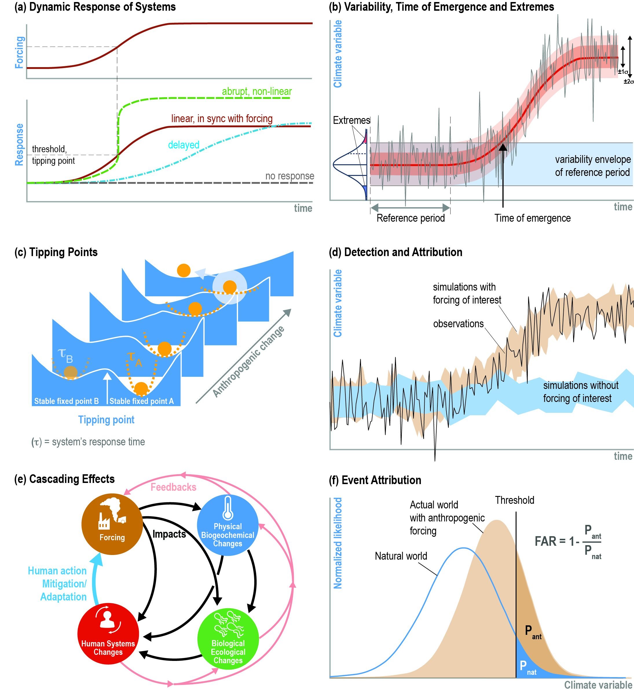
Figure 1.1 | Schematic of key concepts associated with changes in the ocean and cryosphere. (a) Differing responses of systems to gradual forcing (e.g., linear, delayed, abrupt, nonlinear). (b) Evolution of a dynamical system in time, revealing both natural (unforced) variability and a response to a new (e.g., anthropogenic) forcing. Key concepts include (i) the time of emergence and (ii) extreme events near or beyond the observed range of variability. (c) Tipping points and the change of their behaviour through time in response to, for example, anthropogenic change (adapted from Lenton et al., 2008). The two minima represent two stable fixed points, separated by a maximum representing an unstable fixed point, acting as a tipping point. The ball represents the state of the system with the red dash line indicating the stability of the fixed point and the system’s response time to small perturbations. (d) Detection and attribution, i.e., the statistical framework used to determine whether a change occurs or not (detection), and whether this detected change is caused by a particular set of forcings (e.g., greenhouse gases) (attribution). (e) Cascading effects, where changes in one part of a system inevitably affect the state in another, and so forth, ultimately affecting the state of the entire system. These cascading effects can also trigger feedbacks, altering the forcing. (f) Event attribution and fraction of attributable risk. The blue (orange) probability density function shows the likelihood of the occurrence of a particular value of a climate variable of interest under natural (present = including anthropogenic forcing) conditions. The corresponding areas above the threshold indicate the probabilities Pnat and Pant of exceedance of this threshold. The fraction of attributable risk (given by FAR = 1 – Pant/Pnat ) indicates the likelihood that a particular event has occurred as a consequence of anthropogenic change (adapted from Stott et al., 2016).