Special Report: Special Report on the Ocean and Cryosphere in a Changing Climate
Ch 04
Sea Level Rise and Implications for Low-Lying Islands, Coasts and Communities
FAQ 4.1: What challenges does the inevitability of sea level rise present to coastal communities and how can communities adapt?
As the global climate changes, rising sea levels, combined with high tides, storms and flooding, put coastal and island communities increasingly at risk. Protection can be achieved by building dikes or seawalls and by maintaining natural features like mangroves or coral reefs. Communities can also adjust by reclaiming land from the sea and adapting buildings to cope with floods. However, all measures have their limits, and once these are reached people may ultimately have to retreat. Choices made today influence how coastal ecosystems and communities can respond to sea level rise (SLR) in the future. Reducing greenhouse gas (GHG) emissions would not just reduce risks, but also open up more adaptation options.
Global Mean Sea Level (GMSL) is rising and it will continue to do so for centuries. Sustainable development aspirations are at risk because many people, assets and vital resources are concentrated along low-lying coasts around the world. Many coastal communities have started to consider the implications of SLR. Measures are being taken to address coastal hazards exacerbated by rising sea level, such as coastal flooding due to extreme events (e.g. storm surges, tropical cyclones), coastal erosion and salinisation). However, many coastal communities are still not sufficiently adapted to today’s ESLs.
Scientific evidence about SLR is clear: GMSL rose by 1.5 mm yr-1 during the period 1901–1990, accelerating to 3.6 mm yr-1 during the period 2005–2015. It is likely to rise 0.61–1.10 m by 2100 if global GHG emissions are not mitigated (RCP8.5). However, a rise of two or more metres cannot be ruled out. It could rise to more than 3 m by 2300, depending on the level of GHG emissions and the response of the AIS, which are both highly uncertain. Even if efforts to mitigate emissions are very effective, ESL events that were rare over the last century will become common before 2100, and even by 2050 in many locations. Without ambitious adaptation, the combined impact of hazards like coastal storms and very high tides will drastically increase the frequency and severity of flooding on low-lying coasts.
SLR, as well as the context for adaptation, will vary regionally and locally, thus action to reduce risks related to SLR takes different forms depending on the local circumstances. ‘Hard protection’, like dikes and seawalls, can effectively reduce risk under two or more metres of SLR but it is inevitable that limits will be reached. Such protection produces benefits that exceed its costs in low-lying coastal areas that are densely populated, as is the case for many coastal cities and some small islands, but in general, poorer regions will not be able to afford hard protection. Maintaining healthy coastal ecosystems, like mangroves, seagrass beds or coral reefs, can provide ‘soft protection’ and other benefits. SLR can also be ‘accommodated’ by raising buildings on the shoreline, for example. Land can be reclaimed from the sea by building outwards and upwards. In coastal locations where the risk is very high and cannot be effectively reduced, ‘retreat’ from the shoreline is the only way to eliminate such risk. Avoiding new development commitments in areas exposed to coastal hazards and SLR also avoids additional risk.
For those unable to afford protection, accommodation or advance measures, or when such measures are no longer viable or effective, retreat becomes inevitable. Millions of people living on low-lying islands face this prospect, including inhabitants of Small Island Developing States (SIDS), of some densely populated but less intensively developed deltas, of rural coastal villages and towns, and of Arctic communities who already face melting sea ice and unprecedented changes in weather. The resultant impacts on distinctive cultures and ways of life could be devastating. Difficult trade-offs are therefore inevitable when making social choices about rising sea level. Institutionalising processes that lead to fair and just outcomes is challenging, but vitally important.
Choices being made now about how to respond to SLR profoundly influence the trajectory of future exposure and vulnerability to SLR. If concerted emissions mitigation is delayed, risks will progressively increase as SLR accelerates. Prospects for global climate-resilience and sustainable development therefore depend in large part on coastal nations, cities and communities taking urgent and sustained locally-appropriate action to mitigate GHG emissions and adapt to SLR
- Figure 4.1View details
- Figure 4.2View details
- Figure 4.3View details
- Figure 4.4View details
- Figure 4.5View details
- Figure 4.6View details
- Figure 4.9View details
- Figure 4.10View details
- Box 4.1, Figure 1View details
- Figure 4.13View details
- Box 4.3, Figure 1View details
ES
Executive Summary
This chapter assesses past and future contributions to global, regional and extreme sea level changes, associated risk to low-lying islands, coasts, cities, and settlements, and response options and pathways to resilience and sustainable development along the coast.
Observations
Global mean sea level (GMSL) is rising (virtually certain1) and accelerating (high confidence2). The sum of glacier and ice sheet contributions is now the dominant source of GMSL rise (very high confidence). GMSL from tide gauges and altimetry observations increased from 1.4 mm yr–1 over the period 1901–1990 to 2.1 mm yr–1 over the period 1970–2015 to 3.2 mm yr–1 over the period 1993–2015 to 3.6 mm yr–1 over the period 2006–2015 (high confidence). The dominant cause of GMSL rise since 1970 is anthropogenic forcing (high confidence). {4.2.2.1.1, 4.2.2.2}
GMSL was considerably higher than today during past climate states that were warmer than pre-industrial, including the Last Interglacial (LIG; 129–116 ka), when global mean surface temperature was 0.5ºC–1.0ºC warmer, and the mid-Pliocene Warm Period (mPWP; ~3.3 to 3.0 million years ago), 2ºC–4ºC warmer. Despite the modest global warmth of the Last Interglacial, GMSL was likely 6–9 m higher, mainly due to contributions from the Greenland and Antarctic ice sheets (GIS and AIS, respectively), and unlikely more than 10m higher (medium confidence). Based on new understanding about geological constraints since the IPCC 5th Assessment Report (AR5), 25 m is a plausible upper bound on GMSL during the mPWP (low confidence). Ongoing uncertainties in palaeo sea level reconstructions and modelling hamper conclusions regarding the total magnitudes and rates of past sea level rise (SLR). Furthermore, the long (multi-millennial) time scales of these past climate and sea level changes, and regional climate influences from changes in Earth’s orbital configuration and climate system feedbacks, lead to low confidence in direct comparisons with near-term future changes. {Cross-Chapter Box 5 in Chapter 1, 4.2.2, 4.2.2.1, 4.2.2.5, SM 4.1}
Non-climatic anthropogenic drivers, including recent and historical demographic and settlement trends and anthropogenic subsidence, have played an important role in increasing low-lying coastal communities’ exposure and vulnerability to SLR and extreme sea level (ESL) events (very high confidence). In coastal deltas, for example, these drivers have altered freshwater and sediment availability (high confidence). In low-lying coastal areas more broadly, human-induced changes can be rapid and modify coastlines over short periods of time, outpacing the effects of SLR (high confidence). Adaptation can be undertaken in the short- to medium-term by targeting local drivers of exposure and vulnerability, notwithstanding uncertainty about local SLR impacts in coming decades and beyond (high confidence). {4.2.2.4, 4.3.1, 4.3.2.2, 4.3.2.3}
Coastal ecosystems are already impacted by the combination of SLR, other climate-related ocean changes, and adverse effects from human activities on ocean and land (high confidence). Attributing such impacts to SLR, however, remains challenging due to the influence of other climate-related and non-climatic drivers such as infrastructure development and human-induced habitat degradation (high confidence). Coastal ecosystems, including saltmarshes, mangroves, vegetated dunes and sandy beaches, can build vertically and expand laterally in response to SLR, though this capacity varies across sites (high confidence). These ecosystems provide important services that include coastal protection and habitat for diverse biota. However, as a consequence of human actions that fragment wetland habitats and restrict landward migration, coastal ecosystems progressively lose their ability to adapt to climate-induced changes and provide ecosystem services, including acting as protective barriers (high confidence). {4.3.2.3}
Coastal risk is dynamic and increased by widely observed changes in coastal infrastructure, community livelihoods, agriculture and habitability (high confidence). As with coastal ecosystems, attribution of observed changes and associated risk to SLR remains challenging. Drivers and processes inhibiting attribution include demographic, resource and land use changes and anthropogenic subsidence. {4.3.3, 4.3.4}
A diversity of adaptation responses to coastal impacts and risks have been implemented around the world, but mostly as a reaction to current coastal risk or experienced disasters (high confidence). Hard coastal protection measures (dikes, embankments, sea walls and surge barriers) are widespread, providing predictable levels of safety in northwest Europe, East Asia, and around many coastal cities and deltas. Ecosystem-based adaptation (EbA) is continuing to gain traction worldwide, providing multiple co-benefits, but there is still low agreement on its cost and long-term effectiveness. Advance, which refers to the creation of new land by building into the sea (e.g., land reclamation), has a long history in most areas where there are dense coastal populations. Accommodation measures, such as early warning systems (EWS) for ESL events, are widespread. Retreat is observed but largely restricted to small communities or carried out for the purpose of creating new wetland habitat. {4.4.2.3, 4.4.2.4, 4.4.2.5}
Projections
Future rise in GMSL caused by thermal expansion, melting of glaciers and ice sheets and land water storage changes, is strongly dependent on which Representative Concentration Pathway (RCP) emission scenario is followed. SLR at the end of the century is projected to be faster under all scenarios, including those compatible with achieving the long-term temperature goal set out in the Paris Agreement. GMSL will rise between 0.43 m (0.29–0.59 m, likely range; RCP2.6) and 0.84 m (0.61–1.10 m, likely range; RCP8.5) by 2100 (medium confidence) relative to 1986–2005. Beyond 2100, sea level will continue to rise for centuries due to continuing deep ocean heat uptake and mass loss of the GIS and AIS and will remain elevated for thousands of years (high confidence). Under RCP8.5, estimates for 2100 are higher and the uncertainty range larger than in AR5. Antarctica could contribute up to 28 cm of SLR (RCP8.5, upper end of likely range) by the end of the century (medium confidence). Estimates of SLR higher than the likely range are also provided here for decision makers with low risk tolerance. {SR1.5, 4.1, 4.2.3.2, 4.2.3.5}
Under RCP8.5, the rate of SLR will be 15 mm yr–1 (10–20 mm yr–1, likely range) in 2100, and could exceed several cm yr–1 in the 22nd century. These high rates challenge the implementation of adaptation measures that involve a long lead time, but this has not yet been studied in detail. {4.2.3.2, 4.4.2.2.3}
Processes controlling the timing of future ice shelf loss and the spatial extent of ice sheet instabilities could increase Antarctica’s contribution to SLR to values higher than the likely range on century and longer time scales (low confidence). Evolution of the AIS beyond the end of the 21st century is characterized by deep uncertainty as ice sheet models lack realistic representations of some of the underlying physical processes. The few model studies available addressing time scales of centuries to millennia indicate multi-metre (2.3–5.4 m) rise in sea level for RCP8.5 (low confidence). There is low confidence in threshold temperatures for ice sheet instabilities and the rates of GMSL rise they can produce. {Cross-Chapter Box 5 in Chapter 1, Cross-Chapter Box 8 in Chapter 3, and Sections 4.1, 4.2.3.1.1, 4.2.3.1.2, 4.2.3.6}
Sea level rise is not globally uniform and varies regionally. Thermal expansion, ocean dynamics and land ice loss contributions will generate regional departures of about ±30% around the GMSL rise. Differences from the global mean can be greater than ±30% in areas of rapid vertical land movements, including those caused by local anthropogenic factors such as groundwater extraction (high confidence). Subsidence caused by human activities is currently the most important cause of relative sea level rise (RSL) change in many delta regions. While the comparative importance of climate-driven RSL rise will increase over time, these findings on anthropogenic subsidence imply that a consideration of local processes is critical for projections of sea level impacts at local scales (high confidence). {4.2.1.6, 4.2.2.4}
Due to projected GMSL rise, ESLs that are historically rare (for example, today’s hundred-year event) will become common by 2100 under all RCPs (high confidence). Many low-lying cities and small islands at most latitudes will experience such events annually by 2050. Greenhouse gas (GHG) mitigation envisioned in low-emission scenarios (e.g., RCP2.6) is expected to sharply reduce but not eliminate risk to low-lying coasts and islands from SLR and ESL events. Low-emission scenarios lead to slower rates of SLR and allow for a wider range of adaptation options. For the first half of the 21st century differences in ESL events among the scenarios are small, facilitating adaptation planning. {4.2.2.5, 4.2.3.4}
Non-climatic anthropogenic drivers will continue to increase the exposure and vulnerability of coastal communities to future SLR and ESL events in the absence of major adaptation efforts compared to today (high confidence). {4.3.4, Cross-Chapter Box 9}
The expected impacts of SLR on coastal ecosystems over the course of the century include habitat contraction, loss of functionality and biodiversity, and lateral and inland migration. Impacts will be exacerbated in cases of land reclamation and where anthropogenic barriers prevent inland migration of marshes and mangroves and limit the availability and relocation of sediment (high confidence). Under favourable conditions, marshes and mangroves have been found to keep pace with fast rates of SLR (e.g., >10 mm yr-1), but this capacity varies significantly depending on factors such as wave exposure of the location, tidal range, sediment trapping, overall sediment availability and coastal squeeze (high confidence). {4.3.3.5.1}
In the absence of adaptation, more intense and frequent ESL events, together with trends in coastal development will increase expected annual flood damages by 2-3 orders of magnitude by 2100 (high confidence). However, well designed coastal protection is very effective in reducing expected damages and cost efficient for urban and densely populated regions, but generally unaffordable for rural and poorer areas (high confidence). Effective protection requires investments on the order of tens to several hundreds of billions of USD yr-1 globally (high confidence). While investments are generally cost efficient for densely populated and urban areas (high confidence), rural and poorer areas will be challenged to afford such investments with relative annual costs for some small island states amounting to several percent of GDP (high confidence). Even with well-designed hard protection, the risk of possibly disastrous consequences in the event of failure of defences remains. {4.3.4, 4.4.2.2, 4.4.3.2, Cross-Chapter Box 9}
Risk related to SLR (including erosion, flooding and salinisation) is expected to significantly increase by the end of this century along all low-lying coasts in the absence of major additional adaptation efforts (very high confidence). While only urban atoll islands and some Arctic communities are expected to experience moderate to high risk relative to today in a low emission pathway, almost high to very high risks are expected in all low-lying coastal settings at the upper end of the likely range for high emission pathways (medium confidence). However, the transition from moderate to high and from high to very high risk will vary from one coastal setting to another (high confidence). While a slower rate of SLR enables greater opportunities for adapting, adaptation benefits are also expected to vary between coastal settings. Although ambitious adaptation will not necessarily eradicate end-century SLR risk (medium confidence), it will help to buy time in many locations and therefore help to lay a robust foundation for adaptation beyond 2100. {4.1.3, 4.3.4, Box 4.1, SM4.2}
Choosing and Implementing Responses
All types of responses to SLR, including protection, accommodation, EbA, advance and retreat, have important and synergistic roles to play in an integrated and sequenced response to SLR (high confidence). Hard protection and advance (building into the sea) are economically efficient in most urban contexts facing land scarcity (high confidence), but can lead to increased exposure in the long term. Where sufficient space is available, EbA can both reduce coastal risks and provide multiple other benefits (medium confidence). Accommodation such as flood proofing buildings and EWS for ESL events are often both low-cost and highly cost-efficient in all contexts (high confidence). Where coastal risks are already high, and population size and density are low, or in the aftermath of a coastal disaster, retreat may be especially effective, albeit socially, culturally and politically challenging. {4.4.2.2, 4.4.2.3, 4.4.2.4, 4.4.2.5, 4.4.2.6, 4.4.3}
Technical limits to hard protection are expected to be reached under high emission scenarios (RCP8.5) beyond 2100 (high confidence) and biophysical limits to EbA may arise during the 21st century, but economic and social barriers arise well before the end of the century (medium confidence). Economic challenges to hard protection increase with higher sea levels and will make adaptation unaffordable before technical limits are reached (high confidence). Drivers other than SLR are expected to contribute more to biophysical limits of EbA. For corals, limits may be reached during this century, due to ocean acidification and ocean warming, and for tidal wetlands due to pollution and infrastructure limiting their inland migration. Limits to accommodation are expected to occur well before limits to protection occur. Limits to retreat are uncertain, reflecting research gaps. Social barriers (including governance challenges) to adaptation are already encountered. {4.4.2.2, 4.4.2.3., 4.4.2.3.2, 4.4.2.5, 4.4.2.6, 4.4.3, Cross-Chapter Box 9}
Choosing and implementing responses to SLR presents society with profound governance challenges and difficult social choices, which are inherently political and value laden (high confidence). The large uncertainties about post 2050 SLR, and the substantial impact expected, challenge established planning and decision making practises and introduce the need for coordination within and between governance levels and policy domains. SLR responses also raise equity concerns about marginalising those most vulnerable and could potentially spark or compound social conflict (high confidence). Choosing and implementing responses is further challenged through a lack of resources, vexing trade-offs between safety, conservation and economic development, multiple ways of framing the ‘sea level rise problem’, power relations, and various coastal stakeholders having conflicting interests in the future development of heavily used coastal zones (high confidence). {4.4.2, 4.4.3}
Despite the large uncertainties about post 2050 SLR, adaptation decisions can be made now, facilitated by using decision analysis methods specifically designed to address uncertainty (high confidence). These methods favour flexible responses (i.e., those that can be adapted over time) and periodically adjusted decisions (i.e., adaptive decision making). They use robustness criteria (i.e., effectiveness across a range of circumstances) for evaluating alternative responses instead of standard expected utility criteria (high confidence). One example is adaptation pathway analysis, which has emerged as a low-cost tool to assess long-term coastal responses as sequences of adaptive decisions in the face of dynamic coastal risk characterised by deep uncertainty (medium evidence, high agreement). The range of SLR to be considered in decisions depends on the risk tolerance of stakeholders, with stakeholders whose risk tolerance is low also considering SLR higher than the likely range. {4.1, 4.4.4.3}
Adaptation experience to date demonstrates that using a locally appropriate combination of decision analysis, land use planning, public participation and conflict resolution approaches can help to address the governance challenges faced in responding to SLR (high confidence). Effective SLR responses depend, first, on taking a long-term perspective when making short-term decisions, explicitly accounting for uncertainty of locality-specific risks beyond 2050 (high confidence), and building governance capabilities to tackle the complexity of SLR risk (medium evidence, high agreement). Second, improved coordination of SLR responses across scales, sectors and policy domains can help to address SLR impacts and risk (high confidence). Third, prioritising consideration of social vulnerability and equity underpins efforts to promote fair and just climate resilience and sustainable development (high confidence) and can be helped by creating safe community arenas for meaningful public deliberation and conflict resolution (medium evidence, high agreement). Finally, public awareness and understanding about SLR risks and responses can be improved by drawing on local, indigenous and scientific knowledge systems, together with social learning about locality-specific SLR risk and response potential (high confidence). {4.4.4.2, 4.4.5, Table 4.9}
Achieving the United Nations Sustainable Development Goals (SDGs) and charting Climate Resilient Development Pathways depends in part on ambitious and sustained mitigation efforts to contain SLR coupled with effective adaptation actions to reduce SLR impacts and risk (medium evidence, high agreement).
4.1
Synthesis
4.1.1
Purpose, Scope, and Structure of this Chapter
This chapter assesses the literature published since the AR5 on past and future contributions to global, regional and ESL changes, associated risk to low-lying islands, coasts, cities and settlements, and response options and pathways to resilience and sustainable development along the coast. The chapter follows the risk framework of AR5, in which risk is assessed in terms of hazard, exposure and vulnerability (Cross-Chapter Box 1 Chapter 1; Box 4.1), and is structured as follows (Figure 4.1):
- Section 4.1 (this section) presents a high-level synthesis of our assessment and provides entry points to more specific content found in the other sections.
- Section 4.2 assesses the current understanding of processes contributing to mean and extreme SLR globally, regionally and locally, with an emphasis on new insights about the AIS contribution.
- Section 4.3 assesses how mean and extreme sea level changes translate into coastal hazards (e.g., flooding, erosion and salinity intrusion), how these interact with socioeconomic drivers of coastal exposure and vulnerability, and how this interaction translates into observed impacts and projected risks for ecosystems, natural resources and human systems.
- Section 4.4 assesses the cost, effectiveness, co-benefits, efficiency, and technical limits of different types of SLR responses and identifies governance challenges (also called barriers) associated with choosing and implementing responses. Next, planning, public participation, conflict resolution and decision analysis methods for addressing the identified governance challenges are assessed, as well as practical lessons learned in local cases.
4.1.2
Future Sea level Rise and Implications for Responses
For understanding responses to climate-change induced SLR, two aspects of sea level are important to note initially:
- Climate-change induced GMSL rise is caused by thermal expansion of ocean water and ocean mass gain, the latter primarily due to a decrease in land-ice mass. However, responses to SLR are local and hence always based on RSL experienced at a particular location. GMSL is modified regionally by climate processes and locally by a variety of factors, some driven or influenced by human activity. Of particular relevance for responding to SLR is anthropogenic subsidence, which can lead to rates of RSL rise that exceed those of climate-induced SLR by an order of magnitude, specifically in delta regions and near cities (4.2.2.4). In these subsiding regions, one available response to prepare for future climate-induced SLR is to manage and reduce anthropogenic subsidence (4.4.2).
- The combination of gradual change of mean sea level with ESL events such as tides, surges and waves causes coastal impacts (4.2.3). ESL events at the coast that are rare today will become more frequent in the future, which means that for many locations, the main starting point for coastal planning and decision making is information on current and future ESL events. One important response for preparing for future SLR is to improve observational systems (tide gauges, wave buoys and remote sensing techniques), because in many places around the world current frequencies and intensities of ESL events are not well understood due to a lack of observational data (4.2.3.4.1).
After an increase of sea level from 1–2 mm yr–1 in most regions over the past century, rates of 3–4 mm yr–1 are now being experienced that will further increase to 4–9 mm yr–1 under RCP2.6 and 10–20 mm yr–1 at the end of the century under RCP8.5. Nevertheless, up to 2050, uncertainty in climate change-driven future sea level is relatively small, which provides a robust basis for short-term (≤30 years) adaptation planning. GMSL will rise between 0.24 m (0.17–0.32 m, likely range) under RCP2.6 and 0.32 m (0.23–0.40 m, likely range) under RCP8.5 (medium confidence; 4.2.3). The combined effect of mean and extreme sea levels results in events which are rare in the historical context (return period of 100 years or larger; probability <0.01 yr–1) occurring yearly at some locations by the middle of this century under all emission scenarios (4.2.3.4.1; high confidence). This includes, for instance, those parts of the intertropical low-lying coasts that are currently exposed to storm surges only infrequently. Hence, additional adaptation is needed irrespective of the uncertainties in future global GHG emissions and the Antarctic contribution to SLR.
Beyond 2050, uncertainty in climate change induced SLR increases substantially due to uncertainties in emission scenarios and the associated climate changes, and the response of the AIS in a warmer world. Combining process-model based studies in which there is medium confidence, it is found that GMSL is projected to rise between 0.43 m (0.29–0.59 m, likely range) under RCP 2.6 and 0.84 m (0.61–1.10 m, likely range) under RCP 8.5 by 2100 (Figure 4.3). The range that needs to be considered for planning and implementing coastal responses depends on the risk tolerance of stakeholders (i.e., those deciding and those affected by a decision; 4.4.4.3.2). Stakeholders that are risk tolerant (e.g., those planning for investments that can be very easily adapted to unforeseen conditions) may prefer to use the likely ranges of RCP2.6 and RCP8.5 for long-term adaptation planning. Stakeholders with a low risk tolerance (e.g., those planning for coastal safety in cities and long term investment in critical infrastructure) may also consider SLR above this range, because there is a 17% chance that GMSL will exceed 0.59 m under RCP2.6 and 1.10 m under RCP8.5 in 2100. Process-model based studies cannot yet provide this information, but expert elicitation studies show that a GMSL of 2 m in 2100 cannot be ruled out (4.2.3).
Despite the large uncertainty in late 21st century SLR, progress in adaptation planning and implementation is feasible today and may be economically beneficial. Many coastal decisions with time horizons of decades to over a century are made today (e.g., critical infrastructure, coastal protection works, city planning, etc.) and accounting for relative SLR can improve these decisions. Decision-analysis methods specifically targeting situations of large uncertainty are available and, combined with suitable planning, public participation and conflict resolution processes, can improve outcomes (high confidence; 4.4.4.2, 4.4.4.3). For example, adaptation pathway analysis recognises and enables sequenced long-term decision making in the face of dynamic coastal risk characterised by deep uncertainty (medium evidence, high agreement; 4.4.4.3.4). The use of these decision-analysis tools can be integrated into statutory land use or spatial planning provisions to formalise these decisions and enable effective implementation by relevant governing authorities (4.4.4.2).
Beyond 2100, sea level will continue to rise for centuries and will remain elevated for thousands of years (high confidence; 4.2.3.5). Only a few modelling studies are available for SLR beyond 2100. However, all studies agree that the difference in GMSL between RCP2.6 and RCP8.5 increases substantially on multi-centennial and millennial time scales (very high confidence). On a millennial time scale, this difference is about 10 metres in some model simulations, whereas it is only several decimetres at the end of 21st century. The larger the emissions the larger the risks associated with SLR as already assessed in SR1.5. Under RCP8.5 the few available studies indicate a likely range of 2.3–5.4 m (low confidence) in 2300. With strong mitigation efforts (RCP2.6), SLR will be kept to a likely range of 0.6–1.1 m (Figure 4.2). Regardless, ambitious and sustained adaptation efforts are needed to reduce risks.
Figure 4.1
Figure 4.1 | Schematic illustration of the interconnection of Chapter 4 themes, including drivers of sea level rise (SLR) and (extreme) sea level hazards (Section 4.2), exposure, vulnerability, impacts and risk related to SLR (Section 4.3), and responses, associated governance challenges and practises and tools for enabling social choices and addressing governance challenges (Section 4.4).
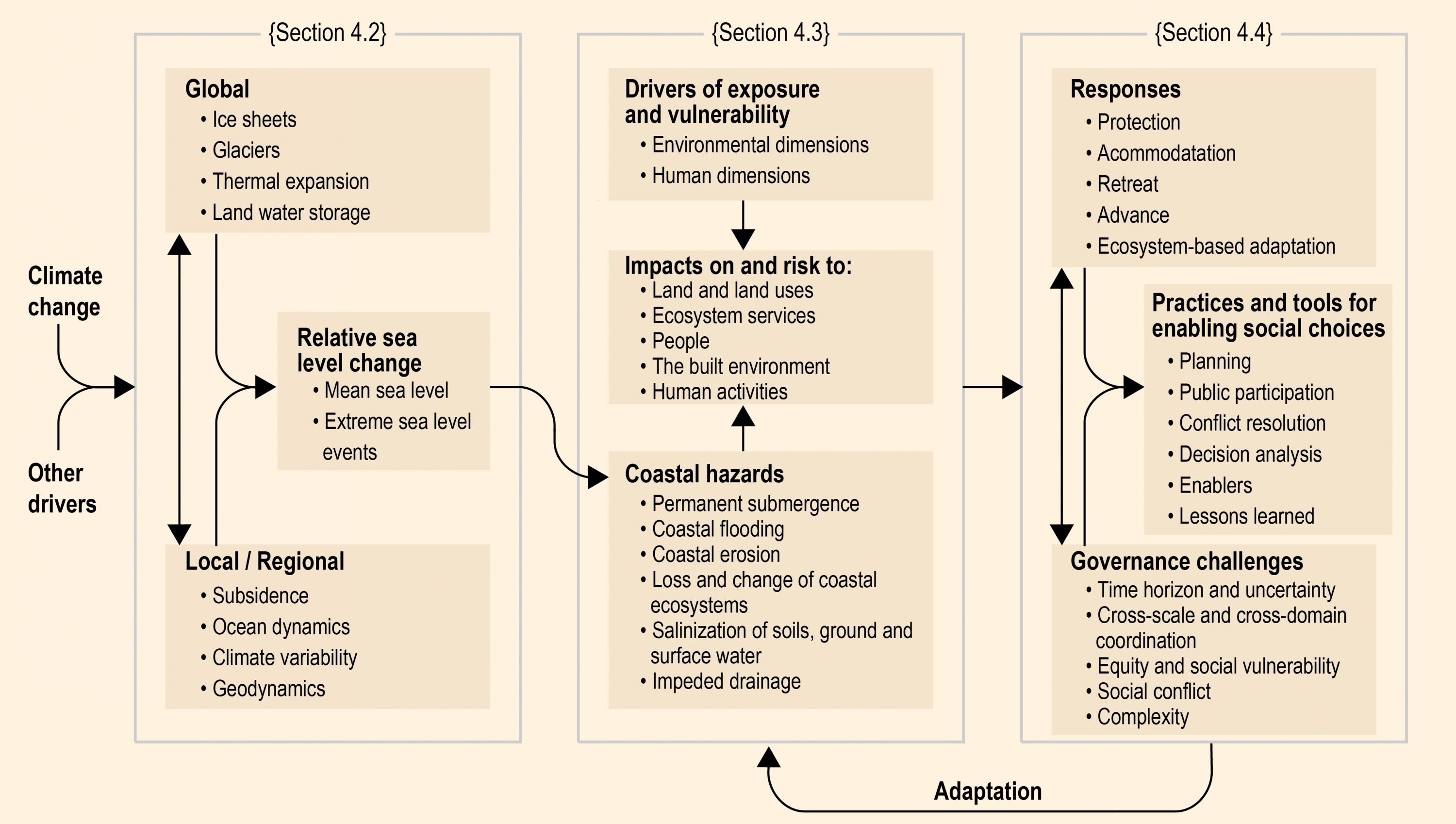
Figure 4.1 | Schematic illustration of the interconnection of Chapter 4 themes, including drivers of sea level rise (SLR) and (extreme) sea level hazards (Section 4.2), exposure, vulnerability, impacts and risk related to SLR (Section 4.3), and responses, associated governance challenges and practises and tools for enabling social choices and addressing governance challenges (Section 4.4).
Figure 4.2
Figure 4.2 | Projected sea level rise (SLR) until 2300. The inset shows an assessment of the likely range of the projections for RCP2.6 and RCP8.5 up to 2100 (medium confidence). Projections for longer time scales are highly uncertain but a range is provided (4.2.3.6; low confidence). For context, results are shown from other estimation […]
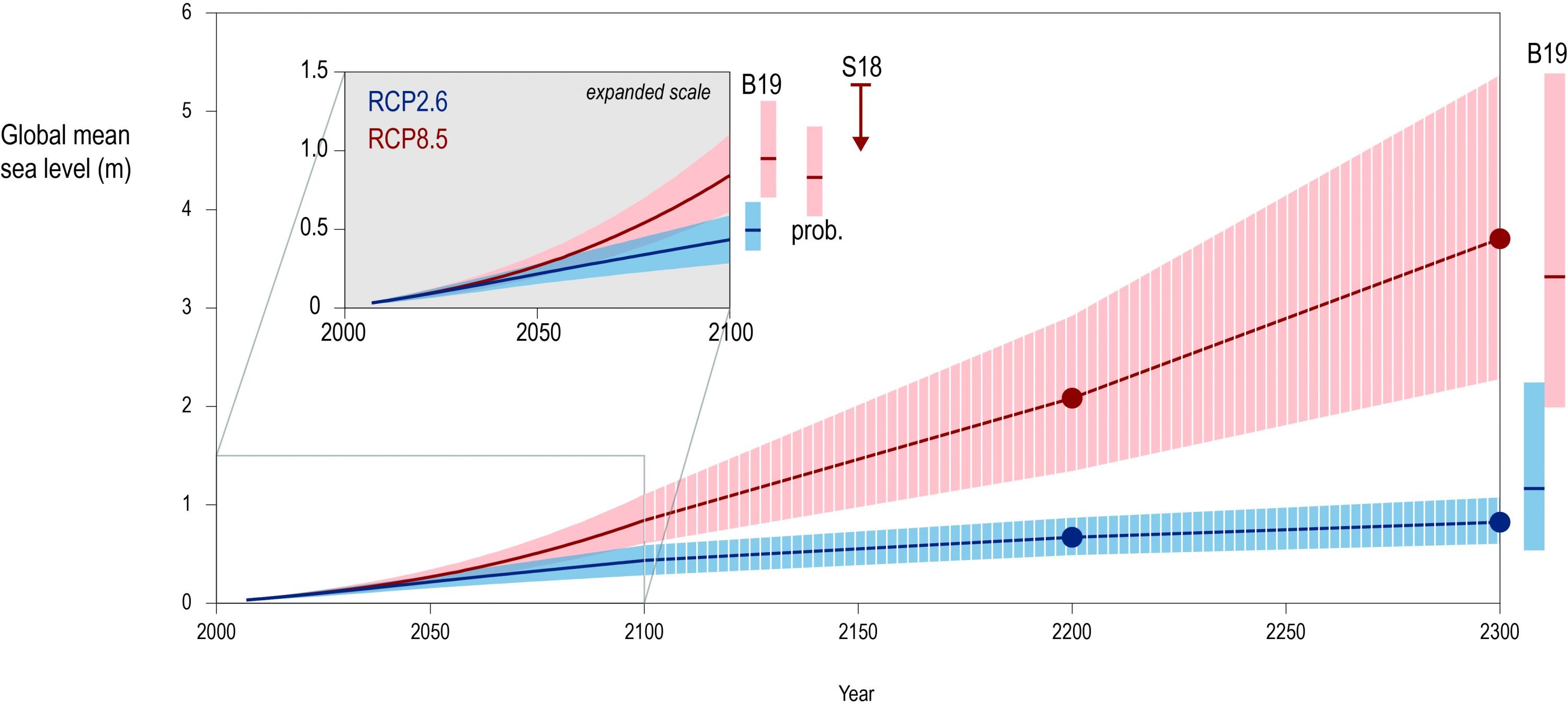
Figure 4.2 | Projected sea level rise (SLR) until 2300. The inset shows an assessment of the likely range of the projections for RCP2.6 and RCP8.5 up to 2100 (medium confidence). Projections for longer time scales are highly uncertain but a range is provided (4.2.3.6; low confidence). For context, results are shown from other estimation approaches in 2100 and 2300. The two sets of two bars labelled B19 are from an expert elicitation for the Antarctic component (Bamber et al., 20191), and reflect the likely range for a 2oC and 5oC temperature warming (low confidence; details section 4.2.3.3.1). The bar labelled “prob.” indicates the likely range of a set of probabilistic projections (4.2.3.2). The arrow indicated by S18 shows the result of an extensive sensitivity experiment with a numerical model for the Antarctic Ice Sheet (AIS) combined, like the results from B19 and “prob.”, with results from Church et al. (2013)2 for the other components of SLR. S18 also shows the likely range.
4.1.3
Sea Level Rise Impacts and Implications for Responses
Rising mean and increasingly extreme sea level threaten coastal zones through a range of coastal hazards including (i) the permanent submergence of land by higher mean sea levels or mean high tides; (ii) more frequent or intense coastal flooding; (iii) enhanced coastal erosion; (iv) loss and change of coastal ecosystems; (v) salinisation of soils, ground and surface water; and (vi) impeded drainage. At the century scale and without adaptation, the vast majority of low-lying islands, coasts and communities face substantial risk from these coastal hazards, whether they are urban or rural, continental or island, at any latitude, and irrespective of their level of development (Section 4.3.4; Figure 4.3; high confidence). In the absence of an ambitious increase in adaptation efforts compared to those currently underway, high to very high risks are expected in many coastal geographies at the upper end of the RCP8.5 likely range. These include resource-rich coastal cities, urban atoll islands, densely populated deltas, and Arctic communities (Chapter 4 Box 4; Figure 4.3 and Section 4.3.4). At the same time coastal protection is very effective and cost-efficient for cities but not for less densely populated rural areas. Some geographies, such as urban atoll islands and Arctic communities face high risk even under RCP2.6 (medium confidence).
In many places, however, non SLR-related, local environmental and human dimensions of exposure and vulnerability play a critical role in increasing exposure and vulnerability to coastal hazards (Section 4.3.2.5). For example, the ability of morphological and ecological systems (Sections 4.3.3.3 and 4.3.3.5) to protect human settlements and infrastructure by attenuating ESL events and stabilising shorelines is progressively being lost due to coastal squeeze, pollution, habitat degradation and fragmentation (Section 4.3.3.5.4; high confidence). Hence, an important near term response to RSL rise is to reduce these adverse environmental and human dimensions of exposure and vulnerability. In addition, the drivers of exposure and vulnerability vary across different coastal contexts ranging from resource-rich cities to small islands (Sections 4.3.3, 4.3.4). Accordingly, effective responses need to be context-specific, and address the locality-specific drivers of risk.
Figure 4.3
Figure 4.3 | Additional risk related to sea level rise (SLR) for low-lying coastal areas by the end of the 21st century. Section 4.3.4 provides a synthesis of the assessment methodology and the findings, while SM4.3 provides details. Left-hand panel describes global mean sea level (GMSL) rise observations for the Present-Day (1986–2005) and projections under […]
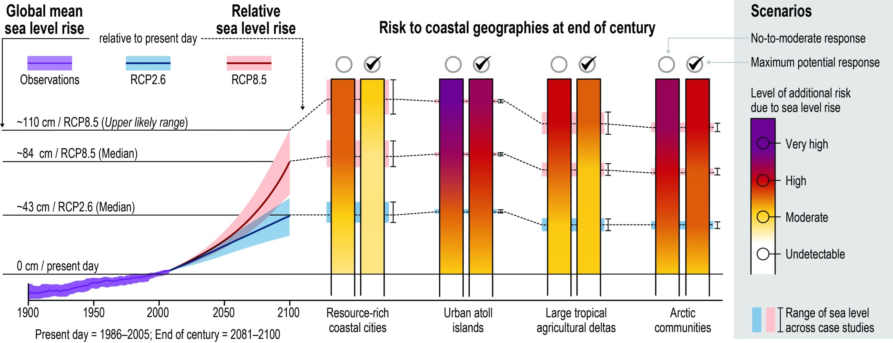
Figure 4.3 | Additional risk related to sea level rise (SLR) for low-lying coastal areas by the end of the 21st century. Section 4.3.4 provides a synthesis of the assessment methodology and the findings, while SM4.3 provides details. Left-hand panel describes global mean sea level (GMSL) rise observations for the Present-Day (1986–2005) and projections under RCP2.6 and RCP8.5 by 2100 relative to the Present-Day according to advances in this chapter. Relative sea level (RSL) changes at specific locations are represented by the coloured blocs (range of the real-world case studies used) and coloured dotted lines (mean) at the background of the middle panel, which describes risk to illustrative geographies as assessed in this chapter. Each illustrative geography is supported by real-world case studies described in the literature (Box 4.1, 4.3.4.1 and Table SM4.2.5): three for resource-rich coastal cities, three for urban atoll islands, two for large tropical agricultural deltas, five for Arctic communities. N.B. (1): Only Arctic communities remote from regions of rapid glacial-isostatic adjustment have been selected for this assessment. N.B (2): according to the specific scope of the chapter, this assessment focuses on the additional risks due to SLR and does not account for changes in extreme event climatology (Sections 4.2.3.4.1 to 4.2.3.4.3, 6.3.1.1 to 6.3.1.3), which in some cases would imply a different level of risk than assessed here. The middle panel also distinguishes between two adaptation scenarios. (A) ‘No-to- moderate response’ represents a business-as-usual scenario where no major additional adaptation efforts compared to today’s level of effort are implemented (i.e., neither further significant intensification of action nor new types of actions). (B) ‘Maximum potential response’ represents the opposite situation, that is, an ambitious combination of both incremental and transformational adaptation that leads to significant additional efforts compared to today and to (A). Here, the authors assume adaptation implemented at its full potential, that is, the extent of adaptation that is technologically possible, with minimal financial, social and political barriers.
4.1.4
Response Options, Governance Challenges and Ways Forward
Responding to SLR refers to reducing hazards, exposure and vulnerability of low-lying coastal areas. It can be approached in fundamentally different ways and five major categories are described in this chapter (Box 4.3): Protection reduces coastal risk and impacts by blocking the inland propagation and other effects of mean or extreme sea levels hazards (e.g., through dikes, seawalls, storm surge barriers, breakwaters, beach-dune systems, etc.). Advance creates new land by building seawards (e.g., reclamation of new land above sea levels or planting vegetation with the specific intention to support natural accretion of land). Ecosystem-based adaptation (EbA) provides a combination of the benefits of protect and advance strategies based on the conservation and restoration of ecosystems such as reefs and coastal vegetation. Accommodation includes a diverse set of biophysical and institutional responses to reduce vulnerability of coastal residents, human activities, ecosystems and the built environment (e.g., raising buildings, planting salt tolerant crops, insurance and EWS for ESL events). Retreat reduces exposure to coastal hazards by moving people, assets and human activities out of the exposed coastal area.
Each type of response has particular advantages and disadvantages, and may play a synergistic role in an integrated and sequenced response to SLR. For example, hard protection needs less space and its effectiveness is more predictable than for EbA (high confidence; 4.4.2.2.4, 4.4.2.3.4). EbA has advantages of contributing to conservation goals and providing additional ecosystem services such as carbon sequestration and improved water quality (4.4.2.2.5). EbA can become more effective over time, because coastal ecosystems can migrate inland with rising sea levels, provided this is not restricted by infrastructure (4.4.2.2.4). In practise, hard, sediment-based and ecosystem-based protection responses are often combined and there is high agreement that such hybrid approaches are a promising way forward (4.4.2.3.1). Advance is an option widely practised when land is scarce and offers the opportunity to finance adaptation through land sale revenues, but can also increase exposure and destroy coastal wetlands and their protective function (4.4.2.4). Accommodation measures such as flood proofing buildings, flood forecasting, early warning and emergency planning have high benefit-cost ratios, which means that implementing them is much cheaper than doing nothing (4.4.2.5.6). Retreat, and avoidance of development in some locations, are the only types of responses that eliminate residual risks, assuming there is sufficiently safe alternative land to retreat to or develop (4.4.2.6, Cross-Chapter Box 9).
Given diverse geographies and contexts (4.1.3), and the pros and cons of different responses, there is no silver bullet for responding to SLR. Rather, each coastal locality requires a tailor-made response that uses an appropriate mix of measures, sequenced over time as sea level rises. Possible integrated response strategies are illustrated for two contrasting types of settlements: densely populated urban and sparsely populated rural coasts.
For densely populated urban low elevation areas, including continental and island cities and megacities, hard protection has played and will continue to play the central role in response strategies (4.4.2.2, Box 4.1). In general, it is technologically feasible and economically efficient to protect large parts of cities against 21st century SLR (high confidence; 4.4.2.2.4, 4.4.2.7). However, questions of affordability remain for poorer and developing regions (4.3.3.4, 4.4.2.2.3). In cities, advance can offer a way to finance coastal protection through revenues generated from newly created land (4.4.2.4), but raises equity concerns with regard to the distribution of costs and access to the new land (4.4.2.4.6). Where space is available, EbA can supplement hard protection (4.4.2.3), except in situations where other human interventions, like infrastructure and pollution, interfere with EbA, especially for RCP8.5 (Cross-Chapter Box 9). Retreat may currently be favoured over rebuilding in the aftermath of major flooding disasters, but in densely populated areas protected by hard infrastructure, general retreat need not be considered until later in the century once it is known whether or not SLR will reach the higher end of the projections (1.1 m or more by 2100; 4.4.2.6).
Along sparsely populated rural coasts, safeguarding communities by conserving coastal ecosystems and natural morphodynamic processes, and restoring those already degraded, is the central element of an integrated strategy. Intact coastal ecosystems can protect settlements and, in some contexts, natural sedimentation processes and avoiding sand mining can help to raise exposed land (4.4.2.2). Hard coastal protection can lead to flooding or erosion elsewhere (4.4.2.2.5), and the destruction of ecosystems and the coastal protection they offer (4.3.3.5). Ecosystem health can be further maintained by reducing non-climatic drivers such as those that interrupt sediment flows in deltas and estuaries (4.3.2.3). Hard protection may be appropriate for areas containing high value assets (e.g., settlements and cultural sites). Retreat is worth considering now where coastal population size and density is low, risks are already high, and the economic, cultural and sociopolitical impacts of retreat and resettlement are carefully considered and addressed by at-risk communities and their governing authorities.
Designing and implementing an appropriate mix of responses is not only a technical task but also an inherently political and value-laden social choice that involves trade-offs between multiple values, goals and interests (Section 4.4.3). Specifically, distinctive features of SLR together with this complex nature of social choices give rise to five overarching governance challenges (Section 4.4.3.3):
- Time horizon and uncertainty associated with SLR beyond 2050 challenge standard planning and decision making practises (high confidence).
- Cross-scale and cross-domain coordination linking differing jurisdictional levels, sectors and policy domains is often needed for effective responses (medium confidence).
- Equity and social vulnerability are often negatively affected by SLR and also responses to SLR, which can undermine societal aspirations such as achieving the SDGs (high confidence).
- Social conflict (i.e., nonviolent struggle between groups, organisations and communities over values, interests, resources, and influence or power) caused or exacerbated by SLR could escalate over time and become very difficult to resolve (high confidence).
- Complexity, reinforced by the combination of the above challenges, makes it difficult to understand and address SLR (high confidence).
These governance challenges can be addressed through an integrated combination of well-established and emerging planning, public participation and conflict resolution practices (Section 4.4.4.2), decision analysis methods (Section 4.4.4.3) and enabling conditions (Section 4.4.5). For example, iterative planning and flexible, adaptive and robust decision making (RDM) can help coastal communities to plan for the future and account for SLR uncertainty. Planning can also enable thinking and action across spatial, temporal and governance scales and thus help to coordinate roles and responsibilities across multiple governance levels. Public participation approaches can be designed to account for divergent perspectives in making difficult social choices, enhancing social learning, experimentation and innovation in developing locally appropriate SLR responses. Conflict resolution approaches have considerable potential to improve adaptation prospects by harnessing the productive potential of nonviolent conflict.
4.2
Physical Basis for Sea Level Change and Associated Hazards
As a consequence of natural and anthropogenic changes in the climate system, sea level changes are occurring on temporal and spatial scales that threaten coastal communities, cities, and low-lying islands. Sea level in this context means the time average height of the sea surface, thus eliminating short duration fluctuations like waves, surges and tides. GMSL rise refers to an increase in the volume of ocean water caused by warmer water having a lower density, and by the increase in mass caused by loss of land ice or a net loss in terrestrial water reservoirs. Spatial variations in volume changes are related to spatial changes in the climate. In addition, mass changes due to the redistribution of water on the Earth’s surface and deformation of the lithosphere leads to a change in the Earth’s rotation and gravitational field, producing distinct spatial patterns in regional sea level change. In addition to the regional changes associated with contemporary ice and water redistribution, the solid Earth may cause sea level changes due to tectonics, mantle dynamics or glacial isostatic adjustment (see Section 4.2.1.5). These processes cause vertical land motion (VLM) and sea surface height changes at coastlines. Hence, RSL change is defined as the change in the difference in elevation between the land and the sea surface at a specific time and location (Farrell and Clark, 19763). Here, regional sea level refers to spatial scales of around 100 km, while local sea level refers to spatial scales smaller than 10 km.
In most places around the world, current annual mean rates of RSL changes are typically on the order of a few mm yr–1 (see Figure 4.6). Risk associated with changing sea level also is related to individual events that have a limited duration, superimposed on the background of these gradual changes. As a result, the gradual changes in time and space have to be assessed together with processes that lead to flooding and erosion events. These processes include storm surges, waves and tides or a combination of these processes and lead to ESL events (see Figure 4.4). In this section, newly emerging understanding of these different episodic and gradual aspects of sea level change are assessed, within a context of sea level changes measured directly over the last century, and those inferred for longer geological time scales. This longer-term perspective is important for contextualising future projections of sea level and providing guidance for process-based models of the individual components of SLR, in particular the ice sheets. In addition, anthropogenic subsidence may affect local sea level substantially in many locations but this process is not taken into account in values reported here for projected SLR unless specifically noted.
4.2.1
Processes of Sea Level Change
Sea level changes have been discussed throughout the various IPCC assessment reports as SLR is a key feature of climate change. Complex interactions between the oceans and ice sheets only recently have been recognised as important drivers of processes that can lead to rapid dynamical changes in the ice sheets. Understanding of basal melt below the ice shelves, ice calving processes and glacial hydrological processes was also limited. Projections of future sea level in the IPCC 4th Assessment Report (AR4; Lemke et al., 20074) were presented with the caveat that dynamical ice sheet processes were not accounted for, as our physical understanding of these processes was too rudimentary and no literature could be assessed (Bindoff et al., 20075). In AR5 (Church et al., 20136), a first attempt was made to quantify the dynamic contribution of the ice sheets, although still with modeling based on limited physcis, relying mainly on an extrapolation of existing observations (Little et al., 20137) and a single process based case study (Bindschadler et al., 20138). Here the focus is on sea level changes around coastlines and low-lying islands, updating the GMSL rise by including a new estimate of the dynamic contribution of Antarctica. The mechanism driving past and contemporary sea level changes and episodic extremes of sea level is explained, and confidence in regional projections of future sea level over the 21st century and beyond is assessed.
4.2.1.1
Ice Sheets and Ice Shelves
The ice sheets on Greenland and Antarctica contain most of the fresh water on the Earth’s surface. As a consequence, they have the greatest potential to cause changes in sea level. Figure 4.4 illustrates the size of land ice reservoirs and the most important processes that drive mass changes of ice sheets.
Ice sheets change sea level through the loss or gain of ice above flotation, defined as the ice thickness in exceedance of the smallest thickness that would remain in contact with the sea floor at hydrostatic equilibrium. The GIS is currently losing mass at roughly twice the pace of the AIS (Table 4.1). However, Antarctica contains eight times more ice above flotation than Greenland. Furthermore, a substantial fraction of the AIS rests on bedrock below sea level, making the ice sheet responsive to changes in ocean-driven melt and possibly vulnerable to marine ice sheet instabilities (Cross-Chapter Box 8 in Chapter 3) that can drive rapid mass loss.
Ice sheets gain or lose mass through changes in surface mass balance (SMB), the sum of accumulation and ablation controlled by atmospheric processes, the loss of ice to the ocean though melting of ice shelves, and by calving (breaking off of ice bergs) at marine-terminating ice fronts (see Chapter 3). Ice shelves, the floating extensions of grounded ice flowing into the ocean (Figure 4.4) do not directly contribute to sea level, but they play an important role in ice sheet dynamics by providing resistance to the seaward flow of the grounded ice upstream (Fürst et al., 20169; Reese et al., 2018b10). Ice shelves gain mass through the inflow of ice from the ice sheet, precipitation, and accretion at the ice-ocean interface. They lose mass through a combination of calving and by melting from below, especially where basal ice is in contact with warm water (Paolo et al., 2015, Khazendar et al., 2016). Calving rates at the terminus of marine terminating ice fronts are governed by complex ice-mechanical processes, the internal strength of the ice, and interaction with ocean waves and tides (Benn et al., 200711; Bassis, 201112; Massom et al., 201813). Sub-ice shelf melts rates are controlled by ice-ocean interactions involving the large-scale circulation, more localised heat and fresh water fluxes, and micro (mm)-scale processes in the ice-ocean boundary layer (Gayen et al., 201514; Dinniman et al., 201615; Schodlok et al., 201616). Ice shelves are also impacted by surface processes. Where surface melt rates are high, ice shelves not only lose mass, they can collapse (hydrofracture) from flexural stresses caused by the movement of the meltwater and the deepening of water-filled crevasses (Banwell et al., 201317; Macayeal and Sergienko, 201318; Kuipers Munneke et al., 201419). These complex ice-ocean interactions, calving and hydrofracture processes remain difficult to model, particularly at the scale of ice sheets.Our understanding of ice sheets has progressed substantially since AR5, although deep uncertainty (Cross-Chapter Box 5 in Chapter 1) remains with regard to their potential contribution to future SLR on time scales longer than a century under any given emissions scenario. This is particularly true for Antarctica.
4.2.1.2
Glaciers
Glaciers outside of the GIS and AIS are important contributors to sea level change (Figure 4.4). Because of their specific accumulation and ablation rates, which are often high compared to those of the ice sheets, they are sensitive indicators of climate change and respond quickly to changes in climate. Over the past century, glaciers have added more mass to the ocean than the GIS and AIS combined (Gregory et al., 201320). However, the mass of glaciers is small by comparison, equivalent to only 0.32 ± 0.08 m mean SLR if only the fraction of ice above sea level is considered (Farinotti et al., 201921). Sections 2.2.3, 3.3.2 and Cross-Chapter Box 6 in Chapter 2 provide a detailed discussion of glacier response to climate change.
4.2.1.3
Ocean Processes
In general, increasing temperatures lead to a lower density (‘thermal expansion’) and therefore the larger its volume per unit of mass. Thus, warming leads to a higher sea level even when the ocean mass remains constant. Over at least the last 1500 years changes in sea level were related to global mean temperatures (Kopp et al., 201622), partly because of ice mass loss, and partly because of thermal expansion. Models and observations indicate that over recent decades, more than 90% of the increase in energy in the climate system has been stored in the ocean. Hence, thermal expansion provides insight into climate sensitivity (Church et al., 201323). Findings from sea level studies and the energy budget are consistent (Otto et al., 201324). As thermal expansion per degree is dependent on the temperature itself, heat uptake by a warm region has a larger impact on SLR than heat uptake by a cold region. This contributes to regional changes in sea level, which are also caused by the water temperature and salinity variations (e.g., Lowe and Gregory, 2006; Suzuki and Ishii, 201125; Bouttes et al., 201426; Saenko et al., 201527). Regional patterns in sea level change are also modified from the global average by oceanic and atmospheric (fluid) dynamics (Griffies and Greatbatch, 201228), including trends in ocean currents, redistribution of temperature and salinity (sea water density), buoyancy, and atmospheric pressure. An analysis of these trends in Coupled Model Intercomparison Project Phase 5 (CMIP5) General Circulation Models (GCMs; Yin, 2012) demonstrates the potential for >15 cm of SLR by 2100 and >30 cm by 2300 (RCP8.5) along the east coast of the USA and Canada from fluid dynamical processes alone. However, Coupled Model Intercomparison Project Phase 6 (CMIP6) GCM simulations are not yet available for an updated analysis of these processes in SROCC.
4.2.1.4
Terrestrial Reservoirs
Global sea level changes are also affected by changes in terrestrial reservoirs of liquid water. Withdrawal of groundwater and storage of fresh water through dam construction (Chao et al., 200829; Fiedler and Conrad, 201030) in the earlier parts of the 20th century dominated, leading to sea level fall, but in recent decades, land water depletion due to domestic, agricultural and industrial usage has begun to contribute to sea level change (Wada et al., 201731). Changes in terrestrial reservoirs may also be related to climate variability: in particular, the El Niño Southern Oscillation (ENSO) has a strong impact on precipitation distribution and temporary storage of water on continents (Boening et al., 201232; Cazenave et al., 201233; Fasullo et al., 201334).
4.2.1.5
Geodynamic Processes
Changing distributions of water mass between land, ice and ocean reservoirs cause nearly instantaneous changes in the Earth’s gravity field and rotation, and elastic deformation of the solid Earth. These processes combine to produce spatially varying patterns of sea level change (Mitrovica et al., 200135; Mitrovica et al., 201136). For example, adjacent to an ice sheet losing mass, reduced gravitational attraction between the ice and nearby ocean causes RSL to fall, despite the rise in GMSL from the input of melt water to the ocean. The opposite effect is found far from the ice sheet, where RSL rise can be enhanced as much as 30% relative to the global average.
On time scales longer than the elastic Earth response, redistributions of water and ice cause time-dependent, visco-elastic deformation. This is observed in regions previously covered by ice during the Last Glacial Maximum (LGM), including much of Scandinavia and parts of North America (Lambeck et al., 199837; Peltier, 200438), where glacio-isostatic adjustment (GIA) is causing uplift and a lowering of RSL that continues today. In other locations proximal to the previous ice load, and where a glacial forebulge once existed, the relaxing forebulge can contribute to a relative SLR, as currently being experienced along the coastline of the northeast United States. Water being syphoned to high latitudes as the peripheral bulges collapse leads to a widespread RSL fall in equatorial regions, while the overall loading of ocean crust by melt water can cause uplift of land areas near continental margins, far from the location of previous ice loading (Mitrovica and Milne, 200339; Milne and Mitrovica, 200840). Rates of modern VLM associated with these post-glacial processes are generally on the order of a few mm yr–1 or less, but can exceed 1 cm yr–1 in some places. Because these gravity, rotation, and deformation (GRD) processes control spatial patterns of SLR from melting land ice, they need to be accounted for in regional-to-local sea level assessments. GRD processes are also important for marine-based ice sheets themselves, because they locally reduce RSL at retreating grounding lines which can slow and reduce retreat (Gomez et al., 201541; see 4.3.3.1.2 and Cross-chapter Box 8 in Chapter 3; Larour et al., 201942).
VLM from tectonics and dynamic topography associated with viscous mantle processes also affect spatial patterns of relative sea level change. These geological processes are important for reconstructing ancient sea levels based on geological indicators (Austermann and Mitrovica, 201543; see SM4.1). Along with other natural and anthropogenic processes including volcanism, compaction, and anthropogenic subsidence from ground water extraction (Section 4.2.2.4) these geodynamic processes can be locally important, producing rates of VLM comparable to or greater than recent climate-driven rates of GMSL change (Wöppelmann and Marcos, 201644). In this chapter, GIA and anthropogenic subsidence are used, and other components of VLM are ignored unless explicitly stated.Changing distributions of water mass between land, ice and ocean reservoirs cause nearly instantaneous changes in the Earth’s gravity field and rotation, and elastic deformation of the solid Earth. These processes combine to produce spatially varying patterns of sea level change (Mitrovica et al., 2001; Mitrovica et al., 2011). For example, adjacent to an ice sheet losing mass, reduced gravitational attraction between the ice and nearby ocean causes RSL to fall, despite the rise in GMSL from the input of melt water to the ocean. The opposite effect is found far from the ice sheet, where RSL rise can be enhanced as much as 30% relative to the global average.
4.2.1.6
Extreme Sea Level Events
Superimposed on gradual changes in RSL, as described in the previous sections, tides, storm surges, waves and other high-frequency processes (Figure 4.4) can be important. Understanding the localised impact of such processes requires detailed knowledge of bathymetry, erosion and sedimentation, as well as a good description of the temporal variability of the wind fields generating waves and storm surges. The potential for compounding effects, like storm surge and high SLR, are of particular concern as they can contribute significantly to flooding risks and extreme events (Little et al., 2015a45). These processes can be captured by hydrodynamical models (see Section 4.2.3.4).
4.2.2
Observed Changes in Sea Level (Past and Present)
Sea level changes in the distant geologic past provide information on the size of the ice sheets in climate states different from today. Past intervals with temperatures comparable to or warmer than today are of particular interest, and since AR5 (Masson-Delmotte et al., 201346) they have been increasingly used to test and calibrate process-based ice sheet models used in future projections (DeConto and Pollard, 201647; Edwards et al., 201948; Golledge et al., 201949). These intervals include the mPWP around 3.3–3.0 Ma, when atmospheric CO2 concentrations were similar to today (~300–450 ppmv; Badger et al., 201350; Martínez-Botí et al., 201551; Stap et al., 201652) and global mean temperature was 2ºC–4ºC warmer than pre-industrial (Dutton et al., 2015a53; Haywood et al., 201654) and the LIG around 129–116 ka, when global mean temperature was 0.5ºC–1.0ºC warmer (Capron et al., 201455; Dutton et al., 2015a56; Fischer et al., 201857) and sea surface temperatures were similar to today (Hoffman et al., 201758). Updated reconstructions of GMSL (Dutton et al., 2015a59) based on ancient shoreline elevations corrected to account for geodynamic processes (4.2.1.5), and geochemical records extracted from marine sediment cores, indicate sea levels were >5 m higher than today during these past warm periods (medium confidence).
Most estimates of peak GMSL during the mPWP range between 6 and 30 m higher than today (Miller et al., 201260; Rovere et al., 201461; Dutton et al., 2015a62) but with deep uncertainty (Cross-Chapter Box 5 in Chapter 1) and few constraints on the high end of the range. The large uncertainty is contributed by uncertain GIA corrections applied to palaeo shoreline indicators (Raymo et al., 201163; Rovere et al., 201464), dynamic topography, the vertical land surface motion associated with Earth’s mantle flow (Rowley et al., 201365), and possible biases in geochemical records of ice volume derived from marine sediments (Raymo et al., 201866). Estimates of GMSL >10 m higher than today require a meltwater contribution from the East Antarctic Ice Sheet in addition to the GIS and West Antarctic Ice Sheets (WAIS; Miller et al., 201267; Dutton et al., 2015a68). Pliocene modelling studies appearing since AR5 (Masson-Delmotte et al., 201369) demonstrate the potential for substantial retreat of East Antarctic ice into deep submarine basins (Austermann and Mitrovica, 201570; Pollard et al., 201571; Aitken et al., 201672; DeConto and Pollard, 201673; Gasson et al., 201674; Golledge et al., 201975), as does emerging geological evidence from marine sediment cores recovered from the East Antarctic margin (Cook et al., 201376; Patterson et al., 201477; Bertram et al., 201878). However, the range of maximum Pliocene GMSL contributions from Antarctic modelling (Austermann and Mitrovica, 201579; Pollard et al., 201580; Yamane et al., 201581; DeConto and Pollard, 201682; Gasson et al., 201683) remains large (5.4–17.8 m), providing little additional constraint on the geological estimates. Land surface exposure measurements on sediment sourced from East Antarctica (Shakun et al., 201884) suggests Pliocene ice loss was limited to marine-based ice, where the bedrock is below sea level and possibly prone to marine ice sheet instabilities (Cross-Chapter box 8 in Chapter 3). The total potential contribution to GMSL rise from marine-based ice in Antarctica is ~22.5 m (Fretwell et al., 201385). Combined with the complete loss of the GIS, this could conceivably produce ~30 m of GMSL rise. However, this would require maximum retreat of GIS and AIS to be synchronous, which is not probable due to orbitally paced, inter-hemispheric asymmetries in Greenland and Antarctic climate (de Boer et al., 2017). As such, 25 m is found to be a reasonable upper bound on GMSL during the mPWP, but with low confidence.
An updated estimate of maximum GMSL during the more geologically recent LIG ranges between 6–9 m higher than today (Dutton et al., 2015a86). This is close to the values reported by a probabilistic analysis of globally distributed sea level indicators (Kopp et al., 200987), but slightly higher than AR5’s central estimate of 6 m. Like the mid-Pliocene, the LIG estimates also suffer from uncertainties in GIA corrections and dynamic topography. Düsterhus et al. (2016)88 applied data assimilation techniques including GIA corrections to the same LIG dataset used by Kopp et al. (2009)89 and found good agreement (7.5 ± 1.1 m likely range) with Kopp et al. (2009) and Dutton et al. (2015a), but the upper range remains poorly constrained. Their estimates of peak LIG sea level are sensitive to the assumed ice history before and after the LIG, consistent with the results of other studies (Lambeck et al., 201290; Dendy et al., 201791). Austermann et al. (2017) compared a compilation of LIG shoreline indicators with dynamic topography simulations. They found that vertical surface motions driven by mantle convection can produce several metres of uncertainty in LIG sea level estimates, but their mean and most probable estimates of 6.7 m and 6.4 m are broadly in line with other estimates.
Greenland and Antarctic climate change on these time scales is influenced by inter-hemispheric differences in polar amplification (Stap et al., 201893), changes in Earth’s orbit, and long-term climate system processes. This complicates relationships between global mean temperature and ice sheet response. On Greenland, the magnitude of LIG summer warming and changes in ice sheet volume continue to be contested. Extreme summer warming of 6ºC or more, reconstructed from ice cores (Dahl-Jensen et al., 201394; Landais et al., 201695; Yau et al., 201696) and lake archives (McFarlin et al., 201897) is in apparent conflict with a persistent, spatially extensive GIS reconstructed from ice cores and radar imaging (Dahl-Jensen et al., 201398). Maximum retreat of the GIS during the LIG varies widely among modelling studies, ranging from ~1 m to ~6 m (Helsen et al., 201399; Quiquet et al., 2013100; Dutton et al., 2015a101; Goelzer et al., 2016102; Yau et al., 2016103); however, the models consistently indicate a small Greenland contribution to GMSL early in the interglacial, implying Antarctica was the dominant contributor to the early interglacial highstand of 6 ± 1.5 m, beginning around 129 ka (Dutton et al., 2015b104). An early LIG loss of Antarctic ice is consistent with recent ice sheet modelling (DeConto and Pollard, 2016105; Goelzer et al., 2016106). Due to its bedrock configuration and susceptibility to marine ice sheet instabilities (Cross-Chapter Box 8 in Chapter 3), the WAIS would have been especially vulnerable to subsurface ocean warming during the LIG (Sutter et al., 2016107). However, most evidence of WAIS retreat during the LIG remains indirect (Steig et al., 2015108) and firm geological evidence has yet to be uncovered. A recent analysis of East Antarctic sediments provides evidence of some ice retreat in Wilkes subglacial basin during the LIG (Wilson and Forsyth, 2018109), but the volume of ice loss is not quantified.
GMSL during the LIG was at times higher than today (virtually certain), with a likely range between 6–9 m, and not expected to be more than 10 m (medium confidence). Due to ongoing uncertainties in the evolution of atmospheric and oceanic warming over and around the ice sheets, and low confidence in the relative contributions of Antarctic versus Greenland meltwater to GMSL change, the LIG is not used here to directly assess the sensitivity of the ice sheets under current or future climate conditions. There is low confidence in the utility of changes in either mPWP or LIG sea level changes to quantitatively inform near-term future rates of GMSL rise.
An expanded summary of recent advances and ongoing difficulties in reconstructing these time periods in terms of climate, sea level, and implications for the future evolution of ice sheets and sea level is provided in SM4.1.
Figure 4.4
Figure 4.4 | A schematic illustration of the climate and non-climate driven processes that can influence global, regional (green colours), relative and extreme sea level (ESL) events (red colours) along coasts. Major ice processes are shown in purple and general terms in black. SLE stands for Sea Level Equivalent and reflects the increase in GMSL […]
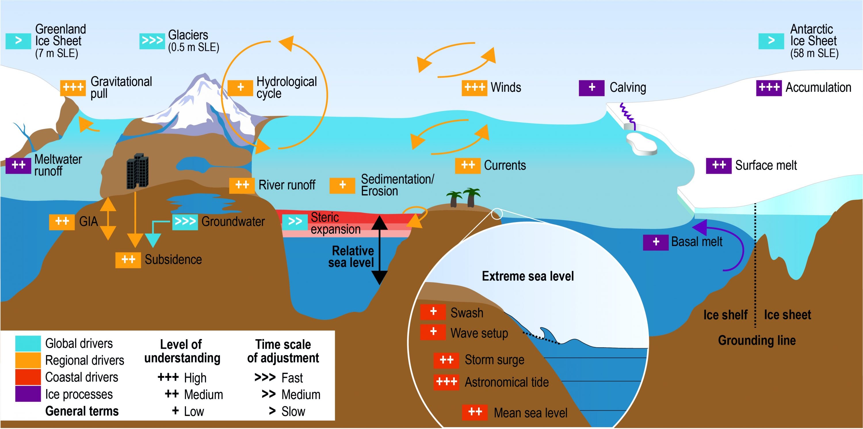
Figure 4.4 | A schematic illustration of the climate and non-climate driven processes that can influence global, regional (green colours), relative and extreme sea level (ESL) events (red colours) along coasts. Major ice processes are shown in purple and general terms in black. SLE stands for Sea Level Equivalent and reflects the increase in GMSL if the mentioned ice mass is melted completely and added to the ocean.
4.2.2.1
Global Mean Sea Level Changes During the Instrumental Period
Observational estimates of the sea level variations over past millennia rely essentially on proxy-based regional relative sea level reconstructions corrected for GIA. Since AR5, the increasing availability of regional proxy-based reconstructions enables the estimation of GMSL change over the last ∼3 kyr. The first statistical integration of the available reconstructions shows that the GMSL experienced variations of ±9 [±7 to ±11] cm (5–95% uncertainty range; Kopp et al., 2016110) over the 2400 years preceding the 20th century (medium confidence). This is more tightly bound than the AR5 assessment which indicated a variability in GMSL that was <±25 cm over the same period. This progress since AR5 confirms that it is virtually certain that the mean rate of GMSL has increased during the last two centuries from relatively low rates of change during the late Holocene (order tenths of mm yr–1) to modern rates (order mm yr–1; Woodruff et al., 2013111).
Over the last two centuries, sea level observations have mostly relied on tide gauge measurements. These records, beginning around 1700 in some locations (Holgate et al., 2012112; PSMSL, 2019113), provide insight into historic sea level trends. Since 1992, the emergence of precise satellite altimetry has advanced our knowledge on GMSL and regional sea level changes considerably through a combination of near global ocean coverage and high spatial resolution. It has also enabled more detailed monitoring of land ice loss. Since 2002, high precision gravity measurements provided by the Gravity Recovery and Climate Experiment (GRACE) and GRACE Follow-On missions show the loss of land ice in Greenland and Antarctica, and confirm independent assessments of ice sheet mass changes based on satellite altimetry (Shepherd et al., 2012114; The Imbie team, 2018) and InSAR measurements combined with ice sheet SMB estimates (Noël et al., 2018115; Rignot et al., 2019116). Since 2006, when the array of Argo profiling floats reached near-global coverage, it has been possible to get an accurate estimate of the ocean thermal expansion (down to 2000 m depth) and test the closure of the sea level budget. The combined analysis of the different observing systems that are available has improved significantly the understanding of the magnitude and relative contributions of the different processes causing sea level change. In particular, important progress has been achieved since AR5 on estimating and understanding the increasing contribution of the ice sheets to SLR.
4.2.2.1.1
Tide gauge records
The number of tide gauges has increased over time from only a few in northern Europe in the 18th century to more than 2000 today along the world’s coastlines. Because of their location and limited number, tide gauges sample the ocean sparsely and non-uniformly with a bias towards the Northern Hemisphere. Most tide gauge records are short and have significant gaps. In addition, tide gauges are anchored on land and are affected by the vertical motion of Earth’s crust caused by both natural processes (e.g., GIA, tectonics and sediment compaction; Wöppelmann and Marcos, 2016117; Pfeffer et al., 2017118) and anthropogenic activities (e.g., groundwater depletion, dam building or settling of landfill in urban areas; Raucoules et al., 2013119; Pfeffer et al., 2017120). When estimating the GMSL due to the ocean thermal expansion and land ice melt, tide gauges must be corrected for this VLM, where VLM = GIA + anthropogenic subsidence + (tectonics, natural subsidence). This is possible with stations of the Global Positioning System (GPS) network when they are co-located with tide gauges (Santamaría-Gómez et al., 2017121; Kleinherenbrink et al., 2018122). However, this approach provides information on the VLM over the past two to three decades and has limited value over longer time scales for places where the VLM has varied significantly through the last century (Riva et al., 2017123).
AR5 assessed the different strategies to estimate the 20th century GMSL changes. These strategies only accounted for the inhomogeneous space and time coverage of tide gauge data and for the VLM induced by GIA (Figure 4.5). Since AR5 two new approaches have been developed. The first one uses a Kalman smoother which combines tide gauge records with the spatial patterns associated with ocean dynamic change, change in land ice and GIA. It enables accounting for the inhomogeneous distribution of tide gauges and the VLM associated with both GIA and current land ice loss (Hay et al., 2015124; Figure 4.5). The second approach uses ad hoc corrections to tide gauge records with an additional spatial pattern associated with changes in terrestrial water storage to account for the inhomogeneous distribution in tide gauges. It also accounts for the total VLM (Dangendorf et al., 2017125; Figure 4.5). Both methods yield significantly lower GMSL changes over the period 1950–1970 than previous estimates, leading to long-term trends since 1900 that are smaller than previous estimates by 0.4 mm yr–1 (Figure 4.5). Different arguments including biases in the tide gauge datasets (Hamlington and Thompson, 2015126), biases in the averaging technique and absence of VLM correction (Dangendorf et al., 2017127), or in the spatial patterns associated with the sea level contributions (Hamlington et al., 2018128) have been proposed to explain these smaller GMSL rates. There is no agreement yet on which is the primary reason for the differences and it is not clear whether all the reasons invoked can actually explain all the differences across reconstructions. As there is no clear evidence to discard any reconstruction, this assessment considers the ensemble of AR5 sea level reconstructions augmented by the two recent reconstructions from Hay et al. (2015)129 and Dangendorf et al. (2017)130 to evaluate the GMSL changes over the 20th century. On this basis, it is estimated that it is very likely that the long-term trend in GMSL estimated from tide gauge records is 1.5 (1.1–1.9) mm yr–1 between 1902 and 2010 for a total SLR of 0.16 (0.12–0.21) m (see also Table 4.1). This estimate is consistent with the AR5 assessment (but with an increased uncertainty range) and confirms that it is virtually certain that GMSL rates over the 20th century are several times as large as GMSL rates during the late Holocene (see 4.2.2.1). Over the 20th century the GMSL record also shows an acceleration (high confidence) as now four out of five reconstructions extending back to at least 1902 show a robust acceleration (Jevrejeva et al., 2008131; Church and White, 2011132; Ray and Douglas, 2011133; Haigh et al., 2014b134; Hay et al., 2015135; Watson, 2016136; Dangendorf et al., 2017137). The estimates of the acceleration ranges between -0.002–0.019 mm yr–1 over 1902–2010 are consistent with AR5.
4.2.2.1.2
Satellite altimetry
High precision satellite altimetry started in October 1992 with the launch of the TOPEX/Poseidon and Jason series of spacecraft. Since then, 11 satellite altimeters have been launched providing nearly global sea level measurements (up to ±82° latitude) over more than 25 years. Six groups (AVISO/CNES, SL_cci/ESA, University of Colorado, CSIRO, NASA/GSFC, NOAA; Nerem et al., 2010;138 Henry et al., 2014139; Leuliette, 2015140; Watson et al., 2015141; Beckley et al., 2017142; Legeais et al., 2018143) provide altimetry-based GMSL time series. Since AR5, several studies using two independent approaches based on tide gauge records (Watson et al., 2015144) and the sea level budget closure (Chen et al., 2017145; Dieng et al., 2017146) identified a drift of 1.5 (0.4–3.4) mm yr–1 in TOPEX A from January 1993 to February 1999. Accounting for this drift leads to a revised GMSL rate from satellite altimetry of 3.16 (2.79–3.53) for 1993–2015 (WCRP Global Sea Level Budget Group, 2018147; see Table 4.1) compared to 3.3 mm yr–1 (2.7–3.9) for 1993–2010 in AR5. Compared to AR5, the revised satellite altimetry GMSL estimates now show with high confidence an acceleration of 0.084 (0.059–0.090) mm yr–1 over 1993–2015 (5–95% uncertainty range; Watson et al., 2015148; Nerem et al., 2018149). This acceleration is due to an increase in Greenland mass loss since the 2000s (Chen et al., 2017150; Dieng et al., 2017151) and a slight increase in all other contributions probably partly due to the recovery from the Pinatubo volcanic eruption in 1991 (Fasullo et al., 2016152) and partly due to increased GHG concentrations e.g., (Slangen et al., 2016153; high confidence). The current sea level rise is 3.6 ± 0.3 mm yr–1 over 2006–2015 (90% confidence level). This is the highest rate measured by satellite altimetry (Ablain et al., 2019154; medium confidence). Before the satellite altimetry era, the highest rate of sea level rise recorded was reached during the period 1935–1944. It amounted 2.5 ± 0.7 mm yr–1 (estimate at the 90% confidence level from sea level reconstructions; Church and White, 2011155; Ray and Douglas, 2011156; Jevrejeva et al., 2008157; Hay et al., 2015158; Dangendorf et al., 2017159). This is expected to be smaller than the current rate of sea level rise, making the current sea level rise the highest on instrumental record (medium confidence).
4.2.2.2
Contributions to Global Mean Sea Level Change During the Instrumental Period
The different contributions to the GMSL rise are independently observed over various time scales. They are compared with simulated estimates from climate model experiments of CMIP5 (Taylor et al., 2012160) when available (see Table 4.1). The observations are compared with experiments beginning in the mid-19th century, forced with past time-dependent anthropogenic changes in atmospheric composition, natural forcings due to volcanic aerosols and variations in solar irradiance (Taylor et al., 2012161). The objective is first, to assess understanding of the causes of observed sea level changes and second, to evaluate the ability of coupled climate models to simulate these causes. It enables the evaluation of the confidence level there is in current coupled climate models that form the basis of future sea level projections.
4.2.2.2.1
Thermal expansion contribution
The ocean thermal expansion is caused by excess heat being absorbed by the ocean, as the climate warms. Thermal expansion is estimated from in situ ocean observations and ocean heat content reanalyses that rely on assimilation of data into numerical models (Storto et al., 2017162; Sections 1.8.1.1 and 1.8.1.4; WCRP Global Sea Level Budget Group, 2018163). Full-depth, high-quality and unbiased ocean temperature profile data with adequate metadata and spatio-temporal coverage are required to estimate thermal expansion and to understand drivers of variability and long-term change (Pfeffer et al., 2018164; Section 5.2.2.2.2).
Historically, however, observational gaps exist and some ocean regions remain under-sampled to date (Sections 1.8.1.1 and 5.2.2.2.2; Figure 1.3; Appendix 1.A, Figure 1.1). Other factors also introduce uncertainty in estimates of thermal expansion like changes in instrumentation, systematic instrumental errors, changes in the quality control of the data and the mapping method used to produce regular grids (Section 5.2.2.2.2; Palmer et al., 2010165). In the upper 700 m, the largest sources of uncertainty for estimates of global mean thermal expansion from 1970 to 2004 are the choice of mapping methods (Boyer et al., 2016166), followed by the choice of bias correction for the bathythermographic observations (Cheng et al., 2016167; Section 5.2.2.2.2). From 2006 onwards, the uncertainty is considerably reduced (Roemmich et al., 2015168; von Schuckmann et al., 2016169; Wijffels et al., 2016170), because the Argo array reached its targeted near-global (up to ±60° latitude) coverage for the upper 2000 m in November 2007 (Riser et al., 2016171; Section 5.2.2.2.2).
Since AR5, in a community effort, the (WCRP Global Sea Level Budget Group, 2018172) revisited the global mean thermal expansion estimates based on observations only. On the basis of a full-depth 13-member ensemble of global mean thermal expansion time series developed with the latest data and corrections available, they estimated that the global thermal expansion was 1.40 (1.08–1.72) mm yr–1 for 2006–2015, 1.36 (0.96–1.76) mm yr–1 for 1993–2015 (see Table 4.1). While the relative contribution of the upper 300 m did not change (~70%) between 2006–2015 and 1993–2015, the 700–2000 m contribution increased around 10% over the Argo decade (2006–2015), when observations for that depth interval soared (Figure 1.3; Appendix 1.A, Figure 1.1). This suggests that observed changes for 700–2000 m may have been underestimated for 1993–2005. Before 1993, estimates are based on a smaller ensemble of 4 datasets in which no thermal expansion is assumed below 2000 m because of lack of data (see Section 5.2.2.2.2 for more details). This ensemble shows a thermal expansion linear rate of 0.89 (0.84–0.94) mm yr–1 for 1970–2015 (see Table 4.1).
Coupled climate models simulate the historical thermal expansion (see Table 4.1). However, for models that omit the volcanic forcing in their control experiment, the imposition of the historical volcanic forcing during the 20th century results in a spurious time mean negative forcing and a spurious persistent ocean cooling related to the control climate (Gregory, 2010173; Gregory et al., 2013174). Since AR5, the magnitude of this effect has been estimated from historical simulations forced by only natural radiative forcing. Then it has been used to correct the historical simulations forced with the full 20th century forcing (Slangen et al., 2016187; Slangen et al., 2017b188). The resulting ensemble mean of simulated thermal expansion provides a good fit to the observations within the uncertainty ranges of both models and observations (Slangen et al., 2017b189; Cheng et al., 2019190; Table 4.1). The spread, which is essentially due to uncertainty in radiative forcing and uncertainty in the modelled climate sensitivity and ocean heat uptake efficiency (Melet and Meyssignac, 2015191), is still larger than the observational uncertainties (Gleckler et al., 2016192; Cheng et al., 2017193; Table 4.1). Compared to AR5, the availability of improved observed and modelled estimates of thermal expansion and the good agreement between both confirm the high confidence level in the simulated thermal expansion using climate models and the high confidence level in their ability to project future thermal expansion.
Table 4.1
Global mean sea level (GMSL) budget over different periods from observations and from climate model base contributions. All values are in mm yr–1. Values in brackets in 4.2 are uncertainties ranging from 5–95%. The climate model historical simulations end in 2005; projections for Representative Concentration Pathway (RCP)8.5 are used for 2006–2015. The modelled thermal expansion, glacier and ice sheet surface mass balance (SMB) contributions are computed from the Coupled Model Intercomparison Project Phase 5 (CMIP5) models as in Slangen et al. (2017b). For the model contributions, uncertainties are estimated from the spread of the ensemble of model simulations following Slangen et al. (2017b), see the footnotes for the details on the uncertainty propagation. GIS is Greenland Ice Sheet.
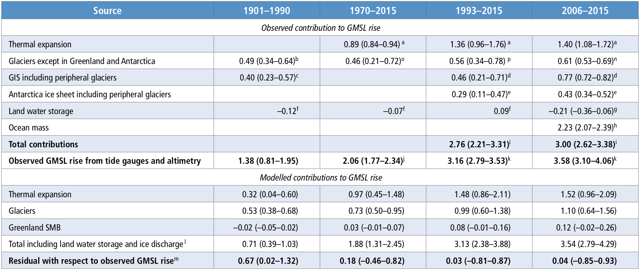
4.2.2.2.2
Ocean mass observations from GRACE and GRACE Follow-On
The ocean mass changes correspond to the sum of land ice and terrestrial water storage changes. Since 2002, the GRACE and GRACE follow-on missions provide direct estimates of the ocean mass changes and thus they provide an independent estimate of the sum of land ice and terrestrial water storage contributions to sea level. Since AR5, GRACE-based estimates of the ocean mass rates are increasingly consistent (WCRP Global Sea Level Budget Group, 2018194) because of the extended length of GRACE missions’ observations (over 15 years), the improved understanding of data and methods for addressing GRACE limitations (e.g., noise filtering, leakage correction and low-degree spherical harmonics estimates), and the improved knowledge of geophysical corrections applied to GRACE data (e.g., GIA). The most recent estimates (Dieng et al., 2015b195; Reager et al., 2016196; Rietbroek et al., 2016197; Chambers et al., 2017198; Blazquez et al., 2018199; Uebbing et al., 2019200) report a global ocean mass increase of 1.7 (1.4–2.0) mm yr–1 over 2003–2015 (see also Table 4.1). The uncertainty arises essentially from differences in the inversion method to compute the ocean mass (Chen et al., 2013201; Jensen et al., 2013202; Johnson and Chambers, 2013204; Rietbroek et al., 2016205), uncertainties in the geocentre motion and uncertainty in the GIA correction (Blazquez et al., 2018205; Uebbing et al., 2019206). The consistency between estimates of the global mean ocean mass on a monthly time scale has also increased since AR5.
4.2.2.2.3
Glaciers
To assess the mass contribution of glaciers to sea level change, global estimates are required. Recent updates and temporal extensions of estimates obtained by different methods continue to provide very high confidence in continuing glacier mass loss on the global scale during the past decade (Bamber et al., 2018207; Wouters et al., 2019; Zemp et al., 2019208), see Section 2.2.3 and Appendix 2.A for a detailed discussion also on regional scales). Updates of the reconstructions of Cogley (2009)210, Leclercq et al. (2011)211 and Marzeion et al. (2012)212, presented and compared in Marzeion et al. (2015)212, show increased agreement on rates of mass loss during the entire 20th century (Marzeion et al., 2015213), compared to earlier estimates reported by AR5. The contribution of glaciers that may be missing in inventories or have already melted during the 20th century is hard to constrain (Parkes and Marzeion, 2018215), and there is low confidence in their estimated contribution. These glaciers are thus neglected in the assessment of the sea level budget (Table 4.1).
While the agreement between the observational estimates of glacier mass changes and the modelled estimates from glacier models forced with climate model simulations has increased since AR5 (Slangen et al., 2017b216), there is only medium confidence in the use of glacier models to reconstruct sea level change because of the limited number of well-observed glaciers available to evaluate models on long time scales, and because of the small number of model-based global glacier reconstructions.
4.2.2.2.4
Greenland and Antarctic ice sheets
Frequent observations of ice sheet mass changes have only been available since the advent of space observations (see Section 3.3.1). In the pre-satellite era, mass balance was geodetically reconstructed only for the GIS (Kjeldsen et al., 2015217). These geodetic reconstructions empirically constrain the contribution of the GIS to SLR between 1900 and 1983 to 17.2 (10.7–23.2; Kjeldsen et al., 2015218). During the satellite era, three approaches have been developed to estimate ice sheet mass balance: 1) Mass loss is estimated by direct measurements of ice sheet height changes with satellite laser or radar altimetry in combination with climatological/glaciological models for firn density and compaction, 2) the input–output method combines measurements of ice flow velocities estimated from satellite (synthetic aperture radar or optical imagery) across key outlets with estimates of net surface balance derived from ice thickness data, 3) space gravimetry data yields direct estimate of the mass changes by inversion of the anomalies in the gravity field (see Section 3.3.1 for more details). AR5 concluded that the three space-based methods give consistent results. They agree in showing that the rate of SLR due to the GIS and AIS’ contributions has increased since the early 1990s. Since AR5, up-to-date observations confirm this statement with increased confidence for both ice sheets (Rignot et al., 2019219; see Section 3.3.1). The assessment of the literature since AR5 made in Section 3.3.1 shows that the contribution from Greenland to SLR over 2012–2016 (0.68 (0.64–0.72) mm yr–1) was similar to the contribution over 2002–2011 (0.73 (0.67–0.79) mm yr–1) and extremely likely greater than over 1992–2001 (0.02 (0.21–0.25) mm yr–1). The contribution from Antarctica over 2012–2016 (0.55 (0.48–0.62) mm yr–1) was extremely likely greater than over the 2002–2011 period (0.23 (0.16–0.30) mm yr–1) and likely greater than over the period 1992–2001 (0.14 (0.12–0.16); see Section 3.3.1 for more details).
Here, the approach of Section 3.3.1 is followed, using the two multi-method assessments from Bamber et al. (2018)220 and the IMBIE team (2018) to evaluate the contribution of ice sheet mass loss to SLR over 1993–2015 and 2006–2015 (see Table 4.1). These two studies agree with results from the WCRP Global Sea Level Budget Group (2018). For the estimation of the AIS contribution, Bamber et al. (2018)221 and the The IMBIE team (2018) use similar but not identical data sources and processing. Both studies find consistent results within uncertainties over both periods. In Table 4.1, the results of these two studies were averaged, and weighted the average on the basis of their uncertainties, because there is no apparent reason to discount either study. For the estimation of the GIS contribution only the Bamber et al. (2018)222 estimate is used, as there is no other multi-method assessment available.
4.2.2.2.5
Contributions from water storage on land
Water is stored on land not only in the form of ice but snow, surface water, soil moisture and groundwater. Temporal changes in land water storage, defined as all forms of water stored on land excluding land ice, contribute to observed changes in ocean mass and thus sea level on annual to centennial time scales (Döll et al., 2016225; Reager et al., 2016226; Hamlington et al., 2017227; Wada et al., 2017228). They are caused by both climate variability and direct human interventions, at the multi-decadal to centennial time scales. Over the past century, the main cause for land water storage changes are the groundwater depletion and impoundment of water behind dams in reservoirs (Döll et al., 2016229; Wada et al., 2016230). While the rate of groundwater depletion and thus its contribution to SLR increased during the 20th century and up to today (Wada et al., 2016231), its effect on sea level was more than balanced by the increase in land water storage due to dam construction between 1950 and 2000 (Wada et al., 2016232). Since about 2000, based on hydrological models, the combined effect of both processes is a positive contribution to SLR (Wada et al., 2016233). Decreased water storage in lakes, wetlands and soils due to human activities are less important for ocean mass changes (Wada et al., 2016234). Overall, the integrated effects of the direct human intervention on land hydrology have reduced land water storage during the last decade, increasing the rate of SLR by 0.15–0.24 mm yr–1 (Wada et al., 2016235; Wada et al., 2017236; Scanlon et al., 2018237; WCRP Global Sea Level Budget Group, 2018238). Over periods of a few decades, land water storage was affected significantly by climate variability (Dieng et al., 2015a239; Reager et al., 2016240; Dieng et al., 2017241). Net land water storage change driven by both climate and direct human interventions can be determined based on GRACE observations and global hydrological modelling. They indicate different estimates of the rate of SLR. Over the period 2002–2014 GRACE-based estimates of the net land water storage (i.e., not including glaciers) show a negative contribution to sea level (e.g., Scanlon et al., 2018) resulting in the negative value after 2006 in Table 1while hydrological models determined a slightly positive one. The reasons for this difference between estimates are not elucidated. There is scientific consensus that uncertainties of both net land water storage contribution to sea level and its individual contributions remain high (WCRP Global Sea Level Budget Group, 2018242). The differences in estimates and the lack of multiple consistent studies give low confidence in the net land water storage contribution to current SLR.
4.2.2.2.6
Budget of global mean sea level change
Drawing on previous sections, the budget of GMSL rise (Table 4.1, Figure 4.5) is assessed with observations over 4 periods: 1901–1990 (which corresponds to the period in the 20th century that is prior to the increase in ice sheet contributions to GMSL rise), 1970–2015 (when ocean observations are sufficiently accurate to estimate the global ocean thermal expansion and when glacier mass balance reconstructions start), 1993–2015 (when precise satellite altimetry is available) and 2006–2015 (when GRACE data is available in addition to satellite altimetry and when the Argo network reaches a near-global coverage). The budget of GMSL rise is also assessed with sea level contributions simulated by climate models over the same periods (Table 4.1, Figure 4.5). The periods 1993–2015 and 2006–2015 are only 23 and 10 years long respectively, short enough so that they can be affected by internal climate variability. Therefore, it is not expected that observations over these periods will be precisely reproduced by climate model historical experiments. For the contribution from land water storage, the estimated effect of direct human intervention was used, neglecting climate-related variations until 2002 (Ngo‐Duc et al., 2005). From 2002 to 2015, total land water storage estimated with GRACE was used. In general, historical simulations of climate models end in 2005. Historical simulations were extended here to 2015 using the RCP8.5 scenario. This choice of RCP scenario is not critical for the simulated sea level, as the different scenarios only start to diverge significantly after the year 2030 (Church et al., 2013243).
For 1993–2015 and 2006–2015, the observed GMSL rise is consistent within uncertainties with the sum of the estimated observed contributions (Table 4.1). Over the period 1993–2015 the two largest terms are the ocean thermal expansion (accounting for 43% of the observed GMSL rise) and the glacier mass loss (accounting for a further 20%). Compared to AR5, the extended observations corrected for the TOPEX-A drift (see Section 4.2.2.1.2) allow us now to identify an acceleration in the observed SLR over 1993–2015 and to attribute this acceleration mainly to Greenland ice loss along with an acceleration in Antarctic ice loss (Velicogna et al., 2014244; Harig and Simons, 2015245; Chen et al., 2017246; Dieng et al., 2017247; Yi et al., 2017248; see also Sections 4.2.2.2.2, 4.2.2.3.4, 3.3.1). Since 2006, land ice, collectively from glaciers and the ice sheets has become the most important contributor to GMSL rise over the thermal expansion with mountain glaciers contributing 20% and ice sheets 33% (see Table 4.1). Over the periods 1993–2015, the sum of the observed sea level contributions is consistent with the total observed sea level within uncertainties at monthly-scales (not shown, e.g., Dieng et al., 2017). This is also true for the period 2006–2015, when uncertainties are significantly smaller. This agreement at monthly time scales represents a significant advance since the AR5 in physical understanding of the causes of past GMSL change. It provides an improved basis for the evaluation of models. Given these elements there is high confidence that the current observing system is capable of resolving decadal to multidecadal changes in GMSL and its components (with an uncertainty of <0.7 mm yr–1 at decadal and longer time scales, see Table 4.1 and for example, WCRP Global Sea Level Budget Group, 2018). However, despite this advance since AR5 there are still no comprehensive observations of ocean thermal expansion below 2000 m, in regions covered by sea ice and in marginal seas. The understanding of glacier mass loss can be improved at regional scale and the understanding of the land water storage contribution is still limited. Thus, for smaller changes in sea level of the order of a few tenths of a mm yr–1 at decadal time scales and shorter time scales there is medium confidence in the capability of the current observing system to resolve them (e.g., WCRP Global Sea Level Budget Group, 2018).
Before 1992, observations are not sufficient to confidently estimate the ice sheet mass balance and before 1970, the space and time sampling of ocean observations are not sufficient to estimate the global ocean thermal expansion. For these reasons, it is difficult to assess the closure of the GMSL rise budget over 1901–1990 and 1970–2015 (Church et al., 2013249; Gregory et al., 2013250; Jevrejeva et al., 2017251; Meyssignac et al., 2017c252; Slangen et al., 2017b253; Parkes and Marzeion, 2018254). For the period 1970–2015, the thermal expansion of the ocean represents 43% of the observed GMSL rise while the glaciers’ contribution represents 22% (see Table 4.1). This result indicates a slightly smaller contribution from glaciers than reported by AR5. If the GIS contribution and the Antarctic SMB is added, then the sum of the contributors to sea level is in agreement with the low end observed SLR estimates over 1970–2015 (Frederikse et al., 2018255). This result suggests that the contribution of Antarctica ice sheet dynamics to SLR has been small, if any, before the 1990s.
Since AR5, extended simulations along with recent findings in observations and improved model estimates allow for a new more robust, consistent and comprehensive comparison between sea level estimates based on observations and climate model simulations (e.g., Meyssignac et al., 2017c; Slangen et al., 2017b256; Parkes and Marzeion, 2018257). Compared to AR5, the simulated thermal expansion from climate models has improved with a new correction for the volcanic activity (see Section 4.2.2.2.1). The glacier contribution from glacier models forced with inputs from climate models is updated with a new glacier inventory and improvements to the glacier mass balance model (Marzeion et al., 2015258). The simulated Greenland SMB is estimated with a new regional SMB-component downscaling technique, which accounts for the regional variations in components of the Greenland SMB (Noël et al., 2015259; Meyssignac et al., 2017a)260. In addition, an updated groundwater extraction contribution from Döll et al. (2014)261 is now used for the land water storage contribution.
For the periods 1970–2015, 1993–2015 and 2006–2015 the simulated contributions from thermal expansion, glaciers mass loss and Greenland SMB explain respectively 84%, 81% and 77% of the observed GMSL (see Table 4.1). For all these periods the residual is consistent within uncertainty with the sum of the contribution from land water storage and ice discharge from Greenland and Antarctica. For each period the consistency is improved compared to AR5 (see Table 4.1) although the uncertainty on the residual is slightly larger because of a larger uncertainty in simulated Glaciers and Greenland SMB contributions.
For the period 1901–1990 the simulated contributions from thermal expansion, glaciers mass loss and Greenland SMB explain only 60% of the observed GMSL and the residual is too large to be explained by the sum of the contribution from land water storage and ice discharge from Greenland and Antarctica. The gap can be explained by a bias in the simulated Greenland SMB and glacier ice loss around Greenland in the early 20th century (Slangen et al., 2017b262). When the glacier model and the Greenland SMB downscaling technique are forced with observed climate from atmospheric reanalyses, rather than the simulated climate from coupled climate models, simulated SLR becomes consistent with the observed SLR (see the dashed blue line on Figure 4.5). This is because atmospheric reanalyses show an increase in air temperatures in and around Greenland over the period 1900–1940, which lead to increased melt in Greenland (Bjørk et al., 2012267; Fettweis et al., 2017268) and surrounding glaciers in the first half of the 20th century. This increase in air temperature over 1900–1940 is not reproduced by climate models (Slangen et al., 2017b269). It may be because this increase in air temperature was due to internal climate variability on temporal and spatial scales that cannot be precisely reproduced by climate models. It may also be due to a bias in atmospheric circulation in climate models (Fettweis et al., 2017270), or an issue with the spatial pattern of the historical aerosol forcing.
In summary, the agreement between climate model simulations and observations of the global thermal expansion, glacier mass loss and Greenland SMB has improved compared to AR5 for periods starting after 1970. However, for periods prior to 1970, significant discrepancies between climate models and observations arise from the inability of climate models to reproduce some observed regional changes in glacier and GIS SMB around the southern tip of Greenland. It is not clear whether this bias in climate models is due to the internal variability of the climate system or deficiencies in climate models. For this reason, there is still medium confidence in the ability of climate models to simulate past and future changes in glaciers mass loss and Greenland SMB.
Figure 4.5
Figure 4.5 | Comparison of simulated (by coupled climate models as in Section 4.4.2.6) and observed global mean sea level change (GMSL) since 1901 (a) and since 1993 (b). The average estimate of 12 Coupled Model Intercomparison Project Phase 5 (CMIP5) climate model simulations is shown in blue with the 5–95% uncertainty range shaded in […]
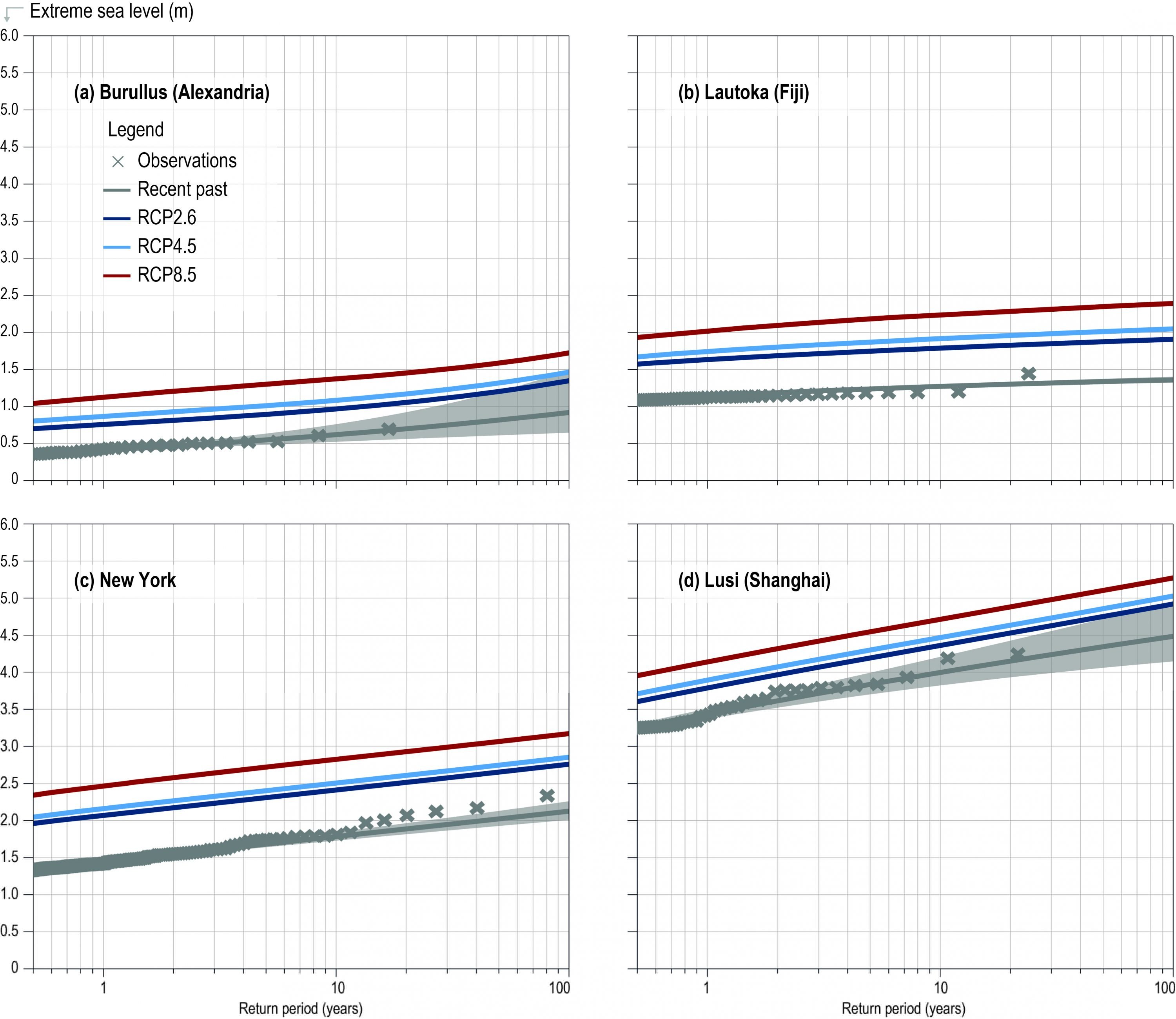
Figure 4.5 | Comparison of simulated (by coupled climate models as in Section 4.4.2.6) and observed global mean sea level change (GMSL) since 1901 (a) and since 1993 (b). The average estimate of 12 Coupled Model Intercomparison Project Phase 5 (CMIP5) climate model simulations is shown in blue with the 5–95% uncertainty range shaded in blue and calculated according to the procedures in Church et al. (2013)263. The average of the 12 model estimates corrected for the bias in glaciers mass loss and Greenland surface mass balance (SMB) over 1900–1940 (see Section 4.2.2.2.6) is shown in dashed blue. The estimates from tide gauge reconstructions is shown in other colours in panel a), with the 5–95% uncertainty range shaded in grey. The satellite altimetry observations from Legeais et al. (2018)264 is shown in black in panel b). GMSL from altimetry corrected for the TOPEX-A drift (Watson et al., 2015265) in orange as well as the tide gauge reconstruction. The 5–95% uncertainty range is shaded in orange (Ablain et al., 2015266). All curves in (a) represent anomalies in sea level with respect to the period 1986–2005 (i.e., with zero time-mean over the period 1986–2005) in order to be consistent with sea level projections in Section 4.2.3. Vertical lines indicate the occurrence of major volcanic eruptions, which cause temporary drops in GMSL. Updated from Slangen et al. (2017b).
4.2.2.3
Regional Sea Level Changes During the Instrumental Period
Sea level does not rise uniformly. Observations from tide gauges and satellite altimetry (Figure 4.6) indicate that sea level shows substantial regional variability at decadal to multi-decadal time scales (e.g., Carson et al., 2017; Hamlington et al., 2018271). These regional changes are essentially due to changing winds, air-sea heat and freshwater fluxes, atmospheric pressure loading and the addition of melting ice into the ocean, which alters the ocean circulation (Stammer et al., 2013272; Forget and Ponte, 2015273; Meyssignac et al., 2017b274). The addition of water into the ocean also change the geoid, alter the rotation of the Earth and deform the ocean floor which in turn change sea level (e.g., Tamisiea, 2011; Stammer et al., 2013275).
Sea level is rising in all ocean basins (virtually certain; Legeais et al. 2018276). Part of this regional sea level rise is due to global sea level rise of which a majority is attributable to anthropogenic greenhouse gas emissions (high confidence; Slangen et al. 2016277). The remaining part of the regional sea-level rise in ocean basins is a combination of the response to anthropogenic GHG emissions and internal variability (e.g., Stammer et al. 2013; medium confidence).
In the open ocean, the spatial variability and trends in sea level observed during the recent altimetry era or reconstructed over the previous decades are dominated by the thermal expansion of the ocean. In shallow shelf seas and at high latitudes (>60°N and <55°S), the effect of dynamic mass redistribution becomes important. At local scale, salinity changes can also generate sizeable changes in the ocean density similar to thermal expansion and lead to significant variability in sea level (Forget and Ponte, 2015278; Meyssignac et al., 2017b279). On global average, the heat and freshwater fluxes from the atmosphere into the ocean are responsible for the total heat that enters the ocean and for the associated GMSL rise. At regional scale and local scale, both the ocean transport divergences caused by wind stress anomalies and the spatial variability in atmospheric heat fluxes are responsible for the spatial variability in thermal expansion and thus for most of the regional sea level departures around the GMSL rise (e.g., Stammer et al., 2013; Forget and Ponte, 2015280).
Over the Pacific, the surface wind anomalies responsible for the sea level spatio-temporal variability are associated with the ENSO, Pacific Decadal Oscillation (PDO) and North Pacific Gyre Oscillation modes (Hamlington et al., 2013281; Moon et al., 2013282; Palanisamy et al., 2015283; Han et al., 2017284). In the Indian Ocean they are associated with the ENSO and Indian Ocean Dipole (IOD) modes (Nidheesh et al., 2013285; Han et al., 2014286; Thompson et al., 2016287; Han et al., 2017288). In particular, the PDO is responsible for most of the intensified SLR that has been observed in the western tropical Pacific Ocean since the 1990s (Moon et al., 2013289; Han et al., 2014290; Thompson and Mitchum, 2014291). Several studies suggested that in addition to the PDO signal, warming of the tropical Indian and Atlantic Oceans enhanced surface easterly trade winds and thus also contributes to the intensified SLR in the western tropical Pacific (England et al., 2014292; Hamlington et al., 2014293; McGregor et al., 2014294).
Over the Atlantic, the regional sea level variability at interannual to multi-decadal time scales, is generated by surface wind anomalies and heat fluxes associated with the North Atlantic Oscillation (NAO; Han et al., 2017295) and also by ocean heat transport due to changes in the Atlantic Meridional Overturning Circulation (AMOC; McCarthy et al., 2015296). Both mechanisms are not independent as heat fluxes and wind stress anomalies associated with NAO can induce changes in the AMOC (Schloesser et al., 2014297; Yeager and Danabasoglu, 2014298). In the Southern Ocean, the sea level variability is dominated by the SAM influence in particular in the Indian and Pacific sectors. The Southern Annular Mode (SAM) influence becomes weaker equator-wards in these sectors while the influence of PDO, ENSO and IOD increases (Frankcombe et al., 2015299). In the southern ocean, the zonal asymmetry in westerly winds associated to the SAM, generates convergent and divergent transport in the Antarctic Circumpolar Current which may have contributed to the regional asymmetry of decadal sea level variations during most of the twentieth century (Thompson and Mitchum, 2014300).
As for GMSL, net regional sea level changes can be estimated from a combination of the various contributions to sea level change. The contributions from dynamic sea level, atmospheric loading, glacier mass changes and ice sheet SMB can be derived from CMIP5 climate model outputs either directly or through downscaling techniques (Perrette et al., 2013301; Kopp et al., 2014302; Slangen et al., 2014a303; Bilbao et al., 2015304; Carson et al., 2016305; Meyssignac et al., 2017a306). The contributions from groundwater depletion, reservoir storage and dynamic ice sheet mass changes are not simulated by coupled climate models over the 20th century and have to be estimated from observations. The sum of all contributions, including the GIA contribution, provides a modelled estimate of the 20th century net regional sea level changes that can be compared with observations from satellite altimetry and tide-gauge records (see Figure 4.6).
In terms of interannual to multi-decadal variability, there is a general agreement between the simulated regional sea level and tide gauge records, over the period 1900–2015 (see inset figures in Figure 4.6). The relatively large, short-term oscillations in observed sea level (black lines in insets in Figure 4.6), which are due to the natural internal climate variability, are included in general within the modelled internal variability of the climate system represented by the blue shaded area (5–95% uncertainty). But, as for GMSL, climate models tend to systematically underestimate the observed sea level trends from tide gauge records, particularly in the first half of the 20th century. This underestimation is explained by a bias identified in modelled Greenland SMB, and glacier ice loss around Greenland in the early 20th century (see Section 4.2.2.2.6; Slangen et al., 2017b307). The correction of this bias improves the agreement between the spatial variability in sea level trends from observations and from climate models (see Figure 4.6). Climate models indicate that the spatial variability in sea level trends observed by tide-gauge records over the 20th century is dominated by the GIA contribution and the thermal expansion contribution over 1900–2015. Locally all contributions to sea level changes are important as any contribution can cause significant local deviations. Around India for example, groundwater depletion is responsible for the low 20th century SLR (because the removal of groundwater mass generated a local decrease in geoid that made local SLR slower; Meyssignac et al., 2017c308)
These results show the ability of models to reproduce the major 20th century regional sea level changes due to GIA, thermal expansion, glacier mass loss and ice sheet SMB. This is tangible progress since AR5. But some doubts remain regarding the ability of climate models to reproduce local variations such as the glaciers and the Greenland SMB contributions to sea level in the region around the southern tip of Greenland (Slangen et al., 2017b309) or such as the thermal expansion in some eddy active regions (Sérazin et al., 2016310). Because of these doubts there is still medium confidence in climate models to project future regional sea level changes associated with thermal expansion, glacier mass loss and ice sheet SMB. Coupled climate models have not simulated the other contributions to 20th century sea level, including the growing ice sheet dynamical contribution and land water storage changes.
Figure 4.6
Figure 4.6 | 20th century simulated regional sea level changes by coupled climate models and comparison with a selection of local tide gauge time series. In the upper left corner: map of changes in simulated relative sea level (RSL) for the period 1901–1920 to 1996–2015 estimated from climate model outputs. Insets: Observed RSL changes (black […]
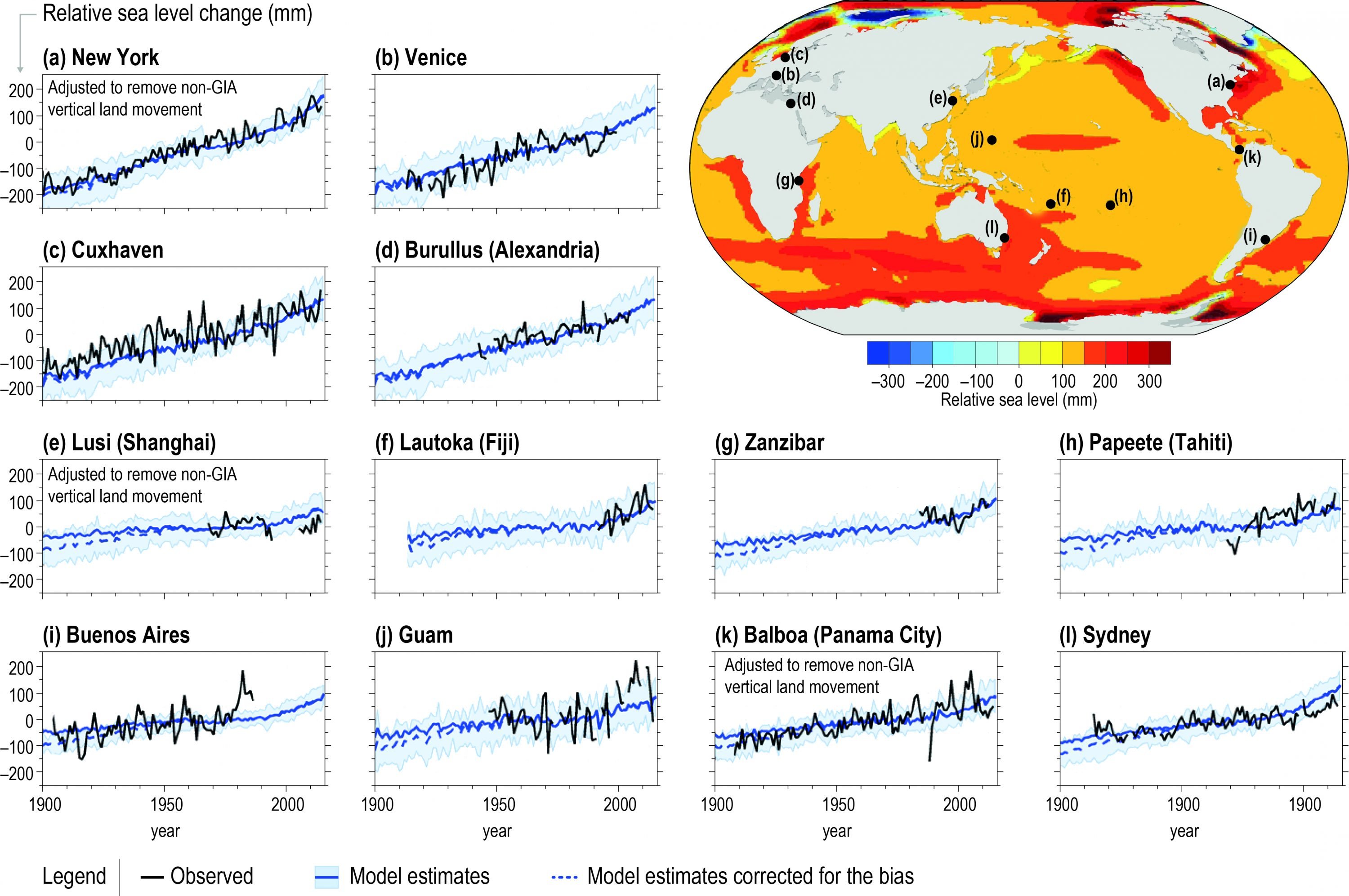
Figure 4.6 | 20th century simulated regional sea level changes by coupled climate models and comparison with a selection of local tide gauge time series. In the upper left corner: map of changes in simulated relative sea level (RSL) for the period 1901–1920 to 1996–2015 estimated from climate model outputs. Insets: Observed RSL changes (black lines) from selected tide gauge stations for the period 1900–2015. For comparison, the estimate of the simulated RSL change at the tide gauge station is also shown (blue plain line for the model estimates and blue dashed line for the model estimates corrected for the bias in glaciers mass loss and Greenland surface mass balance (SMB) over 1900–1940, see Section 4.2.2.2.6). The relatively large, short-term oscillations in observed local sea level (black lines) are due to the natural internal climate variability. For Mediterranean tide gauges, that is, Venice and Alexandria, the local simulated sea level has been computed with the simulated sea level in the Atlantic ocean at the entrance of the strait of Gibraltar following (Adloff et al., 2018). Tide gauge records have been corrected for vertical land motion (VLM) not associated with GIA where available, that is, for New York, Balboa and Lusi. Updated from Meyssignac et al. (2017b) to mimic RSL as good as possible.
4.2.2.4
Local Coastal Sea Level
Since the local coastal sea level (scale ~10 km) is affected by global, regional (scale ~100 km) and coastal scale features and processes like anthropogenic subsidence, it may differ substantially from the regional sea level. At the coast, the sea level change is additionally affected by wave run up, tidal level, wind forcing, sea level pressure (SLP), the dominant modes of climate variability, seasonal climatic periodicities, mesoscale eddies, changes in river flow, as well as anthropogenic subsidence (see also Box 4.1). These local contributions, combined with sea level events generated by storm surges and tides result in anomalous conditions (ESL) which last for a short time in contrast to the gradual increase over time from for instance ice mass loss. Flood risk due to ESL is exacerbated due to its interaction with RSL and hence physical vulnerability assessments combine uncertainties around ESL and RSL, both in terms of contemporary assessments and future projections (Little et al., 2015b312; Vousdoukas, 2016313; Vousdoukas et al., 2016314; Wahl et al., 2017315). Changes in mean sea level have been dealt with in previous sections (e.g., Section 4.2.2.2.6). Here the focus is on some of the components of ESL that have been assessed in combination with changes in RSL. Church et al. (2013) concluded that change in sea level extremes is very likely to be caused by a RSL increase, and that storminess and surges will contribute towards these extremes; however, it was noted that there was low confidence in region-specific projections as there was only a limited number of studies with a poor geographical coverage available.
Recent advances in statistical and dynamical modelling of wave effects at the coast, storm surges and inundation risk have reduced the uncertainties around the inundation risks at the coast (Vousdoukas et al., 2016316; Vitousek et al., 2017317; Melet et al., 2018318; Vousdoukas et al., 2018c319) and assessments of the resulting highly resolved coastal sea levels are now emerging (Cid et al., 2017320; Muis et al., 2017321; Wahl et al., 2017322). This progress was facilitated due to the availability of, for example, the Global Extreme Sea Level Analysis (GESLA-2; Woodworth et al., 2016323) high-frequency (hourly) datasets, advances in the Coordinated Ocean Wave Climate Project (COWCLIP; Hemer et al., 2013324), coastal altimetry datasets (Cipollini et al., 2017325), and the Global Tide and Surge Reanalysis (GTSR; Muis et al., 2016326), while new analyses of datasets that have been available since before the publication of AR5 have continued (e.g., PSML; Holgate et al., 2012327).
Although ESL is experienced episodically by definition, Marcos et al. (2015)328 examined the long-term behaviour of storm surge models and detected decadal and multidecadal variations in storm surge that are not related to changes in RSL. They found that, although 82% of their observed time series showed synchronous patterns at regional scales, the pattern tended to be non-linear, implying that it would be difficult to infer future behaviour unless the physical basis for the responses was understood. An analysis of the relative contributions of SLR and ESL due to storminess showed that in the US Pacific northwest since the early 1980s, increases in wave height and period have had a larger effect on coastal flooding and erosion than RSL (Ruggiero, 2012329) since the early 1980s. This is also true in other regions distributed over the entire globe (Melet et al., 2016330; Melet et al., 2018331). Changes since 1990 in the sea level harmonics and seasonal phases and amplitudes of the wave period and significant wave height were found for the Gulf of Mexico coast and along the US east coast (Wahl et al., 2014332; Wahl and Plant, 2015333). These authors found that high waters have increased twice as much as one would expect from long-term SLR alone, because of additional changes in the seasonal cycle, yielding a 30% increase in risk of flooding. Such effects are likely to be highly dependent on the local conditions. For example, using WAVEWATCH III, TOPEX/Poseidon altimetry tide model data and atmospheric forcing physically downscaled using Delft3D-WAVE and Delft3D-FLOW in what they call the Coastal Storm Modeling System (CoSMoS), Vitousek et al. (2017) were able to detect local inundation hazards (at a scale of hundreds of metres) across regions along the Californian coast. Similarly, Castrucci and Tahvildari (2018)334 simulated the impact of SLR along the Mid-Atlantic region in the USA. A study for the Maldives shows that the contribution of wave setup is essential to estimate flood risks (Wadey et al., 2017335).
In deltas, the local sea level can be dominated by anthropogenic subsidence more than by the processes outlined above. It is often a primary driver of elevated local SLR and increased flood hazards in those regions. This is particularly true for deltaic systems, where fertile soils, low-relief topography, freshwater access, and strategic ports have encouraged the development of many of the world’s most densely populated coastlines and urban centres. For example, globally, one in fourteen humans resides in mid-to-low latitude deltas (Day et al., 2016336). Although in these areas RSL is dominated by anthropogenic subsidence, climate effects need to be included for estimating risks associated with RSL (Syvitski et al., 2009337).
Deltas are formed by the accumulation of unconsolidated river born sediments and porous organic material, both of which are particularly prone to compaction. It is the compaction which causes a drop in land elevation that increases the rate of local SLR above what would be observed along a static coastline or one where only climatological forced processes control the RSL. Under stable deltaic conditions, the accumulation of fluvially-sourced surficial sediment and organic matter offsets this natural subsidence (Syvitski and Saito, 2007338); however, in many cases this natural process of delta construction has been disturbed by reductions in fluvial sediment supply via upstream dams and fluvial channelisation (Vörösmarty et al., 2003339; Syvitski and Saito, 2007340; Syvitski et al., 2009341; Luo et al., 2017342). Further, the extraction of fluids and gas that fill the pore space of deltaic sediments and provide support for overlying material has significantly increased the rate of compaction and resultant anthropogenic subsidence along many populated deltas (Higgins, 2016343). In addition, Nicholls (2011) pointed to anthropogenic subsidence by the weight of buildings in megacities in South-East Asia.
Average natural and anthropogenic subsidence rates of 6–9 mm yr–1 are reported for the highly populated areas of Ganges-Brahmaputra-Meghna delta in the urban centres of Kolkata and Dhaka (Brown and Nicholls, 2015344). A fraction of these subsidence rates might be caused by long-term processes of increased sediment loading during the Holocene resulting from changes in the monsoon system (Karpytchev et al., 2018345). Subsidence rates are expected to decrease in the Ganges-Brahmaputra-Meghna delta in the near future due to planned dam projects and an estimated 21% drop in resulting sediment supply (Tessler et al., 2018346). Observations of enhanced natural and anthropogenic subsidence on the Ganges-Brahmaputra-Meghna are common to most heavily populated deltaic systems. Coastal mega-cities that have been particularly prone to human-enhanced subsidence include Bangkok, Ho Chi Minh city (Vachaud et al., 2018347), Jakarta, Manila, New Orleans, West Netherlands and Shanghai (Yin et al., 2013348; Cheng et al., 2018349). On a global scale, observed rates of modern deltaic anthropogenic subsidence range from 6–100 mm yr–1 (Bucx et al., 2015350; Higgins, 2016351). Rates of recent deltaic subsidence over the last few decades have been at least twice the 3 mm yr–1 rate of GMSL rise observed over this same interval (Higgins, 2016352; Tessler et al., 2018353). Numerical models that have reproduced these observed rates of anthropogenic deltaic subsidence by considering human-induced compaction and reduced sediment supply, support anthropogenic causes for elevated rates of subsidence (Tessler et al., 2018354).
In summary, ESL interacts with RSL rise including anthropogenic subsidence in many vulnerable areas (see Box 4.1). Therefore, it is concluded with high confidence that the inclusion of local processes (wave effects, storm surges, tides, erosion, sedimentation and compaction) is essential to estimate local, relative and changes in ESL events. Although the effect of anthropogenic subsidence may be very large locally, it is not accounted for in the projection sections of this chapter as no global data sets are available which are consistent with RCP scenarios, and because the scale at which these processes take place is often smaller than the spatial scale used in climate models.
4.2.2.5
4.2.2.5 Attribution of Sea Level Change to Anthropogenic Forcing
Bindoff et al. (2013) concluded that it is very likely that there has been a substantial contribution to ocean heat content from anthropogenic forcing (i.e., anthropogenic greenhouse gases, anthropogenic aerosols and land use change) since the 1970s, that it is likely that loss of land ice is partly caused by anthropogenic forcing, and that as a result, it is very likely that there is an anthropogenic contribution to the observed trend in GMSL rise since 1970. However, these conclusions were based on the understanding of the responsible physical processes, since formal attribution studies dedicated to quantifying the effect of individual external forcings were not available for GMSLR. Since AR5, such formal studies have attributed changes in individual components of sea level change (i.e., thermosteric sea level change and glacier mass loss), and in the total GMSL, to anthropogenic forcing.
4.2.2.5.1
Attribution of individual components of sea level change to anthropogenic forcing
Marcos and Amores (2014) found that during the period 1970–2005, 87% (95% confidence interval: 72–100%) of the observed thermosteric SLR in the upper 700 m of the ocean was anthropogenic. Slangen et al. (2014b) included the full ocean depth in their analysis. They concluded that a combination of anthropogenic and natural forcing is necessary to explain the temporal evolution of observed global mean thermosteric sea level change during the period 1957–2005. Anthropogenic forcing was responsible for the amplitude of observed thermosteric sea level change, while natural forcing caused the forced variability of observations. Observations could best be reproduced by scaling the patterns from ‘natural-only’ forcing experiments by using a factor of 0.70 ± 0.30 (2 standard deviations of the CMIP5 ensemble subset used), indicating a potential overestimation of forced variability in the CMIP5 ensemble. Patterns from the ‘anthropogenic-only’ forcing experiments needed to be scaled by a factor of 1.08 ± 0.13 (2 standard deviations of the CMIP5 ensemble subset used), indicating a realistic response of the CMIP5 ensemble to anthropogenic forcing.
For the glacier contribution to GMSL, Marzeion et al. (2014) concluded that while natural climate forcing and long-term adjustment of the glaciers to the end of the preceding Little Ice Age lead to continuous glacier mass loss throughout the simulation period of 1851–2010, the observed rates of glacier mass loss since 1990 can only be explained by including anthropogenic forcing. During the period 1851–2010, only 25 ± 35% of global glacier mass loss can be attributed to anthropogenic forcing, but 69 ± 24% during the period 1991–2010 (see Section 2.2.3 for a more detailed discussion of attribution of glacier mass change on regional scales).
There is medium confidence in evidence linking GIS mass loss to anthropogenic climate change, and low confidence in the evidence that AIS mass balance can be attributed to anthropogenic forcing (see Section 3.3.1.6 for a detailed discussion). The effects of groundwater depletion and reservoir impoundment on sea level change are anthropogenic by definition (e.g., Wada et al., 2012).
4.2.2.5.2
Attribution of global mean sea level change to anthropogenic forcing
By estimating a probabilistic upper range of long-term persistent natural sea level variability, Dangendorf et al. (2015)356 detected a fraction of observed sea level change that is unexplained by natural variability and concluded by inference that it is virtually certain that at least 45% of the observed increase in GMSL since 1900 is attributable to anthropogenic forcing. Similarly, Becker et al. (2014) provided statistical evidence that the observed sea level trend, both in the global mean and at selected tide gauge locations, is not consistent with unforced, internal variability. They inferred that more than half of the observed GMSL trend during the 20th century is attributable to anthropogenic forcing.
Slangen et al. (2016)357 reconstructed GMSL from 1900 to 2005 based on CMIP5 model simulations separating individual components of radiative climate forcing and combining the contributions of thermosteric sea level change with glacier and ice sheet mass loss. They found that the naturally caused sea level change, including the long-term adjustment of sea level to climate change preceding 1900, caused 67 ± 23% of observed change from 1900 to 1950, but only 9 ± 18% between 1970 and 2005. Anthropogenic forcing was found to have caused 15 ± 55% of observed sea level change during 1900–1950, but 69 ± 31% during 1970–2005. The sum of all contributions explains only 74 ± 22% of observed GMSL change during the period 1900–2005 considering the mean of the reconstructions of Church and White (2011)358, Ray and Douglas (2011), Jevrejeva et al. (2014b) and Hay et al. (2015). However, the budget could be closed taking into contribution of glaciers that are missing from the global glacier inventory or have already melted (Parkes and Marzeion, 2018361) which were not considered in Slangen et al. (2016)362.
Based on these multiple lines of evidence, there is high confidence that anthropogenic forcing very likely is the dominant cause of observed GMSL rise since 1970.
4.2.3
Projections of Sea Level Change
As a consequence of climate change, the global and regional mean sea level will change. Coupled climate models are used to make projections of the climate changes and the associated SLR. Results from the CMIP5 model archive used for AR5 provide information on expected changes in the oceans and on the evolution of climate, glaciers and ice sheets. New estimates from CMIP6 are not yet available and will be discussed in the IPCC 6th Assessment Report (AR6), hence only a partly updated projection can be presented here.
Coupled climate models can be applied on century time scales, to provide estimates of the steric (temperature and salinity effects on sea water density) and ocean dynamical (ocean circulation) components of sea level change, both globally and regionally. However, the glacier and ice sheet component are calculated off-line based on temperature and precipitation changes. In the AR5 report, changes in the SMB of glaciers and ice sheet were calculated from the global surface air temperature. In addition, GCMs also resolve climate variability related to changes in precipitation and evaporation. These changes are used to calculate short duration sea level changes (Cazenave and Cozannet, 2014363; Hamlington et al., 2017364). With various degrees of success those models capture ENSO, PDO and other modes of variability (e.g., Yin et al., 2009; Zhang and Church, 2012365), which affect sea level through redistributions of energy and salt in the ocean on slightly longer time scales. Off-line temperature and precipitation fields can be dynamically or statistically downscaled to match the high spatial resolution required for ice sheets and glaciers, but serious limitations remain. This deficiency limits adequate representation of potentially important feedbacks between changes in ice sheet geometry and climate, for example through fresh water and iceberg production that impact on ocean circulation and sea ice, which can have global consequences (Lenaerts et al., 2016366; Donat-Magnin et al., 2017367). Another limitation is the lack of coupling with the solid Earth which controls the ice sheet evolution (Whitehouse et al., 2019368). Dynamics of the interaction of ice streams with bedrock and till at the ice base remain difficult to model due to lack of direct observations. Nevertheless, several new ice sheet models have been generated over the last few years, particularly for Antarctica (Section 4.2.3.1) focusing on the dynamic contribution of the ice sheet to sea level change, which remains the key uncertainty in future projections (Church et al., 2013), particularly beyond 2050 (Kopp et al., 2014370; Nauels et al., 2017b371; Slangen et al., 2017a372; Horton et al., 2018373).
Information beyond that provided by climate models is needed to describe local and RSL changes. Geodynamic models are used to calculate RSL changes due to changes in ice mass in the past and future. This includes solid Earth deformation, gravitational and rotational changes, as ice and water are redistributed around the globe. Input for those models is provided by the mass changes following from the off-line land ice models, time series of terrestrial water mass changes which typically require climate input, and reconstruction of past ice sheet changes over the last glacial cycle provided by coupled ice-Earth models (de Boer et al., 2017). Combining these different models leads to projections of RSL (Section 4.2.3.2).
At the local spatial scales of specific cities, islands and stretches of coastlines, hydrodynamical models (Section 4.2.3.3) and knowledge about anthropogenic subsidence are necessary to analyse the impacts of highly variable processes leading to ESL, such as tropical cyclone-driven storm surges. These hydrodynamical models are capable of providing statistics on the variability or the change in variability of the water level required for flood risk calculations at specific locations and at spatial scales of less than 1 km. The models also rely on input from climate models, like temperature, precipitation, wind regime, and storm tracks (Colbert et al., 2013374; Garner et al., 2017375).
In summary, climate models play an important role at the various stages of projections in providing, together with emission scenarios, geodynamic, ice-dynamic and hydrodynamic models, the required information for hazard estimation for coasts and low-lying islands. This report relies on results of the CMIP5 model runs.
4.2.3.1
Contribution of Ice Sheets to GMSL
4.2.3.1.1
Greenland
The GIS is currently losing mass at roughly twice the pace of the AIS (see Chapter 3 and Table 4.1). About 60% of the mass loss between 1991 and 2015 has been attributed to increasingly negative SMB from surface melt and runoff on the lower elevations of the ice sheet margin. Ice dynamical changes and increased discharge of marine-terminating glaciers account for the remaining 40% of mass loss (Csatho et al., 2014376; Enderlin, 2014377; van den Broeke et al., 2016378). The ability of firn on Greenland to retain meltwater until it refreezes has diminished markedly since the late 1990s, especially in lower elevations and on peripheral ice caps (Noël et al., 2017379). Patterns of surface melt on Greenland are highly dependent on regional atmospheric patterns (Bevis et al., 2019380), adding uncertainty to future projections of SMB. Melt-albedo feedbacks associated with darkening of the ice surface from ponded water, changes in snow and firn properties, and accumulation of impurities are also important, because they can strongly enhance surface melt (Tedesco et al., 2016381; Ryan et al., 2018382; Trusel et al., 2018383; Ryan et al., 2019384). These processes are not fully captured by most Greenland-scale models which is an important deficiency, because surface processes tend to dominate uncertainty in future GIS model projections (e.g., Edwards et al., 2014; Aschwanden et al., 2019385). Increases in meltwater and changes in the basal hydrologic regime, once thought to have a possible destabilising effect on the ice sheet (Zwally et al., 2002386), have been linked with recent reductions in ice velocity in western Greenland. On decadal time scales the effect of meltwater on ice dynamics are now assessed to be small (van de Wal et al., 2015387; Flowers, 2018388), which is supported by ice sheet model experiments (Shannon et al., 2013389). In sum, uncertain climate projections (Edwards et al., 2014390), albedo evolution, uncertainties around meltwater buffering by firn, complex processes linking surface, englacial and basal hydrology with ice dynamics (Goelzer et al., 2013391; Stevens et al., 2016392; Noël et al., 2017393; Hempelmann et al., 2018394) and meltwater induced melting at marine-terminating ice fronts (Chauché et al., 2014395), and coarse spatial model resolution (Pattyn et al., 2018396), all continue to provide substantial challenges for ice sheet and SMB models.
Greenland-scale ice sheet modelling since AR5 (Edwards et al., 2014397; Fürst et al., 2015398; Vizcaino et al., 2015399; Calov et al., 2018400; Golledge et al., 2019401; Aschwanden et al., 2019402) has built upon earlier work by coupling the ice models with regional climate models and using multiple climate and ice sheet models within single studies (Edwards et al., 2014403). Recent modelling studies use higher-order representations of ice flow (Fürst et al., 2015404), include more explicit representations of ice sheet processes including subglacial hydrology (Calov et al., 2018405), run the models at higher resolution and with updated boundary conditions (Aschwanden et al., 2019406), and account for two-way coupling between the ice sheet and the global ocean (Vizcaino et al., 2015407; Golledge et al., 2019408). Among these studies, Fürst et al. (2015), Vizcaino et al. (2015)409, and Aschwanden et al. (2019) provide projections following RCP2.6, RCP4.5, and RCP8.5 emissions scenarios. Calov et al. (2018)412 and Golledge et al. (2019)413 did not consider RCP2.6. Edwards et al. (2014)414 used the Special Report on Emissions Scenarios (SRES) A1B scenario which isn’t directly comparable to the other studies assessed here, but they do provide a rigorous analysis of uncertainty contributed by different climate forcings, varying simplifications of ice flow equations and height-SMB feedbacks.
Fürst et al. (2015)415 used ten different CMIP5 Atmosphere-Ocean General Circulation Model (AOGCM) simulations to provide offline SMB and ocean forcing for their Greenland-wide ice sheet model, accounting for influences of warming subsurface ocean temperatures and basal lubrication on ice dynamics. In their RCP8.5 ensemble, they found a GIS contribution to GMSL in 2100 of 10.15 cm ± 3.24 cm. Similarly, Calov et al. (2018)417 found a range of GMSL contributions between 4.6–13 cm, depending on which CMIP5 GCM is used to force their regional climate model to produce SMB forcing. The wide range of RCP8.5 results in these studies highlights the substantial climate-driven uncertainty in 21st century projections of the GIS as emphasised by Edwards et al. (2014). It was found that central estimates and ranges for RCP8.5 simulated by Fürst et al. (2015), Calov et al. (2018), and Golledge et al. (2019) are in reasonable agreement with previous multi-model results (Bindschadler et al., 2013) and the assessment of AR5 (Church et al., 2013419), which reported a likely RCP8.5 range of Greenland’s contribution to GMSL between 7–21 cm by 2100 (Table 4.2.). The GIS simulations provided by Vizcaino et al. (2015)420, using a relatively course-resolution ice model (10 km) with SMB forcing provided by a single GCM, estimate much less ice loss than other recent studies. Their GMSL projections (Vizcaino et al., 2015421) also fall below the likely range of AR5 estimates. In contrast, the study by Aschwanden et al. (2019)422 shows a significantly higher contribution to GMSL than the other studies, especially under RCP8.5 and beyond 2100 (see 4.2.3.5). This may be due to their SMB forcing, which is based on spatially uniform warming derived from future CMIP5 GCM climatologies averaged over the entire Greenland region. As noted by earlier work (e.g., Van de Wal and Wild, 2001; Gregory and Huybrechts, 2006423), this approach can overestimate melt rates in the ablation zone, which could account for their higher projected ice loss. It is noted that the process-based estimates of future GMSL rise from Greenland found in Aschwanden et al. (2019)424 are closest to those from an updated, structured judgement of glaciological and modelling experts (Bamber et al., 2019425). Calculations from the expert elicitation (Bamber et al., 2019426) result in higher estimates of Greenland ice loss than any of the process-based studies, with a mean and standard deviation of 33 ± 30 cm and a 17–83% range of 10–60 cm by 2100, following a climate scenario comparable to RCP8.5. The combination of the new process-based studies produces central estimates (Table 4.2) consistent with the likely ranges for Greenland’s contribution to GMSL in 2100 assessed by AR5.
Table 4.2
Estimates of the Greenland Ice Sheet (GIS) contribution to Global Mean Sea Level (GMSL; cm) in 2100 reported by process-based modelling studies including the effects of both surface mass balance (SMB) and ice dynamics published since the IPCC 5th Assessment Report (AR5). Only model results including elevation-SMB feedback are shown. All values are reported as the contribution to GMSL in 2100 relative to 2000, with the exception of Aschwanden et al. (2019)428 who report values relative to 2008. The median estimate for comparison with AR5 is based on the average of the three simulations in Calov et al. (2018)429 using different General Climate Models (GCMs), combined with the central estimates from the other studies. RMSD (Fürst et al., 2015430) is the Root Mean Squared Deviation from their ensemble median. The range reported by Aschwanden et al. (2019)431 refers to the 16–84% interval of a 500 member ensemble with varying model physical parameters. RCP is Representative Concentration Pathway.
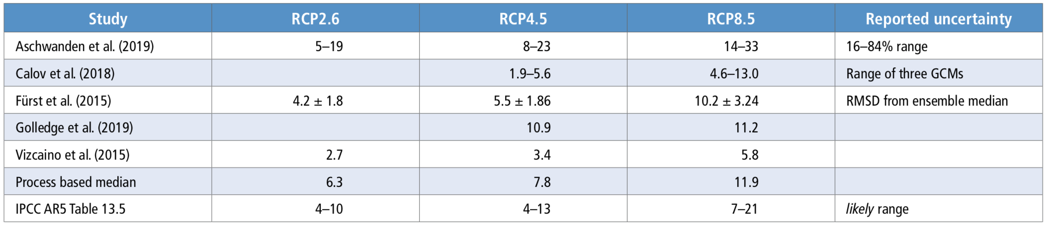
Complimentary to the ice sheet scale simulations discussed above, Nick et al. (2013)427 used detailed flowline models of four Greenland outlet glaciers (Petermann, Kangerdlugssuaq, Jakobshavn Isbræ, and Helheim) to estimate a dynamical contribution to sea level in an RCP8.5 scenario of 11.3–17.5 mm by 2100, and 29–49 mm, by 2200. This demonstrates the limited potential of Greenland outlet glaciers alone to drive GMSL rise. Greenland-wide modelling studies (Table 4.2) consistently find a dominant role of runoff relative to dynamic discharge of ice loss, and a long-term reduction in the rate of dynamic ice discharge to the ocean as the ice sheet margin thins and the termini of outlet glaciers retreat from the coast (Goelzer et al., 2013438; Lipscomb et al., 2013439). Greenland’s bedrock geography and the limited, direct access of thick interior ice to the ocean ultimately limits the potential pace of GMSL rise from the GIS. Figure 4.7 illustrates a fundamental difference between Greenland and Antarctica. In Greenland, most of the bedrock at the ice sheet margin is above sea level (land terminating), with relatively narrow (generally <10 km wide) outlet glaciers reaching the ocean. In contrast, Antarctica has extensive areas with subglacial bedrock below sea level, and thick marine-terminating ice in direct contact with the open ocean. Recent subglacial mapping and mass conservation calculations since AR5 (Morlighem et al., 2014440; Morlighem et al., 2017441) revise earlier bathymetric maps under and around the ice sheet, and reveal deeper and more extensive valley networks extending into the GIS interior than previously known. Accurate subglacial topography is important for modelling individual Greenland outlet glaciers (Aschwanden et al., 2016442; Morlighem et al., 2016443); however, the importance of these revised bedrock boundary conditions for the broader ice sheet has yet to be fully tested. Based on the limited cross sectional area of subglacial valleys and outlet glaciers on Greenland (Figure 4.7) and the results of Nick et al. (2013)444, the effects of uncertain bathymetric boundary conditions are assessed to be small relative to the uncertainties in future SMB forcing (medium confidence).
Figure 4.7
Figure 4.7 | Bedrock topography below the existing ice sheets in Greenland (Morlighem et al., 2017) and Antarctica (right) (Fretwell et al., 2013). Horizontal scales are not the same in both panels. Note the deep subglacial basins in West Antarctica and the East Antarctic margin. The ice above floatation in these areas is equivalent to […]
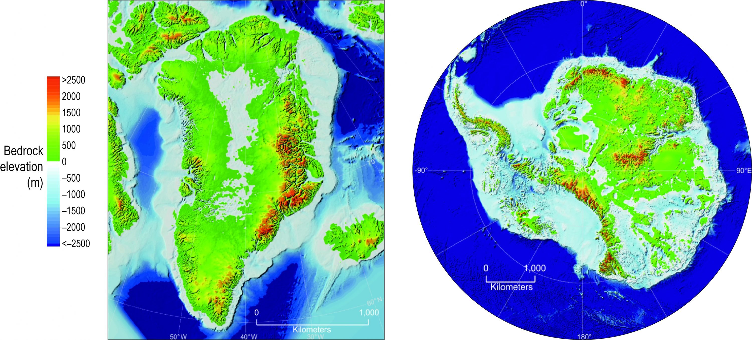
Figure 4.7 | Bedrock topography below the existing ice sheets in Greenland (Morlighem et al., 2017) and Antarctica (right) (Fretwell et al., 2013). Horizontal scales are not the same in both panels. Note the deep subglacial basins in West Antarctica and the East Antarctic margin. The ice above floatation in these areas is equivalent to >20 m of Global Mean Sea Level (GMSL).
In summary, new modelling since AR5 is consistent with previous studies suggesting future Greenland ice loss over the 21st century will be dominated by surface processes, rather than dynamic ice discharge to the ocean, regardless of which emissions scenario is followed (high confidence). Based on these modelling studies, the GIS is not expected to contribute more than 20 cm of GMSL rise by 2100 in a RCP8.5 scenario, similar to the upper end of the likely range reported by AR5 (Church et al., 2013445). GIS simulations are most sensitive to uncertainties in the applied climate forcing, especially over this century (Edwards et al., 2014446), but updated climate projections since AR5 are not yet available. Because of the consistency of recent modelling with the assessment of Church et al. (2013447), Greenland’s contribution to future sea level reported in AR5 was used in our projections of GMSL.
4.2.3.1.2
Antarctica
Unlike Greenland, most of the AIS margin terminates in the ocean. The AIS also contains almost eight times more glacial ice above flotation than Greenland, and nearly half of this ice is marine-based, that is, grounded on bedrock hundreds of metres (or more) below sea level (Figure 4.7; Fretwell et al., 2013448). In places where the subglacial bedrock slopes downward away from the coast (reverse-sloped), the marine-based glacial ice is susceptible to dynamical instabilities (Weertman, 1974449; Schoof, 2007b450; Pollard et al., 2015451) that can contribute rapid ice loss (Cross-Chapter Box 8 in Chapter 3). The instabilities can be triggered by the loss or thinning of ice shelves through changes in the surrounding ocean and increased sub-ice melt rates and changes in the overlying atmosphere affecting SMB and surface meltwater production. Much progress has been made since AR5 in the understanding of these processes, but their representation in continental-scale models continue to be heavily parameterised in most cases. Complex interactions between the ice sheet, ocean, atmosphere and underlying bedrock also remain difficult to simulate collectively.
In contrast to Greenland, Antarctica’s recent contribution to SLR has been dominated by ice-dynamical processes rather than changes in SMB (Mouginot et al., 2014452; Rignot et al., 2014453; Scheuchl et al., 2016454; Shen et al., 2018455; The IMBIE team, 2018). Since AR5, it has become increasingly evident that this ice loss is being driven by sub-ice oceanic melt (thinning) of ice shelves (Paolo et al., 2015456; Wouters et al., 2015) and the resulting loss of back stress (buttressing) that impedes the seaward flow of grounded ice upstream. Elevated melt rates are generally associated with the increased presence of warm Circumpolar Deep Water (CDW) on the continental shelf (Khazendar et al., 2016457). Dynamic ice loss driven by ocean changes have also been observed on the East Antarctic margin (Li et al., 2016458; Shen et al., 2018459). This is an important development, because East Antarctica contains much more ice than West Antarctica, so even minor changes there could make major contributions to sea level in the future.
Several of West Antarctica’s major outlet glaciers, including Pine Island Glacier, and Thwaites Glacier in the Amundsen Sea (Figure 4.8) have grounding lines currently retreating on retrograde bedrock (Rignot et al., 2014460). Thwaites Glacier is particularly important (Figure 4.8), because it extends into the interior of the WAIS, where the bed is >2000 m below sea level in places. By itself, the Thwaites drainage area contains the equivalent of ~0.4 m GMSL (Holt et al., 2006461; Millan et al., 2017462), but loss of the glacier could have a destabilising impact on the entire WAIS (Feldmann and Levermann, 2015463). The WAIS contains enough ice to raise GMSL by ~3.4 m (Fretwell et al., 2013464). Since AR5, a number of ice sheet modelling studies have focussed on limited fractions of Antarctica and so are not included in estimating the SROCC Antarctic contribution to GMSL (see Section 4.2.3.2). However, these studies do allow an assessment of the potential for persistent and increasing ice loss, and the role of the marine ice sheet instability (MISI, see Cross-Chapter Box 8 in Chapter 3).
Joughin et al. (2014)466 modelled the response of the Thwaites Glacier to a combination of elevated sub-ice melt rates and increased precipitation and found persistent future retreat, despite either the partial compensation of increased accumulation or a future reduction in melt. Sub-ice melt rates sustained at current levels were found to generate >1 mm yr–1 equivalent GMSL rise within a millennium. Higher melt rates and an assumed weak ice shelf triggered rapid retreat within a few centuries. Similarly, Waibel et al. (2018) used the BISICLES ice sheet model (Cornford et al., 2015465) to investigate the potential for self-sustained retreat of Thwaites Glacier, by incrementally increasing sub-ice melt rates until retreat is triggered, and then returning to pre-retreat melt rates. Consistent with Joughin et al. (2014)466, they found self-sustained retreat of Thwaites Glacier through MISI. Most uncertainty in their future WAIS simulations arises from uncertainties in the long-term response of Thwaites Glacier (Figure 4.8). Nias et al. (2016) demonstrated model sensitivity of Thwaites Glacier to poorly resolved bedrock boundary conditions (small scale topography), pointing to the need for better geophysical information to reduce model uncertainty (Schlegel et al., 2018468). Arthern and Williams (2017)469 used adaptive mesh techniques, but with a different formulation than Cornford et al., (2015)470, to simulate the future response of Amundsen Sea outlet glaciers. They demonstrate a sustained, but slow future retreat when sub-ice melt is maintained at current rates, and a direct relationship between the strength of ocean forcing and the pace of MISI-driven ice loss. Yu et al. (2018) simulate future Thwaites retreat using a range of model formulations with varying approximations of ice stress balance, different ocean melt schemes, and different basal friction laws. Like Arthern and Williams (2017) they find model-specific dependencies in the rate of ice loss, but all of their simulations demonstrate sustained ice loss and a bathymetrically controlled future acceleration.
Like Thwaites, the neighbouring Pine Island Glacier (PIG) has also been thinning and retreating at an accelerating rate in recent decades, in response to incursions of warm CDW in the waters underlying the glacier’s ice shelf. These incursions of CDW are controlled in part by sea floor bathymetry and climatic variability (Dutrieux et al., 2014471). Favier et al. (2014) used three models with differing formulations to simulate PIG’s response to elevated sub-ice melt. Consistent with modelling of Thwaites Glacier (Joughin et al., 2014473), all three models demonstrate sustained future retreat at an increasing rate, as the glacier backs onto its retrograde bed. Only one of the three models used by Favier et al. (2014) demonstrates the possibility that the glacier can recover if sub-ice melt rates are reduced enough to allow the ice shelf to thicken and pin on bathymetric features to provide buttressing. These results highlight the long-term commitment to marine-based ice loss.
While limited to 50 year simulations, Seroussi et al. (2017)474 provide the first interactively coupled ice-ocean model simulations of Thwaites Glacier at a high spatial resolution. Their model demonstrates MISI-like grounding line retreat at a rate of ~1 km yr–1, comparable to observations between 1992 and 2011 (Rignot et al., 2014). The retreat is interrupted when the main trunk of the glacier stabilises on a bathymetric ridge, ~20 km upstream of the present-day grounding line (Figure 4.8), but due to the short duration of the simulation, the long-term potential for additional retreat into the interior of the ice sheet is not captured.
Despite the use of independent model formulations, forcings, and different geographic settings, the overall agreement among these highly-resolved regional modelling studies and their ability to capture current rates of retreat, increases confidence since AR5 that observed retreat of Amundsen Sea outlet glaciers is driven by processes consistent with MISI theory (medium confidence), will continue (medium confidence), and could accelerate (medium confidence).
Observations of rapid bedrock uplift in the Amundsen Sea, low viscosity of the underlying mantle, and short GIA response times to glacial unloading suggest ice-Earth interactions could be important there (Barletta et al., 2018475). Bedrock uplift and reduced gravitational attraction between the ice sheet and ocean as an ice margin loses mass reduces RSL at the grounding line, promoting stability and providing a negative feedback on retreat (Adhikari et al., 2014476; Gomez et al., 2015477). Using a high-resolution ice sheet-Earth model, Larour et al. (2019) showed that long-term future retreat of Amundsen Sea grounding lines are slowed by these processes, but the effect is found to be minimal until after ~2250. This agrees with other recent modelling accounting for ice-Earth interactions, including the viscoelastic Earth response to changing ice loads and self-gravitation (Gomez et al., 2015478; Konrad et al., 2015479; Pollard et al., 2017480). These studies also showed a small negative feedback on future retreat over the next several centuries, particularly under strong climate forcing. However, the viscosity structure of the Earth under the AIS is not well resolved, and lateral variations in Earth structure could impact these results (Hay et al., 2017481). Based on these consistent model results, and new observational evidence that PIG has been retreating on reverse-sloped bedrock for a half-century or more (Smith et al., 2017), ice-Earth interactions are not expected to substantially slow GMSL rise from marine-based ice in Antarctica over the 21st century (medium confidence). However, these processes could become important for GMSL rise on multi-century and longer time scales.
Figure 4.8
Figure 4.8 | Processes affecting the Thwaites Glacier in the Amundsen Sea sector of Antarctica (adapted from Scambos et al., 2017). The grounding line is currently retreating on reverse-sloped bedrock at a water depth of ~600 m (Joughin et al., 2014; Mouginot et al., 2014). The glacier terminus is ~120 km wide, widens upstream, and […]
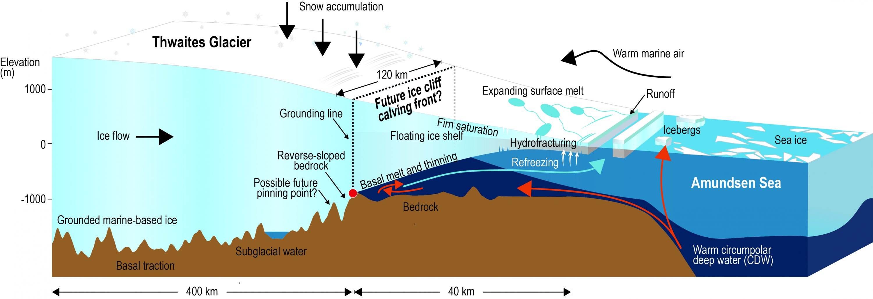
Figure 4.8 | Processes affecting the Thwaites Glacier in the Amundsen Sea sector of Antarctica (adapted from Scambos et al., 2017). The grounding line is currently retreating on reverse-sloped bedrock at a water depth of ~600 m (Joughin et al., 2014483; Mouginot et al., 2014484). The glacier terminus is ~120 km wide, widens upstream, and is minimally buttressed by a laterally discontinuous ~40 km long ice shelf. The remaining shelf is thinning in response to warm, sub-shelf incursions of circumpolar deep water (CDW), with melt rates up 200 m yr–1 near the groundling line in some places (Milillo et al., 2019485). The bathymetry upstream of the grounding zone is complex, but it generally slopes downward into a deep basin, up to 2000 m below sea level under the centre of the West Antarctic Ice Sheet (WAIS) (far left), making the glacier vulnerable to marine ice sheet instabilities (Cross-Chapter Box 8 in Chapter 3).
Atmospheric forcing is also becoming increasingly recognised to be an important factor for the future of the AIS. A sustained (15 days) melt event over the Ross Sea sector of the WAIS in 2016 illustrated both the connectivity of Antarctica to the tropics and El Niño, and the possibility that future meltwater production on ice shelf surfaces could change in the near future (Nicolas et al., 2017487). This was highlighted by Trusel et al. (2015)488, who evaluated the future expansion of surface meltwater using the snow component in the RACMO2 regional atmospheric model (Kuipers Munneke et al., 2012489) and output from CMIP5 GCMs. Under RCP8.5, they found a substantial expansion of surface meltwater production on ice shelves late in the 21st century that exceed melt rates observed before the 2002 collapse of the Larsen B Ice Shelf. Surface meltwater is important for both ice dynamics and SMB due to its potential to reduce albedo, saturate the firn layer, deepen surface crevasses, and to cause flexural stresses that can contribute to ice shelf break-up (hydrofracturing) (Banwell et al., 2013490; Kuipers Munneke et al., 2014491). The presence of surface meltwater does not necessarily lead to immediate ice shelf collapse (Bell et al., 2017b492; Kingslake et al., 2017493), although surface meltwater was a precursor on ice shelves which have collapsed (Scambos et al., 2004494; Banwell et al., 2013495). This dichotomy illustrates the uncertain role of meltwater and the need for additional study. When and if melt rates will be sufficiently high in future warming scenarios to trigger widespread hydrofracturing is a key question, because the loss of ice shelves is associated with the onset of marine ice sheet instabilities (Cross-chapter Box 8 in Chapter 3). Based on the single modelling study by Trusel et al. (2015)496, it is not expected that widespread ice shelf loss will occur before the end of the 21st century, but due to limited observations and modelling to date, there is low confidence in this assessment.
Continental-scale ice sheet simulations are ultimately required to provide projections of future GMSL rise from Antarctica. At this spatial scale, most models rely on simplifying approximations of the equations representing three-dimensional ice flow, and in some cases they parameterise ice flow at the grounding line (Schoof, 2007b497) to improve computational efficiency. Such simplifications are necessary to allow long simulations that can be validated against geological information, in addition to modern observations (Briggs et al., 2013498; Pollard et al., 2016), however processes related to MISI are best represented at high spatial resolution and without simplifications of the underlying physics (Pattyn et al., 2013499; Reese et al., 2018c500).
Various ice sheet model formulations, including the choice of grounding line parameterisations and basal sliding schemes can strongly affect model response to a given forcing (Brondex et al., 2017501; Pattyn, 2017502), although sophisticated statistical methodologies have been increasingly used since AR5 to quantitatively gauge model uncertainty (Bulthuis et al., 2019503; Edwards et al., 2019504). Accurate atmospheric forcing (SMB) and sub-ice melt are also prerequisite to resolving the time-evolving dynamics of the system, with sub-ice melt rates being particularly important (Schlegel et al., 2018505). An important ongoing deficiency is the lack of ice-ocean coupling in most continental-scale studies, which remains too computationally expensive to simulate the ocean at the spatial scales necessary to capture circulation in ice shelf cavities and time-evolving ice-ocean interactions (Donat-Magnin et al., 2017506; Hellmer et al., 2017507). Instead, melt rates are often parameterised as a depth dependent function of nearby ocean temperature derived from offline ocean models, but the lack of ice-ocean interaction can seriously overestimate melt rates in some settings (de Rydt et al., 2015; Seroussi et al., 2017508). Approaches that link offline ocean temperatures with efficient box models of the circulation in ice shelf cavities have been developed (Lazeroms et al., 2018509; Reese et al., 2018a510) and used in long-term future simulations (Bulthuis et al., 2019511), although they still require uncoupled ocean models to provide time-evolving ocean conditions outside the cavities.
Ritz et al. (2015)512 used a hybrid physical-statistical modelling approach, whereby the timing of MISI onset is determined statistically rather than physically. They estimated probabilities of MISI onset in eleven different sectors around the ice sheet margin based on observations of continent-wide retreat and thinning over the last few decades, and expected future climate change following an IPCC SRES A1B emission scenario only. In places where MISI is projected to begin, the persistence and rate of grounding-line retreat is parameterised as a function of the local bedrock topography (slope), ice thickness at grounding lines following Schoof (2007b), and basal friction. This study represents a statistically rigorous approach in which model parameters are based on a synthesis of observations and projected surface and sub-shelf forcing, rather than coming directly from climate and ocean models. However, the model calibrations rely on recent observations, which may not provide adequate guidance under warmer future conditions.
Levermann et al. (2014)513 use simplified emulations of temperature increase in order to estimate both SMB and sub-ice melt (including a parameterised delay for ocean warming) to determine the linearised response of five ice sheet models calibrated against recent rates of retreat. Substantial uncertainty arises from the different model treatments of grounding line dynamics and ice shelves. However, they conclude that the single greatest source of uncertainty stems from the external forcing. Golledge et al. (2015)514 used PISM (Parallel Ice Sheet Model; Winkelmann et al., 2011515) to simulate the future response of the AIS to RCP emission scenarios. PISM links grounded, streaming, and shelf flow, and has freely evolving grounding lines required to capture MISI. PISM’s parameterised treatment of sub-ice melt applies melt under partially grounded grid cells (Feldmann and Levermann, 2015516), making the model sensitive to subsurface ocean warming, although the validity of this approach is contested (Arthern and Williams, 2017517; Seroussi and Morlighem, 2018518; Yu et al., 2018519). While providing alternative outcomes with the two basal melt rate parameterisations, the model is not calibrated to observations and doesn’t provide a probability distribution. In a subsequent study Golledge et al. (2019)520 used PISM, but with updated RCP climate forcing based on CMIP5 GCMs, and with sub-ice ocean melt calibrated to observations. An offline, intermediate-complexity climate model was used to capture global ice-climate feedbacks ignored in most other studies, but the simulations only include RCP4.5 and RCP8.5 and do not extend beyond 2100. Accounting for the climatic effects of meltwater input from Greenland and Antarctica nearly doubled their estimates of Antarctic’s contribution to GMSL in 2100 from 2.4 cm to 4.6 cm in RCP4.5, and from 7.7 cm to 14 cm in RCP8.5. The increase is caused by a combination of SMB decrease over the WAIS, combined with subsurface ocean warming that increases sub-ice melt. However, the climate model used to diagnose the spatial patterns of the atmospheric and oceanic response to the meltwater input is simplistic. Bronselaer et al. (2018)521 tested the global climatic response to future meltwater input from Antarctica using an ensemble of GCM simulations, but without an interactive ice sheet. They simulated an RCP8.5 scenario with and without a massive input of meltwater into the Southern Ocean and demonstrate that the addition of Antarctic meltwater expands sea ice in the Southern Ocean, delays the trajectory of global warming, and moderates atmospheric warming around the Antarctic coastline. Consistent with Golledge et al. (2019)522, they found meltwater-induced stratification around Antarctica warms subsurface ocean temperatures, indicating the potential for a positive meltwater feedback on ice shelf melt. These studies reinforce the need for continental-scale studies to consider two-way ice-climate coupling, but with limited published studies to draw from and no simulations run beyond 2100, firm conclusions regarding the net importance of atmospheric versus ocean melt feedbacks on the long-term future of Antarctica can not be made.
Bulthuis et al. (2019)526 used a different continental-scale ice sheet model (Pattyn, 2017525) with the same simplified atmospheric and ocean forcing used by Golledge et al. (2015)528 to simulate RCP2.6, RCP4.5, and RCP8.5 scenarios. Simulations with varying model parameters were used to quantify uncertainties related to the atmospheric forcing, various ice-model physics, and bedrock response to changing ice loads. A key finding was that irrespective of model parametric uncertainty, the strongly mitigated RCP2.6 scenario prevents catastrophic WAIS collapse over the coming centuries. The probabilistic projections of Antarctic GMSL contributions (Bulthuis et al., 2019531) represent a rigorous blending of physical ice sheet modelling and uncertainty quantification (UQ) techniques, albeit with a simplistic representation of future climate and using a relatively coarse-resolution ice sheet model. These results are well-supported by Schlegel et al. (2018), who blend UQ with a higher resolution ice sheet model than used by Bulthuis et al. (2019), but using an idealised climate forcing scheme not directly linked to time-evolving future climate trajectories. Their 800 simulations, run to 2100, provide not only probabilistic constraints on future GMSL-rise from Antarctica, but an assessment of key drivers of uncertainty, including uniform and regional dependencies on model physical parameters, climate forcing, and boundary conditions. Sub-ice shelf melt rates provide the greatest source of uncertainty in their projections, although the source region dominating the GMSL contribution is found to be dependent on the climate forcing applied, and different from those found by Golledge et al. (2015)530.
DeConto and Pollard (2016)529 used an ice sheet model with a formulation similar to that used by Golledge et al. (2015) and Bulthuis et al. (2019) but they include glaciological processes not accounted for in other continental-scale models: 1) surface melt and rain water influence on hydrofracturing of ice shelves; and 2) brittle failure of thick, marine-terminating ice fronts that have lost their buttressing ice shelves. Where the ice fronts are thick enough to form tall ice cliffs above the waterline, they can produce stresses exceeding the strength of the ice, causing calving (Bassis and Walker, 2012532). Once initiated, ice-cliff calving has been hypothesised to produce a self-sustaining Marine Ice Cliff Instability (MICI; Cross-chapter Box 8, Chapter 3). The validity of MICI remains unproven (Edwards et al., 2019533) and is considered to be characterised by ‘deep uncertainty’, but it has the potential to raise GMSL faster than MISI. DeConto and Pollard (2016) represent hydrofracturing and ice-cliff calving with simple parameterisations, but the glaciological processes themselves are supported by more detailed modelling and observations (Scambos et al., 2009534; Banwell et al., 2013535; Ma et al., 2017536; Wise et al., 2017537; Parizek et al., 2019538). DeConto and Pollard (2016)539 provide four ensembles for RCP2.6, RCP4.5, and RCP8.5 scenarios, representing two alternative ocean model treatments and two alternative palaeo sea level targets used to tune their model physical parameters. However, their ensembles do not explore the full range of model parameter space or provide a probabilistic assessment (Kopp et al., 2017540; Edwards et al., 2019541). Under RCP2.6, DeConto and Pollard (2016) find very little GMSL rise from Antarctica by 2100 (0.02–0.16 m), consistent with the findings of Golledge et al. (2015)542 and Bulthuis et al. (2019)543. In contrast, their four ensemble means range between 0.26–0.58 m for RCP4.5, and 0.64–1.14 m for RCP8.5. In RCP8.5, rates of GMSL rise from Antarctica exceed 5 cm yr-1 in the 22nd century and contribute as much as 15 m of GMSL rise by 2500, largely due to the ice cliff calving process. The climate forcing used by DeConto and Pollard (2016)544 simulates the appearance of extensive surface meltwater several decades earlier than indicated by other CMIP5 climate simulations (Trusel et al., 2015545). Because their model physics are sensitive to melt water through hydrofracturing, this makes the timing and magnitude of their simulated ice loss too uncertain to include in SROCC sea level projections. However, their results do demonstrate the potential for brittle ice sheet processes not considered by AR5 to exert a strong influence on future rates of GMSL rise and the possibility that GMSL beyond 2100 could be considerably higher than the likely range projected by models that do not include these processes.
4.2.3.2
Global and Regional Projections of Sea Level Rise
In addition to the model including MICI from DeConto and Pollard (2016), only a subset of studies (Levermann et al., 2014; Golledge et al., 2015; Ritz et al., 2015; Bulthuis et al., 2019; Golledge et al., 2019), and statistical emulation of DeConto and Pollard (2016) by Edwards et al. (2019) provide continental-scale estimates of future Antarctic ice loss, under a range of GHG emissions scenarios. They all provide probabilistic information, but vary considerably, both in their physical approaches and their resulting projections of Antarctica’s future contribution to GMSL. Such variations facilitate the first quantitative uncertainty assessment of the full dynamical contribution of Antarctica, which could not be made by Church et al. (2013) in AR5. The assessment by Church et al. (2013), based on a single statistical-physical model, reported median values (and likely ranges) of 0.05 m (-0.04–0.13) and 0.04 m (-0.06–0.12), for RCP4.5 and RCP8.5, respectively, for the total Antarctic contribution in 2081–2100 relative to 1986–2005, and added the following: ‘Based on current understanding, only the collapse of marine-based sectors of the AIS, if initiated, could cause GMSL to rise substantially above the likely range during the 21st century. This potential additional contribution cannot be precisely quantified but there is medium confidence that it would not exceed several tenths of a metre of SLR during the 21st century (Church et al., 2013). Given the above-mentioned publications after AR5, Antarctica’s contribution to sea level change was reassessed and now include the possibility of MISI allowing for a more complete assessment of the likely range of the projections for three RCP scenarios. Our assessment is based on process-based numerical models of the AIS, driven by diverse climate scenarios. Results are discussed in the context of an expert elicitation study (Bamber et al., 2019546), probabilistic studies (Perrette et al., 2013547; Slangen et al., 2014a548; Grinsted et al., 2015549; Jackson and Jevrejeva, 2016550) and a sensitivity study (Schlegel et al., 2018551) assessing the uncertainty in snow accumulation, ocean-induced melting, ice viscosity, basal friction, bedrock elevation and the effect of ice shelves on ice mass loss in 2100, Figure 4.4.
Ritz et al. (2015) is difficult to contextualise as they only provided estimates for the A1B scenario and not for the RCP scenarios. Despite this limitation their results, which are close to the other studies, are included as if they represent RCP8.5 and as such supports the assessment. The results by DeConto and Pollard (2016)552 indicate significantly higher mass loss even for RCP4.5, potentially related to their high surface melt rates on the ice shelves as contested by Trusel et al. (2015)553. This early onset of high surface melt rates in DeConto and Pollard (2016) 554leads to extensive hydrofracturing of ice shelves before the end of the 21st century and therefore to rapid ice mass loss. For this reason, their results and probabilistic (e.g., Kopp et al., 2017; Le Bars et al., 2017) and statistical emulation estimates that build on them (Edwards et al., 2019555), are not used in SROCC sea level projections. Consequently, the process-based studies by Golledge et al. (2015)556, Ritz et al. (2015), Levermann et al. (2014)558, Golledge et al. (2019)559, and Bulthuis et al. (2019) are used to assess the Antarctic contribution for the different RCP scenarios. The study by Schlegel et al. (2018) does not provide RCP based scenarios, but is considered as an extensive sensitivity estimate providing a high-end estimate based on physical process understanding of the Antarctic contribution.
Each study expresses an uncertainty in the Antarctic contribution to GMSL rise which is, in part, dependent on a common driver, namely regional warming. The uncertainties were therefore interpreted as being dependent and propagate the total uncertainty accordingly. As a result, the total uncertainty exceeds that of the individual studies, which reflects that the individual studies only sample a fraction of the total uncertainty. The uncertainty estimates of Levermann et al. (2014)561 concentrate on the oceanic basal melt rates including a time delay between atmosphere and ocean temperature, but do not consider other sources of uncertainty. Ritz et al. (2015)562 is constrained by observations and provides an asymmetric distribution of the rate of mass loss. The ice sheet simulations by Golledge et al. (2015) and Golledge et al. (2019) only provide two alternative subgrid parameterisations for sub-ice melt, rather than a statistical estimate of the uncertainty. The more sensitive of these two parameterisations which induces more ice loss is challenged by Seroussi and Morlighem (2018)565. In order to assess a realistic uncertainty for the total Antarctic contribution, it was first assumed that Golledge et al. (2015)566 and Golledge et al. (2019)567 are dependent, because they use similar parameterisations. For each study, a probabilistic distribution is used, assuming a normal distribution with a likely range bounded by the high and low estimate from those studies. Levermann et al. (2014)568 also provides two alternatives, one with and one without a time delay between oceanic temperatures below the Antarctic ice shelves and global mean atmospheric temperature. As it is unclear which version best matches the updated record of ice loss presented by The IMBIE team, (2018), results are combined assuming full probabalistic dependence as for the two Golledge studies. Bulthuis et al. (2019)572 uses a simplified ice sheet model to study the uncertainty caused by the atmospheric forcing, ice dynamics, ice and bed rheology, calving and sub-shelf melting. Finally, the studies by Ritz et al. (2015)571, Bulthuis et al. (2019) and the averages for Golledge and Levermann are combined to identify a best estimate for the Antarctic contribution under RCP8.5. This results in a median contribution of 16 cm in 2100 under RCP8.5. A Monte Carlo technique is used to combine the uncertainties in the aforementioned studies, assuming mutual dependence. The resulting 5–95 percentile range, 2–37 cm in 2100 under RCP8.5, is assessed as the likely range. This assessment is used in order to reflect ongoing limited understanding of the physics and the fact that the individual studies only reflect part of the total uncertainty. The distribution is slightly skewed to higher values, because of an underlying skewness in the studies of Levermann et al. (2014)569 and Ritz et al. (2015)571. This skewed distribution is supported by an expert elicitation study (Bamber et al., 2009). The expert elicitation approach (Bamber et al., 2018), which applied elicitation to both ice sheets, suggests considerably higher values for total SLR for RCP2.6, RCP4.5 and RCP8.5 than provided in Table 4.3.
As the importance of MISI and MICI is difficult to assess on longer time scales, there remains deep uncertainty for the Antarctic contribution to GMSL after 2100 (Cross-Chapter Box 4 in Chapter 1). Results on these long-time scales are discussed in 4.2.3.5.
Table 4.3:
An overview of different studies estimating the future Antarctic contribution to sea level rise (SLR), listed here are median values. Estimates from Golledge et al. (2015) are based on the average contribution to Global Mean Sea Level (GMSL) over the full 21st century, based on two alternative ensembles using different sub-ice melt schemes. This average is not explicitly reported in the original paper where the individual values of 0.1 and 0.39 m are reported. SMB is the surface mass balance, BMB the basal melt balance, LIG is Last Interglacial, MICI is marine ice cliff instability, GCM is General Circulation Model, PDD is positive-degree day.
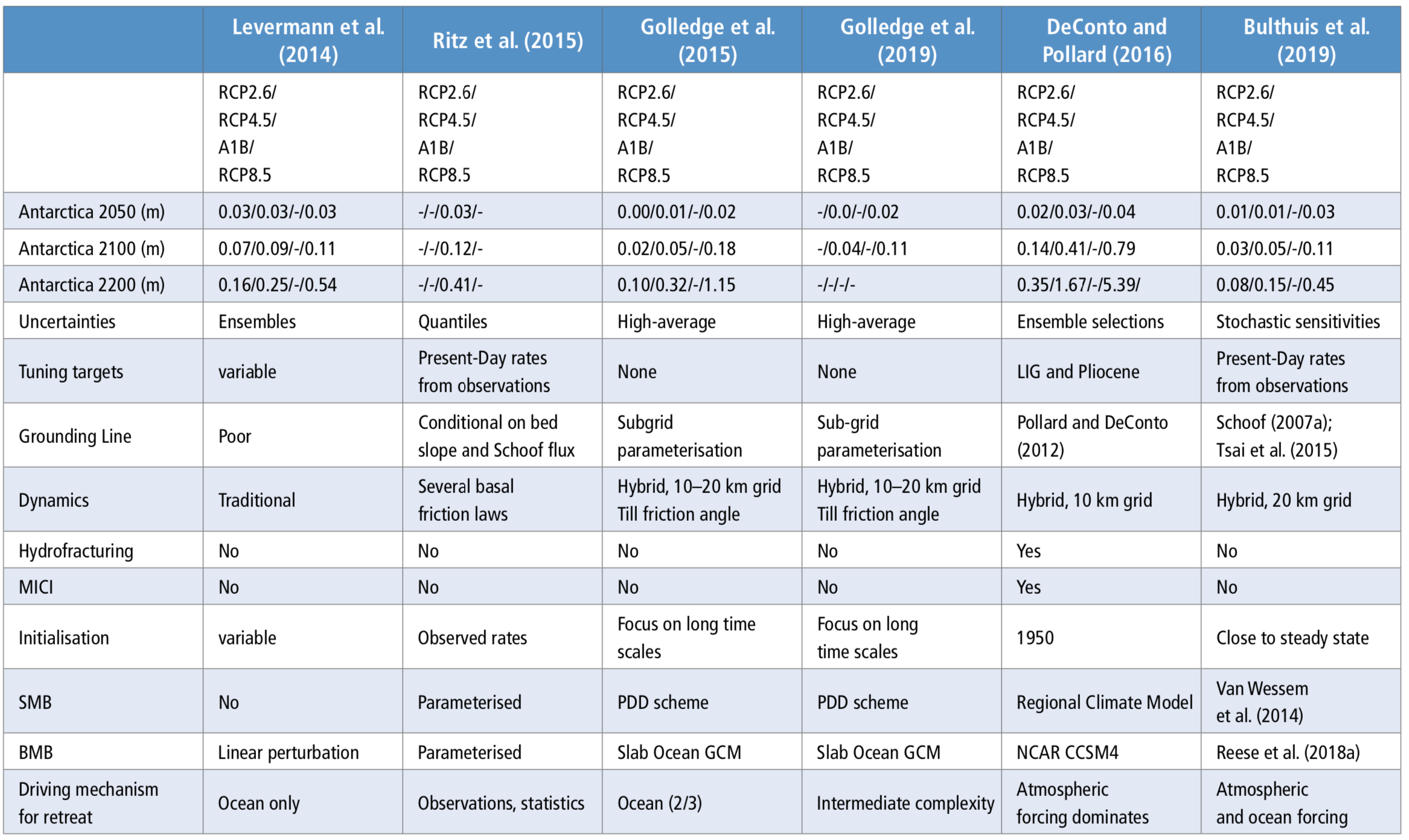
There is limited evidence for major changes since AR5 in the non-Antarctic components. Recent projections of the glacier contribution are nearly identical to AR5 results used here (see Cross-Chapter Box 6 in Chapter 2). Greenland, thermal expansion and land water storage are also not updated, mainly due to a lack of updated CMIP simulations. Hence, our revised projections replace only the AR5 estimate for Antarctica by a new assessment as outlined in the previous paragraph based on post-AR5 literature and maintaining identical contributions for the non-Antarctic components. As no general dependence between the Antarctic contribution and the non-Antarctic components can be derived from the four studies, independent uncertainties are assumed, which is close to the uncertainty propagation by Church et al. (2013)576.
Time series for the different RCP scenarios are shown in Figure 4.9 indicating a divergence in median and upper likely range for RCP8.5 during the second half of the century between this report and the AR5 projections (Church et al., 2013577). The value of the Antarctic contribution in 2081–2100 under RCP8.5 is the individual component with the largest uncertainty. As a consequence, the uncertainty in the GMSL projections is slightly increased compared to Church et al. (2013). Nevertheless, results can also be considered to be consistent with Church et al. (2013)578. In AR5, the potential additional contribution by ice dynamics, was estimated to be not more than several tenths of a metre but excluded from projections; here this value was assessed to be 16 cm (5–95 percentile; 2–37 cm) and include it in the projections. As the projections build on the CMIP5 work presented in AR5, and also given the limited exploration of uncertainty in estimates from each individual study, the results of the 5–95 percentile are interpreted to represent the likely range, that is, the 17–83 percentile, as assessed by Church et al. (2013) and as assessed in AR5 for other CMIP5-derived results.
Table 4.4
Median values and likely ranges for projections of global mean sea level (GMSL) rise in metres in 2081–2100 relative to 1986–2005 for three scenarios. In addition, values of GMSL rise are given for 2046-2065 and 2100, and the rate of GMSL rise is given for 2100. Values between parentheses reflect the likely range. SMB is surface mass balance, DYN is dynamical contribution, LWS is land water storage. Total AR5 minus Antarctica AR5 is the GMSL rise contribution in Church et al. (2013) without the Antarctic contribution of Church et al. (2013). The newly derived Antarctic contribution is added to this to arrive at the GMSL rise.
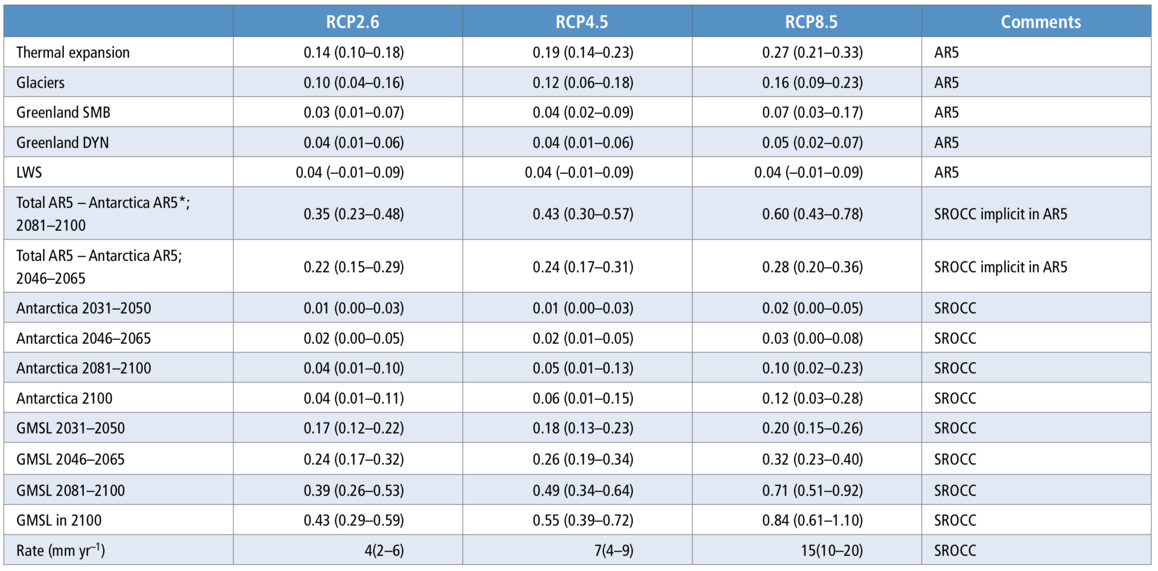
Figure 4.9
Figure 4.9 | Time series of Global Mean Sea Level (GMSL) for Representative Concentration Pathway (RCP)2.6, RCP4.5 and RCP8.5 as used in this report and, for reference the IPCC 5th Assessment Report (AR5) results (Church et al., 2013). Results are based on AR5 results for all components except the Antarctic contribution. Results for the Antarctic […]
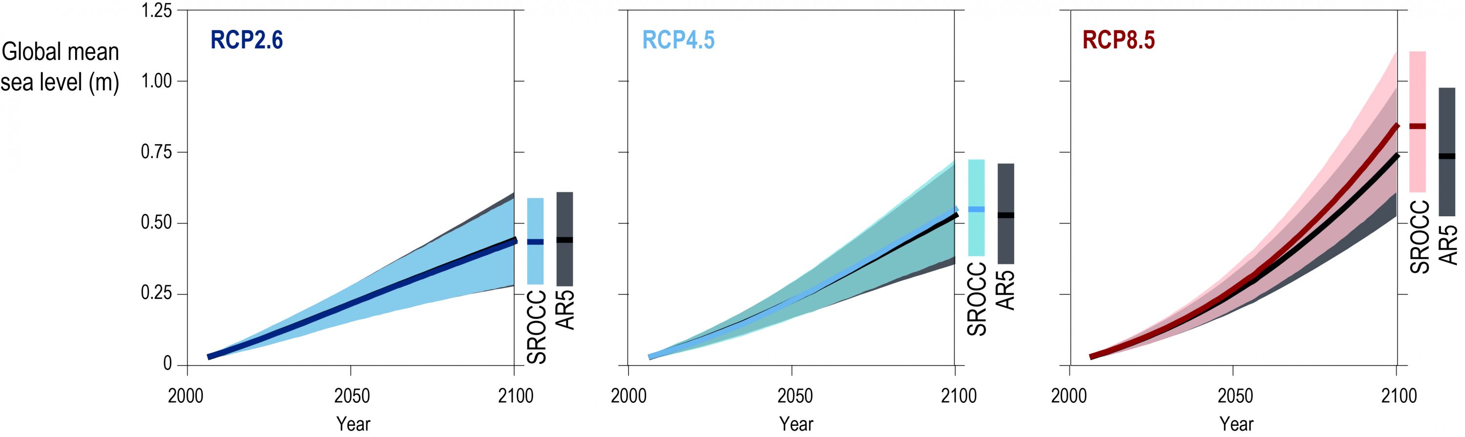
Figure 4.9 | Time series of Global Mean Sea Level (GMSL) for Representative Concentration Pathway (RCP)2.6, RCP4.5 and RCP8.5 as used in this report and, for reference the IPCC 5th Assessment Report (AR5) results (Church et al., 2013). Results are based on AR5 results for all components except the Antarctic contribution. Results for the Antarctic contribution in 2081–2100 are provided in Table 4.4. The shaded region is considered to be the likely range.
Projections as presented in Table 4.4 are used to calculate the regional RSL projections as outlined in AR5 by including gravitational and rotational patterns as shown in Figure 4.10 and subsequently used in 4.2.3.4 to calculate ESL projections. Including the updated results in terms of magnitude and uncertainty for the Antarctic component also changes the regional patterns in sea level projections. Results of the regional patterns in Figure 4.10 show an increased SLR with respect to the results presented in AR5 nearly everywhere for RCP8.5 because of the increased Antarctic contribution.
Figure 4.10
Figure 4.10 | Regional sea level change for RCP2.6, RCP4.5 and RCP8.5 in metres as used in this report for extreme sea level (ESL) events. Results are median values based on the values in Table 4.4 for Antarctica including GIA and the gravitational and rotational effects, and results by Church et al. (2013) for glaciers, […]
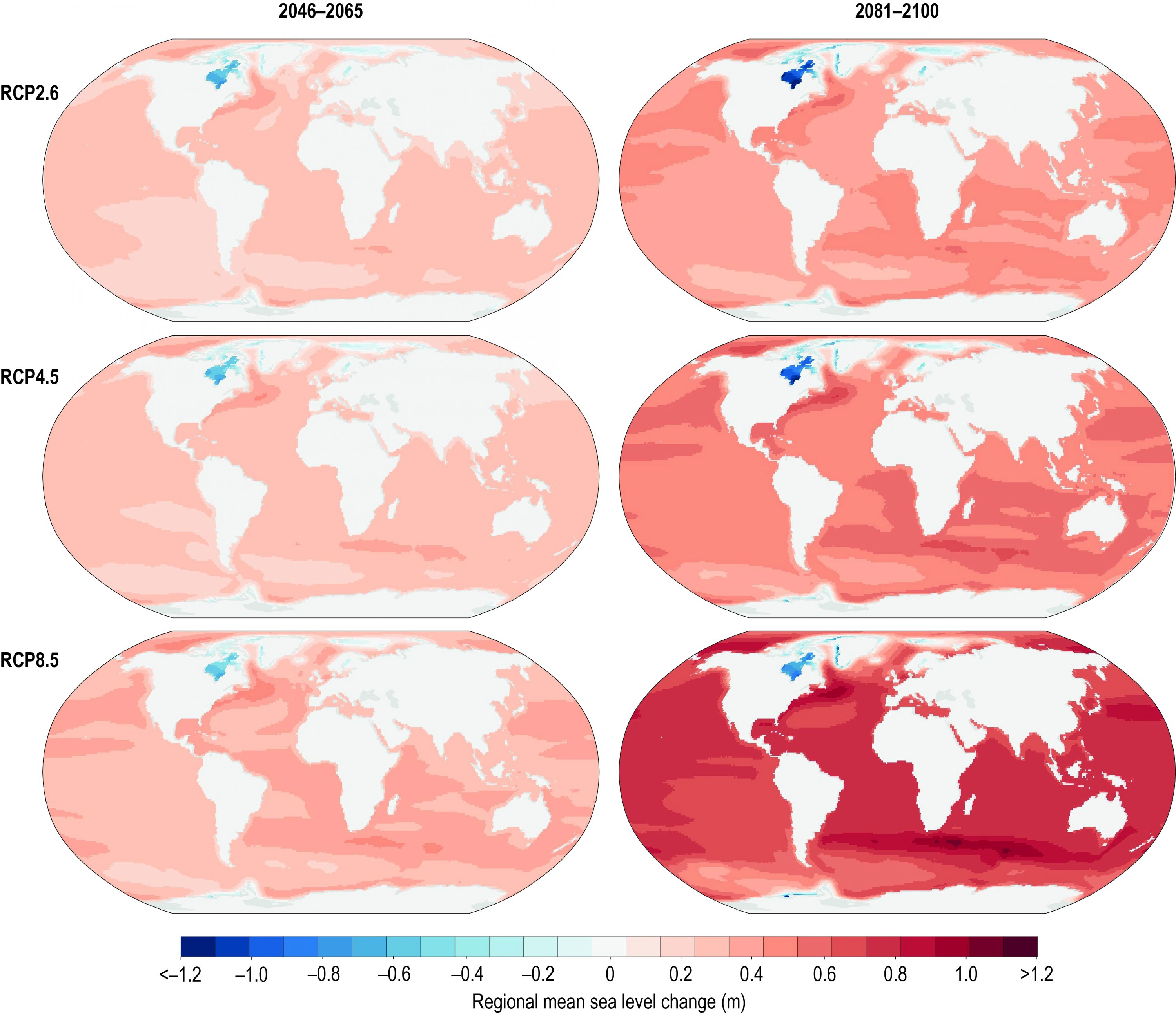
Figure 4.10 | Regional sea level change for RCP2.6, RCP4.5 and RCP8.5 in metres as used in this report for extreme sea level (ESL) events. Results are median values based on the values in Table 4.4 for Antarctica including GIA and the gravitational and rotational effects, and results by Church et al. (2013) for glaciers, land water storage (LWS) and Greenland. The left column is for the time slice 2046–2065 and the right column for 2081–2100.
4.2.3.3
Probabilistic Sea Level Projections
Since AR5, several studies have produced SLR projections in coherent frameworks that link together global-mean and RSL rise projections. The approaches are generally similar to those adopted by AR5 for its global-mean sea level projections: a bottom-up accounting of different contributing processes (e.g., land-ice mass loss, thermal expansion, dynamic sea level), of which many are ‘probabilistic’, in that they attempt to describe more comprehensive probability distributions of sea level change than the likelyranges presented by Church et al. (2013)600. An overview of probabilistic approaches is presented in Garner et al. (2017)601, indicating higher values for post AR5 studies mainly reflecting increased uncertainty based on a single contested study for the Antarctic contribution (DeConto and Pollard, 2016602). As such many of these probabilistic studies present full probability density function conditional not only on an RCP scenario, but with additional and equally important a priori assumptions concerning for instance the Antarctic contribution over which a consensus has yet to solidify. An example is the study by Le Bars et al. (2017) who expand the projection by Church et al. (2013)603 in a probabilistic way with the Antarctic projections by DeConto and Pollard (2016)604 to obtain a full probability density function for SLR for RCP8.5. Other probabilistic approaches are provided by Kopp et al. (2014)605 and Jackson and Jevrejeva (2016)606 using different ice sheet representations drawing on expert elicitation (Bamber and Aspinall, 2013607). Probabilistic estimates are useful for a quantitative risk management perspective (see Section 4.3.3). An even more general approach than the probabilistic estimates has been taken by Le Cozannet et al. (2017) who frame a ‘possibilistic’ framework of SLR including existing probabilistic estimates and combining them.
This section first briefly reviews key sources of information for probabilistic projections (Section 4.2.3.3.1), with a focus on new results since AR5, then summarises the different global and regional projections (Section 4.2.3.3.2). Eventually, bottom-up projections were distinguished which explicitly describe the different components of SLR (Section 4.2.3.3.3) from semi-empirical projections (Section 4.2.3.3.4).
4.2.3.3.1
Components of probabilistic global mean sea level projections
Thermal expansion: Global mean thermal expansion projections rely on coupled climate models projections (Kopp et al., 2014608; Slangen et al., 2014a609; Jackson and Jevrejeva, 2016610) or simple climate model projections (Perrette et al., 2013611; Nauels et al., 2017b612; Wong et al., 2017613), and are substantively unchanged since AR5. For those studies relying on the CMIP5 GCM ensemble, interpretations of the model output differ mainly with regard to how the range is understood. For example, Kopp et al. (2014)614, interprets the 5–95 percentile of CMIP5 values as a likely range of thermal expansion. The differences among the studies yield discrepancies smaller than 10 cm, e.g., Slangen et al. (2014a)615 use 20–36 cm in 2081–2100 with respect to 1986–2005, while (Kopp et al., 2014) project a likely range of 28–46 cm in 2081–2099 with respect to 1991–2009.
Glaciers: Projections of glacier mass change rely either on models of glacier SMB and geometry, forced by temperature and precipitation fields (Slangen and Van de Wal, 2011615; Marzeion et al., 2012616; Hirabayashi et al., 2013617; Radić et al., 2014618; Huss and Hock, 2015619), or simple scaling relationships with global mean temperature (Perrette et al., 2013620; Bakker et al., 2017621; Nauels et al., 2017a622). Glacier mass change projections published since AR5, based on newly developed glacier models, confirm the overall assessment of AR5 (see also Section 4.2.3.2).
Land water storage: Projections of the GMSL rise contributions due to dam impoundment and groundwater withdrawal are generally either calibrated to hydrological models (e.g., Wada et al., 2012) or neglected. Recent coupled climate-hydrological modelling suggests that a significant minority of pumped groundwater remains on land, which may reduce total GMSL rise relative to studies assuming full drainage to the ocean (Wada et al., 2016623). Kopp et al. (2014) estimated land water storage based on population projections. However, there are no substantive updates to projections of the future land-water storage contribution to GMSL rise since AR5.
Ice sheets: GMSL projections in previous IPCC assessments were based on results from physical models of varying degree of complexity interpreted using expert judgment of the assessment authors (Meehl et al., 2007625; Church et al., 2013626). AR5 (Church et al., 2013627) used this approach and is partly based on the assessment of statistical-physical modelling of the Antarctic contribution (Little et al., 2013628). As an alternative to the model-based approach, several studies have applied structured expert elicitation to the GMSL contribution of ice sheets. This approach is based on a more formal expert elicitation protocol (Cooke, 1991629; Bamber and Aspinall, 2013630; Bamber et al., 2019631) instead of physically based models. Combining the Antarctic contribution from the expert elicitation with the non-Antarctic components from AR5 as done for Table 4.4 leads to an estimated SLR of 0.95 m (median) for the high scenario and an upper likely range of 1.32 m (Figure 4.2), which is slightly higher than the process-based results. Results by Bamber and Aspinall (2013)632 were criticised because of their procedure for post-processing the expert data of individual ice sheets to a total sea level contribution from the ice sheets (de Vries and van de Wal, 2015; Bamber et al., 2016; de Vries and van de Wal, 2016). Bamber et al. (2019) avoids this issue by eliciting expert judgments about ice sheet dependence. Alternatively, Horton et al. (2014) used a simpler elicitation protocol focusing on the total SLR rather than the ice sheet contribution alone. Finally, several probabilistic studies (e.g., Bakker et al., 2017; Kopp et al., 2017633; Le Bars et al., 2017) used the results of a single ice sheet model study from DeConto and Pollard (2016)634 as the Antarctic contribution to GMSL.
Beside the total contribution of ice sheets several studies address the individual contribution of either Greenland or Antarctica (see Section 4.2.3.1.1 and 4.2.3.1.2) based on ice dynamical studies. Critical for GMSL projections is the low confidence in the dynamic contribution of the AIS beyond 2050 in previous assessments, as discussed in Section 4.2.3.1.2.
4.2.3.3.2
From probabilistic global mean sea level projections to regional relative sea level change
Differences between GMSL and RSL change are driven by three main factors: (1) changes in the ocean, for instance, the thermal expansion component and the circulation driven changes, (2) gravitational and rotational effects caused by redistribution of mass within cryosphere and hydrosphere, leading to spatial patterns, and (3) long term processes caused by GIA that lead to horizontal and VLM. Finally, the inverse barometer effect caused by changes in the atmospheric pressure, sometimes neglected in projections, can also make a small contribution, particularly on shorter time scales. For the 21st century as a whole, estimates of the latter are smaller than 5 cm at local scales (Church et al., 2013635; Carson et al., 2016636).
Ocean Dynamic sea level: Projections of dynamic sea level change are necessarily derived through interpretations of coupled climate model projections. As with thermal expansion projections, interpretations of the CMIP5 ensemble differ with regard to how the model range is understood and the manner of drift correction, if any (Jackson and Jevrejeva, 2016637). However, relative to tide-gauge observations, coupled climate models tend to overestimate the memory in dynamic sea level; thus, they may underestimate the emergence of the externally forced signal of DSL change above scenario uncertainty (Becker et al., 2016638). ODSL from coupled climate models does not include the changes resulting from ice melt because ice melt is calculated off-line.
Gravitational-rotational and deformational effects (GRD; Gregory et al., 2019638): All projections of RSL change include spatial patterns in sea level for cryospheric changes, which however may differ in the details with which these are represented. Some studies also include a spatial pattern for land-water storage change (Slangen et al., 2014a640), anthropogenic subsidence is not included. Recent work indicates that, for some regions with low mantle viscosity, spatial patterns cannot be treated as fixed on multi-century time scales (Hay et al., 2017641). This effect has not yet been incorporated into comprehensive RSL projections, but is probably only of relevance near ice sheets. For adaptation purposes, Larour et al. (2017) developed a mapping method to indicate which areas of ice mass loss are important for which major port city. There is high confidence in the patterns caused by GRD, as in AR5.
Vertical land motion (VLM): These processes can be an important driver of RSL change, particularly in the near- to intermediate-field of the large ice sheets of the LGM (e.g., North America and northern Europe). This process is incorporated either by physical modelling (Slangen et al., 2014a643) or by estimation of a long-term trend from tide-gauge data (e.g., Kopp et al., 2014), which is then spatially extrapolated. In the former case, only the long-term GIA process is included in the projections, but it excludes other important local factors contributing to VLM (e.g., tectonic uplift/subsidence and groundwater/hydrocarbon withdrawal); by using only tide gauge measurements, projections may assume that these other processes proceed at a steady rate and thus do not allow for management changes that affect groundwater extraction.
4.2.3.3.3
Semi-empirical projections
Semi-empirical models provide an alternative approach to process-based models aiming to close the budget between the observed SLR and the sum of the different components contributing to SLR. In general, motivated by a mechanistic understanding, semi-empirical models use statistical correlations from time series analysis of observations to generate projections (Rahmstorf, 2007644; Vermeer and Rahmstorf, 2009645; Grinsted et al., 2010646; Kemp et al., 2011647; Kopp et al., 2016648). They implicitly assume that the processes driving the observations and feedback mechanisms remain similar over the past and future. In the past, differences between semi-empirical projections and process-based models were significant but for more recent studies the differences are vanishingly small. Ongoing advances in closing the sea level budget and in the process understanding of the dynamics of ice have reduced the salience of estimates from semi-empirical models. Moreover, the results from semi-empirical models (Kopp et al., 2016682; Mengel et al., 2016683) are in general agreement with Church et al. (2013)684, except when those results reflect the combined hydrofracturing and ice cliff instability mechanism as presented by DeConto and Pollard (2016)685. At the same time, semi-empirical models based on past observations capture poorly or miss altogether the recent observed changes in Antarctica. MISI may lend a very different character to ice sheet evolution in the near future than in the recent past and hydrofracturing remains impossible to quantify from observational records only. For this reason, a new generation of semi-empirical models and emulators has been developed that estimate individual components of SLR, which the former models do not (Mengel et al., 2018686). These newer models aim to emulate the response of more complex models providing more detailed information for different climate scenarios or probability estimates than process-based models (Bakker et al., 2017687; Nauels et al., 2017a688; Wong et al., 2017689; Edwards et al., 2019690).
4.2.3.3.4
Recent probabilistic and semi-empirical projections
A wide range of probabilistic sea level projections exist, ranging from simple scaling relations to partly process-based components combined with scaling relations. Table 4.5 illustrates the overlap between many of the studies, a complete overview is presented by Garner et al. (2017), and differences between different classes of models are discussed in Horton et al. (2018)692. Many studies rely on CMIP simulations for an important part of their sea level components. The largest difference can be found in the treatment of the ice dynamics, particularly for Antarctica, which are usually not CMIP5 based. Instead, each derives from one of several estimates of the Antarctic contribution. These results are useful for the purposes of elucidating sensitivities of process-based studies and effects of changing components to the total projection. This report relies on the Antarctic component from Section 4.2.3.2 for calculating the likely range of RSL. Hence the values in Table 4.5 are not used for the final assessment of RSL including the SROCC specific Antarctic contribution presented in Section 4.2.3.2. Comparing the probabilistic projections (Table 4.6) is difficult because of the subtle differences between their assumptions. Nevertheless, values range much more for 2100 than for 2050.
Table 4.5
Table 4.5: Sources of Information Underlying Probabilistic Projections of Sea level Rise (SLR) Projections.
CMIP5 is Coupled Model Intercomparison Project Phase 5, GRD is gravitational, rotational and deformation effects, SMB is surface mass balance, AR4 is IPCC 4th Assessment Report, VLM is vertical land motion, GIA is glacio-isostatic adjustment.
| Study | Thermal expansion | Glaciers | Land water storage | Ice Sheets | Dynamic sea level | GRD | VLM |
| Perrette et al. (2013) | CMIP5 | Global SMB sensitivity and exponent from AR4; total glacier volume from Radić and Hock (2010) | Not included | Greenland’s SMB from AR4; semi-empirical model using historical observations. | CMIP5 | Bamber et al. (2009) | Not included |
| Grinsted et al. (2015) | CMIP5 | Church et al. (2013) | Wada et al. (2012) | Church et al. (2013); Expert elicitation from Bamber and Aspinall (2013) | CMIP5 | Bamber et al. (2009) | GIA projections from Hill et al. (2010) using observations |
| Slangen et al. (2014a) | CMIP5 | CMIP5; glacier area inventory Radić and Hock (2010) in a glacier mass loss model | Wada et al. (2012) | SMB Meehl et al. (2007), ice dynamics Meehl et al. (2007) and Katsman et al. (2011) | CMIP5 | Slangen et al. (2014a) | GIA resulting of ice sheet melt from glacier mass loss model |
| Kopp et al. (2014) | CMIP5 | CMIP5; Marzeion et al. (2012) | Chambers et al. (2017); Konikow (2011) | Church et al. (2013); Expert elicitation from Bamber and Aspinall (2013) | CMIP5 | Mitrovica et al. (2011) | GIA, tectonics, and subsidence from Kopp et al. (2013) |
| Kopp et al. (2017) | CMIP5 | CMIP5; Marzeion et al. (2012) | Chambers et al. (2017); Konikow (2011) | DeConto and Pollard (2016) | CMIP5 | Mitrovica et al. (2011) | GIA, tectonics, and subsidence from Kopp et al. (2013) |
| Le Bars et al. (2017) | CMIP5 | Four glacier models:
Giesen and Oerlemans (2013) Marzeion et al. (2012), Radić et al. (2014) Slangen and Van de Wal (2011) |
Wada et al. (2012) | DeConto and Pollard (2016);
Fettweis et al. (2013) Church et al. (2013) |
CMIP5 | – | – |
| Jackson and Jevrejeva (2016) | CMIP5 | Marzeion et al. (2012) | Wada et al. (2012) | Church et al. (2013); Expert elicitation from Bamber and Aspinall (2013) | CMIP5 | Bamber et al. (2009) | GIA resulting of ice sheet melt from glacier mass loss model Peltier et al. (2015) |
| de Winter et al. (2017) | CMIP5 | CMIP5; glacier area inventory Radić and Hock (2010) in a glacier mass loss model | Wada et al. (2012) | Church et al. (2013); Expert elicitation de Vries and van de Wal (2015); Ritz et al. (2015) | CMIP5 | Mitrovica et al. (2001) | GIA resulting of ice sheet melt from glacier mass loss model |
Table 4.6:
Table 4.6: Median and likely Global Mean Sea Level (GMSL) rise projections (m). Values between brackets are likely range, if no values are given the likely range is not available. The table shows result from the probabilistic and semi-empirical results. A is 2000 as base line year up to 2100; B is the average of 1986–2005 as base line for the projection up to 2081–2100, C 1980–1999 as baseline up to 2090–2099.
| 2050 | 2100 | ||||||
| Period | RCP2.6 | RCP4.5 | RCP8.5 | RCP2.6 | RCP4.5 | RCP8.5 | |
| Perrette et al. (2013) | C | 0.28
(0.23–0.32) |
0.28
(0.23–0.34) |
0.86
(0.66–1.11) |
1.06
(0.78–1.43) |
||
| Grinsted et al. (2015) | A | 0.8
(0.58–1.20) |
|||||
| Slangen et al. (2014a) | B AB B | 0.54
(0.35–0.73) |
0.71
(0.43–0.99) |
||||
| Kopp et al. (2014) | A | 0.25
(0.21–0.29) |
0.26
(0.21–0.31) |
0.29
(0.24–0.34) |
0.50
(0.37–0.65) |
0.59
(0.45–0.77) |
0.79
(0.62–1.00) |
| Kopp et al. (2017) | A | 0.23
(0.16–0.33) |
0.26
(0.18–0.36) |
0.31
(0.22–0.40) |
0.56
(0.37–0.78) |
0.91
(0.66–1.25) |
1.46
(1.09–2.09) |
| de Winter et al. (2017) | B | 0.68/0.86 | |||||
| Jackson and Jevrejeva (2016) | B | 0.54
(0.36–0.72) |
0.75
(0.54–0.98) |
||||
| Le Bars et al. (2017) | B | 1.06
(0.65-1.47) |
1.84
(1.24-2.46) |
||||
| Nauels et al. (2017b) | B | 0.24
(0.19–0.30) |
0.25
(0.21–0.30) |
0.27
(0.23–0.33) |
0.45
(0.35–0.56) |
0.55
(0.45–0.67) |
0.79
(0.65–0.97) |
| Bakker et al. (2017) | A | 0.20 | 0.23 | 0.25 | 0.53 | 0.72 | 1.16 |
| Wong et al. (2017) | A | 0.26 | 0.28 | 0.30 | 0.55 | 0.77 | 1.50 |
| Jevrejeva et al. (2014a) | A | 0.80
(0.6-1.2) |
|||||
| Schaeffer et al. (2012) | A | 0.90 | 1.02 | ||||
| Mengel et al. (2016) | B | 0.18 | 0.18 | 0.21 | 0.39 | 0.53 | 0.85 |
4.2.3.4
Changes in Extreme Sea Level events
ESL events are water level heights that consist of contributions from mean sea level, storm surges and tides. Compound effects of surges and tides are drivers of the ESL events. Section 4.2.3.4.1 discusses the combination of mean sea level change with a characterisation of the ESL events derived from tide gauges over the historical period and the sections 4.2.3.4.2 and 4.2.3.4.3 evaluate possible changes in these characteristics caused by cyclones and waves. This section discusses the importance of ESL and different modelling strategies to improve our understanding of ESL projections.
Even a small increase in mean sea level can significantly augment the frequency and intensity of flooding. This is because SLR elevates the platform for storm surges, tides, and waves, and because there is a log-linear relationship between a flood’s height and its occurrence interval. Changes are most pronounced in shelf seas. Roughly 1.3% of the global population is exposed to a 1 in 100-year-1 flood (Muis et al., 2016699). This exposure to ESL and resulting damage could increase significantly with SLR, potentially amounting to 10% of the global GDP by the end of the century in the absence of adaptation (Hinkel et al., 2014700).
The frequency and intensity of ESL events can be estimated with statistical models or hydrodynamical models constrained by observations. Hydrodynamic models simulate a series of ESL events over time, which can then be fitted by extreme value distributions to estimate the frequency and intensity (e.g. the return level of an event occurring with a period of 100 years or frequency of 0.01 yr-1, also called the 100-year event). A tide model is sometimes included and sometimes added offline to estimate the ESL events. Statistical models fit tide gauge observations to extreme value distributions to directly estimate ESL events or combine probabilistic RSL scenarios with storm surge modelling. This can be done on global scale or local scale. For example, Lin et al. (2016) and Garner et al. (2017)701 estimate the increase in flood frequency along the US east coast. Both of these modelling approaches can account for projections of SLR. Rasmussen et al. (2018) used a combination of a global network of tide gauges and a probabilistic localised SLR to estimate expected ESL events showing inundation reductions for different temperature stabilisation targets as shown in the SR15 report.
An advantage of the use of hydrodynamic models is that they can quantify interactions between the different components of ESL (Arns et al., 2013702). Hydrodynamical models can be executed over the entire ocean with flexible grids at a high resolution (up to 1/20° or ~5 km) where necessary, appropriate for local estimates (Kernkamp et al., 2011703). Input for these models are wind speed and direction, and atmospheric pressure. Results of those models show that the Root Mean Squared Error between modelled and observed sea level is less than 0.2 m for 80% of a data set of 472 stations covering the global coastline (Muis et al., 2016704) at 10-minute temporal resolution over a reference period from 1980–2011. This implies that for most locations it can be used to describe the variability in ESL. However, the areas where ESL is dominated by tropical storms are problematic for hydrodynamical models. Another difficulty arises when these models are forced with climate models: they inherit the limitations (resolution, precision and accuracy) of wind and pressure in climate projections, which is often insufficient to describe the role of waves.
Statistical models have shown that the estimation of ESL is highly sensitive to the characterisation of SLR and flood frequency distributions (Buchanan et al., 2017). This is confirmed by Wahl et al. (2017) who estimate that the 5–95 percentile uncertainty range, attained through the application of different statistical extreme value methods and record lengths, of the current 100-year event is on average 40 cm, whereas the corresponding range in projected GMSL of AR5 under RCP8.5 is 37 cm. For ESL events with a higher return period, differences will be larger. Capturing changes in the ESL return periods in the future is even more complicated because both the changing variability over time and the uncertainty in the mean projection must be combined. A statistical framework to combine RSL and ESL, based on historical tide gauge data was applied to the US coastlines (Buchanan et al., 2016705). Hunter (2012)708 and the AR5 (Church et al., 2013709) projected changes in flood frequency worldwide; however, these analyses used the Gumbel distribution for high water return periods, which implies that the frequency of all ESLs (e.g., whether the 1in 10-year or 1 in 500-year) will change by the same magnitude for a given RSL, an approximation that can underestimate or overestimate ESL (Buchanan et al., 2017710). Hence, the amplification factors of future storm return frequency in AR5 WGI Figure 13.25 may underestimate flood hazards in some areas, while overestimating them in others. By using the Gumbel distribution, Muis et al. (2016)711 may also inadequately estimate flood frequencies.
4.2.3.4.1
Relative sea level and extreme sea level events based on tide gauge records
Changes in ESL are presented here, based on the projections as presented in 4.2.3.2 at the tide gauge locations in the GESLA2 database (Woodworth et al., 2016712). Results include GIA effects, but anthropogenic subsidence is not prescribed. These calculations serve as a signal to guide adaption to SLR (Stephens et al., 2018713). Return periods are calculated as a combination of regional RSL projections and a probabilistic characterisation of the variability in sea level as derived from the GESLA2 data set which contains a quasi-global set of tide gauges. By doing so, it is assumed that the variability in the tide gauge record does not change over time. Models are not accurate enough to address whether this is correct or not.
To quantify the average return period of ESL events, a peak-over-threshold method is applied following Arns et al. (2013)714 and Wahl et al. (2017)715. Tide gauge records are detrended by subtracting a running mean of one year. Peaks above the 99th percentile of hourly water levels are extracted and declustered by applying a minimum time between peaks of 72 hours. This threshold of 99% was recommended by Wahl et al. (2017)716 for global applications. Using a maximum likelihood estimator, a Generalized Pareto Distribution (GPD) is fitted to these peaks, allowing for an extrapolation to return periods beyond the available period of observations. Changes in ESL events due to regional mean SLR are quantified following Hunter (2010)717. Uncertainties in the GPD parameters and projections are propagated using a Monte Carlo approach, from which a best estimate is derived (see SM4.2). Only tide gauge records of 20 years of longer, which are at least 70% complete, are used. However, as can be seen for Guam (Fig 4.9), this does not ensure a good fit of the GPD to all peaks, as rare events may have been captured in this relatively short record.
Projected changes in ESL events are shown for 12 selected tide gauges in Figure 4.11. The magnitude of these changes depends on the relation between ESL events and the associated return periods, as well as regional sea level projections, and the uncertainty therein (see inset Figure 4.11). The change in ESL events is commonly expressed in terms of the amplification factor and the allowance. The amplification factor denotes the amplification in the average occurrence frequency of a certain extreme event, often referenced to the water level with a 100-year return period during the historic period. The allowance denotes the increased height of the water level with a given return period. This allowance equals the regional projection of SLR with an additional height related to the uncertainty in the projection (Hunter, 2012718).
Amplification factors are strongly determined by the local variability in ESL events. Locations where this variability is large due to large storm surges and astronomical tides (e.g., Cuxhaven, see Figure 4.9) will experience a relatively moderate amplification of the occurrence frequency of extremes. In comparison, locations with small variability in ESL events (e.g., Lautoka and Papeete) will experience large amplifications even for a moderate rise in mean sea level (Vitousek et al., 2017719). Globally, this contrast between regions with large and small amplification factors becomes clear for projections by mid-century (Fig 4.11, left panels). Although regional differences in projected mean SLR are small for the coming centuries, regional contrasts in amplification factors are considerable. In particular, many coastal areas in the lower latitudes may expect amplification factors of 100 or larger by mid-century, regardless of the scenario as also shown in SR15 and Rasmussen et al. (2018). This indicates that, at these locations, water levels with return periods of 100 years during recent past will become annual or more frequent events by mid-century. By end-century and in particular under RCP8.5, such amplification factors are widespread along the global coastlines (Vousdoukas et al., 2018a720).
Figure 4.11
Figure 4.11 | The relation between expected extreme sea level (ESL) events and return period at a set of characteristic tide gauge locations (see upper left for their location), referenced to recent past mean sea level, based on observations in the GESLA-2 data base (grey lines) and 2081–2100 conditions for three different RCP scenarios as […]
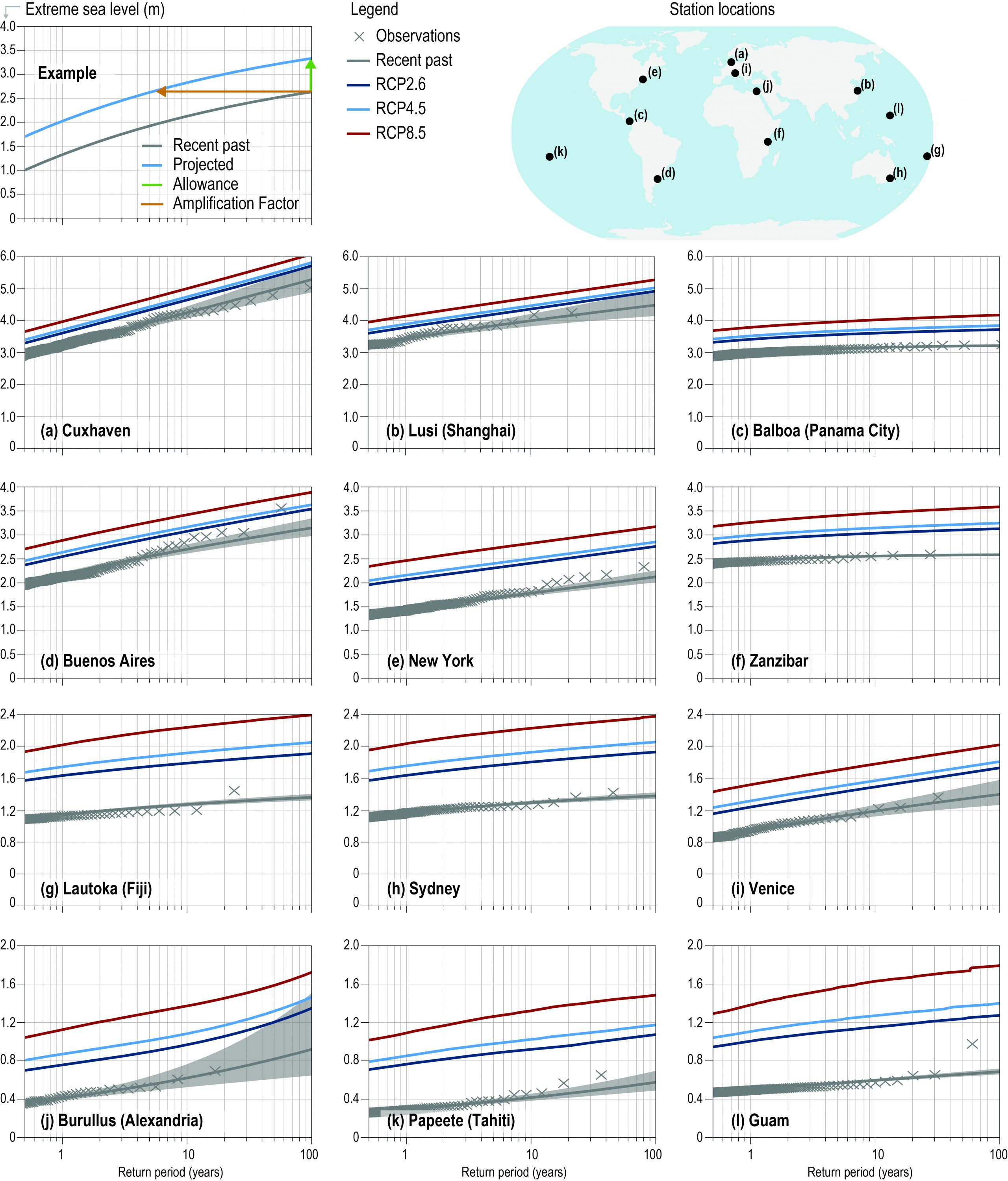
Figure 4.11 | The relation between expected extreme sea level (ESL) events and return period at a set of characteristic tide gauge locations (see upper left for their location), referenced to recent past mean sea level, based on observations in the GESLA-2 data base (grey lines) and 2081–2100 conditions for three different RCP scenarios as presented in Section 4.2.3.2. The grey bands represent the 5–95% uncertainty range in the fit of the extreme value distribution to observations. The upper right hand panel provides an example illustrating the relationship between ESL events and return period for historical and future conditions; the blue line in this panel shows the best estimate ESL event above the 1986–2005 reference mean sea level. The coloured lines for the different locations show this expected ESL events for different RCP scenarios. The horizontal line denoting the amplification factor expresses the increase in frequency of events which historically have a return period of once every 100 years. In the example, a water level of 2.5 m above mean sea level, recurring in the recent climate approximately every 100 years in recent past climate, will occur every 2 to 3 years under future climate conditions. The allowance expresses the increase in ESL for events that historically have a return period of 100 years.
Figure 4.12
Figure 4.12 | The colours of the dots express the factor by which the frequency of extreme sea level (ESL) events increase in the future for events which historically have a return period of 100 years. Hence a value of 50 means that what is currently 1-in-100 year event will happen every 2 years due […]
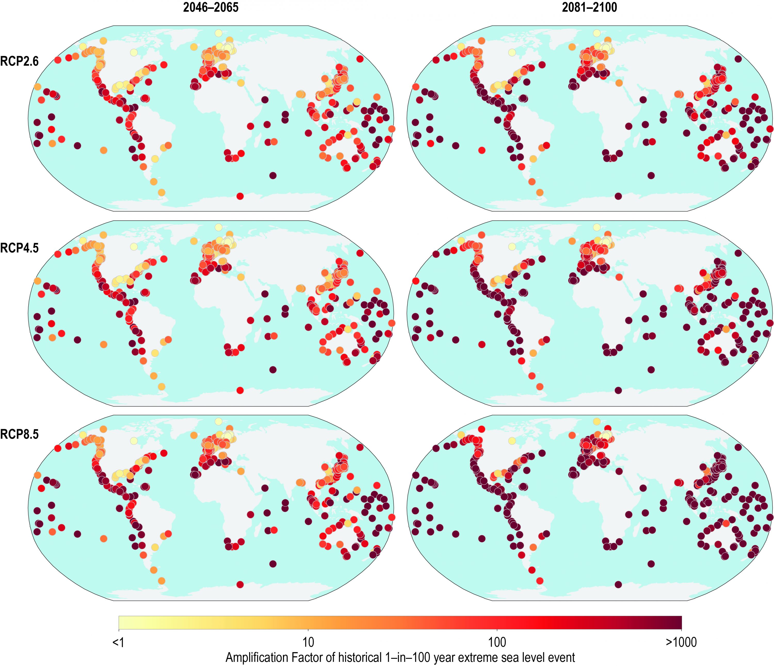
Figure 4.12 | The colours of the dots express the factor by which the frequency of extreme sea level (ESL) events increase in the future for events which historically have a return period of 100 years. Hence a value of 50 means that what is currently 1-in-100 year event will happen every 2 years due to a rise in mean sea level. Results are shown for three RCP scenarios and two future time slices as median values. Results are shown for tide gauges in the GESLA2 database. The accompanying confidence interval can be found in SM4.2 as well as a list of all locations. The data underlying the graph are identical to those presented in Figure 4.11. The amplification factor is schematically explained in the upper right panel of figure 4.11. Storm climatology is constant in these projections.
In summary, ESL events estimates as presented in this subsection, clearly show that as a consequence of SLR, events which are currently rare (e.g., with an average return period of 100 years), will occur annually or more frequently at most available locations for RCP8.5 by the end of the century (high confidence). For some locations, this change will occur as soon as mid-century for RCP8.5 and by 2100 for all emission scenarios. The affected locations are particularly located in low-latitude regions, away from the tropical cyclone (TC) tracks. In these locations, historical sea level variability due to tides and storm surges is small compared to projected mean SLR. Therefore, even limited changes in mean sea level will have a noticeable effect on ESLs, and for some locations, even RCP2.6 will lead to the annual occurrence of historically rare events by mid-century. Results should be treated with caution in regions where TCs are important as they are underrepresented in the observations (Haigh et al., 2014a721).
4.2.3.4.2
Waves
A warming climate is expected to affect wind patterns and storm characteristics, which in turn will impact wind waves that contribute to high coastal water levels. Wind-wave projections are commonly based on dynamical and statistical wave models forced by projected surface winds from GCMs, notably those participating in the CMIP. In the framework of the Coordinated Ocean Wave Climate Project (COWCLIP), an ensemble of Coupled Model Intercomparison Project Phase 3 (CMIP3)-based global wave projections (Hemer et al., 2013) was produced and the results were summarised in the AR5 (WGI Chapter 13). Casas-Prat et al. (2018) expanded the geographic domain to include the Arctic Ocean, highlighting the vulnerability of high-latitude coastlines to wave action as ice retreats. Reduced sea ice allows larger waves and stronger cyclones in the Arctic Ocean, which can further disrupt and break up sea ice (e.g., Thomson and Rogers, 2014; Day and Hodges, 2018). A review and consensus-based analysis of regional and global scale wave projections, including CMIP5-based projections, has been provided by Morim et al. (2018) as part of COWCLIP. Projections of annual and seasonal mean significant wave height changes agree on an increase in the Southern Ocean, tropical eastern Pacific and Baltic Sea; and on a decrease over the North Atlantic, northwestern Pacific and Mediterranean Sea. Projections of mean significant wave height lack consensus over the eastern North Pacific and southern Indian and Atlantic Oceans. Projections of future extreme significant wave height are consistent in projecting an increase over the Southern Ocean and a decrease over the northeastern Atlantic and Mediterranean Sea. Regional projections of wind-waves have mostly been applied to Europe so far, while highly vulnerable regions have been largely overlooked. This is the case for low-lying islands where impacts of SLR and wave-induced flooding are expected to be severe and adaptive capacity is reduced (Hoeke et al., 2013; Albert et al., 2016).
A number of studies have included waves, in addition to tides and sea level anomalies, to assess coastal vulnerability to SLR using dynamical and statistical approaches. CoSMoS (Barnard et al., 2014) includes a series of embedded wave models to estimate high resolution projections of total water levels along the Southern California coast for different extreme scenarios (O’Neill et al., 2017). Arns et al. (2017) find that an increase in sea level may reduce the depth-limitation of waves, thereby resulting in waves with greater energy approaching the coast. Including wave effects is crucial for coastal adaptation and planning (e.g., Isobe, 2013). For example Arns et al. (2017) report that coastal protection design heights need to be increased by 48–56% in the German Bight region relative to a design height based on the effect of SLR on ESL only. Combining SLR with extreme value theory applied to past observations of tides, storm surges and waves, Vitousek et al. (2017) found that a 10–20 cm SLR could result in a doubling of coastal flooding frequency in the tropics. For the southern North Sea region, Weisse et al. (2012) argue that increasing storm activity also increases hazards from ESL events. Global-scale projections of ESL event changes including wave setup indicate a very likely increase of the global average 100-year ESL of 58–172 cm under RCP8.5 (Vousdoukas et al., 2018c). Changes in storm surges and waves enhance the effects of relative SLR along the majority of northern European coasts, with contributions up to 40% in the North Sea (Vousdoukas et al., 2017).
A stationarity of the wave climate is often assumed for projections of ESL events (Vitousek et al., 2017). Yet, wave contributions to coastal sea level changes (setup and swash) depend on several factors that can vary in response to internal climate variability and climate change, including deep-water wave field, water-depth, and geomorphology. Melet et al. (2018) reported that over recent decades, wave setup and swash interannual-to-decadal changes induced by deep-water wave height and period changes alone were sizeable compared to steric and land-ice mass loss coastal sea level changes.
Comprehensive broad-scale projections of sea level at the coast including regional sea level changes, tides, waves, storm surges, interactions between these processes and accounting for changes in period and height of waves and frequency and intensity of storm surges are yet to be performed.
4.2.3.4.3
Effects of cyclones
Tropical and extratropical cyclones (TCs and ETCs) tend to determine ESL events, such as coastal storm surges, high water events, coastal floods, and their associated impacts on coastal communities around the world. The projected potential future changes in TCs and ETCs frequency, track and intensity is therefore of great importance. After AR5, it was realised that the modelled global frequency of TCs is underestimated and that the geographical pattern is poorly resolved in the case of TC tracks, very intense TCs (i.e., Category 4/5) and TC formation by using low resolution climate models (Camargo, 2013). Over recent years, multiple methods including downscaling
CMIP5 climate models (Knutson et al., 2015; Yamada et al., 2017), high-resolution simulations (Camargo, 2013; Yamada et al., 2017), TC–ocean interaction (Knutson et al., 2015; Yamada et al., 2017), statistical models (Ellingwood and Lee, 2016) and statistical-deterministic models (Emanuel et al., 2008) have been developed, and the ability to simulate TCs has been substantially improved. Most models still project a decrease or constant global frequency of TCs, but a robust increase in the lifetimes, precipitation, landfalls and ratio of intense TCs under global warming. This is consistent with IPCC AR5 and many additional studies (Emanuel et al., 2008; Holland et al., 2008; Knutson et al., 2015; Kanada et al., 2017; Nakamura et al., 2017; Scoccimarro et al., 2017; Zheng et al., 2017). It is expected that these projected increases are intensified by favourable marine environmental conditions, expansion of the tropical belt, or ocean warming in the northwest Pacific and north Atlantic, and increasing water vapour in the atmosphere (Kossin et al., 2014; Moon et al., 2015; Cai et al., 2016; Mei and Xie, 2016; Cai et al., 2017; Kossin, 2017; Scoccimarro et al., 2017; Kossin, 2018). However, it is noted that, in contrast to most models, some models do predict an increase in global TC frequency during the 21st century (Emanuel, 2013; Bhatia et al., 2018).
Previous extensive studies indicated the important role of warming oceans in the TC activity (Emanuel, 2005; Mann and Emanuel, 2006; Trenberth and Fasullo, 2007; Trenberth and Fasullo, 2008; Villarini and Vecchi, 2011; Trenberth et al., 2018) and also revealed TCs stir the ocean and mix the subsurface cold water to the surface (Shay et al., 1992; Lin et al., 2009). The resulting increased thermal stratification of the upper ocean under global warming will reduce the projected intensification of TCs (Emanuel, 2015; Huang et al., 2015; Tuleya et al., 2016). A recent study suggests a strengthening effect of ocean freshening in TC intensification, opposing the thermal effect (Balaguru et al., 2016). It is concluded that it is likely that the intensity of severe TCs will increase in a warmer climate, but there is still low confidence in the frequency change of TCs in the future.
Recent projection studies indicate that trends in regional ETCs vary from region to region, for example, a projected increase in the frequency of ETCs in the South and the northeast North Atlantic, the South Indian Ocean, and the Pacific (Colle et al., 2013; Zappa et al., 2013; Cheng et al., 2017; Michaelis et al., 2017) and a decrease in the numbers of ETCs in the North Atlantic basin and the Mediterranean (Zappa et al., 2013; Michaelis et al., 2017). Note that the projected frequency in ETCs still remains uncertain due to different definitions of cyclone, model biases or climate variability (Chang, 2014; Cheng et al., 2016). Considering these processes implies that changes in TC and ETC characteristics will vary locally and therefore there is low confidence in the regional storm changes, which is in agreement with AR5 WGI Chapter 14 (Christensen et al., 2013).
Observed damages from ETCs/TCs to coastal regions has increased over the past 30 years and will continue in the future (Ranson et al., 2014). The global population exposed to ETCs/TCs hazards is expected to continue to increase in a warming climate (Peduzzi et al., 2012; Blöschl et al., 2017; Emanuel, 2017a; Michaelis et al., 2017). The probabilities of sea level extreme events induced by TC storm surge are very likely to increase significantly over the 21st century. Risk from TCs increases in highly vulnerable coastal regions (Hallegatte et al., 2013), e.g., on coasts of China (Feng and Tsimplis, 2014), west Florida, north of Queensland, the Persian Gulf, and even in well protected area such as the Greater Tokyo area (Tebaldi et al., 2012; Lin and Emanuel, 2015; Ellingwood and Lee, 2016; Hoshino et al., 2016; Dinan, 2017; Emanuel, 2017b; Lin and Shullman, 2017). The ESL return period has greatly decreased over recent decades and is also expected to decrease greatly in the near future, for example, in NYC (by 2030–2045; Garner et al., 2017). It is very likely that the ESL return period in low-lying areas such as coastal megacities decreased over the 20th century and frequencies of still unusual ESL events are expected to increase in frequency in the future. In addition, the compound effects of SLR, storm surge and waves on ESL events and the associated flood hazard are assessed in Chapter 6 (Section 6.3.3.3 and 6.3.4).
4.2.3.5
Long-Term Scenarios, Beyond 2100
Sea level at the end of the century will be higher than present day and continuing to rise in all cases even if the Paris Agreement is followed (Nicholls, 2018794). The reasons for this are mainly related to the slow response of glacier melt, thermal expansion and ice sheet mass loss (Solomon et al., 2009794). These processes operate on long time scales, implying that even if the rise in global temperature slows or the trend reverses, sea level will continue to rise (SR1.5 report, AR5). A study by Levermann et al. (2013)799 based on palaeo-evidence and physical models formed the basis of the assessment by Church et al. (2013)803 indicating that committed SLR is approximately 2.3 m per degree warming for the next 2000 years with respect to pre-industrial temperatures. This rate is based on a relation between ocean warming and basal melt as used by Levermann et al. (2013), without accounting for surface melt, hydrofracturing of ice shelves and subsequent ice cliff failure, suggested to be a dominant long term mechanism for ice mass loss (DeConto and Pollard, 2016808). Deep uncertainty (Cross-Chapter Box 5 in Chapter 1) remains on the ice dynamical contribution from Antarctica after 2100.
Beyond the 21st century, the relative importance of the long-term contributions of the various components of SLR changes markedly. For glaciers, the long-term is of limited importance, because the sea level equivalent of all glaciers is restricted to 0.32 ± 0.08 m when taking account of ice mass above present day sea level (Farinotti et al., 2019796). Hence, there is high confidence that the contribution of glaciers to SLR expressed as a rate will decrease over the 22nd century under RCP8.5 (Marzeion et al., 2012797). For thermal expansion the gradual rate of heat absorption in the ocean will lead to a further SLR for several centuries (Zickfeld et al., 2017798). By far, the most important uncertainty on long time scales arises from the contribution of the major ice sheets. The time scale of response of ice sheets is thousands of years. Hence, if ice sheets contribute significantly to sea level in 2100, they will necessarily also contribute to sea level in the centuries to follow. Only for low emission scenarios, like RCP2.6, can substantial ice loss be prevented, according to ice dynamical models (Levermann et al., 2014799; Golledge et al., 2015800; DeConto and Pollard, 2016801; Bulthuis et al., 2019802). For Greenland, surface warming may lead to ablation becoming larger than accumulation, and the associated surface lowering increases ablation further (positive feedback). As a consequence, the ice sheet will significantly retreat. Church et al. (2013)803 concluded that the threshold for perpetual negative mass balance based on modelling studies lies between 1ºC (Robinson et al., 2012804; low confidence) and 4ºC (medium confidence) above pre-industrial temperatures. Pattyn et al. (2018)805 demonstrated that with more than 2.0ºC of summer warming, it becomes more likely than not that the GIS crosses a tipping point, and the ice sheet will enter a long-term state of decline with the potential loss of most or all of the ice sheet over thousands of years. If the warming is sustained, ice loss could become irreversible due to the initiation of positive feedbacks associated with elevation-SMB feedback (reinforced surface melt as the ice sheet surface lowers into warmer elevations), and albedo-melt feedback associated with darkening of the ice surface due to the presence of liquid water, loss of snow, changes in firn and biological processes (Tedesco et al., 2016806; Ryan et al., 2018807). The precise temperature threshold and duration of warming required to trigger such irreversible retreat remains very uncertain, and more research is still needed.
The mechanisms for decay of the AIS are related to ice shelf melt by the ocean, followed by accelerated loss of grounded ice and MISI, possibly exacerbated by hydrofracturing of the ice shelves and ice cliff failure (Cross-Chapter Box 8 in Chapter 3). The latter processes have the potential to drive faster rates of ice mass loss than the SMB processes that are likely to dominate the future loss of ice on Greenland. Furthermore, the loss of marine-based Antarctic ice represents a long-term (millennial) commitment to elevated SLR, due to the long thermal memory of the ocean. Once marine based Antarctic ice is lost, local ocean temperatures will have to cool sufficiently for buttressing ice shelves to reform, allowing retreated grounding lines to re-advance (DeConto and Pollard, 2016808). A minimum time scale, whereby the majority of West Antarctica decays, was derived from a schematic experiment with an ice flow model by Golledge et al. (2017)809, where ice shelves were removed instantaneously and prohibited from re-growing. Results of this experiment indicate that most of West Antarctica’s ice is lost in about a century.
Gradual melt of ice shelves accompanied by partial retreat of East Antarctic ice would yield greater ice melt but on a time scale of millennial or longer (Cross-Chapter Box 8 in Chapter 3). Prescribing a uniform warming of 2°C–3°C in the Southern Ocean triggers an accelerated decay of West Antarctica in a coarse resolution model with a temperature-driven basal melt formulation yielding 1–2 m SLR by the year 3000 and up to 4 m by the year 5000 (Sutter et al., 2016810). Formulating an ice sheet model with Coulomb friction in the grounding line zone yields a SLR of 2 m after 500 year for a sub-ice shelf melt of 20 m a–1 (Pattyn, 2017811). On decadal to millennial time scales the interaction between ice and the solid Earth indicates the possibility of a negative feedback slowing retreat by viscoelastic uplift and gravitational effects that reduce the water depth at the grounding line (Gomez et al., 2010812; de Boer et al., 2014; Gomez et al., 2015813; Konrad et al., 2015814; Pollard et al., 2017815; Barletta et al., 2018816; Section 4.2.3.1.2).
A blended statistical and physical model, calibrated by observed recent ice loss in a few basins (Ritz et al., 2015817) projects an Antarctic contribution to sea level of 30 cm by 2100 and 72 cm by 2200, following the SRES A1B scenario, roughly comparable to RCP6.0. The projected contribution of WAIS was found to be limited to 48 cm in 2200 following the A1B scenario. The key uncertainty in these calculations comes from the dependency on the relation between the sliding velocity and the friction at the ice-bedrock interface. Several parameterisations are used to describe this process. Golledge et al. (2015)820 present values between 0.6–3 m by 2300 for the RCP8.5 scenario. In contrast to the previous studies, Cornford et al. (2015) used an adaptive grid model, which can describe more accurately grounding line migration (Cross-Chapter Box 8 in Chapter 3). Due to the computational complexity of their model, simulations are limited to West Antarctica. Starting from present-day observations, they find that the results are critically dependent on initial conditions, sub ice shelf melt rates, and grid resolution. The glacier with the most uncertain vulnerability is the 120 km-wide Thwaites Glacier, in the Amundsen Sea sector of West Antarctica. Thwaites Glacier is currently retreating in a reverse-sloped trough extending into the central WAIS (Figure 4.8), where the bed is up to 2 km below sea level. In addition to Thwaites, several smaller outlet glaciers and ice streams may contribute to sea level on long time scales, but in the study by Cornford et al. (2015), a full West Antarctic retreat does not occur with limited oceanic heating under the two major ice shelves (Filchner-Ronne and Ross) keeping ice streams flowing into the Ross and Weddell Seas in place. However, the representation of these processes remains simplistic at the continental ice sheet scale (Cross-Chapter Box 8 in Chapter 3).
Nonetheless, recent studies using independently developed Antarctic ice dynamical models (Golledge et al., 2015; DeConto and Pollard, 2016821; Bulthuis et al., 2019822) agree that low emission scenarios, are required to prevent substantial future ice loss (medium confidence). However, observations (Rignot et al., 2014823) and modelling of the Thwaites Glacier in West Antarctica (Joughin et al., 2014824), suggest grounding line retreat on the glacier’s reverse sloped bedrock is already underway and possibly capable of driving major WAIS retreat on century time scales. Whether the retreat is driven by ocean changes driven by climate change or by climate variability (Jenkins et al., 2018825) is still under debate. Hence it is not possible to determine whether a low emission scenario would prevent substantial future ice loss (medium confidence). This is a further elaboration on the SR15 assertion that the chance for passing a threshold is larger for 2°C warming than for 1.5°C warming.
A study by Clark et al. (2016) addresses the evolution of the ice sheets over the next 10,000 years and concludes that given a climate model with an equilibrium climate sensitivity of 3.5°C, the estimated combined loss of Greenland and Antarctica ranges from 25–52 m of equivalent sea level, depending on the emission scenario considered, with rates of GMSL as high as 2–4 m per century. A worst-case scenario was explored with an intermediate complexity climate model coupled to a dynamical ice model (Winkelmann et al., 2015826), in which all readily available fossil fuels are combusted at present-day rates until they are exhausted. The associated climate warming leads to the disappearance of the entire AIS with rates of SLR up to around 3 m per century. A follow up study by Clark et al. (2018)827 addressing the long-term commitment of SLR based on cumulative carbon dioxide emissions points to SLR as an additional measure for setting emission targets. It shows that a 2ºC scenario would result in 0.9 m in 2300 and around 7.4 m in the year 9000 CE.
Similar to the strategy for the 21st century, the long-term projections of sea level were assessed. Since no new CMIP runs are available there are no major new insights in the thermal expansion and glacier component which deviate from the AR5 assessment for the long-term contribution of these components. Some studies updated the contribution of the GIS on long time scales. Vizcaino et al. (2015)828 used a GCM coupled to an ice sheet model to calculate the Greenland contribution which is within the range of estimates presented by Church et al. (2013)829. This is also true for the ice sheet simulations by Calov et al. (2018)830 which are based on off line simulations with a regional climate model forced by RCP4.5 and RCP8.5 scenarios of three different CMIP5 models. On the other hand, Aschwanden et al. (2019)831 used temperatures to calculate SMB which was used to force an ice sheet model to arrive at much higher values for SLR. However, they used a spatially uniform temperature forcing, which is in conflict with earlier work and overestimated temperatures in the ablation zone (e.g., Van de Wal and Wild, 2001; Gregory and Huybrechts, 2006832). Given this limited and contrasting evidence for Greenland, the assessed values presented in Table 13.8 of Church et al. (2013)836 were also used, but again replacing the Antarctic component by the assessed value from the process and climate scenario-based studies published after 2013. The low scenario in Table 13.8 of Church et al. (2013) without the Antarctic contribution was combined with the RCP2.6 estimates for Antarctica simulated by Golledge et al. (2015)833, the mean of the RCP2.6 simulations with and without time delay between global mean atmosphere and ocean temperature around Antarctica of Levermann et al. (2014)834, and the model results of Bulthuis et al. (2019)835. The medium scenario from Church et al. (2013)836 is combined with RCP4.5 results and the high scenario with RCP8.5. Results are shown in Figure 4.2, Section 4.1 and show a strong divergence of RSL rise over time, whereby the estimates in 2300 range from about 1–2 m under RCP2.6 up to 2–5.5 m for RCP8.5.
The specific trajectories that will be followed may depend critically on if and when certain tipping points are reached. Most critical in that respect are presumably the tipping points corresponding (1) to the threshold where the ablation in Greenland becomes larger than the accumulation, causing an irreversible and nearly full retreat of the ice sheet; and (2) the thresholds for ice shelf stability in West Antarctica, which depend on surface melt and sub-ice melt, combined with uncertainties surrounding MISI and/or MICI. There is deep uncertainty about whether and when a tipping point will be passed. For RCP8.5, the chance of passing a tipping-point are considered to be substantially higher than for RCP2.6.
In summary, there is high confidence in continued thermal expansion and the loss of ice from both the GIS and AIS sheets beyond 2100. A complete loss of Greenland ice contributing about 7 m to sea level over a millennium or more would occur for sustained GMST between 1°C (low confidence) and 4°C (medium confidence) above pre-industrial levels. Due to deep uncertainties regarding the dominant processes that could trigger a major retreat, there is low confidence in the estimates of the contribution of the AIS beyond 2100, but our estimates (2.3–5.4 m in 2300) for RCP8.5 are considerably higher than presented in AR5. High-emission scenarios or exhaustion of fossil fuels over a multi-century period lead to rates of SLR as high as several metres per century in the long term (low confidence). Low-emission scenarios lead to a limited contribution over multi-century time scales (high confidence). Discriminating between 1.5°C and 2°C scenarios in terms of long-term sea level change is not possible with the limited evidence. Hence, it is concluded that the SLR on millennial time scales is strongly dependent on the emission scenario followed. This, combined with the lack in predictability of the tipping points, indicates the importance of emissions mitigation for minimising the risk to low-lying coastlines and islands (high confidence).
4.3
Exposure, Vulnerability, Impacts and Risk Related to Sea Level Rise
4.3.1
Introduction
Section 4.2 demonstrates that sea level is rising and accelerating over time, and that it will continue to rise throughout the 21st century and for centuries beyond. It also shows that ESL events that are historically rare, will become common by 2100 under all emission scenarios, leading to severe flooding in the absence of ambitious adaptation efforts (high confidence). In both RCP2.6 and RCP8.5 emission scenarios, many low-lying coastal areas at all latitudes will experience such events annually by 2050. In this context, Section 4.3 updates knowledge on the recent methodological advances in exposure and vulnerability assessments (Box 4.2), dimensions of exposure and vulnerability (Section 4.3.2) and observed and projected impacts (Section 4.3.3). It concludes with a synthesis on future risks to illustrative low-lying coastal geographies (resource-rich coastal cities, urban atoll island, large tropical agricultural deltas and Arctic communities), and according to various adaptation scenarios (Section 4.3.4)
4.3.2
Dimensions of Exposure and Vulnerability to Sea Level Rise
4.3.2.1
Point of Departure
4.3.2.2
Settlement Trends
Major changes in coastal settlement patterns have occurred in the course of the 20th century, and are continuing to take place due to various complex interacting processes (Moser et al., 2012; Bennett et al., 2016) that together configure and concentrate exposure and vulnerability to climate change and SLR along the coast (Newton et al., 2012; Bennett et al., 2016). These processes include population growth and demographic changes (Smith, 2011; Neumann et al., 2015), urbanisation and a rural exodus, tourism development, and displacement or (re)settlement of some indigenous communities (Ford et al., 2015). This has resulted in a growing number of people living in the Low Elevation Coastal Zone (LECZ, coastal areas below 10 m of elevation; around 11% of the world’s population in 2010; Neumann et al., 2015; Jones and O’Neill, 2016; Merkens et al., 2016) and in significant infrastructure and assets being located in risk-prone areas (high confidence). High density coastal urban development is commonplace in both developed and developing countries, as documented in recent case studies, for example in Canada (Fawcett et al., 2017), China (Yin et al., 2015; Lilai et al., 2016; Yan et al., 2016), Fiji (Hay, 2017), France (Genovese and Przyluski, 2013; Chadenas et al., 2014; Magnan and Duvat, 2018), Israel (Felsenstein and Lichter, 2014), Kiribati (Storey and Hunter, 2010; Duvat et al., 2013), New Zealand (Hart, 2011) and the USA (Heberger, 2012; Grifman et al., 2013; Liu et al., 2016b). This has implications for levels of SLR risk at regional and local scales (medium evidence, high agreement). In Latin America and the Caribbean, for example, it is estimated that 6–8% of the population live in areas that are at high or very high risk of being affected by coastal hazards (Reguero et al., 2015; Calil et al., 2017; Villamizar et al., 2017), with higher percentages in Caribbean islands (Mycoo, 2018). In the Pacific, ~57% of Pacific Island countries’ built infrastructure are located in risk-prone coastal areas (Kumar and Taylor, 2015). In Kiribati, due to the flow of outer, rural populations to limited, low-elevated capital islands, together with constraints inherent in the sociocultural land tenure system, the built area located <20 m from the shoreline quadrupled between 1969 and 2007–2008 (Duvat et al., 2013). Other examples of rural exodus are reported in the recent literature, for example in the Maldives (Speelman et al., 2017).
Population densification also affects rural areas’ exposure and vulnerability, and interacts with other factors shaping settlement patterns, such as the fact that ‘indigenous peoples in multiple geographical contexts have been pushed into marginalised territories that are more sensitive to climate impacts, in turn limiting their access to food, cultural resources, traditional livelihoods and place-based knowledge (…) [and therefore undermining] aspects of social-cultural resilience’ (Ford et al., 2016b, p. 350). In the Pacific, for example, ‘while traditional settlements on high islands (…) were often located inland, the move to coastal locations was encouraged by colonial and religious authorities and more recently through the development of tourism’ (Ballu et al., 2011; Nurse et al., 2014, p. 1623; Duvat et al., 2017). Although these population movements are orders of magnitude smaller than the global trends described above, they play a critical role at the very local scale in explaining the emergence of, or changes in exposure and vulnerability. In atoll contexts, for example, the growing pressure on freshwater resources together with a loss in local knowledge (e.g., how to collect water from palm trees), result in increased exposure of communities to brackish, polluted groundwater, inducing water insecurity and health problems (Storey and Hunter, 2010; Lazrus, 2015).
4.3.2.4
Other Human Dimensions
The development of local scale case studies from a social science perspective, for example, in the Arctic (Ford et al., 20121075; Ford et al., 20141076), small islands (Petzold, 20161077; Duvat et al., 20171078) and within cities (Rosenzweig and Solecki, 20141079; Paterson et al., 20171080; Texier-Teixeira and Edelblutte, 20171081) or at the household level (Koerth et al., 20141082) support a better understanding of the anthropogenic drivers of exposure and vulnerability. Four examples of drivers that were only emerging at the time of the AR5 are discussed below. Very importantly, another major emerging dimension that is not discussed here but rather in Section 4.4.4, relates to power asymmetries, politics, and the prevailing political economy, which are important drivers of exposure and vulnerability to SLR-related coastal hazards, and consequently adaptation prospects (Eriksen et al., 20151083; Dolšak and Prakash, 20181084). Recent literature provides examples in coastal megacities like Jakarta, Indonesia (Shatkin, 20191085) as well as in smaller cities, like Maputo, Mozambique (Broto et al., 20151086) and Surat, India (Chu, 2016a; Chu, 2016b), and many other coastal cities and settlements around the world (high confidence; Jones et al., 20151087; Allen et al., 20181088; Hughes et al., 20181089; Sovacool, 20181090).
4.3.2.4.1
Gender inequality
Gender inequality came to prominence only recently in climate change studies (~15 years ago; see Pearse, 20171091). In light of sea-related hazards and SLR specifically, the issue is still mainly investigated in the context of developing countries, although growing attention is paid to the issue in developed countries (e.g., Lee et al., 2015; Pearse, 2017). Recent studies in southern coastal Bangladesh, for example, show that women get less access than men to climate- and disaster-related information (both emergency information and training programmes), decision making processes at the household and community levels, economic resources including financial means such as micro-credit, land ownership, and mobility within and outside the villages (Rahman, 20131092; Alam and Rahman, 20141093; Garai, 20161094). Gender inequity may be inherent in unfavourable background conditions (higher illiteracy rates, deficiencies in food and calories intake and poorer health conditions) as a result of, among other things, traditions, social norms and patriarchy. Together, these barriers disadvantage women more than men in developing effective responses to anticipate gradual environmental changes such as persistent coastal erosion, flooding and soil salinisation (medium evidence, high agreement). Such conclusions are in line with the literature on gender inequality and climate change at large (Alston, 20131095; Pearse, 20171096), thus suggesting no major SLR-inherent specificities.
4.3.2.4.2
Loss of indigenous knowledge and local knowledge
Despite the identification of this issue in AR4, its treatment in AR5 remained limited. Recent literature partly focussing on SLR reaffirms that indigenous knowledge and local knowledge (IK and LK; Cross-Chapter Box 4 in Chapter 1 and Glossary) are key to determining how people recognise and respond to environmental risk (Bridges and McClatchey, 20091097; Lefale, 20101098; Leonard et al., 20131099; Lazrus, 20151100), and therefore to increasing adaptive capacity and reducing long-term vulnerability (Ignatowski and Rosales, 20131101; McMillen et al., 20141102; Hesed and Paolisso, 20151103; Janif et al., 20161104; Morrison, 20171105).
IK and LK contribute both as a foundation for and an outcome of customary resource management systems aimed at regulating resource use and securing critical ecosystem protection (examples in Indonesia; Hiwasaki et al., 20151106), structuring the relationship between people and authorities, and framing and maintaining a strong sense of place in the community (examples in Timor Leste; Hiwasaki et al., 20151107). In turn, this allows local communities to predict and prepare for both sudden shock events that have historical precedent and, when IK and LK are embedded in day-to-day rituals and decision making processes, to also anticipate the consequences of gradual changes, as in sea level (examples in Indonesia; Hiwasaki et al., 20151108). Customary resource management systems based on IK and elders’ leadership—for instance, Rahui in French Polynesia (Gharasian, 20161109), or Mo in the Marshall Islands (Bridges and McClatchey, 2009)—also allow communities to diversify access to marine and terrestrial resources using seasonal calendars, to ensure collective food and water security, and to maintain ecological integrity (McMillen et al., 20141111). In rural Pacific atolls, traditional food preservation and storage (e.g., storing germinated coconuts or drying fish) still play a role in anticipating disruptions in natural resource availability (Campbell, 20151112; Lazrus, 20151113). Such practices have enabled the survival of isolated communities from the Arctic to tropical islands in constraining sea environments for centuries to millennia (McMillen et al., 20141114; Nunn et al., 2017a1115). Morrison (2017) argues that IK and LK can also play a role in supporting internal migration in response to SLR, by avoiding social and cultural uprooting (Cross-Chapter Box 4 in Chapter 1).
In some specific contexts, climate change will also imply no-analogue changes, such as rapid ice-melt and changing conditions in the Arctic that have no precedent in the modern era, and could thus limit the relevance of IK and LK in efforts to address significantly different circumstances. Except in these specific situations, the literature suggests that the loss of IK and LK, and related social norms and mechanisms, will increase populations’ exposure and vulnerability to SLR impacts (Nakashima et al., 20121117). The literature notably points out that modern, externally-driven socioeconomic dynamics, such as the introduction of imported food (noodles, rice, canned meat and fish, etc.), diminish the cultural importance of IK-based practices and diets locally, together with introducing dependency on monetisation and external markets (Hay, 2013; Campbell, 20151118).
As a result, the loss of IK and LK may increase long-term vulnerability to SLR (medium evidence, high agreement). Given that IK and LK are largely based on observing and ‘making sense’ of the surrounding environment (moon, waves, winds, animal behaviours, topography, etc.), such a loss reflects a more general concern about the weakening of environmental connectedness in contemporary societies, which is not limited to remote, rural and developing communities (medium confidence). In developed contexts too, the loss of LK has played a critical role in recent coastal disasters (e.g., Katrina in 2005 in the USA, Kates et al., 2006) and increasing vulnerability to SLR (e.g., Newton and Weichselgartner, 2014; Wong et al., 20141119).
4.3.2.4.3
Social capital
Coastal communities draw on social structures and capabilities that can reduce risk and increase adaptive capacity in the face of coastal hazards (Aldrich, 20171120; Petzold, 20181121). Although the term is subject to debate (Meyer, 20181122), social capital—that is, the level of cohesion between individuals, between groups of individuals, and between people and institutions, within and between communities—is considered to be a key enabler for collective action to reduce risk and build adaptive capacity (Adger, 20101123; Aldrich and Meyer, 20151124; Petzold and Ratter, 20151125). Levels of social capital can be influenced by underlying social processes, such as socioeconomic (in)equalities, gender issues, health, social networks and social media. It applies to both developing and developed countries, for example in densely populated deltas (Jordan, 20151126), European coasts (Jones and Clark, 20141127; Petzold, 20161128), Asian urban or semi-urban coastal areas (Lo et al., 20151129; Triyanti et al., 20171130) and Pacific islands (Neef et al., 20181131). Social capital framed as an enabler for reducing vulnerability has been studied in the context of extreme events (risk prevention mechanisms, emergency responses and post-crisis actions) and collective environmental management (e.g., replanting mangroves, beach cleaning, etc.). Social capital also enables adaptation prospects. For example, its role has been explored in public acceptability of long-term coastal adaptation policies in the UK (Jones and Clark, 20141132; Jones et al., 20151133). The role of social capital in building resilience to climate stress in coastal Bangladesh was explored by Jordan (2015), who found complex and even contradictory interactions between social capital and resilience to climate stress. Among others, Jordan (2015) also advises caution about uncritical importation of such Westernised concepts in seeking to understand and address coastal vulnerability in developing countries.
4.3.2.4.4
Risk perception
Risk perception, which is context-specific and varies from one individual to another, may influence communities’ exposure and vulnerability as it shapes authorities’ and people’s attitudes towards sudden and slow onset hazards, as shown by Terpstra (2011)1134, Lazrus (2015), Elrick-Barr et al. (2017)1135 and O’Neill et al. (2016) in the Netherlands, Tuvalu, Australia and Ireland, respectively. The progressive discounting of coastal hazard risks and subsequent loss of risk memory also played a role in coastal disasters such as Hurricane Katrina in 2005 in the USA (Burby, 20061136; Kates et al., 20061137) and Storm Xynthia in 2010 in France (Vinet et al., 20121138; Genovese and Przyluski, 20131139; Chadenas et al., 20141140).
Risk perceptions stem from intertwined predictors such as ‘gender, political party identification, cause-knowledge, impact-knowledge, response-knowledge, holistic affect, personal experience with extreme weather events, [social norms] and biospheric value orientations’ (Kellens et al., 20111141; Carlton and Jacobson, 20131142; Lujala et al., 20151143; van der Linden, 2015, p. 112; Weber, 20161144; Elrick-Barr et al., 20171145; Goeldner-Gianella et al., 20191146). In general, there is a lack of education, training and thus knowledge and literacy on recent and projected trends in sea level, which compromises ownership of science facts and projections at all levels, from individuals and institutions to society at large.
While some studies have begun to highlight the influence of the distance from the sea on risk perceptions (Milfont et al., 20141147; Lujala et al., 20151148; O’Neill et al., 2016), there is still little knowledge about how risk perceptions vary across different geographical and social contexts, and how this influences exposure and vulnerability to coastal hazards (e.g., Terpstra, 2011; van der Linden, 20151149). There is a critical lack of studies specifically addressing SLR. Some recent works conducted in coastal Australia suggest that while people are confident about their ability to cope with an already experienced event, when it comes to SLR, the dominant narrative is articulated around the barriers related to the ‘uncertainty in the nature and scale of the impacts as well as the response options available’ (Elrick-Barr et al., 2017, p. 1147). Similar conclusions have been highlighted in the Caribbean islands of St. Vincent (Smith, 20181150) and the Bahamas (Thomas and Benjamin, 20181151). SLR is rarely addressed separately from sea-related extreme events, which masks a crucial difference between already-observed and delayed impacts. Climate change is considered a “distant psychological risk” (Spence et al., 20121152), making it and SLR per se ‘markedly different from the way that our ancestors have traditionally perceived threats in their local environment’ (Milfont et al., 20141153; Lujala et al., 20151154; van der Linden, 2015, p. 112; O’Neill et al., 2016).
4.3.2.5
Towards a Synthetic Understanding of the Drivers of Exposure and Vulnerability
Recent literature confirms that anthropogenic drivers played an important role, over the last century, in increasing exposure and vulnerability worldwide, and indicates that they will continue to do so in the absence of adaptation (medium evidence, high agreement). Some scholars argue that ‘even with pervasive and extensive environmental change associated with ~2oC warming, it is non-climatic factors that primarily determine impacts, response options and barriers to adapting’ (Ford et al., 2015, p. 1046). Although it is the interaction of climate and non-climate factors that eventually determine the level of impacts, acknowledging the role of a range of purely anthropogenic drivers has important implications for action. It suggests that major action can be taken now to enhance long-term adaptation prospects, notwithstanding uncertainty about local RSL rise and resultant impacts in the distant future (medium evidence, high agreement; Magnan et al., 20161155). Acting on the human-driven drivers and root causes of vulnerability could yield co-benefits, for example by improving the state and condition of coastal ecosystems – and hence the capacity to cope with or adapt to SLR impacts – or, in deltaic regions, lowering the rates of anthropogenic subsidence and, in turn, minimising changes in sea level.
In addition, coastal ecosystem degradation is acknowledged as another major non-climatic driver of exposure and vulnerability (high confidence). The ability of coastal ecosystems to serve as a buffer zone between the sea and human assets (settlements and infrastructure), and to provide regulating services with respect to SLR-related coastal hazards (including inundation and salinisation), is progressively being lost due to coastal squeeze, pollution, and habitat and land degradation mainly due to land-use conversion.
We now better understand the diversity and interactions of the climate and non-climate drivers of exposure and vulnerability, as well as their dynamics over time (Bennett et al., 20161156; Duvat et al., 20171157). As a result, it is now realised how many context-specificities interact (including geography, economic development, social inequity, power and politics, and risk perceptions) and play a critical role in shaping the direction and influence of individual drivers and of their possible combinations on the ground (medium evidence, high agreement; Eriksen et al., 20151158; Hesed and Paolisso, 20151159; McCubbin et al., 20151160). This also provides a stronger foundation to identify the range of possible responses (Sections 1.6.1, 1.6.2 and 4.4.3) to observed impacts and projected risks, as well as critical areas of action to enhance adaptation pathways (Section 4.4.4).
Recent studies (e.g., cited in Sections 4.3.2.1.1, 4.3.2.2, 4.3.2.4.2 and 4.3.2.4.4) also confirm AR5 conclusions that both developing and developed countries are exposed and vulnerable to SLR (high confidence).
4.3.2.3
Terrestrial Processes Shaping Coastal Exposure and Vulnerability
Coastal areas, including deltas, are highly dynamic as they are affected by natural and/or human-induced processes locally or originating from both the land and the sea. Changes within the catchment can therefore have severe consequences for coastal areas in terms of sediment supply, pollution, and/or land subsidence. Sediment supply reaching the coast is a critical factor for delta sustainability (Tessler et al., 20181037) and has declined drastically in the last few decades due to dam construction, land use changes and sand mining (Ouillon, 20181038; high confidence). For instance, Anthony et al. (2015) reported large-scale erosion affecting over 50% of the delta shoreline in the Mekong delta between 2003 and 2012, which was attributed in part to a reduction in surface-suspended sediments in the Mekong river potentially linked to dam construction within the river basin, sand mining in the river channels, and land subsidence linked to groundwater over-abstraction locally. Schmitt et al. (2017)1039 demonstrated that these and other drivers in sediment budget changes can have severe effects on the very physical existence of the Mekong delta by the end of this century, with the most important single driver leading to inundation of large portions of the delta being ground-water pumping induced land subsidence. Thi Ha et al. (2018) estimated the decline in sediment supply to the Mekong delta to be around 75% between the 1970s and the period 2009–2016. In the Red River, the construction of the Hoa Binh Dam in the 1980s led to a 65% drop in sediment supply to the sea (Vinh et al., 20141040). Based on projections of historical and 21st century sediment delivery to the Ganges-Brahmaputra-Meghna, Mahanadi and Volta deltas, Dunn et al. (2018) showed that these deltas fall short in sediment and may not be able to maintain their current elevation relative to sea level, suggesting increasing salinisation, erosion, flood hazards and adaptation demands.
Another rarely considered factor is the shift in TC climatology which also plays a critical role in explaining changes in fluvial suspended sediment loads to deltas as demonstrated by Darby et al. (2016)1041, again for the Mekong delta. More generally, most conventional engineering strategies that are commonly employed to reduce flood risk (including levees, sea walls, and dams) disrupt a delta’s natural mechanisms for building land. These approaches are rather short-term solutions which overall reduce the long-term resilience of deltas (Tessler et al., 20151042; Welch et al., 20171043). Systems particularly prone to flood risk due to anthropogenic activities include North America’s Mississippi River delta, Europe’s Rhine River delta, and deltas in East Asia (Renaud et al., 20131044; Day et al., 20161045). In regions where suspended sediments are still available in relatively large quantities, rates of sedimentation can vary depending on multiple factors, including the type of infrastructure present locally, as was shown by Rogers and Overeem (2017)1046 for the Ganges-Brahmaputra-Meghna (Bengal) delta in Bangladesh as well as seasonal differences in sediment supply and place of deposition. For example, in meso-tidal and macro-tidal estuaries, during floods most of the sediments are depositing in the coastal zones and a large part of these sediments are brought back to the estuary during the low flow season by tidal pumping. This can lead to significantly higher deposition rates in the dry season as shown by Lefebvre et al. (2012) in the lower Red River estuary and by Gugliotta et al. (2018)1048 in the Mekong delta. Enhanced sedimentation further upstream in estuaries and a silting-up of estuarine navigation channels can have high economic consequences for cities with a large estuarine harbour. In Haiphong city, in North Vietnam, the authorities decided to build a new harbour further downstream, for a cost estimated at 2 billion USD (Duy Vinh et al., 2018).
Overall, reduced freshwater and sediment inputs from the river basins are critical factors determining delta sustainability (Renaud et al., 20131049; Day et al., 20161050). In some contexts, this can be addressed through basin-scale management which allow more natural flows of water and sediments through the system, including methods for long-term flood mitigation such as improved river-floodplain connectivity, the controlled redirection of a river (i.e., avulsions) during times of elevated sediment loads, the removal of levees, and the redirection of future development to lands less prone to extreme flooding (Renaud et al., 20131051; Day et al., 20161052; Brakenridge et al., 20171053). These actions could potentially increase the persistence of coastal landforms in the context of SLR. Next to decreasing sediment inputs to the coast, river bed and beach sand mining has been shown to contribute to shoreline erosion, for example, for shorelines of Crete (Foteinis and Synolakis, 20151054), and several sub-Saharan countries such Kenya, Madagascar, Mozambique, South Africa and Tanzania (UNEP, 20151055). At the global scale, 24% of the world’s sandy beaches are eroding at rates exceeding 0.5 m yr–1, while 28% are accreting for the period 1984–2016. The largest and longest eroding sandy coastal stretches are in North America (Texas; Luijendijk et al., 20181056).
Shoreline erosion leads to coastal squeeze if the eroding coastline approaches fixed and hard built or natural structures as noted in AR5 (Pontee, 20131057; Wong et al., 20141058), a process to which SLR also contributes (Doody, 20131059; Pontee, 20131060). The AR5 further noted that coastal squeeze is expected to accelerate due to rising sea levels (Wong et al., 20141061). Doody (2013) characterised coastal squeeze as coastal habitats being pushed landward through the effects of SLR and other coastal processes on the one hand and, on the other hand, the presence of static natural or artificial barriers effectively blocking this migration, thereby squeezing habitats into an ever narrowing space. Distinctions are made between coastal squeeze being limited to (1) the consequences of SLR vs. other environmental changes on the coastline and (2) the presence of only coastal defence structures vs. natural sloping land or other artificial infrastructure (Pontee, 20131062). Recent publications have emphasised coastal squeeze related to SLR, although inland infrastructure blocking habitat migration is not necessarily limited to defence structures (Torio and Chmura, 20151063; McDougall, 20171064). Coastal ecosystem degradation by human activities leading to coastal erosion is also an important consideration (McDougall, 20171065). Taking into consideration the current challenges to attribute coastal impacts to SLR (Section 4.3.3.1), it can be hypothesised here that as long as SLR impacts remain moderate, the dominant driving factor of coastal squeeze will be anthropogenic land-based development (e.g., Section 4.3.2.2). With higher SLR scenarios and in the case of no further development at the coast, SLR may become the dominant driver before the end of this century.
Preserved coastal habitats can play important roles in reducing risks related to some coastal hazards and initiatives are being put in place to reduce coastal squeeze, such as managed realignment (Sections 4.1, 4.4.3.1) which includes removing inland barriers (Doody, 20131066). Coastal squeeze can lead to degradation of coastal ecosystems and species (Martínez et al., 20141067), but if inland migration is unencumbered, observation data and modelling have shown that the net area of coastal ecosystems could increase under various scenarios of SLR, depending on the ecosystems considered (Torio and Chmura, 20151068; Kirwan et al., 20161069; Mills et al., 20161070). However, recent modelling research has shown that rapid SLR in a context of coastal squeeze could be detrimental to the areal extent and functionality of coastal ecosystems (Mills et al., 20161071) and, for marshes, could lead to a reduction of habitat complexity and loss of connectivity, thus affecting both aquatic and terrestrial organisms (Torio and Chmura, 20151072). Contraction of marsh extent is also identified by Kirwan et al. (2016)1073 when artificial barriers to landward migration are in place. Adaptation to SLR therefore needs to account for both development and conservation objectives so that trade-offs between protection and realignment that satisfy both objectives can be identified (Mills et al., 20161074).
In summary, catchment-scale changes have very direct impacts on the coastline, particularly in terms of water and sediment budgets (high confidence). The changes can be rapid and modify coastlines over short periods of time, outpacing the effects of SLR and leading to increased exposure and vulnerability of social-ecological systems (high confidence). Without losing sight of this fact, management of catchment-level processes contribute to limiting rapid increases in exposure and vulnerability. Further to hinterland influences, coastal squeeze increases coastal exposure as well as vulnerability by the loss of a buffer zone between the sea and infrastructure behind the habitat undergoing coastal squeeze. The clear implication is that coastal ecosystems progressively lose their ability to provide regulating services with respect to coastal hazards, including as a defence against SLR driven inundation and salinisation (high confidence). Vulnerability is also increased if freshwater resources become salinised, particularly if these resources are already scarce. The exposure and vulnerability of human communities is exacerbated by the loss of other provisioning, supporting and cultural services generated by coastal ecosystems, which is especially problematic for coast-dependent communities (high confidence).
4.3.3
Observed Impacts, and Current and Future Risk of Sea Level Rise
SLR leads to hazards and impacts that are also partly inherent in other processes such as starvation of sediments provided by rivers (Kondolf et al., 2014); permafrost thaw and ice retreat; or the disruption of natural dynamics by land reclamation or sediment mining. Six main concerns for low-lying coasts (Figure 4.13) are: (i) permanent submergence of land by mean sea levels or mean high tides; (ii) more frequent or intense flooding; (iii) enhanced erosion; (iv) loss and change of ecosystems; (v) salinisation of soils, ground and surface water; and (vi) impeded drainage. This section discusses some of these hazards (flooding, erosion, salinisation) as well as observed and projected impacts on some critical marine ecosystems (marshes, mangroves, lagoons, coral reefs and seagrasses), ecosystem services (coastal protection) and human societies (people, assets, infrastructures, economic and subsistence activities, inequity and well-being, etc.). In many cases, the Chapter 4 assessment of impacts and responses uses results from literature based on values of SLR and ESL events prior to SROCC. However, the general findings reported here also carry forward with the new SROCC SLR and ESL values. Except in the case of submergence and flooding of coastal areas (Section 4.3.3.2), this section assumes no major additional adaptation efforts compared to today (i.e., neither significant intensification of ongoing action nor new types of action), thus reflecting the state of knowledge in the literature.
Figure 4.13
Figure 4.13 | Overview of the main cascading effects of sea level rise (SLR). Styles and colours of lines (left hand side: light/dark blue; right hand side: dotted/non dotted and orange/green/dark yellow/purple/turquoise) and boxes are used only for the readability of the figure. Sea level hazards are discussed in Section 4.2. The various impacts listed […]
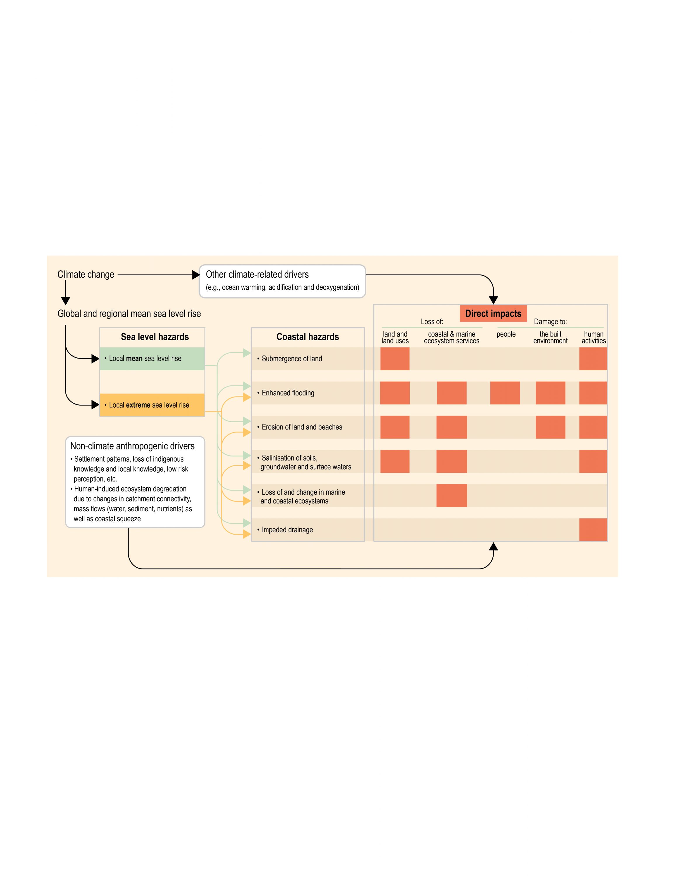
Figure 4.13 | Overview of the main cascading effects of sea level rise (SLR). Styles and colours of lines (left hand side: light/dark blue; right hand side: dotted/non dotted and orange/green/dark yellow/purple/turquoise) and boxes are used only for the readability of the figure. Sea level hazards are discussed in Section 4.2. The various impacts listed in this figure are discussed in the sections below: Submergence of land and enhanced flooding (4.3.3.2); Erosion of land and beaches (4.3.3.3); Salinisation (4.3.3.4); Loss of and changes in ecosystems (4.3.3.5); Loss of land and land uses (4.3.3.2); Loss of ecosystems services (4.3.3.5); Damage to people and to the built environment (4.3.3.2, 4.3.3.3, 4.3.3.4 and 4.3.3.6); Damages to human activities (4.3.3.6). Non-climate anthropogenic drivers are discussed in Section 4.3.2 and other climate-related drivers are notably discussed in Section 5.2.1 and 5.2.2.
4.3.3.1
Attribution of Observed Physical Changes to Sea Level Rise
The AR5 concludes that attribution of coastal changes to SLR is difficult because ‘the coastal sea level change signal is often small when compared to other processes’ (Wong et al., 2014: 375). New literature, however, shows that extreme water levels at the coast are rising due to mean SLR (4.2.2.4 for observations, and 4.3.5 for projections), with observable impacts on chronic flooding in some regions (Sweet and Park, 2014; Strauss et al., 2016).
On coastal morphological changes for example, contemporary SLR currently acts as a ‘background driver’, with extreme events, changes in wave patterns, tides and human intervention often described as the prevailing drivers of observed changes (Grady et al., 2013; Albert et al., 2016). Morphological changes are also interacting with other impacts of SLR, such as coastal flooding (Pollard et al., 2018). Despite the complexity of the attribution issue (Romine et al., 2013; Le Cozannet et al., 2014), recent literature suggests possibly emerging signs of the direct influence of recent SLR on shoreline behaviour, for example on small highly-sensitive reef islands in New Caledonia (Garcin et al., 2016) and in the Solomon Islands (Albert et al., 2016). Early signs of the direct influence of SLR on estuaries’ water salinity are also emerging, for example, in the Delaware, USA, where Ross et al. (2015) estimate a rate of salinity increase by as much as 4.4 psu (Practical Salinity Unit) per metre of SLR since the 1950s.
Overall, while the literature suggests that it is still too early to attribute coastal impacts to SLR in most of the world’s coastal areas, there is very high confidence that as sea level continues to rise (Sections 4.2.3.2, 4.2.3.3), the frequency, severity and duration of hazards and related impacts increases (Woodruff et al., 2013; Lilai et al., 2016; Vitousek et al., 2017; Sections 4.2.3.4, 6.3.1.3). Detectable impacts and attributable impacts on shoreline behaviour are expected as soon as the second half of the 21st century (Nicholls and Cazenave, 2010; Storlazzi et al., 2018).
4.3.3.2
Submergence and Flooding of Coastal Areas
Since AR5, a number of continental and global scale coastal exposure studies have accounted for sub-national human dynamics such as coastward migration or coastal urbanisation. These studies project a population increase in the LECZ (coastal areas below 10 m of elevation) by 2100 of 85 to 239 million people as compared to only considering national dynamics (Merkens et al., 20161176; Section 4.3.2). Under the five SSPs and without SLR, the population living in the LECZ increases from 640–700 million in 2000 to over one billion in 2050 under all SSPs, and then declines to 500–900 million in 2100 under all SSPs, except for SSP3 (i.e., a world in which countries will increasingly focus on domestic issues, or at best regional ones), for which the coastal population reaches 1.1–1.2 billion (Jones and O’Neill, 20161177; Merkens et al., 20161178).
The population exposed to mean and ESL events will grow significantly during the 21st century (high confidence) with socioeconomic development and SLR contributing roughly equally (medium confidence). Considering an average relative SLR of 0.7–0.9 m but no population growth, the number of people living below the hundred-year ESL in Latin America and the Caribbean will increase from 7.5 million in 2011 to 9 million by the end of the century (Reguero et al., 20151179). Considering population growth and urbanisation, only 21 cm of global mean SLR by 2060 would increase the global population living below the hundred-year ESL from about 189 million in 2000 to 316–411 million in 2060, with the largest absolute changes in South and Southeast Asia and the largest relative changes in Africa (Neumann et al., 20151180). Considering population growth, Hauer et al. (2016)1181 estimate that 4.3 and 13.1 million people in the USA would live below the levels of 0.9 and 1.8 m SLR by 2100.
New coastal flood risk studies conducted since AR4 at global, continental and city scale, reinforce AR5 findings that if coastal societies do not adapt, flood risks will increase by 2–3 orders of magnitude reaching catastrophic levels by the end of the century, even under the lower end SLR expected under RCP2.6 (high confidence; Hinkel et al., 20141182; Abadie et al., 20161183; Diaz, 20161184; Hunter et al., 20171185; Lincke and Hinkel, 20181186; Abadie, 20181187; Brown et al., 2018a1188; Nicholls, 20181189). In combination, these studies take into account a SLR scenario range wider than the likely range of AR5 but consistent with the range of projections assessed in this report (Section 4.2.3.2). For example, considering 25–123 cm of SLR in 2100, all SSPs and no adaptation, Hinkel et al. (2014) find that 0.2–4.6% of global population is expected to be flooded annually in 2100, with expected annual damages (EAD) amounting to 0.3–9.3% of global GDP. Assessing 120 cities globally, Abadie (2018) find that under a weighted combination of the probabilistic scenarios, New Orleans and Guangzhou Guangdong rank highest with EAD above 1 trillion USD (not discounted) in each city. For Europe, EAD are expected to rise from 1.25 billion EUR today to 93–960 billion EUR by the end of the century (Vousdoukas et al., 2018b1190). Already today, many small islands face large flood damages relative to their GDP specifically through TCs (Cashman and Nagdee, 20171191) and under SLR EAD can reach up to several percent of GDP in 2100, as highlighted in AR5 (Wong et al., 20141192). Similar to the exposure studies, estimates of future flood risk without considering adaptation, as presented in this paragraph, do not provide a meaningful characterisation of coastal flood risks, because adaptation and specifically hard protection is expected to be widespread during the 21st century in urban areas and cities (high confidence; Section 4.4.3.2.2). Rather, these estimates need to be seen as illustrations of the scale of adaptation needed to offset risk.
Flood risk studies that have included adaptation find that hard coastal protection is generally very effective in reducing flood risks during the 21st century even under high SLR scenarios (high confidence; Hinkel et al., 20141193; Diaz, 20161194; Brown et al., 2018a1195; Hinkel et al., 20181196; Lincke and Hinkel, 20181197; Tamura et al., 20191198) (Section 4.4.2.2.2). For example, Hinkel et al. (2014) find that under 25–123 cm of SLR in 2100 and all SSPs, hard coastal protection reduces the annual number of people affected by coastal floods and EAD by 2–3 orders of magnitude. Under high-end SLR and beyond the 21st century, effectiveness of coastal adaptation is expected to decline rapidly, but there is a lack of studies addressing this issue. Furthermore, there is a lack of studies taking into account responses beyond hard protection such as ecosystem-based adaptation, accommodation, advance and retreat (Sections 4.4.2).
Studies also confirm AR5 findings that the relative costs and benefits of coastal adaptation are distributed unequally across countries and regions (high confidence; Wong et al., 20141199; Diaz, 20161200; Lincke and Hinkel, 20181201; Tamura et al., 20191202). For example, while the median cost of protection and retreat under RCP8.5 in 2050 has been estimated to be under 0.09% of national GDP, large relative costs are found for small island states such as the Marshall Islands (7.6%), the Maldives (7.5%), Tuvalu (4.6%) and Kiribati (4.1%; Diaz, 20161203). Furthermore, on a global average and for urban and densely populated regions, hard protection is highly cost efficient with benefit-cost ratios up to 104, but for poorer and less densely populated areas benefit-cost ratios are generally smaller than one (Lincke and Hinkel, 20181204). Hence, without substantial transfer payments supporting poor areas, coastal flood risks will evolve unequally during this century, with richer and densely populated areas well protected behind hard structures and poorer less densely populated areas suffering losses and damages, and eventually retreating from the coast.
While continental to global scale flood exposure and risk studies have also explored a wider range of uncertainty as compared to AR5, much remains to be done. All of these studies rely on global elevation data, but few studies have explored the underlying bias. For example, for the Po delta in Italy, it was found that elevation data based on the widely used Shuttle Radar Topography Mission (SRTM), Reuter et al. (2007) overestimates the 100-year floodplain by about 50% as compared to local Lidar data (Wolff et al., 20161205), while in the Ria Formosa region in Portugal SRTM underestimates EAD by up to 50% depending on the resampled resolution of the Lidar data (Vousdoukas et al., 2018a1206). For the USA, SRTM data systemically underestimates population exposure below 3 m by more than 60% as compared to coastal Lidar data (Kulp and Strauss, 20161207). A global scale comparison of major contributors to flood risk uncertainty finds that uncertainty in digital elevation data is roughly at equal footing with uncertainties in socioeconomic development, emission scenarios, and SLR in determining the magnitude of flood risks in the 21st century (Hinkel et al., 20141208). At a European level, the number of people living in the 100-year coastal floodplain can vary between 20–70% depending on the different inundation models used and the inclusion or exclusion of wave set up (Vousdoukas, 20161209). Comparing damage functions attained in different studies for European cities, Prahl et al. (20181210) find up to four-fold differences in damages for floods above 3 m. Another major source of uncertainty relates to uncertainties in present-day ESL events due to the application of different extreme value methods (Wahl et al., 20171211; Section 4.2.3.4). While all of the uncertainties reported above affected the actual size of exposure and flood risk figures, they do not affect the overall conclusions drawn here.
4.3.3.3
Coastal Erosion and Projected Global Impacts of Enhanced Erosion on Human Systems
Recent global assessments of coastal erosion indicate that land losses currently dominate over land gains and that human interventions are a major driver of shoreline changes (Cazenave and Cozannet, 20141212; Luijendijk et al., 20181213; Mentaschi et al., 20181214). Luijendijk et al. (2018)1215 estimate that over the 1984–2016 period, about a quarter of the world’s sandy beaches eroded at rates exceeding 0.5m yr–1 while about 28% accreted. While such global results can be challenged due to the relatively large detection threshold used (±0.5 m yr–1), there is growing literature indicating that coastal erosion is occurring or increasing, e.g. in the Arctic (Barnhart et al., 2014a1216; Farquharson et al., 20181217; Irrgang et al., 20191218), Brazil (Amaro et al., 20151219), China (Yang et al., 20171220), Colombia (Rangel-Buitrago et al., 20151221), India (Kankara et al., 20181222), and along a large number of deltaic systems worldwide (e.g., Section 4.2.2.4).
Since AR5, however, there is growing appreciation and understanding of the ability of coastal systems to respond dynamically to SLR (Passeri et al., 20151223; Lentz et al., 20161224; Deng et al., 20171225). Most low-lying coastal systems exhibit important feedbacks between biological and physical processes (e.g., Wright and Nichols, 2018), that have allowed them to maintain a relatively stable morphology under moderate rates of SLR (<0.3 cm yr–1) over the past few millennia (Woodruff et al., 20131226; Cross-Chapter Box 5 in Chapter 1). In a global review on multi-decadal changes in the land area of 709 atoll islands, Duvat (2019)1227 shows that in a context of more rapid SLR than the global mean (Becker et al., 20121228; Palanisamy et al., 20141229), 73.1% of islands were stable in area, while respectively 15.5% and 11.4% increased and decreased in size. While anthropogenic drivers played a major role, especially in urban islands (e.g., shoreline stabilisation by coastal defences, increase in island size as a result of reclamation works), this study and others (e.g., McLean and Kench, 2015) suggest that these islands have had the capacity to maintain their land area by naturally adjusting to SLR over the past decades (high confidence). However, it has been argued that this capacity could be reduced in the coming decades, due to the combination of higher rates of SLR, increased wave energy (Albert et al., 20161230), changes in run-up (Shope et al., 20171231) and storm wave direction (Harley et al., 20171232), effects of ocean warming and acidification on critical ecosystems such as coral reefs (Section 4.3.3.5.2), and a continued increase in anthropogenic pressure.
From a global scale perspective, based on AR4 SLR scenarios and without considering the potential benefits of adaptation, Hinkel et al. (2013b) estimate that about 6000 to 17,000 km2 of land is expected to be lost during the 21st century due to enhanced coastal erosion associated with SLR, in combination with other drivers. This could lead to a displacement of 1.6–5.3 million people and associated cumulative costs of 300 to 1000 billion USD (Section 4.4.3.5). Importantly, these global figures mask the wide diversity of local situations; and some literature is emerging on the non-physical and non-quantifiable impacts of coastal erosion, for example, on the loss of recreational grounds and the induced risks to the associated social dimensions (i.e., how local communities experience coastal erosion impacts; Karlsson et al., 20151233).
4.3.3.4
Salinisation
With rising sea levels, saline water intrusion into coastal aquifers and surface waters and soils is expected to be more frequent and enter farther landwards. Salinisation of groundwater, surface water and soil resources also increases with land-based drought events, decreasing river discharges in combination with water extraction and SLR (high confidence).
4.3.3.4.1
Coastal aquifers and groundwater lenses
Groundwater volumes will primarily be affected by variations in precipitation patterns (Taylor et al., 2013; Jiménez Cisneros et al., 2014), which are expected to increase water stress in small islands (Holding et al., 2016). While SLR will mostly impact groundwater quality (Bailey et al., 2016) and in turn exacerbate salinisation induced by marine flooding events (Gingerich et al., 2017), it will also affect the watertable height (Rotzoll and Fletcher, 2013; Jiménez Cisneros et al., 2014; Masterson et al., 2014; Werner et al., 2017). In addition, the natural migration of groundwater lenses inland in response to SLR can also be severely constrained by urbanisation, for example, in semi-arid South Texas, USA (Uddameri et al., 2014).
These changes will affect both freshwater availability (for drinking water supply and agriculture) and vegetation dynamics. At many locations, however, direct anthropogenic influences, such as groundwater pumping for agricultural or urban uses, already impact salinisation of coastal aquifers more strongly than what is expected from SLR in the 21st century (Ferguson and Gleeson, 2012; Jiménez Cisneros et al., 2014; Uddameri et al., 2014), with trade-offs in terms of groundwater depletion that may contribute to anthropogenic subsidence and thus increase coastal flood risk. Recent studies also suggest that the influence of land-surface inundation on seawater intrusion and resulting salinisation of groundwater lenses on small islands has been underestimated until now (Ataie-Ashtiani et al., 2013; Ketabchi et al., 2014). Such impacts will potentially also combine with a projected drying of most of the tropical-to-temperate islands by mid-century (Karnauskas et al., 2016).
4.3.3.4.2
Surface waters
The quality of surface water resources (in estuaries, rivers, reservoirs, etc.) can be affected by the intrusion of saline water, both in a direct (increased salinity) and indirect way (altered environmental conditions which change the behaviour of pollutants and microbes). In terms of direct impacts, statistical models and long-term (1950 to present) records of salinity show significant upward trends in salinity and a positive correlation between rising sea levels and increasing residual salinity, for example in the Delaware Estuary, USA (Ross et al., 2015). Higher salinity levels, further inland, have also been reported in the Gorai river basin, southwestern Bangladesh (Bhuiyan and Dutta, 2012), and in the Mekong Delta, Vietnam. In the Mekong Delta for instance, salinity intrusion extends around 15 km inland during the rainy season and typically around 50 km during dry season (Gugliotta et al., 2017). Importantly, salinity intrusion in these deltas is caused by a variety of factors such as changes in discharge and water abstraction along with relative SLR. More broadly, the impact of salinity intrusion can be significant in river deltas or low-lying wetlands, especially during low-flow periods such as in the dry season (Dessu et al., 2018). In Bangladesh, for instance, some freshwater fish species are expected to lose their habitat with increasing salinity, with profound consequences on fish-dependent communities (Dasgupta et al., 2017). In the Florida Coastal Everglades, sea level increasingly exceeds ground surface elevation at the most downstream freshwater sites, affecting marine-to-freshwater hydrologic connectivity and transport of salinity and phosphorous upstream from the Gulf of Mexico. The impact of SLR is higher in the dry season when there is practically no freshwater inflow (Dessu et al., 2018). Salinity intrusion was shown to cause shifts in the diatom assemblages, with expected cascading effects through the food web (Mazzei and Gaiser, 2018). Salinisation of surface water may lead to limitations in drinking water supply (Wilbers et al., 2014), as well as to future fresh water shortage in reservoirs, for example in Shanghai (Li et al., 2015). Salinity changes the partitioning and mobility of some metals, and hence their concentration or speciation in the water bodies (Noh et al., 2013; Wong et al., 2015; de Souza Machado et al., 2018). Varying levels of salinity also influence the abundance and toxicity of Vibrio cholerae in the Ganges Delta (Batabyal et al., 2016).
4.3.3.4.3
Soils
Salinisation is one of the major drivers of soil degradation, with sea water intrusion being one of the common causes (Daliakopoulos et al., 2016). In a study in the Ebro Delta, Spain, for instance, soil salinity was shown to be directly related to distances to the river, to the delta inner border, and to the old river mouth (Genua-Olmedo et al., 2016). Land elevation was the most important variable in explaining soil salinity.
SLR was also shown to decrease organic carbon (Corg) concentrations and stocks in sediments of salt marshes as reworked marine particles contribute with a lower amount of Corg than terrigenous sediments. Corg accumulation in tropical salt marshes can be as high as in mangroves and the reduction of Corg stocks by ongoing SLR might cause high CO2 releases (Ruiz-Fernández et al., 2018). In many cases attribution to SLR is missing, but, independent from clear attribution, sea water intrusion leads to a salinisation of exposed soils with changes in carbon dynamics (Ruiz-Fernández et al., 2018) and microbial communities (Sánchez-Rodríguez et al., 2017), soil enzyme activity and metal toxicity (Zheng et al., 2017). Water salinity levels in the pores of coastal marsh soils can become significantly elevated in just one week of flooding by sea water, which can potentially negatively impact associated microbial communities for significantly longer time periods (McKee et al., 2016). SLR will also alter the frequency and magnitude of wet/dry periods and salinity levels in coastal ecosystems, with consequences for the formation of climate relevant GHGs (Liu et al., 2017b) and therefore feedbacks to the climate.
Soil salinisation affects agriculture directly with impacts on plant germination (Sánchez-García et al., 2017), plant biomass (rice and cotton) production (Yao et al., 2015), and yield (Genua-Olmedo et al., 2016). Impact on agriculture is especially relevant in low-lying coastal areas where agricultural production is a major land use, such as in river deltas.
4.3.3.5
Ecosystems and Ecosystem Services
4.3.3.5.1
Tidal wetlands
Global coastal wetlands have been reduced by a half since the pre-industrial period due to the impacts of both climatic and non-climatic drivers such as flooding, coastal urbanisation, alterations in drainage and sediment supply. (Sections 4.3.2.3, 5.3.2). Potentially one of the most important of the eco-morphodynamic feedback allowing for relatively stable morphology under SLR is the ability of marsh and mangrove systems to enhance the trapping of sediment, which in turn allows tidal wetlands to grow and increase the production and accumulaGlobal coastal wetlands have been reduced by a half since the pre-industrial period due to the impacts of both climatic and non-climatic drivers such as flooding, coastal urbanisation, alterations in drainage and sediment supply. (Sections 4.3.2.3, 5.3.2). Potentially one of the most important of the eco-morphodynamic feedbacks allowing for relatively stable morphology under SLR is the ability of marsh and mangrove systems to enhance the trapping of sediment, which in turn allows tidal wetlands to grow and increase the production and accumulation of organic material (Kirwan and Megonigal, 20131272). When ecosystem health is maintained and sufficient sediment exists to support their growth, this particular feedback has generally allowed marshes and mangrove systems to build vertically at rates equal to or greater than SLR up to the present day (Kirwan et al., 20161273; Woodroffe et al., 20161274).
While recent reviews suggest that mangroves’ surface accretion rate will keep pace with a high SLR scenario (RCP8.5) up to years 2055 and 2070 in fringe and basin mangrove settings, respectively (Sasmito et al., 20161275), process-based models of vertical marsh growth that incorporate biological and physical feedbacks support survival under rates of SLR as high as 1–5 cm yr–1 before drowning (Kirwan et al., 20161276). Threshold rates of SLR before marsh drowning however vary significantly from site-to-site and can be substantially lower than 1 cm yr–1 in micro-tidal regions where the tidal trapping of sediment is reduced and/or in areas with low sediment availability (Lovelock et al., 20151277; Ganju et al., 20171278; Jankowski et al., 20171279; Watson et al., 20171280). Global environmental change may also to lead to changes in growth rates, productivity and geographic distribution of different mangrove and marsh species, including the replacement of environmentally sensitive species by those possessing greater climatic tolerance (Krauss et al., 20141281; Reef and Lovelock, 20141282; Coldren et al., 20191283). Processes impacting lateral changes at the marsh boundary including wave erosion are just as important, if not more, than vertical accretion rates in determining coastal wetland survival (e.g., Mariotti and Carr, 2014). For most low-lying coastlines, a seaward loss of wetland area due to marsh retreat could be offset by a similar landward migration of coastal wetlands (Kirwan and Megonigal, 20131284; Schile et al., 20141285), this landward migration having the potential to maintain and even increase the extent of coastal wetlands globally (Morris et al., 20121286; Kirwan et al., 20161287; Schuerch et al., 20181288). This natural process will however be constrained in areas with steep topography or hard engineering structures (i.e., coastal squeeze, Section 4.3.2.4). Seawalls, levees and dams can also prevent the fluvial and marine transport of sediment to wetland areas and reduce their resilience further (Giosan, 20141289; Tessler et al., 20151290; Day et al., 20161291; Spencer et al., 20161292). When ecosystem health is maintained and sufficient sediment exists to support their growth, this particular feedback has generally allowed marshes and mangrove systems to build vertically at rates While recent reviews suggest that mangroes’ surface accretion rate will keep pace with a high SLR scenario (RCP8.5) up to years 2055 and 2070 in fringe and basin mangrove settings, respectively (Sasmito et al., 20161275), process-based models of vertical marsh growth that incorporate biological and physical feedbacks support survival under rates of SLR as high as 1–5 cm yr–1 before drowning (Kirwan et al., 20161276). Threshold rates of SLR before marsh drowning however vary significantly from site-to-site and can be substantially lower than 1 cm yr–1 in micro-tidal regions where the tidal trapping of sediment is reduced and/or in areas with low sediment availability (Lovelock et al., 20151277; Ganju et al., 20171278; Jankowski et al., 20171279; Watson et al., 20171280). Global environmental change may also to lead to changes in growth rates, productivity and geographic distribution of different mangrove and marsh species, including the replacement of environmentally sensitive species by those possessing greater climatic tolerance (Krauss et al., 20141281; Reef and Lovelock, 20141282; Coldren et al., 20191283). Processes impacting lateral changes at the marsh boundary including wave erosion are just as important, if not more, than vertical accretion rates in determining coastal wetland survival (e.g., Mariotti and Carr, 2014). For most low-lying coastlines, a seaward loss of wetland area due to marsh retreat could be offset by a similar landward migration of coastal wetlands (Kirwan and Megonigal, 20131284; Schile et al., 20141285), this landward migration having the potential to maintain and even increase the extent of coastal wetlands globally (Morris et al., 20121286; Kirwan et al., 20161287; Schuerch et al., 20181288). This natural process will however be constrained in areas with steep topography or hard engineering structures (i.e., coastal squeeze, Section 4.3.2.4). Seawalls, levees and dams can also prevent the fluvial and marine transport of sediment to wetland areas and reduce their resilience further (Giosan, 20141289; Tessler et al., 20151290; Day et al., 20161291; Spencer et al., 20161292).
4.3.3.5.2
Coral reefs
Coral reefs are considered to be the marine ecosystem most threatened by climate-related ocean change, especially ocean warming and acidification, even under an RCP2.6 scenario (Gattuso et al., 20151293; Albright et al., 20181294; Hoegh-Guldberg et al., 20181295; Díaz et al., 20191296; Section 5.3.4). AR5 concluded that ‘a number of coral reefs could […] keep up with the maximum rate of SLR of 15.1 mm yr–1 projected for the end of the century […] (medium confidence) [but a future net accretion rate lower] than during the Holocene (Perry et al., 20131297) and increased turbidity (Storlazzi et al., 20111298) will weaken this capability (very high confidence)’ (Wong et al., 2014: 3791299). Subsequently, some studies suggested that SLR may have negligible impacts on coral reefs’ vertical growth because the projected rate and magnitude of SLR by 2100 are within the potential accretion rates of most coral reefs (van Woesik et al., 20151300). Other studies, however, stressed that the overall net vertical accretion of reefs may decrease after the first 30 years of rise in a 1.2 m SLR scenario (Hamylton et al., 20141301), and that most reefs will not be able to keep up with SLR under RCP4.5 and beyond (Perry et al., 20181302). The SR1.5 also concludes that coral reefs ‘are projected to decline by a further 70–90% at 1.5°C (high confidence) with larger losses (>99%) at 2°C (very high confidence)’ (Hoegh-Guldberg et al., 2018: 101303). A key point is that SLR will not act in isolation of other drivers. Cumulative impacts, including anthropogenic drivers, are estimated to reduce the ability of coral reefs to keep pace with future SLR (Hughes et al., 20171304; Yates et al., 20171305) and thereby reduce the capacity of reefs to provide sediments and protection to coastal areas. For example, the combination of reef erosion due to acidification and human-induced mechanical destruction is altering seafloor topography, increasing risks from SLR in carbonate sediment dominated regions (Yates et al., 20171306). Both ocean acidification (Albright et al., 20181307; Eyre et al., 20181308) and ocean warming (Perry and Morgan, 20171309) have been considered to slow future growth rates and reef accretion (Section 5.3.4). Recent literature also shows that alterations of coral reef 3D structure from changes in growth, breakage, disease or acidification can profoundly affect their ability to buffer waves impacts (through wave breaking and wave energy damping), and therefore keep-up with SLR (Yates et al., 20171310; Harris et al., 20181311). Such prospects contribute to raise concerns about the future ability of atoll islands to adjust naturally to SLR and persist (Section 4.3.3.3, Cross-Chapter Box 9). Another concern is that locally, even minimal SLR can increase turbidity on fringing reefs, reducing light and, therefore, photosynthesis and calcification. SLR-induced turbidity can be caused by increased coastal erosion and the transfer of sediment to nearby reefs and enhanced sediment resuspension (Field et al., 20111312).
4.3.3.5.3
Seagrasses
Due to their natural capacity to enhance accretion and in the absence of mechanical or chemical destruction by human activities, seagrasses are not expected to be severely affected by SLR, except indirectly through the increase of the impacts of extreme weather events and waves on coastal morphology (i.e., erosion) as well as through changes in light levels and through effects on adjacent ecosystems (Saunders et al., 20131313). Extreme flooding events have also been shown to cause large-scale losses of seagrass habitats (Bandeira and Gell, 20031314), for example seagrasses in Queensland, Australia, were lost in a disastrous flooding event (Campbell and McKenzie, 20041315). Changes in ocean currents can have either positive or negative effects on seagrasses, creating new space for seagrasses to grow or eroding seagrass beds (Bjork et al., 20081316). But overall, seagrass will primarily be negatively affected by the direct effects of increased sea temperature on growth rates and the occurrence of disease (Marba and Duarte, 20101317; Burge et al., 20131318; Koch et al., 20131319; Thompson et al., 20151320; Chefaoui et al., 20181321; Gattuso et al., 20181322; Section 5.3.2) as well as by heavy rains that may dilute the seawater to a lower salinity. Such impacts will be exacerbated by major causes of seagrass decline including coastal eutrophication, siltation and coastal development (Waycott et al., 20091323). Noteworthy is that some positive impacts are expected, as ocean acidification is expected to benefit photosynthesis and growth rates of seagrass (Repolho et al., 20171324).
4.3.3.5.4
Coastal protection by coastal and marine ecosystems
Major ‘protection’ benefits derived from the above-mentioned coastal ecosystems include wave attenuation and shoreline stabilisation, for example, by coral reefs (Elliff and Silva, 20171325; Siegle and Costa, 20171326), mangroves (Zhang et al., 20121327; Barbier, 20161328; Menéndez et al., 20181329) or salt marshes (Möller et al., 20141330; Hu et al., 20151331). Recently, a global meta-analysis of 69 studies demonstrated that, on average, these ecosystems together reduced wave heights between 35–71% at the limited locations considered (Narayan et al., 20161332), with coral reefs, salt marshes, mangroves and seagrass/kelp beds reducing wave heights by 54–81%, 62–79%, 25–37% and 25–45% respectively (see Narayan et al., 2016 for map of locations considered). Additional studies suggest greater wave attenuation in mangrove systems (Horstman et al., 20141333), and highlight broader complexities in wave attenuation related to total tidal wetland extent, water depth, and species. Global analyses show that natural and artificial seagrasses can attenuate wave height and energy by as much as 40% and 50%, respectively (Fonseca and Cahalan, 19921334; John et al., 20151335), while coral reefs have been observed to reduce total wave energy by 94–98% (n = 13; Ferrario et al., 20141336) and wave driven flooding volume by 72% (Beetham et al., 20171337). In addition, storm surge attenuation based on a recent literature review by Stark et al. (2015)1338 range from -2–25 cm km–1 length of marsh, where the negative value denotes actual amplification. Other ecosystems provide coastal protection, including macroalgae, oyster and mussel beds, and also beaches, dunes and barrier islands, but there is less understanding of the level of protection conferred by these other organisms and habitats (Spalding et al., 20141339).
While there is little literature on the extent to which SLR specifically will affect coastal protection by coastal and marine ecosystems, it is estimated that SLR may reduce this ecosystem service (limited evidence, high agreement) through the above-described impacts on the ecosystems themselves, and in combination with the impacts of other climate-related changes to the ocean (e.g., ocean warming and acidification; Sections 5.3.1 to 5.3.6, 5.4.1). Wave attenuation by coral reefs, for example, is estimated to be negatively affected in the near future by changes in coral reefs’ structural complexity more than by SLR (Harris et al., 20181340); changes in mean and ESL events will rather add a layer of stress. Beck et al. (2018) estimate that under RCP8.5 by 2100, a 1 m loss in coral reefs’ height will increase the global area flooded under a 100-year storm event by 116% compared to today, against +66% with no reef loss.
4.3.3.6
Human Activities
4.3.3.6.1
Coastal agriculture
SLR will affect agriculture mainly through land submergence, soil and fresh groundwater resources salinisation, and land loss due to permanent coastal erosion, with consequences on production, livelihood diversification and food security, especially in heavily coastal agriculture-dependent countries such as Bangladesh (Khanom, 20161341). Recent literature confirms that salinisation is already a major problem for traditional agriculture in deltas (Wong et al., 20141342; Khai et al., 20181343) and low-lying island nations where some edible cultivated plants such as taro patches are threatened (Nunn et al., 2017b1344). Taking the case of rice cultivation, recent works emphasise the prevailing role of combined surface elevation and soil salinity, such as in the Mekong delta (Vietnam; Smajgl et al., 20151345) and in the Ebro delta (Spain; Genua-Olmedo et al., 20161346), estimating for the latter a decrease in the rice production index from 61.2% in 2010 to 33.8% by 2100 in a 1.8 m SLR scenario. For seven wetland species occurring in coastal freshwater marshes in central Veracruz on the Gulf of Mexico, an increase in salinity was shown to affect the germination process under wetland salt intrusion (Sánchez-García et al., 20171347). In coastal Bangladesh, oilseed, sugarcane and jute cultivation was reported to be already discontinued due to challenges to cope with current salinity levels (Khanom, 20161348), and salinity is projected to have an unambiguously negative influence on all dry-season crops over the next 15–45 years (especially in the southwest; Clarke et al., 20181349; Kabir et al., 20181350). Salinity intrusion and salinisation can trigger land use changes towards brackish or saline aquaculture such as shrimp or rice-shrimp systems with impacts on environment, livelihoods and income stability (Renaud et al., 20151351). However, increasing salinity is only one of the land use change drivers along with, for example, policy changes and market prices at the household level (Renaud et al., 20151352).
4.3.3.6.2
Coastal tourism and recreation
SLR may significantly affect tourism and recreation through impacts on landscapes (e.g., beaches), cultural features (e.g., Marzeion and Levermann, 2014; Fang et al., 20161353), and critical transportation infrastructures such as harbours and airports (Monioudi et al., 20181354). Coastal areas’ future tourism and recreation attractiveness will however also depend on changes in air temperature, seasonality and sea surface temperature (including induced effects such as invasive species, e.g., jellyfishes, and disease spreading; Burge et al., 20141355; Weatherdon et al., 20161356; Hoegh-Guldberg et al., 20181357; Section 5.4.2). Future changes in climatic conditions in tourists’ areas of origin will also play a role in reshaping tourism flows (Bujosa and Rosselló, 20131358; Amelung and Nicholls, 20141359), in addition to mitigation policies on air transportation, non-climatic features (e.g., accommodation and travel prices) and tourists’ and tourism developers’ perceptions of climate-related changes (Shakeela and Becken, 20151360). Since AR5, forecasting the consequences of climate change effects on global-to-local tourism flows has remained challenging (Rosselló-Nadal, 20141361; Wong et al., 20141362; Hoegh-Guldberg et al., 20181363). There are also concerns about the effect of SLR on tourism facilities, for example hotels in Ghana (Sagoe-Addy and Addo, 20131364), in a context where tourism infrastructure often contributes to the degradation of natural buffering environments through, for example, coastal squeeze (e.g., Section 4.3.2.4) and human-driven coastal erosion. Again, forecasting is constrained by the lack of scientific studies on tourism stakeholders’ long-term strategies and adaptive capacity (Hoogendoorn and Fitchett, 20181365).
4.3.3.6.3
Coastal fisheries and aquaculture
Recent studies support the AR5 conclusion that ocean warming and acidification are considered more influential drivers of change in fisheries and aquaculture than SLR (Larsen et al., 2014; Nurse et al., 20141366; Wong et al., 20141367). The negative effects of SLR on fisheries and aquaculture are indirect, through adverse impacts on habitats (e.g., coral reef degradation, reduced water quality in deltas and estuarine environments, soil salinisation, etc.), as well as on facilities (e.g., damage to small and large harbours). This makes future projections on SLR implications for coastal and marine fisheries and aquaculture an understudied field of research. Conclusions only state that future impacts will be highly context-specific due to local manifestations of SLR and local fishery-dependent communities’ ability to adapt to alterations in fish and aquaculture conditions and productivity (Hollowed et al., 20131368; Weatherdon et al., 20161369). Salinity intrusion also contributes to conversion of land or freshwater ponds to brackish or saline aquaculture in many low-lying coastal areas of Southeast Asia such as in the Mekong Delta in Vietnam (Renaud et al., 20151370).
4.3.3.6.4
Social values
Social values refer to what people consider of critical importance about the places in which they live, and range from material to immaterial things (assets, beliefs, etc.; Hurlimann et al., 20141371; Rouse et al., 20171372). Consideration of social values offers an opportunity to address a wider perspective on impacts on human systems, for example, complementary to quantitative assessments of health impacts (e.g., loss of source of calories and food insecurity; Keim, 20101374). This also encompasses immaterial dimensions, such as threats to cultural heritage (Marzeion and Levermann, 20141374; Fatorić and Seekamp, 2017a1375), socialising activities (Karlsson et al., 20151376), integration of marginalised groups (Maldonado, 20151377) and cultural ecosystem services (Fish et al., 2016), and provides an opportunity to better reflect context-specificities in valuing the physical/ecological/human/cultural impacts’ importance for and distribution within a given society (Fatorić and Seekamp, 2017b1379). This field of research (no detailed mention found in AR5) is just emerging due to the transdisciplinary and qualitative nature of the topic. Graham et al. (2013)1380 advance a 5-category framing of social values specifically at risk from SLR: health (i.e., the social determinants of survival such as environmental and housing quality and healthy lifestyles), feeling of safety (e.g., financial and job security), belongingness (i.e., attachment to places and people), self-esteem (e.g., social status or pride that can be affected by coastal retreat), and self-actualisation (i.e., people’s efforts to define their own identity). Another emerging issue relates to social values at risk due to land submergence in low-lying islands (Yamamoto and Esteban, 20141381) and parts of countries and individual properties (Marino, 20121382; Maldonado et al., 20131383; Aerts, 20171384; Allgood and McNamara, 20171385). Recent studies also highlight the potential additional risks to social values in areas where displaced people relocate (Davis et al., 20181386).
4.3.4
Conclusion on Coastal Risk: Reasons for Concern and Future Risks
SLR projections for the 21st century, together with other ocean related changes (e.g., acidification and warming) and the possible increase in human-driven pressures at the coast (e.g., demographic and settlement patterns), make low-lying islands, coasts and communities relevant illustrations of some of the five Reasons for Concern (RFCs) developed by the IPCC since the Third Assessment Report (McCarthy et al., 2001; Smith et al., 2001) to assess risks from a global perspective. The AR5 Synthesis Report (IPCC, 2014) as well as the more recent SR1.5 (Hoegh-Guldberg et al., 2018) refined the RFC approach. The AR5 Synthesis Report (IPCC, 2014) developed two additional RFCs related to the coasts, subsequently updated along with the other RFCs (O’Neill et al., 2017). One refers to risks to marine species arising from ocean acidification, and the other one refers to risks to human and natural systems from SLR. Despite the difficulty in attributing observed impacts to SLR per se (Section 4.3.3.1), O’Neill et al. (2017) estimate that risks related to SLR are already detectable globally and will increase rapidly, so that high risk may occur before a 1m rise level is reached. O’Neill et al. (2017) also suggest that limits to coastal protection and EbA by 2100 could occur in a 1 m SLR rise scenario. Previous assessments however left gaps, including quantifying the benefits from adaptation in terms of risk reduction.
4.3.4.1
Methodological Advances
Rather than revisiting the AR5 and O’Neill et al. (2017) assessments from the particular perspective of risk related to SLR and for the global scale, this section provides a complementary perspective by assessing risks for specific geographies (resource-rich coastal cities, urban atoll islands, large tropical agricultural deltas and selected Arctic communities), based on the methodological advances below.
Scale of analysis and geographical scope – To date, the RFCs and associated burning embers have been developed at a global scale (Oppenheimer et al., 2014; Gattuso et al., 2015; O’Neill et al., 2017) and do not address the spatial variability of risk highlighted in this report (Sections 4.3.2.7, 4.3.4, 5.3.7, Cross-Chapter Box 9, Box 4.1). In addition, assessments usually identify risks either for global human dimensions (e.g., to people, livelihood, breakdown of infrastructures, biodiversity, global economy, etc.; IPCC, 2014; Oppenheimer et al., 2014; O’Neill et al., 2017) or for ecosystems and ecosystem services (Gattuso et al., 2015; Hoegh-Guldberg et al., 2018) (Section 5.3.7). This section moves the focus from the global to more local scales by considering four generic categories of low-lying coastal areas (Figure 4.3, Panel B): selected Arctic communities remote from regions of rapid GIA, large tropical agricultural deltas, urban atoll islands, and resource-rich coastal cities. Each of these categories is informed by several real-world case studies.
Risks considered – In line with the AR5 (IPCC, 2014), current and future risks result from the interaction of SLR-related hazards with the vulnerability of exposed ecosystems and societies. According to the specific scope of the chapter, this assessment focusses on the additional risks due to SLR and does not account for changes in extreme event climatology. Hazards considered are coastal flooding (Section 4.3.4.2), erosion (Section 4.3.4.3) and salinisation (Section 4.3.4.4). The proxies used to describe exposure and vulnerability are the density of assets at the coast (Section 4.3.2.2) and the level of degradation of natural buffering by marine and terrestrial ecosystems (Sections 4.3.2.3, 4.3.3.5.4, and 5.3.2 to 5.3.4). The assessment especially addresses risks to human assets at the coast, including populations, infrastructures and livelihoods. Specific metrics were developed (see SM4.3 for details), and their contribution to present-day observed impacts and to end-century risk have been assessed based on the authors’ expert judgment and a methodological grid presented in SM4.3 (SM4.3.1 to SM4.3.6). The author’s expert judgment draws on Sections 4.3.3.2 to 4.3.3.5 as well as additional literature for local scale perspectives (SM4.3.9).
Sea level rise scenarios – Based on the updates for ranges and mean values developed in this chapter (Section 4.2, Table 4.3), this assessment considers the end-century GMSL (2100) relative to 1986–2005 levels for two scenarios, SROCC RCP2.6 and SROCC RCP8.5. Both mean values and the SROCC RCP8.5 upper end of the likely range are used to assess risk transitions (Figure 4.3, Panel A). For the sake of readability, the following values were used: 43 cm (mean SROCC RCP2.6), 84 cm (mean SROCC RCP8.5) and 110 cm (SROCC RCP8.5 upper end of likely range). While GMSL serves as a representation of different possible climate change scenarios (see Panel A in Figure 4.3, Section 4.1.2), the assessment of additional risks due to SLR on specific geographies is developed against end-century relative SLR (RSL) in order to allow a geographically accurate approach (Panel B, Figure 4.3). Accordingly, risk was assessed to illustrative geographies based on RSLs for each of the two SROCC RCP scenarios and each of the real-world case studies to (SM4.3.6 and Table SM4.3.2; see dotted lines in Panel B of Figure 4.3). RSL observations include some or all of the following VLMs: both uplift (e.g., due to tectonics) and subsidence due to natural (e.g., tectonics, sediment compaction) and human (e.g., oil/gas/water extraction, mining activities) factors, as well as to GIA. However, in SROCC, numerical RSL projections only include GIA and the regional gravitational, rotational, and deformational responses (GRD, see Section 4.2.1.5) to ice mass loss. The main reason is the difficulty of projecting the influence on some factors such as human interventions to the end of the century.
Adaptation scenarios – Risk will also depend on the effectiveness of coastal societies’ responses to both extreme events and slow onset changes. To capture the response dimension, four metrics have been considered that refer to the implementation of adequately calibrated hard, engineered coastal defences (Section 4.4.2.2), the restoration of the degraded ecosystems or the creation of new natural buffers areas (Section 4.4.2.2 and 4.4.2.3), planned and local-scale relocation (Section 4.4.2.6), and measures to limit human-induced subsidence (Sections 4.4.2.2, 4.4.2.5). On these bases, two contrasting adaptation scenarios were considered. The first one is called ‘No-to-moderate response’ (see (A) bars in Panel B, Figure 4.3) and represents a business-as-usual scenario where no major additional adaptation efforts compared to today are implemented. That is, neither substantial intensification of current actions nor new types of actions, e.g., only moderate raising of existing protections in high-density areas or sporadic episodes of relocation or beach nourishment where largescale efforts are not already underway. The second one, called ‘Maximum potential response’ (bars (B) in Figure 4.3), refers to an ambitious combination of both incremental and transformational adaptation (i.e., significantly upscaled effort); for example, relocation of entire districts or raised protections in some cities, or creation/restoration at a significant scale of beach-dune systems including indigenous vegetation.
4.3.4.2
Key Findings on Future Risks and Adaptation Benefits
4.3.4.2.1
Future risks
The findings suggest that risks from SLR are already detectable for all of the geographies considered (Panel B in Figure 4.3), and that risk is expected to increase over this century in virtually all low-lying coastal areas whatever their context-specificities or nature (island/continental, developed/developing county) (Cross-Chapter Box 9). In the absence of high adaptation (bars (A)), risk is expected to significantly increase in urban atoll islands and the selected Arctic coastal communities even in a SROCC RCP2.6 scenario, and all geographies are expected to experience almost high to very high risks at the upper likely range of SROCC RCP8.5. These results allow refining AR5 conclusions by showing, first, that high risk can indeed occur before the 1m rise benchmark (Oppenheimer et al., 20141399; O’Neill et al., 2017) and, second, that risk as a function of SLR is highly variable from one geography to another. Some rationale is provided below for our assessment of illustrative geographies, summarising the more detailed description provided in SM4.3 (SM4.3.6 to SM4.3.8). Note however that the text below is not intended to be fully comprehensive and does not necessarily include all elements for which there is a substantive body of literature, nor does it necessarily include all elements which are of particular interest to decision makers.
Resource-rich coastal cities (SM4.3.8.1, Panel B in Figure 4.3) – Resource-rich coastal cities considered in this analysis are Shanghai, New York (see Box 4.1 for further details and references on Shanghai and NYC), and Rotterdam (Brinke et al., 20101400; Hinkel et al., 20181401). High, and in many cases, growing population density and total population, and high exposure of people and infrastructure to GMSL rise and ESL events characterise coastal megacities (Hanson et al., 20111402). These are high concentrations of income and wealth in geographic terms but within relatively small area exhibit large distributional differences of both with important implications for emergency response and adaptation. Concentration translates into high exposure of monetary value to coastal hazards and the cities noted here have both historical and recent experience with damaging ESL events, such as Typhoon Winnie which struck Shanghai in 1997 (Xian et al., 20181403), Hurricane Sandy in New York in 2012 (Rosenzweig and Solecki, 20141404), and the North Sea storm of 1953 which impacted the Rotterdam area (Gerritsen, 20051405; Jonkman et al., 20081406). However, high density, limited space and high cost of land leads to development of below-ground space for transportation (e.g., subways, road tunnels; MTA, 2017) and storage, and even habitation, creating vulnerabilities not seen in low-density areas. Natural ecosystems within the megacity boundaries and nearby have been exploited for centuries and in some cases decimated or even extirpated (Hartig et al., 20021407). Accordingly, they provide limited benefits in terms of coastal protection for the densest part of these cities but can be critically important for protection of lower-density areas, for example, wetlands and sandy beaches in the Jamaica Bay/Rockaway sector of New York that protect nearby residential communities (Hartig et al., 20021408). Space limitations also constrain the potential benefits of EbA measures. Instead, resource-rich coastal cities depend largely on hard defences like sea walls and surge barriers for coastal protection (Section 4.4.2.2). Such defences are costly but generally cost effective due to the aforementioned concentration of population and value. However, barriers to planning and implementing adaptation include governance challenges (Section 4.4.2) such as limited control over finances and the intermittent nature of ESLs which inhibit focused attention over the long time scales needed to plan and implement hard defences (Section 4.4.2.2). As a result, coastal adaptation for resource-rich cities is uneven and the three presented here were selected with a view toward exhibiting a range of current and potential future effectiveness.
Urban atoll islands (SM4.3.8.2, Panel B in Figure 4.3) – The capital islands (or groups of islands) of three atoll nations in the Pacific and Indian Oceans are considered here: Fongafale (Funafuti Atoll, Tuvalu), the South Tarawa Urban District (Tarawa Atoll, Kiribati) and Male’ (North Kaafu Atoll, Maldives). Urban atoll islands have low elevation (<4 m above mean sea level; in South Tarawa, e.g., lagoon sides where settlement concentrates are <1.80 m in elevation) (Duvat, 2013) and are mainly composed of reef-derived unconsolidated material. Their future is of nation-wide importance as they concentrate populations, economic activities and critical infrastructure (airports, main harbours). They illustrate the prominence of anthropogenic-driven disturbances to marine and terrestrial ecosystems (e.g., mangrove clearing in South Tarawa or human-induced coral reef degradation through land reclamation in Male’; Duvat et al., 20131409; Naylor, 20151411) and therefore to services such as coastal protection delivered by the coral reef (i.e., wave energy attenuation that reduces flooding and erosion, and sediment provision that contributes to island persistence over time) (McLean and Kench, 20151412; Quataert et al., 20151413; Elliff and Silva, 20171414; Storlazzi et al., 20181415).
The controlling factors of urban atoll islands’ future habitability are the density of assets exposed to marine flooding and coastal erosion (SM4.3.8.2), future trends in these hazards, and ecosystem response to both ocean-climate related pressures and human activities. Urban atoll islands already experience coastal flooding, for example, in Male’ (Wadey et al., 20171416) and Funafuti (Yamano et al., 20071417; McCubbin et al., 20151418). Coastal erosion is also a major concern along non-armoured shoreline in South Tarawa (Duvat et al., 20131419) and Fongafale (Onaka et al., 20171420), but not in Male’ where surrounding fortifications have extended along almost the entire shoreline from several decades (Naylor, 2015). Salinisation already affects groundwater lenses, but its contribution to risk varies from one case to another, from low in Male’ (relying on desalinised seawater) to important for human consumption and agriculture in South Tarawa (Bailey et al., 20141422; Post et al., 20181423).
Together, high population densities (from ~3,200 people per km2 in South Tarawa to ~65,700 people per km2 in Male’) (Government of the Maldives, 20141424; McIver et al., 20151425) and the concentration of critical infrastructure and settlements in naturally low-lying flood-prone areas already substantially contribute to coastal risk (Duvat et al., 20131426; Field et al., 20171427). Even stabilised densities in the future would translate into a substantial increase of risk under a 43cm GMSL rise. Risk will also be exacerbated by the negative effects of ocean warming and acidification, especially on coral reef and mangrove capacity to cope with SLR (Pendleton et al., 20161428; Van Hooidonk et al., 20161429; Perry and Morgan, 20171430; Perry et al., 20181431) (Sections 4.3.3.5, 5.3). In addition, even small values of SLR will significantly increase risk to atoll islands’ aquifers (Bailey et al., 2016; Storlazzi et al., 2018). Finally, land scarcity in atoll environments will exacerbate the importance of SLR induced damages (on housing, agriculture and infrastructure especially) and cascading impacts (on livelihoods, for example, as a result of groundwater and soil salinisation).
Large tropical agricultural deltas (SM4.3.8.3, Panel B in Figure 4.3) – River deltas considered in this analysis are the Mekong Delta and the Ganges-Brahmaputra-Meghna Delta. Both deltas are large, low-lying and dominated by agricultural production. The risk assessment to SLR considered the entire delta area (not only the coastal fringe; see SM4.3.6 for explanation). High population densities (1280 people per km2 and 433 people per km2 in the Ganges-Brahmaputra-Meghna and Mekong deltas, respectively) (Ericson et al., 20061433; Government of the Maldives, 20141434) and the removal of natural vegetation buffers contribute to high exposure rates to coastal flooding, erosion, and salinisation. Agricultural production contributes to GDP strongly (Smajgl et al., 20151435; Hossain et al., 20181436), making agricultural fields important assets. In both deltas, mangroves are partially degraded (Ghosh et al., 20181437; Veettil et al., 20181438) as well as other wetlands at the coast and further inland (Quan et al., 2018a1439; Rahman et al., 20181440). Currently, riverine flooding dominates in both deltas (Auerbach et al., 20151441; Rahman and Rahman, 20151442; Ngan et al., 20181443). However, high tides and cyclones can generate large coastal flooding events, especially in the Ganges-Brahmaputra-Meghna Delta (Auerbach et al., 20151444; Rahman and Rahman, 20151445). Human-induced subsidence increases the likelihood of flooding in both deltas (Brown et al., 2018b1446). Coastal and river bank erosion is already a problem in both delta (Anthony et al., 20151447; Brown and Nicholls, 20151448; Li et al., 20171449) as well as salinity intrusion, which is impacting coastal aquifers, soils and surface waters (Anthony et al., 20151450; Brown and Nicholls, 20151451; Li et al., 20171452). Salinisation of water and soil resources remains a coastal phenomenon (Smajgl et al., 20151453), but salinity intrusion can reach far inland in some extreme years and significantly contribute to risk at the delta scale (Section 4.3.3.4.2). Both deltas are partly protected with hard engineered defences such as dikes and sluice gates to prevent riverine flooding, and polders and dikes in some coastal stretches to prevent salinity intrusion and storm surges (Smajgl et al., 20151454; Rogers and Overeem, 20171455; Warner et al., 2018a1456). Today, in both deltas, the measures implemented to restore natural buffers are still limited to mangroves ecosystems (Quan et al., 2018a1457; Rahman et al., 20181458), and the measures aiming at reducing subsidence are underdeveloped (Schmidt, 20151459; Schmitt et al., 20171460). Assuming stable population densities in the future, coastal flooding will contribute increasingly to risk at the delta level (Brown and Nicholls, 20151461; Brown et al., 2018a1462; Dang et al., 20181463). Coastal erosion will increase (Anthony et al., 20151464; Liu et al., 2017a1465; Uddin et al., 20191466) and salinisation of coastal waters and soils will be more significant (Tran Anh et al., 20181467; Vu et al., 20181468; Rakib et al., 20191469) and will strongly impact agriculture and water supply for the entire delta (Jiang et al., 20181470; Timsina et al., 20181471; Nhung et al., 20191472). Without increased adaptation, coastal ecosystems will be largely destroyed at 110 cm of SLR (Schmitt et al., 20171473; Mehvar et al., 20191474; Mukul et al., 20191475). Given the size of these deltas, it is only under high emission scenarios, that flooding, erosion and salinisation lead to high risk at the entire delta scale.
Arctic communities (SM4.3.8.4, Panel B in Figure 4.3) – Five small indigenous settlements located on the Arctic Coastal Plain are considered in this analysis: Bykovsky (Lena Delta, Russian Federation), Shishmaref and Kivalina (Alaska, USA), and Shingle Point and Tuktoyaktuk (Mackenzie Delta, Canada). They lie on exposed coasts composed of unlithified ice-rich sediments in permafrost, in areas with seasonal sea ice and slow to moderate SLR. These communities have populations ranging from 380 to 900 (fewer and seasonal at Shingle Point) that are heavily dependent on marine subsistence resources (Forbes, 20111476; Ford et al., 2016a1477). Shishmaref and Kivalina are located on low-lying barrier islands highly susceptible to rising sea level (Marino, 20121478; Bronen and Chapin, 20131479; Fang et al., 20181480; Rolph et al., 20181481). Shingle Point is situated on an active gravel spit; Tuktoyaktuk is built on low ground with high concentrations of massive ice; and Bykovsky is mostly situated on an ice-rich eroding terrace about 20 m above sea level. All the selected communities are remote from regions of rapid positive GIA; many other areas in the Arctic experience rapid GIA uplift (James et al., 20151482; Forbes et al., 20181483) and have very low sensitivity to SLR, which may in fact help to reduce shoaling.
Especially in the Arctic, anthropogenic drivers in recent decades resulted in the induced settlement of indigenous peoples in marginalised climate-sensitive communities (Ford et al., 2016b) and the construction of infrastructure in nearshore areas, with the assumption of stable coastlines. This resulted in increased exposure to coastal hazards. Coastal erosion is already a major problem in all of the case studies, where space for building is usually limited. Accelerating permafrost thaw is promoting rapid erosion of ice-rich sediments, e.g., at Bykovsky (Myers, 20051485; Lantuit et al., 20111486; Vanderlinden et al., 20181487) and Tuktoyaktuk (Lamoureux et al., 20151488; Ford et al., 2016a1489). Related to this, Kivalina, Shishmaref, Shingle Point, Tuktoyaktuk, and parts of the Lena delta (less so for Bykovsky) are already facing high risk of flooding. Shishmaref, for example, experienced 10 flooding events between 1973 and 2015 that resulted in emergency declarations (Bronen and Chapin, 20131490; Lamoureux et al., 20151491; Irrgang et al., 20191492). There is however no evidence of salinisation in the selected communities, but brackish water flooding of the outer Mackenzie Delta caused by a 1999 storm surge (a rare event due to upwelling ahead of the storm) led to widespread die-off of vegetation with negative ecosystem impacts (Pisaric et al., 20111493; Kokelj et al., 20121494).
Permafrost thaw is already accelerating due to increasing ground temperatures that weaken the mechanical stability of frozen ground (Section 3.4.2.2). Arctic SLR and sea surface warming have the potential to substantially contribute to this thawing (Forbes, 20111495; Barnhart et al., 2014b1496; Lamoureux et al., 20151497; Fritz et al., 20171498). An additional factor unique to the polar regions is the decrease in seasonal sea ice extent in the Arctic (Sections 3.2.1 and 3.2.2), which together with a lengthening open water season, provides less protection from storm impacts, particularly later in the year when storms are prevalent (Forbes, 20111499; Lantuit et al., 20111500; Barnhart et al., 2014a1501; Melvin et al., 20171502; Fang et al., 20181503; Forbes, 20191504) and therefore reduces the physical protection of the land (Section 6.3.1.3).
B in Figure 4.3), and that risk is expected to increase over this century in virtually all low-lying coastal areas whatever their context-specificities or nature (island/continental, developed/developing county) (Cross-Chapter Box 9). In the absence of high adaptation (bars (A)), risk is expected to significantly increase in urban atoll islands and the selected Arctic coastal communities even in a SROCC RCP2.6 scenario, and all geographies are expected to experience almost high to very high risks at the upper likely range of SROCC RCP8.5. These results allow refining AR5 conclusions by showing, first, that high risk can indeed occur before the 1m rise benchmark (Oppenheimer et al., 2014; O’Neill et al., 2017) and, second, that risk as a function of SLR is highly variable from one geography to another. Some rationale is provided below for our assessment of illustrative geographies, summarising the more detailed description provided in SM4.3 (SM4.3.6 to SM4.3.8). Note however that the text below is not intended to be fully comprehensive and does not necessarily include all elements for which there is a substantive body of literature, nor does it necessarily include all elements which are of particular interest to decision makers.
Resource-rich coastal cities (SM4.3.8.1, Panel B in Figure 4.3) – Resource-rich coastal cities considered in this analysis are Shanghai, New York (see Box 4.1 for further details and references on Shanghai and NYC), and Rotterdam (Brinke et al., 20101400; Hinkel et al., 20181401). High, and in many cases, growing population density and total population, and high exposure of people and infrastructure to GMSL rise and ESL events characterise coastal megacities (Hanson et al., 20111402). These are high concentrations of income and wealth in geographic terms but within relatively small area exhibit large distributional differences of both with important implications for emergency response and adaptation. Concentration translates into high exposure of monetary value to coastal hazards and the cities noted here have both historical and recent experience with damaging ESL events, such as Typhoon Winnie which struck Shanghai in 1997 (Xian et al., 20181403), Hurricane Sandy in New York in 2012 (Rosenzweig and Solecki, 20141404), and the North Sea storm of 1953 which impacted the Rotterdam area (Gerritsen, 20051405; Jonkman et al., 20081406). However, high density, limited space and high cost of land leads to development of below-ground space for transportation (e.g., subways, road tunnels; MTA, 2017) and storage, and even habitation, creating vulnerabilities not seen in low-density areas. Natural ecosystems within the megacity boundaries and nearby have been exploited for centuries and in some cases decimated or even extirpated (Hartig et al., 20021407). Accordingly, they provide limited benefits in terms of coastal protection for the densest part of these cities but can be critically important for protection of lower-density areas, for example, wetlands and sandy beaches in the Jamaica Bay/Rockaway sector of New York that protect nearby residential communities (Hartig et al., 20021408). Space limitations also constrain the potential benefits of EbA measures. Instead, resource-rich coastal cities depend largely on hard defences like sea walls and surge barriers for coastal protection (Section 4.4.2.2). Such defences are costly but generally cost effective due to the aforementioned concentration of population and value. However, barriers to planning and implementing adaptation include governance challenges (Section 4.4.2) such as limited control over finances and the intermittent nature of ESLs which inhibit focused attention over the long time scales needed to plan and implement hard defences (Section 4.4.2.2). As a result, coastal adaptation for resource-rich cities is uneven and the three presented here were selected with a view toward exhibiting a range of current and potential future effectiveness.
Urban atoll islands (SM4.3.8.2, Panel B in Figure 4.3) – The capital islands (or groups of islands) of three atoll nations in the Pacific and Indian Oceans are considered here: Fongafale (Funafuti Atoll, Tuvalu), the South Tarawa Urban District (Tarawa Atoll, Kiribati) and Male’ (North Kaafu Atoll, Maldives). Urban atoll islands have low elevation (<4 m above mean sea level; in South Tarawa, e.g., lagoon sides where settlement concentrates are <1.80 m in elevation) (Duvat, 20131409) and are mainly composed of reef-derived unconsolidated material. Their future is of nation-wide importance as they concentrate populations, economic activities and critical infrastructure (airports, main harbours).They illustrate the prominence of anthropogenic-driven disturbances to marine and terrestrial ecosystems (e.g., mangrove clearing in South Tarawa or human-induced coral reef degradation through land reclamation in Male’; Duvat et al., 20131410; Naylor, 20151411) and therefore to services such as coastal protection delivered by the coral reef (i.e., wave energy attenuation that reduces flooding and erosion, and sediment provision that contributes to island persistence over time) (McLean and Kench, 20151412; Quataert et al., 20151413; Elliff and Silva, 20171414; Storlazzi et al., 20181415).
The controlling factors of urban atoll islands’ future habitability are the density of assets exposed to marine flooding and coastal erosion (SM4.3.8.2), future trends in these hazards, and ecosystem response to both ocean-climate related pressures and human activities. Urban atoll islands already experience coastal flooding, for example, in Male’ (Wadey et al., 20171416) and Funafuti (Yamano et al., 20071417; McCubbin et al., 20151418). Coastal erosion is also a major concern along non-armoured shoreline in South Tarawa (Duvat et al., 20131419) and Fongafale (Onaka et al., 20171420), but not in Male’ where surrounding fortifications have extended along almost the entire shoreline from several decades (Naylor, 20151421). Salinisation already affects groundwater lenses, but its contribution to risk varies from one case to another, from low in Male’ (relying on desalinised seawater) to important for human consumption and agriculture in South Tarawa (Bailey et al., 20141422; Post et al., 20181423).
Together, high population densities (from ~3,200 people per km2 in South Tarawa to ~65,700 people per km2 in Male’) (Government of the Maldives, 20141424; McIver et al., 20151425) and the concentration of critical infrastructure and settlements in naturally low-lying flood-prone areas already substantially contribute to coastal risk (Duvat et al., 20131426; Field et al., 20171427). Even stabilised densities in the future would translate into a substantial increase of risk under a 43cm GMSL rise. Risk will also be exacerbated by the negative effects of ocean warming and acidification, especially on coral reef and mangrove capacity to cope with SLR (Pendleton et al., 20161428; Van Hooidonk et al., 20161429; Perry and Morgan, 20171430; Perry et al., 20181431) (Sections 4.3.3.5, 5.3). In addition, even small values of SLR will significantly increase risk to atoll islands’ aquifers (Bailey et al., 20161431; Storlazzi et al., 20181432). Finally, land scarcity in atoll environments will exacerbate the importance of SLR induced damages (on housing, agriculture and infrastructure especially) and cascading impacts (on livelihoods, for example, as a result of groundwater and soil salinisation).
Large tropical agricultural deltas (SM4.3.8.3, Panel B in Figure 4.3) – River deltas considered in this analysis are the Mekong Delta and the Ganges-Brahmaputra-Meghna Delta. Both deltas are large, low-lying and dominated by agricultural production. The risk assessment to SLR considered the entire delta area (not only the coastal fringe; see SM4.3.6 for explanation). High population densities (1280 people per km2 and 433 people per km2 in the Ganges-Brahmaputra-Meghna and Mekong deltas, respectively) (Ericson et al., 20061433; Government of the Maldives, 20141434) and the removal of natural vegetation buffers contribute to high exposure rates to coastal flooding, erosion, and salinisation. Agricultural production contributes to GDP strongly (Smajgl et al., 20151435; Hossain et al., 20181436), making agricultural fields important assets. In both deltas, mangroves are partially degraded (Ghosh et al., 20181437; Veettil et al., 20181438) as well as other wetlands at the coast and further inland (Quan et al., 2018a1439; Rahman et al., 20181440). Currently, riverine flooding dominates in both deltas (Auerbach et al., 20151411; Rahman and Rahman, 20151442; Ngan et al., 20181443). However, high tides and cyclones can generate large coastal flooding events, especially in the Ganges-Brahmaputra-Meghna Delta (Auerbach et al., 20151444; Rahman and Rahman, 20151445). Human-induced subsidence increases the likelihood of flooding in both deltas (Brown et al., 2018b1446). Coastal and river bank erosion is already a problem in both delta (Anthony et al., 20151447; Brown and Nicholls, 20151448; Li et al., 20171449) as well as salinity intrusion, which is impacting coastal aquifers, soils and surface waters (Anthony et al., 20151450; Brown and Nicholls, 20151451; Li et al., 20171452). Salinisation of water and soil resources remains a coastal phenomenon (Smajgl et al., 20151453), but salinity intrusion can reach far inland in some extreme years and significantly contribute to risk at the delta scale (Section 4.3.3.4.2). Both deltas are partly protected with hard engineered defences such as dikes and sluice gates to prevent riverine flooding, and polders and dikes in some coastal stretches to prevent salinity intrusion and storm surges (Smajgl et al., 20151454; Rogers and Overeem, 20171455; Warner et al., 2018a1456). Today, in both deltas, the measures implemented to restore natural buffers are still limited to mangroves ecosystems (Quan et al., 2018a1457; Rahman et al., 20181458), and the measures aiming at reducing subsidence are underdeveloped (Schmidt, 20151459; Schmitt et al., 20171460). Assuming stable population densities in the future, coastal flooding will contribute increasingly to risk at the delta level (Brown and Nicholls, 20151461; Brown et al., 2018a1462; Dang et al., 20181463). Coastal erosion will increase (Anthony et al., 20151464; Liu et al., 2017a1465; Uddin et al., 20191466) and salinisation of coastal waters and soils will be more significant (Tran Anh et al., 20181467; Vu et al., 20181468; Rakib et al., 20191469) and will strongly impact agriculture and water supply for the entire delta (Jiang et al., 20181470; Timsina et al., 20181471; Nhung et al., 20191472). Without increased adaptation, coastal ecosystems will be largely destroyed at 110 cm of SLR (Schmitt et al., 20171473; Mehvar et al., 20191474; Mukul et al., 20191475).Given the size of these deltas, it is only under high emission scenarios, that flooding, erosion and salinisation lead to high risk at the entire delta scale.
Arctic communities (SM4.3.8.4, Panel B in Figure 4.3) – Five small indigenous settlements located on the Arctic Coastal Plain are considered in this analysis: Bykovsky (Lena Delta, Russian Federation), Shishmaref and Kivalina (Alaska, USA), and Shingle Point and Tuktoyaktuk (Mackenzie Delta, Canada). They lie on exposed coasts composed of unlithified ice-rich sediments in permafrost, in areas with seasonal sea ice and slow to moderate SLR. These communities have populations ranging from 380 to 900 (fewer and seasonal at Shingle Point) that are heavily dependent on marine subsistence resources (Forbes, 20111476; Ford et al., 2016a1477). Shishmaref and Kivalina are located on low-lying barrier islands highly susceptible to rising sea level (Marino, 20121478; Bronen and Chapin, 20131479; Fang et al., 20181480; Rolph et al., 20181481). Shingle Point is situated on an active gravel spit; Tuktoyaktuk is built on low ground with high concentrations of massive ice; and Bykovsky is mostly situated on an ice-rich eroding terrace about 20 m above sea level. All the selected communities are remote from regions of rapid positive GIA; many other areas in the Arctic experience rapid GIA uplift (James et al., 20151482; Forbes et al., 20181483) and have very low sensitivity to SLR, which may in fact help to reduce shoaling.
Especially in the Arctic, anthropogenic drivers in recent decades resulted in the induced settlement of indigenous peoples in marginalised climate-sensitive communities (Ford et al., 2016b) and the construction of infrastructure in nearshore areas, with the assumption of stable coastlines. This resulted in increased exposure to coastal hazards. Coastal erosion is already a major problem in all of the case studies, where space for building is usually limited. Accelerating permafrost thaw is promoting rapid erosion of ice-rich sediments, e.g., at Bykovsky (Myers, 20051485; Lantuit et al., 20111486; Vanderlinden et al., 20181487) and Tuktoyaktuk (Lamoureux et al., 20151488; Ford et al., 2016a1489). Related to this, Kivalina, Shishmaref, Shingle Point, Tuktoyaktuk, and parts of the Lena delta (less so for Bykovsky) are already facing high risk of flooding. Shishmaref, for example, experienced 10 flooding events between 1973 and 2015 that resulted in emergency declarations (Bronen and Chapin, 20131490; Lamoureux et al., 20151491; Irrgang et al., 20191492). There is however no evidence of salinisation in the selected communities, but brackish water flooding of the outer Mackenzie Delta caused by a 1999 storm surge (a rare event due to upwelling ahead of the storm) led to widespread die-off of vegetation with negative ecosystem impacts (Pisaric et al., 20111493; Kokelj et al., 20121494).
Permafrost thaw is already accelerating due to increasing ground temperatures that weaken the mechanical stability of frozen ground (Section 3.4.2.2). Arctic SLR and sea surface warming have the potential to substantially contribute to this thawing (Forbes, 20111495; Barnhart et al., 2014b1496; Lamoureux et al., 20151497; Fritz et al., 20171498). An additional factor unique to the polar regions is the decrease in seasonal sea ice extent in the Arctic (Sections 3.2.1 and 3.2.2), which together with a lengthening open water season, provides less protection from storm impacts, particularly later in the year when storms are prevalent (Forbes, 20111499; Lantuit et al., 20111500; Barnhart et al., 2014a1501; Melvin et al., 20171502; Fang et al., 20181503; Forbes, 20191504) and therefore reduces the physical protection of the land (Section 6.3.1.3).
4.3.4.2.2
Adaptation benefits
The assessment also shows that benefits in terms of risk reduction over this century are to be expected from ambitious adaptation efforts (bars (B), Sections 4.4.2, 4.4.3 and 4.4.3). In the case of resource-rich coastal cities especially, adequately engineered coastal defences can play a decisive role in reducing risk (Section 4.4.2.2, Box 4.1), for example from high to moderate at the SROCC RCP8.5 upper likely range. In other contexts, such as atoll islands for example, while engineered protection structures will reduce risk of flooding, they will not necessarily prevent seawater infiltration due to the permeable nature of the island substratum. So even adequate coastal protection would not eliminate risk (SM4.3.8.3). In urban atoll islands, large tropical agricultural deltas and the selected Arctic communities, ambitious adaptation efforts mixing adequate coastal defences, the restoration and creation of buffering ecosystems (e.g., coral reefs), and a moderate amount of relocation are expected to reduce risk. For resource-rich coastal cities, adequately engineered hard protection can virtually eliminate risk of flooding up to 84 cm except for residual risk of structural failure (Sections 4.4.2 to 4.4.5). Benefits are relatively important in a 84 cm SLR scenario, as they reduce risk from high-to-very-high to moderate-to-high (atolls, Arctic) and from moderate-to-high to moderate (deltas). These benefits become more modest when approaching the upper likely range of SROCC RCP8.5, and risk tends to return to high-to-very-high (atolls, Arctic) levels once the 110 cm rise in sea level is reached. Noteworthy in urban atoll islands, intensified proactive coastal relocation (e.g., relocation of buildings and infrastructures that are very close to the shoreline) is expected to play a substantial role in risk reduction under all SLR scenarios. Proactive relocation can indeed compensate for the increasing extent of coastal flooding and associated damages (SM4.3.8.3). When taken to the extreme, relocation could lead to the elimination of risk in situ, for example in the case of the relocation of the full population of urban atoll islands either elsewhere in the country (e.g., on another island) or abroad (i.e., international migration). This is an extreme situation where it is hard to distinguish whether the measure is an impact of SLR (and ocean change more broadly), for example, displacement, or an adaptation solution. In addition, relocation of people displaces pressure to destination areas, with a potential increase of risk for the latter. In other words, the broader ‘coastal retreat’ category (Section 4.4.2.6) raises the issue of the ‘limits to adaptation’, which is not represented in Figure 4.3.
These conclusions must be nuanced, first, by the fact that our assessment does not consider either financial or social aspects that can act as limiting factors to the development of adaptation options (Sections 4.4.3 and 4.4.5), for instance, hard engineering coastal defences (Hurlimann et al., 20141505; Jones et al., 20141506; Elrick-Barr et al., 20171507; Hinkel et al., 20181508). However, from a general perspective, these findings suggest that although ambitious adaptation will not necessarily eradicate end-century risk from SLR across all low-lying coastal areas around the world, it will help to buy time in many locations and therefore contribute to developing a robust foundation for adaptation beyond 2100. Second, the future of other climate-related drivers of risk (such as ESL, waves and cyclones; Sections 4.2.3.4.1 to 4.2.3.4.3, 6.3.1.1 to 6.3.1.3) is not fully and systematically included in each risk assessment above, so that much larger risks than assessed here are to be expected.
4.4.
Responding to Sea Level Rise
4.4.1
Introduction
SLR responses refer to legislation, plans and actions undertaken to reduce risk and build resilience in the face of SLR (see Cross-Chapter Box 3 in Chapter 1). These responses range from protecting the coast, accommodating SLR impacts, retreating from the coast, advancing into the ocean by building seawards and EbA (Box 4.3). Identifying the most appropriate way to respond to SLR is not straightforward and is politically and socially contested with a range of governance challenges (also called barriers) arising. This section first assesses the post-AR5 literature on the different types of SLR responses (i.e., protection, accommodation, advance, retreat and EbA) in terms of their effectiveness, technical limits, costs, benefits, co-benefits, drawbacks, economic efficiency and barriers, and the specific governance challenges associated with each type of response (Section 4.4.2). It then identifies a set of overarching governance challenges that arise from the nature of SLR, such as its long-term commitment and uncertainty, and the associated politically and socially contested choices that need to be made (Section 4.4.3). Next, planning, public participation, conflict resolution and decision analysis approaches and tools are assessed that, when applied in combination, can help to address the governance challenges identified, facilitating social choices about SLR responses (Section 4.4.4). Finally, enablers and lessons learned from practical efforts to implement SLR responses are assessed (Section 4.4.5), concluding with a synthesis emphasising the utility of climate resilient development pathways (Section 4.4.6).
4.4.2
Observed and Projected Responses, their Costs, Benefits, Co-benefits, Drawbacks, Efficiency and Governance
4.4.2.1
Types of Responses and Framework for Assessment
Following earlier IPCC Reports Protection, Retreat and Accommodation responses to SLR and its impacts are distinguished between (Nicholls et al., 2007; Wong et al., 2014), and Advance is added as a fourth type of response that consists in building seaward and upward (Box 4.3). Advance had not received much attention in the climate change literature but plays an important role in coastal development across the world (e.g., Institution of Civil Engineers, 2010; Lee, 2014; Donchyts et al., 2016). The broader term response is used here instead of adaptation, because some responses such as retreat may or may not be meaningfully considered to be adaptation (Hinkel et al., 2018). Responses that address the causes of climate change, such as mitigating GHGs or geoengineering temperature and sea level responses to emissions fall beyond the scope of this chapter, and are addressed in SR1.5 (Hoegh-Guldberg et al., 2018). In coastal areas where anthropogenic subsidence contributes to relative SLR, another important type of response is the management of subsidence by, for instance, restricting ground fluid abstraction. Although this type of measure is considered in the risk assessment developed in Section 4.3.4, it is not assessed here due to a lack of space.
Observed coastal responses are rarely responses to climate-change induced SLR only, but also to relative SLR caused by land subsidence as well as current coastal risks and many socioeconomic factors and related hazards. As a consequence, coastal responses have been practised for centuries, and there are many experiences specifically in places that have subsided up to several metres due to earthquakes or anthropogenic ground fluid abstraction in the last century that responding to climate-change induced SLR can draw upon (Esteban et al., 2019). Finally, in practise, many responses are hybrid, applying combinations of protection, accommodation, retreat, advance and EbA.
Since AR5, the literature on SLR responses has grown significantly. It is assessed in this section for the five above-described broad types of responses in terms of the following six criteria:
- Observed responses across geographies, describing where the different types of responses have been implemented.
- Projected responses, which refers to the potential extent of responses in the future, as assessed in the literature through modelling or in a more qualitative way.
- Cost of responses, which refers to the costs of implementing and maintaining responses. Other costs that arise due to negative side-effects of implementing a response are captured under the criterion ‘co-benefits and drawbacks’.
- Effectiveness of responses in terms of reducing SLR risks and impacts. This includes biophysical and technical limits beyond which responses cease to be effective.
- Co-benefits and drawbacks of responses that occur next to the intended benefits of reducing SLR risks and impacts.
- Governance challenges (or barriers), which refers to institutional and organisational factors that have been found to hinder the effective, efficient and equitable implementation of responses (see also Section 4.4.3).
- Economic efficiency of responses, which refers to the overall monetised balance of costs, benefits (in terms of the effectiveness of responses), co-benefits and drawbacks. Economic barriers arise if responses have a negative net benefit or a benefit-cost ratio smaller than one. While it would be desirable to have information on the economic efficiency of integrated responses combining different response types, an assessment cannot be provided here due to the lack of literature.
4.4.2.2
Hard and Sediment-Based Protection
4.4.2.2.1
Observed hard and sediment-based protection across geographies
Coastal protection through hard measures is widespread around the world, although it is difficult to provide estimates on how many people benefit from them. Currently, at least 20 million people living below normal high tides are protected by hard structures (and drainage) in countries such as Belgium, Canada, China, Germany, Italy, Japan, the Netherlands, Poland, Thailand, the UK, and the USA (Nicholls, 2010). Many more people living above high tides are also protected against ESL by hard structures in major cities around the world. There is a concentration of these measures in northwest Europe and East Asia, although extensive defences are also found in and around many coastal cities and deltas. For example, large scale coastal protection exists in Vancouver (Canada), Alexandria (Egypt) and Keta (Ghana; Nairn et al., 19991544) and 6000 km of polder dikes in coastal Bangladesh. Gittman et al. (2015) estimate that 14% of the total US coastline has been armoured, with New Orleans being an example of an area below sea level dependent on extensive engineered protection (Kates et al., 20061545; Rosenzweig and Solecki, 20141546; Cooper et al., 20161547). Defences built and raised for tsunami protection, such as post-2011 in Japan (Raby et al., 20151548), also provide protection against SLR.
The application of sediment-based protection measures also has a long history, offering multiple benefits in terms of enhancing safety, recreation and natural systems (JSCE, 20001549; Dean, 20021550; Hanson et al., 20021551; Cooke et al., 20121552). About 24% of the world’s sandy beaches are currently eroding by rates faster than 0.5 m yr–1 (Luijendijk et al., 20181553). In the USA, Europe and Australia, these responses are often driven by the recreational value of beaches and the high economic benefits associated with beach tourism. More recently, sediment-based measures are implemented as effective and yet flexible measures to address SLR (Kabat et al., 20091554) and experiments are being conducted with innovative decadal scale application of sediments such as the sand engine in the Netherlands (Stive et al., 20131555).
There is high confidence that most major upgrades in defences happen after coastal disasters (Box 4.1). Dikes were raised and reienforced after the devastating coastal flood of 1953 in the Netherlands and the UK, and in 1962 in Germany. In New Orleans, investments in the order of 15 billion USD, including a major storm surge barrier, followed Hurricane Katrina in 2005 (Fischetti, 20151556), and in New York the Federal Government made available 16 billion USD for disaster recovery and adaptation after Superstorm Sandy in 2012 (NYC, 2015). Examples in which SLR has been considered proactively in the planning process include SLR safety margins in, for example, the UK, Germany and France, upgrading defences according to cost-benefit analysis in the Netherlands, and SLR guidance in the USA (USACE, 20111557).
4.4.2.2.2
Projected hard and sediment-based protection
There is high confidence that hard coastal protection will continue to be a widespread response to SLR in densely populated and urban areas during the 21st century, because this response is widely practised (Section 4.4.2.2.2), effective in reducing current (Section 4.4.2.2.2) and future flood risk (Section 4.3.3.2) and highly cost efficient in urban and densely populated areas (Section 4.4.2.7). There is, however, low agreement on the level of hard coastal protections to expect, with projections being based on different assumptions. A model assuming that coastal societies upgrade hard protection following scenario-based cost-benefit analysis finds that 22% of the global coastline will be protected under various SSPs and 1 m of 21st century global mean SLR (Nicholls et al., 20191558). Another model assuming that only areas for which benefit-cost ratios are above 1 under SLR scenarios up to 2 m, all SSPs and discount rates up to 6%, finds that this would lead to protecting 13% of the global coastline (Lincke and Hinkel, 20181559; Figure 4.14).
4.4.2.2.3
Cost of hard and sediment-based protection
There is medium evidence and medium agreement on the costs of hard protection. Data on the costs of hard defences is only available for few countries and unit costs estimated from this data vary substantially depending on building/fill material used, labour cost, urban versus rural settings, hydraulic loads, etc. (Jonkman et al., 20131587; Lenk et al., 20171588; Aerts, 20181589; Nicholls et al., 20191590). In general, there has been limited systematic data collection across sites, although useful national guidance does exist in some cases (Environment Agency, 20151591). Defences depend on good maintenance to remain effective. For some types of infrastructure such as surge barriers, maintenance costs are poorly described and hence more uncertain (Nicholls et al., 20071592). Protection-based adaptation to saltwater intrusion is more complex than adaptation to flooding and erosion, and there is less experience to draw upon.
Based on these unit cost estimates, and different assumptions on future protection, global annual protection costs have been estimated to be 12–71 billion USD considering coastal dikes only (Hinkel et al., 20141593) and about 40–170 billion USD yr-1 considering coastal dikes, river dikes and storm surge barriers, under RCP2.6, and about 25–200 billion USD yr-1 considering coastal dikes only (Tamura et al. 20191594) under RCP8.5. If protection is widely practised through the 21st century, the bulk of the costs will be maintenance rather than capital costs (Nicholls et al., 20191595).
Table 4.7
Table 4.7: Capital and maintenance costs of hard protection measures.
| Measure | Capital cost (in million USD unless stated otherwise) | Annual Maintenance Cost (% of capital cost) |
| Sea Wall | 0.4–27.5 km-1 length and metre height (Linham et al., 2010) | 1–2% per annum (Jonkman et al., 2013) |
| Sea Dike | 0.9–69.9 km-1 length and metre height (Jonkman et al., 2013; Nicholls et al., 2019; Tamura et al., 2019) | 1–2% per annum (Jonkman et al., 2013) |
| Breakwater | 2.5–10.0 km-1 length (Narayan et al., 2016) | 1% per annum (Jonkman et al., 2013) |
| Storm Surge Barrier | 0.9–2.7 (Jonkman et al., 2013) or 2.2 (Mooyaart and Jonkman, 2017) million EUR per metre width | 1% per annum (Mooyaart and Jonkman, 2017) or 5–10% per annum (Nicholls et al., 2007) |
| Saltwater
Intrusion Barriers |
Limited knowledge | Limited knowledge |
Sediment-based measures are generally costed as the unit cost of sand (or gravel) delivery multiplied by the volumetric demand. Unit costs range from 3–21 USD m–³ sand , with some high outlier costs in, for example, the UK, South Africa and New Zealand (Linham et al., 20101596; Aerts, 20181597). Costs are small where sources of sand are plentiful and close to the sites of demand. Costs are further reduced by shoreface nourishment approaches. The Netherlands maintains its entire open coast with large-scale shore nourishment (Mulder et al., 20111598) and the innovative sand engine has been implemented as a full-scale decadal experiment (Stive et al., 20131599). The capital costs for dunes are similar to beach nourishment, although placement and planting vegetation may raise costs. Maintenance costs vary from almost nothing to several million USD km–1, although costs are usually at the lower end of this range (Environment Agency, 20151600).
4.4.2.2.4
Effectiveness of hard and sediment-based protection
There is high confidence that well designed and maintained hard and sediment-based protection is very effective in reducing risk to the impacts of SLR and ESL (Horikawa, 19781572; USACE, 20021673; CIRIA, 20071674). This includes situations in which coastal megacities in river deltas have experienced, and adapted to, relative SLR of several metres caused by land subsidence during the 20th century (Kaneko and Toyota, 20111675; Esteban et al., 20191676; Box 4.1). In principle, there are no technological limits to protect the coast during the 21st century even under high-end SLR of 2 m (Section 4.3.3.2), but technological challenges can make protection very expensive and hence unaffordable in some areas (Hinkel et al., 20181677). Examples include southeast Florida, because protected areas can be flooded by rising groundwater through underlying porous limestone (Bloetscher et al., 20111678). Gradually rising water tables behind defences is also an issue, which can be managed by increasing pumping and drainage (Aerts, 20181679). Maintaining this effectiveness over time requires regular monitoring and maintenance, accounting for changing conditions such as SLR and widespread erosional trends in front of the defences. There will always be residual risks, which can be reduced, but never eliminated, by engineering protection infrastructure to very high standards, such as so-called ‘unbreakable dikes’ (de Bruijn et al., 2013).
It is difficult to assess at what point in time and for which amount of SLR technical limits for coastal protection will be reached. Parts of Tokyo have been protected against five metres of relative SLR during the 21st century (Kaneko and Toyota, 20111680) and it has been argued that it is possible to preserve territorial integrity of the Netherlands even under 5 m SLR, using current engineering technology (Aerts et al., 20081681; Olsthoorn et al., 20081682). This suggests that under RCP2.6, technical limits to adaptation will be rare even under longer-term SLR. Protecting against high-end SLR will be increasingly technically challenging as we move beyond the 21st century. This is not only due to the absolute amount of SLR, but also due to the very high rates of annual SLR (e.g., 10–20 mm yr–1 likely range under RCP8.5 in 2100), which challenge the planning and implementation of hard protection because major protection infrastructure requires decades to plan and implement (Gilbert et al., 19841683; Burcharth et al., 20141684). In summary, the higher and faster SLR, the more challenging coastal protection will be, but quantifying this is difficult. In any case, before technical limits are reached, economic and social limits will be reached because societies are neither economically able nor socially willing to invest in coastal protection (Sections 4.4.2.2 and 4.3.3.2; Hinkel et al., 2018; Esteban et al., 2019).
4.4.2.2.5
Co-benefits and drawbacks of hard and sediment-based protection
When space is limited (e.g., in an urban setting), co-benefits can be generated through multi-functional hard flood defences, which combine flood protection with other urban functions, such as car parks, buildings, roads or recreational spaces into one multifunctional structure (Stalenberg, 20131601; van Loon-Steensma and Vellinga, 2014162). An important co-benefit of sediment-based protection, such as beach nourishment and dune management, is that it preserves beach and associated environments, as well as tourism (Everard et al., 20101603; Hinkel et al., 2013a1604; Stive et al., 20131605).
Drawbacks of hard protection include the alteration of hydrodynamic and morphodynamic patterns, which in turn may export flooding and erosion problems downdrift (Masselink and Gehrels, 20151606; Nicholls et al., 20151607). For example, protection of existing shoreline in estuaries and tidal creeks may increase tidal amplification in the upper parts (Lee et al., 20171608). Hard protection also hinders or prohibits the onshore migration of geomorphic features and ecosystems (called coastal squeeze; Pontee, 20131609; Gittman et al., 20161610), leading to both a loss of habitat as well as of the protection function of ecosystems (see Sections 4.3.2.4 and 4.4.2.2). Another drawback of raising hard structures, also emphasised in AR5, is the risk of lock-in to a development pathway in which development intensifies behind higher and higher defences, with escalating severe consequences in the event of protection failure (Wong et al., 20141611; Welch et al., 20171612), as experienced in Hurricane Katrina impacted New Orleans (Burby, 20061613; Freudenburg et al., 20091614). This lock-in results from protection attracting further economic development in the flood zone within defenses, which then leads to further raising defences with SLR, and the growing value of exposed assets.
Seabed dredging of sand and gravel can have negative impacts on marine ecosystems such as seagrass meadows and corals (Erftemeijer and Lewis III, 20061615; Erftemeijer et al., 20121616). Nourishment practices on sandy beaches have also been shown to have drawbacks for local ecosystems if local habitat factors are not taken into consideration when planning and implementing nourishment and maintenance (Speybroeck et al., 20061617). A further emerging issue is beach material scarcity mainly driven by demand of sand and gravel for construction, but also for beach and shore nourishment (Peduzzi, 20141618; Torres et al., 20171619), which makes sourcing the increasing volumes of beach materials required to sustain beaches in the face of SLR more expensive and challenging (Roelvink, 20151620).
4.4.2.2.6
Governance of hard and sediment-based protection
Reviews and comparative case studies confirm findings of AR5 that governance challenges are amongst the most common hindrance to implementing coastal measures (Ekstrom and Moser, 20141621; Hinkel et al., 20181622). One main issue to resolve is conflicting stakeholder interests. This includes conflicts between those favouring protection and those being negatively affected by adaptation measures. In Catalonia, for example, the tourism sector welcomes beach nourishment because it provides direct benefits, whereas those dependent upon natural resources (e.g., fishermen) are increasingly in opposition because they fear that sand mining destroys coastal habitat and livelihood prospects (González-Correa et al., 20081623).
There is also conflict related to the distribution of public money between communities receiving public support for adaptation and non-coastal communities who pay for this support through taxes (Elrick-Barr et al., 20151624). Generally, access to financial resources for adaptation, including from public sources, development and climate finance or capital markets, frequently constrain adaptation (Ekstrom and Moser, 20141625; Hinkel et al., 20181626). For example, homeowners are often not willing to pay taxes or levies for public protection or sediment-base measures even if they directly benefit, as found, for example in communities on the US east coast where beach nourishment is used to maintain recreational and tourism amenities (Mullin et al., 20191627). In many parts of the world, coastal adaptation governance is further complicated by existing conflicts over resources. For example, illegal coastal sand mining is currently a major driver of coastal erosion in many parts of the developing world (Peduzzi, 20141628). Examples of this can be found in Ghana (Addo, 20151629) and the Comoros (Betzold and Mohamed, 20171630).
An associated governance challenge is ensuring the effective maintenance of coastal protection. Ineffective maintenance has contributed to many coastal disasters in the past, such as in New Orleans (Andersen, 20071631). AR5 highlighted that effective maintenance is challenging in a small island context due to a lack of adequate funds, policies and technical skills (Nurse et al., 20141632). In some countries in which coastal defence systems have a long history, effective governance arrangements for maintenance, such as the Water Boards in the Netherlands, have emerged. In Bangladesh, where Dutch-like polders were introduced in the 1960s, maintenance has been a challenge due to shifts in multi-level governance structures associated with independence, national policy priorities and donor involvement (Dewan et al., 20151633).
4.4.2.2.7
Economics of coastal adaptation
At global scales, new economic assessments of responses have mostly focused on the direct costs of hard protection and the benefits of reducing coastal extreme event flood risks. These studies confirm AR5 findings that the benefits of reducing coastal flood risk through hard protection exceed the costs of protection, on a global average, and for cities and densely populated areas, during the 21st century even under high-end SLR (medium evidence, high agreement; Hallegatte et al., 20131634; Wong et al., 20141635; Diaz, 20161636; Lincke and Hinkel, 20181637). For example, Lincke and Hinkel (2018) find that, during the 21st century, it is economically efficient to protect 13% of the global coastline, which corresponds to 90% of global floodplain population, under SLR scenarios from 0.3–2.0 m, five SSPs and discount rates up to 6% (Figure 4.14). While the above two studies have not considered the effects of hard protection in reducing the area of coastal wetlands, it is expected that coastal hard protection in densely populated areas and conserving wetlands in sparsely populated areas can go hand in hand. Protecting less than 42% of the global coastline would leave coastal wetlands sufficient accommodation space to even grow in areas under rising sea levels during the 21st century (Schuerch et al., 20181639). Diaz (2016), who includes the cost of wetland loss, using a simpler wetland model, finds that both protection and retreat reduce the global net present costs of SLR by a factor of seven as compared to no adaptation (applying a discount rate of 4%) under 21st century SLR of 0.3–1.3 m and SSP2. There is no global study that has considered social costs and benefits of responses (e.g., health, beach amenity, etc.) or looked at the economics of accommodate, retreat and advance responses.
Figure 4.14
Figure 4.14 | Economic robustness of coastal protection under sea level rise (SLR) scenarios from 0.3–2.0 m, the five Shared Socioeconomic Pathways (SSPs) and discount rates of up to 6%. Coastlines are coloured according to the percentage of scenarios under which the benefit-cost ratio of protection (reduced flood risk divided by the cost of protection) […]
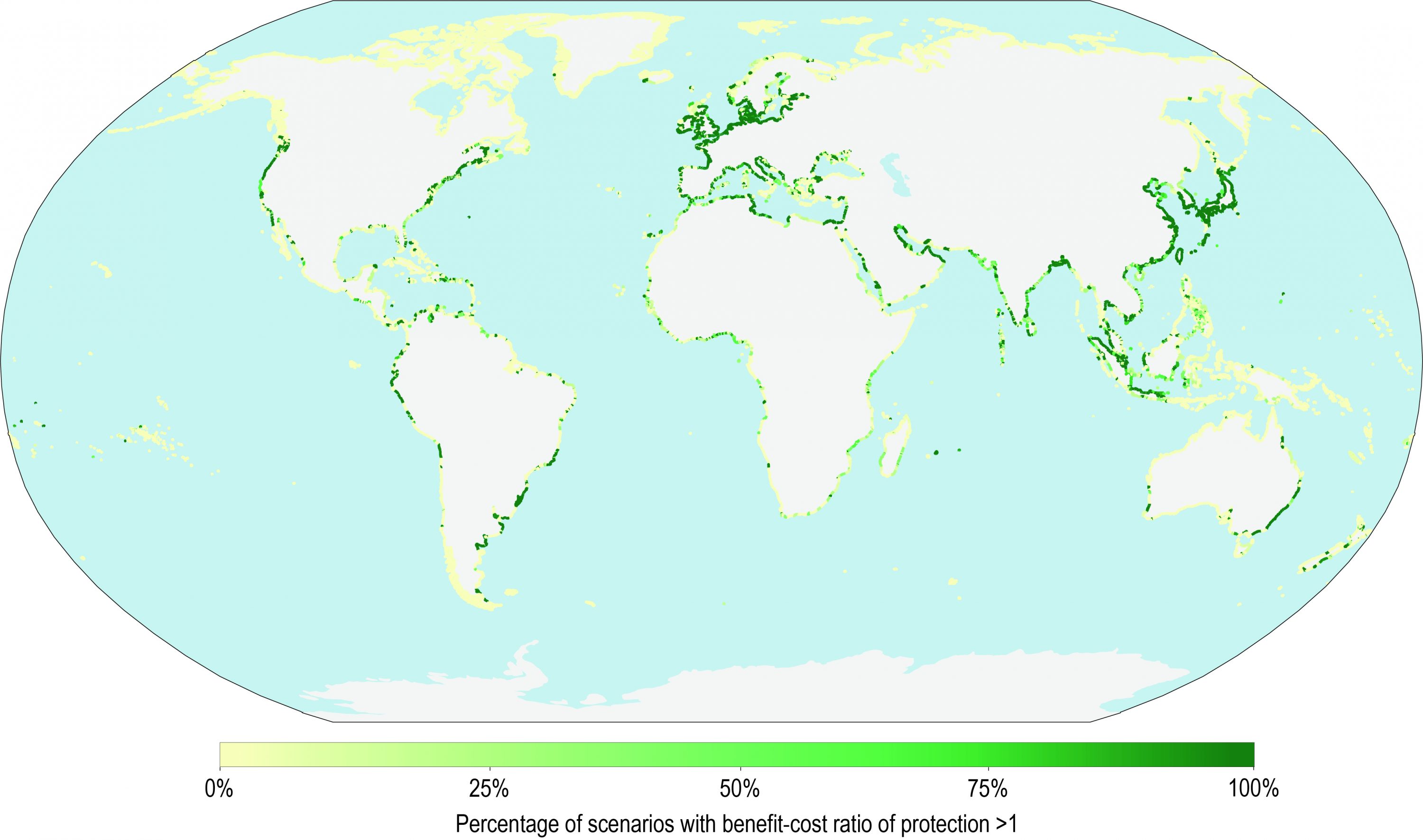
Figure 4.14 | Economic robustness of coastal protection under sea level rise (SLR) scenarios from 0.3–2.0 m, the five Shared Socioeconomic Pathways (SSPs) and discount rates of up to 6%. Coastlines are coloured according to the percentage of scenarios under which the benefit-cost ratio of protection (reduced flood risk divided by the cost of protection) are above 1. Source: Lincke and Hinkel (2018).
At local scales, a large number of economic assessments of response options are available but mostly in the grey literature and again with a focus on hard and sediment-based protection. Similar to the global studies, hard protection is generally found to be economically efficient for urban and densely populated areas such as New York, USA (Aerts et al., 20141640) and Ho Chi Minh City, Vietnam (Scussolini et al., 20171641). Both global and local studies show that sediment-based protection, such as beach nourishment is economically efficient in areas of intensive tourism development due to the large revenues generated within this sector (Rigall-I-Torrent et al., 20111642; Hinkel et al., 2013a1643).
4.4.2.3
Ecosystem-based Adaptation
4.4.2.3.1
Observed ecosystem-based adaptation across geographies
Relative to hard adaptation measures whose global distribution is not known in detail (Scussolini et al., 20151644), the current global distribution of coastal ecosystems is well-studied (e.g., for saltmarshes and mangroves, respectively; Giri et al., 20111645; Mcowen et al., 20171646). EbA, by definition, can only exist and function where the environmental conditions are appropriate for a given ecosystem. Mangroves, salt marshes and reefs occur along about 40–50% of the world’s coastlines (Wessel and Smith, 19961647; Burke, 20111648; Giri et al., 20111649; Mcowen et al., 20171650). However, there is no clear estimate on the global length of coastline covered by ecosystems relevant for EbA in the face of SLR in part because of a mismatch between the spatial resolutions of different estimates available. Mangroves occur on tropical and subtropical coasts, and cover 138,000–152,000 km2 across about 120 countries (Spalding et al., 20101651; Giri et al., 20111652). At least 150,000 km of coastline in over 100 countries benefit from the presence of coral reefs (Burke, 20111653) and these are estimated to protect over 100 million people from wave-induced flooding globally (Ferrario et al., 20141654). The extent of other coastal habitats is less well known: salt marshes are estimated to occur in 99 countries, especially in temperature to high latitude locations, with nearly 5,500,000 ha mapped across 43 countries (Mcowen et al., 20171655).
Since AR5 there has been growing recognition of the value of conserving existing coastal ecosystems, and where possible restoring them, for the flood protection and multiple other benefits they provide (Temmerman et al., 20131656; Arkema et al., 20151657). In parallel, EbA measures are increasingly being incorporated and required within national plans, strategies and targets (Lo, 2016), international adaptation funding mechanisms, such as the Adaptation Fund (AF; e.g., in Sri Lanka and India; Epple et al., 20161658), and national natural capital valuations (Beck and Lange, 20161659). Given their relative novelty, there is widespread interest in building and collecting knowledge of EbA implementation case-studies and examples (Table 4.7). Meanwhile, coastal communities around the globe are already implementing EbA responses at local scales, with emphasis on community participation and ownership and local priorities, needs and capacities (Reid, 20161660; see Section 4.4.4.4).
EbA has been used as an integral part of some retreat, advance and accommodation responses. For example, on coastlines where high-risk properties are relocated inland, space can be made for ecosystem restoration to enhance natural biodiversity and provide coastal protection (French, 20061661; Coastal Protection and Restoration Authority of Louisiana, 20171662). There are also examples of ecosystem restoration to advance coastlines and build land elevation (Chung, 20061663). EbA can also be an element of accommodation responses by, for example, restoring or creating marshes to provide space for flood water (Temmerman et al., 20131664).
4.4.2.3.2
Projected ecosystem-based adaptation
While there are projections available of ecosystem responses to climate change and SLR (Section 4.3.3), to date, there are no large-scale projections available on the future extent of EbA. However, several coastal nations, particularly Small Island Developing States (SIDS) explicitly advocate EbA measures as a means to address future coastal hazard and SLR concerns. Based on Nationally Determined Contributions (NDCs) submitted to the United Nations Framework Convention on Climate Change (UNFCCC), more than 30 SIDS cite EbA as a preferred SLR response, with mangrove planting being the most common measure (Wong, 20181665).
4.4.2.3.3
Cost of ecosystem-based adaptation
There is limited evidence and low agreement on the costs of ecosystem-based measures to make generally valid estimations of the unit costs across large spatial scales. The total cost of an ecosystem-based measure includes capital costs, maintenance costs, the cost of land and, in some situations, permitting costs (Bilkovic, 20171666). The costs of restoring and maintaining coastal habitats depend on coastal setting, habitat type and project conditions. In general, unit restoration costs are lowest for mangroves, higher for salt marshes and oyster reefs, and highest for seagrass beds and coral reefs (Table 4.8).
The conservation of coral reefs and other coastal habitats may also entail substantial opportunity costs because alternative uses of this land, such as through agricultural production, industry and settlements, are generally of high economic value (Stewart et al., 20031667; Balmford et al., 20041668; Adams et al., 20111669; Hunt, 20131670). The high value of these alternative uses are the reason why globally, coastal ecosystems are amongst the ecosystems that face the highest rates of anthropogenic destruction, with estimated annual losses of 1–3% of mangroves area, 2–5% seagrass area and 4–9% corals (Duarte et al., 20131671). Conserving these areas means reversing these trends.
Under the right conditions, and to some extent, EbA measures are free of maintenance costs, because they respond and adapt to changes in their coastal environment. However, maintenance can become important in the aftermath of damage by storms or human action, for example, when wetlands and reefs can be damaged by high winds, waves and surges, or affected by dredging operations (Smith III et al., 20091672; Puotinen et al., 20161673). At present, there is limited evidence about the conditions under which EbA measures can self-adapt and when they require human intervention to recover.
Table 4.8: Costs of ecosystem-based adaptation (EbA). MPA is marine protected area.
| Type of measure | Capital Costs | Maintenance Costs |
| Wetland Conservation | No data available | Thinning, clearing debris after storms, etc.: Mangrove: 5000 USD ha–1 yr–1 in Florida (Lewis, 2001) to 11,000 ha–1 yr–1 (Aerts, 2018).
For mangroves globally, 7–85 USD ha–1 yr–1 (Aerts et al., 2018a); For marshes in the Wadden Sea, 25 USD m–1 yr–1 (Vuik et al., 2019). |
| Wetland Restoration (Marshes/Mangroves, Maritime Forests) | Wetlands: 85,000–230,000 USD ha–1 (Aerts et al., 2018a); Mangroves: USD 9000 ha–1 (median; Bayraktarov et al., 2016);
2000–13,000 USD ha–1 in American Samoa (Gilman and Ellison, 2007); Salt Marshes: 67,000 USD ha–1 (Bayraktarov et al., 2016); Brushwood dams for marsh restoration 150 m–1 (Vuik et al., 2019). |
Similar to maintenance costs for Wetland Conservation |
| Reef Conservation (Coral/ Oyster) | For example, start-up costs for Reef MPAs: 96–40,000 USD km-2 (McCrea-Strub et al., 2011). | For MPAs, 12 million USD yr-1 for the Great Barrier Reef (Balmford et al., 2004). |
| Reef Restoration (Coral/ Oyster) | 165,600 USD ha–1 (median; Bayraktarov et al., 2016); Oyster Reefs: 66,800 USD ha–1 (median; Bayraktarov et al., 2016); Artificial Reefs in the UK 30,000–90,000 USD 100 m–1 (Aerts et al., 2018a) | Similar to maintenance costs for Reef Conservation |
4.4.2.3.4
Effectiveness of ecosystem-based adaptation
While EbA has been able to reduce the impacts of sea level related hazards, there is still little agreement on the size of the effect (Gedan et al., 20111674; Doswald et al., 20121675; Lo, 2016; Renaud et al., 20161676). Dozens of independent field, experimental and numerical studies have observed and measured the wave attenuation and flood reduction benefits provided by natural habitats, such as marsh and mangrove wetlands (Barbier and Enchelmeyer, 20141677; Möller et al., 20141678; Rupprecht et al., 20171679), coral reefs (Ferrario et al., 20141680; Storlazzi et al., 20171681), oyster reefs (Scyphers et al., 20111682) and submerged seagrass beds (Infantes et al., 20121683). Local and global numerical studies indicate that marshes and mangroves can reduce present-day surge-related flood damages by >15% annually, and the loss of a metre of living coral reef can double annual wave-related flood damages (Narayan et al., 20171684; Beck et al., 20181685). Artificial reef restoration along tens of metres of coastline using Reef Ball™ and other structures has been shown to reduce wave heights and stabilise beach widths (Reguero et al., 2018a1686; Torres-Freyermuth et al., 20181687). The effectiveness of EbA measures, however, varies considerably depending on storm, wetland, reef and landscape parameters (Koch et al., 20091700; Loder et al., 20091701; Wamsley et al., 20101702; Pinsky et al., 20131703; Quataert et al., 20151704), which makes it difficult to extrapolate the physical and economic benefits across geographies. Depending on these parameters, rates of surge attenuation can vary between 5–70 cm km-1 (Krauss et al., 20091705; Vuik et al., 20151706).
Critical gaps remain in our understanding about those parameters that together affect the success of ecosystem-based measures including choice of species and restoration techniques, lead time, natural variability and residual risk, temperature, salinity, wave energy and tidal range (Smith, 20061707; Stiles Jr, 20061708). Among reasons commonly cited for the failure of mangrove restoration projects are poor choice of mangrove species, planting in the wrong tidal zones and in areas of excessive wave energy (Primavera and Esteban, 20081709; Bayraktarov et al., 20161710; Kodikara et al., 20171711).
The effectiveness of ecosystem-based measures also exhibits high seasonal, annual and longer-term variability. For example, marsh and seagrass wetlands typically have lower densities in winter which reduces their coastal protection capacity (Möller and Spencer, 20021712; Paul and Amos, 20111713; Schoutens et al., 20191714). In the long-term, there is limited evidence and low agreement on how changes in sea level, sediment inputs, ocean temperature and ocean acidity will influence the extent, distribution and health of marsh and mangrove wetlands, coral reefs and oyster reefs (Hoegh-Guldberg et al., 20071715; Lovelock et al., 20151716; Crosby et al., 2016171; Albert et al., 20171718). EbA measures may have differential lead times before they are effective. For example, newly planted mangroves provide less wave attenuation until they mature (~3–5 years; Mazda et al., 19971719). In contrast, a reef restoration project that uses submerged concrete structures performs as a breakwater as soon as the sub-structure is in place (Reguero et al., 2018a1720).
4.4.2.3.5
Co-benefits and drawbacks of ecosystem-based adaptation
There is high confidence that ecosystem-based measures provide multiple co-benefits such as sequestering carbon (Siikamäki et al., 20121721; Hamilton and Friess, 20181722), income from tourism (Carr and Mendelsohn, 20031723; Spalding et al., 20171724), enhancing coastal fishery productivity (Carrasquilla-Henao and Juanes, 20171725; Taylor et al., 20181726), improving water quality (Coen et al., 20071727; Lamb et al., 20171728), providing raw material for food, medicine, fuel and construction (Hussain and Badola, 20101729; Uddin et al., 20131730), and a range of intangible and cultural benefits (Scyphers et al., 20151731) that help improve the resilience of communities vulnerable to sea level hazards (Sutton-Grier et al., 20151732).
In comparison to hard structures like seawalls, EbA measures, particularly coastal wetlands, require more land (The Royal Society Science Policy Centre, 2014), and competition for land is often why the ecosystems have declined in the first place (4.4.2.3.1). On developed coasts, this land is often not available. In such cases, hybrid measures that either combine EbA measures with structural measures like mangrove forests in front of dikes (Dasgupta et al., 20191733), or build ecological enhancements into engineered structures can provide an effective solution. Like any other feature that interacts with coastal processes, natural wetlands and reefs can increase flooding in some instances, for example, due to the redistribution or acceleration of flows in channels within a wetland system (Marsooli et al., 20161734), or an increase in infragravity wave (i.e., surface gravity waves with frequencies lower than wind waves) energy behind a reef (Roeber and Bricker, 20151735).
4.4.2.3.6
Governance of ecosystem-based adaptation
The coastal protection benefits of natural ecosystems are increasingly being recognised within international discourse and national coastal adaptation, resilience and sustainable development plans and strategies (Section 4.4.2.3.1). In general, obtaining permits for EbA remains more difficult compared to established hard protection measures, in places like the USA (Bilkovic, 20171736). However, there are examples of instruments specifically tailored to retain the protective function of EbA (Borges et al., 20091737; Government of India, 20181738). The Living Shorelines Regulations of the state government of Maryland in the USA (Maryland DEP, 20131739), for instance, requires that private properties must include marsh creation or other non-structural measures when stabilising their shorelines, unless a waiver is obtained.
There are an increasing number of public and private financial mechanisms and policy instruments to encourage the use and implementation of EbA measures (Colgan et al., 20171740; Sutton-Grier et al., 20181741). For example, a regulation by the Federal Emergency Management Agency (FEMA) of the USA, allows proponents of hazard mitigation projects, such as state, territorial and local governments, to take into account the co-benefits of EbA when assessing benefit-cost ratios of FEMA-funded recovery projects (FEMA, 20151742). International guidelines are being developed for designing and implementing EbA measures, with the intention to support wider implementation of these responses (Hardaway Jr and Duhring, 20101743; Van Slobbe et al., 2013; Van Wesenbeeck et al., 2017; Bridges et al., 20181744).
4.4.2.3.7
Economic efficiency of ecosystem-based adaptation
There is limited evidence regarding the economic efficiency of EbA, mainly due to the low agreement about EbA effectiveness (Section 4.4.2.3.2) and costs (Section 4.4.2.3.2). A study of coastal protection measures on the Gulf of Mexico coastline, USA, estimated that EbA measures have average benefit-cost ratios above 3.5 for 2030 flood risk conditions, assuming a discount rate of 2% (Reguero et al., 2018b1745; see Section 4.4.2.3.2). This study also finds that EbA are nearly four times more cost-efficient along developed coastlines as compared to conservation-priority areas because protection benefits are higher in the former case due to the level of asset exposure.
4.4.2.4
Advance
4.4.2.4.1
Observed advance across geographies
Advance has a long history in most areas where there are dense coastal populations and a shortage of land (very high confidence). This includes land reclamation through polders around the southern North Sea (Germany, the Netherlands, Belgium and England) and China (Wang et al., 2014), which coincides with regions where there is extensive hard protection in place (Section 4.4.2.4). Land reclamation has also taken place in all major coastal cities to some degree, even if only for the creation of port and harbour areas by raising coastal flats above normal tidal levels through sediment infill. On some steep coasts, where there is little flat land, such as the Hong Kong Special Administrative Region of China, material from elevated areas has been excavated to create fill material to build land out into the sea.
Globally, it is estimated that about 33,700 km2 of land has been gained from the sea during the last 30 years (about 50% more than has been lost), with the biggest gains being due to land reclamation in places like Dubai, Singapore and China (Wang et al., 2014; Donchyts et al., 2016). In Shanghai alone, 590 km2 land has been reclaimed during the same period (Sengupta et al., 2018). In Lagos, 25 km² of new land is currently being reclaimed (www.ekoatlantic.com). Land reclamation is also popular in some small island settings. The Maldives has recently increased the land area of their capital region by constructing a new island called Hulhumalé, which has been built 60 cm higher than the normal island elevation of 1.5 m, in order to take into account future SLR (Hinkel et al., 2018).
4.4.2.4.2
Projected advance
Advance was not primarily a response to SLR in the past, but due to a range of drivers, including land scarcity, population pressure and extreme events, future advance measures are expected to become more integrated with coastal adaptation and might even be seen as an opportunity to support and fund adaptation in some cases (Linham and Nicholls, 2010; RIBA and ICE, 2010; Nicholls, 2018). While there is no literature on this topic, significant further advance measures can be expected in land scarce situations, such as found in China, Japan and Singapore, in coming decades.
4.4.2.4.3
Costs of advance
Contrary to protection measures, little systematic monetary information is available about costs of advance measures, specifically not in the peer reviewed literature. The costs of land reclamation are extremely variable and depend on the unit cost of fill versus the volumetric requirement to raise the land. Hence, filling shallow areas is preferred on a cost basis.
4.4.2.4.4
Effectiveness of advance
Similar to hard protection, land reclamation is mature and effective technology and can provide predictable levels of safety. If the entire land area is raised above the height of ESLs, residual risks are lower as compared to hard protection as there is no risk of catastrophic defence failure.
4.4.2.4.5
Co-benefits and drawbacks of advance
The major co-benefit of advance is the creation of new land. The major drawbacks include groundwater salinisation, enhanced erosion and loss of coastal ecosystems and habitat, and the growth of the coastal floodplain (Li et al., 2014; Nadzir et al., 2014; Wang et al., 2014; Chee et al., 2017). In China, for example, about 50% of coastal ecosystems have been lost due to land reclamation, leading to a range of impacts such as loss of biodiversity, decline of bird species and fisheries resources, reduced water purification, and more frequent harmful algal blooms (Wang et al., 2014). For example, the reclamation of about 29,000 ha of land in Saemangeum, Republic of Korea, in 2006, has led to a decrease in shorebird numbers by over 30% in two years, probably caused by mortality (Moores et al., 2016). Inadvertently, historic land reclamation through polderisation may have enhanced exposure and risk to coastal flooding by creating new populated floodplains, but this has not been evaluated.
4.4.2.4.6
Governance of advance
Land reclamation raises equity issues with regards to access and distribution of the new land created, specifically due to the political economy associated with high coastal land values, and the involvement of private capital and interests (Bisaro and Hinkel, 2018), but this has hardly been explored in the literature.
4.4.2.4.7
Economic efficiency of advance
There is limited evidence on the efficiency of advance responses in the scientific literature. Benefit-cost ratios of land reclamation can be very high in urban areas due to high land and real estate prices (Bisaro and Hinkel, 2018).
4.4.2.5
Accommodation
4.4.2.5.1
Observed accommodation across geographies
There is a high agreement that accommodation is a core element of adaptation, and it is taking place on various scales based on measures such as flood proofing and raising buildings, implementing drainage systems, land use changes as well as EWS, emergency planning, setback zones and insurance schemes. However, no literature is available that summarises observed accommodation worldwide. There is low evidence of accommodation occurring directly as a consequence of SLR but high evidence of accommodation measures being implemented in response to coastal hazards such as coastal flooding, salinisation and other sea-borne hazards such as cyclones.
Flood proofing may include the use of building designs and materials which make structures less vulnerable to flood damages and/or prevent floodwaters from entering structures. Examples include floating houses in Asia, such as in Vietnam (Trang, 2016), raising the floor of houses in the lower Niger delta (Musa et al., 2016), construction of verandas with sandbags and shelves in houses to elevate goods during floods in coastal communities in Cameroon (Munji et al., 2013). In Semarang City, Indonesia, residents adapted to coastal flooding by elevation of their houses by 50–400 cm or by moving their goods to safer places, without making structural changes (Buchori et al., 2018). Residents of Can Tho City of the Mekong Delta, Vietnam elevated houses in response to tidal flooding (Garschagen, 2015). In urban areas extensive drainage systems contribute to accommodation such as in Hong Kong and Singapore, which rely on urban drainage systems to handle large volumes of surface runoff generated during storm events (Chan et al., 2018). Farming practices have been adapted to frequent flooding in the lower Niger delta: farmers raise crops above floodwaters by planting on mounds of soil and apply ridging and terracing on farmlands to form barriers (Musa et al., 2016). In the floodplains of Bangladesh, floating gardens help to maintain food production even if the area is submerged (Irfanullah et al., 2011). Here, the traditional way to build homesteads is on a raised mound, built with earth from the excavation of canals and ponds (ADPC, 2005). Coastal infrastructure, such as ports, having a functional need to be at the coast, accommodate SLR with elevated piers and critical infrastructure. One example is Los Angeles, where PierS was raised to an elevation of 6 m (Aerts, 2018).
Communities in the Netherlands are experimenting with floating/amphibious houses capable of adapting to different water levels, and similar considerations are also discussed in other geographies, such as in Bangkok (Nilubon et al., 2016). Flood proofing is widely applied in the USA, where wet and dry flood proofing measures are recognised: wet flood proofing reduces damage from flooding while dry flood proofing makes a building watertight or substantially impermeable to floodwaters up to the expected flood height (FEMA, 2014). In that sense, dry flood proofing could also be interpreted as a protection measure on the level of individual structures.
Physical accommodation to salinisation and saline water intrusion is more poorly documented. It mainly entails agricultural adaptation to soil salinity, and saline surface and ground water, as described for the land use changes aimed at alternating rice-shrimp systems and shrimp aquaculture in the Mekong Delta (Renaud et al., 2015) or using methods which decrease soil salinity, such as flushing rice fields with fresh water to wash out salinity (Renaud et al., 2015), or applying maize straw in wheat fields (Xie et al., 2017). Coastal communities are also experimenting with the use of salt tolerant varieties as a result of breeding programmes, for example, in Indonesia (Rumanti et al., 2018), or saline irrigation water in conjunction with fresh water, such as for maize in coastal Bangladesh (Murad et al., 2018).
Adaptation planning for SLR has been incorporated into land use planning in several states in the USA (Butler et al., 2016b). In the Yangtze River Delta, landscape planning designs floodplain zones to accept floodwaters (Seavitt, 2013). In the Mekong Delta, different land use options, including shifting from freshwater agriculture to brackish and saline agriculture, were proposed as seawater intrudes farther inland (Smajgl et al., 2015).
EWS are frequently incorporated into overall risk reduction strategies and are applied for various coastal hazards such as tsunamis in coastal areas of Indonesia (Lauterjung et al., 2017) and hydro-meteorological coastal hazards in Bangladesh and Uruguay (Leal Filho et al., 2018). They fall under ‘accommodation’ as they allow people to remain in the hazard-prone area but provide advance warning or evacuation in the face of imminent danger. In contrast to hard protection measures, EWS have shorter installation time and lower impact on the environment (Sättele et al., 2015). They can work effectively to reduce risk arising from predictable hazardous events but are less well-suited to accommodate slow onset change (i.e., events or processes that happen with high certainty under different climate change scenarios)
Climate risk insurance schemes have been recently developed to address sudden, and in rare cases, slow onset hazards at the coast, and to increase overall resilience. For coastal risks, insurance is mainly applicable for sudden onset hazards, including storm surges and coastal flooding, to buffer against the financial impacts of loss events. For slow onset hazards, insurance schemes are not the first-best tool, whereas resilience building and prevention of loss and damage in such instances may be more cost-effective ways to address these risks (Warner et al., 2013). In this context, index based insurance products are increasingly offered, particularly in low-income countries and have also been included in a number of countries in their NDCs and in some cases in their National Adaptation Plans (NAPs; Kreft et al., 2017). Countries with existing climate risk insurance schemes include, for example, Haiti, Maldives, Seychelles and Vietnam. The InsuResilience Global Partnership for Climate and Disaster Risk Finance and Insurance Solutions was launched at the 2017 UN Climate Conference (COP 23) in Bonn. InsuResilience aims to enable more timely response after a disaster and helps to better prepare for climate and disaster risk through the use of climate and disaster risk finance and insurance solutions. So far, climate risk insurance was used mainly in the context of agriculture, where it has showed great efficacy in boosting investments for increasing productivity (Fernandez and Schäfer, 2018). However, on the global scale, the uptake of index insurance is still low (Yuzva et al., 2018).
4.4.2.5.2
Projected accommodation
While there is no literature on projected accommodation, current trends suggest further uptake of accommodation approaches in coming decades, especially where protection approaches are not economically viable. Flood proofing of houses and establishment of new building codes to accommodate coastal hazards is also expected to become more common in coming decades. Similarly, accommodation measures for salinity are under further development, such as rice breeding programs to improve salt tolerance (Linh et al., 2012; Quan et al., 2018b). However, the achievements to improve salinity tolerance in rice are rather modest so far (Hoang et al., 2016) although efforts are expected to continue or even intensify. Given that index based insurance products have been included in NDCs and NAPs in a number of countries (Kreft et al., 2017), uptake is expected to grow. Ports can continue elevating hazard-prone facilities and the critical parts of port infrastructure can be protected by flood walls. Alternatively, ports can use advance measures to develop port facilities seaward (Aerts, 2018).
In summary, due to the large variety of different measures implemented in ad hoc ways worldwide, there is low confidence in quantitative projections of accommodation measures in response to SLR. However, there is high confidence that accommodation measures will continue to be a widespread adaptation option especially in combination with protection and retreat measures.
4.4.2.5.3
Cost of accommodation
The cost of accommodation varies widely with the measures taken as well as the expected flood height. For flood proofing of buildings in New York City for instance, Aerts et al. (2014) provided an economic rationale for the implementation of improved building codes, such as elevating new buildings and protecting critical infrastructure (see also Box 4.1). Flood proofing can also be undertaken by individuals and even small, inexpensive flood proofing efforts can result in reductions in flood damage (Zhu et al., 2010). In general, costs for flood proofing increase as the flood protection elevation increases. Other costs include those for maintenance and, if applicable, insurance premiums. For example, deciding to elevate a building in the USA will increase the project’s cost; however, the additional elevation may lead to significant savings on flood insurance premiums (FEMA, 2014).
4.4.2.5.4
Effectiveness of accommodation
Accommodation measures can be very effective for current conditions and small amounts of SLR, also buying time to prepare for future SLR. Success stories include the case of Bangladesh where improved early warnings, the construction of shelters, and development of evacuation plans, helped to reduce fatalities as a result of flooding and cyclones (Haque et al., 2012). Illiteracy, lack of awareness and poor communication are, however, still hampering the effectiveness of early warnings (Haque et al., 2012). If well designed, and if the premiums reflect individual risks, insurance can effectively discourage further investments in risky areas as insurance cost provides information on the nature of locality-specific risks and can incentivise investment in risk reduction by requiring that certain minimum standards are met before granting insurance coverage (Kunreuther, 2015). Limits to such accommodation occur much earlier compared to protect, advance and retreat measures. While dikes can be raised to 10 m, and retreat can be implemented to the 10 m contour or higher, accommodating SLR has practical and economic limits, and ultimately retreat or protection will be required.
4.4.2.5.5
Co-benefits and drawbacks of accommodation
The major co-benefit of accommodation is improved resilience of in situ communities without retreat or the use of land and resources for the construction of protection measures. Flood proofing, for example, helps prevent demolition or relocation of structures and it is often an affordable and cost effective approach to reducing flood risk (Zhu et al., 2010). Specific accommodation measures have different co-benefits such as that stilt houses not only protect from flooding but also from wild animals (Biswas et al., 2015). Accommodation—depending on the measure implemented—has the potential to maintain landscape connectivity allowing access to the ocean as well as landward migration of ecosystems, at least to some degree. It also retains flood dynamics and with that the benefits of flooding such as sediment re-distribution. Stilt houses leave space for the floodwater while wet-flood proofing maintains a low hydrostatic pressure on the buildings so that structures are less prone to failure during flooding (FEMA, 2014)
The major drawback of accommodation is that it actually does not prevent flooding or salinisation, which might have consequences not addressed by the accommodation measure itself. Examples include inundation of an area where houses are flood proofed but schooling of children and business operations are nevertheless disrupted. Significant clean up may also be needed after flood water enters buildings, including the removal of sediment, debris or chemical residues (FEMA, 2014). Also, flood proofing measures require the current risk of flooding to be known and communicated to and understood by the public through flood hazard mapping studies and flood warning information (Zhu et al., 2010). Small businesses in particular may face difficulties to recover from flooding due to lack of forward planning (Hoggart et al., 2014).
Co-benefits of insurance include the possibility that sovereign level insurance may improve the credit ratings of vulnerable countries, reducing the cost of capital and allowing them to borrow to invest in resilient infrastructure (Buhr et al., 2018). Major natural disasters can weaken sovereign ratings, especially if there is no insurance in place (Moritz Kramer, 2015). One much discussed drawback of insurance is the moral hazard that may result: since someone else bears the costs of a loss, those insured may be less inclined to take precautionary measures or may act recklessly (Duus-Otterström and Jagers, 2011).
4.4.2.5.6
Governance of accommodation
While accommodation measures to coastal hazards are often taking place at the local level, and are decided by individual homeowners, farmers or communities, from a governance perspective it is important to provide guidance on how and to what extent owners can retrofit their homes to reduce the risk to coastal flooding. In New York City, for instance, changes to building codes, require elevating, or flood proofing of existing and new buildings in the 100-year floodplain, and prevent construction of critical infrastructure like hospitals in the flood zone (NYC, 2014; see also Box 4.1).
Effective coastal risk management efforts rely on good governance that includes understanding the probability and consequences of hazard impacts like flooding and salinisation, and implementing mechanisms to prevent or manage all possible events (EEA, 2013). The effectiveness of accommodation measures based on institutional measures, such as EWS and evacuation plans, largely depends on the governance capabilities they are embedded in.
4.4.2.5.7
Economic-efficiency of accommodation
There is high confidence that many accommodation measures are very cost-efficient. Flood EWS coupled with precautionary measures have been shown to produce significant economic benefits (Parker, 2017). Elevating areas at high risk and retrofitting buildings in Ho Chi Minh City, for example, have benefit-cost ratios of 15 under SLR of 180 cm and a discount rate of 5% during the 21st century (Scussolini et al., 2017). In the context of the National Flood Insurance Program in the USA, it has been estimated that elevating new houses by 60 cm might raise mortgage payments by 240 USD yr-1, but reduce flood insurance by 1000–2000 USD yr-1 depending on the flood zone (FEMA, 2018), although this only addresses present extremes and ignores future SLR (Zhu et al., 2010). In Europe, the benefits of installing a cross-border continental-scale flood EWS are estimated at 400 EUR per EUR invested (Pappenberger et al., 2015).
4.4.2.6
Retreat
4.4.2.6.1
Observed retreat across geographies
There is limited evidence of migration occurring directly as a consequence of impacts associated with environmental change generally and SLR specifically. Research examining the linkages between migration and environmental change has been conducted in the Pacific (Connell, 2012; Janif et al., 2016; Perumal, 2018), South Asia (Szabo et al., 2016; Call et al., 2017; Stojanov et al., 2017), Latin America (Nawrotzki and DeWaard, 2016; Nawrotzki et al., 2017), Alaska, in North America (Marino and Lazrus, 2015; Hamilton et al., 2016) and Africa (Gray and Wise, 2016). While some limited evidence was found on population movement inland associated with shoreline encroachment in Louisiana, USA (Hauer et al., 2018), this research emphasises that the relationship between climate change impacts including SLR and migration is more nuanced than suggested by simplified cause-and-effect models (Adger et al., 2015). Migration is driven by a large number of individual, social, economic, political, demographic and environmental push and pull factors (Black et al., 2011; Koubi et al., 2016), interwoven with mega-trends such as urbanisation, land use change and globalisation, and is influenced by development and political practices and discourses (Bettini and Gioli, 2016; Cross-Chapter Box 7). For example, asset endowed individuals and households are more able to migrate out from flood-prone areas (Milan and Ruano, 2014; Logan et al., 2016), while the poorest households are significantly susceptible to material and human losses following an extreme event or disruptive environmental change (Call et al., 2017). Individual and social drivers include perceptions of environmental change (Koubi et al., 2016), formed by both direct experience of change and indirect information from social networks, mass media and governmental agencies. Environmental factors include the longer term impacts of climate variability and change, which can erode the capacity of ecosystems to provide essential services such as availability of freshwater, soil fertility and energy production acting as a threat multiplier for other drivers of migration(Hunter et al., 2015; McLeman, 2018).
There is robust evidence of disasters displacing people worldwide, but limited evidence that climate change or SLR is the direct cause. In 2017, 18.8 million people were displaced by disasters, of which 18 million were displaced by weather-related events including 8.6 million people displaced by floods and 7.5 million by storms, with hundreds of millions more at risk (IDMC, 2017; Islam and Khan, 2018). The majority of resultant population movements tend to occur within the borders of affected countries (Warner and Afifi, 2014; Hunter et al., 2015; Nawrotzki et al., 2017).
We find robust evidence of planned relocation taking place worldwide in low-lying zones exposed to the impacts of coastal hazards (Hino et al., 2017; Mortreux et al., 2018). While relocation plans are usually discussed after an extreme event occurs, they generally target the reduction of long-term environmental risks, including those of SLR (McAdam and Ferris, 2015; Hino et al., 2017; Morrison, 2017). For example, in the aftermath of Hurricane Katrina, the Louisiana Comprehensive Master Plan for a Sustainable Coast recommended the relocation of several communities in the next 50 years due to expected RSL rise, and relocation of inhabitants from Isle de Jean Charles is already taking place (Barbier, 2015; Coastal Protection and Restoration Authority of Louisiana, 2017). In Shismaref, an Iñupiat community in Alaska, increased shoreline erosion triggered government-led relocation (Bronen and Chapin, 2013; Maldonado et al., 2013). In the Pacific, current coastal risks aggravated by rising sea level are driving the government led relocation of the inhabitants of Taro, the provincial capital of Choiseul Province in the Solomon Islands (Albert et al., 2018). In 2014, the government of Kiribati purchased land on Vanua Levu, the second largest island of Fiji, with the purpose of economic development and food security, but many i-Kiribati associated the acquisition with future relocation to Fiji (Hermann and Kempf, 2017). In southeast Asia, the government of Vietnam assists and manages rural populations’ relocation from disaster prone areas exposed to coastal risks in the Mekong Delta to large industrial areas with high labour demand, such as Ho Chi Minh City and Can Tho City (Collins et al., 2017). Managed realignment carried out for the purposes of habitat creation, improved flood risk management and more affordable coastal protection, is increasingly popular in Europe, but usually involves small-scale projects and few people if any (Esteves, 2013). Most of the managed realignment projects in the UK and Germany have been carried out for habitat creation and to reduce spending on coastal defences (Hino et al., 2017)
4.4.2.6.2
Projected retreat
There is high agreement that climate change has the potential to drastically alter the size and direction of migration flows (Connell, 2012; Gray and Wise, 2016; Janif et al., 2016; Nawrotzki and DeWaard, 2016; Szabo et al., 2016; Call et al., 2017; Nawrotzki et al., 2017), but there is low confidence in quantitative projections of migration in response to SLR and extremes of sea level. The number of modelling studies of migration in response to environmental drivers has increased rapidly over the past decade (Kumari et al. 2018), but only a small portion of these model studies address migration in response to SLR and sea level extremes. Amongst these, a variety of different modelling approaches have been applied, but no model currently accounts for all push and pull factors influencing migration decisions (see Section 4.4.2.6.1).
A model projecting future US county-level populations exposed to permanent inundation was combined with an empirical model of potential migration destinations to produce the first sea level/migration analysis of migrant destinations (Hauer, 2017). Assuming that households with incomes above 100,000 USD yr-1 would have resources to stay and adapt, it was found that 1.8 m SLR by 2100 would displace over two million people in south Florida. Projected population gains due to SLR reach several hundred thousand for some inland urban areas. A gravity model modified to account for both distance to destinations and their attractiveness (deriving from such factors as economic opportunity and environmental amenities) projects a net migration into and out of the East African coastal zone, ranging from out-migration of 750,000 people between 2020 and 2050 to a small in-migration (Kumari et al., 2018). However, this range includes migration stimulated by freshwater availability as well as SLR and episodic flooding. A generalised radiation or diffusion model predicts 0.9 million people will migrate due to SLR in Bangladesh by 2050 and 2.1 million by 2100, largely internally, with substantial implications for nutrition, shelter and employment in destination areas (Davis et al., 2018).
A global dynamic general equilibrium framework (Desmet et al., 2018) provides a more comprehensive approach to accounting for economic factors including changes to trade, innovation, and agglomeration, and political factors, such as policy barriers to mobility, all of which influence the migration response to environmental change. Agent-based models attempt to simulate decisions by individuals who face a variety of socioeconomic and environmental changes (Kniveton et al., 2012). However, neither general equilibrium nor agent-based frameworks have been applied yet to migration responses to SLR. Econometric models, common in climate/migration studies (Millock, 2015), likewise have yet to be applied to the SLR context, except for a single case study where an econometric model was used to interpret the outcome of a discrete choice experiment (Buchanan et al., 2019). For example, an interesting distinction between migration responses to long term temperature and precipitation trends in contrast to extreme events like flooding has been noted (Bohra-Mishra et al., 2014; Mueller et al., 2014), but similar econometric studies have yet to be done comparing responses to gradual land loss versus flooding during ESL events.
4.4.2.6.3
Cost of retreat
We have limited evidence of estimates on the cost of retreat. There are few cost estimates in the literature and these are based on stylised assumptions as little empirical data is available.
The cost of managed relocation, including land acquisition, building of roads and infrastructure and other subsidies, was found to vary from 10,000–270,000 GBP per home in United Kingdom Coastal Change Pathfinder projects (Regeneris Consulting, 2011), and between 10,000 USD in Fiji and 100,000 USD per person in Alaska and in the Isle of Jean Charles in the USA (Hino et al., 2017). For people involved in planned relocation in Shaanxi Province, Northwest China, households receive subsidies ranging from 1200–5100 USD (Lei et al., 2017). The Louisiana’s National Disaster Resilience Competition, Phase II Application states that the proposed relocation of 40 households in the Isle de Jean Charles in Louisiana is estimated to cost 48,379,249 USD, including the cost for land acquisition, infrastructure and construction of new dwellings (State of Louisiana, 2015). Generally, maintenance costs do not arise if people are moved completely out of the hazard zone (Suppasri et al., 2015; Hino et al., 2017). In cases in which people are only moved so that short-term but not long-term risk is reduced, follow up costs for further responses will occur.
The individual costs associated with displacement after an environmental disaster are difficult to obtain. In the literature, there are limited estimates of the social costs to residents of Guadeloupe, Saint Croix, St. Thomas, Puerto Rico, and the southeast USAdisplaced after Hurricanes Hugo (1989) and Katrina (2005). A survey conducted across 18 parishes (i.e. counties) in Louisiana in 2006 revealed that non-displaced households had an average income of 36,000 USD compared to an average income of 30,000 USD recorded for displaced households (Hori and Schafer, 2010).
4.4.2.6.4
Effectiveness of retreat
There is very high confidence that retreat is effective in reducing the risks and impacts of SLR as retreat directly reduces exposure of human settlements and activities (Gioli et al., 2016; Shayegh et al., 2016; Hauer, 2017; Morrison, 2017).
4.4.2.6.5
Co-benefits and drawbacks of retreat
The other outcomes of retreat responses, beyond the one of effectively reducing SLR risks and impacts, are complex and affect both origin and destination. Generally, retreat impacts social networks, access to services and economic and social opportunities, and several well-being indicators (Jones and Clark, 2014; Adams, 2016; Herath et al., 2017; Kura et al., 2017; McNamara et al., 2018). The socioeconomic benefits of migration to individuals and households may include improved access to health and education services, as well as labour markets (Wrathall and Suckall, 2016). Destination areas may gain economically as populations and capital relocate and provide a new source of labour, capital and innovation to inland areas (see Section 4.4.2.6.2; de Haas, 2010). Income inequality may be reduced, but only through migration to areas with growing economies. Remittances can provide flexibility in livelihood options, supply capital for investment and spread risk (Scheffran et al., 2012).
Drawbacks of migration and displacement at the destination can be increased competition for resources and within labour markets, pressure on frontline services and on social cohesion as a result of heightened cultural or ethnic tension (Werz and Hoffman, 2015), as well as cultural, social and psychological losses related to disruptions to sense of place and identity, self-efficacy, and rights to ancestral land and culture (McNamara et al., 2018). The unplanned and unassisted voluntary relocation of the inhabitants of Nuatambu and Nusa Hope in the Solomon Islands to areas further from the coast poses a series of practical challenges with sanitation, access to drinking water and transport (Albert et al., 2018).
The success of planned relocation in terms of the balance of co-benefits and drawbacks varies across relocation schemes (Hino et al., 2017) and outcomes are highly uneven (Genovese and Przyluski, 2013; Ford et al., 2015; Nordstrom et al., 2015; Bukvic and Owen, 2017; Hino et al., 2017; Jamero et al., 2017). On the one hand, well designed and carefully implemented programmes, such as the ongoing resettlement of indigenous communities in Alaska, can improve housing standards and reduce vulnerability (Suppasri et al., 2015; Albert et al., 2018). On the other hand, relocated communities have often become further impoverished (Wilmsen and Webber, 2015), because they are removed from cultural and material resources on which they rely, compounded by poor implementation processes that may fail to ensure fairness, social and environmental justice and well-being (Herath et al., 2017; Mortreux et al., 2018; Nygren and Wayessa, 2018).
4.4.2.6.6
Governance of retreat
Environmentally driven migration and displacement gained major attention over the last decade in the international policy community (Goodwin-Gill and McAdam, 2017). Worldwide programmes, such as the Nansen Initiative, signed by 110 countries to address the serious legal gap around the protection of cross-border migrants impacted by natural disasters, have been implemented (Gemenne and Brücker, 2015). In 2016, the Platform on Disaster Displacement was established to follow up on the work conducted by the Nansen Initiative with the objective of implementing the recommendations of the Protection Agenda (McAdam and Ferris, 2015). Governments are further encouraged by civil society to relocate people at risk and displaced populations out of disaster-prone areas to avoid potential casualties (Lei et al., 2017; Mortreux et al., 2018). There have been discussions among Pacific Island countries and territories and other nations in the Pacific Rim around new policy mechanisms that would facilitate adaptive migration in the region in response to natural hazards including SLR (Burson and Bedford, 2015). There have been cases presented at the Immigration and Protection Tribunal of New Zealand testing refugee claims associated with climate change from Tuvaluan and i-Kiribati applicants, both citing environmental change on their home islands as grounds for remaining in New Zealand. One applicant was successful in the quest to remain in New Zealand on humanitarian grounds, but not on the grounds of refugee status (Farbotko et al., 2016).
The is high agreement that outcomes can be improved by upholding the principle of procedural justice and respecting the autonomy of individuals and their decisions about where and how they live (Warner et al., 2013; Schade et al., 2015; McNamara et al., 2018). However, there are cases where logistical and political stances constrain the application of such approach, such as when the government of Sri Lanka prohibited rebuilding along the coastline of the country after the 2004 tsunami (Hino et al., 2017). Proactive planning, including participation and consultation with those in peril, has the potential to improve outcomes (medium confidence; de Sherbinin et al., 2011; Gemenne and Blocher, 2017). Governments can assist migrants through policy reforms to enable relocation to fast growing economic regions in the country. An example of this approach was adopted in Vietnam by both the National Target Program to Respond to Climate Change and the National Strategy for Natural Disaster Prevention, Response and Mitigation targeted at locations within the Mekong Delta exposed to the impacts of SLR (Nguyen et al., 2015; Collins et al., 2017). Outcomes of retreat for both community of origin and destination can also be improved by building the human capital of migrants (skills, health and education), reducing costs of migration and remittance transfer, and provision of improved safety nets for migrants at their destinations (high agreement) (Gemenne and Blocher, 2017).
4.4.2.6.7
Economic efficiency of retreat
There is limited evidence on the efficiency of retreat responses in the scientific literature.
4.4.3
Governance challenges in responding to sea level rise
4.4.3.1
Introduction
Governance is pivotal to shaping SLR responses. The assessment of SLR responses above has shown that each type of response raises specific governance challenges associated with the distribution of costs, benefits and negative consequences of responses across societal actors. Hence, SLR responses require governance efforts if social conflicts are to be resolved and mutual opportunities amongst all actors realised. Generally, responses involve the interaction of diverse public and private actors at different levels of decision making with divergent values, interests and goals on coastal activities, lifestyles, livelihoods, risks, resilience and sustainability (high confidence; Dovers and Hezri, 2010; Foerster et al., 2015; Giddens, 2015; Mills et al., 2016; Dolšak and Prakash, 2018; Hinkel et al., 2018; Hoegh-Guldberg et al., 2018; AR5). This leads to a number of overarching governance challenges that arise from the nature of SLR, which will be assessed in this section.
While there is a substantial literature on coastal governance, little attention has been focused explicitly on SLR governance, as was also the case in AR5 (Wong et al., 2014). Furthermore, much of the adaptation governance literature has focused on putting forward normative prescriptions on how governance arrangements ought to be (e.g., transformative governance; Chaffin et al., 2016), but with limited empirical evidence on the actual effectiveness of these prescriptions (Klostermann et al., 2018; Runhaar et al., 2018). Hence, understanding the social mechanisms leading to the emergence of particular governance arrangements, and how effective they are in addressing climate change and SLR, is limited (Wong et al., 2014; Bisaro and Hinkel, 2016; Oberlack, 2017; Bisaro et al., 2018; Roggero et al., 2018a; Roggero et al., 2018b). An important post-AR5 development has thus been to move beyond descriptions and normative prescriptions about ‘good governance’ to explore which factors help (called enablers) or hinder (called barriers) how social choices are made and implemented on complex issues like climate change and SLR, as elaborated in the next subsection.
4.4.3.2
Understanding Barriers to Adaptation as Governance Challenges
AR5 stated that there are many reasons why adaptation governance is complex (Klein et al., 2014). The first generation of studies that investigated this question empirically identified many (lists of) barriers that people have experienced in adaptation governance in specific case contexts, including political, institutional, social-cognitive, economic, financial, biophysical and technical barriers (Klein et al., 2014). Although insightful for these specific cases, including SLR (Hinkel et al., 2018), accumulation of empirical findings in building theory proved to be limited, and it did not result in more evidence-informed advice to policy makers on how to deal with barriers (Biesbroek et al., 2013; Eisenack et al., 2014).
In response, in a second generation of studies, several frameworks have been proposed and tested to advance scholarship on barriers to adaptation (Eisenack and Stecker, 2012; Barnett et al., 2015; Lehmann et al., 2015; Bisaro and Hinkel, 2016). A frequently used framework was developed by Moser and Ekstrom (2010) who identified and linked key barriers to certain stages of the policy process: understanding, planning and management stages. Moser and Ekstrom (2010) argue that conditions, such as the scope and scale of adaptation, have significant implications for which barriers are activated in the policy process, and how persistent and difficult they are to overcome. This and other frameworks have been applied in a diversity of contexts, providing valuable insights about the governance challenges involved in adapting to climate change and suggestions for improvement (Ekstrom and Moser, 2014; Rosendo et al., 2018; Thaler et al., 2019).
A recent generation of studies takes more theory based approaches and includes contextual factors to analyse the key social mechanisms that explain why adaptation processes are often complex, result in deadlocks, delays or even failure (Biesbroek et al., 2014; Eisenack et al., 2014; Wellstead et al., 2014; Biesbroek et al., 2015; Bisaro and Hinkel, 2016; Oberlack and Eisenack, 2018; Sieber et al., 2018; Wellstead et al.). Such insights are critical as they can be used by practitioners for policy design (e.g., to prevent certain deadlocks from emerging by (re)designing contextual conditions), or provide insights on strategic interventions in ongoing processes to revitalise deadlocked adaptation governance (Biesbroek et al., 2017).
4.4.3.3
Governance Challenges in the Face of Sea Level Rise
There is a wide diversity of governance challenges and opportunities for tackling SLR, with marked differences within and between coastal communities in developed and developing counties. Five salient overarching governance challenges that arise due to distinctive features of SLR were highlighted. This typology is then used to assess how planning, participation and conflict resolution (Section 4.4.4.2), decision analysis methods (Section 4.4.4.3), and enabling conditions (Section 4.5) can help to address these five challenges.
Time horizon and uncertainty: The long-term commitment to SLR (Section 4.2.3.5) and the large and deep uncertainty about the magnitude and timing of SLR beyond 2050 (Section 4.4.4.3.2), challenge standard planning and decision making practises for several reasons (high confidence; Peters et al., 2017; Pot et al., 2018; Hall et al., 2019; Hinkel et al., 2019). The time horizon of SLR extends beyond usual political, electoral and budget cycles. Furthermore, many planning and decision making practices strive for predictability and certainty, which is at odds with the dynamic risk and deep uncertainty characterising SLR (Hall et al., 2019). Tensions can arise between established risk-based planning that seeks to measure risk, and adaptation responses that embrace uncertainty and complexity (Kuklicke and Demeritt, 2016; Carlsson Kanyama et al., 2019). For example, tensions arise because of the mismatch between the relative inflexibility of existing law and institutions and the evolving nature of SLR risk and impacts (Cosens et al., 2017; Craig et al., 2017; DeCaro et al., 2017). Possible limits of in situ responses to ongoing SLR (e.g., protection and accommodation), bring into question prevailing legal approaches to property rights and land use regulation (Byrne, 2012). In addition, because uncertainty about SLR makes it difficult to decide when to wait and when to act, public actors fear being held accountable for misjudgments (Kuklicke and Demeritt, 2016). The long time horizon and uncertainty of SLR make it difficult to mobilise political will and the leadership required to take visionary action (Cuevas et al., 2016; Gibbs, 2016; Yusuf et al., 2016; Yusuf et al., 2018b).
Cross-scale and cross-domain coordination: SLR creates new coordination problems across jurisdictional levels and domains, because impacts cut across scales, sectors and policy domains and responding often exceeds the capacities of local governments and communities (medium confidence; Araos et al., 2017; Termeer et al., 2017; Pinto et al., 2018; Clar, 2019; Clar and Steurer, 2019; Sections 4.3.2 and 4.4.2). Local responses are generally nested within a hierarchy of local, regional, national and international governance arrangements and cut across sectors (Cuevas, 2018; Chhetri et al., 2019; Clar, 2019). Furthermore responding to SLR is only one administrative priority amongst many, and the choice of SLR response is influenced by multiple co-existing functional responsibilities and perspectives (e.g., planning, emergency management, asset management and community development) that compete for legitimacy, further complicating the coordination challenge (Klein et al., 2016; Vij et al., 2017; Jones et al., 2019).
Equity and social vulnerability: SLR and responses may affect communities and society in ways that are not evenly distributed, which can compound vulnerability and inequity, and undermine societal aspirations, such as achieving SDGs (high confidence; Section 4.3.3.2; Eriksen et al., 2015; Foerster et al., 2015; Sovacool et al., 2015; Clark et al., 2016; Gorddard et al., 2016; Adger et al., 2017; Holland, 2017; Dolšak and Prakash, 2018; Lidström, 2018; Matin et al., 2018; Paprocki and Huq, 2018; Sovacool, 2018; Warner et al., 2018a). Costs and benefits of action and inaction are distributed unevenly, with some coastal nations, particularly small island states, being confronted with adaptation costs amounting to several percent of GDP in the 21st century (Section 4.3.3.2). Land use planning for climate adaptation can exacerbate sociospatial inequalities at the local level, as illustrated in a study of eight cities, namely Boston (USA), New Orleans (USA), Medellin (Colombia), Santiago (Chile), Metro Manila (Philippines), Jakarta (Indonesia), Surat (India), and Dhaka (Bangladesh; Anguelovski et al., 2016). Private responses may also exacerbate inequalities as, for example, in Miami, USA, where purchase of homes in areas at higher elevation has increased property prices displacing poorer communities from these areas (Keenan et al., 2018). In Bangladesh, some adaptation practices have enabled land capture by elites, public servants, the military and roving gangs, and resulted in various forms of marginalisation that compound vulnerability and risk (Sovacool, 2018); a reality also faced by many other coastal communities around the world (Sovacool et al., 2015).
Social conflict: Ongoing SLR could become a catalyst for possibly intractable social conflict by impacting human activities, infrastructure and development along low-lying shorelines (high confidence). Social conflict refers here to the non-violent struggle between groups, organisations and communities over values, interests, resources, and influence or power, whereby parties seek to achieve their own goals, and may seek to prevent others from realising their goals and possibly harm rivals (Coser, 1967; Oberschall, 1978; Pruitt et al., 2003). SLR impacts that could contribute to conflict include: disruptions to critical infrastructure, cultural ties to the coast, livelihoods, coastal economies, public health, well-being, security, identity and the sovereignty of some low-lying island nations (Sections 4.3.2.4, 4.3.3.2, 4.3.3.6; Mills et al., 2016; Yusuf et al., 2016; Nursey-Bray, 2017; Hinkel et al., 2018). SLR responses inevitably raise difficult trade-offs between private and public interests, short- and long-term concerns, and security and conservation goals, which are difficult to reconcile due to divergent problem framing, interests, values and ethical positions (Eriksen et al., 2015; Foerster et al., 2015; Mills et al., 2016; Termeer et al., 2017; Sovacool, 2018). To some countries, SLR presents a security risk due to the scale of potential displacement and migration of people (Section 4.4.2.6). Climate change, and rising seas in particular, could compound sociopolitical stressors (Sovacool et al., 2015), challenge the efficacy of prevailing legal processes (Byrne, 2012; Busch, 2018; Setzer and Vanhala, 2019), and spark or escalate conflict (Lusthaus, 2010; Nursey-Bray, 2017).
Complexity: SLR introduces novel and complex problems that are difficult to understand and address (high confidence; Moser et al., 2012; Alford and Head, 2017; Wright and Nichols, 2018; Hall et al., 2019). As a result of the preceding features of the SLR problem, and the complexity of the nonlinear interactions between biogeophysical and human systems, SLR challenges may be difficult to frame, understand and respond to. Often, disciplinary science is not sufficient for understanding complex problems like SLR and traditional technical problem solving may not be well suited for crafting enduring SLR responses (Lawrence et al., 2015; Termeer et al., 2015). SLR poses a challenge for bridging gaps between science, policy and practice (Hall et al., 2019). The complexity and rapid pace of SLR in some localities is also challenging traditional community decision making practices, for example, in some Pacific Island communities (Nunn et al., 2014).
4.4.4
Planning, Engagement and Decision Tools for Choosing Responses
4.4.4.1
Introduction
4.4.4.2
Planning, Public Participation and Conflict Resolution in the Face of SLR
Land use or spatial planning has the potential to help communities prepare for the future and decide how to manage coastal activities and land use taking into account the uncertainty, complexity and contestation that characterise SLR (high confidence; Hurlimann and March, 2012; Hurlimann et al., 2014; Berke and Stevens, 2016; King et al., 2016; Reiblich et al., 2017) Planners work with governing authorities, the private sector, and local communities to integrate and apply tailor-made decision analysis, public participation and conflict resolution approaches that can be institutionalised in statutory provisions, and aligned with informal institutional structures and processes carried out at various scales (Hurlimann and March, 2012; Smith and Glavovic, 2014; Berke and Stevens, 2016).
Planning can play an important role in crafting SLR responses, addressing several of the governance challenges identified above (Section 4.4.3). Planning is future focused and can assist communities to develop and pursue a shared vision, and understand and address SLR concerns in locality-specific ways (Hurlimann and March, 2012; Berke and Stevens, 2016). Planning can help articulate and clarify roles and responsibilities through statutory planning provisions, complemented by non-statutory processes (Vella et al., 2016). It can build social and administrative networks that mobilise cross-scale SLR responses, and facilitate integration of diverse mitigation and adaptation goals alongside other public aspirations and policy imperatives (Hurlimann and March, 2012; Vella et al., 2016). Planning can also facilitate the establishment of collaborative regional forums that cross jurisdictional boundaries and assist local governments and other stakeholders to pool resources and coordinate roles and responsibilities across multiple governance levels, such as the Southeast Florida Regional Climate Change Compact, USA (Shi et al., 2015; Vella et al., 2016). Regulatory planning can be used by governing authorities to steer future infrastructure, housing, industry and related development away from areas exposed to SLR (Hurlimann and March, 2012; Hurlimann et al., 2014; Smith and Glavovic, 2014; Berke and Stevens, 2016).
The extent to which planning is effective in reducing coastal risk, however, varies widely between and within coastal nations (Glavovic and Smith, 2014; Shi et al., 2015; Cuevas et al., 2016; King et al., 2016; Woodruff and Stults, 2016). Planning can fail to prevent development in at-risk locations, and may even accelerate such development, as experienced in settings as diverse as Java, Indonesia (Suroso and Firman, 2018), the Philippines (Cuevas, 2018), Australia (Hurlimann et al., 2014), and the USA (Vella et al., 2016; Woodruff and Stults, 2016). Planning has exacerbated sociospatial inequalities in cities like Boston, USA, Santiago, Chile, and Jakarta, Indonesia (Anguelovski et al., 2016). A study of vulnerability dynamics in Houston, New Orleans and Tampa, USA shows that vulnerability can be reinforced or ameliorated through adaptation planning and decision making processes (Kashem et al., 2016). Regulatory planning may be non-existent in some settings, such as informal settlements, or when used can paradoxically entrench vulnerability and compound risk (Berquist et al., 2015; Amoako, 2016; Ziervogel et al., 2016b). Planning practice is thus both a contributor to and an outcome of local politics and power. Recognising and navigating these challenges is key to realising the promise of planning for reducing SLR risk, and participatory planning processes that reconcile divergent interests are central to this endeavour (Forester, 2006; Smith and Glavovic, 2014; Anguelovski et al., 2016; Cuevas et al., 2016).
Public participation refers to directly involving citizens in decision making processes rather than only indirectly via voting. Citizen participation is commonplace in public decision making that addresses important societal concerns like SLR (Sarzynski, 2015; Berke and Stevens, 2016; Gorddard et al., 2016; Baker and Chapin III, 2018; Yusuf et al., 2018b). Practices sit along a continuum from manipulation to minimal involvement and more empowering and self-determining practices (Arnstein, 1969; International Association for Public Participation, 2018). Public participation draws on a wide variety of tailored engagement processes and practices, from ‘serious games’ (Wu and Lee, 2015) to role-play simulations (Rumore et al., 2016), and deliberative-analytical engagement (Webler et al., 2016).
There has been a proliferation of public engagement approaches and practices applied to adaptation in recent decades (Webler et al., 2016; Kirshen et al., 2018; Mehring et al., 2018; Nkoana et al., 2018; Yusuf et al., 2018a; Uittenbroek et al., 2019). Increasing citizen participation in adaptation and other public decision making processes shifts the role of government from a chiefly steering and regulating role towards more responsive and enabling roles, sometimes referred to as co-design, co-production, and co-delivery of adaptation responses (Ziervogel et al., 2016a; Mees et al., 2019). Engagement strategies grounded in community deliberation can help to improve understanding about SLR and response options, reducing the polarising effect of alternative political allegiances and worldviews (Akerlof et al., 2016; Uittenbroek et al., 2019). Public participation has also the potential to successfully include vulnerable groups in multi-level adaptation processes (Kirshen et al., 2018), promote justice and enable transformative change (Broto et al., 2015; Schlosberg et al., 2017).
It is widely recognised that authentic and meaningful public participation is important and can help in crafting effective and enduring adaptation responses, but is invariably difficult to achieve in practice (Barton et al., 2015; Cloutier et al., 2015; Sarzynski, 2015; Serrao-Neumann et al., 2015; Berke and Stevens, 2016; Chu et al., 2016; Schlosberg et al., 2017; Baker and Chapin III, 2018; Kirshen et al., 2018; Lawrence et al., 2018; Mehring et al., 2018; Lawrence et al., 2019; Uittenbroek et al., 2019). There is limited empirical evidence that public participation per se improves environmental outcomes (Callahan, 2007; Reed, 2008; Newig and Fritsch, 2009). Major factors determining outcomes are tacit, including trust, environmental preferences, power relationships and the true motivations of sponsor and participants (Reed, 2008; Newig and Fritsch, 2009). Difficulties in realising the anticipated benefits of public participation have been shown in coastal settings including Queensland, Australia (Burton and Mustelin, 2013), Germany’s Baltic Sea (Schernewski et al., 2018), England (Mehring et al., 2018), Sweden (Brink and Wamsler, 2019), and South Africa (Ziervogel, 2019). Research by Uittenbroek et al. (2019) in the Netherlands, for example, shows that public participation objectives are more probable if participation objectives and process design principles and practices are co-produced by community and government stakeholders. In some cities in the Global South, experience shows that a focus on building effective multi-sector governance institutions can facilitate ongoing public involvement in adaptation planning and implementation, and enhance long-term adaptation prospects (Chu, 2016b).
Conflict resolution refers to formal and informal processes that enable parties to create peaceful solutions for their disputes (Bercovitch et al., 2008). They range from litigation and adjudication to more collaborative processes based on facilitation, mediation and negotiation (Susskind et al., 1999; Bercovitch et al., 2008). Such processes can be used in the public domain to make difficult social choices. Whilst it may be impossible to eliminate controversy and disputes due to SLR, conflict resolution can be foundational for achieving effective, fair and just outcomes for coastal communities (Susskind et al., 2015; Nursey-Bray, 2017). Whereas some responses to social conflict (see definition in Section 4.4.3.3) can be destructive (e.g., resorting to violence), constructive approaches to conflict resolution (e.g., negotiation and mediation) can help disputants satisfy their interests and even have transformational adaptation potential (Laws et al., 2014; Nursey-Bray, 2017). Laws et al. (2014), for example, use the term ‘hot adaptation’ to describe adaptation efforts that harness the energy and engagement that conflict provokes; and create opportunities for public deliberation and social learning about complex problems like SLR. Such an approach has particular relevance in settings most at risk to SLR. Realising this potential is, however, challenging in the face of local politics and the differential power and influence of disputants. These realities have been accounted for in public conflict resolution scholarship and practice for many decades (Forester, 1987; Dukes, 1993; Forester, 2006), and lessons learned are beginning to be applied to adaptation (Laws et al., 2014; Nursey-Bray, 2017; Sultana and Thompson, 2017) and SLR response planning (Susskind et al., 2015). Conflict was turned into cooperation in some villages in floodplains in Bangladesh, for example, by facilitated dialogue and incentivised cooperation between local communities and government, with external facilitator assistance, leading to improved water security in a climate stressed environment (Sultana and Thompson, 2017). At a larger scale, the Mekong River Commission, with its water diplomacy framework, provides an institutional structure and processes, with technical support, and legal and strategic mechanisms, that help to negotiate solutions for complex delta problems and, in so doing, help avert widespread destruction of livelihoods and conflict (Kittikhoun and Staubli, 2018).
Many of the techniques used in planning, public participation and conflict resolution, at times together with decision analysis and support tools, are being applied in combination. In New Zealand, for example, a participatory approach was used to combine dynamic adaptive pathways planning with multi-criteria and real options analysis (Section 4.4.4.3.4) to develop a 100-year strategy to manage coastal hazard risk (Lawrence et al., 2019; see Box 4.1). Public participation thereby helped to shift communities towards a longer-term view and towards considering a wider range of adaptation options and pathways. Such combined approaches are also sometimes referred to as Community Based Adaptation, which involve local people directly in understanding and addressing the climate change risks they face (Box 4.4). These processes and practices are used in many settings, from small, isolated indigenous communities to large-scale coastal infrastructure projects in both the Global North and South. See Table 4.9 in Section 4.4.5 for illustrative examples.
4.4.4.3
Decision Analysis Methods
4.4.4.3.1
Introduction
Decision analysis methods are formal methods that help to identify alternatives that perform best or well with regard to given objectives. An alternative (also called response option or, as a sequence of options over time: adaptation pathway) is a specific combination of SLR responses (See Section 4.4.3). Each alternative is characterised for each possible future state-of-the world (e.g., levels of SLR or socioeconomic development) by one or several attributes, which may measure any relevant social, ecological, or economic effect associated with choosing and implementing the alternative (Kleindorfer et al., 19932137). Attributes commonly used include cost of adaptation alternatives, monetary and non-monetary benefits of the SLR impacts avoided, or net present value (NPV), which is the difference between discounted monetised benefits over time and discounted costs over time. Formal decision analysis is one way to support social choices that is generally suggested for decision support if decisions are complex and involve large investments, as is frequently the case in coastal contexts in the face of SLR.
In order to be effective, decision analysis needs to be embedded in a governance process that accounts for societal needs and objectives (Sections 4.4.4.2 and 4.4.5). This is because decision analysis entails a number of normative choices about the objectives chosen, the criteria used, the specific methods and data applied, the set of alternatives considered, and the attributes used to characterise alternatives. These choices need to reflect the diversity of values, preference and goals of all stakeholders involved in and affected by a decision. Furthermore, decision analysis needs to consider all available knowledge, including all major uncertainties in both climate and non-climate factors, ambiguities in expert opinions, and differences in approaches, because a partial consideration of uncertainty and ambiguity could misguide the choice of adaptation alternatives (high confidence; Renn, 20082138; Jones et al., 20142139; Hinkel and Bisaro, 20162140).
Since AR5, the literature on coastal decision analysis has advanced significantly, specifically addressing the large uncertainty about post-2050 SLR through i) using robust decision approaches instead of expected utility, ii) iterating or adapting decisions over time, and iii) increasing flexibility of responses. Each advance is elaborated below. Furthermore, the coastal decision analysis literature also stresses the consideration of multiple criteria or attributes, because adaptation often involves stakeholders with differing objectives and ways of valuing alternatives (Oddo et al., 20172141). Many decision making methods combine each of the three advances highlighted here (Marchau et al., 20192142). The suitability of each method depends strongly on the specific context, including available resources, technical capabilities, policy objectives, stakeholder preferences and available information.
4.4.4.3.2
Using robustness criteria instead of expected utility
A growing literature on decision analysis of coastal adaptation advocates the use of RDM approaches instead of maximising expected utility approaches (Hallegatte et al., 20122143; Haasnoot et al., 20132144; Lempert et al., 20132145; Wong et al., 20172146). The core criterion to be considered for choosing between the two types of approaches is whether one is confronted with a situation of shallow or deep uncertainty (high confidence) (Lempert and Schlesinger, 20012147; Kwakkel et al., 20102148; Kwakkel et al., 2016b2149; Hinkel et al., 20192150). Uncertainty is shallow when a single unambiguous objective or subjective probability distribution can be attached to states-of-the-world. Uncertainty is deep, when this is not possible, either because there is no unambiguous method for deriving objective probabilities or the subjective probability judgements of parties involved differ (Cross-Chapter Box 4 in Chapter 1; Type 2).
Expected utility approaches can only be applied for identifying an optimal response in situations of shallow uncertainty. This is because these approaches require a probability distribution over states of the world in order to identify the optimal alternative which leads to the highest expected utility (i.e., the probability weighted sum of the utilities of all outcomes under a given alternative and all states-of-the-world; Simpson et al., 20162151). A prominent example of this approach is cost-benefit analysis under risk, which assesses expected outcomes across states of the world in terms of NPV (the discounted stream of net benefits). Cost-benefit analysis has several well-known limitations, such as its sensitivity to discount rates and the difficulty to monetise ecological, cultural and other intangible benefits (Section 1.1.4) that have been widely discussed in the climate change literature (Chambwera et al., 20142152; Kunreuther et al., 20142153; Dennig, 20182154).
In the context of coastal adaptation, uncertainty is only shallow if projected SLR does not significantly differ between low end (e.g., RCP2.6) and high end (e.g., RCP8.5) scenarios (Hinkel et al., 20192155). The point in time when this is the case (i.e., time of scenario divergence) depends on what difference in expected utility matters to the particular stakeholders involved in a decision. The time of scenario divergence also differs across locations. In locations where the internal sea level variability is large as compared to relative SLR, it takes longer before the differences in sea levels under low end and high end scenarios become apparent. Figure 4.15 illustrates this effect for the ESL projections of this report (Sections 4.2.3.2 and 4.2.3.4), following the approach of Hinkel et al. (2019). Under the assumption that a 10% statistical distance between the distributions of RCP2.6 and RCP8.5 is decision relevant, scenario divergence occurs before 2050 for approximately two thirds of coastal sites with sufficient observational data, but for 7% of locations this occurs later than 2070.
In principle, a single unambiguous probability distribution on future sea levels could also be attained beyond the time of scenario divergence by attributing subjective probabilities to emission scenarios, but individuals may significantly disagree in their subjective probabilities, which again results in deep uncertainty (Lempert and Schlesinger, 20012156; Stirling, 20102157). For this reason, very few studies that assign subjective probabilities to emission scenarios are found in the literature (Woodward et al., 20142158; Abadie, 20182159). But even before the year of scenario divergence is reached, uncertainty about relative SLR can be deep, because of deep uncertainties about non-climatic contributors to relative sea level change, such as VLM during or after earthquakes and human-induced subsidence (Cross-Chapter 5 in Chapter 1; Section 4.2.2.4; Hinkel et al., 20192160).
Under situations of deep uncertainty, RDM approaches aim to identify alternatives that perform reasonably well (i.e., ‘are robust’) under a wide range of states-of-the-world or scenarios and hence do not require probability assessments. These approaches include minimax or minimax regret (Savage, 1951), info gap theory (Ben-Haim, 20062162), robust optimisation (Ben-Tal et al., 20092163) and exploratory modelling methods that create a large ensemble of plausible future scenarios for each alternative, and then use search and visualisation techniques to extract robust alternatives (Lempert and Schlesinger, 20002164). SLR examples of RDM include Brekelmans (2012) who minimise the average and maximum regret across a range of SLR scenarios for investments in dike rings in the Netherlands and Lempert et al. (2013)2165 who apply RDM in Hoh-Chi-Minh City.
But even if SLR uncertainty is shallow, RDM are more suitable than expected utility approaches if parties involved or affected by a decision have a low uncertainty tolerance, because the goal of the uncertainty intolerant decision maker is to avoid major damages under most or all circumstances (Hinkel et al., 20192166).
An adaptation strategy developed based on the maximisation of expected utility may not meet this goal, because worst case damages occurring can exceed expected damages by orders of magnitude.
The uncertainty tolerance of stakeholders is also determining how large of a SLR range needs to be considered in RDM. Stakeholders (i.e., those deciding and those affected by a decision) that have a high uncertainty tolerance (e.g., those planning for investments that can be very easily adapted) can use the combined likely range of RCP2.6 and RCP8.5 (0.29–1.10 m by 2100) for long-term adaptation decisions. For stakeholders with a low uncertainty tolerance (e.g. those planning for coastal safety in cities and long term investment in critical infrastructure) it is meaningful to also consider SLR above this range, because a 17% chance of GMSL exceeding this range under RCP8.5 is too high to be tolerated from this point of view (Ranger et al., 20132167; Hinkel et al., 20152168; Hinkel et al., 20192169).
Independent of the debate about whether to apply expected utility or robust decision making approaches, there is an extensive literature that applies scenario-based cost-benefit analysis. For example, this approach has been applied for setting the safety standards of Dutch dike rings (Kind, 20142170; Eijgenraam et al., 20162171), exploring future protection alternatives for New York (Aerts et al., 20142172), Ho Chi Minh City (Scussolini et al., 20172173), and for many other locations. Scenario-based cost-benefit analysis differs from cost-benefit analysis under risk discussed above in that scenario-based cost-benefit analysis is not applied to rank alternatives across scenarios, but a ‘separate’ cost-benefit analysis is applied within each emission or SLR scenario considered. While this identifies the optimal alternative under each scenario, it does not formally address the problem faced by a coastal decision maker, namely to decide across scenarios (Lincke and Hinkel, 20182174). Nevertheless, the results of scenario-based cost-benefit analysis (i.e., NPV of each alternative under each scenario) provide guidance for decision makers and can also be used as inputs (i.e., as attributes) to robust and flexible decision making approaches
Figure 4.15
Figure 4.15 | Year of scenario divergence between extreme sea level projections for Representative Concentration Pathway (RCP)2.6 and RCP8.5 for all tide-gauge locations with sufficient observational data relative to a 1986–2005 baseline (bottom panel). Time of divergence is defined using a 10% threshold in the statistical distance between the two distributions, which can be graphically […]
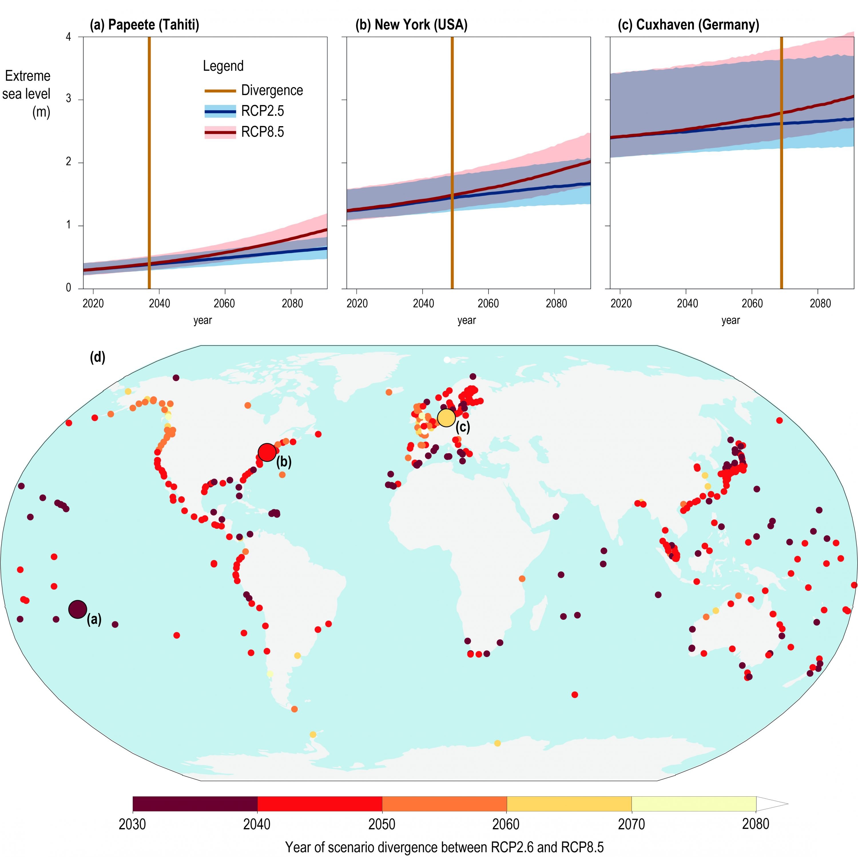
Figure 4.15 | Year of scenario divergence between extreme sea level projections for Representative Concentration Pathway (RCP)2.6 and RCP8.5 for all tide-gauge locations with sufficient observational data relative to a 1986–2005 baseline (bottom panel). Time of divergence is defined using a 10% threshold in the statistical distance between the two distributions, which can be graphically interpreted as the first year in which at least 10% of the area under the probability distribution function (PDF) of RCP8.5 lies outside of the area under the upper half (i.e., above the 50th percentile) of the PDF of RCP2.6. Upper panels indicate the median and 5–95% range of future extreme sea level (ESL) relative to the 1986–2005 baseline for three tide gauge locations with low variability (Papeete), medium variability (New York) and high variability (Cuxhaven). Locations with low variability have a relatively early scenario divergence.
4.4.4.3.3
Adapting decisions over time
Irrespective of whether expected utility or robustness criteria are applied, there is high confidence that an effective way of dealing with large uncertainties is adaptive decision making (also called iterative decision making, adaptive planning or adaptive management), which maintains that decision and decision analysis should be conducted within an iterative policy cycle. This approach includes monitoring of sea level variables and evaluation of alternatives in this light in order to learn from past decisions and collect information to inform future decisions (Haasnoot et al., 20132175; Barnett et al., 20142176; Burch et al., 20142177; Jones et al., 20142178; Wise et al., 20142179; Kelly, 20152180; Lawrence and Haasnoot, 20172181). Such a staged approach is especially suitable for coastal adaptation due to the long lead and lifetimes of many coastal adaptation measures and the deep uncertainties in future sea levels (Hallegatte, 20092182; Kelly, 20152183). Prominent representatives of methods that entail this idea are Dynamic Adaptive Policy Pathways (Haasnoot et al., 20132184) and Dynamic Adaptation Planning (Walker et al., 20012185). An important prerequisite for any adaptive decision-making approach is a monitoring system that can detect sea level signals sufficiently early to enable the required responses (Hermans et al., 20172186; Haasnoot et al., 20182187; Stephens et al., 20182188).
In recent years, many different frameworks for adaptive decision making have been put forward, including Adaptive Policy Making (Walker et al., 20012189), Dynamic Adaptive Policy Pathways (Haasnoot et al., 20132190), Dynamic Adaptive Planning (Walker et al., 20132191), Iterative risk management (Jones et al., 20142192) and Engineering Options Analysis (de Neufville and Smet, 2019). Each frameworks emphasises particular aspects of adaptive decision making and has merits in specific situations depending on the preferences, goals, uncertainties and information at stake (Marchau et al., 20192193). Nevertheless, all of these frameworks share the following generic and iterative steps
- Set the stage: Identify current situation, objectives, options (alternatives) and uncertainties.
- Develop a dynamic plan, which consists of a basic plan plus contingency actions to be carried out based on observed triggers.
- Implement basic plan and monitor system for triggers.
- Monitor and act upon triggers.
4.4.4.3.4
Increasing flexibility of responses
An idea closely related to adaptive decision making is to keep future alternatives open by favouring flexible alternatives over non-flexible ones. An alternative is said to be ‘flexible’ if it allows switching to other alternatives once the implemented alternative is no longer effective. For example, a flexible protection approach would be to build small dikes on foundations designed for higher dikes, in order to be able to raise dikes in the future should SLR necessitate this.
A prominent and straightforward method that addresses the objective of flexibility is adaptation pathways analysis (Haasnoot et al., 20112194; Haasnoot et al., 20122195), which is one component of Dynamic Adaptive Policy Pathways. The method graphically represents alternative combinations of measures over time together with information on the conditions under which alternatives cease to be effective in meeting agreed objectives, as well as possible alternatives that will then be available. As time and SLR progress, monitoring may trigger a decision to switch to another alternative. Adaptation pathway analysis has been widely applied both in the scientific literature as well as in practical cases. Applications after AR5 include Indonesia (Butler et al., 20142196), New York City (Rosenzweig and Solecki, 20142197), Singapore (Buurman and Babovic, 20162198) and Australia (Lin and Shullman, 20172199). In New Zealand, the method has been included in national guidance for coastal hazard and climate change decision making (Lawrence et al., 20182200). There is high confidence that the method is useful in interaction with decision makers and other stakeholders, helping to identify possible alternative sequences of measures over time, avoiding lock-in, and showing decision makers that there are several possible pathways leading to the same desired future (Haasnoot et al., 20122201; Haasnoot et al., 20132202; Brown et al., 20142203; Werners et al., 20152204).
Alternatives can also be characterised through multiple attributes such as costs, effectiveness, co-benefits, social acceptability, etc., which in turn can be used in multi-attribute decision making methods (Haasnoot et al., 20132205). An important attribute is transfer cost, which is the cost of course correction (switching from one alternative to another), reflecting the potential for path dependency (Haasnoot et al., 20192206). Delaying decisions and opting for flexible measures introduces extra costs, such as transfer costs. Also, flexible measures are often more expensive than inflexible ones, and damages may occur whilst delaying the decision. An important question therefore is whether it is cheaper to implement a flexible measure now or to wait and implement a less flexible (i.e., cheaper) measure later in time when more information is at hand.
Technically more demanding methods such as real-options analysis (Dixit et al., 19942207), and decision tree analysis (Conrad, 19802208), can also find pathways that are economically efficient in terms of flexibility and timing of adaptation. There is little application of these approaches in the SLR literature. For example, Woodward et al. (2014) applied real-options analysis to determine flood defences around the Thames Estuary, London, England; Buurman and Babovic (2016) for climate-proofing drainage networks in Singapore; Dawson et al. (2018) for coastal rail infrastructure in southern England; and Kim et al. (2018) for assessing flood defences in southern England. A requirement for applying real-options analysis and decision tree analysis is to quantify today how much will have been learned at a given point in time in the future. The few applications of these methods to SLR-related decisions in the literature have generally used ad-hoc assumptions. For example, Woodward et al. (2011) assumed either perfect learning (i.e., in 2040, which SLR trajectory is occurring will be known) or no learning (i.e., uncertainty ranges and confidence in these remains as today). Others have derived learning rates from comparing past progress in SLR projections and then applied these to the future. An example is given by Dawson et al. (2018) who derive learning rates from the 2002 and 2009 SLR projections of the UK Climate Impacts Programme and apply these in real-options analysis.
4.4.4.3.5
Research needs
Four general gaps can be identified in the literature. First, the generation of SLR information is insufficiently coupled to the use of this information in decision analysis. This constitutes a limitation, as different coastal decision contexts require different decision analysis methods, which in turn require different SLR information. Specifically, applications of decision analysis methods generally convert existing sea level information to fit their method, often misinterpreting the information, making arbitrary assumptions or losing essential information in the process (Hinkel et al., 20152210; Bakker et al., 20172211; Van der Pol and Hinkel, 2018). Second, with the exception of adaptation pathway analysis, methods of robust and flexible decision making are under-represented in the literature despite their suitability (Van der Pol and Hinkel, 2018). Third, research is necessary to compare the various methods, to identity which methods are most suitable in which context and to develop consistent categorisations of methods (Hallegatte et al., 20122212; Haasnoot et al., 20132213; Hinkel et al., 20152214; Watkiss et al., 20152215; Dittrich et al., 20162216; Suckall et al., 20182217). Fourth, future research needs to address how to embed decision analysis better in real world planning and decision making processes, recognising that adaptation to SLR is a multi-stakeholder process often characterised by conflicting interests and interdependence between stakeholders (Section 4.4.3). Addressing these gaps requires closer cooperation between SLR sciences, decision science, and planning and governance scholars. An underlying challenge is to design and integrate relevant formal decision making approaches into the heterogeneous reality of local planning and decision making cultures, institutions, processes and practices, often with community-specific needs and requirements (see Box 4.4).
4.4.5
Enabling Conditions and Lessons Learned From ‘Practice’
In addition to the literature on planning, public participation, conflict resolution and decision making assessed in the last Section, much is being learned from practical experiences gained in adapting to climate change and SLR at the coast. Some salient enabling conditions and lessons learnt are illustrated in Table 4.9 through case studies or examples of real-world experience in diverse coastal communities around the world, structured according to the five overarching SLR governance challenges identified in Section 4.4.3. In these cases, the following stands out as being foundational for enabling the implementation of SLR responses and addressing the governance challenges that arise. First, effective SLR responses take a long-term perspective (e.g., 100 years and beyond) and explicitly account for the uncertainty of locality-specific risks beyond 2050. Second, given the locality-specific but cross-cutting nature of SLR impacts, improving cross-scale and cross-domain coordination of SLR responses may be beneficial. Third, prioritising social vulnerability and equity in SLR responses may be essential because SLR impacts and risks are spread unevenly across society, and within and between coastal communities. Fourth, safe community arenas for working together constructively can help to resolve social conflict arising from SLR. Fifth, a sharp increase may be needed in governance capabilities to tackle the complex problems caused by SLR. There is, however, no one-size-fits-all solution to SLR, and responses need to be tailored to the environmental, social, economic, political, technological, and cultural context in which they are to be implemented. Enablers that work in one context might not be effective in another case. As sea level rises, more experience in addressing SLR governance challenges will be gained, which can in turn be evaluated in order to obtain a better contextual understanding of enabling conditions and effective SLR governance.
Table 4.9
Table 4.9: Enablers and lessons learned to overcome governance challenges arising from sea level rise (SLR).
| Governance challenges | Enablers and lessons learned | Illustrative examples |
| Time horizon and uncertainty | Take action now with the long-term in mind, keeping options open so that new responses can be developed over time (high confidence) (Section 4.4.2) (Haasnoot et al., 2013; Hurlimann et al., 2014; Dewulf and Termeer, 2015; Termeer et al., 2015; Stephens et al., 2018; OECD, 2019) | Participatory scenario planning has been used widely including in Lagos, Nigeria (Ajibade et al., 2016), Dhaka, Bangladesh (Ahmed et al., 2018), Rotterdam, Netherlands, Hong Kong and Guangzhou, China (Francesch-Huidobro et al., 2017), Maputo, Mozambique (Broto et al., 2015), Santos, Brazil (Marengo et al., 2019), Arctic (Flynn et al., 2018), Indonesia (Butler et al., 2016a), Dutch delta (Dewulf and Termeer, 2015; Termeer et al., 2015; Bloemen et al., 2019) and Bangladesh (Paprocki and Huq, 2018). Lessons include:
Long-term adaptation pathways have been developed in New Zealand using ‘serious games’ (Flood et al., 2018) and hybrid processes to integrate decision analysis methods (Section 4.4.2) with public participation and planning (Section 4.4.3) (Cradock-Henry et al., 2018; Lawrence et al., 2019). Lessons include:
|
| Avoid new development commitments in high-risk locations (Section 4.4.3) (medium evidence, high agreement)
(Hurlimann and March, 2012; Glavovic and Smith, 2014; Hurlimann et al., 2014; Tuts et al., 2015; Berke and Stevens, 2016; Butler et al., 2016b; OECD, 2019)
|
Spatial planning to regulate development at risk from SLR is underway in many locations, including Victoria, Australia (Hurlimann et al., 2014) and Florida, USA (Butler et al., 2016a; Vella et al., 2016). Limiting future development in high risk areas is much easier than dealing with existing assets at risk (Tuts et al., 2015; OECD, 2019).
Proactive managed retreat through flexible, tailor-made provisions that address distinctive local circumstances is under way in, for example, USA and Australia, revealing the importance of understanding risks politicians face from local opposition, and distributional impacts (Dyckman et al., 2014; Gibbs, 2016; Siders, 2019). Post Hurricane Sandy managed retreat from Staten Island, New York City, USA, was enabled by community receptivity to buyouts and political expedience (Koslov, 2019; Box 4.1). Lessons include:
|
|
| Cross-scale and cross-domain coordination | Build vertical and horizontal governance networks and linkages across policy domains and sectors to legitimise decisions, build trust and improve coordination (high confidence).
(Glavovic and Smith, 2014; Colenbrander and Sowman, 2015; Dutra et al., 2015; Sowman et al., 2016; Van Putten et al., 2016; Forino et al., 2018; Lund, 2018; Pinto et al., 2018; Clar, 2019; Pittman and Armitage, 2019) |
In the Lesser Antilles multiple state and non-state actors are working together, building trust, and coordinating activities through decentralisation and self-organisation (Pittman and Armitage, 2019). Lessons include:
In South Devon, UK, decentralisation, privatisation and fragmentation impacts adaptation (Den Uyl and Russel, 2018). Lessons include:
|
| Social learning, experimentation and innovation inform technical solutions, build shared understanding and develop locally appropriate SLR responses (high confidence).
(Dyckman et al., 2014; Glavovic and Smith, 2014; Dutra et al., 2015; Ensor and Harvey, 2015; Chu et al., 2018; McFadgen and Huitema, 2018; Mazeka, 2019; Wolfram et al., 2019) |
Innovation is underway to enhance social learning, reflexivity and coalition building (Chu et al., 2018; Bellinson and Chu, 2019; Wolfram et al., 2019), e.g., Surat, India (Chu, 2016a; Chu, 2016b), Santos, Brazil (Marengo et al., 2019), Portland, USA (Fink, 2019), and port cities in Europe and East Asia (Blok and Tschötschel, 2016), In Surat, for example, adaptation experiments created valuable arenas for engaging governance actors and stakeholders, understanding climate and development co-benefits, and testing new ideas (Chu, 2016b). Lessons include:
Accelerate social learning and governance innovations through transnational municipal networks together with local efforts (Hughes et al., 2018), with processes developed and institutionalised through political negotiation, e.g., Rotterdam, Netherlands, and Berkeley, USA (Bellinson and Chu, 2019). |
|
| Equity and social vulnerability | Recognise the political nature of adaptation and explicitly address vulnerability and equity implications to achieve enduring, enabling impact of responses (high confidence).
(Eriksen et al., 2015; Sovacool et al., 2015; Tuts et al., 2015; Adger et al., 2017; Hardy et al., 2017; Holland, 2017; Dolšak and Prakash, 2018; Finkbeiner et al., 2018; Sovacool, 2018; Warner et al., 2018b; OECD, 2019) |
Rights-based approach to participatory adaptation planning in Maputo, Mozambique, fosters a more inclusive and potentially fairer city (Broto et al., 2015). Lessons include:
Race-aware adaptation planning can reveal racial inequalities and overcome passive indifference as shown in, for example, Sapelo Island, Georgia, USA (Hardy et al., 2017). Lessons include:
|
| Focus on enabling community capabilities for responding to SLR, where necessary complementing community knowledge, skills and resources, and political influence and problem solving abilities, with external assistance and government support (high confidence).
(Schlosberg, 2012; Musa et al., 2016; Vedeld et al., 2016; Elrick-Barr et al., 2017; Warrick et al., 2017; Dolšak and Prakash, 2018) |
Various professionals can play valuable support roles in leveraging and building adaptive capacity and resilience of small island communities, recognising diverse needs and capabilities (Robinson, 2017; Weir et al., 2017; Kelman, 2018; Petzold and Magnan, 2019). For example, in poor Caribbean communities, social workers are helping strengthen social capital, enabling individuals to understand and integrate risk, resilience and sustainability principles into day-to-day decision making, and promoting socially and environmentally just adaptation (Joseph, 2017).
In the Solomon Islands, Pacific, community-based approaches enhance community capacity to work with external organisations to plan together, obtain resources, and respond to SLR on their own terms (Warrick et al., 2017). The value of integrating traditional community responses with local government efforts has been demonstrated in Micronesian islands (Nunn et al., 2017b). Local collective action in Monkey River, Belize, helped to overcome power asymmetries and to obtain support otherwise unavailable to vulnerable community members. Working with journalists, researchers and local NGOs, was key for villagers to have concerns heard and a solution found for coastal erosion (Karlsson and Hovelsrud, 2015). Rural coastal community resilience boosted in Albemarle Pamlico Peninsula of North Carolina, USA, by focused attention on local needs through capacity building, and ensuring local voices heard in adaptation planning (Jurjonas and Seekamp, 2018). |
|
| Social conflict | Social conflict can be reduced by tailor-made design and facilitation of participation processes, and involving stakeholders early and consistently throughout decision making and implementation of SLR responses (medium evidence, high agreement).
(Burton and Mustelin, 2013; Berke and Stevens, 2016; Gorddard et al., 2016; Webler et al., 2016; Schlosberg et al., 2017; Kirshen et al., 2018; Lawrence et al., 2018; Mehring et al., 2018; Nkoana et al., 2018; Schernewski et al., 2018; Yusuf et al., 2018b; Uittenbroek et al., 2019) |
Public participation has been foundational for South Africa’s coastal management, risk reduction and adaptation efforts since 1994 (Celliers et al., 2013; Daron and Colenbrander, 2015; Desportes and Colenbrander, 2016; Glavovic et al., 2018; Colenbrander, 2019). Lessons include:
|
| Social conflict can be managed by creating safe arenas for inclusive, informed and meaningful deliberation, negotiation and collaborative problem-solving (medium evidence, high agreement).
(Susskind et al., 1999; Laws et al., 2014; Susskind et al., 2015; Glavovic, 2016; Nursey-Bray, 2017; Sultana and Thompson, 2017) |
Turning conflict into cooperation in Baragaon village, northeast Bangladesh, and eight villages in Narial district, southwest Bangladesh: A flexible and enabling process, founded on local institutions judged robust and fair, prompted government investment in communities beyond their traditional focus on water infrastructure, paid attention to local social dynamics and reduced elite domination and local conflict (Sultana & Thompson 2017). Lessons include:
Innovative collective coastal risk management process, New England (USA) Climate Adaptation Project, developed by university researchers with partner communities to address coastal conflict by:
|
|
| Complexity | Drawing upon multiple knowledge systems to co-design and co-produce SLR responses results in more acceptable and implementable responses (high confidence).
(Dannevig and Aall, 2015; Dutra et al., 2015; Sovacool et al., 2015; Desportes and Colenbrander, 2016; Adger et al., 2017; Betzold and Mohamed, 2017; Onat et al., 2018; Warner et al., 2018b; St. John III and Yusuf, 2019) |
The merits of drawing on scientific and local and indigenous knowledges is recognised in diverse settings such as Australia (Dutra et al., 2015), Comoros (Betzold and Mohamed, 2017), Arctic (Flynn et al., 2018; Huntington et al., 2019), Canada (Chouinard et al., 2015; Chouinard et al., 2017), Portugal (Costas et al., 2015) and Brazil (Marengo et al., 2019).
Storytelling can build shared knowledge and understanding because stories are engaging, help people visualise problems, see things from different positions, and recognise shared goals (Dutra et al., 2015; Elrick-Barr et al., 2017). Māori, indigenous people of New Zealand, use oral history and storytelling to describe their relationship to the coast, which informs how New Zealand responds to SLR (Carter, 2018; Lawrence et al., 2018). Gaps between SLR science, policy and practice can be bridged by adaptation policy experiments with support of actors and organisations who work across organisational boundaries to bring parties together (Dannevig and Aall, 2015; St. John III and Yusuf, 2019). |
| Build governance capabilities to tackle complex problems (medium evidence, high agreement)
(Moser et al., 2012; Head, 2014; Dewulf and Termeer, 2015; Head and Alford, 2015; Termeer et al., 2015; Kwakkel et al., 2016a; Termeer et al., 2016; Alford and Head, 2017; Daviter, 2017; Head, 2018; McConnell, 2018) |
The Dutch Delta Programme aims to future-proof the Netherlands against SLR (Bloemen et al., 2019). Lessons learned in building governance capabilities to deal with associated complex problems include (Dewulf and Termeer, 2015; Bloemen et al., 2018; Bloemen et al., 2019):
|
4.4.6
Towards Climate Resilient Development Pathways
Our assessment shows that failure to mitigate GHG emissions or to adapt to SLR will cause major disruptions to many low-lying coastal communities and jeopardise achievement of all UN SDGs and other societal aspirations. Immediate and ambitious GHG emissions reduction is necessary (Hoegh-Guldberg et al., 2018) to contain the rate and magnitude of SLR, and consequently adaptation prospects. Under unmitigated emissions (RCP8.5), coastal societies, especially poorer, rural and small islands societies, will struggle to maintain their livelihoods and settlements during the 21st century (Sections 4.3.4; 4.4.2). Without mitigation, sea levels will continue to rise for centuries, reaching 2.3–5.4 m by 2300 (likely range) and much more beyond (Section 4.2.3.5), making adaptation extremely challenging, if not impossible, for all low-lying coasts, including more intensively developed urbanised coasts. But even with ambitious mitigation (RCP2.6), sea levels will continue to rise, reaching 0.6–1.1 m by 2300 (likely range; Figure 4.2 Panel B). Hence, adaptation will continue to be imperative irrespective of the uncertainties about future GHG emissions and key physical processes such as those determining the Antarctic contribution to SLR. Our assessment also shows that all types of responses, from hard protection to EbA, advance and retreat, have important and synergistic roles to play in an integrated and sequenced response to SLR. The merits of a particular type of response, at a particular point in time, critically depends on the biophysical, cultural, economic, technical, institutional and political context.
In this context, AR5 put forward the vision of Climate Resilient Development Pathways, which is “a continuing process for managing changes in the climate and other driving forces affecting development, combining flexibility, innovativeness, and participative problem solving with effectiveness in mitigating and adapting to climate change” (Denton et al., 2014: 1106).Charting Climate Resilient Development Pathways in the face of rising sea level depends on how well mitigation, adaption and other sustainable development efforts are combined, and the governance challenges introduced by SLR are resolved. There are no panaceas for solving these complex issues. However, the wise application of the planning, public participation, conflict resolution, and decision analysis methods assessed above can help coastal communities, cities and settlements develop locally relevant, enabling and adaptive SLR responses. Difficult social choices will nonetheless need to be made as sea levels continue to rise. Given the SLR projections outlined here, it is concluded that global resilience and sustainability prospects depend, to a large extent, on how effectively coastal communities develop and implement ambitious, forward-looking adaptation plans in synchrony with drastic mitigation of GHG emissions.
C
Citation
Oppenheimer, M., B.C. Glavovic , J. Hinkel, R. van de Wal, A.K. Magnan, A. Abd-Elgawad, R. Cai, M. Cifuentes-Jara, R.M. DeConto, T. Ghosh, J. Hay, F. Isla, B. Marzeion, B. Meyssignac, and Z. Sebesvari, 2019: Sea Level Rise and Implications for Low-Lying Islands, Coasts and Communities. In: IPCC Special Report on the Ocean and Cryosphere in a Changing Climate [H.-O. Pörtner, D.C. Roberts, V. Masson-Delmotte, P. Zhai, M. Tignor, E. Poloczanska, K. Mintenbeck, A. Alegría, M. Nicolai, A. Okem, J. Petzold, B. Rama, N.M. Weyer (eds.)]. Cambridge University Press, Cambridge, UK and New York, NY, USA, pp. 321-445. https://doi.org/10.1017/9781009157964.006.
SM
Supplementary Material
To view the Supplementary Material for Chapter 4 click on the image below
To download the Chapter 4 data files, click here.
Footnotes
- Each finding is grounded in an evaluation of underlying evidence and agreement. A level of confidence is expressed using five qualifiers: very low, low, medium, high and very high, and typeset in italics, e.g., medium confidence. The following terms have been used to indicate the assessed likelihood of an outcome or a result: virtually certain 99–100% probability, very likely 90–100%, likely 66–100%, about as likely as not 33–66%, unlikely 0–33%, very unlikely 0–10%, exceptionally unlikely 0–1%. Assessed likelihood is typeset in italics, e.g., very likely. This is consistent with AR5 and the other AR6 Special Reports. Additional terms (extremely likely 95–100%, more likely than not >50–100%, more unlikely than likely 0–<50%, extremely unlikely 0–5%) are used when appropriate. This Report also uses the term ‘likely range’ or ‘very likely range’ to indicate that the assessed likelihood of an outcome lies within the 17-83% or 5-95% probability range. For more details see {1.9.2, Figure 1.4} ↩
- Statements about uncertainty in Section 4.2 are contingent upon the RCP or other emissions assumptions that accompany them. In Section 4.4, the entirety of information facing a decision maker is taken into consideration, including the unknown path of future emissions, in assessing uncertainty. Depending on which perspective is chosen, uncertainty may or may not be characterised as ‘deep’. ↩
References
- Bamber, J.L. et al., 2019: Ice sheet contributions to future sea level rise from structured expert judgment. PNAS, 116(23), 11195–11200. ↩
- Church, J.A. et al., 2013: Sea Level Change. In: Climate Change 2013: The Physical Science Basis. Contribution of Working Group I to the Fifth Assessment Report of the Intergovernmental Panel on Climate Change. [Stocker, T.F., D. Qin, G.K. Plattner, M. Tignor, S.K. Allen, J. Boschung, A. Nauels, Y. Xia, V. Bex and P.M. Midgley (eds.)]. Cambridge University Press, Cambridge, United Kingdom and New York, NY, USA. ↩
- Farrell, W.E. and J.A. Clark, 1976: On Postglacial Sea Level. Geophysical Journal of the Royal Astronomical Society, 46(3), 647–667, doi:10.1111/j.1365-246X.1976.tb01252.x. ↩
- Lemke, P. et al., 2007: Observations: Changes in Snow, Ice and Frozen Ground. In Climate Change 2007: The Physical Science Basis. Contribution of Working Group I to the Fourth Assessment Report of the Intergovernmental Panel on Climate Change. [Solomon S. et al. (eds.)], Cambridge University Press Cambridge, UK, pp. 337-383. ↩
- Bindoff, N.L. et al., 2007: Observations: Oceanic Climate Change and Sea Level. In: Climate Change 2007: The Physical Science Basis. Contribution of Working Group I to the Fourth Assessment Report of the Intergovernmental Panel on Climate Change. [Solomon, S., D. Qin, M. Manning, Z. Chen, M. Marquis, K.B. Averyt, M. Tignor and H.L. Miller (eds.)]. Cambridge University Press, Cambridge, United Kingdom and New York, NY, USA, 385-432. ↩
- Church, J.A. et al., 2013: Sea Level Change. In: Climate Change 2013: The Physical Science Basis. Contribution of Working Group I to the Fifth Assessment Report of the Intergovernmental Panel on Climate Change. [Stocker, T.F., D. Qin, G.K. Plattner, M. Tignor, S.K. Allen, J. Boschung, A. Nauels, Y. Xia, V. Bex and P.M. Midgley (eds.)]. Cambridge University Press, Cambridge, United Kingdom and New York, NY, USA. ↩
- Little, C.M., N.M. Urban and M. Oppenheimer, 2013: Probabilistic framework for assessing the ice sheet contribution to sea level change. PNAS, 110(9), 3264–3269. ↩
- Bindoff, N.L. et al., 2013: Detection and Attribution of Climate Change: from Global to Regional. In: Climate Change 2013: The Physical Science Basis. Contribution of Working Group I to the Fifth Assessment Report of the Intergovernmental Panel on Climate Change. [Stocker, T.F., D. Qin, G.K. Plattner, M. Tignor, S.K. Allen, J. Boschung, A. Nauels, Y. Xia, V. Bex and P.M. Midgley (eds.)]. Cambridge University Press, Cambridge, United Kingdom and New York, NY, USA, 867–952. ↩
- Fürst, J.J. et al., 2016: The safety band of Antarctic ice shelves. Nat. Clim. Change, 6, 479, doi:10.1038/nclimate2912. ↩
- Reese, R., G.H. Gudmundsson, A. Levermann and R. Winkelmann, 2018b: The far reach of ice shelf thinning in Antarctica. Nat. Clim. Change, 8(1), 53. ↩
- Benn, D.I., C.R. Warren and R.H. Mottram, 2007: Calving processes and the dynamics of calving glaciers. Earth-Sci. Rev., 82(3), 143–179, doi:10.1016/j.earscirev.2007.02.002. ↩
- Bassis, J.N., 2011: The statistical physics of iceberg calving and the emergence of universal calving laws. J. Glaciol., 57(201), 3–16, doi:10.3189/002214311795306745. ↩
- Massom, R.A. et al., 2018: Antarctic ice shelf disintegration triggered by sea ice loss and ocean swell. Nature, 558(7710), 383–389, doi:10.1038/s41586-018-0212-1. ↩
- Gayen, B., R.W. Griffiths and R.C. Kerr, 2015: Melting Driven Convection at the Ice-seawater Interface. Procedia IUTAM, 15, 78–85, doi:10.1016/j.piutam.2015.04.012. ↩
- Dinniman, M.S. et al., 2016: Modeling ice shelf/ocean interaction in Antarctica: A review. Oceanography, 29(4), 144–153. ↩
- Schodlok, M.P., D. Menemenlis and E.J. Rignot, 2016: Ice shelf basal melt rates around Antarctica from simulations and observations. J. Geophys. Res-Oceans, 121(2), 1085–1109, doi:10.1002/2015JC011117. ↩
- Banwell, A.F., D.R. MacAyeal and O.V. Sergienko, 2013: Breakup of the Larsen B Ice Shelf triggered by chain reaction drainage of supraglacial lakes. Geophys. Res. Lett., 40(22), 5872–5876, doi:10.1002/2013GL057694. ↩
- Macayeal, D.R. and O.V. Sergienko, 2013: The flexural dynamics of melting ice shelves. Ann. Glaciol., 54(63), 1–10, doi:10.3189/2013AoG63A256. ↩
- Kuipers Munneke, P., S.R.M. Ligtenberg, M.R. Van Den Broeke and D.G. Vaughan, 2014: Firn air depletion as a precursor of Antarctic ice shelf collapse. J. Glaciol., 60(220), 205–214, doi:10.3189/2014JoG13J183. ↩
- Gregory, J.M. et al., 2013: Twentieth-century global-mean sea level rise: Is the whole greater than the sum of the parts? J. Clim., 26(13), 4476–4499, doi:10.1175/JCLI-D-12-00319.1. ↩
- Farinotti, D. et al., 2019: A consensus estimate for the ice thickness distribution of all glaciers on Earth. Nature Geoscience, 12(3), 168–173. ↩
- Kopp, R.E. et al., 2016: Temperature-driven global sea level variability in the Common Era. PNAS, 113(11), E1434–E1441. ↩
- Church, J.A. et al., 2013: Sea Level Change. In: Climate Change 2013: The Physical Science Basis. Contribution of Working Group I to the Fifth Assessment Report of the Intergovernmental Panel on Climate Change. [Stocker, T.F., D. Qin, G.K. Plattner, M. Tignor, S.K. Allen, J. Boschung, A. Nauels, Y. Xia, V. Bex and P.M. Midgley (eds.)]. Cambridge University Press, Cambridge, United Kingdom and New York, NY, USA. ↩
- Otto, A. et al., 2013: Energy budget constraints on climate response. Nat. Geosci., 6(6), 415–416, doi:10.1038/ngeo1836. ↩
- Suzuki, T. and M. Ishii, 2011: Regional distribution of sea level changes resulting from enhanced greenhouse warming in the Model for Interdisciplinary Research on Climate version 3.2. Geophys. Res. Lett., 38(2). ↩
- Bouttes, N., J. Gregory, T. Kuhlbrodt and R.J.C.D. Smith, 2014: The drivers of projected North Atlantic sea level change. 43 (5–6), 1531–1544. ↩
- Saenko, O.A. et al., 2015: Separating the influence of projected changes in air temperature and wind on patterns of sea level change and ocean heat content. J. Geophys. Res-Oceans, 120(8), 5749–5765. ↩
- Griffies, S.M. and R.J. Greatbatch, 2012: Physical processes that impact the evolution of global mean sea level in ocean climate models. Ocean Modelling, 51, 37–72, doi:10.1016/j.ocemod.2012.04.003. ↩
- Chao, B.F., Y. Wu and Y. Li, 2008: Impact of artificial reservoir water impoundment on global sea level. Science, 320(5873), 212–214. ↩
- Fiedler, J.W. and C.P. Conrad, 2010: Spatial variability of sea level rise due to water impoundment behind dams. Geophys. Res. Lett., 37(12). ↩
- Wada, Y. et al., 2017: Recent Changes in Land Water Storage and its Contribution to Sea Level Variations. Surv. Geophys., 38(1), 131–152. ↩
- Boening, C. et al., 2012: The 2011 La Niña: So strong, the oceans fell. Geophys. Res. Lett., 39 (19), 1–5, doi:10.1029/2012GL053055. ↩
- Cazenave, A. et al., 2012: Estimating ENSO influence on the global mean sea level, 1993-2010. Marine Geodesy, 35 (sup1), 82–97. ↩
- Fasullo, J.T., C. Boening, F.W. Landerer and R.S. Nerem, 2013: Australia’s unique influence on global sea level in 2010–2011. Geophys. Res. Lett., 40(16), 4368–4373, doi:10.1002/grl.50834. ↩
- Mitrovica, J., M.E. Tamisiea, J.L. Davis and G.A. Milne, 2001: Recent mass balance of polar ice sheets inferred from patterns of global sea level change. Nature, 409, 1026–1029, doi:10.1038/35059054. ↩
- Mitrovica, J. et al., 2011: On the robustness of predictions of sea level fingerprints. Geophys. J. Int., 187(2), 729–742. ↩
- Lambeck, K., C. Smither and P. Johnston, 1998: Sea level change, glacial rebound and mantle viscosity fornorthern Europe. Geophys. J. Int., 134(1), 102–144, doi:10.1046/j.1365-246x.1998.00541.x. ↩
- Peltier, W., 2004: Global glacial isostasy and the surface of the ice-age earth: the ICE-5G(VM2) model and GRACE. Annu. Rev. Earth Planet. Sci., 32, 111–149, doi:10.1146/annurev.earth.32.082503.144359. ↩
- Mitrovica, J.X. and G.A. Milne, 2003: On post-glacial sea level: I. General theory. Geophys. J. Int., 154(2), 253–267. ↩
- Milne, G.A. and J.X. Mitrovica, 2008: Searching for eustasy in deglacial sea level histories. Quat. Sci. Rev., 27(25–26), 2292–2302. ↩
- Gomez, N., D. Pollard and D. Holland, 2015: Sea level feedback lowers projections of future Antarctic Ice sheet mass loss. Nat. Commun., 6, 8798. ↩
- Larour, E. et al., 2019: Slowdown in Antarctic mass loss from solid Earth and sea level feedbacks. Science, 364(6444), doi:10.1126/science.aav7908. ↩
- Austermann, J. and J.X. Mitrovica, 2015: Calculating gravitationally self-consistent sea level changes driven by dynamic topography. Geophys. J. Int., 203(3), 1909–1922, doi:10.1093/gji/ggv371. ↩
- Wöppelmann, G. and M. Marcos, 2016: Vertical land motion as a key to understanding sea level change and variability. Rev. Geophys., 54(1), 64–92. ↩
- Little, C.M. et al., 2015a: Joint projections of US East Coast sea level and storm surge. Nat. Clim. Change, 5(12), 1114–1120. ↩
- Masson-Delmotte, V. et al., 2013: Information from Palaeoclimate Archives. In: Climate Change 2013: The Physical Science Basis: Contribution of Working Group I to the Fifth Assessment Report of the Intergovernmental Panel on Climate Change. [Stocker, T.F., D. Qin, G.K. Plattner, M. Tignor, S.K. Allen, J. Boschung, A. Nauels, Y. Xia, V. Bex and P.M. Midgley (eds.)]. Cambridge University Press, Cambridge, United Kingdom and New York, NY, USA. ↩
- DeConto, R.M. and D. Pollard, 2016: Contribution of Antarctica to past and future sea level rise. Nature, 531(7596), 591–597, doi:10.1038/nature17145. ↩
- Edwards, T.L. et al., 2019: Revisiting Antarctic ice loss due to marine ice-cliff instability. Nature, 566(7742), 58–64, doi:10.1038/s41586-019-0901-4. ↩
- Golledge, N.R. et al., 2019: Global environmental consequences of twenty-first-century ice sheet melt. Nature, 566(7742), 65–72, doi:10.1038/s41586-019-0889-9. ↩
- Badger, M.P.S., D.N. Schmidt, A. Mackensen and R. D. Pancost, 2013: High-resolution alkenone palaeobarometry indicates relatively stable CO2 during the Pliocene (3.3–2.8 Ma). Philos. Trans. Roy. Soc. A., 371(2001), 1–16, doi:10.1098/rsta.2013.0094. ↩
- Martínez-Botí, M.A. et al., 2015: Plio-Pleistocene climate sensitivity evaluated using high-resolution CO2 records. Nature, 518(7537), 49. ↩
- Stap, L.B. et al., 2016: CO2 over the past 5 million years: Continuous simulation and new δ11B-based proxy data. Earth Planet. Sci. Lett., 439, 1–10, doi:10.1016/j.epsl.2016.01.022. ↩
- Dutton, A. et al., 2015a: Sea level rise due to polar ice sheet mass loss during past warm periods. Science, 349 (6244). ↩
- Haywood, A.M., H.J. Dowsett and A.M. Dolan, 2016: Integrating geological archives and climate models for the mid-Pliocene warm period. Nat. Commun., 7, 1–14 doi:10.1038/ncomms10646. ↩
- Capron, E. et al., 2014: Temporal and spatial structure of multi-millennial temperature changes at high latitudes during the Last Interglacial. Quat. Sci. Rev., 103, 116–133. ↩
- Dutton, A. et al., 2015a: Sea level rise due to polar ice sheet mass loss during past warm periods. Science, 349 (6244). ↩
- Fischer, H. et al., 2018: Palaeoclimate constraints on the impact of 2 °C anthropogenic warming and beyond, Nature Geoscience, 11(7). 474–485. ↩
- Hoffman, J.S., P.U. Clark, A.C. Parnell and F. He, 2017: Regional and global sea-surface temperatures during the last interglaciation. Science, 355(6322), 276–279. ↩
- Dutton, A. et al., 2015a: Sea level rise due to polar ice sheet mass loss during past warm periods. Science, 349 (6244). ↩
- Miller, K.G. et al., 2012: High tide of the warm Pliocene: Implications of global sea level for Antarctic deglaciation. Geology, doi:10.1130/g32869.1. ↩
- Rovere, A. et al., 2014: The Mid-Pliocene sea level conundrum: Glacial isostasy, eustasy and dynamic topography. Earth Planet. Sci. Lett., 387, 27–33, doi:10.1016/j.epsl.2013.10.030. ↩
- Dutton, A. et al., 2015a: Sea level rise due to polar ice sheet mass loss during past warm periods. Science, 349 (6244). ↩
- Raymo, M.E. et al., 2011: Departures from eustasy in Pliocene sea level records. Nat. Geosci., 4(5), 328. ↩
- Rovere, A. et al., 2014: The Mid-Pliocene sea level conundrum: Glacial isostasy, eustasy and dynamic topography. Earth Planet. Sci. Lett., 387, 27–33, doi:10.1016/j.epsl.2013.10.030. ↩
- Rowley, D.B. et al., 2013: Dynamic topography change of the eastern United States since 3 million years ago. Science, 340(6140), 1560–1563. ↩
- Raymo, M.E. et al., 2018: The accuracy of mid-Pliocene δ18O-based ice volume and sea level reconstructions. Earth-Sci. Rev., 177, 291–302, doi:10.1016/j.earscirev.2017.11.022. ↩
- Miller, K.G. et al., 2012: High tide of the warm Pliocene: Implications of global sea level for Antarctic deglaciation. Geology, doi:10.1130/g32869.1. ↩
- Dutton, A. et al., 2015a: Sea level rise due to polar ice sheet mass loss during past warm periods. Science, 349 (6244). ↩
- Masson-Delmotte, V. et al., 2013: Information from Palaeoclimate Archives. In: Climate Change 2013: The Physical Science Basis: Contribution of Working Group I to the Fifth Assessment Report of the Intergovernmental Panel on Climate Change. [Stocker, T.F., D. Qin, G.K. Plattner, M. Tignor, S.K. Allen, J. Boschung, A. Nauels, Y. Xia, V. Bex and P.M. Midgley (eds.)]. Cambridge University Press, Cambridge, United Kingdom and New York, NY, USA. ↩
- Austermann, J. and J.X. Mitrovica, 2015: Calculating gravitationally self-consistent sea level changes driven by dynamic topography. Geophys. J. Int., 203(3), 1909–1922, doi:10.1093/gji/ggv371. ↩
- Pollard, D., R.M. DeConto and R.B. Alley, 2015: Potential Antarctic Ice Sheet retreat driven by hydrofracturing and ice cliff failure. Earth Planet. Sci. Lett., 412, 112–121. ↩
- Aitken, A.R.A. et al., 2016: Repeated large-scale retreat and advance of Totten Glacier indicated by inland bed erosion. Nature, 533, 385, doi:10.1038/nature17447. ↩
- DeConto, R.M. and D. Pollard, 2016: Contribution of Antarctica to past and future sea level rise. Nature, 531(7596), 591–597, doi:10.1038/nature17145. ↩
- Gasson, E., R.M. DeConto and D. Pollard, 2016: Modeling the oxygen isotope composition of the Antarctic ice sheet and its significance to Pliocene sea level. Geology, 44(10), 827–830. ↩
- Golledge, N.R. et al., 2019: Global environmental consequences of twenty-first-century ice sheet melt. Nature, 566(7742), 65–72, doi:10.1038/s41586-019-0889-9. ↩
- Cook, C.P. et al., 2013: Dynamic behaviour of the East Antarctic ice sheet during Pliocene warmth. Nat. Geosci., 6(9), 765–769, doi:10.1038/ngeo1889. ↩
- Patterson, M.O. et al., 2014: Orbital forcing of the East Antarctic ice sheet during the Pliocene and Early Pleistocene. Nat. Geosci., 7, 841–847, doi:10.1038/ngeo2273. ↩
- Bertram, R.A. et al., 2018: Pliocene deglacial event timelines and the biogeochemical response offshore Wilkes Subglacial Basin, East Antarctica. Earth Planet. Sci. Lett., 494, 109–116, doi:10.1016/j.epsl.2018.04.054. ↩
- Austermann, J. and J.X. Mitrovica, 2015: Calculating gravitationally self-consistent sea level changes driven by dynamic topography. Geophys. J. Int., 203(3), 1909–1922, doi:10.1093/gji/ggv371. ↩
- Pollard, D., R.M. DeConto and R.B. Alley, 2015: Potential Antarctic Ice Sheet retreat driven by hydrofracturing and ice cliff failure. Earth Planet. Sci. Lett., 412, 112–121. ↩
- Yamane, M. et al., 2015: Exposure age and ice sheet model constraints on Pliocene East Antarctic ice sheet dynamics. Nat. Commun., 6, doi:10.1038/ncomms8016. ↩
- DeConto, R.M. and D. Pollard, 2016: Contribution of Antarctica to past and future sea level rise. Nature, 531(7596), 591–597, doi:10.1038/nature17145. ↩
- Gasson, E., R.M. DeConto and D. Pollard, 2016: Modeling the oxygen isotope composition of the Antarctic ice sheet and its significance to Pliocene sea level. Geology, 44(10), 827–830. ↩
- Shakun, J.D. et al., 2018: Minimal East Antarctic Ice Sheet retreat onto land during the past eight million years. Nature, 558(7709), 284–287, doi:10.1038/s41586-018-0155-6. ↩
- Fretwell, P. et al., 2013: Bedmap2: improved ice bed, surface and thickness datasets for Antarctica. The Cryosphere, 7(1), 375–393. ↩
- Dutton, A. et al., 2015a: Sea level rise due to polar ice sheet mass loss during past warm periods. Science, 349 (6244). ↩
- Kopp, R.E. et al., 2009: Probabilistic assessment of sea level during the last interglacial stage. Nature, 462(7275), 863–867, doi:10.1038/nature08686. ↩
- Düsterhus, A., M.E. Tamisiea and S. Jevrejeva, 2016: Estimating the sea level highstand during the last interglacial: a probabilistic massive ensemble approach. Geophys. J. Int., 206(2), 900–920, doi:10.1093/gji/ggw174. ↩
- Kopp, R.E. et al., 2009: Probabilistic assessment of sea level during the last interglacial stage. Nature, 462(7275), 863–867, doi:10.1038/nature08686. ↩
- Lambeck, K., A. Purcell and A. Dutton, 2012: The anatomy of interglacial sea levels: The relationship between sea levels and ice volumes during the Last Interglacial. Earth Planet. Sci. Lett., 315–316, 4–11, doi:10.1016/j.epsl.2011.08.026. ↩
- Dendy, S., J. Austermann, J. Creveling and J.J.Q.S.R. Mitrovica, 2017: Sensitivity of Last Interglacial sea level high stands to ice sheet configuration during Marine Isotope Stage 6. Quaternary Science Reviews, 171, 234–244. ↩
- Dendy, S., J. Austermann, J. Creveling and J.J.Q.S.R. Mitrovica, 2017: Sensitivity of Last Interglacial sea level high stands to ice sheet configuration during Marine Isotope Stage 6. Quaternary Science Reviews, 171, 234–244. ↩
- Stap, L.B. et al., 2018: Modeled Influence of Land Ice and CO2 on Polar Amplification and Palaeoclimate Sensitivity During the Past 5 Million Years. Paleoceanogr. Paleocl., 33(4), 381–394, doi:10.1002/2017pa003313. ↩
- Dahl-Jensen, D. et al., 2013: Eemian interglacial reconstructed from a Greenland folded ice core. Nature, 493(7433), 489–494, doi:10.1038/nature11789. ↩
- Landais, A. et al., 2016: How warm was Greenland during the last interglacial period? Clim. Past, 12(9), 1933–1948, doi:10.5194/cp-12-1933-2016. ↩
- Yau, A.M., M. Bender, A. Robinson and E. Brook, 2016: Reconstructing the last interglacial at Summit, Greenland: Insights from GISP2. PNAS, 113(35), 9710–9715, doi:10.1073/pnas.1524766113. ↩
- McFadgen, B. and D. Huitema, 2018: Experimentation at the interface of science and policy: a multi-case analysis of how policy experiments influence political decision-makers. Policy Sciences, 51(2), 161–187. ↩
- Dahl-Jensen, D. et al., 2013: Eemian interglacial reconstructed from a Greenland folded ice core. Nature, 493(7433), 489–494, doi:10.1038/nature11789. ↩
- Helsen, M.M. et al., 2013: Coupled regional climate–ice sheet simulation shows limited Greenland ice loss during the Eemian. Clim. Past, 9(4), 1773–1788, doi:10.5194/cp-9-1773-2013. ↩
- Quiquet, A., C. Ritz, H.J. Punge and D. Salas y Mélia, 2013: Greenland ice sheet contribution to sea level rise during the last interglacial period: a modelling study driven and constrained by ice core data. Clim. Past, 9(1), 353–366, doi:10.5194/cp-9-353-2013. ↩
- Dutton, A. et al., 2015a: Sea level rise due to polar ice sheet mass loss during past warm periods. Science, 349 (6244). ↩
- Goelzer, H., P. Huybrechts, M.-F. Loutre and T. Fichefet, 2016: Last Interglacial climate and sea level evolution from a coupled ice sheet–climate model. Clim. Past, 12, 2195–2213, doi:10.5194/cp-12-2195-2016. ↩
- Yau, A.M., M. Bender, A. Robinson and E. Brook, 2016: Reconstructing the last interglacial at Summit, Greenland: Insights from GISP2. PNAS, 113(35), 9710–9715, doi:10.1073/pnas.1524766113. ↩
- Dutton, A., J.M. Webster, D. Zwartz and K. Lambeck, 2015b: Tropical tales of polar ice: evidence of Last Interglacial polar ice sheet retreat recorded by fossil reefs of the granitic Seychelles islands. Quat. Sci. Rev., 107, 182–196. ↩
- DeConto, R.M. and D. Pollard, 2016: Contribution of Antarctica to past and future sea level rise. Nature, 531(7596), 591–597, doi:10.1038/nature17145. ↩
- Goelzer, H., P. Huybrechts, M.-F. Loutre and T. Fichefet, 2016: Last Interglacial climate and sea level evolution from a coupled ice sheet–climate model. Clim. Past, 12, 2195–2213, doi:10.5194/cp-12-2195-2016. ↩
- Sutter, J. et al., 2016: Ocean temperature thresholds for Last Interglacial West Antarctic Ice Sheet collapse. Geophys. Res. Lett., 43(6), 2675–2682, doi:10.1002/2016GL067818. ↩
- Steig, E.J. et al., 2015: Influence of West Antarctic Ice Sheet collapse on Antarctic surface climate. Geophys. Res. Lett., 42(12), 4862–4868, doi:10.1002/2015GL063861. ↩
- Wilson, A.M.W. and C. Forsyth, 2018: Restoring near-shore marine ecosystems to enhance climate security for island ocean states: Aligning international processes and local practices. Mar. Policy., 93, 284-294. ↩
- Kopp, R.E. et al., 2016: Temperature-driven global sea level variability in the Common Era. PNAS, 113(11), E1434–E1441. ↩
- Woodruff, J.D., J.L. Irish and S.J. Camargo, 2013: Coastal flooding by tropical cyclones and sea level rise. Nature, 504(7478), 44–52. ↩
- Holgate, S.J. et al., 2012: New data systems and products at the permanent service for mean sea level. J. Coast. Res., 29(3), 493–504. ↩
- PSMSL, 2019: Tide Gauge Data. Permanent Service for Mean Sea Level. Available at: https://www.psmsl.org/ ↩
- Shepherd, A. et al., 2012: A Reconciled Estimate of Ice sheet Mass Balance. Science, 338(6111), 1183–1189, doi:10.1126/science.1228102. ↩
- Noël, B. et al., 2018: Modelling the climate and surface mass balance of polar ice sheets using RACMO2-Part 1: Greenland (1958–2016). The Cryosphere, 12(3), 811–831. ↩
- Rignot, E. et al., 2019: Four decades of Antarctic Ice Sheet mass balance from 1979–2017. Proceeding of the National Academy of Sciences, 116(4), 1095–1103, doi:10.1073/pnas.1812883116. ↩
- Wöppelmann, G. and M. Marcos, 2016: Vertical land motion as a key to understanding sea level change and variability. Rev. Geophys., 54(1), 64–92. ↩
- Pfeffer, J. et al., 2017: Decoding the origins of vertical land motions observed today at coasts. Geophys. J. Int., 210(1), 148–165. ↩
- Raucoules, D. et al., 2013: High nonlinear urban ground motion in Manila (Philippines) from 1993 to 2010 observed by DInSAR: implications for sea level measurement. Remote Sens. Environ., 139, 386–397. ↩
- Pfeffer, J. et al., 2017: Decoding the origins of vertical land motions observed today at coasts. Geophys. J. Int., 210(1), 148–165. ↩
- Santamaría-Gómez, A. et al., 2017: Uncertainty of the 20th century sea level rise due to vertical land motion errors. Earth Planet. Sci. Lett., 473, 24–32. ↩
- Kleinherenbrink, M., R. Riva and T.J.O.S. Frederikse, 2018: A comparison of methods to estimate vertical land motion trends from GNSS and altimetry at tide gauge stations. Ocean Sci., 14(2), 187-204. ↩
- Riva, R.E. et al., 2017: Brief communication: The global signature of post-1900 land ice wastage on vertical land motion. The Cryosphere, 11(3), 1327–1332. ↩
- Hay, C.C., E. Morrow, R.E. Kopp and J.X. Mitrovica, 2015: Probabilistic reanalysis of twentieth-century sea level rise. Nature, 517(7535), 481–484. ↩
- Dangendorf, S. et al., 2017: Reassessment of 20th century global mean sea level rise. PNAS, 114(23), 5946–5951. ↩
- Hamlington, B. and P. Thompson, 2015: Considerations for estimating the 20th century trend in global mean sea level. Geophys. Res. Lett., 42(10), 4102–4109. ↩
- Dangendorf, S. et al., 2017: Reassessment of 20th century global mean sea level rise. PNAS, 114(23), 5946–5951. ↩
- Hamlington, B. et al., 2018: Observation‐Driven Estimation of the Spatial Variability of 20th Century Sea Level Rise. J. Geophys. Res-Oceans, 123(3), 2129–2140. ↩
- Hay, C.C., E. Morrow, R.E. Kopp and J.X. Mitrovica, 2015: Probabilistic reanalysis of twentieth-century sea level rise. Nature, 517(7535), 481–484. ↩
- Dangendorf, S. et al., 2017: Reassessment of 20th century global mean sea level rise. PNAS, 114(23), 5946–5951. ↩
- Jevrejeva, S., J. Moore, A. Grinsted and P. Woodworth, 2008: Recent global sea level acceleration started over 200 years ago? Geophys. Res. Lett., 35(8), 1-4. ↩
- Church, J.A. and N.J. White, 2011: Sea level rise from the late 19th to the early 21st century. Surv. Geophys., 32(4–5), 585–602. ↩
- Ray, R.D. and B.C. Douglas, 2011: Experiments in reconstructing twentieth-century sea levels. Progr. Oceanogr., 91(4), 496–515. ↩
- Haigh, I.D. et al., 2014b: Timescales for detecting a significant acceleration in sea level rise. Nat. Commun., 5, 3635. ↩
- Hay, C.C., E. Morrow, R.E. Kopp and J.X. Mitrovica, 2015: Probabilistic reanalysis of twentieth-century sea level rise. Nature, 517(7535), 481–484. ↩
- Watson, P.J., 2016: A new perspective on global mean sea level (GMSL) acceleration. Geophys. Res. Lett., 43(12), 6478–6484. ↩
- Dangendorf, S. et al., 2017: Reassessment of 20th century global mean sea level rise. PNAS, 114(23), 5946–5951. ↩
- Nerem, R.S., D.P. Chambers, C. Choe and G.T. Mitchum, 2010: Estimating mean sea level change from the TOPEX and Jason altimeter missions. Mar. Geod., 33(S1), 435–446. ↩
- Henry, O. et al., 2014: Effect of the processing methodology on satellite altimetry-based global mean sea level rise over the Jason-1 operating period. Journal of Geodesy, 88(4), 351–361. ↩
- Leuliette, E.W., 2015: The balancing of the sea level budget. Curr. Clim., 1(3), 185–191. ↩
- Watson, C.S. et al., 2015: Unabated global mean sea level rise over the satellite altimeter era. Nat. Clim. Change, 5(6), 565–568, doi:10.1038/nclimate2635. ↩
- Beckley, B. et al., 2017: On the “Cal‐Mode” Correction to TOPEX Satellite Altimetry and Its Effect on the Global Mean Sea Level Time Series. Journal of Geophysical Research: Oceans, 122(11), 8371–8384. ↩
- Legeais, J.-F. et al., 2018: An improved and homogeneous altimeter sea level record from the ESA Climate Change Initiative. Earth Syst. Sci. Data, 10, 281–301. ↩
- Watson, C.S. et al., 2015: Unabated global mean sea level rise over the satellite altimeter era. Nat. Clim. Change, 5(6), 565–568, doi:10.1038/nclimate2635. ↩
- Chen, X. et al., 2017: The increasing rate of global mean sea level rise during 1993-2014. Nat. Clim. Change, 7(7), 492–495. ↩
- Dieng, H., A. Cazenave, B. Meyssignac and M. Ablain, 2017: New estimate of the current rate of sea level rise from a sea level budget approach. Geophys. Res. Lett., 44(8), 3744–3751. ↩
- WCRP Global Sea Level Budget Group, 2018: Global sea level budget 1993-present. Earth Syst. Sci. Data, 10(3), 1551–1590. ↩
- Watson, C.S. et al., 2015: Unabated global mean sea level rise over the satellite altimeter era. Nat. Clim. Change, 5(6), 565–568, doi:10.1038/nclimate2635. ↩
- Nerem, R.S. et al., 2018: Climate-change–driven accelerated sea level rise detected in the altimeter era. PNAS, 115(9), 2022-2025, doi:10.1073/pnas.1717312115. ↩
- Chen, X. et al., 2017: The increasing rate of global mean sea level rise during 1993-2014. Nat. Clim. Change, 7(7), 492–495. ↩
- Dieng, H., A. Cazenave, B. Meyssignac and M. Ablain, 2017: New estimate of the current rate of sea level rise from a sea level budget approach. Geophys. Res. Lett., 44(8), 3744–3751. ↩
- Fasullo, J., R. Nerem and B. Hamlington, 2016: Is the detection of accelerated sea level rise imminent? Sci. Rep., 6, 31245. ↩
- Slangen, A. et al., 2016: Anthropogenic forcing dominates global mean sea level rise since 1970. Nat. Clim. Change, 6(7), 701–705. ↩
- Ablain, Michaël, et al., 2019: Uncertainty in satellite estimates of global mean sea-level changes, trend and acceleration. Earth System Science Data 11(3), 1189–1202. ↩
- Church, J.A. and N.J. White, 2011: Sea level rise from the late 19th to the early 21st century. Surv. Geophys., 32(4–5), 585–602. ↩
- Ray, R.D. and B.C. Douglas, 2011: Experiments in reconstructing twentieth-century sea levels. Progr. Oceanogr., 91(4), 496–515. ↩
- Jevrejeva, S., J. Moore, A. Grinsted and P. Woodworth, 2008: Recent global sea level acceleration started over 200 years ago? Geophys. Res. Lett., 35(8), 1-4. ↩
- Hay, C.C., E. Morrow, R.E. Kopp and J.X. Mitrovica, 2015: Probabilistic reanalysis of twentieth-century sea level rise. Nature, 517(7535), 481–484. ↩
- Dangendorf, S. et al., 2017: Reassessment of 20th century global mean sea level rise. PNAS, 114(23), 5946–5951. ↩
- Taylor, K.E., R.J. Stouffer and G.A. Meehl, 2012: An overview of CMIP5 and the experiment design. Bull. Am. Meteorol. Soc., 93(4), 485–498. ↩
- Taylor, K.E., R.J. Stouffer and G.A. Meehl, 2012: An overview of CMIP5 and the experiment design. Bull. Am. Meteorol. Soc., 93(4), 485–498. ↩
- Storlazzi, C. et al., 2017: Rigorously valuing the role of coral reefs in coastal protection: An example from Maui, Hawaii, USA. In: Coastal Dynamics 2017, Helsingør, Denmark, [Aagaard, T., R. Deigaard and D. Fuhrman (eds.)], pp. 665–674. ↩
- WCRP Global Sea Level Budget Group, 2018: Global sea level budget 1993-present. Earth Syst. Sci. Data, 10(3), 1551–1590. ↩
- Pfeffer, J., P. Tregoning, A. Purcell and M. Sambridge, 2018: Multitechnique Assessment of the Interannual to Multidecadal Variability in Steric Sea Levels: A Comparative Analysis of Climate Mode Fingerprints. J. Clim., 31(18), 7583–7597. ↩
- Palmer, M. et al., 2010: Future observations for monitoring global ocean heat content. In: Proceedings of OceanObs’09: Sustained Ocean Observations and Information for Society, Venice, Italy, 1–13 pp. ↩
- Boyer, T. et al., 2016: Sensitivity of global upper-ocean heat content estimates to mapping methods, XBT bias corrections, and baseline climatologies. J. Clim., 29(13), 4817–4842. ↩
- Cheng, L. et al., 2016: Observed and simulated full-depth ocean heat-content changes for 1970–2005. Ocean Sci, 12, 925–935. ↩
- Roemmich, D. et al., 2015: Unabated planetary warming and its ocean structure since 2006. Nat. Clim. Change, 5(3), 240–245. ↩
- ↩
- Wijffels, S. et al., 2016: Ocean temperatures chronicle the ongoing warming of Earth. Nat. Clim. Change, 6(2), 116–118. ↩
- Riser, S.C. et al., 2016: Fifteen years of ocean observations with the global Argo array. Nat. Clim. Change, 6(2), 145. ↩
- WCRP Global Sea Level Budget Group, 2018: Global sea level budget 1993-present. Earth Syst. Sci. Data, 10(3), 1551–1590. ↩
- Gregory, J.M., 2010: Long‐term effect of volcanic forcing on ocean heat content. Geophys. Res. Lett., 37(22). ↩
- Gregory, J.M. et al., 2013: Twentieth-century global-mean sea level rise: Is the whole greater than the sum of the parts? J. Clim., 26(13), 4476–4499, doi:10.1175/JCLI-D-12-00319.1. ↩
- Purkey, S.G. and G.C. Johnson, 2010: Warming of global abyssal and deep Southern Ocean waters between the 1990s and 2000s: Contributions to global heat and sea level rise budgets. J. Clim., 23(23), 6336–6351. ↩
- Desbruyères, D., E. L. McDonagh, B. A. King and V. Thierry, 2017: Global and Full-Depth Ocean Temperature Trends during the Early Twenty-First Century from Argo and Repeat Hydrography. J. Clim., 30(6), 1985–1997. ↩
- Marzeion, B., P. Leclercq, J. Cogley and A. Jarosch, 2015: Brief Communication: Global reconstructions of glacier mass change during the 20th century are consistent. The Cryosphere, 9(6), 2399–2404. ↩
- Marzeion, B., P. Leclercq, J. Cogley and A. Jarosch, 2015: Brief Communication: Global reconstructions of glacier mass change during the 20th century are consistent. The Cryosphere, 9(6), 2399–2404. ↩
- Wada, Y. et al., 2016: Fate of water pumped from underground and contributions to sea level rise. Nat. Clim. Change, 6(8), 777–780, doi:10.1038/nclimate3001. ↩
- Frederikse, T., R.E. Riva and M.A.J.G.R.L. King, 2017: Ocean bottom deformation due to present‐day mass redistribution and its impact on sea level observations. Geophysical Research Letters, 44(24), 306–314. ↩
- Lickley, M.J., C.C. Hay, M.E. Tamisiea and J.X. Mitrovica, 2018: Bias in estimates of global mean sea level change inferred from satellite altimetry. J. Clim., 31(13), 5263–5271. ↩
- Ablain, M. et al., 2015: Improved sea level record over the satellite altimetry era (1993–2010) from the Climate Change Initiative project. Ocean Sci., 11(1), 67–82. ↩
- Wada, Y. et al., 2016: Fate of water pumped from underground and contributions to sea level rise. Nat. Clim. Change, 6(8), 777–780, doi:10.1038/nclimate3001. ↩
- Shepherd, A. et al., 2012: A Reconciled Estimate of Ice sheet Mass Balance. Science, 338(6111), 1183–1189, doi:10.1126/science.1228102. ↩
- Zemp, M. et al., 2019: Global glacier mass changes and their contributions to sea level rise from 1961 to 2016. Nature, 568(7752), 382–386, doi:10.1038/s41586-019-1071-0. ↩
- Bamber, J.L., R.M. Westaway, B. Marzeion and B. Wouters, 2018: The land ice contribution to sea level during the satellite era. Environ. Res. Lett. 13(6), 1–21. ↩
- Slangen, A. et al., 2016: Anthropogenic forcing dominates global mean sea level rise since 1970. Nat. Clim. Change, 6(7), 701–705. ↩
- Slangen, A.B. et al., 2017b: Evaluating model simulations of twentieth-century sea level rise. Part I: Global mean sea level change. J. Clim., 30(21), 8539–8563. ↩
- Slangen, A.B. et al., 2017b: Evaluating model simulations of twentieth-century sea level rise. Part I: Global mean sea level change. J. Clim., 30(21), 8539–8563. ↩
- Cheng, L., J. Abraham, Z. Hausfather and K.E.J.S. Trenberth, 2019: How fast are the oceans warming? 363(6423), 128–129. ↩
- Melet, A. and B. Meyssignac, 2015: Explaining the spread in global mean thermosteric sea level rise in CMIP5 climate models. J. Clim., 28(24), 9918–9940. ↩
- Gleckler, P. . et al., 2016: Industrial-era global ocean heat uptake doubles in recent decades. Nat. Clim. Change, 6(4), 394–398. ↩
- Chen, X. et al., 2017: The increasing rate of global mean sea level rise during 1993-2014. Nat. Clim. Change, 7(7), 492–495. ↩
- WCRP Global Sea Level Budget Group, 2018: Global sea level budget 1993-present. Earth Syst. Sci. Data, 10(3), 1551–1590. ↩
- Dieng, H.B. et al., 2015b: The sea level budget since 2003: inference on the deep ocean heat content. Surv. Geophys., 36(2), 209–229. ↩
- Reager, J.T. et al., 2016: A decade of sea level rise slowed by climate-driven hydrology. Science, 351(6274), 699–703, doi:10.1126/science.aad8386. ↩
- Rietbroek, R. et al., 2016: Revisiting the contemporary sea level budget on global and regional scales. PNAS, 113(6), 1504–1509. ↩
- Chambers, D. P. et al., 2017: Evaluation of the global mean sea level budget between 1993 and 2014. Surv. Geophys., 38(1), 309–327. ↩
- Blazquez, A. et al., 2018: Exploring the uncertainty in GRACE estimates of the mass redistributions at the Earth surface: implications for the global water and sea level budgets. Geophys. J. Int., 215(1), 415–430. ↩
- Uebbing, B., J. Kusche, R. Rietbroek and F.W. Landerer, 2019: Processing choices affect ocean mass estimates from GRACE. J. Geophys. Res-Oceans, 124(2), 1029–1044. ↩
- Chen, J., C. Wilson and B. Tapley, 2013: Contribution of ice sheet and mountain glacier melt to recent sea level rise. Nat. Geosci., 6(7), 549–552. ↩
- Jensen, L., R. Rietbroek and J. Kusche, 2013: Land water contribution to sea level from GRACE and Jason‐1measurements. J. Geophys. Res-Oceans, 118(1), 212–226. ↩
- Johnson, G.C. and D.P. Chambers, 2013: Ocean bottom pressure seasonal cycles and decadal trends from GRACE Release‐05: Ocean circulation implications. J. Geophys. Res-Oceans, 118(9), 4228–4240. ↩
- Rietbroek, R. et al., 2016: Revisiting the contemporary sea level budget on global and regional scales. PNAS, 113(6), 1504–1509. ↩
- Blazquez, A. et al., 2018: Exploring the uncertainty in GRACE estimates of the mass redistributions at the Earth surface: implications for the global water and sea level budgets. Geophys. J. Int., 215(1), 415–430. ↩
- Uebbing, B., J. Kusche, R. Rietbroek and F.W. Landerer, 2019: Processing choices affect ocean mass estimates from GRACE. J. Geophys. Res-Oceans, 124(2), 1029–1044. ↩
- Bamber, J.L., R.M. Westaway, B. Marzeion and B. Wouters, 2018: The land ice contribution to sea level during the satellite era. Environ. Res. Lett. 13(6), 1–21. ↩
- Wouters, B., A.S. Gardner and G. Moholdt, 2019: Global glacier mass loss during the GRACE satellite mission (2002-2016). Front. Earth Sci., 7, 96. ↩
- Zemp, M. et al., 2019: Global glacier mass changes and their contributions to sea level rise from 1961 to 2016. Nature, 568(7752), 382–386, doi:10.1038/s41586-019-1071-0. ↩
- Cogley, J.G., 2009: Geodetic and direct mass-balance measurements: comparison and joint analysis. Ann. Glaciol., 50(50), 96–100. ↩
- Leclercq, P.W., J. Oerlemans and J.G. Cogley, 2011: Estimating the glacier contribution to sea level rise for the period 1800–2005. Surv. Geophys., 32(4–5), 519. ↩
- Marzeion, B., A. Jarosch and M. Hofer, 2012: Past and future sea level change from the surface mass balance of glaciers. The Cryosphere, 6(6), 1295. ↩
- Marzeion, B., P. Leclercq, J. Cogley and A. Jarosch, 2015: Brief Communication: Global reconstructions of glacier mass change during the 20th century are consistent. The Cryosphere, 9(6), 2399–2404. ↩
- Marzeion, B., P. Leclercq, J. Cogley and A. Jarosch, 2015: Brief Communication: Global reconstructions of glacier mass change during the 20th century are consistent. The Cryosphere, 9(6), 2399–2404. ↩
- Parkes, D. and B. Marzeion, 2018: Twentieth-century contribution to sea level rise from uncharted glaciers. Nature, 563(7732), 551. ↩
- Slangen, A.B. et al., 2017b: Evaluating model simulations of twentieth-century sea level rise. Part I: Global mean sea level change. J. Clim., 30(21), 8539–8563. ↩
- Kjeldsen, K.K. et al., 2015: Spatial and temporal distribution of mass loss from the Greenland Ice Sheet since AD 1900. Nature, 528(7582), 396. ↩
- Kjeldsen, K.K. et al., 2015: Spatial and temporal distribution of mass loss from the Greenland Ice Sheet since AD 1900. Nature, 528(7582), 396. ↩
- Rignot, E. et al., 2019: Four decades of Antarctic Ice Sheet mass balance from 1979–2017. Proceeding of the National Academy of Sciences, 116(4), 1095–1103, doi:10.1073/pnas.1812883116. ↩
- Bamber, J.L., R.M. Westaway, B. Marzeion and B. Wouters, 2018: The land ice contribution to sea level during the satellite era. Environ. Res. Lett. 13(6), 1–21. ↩
- Bamber, J.L., R.M. Westaway, B. Marzeion and B. Wouters, 2018: The land ice contribution to sea level during the satellite era. Environ. Res. Lett. 13(6), 1–21. ↩
- Bamber, J.L., R.M. Westaway, B. Marzeion and B. Wouters, 2018: The land ice contribution to sea level during the satellite era. Environ. Res. Lett. 13(6), 1–21. ↩
- Bamber, J.L., R.M. Westaway, B. Marzeion and B. Wouters, 2018: The land ice contribution to sea level during the satellite era. Environ. Res. Lett. 13(6), 1–21. ↩
- Bamber, J.L., R.M. Westaway, B. Marzeion and B. Wouters, 2018: The land ice contribution to sea level during the satellite era. Environ. Res. Lett. 13(6), 1–21. ↩
- Döll, P. et al., 2016: Modelling freshwater resources at the global scale: Challenges and prospects. Surv. Geophys., 37(2), 195–221. ↩
- Reager, J.T. et al., 2016: A decade of sea level rise slowed by climate-driven hydrology. Science, 351(6274), 699–703, doi:10.1126/science.aad8386. ↩
- Hamlington, B. et al., 2017: Separating decadal global water cycle variability from sea level rise. Scientific Reports, 7(995), 1–7. ↩
- Wada, Y. et al., 2017: Recent Changes in Land Water Storage and its Contribution to Sea Level Variations. Surv. Geophys., 38(1), 131–152. ↩
- Döll, P. et al., 2016: Modelling freshwater resources at the global scale: Challenges and prospects. Surv. Geophys., 37(2), 195–221. ↩
- Wada, Y. et al., 2016: Fate of water pumped from underground and contributions to sea level rise. Nat. Clim. Change, 6(8), 777–780, doi:10.1038/nclimate3001. ↩
- Wada, Y. et al., 2016: Fate of water pumped from underground and contributions to sea level rise. Nat. Clim. Change, 6(8), 777–780, doi:10.1038/nclimate3001. ↩
- Wada, Y. et al., 2016: Fate of water pumped from underground and contributions to sea level rise. Nat. Clim. Change, 6(8), 777–780, doi:10.1038/nclimate3001. ↩
- Wada, Y. et al., 2016: Fate of water pumped from underground and contributions to sea level rise. Nat. Clim. Change, 6(8), 777–780, doi:10.1038/nclimate3001. ↩
- Wada, Y. et al., 2016: Fate of water pumped from underground and contributions to sea level rise. Nat. Clim. Change, 6(8), 777–780, doi:10.1038/nclimate3001. ↩
- Wada, Y. et al., 2016: Fate of water pumped from underground and contributions to sea level rise. Nat. Clim. Change, 6(8), 777–780, doi:10.1038/nclimate3001. ↩
- Wada, Y. et al., 2017: Recent Changes in Land Water Storage and its Contribution to Sea Level Variations. Surv. Geophys., 38(1), 131–152. ↩
- Scanlon, B.R. et al., 2018: Global models underestimate large decadal declining and rising water storage trends relative to GRACE satellite data. PNAS, 115(6), 1080-1089. ↩
- WCRP Global Sea Level Budget Group, 2018: Global sea level budget 1993-present. Earth Syst. Sci. Data, 10(3), 1551–1590. ↩
- Dieng, H.B. et al., 2015a: Total land water storage change over 2003–2013 estimated from a global mass budget approach. Environ. Res. Lett., 10(12), 124010. ↩
- Reager, J.T. et al., 2016: A decade of sea level rise slowed by climate-driven hydrology. Science, 351(6274), 699–703, doi:10.1126/science.aad8386. ↩
- Dieng, H., A. Cazenave, B. Meyssignac and M. Ablain, 2017: New estimate of the current rate of sea level rise from a sea level budget approach. Geophys. Res. Lett., 44(8), 3744–3751. ↩
- WCRP Global Sea Level Budget Group, 2018: Global sea level budget 1993-present. Earth Syst. Sci. Data, 10(3), 1551–1590. ↩
- Church, J.A. et al., 2013: Sea Level Change. In: Climate Change 2013: The Physical Science Basis. Contribution of Working Group I to the Fifth Assessment Report of the Intergovernmental Panel on Climate Change. [Stocker, T.F., D. Qin, G.K. Plattner, M. Tignor, S.K. Allen, J. Boschung, A. Nauels, Y. Xia, V. Bex and P.M. Midgley (eds.)]. Cambridge University Press, Cambridge, United Kingdom and New York, NY, USA. ↩
- Velicogna, I., T. Sutterley and M. Van Den Broeke, 2014: Regional acceleration in ice mass loss from Greenland and Antarctica using GRACE time‐variable gravity data. Geophys. Res. Lett., 41(22), 8130–8137. ↩
- Harig, C. and F.J. Simons, 2015: Accelerated West Antarctic ice mass loss continues to outpace East Antarctic gains. Earth Planet. Sci. Lett., 415, 134–141. ↩
- ↩
- ↩
- ↩
- Church, J.A. et al., 2013: Sea Level Change. In: Climate Change 2013: The Physical Science Basis. Contribution of Working Group I to the Fifth Assessment Report of the Intergovernmental Panel on Climate Change. [Stocker, T.F., D. Qin, G.K. Plattner, M. Tignor, S.K. Allen, J. Boschung, A. Nauels, Y. Xia, V. Bex and P.M. Midgley (eds.)]. Cambridge University Press, Cambridge, United Kingdom and New York, NY, USA. ↩
- Gregory, J.M. et al., 2013: Twentieth-century global-mean sea level rise: Is the whole greater than the sum of the parts? J. Clim., 26(13), 4476–4499, doi:10.1175/JCLI-D-12-00319.1. ↩
- Jevrejeva, S., A. Matthews and A. Slangen, 2017: The twentieth-century sea level budget: recent progress and ↩
- Meyssignac, B. et al., 2017c: Evaluating model simulations of twentieth-century sea level rise. Part II: Regional sea level changes. J. Clim., 30(21), 8565–8593. ↩
- Slangen, A.B. et al., 2017b: Evaluating model simulations of twentieth-century sea level rise. Part I: Global mean sea level change. J. Clim., 30(21), 8539–8563. ↩
- Parkes, D. and B. Marzeion, 2018: Twentieth-century contribution to sea level rise from uncharted glaciers. Nature, 563(7732), 551. ↩
- Frederikse, T., S. Jevrejeva, R.E. Riva and S. Dangendorf, 2018: A consistent sea level reconstruction and its budget on basin and global scales over 1958–2014. J. Clim., 31(3), 1267–1280. ↩
- Slangen, A.B. et al., 2017b: Evaluating model simulations of twentieth-century sea level rise. Part I: Global mean sea level change. J. Clim., 30(21), 8539–8563. ↩
- Parkes, D. and B. Marzeion, 2018: Twentieth-century contribution to sea level rise from uncharted glaciers. Nature, 563(7732), 551. ↩
- Marzeion, B., P. Leclercq, J. Cogley and A. Jarosch, 2015: Brief Communication: Global reconstructions of glacier mass change during the 20th century are consistent. The Cryosphere, 9(6), 2399–2404. ↩
- Noël, B. et al., 2015: Evaluation of the updated regional climate model RACMO2. 3: summer snowfall impact on the Greenland Ice Sheet. The Cryosphere, 9(5), 1831–1844. ↩
- Meyssignac, B., X. Fettweis, R. Chevrier and G. Spada, 2017a: Regional Sea Level Changes for the Twentieth and the Twenty-First Centuries Induced by the Regional Variability in Greenland Ice Sheet Surface Mass Loss. J. Clim., 30(6), 2011–2028, doi:10.1175/jcli-d-16-0337.1. ↩
- Döll, P. et al., 2014: Global‐scale assessment of groundwater depletion and related groundwater abstractions: Combining hydrological modeling with information from well observations and GRACE satellites. Water Resourc. Res., 50(7), 5698–5720. ↩
- Slangen, A.B. et al., 2017b: Evaluating model simulations of twentieth-century sea level rise. Part I: Global mean sea level change. J. Clim., 30(21), 8539–8563. ↩
- Church, J.A. et al., 2013: Sea Level Change. In: Climate Change 2013: The Physical Science Basis. Contribution of Working Group I to the Fifth Assessment Report of the Intergovernmental Panel on Climate Change. [Stocker, T.F., D. Qin, G.K. Plattner, M. Tignor, S.K. Allen, J. Boschung, A. Nauels, Y. Xia, V. Bex and P.M. Midgley (eds.)]. Cambridge University Press, Cambridge, United Kingdom and New York, NY, USA. ↩
- Legeais, J.-F. et al., 2018: An improved and homogeneous altimeter sea level record from the ESA Climate Change Initiative. Earth Syst. Sci. Data, 10, 281–301. ↩
- Watson, C.S. et al., 2015: Unabated global mean sea level rise over the satellite altimeter era. Nat. Clim. Change, 5(6), 565–568, doi:10.1038/nclimate2635. ↩
- Ablain, M. et al., 2015: Improved sea level record over the satellite altimetry era (1993–2010) from the Climate Change Initiative project. Ocean Sci., 11(1), 67–82. ↩
- Bjørk, A.A. et al., 2012: An aerial view of 80 years of climate-related glacier fluctuations in southeast Greenland. Nat. Geosci., 5(6), 427–432. ↩
- Fettweis, X. et al., 2017: Reconstructions of the 1900–2015 Greenland ice sheet surface mass balance using the regional climate MAR model. The Cryosphere, 11(2), 1015. ↩
- Slangen, A.B. et al., 2017b: Evaluating model simulations of twentieth-century sea level rise. Part I: Global mean sea level change. J. Clim., 30(21), 8539–8563. ↩
- Fettweis, X. et al., 2017: Reconstructions of the 1900–2015 Greenland ice sheet surface mass balance using the regional climate MAR model. The Cryosphere, 11(2), 1015. ↩
- Hamlington, B. et al., 2018: Observation‐Driven Estimation of the Spatial Variability of 20th Century Sea Level Rise. J. Geophys. Res-Oceans, 123(3), 2129–2140. ↩
- Stammer, D., A. Cazenave, R.M. Ponte and M.E. Tamisiea, 2013: Causes for contemporary regional sea level changes. Annu. Rev. Mar. Sci., 5, 21–46. ↩
- Forget, G. and R.M. Ponte, 2015: The partition of regional sea level variability. Progr. Oceanogr., 137, 173–195. ↩
- Meyssignac, B. et al., 2017b: Causes of the regional variability in observed sea level, sea surface temperature and ocean colour over the period 1993–2011. Surv. Geophys., 38, 187–215. ↩
- Stammer, D., A. Cazenave, R.M. Ponte and M.E. Tamisiea, 2013: Causes for contemporary regional sea level changes. Annu. Rev. Mar. Sci., 5, 21–46. ↩
- Legeais, J.-F. et al., 2018: An improved and homogeneous altimeter sea level record from the ESA Climate Change Initiative. Earth Syst. Sci. Data, 10, 281–301. ↩
- Slangen, A. et al., 2016: Anthropogenic forcing dominates global mean sea level rise since 1970. Nat. Clim. Change, 6(7), 701–705. ↩
- Forget, G. and R.M. Ponte, 2015: The partition of regional sea level variability. Progr. Oceanogr., 137, 173–195. ↩
- Meyssignac, B. et al., 2017b: Causes of the regional variability in observed sea level, sea surface temperature and ocean colour over the period 1993–2011. Surv. Geophys., 38, 187–215. ↩
- Forget, G. and R.M. Ponte, 2015: The partition of regional sea level variability. Progr. Oceanogr., 137, 173–195. ↩
- Hamlington, B. et al., 2013: Contribution of the Pacific Decadal Oscillation to global mean sea level trends. Geophys. Res. Lett., 40(19), 5171–5175. ↩
- Moon, J.H., Y.T. Song, P.D. Bromirski and A.J. Miller, 2013: Multidecadal regional sea level shifts in the Pacific over 1958–2008. J. Geophys. Res-Oceans, 118(12), 7024–7035. ↩
- Palanisamy, H., A. Cazenave, T. Delcroix and B. Meyssignac, 2015: Spatial trend patterns in the Pacific Ocean sea level during the altimetry era: the contribution of thermocline depth change and internal climate variability. Ocean Dynam., 65(3), 341–356. ↩
- Han, W. et al., 2017: Spatial patterns of sea level variability associated with natural internal climate modes. Surv. Geophys., 38(1), 217–250. ↩
- Nidheesh, A. et al., 2013: Decadal and long-term sea level variability in the tropical Indo-Pacific Ocean. Clim. Dyn., 41(2), 381–402. ↩
- Han, W. et al., 2014: Intensification of decadal and multi-decadal sea level variability in the western tropical Pacific during recent decades. Clim. Dyn., 43(5–6), 1357–1379. ↩
- Thompson, P. et al., 2016: Forcing of recent decadal variability in the Equatorial and North Indian Ocean. J. Geophys. Res-Oceans, 121(9), 6762–6778. ↩
- Han, W. et al., 2017: Spatial patterns of sea level variability associated with natural internal climate modes. Surv. Geophys., 38(1), 217–250. ↩
- Moon, J.H., Y.T. Song, P.D. Bromirski and A.J. Miller, 2013: Multidecadal regional sea level shifts in the Pacific over 1958–2008. J. Geophys. Res-Oceans, 118(12), 7024–7035. ↩
- Han, W. et al., 2014: Intensification of decadal and multi-decadal sea level variability in the western tropical Pacific during recent decades. Clim. Dyn., 43(5–6), 1357–1379. ↩
- Thompson, P. and G. Mitchum, 2014: Coherent sea level variability on the North Atlantic western boundary. J. Geophys. Res-Oceans, 119(9), 5676–5689. ↩
- England, M.H. et al., 2014: Recent intensification of wind-driven circulation in the Pacific and the ongoing warming hiatus. Nat. Clim. Change, 4(3), 222. ↩
- Hamlington, B. et al., 2014: Uncovering an anthropogenic sea level rise signal in the Pacific Ocean. Nat. Clim. Change, 4(9), 782. ↩
- McGregor, S. et al., 2014: Recent Walker circulation strengthening and Pacific cooling amplified by Atlantic warming. Nat. Clim. Change, 4(10), 888. ↩
- Han, W. et al., 2017: Spatial patterns of sea level variability associated with natural internal climate modes. Surv. Geophys., 38(1), 217–250. ↩
- McCarthy, G.D. et al., 2015: Ocean impact on decadal Atlantic climate variability revealed by sea level observations. Nature, 521(7553), 508. ↩
- Schloesser, F., R. Furue, J. McCreary and A. Timmermann, 2014: Dynamics of the Atlantic meridional overturning circulation. Part 2: Forcing by winds and buoyancy. Progr. Oceanogr., 120, 154–176. ↩
- Yeager, S. and G. Danabasoglu, 2014: The origins of late-twentieth-century variations in the large-scale North Atlantic circulation. J. Clim., 27(9), 3222–3247. ↩
- Frankcombe, L.M., S. McGregor and M.H. England, 2015: Robustness of the modes of Indo-Pacific sea level variability. Clim. Dyn., 45(5–6), 1281–1298. ↩
- Thompson, P. and G. Mitchum, 2014: Coherent sea level variability on the North Atlantic western boundary. J. Geophys. Res-Oceans, 119(9), 5676–5689. ↩
- Perrette, M. et al., 2013: A scaling approach to project regional sea level rise and its uncertainties. Earth Syst. Dyn., 4(1), 11–29, doi:10.5194/esd-4-11-2013. ↩
- Kopp, R.E. et al., 2014: Probabilistic 21st and 22nd century sea‐level projections at a global network of tide‐gauge sites. Earth’s Future, 2(8), 383–406. ↩
- Slangen, A. et al., 2014a: Projecting twenty-first century regional sea level changes. Clim. Change, 124(1–2), 317–332, doi:10.1007/s10584-014-1080-9. ↩
- Bilbao, R.A., J.M. Gregory and N. Bouttes, 2015: Analysis of the regional pattern of sea level change due to ocean dynamics and density change for 1993–2099 in observations and CMIP5 AOGCMs. Clim. Dyn., 45 (9–10), 2647–2666. ↩
- Carson, M. et al., 2016: Coastal sea level changes, observed and projected during the 20th and 21st century. Clim. Change, 134 (1-2), 269-281. ↩
- Meyssignac, B., X. Fettweis, R. Chevrier and G. Spada, 2017a: Regional Sea Level Changes for the Twentieth and the Twenty-First Centuries Induced by the Regional Variability in Greenland Ice Sheet Surface Mass Loss. J. Clim., 30(6), 2011–2028, doi:10.1175/jcli-d-16-0337.1. ↩
- Slangen, A.B. et al., 2017b: Evaluating model simulations of twentieth-century sea level rise. Part I: Global mean sea level change. J. Clim., 30(21), 8539–8563. ↩
- Meyssignac, B. et al., 2017c: Evaluating model simulations of twentieth-century sea level rise. Part II: Regional sea level changes. J. Clim., 30(21), 8565–8593. ↩
- Slangen, A.B. et al., 2017b: Evaluating model simulations of twentieth-century sea level rise. Part I: Global mean sea level change. J. Clim., 30(21), 8539–8563. ↩
- Sérazin, G. et al., 2016: Quantifying uncertainties on regional sea level change induced by multidecadal intrinsic oceanic variability. Geophys. Res. Lett., 43(15), 8151–8159. ↩
- Adloff, F. et al., 2018: Improving sea level simulation in Mediterranean regional climate models. Clim. Dyn., 51(3), 1167–1178. ↩
- Little, C.M. et al., 2015b: Uncertainty in twenty-first-century CMIP5 sea level projections. J. Clim., 28(2), 838–852. ↩
- Vousdoukas, M.I., 2016: Developments in large-scale coastal flood hazard mapping. Nat. Hazards Earth Syst. Sci., 16(8), 1841. ↩
- Vousdoukas, M.I., 2016: Developments in large-scale coastal flood hazard mapping. Nat. Hazards Earth Syst. Sci., 16(8), 1841. ↩
- Wahl, T. et al., 2017: Understanding extreme sea levels for broad-scale coastal impact and adaptation analysis. Nat. Commun., 8, 1-12, doi:10.1038/ncomms16075. ↩
- Vousdoukas, M.I., 2016: Developments in large-scale coastal flood hazard mapping. Nat. Hazards Earth Syst. Sci., 16(8), 1841. ↩
- Vitousek, S. et al., 2017: Doubling of coastal flooding frequency within decades due to sea level rise. Sci. Rep., 7(1), 1399. ↩
- Melet, A., B. Meyssignac, R. Almar and G. Le Cozannet, 2018: Under-estimated wave contribution to coastal sea level rise. Nat. Clim. Change, 1. ↩
- Vousdoukas, M.I. et al., 2018c: Global probabilistic projections of extreme sea levels show intensification of coastal flood hazard. Nat. Commun., 9(1), 2360. ↩
- Cid, A. et al., 2017: Global reconstructed daily surge levels from the 20th Century Reanalysis (1871–2010). Global Planet. Change, 148, 9–21. ↩
- Muis, S. et al., 2017: A comparison of two global datasets of extreme sea levels and resulting flood exposure. Earth’s Future, 5(4), 379–392. ↩
- Wahl, T. et al., 2017: Understanding extreme sea levels for broad-scale coastal impact and adaptation analysis. Nat. Commun., 8, 1-12, doi:10.1038/ncomms16075. ↩
- Woodroffe, C.D. et al., 2016: Mangrove sedimentation and response to relative sea level rise. Annu. Rev. Mar. Sci., 8, 243–266. ↩
- Hemer, M.A. et al., 2013: Projected changes in wave climate from a multi-model ensemble. Nat. Clim. Change, 3(5), 471. ↩
- Cipollini, P. et al., 2017: Monitoring sea level in the coastal zone with satellite altimetry and tide gauges. Surv. Geophys., 38(1), 33–57. ↩
- Muis, S. et al., 2016: A global reanalysis of storm surges and extreme sea levels. Nat. Commun., 7, doi:10.1038/ncomms11969. ↩
- Holgate, S.J. et al., 2012: New data systems and products at the permanent service for mean sea level. J. Coast. Res., 29(3), 493–504. ↩
- Marcos, M., F.M. Calafat, Á. Berihuete and S. Dangendorf, 2015: Long‐term variations in global sea level extremes. J. Geophys. Res-Oceans, 120(12), 8115–8134. ↩
- Ruggiero, P., 2012: Is the intensifying wave climate of the US Pacific Northwest increasing flooding and erosion risk faster than sea level rise? J. Waterway Port Coast., 139(2), 88–97. ↩
- Melet, A., S. Legg and R. Hallberg, 2016: Climatic impacts of parameterized local and remote tidal mixing. J. Clim., 29(10), 3473–3500. ↩
- Melet, A., B. Meyssignac, R. Almar and G. Le Cozannet, 2018: Under-estimated wave contribution to coastal sea level rise. Nat. Clim. Change, 1. ↩
- Wahl, T., F.M. Calafat and M.E. Luther, 2014: Rapid changes in the seasonal sea level cycle along the US Gulf coast from the late 20th century. Geophys. Res. Lett., 41(2), 491–498. ↩
- Wahl, T. and N. G. Plant, 2015: Changes in erosion and flooding risk due to long‐term and cyclic oceanographic trends. Geophys. Res. Lett., 42(8), 2943–2950. ↩
- Castrucci, L. and N. J. M. T. S. J. Tahvildari, 2018: Modeling the Impacts of Sea Level Rise on Storm Surge Inundation in Flood-Prone Urban Areas of Hampton Roads, Virginia. 52(2), 92–105. ↩
- Wadey, M., S. Brown, R.J. Nicholls and I. Haigh, 2017: Coastal flooding in the Maldives: an assessment of historic events and their implications. Nat. Hazards, 89(1), 131–159. ↩
- Day, J.W. et al., 2016: Approaches to defining deltaic sustainability in the 21st century. Estuar. Coast. Shelf Sci., 183, 275–291. ↩
- Syvitski, J.P. et al., 2009: Sinking deltas due to human activities. Nat. Geosci., 2(10), 681–686. ↩
- Syvitski, J.P. and Y. Saito, 2007: Morphodynamics of deltas under the influence of humans. Global Planet. Change, 57(3–4), 261–282. ↩
- Vörösmarty, C.J. et al., 2003: Anthropogenic sediment retention: major global impact from registered river impoundments. Global Planet. Change, 39(1–2), 169–190. ↩
- Syvitski, J.P. and Y. Saito, 2007: Morphodynamics of deltas under the influence of humans. Global Planet. Change, 57(3–4), 261–282. ↩
- Syvitski, J.P. et al., 2009: Sinking deltas due to human activities. Nat. Geosci., 2(10), 681–686. ↩
- Luo, X. et al., 2017: New evidence of Yangtze delta recession after closing of the Three Gorges Dam. Sci. Rep., 7, 41735. ↩
- Higgins, S.A., 2016: Advances in delta-subsidence research using satellite methods. Hydrogeol. J., 24(3), 587–600. ↩
- Brown, S. and R. Nicholls, 2015: Subsidence and human influences in mega deltas: the case of the Ganges–Brahmaputra–Meghna. Sci. Total Environ., 527, 362–374. ↩
- Karpytchev, M. et al., 2018: Contributions of a Strengthened Early Holocene Monsoon and Sediment Loading to Present‐Day Subsidence of the Ganges‐Brahmaputra Delta. Geophys. Res. Lett., 45(3), 1433–1442. ↩
- Tessler, Z.D., C.J. Vörösmarty, I. Overeem and J.P. Syvitski, 2018: A model of water and sediment balance as determinants of relative sea level rise in contemporary and future deltas. Geomorphology, 305, 209-220. ↩
- Vachaud, G. et al., 2018: Flood-related risks in Ho Chi Minh City and ways of mitigation. J. Hydrol., 573, 1021-1027. ↩
- Yin, J. et al., 2013: Modelling the combined impacts of sea level rise and land subsidence on storm tides induced flooding of the Huangpu River in Shanghai, China. Clim. Change, 119(3–4), 919–932. ↩
- Cheng, H. et al., 2018: Mapping Sea Level Rise Behavior in an Estuarine Delta System: A Case Study along the Shanghai Coast. Engineering, 4(1), 156–163. ↩
- Bucx, T., C. van Ruiten, G. Erkens and G. de Lange, 2015: An integrated assessment framework for land subsidence in delta cities. Proc. Int. Assoc. Hydrology. Sci., 372, 485. ↩
- Higgins, S.A., 2016: Advances in delta-subsidence research using satellite methods. Hydrogeol. J., 24(3), 587–600. ↩
- Higgins, S.A., 2016: Advances in delta-subsidence research using satellite methods. Hydrogeol. J., 24(3), 587–600. ↩
- Tessler, Z.D., C.J. Vörösmarty, I. Overeem and J.P. Syvitski, 2018: A model of water and sediment balance as determinants of relative sea level rise in contemporary and future deltas. Geomorphology, 305, 209-220. ↩
- Tessler, Z.D., C.J. Vörösmarty, I. Overeem and J.P. Syvitski, 2018: A model of water and sediment balance as determinants of relative sea level rise in contemporary and future deltas. Geomorphology, 305, 209-220. ↩
- Marcos, M. and A. Amores, 2014: Quantifying anthropogenic and natural contributions to thermosteric sea level rise. Geophys. Res. Lett., 41(7), 2502–2507, doi:10.1002/2014GL059766. ↩
- Dangendorf, S. et al., 2015: Detecting anthropogenic footprints in sea level rise. Nat. Commun., 6, 1–9. ↩
- Slangen, A. et al., 2016: Anthropogenic forcing dominates global mean sea level rise since 1970. Nat. Clim. Change, 6(7), 701–705. ↩
- Church, J.A. and N.J. White, 2011: Sea level rise from the late 19th to the early 21st century. Surv. Geophys., 32(4–5), 585–602. ↩
- Church, J.A. and N.J. White, 2011: Sea level rise from the late 19th to the early 21st century. Surv. Geophys., 32(4–5), 585–602. ↩
- Hay, C.C., E. Morrow, R.E. Kopp and J.X. Mitrovica, 2015: Probabilistic reanalysis of twentieth-century sea level rise. Nature, 517(7535), 481–484. ↩
- Parkes, D. and B. Marzeion, 2018: Twentieth-century contribution to sea level rise from uncharted glaciers. Nature, 563(7732), 551. ↩
- Slangen, A. et al., 2016: Anthropogenic forcing dominates global mean sea level rise since 1970. Nat. Clim. Change, 6(7), 701–705. ↩
- Cazenave, A. and G.L. Cozannet, 2014: Sea level rise and its coastal impacts. Earth’s Future, 2(2), 15–34. ↩
- Hamlington, B. et al., 2017: Separating decadal global water cycle variability from sea level rise. Scientific Reports, 7(995), 1–7. ↩
- Zhang, K. et al., 2012: The role of mangroves in attenuating storm surges. Estuar. Coast. Shelf Sci., 102, 11–23. ↩
- Lenaerts, J. et al., 2016: Meltwater produced by wind–albedo interaction stored in an East Antarctic ice shelf. Nat. Clim. Change, 7(1), 58. ↩
- Donat-Magnin, M. et al., 2017: Ice shelf Melt Response to Changing Winds and Glacier Dynamics in the Amundsen Sea Sector, Antarctica. J. Geophys. Res-Oceans, 122(12), 10206–10224, doi:10.1002/2017JC013059. ↩
- Whitehouse, P.L., N. Gomez, M.A. King and D.A. Wiens, 2019: Solid Earth change and the evolution of the Antarctic Ice Sheet. Nat. Commun., 10(1), 503. ↩
- Church, J.A. et al., 2013: Sea Level Change. In: Climate Change 2013: The Physical Science Basis. Contribution of Working Group I to the Fifth Assessment Report of the Intergovernmental Panel on Climate Change. [Stocker, T.F., D. Qin, G.K. Plattner, M. Tignor, S.K. Allen, J. Boschung, A. Nauels, Y. Xia, V. Bex and P.M. Midgley (eds.)]. Cambridge University Press, Cambridge, United Kingdom and New York, NY, USA. ↩
- Kopp, R.E. et al., 2014: Probabilistic 21st and 22nd century sea‐level projections at a global network of tide‐gauge sites. Earth’s Future, 2(8), 383–406. ↩
- Nauels, A. et al., 2017b: Linking sea level rise and socioeconomic indicators under the Shared Socioeconomic Pathways. Environ. Res. Lett., 12(11), 114002. ↩
- Slangen, A. et al., 2017a: The impact of uncertainties in ice sheet dynamics on sea level allowances at tide gauge locations. J. Mar. Sci Eng., 5(2), 1-20, doi:10.3390/jmse5020021. ↩
- Horton, B.P. et al., 2018: Mapping sea level change in time, space, and probability. Annu. Rev. Environ. Resourc., 43, 481–521. ↩
- Colbert, A.J., B.J. Soden, G.A. Vecchi and B.P. Kirtman, 2013: The impact of anthropogenic climate change on North Atlantic tropical cyclone tracks. J. Clim., 26(12), 4088–4095. ↩
- Garner, A.J. et al., 2017: Impact of climate change on NYC’s coastal flood hazard: Increasing flood heights from the preindustrial to 2300 CE. PNAS, 114(45), 11861–11866. ↩
- Csatho, B.M. et al., 2014: Laser altimetry reveals complex pattern of Greenland Ice Sheet dynamics. PNAS, 111(52), 18478–18483. ↩
- Enderlin, E.M., I.M. Howat, S. Jeong, M.-J. Noh, J.H. van Angelen, and M.R. van den Broeke, 2014: An improved mass budget for the Greenland ice sheet. Geophys. Res. Lett, 41, 866–872, doi:10.1002/2013GL059010. ↩
- van den Broeke, M.R. et al., 2016: On the recent contribution of the Greenland ice sheet to sea level change. The Cryosphere, 10, 1933–1946, doi:10.5194/tc-10-1933-2016. ↩
- Noël, B. et al., 2017: A tipping point in refreezing accelerates mass loss of Greenland’s glaciers and ice caps. Nat. Commun., 8, 14730, doi:10.1038/ncomms14730. ↩
- Bevis, M. et al., 2019: Accelerating changes in ice mass within Greenland, and the ice sheet’s sensitivity to atmospheric forcing. PNAS, 116(6), 1934–1939, doi:10.1073/pnas.1806562116. ↩
- Tedesco, M. et al., 2016: The darkening of the Greenland ice sheet: trends, drivers, and projections (1981–2100). The Cryosphere, 10(2), 477–496, doi:10.5194/tc-10-477-2016. ↩
- Ryan, J.C. et al., 2018: Dark zone of the Greenland Ice Sheet controlled by distributed biologically-active impurities. Nat. Commun., 9(1), 1065, doi:10.1038/s41467-018-03353-2. ↩
- Trusel, L.D. et al., 2018: Nonlinear rise in Greenland runoff in response to post-industrial Arctic warming. Nature, 564(7734), 104–108, doi:10.1038/s41586-018-0752-4. ↩
- Ryan, J.C. et al., 2019: Greenland Ice Sheet surface melt amplified by snowline migration and bare ice exposure. Sci. Adv., 5(3), eaav3738, doi:10.1126/sciadv.aav3738. ↩
- Aschwanden, A. et al., 2019: Contribution of the Greenland Ice Sheet to sea level over the next millennium. Sci. Adv., 5, 1–11. ↩
- Zwally, H.J. et al., 2002: Surface Melt-Induced Acceleration of Greenland Ice sheet Flow. Science, 297(5579), 218–222, doi:10.1126/science.1072708. ↩
- van de Wal, R. .W. et al., 2015: Self-regulation of ice flow varies across the ablation area in south-west Greenland. The Cryosphere, 9(2), 603–611, doi:10.5194/tc-9-603-2015. ↩
- Flowers, G.E., 2018: Hydrology and the future of the Greenland Ice Sheet. Nat. Commun., 9(1), 2729, doi:10.1038/s41467-018-05002-0. ↩
- Shannon, S.R. et al., 2013: Enhanced basal lubrication and the contribution of the Greenland ice sheet to future sea level rise. PNAS, 110(35), 14156–14161. ↩
- Edwards, T. et al., 2014: Effect of uncertainty in surface mass balance-elevation feedback on projections of the future sea level contribution of the Greenland ice sheet. The Cryosphere, 8(1), 195. ↩
- Goelzer, H. et al., 2013: Sensitivity of Greenland ice sheet projections to model formulations. J. Glaciol., 59(216), 733–749. ↩
- Stevens, L.A. et al., 2016: Greenland Ice Sheet flow response to runoff variability. Geophys. Res. Lett., 43(21), 11295–11303, doi:10.1002/2016GL070414. ↩
- Noël, B. et al., 2017: A tipping point in refreezing accelerates mass loss of Greenland’s glaciers and ice caps. Nat. Commun., 8, 14730, doi:10.1038/ncomms14730. ↩
- Hempelmann, N. et al., 2018: Web processing service for climate impact and extreme weather event analyses. Flyingpigeon (Version 1.0). Comput. Geosci., 110, 65–72. ↩
- Chauché, N. et al., 2014: Ice–ocean interaction and calving front morphology at two west Greenland tidewater outlet glaciers. The Cryosphere, 8(4), 145–1468, doi:10.5194/tc-8-1457-2014. ↩
- Pattyn, F. et al., 2018: The Greenland and Antarctic ice sheets under 1.5 °C global warming. Nat. Clim. Change, 8(12), 1053–1061, doi:10.1038/s41558-018-0305-8. ↩
- Edwards, T. et al., 2014: Effect of uncertainty in surface mass balance-elevation feedback on projections of the future sea level contribution of the Greenland ice sheet. The Cryosphere, 8(1), 195. ↩
- Fürst, J., H. Goelzer and P. Huybrechts, 2015: Ice-dynamic projections of the Greenland ice sheet in response to atmospheric and oceanic warming. The Cryosphere, 9(3), 1039–1062. ↩
- Vizcaino, M. et al., 2015: Coupled simulations of Greenland Ice Sheet and climate change up to AD 2300. Geophys. Res. Lett., 42(10), 3927–3935. ↩
- Calov, R. et al., 2018: Simulation of the future sea level contribution of Greenland with a new glacial system model. The Cryosphere, 12, 3097–3121. ↩
- Golledge, N.R. et al., 2019: Global environmental consequences of twenty-first-century ice sheet melt. Nature, 566(7742), 65–72, doi:10.1038/s41586-019-0889-9. ↩
- Aschwanden, A. et al., 2019: Contribution of the Greenland Ice Sheet to sea level over the next millennium. Sci. Adv., 5, 1–11. ↩
- Edwards, T. et al., 2014: Effect of uncertainty in surface mass balance-elevation feedback on projections of the future sea level contribution of the Greenland ice sheet. The Cryosphere, 8(1), 195. ↩
- Fürst, J., H. Goelzer and P. Huybrechts, 2015: Ice-dynamic projections of the Greenland ice sheet in response to atmospheric and oceanic warming. The Cryosphere, 9(3), 1039–1062. ↩
- Calov, R. et al., 2018: Simulation of the future sea level contribution of Greenland with a new glacial system model. The Cryosphere, 12, 3097–3121. ↩
- Aschwanden, A. et al., 2019: Contribution of the Greenland Ice Sheet to sea level over the next millennium. Sci. Adv., 5, 1–11. ↩
- Vizcaino, M. et al., 2015: Coupled simulations of Greenland Ice Sheet and climate change up to AD 2300. Geophys. Res. Lett., 42(10), 3927–3935. ↩
- Golledge, N.R. et al., 2019: Global environmental consequences of twenty-first-century ice sheet melt. Nature, 566(7742), 65–72, doi:10.1038/s41586-019-0889-9. ↩
- Vizcaino, M. et al., 2015: Coupled simulations of Greenland Ice Sheet and climate change up to AD 2300. Geophys. Res. Lett., 42(10), 3927–3935. ↩
- Vizcaino, M. et al., 2015: Coupled simulations of Greenland Ice Sheet and climate change up to AD 2300. Geophys. Res. Lett., 42(10), 3927–3935. ↩
- Golledge, N.R. et al., 2019: Global environmental consequences of twenty-first-century ice sheet melt. Nature, 566(7742), 65–72, doi:10.1038/s41586-019-0889-9. ↩
- Calov, R. et al., 2018: Simulation of the future sea level contribution of Greenland with a new glacial system model. The Cryosphere, 12, 3097–3121. ↩
- Golledge, N.R. et al., 2019: Global environmental consequences of twenty-first-century ice sheet melt. Nature, 566(7742), 65–72, doi:10.1038/s41586-019-0889-9. ↩
- Edwards, T. et al., 2014: Effect of uncertainty in surface mass balance-elevation feedback on projections of the future sea level contribution of the Greenland ice sheet. The Cryosphere, 8(1), 195. ↩
- Fürst, J., H. Goelzer and P. Huybrechts, 2015: Ice-dynamic projections of the Greenland ice sheet in response to atmospheric and oceanic warming. The Cryosphere, 9(3), 1039–1062. ↩
- Calov, R. et al., 2018: Simulation of the future sea level contribution of Greenland with a new glacial system model. The Cryosphere, 12, 3097–3121. ↩
- Golledge, N.R. et al., 2019: Global environmental consequences of twenty-first-century ice sheet melt. Nature, 566(7742), 65–72, doi:10.1038/s41586-019-0889-9. ↩
- Bindoff, N.L. et al., 2013: Detection and Attribution of Climate Change: from Global to Regional. In: Climate Change 2013: The Physical Science Basis. Contribution of Working Group I to the Fifth Assessment Report of the Intergovernmental Panel on Climate Change. [Stocker, T.F., D. Qin, G.K. Plattner, M. Tignor, S.K. Allen, J. Boschung, A. Nauels, Y. Xia, V. Bex and P.M. Midgley (eds.)]. Cambridge University Press, Cambridge, United Kingdom and New York, NY, USA, 867–952. ↩
- Church, J.A. et al., 2013: Sea Level Change. In: Climate Change 2013: The Physical Science Basis. Contribution of Working Group I to the Fifth Assessment Report of the Intergovernmental Panel on Climate Change. [Stocker, T.F., D. Qin, G.K. Plattner, M. Tignor, S.K. Allen, J. Boschung, A. Nauels, Y. Xia, V. Bex and P.M. Midgley (eds.)]. Cambridge University Press, Cambridge, United Kingdom and New York, NY, USA. ↩
- Vizcaino, M. et al., 2015: Coupled simulations of Greenland Ice Sheet and climate change up to AD 2300. Geophys. Res. Lett., 42(10), 3927–3935. ↩
- Vizcaino, M. et al., 2015: Coupled simulations of Greenland Ice Sheet and climate change up to AD 2300. Geophys. Res. Lett., 42(10), 3927–3935. ↩
- Aschwanden, A. et al., 2019: Contribution of the Greenland Ice Sheet to sea level over the next millennium. Sci. Adv., 5, 1–11. ↩
- Gregory, J. and P. Huybrechts, 2006: Ice sheet contributions to future sea level change. Philos. Trans. Roy. Soc. A., 364(1844), 1709–1732. ↩
- Aschwanden, A. et al., 2019: Contribution of the Greenland Ice Sheet to sea level over the next millennium. Sci. Adv., 5, 1–11. ↩
- Bamber, J.L. et al., 2019: Ice sheet contributions to future sea level rise from structured expert judgment. PNAS, 116(23), 11195–11200. ↩
- Bamber, J.L. et al., 2019: Ice sheet contributions to future sea level rise from structured expert judgment. PNAS, 116(23), 11195–11200. ↩
- Nick, F.M. et al., 2013: Future sea level rise from Greenland’s main outlet glaciers in a warming climate. Nature, 497(7448), 235–238, doi:10.1038/nature12068. ↩
- Aschwanden, A. et al., 2019: Contribution of the Greenland Ice Sheet to sea level over the next millennium. Sci. Adv., 5, 1–11. ↩
- Calov, R. et al., 2018: Simulation of the future sea level contribution of Greenland with a new glacial system model. The Cryosphere, 12, 3097–3121. ↩
- Fürst, J., H. Goelzer and P. Huybrechts, 2015: Ice-dynamic projections of the Greenland ice sheet in response to atmospheric and oceanic warming. The Cryosphere, 9(3), 1039–1062. ↩
- Aschwanden, A. et al., 2019: Contribution of the Greenland Ice Sheet to sea level over the next millennium. Sci. Adv., 5, 1–11. ↩
- Aschwanden, A. et al., 2019: Contribution of the Greenland Ice Sheet to sea level over the next millennium. Sci. Adv., 5, 1–11. ↩
- Fürst, J., H. Goelzer and P. Huybrechts, 2015: Ice-dynamic projections of the Greenland ice sheet in response to atmospheric and oceanic warming. The Cryosphere, 9(3), 1039–1062. ↩
- Fürst, J., H. Goelzer and P. Huybrechts, 2015: Ice-dynamic projections of the Greenland ice sheet in response to atmospheric and oceanic warming. The Cryosphere, 9(3), 1039–1062. ↩
- Calov, R. et al., 2018: Simulation of the future sea level contribution of Greenland with a new glacial system model. The Cryosphere, 12, 3097–3121. ↩
- Morlighem, M. et al., 2017: BedMachine v3: Complete bed topography and ocean bathymetry mapping of Greenland from multibeam echo sounding combined with mass conservation. Geophys. Res. Lett., 44(21), 11051–11061, doi:10.1002/2017GL074954. ↩
- Fretwell, P. et al., 2013: Bedmap2: improved ice bed, surface and thickness datasets for Antarctica. The Cryosphere, 7(1), 375–393. ↩
- Goelzer, H. et al., 2013: Sensitivity of Greenland ice sheet projections to model formulations. J. Glaciol., 59(216), 733–749. ↩
- Lipscomb, W.H. et al., 2013: Implementation and initial evaluation of the glimmer community ice sheet model in the community earth system model. J. Clim., 26(19), 7352–7371. ↩
- Morlighem, M. et al., 2014: Deeply incised submarine glacial valleys beneath the Greenland ice sheet. Nat. Geosci., 7(6), 418–422. ↩
- Morlighem, M. et al., 2017: BedMachine v3: Complete bed topography and ocean bathymetry mapping of Greenland from multibeam echo sounding combined with mass conservation. Geophys. Res. Lett., 44(21), 11051–11061, doi:10.1002/2017GL074954. ↩
- Aschwanden, A., M.A. Fahnestock and M. Truffer, 2016: Complex Greenland outlet glacier flow captured. Nat. Commun., 7, 10524, doi:10.1038/ncomms10524. ↩
- Morlighem, M. et al., 2016: Modeling of Store Gletscher’s calving dynamics, West Greenland, in response to ocean thermal forcing. Geophys. Res. Lett., 43(6), 2659–2666, doi:10.1002/2016gl067695. ↩
- Nick, F.M. et al., 2013: Future sea level rise from Greenland’s main outlet glaciers in a warming climate. Nature, 497(7448), 235–238, doi:10.1038/nature12068. ↩
- Church, J.A. et al., 2013: Sea Level Change. In: Climate Change 2013: The Physical Science Basis. Contribution of Working Group I to the Fifth Assessment Report of the Intergovernmental Panel on Climate Change. [Stocker, T.F., D. Qin, G.K. Plattner, M. Tignor, S.K. Allen, J. Boschung, A. Nauels, Y. Xia, V. Bex and P.M. Midgley (eds.)]. Cambridge University Press, Cambridge, United Kingdom and New York, NY, USA. ↩
- Edwards, T. et al., 2014: Effect of uncertainty in surface mass balance-elevation feedback on projections of the future sea level contribution of the Greenland ice sheet. The Cryosphere, 8(1), 195. ↩
- Church, J.A. et al., 2013: Sea Level Change. In: Climate Change 2013: The Physical Science Basis. Contribution of Working Group I to the Fifth Assessment Report of the Intergovernmental Panel on Climate Change. [Stocker, T.F., D. Qin, G.K. Plattner, M. Tignor, S.K. Allen, J. Boschung, A. Nauels, Y. Xia, V. Bex and P.M. Midgley (eds.)]. Cambridge University Press, Cambridge, United Kingdom and New York, NY, USA. ↩
- Fretwell, P. et al., 2013: Bedmap2: improved ice bed, surface and thickness datasets for Antarctica. The Cryosphere, 7(1), 375–393. ↩
- Weertman, J., 1974: Stability of the junction of an ice sheet and an ice shelf. J. Glaciol., 13(67), 3–11. ↩
- Schoof, C., 2007b: Marine ice sheet dynamics. Part 1. the case of rapid sliding. J. Fluid Mech., 573, 27–55, doi:10.1017/S0022112006003570. ↩
- Pollard, D., R.M. DeConto and R.B. Alley, 2015: Potential Antarctic Ice Sheet retreat driven by hydrofracturing and ice cliff failure. Earth Planet. Sci. Lett., 412, 112–121. ↩
- Mouginot, J., E. Rignot and B. Scheuchl, 2014: Sustained increase in ice discharge from the Amundsen Sea Embayment, West Antarctica, from 1973 to 2013. Geophys. Res. Lett., 41(5), 1576–1584.MTA, 2017: MTA Announces Superstorm Sandy Recovery and Resiliency Progress 5 Years After Storm. Metropolitan Transportation Authority, NY, New York, USA. Available at: http://www.mta.info/news-mta-new-york-city-transit-bridges-tunnels/2017/10/30/mta-announces-superstorm-sandy-recovery. ↩
- Rignot, E. et al., 2014: Widespread, rapid grounding line retreat of Pine Island, Thwaites, Smith, and Kohler glaciers, West Antarctica, from 1992 to 2011. Geophys. Res. Lett., 41(10), 3502–3509. ↩
- Scheuchl, B. et al., 2016: Grounding line retreat of Pope, Smith, and Kohler Glaciers, West Antarctica, measured with Sentinel‐1a radar interferometry data. Geophys. Res. Lett., 43(16), 8572–8579. ↩
- Shen, Q. et al., 2018: Recent high-resolution Antarctic ice velocity maps reveal increased mass loss in Wilkes Land, East Antarctica. Sci. Rep., 8(1), 4477, doi:10.1038/s41598-018-22765-0. ↩
- Paolo, F.S., H.A. Fricker and L. Padman, 2015: Volume loss from Antarctic ice shelves is accelerating. Science, 348(6232), 327–331. ↩
- Khazendar, A. et al., 2016: Rapid submarine ice melting in the grounding zones of ice shelves in West Antarctica. Nat. Commun., 7, 13243. ↩
- Li, X., E. Rignot, J. Mouginot and B. Scheuchl, 2016: Ice flow dynamics and mass loss of Totten Glacier, East Antarctica, from 1989 to 2015. Geophys. Res. Lett., 43(12), 6366–6373. ↩
- Shen, Q. et al., 2018: Recent high-resolution Antarctic ice velocity maps reveal increased mass loss in Wilkes Land, East Antarctica. Sci. Rep., 8(1), 4477, doi:10.1038/s41598-018-22765-0. ↩
- Rignot, E. et al., 2014: Widespread, rapid grounding line retreat of Pine Island, Thwaites, Smith, and Kohler glaciers, West Antarctica, from 1992 to 2011. Geophys. Res. Lett., 41(10), 3502–3509. ↩
- Holt, J.W. et al., 2006: New boundary conditions for the West Antarctic Ice Sheet: Subglacial topography of the Thwaites and Smith glacier catchments. Geophys. Res. Lett., 33(9). ↩
- Millan, R. et al., 2017: Bathymetry of the Amundsen Sea Embayment sector of West Antarctica from Operation IceBridge gravity and other data. Geophys. Res. Lett., 44(3), 1360–1368. ↩
- Feldmann, J. and A. Levermann, 2015: Collapse of the West Antarctic Ice Sheet after local destabilization of the Amundsen Basin. PNAS, 112(46), 14191–14196. ↩
- Fretwell, P. et al., 2013: Bedmap2: improved ice bed, surface and thickness datasets for Antarctica. The Cryosphere, 7(1), 375–393. ↩
- Cornford, S.L. et al., 2015: Century-scale simulations of the response of the West Antarctic Ice Sheet to a warming climate. The Cryosphere, 9(4), 1579–1600, doi:10.5194/tc-9-1579-2015. ↩
- Joughin, I., B.E. Smith and B. Medley, 2014: Marine ice sheet collapse potentially under way for the thwaites glacier basin, West Antarctica. Science, 344(6185), 735–738, doi:10.1126/science.1249055. ↩
- Figueiredo, R. and M. Martina, 2016: Using open building data in the development of exposure data sets for catastrophe risk modelling. Nat. Hazards Earth Syst. Sci., 16(2), 417. ↩
- Schlegel, N.J. et al., 2018: Exploration of Antarctic Ice Sheet 100-year contribution to sea level rise and associated model uncertainties using the ISSM framework. The Cryosphere, 12(11), 3511–3534, doi:10.5194/tc-12-3511-2018. ↩
- Arthern, R. J. and C. R. Williams, 2017: The sensitivity of West Antarctica to the submarine melting feedback. Geophys. Res. Lett., 44(5), 2352–2359. ↩
- Cornford, S.L. et al., 2015: Century-scale simulations of the response of the West Antarctic Ice Sheet to a warming climate. The Cryosphere, 9(4), 1579–1600, doi:10.5194/tc-9-1579-2015. ↩
- Dutrieux, P. et al., 2014: Strong sensitivity of Pine Island ice shelf melting to climatic variability. Science, 343, 174–178. ↩
- Dutrieux, P. et al., 2014: Strong sensitivity of Pine Island ice shelf melting to climatic variability. Science, 343, 174–178. ↩
- Joughin, I., B.E. Smith and B. Medley, 2014: Marine ice sheet collapse potentially under way for the thwaites glacier basin, West Antarctica. Science, 344(6185), 735–738, doi:10.1126/science.1249055. ↩
- Seroussi, H. et al., 2017: Continued retreat of Thwaites Glacier, West Antarctica, controlled by bed topography and ocean circulation. Geophys. Res. Lett., 44(12), 6191-6199. ↩
- Barletta, V.R. et al., 2018: Observed rapid bedrock uplift in Amundsen Sea Embayment promotes ice sheet stability. Science, 360(6395), 1335–1339, doi:10.1126/science.aao1447. ↩
- Adhikari, S. et al., 2014: Future Antarctic bed topography and its implications for ice sheet dynamics. Solid Earth, 5, 569–584, doi:10.5194/se-5-569-2014. ↩
- Gomez, N., D. Pollard and D. Holland, 2015: Sea level feedback lowers projections of future Antarctic Ice sheet mass loss. Nat. Commun., 6, 8798. ↩
- Gomez, N., D. Pollard and D. Holland, 2015: Sea level feedback lowers projections of future Antarctic Ice sheet mass loss. Nat. Commun., 6, 8798. ↩
- Konrad, H., I. Sasgen, D. Pollard and V. Klemann, 2015: Potential of the solid-Earth response for limiting long-term West Antarctic Ice Sheet retreat in a warming climate. Earth Planet. Sci. Lett., 432, 254–264. ↩
- Pollard, D., N. Gomez and R.M. Deconto, 2017: Variations of the Antarctic Ice Sheet in a Coupled Ice Sheet‐Earth‐Sea Level Model: Sensitivity to Viscoelastic Earth Properties. J. Geophys. Res-Earth, 122(11), 2124–2138. ↩
- Hay, C.C. et al., 2017: Sea Level Fingerprints in a Region of Complex Earth Structure: The Case of WAIS. Journal of Climate, 30(6), 1881–1892. ↩
- Rignot, E. et al., 2014: Widespread, rapid grounding line retreat of Pine Island, Thwaites, Smith, and Kohler glaciers, West Antarctica, from 1992 to 2011. Geophys. Res. Lett., 41(10), 3502–3509. ↩
- Joughin, I., B.E. Smith and B. Medley, 2014: Marine ice sheet collapse potentially under way for the thwaites glacier basin, West Antarctica. Science, 344(6185), 735–738, doi:10.1126/science.1249055. ↩
- Mouginot, J., E. Rignot and B. Scheuchl, 2014: Sustained increase in ice discharge from the Amundsen Sea Embayment, West Antarctica, from 1973 to 2013. Geophys. Res. Lett., 41(5), 1576–1584.MTA, 2017: MTA Announces Superstorm Sandy Recovery and Resiliency Progress 5 Years After Storm. Metropolitan Transportation Authority, NY, New York, USA. Available at: http://www.mta.info/news-mta-new-york-city-transit-bridges-tunnels/2017/10/30/mta-announces-superstorm-sandy-recovery. ↩
- Milillo, P. et al., 2019: Heterogeneous retreat and ice melt of Thwaites Glacier, West Antarctica. Sci. Adv., 5(1), doi:10.1126/sciadv.aau3433. ↩
- Smith, L.C. et al., 2017: Direct measurements of meltwater runoff on the Greenland ice sheet surface. PNAS, 114(50), E10622–E10631, doi:10.1073/pnas.1707743114. ↩
- Nicolas, J.P. et al., 2017: January 2016 extensive summer melt in West Antarctica favoured by strong El Niño. Nat. Commun., 8, ncomms15799. ↩
- Trusel, L.D. et al., 2015: Divergent trajectories of Antarctic surface melt under two twenty-first-century climate scenarios. Nat. Geosci., 8, 927, doi:10.1038/ngeo2563. ↩
- Kuipers Munneke, P. et al., 2012: Insignificant change in Antarctic snowmelt volume since 1979. Geophys. Res. Lett., 39(1), 1-5. ↩
- Banwell, A.F., D.R. MacAyeal and O.V. Sergienko, 2013: Breakup of the Larsen B Ice Shelf triggered by chain reaction drainage of supraglacial lakes. Geophys. Res. Lett., 40(22), 5872–5876, doi:10.1002/2013GL057694. ↩
- Kuipers Munneke, P., S.R.M. Ligtenberg, M.R. Van Den Broeke and D.G. Vaughan, 2014: Firn air depletion as a precursor of Antarctic ice shelf collapse. J. Glaciol., 60(220), 205–214, doi:10.3189/2014JoG13J183. ↩
- Bell, R.E. et al., 2017b: Antarctic ice shelf potentially stabilized by export of meltwater in surface river. Nature, 544 (7650), 344–348. ↩
- Kingslake, J., J.C. Ely, I. Das and R.E. Bell, 2017: Widespread movement of meltwater onto and across Antarctic ice shelves. Nature, 544(7650), 349–352. ↩
- Scambos, T.A., J. Bohlander, C.U. Shuman and P. Skvarca, 2004: Glacier acceleration and thinning after ice shelf collapse in the Larsen B embayment, Antarctica. Geophys. Res. Lett., 31(18). ↩
- Banwell, A.F., D.R. MacAyeal and O.V. Sergienko, 2013: Breakup of the Larsen B Ice Shelf triggered by chain reaction drainage of supraglacial lakes. Geophys. Res. Lett., 40(22), 5872–5876, doi:10.1002/2013GL057694. ↩
- Trusel, L.D. et al., 2015: Divergent trajectories of Antarctic surface melt under two twenty-first-century climate scenarios. Nat. Geosci., 8, 927, doi:10.1038/ngeo2563. ↩
- Schoof, C., 2007b: Marine ice sheet dynamics. Part 1. the case of rapid sliding. J. Fluid Mech., 573, 27–55, doi:10.1017/S0022112006003570. ↩
- Briggs, R., D. Pollard and L. Tarasov, 2013: A glacial systems model configured for large ensemble analysis of Antarctic deglaciation. The Cryosphere, 7(6), 1949–1970. ↩
- Pattyn, F. et al., 2013: Grounding-line migration in plan-view marine ice sheet models: results of the ice2sea MISMIP3d intercomparison. J. Glaciol., 59(215), 410–422. ↩
- Reese, R., R. Winkelmann and G.H. Gudmundsson, 2018c: Grounding-line flux formula applied as a flux condition in numerical simulations fails for buttressed Antarctic ice streams. The Cryosphere, 12(10), 3229–3242, doi:10.5194/tc-12-3229-2018. ↩
- Brondex, J., O. Gagliardini, F. Gillet-Chaulet and G. Durand, 2017: Sensitivity of grounding line dynamics to the choice of the friction law. J. Glaciol., 63(241), 854–866, doi:10.1017/jog.2017.51. ↩
- Pattyn, F., 2017: Sea level response to melting of Antarctic ice shelves on multi-centennial timescales with the fast Elementary Thermomechanical Ice Sheet model (f. ETISh v1. 0). The Cryosphere, 11(4), 1851–1878. ↩
- Bulthuis, K., M. Arnst, S. Sun and F. Pattyn, 2019: Uncertainty quantification of the multi-centennial response of the Antarctic ice sheet to climate change. The Cryosphere, 13, 1349–1380. ↩
- Edwards, T.L. et al., 2019: Revisiting Antarctic ice loss due to marine ice-cliff instability. Nature, 566(7742), 58–64, doi:10.1038/s41586-019-0901-4. ↩
- Schlegel, N.J. et al., 2018: Exploration of Antarctic Ice Sheet 100-year contribution to sea level rise and associated model uncertainties using the ISSM framework. The Cryosphere, 12(11), 3511–3534, doi:10.5194/tc-12-3511-2018. ↩
- Donat-Magnin, M. et al., 2017: Ice shelf Melt Response to Changing Winds and Glacier Dynamics in the Amundsen Sea Sector, Antarctica. J. Geophys. Res-Oceans, 122(12), 10206–10224, doi:10.1002/2017JC013059. ↩
- Hellmer, H.H., F. Kauker, R. Timmermann and T. Hattermann, 2017: The Fate of the Southern Weddell Sea Continental Shelf in a Warming Climate. J. Clim., 30(12), 4337–4350, doi:10.1175/jcli-d-16-0420.1. ↩
- Seroussi, H. et al., 2017: Continued retreat of Thwaites Glacier, West Antarctica, controlled by bed topography and ocean circulation. Geophys. Res. Lett., 44(12), 6191-6199. ↩
- Lazeroms, W.M., A. Jenkins, G.H. Gudmundsson and R.S. van de Wal, 2018: Modelling present-day basal melt rates for Antarctic ice shelves using a parametrization of buoyant meltwater plumes. The Cryosphere, 12(1), 49. ↩
- Reese, R. et al., 2018a: Antarctic sub-shelf melt rates via PICO. The Cryosphere, 12(6), 1969–1985, doi:10.5194/tc-12-1969-2018. ↩
- Bulthuis, K., M. Arnst, S. Sun and F. Pattyn, 2019: Uncertainty quantification of the multi-centennial response of the Antarctic ice sheet to climate change. The Cryosphere, 13, 1349–1380. ↩
- Ritz, C. et al., 2015: Potential sea level rise from Antarctic ice sheet instability constrained by observations. Nature, 528(7580), 115–118. ↩
- Levermann, A. et al., 2014: Projecting Antarctic ice discharge using response functions from SeaRISE ice sheet models. Earth Syst. Dyn., 5(2), 271. ↩
- Golledge, N.R. et al., 2015: The multi-millennial Antarctic commitment to future sea level rise. Nature, 526(7573), 421–425. ↩
- Winkelmann, R. et al., 2011: The Potsdam parallel ice sheet model (PISM-PIK)-Part 1: Model description. The Cryosphere, 5(3), 715. ↩
- Feldmann, J. and A. Levermann, 2015: Collapse of the West Antarctic Ice Sheet after local destabilization of the Amundsen Basin. PNAS, 112(46), 14191–14196. ↩
- Arthern, R. J. and C. R. Williams, 2017: The sensitivity of West Antarctica to the submarine melting feedback. Geophys. Res. Lett., 44(5), 2352–2359. ↩
- Seroussi, H. and M. Morlighem, 2018: Representation of basal melting at the grounding line in ice flow models. The Cryosphere, 12(10), 3085–3096, doi:10.5194/tc-12-3085-2018. ↩
- Yu, H., E. Rignot, H. Seroussi and M. Morlighem, 2018: Retreat of Thwaites Glacier, West Antarctica, over the next 100 years using various ice flow models, ice shelf melt scenarios and basal friction laws. The Cryosphere Discussions, 12(12), 3861-3876, doi:10.5194/tc-2018-104. ↩
- Golledge, N.R. et al., 2019: Global environmental consequences of twenty-first-century ice sheet melt. Nature, 566(7742), 65–72, doi:10.1038/s41586-019-0889-9. ↩
- Bronselaer, B. et al., 2018: Change in future climate due to Antarctic meltwater. Nature, 564(7734), 53–58, doi:10.1038/s41586-018-0712-z. ↩
- Golledge, N.R. et al., 2019: Global environmental consequences of twenty-first-century ice sheet melt. Nature, 566(7742), 65–72, doi:10.1038/s41586-019-0889-9. ↩
- Golledge, N.R. et al., 2019: Global environmental consequences of twenty-first-century ice sheet melt. Nature, 566(7742), 65–72, doi:10.1038/s41586-019-0889-9. ↩
- Pattyn, F., 2017: Sea level response to melting of Antarctic ice shelves on multi-centennial timescales with the fast Elementary Thermomechanical Ice Sheet model (f. ETISh v1. 0). The Cryosphere, 11(4), 1851–1878. ↩
- Golledge, N.R. et al., 2015: The multi-millennial Antarctic commitment to future sea level rise. Nature, 526(7573), 421–425. ↩
- Bulthuis, K., M. Arnst, S. Sun and F. Pattyn, 2019: Uncertainty quantification of the multi-centennial response of the Antarctic ice sheet to climate change. The Cryosphere, 13, 1349–1380. ↩
- Bulthuis, K., M. Arnst, S. Sun and F. Pattyn, 2019: Uncertainty quantification of the multi-centennial response of the Antarctic ice sheet to climate change. The Cryosphere, 13, 1349–1380. ↩
- Golledge, N.R. et al., 2015: The multi-millennial Antarctic commitment to future sea level rise. Nature, 526(7573), 421–425. ↩
- DeConto, R.M. and D. Pollard, 2016: Contribution of Antarctica to past and future sea level rise. Nature, 531(7596), 591–597, doi:10.1038/nature17145. ↩
- Golledge, N.R. et al., 2015: The multi-millennial Antarctic commitment to future sea level rise. Nature, 526(7573), 421–425. ↩
- Bulthuis, K., M. Arnst, S. Sun and F. Pattyn, 2019: Uncertainty quantification of the multi-centennial response of the Antarctic ice sheet to climate change. The Cryosphere, 13, 1349–1380. ↩
- Bassis, J. and C. Walker, 2012: Upper and lower limits on the stability of calving glaciers from the yield strength envelope of ice. Proc. Royal Soc. Lond, A., 468(2140), 913–931. ↩
- Edwards, T.L. et al., 2019: Revisiting Antarctic ice loss due to marine ice-cliff instability. Nature, 566(7742), 58–64, doi:10.1038/s41586-019-0901-4. ↩
- Scambos, T.A. et al., 2009: Ice shelf disintegration by plate bending and hydro-fracture: Satellite observations and model results of the 2008 Wilkins ice shelf break-ups. Earth Planet. Sci. Lett., 280(1–4), 51–60. ↩
- Banwell, A.F., D.R. MacAyeal and O.V. Sergienko, 2013: Breakup of the Larsen B Ice Shelf triggered by chain reaction drainage of supraglacial lakes. Geophys. Res. Lett., 40(22), 5872–5876, doi:10.1002/2013GL057694. ↩
- Ma, Y., C.S. Tripathy and J.N. Bassis, 2017: Bounds on the calving cliff height of marine terminating glaciers. Geophys. Res. Lett., 44(3), 1369–1375. ↩
- Wise, M.G., J.A. Dowdeswell, M. Jakobsson and R.D. Larter, 2017: Evidence of marine ice-cliff instability in Pine Island Bay from iceberg-keel plough marks. Nature, 550(7677), 506–510, doi:10.1038/nature24458. ↩
- Parizek, B.R. et al., 2019: Ice-cliff failure via retrogressive slumping. Geology, 47(5), 1–4, doi:10 .1130 /G45880.1. ↩
- DeConto, R.M. and D. Pollard, 2016: Contribution of Antarctica to past and future sea level rise. Nature, 531(7596), 591–597, doi:10.1038/nature17145. ↩
- Kopp, R.E. et al., 2017: Evolving Understanding of Antarctic Ice sheet Physics and Ambiguity in Probabilistic Sea level Projections. Earth’s Future, 5(12), 1217–1233, doi:10.1002/2017ef000663. ↩
- Edwards, T.L. et al., 2019: Revisiting Antarctic ice loss due to marine ice-cliff instability. Nature, 566(7742), 58–64, doi:10.1038/s41586-019-0901-4. ↩
- Golledge, N.R. et al., 2015: The multi-millennial Antarctic commitment to future sea level rise. Nature, 526(7573), 421–425. ↩
- Bulthuis, K., M. Arnst, S. Sun and F. Pattyn, 2019: Uncertainty quantification of the multi-centennial response of the Antarctic ice sheet to climate change. The Cryosphere, 13, 1349–1380. ↩
- DeConto, R.M. and D. Pollard, 2016: Contribution of Antarctica to past and future sea level rise. Nature, 531(7596), 591–597, doi:10.1038/nature17145. ↩
- Trusel, L.D. et al., 2015: Divergent trajectories of Antarctic surface melt under two twenty-first-century climate scenarios. Nat. Geosci., 8, 927, doi:10.1038/ngeo2563. ↩
- Bamber, J.L. et al., 2019: Ice sheet contributions to future sea level rise from structured expert judgment. PNAS, 116(23), 11195–11200. ↩
- Perrette, M. et al., 2013: A scaling approach to project regional sea level rise and its uncertainties. Earth Syst. Dyn., 4(1), 11–29, doi:10.5194/esd-4-11-2013. ↩
- Slangen, A. et al., 2014a: Projecting twenty-first century regional sea level changes. Clim. Change, 124(1–2), 317–332, doi:10.1007/s10584-014-1080-9. ↩
- Grinsted, A., S. Jevrejeva, R.E.M. Riva and D. Dahl-Jensen, 2015: Sea level rise projections for Northern Europe under RCP8.5. Clim. Res., 64(1), 15–23, doi:10.3354/cr01309. ↩
- Jackson, L.P. and S. Jevrejeva, 2016: A probabilistic approach to 21st century regional sea level projections using RCP and high-end scenarios. Global Planet. Change, 146, 179–189. ↩
- Schlegel, N.J. et al., 2018: Exploration of Antarctic Ice Sheet 100-year contribution to sea level rise and associated model uncertainties using the ISSM framework. The Cryosphere, 12(11), 3511–3534, doi:10.5194/tc-12-3511-2018. ↩
- DeConto, R.M. and D. Pollard, 2016: Contribution of Antarctica to past and future sea level rise. Nature, 531(7596), 591–597, doi:10.1038/nature17145. ↩
- Trusel, L.D. et al., 2015: Divergent trajectories of Antarctic surface melt under two twenty-first-century climate scenarios. Nat. Geosci., 8, 927, doi:10.1038/ngeo2563. ↩
- DeConto, R.M. and D. Pollard, 2016: Contribution of Antarctica to past and future sea level rise. Nature, 531(7596), 591–597, doi:10.1038/nature17145. ↩
- Edwards, T.L. et al., 2019: Revisiting Antarctic ice loss due to marine ice-cliff instability. Nature, 566(7742), 58–64, doi:10.1038/s41586-019-0901-4. ↩
- Golledge, N.R. et al., 2015: The multi-millennial Antarctic commitment to future sea level rise. Nature, 526(7573), 421–425. ↩
- Golledge, N.R. et al., 2015: The multi-millennial Antarctic commitment to future sea level rise. Nature, 526(7573), 421–425. ↩
- Levermann, A. et al., 2014: Projecting Antarctic ice discharge using response functions from SeaRISE ice sheet models. Earth Syst. Dyn., 5(2), 271. ↩
- Golledge, N.R. et al., 2019: Global environmental consequences of twenty-first-century ice sheet melt. Nature, 566(7742), 65–72, doi:10.1038/s41586-019-0889-9. ↩
- Golledge, N.R. et al., 2019: Global environmental consequences of twenty-first-century ice sheet melt. Nature, 566(7742), 65–72, doi:10.1038/s41586-019-0889-9. ↩
- Levermann, A. et al., 2014: Projecting Antarctic ice discharge using response functions from SeaRISE ice sheet models. Earth Syst. Dyn., 5(2), 271. ↩
- Ritz, C. et al., 2015: Potential sea level rise from Antarctic ice sheet instability constrained by observations. Nature, 528(7580), 115–118. ↩
- Ritz, C. et al., 2015: Potential sea level rise from Antarctic ice sheet instability constrained by observations. Nature, 528(7580), 115–118. ↩
- Golledge, N.R. et al., 2019: Global environmental consequences of twenty-first-century ice sheet melt. Nature, 566(7742), 65–72, doi:10.1038/s41586-019-0889-9. ↩
- Seroussi, H. and M. Morlighem, 2018: Representation of basal melting at the grounding line in ice flow models. The Cryosphere, 12(10), 3085–3096, doi:10.5194/tc-12-3085-2018. ↩
- Golledge, N.R. et al., 2015: The multi-millennial Antarctic commitment to future sea level rise. Nature, 526(7573), 421–425. ↩
- Golledge, N.R. et al., 2019: Global environmental consequences of twenty-first-century ice sheet melt. Nature, 566(7742), 65–72, doi:10.1038/s41586-019-0889-9. ↩
- Levermann, A. et al., 2014: Projecting Antarctic ice discharge using response functions from SeaRISE ice sheet models. Earth Syst. Dyn., 5(2), 271. ↩
- Levermann, A. et al., 2014: Projecting Antarctic ice discharge using response functions from SeaRISE ice sheet models. Earth Syst. Dyn., 5(2), 271. ↩
- Golledge, N.R. et al., 2015: The multi-millennial Antarctic commitment to future sea level rise. Nature, 526(7573), 421–425. ↩
- Ritz, C. et al., 2015: Potential sea level rise from Antarctic ice sheet instability constrained by observations. Nature, 528(7580), 115–118. ↩
- Bulthuis, K., M. Arnst, S. Sun and F. Pattyn, 2019: Uncertainty quantification of the multi-centennial response of the Antarctic ice sheet to climate change. The Cryosphere, 13, 1349–1380. ↩
- Golledge, N.R. et al., 2019: Global environmental consequences of twenty-first-century ice sheet melt. Nature, 566(7742), 65–72, doi:10.1038/s41586-019-0889-9. ↩
- DeConto, R.M. and D. Pollard, 2016: Contribution of Antarctica to past and future sea level rise. Nature, 531(7596), 591–597, doi:10.1038/nature17145. ↩
- Edwards, T.L. et al., 2019: Revisiting Antarctic ice loss due to marine ice-cliff instability. Nature, 566(7742), 58–64, doi:10.1038/s41586-019-0901-4. ↩
- Church, J.A. et al., 2013: Sea Level Change. In: Climate Change 2013: The Physical Science Basis. Contribution of Working Group I to the Fifth Assessment Report of the Intergovernmental Panel on Climate Change. [Stocker, T.F., D. Qin, G.K. Plattner, M. Tignor, S.K. Allen, J. Boschung, A. Nauels, Y. Xia, V. Bex and P.M. Midgley (eds.)]. Cambridge University Press, Cambridge, United Kingdom and New York, NY, USA. ↩
- Church, J.A. et al., 2013: Sea Level Change. In: Climate Change 2013: The Physical Science Basis. Contribution of Working Group I to the Fifth Assessment Report of the Intergovernmental Panel on Climate Change. [Stocker, T.F., D. Qin, G.K. Plattner, M. Tignor, S.K. Allen, J. Boschung, A. Nauels, Y. Xia, V. Bex and P.M. Midgley (eds.)]. Cambridge University Press, Cambridge, United Kingdom and New York, NY, USA. ↩
- Church, J.A. et al., 2013: Sea Level Change. In: Climate Change 2013: The Physical Science Basis. Contribution of Working Group I to the Fifth Assessment Report of the Intergovernmental Panel on Climate Change. [Stocker, T.F., D. Qin, G.K. Plattner, M. Tignor, S.K. Allen, J. Boschung, A. Nauels, Y. Xia, V. Bex and P.M. Midgley (eds.)]. Cambridge University Press, Cambridge, United Kingdom and New York, NY, USA. ↩
- Bulthuis, K., M. Arnst, S. Sun and F. Pattyn, 2019: Uncertainty quantification of the multi-centennial response of the Antarctic ice sheet to climate change. The Cryosphere, 13, 1349–1380. ↩
- Ritz, C. et al., 2015: Potential sea level rise from Antarctic ice sheet instability constrained by observations. Nature, 528(7580), 115–118. ↩
- Bulthuis, K., M. Arnst, S. Sun and F. Pattyn, 2019: Uncertainty quantification of the multi-centennial response of the Antarctic ice sheet to climate change. The Cryosphere, 13, 1349–1380. ↩
- Levermann, A. et al., 2014: Projecting Antarctic ice discharge using response functions from SeaRISE ice sheet models. Earth Syst. Dyn., 5(2), 271. ↩
- Ritz, C. et al., 2015: Potential sea level rise from Antarctic ice sheet instability constrained by observations. Nature, 528(7580), 115–118. ↩
- Bamber, J.L., R.E. Riva, B.L.A. Vermeersen and A.M. LeBrocq, 2009: Reassessment of the potential sea level rise from a collapse of the West Antarctic Ice Sheet. Science, 324(5929), 901–903, doi:10.1126/science.1169335. ↩
- Bamber, J.L., R.M. Westaway, B. Marzeion and B. Wouters, 2018: The land ice contribution to sea level during the satellite era. Environ. Res. Lett. 13(6), 1–21. ↩
- Church, J.A. et al., 2013: Sea Level Change. In: Climate Change 2013: The Physical Science Basis. Contribution of Working Group I to the Fifth Assessment Report of the Intergovernmental Panel on Climate Change. [Stocker, T.F., D. Qin, G.K. Plattner, M. Tignor, S.K. Allen, J. Boschung, A. Nauels, Y. Xia, V. Bex and P.M. Midgley (eds.)]. Cambridge University Press, Cambridge, United Kingdom and New York, NY, USA. ↩
- Church, J.A. et al., 2013: Sea Level Change. In: Climate Change 2013: The Physical Science Basis. Contribution of Working Group I to the Fifth Assessment Report of the Intergovernmental Panel on Climate Change. [Stocker, T.F., D. Qin, G.K. Plattner, M. Tignor, S.K. Allen, J. Boschung, A. Nauels, Y. Xia, V. Bex and P.M. Midgley (eds.)]. Cambridge University Press, Cambridge, United Kingdom and New York, NY, USA. ↩
- Church, J.A. et al., 2013: Sea Level Change. In: Climate Change 2013: The Physical Science Basis. Contribution of Working Group I to the Fifth Assessment Report of the Intergovernmental Panel on Climate Change. [Stocker, T.F., D. Qin, G.K. Plattner, M. Tignor, S.K. Allen, J. Boschung, A. Nauels, Y. Xia, V. Bex and P.M. Midgley (eds.)]. Cambridge University Press, Cambridge, United Kingdom and New York, NY, USA. ↩
- Church, J.A. et al., 2013: Sea Level Change. In: Climate Change 2013: The Physical Science Basis. Contribution of Working Group I to the Fifth Assessment Report of the Intergovernmental Panel on Climate Change. [Stocker, T.F., D. Qin, G.K. Plattner, M. Tignor, S.K. Allen, J. Boschung, A. Nauels, Y. Xia, V. Bex and P.M. Midgley (eds.)]. Cambridge University Press, Cambridge, United Kingdom and New York, NY, USA. ↩
- Golledge, N.R. et al., 2015: The multi-millennial Antarctic commitment to future sea level rise. Nature, 526(7573), 421–425. ↩
- Ritz, C. et al., 2015: Potential sea level rise from Antarctic ice sheet instability constrained by observations. Nature, 528(7580), 115–118. ↩
- Ritz, C. et al., 2015: Potential sea level rise from Antarctic ice sheet instability constrained by observations. Nature, 528(7580), 115–118. ↩
- Golledge, N.R. et al., 2019: Global environmental consequences of twenty-first-century ice sheet melt. Nature, 566(7742), 65–72, doi:10.1038/s41586-019-0889-9. ↩
- DeConto, R.M. and D. Pollard, 2016: Contribution of Antarctica to past and future sea level rise. Nature, 531(7596), 591–597, doi:10.1038/nature17145. ↩
- Bulthuis, K., M. Arnst, S. Sun and F. Pattyn, 2019: Uncertainty quantification of the multi-centennial response of the Antarctic ice sheet to climate change. The Cryosphere, 13, 1349–1380. ↩
- Pollard, D. and R. DeConto, 2012: Description of a hybrid ice sheet-shelf model, and application to Antarctica. Geosci. Model Dev., 5(5), 1273. ↩
- Schodlok, M.P., D. Menemenlis and E.J. Rignot, 2016: Ice shelf basal melt rates around Antarctica from simulations and observations. J. Geophys. Res-Oceans, 121(2), 1085–1109, doi:10.1002/2015JC011117. ↩
- Church, J.A. et al., 2013: Sea Level Change. In: Climate Change 2013: The Physical Science Basis. Contribution of Working Group I to the Fifth Assessment Report of the Intergovernmental Panel on Climate Change. [Stocker, T.F., D. Qin, G.K. Plattner, M. Tignor, S.K. Allen, J. Boschung, A. Nauels, Y. Xia, V. Bex and P.M. Midgley (eds.)]. Cambridge University Press, Cambridge, United Kingdom and New York, NY, USA. ↩
- Church, J.A. et al., 2013: Sea Level Change. In: Climate Change 2013: The Physical Science Basis. Contribution of Working Group I to the Fifth Assessment Report of the Intergovernmental Panel on Climate Change. [Stocker, T.F., D. Qin, G.K. Plattner, M. Tignor, S.K. Allen, J. Boschung, A. Nauels, Y. Xia, V. Bex and P.M. Midgley (eds.)]. Cambridge University Press, Cambridge, United Kingdom and New York, NY, USA. ↩
- Church, J.A. et al., 2013: Sea Level Change. In: Climate Change 2013: The Physical Science Basis. Contribution of Working Group I to the Fifth Assessment Report of the Intergovernmental Panel on Climate Change. [Stocker, T.F., D. Qin, G.K. Plattner, M. Tignor, S.K. Allen, J. Boschung, A. Nauels, Y. Xia, V. Bex and P.M. Midgley (eds.)]. Cambridge University Press, Cambridge, United Kingdom and New York, NY, USA. ↩
- Garner, A.J. et al., 2017: Impact of climate change on NYC’s coastal flood hazard: Increasing flood heights from the preindustrial to 2300 CE. PNAS, 114(45), 11861–11866. ↩
- DeConto, R.M. and D. Pollard, 2016: Contribution of Antarctica to past and future sea level rise. Nature, 531(7596), 591–597, doi:10.1038/nature17145. ↩
- Church, J.A. et al., 2013: Sea Level Change. In: Climate Change 2013: The Physical Science Basis. Contribution of Working Group I to the Fifth Assessment Report of the Intergovernmental Panel on Climate Change. [Stocker, T.F., D. Qin, G.K. Plattner, M. Tignor, S.K. Allen, J. Boschung, A. Nauels, Y. Xia, V. Bex and P.M. Midgley (eds.)]. Cambridge University Press, Cambridge, United Kingdom and New York, NY, USA. ↩
- DeConto, R.M. and D. Pollard, 2016: Contribution of Antarctica to past and future sea level rise. Nature, 531(7596), 591–597, doi:10.1038/nature17145. ↩
- Kopp, R.E. et al., 2014: Probabilistic 21st and 22nd century sea‐level projections at a global network of tide‐gauge sites. Earth’s Future, 2(8), 383–406. ↩
- Jackson, L.P. and S. Jevrejeva, 2016: A probabilistic approach to 21st century regional sea level projections using RCP and high-end scenarios. Global Planet. Change, 146, 179–189. ↩
- Bamber, J. and W. Aspinall, 2013: An expert judgement assessment of future sea level rise from the ice sheets. Nat. Clim. Change, 3(4), 424–427. ↩
- Kopp, R.E. et al., 2014: Probabilistic 21st and 22nd century sea‐level projections at a global network of tide‐gauge sites. Earth’s Future, 2(8), 383–406. ↩
- Slangen, A. et al., 2014a: Projecting twenty-first century regional sea level changes. Clim. Change, 124(1–2), 317–332, doi:10.1007/s10584-014-1080-9. ↩
- Jackson, L.P. and S. Jevrejeva, 2016: A probabilistic approach to 21st century regional sea level projections using RCP and high-end scenarios. Global Planet. Change, 146, 179–189. ↩
- Perrette, M. et al., 2013: A scaling approach to project regional sea level rise and its uncertainties. Earth Syst. Dyn., 4(1), 11–29, doi:10.5194/esd-4-11-2013. ↩
- Nauels, A. et al., 2017b: Linking sea level rise and socioeconomic indicators under the Shared Socioeconomic Pathways. Environ. Res. Lett., 12(11), 114002. ↩
- Wong, T.E., A.M. Bakker and K. Keller, 2017: Impacts of Antarctic fast dynamics on sea level projections and coastal flood defense. Clim. Change, 144(2), 347–364. ↩
- Kopp, R.E. et al., 2014: Probabilistic 21st and 22nd century sea‐level projections at a global network of tide‐gauge sites. Earth’s Future, 2(8), 383–406. ↩
- Slangen, A. and R. Van de Wal, 2011: An assessment of uncertainties in using volume-area modelling for computing the twenty-first century glacier contribution to sea level change. The Cryosphere, 5(3), 673. ↩
- Marzeion, B., A. Jarosch and M. Hofer, 2012: Past and future sea level change from the surface mass balance of glaciers. The Cryosphere, 6(6), 1295. ↩
- Hirabayashi, Y. et al., 2013: Projection of glacier mass changes under a high-emission climate scenario using the global glacier model HYOGA2. Hydrol. Res. Lett., 7(1), 6–11. ↩
- Radić, V. et al., 2014: Regional and global projections of twenty-first century glacier mass changes in response to climate scenarios from global climate models. Clim. Dyn., 42(1–2), 37–58. ↩
- Huss, M. and R. Hock, 2015: A new model for global glacier change and sea level rise. Front. Earth Sci., 3, 54. ↩
- Perrette, M. et al., 2013: A scaling approach to project regional sea level rise and its uncertainties. Earth Syst. Dyn., 4(1), 11–29, doi:10.5194/esd-4-11-2013. ↩
- Bakker, A.M., T.E. Wong, K.L. Ruckert and K. Keller, 2017: Sea level projections representing the deeply uncertain contribution of the West Antarctic ice sheet. Sci. Rep., 7(1), 3880, doi:10.1038/s41598-017-04134-5. ↩
- Nauels, A. et al., 2017a: Synthesizing long-term sea level rise projections–the MAGICC sea level model v2. 0. Geosci. Model Dev., 10(6), 2495. ↩
- Wada, Y. et al., 2016: Fate of water pumped from underground and contributions to sea level rise. Nat. Clim. Change, 6(8), 777–780, doi:10.1038/nclimate3001. ↩
- Kopp, R.E. et al., 2014: Probabilistic 21st and 22nd century sea‐level projections at a global network of tide‐gauge sites. Earth’s Future, 2(8), 383–406. ↩
- Meehl, G.A. et al., 2007: Global climate projections. In: Climate change 2007: the physical science basis. Contribution of Working Group 1 to the Fourth Assessment Report of the Intergovernmental Panel on Climate Change, [Solomon S., Q.D. Manning, M.Z. Chen, M. Marquis, K.B. Averyt, M. Tignor, H.L. Miller (eds.)]. Cambridge University Press, Cambridge, United Kingdom and New York, NY, USA. ↩
- Church, J.A. et al., 2013: Sea Level Change. In: Climate Change 2013: The Physical Science Basis. Contribution of Working Group I to the Fifth Assessment Report of the Intergovernmental Panel on Climate Change. [Stocker, T.F., D. Qin, G.K. Plattner, M. Tignor, S.K. Allen, J. Boschung, A. Nauels, Y. Xia, V. Bex and P.M. Midgley (eds.)]. Cambridge University Press, Cambridge, United Kingdom and New York, NY, USA. ↩
- Church, J.A. et al., 2013: Sea Level Change. In: Climate Change 2013: The Physical Science Basis. Contribution of Working Group I to the Fifth Assessment Report of the Intergovernmental Panel on Climate Change. [Stocker, T.F., D. Qin, G.K. Plattner, M. Tignor, S.K. Allen, J. Boschung, A. Nauels, Y. Xia, V. Bex and P.M. Midgley (eds.)]. Cambridge University Press, Cambridge, United Kingdom and New York, NY, USA. ↩
- Little, C.M., N.M. Urban and M. Oppenheimer, 2013: Probabilistic framework for assessing the ice sheet contribution to sea level change. PNAS, 110(9), 3264–3269. ↩
- Cooke, R., 1991: Experts in uncertainty: opinion and subjective probability in science. Oxford University Press on Demand, New York, NY, USA, 319 pp., ISBN 0-19-506465-8. ↩
- Bamber, J. and W. Aspinall, 2013: An expert judgement assessment of future sea level rise from the ice sheets. Nat. Clim. Change, 3(4), 424–427. ↩
- Bamber, J.L. et al., 2019: Ice sheet contributions to future sea level rise from structured expert judgment. PNAS, 116(23), 11195–11200. ↩
- Bamber, J., W. Aspinall and R. Cooke, 2016: A commentary on “how to interpret expert judgment assessments of twenty-first century sea level rise” by Hylke de Vries and Roderik SW van de Wal. Clim. Change, 137(3–4), 321–328. ↩
- Kopp, R.E. et al., 2017: Evolving Understanding of Antarctic Ice sheet Physics and Ambiguity in Probabilistic Sea level Projections. Earth’s Future, 5(12), 1217–1233, doi:10.1002/2017ef000663. ↩
- DeConto, R.M. and D. Pollard, 2016: Contribution of Antarctica to past and future sea level rise. Nature, 531(7596), 591–597, doi:10.1038/nature17145. ↩
- Church, J.A. et al., 2013: Sea Level Change. In: Climate Change 2013: The Physical Science Basis. Contribution of Working Group I to the Fifth Assessment Report of the Intergovernmental Panel on Climate Change. [Stocker, T.F., D. Qin, G.K. Plattner, M. Tignor, S.K. Allen, J. Boschung, A. Nauels, Y. Xia, V. Bex and P.M. Midgley (eds.)]. Cambridge University Press, Cambridge, United Kingdom and New York, NY, USA. ↩
- Carson, M. et al., 2016: Coastal sea level changes, observed and projected during the 20th and 21st century. Clim. Change, 134 (1-2), 269-281. ↩
- Jackson, L.P. and S. Jevrejeva, 2016: A probabilistic approach to 21st century regional sea level projections using RCP and high-end scenarios. Global Planet. Change, 146, 179–189. ↩
- Beck, M.W. and G.M. Lange, 2016: Managing Coasts with Natural Solutions: Guidelines for Measuring and Valuing the Coastal Protection Services of Mangroves and Coral Reefs, The World Bank, Washington, DC, 166 pp. ↩
- Gregory, J. et al., 2019: Concepts and terminology for sea level—mean, variability and change, both local and global. Surveys of Geophysics, 39 pp. ↩
- Slangen, A. et al., 2014a: Projecting twenty-first century regional sea level changes. Clim. Change, 124(1–2), 317–332, doi:10.1007/s10584-014-1080-9. ↩
- Hay, C.C. et al., 2017: Sea Level Fingerprints in a Region of Complex Earth Structure: The Case of WAIS. Journal of Climate, 30(6), 1881–1892. ↩
- Hay, C.C. et al., 2017: Sea Level Fingerprints in a Region of Complex Earth Structure: The Case of WAIS. Journal of Climate, 30(6), 1881–1892. ↩
- Slangen, A. et al., 2014a: Projecting twenty-first century regional sea level changes. Clim. Change, 124(1–2), 317–332, doi:10.1007/s10584-014-1080-9. ↩
- Rahmstorf, S., 2007: A semi-empirical approach to projecting future sea level rise. Science, 315(5810), 368–370. ↩
- Vermeer, M. and S. Rahmstorf, 2009: Global sea level linked to global temperature. PNAS, 106(51), 21527–21532. ↩
- Grinsted, A., J.C. Moore and S. Jevrejeva, 2010: Reconstructing sea level from palaeo and projected temperatures 200 to 2100 AD. Clim. Dyn., 34(4), 461–472. ↩
- Kemp, A.C. et al., 2011: Climate related sea level variations over the past two millennia. PNAS, 108(27), 11017–11022. ↩
- Kopp, R.E. et al., 2016: Temperature-driven global sea level variability in the Common Era. PNAS, 113(11), E1434–E1441. ↩
- Radić, V. and R. Hock, 2010: Regional and global volumes of glaciers derived from statistical upscaling of glacier inventory data. J. Geophys. Res-Earth, 115(F1), 1-10. ↩
- Grinsted, A., S. Jevrejeva, R.E.M. Riva and D. Dahl-Jensen, 2015: Sea level rise projections for Northern Europe under RCP8.5. Clim. Res., 64(1), 15–23, doi:10.3354/cr01309. ↩
- Wada, Y. et al., 2012: Past and future contribution of global groundwater depletion to sea‐level rise. Geophys. Res. Lett., 39(9), 1-6. ↩
- Church, J.A. et al., 2013: Sea Level Change. In: Climate Change 2013: The Physical Science Basis. Contribution of Working Group I to the Fifth Assessment Report of the Intergovernmental Panel on Climate Change. [Stocker, T.F., D. Qin, G.K. Plattner, M. Tignor, S.K. Allen, J. Boschung, A. Nauels, Y. Xia, V. Bex and P.M. Midgley (eds.)]. Cambridge University Press, Cambridge, United Kingdom and New York, NY, USA. ↩
- Church, J.A. et al., 2013: Sea Level Change. In: Climate Change 2013: The Physical Science Basis. Contribution of Working Group I to the Fifth Assessment Report of the Intergovernmental Panel on Climate Change. [Stocker, T.F., D. Qin, G.K. Plattner, M. Tignor, S.K. Allen, J. Boschung, A. Nauels, Y. Xia, V. Bex and P.M. Midgley (eds.)]. Cambridge University Press, Cambridge, United Kingdom and New York, NY, USA. ↩
- Hill, E.M., J.L. Davis, M.E. Tamisiea and M. Lidberg, 2010: Combination of geodetic observations and models for glacial isostatic adjustment fields in Fennoscandia. J. Geophys. Res-Earth, 115(B07403), 1–12. ↩
- Radić, V. and R. Hock, 2010: Regional and global volumes of glaciers derived from statistical upscaling of glacier inventory data. J. Geophys. Res-Earth, 115(F1), 1-10. ↩
- Wada, Y. et al., 2012: Past and future contribution of global groundwater depletion to sea‐level rise. Geophys. Res. Lett., 39(9), 1-6. ↩
- Katsman, C.A. et al., 2011: Exploring high-end scenarios for local sea level rise to develop flood protection strategies for a low-lying delta—the Netherlands as an example. Clim. Change, 109(3–4), 617–645. ↩
- Chambers, D. P. et al., 2017: Evaluation of the global mean sea level budget between 1993 and 2014. Surv. Geophys., 38(1), 309–327. ↩
- Konikow, L F., 2011: Contribution of global groundwater depletion since 1900 to sea‐level rise. Geophys. Res. Lett., 38(17), 1-5. ↩
- Church, J.A. et al., 2013: Sea Level Change. In: Climate Change 2013: The Physical Science Basis. Contribution of Working Group I to the Fifth Assessment Report of the Intergovernmental Panel on Climate Change. [Stocker, T.F., D. Qin, G.K. Plattner, M. Tignor, S.K. Allen, J. Boschung, A. Nauels, Y. Xia, V. Bex and P.M. Midgley (eds.)]. Cambridge University Press, Cambridge, United Kingdom and New York, NY, USA. ↩
- Church, J.A. et al., 2013: Sea Level Change. In: Climate Change 2013: The Physical Science Basis. Contribution of Working Group I to the Fifth Assessment Report of the Intergovernmental Panel on Climate Change. [Stocker, T.F., D. Qin, G.K. Plattner, M. Tignor, S.K. Allen, J. Boschung, A. Nauels, Y. Xia, V. Bex and P.M. Midgley (eds.)]. Cambridge University Press, Cambridge, United Kingdom and New York, NY, USA. ↩
- Kopp, R.E. et al., 2013: A probabilistic assessment of sea level variations within the last interglacial stage. Geophys. J. Int., 193(2), 711–716. ↩
- Kopp, R.E. et al., 2017: Evolving Understanding of Antarctic Ice sheet Physics and Ambiguity in Probabilistic Sea level Projections. Earth’s Future, 5(12), 1217–1233, doi:10.1002/2017ef000663. ↩
- Chambers, D. P. et al., 2017: Evaluation of the global mean sea level budget between 1993 and 2014. Surv. Geophys., 38(1), 309–327. ↩
- Konikow, L F., 2011: Contribution of global groundwater depletion since 1900 to sea‐level rise. Geophys. Res. Lett., 38(17), 1-5. ↩
- DeConto, R.M. and D. Pollard, 2016: Contribution of Antarctica to past and future sea level rise. Nature, 531(7596), 591–597, doi:10.1038/nature17145. ↩
- Kopp, R.E. et al., 2013: A probabilistic assessment of sea level variations within the last interglacial stage. Geophys. J. Int., 193(2), 711–716. ↩
- Giesen, R.H. and J. Oerlemans, 2013: Climate-model induced differences in the 21st century global and regional glacier contributions to sea level rise. Clim. Dyn., 41(11–12), 3283–3300. ↩
- Marzeion, B., A. Jarosch and M. Hofer, 2012: Past and future sea level change from the surface mass balance of glaciers. The Cryosphere, 6(6), 1295. ↩
- Radić, V. et al., 2014: Regional and global projections of twenty-first century glacier mass changes in response to climate scenarios from global climate models. Clim. Dyn., 42(1–2), 37–58. ↩
- Slangen, A. and R. Van de Wal, 2011: An assessment of uncertainties in using volume-area modelling for computing the twenty-first century glacier contribution to sea level change. The Cryosphere, 5(3), 673. ↩
- DeConto, R.M. and D. Pollard, 2016: Contribution of Antarctica to past and future sea level rise. Nature, 531(7596), 591–597, doi:10.1038/nature17145. ↩
- Fettweis, X. et al., 2013: Estimating the Greenland ice sheet surface mass balance contribution to future sea level rise using the regional atmospheric climate model MAR. The Cryosphere, 7, 469–489. ↩
- Fettweis, X. et al., 2013: Estimating the Greenland ice sheet surface mass balance contribution to future sea level rise using the regional atmospheric climate model MAR. The Cryosphere, 7, 469–489. ↩
- Jackson, L.P. and S. Jevrejeva, 2016: A probabilistic approach to 21st century regional sea level projections using RCP and high-end scenarios. Global Planet. Change, 146, 179–189. ↩
- Church, J.A. et al., 2013: Sea Level Change. In: Climate Change 2013: The Physical Science Basis. Contribution of Working Group I to the Fifth Assessment Report of the Intergovernmental Panel on Climate Change. [Stocker, T.F., D. Qin, G.K. Plattner, M. Tignor, S.K. Allen, J. Boschung, A. Nauels, Y. Xia, V. Bex and P.M. Midgley (eds.)]. Cambridge University Press, Cambridge, United Kingdom and New York, NY, USA. ↩
- Church, J.A. et al., 2013: Sea Level Change. In: Climate Change 2013: The Physical Science Basis. Contribution of Working Group I to the Fifth Assessment Report of the Intergovernmental Panel on Climate Change. [Stocker, T.F., D. Qin, G.K. Plattner, M. Tignor, S.K. Allen, J. Boschung, A. Nauels, Y. Xia, V. Bex and P.M. Midgley (eds.)]. Cambridge University Press, Cambridge, United Kingdom and New York, NY, USA. ↩
- Peltier, W., D. Argus and R. Drummond, 2015: Space geodesy constrains ice age terminal deglaciation: The global ICE‐6G_C (VM5a) model. J. Geophys. Res-Earth, 120(1), 450–487. ↩
- Radić, V. and R. Hock, 2010: Regional and global volumes of glaciers derived from statistical upscaling of glacier inventory data. J. Geophys. Res-Earth, 115(F1), 1-10. ↩
- Wada, Y. et al., 2012: Past and future contribution of global groundwater depletion to sea‐level rise. Geophys. Res. Lett., 39(9), 1-6. ↩
- Church, J.A. et al., 2013: Sea Level Change. In: Climate Change 2013: The Physical Science Basis. Contribution of Working Group I to the Fifth Assessment Report of the Intergovernmental Panel on Climate Change. [Stocker, T.F., D. Qin, G.K. Plattner, M. Tignor, S.K. Allen, J. Boschung, A. Nauels, Y. Xia, V. Bex and P.M. Midgley (eds.)]. Cambridge University Press, Cambridge, United Kingdom and New York, NY, USA. ↩
- Kopp, R.E. et al., 2016: Temperature-driven global sea level variability in the Common Era. PNAS, 113(11), E1434–E1441. ↩
- Mengel, M. et al., 2016: Future sea level rise constrained by observations and long-term commitment. PNAS, 113(10), 2597–2602, doi:10.1073/pnas.1500515113. ↩
- Church, J.A. et al., 2013: Sea Level Change. In: Climate Change 2013: The Physical Science Basis. Contribution of Working Group I to the Fifth Assessment Report of the Intergovernmental Panel on Climate Change. [Stocker, T.F., D. Qin, G.K. Plattner, M. Tignor, S.K. Allen, J. Boschung, A. Nauels, Y. Xia, V. Bex and P.M. Midgley (eds.)]. Cambridge University Press, Cambridge, United Kingdom and New York, NY, USA. ↩
- DeConto, R.M. and D. Pollard, 2016: Contribution of Antarctica to past and future sea level rise. Nature, 531(7596), 591–597, doi:10.1038/nature17145. ↩
- Mengel, M., A. Nauels, J. Rogelj and C.-F. Schleussner, 2018: Committed sea level rise under the Paris Agreement and the legacy of delayed mitigation action. Nat. Commun., 9(1), 601. ↩
- Bakker, A.M., T.E. Wong, K.L. Ruckert and K. Keller, 2017: Sea level projections representing the deeply uncertain contribution of the West Antarctic ice sheet. Sci. Rep., 7(1), 3880, doi:10.1038/s41598-017-04134-5. ↩
- Nauels, A. et al., 2017a: Synthesizing long-term sea level rise projections–the MAGICC sea level model v2. 0. Geosci. Model Dev., 10(6), 2495. ↩
- Wong, T.E., A.M. Bakker and K. Keller, 2017: Impacts of Antarctic fast dynamics on sea level projections and coastal flood defense. Clim. Change, 144(2), 347–364. ↩
- Edwards, T.L. et al., 2019: Revisiting Antarctic ice loss due to marine ice-cliff instability. Nature, 566(7742), 58–64, doi:10.1038/s41586-019-0901-4. ↩
- Bakker, A.M., T.E. Wong, K.L. Ruckert and K. Keller, 2017: Sea level projections representing the deeply uncertain contribution of the West Antarctic ice sheet. Sci. Rep., 7(1), 3880, doi:10.1038/s41598-017-04134-5. ↩
- Horton, B.P. et al., 2018: Mapping sea level change in time, space, and probability. Annu. Rev. Environ. Resourc., 43, 481–521. ↩
- Perrette, M. et al., 2013: A scaling approach to project regional sea level rise and its uncertainties. Earth Syst. Dyn., 4(1), 11–29, doi:10.5194/esd-4-11-2013. ↩
- Kopp, R.E. et al., 2017: Evolving Understanding of Antarctic Ice sheet Physics and Ambiguity in Probabilistic Sea level Projections. Earth’s Future, 5(12), 1217–1233, doi:10.1002/2017ef000663. ↩
- Jackson, L.P. and S. Jevrejeva, 2016: A probabilistic approach to 21st century regional sea level projections using RCP and high-end scenarios. Global Planet. Change, 146, 179–189. ↩
- Nauels, A. et al., 2017a: Synthesizing long-term sea level rise projections–the MAGICC sea level model v2. 0. Geosci. Model Dev., 10(6), 2495. ↩
- Schaeffer, M., W. Hare, S. Rahmstorf and M. Vermeer, 2012: Long-term sea level rise implied by 1.5 C and 2°C warming levels. Nat. Clim. Change, 2(12), 867–870. ↩
- Mengel, M. et al., 2016: Future sea level rise constrained by observations and long-term commitment. PNAS, 113(10), 2597–2602, doi:10.1073/pnas.1500515113. ↩
- Muis, S. et al., 2016: A global reanalysis of storm surges and extreme sea levels. Nat. Commun., 7, doi:10.1038/ncomms11969. ↩
- Hinkel, J. et al., 2014: Coastal flood damage and adaptation costs under 21st century sea level rise. PNAS, 111(9), 3292–3297. ↩
- Garner, A.J. et al., 2017: Impact of climate change on NYC’s coastal flood hazard: Increasing flood heights from the preindustrial to 2300 CE. PNAS, 114(45), 11861–11866. ↩
- Arns, A. et al., 2013: Estimating extreme water level probabilities: A comparison of the direct methods and recommendations for best practise. Coast. Eng. J., 81, 51-66. ↩
- Kernkamp, H.W.J., A. Van Dam, G.S. Stelling and E.D. De Goede, 2011: Efficient scheme for the shallow water equations on unstructured grids with application to the Continental Shelf. Ocean Dynam., 61(8), 1175–1188, doi:10.1007/s10236-011-0423-6. ↩
- Muis, S. et al., 2016: A global reanalysis of storm surges and extreme sea levels. Nat. Commun., 7, doi:10.1038/ncomms11969. ↩
- Buchanan, M.K., M. Oppenheimer and R.E. Kopp, 2017: Amplification of flood frequencies with local sea level rise and emerging flood regimes. Environ. Res. Lett., 12(6), 064009. ↩
- Buchanan, M.K., M. Oppenheimer and R.E. Kopp, 2017: Amplification of flood frequencies with local sea level rise and emerging flood regimes. Environ. Res. Lett., 12(6), 064009. ↩
- Buchanan, M.K., R.E. Kopp, M. Oppenheimer and C. Tebaldi, 2016: Allowances for evolving coastal flood risk under uncertain local sea level rise. Clim. Change, 137(3–4), 347–362. ↩
- Hunter, J., 2012: A simple technique for estimating an allowance for uncertain sea level rise. Clim. Change, 113(2), 239–252, doi:10.1007/s10584-011-0332-1. ↩
- Church, J.A. et al., 2013: Sea Level Change. In: Climate Change 2013: The Physical Science Basis. Contribution of Working Group I to the Fifth Assessment Report of the Intergovernmental Panel on Climate Change. [Stocker, T.F., D. Qin, G.K. Plattner, M. Tignor, S.K. Allen, J. Boschung, A. Nauels, Y. Xia, V. Bex and P.M. Midgley (eds.)]. Cambridge University Press, Cambridge, United Kingdom and New York, NY, USA. ↩
- Buchanan, M.K., M. Oppenheimer and R.E. Kopp, 2017: Amplification of flood frequencies with local sea level rise and emerging flood regimes. Environ. Res. Lett., 12(6), 064009. ↩
- Muis, S. et al., 2016: A global reanalysis of storm surges and extreme sea levels. Nat. Commun., 7, doi:10.1038/ncomms11969. ↩
- Woodroffe, C.D. et al., 2016: Mangrove sedimentation and response to relative sea level rise. Annu. Rev. Mar. Sci., 8, 243–266. ↩
- Stephens, S.A., R.G. Bell and J. Lawrence, 2018: Developing signals to trigger adaptation to sea level rise. Environ. Res. Lett., 13(10), 104004. ↩
- Arns, A. et al., 2013: Estimating extreme water level probabilities: A comparison of the direct methods and recommendations for best practise. Coast. Eng. J., 81, 51-66. ↩
- Wahl, T. et al., 2017: Understanding extreme sea levels for broad-scale coastal impact and adaptation analysis. Nat. Commun., 8, 1-12, doi:10.1038/ncomms16075. ↩
- Wahl, T. et al., 2017: Understanding extreme sea levels for broad-scale coastal impact and adaptation analysis. Nat. Commun., 8, 1-12, doi:10.1038/ncomms16075. ↩
- Hunter, J., 2010: Estimating sea level extremes under conditions of uncertain sea level rise. Clim. Change, 99(3–4), 331–350. ↩
- Hunter, J., 2012: A simple technique for estimating an allowance for uncertain sea level rise. Clim. Change, 113(2), 239–252, doi:10.1007/s10584-011-0332-1. ↩
- Vitousek, S. et al., 2017: Doubling of coastal flooding frequency within decades due to sea level rise. Sci. Rep., 7(1), 1399. ↩
- Vousdoukas, M.I. et al., 2018a: Understanding epistemic uncertainty in large-scale coastal flood risk assessment for present and future climates. Nat. Hazards Earth Syst. Sci., 18(8), 2127–2142. ↩
- Haigh, I.D. et al., 2014a: Estimating present day extreme water level exceedance probabilities around the coastline of Australia: tropical cyclone-induced storm surges. Clim. Dyn., 42(1–2), 139–157. ↩
- Hemer, M.A. et al., 2013: Projected changes in wave climate from a multi-model ensemble. Nat. Clim. Change, 3(5), 471. ↩
- Day, J.J. and K.I. Hodges, 2018: Growing land‐sea temperature contrast and the intensification of Arctic cyclones. Geophys. Res. Lett., 45(8), 3673–3681. ↩
- Hoeke, R.K. et al., 2013: Widespread inundation of Pacific islands triggered by distant-source wind-waves. Global Planet. Change, 108, 128–138. ↩
- Albert, S. et al., 2016: Interactions between sea level rise and wave exposure on reef island dynamics in the Solomon Islands. Environ. Res. Lett., 11(5), 054011. ↩
- Barnard, P.L. et al., 2014: Development of the Coastal Storm Modeling System (CoSMoS) for predicting the impact of storms on high-energy, active-margin coasts. Nat. Hazards, 74(2), 1095–1125. ↩
- Vousdoukas, M.I. et al., 2018c: Global probabilistic projections of extreme sea levels show intensification of coastal flood hazard. Nat. Commun., 9(1), 2360. ↩
- Vousdoukas, M.I. et al., 2017: Extreme sea levels on the rise along Europe’s coasts. Earth’s Future, 5(3), 304–323. ↩
- Vitousek, S. et al., 2017: Doubling of coastal flooding frequency within decades due to sea level rise. Sci. Rep., 7(1), 1399. ↩
- Melet, A., B. Meyssignac, R. Almar and G. Le Cozannet, 2018: Under-estimated wave contribution to coastal sea level rise. Nat. Clim. Change, 1. ↩
- Camargo, S.J., 2013: Global and regional aspects of tropical cyclone activity in the CMIP5 models. J. Clim., 26(24), 9880–9902, doi:10.1175/JCLI-D-12-00549.1. ↩
- Knutson, T.R. et al., 2015: Global projections of intense tropical cyclone activity for the late twenty-first century from dynamical downscaling of CMIP5/RCP4.5 scenarios. J. Clim., 28(18), 7203–7224, doi:10.1175/JCLI-D-15-0129.1. ↩
- Yamada, Y. et al., 2017: Response of Tropical Cyclone Activity and Structure to Global Warming in a High-Resolution Global Nonhydrostatic Model. J. Clim., 30(23), 9703–9724, doi:10.1175/jcli-d-17-0068.1. ↩
- Camargo, S.J., 2013: Global and regional aspects of tropical cyclone activity in the CMIP5 models. J. Clim., 26(24), 9880–9902, doi:10.1175/JCLI-D-12-00549.1. ↩
- Yamada, Y. et al., 2017: Response of Tropical Cyclone Activity and Structure to Global Warming in a High-Resolution Global Nonhydrostatic Model. J. Clim., 30(23), 9703–9724, doi:10.1175/jcli-d-17-0068.1. ↩
- Knutson, T.R. et al., 2015: Global projections of intense tropical cyclone activity for the late twenty-first century from dynamical downscaling of CMIP5/RCP4.5 scenarios. J. Clim., 28(18), 7203–7224, doi:10.1175/JCLI-D-15-0129.1. ↩
- Yamada, Y. et al., 2017: Response of Tropical Cyclone Activity and Structure to Global Warming in a High-Resolution Global Nonhydrostatic Model. J. Clim., 30(23), 9703–9724, doi:10.1175/jcli-d-17-0068.1. ↩
- Ellingwood, B.R. and J.Y. Lee, 2016: Managing risks to civil infrastructure due to Nat. Hazards: communicating long-term risks due to climate change. In: Risk Analysis of Natural Hazards. Gardoni P., Murphy C., Rowell A. (eds.) Springer, pp. 97–112, ISBN: 987-3-319-22126-7. ↩
- Emanuel, K., R. Sundararajan and J. Williams, 2008: Hurricanes and global warming: Results from downscaling IPCC AR4 simulations. Bull. Am. Meteorol. Soc., 89(3), 347–367, doi:10.1175/bams-89-3-347. ↩
- Emanuel, K., R. Sundararajan and J. Williams, 2008: Hurricanes and global warming: Results from downscaling IPCC AR4 simulations. Bull. Am. Meteorol. Soc., 89(3), 347–367, doi:10.1175/bams-89-3-347. ↩
- Holland, P.R., A. Jenkins and D.M. Holland, 2008: The response of ice shelf basal melting to variations in ocean temperature. J. Clim., 21(11), 2558–2572. ↩
- Knutson, T.R. et al., 2015: Global projections of intense tropical cyclone activity for the late twenty-first century from dynamical downscaling of CMIP5/RCP4.5 scenarios. J. Clim., 28(18), 7203–7224, doi:10.1175/JCLI-D-15-0129.1. ↩
- Kanada, S. et al., 2017: A Multimodel Intercomparison of an Intense Typhoon in Future, Warmer Climates by Four 5-km-Mesh Models. J. Clim., 30(15), 6017–6036. ↩
- Nakamura, J. et al., 2017: Western North Pacific Tropical Cyclone Model Tracks in Present and Future Climates. J. Geophys. Res-Atmos., 122(18), 9721–9744, doi:10.1002/2017JD027007. ↩
- Scoccimarro, E. et al., 2017: Tropical Cyclone Rainfall Changes in a Warmer Climate. In: Hurricanes and Climate Change [Collins, J.M. and K. Walsh (eds.)]. Springer International Publishing, Cham, 3, 243–255. ↩
- Zheng, L. et al., 2017: Impact of salinity and Pb on enzyme activities of a saline soil from the Yellow River delta: A microcosm study. Phys. Chem. Earth, 97, 77–87. ↩
- Kossin, J.P., K.A. Emanuel and G.A. Vecchi, 2014: The poleward migration of the location of tropical cyclone maximum intensity. Nature, 509(7500), 349–352, doi:10.1038/nature13278. ↩
- Moon, I.-J., S.-H. Kim, P. Klotzbach and J.C.L. Chan, 2015: Roles of interbasin frequency changes in the poleward shifts of the maximum intensity location of tropical cyclones. Environ. Res. Lett., 10(10), 1–9, doi:10.1088/1748-9326/10/10/104004. ↩
- Cai, R., H. Tan and Q. Qi, 2016: Impacts of and adaptation to inter-decadal marine climate change in coastal China seas. Int. J. Climatol., 36(11), 3770–3780, doi:10.1002/joc.4591. ↩
- Mei, W. and S.-P. Xie, 2016: Intensification of landfalling typhoons over the northwest Pacific since the late 1970s. Nat. Geosci., 9(10), 753–757, doi:10.1038/ngeo2792. ↩
- Cai, R., H. Tan and H. Kontoyiannis, 2017: Robust Surface Warming in Offshore China Seas and Its Relationship to the East Asian Monsoon Wind Field and Ocean Forcing on Interdecadal Time Scales. J. Clim., 30(22), 8987–9005. ↩
- Kossin, J.P., 2017: Hurricane intensification along United States coast suppressed during active hurricane periods. Nature, 541(7637), 390. ↩
- Scoccimarro, E. et al., 2017: Tropical Cyclone Rainfall Changes in a Warmer Climate. In: Hurricanes and Climate Change [Collins, J.M. and K. Walsh (eds.)]. Springer International Publishing, Cham, 3, 243–255. ↩
- Kossin, J.P., 2018: A global slowdown of tropical–cyclone translation speed. Nature, 558(7708), 104. ↩
- Emanuel, K., 2013: Downscaling CMIP5 climate models shows increased tropical cyclone activity over the 21st century. PNAS, 110(30), 12219–12224, doi:10.1073/pnas.1301293110. ↩
- Bhatia, K. et al., 2018: Projected response of tropical cyclone intensity and intensification in a global climate model. J. Clim., 31(20), 8281–8303. ↩
- Emanuel, K., 2005: Increasing destructiveness of tropical cyclones over the past 30 years. Nature, 436, 686, doi:10.1038/nature03906. ↩
- Mann, M.E. and K.A. Emanuel, 2006: Atlantic hurricane trends linked to climate change. Eos, 87(24), 233–241, doi:10.1029/2006EO240001. ↩
- Trenberth, K.E. and J. Fasullo, 2007: Water and energy budgets of hurricanes and implications for climate change. J. Geophys. Res-Atmos., 112(D23), 1–10, doi:10.1029/2006JD008304. ↩
- Trenberth, K. E. and J. Fasullo, 2008: Energy budgets of Atlantic hurricanes and changes from 1970. Geochemistry, Geophysics, Geosystems, 9(9), 1–12, doi:10.1029/2007GC001847. ↩
- Villarini, G. and G.A. Vecchi, 2011: North Atlantic Power Dissipation Index (PDI) and Accumulated Cyclone Energy (ACE): Statistical Modeling and Sensitivity to Sea Surface Temperature Changes. J. Clim., 25(2), 625–637, doi:10.1175/JCLI-D-11-00146.1. ↩
- Trenberth, K.E. et al., 2018: Hurricane Harvey links to Ocean Heat Content and Climate Change Adaptation. Earth’s Future, 6(5), 730-744. ↩
- Shay, L.K. et al., 1992: Upper ocean response to Hurricane Gilbert. J. Geophys. Res-Oceans, 97(C12), 20227–20248, doi:10.1029/92JC01586. ↩
- Lin, I.I. et al., 2009: Warm ocean anomaly, air sea fluxes, and the rapid intensification of tropical cyclone Nargis (2008). Geophys. Res. Lett., 36(3), 1-5, doi:10.1029/2008GL035815. ↩
- Emanuel, K., 2015: Effect of Upper-Ocean Evolution on Projected Trends in Tropical Cyclone Activity. J. Clim., 28(20), 8165–8170, doi:10.1175/JCLI-D-15-0401.1. ↩
- Huang, P., I.I. Lin, C. Chou and R.-H. Huang, 2015: Change in ocean subsurface environment to suppress tropical cyclone intensification under global warming. Nat. Commun., 6, 7188, doi:10.1038/ncomms8188. ↩
- Tuleya, R.E. et al., 2016: Impact of Upper-Tropospheric Temperature Anomalies and Vertical Wind Shear on Tropical Cyclone Evolution Using an Idealized Version of the Operational GFDL Hurricane Model. J. Atmos. Sci., 73(10), 3803–3820, doi:10.1175/JAS-D-16-0045.1. ↩
- Balaguru, K., G.R. Foltz, L.R. Leung and K.A. Emanuel, 2016: Global warming-induced upper-ocean freshening and the intensification of super typhoons. Nat. Commun., 7, 13670, doi:10.1038/ncomms13670. ↩
- Colle, B.A. et al., 2013: Historical evaluation and future prediction of eastern North American and western Atlantic extratropical cyclones in the CMIP5 models during the cool season. J. Clim., 26(18), 6882–6903. ↩
- Zappa, G., L.C. Shaffrey and K.I. Hodges, 2013: The ability of CMIP5 models to simulate North Atlantic extratropical cyclones. J. Clim., 26(15), 5379–5396. ↩
- Chen, X. et al., 2017: The increasing rate of global mean sea level rise during 1993-2014. Nat. Clim. Change, 7(7), 492–495. ↩
- Michaelis, A.C., J. Willison, G.M. Lackmann and W.A. Robinson, 2017: Changes in winter North Atlantic extratropical cyclones in high-resolution regional pseudo-global warming simulations. J. Clim., 30(17), 6905–6925, doi:10.1175/JCLI-D-16-0697.1. ↩
- Zappa, G., L.C. Shaffrey and K.I. Hodges, 2013: The ability of CMIP5 models to simulate North Atlantic extratropical cyclones. J. Clim., 26(15), 5379–5396. ↩
- Michaelis, A.C., J. Willison, G.M. Lackmann and W.A. Robinson, 2017: Changes in winter North Atlantic extratropical cyclones in high-resolution regional pseudo-global warming simulations. J. Clim., 30(17), 6905–6925, doi:10.1175/JCLI-D-16-0697.1. ↩
- Chang, E.K.M., 2014: Impacts of background field removal on CMIP5 projected changes in Pacific winter cyclone activity. J. Geophys. Res-Atmos., 119(8), 4626–4639. ↩
- Cheng, L. et al., 2016: Observed and simulated full-depth ocean heat-content changes for 1970–2005. Ocean Sci, 12, 925–935. ↩
- Christensen, J.H. et al., 2013: Climate Phenomena and their Relevance for Future Regional Climate Change. In: Climate Change 2013: The Physical Science Basis. Contribution of Working Group I to the Fifth Assessment Report of the Intergovernmental Panel on Climate Change [Stocker, T.F., D. Qin, G.K. Plattner, M. Tignor, S.K. Allen, J. Boschung, A. Nauels, Y. Xia, V. Bex and P.M. Midgley (eds.)], Cambridge, United Kingdom and New York, NY, USA. ↩
- Ranson, M. et al., 2014: Tropical and extratropical cyclone damages under climate change. Clim. Change, 127(2), 227f241, doi:10.1007/s10584-014-1255-4. ↩
- Peduzzi, P. et al., 2012: Global trends in tropical cyclone risk. Nat. Clim. Change, 2(4), 289–294, doi:10.1038/nclimate1410. ↩
- Blöschl, G. et al., 2017: Changing climate shifts timing of European floods. Science, 357(6351), 588–590. ↩
- Emanuel, K., 2017a: Assessing the present and future probability of Hurricane Harvey’s rainfall. PNAS, 114(48), 12681–12684. ↩
- Michaelis, A.C., J. Willison, G.M. Lackmann and W.A. Robinson, 2017: Changes in winter North Atlantic extratropical cyclones in high-resolution regional pseudo-global warming simulations. J. Clim., 30(17), 6905–6925, doi:10.1175/JCLI-D-16-0697.1. ↩
- Hallegatte, S., C. Green, R.J. Nicholls and J. Corfee-Morlot, 2013: Future flood losses in major coastal cities. Nat. Clim. Change, 3(9), 802. ↩
- Feng, X. and M.N. Tsimplis, 2014: Sea level extremes at the coasts of China. J. Geophys. Res-Oceans, 119(3), 1593–1608, doi:10.1002/2013JC009607. ↩
- Tebaldi, C., B.H. Strauss and C.E. Zervas, 2012: Modelling sea level rise impacts on storm surges along US coasts. Environ. Res. Lett., 7(1), 014032. ↩
- Lin, N. and K. Emanuel, 2015: Grey swan tropical cyclones. Nat. Clim. Change, 6(1), 106–111, doi:10.1038/nclimate2777. ↩
- Ellingwood, B.R. and J.Y. Lee, 2016: Managing risks to civil infrastructure due to Nat. Hazards: communicating long-term risks due to climate change. In: Risk Analysis of Natural Hazards. Gardoni P., Murphy C., Rowell A. (eds.) Springer, pp. 97–112, ISBN: 987-3-319-22126-7. ↩
- Hoshino, S. et al., 2016: Estimation of increase in storm surge damage due to climate change and sea level rise in the Greater Tokyo area. Nat. Hazards, 80(1), 539–565. ↩
- Dinan, T., 2017: Projected Increases in Hurricane Damage in the United States: The Role of Climate Change and Coastal Development. Ecol. Econ., 138, 186–198. ↩
- Emanuel, K., 2017b: Will Global Warming Make Hurricane Forecasting More Difficult? Bull. Am. Meteorol. Soc., 98(3), 495–501, doi:10.1175/BAMS-D-16-0134.1. ↩
- Lin, N. and E. Shullman, 2017: Dealing with hurricane surge flooding in a changing environment: part I. Risk assessment considering storm climatology change, sea level rise, and coastal development. Stoch. Env. Res. Risk A., 31(9), 2379–2400, doi:10.1007/s00477-016-1377-5. ↩
- Garner, A.J. et al., 2017: Impact of climate change on NYC’s coastal flood hazard: Increasing flood heights from the preindustrial to 2300 CE. PNAS, 114(45), 11861–11866. ↩
- Nicholls, R.J., 2018: Adapting to Sea level Rise. In: Resilience: The Science of Adaptation to Climate Change [Zommers, Z. and K. Alverson (eds.)]. Elsevier, Oxford, UK, pp. 13–29, ISBN: 978-0-12-811891-7. ↩
- Solomon, S., G.-K. Plattner, R. Knutti and P. Friedlingstein, 2009: Irreversible climate change due to carbon dioxide emissions. PNAS, 106(6), 1704–1709. ↩
- DeConto, R.M. and D. Pollard, 2016: Contribution of Antarctica to past and future sea level rise. Nature, 531(7596), 591–597, doi:10.1038/nature17145. ↩
- Farinotti, D. et al., 2019: A consensus estimate for the ice thickness distribution of all glaciers on Earth. Nature Geoscience, 12(3), 168–173. ↩
- Marzeion, B., A. Jarosch and M. Hofer, 2012: Past and future sea level change from the surface mass balance of glaciers. The Cryosphere, 6(6), 1295. ↩
- Zickfeld, K., S. Solomon and D.M. Gilford, 2017: Centuries of thermal sea level rise due to anthropogenic emissions of short-lived greenhouse gases. PNAS, 114(4), 657–662, doi:10.1073/pnas.1612066114. ↩
- Levermann, A. et al., 2014: Projecting Antarctic ice discharge using response functions from SeaRISE ice sheet models. Earth Syst. Dyn., 5(2), 271. ↩
- Golledge, N.R. et al., 2015: The multi-millennial Antarctic commitment to future sea level rise. Nature, 526(7573), 421–425. ↩
- DeConto, R.M. and D. Pollard, 2016: Contribution of Antarctica to past and future sea level rise. Nature, 531(7596), 591–597, doi:10.1038/nature17145. ↩
- Bulthuis, K., M. Arnst, S. Sun and F. Pattyn, 2019: Uncertainty quantification of the multi-centennial response of the Antarctic ice sheet to climate change. The Cryosphere, 13, 1349–1380. ↩
- Church, J.A. et al., 2013: Sea Level Change. In: Climate Change 2013: The Physical Science Basis. Contribution of Working Group I to the Fifth Assessment Report of the Intergovernmental Panel on Climate Change. [Stocker, T.F., D. Qin, G.K. Plattner, M. Tignor, S.K. Allen, J. Boschung, A. Nauels, Y. Xia, V. Bex and P.M. Midgley (eds.)]. Cambridge University Press, Cambridge, United Kingdom and New York, NY, USA. ↩
- Robinson, A., R. Calov and A. Ganopolski, 2012: Multistability and critical thresholds of the Greenland ice sheet. Nat. Clim. Change, 2, 429–432, doi:10.1038/nclimate1449 https://www.nature.com/articles/nclimate1449#supplementary-information. ↩
- Pattyn, F. et al., 2018: The Greenland and Antarctic ice sheets under 1.5 °C global warming. Nat. Clim. Change, 8(12), 1053–1061, doi:10.1038/s41558-018-0305-8. ↩
- Tedesco, M. et al., 2016: The darkening of the Greenland ice sheet: trends, drivers, and projections (1981–2100). The Cryosphere, 10(2), 477–496, doi:10.5194/tc-10-477-2016. ↩
- Ryan, J.C. et al., 2018: Dark zone of the Greenland Ice Sheet controlled by distributed biologically-active impurities. Nat. Commun., 9(1), 1065, doi:10.1038/s41467-018-03353-2. ↩
- DeConto, R.M. and D. Pollard, 2016: Contribution of Antarctica to past and future sea level rise. Nature, 531(7596), 591–597, doi:10.1038/nature17145. ↩
- Golledge, N.R., R.H. Levy, R.M. McKay and T.R. Naish, 2017: East Antarctic ice sheet most vulnerable to Weddell Sea warming. Geophys. Res. Lett., 44(5), 2343–2351, doi:10.1002/2016GL072422. ↩
- Sutter, J. et al., 2016: Ocean temperature thresholds for Last Interglacial West Antarctic Ice Sheet collapse. Geophys. Res. Lett., 43(6), 2675–2682, doi:10.1002/2016GL067818. ↩
- Pattyn, F., 2017: Sea level response to melting of Antarctic ice shelves on multi-centennial timescales with the fast Elementary Thermomechanical Ice Sheet model (f. ETISh v1. 0). The Cryosphere, 11(4), 1851–1878. ↩
- Gomez, N., J.X. Mitrovica, P. Huybers and P.U. Clark, 2010: Sea level as a stabilizing factor for marine-ice sheet grounding lines. Nat. Geosci., 3(12), 850. ↩
- Gomez, N., D. Pollard and D. Holland, 2015: Sea level feedback lowers projections of future Antarctic Ice sheet mass loss. Nat. Commun., 6, 8798. ↩
- Konrad, H., I. Sasgen, D. Pollard and V. Klemann, 2015: Potential of the solid-Earth response for limiting long-term West Antarctic Ice Sheet retreat in a warming climate. Earth Planet. Sci. Lett., 432, 254–264. ↩
- Pollard, D., N. Gomez and R.M. Deconto, 2017: Variations of the Antarctic Ice Sheet in a Coupled Ice Sheet‐Earth‐Sea Level Model: Sensitivity to Viscoelastic Earth Properties. J. Geophys. Res-Earth, 122(11), 2124–2138. ↩
- Barletta, V.R. et al., 2018: Observed rapid bedrock uplift in Amundsen Sea Embayment promotes ice sheet stability. Science, 360(6395), 1335–1339, doi:10.1126/science.aao1447. ↩
- Ritz, C. et al., 2015: Potential sea level rise from Antarctic ice sheet instability constrained by observations. Nature, 528(7580), 115–118. ↩
- Ritz, C. et al., 2015: Potential sea level rise from Antarctic ice sheet instability constrained by observations. Nature, 528(7580), 115–118. ↩
- Ritz, C. et al., 2015: Potential sea level rise from Antarctic ice sheet instability constrained by observations. Nature, 528(7580), 115–118. ↩
- Golledge, N.R. et al., 2015: The multi-millennial Antarctic commitment to future sea level rise. Nature, 526(7573), 421–425. ↩
- DeConto, R.M. and D. Pollard, 2016: Contribution of Antarctica to past and future sea level rise. Nature, 531(7596), 591–597, doi:10.1038/nature17145. ↩
- Bulthuis, K., M. Arnst, S. Sun and F. Pattyn, 2019: Uncertainty quantification of the multi-centennial response of the Antarctic ice sheet to climate change. The Cryosphere, 13, 1349–1380. ↩
- Rignot, E. et al., 2014: Widespread, rapid grounding line retreat of Pine Island, Thwaites, Smith, and Kohler glaciers, West Antarctica, from 1992 to 2011. Geophys. Res. Lett., 41(10), 3502–3509. ↩
- Joughin, I., B.E. Smith and B. Medley, 2014: Marine ice sheet collapse potentially under way for the thwaites glacier basin, West Antarctica. Science, 344(6185), 735–738, doi:10.1126/science.1249055. ↩
- Jenkins, A. et al., 2018: West Antarctic Ice Sheet retreat in the Amundsen Sea driven by decadal oceanic variability. Nat. Geosci., 11(10), 733-741. ↩
- Winkelmann, R., A. Levermann, A. Ridgwell and K. Caldeira, 2015: Combustion of available fossil fuel resources sufficient to eliminate the Antarctic Ice Sheet. Sci. Adv., 1(8), e1500589. ↩
- Clark, P.U. et al., 2018: Sea level commitment as a gauge for climate policy. Nat. Clim. Change, 8(8), 653–655. ↩
- Vizcaino, M. et al., 2015: Coupled simulations of Greenland Ice Sheet and climate change up to AD 2300. Geophys. Res. Lett., 42(10), 3927–3935. ↩
- Church, J.A. et al., 2013: Sea Level Change. In: Climate Change 2013: The Physical Science Basis. Contribution of Working Group I to the Fifth Assessment Report of the Intergovernmental Panel on Climate Change. [Stocker, T.F., D. Qin, G.K. Plattner, M. Tignor, S.K. Allen, J. Boschung, A. Nauels, Y. Xia, V. Bex and P.M. Midgley (eds.)]. Cambridge University Press, Cambridge, United Kingdom and New York, NY, USA. ↩
- Calov, R. et al., 2018: Simulation of the future sea level contribution of Greenland with a new glacial system model. The Cryosphere, 12, 3097–3121. ↩
- Aschwanden, A. et al., 2019: Contribution of the Greenland Ice Sheet to sea level over the next millennium. Sci. Adv., 5, 1–11. ↩
- Gregory, J. and P. Huybrechts, 2006: Ice sheet contributions to future sea level change. Philos. Trans. Roy. Soc. A., 364(1844), 1709–1732. ↩
- Golledge, N.R. et al., 2015: The multi-millennial Antarctic commitment to future sea level rise. Nature, 526(7573), 421–425. ↩
- Levermann, A. et al., 2014: Projecting Antarctic ice discharge using response functions from SeaRISE ice sheet models. Earth Syst. Dyn., 5(2), 271. ↩
- Bulthuis, K., M. Arnst, S. Sun and F. Pattyn, 2019: Uncertainty quantification of the multi-centennial response of the Antarctic ice sheet to climate change. The Cryosphere, 13, 1349–1380. ↩
- Church, J.A. et al., 2013: Sea Level Change. In: Climate Change 2013: The Physical Science Basis. Contribution of Working Group I to the Fifth Assessment Report of the Intergovernmental Panel on Climate Change. [Stocker, T.F., D. Qin, G.K. Plattner, M. Tignor, S.K. Allen, J. Boschung, A. Nauels, Y. Xia, V. Bex and P.M. Midgley (eds.)]. Cambridge University Press, Cambridge, United Kingdom and New York, NY, USA. ↩
- Chandra, A. and P. Gaganis, 2016: Deconstructing vulnerability and adaptation in a coastal river basin ecosystem: a participatory analysis of flood risk in Nadi, Fiji Islands. Clim. Dev., 8(3), 256–269. ↩
- Xian, S., J. Yin, N. Lin and M. Oppenheimer, 2018: Influence of risk factors and past events on flood resilience in coastal megacities: comparative analysis of NYC and Shanghai. Sci. Total Environ., 610, 1251–1261. ↩
- Rosenzweig, C. and W. Solecki, 2014: Hurricane Sandy and adaptation pathways in New York: lessons from a first-responder city. Global Environ. Chang., 28, 395–408. ↩
- Xian, S., J. Yin, N. Lin and M. Oppenheimer, 2018: Influence of risk factors and past events on flood resilience in coastal megacities: comparative analysis of NYC and Shanghai. Sci. Total Environ., 610, 1251–1261. ↩
- Wei, Y.D. and C.K. Leung, 2005: Development zones, foreign investment, and global city formation in Shanghai. Growth Change, 36(1), 16–40. ↩
- Yin, J. et al., 2011: Monitoring urban expansion and land use/land cover changes of Shanghai metropolitan area during the transitional economy (1979–2009) in China. Environ. Monit. Assess., 177(1–4), 609–621. ↩
- Rosenzweig, C. and W. Solecki, 2014: Hurricane Sandy and adaptation pathways in New York: lessons from a first-responder city. Global Environ. Chang., 28, 395–408. ↩
- Zhang, L.-Y., 2003: Economic development in Shanghai and the role of the state. Urban Studies, 40(8), 1549–1572. ↩
- Jacob Balter, R.B., et al., 2017: MTA Climate Adaptation Task Force Resiliency Report [Projjal Dutta, M.J., Madeline Smith, Nelson Smith, Susan Yoon (ed.)]. MTA, MTA, New York (Available at: http://web.mta.info/sustainability/pdf/ResiliencyReport.pdf). Accessed: 2019/09/20. ↩
- Binder, S.B., J.P. Barile, C.K. Baker and B. Kulp, 2019: Home buyouts and household recovery: neighborhood differences three years after Hurricane Sandy. Environ. Hazards, 18(2), 127–145. ↩
- Buchanan, M.K., M. Oppenheimer and A. Parris, 2019: Values, bias, and stressors affect intentions to adapt to coastal flood risk: a case study from NYC. Weather, Climate, and Society, 11(4), 809–821. ↩
- Shaltout, M., K. Tonbol and A. Omstedt, 2015: Sea level change and projected future flooding along the Egyptian Mediterranean coast. Oceanologia, 57(4), 293–307. ↩
- Hereher, M.E., 2010: Vulnerability of the Nile Delta to sea level rise: an assessment using remote sensing. Geomat. Nat. Hazards Risk, 1(4), 315–321. ↩
- World Bank, 2017: Population of Egypt. The World Bank. ↩
- Bucx, T., M. Marchand, B. Makaske and C. van de Guchte, 2010: Comparative assessment of the vulnerability and resilience of 10 deltas: work document (No.1), 177, Deltares, Netherlands, ISBN 9789490070397. ↩
- Hereher, M., 2009: Inventory of agricultural land area of Egypt using MODIS data. Egypt J. Remote Sens. Space Sci., 12, 179–184. ↩
- El-Sayed, A.-F.M., 2016: Fish and fisheries in the Nile Delta. In: The Nile Delta: the handbook of environmental chemistry, Springer, Cham, pp. 495–516, ISBN: 978-3-319-56124-0. ↩
- Hereher, M.E., 2010: Vulnerability of the Nile Delta to sea level rise: an assessment using remote sensing. Geomat. Nat. Hazards Risk, 1(4), 315–321. ↩
- Government of Egypt, 2016: Egypt Third National Communication: Under the United Nations Framework Convention on Climate Change. Ministry of State for Environmental Affairs Egyptian Environmental Affairs Agency; United Nations Development Program; Global Environment Facility, Agency, E.E.A., Cairo, Egypt [Available at: https://unfccc.int/files/national_reports/non-annex_i_parties/biennial_update_reports/application/pdf/tnc_report.pdf%5D. ↩
- UNDP, 2017: Enhancing Climate Change Adaptation in the North Coast and Nile Delta Regions in Egypt (Funding proposal FP053). United Nations Development Programme, Egypt. [Available at: https://www.greenclimate.fund/documents/20182/574760/Funding_proposal_-_FP053_-_UNDP_-_Egypt.pdf/6f006804-3009-43dc-9c49-4ad01c5d7e05%5D. Accessed: 2019/09/20. ↩
- Shaltout, M., K. Tonbol and A. Omstedt, 2015: Sea level change and projected future flooding along the Egyptian Mediterranean coast. Oceanologia, 57(4), 293–307. ↩
- Frihy, O.E.S., E.A. Deabes, S.M. Shereet and F.A. Abdalla, 2010: Alexandria-Nile Delta coast, Egypt: update and future projection of relative sea level rise. Environ. Earth Sci., 61(2), 253–273. ↩
- Gebremichael, E. et al., 2018: Assessing Land Deformation and Sea Encroachment in the Nile Delta: A Radar Interferometric and Inundation Modeling Approach. J. Geophys. Res-Earth, 123(4), 3208–3224. ↩
- Gebremichael, E. et al., 2018: Assessing Land Deformation and Sea Encroachment in the Nile Delta: A Radar Interferometric and Inundation Modeling Approach. J. Geophys. Res-Earth, 123(4), 3208–3224. ↩
- Frihy, O.E.S., E.A. Deabes, S.M. Shereet and F.A. Abdalla, 2010: Alexandria-Nile Delta coast, Egypt: update and future projection of relative sea level rise. Environ. Earth Sci., 61(2), 253–273. ↩
- Elshinnawy, I. et al., 2010: Climate Change Risks to Coastal Development and Adaptation Options in the Nile Delta. United Nations Development Programme; Stockholm Environment Institute; Coastal Research Institute, Fund, M.A. [Available at: http://www.nile-delta-adapt.org/index.php?view=DownLoadAct&id=4%5D. Accessed: 2019/09/20. ↩
- Gebremichael, E. et al., 2018: Assessing Land Deformation and Sea Encroachment in the Nile Delta: A Radar Interferometric and Inundation Modeling Approach. J. Geophys. Res-Earth, 123(4), 3208–3224. ↩
- Stanley, J.-D. and P. L. Clemente, 2017: Increased land subsidence and sea level rise are submerging Egypt’s Nile Delta coastal margin. GSA Today, 27(5), 4–11. ↩
- UNDP, 2017: Enhancing Climate Change Adaptation in the North Coast and Nile Delta Regions in Egypt (Funding proposal FP053). United Nations Development Programme, Egypt. [Available at: https://www.greenclimate.fund/documents/20182/574760/Funding_proposal_-_FP053_-_UNDP_-_Egypt.pdf/6f006804-3009-43dc-9c49-4ad01c5d7e05%5D. Accessed: 2019/09/20. ↩
- Government of Egypt, 2016: Egypt Third National Communication: Under the United Nations Framework Convention on Climate Change. Ministry of State for Environmental Affairs Egyptian Environmental Affairs Agency; United Nations Development Program; Global Environment Facility, Agency, E.E.A., Cairo, Egypt [Available at: https://unfccc.int/files/national_reports/non-annex_i_parties/biennial_update_reports/application/pdf/tnc_report.pdf%5D. ↩
- UNDP, 2017: Enhancing Climate Change Adaptation in the North Coast and Nile Delta Regions in Egypt (Funding proposal FP053). United Nations Development Programme, Egypt. [Available at: https://www.greenclimate.fund/documents/20182/574760/Funding_proposal_-_FP053_-_UNDP_-_Egypt.pdf/6f006804-3009-43dc-9c49-4ad01c5d7e05%5D. Accessed: 2019/09/20. ↩
- UNDP, 2017: Enhancing Climate Change Adaptation in the North Coast and Nile Delta Regions in Egypt (Funding proposal FP053). United Nations Development Programme, Egypt. [Available at: https://www.greenclimate.fund/documents/20182/574760/Funding_proposal_-_FP053_-_UNDP_-_Egypt.pdf/6f006804-3009-43dc-9c49-4ad01c5d7e05%5D. Accessed: 2019/09/20. ↩
- UNDP, 2017: Enhancing Climate Change Adaptation in the North Coast and Nile Delta Regions in Egypt (Funding proposal FP053). United Nations Development Programme, Egypt. [Available at: https://www.greenclimate.fund/documents/20182/574760/Funding_proposal_-_FP053_-_UNDP_-_Egypt.pdf/6f006804-3009-43dc-9c49-4ad01c5d7e05%5D. Accessed: 2019/09/20. ↩
- UNDP, 2017: Enhancing Climate Change Adaptation in the North Coast and Nile Delta Regions in Egypt (Funding proposal FP053). United Nations Development Programme, Egypt. [Available at: https://www.greenclimate.fund/documents/20182/574760/Funding_proposal_-_FP053_-_UNDP_-_Egypt.pdf/6f006804-3009-43dc-9c49-4ad01c5d7e05%5D. Accessed: 2019/09/20. ↩
- UNDP, 2017: Enhancing Climate Change Adaptation in the North Coast and Nile Delta Regions in Egypt (Funding proposal FP053). United Nations Development Programme, Egypt. [Available at: https://www.greenclimate.fund/documents/20182/574760/Funding_proposal_-_FP053_-_UNDP_-_Egypt.pdf/6f006804-3009-43dc-9c49-4ad01c5d7e05%5D. Accessed: 2019/09/20. ↩
- UNDP, 2017: Enhancing Climate Change Adaptation in the North Coast and Nile Delta Regions in Egypt (Funding proposal FP053). United Nations Development Programme, Egypt. [Available at: https://www.greenclimate.fund/documents/20182/574760/Funding_proposal_-_FP053_-_UNDP_-_Egypt.pdf/6f006804-3009-43dc-9c49-4ad01c5d7e05%5D. Accessed: 2019/09/20. ↩
- UNDP, 2017: Enhancing Climate Change Adaptation in the North Coast and Nile Delta Regions in Egypt (Funding proposal FP053). United Nations Development Programme, Egypt. [Available at: https://www.greenclimate.fund/documents/20182/574760/Funding_proposal_-_FP053_-_UNDP_-_Egypt.pdf/6f006804-3009-43dc-9c49-4ad01c5d7e05%5D. Accessed: 2019/09/20. ↩
- Ghoneim, E. et al., 2015: Nile Delta exhibited a spatial reversal in the rates of shoreline retreat on the Rosetta promontory comparing pre-and post-beach protection. Geomorphology, 228, 1–14. ↩
- UNDP, 2017: Enhancing Climate Change Adaptation in the North Coast and Nile Delta Regions in Egypt (Funding proposal FP053). United Nations Development Programme, Egypt. [Available at: https://www.greenclimate.fund/documents/20182/574760/Funding_proposal_-_FP053_-_UNDP_-_Egypt.pdf/6f006804-3009-43dc-9c49-4ad01c5d7e05%5D. Accessed: 2019/09/20. ↩
- UNDP, 2017: Enhancing Climate Change Adaptation in the North Coast and Nile Delta Regions in Egypt (Funding proposal FP053). United Nations Development Programme, Egypt. [Available at: https://www.greenclimate.fund/documents/20182/574760/Funding_proposal_-_FP053_-_UNDP_-_Egypt.pdf/6f006804-3009-43dc-9c49-4ad01c5d7e05%5D. Accessed: 2019/09/20. ↩
- UNDP, 2017: Enhancing Climate Change Adaptation in the North Coast and Nile Delta Regions in Egypt (Funding proposal FP053). United Nations Development Programme, Egypt. [Available at: https://www.greenclimate.fund/documents/20182/574760/Funding_proposal_-_FP053_-_UNDP_-_Egypt.pdf/6f006804-3009-43dc-9c49-4ad01c5d7e05%5D. Accessed: 2019/09/20. ↩
- Kulp, S. and B.H. Strauss, 2017: Rapid escalation of coastal flood exposure in US municipalities from sea level rise. Clim. Change, 142(3–4), 477–489. ↩
- Kulp, S. and B.H. Strauss, 2017: Rapid escalation of coastal flood exposure in US municipalities from sea level rise. Clim. Change, 142(3–4), 477–489. ↩
- Smith, A., D. Martin and S. Cockings, 2016: Spatio-temporal population modelling for enhanced assessment of urban exposure to flood risk. Appl. Spat. Anal. Policy, 9(2), 145–163. ↩
- Renner, K. et al., 2017: Spatio-temporal population modelling as improved exposure information for risk assessments tested in the Autonomous Province of Bolzano. Int. J. Disast. Risk Reduc., 27, 470-479. ↩
- Stevens, F.R., A.E. Gaughan, C. Linard and A.J. Tatem, 2015: Disaggregating census data for population mapping using random forests with remotely-sensed and ancillary data. PLoS One, 10(2), e0107042. ↩
- Figueiredo, R. and M. Martina, 2016: Using open building data in the development of exposure data sets for catastrophe risk modelling. Nat. Hazards Earth Syst. Sci., 16(2), 417. ↩
- Deville, P. et al., 2014: Dynamic population mapping using mobile phone data. PNAS, 111(45), 15888–15893. ↩
- Ahas, R. et al., 2015: Everyday space–time geographies: using mobile phone-based sensor data to monitor urban activity in Harbin, Paris, and Tallinn. Int. J. Geogr. Info. Sci., 29(11), 2017–2039. ↩
- Steig, E.J. et al., 2015: Influence of West Antarctic Ice Sheet collapse on Antarctic surface climate. Geophys. Res. Lett., 42(12), 4862–4868, doi:10.1002/2015GL063861. ↩
- Smith, A., D. Martin and S. Cockings, 2016: Spatio-temporal population modelling for enhanced assessment of urban exposure to flood risk. Appl. Spat. Anal. Policy, 9(2), 145–163. ↩
- Jongman, B., P.J. Ward and J.C. Aerts, 2012: Global exposure to river and coastal flooding: Long term trends and changes. Global Environ. Chang., 22(4), 823–835. ↩
- Hauer, M.E., J.M. Evans and D.R. Mishra, 2016: Millions projected to be at risk from sea–level rise in the continental United States. Nat. Clim. Change, 6(7), 691. ↩
- Neumann, B., A.T. Vafeidis, J. Zimmermann and R.J. Nicholls, 2015: Future coastal population growth and exposure to sea level rise and coastal flooding-a global assessment. PLoS One, 10(3), e0118571. ↩
- Sleeter, B.M., N.J. Wood, C.E. Soulard and T.S. Wilson, 2017: Projecting community changes in hazard exposure to support long-term risk reduction: a case study of tsunami hazards in the US Pacific Northwest. Int. J. Disast. Risk Reduc., 22, 10–22. ↩
- Merkens, J.-L., L. Reimann, J. Hinkel and A.T. Vafeidis, 2016: Gridded population projections for the coastal zone under the Shared Socioeconomic Pathways. Global Planet. Change, 145, 57–66. ↩
- Hauer, M.E., 2017: Migration induced by sea level rise could reshape the US population landscape. Nat. Clim. Change, 7(5), 321. ↩
- Song, J. et al., 2017: An examination of land use impacts of flooding induced by sea level rise. Nat. Hazards Earth Syst. Sci., 17(3), 315. ↩
- Kulp, S. and B.H. Strauss, 2017: Rapid escalation of coastal flood exposure in US municipalities from sea level rise. Clim. Change, 142(3–4), 477–489. ↩
- Shepherd, M. and K.C. Binita, 2015: Climate change and African Americans in the USA. Geogr. Compass, 9(11), 579–591, doi:10.1111/gec3.12244. ↩
- Hardy, R.D. and M.E. Hauer, 2018: Social vulnerability projections improve sea level rise risk assessments. Appl. Geogr., 91, 10–20. ↩
- Rao, N.D., B.J. van Ruijven, K. Riahi and V. Bosetti, 2017: Improving poverty and inequality modelling in climate research. Nat. Clim. Change, 7(12), 857. ↩
- Hardy, R.D. and M.E. Hauer, 2018: Social vulnerability projections improve sea level rise risk assessments. Appl. Geogr., 91, 10–20. ↩
- Merkens, J.-L., L. Reimann, J. Hinkel and A.T. Vafeidis, 2016: Gridded population projections for the coastal zone under the Shared Socioeconomic Pathways. Global Planet. Change, 145, 57–66. ↩
- Vousdoukas, M.I. et al., 2018b: Climatic and socioeconomic controls of future coastal flood risk in Europe. Nat. Clim. Change, 8(9), 776. ↩
- Jurgilevich, A., A. Räsänen, F. Groundstroem and S. Juhola, 2017: A systematic review of dynamics in climate risk and vulnerability assessments. Environ. Res. Lett., 12(1), 013002. ↩
- Jongman, B. et al., 2015: Declining vulnerability to river floods and the global benefits of adaptation. PNAS, 112(18), E2271-E2280. ↩
- Mechler, R. and L.M. Bouwer, 2015: Understanding trends and projections of disaster losses and climate change: is vulnerability the missing link? Clim. Change, 133(1), 23–35. ↩
- Kreibich, H. et al., 2017: Adaptation to flood risk: Results of international paired flood event studies. Earth’s Future, 5(10), 953–965. ↩
- Viguié, V., S. Hallegatte and J. Rozenberg, 2014: Downscaling long term socioeconomic scenarios at city scale: A case study on Paris. Technol. Forecast. Soc. Change, 87, 305–324. ↩
- Absar, S.M. and B.L. Preston, 2015: Extending the Shared Socioeconomic Pathways for sub-national impacts, adaptation, and vulnerability studies. Global Environ. Chang., 33, 83–96. ↩
- Ordóñez, C. and P. Duinker, 2015: Climate change vulnerability assessment of the urban forest in three Canadian cities. Clim. Change, 131(4), 531–543. ↩
- Tellman, B., J.E. Saiers and O.A.R. Cruz, 2016: Quantifying the impacts of land use change on flooding in data-poor watersheds in El Salvador with community-based model calibration. Reg. Environ. Change, 16(4), 1183–1196. ↩
- Jurgilevich, A., A. Räsänen, F. Groundstroem and S. Juhola, 2017: A systematic review of dynamics in climate risk and vulnerability assessments. Environ. Res. Lett., 12(1), 013002. ↩
- Hewitson, B. et al., 2014: Regional context. In: Climate Change 2014: Impacts, Adaptation, and Vulnerability. Part B: Regional Aspects. Contribution of Working Group II to the Fifth Assessment Report of the Intergovernmental Panel on Climate Change. [VR Barros et al. (eds.)] Cambridge University Press, Cambridge, United Kingdom and New York, NY, USA, 1133–1197. ↩
- Jurgilevich, A., A. Räsänen, F. Groundstroem and S. Juhola, 2017: A systematic review of dynamics in climate risk and vulnerability assessments. Environ. Res. Lett., 12(1), 013002. ↩
- Aerts, J.C.J.H. et al., 2018b: Integrating human behaviour dynamics into flood disaster risk assessment. Nat. Clim. Change, 8(3), 193–199. ↩
- Serre, D. and C. Heinzlef, 2018: Assessing and mapping urban resilience to floods with respect to cascading effects through critical infrastructure networks. Int. J. Disast. Risk Reduc., 30, 235–243. ↩
- Metcalf, S.J. et al., 2015: Measuring the vulnerability of marine social-ecological systems: a prerequisite for the identification of climate change adaptations. Ecol. Soc., 20(2), 1-21. ↩
- Maina, J. et al., 2016: Integrating social–ecological vulnerability assessments with climate forecasts to improve local climate adaptation planning for coral reef fisheries in Papua New Guinea. Reg. Environ. Change, 16(3), 881–891. ↩
- Beichler, S.A., 2015: Exploring the link between supply and demand of cultural ecosystem services–towards an integrated vulnerability assessment. International Journal of Biodiversity Science, Ecosystem Services & Management, 11(3), 250–263. ↩
- Hagenlocher, M., F.G. Renaud, S. Haas and Z. Sebesvari, 2018: Vulnerability and risk of deltaic social-ecological systems exposed to multiple hazards. Sci. Total Environ., 631, 71–80. ↩
- Thiault, L. et al., 2018: Space and time matter in social-ecological vulnerability assessments. Mar. Policy, 88, 213–221. ↩
- Sebesvari, Z. et al., 2016: A review of vulnerability indicators for deltaic social–ecological systems. Sustain. Sci., 11(4), 575–590. ↩
- Kunte, P.D. et al., 2014: Multi-hazards coastal vulnerability assessment of Goa, India, using geospatial techniques. Ocean Coast. Manage, 95, 264–281. ↩
- Hagenlocher, M., F.G. Renaud, S. Haas and Z. Sebesvari, 2018: Vulnerability and risk of deltaic social-ecological systems exposed to multiple hazards. Sci. Total Environ., 631, 71–80. ↩
- Tarbotton, C., F. Dall’Osso, D. Dominey-Howes and J. Goff, 2015: The use of empirical vulnerability functions to assess the response of buildings to tsunami impact: comparative review and summary of best practice. Earth-Sci. Rev., 142, 120–134. ↩
- Hatzikyriakou, A. and N. Lin, 2017: Simulating storm surge waves for structural vulnerability estimation and flood hazard mapping. Nat. Hazards, 89(2), 939–962. ↩
- El-Zein, A. and F.N. Tonmoy, 2017: Nonlinearity, fuzziness and incommensurability in indicator-based assessments of vulnerability to climate change: A new mathematical framework. Ecol. Indic., 82, 82–93. ↩
- Tonmoy, F. N. and A. El-Zein, 2018: Vulnerability to sea level rise: A novel local-scale indicator-based assessment methodology and application to eight beaches in Shoalhaven, Australia. Ecol. Indic., 85, 295–307. ↩
- Steele, J.E. et al., 2017: Mapping poverty using mobile phone and satellite data. J. R. Soc. Interface, 14(127), 20160690. ↩
- Pezzulo, C. et al., 2017: Sub-national mapping of population pyramids and dependency ratios in Africa and Asia. Sci. Data, 4, 170089. ↩
- Lavery, P.S., M.Á. Mateo, O. Serrano and M. Rozaimi, 2013: Variability in the Carbon Storage of Seagrass Habitats and Its Implications for Global Estimates of Blue Carbon Ecosystem Service. PLoS One, 8(9), 1-12, doi:10.1371/journal.pone.0073748. ↩
- Serrano, O., P.S. Lavery, M. Rozaimi and M.Á. Mateo, 2014: Influence of water depth on the carbon sequestration capacity of seagrasses. Glob. Biogeochem. Cy., 28(9), 950–961. ↩
- Short, F.T. et al., 2014: Monitoring in the Western Pacific region shows evidence of seagrass decline in line with global trends. Mar. Pollut. Bull., 83(2), 408–416, doi:10.1016/J.MARPOLBUL.2014.03.036. ↩
- Yaakub, S.M. et al., 2014: Courage under fire: Seagrass persistence adjacent to a highly urbanised city–state. Mar. Pollut. Bull., 83(2), 417–424, doi:10.1016/J.MARPOLBUL.2014.01.012. ↩
- Cullen-Unsworth, L.C. and R.K.F. Unsworth, 2016: Strategies to enhance the resilience of the world’s seagrass meadows. J. Appl. Ecol., 53(4), 967–972, doi:10.1111/1365-2664.12637. ↩
- Breininger, D.R., R.D. Breininger and C.R. Hall, 2017: Effects of surrounding land use and water depth on seagrass dynamics relative to a catastrophic algal bloom. Conserv. Biol., 31(1), 67–75. ↩
- Kirwan, M.L. and J.P. Megonigal, 2013: Tidal wetland stability in the face of human impacts and sea level rise. Nature, 504(7478), 53–60. ↩
- Schile, L.M. et al., 2014: Modeling tidal marsh distribution with sea level rise: Evaluating the role of vegetation, sediment, and upland habitat in marsh resiliency. PLoS One, 9(2), e88760. ↩
- Hopper, T. and M.S. Meixler, 2016: Modeling Coastal Vulnerability through Space and Time. PLoS One, 11(10), e0163495–e0163495, doi:10.1371/journal.pone.0163495. ↩
- Burdick, D. M. and C. T. Roman (eds.), 2012: Salt marsh responses to tidal restriction and restoration. In: Tidal marsh restoration. Springer, pp. 373–382. ↩
- Prisco, I., M. Carboni and A.T.R. Acosta, 2013: The Fate of Threatened Coastal Dune Habitats in Italy under Climate Change Scenarios. PLoS One, 8(7), 1-14, doi:10.1371/journal.pone.0068850. ↩
- Telesca, L. et al., 2015: Seagrass meadows (Posidonia oceanica) distribution and trajectories of change. Sci. Rep., 5, 12505–12505, doi:10.1038/srep12505. ↩
- Unsworth, R.K. et al., 2015: A framework for the resilience of seagrass ecosystems. Mar. Pollut. Bull., 100(1), 34–46, doi:10.1016/J.MARPOLBUL.2015.08.016. ↩
- Samper-Villarreal, J. et al., 2016: Organic carbon in seagrass sediments is influenced by seagrass canopy complexity, turbidity, wave height, and water depth. Limnol. Oceanogr., 61(3), 938–952, doi:10.1002/lno.10262. ↩
- Balestri, E., F. Vallerini and C. Lardicci, 2017: Recruitment and Patch Establishment by Seed in the Seagrass Posidonia oceanica: Importance and Conservation Implications. Front. Plant Sci., 8, 1067. ↩
- Saunders, M.I. et al., 2013: Coastal retreat and improved water quality mitigate losses of seagrass from sea level rise. Global Change Biol., 19(8), 2569–2583, doi:10.1111/gcb.12218. ↩
- Ray, B.R., M.W. Johnson, K. Cammarata and D.L. Smee, 2014: Changes in Seagrass Species Composition in Northwestern Gulf of Mexico Estuaries: Effects on Associated Seagrass Fauna. PLoS One, 9(9), e107751–e107751, doi:10.1371/journal.pone.0107751. ↩
- Deudero, S., M. Vázquez-Luis and E. Álvarez, 2015: Human stressors are driving coastal benthic long-lived sessile fan mussel Pinna nobilis population structure more than environmental stressors. PLoS One, 10(7), e0134530. ↩
- Abrams, J.F. et al., 2016: The impact of Indonesian peatland degradation on downstream marine ecosystems and the global carbon cycle. Global Change Biol., 22(1), 325–337, doi:10.1111/gcb.13108. ↩
- Benham, C.F., S.G. Beavis, R.A. Hendry and E.L. Jackson, 2016: Growth effects of shading and sedimentation in two tropical seagrass species: Implications for port management and impact assessment. Mar. Pollut. Bull., 109(1), 461–470, doi:10.1016/J.MARPOLBUL.2016.05.027. ↩
- Mayer-Pinto, M., M.G. Matias and R.A. Coleman, 2016: The interplay between habitat structure and chemical contaminants on biotic responses of benthic organisms. PeerJ, 4, e1985-e1985, doi:10.7717/peerj.1985. ↩
- Thorhaug, A. et al., 2017: Seagrass blue carbon dynamics in the Gulf of Mexico: Stocks, losses from anthropogenic disturbance, and gains through seagrass restoration. Sci. Total Environ., 605–606, 626–636, doi:10.1016/J.SCITOTENV.2017.06.189. ↩
- Yaakub, S.M. et al., 2014: Courage under fire: Seagrass persistence adjacent to a highly urbanised city–state. Mar. Pollut. Bull., 83(2), 417–424, doi:10.1016/J.MARPOLBUL.2014.01.012. ↩
- Telesca, L. et al., 2015: Seagrass meadows (Posidonia oceanica) distribution and trajectories of change. Sci. Rep., 5, 12505–12505, doi:10.1038/srep12505. ↩
- Ray, B.R., M.W. Johnson, K. Cammarata and D.L. Smee, 2014: Changes in Seagrass Species Composition in Northwestern Gulf of Mexico Estuaries: Effects on Associated Seagrass Fauna. PLoS One, 9(9), e107751–e107751, doi:10.1371/journal.pone.0107751. ↩
- Tuya, F. et al., 2014: Ecological structure and function differs between habitats dominated by seagrasses and green seaweeds. Mar. Environ. Res., 98, 1–13, doi:10.1016/j.marenvres.2014.03.015. ↩
- Garner, K.L. et al., 2015: Impacts of sea level rise and climate change on coastal plant species in the central California coast. PeerJ, 3, e958–e958, doi:10.7717/peerj.958. ↩
- Osland, M.J. et al., 2017: Assessing coastal wetland vulnerability to sea level rise along the northern Gulf of Mexico coast: Gaps and opportunities for developing a coordinated regional sampling network. PLoS One, 12(9), 1-23, doi:10.1371/journal.pone.0183431. ↩
- Mantyka-Pringle, C.S., T.G. Martin and J.R. Rhodes, 2013: Interactions between climate and habitat loss effects on biodiversity: a systematic review and meta-analysis. Global Change Biol., 19(5), 1642–1644, doi:10.1111/gcb.12148. ↩
- Crespo, D. et al., 2017: New climatic targets against global warming: Will the maximum 2°C temperature rise affect estuarine benthic communities. Sci. Rep., 7(1), 1–14, doi:10.1038/s41598-017-04309-0. ↩
- Hernán, G. et al., 2017: Future warmer seas: increased stress and susceptibility to grazing in seedlings of a marine habitat-forming species. Global Change Biol., 23(11), 4530–4543, doi:10.1111/gcb.13768. ↩
- Kaniewski, D. et al., 2014: Vulnerability of mediterranean ecosystems to long-term changes along the coast of Israel. PLoS One, 9(7), 1–9, doi:10.1371/journal.pone.0102090. ↩
- Sherwood, E.T. and H.S. Greening, 2014: Potential Impacts and Management Implications of Climate Change on Tampa Bay Estuary Critical Coastal Habitats. Environ. Manage., 53(2), 401–415, doi:10.1007/s00267-013-0179-5. ↩
- Villnäs, A. et al., 2013: The role of recurrent disturbances for ecosystem multifunctionality. Ecology, 94(10), 2275–2287. ↩
- Foster, T.E. et al., 2017: Modeling vegetation community responses to sea level rise on Barrier Island systems: A case study on the Cape Canaveral Barrier Island complex, Florida, USA. PLoS One, 12(8), e0182605. ↩
- Thorner, J., L. Kumar and S.D.A. Smith, 2014: Impacts of climate-change-driven sea level rise on intertidal rocky reef habitats will be variable and site specific. PLoS One, 9(1), 1–7, doi:10.1371/journal.pone.0086130. ↩
- Wasson, K., A. Woolfolk and C. Fresquez, 2013: Ecotones as Indicators of Changing Environmental Conditions: Rapid Migration of Salt Marsh-Upland Boundaries. Estuaries Coasts, 36(3), 654–664, doi:10.1007/s12237-013-9601-8. ↩
- Richards, D.R. and D.A. Friess, 2017: Characterizing Coastal Ecosystem Service Trade-offs with Future Urban Development in a Tropical City. Environ. Manage., 60(5), 961–973. ↩
- Campbell, J.E. and J.W. Fourqurean, 2014: Ocean acidification outweighs nutrient effects in structuring seagrass epiphyte communities. J. Ecol., 102(3), 730–737, doi:10.1111/1365-2745.12233. ↩
- Lefcheck, J.S. et al., 2017: Multiple stressors threaten the imperiled coastal foundation species eelgrass (Zostera marina) in Chesapeake Bay, USA. Global Change Biol., 23(9), 3474–3483. ↩
- Moftakhari, H.R. et al., 2017: Compounding effects of sea level rise and fluvial flooding. PNAS, 114(37), 9785–9790. ↩
- Noto, A.E. and J.B. Shurin, 2017: Early Stages of Sea level Rise Lead To Decreased Salt Marsh Plant Diversity through Stronger Competition in Mediterranean- Climate Marshes. PLoS One, 12(1), 1-11, doi:10.1371/journal.pone.0169056. ↩
- Brown, C.J., M.I. Saunders, H.P. Possingham and A.J. Richardson, 2013: Managing for Interactions between Local and Global Stressors of Ecosystems. PLoS One, 8(6), 1–10, doi:10.1371/journal.pone.0065765. ↩
- Conlisk, E. et al., 2013: Uncertainty in assessing the impacts of global change with coupled dynamic species distribution and population models. Global Change Biol., 19(3), 858–869, doi:10.1111/gcb.12090. ↩
- Maxwell, P.S. et al., 2015: Identifying habitats at risk: simple models can reveal complex ecosystem dynamics. Ecol. Appl., 25(2), 573-587, doi:10.1890/14–0395.1. ↩
- Crotty, S.M., C. Angelini and M.D. Bertness, 2017: Multiple stressors and the potential for synergistic loss of New England salt marshes. PLoS One, 12(8), 1–13, doi:10.1371/journal.pone.0183058. ↩
- Connell, S.D. et al., 2017: Testing for thresholds of ecosystem collapse in seagrass meadows. Conserv. Biol., 31(5), 1196–1201, doi:10.1111/cobi.12951. ↩
- Wu, W., P. Biber and M. Bethel, 2017: Thresholds of sea level rise rate and sea level rise acceleration rate in a vulnerable coastal wetland. Ecol. Evol., 7(24), 10890–10903, doi:10.1002/ece3.3550. ↩
- Crotty, S.M., C. Angelini and M.D. Bertness, 2017: Multiple stressors and the potential for synergistic loss of New England salt marshes. PLoS One, 12(8), 1–13, doi:10.1371/journal.pone.0183058. ↩
- Maxwell, P.S. et al., 2015: Identifying habitats at risk: simple models can reveal complex ecosystem dynamics. Ecol. Appl., 25(2), 573-587, doi:10.1890/14–0395.1. ↩
- Unsworth, R.K. et al., 2015: A framework for the resilience of seagrass ecosystems. Mar. Pollut. Bull., 100(1), 34–46, doi:10.1016/J.MARPOLBUL.2015.08.016. ↩
- Brown, C.J., M.I. Saunders, H.P. Possingham and A.J. Richardson, 2013: Managing for Interactions between Local and Global Stressors of Ecosystems. PLoS One, 8(6), 1–10, doi:10.1371/journal.pone.0065765. ↩
- McKee, K.L. and W.C. Vervaeke, 2018: Will fluctuations in salt marsh-mangrove dominance alter vulnerability of a subtropical wetland to sea level rise? Global Change Biol., 24(3), 1224–1238, doi:10.1111/gcb.13945. ↩
- Lovelock, C.E. et al., 2015: The vulnerability of Indo-Pacific mangrove forests to sea level rise. Nature, 526(7574), 559–563. ↩
- Koch, M.S. et al., 2015: Climate Change Projected Effects on Coastal Foundation Communities of the Greater Everglades Using a 2060 Scenario: Need for a New Management Paradigm. Environ. Manage., 55(4), 857–875, doi:10.1007/s00267-014-0375-y. ↩
- Flower, H., M. Rains and C. Fitz, 2017: Visioning the Future: Scenarios Modeling of the Florida Coastal Everglades. Environ. Manage., 60(5), 989–1009, doi:10.1007/s00267-017-0916-2. ↩
- Barr, J.G. et al., 2013: Summertime influences of tidal energy advection on the surface energy balance in a mangrove forest. Biogeosciences, 10, 501–511, doi:10.5194/bg-10-501-2013. ↩
- Field, C.R., A.A. Dayer and C.S. Elphick, 2017: Landowner behavior can determine the success of conservation strategies for ecosystem migration under sea level rise. PNAS, 114(34), 9134–9139, doi:10.1073/pnas.1620319114. ↩
- Foster, T.E. et al., 2017: Modeling vegetation community responses to sea level rise on Barrier Island systems: A case study on the Cape Canaveral Barrier Island complex, Florida, USA. PLoS One, 12(8), e0182605. ↩
- Thompson, E.L. et al., 2015: Differential proteomic responses of selectively bred and wild‐type Sydney rock oyster populations exposed to elevated CO2. Mol. Ecol., 24(6), 1248–1262. ↩
- Giakoumi, S. et al., 2015: Towards a framework for assessment and management of cumulative human impacts on marine food webs. Conserv. Biol., 29(4), 1228–1234, doi:10.1111/cobi.12468. ↩
- Field, C.R., A.A. Dayer and C.S. Elphick, 2017: Landowner behavior can determine the success of conservation strategies for ecosystem migration under sea level rise. PNAS, 114(34), 9134–9139, doi:10.1073/pnas.1620319114. ↩
- Arkema, K.K. et al., 2013: Coastal habitats shield people and property from sea level rise and storms. Nat. Clim. Change, 3(10), 913. ↩
- Díaz, S. et al., 2019: Summary for policymakers of the global assessment report on biodiversity and ecosystem services of the Intergovernmental Science-Policy Platform on Biodiversity and Ecosystem Services [Cunha, M.C.d., G. Mace and H. Mooney (eds.)]. Intergovernmental Science-Policy Platform on Biodiversity and Ecosystem Services, IPBES Secretariat, Bonn, Germany, 45 pp. ↩
- Marino, E., 2012: The long history of environmental migration: Assessing vulnerability construction and obstacles to successful relocation in Shishmaref, Alaska. Global Environ. Chang., 22(2), 374–381. ↩
- Duvat, V. et al., 2017: Trajectories of exposure and vulnerability of small islands to climate change. WiRes. Clim. Change, 8(6), 1–14. ↩
- Fawcett, D., T. Pearce, J.D. Ford and L. Archer, 2017: Operationalizing longitudinal approaches to climate change vulnerability assessment. Global Environ. Chang., 45, 79–88. ↩
- Woodruff, J.D., J.L. Irish and S.J. Camargo, 2013: Coastal flooding by tropical cyclones and sea level rise. Nature, 504(7478), 44–52. ↩
- Fincher, R., J. Barnett, S. Graham and A. Hurlimann, 2014: Time stories: Making sense of futures in anticipation of sea level rise. Geoforum, 56, 201–210. ↩
- Oppenheimer, M. and R.B. Alley, 2016: How high will the seas rise? Science, 354(6318), 1375–1377. ↩
- Elrick-Barr, C.E., D.C. Thomsen, B.L. Preston and T.F. Smith, 2017: Perceptions matter: household adaptive capacity and capability in two Australian coastal communities. Reg. Environ. Change, 17(4), 1141–1151. ↩
- Moser, S.C., S. Jeffress Williams and D.F. Boesch, 2012: Wicked challenges at land’s end: Managing coastal vulnerability under climate change. Annu. Rev. Environ. Resourc., 37, 51–78. ↩
- Bennett, N.J., J. Blythe, S. Tyler and N.C. Ban, 2016: Communities and change in the anthropocene: understanding social-ecological vulnerability and planning adaptations to multiple interacting exposures. Reg. Environ. Change, 16(4), 907–926. ↩
- Newton, A., T. J. Carruthers and J. Icely, 2012: The coastal syndromes and hotspots on the coast. Estuar. Coast. Shelf Sci., 96, 39–47. ↩
- Bennett, N.J., J. Blythe, S. Tyler and N.C. Ban, 2016: Communities and change in the anthropocene: understanding social-ecological vulnerability and planning adaptations to multiple interacting exposures. Reg. Environ. Change, 16(4), 907–926. ↩
- Smith, K., 2011: We are seven billion. Nat. Clim. Change, 1, 331–335. ↩
- Neumann, B., A.T. Vafeidis, J. Zimmermann and R.J. Nicholls, 2015: Future coastal population growth and exposure to sea level rise and coastal flooding-a global assessment. PLoS One, 10(3), e0118571. ↩
- Ford, J.D., G. McDowell and T. Pearce, 2015: The adaptation challenge in the Arctic. Nat. Clim. Change, 5(12), 1046–1053. ↩
- Neumann, B., A.T. Vafeidis, J. Zimmermann and R.J. Nicholls, 2015: Future coastal population growth and exposure to sea level rise and coastal flooding-a global assessment. PLoS One, 10(3), e0118571. ↩
- Jones, B. and B. O’Neill, 2016: Spatially explicit global population scenarios consistent with the Shared Socioeconomic Pathways. Environ. Res. Lett., 11(8), 1-10. ↩
- Merkens, J.-L., L. Reimann, J. Hinkel and A.T. Vafeidis, 2016: Gridded population projections for the coastal zone under the Shared Socioeconomic Pathways. Global Planet. Change, 145, 57–66. ↩
- Fawcett, D., T. Pearce, J.D. Ford and L. Archer, 2017: Operationalizing longitudinal approaches to climate change vulnerability assessment. Global Environ. Chang., 45, 79–88. ↩
- Yin, J., M. Ye, Z. Yin and S. Xu, 2015: A review of advances in urban flood risk analysis over China. Stoch. Env. Res. Risk A., 29(3), 1063–1070. ↩
- Lilai, X., H. Yuanrong and H. Wei, 2016: A multi-dimensional integrated approach to assess flood risks on a coastal city, induced by sea level rise and storm tides. Environ. Res. Lett., 11(1), 014001. ↩
- Yan, B. et al., 2016: Socioeconomic vulnerability of the megacity of Shanghai (China) to sea level rise and associated storm surges. Reg. Environ. Change, 16(5), 1443–1456. ↩
- Genovese, E. and V. Przyluski, 2013: Storm surge disaster risk management: the Xynthia case study in France. J. Risk Res., 16(7), 825–841. ↩
- Chadenas, C., A. Creach and D. Mercier, 2014: The impact of storm Xynthia in 2010 on coastal flood prevention policy in France. J. Coast. Conserv., 18(5), 529–538. ↩
- Magnan, A.K. and V.K.E. Duvat, 2018: Unavoidable solutions for coastal adaptation in Reunion Island (Indian Ocean). Environ. Sci. Policy, 89, 393–400, doi:10.1016/j.envsci.2018.09.002. ↩
- Felsenstein, D. and M. Lichter, 2014: Social and economic vulnerability of coastal communities to sea level rise and extreme flooding. Nat. Hazards, 71(1), 463–491. ↩
- Storey, D. and S. Hunter, 2010: Kiribati: an environmental ‘perfect storm’. Austral. Geogr., 41(2), 167–181. ↩
- Duvat, V., 2013: Coastal protection structures in Tarawa atoll, Republic of Kiribati. Sustain. Sci., 8(3), 363–379. ↩
- Hart, G., 2011: Vulnerability and adaptation to sea level rise in Auckland, New Zealand. New Zealand Climate Change ↩
- Heberger, M., 2012: The impacts of sea level rise on the San Francisco Bay. California Energy Commission. [Available at: https://ww2.energy.ca.gov/2012publications/CEC-500-2012-014/CEC-500-2012-014.pdf%5D. Accessed 2019/09/20. ↩
- Grifman, P. et al., 2013: Sea Level Rise Vulnerability Study for the City of Los Angeles. University of Southern ↩
- Liu, H., J.G. Behr and R. Diaz, 2016b: Population vulnerability to storm surge flooding in coastal Virginia, USA. Integr. Environ. Assess., 12(3), 500–509. ↩
- Reguero, B.G. et al., 2015: Effects of climate change on exposure to coastal flooding in Latin America and the Caribbean. PLoS One, 10(7), e0133409. ↩
- Calil, J. et al., 2017: Comparative Coastal Risk Index (CCRI): A multidisciplinary risk index for Latin America and the Caribbean. PLoS One, 12(11), e0187011. ↩
- Villamizar, A. et al., 2017: Climate adaptation in South America with emphasis in coastal areas: the state-of-the-art and case studies from Venezuela and Uruguay. Clim. Dev., 9(4), 364–382. ↩
- Mycoo, M.A., 2018: Beyond 1.5 C: vulnerabilities and adaptation strategies for Caribbean Small Island developing states. Reg. Environ. Change, 18(8), 2341–2353. ↩
- Kumar, L. and S. Taylor, 2015: Exposure of coastal built assets in the South Pacific to climate risks. Nat. Clim. Change, 5(11), 992–996. ↩
- Duvat, V., 2013: Coastal protection structures in Tarawa atoll, Republic of Kiribati. Sustain. Sci., 8(3), 363–379. ↩
- Speelman, L.H., R.J. Nicholls and J. Dyke, 2017: Contemporary migration intentions in the Maldives: the role of environmental and other factors. Sustain. Sci., 12(3), 433–451. ↩
- Ballu, V. et al., 2011: Comparing the role of absolute sea level rise and vertical tectonic motions in coastal flooding, Torres Islands (Vanuatu). PNAS, 108(32), 13019–13022. ↩
- Duvat, V. et al., 2017: Trajectories of exposure and vulnerability of small islands to climate change. WiRes. Clim. Change, 8(6), 1–14. ↩
- Storey, D. and S. Hunter, 2010: Kiribati: an environmental ‘perfect storm’. Austral. Geogr., 41(2), 167–181. ↩
- Lazrus, H., 2015: Risk perception and climate adaptation in Tuvalu: a combined cultural theory and traditional knowledge approach. Hum. Organ., 74(1), 52–61. ↩
- Tessler, Z.D., C.J. Vörösmarty, I. Overeem and J.P. Syvitski, 2018: A model of water and sediment balance as determinants of relative sea level rise in contemporary and future deltas. Geomorphology, 305, 209-220. ↩
- Ouillon, S., 2018: Why and How Do We Study Sediment Transport? Focus on Coastal Zones and Ongoing Methods. Water, 10(4), 1-34. ↩
- Schmitt, R., Z. Rubin and G. Kondolf, 2017: Losing ground-scenarios of land loss as consequence of shifting sediment budgets in the Mekong Delta. Geomorphology, 294, 58–69. ↩
- Vinh, V.D., S. Ouillon, T.D. Thanh and L. Chu, 2014: Impact of the Hoa Binh dam (Vietnam) on water and sediment budgets in the Red River basin and delta. Hydrol. Earth Syst. Sci., 18(10), 3987–4005. ↩
- Darby, S.E. et al., 2016: Fluvial sediment supply to a mega-delta reduced by shifting tropical-cyclone activity. Nature, 539(7628), 276. ↩
- Tessler, Z. et al., 2015: Profiling risk and sustainability in coastal deltas of the world. Science, 349(6248), 638–643. ↩
- Welch, A., R. Nicholls and A. Lázár, 2017: Evolving deltas: Coevolution with engineered interventions. Elem Sci Anth, 5(49), 1-18. ↩
- Renaud, F.G. et al., 2013: Tipping from the Holocene to the Anthropocene: How threatened are major world deltas? Curr. Opin. Environ. Sustain., 5(6), 644–654. ↩
- Day, J.W. et al., 2016: Approaches to defining deltaic sustainability in the 21st century. Estuar. Coast. Shelf Sci., 183, 275–291. ↩
- Rogers, K.G. and I. Overeem, 2017: Doomed to drown? Sediment dynamics in the human-controlled floodplains of the active Bengal Delta. Elementa-Sci. Anthrop., 5(66), 1-15, doi:10.1525/elementa.250. ↩
- Lefebvre, J.-P. et al., 2012: Seasonal variability of cohesive sediment aggregation in the Bach Dang–Cam Estuary, Haiphong (Vietnam). Geo-Marine Letters, 32(2), 103–121. ↩
- Gugliotta, M. et al., 2018: Sediment distribution and depositional processes along the fluvial to marine transition zone of the Mekong River delta, Vietnam. Sedimentology, 66(1), 146–164. ↩
- Renaud, F.G. et al., 2013: Tipping from the Holocene to the Anthropocene: How threatened are major world deltas? Curr. Opin. Environ. Sustain., 5(6), 644–654. ↩
- Day, J.W. et al., 2016: Approaches to defining deltaic sustainability in the 21st century. Estuar. Coast. Shelf Sci., 183, 275–291. ↩
- Renaud, F.G. et al., 2013: Tipping from the Holocene to the Anthropocene: How threatened are major world deltas? Curr. Opin. Environ. Sustain., 5(6), 644–654. ↩
- Day, J.W. et al., 2016: Approaches to defining deltaic sustainability in the 21st century. Estuar. Coast. Shelf Sci., 183, 275–291. ↩
- Brakenridge, G. et al., 2017: Design with nature: Causation and avoidance of catastrophic flooding, Myanmar. Earth-Sci. Rev., 165, 81–109. ↩
- Foteinis, S. and C.E. Synolakis, 2015: Beach erosion threatens Minoan beaches: a case study of coastal retreat in Crete. Shore Beach, 83(1), 53–62. ↩
- UNEP, 2015: Regional State of the Coast Report: Western Indian Ocean. United Nations Environment Programme, Nairobi, Kenya, 546. ↩
- Luijendijk, A. et al., 2018: The State of the World’s Beaches. Nature Sci. Rep., 8, 1-11. ↩
- Pontee, N., 2013: Defining coastal squeeze: A discussion. Ocean Coast. Manage, 84, 204–207. ↩
- Wong, P.P. et al., 2014: Coastal systems and low-lying areas. In: Climate Change 2014: Impacts, Adaptation, and Vulnerability. Part A: Global and Sectoral Aspects. Contribution of Working Group II to the Fifth Assessment Report of the Intergovernmental Panel of Climate Change [Barros, V.R., C.B. Field, D.J. Dokken, M.D. Mastrandrea, K.J. Mach, T.E. Bilir, M. Chatterjee, K.L. Ebi, Y.O. Estrada, R.C. Genova, B. Girma, E.S. Kissel, A.N. Levy, S. MacCracken, P.R. Mastrandrea, L.L. White, R.J. Nicholls and F. Santos (eds.)]. Cambridge University Press, Cambridge, United Kingdom and New York, NY, USA. 361–409. ↩
- Doody, J.P., 2013: Coastal squeeze and managed realignment in southeast England, does it tell us anything about the future? Ocean Coast. Manage, 79, 34–41. ↩
- Pontee, N., 2013: Defining coastal squeeze: A discussion. Ocean Coast. Manage, 84, 204–207. ↩
- Wong, P.P. et al., 2014: Coastal systems and low-lying areas. In: Climate Change 2014: Impacts, Adaptation, and Vulnerability. Part A: Global and Sectoral Aspects. Contribution of Working Group II to the Fifth Assessment Report of the Intergovernmental Panel of Climate Change [Barros, V.R., C.B. Field, D.J. Dokken, M.D. Mastrandrea, K.J. Mach, T.E. Bilir, M. Chatterjee, K.L. Ebi, Y.O. Estrada, R.C. Genova, B. Girma, E.S. Kissel, A.N. Levy, S. MacCracken, P.R. Mastrandrea, L.L. White, R.J. Nicholls and F. Santos (eds.)]. Cambridge University Press, Cambridge, United Kingdom and New York, NY, USA. 361–409. ↩
- Pontee, N., 2013: Defining coastal squeeze: A discussion. Ocean Coast. Manage, 84, 204–207. ↩
- Torio, D. D. and G. L. Chmura, 2015: Impacts of sea level rise on marsh as fish habitat. Estuaries Coasts, 38(4), 1288–1303. ↩
- McDougall, C., 2017: Erosion and the beaches of Negril. Ocean Coast. Manage, 148, 204–213. ↩
- McDougall, C., 2017: Erosion and the beaches of Negril. Ocean Coast. Manage, 148, 204–213. ↩
- Doody, J.P., 2013: Coastal squeeze and managed realignment in southeast England, does it tell us anything about the future? Ocean Coast. Manage, 79, 34–41. ↩
- Martínez, M.L., G. Mendoza-González, R. Silva-Casarín and E. Mendoza-Baldwin, 2014: Land use changes and sea level rise may induce a “coastal squeeze” on the coasts of Veracruz, Mexico. Global Environ. Chang., 29, 180–188. ↩
- Torio, D. D. and G. L. Chmura, 2015: Impacts of sea level rise on marsh as fish habitat. Estuaries Coasts, 38(4), 1288–1303. ↩
- Kirwan, M.L. et al., 2016: Overestimation of marsh vulnerability to sea level rise. Nat. Clim. Change, 6(3), 253. ↩
- Mills, M. et al., 2016: Reconciling Development and Conservation under Coastal Squeeze from Rising Sea Level. Conserv. Lett., 9(5), 361–368. ↩
- Mills, M. et al., 2016: Reconciling Development and Conservation under Coastal Squeeze from Rising Sea Level. Conserv. Lett., 9(5), 361–368. ↩
- Torio, D. D. and G. L. Chmura, 2015: Impacts of sea level rise on marsh as fish habitat. Estuaries Coasts, 38(4), 1288–1303. ↩
- Kirwan, M.L. et al., 2016: Overestimation of marsh vulnerability to sea level rise. Nat. Clim. Change, 6(3), 253. ↩
- Mills, M. et al., 2016: Reconciling Development and Conservation under Coastal Squeeze from Rising Sea Level. Conserv. Lett., 9(5), 361–368. ↩
- Ford, J.D. et al., 2012: Mapping human dimensions of climate change research in the Canadian Arctic. Ambio, 41(8), 808–822. ↩
- Ford, J.D., G. McDowell and J. Jones, 2014: The state of climate change adaptation in the Arctic. Environ. Res. Lett., 9(10), 104005. ↩
- Petzold, J., 2016: Limitations and opportunities of social capital for adaptation to climate change: a case study on the Isles of Scilly. Geogr. J., 182(2), 123–134. ↩
- Duvat, V. et al., 2017: Trajectories of exposure and vulnerability of small islands to climate change. WiRes. Clim. Change, 8(6), 1–14. ↩
- Rosenzweig, C. and W. Solecki, 2014: Hurricane Sandy and adaptation pathways in New York: lessons from a first-responder city. Global Environ. Chang., 28, 395–408. ↩
- Paterson, S.K. et al., 2017: Size does matter: City scale and the asymmetries of climate change adaptation in three coastal towns. Geoforum, 81, 109–119. ↩
- Texier-Teixeira, P. and E. Edelblutte, 2017: Jakarta: Mumbai—Two Megacities Facing Floods Engaged in a Marginalization Process of Slum Areas. In: Identifying Emerging Issues in Disaster Risk Reduction, Migration, Climate Change and Sustainable Development. Springer, pp. 81–99. ↩
- Koerth, J. et al., 2014: A typology of household-level adaptation to coastal flooding and its spatio-temporal patterns. SpringerPlus, 3(1), 466. ↩
- Eriksen, S.H., A.J. Nightingale and H. Eakin, 2015: Reframing adaptation: The political nature of climate change adaptation. Global Environ. Chang., 35, 523–533. ↩
- Dolšak, N. and A. Prakash, 2018: The politics of climate change adaptation. Annu. Rev. Environ. Resourc., 43, 317–341. ↩
- Shatkin, G., 2019: Futures of Crisis, Futures of Urban Political Theory: Flooding in Asian Coastal Megacities. Int. J. Urban Reg. Res., 43(2), 207–226. ↩
- Broto, V.C., E. Boyd and J. Ensor, 2015: Participatory urban planning for climate change adaptation in coastal cities: lessons from a pilot experience in Maputo, Mozambique. Curr. Opin. Environ. Sustain., 13, 11–18. ↩
- Jones, N., J.R. Clark and C. Malesios, 2015: Social capital and willingness-to-pay for coastal defences in south-east England. Ecol. Econ., 119, 74–82. ↩
- Allen, J.S., S.B. Longo and T.E. Shriver, 2018: Politics, the state, and sea level rise: the treadmill of production and structural selectivity in North Carolina’s coastal resource commission. Sociol. Q., 59(2), 320–337. ↩
- Hughes, S., E.K. Chu and S.G. Mason, 2018: Climate change in cities. Innovations in Multi-Level Governance. Cham: Springer International Publishing (The Urban Book Series), ISBN: 978-3-319-65003-6. ↩
- Sovacool, B.K., 2018: Bamboo beating bandits: Conflict, inequality, and vulnerability in the political ecology of climate change adaptation in Bangladesh. World Dev., 102, 183–194. ↩
- Pearse, R., 2017: Gender and climate change. WiRes. Clim. Change, 8(2), 1-16. ↩
- Rahman, M.S., 2013: Climate change, disaster and gender vulnerability: A study on two divisions of Bangladesh. Am. J. Hum. Ecol., 2(2), 72–82. ↩
- Alam, K. and M. H. Rahman, 2014: Women in natural disasters: a case study from southern coastal region of Bangladesh. Int. J. Disast. Risk Reduc., 8, 68–82. ↩
- Garai, J., 2016: Gender Specific Vulnerability in Climate Change and Possible Sustainable Livelihoods of Coastal People. A Case from Bangladesh. Revista de Gestão Costeira Integrada-Journal of Integrated Coastal Zone Management, 16(1), 79–88. ↩
- Alston, M., 2013: Women and adaptation. WiRes. Clim. Change, 4(5), 351–358. ↩
- Pearse, R., 2017: Gender and climate change. WiRes. Clim. Change, 8(2), 1-16. ↩
- Bridges, K.W. and W.C. McClatchey, 2009: Living on the margin: ethnoecological insights from Marshall Islanders at Rongelap atoll. Global Environ. Chang., 19(2), 140–146. ↩
- Lefale, P.F., 2010: Ua ‘afa le Aso Stormy weather today: traditional ecological knowledge of weather and climate. The Samoa experience. Clim. Change, 100(2), 317–335. ↩
- Leonard, S., M. Parsons, K. Olawsky and F. Kofod, 2013: The role of culture and traditional knowledge in climate change adaptation: Insights from East Kimberley, Australia. Global Environ. Chang., 23(3), 623–632. ↩
- Lazrus, H., 2015: Risk perception and climate adaptation in Tuvalu: a combined cultural theory and traditional knowledge approach. Hum. Organ., 74(1), 52–61. ↩
- Ignatowski, J.A. and J. Rosales, 2013: Identifying the exposure of two subsistence villages in Alaska to climate change using traditional ecological knowledge. Clim. Change, 121(2), 285–299. ↩
- McMillen, H. et al., 2014: Small islands, valuable insights: systems of customary resource use and resilience to climate change in the Pacific. Ecol. Soc., 19(4), 1-17. ↩
- Hesed, C.D.M. and M. Paolisso, 2015: Cultural knowledge and local vulnerability in African American communities. Nat. Clim. Change, 5(7), 683–687. ↩
- Janif, S. et al., 2016: Value of traditional oral narratives in building climate–change resilience: insights from rural communities in Fiji. Ecol. Soc., 21(2), 1-10. ↩
- Morrison, K., 2017: The Role of Traditional Knowledge to Frame Understanding of Migration as Adaptation to the “Slow Disaster” of Sea Level Rise in the South Pacific. In: Identifying Emerging Issues in Disaster Risk Reduction, Migration, Climate Change and Sustainable Development. Springer, pp. 249–266. ↩
- Hiwasaki, L., E. Luna and J.A. Marçal, 2015: Local and indigenous knowledge on climate-related hazards of coastal and small island communities in Southeast Asia. Clim. Change, 128(1–2), 35–56. ↩
- Hiwasaki, L., E. Luna and J.A. Marçal, 2015: Local and indigenous knowledge on climate-related hazards of coastal and small island communities in Southeast Asia. Clim. Change, 128(1–2), 35–56. ↩
- Hiwasaki, L., E. Luna and J.A. Marçal, 2015: Local and indigenous knowledge on climate-related hazards of coastal and small island communities in Southeast Asia. Clim. Change, 128(1–2), 35–56. ↩
- Gharasian, C., 2016: Protection of natural resources through a sacred prohibition: The rahui on Rapa iti. In: The Rahui : legal pluralism in Polynesian traditional management of resources and territories [Bambridge, T. (ed.)]. Australian National University Press, Acton, Australian, pp. 139–153, ISBN: 9781925022919. ↩
- Bridges, K.W. and W.C. McClatchey, 2009: Living on the margin: ethnoecological insights from Marshall Islanders at Rongelap atoll. Global Environ. Chang., 19(2), 140–146. ↩
- McMillen, H. et al., 2014: Small islands, valuable insights: systems of customary resource use and resilience to climate change in the Pacific. Ecol. Soc., 19(4), 1-17. ↩
- Campbell, J.R., 2015: Development, global change and traditional food security in Pacific Island countries. Reg. Environ. Change, 15(7), 1313–1324. ↩
- Lazrus, H., 2015: Risk perception and climate adaptation in Tuvalu: a combined cultural theory and traditional knowledge approach. Hum. Organ., 74(1), 52–61. ↩
- McMillen, H. et al., 2014: Small islands, valuable insights: systems of customary resource use and resilience to climate change in the Pacific. Ecol. Soc., 19(4), 1-17. ↩
- Nunn, P.D., A. Kohler and R. Kumar, 2017a: Identifying and assessing evidence for recent shoreline change attributable to uncommonly rapid sea level rise in Pohnpei, Federated States of Micronesia, Northwest Pacific Ocean. J. Coast. Conserv. 21(6), 719–730. ↩
- Nunn, P.D., A. Kohler and R. Kumar, 2017a: Identifying and assessing evidence for recent shoreline change attributable to uncommonly rapid sea level rise in Pohnpei, Federated States of Micronesia, Northwest Pacific Ocean. J. Coast. Conserv. 21(6), 719–730. ↩
- Nakashima, D.J. et al., 2012: Weathering uncertainty: traditional knowledge for climate change assessment and adaptation. UNESCO and UNU, Paris and Darwin, 120 pp, ISBN: 978-92-3-001068-3. ↩
- Campbell, J.R., 2015: Development, global change and traditional food security in Pacific Island countries. Reg. Environ. Change, 15(7), 1313–1324. ↩
- Wong, P.P. et al., 2014: Coastal systems and low-lying areas. In: Climate Change 2014: Impacts, Adaptation, and Vulnerability. Part A: Global and Sectoral Aspects. Contribution of Working Group II to the Fifth Assessment Report of the Intergovernmental Panel of Climate Change [Barros, V.R., C.B. Field, D.J. Dokken, M.D. Mastrandrea, K.J. Mach, T.E. Bilir, M. Chatterjee, K.L. Ebi, Y.O. Estrada, R.C. Genova, B. Girma, E.S. Kissel, A.N. Levy, S. MacCracken, P.R. Mastrandrea, L.L. White, R.J. Nicholls and F. Santos (eds.)]. Cambridge University Press, Cambridge, United Kingdom and New York, NY, USA. 361–409. ↩
- Aldrich, D.P., 2017: The importance of social capital in building community resilience. In: Rethinking Resilience, Adaptation and Transformation in a Time of Change. Springer, Cham, 357–364. ↩
- Petzold, J., 2018: Social adaptability in ecotones: sea level rise and climate change adaptation in Flushing and the Isles of Scilly, UK. Isl. Stud. J., 13(1), 101-118. ↩
- Meyer, M.A., 2018: Social capital in disaster research. In: Handbook of disaster research [Rodríguez, H., W. Donner and J.E. Trainor (eds.)]. Springer, Cham, Switzerland, pp. 263–286, ISBN: 978-3-319-63253-7. ↩
- Adger, W.N., 2010: Social capital, collective action, and adaptation to climate change. In: Der klimawandel [Voss M. (eds.)]. VS Verlag für Sozialwissenschaften, pp. 327–345. ↩
- Aldrich, D.P. and M. A. Meyer, 2015: Social capital and community resilience. Am. Behav. Sci., 59(2), 254–269. ↩
- Petzold, J. and B.M. Ratter, 2015: Climate change adaptation under a social capital approach–An analytical framework for small islands. Ocean Coast. Manage, 112, 36–43. ↩
- Jordan, J.C., 2015: Swimming alone? The role of social capital in enhancing local resilience to climate stress: a case study from Bangladesh. Clim. Dev., 7(2), 110–123. ↩
- Jones, N. and J. Clark, 2014: Social capital and the public acceptability of climate change adaptation policies: a case study in Romney Marsh, UK. Clim. Change, 123(2), 133–145. ↩
- Petzold, J., 2016: Limitations and opportunities of social capital for adaptation to climate change: a case study on the Isles of Scilly. Geogr. J., 182(2), 123–134. ↩
- Lo, A.Y., B. Xu, F.K. Chan and R. Su, 2015: Social capital and community preparation for urban flooding in China. Appl. Geogr., 64, 1–11. ↩
- Triyanti, A., M. Bavinck, J. Gupta and M.A. Marfai, 2017: Social capital, interactive governance and coastal protection: The effectiveness of mangrove ecosystem-based strategies in promoting inclusive development in Demak, Indonesia. Ocean Coast. Manage, 150, 3–11. ↩
- Neef, A. et al., 2018: Climate adaptation strategies in Fiji: The role of social norms and cultural values. World Dev., 107, 125–137. ↩
- Jones, N. and J. Clark, 2014: Social capital and the public acceptability of climate change adaptation policies: a case study in Romney Marsh, UK. Clim. Change, 123(2), 133–145. ↩
- Jones, N., J.R. Clark and C. Malesios, 2015: Social capital and willingness-to-pay for coastal defences in south-east England. Ecol. Econ., 119, 74–82. ↩
- Terpstra, T., 2011: Emotions, trust, and perceived risk: Affective and cognitive routes to flood preparedness behavior. Risk Anal., 31(10), 1658–1675. ↩
- Elrick-Barr, C.E., D.C. Thomsen, B.L. Preston and T.F. Smith, 2017: Perceptions matter: household adaptive capacity and capability in two Australian coastal communities. Reg. Environ. Change, 17(4), 1141–1151. ↩
- Burby, R.J., 2006: Hurricane Katrina and the paradoxes of government disaster policy: Bringing about wise governmental decisions for hazardous areas. Ann. Am. Acad. Political. Soc. Sci., 604(1), 171–191. ↩
- Kates, R.W., C.E. Colten, S. Laska and S.P. Leatherman, 2006: Reconstruction of New Orleans after Hurricane Katrina: a research perspective. PNAS, 103(40), 14653–14660. ↩
- Vinet, F., D. Lumbroso, S. Defossez and L. Boissier, 2012: A comparative analysis of the loss of life during two recent floods in France: the sea surge caused by the storm Xynthia and the flash flood in Var. Nat. Hazards, 61(3), 1179–1201. ↩
- Genovese, E. and V. Przyluski, 2013: Storm surge disaster risk management: the Xynthia case study in France. J. Risk Res., 16(7), 825–841. ↩
- Chadenas, C., A. Creach and D. Mercier, 2014: The impact of storm Xynthia in 2010 on coastal flood prevention policy in France. J. Coast. Conserv., 18(5), 529–538. ↩
- Kellens, W. et al., 2011: An analysis of the public perception of flood risk on the Belgian coast. Risk Anal., 31(7), 1055–1068. ↩
- Carlton, S.J. and S.K. Jacobson, 2013: Climate change and coastal environmental risk perceptions in Florida. J. Environ. Manage., 130, 32–39. ↩
- Lujala, P., H. Lein and J.K. Rød, 2015: Climate change, Nat. Hazards, and risk perception: the role of proximity and personal experience. Local Environ., 20(4), 489–509. ↩
- Weber, E.U., 2016: What shapes perceptions of climate change? New research since 2010. WiRes. Clim. Change, 7(1), 125–134. ↩
- Elrick-Barr, C.E., D.C. Thomsen, B.L. Preston and T.F. Smith, 2017: Perceptions matter: household adaptive capacity and capability in two Australian coastal communities. Reg. Environ. Change, 17(4), 1141–1151. ↩
- Goeldner-Gianella, L. et al., 2019: The perception of climate-related coastal risks and environmental changes on the Rangiroa and Tikehau atolls, French Polynesia: The role of sensitive and intellectual drivers. Ocean Coast. Manage, 172, 14–29. ↩
- Milfont, T.L. et al., 2014: Proximity to coast is linked to climate change belief. PLoS One, 9(7), e103180. ↩
- Lujala, P., H. Lein and J.K. Rød, 2015: Climate change, Nat. Hazards, and risk perception: the role of proximity and personal experience. Local Environ., 20(4), 489–509. ↩
- van de Wal, R. .W. et al., 2015: Self-regulation of ice flow varies across the ablation area in south-west Greenland. The Cryosphere, 9(2), 603–611, doi:10.5194/tc-9-603-2015. ↩
- Smith, R.-A., 2018: Risk perception and adaptive responses to climate change and climatic variability in northeastern St. Vincent. J. Environ. Stud. Sci., 8(1), 73–85. ↩
- Thomas, A. and L. Benjamin, 2018: Perceptions of climate change risk in The Bahamas. J. Environ. Stud. Sci., 8(1), 63–72. ↩
- Spence, A., W. Poortinga and N. Pidgeon, 2012: The psychological distance of climate change. Risk Anal., 32(6), 957–972. ↩
- Milfont, T.L. et al., 2014: Proximity to coast is linked to climate change belief. PLoS One, 9(7), e103180. ↩
- Lujala, P., H. Lein and J.K. Rød, 2015: Climate change, Nat. Hazards, and risk perception: the role of proximity and personal experience. Local Environ., 20(4), 489–509. ↩
- Magnan, A. et al., 2016: Addressing the risk of maladaptation to climate change. WiRes. Clim. Change, 7(5), 646–665. ↩
- Bennett, N.J., J. Blythe, S. Tyler and N.C. Ban, 2016: Communities and change in the anthropocene: understanding social-ecological vulnerability and planning adaptations to multiple interacting exposures. Reg. Environ. Change, 16(4), 907–926. ↩
- Duvat, V. et al., 2017: Trajectories of exposure and vulnerability of small islands to climate change. WiRes. Clim. Change, 8(6), 1–14. ↩
- Eriksen, S.H., A.J. Nightingale and H. Eakin, 2015: Reframing adaptation: The political nature of climate change adaptation. Global Environ. Chang., 35, 523–533. ↩
- Hesed, C.D.M. and M. Paolisso, 2015: Cultural knowledge and local vulnerability in African American communities. Nat. Clim. Change, 5(7), 683–687. ↩
- McCubbin, S., B. Smit and T. Pearce, 2015: Where does climate fit? Vulnerability to climate change in the context of multiple stressors in Funafuti, Tuvalu. Global Environ. Chang., 30, 43–55. ↩
- Kondolf, G.M. et al., 2014: Sustainable sediment management in reservoirs and regulated rivers: Experiences from five continents. Earth’s Future, 2(5), 256–280. ↩
- Wong, P.P. et al., 2014: Coastal systems and low-lying areas. In: Climate Change 2014: Impacts, Adaptation, and Vulnerability. Part A: Global and Sectoral Aspects. Contribution of Working Group II to the Fifth Assessment Report of the Intergovernmental Panel of Climate Change [Barros, V.R., C.B. Field, D.J. Dokken, M.D. Mastrandrea, K.J. Mach, T.E. Bilir, M. Chatterjee, K.L. Ebi, Y.O. Estrada, R.C. Genova, B. Girma, E.S. Kissel, A.N. Levy, S. MacCracken, P.R. Mastrandrea, L.L. White, R.J. Nicholls and F. Santos (eds.)]. Cambridge University Press, Cambridge, United Kingdom and New York, NY, USA. 361–409. ↩
- Sweet, W.V. and J. Park, 2014: From the extreme to the mean: Acceleration and tipping points of coastal inundation from sea level rise. Earth’s Future, 2(12), 579–600. ↩
- Strauss, B.H., R.E. Kopp, W.V. Sweet and K. Bittermann, 2016: Unnatural coastal floods: Sea level rise and the human fingerprint on US floods since 1950. Climate Central, Princeton, NJ, USA, 1–16, Available at: http://sealevel.climatecentral.org/uploads/research/Unnatural-Coastal-Floods-2016.pdf ↩
- Grady, A. et al., 2013: The influence of sea level rise and changes in fringing reef morphology on gradients in alongshore sediment transport. Geophys. Res. Lett., 40(12), 3096–3101. ↩
- Albert, S. et al., 2016: Interactions between sea level rise and wave exposure on reef island dynamics in the Solomon Islands. Environ. Res. Lett., 11(5), 054011. ↩
- Pollard, J., T. Spencer and S. Brooks, 2018: The interactive relationship between coastal erosion and flood risk. Progress in Physical Geography: Earth and Environment, 43(4), 574-585. ↩
- Romine, B.M. et al., 2013: Are beach erosion rates and sea level rise related in Hawaii? Global Planet. Change, 108, 149–157. ↩
- Garcin, M. et al., 2016: Lagoon islets as indicators of recent environmental changes in the South Pacific–The New Caledonian example. Cont. Shelf Res., 122, 120–140. ↩
- Albert, S. et al., 2016: Interactions between sea level rise and wave exposure on reef island dynamics in the Solomon Islands. Environ. Res. Lett., 11(5), 054011. ↩
- Woodruff, J.D., J.L. Irish and S.J. Camargo, 2013: Coastal flooding by tropical cyclones and sea level rise. Nature, 504(7478), 44–52. ↩
- Lilai, X., H. Yuanrong and H. Wei, 2016: A multi-dimensional integrated approach to assess flood risks on a coastal city, induced by sea level rise and storm tides. Environ. Res. Lett., 11(1), 014001. ↩
- Vitousek, S. et al., 2017: Doubling of coastal flooding frequency within decades due to sea level rise. Sci. Rep., 7(1), 1399. ↩
- Nicholls, R.J., 2010: Impacts of and responses to sea‐level rise. In: Understanding sea level rise and variability, 17–51, [Church et al. (eds.)], Blackwell Publishing Ltd, West Sussex, UK, ISBN: 9781444323276. ↩
- Storlazzi, C. et al., 2018: Most atolls will be uninhabitable by the mid-21st century due to sea level rise exacerbating wave-driven flooding. Sci. Adv., 4(4), 1-9. ↩
- Merkens, J.-L., L. Reimann, J. Hinkel and A.T. Vafeidis, 2016: Gridded population projections for the coastal zone under the Shared Socioeconomic Pathways. Global Planet. Change, 145, 57–66. ↩
- Jones, B. and B. O’Neill, 2016: Spatially explicit global population scenarios consistent with the Shared Socioeconomic Pathways. Environ. Res. Lett., 11(8), 1-10. ↩
- Merkens, J.-L., L. Reimann, J. Hinkel and A.T. Vafeidis, 2016: Gridded population projections for the coastal zone under the Shared Socioeconomic Pathways. Global Planet. Change, 145, 57–66. ↩
- Reguero, B.G. et al., 2015: Effects of climate change on exposure to coastal flooding in Latin America and the Caribbean. PLoS One, 10(7), e0133409. ↩
- Neumann, B., A.T. Vafeidis, J. Zimmermann and R.J. Nicholls, 2015: Future coastal population growth and exposure to sea level rise and coastal flooding-a global assessment. PLoS One, 10(3), e0118571. ↩
- Hauer, M.E., J.M. Evans and D.R. Mishra, 2016: Millions projected to be at risk from sea–level rise in the continental United States. Nat. Clim. Change, 6(7), 691. ↩
- Hinkel, J. et al., 2014: Coastal flood damage and adaptation costs under 21st century sea level rise. PNAS, 111(9), 3292–3297. ↩
- Abadie, L.M., E. Sainz de Murieta and I. Galarraga, 2016: Climate risk assessment under uncertainty: an application to main European coastal cities. Front. Mar. Sci., 3, 265. ↩
- Diaz, D.B., 2016: Estimating global damages from sea level rise with the Coastal Impact and Adaptation Model (CIAM). Clim. Change, 137 (1–2), 143–156. ↩
- Hunter, J., P. Woodworth, T. Wahl and R. Nicholls, 2017: Using global tide gauge data to validate and improve the representation of extreme sea levels in flood impact studies. Global Planet. Change, 156, 34–45. ↩
- Lincke, D. and J. Hinkel, 2018: Economically robust protection against 21st century sea level rise. Global Environ. Chang., 51, 67–73. ↩
- Abadie, L.M., 2018: Sea level damage risk with probabilistic weighting of IPCC scenarios: An application to major coastal cities. J. Clean. Prod., 175, 582–598, doi:10.1016/j.jclepro.2017.11.069. ↩
- Brown, S. et al., 2018a: Quantifying Land and People Exposed to Sea‐Level Rise with No Mitigation and 1.5 and 2.0° C Rise in Global Temperatures to Year 2300. Earth’s Future, 6(3), 583–600. ↩
- Nicholls, R.J., 2018: Adapting to Sea level Rise. In: Resilience: The Science of Adaptation to Climate Change [Zommers, Z. and K. Alverson (eds.)]. Elsevier, Oxford, UK, pp. 13–29, ISBN: 978-0-12-811891-7. ↩
- Vousdoukas, M.I. et al., 2018b: Climatic and socioeconomic controls of future coastal flood risk in Europe. Nat. Clim. Change, 8(9), 776. ↩
- Cashman, A. and M.R. Nagdee, 2017: Impacts of climate change on settlements and infrastructure in the coastal and marine environments of Caribbean small island developing states (SIDS). Sci. Rev., 2017, 155–173. ↩
- Wong, P.P. et al., 2014: Coastal systems and low-lying areas. In: Climate Change 2014: Impacts, Adaptation, and Vulnerability. Part A: Global and Sectoral Aspects. Contribution of Working Group II to the Fifth Assessment Report of the Intergovernmental Panel of Climate Change [Barros, V.R., C.B. Field, D.J. Dokken, M.D. Mastrandrea, K.J. Mach, T.E. Bilir, M. Chatterjee, K.L. Ebi, Y.O. Estrada, R.C. Genova, B. Girma, E.S. Kissel, A.N. Levy, S. MacCracken, P.R. Mastrandrea, L.L. White, R.J. Nicholls and F. Santos (eds.)]. Cambridge University Press, Cambridge, United Kingdom and New York, NY, USA. 361–409. ↩
- Hinkel, J. et al., 2014: Coastal flood damage and adaptation costs under 21st century sea level rise. PNAS, 111(9), 3292–3297. ↩
- Diaz, D.B., 2016: Estimating global damages from sea level rise with the Coastal Impact and Adaptation Model (CIAM). Clim. Change, 137 (1–2), 143–156. ↩
- Brown, S. et al., 2018a: Quantifying Land and People Exposed to Sea‐Level Rise with No Mitigation and 1.5 and 2.0° C Rise in Global Temperatures to Year 2300. Earth’s Future, 6(3), 583–600. ↩
- Hinkel, J. et al., 2018: The ability of societies to adapt to twenty-first-century sea level rise. Nat. Clim. Change, 8(7), 570–578, doi:10.1038/s41558-018-0176-z. ↩
- Lincke, D. and J. Hinkel, 2018: Economically robust protection against 21st century sea level rise. Global Environ. Chang., 51, 67–73. ↩
- Tamura, M., N. Kumano, M. Yotsukuri and H. Yokoki, 2019: Global assessment of the effectiveness of adaptation in coastal areas based on RCP/SSP scenarios. Clim. Change, 152(3-4), 1–15. ↩
- Wong, P.P. et al., 2014: Coastal systems and low-lying areas. In: Climate Change 2014: Impacts, Adaptation, and Vulnerability. Part A: Global and Sectoral Aspects. Contribution of Working Group II to the Fifth Assessment Report of the Intergovernmental Panel of Climate Change [Barros, V.R., C.B. Field, D.J. Dokken, M.D. Mastrandrea, K.J. Mach, T.E. Bilir, M. Chatterjee, K.L. Ebi, Y.O. Estrada, R.C. Genova, B. Girma, E.S. Kissel, A.N. Levy, S. MacCracken, P.R. Mastrandrea, L.L. White, R.J. Nicholls and F. Santos (eds.)]. Cambridge University Press, Cambridge, United Kingdom and New York, NY, USA. 361–409. ↩
- Diaz, D.B., 2016: Estimating global damages from sea level rise with the Coastal Impact and Adaptation Model (CIAM). Clim. Change, 137 (1–2), 143–156. ↩
- Lincke, D. and J. Hinkel, 2018: Economically robust protection against 21st century sea level rise. Global Environ. Chang., 51, 67–73. ↩
- Tamura, M., N. Kumano, M. Yotsukuri and H. Yokoki, 2019: Global assessment of the effectiveness of adaptation in coastal areas based on RCP/SSP scenarios. Clim. Change, 152(3-4), 1–15. ↩
- Diaz, D.B., 2016: Estimating global damages from sea level rise with the Coastal Impact and Adaptation Model (CIAM). Clim. Change, 137 (1–2), 143–156. ↩
- Lincke, D. and J. Hinkel, 2018: Economically robust protection against 21st century sea level rise. Global Environ. Chang., 51, 67–73. ↩
- Wolff, C. et al., 2016: Effects of scale and input data on assessing the future impacts of coastal flooding: an application of DIVA for the Emilia-Romagna coast. Front. Mar. Sci., 3, 41. ↩
- Vousdoukas, M.I. et al., 2018a: Understanding epistemic uncertainty in large-scale coastal flood risk assessment for present and future climates. Nat. Hazards Earth Syst. Sci., 18(8), 2127–2142. ↩
- Kulp, S. and B.H. Strauss, 2016: Global DEM errors underpredict coastal vulnerability to sea level rise and flooding. Front. Earth Sci., 4, 36. ↩
- Hinkel, J. et al., 2014: Coastal flood damage and adaptation costs under 21st century sea level rise. PNAS, 111(9), 3292–3297. ↩
- Vousdoukas, M.I., 2016: Developments in large-scale coastal flood hazard mapping. Nat. Hazards Earth Syst. Sci., 16(8), 1841. ↩
- Prahl, B.F. et al., 2018: Damage and protection cost curves for coastal floods within the 600 largest European cities. Sci. Data, 5, 180034. ↩
- Wahl, T. et al., 2017: Understanding extreme sea levels for broad-scale coastal impact and adaptation analysis. Nat. Commun., 8, 1-12, doi:10.1038/ncomms16075. ↩
- Cazenave, A. and G.L. Cozannet, 2014: Sea level rise and its coastal impacts. Earth’s Future, 2(2), 15–34. ↩
- Luijendijk, A. et al., 2018: The State of the World’s Beaches. Nature Sci. Rep., 8, 1-11. ↩
- Mentaschi, L. et al., 2018: Global long-term observations of coastal erosion and accretion. Sci. Rep., 8(1), 12876. ↩
- Luijendijk, A. et al., 2018: The State of the World’s Beaches. Nature Sci. Rep., 8, 1-11. ↩
- Barnhart, K., I. Overeem and R. Anderson, 2014a: The effect of changing sea ice on the physical vulnerability of Arctic coasts. The Cryosphere, 8(5), 1777–1799. ↩
- Farquharson, L. et al., 2018: Temporal and spatial variability in coastline response to declining sea-ice in northwest Alaska. Mar. Geol., 404, 71–83. ↩
- Irrgang, A.M. et al., 2019: Impacts of past and future coastal changes on the Yukon coast—threats for cultural sites, infrastructure, and travel routes. Arctic Science, 5(2), 107–126. ↩
- Amaro, V.E. et al., 2015: Multitemporal analysis of coastal erosion based on multisource satellite images, Ponta Negra Beach, Natal City, Northeastern Brazil. Marine Geodesy, 38(1), 1–25. ↩
- Yang, H. et al., 2017: Erosion potential of the Yangtze Delta under sediment starvation and climate change. Sci. Rep., 7(1), 10535. ↩
- Rangel-Buitrago, N.G., G. Anfuso and A.T. Williams, 2015: Coastal erosion along the Caribbean coast of Colombia: magnitudes, causes and management. Ocean Coast. Manage, 114, 129–144. ↩
- Kankara, R.S., M.V. Ramana Murthy and M. Rajeevan, 2018: National Assessment of Shoreline changes along Indian Coast: Status report for 26 years (1990 – 2016). Ministry of Earth Sciences, National Centre for Coastal Research, Chennai [Available at: https://www.indiaspend.com/wp-content/uploads/2018/11/National-Assessment-of-Shoreline-Changes-NCCR-report.pdf%5D. Accessed: 2019/09/20. ↩
- Passeri, D.L. et al., 2015: The dynamic effects of sea level rise on low‐gradient coastal landscapes: A review. Earth’s Future, 3(6), 159–181. ↩
- Lentz, E.E. et al., 2016: Evaluation of dynamic coastal response to sea level rise modifies inundation likelihood. Nat. Clim. Change, 6(7), 696–700. ↩
- Deng, J., C.D. Woodroffe, K. Rogers and J. Harff, 2017: Morphogenetic modelling of coastal and estuarine evolution. Earth-Sci. Rev. 171, 254–271. ↩
- Woodruff, J.D., J.L. Irish and S.J. Camargo, 2013: Coastal flooding by tropical cyclones and sea level rise. Nature, 504(7478), 44–52. ↩
- Duvat, V.K., 2019: A global assessment of atoll island planform changes over the past decades. WiRes. Clim. Change, 10(1), e557. ↩
- Becker, M. et al., 2012: Sea level variations at tropical Pacific islands since 1950. Global Planet. Change, 80, 85–98. ↩
- Palanisamy, H. et al., 2014: Regional sea level variability, total relative sea level rise and its impacts on islands and coastal zones of Indian Ocean over the last sixty years. Global Planet. Change, 116, 54–67. ↩
- Albert, S. et al., 2016: Interactions between sea level rise and wave exposure on reef island dynamics in the Solomon Islands. Environ. Res. Lett., 11(5), 054011. ↩
- Shope, J.B., C.D. Storlazzi and R.K. Hoeke, 2017: Projected atoll shoreline and run-up changes in response to sea level rise and varying large wave conditions at Wake and Midway Atolls, Northwestern Hawaiian Islands. Geomorphology, 295, 537–550. ↩
- Harley, M.D. et al., 2017: Extreme coastal erosion enhanced by anomalous extratropical storm wave direction. Sci. Rep., 7(1), 6033. ↩
- Karlsson, M. and G.K. Hovelsrud, 2015: Local collective action: Adaptation to coastal erosion in the Monkey River Village, Belize. Global Environ. Chang., 32, 96–107. ↩
- Taylor, R.G. et al., 2013: Ground water and climate change. Nat. Clim. Change, 3(4), 322–329. ↩
- Jiménez Cisneros, B.E. et al., 2014: Freshwater resources. In Climate Change 2014: Impacts, Adaptation, and Vulnerability. Part A: Global and Sectoral Aspects. Contribution of Working Group II to the Fifth Assessment Report of the Intergovernmental Panel on Climate Change. Cambridge University Press, Cambridge, United Kingdom and New York, NY, USA. ↩
- Bailey, R.T., K. Barnes and C.D. Wallace, 2016: Predicting Future Groundwater Resources of Coral Atoll Islands. Hydrol. Process., 30(13), 2092–2105. ↩
- Gingerich, S.B., C.I. Voss and A.G. Johnson, 2017: Seawater-flooding events and impact on freshwater lenses of low-lying islands: Controlling factors, basic management and mitigation. J. Hydrol., 551, 676–688. ↩
- Rotzoll, K. and C.H. Fletcher, 2013: Assessment of groundwater inundation as a consequence of sea level rise. Nat. Clim. Change, 3(5), 477. ↩
- Jiménez Cisneros, B.E. et al., 2014: Freshwater resources. In Climate Change 2014: Impacts, Adaptation, and Vulnerability. Part A: Global and Sectoral Aspects. Contribution of Working Group II to the Fifth Assessment Report of the Intergovernmental Panel on Climate Change. Cambridge University Press, Cambridge, United Kingdom and New York, NY, USA. ↩
- Masterson, J.P. et al., 2014: Effects of sea‐level rise on barrier island groundwater system dynamics–ecohydrological implications. Ecohydrology, 7(3), 1064–1071. ↩
- Werner, A.D. et al., 2017: Hydrogeology and management of freshwater lenses on atoll islands: Review of current knowledge and research needs. J. Hydrol., 551, 819–844. ↩
- Uddameri, V., S. Singaraju and E.A. Hernandez, 2014: Impacts of sea level rise and urbanization on groundwater availability and sustainability of coastal communities in semi-arid South Texas. Environ. Earth Sci., 71(6), 2503–2515. ↩
- Ferguson, G. and T. Gleeson, 2012: Vulnerability of coastal aquifers to groundwater use and climate change. Nat. Clim. Change, 2(5), 342. ↩
- Jiménez Cisneros, B.E. et al., 2014: Freshwater resources. In Climate Change 2014: Impacts, Adaptation, and Vulnerability. Part A: Global and Sectoral Aspects. Contribution of Working Group II to the Fifth Assessment Report of the Intergovernmental Panel on Climate Change. Cambridge University Press, Cambridge, United Kingdom and New York, NY, USA. ↩
- Uddameri, V., S. Singaraju and E.A. Hernandez, 2014: Impacts of sea level rise and urbanization on groundwater availability and sustainability of coastal communities in semi-arid South Texas. Environ. Earth Sci., 71(6), 2503–2515. ↩
- Ataie-Ashtiani, B. et al., 2013: How important is the impact of land-surface inundation on seawater intrusion caused by sea level rise? Hydrogeol. J., 21(7), 1673–1677. ↩
- Ketabchi, H. et al., 2014: Sea‐level rise impact on fresh groundwater lenses in two‐layer small islands. Hydrol. Process., 28(24), 5938–5953. ↩
- Karnauskas, K.B., J.P. Donnelly and K.J. Anchukaitis, 2016: Future freshwater stress for island populations. Nat. Clim. Change, 6(7), 720–725. ↩
- Ross, A.C. et al., 2015: Sea level rise and other influences on decadal-scale salinity variability in a coastal plain estuary. Estuar. Coast. Shelf Sci., 157, 79–92. ↩
- Bhuiyan, M.J.A.N. and D. Dutta, 2012: Assessing impacts of sea level rise on river salinity in the Gorai river network, Bangladesh. Estuar. Coast. Shelf Sci., 96, 219–227. ↩
- Gugliotta, M. et al., 2017: Process regime, salinity, morphological, and sedimentary trends along the fluvial to marine transition zone of the mixed-energy Mekong River delta, Vietnam. Cont. Shelf Res., 147, 7–26. ↩
- Dessu, S.B., R.M. Price, T.G. Troxler and J.S. Kominoski, 2018: Effects of sea level rise and freshwater management on long-term water levels and water quality in the Florida Coastal Everglades. J. Environ. Manage., 211, 164–176. ↩
- Dasgupta, S. et al., 2017: The impact of aquatic salinization on fish habitats and poor communities in a changing climate: evidence from southwest coastal Bangladesh. Ecol. Econ., 139, 128–139. ↩
- Dessu, S.B., R.M. Price, T.G. Troxler and J.S. Kominoski, 2018: Effects of sea level rise and freshwater management on long-term water levels and water quality in the Florida Coastal Everglades. J. Environ. Manage., 211, 164–176. ↩
- Mazzei, V. and E. Gaiser, 2018: Diatoms as tools for inferring ecotone boundaries in a coastal freshwater wetland threatened by saltwater intrusion. Ecol. Indic., 88, 190–204, doi:10.1016/j.ecolind.2018.01.003. ↩
- Wilbers, G.-J., M. Becker, Z. Sebesvari and F. G. Renaud, 2014: Spatial and temporal variability of surface water pollution in the Mekong Delta, Vietnam. Sci. Total Environ., 485, 653–665. ↩
- Li, X. et al., 2015: Grounding line retreat of Totten Glacier, East Antarctica, 1996 to 2013. Geophys. Res. Lett., 42(19), 8049–8056. ↩
- Noh, S. et al., 2013: Influence of salinity intrusion on the speciation and partitioning of mercury in the Mekong River Delta. Geochimica et Cosmochimica Acta, 106, 379–390. ↩
- Wong, V.N. et al., 2015: Seawater inundation of coastal floodplain sediments: short-term changes in surface water and sediment geochemistry. Chem. Geol., 398, 32–45. ↩
- Batabyal, P. et al., 2016: Environmental drivers on seasonal abundance of riverine-estuarine V. cholerae in the Indian Sundarban mangrove. Ecol. Indic., 69, 59–65. ↩
- Daliakopoulos, I. et al., 2016: The threat of soil salinity: A European scale review. Sci. Total Environ., 573, 727–739. ↩
- Genua-Olmedo, A., C. Alcaraz, N. Caiola and C. Ibáñez, 2016: Sea level rise impacts on rice production: The Ebro Delta as an example. Sci. Total Environ., 571, 1200–1210. ↩
- Ruiz-Fernández, A. et al., 2018: Carbon burial and storage in tropical salt marshes under the influence of sea level rise. Sci. Total Environ., 630, 1628–1640. ↩
- Ruiz-Fernández, A. et al., 2018: Carbon burial and storage in tropical salt marshes under the influence of sea level rise. Sci. Total Environ., 630, 1628–1640. ↩
- Sánchez-García, E.A., K. Rodríguez-Medina and P. Moreno-Casasola, 2017: Effects of soil saturation and salinity on seed germination in seven freshwater marsh species from the tropical coast of the Gulf of Mexico. Aquat. Bot., 140, 4–12. ↩
- Zheng, L. et al., 2017: Impact of salinity and Pb on enzyme activities of a saline soil from the Yellow River delta: A microcosm study. Phys. Chem. Earth, 97, 77–87. ↩
- McKee, M., J. White and L. Putnam-Duhon, 2016: Simulated storm surge effects on freshwater coastal wetland soil porewater salinity and extractable ammonium levels: Implications for marsh recovery after storm surge. Estuar. Coast. Shelf Sci., 181, 338–344. ↩
- Liu, X. et al., 2017b: Effects of salinity and wet–dry treatments on C and N dynamics in coastal-forested wetland soils: Implications of sea level rise. Soil Biol. Biochem., 112, 56–67. ↩
- Sánchez-García, E.A., K. Rodríguez-Medina and P. Moreno-Casasola, 2017: Effects of soil saturation and salinity on seed germination in seven freshwater marsh species from the tropical coast of the Gulf of Mexico. Aquat. Bot., 140, 4–12. ↩
- Yao, R.-J. et al., 2015: Determining soil salinity and plant biomass response for a farmed coastal cropland using the electromagnetic induction method. Comput. Electron. Agr., 119, 241–253. ↩
- Genua-Olmedo, A., C. Alcaraz, N. Caiola and C. Ibáñez, 2016: Sea level rise impacts on rice production: The Ebro Delta as an example. Sci. Total Environ., 571, 1200–1210. ↩
- Kirwan, M.L. and J.P. Megonigal, 2013: Tidal wetland stability in the face of human impacts and sea level rise. Nature, 504(7478), 53–60. ↩
- Kirwan, M.L. et al., 2016: Overestimation of marsh vulnerability to sea level rise. Nat. Clim. Change, 6(3), 253. ↩
- Woodroffe, C.D. et al., 2016: Mangrove sedimentation and response to relative sea level rise. Annu. Rev. Mar. Sci., 8, 243–266. ↩
- Sasmito, S.D., D. Murdiyarso, D.A. Friess and S. Kurnianto, 2016: Can mangroves keep pace with contemporary sea level rise? A global data review. Wetl. Ecol. Manag., 24(2), 263–278. ↩
- Kirwan, M.L. et al., 2016: Overestimation of marsh vulnerability to sea level rise. Nat. Clim. Change, 6(3), 253. ↩
- Lovelock, C.E. et al., 2015: The vulnerability of Indo-Pacific mangrove forests to sea level rise. Nature, 526(7574), 559–563. ↩
- Ganju, N.K. et al., 2017: Spatially integrative metrics reveal hidden vulnerability of microtidal salt marshes. Nat. Commun., 8, 1–7. ↩
- Jankowski, K.L., T.E. Törnqvist and A.M. Fernandes, 2017: Vulnerability of Louisiana’s coastal wetlands to present-day rates of relative sea level rise. Nat. Commun., 8, 14792. ↩
- Watson, E. et al., 2017: Anthropocene Survival of Southern New England’s Salt Marshes. Estuaries Coasts, 40(3), 617–625. ↩
- Krauss, K.W. et al., 2014: How mangrove forests adjust to rising sea level. New Phytol., 202(1), 19–34, doi:10.1111/nph.12605. ↩
- Reef, R. and C.E. Lovelock, 2014: Historical analysis of mangrove leaf traits throughout the 19th and 20th centuries reveals differential responses to increases in atmospheric CO2. Global Ecol. Biogeogr., 23(11), 1209–1214. ↩
- Coldren, G.A., J.A. Langley, I.C. Feller and S.K. Chapman, 2019: Warming accelerates mangrove expansion and surface elevation gain in a subtropical wetland. J. Ecol., 107(1), 79–90. ↩
- Kirwan, M.L. and J.P. Megonigal, 2013: Tidal wetland stability in the face of human impacts and sea level rise. Nature, 504(7478), 53–60. ↩
- Schile, L.M. et al., 2014: Modeling tidal marsh distribution with sea level rise: Evaluating the role of vegetation, sediment, and upland habitat in marsh resiliency. PLoS One, 9(2), e88760. ↩
- Morris, J.T., J. Edwards, S. Crooks and E. Reyes, 2012: Assessment of carbon sequestration potential in coastal wetlands. In: Recarbonization of the Biosphere. Springer, pp. 517–531. ↩
- Kirwan, M.L. et al., 2016: Overestimation of marsh vulnerability to sea level rise. Nat. Clim. Change, 6(3), 253. ↩
- Schuerch, M. et al., 2018: Future response of global coastal wetlands to sea level rise. Nature, 561(7722), 231. ↩
- Giosan, L., 2014: Protect the world’s deltas. Nature, 516(7529), 31. ↩
- Tessler, Z. et al., 2015: Profiling risk and sustainability in coastal deltas of the world. Science, 349(6248), 638–643. ↩
- Day, J.W. et al., 2016: Approaches to defining deltaic sustainability in the 21st century. Estuar. Coast. Shelf Sci., 183, 275–291. ↩
- Spencer, T. et al., 2016: Global coastal wetland change under sea level rise and related stresses: The DIVA Wetland Change Model. Global Planet. Change, 139, 15–30. ↩
- Gattuso, J.-P. et al., 2015: Contrasting futures for ocean and society from different anthropogenic CO2 emissions scenarios. Science, 349(6243), aac4722. ↩
- Albright, R. et al., 2018: Carbon dioxide addition to coral reef waters suppresses net community calcification. Nature, 555(7697), 516–519, doi:10.1038/nature25968. ↩
- Hoegh-Guldberg, O. et al., 2018: Impacts of 1.5 ºC global warming on natural and human systems. In: Global Warming of 1.5°C. An IPCC Special Report on the impacts of global warming of 1.5°C above pre-industrial levels and related global greenhouse gas emission pathways, in the context of strengthening the global response to the threat of climate change, sustainable development, and efforts to eradicate poverty [Masson-Delmotte, V., P. Zhai, H.-O. Pörtner, D. Roberts, J. Skea, P.R. Shukla, A. Pirani, W. Moufouma-Okia, C. Péan, R. Pidcock, S. Connors, J.B.R. Matthews, Y. Chen, X. Zhou, M.I. Gomis, E. Lonnoy, T. Maycock, M. Tignor and T. Waterfield (eds.)], 175-311. ↩
- Díaz, S. et al., 2019: Summary for policymakers of the global assessment report on biodiversity and ecosystem services of the Intergovernmental Science-Policy Platform on Biodiversity and Ecosystem Services [Cunha, M.C.d., G. Mace and H. Mooney (eds.)]. Intergovernmental Science-Policy Platform on Biodiversity and Ecosystem Services, IPBES Secretariat, Bonn, Germany, 45 pp. ↩
- Perrette, M. et al., 2013: A scaling approach to project regional sea level rise and its uncertainties. Earth Syst. Dyn., 4(1), 11–29, doi:10.5194/esd-4-11-2013. ↩
- Storlazzi, C., E. Elias, M. Field and M. Presto, 2011: Numerical modeling of the impact of sea level rise on fringing coral reef hydrodynamics and sediment transport. Coral Reefs, 30(1), 83–96. ↩
- Wong, P.P. et al., 2014: Coastal systems and low-lying areas. In: Climate Change 2014: Impacts, Adaptation, and Vulnerability. Part A: Global and Sectoral Aspects. Contribution of Working Group II to the Fifth Assessment Report of the Intergovernmental Panel of Climate Change [Barros, V.R., C.B. Field, D.J. Dokken, M.D. Mastrandrea, K.J. Mach, T.E. Bilir, M. Chatterjee, K.L. Ebi, Y.O. Estrada, R.C. Genova, B. Girma, E.S. Kissel, A.N. Levy, S. MacCracken, P.R. Mastrandrea, L.L. White, R.J. Nicholls and F. Santos (eds.)]. Cambridge University Press, Cambridge, United Kingdom and New York, NY, USA. 361–409. ↩
- van Woesik, R., Y. Golbuu and G. Roff, 2015: Keep up or drown: adjustment of western Pacific coral reefs to sea level rise in the 21st century. R. Soc. Open Sci., 2(7), 150181. ↩
- Hamylton, S., J.X. Leon, M.I. Saunders and C. Woodroffe, 2014: Simulating reef response to sea level rise at Lizard Island: A geospatial approach. Geomorphology, 222, 151–161. ↩
- Perry, C.T. et al., 2018: Loss of coral reef growth capacity to track future increases in sea level. Nature, 558(7710), 396. ↩
- Hoegh-Guldberg, O. et al., 2018: Impacts of 1.5 ºC global warming on natural and human systems. In: Global Warming of 1.5°C. An IPCC Special Report on the impacts of global warming of 1.5°C above pre-industrial levels and related global greenhouse gas emission pathways, in the context of strengthening the global response to the threat of climate change, sustainable development, and efforts to eradicate poverty [Masson-Delmotte, V., P. Zhai, H.-O. Pörtner, D. Roberts, J. Skea, P.R. Shukla, A. Pirani, W. Moufouma-Okia, C. Péan, R. Pidcock, S. Connors, J.B.R. Matthews, Y. Chen, X. Zhou, M.I. Gomis, E. Lonnoy, T. Maycock, M. Tignor and T. Waterfield (eds.)], 175-311. ↩
- Hughes, T.P. et al., 2017: Coral reefs in the Anthropocene. Nature, 546(7656), 82. ↩
- Yates, K.K., D.G. Zawada, N.A. Smiley and G. Tiling-Range, 2017: Divergence of seafloor elevation and sea level rise in coral reef ecosystems. Biogeosciences, 14(6), 1739. ↩
- Yates, K.K., D.G. Zawada, N.A. Smiley and G. Tiling-Range, 2017: Divergence of seafloor elevation and sea level rise in coral reef ecosystems. Biogeosciences, 14(6), 1739. ↩
- Albright, R. et al., 2018: Carbon dioxide addition to coral reef waters suppresses net community calcification. Nature, 555(7697), 516–519, doi:10.1038/nature25968. ↩
- Eyre, B.D. et al., 2018: Coral reefs will transition to net dissolving before end of century. Science, 359(6378), 908–911. ↩
- Perry, C. and K. Morgan, 2017: Bleaching drives collapse in reef carbonate budgets and reef growth potential on southern Maldives reefs. Sci. Rep., 7, 40581. ↩
- Yates, K.K., D.G. Zawada, N.A. Smiley and G. Tiling-Range, 2017: Divergence of seafloor elevation and sea level rise in coral reef ecosystems. Biogeosciences, 14(6), 1739. ↩
- Harris, D.L. et al., 2018: Coral reef structural complexity provides important coastal protection from waves under rising sea levels. Sci. Adv., 4(2). ↩
- Field, M.E., A.S. Ogston and C.D. Storlazzi, 2011: Rising sea level may cause decline of fringing coral reefs. Eos, 92(33), 273–274. ↩
- Saunders, M.I. et al., 2013: Coastal retreat and improved water quality mitigate losses of seagrass from sea level rise. Global Change Biol., 19(8), 2569–2583, doi:10.1111/gcb.12218. ↩
- Bandeira, S. and F. Gell, 2003: The seagrasses of Mozambique and southeastern Africa. In: World Atlas of Seagrasses [Green, E. P. (ed.)], 93–100, ISBN 0520240472. ↩
- Campbell, S.J. and L.J. McKenzie, 2004: Flood related loss and recovery of intertidal seagrass meadows in southern Queensland, Australia. Estuar. Coast. Shelf Sci., 60(3), 477–490. ↩
- Bjork, M., F.T. Short, E. Mcleod and S. Beer, 2008: Managing Seagrasses for Resilience to Climate Change. IUCN Global Marine Programme, Gland, Switzerland, 1–55, ISBN 978-2-8317-1089-1. ↩
- Marba, N. and C.M. Duarte, 2010: Mediterranean warming triggers seagrass (Posidonia oceanica) shoot mortality. Global Change Biol., 16(8), 2366–2375. ↩
- Burge, C.A., C.J. Kim, J.M. Lyles and C.D. Harvell, 2013: Special issue oceans and humans health: the ecology of marine opportunists. Microb. Ecol., 65(4), 869–879. ↩
- Koch, M., G. Bowes, C. Ross and X. H. Zhang, 2013: Climate change and ocean acidification effects on seagrasses and marine macroalgae. Global Change Biol., 19(1), 103–132. ↩
- Thompson, E.L. et al., 2015: Differential proteomic responses of selectively bred and wild‐type Sydney rock oyster populations exposed to elevated CO2. Mol. Ecol., 24(6), 1248–1262. ↩
- Chefaoui, R.M., C.M. Duarte and E.A. Serrão, 2018: Dramatic loss of seagrass habitat under projected climate change in the Mediterranean Sea. Global Change Biol., 24(10), 4919–4928. ↩
- Gattuso, J.-P. et al., 2018: Ocean solutions to address climate change and its effects on marine ecosystems. Front. Mar. Sci., 5, 337. ↩
- Waycott, M. et al., 2009: Accelerating loss of seagrasses across the globe threatens coastal ecosystems. PNAS, 106(30), 12377–12381. ↩
- Repolho, T. et al., 2017: Seagrass ecophysiological performance under ocean warming and acidification. Sci. Rep., 7, 41443. ↩
- Elliff, C.I. and I.R. Silva, 2017: Coral reefs as the first line of defense: Shoreline protection in face of climate change. Mar. Environ. Res., 127, 148–154. ↩
- Siegle, E. and M.B. Costa, 2017: Nearshore Wave Power Increase on Reef‐Shaped Coasts Due to Sea‐Level Rise. Earth’s Future, 5(10), 1054–1065. ↩
- Zhang, K. et al., 2012: The role of mangroves in attenuating storm surges. Estuar. Coast. Shelf Sci., 102, 11–23. ↩
- Barbier, E.B., 2016: The protective service of mangrove ecosystems: a review of valuation methods. Mar. Pollut. Bull., 109(2), 676–681. ↩
- Menéndez, P. et al., 2018: Valuing the protection services of mangroves at national scale: The Philippines. Ecosyst. Serv., 34, 24–36. ↩
- Möller, I. et al., 2014: Wave attenuation over coastal salt marshes under storm surge conditions. Nat. Geosci., 7(10), 727. ↩
- Hu, K., Q. Chen and H. Wang, 2015: A numerical study of vegetation impact on reducing storm surge by wetlands in a semi-enclosed estuary. Coast. Eng. J., 95, 66–76. ↩
- Narayan, S. et al., 2016: The effectiveness, costs and coastal protection benefits of natural and nature-based defences. PLoS One, 11(5), e0154735. ↩
- Horstman, E. et al., 2014: Wave attenuation in mangroves: A quantitative approach to field observations. Coast. Eng. J., 94, 47–62. ↩
- Fonseca, M.S. and J.A. Cahalan, 1992: A preliminary evaluation of wave attenuation by four species of seagrass. Estuar. Coast. Shelf Sci., 35(6), 565–576. ↩
- John, B.M., K.G. Shirlal and S. Rao, 2015: Effect of Artificial Sea Grass on Wave Attenuation-An Experimental Investigation. Aquatic Procedia, 4, 221–226. ↩
- Ferrario, F. et al., 2014: The effectiveness of coral reefs for coastal hazard risk reduction and adaptation. Nat. Commun., 5, 1–9. ↩
- Beetham, E., P.S. Kench and S. Popinet, 2017: Future Reef Growth Can Mitigate Physical Impacts of Sea‐Level Rise on Atoll Islands. Earth’s Future, 5(10), 1002–1014. ↩
- Stark, J., T. Van Oyen, P. Meire and S. Temmerman, 2015: Observations of tidal and storm surge attenuation in a large tidal marsh. Limnol. Oceanogr., 60(4), 1371–1381. ↩
- Spalding, M. et al., 2014: Coastal ecosystems: a critical element of risk reduction. Conserv. Lett., 7(3), 293–301. ↩
- Harris, D.L. et al., 2018: Coral reef structural complexity provides important coastal protection from waves under rising sea levels. Sci. Adv., 4(2). ↩
- Khanom, T., 2016: Effect of salinity on food security in the context of interior coast of Bangladesh. Ocean Coast. Manage, 130, 205–212. ↩
- Wong, P.P. et al., 2014: Coastal systems and low-lying areas. In: Climate Change 2014: Impacts, Adaptation, and Vulnerability. Part A: Global and Sectoral Aspects. Contribution of Working Group II to the Fifth Assessment Report of the Intergovernmental Panel of Climate Change [Barros, V.R., C.B. Field, D.J. Dokken, M.D. Mastrandrea, K.J. Mach, T.E. Bilir, M. Chatterjee, K.L. Ebi, Y.O. Estrada, R.C. Genova, B. Girma, E.S. Kissel, A.N. Levy, S. MacCracken, P.R. Mastrandrea, L.L. White, R.J. Nicholls and F. Santos (eds.)]. Cambridge University Press, Cambridge, United Kingdom and New York, NY, USA. 361–409. ↩
- Khai, H.V., N.H. Dang and M. Yabe, 2018: Impact of Salinity Intrusion on Rice Productivity in the Vietnamese Mekong Delta. 九州大学大学院農学研究院紀要, 63(1), 143–148. ↩
- Nunn, P.D., J. Runman, M. Falanruw and R. Kumar, 2017b: Culturally grounded responses to coastal change on islands in the Federated States of Micronesia, northwest Pacific Ocean. Reg. Environ. Change, 17(4), 959–971. ↩
- Smajgl, A. et al., 2015: Responding to rising sea levels in the Mekong Delta. Nat. Clim. Change, 5(2), 167–174. ↩
- Genua-Olmedo, A., C. Alcaraz, N. Caiola and C. Ibáñez, 2016: Sea level rise impacts on rice production: The Ebro Delta as an example. Sci. Total Environ., 571, 1200–1210. ↩
- Sánchez-García, E.A., K. Rodríguez-Medina and P. Moreno-Casasola, 2017: Effects of soil saturation and salinity on seed germination in seven freshwater marsh species from the tropical coast of the Gulf of Mexico. Aquat. Bot., 140, 4–12. ↩
- Khanom, T., 2016: Effect of salinity on food security in the context of interior coast of Bangladesh. Ocean Coast. Manage, 130, 205–212. ↩
- Clark, P.U. et al., 2018: Sea level commitment as a gauge for climate policy. Nat. Clim. Change, 8(8), 653–655. ↩
- Kabir, M.J., D.S. Gaydon, R. Cramb and C.H. Roth, 2018: Bio-economic evaluation of cropping systems for saline coastal Bangladesh: I. Biophysical simulation in historical and future environments. Agric. Syst., 162, 107–122. ↩
- Renaud, F.G. et al., 2015: Resilience and shifts in agro-ecosystems facing increasing sea level rise and salinity intrusion in Ben Tre Province, Mekong Delta. Clim. Change, 133(1), 69–84. ↩
- Renaud, F.G. et al., 2015: Resilience and shifts in agro-ecosystems facing increasing sea level rise and salinity intrusion in Ben Tre Province, Mekong Delta. Clim. Change, 133(1), 69–84. ↩
- Fang, Y., J. Yin and B. Wu, 2016: Flooding risk assessment of coastal tourist attractions affected by sea level rise and storm surge: a case study in Zhejiang Province, China. Nat. Hazards, 84(1), 611–624. ↩
- Monioudi, I Ν. et al., 2018: Climate change impacts on critical international transportation assets of Caribbean Small Island Developing States (SIDS): the case of Jamaica and Saint Lucia. Reg. Environ. Change, 18(8), 1–15. ↩
- Burge, C.A. et al., 2014: Climate change influences on marine infectious diseases: implications for management and society, Annual review of marine science, 6, 249–277. ↩
- Weatherdon, L.V. et al., 2016: Observed and projected impacts of climate change on marine fisheries, aquaculture, coastal tourism, and human health: an update. Front. Mar. Sci., 3, 48. ↩
- Hoegh-Guldberg, O. et al., 2018: Impacts of 1.5 ºC global warming on natural and human systems. In: Global Warming of 1.5°C. An IPCC Special Report on the impacts of global warming of 1.5°C above pre-industrial levels and related global greenhouse gas emission pathways, in the context of strengthening the global response to the threat of climate change, sustainable development, and efforts to eradicate poverty [Masson-Delmotte, V., P. Zhai, H.-O. Pörtner, D. Roberts, J. Skea, P.R. Shukla, A. Pirani, W. Moufouma-Okia, C. Péan, R. Pidcock, S. Connors, J.B.R. Matthews, Y. Chen, X. Zhou, M.I. Gomis, E. Lonnoy, T. Maycock, M. Tignor and T. Waterfield (eds.)], 175-311. ↩
- Bujosa, A. and J. Rosselló, 2013: Climate change and summer mass tourism: the case of Spanish domestic tourism. Clim. Change, 117(1–2), 363–375. ↩
- Amelung, B. and S. Nicholls, 2014: Implications of climate change for tourism in Australia. Tourism Manage., 41, 228–244. ↩
- Shakeela, A. and S. Becken, 2015: Understanding tourism leaders’ perceptions of risks from climate change: An assessment of policy-making processes in the Maldives using the social amplification of risk framework (SARF). J. Sustain. Tourism, 23(1), 65–84. ↩
- Rosselló-Nadal, J., 2014: How to evaluate the effects of climate change on tourism. Tourism Manage., 42, 334–340. ↩
- Wong, P.P. et al., 2014: Coastal systems and low-lying areas. In: Climate Change 2014: Impacts, Adaptation, and Vulnerability. Part A: Global and Sectoral Aspects. Contribution of Working Group II to the Fifth Assessment Report of the Intergovernmental Panel of Climate Change [Barros, V.R., C.B. Field, D.J. Dokken, M.D. Mastrandrea, K.J. Mach, T.E. Bilir, M. Chatterjee, K.L. Ebi, Y.O. Estrada, R.C. Genova, B. Girma, E.S. Kissel, A.N. Levy, S. MacCracken, P.R. Mastrandrea, L.L. White, R.J. Nicholls and F. Santos (eds.)]. Cambridge University Press, Cambridge, United Kingdom and New York, NY, USA. 361–409. ↩
- Hoegh-Guldberg, O. et al., 2018: Impacts of 1.5 ºC global warming on natural and human systems. In: Global Warming of 1.5°C. An IPCC Special Report on the impacts of global warming of 1.5°C above pre-industrial levels and related global greenhouse gas emission pathways, in the context of strengthening the global response to the threat of climate change, sustainable development, and efforts to eradicate poverty [Masson-Delmotte, V., P. Zhai, H.-O. Pörtner, D. Roberts, J. Skea, P.R. Shukla, A. Pirani, W. Moufouma-Okia, C. Péan, R. Pidcock, S. Connors, J.B.R. Matthews, Y. Chen, X. Zhou, M.I. Gomis, E. Lonnoy, T. Maycock, M. Tignor and T. Waterfield (eds.)], 175-311. ↩
- Sagoe-Addy, K. and K.A. Addo, 2013: Effect of predicted sea level rise on tourism facilities along Ghana’s Accra coast. J. Coast. Conserv., 17(1), 155–166. ↩
- Hoogendoorn, G. and J.M. Fitchett, 2018: Tourism and climate change: A review of threats and adaptation strategies for Africa. Current Issues in Tourism, 21(7), 742–759. ↩
- Nurse, L.A. et al., 2014: Small islands. In: Climate Change 2014: Impacts, Adaptation, and Vulnerability. Part B: Regional Aspects. Contribution of Working Group II to the Fifth Assessment Report of the Intergovernmental Panel of Climate Change. [Barros, V.R., C.B. Field, D.J. Dokken, M.D. Mastrandrea, K.J. Mach, T.E. Bilir, M. Chatterjee, K.L. Ebi, Y.O. Estrada, R.C. Genova, B. Girma, E.S. Kissel, A.N. Levy, S. MacCracken, P.R. Mastrandrea and L L. White (eds.)]. Cambridge University Press, Cambridge, United Kingdom and New York, NY, USA. ↩
- Wong, P.P. et al., 2014: Coastal systems and low-lying areas. In: Climate Change 2014: Impacts, Adaptation, and Vulnerability. Part A: Global and Sectoral Aspects. Contribution of Working Group II to the Fifth Assessment Report of the Intergovernmental Panel of Climate Change [Barros, V.R., C.B. Field, D.J. Dokken, M.D. Mastrandrea, K.J. Mach, T.E. Bilir, M. Chatterjee, K.L. Ebi, Y.O. Estrada, R.C. Genova, B. Girma, E.S. Kissel, A.N. Levy, S. MacCracken, P.R. Mastrandrea, L.L. White, R.J. Nicholls and F. Santos (eds.)]. Cambridge University Press, Cambridge, United Kingdom and New York, NY, USA. 361–409. ↩
- Hollowed, A.B. et al., 2013: Projected impacts of climate change on marine fish and fisheries. ICES J. Mar. Sci., 70(5), 1023–1037. ↩
- Weatherdon, L.V. et al., 2016: Observed and projected impacts of climate change on marine fisheries, aquaculture, coastal tourism, and human health: an update. Front. Mar. Sci., 3, 48. ↩
- Renaud, F.G. et al., 2015: Resilience and shifts in agro-ecosystems facing increasing sea level rise and salinity intrusion in Ben Tre Province, Mekong Delta. Clim. Change, 133(1), 69–84. ↩
- Hurlimann, A. et al., 2014: Urban planning and sustainable adaptation to sea level rise. Landscape and Urban Planning, 126, 84–93. ↩
- Rouse, H. et al., 2017: Coastal adaptation to climate change in Aotearoa-New Zealand. New Zeal. J. Mar. Fresh., 51(2), 183–222. ↩
- Keim, M.E., 2010: Sea level-rise disaster in Micronesia: sentinel event for climate change? Disaster Med. Public Health Prep., 4(1), 81–87. ↩
- Marzeion, B., J.G. Cogley, K. Richter and D. Parkes, 2014: Attribution of global glacier mass loss to anthropogenic and natural causes. Science, 345(6199), 919–921. ↩
- Fatorić, S. and E. Seekamp, 2017a: Are cultural heritage and resources threatened by climate change? A systematic literature review. Clim. Change, 142(1–2), 227–254. ↩
- Karlsson, M. and G.K. Hovelsrud, 2015: Local collective action: Adaptation to coastal erosion in the Monkey River Village, Belize. Global Environ. Chang., 32, 96–107. ↩
- Maldonado, J.K., 2015: Everyday practices and symbolic forms of resistance: adapting to environmental change in coastal Louisiana. In: Hazards, Risks and Disasters in Society. Elsevier, pp. 199–216, ISBN: 978-0-12-396451-9. ↩
- Fish, R., A. Church and M. Winter, 2016: Conceptualising cultural ecosystem services: a novel framework for research and critical engagement. Ecosyst. Serv., 21, 208–217. ↩
- Fatorić, S. and E. Seekamp, 2017b: Evaluating a decision analytic approach to climate change adaptation of cultural resources along the Atlantic Coast of the United States. Land Use Policy, 68, 254–263. ↩
- Graham, S. et al., 2013: The social values at risk from sea level rise. Environ. Impact Assess. Rev., 41, 45–52. ↩
- Yamamoto, L. and M. Esteban, 2014: Atoll Island States and International Law Climate Change Displacement and Sovereignty. Springer, Berlin. ↩
- Marino, E., 2012: The long history of environmental migration: Assessing vulnerability construction and obstacles to successful relocation in Shishmaref, Alaska. Global Environ. Chang., 22(2), 374–381. ↩
- Maldonado, J.K. et al., 2013: The impact of climate change on tribal communities in the US: displacement, relocation, and human rights. Clim. Change, 120(3), 601–614. ↩
- Aerts, J.C.J.H., 2017: Climate-induced migration: Impacts beyond the coast. Nat. Clim. Change. 7(5), 315–316. ↩
- Allgood, L. and K.E. McNamara, 2017: Climate‐induced migration: Exploring local perspectives in Kiribati. Singapore Journal of Tropical Geography, 38(3), 370–385. ↩
- Davis, K.F., A. Bhattachan, P. D’Odorico and S. Suweis, 2018: A universal model for predicting human migration under climate change: examining future sea level rise in Bangladesh. Environ. Res. Lett., 13(6), 064030. ↩
- McCarthy, J.J. et al., (eds.), 2001: Climate change 2001: impacts, adaptation, and vulnerability: contribution of Working Group II to the third assessment report of the Intergovernmental Panel on Climate Change. Cambridge University Press, Cambridge, UK, ↩
- Smith, J.B. et al., 2001: Vulnerability to climate change and reasons for concern: a synthesis. Clim. Change, 913–967. ↩
- IPCC, 2014: Climate Change 2014: Synthesis Report. Contribution of Working Groups I, II and III to the Fifth Assessment Report of the Intergovernmental Panel on Climate Change. IPCC, Geneva, Switzerland. 151 pp. ↩
- Hoegh-Guldberg, O. et al., 2018: Impacts of 1.5 ºC global warming on natural and human systems. In: Global Warming of 1.5°C. An IPCC Special Report on the impacts of global warming of 1.5°C above pre-industrial levels and related global greenhouse gas emission pathways, in the context of strengthening the global response to the threat of climate change, sustainable development, and efforts to eradicate poverty [Masson-Delmotte, V., P. Zhai, H.-O. Pörtner, D. Roberts, J. Skea, P.R. Shukla, A. Pirani, W. Moufouma-Okia, C. Péan, R. Pidcock, S. Connors, J.B.R. Matthews, Y. Chen, X. Zhou, M.I. Gomis, E. Lonnoy, T. Maycock, M. Tignor and T. Waterfield (eds.)], 175-311. ↩
- IPCC, 2014: Climate Change 2014: Synthesis Report. Contribution of Working Groups I, II and III to the Fifth Assessment Report of the Intergovernmental Panel on Climate Change. IPCC, Geneva, Switzerland. 151 pp. ↩
- Oppenheimer, M. et al., 2014: Emergent risks and key vulnerabilities. In: Climate Chagne 2014 Impacts, Adaptation and Vulnerability, 1039–1099, Cambridge University Press, Cambridge, UK, ISBN: 9781107415379. ↩
- Gattuso, J.-P. et al., 2015: Contrasting futures for ocean and society from different anthropogenic CO2 emissions scenarios. Science, 349(6243), aac4722. ↩
- Hoegh-Guldberg, O. et al., 2018: Impacts of 1.5 ºC global warming on natural and human systems. In: Global Warming of 1.5°C. An IPCC Special Report on the impacts of global warming of 1.5°C above pre-industrial levels and related global greenhouse gas emission pathways, in the context of strengthening the global response to the threat of climate change, sustainable development, and efforts to eradicate poverty [Masson-Delmotte, V., P. Zhai, H.-O. Pörtner, D. Roberts, J. Skea, P.R. Shukla, A. Pirani, W. Moufouma-Okia, C. Péan, R. Pidcock, S. Connors, J.B.R. Matthews, Y. Chen, X. Zhou, M.I. Gomis, E. Lonnoy, T. Maycock, M. Tignor and T. Waterfield (eds.)], 175-311. ↩
- IPCC, 2014: Climate Change 2014: Synthesis Report. Contribution of Working Groups I, II and III to the Fifth Assessment Report of the Intergovernmental Panel on Climate Change. IPCC, Geneva, Switzerland. 151 pp. ↩
- Oppenheimer, M. et al., 2014: Emergent risks and key vulnerabilities. In: Climate Chagne 2014 Impacts, Adaptation and Vulnerability, 1039–1099, Cambridge University Press, Cambridge, UK, ISBN: 9781107415379. ↩
- Brinke, T. et al., 2010: Contingency planning for large‐scale floods in the Netherlands. J. Contingencies Crisis Manage., 18 (1), 55–69. ↩
- Hinkel, J. et al., 2018: The ability of societies to adapt to twenty-first-century sea level rise. Nat. Clim. Change, 8(7), 570–578, doi:10.1038/s41558-018-0176-z. ↩
- Hanson, S. et al., 2011: A global ranking of port cities with high exposure to climate extremes. Clim. Change, 104(1), 89–111. ↩
- Xian, S., J. Yin, N. Lin and M. Oppenheimer, 2018: Influence of risk factors and past events on flood resilience in coastal megacities: comparative analysis of NYC and Shanghai. Sci. Total Environ., 610, 1251–1261. ↩
- Rosenzweig, C. and W. Solecki, 2014: Hurricane Sandy and adaptation pathways in New York: lessons from a first-responder city. Global Environ. Chang., 28, 395–408. ↩
- Gerritsen, H., 2005: What happened in 1953? The Big Flood in the Netherlands in retrospect. Philos. Trans. Roy. Soc. A., 363(1831), 1271–1291. ↩
- Jonkman, S., J. Vrijling and A. Vrouwenvelder, 2008: Methods for the estimation of loss of life due to floods: a literature review and a proposal for a new method. Nat. Hazards, 46(3), 353–389. ↩
- Hartig, E.K. et al., 2002: Anthropogenic and climate-change impacts on salt marshes of Jamaica Bay, NYC. Wetlands, 22(1), 71–89. ↩
- Hartig, E.K. et al., 2002: Anthropogenic and climate-change impacts on salt marshes of Jamaica Bay, NYC. Wetlands, 22(1), 71–89. ↩
- Duvat, V., 2013: Coastal protection structures in Tarawa atoll, Republic of Kiribati. Sustain. Sci., 8(3), 363–379. ↩
- Duvat, V., 2013: Coastal protection structures in Tarawa atoll, Republic of Kiribati. Sustain. Sci., 8(3), 363–379. ↩
- Naylor, A. K., 2015: Island morphology, reef resources, and development paths in the Maldives. Progr. Phys. Geogr., 39(6), 728–749. ↩
- McLean, R. and P. Kench, 2015: Destruction or persistence of coral atoll islands in the face of 20th and 21st century sea‐level rise? WiRes. Clim. Change, 6(5), 445–463. ↩
- Quataert, E. et al., 2015: The influence of coral reefs and climate change on wave‐driven flooding of tropical coastlines. Geophys. Res. Lett., 42(15), 6407–6415. ↩
- Elliff, C.I. and I.R. Silva, 2017: Coral reefs as the first line of defense: Shoreline protection in face of climate change. Mar. Environ. Res., 127, 148–154. ↩
- Storlazzi, C. et al., 2018: Most atolls will be uninhabitable by the mid-21st century due to sea level rise exacerbating wave-driven flooding. Sci. Adv., 4(4), 1-9. ↩
- Wadey, M., S. Brown, R.J. Nicholls and I. Haigh, 2017: Coastal flooding in the Maldives: an assessment of historic events and their implications. Nat. Hazards, 89(1), 131–159. ↩
- Yamano, H. et al., 2007: Atoll island vulnerability to flooding and inundation revealed by historical reconstruction: Fongafale Islet, Funafuti Atoll, Tuvalu. Global Planet. Change, 57(3–4), 407–416. ↩
- McCubbin, S., B. Smit and T. Pearce, 2015: Where does climate fit? Vulnerability to climate change in the context of multiple stressors in Funafuti, Tuvalu. Global Environ. Chang., 30, 43–55. ↩
- Duvat, V., 2013: Coastal protection structures in Tarawa atoll, Republic of Kiribati. Sustain. Sci., 8(3), 363–379. ↩
- Onaka, S. et al., 2017: Effectiveness of gravel beach nourishment on Pacific Island. In: Asian And Pacific Coast 2017: Proceedings Of The 9th International Conference On Apac 2017 [Suh, K.-D., E.C. Cruz and Y. Tajima (eds.)]. 651-662, World Scientific, London, UK. ↩
- Naylor, A. K., 2015: Island morphology, reef resources, and development paths in the Maldives. Progr. Phys. Geogr., 39(6), 728–749. ↩
- Bailey, R.T., A. Khalil and V. Chatikavanij, 2014: Estimating transient freshwater lens dynamics for atoll islands of the Maldives. J. Hydrol., 515, 247–256. ↩
- Post, V.E. et al., 2018: On the resilience of small-island freshwater lenses: Evidence of the long-term impacts of groundwater abstraction on Bonriki Island, Kiribati. J. Hydrol., 564, 133–148. ↩
- Government of the Maldives. Census 2014. [Available at: http://statisticsmaldives.gov.mv/census-2014/%5D. Accessed 2019/09/20. ↩
- McIver, L. et al., 2015: Climate change, overcrowding and non-communicable diseases: The ‘triple whammy’ of tuberculosis transmission risk in Pacific atoll countries. Annals of the ACTM: An International Journal of Tropical and Travel Medicine, 16(3), 57. ↩
- Duvat, V., 2013: Coastal protection structures in Tarawa atoll, Republic of Kiribati. Sustain. Sci., 8(3), 363–379. ↩
- Field, C.R., A.A. Dayer and C.S. Elphick, 2017: Landowner behavior can determine the success of conservation strategies for ecosystem migration under sea level rise. PNAS, 114(34), 9134–9139, doi:10.1073/pnas.1620319114. ↩
- Pendleton, L. et al., 2016: Coral reefs and people in a high-CO2 world: Where can science make a difference to people? PLoS One, 11(11), e0164699. ↩
- Perry, C. and K. Morgan, 2017: Bleaching drives collapse in reef carbonate budgets and reef growth potential on southern Maldives reefs. Sci. Rep., 7, 40581. ↩
- Perry, C.T. et al., 2018: Loss of coral reef growth capacity to track future increases in sea level. Nature, 558(7710), 396. ↩
- Bailey, R.T., K. Barnes and C.D. Wallace, 2016: Predicting Future Groundwater Resources of Coral Atoll Islands. Hydrol. Process., 30(13), 2092–2105. ↩
- Storlazzi, C. et al., 2018: Most atolls will be uninhabitable by the mid-21st century due to sea level rise exacerbating wave-driven flooding. Sci. Adv., 4(4), 1-9. ↩
- Ericson, J.P. et al., 2006: Effective sea level rise and deltas: causes of change and human dimension implications. Global Planet. Change, 50(1–2), 63–82. ↩
- Government of the Maldives. Census 2014. [Available at: http://statisticsmaldives.gov.mv/census-2014/%5D. Accessed 2019/09/20. ↩
- Smajgl, A. et al., 2015: Responding to rising sea levels in the Mekong Delta. Nat. Clim. Change, 5(2), 167–174. ↩
- Hossain, M. ., M. Ahmed, E. Ojea and J.A. Fernandes, 2018: Impacts and responses to environmental change in coastal livelihoods of south-west Bangladesh. Sci. Total Environ., 637, 954–970. ↩
- Ghosh, M.K., L. Kumar and P.K. Langat, 2018: Mapping tidal channel dynamics in the Sundarbans, Bangladesh, between 1974 and 2017, and implications for the sustainability of the Sundarbans mangrove forest. Environ. Monit. Assess., 190(10), 582. ↩
- Veettil, B.K. et al., 2018: Mangroves of Vietnam: Historical development, current state of research and future threats. Estuar. Coast. Shelf Sci., 218, 212-236. ↩
- Quan, N.H. et al., 2018a: Conservation of the Mekong Delta wetlands through hydrological management. Ecol. Res., 33(1), 87–103. ↩
- Rahman, M.M., Y. Jiang and K. Irvine, 2018: Assessing wetland services for improved development decision-making: a case study of mangroves in coastal Bangladesh. Wetl. Ecol. Manag., 26(4), 563–580. ↩
- Auerbach, L. et al., 2015: Flood risk of natural and embanked landscapes on the Ganges–Brahmaputra tidal delta plain. Nat. Clim. Change, 5(2), 153. ↩
- Rahman, M.A. and S. Rahman, 2015: Natural and traditional defense mechanisms to reduce climate risks in coastal zones of Bangladesh. Weather and Climate Extremes, 7, 84–95. ↩
- Ngan, L.T. et al., 2018: Interplay between land use dynamics and changes in hydrological regime in the Vietnamese Mekong Delta. Land use policy, 73, 269–280. ↩
- Auerbach, L. et al., 2015: Flood risk of natural and embanked landscapes on the Ganges–Brahmaputra tidal delta plain. Nat. Clim. Change, 5(2), 153. ↩
- Rahman, M.A. and S. Rahman, 2015: Natural and traditional defense mechanisms to reduce climate risks in coastal zones of Bangladesh. Weather and Climate Extremes, 7, 84–95. ↩
- Brown, S. et al., 2018b: What are the implications of sea level rise for a 1.5, 2 and 3° C rise in global mean temperatures in the Ganges-Brahmaputra-Meghna and other vulnerable deltas? Reg. Environ. Change, 18(6), 1829–1842. ↩
- Anthony, E. J. et al., 2015: Linking rapid erosion of the Mekong River delta to human activities. Sci. Rep., 5, 14745, doi:10.1038/srep14745. ↩
- Brown, S. and R. Nicholls, 2015: Subsidence and human influences in mega deltas: the case of the Ganges–Brahmaputra–Meghna. Sci. Total Environ., 527, 362–374. ↩
- Li, X., J.P. Liu, Y. Saito and V.L. Nguyen, 2017: Recent evolution of the Mekong Delta and the impacts of dams. Earth-Sci. Rev., 175, 1–17. ↩
- Smajgl, A. et al., 2015: Responding to rising sea levels in the Mekong Delta. Nat. Clim. Change, 5(2), 167–174. ↩
- Smajgl, A. et al., 2015: Responding to rising sea levels in the Mekong Delta. Nat. Clim. Change, 5(2), 167–174. ↩
- Rogers, K.G. and I. Overeem, 2017: Doomed to drown? Sediment dynamics in the human-controlled floodplains of the active Bengal Delta. Elementa-Sci. Anthrop., 5(66), 1-15, doi:10.1525/elementa.250. ↩
- Warner, J.F., M.F. van Staveren and J. van Tatenhove, 2018a: Cutting dikes, cutting ties? Reintroducing flood dynamics in coastal polders in Bangladesh and the netherlands. Int. J. Disast. Risk Reduc., 32, 106–112. ↩
- Quan, N.H. et al., 2018a: Conservation of the Mekong Delta wetlands through hydrological management. Ecol. Res., 33(1), 87–103. ↩
- Rahman, M.M., Y. Jiang and K. Irvine, 2018: Assessing wetland services for improved development decision-making: a case study of mangroves in coastal Bangladesh. Wetl. Ecol. Manag., 26(4), 563–580. ↩
- Schmidt, C.W., 2015: Delta subsidence: an imminent threat to coastal populations. Environ Health Perspect, 123(8), A204-A209. ↩
- Schmitt, R., Z. Rubin and G. Kondolf, 2017: Losing ground-scenarios of land loss as consequence of shifting sediment budgets in the Mekong Delta. Geomorphology, 294, 58–69. ↩
- Brown, S. and R. Nicholls, 2015: Subsidence and human influences in mega deltas: the case of the Ganges–Brahmaputra–Meghna. Sci. Total Environ., 527, 362–374. ↩
- Brown, S. et al., 2018a: Quantifying Land and People Exposed to Sea‐Level Rise with No Mitigation and 1.5 and 2.0° C Rise in Global Temperatures to Year 2300. Earth’s Future, 6(3), 583–600. ↩
- Dang, T.D., T.A. Cochrane and M.E. Arias, 2018: Future hydrological alterations in the Mekong Delta under the impact of water resources development, land subsidence and sea level rise. J. Hydrol. Reg. Stud., 15, 119–133. ↩
- Anthony, E. J. et al., 2015: Linking rapid erosion of the Mekong River delta to human activities. Sci. Rep., 5, 14745, doi:10.1038/srep14745. ↩
- Liu, J.P. et al., 2017a: Stratigraphic formation of the Mekong River Delta and its recent shoreline changes. Oceanography, 30(3), 72–83. ↩
- Uddin, M.N. et al., 2019: Mapping of climate vulnerability of the coastal region of Bangladesh using principal component analysis. Appl. Geogr., 102, 47–57. ↩
- Tran Anh, D., L. Hoang, M. Bui and P. Rutschmann, 2018: Simulating future flows and salinity intrusion using combined one-and two-dimensional hydrodynamic modelling—the case of Hau River, Vietnamese Mekong delta. Water, 10(7), 897. ↩
- Vu, D., T. Yamada and H. Ishidaira, 2018: Assessing the impact of sea level rise due to climate change on seawater intrusion in Mekong Delta, Vietnam. Water Sci. Technol., 77(6), 1632–1639. ↩
- Rakib, M., J. Sasaki, H. Matsuda and M. Fukunaga, 2019: Severe salinity contamination in drinking water and associated human health hazards increase migration risk in the southwestern coastal part of Bangladesh. J. Environ. Manage., 240, 238–248. ↩
- Jiang, Z. et al., 2018: Future changes in rice yields over the Mekong River Delta due to climate change—Alarming or alerting? Theor. Appl. Climatol., 127(1-2), 545-555. ↩
- Timsina, J. et al., 2018: Can Bangladesh produce enough cereals to meet future demand? Agric. Syst., 163, 36–44. ↩
- Nhung, T.T., P. Le Vo, V. Van Nghi and H.Q. Bang, 2019: Salt intrusion adaptation measures for sustainable agricultural development under climate change effects: A case of Ca Mau Peninsula, Vietnam. Clim. Risk Manage., 23, 88–100. ↩
- Schmitt, R., Z. Rubin and G. Kondolf, 2017: Losing ground-scenarios of land loss as consequence of shifting sediment budgets in the Mekong Delta. Geomorphology, 294, 58–69. ↩
- Mehvar, S. et al., 2019: Climate change-driven losses in ecosystem services of coastal wetlands: A case study in the West coast of Bangladesh. Ocean Coast. Manage, 169, 273–283. ↩
- Mukul, S.A. et al., 2019: Combined effects of climate change and sea level rise project dramatic habitat loss of the globally endangered Bengal tiger in the Bangladesh Sundarbans. Sci. Total Environ., 663, 830–840. ↩
- Forbes, D.L., 2011: State of the Arctic coast 2010: scientific review and outlook. Land-Ocean Interactions in the Coastal Zone, Institute of Coastal Research. ↩
- Ford, J., T. Bell and N. Couture, 2016a: Perspectives of Canada’s North Coast region. Climate Change Impacts and Adaptation Assessment of Canada’s Marine Coasts, [D.S. Lemmen, F.J. Warren, T.S. James and C.S.L. Mercer Clarke; Government of Canada (eds.)], Ottawa, Canada, pp. 153–206. ↩
- Marino, E., 2012: The long history of environmental migration: Assessing vulnerability construction and obstacles to successful relocation in Shishmaref, Alaska. Global Environ. Chang., 22(2), 374–381. ↩
- Bronen, R. and F. S. Chapin, 2013: Adaptive governance and institutional strategies for climate-induced community relocations in Alaska. PNAS, 110(23), 9320–9325. ↩
- Fang, Z., P.T. Freeman, C.B. Field and K.J. Mach, 2018: Reduced sea ice protection period increases storm exposure in Kivalina, Alaska. Arctic Science, 4(4), 525–537. ↩
- Rolph, R.J., A.R. Mahoney, J. Walsh and P.A. Loring, 2018: Impacts of a lengthening open water season on Alaskan coastal communities: deriving locally relevant indices from large-scale datasets and community observations. Cryosphere, 12(5), 1779-1790. ↩
- James, T. et al., 2015: Tabulated values of relative sea level projections in Canada and the adjacent mainland United States. Geological Survey of Canada, Open File 7942. doi:10.4095/297048. ↩
- Forbes, D.L. et al., 2018: Coastal environments and drivers. In: From Science to Policy in the Eastern Canadian Arctic: An Integrated Regional Impact Study (IRIS) of Climate Change and Moderization [Bell, T. and T.M. Brown (eds.)]. ArcticNet, Quebec, pp. 210–249. ↩
- Ford, J.D. et al., 2016b: Including indigenous knowledge and experience in IPCC assessment reports. Nat. Clim. Change, 6(4), 349–353. ↩
- Myers, S.L., Revkin, A.C., Romero, S., Krauss, C., 2005: Old ways of life are fading as the Arctic thaws. New York Times, Available at: https://www.nytimes.com/2005/10/20/science/earth/old-ways-of-life-are-fading-as-the-arctic-thaws.html ↩
- Lantuit, H. et al., 2011: Coastal erosion dynamics on the permafrost-dominated Bykovsky Peninsula, north Siberia, 1951–2006. Polar Res., 30(1), 7341. ↩
- Vanderlinden, J.-P. et al., 2018: Scoping the risks associated with accelerated coastal permafrost thaw: lessons from Bykovsky (Sakha Republic, Russian Federation) and Tuktoyaktuk (Northwest Territories, Canada). In: European Geosciences Union General Assembly, Vienna, Austria, Geophysical Research Abstracts 20. ↩
- Lamoureux, S. et al., 2015: The impact of climate change on infrastructure in the western and central Canadian Arctic. In: From Science to Policy in the Western and Central Canadian Arctic: an Integrated Regional Impact Study (IRIS) of Climate Change and Modernization [Stern, G.A. and A. Gaden (eds.)]. ArcticNet, Quebec, pp. 300–341. ↩
- Ford, J., T. Bell and N. Couture, 2016a: Perspectives of Canada’s North Coast region. Climate Change Impacts and Adaptation Assessment of Canada’s Marine Coasts, [D.S. Lemmen, F.J. Warren, T.S. James and C.S.L. Mercer Clarke; Government of Canada (eds.)], Ottawa, Canada, pp. 153–206. ↩
- Bronen, R. and F. S. Chapin, 2013: Adaptive governance and institutional strategies for climate-induced community relocations in Alaska. PNAS, 110(23), 9320–9325. ↩
- Lamoureux, S. et al., 2015: The impact of climate change on infrastructure in the western and central Canadian Arctic. In: From Science to Policy in the Western and Central Canadian Arctic: an Integrated Regional Impact Study (IRIS) of Climate Change and Modernization [Stern, G.A. and A. Gaden (eds.)]. ArcticNet, Quebec, pp. 300–341. ↩
- Irrgang, A.M. et al., 2019: Impacts of past and future coastal changes on the Yukon coast—threats for cultural sites, infrastructure, and travel routes. Arctic Science, 5(2), 107–126. ↩
- Pisaric, M.F. et al., 2011: Impacts of a recent storm surge on an Arctic delta ecosystem examined in the context of the last millennium. PNAS, 108(22), 8960–8965. ↩
- Kokelj, S.V. et al., 2012: Using multiple sources of knowledge to investigate northern environmental change: regional ecological impacts of a storm surge in the outer Mackenzie Delta, NWT. Arctic, 257–272. ↩
- Forbes, D.L., 2011: State of the Arctic coast 2010: scientific review and outlook. Land-Ocean Interactions in the Coastal Zone, Institute of Coastal Research. ↩
- Barnhart, K.R. et al., 2014b: Modeling erosion of ice‐rich permafrost bluffs along the Alaskan Beaufort Sea coast. J. Geophys. Res-Earth, 119(5), 1155–1179. ↩
- Lamoureux, S. et al., 2015: The impact of climate change on infrastructure in the western and central Canadian Arctic. In: From Science to Policy in the Western and Central Canadian Arctic: an Integrated Regional Impact Study (IRIS) of Climate Change and Modernization [Stern, G.A. and A. Gaden (eds.)]. ArcticNet, Quebec, pp. 300–341. ↩
- Fritz, M., J. E. Vonk and H. Lantuit, 2017: Collapsing arctic coastlines. Nat. Clim. Change, 7(1), 6. ↩
- Forbes, D.L., 2011: State of the Arctic coast 2010: scientific review and outlook. Land-Ocean Interactions in the Coastal Zone, Institute of Coastal Research. ↩
- Lantuit, H. et al., 2011: Coastal erosion dynamics on the permafrost-dominated Bykovsky Peninsula, north Siberia, 1951–2006. Polar Res., 30(1), 7341. ↩
- Barnhart, K., I. Overeem and R. Anderson, 2014a: The effect of changing sea ice on the physical vulnerability of Arctic coasts. The Cryosphere, 8(5), 1777–1799. ↩
- Melvin, A.M. et al., 2017: Climate change damages to Alaska public infrastructure and the economics of proactive adaptation. PNAS, 114(2), E122–E131. ↩
- Fang, Z., P.T. Freeman, C.B. Field and K.J. Mach, 2018: Reduced sea ice protection period increases storm exposure in Kivalina, Alaska. Arctic Science, 4(4), 525–537. ↩
- Forbes, D.L., 2019: Arctic Deltas and Estuaries: A Canadian Perspective. Coasts and Estuaries. [Wolanski, E., Day, J., Elliott, M. and Ramachandran, R. (eds.)]. Elsevier, 123–147, ISBN 9780128140031. ↩
- Hurlimann, A. et al., 2014: Urban planning and sustainable adaptation to sea level rise. Landscape and Urban Planning, 126, 84–93. ↩
- Jones, N. and J. Clark, 2014: Social capital and the public acceptability of climate change adaptation policies: a case study in Romney Marsh, UK. Clim. Change, 123(2), 133–145. ↩
- Elrick-Barr, C.E., D.C. Thomsen, B.L. Preston and T.F. Smith, 2017: Perceptions matter: household adaptive capacity and capability in two Australian coastal communities. Reg. Environ. Change, 17(4), 1141–1151. ↩
- Hinkel, J. et al., 2018: The ability of societies to adapt to twenty-first-century sea level rise. Nat. Clim. Change, 8(7), 570–578, doi:10.1038/s41558-018-0176-z. ↩
- Nicholls, R.J., 2018: Adapting to Sea level Rise. In: Resilience: The Science of Adaptation to Climate Change [Zommers, Z. and K. Alverson (eds.)]. Elsevier, Oxford, UK, pp. 13–29, ISBN: 978-0-12-811891-7. ↩
- Coombes, M.A., E.C. La Marca, L.A. Naylor and R.C. Thompson, 2015: Getting into the groove: opportunities to enhance the ecological value of hard coastal infrastructure using fine-scale surface textures. Ecol. Eng., 77, 314–323. ↩
- Trang, N.T.T., 2016: Architectural Approaches to a Sustainable Community with Floating Housing Units Adapting to Climate Change and Sea Level Rise in Vietnam. World Academy of Science, Engineering and Technology, International Journal of Civil, Environmental, Structural, Construction and Architectural Engineering, 10(2), 168–179. ↩
- Nurse, L.A. et al., 2014: Small islands. In: Climate Change 2014: Impacts, Adaptation, and Vulnerability. Part B: Regional Aspects. Contribution of Working Group II to the Fifth Assessment Report of the Intergovernmental Panel of Climate Change. [Barros, V.R., C.B. Field, D.J. Dokken, M.D. Mastrandrea, K.J. Mach, T.E. Bilir, M. Chatterjee, K.L. Ebi, Y.O. Estrada, R.C. Genova, B. Girma, E.S. Kissel, A.N. Levy, S. MacCracken, P.R. Mastrandrea and L L. White (eds.)]. Cambridge University Press, Cambridge, United Kingdom and New York, NY, USA. ↩
- Wong, P.P. et al., 2014: Coastal systems and low-lying areas. In: Climate Change 2014: Impacts, Adaptation, and Vulnerability. Part A: Global and Sectoral Aspects. Contribution of Working Group II to the Fifth Assessment Report of the Intergovernmental Panel of Climate Change [Barros, V.R., C.B. Field, D.J. Dokken, M.D. Mastrandrea, K.J. Mach, T.E. Bilir, M. Chatterjee, K.L. Ebi, Y.O. Estrada, R.C. Genova, B. Girma, E.S. Kissel, A.N. Levy, S. MacCracken, P.R. Mastrandrea, L.L. White, R.J. Nicholls and F. Santos (eds.)]. Cambridge University Press, Cambridge, United Kingdom and New York, NY, USA. 361–409. ↩
- Wang, W., H. Liu, Y. Li and J. Su, 2014: Development and management of land reclamation in China. Ocean Coast. Manage, 102, 415–425. ↩
- Donchyts, G. et al., 2016: Earth’s surface water change over the past 30 years. Nature Clim. Change, 6(9), 810–813, doi:10.1038/nclimate3111. ↩
- Adger, W.N. et al., 2014: Human security. In: Climate Change 2014: Impacts, Adaptation, and Vulnerability. Part A: Global and Sectoral Aspects. Contribution of Working Group II to the Fifth Assessment Report of the Intergovernmental Panel of Climate Change. [Field, C.B., V.R. Barros, D.J. Dokken, K.J. Mach, M.D. Mastrandrea, T.E. Bilir, M. Chatterjee, K.L. Ebi, Y.O. Estrada, R.C. Genova, B. Girma, E.S. Kissel, A.N. Levy, S. MacCracken, P.R. Mastrandrea and L L. White (eds.)]. Cambridge University Press, Cambridge, United Kingdom and New York, NY, USA. ↩
- Black, R. et al., 2013: Migration, immobility and displacement outcomes following extreme events. Environ. Sci. Policy, 27, S32–S43. ↩
- Islam, M.R. and N.A. Khan, 2018: Threats, vulnerability, resilience and displacement among the climate change and natural disaster-affected people in South-East Asia: an overview. Journal of the Asia Pacific Economy, 23(2), 297–323. ↩
- McLeman, R., 2018: Thresholds in climate migration. Popul. Environ., 39(4), 319–338. ↩
- Mortreux, C. et al., 2018: Political economy of planned relocation: A model of action and inaction in government responses. Global Environ. Chang., 50, 123–132. ↩
- Wong, P.P. et al., 2014: Coastal systems and low-lying areas. In: Climate Change 2014: Impacts, Adaptation, and Vulnerability. Part A: Global and Sectoral Aspects. Contribution of Working Group II to the Fifth Assessment Report of the Intergovernmental Panel of Climate Change [Barros, V.R., C.B. Field, D.J. Dokken, M.D. Mastrandrea, K.J. Mach, T.E. Bilir, M. Chatterjee, K.L. Ebi, Y.O. Estrada, R.C. Genova, B. Girma, E.S. Kissel, A.N. Levy, S. MacCracken, P.R. Mastrandrea, L.L. White, R.J. Nicholls and F. Santos (eds.)]. Cambridge University Press, Cambridge, United Kingdom and New York, NY, USA. 361–409. ↩
- Hino, M., C.B. Field and K.J. Mach, 2017: Managed retreat as a response to natural hazard risk. Nat. Clim. Change. ↩
- Mortreux, C. et al., 2018: Political economy of planned relocation: A model of action and inaction in government responses. Global Environ. Chang., 50, 123–132. ↩
- Krauss, K.W. et al., 2009: Water level observations in mangrove swamps during two hurricanes in Florida. Wetlands, 29, 142–149. ↩
- Zhang, K. et al., 2012: The role of mangroves in attenuating storm surges. Estuar. Coast. Shelf Sci., 102, 11–23. ↩
- Vuik, V. et al., 2015: Nature-based flood protection: the efficiency of vegetated foreshores in reducing wave run-up. In: Proceedings of the 36th IAHR World Congr, 36, 1–7. ↩
- Rupprecht, F. et al., 2017: Vegetation-wave interactions in salt marshes under storm surge conditions. Ecol. Eng., 100, 301–315. ↩
- Shepard, C.C., C.M. Crain and M.W. Beck, 2011: The protective role of coastal marshes: a systematic review and meta-analysis. PLoS One, 6(11), e27374. ↩
- Shepard, C.C., C.M. Crain and M.W. Beck, 2011: The protective role of coastal marshes: a systematic review and meta-analysis. PLoS One, 6(11), e27374. ↩
- McIvor, A., I. Möller, T. Spencer and M. Spalding, 2012a: Reduction of wind and swell waves by mangroves (Natural Coastal Protection Series: Report 1. Cambridge Coastal Research Unit Working Paper 40). The Nature Conservancy and Wetlands International, Cambridge, UK, ISSN: 2050-7941, pp. 27. ↩
- McIvor, A., T. Spencer, I. Möller and M. Spalding, 2012b: Storm surge reduction by mangroves. Natural Coastal Protection Series, Cambridge Coastal Research Unit, University of Cambridge, Conservancy, T.N. and W. International [Available at: https://www.conservationgateway.org/ConservationPractices/Marine/crr/library/Documents/storm-surge-reduction-by-mangroves-report.pdf%5D. Accessed: 2019/09/20. ↩
- Cheong, S.-M. et al., 2013: Coastal adaptation with ecological engineering. Nature Clim. Change, 3, 787–791. ↩
- McIvor, A., T. Spencer, I. Möller and M. Spalding, 2013: The response of mangrove soil surface elevation to sea level rise. Natural Coastal Protection Series, Cambridge Coastal Research Unit, University of Cambridge, Conservancy, T. N. and W. International [Available at: https://www.conservationgateway.org/ConservationPractices/Marine/crr/library/Documents/mangrove-surface-elevation-and-sea level-rise.pdf]. Accessed: 2019/09/20. ↩
- Spalding, M. et al., 2014: Coastal ecosystems: a critical element of risk reduction. Conserv. Lett., 7(3), 293–301. ↩
- Bridges, T., Wagner, P.W., Burks-Copes, K.A., Bates, M.E., Collier, Z.A., Fischenich, C.J., Gailani, J.Z., Leuck, L.D., Piercy, C.D., Rosati, J.D., Russo, E.J., Shafer, D.J., Suedel, B.C., Vuxton, E.A., Wamsley, T. V., 2015: Use of Natural and Nature-Based Features (NNBF) for Coastal Resilience, North Atlantic Coast Comprehensive Study: Resilient Adaptation to Increasing Risk. US Army Corps of Engineers: Engineer Research and Development Center, Vicksburg, MS, USA, 412 pp. ↩
- Pontee, N., S. Narayan, M.W. Beck and A.H. Hosking, 2016: Nature-based solutions: lessons from around the world. Maritime Engineering, 169(1), 29–36. ↩
- Nicholls, R.J., N.J. Cooper and I.H. Townend, 2007: The management of coastal flooding and erosion. In: Future flooding and coastal erosion risks [Thorne, C. (ed.)]. Thomas Telford, London, pp. 392–413, ISBN: 978-0-7277-3449-5. ↩
- Wong, P.P. et al., 2014: Coastal systems and low-lying areas. In: Climate Change 2014: Impacts, Adaptation, and Vulnerability. Part A: Global and Sectoral Aspects. Contribution of Working Group II to the Fifth Assessment Report of the Intergovernmental Panel of Climate Change [Barros, V.R., C.B. Field, D.J. Dokken, M.D. Mastrandrea, K.J. Mach, T.E. Bilir, M. Chatterjee, K.L. Ebi, Y.O. Estrada, R.C. Genova, B. Girma, E.S. Kissel, A.N. Levy, S. MacCracken, P.R. Mastrandrea, L.L. White, R.J. Nicholls and F. Santos (eds.)]. Cambridge University Press, Cambridge, United Kingdom and New York, NY, USA. 361–409. ↩
- Donchyts, G. et al., 2016: Earth’s surface water change over the past 30 years. Nature Clim. Change, 6(9), 810–813, doi:10.1038/nclimate3111. ↩
- Hinkel, J. et al., 2018: The ability of societies to adapt to twenty-first-century sea level rise. Nat. Clim. Change, 8(7), 570–578, doi:10.1038/s41558-018-0176-z. ↩
- Hoegh-Guldberg, O. et al., 2018: Impacts of 1.5 ºC global warming on natural and human systems. In: Global Warming of 1.5°C. An IPCC Special Report on the impacts of global warming of 1.5°C above pre-industrial levels and related global greenhouse gas emission pathways, in the context of strengthening the global response to the threat of climate change, sustainable development, and efforts to eradicate poverty [Masson-Delmotte, V., P. Zhai, H.-O. Pörtner, D. Roberts, J. Skea, P.R. Shukla, A. Pirani, W. Moufouma-Okia, C. Péan, R. Pidcock, S. Connors, J.B.R. Matthews, Y. Chen, X. Zhou, M.I. Gomis, E. Lonnoy, T. Maycock, M. Tignor and T. Waterfield (eds.)], 175-311. ↩
- Esteban, M. et al., 2019: Adaptation to sea level rise on low coral islands: Lessons from recent events. Ocean Coast. Manage, 168, 35–40. ↩
- Nicholls, R.J., 2010: Impacts of and responses to sea‐level rise. In: Understanding sea level rise and variability, 17–51, [Church et al. (eds.)], Blackwell Publishing Ltd, West Sussex, UK, ISBN: 9781444323276. ↩
- Nairn, R. et al., 1999: Coastal Erosion at Keta Lagoon, Ghana–Large Scale Solution to a Large Scale Problem. In: Coastal Engineering 1998 [Edge, B. L. (ed.)]. American Society of Civil Engineers, 3192–3205. ↩
- Kates, R.W., C.E. Colten, S. Laska and S.P. Leatherman, 2006: Reconstruction of New Orleans after Hurricane Katrina: a research perspective. PNAS, 103(40), 14653–14660. ↩
- Rosenzweig, C. and W. Solecki, 2014: Hurricane Sandy and adaptation pathways in New York: lessons from a first-responder city. Global Environ. Chang., 28, 395–408. ↩
- Cooper, J., M. O’Connor and S. McIvor, 2016: Coastal defences versus coastal ecosystems: a regional appraisal. Mar. Policy. ↩
- Raby, A. et al., 2015: Implications of the 2011 Great East Japan Tsunami on sea defence design. Int. J. Disast. Risk Reduc., 14, 332–346. ↩
- JSCE, 2000: Design Manual for Coastal Facilities. Japanese Society of Civil Engineers, Toyko, 577 pp. ↩
- Dean, R.G., 2002: Beach Nourishment: Theory and Practice. World Scientific, Singapore, 420 pp. ↩
- Hanson, H. et al., 2002: Beach nourishment projects, practices, and objectives—a European overview. Coast. Eng. J., 47(2), 81–111. ↩
- Cooke, B.C., A.R. Jones, I.D. Goodwin and M.J. Bishop, 2012: Nourishment practices on Australian sandy beaches: a review. J. Environ. Manage., 113, 319–327. ↩
- Luijendijk, A. et al., 2018: The State of the World’s Beaches. Nature Sci. Rep., 8, 1-11. ↩
- Kabat, P. et al., 2009: Dutch coasts in transition. Nat. Geosci., 2(7), 450. ↩
- Stive, M.J. et al., 2013: A new alternative to saving our beaches from sea level rise: The sand engine. J. Coast. Res., 29(5), 1001–1008. ↩
- Fischetti, M., 2015: Is New Orleans Safer Today Than When Katrina Hit 10 Years Ago? Sci. American, [Available at: https://www.scientificamerican.com/article/is-new-orleans-safer-today-than-when-katrina-hit-10-years-ago/%5D. Accessed: 2019/09/20. ↩
- USACE, 2011: Sea level Change Considerations for Civil Works Programs. Department of the Army, U.S. Army Corps of Engineers, Engineers, Washington, DC [Available at: https://web.archive.org/web/20160519022621/http://www.corpsclimate.us/docs/EC_1165-2-212%20-Final_10_Nov_2011.pdf%5D. ↩
- Nicholls, R.J., D. Lincke, J. Hinkel and T. van der Pol, 2019: Global Investment Costs for Coastal Defence Through the 21st Century. World Bank, Group, W.B.G.S.D.P. [Available at: http://documents.worldbank.org/curated/en/433981550240622188/pdf/WPS8745.pdf%5D. Accessed: 2019/09/20. ↩
- Lincke, D. and J. Hinkel, 2018: Economically robust protection against 21st century sea level rise. Global Environ. Chang., 51, 67–73. ↩
- Linham, M., C. Green and R. Nicholls, 2010: AVOID Report on the Costs of adaptation to the effects of climate change ↩
- Narayan, S. et al., 2016: The effectiveness, costs and coastal protection benefits of natural and nature-based defences. PLoS One, 11(5), e0154735. ↩
- Jonkman, S.N. et al., 2013: Costs of adapting coastal defences to sea level rise—New estimates and their implications. J. Coast. Res., 290, 1212–1226. ↩
- Jonkman, S.N. et al., 2013: Costs of adapting coastal defences to sea level rise—New estimates and their implications. J. Coast. Res., 290, 1212–1226. ↩
- Jonkman, S.N. et al., 2013: Costs of adapting coastal defences to sea level rise—New estimates and their implications. J. Coast. Res., 290, 1212–1226. ↩
- Nicholls, R.J., D. Lincke, J. Hinkel and T. van der Pol, 2019: Global Investment Costs for Coastal Defence Through the 21st Century. World Bank, Group, W.B.G.S.D.P. [Available at: http://documents.worldbank.org/curated/en/433981550240622188/pdf/WPS8745.pdf%5D. Accessed: 2019/09/20. ↩
- Tamura, M., N. Kumano, M. Yotsukuri and H. Yokoki, 2019: Global assessment of the effectiveness of adaptation in coastal areas based on RCP/SSP scenarios. Clim. Change, 152(3-4), 1–15. ↩
- Jonkman, S.N. et al., 2013: Costs of adapting coastal defences to sea level rise—New estimates and their implications. J. Coast. Res., 290, 1212–1226. ↩
- Jonkman, S.N. et al., 2013: Costs of adapting coastal defences to sea level rise—New estimates and their implications. J. Coast. Res., 290, 1212–1226. ↩
- Mooyaart, L. and S. Jonkman, 2017: Overview and Design Considerations of Storm Surge Barriers. J. Waterway Port Coast., 143(4), 06017001. ↩
- Mooyaart, L. and S. Jonkman, 2017: Overview and Design Considerations of Storm Surge Barriers. J. Waterway Port Coast., 143(4), 06017001. ↩
- Nicholls, R.J., N.J. Cooper and I.H. Townend, 2007: The management of coastal flooding and erosion. In: Future flooding and coastal erosion risks [Thorne, C. (ed.)]. Thomas Telford, London, pp. 392–413, ISBN: 978-0-7277-3449-5. ↩
- Horikawa, K., 1978: Coastal Engineering. University of Tokyo Press, 402 pp. ↩
- USACE, 2002: Coastal Engineering Manual. Department of the Army, U.S. Army Corps of Engineers, Engineers, Vicksburg, Mississippi, USA [Available at: http://www.plainwater.com/pubs/em/em-1110-2-1100-coastal-engineering-manual/%5D. Accessed: 2019/09/20. ↩
- CIRIA, 2007: The Rock Manual: The Use of Rock for Hydraulic Engineering. C683, CIRIA, CUR and CETMEF, London. ↩
- Kaneko, S. and T. Toyota, 2011: Long-term urbanization and land subsidence in Asian Megacities: an indicators system approach. In: Groundwater and Subsurface Environments [Taniguchi, M. (ed.)]. Springer, Tokyo, pp. 249–270, ISBN: 978-4-431-53904-9. ↩
- Esteban, M. et al., 2019: Adaptation to sea level rise on low coral islands: Lessons from recent events. Ocean Coast. Manage, 168, 35–40. ↩
- Hinkel, J. et al., 2018: The ability of societies to adapt to twenty-first-century sea level rise. Nat. Clim. Change, 8(7), 570–578, doi:10.1038/s41558-018-0176-z. ↩
- Bloetscher, F., B. Heimlich and D. E. Meeroff, 2011: Development of an adaptation toolbox to protect southeast Florida water supplies from climate change. Environ. Rev., 19, 397–417. ↩
- Aerts, J., 2018: A review of cost estimates for flood adaptation. Water, 10(11), 1646. ↩
- Kaneko, S. and T. Toyota, 2011: Long-term urbanization and land subsidence in Asian Megacities: an indicators system approach. In: Groundwater and Subsurface Environments [Taniguchi, M. (ed.)]. Springer, Tokyo, pp. 249–270, ISBN: 978-4-431-53904-9. ↩
- Aerts, J. et al., 2008: Aandacht voor veiligheid, leven met water, klimaat voor ruimte, dg water. VU, Amsterdam, Amsterdam. ↩
- Olsthoorn, X., P. van der Werff, L.M. Bouwer and D. Huitema, 2008: Neo-Atlantis: The Netherlands under a 5-m sea level rise. Clim. Change, 91(1–2), 103–122. ↩
- Gilbert, S., R. Horner, S. Gilbert and R. Horner, 1984: The Thames Barrier. Society of Civil Engineers, London, ISBN 978-0727701824. ↩
- Burch, S., A. Shaw, A. Dale and J. Robinson, 2014: Triggering transformative change: a development path approach to climate change response in communities. Clim. Policy, 14(4), 467–487. ↩
- Hinkel, J. et al., 2018: The ability of societies to adapt to twenty-first-century sea level rise. Nat. Clim. Change, 8(7), 570–578, doi:10.1038/s41558-018-0176-z. ↩
- Esteban, M. et al., 2019: Adaptation to sea level rise on low coral islands: Lessons from recent events. Ocean Coast. Manage, 168, 35–40. ↩
- Jonkman, S.N. et al., 2013: Costs of adapting coastal defences to sea level rise—New estimates and their implications. J. Coast. Res., 290, 1212–1226. ↩
- Lenk, S. et al., 2017: Costs of sea dikes–regressions and uncertainty estimates. Nat. Hazards Earth Syst. Sci., 17(5), 765–779. ↩
- Aerts, J., 2018: A review of cost estimates for flood adaptation. Water, 10(11), 1646. ↩
- Nicholls, R.J., D. Lincke, J. Hinkel and T. van der Pol, 2019: Global Investment Costs for Coastal Defence Through the 21st Century. World Bank, Group, W.B.G.S.D.P. [Available at: http://documents.worldbank.org/curated/en/433981550240622188/pdf/WPS8745.pdf%5D. Accessed: 2019/09/20. ↩
- Environment Agency, 2015: Cost estimation for coastal protection – summary of evidence. Environment Agency, Bristol, UK, Report SC080039/R7. ↩
- Nicholls, R.J., N.J. Cooper and I.H. Townend, 2007: The management of coastal flooding and erosion. In: Future flooding and coastal erosion risks [Thorne, C. (ed.)]. Thomas Telford, London, pp. 392–413, ISBN: 978-0-7277-3449-5. ↩
- Hinkel, J. et al., 2014: Coastal flood damage and adaptation costs under 21st century sea level rise. PNAS, 111(9), 3292–3297. ↩
- Tamura, M., N. Kumano, M. Yotsukuri and H. Yokoki, 2019: Global assessment of the effectiveness of adaptation in coastal areas based on RCP/SSP scenarios. Clim. Change, 152(3-4), 1–15. ↩
- Nicholls, R.J., D. Lincke, J. Hinkel and T. van der Pol, 2019: Global Investment Costs for Coastal Defence Through the 21st Century. World Bank, Group, W.B.G.S.D.P. [Available at: http://documents.worldbank.org/curated/en/433981550240622188/pdf/WPS8745.pdf%5D. Accessed: 2019/09/20. ↩
- Linham, M., C. Green and R. Nicholls, 2010: AVOID Report on the Costs of adaptation to the effects of climate change ↩
- Aerts, J., 2018: A review of cost estimates for flood adaptation. Water, 10(11), 1646. ↩
- Mulder, J.P., S. Hommes and E.M. Horstman, 2011: Implementation of coastal erosion management in the Netherlands. Ocean Coast. Manage, 54(12), 888–897. ↩
- Stive, M.J. et al., 2013: A new alternative to saving our beaches from sea level rise: The sand engine. J. Coast. Res., 29(5), 1001–1008. ↩
- Environment Agency, 2015: Cost estimation for coastal protection – summary of evidence. Environment Agency, Bristol, UK, Report SC080039/R7. ↩
- Stalenberg, B., 2013: Innovative flood defences in highly urbanised water cities. In: Climate Adaptation and Flood Risk in Coastal Cities, [Aerts et al. (eds.)], 145–164. Earthscan, Oxon, UK, ISBN: 978-1-84971-346-7. ↩
- van Loon-Steensma, J. and P. Vellinga, 2014: Robust, multifunctional flood defenses in the Dutch rural riverine area. Nat. Hazards Earth. Syst. Sci., 14(5), 1085–1098. ↩
- Everard, M., L. Jones and B. Watts, 2010: Have we neglected the societal importance of sand dunes? An ecosystem services perspective. Aquat. Conserv.: Mar. Freshw. Ecosyst., 20(4), 476–487. ↩
- Hinkel, J. et al., 2013a: A global analysis of erosion of sandy beaches and sea level rise: An application of DIVA. Global Planet. Change, 111, 150–158. ↩
- Stive, M.J. et al., 2013: A new alternative to saving our beaches from sea level rise: The sand engine. J. Coast. Res., 29(5), 1001–1008. ↩
- Masselink, G. and R. Gehrels, 2015: Coastal Environments and Global Change, Hoboken, NJ, USA, pp. 432, ISBN: 9781119117261. ↩
- Nicholls, R.J., R.J. Dawson and S.A. Day, (eds.), 2015: Broad Scale Coastal Simulation. Springer, London, UK, 395 pp., ISBN: 978-94-007-5257-3. ↩
- Lee, S.B., M. Li and F. Zhang, 2017: Impact of sea level rise on tidal range in Chesapeake and Delaware Bays. J. Geophys. Res-Oceans, 122(5), 3917–3938. ↩
- Pontee, N., 2013: Defining coastal squeeze: A discussion. Ocean Coast. Manage, 84, 204–207. ↩
- Gittman, R.K. et al., 2016: Ecological consequences of shoreline hardening: a meta-analysis. BioScience, 66(9), 763–773. ↩
- Wong, P.P. et al., 2014: Coastal systems and low-lying areas. In: Climate Change 2014: Impacts, Adaptation, and Vulnerability. Part A: Global and Sectoral Aspects. Contribution of Working Group II to the Fifth Assessment Report of the Intergovernmental Panel of Climate Change [Barros, V.R., C.B. Field, D.J. Dokken, M.D. Mastrandrea, K.J. Mach, T.E. Bilir, M. Chatterjee, K.L. Ebi, Y.O. Estrada, R.C. Genova, B. Girma, E.S. Kissel, A.N. Levy, S. MacCracken, P.R. Mastrandrea, L.L. White, R.J. Nicholls and F. Santos (eds.)]. Cambridge University Press, Cambridge, United Kingdom and New York, NY, USA. 361–409. ↩
- Welch, A., R. Nicholls and A. Lázár, 2017: Evolving deltas: Coevolution with engineered interventions. Elem Sci Anth, 5(49), 1-18. ↩
- Burby, R.J., 2006: Hurricane Katrina and the paradoxes of government disaster policy: Bringing about wise governmental decisions for hazardous areas. Ann. Am. Acad. Political. Soc. Sci., 604(1), 171–191. ↩
- Freudenburg, W.R., R.B. Gramling, S. Laska and K. Erikson, 2009: Catastrophe in the making: the engineering of Katrina and the disasters of tomorrow. Island Press, Washington, D.C., USA, 201 pp., ISBN 978-1-59726-682-6. ↩
- Erftemeijer, P.L. and R.R.R. Lewis III, 2006: Environmental impacts of dredging on seagrasses: a review. Mar. Pollut. Bull., 52(12), 1553–1572. ↩
- Erftemeijer, P.L., B. Riegl, B.W. Hoeksema and P.A. Todd, 2012: Environmental impacts of dredging and other sediment disturbances on corals: a review. Mar. Pollut. Bull., 64(9), 1737–1765. ↩
- Speybroeck, J. et al., 2006: Beach nourishment: an ecologically sound coastal defence alternative? A review. Aquat. Conserv.: Mar. Freshw. Ecosyst., 16(4), 419–435. ↩
- Peduzzi, P., 2014: Sand, rarer than one thinks. Environ. Dev., 11, 208–218. ↩
- Torres, A., J. Brandt, K. Lear and J. Liu, 2017: A looming tragedy of the sand commons. Science, 357(6355), 970–971. ↩
- Roelvink, D., 2015: Addressing local and global sediment imbalances: coastal sediments as rare minerals. In: The Proceedings of the Coastal Sediments 2015 [Wang, P., J.D. Rosati and J. Cheng (eds.)]. World Scientific, London, UK, ISBN: 978-981-4689-97-9. ↩
- Ekstrom, J.A. and S C. Moser, 2014: Identifying and overcoming barriers in urban climate adaptation: case study findings from the San Francisco Bay Area, California, USA. Urban Clim., 9, 54–74. ↩
- Hinkel, J. et al., 2018: The ability of societies to adapt to twenty-first-century sea level rise. Nat. Clim. Change, 8(7), 570–578, doi:10.1038/s41558-018-0176-z. ↩
- González-Correa, J.M., Y.F. Torquemada and J.L.S. Lizaso, 2008: Long-term effect of beach replenishment on natural recovery of shallow Posidonia oceanica meadows. Estuar. Coast. Shelf Sci., 76(4), 834–844. ↩
- Elrick-Barr, C., B.C. Glavovic and R. Kay, 2015: A tale of two atoll nations: A comparison of risk, resilience, and adaptive response of Kiribati and the Maldives. In: Climate Change and the Coast: Building Resilient Communities. Bruce Glavovic; Michael Kelly; Robert Kay; Ailbhe Travers (eds). CRC Press, pp. 313–336, ISBN: 9780415464871. ↩
- Ekstrom, J.A. and S C. Moser, 2014: Identifying and overcoming barriers in urban climate adaptation: case study findings from the San Francisco Bay Area, California, USA. Urban Clim., 9, 54–74. ↩
- Hinkel, J. et al., 2018: The ability of societies to adapt to twenty-first-century sea level rise. Nat. Clim. Change, 8(7), 570–578, doi:10.1038/s41558-018-0176-z. ↩
- Mullin, M., M.D. Smith and D.E. McNamara, 2019: Paying to save the beach: effects of local finance decisions on coastal management. Clim. Change, 152(2), 275–289. ↩
- Peduzzi, P., 2014: Sand, rarer than one thinks. Environ. Dev., 11, 208–218. ↩
- Addo, K.A., 2015: Monitoring sea level rise-induced hazards along the coast of Accra in Ghana. Nat. Hazards, 78(2), 1293–1307. ↩
- Betzold, C. and I. Mohamed, 2017: Seawalls as a response to coastal erosion and flooding: a case study from Grande Comore, Comoros (West Indian Ocean). Reg. Environ. Change, 17(4), 1077–1087. ↩
- Andersen, C.F., 2007: The New Orleans hurricane protection system: what went wrong and why: A report. [American ↩
- Nurse, L.A. et al., 2014: Small islands. In: Climate Change 2014: Impacts, Adaptation, and Vulnerability. Part B: Regional Aspects. Contribution of Working Group II to the Fifth Assessment Report of the Intergovernmental Panel of Climate Change. [Barros, V.R., C.B. Field, D.J. Dokken, M.D. Mastrandrea, K.J. Mach, T.E. Bilir, M. Chatterjee, K.L. Ebi, Y.O. Estrada, R.C. Genova, B. Girma, E.S. Kissel, A.N. Levy, S. MacCracken, P.R. Mastrandrea and L L. White (eds.)]. Cambridge University Press, Cambridge, United Kingdom and New York, NY, USA. ↩
- Dewan, C., A. Mukherji and M.-C. Buisson, 2015: Evolution of water management in coastal Bangladesh: from temporary earthen embankments to depoliticized community-managed polders. Water Int., 40(3), 401–416. ↩
- Hallegatte, S., C. Green, R.J. Nicholls and J. Corfee-Morlot, 2013: Future flood losses in major coastal cities. Nat. Clim. Change, 3(9), 802. ↩
- Wong, P.P. et al., 2014: Coastal systems and low-lying areas. In: Climate Change 2014: Impacts, Adaptation, and Vulnerability. Part A: Global and Sectoral Aspects. Contribution of Working Group II to the Fifth Assessment Report of the Intergovernmental Panel of Climate Change [Barros, V.R., C.B. Field, D.J. Dokken, M.D. Mastrandrea, K.J. Mach, T.E. Bilir, M. Chatterjee, K.L. Ebi, Y.O. Estrada, R.C. Genova, B. Girma, E.S. Kissel, A.N. Levy, S. MacCracken, P.R. Mastrandrea, L.L. White, R.J. Nicholls and F. Santos (eds.)]. Cambridge University Press, Cambridge, United Kingdom and New York, NY, USA. 361–409. ↩
- Diaz, D.B., 2016: Estimating global damages from sea level rise with the Coastal Impact and Adaptation Model (CIAM). Clim. Change, 137 (1–2), 143–156. ↩
- Lincke, D. and J. Hinkel, 2018: Economically robust protection against 21st century sea level rise. Global Environ. Chang., 51, 67–73. ↩
- Lincke, D. and J. Hinkel, 2018: Economically robust protection against 21st century sea level rise. Global Environ. Chang., 51, 67–73. ↩
- Schuerch, M. et al., 2018: Future response of global coastal wetlands to sea level rise. Nature, 561(7722), 231. ↩
- Aerts, J.C.J.H. et al., 2014: Evaluating Flood Resilience Strategies for Coastal Megacities. Science, 344, 473–475, doi:10.1126/science.1248222. ↩
- Scussolini, P. et al., 2017: Adaptation to Sea Level Rise: A Multidisciplinary Analysis for Ho Chi Minh City, Vietnam. Water Resourc. Res., 53, 10841–10857, doi:10.1002/2017WR021344. ↩
- Rigall-I-Torrent, R. et al., 2011: The effects of beach characteristics and location with respect to hotel prices. Tourism Manage., 32(5), 1150–1158. ↩
- Hinkel, J. et al., 2013a: A global analysis of erosion of sandy beaches and sea level rise: An application of DIVA. Global Planet. Change, 111, 150–158. ↩
- Scussolini, P. et al., 2015: FLOPROS: an evolving global database of flood protection standards. Nat. Hazards Earth Syst. Sci. Discuss, 3, 7275–309. ↩
- Giri, C. et al., 2011: Status and distribution of mangrove forests of the world using earth observation satellite data. Glob. Ecol. Biogeogr, 20, 154–159. ↩
- Mcowen, C.J. et al., 2017: A global map of saltmarshes. Biodiversity data journal, 5(e11764), 1-13. ↩
- Wessel, P. and W.H. Smith, 1996: A global, self‐consistent, hierarchical, high‐resolution shoreline database. J. Geophys. Res-Earth, 101(B4), 8741–8743. ↩
- Burke, L., K. Reytar, M. Spalding, A. Perry, 2011: Reefs at Risk Revisited. World Resources Institute, Washington, DC, 130 pp. ↩
- Giri, C. et al., 2011: Status and distribution of mangrove forests of the world using earth observation satellite data. Glob. Ecol. Biogeogr, 20, 154–159. ↩
- Mcowen, C.J. et al., 2017: A global map of saltmarshes. Biodiversity data journal, 5(e11764), 1-13. ↩
- Spalding, M., M. Kainuma and L. Collins, 2010: World Atlas of Mangroves. Earthscan, London, UK, 336 pp., ISBN: 978-1-84407-657-4. ↩
- Giri, C. et al., 2011: Status and distribution of mangrove forests of the world using earth observation satellite data. Glob. Ecol. Biogeogr, 20, 154–159. ↩
- Burke, L., K. Reytar, M. Spalding, A. Perry, 2011: Reefs at Risk Revisited. World Resources Institute, Washington, DC, 130 pp. ↩
- Ferrario, F. et al., 2014: The effectiveness of coral reefs for coastal hazard risk reduction and adaptation. Nat. Commun., 5, 1–9. ↩
- Mcowen, C.J. et al., 2017: A global map of saltmarshes. Biodiversity data journal, 5(e11764), 1-13. ↩
- Temmerman, S. et al., 2013: Ecosystem-based coastal defence in the face of global change. Nature, 504(7478), 79. ↩
- Arkema, K.K. et al., 2015: Embedding ecosystem services in coastal planning leads to better outcomes for people and nature. PNAS, 112(24), 7390–7395. ↩
- Epple, C. et al., 2016: Shared goals – joined-up approaches? Why action under the Paris Agreement, the Sustainable Development Goals and the Strategic Plan for Biodiversity 2011–2020 needs to come together at the landscape level. In: CBD COP 13, UNEP-WCMC and IUCN, IIED code: G04113. [Available at: https://pubs.iied.org/G04113/%5D. Accessed: 2019/09/20. ↩
- Beck, M.W. and G.M. Lange, 2016: Managing Coasts with Natural Solutions: Guidelines for Measuring and Valuing the Coastal Protection Services of Mangroves and Coral Reefs, The World Bank, Washington, DC, 166 pp. ↩
- Reid, H., 2016: Ecosystem-and community-based adaptation: learning from community-based natural resource management. Clim. Dev., 8(1), 4–9. ↩
- French, P.W., 2006: Managed realignment–the developing story of a comparatively new approach to soft engineering. Estuar. Coast. Shelf Sci., 67(3), 409–423. ↩
- Coastal Protection and Restoration Authority of Louisiana, 2017: Louisiana’s Comprehensive Master Plan for a Sustainable Coast. Coastal Protection and Restoration Authority of Louisiana, Louisiana, USA. ↩
- Chung, C.-H., 2006: Forty years of ecological engineering with Spartina plantations in China. Ecol. Eng., 27, 49–57. ↩
- Temmerman, S. et al., 2013: Ecosystem-based coastal defence in the face of global change. Nature, 504(7478), 79. ↩
- Wong, P.P., 2018: Coastal Protection Measures–Case of Small Island Developing States to Address Sea level Rise. Asian Journal of Environment & Ecology, 6(3), 1–14. ↩
- Bilkovic, D., Mitchell, M., Peyre, M. La, Toft, J. , 2017: Living shorelines: the science and management of ↩
- Stewart, R., T. Noyce and H. Possingham, 2003: Opportunity cost of ad hoc marine reserve design decisions: an example from South Australia. Mar. Ecol. Prog. Ser., 253, 25–38. ↩
- Balmford, A. et al., 2004: The worldwide costs of marine protected areas. PNAS, 101(26), 9694–9697. ↩
- Adams, V.M., M. Mills, S. D. Jupiter and R. L. Pressey, 2011: Improving social acceptability of marine protected area networks: A method for estimating opportunity costs to multiple gear types in both fished and currently unfished areas. Biol. Conserv., 144, 350–361. ↩
- Hunt, C., 2013: Benefits and opportunity costs of Australia’s Coral Sea marine protected area: A precautionary tale. Mar. Policy, 39(352–260). ↩
- Duarte, C.M. et al., 2013: The role of coastal plant communities for climate change mitigation and adaptation. Nat. Clim. Change, 3(11), 961. ↩
- Smith III, T.J. et al., 2009: Cumulative impacts of hurricanes on Florida mangrove ecosystems: sediment deposition, storm surges and vegetation. Wetlands, 29(1), 24–34. ↩
- Puotinen, M. et al., 2016: A robust operational model for predicting where tropical cyclone waves damage coral reefs. Sci. Rep., 6, 26009. ↩
- Gedan, K.B. et al., 2011: The present and future role of coastal wetland vegetation in protecting shorelines: answering recent challenges to the paradigm. Clim. Change, 106(1), 7–29. ↩
- Doswald, N. et al., 2012: Review of the evidence base for ecosystem-based approaches for adaptation to climate change. Environ. Evid., 1, 1–11. ↩
- Renaud, F.G., K. Sudmeier-Rieux, M. Estrella and U. Nehren, 2016: Ecosystem-based disaster risk reduction and ↩
- Barbier, E.B. and B.S. Enchelmeyer, 2014: Valuing the storm surge protection service of US Gulf Coast wetlands. J. Environ. Econ. Policy, 3, 167–185. ↩
- Möller, I. et al., 2014: Wave attenuation over coastal salt marshes under storm surge conditions. Nat. Geosci., 7(10), 727. ↩
- Rupprecht, F. et al., 2017: Vegetation-wave interactions in salt marshes under storm surge conditions. Ecol. Eng., 100, 301–315. ↩
- Ferrario, F. et al., 2014: The effectiveness of coral reefs for coastal hazard risk reduction and adaptation. Nat. Commun., 5, 1–9. ↩
- Storlazzi, C. et al., 2017: Rigorously valuing the role of coral reefs in coastal protection: An example from Maui, Hawaii, USA. In: Coastal Dynamics 2017, Helsingør, Denmark, [Aagaard, T., R. Deigaard and D. Fuhrman (eds.)], pp. 665–674. ↩
- Scyphers, S.B., S.P. Powers, K.L. Heck Jr and D. Byron, 2011: Oyster reefs as natural breakwaters mitigate shoreline loss and facilitate fisheries. PLoS One, 6(8), e22396. ↩
- Infantes, E. et al., 2012: Effect of a seagrass (Posidonia oceanica) meadow on wave propagation. Mar. Ecol. Prog. Ser., 456, 63–72. ↩
- Narayan, S. et al., 2017: The Value of Coastal Wetlands for Flood Damage Reduction in the Northeastern USA. Sci. Rep., 7(1), 9463. ↩
- Beck, M.W. et al., 2018: The global flood protection savings provided by coral reefs. Nat. Commun., 9(1), 2186. ↩
- Reguero, B. et al., 2018a: Coral reefs for coastal protection: A new methodological approach and engineering case study in Grenada. J. Environ. Manage., 210, 146–161. ↩
- Torres-Freyermuth, A. et al., 2018: On the assesment of detached breakwaters on a sea-breeze dominated beach. Coast. Eng. Proc., 1(36), 36. ↩
- Lewis, R.R., 2001: Mangrove restoration-Costs and benefits of successful ecological restoration. In: Proceedings of the Mangrove Valuation Workshop, Universiti Sains Malaysia, Penang, Penang, Malaysia, Beijer International Institute of Ecological Economics, pp. 4–8. ↩
- Aerts, J., 2018: A review of cost estimates for flood adaptation. Water, 10(11), 1646. ↩
- Aerts, J.C. et al., 2018a: Pathways to resilience: adapting to sea level rise in Los Angeles. Ann. NY. Acad. Sci., 1427(1), 1–90. ↩
- Vuik, V., B.W. Borsje, P.W. Willemsen and S.N. Jonkman, 2019: Salt marshes for flood risk reduction: Quantifying long-term effectiveness and life-cycle costs. Ocean Coast. Manage, 171, 96–110. ↩
- Aerts, J.C. et al., 2018a: Pathways to resilience: adapting to sea level rise in Los Angeles. Ann. NY. Acad. Sci., 1427(1), 1–90. ↩
- Bayraktarov, E. et al., 2016: The cost and feasibility of marine coastal restoration. Ecol. Appl., 26, 1055–1074. ↩
- Gilman, E. and J. Ellison, 2007: Efficacy of alternative low-cost approaches to mangrove restoration, American Samoa. Estuaries Coasts, 30(4), 641–651. ↩
- Bayraktarov, E. et al., 2016: The cost and feasibility of marine coastal restoration. Ecol. Appl., 26, 1055–1074. ↩
- Vuik, V., B.W. Borsje, P.W. Willemsen and S.N. Jonkman, 2019: Salt marshes for flood risk reduction: Quantifying long-term effectiveness and life-cycle costs. Ocean Coast. Manage, 171, 96–110. ↩
- Bayraktarov, E. et al., 2016: The cost and feasibility of marine coastal restoration. Ecol. Appl., 26, 1055–1074. ↩
- Bayraktarov, E. et al., 2016: The cost and feasibility of marine coastal restoration. Ecol. Appl., 26, 1055–1074. ↩
- Aerts, J.C. et al., 2018a: Pathways to resilience: adapting to sea level rise in Los Angeles. Ann. NY. Acad. Sci., 1427(1), 1–90. ↩
- Koch, E.W. et al., 2009: Non-linearity in ecosystem services: temporal and spatial variability in coastal protection. Front. Ecol. Environ., 7, 29–37. ↩
- Loder, N., J.L. Irish, M. Cialone and T. Wamsley, 2009: Sensitivity of hurricane surge to morphological parameters of coastal wetlands. Estuar. Coast. Shelf Sci., 84(4), 625–636. ↩
- Wamsley, T.V. et al., 2010: The potential of wetlands in reducing storm surge. Ocean Engineering, 37(1), 59–68. ↩
- Pinsky, M.L., G. Guannel and K.K. Arkema, 2013: Quantifying wave attenuation to inform coastal habitat conservation. Ecosphere, 4(8), 1–16. ↩
- Quataert, E. et al., 2015: The influence of coral reefs and climate change on wave‐driven flooding of tropical coastlines. Geophys. Res. Lett., 42(15), 6407–6415. ↩
- Krauss, K.W. et al., 2009: Water level observations in mangrove swamps during two hurricanes in Florida. Wetlands, 29, 142–149. ↩
- Vuik, V. et al., 2015: Nature-based flood protection: the efficiency of vegetated foreshores in reducing wave run-up. In: Proceedings of the 36th IAHR World Congr, 36, 1–7. ↩
- Smith, K.M., 2006: Integrating habitat and shoreline dynamics into living shoreline applications. In: Management, Policy, Science, and Engineering of Nonstructural Erosion Control in the Chesapeake Bay, 9–11, Proceedings of the 2006 Living Shoreline Summit, Edgewater, MD, USA. ↩
- Stiles Jr, W.A., 2006: Living Shorelines: A Strategic Approach to Making it Work on the Ground in Virginia in Management, Policy, Science, and Engineering of Nonstructural Erosion Control in the Chesapeake Bay. In: Living Shoreline Summit, [Erdle, S.Y., J.L.D. Davis and K.G. Sellner (eds.)], CRC Press, Edgewater, MD, USA, pp. 99–105. ↩
- Primavera, J.H. and J.M.A. Esteban, 2008: A review of mangrove rehabilitation in the Philippines: successes, failures and future prospects. Wetl. Ecol. Manag., 16(5), 345–358. ↩
- Bayraktarov, E. et al., 2016: The cost and feasibility of marine coastal restoration. Ecol. Appl., 26, 1055–1074. ↩
- Kodikara, K.A S. et al., 2017: Have mangrove restoration projects worked? An in-depth study in Sri Lanka. Restor. Ecol., 25(5), 705-716. ↩
- Möller, I. and T. Spencer, 2002: Wave dissipation over macro-tidal saltmarshes: Effects of marsh edge typology and vegetation change. J. Coast. Res., 36(sp1), 506–521. ↩
- Paul, M. and C. Amos, 2011: Spatial and seasonal variation in wave attenuation over Zostera noltii. J. Geophys. Res-Oceans, 116(C8). ↩
- Schoutens, K. et al., 2019: How effective are tidal marshes as nature‐based shoreline protection throughout seasons? Limnol. Oceanogr, 64, 1750-1762. ↩
- Hoegh-Guldberg, O. et al., 2007: Coral Reefs Under Rapid Climate Change and Ocean Acidification. Science, 80(318). ↩
- Lovelock, C.E. et al., 2015: The vulnerability of Indo-Pacific mangrove forests to sea level rise. Nature, 526(7574), 559–563. ↩
- Crosby, S.C. et al., 2016: Salt marsh persistence is threatened by predicted sea level rise. Estuar. Coast. Shelf Sci., 181, 93–99. ↩
- Albert, S. et al., 2017: Winners and losers as mangrove, coral and seagrass ecosystems respond to sea level rise in Solomon Islands. Environ. Res. Lett., 12(9), 2–11. ↩
- Mazda, Y., M. Magi, M. Kogo and P.N. Hong, 1997: Mangroves as a coastal protection from waves in the Tong King delta, Vietnam. Mangroves and Salt Marshes, 1(2), 127–135. ↩
- Reguero, B. et al., 2018a: Coral reefs for coastal protection: A new methodological approach and engineering case study in Grenada. J. Environ. Manage., 210, 146–161. ↩
- Siikamäki, J., J.N. Sanchirico and S.L. Jardine, 2012: Global economic potential for reducing carbon dioxide emissions from mangrove loss. PNAS, 109(36), 14369–14374. ↩
- Hamilton, S.E. and D.A. Friess, 2018: Global carbon stocks and potential emissions due to mangrove deforestation from 2000 to 2012. Nature Clim. Change, 8(3), 240–244. ↩
- Carr, L. and R. Mendelsohn, 2003: Valuing Coral Reefs: A Travel Cost Analysis of the Great Barrier Reef. AMBIO, 32, 353–357. ↩
- Spalding, M. et al., 2017: Mapping the global value and distribution of coral reef tourism. Mar. Policy, 82, 104–113. ↩
- Carrasquilla-Henao, M. and F. Juanes, 2017: Mangroves enhance local fisheries catches: a global meta-analysis. Fish Fish., 18, 79–93. ↩
- Taylor, M.D., T.F. Gaston and V. Raoult, 2018: The economic value of fisheries harvest supported by saltmarsh and mangrove productivity in two Australian estuaries. Ecol. Indic., 84, 701–709. ↩
- Coen, L.D. et al., 2007: Ecosystem services related to oyster restoration. Mar. Ecol. Prog. Ser., 341, 303–307. ↩
- Lamb, J.B. et al., 2017: Seagrass ecosystems reduce exposure to bacterial pathogens of humans, fishes, and invertebrates. Science, 355, 731–733. ↩
- Hussain, S.A. and R. Badola, 2010: Valuing mangrove benefits: contribution of mangrove forests to local livelihoods in Bhitarkanika Conservation Area, East Coast of India. Wetl. Ecol. Manag., 18, 321–331. ↩
- Uddin, M.S., E.d.R. van Steveninck, M. Stuip and M.A.R. Shah, 2013: Economic valuation of provisioning and cultural services of a protected mangrove ecosystem: a case study on Sundarbans Reserve Forest, Bangladesh. Ecosyst. Serv., 5, 88–93. ↩
- Scyphers, S.B., J.S. Picou and S.P. Powers, 2015: Participatory conservation of coastal habitats: the importance of understanding homeowner decision making to mitigate cascading shoreline degradation. Conserv. Lett., 8(1), 41–49. ↩
- Sutton-Grier, A.E., K. Wowk and H. Bamford, 2015: Future of our coasts: the potential for natural and hybrid infrastructure to enhance the resilience of our coastal communities, economies and ecosystems. Environ. Sci. Policy, 51, 137–148. ↩
- Dasgupta, S. et al., 2019: Quantifying the protective capacity of mangroves from storm surges in coastal Bangladesh. PLoS One, 14(3), e0214079. ↩
- Marsooli, R., P.M. Orton, N. Georgas and A.F. Blumberg, 2016: Three-dimensional hydrodynamic modeling of coastal flood mitigation by wetlands. Coast. Eng. J., 111, 83–94. ↩
- Roeber, V. and J.D. Bricker, 2015: Destructive tsunami-like wave generated by surf beat over a coral reef during Typhoon Haiyan. Nat. Commun., 6, 7854. ↩
- Bilkovic, D., Mitchell, M., Peyre, M. La, Toft, J. , 2017: Living shorelines: the science and management of ↩
- Borges, A. et al., 2009: Convenient solutions to an inconvenient truth: Ecosystem-based approaches to climate change. ↩
- Government of India, 2018: Draft Coastal Regulation Zone Notification, 2018. New Delhi, India. [Available at: http://www.indiaenvironmentportal.org.in/files/file/Draft%20Coastal%20Regulation%20Zone%20Notification,%202018.pdf%5D. Accessed 2019/09/20. ↩
- Maryland DEP, 2013: New Tidal Wetland Regulations for Living Shorelines. 1-10. Available at: https://mde.state.md.us/programs/Water/WetlandsandWaterways/Documents/www.mde.state.md.us/assets/document/wetlandswaterways/Living%20Shoreline%20Regulations.Final.Effective%2002-04-13.pdf ↩
- Colgan, C.S., M.W. Beck and S. Narayan, 2017: Financing Natural Infrastructure for Coastal Flood Damage Reduction. Lloyd’s Tercentenary Research Foundation, London. ↩
- Sutton-Grier, A.E. et al., 2018: Investing in Natural and Nature-Based Infrastructure: Building Better Along Our Coasts. Sustainability, 10(2), 523. ↩
- FEMA, 2015: Hazard Mitigation Assistance Guidance. Hazard Mitigation Grant Program, Pre-Disaster Mitigation Program, and Flood Mitigation Assistance Program, Federal Emergency Management Agency, Washington, D.C., USA [Available at: https://www.fema.gov/media-library-data/1424983165449-38f5dfc69c0bd4ea8a161e8bb7b79553/HMA_Guidance_022715_508.pdf%5D. Accessed: 2019/09/20. ↩
- Hardaway Jr, C.S. and K. Duhring, 2010: Living Shoreline Design Guidelines for Shore Protection in Virginia’s Estuarine Environments Verson 1.2. Virginia Institute of Marine Science, College of William and Mary, Gloucester Point, Virginia [Available at: https://www.vims.edu/research/departments/physical/programs/ssp/_docs/living_shorelines_guidelines.pdf%5D. Accessed: 2019/09/20. ↩
- Bridges, T., J. Simm, N. Pontee and J. Guy, 2018: International guidance on use of natural and nature-based features in flood and coastal management. [Available at: https: https://ewn.el.erdc.dren.mil/nnbf-guidelines.html.%5D Accessed: 2019/09/20. ↩
- Reguero, B.G. et al., 2018b: Comparing the cost effectiveness of nature-based and coastal adaptation: A case study from the Gulf Coast of the United States. PLoS One, 13(4), e0192132. ↩
- Wang, W., H. Liu, Y. Li and J. Su, 2014: Development and management of land reclamation in China. Ocean Coast. Manage, 102, 415–425. ↩
- Wang, W., H. Liu, Y. Li and J. Su, 2014: Development and management of land reclamation in China. Ocean Coast. Manage, 102, 415–425. ↩
- Donchyts, G. et al., 2016: Earth’s surface water change over the past 30 years. Nature Clim. Change, 6(9), 810–813, doi:10.1038/nclimate3111. ↩
- Sengupta, D., R. Chen and M.E. Meadows, 2018: Building beyond land: An overview of coastal land reclamation in 16 global megacities. Appl. Geogr., 90, 229–238. ↩
- Hinkel, J. et al., 2018: The ability of societies to adapt to twenty-first-century sea level rise. Nat. Clim. Change, 8(7), 570–578, doi:10.1038/s41558-018-0176-z. ↩
- Linham, M., C. Green and R. Nicholls, 2010: AVOID Report on the Costs of adaptation to the effects of climate change ↩
- RIBA and ICE, 2010: Facing-up to rising sea levels. Retreat? Defend? Attack?, Royal Institute of British Architects; Institution of Civil Engineers, London [Available at: https://tamug-ir.tdl.org/bitstream/handle/1969.3/29265/Facing_Up_To_Rising_Sea_Levels.pdf?sequence=1&isAllowed=y%5D. ↩
- Nicholls, R.J., 2018: Adapting to Sea level Rise. In: Resilience: The Science of Adaptation to Climate Change [Zommers, Z. and K. Alverson (eds.)]. Elsevier, Oxford, UK, pp. 13–29, ISBN: 978-0-12-811891-7. ↩
- Li, Y. et al., 2014: Coastal wetland loss and environmental change due to rapid urban expansion in Lianyungang, Jiangsu, China. Reg. Environ. Change, 14(3), 1175–1188. ↩
- Nadzir, N.M., M. Ibrahim and M. Mansor, 2014: Impacts of coastal reclamation to the quality of life: Tanjung Tokong community, Penang. Procedia-Social and Behavioral Sciences, 153, 159–168. ↩
- Wang, W., H. Liu, Y. Li and J. Su, 2014: Development and management of land reclamation in China. Ocean Coast. Manage, 102, 415–425. ↩
- Chee, S.Y. et al., 2017: Land reclamation and artificial islands: Walking the tightrope between development and conservation. Global Ecol. Conserv., 12, 80–95, doi:10.1016/j.gecco.2017.08.005. ↩
- Wang, W., H. Liu, Y. Li and J. Su, 2014: Development and management of land reclamation in China. Ocean Coast. Manage, 102, 415–425. ↩
- Moores, N., D.I. Rogers, K. Rogers and P.M. Hansbro, 2016: Reclamation of tidal flats and shorebird declines in Saemangeum and elsewhere in the Republic of Korea. Emu., 116(2), 136–146. ↩
- Bisaro, A. and J. Hinkel, 2018: Mobilizing private finance for coastal adaptation: A literature review. WiRes. Clim. Change, 9(3), e514. ↩
- Bisaro, A. and J. Hinkel, 2018: Mobilizing private finance for coastal adaptation: A literature review. WiRes. Clim. Change, 9(3), e514. ↩
- Trang, N.T.T., 2016: Architectural Approaches to a Sustainable Community with Floating Housing Units Adapting to Climate Change and Sea Level Rise in Vietnam. World Academy of Science, Engineering and Technology, International Journal of Civil, Environmental, Structural, Construction and Architectural Engineering, 10(2), 168–179. ↩
- Musa, Z.N., I. Popescu and A. Mynett, 2016: Assessing the sustainability of local resilience practices against sea level rise impacts on the lower Niger delta. Ocean Coast. Manage, 130, 221–228. ↩
- Munji, C.A. et al., 2013: Vulnerability to coastal flooding and response strategies: the case of settlements in Cameroon mangrove forests. Environ. Dev., 5, 54–72. ↩
- Buchori, I. et al., 2018: Adaptation to coastal flooding and inundation: Mitigations and migration pattern in Semarang City, Indonesia. Ocean Coast. Manage, 163, 445–455. ↩
- Garschagen, M., 2015: Risky change? Vietnam’s urban flood risk governance between climate dynamics and transformation. Pac. Aff., 88(3), 599–621. ↩
- Chan, F. et al., 2018: Towards resilient flood risk management for Asian coastal cities: Lessons learned from Hong Kong and Singapore. J. Clean. Prod., 187, 576–589. ↩
- Musa, Z.N., I. Popescu and A. Mynett, 2016: Assessing the sustainability of local resilience practices against sea level rise impacts on the lower Niger delta. Ocean Coast. Manage, 130, 221–228. ↩
- Irfanullah, H., A.K. Azad, Kamruzzaman and A. Wahed, 2011: Floating Gardening in Bangladesh: a means to rebuild lives after devastating flood. Indian J. Tradit. Know., 10(1), 31–38. ↩
- ADPC, 2005: Handbook on Design and Construction of Housing for Flood-prone Rural Areas of Bangladesh. Asian Disaster Preparedness Center [Available at: https://www.adpc.net/igo/category/ID189/doc/2013-p74Wob-ADPC-handbook_complete-b.pdf%5D. Accessed: 2019/09/20. ↩
- Aerts, J., 2018: A review of cost estimates for flood adaptation. Water, 10(11), 1646. ↩
- Nilubon, P., W. Veerbeek and C. Zevenbergen, 2016: Amphibious Architecture and Design: A Catalyst of Opportunistic Adaptation?–Case Study Bangkok. Procedia-Social and Behavioral Sciences, 216, 470–480. ↩
- FEMA, 2014: Homeowner’s Guide to Retrofitting P-312. Federal Emergency Management Agency, Washington, D.C., USA. [Available at: https://www.fema.gov/media-library-data/1404148604102-f210b5e43aba0fb393443fe7ae9cd953/FEMA_P-312.pdf%5D. Accessed: 2019/09/20. ↩
- Renaud, F.G. et al., 2015: Resilience and shifts in agro-ecosystems facing increasing sea level rise and salinity intrusion in Ben Tre Province, Mekong Delta. Clim. Change, 133(1), 69–84. ↩
- Renaud, F.G. et al., 2015: Resilience and shifts in agro-ecosystems facing increasing sea level rise and salinity intrusion in Ben Tre Province, Mekong Delta. Clim. Change, 133(1), 69–84. ↩
- Xie, W. et al., 2017: Effects of straw application on coastal saline topsoil salinity and wheat yield trend. Soil Tillage Res., 169, 1–6. ↩
- Rumanti, I.A. et al., 2018: Development of tolerant rice varieties for stress-prone ecosystems in the coastal deltas of Indonesia. Field Crops Research, 223, 75–82. ↩
- Murad, K.F.I. et al., 2018: Conjunctive use of saline and fresh water increases the productivity of maize in saline coastal region of Bangladesh. Agric. Water Manage., 204, 262–270. ↩
- Butler, W.H., R.E. Deyle and C. Mutnansky, 2016b: Low-regrets incrementalism: Land use planning adaptation to accelerating sea level rise in Florida’s Coastal Communities. J. Plan. Educ. Res., 36(3), 319–332. ↩
- Seavitt, C., 2013: Yangtze river delta project. Scenario 03: Rethinking Infrastructure. Available at: https://scenariojournal.com/article/yangtze-river-delta-project/ ↩
- Smajgl, A. et al., 2015: Responding to rising sea levels in the Mekong Delta. Nat. Clim. Change, 5(2), 167–174. ↩
- Lauterjung, J. et al., 2017: 10 Years Indonesian Tsunami Early Warning System: Experiences, Lessons Learned and Outlook [Lauterjung, J. and H. Letz (eds.)]. GFZ German Research Centre for Geosciences Potsdam, Germany, 68 pp. [Available at: http://gfzpublic.gfz-potsdam.de/pubman/item/escidoc:2431901:13/component/escidoc:2469889/10_years_InaTEWS_2431901.pdf%5D. Accessed: 2019/09/201. ↩
- Leal Filho, W. et al., 2018: Fostering coastal resilience to climate change vulnerability in Bangladesh, Brazil, Cameroon and Uruguay: a cross-country comparison. Mitig. Adapt. Strat. Gl., 23(4), 579–602. ↩
- Sättele, M., M. Bründl and D. Straub, 2015: Reliability and effectiveness of early warning systems for Nat. Hazards: Concept and application to debris flow warning. Reliability Engineering & System Safety, 142, 192–202. ↩
- Warner, K. et al., 2013: Changing climate, moving people: framing migration, displacement and planned relocation. UNU-EHS, Bonn. (Available at: https://i.unu.edu/media/migration.unu.edu/publication/229/Policybrief_8_web.pdf). Accessed: 2019/09/20. ↩
- Kreft, S., L. Schaefer, E. Behre and D. Matias, 2017: Climate Risk Insurance for Resilience: Assessing Countries Implementation Plans., United Nations University Institute for Environment and Human Security (UNU-EHS), Bonn, Germany [Available at: https://collections.unu.edu/eserv/UNU:6321/MCII_DIE_171107_meta.pdf%5D. Accessed: 2019/09/20. ↩
- Fernandez, R. and L. Schäfer, 2018: Impact evaluation of climate risk insurance approaches. Status quo and way forward. [Series, D.P. (ed.)]. United Nations University-Institute for Environment and Human Security, Bonn, Germany [Available at: https://collections.unu.edu/eserv/UNU:6699/Discussion_paper_MCII_Final_June_11_vs.pdf%5D. Accessed: 2019/09/20. ↩
- Yuzva, K., W. W. Botzen, J. Aerts and R. Brouwer, 2018: A global review of the impact of basis risk on the functioning of and demand for index insurance. Int. J. Disast. Risk Reduc., 28, 845-853. ↩
- Linh, L.H. et al., 2012: Molecular breeding to improve salt tolerance of rice (Oryza sativa L.) in the Red River Delta of Vietnam. Int. J. Plant Genom, 2012, 1-9. ↩
- Quan, R. et al., 2018b: Improvement of Salt Tolerance Using Wild Rice Genes. Front. Plant Sci., 8, 2269. ↩
- Hoang, T.M.L. et al., 2016: Improvement of salinity stress tolerance in rice: challenges and opportunities. Agronomy, 6(4), 54. ↩
- Kreft, S., L. Schaefer, E. Behre and D. Matias, 2017: Climate Risk Insurance for Resilience: Assessing Countries Implementation Plans., United Nations University Institute for Environment and Human Security (UNU-EHS), Bonn, Germany [Available at: https://collections.unu.edu/eserv/UNU:6321/MCII_DIE_171107_meta.pdf%5D. Accessed: 2019/09/20. ↩
- Aerts, J., 2018: A review of cost estimates for flood adaptation. Water, 10(11), 1646. ↩
- Aerts, J.C.J.H. et al., 2014: Evaluating Flood Resilience Strategies for Coastal Megacities. Science, 344, 473–475, doi:10.1126/science.1248222. ↩
- Zhu, X., M. M. Linham and R. J. Nicholls, 2010: Technologies for Climate Change Adaptation: Coastal Erosion and Flooding. TNA Guidebook Series, Roskilde: Danmarks Tekniske Universitet, Risø Nationallaboratoriet for Bæredygtig Energi [Available at: http://orbit.dtu.dk/files/5699563/Technologies%20for%20Climate%20Change%20Adaptation-Coastal%20Erosion%20and%20Flooding.pdf%5D. Accessed: 2019/09/20. ↩
- FEMA, 2014: Homeowner’s Guide to Retrofitting P-312. Federal Emergency Management Agency, Washington, D.C., USA. [Available at: https://www.fema.gov/media-library-data/1404148604102-f210b5e43aba0fb393443fe7ae9cd953/FEMA_P-312.pdf%5D. Accessed: 2019/09/20. ↩
- Haque, U. et al., 2012: Reduced death rates from cyclones in Bangladesh: what more needs to be done? Bull. World Health Organ., 90, 150–156. ↩
- Haque, U. et al., 2012: Reduced death rates from cyclones in Bangladesh: what more needs to be done? Bull. World Health Organ., 90, 150–156. ↩
- Kunreuther, H., 2015: The role of insurance in reducing losses from extreme events: The need for public–private partnerships. The Geneva Papers on Risk and Insurance-Issues and Practice, 40(4), 741–762. ↩
- Zhu, X., M. M. Linham and R. J. Nicholls, 2010: Technologies for Climate Change Adaptation: Coastal Erosion and Flooding. TNA Guidebook Series, Roskilde: Danmarks Tekniske Universitet, Risø Nationallaboratoriet for Bæredygtig Energi [Available at: http://orbit.dtu.dk/files/5699563/Technologies%20for%20Climate%20Change%20Adaptation-Coastal%20Erosion%20and%20Flooding.pdf%5D. Accessed: 2019/09/20. ↩
- Biswas, S., M.A. Hasan and M.S. Inslam, 2015: Stilt Housing Technology for Flood Disaster Reduction in the Rural Areas of Bangladesh. Int. J. Res.Civ. Eng., 3, 1–6. ↩
- FEMA, 2014: Homeowner’s Guide to Retrofitting P-312. Federal Emergency Management Agency, Washington, D.C., USA. [Available at: https://www.fema.gov/media-library-data/1404148604102-f210b5e43aba0fb393443fe7ae9cd953/FEMA_P-312.pdf%5D. Accessed: 2019/09/20. ↩
- FEMA, 2014: Homeowner’s Guide to Retrofitting P-312. Federal Emergency Management Agency, Washington, D.C., USA. [Available at: https://www.fema.gov/media-library-data/1404148604102-f210b5e43aba0fb393443fe7ae9cd953/FEMA_P-312.pdf%5D. Accessed: 2019/09/20. ↩
- Zhu, X., M. M. Linham and R. J. Nicholls, 2010: Technologies for Climate Change Adaptation: Coastal Erosion and Flooding. TNA Guidebook Series, Roskilde: Danmarks Tekniske Universitet, Risø Nationallaboratoriet for Bæredygtig Energi [Available at: http://orbit.dtu.dk/files/5699563/Technologies%20for%20Climate%20Change%20Adaptation-Coastal%20Erosion%20and%20Flooding.pdf%5D. Accessed: 2019/09/20. ↩
- Hoggart, S. et al., 2014: The consequences of doing nothing: the effects of seawater flooding on coastal zones. Coast. Eng. J., 87, 169–182. ↩
- Buhr, B. et al., 2018: Climate Change and the Cost of Capital in Developing Countries. UN Environment, UNEP Inquiry, Imperial College Business School Center for Climate Finance and Investment and SOAS [Available at: http://unepinquiry.org/wp-content/uploads/2018/07/Climate_Change_and_the_Cost_of_Capital_in_Developing_Countries.pdf%5D. Accessed: 2019/09/20. ↩
- Moritz Kramer, M.M., A. Petrov, B. Glass, 2015: Storm Alert: Natural Disasters Can Damage Sovereign Creditworthiness. Standard and Poor’s Financial Services LLC [Available at: https://unepfi.org/pdc/wp-content/uploads/StormAlert.pdf%5D. Accessed: 2019/09/20. ↩
- Duus-Otterström, G. and S.C. Jagers, 2011: Why (most) climate insurance schemes are a bad idea. Environ. Politics, 20(3), 322–339. ↩
- Parker, D.J., 2017: Risk Communication and Warnings, Risk Management, Response, Floods, Preparedness. Natural Hazard Science, doi: 10.1093/acrefore/9780199389407.013.84. ↩
- Scussolini, P. et al., 2017: Adaptation to Sea Level Rise: A Multidisciplinary Analysis for Ho Chi Minh City, Vietnam. Water Resourc. Res., 53, 10841–10857, doi:10.1002/2017WR021344. ↩
- FEMA, 2018: 2017 Hurricane Season: FEMA After-Action Report. Federal Emergency Management Agency, Washington, D.C., USA [Available at: https://www.fema.gov/media-library-data/1531743865541-d16794d43d3082544435e1471da07880/2017FEMAHurricaneAAR.pdf%5D. Accessed: 2019/09/20. ↩
- Zhu, X., M. M. Linham and R. J. Nicholls, 2010: Technologies for Climate Change Adaptation: Coastal Erosion and Flooding. TNA Guidebook Series, Roskilde: Danmarks Tekniske Universitet, Risø Nationallaboratoriet for Bæredygtig Energi [Available at: http://orbit.dtu.dk/files/5699563/Technologies%20for%20Climate%20Change%20Adaptation-Coastal%20Erosion%20and%20Flooding.pdf%5D. Accessed: 2019/09/20. ↩
- Pappenberger, F. et al., 2015: The monetary benefit of early flood warnings in Europe. Environ. Sci. Policy, 51, 278–291. ↩
- Connell, J., 2012: Population Resettlement in the Pacific: lessons from a hazardous history? Austral. Geogr., 43(2), 127–142. ↩
- Janif, S. et al., 2016: Value of traditional oral narratives in building climate–change resilience: insights from rural communities in Fiji. Ecol. Soc., 21(2), 1-10. ↩
- Perumal, N., 2018: “The place where I live is where I belong”: community perspectives on climate change and climate-related migration in the Pacific island nation of Vanuatu. Isl. Stud. J., 13(1), 45-64. ↩
- Szabo, S. et al., 2016: Soil salinity, household wealth and food insecurity in tropical deltas: evidence from south-west coast of Bangladesh. Sustain. Sci., 11(3), 411–421. ↩
- Call, M.A., C. Gray, M. Yunus and M. Emch, 2017: Disruption, not displacement: environmental variability and temporary migration in Bangladesh. Global Environ. Chang., 46, 157–165. ↩
- Stojanov, R. et al., 2017: Local perceptions of climate change impacts and migration patterns in Malé, Maldives. Geogr. J., 183(4), 370–385. ↩
- Nawrotzki, R.J. and J. DeWaard, 2016: Climate shocks and the timing of migration from Mexico. Popul. Environ., 38(1), 72–100. ↩
- Nawrotzki, R.J., J. DeWaard, M. Bakhtsiyarava and J.T. Ha, 2017: Climate shocks and rural-urban migration in Mexico: exploring nonlinearities and thresholds. Clim. Change, 140(2), 243–258. ↩
- Marino, E. and H. Lazrus, 2015: Migration or forced displacement?: the complex choices of climate change and disaster migrants in Shishmaref, Alaska and Nanumea, Tuvalu. Hum. Organ., (2015), 341–350. ↩
- Hamilton, L.C. et al., 2016: Climigration? Population and climate change in Arctic Alaska. Popul. Environ., 38(2), 115–133. ↩
- Gray, C. and E. Wise, 2016: Country-specific effects of climate variability on human migration. Clim. Change, 135(3–4), 555–568. ↩
- Hauer, M.E., R.D. Hardy, D.R. Mishra and J.S. Pippin, 2018: No landward movement: examining 80 years of population migration and shoreline change in Louisiana. Popul. Environ., 40(4), 1–19. ↩
- Adger, W.N. et al., 2015: Focus on environmental risks and migration: causes and consequences. Environ. Res. Lett., 10(6), 1–6. ↩
- Black, R. et al., 2011: The effect of environmental change on human migration. Global Environ. Chang., 21, S3–S11. ↩
- Koubi, V., G. Spilker, L. Schaffer and T. Böhmelt, 2016: The role of environmental perceptions in migration decision-making: evidence from both migrants and non-migrants in five developing countries. Popul. Environ., 38(2), 134–163. ↩
- Bettini, G. and G. Gioli, 2016: Waltz with development: insights on the developmentalization of climate-induced migration. Migration and Development, 5(2), 171–189. ↩
- Milan, A. and S. Ruano, 2014: Rainfall variability, food insecurity and migration in Cabricán, Guatemala. Clim. Dev., 6(1), 61–68. ↩
- Logan, J.R., S. Issar and Z. Xu, 2016: Trapped in Place? Segmented Resilience to Hurricanes in the Gulf Coast, 1970–2005. Demography, 53(5), 1511–1534. ↩
- Call, M.A., C. Gray, M. Yunus and M. Emch, 2017: Disruption, not displacement: environmental variability and temporary migration in Bangladesh. Global Environ. Chang., 46, 157–165. ↩
- Koubi, V., G. Spilker, L. Schaffer and T. Böhmelt, 2016: The role of environmental perceptions in migration decision-making: evidence from both migrants and non-migrants in five developing countries. Popul. Environ., 38(2), 134–163. ↩
- Hunter, L.M., J.K. Luna and R.M. Norton, 2015: Environmental dimensions of migration. Annu. Rev. Sociol., 41, 377–397. ↩
- McLeman, R., 2018: Thresholds in climate migration. Popul. Environ., 39(4), 319–338. ↩
- IDMC, 2017: Global Report on International Displacement. International Displacement Monitoring Centre [Available at: http://www.internal-displacement.org/global-report/grid2017/#download%5D. Accessed: 2019/09/20. ↩
- Islam, M.R. and N.A. Khan, 2018: Threats, vulnerability, resilience and displacement among the climate change and natural disaster-affected people in South-East Asia: an overview. Journal of the Asia Pacific Economy, 23(2), 297–323. ↩
- Warner, K. and T. Afifi, 2014: Where the rain falls: Evidence from 8 countries on how vulnerable households use migration to manage the risk of rainfall variability and food insecurity. Clim. Dev., 6(1), 1–17. ↩
- Hunter, L.M., J.K. Luna and R.M. Norton, 2015: Environmental dimensions of migration. Annu. Rev. Sociol., 41, 377–397. ↩
- Nawrotzki, R.J., J. DeWaard, M. Bakhtsiyarava and J.T. Ha, 2017: Climate shocks and rural-urban migration in Mexico: exploring nonlinearities and thresholds. Clim. Change, 140(2), 243–258. ↩
- Hino, M., C.B. Field and K.J. Mach, 2017: Managed retreat as a response to natural hazard risk. Nat. Clim. Change. ↩
- Mortreux, C. et al., 2018: Political economy of planned relocation: A model of action and inaction in government responses. Global Environ. Chang., 50, 123–132. ↩
- McAdam, J. and E. Ferris, 2015: Planned relocations in the context of climate change: unpacking the legal and conceptual issues. Cambridge J. Intl & Comp. L., 4, 137. ↩
- Hino, M., C.B. Field and K.J. Mach, 2017: Managed retreat as a response to natural hazard risk. Nat. Clim. Change. ↩
- Morrison, K., 2017: The Role of Traditional Knowledge to Frame Understanding of Migration as Adaptation to the “Slow Disaster” of Sea Level Rise in the South Pacific. In: Identifying Emerging Issues in Disaster Risk Reduction, Migration, Climate Change and Sustainable Development. Springer, pp. 249–266. ↩
- Barbier, E.B., 2015: Hurricane Katrina’s lessons for the world. Nature, 524(7565), 285. ↩
- Coastal Protection and Restoration Authority of Louisiana, 2017: Louisiana’s Comprehensive Master Plan for a Sustainable Coast. Coastal Protection and Restoration Authority of Louisiana, Louisiana, USA. ↩
- Bronen, R. and F. S. Chapin, 2013: Adaptive governance and institutional strategies for climate-induced community relocations in Alaska. PNAS, 110(23), 9320–9325. ↩
- Maldonado, J.K. et al., 2013: The impact of climate change on tribal communities in the US: displacement, relocation, and human rights. Clim. Change, 120(3), 601–614. ↩
- Albert, S. et al., 2018: Heading for the hills: climate-driven community relocations in the Solomon Islands and Alaska provide insight for a 1.5 C future. Reg. Environ. Change, 18(8), 2261–2272. ↩
- Hermann, E. and W. Kempf, 2017: Climate change and the imagining of Migration: Emerging discourses on Kiribati’s land purchase in Fiji. Contemp. Pac., 29(2), 231–263. ↩
- Collins, N., S. Jones, T.H. Nguyen and P. Stanton, 2017: The contribution of human capital to a holistic response to climate change: learning from and for the Mekong Delta, Vietnam. Asia Pacific Business Review, 23(2), 230–242. ↩
- Esteves, L.S., 2013: Is managed realignment a sustainable long-term coastal management approach? J. Coast. Res., 65(sp1), 933–939. ↩
- Hino, M., C.B. Field and K.J. Mach, 2017: Managed retreat as a response to natural hazard risk. Nat. Clim. Change. ↩
- Connell, J., 2012: Population Resettlement in the Pacific: lessons from a hazardous history? Austral. Geogr., 43(2), 127–142. ↩
- Gray, C. and E. Wise, 2016: Country-specific effects of climate variability on human migration. Clim. Change, 135(3–4), 555–568. ↩
- Janif, S. et al., 2016: Value of traditional oral narratives in building climate–change resilience: insights from rural communities in Fiji. Ecol. Soc., 21(2), 1-10. ↩
- Nawrotzki, R.J. and J. DeWaard, 2016: Climate shocks and the timing of migration from Mexico. Popul. Environ., 38(1), 72–100. ↩
- Szabo, S. et al., 2016: Soil salinity, household wealth and food insecurity in tropical deltas: evidence from south-west coast of Bangladesh. Sustain. Sci., 11(3), 411–421. ↩
- Call, M.A., C. Gray, M. Yunus and M. Emch, 2017: Disruption, not displacement: environmental variability and temporary migration in Bangladesh. Global Environ. Chang., 46, 157–165. ↩
- Nawrotzki, R.J., J. DeWaard, M. Bakhtsiyarava and J.T. Ha, 2017: Climate shocks and rural-urban migration in Mexico: exploring nonlinearities and thresholds. Clim. Change, 140(2), 243–258. ↩
- Kumari, R. et al., 2018: Groundswell: Preparing for Internal Climate Migration. Chapter 2., The World Bank, Washington, DC [Available at: https://www.worldbank.org/en/news/infographic/2018/03/19/groundswell—preparing-for-internal-climate-migration%5D. Accessed 2019/09/20. ↩
- Hauer, M.E., 2017: Migration induced by sea level rise could reshape the US population landscape. Nat. Clim. Change, 7(5), 321. ↩
- Kumari, R. et al., 2018: Groundswell: Preparing for Internal Climate Migration. Chapter 2., The World Bank, Washington, DC [Available at: https://www.worldbank.org/en/news/infographic/2018/03/19/groundswell—preparing-for-internal-climate-migration%5D. Accessed 2019/09/20. ↩
- Davis, K.F., A. Bhattachan, P. D’Odorico and S. Suweis, 2018: A universal model for predicting human migration under climate change: examining future sea level rise in Bangladesh. Environ. Res. Lett., 13(6), 064030. ↩
- Desmet, K., D.K. Nagy and E. Rossi-Hansberg, 2018: The geography of development. J. Politic. Econ., 126 (3), 903–983. ↩
- Kniveton, D.R., C.D. Smith and R. Black, 2012: Emerging migration flows in a changing climate in dryland Africa. Nat. Clim. Change, 2(6), 444. ↩
- Millock, K., 2015: Migration and environment. Annu. Rev. Resour. Econ., 7, 35-60. ↩
- Buchanan, M.K., M. Oppenheimer and A. Parris, 2019: Values, bias, and stressors affect intentions to adapt to coastal flood risk: a case study from NYC. Weather, Climate, and Society, 11(4), 809–821. ↩
- Bohra-Mishra, P., M. Oppenheimer and S.M. Hsiang, 2014: Nonlinear permanent migration response to climatic variations but minimal response to disasters. PNAS, 111(27), 9780–9785. ↩
- Mueller, V., C. Gray and K. Kosec, 2014: Heat stress increases long-term human migration in rural Pakistan. Nat. Clim. Change, 4(3), 182. ↩
- Regeneris Consulting, 2011: Coastal Pathfinder Evaluation: An Assessment of the Five Largest Pathfinder Projects Department for Environment Food and Rural Affairs, Affairs, London. [Available at: https://assets.publishing.service.gov.uk/government/uploads/system/uploads/attachment_data/file/69509/pb13721-coastal-pathfinder-evaluation.pdf%5D. Accessed: 2019/09/20. ↩
- Hino, M., C.B. Field and K.J. Mach, 2017: Managed retreat as a response to natural hazard risk. Nat. Clim. Change. ↩
- Lei, Y. et al., 2017: Using Government Resettlement Projects as a Sustainable Adaptation Strategy for Climate Change. Sustainability, 9(8), 1373. ↩
- State of Louisiana, 2015: National Disaster Resilience Competition, Phase II Application. State of Louisiana, Louisiana ↩
- Suppasri, A. et al., 2015: A decade after the 2004 Indian Ocean Tsunami: The progress in disaster preparedness and future challenges in Indonesia, Sri Lanka, Thailand and the Maldives. Pure Appl. Geophys., 172(12), 3313–3341. ↩
- Hino, M., C.B. Field and K.J. Mach, 2017: Managed retreat as a response to natural hazard risk. Nat. Clim. Change. ↩
- Hori, M. and M.J. Schafer, 2010: Social costs of displacement in Louisiana after Hurricanes Katrina and Rita. Popul. Environ., 31(1–3), 64–86. ↩
- Gioli, G., G. Hugo, M.M. Costa and J. Scheffran, 2016: Human mobility, climate adaptation, and development. Migration and Development, 5(2), 165–170. ↩
- Shayegh, S., J. Moreno-Cruz and K. Caldeira, 2016: Adapting to rates versus amounts of climate change: a case of adaptation to sea level rise. Environ. Res. Lett., 11(10), 104007. ↩
- Hauer, M.E., 2017: Migration induced by sea level rise could reshape the US population landscape. Nat. Clim. Change, 7(5), 321. ↩
- Morrison, K., 2017: The Role of Traditional Knowledge to Frame Understanding of Migration as Adaptation to the “Slow Disaster” of Sea Level Rise in the South Pacific. In: Identifying Emerging Issues in Disaster Risk Reduction, Migration, Climate Change and Sustainable Development. Springer, pp. 249–266. ↩
- Jones, N. and J. Clark, 2014: Social capital and the public acceptability of climate change adaptation policies: a case study in Romney Marsh, UK. Clim. Change, 123(2), 133–145. ↩
- Adams, H., 2016: Why populations persist: mobility, place attachment and climate change. Popul. Environ., 37(4), 429–448. ↩
- Herath, D., R. Lakshman and A. Ekanayake, 2017: Urban Resettlement in Colombo from a Wellbeing Perspective: Does Development-Forced Resettlement Lead to Improved Wellbeing? J. Refug. Stud., 30(4), 554–579. ↩
- Kura, Y., O. Joffre, B. Laplante and B. Sengvilaykham, 2017: Coping with resettlement: A livelihood adaptation analysis in the Mekong River basin. Land Use Policy, 60, 139–149. ↩
- McNamara, K.E., R. Bronen, N. Fernando and S. Klepp, 2018: The complex decision-making of climate-induced relocation: adaptation and loss and damage. Clim. Policy, 18(1), 111–117. ↩
- Wrathall, D.J. and N. Suckall, 2016: Labour migration amidst ecological change. Migration and Development, 5(2), 314–329. ↩
- Scheffran, J., E. Marmer and P. Sow, 2012: Migration as a contribution to resilience and innovation in climate adaptation: Social networks and co-development in Northwest Africa. Appl. Geogr., 33, 119–127. ↩
- Werz, M. and M. Hoffman, 2015: Climate change, migration, and the demand for greater resources: challenges and responses. SAIS Rev. Int. Aff., 35(1), 99–108. ↩
- McNamara, K.E., R. Bronen, N. Fernando and S. Klepp, 2018: The complex decision-making of climate-induced relocation: adaptation and loss and damage. Clim. Policy, 18(1), 111–117. ↩
- Albert, S. et al., 2018: Heading for the hills: climate-driven community relocations in the Solomon Islands and Alaska provide insight for a 1.5 C future. Reg. Environ. Change, 18(8), 2261–2272. ↩
- Hino, M., C.B. Field and K.J. Mach, 2017: Managed retreat as a response to natural hazard risk. Nat. Clim. Change. ↩
- Genovese, E. and V. Przyluski, 2013: Storm surge disaster risk management: the Xynthia case study in France. J. Risk Res., 16(7), 825–841. ↩
- Ford, J.D., G. McDowell and T. Pearce, 2015: The adaptation challenge in the Arctic. Nat. Clim. Change, 5(12), 1046–1053. ↩
- Nordstrom, K.F., C. Armaroli, N.L. Jackson and P. Ciavola, 2015: Opportunities and constraints for managed retreat on exposed sandy shores: Examples from Emilia-Romagna, Italy. Ocean Coast. Manage, 104, 11–21. ↩
- Bukvic, A. and G. Owen, 2017: Attitudes towards relocation following Hurricane Sandy: should we stay or should we go? Disasters, 41(1), 101–123. ↩
- Hino, M., C.B. Field and K.J. Mach, 2017: Managed retreat as a response to natural hazard risk. Nat. Clim. Change. ↩
- Jamero, M.L. et al., 2017: Small-island communities in the Philippines prefer local measures to relocation in response to sea level rise. Nat. Clim. Change, 7(8), 581–586. ↩
- Suppasri, A. et al., 2015: A decade after the 2004 Indian Ocean Tsunami: The progress in disaster preparedness and future challenges in Indonesia, Sri Lanka, Thailand and the Maldives. Pure Appl. Geophys., 172(12), 3313–3341. ↩
- Albert, S. et al., 2018: Heading for the hills: climate-driven community relocations in the Solomon Islands and Alaska provide insight for a 1.5 C future. Reg. Environ. Change, 18(8), 2261–2272. ↩
- Wilmsen, B. and M. Webber, 2015: What can we learn from the practice of development-forced displacement and resettlement for organised resettlements in response to climate change? Geoforum, 58, 76–85. ↩
- Herath, D., R. Lakshman and A. Ekanayake, 2017: Urban Resettlement in Colombo from a Wellbeing Perspective: Does Development-Forced Resettlement Lead to Improved Wellbeing? J. Refug. Stud., 30(4), 554–579. ↩
- Mortreux, C. et al., 2018: Political economy of planned relocation: A model of action and inaction in government responses. Global Environ. Chang., 50, 123–132. ↩
- Nygren, A. and G. Wayessa, 2018: At the intersections of multiple marginalisations: displacements and environmental justice in Mexico and Ethiopia. Environmental Sociology, 4(1), 148–161. ↩
- Goodwin-Gill, G. S. and J. McAdam, 2017: Climate Change Disasters and Displacement. UNHCR [Available at: https://www.unhcr.org/596f25467.pdf%5D. Accessed: 2019/09/20. ↩
- Gemenne, F. and P. Brücker, 2015: From the guiding principles on internal displacement to the Nansen initiative: What the governance of environmental migration can learn from the governance of internal displacement. Int. J. Refug. Law, 27(2), 245–263. ↩
- McAdam, J. and E. Ferris, 2015: Planned relocations in the context of climate change: unpacking the legal and conceptual issues. Cambridge J. Intl & Comp. L., 4, 137. ↩
- Lei, Y. et al., 2017: Using Government Resettlement Projects as a Sustainable Adaptation Strategy for Climate Change. Sustainability, 9(8), 1373. ↩
- Mortreux, C. et al., 2018: Political economy of planned relocation: A model of action and inaction in government responses. Global Environ. Chang., 50, 123–132. ↩
- Burson, B. and R. Bedford, 2015: Facilitating voluntary adaptive migration in the Pacific. Forced Migration Review, (49), 54. ↩
- Farbotko, C., E. Stratford and H. Lazrus, 2016: Climate migrants and new identities? The geopolitics of embracing or rejecting mobility. Social & Cultural Geography, 17(4), 533–552. ↩
- Warner, K. et al., 2013: Changing climate, moving people: framing migration, displacement and planned relocation. UNU-EHS, Bonn. (Available at: https://i.unu.edu/media/migration.unu.edu/publication/229/Policybrief_8_web.pdf). Accessed: 2019/09/20. ↩
- Schade, J. et al., 2015: Climate change and climate policy induced relocation: a challenge for social justice. University Bielefeld, Centre on Migration, Citizenship and Development. Available at: https://www.ssoar.info/ssoar/handle/document/50741. ↩
- McNamara, K.E., R. Bronen, N. Fernando and S. Klepp, 2018: The complex decision-making of climate-induced relocation: adaptation and loss and damage. Clim. Policy, 18(1), 111–117. ↩
- Hino, M., C.B. Field and K.J. Mach, 2017: Managed retreat as a response to natural hazard risk. Nat. Clim. Change. ↩
- Gemenne, F. and J. Blocher, 2017: How can migration serve adaptation to climate change? Challenges to fleshing out a policy ideal. Geogr. J., 183(4), 336–347, doi:10.1111/geoj.12205. ↩
- Nguyen, L.D., K. Raabe and U. Grote, 2015: Rural–urban migration, household vulnerability, and welfare in Vietnam. World Dev., 71, 79–93. ↩
- Collins, N., S. Jones, T.H. Nguyen and P. Stanton, 2017: The contribution of human capital to a holistic response to climate change: learning from and for the Mekong Delta, Vietnam. Asia Pacific Business Review, 23(2), 230–242. ↩
- Gemenne, F. and J. Blocher, 2017: How can migration serve adaptation to climate change? Challenges to fleshing out a policy ideal. Geogr. J., 183(4), 336–347, doi:10.1111/geoj.12205. ↩
- Dovers, S.R. and A.A. Hezri, 2010: Institutions and policy processes: the means to the ends of adaptation. WiRes. Clim. Change, 1(2), 212–231. ↩
- Foerster, A., A. Macintosh and J. McDonald, 2015: Trade-Offs in Adaptation Planning: Protecting Public Interest Environmental Values. J. Environ. Law, 27(3), 459–487. ↩
- Giddens, A., 2015: The politics of climate change. Policy & Politics, 43(2), 155–162. ↩
- Mills, M. et al., 2016: Reconciling Development and Conservation under Coastal Squeeze from Rising Sea Level. Conserv. Lett., 9(5), 361–368. ↩
- Dolšak, N. and A. Prakash, 2018: The politics of climate change adaptation. Annu. Rev. Environ. Resourc., 43, 317–341. ↩
- Hinkel, J. et al., 2018: The ability of societies to adapt to twenty-first-century sea level rise. Nat. Clim. Change, 8(7), 570–578, doi:10.1038/s41558-018-0176-z. ↩
- Hoegh-Guldberg, O. et al., 2018: Impacts of 1.5 ºC global warming on natural and human systems. In: Global Warming of 1.5°C. An IPCC Special Report on the impacts of global warming of 1.5°C above pre-industrial levels and related global greenhouse gas emission pathways, in the context of strengthening the global response to the threat of climate change, sustainable development, and efforts to eradicate poverty [Masson-Delmotte, V., P. Zhai, H.-O. Pörtner, D. Roberts, J. Skea, P.R. Shukla, A. Pirani, W. Moufouma-Okia, C. Péan, R. Pidcock, S. Connors, J.B.R. Matthews, Y. Chen, X. Zhou, M.I. Gomis, E. Lonnoy, T. Maycock, M. Tignor and T. Waterfield (eds.)], 175-311. ↩
- Wong, P.P. et al., 2014: Coastal systems and low-lying areas. In: Climate Change 2014: Impacts, Adaptation, and Vulnerability. Part A: Global and Sectoral Aspects. Contribution of Working Group II to the Fifth Assessment Report of the Intergovernmental Panel of Climate Change [Barros, V.R., C.B. Field, D.J. Dokken, M.D. Mastrandrea, K.J. Mach, T.E. Bilir, M. Chatterjee, K.L. Ebi, Y.O. Estrada, R.C. Genova, B. Girma, E.S. Kissel, A.N. Levy, S. MacCracken, P.R. Mastrandrea, L.L. White, R.J. Nicholls and F. Santos (eds.)]. Cambridge University Press, Cambridge, United Kingdom and New York, NY, USA. 361–409. ↩
- Chaffin, B. C. et al., 2016: Transformative environmental governance. Annu. Rev. Environ. Resourc., 41, 399–423. ↩
- Klostermann, J. et al., 2018: Towards a framework to assess, compare and develop monitoring and evaluation of climate change adaptation in Europe. Mitig. Adapt. Strat. Gl., 23(2), 187–209. ↩
- Runhaar, H. et al., 2018: Mainstreaming climate adaptation: taking stock about “what works” from empirical research worldwide. Reg. Environ. Change, 18(4), 1201–1210. ↩
- Wong, P.P. et al., 2014: Coastal systems and low-lying areas. In: Climate Change 2014: Impacts, Adaptation, and Vulnerability. Part A: Global and Sectoral Aspects. Contribution of Working Group II to the Fifth Assessment Report of the Intergovernmental Panel of Climate Change [Barros, V.R., C.B. Field, D.J. Dokken, M.D. Mastrandrea, K.J. Mach, T.E. Bilir, M. Chatterjee, K.L. Ebi, Y.O. Estrada, R.C. Genova, B. Girma, E.S. Kissel, A.N. Levy, S. MacCracken, P.R. Mastrandrea, L.L. White, R.J. Nicholls and F. Santos (eds.)]. Cambridge University Press, Cambridge, United Kingdom and New York, NY, USA. 361–409. ↩
- Bisaro, A. and J. Hinkel, 2016: Governance of social dilemmas in climate change adaptation. Nat. Clim. Change, 6(4), 354–359. ↩
- Oberlack, C., 2017: Diagnosing institutional barriers and opportunities for adaptation to climate change. Mitig. Adapt. Strat. Gl., 22(5), 805–838. ↩
- Bisaro, A. and J. Hinkel, 2018: Mobilizing private finance for coastal adaptation: A literature review. WiRes. Clim. Change, 9(3), e514. ↩
- Roggero, M., A. Bisaro and S. Villamayor-Tomas, 2018a: Institutions in the climate adaptation literature: a systematic literature review through the lens of the Institutional Analysis and Development framework. Journal of Institutional Economics, 14(3), 423–448. ↩
- Roggero, M. et al., 2018b: Introduction to the special issue on adapting institutions to climate change. Journal of institutional economics, 14(3), 409–422. ↩
- Klein, R.J. et al., 2014: Adaptation opportunities, constraints, and limits. Constraints, 16, 4. ↩
- Klein, R.J. et al., 2014: Adaptation opportunities, constraints, and limits. Constraints, 16, 4. ↩
- Hinkel, J. et al., 2018: The ability of societies to adapt to twenty-first-century sea level rise. Nat. Clim. Change, 8(7), 570–578, doi:10.1038/s41558-018-0176-z. ↩
- Biesbroek, G.R., J.E. Klostermann, C.J. Termeer and P. Kabat, 2013: On the nature of barriers to climate change adaptation. Reg. Environ. Change, 13(5), 1119–1129. ↩
- Eisenack, K. et al., 2014: Explaining and overcoming barriers to climate change adaptation. Nat. Clim. Change, 4(10), 867–872. ↩
- Eisenack, K. and R. Stecker, 2012: A framework for analyzing climate change adaptations as actions. Mitig. Adapt. Strat. Gl., 17(3), 243–260. ↩
- Barnett, J. et al., 2015: From barriers to limits to climate change adaptation: path dependency and the speed of change. Ecol. Soc., 20(3), 1–11. ↩
- Lehmann, P. et al., 2015: Barriers and opportunities for urban adaptation planning: analytical framework and evidence from cities in Latin America and Germany. Mitig. Adapt. Strat. Gl., 20(1), 75–97. ↩
- Bisaro, A. and J. Hinkel, 2016: Governance of social dilemmas in climate change adaptation. Nat. Clim. Change, 6(4), 354–359. ↩
- Moser, S.C. and J.A. Ekstrom, 2010: A framework to diagnose barriers to climate change adaptation. PNAS, 107(51), 22026–22031. ↩
- Moser, S.C. and J.A. Ekstrom, 2010: A framework to diagnose barriers to climate change adaptation. PNAS, 107(51), 22026–22031. ↩
- Ekstrom, J.A. and S C. Moser, 2014: Identifying and overcoming barriers in urban climate adaptation: case study findings from the San Francisco Bay Area, California, USA. Urban Clim., 9, 54–74. ↩
- Rosendo, S., L. Celliers and M. Mechisso, 2018: Doing more with the same: A reality-check on the ability of local government to implement Integrated Coastal Management for climate change adaptation. Mar. Policy, 87, 29–39. ↩
- Thaler, T. et al., 2019: Drivers and barriers of adaptation initiatives–How societal transformation affects natural hazard management and risk mitigation in Europe. Sci. Total Environ., 650, 1073–1082. ↩
- Biesbroek, G.R., C.J. Termeer, J.E. Klostermann and P. Kabat, 2014: Rethinking barriers to adaptation: Mechanism-based explanation of impasses in the governance of an innovative adaptation measure. Global Environ. Chang., 26, 108–118. ↩
- Eisenack, K. et al., 2014: Explaining and overcoming barriers to climate change adaptation. Nat. Clim. Change, 4(10), 867–872. ↩
- Wellstead, A., J. Rayner and M. Howlett, 2014: Beyond the black box: forest sector vulnerability assessments and adaptation to climate change in North America. Environ. Sci. Policy, 35, 109–116. ↩
- Biesbroek, R. et al., 2015: Opening up the black box of adaptation decision-making. Nat. Clim. Change, 5(6), 493. ↩
- Bisaro, A. and J. Hinkel, 2016: Governance of social dilemmas in climate change adaptation. Nat. Clim. Change, 6(4), 354–359. ↩
- Oberlack, C. and K. Eisenack, 2018: Archetypical barriers to adapting water governance in river basins to climate change. Journal of Institutional Economics, 14(3), 527–555. ↩
- Sieber, I.M., R. Biesbroek and D. de Block, 2018: Mechanism-based explanations of impasses in the governance of ecosystem-based adaptation. Reg. Environ. Change, 18(8), 2379–2390. ↩
- Biesbroek, R., J. Dupuis and A. Wellstead, 2017: Explaining through causal mechanisms: resilience and governance of social–ecological systems. Curr. Opin. Environ. Sustain., 28, 64–70. ↩
- Peters, B.G., A. Jordan and J. Tosun, 2017: Over-reaction and under-reaction in climate policy: An institutional analysis. J. Environ. Pol. Plan., 19(6), 612–624. ↩
- Pot, W. et al., 2018: What makes long-term investment decisions forward looking: A framework applied to the case of Amsterdam’s new sea lock. Technol. Forecast. Soc. Change, 132, 174–190. ↩
- Hall, J.A. et al., 2019: Rising sea levels: Helping decision-makers confront the inevitable. Coastal Manage., 47(2), 1–24. ↩
- Hinkel, J. et al., 2019: Meeting user needs for sea‐level rise information: a decision analysis perspective. Earth’s Future, 7(3), 320–337. ↩
- Hall, J.A. et al., 2019: Rising sea levels: Helping decision-makers confront the inevitable. Coastal Manage., 47(2), 1–24. ↩
- Kuklicke, C. and D. Demeritt, 2016: Adaptive and risk-based approaches to climate change and the management of uncertainty and institutional risk: The case of future flooding in England. Global Environ. Chang., 37, 56–68. ↩
- Carlsson Kanyama, A., P. Wikman‐Svahn and K. Mossberg Sonnek, 2019: “We want to know where the line is”: comparing current planning for future sea level rise with three core principles of robust decision support approaches. J. Environ. Plan. Manage., 62(8), 1339–1358. ↩
- Cosens, B.A. et al., 2017: The role of law in adaptive governance. Ecol. Soc. 22(1), 1–30. ↩
- Craig, R.K. et al., 2017: Balancing stability and flexibility in adaptive governance: an analysis of tools available in US environmental law. Ecol. Soc. 22(2), 1–3. ↩
- DeCaro, D.A. et al., 2017: Legal and institutional foundations of adaptive environmental governance. Ecol. Soc. 22(1), 1–32. ↩
- Byrne, J.P., 2012: The cathedral engulfed: Sea level rise, property rights, and time. La. L. Rev., 73, 69. ↩
- Kuklicke, C. and D. Demeritt, 2016: Adaptive and risk-based approaches to climate change and the management of uncertainty and institutional risk: The case of future flooding in England. Global Environ. Chang., 37, 56–68. ↩
- Cuevas, S.C., A. Peterson, C. Robinson and T.H. Morrison, 2016: Institutional capacity for long-term climate change adaptation: evidence from land use planning in Albay, Philippines. Reg. Environ. Change, 16(7), 2045–2058. ↩
- Gibbs, M.T., 2016: Why is coastal retreat so hard to implement? Understanding the political risk of coastal adaptation pathways. Ocean Coast. Manage, 130, 107–114. ↩
- Yusuf, J.-E. et al., 2016: The sea is rising… but not onto the policy agenda: A multiple streams approach to understanding sea level rise policies. Environ. Plan. C., 34(2), 228–243. ↩
- Yusuf, J.E., B. St. John III, M. Covi and J.G. Nicula, 2018b: Engaging Stakeholders in Planning for Sea Level Rise and Resilience. J. Contemp. Water Res. Educ., 164(1), 112–123. ↩
- Araos, M. et al., 2017: Climate change adaptation planning for Global South megacities: the case of Dhaka. J. Environ. Pol. Plan., 19 6), 682–696. ↩
- Termeer, C.J., A. Dewulf and G.R. Biesbroek, 2017: Transformational change: governance interventions for climate change adaptation from a continuous change perspective. J. Environ. Plan. Manage., 60(4), 558–576. ↩
- Pinto, P.J., G.M. Kondolf and P.L.R. Wong, 2018: Adapting to sea level rise: Emerging governance issues in the San Francisco Bay Region. Environ. Sci. Policy, 90, 28–37. ↩
- Clar, C., 2019: Coordinating climate change adaptation across levels of government: the gap between theory and practice of integrated adaptation strategy processes. J. Environ. Plan. Manage., 61(11), 1–20. ↩
- Clar, C., 2019: Coordinating climate change adaptation across levels of government: the gap between theory and practice of integrated adaptation strategy processes. J. Environ. Plan. Manage., 61(11), 1–20. ↩
- Cuevas, S.C., 2018: Institutional dimensions of climate change adaptation: insights from the Philippines. Clim. Policy, 18(4), 499–511. ↩
- Chhetri, N., M. Stuhlmacher and A. Ishtiaque, 2019: Nested pathways to adaptation. Environ. Res. Commun., 1(1), 015001. ↩
- Clar, C., 2019: Coordinating climate change adaptation across levels of government: the gap between theory and practice of integrated adaptation strategy processes. J. Environ. Plan. Manage., 61(11), 1–20. ↩
- Klein, J., R. Mäntysalo and S. Juhola, 2016: Legitimacy of urban climate change adaptation: a case in Helsinki. Reg. Environ. Change, 16(3), 815–826. ↩
- Vij, S. et al., 2017: Climate adaptation approaches and key policy characteristics: Cases from South Asia. Environ. Sci. Policy, 78, 58–65. ↩
- Jones, S. et al., 2019: Roads to Nowhere in Four States: State and Local Governments in the Atlantic Southeast Facing Sea level Rise. Colum. J. Envtl. L., 44, 67. ↩
- Eriksen, S.H., A.J. Nightingale and H. Eakin, 2015: Reframing adaptation: The political nature of climate change adaptation. Global Environ. Chang., 35, 523–533. ↩
- Foerster, A., A. Macintosh and J. McDonald, 2015: Trade-Offs in Adaptation Planning: Protecting Public Interest Environmental Values. J. Environ. Law, 27(3), 459–487. ↩
- Sovacool, B.K., B.-O. Linnér and M.E. Goodsite, 2015: The political economy of climate adaptation. Nat. Clim. Change, 5(7), 616. ↩
- Clark, P.U. et al., 2016: Consequences of twenty-first-century policy for multi-millennial climate and sea level change. Nat. Clim. Change, 6(4), 360–369, doi:10.1038/nclimate2923. ↩
- Gorddard, R. et al., 2016: Values, rules and knowledge: adaptation as change in the decision context. Environ. Sci. Policy, 57, 60–69. ↩
- Adger, W.N., C. Butler and K. Walker-Springett, 2017: Moral reasoning in adaptation to climate change. Environ. Politics, 26(3), 371–390. ↩
- Holland, B., 2017: Procedural justice in local climate adaptation: political capabilities and transformational change. Environ. Politics, 26(3), 391–412. ↩
- Dolšak, N. and A. Prakash, 2018: The politics of climate change adaptation. Annu. Rev. Environ. Resourc., 43, 317–341. ↩
- Lidström, S., 2018: Sea level rise in public science writing: history, science and reductionism. Environ. Commun., 12(1), 15–27. ↩
- Matin, N., J. Forrester and J. Ensor, 2018: What is equitable resilience? World Dev., 109, 197–205. ↩
- Paprocki, K. and S. Huq, 2018: Shrimp and coastal adaptation: on the politics of climate justice. Clim. Dev., 10(1), 1–3. ↩
- Sovacool, B.K., 2018: Bamboo beating bandits: Conflict, inequality, and vulnerability in the political ecology of climate change adaptation in Bangladesh. World Dev., 102, 183–194. ↩
- Warner, J.F., M.F. van Staveren and J. van Tatenhove, 2018a: Cutting dikes, cutting ties? Reintroducing flood dynamics in coastal polders in Bangladesh and the netherlands. Int. J. Disast. Risk Reduc., 32, 106–112. ↩
- Anguelovski, I. et al., 2016: Equity impacts of urban land use planning for climate adaptation: Critical perspectives from the global north and south. J. Plan. Educ. Res., 36(3), 333–348. ↩
- Keenan, J.M., T. Hill and A. Gumber, 2018: Climate gentrification: from theory to empiricism in Miami-Dade County, Florida. Environ. Res. Lett., 13(5), 054001. ↩
- Sovacool, B.K., 2018: Bamboo beating bandits: Conflict, inequality, and vulnerability in the political ecology of climate change adaptation in Bangladesh. World Dev., 102, 183–194. ↩
- Sovacool, B.K., B.-O. Linnér and M.E. Goodsite, 2015: The political economy of climate adaptation. Nat. Clim. Change, 5(7), 616. ↩
- Coser, L.A., 1967: Continuities in the study of social conflict. Free Press, New York, NY, USA. ↩
- Oberschall, A., 1978: Theories of social conflict. Annu. Rev. Sociol., 4(1), 291–315. ↩
- Pruitt, D., J. Rubin and S.H. Kim, 2003: Social Conflict: Escalation, Stalemate, and Settlement (Third edition). McGraw-Hill Education, 316 pp, McGraw-Hill, Boston, USA. ↩
- Mills, M. et al., 2016: Reconciling Development and Conservation under Coastal Squeeze from Rising Sea Level. Conserv. Lett., 9(5), 361–368. ↩
- Yusuf, J.-E. et al., 2016: The sea is rising… but not onto the policy agenda: A multiple streams approach to understanding sea level rise policies. Environ. Plan. C., 34(2), 228–243. ↩
- Nursey-Bray, M., 2017: Towards socially just adaptive climate governance: the transformative potential of conflict. Local Environ., 22(2), 156–171. ↩
- Hinkel, J. et al., 2018: The ability of societies to adapt to twenty-first-century sea level rise. Nat. Clim. Change, 8(7), 570–578, doi:10.1038/s41558-018-0176-z. ↩
- Eriksen, S.H., A.J. Nightingale and H. Eakin, 2015: Reframing adaptation: The political nature of climate change adaptation. Global Environ. Chang., 35, 523–533. ↩
- Foerster, A., A. Macintosh and J. McDonald, 2015: Trade-Offs in Adaptation Planning: Protecting Public Interest Environmental Values. J. Environ. Law, 27(3), 459–487. ↩
- Mills, M. et al., 2016: Reconciling Development and Conservation under Coastal Squeeze from Rising Sea Level. Conserv. Lett., 9(5), 361–368. ↩
- Termeer, C.J., A. Dewulf and G.R. Biesbroek, 2017: Transformational change: governance interventions for climate change adaptation from a continuous change perspective. J. Environ. Plan. Manage., 60(4), 558–576. ↩
- Sovacool, B.K., 2018: Bamboo beating bandits: Conflict, inequality, and vulnerability in the political ecology of climate change adaptation in Bangladesh. World Dev., 102, 183–194. ↩
- Sovacool, B.K., B.-O. Linnér and M.E. Goodsite, 2015: The political economy of climate adaptation. Nat. Clim. Change, 5(7), 616. ↩
- Byrne, J.P., 2012: The cathedral engulfed: Sea level rise, property rights, and time. La. L. Rev., 73, 69. ↩
- Busch, S.V., 2018: Sea Level Rise and Shifting Maritime Limits: Stable Baselines as a Response to Unstable Coastlines. Arctic Rev., 9, 174–194. ↩
- Setzer, J. and L. Vanhala, 2019: Climate change litigation: a review of research on courts and litigants in climate government. WiRes. Clim. Change. 10(3), 1-19. ↩
- Lusthaus, J., 2010: Shifting sands: sea level rise, maritime boundaries and inter-state conflict. Politics, 30(2), 113–118. ↩
- Nursey-Bray, M., 2017: Towards socially just adaptive climate governance: the transformative potential of conflict. Local Environ., 22(2), 156–171. ↩
- Moser, S.C., S. Jeffress Williams and D.F. Boesch, 2012: Wicked challenges at land’s end: Managing coastal vulnerability under climate change. Annu. Rev. Environ. Resourc., 37, 51–78. ↩
- Alford, J. and B.W. Head, 2017: Wicked and less wicked problems: a typology and a contingency framework. Policy and Society, 36(3), 397–413. ↩
- Wright, L.D. and C.R. Nichols, (eds.), 2018: Tomorrow’s Coasts: Complex and Impermanent. Springer, Heidelberg, Germany. ↩
- Hall, J.A. et al., 2019: Rising sea levels: Helping decision-makers confront the inevitable. Coastal Manage., 47(2), 1–24. ↩
- Lawrence, J. et al., 2015: Adapting to changing climate risk by local government in New Zealand: institutional practice barriers and enablers. Local Environ., 20(3), 298–320. ↩
- Termeer, C.J., A. Dewulf, G. Breeman and S. J. Stiller, 2015: Governance capabilities for dealing wisely with wicked problems. Adm. Soc., 47(6), 680–710. ↩
- Hall, J.A. et al., 2019: Rising sea levels: Helping decision-makers confront the inevitable. Coastal Manage., 47(2), 1–24. ↩
- Nunn, P.D., W. Aalbersberg, S. Lata and M. Gwilliam, 2014: Beyond the core: community governance for climate-change adaptation in peripheral parts of Pacific Island Countries. Reg. Environ. Change, 14(1), 221–235. ↩
- Byrne, J.P., 2012: The cathedral engulfed: Sea level rise, property rights, and time. La. L. Rev., 73, 69. ↩
- Vidas, D., 2014: Sea level rise and international law: At the convergence of two epochs. Clim. Law, 4(1–2), 70–84. ↩
- Reiblich, J. et al., 2019: Bridging climate science, law, and policy to advance coastal adaptation planning. Mar. Policy, 104, 125–134. ↩
- Setzer, J. and L. Vanhala, 2019: Climate change litigation: a review of research on courts and litigants in climate government. WiRes. Clim. Change. 10(3), 1-19. ↩
- Carter, L., 2018: Indigenous Pacific Approaches to Climate Change: Aotearoa/New Zealand, 1–103, Springer, Cham, Switzerland, ISBN 978-3-319-96438-6. ↩
- Hurlimann, A.C. and A.P. March, 2012: The role of spatial planning in adapting to climate change. WiRes. Clim. Change, 3(5), 477–488. ↩
- Hurlimann, A. et al., 2014: Urban planning and sustainable adaptation to sea level rise. Landscape and Urban Planning, 126, 84–93. ↩
- Berke, P.R. and M.R. Stevens, 2016: Land use planning for climate adaptation: Theory and practice. J. Plan. Educ. Res., 36(3), 283–289. ↩
- King, D. et al., 2016: Land use planning for disaster risk reduction and climate change adaptation: Operationalizing policy and legislation at local levels. Int. J. Disaster Resilience Built Environ. 7(2), 158–172. ↩
- Reiblich, J., L. Wedding and E. Hartge, 2017: Enabling and Limiting Conditions of Coastal Adaptation: Local Governments, Land Uses, and Legal Challenges. Ocean Coast. Law J., 22(2), 156-194. ↩
- Hurlimann, A.C. and A.P. March, 2012: The role of spatial planning in adapting to climate change. WiRes. Clim. Change, 3(5), 477–488. ↩
- Smith, G.P. and B.C. Glavovic, 2014: Conclusions: integrating Nat. Hazards risk management and climate change adaptation through Nat. Hazards planning. In: Adapting to Climate Change. Springer, pp. 405–450, NY, New York, USA, ISBN 978-94-017-8630-0. ↩
- Berke, P.R. and M.R. Stevens, 2016: Land use planning for climate adaptation: Theory and practice. J. Plan. Educ. Res., 36(3), 283–289. ↩
- Hurlimann, A.C. and A.P. March, 2012: The role of spatial planning in adapting to climate change. WiRes. Clim. Change, 3(5), 477–488. ↩
- Berke, P.R. and M.R. Stevens, 2016: Land use planning for climate adaptation: Theory and practice. J. Plan. Educ. Res., 36(3), 283–289. ↩
- Vella, K. et al., 2016: Voluntary collaboration for adaptive governance: the southeast Florida regional climate change compact. J. Plan. Educ. Res., 36(3), 363–376. ↩
- Hurlimann, A.C. and A.P. March, 2012: The role of spatial planning in adapting to climate change. WiRes. Clim. Change, 3(5), 477–488. ↩
- Vella, K. et al., 2016: Voluntary collaboration for adaptive governance: the southeast Florida regional climate change compact. J. Plan. Educ. Res., 36(3), 363–376. ↩
- Shi, L., E. Chu and J. Debats, 2015: Explaining progress in climate adaptation planning across 156 US municipalities. J. Am. Plan. Assoc., 81(3), 191–202. ↩
- Vella, K. et al., 2016: Voluntary collaboration for adaptive governance: the southeast Florida regional climate change compact. J. Plan. Educ. Res., 36(3), 363–376. ↩
- Hurlimann, A.C. and A.P. March, 2012: The role of spatial planning in adapting to climate change. WiRes. Clim. Change, 3(5), 477–488. ↩
- Hurlimann, A. et al., 2014: Urban planning and sustainable adaptation to sea level rise. Landscape and Urban Planning, 126, 84–93. ↩
- Smith, G.P. and B.C. Glavovic, 2014: Conclusions: integrating Nat. Hazards risk management and climate change adaptation through Nat. Hazards planning. In: Adapting to Climate Change. Springer, pp. 405–450, NY, New York, USA, ISBN 978-94-017-8630-0. ↩
- Berke, P.R. and M.R. Stevens, 2016: Land use planning for climate adaptation: Theory and practice. J. Plan. Educ. Res., 36(3), 283–289. ↩
- Glavovic, B.C. and G.P. Smith, 2014: Adapting to climate change: Lessons from Natural Hazards planning. Springer, New York, NY, USA, ISBN 978-94-017-8630-0, 451 pp. ↩
- Shi, L., E. Chu and J. Debats, 2015: Explaining progress in climate adaptation planning across 156 US municipalities. J. Am. Plan. Assoc., 81(3), 191–202. ↩
- Cuevas, S.C., A. Peterson, C. Robinson and T.H. Morrison, 2016: Institutional capacity for long-term climate change adaptation: evidence from land use planning in Albay, Philippines. Reg. Environ. Change, 16(7), 2045–2058. ↩
- King, D. et al., 2016: Land use planning for disaster risk reduction and climate change adaptation: Operationalizing policy and legislation at local levels. Int. J. Disaster Resilience Built Environ. 7(2), 158–172. ↩
- Woodroffe, C.D. et al., 2016: Mangrove sedimentation and response to relative sea level rise. Annu. Rev. Mar. Sci., 8, 243–266. ↩
- Suroso, D. S. A. and T. Firman, 2018: The role of spatial planning in reducing exposure towards impacts of global sea level rise case study: Northern coast of Java, Indonesia. Ocean Coast. Manage, 153, 84–97. ↩
- Cuevas, S.C., 2018: Institutional dimensions of climate change adaptation: insights from the Philippines. Clim. Policy, 18(4), 499–511. ↩
- Hurlimann, A. et al., 2014: Urban planning and sustainable adaptation to sea level rise. Landscape and Urban Planning, 126, 84–93. ↩
- Vella, K. et al., 2016: Voluntary collaboration for adaptive governance: the southeast Florida regional climate change compact. J. Plan. Educ. Res., 36(3), 363–376. ↩
- Woodroffe, C.D. et al., 2016: Mangrove sedimentation and response to relative sea level rise. Annu. Rev. Mar. Sci., 8, 243–266. ↩
- Anguelovski, I. et al., 2016: Equity impacts of urban land use planning for climate adaptation: Critical perspectives from the global north and south. J. Plan. Educ. Res., 36(3), 333–348. ↩
- Kashem, S.B., B. Wilson and S. Van Zandt, 2016: Planning for climate adaptation: Evaluating the changing patterns of social vulnerability and adaptation challenges in three coastal cities. J. Plan. Educ. Res., 36(3), 304–318. ↩
- Berquist, M., A. Daniere and L. Drummond, 2015: Planning for global environmental change in Bangkok’s informal settlements. J. Environ. Plan. Manage., 58(10), 1711–1730. ↩
- Amoako, C., 2016: Brutal presence or convenient absence: The role of the state in the politics of flooding in informal Accra, Ghana. Geoforum, 77, 5–16. ↩
- Ziervogel, G., J. Waddell, W. Smit and A. Taylor, 2016b: Flooding in Cape Town’s informal settlements: barriers to collaborative urban risk governance. South African Geographical Journal, 98(1), 1–20. ↩
- Forester, J., 2006: Making participation work when interests conflict: Moving from facilitating dialogue and moderating debate to mediating negotiations. J. Am. Plan. Assoc., 72(4), 447–456. ↩
- Smith, G.P. and B.C. Glavovic, 2014: Conclusions: integrating Nat. Hazards risk management and climate change adaptation through Nat. Hazards planning. In: Adapting to Climate Change. Springer, pp. 405–450, NY, New York, USA, ISBN 978-94-017-8630-0. ↩
- Anguelovski, I. et al., 2016: Equity impacts of urban land use planning for climate adaptation: Critical perspectives from the global north and south. J. Plan. Educ. Res., 36(3), 333–348. ↩
- Cuevas, S.C., A. Peterson, C. Robinson and T.H. Morrison, 2016: Institutional capacity for long-term climate change adaptation: evidence from land use planning in Albay, Philippines. Reg. Environ. Change, 16(7), 2045–2058. ↩
- Sarzynski, A., 2015: Public participation, civic capacity, and climate change adaptation in cities. Urban Climate, 14, 52–67, doi:10.1016/j.uclim.2015.08.002. ↩
- Berke, P.R. and M.R. Stevens, 2016: Land use planning for climate adaptation: Theory and practice. J. Plan. Educ. Res., 36(3), 283–289. ↩
- Gorddard, R. et al., 2016: Values, rules and knowledge: adaptation as change in the decision context. Environ. Sci. Policy, 57, 60–69. ↩
- Baker, S. and F.S. Chapin III, 2018: Going beyond “it depends:” the role of context in shaping participation in natural resource management. Ecol. Soc., 23(1), 1–11. ↩
- Yusuf, J.E., B. St. John III, M. Covi and J.G. Nicula, 2018b: Engaging Stakeholders in Planning for Sea Level Rise and Resilience. J. Contemp. Water Res. Educ., 164(1), 112–123. ↩
- Arnstein, S. R., 1969: A ladder of citizen participation. Journal of the American Institute of planners, 35(4), 216–224. ↩
- International Association for Public Participation, 2018: IAP2 Spectrum of Public Participation IAP2 International Federation, Australasia. [Available at: https://cdn.ymaws.com/www.iap2.org/resource/resmgr/pillars/Spectrum_8.5x11_Print.pdf%5D. Accessed 2019/09/20. ↩
- Wu, J.S. and J.J. Lee, 2015: Climate change games as tools for education and engagement. Nat. Clim. Change, 5(5), 413. ↩
- Rumore, D., T. Schenk and L. Susskind, 2016: Role-play simulations for climate change adaptation education and engagement. Nat. Clim. Change, 6(8), 745. ↩
- Webler, T. et al., 2016: Design and evaluation of a local analytic-deliberative process for climate adaptation planning. Local Environ., 21(2), 166–188. ↩
- Webler, T. et al., 2016: Design and evaluation of a local analytic-deliberative process for climate adaptation planning. Local Environ., 21(2), 166–188. ↩
- Kirshen, P. et al., 2018: Engaging Vulnerable Populations in Multi-Level Stakeholder Collaborative Urban Adaptation Planning for Extreme Events and Climate Risks—A Case Study of East Boston USA. Journal of Extreme Events, 5(02n03), 1850013. ↩
- Mehring, P., H. Geoghegan, H.L. Cloke and J. Clark, 2018: What is going wrong with community engagement? How flood communities and flood authorities construct engagement and partnership working. Environ. Sci. Policy, 89, 109–115. ↩
- Nkoana, E., A. Verbruggen and J. Hugé, 2018: Climate change adaptation tools at the community level: An integrated literature review. Sustainability, 10(3), 796. ↩
- Yusuf, J.-E. W. et al., 2018a: Participatory GIS as a Tool for Stakeholder Engagement in Building Resilience to Sea Level Rise: A Demonstration Project. Mar. Technol. Soc. J., 52(2), 45–55. ↩
- Uittenbroek, C.J., H.L. Mees, D.L. Hegger and P.P. Driessen, 2019: The design of public participation: who participates, when and how? Insights in climate adaptation planning from the Netherlands. J. Environ. Plan. Manage., 1–19. ↩
- Ziervogel, G., E. Archer van Garderen and P. Price, 2016a: Strengthening the knowledge–policy interface through co-production of a climate adaptation plan: leveraging opportunities in Bergrivier Municipality, South Africa. Environ. Urban., 28(2), 455–474. ↩
- Mees, H.L., C.J. Uittenbroek, D.L. Hegger and P.P. Driessen, 2019: From citizen participation to government participation: A n exploration of the roles of local governments in community initiatives for climate change adaptation in the N etherlands. Environ. Policy Governance, 29, 198-208. ↩
- Akerlof, K.L. et al., 2016: Risky business: Engaging the public on sea level rise and inundation. Environ. Sci. Policy, 66, 314–323, doi:10.1016/j.envsci.2016.07.002. ↩
- Uittenbroek, C.J., H.L. Mees, D.L. Hegger and P.P. Driessen, 2019: The design of public participation: who participates, when and how? Insights in climate adaptation planning from the Netherlands. J. Environ. Plan. Manage., 1–19. ↩
- Kirshen, P. et al., 2018: Engaging Vulnerable Populations in Multi-Level Stakeholder Collaborative Urban Adaptation Planning for Extreme Events and Climate Risks—A Case Study of East Boston USA. Journal of Extreme Events, 5(02n03), 1850013. ↩
- Broto, V.C., E. Boyd and J. Ensor, 2015: Participatory urban planning for climate change adaptation in coastal cities: lessons from a pilot experience in Maputo, Mozambique. Curr. Opin. Environ. Sustain., 13, 11–18. ↩
- Schlosberg, D., L.B. Collins and S. Niemeyer, 2017: Adaptation policy and community discourse: risk, vulnerability, and just transformation. Environ. Politics, 26(3), 413–437. ↩
- Barton, J.R., K. Krellenberg and J.M. Harris, 2015: Collaborative governance and the challenges of participatory climate change adaptation planning in Santiago de Chile. Clim. Dev., 7(2), 175–184. ↩
- Cloutier, G. et al., 2015: Planning adaptation based on local actors’ knowledge and participation: A climate governance experiment. Clim. Policy, 15(4), 458–474. ↩
- Sarzynski, A., 2015: Public participation, civic capacity, and climate change adaptation in cities. Urban Climate, 14, 52–67, doi:10.1016/j.uclim.2015.08.002. ↩
- Serrao-Neumann, S. et al., 2015: Maximising synergies between disaster risk reduction and climate change adaptation: Potential enablers for improved planning outcomes. Environ. Sci. Policy, 50, 46–61. ↩
- Berke, P.R. and M.R. Stevens, 2016: Land use planning for climate adaptation: Theory and practice. J. Plan. Educ. Res., 36(3), 283–289. ↩
- Chu, E., 2016a: The political economy of urban climate adaptation and development planning in Surat, India. Environ. Plan. C., 34(2), 281–298. ↩
- Schlosberg, D., L.B. Collins and S. Niemeyer, 2017: Adaptation policy and community discourse: risk, vulnerability, and just transformation. Environ. Politics, 26(3), 413–437. ↩
- Baker, S. and F.S. Chapin III, 2018: Going beyond “it depends:” the role of context in shaping participation in natural resource management. Ecol. Soc., 23(1), 1–11. ↩
- Kirshen, P. et al., 2018: Engaging Vulnerable Populations in Multi-Level Stakeholder Collaborative Urban Adaptation Planning for Extreme Events and Climate Risks—A Case Study of East Boston USA. Journal of Extreme Events, 5(02n03), 1850013. ↩
- Lawrence, J. et al., 2018: National guidance for adapting to coastal hazards and sea level rise: Anticipating change, when and how to change pathway. Environ. Sci. Policy, 82, 100–107. ↩
- Mehring, P., H. Geoghegan, H.L. Cloke and J. Clark, 2018: What is going wrong with community engagement? How flood communities and flood authorities construct engagement and partnership working. Environ. Sci. Policy, 89, 109–115. ↩
- Lawrence, J., R. Bell and A. Stroombergen, 2019: A Hybrid Process to Address Uncertainty and Changing Climate Risk in Coastal Areas Using Dynamic Adaptive Pathways Planning, Multi-Criteria Decision Analysis & Real Options Analysis: A New Zealand Application. Sustainability, 11(2), 406. ↩
- Uittenbroek, C.J., H.L. Mees, D.L. Hegger and P.P. Driessen, 2019: The design of public participation: who participates, when and how? Insights in climate adaptation planning from the Netherlands. J. Environ. Plan. Manage., 1–19. ↩
- Callahan, K., 2007: Citizen participation: Models and methods. Int. J. Public Admin., 30(11), 1179–1196. ↩
- Reed, M.S., 2008: Stakeholder participation for environmental management: a literature review. Biol. Conserv., 141(10), 2417–2431. ↩
- Newig, J. and O. Fritsch, 2009: Environmental governance: participatory, multi‐level–and effective? Environ. Policy Governance, 19(3), 197–214. ↩
- Reed, M.S., 2008: Stakeholder participation for environmental management: a literature review. Biol. Conserv., 141(10), 2417–2431. ↩
- Newig, J. and O. Fritsch, 2009: Environmental governance: participatory, multi‐level–and effective? Environ. Policy Governance, 19(3), 197–214. ↩
- Burton, P. and J. Mustelin, 2013: Planning for climate change: is greater public participation the key to success? Urban Policy Res., 31(4), 399–415. ↩
- Schernewski, G., J. Schumacher, E. Weisner and L. Donges, 2018: A combined coastal protection, realignment and wetland restoration scheme in the southern Baltic: planning process, public information and participation. J. Coast. Conserv., 22(3), 533–547. ↩
- Mehring, P., H. Geoghegan, H.L. Cloke and J. Clark, 2018: What is going wrong with community engagement? How flood communities and flood authorities construct engagement and partnership working. Environ. Sci. Policy, 89, 109–115. ↩
- Brink, E. and C. Wamsler, 2019: Citizen engagement in climate adaptation surveyed: The role of values, worldviews, gender and place. J. Clean. Prod., 209, 1342–1353. ↩
- Ziervogel, G., 2019: Building transformative capacity for adaptation planning and implementation that works for the urban poor: Insights from South Africa. Ambio, 48(5), 1–13. ↩
- Bercovitch, J., V. Kremenyuk and I. W. Zartman, 2008: The SAGE handbook of conflict resolution. Sage, Great Britain, Cromwell Press Ltd, ISBN 978-1-4129-2192-3. ↩
- Susskind, L.E., S. McKearnen and J. Thomas-Lamar, (eds.), 1999: The consensus building handbook: A comprehensive guide to reaching agreement. SAGE Publications, ↩
- Bercovitch, J., V. Kremenyuk and I. W. Zartman, 2008: The SAGE handbook of conflict resolution. Sage, Great Britain, Cromwell Press Ltd, ISBN 978-1-4129-2192-3. ↩
- Susskind, L., D. Rumore, C. Hulet and P. Field, 2015: Managing climate risks in coastal communities: Strategies for engagement, readiness and adaptation. Anthem Environment and Sustainability, Anthem Press. ↩
- Nursey-Bray, M., 2017: Towards socially just adaptive climate governance: the transformative potential of conflict. Local Environ., 22(2), 156–171. ↩
- Laws, D., D. Hogendoorn and H. Karl, 2014: Hot adaptation: what conflict can contribute to collaborative natural resource management. Ecol. Soc., 19(2), 1-9. ↩
- Forester, J., 1987: Planning in the face of conflict: Negotiation and mediation strategies in local land use regulation. J. Am. Plan. Assoc., 53(3), 303–314. ↩
- Dukes, F., 1993: Public conflict resolution: A transformative approach. Negot. J., 9(1), 45–57. ↩
- Forester, J., 2006: Making participation work when interests conflict: Moving from facilitating dialogue and moderating debate to mediating negotiations. J. Am. Plan. Assoc., 72(4), 447–456. ↩
- Laws, D., D. Hogendoorn and H. Karl, 2014: Hot adaptation: what conflict can contribute to collaborative natural resource management. Ecol. Soc., 19(2), 1-9. ↩
- Nursey-Bray, M., 2017: Towards socially just adaptive climate governance: the transformative potential of conflict. Local Environ., 22(2), 156–171. ↩
- Sultana, P. and P.M. Thompson, 2017: Adaptation or conflict? Responses to climate change in water management in Bangladesh. Environ. Sci. Policy, 78, 149–156. ↩
- Susskind, L., D. Rumore, C. Hulet and P. Field, 2015: Managing climate risks in coastal communities: Strategies for engagement, readiness and adaptation. Anthem Environment and Sustainability, Anthem Press. ↩
- Sultana, P. and P.M. Thompson, 2017: Adaptation or conflict? Responses to climate change in water management in Bangladesh. Environ. Sci. Policy, 78, 149–156. ↩
- Kittikhoun, A. and D.M. Staubli, 2018: Water diplomacy and conflict management in the Mekong: From rivalries to cooperation. J. Hydrol., 567, 654–667. ↩
- Lawrence, J., R. Bell and A. Stroombergen, 2019: A Hybrid Process to Address Uncertainty and Changing Climate Risk in Coastal Areas Using Dynamic Adaptive Pathways Planning, Multi-Criteria Decision Analysis & Real Options Analysis: A New Zealand Application. Sustainability, 11(2), 406. ↩
- Kleindorfer, P.R., H.G. Kunreuther and P.J. Schoemaker, 1993: Decision sciences: an integrative perspective. Cambridge University Press, Cambridge, UK, pp 55, ISBN 0-521-32867-5. ↩
- Renn, O., 2008: Risk governance: coping with uncertainty in a complex world. Earthscan, Sterling, VA, USA, 445 pp., ISBN: 978-1-84407-291-0. ↩
- Jones, N. and J. Clark, 2014: Social capital and the public acceptability of climate change adaptation policies: a case study in Romney Marsh, UK. Clim. Change, 123(2), 133–145. ↩
- Hinkel, J. and A. Bisaro, 2016: Methodological choices in solution-oriented adaptation research: a diagnostic framework. Reg. Environ. Change, 16, 7–20, doi:10.1007/s10113-014-0682-0. ↩
- Oddo, P.C. et al., 2017: Deep Uncertainties in Sea level Rise and Storm Surge Projections: Implications for Coastal Flood Risk Management: Deep Uncertainties in Coastal Flood Risk Management. Risk Anal., 1-16, doi:10.1111/risa.12888. ↩
- Marchau, V.A.W.J., W.E. Walker, P.J.T.M. Bloemen and S. Popper, (eds)., 2019: Decision Making under Deep Uncertainty. Springer International Publishing, Cham, 1-401, ISBN: 9783030052522. ↩
- Hallegatte, S. et al., 2012: Investment Decision Making under Deep Uncertainty – Application to Climate Change. Policy Research Working Papers, The World Bank [Available at: http://hdl.handle.net/10986/12028%5D. Accessed: 2019/09/20. ↩
- Haasnoot, M., J.H. Kwakkel, W.E. Walker and J. ter Maat, 2013: Dynamic adaptive policy pathways: A method for crafting robust decisions for a deeply uncertain world. Global Environ. Chang., 23, 485–498, doi:10.1016/j.gloenvcha.2012.12.006. ↩
- Lempert, R. et al., 2013: Ensuring Robust Flood Risk Management in Ho Chi Minh City. The World Bank Sustainable Development Network. [Available at: https://www.researchgate.net/publication/255698092_Ensuring_Robust_Flood_Risk_Management_in_Ho_Chi_Minh_City%5D. Accessed: 2019/09/20. ↩
- Wong, T.E., A.M. Bakker and K. Keller, 2017: Impacts of Antarctic fast dynamics on sea level projections and coastal flood defense. Clim. Change, 144(2), 347–364. ↩
- Lempert, R. and M. Schlesinger, 2001: Climate-change strategy needs to be robust. Nature, 412(6845), 375–375, doi:10.1038/35086617. ↩
- Kwakkel, J.H., W.E. Walker and V.A. Marchau, 2010: Classifying and communicating uncertainties in model-based policy analysis. Int. J. Technol. Policy Manage., 10(4), 299–315. ↩
- Kwakkel, J.H., W.E. Walker and M. Haasnoot, 2016b: Coping with the wickedness of public policy problems: approaches for decision making under deep uncertainty. J. Water Res. Plan. Man., 142(3), 1-5. ↩
- Hinkel, J. et al., 2019: Meeting user needs for sea‐level rise information: a decision analysis perspective. Earth’s Future, 7(3), 320–337. ↩
- Simpson, M. et al., 2016: Decision analysis for management of Nat. Hazards. Annu. Rev. Environ. Resourc., 41, 489–516. ↩
- Chambers, D. P. et al., 2017: Evaluation of the global mean sea level budget between 1993 and 2014. Surv. Geophys., 38(1), 309–327. ↩
- Kunreuther, H. et al., 2014: Integrated Risk and Uncertainty Assessment of Climate Change Response Policies. In: Climate Change 2014: Mitigation of Climate Change. Contribution of Working Group III to the Fifth Assessment Report of the Intergovernmental Panel on Climate Change. [Edenhofer, O., R. Pichs-Madruga, Y. Sokona, E. Farahani, S. Kadner, K. Seyboth, A. Adler, I. Baum, S. Brunner, P. Eickemeier, B. Kriemann, J. Savolainen, S. Schlömer, C.v. Stechow, T. Zwickel and J.C. Minx (eds.)]. Cambridge University Press, Cambridge, United Kingdom and New York, NY, USA. ↩
- Dennig, F., 2018: Climate change and the re-evaluation of cost-benefit analysis. Clim. Change, 151(1), 43–54. ↩
- Hinkel, J. et al., 2019: Meeting user needs for sea‐level rise information: a decision analysis perspective. Earth’s Future, 7(3), 320–337. ↩
- Lempert, R. and M. Schlesinger, 2001: Climate-change strategy needs to be robust. Nature, 412(6845), 375–375, doi:10.1038/35086617. ↩
- Stirling, A., 2010: Keep it complex. Nature, 468, 1029–1031, doi:10.1038/4681029a. ↩
- Woodward, M., Z. Kapelan and B. Gouldby, 2014: Adaptive Flood Risk Management Under Climate Change Uncertainty Using Real Options and Optimization: Adaptive Flood Risk Management. Risk Anal., 34, 75–92, doi:10.1111/risa.12088. ↩
- Abadie, L.M., 2018: Sea level damage risk with probabilistic weighting of IPCC scenarios: An application to major coastal cities. J. Clean. Prod., 175, 582–598, doi:10.1016/j.jclepro.2017.11.069. ↩
- Hinkel, J. et al., 2019: Meeting user needs for sea‐level rise information: a decision analysis perspective. Earth’s Future, 7(3), 320–337. ↩
- Savage, L.J., 1951: The Theory of Statistical Decision. J. Am. Stat. Assoc., 46, 55–67, doi:10.1080/01621459.1951.10500768. ↩
- Ben-Haim, Y., 2006: Info-gap decision theory: decisions under severe uncertainty. Academic Press, Oxford, ISBN-13 978-0-12-373552-2, 361 pp. ↩
- Ben-Tal, A., L. El Ghaoui and A. Nemirovski, 2009: Robust optimization. Princeton University Press, 28, ISBN 978-0-691-14368-2. ↩
- Lempert, R. and M.E. Schlesinger, 2000: Robust strategies for abating climate change. Clim. Change, 45, 387–401. ↩
- Lempert, R. et al., 2013: Ensuring Robust Flood Risk Management in Ho Chi Minh City. The World Bank Sustainable Development Network. [Available at: https://www.researchgate.net/publication/255698092_Ensuring_Robust_Flood_Risk_Management_in_Ho_Chi_Minh_City%5D. Accessed: 2019/09/20. ↩
- Hinkel, J. et al., 2019: Meeting user needs for sea‐level rise information: a decision analysis perspective. Earth’s Future, 7(3), 320–337. ↩
- Ranger, N., T. Reeder and J. Lowe, 2013: Addressing ‘deep’uncertainty over long-term climate in major infrastructure projects: four innovations of the Thames Estuary 2100 Project. EURO Journal on Decision Processes, 1(3–4), 233f262. ↩
- Hinkel, J. et al., 2015: Sea level rise scenarios and coastal risk management. Nat. Clim. Change, 5(3), 188–190. ↩
- Hinkel, J. et al., 2019: Meeting user needs for sea‐level rise information: a decision analysis perspective. Earth’s Future, 7(3), 320–337. ↩
- Kind, J.M., 2014: Economically efficient flood protection standards for the Netherlands: Efficient flood protection standards for the Netherlands. J. Flood Risk Manage., 7, 103–117, doi:10.1111/jfr3.12026. ↩
- Eijgenraam, C., R. Brekelmans, D. den Hertog and K. Roos, 2016: Optimal Strategies for Flood Prevention. Manag. Sci., 63, 1644–1656, doi:10.1287/mnsc.2015.2395. ↩
- Aerts, J.C.J.H. et al., 2014: Evaluating Flood Resilience Strategies for Coastal Megacities. Science, 344, 473–475, doi:10.1126/science.1248222. ↩
- Scussolini, P. et al., 2017: Adaptation to Sea Level Rise: A Multidisciplinary Analysis for Ho Chi Minh City, Vietnam. Water Resourc. Res., 53, 10841–10857, doi:10.1002/2017WR021344. ↩
- Lincke, D. and J. Hinkel, 2018: Economically robust protection against 21st century sea level rise. Global Environ. Chang., 51, 67–73. ↩
- Haasnoot, M., J.H. Kwakkel, W.E. Walker and J. ter Maat, 2013: Dynamic adaptive policy pathways: A method for crafting robust decisions for a deeply uncertain world. Global Environ. Chang., 23, 485–498, doi:10.1016/j.gloenvcha.2012.12.006. ↩
- Barnard, P.L. et al., 2014: Development of the Coastal Storm Modeling System (CoSMoS) for predicting the impact of storms on high-energy, active-margin coasts. Nat. Hazards, 74(2), 1095–1125. ↩
- Burch, S., A. Shaw, A. Dale and J. Robinson, 2014: Triggering transformative change: a development path approach to climate change response in communities. Clim. Policy, 14(4), 467–487. ↩
- Jones, N. and J. Clark, 2014: Social capital and the public acceptability of climate change adaptation policies: a case study in Romney Marsh, UK. Clim. Change, 123(2), 133–145. ↩
- Wise, R. et al., 2014: Reconceptualising adaptation to climate change as part of pathways of change and response. Global Environ. Chang., 28, 325–336. ↩
- Kelly, P.M., 2015: Climate drivers in coastal zone. In: Climate Change and the Coast: Building Resilient Communities [Glavovic, B., M. Kelly, R. Kay and A. Travers (eds.)]. CRC Press, Boca Raton; London; New York, pp. 29–49, ISBN 978-1-4822-8858-2. ↩
- Lawrence, J. and M. Haasnoot, 2017: What it took to catalyse uptake of dynamic adaptive pathways planning to address climate change uncertainty. Environ. Sci. Policy, 68, 47–57. ↩
- Hallegatte, S., 2009: Strategies to adapt to an uncertain climate change. Global Environ. Chang., 19(2), 240–247. ↩
- Kelly, P.M., 2015: Climate drivers in coastal zone. In: Climate Change and the Coast: Building Resilient Communities [Glavovic, B., M. Kelly, R. Kay and A. Travers (eds.)]. CRC Press, Boca Raton; London; New York, pp. 29–49, ISBN 978-1-4822-8858-2. ↩
- Haasnoot, M., J.H. Kwakkel, W.E. Walker and J. ter Maat, 2013: Dynamic adaptive policy pathways: A method for crafting robust decisions for a deeply uncertain world. Global Environ. Chang., 23, 485–498, doi:10.1016/j.gloenvcha.2012.12.006. ↩
- Walker, W.E., S.A. Rahman and J. Cave, 2001: Adaptive policies, policy analysis, and policy-making. European J. Oper. Res. Soc., 128(2), 282–289, doi:10.1016/0377-2217(00)00071-0. ↩
- Hermann, E. and W. Kempf, 2017: Climate change and the imagining of Migration: Emerging discourses on Kiribati’s land purchase in Fiji. Contemp. Pac., 29(2), 231–263. ↩
- Haasnoot, M., S. van’t Klooster and J. van Alphen, 2018: Designing a monitoring system to detect signals to adapt to uncertain climate change. Global Environ. Chang., 52, 273–285. ↩
- Stephens, S.A., R.G. Bell and J. Lawrence, 2018: Developing signals to trigger adaptation to sea level rise. Environ. Res. Lett., 13(10), 104004. ↩
- Walker, W.E., S.A. Rahman and J. Cave, 2001: Adaptive policies, policy analysis, and policy-making. European J. Oper. Res. Soc., 128(2), 282–289, doi:10.1016/0377-2217(00)00071-0. ↩
- Haasnoot, M., J.H. Kwakkel, W.E. Walker and J. ter Maat, 2013: Dynamic adaptive policy pathways: A method for crafting robust decisions for a deeply uncertain world. Global Environ. Chang., 23, 485–498, doi:10.1016/j.gloenvcha.2012.12.006. ↩
- Walker, W.E., V.A.W.J. Marchau and J.H. Kwakkel, 2013: Uncertainty in the Framework of Policy Analysis. In: Public Policy Analysis: New Developments [Thissen, W.A.H. and W.E. Walker (eds.)]. Springer US, Boston, pp. 215–261. ↩
- Jones, N. and J. Clark, 2014: Social capital and the public acceptability of climate change adaptation policies: a case study in Romney Marsh, UK. Clim. Change, 123(2), 133–145. ↩
- Marchau, V.A.W.J., W.E. Walker, P.J.T.M. Bloemen and S. Popper, (eds)., 2019: Decision Making under Deep Uncertainty. Springer International Publishing, Cham, 1-401, ISBN: 9783030052522. ↩
- Haasnoot, M., H. Middelkoop, E. van Beek and W.P.A. van Deursen, 2011: A method to develop sustainable water management strategies for an uncertain future. Sustain. Dev., 19, 369–381, doi:10.1002/sd.438. ↩
- Haasnoot, M., J.H. Kwakkel, W.E. Walker and J. ter Maat, 2013: Dynamic adaptive policy pathways: A method for crafting robust decisions for a deeply uncertain world. Global Environ. Chang., 23, 485–498, doi:10.1016/j.gloenvcha.2012.12.006. ↩
- Butler, J. et al., 2014: Framing the application of adaptation pathways for rural livelihoods and global change in eastern Indonesian islands. Global Environ. Chang., 28, 368–382. ↩
- Rosenzweig, C. and W. Solecki, 2014: Hurricane Sandy and adaptation pathways in New York: lessons from a first-responder city. Global Environ. Chang., 28, 395–408. ↩
- Buurman, J. and V. Babovic, 2016: Adaptation Pathways and Real Options Analysis: An approach to deep uncertainty in climate change adaptation policies. Policy and Society, 35(2), 137150. ↩
- Lin, N. and E. Shullman, 2017: Dealing with hurricane surge flooding in a changing environment: part I. Risk assessment considering storm climatology change, sea level rise, and coastal development. Stoch. Env. Res. Risk A., 31(9), 2379–2400, doi:10.1007/s00477-016-1377-5. ↩
- Lawrence, J. et al., 2018: National guidance for adapting to coastal hazards and sea level rise: Anticipating change, when and how to change pathway. Environ. Sci. Policy, 82, 100–107. ↩
- Haasnoot, M., J.H. Kwakkel, W.E. Walker and J. ter Maat, 2013: Dynamic adaptive policy pathways: A method for crafting robust decisions for a deeply uncertain world. Global Environ. Chang., 23, 485–498, doi:10.1016/j.gloenvcha.2012.12.006. ↩
- Haasnoot, M., J.H. Kwakkel, W.E. Walker and J. ter Maat, 2013: Dynamic adaptive policy pathways: A method for crafting robust decisions for a deeply uncertain world. Global Environ. Chang., 23, 485–498, doi:10.1016/j.gloenvcha.2012.12.006. ↩
- Brown, S. et al., 2014: Shifting perspectives on coastal impacts and adaptation. Nat. Clim. Change, 4(9), 752–755. ↩
- Werners, S. et al., 2015: Turning points in climate change adaptation. Ecol. Soc., 20(4). ↩
- Haasnoot, M., J.H. Kwakkel, W.E. Walker and J. ter Maat, 2013: Dynamic adaptive policy pathways: A method for crafting robust decisions for a deeply uncertain world. Global Environ. Chang., 23, 485–498, doi:10.1016/j.gloenvcha.2012.12.006. ↩
- Haasnoot, M. et al., 2019: Investments under non-stationarity: economic evaluation of adaptation pathways. Clim. Change, 1–13. ↩
- Dixit, A.K., R.K. Dixit, R.S. Pindyck and R. Pindyck, 1994: Investment under uncertainty. Princeton University Press, Princeton, NJ, USA, 445 pp., ISBN 978-0-691-03410-2. ↩
- Conrad, J.M., 1980: Quasi-option value and the expected value of information. Quart. J. Econ., 94(4), 813–820. ↩
- Dawson, D.A., A. Hunt, J. Shaw and W.R. Gehrels, 2018: The Economic Value of Climate Information in Adaptation Decisions: Learning in the Sea level Rise and Coastal Infrastructure Context. Ecol. Econ., 150, 1–10. ↩
- Hinkel, J. et al., 2015: Sea level rise scenarios and coastal risk management. Nat. Clim. Change, 5(3), 188–190. ↩
- Bakker, A.M., T.E. Wong, K.L. Ruckert and K. Keller, 2017: Sea level projections representing the deeply uncertain contribution of the West Antarctic ice sheet. Sci. Rep., 7(1), 3880, doi:10.1038/s41598-017-04134-5. ↩
- Hallegatte, S. et al., 2012: Investment Decision Making under Deep Uncertainty – Application to Climate Change. Policy Research Working Papers, The World Bank [Available at: http://hdl.handle.net/10986/12028%5D. Accessed: 2019/09/20. ↩
- Haasnoot, M., J.H. Kwakkel, W.E. Walker and J. ter Maat, 2013: Dynamic adaptive policy pathways: A method for crafting robust decisions for a deeply uncertain world. Global Environ. Chang., 23, 485–498, doi:10.1016/j.gloenvcha.2012.12.006. ↩
- Hinkel, J. et al., 2015: Sea level rise scenarios and coastal risk management. Nat. Clim. Change, 5(3), 188–190. ↩
- Watkiss, P., A. Hunt, W. Blyth and J. Dyszynski, 2015: The use of new economic decision support tools for adaptation assessment: A review of methods and applications, towards guidance on applicability. Clim. Change, 132, 401–416, doi:10.1007/s10584-014-1250-9. ↩
- Dittrich, R., A. Wreford and D. Moran, 2016: A survey of decision-making approaches for climate change adaptation: Are robust methods the way forward? Ecol. Econ., 122, 79–89, doi:10.1016/j.ecolecon.2015.12.006. ↩
- Suckall, N. et al., 2018: A framework for identifying and selecting long term adaptation policy directions for deltas. Sci. Total Environ., 633, 946–957. ↩
- Government of Canada, 1984: Western Arctic (Inuvialuit) Claims Settlement Act, S.C. 1984, c. 24 (amended 2003). Minister of Justice, Ottawa. ↩
- Lamoureux, S. et al., 2015: The impact of climate change on infrastructure in the western and central Canadian Arctic. In: From Science to Policy in the Western and Central Canadian Arctic: an Integrated Regional Impact Study (IRIS) of Climate Change and Modernization [Stern, G.A. and A. Gaden (eds.)]. ArcticNet, Quebec, pp. 300–341. ↩
- Ford, J., T. Bell and N. Couture, 2016a: Perspectives of Canada’s North Coast region. Climate Change Impacts and Adaptation Assessment of Canada’s Marine Coasts, [D.S. Lemmen, F.J. Warren, T.S. James and C.S.L. Mercer Clarke; Government of Canada (eds.)], Ottawa, Canada, pp. 153–206. ↩
- Bell, T., 2016: Turning Research Inside Out: Labrador Inuit focus on research priorities that strengthen community sustainability and well-being. Newfoundland Quarterly, 109(1), 37–41. ↩
- Lawrence, J. and M. Haasnoot, 2017: What it took to catalyse uptake of dynamic adaptive pathways planning to address climate change uncertainty. Environ. Sci. Policy, 68, 47–57. ↩
- Lawrence, J., R. Bell and A. Stroombergen, 2019: A Hybrid Process to Address Uncertainty and Changing Climate Risk in Coastal Areas Using Dynamic Adaptive Pathways Planning, Multi-Criteria Decision Analysis & Real Options Analysis: A New Zealand Application. Sustainability, 11(2), 406. ↩
- Kench, P.S. et al., 2018: Co-creating resilience solutions to coastal hazards through an interdisciplinary research project in New Zealand. J. Coast. Res., 85(sp1), 1496–1500. ↩
- Haasnoot, M., J.H. Kwakkel, W.E. Walker and J. ter Maat, 2013: Dynamic adaptive policy pathways: A method for crafting robust decisions for a deeply uncertain world. Global Environ. Chang., 23, 485–498, doi:10.1016/j.gloenvcha.2012.12.006. ↩
- Lawrence, J., R. Bell and A. Stroombergen, 2019: A Hybrid Process to Address Uncertainty and Changing Climate Risk in Coastal Areas Using Dynamic Adaptive Pathways Planning, Multi-Criteria Decision Analysis & Real Options Analysis: A New Zealand Application. Sustainability, 11(2), 406. ↩
- Minister of Conservation, 2010: New Zealand Coastal Policy Statement. New Zealand Department of Conservation, Team, D.o.C.P., Wellington, New Zealand. 30 pp. [Available at: https://www.doc.govt.nz/Documents/conservation/marine-and-coastal/coastal-management/nz-coastal-policy-statement-2010.pdf%5D. Accessed: 2019/09/20. ↩
- Bell, R. et al., 2017a: Coastal Hazards and Climate Change: Guidance for Local Government. Ministry for the Environment, New Zealand [Available at: https://www.mfe.govt.nz/sites/default/files/media/Climate%20Change/coastal-hazards-guide-final.pdf%5D. Accessed: 2019/09/20. ↩
- Haasnoot, M., J.H. Kwakkel, W.E. Walker and J. ter Maat, 2013: Dynamic adaptive policy pathways: A method for crafting robust decisions for a deeply uncertain world. Global Environ. Chang., 23, 485–498, doi:10.1016/j.gloenvcha.2012.12.006. ↩
- Hurlimann, A. et al., 2014: Urban planning and sustainable adaptation to sea level rise. Landscape and Urban Planning, 126, 84–93. ↩
- Dewulf, A. and C. Termeer, 2015: Governing the future? The potential of adaptive delta management to contribute to governance capabilities for dealing with the wicked problem of climate change adaptation. J. Water Clim. Change, 6(4), 759–771. ↩
- Termeer, C.J., A. Dewulf, G. Breeman and S. J. Stiller, 2015: Governance capabilities for dealing wisely with wicked problems. Adm. Soc., 47(6), 680–710. ↩
- Stephens, S.A., R.G. Bell and J. Lawrence, 2018: Developing signals to trigger adaptation to sea level rise. Environ. Res. Lett., 13(10), 104004. ↩
- OECD, 2019: Responding to Rising Seas. OECD Publishing, Paris, 176 pp. ↩
- Ajibade, I., M. Pelling, J. Agboola and M. Garschagen, 2016: Sustainability transitions: exploring risk management and the future of adaptation in the megacity of Lagos. Journal of Extreme Events, 3(03), 1650009. ↩
- Ahmed, F. et al., 2018: Tipping points in adaptation to urban flooding under climate change and urban growth: The case of the Dhaka megacity. Land Use Policy, 79, 496–506. ↩
- Francesch-Huidobro, M. et al., 2017: Governance challenges of flood-prone delta cities: Integrating flood risk management and climate change in spatial planning. Progress in Planning, 114, 1–27. ↩
- Broto, V.C., E. Boyd and J. Ensor, 2015: Participatory urban planning for climate change adaptation in coastal cities: lessons from a pilot experience in Maputo, Mozambique. Curr. Opin. Environ. Sustain., 13, 11–18. ↩
- Marengo, J.A., F. Muller-Karger, M. Pelling and C.J. Reynolds, 2019: The METROPOLE Project–An Integrated Framework to Analyse Local Decision Making and Adaptive Capacity to Large-Scale Environmental Change: Decision Making and Adaptation to Sea Level Rise in Santos, Brazil. In: Climate Change in Santos Brazil: Projections, Impacts and Adaptation Options [Hidalgo Nunes, L., R. Greco and J.A. Marengo (eds.)]. Springer, pp. 3–15, ISBN: 978-3-319-96534-5, 285 pp. ↩
- Flynn, M. et al., 2018: Participatory scenario planning and climate change impacts, adaptation and vulnerability research in the Arctic. Environ. Sci. Policy, 79, 45–53. ↩
- Butler, J. et al., 2016a: Scenario planning to leap-frog the Sustainable Development Goals: an adaptation pathways approach. Clim. Risk Manage., 12, 83–99. ↩
- Dewulf, A. and C. Termeer, 2015: Governing the future? The potential of adaptive delta management to contribute to governance capabilities for dealing with the wicked problem of climate change adaptation. J. Water Clim. Change, 6(4), 759–771. ↩
- Termeer, C.J., A. Dewulf, G. Breeman and S. J. Stiller, 2015: Governance capabilities for dealing wisely with wicked problems. Adm. Soc., 47(6), 680–710. ↩
- Bloemen, P., M. Van Der Steen and Z. Van Der Wal, 2019: Designing a century ahead: Climate change adaptation in the Dutch Delta. Policy and Society, 38 (1), 58–76. ↩
- Paprocki, K. and S. Huq, 2018: Shrimp and coastal adaptation: on the politics of climate justice. Clim. Dev., 10(1), 1–3. ↩
- Tuts, R. et al., 2015: Guiding principles for city climate action planning [Osanjo, T. (ed.)]. UN-Habitat, Nairobi, Kenya [Available at: http://e-lib.iclei.org/wp-content/uploads/2016/02/Guiding-Principles-for-City-Climate-Action-Planning.pdf%5D. Accessed: 2019/09/20. ↩
- Brown, I., J. Martin-Ortega, K. Waylen and K. Blackstock, 2016: Participatory scenario planning for developing innovation in community adaptation responses: three contrasting examples from Latin America. Reg. Environ. Change, 16(6), 1685–1700. ↩
- OECD, 2019: Responding to Rising Seas. OECD Publishing, Paris, 176 pp. ↩
- Flynn, M. et al., 2018: Participatory scenario planning and climate change impacts, adaptation and vulnerability research in the Arctic. Environ. Sci. Policy, 79, 45–53. ↩
- Broto, V.C., E. Boyd and J. Ensor, 2015: Participatory urban planning for climate change adaptation in coastal cities: lessons from a pilot experience in Maputo, Mozambique. Curr. Opin. Environ. Sustain., 13, 11–18. ↩
- Butler, J. et al., 2016a: Scenario planning to leap-frog the Sustainable Development Goals: an adaptation pathways approach. Clim. Risk Manage., 12, 83–99. ↩
- Flood, S., N.A. Cradock-Henry, P. Blackett and P. Edwards, 2018: Adaptive and interactive climate futures: Systematic review of ‘serious games’ for engagement and decision-making. Environ. Res. Lett., 13(6), 063005. ↩
- Cradock-Henry, N.A. et al., 2018: Dynamic adaptive pathways in downscaled climate change scenarios. Clim. Change, 150(3–4), 333–341. ↩
- Lawrence, J., R. Bell and A. Stroombergen, 2019: A Hybrid Process to Address Uncertainty and Changing Climate Risk in Coastal Areas Using Dynamic Adaptive Pathways Planning, Multi-Criteria Decision Analysis & Real Options Analysis: A New Zealand Application. Sustainability, 11(2), 406. ↩
- Hurlimann, A.C. and A.P. March, 2012: The role of spatial planning in adapting to climate change. WiRes. Clim. Change, 3(5), 477–488. ↩
- Glavovic, B.C. and G.P. Smith, 2014: Adapting to climate change: Lessons from Natural Hazards planning. Springer, New York, NY, USA, ISBN 978-94-017-8630-0, 451 pp. ↩
- Hurlimann, A. et al., 2014: Urban planning and sustainable adaptation to sea level rise. Landscape and Urban Planning, 126, 84–93. ↩
- Tuts, R. et al., 2015: Guiding principles for city climate action planning [Osanjo, T. (ed.)]. UN-Habitat, Nairobi, Kenya [Available at: http://e-lib.iclei.org/wp-content/uploads/2016/02/Guiding-Principles-for-City-Climate-Action-Planning.pdf%5D. Accessed: 2019/09/20. ↩
- Berke, P.R. and M.R. Stevens, 2016: Land use planning for climate adaptation: Theory and practice. J. Plan. Educ. Res., 36(3), 283–289. ↩
- Butler, W.H., R.E. Deyle and C. Mutnansky, 2016b: Low-regrets incrementalism: Land use planning adaptation to accelerating sea level rise in Florida’s Coastal Communities. J. Plan. Educ. Res., 36(3), 319–332. ↩
- OECD, 2019: Responding to Rising Seas. OECD Publishing, Paris, 176 pp. ↩
- Hurlimann, A. et al., 2014: Urban planning and sustainable adaptation to sea level rise. Landscape and Urban Planning, 126, 84–93. ↩
- Butler, J. et al., 2016a: Scenario planning to leap-frog the Sustainable Development Goals: an adaptation pathways approach. Clim. Risk Manage., 12, 83–99. ↩
- Vella, K. et al., 2016: Voluntary collaboration for adaptive governance: the southeast Florida regional climate change compact. J. Plan. Educ. Res., 36(3), 363–376. ↩
- Tuts, R. et al., 2015: Guiding principles for city climate action planning [Osanjo, T. (ed.)]. UN-Habitat, Nairobi, Kenya [Available at: http://e-lib.iclei.org/wp-content/uploads/2016/02/Guiding-Principles-for-City-Climate-Action-Planning.pdf%5D. Accessed: 2019/09/20. ↩
- OECD, 2019: Responding to Rising Seas. OECD Publishing, Paris, 176 pp. ↩
- Dyckman, C.S., C.S. John and J.B. London, 2014: Realizing managed retreat and innovation in state-level coastal management planning. Ocean Coast. Manage, 102, 212–223. ↩
- Gibbs, M.T., 2016: Why is coastal retreat so hard to implement? Understanding the political risk of coastal adaptation pathways. Ocean Coast. Manage, 130, 107–114. ↩
- Siders, A., 2019: Social justice implications of US managed retreat buyout programs. Clim. Change, 152(2), 239–257. ↩
- Koslov, L., 2019: Avoiding Climate Change:“Agnostic Adaptation” and the Politics of Public Silence. Ann. Am. Assoc. Geogr., 109(2), 568–580. ↩
- Kousky, C., 2014: Managing shoreline retreat: a US perspective. Clim. Change, 124(1–2), 9–20. ↩
- Glavovic, B.C. and G.P. Smith, 2014: Adapting to climate change: Lessons from Natural Hazards planning. Springer, New York, NY, USA, ISBN 978-94-017-8630-0, 451 pp. ↩
- Colenbrander, D.R. and M.R. Sowman, 2015: Merging Socioeconomic Imperatives with Geospatial Data: A Non-Negotiable for Coastal Risk Management in South Africa. Coastal Manage., 43(3), 270–300. ↩
- Dutra, L.X. et al., 2015: Organizational drivers that strengthen adaptive capacity in the coastal zone of Australia. Ocean Coast. Manage, 109, 64–76. ↩
- Sowman, M., D. Scott and C. Sutherland, 2016: Governance and Social Justice Position Paper: Milnerton Beach. ERMD, City of Cape Town. ↩
- Forino, G., J. Von Meding and G.J. Brewer, 2018: Challenges and opportunities for Australian local governments in governing climate change adaptation and disaster risk reduction integration. Int. J. Disaster Resilience Built Environ. 9(3), 258–272. ↩
- Lund, D.H., 2018: Governance innovations for climate change adaptation in urban Denmark. J. Environ. Pol. Plan., 20(5), 632–644. ↩
- Pinto, P.J., G.M. Kondolf and P.L.R. Wong, 2018: Adapting to sea level rise: Emerging governance issues in the San Francisco Bay Region. Environ. Sci. Policy, 90, 28–37. ↩
- Clar, C., 2019: Coordinating climate change adaptation across levels of government: the gap between theory and practice of integrated adaptation strategy processes. J. Environ. Plan. Manage., 61(11), 1–20. ↩
- Pittman, J. and D. Armitage, 2019: Network Governance of Land-Sea Social-Ecological Systems in the Lesser Antilles. Ecol. Econ., 157, 61–70. ↩
- Pittman, J. and D. Armitage, 2019: Network Governance of Land-Sea Social-Ecological Systems in the Lesser Antilles. Ecol. Econ., 157, 61–70. ↩
- Dyckman, C.S., C.S. John and J.B. London, 2014: Realizing managed retreat and innovation in state-level coastal management planning. Ocean Coast. Manage, 102, 212–223. ↩
- Glavovic, B.C. and G.P. Smith, 2014: Adapting to climate change: Lessons from Natural Hazards planning. Springer, New York, NY, USA, ISBN 978-94-017-8630-0, 451 pp. ↩
- Dutra, L.X. et al., 2015: Organizational drivers that strengthen adaptive capacity in the coastal zone of Australia. Ocean Coast. Manage, 109, 64–76. ↩
- Ensor, J. and B. Harvey, 2015: Social learning and climate change adaptation: evidence for international development practice. WiRes. Clim. Change, 6(5), 509–522. ↩
- Chu, E.K., S. Hughes and S.G. Mason (eds.), 2018: Conclusion: Multilevel Governance and Climate Change Innovations in Cities. In: Climate Change in Cities. Springer, Cham, pp. 361–378, ISBN 978-3-319-65003-6. ↩
- McFadgen, B. and D. Huitema, 2018: Experimentation at the interface of science and policy: a multi-case analysis of how policy experiments influence political decision-makers. Policy Sciences, 51(2), 161–187. ↩
- Mazeka, B., Sutherland, C., Buthelezi, S., Khumalo, D., 2019: Community-Based Mapping Methodology for Climate Change Adaptation: A Case Study of Quarry Road West Informal Settlement, Durban, South Africa. In: The Geography of Climate Change Adaptation in Urban Africa [Cobbinah, P.B. and M. Addaney (eds.)]. Palgrave McMillan, Cham, pp. 57–88, ISSN: 9783030048730. ↩
- Wolfram, M., J. van der Heijden, S. Juhola and J. Patterson, 2019: Learning in urban climate governance: concepts, key issues and challenges. J. Environ. Pol. Plan., 21(1), 1–15. ↩
- Chu, E.K., S. Hughes and S.G. Mason (eds.), 2018: Conclusion: Multilevel Governance and Climate Change Innovations in Cities. In: Climate Change in Cities. Springer, Cham, pp. 361–378, ISBN 978-3-319-65003-6. ↩
- Bell, R. et al., 2017a: Coastal Hazards and Climate Change: Guidance for Local Government. Ministry for the Environment, New Zealand [Available at: https://www.mfe.govt.nz/sites/default/files/media/Climate%20Change/coastal-hazards-guide-final.pdf%5D. Accessed: 2019/09/20. ↩
- Wolfram, M., J. van der Heijden, S. Juhola and J. Patterson, 2019: Learning in urban climate governance: concepts, key issues and challenges. J. Environ. Pol. Plan., 21(1), 1–15. ↩
- Marengo, J.A., F. Muller-Karger, M. Pelling and C.J. Reynolds, 2019: The METROPOLE Project–An Integrated Framework to Analyse Local Decision Making and Adaptive Capacity to Large-Scale Environmental Change: Decision Making and Adaptation to Sea Level Rise in Santos, Brazil. In: Climate Change in Santos Brazil: Projections, Impacts and Adaptation Options [Hidalgo Nunes, L., R. Greco and J.A. Marengo (eds.)]. Springer, pp. 3–15, ISBN: 978-3-319-96534-5, 285 pp. ↩
- Fink, J.H., 2019: Contrasting governance learning processes of climate-leading and-lagging cities: Portland, Oregon, and Phoenix, Arizona, USA. J. Environ. Pol. Plan., 21(1), 16–29. ↩
- Blok, A. and R. Tschötschel, 2016: World port cities as cosmopolitan risk community: Mapping urban climate policy experiments in Europe and East Asia. Environ. Plan. C., 34(4), 717–736. ↩
- Hughes, S., E.K. Chu and S.G. Mason, 2018: Climate change in cities. Innovations in Multi-Level Governance. Cham: Springer International Publishing (The Urban Book Series), ISBN: 978-3-319-65003-6. ↩
- Bell, R. et al., 2017a: Coastal Hazards and Climate Change: Guidance for Local Government. Ministry for the Environment, New Zealand [Available at: https://www.mfe.govt.nz/sites/default/files/media/Climate%20Change/coastal-hazards-guide-final.pdf%5D. Accessed: 2019/09/20. ↩
- Eriksen, S.H., A.J. Nightingale and H. Eakin, 2015: Reframing adaptation: The political nature of climate change adaptation. Global Environ. Chang., 35, 523–533. ↩
- Sovacool, B.K., B.-O. Linnér and M.E. Goodsite, 2015: The political economy of climate adaptation. Nat. Clim. Change, 5(7), 616. ↩
- Tuts, R. et al., 2015: Guiding principles for city climate action planning [Osanjo, T. (ed.)]. UN-Habitat, Nairobi, Kenya [Available at: http://e-lib.iclei.org/wp-content/uploads/2016/02/Guiding-Principles-for-City-Climate-Action-Planning.pdf%5D. Accessed: 2019/09/20. ↩
- Adger, W.N., C. Butler and K. Walker-Springett, 2017: Moral reasoning in adaptation to climate change. Environ. Politics, 26(3), 371–390. ↩
- Hardy, R.D., R.A. Milligan and N. Heynen, 2017: Racial coastal formation: The environmental injustice of colorblind adaptation planning for sea level rise. Geoforum, 87, 62–72. ↩
- Holland, B., 2017: Procedural justice in local climate adaptation: political capabilities and transformational change. Environ. Politics, 26(3), 391–412. ↩
- Dolšak, N. and A. Prakash, 2018: The politics of climate change adaptation. Annu. Rev. Environ. Resourc., 43, 317–341. ↩
- Finkbeiner, E.M. et al., 2018: Exploring trade-offs in climate change response in the context of Pacific Island fisheries. Mar. Policy, 88, 359–364. ↩
- Sovacool, B.K., 2018: Bamboo beating bandits: Conflict, inequality, and vulnerability in the political ecology of climate change adaptation in Bangladesh. World Dev., 102, 183–194. ↩
- Warner, J.F., A.J. Wesselink and G.D. Geldof, 2018b: The politics of adaptive climate management: Scientific recipes and lived reality. WiRes. Clim. Change, 9(3), e515. ↩
- OECD, 2019: Responding to Rising Seas. OECD Publishing, Paris, 176 pp. ↩
- Broto, V.C., E. Boyd and J. Ensor, 2015: Participatory urban planning for climate change adaptation in coastal cities: lessons from a pilot experience in Maputo, Mozambique. Curr. Opin. Environ. Sustain., 13, 11–18. ↩
- Hardy, R.D., R.A. Milligan and N. Heynen, 2017: Racial coastal formation: The environmental injustice of colorblind adaptation planning for sea level rise. Geoforum, 87, 62–72. ↩
- Schlosberg, D., 2012: Climate justice and capabilities: a framework for adaptation policy. Ethics & International Affairs, 26(4), 445–461. ↩
- Musa, Z.N., I. Popescu and A. Mynett, 2016: Assessing the sustainability of local resilience practices against sea level rise impacts on the lower Niger delta. Ocean Coast. Manage, 130, 221–228. ↩
- Vedeld, T., A. Coly, N.M. Ndour and S. Hellevik, 2016: Climate adaptation at what scale? Multi-level governance, resilience, and coproduction in Saint Louis, Senegal. Nat. Hazards, 82(2), 173–199. ↩
- Elrick-Barr, C.E., D.C. Thomsen, B.L. Preston and T.F. Smith, 2017: Perceptions matter: household adaptive capacity and capability in two Australian coastal communities. Reg. Environ. Change, 17(4), 1141–1151. ↩
- Warrick, O. et al., 2017: The ‘Pacific adaptive capacity analysis framework’: guiding the assessment of adaptive capacity in Pacific Island communities. Reg. Environ. Change, 17(4), 1039–1051. ↩
- Dolšak, N. and A. Prakash, 2018: The politics of climate change adaptation. Annu. Rev. Environ. Resourc., 43, 317–341. ↩
- Robinson, S.-a., 2017: Climate change adaptation trends in small island developing states. Mitig. Adapt. Strat. Gl., 22(4), 669–691. ↩
- Weir, T., L. Dovey and D. Orcherton, 2017: Social and cultural issues raised by climate change in Pacific Island countries: an overview. Reg. Environ. Change, 17(4), 1017–1028. ↩
- Kelman, I., 2018: Islandness within climate change narratives of small island developing states (SIDS). Isl. Stud. J., 13(1), 149–166. ↩
- Petzold, J. and A.K. Magnan, 2019: Climate change: thinking small islands beyond Small Island Developing States (SIDS). Clim. Change, 152(1), 145–165. ↩
- Joseph, D.D., 2017: Social work models for climate adaptation: the case of small islands in the Caribbean. Reg. Environ. Change, 17(4), 1117–1126. ↩
- Warrick, O. et al., 2017: The ‘Pacific adaptive capacity analysis framework’: guiding the assessment of adaptive capacity in Pacific Island communities. Reg. Environ. Change, 17(4), 1039–1051. ↩
- Nunn, P.D., J. Runman, M. Falanruw and R. Kumar, 2017b: Culturally grounded responses to coastal change on islands in the Federated States of Micronesia, northwest Pacific Ocean. Reg. Environ. Change, 17(4), 959–971. ↩
- Karlsson, M. and G.K. Hovelsrud, 2015: Local collective action: Adaptation to coastal erosion in the Monkey River Village, Belize. Global Environ. Chang., 32, 96–107. ↩
- Jurjonas, M. and E. Seekamp, 2018: Rural coastal community resilience: Assessing a framework in eastern North Carolina. Ocean Coast. Manage, 162, 137–150. ↩
- Burton, P. and J. Mustelin, 2013: Planning for climate change: is greater public participation the key to success? Urban Policy Res., 31(4), 399–415. ↩
- Berke, P.R. and M.R. Stevens, 2016: Land use planning for climate adaptation: Theory and practice. J. Plan. Educ. Res., 36(3), 283–289. ↩
- Gorddard, R. et al., 2016: Values, rules and knowledge: adaptation as change in the decision context. Environ. Sci. Policy, 57, 60–69. ↩
- Webler, T. et al., 2016: Design and evaluation of a local analytic-deliberative process for climate adaptation planning. Local Environ., 21(2), 166–188. ↩
- Schlosberg, D., L.B. Collins and S. Niemeyer, 2017: Adaptation policy and community discourse: risk, vulnerability, and just transformation. Environ. Politics, 26(3), 413–437. ↩
- Kirshen, P. et al., 2018: Engaging Vulnerable Populations in Multi-Level Stakeholder Collaborative Urban Adaptation Planning for Extreme Events and Climate Risks—A Case Study of East Boston USA. Journal of Extreme Events, 5(02n03), 1850013. ↩
- Lawrence, J. et al., 2018: National guidance for adapting to coastal hazards and sea level rise: Anticipating change, when and how to change pathway. Environ. Sci. Policy, 82, 100–107. ↩
- Mehring, P., H. Geoghegan, H.L. Cloke and J. Clark, 2018: What is going wrong with community engagement? How flood communities and flood authorities construct engagement and partnership working. Environ. Sci. Policy, 89, 109–115. ↩
- Nkoana, E., A. Verbruggen and J. Hugé, 2018: Climate change adaptation tools at the community level: An integrated literature review. Sustainability, 10(3), 796. ↩
- Schernewski, G., J. Schumacher, E. Weisner and L. Donges, 2018: A combined coastal protection, realignment and wetland restoration scheme in the southern Baltic: planning process, public information and participation. J. Coast. Conserv., 22(3), 533–547. ↩
- Yusuf, J.E., B. St. John III, M. Covi and J.G. Nicula, 2018b: Engaging Stakeholders in Planning for Sea Level Rise and Resilience. J. Contemp. Water Res. Educ., 164(1), 112–123. ↩
- Uittenbroek, C.J., H.L. Mees, D.L. Hegger and P.P. Driessen, 2019: The design of public participation: who participates, when and how? Insights in climate adaptation planning from the Netherlands. J. Environ. Plan. Manage., 1–19. ↩
- Celliers, L., S. Rosendo, I. Coetzee and G. Daniels, 2013: Pathways of integrated coastal management from national policy to local implementation: Enabling climate change adaptation. Mar. Policy, 39, 72–86. ↩
- Daron, J.D. and D.R. Colenbrander, 2015: A critical investigation of evaluation matrices to inform coastal adaptation and planning decisions at the local scale. J. Environ. Plan. Manage., 58(12), 2250–2270. ↩
- Desportes, I. and D.R. Colenbrander, 2016: Navigating interests, navigating knowledge: Towards an inclusive set-back delineation along Cape Town’s coastline. Habitat Int., 54, 124–135. ↩
- Glavovic, B.C., C. Cullinan and M. Groenink, 2018: The Coast. In: Fuggle and Rabie’s Environmental Management in South Africa, 3rd Edition [King, N.D., H.A. Strydom and F.P. Retief (eds.)]. Juta and Co., Cape Town, pp. 653–733. ↩
- Colenbrander, D., 2019: Dissonant discourses: revealing South Africa’s policy-to-praxis challenges in the governance of coastal risk and vulnerability. J. Environ. Plan. Manage., 62(10), 1–20. ↩
- Colenbrander, D.R. and M.R. Sowman, 2015: Merging Socioeconomic Imperatives with Geospatial Data: A Non-Negotiable for Coastal Risk Management in South Africa. Coastal Manage., 43(3), 270–300. ↩
- Daron, J.D. and D.R. Colenbrander, 2015: A critical investigation of evaluation matrices to inform coastal adaptation and planning decisions at the local scale. J. Environ. Plan. Manage., 58(12), 2250–2270. ↩
- Daron, J.D. and D.R. Colenbrander, 2015: A critical investigation of evaluation matrices to inform coastal adaptation and planning decisions at the local scale. J. Environ. Plan. Manage., 58(12), 2250–2270. ↩
- Colenbrander, D., A. Cartwright and A. Taylor, 2016: Drawing a line in the sand: managing coastal risks in the City Of Cape Town, South African Geographical Journal 97(1), 1-17. South African Geographical Journal, 98(1), 104. ↩
- Colenbrander, D. and M. Bavinck, 2017: Exploring the role of bureaucracy in the production of coastal risks, City of Cape Town, South Africa. Ocean Coast. Manage, 150, 35–50. ↩
- Colenbrander, D. and M. Bavinck, 2017: Exploring the role of bureaucracy in the production of coastal risks, City of Cape Town, South Africa. Ocean Coast. Manage, 150, 35–50. ↩
- Leck, H. and D. Roberts, 2015: What lies beneath: understanding the invisible aspects of municipal climate change governance. Curr. Opin. Environ. Sustain., 13, 61–67. ↩
- Desportes, I. and D.R. Colenbrander, 2016: Navigating interests, navigating knowledge: Towards an inclusive set-back delineation along Cape Town’s coastline. Habitat Int., 54, 124–135. ↩
- Pasquini, L., R. Cowling and G. Ziervogel, 2013: Facing the heat: Barriers to mainstreaming climate change adaptation in local government in the Western Cape Province, South Africa. Habitat Int., 40, 225–232. ↩
- Colenbrander, D., 2019: Dissonant discourses: revealing South Africa’s policy-to-praxis challenges in the governance of coastal risk and vulnerability. J. Environ. Plan. Manage., 62(10), 1–20. ↩
- Sowman, M. and M. Gawith, 1994: Participation of disadvantaged communities in project planning and decision‐making: A case‐study of Hout Bay. Development Southern Africa, 11(4), 557–571. ↩
- Ziervogel, G., J. Waddell, W. Smit and A. Taylor, 2016b: Flooding in Cape Town’s informal settlements: barriers to collaborative urban risk governance. South African Geographical Journal, 98(1), 1–20. ↩
- Pasquini, L., G. Ziervogel, R.M. Cowling and C. Shearing, 2015: What enables local governments to mainstream climate change adaptation? Lessons learned from two municipal case studies in the Western Cape, South Africa. Clim. Dev., 7(1), 60–70. ↩
- Susskind, L.E., S. McKearnen and J. Thomas-Lamar, (eds.), 1999: The consensus building handbook: A comprehensive guide to reaching agreement. SAGE Publications, ↩
- Laws, D., D. Hogendoorn and H. Karl, 2014: Hot adaptation: what conflict can contribute to collaborative natural resource management. Ecol. Soc., 19(2), 1-9. ↩
- Susskind, L., D. Rumore, C. Hulet and P. Field, 2015: Managing climate risks in coastal communities: Strategies for engagement, readiness and adaptation. Anthem Environment and Sustainability, Anthem Press. ↩
- Glavovic, B.C., 2016: Towards deliberative coastal governance: insights from South Africa and the Mississippi Delta. Reg. Environ. Change, 16(2), 353–365. ↩
- Nursey-Bray, M., 2017: Towards socially just adaptive climate governance: the transformative potential of conflict. Local Environ., 22(2), 156–171. ↩
- Sultana, P. and P.M. Thompson, 2017: Adaptation or conflict? Responses to climate change in water management in Bangladesh. Environ. Sci. Policy, 78, 149–156. ↩
- Sultana, P. and P.M. Thompson, 2017: Adaptation or conflict? Responses to climate change in water management in Bangladesh. Environ. Sci. Policy, 78, 149–156. ↩
- Rumore, D., 2014: Building the Capacity of Coastal Communities to Adapt to Climate Change through Participatory Action Research. Carolina Planning, 39, 16-12. ↩
- Susskind, L., D. Rumore, C. Hulet and P. Field, 2015: Managing climate risks in coastal communities: Strategies for engagement, readiness and adaptation. Anthem Environment and Sustainability, Anthem Press. ↩
- Dannevig, H. and C. Aall, 2015: The regional level as boundary organization? An analysis of climate change adaptation governance in Norway. Environ. Sci. Policy, 54, 168–175. ↩
- Dutra, L.X. et al., 2015: Organizational drivers that strengthen adaptive capacity in the coastal zone of Australia. Ocean Coast. Manage, 109, 64–76. ↩
- Sovacool, B.K., B.-O. Linnér and M.E. Goodsite, 2015: The political economy of climate adaptation. Nat. Clim. Change, 5(7), 616. ↩
- Desportes, I. and D.R. Colenbrander, 2016: Navigating interests, navigating knowledge: Towards an inclusive set-back delineation along Cape Town’s coastline. Habitat Int., 54, 124–135. ↩
- Adger, W.N., C. Butler and K. Walker-Springett, 2017: Moral reasoning in adaptation to climate change. Environ. Politics, 26(3), 371–390. ↩
- Betzold, C. and I. Mohamed, 2017: Seawalls as a response to coastal erosion and flooding: a case study from Grande Comore, Comoros (West Indian Ocean). Reg. Environ. Change, 17(4), 1077–1087. ↩
- Onat, Y., O.P. Francis and K. Kim, 2018: Vulnerability assessment and adaptation to sea level rise in high-wave environments: A case study on O’ahu, Hawai’i. Ocean Coast. Manage, 157, 147–159. ↩
- Warner, J.F., A.J. Wesselink and G.D. Geldof, 2018b: The politics of adaptive climate management: Scientific recipes and lived reality. WiRes. Clim. Change, 9(3), e515. ↩
- Dutra, L.X. et al., 2015: Organizational drivers that strengthen adaptive capacity in the coastal zone of Australia. Ocean Coast. Manage, 109, 64–76. ↩
- Betzold, C. and I. Mohamed, 2017: Seawalls as a response to coastal erosion and flooding: a case study from Grande Comore, Comoros (West Indian Ocean). Reg. Environ. Change, 17(4), 1077–1087. ↩
- Flynn, M. et al., 2018: Participatory scenario planning and climate change impacts, adaptation and vulnerability research in the Arctic. Environ. Sci. Policy, 79, 45–53. ↩
- Huntington, H.P. et al., 2019: Climate change in context: putting people first in the Arctic. Reg. Environ. Change, 19(4), 1217–1223. ↩
- Chouinard, O., S. Weissenberger and D. Lane, 2015: L’adaptation au changement climatique en zone côtière selon l’approche communautaire: études de cas de projets de recherche-action participative au Nouveau-Brunswick (Canada). VertigO-la revue électronique en sciences de l’environnement, (Hors-série 23). ↩
- Chouinard, O. et al., 2017: The Participative Action Research Approach to Climate Change Adaptation in Atlantic ↩
- Costas, S., O. Ferreira and G. Martinez, 2015: Why do we decide to live with risk at the coast? Ocean Coast. Manage, 118, 1–11. ↩
- Marengo, J.A., F. Muller-Karger, M. Pelling and C.J. Reynolds, 2019: The METROPOLE Project–An Integrated Framework to Analyse Local Decision Making and Adaptive Capacity to Large-Scale Environmental Change: Decision Making and Adaptation to Sea Level Rise in Santos, Brazil. In: Climate Change in Santos Brazil: Projections, Impacts and Adaptation Options [Hidalgo Nunes, L., R. Greco and J.A. Marengo (eds.)]. Springer, pp. 3–15, ISBN: 978-3-319-96534-5, 285 pp. ↩
- Dutra, L.X. et al., 2015: Organizational drivers that strengthen adaptive capacity in the coastal zone of Australia. Ocean Coast. Manage, 109, 64–76. ↩
- Elrick-Barr, C.E., D.C. Thomsen, B.L. Preston and T.F. Smith, 2017: Perceptions matter: household adaptive capacity and capability in two Australian coastal communities. Reg. Environ. Change, 17(4), 1141–1151. ↩
- Carter, L., 2018: Indigenous Pacific Approaches to Climate Change: Aotearoa/New Zealand, 1–103, Springer, Cham, Switzerland, ISBN 978-3-319-96438-6. ↩
- Lawrence, J. et al., 2018: National guidance for adapting to coastal hazards and sea level rise: Anticipating change, when and how to change pathway. Environ. Sci. Policy, 82, 100–107. ↩
- Dannevig, H. and C. Aall, 2015: The regional level as boundary organization? An analysis of climate change adaptation governance in Norway. Environ. Sci. Policy, 54, 168–175. ↩
- Moser, S.C., S. Jeffress Williams and D.F. Boesch, 2012: Wicked challenges at land’s end: Managing coastal vulnerability under climate change. Annu. Rev. Environ. Resourc., 37, 51–78. ↩
- Head, B.W., 2014: Evidence, uncertainty, and wicked problems in climate change decision making in Australia. Environ. Plan. C., 32(4), 663–679. ↩
- Dewulf, A. and C. Termeer, 2015: Governing the future? The potential of adaptive delta management to contribute to governance capabilities for dealing with the wicked problem of climate change adaptation. J. Water Clim. Change, 6(4), 759–771. ↩
- Head, B.W. and J. Alford, 2015: Wicked problems: Implications for public policy and management. Adm. Soc., 47(6), 711–739. ↩
- Termeer, C.J., A. Dewulf, G. Breeman and S. J. Stiller, 2015: Governance capabilities for dealing wisely with wicked problems. Adm. Soc., 47(6), 680–710. ↩
- Kwakkel, J.H., M. Haasnoot and W.E. Walker, 2016a: Comparing robust decision-making and dynamic adaptive policy pathways for model-based decision support under deep uncertainty. Environ. Modell. Softw., 86, 168–183. ↩
- Termeer, C. et al., 2016: Coping with the wicked problem of climate adaptation across scales: The Five R Governance Capabilities. Landscape Urban Plan., 154, 11–19. ↩
- Alford, J. and B.W. Head, 2017: Wicked and less wicked problems: a typology and a contingency framework. Policy and Society, 36(3), 397–413. ↩
- Daviter, F., 2017: Coping, taming or solving: alternative approaches to the governance of wicked problems. Policy Studies, 38(6), 571–588. ↩
- Head, B.W., 2018: Forty years of wicked problems literature: forging closer links to policy studies. Policy and Society, 38(2), 1–18. ↩
- McConnell, A., 2018: Rethinking wicked problems as political problems and policy problems. Policy & Politics, 46(1), 165–180. ↩
- Bloemen, P., M. Van Der Steen and Z. Van Der Wal, 2019: Designing a century ahead: Climate change adaptation in the Dutch Delta. Policy and Society, 38 (1), 58–76. ↩
- Dewulf, A. and C. Termeer, 2015: Governing the future? The potential of adaptive delta management to contribute to governance capabilities for dealing with the wicked problem of climate change adaptation. J. Water Clim. Change, 6(4), 759–771. ↩
- Bloemen, P. et al., 2018: Lessons learned from applying adaptation pathways in flood risk management and challenges for the further development of this approach. Mitig. Adapt. Strat. Gl., 23(7), 1083–1108. ↩
- Bloemen, P., M. Van Der Steen and Z. Van Der Wal, 2019: Designing a century ahead: Climate change adaptation in the Dutch Delta. Policy and Society, 38 (1), 58–76. ↩
- Hoegh-Guldberg, O. et al., 2018: Impacts of 1.5 ºC global warming on natural and human systems. In: Global Warming of 1.5°C. An IPCC Special Report on the impacts of global warming of 1.5°C above pre-industrial levels and related global greenhouse gas emission pathways, in the context of strengthening the global response to the threat of climate change, sustainable development, and efforts to eradicate poverty [Masson-Delmotte, V., P. Zhai, H.-O. Pörtner, D. Roberts, J. Skea, P.R. Shukla, A. Pirani, W. Moufouma-Okia, C. Péan, R. Pidcock, S. Connors, J.B.R. Matthews, Y. Chen, X. Zhou, M.I. Gomis, E. Lonnoy, T. Maycock, M. Tignor and T. Waterfield (eds.)], 175-311. ↩
- Denton, F. et al., 2014: Climate-resilient pathways: adaptation, mitigation, and sustainable development. In: Climate ↩