Summary for Policymakers


This Summary for Policymakers should be cited as:
IPCC, 2021: Summary for Policymakers. In: Climate Change 2021: The Physical Science Basis. Contribution of Working Group I to the Sixth Assessment Report of the Intergovernmental Panel on Climate Change [Masson-Delmotte, V., P. Zhai, A. Pirani, S.L. Connors, C. Péan, S. Berger, N. Caud, Y. Chen, L. Goldfarb, M.I. Gomis, M. Huang, K. Leitzell, E. Lonnoy, J.B.R. Matthews, T.K. Maycock, T. Waterfield, O. Yelekçi, R. Yu, and B. Zhou (eds.)]. In Press.
Introduction
This Summary for Policymakers (SPM) presents key findings of the Working Group I (WGI) contribution to the Intergovernmental Panel on Climate Change (IPCC) Sixth Assessment Report (AR6)1on the physical science basis of climate change. The report builds upon the 2013 Working Group I contribution to the IPCC’s Fifth Assessment Report (AR5) and the 2018–2019 IPCC Special Reports2 of the AR6 cycle and incorporates subsequent new evidence from climate science. 3
This SPM provides a high-level summary of the understanding of the current state of the climate, including how it is changing and the role of human influence, the state of knowledge about possible climate futures, climate information relevant to regions and sectors, and limiting human-induced climate change.
Based on scientific understanding, key findings can be formulated as statements of fact or associated with an assessed level of confidence indicated using the IPCC calibrated language. 4
The scientific basis for each key finding is found in chapter sections of the main Report and in the integrated synthesis presented in the Technical Summary (hereafter TS), and is indicated in curly brackets. The AR6 WGI Interactive Atlas facilitates exploration of these key synthesis findings, and supporting climate change information, across the WGI reference regions. 5
A. The Current State of the Climate
A.1 It is unequivocal that human influence has warmed the atmosphere, ocean and land. Widespread and rapid changes in the atmosphere, ocean, cryosphere and biosphere have occurred. Expand Figures SPM.1, SPM.2Links to chapters2.2, 2.3, Cross-Chapter Box 2.3, 3.3, 3.4, 3.5, 3.6, 3.8, 5.2, 5.3, 6.4, 7.3, 8.3, 9.2, 9.3, 9.5, 9.6, Cross-Chapter Box 9.1
A.1.1 Observed increases in well-mixed greenhouse gas (GHG) concentrations since around 1750 are unequivocally caused by human activities. Since 2011 (measurements reported in AR5), concentrations have continued to increase in the atmosphere, reaching annual averages of 410 parts per million (ppm) for carbon dioxide (CO2), 1866 parts per billion (ppb) for methane (CH4), and 332 ppb for nitrous oxide (N2O) in 2019. 6Land and ocean have taken up a near-constant proportion (globally about 56% per year) of CO2 emissions from human activities over the past six decades, with regional differences (high confidence). 7 Links to chapters2.2, 5.2, 7.3, TS.2.2, Box TS.5
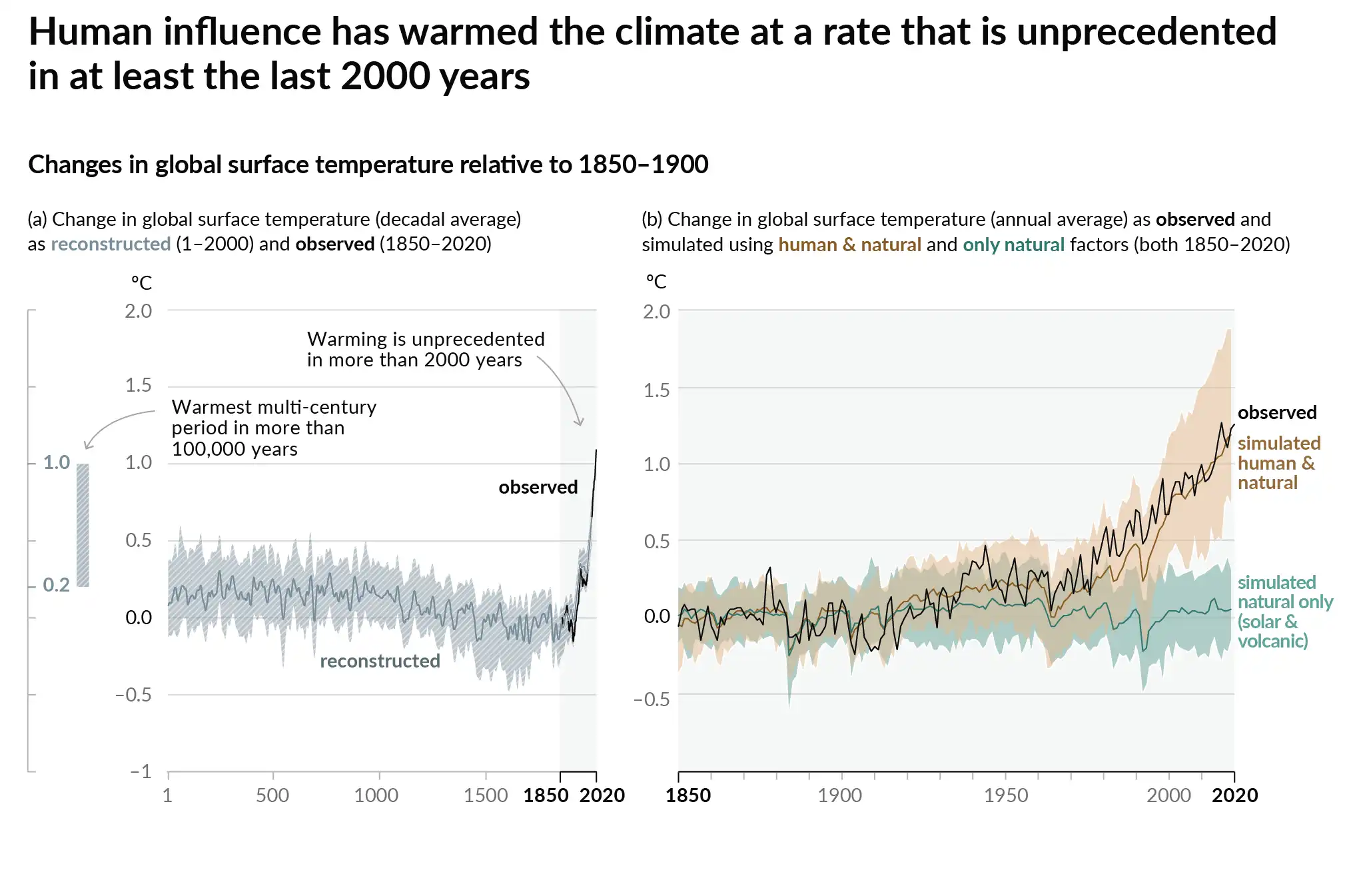
A.1.2 Each of the last four decades has been successively warmer than any decade that preceded it since 1850. Global surface temperature8 in the first two decades of the 21st century (2001–2020) was 0.99 [0.84 to 1.10] °C higher than 1850–1900. 9Global surface temperature was 1.09 [0.95 to 1.20] °C higher in 2011–2020 than 1850–1900, with larger increases over land (1.59 [1.34 to 1.83] °C) than over the ocean (0.88 [0.68 to 1.01] °C). The estimated increase in global surface temperature since AR5 is principally due to further warming since 2003–2012 (+0.19 [0.16 to 0.22] °C). Additionally, methodological advances and new datasets contributed approximately 0.1°C to the updated estimate of warming in AR6. 10 Links to chapters2.3, Cross-Chapter Box 2.3 Figure SPM.1
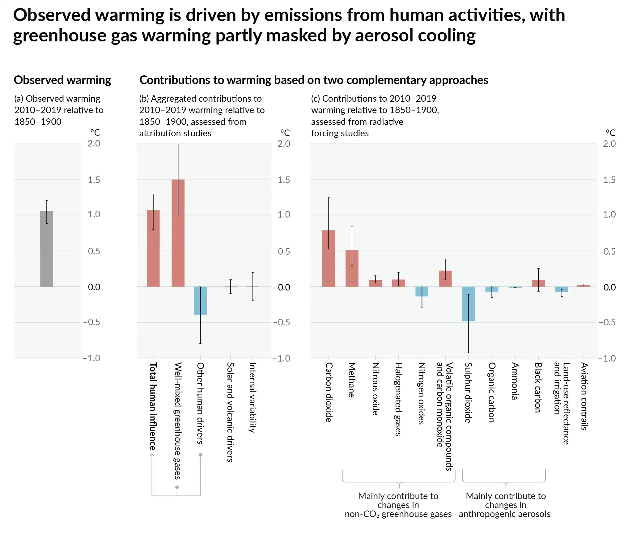
A.1.3 The likely range of total human-caused global surface temperature increase from 1850–1900 to 2010–201911is 0.8°C to 1.3°C, with a best estimate of 1.07°C. It is likely that well-mixed GHGs contributed a warming of 1.0°C to 2.0°C, other human drivers (principally aerosols) contributed a cooling of 0.0°C to 0.8°C, natural drivers changed global surface temperature by –0.1°C to +0.1°C, and internal variability changed it by –0.2°C to +0.2°C. It is very likely that well-mixed GHGs were the main driver12 of tropospheric warming since 1979 and extremely likely that human-caused stratospheric ozone depletion was the main driver of cooling of the lower stratosphere between 1979 and the mid-1990s. Links to chapters3.3, 6.4, 7.3, TS.2.3, Cross-Section Box TS.1 Figure SPM.2
A.1.4 Globally averaged precipitation over land has likely increased since 1950, with a faster rate of increase since the 1980s (medium confidence). It is likely that human influence contributed to the pattern of observed precipitation changes since the mid-20th century and extremely likely that human influence contributed to the pattern of observed changes in near-surface ocean salinity. Mid-latitude storm tracks have likely shifted poleward in both hemispheres since the 1980s, with marked seasonality in trends (medium confidence). For the Southern Hemisphere, human influence very likely contributed to the poleward shift of the closely related extratropical jet in austral summer. Links to chapters2.3, 3.3, 8.3, 9.2, TS.2.3, TS.2.4, Box TS.6
A.1.5 Human influence is very likely the main driver of the global retreat of glaciers since the 1990s and the decrease in Arctic sea ice area between 1979–1988 and 2010–2019 (decreases of about 40% in September and about 10% in March). There has been no significant trend in Antarctic sea ice area from 1979 to 2020 due to regionally opposing trends and large internal variability. Human influence very likely contributed to the decrease in Northern Hemisphere spring snow cover since 1950. It is very likely that human influence has contributed to the observed surface melting of the Greenland Ice Sheet over the past two decades, but there is onlylimited evidence, with medium agreement, of human influence on the Antarctic Ice Sheet mass loss. Links to chapters2.3, 3.4, 8.3, 9.3, 9.5, TS.2.5
A.1.6 It is virtually certain that the global upper ocean (0–700 m) has warmed since the 1970s and extremely likely that human influence is the main driver. It is virtually certain that human-caused CO2 emissions are the main driver of current global acidification of the surface open ocean. There is high confidence that oxygen levels have dropped in many upper ocean regions since the mid-20th century and medium confidence that human influence contributed to this drop. Links to chapters2.3, 3.5, 3.6, 5.3, 9.2, TS.2.4
A.1.7 Global mean sea level increased by 0.20 [0.15 to 0.25] m between 1901 and 2018. The average rate of sea level rise was 1.3 [0.6 to 2.1] mm yr–1 between 1901 and 1971, increasing to 1.9 [0.8 to 2.9] mm yr–1 between 1971 and 2006, and further increasing to 3.7 [3.2 to 4.2] mm yr–1 between 2006 and 2018 (high confidence). Human influence was very likely the main driver of these increases since at least 1971. Links to chapters2.3, 3.5, 9.6, Cross-Chapter Box 9.1, Box TS.4
A.1.8 Changes in the land biosphere since 1970 are consistent with global warming: climate zones have shifted poleward in both hemispheres, and the growing season has on average lengthened by up to two days per decade since the 1950s in the Northern Hemisphere extratropics (high confidence). Links to chapters2.3, TS.2.6
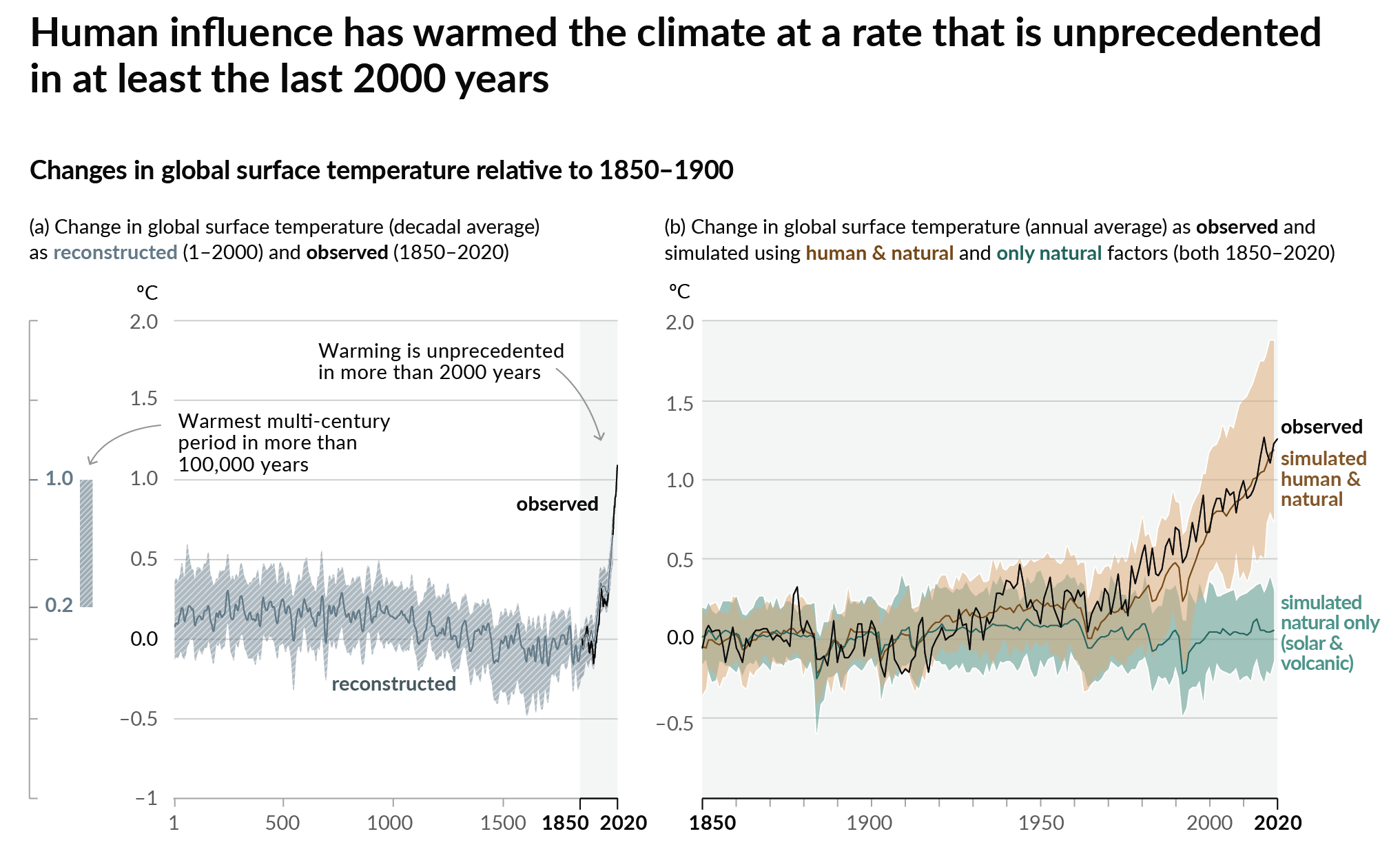
Figure SPM.1 | History of global temperature change and causes of recent warming
Panel (a) Changes in global surface temperature reconstructed from paleoclimate archives (solid grey line, years 1–2000) and from direct observations(solid black line, 1850–2020), both relative to 1850–1900 and decadally averaged. The vertical bar on the left shows the estimated temperature (very likely range) during the warmest multi-century period in at least the last 100,000 years, which occurred around 6500 years ago during the current interglacial period (Holocene). The Last Interglacial, around 125,000 years ago, is the next most recent candidate for a period of higher temperature. These past warm periods were caused by slow (multi-millennial) orbital variations. The grey shading with white diagonal lines shows the very likely ranges for the temperature reconstructions.
Panel (b) Changes in global surface temperature over the past 170 years (black line) relative to 1850–1900 and annually averaged, compared to Coupled Model Intercomparison Project Phase 6 (CMIP6) climate model simulations (see Box SPM.1) of the temperature response to both human and natural drivers (brown) and to only natural drivers (solar and volcanic activity, green). Solid coloured lines show the multi-model average, and coloured shades show the very likely range of simulations. (See Figure SPM.2 for the assessed contributions to warming). Links to chapters2.3.1, Cross-Chapter Box 2.3, 3.3, TS.2.2, Cross-Section Box TS.1, Figure 1a
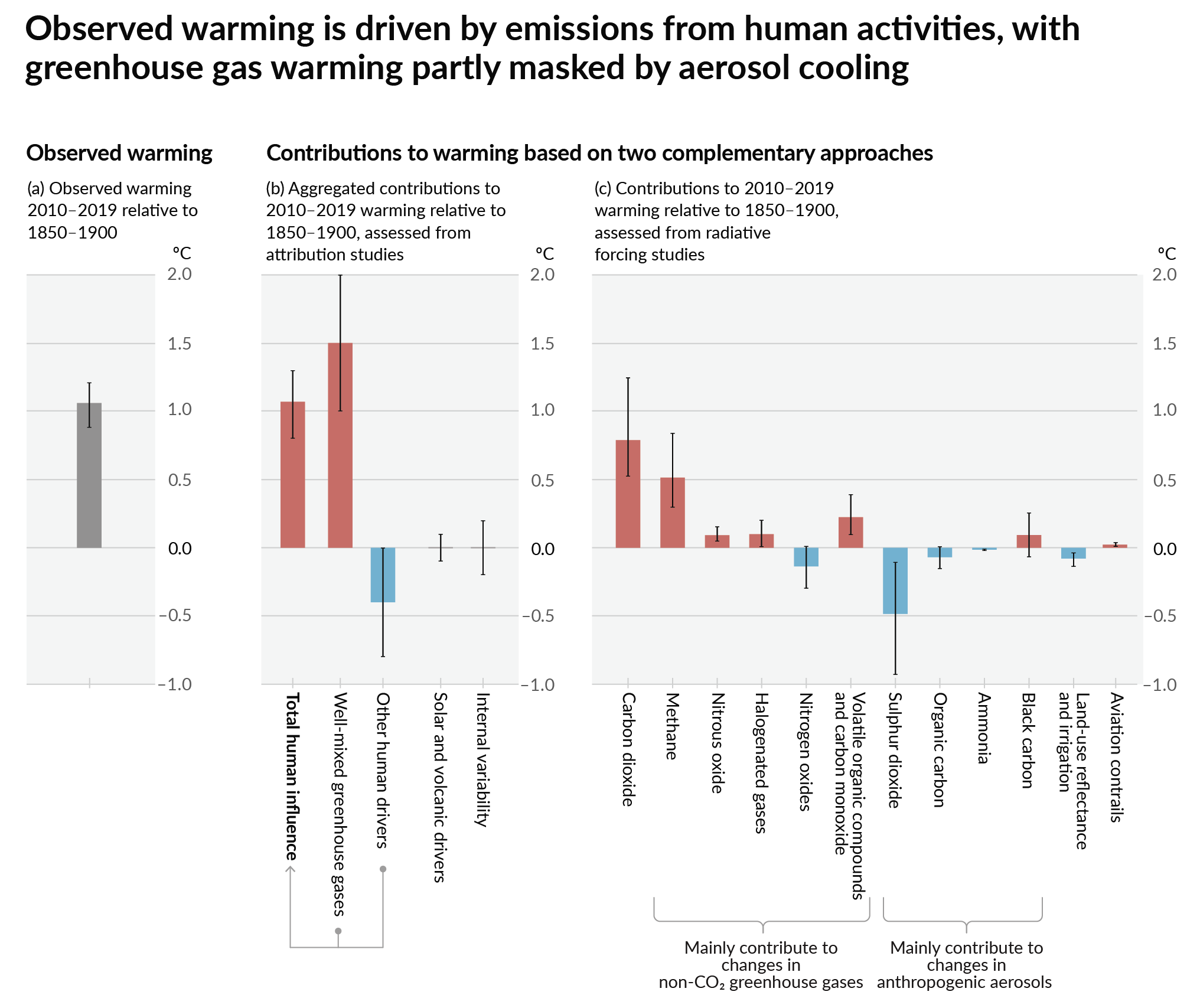
Figure SPM.2 | Assessed contributions to observed warming in 2010–2019 relative to 1850–1900
Panel (a) Observed global warming (increase in global surface temperature). Whiskers show the very likely range.
Panel (b) Evidence from attribution studies, which synthesize information from climate models and observations. The panel shows temperature change attributed to: total human influence; changes in well-mixed greenhouse gas concentrations; other human drivers due to aerosols, ozone and land-use change (land-use reflectance); solar and volcanic drivers; and internal climate variability. Whiskers showlikely ranges.
Panel (c) Evidence from the assessment of radiative forcing and climate sensitivity. The panel shows temperature changes from individual components of human influence: emissions of greenhouse gases, aerosols and their precursors; land-use changes (land-use reflectance and irrigation); and aviation contrails. Whiskers showvery likely ranges. Estimates account for both direct emissions into the atmosphere and their effect, if any, on other climate drivers. For aerosols, both direct effects (through radiation) and indirect effects (through interactions with clouds) are considered. Links to chaptersCross-Chapter Box 2.3, 3.3.1, 6.4.2, 7.3
A.2 The scale of recent changes across the climate system as a whole – and the present state of many aspects of the climate system – are unprecedented over many centuries to many thousands of years. Expand Figure SPM.1Links to chapters2.2, 2.3, Cross-Chapter Box 2.1, 5.1
A.2.1 In 2019, atmospheric CO2 concentrations were higher than at any time in at least 2 million years (high confidence), and concentrations of CH4 and N2O were higher than at any time in at least 800,000 years (very high confidence). Since 1750, increases in CO2 (47%) and CH4 (156%) concentrations far exceed – and increases in N2O (23%) are similar to – the natural multi-millennial changes between glacial and interglacial periods over at least the past 800,000 years (very high confidence). Links to chapters2.2, 5.1, TS.2.2
A.2.2 Global surface temperature has increased faster since 1970 than in any other 50-year period over at least the last 2000 years (high confidence). Temperatures during the most recent decade (2011–2020) exceed those of the most recent multi-century warm period, around 6500 years ago13[0.2°C to 1°C relative to 1850–1900] (medium confidence). Prior to that, the next most recent warm period was about 125,000 years ago, when the multi-century temperature [0.5°C to 1.5°C relative to 1850–1900] overlaps the observations of the most recent decade (medium confidence). Links to chapters2.3, Cross-Chapter Box 2.1, Cross-Section Box TS.1 Figure SPM.1
A.2.3 In 2011–2020, annual average Arctic sea ice area reached its lowest level since at least 1850 (high confidence). Late summer Arctic sea ice area was smaller than at any time in at least the past 1000 years (medium confidence). The global nature of glacier retreat since the 1950s, with almost all of the world’s glaciers retreating synchronously, is unprecedented in at least the last 2000 years (medium confidence). Links to chapters2.3, TS.2.5
A.2.4 Global mean sea level has risen faster since 1900 than over any preceding century in at least the last 3000 years (high confidence). The global ocean has warmed faster over the past century than since the end of the last deglacial transition (around 11,000 years ago) (medium confidence). A long-term increase in surface open ocean pH occurred over the past 50 million years (high confidence). However, surface open ocean pH as low as recent decades is unusual in the last 2 million years (medium confidence). Links to chapters2.3, TS.2.4, Box TS.4
A.3 Human-induced climate change is already affecting many weather and climate extremes in every region across the globe. Evidence of observed changes in extremes such as heatwaves, heavy precipitation, droughts, and tropical cyclones, and, in particular, their attribution to human influence, has strengthened since AR5. Expand Figure SPM.3Links to chapters2.3, 3.3, 8.2, 8.3, 8.4, 8.5, 8.6, Box 8.1, Box 8.2, Box 9.2, 10.6, 11.2, 11.3, 11.4, 11.6, 11.7, 11.8, 11.9, 12.3
A.3.1 It is virtually certain that hot extremes (including heatwaves) have become more frequent and more intense across most land regions since the 1950s, while cold extremes (including cold waves) have become less frequent and less severe, with high confidence that human-induced climate change is the main driver14 of these changes. Some recent hot extremes observed over the past decade would have been extremely unlikely to occur without human influence on the climate system. Marine heatwaves have approximately doubled in frequency since the 1980s (high confidence), and human influence has very likely contributed to most of them since at least 2006. Figure SPM.3Links to chaptersBox 9.2, 11.2, 11.3, 11.9, TS.2.4, TS.2.6, Box TS.10
A.3.2 The frequency and intensity of heavy precipitation events have increased since the 1950s over most land area for which observational data are sufficient for trend analysis (high confidence), and human-induced climate change is likely the main driver. Human-induced climate change has contributed to increases in agricultural and ecological droughts15 in some regions due to increased land evapotranspiration16 (medium confidence). Figure SPM.3 Links to chapters8.2, 8.3, 11.4, 11.6, 11.9, TS.2.6, Box TS.10
A.3.3 Decreases in global land monsoon precipitation17 from the 1950s to the 1980s are partly attributed to human-caused Northern Hemisphere aerosol emissions, but increases since then have resulted from rising GHG concentrations and decadal to multi-decadal internal variability (medium confidence). Over South Asia, East Asia and West Africa, increases in monsoon precipitation due to warming from GHG emissions were counteracted by decreases in monsoon precipitation due to cooling from human-caused aerosol emissions over the 20th century (high confidence). Increases in West African monsoon precipitation since the 1980s are partly due to the growing influence of GHGs and reductions in the cooling effect of human-caused aerosol emissions over Europe and North America (medium confidence). Links to chapters2.3, 3.3, 8.2, 8.3, 8.4, 8.5, 8.6, Box 8.1, Box 8.2, 10.6, Box TS.13
A.3.4 It is likely that the global proportion of major (Category 3–5) tropical cyclone occurrence has increased over the last four decades, and it is very likely that the latitude where tropical cyclones in the western North Pacific reach their peak intensity has shifted northward; these changes cannot be explained by internal variability alone (medium confidence). There is low confidence in long-term (multi-decadal to centennial) trends in the frequency of all-category tropical cyclones. Event attribution studies and physical understanding indicate that human-induced climate change increases heavy precipitation associated with tropical cyclones (high confidence), but data limitations inhibit clear detection of past trends on the global scale. Links to chapters8.2, 11.7, Box TS.10
A.3.5 Human influence has likely increased the chance of compound extreme events18 since the 1950s. This includes increases in the frequency of concurrent heatwaves and droughts on the global scale (high confidence), fire weather in some regions of all inhabited continents (medium confidence), and compound flooding in some locations (medium confidence). Links to chapters11.6, 11.7, 11.8, 12.3, 12.4, TS.2.6, Table TS.5, Box TS.10
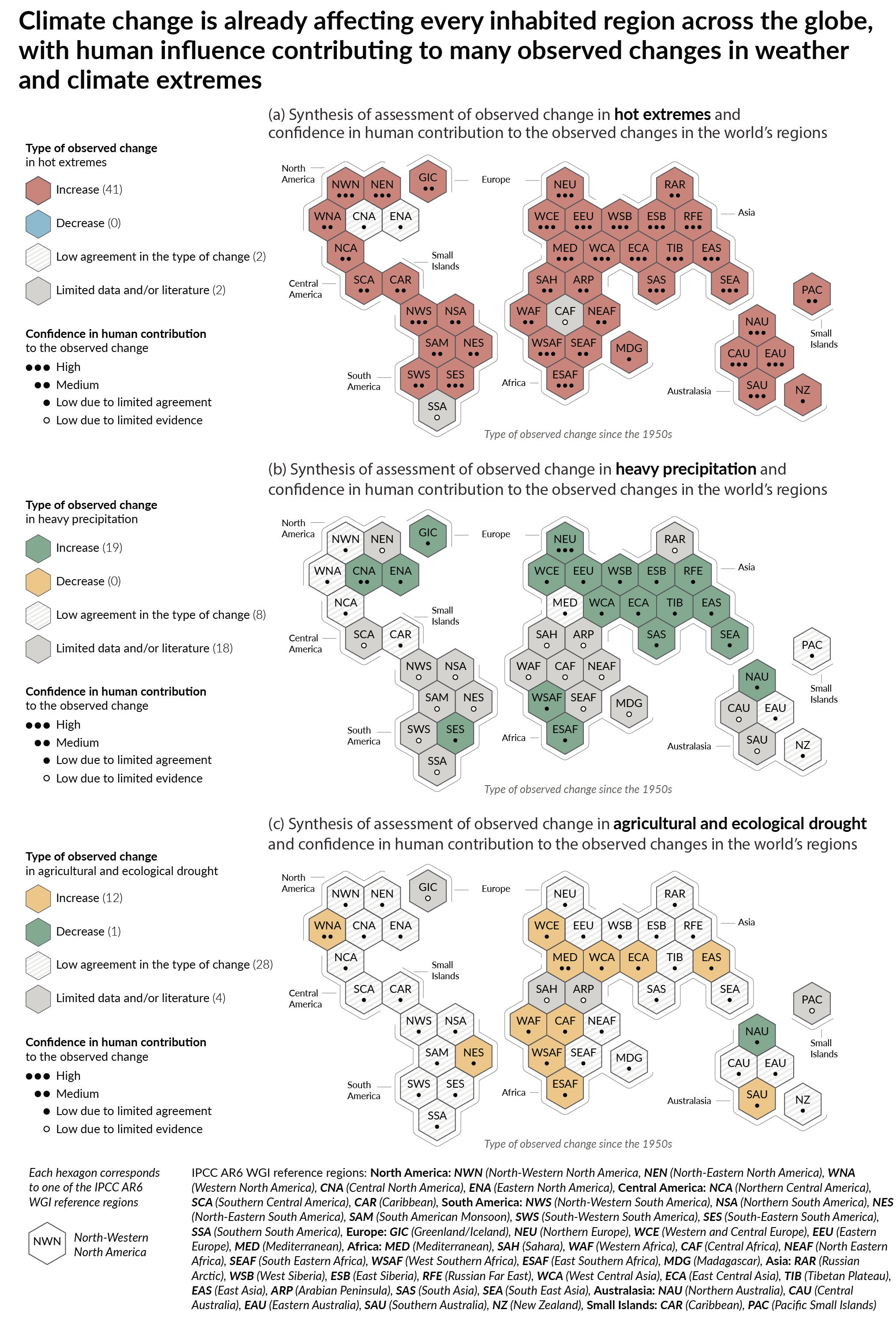 Figure SPM.3 | Synthesis of assessed observed and attributable regional changes
The IPCC AR6 WGI inhabited regions are displayed as hexagons with identical size in their approximate geographical location (see legend for regional acronyms). All assessments are made for each region as a whole and for the 1950s to the present. Assessments made on different time scales or more local spatial scales might differ from what is shown in the figure. The colours in each panel represent the four outcomes of the assessment on observed changes. Striped hexagons (white and light-grey) are used where there is low agreement in the type of change for the region as a whole, and grey hexagons are used when there is limited data and/or literature that prevents an assessment of the region as a whole. Other colours indicate at least medium confidence in the observed change. The confidence level for the human influence on these observed changes is based on assessing trend detection and attribution and event attribution literature, and it is indicated by the number of dots: three dots for high confidence, two dots formedium confidence and one dot forlow confidence (single, filled dot: limited agreement; single, empty dot: limited evidence).
Panel (a) For hot extremes, the evidence is mostly drawn from changes in metrics based on daily maximum temperatures; regional studies using other indices (heatwave duration, frequency and intensity) are used in addition. Red hexagons indicate regions where there is at least medium confidence in an observed increase in hot extremes.
Panel (b) For heavy precipitation, the evidence is mostly drawn from changes in indices based on one-day or five-day precipitation amounts using global and regional studies. Green hexagons indicate regions where there is at least medium confidence in an observed increase in heavy precipitation.
Panel (c) Agricultural and ecological droughts are assessed based on observed and simulated changes in total column soil moisture, complemented by evidence on changes in surface soil moisture, water balance (precipitation minus evapotranspiration) and indices driven by precipitation and atmospheric evaporative demand. Yellow hexagons indicate regions where there is at least medium confidence in an observed increase in this type of drought, and green hexagons indicate regions where there is at least medium confidence in an observed decrease in agricultural and ecological drought.
For all regions, Table TS.5 shows a broader range of observed changes besides the ones shown in this figure. Note that Southern South America (SSA) is the only region that does not display observed changes in the metrics shown in this figure, but is affected by observed increases in mean temperature, decreases in frost and increases in marine heatwaves. Links to chapters11.9, Atlas 1.3.3, Figure Atlas.2, Table TS.5, Box TS.10, Figure 1
A.4 Improved knowledge of climate processes, paleoclimate evidence and the response of the climate system to increasing radiative forcing gives a best estimate of equilibrium climate sensitivity of 3°C, with a narrower range compared to AR5. ExpandLinks to chapters2.2, 7.3, 7.4, 7.5, Box 7.2, 9.4, 9.5, 9.6, Cross-Chapter Box 9.1
A.4.1 Human-caused radiative forcing of 2.72 [1.96 to 3.48] W m–2 in 2019 relative to 1750 has warmed the climate system. This warming is mainly due to increased GHG concentrations, partly reduced by cooling due to increased aerosol concentrations. The radiative forcing has increased by 0.43 W m–2 (19%) relative to AR5, of which 0.34 W m–2 is due to the increase in GHG concentrations since 2011. The remainder is due to improved scientific understanding and changes in the assessment of aerosol forcing, which include decreases in concentration and improvement in its calculation (high confidence). Links to chapters2.2, 7.3, TS.2.2, TS.3.1
A.4.2 Human-caused net positive radiative forcing causes an accumulation of additional energy (heating) in the climate system, partly reduced by increased energy loss to space in response to surface warming. The observed average rate of heating of the climate system increased from 0.50 [0.32 to 0.69] W m–2 for the period 1971–200619 to 0.79 [0.52 to 1.06] W m–2 for the period 2006–201820 (high confidence). Ocean warming accounted for 91% of the heating in the climate system, with land warming, ice loss and atmospheric warming accounting for about 5%, 3% and 1%, respectively (high confidence). Links to chapters7.2, Box 7.2, TS.3.1
A.4.3 Heating of the climate system has caused global mean sea level rise through ice loss on land and thermal expansion from ocean warming. Thermal expansion explained 50% of sea level rise during 1971–2018, while ice loss from glaciers contributed 22%, ice sheets 20% and changes in land-water storage 8%. The rate of ice-sheet loss increased by a factor of four between 1992–1999 and 2010–2019. Together, ice-sheet and glacier mass loss were the dominant contributors to global mean sea level rise during 2006–2018 (high confidence). Links to chapters9.4, 9.5, 9.6, Cross-Chapter Box 9.1
A.4.4 The equilibrium climate sensitivity is an important quantity used to estimate how the climate responds to radiative forcing. Based on multiple lines of evidence, 21 The very likely range of equilibrium climate sensitivity is between 2°C (high confidence) and 5°C (medium confidence). The AR6 assessed best estimate is 3°C with a likely range of 2.5°C to 4°C (high confidence), compared to 1.5°C to 4.5°C in AR5, which did not provide a best estimate. Links to chapters7.4, 7.5, TS.3.2
B. Possible Climate Futures
Box SPM.1 | Scenarios, Climate Models and ProjectionsExpand
Box SPM.1.1: This Report assesses the climate response to five illustrative scenarios that cover the range of possible future development of anthropogenic drivers of climate change found in the literature. They start in 2015, and include scenarios22 with high and very high GHG emissions (SSP3-7.0 and SSP5-8.5) and CO2 emissions that roughly double from current levels by 2100 and 2050, respectively, scenarios with intermediate GHG emissions (SSP2-4.5) and CO2 emissions remaining around current levels until the middle of the century, and scenarios with very low and low GHG emissions and CO2 emissions declining to net zero around or after 2050, followed by varying levels of net negative CO2 emissions23 (SSP1-1.9 and SSP1-2.6), as illustrated in Figure SPM.4. Emissions vary between scenarios depending on socio-economic assumptions, levels of climate change mitigation and, for aerosols and non-methane ozone precursors, air pollution controls. Alternative assumptions may result in similar emissions and climate responses, but the socio-economic assumptions and the feasibility or likelihood of individual scenarios are not part of the assessment. Links to chapters1.6, Cross-Chapter Box 1.4, TS.1.3 Figure SPM.4
Box SPM.1.2: This Report assesses results from climate models participating in the Coupled Model Intercomparison Project Phase 6 (CMIP6) of the World Climate Research Programme. These models include new and better representations of physical, chemical and biological processes, as well as higher resolution, compared to climate models considered in previous IPCC assessment reports. This has improved the simulation of the recent mean state of most large-scale indicators of climate change and many other aspects across the climate system. Some differences from observations remain, for example in regional precipitation patterns. The CMIP6 historical simulations assessed in this Report have an ensemble mean global surface temperature change within 0.2°C of the observations over most of the historical period, and observed warming is within the very likely range of the CMIP6 ensemble. However, some CMIP6 models simulate a warming that is either above or below the assessed very likely range of observed warming. Links to chapters1.5, Cross-Chapter Box 2.2, 3.3, 3.8, TS.1.2, Cross-Section Box TS.1 Figure SPM.1b, Figure SPM.2
Box SPM.1.3: The CMIP6 models considered in this Report have a wider range of climate sensitivity than in CMIP5 models and the AR6 assessed very likely range, which is based on multiple lines of evidence. These CMIP6 models also show a higher average climate sensitivity than CMIP5 and the AR6 assessed best estimate. The higher CMIP6 climate sensitivity values compared to CMIP5 can be traced to an amplifying cloud feedback that is larger in CMIP6 by about 20%. Links to chaptersBox 7.1, 7.3, 7.4, 7.5, TS.3.2
Box SPM.1.4: For the first time in an IPCC report, assessed future changes in global surface temperature, ocean warming and sea level are constructed by combining multi-model projections with observational constraints based on past simulated warming, as well as the AR6 assessment of climate sensitivity. For other quantities, such robust methods do not yet exist to constrain the projections. Nevertheless, robust projected geographical patterns of many variables can be identified at a given level of global warming, common to all scenarios considered and independent of timing when the global warming level is reached. Links to chapters1.6, 4.3, 4.6, Box 4.1, 7.5, 9.2, 9.6, Cross-Chapter Box 11.1, Cross-Section Box TS.1
Box SPM.1
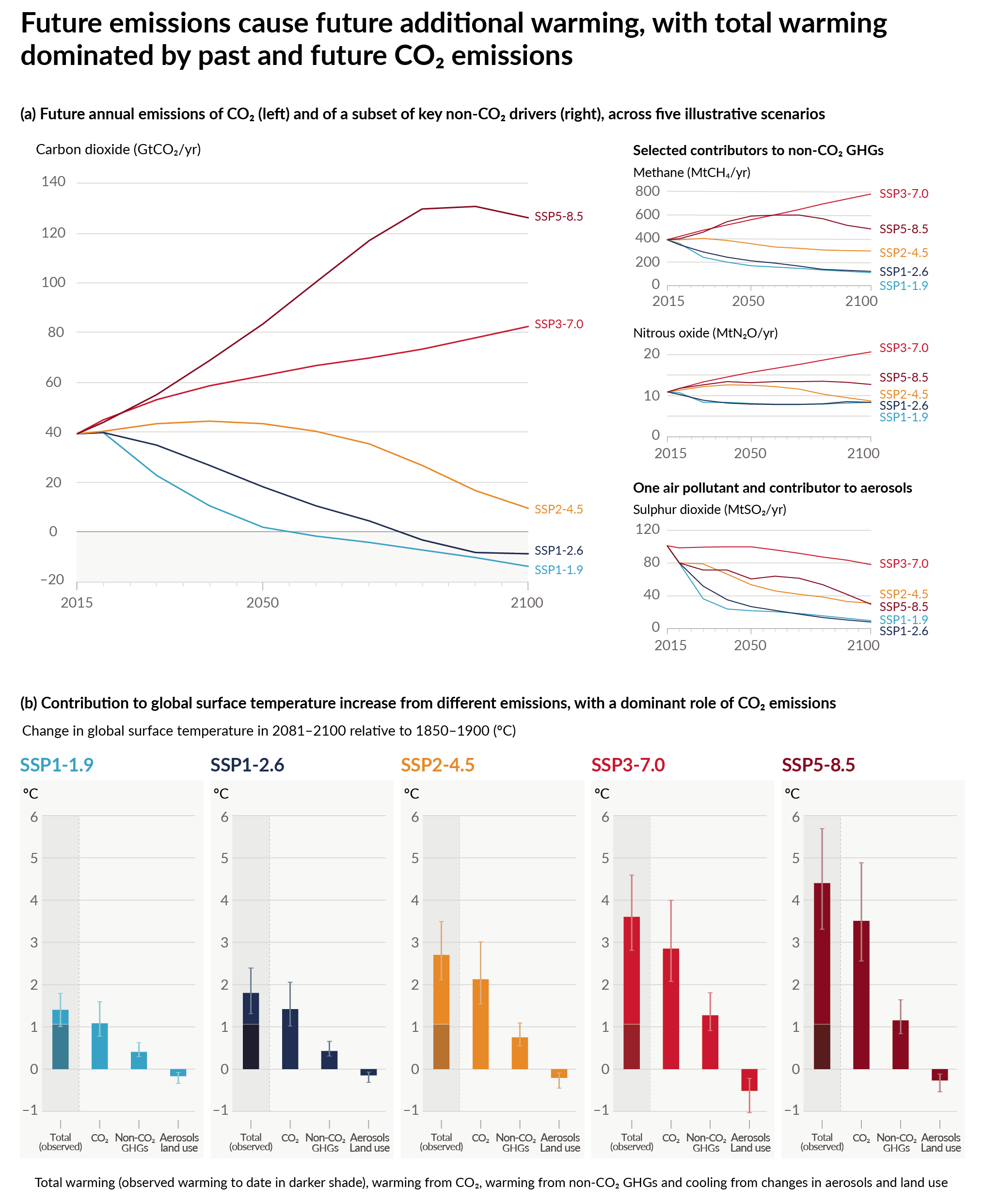
Figure SPM.4 | Future anthropogenic emissions of key drivers of climate change and warming contributions by groups of drivers for the five illustrative scenarios used in this report. The five scenarios are SSP1-1.9, SSP1-2.6, SSP2-4.5, SSP3-7.0 and SSP5-8.5.
Panel (a) Annual anthropogenic (human-caused) emissions over the 2015–2100 period. Shown are emissions trajectories for carbon dioxide (CO2) from all sectors (GtCO2 /yr) (left graph) and for a subset of three key non-CO2 drivers considered in the scenarios: methane (CH4, MtCH4/yr, top-right graph); nitrous oxide (N2O, MtN2O/yr, middle-right graph); and sulphur dioxide (SO2, MtSO2/yr, bottom-right graph, contributing to anthropogenic aerosols in panel (b).
Panel (b) Warming contributions by groups of anthropogenic drivers and by scenario are shown as the change in global surface temperature (°C) in 2081–2100 relative to 1850–1900, with indication of the observed warming to date. Bars and whiskers represent median values and the very likely range, respectively. Within each scenario bar plot, the bars represent: total global warming (°C; ‘total’bar) (see Table SPM.1); warming contributions (°C) from changes in CO2 (‘CO2 ’bar) and from non-CO2 greenhouse gases (GHGs; ‘non-CO2 GHGs’bar: comprising well-mixed greenhouse gases and ozone); and net cooling from other anthropogenic drivers (‘aerosols and land use’bar: anthropogenic aerosols, changes in reflectance due to land-use and irrigation changes, and contrails from aviation) (see Figure SPM.2, panel c, for the warming contributions to date for individual drivers). The best estimate for observed warming in 2010–2019 relative to 1850–1900 (see Figure SPM.2, panel a) is indicated in the darker column in the ‘total’ bar. Warming contributions in panel (b) are calculated as explained in Table SPM.1 for the total bar. For the other bars, the contribution by groups of drivers is calculated with a physical climate emulator of global surface temperature that relies on climate sensitivity and radiative forcing assessments. Links to chaptersCross-Chapter Box 1.4, 4.6, Figure 4.35, 6.7, Figures 6.18, 6.22 and 6.24, 7.3, Cross-Chapter Box 7.1, Figure 7.7, Box TS.7, Figures TS.4 and TS.15
B.1 Global surface temperature will continue to increase until at least mid-century under all emissions scenarios considered. Global warming of 1.5°C and 2°C will be exceeded during the 21st century unless deep reductions in CO2 and other greenhouse gas emissions occur in the coming decades. Expand Figures SPM.1, SPM.4 SPM.8  Table SPM.1
  Box SPM.1Links to chapters2.3, Cross-Chapter Box 2.3, Cross-Chapter Box 2.4, 4.3, 4.4, 4.5
B.1.1 Compared to 1850–1900, global surface temperature averaged over 2081–2100 is very likely to be higher by 1.0°C to 1.8°C under the very low GHG emissions scenario considered (SSP1-1.9), by 2.1°C to 3.5°C in the intermediate GHG emissions scenario (SSP2-4.5) and by 3.3°C to 5.7°C under the very high GHG emissions scenario (SSP5-8.5). 24 The last time global surface temperature was sustained at or above 2.5°C higher than 1850–1900 was over 3 million years ago (medium confidence). Table SPM.1Links to chapters2.3, Cross-Chapter Box 2.4, 4.3, 4.5, Box TS.2, Box TS.4, Cross-Section Box TS.1
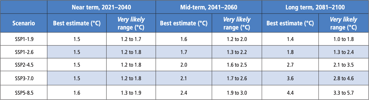
B.1.2 Based on the assessment of multiple lines of evidence, global warming of 2°C, relative to 1850–1900, would be exceeded during the 21st century under the high and very high GHG emissions scenarios considered in this report (SSP3-7.0 and SSP5-8.5, respectively). Global warming of 2°C would extremely likely be exceeded in the intermediate GHG emissions scenario (SSP2-4.5). Under the very low and low GHG emissions scenarios, global warming of 2°C is extremely unlikely to be exceeded (SSP1-1.9) orunlikely to be exceeded (SSP1-2.6). 25 Crossing the 2°C global warming level in the mid-term period (2041–2060) is very likely to occur under the very high GHG emissions scenario (SSP5-8.5), likely to occur under the high GHG emissions scenario (SSP3-7.0), and more likely than not to occur in the intermediate GHG emissions scenario (SSP2-4.5). 26 Table SPM.1 Box SPM.1Links to chapters4.3, Cross-Section Box TS.1
B.1.3 Global warming of 1.5°C relative to 1850–1900 would be exceeded during the 21st century under the intermediate, high and very high GHG emissions scenarios considered in this report (SSP2-4.5, SSP3-7.0 and SSP5-8.5, respectively). Under the five illustrative scenarios, in the near term (2021–2040), the 1.5°C global warming level is very likely to be exceeded under the very high GHG emissions scenario (SSP5-8.5), likely to be exceeded under the intermediate and high GHG emissions scenarios (SSP2-4.5 and SSP3-7.0), more likely than not to be exceeded under the low GHG emissions scenario (SSP1-2.6) and more likely than not to be reached under the very low GHG emissions scenario (SSP1-1.9). 27Furthermore, for the very low GHG emissions scenario (SSP1-1.9), it is more likely than not that global surface temperature would decline back to below 1.5°C toward the end of the 21st century, with a temporary overshoot of no more than 0.1°C above 1.5°C global warming. Box SPM.1 Figure SPM.4Links to chapters4.3, Cross-Section Box TS.1
B.1.4 Global surface temperature in any single year can vary above or below the long-term human-induced trend, due to substantial natural variability. 28 The occurrence of individual years with global surface temperature change above a certain level, for example 1.5°C or 2°C, relative to 1850–1900 does not imply that this global warming level has been reached. 29 Table SPM.1 Figure SPM.1, Figure SPM.8Links to chaptersCross-Chapter Box 2.3, 4.3, 4.4, Box 4.1, Cross-Section Box TS.1
B.2 Many changes in the climate system become larger in direct relation to increasing global warming. They include increases in the frequency and intensity of hot extremes, marine heatwaves, heavy precipitation, and, in some regions, agricultural and ecological droughts; an increase in the proportion of intense tropical cyclones; and reductions in Arctic sea ice, snow cover and permafrost. Expand Figures SPM.5, SPM.6, SPM.8Links to chapters4.3, 4.5, 4.6, 7.4, 8.2, 8.4, Box 8.2, 9.3, 9.5, Box 9.2, 11.1, 11.2, 11.3, 11.4, 11.6, 11.7, 11.9, Cross-Chapter Box 11.1, 12.4, 12.5, Cross-Chapter Box 12.1, Atlas.4, Atlas.5, Atlas.6, Atlas.7, Atlas.8, Atlas.9, Atlas.10, Atlas.11
B.2.1 It is virtually certain that the land surface will continue to warm more than the ocean surface (likely 1.4 to 1.7 times more). It is virtually certain that the Arctic will continue to warm more than global surface temperature, with high confidence above two times the rate of global warming. Links to chapters2.3, 4.3, 4.5, 4.6, 7.4, 11.1, 11.3, 11.9, 12.4, 12.5, Cross-Chapter Box 12.1, Atlas.4, Atlas.5, Atlas.6, Atlas.7, Atlas.8, Atlas.9, Atlas.10, Atlas.11, Cross-Section Box TS.1, TS.2.6 Figure SPM.5
B.2.2 With every additional increment of global warming, changes in extremes continue to become larger. For example, every additional 0.5°C of global warming causes clearly discernible increases in the intensity and frequency of hot extremes, including heatwaves (very likely) , and heavy precipitation (high confidence), as well as agricultural and ecological droughts30 in some regions (high confidence). Discernible changes in intensity and frequency of meteorological droughts, with more regions showing increases than decreases, are seen in some regions for every additional 0.5°C of global warming (medium confidence). Increases in frequency and intensity of hydrological droughts become larger with increasing global warming in some regions (medium confidence). There will be an increasing occurrence of some extreme events unprecedented in the observational record with additional global warming, even at 1.5°C of global warming. Projected percentage changes in frequency are larger for rarer events (high confidence). Links to chapters8.2, 11.2, 11.3, 11.4, 11.6, 11.9, Cross-Chapter Box 11.1, Cross-Chapter Box 12.1, TS.2.6 Figure SPM.5 Figure SPM.6
B.2.3 Some mid-latitude and semi-arid regions, and the South American Monsoon region, are projected to see the highest increase in the temperature of the hottest days, at about 1.5 to 2 times the rate of global warming (high confidence). The Arctic is projected to experience the highest increase in the temperature of the coldest days, at about three times the rate of global warming (high confidence). With additional global warming, the frequency of marine heatwaves will continue to increase (high confidence), particularly in the tropical ocean and the Arctic (medium confidence). Links to chaptersBox 9.2, 11.1, 11.3, 11.9, Cross-Chapter Box 11.1, Cross-Chapter Box 12.1, 12.4, TS.2.4, TS.2.6 Figure SPM.6
B.2.4 It is very likely that heavy precipitation events will intensify and become more frequent in most regions with additional global warming. At the global scale, extreme daily precipitation events are projected to intensify by about 7% for each 1°C of global warming (high confidence). The proportion of intense tropical cyclones (Category 4–5) and peak wind speeds of the most intense tropical cyclones are projected to increase at the global scale with increasing global warming (high confidence). Links to chapters8.2, 11.4, 11.7, 11.9, Cross-Chapter Box 11.1, Box TS.6, TS.4.3.1 Figure SPM.5 Figure SPM.6
B.2.5 Additional warming is projected to further amplify permafrost thawing and loss of seasonal snow cover, of land ice and of Arctic sea ice (high confidence). The Arctic is likely to be practically sea ice-free in September31 at least once before 2050 under the five illustrative scenarios considered in this report, with more frequent occurrences for higher warming levels. There is low confidence in the projected decrease of Antarctic sea ice. Links to chapters4.3, 4.5, 7.4, 8.2, 8.4, Box 8.2, 9.3, 9.5, 12.4, Cross-Chapter Box 12.1, Atlas.5, Atlas.6, Atlas.8, Atlas.9, Atlas.11, TS.2.5 Figure SPM.8
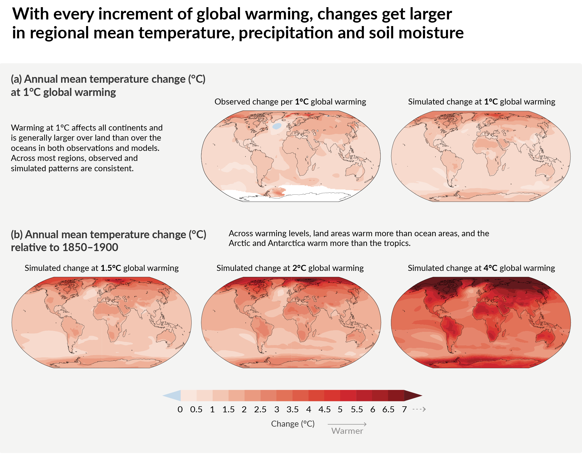
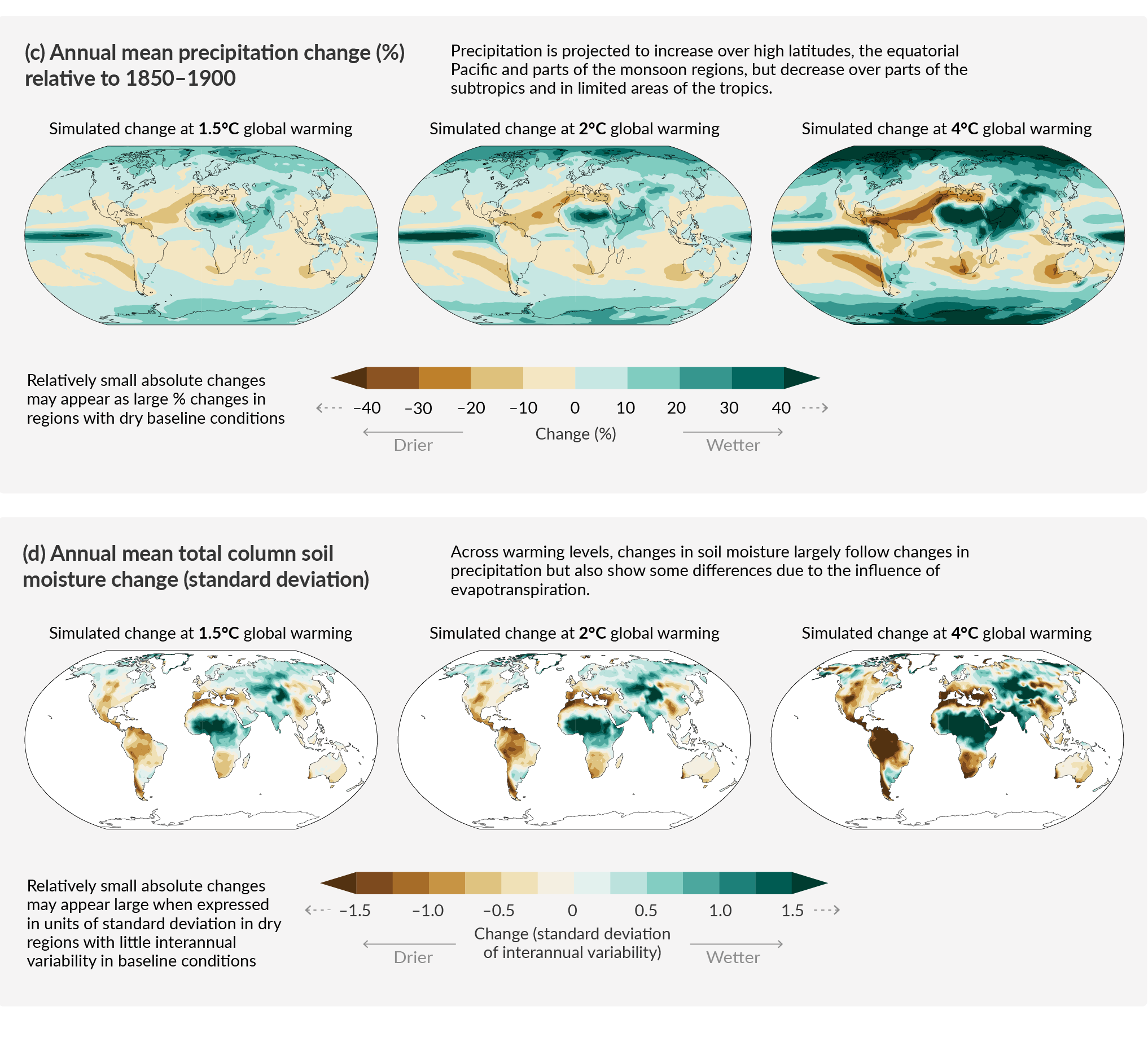 Figure SPM.5 | Changes in annual mean surface temperature, precipitation, and soil moisture
Panel (a) Comparison of observed and simulated annual mean surface temperature change. The left map shows the observed changes in annual mean surface temperature in the period 1850–2020 per °C of global warming (°C). The local (i.e., grid point) observed annual mean surface temperature changes are linearly regressed against the global surface temperature in the period 1850–2020. Observed temperature data are from Berkeley Earth, the dataset with the largest coverage and highest horizontal resolution. Linear regression is applied to all years for which data at the corresponding grid point is available. The regression method was used to take into account the complete observational time series and thereby reduce the role of internal variability at the grid point level. White indicates areas where time coverage was 100 years or less and thereby too short to calculate a reliable linear regression. The right map is based on model simulations and shows change in annual multi-model mean simulated temperatures at a global warming level of 1°C (20-year mean global surface temperature change relative to 1850–1900). The triangles at each end of the colour bar indicate out-of-bound values, that is, values above or below the given limits.
Panel (b) Simulated annual mean temperature change (°C), panel (c) precipitation change (%), and panel (d) total column soil moisture change (standard deviation of interannual variability) at global warming levels of 1.5°C, 2°C and 4°C (20-year mean global surface temperature change relative to 1850–1900). Simulated changes correspond to Coupled Model Intercomparison Project Phase 6 (CMIP6) multi-model mean change (median change for soil moisture) at the corresponding global warming level, that is, the same method as for the right map in panel (a).
In panel (c), high positive percentage changes in dry regions may correspond to small absolute changes. In panel (d), the unit is the standard deviation of interannual variability in soil moisture during 1850–1900. Standard deviation is a widely used metric in characterizing drought severity. A projected reduction in mean soil moisture by one standard deviation corresponds to soil moisture conditions typical of droughts that occurred about once every six years during 1850–1900. In panel (d), large changes in dry regions with little interannual variability in the baseline conditions can correspond to small absolute change. The triangles at each end of the colour bars indicate out-of-bound values, that is, values above or below the given limits. Results from all models reaching the corresponding warming level in any of the five illustrative scenarios (SSP1-1.9, SSP1-2.6, SSP2-4.5, SSP3-7.0 and SSP5-8.5) are averaged. Maps of annual mean temperature and precipitation changes at a global warming level of 3°C are available in Figure 4.31 and Figure 4.32 in Section 4.6. Corresponding maps of panels (b), (c) and (d), including hatching to indicate the level of model agreement at grid-cell level, are found in Figures 4.31, 4.32 and 11.19, respectively; as highlighted in Cross-Chapter Box Atlas.1, grid-cell level hatching is not informative for larger spatial scales (e.g., over AR6 reference regions) where the aggregated signals are less affected by small-scale variability, leading to an increase in robustness. Links to chapters Figure 1.14, 4.6.1, Cross-Chapter Box 11.1, Cross-Chapter Box Atlas.1, TS.1.3.2, Figures TS.3 and TS.5
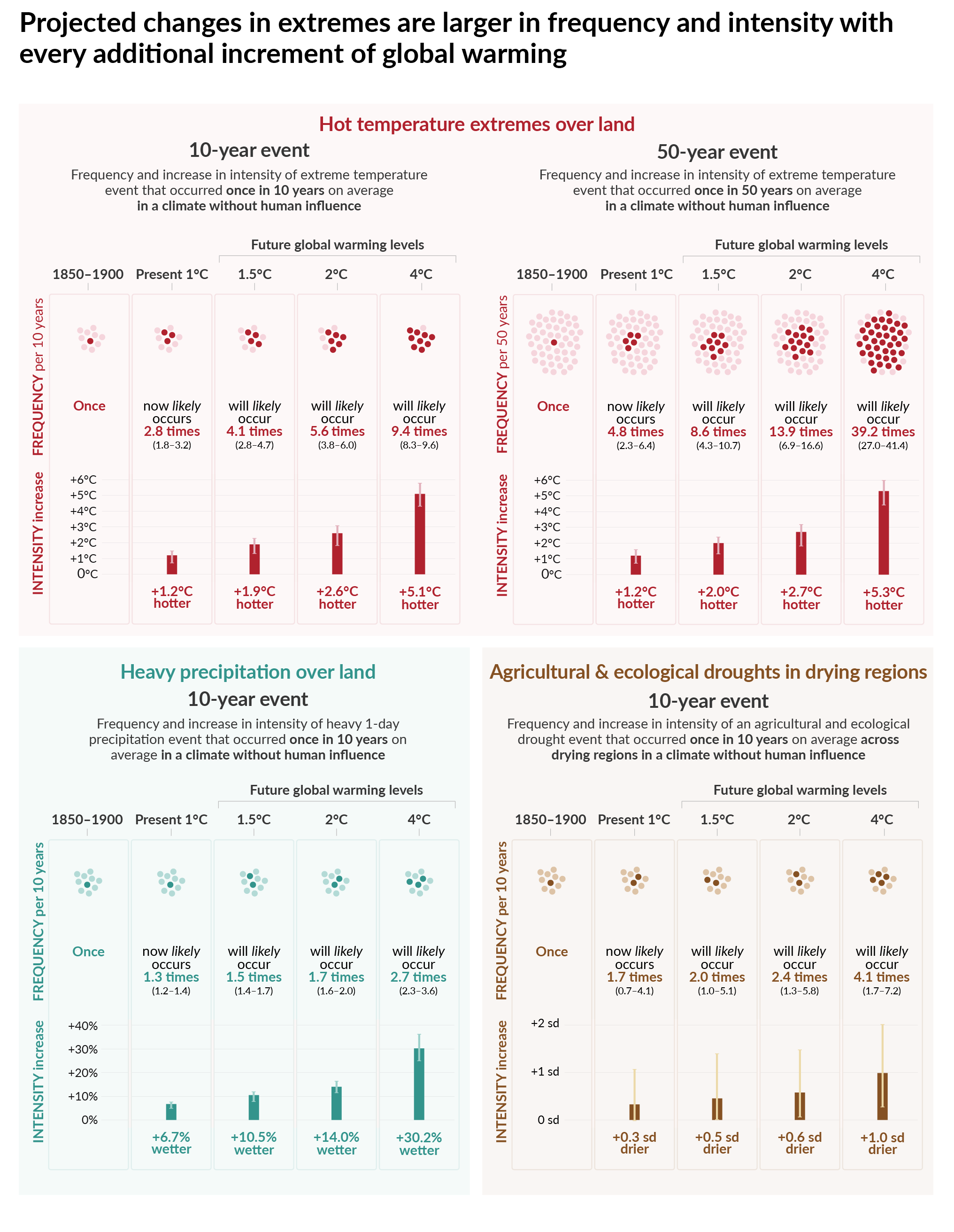 Figure SPM.6 | Projected changes in the intensity and frequency of hot temperature extremes over land, extreme precipitation over land, and agricultural and ecological droughts in drying regions
Projected changes are shown at global warming levels of 1°C, 1.5°C, 2°C, and 4°C and are relative to 1850–1900, 9representing a climate without human influence. The figure depicts frequencies and increases in intensity of 10- or 50-year extreme events from the base period (1850–1900) under different global warming levels.
Hot temperature extremes are defined as the daily maximum temperatures over land that were exceeded on average once in a decade (10-year event) or once in 50 years (50-year event) during the 1850–1900 reference period. Extreme precipitation events are defined as the daily precipitation amount over land that was exceeded on average once in a decade during the 1850–1900 reference period. Agricultural and ecological drought events are defined as the annual average of total column soil moisture below the 10th percentile of the 1850–1900 base period. These extremes are defined on model grid box scale. For hot temperature extremes and extreme precipitation, results are shown for the global land. For agricultural and ecological drought, results are shown for drying regions only, which correspond to the AR6 regions in which there is at least medium confidence in a projected increase in agricultural and ecological droughts at the 2°C warming level compared to the 1850–1900 base period in the Coupled Model Intercomparison Project Phase 6 (CMIP6). These regions include Western North America, Central North America, Northern Central America, Southern Central America, Caribbean, Northern South America, North-Eastern South America, South American Monsoon, South-Western South America, Southern South America, Western and Central Europe, Mediterranean, West Southern Africa, East Southern Africa, Madagascar, Eastern Australia, and Southern Australia (Caribbean is not included in the calculation of the figure because of the too-small number of full land grid cells). The non-drying regions do not show an overall increase or decrease in drought severity. Projections of changes in agricultural and ecological droughts in the CMIP Phase 5 (CMIP5) multi-model ensemble differ from those in CMIP6 in some regions, including in parts of Africa and Asia. Assessments of projected changes in meteorological and hydrological droughts are provided in Chapter 11.
In the ‘frequency’ section, each year is represented by a dot. The dark dots indicate years in which the extreme threshold is exceeded, while light dots are years when the threshold is not exceeded. Values correspond to the medians (in bold) and their respective 5–95% range based on the multi-model ensemble from simulations of CMIP6 under different Shared Socio-economic Pathway scenarios. For consistency, the number of dark dots is based on the rounded-up median. In The ‘intensity’ section, medians and their 5–95% range, also based on the multi-model ensemble from simulations of CMIP6, are displayed as dark and light bars, respectively. Changes in the intensity of hot temperature extremes and extreme precipitation are expressed as degree Celsius and percentage. As for agricultural and ecological drought, intensity changes are expressed as fractions of standard deviation of annual soil moisture. Links to chapters11.1; 11.3; 11.4; 11.6; 11.9; Figures 11.12, 11.15, 11.6, 11.7, and 11.18
B.3 Continued global warming is projected to further intensify the global water cycle, including its variability, global monsoon precipitation and the severity of wet and dry events. Expand Figures SPM.5, SPM.6Links to chapters4.3, 4.4, 4.5, 4.6, 8.2, 8.3, 8.4, 8.5, Box 8.2, 11.4, 11.6, 11.9, 12.4, Atlas.3
B.3.1 There is strengthened evidence since AR5 that the global water cycle will continue to intensify as global temperatures rise (high confidence), with precipitation and surface water flows projected to become more variable over most land regions within seasons (high confidence) and from year to year (medium confidence). The average annual global land precipitation is projected to increase by 0–5% under the very low GHG emissions scenario (SSP1-1.9), 1.5–8% for the intermediate GHG emissions scenario (SSP2-4.5) and 1–13% under the very high GHG emissions scenario (SSP5-8.5) by 2081–2100 relative to 1995–2014 (likely ranges). Precipitation is projected to increase over high latitudes, the equatorial Pacific and parts of the monsoon regions, but decrease over parts of the subtropics and limited areas in the tropics in SSP2-4.5, SSP3-7.0 and SSP5-8.5 (very likely) . The portion of the global land experiencing detectable increases or decreases in seasonal mean precipitation is projected to increase (medium confidence). There is high confidence in an earlier onset of spring snowmelt, with higher peak flows at the expense of summer flows in snow-dominated regions globally. Figure SPM.5Links to chapters4.3, 4.5, 4.6, 8.2, 8.4, Atlas.3, TS.2.6, TS.4.3, Box TS.6
B.3.2 A warmer climate will intensify very wet and very dry weather and climate events and seasons, with implications for flooding or drought (high confidence), but the location and frequency of these events depend on projected changes in regional atmospheric circulation, including monsoons and mid-latitude storm tracks. It is very likely that rainfall variability related to the El Niño–Southern Oscillation is projected to be amplified by the second half of the 21st century in the SSP2-4.5, SSP3-7.0 and SSP5-8.5 scenarios. Figure SPM.5 Figure SPM.6 Links to chapters4.3, 4.5, 4.6, 8.2, 8.4, 8.5, 11.4, 11.6, 11.9, 12.4, TS.2.6, TS.4.2, Box TS.6
B.3.3 Monsoon precipitation is projected to increase in the mid- to long term at the global scale, particularly over South and South East Asia, East Asia and West Africa apart from the far west Sahel (high confidence). The monsoon season is projected to have a delayed onset over North and South America and West Africa (high confidence) and a delayed retreat over West Africa (medium confidence). Links to chapters4.4, 4.5, 8.2, 8.3, 8.4, Box 8.2, Box TS.13
B.3.4 A projected southward shift and intensification of Southern Hemisphere summer mid-latitude storm tracks and associated precipitation is likely in the long term under high GHG emissions scenarios (SSP3-7.0, SSP5-8.5), but in the near term the effect of stratospheric ozone recovery counteracts these changes (high confidence). There is medium confidence in a continued poleward shift of storms and their precipitation in the North Pacific, while there is low confidence in projected changes in the North Atlantic storm tracks. Links to chapters4.4, 4.5, 8.4, TS.2.3, TS.4.2
B.4 Under scenarios with increasing CO2 emissions, the ocean and land carbon sinks are projected to be less effective at slowing the accumulation of CO2 in the atmosphere. Expand Figure SPM.7Links to chapters4.3, 5.2, 5.4, 5.5, 5.6
B.4.1 While natural land and ocean carbon sinks are projected to take up, in absolute terms, a progressively larger amount of CO2 under higher compared to lower CO2 emissions scenarios, they become less effective, that is, the proportion of emissions taken up by land and ocean decrease with increasing cumulative CO2 emissions. This is projected to result in a higher proportion of emitted CO2 remaining in the atmosphere (high confidence). Figure SPM.7 Links to chapters5.2, 5.4, Box TS.5
B.4.2 Based on model projections, under the intermediate GHG emissions scenario that stabilizes atmospheric CO2 concentrations this century (SSP2-4.5), the rates of CO2 taken up by the land and ocean are projected to decrease in the second half of the 21st century (high confidence). Under the very low and low GHG emissions scenarios (SSP1-1.9, SSP1-2.6), where CO2 concentrations peak and decline during the 21st century, the land and ocean begin to take up less carbon in response to declining atmospheric CO2 concentrations (high confidence) and turn into a weak net source by 2100 under SSP1-1.9 (medium confidence). It is very unlikely that the combined global land and ocean sink will turn into a source by 2100 under scenarios without net negative emissions (SSP2-4.5, SSP3-7.0, SSP5-8.5). 32 Links to chapters4.3, 5.4, 5.5, 5.6, Box TS.5, TS.3.3
B.4.3 The magnitude of feedbacks between climate change and the carbon cycle becomes larger but also more uncertain in high CO2 emissions scenarios (very high confidence). However, climate model projections show that the uncertainties in atmospheric CO2 concentrations by 2100 are dominated by the differences between emissions scenarios (high confidence). Additional ecosystem responses to warming not yet fully included in climate models, such as CO2 and CH4 fluxes from wetlands, permafrost thaw and wildfires, would further increase concentrations of these gases in the atmosphere (high confidence). Links to chapters5.4, Box TS.5, TS.3.2
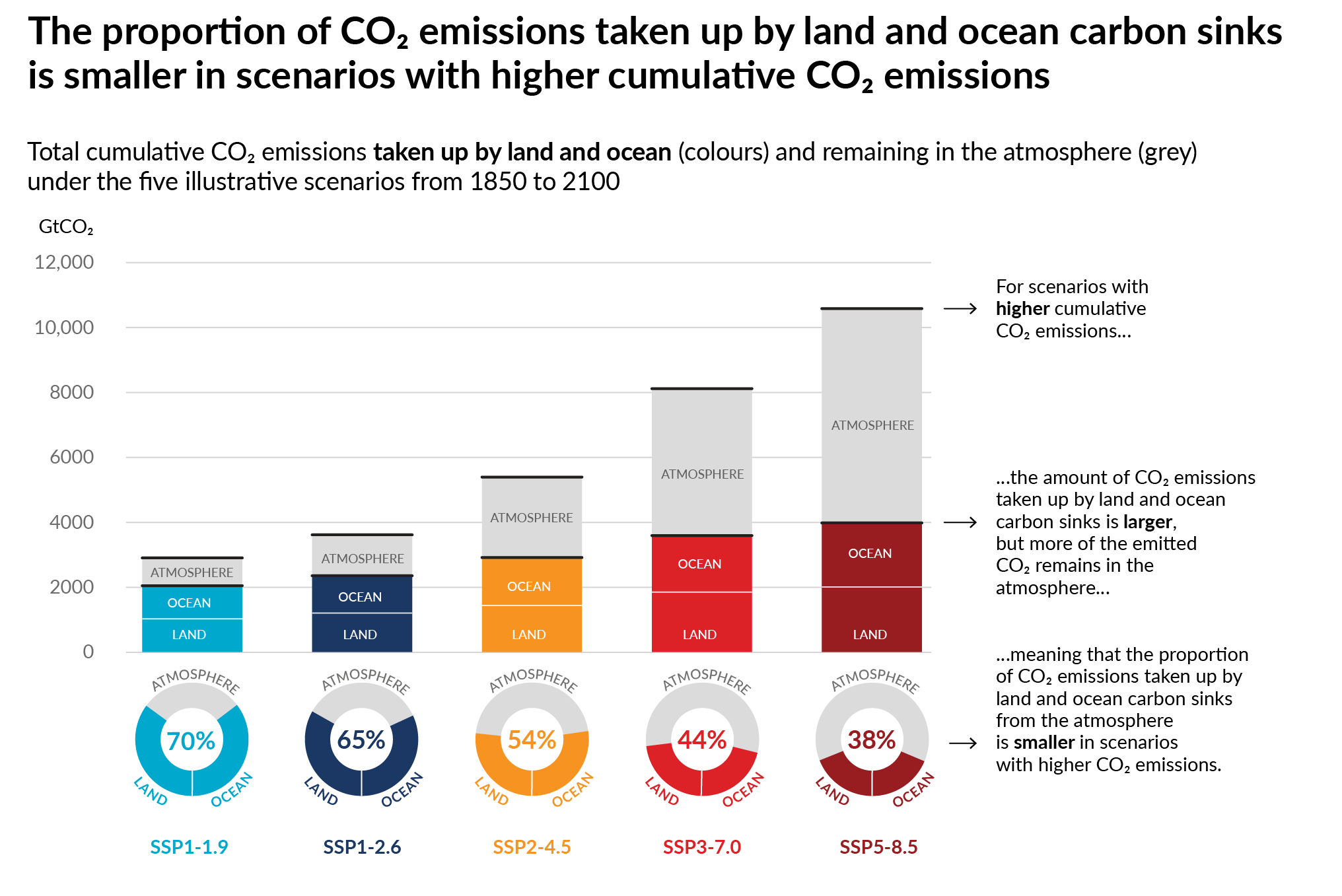 Figure SPM.7 | Cumulative anthropogenic CO2 emissions taken up by land and ocean sinks by 2100 under the five illustrative scenarios
The cumulative anthropogenic (human-caused) carbon dioxide (CO2) emissions taken up by the land and ocean sinks under the five illustrative scenarios (SSP1-1.9, SSP1-2.6, SSP2-4.5, SSP3-7.0 and SSP5-8.5) are simulated from 1850 to 2100 by Coupled Model Intercomparison Project Phase 6 (CMIP6) climate models in the concentration-driven simulations. Land and ocean carbon sinks respond to past, current and future emissions; therefore, cumulative sinks from 1850 to 2100 are presented here. During the historical period (1850–2019) the observed land and ocean sink took up 1430 GtCO2 (59% of the emissions).
The bar chart illustrates the projected amount of cumulative anthropogenic CO2 emissions (GtCO2) between 1850 and 2100 remaining in the atmosphere (grey part) and taken up by the land and ocean (coloured part) in the year 2100. The doughnut chart illustrates the proportion of the cumulative anthropogenic CO2 emissions taken up by the land and ocean sinks and remaining in the atmosphere in the year 2100. Values in % indicate the proportion of the cumulative anthropogenic CO2 emissions taken up by the combined land and ocean sinks in the year 2100. The overall anthropogenic carbon emissions are calculated by adding the net global land-use emissions from the CMIP6 scenario database to the other sectoral emissions calculated from climate model runs with prescribed CO2 concentrations. 33Land and ocean CO2 uptake since 1850 is calculated from the net biome productivity on land, corrected for CO2 losses due to land-use change by adding the land-use change emissions, and net ocean CO2 flux. Links to chapters5.2.1; Table 5.1; 5.4.5; Figure 5.25; Box TS.5; Box TS.5, Figure 1
B.5 Many changes due to past and future greenhouse gas emissions are irreversible for centuries to millennia, especially changes in the ocean, ice sheets and global sea level. Expand Figure SPM.8Links to chapters2.3, Cross-Chapter Box 2.4, 4.3, 4.5, 4.7, 5.3, 9.2, 9.4, 9.5, 9.6, Box 9.4
B.5.1 Past GHG emissions since 1750 have committed the global ocean to future warming (high confidence). Over the rest of the 21st century, likely ocean warming ranges from 2–4 (SSP1-2.6) to 4–8 times (SSP5-8.5) the 1971–2018 change. Based on multiple lines of evidence, upper ocean stratification (virtually certain), ocean acidification (virtually certain) and ocean deoxygenation (high confidence) will continue to increase in the 21st century, at rates dependent on future emissions. Changes are irreversible on centennial to millennial time scales in global ocean temperature (very high confidence), deep-ocean acidification (very high confidence) and deoxygenation (medium confidence). Figure SPM.8Links to chapters4.3, 4.5, 4.7, 5.3, 9.2, TS.2.4
B.5.2 Mountain and polar glaciers are committed to continue melting for decades or centuries (very high confidence). Loss of permafrost carbon following permafrost thaw is irreversible at centennial time scales (high confidence). Continued ice loss over the 21st century is virtually certain for the Greenland Ice Sheet and likely for the Antarctic Ice Sheet. There is high confidence that total ice loss from the Greenland Ice Sheet will increase with cumulative emissions. There is limited evidence for low-likelihood, high-impact outcomes (resulting from ice-sheet instability processes characterized by deep uncertainty and in some cases involving tipping points) that would strongly increase ice loss from the Antarctic Ice Sheet for centuries under high GHG emissions scenarios. 34 Links to chapters4.3, 4.7, 5.4, 9.4, 9.5, Box 9.4, Box TS.1, TS.2.5
B.5.3 It is virtually certain that global mean sea level will continue to rise over the 21st century. Relative to 1995–2014, the likely global mean sea level rise by 2100 is 0.28–0.55 m under the very low GHG emissions scenario (SSP1-1.9); 0.32–0.62 m under the low GHG emissions scenario (SSP1-2.6); 0.44–0.76 m under the intermediate GHG emissions scenario (SSP2-4.5); and 0.63–1.01 m under the very high GHG emissions scenario (SSP5-8.5); and by 2150 is 0.37–0.86 m under the very low scenario (SSP1-1.9); 0.46–0.99 m under the low scenario (SSP1-2.6); 0.66–1.33 m under the intermediate scenario (SSP2-4.5); and 0.98–1.88 m under the very high scenario (SSP5-8.5) (medium confidence). 35Global mean sea level rise above the likely range – approaching 2 m by 2100 and 5 m by 2150 under a very high GHG emissions scenario (SSP5-8.5) (low confidence) – cannot be ruled out due to deep uncertainty in ice-sheet processes. Figure SPM.8Links to chapters4.3, 9.6, Box 9.4, Box TS.4
B.5.4 In the longer term, sea level is committed to rise for centuries to millennia due to continuing deep-ocean warming and ice-sheet melt and will remain elevated for thousands of years (high confidence). Over the next 2000 years, global mean sea level will rise by about 2 to 3 m if warming is limited to 1.5°C, 2 to 6 m if limited to 2°C and 19 to 22 m with 5°C of warming, and it will continue to rise over subsequent millennia (low confidence). Projections of multi-millennial global mean sea level rise are consistent with reconstructed levels during past warm climate periods: likely 5–10 m higher than today around 125,000 years ago, when global temperatures were very likely 0.5°C–1.5°C higher than 1850–1900; and very likely 5–25 m higher roughly 3 million years ago, when global temperatures were 2.5°C–4°C higher (medium confidence). Links to chapters2.3, Cross-Chapter Box 2.4, 9.6, Box TS.2, Box TS.4, Box TS.9
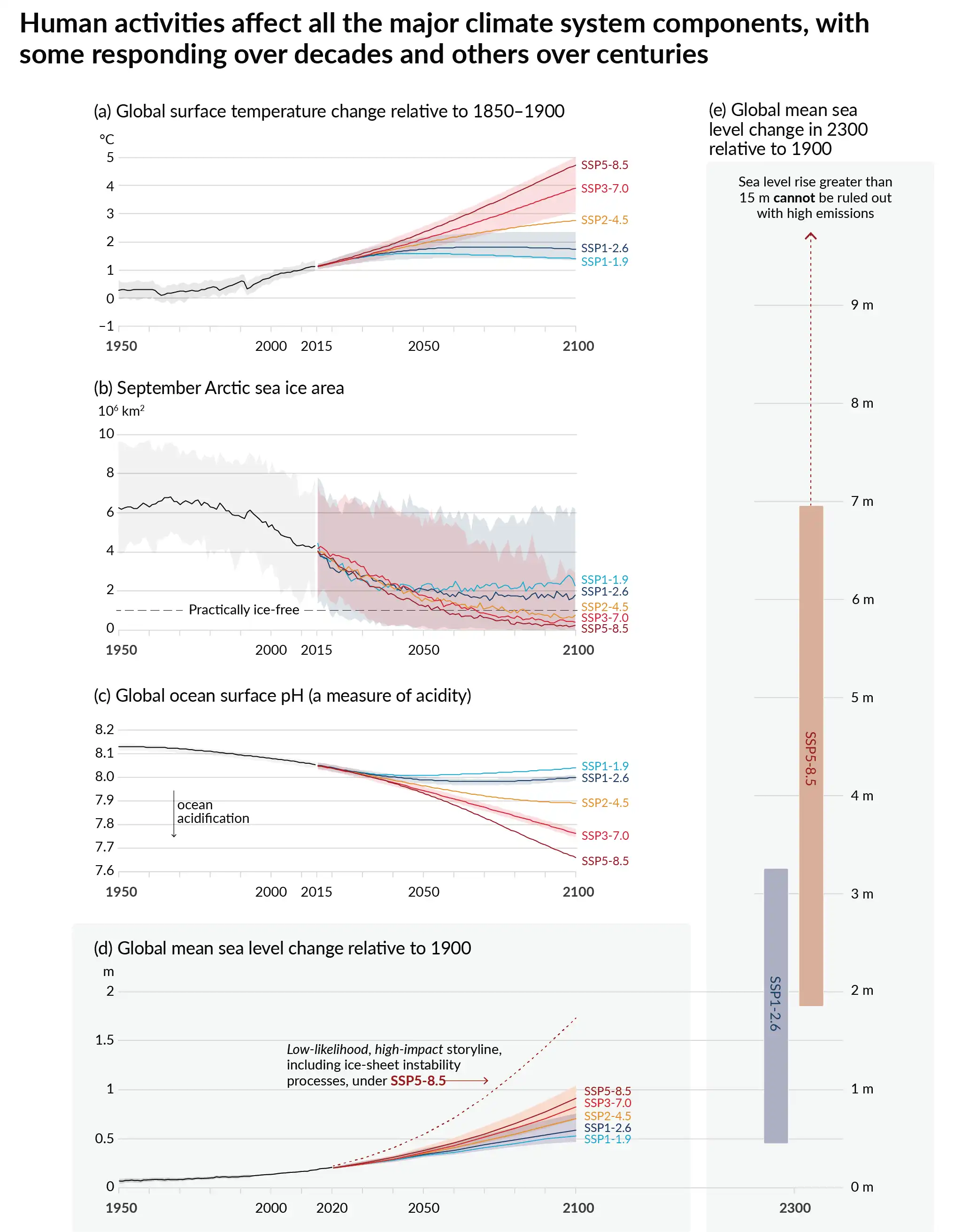
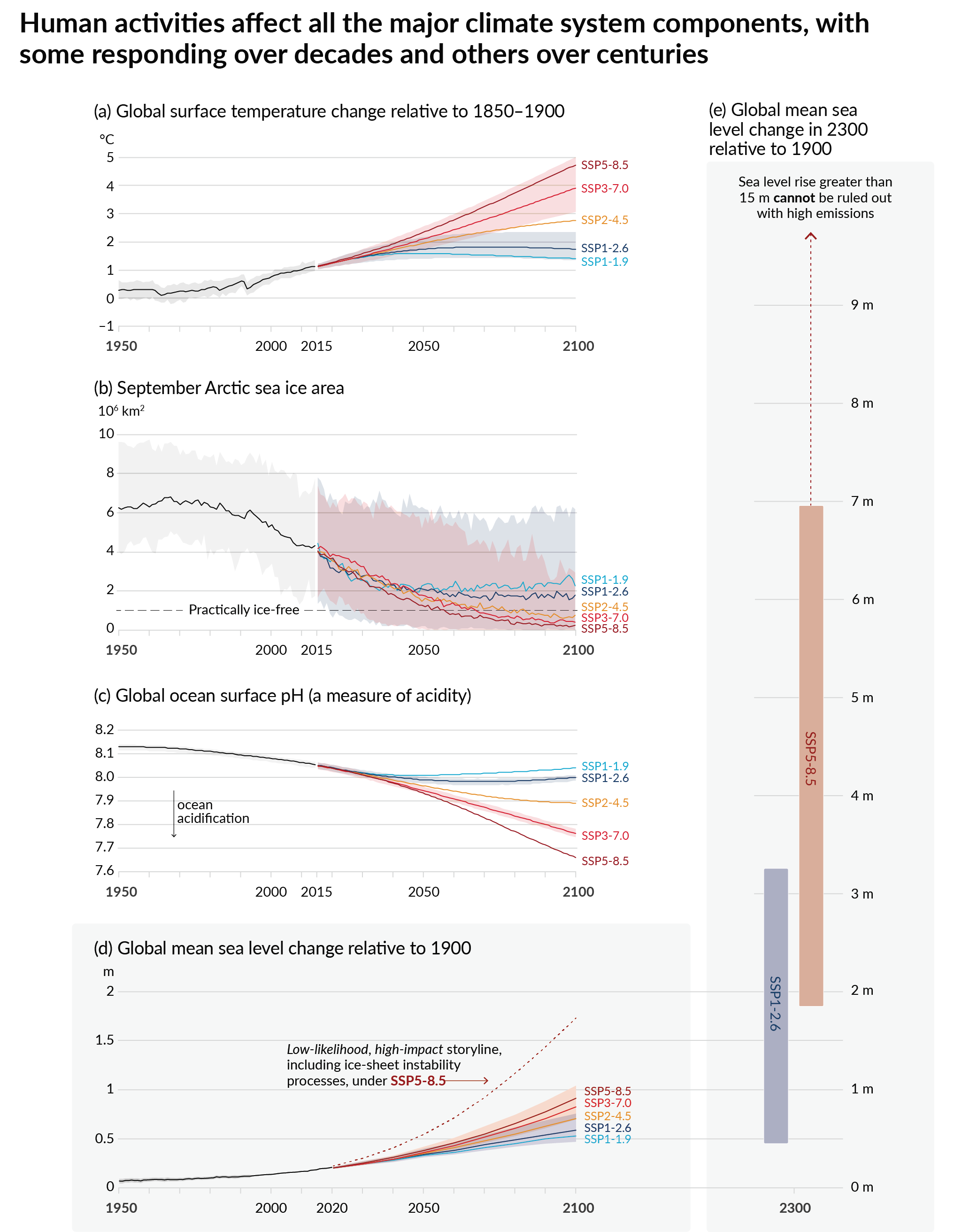 Figure SPM.8 | Selected indicators of global climate change under the five illustrative scenarios used in this Report
 The projections for each of the five scenarios are shown in colour. Shades represent uncertainty ranges – more detail is provided for each panel below. The black curves represent the historical simulations (panels a, b, c) or the observations (panel d). Historical values are included in all graphs to provide context for the projected future changes.
Panel (a) Global surface temperature changes in °C relative to 1850–1900. These changes were obtained by combining Coupled Model Intercomparison Project Phase 6 (CMIP6) model simulations with observational constraints based on past simulated warming, as well as an updated assessment of equilibrium climate sensitivity (see Box SPM.1). Changes relative to 1850–1900 based on 20-year averaging periods are calculated by adding 0.85°C (the observed global surface temperature increase from 1850–1900 to 1995–2014) to simulated changes relative to 1995–2014. Very likely ranges are shown for SSP1-2.6 and SSP3-7.0.
Panel (b) September Arctic sea ice area in 106km2 based on CMIP6 model simulations. Very likely ranges are shown for SSP1-2.6 and SSP3-7.0. The Arctic is projected to be practically ice-free near mid-century under intermediate and high GHG emissions scenarios.
Panel (c) Global ocean surface pH (a measure of acidity) based on CMIP6 model simulations. Very likely ranges are shown for SSP1-2.6 and SSP3-7.0.
Panel (d) Global mean sea level change in metres, relative to 1900. The historical changes are observed (from tide gauges before 1992 and altimeters afterwards), and the future changes are assessed consistently with observational constraints based on emulation of CMIP, ice-sheet, and glacier models. Likely ranges are shown for SSP1-2.6 and SSP3-7.0. Onlylikely ranges are assessed for sea level changes due to difficulties in estimating the distribution of deeply uncertain processes. The dashed curve indicates the potential impact of these deeply uncertain processes. It shows the 83rd percentile of SSP5-8.5 projections that include low-likelihood, high-impact ice-sheet processes that cannot be ruled out; because oflow confidence in projections of these processes, this curve does not constitute part of a likely range. Changes relative to 1900 are calculated by adding 0.158 m (observed global mean sea level rise from 1900 to 1995–2014) to simulated and observed changes relative to 1995–2014.
Panel (e) Global mean sea level change at 2300 in metres relative to 1900. Only SSP1-2.6 and SSP5-8.5 are projected at 2300, as simulations that extend beyond 2100 for the other scenarios are too few for robust results. The 17th–83rd percentile ranges are shaded. The dashed arrow illustrates the 83rd percentile of SSP5-8.5 projections that include low-likelihood, high-impact ice-sheet processes that cannot be ruled out.
Panels (b) and (c) are based on single simulations from each model, and so include a component of internal variability. Panels (a), (d) and (e) are based on long-term averages, and hence the contributions from internal variability are small. Links to chapters4.3; Figures 4.2, 4.8, 4.11; 9.6; Figure 9.27; Figures TS.8 and TS.11; Box TS.4 Figure 1
C. Climate Information for Risk Assessment and Regional Adaptation
C.1 Natural drivers and internal variability will modulate human-caused changes, especially at regional scales and in the near term, with little effect on centennial global warming. These modulations are important to consider in planning for the full range of possible changes. ExpandLinks to chapters1.4, 2.2, 3.3, Cross-Chapter Box 3.1, 4.4, 4.6, Cross-Chapter Box 4.1, Box 7.2, 8.3, 8.5, 9.2, 10.3, 10.4, 10.6, 11.3, 12.5, Atlas.4, Atlas.5, Atlas.8, Atlas.9, Atlas.10, Atlas.11, Cross-Chapter Box Atlas.2
C.1.1 The historical global surface temperature record highlights that decadal variability has both enhanced and masked underlying human-caused long-term changes, and this variability will continue into the future (very high confidence). For example, internal decadal variability and variations in solar and volcanic drivers partially masked human-caused surface global warming during 1998–2012, with pronounced regional and seasonal signatures (high confidence). Nonetheless, the heating of the climate system continued during this period, as reflected in both the continued warming of the global ocean (very high confidence) and in the continued rise of hot extremes over land (medium confidence). Figure SPM.1Links to chapters1.4, 3.3, Cross-Chapter Box 3.1, 4.4, Box 7.2, 9.2, 11.3, Cross-Section Box TS.1
C.1.2 Projected human-caused changes in mean climate and climatic impact-drivers (CIDs), 36 including extremes, will be either amplified or attenuated by internal variability (high confidence). 37Near-term cooling at any particular location with respect to present climate could occur and would be consistent with the global surface temperature increase due to human influence (high confidence). Links to chapters1.4, 4.4, 4.6, 10.4, 11.3, 12.5, Atlas.5, Atlas.10, Atlas.11, TS.4.2
C.1.3 Internal variability has largely been responsible for the amplification and attenuation of the observed human-caused decadal-to-multi-decadal mean precipitation changes in many land regions (high confidence). At global and regional scales, near-term changes in monsoons will be dominated by the effects of internal variability (medium confidence). In addition to the influence of internal variability, near-term projected changes in precipitation at global and regional scales are uncertain because of model uncertainty and uncertainty in forcings from natural and anthropogenic aerosols (medium confidence). Links to chapters1.4, 4.4, 8.3, 8.5, 10.3, 10.4, 10.5, 10.6, Atlas.4, Atlas.8, Atlas.9, Atlas.10, Atlas.11, Cross-Chapter Box Atlas.2, TS.4.2, Box TS.6, Box TS.13
C.1.4 Based on paleoclimate and historical evidence, it is likely that at least one large explosive volcanic eruption would occur during the 21st century. 38Such an eruption would reduce global surface temperature and precipitation, especially over land, for one to three years, alter the global monsoon circulation, modify extreme precipitation and change many CIDs (medium confidence). If such an eruption occurs, this would therefore temporarily and partially mask human-caused climate change. Links to chapters2.2, 4.4, Cross-Chapter Box 4.1, 8.5, TS.2.1
C.2 With further global warming, every region is projected to increasingly experience concurrent and multiple changes in climatic impact-drivers. Changes in several climatic impact-drivers would be more widespread at 2°C compared to 1.5°C global warming and even more widespread and/or pronounced for higher warming levels. Expand Table SPM.1 Figure SPM.9Links to chapters8.2, 9.3, 9.5, 9.6, Box 10.3, 11.3, 11.4, 11.5, 11.6, 11.7, 11.9, Box 11.3, Box 11.4, Cross-Chapter Box 11.1, 12.2, 12.3, 12.4, 12.5, Cross-Chapter Box 12.1, Atlas.4, Atlas.5, Atlas.6, Atlas.7, Atlas.8, Atlas.9, Atlas.10, Atlas.11
C.2.1 All regions39 are projected to experience further increases in hot climatic impact-drivers (CIDs) and decreases in cold CIDs (high confidence). Further decreases are projected in permafrost; snow, glaciers and ice sheets; and lake and Arctic sea ice (medium to high confidence). 40 These changes would be larger at 2°C global warming or above than at 1.5°C (high confidence). For example, extreme heat thresholds relevant to agriculture and health are projected to be exceeded more frequently at higher global warming levels (high confidence). Table SPM.1 Figure SPM.9Links to chapters9.3, 9.5, 11.3, 11.9, Cross-Chapter Box 11.1, 12.3, 12.4, 12.5, Cross-Chapter Box 12.1, Atlas.4, Atlas.5, Atlas.6, Atlas.7, Atlas.8, Atlas.9, Atlas.10, Atlas.11, TS.4.3
C.2.2 At 1.5°C global warming, heavy precipitation and associated flooding are projected to intensify and be more frequent in most regions in Africa and Asia (high confidence), North America (medium to high confidence)40 and Europe (medium confidence). Also, more frequent and/or severe agricultural and ecological droughts are projected in a few regions in all inhabited continents except Asia compared to 1850–1900 (medium confidence); increases in meteorological droughts are also projected in a few regions (medium confidence). A small number of regions are projected to experience increases or decreases in mean precipitation (medium confidence). Table SPM.1Links to chapters11.4, 11.5, 11.6, 11.9, Atlas.4, Atlas.5, Atlas.7, Atlas.8, Atlas.9, Atlas.10, Atlas.11, TS.4.3
C.2.3 At 2°C global warming and above, the level of confidence in and the magnitude of the change in droughts and heavy and mean precipitation increase compared to those at 1.5°C. Heavy precipitation and associated flooding events are projected to become more intense and frequent in the Pacific Islands and across many regions of North America and Europe (medium to high confidence). 40 These changes are also seen in some regions in Australasia and Central and South America (medium confidence). Several regions in Africa, South America and Europe are projected to experience an increase in frequency and/or severity of agricultural and ecological droughts with medium to high confidence;40 increases are also projected in Australasia, Central and North America, and the Caribbean with medium confidence. A small number of regions in Africa, Australasia, Europe and North America are also projected to be affected by increases in hydrological droughts, and several regions are projected to be affected by increases or decreases in meteorological droughts, with more regions displaying an increase (medium confidence). Mean precipitation is projected to increase in all polar, northern European and northern North American regions, most Asian regions and two regions of South America (high confidence). Table SPM.1 Figure SPM.5, Figure SPM.6 Figure SPM.9Links to chapters11.4, 11.6, 11.9, Cross-Chapter Box 11.1, 12.4, 12.5, Cross-Chapter Box 12.1, Atlas.5, Atlas.7, Atlas.8, Atlas.9, Atlas.11, TS.4.3
C.2.4 More CIDs across more regions are projected to change at 2°C and above compared to 1.5°C global warming (high confidence). Region-specific changes include intensification of tropical cyclones and/or extratropical storms (medium confidence), increases inriver floods (medium to high confidence), 40 reductions in mean precipitation and increases in aridity (medium to high confidence), 40 and increases in fire weather (medium to high confidence). 40 There is low confidence in most regions in potential future changes in other CIDs, such as hail, ice storms, severe storms, dust storms, heavy snowfall and landslides. Table SPM.1 Figure SPM.9Links to chapters11.7, 11.9, Cross-Chapter Box 11.1, 12.4, 12.5, Cross-Chapter Box 12.1, Atlas.4, Atlas.6, Atlas.7, Atlas.8, Atlas.10, TS.4.3.1, TS.4.3.2, TS.5
C.2.5 It is very likely to virtually certain40that regional mean relative sea level rise will continue throughout the 21st century, except in a few regions with substantial geologic land uplift rates. Approximately two-thirds of the global coastline has a projected regional relative sea level rise within ±20% of the global mean increase (medium confidence). Due to relative sea level rise, extreme sea level events that occurred once per century in the recent past are projected to occur at least annually at more than half of all tide gauge locations by 2100 (high confidence). Relative sea level rise contributes to increases in the frequency and severity of coastal flooding in low-lying areas and to coastal erosion along most sandy coasts (high confidence). Figure SPM.9Links to chapters9.6, 12.4, 12.5, Cross-Chapter Box 12.1, Box TS.4, TS.4.3
C.2.6 Cities intensify human-induced warming locally, and further urbanization together with more frequent hot extremes will increase the severity of heatwaves (very high confidence). Urbanization also increases mean and heavy precipitation over and/or downwind of cities (medium confidence) and resulting runoff intensity (high confidence). In coastal cities, the combination of more frequent extreme sea level events (due to sea level rise and storm surge) and extreme rainfall/riverflow events will make flooding more probable (high confidence). Links to chapters8.2, Box 10.3, 11.3, 12.4, Box TS.14
C.2.7 Many regions are projected to experience an increase in the probability of compound events with higher global warming (high confidence). In particular, concurrent heatwaves and droughts are likely to become more frequent. Concurrent extremes at multiple locations, including in crop-producing areas, become more frequent at 2°C and above compared to 1.5°C global warming (high confidence). Table SPM.1Links to chapters11.8, Box 11.3, Box 11.4, 12.3, 12.4, Cross-Chapter Box 12.1, TS.4.3
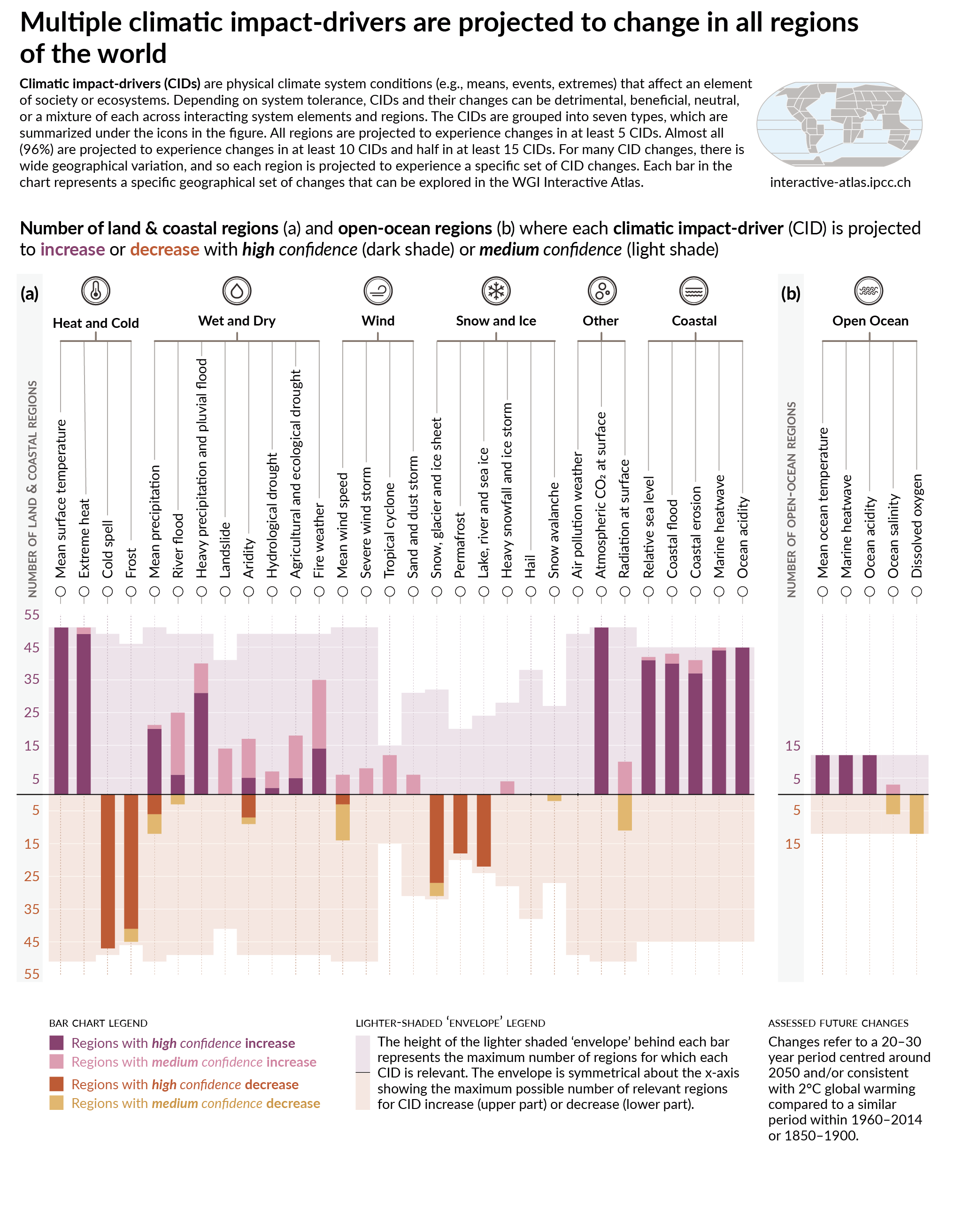
Figure SPM.9 | Synthesis of the number of AR6 WGI reference regions where climatic impact-drivers are projected to change
A total of 35 climatic impact-drivers (CIDs) grouped into seven types are shown: heat and cold; wet and dry; wind; snow and ice; coastal; open ocean; and other. For each CID, the bar in the graph below displays the number of AR6 WGI reference regions where it is projected to change. The colours represent the direction of change and the level of confidence in the change: purple indicates an increase while brown indicates a decrease; darker and lighter shades refer to high and medium confidence, respectively. Lighter background colours represent the maximum number of regions for which each CID is broadly relevant.
Panel (a) shows the 30 CIDs relevant to the land and coastal regions, while panel (b) shows the five CIDs relevant to the open-ocean regions. Marine heatwaves and ocean acidity are assessed for coastal ocean regions in panel (a) and for open-ocean regions in panel (b). Changes refer to a 20–30-year period centred around 2050 and/or consistent with 2°C global warming compared to a similar period within 1960–2014, except for hydrological drought and agricultural and ecological drought, which is compared to 1850–1900. Definitions of the regions are provided in Sections 12.4 and Atlas.1 and the Interactive Atlas (see https://interactive-atlas.ipcc.ch/). Table SPM.1Links to chapters11.9, 12.2, 12.4, Atlas.1, Table TS.5, Figures TS.22 and TS.25
C.3 Low-likelihood outcomes, such as ice-sheet collapse, abrupt ocean circulation changes, some compound extreme events, and warming substantially larger than the assessedvery likely range of future warming, cannot be ruled out and are part of risk assessment. Expand Table SPM.1Links to chapters1.4, Cross-Chapter Box 1.3, 4.3, 4.4, 4.8, Cross-Chapter Box 4.1, 8.6, 9.2, Box 9.4, 11.8, Box 11.2, Cross-Chapter Box 12.1
C.3.1 If global warming exceeds the assessed very likely range for a given GHG emissions scenario, including low GHG emissions scenarios, global and regional changes in many aspects of the climate system, such as regional precipitation and other CIDs, would also exceed their assessed very likely ranges (high confidence). Such low-likelihood, high-warming outcomes are associated with potentially very large impacts, such as through more intense and more frequent heatwaves and heavy precipitation, and high risks for human and ecological systems, particularly for high GHG emissions scenarios. Table SPM.1Links to chaptersCross-Chapter Box 1.3, 4.3, 4.4, 4.8, Box 9.4, Box 11.2, Cross-Chapter Box 12.1, TS.1.4, Box TS.3, Box TS.4
C.3.2 Low-likelihood, high-impact outcomes34could occur at global and regional scales even for global warming within the very likely range for a given GHG emissions scenario. The probability of low-likelihood, high-impact outcomes increases with higher global warming levels (high confidence). Abrupt responses and tipping points of the climate system, such as strongly increased Antarctic ice-sheet melt and forest dieback, cannot be ruled out (high confidence). Table SPM.1Links to chapters1.4, 4.3, 4.4, 4.8, 5.4, 8.6, Box 9.4, Cross-Chapter Box 12.1, TS.1.4, TS.2.5, Box TS.3, Box TS.4, Box TS.9
C.3.3 If global warming increases, some compound extreme events18 with low likelihood in past and current climate will become more frequent, and there will be a higher likelihood that events with increased intensities, durations and/or spatial extents unprecedented in the observational record will occur (high confidence). Links to chapters11.8, Box 11.2, Cross-Chapter Box 12.1, Box TS.3, Box TS.9
C.3.4 The Atlantic Meridional Overturning Circulation is very likely to weaken over the 21st century for all emissions scenarios. While there is high confidence in the 21st century decline, there is onlylow confidence in the magnitude of the trend. There is medium confidence that there will not be an abrupt collapse before 2100. If such a collapse were to occur, it would very likely cause abrupt shifts in regional weather patterns and water cycle, such as a southward shift in the tropical rain belt, weakening of the African and Asian monsoons and strengthening of Southern Hemisphere monsoons, and drying in Europe. Links to chapters4.3, 8.6, 9.2, TS2.4, Box TS.3
C.3.5 Unpredictable and rare natural events not related to human influence on climate may lead to low-likelihood, high-impact outcomes. For example, a sequence of large explosive volcanic eruptions within decades has occurred in the past, causing substantial global and regional climate perturbations over several decades. Such events cannot be ruled out in the future, but due to their inherent unpredictability they are not included in the illustrative set of scenarios referred to in this Report Box SPM.1Links to chapters2.2, Cross-Chapter Box 4.1, Box TS.3
D. Limiting Future Climate Change
D.1 From a physical science perspective, limiting human-induced global warming to a specific level requires limiting cumulative CO2 emissions, reaching at least net zero CO2 emissions, along with strong reductions in other greenhouse gas emissions. Strong, rapid and sustained reductions in CH4 emissions would also limit the warming effect resulting from declining aerosol pollution and would improve air quality. Expand Figure SPM.10 Table SPM.2Links to chapters3.3, 4.6, 5.1, 5.2, 5.4, 5.5, 5.6, Box 5.2, Cross-Chapter Box 5.1, 6.7, 7.6, 9.6
D.1.1 This Report reaffirms with high confidence the AR5 finding that there is a near-linear relationship between cumulative anthropogenic CO2 emissions and the global warming they cause. Each 1000 GtCO2 of cumulative CO2 emissions is assessed to likely cause a 0.27°C to 0.63°C increase in global surface temperature with a best estimate of 0.45°C. 41 This is a narrower range compared to AR5 and SR1.5. This quantity is referred to as the transient climate response to cumulative CO2 emissions (TCRE). This relationship implies that reaching net zero anthropogenic CO2 emissions42 is a requirement to stabilize human-induced global temperature increase at any level, but that limiting global temperature increase to a specific level would imply limiting cumulative CO2 emissions to within a carbon budget. 43 Figure SPM.10Links to chapters5.4, 5.5, TS.1.3, TS.3.3, Box TS.5
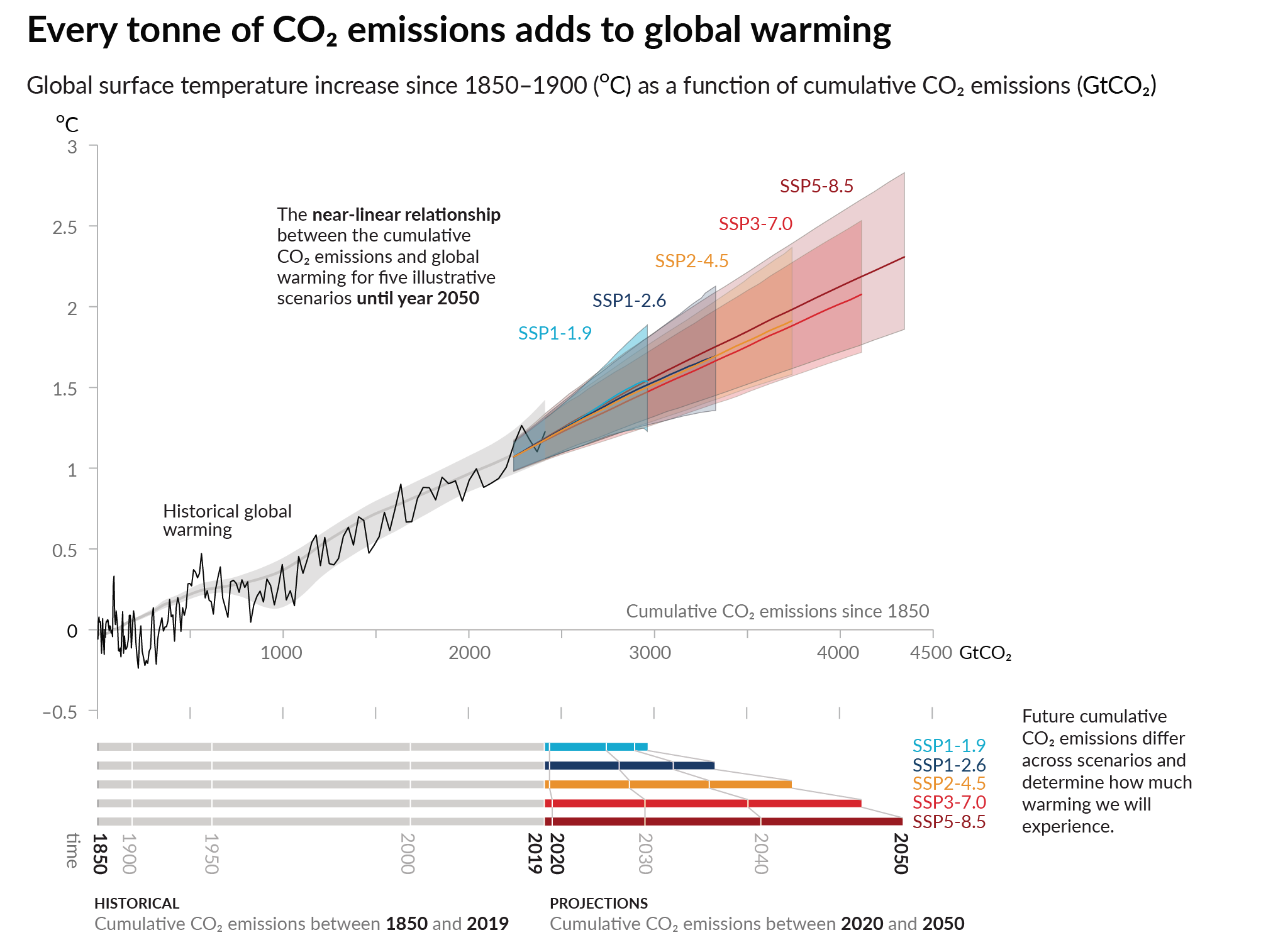
Figure SPM.10 | Near-linear relationship between cumulative CO2 emissions and the increase in global surface temperature
Top panel: Historical data (thin black line) shows observed global surface temperature increase in °C since 1850–1900 as a function of historical cumulative carbon dioxide (CO2) emissions in GtCO2 from 1850 to 2019. The grey range with its central line shows a corresponding estimate of the historical human-caused surface warming (see Figure SPM.2). Coloured areas show the assessed very likely range of global surface temperature projections, and thick coloured central lines show the median estimate as a function of cumulative CO2 emissions from 2020 until year 2050 for the set of illustrative scenarios (SSP1-1.9, SSP1-2.6, SSP2-4.5, SSP3-7.0, and SSP5-8.5; see Figure SPM.4). Projections use the cumulative CO2 emissions of each respective scenario, and the projected global warming includes the contribution from all anthropogenic forcers. The relationship is illustrated over the domain of cumulative CO2 emissions for which there is high confidence that the transient climate response to cumulative CO2 emissions (TCRE) remains constant, and for the time period from 1850 to 2050 over which global CO2 emissions remain net positive under all illustrative scenarios, as there is limited evidence supporting the quantitative application of TCRE to estimate temperature evolution under net negative CO2 emissions.
Bottom panel: Historical and projected cumulative CO2 emissions in GtCO2 for the respective scenarios. Links to chaptersSection 5.5, Figure 5.31, Figure TS.18
D.1.2 Over the period 1850–2019, a total of 2390 ± 240 (likely range) GtCO2 of anthropogenic CO2 was emitted. Remaining carbon budgets have been estimated for several global temperature limits and various levels of probability, based on the estimated value of TCRE and its uncertainty, estimates of historical warming, variations in projected warming from non-CO2 emissions, climate system feedbacks such as emissions from thawing permafrost, and the global surface temperature change after global anthropogenic CO2 emissions reach net zero. Table SPM.2Links to chapters5.1, 5.5, Box 5.2, TS.3.3
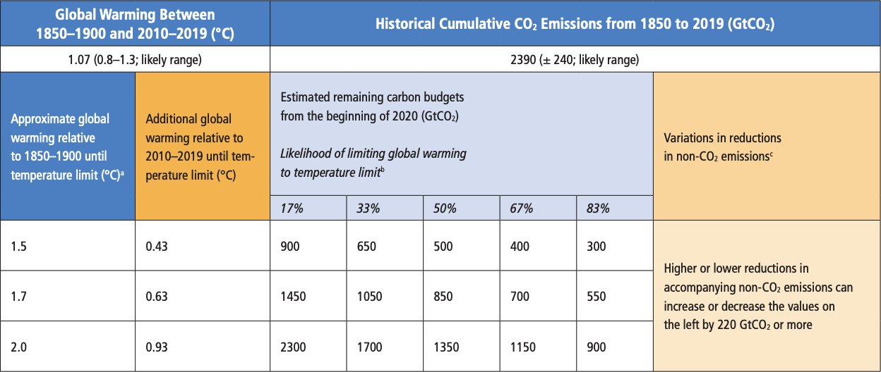
aValues at each 0.1°C increment of warming are available in Tables TS.3 and 5.8.
bThis likelihood is based on the uncertainty in transient climate response to cumulative CO2 emissions (TCRE) and additional Earth system feedbacks and provides the probability that global warming will not exceed the temperature levels provided in the two left columns. Uncertainties related to historical warming (±550 GtCO2) and non-CO2 forcing and response (±220 GtCO2) are partially addressed by the assessed uncertainty in TCRE, but uncertainties in recent emissions since 2015 (±20 GtCO2) and the climate response after net zero CO2 emissions are reached (±420 GtCO2) are separate.
cRemaining carbon budget estimates consider the warming from non-CO2 drivers as implied by the scenarios assessed in SR1.5. The Working Group III Contribution to AR6 will assess mitigation of non-CO2 emissions.
D.1.3 Several factors that determine estimates of the remaining carbon budget have been re-assessed, and updates to these factors since SR1.5 are small. When adjusted for emissions since previous reports, estimates of remaining carbon budgets are therefore of similar magnitude compared to SR1.5 but larger compared to AR5 due to methodological improvements. 44 Table SPM.2Links to chapters5.5, Box 5.2, TS.3.3
D.1.4 Anthropogenic CO2 removal (CDR) has the potential to remove CO2 from the atmosphere and durably store it in reservoirs (high confidence). CDR aims to compensate for residual emissions to reach net zero CO2 or net zero GHG emissions or, if implemented at a scale where anthropogenic removals exceed anthropogenic emissions, to lower surface temperature. CDR methods can have potentially wide-ranging effects on biogeochemical cycles and climate, which can either weaken or strengthen the potential of these methods to remove CO2 and reduce warming, and can also influence water availability and quality, food production and biodiversity45 (high confidence). Links to chapters5.6, Cross-Chapter Box 5.1, TS.3.3
D.1.5 Anthropogenic CO2 removal (CDR) leading to global net negative emissions would lower the atmospheric CO2 concentration and reverse surface ocean acidification (high confidence). Anthropogenic CO2 removals and emissions are partially compensated by CO2 release and uptake respectively, from or to land and ocean carbon pools (very high confidence). CDR would lower atmospheric CO2 by an amount approximately equal to the increase from an anthropogenic emission of the same magnitude (high confidence). The atmospheric CO2 decrease from anthropogenic CO2 removals could be up to 10% less than the atmospheric CO2 increase from an equal amount of CO2 emissions, depending on the total amount of CDR (medium confidence). Links to chapters5.3, 5.6, TS.3.3
D.1.6 If global net negative CO2 emissions were to be achieved and be sustained, the global CO2 -induced surface temperature increase would be gradually reversed but other climate changes would continue in their current direction for decades to millennia (high confidence). For instance, it would take several centuries to millennia for global mean sea level to reverse course even under large net negative CO2 emissions (high confidence). Links to chapters4.6, 9.6, TS.3.3
D.1.7 In the five illustrative scenarios, simultaneous changes in CH4, aerosol and ozone precursor emissions, which also contribute to air pollution, lead to a net global surface warming in the near and long term (high confidence). In the long term, this net warming is lower in scenarios assuming air pollution controls combined with strong and sustained CH4 emissions reductions (high confidence). In the low and very low GHG emissions scenarios, assumed reductions in anthropogenic aerosol emissions lead to a net warming, while reductions in CH4 and other ozone precursor emissions lead to a net cooling. Because of the short lifetime of both CH4 and aerosols, these climate effects partially counterbalance each other, and reductions in CH4 emissions also contribute to improved air quality by reducing global surface ozone (high confidence). Figure SPM.2 Box SPM.1Links to chapters6.7, Box TS.7
D.1.8 Achieving global net zero CO2 emissions, with anthropogenic CO2 emissions balanced by anthropogenic removals of CO2, is a requirement for stabilizing CO2 -induced global surface temperature increase. This is different from achieving net zero GHG emissions, where metric-weighted anthropogenic GHG emissions equal metric-weighted anthropogenic GHG removals. For a given GHG emissions pathway, the pathways of individual GHGs determine the resulting climate response, 46 whereas the choice of emissions metric47used to calculate aggregated emissions and removals of different GHGs affects what point in time the aggregated GHGs are calculated to be net zero. Emissions pathways that reach and sustain net zero GHG emissions defined by the 100-year global warming potential are projected to result in a decline in surface temperature after an earlier peak (high confidence). Links to chapters4.6, 7.6, Box 7.3, TS.3.3
D.2 Scenarios with very low or low GHG emissions (SSP1-1.9 and SSP1-2.6) lead within years to discernible effects on greenhouse gas and aerosol concentrations and air quality, relative to high and very high GHG emissions scenarios (SSP3-7.0 or SSP5-8.5). Under these contrasting scenarios, discernible differences in trends of global surface temperature would begin to emerge from natural variability within around 20 years, and over longer time periods for many other climatic impact-drivers (high confidence). Expand Figures SPM.8, SPM.10Links to chapters4.6, 6.6, 6.7, Cross-Chapter Box 6.1, 9.6, 11.2, 11.4, 11.5, 11.6, Cross-Chapter Box 11.1, 12.4, 12.5
D.2.1 Emissions reductions in 2020 associated with measures to reduce the spread of COVID-19 led to temporary but detectable effects on air pollution (high confidence) and an associated small, temporary increase in total radiative forcing, primarily due to reductions in cooling caused by aerosols arising from human activities (medium confidence). Global and regional climate responses to this temporary forcing are, however, undetectable above natural variability (high confidence). Atmospheric CO2 concentrations continued to rise in 2020, with no detectable decrease in the observed CO2 growth rate (medium confidence). 48 Links to chaptersCross-Chapter Box 6.1, TS.3.3
D.2.2 Reductions in GHG emissions also lead to air quality improvements. However, in the near term, 49even in scenarios with strong reduction of GHGs, as in the low and very low GHG emissions scenarios (SSP1-2.6 and SSP1-1.9), these improvements are not sufficient in many polluted regions to achieve air quality guidelines specified by the World Health Organization (high confidence). Scenarios with targeted reductions of air pollutant emissions lead to more rapid improvements in air quality within years compared to reductions in GHG emissions only, but from 2040, further improvements are projected in scenarios that combine efforts to reduce air pollutants as well as GHG emissions, with the magnitude of the benefit varying between regions (high confidence). Links to chapters6.6, 6.7, Box TS.7.
D.2.3 Scenarios with very low or low GHG emissions (SSP1-1.9 and SSP1-2.6) would have rapid and sustained effects to limit human-caused climate change, compared with scenarios with high or very high GHG emissions (SSP3-7.0 or SSP5-8.5), but early responses of the climate system can be masked by natural variability. For global surface temperature, differences in 20-year trends would likely emerge during the near term under a very low GHG emissions scenario (SSP1-1.9), relative to a high or very high GHG emissions scenario (SSP3-7.0 or SSP5-8.5). The response of many other climate variables would emerge from natural variability at different times later in the 21st century (high confidence). Figure SPM.8 Figure SPM.10Links to chapters4.6, Cross-Section Box TS.1
D.2.4 Scenarios with very low and low GHG emissions (SSP1-1.9 and SSP1-2.6) would lead to substantially smaller changes in a range of CIDs36beyond 2040 than under high and very high GHG emissions scenarios (SSP3-7.0 and SSP5-8.5). By the end of the century, scenarios with very low and low GHG emissions would strongly limit the change of several CIDs, such as the increases in the frequency of extreme sea level events, heavy precipitation and pluvial flooding, and exceedance of dangerous heat thresholds, while limiting the number of regions where such exceedances occur, relative to higher GHG emissions scenarios (high confidence). Changes would also be smaller in very low compared to low GHG emissions scenarios, as well as for intermediate (SSP2-4.5) compared to high or very high GHG emissions scenarios (high confidence). Links to chapters9.6, 11.2, 11.3, 11.4, 11.5, 11.6, 11.9, Cross-Chapter Box 11.1, 12.4, 12.5, TS.4.3
1Decision IPCC/XLVI-2.
2The three Special Reports are: Global Warming of 1.5°C: An IPCC Special Report on the impacts of global warming of 1.5°C above pre-industrial levels and related global greenhouse gas emission pathways, in the context of strengthening the global response to the threat of climate change, sustainable development, and efforts to eradicate poverty (SR1.5); Climate Change and Land: An IPCC Special Report on climate change, desertification, land degradation, sustainable land management, food security, and greenhouse gas fluxes in terrestrial ecosystems (SRCCL); IPCC Special Report on the Ocean and Cryosphere in a Changing Climate (SROCC).
3The assessment covers scientific literature accepted for publication by 31 January 2021.
4Each finding is grounded in an evaluation of underlying evidence and agreement. A level of confidence is expressed using five qualifiers: very low, low, medium, high and very high, and typeset in italics, for example, medium confidence. The following terms have been used to indicate the assessed likelihood of an outcome or result: virtually certain 99–100% probability; very likely 90–100%; likely 66–100%; about as likely as not 33–66%; unlikely 0–33%; very unlikely 0–10%; and exceptionally unlikely 0–1%. Additional terms (extremely likely 95–100%; more likely than not >50–100%; and extremely unlikely 0–5%) are also used when appropriate. Assessed likelihood is typeset in italics, for example, very likely . This is consistent with AR5. In this Report, unless stated otherwise, square brackets [x to y] are used to provide the assessed very likely range, or 90% interval.
5The Interactive Atlas is available at https://interactive-atlas.ipcc.ch
6Other GHG concentrations in 2019 were: perfluorocarbons (PFCs) – 109 parts per trillion (ppt) CF4 equivalent; sulphur hexafluoride (SF6) – 10 ppt; nitrogen trifluoride (NF3)– 2 ppt; hydrofluorocarbons (HFCs) – 237 ppt HFC-134a equivalent; other Montreal Protocol gases (mainly chlorofluorocarbons (CFCs) and hydrochlorofluorocarbons (HCFCs)) – 1032 ppt CFC-12 equivalent). Increases from 2011 are 19 ppm for CO2, 63 ppb for CH4 and 8 ppb for N2O.
7Land and ocean are not substantial sinks for other GHGs.
8The term ‘global surface temperature’ is used in reference to both global mean surface temperature and global surface air temperature throughout this SPM. Changes in these quantities are assessed with high confidence to differ by at most 10% from one another, but conflicting lines of evidence lead tolow confidence in the sign (direction) of any difference in long-term trend. Links to chaptersCross-Section Box TS.1
9The period 1850–1900 represents the earliest period of sufficiently globally complete observations to estimate global surface temperature and, consistent with AR5 and SR1.5, is used as an approximation for pre-industrial conditions.
10Since AR5, methodological advances and new datasets have provided a more complete spatial representation of changes in surface temperature, including in the Arctic. These and other improvements have also increased the estimate of global surface temperature change by approximately 0.1°C, but this increase does not represent additional physical warming since AR5.
11The period distinction with A.1.2 arises because the attribution studies consider this slightly earlier period. The observed warming to 2010–2019 is 1.06 [0.88 to 1.21] °C.
12Throughout this SPM, ‘main driver’ means responsible for more than 50% of the change.
13As stated in section B.1, even under the very low emissions scenario SSP1-1.9, temperatures are assessed to remain elevated above those of the most recent decade until at least 2100 and therefore warmer than the century-scale period 6500 years ago.
14As indicated in footnote 12, throughout this SPM, ‘main driver’ means responsible for more than 50% of the change.
15Agricultural and ecological drought (depending on the affected biome): a period with abnormal soil moisture deficit, which results from combined shortage of precipitation and excess evapotranspiration, and during the growing season impinges on crop production or ecosystem function in general (see Annex VII: Glossary). Observed changes in meteorological droughts (precipitation deficits) and hydrological droughts (streamflow deficits) are distinct from those in agricultural and ecological droughts and are addressed in the underlying AR6 material (Chapter 11).
16The combined processes through which water is transferred to the atmosphere from open water and ice surfaces, bare soils and vegetation that make up the Earth’s surface (Glossary).
17The global monsoon is defined as the area in which the annual range (local summer minus local winter) of precipitation is greater than 2.5 mm day–1(Glossary). Global land monsoon precipitation refers to the mean precipitation over land areas within the global monsoon.
18Compound extreme events are the combination of multiple drivers and/or hazards that contribute to societal or environmental risk (Glossary). Examples are concurrent heatwaves and droughts, compound flooding (e.g., a storm surge in combination with extreme rainfall and/or river flow), compound fire weather conditions (i.e., a combination of hot, dry and windy conditions), or concurrent extremes at different locations.
19Cumulative energy increase of 282 [177 to 387] ZJ over 1971–2006 (1 ZJ = 1021 joules).
20Cumulative energy increase of 152 [100 to 205] ZJ over 2006–2018.
21Understanding of climate processes, the instrumental record, paleoclimates and model-based emergent constraints (Glossary).
22Throughout this Report, the five illustrative scenarios are referred to as SSPx-y, where ‘SSPx’ refers to the Shared Socio-economic Pathway or ‘SSP’ describing the socio-economic trends underlying the scenario, and ‘y’ refers to the approximate level of radiative forcing (in watts per square metre, or W m–2) resulting from the scenario in the year 2100. A detailed comparison to scenarios used in earlier IPCC reports is provided in Section TS.1.3, and Sections 1.6 and 4.6. The SSPs that underlie the specific forcing scenarios used to drive climate models are not assessed by WGI. Rather, the SSPx-y labelling ensures traceability to the underlying literature in which specific forcing pathways are used as input to the climate models. IPCC is neutral with regard to the assumptions underlying the SSPs, which do not cover all possible scenarios. Alternative scenarios may be considered or developed.
23Net negative CO2 emissions are reached when anthropogenic removals of CO2 exceed anthropogenic emissions (Glossary).
24Changes in global surface temperature are reported as running 20-year averages, unless stated otherwise.
25SSP1-1.9 and SSP1-2.6 are scenarios that start in 2015 and have very low and low GHG emissions, respectively, and CO2 emissions declining to net zero around or after 2050, followed by varying levels of net negative CO2 emissions.
26 Crossing is defined here as having the assessed global surface temperature change, averaged over a 20-year period, exceed a particular global warming level.
27The AR6 assessment of when a given global warming level is first exceeded benefits from the consideration of the illustrative scenarios, the multiple lines of evidence entering the assessment of future global surface temperature response to radiative forcing, and the improved estimate of historical warming. The AR6 assessment is thus not directly comparable to the SR1.5 SPM, which reportedlikely reaching 1.5°C global warming between 2030 and 2052, from a simple linear extrapolation of warming rates of the recent past. When considering scenarios similar to SSP1-1.9 instead of linear extrapolation, the SR1.5 estimate of when 1.5°C global warming is first exceeded is close to the best estimate reported here.
28Natural variability refers to climatic fluctuations that occur without any human influence, that is, internal variability combined with the response to external natural factors such as volcanic eruptions, changes in solar activity and, on longer time scales, orbital effects and plate tectonics (Glossary).
29The internal variability in any single year is estimated to be about ±0.25°C (5–95% range, high confidence).
30Projected changes in agricultural and ecological droughts are primarily assessed based on total column soil moisture. See footnote 15 for definition and relation to precipitation and evapotranspiration.
31Monthly average sea ice area of less than 1 million km2, which is about 15% of the average September sea ice area observed in 1979–1988.
32These projected adjustments of carbon sinks to stabilization or decline of atmospheric CO2 are accounted for in calculations of remaining carbon budgets.
33The other sectoral emissions are calculated as the residual of the net land and ocean CO2 uptake and the prescribed atmospheric CO2 concentration changes in the CMIP6 simulations. These calculated emissions are net emissions and do not separate gross anthropogenic emissions from removals, which are included implicitly.
34Low-likelihood, high-impact outcomes are those whose probability of occurrence is low or not well known (as in the context of deep uncertainty) but whose potential impacts on society and ecosystems could be high. A tipping point is a critical threshold beyond which a system reorganizes, often abruptly and/or irreversibly. (Glossary) Links to chapters1.4, Cross-Chapter Box 1.3, 4.7
35To compare to the 1986–2005 baseline period used in AR5 and SROCC, add 0.03 m to the global mean sea level rise estimates. To compare to the 1900 baseline period used in Figure SPM.8, add 0.16 m.
36Climatic impact-drivers (CIDs) are physical climate system conditions (e.g., means, events, extremes) that affect an element of society or ecosystems. Depending on system tolerance, CIDs and their changes can be detrimental, beneficial, neutral, or a mixture of each across interacting system elements and regions (Glossary). CID types include heat and cold, wet and dry, wind, snow and ice, coastal and open ocean.
37The main internal variability phenomena include El Niño–Southern Oscillation, Pacific Decadal Variability and Atlantic Multi-decadal Variability through their regional influence.
38Based on 2500 year reconstructions, eruptions more negative than –1 W m–2 occur on average twice per century.
39Regions here refer to the AR6 WGI reference regions used in this Report to summarize information in sub-continental and oceanic regions. Changes are compared to averages over the last 20–40 years unless otherwise specified. Links to chapters1.4, 12.4, Atlas.1.
40The specific level of confidence or likelihood depends on the region considered. Details can be found in the Technical Summary and the underlying Report.
41In the literature, units of °C per 1000 PgC (petagrams of carbon) are used, and the AR6 reports the TCRElikely range as 1.0°C to 2.3°C per 1000 PgC in the underlying report, with a best estimate of 1.65°C.
42The condition in which anthropogenic carbon dioxide (CO2) emissions are balanced by anthropogenic CO2 removals over a specified period (Glossary).
43The term ‘carbon budget’ refers to the maximum amount of cumulative net global anthropogenic CO2 emissions that would result in limiting global warming to a given level with a given probability, taking into account the effect of other anthropogenic climate forcers. This is referred to as the total carbon budget when expressed starting from the pre-industrial period, and as the remaining carbon budget when expressed from a recent specified date (Glossary). Historical cumulative CO2 emissions determine to a large degree warming to date, while future emissions cause future additional warming. The remaining carbon budget indicates how much CO2 could still be emitted while keeping warming below a specific temperature level.
44Compared to AR5, and when taking into account emissions since AR5, estimates in AR6 are about 300–350 GtCO2 larger for the remaining carbon budget consistent with limiting warming to 1.5°C; for 2°C, the difference is about 400–500 GtCO2.
45Potential negative and positive effects of CDR for biodiversity, water and food production are methods-specific and are often highly dependent on local context, management, prior land use, and scale. IPCC Working Groups II and III assess the CDR potential and ecological and socio-economic effects of CDR methods in their AR6 contributions.
46A general term for how the climate system responds to a radiative forcing (Glossary).
47The choice of emissions metric depends on the purposes for which gases or forcing agents are being compared. This Report contains updated emissions metric values and assesses new approaches to aggregating gases.
48For other GHGs, there was insufficient literature available at the time of the assessment to assess detectable changes in their atmospheric growth rate during 2020.
49Near term: 2021–2040.


