Chapter 4: Future Global Climate: Scenario-based Projections and Near-term Information


This chapter should be cited as:
Lee, J.-Y., J. Marotzke, G. Bala, L. Cao, S. Corti, J.P. Dunne, F. Engelbrecht, E. Fischer, J.C. Fyfe, C. Jones, A. Maycock, J. Mutemi, O. Ndiaye, S. Panickal, and T. Zhou, 2021: Future Global Climate: Scenario-Based Projections and Near-Term Information. In Climate Change 2021: The Physical Science Basis. Contribution of Working Group I to the Sixth Assessment Report of the Intergovernmental Panel on Climate Change [Masson-Delmotte, V., P. Zhai, A. Pirani, S.L. Connors, C. Péan, S. Berger, N. Caud, Y. Chen, L. Goldfarb, M.I. Gomis, M. Huang, K. Leitzell, E. Lonnoy, J.B.R. Matthews, T.K. Maycock, T. Waterfield, O. Yelekçi, R. Yu, and B. Zhou (eds.)]. Cambridge University Press, Cambridge, United Kingdom and New York, NY, USA, pp. 553–672, doi: 10.1017/9781009157896.006.
Executive Summary
This chapter assesses simulations of future global climate change, spanning time horizons from the near term (2021–2040), mid-term (2041–2060), and long term (2081–2100) out to the year 2300. Changes are assessed relative to both the recent past (1995–2014) and the 1850–1900 approximation to the pre-industrial period.
The projections assessed here are mainly based on a new range of scenarios, the Shared Socio-economic Pathways (SSPs) used in the Coupled Model Intercomparison Project Phase 6 (CMIP6). Among the SSPs, the focus is on the five scenarios SSP1-1.9, SSP1-2.6, SSP2-4.5, SSP3-7.0, and SSP5-8.5. In the SSP labels, the first number refers to the assumed shared socio-economic pathway, and the second refers to the approximate global effective radiative forcing (ERF) in 2100. Where appropriate, this chapter also assesses new results from CMIP5, which used scenarios based on Representative Concentration Pathways (RCPs). Additional lines of evidence enter the assessment, especially for change in globally averaged surface air temperature (GSAT) and global mean sea level (GMSL), while assessment for changes in other quantities is mainly based on CMIP6 results. Unless noted otherwise, the assessments assume that there will be no major volcanic eruption in the 21st century. {1.6, 4.2.2, 4.3.2, 4.3.4, 4.6.2, Box 4.1, Cross-Chapter Box 4.1, Cross-Chapter Box 7.1, 9.6}
Temperature
Assessed future change in GSAT is, for the first time in an IPCC report, explicitly constructed by combining scenario-based projections with observational constraints based on past simulated warming, as well as an updated assessment of equilibrium climate sensitivity (ECS) and transient climate response (TCR). Climate forecasts initialized using recent observations have also been used for the period 2019–2028. The inclusion of additional lines of evidence has reduced the assessed uncertainty ranges for each scenario. {4.3.1, 4.3.4, 4.4.1, 7.5}
In the near term (2021–2040), a 1.5°C increase in the 20-year average of GSAT, relative to the average over the period 1850–1900, is very likely to occur in scenario SSP5-8.5, likely to occur in scenarios SSP2-4.5 and SSP3-7.0, and more likely than not to occur in scenarios SSP1-1.9 and SSP1-2.6. The threshold-crossing time is defined as the midpoint of the first 20-year period during which the average GSAT exceeds the threshold. In all scenarios assessed here except SSP5-8.5, the central estimate of crossing the 1.5°C threshold lies in the early 2030s. This is in the early part of the likely range (2030–2052) assessed in the IPCC Special Report on Global Warming of 1.5°C (SR1.5), which assumed continuation of the then-current warming rate; this rate has been confirmed in the AR6. Roughly half of this difference between assessed crossing times arises from a larger historical warming diagnosed in AR6. The other half arises because for central estimates of climate sensitivity, most scenarios show stronger warming over the near term than was assessed as ‘current’ in SR1.5 (medium confidence). When considering scenarios similar to SSP1-1.9 instead of linear extrapolation, the SR1.5 estimate of when 1.5°C global warming is crossed is close to the central estimate reported here. It is more likely than not that under SSP1-1.9, GSAT relative to 1850–1900 will remain below 1.6°C throughout the 21st century, implying a potential temporary overshoot of 1.5°C global warming of no more than 0.1°C. If climate sensitivity lies near the lower end of the assessed very likely range, crossing the 1.5°C warming threshold is avoided in scenarios SSP1-1.9 and SSP1-2.6 (medium confidence). {2.3.1, Cross-Chapter Box 2.3, 3.3.1, 4.3.4, Box 4.1, 7.5}
By 2030, GSAT in any individual year could exceed 1.5°C relative to 1850–1900 with a likelihood between 40% and 60%, across the scenarios considered here (medium confidence). Uncertainty in near-term projections of annual GSAT arises in roughly equal measure from natural internal variability and model uncertainty (high confidence). By contrast, near-term annual GSAT levels depend less on the scenario chosen, consistent with the IPCC Fifth Assessment Report (AR5) assessment. Forecasts initialized from recent observations simulate annual GSAT changes for the period 2019–2028 relative to the recent past that are consistent with the assessed very likely range (high confidence). {4.4.1, Box 4.1}
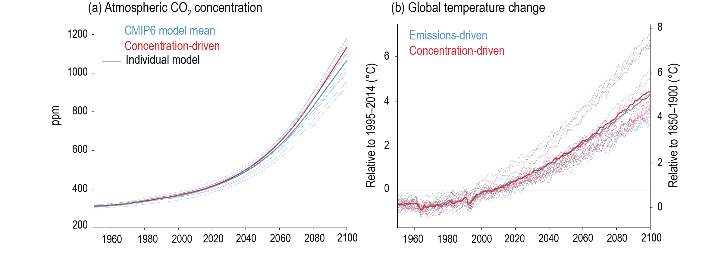
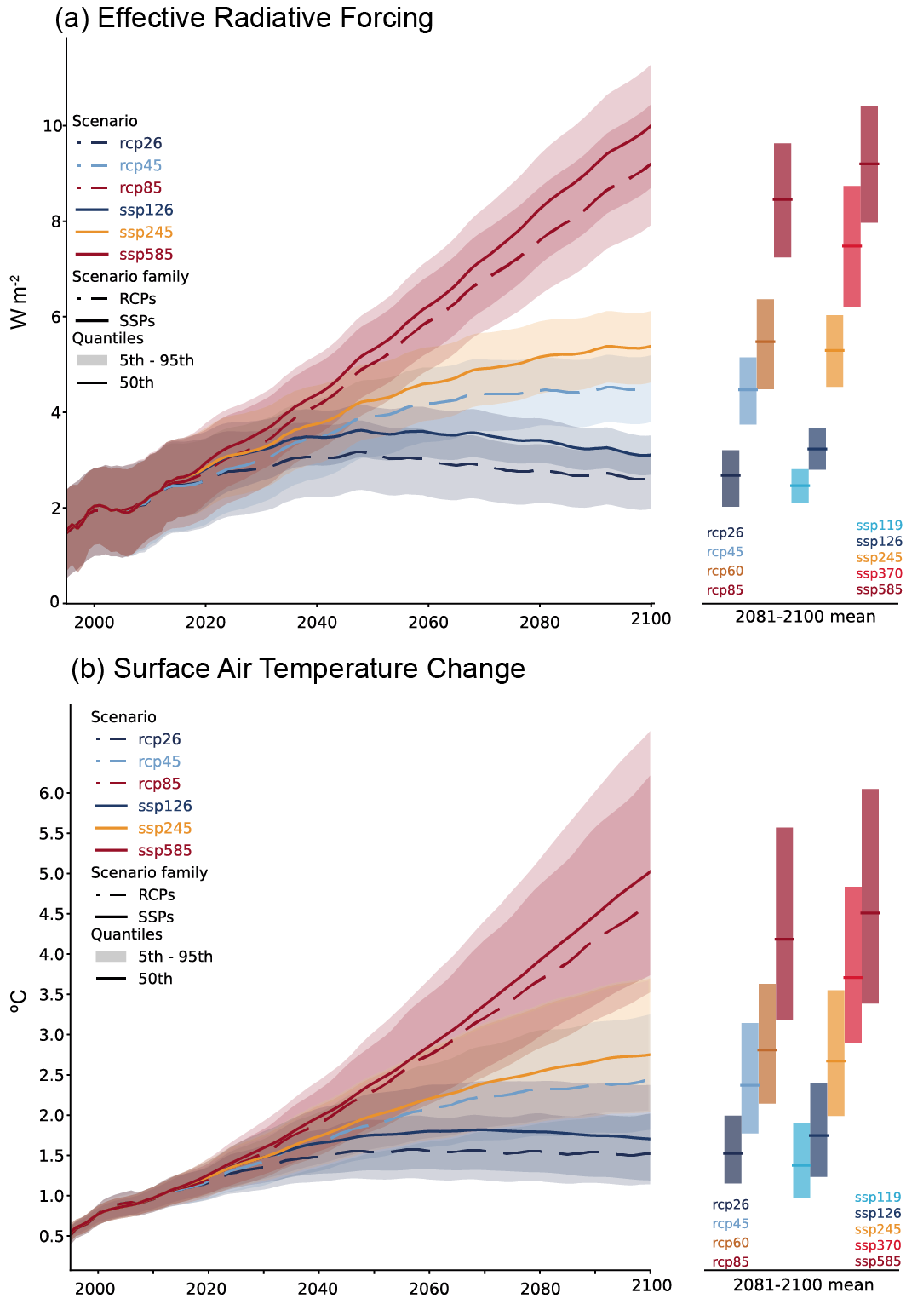
Compared to the recent past (1995–2014), GSAT averaged over the period 2081–2100 is very likely to be higher by 0.2°C–1.0°C in the low-emissions scenario SSP1-1.9 and by 2.4°C–4.8°C in the high-emissions scenario SSP5-8.5. Forthe scenarios SSP1-2.6, SSP2-4.5, and SSP3-7.0, the correspondingvery likely ranges are 0.5°C–1.5°C, 1.2°C–2.6°C, and 2.0°C–3.7°C, respectively. The uncertainty ranges for the period 2081–2100 continue to be dominated by the uncertainty in ECS and TCR (very high confidence). Emissions-driven simulations for SSP5-8.5 show that carbon-cycle uncertainty is too small to change the assessment of GSAT projections (high confidence). {4.3.1, 4.3.4, 4.6.2, 7.5}
The CMIP6 models project a wider range of GSAT change than the assessed range (high confidence); furthermore, the CMIP6 GSAT increase tends to be larger than in CMIP5 (very high confidence). About half of the increase in simulated warming has occurred because higher climate sensitivity is more prevalent in CMIP6 than in CMIP5; the other half arises from higher ERF in nominally comparable scenarios (e.g., RCP8.5 and SSP5-8.5; medium confidence). In SSP1-2.6 and SSP2-4.5, ERF changes also explain about half of the changes in the range of warming (medium confidence). For SSP5-8.5, higher climate sensitivity is the primary reason behind the upper end of the warming being higher than in CMIP5 (medium confidence). {4.3.1, 4.3.4, 4.6.2, 7.5.6}
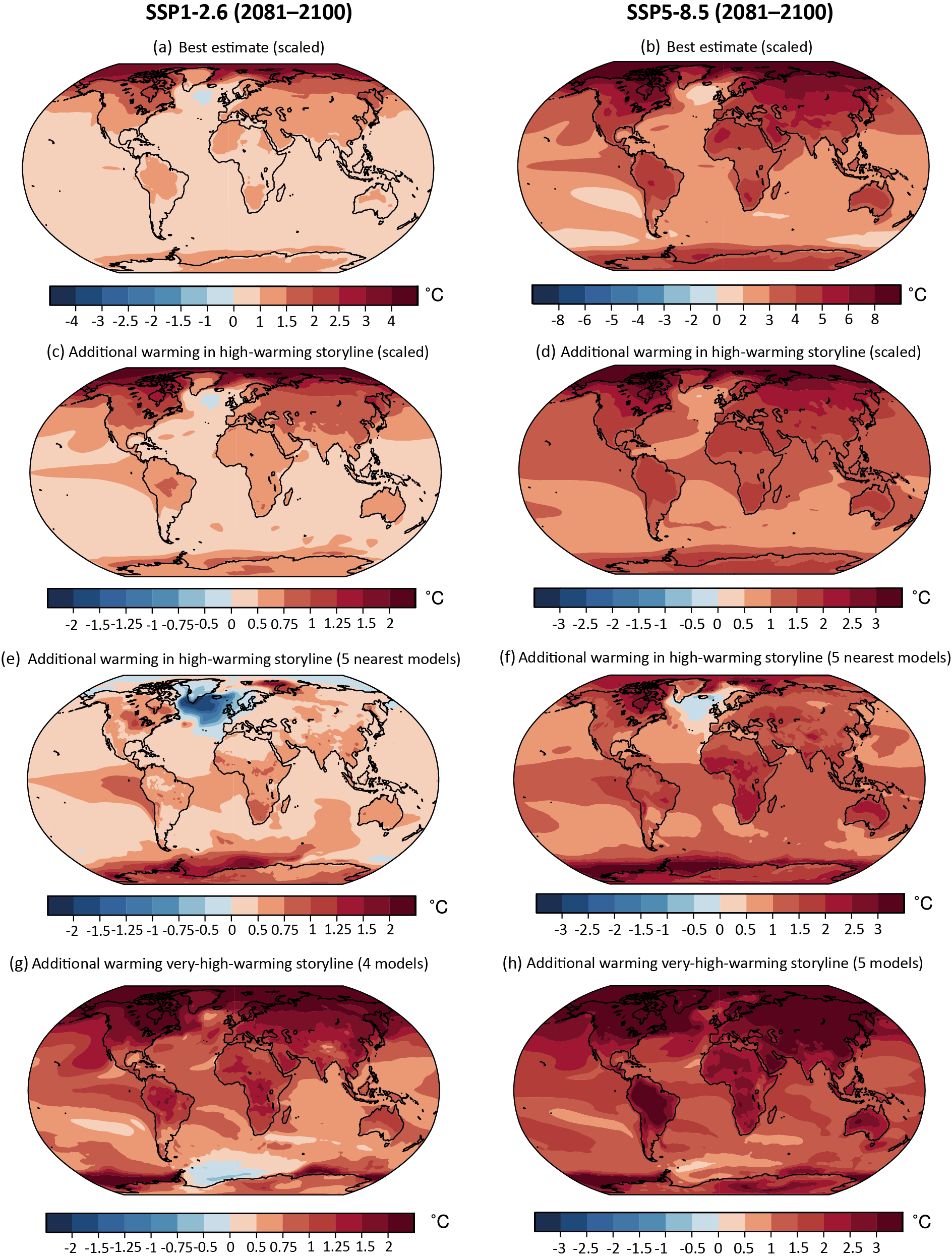
While high-warming storylines – those associated with GSAT levels above the upper bound of the assessed very likely range – are by definition extremely unlikely, they cannot be ruled out. For SSP1-2.6, such a high-warming storyline implies long-term (2081–2100) warming well above, rather than well below, 2°C (high confidence). Irrespective of scenario, high-warming storylines imply changes in many aspects of the climate system that exceed the patterns associated with the central estimate of GSAT changes by up to more than 50% (high confidence). {4.3.4, 4.8}
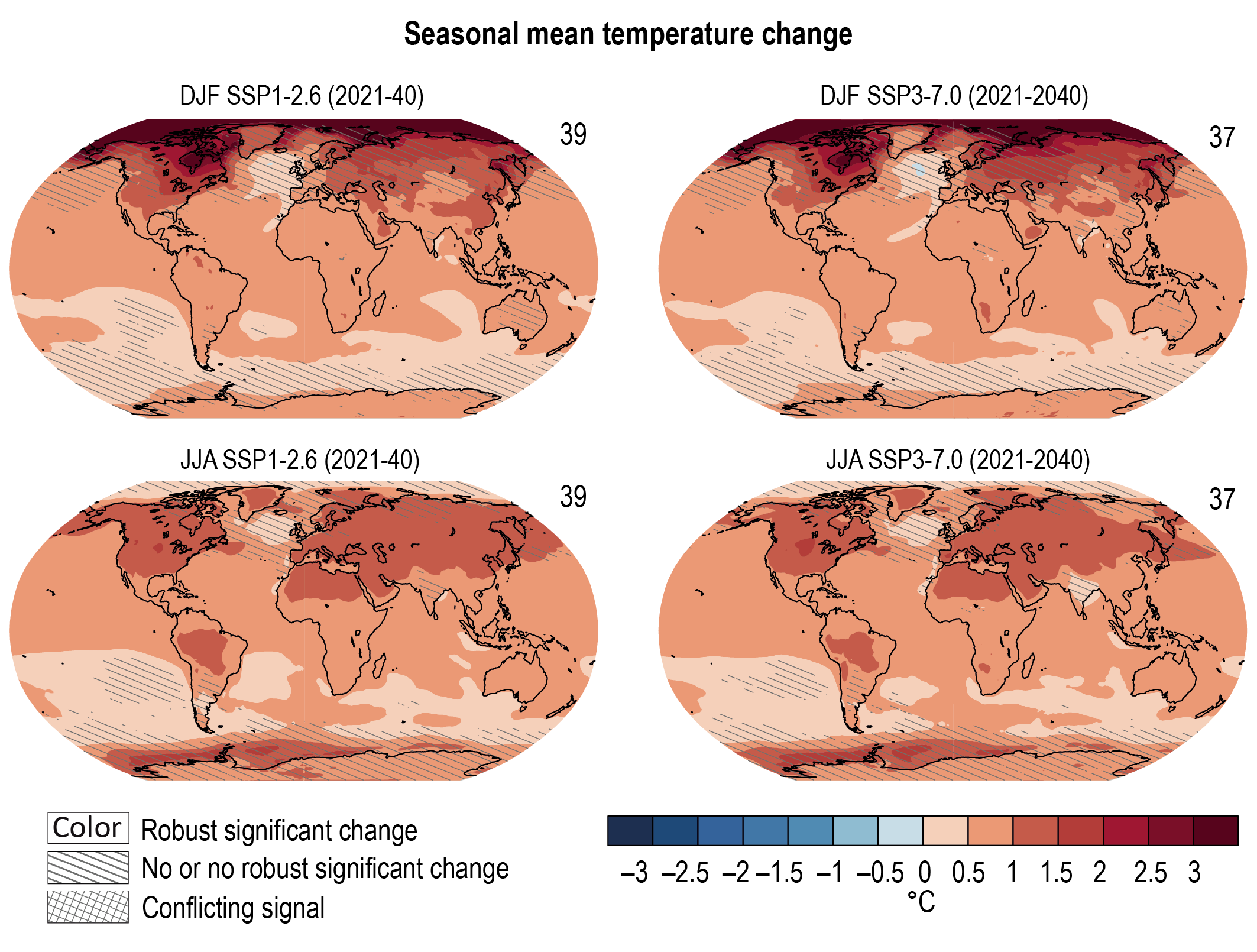
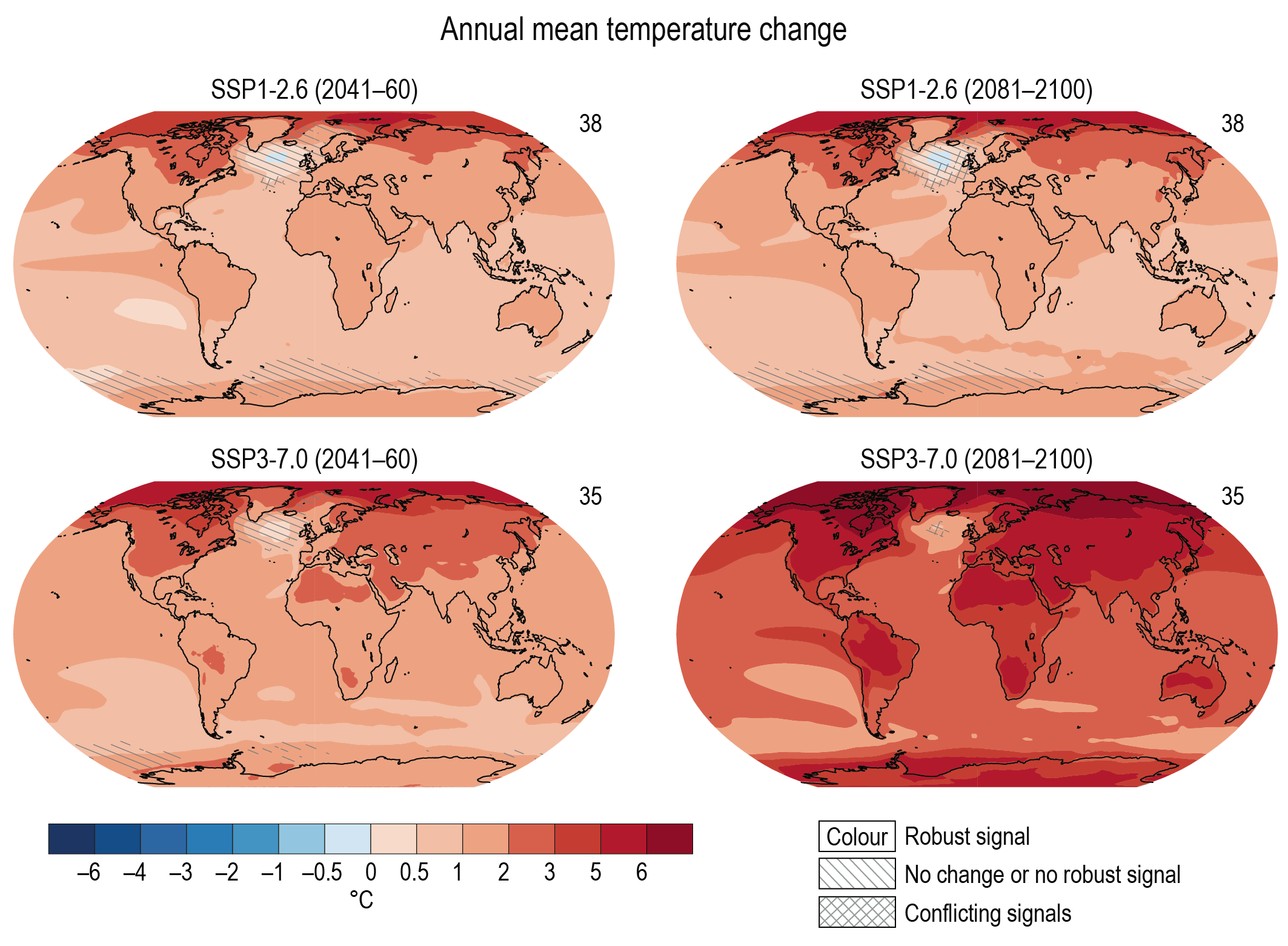
It is virtually certain that the average surface warming will continue to be higher over land than over the ocean and that the surface warming in the Arctic will continue to be more pronounced than the global average over the 21st century. On average, the surface is expected to warm faster over land than over the ocean by a factor of 1.5 (likely range 1.4 to 1.7). The warming pattern likely varies across seasons, with northern high latitudes warming more during boreal winter than summer (medium confidence). Regions with increasing or decreasing year-to-year variability of seasonal mean temperatures will likely increase in their spatial extent. {4.3.1, 4.5.1, 7.4.4}
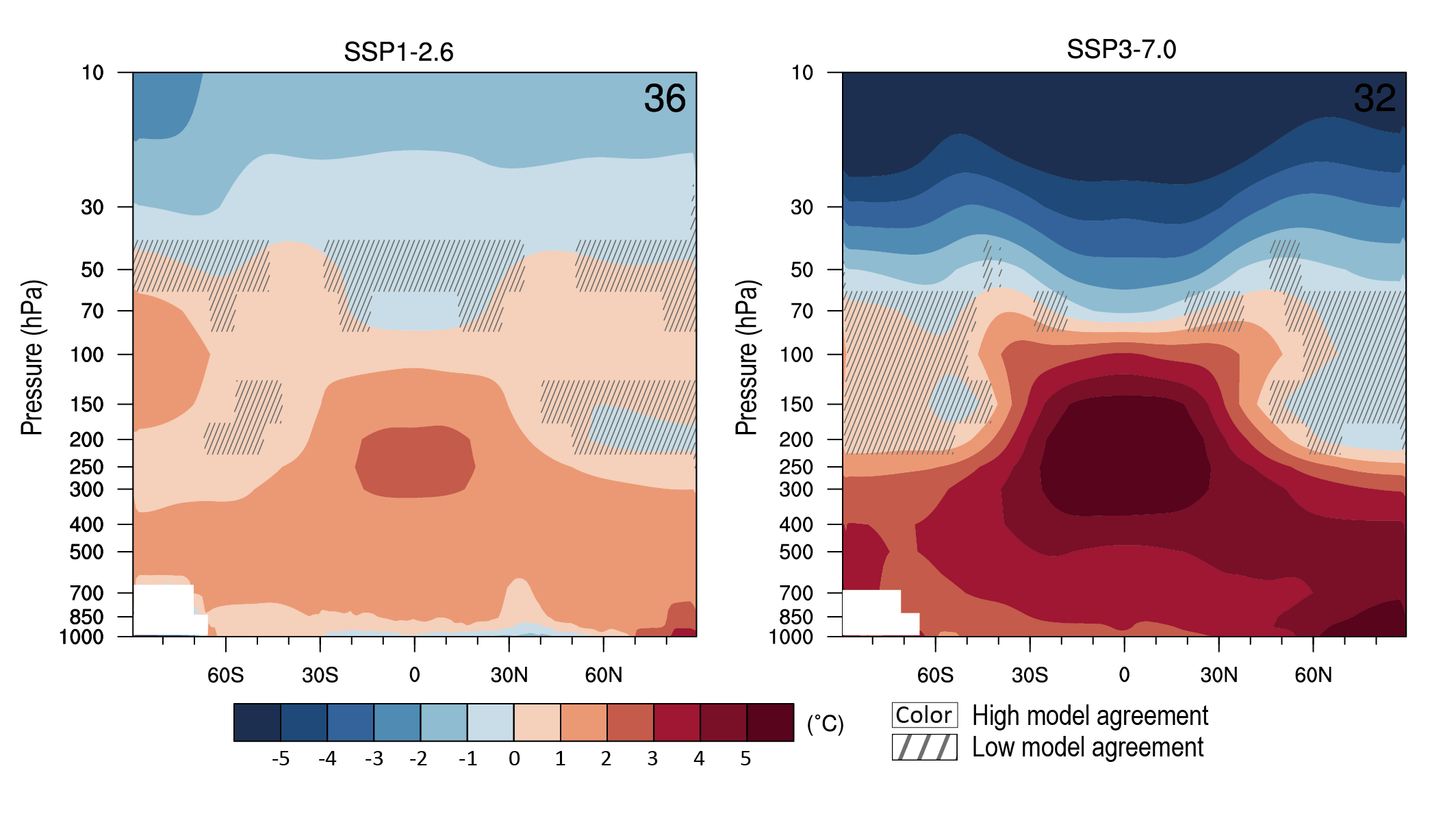
It is very likely that long-term lower-tropospheric warming will be larger in the Arctic than in the global mean. It is very likely that global mean stratospheric cooling will be larger by the end of the 21st century in a pathway with higher atmospheric CO2 concentrations. It is likely that tropical upper tropospheric warming will be larger than at the tropical surface, but with an uncertain magnitude owing to the effects of natural internal variability and uncertainty in the response of the climate system to anthropogenic forcing. {4.5.1, 3.3.1.2}
Precipitation
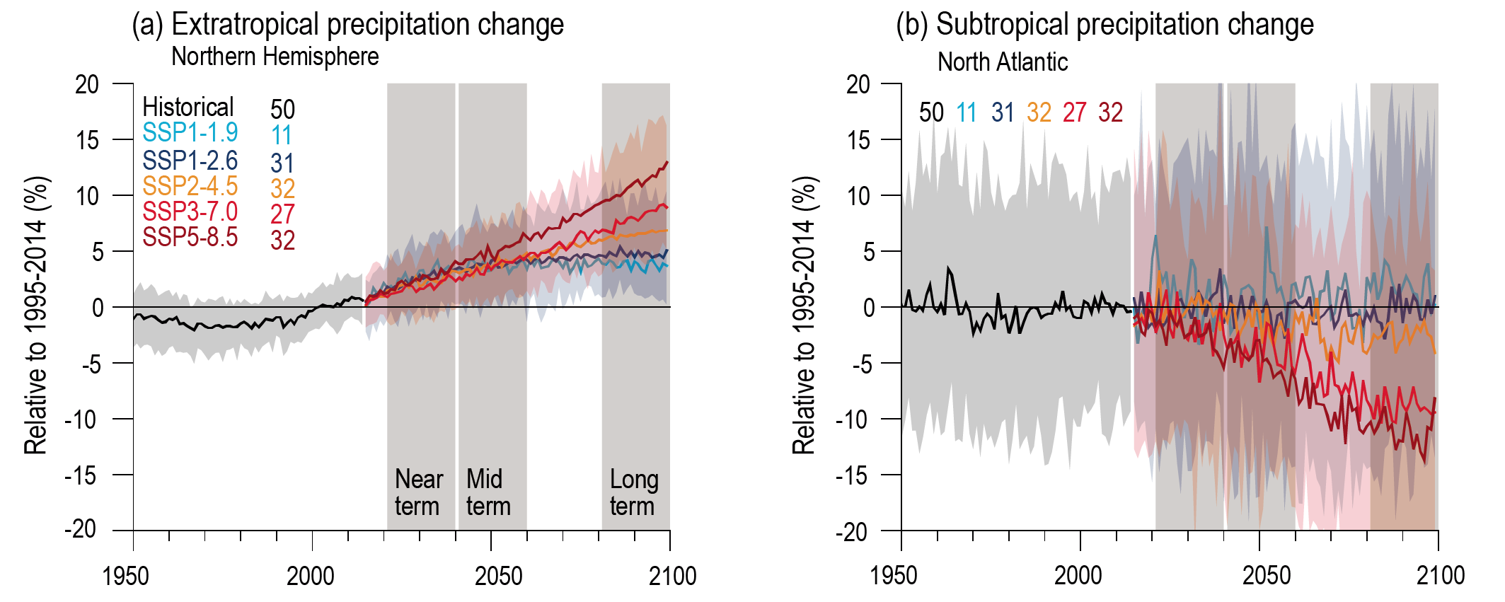
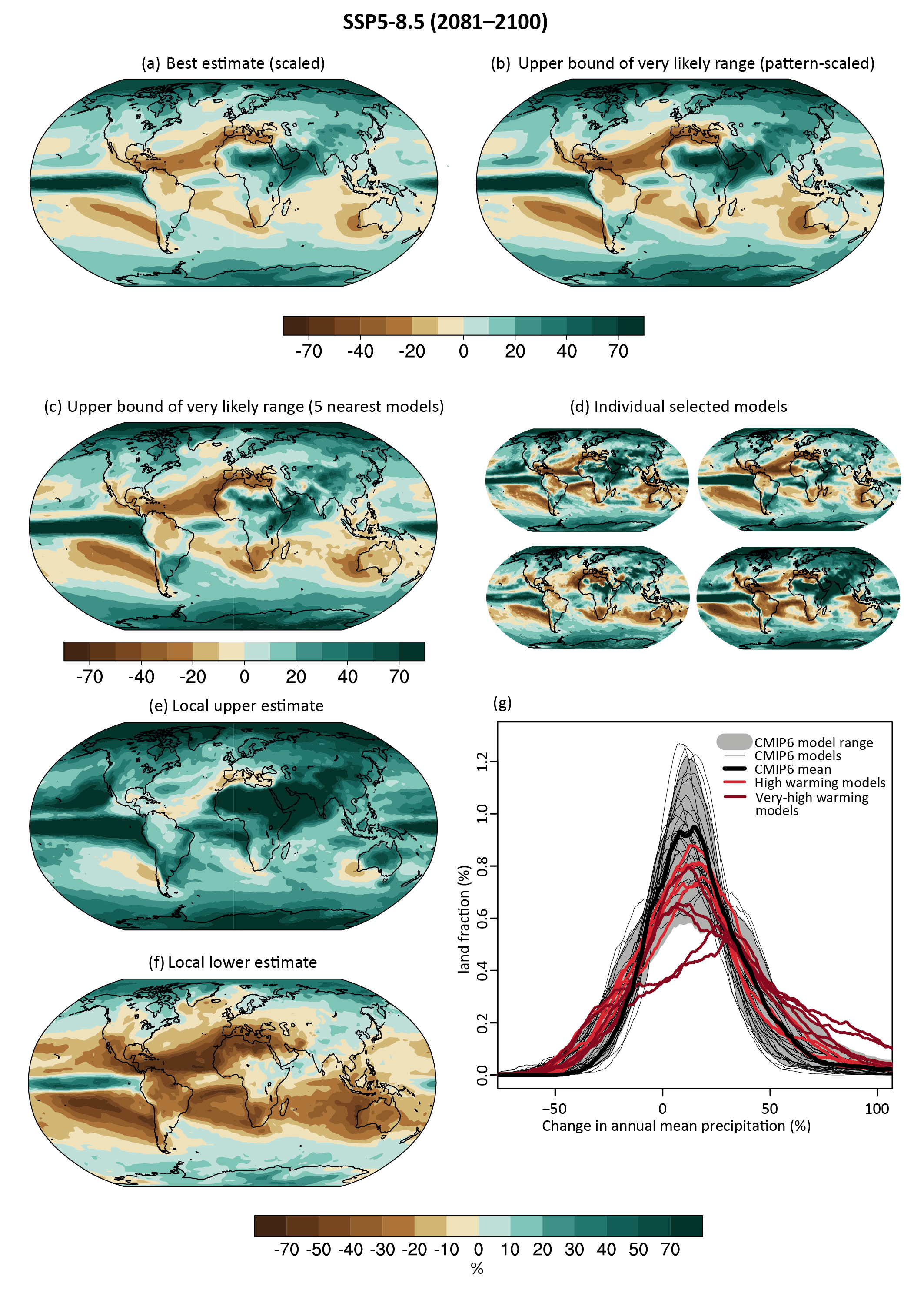
Annual global land precipitation will increase over the 21st century as GSAT increases (high confidence). The likely range of change in globally averaged annual land precipitation during 2081–2100 relative to 1995–2014 is –0.2 to +4.7% in the low-emissions scenario SSP1-1.9 and 0.9–12.9% in the high-emissions scenario SSP5-8.5, based on all available CMIP6 models. The corresponding likely ranges are 0.0–6.6% in SSP1-2.6, 1.5–8.3% in SSP2-4.5, and 0.5–9.6% in SSP3-7.0. {4.3.1, 4.5.1, 4.6.1, 8.4.1}
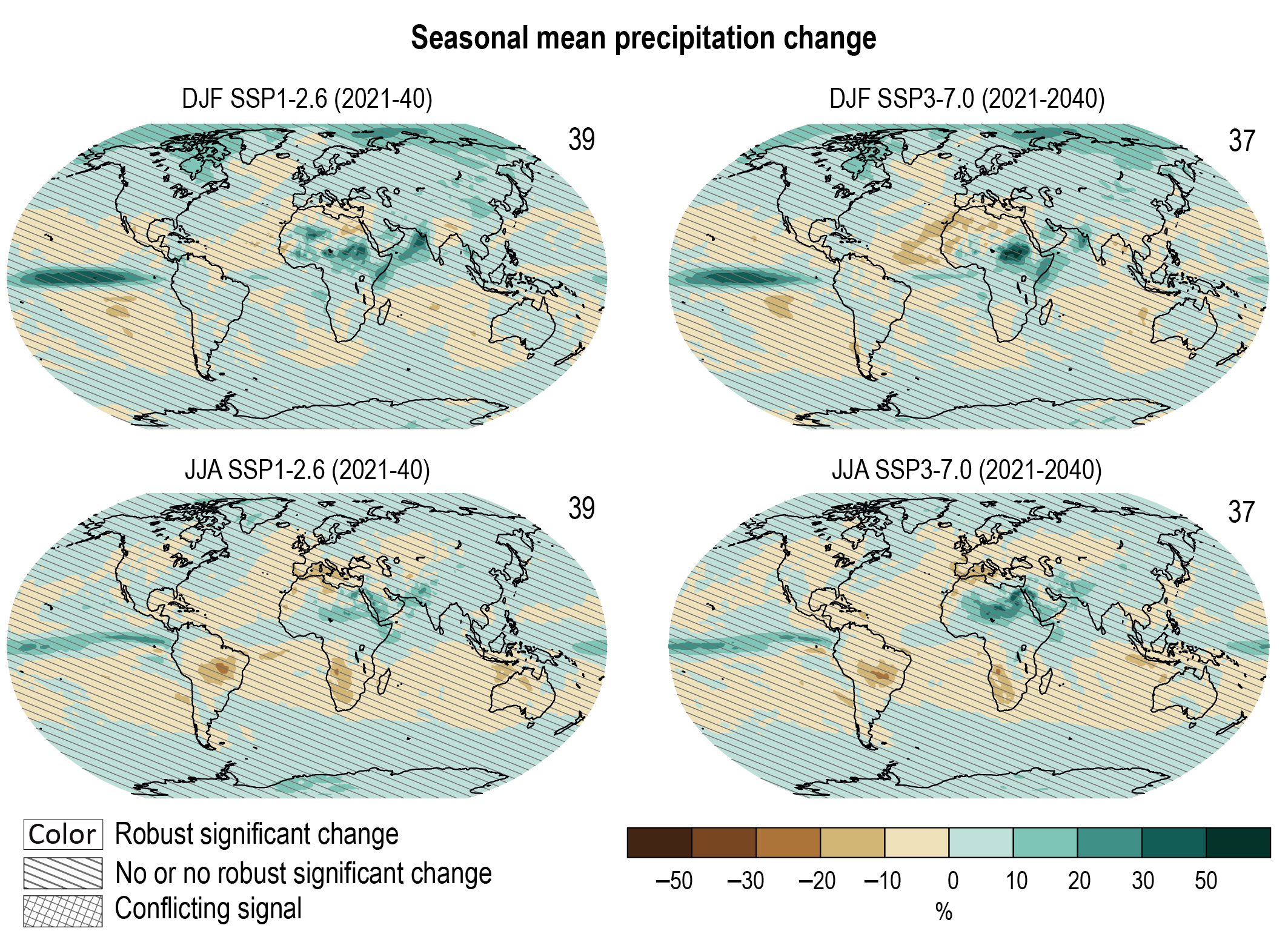
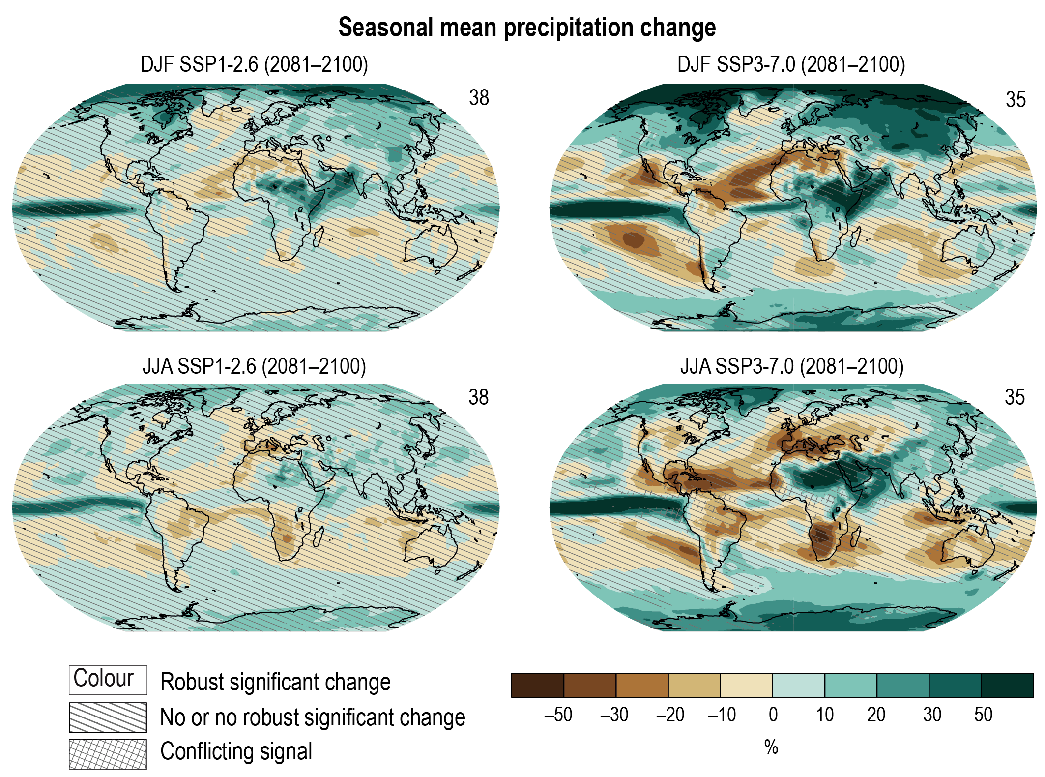
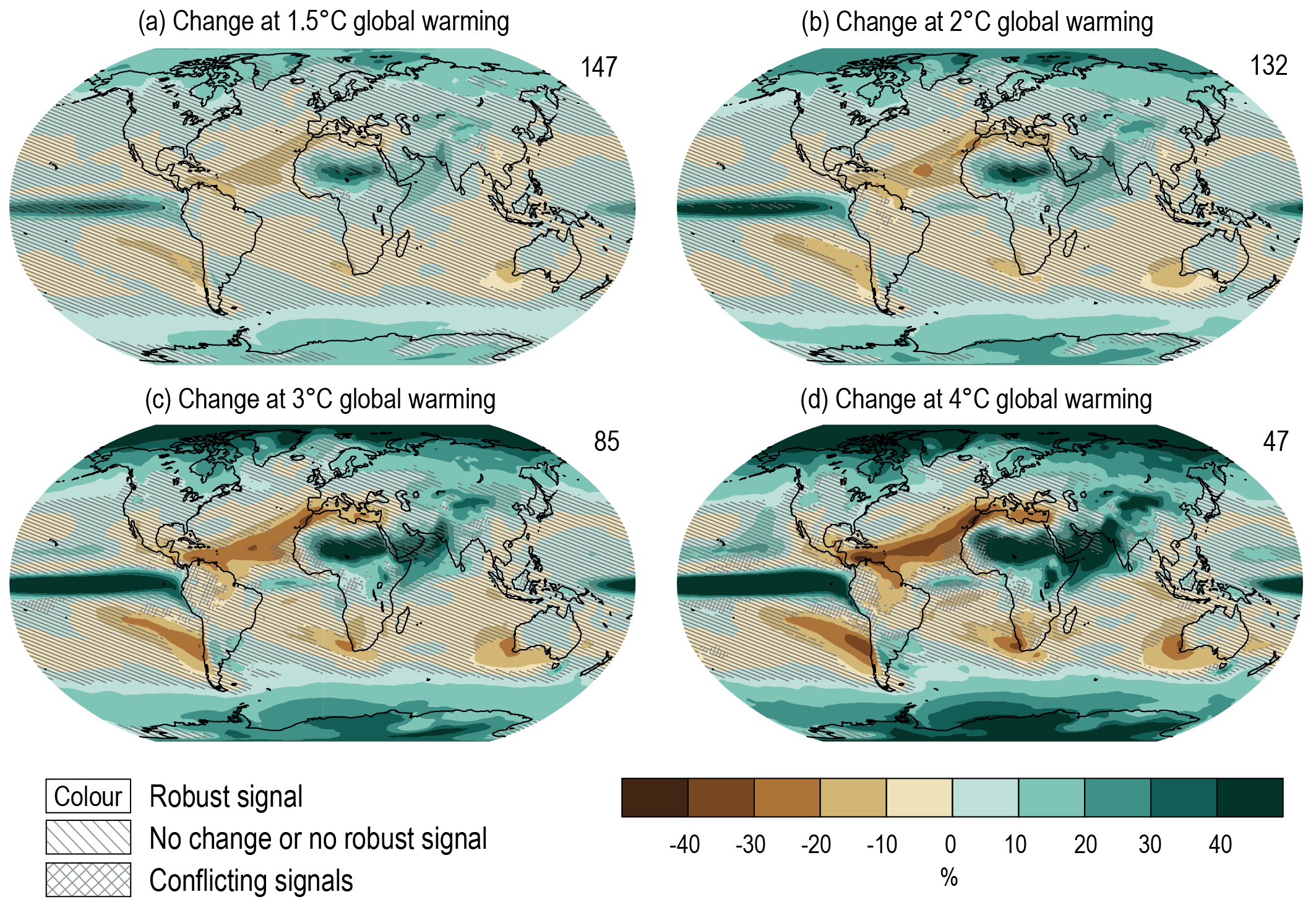
Precipitation change will exhibit substantial regional differences and seasonal contrast as GSAT increases over the 21st century (high confidence). As warming increases, a larger land area will experience statistically significant increases or decreases in precipitation (medium confidence). Precipitation will very likely increase over high latitudes and the tropical oceans, and likely increase in large parts of the monsoon region, but likely decrease over large parts of the subtropics in response to greenhouse gas-induced warming. Interannual variability of precipitation over many land regions will increase with global warming (medium confidence). {4.5.1, 4.6.1, 8.4.1}
Near-term projected changes in precipitation are uncertain, mainly because of natural internal variability, model uncertainty, and uncertainty in natural and anthropogenic aerosol forcing (medium confidence). In the near term, no discernible differences in precipitation changes are projected between different SSPs (high confidence). The anthropogenic aerosol forcing decreases in most scenarios, contributing to increases in GSAT (medium confidence) and global mean land precipitation (low confidence). {4.3.1, 4.4.1, 4.4.4, 8.5}
In response to greenhouse gas-induced warming, it is likely that global land monsoon precipitation will increase, particularly in the Northern Hemisphere, although Northern Hemisphere monsoon circulation will likely weaken. In the long term (2081–2100), monsoon rainfall change will feature a north–south asymmetry characterized by a greater increase in the Northern Hemisphere than in the Southern Hemisphere and an east–west asymmetry characterized by an increase in Asian-African monsoon regions and a decrease in the North American monsoon region (medium confidence). Near-term changes in global monsoon precipitation and circulation are uncertain due to model uncertainty and internal variability such as Atlantic Multi-decadal Variability and Pacific Decadal Variability (medium confidence). {4.4.1, 4.5.1, 8.4.1, 10.6.3}
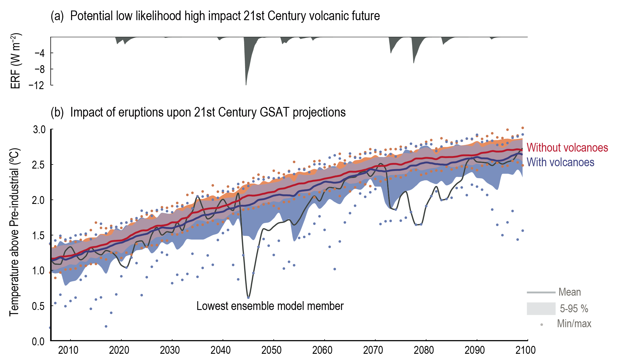
It is likely that at least one large volcanic eruption will occur during the 21st century. Such an eruption would reduce GSAT for several years, decrease global mean land precipitation, alter monsoon circulation, modify extreme precipitation, and change the profile of many regional climatic impact-drivers. A low-likelihood, high-impact outcome would be several large eruptions that would greatly alter the 21st century climate trajectory compared to SSP-based Earth system model projections. {Cross-Chapter Box 4.1}
Large-scale Circulation and Modes of Variability
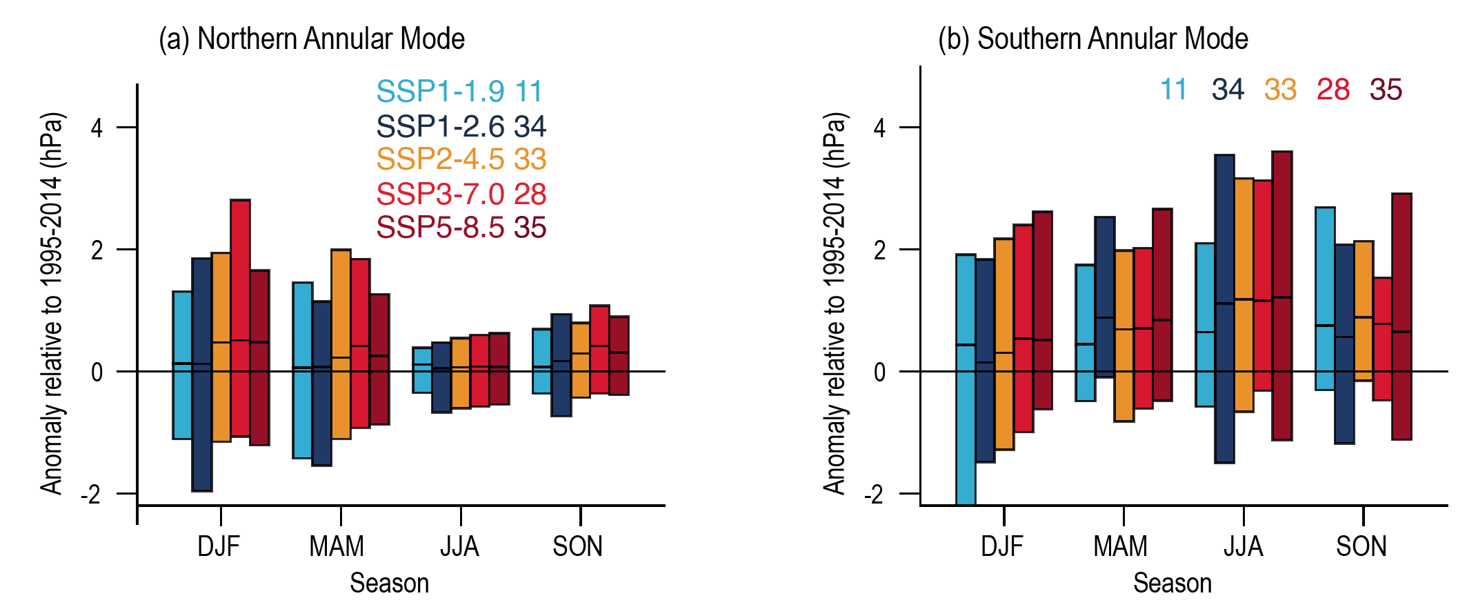
In the near term, the forced change in Southern Annular Mode in austral summer is likely to be weaker than observed during the late 20th century under all five SSPs assessed. This is because of the opposing influence in the near- to mid-term from stratospheric ozone recovery and increases in other greenhouse gases on the Southern Hemisphere summertime mid-latitude circulation (high confidence). In the near term, forced changes in the Southern Annular Mode in austral summer are therefore likely to be smaller than changes due to natural internal variability. {4.3.3, 4.4.3}
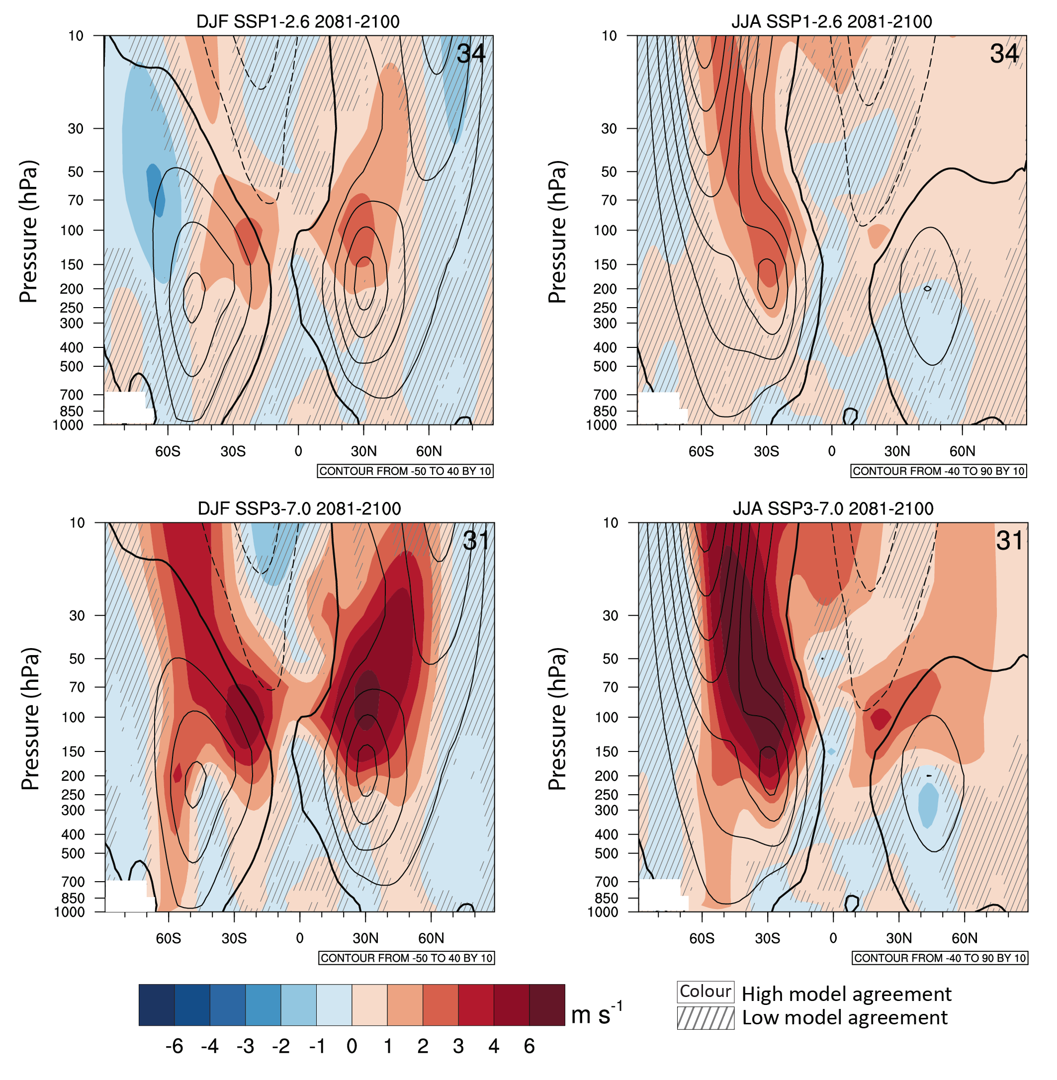
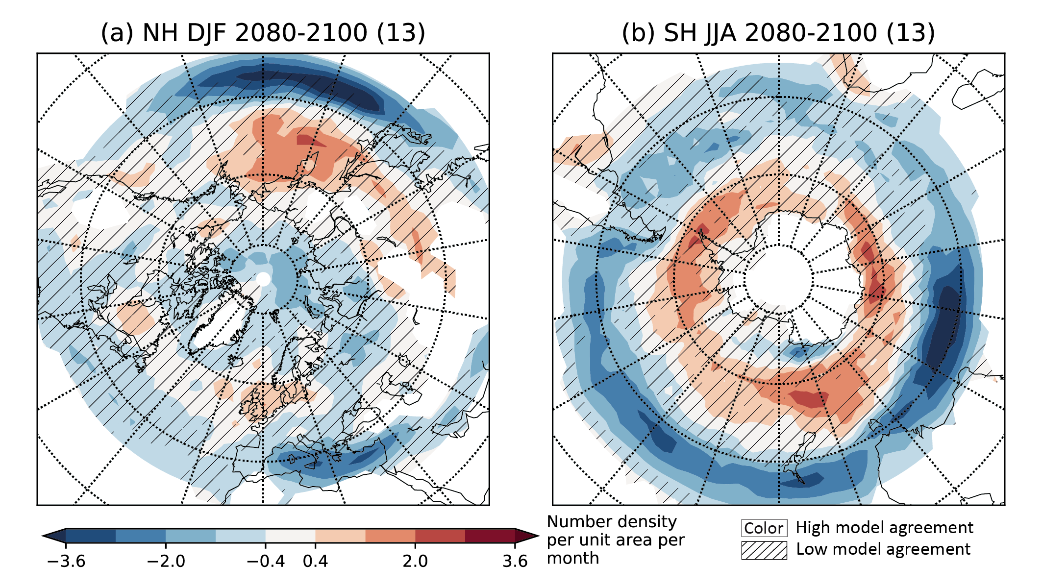
In the long term, the Southern Hemisphere mid-latitude jet is likely to shift poleward and strengthen under SSP5-8.5 relative to 1995–2014. This is likely to be accompanied by an increase in the Southern Annular Mode index in all seasons relative to 1995–2014. For SSP1-2.6, CMIP6 models project no robust change in the Southern Annular Mode index in the long term. It is likely that wind speeds associated with extratropical cyclones will strengthen in the Southern Hemisphere storm track for SSP5-8.5. {4.5.1, 4.5.3}
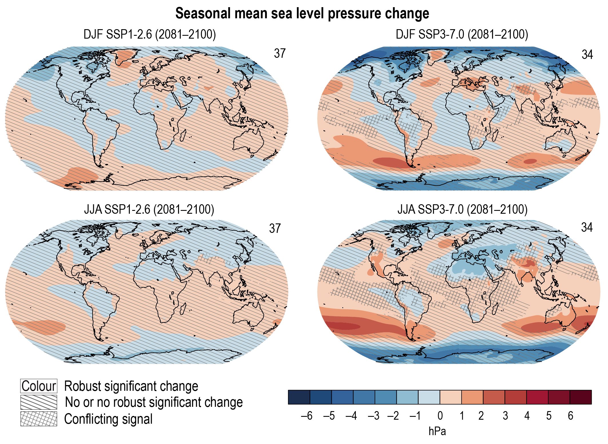
The CMIP6 multi-model ensemble projects a long-term increase in the boreal wintertime Northern Annular Mode index under the high-emissions scenarios of SSP3-7.0 andSSP5-8.5, but regional changes may deviate from a simple shift in the mid-latit ude circulation. Substantial uncertainty and thus low confidence remain in projecting regional changes in Northern Hemisphere jet streams and storm tracks, especially for the North Atlantic basin in winter; this is due to large natural internal variability, the competing effects of projected upper- and lower-tropospheric temperature gradient changes, and new evidence of weaknesses in simulating past variations in North Atlantic atmospheric circulation on seasonal-to-decadal time scales. One exception is the expected decrease in frequency of atmospheric blocking events over Greenland and the North Pacific in boreal winter in SSP3-7.0 and SSP5-8.5 scenarios (medium confidence). {4.5.1}
Near-term predictions and projections of the sub-polar branch of the Atlantic Multi-decadal Variability (AMV) on the decadal time scale have improved in CMP6 models compared to CMIP5 (high confidence). This is likely to be related to a more accurate response to natural forcing in CMIP6 models. Initialization contributes to the reduction of uncertainty and to predicting subpolar sea surface temperature. AMV influences on the nearby regions can be predicted over lead times of 5–8 years (medium confidence). {4.4.3}
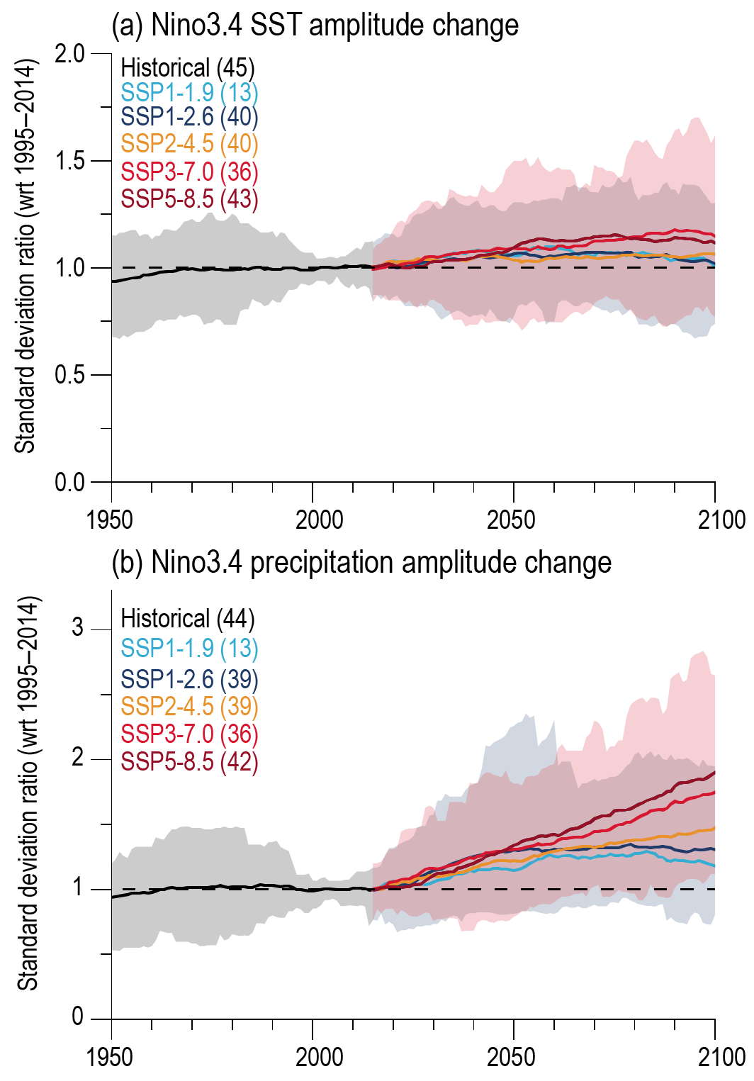
It is virtually certain that the El Niño–Southern Oscillation (ENSO) will remain the dominant mode of interannual variability in a warmer world. There is no model consensus for a systematic change in intensity of ENSO sea surface temperature variability over the 21st century in any of the SSP scenarios assessed (medium confidence). However, it is very likely that ENSO rainfall variability, used for defining extreme El Niños and La Niñas, will increase significantly, regardless of amplitude changes in ENSO SST variability, by the second half of the 21st century in scenarios SSP2-4.5, SSP3-7.0, and SSP5-8.5. {4.3.3, 4.5.3, 8.4.2}
Cryosphere and Ocean
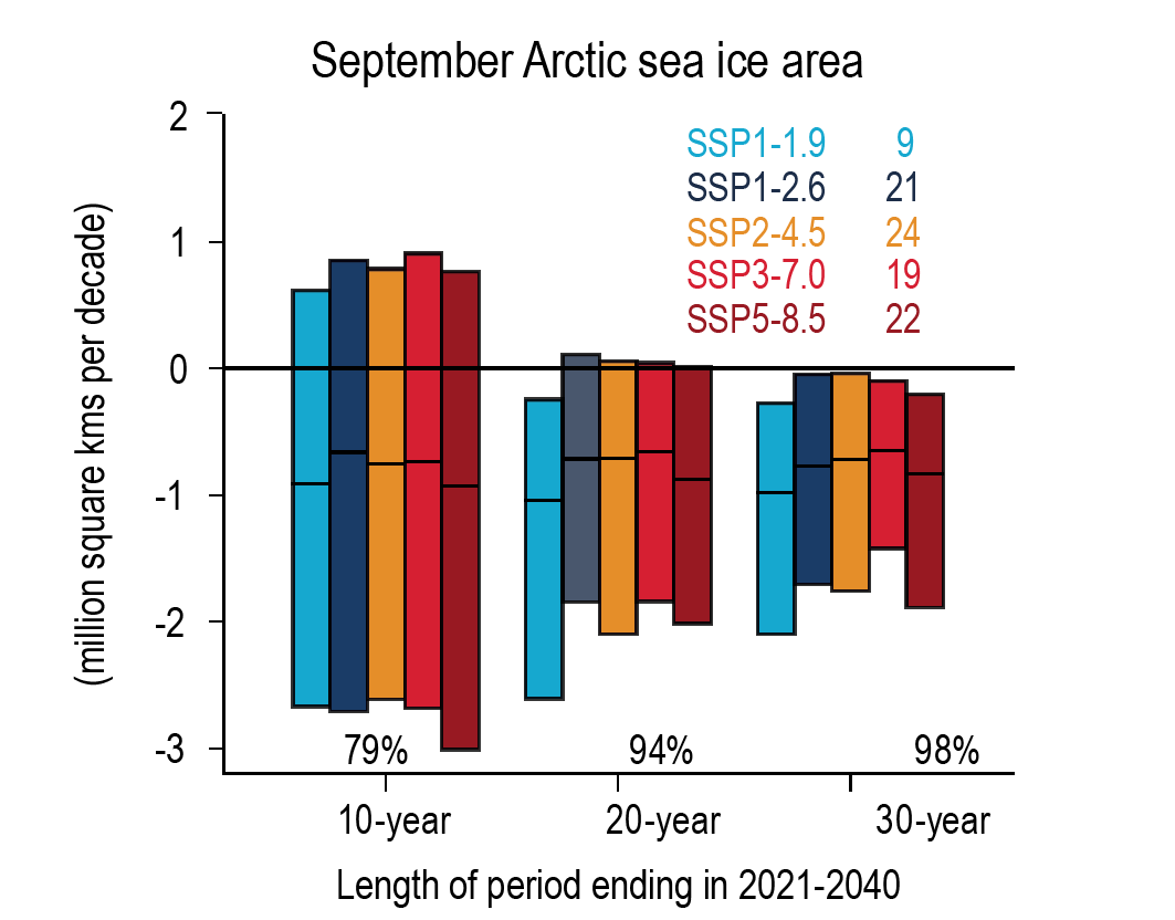
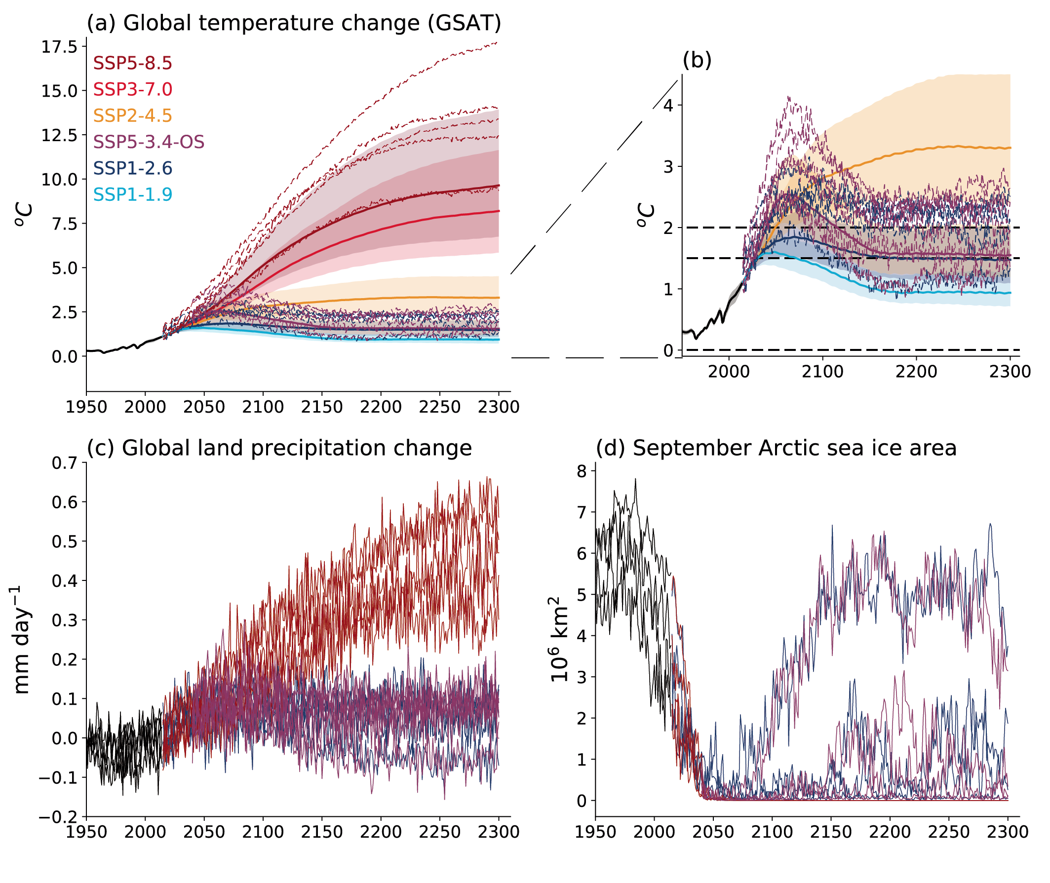
Under the SSP2-4.5, SSP3-7.0, and SSP5-8.5 scenarios, it is likely that the Arctic Ocean in September, the month of annual minimum sea ice area, will become practically ice-free (sea ice area less than 1 million km2) averaged over 2081–2100 and all available simulations. Arctic sea ice area in March, the month of annual maximum sea ice area, also decreases in the future under each of the considered scenarios, but to a much lesser degree (in percentage terms) than in September (high confidence). {4.3.2}
Under the five scenarios assessed, it is virtually certain that global mean sea level (GMSL) will continue to rise through the 21st century. For the period 2081–2100 relative to 1995–2014, GMSL is likely to rise by 0.46–0.74 m under SSP3-7.0 and by 0.30–0.54 m under SSP1-2.6 (medium confidence). For the assessment of change in GMSL, the contribution from land-ice melt has been added offline to the CMIP6-simulated contributions from thermal expansion. {4.3.2. 9.6}
It is very likely that the cumulative uptake of carbon by the ocean and by land will increase through to the end of the 21st century. Carbon uptake by land shows greater increases but with greater uncertainties than for ocean carbon uptake. The fraction of emissions absorbed by land and ocean sinks will be smaller under high emissions scenarios than under low emissions scenarios (high confidence). Ocean surface pH will decrease steadily through the 21st century, except for SSP1-1.9 and SSP1-2.6 where values decrease until around 2070 and then increase slightly to 2100 (high confidence). {4.3.2, 5.4}
Climate Response to Emissions Reduction, Carbon Dioxide Removal and Solar Radiation Modification
If strong mitigation is applied from 2020 onward as reflected in SSP1-1.9, its effect on 20-year trends in GSAT wouldlikely emerge during the near term (2021–2040), measured against an assumed non-mitigation scenario such as SSP3-7. 0 and SSP5-8.5. However, the response of many other climate quantities to mitigation would be largely masked by internal variability during the near term, especially on the regional scale (high confidence). The mitigation benefits for these quantities would emerge only later during the 21st century (high confidence). During the near term, a small fraction of the surface can show cooling under all scenarios assessed here, so near-term cooling at any given location is fully consistent with GSAT increase (high confidence). Events of reduced and increased GSAT trends at decadal time scales will continue to occur in the 21st century but will not affect the centennial warming (very high confidence). {4.6.3, Cross-Chapter Box 3.1}
Because of the near-linear relationship between cumulative carbon emissions and GSAT change, the cooling or avoided warming from carbon dioxide removal (CDR) is proportional to the cumulative amount of CO2 removed by CDR (high confidence). The climate system response to net negative CO2 emissions is expected to be delayed by years to centuries. Net negative CO2 emissions due to CDR will not reverse some climate change, such as sea level rise, at least for several centuries (high confidence). The climate effect of a sudden and sustained CDR termination would depend on the amount of CDR-induced cooling prior to termination and the rate of background CO2 emissions at the time of termination (high confidence). {4.6.3, 5.5, 5.6}
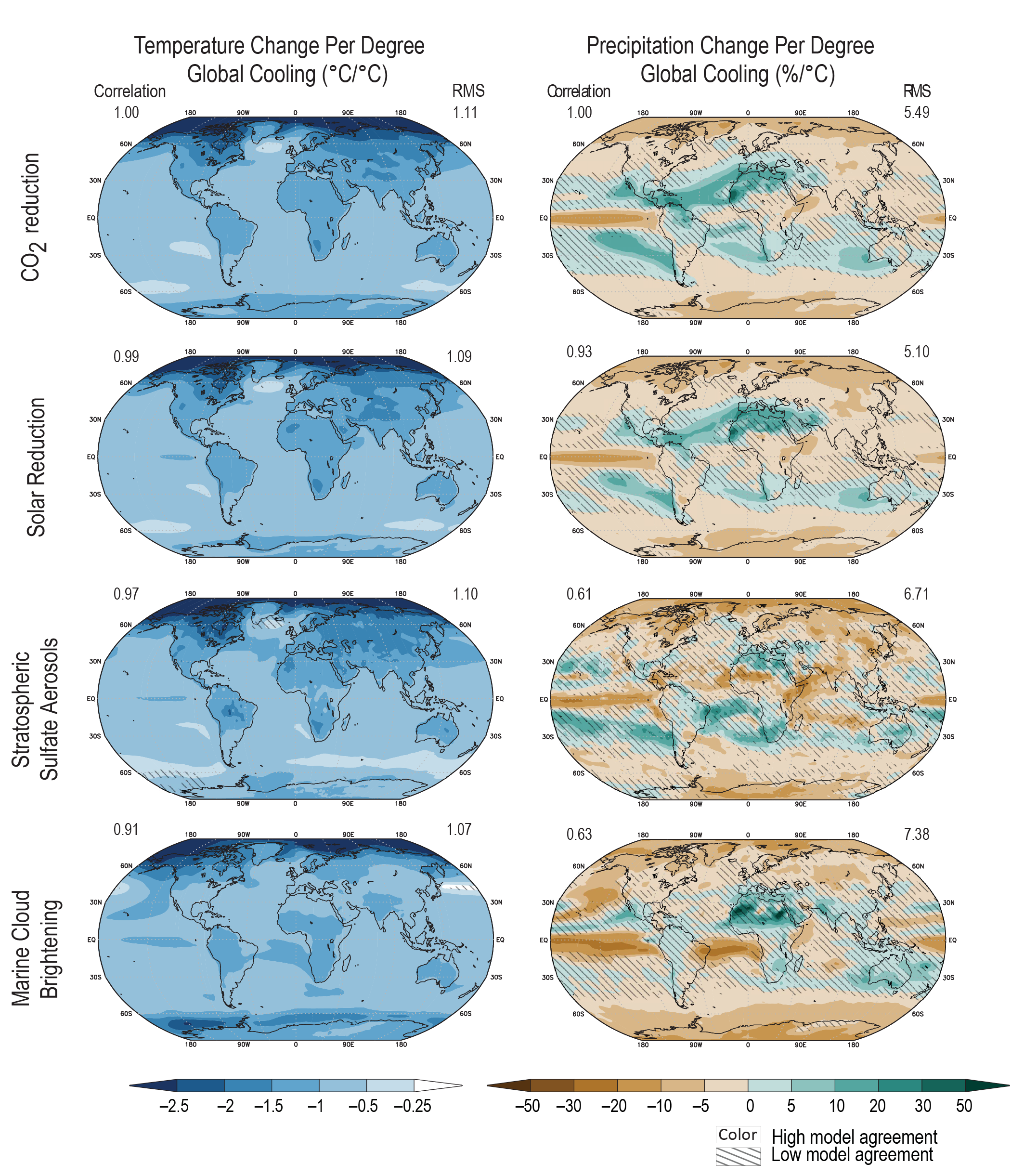
Solar radiation modification (SRM) could offset some of the effects of anthropogenic warming on global and regional climate, but there would be substantial residual and overcompensating climate change at the regional scale and seasonal time scale (high confidence), and there is low confidencein our understanding of the climate response to SRM, specifically at the regional scale. Since AR5, understanding of the global and regional climate response to SRM has improved, due to modelling work with more sophisticated treatment of aerosol-based SRM options and stratospheric processes. Improved modelling suggests that multiple climate goals could be met simultaneously. A sudden and sustained termination of SRM in a high-emissions scenario such as SSP5-8.5 would cause a rapid climate change (high confidence). However, a gradual phase-out of SRM combined with emissions reductions and CDR would morelikely than not avoid larger rates of warming. {4.6.3}
Climate Change Commitment and Change Beyond 2100
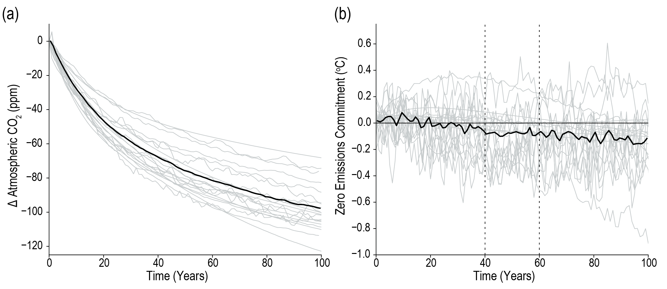
Earth system modelling experiments since AR5 confirm that the zero CO2 emissions commitment (the additional rise in GSAT after all CO2 emissions cease) is small (likely less than 0.3°C in magnitude) on decadal time scales, but that it may be positive or negative. There is low confidence in the sign of the zero CO2 emissions commitment. Consistent with SR1.5, the central estimate is taken as zero for assessments of remaining carbon budgets for global warming levels of 1.5°C or 2°C. {4.7.2, 5.5.2}.
Overshooting specific global warming levels such as 2°C has effects on the climate system that persist beyond 2100 (medium confidence). Under one scenario including a peak and decline in atmospheric CO2 concentration (SSP5-3.4-OS), some climate metrics such as GSAT begin to decline but do not fully reverse by 2100 to levels prior to the CO2 peak (medium confidence). GMSL continues to rise in all models up to 2100 despite a reduction in CO2 to 2040 levels. {4.6.3, 4.7.1, 4.7.2}
Using extended scenarios beyond 2100, projections show likely warming by 2300, relative to 1850-1900, of 1.0°C-2.2°C for SSP1-2.6 and 6.6°C-14.1°C for SSP5-8.5. By 2300, warming under the SSP5-3.4-OS overshoot scenario decreases from a peak around year 2060 to a level very similar to SSP1-2.6. Precipitation over land continues to increase strongly under SSP5-8.5. GSAT projected for the end of the 23rd century under SSP2-4.5 (likely 2.3°C–4.6°C higher than over the period 1850–1900) has not been experienced since the mid-Pliocene, about 3 million years ago. GSAT projected for the end of the 23rd century under SSP5-8.5 (likely 6.6°C–14.1°C higher than over the period 1850–1900) overlaps with the range estimated for the Miocene Climatic Optimum (5°C–10°C higher) and Early Eocene Climatic Optimum (10°C–18°C higher), about 15 and 50 million years ago, respectively (medium confidence). {2.3.1.1, 4.7.1}
4.1 Scope and Overview of This Chapter
This chapter assesses simulations of future climate change, covering both near-term and long-term global changes. The chapter assesses simulations of physical indicators of global climate change, such as global surface air temperature (GSAT), global land precipitation, Arctic sea ice area (SIA), and global mean sea level (GMSL). Furthermore, the chapter covers indices and patterns of properties and circulation not only for mean fields but also for modes of variability that have global significance. The choice of quantities to be assessed is summarized in Cross-Chapter Box 2.2 and comprises a subset of the quantities covered in Chapters 2 and 3. This chapter provides consistent coverage from near-term to long-term global changes and provides the global reference for the later chapters covering important processes and regional change.
Essential input to the simulations assessed here is provided by future scenarios of concentrations or anthropogenic emissions of radiatively active substances; the scenarios represent possible sets of decisions by humanity, without any assessment that one set of decisions is more probable to occur than any other set (Section 1.6). As in previous assessment reports, these scenarios are used for projections of future climate using global atmosphere–ocean general circulation models (AOGCMs) and Earth system models (ESMs; Section 1.5.3); the latter include representation of various biogeochemical cycles such as the carbon cycle, the sulphur cycle, or ozone (e.g., Flato, 2011; Flato et al., 2013). This chapter thus provides a comprehensive assessment of the future global climate response to different future anthropogenic perturbations to the climate system.
Every projection assessment is conditioned on a particular forcing scenario. If sufficient evidence is available, a detailed probabilistic assessment of a physical climate outcome can be performed for each scenario separately. By contrast, there is no agreed-upon approach to assigning probabilities to forcing scenarios, to the point that it has been debated whether such an approach can even exist (e.g., Grübler and Nakicenovic, 2001; Schneider, 2001, 2002). Although there were some recent attempts to ascribe subjective probabilities to scenarios (e.g., Ho et al., 2019; Hausfather and Peters, 2020), and although ‘feasibility’ along different dimensions is an important concept in scenario research (see AR6 WGIII Chapter 3), the scenarios used for the model-based projections assessed in this chapter do not come with statements about their likelihood of actually unfolding in the future. Therefore, it is usually not possible to combine responses to individual scenarios into an overall probabilistic statement about expected future climate. Exceptions to this limit in the assessment are possible only under special circumstances, such as for some statements about near-term climate changes that are largely independent of the scenario chosen (e.g., Section 4.4.1). Beyond this, no combination of responses to different scenarios can be assessed in this chapter but may be possible in future assessments.
A central element of this chapter is a comprehensive assessment of the sources of uncertainty of future projections (Section 1.4.3). Uncertainty can be broken down into scenario uncertainty, model uncertainty involving model biases, uncertainty in simulated effective radiative forcing and model response, and the uncertainty arising from internal variability (Cox and Stephenson, 2007; Hawkins and Sutton, 2009). An additional source of projection uncertainty arises from possible future volcanic eruptions and future solar variability. Assessment of uncertainty relies on multi-model ensembles such as the Coupled Model Intercomparison Project Phase 6 (CMIP6, Eyring et al., 2016), single-model initial-condition large ensembles (e.g., Kay et al., 2015; Deser et al., 2020), and ensembles initialized from the observed climate state (decadal predictions, e.g., Smith et al., 2013a; Meehl et al., 2014; Boer et al., 2016; Marotzke et al., 2016). Ensemble evaluation methods include assessment of model performance and independence (e.g., Knutti et al., 2017; Boé, 2018; Abramowitz et al., 2019); emergent and other observational constraints (e.g., Allen and Ingram, 2002; Hall and Qu, 2006; Cox et al., 2018); and the uncertainty assessment of equilibrium climate sensitivity and transient climate response in Chapter 7. Ensemble evaluation is assessed in Box 4.1 through the inclusion of lines of evidence in addition to the projection ensembles, including implications for potential model weighting.
The uncertainty assessment in this chapter builds on one particularly noteworthy advance since the IPCC Fifth Assessment Report (AR5). Internal variability, which constitutes irreducible uncertainty over much of the time horizon considered here (Hawkins et al., 2016; Marotzke, 2019), can be better estimated in models even under a changing climate through the use of large initial-condition ensembles (Kay et al., 2015). For many climate quantities and compared to the forced climate change signal, internal variability is dominant in any individual realization – including the one that will unfold in reality – in the near term (Kirtman et al., 2013; Marotzke and Forster, 2015), is substantial in the mid-term, and is still recognizable in the long term in many quantities (Deser et al., 2012a; Marotzke and Forster, 2015). This chapter will use the strengthened information on internal variability throughout.
The expanded treatment of uncertainty allows this chapter a more comprehensive assessment of the benefits from mitigation than in previous IPCC reports, as well as the climate response to carbon dioxide removal (CDR) and solar radiation modification (SRM), and how to detect them against the backdrop of internal variability. Important advances have been made in the detection and attribution of mitigation, CDR, and SRM (Bürger and Cubasch, 2015; Lo et al., 2016; Ciavarella et al., 2017); exploring the ‘time of emergence’ (ToE; see Annex VII: Glossary) of responses to assumed emissions reductions (Tebaldi and Friedlingstein, 2013; Samset et al., 2020)and the attribution of decadal events to forcing changes that reflect emissions reductions (Marotzke, 2019; Spring et al., 2020; McKenna et al., 2021).
The question of the potential crossing of thresholds relative to global temperature goals (Geden and Loeschel, 2017) is intimately related to the benefits of mitigation; a prerequisite is an assessment of how robustly magnitudes of warming can be defined (Millar et al., 2017). This chapter provides an update to the IPCC Special Report on Global Warming of 1.5°C (SR1.5, IPCC, 2018a) and constitutes a reference point for later chapters and AR6 WGIII on the effects of mitigation, including a robust uncertainty assessment.
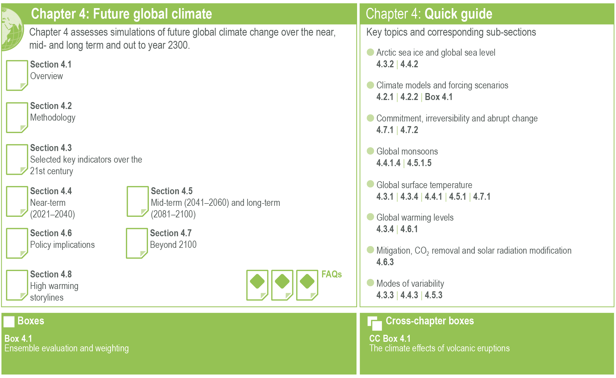
The chapter is organized as follows (Figure 4.1). After (Section 4.2 on the methodologies used in the assessment, Section 4.3 assesses projected changes in key global climate indicators throughout the 21st century, relative to the period 1995–2014, which comprises the last 20 years of the historical simulations of CMIP6 (Eyring et al., 2016) and hence the most recent past simulated with the observed atmospheric composition. The global climate indicators assessed include GSAT, global land precipitation, Arctic sea ice area (SIA), global mean sea level (GMSL), the Atlantic Meridional Overturning Circulation (AMOC), global mean ocean surface pH, carbon uptake by land and ocean, the global monsoon, the Northern and Southern Annular Modes (NAM and SAM), and the El Niño–Southern Oscillation (ENSO). Differently from the assessment for changes in other quantities only based on the range of CMIP6 projections, additional lines of evidence enter the assessment for GSAT and GMSL change. For most results and figures based on CMIP6, one realization from each model (the first of the uploaded set) is used. Section 4.3 finally synthesizes the assessment of GSAT change using multiple lines of evidence in addition to the CMIP6 projection simulations.
 Figure 4.1 | Visual guide to Chapter 4.
 (Section 4.4 covers near-term climate change, defined here as the period 2021–2040 and taken relative to the period 1995–2014. Section 4.4 focuses on global and large-scale climate indicators, including precipitation and circulation indices and selected modes of variability (see Cross-Chapter Box 2.2 and Annex IV: Modes of Variability), as well as on the spatial distribution of warming. The potential roles of short-lived climate forcers (SLCFs) and volcanic eruptions on near-term climate change are also discussed. Section 4.4 synthesizes information from initialized predictions and non-initialized projections for the near-term change.
(Section 4.5 then covers mid-term and long-term climate change, defined here as the periods 2041–2060 and 2081–2100, respectively, again relative to the period 1995–2014. The mid-term period is thus chosen as the twenty-year period following the short-term period and straddling the mid-century point, year 2050; it is during the mid-term that differences between scenarios are expected to emerge against internal variability. The long-term period is defined, as in AR5, as the 20-year period at the end of the century. Section 4.5 assesses the same set of indicators as (Section 4.4, as well as changes in internal variability and in large-scale patterns, both of which are expected to emerge in the mid- to long-term. The chapter sub-division according to time slices (near term, mid-term, and long term) is thus to a large extent motivated by the different roles that internal variability plays in each period, compared to the expected forced climate-change signal.
(Section 4.6 assesses the climate implications of climate policies, as simulated with climate models. First, Section 4.6 assesses patterns of climate change expected for various levels of GSAT rise including 1.5°C, 2°C, 3°C, and 4°C, compared to the approximation to the pre-industrial period 1850–1900 to facilitate immediate connection to SR1.5 and the temperature goals specified in the Paris Agreement (UNFCCC, 2016). Section 4.6 continues with climate goals, overshoot, and path-dependence, as well as the climate response to mitigation, CDR, and SRM. Section 4.6 also covers the consistency between RCPs and SSPs.
(Section 4.7 assesses very long-term changes in selected global climate indicators, from 2100 to 2300. Section 4.7 continues with climate-change commitment and the potential for irreversibility and abrupt climate change. The chapter concludes with Section 4.8 on the potential for low-likelihood, high-impact storylines, followed by answers to three frequently asked questions (FAQs).
4.2 Methodology
4.2.1 Models, Model Intercomparison Projects, and Ensemble Methodologies
Similar to the approach used in AR5 (Flato et al., 2013), the primary lines of evidence of this chapter are comprehensive climate models (atmosphere–ocean general circulation models, AOGCMs) and Earth system models (ESMs); ESMs differ from AOGCMs by including representations of various biogeochemical cycles. We also build on results from ESMs of intermediate complexity (EMICs; Claussen et al., 2002; Eby et al., 2013) and other types of models where appropriate. This chapter focuses on a particular set of coordinated multi-model experiments known as model intercomparison projects (MIPs). These frameworks recommend and document standards for experimental design for running AOGCMs and ESMs to minimize the chance of differences in results being misinterpreted. CMIP is an activity of the World Climate Research Programme (WCRP), and the latest phase is CMIP6 (Eyring et al., 2016). To establish robustness of results, it is vital to assess the performance of these models in terms of mean state, variability, and the response to external forcings. That evaluation has been undertaken using the CMIP6 ‘Diagnostic, Evaluation and Characterization of Klima’ (DECK) and historical simulations in Chapter 3 of this Report, which concludes that there is high confidence that the CMIP6 multi-model mean captures most aspects of observed climate change well (Section 3.8.3.1).
This chapter draws mainly on future projections referenced both against the period 1850–1900 and the recent past, 1995–2014, performed primarily under ScenarioMIP (O’Neill et al., 2016). This allows us to assess both dimensions of integration across scenarios (Section 4.3) and global warming levels (Section 4.6) as discussed in Chapter 1 (Section 1.6). Other MIPs also target future scenarios with a focus on specific processes or feedbacks and are summarized in Table 4.1.
MIP/Experiment | Usage | Chapter/Section | Reference |
DECK, 1%, 4×CO2 | Diagnosing climate sensitivity | Assessed in Chapter 7 ECS and TCR used in GSAT assessment | |
CMIP6 Historical | Evaluation, baseline | Assessed in Chapter 3, used in Chapter 4 to cover reference period | |
ScenarioMIP | Future projections | Used throughout Chapter 4 | |
AerChemMIP | Aerosols and trace gases | 4.4.4 | |
C4MIP | CO2 emissions-driven simulations | 4.3.1 | C.D. Jones et al. (2016a) |
CDRMIP | Carbon dioxide removal | 4.6.3 | |
DCPP | Near-term climate change | 4.2.3, Box 4.1, 4.4 | |
GeoMIP | Solar radiation modification | 4.6.3 | |
PDRMIP | Forcing dependence of precipitation | 4.5.1 | |
SIMIP | Sea ice assessment | 4.3 | |
ZECMIP | Zero emissions commitment | 4.7.1 | |
CMIP5 | RCP scenario assessment | 4.6.2, 4.7.1 |
Multi-model ensembles provide the central focus of projection assessment. While single-model experiments have great value for exploring new results and theories, multi-model ensembles additionally underpin the assessment of the robustness, reproducibility, and uncertainty attributable to model internal structure and processes variability (Section 4.2.5; Hawkins and Sutton, 2009). Techniques underlying the combination of evaluation and weighting that are applied in this chapter are synthesized in Box 4.1.
Climate model simulations can be performed in either ‘concentration-driven’ or ‘emissions-driven’ configurations reflecting whether the CO2 concentration is prescribed to follow a pre-defined pathway or is simulated by the Earth system models in response to prescribed emissions of CO2 (Box 6.4, Ciais et al., 2013). The majority of CMIP6 experiments are conducted in concentration-driven configurations in order to enable models without a fully interactive carbon cycle to perform them, and throughout most of this chapter we present results from those simulations unless otherwise stated. Concentrations of other greenhouse gases are always prescribed. However, the SSP5-8.5 scenario has also been performed in emissions-driven configuration (‘esm-ssp585’) by 10 ESMs, and in Section 4.3.1.1 we assess the impact on simulated climate over the 21st century.
Internal variability complicates the identification of forced climate signals, especially when considering regional climate signals over short time scales (up to a few decades), such as local trends over the satellite era (Hawkins and Sutton, 2009; Deser et al., 2012a; Xie et al., 2015; Lovenduski et al., 2016; Suárez-Gutiérrez et al., 2017). Large initial-condition ensembles, where the same model is run repeatedly under identical forcing but with initial conditions varied through small perturbations or by sampling different times of a pre-industrial control run, have substantially grown in their use since AR5 (Deser et al., 2012a; Kay et al., 2015; Rodgers et al., 2015; Hedemann et al., 2017; Stolpe et al., 2018; Maher et al., 2019). Such large ensembles have shown potential to quantify uncertainty due to internal variability (Hawkins et al., 2016; McCusker et al., 2016; Sigmond and Fyfe, 2016; Lehner et al., 2017; McKinnon et al., 2017; Marotzke, 2019) and thereby extract the forced signal from the internal variability, which can be calibrated against observational data to improve the reliability of probabilistic climate projections over the near and mid-term (O’Reilly et al., 2020). Moreover, they allow the investigation of forced changes in internal variability (e.g., Maher et al., 2018). A key assumption is that a given model skilfully represents internal variability; structural uncertainty is not accounted for.
A complementary approach that represents structural uncertainty in a given model is stochastic physics (Berner et al., 2017). The approach has proven useful in representing structural uncertainty on seasonal climate time scales (Weisheimer et al., 2014; Batté and Doblas-Reyes, 2015; MacLachlan et al., 2015). Stochastic physics can markedly improve the internal variability in a given model (Dawson and Palmer, 2015; Wang et al., 2016; Christensen et al., 2017; Davini et al., 2017; Watson et al., 2017; Strømmen et al., 2018; Yang et al., 2019). Stochastic physics can also correct long-standing mean-state biases (Sanchez-Gomez et al., 2016) and can influence the predicted climate sensitivity (Christensen and Berner, 2019; Strommen et al., 2019; Meccia et al., 2020).
Perturbed-physics ensembles (Murphy et al., 2004) are also used to systematically account for parameter uncertainty in a given model. Uncertain model parameters are identified and ranges in their values selected that conform to emergent observational constraints (see Section 1.5.4.2). These parameters are then changed between ensemble members to sample the effect of parameter uncertainty on climate (Piani et al., 2005; Sexton et al., 2012; Johnson et al., 2018; Regayre et al., 2018). It is possible to weight ensemble members according to some performance metric or emergent constraint (e.g., Fasullo et al., 2015; Section 1.5.4.7) to improve the ensemble distribution (Box 4.1).
4.2.2 Scenarios
The AR5 drew heavily on four main scenarios, known as Representative Concentration Pathways (RCPs: Meinshausen et al., 2011; van Vuuren et al., 2011), and simulation results from CMIP5 (Section 4.2.1; Taylor et al., 2012). The RCPs were labelled by the approximate radiative forcing reached at the year 2100, going from 2.6, 4.5, 6.0 to 8.5 W m–2.
This chapter draws on model simulations from CMIP6 (Eyring et al., 2016) using a new range of scenarios based on Shared Socio-economic Pathways (SSPs; O’Neill et al., 2016). The set of SSPs is described in detail in Chapter 1 (Section 1.6) and recognizes that global radiative forcing levels can be achieved by different pathways of CO2, non-CO2 greenhouse gases (GHGs), aerosols (Amann et al., 2013; Rao et al., 2017) and land use; the set of SSPs therefore establishes a matrix of global forcing levels and socio-economic storylines. ScenarioMIP (O’Neill et al., 2016) identifies four priority (tier-1) scenarios that participating modelling groups are asked to perform, SSP1-2.6 for sustainable pathways, SSP2-4.5 for middle-of-the-road, SSP3-7.0 for regional rivalry, and SSP5-8.5 for fossil fuel-rich development. This chapter focuses its assessment on these, plus the SSP1-1.9 scenario, which is directly relevant to the assessment of the 1.5°C Paris Agreement goal. Further, this chapter discusses these scenarios and their extensions past 2100 in the context of the very long-term climate change in Section 4.7.1. Projections of short-lived climate forcers (SLCFs) are assessed in more detail in Chapter 6 (Section 6.7).
In presenting results and evidence, this chapter tries to be as comprehensive as possible. In tables we show multi-model mean change and 5–95% range for all five SSPs, while in time series figures we show multi-model mean change for all five SSPs but for clarity 5–95% range only for SSP1-2.6 and SSP3-7.0. Where maps are presented, due to space restrictions we focus on showing multi-model mean change for SSP1-2.6 and SSP3-7.0. SSP1-2.6 is preferred over SSP1-1.9 because the latter has far fewer simulations available. The high-end scenarios RCP8.5 or SSP5-8.5 have recently been argued to be implausible to unfold (e.g., Hausfather and Peters, 2020; see Chapter 3 of the AR6 WGIII). However, where relevant we show results for SSP5-8.5, for example to enable backwards compatibility with AR5, for comparison between emissions-driven and concentration-driven simulations, and because there is greater data availability of daily output for SSP5-8.5. When presenting low-likelihood, high-warming storylines we also show results from the high-end SSP5-8.5 scenario.
ScenarioMIP simulations include advances in techniques to better harmonize with historical forcings relative to CMIP5. For example, projected changes in the solar cycle include long-term modulation rather than a repeating solar cycle (Matthes et al., 2017). Background natural aerosols are ramped down to an average historical level used in the control simulation by 2025 and background volcanic forcing is ramped up from the value at the end of the historical simulation period (2015) over 10 years to the same constant value prescribed for the pre-industrial control (piControl) simulations in the DECK, and then kept fixed – both changes are intended to avoid inconsistent model treatment of unknowable natural forcing to affect the near-term projected warming.
Complete backward comparability between CMIP5 and CMIP6 scenarios cannot be established for detailed regional assessments, because the SSP scenarios include regional forcings – especially from land use and aerosols – that are different from the CMIP5 RCPs. Even at a global level, a quantitative comparison is challenging between corresponding SSP and RCP radiative forcing levels due to differing contributions to the forcing (Meinshausen et al., 2020) and evidence of differing model responses (Section 4.6.2.2; Wyser et al., 2020). The RCP scenarios assessed in AR5 all showed similar, rapid reductions in SLCFs and emissions of SLCF precursor species over the 21st century; the CMIP5 projections hence did not sample a wide range of possible trajectories for future SLCFs (Chuwah et al., 2013). The SSP scenarios assessed in the AR6 offer more scope to explore SLCF pathways as they sample a broader range of air quality policy options (Gidden et al., 2019) and relationships of CO2 to non-CO2 greenhouse gases (Meinshausen et al., 2020). Section 4.6.2.2 assesses RCP and SSP differences. Other MIPs (see Section 4.2.1) have been designed to explicitly explore some of the implications of the different socio-economic storylines for a given radiative forcing level.
4.2.3 Sources of Near-term Information
This subsection describes the three main sources of near-term information used in Chapter 4. These are (i) the projections from the CMIP6 multi-model ensemble introduced in Section 4.2.1 (Eyring et al., 2016; O’Neill et al., 2016); (ii) observationally constrained projections (Gillett et al., 2013; Stott et al., 2013); and (iii) the initialized predictions contributed to CMIP6 from the Decadal Climate Prediction Project (DCPP; Boer et al., 2016). The projections under (i) and the observational constraints under (ii) are used for all time horizons considered in this chapter, whereas the initialized predictions under (iii) are relevant only in the near term.
Observationally constrained projections (Gillett et al., 2013, 2021; Shiogama et al., 2016; Ribes et al., 2021) use detection and attribution methods to attempt to reach consistency between observations and models and thus provide improved projections of near-term change. Notable advances have been made since AR5, for example the ability to observationally constrain estimates of Arctic sea ice loss for global warming of 1.5°C, 2.0°C, and 3.0°C above pre-industrial levels (Screen and Williamson, 2017; Jahn, 2018; Screen, 2018; Sigmond et al., 2018). There is high confidence that these approaches can reduce the uncertainties involved in such estimates.
The AR5 was the first IPCC report to assess decadal climate predictions initialized from the observed climate state (Kirtman et al., 2013), and assessed with high confidence that these predictions exhibit positive skill for near-term average surface temperature information, globally and over large regions, for up to ten years. Substantially more experience in producing initialized decadal predictions has been gained since AR5; the remainder of this subsection assesses the advances made.
Because the ‘memory’ that potentially enables prediction of multi-year to decadal internal variability resides mainly in the ocean, some systems initialize the ocean state only (e.g., Müller et al., 2012; Yeager et al., 2018), whereas others incorporate observed information in the initial atmospheric states (e.g., Pohlmann et al., 2013; Knight et al., 2014) or other non-oceanic drivers that provide further sources of predictability (Alessandri et al., 2014; Weiss et al., 2014; Bellucci et al., 2015a).
Ocean initialization techniques generally use one of two strategies. Under full-field initialization, estimates of observed climate states are represented directly on the model grid. A potential drawback is that predictions initialized using the full-field approach tend to drift toward the biased climate preferred by the model (Smith et al., 2013a; Bellucci et al., 2015b; Sanchez-Gomez et al., 2016; Kröger et al., 2018; Nadiga et al., 2019). Such drifts can be as large as, or larger than, the climate anomaly being predicted and may therefore obscure predicted climate anomalies (Kröger et al., 2018) unless corrected for through post-processing. By contrast, anomaly initialization reduces drifts by adding observed anomalies (i.e., deviations from mean climate) to the mean model climate (Pohlmann et al., 2013; Smith et al., 2013a; Thoma et al., 2015b; Cassou et al., 2018), but has the disadvantage that the model state is then further from the real world from the start of the prediction. For both approaches, unrealistic features in the observation data used for initialization may induce unrealistic transient behavior (Pohlmann et al., 2017; Teng et al., 2017; Nadiga et al., 2019), and non-linearity can reduce forecast skill (Chikamoto et al., 2019). As yet, neither of the initialization strategies has been clearly shown to be superior (Hazeleger et al., 2013; Magnusson et al., 2013; Smith et al., 2013a; Marotzke et al., 2016), although such comparisons may be sensitive to the model, region, and details of the initialization and forecast assessment procedures considered (Polkova et al., 2014; Bellucci et al., 2015b).
There is also a wide range of techniques employed to assimilate observed information into models in order to generate suitable initial conditions (Polkova et al., 2019). These range in complexity from simple relaxation towards observed time series of sea surface temperature (SST) (Mignot et al., 2016) or wind stress anomalies (Thoma et al., 2015a, b), to relaxation toward three-dimensional ocean and sometimes atmospheric state estimates from various sources (e.g., Pohlmann et al., 2013; Knight et al., 2014; Dunstone et al., 2016), or hybrid relaxation combining surface and tri-dimensional restoring as function of ocean basins and depth (Sanchez-Gomez et al., 2016), to sophisticated data assimilation methods such as the ensemble Kalman filter (Nadiga et al., 2013; Counillon et al., 2014, 2016; Msadek et al., 2014; Karspeck et al., 2015; Brune et al., 2018; Cassou et al., 2018; Polkova et al., 2019), the four-dimensional ensemble-variational hybrid data assimilation (He et al., 2017, 2020) and the initialization of sea ice (Guemas et al., 2016; Kimmritz et al., 2018). In addition, decadal predictions necessarily consist of ensembles of forecasts to quantify uncertainty, as discussed in Section 4.2.1. A common way to generate an ensemble is through sets of initial conditions containing small variations that lead to different subsequent climate trajectories. A variety of methods and assumptions has been employed to generate and filter initial-condition ensembles for decadal prediction (e.g., Marini et al., 2016; Kadow et al., 2017). As yet, there is no clear consensus as to which initialization and ensemble generation techniques are most effective, and evaluations of their comparative performance within a single modelling framework are needed (Cassou et al., 2018).
A consequence of model imperfections and resulting model systematic errors is that estimates of these errors must be removed from the prediction to isolate the predicted climate anomaly and the phase of the decadal modes of climate variability (Sections 4.4.3.5 and 4.4.3.6, and Annex IV, Sections AIV.2.6 and AIV.2.7). Because of the tendency for systematic drifts to occur following initialization, bias corrections generally depend on time since the start of the forecast, often referred to as lead time. In practice, the lead-time-dependent biases are calculated using ensemble retrospective predictions, also known as hindcasts, and recommended basic procedures for such corrections are provided in previous studies (Goddard et al., 2013; Boer et al., 2016). The biases are also dynamically corrected during hindcasts and predictions by incorporating the multi-year monthly mean analysis increments from the initialization into the initial condition at each integration step (Wang et al., 2013b). Besides mean climate as a function of lead time, further aspects of decadal predictions may be biased, such as the modes of variability (see Section 3.7 and Annex IV) upon which drift patterns are projected (Sanchez-Gomez et al., 2016), and additional correction procedures have thus been proposed to remove biases in representing long-term trends (Kharin et al., 2012; Kruschke et al., 2016; Balaji et al., 2018; Pasternack et al., 2018), as well as more general dependences of drift on initial conditions (Fučkar et al., 2014; Pasternack et al., 2018; Nadiga et al., 2019).
Many skill measures exist that describe different aspects of the correspondence between predicted and observed conditions, and no single metric should be considered exclusively. Important aspects of forecast performance captured by different skill measures include: (i) the ability to predict the sign and phases of the main modes of decadal variability and their regional fingerprint through teleconnections; (ii) the typical magnitude of differences between predicted and observed values, forecast reliability and resolution (Corti et al., 2012); and (iii) whether the forecast ensemble appropriately represents uncertainty in the predictions. A framework for skill assessment that encompasses each of these aspects of forecast quality has been proposed (Goddard et al., 2013). A new, process-based method to assess forecast skill in decadal predictions is to analyse how well a specific mechanism is represented at each lead time (Mohino et al., 2016).
One additional aspect of forecast quality assessment is that estimated skill can be degraded by errors in observational datasets used for verification, in addition to errors in the predictions (Massonnet et al., 2016; Ferro, 2017; Karspeck et al., 2017; Juricke et al., 2018). This suggests that skill may tend to be underestimated, particularly for climate variables whose observational uncertainties are relatively large, and that the predictions themselves may prove useful for assessing the quality of observational datasets (Massonnet, 2019).
Skill assessmentshave shown that initialized predictions can out-perform their uninitialized counterparts (Doblas-Reyes et al., 2013; Meehl et al., 2014; Bellucci et al., 2015a; D.M. Smith et al., 2018, 2019; Yeager et al., 2018), although such comparisons are sensitive to the region and variable considered, multi-model predictions are generally more skilful than individual models (Doblas-Reyes et al., 2013; D.M. Smith et al., 2013b, 2019). Considerable skill, especially for temperature, can be attributed to external forcings such as changes in GHG, aerosol concentrations, and volcanic eruptions. On a global scale, this contribution to skill has been found to exceed that from the prediction of internal variability except in the early stages (about one year for global SST) of the forecast (Corti et al., 2015; Sospedra-Alfonso and Boer, 2020; Bilbao et al., 2021), though idealized potential skill measures and observations-based studies suggest that improving the prediction of internal variability could extend this crossover to longer lead times (Boer et al., 2013; Årthun et al., 2017). In some cases, part of the skill arises from the ability of initialized predictions to capture observed transitions of major modes of climate variability (Meehl et al., 2016) such as the Pacific Decadal Variability (PDV) and the Atlantic Multi-decadal Variability (AMV; see Sections 4.4.3.5 and 4.4.3.6, and Annex IV, Sections AIV.2.6 and AIV.2.7).
Initialized predictions of near-surface temperature are particularly skilful over the North Atlantic, a region of high potential and realized predictability (Keenlyside et al., 2008; Pohlmann et al., 2009; Boer et al., 2013; Yeager and Robson, 2017). Much of this predictability is associated with the North Atlantic subpolar gyre (Wouters et al., 2013), where skill in predicting ocean conditions is typically high (Hazeleger et al., 2013; Brune and Baehr, 2020) and shifts in ocean temperature and salinity potentially affecting surface climate can be predicted up to several years in advance (Robson et al., 2012; Hermanson et al., 2014), although such assessments remain challenging due to incomplete knowledge of the state of the ocean during the hindcast evaluation periods (Menary and Hermanson, 2018). A substantial improvement of the sub-polar gyre SST prediction is found in CMIP6 models, which is attributed to a more accurate response to the AMOC-related delayed response to volcanic eruptions (Section 4.4.3; Borchert et al., 2021). A significant improvement GSAT prediction skill is also found over some land regions including East Asia (Monerie et al., 2018), Eurasia (Wu et al., 2019), Europe (Müller et al., 2012; D.M. Smith et al., 2019) and the Middle East (D.M. Smith et al., 2019).
Skill for multi-year to decadal precipitation forecasts is generally much lower than for temperature, although one exception is Sahel rainfall (Sheen et al., 2017), due to its dependence on predictable variations in North Atlantic SST through teleconnections (Annex IV; Martin and Thorncroft, 2014a). Predictive skill on decadal time scales is found for extratropical storm-tracks and storm density (Kruschke et al., 2016; Schuster et al., 2019), atmospheric blocking (Schuster et al., 2019; Athanasiadis et al., 2020), the Quasi-Biennial Oscillation (QBO; Scaife et al., 2014; Pohlmann et al., 2019) and over the tropical oceans (tropical trans-basin variability; Chikamoto et al., 2015). In addition, decadal predictions with large ensemble sizes are able to predict multi-annual temperature (Peters et al., 2011; Sienz et al., 2016; Borchert et al., 2019; Sospedra-Alfonso and Boer, 2020), precipitation (Yeager et al., 2018; D.M. Smith et al., 2019), and atmospheric circulation (Smith et al., 2020) anomalies over certain land regions, although the ensemble-mean magnitudes are much weaker than observed. This discrepancy may be symptomatic of an apparent deficiency in climate models that causes some predictable signal, such as that associated to the North Atlantic Oscillation (NAO; Section AIV.2.1), to be much weaker than in nature (Eade et al., 2014; Scaife and Smith, 2018; Strommen and Palmer, 2019; Smith et al., 2020), while others, such as that linked to the SAM (Section AIV.2.2), are more consistent with observations (Byrne et al., 2019).
Evidence is accumulating that additional properties of the Earth system relating to ocean variability may be skilfully predicted on multi-annual time scales. These include levels of Atlantic hurricane activity (Smith et al., 2010; Caron et al., 2017), winter sea ice in the Arctic (Onarheim et al., 2015; Dai et al., 2020), drought and wildfire (Chikamoto et al., 2017; Paxian et al., 2019; Solaraju-Murali et al., 2019), and variations in the ocean carbon cycle including CO2 uptake (H. Li et al., 2016, 2019; Lovenduski et al., 2019; Fransner et al., 2020) and chlorophyll (Park et al., 2019).
In summary, despite challenges (Cassou et al., 2018), there is high confidence that initialized predictions contribute information to near-term climate change for some regions over multi-annual to decadal time scales. Furthermore, there are indications that initialized predictions can constrain near-term projections (Befort et al., 2020). The clearest improvements through initialization are seen in the North Atlantic and related phenomena such as hurricane frequency, Sahel and European rainfall. By contrast, there is mediumor low confidence that uncertainty is reduced for other climate variables.
4.2.4 Pattern Scaling
Projected climate change is typically represented in this chapter for specific future periods. One important source of uncertainty in projections presented for fixed future epochs (time-slabs/time-slices) is the underlying scenario used; another is the structural uncertainty associated with model climate sensitivity. Presenting projections and associated measures of uncertainty for specific periods (see Sections 4.4 and 4.5) remains the most widely applied methodology towards informing climate change impact studies. It is becoming increasingly important from the perspective of climate change and mitigation policy, however, to present projections also as a function of the change in global mean temperature (i.e., global warming levels, GWLs). They are expressed either in terms of changes of global mean surface temperature (GMST) or GSAT (see Section 1.6.2 and Cross-Chapter Box 2.3). For example, the IPCC SR1.5 (Hoegh-Guldberg et al., 2018) assessed the regional patterns of warming and precipitation change for GMST increase of 1.5°C and 2°C above 1850–1900 levels. Techniques used to represent the spatial variations in climate at a given GWL are referred to as pattern scaling.
In the ‘traditional’ methodology as applied in AR5 (Collins et al., 2013), patterns of climate change in space are calculated as the product of the change in GSAT at a given point in time and a spatial pattern of change that is constant over time and the scenario under consideration, and which may or may not depend on a particular climate model (Allen and Ingram, 2002; Mitchell, 2003; Lambert and Allen, 2009; Andrews and Forster, 2010; Bony et al., 2013; Lopez et al., 2014). This approach assumes that external forcing does not affect the internal variability of the climate system, which may be regarded a stringent assumption when taking into account decadal and multi-decadal variability (Lopez et al., 2014) and the potential non-linearity of the climate change signal. Moreover, pattern scaling is expected to have lower skill for variables with large spatial variability (Tebaldi and Arblaster, 2014). Pattern scaling also fails to capture changes in boundaries that move poleward such as sea ice extent and snow cover (Collins et al., 2013), and temporal frequency quantities such as frost days that decrease under warming but are bounded at zero. Spatial patterns are also expected to be different between transient and equilibrium simulations because of the long adjustment time scale of the deep ocean.
Further developments of the AR5 approach have since explored the role of aerosols in modifying regional climate responses at a specific degree of global warming and also the effect of different GCMs and scenarios on the scaled spatial patterns (Frieler et al., 2012; Levy et al., 2013). Furthermore, the modified forcing-response framework (Kamae and Watanabe, 2012, 2013; Sherwood et al., 2015), which decomposes the total climate change into fast adjustments and slow response, identifies the fast adjustment as forcing-dependent and the slow response as forcing-independent, scaling with the change in GSAT.
For precipitation change, there is near-zero fast adjustment for solar forcing but suppression during the fast-adjustment phase for CO2 and black-carbon radiative forcing (Andrews et al., 2009; Bala et al., 2010; Cao et al., 2015). By contrast, the slow response in precipitation change is independent of the forcing. This indicates that pattern scaling is not expected to work well for climate variables that have a large fast-adjustment component. Even in such cases, pattern scaling still works for the slow response component, but a correction for the forcing-dependent fast adjustment would be necessary to apply pattern scaling to the total climate change signal. In a multi-model setting, it has been shown that temperature change patterns conform better to pattern scaling approximation than precipitation patterns (Tebaldi and Arblaster, 2014).
Herger et al. (2015) have explored the use of multiple predictors for the spatial pattern of change at a given degree of global warming, following the approach of Joshi et al. (2013) that explored the role of the land–sea warming ratio as a second predictor. They found that the land–sea warming contrast changes in a non-linear way with GSAT, and that it approximates the role of the rate of global warming in determining regional patterns of climate change. The inclusion of the land–sea warming contrast as the second predictor provides the largest improvement over the traditional technique. However, as pointed out by Herger et al. (2015), multiple-predictor approaches still cannot detect non-linearities (or internal variability), such as the apparent dependence of spatial temperature variability in the mid- to high latitudes on GSAT (e.g., Fischer and Knutti, 2014; Screen, 2014).
An alternative to the traditional pattern scaling approach is the time-shift method described by Herger et al. (2015) which is applied in this chapter (also called the epoch approach; see Section 4.6.1). When applied to a transient scenario such as SSP5-8.5, a future time-slab is referenced to a particular increase in the GSAT (e.g., 1.5°C or 2°C of global warming above pre-industrial levels). The spatial patterns that result represent a direct scaling of the spatial variations of climate change at the particular level of global warming. An important advantage of this approach is that it ensures physical consistency between the different variables for which changes are presented (Herger et al., 2015). The internal variability does not have to be scaled and is consistent with the GSAT change. Furthermore, the time-shift method allows for a partial comparison of how the rate of increase in GSAT influences the regional spatial patterns of climate change. For example, spatial patterns of change for global warming of 2°C can be compared across the SSP2-4.5 and SSP5-8.5 scenarios. Direct comparisons can also be obtained between variations in the regional impacts of climate change for the case where global warming stabilizes at, for instance, 1.5°C or 2°C of global warming, as opposed to the case where the GSAT reaches and then exceeds the 1.5°C or 2°C thresholds (Tebaldi and Knutti, 2018). An important potential caveat is that forcing mechanisms such as aerosol radiative forcing are represented differently in different models, even for the same SSP. This may imply different regional aerosol direct and indirect effects, implying different regional climate change patterns. Hence, it is important to consider the variations in the forcing mechanisms responsible for a specific increase in GSAT towards understanding the uncertainty range associated with the variations in regional climate change. A minor practical limitation of this approach is that stabilization scenarios at 1.5°C or 2°C of global warming, such as SSP1-2.6, do not allow for spatial patterns of change to be calculated from these scenarios at higher levels of global warming, while it is possible in scenarios such as SSP5-8.5 (Herger et al., 2015).
In this chapter, the spatial patterns of change as a function of GWLs (defined in terms of the increase in the GSAT relative to 1850–1900) are thus constructed using the time-shift approach, thereby accounting for various non-linearities and internal variability that influence the projected climate change signal. This implies a reliance on large ensemble sizes to quantify the role of uncertainties in regional responses to different degrees of global warming. The assessment in Section 4.6.1 also explores how the rate of global warming (as represented by different SSPs), aerosol effects, and transient as opposed to stabilization scenarios influence the spatial variations in climate change at specific levels of global warming.
4.2.5 Quantifying Various Sources of Uncertainty
The AR5 assessed with very high confidence that climate models reproduce the general features of the global-scale annual mean surface temperature increase over the historical period, including the more rapid warming in the second half of the 20th century, and the cooling immediately following large volcanic eruptions. Furthermore, because climate and Earth system models are based on physical principles, they were assessed in AR5 to reproduce many important aspects of observed climate. Both aspects were argued to contribute to our confidence in the models’ suitability for their application in quantitative future predictions and projections (Flato et al., 2013). This Report assesses (in Section 3.8.2) with high confidence that for most large-scale indicators of climate change, the recent mean climate simulated by the latest generation climate models underpinning this assessment has improved compared to the models assessed in AR5, and with high confidence that the multi-model mean captures most aspects of observed climate change well. These assessments form the foundation of applying climate and Earth system models to the projections assessed in this chapter. Where appropriate, the assessment of projected changes is accompanied by an assessment of process understanding and model evaluation.
That said, fitness-for-purpose of the climate models used for long-term projections is fundamentally difficult to ascertain and remains an epistemological challenge (Parker, 2009; Frisch, 2015; Baumberger et al., 2017). Some literature exists comparing previous IPCC projections to what has unfolded over the subsequent decades (Cubasch et al., 2013), and recent work has confirmed that climate models since around 1970 have projected global surface warming in reasonable agreement with observations once the difference between assumed and actual forcing has been taken into account (Hausfather et al., 2020). However, the long-term perspective to the end of the 21st century or even out to 2300 takes us beyond what can be observed in time for a standard evaluation of model projections, and in this sense the assessment of long-term projections will remain fundamentally limited.
The spread across individual runs within a multi-model ensemble represents the response to a combination of different sources of uncertainties (Section 1.4.3), specifically: scenario uncertainties, climate response uncertainties (also referred to as model uncertainties) related to parametric and other structural uncertainties in the model representation of the climate system, and internal variability (e.g., Hawkins and Sutton, 2009; Kirtman et al., 2013). While the nature of these uncertainties was introduced in Section 1.4.3, this subsection assesses methods to disentangle different sources of uncertainties and quantify their contributions to the overall ensemble spread.
As discussed extensively in AR5 (Collins et al., 2013), ensemble spread in projections performed with different climate models accounts for only part of the entire model uncertainty, even when considering the uncertainty in the radiative forcing in projections (Vial et al., 2013) and forced response. The AR5 uncertainty characterisation (Kirtman et al., 2013) followed Hawkins and Sutton (2009) and diagnosed internal variability through a high-pass temporal filter. This approach has deficiencies particularly if internal variability manifests on the multi-decadal time scales (Deser et al., 2012a; Marotzke and Forster, 2015) and is classified as (model) response uncertainty instead of internal variability. Single-model initial-condition large ensembles revealed that the AR5 approach underestimates the role of internal variability uncertainty and overestimates the role of model uncertainty (Maher et al., 2018; Stolpe et al., 2018; Lehner et al., 2020) particularly at the local scale while yielding a reasonable approximation for uncertainty separation for GSAT (Lehner et al., 2020).
Single-model initial-condition large ensembles thus represent a crucial step towards a cleaner separation of model uncertainty and internal variability than available for AR5 (Deser et al., 2014, 2016; Saffioti et al., 2017; Sippel et al., 2019; Milinski et al., 2020; von Trentini et al., 2020; Maher et al., 2021). Novel approaches have been proposed to further quantify internal variability in multi-model ensembles (Hingray and Saïd, 2014; Evin et al., 2019; Hingray et al., 2019). For time horizons beyond the limit of decadal predictability (Branstator and Teng, 2010; Meehl et al., 2014; Marotzke et al., 2016), such as in the CMIP6 projections, the simulations are starting from random rather than assimilated initial conditions. Internal variability constitutes an uncertainty in the projection of the climate in a future period of 10 or 20 years that is irreducible, but can be precisely quantified for individual models using sufficiently large initial-condition ensembles (Fischer et al., 2013; Deser et al., 2016, 2020; Hawkins et al., 2016; Pendergrass et al., 2017; Luo et al., 2018; Dai and Bloecker, 2019; Maher et al., 2019).
Uncertainties in emissions of greenhouse gases and aerosols that affect future radiative forcings are represented by selected SSP scenarios (Sections 1.6.1 and 4.2.2). In addition to emission uncertainties, SSPs represent uncertainties in land use changes (van Vuuren et al., 2011; Ciais et al., 2013; O’Neill et al., 2016; Christensen et al., 2018). Additional uncertainty comes from climate carbon-cycle feedbacks and the residence time of atmospheric constituents, and are at least partly accounted for in emissions-driven simulations as opposed to concentration-driven simulations (Friedlingstein et al., 2014; Hewitt et al., 2016). The climate carbon-cycle feedbacks affect the transient climate response to cumulative CO2 emissions (TCRE). Constraining this uncertainty is crucial for the assessment of remaining carbon budgets consistent with global mean temperature levels (Millar et al., 2017; IPCC, 2018a) and is covered in Chapter 5 of this Report. Finally, there are uncertainties in future solar and volcanic forcing (Cross-Chapter Box 4.1).
The relative magnitude of model uncertainty and internal variability depends on the time horizon of the projection, location, spatial and temporal aggregation, variable, and signal strength (Rowell, 2012; Fischer et al., 2013; Deser et al., 2014; Saffioti et al., 2017; Kirchmeier-Young et al., 2019). New literature published after AR5 systematically discusses the role of different sources of uncertainty and shows that the relative contribution of internal variability is larger for short than for long projection horizons (Marotzke and Forster, 2015; Lehner et al., 2020; Maher et al., 2021), larger for high latitudes than for low latitudes, larger for land than for ocean variables, larger at station level than for continental or global means, larger for annual maxima/minima than for multi-decadal means, larger for dynamic quantities (and, by implication, precipitation) than for temperature (Fischer et al., 2014).
The method introduced by Hawkins and Sutton (2009) and applied to GSAT projections reveals that by the end of the 21st century, the fraction contribution of the climate model response uncertainty to the total uncertainty is larger in CMIP6 than in CMIP5 whereas the relative contribution of scenario uncertainty is smaller (Lehner et al., 2020). This is the case even when sub-selecting pathways and scenarios that are most similar in CMIP5 and CMIP6, that is, the range from RCP2.6 to RCP8.5 vs SSP1-2.6 to SSP5-8-5, respectively (Lehner et al., 2020). The larger range of response uncertainty is further consistent with the larger range of TCR and GSAT warming for a comparable pathway in CMIP6 than CMIP5 (Forster et al., 2020; Tokarska et al., 2020).
Some uncertainties are not, or only partially accounted for in the CMIP6 experiments, such as uncertainties in natural forcings from solar and volcanic forcings, long-term Earth system feedbacks including land–ice feedbacks, groundwater feedbacks (Smerdon, 2017) or some long-term carbon-cycle feedbacks (Fischer et al., 2018). Where appropriate, this chapter uses results from non-CMIP ESMs or EMICs to assess the role of these feedbacks. Still other uncertainties – such as further pandemics, nuclear holocaust, global natural disaster such as tsunami or asteroid impact, or fundamental technological change such as fusion – are not accounted for at all.
4.2.6 Display of Model Agreement and Spread
Maps of multi-model mean changes provide an average estimate for the forced model climate response to a certain forcing. However, they do not include any information on the robustness of the response across models nor on the significance of the change with respect to unforced internal variability (Tebaldi et al., 2011). Models can consistently show absence of significant change, in which case they should not be expected to agree on the sign of a change (e.g., Tebaldi et al., 2011; Knutti and Sedláček, 2013; Fischer et al., 2014). If a multi-model mean map of precipitation shows no change, it is unclear whether the models consistently project insignificant changes or whether projections span both significant increases and significant decreases. Several methods have been proposed to distinguish significant conflicting signals from agreement on no significant change (Tebaldi et al., 2011; Knutti and Sedláček, 2013; McSweeney and Jones, 2013; Zappa et al., 2021). A set of different methods have been introduced in the literature to display model robustness and to put a climate change signal into the context of internal variability. Box 12.1 in AR5 provides a detailed assessment of different methods of mapping model robustness and Cross-Chapter Box Atlas.1 provides an update of recent proposals including the methods used in this Report.
Most methods for quantifying robustness assume that only one realization from each model is applied. There are challenges that arise from having heterogeneous multi-model ensembles with many members for some models and single members for others (Olonscheck and Notz, 2017; Evin et al., 2019). Furthermore, the methods that map model robustness usually ignore that sharing parametrizations or entire components across coupled models can lead to substantial model interdependence (Fischer et al., 2011; Kharin et al., 2012; Knutti et al., 2013, 2017; Leduc et al., 2015; Sanderson et al., 2015, 2017; Annan and Hargreaves, 2017; Boé, 2018; Abramowitz et al., 2019). This may lead to a biased estimate of model agreement if a substantial fraction of models is interdependent. The methodologies and results in this literature since AR5 are higher in quality and clarity. However, quantifying and accounting for model dependence in a robust way remains challenging (Abramowitz et al., 2019). Furthermore, absence of significant mean change in a certain climate variable does not imply absence of substantial impact, because there may be substantial change in variability, which is typically not mapped (McSweeney and Jones, 2013).
Chapter 4 uses the advanced approach, taking into account the sign and significance of the change (Cross-Chapter Box Atlas.1, approach C). Where not applicable, such as due to a lack of the necessary model output, the simple method is used taking into account only agreement on the sign of the change across the multi-model ensemble (Cross-Chapter Box Atlas.1, approach B). The advanced approach is similar to the method used in AR5 but isolates conflicting signals as proposed in Zappa et al. (2021). It uses three mutually exclusive categories and distinguishes (i) areas with significant change and high model agreement (no overlay), (ii) areas with no change or no robust change (diagonal lines), and (iii) areas with significant change butlow agreement (crossed lines). Category (i) marks areas where the climate change signals likely emerge from internal variability, where two-thirds or more of the models project changes greater than internal variability and 80% or more of the models agree on the sign of the change. Category (ii) marks areas where fewer than two-thirds of the models project changes greater than internal variability, and category (iii) marks areas with significant but conflicting signals, where two-thirds or more of the models project changes greater than internal variability but less than 80% agree on the sign of the change.
In this chapter variability is defined as
Box 4.1 | Ensemble Evaluation and Weighting
The AR5 used a pragmatic approach to quantify the uncertainty in CMIP5 GSAT projections (Collins et al., 2013). The multi-model ensemble was constructed by picking one realization per model per scenario. For most quantities, the 5–95% ensemble range was used to characterize the uncertainty, but the 5–95% ensemble range was interpreted as the 17–83% (likely) uncertainty range. The uncertainty was thus explicitly assumed to contain sources not represented by the model range. While straightforward and clearly communicated, this approach had several drawbacks.
- The uncertainty breakdown into scenario uncertainty, model uncertainty, and internal variability (Cox and Stephenson, 2007; Hawkins and Sutton, 2009) in AR5 followed Hawkins and Sutton (2009) and diagnosed internal variability through a high-pass temporal filter (Kirtman et al., 2013), but it has since become clear that even multi-decadal trends contain substantial internal variability relative to the forced response in many variables (e.g., Deser et al., 2012a, 2020; Marotzke and Forster, 2015; Lehner et al., 2020); hence a more comprehensive approach is needed.
- The uncertainty characterization ignores observation-based information about internal climate variability during the most recent past, such as is used in initialized predictions. While this may matter little for the long-term projections (Collins et al., 2013), it is very important for the near-term future (Kirtman et al., 2013). The AR5 included additional uncertainty quantification for the near-term projections (Kirtman et al., 2013), leading to a downward adjustment of assessed near-term GSAT change, which created an inconsistency in the transition from near-term to long-term GSAT assessment in AR5.
- The AR5 used the range of CMIP5 equilibrium climate sensitivity (ECS) side-by-side with the ECSlikely range assessed from multiple lines of evidence (the CMIP5 ensemble, instrumental observations, and paleo-information; Collins et al., 2013). While the CMIP5 range in ECS and AR5 ECSlikely range did not differ much, the difference did create an inconsistency. Furthermore, AR5 WGIII used the assessed likely range for ECS in their calculations of carbon budgets (IPCC, 2014), and these uncertainties matter a great deal when assessing remaining carbon budgets consistent with limiting global warming to 1.5°C above pre-industrial levels (Millar et al., 2017, 2018a, b; Rogelj et al., 2018b; Schurer et al., 2018).
Another important consideration concerns the potential weighting of model contributions to an ensemble, based on model independence, model performance during the historical period, or both. Such model weighting (in fact, model selection) was performed in AR5 for projections of Arctic sea ice (Collins et al., 2013), but that particular application has subsequently been shown by Notz (2015) to be contaminated by internal variability, making the resulting weighting questionable (Stroeve and Notz, 2015). For a general cautionary note, see Weigel et al. (2010). Approaches that take into account internal variability and model independence have been proposed since AR5 (Knutti et al., 2017; Boé, 2018; Abramowitz et al., 2019; Brunner et al., 2020).
There are hence good reasons for basing an assessment of future global climate on lines of evidence in addition to the projection simulations. However, despite some progress, no universal, robust method for weighting a multi-model projection ensemble is available, and expert judgement must be included, as it did for AR5, in the assessment of the projections. The default in this chapter follows the AR5 approach for GSAT (Collins et al., 2013) and interprets the CMIP6 5–95% ensemble range as the likely uncertainty range.
Additional lines of evidence enter the assessment particularly for the most important indicator of global climate change, GSAT. The CMIP6 ensemble generally shows larger projected warming by the end of the 21st century, relative to the average over the period 1995–2014, than the CMIP5 ensemble (Section 4.3.1). The warming has increased in part because of models with higher ECS in CMIP6, compared to CMIP5 (high confidence) (e.g., Meehl et al., 2020; Tokarska et al., 2020; Zelinka et al., 2020; J. Zhu et al., 2020), and in part because of higher ERF in CMIP6 than in CMIP5 (e.g., Tebaldi et al., 2021, Section 4.6.2). Because change in several other important climate quantities scales with change in GSAT (Section 4.2.4), bringing in additional lines of evidence is particularly important for the GSAT assessment.
The Chapter 4 assessment uses information from the following sources:
- The CMIP6 multi-model ensemble (Eyring et al., 2016), augmented if appropriate by the CMIP5 ensemble (Taylor et al., 2012).
- Single-model large initial-condition ensembles (e.g., Kay et al., 2015; Sigmond and Fyfe, 2016; Maher et al., 2019) and combinations of control runs with CMIP transient simulations (e.g., Thompson et al., 2015; Olonscheck and Notz, 2017) to characterize internal variability. Several analyses using multiple large ensembles have recently become available and add robustness to the results (Maher et al., 2018, 2019, 2020, 2021; Deser et al., 2020; Lehner et al., 2020).
- Assessed best estimates, likely, and very likely ranges of ECS and TCR, from process understanding, warming in the instrumental record, paleoclimates, and emergent constraints (Tables 7.13 and 7.14, and Section 7.5). The ECS and TCR ranges are converted into GSAT ranges using as an emulator a two-layer energy balance model (EBM, e.g., Held et al., 2010) that is driven by the effective radiative forcing (ERF) assessed in Chapter 7 (Cross-Chapter Box 7.1). Assuming for the ERF resulting from a doubling of the CO2 concentration, ∆F2 × CO2= 4.0 W m–2 (close to the best estimate of 3.93 W m–2, Section 7.3), and using the so-called zero-layer approximation to the EBM (e.g., Marotzke and Forster, 2015; Jiménez-de-la-Cuesta and Mauritsen, 2019) permits a one-to-one translation of any pair of ECS and TCR into a pair of climate feedback parameter α and ocean heat uptake coefficientκε, using the simple equations α = –∆F2 × CO2 ECS–1 and κε=∆F2 × CO2TCR–1–∆F2 × CO2 ECS–1 (e.g., Jiménez-de-la-Cuesta and Mauritsen, 2019; see Chapter 7 for a detailed discussion). The results are displayed in Box 4.1, Figure 1 and are used in the synthesis GSAT assessment in Section 4.3.4.
- Model independence diagnosed a priori, based on shared model components for atmosphere, ocean, land surface, and sea ice of CMIP5 models (Boé, 2018). CMIP5 models have been re-sampled assuming that two models sharing either the atmosphere or the ocean component are effectively the same model (Maher et al., 2021). Downweighting CMIP5 models that share a component with another has substantial influence on diagnosed model agreement on change in ENSO (Maher et al., 2021), but has negligible influence (much less than 0.1°C) on the ensemble mean and range of GSAT change over the 21st century. No corresponding diagnosis exists yet for CMIP6 models, and no weighting based on a-priori independence is applied here.
- Performance in simulating the past and a-posteriori independence based on comparison against observations (Knutti et al., 2017; Abramowitz et al., 2019). This approach has been applied to CMIP6-simulated GSAT and has led to a substantial reduction in model range (Brunner et al., 2020; Liang et al., 2020; Section 4.3.4). The CMIP6-simulated Arctic sea ice area has been compared to the observed record, and models have been selected whose ensemble range across their individual realizations (Olonscheck and Notz, 2017) includes the observational range of uncertainty. A larger fraction of these selected simulations show an ice-free Arctic in September before 2050, compared to the entire CMIP6 ensemble (Notz and SIMIP Community, 2020; Section 4.3.2).
- A linear inverse method (kriging) has combined the entire GSAT record since 1850 with the CMIP6 historical simulations to produce constrained projections for the 21st century; again the reduction in range has been substantial (Ribes et al., 2021; Section 4.3.4; Section 4.3.4).
- Emergent constraints (e.g., Hall and Qu, 2006; Cox et al., 2018; Brient, 2020), which for the post-1970 warming have been applied to the CMIP5 (Jiménez-de-la-Cuesta and Mauritsen, 2019) and CMIP6 ensembles (Nijsse et al., 2020; Tokarska et al., 2020) and have likewise led to a substantial reduction in GSAT ensemble range (Section 4.3.4).
- Climate predictions initialized from recent observations (e.g., Kirtman et al., 2013) and the Decadal Climate Prediction Project (DCPP) contribution to CMIP6 (Boer et al., 2016; Smith et al., 2020; Sospedra-Alfonso and Boer, 2020). Initialized predictions for the period 2019–2028 exist for eight DCPP models and are used here (Box 4.1, Figure 1 and Section 4.4.1). The DCPP results have been drift-removed and referenced to the time-averaged hindcasts for 1995–2014 lead-year by lead-year, following (Kharin et al., 2012; Kruschke et al., 2016).
Box 4.1, Figure 1 shows annual mean GSAT simulated by CMIP6 models for both the historical period and forced by scenario SSP2-4.5 until 2100, combined with various characterizations of uncertainty. First, internal variability is estimated with the 50-member ensemble simulated with CanESM5. The 5–95% ensemble range for annual mean GSAT in CanESM5 is slightly below 0.4°C; in other CMIP6 large ensembles this range is about 0.5°C (MIROC6, IPSL-CM6A) and slightly above 0.6°C (S-LENS/EC-Earth3). The CMIP5 large ensemble MPI-GE shows a range of slightly below 0.5°C (Bengtsson and Hodges, 2019), in reasonable agreement with observed variability (Maher et al., 2019). There is thus high confidence in the CMIP6-simulated level of internal variability in annual mean GSAT, as displayed in Box 4.1, Figure 1.
Second, Section 7.5 very likely ECS and TCR ranges are converted into GSAT ranges with the EBM as an emulator using, in this example, SSP2-4.5 radiative forcing information. Because the ECS and TCR assessments in Section 7.5 are based on multiple lines of evidence and the EBM physics are well understood, there is likewise high confidence in the EBM-emulated warming. Third, the initialized-forecast ensembles from eight CMIP6 DCPP models are shown in the inset, for the period 2019–2028. During this period, the initialized forecasts are consistent, within internal variability, with the EBM-emulated range, further adding to the high confidence in the assessed-GSAT range.
The constrained range of GSAT change is useful for quantifying uncertainties in changes of other climate quanties that scale well with GSAT change, such as September Arctic sea ice area, global mean precipitation, and many climate extremes (Cross-Chapter Box 11.1). However, there are also quantities that do not scale linearly with GSAT change, such as global mean land precipitation, atmospheric circulation, AMOC, and modes of variability, especially ENSO SST variability. Because we do not have robust scientific evidence to constrain changes in other quantities, uncertainty quantification for their changes is based on CMIP6 projections and expert judgement. For the assessment for changes in GMSL, the contribution from land-ice melt has been added offline to the CMIP6 simulated contributions from thermal expansion, consistent with Chapter 9 (Section 9.6).
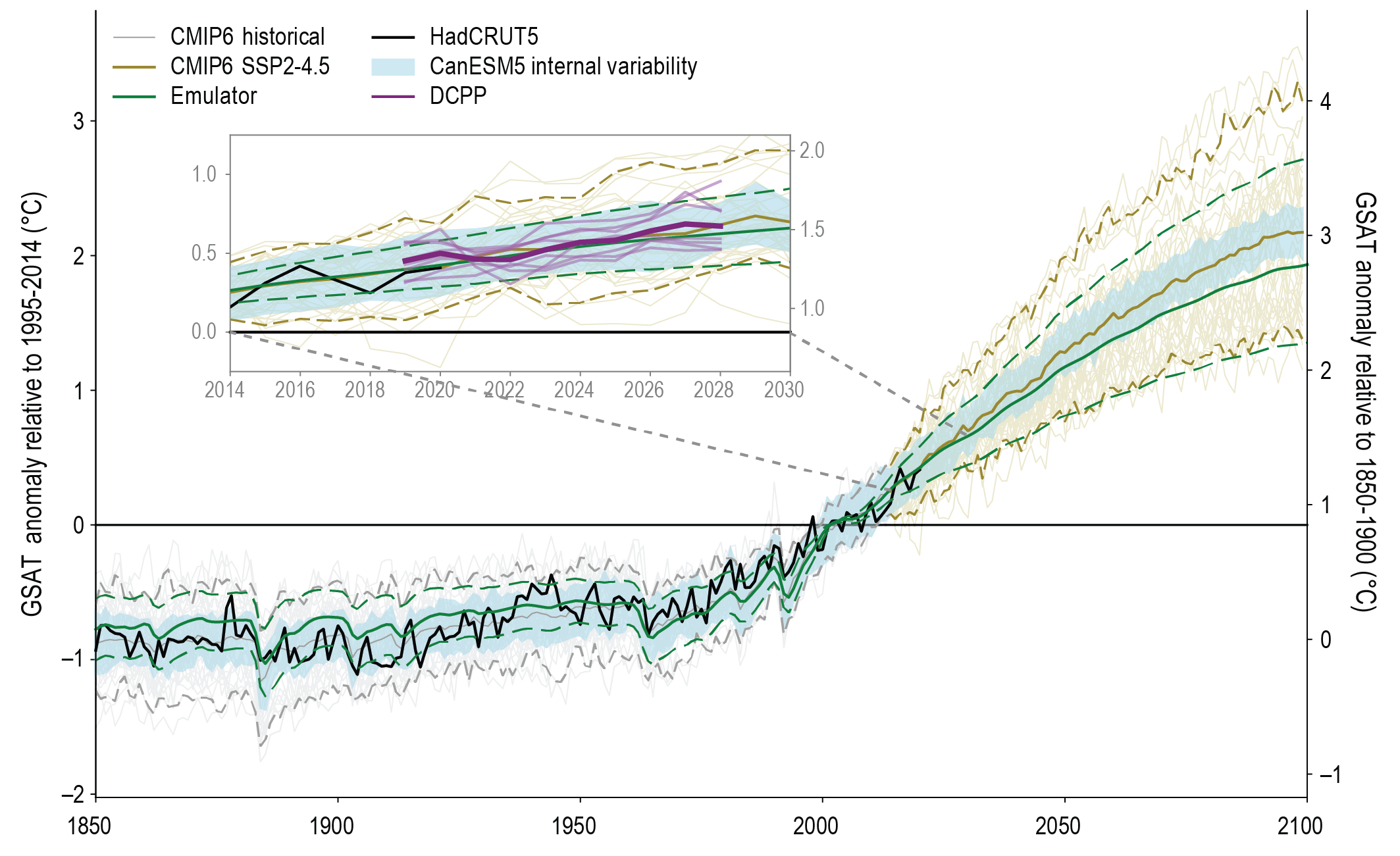
Box 4.1 Figure 1 | CMIP6 annual mean global surface air temperature (GSAT) simulations and various contributions to uncertainty in the projections ensemble. The figure shows anomalies relative to the period 1995–2014 (left y-axis), converted to anomalies relative to 1850–1900 (right y-axis); the difference between the y-axes is 0.85°C (Cross-Chapter Box 2.3). Shown are historical simulations with 39 CMIP6 models (grey) and projections following scenario SSP2-4.5 (dark yellow; thin lines: individual simulations; heavy line; ensemble mean; dashed lines: 5% and 95% ranges). The black curve shows the observations-based estimate (HadCRUT5; Morice et al., 2021). Light blue shading shows the 50-member ensemble CanESM5, such that the deviations from the CanESM5 ensemble mean have been added to the CMIP6 multi-model mean. The green curves are from the emulator and show the central estimate (solid) and very likely range (dashed) for GSAT. The inset shows a cut-out from the main plot and additionally in light purple for the period 2019–2028 the initialized forecasts from eight models contributing to DCPP (Boer et al., 2016); the deep-purple curve shows the average of the forecasts. Further details on data sources and processing are available in the chapter data table (Table 4.SM.1).
4.3 Projected Changes in Global Climate Indices in the 21st Century
This section assesses the latest simulations of representative indicators of global climate change presented as time series and tabulated values over the 21st century and across the main realms of the global climate system. In the atmospheric realm (Section 4.3.1), we assess simulations of GSAT (Figure 4.2a) and global land precipitation (Figure 4.2b). Across the cryospheric, oceanic, and biospheric realms (Section 4.3.2), we assess simulations of Arctic SIA (Figure 4.2c), GMSL (Figure 4.2d), the AMOC, ocean and land carbon uptake, and pH. In (Section 4.3.3 we assess simulations of several indices of climate variability, namely, the indices of the NAM, SAM, and ENSO. Finally, Section 4.3.4 assesses future GSAT change based on the CMIP6 ensemble in combination with other lines of evidence. An assessment of projected changes in related global extreme indices can be found in Chapter 11.
 Figure 4.2 | Selected indicators of global climatechange from CMIP6 historical and scenario simulations. (a) Global surface air temperature changes relative to the 1995–2014 average (left axis) and relative to the 1850–1900 average (right axis; offset by 0.82°C, which is the multi-model mean and close to observed best estimate, Cross-Chapter Box 2.1, Table 1). (b) Global land precipitation changes relative to the 1995–2014 average. (c) September Arctic sea ice area. (d) Global mean sea level (GMSL) change relative to the 1995–2014 average. (a), (b) and (d) are annual averages, (c) are September averages. In (a–c), the curves show averages over the CMIP6 simulations, the shadings around the SSP1-2.6 and SSP3-7.0 curves show 5–95% ranges, and the numbers near the top show the number of model simulations used. Results are derived from concentration-driven simulations. In (d), the barystatic contribution to GMSL (i.e., the contribution from land-ice melt) has been added offline to the CMIP6 simulated contributions from thermal expansion (thermosteric). The shadings around the SSP1-2.6 and SSP3-7.0 curves show 5–95% ranges. The dashed curve is the low confidence and low likelihood outcome at the high end of SSP5-8.5 and reflects deep uncertainties arising from potential ice-sheet and ice-cliff instabilities. This curve at year 2100 indicates 1.7 m of GMSL rise relative to 1995–2014. More information on the calculation of GMSL is available in Chapter 9, and further regional details are provided in the Atlas. Further details on data sources and processing are available in the chapter data table (Table 4.SM.1).
 From the CMIP6 multi-model ensemble we consider historical simulations with observed external forcings to 2014 and extensions to 2100 based on the five high-priority scenarios. We use the first realization (‘r1’) contributed by each modelling group. In tabular form, we show ensemble-mean changes and uncertainties for the near-term (2021–2040), mid-term (2041–2060), and the long-term (2081–2100), relative to present-day (1995–2014) and the approximation to pre-industrial (1850–1900). Changes in precipitation over land near 1.5°C, 2.0°C, 3.0°C, and 4.0°C of global warming relative to 1850–1900 are also assessed.
4.3.1 Atmosphere
4.3.1.1 Surface Air Temperature
The AR5 assessed from CMIP5 simulations and other lines of evidence that GSAT will continue to rise over the 21st century if greenhouse gas (GHG) concentrations continue increasing (Collins et al., 2013). The AR5 concluded that GSAT for 2081–2100, relative to 1986–2005 will likely be in the 5–95% range of 0.3°C–1.7°C under RCP2.6 and 2.6°C–4.8°C under RCP8.5. The corresponding ranges for the intermediate emissions scenarios with emissions peaking around 2040 (RCP4.5) and 2060 (RCP6.0) are 1.1°C–2.6°C and 1.4°C–3.1°C, respectively. The AR5 further assessed that GSAT averaged over the period 2081–2100 are projected to likely exceed 1.5°C above 1850–1900 for RCP4.5, RCP6.0 and RCP8.5 (high confidence) and are likely to exceed 2°C above 1850–1900 for RCP6.0 and RCP8.5 (high confidence). Global surface temperature changes above 2°C under RCP2.6 were deemed unlikely (medium confidence).
Here, for continuity’s sake, we assess the CMIP6 simulations of GSAT in a fashion similar to the AR5 assessment of the CMIP5 simulations. From these, we compute anomalies relative to 1995–2014 and display the evolution of ensemble means and 5–95% ranges (Figure 4.2). We also use the ensemble mean GSAT difference between 1850–1900 and 1995–2014, 0.82°C, to provide an estimate of the changes since 1850–1900 (Figure 4.2, right axis). Finally, we tabulate the ensemble mean changes between 1995–2014 and 2021–2040, 2041–2060, and 2081–2100 respectively (Figure 4.2).
The CMIP6 models show a 5–95% range of GSAT change for 2081–2100, relative to 1995–2014, of 0.6°C–2.0°C under SSP1-2.6 where CO2 concentrations peak between 2040 and 2060 (see Table 4.2). The corresponding range under the highest overall emissions scenario (SSP5-8.5) is 2.7°C–5.7°C. The ranges for the intermediate and high emissions scenarios (SSP2-4.5 and SSP3-7.0), where CO2 concentrations increase to 2100, but less rapidly than SSP5-8.5, are 1.4°C–3.0°C and 2.2°C–4.7°C, respectively. The range for the lowest emissions scenario (SSP1-1.9) is 0.2°C–1.3°C.
Time Period and Region | SSP1-1.9 (°C) | SSP1-2.6 (°C) | SSP2-4.5 (°C) | SSP3-7.0 (°C) | SSP5-8.5 (°C) |
Global: 2021–2040 Relative to 1995–2014 Relative to 1850–1900 | 0.7 (0.3, 1.1) 1.5 (1.1, 2.2) | 0.7 (0.4, 1.1) 1.6 (1.1, 2.2) | 0.7 (0.4, 1.2) 1.6 (1.0, 2.3) | 0.7 (0.5, 1.2) 1.6 (1.0, 2.4) | 0.8 (0.5, 1.3) 1.7 (1.2, 2.4) |
Global: 2041–2060 Relative to 1995–2014 Relative to 1850–1900 | 0.8 (0.3, 1.5) 1.7 (1.1, 2.4) | 1.0 (0.6, 1.6) 1.9 (1.2, 2.7) | 1.3 (0.8, 1.9) 2.1 (1.5, 3.0) | 1.4 (0.9, 2.3) 2.3 (1.6, 3.2) | 1.7 (1.2, 2.5) 2.6 (1.8, 3.4) |
Global: 2081–2100 Relative to 1995–2014 Relative to 1850–1900 | 0.7 (0.2, 1.5) 1.5 (1.0, 2.2) | 1.2 (0.6, 2.0) 2.0 (1.3, 2.8) | 2.0 (1.4, 3.0) 2.9 (2.1, 4.0) | 3.1 (2.2, 4.7) 3.9 (2.8, 5.5) | 4.0 (2.7, 5.7) 4.8 (3.6, 6.5) |
Land: 2081–2100 Relative to 1995–2014 | 0.9 (0.3, 2.0) | 1.5 (0.8, 2.6) | 2.7 (1.7, 4.0) | 4.1 (3.0, 6.2) | 5.3 (3.5, 7.6) |
Ocean: 2081–2100 Relative to 1995–2014 | 0.6 (0.1, 1.2) | 1.0 (0.5, 1.8) | 1.8 (1.2, 2.7) | 2.7 (1.8, 4.0) | 3.4 (2.3, 4.9) |
Tropics: 2081–2100 Relative to 1995–2014 | 0.5 (0.1, 1.1) | 1.0 (0.5, 1.6) | 1.8 (1.2, 2.5) | 2.7 (2.0, 4.0) | 3.5 (2.4, 4.9) |
Arctic: 2081–2100 Relative to 1995–2014 | 2.4 (0.5, 6.6) | 3.3 (0.4, 7.5) | 5.4 (2.8, 10.0) | 7.7 (4.5, 13.4) | 10.0 (6.2, 15.2) |
Antarctic: 2081–2100 Relative to 1995–2014 | 0.5 (0.0, 1.1) | 1.1 (0.1, 2.9) | 1.9 (0.6, 3.2) | 2.8 (1.3, 4.5) | 3.6 (1.7, 5.6) |
In summary, the CMIP6 models show a general tendency toward larger long-term globally averaged surface warming than did the CMIP5 models, for nominally comparable scenarios (very high confidence). In SSP1-2.6 and SSP2-4.5, the 5–95% ranges have remained similar to the ranges in RCP2.6 and RCP4.5, respectively, but the distributions have shifted upward by about 0.3°C (high confidence). For SSP5-8.5 compared to RCP8.5, the 5% bound of the distribution has hardly changed, but the 95% bound and the range have increased by about 20% and 40%, respectively (high confidence). About half of the warming increase has occurred because of more models with higher climate sensitivity in CMIP6, compared to CMIP5; the other half of the warming increase arises from higher effective radiative forcing in nominally comparable scenarios (medium confidence, see Section 4.6.2).
With regards to global warming levels (GWLs) of 1.5°C, 2.0°C and 3.0°C, we note that there is unanimity across all of the CMIP6 model simulations that GSAT change relative to 1850–1900 will rise above: (i) 1.5°C following SSP2-4.5, SSP3-7.0, or SSP5-8.5 (on average around 2030); (ii) 2.0°C following either SSP3-7.0 or SSP5-8.5 (on average around 2043); and (iii) 3.0°C following SSP5-8.5 (on average around 2062). Under SSP1-1.9, 55% and 36% of the model simulations rise above 1.5°C and 2.0°C, respectively, while for SSP1-2.6 those percentages increase to 87% and 58%, respectively. Here, the time of GSAT exceedance is determined as the first year at which 21-year running averages of GSAT exceed the given GWL. In (Section 4.3.4, these values are reassessed using CMIP6 ensemble in combination with other lines of evidence.
CMIP6 models project increases in area-weighted land, ocean, tropical (30°S–30°N), Arctic (67.7°N–90°N), and Antarctic (90°S–55°S) surface air temperature (Table 4.2). Consistent with AR5, and earlier assessments, CMIP6 models project that annual average surface air temperature will warm about 50% more over land than over the ocean, and that the Arctic will warm about more than 2.5 times the global average (Section 4.5.1). For 2081–2100, relative to 1995–2014, the CMIP6 models show 5–95% ranges of warming over land of 0.3°C–2.0°C and 3.5°C–7.6°C following SSP1-1.9 and SSP5-8.5, respectively. The corresponding ranges for Arctic surface air temperature change are 0.5°C–6.6°C and 6.2°C–15.2°C, respectively.
The concentration-driven simulations presented above use a prescribed CO2 pathway calculated by the MAGICC7.0 model using the CMIP6 emissions (Meinshausen et al., 2020). This is compared here with the CO2 concentration simulated by CMIP6 ESMs in response to the SSP5-8.5 emissions (Figure 4.3). The 1995–2014 mean simulated CO2 level is 375 ppm, very similar to the prescribed 378 ppm, but the ESM 5–95% range is 357–391 ppm. By the end of the 21st century (2081–2100), the ESM mean is 953 ppm – below the prescribed CO2 pathway (1004 ppm), but with a large 5–95% range of 848–1045 ppm, which spans the prescribed concentration level. This result differs from CMIP5, which showed that ESMs typically simulated CO2 concentrations higher than the prescribed concentration-driven RCP pathways. Reduced spread in CMIP6 carbon cycle feedbacks compared to CMIP5 has been postulated to be due to the inclusion of nitrogen cycle processes in about half of CMIP6 ESMs (Arora et al., 2020). This means that the CMIP6 spread in GSAT response to CO2 emissions is dominated by climate sensitivity differences between ESMs more than by carbon cycle differences (high confidence) (Jones and Friedlingstein, 2020; Williams et al., 2020).
 Figure 4.3 | Comparison ofconcentration-driven and emissions-driven simulation. (a) Atmospheric CO2 concentration; (b) global surface air temperature from models which performed SSP5-8.5 scenario simulations in both emissions-driven (blue) and concentration-driven (red) configurations. For concentration driven simulations, CO2 concentration is prescribed, and follows the red line in panel (a) in all models. For emissions-driven simulations, CO2 concentration is simulated and can therefore differ for each model, blue lines in panel (a). Further details on data sources and processing are available in the chapter data table (Table 4.SM.1).
 Simulated GSAT over 1995–2014, relative to 1850–1900 period, warms by very similar amounts in the two sets of simulations: 0.82°C (0.45–1.31) in emissions-driven compared with 0.75°C (0.53–1.09) in concentration-driven simulations. By the end of the 21st century, warming in emissions-driven simulations is very similar: 4.58°C (3.53–6.70), reflecting the slightly lower CO2 concentration simulated by the ESMs compared with warming under the prescribed CO2 pathway of 4.69°C (3.70–6.77). This difference in model-mean response is more than an order of magnitude smaller than the 5–95% spread across model projections. The spread in CO2 concentration, compared with the prescribed default concentration, leads to a very small increase by about 0.1°C in the spread of GSAT projections, but it is not possible to tell if this is a direct consequence of the simulation configuration or internal variability of the model simulations. These differences due to experimental configuration would be smaller still under scenarios with lower CO2 levels, and so we assess that results from concentration-driven and emissions-driven configurations do not affect the assessment of GSAT projections (high confidence).
4.3.1.2 Precipitation
The AR5 assessed from CMIP5 projections that global mean precipitation over the 21st century will increase by more than 0.05 mm day–1 (about 2% of global precipitation) and 0.15 mm day–1 (about 5% of global precipitation) under the RCP2.6 and RCP8.5 scenarios, respectively (Collins et al., 2013). These changes are generally in line with those from the CMIP6 simulations following SSP1-2.6 and SSP5-8.5 (Table 4.3).
Time Period and Region | SSP1-1.9 (%) | SSP1-2.6 (%) | SSP2-4.5 (%) | SSP3-7.0 (%) | SSP5-8.5 (%) | |
Land | 2021–2040 | 2.4 (0.7, 4.1) | 2.0 (–0.6, 3.6) | 1.5 (–0.4, 3.6) | 1.2 (–1.0, 3.4) | 1.7 (–0.1, 4.1) |
2041–2060 | 2.7 (0.6, 5.0) | 2.8 (–0.4, 5.2) | 2.7 (0.3, 5.2) | 2.5 (–0.8, 5.1) | 3.7 (–0.1, 6.9) | |
2081–2100 | 2.4 (–0.2, 4.7) | 3.3 (0.0, 6.6) | 4.6 (1.5, 8.3) | 5.8 (0.5, 9.6) | 8.3 (0.9, 12.9) | |
Global | 2081–2100 | 2.0 (0.4, 4.2) | 2.9 (1.0, 5.2) | 4.0 (2.3, 6.7) | 4.7 (2.3, 8.2) | 6.5 (3.4, 10.9) |
Ocean | 2081–2100 | 1.9 (0.6, 4.1) | 2.8 (1.1, 5.4) | 3.8 (2.0, 6.8) | 4.4 (2.1, 7.9) | 6.0 (2.9, 10.5) |
Land | ∆T > 1.5°C | 2.0 (0.6, 4.4) 55 | 1.7 (–2.0, 6.9) 87 | 1.7 (–2.9, 6.2) 100 | 1.5 (–3.9, 6.6) 100 | 1.5 (–3.5, 6.4) 100 |
∆T > 2.0°C | 3.8 (2.4, 5.8) 36 | 2.2 (–2.0, 4.6) 58 | 2.8 (–2.2, 8.1) 97 | 2.4 (–4.4, 7.7) 100 | 2.8 (–2.8, 8.3) 100 | |
∆T > 3.0°C | – (–, –) 0 | – (–, –) 0 | 4.9 (1.5, 9.6) 54 | 4.3 (–4.4, 11.5) 97 | 4.9 (–2.6, 11.0) 100 | |
∆T > 4.0°C | – (–, –) 0 | – (–, –) 0 | 4.2 (1.3, 6.3) 9 | 5.1 (–2.5, 11.1) 57 | 6.4 (–3.4, 15.0) 85 | |
 Figure 4.4 | CMIP6 annual mean precipitation changes (%) from historical and scenario simulations. (a) Northern Hemisphere extratropics (30°N–90°N). (b) North Atlantic subtropics (5°N–30°N, 80°W–0°). Changes are relative to 1995–2014 averages. Displayed are multi-model averages and, in parentheses, 5–95% ranges. The numbers inside each panel are the number of model simulations. Results are derived from concentration-driven simulations. Further details on data sources and processing are available in the chapter data table (Table 4.SM.1).
 Unlike AR5, our focus here is on land rather than global precipitation because land precipitation has greater societal relevance. These are displayed as percent changes relative to 1995–2014 (Figure 4.2b). Based on these results, we conclude that global land precipitation is larger during the period 2081–2100 than during the period 1995–2014, under all scenarios considered here (high confidence) (Table 4.3). Global land precipitation for 2081–2100, relative to 1995–2014, shows a 5–95% range of –0.2 to +4.7% under SSP1-1.9 and 0.9–12.9% under SSP5-8.5, respectively. The corresponding ranges under the other emissions scenarios are 0.0–6.6% (SSP1-2.6), 1.5–8.3% (SSP2-4.5), and 0.5–9.6% (SSP3-7.0). A detailed assessment of hydrological sensitivity, or change in precipitation per degree warming, can be found in Chapter 8 (Section 8.2.1).
For scenarios where unanimity across all of the model simulations that GSAT change relative to 1850–1900 rises above 1.5°C (SSP2-4.5, SSP3-7.0, or SSP5-8.5), the ensemble-mean change in global land precipitation from 1850–1900 until the time of exceedance is on average about 1.6%. For scenarios with unanimous global warming above 2.0°C (SSP3-7.0, or SSP5-8.5) and 3.0°C (SSP5-8.5), the ensemble-mean increase in global land precipitation for those models that do exceed 2.0°C and 3.0°C is on average about 2.6% and 4.9%, respectively. On average under SSP1-1.9 and SSP1-2.6, the global land precipitation change for simulations where global warming exceeds 1.5°C and 2.0°C will be about 1.9% and 3.0%, respectively.
Relative to 1995–2014, and across all of the scenarios considered here, CMIP6 models show greater increases in precipitation over land than either globally or over the ocean (Table 4.3; high confidence). Over the Northern Hemisphere (NH) extratropics, the 5–95% changes in precipitation over land between 1995–2014 and 2021–2040, 2041–2060, and 2081–2100, following SSP5-8.5, are 0.6–4.9%, 1.5–8.8%, and 4.7–17.2%, respectively (Figure 4.4). At the other end of scenario spectrum, SSP1-1.9, the corresponding changes are 0.6–5.4%, 0.6–7.3%, and 0.2–7.7%, respectively. By contrast, over the North Atlantic subtropics, precipitation decreases by about 10% following SSP3-7.0 and SSP5-8. There is no change in subtropical precipitation in the North Atlantic following SSP1-1.9, SSP1-2.6, or SSP2-4.5 (high confidence); thereby highlighting the potential limitations of pattern scaling for regional hydrological changes (Section 8.5.3). The reasons for the opposing changes in these two regions are assessed in Chapter 8.
4.3.2 Cryosphere,Ocean and Biosphere
4.3.2.1 Arctic Sea Ice
The AR5 assessed from CMIP5 simulations that there will be year-round reductions of Arctic sea ice coverage by the end of this century (Collins et al., 2013). These range from 43% under RCP2.6 and 94% under RCP8.5 in September, and from 8% under RCP2.6 and 34% under RCP8.5 in March (medium confidence). Based on a five-member selection of CMIP5 models, AR5 further assessed that for RCP8.5, Arctic sea ice coverage in September will drop below 1 million km2 and be practically ice free at some point between 2040 and 2060. The SROCC further assessed that the probability of an ice-free Arctic in September for stabilized global warming of 1.5°C and 2.0°C is approximately 1% and 10–35%, respectively (IPCC, 2019).
With regards to the model selection in AR5, model evaluation studies have since identified shortcomings of the CMIP5 models to match the observed distribution of sea ice thickness in the Arctic (Stroeve et al., 2014; Shu et al., 2015) and the observed evolution of albedo on seasonal scales (Koenigk et al., 2014). It was also found that many models’ deviation from observed sea ice cover climatology cannot be explained by internal variability, whereas the models’ deviation from observed sea ice cover trend (over the satellite period) can often be explained by internal variability (Olonscheck and Notz, 2017). This hinders a selection of models according to their simulated trends, which additionally has been shown to only have a weak effect on the magnitude of simulated future trends (Stroeve and Notz, 2015).
Based on results from the CMIP6 models, we conclude that on average the Arctic will become practically ice-free in September by the end of the 21st century under SSP2-4.5, SSP3-7.0, and SSP5-8.5 (high confidence) (Figure 4.2c and Table 4.4). Also, in the CMIP6 models, Arctic SIA in March decreases in the future, but to a much lesser degree, in percentage terms, than in September (high confidence) (Table 4.4). A more detailed assessment of projected Arctic and also Antarctic sea ice change can be obtained in Chapter 9 (Section 9.3.1).
Month and Time Period | SSP1-1.9 (106km2) | SSP1-2.6 (106km2) | SSP2-4.5 (106km2) | SSP3-7.0 (106km2) | SSP5-8.5 (106km2) | |
September | 2021–2040 | 2.6 (1.1, 6.5) | 2.7 (0.6, 6.4) | 2.8 (0.7, 6.4) | 3.1 (1.1, 6.4) | 2.5 (0.4, 5.8) |
2041–2060 | 2.2 (0.3, 6.5) | 2.0 (0.2, 6.1) | 1.7 (0.1, 5.6) | 1.7 (0.1, 5.7) | 1.2 (0.0, 5.2) | |
2081–2100 | 2.4 (0.2, 6.2) | 1.7 (0.0, 6.0) | 0.8 (0.0, 4.6) | 0.5 (0.0, 3.3) | 0.3 (0.0, 2.2) | |
March | 2021–2040 | 14.0 (11.4, 18.7) | 14.9 (11.9, 25.8) | 14.9 (11.9, 23.5) | 15.0 (11.7, 27.3) | 14.9 (11.9, 24.7) |
2041–2060 | 13.8 (10.9, 18.3) | 14.5 (10.9, 25.7) | 14.3 (11.1, 23.3) | 14.2 (10.5, 27.1) | 13.9 (10.2, 24.5) | |
2081–2100 | 13.7 (10.9, 18.5) | 14.2 (10.6, 25.7) | 13.1 (9.5, 22.2) | 11.8 (5.4, 25.5) | 9.7 (3.1, 21.6) | |
Studies focusing on the relationship of sea ice extent and changes in external drivers have consistently found a much-reduced likelihood of a practically ice-free Arctic Ocean during summer for global warming of 1.5°C than for 2.0°C (Screen and Williamson, 2017; Jahn, 2018; Niederdrenk and Notz, 2018; Notz and Stroeve, 2018; Sigmond et al., 2018; Olson et al., 2019). This is shown here in a large initial-condition ensemble of observationally constrained model simulations where GSAT are stabilized at 1.5°C, 2.0°C and 3.0°C warming relative to 1850–1900 in the RCP8.5 scenario (Figure 4.5). Temperature stabilization is achieved by switching off all the anthropogenic emissions around the time that GSAT first reaches the stabilization thresholds. Simulations have been observationally constrained to correct for a model bias in simulated historical September sea ice extent. In these simulations, Arctic sea ice coverage in September is simulated, on average, to drop below 1 million km2 around 2040, consistent with the AR5 set of assessed models (Sigmond et al., 2018). The individual model simulations, for which there are twenty for each stabilized temperature level, show that the probability of the Arctic becoming practically ice free at the end of the 21st century is significantly higher for 2°C warming than for 1.5°C warming above 1850–1900 levels (high confidence).
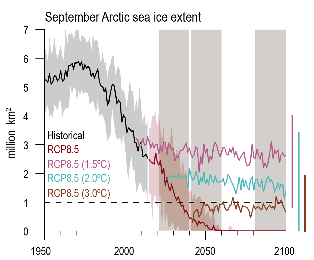 Figure 4.5 | Arctic sea ice extent in September in a large initial-condition ensemble of observationally-constrained simulations of an Earth system model (CanESM2). The black and red curves are averages over twenty simulations following historical forcings to 2015 and RCP8.5 extensions to 2100. The other curves are averages of over 20 simulations each after global surface air temperature has been stabilized at the indicated degree of global mean warming relative to 1850–1900. The bars to the right are the minimum to maximum ranges over 2081–2100 (Sigmond et al., 2018). The horizontal dashed line indicates a practically sea ice-free Arctic. Further details on data sources and processing are available in the chapter data table (Table 4.SM.1).
 4.3.2.2 Global Mean Sea Level
The AR5 assessed from CMIP5 process-based simulations that the rate of GMSL rise during the 21st century will very likely exceed the rate observed during 1971–2010 for all RCP scenarios due to increases in ocean warming and loss of mass from glaciers and ice sheets (Church et al., 2013). Further, AR5 concluded that for the period 2081–2100, compared to 1986–2005, GMSL rise is likely (medium confidence) to be in the 5–95% range of projections from process-based models, which give 0.26–0.55 m for RCP2.6, 0.32–0.63 m for RCP4.5, 0.33–0.63 m for RCP6.0, and 0.45–0.82 m for RCP8.5. For RCP8.5, the rise by 2100 is 0.52–0.98 m with a rate during 2081–2100 of 8–16 mm yr–1.
There have been substantial modelling advances since AR5, with most sea level projections corresponding to one of three categories: (i) central-range projections, combining scenario-conditional probability distributions for the different contributions to estimate a central range under different scenarios; (ii) probabilistic projections, which explicitly consider outcomes for a wide range of likelihoods, including low-likelihood, high-impact outcomes; and (iii) semi-empirical projections, based on statistical relationships between past GMSL changes and climate variables, which now calibrate individual contributions and are consistent with physical-model based estimates (Section 9.6.3).
Based on the assessment of the latest modelling information (Figure 4.2d and Section 9.6.3), we conclude that under the SSP3-7.0, the likely range of GMSL change averaged over 2081–2100 relative to 1995–2014 is 0.46–0.74 m. Under SSP1-2.6, the likely range over the long-term is 0.30–0.54 m. Further, in SSP2-4.5, SSP3-7.0, and SSP5-8.5, the rise in GMSL is projected to accelerate over the 21st century. A detailed assessment of the processes contributing to these projected rises and accelerations in GMSL, together with a comparison to AR5 and SROCC, can be found in Chapter 9 (Section 9.6.3). Projected changes in the thermosteric component of GMSL beyond 2300 are assessed in Section 4.7.1.
In summary, it is virtually certain that under any one of the assessed SSPs, there will be continued rise in GMSL through the 21st century.
4.3.2.3 Atlantic Meridional Overturning Circulation
The AR5 assessed from CMIP5 simulations that the Atlantic Meridional Overturning Circulation (AMOC) will very likely weaken over the 21st century, and the projected weakening of the AMOC is consistent with CMIP5 projections of an increase of high-latitude temperature and high-latitude precipitation, with both effects causing the surface waters at high latitudes to become less dense and therefore more stable (Collins et al., 2013).
Based on CMIP6 models, we find that over the 21st century, AMOC strength, relative to 1995–2014, shows a multi-model mean decrease in each of the SSP scenarios but with a large spread across the individual simulations (Figure 4.6). We also note that the magnitude of the ensemble-mean strength decrease is approximately scenario independent up to about 2060 (Weijer et al., 2020). A more detailed assessment of these projected AMOC changes, and the mechanisms involved, can be found in Chapter 9 (Section 9.2.3).
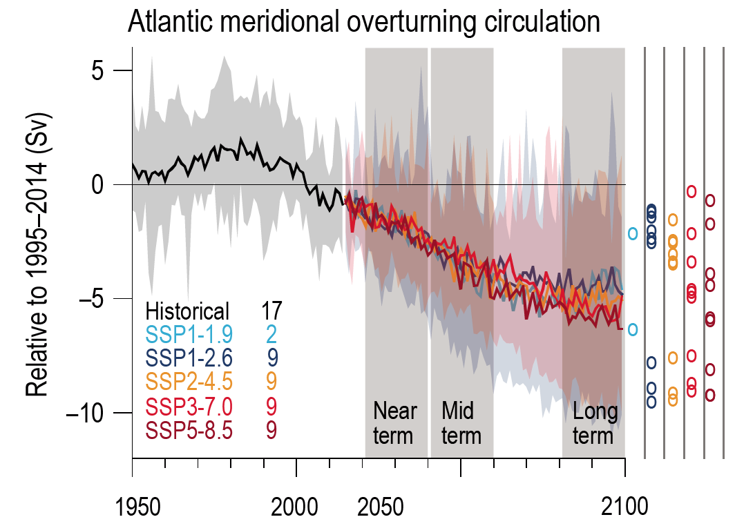 Figure 4.6 | CMIP6 annual mean Atlantic Meridional Overturning Circulation (AMOC) strength change in historical and scenario simulations. Changes are relative to averages from 1995–2014. The curves show ensemble averages and the shadings the 5–95% ranges across the SSP1-2.6 and SSP3-7.0 ensembles. The circles to the right of the panel show the anomalies averaged from 2081–2100 for each of the available model simulations. The numbers inside the panel are the number of model simulations. Here, the strength of the AMOC is computed as the maximum value of annual mean ocean meridional overturning mass stream function in the Atlantic at 26°N. Results are from concentration-driven simulations. Further details on data sources and processing are available in the chapter data table (Table 4.SM.1).
 In summary, we assess from the CMIP6 models that AMOC weakening over the 21st century is very likely ; the rate of weakening is approximately independent of the emissions scenario (high confidence).
Based on a large initial condition ensemble of simulations with a CMIP5 model (CanESM2) with emissions scenarios leading to stabilization of global warming of 1.5°C, 2.0°C, or 3.0°C relative to 1850–1900, AMOC continues to decline for 5–10 years after GSAT is effectively stabilized at the given GWL (Sigmond et al., 2020). This is followed by a recovery of AMOC strength for about the next 150 years to a level that is approximately independent of the considered stabilization scenario. These results are replicated in simulations in a CMIP6 model (CanESM5) with emissions cessation after diagnosed CO2 emissions reach 750 Gt, 1000 Gt, or 1500 Gt. These emissions levels lead to global warming stabilization at 1.5°C, 2.0°C, or 3.0°C relative to 1850–1900. In summary, in these model simulations the AMOC recovers over several centuries after the cessation of CO2 emissions (medium confidence).
4.3.2.4 Ocean and Land Carbon Uptake
The AR5 concluded with very high confidence that ocean carbon uptake of anthropogenic CO2 will continue under all RCPs through the 21st century, with higher uptake corresponding to higher concentration pathways. The future evolution of the land carbon uptake was assessed to be much more uncertain than for ocean carbon uptake, with a majority of CMIP5 models projecting a continued cumulative carbon uptake.
Based on results from the CMIP6 models, we conclude that the flux of carbon from the atmosphere into the ocean increases continually through most of 21st century in the two highest emissions and decreases continually under the other emissions scenarios (Figure 4.7a). The flux of carbon from the atmosphere to land shows a similar 21st century behaviour across the scenarios but with much higher year-to-year variation than ocean carbon flux (Figure 4.7b). A more in-depth assessment and discussion of the mechanism involved can be found in Chapter 5 (Section 5.4.5).
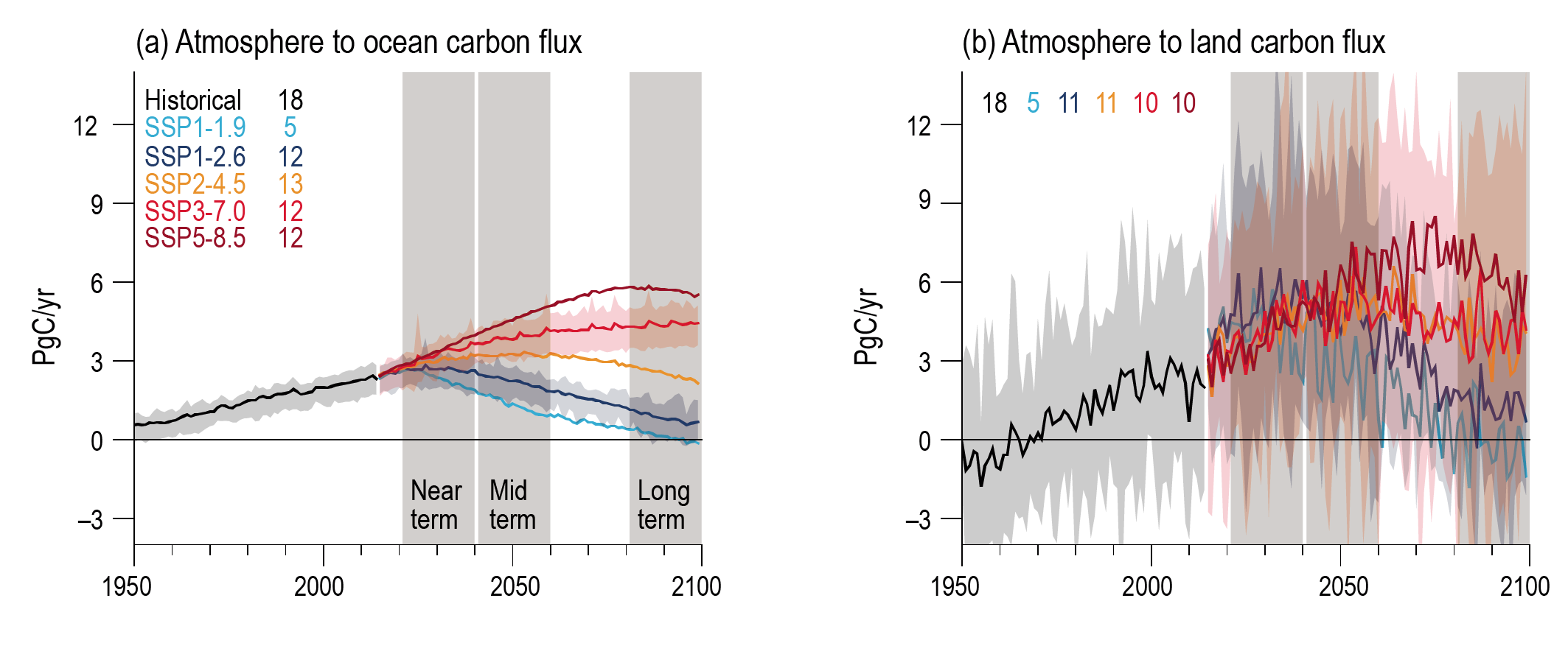 Figure 4.7 | CMIP6 carbon uptake in historical and scenario simulations. (a) Atmosphere to ocean carbon flux (PgC yr–1). (b) Atmosphere to land carbon flux (PgC yr–1). The curves show ensemble averages and the shadings show the 5–95% ranges across the SSP1-2.6 and SSP3-7.0 ensembles. The numbers inside each panel are the number of model simulations. The land uptake is taken as Net Biome Productivity (NBP) and so includes any modelled net land-use change emissions. Results are from concentration-driven simulations. Further details on data sources and processing are available in the chapter data table (Table 4.SM.1).
 In summary, we assess that the cumulative uptake of carbon by the ocean and by land will increase through the 21st century irrespective of the considered emissions scenarios except SSP1-1.9 (very high confidence).
4.3.2.5 Surface Ocean pH
The AR5 assessed from CMIP5 simulations that it is virtually certain that increasing storage of carbon by the ocean under all four RCPs through to 2100 will increase ocean acidification in the future (Ciais et al., 2013). Specifically, AR5 reported that CMIP5 models project increased ocean acidification globally to 2100 under all RCPs, and that the corresponding model mean and model spread in the decrease in surface ocean pH from 1986–2005 to 2081–2100 would be 0.065 (0.06–0.07) for RCP2.6, 0.145 (0.14–0.15) for RCP4.5, 0.203 (0.20–0.21) for RCP6.0 and 0.31 (0.30–0.32) for RCP8.5.
Based on results from the CMIP6 models we conclude that, except for the lower-emissions scenarios SSP1-1.9 and SSP1-2.6, ocean surface pH decreases monotonically through the 21st century (high confidence) (Figure 4.8).
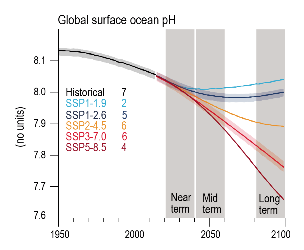 Figure 4.8 | Global average surface ocean pH. The shadings around the SSP1-2.6 and SSP5-7.0 curves are the 5–95% ranges across those ensembles. The numbers inside each panel are the number of model simulations. Results are from concentration-driven simulations. Further details on data sources and processing are available in the chapter data table (Table 4.SM.1).
 4.3.3 Modes of Variability
4.3.3.1 Northern and Southern Annular Modes
4.3.3.1.1 Northern Annular Mode
The Northern Annular Mode (NAM) is the leading mode of variability in the NH extratropical atmosphere (Section AIV.2.1). Throughout this chapter, we use a simple fixed latitude-based NAM index defined as the difference in SLP between 35°N and 65°N (Section AIV.2.1; Li and Wang, 2003). The NAM index computed from the latitudinal gradient in SLP is strongly correlated with variations in the latitudinal position and strength of the mid-latitude westerly jets, and with the spatial distribution of Arctic sea ice (Caian et al., 2018). Projected changes in the position and strength of the mid-latitude westerly jets, storm tracks, and atmospheric blocking in both hemispheres are assessed in Section 4.5.1.6. The AR5 referred to the NAM, and its synonym the Arctic Oscillation (AO), through its regional counterpart, the North Atlantic Oscillation (NAO). Here, we use the term NAM to refer also to the AO and NAO (Section AIV.2.1), accepting that the AO and NAO are not identical entities.
We first summarize the assessment of past NAM changes and their attribution from Chapters 2 and 3 to put into context the future projections described here. Strong positive trends for the NAM/NAO indices were observed since 1960, which have weakened since the 1990s (high confidence) (Section 2.4.1.1). The NAO variability in the instrumental record was likely not unusual in the millennial and multi-centennial context (Section 2.4.1.1). Climate models simulate the gross features of the NAM with reasonable fidelity, including its interannual variability, but models tend to systematically underestimate the amount of multi-decadal variability of the NAM and jet stream compared to observations (Section 3.7.1; J. Wang et al., 2017b; Bracegirdle et al., 2018; Simpson et al., 2018), with the caveat of the observational record being relatively short to characterize decadal variability (Chiodo et al., 2019). A realistic simulation of the stratosphere and SST variability in the tropics and northern extratropics are important for a model to realistically capture the observed NAM variability. Despite some evidence from climate model studies that anthropogenic forcings influence the NAM, there is limited evidence for a significant role for anthropogenic forcings in driving the observed multi-decadal variations of the NAM over the instrumental period (Section 3.7.1).
The AR5 assessed from CMIP5 simulations that the future boreal wintertime NAM is very likely to exhibit large natural variations and trends of similar magnitude to that observed in the past and is likely to become slightly more positive in the future (Collins et al., 2013). Based on CMIP6 model results displayed in Figure 4.9a, we conclude that the boreal wintertime surface NAM is more positive by the end of the 21st century under SSP3-7.0 and SSP5-8.5 (high confidence). For these high emissions scenarios, the 5–95% range of NAM index anomalies averaged from 2081–2100 are 0.3–3.8 hPa and 0.32–5.2 hPa, respectively. On the other hand, under neither of the lowest emissions scenarios, SSP1-1.9 and SSP1-2.6, does the NAM show a robust change, by the end of the 21st century (high confidence).
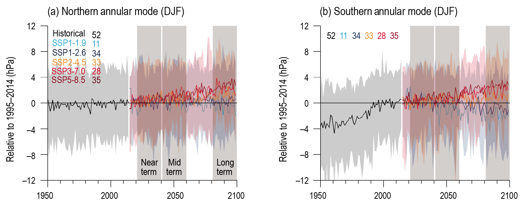 Figure 4.9 | CMIP6 simulations of boreal winter (December–January–February, DJF) Annular Mode indices. (a) NAM and (b) SAM. The NAM is defined as the difference in zonal mean SLP at 35°N and 65°N (Li and Wang, 2003) and the SAM as the difference in zonal mean SLP at 40°S and 65°S (Gong and Wang, 1999). All anomalies are relative to averages from 1995–2014. The curves show multi-model ensemble averages over the CMIP6 r1 simulations. The shadings around the SSP1-2.6 and SSP3-7.0 curves denote the 5–95% ranges of the ensembles. The numbers inside each panel are the number of model simulations. The results are for concentration-driven simulations. Further details on data sources and processing are available in the chapter data table (Table 4.SM.1).
 Significant progress has been made since AR5 in understanding the physical mechanisms responsible for changes in the NAM, although uncertainties remain. It is now clear from the literature that the NAM response, and the closely-related response of the mid-latitude storm tracks, to anthropogenic forcing in CMIP5-era climate models is determined by a ‘tug-of-war’ between two opposing processes (Harvey et al., 2014; Shaw et al., 2016; Screen et al., 2018a): (i) Arctic amplification (Sections 4.5.1.1 and 7.4.4.1), which decreases the low-level meridional temperature gradient, reduces baroclinicity on the poleward flank of the eddy-driven jet, and shifts the storm tracks equatorward and leading to a negative NAM (see Box 10.1; Harvey et al., 2015; Hoskins and Woollings, 2015; Peings et al., 2017; Screen et al., 2018a); and (ii) enhanced warming in the tropical upper-troposphere, due to GHG increases and associated water vapour and lapse rate feedbacks, which increases the upper-level meridional temperature gradient and causes a poleward shift of the storm tracks and a positive NAM (Harvey et al., 2014; Vallis et al., 2015; Shaw, 2019). The large diversity in projected NAM changes in CMIP5 multi-model ensemble (Gillett and Fyfe, 2013) appears to be at least partly explained by the relative importance of these two mechanisms in particular models (Harvey et al., 2014, 2015; Vallis et al., 2015; McCusker et al., 2017; Oudar et al., 2017). Models that produce larger Arctic amplification also tend to produce larger equatorward shifts of the mid-latitude jets and associated negative NAM responses (Barnes and Polvani, 2015; Harvey et al., 2015; Zappa and Shepherd, 2017; McKenna et al., 2018; Screen et al., 2018a; Zappa et al., 2018).
Another area of progress is new understanding the role of cloud radiative effects in shaping the mid-latitude circulation response to anthropogenic forcing. Through their non-uniform distribution of radiative heating, cloud changes can modify meridional temperature gradients and alter mid-latitude circulation and the annular modes in both hemispheres (Ceppi et al., 2014; Voigt and Shaw, 2015, 2016; Ceppi and Hartmann, 2016; Ceppi and Shepherd, 2017; Lipat et al., 2018; Albern et al., 2019; Voigt et al., 2019). In addition to the effects of changing upper and lower tropospheric temperature gradients on the NAM, progress has been made since AR5 in understanding the effect of simulated changes in the strength of the stratospheric polar vortex on winter NAM projections (Manzini et al., 2014; Zappa and Shepherd, 2017; Simpson et al., 2018).
4.3.3.1.2 Southern Annular Mode
The Southern Annular Mode (SAM) is the leading mode of large-scale extratropical atmospheric variability in the Southern Hemisphere and influences most of the southern extratropics (Annex IV, Section AIV.2.2). In its positive phase, the SAM characterizes anomalously low pressure over the polar cap and high pressure in southern mid-latitudes (Marshall, 2003). While there are some zonal asymmetries to the structure of the SAM (Section AIV.2.2), it is more symmetric than its NH counterpart (Fyfe et al., 1999). Throughout this chapter, we use a simple fixed latitude-based SAM index defined as the difference in zonal mean SLP between 40°S and 65°S (Gong and Wang, 1999; see Section AIV.2.2 for discussion of other SAM indices). Although the SAM is often used as a proxy for the location of the mid-latitude westerly wind belt, trends in the SAM can reflect a combination of changes in jet position, width, and strength. The changes in the Southern Hemisphere circulation associated with the SAM influence surface wind stress (Wang et al., 2014) and hence affect the Southern Ocean.
Over the instrumental period, there has been a robust positive trend in the SAM index, particularly since 1970 (high confidence) (Section 2.4.1.2). There is medium confidence that the recent trend in the SAM is unprecedented in the past several centuries (Section 2.4.1.2). There is high confidence that stratospheric ozone depletion and GHG increases have contributed to the positive SAM trend during the late 20th century, with ozone depletion dominating in austral summer, following the peak of the Antarctic ozone hole in September –October, and GHG increases dominating in other seasons (Section 3.7.2). To capture the effects of stratospheric ozone changes on the SAM, climate models must include a realistic representation of ozone variations (Section 3.7.2). In models that do not explicitly represent stratospheric ozone chemistry, which includes the majority of the CMIP6 model ensemble, an ozone dataset is prescribed. To properly capture the effects of ozone depletion and recovery on the stratosphere and surface climate, the prescribed ozone dataset must realistically capture observed stratospheric ozone trends with sufficiently high temporal resolution (Neely et al., 2014; Young et al., 2014). The CMIP6 experiment protocol recommended the use of a prescribed 4-D monthly mean ozone concentration field for models without stratospheric chemistry (Eyring et al., 2016).
The AR5 assessed that the positive trend in the austral summer/autumn SAM observed since 1970 (see Section 2.4.1.2) is likely to weaken considerably as stratospheric ozone recovers through the mid-21st century, while in other seasons the SAM changes depend on the emissions scenario, with a larger increase in SAM for higher emissions scenarios. In CMIP6 models, the austral summer SAM is more positive by the end of the 21st century under SSP3-7.0 and SSP5-8.5 (Figure 4.9b). On the other hand, under SSP1-1.9 and SSP1-2.6, the SAM is projected to be less positive, especially under SSP1-1.9 where the 5–95% ranges of anomalies relative to 1995–2014 are –3.1 to 0.0 hPa averaged from 2081–2100. In summary, under the highest emissions scenarios in the CMIP6 models, the SAM in the austral summer becomes more positive through the 21st century (high confidence).
4.3.3.2 El Niño–Southern Oscillation
The El Niño–Southern Oscillation (ENSO) is the most dominant mode of variability on interannual time scales and also the dominant source of seasonal climate predictability (Box 11.3 and Annex IV, Section AIV.2.3; Timmermann et al., 2018). The AR5 assessed from CMIP5 simulations that ENSO variability will very likely remain the dominant mode of interannual climate variability in the future, and that associated ENSO precipitation variability on regional scales is likely to intensify (Christensen et al., 2013). However, they assessed there was low confidence in projected changes in ENSO variability in the 21st century due to a strong component of internal variability.
Among a range of indices proposed for representing ENSO, we use the most prominent one, the Niño 3.4 index, defined as the average equatorial SST or precipitation across the central equatorial Pacific (5°S–5°N, 170°W–120°W; Section AIV.2.3). Here, we consider the evolution of the amplitude of Niño 3.4 index for SST and precipitation over the 21st century as projected by CMIP6 models. Analysis of CMIP6 models shows there is no robust model consensus on the forced changes in the amplitude of ENSO SST variability even under the high-emissions scenarios SSP3-7.0 and SSP5-8.5, but a significant increasing trend in the amplitude of ENSO precipitation variability is projected across the 21st century in the four SSPs (Figure 4.10). This is broadly consistent with results from CMIP5 models (Christensen et al., 2013; Power et al., 2013; Cai et al., 2015; Chen et al., 2017; Wengel et al., 2018), recent studies with CMIP6 models (Brown et al., 2020; Fredriksen et al., 2020; Freund et al., 2020; Yun et al., 2021), and large initial-condition ensemble experiments (Maher et al., 2018; Zheng et al., 2018; Haszpra et al., 2020).
 Figure 4.10 | Changes in amplitude of ENSO Variability. Variability of (a) SST and (b) precipitation anomalies averaged over Niño 3.4 region for 1950–2014 from CMIP6 historical simulations and for 2015–2100 from four SSPs. Thick lines stand for multi-model mean and shading is the 5–95% range across CMIP6 models for historical simulation (grey), SSP1-2.6 (blue) and SSP3-7.0 (pink), respectively. The amplitude of ENSO SST and rainfall variability is defined as the standard deviation of the detrended Niño 3.4-area averaged SST and rainfall index, respectively, over 30-year running windows. The standard deviation in every single model is normalized by each model’s present-day standard deviation averaged from 1995 to 2014. The number of available models is listed in parentheses. This figure is adopted from Yun et al. (2021). Further details on data sources and processing are available in the chapter data table (Table 4.SM.1).
 It is therefore very likely that the amplitude of ENSO rainfall variability will intensify in response to global warming over the 21st century although there is no robust consensus from CMIP6 climate models for a systematic change in amplitude of ENSO SST variability even in the high-emissions scenarios of SSP3-7.0 and SSP5-8.5.
4.3.4 Synthesis Assessment of Projected Change in Global Surface Air Temperature
GSAT change is assessed using multiple lines of evidence including the CMIP6 projection simulations out to year 2100. The assessment combines CMIP6 projections driven by SSP scenarios with observational constraints on simulated past warming (Box 4.1 and Figure 4.11a,b; Brunner et al., 2020; Liang et al., 2020; Nijsse et al., 2020; Tokarska et al., 2020; Ribes et al., 2021), as well as the AR6-updated assessment of ECS and TCR in Section 7.5. The approaches of (Liang et al., 2020; Tokarska et al., 2020; Ribes et al., 2021) have first been extended to all 20-year averaging periods between 2000 and 2100. For each 20-year period, the 5%, 50%, and 95% percentile GSAT values of these three constrained CMIP6 results are averaged percentile by percentile (Figure 4.11c). Then, an emulator based on a two-layer energy balance model (e.g., Held et al., 2010) is driven by the Chapter 7-derived ERF. The emulator parameters are chosen such that the central estimate, lower bound of the very likely range, and upper bound of the very likely range of climate feedback parameter and ocean heat uptake coefficient take the values that map onto the corresponding combination of ECS (3°C, 2°C and 5°C, respectively) and TCR (1.8°C, 1.2°C and 2.4°C, respectively) of Section 7.5 (see Box 4.1). As a final step, the constrained-CMIP6 and the emulator-based 5%, 50%, and 95% percentile GSAT values are averaged percentile by percentile (Figure 4.11c,d and Table 4.5). Constrained CMIP6 results and the ECS- and TCR-based emulator thus contribute one-half each to the GSAT assessment. Because the emulator results and (Ribes et al., 2021) represent the forced response only, and averaging over the other two individual estimates (Liang et al., 2020; Tokarska et al., 2020) further reduces the contribution from internal variability, the assessed GSAT time series are assumed to represent purely the forced response.
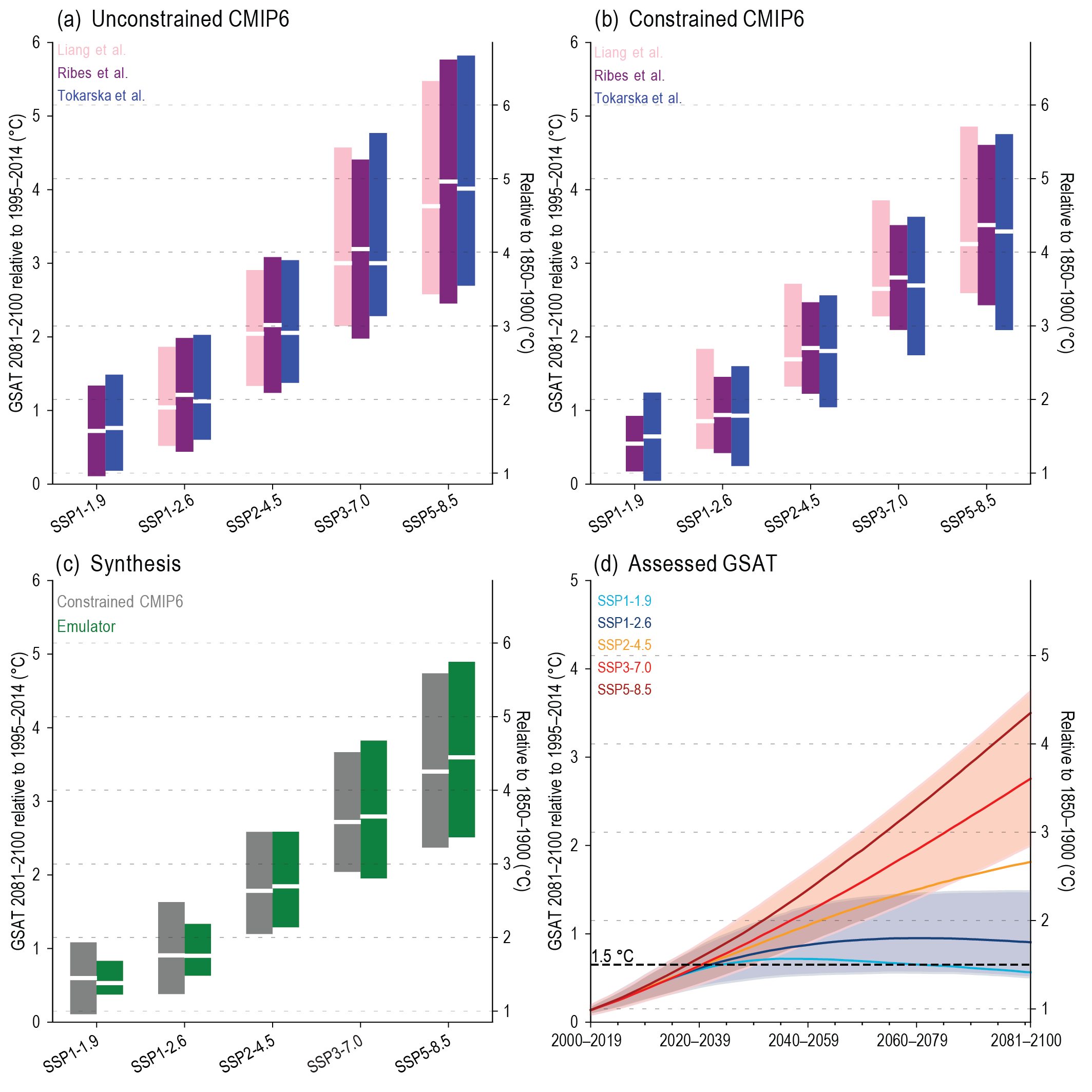 Figure 4.11 | Multiple lines of evidence for global surface air temperature (GSAT) changes for the long-term period, 2081–2100, relative to the average over 1995–2014, for all five priority scenarios. The unconstrained CMIP6 5–95% ranges (coloured bars) in (a) differ slightly because different authors used different subsamples of the CMIP6 archive. The constrained CMIP6 5–95% ranges (coloured bars) in (b) are smaller than the unconstrained ranges in (a) and differ because of different samples from the CMIP6 archive and because different observations and methods are used. In (c), the average of the ranges in (b) is formed (grey bars). Green bars in (c) show the emulator ranges, defined such that the best estimate, lower bound of the very likely range, and upper bound of the very likely range of climate feedback parameter and ocean heat uptake coefficient take the values that map onto the corresponding values of ECS and TCR of Section 7.5 (see Box 4.1). The time series in (d) are constructed by taking the average of the constrained CMIP6 ranges and the emulator ranges. The y-axes on the right-hand side are shifted upward by 0.85°C, the central estimate of the observed warming for 1995–2014, relative to 1850–1900 (Cross-Chapter Box 2.3, Table 1). Further details on data sources and processing are available in the chapter data table (Table 4.SM.1).
 Averaged over the period 2081–2100, GSAT is very likely to be higher than in the recent past (1995–2014) by 0.3°C–0.9°C in the low-emissions scenario SSP1-1.9 and by 2.6°C–4.7°C in the high-emission scenario SSP5-8.5. For the scenarios SSP1-2.6, SSP2-4.5, and SSP3-7.0, the correspondingvery likely ranges are 0.6°C–1.4°C, 1.3°C–2.5°C, and 2.0°C–3.8°C, respectively (Figure 4.11 and Table 4.5). Because the different approaches for estimating long-term GSAT change produce consistent results (Figure 4.11), there is high confidence in this assessment. These ranges of the long-term projected GSAT change generally correspond to AR5 ranges for related scenarios but the likelihood is increased to very likely ranges, in contrast to the likely ranges in AR5. Over the mid-term period 2041–2060, the very likely GSAT ranges of SSP1-1.9 and SSP5-8.5 are almost completely distinct (high confidence) (Table 4.5; see also Section 4.3.1).
CMIP6 models project a wider range of GSAT change than the assessed range (high confidence) (Section 4.3.1). The CMIP6 models with a higher climate sensitivity simulate warming rates higher than assessed very likely here (Section 4.3.1); these rates are very unlikely but not impossible to occur and hence cannot be excluded. The implications of these very unlikely warming rates for patterns of surface temperature and precipitation change are assessed in Section 4.8.
For the near term, initialized decadal forecasts constitute another line of evidence over the period 2019–2028 (Box 4.1). The forecasts are consistent with the assessed GSATvery likely range (Box 4.1, Figure 1), strengthening the confidence in the near-term assessment.
The assessed ranges of GSAT change can be converted to change relative to mean GSAT over the period 1850–1900 for a consistent comparison with AR5 (IPCC, 2013) and SR1.5 (IPCC, 2018a). GSAT was warmer in 1995–2014 (recent past) than 1850–1900 by 0.85 [0.67 to 0.98] °C. GSAT diagnosed for 1986–2005 (AR5 recent past) relative to 1850–1900 is 0.08°C higher than was diagnosed in AR5, due to methodological and dataset updates (Cross-Chapter Box 2.3, Table 1).
The uncertainty in GSAT relative to 1850–1900 includes the very likely ranges of assessed GSAT change relative to 1995–2014 (depending on scenario and period, between 0.5°C and 2.4°C; Figure 4.11d and Table 4.5), the uncertainty in historical GSAT change from the mean over 1850–1900 to 1995–2014 (about 0.3°C; Cross-Chapter Box 2.3), and the estimate of internal variability in 20-year GSAT averages (5–95% range about 0.15°C, Box 4.1; Maher et al., 2019). These uncertainties are assumed to be independent and are added in quadrature, meaning that the total uncertainty is only slightly larger than the dominating contribution by the GSAT change relative to 1995–2014 (Table 4.5). The addition is done by numerically sampling a normal distribution fitted to the 5%, 50% and 95% percentiles of the internal variability, as well as sampling skew-normal distributions (e.g., O’Hagan and Leonard, 1976) fitted to the 5%, 50% and 95% percentiles of both historical warming and GSAT relative to 1995–2014. The result is a joint probability distribution of GSAT change and 20-year period.
Averaged over the period 2081–2100, GSAT is very likely to be higher than in the period 1850–1900 by 1.0°C–1.8°C in the low-emissions scenarios SSP1-1.9 and by 3.3°C–5.7°C in the high-emissions scenario SSP5-8.5. For the scenarios SSP1-2.6, SSP2-4.5, and SSP3-7.0, the correspondingvery likely ranges are 1.3°C–2.4°C, 2.1°C–3.5°C, and 2.8°C–4.6°C, respectively (Table 4.5).
Time series of assessed GSAT change are now used to assess the time when certain thresholds of GSAT increases are crossed (Table 4.5). The threshold-crossing time is defined as the midpoint of the first 20-year period during which the average GSAT exceeds the threshold. During the near term (2021–2040), a 1.5°C increase in the 20-year average of GSAT, relative to the average over the period 1850–1900, is very likely to occur in scenario SSP5-8.5, likely to occur in scenarios SSP2-4.5 and SSP3-7.0, and more likely than not to occur in scenarios SSP1-1.9 and SSP1-2.6. In all scenarios assessed here except SSP5-8.5, the central estimate of crossing the 1.5°C threshold lies in the early 2030s, in the early part of the likely range (2030–2052) assessed in SR1.5, which assumed continuation of the then-current warming rate. Roughly half of this difference arises from a larger historical warming diagnosed in AR6, while the other half arises because for central estimates of climate sensitivity, most scenarios show stronger warming over the near term than was estimated as ‘current’ in SR1.5 (medium confidence). The SR1.5 estimate with a median of 0.2°C per decade has been confirmed in AR6 (Section 3.3.1); by contrast, the assessed GSAT change shows central-estimate rates over the period 2010 to 2035 that range from 0.21°C per decade under SSP1-1.9 to 0.30°C per decade under SSP5-8.5. When considering scenarios similar to SSP1-1.9 instead of linear extrapolation, the SR1.5 estimate of when 1.5°C global warming is crossed is close to the central estimate reported here (SR1.5, Table 2.SM. 12). If ECS and TCR lie near the lower end of the assessed very likely range, crossing the 1.5°C warming threshold is avoided in scenarios SSP1-1.9 and SSP1-2.6 (medium confidence). It is more likely than not that under SSP1-1.9, GSAT relative to 1850–1900 will remain below 1.6°C throughout the 21st century, implying a potential temporary overshoot above 1.5°C of no more than 0.1°C. All statements about crossing the 1.5°C threshold assume that no major volcanic eruption occurs during the near term.
A warming level of 2°C in GSAT, relative to the period 1850–1900, is very likely to be crossed in the mid-term period 2041–2060 under SSP5-8.5, likely to be crossed in the mid-term period under SSP3-7.0, and more likely than not to be crossed during the mid-term period under SSP2-4.5. During the entire 21st century, a warming level of 2°C in GSAT, relative to the period 1850–1900, will be crossed under SSP5-8.5 and SSP3-7.0, will extremely likely be crossed under SSP2-4.5, will unlikely be crossed under SSP1-2.6, and will extremely unlikely be crossed under SSP1-1.9.
Time Period | SSP1-1.9 (°C) | SSP1-2.6 (°C) | SSP2-4.5 (°C) | SSP3-7.0 (°C) | SSP5-8.5 (°C) |
Near Term: 2021–2040 Relative to 1995–2014 Relative to 1850–1900 | 0.6 [0.4 to 0.9] 1.5 [1.2 to 1.7] | 0.6 [0.4 to 0.9] 1.5 [1.2 to 1.8] | 0.7 [0.4 to 0.9] 1.5 [1.2 to 1.8] | 0.7 [0.4 to 0.9] 1.5 [1.2 to 1.8] | 0.8 [0.5 to 1.0] 1.6 [1.3 to 1.9] |
Mid-term: 2041–2060 Relative to 1995–2014 Relative to 1850–1900 | 0.7 [0.4 to 1.1] 1.6 [1.2 to 2.0] | 0.9 [0.5 to 1.3] 1.7 [1.3 to 2.2] | 1.1 [0.8 to 1.6] 2.0 [1.6 to 2.5] | 1.3 [0.9 to 1.7] 2.1 [1.7 to 2.6] | 1.5 [1.1 to 2.1] 2.4 [1.9 to 3.0] |
Long Term: 2081–2100 Relative to 1995–2014 Relative to 1850–1900 | 0.6 [0.2 to 1.0] 1.4 [1.0 to 1.8] | 0.9 [0.5 to 1.5] 1.8 [1.3 to 2.4] | 1.8 [1.2 to 2.6] 2.7 [2.1 to 3.5] | 2.8 [2.0 to 3.7] 3.6 [2.8 to 4.6] | 3.5 [2.4 to 4.8] 4.4 [3.3 to 5.7] |
1.5°C Relative to 1850–1900 | 2025–2044 [2013–2032 to n.c.] | 2023–2042 [2012–2031 to n.c.] | 2021–2040 [2012–2031 to 2037–2056] | 2021–2040 [2013–2032 to 2033–2052] | 2018–2037 [2011–2030 to 2029–2048] |
2°C Relative to 1850–1900 | n.c. [n.c. to n.c.] | n.c. [2031–2050 to n.c.] | 2043–2062 [2028–2047 to 2075–2094] | 2037–2056 [2026–2045 to 2053–2072] | 2032–2051 [2023–2042 to 2044–2063] |
3°C Relative to 1850–1900 | n.c. [n.c. to n.c.] | n.c. [n.c. to n.c.] | n.c. [2061–2080 to n.c.] | 2066–2085 [2050–2069 to n.c.] | 2055–2074 [2042–2061 to 2074–2093] |
4°C Relative to 1850–1900 | n.c. [n.c. to n.c.] | n.c. [n.c. to n.c.] | n.c. [n.c. to n.c.] | n.c. [2070–2089 to n.c.] | 2075–2094 [2058–2077 to n.c.] |
4.4 Near-term Global Climate Changes
This section assesses changes in large-scale climate over the period 2021–2040 and includes information from both projections and initialized decadal predictions. The structure is similar to (Section 4.3. Unless noted otherwise, the assessment assumes that there will be no major volcanic eruption in the near term. The climatic effects of volcanic eruptions are assessed in Section 4.4.4 and Cross-Chapter Box 4.1; Section 4.4.4 also assesses the climate effects of short-lived climate forcers.
4.4.1 Atmosphere
4.4.1.1 Average Global Surface Air Temperature
The AR5 assessed that it is likely that GSAT will increase in the range 0.3°C–0.7°C over the period 2016–2035 relative to 1986–2005 (medium confidence), and that there were not large differences in the GSAT change among different RCPs in this period (Kirtman et al., 2013). The AR5 further assessed that it is more likely than not that the mean GSAT for the period 2016–2035 will be more than 1°C above the mean for 1850–1900, and it is very unlikely that it will be more than 1.5°C above the 1850–1900 mean (medium confidence). It was shown that in the period 2016–2035, differences in GSAT across RCP scenarios for a single climate model are typically smaller than differences between climate models under a single RCP scenario, indicating that model structural uncertainty is larger than scenario uncertainty over that period (Hawkins and Sutton, 2009).
Near-term (2021–2040) GSAT changes relative to 1995–2014 exhibit only minor dependence on SSP scenario, consistent with AR5 (Table 4.5). Averaged over the twenty years of the near term and across all scenarios, GSAT is very likely to be higher than over 1995–2014 by 0.4°C–1.0°C (Table 4.5), with most of the uncertainty arising from that in ECS and TCR (high confidence) (Section 4.3.4; e.g., Lehner et al., 2020). The assessed near-term warming is thus larger than in AR5 by 0.1°C to 0.2°C. This upward revision has the same magnitude as the ad-hoc downward adjustment to near-term projected GSAT change that was performed in AR5 (Box 4.1; Kirtman et al., 2013).
Averaged near-term GSAT is as likely as not at least 1.5°C higher than during 1850–1900, across the five SSP scenarios used here (Table 4.5 and Section 4.3.4). This much higher likelihood of near-term warming reaching 1.5°C than in AR5 arises both because surface warming has continued since AR5 (the period 1995–2014 was warmer by 0.16°C than 1986–2005; Cross-Chapter Box 2.3, Table 1), and because of methodological and dataset updates (the AR6 assessment of 1986–2005 GSAT change relative to 1850–1900 is 0.08°C higher than in the AR5; Cross-Chapter Box 2.3, Table 1).
For annual mean GSAT, uncertainty in near-term projections arises in roughly equal measure from internal variability and model uncertainty (high confidence) (Box 4.1). Forecasts initialized from recent observations simulate GSAT changes for the period 2019–2028 relative to the recent past that are consistent with the assessed very likely range in annual mean GSAT (high confidence) (Box 4.1, Figure 1, and Table 4.5). Because annual mean GSAT shows a higher level of internal variability than the 20-year mean, individual years are expected to cross the 1.5°C earlier than the assessed GSAT does. For example, Smith et al. (2018) apply a multi-model decadal-forecast ensemble to assess the likelihood that global warming of 1.5°C higher than over 1850–1900 will be temporarily exceeded in the near future.
When we repeat the uncertainty quantification for GSAT as in Section 4.3.4 but with the corresponding higher level of internal variability for annual instead of 20-year averages added in quadrature, we can estimate the likelihood that an individual year would cross the GSAT 1.5°C threshold. By 2030, GSAT in any individual year could exceed 1.5°C relative to 1850–1900 with a likelihood between 40 and 60 percent, across the scenarios considered here (medium confidence).
4.4.1.2 Spatial Patterns of Surface Warming
Consistent with AR5 and earlier assessments, Figure 4.12 shows for SSP1-2.6 and SSP3-7.0 that the largest warming occurs at high latitudes, particularly in boreal winter in the Arctic (Section 4.5.1.1), and larger warming over land than over the ocean (Section 4.5.1.1). In both scenarios, the increase in seasonal mean surface temperatures over many NH land regions exceeds 1°C relative to 1995–2014. In the near term, the two scenarios show surface temperature changes that are similar in magnitude. The trajectories for well-mixed GHGs, and as a consequence the effective radiative forcing, in the scenarios have not yet diverged that much (O’Neill et al., 2016; Riahi et al., 2017). Based on the currently available CMIP6 models, regions that do not show robust warming in the near-term include the northern North Atlantic, parts of India, parts of North America and Eurasia in winter, and the subtropical eastern Pacific in the Southern Hemisphere.
 Figure 4.12 | Near-term change of seasonal mean surface temperature. Displayed are projected spatial patterns of CMIP6 multi-model mean change (°C) in (top) December–January–February (DJF) and (bottom) June–July–August (JJA) near-surface air temperature for 2021–2040 from SSP1-2.6 and SSP3-7.0 relative to 1995–2014. The number of models used is indicated in the top right of the maps. No overlay indicates regions where the change is robust and likely emerges from internal variability, that is, where at least 66% of the models show a change greater than the internal-variability threshold (Section 4.2.6) and at least 80% of the models agree on the sign of change. Diagonal lines indicate regions with no change or no robust significant change, where fewer than 66% of the models show change greater than the internal-variability threshold. Crossed lines indicate areas of conflicting signals where at least 66% of the models show change greater than the internal-variability threshold but fewer than 80% of all models agree on the sign of change. Further details on data sources and processing are available in the chapter data table (Table 4.SM.1).
 The ERF patterns from aerosols and well-mixed GHGs are distinct (Chapter 7), and warming patterns therefore depend on the precise mix of forcing agents in the scenarios. The spatial efficacies – the change in surface temperature per unit ERF – for CO2, sulphate and black carbon aerosols and solar forcing have been recently evaluated in climate models (Modak et al., 2016, 2018; Duan et al., 2018; Modak and Bala, 2019; Richardson et al., 2019). On average, the spatial patterns of near-surface warming are largely similar for different external drivers (Xie et al., 2013; Richardson et al., 2019; Samset et al., 2020), despite the patterns of forcing being different and despite the large spread across different models (Richardson et al., 2019).
Internal variability in near-surface temperature change is large in many regions, particularly in mid-latitudes and polar regions (Hawkins and Sutton, 2012). Projections from individual realizations can therefore exhibit divergent regional responses in the near-term in areas where the amplitude of a forced signal is relatively small compared to internal variability (Deser et al., 2012b, 2014, 2016).
4.4.1.3 Precipitation
The AR5 assessed that zonal mean precipitation will very likely increase in high and some of the mid latitudes and will more likely than not decrease in the subtropics. The AR5 further assessed that the near-term changes in precipitation are largely uncertain at regional scales, and much of the non-robustness in near-term projections is attributable to internal variability and model uncertainty.
The mean patterns of seasonal precipitation change in CMIP6 models are consistent with AR5, increasing at high latitudes, over oceanic regions, and in wet regions over the tropics; and decreasing in dry regions including large parts of the subtropics (Figure 4.13). The magnitude of projected changes in precipitation in the near term, especially on regional scales is small compared to the magnitude of internal variability (Section 10.4.3; Hawkins and Sutton, 2011, 2016; Hoerling et al., 2011; Deser et al., 2012b; Power et al., 2012). Analyses of CMIP5, CMIP6, and single-model large-ensemble simulations show that for the uncertainty in near-term precipitation projections, model uncertainty and internal variability dominate while the scenario uncertainty is very small (Section 8.5; Lehner et al., 2020). Based on large ensembles of climate change experiments, it was shown that internal variability decreases over time for both temperature and precipitation on decadal scales (Zhang and Delworth, 2018; Tebaldi et al., 2021). The precipitation projections from CMIP6 models shows larger model uncertainty associated with the higher average transient climate response (Lehner et al., 2020).
 Figure 4.13 | Near-term change ofseasonal mean precipitation. Displayed are projected spatial patterns of CMIP6 multi-model mean change (%) in (top) December–January–February (DJF) and (bottom) June–July–August (JJA) precipitation from SSP1-2.6 and SSP3-7.0 in 2021–2040 relative to 1995–2014. The number of models used is indicated in the top right of the maps. No overlay indicates regions where the change is robust and likely emerges from internal variability, that is, where at least 66% of the models show a change greater than the internal-variability threshold (Section 4.2.6) and at least 80% of the models agree on the sign of change. Diagonal lines indicate regions with no change or no robust significant change, where fewer than 66% of the models show change greater than the internal-variability threshold. Crossed lines indicate areas of conflicting signals where at least 66% of the models show change greater than the internal-variability threshold but fewer than 80% of all models agree on the sign of change. Further details on data sources and processing are available in the chapter data table (Table 4.SM.1).
 The ‘wet get wetter, dry get drier’ paradigm, which has been used to explain the global precipitation pattern responding to global warming (Held and Soden, 2006), might not hold, especially over subtropical land regions (Greve et al., 2014; Feng and Zhang, 2015; Greve and Seneviratne, 2015). Over the tropical oceans, precipitation changes are largely driven by the pattern of SST changes (He et al., 2018), and in the subtropics, precipitation response is driven primarily by the fast adjustment to CO2 forcing (He and Soden, 2017). In addition to the response to GHG forcing, forcing from natural and anthropogenic aerosols exert impacts on regional patterns of precipitation (Section 10.3.1; Ramanathan et al., 2005; Bollasina et al., 2011; Polson et al., 2014; Krishnan et al., 2016; L. Liu et al., 2018; Shawki et al., 2018). The large uncertainties in near-term regional precipitation projections arise due to the interplay between internal variability and anthropogenic external forcing (Endo et al., 2018; Wang et al.,2021). Uncertainties in future aerosol emissions scenarios contribute to uncertainties in regional precipitation projections (Wilcox et al., 2020). Aerosol changes induce a drying in the SH tropical band compensated by wetter conditions in the NH counterpart (Acosta Navarro et al., 2017). The spatially uneven distribution of the aerosol forcing may also induce changes in tropical precipitation caused by shifts in the mean location of the intertropical convergence zone (ITCZ) (Hwang et al., 2013; Ridley et al., 2015; Voigt et al., 2017). Because of the large uncertainty in the aerosol radiative forcing and the dynamical response to the aerosol forcing there is medium confidence in the impacts of aerosols on near-term projected changes in precipitation. Precipitation changes in the near term show seasonal amplification, precipitation increase in the rainy season and decrease in the dry season (Fujita et al., 2019).
Consistent with AR5, we conclude that projected changes of seasonal mean precipitation in the near term will increase at high latitudes. Near-term projected changes in precipitation are uncertain mainly because of natural internal variability, model uncertainty, and uncertainty in natural and anthropogenic aerosol forcing (medium confidence).
4.4.1.4 Global Monsoon Precipitation and Circulation
The global monsoon is a forced response of the coupled atmosphere–land–ocean system to the annual cycle of solar insolation and characterized by a seasonal reversal of circulation and a seasonal alternation of dry and wet conditions (Section 8.3.2, Figure 8.11 and Annex V). The global monsoon concept helps to dissect the mechanisms and controlling factors of monsoon variability at various temporal-spatial scales (Wang and Ding, 2008; P.X. Wang et al., 2017).
In AR5, there was no specific assessment on global monsoon changes in the near term, but information can be derived from CMIP5 projections of the spatial patterns of precipitation change. While the basic pattern of wet regions, including global monsoon regions, tending to get wetter and dry regions tending to get drier is apparent, large response uncertainty is evident in the substantial spread in the magnitude of projected change from different simulations. Over the global land monsoon regions, model uncertainty and internal variability together explain 99.7% of the fraction of total variance (Zhou et al., 2020), near-term projected multi-model mean precipitation changes are almost everywhere smaller than the estimated standard deviation of internal variability (Figure 4.13).
The global land monsoon precipitation index, defined as the area-weighted precipitation rate in the global land monsoon domain, tends to increase in the near term under all five core SSPs (Figure 4.14a) (Chen et al., 2020), but changes are small compared to the intermodel spread in the historical period. The Northern Hemisphere summer monsoon circulation index, defined as the vertical shear of zonal winds between 850 and 200 hPa averaged in a zone stretching from Mexico eastward to the Philippines (0°–20°N, 120°W–120°E), tends to decrease under four of the five SSP scenarios (Figure 4.14b), potentially offsetting monsoon precipitation increase. Projected changes in the global monsoon circulation are also uncertain, because they are influenced by internal variability such as AMV and PDV (see Section 3.3.3.2) and structural differences across models. In the near-term, for CMIP6 projections (Figure 4.14a), the multi-model mean (5–95% range) of global land monsoon precipitation change is 1.9% (–0.4 to 4.9%), 1.6% (–1.0 to 5.2%), 1.3% (–1.7 to 3.7%), and 1.9% (–0.8 to 5.2%) under SSP1-2.6, SSP2-4.5, SSP3-7.0, and SSP5-8.5, respectively.
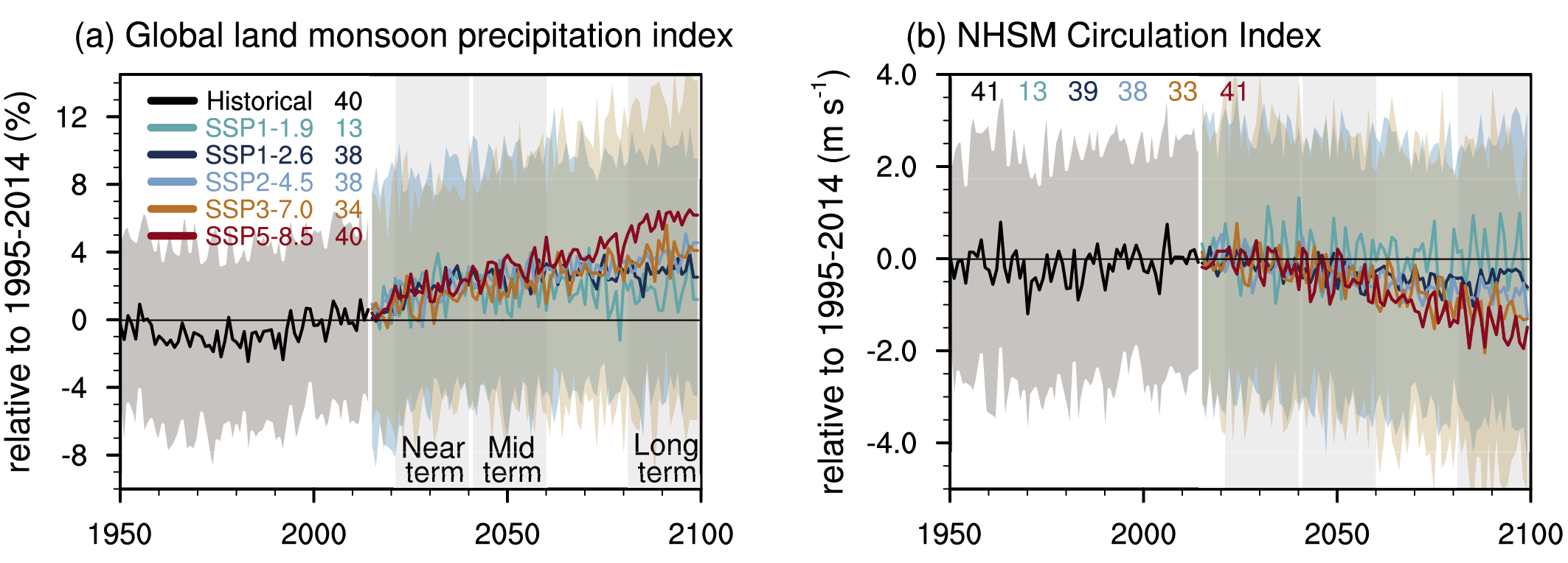 Figure 4.14 | Time series of global land monsoon precipitation and Northern Hemisphere summer monsoon (NHSM) circulation index anomalies. (a) Global land monsoon precipitation index anomalies (unit: %) defined as the area-weighted mean precipitation rate in the global land monsoon domain (as defined by Wang et al. (2013a) for the CMIP6 historical simulation (1950–2014) and five SSPs (2015–2100). (b) Anomalies in NHSM circulation index (unit: m s–1), defined as the vertical shear of zonal winds between 850 and 200 hPa averaged in a zone stretching from Mexico eastward to the Philippines (0°–20°N, 120°W–120°E; Wang et al., 2013a) for the CMIP6 historical simulation and five SSPs. One realization is averaged from each model. Anomalies are shown relative to the present-day (1995–2014) mean. The curves show averages over the simulations, the shadings around the SSP1-2.6 and SSP3-7.0 curves show 5–95% ranges, and the numbers near the top show the number of model simulations used. Further details on data sources and processing are available in the chapter data table (Table 4.SM.1).
 In summary, we assess that near-term changes in global monsoon precipitation and circulation will be affected by the combined effects of model uncertainty and internal variability, such as AMV and PDV, which together are larger than the forced signal (medium confidence).
4.4.2 Cryosphere, Ocean and Biosphere
4.4.2.1 Arctic Sea Ice
The AR5 assessed that for RCP8.5, Arctic sea ice coverage in September will drop below 1 million km2, or become practically ice-free, at some point between 2040 and 2060 (Collins et al., 2013). Since AR5, there has been substantial progress in understanding the response of Arctic sea ice to near-term changes in external forcing. In particular, it is very likely that different trajectories of the near-term evolution of anthropogenic forcing cause distinctly different likelihood ranges for very low sea ice coverage to occur over the next two decades (Notz and Stroeve, 2018). For example, there is an unlikely drop of September Arctic sea ice coverage to below 1 million km2 before 2040 for RCP 2.6, and a likely drop of September Arctic sea ice coverage to below 1 million km2 before 2040 for RCP 8.5 (medium confidence given the single study). The much higher likelihood of a practically sea ice free Arctic Ocean during summer before 2040 in RCP8.5 compared to RCP2.6 is consistent with related studies assessed in SROCC that find a substantially increased likelihood of an ice-free Arctic Ocean for 2.0°C compared to 1.5°C mean global warming relative to pre-industrial levels (Screen and Williamson, 2017; Jahn, 2018; Niederdrenk and Notz, 2018; Notz and Stroeve, 2018; Sigmond et al., 2018; Olson et al., 2019).
Based on results from CMIP6 models, we conclude that Arctic SIA will decrease in September in the near term (Figure 4.15, high confidence). In the case of 10-year trends ending in the near term, 79% of the simulations considered across all the core SSPs project decreasing Arctic sea ice area in September. Due to less of an influence from internal variability, this number rises to 98% in the case of 30-year trends. A more detailed assessment of near-term Arctic sea ice changes can be found in Chapter 9 (Section 9.3.1). A detailed assessment of Antarctic sea ice changes is in Chapter 9 (Section 9.3.2).
 Figure 4.15 | CMIP6 linear trends in September Arctic sea-ice area for 10-year, 20-year, and 30-year periods ending in 2021–2040 following five SSPs. Plotted are the 5–95% ranges across the ensembles of simulations. The numbers at the top of the plot are the number of model simulations in each SSP ensemble. The numbers near the bottom of the plot indicate the percentage of simulations across all the SSPs with decreasing sea-ice area. Results are from concentration-driven simulations. Further details on data sources and processing are available in the chapter data table (Table 4.SM.1).
 4.4.2.2 Ocean and Land Carbon Flux
Ocean carbon flux is both a key feature of the physical ocean in mitigating the rise of atmospheric CO2 and a driver of changes in the ocean biosphere, including changes in ocean acidity. Based on results from CMIP6 models, we conclude that SSP2-4.5, SSP3-7.0, and SSP5-8.5 all clearly lead to increasing 10-, 20-, and 30-year trends in ocean carbon flux over the near term (high confidence) (Figure 4.16,). Increasing trends in ocean carbon flux are less obvious in the lower-emissions scenarios. Ensemble-mean trends in land carbon flux over the near term are generally increasing, but these are unlikely to be detected given a large component of terrestrial variability combined with model uncertainty. A more detailed assessment is in Chapter 5 (Section 5.2.1).
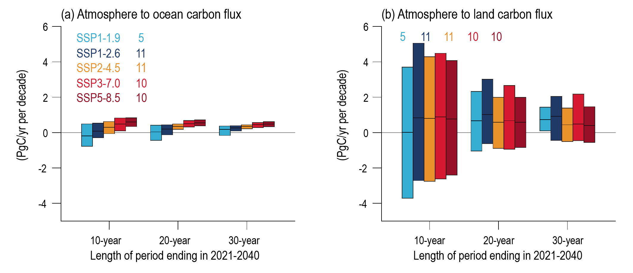 Figure 4.16 | CMIP6 trends in ocean and land carbon flux for 10-year, 20-year, and 30-year periods ending in 2021–2040. (a) Ocean carbon flux. (b) Land carbon flux. Plotted are the 5–95% ranges across the ensembles of simulations, for five SSPs. The numbers at the top of the plots are the number of model simulations in each SSP ensemble. Units are PgC yr–1 per decade. Further details on data sources and processing are available in the chapter data table (Table 4.SM.1).
 In summary, it is likely that ocean carbon flux will increase in the near term under the higher emissions scenarios, while a large component of terrestrial variability makes it is unlikely that an increase in land carbon flux will be detected over this period.
4.4.3 Modes of Variability
This subsection assesses the near-term evolution of the large-scale modes of climate variability. Assessment of the physical mechanisms and the individual feedbacks involved in the future change of each mode and their role on future regional climate variability are provided in Sections 8.4.2, 9.2.3 and 10.1.3, and Cross-Chapter Box 10.1.
4.4.3.1 Northern and Southern Annular Modes
4.4.3.1.1 The NorthernAnnular Mode
The AR5 assessed from CMIP5 simulations that there is only medium confidence in near-term projections of a northward shift of NH storm track and westerlies, and an associated increase in the NAM index, because of the large response uncertainty and the potentially large influence of internal variability. A tendency in the near term towards a slightly more positive NAM in the three highest emissions scenarios during boreal fall, winter, and spring is apparent in Figure 4.17a. However, in general the projected near-term multi-model mean change in the NAM is small in magnitude compared to the inter-model and/or multi-realization variability within the ensemble (Figure 4.17a; Deser et al., 2012b, 2017; Barnes and Polvani, 2015).
 Figure 4.17 | CMIP6 Annular Mode index change (hPa) from 1995–2014 to 2021–2040. (a) Northern Annular Mode (NAM); (b) Southern Annular Mode (SAM). The NAM is defined as the difference in zonal mean sea level pressure (SLP) at 35°N and 65°N (Li and Wang, 2003) and the SAM as the difference in zonal mean SLP at 40°S and 65°S (Gong and Wang, 1999). The shadings are the 5–95% ranges across the simulations. The numbers near the top of each panel are the numbers of model simulations in each SSP ensemble. Further details on data sources and processing are available in the chapter data table (Table 4.SM.1).
 On seasonal to interannual time scales, there is new evidence since AR5 that initialized predictions show lower potential predictability for the boreal winter NAO than the correlation skill with respect to observations (Eade et al., 2014; Baker et al., 2018; Scaife and Smith, 2018; Athanasiadis et al., 2020). This has been referred to in the literature as a ‘signal-to-noise paradox’ and means that very large ensembles of predictions are needed to isolate the predictable component of the NAO. While the processes that contribute to the predictability of the winter NAO on seasonal time scales may be distinct from the processes that drive multi-decadal trends, there is emerging evidence that initialized predictions also underrepresent the predictability of the winter NAO on decadal time scales (D.M. Smith et al., 2019). Post-processing and aggregation of initialized predictions may therefore reveal significant skill for predicting the winter NAO on decadal time scales (Smith et al., 2020). Considering these new results since AR5, in the near-term it is likely that any anthropogenic forced signal in the NAM will be of comparable magnitude or smaller than natural internal variability in the NAM (medium confidence).
4.4.3.1.2 The Southern Annular Mode
The AR5 assessed that it is likely that increases in GHGs and the projected recovery of the Antarctic ozone hole will be the principal drivers of future SAM trends. Additionally, the positive trend in austral summer/autumn SAM observed over the past several decades (Section 2.4.1.2; Chapter 2 in AR5, Hartmann et al., 2013), is likely to weaken considerably as stratospheric ozone recovers through to the mid-21st century. The effects of ozone depletion and recovery on the SH circulation primarily occur in austral summer, while GHGs influence the SH circulation year round (Gillett and Fyfe, 2013; Grise and Polvani, 2014b). Therefore, they are likely to be the dominant driver of projected circulation changes outside of austral summer (Gillett and Fyfe, 2013; Barnes et al., 2014; Solomon and Polvani, 2016). Based on current scenarios specifying future atmospheric decline of ozone depleting substances (WMO, 2011), chemistry-climate models project the Antarctic ozone hole in October to recover by around 2060 (WMO, 2014, 2018; Dhomse et al., 2018). Observational evidence since AR5 shows the onset of Antarctic ozone hole recovery (Solomon et al., 2016; WMO, 2018) that has been attributed to a pause in the summer SAM trend over the past couple of decades (Saggioro and Shepherd, 2019; Banerjee et al., 2020). In austral summer, ozone recovery and increasing GHGs will have opposing effects on the SAM over the next several decades (Barnes et al., 2014).
Since AR5, there have been advances in understanding the role of internal climate variability for projected near-term SH circulation trends (Solomon and Polvani, 2016). A large initial-condition ensemble following the RCP4.5 emissions scenario shows a monotonic positive SAM trend in austral winter. In austral summer, the SAM trend over the first half of the 21st century is weaker compared to the strongly positive trend observed and simulated over the late 20th century. In that model, the number of realizations required to identify a detectable change in decadal mean austral winter SAM index from a year 2000 reference state decreased to below five by around 2025–2030 (Solomon and Polvani, 2016). However, in December–January–February (DJF) the same criterion is not met until the second half of the 21st century, owing to the near-term opposing effects of ozone recovery and GHGs on the austral-summer SAM. In austral summer, forced changes in the SAM index in the near-term are therefore likely to be smaller than changes due to internal variability (Figure 4.17b; Barnes et al., 2014; Solomon and Polvani, 2016).
CMIP6 models show a tendency in the near-term towards a more positive SAM index especially in the austral winter (June–July–August, JJA; Figure 4.17b). In all seasons, the differences between the central estimates of the change in the SAM index for each SSP are much smaller than the inter-model ensemble spread. The number of CMIP6 realizations in Figure 4.17b is larger than the suggested threshold of five realizations needed to detect a significant near-term change in decadal-mean austral winter SAM index for a single CMIP5 model (Solomon and Polvani, 2016), and yet the 5–95% intervals on the CMIP6 ensemble spread encompass zero for all core SSPs. This suggests both internal variability and model uncertainty contribute to the CMIP6 ensemble spread in near-term SAM index changes. Based on these results, it is more likely than not that in the near-term under all assessed SSP scenarios the SAM index would become more positive than in present-day in austral autumn, winter and spring.
An influence of forcing agents other than stratospheric ozone and GHGs, such as anthropogenic aerosols, on SAM changes over the historical period has been reported in some climate models (Rotstayn, 2013), but the response across a larger set of CMIP5 models is not robust (Steptoe et al., 2016) and depends on how tropospheric temperature responds to aerosols (Choi et al., 2019). This gives low confidence in the potential influence of anthropogenic aerosols on the SAM in the future.
4.4.3.2 El Niño–Southern Oscillation
The AR5 assessed that it is very likely that the ENSO will remain the dominant mode of interannual variability in the future but did not specify its change in near term. A subset of CMIP5 models that simulate the ENSO Bjerknes index most realistically show an increase of ENSO SST amplitude in the near-term future and decline thereafter (Kim et al., 2014). However, detection of robust near-term changes of ENSO SST variability in response to anthropogenic forcing is difficult to achieve due to pronounced unforced low-frequency modulations of ENSO (Wittenberg, 2009; Maher et al., 2018; Wengel et al., 2018). Figure 4.10 in Section 4.3.3.2, using CMIP6 models, also shows no robust change in ENSO SST variability in the near term.
While there is no strong model consensus on the change in amplitude of ENSO SST variability, the amplitude of ENSO-associated rainfall variabilitylikely increases (Power et al., 2013; Cai et al., 2015). Analysis of CMIP6 models shows a slight increasing trend in amplitude of rainfall variability over Niño 3.4 region in the near term attributable to mean moisture increase, regardless of changes in ENSO SST variability (Figure 4.10). However, there are no distinguishable changes in the rainfall variability among five SSPs with significant model spread in the near term. Hence, no robust change in amplitude of ENSO SST and rainfall variability is expected in the near term although the rainfall variability slightly increases (medium confidence).
4.4.3.3 Indian Ocean Basin and Dipole Modes
Important modes of interannual climate variability with pronounced climate impacts in the Africa–Indo-Pacific areas of the globe are the Indian Ocean Dipole (IOD), which is closely related to, and often coincides with, ENSO phases (Stuecker et al., 2017), and the Indian Ocean basin (IOB) mode. This is often described as a capacitor effect in response to ENSO (Xie et al., 2009; Du et al., 2013) and can feed back onto ENSO evolution (Cai et al., 2019). IOD and IOB are extensively described in Annex IV (Section AIV2.4).
The projected climate mean state changes in the tropical Indian Ocean resemble a positive IOD state, with faster warming in the west compared to the east. This mean state change will potentially lead to a reduction in the amplitude of IOD events, albeit with no robust change in IOD frequency (Cai et al., 2014b). There is no robust evidence yet suggesting a cessation of IOD variability or a significant change in the IOB mode in the near-term.
4.4.3.4 Tropical Atlantic Modes
Interannual variability of the tropical Atlantic can be described in terms of two main climate modes: the Atlantic equatorial mode and the Atlantic meridional mode (AMM; Annex IV, Section AIV2.5). The Atlantic equatorial mode, also commonly referred to as the Atlantic Niño or Atlantic Zonal Mode, is associated with SST anomalies near the equator, peaking in the eastern basin, while the AMM is characterized by an inter-hemispheric gradient of SST and wind anomalies. Both modes are associated with changes in the ITCZ and related winds and exert a strong influence on the climate in adjacent and remote regions.
Despite considerable improvements in CMIP5 with respect to CMIP3, most CMIP5 models have difficulties in simulating the mean climate of the tropical Atlantic (Mohino et al., 2019) and are not able to correctly simulate the main aspects of Tropical Atlantic Variability (TAV) and associated impacts. This is presumably the main reason why there is a lack of specific studies dealing with near-term changes in tropical Atlantic modes. Nevertheless, AR5 reported that the ocean is more predictable than continental areas at the decadal time scale (Kirtman et al., 2013). In particular, the predictability in the tropical oceans is mainly associated with decadal variations of the external forcing component. Since the AMV affects the tropical Atlantic, near-term variations of the AMV can modulate the equatorial mode and the AMM as well as associated impacts.
There are no specific studies focusing on near-term changes in tropical Atlantic modes; nevertheless, decadal predictions show that although the North Atlantic stands out in most CMIP5 models as the primary region where skill might be improved because of initialization, encouraging results have also been found in the tropical Atlantic (Meehl et al., 2014). The effect of initialization in the tropical Atlantic is not only visible in surface temperature but also in the subsurface ocean (Corti et al., 2015). In particular, initialization improves the skill via remote ocean conditions in the North Atlantic subpolar gyre and tropical Pacific, which influence the tropical Atlantic through atmospheric teleconnections (Dunstone et al., 2011; Vecchi et al., 2014; García-Serrano et al., 2015). Improvements of some aspects of climate prediction systems (initialization techniques, large ensembles, increasing model resolution) have also led to skill improvements over the tropical Atlantic (Pohlmann et al., 2013; Monerie et al., 2017; Yeager and Robson, 2017).
Recent studies have shown that the AMV can modulate not only the characteristics of the Atlantic Niños, but also their inter-basin teleconnections (Indian and Pacific). In particular, the Atlantic Niño–ENSO relationship is strongest during negative AMV phases (Martín-Rey et al., 2014; Losada and Rodríguez-Fonseca, 2016) when equatorial Atlantic SST variability is enhanced (Martín-Rey et al., 2017; Lübbecke et al., 2018).
Based on CMIP5 and available CMIP6 results, we conclude that there is a lack of studies on the near-term evolution of TAV and associated teleconnections for a comprehensive assessment. However, some studies show that despite severe model biases there are skilful predictions in the mean state of tropical Atlantic surface temperature several years ahead (medium confidence), though skill in simulated variability has not been assessed yet. Decadal changes in the Atlantic Niño spatial configuration and associated teleconnections might be modulated by the AMV, but there is limited evidence and therefore low confidence in these results.
4.4.3.5 Pacific Decadal Variability
Climate variability of the Pacific Ocean on decadal and inter-decadal time scales is described in terms of a number of quasi-oscillatory SST patterns such as the Pacific Decadal Oscillation (PDO; Mantua et al., 1997) and the Inter-decadal Pacific Oscillation (IPO; Folland, 2002), which are referred to as the Pacific Decadal Variability (PDV; Newman et al., 2016). PDV comprises an inter-hemispheric pattern that varies at decadal to inter-decadal time scales (Figure 3.35). However, although the spatial domains to derive the IPO and PDO indices differ, and despite uncertainty related to trend removal and time-filtering (Newman et al., 2016; Tung et al., 2019), the IPO and PDO are highly correlated in time and they will be assessed together as the PDV (Annex IV, Section AIV.2.6).
The AR5 assessed that near-term predictions of PDV (then referred to as PDO or IPO) were largely model dependent (Mochizuki et al., 2012; van Oldenborgh et al., 2012), not robust to sampling of initialization start-dates, overall not statistically significant, and worse than persistence (Doblas-Reyes et al., 2013), although some studies showed positive skill for PDV (Mochizuki et al., 2010; Chikamoto et al., 2013). The CMIP5 decadal-prediction ensemble yielded no prediction skill of SST over the key PDV centres of action in the Pacific Ocean, both at two-to-five-year and six-to-nine-year forecast averages (Doblas-Reyes et al., 2013; Guemas et al., 2013; Boer and Sospedra-Alfonso, 2019).
Since AR5, the processes causing the multi-decadal variability in the Pacific Ocean have become better understood (Newman et al., 2016; Henley, 2017). However, the relative importance oftropical and extratropical processes underlying PDV remains unclear; although it seems to be stochastically driven rather than self-excited (Liu, 2012; Liu and Di Lorenzo, 2018), the South Pacific being a key region for the tropical branch of PDV (Chung et al., 2019; Liguori and Di Lorenzo, 2019).
Because PDV represents not one, but many dynamical processes, it represents a challenge as a target for near-term climate predictions and projections. The new generation of decadal forecast systems keeps showing poor (Shaffrey et al., 2017) to moderate (D.M. Smith et al., 2019) multi-year prediction skill for PDV, although the potential for forecasting capabilities is demonstrated in case studies (Meehl and Teng, 2012; Meehl et al., 2014). For the near-term, a transition of PDV from the negative phase (1999–2012) towards a positive phase is predicted in the coming years (2013–2022; Meehl et al., 2016).
The PDV has been shown to influence the pace of global warming (Cross-Chapter Box 3.1), but the extent to which PDV is externally forced or internally generated (Mann et al., 2020) remains an open question, and there is still no robust evidence. Thus, there is low confidence on how the PDV will evolve in the near-term (Bordbar et al., 2019).
4.4.3.6 Atlantic Multi-decadal Variability
The Atlantic Multi-decadal Variability (AMV) is a large-scale climate mode accounting for the main fluctuations in North Atlantic SST on multi-decadal time scales (Section AIV.2.7). The AMV influences air temperatures and precipitation over adjacent and remote continents, and its undulations can partially explain the observed variations in the NH mean temperatures (Steinman et al., 2015). The origin of this variability is still uncertain. Ocean dynamics (e.g., changes in the AMOC), external forcing, and local atmospheric forcing all seem to play a role (Menary et al., 2015; Ruprich-Robert and Cassou, 2015; Brown et al., 2016; Cassou et al., 2018; Wills et al., 2019). Recent studies have discussed that the ocean dynamics play an active role in generating AMV (Oelsmann et al., 2020) and its interplay with the NAO (Vecchi et al., 2017; R. Zhang et al., 2019; Kim et al., 2020), although natural and anthropogenic external forcing might be crucial in modulating its amplitude and timing (Bellucci et al., 2017; Bellomo et al., 2018; Andrews et al., 2020; Borchertet al., 2021; Mann et al., 2021; see Sections 3.7.7 and AIV.2.7).
The AR5 assessed with high confidence that initialized predictions can improve the skill for temperature over the North Atlantic, in particular in the sub-polar branch of AMV, compared to the projections, for the first five years (see AR5 WGI Figures 11.3 and 11.4). However, non-initialized predictions showed positive correlation over the same time-range as well, consistent with the notion that part of this variability is caused by external forcing (Section 3.7.7).
Since AR5, near-term initialized predictions, both multi-model (Bellucci et al., 2015a; García-Serrano et al., 2015; D.M. Smith et al., 2019) and single-model ensembles (Marotzke et al., 2016; Simpson et al., 2018; Yeager et al., 2018; Hermanson et al., 2020; Bilbao et al., 2021), confirm substantial skill in hindcasting North Atlantic SST anomalies on a time range of eight to ten years. On the same time range, Borchert et al. (2021) show a substantial improvement in the prediction of the subpolar gyre SST (the northern component of the AMV) in CMIP6 models compared to CMIP5, in both initialized and non-initialized simulations. The higher skill of CMIP6 models can be attributed to a more accurate response of SST variations in the subpolar gyre to natural forcing, possibly originating from the AMOC-related delayed response to volcanic eruptions (Hermanson et al., 2020).
Initialization contributes to the reduction of uncertainty and to predicting subpolar SST amplitude (Borchert et al., 2021). Yet, skill in predicting the AMV is not always translated into equally successful predictions of temperature and precipitation over the nearby land and ocean regions (Langehaug et al., 2017). This might be related to systematic model errors in the simulation of the spatial and temporal structure of the AMV and too weak associated teleconnections (Section 3.7.7), and also to the larger noise in regional land variables compared to the AMV index. However, AMV predictions can be used as proxies to predict other variables such as precipitation over Western Europe and Eurasia and SAT over Mediterranean, Northern Europe and north-east Asia (Årthun et al., 2018; Borchert et al., 2019; Ruggieri et al., 2021) whose relationship with North Atlantic SST is robust in observations, but not well captured in climate models.
Encouraging results about the prediction of land precipitation linked to the warm AMV phase (Section 3.7.7 and Annex IV, Figure AIV.2.7) on a two-to-nine-year time scale are reported in the multi-model study by D.M. Smith et al. (2019). Positive correlations with observations are found in the Sahel, South America, the Maritime Continent. Analyses from large-ensemble decadal prediction systems such as the community Earth system model decadal prediction large ensemble (CESM-DPLE; Yeager et al., 2018) show an improvement with respect to the CMIP5 decadal hindcasts (Martin and Thorncroft, 2014b) in forecasting Sahel precipitation over three to seven years, which is consistent with the current understanding of AMV impact over Africa (Mohino et al., 2016; D.M. Smith et al., 2019). CESM-DPLE predicts drought conditions over the Sahel through 2020, which is compatible with a shift towards a negative phase of AMV as a result of a weakening of the AMOC, advocated by a number of studies (Hermanson et al., 2014; Robson et al., 2014; Yeager et al., 2015).
In summary, the confidence in the predictions of AMV and its effects is medium. However, there is high confidence that the AMV skill over five-to-eight-year lead times is improved by using initialized predictions, compared to non-initialized simulations.
4.4.4 Response to Short-lived Climate Forcers and Volcanic Eruptions
Mitigation of SLCFs affects future climate projections and could alter the time of emergence of anthropogenic climate change signals. The AR5 assessed that emission reductions aimed at decreasing local air pollution could have a near-term warming impact on climate (high confidence) (Kirtman et al., 2013). Because of their shorter lifetimes, reductions in emissions of SLCF species mainly influence near-term GSAT trends (Chalmers et al., 2012; Shindell et al., 2017; Shindell and Smith, 2019), but on decadal time scales the near-term response to even very large reductions in SLCFs may be difficult to detect in the presence of large internal climate variability (Samset et al., 2020). The changes in SLCF emissions during the COVID-19 pandemic has resulted in a small net radiative forcing without a discernible impact on GSAT (Cross-Chapter Box 6.1). SLCF mitigation also leads to a higher GSAT in the mid- to long-term (Smith and Mizrahi, 2013; Stohl et al., 2015; Hienola et al., 2018) and can influence peak warming during the 21st century (Rogelj et al., 2014; Hienola et al., 2018). This section focuses on the total effect of SLCF changes on GSAT projections in the SSP scenarios. A more detailed breakdown of the separate climate effects of SLCF species and precursor species can be found in Sections 6.7.2 and 6.7.3.
A model experiment based on the SSP3-7.0 scenario with aerosols, their precursors, and non-methane tropospheric ozone precursors set to SSP1-1.9 abundances (SSP3-7.0-lowSLCF-highCH4; Collins et al., 2017) shows a projected multi-model mean GSAT anomaly that is higher by 0.22°C at mid-century (2045-2054) compared to SSP3-7.0 (Figure 4.18; Allen et al., 2020), but this difference is smaller than the inter-model spread of the SSP3-7.0 projections based on the CMIP6 models. Note the SSP3-7.0-lowSLCF-highCH4 experiment does not perturb methane from SSP3-7.0 concentrations. A modified SSP3-7.0-lowSLCF-lowCH4 scenario that also includes methane mitigation shows a lower GSAT by mid-century compared to SSP3-7.0 (Allen et al., 2021).
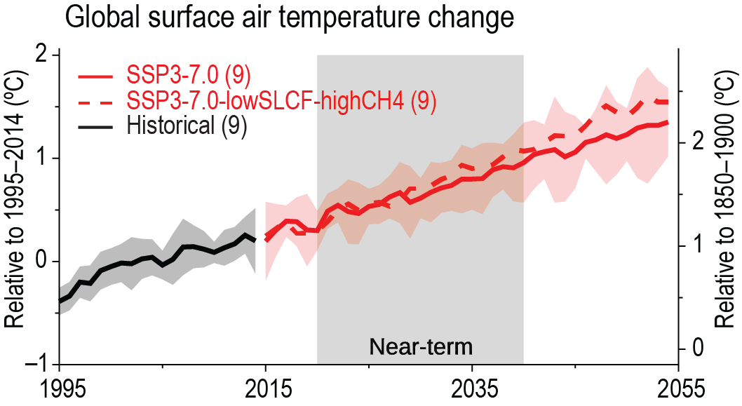 Figure 4.18 | Influence of SLCFs on projected GSAT change. Change is shown relative to the 1995–2014 average (left axis) and relative to the 1850–1900 average (right axis). The comparison is for CMIP6 models for the AerChemMIP (Collins et al., 2017) SSP3-7.0-lowSLCF-highCH4 experiment (red dashed; note in the original experiment protocol this is called SSP3-7.0-lowNTCF), where concentrations of short-lived species are reduced compared to reference SSP3-7.0 scenario (red solid). Black shows the historical simulation until 2014 for the same 9 models as the projections. The curves show averages over the r1 simulations contributed to the CMIP6 exercise, the shadings around the historical and SSP3-7.0 curves shows 5–95% ranges and the numbers near the top show the number of model simulations.
 Building on CMIP6 results for the effects of reducing SLCF emissions from a baseline of SSP3-7.0, the overall contribution of SLCFs to GSAT changes in the marker SSPs are now quantified using a simple climate model emulator. For consistency with Section 6.7.2 and Figure 6.22, the basket of SLCF compounds considered includes aerosols, ozone, methane, black carbon on snow and hydrofluorocarbons (HFCs) with lifetimes of less than 50 years. In the five marker SSPs considered, the net effect of SLCFs contributes to a higher GSAT in the near, mid- and long term (Table 4.6 and Section 6.7.2). In the SSP1-1.9 and SSP1-2.6 scenarios, SLCFs contribute to a higher GSAT by a central estimate of around 0.3°C compared to 1995–2014 across the three-time horizons. In the long-term, the 0.3C warming due to SLCFs in SSP1-2.6 can be compared to the assessed very likely GSAT change for this period of 0.5°C–1.5°C (Section 4.3.4 and Table 4.5). The SSP2-4.5, SSP3-7.0 and SSP5-8.5 scenarios all show a larger SLCF effect on GSAT in the long term relative to the near term. In SSP3-7.0, the long-term warming due to SLCFs by 0.7°C can be compared with the assessed very likely GSAT anomaly for this period of 2.0°C –3.7°C (Section 4.3.4). In summary, it is very likely that changes in SLCFs contribute to an overall warmer GSAT over the near, mid- and long term in the five SSP scenarios considered (Table 4.6, Section 6.7.2 and Figure 6.22).
In addition to effects on GSAT, SLCFs affect other aspects of the global climate system (Section 6.7.2). The additional warming at high northern latitudes associated with projected reductions in aerosol emissions over the 21st century leads to a more rapid reduction in Arctic sea ice extent in the RCP scenarios (Gagné et al., 2015). Furthermore, mitigation of non-methane SLCFs in the SSP3-7.0-lowSLCF-highCH4 scenario causes an increase in global mean precipitation, with larger regional changes in southern and eastern Asia (Allen et al., 2020).
Time Period | SSP1-1.9 (°C) | SSP1-2.6 (°C) | SSP2-4.5 (°C) | SSP3-7.0 (°C) | SSP5-8.5 (°C) |
Near Term (2021–2040) | 0.2 (0.1, 0.3) | 0.2 (0.1, 0.3) | 0.2 (0.1, 0.3) | 0.2 (0.1, 0.3) | 0.3 (0.2, 0.4) |
Mid-Term (2041–2060) | 0.2 (0.0, 0.4) | 0.2 (0.0, 0.4) | 0.3 (0.2, 0.4) | 0.3 (0.2, 0.4) | 0.5 (0.3, 0.7) |
Long Term (2081–2100) | 0.1 (-0.1, 0.4) | 0.2 (0.0, 0.4) | 0.3 (0.1, 0.6) | 0.5 (0.4, 0.8) | 0.7 (0.4, 1.0) |
The main uncertainties in climate effects of SLCFs in the future come from: (i) the uncertainty in anthropogenic aerosol ERF (Section 7.3.3); (ii) uncertainty in the relative emissions of different SLCFs that have warming and cooling effects in the current climate (Section 6.2); and (iii) physical uncertainty including the efficacy of the climate response to SLCFs compared to long-lived GHGs (Marvel et al., 2016; Richardson et al., 2019). One example of physical uncertainty is that the shortwave radiative forcing from methane was neglected in previous calculations (Etminan et al., 2016; Collins et al., 2018), which affects understanding of present day and future methane ERF (Modak et al., 2018). Another example of physical uncertainty is projected changes in lightning-NOx production, which contribute to future ozone radiative forcing (Banerjee et al., 2014, 2018; Finney et al., 2018).
Another factor that could substantially alter projections in the near-term would be the occurrence of a large explosive volcanic eruption, or even a decadal to multi-decadal sequence of small-to-moderate volcanic eruptions as witnessed over the early 21st century (Cross-Chapter Box 4.1; Santer et al., 2014). An eruption similar to the last large tropical eruption, Mount Pinatubo in the Philippines in June 1991, is expected to cause substantial Northern Hemisphere (NH) cooling, peaking between 0.09°C and 0.38°C and lasting for three to five years, as indicated by climate model simulations over the past millennium (e.g., Jungclaus et al., 2010). Phase 3 of Paleoclimate Modelling Intercomparison Project (PMIP3) simulated a significant NH cooling in response to individual volcanic events (peaks between 0.1°C and 0.5°C, depending on model, during the first year after the eruption) that lasts for three to five years. On a regional scale, the double volcanic events that occurred in 536 and 540 CE resulted in a cooling of 2°C (Büntgen et al., 2016; Toohey et al., 2016).
Since AR5, there has been growing progress in understanding the climate impacts of volcanic eruptions. Volcanic forcing is regarded as the dominant driver of forced variability in preindustrial surface air temperature (Schurer et al., 2013, 2014). Large eruptions in the tropics and high latitudes were primary drivers of interannual-to-decadal temperature variability in the Northern Hemisphere during the past 2,500 years, with cooling persisting for up to ten years after some of the largest eruptive episodes (Sigl et al., 2015). Repeated clusters of volcanic eruptions can induce a net negative radiative forcing that results in a centennial- and global-scale cooling trend via a decline in mixed-layer oceanic heat content (McGregor et al., 2015). The response to multi-decadal changes in volcanic forcing (representing clusters of eruptions) shows similar cooling in both simulations and reconstructions of NH temperature. Volcanic eruptions generally result in decreased global precipitation for up to a few years following the eruption (Iles and Hegerl, 2014, 2015; Man et al., 2014), with climatologically wet regions drying and climatologically dry regions wetting (medium confidence), which is opposite to the response under global warming (Held and Soden, 2006; Iles et al., 2013; Zuo et al., 2019a, b). El Niño-like warming appears after large volcanic eruptions, as seen in both observations (Adams et al., 2003; McGregor et al., 2010; Khodri et al., 2017) and climate model simulations (Ohba et al., 2013; Pausata et al., 2015; Colose et al., 2016; Stevenson et al., 2016; Khodri et al., 2017; Predybaylo et al., 2017; Zuo et al., 2018). The large tropical eruptions are coincident with positive Indian Ocean dipole events (Maher et al., 2015).
In AR5, uncertainty due to future volcanic activity was not considered in the assessment of the CMIP5 21st century climate projections (Taylor et al., 2012; O’Neill et al., 2016). Since AR5, there has been considerable progress in quantifying the impacts of volcanic eruptions on decadal climate prediction and longer-term climate projections (Meehl et al., 2015; Swingedouw et al., 2015, 2017; Timmreck et al., 2016; Bethke et al., 2017; Illing et al., 2018). By exploring 60 possible volcanic futures under RCP4.5, it has been demonstrated that the inclusion of time-varying volcanic forcing may enhance climate variability on annual-to-decadal time scales (Bethke et al., 2017). Consistent with a tropospheric cooling response, the change in ensemble spread in the volcanic cases is skewed towards lower GSAT relative to the non-volcanic cases (Cross-Chapter Box 4.1, Figure 1). In these simulations with multiple volcanic forcing futures there is: (i) an increase in the frequency of extremely cold individual years; (ii) an increased likelihood of decades with negative GSAT trend (decades with negative GSAT trends become 50% more commonplace); (iii) later anthropogenic signal emergence (the mean time at which the signal of global warming emerges from the noise of natural climate variability is delayed almost everywhere) (high confidence); and (iv) a 10% overall reduction in global land monsoon precipitation and a 20% overall increase in the ensemble spread (Man et al., 2021).
Cross-Chapter Box 4.1 | The Climate Effects of Volcanic Eruption
Contributing Authors: Sarah L. Connors (France/United Kingdom), Amanda Maycock (United Kingdom), Peter W. Thorne (Ireland/United Kingdom), Nicolas Bellouin (United Kingdom/France), Ingo Bethke (Norway/Germany), Deliang Chen (Sweden), Annalisa Cherchi (Italy), Alejandro Di Luca (Australia/Canada/Argentina), Piers Forster (United Kingdom), Nathan P. Gillett (Canada), Darrell S. Kaufmann (The United States of America), June-Yi Lee (Republic of Korea), Elizaveta Malinina (Canada/Russian Federation), Seung-Ki Min (Republic of Korea), Johannes Quaas (Germany), Alex C. Ruane (The United States of America), Jean-Baptiste Sallée (France), Sonia I. Seneviratne (Switzerland), Chris Smith (United Kingdom), Matthew Toohey (Canada, Germany/Canada), Andrew Turner (United Kingdom), Cunde Xiao (China), Tianjun Zhou (China)
Before the industrial period, explosive volcanic eruptions were the largest source of forced climate variability globally on interannual to centennial time scales (Section 2.2). While usually omitted from scenarios used for future climate projections, as they are unpredictable, volcanic eruptions have the potential to influence future climate on multi-annual to decadal time scales and affect many climatic impact drivers (as defined in Sections 12.1 and 12.3). Since AR5, more comprehensive paleo evidence and observations, as well as improved modelling have advanced understanding of the climate response to past volcanic eruptions. Building on multiple chapter assessments, this box synthesizes how volcanic eruptions affect climate and considers implications of possible future events.
How frequent are volcanic eruptions?
Proxy records show that large volcanic eruptions with effective radiative forcing (ERF) more negative than –1 W m–2 occurred on average twice a century throughout the last 2500 years, the most recent being Pinatubo in 1991 (Section 2.2.2). About eight larger eruptions (ERF stronger than –5 W m–2) also occurred during this period (Figure 2.2), notably Tambora about 1815 and Samalas about 1257. A Samalas-type eruption may occur one to two times per millennium on average (Newhall et al., 2018). Typically, three in every four centuries have experienced at least one eruption stronger than –1 W m–2 (Pinatubo or larger). The volcanic aerosol burden was 14% lower during the 20th century compared to the average of the preceding 24 centuries (Section 2.2.2), whereas the 13th century was among the most volcanically active, with four eruptions exceeding that of Pinatubo-1991 (Sigl et al., 2015).
Past climate responses to volcanic activity
Major eruptions drive a range of climate system responses for several years depending upon whether the eruption occurs in the tropics (stratospheric aerosol dispersion into both hemispheres) or the extratropics (dispersion into the hemisphere of eruption) owing to the Brewer-Dobson circulation. The climatic response also depends on the effective injection height, sulphur mass injected, and time of year of the eruption (Marshall et al., 2019, 2020). These factors determine the total mass, lifetime and optical properties of volcanic aerosol in the stratosphere and influence the stratospheric aerosol optical depth (SAOD). The ERF from volcanic stratospheric aerosol is assessed to be –20 ± 5 W m–2 per unit sAOD (Section 7.3.4.6).
Due to the direct radiative effect of volcanic stratospheric aerosols, large volcanic eruptions lead to an overall decrease of GSAT, which can extend to multi-decadal or century time scales in the case of clustered volcanism (Section 3.3.1.1; Schurer et al., 2013; McGregor et al., 2015; Sigl et al., 2015; Kobashi et al., 2017; Zambri et al., 2017; Brönnimann et al., 2019; Neukom et al., 2019). Large eruptions also increase the frequency of extremely cold individual years and the likelihood of cooling trends occurring in individual decades (Cross-Chapter Box 3.1 and Section 4.4.4; Paik and Min, 2018). Re-dating of ice core chronologies now confirms that the coldest decades of the past approximately 2000 years are the outcome of volcanic eruptions (Sigl et al., 2015; Büntgen et al., 2016; Toohey et al., 2016; Neukom et al., 2019). CMIP5 and CMIP6 models reproduce the decreased GSAT that follows periods of intense volcanism. New reconciliations between simulations and proxy-based reconstructions of past eruptions have been achieved through better Earth System Model representation of volcanic plume chemical compositions (Legrande et al., 2016; Marshall et al., 2020; F. Zhu et al., 2020). Yet, remaining disagreements reflect differences in the volcanic forcing datasets used in the simulations (medium confidence) (Section 3.3.1.1 and Figure 3.2c).
Although incomplete, proxy records show large impacts upon contemporary society from eruptions such as 1257 Samalas and 1815 Tambora, the latter resulting in ‘the year without a summer’ with multiple harvest failures across the Northern Hemisphere (e.g., Raible et al., 2016). Comparing CMIP5 multi-model simulations with observations has improved understanding of the hydrological responses to 20th century eruptions, particularly global land monsoon drying, and associated uncertainties (Section 3.3.2.3). Global mean land precipitation decreases for up to a few years following the eruption, with climatologically wet regions drying and dry regions wetting (Sections 3.3.2.3 and 4.4.4). Changes in monsoon circulations occur with a general weakening of tropical precipitation (Section 8.5.2.3) and a decrease in extreme precipitation over global monsoon regions (Section 11.4.4). Monsoon precipitation in one hemisphere tends to be enhanced by eruptions occurring in the other hemisphere or reduced if they occur in the same hemisphere (Sections 3.3.2.3 and 8.5.2.3). Volcanic eruptions have been linked to the onset of El Niñofollowed by La Niña although this connection remains contentious (Adams et al., 2003; Bradley et al., 2003; McGregor et al., 2010; Khodri et al., 2017; F. Liu et al., 2018; Sun et al., 2019;Paik et al., 2020; Predybaylo et al., 2020). Volcanic activity could drive short-term (one-to-three-year) positive changes in the annual SAM index through modulations in the extratropical temperature gradient and wave driving of the polar stratosphere (Yang and Xiao, 2018). In the cryosphere, Arctic sea ice extent increases for years to decades (Gagné et al., 2017a), and modelling indicates that sea ice/ocean feedbacks can prolong cooling long after volcanic aerosols are removed (Miller et al., 2012). On annual time scales, the ocean buffers the atmospheric response to volcanic eruptions by storing the cooling in the ocean subsurface, then feeding it back to the atmosphere. Large eruptions affect ocean heat content and thermosteric sea level over decadal-to-centennial scales (Section 9.2.2.1).
Potential implications on 21st century projections
Given the unpredictability of individual eruptions, volcanic forcing is prescribed as a constant background loading in CMIP6 models (Eyring et al., 2016). This means the effects of potential large volcanic eruptions are largely absent from model projections, and few studies have addressed the potential implications on 21st century warming. One study considered future scenarios with hypothetical volcanic eruptions consistent with levels of Common Era volcanic activity (Bethke et al., 2017) under RCP4.5 and found that climate projections could be substantially altered (Cross-Chapter Box 4.1, Figure 1). Although temporary, close to pre-industrial level temperatures could be experienced globally for a few years after a 1257 Samalas-sized eruption. Several other key climate indicators are also changed substantially, consistent with evidence from past events. Bethke et al. (2017) suggest that an eruption early in the 21st century could delay the timing of crossing 1.5°C global warming by several years. Clustered eruptions would have substantial impact upon GSAT evolution throughout the century (Cross-Chapter Box 4.1, Figure 1), and could have far-reaching implications, as observed for past eruptions. For near-term response options, decadal prediction models can update 21st-century projections once a volcanic eruption occurs (Timmreck et al., 2016).

Cross-Chapter Box 4.1, Figure 1 | Potential impact of volcanic eruption on future global temperature change. CMIP5 projections of possible 21st-century futures under RCP4.5 after a 1257 Samalas magnitude volcanic eruption in 2044, from Bethke et al. (2017). (a) Volcanic ERF of the most volcanically active ensemble member, estimated from SAOD. (b) Annual mean global surface air temperature. Ensemble mean (solid) of future projections including volcanoes (blue) and excluding volcanoes (red) with 5–95% range (shading) and ensemble minima/maxima (dots); evolution of the most volcanically active member (black). Data created using a SMILE approach with NorESM1 in its CMIP5 configuration. See Sections 2.2.2 and 4.4.4 for more details. Further details on data sources and processing are available in the chapter data table (Table 4.SM.1).
Summary
It is likely that at least one large eruption will occur during the 21st century. Such an eruption would reduce GSAT for several years, decrease global mean land precipitation, alter monsoon circulation, modify extreme precipitation, and change the profile of many regional climatic impact-drivers. A low-likelihood, high-impact outcome would be several large eruptions that would greatly alter the 21st century climate trajectory compared to SSP-based ESM projections.
4.5 Mid- to Long-term Global Climate Change
4.5.1 Atmosphere
This section assesses how the global atmospheric indicators assessed in Section 4.3 manifest themselves in large-scale spatial patterns of atmospheric change in the mid-term (2041–2060) and long term (2081–2100). The patterns of change in any given future period represent a combination of unforced internal variability and a forced response including their interaction (Deser et al., 2016). The role of internal variability is much larger at the local to regional scale than in the global mean projections. We here assess multi-model mean patterns based on CMIP6 models without any weighting or emergent constraints. The mean represents an estimate of the forced response and is a more homogeneous pattern than the 20-year mean change patterns in any individual model realization (Knutti et al., 2010).
4.5.1.1 Near-surface Air Temperature
Patterns of near-surface air temperature changes show widespread warming by 2041–2060 and 2081–2100 (Figure 4.19) for all SSPs relative to 1995–2014. The area fraction experiencing warming increases with the level of global mean warming. As GSAT continues to increase, it is very likely that by the middle and the end of the 21st century most of the global land and ocean areas will be warmer than in 1995–2014 (high confidence, Section 4.3.1.1).
 Figure 4.19 | Mid-and long-term change of annual mean surface temperature. Displayed are projected spatial patterns of multi-model mean change in annual mean near-surface air temperature (°C) in 2041–2060 and 2081–2100 relative to 1995–2014 for (top) SSP1-2.6 and (bottom) SSP3-7.0. The number of models used is indicated in the top right of the maps. No overlay indicates regions where the change is robust and likely emerges from internal variability, that is, where at least 66% of the models show a change greater than the internal-variability threshold (see Section 4.2.6) and at least 80% of the models agree on the sign of change. Diagonal lines indicate regions with no change or no robust significant change, where fewer than 66% of the models show change greater than the internal-variability threshold. Crossed lines indicate areas of conflicting signals where at least 66% of the models show change greater than the internal-variability threshold but fewer than 80% of all models agree on the sign of change. Further details on data sources and processing are available in the chapter data table (Table 4.SM.1).
 The multi-model mean temperature change pattern (Figure 4.19) shows some robust key characteristics that are independent of the time horizon and scenario, such as a land–ocean warming contrast, amplified warming over the Arctic region, assessed below, or the comparatively small warming or even cooling in the North Atlantic subpolar gyre (Section 9.2.1.1). Furthermore, changes in aerosol concentrations and land use and land management can have a direct imprint on the regional warming pattern (Bright et al., 2017; Kasoar et al., 2018). Note that the global average of the pattern shown in Figure 4.19 corresponds to CMIP6 multi-model mean GSAT warming (Section 4.3.1) and is thus somewhat warmer than the warming pattern consistent with the central estimate of the GSAT range assessed in Section 4.3.4. Since the regional mean warming scales well with global warming levels independent of the emissions scenario (Section 4.2.4), the key characteristics of the spatial pattern assessed here are largely independent of the difference between CMIP6 multi-model global mean and assessed global GSAT change.
4.5.1.1.1 Land–ocean warming contrast
It is virtually certain that future average warming will be higher over land than over the ocean. Section 2.2.1 of SRCCL (G. Jia et al., 2019) assessed that it is certain that land temperatures have increased more than global mean temperatures since the pre-industrial period. This so-called land–ocean warming contrast is a striking feature of observed trends (Lambert and Chiang, 2007; Byrne and O’Gorman, 2018) and projected changes in surface-air temperature (Sutton et al., 2007; Joshi and Gregory, 2008; Dong et al., 2009; Lambert et al., 2011; Drost et al., 2012; Bayr and Dommenget, 2013; Byrne and O’Gorman, 2013b; Izumi et al., 2013; Joshi et al., 2013). Between 1979 and 2016, average temperature over land increased by 42% more than over the ocean (Byrne and O’Gorman, 2018). A similar warming contrast is found in CMIP5 projections though with large differences across models and latitudes (Sutton et al., 2007; Drost et al., 2012; Byrne and O’Gorman, 2013b; Joshi et al., 2013), which is also consistent with paleoclimate evidence (Izumi et al., 2013; Schmidt et al., 2014). The ratio of land-to-ocean warming is greater than one for almost all regions (high confidence) and is larger for dry subtropical continents (about 1.5) than for moist regions in the tropics and mid-latitudes (about 1.2; Byrne and O’Gorman, 2013a). Projected warming over land and ocean only is shown in Table 4.2 for different scenarios, and the global average ratio of land-to-ocean warming in CMIP6 is 1.5 with a likely range of 1.4 to 1.7, which is consistent with estimates based on CMIP5.
Since AR5, a robust physical understanding of the warming contrast been developed. A simple theory based on atmospheric dynamics and moisture transport shows that surface-air temperature and relative humidity over land are strongly coupled, and demonstrates that the warming contrast occurs because air over land is drier than over the ocean (Joshi et al., 2008; Byrne and O’Gorman, 2013a, b, 2018). The warming contrast causes land relative humidity to decrease (Byrne and O’Gorman, 2016, 2018; Chadwick et al., 2016) and this feeds back on and strengthens the warming contrast. Differences in land-relative humidity responses across models are the primary cause of uncertainty in the land–ocean warming contrast (Byrne and O’Gorman, 2013b). These land-relative humidity changes are ultimately controlled by moisture transport between the land and ocean boundary layers (Byrne and O’Gorman, 2016; Chadwick et al., 2016) and are also sensitive to characteristics of land surfaces that are challenging to model, including stomatal conductance and soil moisture (Berg et al., 2016; Zarakas et al., 2020).
4.5.1.1.2 Polar amplification
It is very likely that under all SSPs the warming in the Arctic will be more pronounced than in the global average over the 21st century. Since AR5 the understanding of the physical mechanisms driving polar amplification has improved.
The Arctic surface is projected to warm more than the global average over the 21st century, with annual-average Arctic warming of about 3°C (SSP1-2.6), 10°C (SSP3-7.0) and 12°C in (SSP5-8.5) by 2081–2100 relative to 1995–2014 (Figure 4.19). This phenomenon, known as polar or Arctic amplification, is a ubiquitous feature of the response to GHG forcing simulated by climate models (Manabe and Wetherald, 1975, 1980; Manabe and Stouffer, 1980; Robock, 1983; Hansen et al., 1984; Manabe et al., 1991; Holland and Bitz, 2003; Winton, 2006; Pithan and Mauritsen, 2014) and has been observed over recent decades concurrent with Arctic sea ice loss (Section 2.3.2.1; Serreze and Barry, 2011). Based on robust scientific understanding and agreement across multiple lines of evidence (Section 7.4.4.1), there is high confidence that the rate of Arctic surface warming will continue to exceed the global average over the 21st century.
A variety of mechanisms contribute to Arctic amplification (Section 7.4.4.1.1). While surface-albedo feedbacks associated with the loss of sea ice and snow have long been known to play important roles (Arrhenius, 1896; Manabe and Stouffer, 1980; Robock, 1983; Hall, 2004), it is now recognized that temperature (lapse-rate and Planck) feedbacks also contribute to Arctic amplification through a less efficient longwave radiative damping to space with warming at high latitudes (Winton, 2006; Pithan and Mauritsen, 2014; Goosse et al., 2018; Stuecker et al., 2018). Increases in poleward atmospheric latent heat transport and oceanic heat transport also contribute to Arctic warming (Holland and Bitz, 2003; Bitz et al., 2006; Lee et al., 2011, Lee et al., 2017; Alexeev and Jackson, 2013; Marshall et al., 2014, 2015; Woods and Caballero, 2016; Nummelin et al., 2017; Singh et al., 2017; Merlis and Henry, 2018; Oldenburg et al., 2018; Armour et al., 2019; Beer et al., 2020). Projected reduction in the strength of the AMOC over the 21st century is expected to reduce Arctic warming, but even a strong AMOC reduction would not eliminate Arctic amplification entirely (medium confidence) (Liu et al., 2017; Liu et al., 2018; Wen et al., 2018).
There remains substantial uncertainty in the magnitude of projected Arctic amplification (Smith et al., 2020), with the Arctic warming ranging from two to four times the global average in models (Holland and Bitz, 2003; Nummelin et al., 2017). This uncertainty primarily stems from different representations of polar surface-albedo, lapse-rate, and cloud feedbacks, and from different projected poleward energy transport changes (Holland and Bitz, 2003; Crook et al., 2011; Mahlstein and Knutti, 2011; Pithan and Mauritsen, 2014; Bonan et al., 2018). The magnitude of Arctic amplification may also depend on the mix of radiative forcing agents (Najafi et al., 2015; Sand et al., 2016; Stjern et al., 2019) such as the contribution of ozone depleting substances (Polvani et al., 2020). Tropospheric aerosol emissions tend to reduce simulated Arctic warming over the middle of the 20th century (Gagné et al., 2017b) and consequently aerosol emission reductions in observations and SSP scenarios enhance simulated Arctic warming over recent and future decades (Section 6.4.3; Gagné et al., 2015; Acosta Navarro et al., 2016; Wobus et al., 2016; Wang et al., 2018).
Climate models project a weaker polar amplification in the SH than in the NH under transient warming (Figure 4.19). Model simulations (Hall, 2004; Danabasoglu and Gent, 2009; Li et al., 2013) and paleoclimate proxies indicate polar amplification in both hemispheres near equilibrium, but generally with less warming in the Antarctic than the Arctic (Section 7.4.4.1.2). The primary driver of delayed warming of the southern high latitudes is the upwelling in the Southern Ocean and associated ocean heat uptake that is then transported away from Antarctica by northward flowing surface waters (Frölicher et al., 2015; Marshall et al., 2015; Armour et al., 2016; Liu et al., 2018), although asymmetries in feedbacks between the poles also play a role (Section 7.4.4.1.1). Changes in westerly surface winds over the Southern Ocean have the potential to affect the rate of sea-surface warming, but there is currentlylow confidence in even the sign of the effect based on a diverse range of climate model responses to wind changes (Marshall et al., 2014; Ferreira et al., 2015; Kostov et al., 2017; Seviour et al., 2019). A substantial increase in freshwater input to the ocean from the Antarctic ice sheet could further slow the emergence of SH polar amplification by cooling the Southern Ocean surface (Bronselaer et al., 2018; Golledge et al., 2019; Schloesser et al., 2019), but this process is not represented in current climate models which lack dynamic ice sheets. Thus, while there is high confidence that the SH high latitudes will warm by more than the tropics on centennial time scales, there is low confidence that such a feature will emerge this century (Section 7.4.4.1).
Seasonal warming patterns
The warming pattern shows distinct seasonal characteristics. The majority of models show a stronger hemispheric winter than summer warming over land poleward of about 55°N and 55°S (Figure 4.20) and thereby a reduced amplitude of the temperature cycle (Dwyer et al., 2012; Donohoe and Battisti, 2013). On the other hand, over most of the subtropics and mid-latitudinal land regions except for parts of Asia, models project stronger warming in hemispheric summer than winter (Donohoe and Battisti, 2013; Santer et al., 2018), leading to an amplification of the seasonal cycle. This phenomenon has been studied particularly in the case of the amplified summer warming over the Mediterranean region (Seager et al., 2014a; Kröner et al., 2017; Brogli et al., 2019).
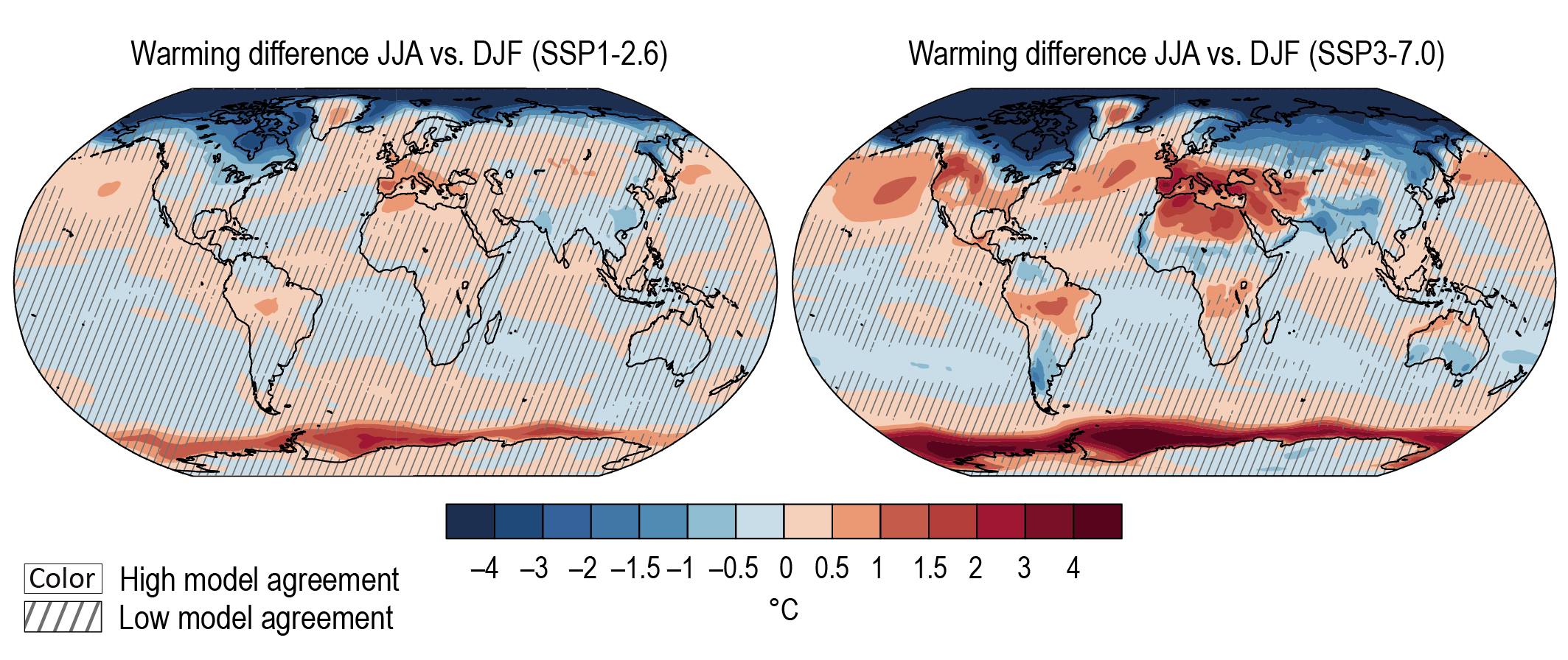 Figure 4.20 | Difference of surface temperature change between June–July–August (JJA) and December–January–February (DJF). Displayed are spatial patterns of multi-model mean difference in projected warming in JJA minus warming in DJF in 2081–2100 relative to 1995–2014 for (left) SSP1-2.6 and (right) SSP3-7.0. Diagonal lines mark areas where fewer than 80% of the models agree on the sign of change, and no overlay where at least 80% of the models agree. Further details on data sources and processing are available in the chapter data table (Table 4.SM.1).
 4.5.1.1.3 Changes in temperature variability
It has long been recognized that along with mean temperatures also variance and skewness of the temperature distribution may be changing (Gregory and Mitchell, 1995; Mearns et al., 1997). By amplifying or dampening changes in the tail of temperature distribution such changes are potentially highly relevant to extremes (Section 11.3.1) and pose a serious challenge to adaptation measures. Changes in temperature variability can occur from diurnal to multi-decadal time scales and from the local to the global scale with potentially even opposing signals in different seasons and at the different spatial scales
Changes in GSAT variability are poorly understood. Based on model experiments it has been suggested that unforced variability of GSAT tends to decrease in a warmer world as a result of reduced albedo variability in high latitudes resulting from melting snow and sea ice (Huntingford et al., 2013; Brown et al., 2017), but confidence remains low and an observed change has not been detected. An assessment of changes in global temperature variability is inherently challenging due to the interplay of unforced internal variability and forced changes.
Changes in tropical temperature variability may arise from changes in the amplitude of ENSO (Section 4.5.3.2). Over the extratropics, several studies have identified robust large-scale patterns of changes in variability of annual and particularly seasonal mean temperature, including (i) a reduction in mid- to high-latitude winter temperature variability and (ii) an increase in summer temperature variability over land in the tropics and subtropics (Huntingford et al., 2013; Holmes et al., 2016; see Figure 4.21). The multi-ensemble average across seven single-model initial-condition large ensembles projects a consistent reduction in year-to-year December–January–February (DJF) variability around about 50°N–70°N and June–July–August (JJA) variability around 55°S–70°S along the edge of the sea ice- and snow-covered region (Figure 4.21). There is growing evidence that year-to-year and day-to-day temperature variability decreases in winter over northern mid- to high-latitudes (Fischer et al., 2011; De Vries et al., 2012; Screen, 2014; Schneider et al., 2015; Holmes et al., 2016; Borodina et al., 2017; Tamarin-Brodsky et al., 2020) which implies that the lowest temperatures rise more than the respective climatological mean temperatures (medium confidence). Over the NH, reduced high-latitude temperature variability is associated with disproportionally large warming in source region of cold-air advection due to Arctic amplification and land–sea contrast (De Vries et al., 2012; Screen, 2014; Holmes et al., 2016). It has further been argued that a reduction in snow and sea ice coverage from partly to completely snow- and ice-free ocean and land surface would substantially reduce cold-season temperature variability (Gregory and Mitchell, 1995; Fischer et al., 2011; Borodina et al., 2017) and lead to a shortening of the cold season and earlier onset of the warm season (Cassou and Cattiaux, 2016). Mid-latitudinal winter temperature variability is further affected by a complex interplay of a multitude of processes including potential changes in atmospheric circulation, but there is low confidence in the dominant contribution of Arctic warming compared to other drivers (Cross-Chapter Box 10.1).
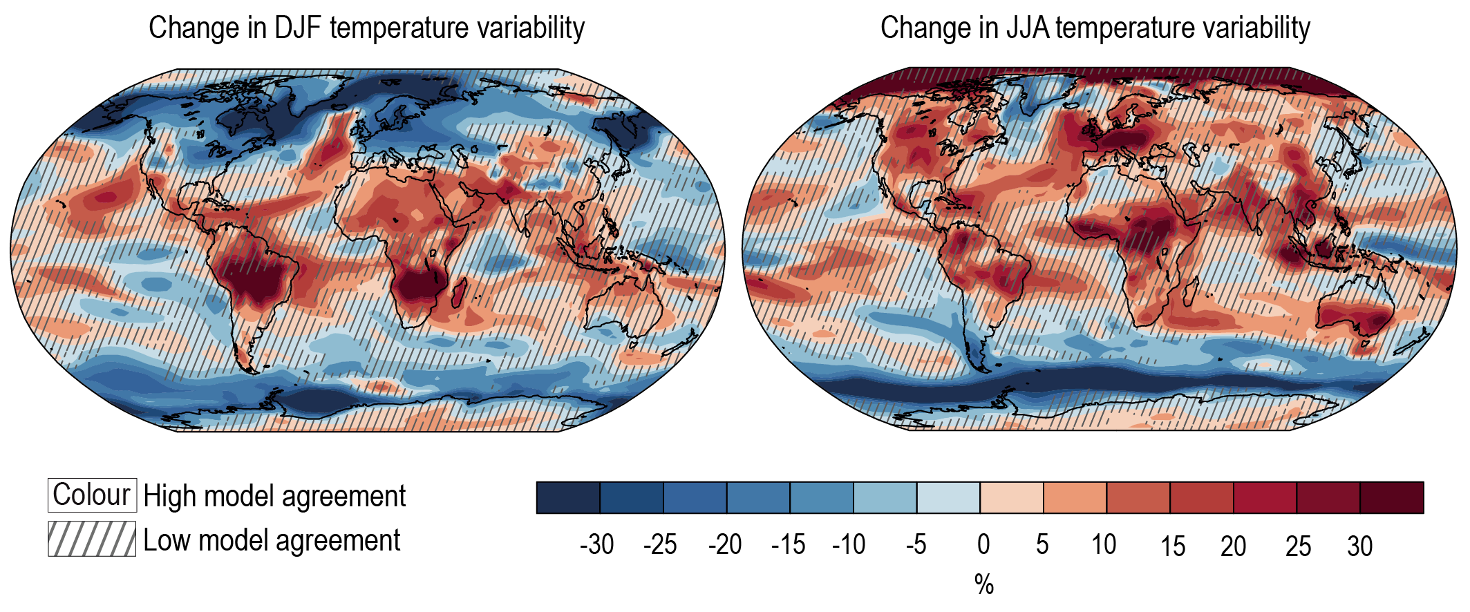 Figure 4.21 | Percentage change in interannual variability of (left) December–January–February (DJF) and (right) June–July–August (JJA) mean temperature averaged across seven large initial condition ensembles. Average changes across seven single-model, initial-condition large ensembles are shown for RCP8.5 in 2081–2100 (and where not available for 2080–2099) relative to 1995–2014. Standard deviations are calculated across all members of the large ensembles for every given year to avoid inflation due to the underlying trend and then averaged across the period. Changes are averaged across the ensembles MPI-GE (100 members, Maher et al., 2019), CanESM2 (50 members, Kirchmeier-Young et al., 2017), NCAR-CESM (30 members, Kay et al., 2015), GFDL-CM3 (20 members, Sun et al., 2018), GFDL-ESM2M (30 members, Rodgers et al., 2015), CSIRO-Mk3-6-0 (30 members, Jeffrey et al., 2013) and EC-EARTH (16 members, Hazeleger et al., 2010). Also see Deser et al. (2020) for further information on those ensembles. Diagonal lines indicate areas with low model agreement where fewer than 80% of the models agree on the sign of the change, and no overlay areas with high model agreement where at least 80% of the models agree on the sign of the change. Further details on data sources and processing are available in the chapter data table (Table 4.SM.1).
 In JJA, the multi-model average projects an increase in year-to-year JJA variability over Central Europe and North America (Figure 4.21). In particular an increase in daily to interannual summer temperature variability has been projected over central Europe as a result of larger year-to-year variability in soil moisture conditions varying between a wet and dry regime and leading to enhanced land–atmosphere interaction (Seneviratne et al., 2006; Fischer et al., 2012; Holmes et al., 2016). Furthermore, the amplified warming in the source regions of warm-air advection due to land–ocean warming contrast and amplified Mediterranean warming (Seager et al., 2014a; Brogli et al., 2019), may lead to disproportionally strong warming of the hottest days and summers and thereby increased variability. Enhanced temperature variability is further projected over some land regions in the subtropics and tropics (Bathiany et al., 2018).
In summary, there is medium confidence that continued warming will regionally lead to increased and decreased year-to-year temperature variability in the extratropics and there is medium confidence that year-to-year temperature variability will decrease over parts of the mid- to high- latitudes of the winter hemisphere.
4.5.1.2 Annual Mean Atmospheric Temperature
Section 12.4.3.2 of AR5 assessed that there is high confidence in the overall pattern of projected end of 21st century tropospheric temperature change and that it is very likely that some of the largest warming will occur in the northern high latitudes. They further assessed that proportionately larger warming is likely to occur in the tropical upper troposphere than at the tropical surface, but with medium confidence owing to the relatively large observational uncertainties and contradictory analyses regarding model accuracy in simulating tropical upper tropospheric temperature trends.
CMIP6 projections show warming throughout the troposphere by the end of this century and a mix of warming and cooling in the stratosphere depending on the emissions scenario (Figure 4.22). The patterns of tropospheric temperature change are highly consistent with those derived from earlier generations of climate models as assessed in AR5, AR4 and TAR. In SSP1-2.6, the multi-model mean warming remains below 3°C everywhere in the troposphere except near the surface in the Arctic; this is similar to the findings in AR5 based on CMIP5 models for RCP2.6. In SSP3-7.0, the zonal mean tropospheric warming is also largest in the tropical upper troposphere, reaching more than 5°C, and near the surface in the Arctic where warming exceeds 8°C (Figure 4.22). It is likely that the warmer projected GSAT in the unconstrained CMIP6 model ensemble contributes to larger warming in the tropical upper troposphere and in the Arctic lower troposphere. This assessment is based on the understanding of polar amplification assessed in Chapter 7 (Section 7.4.4.1), and at low latitudes is based on the understanding of moist convective processes as well as the relationship between CMIP5- and CMIP6-simulated surface temperatures and tropical upper tropospheric warming over the historical period (Section 3.3.1.2).
 Figure 4.22 | Long-term change of annual and zonal mean atmospheric temperature. Displayed are multi-model mean change in annual and zonal mean atmospheric temperature (°C) in 2081–2100 relative to 1995–2014 for (left) SSP1-2.6 and (right) SSP3-7.0. The number of models used is indicated in the top right of the maps. Diagonal lines indicate regions where less than 80% of the models agree on the sign of the change and no overlay where 80% or more of the models agree on the sign of the change. Further details on data sources and processing are available in the chapter data table (Table 4.SM.1).
 Projected stratospheric temperature trends are determined by a balance between the major radiative drivers from ozone recovery, rising CO2 and other greenhouse gases (including stratospheric water vapour) (Maycock, 2016), as well as future changes in the Brewer –Dobson circulation, which can alter the latitudinal pattern of stratospheric temperature trends (Fu et al., 2015, 2019). In the lower stratosphere, the CMIP6 models project a weak cooling in the inner tropics in SSP1-2.6 and a warming at other latitudes (Figure 4.22). There is enhanced lower stratospheric warming over the Antarctic pole owing to the effects of ozone hole recovery on polar temperatures (Maycock, 2016; Solomon et al., 2017). The projected strengthening of the Brewer –Dobson circulation in the future (Hardiman et al., 2014) also affects stratospheric temperature trends, with adiabatic cooling at low latitudes and warming in middle and high latitudes (Fu et al., 2015, 2019). In SSP3-7.0, there is widespread cooling across much of the stratosphere, as expected from the higher GHG emissions, with a smaller warming in the Antarctic lower stratosphere. Owing to the importance of ozone recovery for the radiative balance of the stratosphere, future global and local stratospheric temperature trends do not scale with projected GSAT change.
In summary, new results since AR5 do not generally alter the understanding of projected zonal mean atmospheric temperature changes. There is high confidence in the overall pattern of projected tropospheric temperature changes given its robustness across many generations of climate models. It is furthervery likely that projected long-term tropospheric warming will be larger than the global mean in the Arctic lower troposphere. It is likely that tropical upper tropospheric warming will be larger than at the tropical surface, however with an uncertain magnitude owing to the potentially large role of natural internal variability and differences across models in the simulated free tropospheric temperature response to a given forcing scenario (Section 3.3.1.2). It is very likely that global mean stratospheric cooling will be larger by the end of the 21st century in a pathway with higher atmospheric CO2 concentrations.
4.5.1.3 Near-surface Relative Humidity
The AR5 contrasted future changes in near-surface relative humidity (RH) over land and ocean, concluding with medium confidence that reductions in near-surface RH over many land areas are likely . The decrease in near-surface RH over most land areas is associated with the larger warming rates over land than over the ocean and is termed the last-saturation-temperature constraint, as explained in AR5.
Since AR5, significant effort has been devoted to understanding the mechanisms for the decrease in near-surface land RH under global warming, and the relevance of RH changes for the land–sea warming contrast and the water cycle. For the near-surface RH decrease over land, both the moisture transport from the ocean and land–atmosphere feedback processes contribute. For changes in specific humidity over land, the moisture transport from the ocean is dominant while the role of evapotranspiration is secondary (Byrne and O’Gorman, 2016; Chadwick et al., 2016). Nevertheless, the changes in near-surface land RH are also strongly influenced by evapotranspiration, which is suppressed by the drying of soils and plant responses to increasing CO2 related to stomatal closure under climate change (Byrne and O’Gorman, 2015; Berg et al., 2016; Chadwick et al., 2016; Swann et al., 2016; Lemordant et al., 2018). The combination of oceanic and continental influences can explain the spatially diverse trends in the near-surface RH over land in the observations for the recent decades, with a generally dominant negative trend at the global scale (Vicente-Serrano et al., 2018). There is a strong feedback between the near-surface land RH decrease and land–ocean warming contrast under future warming projections (Section 4.5.1.1).
Changes in land RH can modulate the response of the water cycle to global warming (Chadwick et al., 2013; Byrne and O’Gorman, 2015). Most CMIP5 models project higher precipitation associated with higher near-surface RH and temperature under climate change (Lambert et al., 2017). Over land, the spatial gradients of fractional changes in near-surface RH contribute to a drying tendency in precipitation minus evapotranspiration with warming, which partly explains why the ‘wet gets wetter, dry gets drier’ paradigm does not hold over land (Byrne and O’Gorman, 2015). Terrestrial aridity is projected to increase over land, as manifested by a decrease in the ratio of precipitation to potential evapotranspiration, in which the decrease in near-surface land RH has a contribution of about 35% in CMIP5 models under doubled CO2 forcing (Fu and Feng, 2014). The aridity can be further amplified by the feedbacks of projected drier soils on land surface temperature, RH, and precipitation (Berg et al., 2016).
The CMIP6 multi-model ensemble projects general decreases in near-surface relative humidity over a large fraction of land areas, but moderate increases over the ocean (Figure 4.23). The projected changes depend on emissions scenario and season. Changes in near-surface RH under SSP1-2.6 are insignificant compared to natural variability. Under SSP3-7.0, during boreal summer, significant decreases relative to natural variability are projected in continental Europe and the Middle East, North America, South America and South Africa.
 Figure 4.23 | Long-term changes in seasonal mean relative humidity. Displayed are projected spatial patterns of multi-model mean change (%) in seasonal (top) December–January–February (DJF) and (bottom) June–July–August (JJA) mean near-surface relative humidity in 2081–2100 relative to 1995–2014, for (left) SSP1-2.6 and (right) SSP3-7.0. The number of models used is indicated in the top right of the maps. No overlay indicates regions where the change is robust and likely emerges from internal variability, that is, where at least 66% of the models show a change greater than the internal variability threshold (Section 4.2.6) and at least 80% of the models agree on the sign of change. Diagonal lines indicate regions with no change or no robust significant change, where fewer than 66% of the models show change greater than the internal-variability threshold. Crossed lines indicate areas of conflicting signals where at least 66% of the models show change greater than the internal-variability threshold but fewer than 80% of all models agree on the sign of change. Further details on data sources and processing are available in the chapter data table (Table 4.SM.1).
 In summary, there is medium confidence that continued warming will lead to decreased near-surface relative humidity over a large fraction of land areas, but moderate increases over the ocean. There is high confidence that near-surface relative humidity will decrease over parts of the tropical and subtropical latitudes over land.
4.5.1.4 Precipitation
The AR5 assessed that changes in mean precipitation in a warmer world will exhibit substantial spatial variation. Also, the contrast of mean precipitation between dry and wet regions and between dry and wet seasons will increase over most of globe as temperatures increase. The general pattern of change indicates that high latitude land masses are likely to experience greater amounts of precipitation due to the increased specific humidity of the warmer troposphere as well as increased transport of water vapour from the tropics by the end of this century under the RCP8.5 scenario. Many mid-latitude and subtropical arid and semi-arid regions will likely experience less precipitation, while many moist mid-latitude regions will likely experience more precipitation by the end of this century under the RCP8.5 scenario.
Since AR5, progress has been achieved in understanding changes in patterns and rates of precipitation with GSAT rise. The projected precipitation changes can be decomposed into a part that is related to atmospheric circulation referred to as dynamical component and a part related to water vapour changes, the thermodynamic component. Based on process understanding and modelling (Fläschner et al., 2016; Samset et al., 2016), global mean precipitation will very likely increase by 1–3% per °C of GSAT warming (Section 8.2.1). The increase in atmospheric water vapour is a robust change under global warming, the sensitivity of global precipitation change to warming is smaller (2% per °C) as compared to water vapour change (7% per °C; Held and Soden, 2006). Global energy balance places a strong constraint on the global mean precipitation (Allen and Ingram, 2002; Pendergrass and Hartmann, 2014; Myhre et al., 2018; Siler et al., 2019). Tropospheric radiative cooling constrains global precipitation (Pendergrass and Hartmann, 2014), leading to a slow SST-dependent response and a forcing-dependent rapid adjustment. Rapid adjustments account for large regional differences in hydrological sensitivity across multiple drivers (Samset et al., 2016; Myhre et al., 2017). The rapid regional precipitation response to increased CO2 is robust across models, implying that the uncertainty in long-term changes is mainly associated with the response to SST-mediated feedbacks (Richardson et al., 2016). Precipitation response to fast adjustments and slow temperature-driven responses are assessed in detail in Chapter 8 (Section 8.2.1).
The thermodynamic response to global warming is associated with a ‘wet get wetter’ mechanism, with enhanced moisture flux leading to subtropical dry regions getting drier and tropical and mid-latitude wet regions getting wetter (Held and Soden, 2006; Chou et al., 2009). Recent studies suggest that the dry-get-drier argument does not hold, especially over subtropical land regions (Greve et al., 2014; Feng and Zhang, 2015; Greve and Seneviratne, 2015). The discrepancy may be partly arising due to differences in model climatologies and by change in the location of wet and dry regions (Polson and Hegerl, 2017). Over the 21st century, significant rate of precipitation change is associated with a spatial stabilization and intensification of moistening and drying patterns (Chavaillaz et al., 2016). In the tropics, weakening of circulation leads to a ‘wet gets drier, dry gets wetter’ pattern (Chadwick et al., 2013). Climate model agreement for precipitation change in the tropics is lower than for other regions (Knutti and Sedláček, 2013; McSweeney and Jones, 2013). Sources of inter-model uncertainty in regional rainfall projections arise from circulation changes (Kent et al., 2015; Chadwick, 2016) and spatial shifts in convection and convergence, associated with SST pattern change and land–sea thermal contrast change (Kent et al., 2015; Chadwick et al., 2017) with a secondary contribution from the response to direct CO2 forcing (Chadwick, 2016). Factors governing changes in large-scale precipitation patterns are assessed in detail in Sections 8.2.2 and 10.4.1.
Long-term multi-model mean change in seasonal precipitation (JJA and DJF) from CMIP6 models (Figure 4.24) shows substantial regional differences and seasonal contrast. Changes in seasonal precipitation under SSP1-2.6 are small compared to internal variability. Consistent with the AR5, patterns of precipitation change are very likely to increase in the high latitudes especially during local winter and over tropical oceans under SSP3-7.0 (high confidence). CMIP6 projections show an increase in precipitation over larger parts of the monsoon regions and decreases in many subtropical regions including the Mediterranean, southern Africa and south-west Australia (medium confidence). The large-scale patterns of precipitation shown in Figure 4.24 are consistent with the patterns presented in Section 8.4.1.3. Precipitation changes exhibit strong seasonal characteristics (Box 8.2), and, in many regions, the sign of the precipitation changes varies with season. Precipitation variability is projected to increase over a majority of global land area, as assessed in Chapter 8 (Section 8.4.1.3.3), over a wide range of time scales in response to warming (Pendergrass et al., 2017).
 Figure 4.24 | Long-term change of seasonal mean precipitation. Displayed are projected spatial patterns of multi-model mean change (%) in (top) December–January–February (DJF) and (bottom) June–July–August (JJA) mean precipitation in 2081–2100 relative to 1995–2014, for (left) SSP1-2.6 and (right) SSP3-7.0. The number of models used is indicated in the top right of the maps. No map overlay indicates regions where the change is robust and likely emerges from internal variability, that is, where at least 66% of the models show a change greater than the internal-variability threshold (Section 4.2.6) and at least 80% of the models agree on the sign of change. Diagonal lines indicate regions with no change or no robust significant change, where fewer than 66% of the models show change greater than the internal-variability threshold. Crossed lines indicate areas of conflicting signals where at least 66% of the models show change greater than the internal-variability threshold but fewer than 80% of all models agree on the sign of change. Further details on data sources and processing are available in the chapter data table (Table 4.SM.1).
 Most of the projected changes in precipitation exhibit a sharp contrast between land and ocean (Sections 8.2.1 and 8.4.1). Temperature-driven intensification of land-mean precipitation during the 20th century has been masked by fast precipitation responses to anthropogenic sulphate and volcanic forcing (Allen and Ingram, 2002; Richardson et al., 2018a). Based on the Precipitation Driver and Response Model Intercomparison Project (PDRMIP), land-mean precipitation is expected to increase more rapidly with the projected decrease in sulphate forcing and continued warming, contributing to increased global mean precipitation (Table 4.3) and will be clearly observable by the mid-21st century based on RCP4.5 and RCP8.5 scenarios (Richardson et al., 2018a).
Consistent with the findings of AR5, a gradual increase in global mean precipitation is projected over the 21st century with an increase of approximately 2.9% (1.0–5.2%) under SSP1-2.6 and 4.7% (2.3–8.2%) under SSP3-7.0 during 2081–2100 relative to 1995–2014. The corresponding increase in annual mean global land precipitation is 3.3% (0–6.6%), in the SSP1-2.6 and 5.8% (0.5–9.6%) in the SSP3-7.0 (Table 4.3). CMIP6 models show greater increases in precipitation over land than either globally or over the ocean (high confidence).
Based on the assessment of CMIP6 models, we conclude that it is very likely that, in the long term, global mean land and global mean ocean precipitation will increase with increasing GSAT. Annual mean and global mean precipitation will very likely increase by 1–3% per °C GSAT warming. The patterns of precipitation change will exhibit substantial regional differences and seasonal contrast as GSAT increases over the 21st century (high confidence). Precipitation will very likely increase over high latitudes and the tropical ocean and will likely increase in large parts of the monsoon regions. However, it is likely to decrease over the subtropics, including Mediterranean, southern Africa and south-west Australia, in response to GHG-induced warming.
4.5.1.5 Global Monsoon Precipitation and Circulation
The AR5 assessed changes of the global monsoon in the context of long-term trends across the 21st century and the change by 2081–2100. The AR5 showed growing evidence of improved skill of climate models in reproducing the climatological features of the global monsoon. Taken together with identified model agreement on future changes, the global monsoon precipitation, aggregated over all regional monsoon regions, is likely to strengthen in the 21st century with increases in its area and intensity, while the monsoon circulation weakens. In all RCP scenarios, the global monsoon area is very likely to increase, and the global monsoon precipitation intensity is likely to increase, resulting in avery likely increase in the global monsoon total precipitation, by 2081–2100 (Kitoh et al., 2013).
Since AR5, there has been progress in understanding physical mechanisms for the projected changes in global monsoon and quantifying the sources of uncertainty in projections. The increase in global monsoon precipitation under warming is primarily attributed to the increase of moisture convergence, which comes mainly from the thermodynamic effect due to increasing atmospheric moisture but is partly offset by reduced convergence (W. Zhang et al., 2019; Chen et al., 2020). The dynamic effect, such as monsoon circulation changes, dominates regional differences in the projected monsoon precipitation changes (Chen et al., 2020). Specifically, NH monsoon precipitation will increase more strongly than its SH counterpart, due to an increase in hemispheric temperature difference between the NH and SH, enhancement of the Hadley circulation, and atmospheric moistening, countered by stabilization of the troposphere (Lee and Wang, 2014). The seasonality of global monsoon rainfall is projected to be enhanced in response to warming, featuring a greater wet–dry season contrast (Lee and Wang 2014; Zhang et al. 2019). In addition, the interannual variability of global monsoon rainfall is projected to intensify mainly over land, with a strengthened relationship between global monsoon and ENSO (Hsu et al., 2013; Wang et al., 2020, 2021).
For the uncertainty in mean monsoon precipitation projections, the model uncertainty is the dominant contributor throughout the century and explains more than 70% of the inter-model variance during near term, mid-term, and long term. The contribution of internal variability is only important at the beginning in early decades, while scenario uncertainty becomes important at the end of the 21st century. The sources of uncertainty for the mean and extreme monsoon precipitation mainly differ in the long-term projection, when the contribution of scenario uncertainty is comparable to the model uncertainty for extreme precipitation (Zhou et al., 2020). Although the magnitude of internal variability differs between CMIP5 models and single-model, initial-condition large ensembles, the impact is only evident in the beginning decades. For the mid- and long term, the magnitude difference does not alter that model uncertainty is the dominant source of uncertainty in the projections of global land monsoon precipitation (Zhou et al., 2020).
Based on the projections of changes in precipitation from CMIP6 under the four SSPs, the global monsoon precipitation is likely to strengthen in the 21st century with increases in its intensity, while NH summer monsoon circulation weakens (Figure 4.14). Global land monsoon precipitation will likely increase by 1.3–2.4% per °C GSAT warming among the four scenarios considered here. In the long term, the multi-model mean change (5–95% range of the available 41 projections) of global land monsoon precipitation index is 2.9% (–0.8 to +7.8%), 3.7% (–2.5 to +8.6%), 3.77% (–3.2 to +8.1%), and 5.7% (–2.8 to +12.3%) under SSP1-2.6, SSP2-4.5, SSP3-7.0, and SSP5-8.5, respectively. This enhancement is caused by thermodynamic responses due to increased moisture, which is partly offset by dynamic responses due to a weakened circulation (Chen et al., 2020). The patterns of monsoon rainfall change in the mid- to long-term include a north–south asymmetry characterized by greater increase in the NH than the SH, and an East–West asymmetry characterized by enhanced Asian-African monsoons and weakened North American monsoon (medium confidence) (Lee and Wang, 2014; Mohtadi et al., 2016; Pascale et al., 2017; Wang et al., 2021).
Based on the assessment of CMIP6 models, we conclude that it is likely that, in the mid- to long term, the global land monsoon precipitation will increase with GSAT rise despite a weakened monsoon circulation. The global land monsoon precipitation will likely increase by 1.3–2.4% per °C GSAT warming among the four scenarios. Monsoon precipitation responses depend on region and emissions scenario (high confidence).
4.5.1.6 Sea Level Pressure, Large-scale Atmospheric Circulation, Storm Tracks and Blocking
This subsection provides a global overview of long-term changes in atmospheric dynamical features that is complementary to the regional assessment of links to the hydrological cycle in Chapter 8 (Section 8.4.2), and assessment of the connections to extreme events in Chapter 11 (Section 11.7.2).
4.5.1.6.1 Sea level pressure
The AR5 assessed that mean sea level pressure is projected to decrease in high latitudes and to increase in mid-latitudes. Such a pattern is associated with a poleward shift in the storm track and an increase in the annular mode index. This broad pattern is also found in CMIP6 models (Figure 4.25). Under SSP1-2.6, the pattern in sea level pressure change resembles that for SSP3-7.0, but the amplitudes are small compared to internal variability in 20-year means (Figure 4.25). One exception is found in the SH mid-latitudes, where pressure robustly increases in SSP3-7.0 in both austral summer and winter, but shows no robust change in SSP1-2.6. This is likely attributable to the larger GHG forcing in SSP3-7.0 compared to SSP1-2.6, which contributes to a poleward shift of the SH mid-latitude circulation and becomes relatively more important than the effect of ozone recovery which drives an equatorward shift in the circulation (see Section 4.5.3.1 on the Southern Annular Mode; Barnes and Polvani, 2013; Barnes et al., 2014; Bracegirdle et al., 2020b). The poleward shift in SH mid-latitude circulation in SSP3-7.0 likely contributes to the wetting trend at high southern latitudes (Figure 4.25).
 Figure 4.25 | Long-term change of seasonal-mean sea level pressure. Displayed are projected spatial patterns of multi-model mean change in (top) December–January–February (DJF) and (bottom) June–July–August (JJA) mean sea level pressure (hPa) in 2081–2100 relative to 1995–2014, for (left) SSP1-2.6 and (right) SSP3-7.0. The number of models used is indicated in the top right of the maps. No overlay indicates regions where the change is robust and likely emerges from internal variability, that is, where at least 66% of the models show a change greater than the internal-variability threshold (Section 4.2.6) and at least 80% of the models agree on the sign of change. Diagonal lines indicate regions with no change or no robust significant change, where fewer than 66% of the models show change greater than the internal-variability threshold. Crossed lines indicate areas of conflicting signals where at least 66% of the models show change greater than the internal-variability threshold but fewer than 80% of all models agree on the sign of change. Further details on data sources and processing are available in the chapter data table (Table 4.SM.1).
 As was found in AR5, several regional sea level pressure features stand out from the zonal-mean change. Sea level pressure markedly decreases in north-eastern North America and north-eastern Asia in boreal winter. In boreal summer, sea level pressure robustly decreases in the Mediterranean and the Middle-East, a decrease that has been linked to a large-scale heat low forced by the amplified warming of the region (Haarsma et al., 2009). It is likely that sea level pressure will increase across the south-western North America and Central America in boreal summer under SSP3-7.0 due to an intensification of the eastern North Pacific subtropical summer high (Li et al., 2012) and a weakening of the North American monsoon (Section 4.5.1.5; Pascale et al., 2017; Wang et al., 2020). These changes in circulation are connected to drying across the eastern subtropical Pacific and Central America regions (Figure 4.24).
4.5.1.6.2 Zonal wind and westerly jets
Storm tracks and mid-latitude westerly jets are dynamically related aspects of mid-latitude circulation. The AR5 assessed that a poleward shift of the SH westerlies and storm track is likely by the end of the 21st century under RCP8.5 (medium confidence). In contrast, low confidence was assessed for the storm-track response in the NH.
Under both SSP1-2.6 and SSP3-7.0 there is a strengthening and lifting of the subtropical jets in both hemispheres (Figure 4.26), consistent with the response to large-scale tropospheric warming found in earlier generations of climate models (Collins et al., 2013). In the SH, GHG emissions tend to force a poleward shift of the jet, but this is opposed, particularly in austral summer, by the stratospheric ozone hole recovery (Barnes and Polvani, 2013; Barnes et al., 2014; Bracegirdle et al., 2020b). Consistent with sea level pressure changes, CMIP6 models project a strengthening and poleward shift of the SH jet in austral summer and winter under SSP3-7.0, but smaller and non-robust changes in SH mid-latitude zonal winds under SSP1-2.6 (Figure 4.26; see also Section 4.5.3.1). CMIP6 models show an improved simulation of the SH jet stream latitude (Bracegirdle et al., 2020a; Curtis et al., 2020). This has been linked to a reduction in the projected poleward shift of the SH jet in austral summer compared to the CMIP5 models (Curtis et al., 2020; Goyal et al., 2021), although differences in the pattern of SST response may also play a role (Wood et al., 2020). In the NH extratropics, the changes in lower-tropospheric zonal-mean zonal winds by the end of the century are generally smaller than in the SH. In boreal winter, there is a weak poleward shift of the NH zonal-mean westerly jet maximum in SSP3-7.0.
 Figure 4.26 | Long-term change of zonal-mean, zonal wind. Displayed are multi-model mean changes in (left) boreal winter(December–January–February, DJF) and (right) austral winter (June–July–August, JJA) zonal mean, zonal wind (m s–1) in 2081–2100 for (top) SSP1-2.6 and (bottom) SSP3-7.0 relative to 1995–2014. The 1995–2014 climatology is shown in contours with spacing 10 m s–1. Diagonal lines indicate regions where less than 80% of the models agree on the sign of the change and no overlay where at least 80% of the models agree on the sign of the change. Further details on data sources and processing are available in the chapter data table (Table 4.SM.1).
 CMIP5 and CMIP6 models show a strong seasonal and regional dependence in the response to climate change of NH westerlies (Barnes and Polvani, 2013; Grise and Polvani, 2014b; Simpson et al., 2014; Zappa et al., 2015; Harvey et al., 2020; Oudar et al., 2020). CMIP5 projections indicate a poleward shift of the westerlies in the North Atlantic in boreal summer, while the North Pacific jet weakens in this season (Simpson et al., 2014; Davini and D’Andrea, 2020; Harvey et al., 2020). There is a poleward shift in the westerlies in both the North Pacific and North Atlantic in Autumn (Barnes and Polvani, 2013; Simpson et al., 2014). However, the shift of the westerlies is more uncertain in the other seasons, particularly in the North Atlantic in winter (Simpson et al., 2014; Zappa and Shepherd, 2017). Here, the circulation response is not well described as a simple shift, since the North Atlantic jet tends to be squeezed on both its equatorward and poleward flanks, together with an eastward extension into Europe (Li et al., 2018; Peings et al., 2018; Simpson et al., 2019a; Harvey et al., 2020; Oudar et al., 2020). Simulations indicate that most of the changes in winter storminess over the Euro-Atlantic region will occur only after exceeding the 1.5°C warming level (Barcikowska et al., 2018).
Progress since AR5 has improved understanding of the climate change aspects that can drive these different, and potentially opposite, responses in the mid-latitude jets and storm tracks. A poleward shift of the jets and storm tracks is expected in response to an increase in the atmospheric stratification and in the upper-tropospheric equator-to-pole meridional temperature gradient, while it is opposed by the decrease in the meridional temperature gradient in the lower troposphere associated with the polar amplification of global warming (Harvey et al., 2014; Shaw et al., 2016). Recent analyses have identified additional climate aspects that can drive mid-latitude jet changes, including patterns in sea surface warming (Mizuta et al., 2014; Langenbrunner et al., 2015; Ceppi et al., 2018; Wood et al., 2020), land–sea warming contrast (Shaw and Voigt, 2015), loss of sea ice (Deser et al., 2015; Harvey et al., 2015; Screen et al., 2018b; Zappa et al., 2018), and changes in the strength of the stratospheric polar vortex (Manzini et al., 2014; Grise and Polvani, 2017; Simpson et al., 2018; Ceppi and Shepherd, 2019). From an energetics perspective,the uncertainty in the response of the jet streams depends on the response of clouds, their non-spatially uniform radiative feedbacks shaping the meridional profile of warming (Ceppi et al., 2014; Voigt and Shaw, 2015, 2016; Ceppi and Hartmann, 2016; Ceppi and Shepherd, 2017; Lipat et al., 2018; Albern et al., 2019; Voigt et al., 2019). Climate models seem to underestimate the forced component of the year-to-year variability in the atmospheric circulation, particularly in the North Atlantic sector (Scaife and Smith, 2018), which suggests some relevant dynamical processes may not be well represented. Whether and how this may affect long-term projections is unknown. In conclusion, due to the influence from competing dynamical drivers and the absence of observational evidence, there is medium confidence in a projected poleward shift of the NH zonal-mean low-level westerlies in autumn and summer and low confidence in the other seasons. There is also overall low confidence in projected regional changes in the NH low-level westerlies, particularly for the North Atlantic basin in boreal winter.
The anthropogenic forced signal in extratropical atmospheric circulation may well be small compared to internal variability (Deser et al., 2012b, 2014) and, as assessed in AR5, there is generallylow agreement across models in many aspects of regional atmospheric circulation change particularly in the NH (Shepherd, 2014). The latter means that, in some regions, a multi-model average perspective of atmospheric circulation change represents a small residual after averaging over large intermodel spread. This is in strong contrast to thermodynamic aspects of climate change, such as surface temperature change, for which model results are generally highly consistent (see, e.g., Figure 4.19). Furthermore, models share systematic biases in some aspects of extratropical atmospheric circulation such as mid-latitude jets, which can have complex implications for understanding forced changes (Simpson and Polvani, 2016). Given these issues, an emerging field of research since AR5 has focused on the development of ‘storylines’ for regional atmospheric circulation change (Shepherd, 2019). The storyline approach is grounded in the identification of a set of physical predictors of atmospheric circulation change, such as those described above (Harvey et al., 2014; Manzini et al., 2014; Shepherd et al., 2018), which act together to determine a specific outcome in the projected atmospheric circulation change. The consequences of multi-model spread in the physical predictors of atmospheric circulation change can be investigated, conditioned on a specified level of global warming (see also Section 1.4.4.2 and Box 10.2; Zappa and Shepherd, 2017; Zappa, 2019; Mindlin et al., 2020).
4.5.1.6.3 Storm tracks
As stated in AR5, the number of extratropical cyclones (ETC) composing the storm tracks is projected to weakly decline in future projections, but by no more than a few percent change. The reduction is mostly located on the equatorward flank of the storm tracks, which is associated with the Hadley cell expansion and a poleward shift in the mean genesis latitude of ETCs (Tamarin-Brodsky and Kaspi, 2017). Furthermore, the poleward propagation of individual ETCs is expected to increase with warming (Graff and LaCasce, 2014; Tamarin-Brodsky and Kaspi, 2017), thus contributing to a poleward shift in the mid-latitude transient-eddy kinetic energy. The increased poleward propagation results from the strengthening of the upper tropospheric jet and increased cyclone-associated precipitation (Tamarin-Brodsky and Kaspi, 2017), which are robust aspects of climate change.
In the NH boreal winter, CMIP6 models show a northward shift of the ETC density in the North Pacific, a tripolar pattern in the North Atlantic, and a weakening of the Mediterranean storm track (Figure 4.27a). CMIP6 models show overall low agreement on changes in ETC density in the North Atlantic in boreal winter (Figure 4.27a). A poleward shift of the storm track is evident in the SH (Figure 4.27b), particularly in the Indian and Pacific Ocean sectors. CMIP6 models still feature long-standing biases in the representation of storm tracks; for example, the winter storm track into Europe is too zonal, though different measures of storm track activity indicate some improvements compared to the previous generations of models (Harvey et al., 2020; Priestley et al., 2020).
 Figure 4.27 | Changes in extratropical storm track density. Displayed are projected spatial pattern of multi-model mean change of extratropical storm track density in winter (Northern Hemisphere December –January–Februrary, NH DJF, and Southern Hemisphere June–July–August, SH JJA) in 2080–2100 for SSP5-8.5 relative to 1979–2014 based on 13 CMIP6 models. Diagonal lines indicate regions where fewer than 80% of the models agree on the sign of the change and no overlay where at least 80% of the models agree on the sign of change. Units are number density per 5° spherical cap per month. Further details on data sources and processing are available in the chapter data table (Table 4.SM.1).
 Regarding the dynamical intensity of the storm tracks (Section 11.7.2), the number of ETCs associated with intense surface wind speeds and undergoing explosive pressure deepening are projected to strongly decrease in the NH winter (Seiler and Zwiers, 2016; Chang, 2018). The weakening of surface winds of ETCs in the NH is attributed to the reduced low-level baroclinicity from SST and sea ice changes (Harvey et al., 2014; Seiler and Zwiers, 2016; J. Wang et al., 2017a). There are, however, regional exceptions such as in the northern North Pacific, where explosive and intense ETCs are projected to increase in association with the poleward shift of the jet and increased upper-level baroclinicity (Seiler and Zwiers, 2016). Eddy kinetic energy and intense cyclone activity are also projected to decrease in the NH summer in association with a weakening of the jet (Lehmann et al., 2014; Chang et al., 2016). However, explosive cyclones tend to be too weak in climate models (Seiler and Zwiers, 2016; Priestley et al., 2020), though this bias seems to be reduced in high-resolution simulations (Jiaxiang et al., 2020). Furthermore, models may not fully capture the contribution of the future increase in mesoscale latent heating to cyclone intensification (Li et al., 2014; Pfahl et al., 2015; Willison et al., 2015; Michaelis et al., 2017). In conclusion, there is only medium confidence in the projected decrease in the frequency of intense NH ETCs.
In contrast to the Northern Hemisphere, the Southern Hemisphere shows an increase in the frequency of intense ETCs in CMIP5 models (Chang, 2017), and there is high confidence that wind speeds associated with ETCs are expected to intensify in the SH storm track for high emissions scenarios. These changes in intensity are accompanied by an overall southward shift of the SH winter storm track (Figure 4.27b) due to the poleward shift in the upper-level jet and the increase in the meridional SST gradient linked to the slower warming of the Southern Ocean (Grieger et al., 2014).
Regardless of dynamical intensity changes, there is high confidence that the number of ETCs associated with extreme precipitation is projected to increase with warming, due to the increased moisture-loading capacity of the atmosphere (Section 8.4.2; Yettella and Kay, 2017; Hawcroft et al., 2018).
4.5.1.6.4 Atmospheric blocking
Blocking is associated with a class of quasi-stationary, high-pressure weather systems in the middle and high latitudes that disrupt the prevailing westerly flow. These events can persist for extended periods, such as a week or longer, and can cause long-lived extreme weather conditions, from heat waves in summer to cold spells in winter (see Section 11.7.2 for a detailed discussion of these features and Section 3.3.3.3 for the assessment of blocking biases in models simulations). The AR5 assessed with medium confidence that the frequency of blocking would not increase under enhanced GHG concentrations, while changes in blocking intensity and persistence remained uncertain.
The CMIP5 projections suggest that the response of blocking frequency to climate change might be quite complex (Dunn-Sigouin et al., 2013; Masato et al., 2013). An eastward shift of winter blocking activity in the NH is indicated (Masato et al., 2013; Kitano and Yamada, 2016; Lee and Ahn, 2017; Matsueda and Endo, 2017) while during boreal summer, blocking frequency tends to decrease in mid-latitudes (Matsueda and Endo, 2017), with the exception of the eastern Europe–western Russia region (Masato et al., 2013). The projected decrease of blocking in boreal summer partially contrasts with the observed increase in Greenland blocking (Hanna et al., 2018; Davini and D’Andrea, 2020). However, as shown in Woollings et al. (2018), the spatial distribution and the magnitude of the suggested changes are sensitive to the blocking detection methods (Schwierz et al., 2004; Barriopedro et al., 2010; Davini et al., 2012). In the SH, blocking frequency is projected to decrease in the Pacific sector during austral spring and summer. However, seasonal and regional changes are not totally consistent across the models (Parsons et al., 2016), and, as assessed in Section 3.3.3.3, model biases might affect their response.
To better understand the uncertainty in future blocking activity, a process-oriented approach has been proposed that aims to link blocking responses to different features of the global warming pattern. Upper-level tropical warming might be the key factor leading to a reduced blocking, because of the strengthening of zonal winds (Kennedy et al., 2016). The more controversial influence of near-surface Arctic warming might lead to an increased blocking frequency (Mori et al., 2014; Francis and Vavrus, 2015) (see Chapter 10, Box 10.1).
Figure 4.28 shows a clear decrease in blocking activity over Greenland and North Pacific for SSP7.0 and SSP8.5. Models with the largest decrease in blocking frequency in boreal winter are those showing the smallest frequency bias during the historical period (Davini and D’Andrea, 2020). In conclusion, there is medium confidence that the frequency of atmospheric blocking events over Greenland and the North Pacific will decrease in boreal winter in the SSP3-7.0 and SSP5-8.5 scenarios.
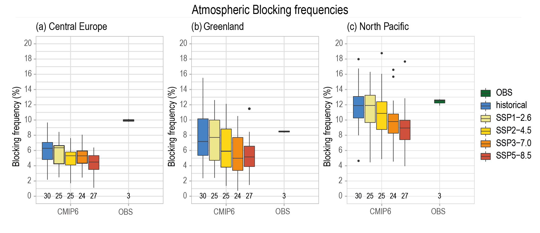 Figure 4.28 | Projected winter atmospheric blocking frequencies. Box plot showing December –March atmospheric blocking frequencies from historical simulations over 1995–2014 and projections over 2081–2100, over (a) the Central European region (20°W–20°E, 45°N–65°N); (b) the Greenland region (65°W–20°W, 62.5°N–72.5°N); (c) the North Pacific region (130°E–150°W, 60°N–75°N). Values show the percentage of blocked days per season following the (Davini et al., 2012) index. Median values are the thick black horizontal bar. The lower whiskers extend from the first quartile to the smallest value in the ensemble, and the upper whiskers extend from the third quartile to the largest value. The whiskers are limited to an upper bound that is 1.5 times the interquartile range (the distance between the third and first quartiles). Black dots show outliers from the whiskers. The numbers below each bar report the number of models included. Observationally-based values are obtained as the average of the ERA-Interim Reanalysis, the JRA-55 Reanalysis and the NCEP/NCAR Reanalysis. Adapted from Davini and D’Andrea (2020). Further details on data sources and processing are available in the chapter data table (Table 4.SM.1).
 4.5.2 Ocean
4.5.2.1 Ocean Temperature
Projections of long-term ocean thermal properties are assessed comprehensively in Chapter 9 (Sections 9.2.1.1 and 9.2.2.1) and are not covered here to avoid unnecessary overlap.
4.5.2.2 Ocean Acidification
The model-simulated, long-term trend of ocean acidification is assessed in Section 4.3.2.5 and Chapter 5 (Section 5.3.4.1). It is virtually certain that surface ocean acidification will continue in response to the rise in atmospheric CO2, and continued penetration of anthropogenic CO2 from the surface to the deep ocean will acidify the ocean interior (Figure 4.29). By the end of this century, under SSP3-7.0, a pH reduction of about 0.3 is found at a few hundred metres depth of the global ocean, with stronger acidification in the interior North Atlantic and the mid- to high-latitude Southern Ocean. At a depth of about 1 km, a pH reduction of about 0.1 is found.
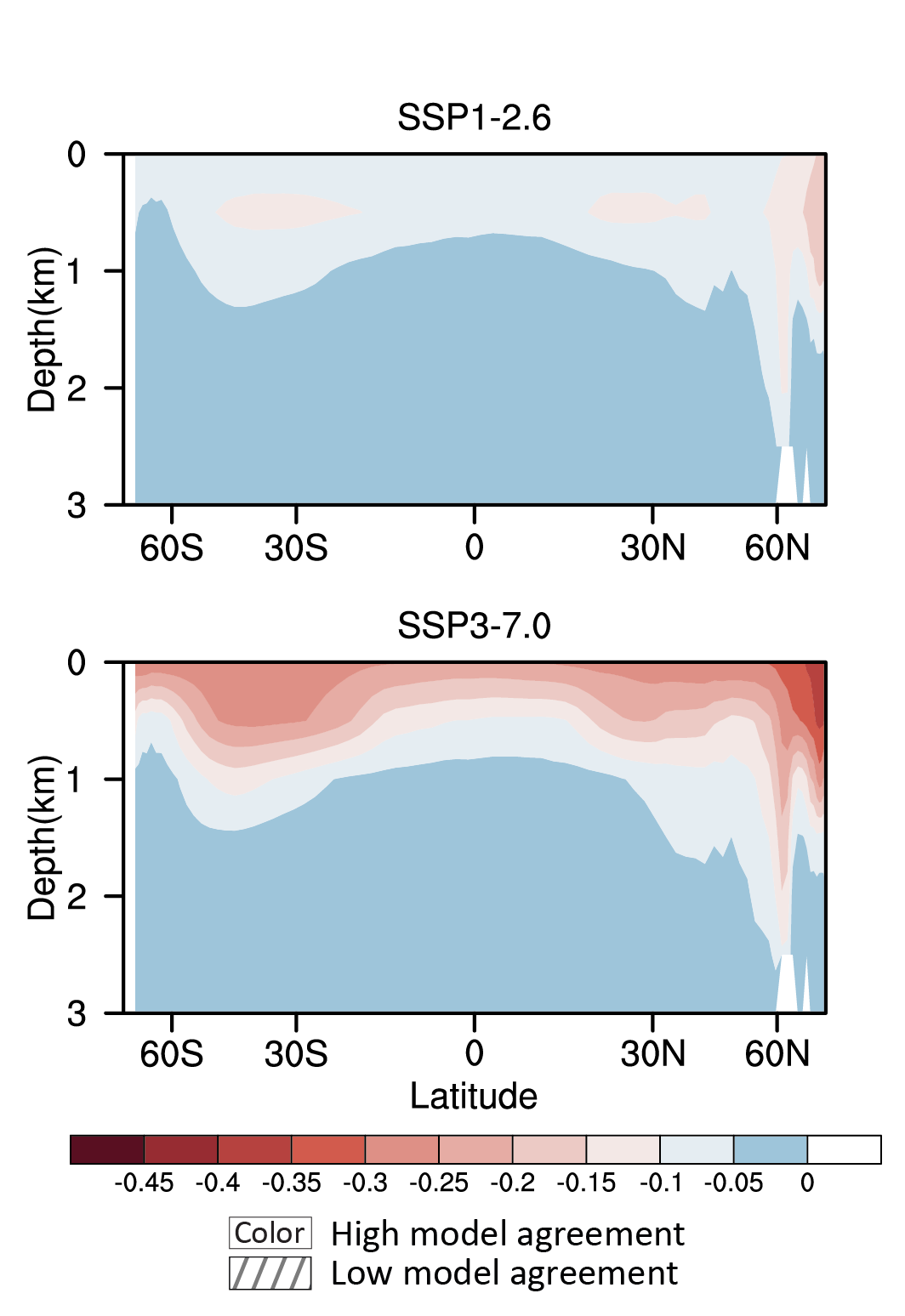 Figure 4.29 | Long-term change of annual and zonal ocean pH. Displayed are multi-model mean change in annual and zonal ocean pH in 2081–2100 relative to themean of 1995–2014 for SSP1-2.6 and SSP3-7.0, respectively. Eleven CMIP6 model results are used. Diagonal lines indicate regions where fewer than 80% of the models agree on the sign of the change and no overlay where at least 80% of the models agree on the sign of change. Further details on data sources and processing are available in the chapter data table (Table 4.SM.1).
 Projections with CMIP6 ESMs (Kwiatkowski et al., 2020) show a surface pH decline of –0.16 ± 0.002 (±1 standard deviation) under SSP1-2.6 and –0.44 ± 0.005 under SSP5-8.5 from 1870–1899 to 2080–2099. The high-latitude oceans, in particular the Arctic, show greater decline in pH and accelerated acidification (Terhaar et al., 2020). For the same period, model-projected bottom-water pH decline is –0.018 ± 0.001 under SSP1-2.6 and –0.030 ± 0.002 under SSP5-8.5. The projected large-scale surface ocean acidification will be primarily determined by the pathway of atmospheric CO2, with weak dependence on change in climate (high confidence) (Section 5.3.4.1; Hurd et al., 2018). However, for a given atmospheric CO2 scenario, uncertainty in projected ocean acidification increases with ocean depth because of model-simulated differences in ocean circulation that transports anthropogenic CO2 from the surface to bottom ocean (high confidence) (Kwiatkowski et al., 2020). For example, projected surface pH fully separates between SSPs scenarios before 2050, but some overlap across SSPs is still found for projected bottom-water pH in 2080 (Kwiatkowski et al., 2020).
4.5.3 Modes of Variability
4.5.3.1 Northern and Southern Annular Modes
4.5.3.1.1 The Northern Annular Mode
The AR5 assessed from CMIP5 simulations that the future boreal wintertime NAM is very likely to exhibit natural variability and forced trends of similar magnitude to that observed in the historical period and is likely to become slightly more positive in the future. Considerable uncertainty is related to physical mechanisms to explain the observed and projected changes in the NAM, but NAM trends are clearly closely connected to projected shifts in the mid-latitude jets and storm tracks.
NAM projections from climate models analysed since AR5 reveal broadly similar results to the late 21st century. CMIP6 models show a positive ensemble-mean trend in most seasons and the higher emissions scenarios that is comparable to between-model or between-realization variability (Figure 4.30a). The NAM generally becomes more positive by the end of the century except in boreal summer (JJA) when there is no change in the NAM in these simulations. In boreal winter (DJF) under SSP5-8.5, the central estimate is an increase in the NAM by almost 3 hPa in the long-term compared to 1995–2014. This can be compared to a multi-model mean interannual standard deviation in the winter NAM index of 3.4 hPa during the period 1850–1900. We conclude with high confidence that in the mid- to long-term, the boreal wintertime surface NAM is more positive under SSP3-7.0 and SSP5-8.5, while under SSP1-1.9 and SSP1-2.6, the NAM does not show any robust change.
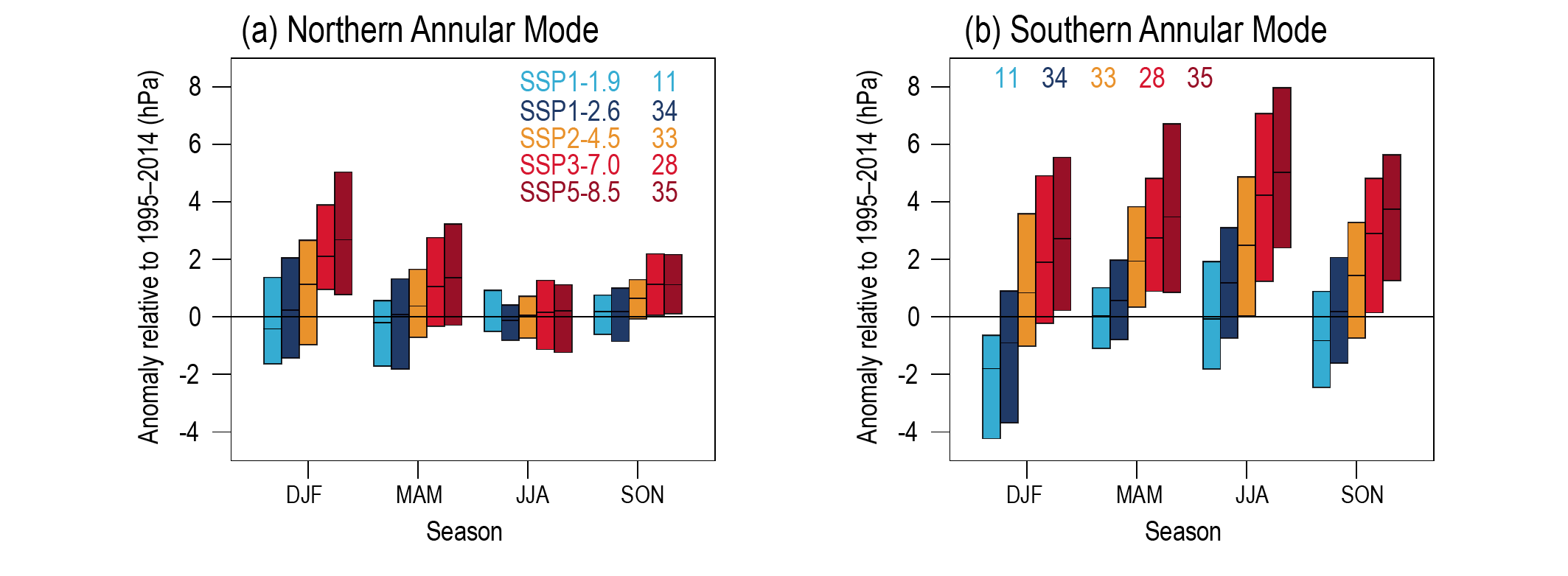 Figure 4.30 | CMIP6 Annular Mode index change from 1995–2014 to 2081–2100. (a) Northern Annular Mode (NAM) and (b) Southern Annular Mode (SAM). The NAM is defined as the difference in zonal mean SLP at 35°N and 65°N (Li and Wang, 2003) and the SAM as the difference in zonal mean SLP at 40°S and 65°S (Gong and Wang, 1999). The shadings are the 5–95% ranges across the simulations. The numbers near the top are the numbers of model simulations in each SSP ensemble. Further details on data sources and processing are available in the chapter data table (Table 4.SM.1).
 4.5.3.1.2 The Southern Annular Mode
The AR5 assessed it is likely that the evolution of the SAM over the 21st century will be primarily determined by the interplay between the effects of ozone recovery and changing GHG concentrations and influence the SAM in opposing ways. Owing to the relative effects of these two drivers, CMIP5 model SAM and Southern Hemisphere circulation projections differed markedly across forcing scenarios and across seasons (Barnes and Polvani, 2013; Barnes et al., 2014). CMIP5 models simulated a weak negative SAM trend in austral summer for RCP4.5 by the end of the century (F. Zheng et al., 2013), while for RCP8.5 they simulated a weak positive SAM trend in austral summer (F. Zheng et al., 2013). A substantial fraction of the spread in CMIP5 projections of the end of century SH summer jet shift under RCP8.5 may be attributable to differences in the simulated change in break-up of the stratospheric polar vortex, with models that produce a later break-up date showing a larger summertime poleward jet shift (Ceppi and Shepherd, 2019). For RCP2.6, the effect of ozone recovery on the SAM has been found to dominate over that of GHGs in austral summer (Eyring et al., 2013). In austral winter, the poleward shift of the SH circulation in CMIP5 models, and the associated increase in the SAM index, tends to be larger, on average, in higher forcing scenarios though with substantial inter-model spread (Barnes et al., 2014). New research since the AR5 shows that the previous theory for the apparent relationship across models between the annual mean climatological SH jet position and the amplitude of forced SH jet shift (Kidston and Gerber, 2010) does not hold at seasonal time scales (Simpson and Polvani, 2016).
In most seasons, the SAM becomes more positive by the end of the century relative to 1995–2014 under SSP2-4.5, SSP3-7.0, and SSP5-8.5 (Figure 4.30b). Conversely, under SSP1-1.9 and SSP1-2.6, in most seasons the SAM index does not show a robust change compared to 1995–2014 except in austral summer when it becomes significantly more negative. The greatest change in the SAM occurs in austral winter, where CMIP6 models show an ensemble-mean increase in the SAM index of almost 5 hPa in SSP5-8.5. This can be compared to a multi-model mean interannual standard deviation in the austral winter SAM index of 4.0 hPa during 1850–1900. In conclusion, there is high confidence that in high emissions scenarios (SSP3-7.0 and SSP5-8.5) the SAM becomes more positive in all seasons, while in the lowest scenario (SSP1-1.9) there is a robust decrease in austral summer.
4.5.3.2 El Niño–Southern Oscillation
The AR5 assessed that it is very likely that the El Niño–Southern Oscillation (ENSO) will remain the dominant mode of interannual variability in the future. Moreover, due to increased moisture availability, the associated precipitation variability on regional scales was assessed to likely intensify. An eastward shift in the patterns of temperature and precipitation variations in the North Pacific and North America related to El Niño and La Niña teleconnections was projected with medium confidence. The stability of teleconnections to other regional implications including those in Central and South America, the Caribbean, parts of Africa, most of Asia, Australia and most Pacific Islands were assessed to be uncertain (Christensen et al., 2013).
There is no consensus on changes in amplitude of ENSO SST variability across CMIP iterations. The main factors driving the diversity of ENSO SST amplitude change in climate models are internal variability, SST-mean warming pattern, and model systematic biases. First, pronounced low-frequency modulations of ENSO exist even in unforced control simulations due to internal variability, which leads a large uncertainty in quantifying future ENSO changes (Wittenberg, 2009; Vega-Westhoff and Sriver, 2017; Zheng et al., 2018). Second, ENSO characteristics depend on the climate mean state of the tropical Pacific; however, ENSO can also influence the mean state through non-linear processes (Cai et al., 2015; Timmermann et al., 2018). The response of the tropical Pacific mean state to anthropogenic forcing is characterized by a faster warming on the equator compared to the off-equatorial region, a faster warming of the eastern equatorial Pacific compared to the central tropical Pacific (e.g., El Niño-like mean SST warming, see Section 7.4.4.2), and a weakening of the Walker circulation in most models. Those models with a El Niño-like warming tend to project a strengthening of ENSO SST variability whereas models with a La Niña-like warming tend to project a weakening of variability (Zheng et al., 2016; Kohyama and Hartmann, 2017; J. Wang et al., 2017b; Cai et al., 2018a; Fredriksen et al., 2020). Third, how to take model biases into account leads to different ENSO changes. Kim et al. (2014) suggested that a subset of CMIP5 models that simulate linear ENSO stability realistically exhibit a decrease in ENSO amplitude by the second half of the 21st century. However, an increase of ENSO SST variability has been projected when considering biases in ENSO pattern simulation by different models (Zheng et al., 2016; Cai et al., 2018a). This highlights the importance of constraining tropical Pacific mean state changes in order to enhance confidence in the projected response of ENSO.
There is also no robust consensus on changes in ENSO diversity. Several studies suggest that an increase in Eastern Pacific (EP)-ENSO events tends to be projected particularly in the models with an El Niño-like warming (Zheng et al., 2016; Cai et al., 2018a; Fredriksen et al., 2020). However, Freund et al. (2020) suggested that models with a El Niño-like mean warming show a tendency toward more Central Pacific (CP) events but fewer EP events compared to models with an La Niña-like warming in both CMIP5 and CMIP6 models.
Even though there is low agreement in simulated changes in ENSO SST variability, the majority of models project an increase in amplitude of ENSO rainfall variability attributable to the increase in mean SST and moisture in CMIP5 (Power et al., 2013; Watanabe et al., 2014; Huang and Xie, 2015) and CMIP6 (Yun et al., 2021). It is likely that extreme El Niño events, accompanied by the eastern equatorial Pacific rainfall exceeding the 5 mm day–1rainfall threshold, will increase in intensity (Cai et al., 2014a, 2017). However, it has also been suggested that historical model biases over the equatorial Pacific cold tongue in CMIP5 may lead to the greater precipitation mean change and amplification of extreme ENSO-associated rainfall in CMIP5 (Stevenson et al., 2021).
There is limited intermodel agreement on future changes in ENSO teleconnections largely depending on changes in the mean state and changes in ENSO properties (Yeh et al., 2018). Many CMIP5 and CMIP6 models project that the centres of the extratropical teleconnection over North Pacific and North America will shift eastward in association with an eastward shift in tropical convective anomalies (Yeh et al., 2018; Fredriksen et al., 2020). There is an indication that tropical cyclones will become more frequent during future El Niño events (and less frequent during future La Niña events) by the end of the 21st century (Chand et al., 2017), thus contributing to the projected increase in ENSO-associated hydro-climate impacts.
While CMIP6 models show no robust change in ENSO SST amplitude in the mid- and long-term period across all four SSPs, a robust increase in ENSO rainfall amplitude is found particularly in SSP2-4.5, SSP3-7.0, and SSP5-8.5 (Figure 4.10). The changes in ENSO rainfall amplitude in the long-term future (2081–2100) relative to the recent past (1995–2014) are statistically significant at the 95% confidence.
To conclude, the forced change in ENSO SST variability is highly uncertain in CMIP5 and CMIP6 models (medium confidence). However, it is very likely that ENSO-related rainfall variability will increase significantly regardless of ENSO amplitude changes in the mid- and long-term future. It is likely that the pattern of ENSO teleconnection over the North Pacific and North America will shift eastward.
4.5.3.3 Indian Ocean Basin and Dipole Modes
In the mid- to long-term, projected climate mean state changes in the tropical Indian Ocean are expected to resemble a positive IOD state, with faster warming in the west compared to the east (Cai et al., 2013; X.-T. Zheng et al., 2013). However, it was argued that this projected mean state change could be due to the large mean state biases in the simulated current climate and potentially not a realistic outcome (G. Li et al., 2016). Mean state biases also lead to lack of consensus on projected equatorial Indian Ocean SST variability and equatorial modes of climate variability independent of the IOD (DiNezio et al., 2020). If mean state change will indeed resemble a positive IOD state, however, this would lead to a reduction in the amplitude difference between positive and negative IOD events, but with no robust change in IOD frequency (Cai et al., 2013). For a small subset of CMIP5 models that simulate IOD events best, a slight increase in IOD frequency was found under the CMIP5 RCP4.5 scenario (Chu et al., 2014).
However, it was also found that the frequency of extreme positive IOD events, which exhibit the largest climate impacts, might increase by a factor of about three under the CMIP5 RCP8.5 scenario (Cai et al., 2014b). Partially consistent with the above result, a more recent study by Cai et al. (2021), based on CMIP5 RCP8.5 and CMIP6 SSP5-8.5 simulations, shows a robust increased SST variability of large positive IOD events, but a decreased variability of moderate IOD events. An approximate doubling of these extreme positive IOD events was still found for global warming of 1.5°C warming above pre-industrial levels, without a projected decline thereafter (Cai et al., 2018b). These results depend, however, on the realism of the projected mean state change in the Indian Ocean (G. Li et al., 2016).
To conclude, the forced change in IOD in mid- and long-term future remains uncertain due to limited lines of evidence and its dependence on model mean biases. However, there is low confidence that the frequency of extreme positive IOD events will increase under the high-emissions scenario of SSP5-8.5.
4.5.3.4 Tropical Atlantic Modes
The AR5 assessed that there is low confidence in projected changes of the Tropical Atlantic Variability (TAV) because of the general failure of climate models to simulate main aspects of this variability such as the northward displaced ITCZ. The models that best represent the Atlantic meridional mode (AMM) show a weakening for future climate conditions. However, model biases in representation of Altantic Niños strongly limit an assessment of future changes.
Long-term changes in TAVs and associated teleconnections are expected as a result of global warming, but large uncertainties exist due to the models’ systematic underestimation of the connection between PDV and Indo-Pacific SST variations (Lübbecke et al., 2018; Cai et al., 2019). Observational analyses show large discrepancies in SST and trade wind strength (Servain et al., 2014; Mohino and Losada, 2015). Single-model sensitivity experiments show that Atlantic Niño characteristics at the end of 21st century remain consistent with those of the 20th century, though changes in the climatological SSTs can lead to changes in the associated teleconnections (Mohino and Losada, 2015).
The weakening of the AMOC expected from global warming (see Section 4.3.2.3) has been suggested to have an influence on the mean background state of tropical-Atlantic surface conditions, thereby enhancing equatorial Atlantic variability and resulting in a stronger tropical Atlantic–ENSO teleconnection (see Section 3.7.5 for a detailed discussion; Svendsen et al., 2014). A recent multi-model study, based on CMIP5, concluded that the TAV-Pacific teleconnection will weaken under global warming due to the increased thermal stability of the atmosphere (F. Jia et al., 2019). However, there is still a clear lack of model studies, and hence no robust evidence on the long-term evolution of TAV and associated teleconnections.
4.5.3.5 Pacific Decadal Variability
The AR5 assessed that there is low confidence in projections of future changes in Pacific decadal variability (PDV) due to the inability of CMIP5 models to represent the connection between PDV and Indo-Pacific SST variations. Because the PDV appears to encompass the combined effects of different dynamical processes operating at different time scales, representation of PDV in climate models remains a challenge (Section 3.7.6) and its long-term evolution under climate change uncertain.
In addition to uncertainty from the future evolution of the mechanisms that determined the PDV, it is also unclear how the background state in the Pacific Ocean will change due to time-varying radiative forcing, and how this change will interact with variability at interannual and low-frequency time scales (Fedorov et al., 2020). Recent research suggests that the PDV will have a weaker amplitude and higher frequency with global warming (Zhang and Delworth, 2016; Xu and Hu, 2017; Geng et al., 2019). The former appears to be associated with a decrease in SST variability and the meridional gradient over the Kuroshio-Oyashio region, with a reduction in North Pacific wind stress and meandering of the subpolar/subtropical gyre interplay (Zhang and Delworth, 2016). The latter is hypothesized to rely on the enhanced ocean stratification and shallower mixed layers of a warmer climate, which would increase the phase speed of the westward-propagating oceanic waves, hence shortening the decadal to inter-decadal component (Goodman and Marshall, 1999; Zhang and Delworth, 2016; Xu and Hu, 2017). The weakening of the PDV in a warmer climate may reduce the internal variability of global mean surface temperature, to which PDV seems associated (Zhang et al., 1997; Kosaka and Xie, 2016; Geng et al., 2019). Thus, a weaker and higher frequency PDV could reduce the contribution of internal variability to the GSAT trend and eventually lead to a reduced probability of surface-warming hiatus events.
In summary, based on CMIP5, there is medium confidence that a weaker and higher frequency PDV is expected under global warming.
4.5.3.6 Atlantic Multi-decadal Variability
Based on paleoclimate reconstructions and model simulations, AR5 assessed that AMV is unlikely to change its behaviour in the future. However, AMV fluctuations over the coming decades are likely to influence regional climate, enhancing or offsetting some of the effects of global warming.
Recent proxy-derived reconstructions of AMV-related signals show persistent multi-decadal variability over the last three centuries (Kilbourne et al., 2014; Svendsen et al., 2014; Moore et al., 2017), up to the last millennium (Chylek et al., 2011; Zhou et al., 2016; J. Wang et al., 2017b) and beyond (Knudsen et al., 2011). This implies that in the past AMV properties were little affected by large climatic excursions.
AMV long-term changes under future warming scenarios have so far scarcely been investigated. A study on the CMIP5 multi-model simulations under RCP8.5 scenario by (Villamayor et al., 2018) found no substantial differences in the simulated SST patterns (and in the related tropical rainfall response) when RCP8.5, historical and piControl simulations are compared. Such results suggest that the AMV is not expected to change under global warming. A more recent single-model large ensemble study (Hand et al., 2020) shows a pronounced change in the AMV pattern under global warming linked to a strong reduction of the mean AMOC and its variability. However, since a superposition of multiple processes controls the AMV, as extensively discussed in Annex IV (Section AIV.2.7), in Chapter 3 (Section 3.7.7), and in Chapter 9 (Section 9.2.3.1), the length of the RCP8.5 simulations might be not sufficient to properly evaluate the respective weight and interplay of internal components and influences from external forcing on AMV projections.
In conclusion, on the basis of paleoclimate reconstructions and CMIP5 model simulations, there is low confidence that the AMV is not expected to change in the future.
4.6 Implications of Climate Policy
4.6.1 Patterns of Climate Change for Specific Levels of Global Warming
This subsection provides an assessment of changes in climate at 1.5°C, 2°C, 3°C, and 4°C of globalwarming relative to the period 1850–1900 (Section 1.6.2), in particular a discussion of the regional patterns of change in temperature (Section 4.6.1.1), precipitation (Section 4.6.1.2), and aspects of atmospheric circulation (Section 4.6.1.3). An assessment of changes in extreme weather events as a function of different levels of global warming is provided in Chapter 11, while corresponding analyses of regional climate change are provided in Chapter 12 and in the Atlas. This section builds upon assessments from AR5 (Bindoff et al., 2013; Christensen et al., 2013; Collins et al., 2013; Hartmann et al., 2013) and SR1.5 (SR1.5; Hoegh-Guldberg et al., 2018), as well as new literature related to projections of climate at 1.5°C, 2°C, and higher levels of global warming above pre-industrial levels.
Several methodologies have been applied to estimate the spatial patterns of climate change associated with a given level of global warming. These include performing model simulations under stabilisation scenarios designed to achieve a specific level of global warming, the analysis of epochs identified within transient simulations that systematically exceed different thresholds of global warming (e.g., Mitchell et al., 2017; Dosio et al., 2018; Hoegh-Guldberg et al., 2018; Kjellström et al., 2018), and analysis based on statistical methodologies that include empirical scaling relationships (ESR; Schleussner et al., 2017; Dosio and Fischer, 2018; Seneviratne et al., 2018) and statistical pattern scaling (e.g., Kharin et al., 2018). These different methodologies are assessed in some detail in Section 4.2.4 (James et al., 2017) and generally provide qualitatively consistent results regarding changes in the spatial patterns of temperature and rainfall means and extremes (see Chapter 11) at different levels of global warming.
In this subsection, we present the projected patterns of climate change obtained following the epoch approach (also called the time-shift method, see Section 4.2.4) under the Tier 1 SSPs (SSP1-2.6, SSP2-4.5, SSP3-7.0 and SSP5-8.5). For each model simulation considered under each of these SSPs, 20-year moving averages of the global average atmospheric surface temperature are first constructed, then this time series is used to detect the first year during when GSAT exceeds the 1.5°C, 2°C, 3°C and 4°C thresholds with respect to the 1850–1900 (Cross-Chapter Box 11.1). The temperature thresholds are not exceeded in all the model simulations across the Tier 1 SSPs. That is, decreasing numbers of simulations are available for the analysis of patterns of change as the temperature threshold increases. For each simulation within which a given temperature threshold is exceeded, a 20-year global climatology is subsequently constructed to represent that level of global warming, centred on the year for which the threshold was first exceeded. The composite of all such climatologies across the Tier 1 SSPs and model simulations constitute the spatial patterns of change for a given temperature threshold. Some of the complexities of scaling patterns of climate change with different levels of global warming are also discussed in the following sections. These include overshoot versus stabilization scenarios and limitations of pattern scaling for strong mitigation and stabilization scenarios (Tebaldi and Arblaster, 2014). At least for the case of annual mean temperature and precipitation, strong evidence exists that even for strong mitigation and stabilization scenarios, patterns of change at lower levels of warming scale similarly to those reconstructed from transient simulations using either standard pattern-correlation or time-shift methodologies (Tebaldi and Knutti, 2018).
Pattern scaling performance based on scenario experiments is generally better for near-surface temperature than for precipitation (Ishizaki et al., 2013). For precipitation, rapid adjustments due to different forcing agents must be accounted for (Richardson et al., 2016). Possible non-linear responses to different forcing levels are also important (Good et al., 2015, 2016). Pattern scaling does not work as well at high forcing levels (Osborn et al., 2018). It is also important to distinguish the forced response from internal variability when comparing similar warming levels (Suárez-Gutiérrez et al., 2018). The purpose of this section is not to repeat the analysis for all the variables considered in Sections 4.4 and 4.5, but rather to show a selected number of key variables that are important from the perspective of understanding the response of the physical climate system to different levels of warming.
4.6.1.1 Temperature
Global warming of 1.5°C implies higher mean temperatures compared to 1850–1900, with generally higher warming over land compared to ocean areas (virtuallycertain) and larger warming in high latitudes compared to low latitudes (Figure 4.31). In addition, global warming of 2°C versus 1.5°C results in robust increases in the mean temperatures in almost all locations, both on land and in the ocean (virtually certain), with subsequent further warming at almost all locations at higher levels of global warming (virtually certain) (Hoegh-Guldberg et al., 2018). For each particular level of global warming, relatively larger mean warming is projected for land regions (virtually certain) (see Figure 4.31; Christensen et al., 2013; Collins et al., 2013; Seneviratne et al., 2016). The projected changes at 1.5°C and 2°C global warming are consistent with observed historical global trends in temperature and their attribution to anthropogenic forcing (Chapter 3), as well as with observed changes under the recent global warming of 0.5°C (Schleussner et al., 2017; Hoegh-Guldberg et al., 2018). That is, spatial patterns of temperature changes associated with the 0.5°C difference in GMST warming between 1991–2010 and 1960–1979 (Schleussner et al., 2017; Hoegh-Guldberg et al., 2018) are consistent with projected changes under 1.5°C and 2°C of global warming.
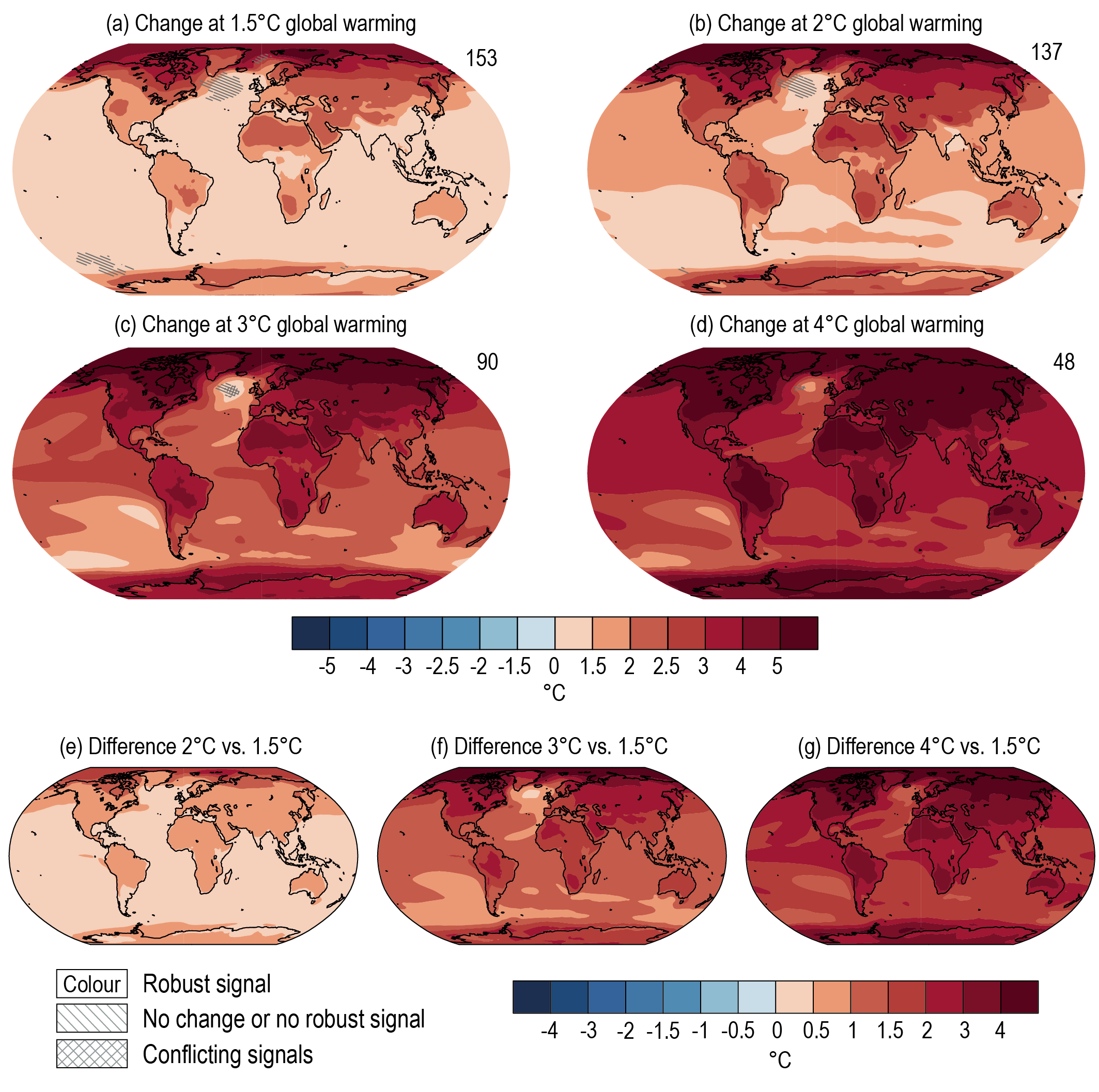 Figure 4.31 | Projected spatial patterns of change in annual average near-surface temperature (°C) at different levels of global warming. Displayed are (a–d) spatial patterns of change in annual average near-surface temperature at 1.5°C, 2°C, 3°C, and 4°C of global warming relative to the period 1850–1900 and (e–g) spatial patterns of differences in temperature change at 2°C, 3°C, and 4°C of global warming compared to 1.5°C of global warming. The number of models used is indicated in the top right of the maps. No overlay indicates regions where the change is robust and likely emerges from internal variability. That is, where at least 66% of the models show a change greater than the internal-variability threshold (Section 4.2.6) and at least 80% of the models agree on the sign of change. Diagonal lines indicate regions with no change or no robust significant change, where fewer than 66% of the models show change greater than the internal-variability threshold. Crossed lines indicate areas of conflicting signals where at least 66% of the models show change greater than the internal-variability threshold but fewer than 80% of all models agree on the sign of change. Values were assessed from a 20-year period at a given warming level, based on model simulations under the Tier-1 SSPs of CMIP6. Further details on data sources and processing are available in the chapter data table (Table 4.SM.1).
 The largest increase in annual mean temperature is found in the high latitudes of the Northern Hemisphere across all levels of global warming (virtually certain) (Figure 4.31). This phenomenon peaks in the Arctic and is known as Arctic amplification, with the underlying physical mechanisms assessed in detail in Section 4.5.1 and Chapter 7 (Section 7.4.4.1). For the CMIP6 ensemble average considered here, Arctic annual mean temperatures warm by a factor of 2.3, 2.5, 2.4 and 2.4 for 1.5°C, 2°C, 3°C and 4°C of global warming, respectively. That is, Arctic warming scales approximately linearly with GSAT. Generally, when Arctic amplification is considered across individual models, warming occurs at a factor of two to four times the global level of warming. It is unlikely that warming in the Southern Hemisphere high latitudes in the 21st century will exceed the change in GSAT, or that it will substantially exceed warming in the tropics, for GSAT change ranging between 1.5°C and 4°C (Figure 4.31 and Table 4.2). Correspondingly, there is low confidence of Antarctic amplification occurring under transient, 21st century low mitigation scenarios (Table 4.2 and Section 7.4.4.1). The Antarctic continent is projected to warm at a higher rate than the mid-latitude Southern Ocean, however, at all levels of global warming (Figure 4.31). The relevant physical mechanisms that reduce the amplitude of polar amplification over Antarctica compared to the Arctic are assessed in detail in Section 4.5.1 and Chapter 7 (Section 7.4.4.1). In the Southern Hemisphere the strongest warming over land is to occur, at any given level of global warming, over the subtropical areas of South America, southern Africa and Australia (high confidence). The relatively strong warming in subtropical southern Africa may be attributed to strong soil-moisture–temperature coupling and projected increased dryness under enhanced subsidence (Engelbrecht et al., 2015; Vogel et al., 2017). Across the globe, in the tropics, subtropics, and mid- to high latitudes, temperatures tend to scale linearly with the level of increase in GSAT and patterns of change are largely scenario independent (high confidence).
4.6.1.2 Precipitation
While global mean precipitation increases as GSAT rises with the very likely range of 1–3% per 1°C (high confidence) (Sections 8.2.1 and 8.4.1), patterns of precipitation change do not scale as linearly with GSAT increase. Nevertheless, common features of precipitation change in the multi-model mean across scenarios still exist for different levels of global warming (Figure 4.32). Precipitation will very likely increase in the high latitudes and over tropical regions, and will likely increase in large parts of the monsoon region, but are likely to decrease over the subtropical regions, including the Mediterranean, southern Africa, parts of Australia and South America at all four levels of global warming. The increases and decreases in precipitation will amplify at higher levels of global warming (high confidence) (Figure 4.32). Changes in extreme precipitation events under different levels of global warming are assessed in Chapter 11.
 Figure 4.32 | Projected spatial patterns of change in annual average precipitation (expressed as a percentage change) at different levels of global warming. Displayed are (a–d) spatialpatterns of change in annual precipitation at 1.5°C, 2°C, 3°C, and 4°C of global warming relative to the period 1850–1900. No map overlay indicates regions where the change is robust and likely emerges from internal variability, that is, where at least 66% of the models show a change greater than the internal-variability threshold (Section 4.2.6) and at least 80% of the models agree on the sign of change. Diagonal lines indicate regions with no change or no robust significant change, where fewer than 66% of the models show change greater than the internal-variability threshold. Crossed lines indicate areas of conflicting signals where at least 66% of the models show change greater than the internal-variability threshold but fewer than 80% of all models agree on the sign of change. Values were assessed from a 20-year period at a given warming level, based on model simulations under the Tier-1 SSPs of CMIP6. Further details on data sources and processing are available in the chapter data table (Table 4.SM.1).
 The SR1.5 stated low confidence regarding changes in global monsoons at 1.5°C versus 2°C of global warming, as well as differences in monsoon responses at 1.5°C versus 2°C. Generally, statistically significant changes in regional annual average precipitation are expected at a global mean warming of 2.5°C–3°C or more (Tebaldi et al., 2015). Over the austral-winter rainfall regions of south-western South America, South Africa and Australia, projected decreases in mean annual rainfall showhigh agreement across models and a strong climate change signal even under 1.5°C of global warming, with further amplification of the signal at higher levels of global warming (high confidence) (Mindlin et al., 2020). This is a signal evident in observed rainfall trends over these regions (Sections 2.3.1.3 and 8.3.1.6 ). Also, over the Asian monsoon regions, increases in rainfall will occur at 1.5°C and 2°C of global warming (Chevuturi et al., 2018). At warming levels of 1.5°C and 2°C, the changes in global monsoons are strongly dependent on the modelling strategies used, such as fully coupled transient, fully coupled quasi-equilibrium, and atmosphere-only quasi-equilibrium simulations. In particular, the differences of regional monsoon changes among model setups are dominated by strategy choices such as transient versus quasi-equilibrium set-up, prescription of SST, and treatment of aerosols (Zhang and Zhou, 2021).
The global and land area fractions with significant precipitation changes with global warming are shown in Figure 4.33. It is virtually certain that average warming will be higher over land. As warming increases, a larger global and land area will experience statistically significant increases or decreases in precipitation (medium confidence). The increase of the area fraction with significant precipitation increase is larger over land than over the ocean, but the increase of the area fraction with significant precipitation decrease is larger over the ocean than over land (Figure 4.33). Precipitation variability in most climate models increases over the global land area in response to warming (Pendergrass et al., 2017).
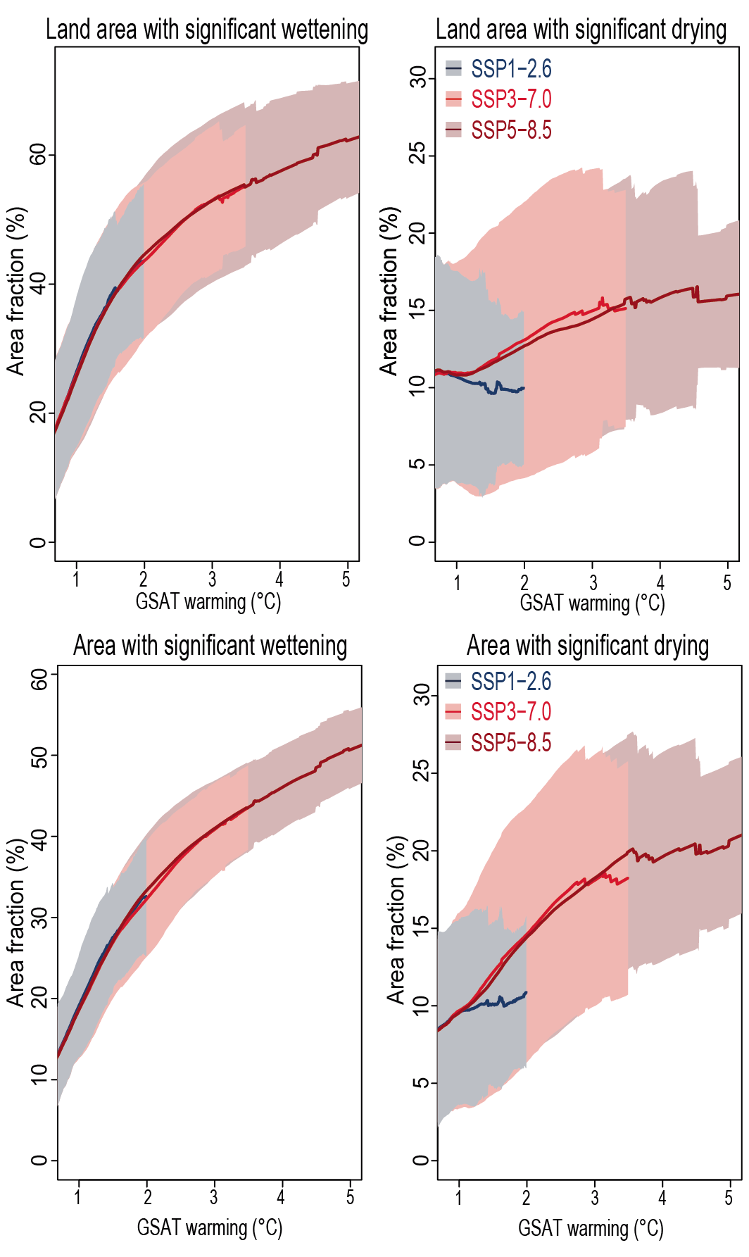 Figure 4.33 | Area fraction of significant precipitation change at 1.5°C, 2°C, 3°C, and 4°C of global warming. Range of land fraction (top) and global area fraction (bottom) with significant precipitation increase (left-hand side) and decrease (right-hand side) in the projected annual precipitation change (%) at levels of global warming compared to the period 1850–1900. Values were assessed from a 20-year period at a given warming level from SSP1-2.6, SSP3-7.0 and SSP5-8.5 in CMIP6. The solid line illustrates the CMIP6-multi model mean and the shaded band is the 5–95% range across models that reach a given level of warming. Further details on data sources and processing are available in the chapter data table (Table 4.SM.1).
 In summary, based on the assessment of CMIP6 models, there is high confidence that global mean precipitation will increase with increase in global mean surface temperature. Precipitation will very likely increase in the high latitudes and over tropical regions, likely increase in large parts of the monsoon region, but will likely decrease over the subtropical regions. There is high confidence that increases and decreases in precipitation will amplify over higher levels of global warming. As warming increases, there is medium confidence that a larger land area will experience statistically significant increases or decreases in precipitation.
4.6.1.3 Atmospheric Circulation
The AR5 reported that the application of pattern scaling to extract information on variables other than surface temperature and precipitation was relativelyunexplored. Since AR5, new studies have examined the relationship between projections of mid-latitude atmospheric circulation and GSAT both in terms of interpreting spread in responses across the CMIP5 multi-model ensemble (Grise and Polvani, 2014a, 2016) and to investigate variations in the circulation response as a function of GSAT change over time within a given forcing experiment (Grise and Polvani, 2017; Ceppi et al., 2018).
At a fixed time horizon, the CMIP5 multi-model spread in GSAT explains only a small fraction of the spread in the shift of the Northern Hemisphere mid-latitude circulation due to an abrupt quadrupling in CO2 (Grise and Polvani, 2016). The fraction of model spread explained by GSAT in the shift of the Southern Hemisphere circulation is larger, but still fairly small (Grise and Polvani, 2014a, 2016). At a fixed time horizon and for a given emissions scenario, CMIP5 multi-model spread in storm track shifts, and the closely related mid-latitude jets, can be better explained by multi-model spread in lower and upper level meridional temperature gradients than by GSAT (Harvey et al., 2014; Grise and Polvani, 2016).
In the North Atlantic, North Pacific, and Southern Hemisphere, the transient response of the mid-latitude jets to forcing behaves non-linearly with GSAT (Grise and Polvani, 2017; Ceppi et al., 2018). This is a consequence of the time-dependence of the relationship between radiative forcing and GSAT and the temporal evolution of SST patterns (Ceppi et al., 2018), with a potential seasonal component in the SH associated with polar stratospheric temperature changes (Grise and Polvani, 2017). Consequently, the epoch approach applied to a transient simulation of the 21st century will overestimate the mid-latitude circulation response in a stabilized climate. Dedicated time slice experiments simulating stabilized climates are therefore required to assess differences in mid-latitude circulation at given levels of global warming (Li et al., 2018). A further complication in the SH is the competing influences of ozone recovery and increasing GHG concentrations on the austral-summer mid-latitude circulation during the first half the 21st century (Barnes and Polvani, 2013; Barnes et al., 2014). Using transient 21st century experiments to diagnose changes in SH mid-latitude circulation at different levels of warming therefore confounds the effects of ozone recovery and GHG increases (Ceppi et al., 2018). Given these various limitations, we do not apply epoch analysis to assess mid-latitude atmospheric circulation changes and related annular modes of variability.
4.6.2 Climate Goals, Overshoot, and Path-Dependence
Many scenarios aiming at limiting warming by 2100 to 1.5°C involve overshoot – ERF temporarily exceeds a certain level before peaking and declining again (Annex VII: Glossary). To quantify the implications of any such overshoot, this subsection assesses reversibility of climate due to temporary overshoot of GSAT levels during the 21st century, and implications for the use of carbon budgets. It also assesses differences in climate outcomes under different pathways, with a focus on comparing the SSPs used in CMIP6 with the RCPs used in CMIP5.
4.6.2.1 Climate Change Under Overshoot
The SR1.5 (IPCC, 2018b) concluded with high confidence that overshoot trajectories ‘result in higher impacts and associated challenges compared to pathways that limit global warming to 1.5°C with no or limited overshoot’. The degree and duration of overshoot affects the risks and impacts likely to be experienced (Hoegh-Guldberg et al., 2018) and the emissions pathway required to achieve it (Akimoto et al., 2018). Consequences relating to ice sheets and climatic extremes have been found to be greater at 2°C of global warming than at 1.5°C (Schleussner et al., 2016; Hoegh-Guldberg et al., 2018) but even on recovery to lower temperatures, these effects may not reverse. Overshoot has been found to lead to irreversible changes in thermosteric sea level (Tokarska and Zickfeld, 2015; Palter et al., 2018; Tachiiri et al., 2019), AMOC (Palter et al., 2018), ice sheets, and permafrost carbon (Sections 4.7.2 and 5.4.9) and to long-lasting effects on ocean heat (Tsutsui et al., 2006). Abrupt changes and tipping points are not well understood, but the higher the warming level and the longer the duration of overshoot, the greater the risk of unexpected changes (Section 4.7.2). Non-reversal of the hydrological cycle has also been found in some studies with an increase in global precipitation following CO2 decrease being attributed to a build-up of ocean heat (Wu et al., 2010), and to a fast atmospheric adjustment to CO2 radiative forcing (Cao et al., 2011).
Global temperature is expected to remain approximately constant if emissions of CO2 were to cease (Section 4.7.1.1), and so reductions in GSAT are only possible in the event of net negative global CO2 emissions. We assess here results from an overshoot scenario (SSP5-3.4-OS; O’Neill et al., 2016), which explores the implications of a peak and decline in forcing during the 21st century. Reversibility under more extreme and idealized carbon dioxide removal (CDR) scenarios is assessed in Section 4.6.3. In SSP5-3.4-OS, CO2 peaks at 571 ppm in the year 2062 and reverts to 497 ppm by 2100 – approximately the same level as in 2040. SSP5-3.4-OS has strong net negative emissions of CO2, exceeding those in SSP1-2.6 and SSP1-1.9 from 2070 onwards and reaching –5.5 PgC yr–1 (–20 GtCO2 yr–1) by 2100. While this causes global mean temperature to decline, changes in climate have not fully reversed by 2100 under this reversal of CO2 concentration (Figure 4.34). Quantities are compared for 2081–2100 relative to a 20-year period (2034–2053) of the same average CO2. Differences between these two periods of the same CO2 are: GSAT: 0.28 ± 0.30°C (mean ± standard deviation); global land precipitation: 0.026 ± 0.011 mm day–1; September Arctic sea ice area: –0.32 ± 0.53 million km2; thermosteric sea level: 12 ± 0.8 cm. As assessed in Section 9.3.1.1, Arctic sea ice area is linearly reversible with GSAT. Although these climate quantities are not fully reversible, the overshoot scenario results in reduced climate change compared with stabilisation or continued increase in greenhouse gases (Tsutsui et al., 2006; Palter et al., 2018; Tachiiri et al., 2019) (high confidence).
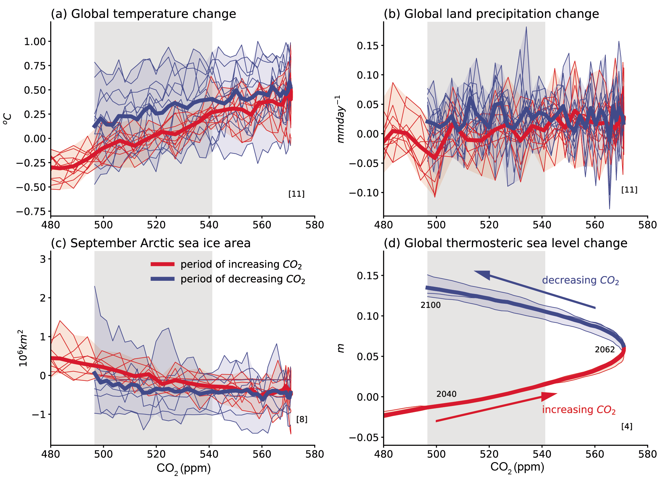 Figure 4.34 | Simulated changes in climate indices for SSP5-3.4-OS plotted against atmospheric CO2 concentration (ppm) from 480 up to 571 and back to 496 by 2100. (a) Global surface air temperature change; (b) Global land precipitation change; (c) September Arctic sea ice area change; (d) Global thermosteric sea level change. Plotted changes are relative to the 2034–2053 mean which has same CO2 as 2081–2100 mean (shaded grey bar). Red lines denote changes during the period up to 2062 when CO2 is rising, blue lines denote changes after 2062 when CO2 is decreasing again. Thick line is multi-model mean; thin lines and shading show individual models and complete model range. Numbers in square brackets indicate number of models used in each panel. Further details on data sources and processing are available in the chapter data table (Table 4.SM.1).
 The transient climate response to cumulative CO2 emissions, TCRE, allows climate policy goals to be associated with remaining carbon budgets as global temperature increase is near-linear with cumulative emissions (Section 5.5). Research since AR5 has shown that the concept of near-linearity of climate change to cumulative carbon emissions holds for measures other than just GSAT, such as regional climate (Leduc et al., 2016) or extremes (Harrington et al., 2016; Seneviratne et al., 2016). However, ocean heat and carbon uptake do exhibit path dependence, leading to deviation from the TCRE relationship for levels of overshoot above 300 PgC (Zickfeld et al., 2016; Tokarska et al., 2019). Sea level rise, loss of ice sheets, and permafrost carbon release may not reverse under overshoot and recovery of GSAT and cumulative emissions (Section 4.7). TCRE remains a valuable concept to assess climate policy goals and how to achieve them but given the non-reversibility of different climate metrics with CO2 and GSAT reductions, it has limitations associated with evaluating the climate response under overshoot scenarios and CO2 removal (medium confidence).
4.6.2.2 Consistency Between Shared Socio-economic Pathways and Representative Concentration Pathways
As CMIP5 and CMIP6 employed different scenario sets (RCPs and SSPs, respectively; see Section 1.6.1.1and Cross-Chapter Box 1.4), we assess how much of the differences in projections are due to the scenario change and how much due to model changes. The CMIP6-simulated GSAT increases tend to be larger than in CMIP5, for nominally comparable scenarios (Section 4.3.1; Tebaldi et al., 2021).
The radiative forcing labels on SSP and RCP scenarios is approximate and enables the multiple climate forcings within the scenario to be characterized by a single number. While the scenarios are similar in terms of the stratospheric adjusted radiative forcing (Tebaldi et al., 2021), they differ more in their effective radiative forcing (ERF). The combination of component forcings (CO2, non-CO2 greenhouse gases, aerosols) within the scenario also differ (Meinshausen et al., 2020). The ERF levels in the RCP and SSP scenarios have been calculated by sampling uncertainty in forcing from a range of different GHG species and aerosols (see 7.SM.1.4 for details). Figure 4.35 shows the time evolution and 2081–2100 mean across the families of scenarios and how this affects projections of GSAT. That the ERFs differ between corresponding SSP and RCP scenarios makes a comparison between CMIP6 and CMIP5 projections challenging (Tebaldi et al., 2021). Wyser et al. (2020) find the EC-Earth3-Veg model exhibits stronger radiative forcing and substantially greater warming under SSP5-8.5 than RCP8.5, and similar, but smaller additional warmings for SSP2-4.5and SSP1-2.6 compared with RCP4.5 and RCP2.6, respectively. In addition to the global response, climate can vary regionally due to non-CO2 components of forcing (Samset et al., 2016; Richardson et al., 2018a, b).
 Figure 4.35 | Comparison of RCPs and SSPs run by a single emulator to estimate scenario differences. Time series with 5–95% ranges and medians of (a) effective radiative forcings, calculated as described in Annex 7.A.1; and (b) global surface air temperature projections relative to 1850–1900 for the RCP and SSP scenarios from MAGICC 7.5. Note that the nameplate radiative forcing level refers to stratospheric adjusted radiative forcings in AR5-consistent settings (Tebaldi et al., 2021) while ERFs may differ. MAGICC7.5 is here run in the recommended setup for WGIII, prescribing observed GHG concentrations for the historical period and switching to emissions-driven runs in 2015. Further details on data sources and processing are available in the chapter data table (Table 4.SM.1).
 Emulators (Cross-Chapter Box 7.1) can be used to aid understanding of differences between generations of scenarios. The AR5 (Collins et al., 2013) explored the differences between CMIP3 and CMIP5 (their Figure 12.40). Here we use an emulator calibrated to AR6 assessed GSAT ranges, thus eliminating the effect of differences in the model ensembles, to analyse the differences between SSP and RCP scenarios. MAGICC7.5 in its WGIII-calibrated setup (see Cross-Chapter Box 7.1) projects differences in 2081–2100 mean warming between the RCP2.6 and SSP1-2.6 scenarios of around 0.2°C, between RCP4.5 and SSP2-4.5 ofaround 0.3°C and between RCP8.5 and SSP5-8.5 of around 0.3°C (Figure 4.35b). The SSP scenarios also have a wider 5–95% range simulated by MAGICC7.5 explaining about half of the increased range seen when comparing CMIP5 and CMIP6 models. Higher climate sensitivity is, though, the primary reason behind the upper end of the warming for SSP5-8.5 reaching 1.5°C higher than the CMIP5 results. Compared with the differences between the CMIP5 and CMIP6 multi-model ensembles for the same scenario pairs (Table A6 in Tebaldi et al., 2021), the higher ERFs of the SSP scenarios contribute approximately half of the warmer CMIP6 SSP outcomes (medium confidence).
In summary, there is medium confidence that about half of the warming increase in CMIP6 compared to CMIP5 is due to higher climate sensitivity in CMIP6 models; the other half arises from higher ERF in nominally comparable scenarios (e.g., RCP8.5 and SSP5-8.5).
4.6.3 Climate Response to Mitigation, Carbon Dioxide Removal and Solar Radiation Modification
Most strong-mitigation scenarios assume – in addition to emissions reductions – some form of carbon dioxide removal (CDR). Anthropogenic activities that remove CO2 from the atmosphere and durably store it in geological, terrestrial, or ocean reservoirs, or in products (see Glossary). The SR1.5 (Rogelj et al., 2018b) assessed that all pathways that limit warming to 1.5°C by 2100 with no or limited overshoot use CDR. In the SSP class of scenarios, SSP1-1.9 is characterized by a rapid decline of net CO2 emissions to zero by 2050 and net negative CO2 emissions in the second half of this century (O’Neill et al., 2016; Rogelj et al., 2018a), implying the use of CDR. The term ‘net CO2 emissions’ refers to the difference between anthropogenic CO2 emissions and removal by CDR options, and ‘net negative CO2 emissions’ imply a scenario where CO2 removal exceeds emissions (van Vuuren et al., 2011, 2016). The terms ‘negative emissions’ and ‘net negative emissions’ refer to and include all GHGs (see Glossary).
Climate change can be also offset by solar radiation modification (SRM) measures that modify the Earth’s radiation budget to reduce global warming (see Glossary). CDR and SRM approaches have been together referred to as ‘geoengineering’ or ‘climate engineering’ in the literature (The Royal Society, 2009; NRC, 2015a, b; Schäfer et al., 2015). However, following SR1.5 (de Coninck et al., 2018), these terms are inconsistently used in the literature, so that CDR and SRM are explicitly differentiated here. SRM contrasts with climate change mitigation because it introduces a ‘mask’ to the climate change problem by altering the Earth’s radiation budget, rather than attempting to address the root cause of the problem, which is the increase in GHGs in the atmosphere.
(Section 4.6.3.1 assesses the emergence of the climate response to mitigation, which is reflected by the difference between high- and low-emissions scenarios. Section 4.6.3.2 then assesses the climate response to mitigation through CDR options, usually assumed against the background of some emissions scenario; note that the CDR options themselves are assessed in Chapter 5 (Section 5.6.2). Section 4.6.3.3 assesses the climate system response to SRM options. The biogeochemical implications of CDR and SRM are assessed in Chapter 5 (Sections 5.6.2 and 5.6.3, respectively). The importance of CDR for reaching net zero or negative CO2 emissions in mitigation pathways is assessed in the AR6 WGIII report (Chapters 3, 4, 6, 7 and 12). The risks for and impacts on human and natural systems due to SRM are assessed in the AR6 WGII report (Chapter 16), and the international governance issues related to SRM and CDR are assessed in the AR6 WGIII report (Chapter 14).
4.6.3.1 Emergence of the Climate Response to Mitigation
Reducing GHG emissions will eventually slow and limit the degree of climate change relative to high-emissions scenarios such as SSP5-8.5 (very high confidence). Even when CO2 emissions are reduced, however, atmospheric CO2 concentrations continue to increase as long as emissions exceed removal by sinks (Millar et al., 2017). Surface warming would likewise initially continue under scenarios of decreasing emissions, resulting in a substantial lag between a peak in CO2 emissions and peak warming (high confidence) (Ricke and Caldeira, 2014; Zickfeld and Herrington, 2015). The lag between peak emissions and warming depends on the emissions history prior to the peak and also on the rate of the subsequent emissions reductions (Matthews, 2010; Ricke and Caldeira, 2014; Zickfeld and Herrington, 2015).
In addition to the lag between peak emissions and peak warming,the climate response to reduced emissions would be overlain by internal variability, which can amplify or attenuate the forced response. The resulting masking of differences between scenarios is illustrated in Figure 4.36 for GSAT trends over 2021–2040 (Maher et al., 2020). The overall trends conform to expectations in that most simulations show warming almost everywhere, especially under scenario RCP8.5 (Figure 4.36 bottom row). But any individual grid point can in principle show no warming or even cooling, even under RCP 8.5, over the near term (Figure 4.36, middle row). The magnitude of pointwise maximum and minimum temperature trends can be as large as 0.5°C per year (Figure 4.36, top and middle rows), exceeding possible trends in the global mean by one order of magnitude. While it is only a small fraction of the surface that simultaneously can show cooling, cooling at any given location is fully consistent with globally averaged surface warming over the near term (high confidence, since the findings of Maher et al. (2020) are consistent across six different large initial-condition ensembles).
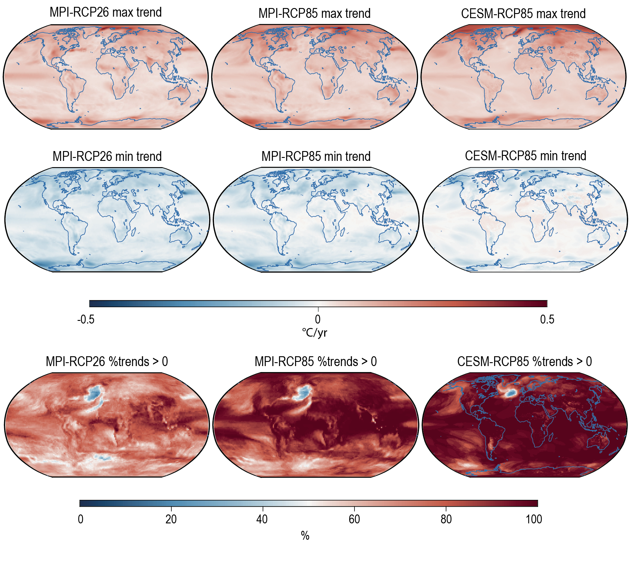 Figure 4.36 | Masking of climate response to mitigation by internal variability in the near term. Near-term (2021–2040) pointwise maximum (top row) and pointwise minimum (middle row) surface air temperature trends in the large initial-condition ensemble from MPI (left and centre columns), and CESM (right-hand column) models in the RCP2.6 (left-hand column) and RCP8.5 scenarios (centre and right columns). The percentage of ensemble members with a warming trend in the near term is shown in the bottom panels. Figure modified from Maher et al. (2020). Further details on data sources and processing are available in the chapter data table (Table 4.SM.1).
 An important development since AR5 has been the quantification of when the climate response to mitigation can be expected to emerge from the background noise of internal variability (illustrated in Figure 4.36; see Section 1.4.2.2 and Glossary). A basic ambiguity arises because once mitigation measures are in place, it is no longer possible to observe what the climate would have been without these measures, and any statement about emergence of the response to mitigation is contingent upon the assumed strength of mitigation in relation to an assumed (‘counterfactual’) no-mitigation scenario. Still, there is high agreement on the emergence of the climate response to mitigation across a number of independent studies using different models and different statistical approaches.
Among global quantities, emergence of the response to differing CO2 emissions – representing differences between low- and high-emissions scenarios – is first expected to arise in global mean CO2 concentrations, about 10 years after emissions pathways have started diverging (high confidence) (Tebaldi and Friedlingstein, 2013; Peters et al., 2017; Schwartzman and Keeling, 2020; Spring et al., 2020). In these studies, emergence is generally defined as the time at which the global mean concentration first differs between mitigation and non-mitigation scenarios by more than two standard deviations of internal variability, although there are some methodological differences.
Emergence in GSAT would be delayed further, owing to the inertia in the climate system. Although not investigating emergence as defined here in AR6, Tebaldi et al. (2021) used a 20-year running-mean GSAT and compared pairwise either model-by-model or between CM IP6 ensemble means from the core set of five scenarios assessed in this chapter. Differences by more than 0.1°C showed up in most cases in the near term, with only some of the individual models and the comparisons of the closest scenarios showing a delay until the mid-term. Taking internal variability explicitly into account, Tebaldi and Friedlingstein (2013) and Samset et al. (2020) found emergence of mitigation benefits in GSAT changes about 25–30 years after RCP2.6 emissions diverge from the higher-emissions trajectories in RCP4.5 and RCP8.5. Consistently, Marotzke (2019) found about one-third likelihood that a trend reduction in GSAT, over the period 2021–2035 relative to 2005–2020, would be attributable to the emissions reductions implied by the difference between RCP2.6 and RCP4.5. Emergence of the GSAT response to mitigation of individual short-lived climate forcers (SLCFs) would likewise not occur until several decades after emissions trajectories diverge, owing to the relatively small influence of individual SLCFs on the total ERF (Samset et al., 2020), see also Section 4.4.4 and Figure 4.18.
In contrast to the earlier studies, emergence in GSAT within the near-term has recently been found by McKenna et al. (2021) who investigated the likelihood that under the SSP scenarios GSAT trends will exceed the largest historical observed 20-year trends. They found that under scenario SSP1-1.9, the 20-year GSAT trends would likely be lower than in SSP3-7.0 and SSP5-8.5 within the near term. This earlier diagnosed time of emergence compared to Marotzke (2019), while using a similar statistical approach, presumably arose because of the longer-period trends (20 rather than 15 years) and the larger difference between emissions trajectories considered (medium confidence). Using 20-year temperature anomalies relative to 1995–2014 instead of 20-year trends yielded a low probability of emergence (McKenna et al., 2021), consistent with the AR5 (Collins et al., 2013; Kirtman et al., 2013; Tebaldi and Friedlingstein, 2013; Samset et al., 2020). It is not yet understood why GSAT trends appear to show faster emergence of mitigation benefits, compared to GSAT anomalies.
Emergence of mitigation benefits has been studied much less for quantities other than globally and annually averaged CO2 concentration and surface temperature. Boreal-winter temperatures are more challenging for emergence, due to larger variability in boreal winter and adding a decade to the time of emergence, whereas emergence times for boreal-summer averages are similar to the annual temperature averages (Tebaldi and Friedlingstein, 2013). Emergence happens later at the regional scale, with a median time of emergence of 30–45 years after emissions paths separate in RCP2.6 relative to RCP4.5 and RCP8.5; a stricter requirement of 95% confidence level instead of median induces a delay of several decades, bringing time of emergence toward the end of the 21st century at regional scales (Tebaldi and Friedlingstein, 2013).
Attribution to emissions reductions, for the case of RCP2.6 relative to RCP4.5, is not substantially more likely for 2021–2035 trends in upper-2000 m OHC than for GSAT (Marotzke, 2019), although OHC change is thought to be less susceptible to internal variability. Furthermore, Marotzke (2019) found only around 10% likelihood of mitigation-benefit emergence during 2021–2035 for change in AMOC and September Arctic sea ice area. Tebaldi and Wehner (2018) showed that the differences in temperature extremes between RCP4.5 and RCP8.5 over all land areas become statistically significant by 2050. The seemingly contrasting result of Ciavarella et al. (2017) that mitigation benefits arise earlier for climate extremes poses no contradiction, because Ciavarella et al. (2017) did not look at emergence as defined here but at the extremes of a distribution, which differ between scenarios already at a time when the distributions are still largely overlapping.
In summary, if strong mitigation is applied from 2020 onward as reflected in SSP1-1.9, its effect on 20-year trends in GSAT would likely emerge during the near term, measured against an assumed non-mitigation scenario such as SSP3-7.0 and SSP5-8.5. However, the response of many other climate quantities to mitigation would be largely masked by internal variability during the near term, especially on the regional scale (high confidence). The mitigation benefits for these quantities would emerge only later during the 21st century (high confidence). During the near term, a small fraction of the surface can show cooling under all scenarios assessed here, so near-term cooling at any given location is fully consistent with globally averaged surface warming (high confidence).
4.6.3.2 Climate Response to Mitigation by Carbon Dioxide Removal
CDR options include afforestation, soil carbon sequestration, bioenergy with carbon capture and storage (BECCS), wet land restoration, ocean fertilization, ocean alkalinisation, enhanced terrestrial weathering and direct air capture and storage (see Section 5.6.2 and Table 5.9 for a more complete discussion). Chapter 8 (Section 8.4.3) assesses the implications of CDR for water cycle changes. The potential of different CDR options in terms of the amount of CO2 removed per year from the atmosphere, costs, co-benefits and side effects of the CDR approaches are assessed in SR1.5 (de Coninck et al., 2018), the AR6 WGIII Report (see Chapters 7 and 12), and in several review papers (Fuss et al., 2018; Lawrence et al., 2018; Nemet et al., 2018). In the literature, CDR options are also referred to as ‘negative CO2 emissions technologies’.
Deployment of CDR will lead to a reduction in atmospheric CO2 levels only if uptake by sinks exceeds net CO2 emissions. Hence, there could be a substantial delay between the initiation of CDR and net CO2 emissions turning negative (van Vuuren et al., 2016), and the time to reach net negative CO2 emissions and the evolution of atmospheric CO2 and climate thereafter would depend on the combined pathways of anthropogenic CO2 emissions, CDR, and natural sinks. The cooling (or avoided warming) due to CDR would be proportional to the cumulative amount of CO2 removed from the atmosphere by CDR (Tokarska and Zickfeld, 2015; Zickfeld et al., 2016), as implied by the near-linear relationship between cumulative carbon emissions and GSAT change (Section 5.5).
Emissions pathways that limit globally averaged warming to 1.5°C or 2°C by the year 2100 assume the use of CDR approaches in combination with emissions reductions to follow net negative CO2 emissions trajectory in the second half of this century. For instance, in SR1.5, all analysed pathways limiting warming to 1.5°C by 2100 with no or limited overshoot include the use of CDR to some extent to offset anthropogenic CO2 emissions and the median of CO2 removal across all scenarios was 730 GtCO2 in the 21st century (Rickels et al., 2018; Rogelj et al., 2018b). Affordable and environmentally and socially acceptable CDR options at scale well before 2050 are an important element of 1.5°C-consistent pathways especially in overshoot scenarios (de Coninck et al., 2018). The required scale of removal by CDR can vary from 1–2 GtCO2 yr–1year from 2050 onwards to as much as 20 GtCO2 yr–1 (Waisman et al., 2019). In the SSP class of scenarios, net CO2 emissions turn negative from around 2050 in SSP1-1.9 and around 2070 in SSP1-2.6 and in the overshoot scenario SSP5-3.4-OS (O’Neill et al., 2016). Thus, CDR would play a pivotal role in limiting climate warming to 1.5°C or 2°C (Minx et al., 2018). In stark contrast, however, two extensive reviews (Lawrence et al., 2018; Nemet et al., 2018) conclude that it is implausible that any CDR technique can be implemented at the scale needed by 2050.
When CDR is applied continuously and at scales as large as currently deemed possible, under RCP8.5 as the background scenario, the widely discussed CDR options such as afforestation, ocean iron fertilization and surface ocean alkalinisation are individually expected to be relatively ineffective, with limited (8%) warming reductions relative to the scenario with no CDR option (Keller et al., 2014). Hence, the potential role that CDR will play in lowering the temperature in high-emissions scenarios is limited (medium confidence). The challenges involved in comparing the climatic effects of various CDR options has also been recognized in recent studies (Sonntag et al., 2018; Mengis et al., 2019). For instance, due to compensating processes such as biogeophysical effects of afforestation (warming from albedo decrease when croplands are converted to forests) more carbon is expected to be removed from the atmosphere by afforestation than by ocean alkalinisation to reach the same global mean cooling.
The climate response to CDR-caused net negative CO2 emissions has been studied in Earth system models by prescribing idealized ramp-down of CO2 concentrations (MacDougall,2013; Zickfeld et al., 2016; Schwinger and Tjiputra, 2018), CO2 concentrations of RCP scenarios that have net negative CO2 emissions (C.D. Jones et al., 2016b), and idealized net negative CO2 emissions scenarios (Tokarska and Zickfeld, 2015). The Carbon Dioxide Removal Model Intercomparison Project (CDRMIP) uses multiple ESMs to explore the climate response, effectiveness of CO2 removal, and challenges of CDR options (Keller et al., 2018). Idealized CDRMIP simulations increase CO2 concentrations at 1% per year from the level in the pre-industrial control run (piControl) to 4×CO2 and subsequently decrease at the same rate to the piControl level. This section assesses the lag in climate response to CDR-caused negative emissions; climate ‘reversibility’ is assessed in Section 4.7.2. The ramp-down phase, though unrealistic, represents the ‘net negative CO2 emissions’ phase.
Figure 4.37 illustrates the first results from CDRMIP (Keller et al., 2018). Other studies that use similar (Zickfeld et al.,2016; Schwinger and Tjiputra, 2018; Jeltsch-Thömmes et al., 2020) or other idealized scenarios (MacDougall, 2013) or more realistic net negative CO2 emissions scenarios such as RCP2.6 (C.D. Jones et al., 2016b) and scenarios that limit warming to 2°C or less after different levels of overshoot (Tokarska and Zickfeld, 2015) arrive at similar conclusions. Changes in key climate variables substantially lag behind the decline in CO2 (Figure 4.37). The precipitation increase at the beginning of the ramp-down phase agrees with the increase in precipitation for an abrupt decline in CO2 (Cao et al., 2011). Notwithstanding a decline in atmospheric CO2, global mean thermosteric sea level would continue to rise. When atmospheric CO2 returns to the piControl level, global mean thermosteric sea level is higher than its value at peak CO2 (Figure 4.37), and it is likely that thermosteric global sea level would not return to piControl levels for over 1000 years after atmospheric CO2 is restored to piControl concentrations (Tokarska and Zickfeld, 2015; Ehlert and Zickfeld, 2018). Therefore, there is high confidence that sea level rise will not be reversed by CDR at least for several centuries (Chapter 9 (Section 9.6.3.5). A comparison of different models shows recovery of AMOC intensity during net negative CO2 emissions, but the results are model dependent – strengthening with an overshoot in most models (Jackson et al., 2014) and strengthening but not reaching the initial state in some models (Sgubin et al., 2015). The overall lag in response is qualitatively similar to the lagged climate system response in the overshoot scenario SSP5-34-OS where CO2 rises until 2062 and decreases thereafter (Figure 4.34). The lag in climate response to CDR causes hysteresis between key climate variables such as temperature, precipitation, AMOC and sea level, and atmosphere CO2 with the hysteresis characteristics dependent on the rate of CDR and climate sensitivity (MacDougall, 2013; Jeltsch-Thömmes et al., 2020).
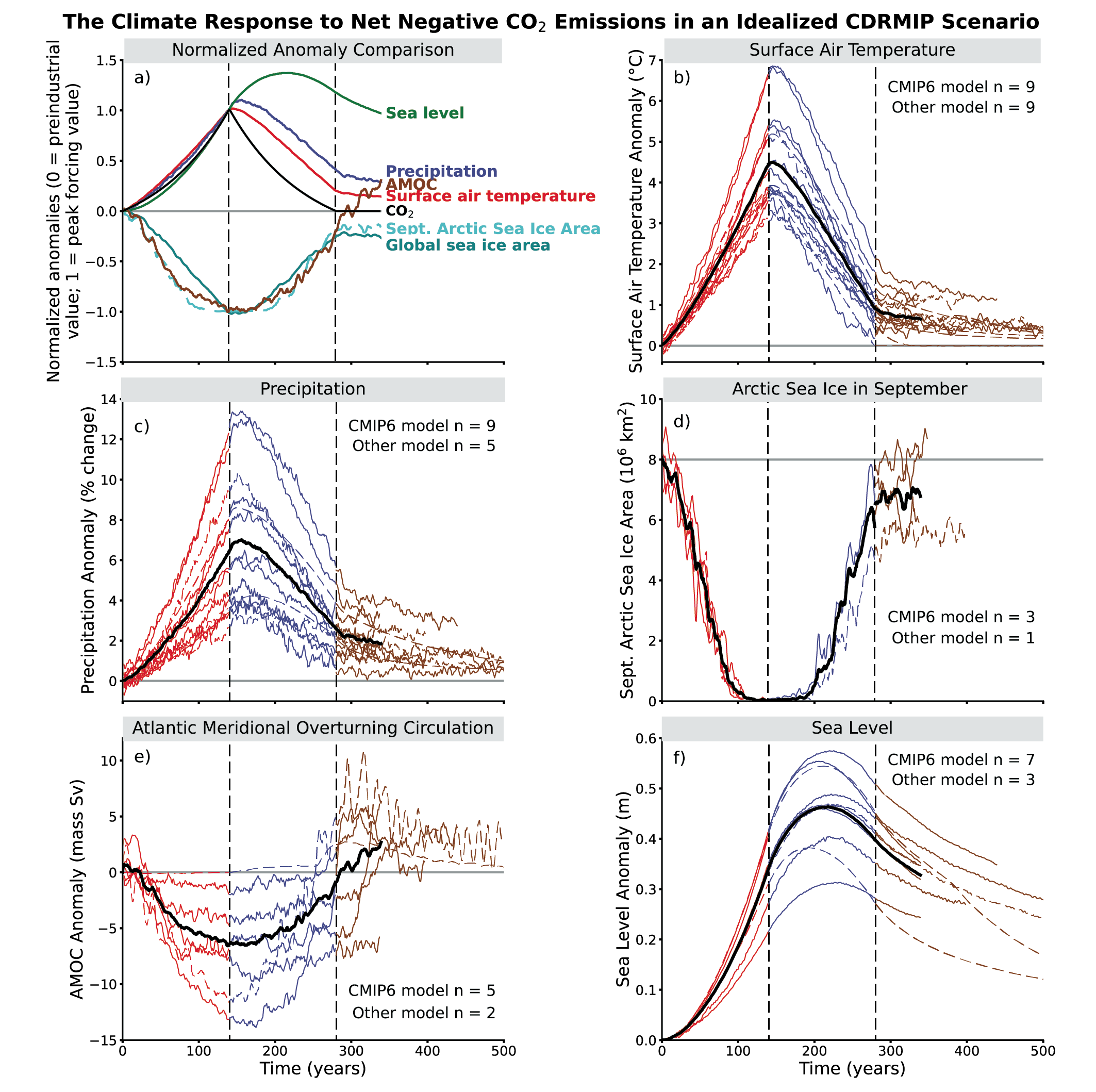 Figure 4.37 | Delayed climate response to carbon dioxide removal (CDR)-caused net negative CO2 emissions. Multi-model simulated response in global and annual mean climate variables for a ramp-up followed by ramp-down of CO2. Atmospheric CO2 increases from the pre-industrial level at a rate of 1% yr–1 to 4×CO2, then decreases at the same rate to the pre-industrial level and then remains constant. The ramp-down phase represents the period of net negative CO2 emissions. (a) Normalized ensemble mean anomaly of key variables as a function of year, including atmospheric CO2, surface air temperature, precipitation, thermosteric sea level change (see Glossary), global sea ice area, Northern Hemisphere sea ice area in September, and Atlantic meridional overturning circulation (AMOC); (b) surface air temperature; (c) precipitation; (d) September Arctic sea ice area; (e) AMOC; (f) thermosteric sea level; five-year running means are shown for all variables except the sea level change. In (b, f), red lines represent the phase of CO2 ramp-up, blue lines represent the phase of CO2 ramp-down, brown lines represent the period after CO2 has returned to pre-industrial level, and black lines represent the multi-model mean. For all of the segments in (b, f), the solid coloured lines are CMIP6 models, and the dashed lines are other models (i.e., EMICs, CMIP5-era models). Vertical dashed lines indicate peak CO2 and when CO2 again reaches pre-industrial value. The number of CMIP6 and non-CMIP6 models used is indicated in each panel. The time series for the multi-model means (b, f) and the normalized anomalies (a) are terminated when data from all models are not available, in order to avoid the discontinuity in the time series. Further details on data sources and processing are available in the chapter data table (Table 4.SM.1).
 Termination of CDR refers to a sudden and sustained discontinuation of CDR deployment (see Section 4.6.3.3 for termination effects of SRM). The literature on the termination effects of CDR is limited, mostly considering scenarios where CDR implementation is explicit and does not result in net negative CO2 emissions (Keller et al., 2014; González et al., 2018). In simulations where CDR is applied on the RCP8.5 scenario at scales as large as currently deemed possible, the increase in global mean warming rates following CDR termination are relatively small in comparison to SRM termination (Keller et al., 2014). The exception is artificial ocean upwelling where surface cooling is mainly caused by bringing cold water from the deep ocean; upon termination this causes larger rates of surface warming (Oschlies et al., 2010). When background emissions are as high as in RCP8.5, termination of a large global-scale application of CDR such as ocean alkalinisation for multiple decades could also result in large regional warming rates (up to 0.15°C per year) that are comparable to those caused by termination of SRM (González et al., 2018). In such cases, large amounts of CO2 would be removed from the atmosphere before termination, and termination would cause a temporal trajectory of atmospheric CO2 that is parallel to the high-emissions scenario but from an atmosphere with much lower CO2 levels. Because CO2 radiative forcing is a logarithmic function of CO2 concentration, large regional warming rates are simulated in such terminations. Thus, there is high confidence that the climate effect of CDR termination would depend on the amount CO2 removed by CDR prior to termination and the rate of background CO2 emissions at the time of termination. See also Chapter 5, Table 5.9, which summarizes the termination effects of individual CDR options.
In summary, there is high confidence that, due to the near-linear relationship between cumulative carbon emissions and GSAT change, cooling or avoided warming due to a CDR option would depend on the cumulative amount of CO2 removed by that CDR option. The climate system response to the deployment of CDR is expected to be delayed by years (e.g., in temperature, precipitation, sea ice extent) to centuries (e.g., sea level and AMOC) (high confidence). The climate response to a sudden and sustained CDR termination would depend on the amount of CDR-induced cooling prior to termination and the rate of background CO2 emissions at the time of termination (high confidence).
4.6.3.3 Climate Response to Solar Radiation Modification
Most SRM approaches, including stratospheric aerosol injection (SAI), marine cloud brightening (MCB), and surface albedo enhancements (Table 4.7), aim to cool the Earth by deflecting more solar radiation to space. Although cirrus cloud thinning (CCT) aims to cool the planet by increasing the longwave emission to space, it is included in the portfolio of SRM options (Table 4.7) for consistency with AR5 (Boucher et al., 2013) and SR1.5 (de Coninck et al., 2018). Other approaches such as injection of sulphate aerosols into the Arctic troposphere and sea ice albedo enhancements for moderatingregional warming have also been suggested (MacCracken, 2016; Field et al., 2018). As noted in SR1.5 (de Coninck et al., 2018), SRM is only considered as a potential supplement to deep mitigation, for example in overshoot scenarios (MacMartin et al., 2018).
The AR5 assessed the climate response to, as well as risks and side effects of, several SRM options (Boucher et al., 2013) and concluded with high confidence that SRM, if practicable, could substantially offset a global temperature rise and partially offset some other impacts of global warming, but the compensation for the climate change caused by GHGs would be imprecise. The AR5 furthermore concluded that models consistently suggest that SRM would generally reduce climate differences compared to a world with elevated GHG concentrations and no SRM; however, there would also be residual regional differences in climate (e.g., temperature and rainfall) when compared to a climate without elevated GHGs. The AR5 concluded with high confidence that scaling SRM to substantial levels would carry the risk that if the SRM were terminated for any reason, surface temperatures would increase rapidly (within a decade or two) to values consistent with the GHG forcing (Boucher et al., 2013).
SRM Approach | Proposed Mechanism and Associated Uncertainties of the SRM Approach | Global Mean Negative Radiative Forcing Potential and Characteristics | Key Climate and Environmental Effects | References |
Stratospheric Aerosol Injection (SAI) | Injection of aerosols or their precursor gases into the stratosphere to scatter sunlight back to space; Aerosol types such as sulphates, calcium carbonate, and titanium dioxide have been proposed; large uncertainties associated with type of aerosol, aerosol radiative properties, microphysics, chemistry, stratospheric processes, and temporal and spatial strategy of aerosol injection. | 1–8 W m–2, depending on the amount and pattern of injection, and transport and growth of injected particles; compared to other SRM approaches, radiative forcing could be more homogenously distributed. | Change in temperature and precipitation pattern; precipitation reduction in some monsoon regions; decrease in direct and increase in diffuse sunlight at surface; stratospheric heating and changes to stratospheric dynamics and chemistry; potential delay in ozone hole recovery; changes in surface UV radiation; changes in crop yields. | Visioni et al. (2017); Tilmes et al. (2018b); Simpson et al. (2019b) |
Marine Cloud Brightening (MCB) | Injection of sea salt or other types of aerosols to increase the albedo of marine stratocumulus clouds; regional option to reduce SST in hurricane formation regions and in coral reef areas; large uncertainties associated with cloud microphysics and aerosol–cloud-radiation interactions. | 1–5 W m–2, depending on the scale and amount of sea salt injection; heterogeneous radiative forcing. | Change in land–sea contrast and precipitation patterns. | Latham et al., (2012, 2014); Ahlm et al. (2017); Stjern et al. (2018) |
Cirrus Cloud Thinning (CCT) | Inject ice nuclei in the upper troposphere to reduce the lifetime and optical thickness of cirrus clouds to allow more longwave radiation to escape to space; large uncertainties associated with cirrus cloud formation processes, cirrus microphysics, and interaction with aerosol. | 1–2 W m–2, depending on cirrus microphysical response and seeding strategy; heterogeneous radiative forcing; loss in cirrus clouds could also cause significant shortwave forcing regionally; risk of overseeding and consequent warming. | Changes in temperature and precipitation pattern; increase in solar radiation reaching surface. | Storelvmo and Herger (2014); Jackson et al. (2016); Gasparini et al. (2020) |
Surface-Based Albedo Modification | Increase ocean albedo by creating microbubbles; add reflective material to increase desert albedo; paint the roof of buildings white to increase roof reflectivity; increase albedo of agriculture land via no-till farming or modifying crop albedo, add reflective material to increase sea ice albedo. | Radiative forcing of a few W m–2 might be achieved via increase in ocean and desert albedo, but the large-scale implementation is not feasible; less than 0.5 W m–2 for white roof and crop albedo enhancement; heterogeneous radiative forcing. | Change in land–sea contrast and precipitation pattern for ocean and desert albedo increase; more localized effect for white roofs, no-till farming, and crop albedo modification. | Evans et al. (2010); Davin et al. (2014); Zhang et al. (2016); Field et al. (2018); Kravitz et al. (2018) |
The SR1.5 (de Coninck et al., 2018) assessed SRM in terms of its potential to limit warming to below 1.5°C in temporary overshoot scenarios and the associated impacts. It concluded that SAI could limit warming to below 1.5°C but that the climate response to SAI is uncertain and varies across climate models. Overall, the assessment concluded that the combined uncertainties related to SRM approaches, including technological maturity, limited physical understanding of the response to SRM, potential impacts, and challenges of governance, constrain potential deployment of SRM in the near future.
This subsection assesses the global and large-scale physical climate system response to SRM based on theoretical and modelling studies. There is no mature technology today to implement any of the SRM options assessed here. A short summary of the SRM options, including the proposed mechanism of each SRM approach, radiative forcing potential, and key climate and environmental effects, is listed in Table 4.7. Chapter 5 (Section 5.6.3) assesses the biogeochemical implications of SRM, Chapter 6 (Section 6.4.6) assesses the potential ERF of the aerosol-based SRM options and Chapter 8 (Section 8.6.3) assesses the abrupt water cycle changes in response to initiation or termination of SRM. The risks to human and natural systems, impacts of SRM, ethics, and perceptions are assessed in the WGII Report (Chapter 16). Governance issues associated with SRM research and deployment are assessed in the WGII and WGIII Reports. The assessment of technical feasibility and engineering aspects of SRM is beyond the scope of this Report.
The AR5 assessed SRM modelling mainly based on idealized simulations that used solar constant reductions. Since then, more in-depth investigations into specific SRM approaches have been conducted with more sophisticated treatment of aerosol–cloud–radiative interactions and stratospheric dynamics and chemistry underlying SAI, MCB, and CCT. Another major development since AR5 is the investigation into whether multiple climate policy goals may be met by optimally designed SRM strategies, including large-ensemble SAI simulations using multiple injection locations. There are large uncertainties in important SRM-related processes such as aerosol microphysics and aerosol–cloud–radiation interaction and hence the level of understanding is low.
As assessed in SR1.5 (de Coninck et al., 2018), most of the knowledge about SRM is based on idealized model simulations and some natural analogues. In addition to single-model studies, more results from the coordinated modelling work of Geoengineering Model Intercomparison Project (GeoMIP) have become available. GeoMIP was initiated at the time of AR5 (Kravitz et al., 2011, 2013a) and is now in its second phase under the framework of CMIP6 (GEOMIP6, Kravitz et al., 2015). However, studies based on GeoMIP6 data are currently limited and hence the assessment on climate response to SRM here is derived mostly from GeoMIP literature together with studies with single models.
Simple calculations and climate modelling studies show that about 2% extra solar irradiance reflected away from Earth or a one percentage point increase in planetary albedo (0.31 to 0.32) would suffice to offset global mean warming from a doubling of the CO2 concentration (TheRoyal Society, 2009; Kravitz et al., 2013a, 2021). To offset the same amount of CO2 -induced GSAT increase, different levels of ERF are required for different methods of SRM (Schmidt et al., 2012; Chiodo and Polvani, 2016; Modak et al., 2016; Duan et al., 2018; Russotto and Ackerman, 2018; Krishnamohan et al., 2019; Zhao et al., 2021).
As assessed in AR5 (Boucher et al., 2013), abruptly introducing SRM to fully offset global warming reduces temperature toward 1850–1900values with an e-folding time of only about five years (Matthews and Caldeira, 2007). A more realistic approach would be a slow ramp-up of SRM to offset further warming (MacCracken, 2016; Tilmes et al., 2016). Modelling studies have consistently shown that SRM has the potential to offset some effects of increasing GHGs on global and regional climate, including the melting of Arctic sea ice (Berdahl et al., 2014; Moore et al., 2014) and mountain glaciers (Zhao et al., 2017), weakening of Atlantic meridional overturning circulation (AMOC; Cao et al., 2016; Hong et al., 2017; Tilmes et al., 2020), changes in extremes of temperature and precipitation (Curry et al., 2014; Ji et al., 2018; Muthyala et al., 2018), and changes in frequency and intensity of tropical cyclone (Moore et al., 2015; Jones et al., 2017).
The climate response to SRM depends greatly on the characteristics of SRM implementation approaches. There could be substantial residual or overcompensating climate change at both the global and regional scales and seasonal time scales (Kravitz et al., 2014; McCusker et al., 2015; Irvine et al., 2016; Fasullo et al., 2018; Jiang et al., 2019; Gertler et al., 2020). This is because the climate response to SRM options is different from the response to GHG increase (Figure 4.38). For instance, when global mean warming is offset by a uniform reduction in incoming sunlight, there is residual warming in the high latitudes and overcooling in the tropics (Kravitz et al., 2013a; Kalidindi et al., 2015), and a reduction in tropical mean rainfall (Tilmes et al., 2013). In simulations of stratospheric SO2 injection, SRM diminishes the amplitude of the seasonal cycle of temperature at many high‐latitude locations, with warmer winters and cooler summers (Jiang et al., 2019). Further, the rates of response could differ between surface temperature and slow components in the climate system such as sea level rise (Irvine et al., 2012; Jones et al., 2018). SRM implemented at a moderate intensity, for example by offsetting half of the global warming, has the potential to reduce negative effects such as reduced precipitation that are associated with fully offsetting global mean warming (Irvine et al., 2019; Irvine and Keith, 2020).
 Figure 4.38 | Multi-model response per degree global mean cooling in temperature and precipitation in response to CO2 forcing and SRM forcing. Top row shows the response to a CO2 decrease, calculated as the difference between pre-industrial control simulation and abrupt4xCO2 simulations where the CO2 concentration is quadrupled abruptly from the pre-industrial level (11-model average); second row shows the response to a globally uniform solar reduction, calculated as the difference between GeoMIP experiment G1 and abrupt4xCO2 (11-model average); third row shows the response to stratospheric sulphate aerosol injection, calculated as the difference between GeoMIP experiment G4 (a continuous injection of 5 Tg SO2 year–1 at one point on the equator into the lower stratosphere against the RCP4.5 background scenario) and RCP4.5 (six-model average); and The bottom row shows the response to marine cloud brightening, calculated as the difference between GeoMIP experiment G4cdnc (increase cloud droplet concentration number in marine low cloud by 50% over the global ocean against RCP4.5 background scenario) and RCP4.5 (eight-model average). All differences (average of years 11–50 of simulation) are normalized by the global mean cooling in each scenario, averaged over years 11–50. Diagonal lines represent regions where fewer than 80% of the models agree on the sign of change. The values of correlation represent the spatial correlation of each SRM-induced temperature and precipitation change pattern with the pattern of change caused by a reduction of atmospheric CO2. RMS (root mean square) is calculated based on the fields shown in the maps (normalized by global mean cooling). Further details on data sources and processing are available in the chapter data table (Table 4.SM.1).
 For the same amount of global mean cooling achieved, the pattern of climate response would depend on SRM characteristics (Niemeier et al., 2013; Duan et al., 2018; Muri et al., 2018). This is illustrated in Figure 4.38 for temperature and precipitation change relative to a high-CO2 world for scenarios of CO2 reduction, solar irradiance reduction, SAI, and MCB. The pattern differences for different methods are much larger for precipitation than for temperature. The pattern of climate change resulting from SRM is also different from that resulting from CO2 reduction (Figure 4.38). It is virtually certain that SRM approaches would not be able to precisely offset the GHG-induced anthropogenic climate change at global and regional scales.
Because of different sensitivity of precipitation change to CO2 and solar forcings (Myhre et al., 2017), if shortwave-based SRM is used to fully offset GHG-induced global mean warming, there would be a overcompensation of GHG-induced increase in global mean precipitation (Kravitz et al., 2013a; Tilmes et al., 2013; Irvine et al., 2016). Further, regional SRM approaches such as aerosol injections into the Arctic stratosphere are likely to remotely influence on tropical monsoon precipitation by shifting the mean position of ITCZ (Nalam et al., 2018). However, the shift could be avoided by simultaneously cooling the southern hemisphere (MacCracken et al., 2013; Kravitz et al., 2016; Nalam et al., 2018). The SRM response of precipitation minus evapotranspiration (P–E) is found to be smaller than that of precipitation because of reduction in both precipitation and evapotranspiration (Tilmes et al., 2013; Nalam et al., 2018; Irvine et al., 2019). Thus, global mean soil moisture could be effectively maintained, though with significant regional variability (Cheng et al., 2019).
The Geoengineering Large Ensemble Project (GLENS) has investigated achieving multiple climate policy goals by adjusting the rate of stratospheric SO2 injection at four different latitudes. GSAT, the inter-hemispheric temperature difference, and the equator-to-pole temperature gradient could be maintained simultaneously at the year-2020 level under RCP 8.5 (Tilmes et al., 2018a). The possibility of using SAI to simultaneously stabilize non-temperature metrics such as tropical precipitation and Arctic sea ice extent is also explored (Lee et al., 2020). Furthermore, the potential of achieving multiple climate policy goals by combining two SRM approaches is also examined in a few modelling studies, with low confidence in the outcome of combining various approaches and the related climate response (Boucher et al., 2017; Cao et al., 2017).
4.6.3.3.1 Stratospheric aerosol injection
Most SRM research has focused on stratospheric aerosol injection (SAI) and most SAI studies have assessed the effects of injection. Most research has focused on stratospheric aerosol injection (SAI): the injection of sulphate particles or its precursor gases such as SO2, which would then be oxidized to H2SO4. Injection of other types of aerosol particles, such as calcite (CaCO3), titanium dioxide (TiO2), aluminium oxide (Al2O3), and engineered nanoparticles has also been proposed (Keith, 2010; Ferraro et al., 2011; Pope et al., 2012; Weisenstein et al., 2015; A.C. Jones et al., 2016; Keith et al., 2016), but are much less studied compared to sulphate injection. The natural analogue for sulphate aerosol injection is major volcanic eruptions (Cross-Chapter Box 4.1). While volcanic eruptions are not perfect analogues for SAI (Robock et al., 2013; Plazzotta et al., 2018; Duan et al., 2019), studies on climate impacts of past volcanic eruptions can inform on the potential impact of stratospheric sulphate injection. For example, emergent constraints (Chapters 1 and 5) that relate the climate system response to volcanic eruptions can be used to reduce uncertainty of the land surface temperature response to SAI (Plazzotta et al., 2018).
The cooling potential of SAI using sulphate aerosols depends on many factors (Visioni et al., 2017) including the amount of injection (Niemeier and Timmreck, 2015), aerosol microphysics (Krishnamohan et al., 2020), the spatial and temporal pattern of injection (Tilmes et al., 2017), response of stratospheric dynamics and chemistry (Richter Jadwiga et al., 2018), and aerosol effect on cirrus clouds (Visioni et al., 2018). A negative radiative forcing of a few W m–2 (ranging from one to eight W m–2) could be achieved depending on the amount and location of SO2 injected into the stratosphere (Aquila et al., 2014; Pitari et al., 2014; Niemeier and Timmreck, 2015; Kravitz et al., 2017; Kleinschmitt et al., 2018; Tilmes et al., 2018a). The simulated efficacy of SAI by emission of SO2 (radiative forcing per mass of injection rate) generally decreases with the increase in injection rate because of the growth of larger particles (about 0.5 microns) through condensation and coagulation reducing the mass scattering efficiency (Niemeier and Timmreck, 2015; Kleinschmitt et al., 2018). However, efficacy changes little for total injection rate up to about 25 Tg sulphur per year when SO2 is injected at multiple locations simultaneously (Kravitz et al., 2017; Tilmes et al., 2018a). Differences in model representation of aerosol microphysics, evolution of particle size, stratospheric dynamics and chemistry, and aerosol microphysics–radiation–circulation interactions all contribute to the uncertainty in simulated cooling efficiency of SAI. Compared to sulphate aerosols, injection of non-sulphate particles would result in different cooling efficacy, but understanding is limited (Pope et al.,2012; Weisenstein et al., 2015; A.C. Jones et al., 2016).
Earlier modelling studies focused on the effect of equatorial sulphate injection that tends to overcool the tropics and undercool the poles. Compared to equatorial injection, off-equatorial injection at multiple locations shows a closer resemblance to the baseline climate in many aspects, including temperature, precipitation, and sea ice coverage (Kravitz et al., 2019). However, significant regional and seasonal residual and overcompensating climate change is reported, including regional shifts in precipitation, continued warming of polar oceans, and shifts in the seasonal cycle of snow depth and sea ice cover (Fasullo et al., 2018; Jiang et al., 2019; Simpson et al., 2019b). By appropriately adjusting the amount, latitude, altitude, and timing of the aerosol injection, modelling studies suggest that SAI is conceptually able to achieve some desired combination of radiative forcing and climate response (medium confidence) (MacMartin et al., 2017; Dai et al., 2018; Lee et al., 2020; Visioni et al., 2020b).
There is large uncertainty in the stratospheric response to SAI, and the change in stratospheric dynamics and chemistry would depend on the amount, size, type, location, and timing of injection. There is high confidence that aerosol-induced stratospheric heating will play an important role in surface climate change (Simpson et al., 2019b) by altering the effective radiative forcing (Krishnamohan et al., 2019), lower stratosphere stability (Ferraro and Griffiths, 2016), quasi-biennial oscillation (QBO) (Aquila et al., 2014; Niemeier and Schmidt, 2017; Kleinschmitt et al., 2018), polar vortexes (Visioni et al., 2020a), and North Atlantic Oscillation (Jones et al., 2021). Model simulations indicate stronger polar jets and weaker storm tracks and a poleward shift of the tropospheric mid-latitude jets in response to stratospheric sulphate injections in the tropics (Ferraro et al., 2015; Richter Jadwiga et al., 2018), as the meridional temperature gradient is increased in the lower stratosphere by the aerosol-induced heating. The aerosol-induced warming would also offset some of the GHG-induced stratospheric cooling. Compared to equatorial injection, off-equatorial injection is likely to result in reduced change in stratospheric heating, circulation, and QBO (Richter Jadwiga et al., 2018; Kravitz et al., 2019). Stratospheric ozone response to sulphate injection is uncertain depending on the amount, altitude, and location of injection (WMO, 2018). It is likely that sulphate injection would cause a reduction in polar column ozone concentration and delay the recovery of Antarctic ozone hole (Pitari et al., 2014; Richter Jadwiga et al., 2018; Tilmes et al., 2018b), which would have implications for UV radiation and surface ozone (Pitari et al., 2014; Xia et al., 2017; Richter Jadwiga et al., 2018; Tilmes et al., 2018b). Injection of non-sulphate aerosols is likely to result in less stratospheric heating and ozone loss (Pope et al., 2012; Weisenstein et al., 2015; Keith et al., 2016). One side effect of SAI is increased sulphate deposition at surface. A recent modelling study indicates that to maintain global temperature at 2020 levels under RCP 8.5, increased sulphate deposition from stratospheric sulphate injection could be globally balanced by the projected decrease in tropospheric anthropogenic SO2 emissions, but the spatial distribution of sulphate deposition would move from low to high latitudes (Visioni et al., 2020c).
4.6.3.3.2 Marine cloud brightening
Marine cloud brightening (MCB) involves injecting small aerosols such as sea salt into the base of marine stratocumulus clouds where the aerosols act as cloud condensation nuclei (CCN). In the absence of other changes, an increase in CCN would produce higher cloud droplet number concentration with reduced droplet sizes, increasing cloud albedo. Increased droplet concentration may also increase cloud water content and optical thickness, but recent studies suggest that liquid water path response to anthropogenic aerosols is weak due to the competing effects of suppressed precipitation and enhanced cloud water evaporation (Toll et al., 2019). An analogue for MCB are reflective, persistent ‘ship tracks’ observed after the passage of a sea-going vessel emitting combustion aerosols into susceptible clouds (Christensen and Stephens, 2011; Chen et al., 2012; Gryspeerdt et al., 2019). A recent study (Diamond et al., 2020) found a substantial increase in cloud reflectivity from shipping in south-east Atlantic basin, suggesting that a regional-scale test of MCB in stratocumulus‐dominated regions could be successful.
Modelling studiessuggest that MCB has the potential to achieve a negative forcing of about 1 to 5 W m–2, depending on the deployment area and strategies of cloud seeding (Hill and Ming, 2012; Partanen et al., 2012; Alterskjær et al., 2013; Ahlm et al., 2017; Stjern et al., 2018). Regional applications of MCB has also been suggested for offsetting severe impacts from tropical cyclones whose genesis is associated with higher SST (MacCracken, 2016; Latham et al., 2014) and for protecting coral reefs from higher SST (Latham et al., 2013). However, such regional approaches also involve large uncertainties in the magnitude of the responses and consequences.
Several modelling studies suggest that the direct scattering effect by injected particles might also play an important role in the cooling effect of MCB, but the relative contribution of aerosol–cloud and aerosol–cloud–radiation effect is uncertain (Partanen et al., 2012; Kravitz et al., 2013b; Ahlm et al., 2017). Relative to the high-GHG climate, it is likely that MCB would increase precipitation over tropical land due to the inhomogeneous forcing pattern of MCB over ocean and land (medium confidence) (Bala et al., 2011; Alterskjær et al., 2013; Niemeier et al., 2013; Ahlm et al., 2017; Muri et al., 2018; Stjern et al., 2018). Because of the high level of uncertainty associated with cloud microphysics and aerosol–cloud–radiation interaction (Section 7.3), the climate response to MCB is as uncertain. Results from global climate models are subject to large uncertainty because of different treatment of cloud microphysics and inadequate representation of sub-grid aerosol and cloud processes (Alterskjær and Kristjánsson, 2013; Stuart et al., 2013; Connolly et al., 2014; Stjern et al., 2018). Sea salt deposition over land (Muri et al., 2015) and the effect of sea salt emission on atmospheric chemistry (Horowitz et al., 2020) are some of the potential side effects of MCB.
4.6.3.3.3 Cirrus cloud thinning
Cirrus clouds trap more outgoing thermal radiation than they reflect incoming solar radiation and thus have an overall warming effect on the climate system (Mitchell and Finnegan, 2009). The aim of cirrus cloud thinning (CCT) is to reduce cirrus cloud optical depth by increasing the heterogeneous nucleation via seeding cirrus clouds with an optimal concentration of ice nucleating particles, which might cause larger ice crystals and rapid fallout, resulting in reduced lifetime and coverage of cirrus clouds (Muri et al., 2014; Gasparini et al., 2017; Lohmann and Gasparini, 2017; Gruber et al., 2019). CCT aims to achieve the opposite effect of contrails that increase cirrus cover and cause a small positive ERF (Section 7.3). A high-resolution modelling study of CCT over a limited area of the Arctic suggested that cirrus seeding causes a decrease in ice crystal number concentration and a reduction in mixed-phase cloud cover, both of which cause a cooling effect (Gruber et al., 2019).
Under present-day climate, cirrus clouds exerts a net positive radiative forcing of about 5 W m–2 (Gasparini and Lohmann, 2016; Hong et al., 2016), indicating a maximum cooling potential of the same magnitude if all cirrus cloud were removed from the climate system. However, modelling results show a much smaller cooling effect of CCT. For the optimal ice nuclei seeding concentration and globally non-uniform seeding strategy, a net negative cloud radiative forcing of about 1 to 2 W m–2 is achieved (Storelvmo and Herger, 2014; Gasparini et al., 2020). A few studies find that no seeding strategy could achieve a significant cooling effect, owing to complex microphysical mechanisms limiting robust climate responses to cirrus seeding (Penner et al., 2015; Gasparini and Lohmann, 2016). A higher than optimal concentration of ice nucleating particles could also result in over-seeding that increases rather than decreases cirrus optical thickness (Storelvmo et al., 2013; Gasparini and Lohmann, 2016). Thus, there is low confidence in the cooling effect of CCT, due to limited understanding of cirrus microphysics, its interaction with aerosols, and the complexity of seeding strategy.
Relative to the high-GHG climate and for the same amount of global cooling, CCT is simulated to cause an increase in global precipitation compared to shortwave-based SRM options such as SAI and MCB (Duan et al., 2018; Muriet al., 2018) because of the opposing effects of CCT and increased CO2 on outgoing longwave radiation (Kristjánsson et al., 2015; Jackson et al., 2016). Combining SAI and CCT has suggested that GHG-induced changes in global mean temperature and precipitation can be simultaneously offset (Cao et al., 2017), but there is low confidence in the applicability of this result to the real world owing to the large uncertainty in simulating aerosol forcing and the complex cirrus microphysical processes.
4.6.3.3.4 Surface-based albedo modification
Surface-based albedo modification could, in principle, achieve a negative radiative forcing of a few W m–2 by enhancing the albedo of the ocean surface (Gabriel et al., 2017; Kravitz et al., 2018). However, the technology does not exist today to increase ocean albedo at large scale. An increase in crop albedo or roof albedo in urban areas could help to reduce warming in densely populated and important agricultural regions, but the effect would be limited to local scales and ineffective at counteracting global warming (Crook et al., 2015; Zhang et al., 2016). Large changes in desert albedo could in principle result in substantial global cooling, but would severely alter the hydrological cycle (Crook et al., 2015).
In addition to above-mentioned SRM methods, a number of local intervention methods have been proposed to limit the loss of cryosphere, such as applying reflective materials over sea ice (Field et al., 2018), pumping seawater on top of the ice surface (Desch et al., 2017; Zampieri and Goessling, 2019), depositing a massive amount of snow over ice sheets (Feldmann et al., 2019), and blocking warm seawater from reaching glaciers (J.C. Moore et al., 2018). The stabilization of ice sheets through local intervention methods would reduce sea level commitment (Section 9.6.3.5). However, these methods are subject to large uncertainty concerning their feasibility and effectiveness, and their effects would be largely localized.
4.6.3.3.5 Detectability of climate response to solar radiation modification
Internal variability could mask the response to solar radiation modification (SRM)-related forcing in the near term (Section 4.6.3.1). A detection of the global scale climate system response to stratospheric sulphate aerosol injection will likely require a forcing of the size produced by the 1991 Mount Pinatubo eruption (Robock et al., 2010). In model simulations of where 5 Tg SO2 is injected into the stratosphere continuously (roughly one fourth of the 1991 Pinatubo eruption per year) under RCP 4.5, it is shown that, relative to the high-GHG world without SRM, the effect of SRM on global temperature and precipitation is detectable after one to two decades (Bürger and Cubasch, 2015; Lo et al., 2016) which is similar to the time scale for the emergence of GSAT trends due to strong mitigation (Section 4.6.3.1). The detection time is sensitive to detection methods and filtering techniques (Lo et al., 2016). An analysis using GLENS simulation (MacMartin et al., 2019) compares response in temperature, precipitation, and precipitation minus evapotranspiration (P-E) between a climate state with GHG-induced 1.5°C global mean temperature change and that with the same global mean temperature but under RCP4.5 emissions and a limited deployment of SO2 injection. It is found that at grid-scale, difference in climate response between these two climate states are not detectable by the end of this century. However, for higher emissions scenarios of the RCP8.5 and correspondingly larger SRM deployment for maintaining the same global mean temperature change of 1.5°C, the regional differences are detectable before the end of the century. In addition to surface temperature and precipitation, observations of aerosol burden and temperature in the stratosphere via the deployment of stratospheric aerosol observing system might facilitate the detection of climate response to SAI.
4.6.3.3.6 Climate response to termination of solar radiation modification
A hypothetical, sudden and sustained termination of SRM in a world with high GHG concentrations has been simulated to cause climate rebound effects such as rapid increase in global temperature, precipitation, and sea level, and rapid reduction in sea ice area (Jones et al., 2013; McCusker et al., 2014; Crook et al., 2015; Muri et al., 2018). Model simulations also show reduced precipitation over land areas in the first few years following termination, indicating general drying that would exacerbate the effects of rapid warming (McCusker et al., 2014). A sudden and sustained termination of SRM is also expected to weaken carbon sinks, accelerating atmospheric CO2 accumulation andwarming (Tjiputra et al., 2016; Muri et al., 2018; Plazzotta et al., 2019). A gradual phase-out of SRM combined with mitigation and CDR could reduce the large warming rates from sudden SRM termination (MacMartin et al., 2014; Keith and MacMartin, 2015; Tilmes et al., 2016), though this would be limited by how rapidly emission reductions can be scaled up (Ekholm and Korhonen, 2016).
4.6.3.3.7 Synthesis of theclimate response to solar radiation modification
Modelling studies have consistently shown that SRM has the potential to offset some effect of increasing GHGs on global and regional climate (high confidence), but there would be substantial residual or overcompensating climate change at the regional scale and seasonal time scale (high confidence). Large uncertainties associated with aerosol–cloud–radiation interactions persist in our understanding of climate response to aerosol-based SRM options. For the same amount of global mean cooling, different SRM options would cause different patterns of climate change (medium confidence). Modelling studies suggest that it is conceptually possible to achieve multiple climate policy goals by optimally designed SRM strategies.
The effect of SRM options on global temperature and precipitation response would be detectable after one or two decades, which is similar to the time scale for the detection of strong mitigation. There is high confidence that a sudden and sustained termination of a high level of SRM against a high-GHG background would cause a rapid increase in temperature at a rate that far exceeds that projected for climate change without SRM. However, a gradual phase-out of SRM combined with mitigation and CDR would more likely than not avoid large rates of warming.
4.7 Climate Change Beyond 2100
This section assesses changes in climate beyond 2100. An advance since AR5 is the availability of ESM results for scenarios beyond 2100 and for much longer stabilisation simulations compared with analysis predominantly based on Earth system models of intermediate complexity (EMICs) at the time of AR5 (e.g., Eby et al., 2013; Zickfeld et al., 2013). Long-term commitment of sea level rise due to thermal expansion and ice-sheet loss is assessed in Chapter 9 (Section 9.6.3.5 and Figure 9.30). Here we assess projections of GSAT, global precipitation, and Arctic sea ice. Uncertainties relating to potential long-term changes in AMOC are treated in Section 9.2.3.1.
On multi-century time scales it is common to explore changes that are due to long-term commitment. Here we differentiate between:
- Committed emissions due to infrastructure. Infrastructure that causes greenhouse gas emissions cannot be changed straight away leading to a commitment from existing infrastructure that some emissions will continue for a number of years into the future (Davis and Socolow, 2014; C.J. Smith et al., 2019). Further consideration of this aspect of commitment will be assessed by WGIII.
- Climate response to constant emissions. Some of the scenario extensions beyond 2100 make assumptions about constant emissions (either positive or negative). Section 4.7.1 will assess changes in climate under scenario extensions beyond 2100.
- Committed climate change to constant atmospheric composition. There is widespread literature on how the climate continues to change after stabilisation of radiative forcing. This includes diagnosing the long-term climate response to a doubling of CO2 (ECS, Chapter 7). Since AR5, more GCMs have run stabilized forcing simulations for many centuries allowing new insights into their very long-term behaviour (Section 7.4.3).
- Committed response to zero emissions. How climate would continue to evolve if all emissions ceased. The SR1.5 assessed changes in climate if emissions of all greenhouse gases and aerosols ceased. Section 4.7.2 assesses new results considering cessation of CO2 -only emissions which forms a significant term in calculating remaining carbon budgets.
- Irreversibility. Some changes do not revert if the forcing is removed, leaving a committed change to the system. Section 4.7.2 assesses changes in the Earth system which may be irreversible.
- Abrupt changes. If a tipping point in the climate system is passed, then some elements may continue to respond if the forcing which caused them is removed. Section 4.7.2 assesses the potential for abrupt changes in the Earth system.
4.7.1 Commitment and ClimateChange Beyond 2100
4.7.1.1 Climate Change Following Zero Emissions
The zero emissions commitment (ZEC) is the climate change commitment that would result, in terms of projected GSAT, from setting carbon dioxide (CO2) emissions to zero. It is determined by both inertia in physical climate system components (ocean, cryosphere, land surface) and carbon cycle inertia (see Annex VII). In its widest sense it refers to emissions of all compounds including greenhouses gases, aerosols and their pre-cursors. A specific sub-category of zero emissions commitment is the zero CO2 emissions commitment, which refers to the climate system response to a cessation of anthropogenic CO2 emissions excluding the impact of non-CO2 forcers. Assessment of remaining carbon budgets requires an assessment of zero CO2 emissions commitment as well as of the transient climate response to cumulative carbon emissions (TCRE; Section 5.5.2).
There is an offset of continued warming following cessation of emissions by continued CO2 removal by natural sinks (high confidence) (e.g., Matthews and Caldeira, 2008; Solomon et al., 2009; Joos et al., 2013; Ricke and Caldeira, 2014). Some models continue warming by up to 0.5°C after emissions cease at 2°C of warming (Frölicher et al., 2014; Frölicher and Paynter, 2015; Williams et al., 2017), while others simulate little to no additional warming (Nohara et al., 2015). In SR1.5, the available evidence indicated that past CO2 emissions do not commit to substantial further warming (Allen et al., 2018). A ZEC close to zero was thus applied for the computation of the remaining carbon budget (Rogelj et al., 2018b). However, the available literature consisted of simulations from a small number of models using a variety of experimental designs, with some simulations showing a complex evolution of temperature following cessation of emissions (e.g., Frölicher et al., 2014; Frölicher and Paynter, 2015; Williams et al., 2017).
Here we draw on new simulations to provide an assessment of ZEC using multiple ESMs (Jones et al., 2019) and EMICs (MacDougall et al., 2020). Figure 4.39 shows results from 20 models that simulate the evolution of CO2 and the GSAT response following cessation of CO2 emissions for an experiment where 1000 PgC is emitted during a 1% per year CO2 increase. All simulations show a strong reduction in atmospheric CO2 concentration following cessation of CO2 emissions in agreement with previous studies and basic theory that natural carbon sinks will persist. Therefore, there is very high confidence that atmospheric CO2 concentrations would decline for decades if CO2 emissions cease. Temperature evolution in the 100 years following cessation of emissions varies by model and across time scales, with some models showing declining temperature, others having ZEC close to zero, and others showing continued warming following cessation of emissions (Figure 4.39). The GSAT response depends on the balance of carbon sinks and ocean heat uptake (MacDougall et al., 2020). The 20-year average GSAT change 50 years after the cessation of emissions (ZEC50) is summarized in Table 4.8. The mean value of ZEC50 is –0.079°C, with 5–95% range –0.34°C–0.28°C. There is no strong relationship between ZEC50 and modelled climate sensitivity (neither ECS nor TCR; MacDougall et al., 2020). It is therefore likely that the absolute magnitude of ZEC50 is less than 0.3°C, but we assess low confidence in the sign of ZEC on 50-year time scales. This is small compared with natural variability in GSAT.
 Figure 4.39 | Zero emissions commitment (ZEC). Changes in (a) atmospheric CO2 concentration and (b) evolution of global surface air temperature (GSAT) following cessation of CO2 emissions branched from the 1% per year experiment after emissions of 1000 Pg C (Jones et al., 2019; MacDougall et al., 2020). ZEC is the temperature anomaly relative to the estimated temperature at the year of cessation. ZEC50 is the 20-year mean GSAT change centred on 50 years after the time of cessation (see Table 4.8) – this period is marked with the vertical dotted lines. Multi-model mean is shown as thick black line, individual model simulations are in grey. Further details on data sources and processing are available in the chapter data table (Table 4.SM.1).
 Model | ZEC50 (°C) |
ACCESS-ESM1.5 | 0.01 |
CanESM5 | –0.14 |
CESM2 | –0.31 |
CNRM-ESM2-1 | 0.06 |
GFDL-ESM2M | –0.27 |
GFDL-ESM4 | –0.21 |
GISS-E2-1-G | –0.15 |
MIROC-ES2L | –0.08 |
MPI-ESM1.2-LR | –0.27 |
NorESM2-LM | –0.33 |
UKESM1-0-LL | 0.28 |
Bern3D-LPX | 0.01 |
DCESS1.0 | 0.06 |
CLIMBER-2 | –0.07 |
IAPRAS | 0.28 |
LOVECLIM 1.2 | –0.04 |
MESM | 0.01 |
MIROC-lite | –0.06 |
PLASM-GENIE | –0.36 |
UVic ESCM 2.10 | 0.03 |
4.7.1.2 Change in Global Climate Indices Beyond 2100
This subsection assesses changes in global climate indices out to 2300 using extensions of the SSP scenarios (Meinshausen et al., 2020) and literature based on extensions to the RCP scenarios from CMIP5 (Meinshausen et al., 2011), which differ from the SSPs despite similar labelling of global radiative forcing levels (Section 4.6.2). Meinshausen et al. (2020) describe the extensions to the SSP scenarios, which differ slightly from the ScenarioMIP documentation (O’Neill et al., 2016). A simplified approach across scenarios reduces emissions such that after 2100, land-use CO2 emissions are reduced to zero by 2150; any net negative fossil CO2 emissions are reduced to zero by 2200, and positive fossil CO2 emissions are reduced to zero by 2250. Non-CO2 fossil fuel emissions are also reduced to zero by 2250 while land-use-related non-CO2 emissions are held constant at 2100 levels. The extensions are created up to the year 2500, but ESM simulations have only been requested, as part of the CMIP6 protocol, to run to 2300. As a result, unlike the RCP8.5 extension, SSP5-8.5 sees a decline in CO2 concentration after 2250, but the radiative forcing level is similar, reaching approximately 12 W m–2 during most of the extension. Both SSP1-2.6 and SSP5-3.4-OS decrease radiative forcing after 2100. SSP5-3.4-OS is designed to return to the same level of forcing as SSP1-2.6 during the first half of the 22nd century. Because relatively few CMIP6 ESMs have submitted results beyond 2100, GSAT projections using the MAGICC7 emulator (see Cross-Chapter Box 7.1) are also shown here.
Changes in climate at 2300 have impacts and commitments beyond this timeframe (high confidence). Sea level rise may exceed 2 m on millennial time scales even when warming is limited to 1.5°C–2°C, and tens of metres for higher warming levels (Table 9.10). Randerson et al. (2015) showed increasing importance on carbon cycle feedbacks of slow ocean processes, Mahowald et al. (2017) showed the long-lasting legacy of land-use effects and J.K. Moore et al. (2018) show how changes in Southern Ocean winds affect nutrients and marine productivity well beyond 2300. Clark et al. (2016) show that physical and biogeochemical impacts of 21st century emissions have a potential committed legacy of at least 10,000 years.
4.7.1.2.1 Global surface air temperature
Both CMIP6 and CMIP5 results show that global temperature beyond 2100 is strongly dependent on scenario, and the difference in GSAT projections between high- and low-emissions scenarios continues to increase (high confidence). Under the extended RCP2.6 (Caesar et al., 2013) and SSP1-2.6 scenarios, where CO2 concentration and radiative forcing continue to decline beyond 2100, GSAT stabilizes during the 21st century before decreasing and remaining below 2°C until 2300, except in some of the very high climate-sensitivity ESMs, which project GSAT to stay above 2°C by 2300 (Figure 4.40). Under RCP8.5, regional temperature changes above 20°C have been reported in multiple models over high-latitude land areas (Caesar et al., 2013; Randerson et al., 2015). Non-CO2 forcing and feedbacks remain important by 2300 (high confidence). Randerson et al. (2015) found that 1.6°C of warming by 2300 came from non-CO2 forcing alone in RCP8.5, and Rind et al. (2018) show that regional forcing from aerosols can have notable effects on ocean circulation on centennial time scales. High latitude warming led to longer growing seasons and increased vegetation growth in the CESM1 model (Liptak et al., 2017), and Burke et al. (2017) found that carbon release from permafrost areas susceptible to this warming may amplify future climate change by up to 17% by 2300.
 Figure 4.40 | Simulated climate changes up to 2300 under the extended SSP scenarios. Displayed are (a) projected global surface air temperature (GSAT) change, relative to 1850–1900, from CMIP6 models (individual lines) and MAGICC7 (shaded plumes); (b) as (a) but zoomed in to show low-emissions scenarios; (c) global land precipitation change; and (d) September Arctic sea ice area. Further details on data sources and processing are available in the chapter data table (Table 4.SM.1).
 Too few CMIP6 models performed the extension simulations to allow a robust assessment of GSAT projection, and some of those which did had higher than average climate sensitivity values. Therefore, we base our assessment of GSAT projections (Table 4.9) on the MAGICC7 emulator calibrated against assessed GSAT to 2100 (Section 4.3.4, Cross-Chapter Box 7.1). Because the emulator approach has not been evaluated in depth up to 2300 in the same way as it has up to 2100 (Cross-Chapter Box 7.1) we account for possible additional uncertainty by assessing the 5–95% range from MAGICC as likely instead of very likely . It is therefore likely that GSAT will exceed 2°C above that of the period 1850–1900 at the year 2300 in the extended SSP scenarios SSP2-4.5, SSP3-7.0 and SSP5-8.5 (Figure 4.40). For SSP1-2.6 and SSP1-1.9, mean warming at 2300 is 1.5°C and 0.9°C respectively. GSAT differences between SSP5-3.4-overshoot and SSP1-2.6 peak during the 21st century but decline to less than about 0.25°C after 2150 (medium confidence).
Scenario | Median (°C) | 5–95% Range (°C) |
SSP5-8.5 | 9.6 | 6.6–14.1 |
SSP3-7.0 | 8.2 | 5.7–11.8 |
SSP2-4.5 | 3.3 | 2.3–4.6 |
SSP5-3.4-OS | 1.6 | 1.1–2.2 |
SSP1-2.6 | 1.5 | 1.0–2.2 |
SSP1-1.9 | 0.9 | 0.6–1.4 |
To place the temperature projections for the end of the 23rd century into the context of paleo temperatures, GSAT under SSP2-4.5 (likely 2.3°C–4.6°C higher than over the period 1850–1900) has not been experienced since the Mid Pliocene, about three million years ago. GSAT projected for the end of the 23rd century under SSP5-8.5 (likely 6.6°C–14.1°C higher than over the period 1850–1900) overlaps with the range estimated for the Miocene Climatic Optimum (5°C–10°C higher) and Early Eocene Climatic Optimum (10°C–18°C higher), about 15 and 50 million years ago, respectively (medium confidence) (Chapter 2).
4.7.1.2.2 Global land precipitation
Global land precipitation will continue to increase in line with GSAT under high emissions scenarios (medium confidence). Precipitation changes over land show larger variability and a less clear signal than global total precipitation. Caesar et al. (2013) showed that under the CMIP5 extension simulations, HadGEM2-ES projected global land precipitation to remain roughly the same in RCP2.6, to increase by about 4% in RCP4.5 and to increase by about 7% in RCP8.5. Their results showed global precipitation increasing linearly with temperature while radiative forcing increases, but then more quickly if forcing is stabilized or reduced. This backs up findings of an intensification of the hydrological cycle following CO2 decrease which has been attributed to a build-up of ocean heat (Wu et al., 2010), and to a fast atmospheric adjustment to CO2 radiative forcing (Cao et al., 2011). Figure 4.40 shows that global land precipitation increases in CMIP6 models until 2300 for SSP5-8.5 but stabilizes in SSP1-2.6 and SSP5-3.4-OS. SSP1-2.6 and SSP5-3.4-OS are not distinguishable in behaviour of projected global land precipitation after 2100.
4.7.1.2.3 Arctic sea ice
Chapter 9 assesses with high confidence that on decadal and longer time scales, Arctic summer sea ice area will remain highly correlated with global mean temperature until the summer sea ice has vanished (Section 9.3.1.1). This means that Arctic sea ice will continue to decline in scenarios of continued warming but will begin to recover in scenarios where GSAT begins to decrease. Under the CMIP5 extension simulations, minimum (September) Arctic sea ice area began to recover for most models under RCP2.6 out to 2300, while RCP4.5 and RCP8.5 extensions became ice-free in September (Hezel et al., 2014; Bathiany et al., 2016). They also found increasingly strong winter responses under continued warming such that under the RCP8.5 extension, the Arctic became ice-free nearly year-round by 2300. Consistent with the assessment in Section 9.3.1.1 that Arctic sea ice area is correlated with GSAT, CMIP6 projections to 2300 show partial sea ice recovery by 2300 in SSP1-2.6 in line with GSAT (Figure 4.40), with one model (MRI-ESM2-0) showing near complete recovery to present-day values. SSP1-2.6 and SSP5-3.4-OS are not distinguishable in behaviour of Arctic sea ice in these models after 2100. SSP5-8.5 remains ice-free in September up to 2300.
4.7.2 Potential for Abrupt and Irreversible Climate Change
Similar to AR5 and SROCC, AR6 defines an abrupt climate change as a large-scale abrupt change in the climate system that takes place over a few decades or less, persists (or is anticipated to persist) for at least a few decades and causes substantial impacts in human and/or natural systems (Glossary). Further, AR6 considers such a perturbed state of a dynamical system as irreversible on a given time scale, if the recovery time scale from this state due to natural processes takes substantially longer than the time scale of interest (Glossary). The AR6 adopts the related definition of a tipping point as a critical threshold beyond which a system reorganizes, often abruptly and/or irreversibly, and a tipping element as a component of the Earth system that is susceptible to a tipping point (Glossary). Tipping points may involve global or regional climate changes from one stable state to another stable state or to changes that occur faster than the rate of change of forcing (Alley et al., 2003) and include shifts from one equilibrium state to another and other responses of the climate system to external forcing (Section 1.2.4.2). While reversibility has been defined alternatively in the literature with respect to the response specifically to idealized CO2 forcing and generally GSAT change, AR6 considers both definitions synonymous, because it has been widely demonstrated that the GSAT change is reversible in models with respect to CO2 with a several-year lag (Boucher et al., 2012).
Abrupt and irreversible changes in the climate system are assessed across multiple chapters in AR6. This section provides a cross-chapter synthesis of these assessments as an update to Table 12.4 in AR5 and Table 6.1 in SROCC. Understanding of abrupt climate change and irreversibility has advanced considerably since AR5 with many of the projected changes in proposed Tipping Elements having grown more confident (Table 4.10). Many aspects of the physical climate changes induced by GHG warming previously demonstrated to be reversible in a single model have been confirmed in multiple models (Boucher et al., 2012; Tokarska and Zickfeld, 2015) with others such as sea level rise or terrestrial ecosystems confirmed to continue to respond on long time scales (Clark et al., 2016; Zickfeld et al., 2017; Pugh et al., 2018).
Earth System Component/Tipping Element | Potential Abrupt Climate Change? | Irreversibility if Forcing Reversed (Time Scales Indicated) | Projected 21st Century Change Under Continued Warming | Change in Assessment |
Global Monsoon (4.5.1.5; 8.6) | Yes, under AMOC collapse, medium confidence | Reversible within years to decades, medium confidence | Medium confidence in global monsoon increase; medium confidence in Asian-African strengthening and North American weakening | More lines of evidence than AR5 |
Tropical Forest (5.4.8; 8.6.2) | Yes, low confidence | Irreversible for multi-decades, medium confidence | Medium confidence of increasing vegetation carbon storage depending on human disturbance | More confident rates than AR5 |
Boreal Forest (5.4.8) | Yes, low confidence | Irreversible for multi-decades, medium confidence | Medium confidence in offsetting lower latitude dieback and poleward extension depending on human disturbance | More confident rates than AR5 |
Permafrost Carbon (5.4.8) | Yes, high confidence | Irreversible for centuries, high confidence | Virtually certain decline in frozen carbon; low confidence in net carbon change | More confident rates than SROCC |
Arctic Summer Sea Ice (4.3.2; 4.6.2.1; 9.3.1) | No, high confidence | Reversible within years to decades, high confidence | Likely complete loss | More specificity than SROCC |
Arctic Winter Sea Ice (4.3.2; 9.3.1) | Yes, high confidence | Reversible within years to decades, high confidence | High confidence in moderate winter declines | More specificity than SROCC |
Antarctic Sea Ice (9.3.2) | Yes, low confidence | Unknown, low confidence | Low confidence in moderate winter and summer declines | Improved CMIP6 simulation |
Greenland Ice Sheet (9.4.1) | No, high confidence | Irreversible for millennia, high confidence | Virtually certain mass loss under all scenarios | More lines of evidence than SROCC |
West Antarctic Ice Sheet and Shelves (9.4.2; Box 9.4) | Yes, high confidence | Irreversible for decades to millennia, high confidence | Likely mass loss under all scenarios; deep uncertainty in projections for above 3°C | Added deep uncertainty at GWL >3°C |
Global Ocean Heat Content (4.5.2.1; 4.6.2.1; 9.2.2; CCBox 7.1) | No, high confidence | Irreversible for centuries, very high confidence | Very high confidence oceans will continue to warm | Better consistency with ECS/TCR |
Global Sea-Level Rise (4.6.2.1; 4.6.3.2; 9.6.3.5; Box 9.4) | Yes, high confidence | Irreversible for centuries, very high confidence | Very high confidence in continued rise; deep uncertainty in projections above 3°C | Added deep uncertainty at GWL >3°C |
AMOC (4.6.3.2; 8.6.1; 9.2.3.1) | Yes, medium confidence | Reversible within centuries, high confidence | Very likely decline; medium confidence of no collapse | More lines of evidence than SROCC |
Southern MOC (9.2.3.2) | Yes, medium confidence | Reversible within decades to centuries, low confidence | Medium confidence in decrease in strength | More lines of evidence than SROCC |
Ocean Acidification (4.3.2.5; 5.4.2; 5.4.4) | Yes, high confidence | Reversible at surface; irreversible for centuries to millennia at depth, very high confidence | Virtually certain to continue with increasing CO2 ; likely polar aragonite undersaturation | More lines of evidence than SROCC |
Ocean Deoxygenation (5.3.3.2) | Yes, high confidence | Reversible at surface; irreversible for centuries to millennia at depth, medium confidence | Medium confidence in deoxygenation rates and increased hypoxia | Improved CMIP6 simulation |
The Carbon Dioxide Removal Model Intercomparison Project (CDR-MIP; Keller et al., 2018) comprises a set of 1% ramp-up, ramp-down simulations aimed at establishing a multi-model assessment of reversibility of Earth system components. Preliminary results from CDRMIP are presented in Section 4.6.3. Results from the SSP5-3.4-Overshoot scenario and other quantities of climate change at the same CO2 level before and after overshoot are assessed in Section 4.6.2. Forcing reversal is followed by reversal of ocean surface and land temperature along with land and ocean precipitation, snow cover, and Arctic sea ice with a lag of a few years to decades (Table 4.10). Other tipping elements have much longer time scales of reversibility from decades to millennia. Drijfhout et al. (2015) provided an assessment of 13 regional mechanisms of abrupt change, finding abrupt changes in sea ice, oceanic flows, land ice, and terrestrial ecosystem response, although with little consistency among the models. The potential for abrupt changes in ice sheets, the AMOC, tropical forests, and ecosystem responses to ocean acidification were also recently reviewed by (Good et al., 2018). They found that some degree of irreversible loss of the West Antarctic Ice Sheet (WAIS) may have already begun, that tropical forests are adversely affected by drought, and rapid development of aragonite undersaturation at high latitudes affecting calcifying organisms.
New since AR5 is the fundamental recognition in SRCCL and in this Report (Chapter 5) that projected changes in forests strongly depend on the human disturbance and that tropical forest dieback in the absence of disturbance is largely driven by the increased potential for drought, while that in boreal forests includes both thermal and hydrological factors (Drijfhout et al., 2015). For some proposed tipping elements, the role of seasonal change has become better understood. For example, the lack of a tipping point in the reduction of summer Arctic sea ice area (Stroeve and Notz, 2015) has been further substantiated. The role of abrupt change at the edges (Bathiany et al., 2020) has also been clarified, as has been the importance of distinguishing summer from winter mechanisms and associated abruptness, because ice area reduces gradually in summer, but not necessarily in winter (Bathiany et al., 2016). For other tipping elements including AMOC (Section 9.2.3.1), mixed layer depth (Section 9.2.1.3), and sea level rise (), an increase in the diversity of model structure and sensitivity to multiple factors has led to a better understanding of the complexity of the problem, with some increase in assessed uncertainty and an assessed deep uncertainty (Glossary) related to projected sea level rise with global warming levels above 3°C (Section 9.6.3.5). In still other cases such as Antarctic sea ice (Section 9.3.2) and Southern Ocean Meridional Overturning Circulation (MOC; Section 9.2.3.1), uncertainty remains high. Finally, it has also been postulated that models may be prone to being too stable (Valdes, 2011) based on the limitations of models as well as other lines of evidence such paleo-evidence of abrupt events (Dakos et al., 2008; Klus et al., 2018; Sime et al., 2019).
4.8 Low-likelihood, High-warming Storylines
Previous IPCC assessments have primarily assessed the projected likely range of changes (e.g., Collins et al., 2013; see also Box 1.1). The focus on the likely range partly results from the design of model intercomparison projects that are not targeted to systematically assess the upper and lower bounds of projections, which in principle would require a systematic sampling of structural and parametric model uncertainties. The upper and lower bounds of model projections may further be sensitive to the missing representation of processes and to deep uncertainties about aspects of the climate system (Section 1.2.3.1).
However, a comprehensive risk assessment requires taking into account high potential levels of warming whose likelihood is low, but potential impacts on society and ecosystems are high (Xu and Ramanathan, 2017; Sutton, 2018). Climate-related risks have been argued to increase with increasing levels of global warming even if their likelihood decreases (O’Neill et al., 2017). Thus, it has recently been argued that an assessment that is too narrowly focused on the likely range potentially ignores the changes in the physical climate system associated with the highest risks (Sutton, 2018; see Section 1.4.4.1).
Given that the CMIP experiments can be considered ensembles of opportunity that are not designed for probabilistic assessments, alternative approaches such as physically plausible high-impact scenarios (Sutton, 2018) or storylines have been suggested to investigate the tail of the distribution (Lenderink et al., 2014; Zappa and Shepherd, 2017; Kjellström et al., 2018; Shepherd et al., 2018; see Section 1.4.4). Such storylines informed by a combination of process understanding, model evidence, and paleo information can be used for risk assessment and adaptation planning to test how well adaptation strategies would cope if the impacts of climate change were more severe than suggested by the likely model range (Section 1.4.4). Note that by definition the lower bound of the likely model range (Box 4.1) is equally likely as the upper bound. However, low-warming storylines are not specifically assessed in this section to focus on storylines associated with highest risks. This section further focuses on storylines of high and very high global warming levels along with their manifestation in global patterns of temperature and precipitation changes. However, this does not account for the largest potential changes at regional levels, which would require taking into account storylines of regional changes dependent on changes in atmospheric circulation, land–atmosphere interactions, and regional to local feedbacks.
This section adopts an approach suggested in Sutton (2018). Since changes in temperature and precipitation tend to increase with the level of warming (Section 4.6.1), low-likelihood, high-warming storylines are here illustrated for a level of warming consistent with the upper bound of the assessed very likely range (Section 4.3.4) and for a level of warming above the very likely range. ECS and TCR are the dominant sources of uncertainty in projections of future warming under moderate to strong emissions scenarios (Section 7.5.7). Thus, a very high level of warming may occur if ECS and TCR are close to or above the upper bound of the assessed very likely range, which, to agree with historical trends, would require a strong historical aerosol cooling and/or strong SST pattern effects, combined with strong positive cloud feedback and substantial biases in paleoclimate temperature reconstructions, each of which are assessed as either unlikely orvery unlikely, though not ruled out (Section 7.5.5).
For SSP1-2.6, the warming consistent with the upper bound of the assessed very likely range corresponds to a warming of 1.5°C in 2081–2100 relative to 1995–2014 and 2.4°C relative to 1850–1900 (Section 4.3.4), a warming well above the 2°C warming level even in SSP1-2.6. Based on different lines of evidence, Figure 4.41 illustrates by how much such a low-likelihood, high-warming storyline exceeds the warming pattern consistent with the assessed best estimate GSAT warming of 0.9°C relative to 1995–2014. The first estimate (Figure 4.41, second row) is based on the assumption that the multi-model mean temperature pattern scales linearly with global mean warming. While linear scaling provides an appropriate approximation for changes in temperatures patterns at lower levels of warming (Section 4.2.4), this assumption cannot easily be tested for an extrapolation to higher levels of warming. Thus, a second estimate (Figure 4.41, third row) is based on the average of the five models that simulate a GSAT warming most consistent with the upper bound of the assessed very likely range (Section 4.3.4 and Box 4.1; note some of the models share components). The two estimates for the annual mean temperature pattern for a low-likelihood, high-warming storyline consistently show a warming pattern that substantially exceeds the best estimate warming pattern in most regions except around the North Atlantic and the parts of the Arctic. Pattern scaling suggests more than 50% warming above the best estimate, with 2°C–3°C warming over much of Eurasia and North America and more than 4°C warming relative to 1995–2014 over the Arctic (Figure 4.41c). The other approach based on five models shows less warming than the best estimate and even larger area of cooling in the North Atlantic but more warming than the best estimate over much of the tropical Pacific, Atlantic, around Antarctica and other the land regions (Figure 4.41e).
 Figure 4.41 | High-warming storylines for changes in annual mean temperature. (a, b) Changes in 2081–2100 relative to 1995–2014 consistent with the assessed best global surface air temperature (GSAT) estimate (0.9°C and 3.5°C relative to 1995–2014 for SSP1-2.6 and SSP5-8.5, respectively). The CMIP6 multi-model mean is linearly pattern-scaled to the best GSAT estimate. (c–h) Annual mean warming above the best estimate, relative to panels (a) and (b) respectively; note the different colour bar in a high and very high-warming storyline for 2081–2100. (c, d) Multi-model mean warming pattern scaled to very high GSAT level corresponding to the upper bound of the assessed very likely range (4.8°C for SSP5-8.5 and 1.5°C for SSP1-2.6; see Section 4.3.4). (e, f) Average of five models with high GSAT warming nearest to the upper estimate of the very likely range (CESM2, CESM2-WACCM, CNRM-CM6-1, CNRM-CM6-1-HR, EC-Earth3 for SSP1-2.6 and ACCESS-CM2, CESM2, CESM2-WACCM, CNRM-CM6-1, CNRM-CM6-1-HRfor SSP5-8.5); (g, h) Average of four and five models, respectively (ACCESS-CM2, HadGEM3-GC31-LL, HadGEM3-GC31-MM, UKESM1-0-LL for SSP1-2.6 and CanESM5, CanESM5-CanOE, HadGEM3-GC31-LL: HadGEM3-GC31-MM, UKESM1-0-LL for SSP5-8.5) projecting very high GSAT warming exceeding the very likely range. Further details on data sources and processing are available in the chapter data table (Table 4.SM.1).
 For the high-emissions scenarios SSP3-7.0 and SSP5-8.5, a high-warming storyline is associated with wide-spread warming that exceeds the already high best-estimate warming by another 35–50%. For SSP5-8.5, this corresponds to a warming of 1°C–3°C in addition to the best estimate over most land regions, which implies more than 6°C relative to 1995–2014 over most extratropical land regions and Amazonia. Over large parts of the Arctic, annual mean temperatures increase by more than 10°C relative to 1995–2014 in such a high-warming storyline under SSP5-8.5. The two lines of evidence yield more consistent patterns for SSP5-8.5 than for SSP1-2.6, but there are substantial differences concerning whether the strongest warming above the best estimate occurs over the tropics or extratropical land regions.
While individual models project even stronger warming over extratropical land regions (Figure 4.41 bottom row), their projected GSAT warming exceeds the assessed very likely 5–95% range and thus correspond to anextremely unlikely (below 5% likelihood) storyline. While all the models consistent with such a storyline tend to overestimate the observed warming trend over the historical period (Brunner et al., 2020; Liang et al., 2020; Nijsse et al., 2020; Tokarska et al., 2020; Ribes et al., 2021), some of them show a good representation of several aspects of the present-day climate (Andrews et al., 2019; Sellar et al., 2019; Swart et al., 2019). Such a very high-warming storyline implies widespread warming of more than 1.5°C and 3°C above the best-estimate warming pattern under SSP1-2.6 and SSP5-8.5, respectively. Under SSP1-2.6, this corresponds to more than 3°C warming relative to 1995–2014 over land regions in the northern mid- to high latitudes and more than 6°C in the Arctic (Figure 4.41g). Under SSP5-8.5, such a very high-warming storyline implies more than 8°C warming over parts of Amazonia and more than 6°C over most other tropical land regions (Figure 4.41h).
High-warming storylines are very likely also associated with substantial changes in the hydrological cycle due to strong thermodynamic changes, which can be amplified or offset by dynamical changes (Emori and Brown, 2005; Seager et al., 2014b; Chavaillaz et al., 2016; Kröner et al., 2017; Chen et al., 2019). Here the assessment of the hydrological cycle in high-warming storylines is limited to changes in annual mean precipitation, but changes in seasonal mean precipitation can be even stronger due to enhanced seasonality in many regions (Box 8.2).
Quantifying precipitation changes associated with high-warming storylines is challenging since models show the largest changes in precipitation over different regions (Sections Section 4.5.1 and 4.6.1). In some areas, models project opposing signals in different seasons or a combination of decreasing mean and increasing extreme precipitation (Kendon et al., 2014; Ban et al., 2015; Giorgi et al., 2016; Pendergrass et al., 2017). Models with the most pronounced GSAT warming are not necessarily associated with the strongest precipitation response in all regions, in part due to projected changes in atmospheric dynamics (Madsen et al., 2017; Zappa and Shepherd, 2017; Li et al., 2018).
Different alternative estimates of changes in annual mean precipitation patterns consistent with high-warming levels are compared here. The first estimate (Figure 4.42b) is based on a linear pattern scaling of the multi-model mean precipitation pattern for SSP5-8.5 (Figure 4.42a) to be consistent with the upper bound of the assessed very likely GSAT range (see above). This estimate is reasonably consistent with the average response of the five models with GSAT warming most consistent with the upper bound of the very likely warming range (Figure 4.42c) except for Australia. Both estimates show about 30–40% larger changes in annual mean precipitation than the response pattern consistent with the best GSAT estimate. In a high-warming storyline, widespread increases of more than 30% occur in many regions north of 50°N and over parts of the tropics. Around the Mediterranean and other parts of the subtropics, a high-warming storyline is associated with a reduction in annual mean precipitation of more than 30% depending on the season.
 Figure 4.42 | High-warming storylines for changes in annual mean precipitation.
 (a) Estimates for annual mean precipitation changes in 2081–2100, relative to 1995–2014, consistent with the best global surface air temperature (GSAT) estimate derived by linearly scaling the CMIP6 multi-model mean changes to a GSAT change of 3.5°C. (b, c) Estimates for annual mean precipitation changes in 2081–2100 relative 1995–2014 in a storyline representing a physically plausible high-global-warming level. (b) Multi-model-mean precipitation scaled to high-global-warming level (corresponding to 4.8°C, the upper bound of the very likely range; see Section 4.3.4). (c) Average of five models with GSAT warming nearest to the high level of warming (ACCESS-CM2, CESM2, CESM2-WACCM, CNRM-CM6-1, CNRM-CM6-1-HR) (d) Annual mean precipitation changes in four of the five individual model simulations averaged in (c). (e, f) Local upper estimate (95% quantile across models) and lower estimate (5% quantile across models) at each grid point. Information at individual grid points comes from different model simulations and illustrates local uncertainty range but should not be interpreted as a pattern. (g) Area fraction of changes in annual mean precipitation 2081–2100 relative to 1995–2014 for (i) all CMIP6 model simulations (thin black lines), (ii) models shown in (c) (red lines), and (iii) models showing very high warming above the models shown in (c) (dark red lines). The grey range illustrates the 5–95% range across CMIP6 models and the solid black line the area fraction of the multi-model mean pattern shown in (a). Further details on data sources and processing are available in the chapter data table (Table 4.SM.1).
Both the multi-model mean and the pattern-scaled responses show a smoother pattern than in individual simulations (Tebaldi and Knutti, 2007; Knutti et al., 2010), because the multi-model mean filters out internal variability and because model differences in the location of the largest change tend to cancel. Individual model simulations show opposing signs in precipitation change such as over parts of Australia, the west coast of North America, parts of West Africa and India (Figure 4.42d), which tend to offset in the multi-model mean response. The spatial probability distribution of precipitation changes shows that areas of strong precipitation increase or decrease occur in all models (Figure 4.42g, see also Section 4.6.1). However, due to the spatial smoothing, the multi-model mean response shows a lower area fraction of drying than most of the individual models (Tebaldi and Knutti, 2007; Knutti et al., 2010). The five models with GSAT warming consistent with a high-warming storyline and the two models projecting GSAT warming exceeding the very likely GSAT warming range show a much larger area fraction of drying and somewhat larger fraction of strong precipitation increases than the multi-model mean (Figure 4.42b–d).
The high-warming storyline shown in Figure 4.42b,c does not correspond to an upper or lower estimate of annual precipitation increase and decrease over individual locations, which in many regions may differ in the sign of the response (Figure 4.42e,f) due to differences in the model response and internal variability (Madsen et al., 2017). Figure 4.42e,f illustrates upper and lower local estimates corresponding to the 5–95% model range of local uncertainties as opposed to the global-warming storylines. Note, however, that Figure 4.42e,f does not show a physically plausible global precipitation response pattern, because information at the different grid points is taken from different model simulations.
Again, the manifestation of changes in the hydrological cycle for a high-warming storyline is not limited to precipitation, but would substantially affect other variables such as soil moisture, runoff, atmospheric humidity, and evapotranspiration. The changes are also not limited to annual mean precipitation but may be stronger or weaker for individual seasons and for precipitation extremes and dry spells.
While this assessment is limited to temperature and precipitation, such a high-warming storyline would manifest itself also in other climate variables (Sanderson et al., 2011) assessed in this chapter such as Arctic sea ice, atmospheric circulation changes, and sea level rise (Ramanathan and Feng, 2008; Xu and Ramanathan, 2017; Steffen et al., 2018).
In summary, while high-warming storylines – those associated with global warming levels above the upper bound of the assessed very likely range – are by definition extremely unlikely, they cannot be ruled out. For SSP1-2.6, such a high-warming storyline implies warming well above rather than well below 2°C (high confidence). Irrespective of scenario, high-warming storylines imply changes in many aspects of the climate system that exceed the patterns associated with the best estimate of GSAT changes by up to more than 50% (high confidence).
Acknowledgements
The authors are deeply grateful to the WGI Bureau and Technical Support Unit for their support throughout the writing process. Special thanks go to Anna Pirani, Sarah Connors, Clotilde Pean, Robin Matthews and Elisabeth Lonnoy for their organizational support. Special thanks go to Michael Sigmond, Sophie Berger, Paolo Davini, Melissa Gomis and Tom Maycock for their contributions to figures and FAQs. We acknowledge outstanding contributions from our two chapter scientists, Sebastian Milinski and Kyung-Sook Yun. We thank Ziming Chen for contributing the analysis of CMIP6 models. Finally, we would like to thank all reviewers for their constructive comments.
Frequently Asked Questions
FAQ 4.1 | How Will the Climate Change Over the Next Twenty Years?
The parts of the climate system that have shown clear increasing or decreasing trends in recent decades will continue these trends for at least the next twenty years. Examples include changes in global surface temperature, Arctic sea ice cover, and global average sea level. However, over a period as short as twenty years, these trends are substantially influenced by natural climate variability, which can either amplify or attenuate the trend expected from the further increase in greenhouse gas concentrations.
Twenty years are a long time by human standards but a short time from a climate point of view. Emissions of greenhouse gases will continue over the next twenty years, as assumed in all the scenarios considered in this Report, albeit with varying rates. These emissions will further increase concentrations of greenhouse gases in the atmosphere (see FAQ 4.2), leading to continued trends in global surface warming and other parts of the climate system, including Arctic sea ice and global average sea level (see FAQ 9.2). FAQ 4.1, Figure 1 shows that both global surface temperature rise and the shrinking of sea ice in the Arctic will continue, with little difference between high- and low-emissions scenarios over the next 20 years (that is, between the red and blue lines).
However, these expected trends will be overlain by natural climate variability (see FAQ 3.2). First, a major volcanic eruption might occur, such as the 1991 eruption of Mt. Pinatubo on the Philippines; such an eruption might cause a global surface cooling of a few tenths of a degree Celsius lasting several years. Second, both atmosphere and ocean show variations that occur spontaneously, without any external influence. These variations range from localized weather systems to continent- and ocean-wide patterns and oscillations that change over months, years, or decades. Over a period of twenty years, natural climate variability strongly influences many climate quantities, when compared to the response to the increase in greenhouse gas concentrations from human activities. The effect of natural variability is illustrated by the very different trajectories that individual black, red or blue lines can take in FAQ 4.1, Figure 1. Whether natural variability would amplify or attenuate the human influence cannot generally be predicted out to twenty years into the future. Natural climate variability over the next twenty years thus constitutes an uncertainty that at best can be quantified accurately but that cannot be reduced.
Locally, the effect of natural variability would be much larger still. Simulations (not shown here) indicate that, locally, a cooling trend over the next twenty years cannot be ruled out, even under the high-emissions scenario – at a small number of locations on Earth, but these might lie anywhere. Globally, though, temperatures would rise under all scenarios.
In summary, while the direction of future change is clear for the two important climate quantities shown here – the global surface temperature and the Arctic sea ice area in September – the magnitude of the change is much less clear because of natural variability.
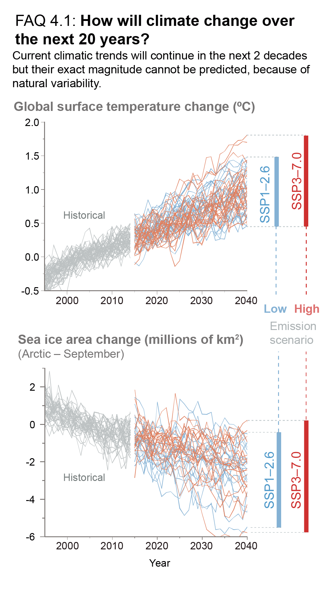
FAQ 4.1, Figure 1 | Simulations over the period 1995–2040, encompassing the recent past and the next twenty years, of two important indicators of global climate change. (Top) Global surface temperature, and (bottom), the area of Arctic sea ice in September. Both quantities are shown as deviations from the average over the period 1995–2014. The grey curves are for the historical period ending in 2014; the blue curves represent a low-emissions scenario (SSP1-2.6) and the red curves one high-emissions scenario (SSP3-7.0).
FAQ 4.2 | How Quickly Would We See the Effects of Reducing Carbon Dioxide Emissions?
The effects of substantial reductions in carbon dioxide emissions would not be apparent immediately, and the time required to detect the effects would depend on the scale and pace of emissions reductions. Under the lower-emissions scenarios considered in this Report, the increase in atmospheric carbon dioxide concentrations would slow visibly after about five to ten years, while the slowing down of global surface warming would be detectable after about twenty to thirty years. The effects on regional precipitation trends would only become apparent after several decades.
Reducing emissions of carbon dioxide (CO2) – the most important greenhouse gas emitted by human activities – would slow down the rate of increase in atmospheric CO2 concentration. However, concentrations would only begin to decrease when net emissions approach zero, that is, when most or all of the CO2 emitted into the atmosphere each year is removed by natural and human processes (see FAQ 5.1 and FAQ 5.3). This delay between a peak in emissions and a decrease in concentration is a manifestation of the very long lifetime of CO2 in the atmosphere; part of the CO2 emitted by humans remains in the atmosphere for centuries to millennia.
Reducing the rate of increase in CO2 concentration would slow down global surface warming within a decade. But this reduction in the rate of warming would initially be masked by natural climate variability and might not be detected for a few decades (see FAQ 1.2, FAQ 3.2 and FAQ 4.1). Detecting whether surface warming has indeed slowed down would thus be difficult in the years right after emissions reductions begin.
The time needed to detect the effect of emissions reductions is illustrated by comparing low- and high-emissions scenarios (FAQ 4.2, Figure 1). In the low-emissions scenario (SSP1-2.6), CO2 emissions level off after 2015 and begin to fall in 2020, while they keep increasing throughout the 21st century in the high-emissions scenario (SSP3-7.0). The uncertainty arising from natural internal variability in the climate system is represented by simulating each scenario ten times with the same climate model but starting from slightly different initial states back in 1850 (thin lines). For each scenario, the differences between individual simulations are caused entirely by simulated natural internal variability. The average of all simulations represents the climate response expected for a given scenario. The climate history that would actually unfold under each scenario would consist of this expected response combined with the contribution from natural internal variability and the contribution from potential future volcanic eruptions (the latter effect is not represented here).
FAQ 4.2, Figure 1 shows that the atmospheric CO2 concentrations differ noticeably between the two scenarios about five to ten years after the emissions have begun to diverge in year 2015. In contrast, the difference in global surface temperatures between the two scenarios does not become apparent until later – about two to three decades after the emissions histories have begun to diverge in this example. This time would be longer if emissions were reduced more slowly than in the low-emissions scenario illustrated here and shorter in the case of stronger reductions. Detection would take longer for regional quantities and for precipitation changes, which vary more strongly from natural causes. For instance, even in the low-emissions scenario, the effect of reduced CO2 emissions would not become visible in regional precipitation until late in the 21st century.
In summary, it is only after a few decades of reducing CO2 emissions that we would clearly see global temperatures starting to stabilize. By contrast, short-term reductions in CO2 emissions, such as during the COVID-19 pandemic, do not have detectable effects on either CO2 concentration or global temperature. Only sustained emissions reductions over decades would have a widespread effect across the climate system.
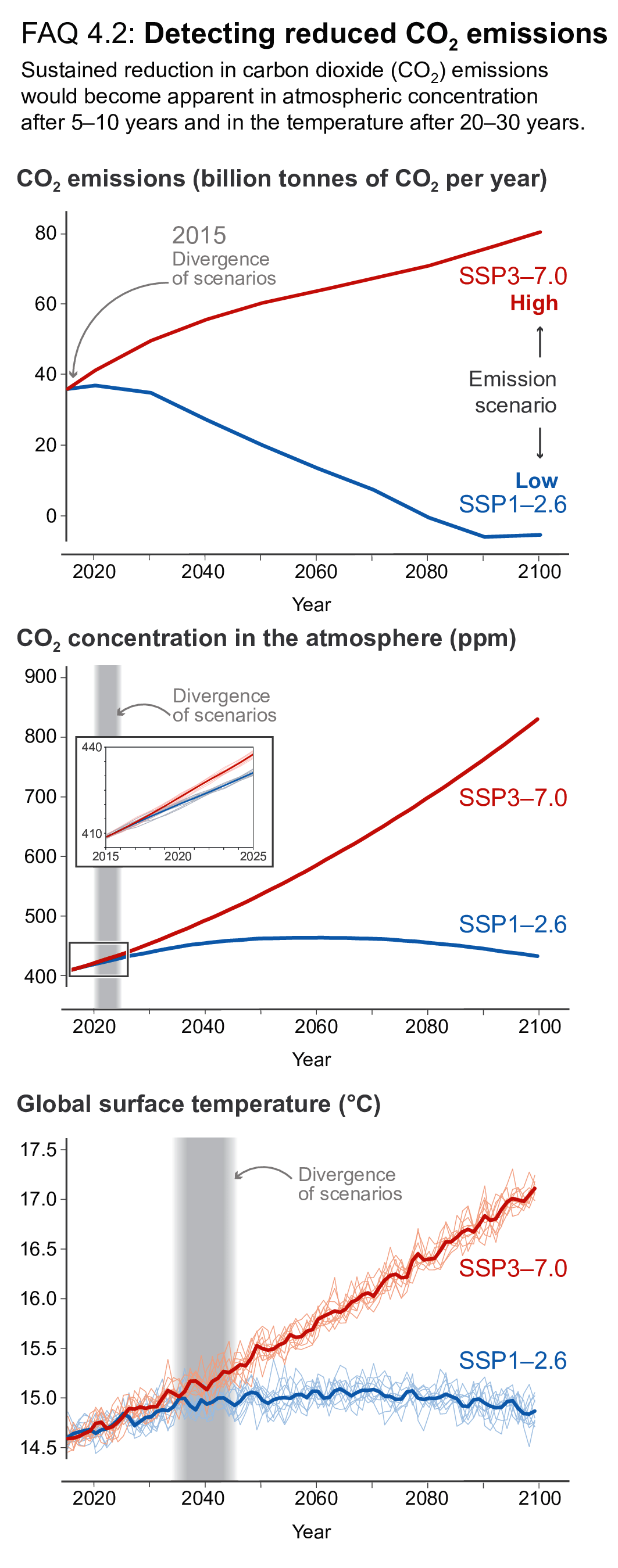
FAQ 4.2, Figure 1 | Observing the benefits of emissions reductions. (Top) Carbon dioxide (CO2) emissions, (middle) CO2 concentration in the atmosphere and (bottom) effect on global surface temperature for two scenarios: a low-emissions scenario (SSP1-2.6, blue) and a high-emissions scenario (SSP3-7.0). In the low-emissions scenario, CO2 emissions begin to decrease in 2020 whereas they keep increasing throughout the 21st century in the high-emissions scenario. The thick lines are the average of the 10 individual simulations (thin line) for each scenario. Differences between individual simulations reflect natural variability.
FAQ 4.3 | At a Given Level of Global Warming, What Are the Spatial Patterns of Climate Change?
As the planet warms, climate change does not unfold uniformly across the globe, but some patterns of regional change show clear, direct and consistent relationships to increases in global surface temperature. The Arctic warms more than other regions, land areas warm more than the ocean surface, and the Northern Hemisphere more than the Southern Hemisphere. Precipitation increases over high latitudes, tropics and large parts of the monsoon regions, but decreases over the subtropics. For cases like these, we can infer the direction and magnitude of some regional changes – particularly temperature and precipitation changes – for any given level of global warming.
The intensity of climate change will depend on the level of global warming. It is possible to identify certain patterns of regional climate change that occur consistently, but increase in amplitude, across increasing levels of global warming. Such robust spatial patterns of climate change are largely independent of the specific scenario (and pathway in time) that results in a given level of global warming. That is, as long as different scenarios result in the same global warming level, irrespective of the time when this level is attained in each scenario, we can infer the patterns of regional change that would result from this warming. When patterns of changes are robust, regional consequences can be assessed for all levels of global warming, for all future time periods, and for all scenarios. Temperature and precipitation show such robust patterns of changes that are particularly striking.
The high latitudes of the Northern Hemisphere are projected to warm the most, by two to four times the level of global warming – a phenomenon referred to as Arctic amplification (FAQ 4.3, Figure 1, left). Several processes contribute to this high rate of warming, including increases in the absorption of solar radiation due to the loss of reflective sea ice and snow in a warmer world. In the Southern Hemisphere, Antarctica is projected to warm faster than the mid-latitude Southern Ocean, but the Southern Hemisphere high latitudes are projected to warm at a reduced amplitude compared to the level of global warming (FAQ 4.3, Figure 1, left). An important reason for the relatively slower warming of the Southern Hemisphere high latitudes is the upwelling of Antarctic deep waters that drives a large surface heat uptake in the Southern Ocean.
The warming is generally stronger over land than over the ocean, and in the Northern Hemisphere compared to the Southern Hemisphere, and with less warming over the central subpolar North Atlantic and the southernmost Pacific. The differences are the result of several factors, including differences in how land and ocean areas absorb and retain heat, the fact that there is more land area in the Northern Hemisphere than in the Southern Hemisphere, and the influence of ocean circulation. In the Southern Hemisphere, robust patterns of relatively high warming are projected for subtropical South America, southern Africa, and Australia. The relatively strong warming in subtropical southern Africa arises from strong interactions between soil moisture and temperature and from increased solar radiation as a consequence of enhanced subsidence.
Precipitation changes are also proportional to the level of global warming (FAQ 4.3, Figure 1, right), although uncertainties are larger than for the temperature change. In the high latitudes of both the Southern and Northern Hemispheres, increases in precipitation are expected as the planet continues to warm, with larger changes expected at higher levels of global warming (FAQ 4.3, Figure 1, right). The same holds true for the projected precipitation increases over the tropics and large parts of the monsoon regions. General drying is expected over the subtropical regions, particularly over the Mediterranean, southern Africa and parts of Australia, South America, and south-west North America, as well as over the subtropical Atlantic and parts of the subtropical Indian and Pacific Oceans. Increases in precipitation over the tropics and decreases over the subtropics amplify with higher levels of global warming.
Some regions that are already dry and warm, such as southern Africa and the Mediterranean, are expected to become progressively drier and drastically warmer at higher levels of global warming.
In summary, climate change will not affect all the parts of the globe evenly. Rather, distinct regional patterns of temperature and precipitation change can be identified, and these changes are projected to amplify as the level of global warming increases.
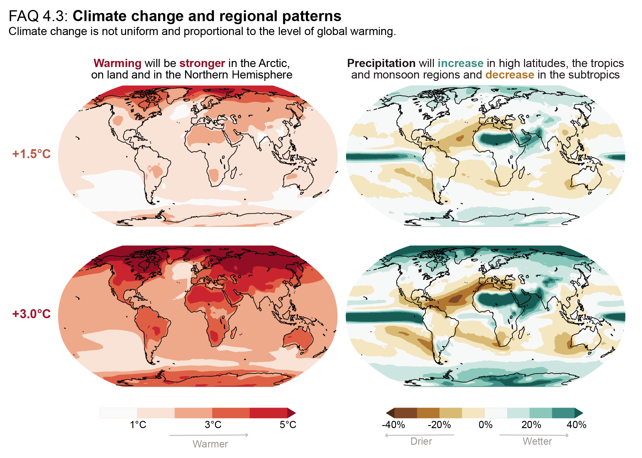
FAQ 4.3, Figure 1 | Regional changes in temperature (left) and precipitation (right) are proportional to the level of global warming, irrespective of the scenario through which the level of global warming is reached. Surface warming and precipitation change are shown relative to the 1850–1900 climate, and for time periods over which the globally averaged surface warming is 1.5°C (top) and 3°C (bottom), respectively. Changes presented here are based on 31 CMIP6 models using the high-emissions scenario SSP3-7.0.
References
Abramowitz, G. et al., 2019: ESD Reviews: Model dependence in multi-model climate ensembles: weighting, sub-selection and out-of-sample testing. Earth System Dynamics, 10(1), 91–105, doi: 10.5194/esd-10-91-2019.
Adams, J.B., M.E. Mann, and C.M. Ammann, 2003: Proxy evidence for an El Niño-like response to volcanic forcing. Nature, 426(6964), 274–278, doi: 10.1038/nature02101.
Ahlm, L. et al., 2017: Marine cloud brightening – as effective without clouds. Atmospheric Chemistry and Physics, 17(21), 13071–13087, doi: 10.5194/acp-17-13071-2017.
Akimoto, K., F. Sano, and T. Tomoda, 2018: GHG emission pathways until 2300 for the 1.5°C temperature rise target and the mitigation costs achieving the pathways. Mitigation and Adaptation Strategies for Global Change, 23(6), 839–852, doi: 10.1007/s11027-017-9762-z.
Albern, N., A. Voigt, and J.G. Pinto, 2019: Cloud-Radiative Impact on the Regional Responses of the Midlatitude Jet Streams and Storm Tracks to Global Warming. Journal of Advances in Modeling Earth Systems, 11(7), 1940–1958, doi: 10.1029/2018ms001592.
Alessandri, A. et al., 2014: Multi-scale enhancement of climate prediction over land by increasing the model sensitivity to vegetation variability in EC-Earth. Journal of Climate, 49(4), 8563–8577, doi: 10.1007/s00382-016-3372-4.
Alexeev, V.A. and C.H. Jackson, 2013: Polar amplification: is atmospheric heat transport important?Climate Dynamics, 41(2), 533–547, doi: 10.1007/s00382-012-1601-z.
Allen, M.R. and W.J. Ingram, 2002: Constraints on future changes in climate and the hydrologic cycle. Nature, 419(6903), 224–232, doi: 10.1038/nature01092.
Allen, M.R. et al., 2018: Framing and Context. In: Global Warming of 1.5°C. An IPCC Special Report on the impacts of global warming of 1.5°C above pre-industrial levels and related global greenhouse gas emission pathways, in the context of strengthening the global response to the threat of climate change, sustainable development, and efforts to eradicate poverty[Masson-Delmotte, V., P. Zhai, H.-O. Pörtner, D. Roberts, J. Skea, P.R. Shukla, A. Pirani, W. Moufouma-Okia, C. Péan, R. Pidcock, S. Connors, J.B.R. Matthews, Y. Chen, X. Zhou, M.I. Gomis, E. Lonnoy, T. Maycock, M. Tignor, and T. Waterfield (eds.)]. In Press, pp. 49–92, www.ipcc.ch/sr15/chapter/chapter-1.
Allen, R.J. et al., 2020: Climate and air quality impacts due to mitigation of non-methane near-term climate forcers. Atmospheric Chemistry and Physics, 20(16), 9641–9663, doi: 10.5194/acp-20-9641-2020.
Allen, R.J. et al., 2021: Significant climate benefits from near-term climate forcer mitigation in spite of aerosol reductions. Environmental Research Letters, 16(3), 034010, doi: 10.1088/1748-9326/abe06b.
Alley, R.B. et al., 2003: Abrupt Climate Change. Science, 299(5615), 2005–2010, doi: 10.1126/science.1081056.
Alterskjær, K. and J.E. Kristjánsson, 2013: The sign of the radiative forcing from marine cloud brightening depends on both particle size and injection amount. Geophysical Research Letters, 40(1), 210–215, doi: 10.1029/2012gl054286.
Alterskjær, K. et al., 2013: Sea-salt injections into the low-latitude marine boundary layer: The transient response in three Earth system models. Journal of Geophysical Research: Atmospheres, 118(21), 12195–12206, doi: 10.1002/2013jd020432.
Amann, M., Z. Klimont, and F. Wagner, 2013: Regional and Global Emissions of Air Pollutants: Recent Trends and Future Scenarios. Annual Review of Environment and Resources, 38(1), 31–55, doi: 10.1146/annurev-environ-052912-173303.
Andrews, M.B. et al., 2020: Historical Simulations With HadGEM3-GC3.1 for CMIP6. Journal of Advances in Modeling Earth Systems, 12(6), e2019MS001995, doi: 10.1029/2019ms001995.
Andrews, T. and P.M. Forster, 2010: The transient response of global-mean precipitation to increasing carbon dioxide levels. Environmental Research Letters, 5(2), 1–6, doi: 10.1088/1748-9326/5/2/025212.
Andrews, T., P.M. Forster, and J.M. Gregory, 2009: A surface energy perspective on climate change. Journal of Climate, 22(10), 2557–2570, doi: 10.1175/2008jcli2759.1.
Andrews, T. et al., 2019: Forcings, Feedbacks, and Climate Sensitivity in HadGEM3-GC3.1 and UKESM1. Journal of Advances in Modeling Earth Systems, 11(12), 4377–4394, doi: 10.1029/2019ms001866.
Annan, J.D. and J.C. Hargreaves, 2017: On the meaning of independence in climate science. Earth System Dynamics, 8, 211–224, doi: 10.5194/esd-8-211-2017.
Aquila, V., C.I. Garfinkel, P.A. Newman, L.D. Oman, and D.W. Waugh, 2014: Modifications of the quasi-biennial oscillation by a geoengineering perturbation of the stratospheric aerosol layer. Geophysical Research Letters, 41(5), 1738–1744, doi: 10.1002/2013gl058818.
Armour, K.C., N. Siler, A. Donohoe, and G.H. Roe, 2019: Meridional Atmospheric Heat Transport Constrained by Energetics and Mediated by Large-Scale Diffusion. Journal of Climate, 32(12), 3655–3680, doi: 10.1175/jcli-d-18-0563.1.
Armour, K.C., J. Marshall, J.R. Scott, A. Donohoe, and E.R. Newsom, 2016: Southern Ocean warming delayed by circumpolar upwelling and equatorward transport. Nature Geoscience, 9, 549–554, doi: 10.1038/ngeo2731.
Arora, V.K. et al., 2020: Carbon–concentration and carbon–climate feedbacks in CMIP6 models and their comparison to CMIP5 models. Biogeosciences, 17(16), 4173–4222, doi: 10.5194/bg-17-4173-2020.
Arrhenius, S., 1896: On the influence of carbonic acid in the air upon the temperature of the ground. The London, Edinburgh, and Dublin Philosophical Magazine and Journal of Science, 41(251), 237–276, doi: 10.1080/14786449608620846.
Årthun, M., K.E. W., T. Eldevik, and K.N. S., 2018: Time Scales and Sources of European Temperature Variability. Geophysical Research Letters, 45(8), 3597–3604, doi: 10.1002/2018gl077401.
Årthun, M. et al., 2017: Skillful prediction of northern climate provided by the ocean. Nature Communications, 8(1), 15875, doi: 10.1038/ncomms15875.
Athanasiadis, P.J. et al., 2020: Decadal predictability of North Atlantic blocking and the NAO. npj Climate and Atmospheric Science, 3(1), 20, doi: 10.1038/s41612-020-0120-6.
Baker, L.H., L.C. Shaffrey, R.T. Sutton, A. Weisheimer, and A.A. Scaife, 2018: An Intercomparison of Skill and Overconfidence/Underconfidence of the Wintertime North Atlantic Oscillation in Multimodel Seasonal Forecasts. Geophysical Research Letters, 45(15), 7808–7817, doi: 10.1029/2018gl078838.
Bala, G., K. Caldeira, and R. Nemani, 2010: Fast versus slow response in climate change: Implications for the global hydrological cycle. Climate Dynamics, 35(2–3), 423–434, doi: 10.1007/s00382-009-0583-y.
Bala, G. et al., 2011: Albedo enhancement of marine clouds to counteract global warming: impacts on the hydrological cycle. Climate Dynamics, 37(5), 915–931, doi: 10.1007/s00382-010-0868-1.
Balaji, V. et al., 2018: Requirements for a global data infrastructure in support of CMIP6. Geoscientific Model Development, 11(9), 3659–3680, doi: 10.5194/gmd-11-3659-2018.
Ban, N., J. Schmidli, and C. Schär, 2015: Heavy precipitation in a changing climate: Does short-term summer precipitation increase faster?Geophysical Research Letters, 42(4), 1165–1172, doi: 10.1002/2014gl062588.
Banerjee, A., A.C. Maycock, and J.A. Pyle, 2018: Chemical and climatic drivers of radiative forcing due to changes in stratospheric and tropospheric ozone over the 21st century. Atmospheric Chemistry and Physics, 18(4), 2899–2911, doi: 10.5194/acp-18-2899-2018.
Banerjee, A., J.C. Fyfe, L.M. Polvani, D. Waugh, and K.-L. Chang, 2020: A pause in Southern Hemisphere circulation trends due to the Montreal Protocol. Nature, 579(7800), 544–548, doi: 10.1038/s41586-020-2120-4.
Banerjee, A. et al., 2014: Lightning NOx, a key chemistry-climate interaction: Impacts of future climate change and consequences for tropospheric oxidising capacity. Atmospheric Chemistry and Physics, 14(18), 9871–9881, doi: 10.5194/acp-14-9871-2014.
Barcikowska, M.J. et al., 2018: Euro-Atlantic winter storminess and precipitation extremes under 1.5°C vs. 2°C warming scenarios. Earth System Dynamics, 9(2), 679–699, doi: 10.5194/esd-9-679-2018.
Barnes, E.A. and L. Polvani, 2013: Response of the Midlatitude Jets, and of Their Variability, to Increased Greenhouse Gases in the CMIP5 Models. Journal of Climate, 26(18), 7117–7135, doi: 10.1175/jcli-d-12-00536.1.
Barnes, E.A. and L.M. Polvani, 2015: CMIP5 projections of arctic amplification, of the North American/North Atlantic circulation, and of their relationship. Journal of Climate, 28, 5254–5271, doi: 10.1175/jcli-d-14-00589.1.
Barnes, E.A., N.W. Barnes, and L.M. Polvani, 2014: Delayed southern hemisphere climate change induced by stratospheric ozone recovery, as projected by the CMIP5 models. Journal of Climate, 27, 852–867, doi: 10.1175/jcli-d-13-00246.1.
Barriopedro, D., R. García-Herrera, and R.M. Trigo, 2010: Application of blocking diagnosis methods to General Circulation Models. Part I: a novel detection scheme. Climate Dynamics, 35(7–8), 1373–1391, doi: 10.1007/s00382-010-0767-5.
Bathiany, S., J. Hidding, and M. Scheffer, 2020: Edge Detection Reveals Abrupt and Extreme Climate Events. Journal of Climate, 33(15), 6399–6421, doi: 10.1175/jcli-d-19-0449.1.
Bathiany, S., V. Dakos, M. Scheffer, and T.M. Lenton, 2018: Climate models predict increasing temperature variability in poor countries. Science Advances, 4(5), eaar5809, doi: 10.1126/sciadv.aar5809.
Bathiany, S., D. Notz, T. Mauritsen, G. Raedel, and V. Brovkin, 2016: On the potential for abrupt Arctic winter sea ice loss. Journal of Climate, 29(7), 2703–2719, doi: 10.1175/jcli-d-15-0466.1.
Batté, L. and F.J. Doblas-Reyes, 2015: Stochastic atmospheric perturbations in the EC-Earth3 global coupled model: impact of SPPT on seasonal forecast quality. Climate Dynamics, 45(11), 3419–3439, doi: 10.1007/s00382-015-2548-7.
Baumberger, C., R. Knutti, and G. Hirsch Hadorn, 2017: Building confidence in climate model projections: an analysis of inferences from fit. WIREs Climate Change, 8(3), e454, doi: 10.1002/wcc.454.
Bayr, T. and D. Dommenget, 2013: The Tropospheric Land–Sea Warming Contrast as the Driver of Tropical Sea Level Pressure Changes. Journal of Climate, 26(4), 1387–1402, doi: 10.1175/jcli-d-11-00731.1.
Beer, E., I. Eisenman, and T.J.W. Wagner, 2020: Polar Amplification Due to Enhanced Heat Flux Across the Halocline. Geophysical Research Letters, 47(4), e2019GL086706, doi: 10.1029/2019gl086706.
Befort, D.J., C.H. O’Reilly, and A. Weisheimer, 2020: Constraining Projections Using Decadal Predictions. Geophysical Research Letters, 47(18), e2020GL087900, doi: 10.1029/2020gl087900.
Bellomo, K., L.N. Murphy, M.A. Cane, A.C. Clement, and L.M. Polvani, 2018: Historical forcings as main drivers of the Atlantic multidecadal variability in the CESM large ensemble. Climate Dynamics, 50(9), 3687–3698, doi: 10.1007/s00382-017-3834-3.
Bellucci, A., A. Mariotti, and S. Gualdi, 2017: The Role of Forcings in the Twentieth-Century North Atlantic Multidecadal Variability: The 1940–75 North Atlantic Cooling Case Study. Journal of Climate, 30(18), 7317–7337, doi: 10.1175/jcli-d-16-0301.1.
Bellucci, A. et al., 2015a: Advancements in decadal climate predictability: The role of nonoceanic drivers. Reviews of Geophysics, 53(2), 165–202, doi: 10.1002/2014rg000473.
Bellucci, A. et al., 2015b: An assessment of a multi-model ensemble of decadal climate predictions. Climate Dynamics, 44(9–10), 2787–2806, doi: 10.1007/s00382-014-2164-y.
Bengtsson, L. and K.I. Hodges, 2019: Can an ensemble climate simulation be used to separate climate change signals from internal unforced variability?Climate Dynamics, 52(5–6), 3553–3573, doi: 10.1007/s00382-018-4343-8.
Berdahl, M. et al., 2014: Arctic cryosphere response in the Geoengineering Model Intercomparison Project G3 and G4 scenarios. Journal of Geophysical Research: Atmospheres, 119(3), 1308–1321, doi: 10.1002/2013jd020627.
Berg, A. et al., 2016: Land–atmosphere feedbacks amplify aridity increase over land under global warming. Nature Climate Change, 6(9), 869–874, doi: 10.1038/nclimate3029.
Berner, J. et al., 2017: Stochastic Parameterization: Toward a New View of Weather and Climate Models. Bulletin of the American Meteorological Society, 98(3), 565–588, doi: 10.1175/bams-d-15-00268.1.
Bethke, I. et al., 2017: Potential volcanic impacts on future climate variability. Nature Climate Change, 7(11), 799–805, doi: 10.1038/nclimate3394.
Bilbao, R. et al., 2021: Assessment of a full-field initialized decadal climate prediction system with the CMIP6 version of EC-Earth. Earth System Dynamics, 12(1), 173–196, doi: 10.5194/esd-12-173-2021.
Bindoff, N.L. et al., 2013: Detection and Attribution of Climate Change: from Global to Regional. In: Climate Change 2013: The Physical Science Basis. Contribution of Working Group I to the Fifth Assessment Report of the Intergovernmental Panel on Climate Change[Stocker, T.F., D. Qin, G.-K. Plattner, M. Tignor, S.K. Allen, J. Boschung, A. Nauels, Y. Xia, V. Bex, and P.M. Midgley (eds.)]. Cambridge University Press, Cambridge, United Kingdom and New York, NY, USA, pp. 867–952, doi: 10.1017/cbo9781107415324.022.
Bitz, C.M., P.R. Gent, R.A. Woodgate, M.M. Holland, and R. Lindsay, 2006: The influence of sea ice on ocean heat uptake in response to increasing CO2. Journal of Climate, 19(11), 2437–2450, doi: 10.1175/jcli3756.1.
Boé, J., 2018: Interdependency in Multimodel Climate Projections: Component Replication and Result Similarity. Geophysical Research Letters, 45(6), 2771–2779, doi: 10.1002/2017gl076829.
Boer, G.J. and R. Sospedra-Alfonso, 2019: Assessing the skill of the Pacific Decadal Oscillation (PDO) in a decadal prediction experiment. Climate Dynamics, 53(9), 5763–5775, doi: 10.1007/s00382-019-04896-w.
Boer, G.J., V. Kharin, and W.J. Merryfield, 2013: Decadal predictability and forecast skill. Climate Dynamics, 41(7–8), 1817–1833, doi: 10.1007/s00382-013-1705-0.
Boer, G.J. et al., 2016: The Decadal Climate Prediction Project (DCPP) contribution to CMIP6. Geoscientific Model Development, 9(10), 3751–3777, doi: 10.5194/gmd-9-3751-2016.
Bollasina, M.A., Y. Ming, and V. Ramaswamy, 2011: Anthropogenic Aerosols and the Weakening of the South Asian Summer Monsoon. Science, 334(6055), 502–505, doi: 10.1126/science.1204994.
Bonan, D.B., K.C. Armour, G.H. Roe, N. Siler, and N. Feldl, 2018: Sources of Uncertainty in the Meridional Pattern of Climate Change. Geophysical Research Letters, 45, 9131–9140, doi: 10.1029/2018gl079429.
Bony, S. et al., 2013: Robust direct effect of carbon dioxide on tropical circulation and regional precipitation. Nature Geoscience, 6(6), 447–451, doi: 10.1038/ngeo1799.
Borchert, L.F. et al., 2019: Decadal Predictions of the Probability of Occurrence for Warm Summer Temperature Extremes. Geophysical Research Letters, 46(23), 14042–14051, doi: 10.1029/2019gl085385.
Borchert, L.F. et al., 2021: Improved Decadal Predictions of North Atlantic Subpolar Gyre SST in CMIP6. Geophysical Research Letters, 48(3), e2020GL091307, doi: 10.1029/2020gl091307.
Bordbar, M.H. et al., 2019: Uncertainty in near-term global surface warming linked to tropical Pacific climate variability. Nature Communications, 10(1), 1990, doi: 10.1038/s41467-019-09761-2.
Borodina, A., E.M. Fischer, and R. Knutti, 2017: Emergent constraints in climate projections: A case study of changes in high-latitude temperature variability. Journal of Climate, 30, 3655–3670, doi: 10.1175/jcli-d-16-0662.1.
Boucher, O., C. Kleinschmitt, and G. Myhre, 2017: Quasi-Additivity of the Radiative Effects of Marine Cloud Brightening and Stratospheric Sulfate Aerosol Injection. Geophysical Research Letters, 44(21), 11158–11165, doi: 10.1002/2017gl074647.
Boucher, O. et al., 2012: Reversibility in an Earth System model in response to CO2 concentration changes. Environmental Research Letters, 7(2), 024013, doi: 10.1088/1748-9326/7/2/024013.
Boucher, O. et al., 2013: Clouds and Aerosols. In: Climate Change 2013: The Physical Science Basis. Contribution of Working Group I to the Fifth Assessment Report of the Intergovernmental Panel on Climate Change[Stocker, T.F., D. Qin, G.-K. Plattner, M. Tignor, S.K. Allen, J. Boschung, A. Nauels, Y. Xia, V. Bex, and P.M. Midgley (eds.)]. Cambridge University Press, Cambridge, United Kingdom and New York, NY, USA, pp. 571–657, doi: 10.1017/cbo9781107415324.016.
Bracegirdle, T.J., H. Lu, R. Eade, and T. Woollings, 2018: Do CMIP5 Models Reproduce Observed Low-Frequency North Atlantic Jet Variability?Geophysical Research Letters, 45(14), 7204–7212, doi: 10.1029/2018gl078965.
Bracegirdle, T.J. et al., 2020a: Improvements in Circumpolar Southern Hemisphere Extratropical Atmospheric Circulation in CMIP6 Compared to CMIP5. Earth and Space Science, 7(6), e2019EA001065, doi: 10.1029/2019ea001065.
Bracegirdle, T.J. et al., 2020b: Twenty first century changes in Antarctic and Southern Ocean surface climate in CMIP6. Atmospheric Science Letters, 21(9), e984, doi: 10.1002/asl.984.
Bradley, R.S., K.R. Briffa, J. Cole, M.K. Hughes, and T.J. Osborn, 2003: The Climate of the Last Millennium. In: Paleoclimate, Global Change and the Future[Alverson, K.D., T.F. Pedersen, and R.S. Bradley (eds.)]. Global Change – The IGBP Series, Springer, Berlin and Heidelberg, Germany, pp. 105–141, doi: 10.1007/978-3-642-55828-3_6.
Branstator, G. and H.Y. Teng, 2010: Two limits of initial-value decadal predictability in a CGCM. Journal of Climate, 23(23), 6292–6311, doi: 10.1175/2010jcli3678.1.
Brient, F., 2020: Reducing Uncertainties in Climate Projections with Emergent Constraints: Concepts, Examples and Prospects. Advances in Atmospheric Sciences, 37(1), 1–15, doi: 10.1007/s00376-019-9140-8.
Bright, R.M. et al., 2017: Local temperature response to land cover and management change driven by non-radiative processes. Nature Climate Change, 7(4), 296–302, doi: 10.1038/nclimate3250.
Brogli, R., N. Kröner, S.L. Sørland, D. Lüthi, and C. Schär, 2019: The Role of Hadley Circulation and Lapse-Rate Changes for the Future European Summer Climate. Journal of Climate, 32(2), 385–404, doi: 10.1175/jcli-d-18-0431.1.
Brönnimann, S. et al., 2019: Last phase of the Little Ice Age forced by volcanic eruptions. Nature Geoscience, 12(8), 650–656, doi: 10.1038/s41561-019-0402-y.
Bronselaer, B. et al., 2018: Change in future climate due to Antarctic meltwater. Nature, 564, 55–58, doi: 10.1038/s41586-018-0712-z.
Brown, J.R. et al., 2020: Comparison of past and future simulations of ENSO in CMIP5/PMIP3 and CMIP6/PMIP4 models. Climate of the Past, 16(5), 1777–1805, doi: 10.5194/cp-16-1777-2020.
Brown, P.T., M.S. Lozier, R. Zhang, and W. Li, 2016: The necessity of cloud feedback for a basin-scale Atlantic Multidecadal Oscillation. Geophysical Research Letters, 43(8), 3955–3963, doi: 10.1002/2016gl068303.
Brown, P.T., Y. Ming, W. Li, and S.A. Hill, 2017: Change in the magnitude and mechanisms of global temperature variability with warming. Nature Climate Change, 7(10), 743–748, doi: 10.1038/nclimate3381.
Brune, S. and J. Baehr, 2020: Preserving the coupled atmosphere–ocean feedback in initializations of decadal climate predictions. WIREs Climate Change, 11(3), e637, doi: 10.1002/wcc.637.
Brune, S., A. Düsterhus, H. Pohlmann, W.A. Müller, and J. Baehr, 2018: Time dependency of the prediction skill for the North Atlantic subpolar gyre in initialized decadal hindcasts. Climate Dynamics, 51(5), 1947–1970, doi: 10.1007/s00382-017-3991-4.
Brunner, L. et al., 2020: Reduced global warming from CMIP6 projections when weighting models by performance and independence. Earth System Dynamics, 11(4), 995–1012, doi: 10.5194/esd-11-995-2020.
Büntgen, U. et al., 2016: Cooling and societal change during the Late Antique Little Ice Age from 536 to around 660 AD. Nature Geoscience, 9(3), 231–236, doi: 10.1038/ngeo2652.
Bürger, G. and U. Cubasch, 2015: The detectability of climate engineering. Journal of Geophysical Research: Atmospheres, 120(22), 11404–11418, doi: 10.1002/2015jd023954.
Burke, E.J. et al., 2017: Quantifying uncertainties of permafrost carbon–climate feedbacks. Biogeosciences, 14(12), 3051–3066, doi: 10.5194/bg-14-3051-2017.
Byrne, M.P. and P.A. O’Gorman, 2013a: Land–Ocean Warming Contrast over a Wide Range of Climates: Convective Quasi-Equilibrium Theory and Idealized Simulations. Journal of Climate, 26(12), 4000–4016, doi: 10.1175/jcli-d-12-00262.1.
Byrne, M.P. and P.A. O’Gorman, 2013b: Link between land–ocean warming contrast and surface relative humidities in simulations with coupled climate models. Geophysical Research Letters, 40, 5223–5227, doi: 10.1002/grl.50971.
Byrne, M.P. and P.A. O’Gorman, 2015: The Response of Precipitation Minus Evapotranspiration to Climate Warming: Why the “Wet-Get-Wetter, Dry-Get-Drier” Scaling Does Not Hold over Land. Journal of Climate, 28(20), 8078–8092, doi: 10.1175/jcli-d-15-0369.1.
Byrne, M.P. and P.A. O’Gorman, 2016: Understanding Decreases in Land Relative Humidity with Global Warming: Conceptual Model and GCM Simulations. Journal of Climate, 29(24), 9045–9061, doi: 10.1175/jcli-d-16-0351.1.
Byrne, M.P. and P.A. O’Gorman, 2018: Trends in continental temperature and humidity directly linked to ocean warming. Proceedings of the National Academy of Sciences, 115(19), 4863–4868, doi: 10.1073/pnas.1722312115.
Byrne, N.J., T.G. Shepherd, and I. Polichtchouk, 2019: Subseasonal-to-Seasonal Predictability of the Southern Hemisphere Eddy-Driven Jet During Austral Spring and Early Summer. Journal of Geophysical Research: Atmospheres, 124(13), 6841–6855, doi: 10.1029/2018jd030173.
Caesar, J. et al., 2013: Response of the HadGEM2 Earth System Model to future greenhouse gas emissions pathways to the year 2300. Journal of Climate, 26(10), 3275–3284, doi: 10.1175/jcli-d-12-00577.1.
Cai, W., G. Wang, A. Santoso, X. Lin, and L. Wu, 2017: Definition of Extreme El Niño and Its Impact on Projected Increase in Extreme El Niño Frequency. Geophysical Research Letters, 44(21), 11184-11190, doi: 10.1002/2017gl075635.
Cai, W. et al., 2013: Projected response of the Indian Ocean Dipole to greenhouse warming. Nature Geoscience, 6, 997–1007, doi: 10.1038/ngeo2009.
Cai, W. et al., 2014a: Increasing frequency of extreme El Niño events due to greenhouse warming. Nature Climate Change, 4(2), 111–116, doi: 10.1038/nclimate2100.
Cai, W. et al., 2014b: Increased frequency of extreme Indian Ocean Dipole events due to greenhouse warming. Nature, 510, 254–258, doi: 10.1038/nature13327.
Cai, W. et al., 2015: ENSO and greenhouse warming. Nature Climate Change, 5(9), 849–859, doi: 10.1038/nclimate2743.
Cai, W. et al., 2018a: Increased variability of eastern Pacific El Niño under greenhouse warming. Nature, 564(7735), 201–206, doi: 10.1038/s41586-018-0776-9.
Cai, W. et al., 2018b: Stabilised frequency of extreme positive Indian Ocean Dipole under 1.5°C warming. Nature Communications, 9(1), 1419, doi: 10.1038/s41467-018-03789-6.
Cai, W. et al., 2019: Pantropical climate interactions. Science, 363(6430), eaav4236, doi: 10.1126/science.aav4236.
Cai, W. et al., 2021: Opposite response of strong and moderate positive Indian Ocean Dipole to global warming. Nature Climate Change, 11(1), 27–32, doi: 10.1038/s41558-020-00943-1.
Caian, M., T. Koenigk, R. Döscher, and A. Devasthale, 2018: An interannual link between Arctic sea-ice cover and the North Atlantic Oscillation. Climate Dynamics, 50(1–2), 423–441, doi: 10.1007/s00382-017-3618-9.
Cao, L., G. Bala, and K. Caldeira, 2011: Why is there a short-term increase in global precipitation in response to diminished CO2 forcing?Geophysical Research Letters, 38(6), L06703, doi: 10.1029/2011gl046713.
Cao, L., G. Bala, M. Zheng, and K. Caldeira, 2015: Fast and slow climate responses to CO2 and solar forcing: A linear multivariate regression model characterizing transient climate change. Journal of Geophysical Research: Atmospheres, 120(23), 12037–12053, doi: 10.1002/2015jd023901.
Cao, L., L. Duan, G. Bala, and K. Caldeira, 2016: Simulated long-term climate response to idealized solar geoengineering. Geophysical Research Letters, 43(5), 2209–2217, doi: 10.1002/2016gl068079.
Cao, L., L. Duan, G. Bala, and K. Caldeira, 2017: Simultaneous stabilization of global temperature and precipitation through cocktail geoengineering. Geophysical Research Letters, 44(14), 7429–7437, doi: 10.1002/2017gl074281.
Caron, L.-P. et al., 2017: How Skillful are the Multiannual Forecasts of Atlantic Hurricane Activity?Bulletin of the American Meteorological Society, 99(2), 403–413, doi: 10.1175/bams-d-17-0025.1.
Cassou, C. and J. Cattiaux, 2016: Disruption of the European climate seasonal clock in a warming world. Nature Climate Change, 6(6), 589–594, doi: 10.1038/nclimate2969.
Cassou, C. et al., 2018: Decadal Climate Variability and Predictability: Challenges and Opportunities. Bulletin of the American Meteorological Society, 99(3), 479–490, doi: 10.1175/bams-d-16-0286.1.
Ceppi, P. and D.L. Hartmann, 2016: Clouds and the Atmospheric Circulation Response to Warming. Journal of Climate, 29(2), 783–799, doi: 10.1175/jcli-d-15-0394.1.
Ceppi, P. and T.G. Shepherd, 2017: Contributions of Climate Feedbacks to Changes in Atmospheric Circulation. Journal of Climate, 30(22), 9097–9118, doi: 10.1175/jcli-d-17-0189.1.
Ceppi, P. and T.G. Shepherd, 2019: The Role of the Stratospheric Polar Vortex for the Austral Jet Response to Greenhouse Gas Forcing. Geophysical Research Letters, 46(12), 6972–6979, doi: 10.1029/2019gl082883.
Ceppi, P., M.D. Zelinka, and D.L. Hartmann, 2014: The response of the Southern Hemispheric eddy-driven jet to future changes in shortwave radiation in CMIP5. Geophysical Research Letters, 41(9), 3244–3250, doi: 10.1002/2014gl060043.
Ceppi, P., G. Zappa, T.G. Shepherd, and J.M. Gregory, 2018: Fast and Slow Components of the Extratropical Atmospheric Circulation Response to CO2 forcing. Journal of Climate, 31(3), 1091–1105, doi: 10.1175/jcli-d-17-0323.1.
Chadwick, R., 2016: Which Aspects of CO2 forcing and SST Warming Cause Most Uncertainty in Projections of Tropical Rainfall Change over Land and Ocean?Journal of Climate, 29(7), 2493–2509, doi: 10.1175/jcli-d-15-0777.1.
Chadwick, R., I. Boutle, and G. Martin, 2013: Spatial Patterns of Precipitation Change in CMIP5: Why the Rich Do Not Get Richer in the Tropics. Journal of Climate, 26(11), 3803–3822, doi: 10.1175/jcli-d-12-00543.1.
Chadwick, R., P. Good, and K. Willett, 2016: A Simple Moisture Advection Model of Specific Humidity Change over Land in Response to SST Warming. Journal of Climate, 29(21), 7613–7632, doi: 10.1175/jcli-d-16-0241.1.
Chadwick, R., H. Douville, and C.B. Skinner, 2017: Timeslice experiments for understanding regional climate projections: applications to the tropical hydrological cycle and European winter circulation. Climate Dynamics, 49(9–10), 3011–3029, doi: 10.1007/s00382-016-3488-6.
Chalmers, N., E.J. Highwood, E. Hawkins, R. Sutton, and L.J. Wilcox, 2012: Aerosol contribution to the rapid warming of near-term climate under RCP 2.6. Geophysical Research Letters, 39(17), 2–7, doi: 10.1029/2012gl052848.
Chand, S.S., K.J. Tory, H. Ye, and K.J.E. Walsh, 2017: Projected increase in El Niño-driven tropical cyclone frequency in the Pacific. Nature Climate Change, 7, 123–127, doi: 10.1038/nclimate3181.
Chang, E.K.-M., 2017: Projected Significant Increase in the Number of Extreme Extratropical Cyclones in the Southern Hemisphere. Journal of Climate, 30(13), 4915–4935, doi: 10.1175/jcli-d-16-0553.1.
Chang, E.K.-M., 2018: CMIP5 Projected Change in Northern Hemisphere Winter Cyclones with Associated Extreme Winds. Journal of Climate, 31(16), 6527–6542, doi: 10.1175/jcli-d-17-0899.1.
Chang, E.K.-M., C.-G. Ma, C. Zheng, and A.M.W. Yau, 2016: Observed and projected decrease in Northern Hemisphere extratropical cyclone activity in summer and its impacts on maximum temperature. Geophysical Research Letters, 43(5), 2200–2208, doi: 10.1002/2016gl068172.
Chavaillaz, Y., S. Joussaume, S. Bony, and P. Braconnot, 2016: Spatial stabilization and intensification of moistening and drying rate patterns under future climate change. Climate Dynamics, 47(3–4), 951–965, doi: 10.1007/s00382-015-2882-9.
Chen, G. et al., 2019: Thermodynamic and Dynamic Mechanisms for Hydrological Cycle Intensification over the Full Probability Distribution of Precipitation Events. Journal of the Atmospheric Sciences, 76(2), 497–516, doi: 10.1175/jas-d-18-0067.1.
Chen, L., T. Li, Y. Yu, and S.K. Behera, 2017: A possible explanation for the divergent projection of ENSO amplitude change under global warming. Climate Dynamics, 49(11–12), 3799–3811, doi: 10.1007/s00382-017-3544-x.
Chen, Y.-C. et al., 2012: Occurrence of lower cloud albedo in ship tracks. Atmospheric Chemistry and Physics, 12(17), 8223–8235, doi: 10.5194/acp-12-8223-2012.
Chen, Z. et al., 2020: Global Land Monsoon Precipitation Changes in CMIP6 Projections. Geophysical Research Letters, 47(14), e2019GL086902, doi: 10.1029/2019gl086902.
Cheng, W. et al., 2019: Soil Moisture and Other Hydrological Changes in a Stratospheric Aerosol Geoengineering Large Ensemble. Journal of Geophysical Research: Atmospheres, 124(23), 12773–12793, doi: 10.1029/2018jd030237.
Chevuturi, A., N.P. Klingaman, A.G. Turner, and S. Hannah, 2018: Projected Changes in the Asian-Australian Monsoon Region in 1.5°C and 2.0°C Global-Warming Scenarios. Earth’s Future, 6(3), 339–358, doi: 10.1002/2017ef000734.
Chikamoto, Y., A. Timmermann, M.J. Widlansky, M.A. Balmaseda, and L. Stott, 2017: Multi-year predictability of climate, drought, and wildfire in southwestern North America. Scientific Reports, 7(1), 6568, doi: 10.1038/s41598-017-06869-7.
Chikamoto, Y., A. Timmermann, M.J. Widlansky, S. Zhang, and M.A. Balmaseda, 2019: A Drift-Free Decadal Climate Prediction System for the Community Earth System Model. Journal of Climate, 32(18), 5967–5995, doi: 10.1175/jcli-d-18-0788.1.
Chikamoto, Y. et al., 2013: An overview of decadal climate predictability in a multi-model ensemble by climate model MIROC. Climate Dynamics, 40(5–6), 1201–1222, doi: 10.1007/s00382-012-1351-y.
Chikamoto, Y. et al., 2015: Skilful multi-year predictions of tropical trans-basin climate variability. Nature Communications, 6(1), 6869, doi: 10.1038/ncomms7869.
Chiodo, G. and L.M. Polvani, 2016: Reduction of Climate Sensitivity to Solar Forcing due to Stratospheric Ozone Feedback. Journal of Climate, 29(12), 4651–4663, doi: 10.1175/jcli-d-15-0721.1.
Chiodo, G., J. Oehrlein, L.M. Polvani, J.C. Fyfe, and A.K. Smith, 2019: Insignificant influence of the 11-year solar cycle on the North Atlantic Oscillation. Nature Geoscience, 12(2), 94–99, doi: 10.1038/s41561-018-0293-3.
Choi, J., S.W. Son, and R.J. Park, 2019: Aerosol versus greenhouse gas impacts on Southern Hemisphere general circulation changes. Climate Dynamics, 52(7–8), 4127–4142, doi: 10.1007/s00382-018-4370-5.
Chou, C., J.D. Neelin, C.-A. Chen, and J.-Y. Tu, 2009: Evaluating the “Rich-Get-Richer” Mechanism in Tropical Precipitation Change under Global Warming. Journal of Climate, 22(8), 1982–2005, doi: 10.1175/2008jcli2471.1.
Christensen, H.M. and J. Berner, 2019: From reliable weather forecasts to skilful climate response: A dynamical systems approach. Quarterly Journal of the Royal Meteorological Society, 145(720), 1052–1069, doi: 10.1002/qj.3476.
Christensen, H.M., J. Berner, D.R.B. Coleman, and T.N. Palmer, 2017: Stochastic Parameterization and El Niño-Southern Oscillation. Journal of Climate, 30, 17–38, doi: 10.1175/jcli-d-16-0122.1.
Christensen, J.H. et al., 2013: Climate Phenomena and their Relevance for Future Regional Climate Change. In: Climate Change 2013: The Physical Science Basis. Contribution of Working Group I to the Fifth Assessment Report of the Intergovernmental Panel on Climate Change[Stocker, T.F., D. Qin, G.-K. Plattner, M. Tignor, S.K. Allen, J. Boschung, A. Nauels, Y. Xia, V. Bex, and P.M. Midgley (eds.)]. Cambridge University Press, Cambridge, United Kingdom and New York, NY, USA, pp. 1217–1308, doi: 10.1017/cbo9781107415324.028.
Christensen, M.W. and G.L. Stephens, 2011: Microphysical and macrophysical responses of marine stratocumulus polluted by underlying ships: Evidence of cloud deepening. Journal of Geophysical Research: Atmospheres, 116(D3), D03201, doi: 10.1029/2010jd014638.
Christensen, P., K. Gillingham, and W. Nordhaus, 2018: Uncertainty in forecasts of long-run economic growth. Proceedings of the National Academy of Sciences, 115(21), 5409–5414, doi: 10.1073/pnas.1713628115.
Chu, J.-E. et al., 2014: Future change of the Indian Ocean basin-wide and dipole modes in the CMIP5. Climate Dynamics, 43(1–2), 535–551, doi: 10.1007/s00382-013-2002-7.
Chung, C.T.Y., S.B. Power, A. Sullivan, and F. Delage, 2019: The role of the South Pacific in modulating Tropical Pacific variability. Scientific Reports, 9(1), 18311, doi: 10.1038/s41598-019-52805-2.
Church, J. et al., 2013: Sea Level Change. In: Climate Change 2013: The Physical Science Basis. Contribution of Working Group I to the Fifth Assessment Report of the Intergovernmental Panel on Climate Change[Stocker, T.F., D. Qin, G.-K. Plattner, M. Tignor, S.K. Allen, J. Boschung, A. Nauels, Y. Xia, V. Bex, and P.M. Midgley (eds.)]. Cambridge University Press, Cambridge, United Kingdom and New York, NY, USA, pp. 1137–1216, doi: 10.1017/cbo9781107415324.026.
Chuwah, C. et al., 2013: Implications of alternative assumptions regarding future air pollution control in scenarios similar to the Representative Concentration Pathways. Atmospheric Environment, 79, 787–801, doi: 10.1016/j.atmosenv.2013.07.008.
Chylek, P., C.K. Folland, H.A. Dijkstra, G. Lesins, and M.K. Dubey, 2011: Ice-core data evidence for a prominent near 20 year time-scale of the Atlantic Multidecadal Oscillation. Geophysical Research Letters, 38(13), L13704, doi: 10.1029/2011gl047501.
Ciais, P. et al., 2013: Carbon and Other Biogeochemical Cycles. In: Climate Change 2013: The Physical Science Basis. Contribution of Working Group I to the Fifth Assessment Report of the Intergovernmental Panel on Climate Change[Stocker, T.F., D. Qin, G.-K. Plattner, M. Tignor, S.K. Allen, J. Boschung, A. Nauels, Y. Xia, V. Bex, and P.M. Midgley (eds.)]. Cambridge University Press, Cambridge, United Kingdom and New York, NY, USA, pp. 465–570, doi: 10.1017/cbo9781107415324.015.
Ciavarella, A., P. Stott, and J. Lowe, 2017: Early benefits of mitigation in risk of regional climate extremes. Nature Climate Change, 7(5), 326–330, doi: 10.1038/nclimate3259.
Clark, P.U. et al., 2016: Consequences of twenty-first-century policy for multi-millennial climate and sea-level change. Nature Climate Change, 6, 360–369, doi: 10.1038/nclimate2923.
Claussen, M. et al., 2002: Earth system models of intermediate complexity: closing the gap in the spectrum of climate system models. Climate Dynamics, 18(7), 579–586, doi: 10.1007/s00382-001-0200-1.
Collins, M. et al., 2013: Long-term Climate Change: Projections, Commitments and Irreversibility. In: Climate Change 2013: The Physical Science Basis. Contribution of Working Group I to the Fifth Assessment Report of the Intergovernmental Panel on Climate Change[Stocker, T.F., D. Qin, G.-K. Plattner, M. Tignor, S.K. Allen, J. Boschung, A. Nauels, Y. Xia, V. Bex, and P.M. Midgley (eds.)]. Cambridge University Press, Cambridge, United Kingdom and New York, NY, USA, pp. 1029–1136, doi: 10.1017/cbo9781107415324.024.
Collins, W.D., D.R. Feldman, C. Kuo, and N.H. Nguyen, 2018: Large regional shortwave forcing by anthropogenic methane informed by Jovian observations. Science Advances, 4(9), 1–10, doi: 10.1126/sciadv.aas9593.
Collins, W.J. et al., 2017: AerChemMIP: quantifying the effects of chemistry and aerosols in CMIP6. Geoscientific Model Development, 10(2), 585–607, doi: 10.5194/gmd-10-585-2017.
Colose, C.M., A.N. LeGrande, and M. Vuille, 2016: The influence of volcanic eruptions on the climate of tropical South America during the last millennium in an isotope-enabled general circulation model. Climate of the Past, 12(4), 961–979, doi: 10.5194/cp-12-961-2016.
Connolly, P.J., G.B. McFiggans, R. Wood, and A. Tsiamis, 2014: Factors determining the most efficient spray distribution for marine cloud brightening. Philosophical Transactions of the Royal Society A: Mathematical, Physical and Engineering Sciences, 372(2031), 20140056, doi: 10.1098/rsta.2014.0056.
Corti, S., A. Weisheimer, T.N. Palmer, F.J. Doblas-Reyes, and L. Magnusson, 2012: Reliability of decadal predictions. Geophysical Research Letters, 39, L21712, doi: 10.1029/2012gl053354.
Corti, S. et al., 2015: Impact of initial conditions versus external forcing in decadal climate predictions: A sensitivity experiment. Journal of Climate, 28, 4454–4470, doi: 10.1175/jcli-d-14-00671.1.
Counillon, F. et al., 2014: Seasonal-to-decadal predictions with the ensemble Kalman filter and the Norwegian Earth System Model: a twin experiment. Tellus A: Dynamic Meteorology and Oceanography, 66(1), 21074, doi: 10.3402/tellusa.v66.21074.
Counillon, F. et al., 2016: Flow-dependent assimilation of sea surface temperature in isopycnal coordinates with the Norwegian Climate Prediction Model. Tellus A: Dynamic Meteorology and Oceanography, 68(1), 32437, doi: 10.3402/tellusa.v68.32437.
Cox, P.M. and D. Stephenson, 2007: A Changing Climate for Prediction. Science, 317(5835), 207–208, doi: 10.1126/science.1145956.
Cox, P.M., C. Huntingford, and M.S. Williamson, 2018: Emergent constraint on equilibrium climate sensitivity from global temperature variability. Nature, 553(7688), 319–322, doi: 10.1038/nature25450.
Crook, J.A., P.M. Forster, and N. Stuber, 2011: Spatial patterns of modeled climate feedback and contributions to temperature response and polar amplification. Journal of Climate, 24, 3575–3592, doi: 10.1175/2011jcli3863.1.
Crook, J.A., L.S. Jackson, S.M. Osprey, and P.M. Forster, 2015: A comparison of temperature and precipitation responses to different Earth radiation management geoengineering schemes. Journal of Geophysical Research: Atmospheres, 120(18), 9352–9373, doi: 10.1002/2015jd023269.
Cubasch, U. et al., 2013: Introduction. In: Climate Change 2013: The Physical Science Basis. Contribution of Working Group I to the Fifth Assessment Report of the Intergovernmental Panel on Climate Change[Stocker, T.F., D. Qin, G.-K. Plattner, M. Tignor, S.K. Allen, J. Boschung, A. Nauels, Y. Xia, V. Bex, and P.M. Midgley (eds.)]. Cambridge University Press, Cambridge, United Kingdom and New York, NY, USA, pp. 119–158, doi: 10.1017/cbo9781107415324.007.
Curry, C.L. et al., 2014: A multimodel examination of climate extremes in an idealized geoengineering experiment. Journal of Geophysical Research: Atmospheres, 119(7), 3900–3923, doi: 10.1002/2013jd020648.
Curtis, P.E., P. Ceppi, and G. Zappa, 2020: Role of the mean state for the Southern Hemispheric jet stream response to CO2 forcing in CMIP6 models. Environmental Research Letters, 15(6), 064011, doi: 10.1088/1748-9326/ab8331.
Dai, A. and C.E. Bloecker, 2019: Impacts of internal variability on temperature and precipitation trends in large ensemble simulations by two climate models. Climate Dynamics, 52(1–2), 289–306, doi: 10.1007/s00382-018-4132-4.
Dai, P. et al., 2020: Seasonal to decadal predictions of regional Arctic sea ice by assimilating sea surface temperature in the Norwegian Climate Prediction Model. Climate Dynamics, 54(9–10), 3863–3878, doi: 10.1007/s00382-020-05196-4.
Dai, Z., D.K. Weisenstein, and D.W. Keith, 2018: Tailoring Meridional and Seasonal Radiative Forcing by Sulfate Aerosol Solar Geoengineering. Geophysical Research Letters, 45(2), 1030–1039, doi: 10.1002/2017gl076472.
Dakos, V. et al., 2008: Slowing down as an early warning signal for abrupt climate change. Proceedings of the National Academy of Sciences, 105(38), 14308–14312, doi: 10.1073/pnas.0802430105.
Danabasoglu, G. and P.R. Gent, 2009: Equilibrium climate sensitivity: Is it accurate to use a slab ocean model?Journal of Climate, 22, 2494–2499, doi: 10.1175/2008jcli2596.1.
Davin, E.L., S.I. Seneviratne, P. Ciais, A. Olioso, and T. Wang, 2014: Preferential cooling of hot extremes from cropland albedo management. Proceedings of the National Academy of Sciences, 111(27), 9757–9761, doi: 10.1073/pnas.1317323111.
Davini, P. and F. D’Andrea, 2020: From CMIP3 to CMIP6: Northern Hemisphere Atmospheric Blocking Simulation in Present and Future Climate. Journal of Climate, 33(23), 10021–10038, doi: 10.1175/jcli-d-19-0862.1.
Davini, P., C. Cagnazzo, S. Gualdi, and A. Navarra, 2012: Bidimensional Diagnostics, Variability, and Trends of Northern Hemisphere Blocking. Journal of Climate, 25(19), 6496–6509, doi: 10.1175/jcli-d-12-00032.1.
Davini, P. et al., 2017: Climate SPHINX: Evaluating the impact of resolution and stochastic physics parameterisations in the EC-Earth global climate model. Geoscientific Model Development, 10, 1383–1402, doi: 10.5194/gmd-10-1383-2017.
Davis, S.J. and R.H. Socolow, 2014: Commitment accounting of CO2 emissions. Environmental Research Letters, 9(8), 84018, doi: 10.1088/1748-9326/9/8/084018.
Dawson, A. and T.N. Palmer, 2015: Simulating weather regimes: impact of model resolution and stochastic parameterization. Climate Dynamics, 44(7–8), 2177–2193, doi: 10.1007/s00382-014-2238-x.
de Coninck, H. et al., 2018: Strengthening and Implementing the Global Response Supplementary Material. In: Global Warming of 1.5°C. An IPCC Special Report on the impacts of global warming of 1.5°C above pre-industrial levels and related global greenhouse gas emission pathways, in the context of strengthening the global response to the threat of climate change, sustainable development, and efforts to eradicate poverty[Masson-Delmotte, V., P. Zhai, H.-O. Pörtner, D. Roberts, J. Skea, P.R. Shukla, A. Pirani, W. Moufouma-Okia, C. Péan, R. Pidcock, S. Connors, J.B.R. Matthews, Y. Chen, X. Zhou, M.I. Gomis, E. Lonnoy, T. Maycock, M. Tignor, and T. Waterfield (eds.)]. In Press, pp. 4SM: 1–82, www.ipcc.ch/sr15/download.
De Vries, H., R.J. Haarsma, and W. Hazeleger, 2012: Western European cold spells in current and future climate. Geophysical Research Letters, 39, L04706, doi: 10.1029/2011gl050665.
Desch, S.J. et al., 2017: Arctic ice management. Earth’s Future, 5(1), 107–127, doi: 10.1002/2016ef000410.
Deser, C., R.A. Tomas, and L. Sun, 2015: The Role of Ocean–Atmosphere Coupling in the Zonal-Mean Atmospheric Response to Arctic Sea Ice Loss. Journal of Climate, 28(6), 2168–2186, doi: 10.1175/jcli-d-14-00325.1.
Deser, C., L. Terray, and A.S. Phillips, 2016: Forced and internal components of winter air temperature trends over North America during the past 50 years: Mechanisms and implications. Journal of Climate, 29, 2237–2258, doi: 10.1175/jcli-d-15-0304.1.
Deser, C., J.W. Hurrell, and A.S. Phillips, 2017: The role of the North Atlantic Oscillation in European climate projections. Climate Dynamics, 49(9–10), 3141–3157, doi: 10.1007/s00382-016-3502-z.
Deser, C., R. Knutti, S. Solomon, and A.S. Phillips, 2012a: Communication of the role of natural variability in future North American climate. Nature Climate Change, 2(11), 775–779, doi: 10.1038/nclimate1562.
Deser, C., A. Phillips, V. Bourdette, and H. Teng, 2012b: Uncertainty in climate change projections: the role of internal variability. Climate Dynamics, 38(3), 527–546, doi: 10.1007/s00382-010-0977-x.
Deser, C., A.S. Phillips, M.A. Alexander, and B. Smoliak, 2014: Projecting North American climate over the next 50 years: Uncertainty due to internal variability. Journal of Climate, 27(6), 2271–2296, doi: 10.1175/jcli-d-13-00451.1.
Deser, C. et al., 2020: Insights from Earth system model initial-condition large ensembles and future prospects. Nature Climate Change, 10(4), 277–286, doi: 10.1038/s41558-020-0731-2.
Dhomse, S.S. et al., 2018: Estimates of ozone return dates from Chemistry-Climate Model Initiative simulations. Atmospheric Chemistry and Physics, 18(11), 8409–8438, doi: 10.5194/acp-18-8409-2018.
Diamond, M.S., H.M. Director, R. Eastman, A. Possner, and R. Wood, 2020: Substantial Cloud Brightening From Shipping in Subtropical Low Clouds. AGU Advances, 1(1), e2019AV000111, doi: 10.1029/2019av000111.
DiNezio, P.N., M. Puy, K. Thirumalai, F.-F. Jin, and J.E. Tierney, 2020: Emergence of an equatorial mode of climate variability in the Indian Ocean. Science Advances, 6(19), doi: 10.1126/sciadv.aay7684.
Doblas-Reyes, F.J. et al., 2013: Initialized near-term regional climate change prediction. Nature Communications, 4, 1715, doi: 10.1038/ncomms2704.
Dong, B., J.M. Gregory, and R.T. Sutton, 2009: Understanding Land–Sea Warming Contrast in Response to Increasing Greenhouse Gases. Part I: Transient Adjustment. Journal of Climate, 22(11), 3079–3097, doi: 10.1175/2009jcli2652.1.
Donohoe, A. and D.S. Battisti, 2013: The Seasonal Cycle of Atmospheric Heating and Temperature. Journal of Climate, 26(14), 4962–4980, doi: 10.1175/jcli-d-12-00713.1.
Dosio, A. and E.M. Fischer, 2018: Will Half a Degree Make a Difference? Robust Projections of Indices of Mean and Extreme Climate in Europe Under 1.5°C, 2°C, and 3°C Global Warming. Geophysical Research Letters, 45(2), 935–944, doi: 10.1002/2017gl076222.
Dosio, A., L. Mentaschi, E.M. Fischer, and K. Wyser, 2018: Extreme heat waves under 1.5°C and 2°C global warming. Environmental Research Letters, 13(5), 054006, doi: 10.1088/1748-9326/aab827.
Drijfhout, S. et al., 2015: Catalogue of abrupt shifts in Intergovernmental Panel on Climate Change climate models. Proceedings of the National Academy of Sciences, 112(43), E5777–E5786, doi: 10.1073/pnas.1511451112.
Drost, F., D. Karoly, and K. Braganza, 2012: Communicating global climate change using simple indices: an update. Climate Dynamics, 39(3–4), 989–999, doi: 10.1007/s00382-011-1227-6.
Du, Y. et al., 2013: Indian Ocean Variability in the CMIP5 Multimodel Ensemble: The Basin Mode. Journal of Climate, 26(18), 7240–7266, doi: 10.1175/jcli-d-12-00678.1.
Duan, L., L. Cao, G. Bala, and K. Caldeira, 2018: Comparison of the Fast and Slow Climate Response to Three Radiation Management Geoengineering Schemes. Journal of Geophysical Research: Atmospheres, 123(21), 11980–12001, doi: 10.1029/2018jd029034.
Duan, L., L. Cao, G. Bala, and K. Caldeira, 2019: Climate Response to Pulse Versus Sustained Stratospheric Aerosol Forcing. Geophysical Research Letters, 46(15), 8976–8984, doi: 10.1029/2019gl083701.
Dunn-Sigouin, E., S.-W. Son, and H. Lin, 2013: Evaluation of Northern Hemisphere Blocking Climatology in the Global Environment Multiscale Model. Monthly Weather Review, 141(2), 707–727, doi: 10.1175/mwr-d-12-00134.1.
Dunstone, N.J., D.M. Smith, and R. Eade, 2011: Multi-year predictability of the tropical Atlantic atmosphere driven by the high latitude North Atlantic Ocean. Geophysical Research Letters, 38(14), L14701, doi: 10.1029/2011gl047949.
Dunstone, N.J. et al., 2016: Skilful predictions of the winter North Atlantic Oscillation one year ahead. Nature Geoscience, 9(11), 809–814, doi: 10.1038/ngeo2824.
Dwyer, J.G., M. Biasutti, and A.H. Sobel, 2012: Projected Changes in the Seasonal Cycle of Surface Temperature. Journal of Climate, 25(18), 6359–6374, doi: 10.1175/jcli-d-11-00741.1.
Eade, R. et al., 2014: Do seasonal-to-decadal climate predictions underestimate the predictability of the real world?Geophysical Research Letters, 41(15), 5620–5628, doi: 10.1002/2014gl061146.
Eby, M. et al., 2013: Historical and idealized climate model experiments: an intercomparison of Earth system models of intermediate complexity. Climate of the Past, 9(3), 1111–1140, doi: 10.5194/cp-9-1111-2013.
Ehlert, D. and K. Zickfeld, 2018: Irreversible ocean thermal expansion under carbon dioxide removal. Earth System Dynamics, 9(1), 197–210, doi: 10.5194/esd-9-197-2018.
Ekholm, T. and H. Korhonen, 2016: Climate change mitigation strategy under an uncertain Solar Radiation Management possibility. Climatic Change, 139(3), 503–515, doi: 10.1007/s10584-016-1828-5.
Emori, S. and S.J. Brown, 2005: Dynamic and thermodynamic changes in mean and extreme precipitation under changed climate. Geophysical Research Letters, 32(17), L17706, doi: 10.1029/2005gl023272.
Endo, H., A. Kitoh, and H. Ueda, 2018: A Unique Feature of the Asian Summer Monsoon Response to Global Warming: The Role of Different Land–Sea Thermal Contrast Change between the Lower and Upper Troposphere. SOLA, 14, 57–63, doi: 10.2151/sola.2018-010.
Engelbrecht, F. et al., 2015: Projections of rapidly rising surface temperatures over Africa under low mitigation. Environmental Research Letters, 10(8), 085004, doi: 10.1088/1748-9326/10/8/085004.
Etminan, M., G. Myhre, E.J. Highwood, and K.P. Shine, 2016: Radiative forcing of carbon dioxide, methane, and nitrous oxide: A significant revision of the methane radiative forcing. Geophysical Research Letters, 43(24), 12,614–12,623, doi: 10.1002/2016gl071930.
Evans, J.R.G., E.P.J. Stride, M.J. Edirisinghe, D.J. Andrews, and R.R. Simons, 2010: Can oceanic foams limit global warming?Climate Research, 42(2), 155–160, doi: 10.3354/cr00885.
Evin, G. et al., 2019: Partitioning uncertainty components of an incomplete ensemble of climate projections using data augmentation. Journal of Climate, 32(8), 2423–2440, doi: 10.1175/jcli-d-18-0606.1.
Eyring, V. et al., 2013: Long-term ozone changes and associated climate impacts in CMIP5 simulations. Journal of Geophysical Research: Atmospheres, 118(10), 5029–5060, doi: 10.1002/jgrd.50316.
Eyring, V. et al., 2016: Overview of the Coupled Model Intercomparison Project Phase 6 (CMIP6) experimental design and organization. Geoscientific Model Development, 9(5), 1937–1958, doi: 10.5194/gmd-9-1937-2016.
Fasullo, J.T., B.M. Sanderson, and K.E. Trenberth, 2015: Recent Progress in Constraining Climate Sensitivity With Model Ensembles. Current Climate Change Reports, 1(4), 268–275, doi: 10.1007/s40641-015-0021-7.
Fasullo, J.T. et al., 2018: Persistent polar ocean warming in a strategically geoengineered climate. Nature Geoscience, 11(12), 910–914, doi: 10.1038/s41561-018-0249-7.
Fedorov, A., S. Hu, A.T. Wittenberg, A.F.Z. Levine, and C. Deser, 2020: ENSO Low-Frequency Modulation and Mean State Interactions. In: El Niño Southern Oscillation in a Changing Climate[McPhaden, M., A. Santoso, and W. Cai (eds.)]. American Geophysical Union (AGU), Washington, DC, USA, pp. 173–198, doi: 10.1002/9781119548164.ch8.
Feldmann, J., A. Levermann, and M. Mengel, 2019: Stabilizing the West Antarctic Ice Sheet by surface mass deposition. Science Advances, 5(7), eaaw4132, doi: 10.1126/sciadv.aaw4132.
Feng, H. and M. Zhang, 2015: Global land moisture trends: drier in dry and wetter in wet over land. Scientific Reports, 5(1), 18018, doi: 10.1038/srep18018.
Ferraro, A.J. and H.G. Griffiths, 2016: Quantifying the temperature-independent effect of stratospheric aerosol geoengineering on global-mean precipitation in a multi-model ensemble. Environmental Research Letters, 11(3), 034012, doi: 10.1088/1748-9326/11/3/034012.
Ferraro, A.J., E.J. Highwood, and A.J. Charlton-Perez, 2011: Stratospheric heating by potential geoengineering aerosols. Geophysical Research Letters, 38(24), 1–6, doi: 10.1029/2011gl049761.
Ferraro, A.J., A.J. Charlton-Perez, and E.J. Highwood, 2015: Stratospheric dynamics and midlatitude jets under geoengineering with space mirrors and sulfate and titania aerosols. Journal of Geophysical Research: Atmospheres, 120(2), 414–429, doi: 10.1002/2014jd022734.
Ferreira, D., J. Marshall, C.M. Bitz, S. Solomon, and A. Plumb, 2015: Antarctic ocean and sea ice response to ozone depletion: A two-time-scale problem. Journal of Climate, 28(3), 1206–1226, doi: 10.1175/jcli-d-14-00313.1.
Ferro, C.A.T., 2017: Measuring forecast performance in the presence of observation error. Quarterly Journal of the Royal Meteorological Society, 143(708), 2665–2676, doi: 10.1002/qj.3115.
Field, L. et al., 2018: Increasing Arctic Sea Ice Albedo Using Localized Reversible Geoengineering. Earth’s Future, 6(6), 882–901, doi: 10.1029/2018ef000820.
Finney, D.L. et al., 2018: A projected decrease in lightning under climate change. Nature Climate Change, 8(3), 210–213, doi: 10.1038/s41558-018-0072-6.
Fischer, E.M. and R. Knutti, 2014: Heated debate on cold weather. Nature Climate Change, 4(7), 537–538, doi: 10.1038/nclimate2286.
Fischer, E.M., D.M. Lawrence, and B.M. Sanderson, 2011: Quantifying uncertainties in projections of extremes – a perturbed land surface parameter experiment. Climate Dynamics, 37(7–8), 1381–1398, doi: 10.1007/s00382-010-0915-y.
Fischer, E.M., J. Rajczak, and C. Schär, 2012: Changes in European summer temperature variability revisited. Geophysical Research Letters, 39, L19702, doi: 10.1029/2012gl052730.
Fischer, E.M., U. Beyerle, and R. Knutti, 2013: Robust spatially aggregated projections of climate extremes. Nature Climate Change, 3, 1033–1038, doi: 10.1038/nclimate2051.
Fischer, E.M., J. Sedláček, E. Hawkins, and R. Knutti, 2014: Models agree on forced response pattern of precipitation and temperature extremes. Geophysical Research Letters, 41(23), 8554–8562, doi: 10.1002/2014gl062018.
Fischer, H. et al., 2018: Palaeoclimate constraints on the impact of 2°C anthropogenic warming and beyond. Nature Geoscience, 11, 474–485, doi: 10.1038/s41561-018-0146-0.
Fläschner, D., T. Mauritsen, and B. Stevens, 2016: Understanding the intermodel spread in global-mean hydrological sensitivity. Journal of Climate, 29(2), 801–817, doi: 10.1175/jcli-d-15-0351.1.
Flato, G. et al., 2013: Evaluation of Climate Models. In: Climate Change 2013: The Physical Science Basis. Contribution of Working Group I to the Fifth Assessment Report of the Intergovernmental Panel on Climate Change[Stocker, T.F., D. Qin, G.-K. Plattner, M. Tignor, S.K. Allen, J. Boschung, A. Nauels, Y. Xia, V. Bex, and P.M. Midgley (eds.)]. Cambridge University Press, Cambridge, United Kingdom and New York, NY, USA, pp. 741–866, doi: 10.1017/cbo9781107415324.020.
Flato, G.M., 2011: Earth system models: an overview. WIREs Climate Change, 2(6), 783–800, doi: 10.1002/wcc.148.
Folland, C.K., 2002: Relative influences of the Interdecadal Pacific Oscillation and ENSO on the South Pacific Convergence Zone. Geophysical Research Letters, 29(13), 1643, doi: 10.1029/2001gl014201.
Forster, P.M., A.C. Maycock, C.M. McKenna, and C.J. Smith, 2020: Latest climate models confirm need for urgent mitigation. Nature Climate Change, 10(1), 7–10, doi: 10.1038/s41558-019-0660-0.
Francis, J.A. and S.J. Vavrus, 2015: Evidence for a wavier jet stream in response to rapid Arctic warming. Environmental Research Letters, 10(1), 014005, doi: 10.1088/1748-9326/10/1/014005.
Fransner, F. et al., 2020: Ocean Biogeochemical Predictions – Initialization and Limits of Predictability. Frontiers in Marine Science, 7, 386, doi: 10.3389/fmars.2020.00386.
Fredriksen, H.-B., J. Berner, A.C. Subramanian, and A. Capotondi, 2020: How Does El Niño-Southern Oscillation Change Under Global Warming – A First Look at CMIP6. Geophysical Research Letters, 47(22), e2020GL090640, doi: 10.1029/2020gl090640.
Freund, M.B., J.N.J.R. Brown, B.J. Henley, D.J. Karoly, and J.N.J.R. Brown, 2020: Warming Patterns Affect El Niño Diversity in CMIP5 and CMIP6 Models. Journal of Climate, 33(19), 8237–8260, doi: 10.1175/jcli-d-19-0890.1.
Friedlingstein, P. et al., 2014: Uncertainties in CMIP5 climate projections due to carbon cycle feedbacks. Journal of Climate, 27(2), 511–526, doi: 10.1175/jcli-d-12-00579.1.
Frieler, K., M. Meinshausen, M. Mengel, N. Braun, and W. Hare, 2012: A scaling approach to probabilistic assessment of regional climate change. Journal of Climate, 25(9), 3117–3144, doi: 10.1175/jcli-d-11-00199.1.
Frisch, M., 2015: Predictivism and old evidence: a critical look at climate model tuning. European Journal for Philosophy of Science, 5(2), 171–190, doi: 10.1007/s13194-015-0110-4.
Frölicher, T.L. and D.J. Paynter, 2015: Extending the relationship between global warming and cumulative carbon emissions to multi-millennial timescales. Environmental Research Letters, 10(7), 075002, doi: 10.1088/1748-9326/10/7/075002.
Frölicher, T.L., M. Winton, and J.L. Sarmiento, 2014: Continued global warming after CO2 emissions stoppage. Nature Climate Change, 4(1), 40–44, doi: 10.1038/nclimate2060.
Frölicher, T.L. et al., 2015: Dominance of the Southern Ocean in Anthropogenic Carbon and Heat Uptake in CMIP5 Models. Journal of Climate, 28(2), 862–886, doi: 10.1175/jcli-d-14-00117.1.
Fu, Q. and S. Feng, 2014: Responses of terrestrial aridity to global warming. Journal of Geophysical Research: Atmospheres, 119(13), 7863–7875, doi: 10.1002/2014jd021608.
Fu, Q., P. Lin, S. Solomon, and D.L. Hartmann, 2015: Observational evidence of strengthening of the Brewer-Dobson circulation since 1980. Journal of Geophysical Research: Atmospheres, 120(19), 10214–10228, doi: 10.1002/2015jd023657.
Fu, Q., S. Solomon, H.A. Pahlavan, and P. Lin, 2019: Observed changes in Brewer-Dobson circulation for 1980–2018. Environmental Research Letters, 14(11), 114026, doi: 10.1088/1748-9326/ab4de7.
Fučkar, N.S., D. Volpi, V. Guemas, and F.J. Doblas-Reyes, 2014: A posteriori adjustment of near-term climate predictions: Accounting for the drift dependence on the initial conditions. Geophysical Research Letters, 41(14), 5200–5207, doi: 10.1002/2014gl060815.
Fujita, M. et al., 2019: Precipitation Changes in a Climate With 2-K Surface Warming From Large Ensemble Simulations Using 60-km Global and 20-km Regional Atmospheric Models. Geophysical Research Letters, 46(1), 435–442, doi: 10.1029/2018gl079885.
Fuss, S. et al., 2018: Negative emissions – Part 2: Costs, potentials and side effects. Environmental Research Letters, 13(6), 063002, doi: 10.1088/1748-9326/aabf9f .
Fyfe, J.C., G.J. Boer, and G.M. Flato, 1999: The Arctic and Antarctic oscillations and their projected changes under global warming. Geophysical Research Letters, 26(11), 1601–1604, doi: 10.1029/1999gl900317.
Gabriel, C.J., A. Robock, L. Xia, B. Zambri, and B. Kravitz, 2017: The G4Foam Experiment: global climate impacts of regional ocean albedo modification. Atmospheric Chemistry and Physics, 17(1), 595–613, doi: 10.5194/acp-17-595-2017.
Gagné, M.-È., N.P. Gillett, and J.C. Fyfe, 2015: Impact of aerosol emission controls on future Arctic sea ice cover. Geophysical Research Letters, 42(20), 8481–8488, doi: 10.1002/2015gl065504.
Gagné, M.-È., M.C. Kirchmeier-Young, N.P. Gillett, and J.C. Fyfe, 2017a: Arctic sea ice response to the eruptions of Agung, El Chichón, and Pinatubo. Journal of Geophysical Research: Atmospheres, 122(15), 8071–8078, doi: 10.1002/2017jd027038.
Gagné, M.-È., J.C. Fyfe, N.P. Gillett, I. Polyakov, and G.M. Flato, 2017b: Aerosol-driven increase in Arctic sea ice over the middle of the twentieth century. Geophysical Research Letters, 44(14), 7338–7346, doi: 10.1002/2016gl071941.
García-Serrano, J., V. Guemas, and F.J. Doblas-Reyes, 2015: Added-value from initialization in predictions of Atlantic multi-decadal variability. Climate Dynamics, 44(9–10), 2539–2555, doi: 10.1007/s00382-014-2370-7.
Gasparini, B. and U. Lohmann, 2016: Why cirrus cloud seeding cannot substantially cool the planet. Journal of Geophysical Research: Atmospheres, 121(9), 4877–4893, doi: 10.1002/2015jd024666.
Gasparini, B., Z. McGraw, T. Storelvmo, and U. Lohmann, 2020: To what extent can cirrus cloud seeding counteract global warming?Environmental Research Letters, 15(5), 54002, doi: 10.1088/1748-9326/ab71a3.
Gasparini, B., S. Münch, L. Poncet, M. Feldmann, and U. Lohmann, 2017: Is increasing ice crystal sedimentation velocity in geoengineering simulations a good proxy for cirrus cloud seeding?Atmospheric Chemistry and Physics, 17(7), 4871–4885, doi: 10.5194/acp-17-4871-2017.
Geden, O. and A. Loeschel, 2017: Define limits for temperature overshoot targets. Nature Geoscience, 10(12), 881–882, doi: 10.1038/s41561-017-0026-z.
Geng, T., Y. Yang, and L. Wu, 2019: On the Mechanisms of Pacific Decadal Oscillation Modulation in a Warming Climate. Journal of Climate, 32(5), 1443–1459, doi: 10.1175/jcli-d-18-0337.1.
Gertler, C.G. et al., 2020: Weakening of the Extratropical Storm Tracks in Solar Geoengineering Scenarios. Geophysical Research Letters, 47(11), e2020GL087348, doi: 10.1029/2020gl087348.
Gidden, M.J. et al., 2019: Global emissions pathways under different socioeconomic scenarios for use in CMIP6: a dataset of harmonized emissions trajectories through the end of the century. Geoscientific Model Development, 12(4), 1443–1475, doi: 10.5194/gmd-12-1443-2019.
Gillett, N.P. and J.C. Fyfe, 2013: Annular mode changes in the CMIP5 simulations. Geophysical Research Letters, 40(6), 1189–1193, doi: 10.1002/grl.50249.
Gillett, N.P., V.K. Arora, D. Matthews, and M.R. Allen, 2013: Constraining the Ratio of Global Warming to Cumulative CO2 emissions Using CMIP5 Simulations. Journal of Climate, 26(18), 6844–6858, doi: 10.1175/jcli-d-12-00476.1.
Gillett, N.P. et al., 2021: Constraining human contributions to observed warming since the pre-industrial period. Nature Climate Change, 11(3), 207–212, doi: 10.1038/s41558-020-00965-9.
Giorgi, F. et al., 2016: Enhanced summer convective rainfall at Alpine high elevations in response to climate warming. Nature Geoscience, 9(8), 584–589, doi: 10.1038/ngeo2761.
Goddard, L. et al., 2013: A verification framework for interannual-to-decadal predictions experiments. Climate Dynamics, 40(1–2), 245–272, doi: 10.1007/s00382-012-1481-2.
Golledge, N.R. et al., 2019: Global environmental consequences of twenty-first-century ice-sheet melt. Nature, 566(7742), 65–72, doi: 10.1038/s41586-019-0889-9.
Gong, D. and S. Wang, 1999: Definition of Antarctic Oscillation index. Geophysical Research Letters, 26(4), 459–462, doi: 10.1029/1999gl900003.
González, M.F., T. Ilyina, S. Sonntag, and H. Schmidt, 2018: Enhanced Rates of Regional Warming and Ocean Acidification After Termination of Large-Scale Ocean Alkalinization. Geophysical Research Letters, 45(14), 7120–7129, doi: 10.1029/2018gl077847.
Good, P. et al., 2015: Nonlinear regional warming with increasing CO2 concentrations. Nature Climate Change, 5, 138–142, doi: 10.1038/nclimate2498.
Good, P. et al., 2016: Large differences in regional precipitation change between a first and second 2 K of global warming. Nature Communications, 7, 13667, doi: 10.1038/ncomms13667.
Good, P. et al., 2018: Recent progress in understanding climate thresholds. Progress in Physical Geography: Earth and Environment, 42(1), 24–60, doi: 10.1177/0309133317751843.
Goodman, J. and J. Marshall, 1999: A Model of Decadal Middle-Latitude Atmosphere–Ocean Coupled Modes. Journal of Climate, 12(2), 621–641, doi: 10.1175/1520-0442(1999)012<0621:amodml>2.0.co;2.
Goosse, H. et al., 2018: Quantifying climate feedbacks in polar regions. Nature Communications, 9(1), 1919, doi: 10.1038/s41467-018-04173-0.
Goyal, R., A. Sen Gupta, M. Jucker, and M.H. England, 2021: Historical and Projected Changes in the Southern Hemisphere Surface Westerlies. Geophysical Research Letters, 48, e2020GL090849, doi: 10.1029/2020gl090849.
Graff, L.S. and J.H. LaCasce, 2014: Changes in Cyclone Characteristics in Response to Modified SSTs. Journal of Climate, 27(11), 4273–4295, doi: 10.1175/jcli-d-13-00353.1.
Gregory, J.M. and J.F.B. Mitchell, 1995: Simulation of daily variability of surface temperature and precipitation over europe in the current and 2 × CO2 climates using the UKMO climate model. Quarterly Journal of the Royal Meteorological Society, 121(526), 1451–1476, doi: 10.1002/qj.49712152611.
Greve, P. and S.I. Seneviratne, 2015: Assessment of future changes in water availability and aridity. Geophysical Research Letters, 42(13), 5493–5499, doi: 10.1002/2015gl064127.
Greve, P. et al., 2014: Global assessment of trends in wetting and drying over land. Nature Geoscience, 7(10), 716–721, doi: 10.1038/ngeo2247.
Grieger, J., G.C. Leckebusch, M.G. Donat, M. Schuster, and U. Ulbrich, 2014: Southern Hemisphere winter cyclone activity under recent and future climate conditions in multi-model AOGCM simulations. International Journal of Climatology, 34(12), 3400–3416, doi: 10.1002/joc.3917.
Grise, K.M. and L.M. Polvani, 2014a: Is climate sensitivity related to dynamical sensitivity? A Southern Hemisphere perspective. Geophysical Research Letters, 41(2), 534–540, doi: 10.1002/2013gl058466.
Grise, K.M. and L.M. Polvani, 2014b: The response of midlatitude jets to increased CO2 : Distinguishing the roles of sea surface temperature and direct radiative forcing. Geophysical Research Letters, 41(19), 6863–6871, doi: 10.1002/2014gl061638.
Grise, K.M. and L.M. Polvani, 2016: Is climate sensitivity related to dynamical sensitivity?Journal of Geophysical Research: Atmospheres, 121(10), 5159–5176, doi: 10.1002/2015jd024687.
Grise, K.M. and L.M. Polvani, 2017: Understanding the Time Scales of the Tropospheric Circulation Response to Abrupt CO2 Forcing in the Southern Hemisphere: Seasonality and the Role of the Stratosphere. Journal of Climate, 30(21), 8497–8515, doi: 10.1175/jcli-d-16-0849.1.
Gruber, S. et al., 2019: A Process Study on Thinning of Arctic Winter Cirrus Clouds With High-Resolution ICON-ART Simulations. Journal of Geophysical Research: Atmospheres, 124(11), 5860–5888, doi: 10.1029/2018jd029815.
Grübler, A. and N. Nakicenovic, 2001: Identifying dangers in an uncertain climate. Nature, 412(6842), 15, doi: 10.1038/35083752.
Gryspeerdt, E., T.W.P. Smith, E. O’Keeffe, M.W. Christensen, and F.W. Goldsworth, 2019: The Impact of Ship Emission Controls Recorded by Cloud Properties. Geophysical Research Letters, 46(21), 12547–12555, doi: 10.1029/2019gl084700.
Guemas, V. et al., 2013: The Indian Ocean: The Region of Highest Skill Worldwide in Decadal Climate Prediction. Journal of Climate, 26(3), 726–739, doi: 10.1175/jcli-d-12-00049.1.
Guemas, V. et al., 2016: A review on Arctic sea-ice predictability and prediction on seasonal to decadal time-scales. Quarterly Journal of the Royal Meteorological Society, 142, 546–561, doi: 10.1002/qj.2401.
Haarsma, R.J., F. Selten, B. Hurk, W. Hazeleger, and X. Wang, 2009: Drier Mediterranean soils due to greenhouse warming bring easterly winds over summertime central Europe. Geophysical Research Letters, 36(4), L04705, doi: 10.1029/2008gl036617.
Hall, A., 2004: The Role of Surface Albedo Feedback in Climate. Journal of Climate, 17(7), 1550–1568, doi: 10.1175/1520-0442(2004)017<1550:trosaf>2.0.co;2.
Hall, A. and X. Qu, 2006: Using the current seasonal cycle to constrain snow albedo feedback in future climate change. Geophysical Research Letters, 33(3), L03502, doi: 10.1029/2005gl025127.
Hand, R., J. Bader, D. Matei, R. Ghosh, and J.H. Jungclaus, 2020: Changes of Decadal SST Variations in the Subpolar North Atlantic under Strong CO2 Forcing as an Indicator for the Ocean Circulation’s Contribution to Atlantic Multidecadal Variability. Journal of Climate, 33(8), 3213–3228, doi: 10.1175/jcli-d-18-0739.1.
Hanna, E., X. Fettweis, and R.J. Hall, 2018: Brief communication: Recent changes in summer Greenland blocking captured by none of the CMIP5 models. The Cryosphere, 12(10), 3287–3292, doi: 10.5194/tc-12-3287-2018.
Hansen, J. et al., 1984: Climate sensitivity: Analysis of feedback mechanisms. In: Climate Processes and Climate Sensitivity[Hansen, J.E. and T. Takahashi (eds.)]. American Geophysical Union (AGU), Washington, DC, USA, pp. 130–163, doi: 10.1029/gm029p0130.
Hardiman, S.C., N. Butchart, and N. Calvo, 2014: The morphology of the Brewer-Dobson circulation and its response to climate change in CMIP5 simulations. Quarterly Journal of the Royal Meteorological Society, 140(683), 1958–1965, doi: 10.1002/qj.2258.
Harrington, L.J. et al., 2016: Poorest countries experience earlier anthropogenic emergence of daily temperature extremes. Environmental Research Letters, 11(5), 055007, doi: 10.1088/1748-9326/11/5/055007.
Hartmann, D.L. et al., 2013: Observations: Atmosphere and Surface. In: Climate Change 2013: The Physical Science Basis. Contribution of Working Group I to the Fifth Assessment Report of the Intergovernmental Panel on Climate Change[Stocker, T.F., D. Qin, G.-K. Plattner, M. Tignor, S.K. Allen, J. Boschung, A. Nauels, Y. Xia, V. Bex, and P.M. Midgley (eds.)]. Cambridge University Press, Cambridge, United Kingdom and New York, NY, USA, pp. 159–254, doi: 10.1017/cbo9781107415324.008.
Harvey, B.J., L.C. Shaffrey, and T.J. Woollings, 2014: Equator-to-pole temperature differences and the extra-tropical storm track responses of the CMIP5 climate models. Climate Dynamics, 43(5–6), 1171–1182, doi: 10.1007/s00382-013-1883-9.
Harvey, B.J., L.C. Shaffrey, and T.J. Woollings, 2015: Deconstructing the climate change response of the Northern Hemisphere wintertime storm tracks. Climate Dynamics, 45(9–10), 2847–2860, doi: 10.1007/s00382-015-2510-8.
Harvey, B.J., P. Cook, L.C. Shaffrey, and R. Schiemann, 2020: The Response of the Northern Hemisphere Storm Tracks and Jet Streams to Climate Change in the CMIP3, CMIP5, and CMIP6 Climate Models. Journal of Geophysical Research: Atmospheres, 125(23), e2020JD032701, doi: 10.1029/2020jd032701.
Haszpra, T., M. Herein, and T. Bódai, 2020: Investigating ENSO and its teleconnections under climate change in an ensemble view – a new perspective. Earth System Dynamics, 11(1), 267–280, doi: 10.5194/esd-11-267-2020.
Hausfather, Z. and G.P. Peters, 2020: Emissions – the ‘business as usual’ story is misleading. Nature, 577, 618–620, doi: 10.1038/d41586-020-00177-3.
Hausfather, Z., H.F. Drake, T. Abbott, and G.A. Schmidt, 2020: Evaluating the performance of past climate model projections. Geophysical Research Letters, 47(1), e2019GL085378, doi: 10.1029/2019gl085378.
Hawcroft, M., E. Walsh, K. Hodges, and G. Zappa, 2018: Significantly increased extreme precipitation expected in Europe and North America from extratropical cyclones. Environmental Research Letters, 13(12), 124006, doi: 10.1088/1748-9326/aaed59.
Hawkins, E. and R. Sutton, 2009: The Potential to Narrow Uncertainty in Regional Climate Predictions. Bulletin of the American Meteorological Society, 90(8), 1095–1108, doi: 10.1175/2009bams2607.1.
Hawkins, E. and R. Sutton, 2011: The potential to narrow uncertainty in projections of regional precipitation change. Climate Dynamics, 37(1), 407–418, doi: 10.1007/s00382-010-0810-6.
Hawkins, E. and R. Sutton, 2012: Time of emergence of climate signals. Geophysical Research Letters, 39(1), L01702, doi: 10.1029/2011gl050087.
Hawkins, E. and R. Sutton, 2016: Connecting Climate Model Projections of Global Temperature Change with the Real World. Bulletin of the American Meteorological Society, 97(6), 963–980, doi: 10.1175/bams-d-14-00154.1.
Hawkins, E., R.S. Smith, J.M. Gregory, and D.A. Stainforth, 2016: Irreducible uncertainty in near-term climate projections. Climate Dynamics, 46(11), 3807–3819, doi: 10.1007/s00382-015-2806-8.
Hazeleger, W. et al., 2010: EC-Earth: A Seamless Earth-System Prediction Approach in Action. Bulletin of the American Meteorological Society, 91(10), 1357–1364, doi: 10.1175/2010bams2877.1.
Hazeleger, W. et al., 2013: Multiyear climate predictions using two initialization strategies. Geophysical Research Letters, 40(9), 1794–1798, doi: 10.1002/grl.50355.
He, J. and B.J. Soden, 2017: A re-examination of the projected subtropical precipitation decline. Nature Climate Change, 7(1), 53–57, doi: 10.1038/nclimate3157.
He, J. et al., 2018: Precipitation Sensitivity to Local Variations in Tropical Sea Surface Temperature. Journal of Climate, 31(22), 9225–9238, doi: 10.1175/jcli-d-18-0262.1.
He, Y. et al., 2017: Reduction of initial shock in decadal predictions using a new initialization strategy. Geophysical Research Letters, 44(16), 8538–8547, doi: 10.1002/2017gl074028.
He, Y. et al., 2020: A new DRP-4DVar-based coupled data assimilation system for decadal predictions using a fast online localization technique. Climate Dynamics, 54(7–8), 3541–3559, doi: 10.1007/s00382-020-05190-w.
Hedemann, C., T. Mauritsen, J. Jungclaus, and J. Marotzke, 2017: The subtle origins of surface-warming hiatuses. Nature Climate Change, 7(5), 336–339, doi: 10.1038/nclimate3274.
Held, I.M. and B.J. Soden, 2006: Robust Responses of the Hydrological Cycle to Global Warming. Journal of Climate, 19(21), 5686–5699, doi: 10.1175/jcli3990.1.
Held, I.M. et al., 2010: Probing the Fast and Slow Components of Global Warming by Returning Abruptly to Preindustrial Forcing. Journal of Climate, 23(9), 2418–2427, doi: 10.1175/2009jcli3466.1.
Henley, B.J., 2017: Pacific decadal climate variability: Indices, patterns and tropical–extratropical interactions. Global and Planetary Change, 155, 42–55, doi: 10.1016/j.gloplacha.2017.06.004.
Herger, N., B.M. Sanderson, and R. Knutti, 2015: Improved pattern scaling approaches for the use in climate impact studies. Geophysical Research Letters, 42(9), 3486–3494, doi: 10.1002/2015gl063569.
Hermanson, L. et al., 2014: Forecast cooling of the Atlantic subpolar gyre and associated impacts. Geophysical Research Letters, 41(14), 5167–5174, doi: 10.1002/2014gl060420.
Hermanson, L. et al., 2020: Robust Multiyear Climate Impacts of Volcanic Eruptions in Decadal Prediction Systems. Journal of Geophysical Research: Atmospheres, 125(9), e2019JD031739, doi: 10.1029/2019jd031739.
Hewitt, A.J. et al., 2016: Sources of Uncertainty in Future Projections of the Carbon Cycle. Journal of Climate, 29(20), 7203–7213, doi: 10.1175/jcli-d-16-0161.1.
Hezel, P.J., T. Fichefet, and F. Massonnet, 2014: Modeled Arctic sea ice evolution through 2300 in CMIP5 extended RCPs. The Cryosphere, 8(4), 1195–1204, doi: 10.5194/tc-8-1195-2014.
Hienola, A. et al., 2018: The impact of aerosol emissions on the 1.5°C pathways. Environmental Research Letters, 13(4), 044011, doi: 10.1088/1748-9326/aab1b2.
Hill, S. and Y. Ming, 2012: Nonlinear climate response to regional brightening of tropical marine stratocumulus. Geophysical Research Letters, 39(15), L15707, doi: 10.1029/2012gl052064.
Hingray, B. and M. Saïd, 2014: Partitioning Internal Variability and Model Uncertainty Components in a Multimember Multimodel Ensemble of Climate Projections. Journal of Climate, 27(17), 6779–6798, doi: 10.1175/jcli-d-13-00629.1.
Hingray, B., J. Blanchet, G. Evin, and J.P. Vidal, 2019: Uncertainty component estimates in transient climate projections: Precision of estimators in a single time or time series approach. Climate Dynamics, 53(5–6), 2501–2516, doi: 10.1007/s00382-019-04635-1.
Ho, E., D. Budescu, V. Bosetti, D.P. van Vuuren, and K. Keller, 2019: Not all carbon dioxide emission scenarios are equally likely : a subjective expert assessment. Climatic Change, 155(4), 545–561, doi: 10.1007/s10584-019-02500-y.
Hoegh-Guldberg, O. et al., 2018: Impacts of 1.5°C Global Warming on Natural and Human Systems. In: Global Warming of 1.5°C. An IPCC Special Report on the impacts of global warming of 1.5°C above pre-industrial levels and related global greenhouse gas emission pathways, in the context of strengthening the global response to the threat of climate change, sustainable development, and efforts to eradicate poverty[Masson-Delmotte, V., P. Zhai, H.-O. Pörtner, D. Roberts, J. Skea, P.R. Shukla, A. Pirani, W. Moufouma-Okia, C. Péan, R. Pidcock, S. Connors, J.B.R. Matthews, Y. Chen, X. Zhou, M.I. Gomis, E. Lonnoy, T. Maycock, M. Tignor, and T. Waterfield (eds.)]. In Press, pp. 175–312, www.ipcc.ch/sr15/chapter/chapter-3.
Hoerling, M. et al., 2011: On North American Decadal Climate for 2011–20. Journal of Climate, 24(16), 4519–4528, doi: 10.1175/2011jcli4137.1.
Holland, M.M. and C.M. Bitz, 2003: Polar amplification of climate change in coupled models. Climate Dynamics, 21(3–4), 221–232, doi: 10.1007/s00382-003-0332-6.
Holmes, C.R., T. Woollings, E. Hawkins, and H. de Vries, 2016: Robust Future Changes in Temperature Variability under Greenhouse Gas Forcing and the Relationship with Thermal Advection. Journal of Climate, 29(6), 2221–2236, doi: 10.1175/jcli-d-14-00735.1.
Hong, Y., G. Liu, and J.-L.F. Li, 2016: Assessing the Radiative Effects of Global Ice Clouds Based on CloudSat and CALIPSO Measurements. Journal of Climate, 29(21), 7651–7674, doi: 10.1175/jcli-d-15-0799.1.
Hong, Y. et al., 2017: Impact of the GeoMIP G1 sunshade geoengineering experiment on the Atlantic meridional overturning circulation. Environmental Research Letters, 12(3), 034009, doi: 10.1088/1748-9326/aa5fb8.
Horowitz, H.M. et al., 2020: Effects of Sea Salt Aerosol Emissions for Marine Cloud Brightening on Atmospheric Chemistry: Implications for Radiative Forcing. Geophysical Research Letters, 47(4), e2019GL085838, doi: 10.1029/2019gl085838.
Hoskins, B. and T. Woollings, 2015: Persistent Extratropical Regimes and Climate Extremes. Current Climate Change Reports, 1(3), 115–124, doi: 10.1007/s40641-015-0020-8.
Hsu, P.-C., T. Li, H. Murakami, and A. Kitoh, 2013: Future change of the global monsoon revealed from 19 CMIP5 models. Journal of Geophysical Research: Atmospheres, 118(3), 1247–1260, doi: 10.1002/jgrd.50145.
Huang, P. and S.-P. Xie, 2015: Mechanisms of change in ENSO-induced tropical Pacific rainfall variability in a warming climate. Nature Geoscience, 8(12), 922–926, doi: 10.1038/ngeo2571.
Huntingford, C., P.D. Jones, V.N. Livina, T.M. Lenton, and P.M. Cox, 2013: No increase in global temperature variability despite changing regional patterns. Nature, 500(7462), 327–330, doi: 10.1038/nature12310.
Hurd, C.L., A. Lenton, B. Tilbrook, and P.W. Boyd, 2018: Current understanding and challenges for oceans in a higher-CO2 world. Nature Climate Change, 8(8), 686–694, doi: 10.1038/s41558-018-0211-0.
Hwang, Y.-T., D.M.W. Frierson, and S.M. Kang, 2013: Anthropogenic sulfate aerosol and the southward shift of tropical precipitation in the late 20th century. Geophysical Research Letters, 40(11), 2845–2850, doi: 10.1002/grl.50502.
Iles, C.E. and G.C. Hegerl, 2014: The global precipitation response to volcanic eruptions in the CMIP5 models. Environmental Research Letters, 9(10), 104012, doi: 10.1088/1748-9326/9/10/104012.
Iles, C.E. and G.C. Hegerl, 2015: Systematic change in global patterns of streamflow following volcanic eruptions. Nature Geoscience, 8, 838–842, doi: 10.1038/ngeo2545.
Iles, C.E., G.C. Hegerl, A.P. Schurer, and X. Zhang, 2013: The effect of volcanic eruptions on global precipitation. Journal of Geophysical Research: Atmospheres, 118(16), 8770–8786, doi: 10.1002/jgrd.50678.
Illing, S., C. Kadow, H. Pohlmann, and C. Timmreck, 2018: Assessing the impact of a future volcanic eruption on decadal predictions. Earth System Dynamics, 9(2), 701–715, doi: 10.5194/esd-9-701-2018.
IPCC, 2013: Climate Change 2013: The Physical Science Basis. Contribution of Working Group I to the Fifth Assessment Report of the Intergovernmental Panel on Climate Change [Stocker, T.F., D. Qin, G.-K. Plattner, M. Tignor, S.K. Allen, J. Boschung, A. Nauels, Y. Xia, V. Bex, and P.M. Midgley (eds.)]. Cambridge University Press, Cambridge, United Kingdom and New York, NY, USA, 1535 pp., doi: 10.1017/cbo9781107415324.
IPCC, 2014: Climate Change 2014: Mitigation of Climate Change. Contribution of Working Group III to the Fifth Assessment Report of the Intergovernmental Panel on Climate Change [Edenhofer, O., R. Pichs-Madruga, Y. Sokona, E. Farahani, S. Kadner, K. Seyboth, A. Adler, I. Baum, S. Brunner, P. Eickemeier, B. Kriemann, J. Savolainen, S. Schlömer, C. Stechow, T. Zwickel, and J.C. Minx (eds.)]. Cambridge University Press, Cambridge, United Kingdom and New York, NY, USA, 1435 pp., doi: 10.1017/cbo9781107415416.
IPCC, 2018a: Global Warming of 1.5°C. An IPCC Special Report on the impacts of global warming of 1.5°C above pre-industrial levels and related global greenhouse gas emission pathways, in the context of strengthening the global response to the threat of climate change, sustainable development, and efforts to eradicate poverty. [Masson-Delmotte, V., P. Zhai, H.-O. Pörtner, D. Roberts, J. Skea, P.R. Shukla, A. Pirani, W. Moufouma-Okia, C. Péan, R. Pidcock, S. Connors, J.B.R. Matthews, Y. Chen, X. Zhou, M.I. Gomis, E. Lonnoy, T. Maycock, M. Tignor, and T. Waterfield (eds.)]. In Press, 616 pp., www.ipcc.ch/sr15.
IPCC, 2018b: Summary for Policymakers. In: Global Warming of 1.5°C. An IPCC Special Report on the impacts of global warming of 1.5°C above pre-industrial levels and related global greenhouse gas emission pathways, in the context of strengthening the global response to the threat of climate change, sustainable development, and efforts to eradicate poverty[Masson-Delmotte, V., P. Zhai, H.-O. Pörtner, D. Roberts, J. Skea, P.R. Shukla, A. Pirani, W. Moufouma-Okia, C. Péan, R. Pidcock, S. Connors, J.B.R. Matthews, Y. Chen, X. Zhou, M.I. Gomis, E. Lonnoy, T. Maycock, M. Tignor, and T. Waterfield (eds.)]. In Press, pp. 3–24, www.ipcc.ch/sr15/chapter/spm.
IPCC, 2019: IPCC Special Report on the Ocean and Cryosphere in a Changing Climate [Pörtner, H.-O., D.C. Roberts, V. Masson-Delmotte, P. Zhai, M. Tignor, E. Poloczanska, K. Mintenbeck, A. Alegria, M. Nicolai, A. Okem, J. Petzold, B. Rama, and N.M. Weyer (eds.)]. In Press, 755 pp., www.ipcc.ch/report/srocc.
Irvine, P.J. and D.W. Keith, 2020: Halving warming with stratospheric aerosol geoengineering moderates policy-relevant climate hazards. Environmental Research Letters, 15(4), 44011, doi: 10.1088/1748-9326/ab76de.
Irvine, P.J., R.L. Sriver, and K. Keller, 2012: Tension between reducing sea-level rise and global warming through solar-radiation management. Nature Climate Change, 2(2), 97–100, doi: 10.1038/nclimate1351.
Irvine, P.J., B. Kravitz, M.G. Lawrence, and H. Muri, 2016: An overview of the Earth system science of solar geoengineering. WIREs Climate Change, 7(6), 815–833, doi: 10.1002/wcc.423.
Irvine, P.J. et al., 2019: Halving warming with idealized solar geoengineering moderates key climate hazards. Nature Climate Change, 9(4), 295–299, doi: 10.1038/s41558-019-0398-8.
Ishizaki, Y. et al., 2013: Dependence of Precipitation Scaling Patterns on Emission Scenarios for Representative Concentration Pathways. Journal of Climate, 26(22), 8868–8879, doi: 10.1175/jcli-d-12-00540.1.
Izumi, K., P.J. Bartlein, and S.P. Harrison, 2013: Consistent large-scale temperature responses in warm and cold climates. Geophysical Research Letters, 40, 1817–1823, doi: 10.1002/grl.50350.
Jackson, L.C., N. Schaller, R.S. Smith, M.D. Palmer, and M. Vellinga, 2014: Response of the Atlantic meridional overturning circulation to a reversal of greenhouse gas increases. Climate dynamics, 42(11–12), 3323–3336.
Jackson, L.S., J.A. Crook, and P.M. Forster, 2016: An intensified hydrological cycle in the simulation of geoengineering by cirrus cloud thinning using ice crystal fall speed changes. Journal of Geophysical Research: Atmospheres, 121(12), 6822–6840, doi: 10.1002/2015jd024304.
Jahn, A., 2018: Reduced probability of ice-free summers for 1.5°C compared to 2°C warming. Nature Climate Change, 8(5), 409–413, doi: 10.1038/s41558-018-0127-8.
James, R., R. Washington, C.-F. Schleussner, J. Rogelj, and D. Conway, 2017: Characterizing half-a-degree difference: a review of methods for identifying regional climate responses to global warming targets. WIREs Climate Change, 8(2), e457, doi: 10.1002/wcc.457.
Jeffrey, S. et al., 2013: Australia’s CMIP5 submission using the CSIRO-Mk3.6 model. Australian Meteorological and Oceanographic Journal, 63(1), 1–14, doi: 10.22499/2.6301.001.
Jeltsch-Thömmes, A., T.F. Stocker, and F. Joos, 2020: Hysteresis of the Earth system under positive and negative CO2 emissions. Environmental Research Letters, 15(12), 124026, doi: 10.1088/1748-9326/abc4af .
Ji, D. et al., 2018: Extreme temperature and precipitation response to solar dimming and stratospheric aerosol geoengineering. Atmospheric Chemistry and Physics, 18(14), 10133–10156, doi: 10.5194/acp-18-10133-2018.
Jia, F. et al., 2019: Weakening Atlantic Niño–Pacific connection under greenhouse warming. Science Advances, 5(8), eaax4111, doi: 10.1126/sciadv.aax4111.
Jia, G. et al., 2019: Land–climate interactions. In: Climate Change and Land: an IPCC special report on climate change, desertification, land degradation, sustainable land management, food security, and greenhouse gas fluxes in terrestrial ecosystems[Shukla, P.R., J. Skea, E.C. Buendia, V. Masson-Delmotte, H.-O. Pörtner, D.C. Roberts, P. Zhai, R. Slade, S. Connors, R. Diemen, M. Ferrat, E. Haughey, S. Luz, S. Neogi, M. Pathak, J. Petzold, J.P. Pereira, P. Vyas, E. Huntley, K. Kissick, M. Belkacemi, and J. Malley (eds.)]. In Press, pp. 131–248, www.ipcc.ch/srccl/chapter/chapter-2.
Jiang, J. et al., 2019: Stratospheric Sulfate Aerosol Geoengineering Could Alter the High-Latitude Seasonal Cycle. Geophysical Research Letters, 46(23), 14153–14163, doi: 10.1029/2019gl085758.
Jiaxiang, G. et al., 2020: Influence of model resolution on bomb cyclones revealed by HighResMIP-PRIMAVERA simulations. Environmental Research Letters, 15(8), 084001, doi: 10.1088/1748-9326/ab88fa.
Jiménez-de-la-Cuesta, D. and T. Mauritsen, 2019: Emergent constraints on Earth’s transient and equilibrium response to doubled CO2 from post-1970s global warming. Nature Geoscience, 12(11), 902–905, doi: 10.1038/s41561-019-0463-y.
Johnson, J.S. et al., 2018: The importance of comprehensive parameter sampling and multiple observations for robust constraint of aerosol radiative forcing. Atmospheric Chemistry and Physics, 18(17), 13031–13053, doi: 10.5194/acp-18-13031-2018.
Jones, A. et al., 2013: The impact of abrupt suspension of solar radiation management (termination effect) in experiment G2 of the Geoengineering Model Intercomparison Project (GeoMIP). Journal of Geophysical Research: Atmospheres, 118(17), 9743–9752, doi: 10.1002/jgrd.50762.
Jones, A. et al., 2021: North Atlantic Oscillation response in GeoMIP experiments G6solar and G6sulfur: why detailed modelling is needed for understanding regional implications of solar radiation management. Atmospheric Chemistry and Physics, 21(2), 1287–1304, doi: 10.5194/acp-21-1287-2021.
Jones, A.C., J.M. Haywood, and A. Jones, 2016: Climatic impacts of stratospheric geoengineering with sulfate, black carbon and titania injection. Atmospheric Chemistry and Physics, 16(5), 2843–2862, doi: 10.5194/acp-16-2843-2016.
Jones, A.C. et al., 2017: Impacts of hemispheric solar geoengineering on tropical cyclone frequency. Nature Communications, 8(1), 1382, doi: 10.1038/s41467-017-01606-0.
Jones, A.C. et al., 2018: Regional Climate Impacts of Stabilizing Global Warming at 1.5 K Using Solar Geoengineering. Earth’s Future, 6(2), 230–251, doi: 10.1002/2017ef000720.
Jones, C.D. and P. Friedlingstein, 2020: Quantifying process-level uncertainty contributions to TCRE and carbon budgets for meeting Paris Agreement climate targets. Environmental Research Letters, 15(7), 074019, doi: 10.1088/1748-9326/ab858a.
Jones, C.D. et al., 2016a: C4MIP – The Coupled Climate–Carbon Cycle Model Intercomparison Project: experimental protocol for CMIP6. Geoscientific Model Development, 9(8), 2853–2880, doi: 10.5194/gmd-9-2853-2016.
Jones, C.D. et al., 2016b: Simulating the Earth system response to negative emissions. Environmental Research Letters, 11(9), 095012, doi: 10.1088/1748-9326/11/9/095012.
Jones, C.D. et al., 2019: The Zero Emissions Commitment Model Intercomparison Project (ZECMIP) contribution to C4MIP: quantifying committed climate changes following zero carbon emissions. Geoscientific Model Development, 12(10), 4375–4385, doi: 10.5194/gmd-12-4375-2019.
Joos, F. et al., 2013: Carbon dioxide and climate impulse response functions for the computation of greenhouse gas metrics: a multi-model analysis. Atmospheric Chemistry and Physics, 13(5), 2793–2825, doi: 10.5194/acp-13-2793-2013.
Joshi, M.M. and J. Gregory, 2008: Dependence of the land–sea contrast in surface climate response on the nature of the forcing. Geophysical Research Letters, 35(24), L24802, doi: 10.1029/2008gl036234.
Joshi, M.M., F.H. Lambert, and M.J. Webb, 2013: An explanation for the difference between twentieth and twenty-first century land–sea warming ratio in climate models. Climate Dynamics, 41(7–8), 1853–1869, doi: 10.1007/s00382-013-1664-5.
Joshi, M.M., J.M. Gregory, M.J. Webb, D.M.H. Sexton, and T.C. Johns, 2008: Mechanisms for the land/sea warming contrast exhibited by simulations of climate change. Climate Dynamics, 30(5), 455–465, doi: 10.1007/s00382-007-0306-1.
Jungclaus, J.H. et al., 2010: Climate and carbon-cycle variability over the last millennium. Climate of the Past, 6(5), 723–737, doi: 10.5194/cp-6-723-2010.
Juricke, S., D. MacLeod, A. Weisheimer, L. Zanna, and T.N. Palmer, 2018: Seasonal to annual ocean forecasting skill and the role of model and observational uncertainty. Quarterly Journal of the Royal Meteorological Society, 144(715), 1947–1964, doi: 10.1002/qj.3394.
Kadow, C., S. Illing, I. Kröner, U. Ulbrich, and U. Cubasch, 2017: Decadal climate predictions improved by ocean ensemble dispersion filtering. Journal of Advances in Modeling Earth Systems, 9(2), 1138–1149, doi: 10.1002/2016ms000787.
Kalidindi, S., G. Bala, A. Modak, and K. Caldeira, 2015: Modeling of solar radiation management: a comparison of simulations using reduced solar constant and stratospheric sulphate aerosols. Climate Dynamics, 44(9–10), 2909–2925, doi: 10.1007/s00382-014-2240-3.
Kamae, Y. and M. Watanabe, 2012: On the robustness of tropospheric adjustment in CMIP5 models. Geophysical Research Letters, 39(23), L23808, doi: 10.1029/2012gl054275.
Kamae, Y. and M. Watanabe, 2013: Tropospheric adjustment to increasing CO2 : Its timescale and the role of land–sea contrast. Climate Dynamics, 41(11–12), 3007–3024, doi: 10.1007/s00382-012-1555-1.
Karspeck, A.R., S. Yeager, G. Danabasoglu, and H. Teng, 2015: An evaluation of experimental decadal predictions using CCSM4. Climate Dynamics, 44(3), 907–923, doi: 10.1007/s00382-014-2212-7.
Karspeck, A.R. et al., 2017: Comparison of the Atlantic meridional overturning circulation between 1960 and 2007 in six ocean reanalysis products. Climate Dynamics, 49(3), 957–982, doi: 10.1007/s00382-015-2787-7.
Kasoar, M., D. Shawki, and A. Voulgarakis, 2018: Similar spatial patterns of global climate response to aerosols from different regions. npj Climate and Atmospheric Science, 1(1), 12, doi: 10.1038/s41612-018-0022-z.
Kay, J.E. et al., 2015: The Community Earth System Model (CESM) Large Ensemble Project: A Community Resource for Studying Climate Change in the Presence of Internal Climate Variability. Bulletin of the American Meteorological Society, 96(8), 1333–1349, doi: 10.1175/bams-d-13-00255.1.
Keenlyside, N.S., M. Latif, J. Jungclaus, L. Kornblueh, and E. Roeckner, 2008: Advancing decadal-scale climate prediction in the North Atlantic sector. Nature, 453(7191), 84–88, doi: 10.1038/nature06921.
Keith, D.W., 2010: Photophoretic levitation of engineered aerosols for geoengineering. Proceedings of the National Academy of Sciences, 107(38), 16428–16431, doi: 10.1073/pnas.1009519107.
Keith, D.W. and D.G. MacMartin, 2015: A temporary, moderate and responsive scenario for solar geoengineering. Nature Climate Change, 5(3), 201–206, doi: 10.1038/nclimate2493.
Keith, D.W., D.K. Weisenstein, J.A. Dykema, and F.N. Keutsch, 2016: Stratospheric solar geoengineering without ozone loss. Proceedings of the National Academy of Sciences, 113(52), 14910–14914, doi: 10.1073/pnas.1615572113.
Keller, D.P., E.Y. Feng, and A. Oschlies, 2014: Potential climate engineering effectiveness and side effects during a high carbon dioxide-emission scenario. Nature Communications, 5(1), 3304, doi: 10.1038/ncomms4304.
Keller, D.P. et al., 2018: The Carbon Dioxide Removal Model Intercomparison Project (CDRMIP): rationale and experimental protocol for CMIP6. Geoscientific Model Development, 11(3), 1133–1160, doi: 10.5194/gmd-11-1133-2018.
Kendon, E.J. et al., 2014: Heavier summer downpours with climate change revealed by weather forecast resolution model. Nature Climate Change, 4(7), 570–576, doi: 10.1038/nclimate2258.
Kennedy, D., T. Parker, T. Woollings, B. Harvey, and L. Shaffrey, 2016: The response of high-impact blocking weather systems to climate change. Geophysical Research Letters, 43(13), 7250–7258, doi: 10.1002/2016gl069725.
Kent, C., R. Chadwick, and D.P. Rowell, 2015: Understanding Uncertainties in Future Projections of Seasonal Tropical Precipitation. Journal of Climate, 28(11), 4390–4413, doi: 10.1175/jcli-d-14-00613.1.
Kharin, V., G.J. Boer, W.J. Merryfield, J.F. Scinocca, and W.-S. Lee, 2012: Statistical adjustment of decadal predictions in a changing climate. Geophysical Research Letters, 39(19), L19705, doi: 10.1029/2012gl052647.
Kharin, V. et al., 2018: Risks from Climate Extremes Change Differently from 1.5°C to 2.0°C Depending on Rarity. Earth’s Future, 6(5), 704–715, doi: 10.1002/2018ef000813.
Khodri, M. et al., 2017: Tropical explosive volcanic eruptions can trigger El Ninõ by cooling tropical Africa. Nature Communications, 8(1), 1–12, doi: 10.1038/s41467-017-00755-6.
Kidston, J. and E.P. Gerber, 2010: Intermodel variability of the poleward shift of the austral jet stream in the CMIP3 integrations linked to biases in 20th century climatology. Geophysical Research Letters, 37(9), 1–5, doi: 10.1029/2010gl042873.
Kilbourne, K.H., M.A. Alexander, and J.A. Nye, 2014: A low latitude paleoclimate perspective on Atlantic multidecadal variability. Journal of Marine Systems, 133, 4–13, doi: 10.1016/j.jmarsys.2013.09.004.
Kim, S.T. et al., 2014: Response of El Niño sea surface temperature variability to greenhouse warming. Nature Climate Change, 4(9), 786–790, doi: 10.1038/nclimate2326.
Kim, W.M., S. Yeager, and G. Danabasoglu, 2020: Atlantic Multidecadal Variability and Associated Climate Impacts Initiated by Ocean Thermohaline Dynamics. Journal of Climate, 33(4), 1317–1334, doi: 10.1175/jcli-d-19-0530.1.
Kimmritz, M. et al., 2018: Optimising assimilation of sea ice concentration in an Earth system model with a multicategory sea ice model. Tellus A: Dynamic Meteorology and Oceanography, 70(1), 1–23, doi: 10.1080/16000870.2018.1435945.
Kirchmeier-Young, M.C., F.W. Zwiers, and N.P. Gillett, 2017: Attribution of Extreme Events in Arctic Sea Ice Extent. Journal of Climate, 30(2), 553–571, doi: 10.1175/jcli-d-16-0412.1.
Kirchmeier-Young, M.C., H. Wan, X. Zhang, and S.I. Seneviratne, 2019: Importance of Framing for Extreme Event Attribution: The Role of Spatial and Temporal Scales. Earth’s Future, 7(10), 1192–1204, doi: 10.1029/2019ef001253.
Kirtman, B. et al., 2013: Near-term climate change: projections and predictability. In: Climate Change 2013: The Physical Science Basis. Contribution of Working Group I to the Fifth Assessment Report of the Intergovernmental Panel on Climate Change[Stocker, T.F., D. Qin, G.-K. Plattner, M. Tignor, S.K. Allen, J. Boschung, A. Nauels, Y. Xia, V. Bex, and P.M. Midgley (eds.)]. Cambridge University Press, Cambridge, United Kingdom and New York, NY, USA, pp. 953–1028, doi: 10.1017/cbo9781107415324.023.
Kitano, Y. and T.J. Yamada, 2016: Relationship between atmospheric blocking and cold day extremes in current and RCP8.5 future climate conditions over Japan and the surrounding area. Atmospheric Science Letters, 17(11), 616–622, doi: 10.1002/asl.711.
Kitoh, A. et al., 2013: Monsoons in a changing world: A regional perspective in a global context. Journal of Geophysical Research: Atmospheres, 118(8), 3053–3065, doi: 10.1002/jgrd.50258.
Kjellström, E. et al., 2018: European climate change at global mean temperature increases of 1.5 and 2°C above pre-industrial conditions as simulated by the EURO-CORDEX regional climate models. Earth System Dynamics, 9(2), 459–478, doi: 10.5194/esd-9-459-2018.
Kleinschmitt, C., O. Boucher, and U. Platt, 2018: Sensitivity of the radiative forcing by stratospheric sulfur geoengineering to the amount and strategy of the SO2 injection studied with the LMDZ-S3A model. Atmospheric Chemistry and Physics, 18(4), 2769–2786, doi: 10.5194/acp-18-2769-2018.
Klus, A., M. Prange, V. Varma, L.B. Tremblay, and M. Schulz, 2018: Abrupt cold events in the North Atlantic Ocean in a transient Holocene simulation. Climate of the Past, 14(8), 1165–1178, doi: 10.5194/cp-14-1165-2018.
Knight, J.R. et al., 2014: Predictions of Climate Several Years Ahead Using an Improved Decadal Prediction System. Journal of Climate, 27(20), 7550–7567, doi: 10.1175/jcli-d-14-00069.1.
Knudsen, M.F., M.-S. Seidenkrantz, B.H. Jacobsen, and A. Kuijpers, 2011: Tracking the Atlantic Multidecadal Oscillation through the last 8,000 years. Nature Communications, 2(1), 178, doi: 10.1038/ncomms1186.
Knutti, R. and J. Sedláček, 2013: Robustness and uncertainties in the new CMIP5 climate model projections. Nature Climate Change, 3(4), 369–373, doi: 10.1038/nclimate1716.
Knutti, R., D. Masson, and A. Gettelman, 2013: Climate model genealogy: Generation CMIP5 and how we got there. Geophysical Research Letters, 40(6), 1194–1199, doi: 10.1002/grl.50256.
Knutti, R., R. Furrer, C. Tebaldi, J. Cermak, and G. Meehl, 2010: Challenges in Combining Projections from Multiple Climate Models. Journal of Climate, 23(10), 2739–2758, doi: 10.1175/2009jcli3361.1.
Knutti, R. et al., 2017: A climate model projection weighting scheme accounting for performance and interdependence. Geophysical Research Letters, 44(4), 1909–1918, doi: 10.1002/2016gl072012.
Kobashi, T. et al., 2017: Volcanic influence on centennial to millennial Holocene Greenland temperature change. Scientific Reports, 7(1), 1–10, doi: 10.1038/s41598-017-01451-7.
Koenigk, T., A. Devasthale, and K.G. Karlsson, 2014: Summer arctic sea ice albedo in CMIP5 models. Atmospheric Chemistry and Physics, 14(4), 1987–1998, doi: 10.5194/acp-14-1987-2014.
Kohyama, T. and D.L. Hartmann, 2017: Nonlinear ENSO Warming Suppression (NEWS). Journal of Climate, 30(11), 4227–4251, doi: 10.1175/jcli-d-16-0541.1.
Kosaka, Y. and S.-P. Xie, 2016: The tropical Pacific as a key pacemaker of the variable rates of global warming. Nature Geoscience, 9(9), 669–673, doi: 10.1038/ngeo2770.
Kostov, Y. et al., 2017: Fast and slow responses of Southern Ocean sea surface temperature to SAM in coupled climate models. Climate Dynamics, 48(5–6), 1595–1609, doi: 10.1007/s00382-016-3162-z.
Kravitz, B., D.G. MacMartin, H. Wang, and P.J. Rasch, 2016: Geoengineering as a design problem. Earth System Dynamics, 7(2), 469–497, doi: 10.5194/esd-7-469-2016.
Kravitz, B. et al., 2011: The Geoengineering Model Intercomparison Project (GeoMIP). Atmospheric Science Letters, 12(2), 162–167, doi: 10.1002/asl.316.
Kravitz, B. et al., 2013a: Climate model response from the Geoengineering Model Intercomparison Project (GeoMIP). Journal of Geophysical Research: Atmospheres, 118(15), 8320–8332, doi: 10.1002/jgrd.50646.
Kravitz, B. et al., 2013b: Sea spray geoengineering experiments in the geoengineering model intercomparison project (GeoMIP): Experimental design and preliminary results. Journal of Geophysical Research: Atmospheres, 118(19), 11175–11186, doi: 10.1002/jgrd.50856.
Kravitz, B. et al., 2014: A multi-model assessment of regional climate disparities caused by solar geoengineering. Environmental Research Letters, 9(7), 074013, doi: 10.1088/1748-9326/9/7/074013.
Kravitz, B. et al., 2015: The Geoengineering Model Intercomparison Project Phase 6 (GeoMIP6): simulation design and preliminary results. Geoscientific Model Development, 8(10), 3379–3392, doi: 10.5194/gmd-8-3379-2015.
Kravitz, B. et al., 2017: First Simulations of Designing Stratospheric Sulfate Aerosol Geoengineering to Meet Multiple Simultaneous Climate Objectives. Journal of Geophysical Research: Atmospheres, 122(23), 12616–12634, doi: 10.1002/2017jd026874.
Kravitz, B. et al., 2018: The climate effects of increasing ocean albedo: an idealized representation of solar geoengineering. Atmospheric Chemistry and Physics, 18(17), 13097–13113, doi: 10.5194/acp-18-13097-2018.
Kravitz, B. et al., 2019: Comparing Surface and Stratospheric Impacts of Geoengineering With Different SO2 injection Strategies. Journal of Geophysical Research: Atmospheres, 124(14), 7900–7918, doi: 10.1029/2019jd030329.
Kravitz, B. et al., 2021: Comparing different generations of idealized solar geoengineering simulations in the Geoengineering Model Intercomparison Project (GeoMIP). Atmospheric Chemistry and Physics, 21(6), 4231–4247, doi: 10.5194/acp-21-4231-2021.
Krishnamohan, K.-P.S.-P., G. Bala, L. Cao, L. Duan, and K. Caldeira, 2019: Climate system response to stratospheric sulfate aerosols: sensitivity to altitude of aerosol layer. Earth System Dynamics, 10(4), 885–900, doi: 10.5194/esd-10-885-2019.
Krishnamohan, K.-P.S.-P., G. Bala, L. Cao, L. Duan, and K. Caldeira, 2020: The Climatic Effects of Hygroscopic Growth of Sulfate Aerosols in the Stratosphere. Earth’s Future, 8(2), e2019EF001326, doi: 10.1029/2019ef001326.
Krishnan, R. et al., 2016: Deciphering the desiccation trend of the South Asian monsoon hydroclimate in a warming world. Climate Dynamics, 47(3), 1007–1027, doi: 10.1007/s00382-015-2886-5.
Kristjánsson, J.E., H. Muri, and H. Schmidt, 2015: The hydrological cycle response to cirrus cloud thinning. Geophysical Research Letters, 42(24), 10807–10815, doi: 10.1002/2015gl066795.
Kröger, J. et al., 2018: Full-field initialized decadal predictions with the MPI Earth system model: an initial shock in the North Atlantic. Climate Dynamics, 51, 2593–2608, doi: 10.1007/s00382-017-4030-1.
Kröner, N. et al., 2017: Separating climate change signals into thermodynamic, lapse-rate and circulation effects: theory and application to the European summer climate. Climate Dynamics, 48(9–10), 3425–3440, doi: 10.1007/s00382-016-3276-3.
Kruschke, T. et al., 2016: Probabilistic evaluation of decadal prediction skill regarding Northern Hemisphere winter storms. Meteorologische Zeitschrift, 25(6), 721–738, doi: 10.1127/metz/2015/0641.
Kwiatkowski, L. et al., 2020: Twenty-first century ocean warming, acidification, deoxygenation, and upper-ocean nutrient and primary production decline from CMIP6 model projections. Biogeosciences, 17(13), 3439–3470, doi: 10.5194/bg-17-3439-2020.
Lambert, F.H. and J.C.H. Chiang, 2007: Control of land–ocean temperature contrast by ocean heat uptake. Geophysical Research Letters, 34(13), L13704, doi: 10.1029/2007gl029755.
Lambert, F.H. and M.R. Allen, 2009: Are changes in global precipitation constrained by the tropospheric energy budget?Journal of Climate, 22(3), 499–517, doi: 10.1175/2008jcli2135.1.
Lambert, F.H., M.J. Webb, and M.M. Joshi, 2011: The Relationship between Land–Ocean Surface Temperature Contrast and Radiative Forcing. Journal of Climate, 24(13), 3239–3256, doi: 10.1175/2011jcli3893.1.
Lambert, F.H., A.J. Ferraro, and R. Chadwick, 2017: Land–Ocean Shifts in Tropical Precipitation Linked to Surface Temperature and Humidity Change. Journal of Climate, 30(12), 4527–4545, doi: 10.1175/jcli-d-16-0649.1.
Langehaug, H.R., D. Matei, T. Eldevik, K. Lohmann, and Y. Gao, 2017: On model differences and skill in predicting sea surface temperature in the Nordic and Barents Seas. Climate Dynamics, 48(3–4), 913–933, doi: 10.1007/s00382-016-3118-3.
Langenbrunner, B., J.D. Neelin, B.R. Lintner, and B.T. Anderson, 2015: Patterns of Precipitation Change and Climatological Uncertainty among CMIP5 Models, with a Focus on the Midlatitude Pacific Storm Track. Journal of Climate, 28(19), 7857–7872, doi: 10.1175/jcli-d-14-00800.1.
Latham, J., J. Kleypas, R. Hauser, B. Parkes, and A. Gadian, 2013: Can marine cloud brightening reduce coral bleaching?Atmospheric Science Letters, 14(4), 214–219, doi: 10.1002/asl2.442.
Latham, J. et al., 2012: Marine cloud brightening. Philosophical Transactions of the Royal Society A: Mathematical, Physical and Engineering Sciences, 370(1974), 4217–4262, doi: 10.1098/rsta.2012.0086.
Latham, J. et al., 2014: Marine cloud brightening: regional applications. Philosophical Transactions of the Royal Society A: Mathematical, Physical and Engineering Sciences, 372(2031), 20140053, doi: 10.1098/rsta.2014.0053.
Lawrence, M.G. et al., 2018: Evaluating climate geoengineering proposals in the context of the Paris Agreement temperature goals. Nature Communications, 9(1), 3734, doi: 10.1038/s41467-018-05938-3.
Leduc, M., H.D. Matthews, and R. De Elía, 2015: Quantifying the limits of a linear temperature response to cumulative CO2 emissions. Journal of Climate, 28(24), 9955–9968, doi: 10.1175/jcli-d-14-00500.1.
Leduc, M., H.D. Matthews, and R. de Elía, 2016: Regional estimates of the transient climate response to cumulative CO2 emissions. Nature Climate Change, 6(5), 474–478, doi: 10.1038/nclimate2913.
Lee, D.Y. and J.-B. Ahn, 2017: Future change in the frequency and intensity of wintertime North Pacific blocking in CMIP5 models. International Journal of Climatology, 37(5), 2765–2781, doi: 10.1002/joc.4878.
Lee, H.J. et al., 2017: Impact of Poleward Moisture Transport from the North Pacific on the Acceleration of Sea Ice Loss in the Arctic since 2002. Journal of Climate, 30(17), 6757–6769, doi: 10.1175/jcli-d-16-0461.1.
Lee, J.Y. and B. Wang, 2014: Future change of global monsoon in the CMIP5. Climate Dynamics, 42(1–2), 101–119, doi: 10.1007/s00382-012-1564-0.
Lee, S., T. Gong, N. Johnson, S.B. Feldstein, and D. Pollard, 2011: On the Possible Link between Tropical Convection and the Northern Hemisphere Arctic Surface Air Temperature Change between 1958 and 2001. Journal of Climate, 24(16), 4350–4367, doi: 10.1175/2011jcli4003.1.
Lee, W., D. MacMartin, D. Visioni, and B. Kravitz, 2020: Expanding the design space of stratospheric aerosol geoengineering to include precipitation-based objectives and explore trade-offs. Earth System Dynamics, 11(4), 1051–1072, doi: 10.5194/esd-11-1051-2020.
Legrande, A.N., K. Tsigaridis, and S.E. Bauer, 2016: Role of atmospheric chemistry in the climate impacts of stratospheric volcanic injections. Nature Geoscience, 9(9), 652–655, doi: 10.1038/ngeo2771.
Lehmann, J., D. Coumou, K. Frieler, A. Eliseev, and A. Levermann, 2014: Future changes in extratropical storm tracks and baroclinicity under climate change. Environmental Research Letters, 9(8), 084002, doi: 10.1088/1748-9326/9/8/084002.
Lehner, F., C. Deser, and L. Terray, 2017: Toward a new estimate of “Time of Emergence” of anthropogenic warming: Insights from dynamical adjustment and a large initial-condition model ensemble. Journal of Climate, 30(19), 7739–7756, doi: 10.1175/jcli-d-16-0792.1.
Lehner, F. et al., 2020: Partitioning climate projection uncertainty with multiple large ensembles and CMIP5/6. Earth System Dynamics, 11(2), 491–508, doi: 10.5194/esd-11-491-2020.
Lemordant, L., P. Gentine, A.S. Swann, B.I. Cook, and J. Scheff, 2018: Critical impact of vegetation physiology on the continental hydrologic cycle in response to increasing CO2. Proceedings of the National Academy of Sciences, 115(16), 4093–4098, doi: 10.1073/pnas.1720712115.
Lenderink, G. et al., 2014: Preparing local climate change scenarios for the Netherlands using resampling of climate model output. Environmental Research Letters, 9(11), 115008, doi: 10.1088/1748-9326/9/11/115008.
Levy, H. et al., 2013: The roles of aerosol direct and indirect effects in past and future climate change. Journal of Geophysical Research: Atmospheres, 118(10), 4521–4532, doi: 10.1002/jgrd.50192.
Li, C., J.-S. von Storch, and J. Marotzke, 2013: Deep-ocean heat uptake and equilibrium climate response. Climate Dynamics, 40(5–6), 1071–1086, doi: 10.1007/s00382-012-1350-z.
Li, C. et al., 2018: Midlatitude atmospheric circulation responses under 1.5 and 2.0°C warming and implications for regional impacts. Earth System Dynamics, 9(2), 359–382, doi: 10.5194/esd-9-359-2018.
Li, G., S.-P. Xie, and Y. Du, 2016: A Robust but Spurious Pattern of Climate Change in Model Projections over the Tropical Indian Ocean. Journal of Climate, 29(15), 5589–5608, doi: 10.1175/jcli-d-15-0565.1.
Li, H., T. Ilyina, W.A. Müller, and F. Sienz, 2016: Decadal predictions of the North Atlantic CO2 uptake. Nature Communications, 7, 10.1038/ncomms11076, doi: 10.1038/ncomms11076.
Li, H., T. Ilyina, W.A. Müller, and P. Landschützer, 2019: Predicting the variable ocean carbon sink. Science Advances, 5(4), eaav6471, doi: 10.1126/sciadv.aav6471.
Li, J. and J.X.L. Wang, 2003: A modified zonal index and its physical sense. Geophysical Research Letters, 30(12), 1632, doi: 10.1029/2003gl017441.
Li, M., T. Woollings, K. Hodges, and G. Masato, 2014: Extratropical cyclones in a warmer, moister climate: A recent Atlantic analogue. Geophysical Research Letters, 41(23), 8594–8601, doi: 10.1002/2014gl062186.
Li, W., L. Li, M. Ting, and Y. Liu, 2012: Intensification of Northern Hemisphere subtropical highs in a warming climate. Nature Geoscience, 5(11), 830–834, doi: 10.1038/ngeo1590.
Liang, Y., N.P. Gillett, and A.H. Monahan, 2020: Climate Model Projections of 21st Century Global Warming Constrained Using the Observed Warming Trend. Geophysical Research Letters, 47(12), e2019GL086757, doi: 10.1029/2019gl086757.
Liguori, G. and E. Di Lorenzo, 2019: Separating the North and South Pacific Meridional Modes Contributions to ENSO and Tropical Decadal Variability. Geophysical Research Letters, 46(2), 906–915, doi: 10.1029/2018gl080320.
Lipat, B.R., A. Voigt, G. Tselioudis, and L.M. Polvani, 2018: Model uncertainty in cloud–circulation coupling, and cloud-radiative response to increasing CO2, linked to biases in climatological circulation. Journal of Climate, 31(24), 10013–10020, doi: 10.1175/jcli-d-17-0665.1.
Liptak, J., G. Keppel-Aleks, and K. Lindsay, 2017: Drivers of multi-century trends in the atmospheric CO2 mean annual cycle in a prognostic ESM. Biogeosciences, 14(6), 1383–1401, doi: 10.5194/bg-14-1383-2017.
Liu, F. et al., 2018: How Do Tropical, Northern Hemispheric, and Southern Hemispheric Volcanic Eruptions Affect ENSO Under Different Initial Ocean Conditions?Geophysical Research Letters, 45(23), 13,041–13,049, doi: 10.1029/2018gl080315.
Liu, L. et al., 2018: A PDRMIP Multimodel Study on the Impacts of Regional Aerosol Forcings on Global and Regional Precipitation. Journal of Climate, 31(11), 4429–4447, doi: 10.1175/jcli-d-17-0439.1.
Liu, W., S.-P. Xie, Z. Liu, and J. Zhu, 2017: Overlooked possibility of a collapsed Atlantic Meridional Overturning Circulation in warming climate. Science Advances, 3(1), e1601666, doi: 10.1126/sciadv.1601666.
Liu, W., J. Lu, S.-P. Xie, and A. Fedorov, 2018: Southern Ocean Heat Uptake, Redistribution, and Storage in a Warming Climate: The Role of Meridional Overturning Circulation. Journal of Climate, 31(12), 4727–4743, doi: 10.1175/jcli-d-17-0761.1.
Liu, Y. et al., 2018: Climate response to the meltwater runoff from Greenland ice sheet: evolving sensitivity to discharging locations. Climate Dynamics, 51(5–6), 1733–1751, doi: 10.1007/s00382-017-3980-7.
Liu, Z., 2012: Dynamics of Interdecadal Climate Variability: A Historical Perspective. Journal of Climate, 25(6), 1963–1995, doi: 10.1175/2011jcli3980.1.
Liu, Z. and E. Di Lorenzo, 2018: Mechanisms and Predictability of Pacific Decadal Variability. Current Climate Change Reports, 4(2), 128–144, doi: 10.1007/s40641-018-0090-5.
Lo, Y.T.E., A.J. Charlton-Perez, F.C. Lott, and E.J. Highwood, 2016: Detecting sulphate aerosol geoengineering with different methods. Scientific Reports, 6, 1–10, doi: 10.1038/srep39169.
Lohmann, U. and B. Gasparini, 2017: A cirrus cloud climate dial?Science, 357(6348), 248–249, doi: 10.1126/science.aan3325.
Lopez, A., E.B. Suckling, and L.A. Smith, 2014: Robustness of pattern scaled climate change scenarios for adaptation decision support. Climatic Change, 122(4), 555–566, doi: 10.1007/s10584-013-1022-y.
Losada, T. and B. Rodríguez-Fonseca, 2016: Tropical atmospheric response to decadal changes in the Atlantic Equatorial Mode. Climate Dynamics, 47(3–4), 1211–1224, doi: 10.1007/s00382-015-2897-2.
Lovenduski, N.S., S.G. Yeager, K. Lindsay, and M.C. Long, 2019: Predicting near-term variability in ocean carbon uptake. Earth System Dynamics, 10(1), 45–57, doi: 10.5194/esd-10-45-2019.
Lovenduski, N.S., G.A. McKinley, A.R. Fay, K. Lindsay, and M.C. Long, 2016: Partitioning uncertainty in ocean carbon uptake projections: Internal variability, emission scenario, and model structure. Global Biogeochemical Cycles, 30(9), 1276–1287, doi: 10.1002/2016gb005426.
Lübbecke, J.F. et al., 2018: Equatorial Atlantic variability-Modes, mechanisms, and global teleconnections. WIREs Climate Change, 9(4), e527, doi: 10.1002/wcc.527.
Luo, D., X. Chen, A. Dai, and I. Simmonds, 2018: Changes in Atmospheric Blocking Circulations Linked with Winter Arctic Warming: A New Perspective. Journal of Climate, 31(18), 7661–7678, doi: 10.1175/jcli-d-18-0040.1.
MacCracken, M.C., 2016: The rationale for accelerating regionally focused climate intervention research. Earth’s Future, 4(12), 649–657, doi: 10.1002/2016ef000450.
MacCracken, M.C., H.J. Shin, K. Caldeira, and G.A. Ban-Weiss, 2013: Climate response to imposed solar radiation reductions in high latitudes. Earth System Dynamics, 4(2), 301–315, doi: 10.5194/esd-4-301-2013.
MacDougall, A.H., 2013: Reversing climate warming by artificial atmospheric carbon-dioxide removal: Can a Holocene-like climate be restored?Geophysical Research Letters, 40(20), 5480–5485.
MacDougall, A.H. et al., 2020: Is there warming in the pipeline? A multi-model analysis of the Zero Emissions Commitment from CO2. Biogeosciences, 17(11), 2987–3016, doi: 10.5194/bg-17-2987-2020.
MacLachlan, C. et al., 2015: Global Seasonal forecast system version 5 (GloSea5): a high-resolution seasonal forecast system. Quarterly Journal of the Royal Meteorological Society, 141(689), 1072–1084, doi: 10.1002/qj.2396.
MacMartin, D.G., K. Caldeira, and D.W. Keith, 2014: Solar geoengineering to limit the rate of temperature change. Philosophical Transactions of the Royal Society A: Mathematical, Physical and Engineering Sciences, 372(2031), 20140134, doi: 10.1098/rsta.2014.0134.
MacMartin, D.G., K.L. Ricke, and D.W. Keith, 2018: Solar geoengineering as part of an overall strategy for meeting the 1.5°C Paris target. Philosophical Transactions of the Royal Society A: Mathematical, Physical and Engineering Sciences, 376(2119), 20160454, doi: 10.1098/rsta.2016.0454.
MacMartin, D.G. et al., 2017: The Climate Response to Stratospheric Aerosol Geoengineering Can Be Tailored Using Multiple Injection Locations. Journal of Geophysical Research: Atmospheres, 122(23), 12574–12590, doi: 10.1002/2017jd026868.
MacMartin, D.G. et al., 2019: Timescale for Detecting the Climate Response to Stratospheric Aerosol Geoengineering. Journal of Geophysical Research: Atmospheres, 124(3), 1233–1247, doi: 10.1029/2018jd028906.
Madsen, M.S., P.L. Langen, F. Boberg, and J.H. Christensen, 2017: Inflated Uncertainty in Multimodel-Based Regional Climate Projections. Geophysical Research Letters, 44(22), 11606–11613, doi: 10.1002/2017gl075627.
Magnusson, L., M. Alonso-Balmaseda, S. Corti, F. Molteni, and T. Stockdale, 2013: Evaluation of forecast strategies for seasonal and decadal forecasts in presence of systematic model errors. Climate Dynamics, 41(9–10), 2393–2409, doi: 10.1007/s00382-012-1599-2.
Maher, N., F. Lehner, and J. Marotzke, 2020: Quantifying the role of internal variability in the temperature we expect to observe in the coming decades. Environmental Research Letters, 15(5), 054014, doi: 10.1088/1748-9326/ab7d02.
Maher, N., S.B. Power, and J. Marotzke, 2021: More accurate quantification of model-to-model agreement in externally forced climatic responses over the coming century. Nature Communications, 12(1), 788, doi: 10.1038/s41467-020-20635-w.
Maher, N., S. McGregor, M.H. England, and A. Gupta, 2015: Effects of volcanism on tropical variability. Geophysical Research Letters, 42(14), 6024–6033, doi: 10.1002/2015gl064751.
Maher, N., D. Matei, S. Milinski, and J. Marotzke, 2018: ENSO Change in Climate Projections: Forced Response or Internal Variability?Geophysical Research Letters, 45(20), 11390–11398, doi: 10.1029/2018gl079764.
Maher, N. et al., 2019: The Max Planck Institute Grand Ensemble: Enabling the Exploration of Climate System Variability. Journal of Advances in Modeling Earth Systems, 11(7), 2050–2069, doi: 10.1029/2019ms001639.
Mahlstein, I. and R. Knutti, 2011: Ocean Heat Transport as a Cause for Model Uncertainty in Projected Arctic Warming. Journal of Climate, 24(5), 1451–1460, doi: 10.1175/2010jcli3713.1.
Mahowald, N.M. et al., 2017: Interactions between land use change and carbon cycle feedbacks. Global Biogeochemical Cycles, 31(1), 96–113, doi: 10.1002/2016gb005374.
Man, W., T. Zhou, and J.H. Jungclaus, 2014: Effects of Large Volcanic Eruptions on Global Summer Climate and East Asian Monsoon Changes during the Last Millennium: Analysis of MPI-ESM Simulations. Journal of Climate, 27(19), 7394–7409, doi: 10.1175/jcli-d-13-00739.1.
Man, W. et al., 2021: Potential Influences of Volcanic Eruptions on Future Global Land Monsoon Precipitation Changes. Earth’s Future, 9(3), e2020EF001803, doi: 10.1029/2020ef001803.
Manabe, S. and R.T. Wetherald, 1975: The Effects of Doubling the CO2 concentration on the climate of a General Circulation Model. Journal of the Atmospheric Sciences, 32(1), 3–15, doi: 10.1175/1520-0469(1975)032<0003:teodtc>2.0.co;2.
Manabe, S. and R.J. Stouffer, 1980: Sensitivity of a global climate model to an increase of CO2 concentration in the atmosphere. Journal of Geophysical Research: Oceans, 85(C10), 5529, doi: 10.1029/jc085ic10p05529.
Manabe, S. and R.T. Wetherald, 1980: On the Distribution of Climate Change Resulting from an Increase in CO2 Content of the Atmosphere. Journal of the Atmospheric Sciences, 37(1), 99–118, doi: 10.1175/1520-0469(1980)037<0099:otdocc>2.0.co;2.
Manabe, S., R.J. Stouffer, M.J. Spelman, and K. Bryan, 1991: Transient Responses of a Coupled Ocean–Atmosphere Model to Gradual Changes of Atmospheric CO2. Part I. Annual Mean Response. Journal of Climate, 4(8), 785–818, doi: 10.1175/1520-0442(1991)004<0785:troaco>2.0.co;2.
Mann, M.E., B.A. Steinman, and S.K. Miller, 2020: Absence of internal multidecadal and interdecadal oscillations in climate model simulations. Nature Communications, 11(1), 49, doi: 10.1038/s41467-019-13823-w.
Mann, M.E., B.A. Steinman, D.J. Brouillette, and S.K. Miller, 2021: Multidecadal climate oscillations during the past millennium driven by volcanic forcing. Science, 371(6533), 1014–1019, doi: 10.1126/science.abc5810.
Mantua, N.J., S.R. Hare, Y. Zhang, J.M. Wallace, and R.C. Francis, 1997: A Pacific Interdecadal Climate Oscillation with Impacts on Salmon Production. Bulletin of the American Meteorological Society, 78(6), 1069–1079, doi: 10.1175/1520-0477(1997)078<1069:apicow>2.0.co;2.
Manzini, E. et al., 2014: Northern winter climate change: Assessment of uncertainty in CMIP5 projections related to stratosphere–troposphere coupling. Journal of Geophysical Research: Atmospheres, 119(13), 7979–7998, doi: 10.1002/2013jd021403.
Marini, C., I. Polkova, A. Köhl, and D. Stammer, 2016: A Comparison of Two Ensemble Generation Methods Using Oceanic Singular Vectors and Atmospheric Lagged Initialization for Decadal Climate Prediction. Monthly Weather Review, 144(7), 2719–2738, doi: 10.1175/mwr-d-15-0350.1.
Marotzke, J., 2019: Quantifying the irreducible uncertainty in near-term climate projections. WIREs Climate Change, 10(1), e563, doi: 10.1002/wcc.563.
Marotzke, J. and P.M. Forster, 2015: Forcing, feedback and internal variability in global temperature trends. Nature, 517(7536), 565–570, doi: 10.1038/nature14117.
Marotzke, J. et al., 2016: MiKlip: A national research project on decadal climate prediction. Bulletin of the American Meteorological Society, 97(12), 2379–2394, doi: 10.1175/bams-d-15-00184.1.
Marshall, G.J., 2003: Trends in the Southern Annular Mode from Observations and Reanalyses. Journal of Climate, 16(24), 4134–4143, doi: 10.1175/1520-0442(2003)016<4134:titsam>2.0.co;2.
Marshall, J. et al., 2014: The ocean’s role in polar climate change: asymmetric Arctic and Antarctic responses to greenhouse gas and ozone forcing. Philosophical Transactions of the Royal Society A: Mathematical, Physical and Engineering Sciences, 372(2019), 20130040, doi: 10.1098/rsta.2013.0040.
Marshall, J. et al., 2015: The ocean’s role in the transient response of climate to abrupt greenhouse gas forcing. Climate Dynamics, 44(7–8), 2287–2299, doi: 10.1007/s00382-014-2308-0.
Marshall, L.R. et al., 2019: Exploring How Eruption Source Parameters Affect Volcanic Radiative Forcing Using Statistical Emulation. Journal of Geophysical Research: Atmospheres, 124(2), 964–985, doi: 10.1029/2018jd028675.
Marshall, L.R. et al., 2020: Large Variations in Volcanic Aerosol Forcing Efficiency Due to Eruption Source Parameters and Rapid Adjustments. Geophysical Research Letters, 47(19), e2020GL090241, doi: 10.1029/2020gl090241.
Martin, E.R. and C. Thorncroft, 2014a: Sahel rainfall in multimodel CMIP5 decadal hindcasts. Geophysical Research Letters, 41(6), 2169–2175, doi: 10.1002/2014gl059338.
Martin, E.R. and C.D. Thorncroft, 2014b: The impact of the AMO on the West African monsoon annual cycle. Quarterly Journal of the Royal Meteorological Society, 140(678), 31–46, doi: 10.1002/qj.2107.
Martín-Rey, M., B. Rodríguez-Fonseca, I. Polo, and F. Kucharski, 2014: On the Atlantic–Pacific Niños connection: a multidecadal modulated mode. Climate Dynamics, 43(11), 3163–3178, doi: 10.1007/s00382-014-2305-3.
Martín-Rey, M., I. Polo, B. Rodríguez-Fonseca, T. Losada, and A. Lazar, 2017: Is There Evidence of Changes in Tropical Atlantic Variability Modes under AMO Phases in the Observational Record?Journal of Climate, 41(7), 3071–3089, doi: 10.1007/s00382-015-2471-y.
Marvel, K., G.A. Schmidt, R.L. Miller, and L.S. Nazarenko, 2016: Implications for climate sensitivity from the response to individual forcings. Nature Climate Change, 6(4), 386–389, doi: 10.1038/nclimate2888.
Masato, G., B.J. Hoskins, and T. Woollings, 2013: Winter and Summer Northern Hemisphere Blocking in CMIP5 Models. Journal of Climate, 26(18), 7044–7059, doi: 10.1175/jcli-d-12-00466.1.
Massonnet, F., 2019: Climate Models as Guidance for the Design of Observing Systems: the Case of Polar Climate and Sea Ice Prediction. Current Climate Change Reports, 5(4), 334–344, doi: 10.1007/s40641-019-00151-w.
Massonnet, F., O. Bellprat, V. Guemas, and F.J. Doblas-Reyes, 2016: Using climate models to estimate the quality of global observational data sets. Science, 354(6311), 452–455, doi: 10.1126/science.aaf6369.
Matsueda, M. and H. Endo, 2017: The robustness of future changes in Northern Hemisphere blocking: A large ensemble projection with multiple sea surface temperature patterns. Geophysical Research Letters, 44(10), 5158–5166, doi: 10.1002/2017gl073336.
Matthes, K. et al., 2017: Solar forcing for CMIP6 (v3.2). Geoscientific Model Development, 10(6), 2247–2302, doi: 10.5194/gmd-10-2247-2017.
Matthews, H.D., 2010: Can carbon cycle geoengineering be a useful complement to ambitious climate mitigation?Carbon Management, 1(1), 135–144, doi: 10.4155/cmt.10.14.
Matthews, H.D. and K. Caldeira, 2007: Transient climate carbon simulations of planetary geoengineering. Proceedings of the National Academy of Sciences, 104(24), 9949–9954, doi: 10.1073/pnas.0700419104.
Matthews, H.D. and K. Caldeira, 2008: Stabilizing climate requires near-zero emissions. Geophysical Research Letters, 35(4), L04705, doi: 10.1029/2007gl032388.
Maycock, A.C., 2016: The contribution of ozone to future stratospheric temperature trends. Geophysical Research Letters, 43(9), 4609–4616, doi: 10.1002/2016gl068511.
McCusker, K.E., D.S. Battisti, and C.M. Bitz, 2015: Inability of stratospheric sulfate aerosol injections to preserve the West Antarctic Ice Sheet. Geophysical Research Letters, 42(12), 4989–4997, doi: 10.1002/2015gl064314.
McCusker, K.E., J.C. Fyfe, and M. Sigmond, 2016: Twenty-five winters of unexpected Eurasian cooling unlikely due to Arctic sea-ice loss. Nature Geoscience, 9(11), 838–842, doi: 10.1038/ngeo2820.
McCusker, K.E., K.C. Armour, C.M. Bitz, and D.S. Battisti, 2014: Rapid and extensive warming following cessation of solar radiation management. Environmental Research Letters, 9(2), 024005, doi: 10.1088/1748-9326/9/2/024005.
McCusker, K.E. et al., 2017: Remarkable separability of circulation response to Arctic sea ice loss and greenhouse gas forcing. Geophysical Research Letters, 44(15), 7955–7964, doi: 10.1002/2017gl074327.
McGregor, H. et al., 2015: Robust global ocean cooling trend for the pre-industrial Common Era. Nature Geoscience, 8(9), 671–677, doi: 10.1038/ngeo2510.
McGregor, S., A. Timmermann, and O. Timm, 2010: A unified proxy for ENSO and PDO variability since 1650. Climate of the Past, 6(1), 1–17, doi: 10.5194/cp-6-1-2010.
McKenna, C.M., T.J. Bracegirdle, E.F. Shuckburgh, P.H. Haynes, and M.M. Joshi, 2018: Arctic Sea Ice Loss in Different Regions Leads to Contrasting Northern Hemisphere Impacts. Geophysical Research Letters, 45(2), 945–954, doi: 10.1002/2017gl076433.
McKenna, C.M., A.C. Maycock, P.M. Forster, C.J. Smith, and K.B. Tokarska, 2021: Stringent mitigation substantially reduces risk of unprecedented near-term warming rates. Nature Climate Change, 11(2), 126–131, doi: 10.1038/s41558-020-00957-9.
McKinnon, K.A., A. Poppick, E. Dunn-Sigouin, and C. Deser, 2017: An “Observational Large Ensemble” to Compare Observed and Modeled Temperature Trend Uncertainty due to Internal Variability. Journal of Climate, 30(19), 7585–7598, doi: 10.1175/jcli-d-16-0905.1.
McSweeney, C.F. and R.G. Jones, 2013: No consensus on consensus: the challenge of finding a universal approach to measuring and mapping ensemble consistency in GCM projections. Climatic Change, 119(3–4), 617–629, doi: 10.1007/s10584-013-0781-9.
Mearns, L.O., C. Rosenzweig, and R. Goldberg, 1997: Mean and variance change in climate scenarios: Methods, agricultural applications, and measures of uncertainty. Climatic Change, 35(4), 367–396, doi: 10.1023/a:1005358130291.
Meccia, V.L., F. Fabiano, P. Davini, and S. Corti, 2020: Stochastic Parameterizations and the Climate Response to External Forcing: An Experiment With EC-Earth. Geophysical Research Letters, 47(3), e2019GL085951, doi: 10.1029/2019gl085951.
Meehl, G.A. and H. Teng, 2012: Case studies for initialized decadal hindcasts and predictions for the Pacific region. Geophysical Research Letters, 39(22), L22705, doi: 10.1029/2012gl053423.
Meehl, G.A., A. Hu, and H. Teng, 2016: Initialized decadal prediction for transition to positive phase of the Interdecadal Pacific Oscillation. Nature Communications, 7(1), 11718, doi: 10.1038/ncomms11718.
Meehl, G.A., H. Teng, N. Maher, and M.H. England, 2015: Effects of the Mount Pinatubo eruption on decadal climate prediction skill of Pacific sea surface temperatures. Geophysical Research Letters, 42(24), 10840–10846, doi: 10.1002/2015gl066608.
Meehl, G.A. et al., 2014: Decadal climate prediction an update from the trenches. Bulletin of the American Meteorological Society, 95(2), 243–267, doi: 10.1175/bams-d-12-00241.1.
Meehl, G.A. et al., 2020: Context for interpreting equilibrium climate sensitivity and transient climate response from the CMIP6 Earth system models. Science Advances, 6(26), eaba1981, doi: 10.1126/sciadv.aba1981.
Meinshausen, M. et al., 2011: The RCP greenhouse gas concentrations and their extensions from 1765 to 2300. Climatic Change, 109(1–2), 213–241, doi: 10.1007/s10584-011-0156-z.
Meinshausen, M. et al., 2020: The shared socio-economic pathway (SSP) greenhouse gas concentrations and their extensions to 2500. Geoscientific Model Development, 13(8), 3571–3605, doi: 10.5194/gmd-13-3571-2020.
Menary, M.B. and L. Hermanson, 2018: Limits on determining the skill of North Atlantic Ocean decadal predictions. Nature Communications, 9(1), 1694, doi: 10.1038/s41467-018-04043-9.
Menary, M.B. et al., 2015: Exploring the impact of CMIP5 model biases on the simulation of North Atlantic decadal variability. Geophysical Research Letters, 42(14), 5926–5934, doi: 10.1002/2015gl064360.
Mengis, N., D.P. Keller, W. Rickels, M. Quaas, and A. Oschlies, 2019: Climate engineering-induced changes in correlations between Earth system variables – implications for appropriate indicator selection. Climatic Change, 153(3), 305–322, doi: 10.1007/s10584-019-02389-7.
Merlis, T.M. and M. Henry, 2018: Simple Estimates of Polar Amplification in Moist Diffusive Energy Balance Models. Journal of Climate, 31(15), 5811–5824, doi: 10.1175/jcli-d-17-0578.1.
Michaelis, A.C., J. Willison, G.M. Lackmann, and W.A. Robinson, 2017: Changes in Winter North Atlantic Extratropical Cyclones in High-Resolution Regional Pseudo–Global Warming Simulations. Journal of Climate, 30(17), 6905–6925, doi: 10.1175/jcli-d-16-0697.1.
Mignot, J. et al., 2016: Decadal prediction skill in the ocean with surface nudging in the IPSL-CM5A-LR climate model. Climate Dynamics, 47(3–4), 1225–1246, doi: 10.1007/s00382-015-2898-1.
Milinski, S., N. Maher, and D. Olonscheck, 2020: How large does a large ensemble need to be?Earth System Dynamics, 11(4), 885–901, doi: 10.5194/esd-11-885-2020.
Millar, R.J. et al., 2017: Emission budgets and pathways consistent with limiting warming to 1.5°C. Nature Geoscience, 10(10), 741–748, doi: 10.1038/ngeo3031.
Millar, R.J. et al., 2018a: Author Correction: Emission budgets and pathways consistent with limiting warming to 1.5°C. Nature Geoscience, 11(6), 454–455, doi: 10.1038/s41561-018-0153-1.
Millar, R.J. et al., 2018b: Reply to ’Interpretations of the Paris climate target’. Nature Geoscience, 11(4), 222, doi: 10.1038/s41561-018-0087-7.
Miller, G.H. et al., 2012: Abrupt onset of the Little Ice Age triggered by volcanism and sustained by sea-ice/ocean feedbacks. Geophysical Research Letters, 39(2), 1–5, doi: 10.1029/2011gl050168.
Mindlin, J. et al., 2020: Storyline description of Southern Hemisphere midlatitude circulation and precipitation response to greenhouse gas forcing. Climate Dynamics, 54(9–10), 4399–4421, doi: 10.1007/s00382-020-05234-1.
Minx, J.C. et al., 2018: Negative emissions – Part 1: Research landscape and synthesis. Environmental Research Letters, 13(6), 063001, doi: 10.1088/1748-9326/aabf9b.
Mitchell, D. et al., 2017: Half a degree additional warming, prognosis and projected impacts (HAPPI): background and experimental design. Geoscientific Model Development, 10(2), 571–583, doi: 10.5194/gmd-10-571-2017.
Mitchell, D.L. and W. Finnegan, 2009: Modification of cirrus clouds to reduce global warming. Environmental Research Letters, 4(4), 045102, doi: 10.1088/1748-9326/4/4/045102.
Mitchell, T.D., 2003: Pattern Scaling: An Examination of the Accuracy of the Technique for Describing Future Climates. Climatic Change, 60(3), 217–242, doi: 10.1023/a:1026035305597.
Mizuta, R. et al., 2014: Classification of CMIP5 Future Climate Responses by the Tropical Sea Surface Temperature Changes. SOLA, 10, 167–171, doi: 10.2151/sola.2014-035.
Mochizuki, T. et al., 2010: Pacific decadal oscillation hindcasts relevant to near-term climate prediction. Proceedings of the National Academy of Sciences, 107(5), 1833–1837, doi: 10.1073/pnas.0906531107.
Mochizuki, T. et al., 2012: Decadal Prediction Using a Recent Series of MIROC Global Climate Models. Journal of the Meteorological Society of Japan, 90A, 373–383, doi: 10.2151/jmsj.2012-a22.
Modak, A. and G. Bala, 2019: Efficacy of black carbon aerosols: the role of shortwave cloud feedback. Environmental Research Letters, 14(8), 084029, doi: 10.1088/1748-9326/ab21e7.
Modak, A., G. Bala, L. Cao, and K. Caldeira, 2016: Why must a solar forcing be larger than a CO2 forcing to cause the same global mean surface temperature change?Environmental Research Letters, 11(4), 044013, doi: 10.1088/1748-9326/11/4/044013.
Modak, A., G. Bala, K. Caldeira, and L. Cao, 2018: Does shortwave absorption by methane influence its effectiveness?Climate Dynamics, 51(9–10), 3653–3672, doi: 10.1007/s00382-018-4102-x.
Mohino, E. and T. Losada, 2015: Impacts of the Atlantic Equatorial Mode in a warmer climate. Climate Dynamics, 45(7–8), 2255–2271, doi: 10.1007/s00382-015-2471-y.
Mohino, E., N. Keenlyside, and H. Pohlmann, 2016: Decadal prediction of Sahel rainfall: where does the skill (or lack thereof) come from?Climate Dynamics, 47(11), 3593–3612, doi: 10.1007/s00382-016-3416-9.
Mohino, E., B. Rodríguez-Fonseca, C.R. Mechoso, T. Losada, and I. Polo, 2019: Relationships among Intermodel Spread and Biases in Tropical Atlantic Sea Surface Temperatures. Journal of Climate, 32(12), 3615–3635, doi: 10.1175/jcli-d-18-0846.1.
Mohtadi, M., M. Prange, and S. Steinke, 2016: Palaeoclimatic insights into forcing and response of monsoon rainfall. Nature, 533(7602), 191–199, doi: 10.1038/nature17450.
Monerie, P.-A., J. Robson, B. Dong, and N. Dunstone, 2018: A role of the Atlantic Ocean in predicting summer surface air temperature over North East Asia?Climate Dynamics, 51(1), 473–491, doi: 10.1007/s00382-017-3935-z.
Monerie, P.-A. et al., 2017: Decadal prediction skill using a high-resolution climate model. Climate Dynamics, 49(9–10), 3527–3550, doi: 10.1007/s00382-017-3528-x.
Moore, G.W.K., J. Halfar, H. Majeed, W. Adey, and A. Kronz, 2017: Amplification of the Atlantic Multidecadal Oscillation associated with the onset of the industrial-era warming. Scientific Reports, 7(1), 40861, doi: 10.1038/srep40861.
Moore, J.C., R. Gladstone, T. Zwinger, and M. Wolovick, 2018: Geoengineer polar glaciers to slow sea-level rise. Nature, 555(7696), 303–305, doi: 10.1038/d41586-018-03036-4.
Moore, J.C. et al., 2014: Arctic sea ice and atmospheric circulation under the GeoMIP G1 scenario. Journal of Geophysical Research: Atmospheres, 119(2), 567–583, doi: 10.1002/2013jd021060.
Moore, J.C. et al., 2015: Atlantic hurricane surge response to geoengineering. Proceedings of the National Academy of Sciences, 112(45), 13794–9, doi: 10.1073/pnas.1510530112.
Moore, J.K. et al., 2018: Sustained climate warming drives declining marine biological productivity. Science, 359(6380), 1139–1143, doi: 10.1126/science.aao6379.
Mori, M., M. Watanabe, H. Shiogama, J. Inoue, and M. Kimoto, 2014: Robust Arctic sea-ice influence on the frequent Eurasian cold winters in past decades. Nature Geoscience, 7(12), 869–873, doi: 10.1038/ngeo2277.
Morice, C.P. et al., 2021: An Updated Assessment of Near-Surface Temperature Change From 1850: The HadCRUT5 Data Set. Journal of Geophysical Research: Atmospheres, 126(3), e2019JD032361, doi: 10.1029/2019jd032361.
Msadek, R., G.A. Vecchi, M. Winton, and R.G. Gudgel, 2014: Importance of initial conditions in seasonal predictions of Arctic sea ice extent. Geophysical Research Letters, 41(14), 5208–5215, doi: 10.1002/2014gl060799.
Müller, W.A. et al., 2012: Forecast skill of multi-year seasonal means in the decadal prediction system of the Max Planck Institute for Meteorology. Geophysical Research Letters, 39(22), L22707, doi: 10.1029/2012gl053326.
Muri, H., U. Niemeier, and J.E. Kristjánsson, 2015: Tropical rainforest response to marine sky brightening climate engineering. Geophysical Research Letters, 42(8), 2951–2960, doi: 10.1002/2015gl063363.
Muri, H., J.E. Kristjansson, T. Storelvmo, and M.A. Pfeffer, 2014: The climatic effects of modifying cirrus clouds in a climate engineering framework. Journal of Geophysical Research: Atmospheres, 119(7), 4174–4191, doi: 10.1002/2013jd021063.
Muri, H. et al., 2018: Climate response to aerosol geoengineering: A multimethod comparison. Journal of Climate, 31(16), 6319–6340, doi: 10.1175/jcli-d-17-0620.1.
Murphy, J.M. et al., 2004: Quantification of modelling uncertainties in a large ensemble of climate change simulations. Nature, 430(7001), 768–772, doi: 10.1038/nature02771.
Muthyala, R., G. Bala, and A. Nalam, 2018: Regional Scale Analysis of Climate Extremes in an SRM Geoengineering Simulation, Part 1: Precipitation Extremes. Current Science, 114(05), 1024–1035, doi: 10.18520/cs/v114/i05/1024-1035.
Myhre, G. et al., 2017: PDRMIP: A Precipitation Driver and Response Model Intercomparison Project-Protocol and Preliminary Results. Bulletin of the American Meteorological Society, 98(6), 1185–1198, doi: 10.1175/bams-d-16-0019.1.
Myhre, G. et al., 2018: Sensible heat has significantly affected the global hydrological cycle over the historical period. Nature Communications, 9(1), 1922, doi: 10.1038/s41467-018-04307-4.
Nadiga, B.T., W.R. Casper, and P.W. Jones, 2013: Ensemble-based global ocean data assimilation. Ocean Modelling, 72, 210–230, doi: 10.1016/j.ocemod.2013.09.002.
Nadiga, B.T., T. Verma, W. Weijer, and N.M. Urban, 2019: Enhancing Skill of Initialized Decadal Predictions Using a Dynamic Model of Drift. Geophysical Research Letters, 46(16), 9991–9999, doi: 10.1029/2019gl084223.
Najafi, M.R., F.W. Zwiers, and N.P. Gillett, 2015: Attribution of Arctic temperature change to greenhouse-gas and aerosol influences. Nature Climate Change, 5(3), 246–249, doi: 10.1038/nclimate2524.
Nalam, A., G. Bala, and A. Modak, 2018: Effects of Arctic geoengineering on precipitation in the tropical monsoon regions. Climate Dynamics, 50(9–10), 3375–3395, doi: 10.1007/s00382-017-3810-y.
Neely, R.R., D.R. Marsh, K.L. Smith, S.M. Davis, and L.M. Polvani, 2014: Biases in southern hemisphere climate trends induced by coarsely specifying the temporal resolution of stratospheric ozone. Geophysical Research Letters, 41(23), 8602–8610, doi: 10.1002/2014gl061627.
Nemet, G.F. et al., 2018: Negative emissions – Part 3: Innovation and upscaling. Environmental Research Letters, 13(6), 063003, doi: 10.1088/1748-9326/aabff4.
Neukom, R. et al., 2019: Consistent multidecadal variability in global temperature reconstructions and simulations over the Common Era. Nature Geoscience, 12(8), 643–649, doi: 10.1038/s41561-019-0400-0.
Newhall, C., S. Self, and A. Robock, 2018: Anticipating future Volcanic Explosivity Index (VEI) 7 eruptions and their chilling impacts. Geosphere, 14(2), 572–603, doi: 10.1130/ges01513.1.
Newman, M. et al., 2016: The Pacific Decadal Oscillation, Revisited. Journal of Climate, 29(12), 4399–4427, doi: 10.1175/jcli-d-15-0508.1.
Niederdrenk, A.L. and D. Notz, 2018: Arctic Sea Ice in a 1.5°C Warmer World. Geophysical Research Letters, 45(4), 1963–1971, doi: 10.1002/2017gl076159.
Niemeier, U. and C. Timmreck, 2015: What is the limit of climate engineering by stratospheric injection of SO2?Atmospheric Chemistry and Physics, 15(16), 9129–9141, doi: 10.5194/acp-15-9129-2015.
Niemeier, U. and H. Schmidt, 2017: Changing transport processes in the stratosphere by radiative heating of sulfate aerosols. Atmospheric Chemistry and Physics, 17(24), 14871–14886, doi: 10.5194/acp-17-14871-2017.
Niemeier, U., H. Schmidt, K. Alterskjær, and J.E. Kristjánsson, 2013: Solar irradiance reduction via climate engineering: Impact of different techniques on the energy balance and the hydrological cycle. Journal of Geophysical Research: Atmospheres, 118(21), 11905–11917, doi: 10.1002/2013jd020445.
Nijsse, F.J.M.M., P.M. Cox, and M.S. Williamson, 2020: Emergent constraints on transient climate response (TCR) and equilibrium climate sensitivity (ECS) from historical warming in CMIP5 and CMIP6 models. Earth System Dynamics, 11(3), 737–750, doi: 10.5194/esd-11-737-2020.
Nohara, D. et al., 2015: Examination of a climate stabilization pathway via zero-emissions using Earth system models. Environmental Research Letters, 10(9), 095005, doi: 10.1088/1748-9326/10/9/095005.
Notz, D., 2015: How well must climate models agree with observations?Philosophical Transactions of the Royal Society A: Mathematical, Physical and Engineering Sciences, 373(2052), 20140164, doi: 10.1098/rsta.2014.0164.
Notz, D. and J. Stroeve, 2018: The Trajectory Towards a Seasonally Ice-Free Arctic Ocean. Current Climate Change Reports, 4(4), 407–416, doi: 10.1007/s40641-018-0113-2.
Notz, D. and SIMIP Community, 2020: Arctic Sea Ice in CMIP6. Geophysical Research Letters, 47(10), e2019GL086749, doi: 10.1029/2019gl086749.
Notz, D. et al., 2016: The CMIP6 Sea-Ice Model Intercomparison Project (SIMIP): understanding sea ice through climate-model simulations. Geoscientific Model Development, 9(9), 3427–3446, doi: 10.5194/gmd-9-3427-2016.
NRC, 2015a: Climate Intervention: Carbon Dioxide Removal and Reliable Sequestration. National Research Council (NRC). The National Academies Press, Washington, DC, USA, 154 pp., doi: 10.17226/18805.
NRC, 2015b: Climate Intervention: Reflecting Sunlight to Cool Earth. National Research Council (NRC). The National Academies Press, Washington, DC, USA, 260 pp., doi: 10.17226/18988.
Nummelin, A., C. Li, and P.J. Hezel, 2017: Connecting ocean heat transport changes from the midlatitudes to the Arctic Ocean. Geophysical Research Letters, 44, 1899–1908, doi: 10.1002/2016gl071333.
O’Hagan, A. and T.O.M. Leonard, 1976: Bayes estimation subject to uncertainty about parameter constraints. Biometrika, 63(1), 201–203, doi: 10.1093/biomet/63.1.201.
O’Neill, B.C. et al., 2016: The Scenario Model Intercomparison Project (ScenarioMIP) for CMIP6. Geoscientific Model Development, 9(9), 3461–3482, doi: 10.5194/gmd-9-3461-2016.
O’Neill, B.C. et al., 2017: IPCC reasons for concern regarding climate change risks. Nature Climate Change, 7(1), 28–37, doi: 10.1038/nclimate3179.
O’Reilly, C.H., D.J. Befort, and A. Weisheimer, 2020: Calibrating large-ensemble European climate projections using observational data. Earth System Dynamics, 11(4), 1033–1049, doi: 10.5194/esd-11-1033-2020.
Oelsmann, J., L. Borchert, R. Hand, J. Baehr, and J.H. Jungclaus, 2020: Linking Ocean Forcing and Atmospheric Interactions to Atlantic Multidecadal Variability in MPI-ESM1.2. Geophysical Research Letters, 47(10), e2020GL087259, doi: 10.1029/2020gl087259.
Ohba, M., H. Shiogama, T. Yokohata, and M. Watanabe, 2013: Impact of Strong Tropical Volcanic Eruptions on ENSO Simulated in a Coupled GCM. Journal of Climate, 26(14), 5169–5182, doi: 10.1175/jcli-d-12-00471.1.
Oldenburg, D., K.C. Armour, L.A.A. Thompson, and C.M. Bitz, 2018: Distinct Mechanisms of Ocean Heat Transport Into the Arctic Under Internal Variability and Climate Change. Geophysical Research Letters, 45(15), 7692–7700, doi: 10.1029/2018gl078719.
Olonscheck, D. and D. Notz, 2017: Consistently Estimating Internal Climate Variability from Climate Model Simulations. Journal of Climate, 30(23), 9555–9573, doi: 10.1175/jcli-d-16-0428.1.
Olson, R. et al., 2019: A novel method to test non-exclusive hypotheses applied to Arctic ice projections from dependent models. Nature Communications, 10(1), 3016, doi: 10.1038/s41467-019-10561-x.
Onarheim, I.H., T. Eldevik, M. Årthun, R.B. Ingvaldsen, and L.H. Smedsrud, 2015: Skillful prediction of Barents Sea ice cover. Geophysical Research Letters, 42(13), 5364–5371, doi: 10.1002/2015gl064359.
Osborn, T.J., C.J. Wallace, J.A. Lowe, and D. Bernie, 2018: Performance of Pattern-Scaled Climate Projections under High-End Warming. Part I: Surface Air Temperature over Land. Journal of Climate, 31(14), 5667–5680, doi: 10.1175/jcli-d-17-0780.1.
Oschlies, A., M. Pahlow, A. Yool, and R.J. Matear, 2010: Climate engineering by artificial ocean upwelling: Channelling the sorcerer’s apprentice. Geophysical Research Letters, 37(4), 1–5, doi: 10.1029/2009gl041961.
Oudar, T., J. Cattiaux, and H. Douville, 2020: Drivers of the Northern Extratropical Eddy-Driven Jet Change in CMIP5 and CMIP6 Models. Geophysical Research Letters, 47(8), e2019GL086695, doi: 10.1029/2019gl086695.
Oudar, T. et al., 2017: Respective roles of direct GHG radiative forcing and induced Arctic sea ice loss on the Northern Hemisphere atmospheric circulation. Climate Dynamics, 49(11–12), 3693–3713, doi: 10.1007/s00382-017-3541-0.
Paik, S. and S.K. Min, 2018: Assessing the impact of volcanic eruptions on climate extremes using CMIP5 models. Journal of Climate, 31(14), 5333–5349, doi: 10.1175/jcli-d-17-0651.1.
Paik, S., S.K. Min, C.E. Iles, E.M. Fischer, and A.P. Schurer, 2020: Volcanic-induced global monsoon drying modulated by diverse El Ninõ responses. Science Advances, 6(21), 1–9, doi: 10.1126/sciadv.aba1212.
Palter, J.B., T.L. Frölicher, D. Paynter, and J.G. John, 2018: Climate, ocean circulation, and sea level changes under stabilization and overshoot pathways to 1.5 K warming. Earth System Dynamics, 9(2), 817–828, doi: 10.5194/esd-9-817-2018.
Park, J.-Y., C.A. Stock, J.P. Dunne, X. Yang, and A. Rosati, 2019: Seasonal to multiannual marine ecosystem prediction with a global Earth system model. Science, 365(6450), 284–288, doi: 10.1126/science.aav6634.
Parker, W.S., 2009: II – Confirmation and adequacy-for-Purpose in Climate Modelling. Aristotelian Society Supplementary Volume, 83(1), 233–249, doi: 10.1111/j.1467-8349.2009.00180.x.
Parsons, L.A., M.K. Brennan, R.C.J. Wills, and C. Proistosescu, 2020: Magnitudes and Spatial Patterns of Interdecadal Temperature Variability in CMIP6. Geophysical Research Letters, 47(7), e2019GL086588, doi: 10.1029/2019gl086588.
Parsons, S., J.A. Renwick, and A.J. McDonald, 2016: An Assessment of Future Southern Hemisphere Blocking Using CMIP5 Projections from Four GCMs. Journal of Climate, 29(21), 7599–7611, doi: 10.1175/jcli-d-15-0754.1.
Partanen, A.-I. et al., 2012: Direct and indirect effects of sea spray geoengineering and the role of injected particle size. Journal of Geophysical Research: Atmospheres, 117(D2), D02203, doi: 10.1029/2011jd016428.
Pascale, S. et al., 2017: Weakening of the North American monsoon with global warming. Nature Climate Change, 7(11), 806–812, doi: 10.1038/nclimate3412.
Pasternack, A. et al., 2018: Parametric decadal climate forecast recalibration (DeFoReSt 1.0). Geoscientific Model Development, 11(1), 351–368, doi: 10.5194/gmd-11-351-2018.
Pausata, F.S.R., L. Chafik, R. Caballero, and D.S. Battisti, 2015: Impacts of high-latitude volcanic eruptions on ENSO and AMOC. Proceedings of the National Academy of Sciences, 112(45), 13784–13788, doi: 10.1073/pnas.1509153112.
Paxian, A. et al., 2019: User-oriented global predictions of the GPCC drought index for the next decade. Meteorologische Zeitschrift, 28(1), 3–21, doi: 10.1127/metz/2018/0912.
Peings, Y., J. Cattiaux, S. Vavrus, and G. Magnusdottir, 2017: Late twenty-first-century changes in the midlatitude atmospheric circulation in the CESM large ensemble. Journal of Climate, 30(15), 5943–5960, doi: 10.1175/jcli-d-16-0340.1.
Peings, Y., J. Cattiaux, S.J. Vavrus, and G. Magnusdottir, 2018: Projected squeezing of the wintertime North-Atlantic jet. Environmental Research Letters, 13(7), 74016, doi: 10.1088/1748-9326/aacc79.
Pendergrass, A.G. and D.L. Hartmann, 2014: The Atmospheric Energy Constraint on Global-Mean Precipitation Change. Journal of Climate, 27(2), 757–768, doi: 10.1175/jcli-d-13-00163.1.
Pendergrass, A.G., R. Knutti, F. Lehner, C. Deser, and B.M. Sanderson, 2017: Precipitation variability increases in a warmer climate. Scientific Reports, 7(1), 17966, doi: 10.1038/s41598-017-17966-y.
Penner, J.E., C. Zhou, and X. Liu, 2015: Can cirrus cloud seeding be used for geoengineering?Geophysical Research Letters, 42(20), 8775–8782, doi: 10.1002/2015gl065992.
Peters, G.P., B. Aamaas, T. Berntsen, and J.S. Fuglestvedt, 2011: The integrated global temperature change potential (iGTP) and relationships between emission metrics. Environmental Research Letters, 6(4), 044021, doi: 10.1088/1748-9326/6/4/044021.
Peters, G.P. et al., 2017: Towards real-time verification of CO2 emissions. Nature Climate Change, 7(12), 848–850, doi: 10.1038/s41558-017-0013-9.
Pfahl, S., P.A. O’Gorman, and M.S. Singh, 2015: Extratropical Cyclones in Idealized Simulations of Changed Climates. Journal of Climate, 28(23), 9373–9392, doi: 10.1175/jcli-d-14-00816.1.
Piani, C., D.J. Frame, D.A. Stainforth, and M.R. Allen, 2005: Constraints on climate change from a multi-thousand member ensemble of simulations. Geophysical Research Letters, 32(23), L23825, doi: 10.1029/2005gl024452.
Pitari, G. et al., 2014: Stratospheric ozone response to sulfate geoengineering: Results from the Geoengineering Model Intercomparison Project (GeoMIP). Journal of Geophysical Research: Atmospheres, 119(5), 2629–2653, doi: 10.1002/2013jd020566.
Pithan, F. and T. Mauritsen, 2014: Arctic amplification dominated by temperature feedbacks in contemporary climate models. Nature Geoscience, 7(3), 181–184, doi: 10.1038/ngeo2071.
Plazzotta, M., R. Séférian, and H. Douville, 2019: Impact of Solar Radiation Modification on Allowable CO2 Emissions: What Can We Learn From Multimodel Simulations?Earth’s Future, 7(6), 664–676, doi: 10.1029/2019ef001165.
Plazzotta, M., R. Séférian, H. Douville, B. Kravitz, and J. Tjiputra, 2018: Land Surface Cooling Induced by Sulfate Geoengineering Constrained by Major Volcanic Eruptions. Geophysical Research Letters, 45, 5663–5671, doi: 10.1029/2018gl077583.
Pohlmann, H., J. Kröger, R.J. Greatbatch, and W.A. Müller, 2017: Initialization shock in decadal hindcasts due to errors in wind stress over the tropical Pacific. Climate Dynamics, 49(7–8), 2685–2693, doi: 10.1007/s00382-016-3486-8.
Pohlmann, H., J.H. Jungclaus, A. Köhl, D. Stammer, and J. Marotzke, 2009: Initializing Decadal Climate Predictions with the GECCO Oceanic Synthesis: Effects on the North Atlantic. Journal of Climate, 22(14), 3926–3938, doi: 10.1175/2009jcli2535.1.
Pohlmann, H. et al., 2013: Improved forecast skill in the tropics in the new MiKlip decadal climate predictions. Geophysical Research Letters, 40(21), 5798–5802, doi: 10.1002/2013gl058051.
Pohlmann, H. et al., 2019: Realistic Quasi-Biennial Oscillation Variability in Historical and Decadal Hindcast Simulations Using CMIP6 Forcing. Geophysical Research Letters, 46(23), 14118–14125, doi: 10.1029/2019gl084878.
Polkova, I., A. Köhl, and D. Stammer, 2014: Impact of initialization procedures on the predictive skill of a coupled ocean–atmosphere model. Climate Dynamics, 42(11–12), 3151–3169, doi: 10.1007/s00382-013-1969-4.
Polkova, I. et al., 2019: Initialization and Ensemble Generation for Decadal Climate Predictions: A Comparison of Different Methods. Journal of Advances in Modeling Earth Systems, 11(1), 149–172, doi: 10.1029/2018ms001439.
Polson, D. and G.C. Hegerl, 2017: Strengthening contrast between precipitation in tropical wet and dry regions. Geophysical Research Letters, 44(1), 365–373, doi: 10.1002/2016gl071194.
Polson, D., M. Bollasina, G.C. Hegerl, and L.J. Wilcox, 2014: Decreased monsoon precipitation in the Northern Hemisphere due to anthropogenic aerosols. Geophysical Research Letters, 41(16), 6023–6029, doi: 10.1002/2014gl060811.
Polvani, L.M., M. Previdi, M.R. England, G. Chiodo, and K.L. Smith, 2020: Substantial twentieth-century Arctic warming caused by ozone-depleting substances. Nature Climate Change, 10(2), 130–133, doi: 10.1038/s41558-019-0677-4.
Pope, F.D. et al., 2012: Stratospheric aerosol particles and solar-radiation management. Nature Climate Change, 2(10), 713–719, doi: 10.1038/nclimate1528.
Power, S.B., F. Delage, R. Colman, and A. Moise, 2012: Consensus on Twenty-First-Century Rainfall Projections in Climate Models More Widespread than Previously Thought. Journal of Climate, 25(11), 3792–3809, doi: 10.1175/jcli-d-11-00354.1.
Power, S.B., F. Delage, C. Chung, G. Kociuba, and K. Keay, 2013: Robust twenty-first-century projections of El Niño and related precipitation variability. Nature, 502(7472), 541–545, doi: 10.1038/nature12580.
Predybaylo, E., G.L. Stenchikov, A.T. Wittenberg, and F. Zeng, 2017: Impacts of a Pinatubo-size volcanic eruption on ENSO. Journal of Geophysical Research: Atmospheres, 122(2), 925–947, doi: 10.1002/2016jd025796.
Predybaylo, E., G. Stenchikov, A.T. Wittenberg, and S. Osipov, 2020: El Niño/Southern Oscillation response to low-latitude volcanic eruptions depends on ocean pre-conditions and eruption timing. Communications Earth & Environment, 1(1), 1–13, doi: 10.1038/s43247-020-0013-y.
Priestley, M.D.K. et al., 2020: An Overview of the Extratropical Storm Tracks in CMIP6 Historical Simulations. Journal of Climate, 33(15), 6315–6343, doi: 10.1175/jcli-d-19-0928.1.
Pugh, T.A.M. et al., 2018: A Large Committed Long-Term Sink of Carbon due to Vegetation Dynamics. Earth’s Future, 6(10), 1413–1432, doi: 10.1029/2018ef000935.
Raible, C.C. et al., 2016: Tambora 1815 as a test case for high impact volcanic eruptions: Earth system effects. WIREs Climate Change, 7(4), 569–589, doi: 10.1002/wcc.407.
Ramanathan, V. and Y. Feng, 2008: On avoiding dangerous anthropogenic interference with the climate system: Formidable challenges ahead. Proceedings of the National Academy of Sciences, 105(38), 14245–14250, doi: 10.1073/pnas.0803838105.
Ramanathan, V. et al., 2005: Atmospheric brown clouds: Impacts on South Asian climate and hydrological cycle. Proceedings of the National Academy of Sciences, 102(15), 5326–5333, doi: 10.1073/pnas.0500656102.
Randerson, J.T. et al., 2015: Multicentury changes in ocean and land contributions to the climate–carbon feedback. Global Biogeochemical Cycles, 29(6), 744–759, doi: 10.1002/2014gb005079.
Rao, S. et al., 2017: Future air pollution in the Shared Socio-economic Pathways. Global Environmental Change, 42, 346–358, doi: 10.1016/j.gloenvcha.2016.05.012.
Regayre, L.A. et al., 2018: Aerosol and physical atmosphere model parameters are both important sources of uncertainty in aerosol ERF. Atmospheric Chemistry and Physics, 18(13), 9975–10006, doi: 10.5194/acp-18-9975-2018.
Riahi, K. et al., 2017: The Shared Socioeconomic Pathways and their energy, land use, and greenhouse gas emissions implications: An overview. Global Environmental Change, 42, 153–168, doi: 10.1016/j.gloenvcha.2016.05.009.
Ribes, A., S. Qasmi, and N.P. Gillett, 2021: Making climate projections conditional on historical observations. Science Advances, 7(4), eabc0671, doi: 10.1126/sciadv.abc0671.
Richardson, T.B., P.M. Forster, T. Andrews, and D.J. Parker, 2016: Understanding the Rapid Precipitation Response to CO2 and Aerosol Forcing on a Regional Scale. Journal of Climate, 29(2), 583–594, doi: 10.1175/jcli-d-15-0174.1.
Richardson, T.B. et al., 2018a: Drivers of Precipitation Change: An Energetic Understanding. Journal of Climate, 31(23), 9641–9657, doi: 10.1175/jcli-d-17-0240.1.
Richardson, T.B. et al., 2018b: Carbon Dioxide Physiological Forcing Dominates Projected Eastern Amazonian Drying. Geophysical Research Letters, 45(6), 2815–2825, doi: 10.1002/2017gl076520.
Richardson, T.B. et al., 2019: Efficacy of Climate Forcings in PDRMIP Models. Journal of Geophysical Research: Atmospheres, 124(23), 12824–12844, doi: 10.1029/2019jd030581.
Richter Jadwiga, H. et al., 2018: Stratospheric Response in the First Geoengineering Simulation Meeting Multiple Surface Climate Objectives. Journal of Geophysical Research: Atmospheres, 123(11), 5762–5782, doi: 10.1029/2018jd028285.
Ricke, K.L. and K. Caldeira, 2014: Maximum warming occurs about one decade after a carbon dioxide emission. Environmental Research Letters, 9(12), 124002, doi: 10.1088/1748-9326/9/12/124002.
Rickels, W., F. Reith, D. Keller, A. Oschlies, and M.F. Quaas, 2018: Integrated Assessment of Carbon Dioxide Removal. Earth’s Future, 6(3), 565–582, doi: 10.1002/2017ef000724.
Ridley, H.E. et al., 2015: Aerosol forcing of the position of the intertropical convergence zone since ad 1550. Nature Geoscience, 8(3), 195–200, doi: 10.1038/ngeo2353.
Rind, D. et al., 2018: Multicentury Instability of the Atlantic Meridional Circulation in Rapid Warming Simulations With GISS ModelE2. Journal of Geophysical Research: Atmospheres, 123(12), 6331–6355, doi: 10.1029/2017jd027149.
Robock, A., 1983: Ice and Snow Feedbacks and the Latitudinal and Seasonal Distribution of Climate Sensitivity. Journal of the Atmospheric Sciences, 40(4), 986–997, doi: 10.1175/1520-0469(1983)040<0986:iasfat>2.0.co;2.
Robock, A., M. Bunzl, B. Kravitz, and G.L. Stenchikov, 2010: A Test for Geoengineering?Science, 327(5965), 530–531, doi: 10.1126/science.1186237.
Robock, A., D.G. MacMartin, R. Duren, and M.W. Christensen, 2013: Studying geoengineering with natural and anthropogenic analogs. Climatic Change, 121(3), 445–458, doi: 10.1007/s10584-013-0777-5.
Robson, J.I., R.T. Sutton, and D.M. Smith, 2012: Initialized decadal predictions of the rapid warming of the North Atlantic Ocean in the mid 1990s. Geophysical Research Letters, 39(19), L19713, doi: 10.1029/2012gl053370.
Robson, J.I., R.T. Sutton, and D.M. Smith, 2014: Decadal predictions of the cooling and freshening of the North Atlantic in the 1960s and the role of ocean circulation. Climate Dynamics, 42(9), 2353–2365, doi: 10.1007/s00382-014-2115-7.
Rodgers, K.B., J. Lin, and T.L. Frölicher, 2015: Emergence of multiple ocean ecosystem drivers in a large ensemble suite with an Earth system model. Biogeosciences, 12(11), 3301–3320, doi: 10.5194/bg-12-3301-2015.
Rogelj, J. et al., 2014: Disentangling the effects of CO2 and short-lived climate forcer mitigation. Proceedings of the National Academy of Sciences, 111(46), 16325–16330, doi: 10.1073/pnas.1415631111.
Rogelj, J. et al., 2018a: Scenarios towards limiting global mean temperature increase below 1.5°C. Nature Climate Change, 8(4), 325–332, doi: 10.1038/s41558-018-0091-3.
Rogelj, J. et al., 2018b: Mitigation Pathways Compatible with 1.5°C in the Context of Sustainable Development Supplementary Material. In: Global Warming of 1.5°C. An IPCC Special Report on the impacts of global warming of 1.5°C above pre-industrial levels and related global greenhouse gas emission pathways, in the context of strengthening the global response to the threat of climate change, sustainable development, and efforts to eradicate poverty[Masson-Delmotte, V., P. Zhai, H.-O. Pörtner, D. Roberts, J. Skea, P.R. Shukla, A. Pirani, W. Moufouma-Okia, C. Péan, R. Pidcock, S. Connors, J.B.R. Matthews, Y. Chen, X. Zhou, M.I. Gomis, E. Lonnoy, T. Maycock, M. Tignor, and T. Waterfield (eds.)]. In Press, pp. 2SM: 1–50, w ww.ipcc.ch/sr15/download.
Rotstayn, L.D., 2013: Projected effects of declining anthropogenic aerosols on the southern annular mode. Environmental Research Letters, 8(4), 044028, doi: 10.1088/1748-9326/8/4/044028.
Rowell, D.P., 2012: Sources of uncertainty in future changes in local precipitation. Climate Dynamics, 39(7–8), 1929–1950, doi: 10.1007/s00382-011-1210-2.
Ruggieri, P. et al., 2021: Atlantic Multidecadal Variability and North Atlantic Jet: A Multimodel View from the Decadal Climate Prediction Project. Journal of Climate, 34(1), 347–360, doi: 10.1175/jcli-d-19-0981.1.
Ruprich-Robert, Y. and C. Cassou, 2015: Combined influences of seasonal East Atlantic Pattern and North Atlantic Oscillation to excite Atlantic multidecadal variability in a climate model. Climate Dynamics, 44(1–2), 229–253, doi: 10.1007/s00382-014-2176-7.
Russotto, R.D. and T.P. Ackerman, 2018: Changes in clouds and thermodynamics under solar geoengineering and implications for required solar reduction. Atmospheric Chemistry and Physics, 18(16), 11905–11925, doi: 10.5194/acp-18-11905-2018.
Saffioti, C., E.M. Fischer, and R. Knutti, 2017: Improved Consistency of Climate Projections over Europe after Accounting for Atmospheric Circulation Variability. Journal of Climate, 30(18), 7271–7291, doi: 10.1175/jcli-d-16-0695.1.
Saggioro, E. and T.G. Shepherd, 2019: Quantifying the Timescale and Strength of Southern Hemisphere Intraseasonal Stratosphere-troposphere Coupling. Geophysical Research Letters, 46(22), 13479–13487, doi: 10.1029/2019gl084763.
Samset, B.H., J.S. Fuglestvedt, and M.T. Lund, 2020: Delayed emergence of a global temperature response after emission mitigation. Nature Communications, 11(1), 3261, doi: 10.1038/s41467-020-17001-1.
Samset, B.H. et al., 2016: Fast and slow precipitation responses to individual climate forcers: A PDRMIP multimodel study. Geophysical Research Letters, 43(6), 2782–2791, doi: 10.1002/2016gl068064.
Sanchez-Gomez, E., C. Cassou, Y. Ruprich-Robert, E. Fernandez, and L. Terray, 2016: Drift dynamics in a coupled model initialized for decadal forecasts. Climate Dynamics, 46(5–6), 1819–1840, doi: 10.1007/s00382-015-2678-y.
Sand, M. et al., 2016: Response of Arctic temperature to changes in emissions of short-lived climate forcers. Nature Climate Change, 6(3), 286–289, doi: 10.1038/nclimate2880.
Sanderson, B.M., R. Knutti, and P. Caldwell, 2015: Addressing Interdependency in a Multimodel Ensemble by Interpolation of Model Properties. Journal of Climate, 28(13), 5150–5170, doi: 10.1175/jcli-d-14-00361.1.
Sanderson, B.M., M. Wehner, and R. Knutti, 2017: Skill and independence weighting for multi-model assessments. Geoscientific Model Development, 10(6), 2379–2395, doi: 10.5194/gmd-10-2379-2017.
Sanderson, B.M. et al., 2011: The response of the climate system to very high greenhouse gas emission scenarios. Environmental Research Letters, 6(3), 034005, doi: 10.1088/1748-9326/6/3/034005.
Santer, B.D. et al., 2014: Volcanic contribution to decadal changes in tropospheric temperature. Nature Geoscience, 7(3), 185–189, doi: 10.1038/ngeo2098.
Santer, B.D. et al., 2018: Human influence on the seasonal cycle of tropospheric temperature. Science, 361(6399), eaas8806, doi: 10.1126/science.aas8806.
Scaife, A.A. and D. Smith, 2018: A signal-to-noise paradox in climate science. npj Climate and Atmospheric Science, 1(1), 28, doi: 10.1038/s41612-018-0038-4.
Scaife, A.A. et al., 2014: Predictability of the quasi-biennial oscillation and its northern winter teleconnection on seasonal to decadal timescales. Geophysical Research Letters, 41(5), 1752–1758, doi: 10.1002/2013gl059160.
Schäfer, S. et al. (eds.), 2015: The European Transdisciplinary Assessment of Climate Engineering (EuTRACE): Removing Greenhouse Gases from the Atmosphere and Reflecting Sunlight away from Earth. Funded by the European Union’s Seventh Framework Programme under Grant Agreement 306993, Institute for Advanced Sustainability Studies (IASS), Potsdam, Germany, 170 pp., doi: 10.2312/iass.2015.024.
Schleussner, C.-F., P. Pfleiderer, and E.M. Fischer, 2017: In the observational record half a degree matters. Nature Climate Change, 7(7), 460–462, doi: 10.1038/nclimate3320.
Schleussner, C.-F. et al., 2016: Differential climate impacts for policy-relevant limits to global warming: the case of 1.5°C and 2°C. Earth System Dynamics, 7(2), 327–351, doi: 10.5194/esd-7-327-2016.
Schloesser, F., T. Friedrich, A. Timmermann, R.M. DeConto, and D. Pollard, 2019: Antarctic iceberg impacts on future Southern Hemisphere climate. Nature Climate Change, 9(9), 672–677, doi: 10.1038/s41558-019-0546-1.
Schmidt, G.A. et al., 2014: Using palaeo-climate comparisons to constrain future projections in CMIP5. Climate of the Past, 10(1), 221–250, doi: 10.5194/cp-10-221-2014.
Schmidt, H. et al., 2012: Solar irradiance reduction to counteract radiative forcing from a quadrupling of CO2: Climate responses simulated by four earth system models. Earth System Dynamics, 3(1), 63–78, doi: 10.5194/esd-3-63-2012.
Schneider, S.H., 2001: What is ’dangerous’ climate change?Nature, 411(6833), 17–19, doi: 10.1038/35075167.
Schneider, S.H., 2002: Can we estimate the likelihood of climatic changes at 2100?Climatic Change, 52(4), 441–451, doi: 10.1023/a:1014276210717.
Schneider, T., T. Bischoff, and H. Płotka, 2015: Physics of Changes in Synoptic Midlatitude Temperature Variability. Journal of Climate, 28(6), 2312–2331, doi: 10.1175/jcli-d-14-00632.1.
Schurer, A.P., S.F.B. Tett, and G.C. Hegerl, 2014: Small influence of solar variability on climate over the past millennium. Nature Geoscience, 7(2), 104–108, doi: 10.1038/ngeo2040.
Schurer, A.P., G.C. Hegerl, M.E. Mann, S.F.B. Tett, and S.J. Phipps, 2013: Separating Forced from Chaotic Climate Variability over the Past Millennium. Journal of Climate, 26(18), 6954–6973, doi: 10.1175/jcli-d-12-00826.1.
Schurer, A.P. et al., 2018: Interpretations of the Paris climate target. Nature Geoscience, 11(4), 220–221, doi: 10.1038/s41561-018-0086-8.
Schuster, M. et al., 2019: Improvement in the decadal prediction skill of the North Atlantic extratropical winter circulation through increased model resolution. Earth System Dynamics, 10(4), 901–917, doi: 10.5194/esd-10-901-2019.
Schwartzman, A. and R.F. Keeling, 2020: Achieving atmospheric verification of CO2 emissions. Nature Climate Change, 10(5), 416–417, doi: 10.1038/s41558-020-0735-y.
Schwierz, C., M. Croci-Maspoli, and H.C. Davies, 2004: Perspicacious indicators of atmospheric blocking. Geophysical Research Letters, 31(6), L06125, doi: 10.1029/2003gl019341.
Schwinger, J. and J. Tjiputra, 2018: Ocean Carbon Cycle Feedbacks Under Negative Emissions. Geophysical Research Letters, 45(10), 5062–5070, doi: 10.1029/2018gl077790.
Screen, J.A., 2014: Arctic amplification decreases temperature variance in northern mid- to high-latitudes. Nature Climate Change, 4(7), 577–582, doi: 10.1038/nclimate2268.
Screen, J.A., 2018: Arctic sea ice at 1.5 and 2°C. Nature Climate Change, 8(5), 362–363, doi: 10.1038/s41558-018-0137-6.
Screen, J.A. and D. Williamson, 2017: Ice-free Arctic at 1.5°C?Nature Climate Change, 7(4), 230–231, doi: 10.1038/nclimate3248.
Screen, J.A., T.J. Bracegirdle, and I. Simmonds, 2018a: Polar Climate Change as Manifest in Atmospheric Circulation. Current Climate Change Reports, 4(4), 383–395, doi: 10.1007/s40641-018-0111-4.
Screen, J.A. et al., 2018b: Consistency and discrepancy in the atmospheric response to Arctic sea-ice loss across climate models. Nature Geoscience, 11(3), 155–163, doi: 10.1038/s41561-018-0059-y.
Seager, R. et al., 2014a: Causes of Increasing Aridification of the Mediterranean Region in Response to Rising Greenhouse Gases. Journal of Climate, 27(12), 4655–4676, doi: 10.1175/jcli-d-13-00446.1.
Seager, R. et al., 2014b: Dynamical and Thermodynamical Causes of Large-Scale Changes in the Hydrological Cycle over North America in Response to Global Warming. Journal of Climate, 27(20), 7921–7948, doi: 10.1175/jcli-d-14-00153.1.
Seiler, C. and F.W. Zwiers, 2016: How will climate change affect explosive cyclones in the extratropics of the Northern Hemisphere?Climate Dynamics, 46(11–12), 3633–3644, doi: 10.1007/s00382-015-2791-y.
Sellar, A.A. et al., 2019: UKESM1: Description and Evaluation of the U.K. Earth System Model. Journal of Advances in Modeling Earth Systems, 11(12), 4513–4558, doi: 10.1029/2019ms001739.
Seneviratne, S.I., D. Lüthi, M. Litschi, and C. Schär, 2006: Land–atmosphere coupling and climate change in Europe. Nature, 443(7108), 205–209, doi: 10.1038/nature05095.
Seneviratne, S.I., M.G. Donat, A.J. Pitman, R. Knutti, and R.L. Wilby, 2016: Allowable CO2 emissions based on regional and impact-related climate targets. Nature, 529(7587), 477–483, doi: 10.1038/nature16542.
Seneviratne, S.I. et al., 2018: Climate extremes, land–climate feedbacks and land-use forcing at 1.5°C. Philosophical Transactions of the Royal Society A: Mathematical, Physical and Engineering Sciences, 376(2119), 20160450, doi: 10.1098/rsta.2016.0450.
Serreze, M.C. and R.G. Barry, 2011: Processes and impacts of Arctic amplification: A research synthesis. Global and Planetary Change, 77(1–2), 85–96, doi: 10.1016/j.gloplacha.2011.03.004.
Servain, J., G. Caniaux, Y.K. Kouadio, M.J. McPhaden, and M. Araujo, 2014: Recent climatic trends in the tropical Atlantic. Climate Dynamics, 43(11), 3071–3089, doi: 10.1007/s00382-014-2168-7.
Seviour, W.J.M. et al., 2019: The Southern Ocean Sea Surface Temperature Response to Ozone Depletion: A Multimodel Comparison. Journal of Climate, 32(16), 5107–5121, doi: 10.1175/jcli-d-19-0109.1.
Sexton, D.M.H., J.M. Murphy, M. Collins, and M.J. Webb, 2012: Multivariate probabilistic projections using imperfect climate models part I: outline of methodology. Climate Dynamics, 38(11–12), 2513–2542, doi: 10.1007/s00382-011-1208-9.
Sgubin, G., D. Swingedouw, S. Drijfhout, S. Hagemann, and E. Robertson, 2015: Multimodel analysis on the response of the AMOC under an increase of radiative forcing and its symmetrical reversal. Climate Dynamics, 45(5–6), 1429–1450, doi: 10.1007/s00382-014-2391-2.
Shaffrey, L.C. et al., 2017: Decadal predictions with the HiGEM high resolution global coupled climate model: description and basic evaluation. Climate Dynamics, 48(1–2), 297–311, doi: 10.1007/s00382-016-3075-x.
Shaw, T.A., 2019: Mechanisms of Future Predicted Changes in the Zonal Mean Mid-Latitude Circulation. Current Climate Change Reports, 5(4), 345–357, doi: 10.1007/s40641-019-00145-8.
Shaw, T.A. and A. Voigt, 2015: Tug of war on summertime circulation between radiative forcing and sea surface warming. Nature Geoscience, 8(7), 560–566, doi: 10.1038/ngeo2449.
Shaw, T.A. et al., 2016: Storm track processes and the opposing influences of climate change. Nature Geoscience, 9(9), 656–664, doi: 10.1038/ngeo2783.
Shawki, D., A. Voulgarakis, A. Chakraborty, M. Kasoar, and J. Srinivasan, 2018: The South Asian Monsoon Response to Remote Aerosols: Global and Regional Mechanisms. Journal of Geophysical Research: Atmospheres, 123(20), 11585–11601, doi: 10.1029/2018jd028623.
Sheen, K.L. et al., 2017: Skilful prediction of Sahel summer rainfall on inter-annual and multi-year timescales. Nature Communications, 8(1), 14966, doi: 10.1038/ncomms14966.
Shepherd, T.G., 2014: Atmospheric circulation as a source of uncertainty in climate change projections. Nature Geoscience, 7(10), 703–708, doi: 10.1038/ngeo2253.
Shepherd, T.G., 2019: Storyline approach to the construction of regional climate change information. Proceedings of the Royal Society A: Mathematical, Physical and Engineering Sciences, 475(2225), 20190013, doi: 10.1098/rspa.2019.0013.
Shepherd, T.G. et al., 2018: Storylines: an alternative approach to representing uncertainty in physical aspects of climate change. Climatic Change, 151(3–4), 555–571, doi: 10.1007/s10584-018-2317-9.
Sherwood, S.C. et al., 2015: Adjustments in the Forcing–Feedback Framework for Understanding Climate Change. Bulletin of the American Meteorological Society, 96(2), 217–228, doi: 10.1175/bams-d-13-00167.1.
Shindell, D. and C.J. Smith, 2019: Climate and air-quality benefits of a realistic phase-out of fossil fuels. Nature, 573(7774), 408–411, doi: 10.1038/s41586-019-1554-z.
Shindell, D. et al., 2017: A climate policy pathway for near- and long-term benefits. Science, 356(6337), 493–494, doi: 10.1126/science.aak9521.
Shiogama, H. et al., 2016: Predicting future uncertainty constraints on global warming projections. Scientific Reports, 6(1), 18903, doi: 10.1038/srep18903.
Shu, Q., Z. Song, and F. Qiao, 2015: Assessment of sea ice simulations in the CMIP5 models. The Cryosphere, 9(1), 399–409, doi: 10.5194/tc-9-399-2015.
Sienz, F., W.A. Müller, and H. Pohlmann, 2016: Ensemble size impact on the decadal predictive skill assessment. Meteorologische Zeitschrift, 25(6), 645–655, doi: 10.1127/metz/2016/0670.
Sigl, M. et al., 2015: Timing and climate forcing of volcanic eruptions for the past 2,500 years. Nature, 523(7562), 543–549, doi: 10.1038/nature14565.
Sigmond, M. and J.C. Fyfe, 2016: Tropical Pacific impacts on cooling North American winters. Nature Climate Change, 6(10), 970–974, doi: 10.1038/nclimate3069.
Sigmond, M., J.C. Fyfe, and N.C. Swart, 2018: Ice-free Arctic projections under the Paris Agreement. Nature Climate Change, 8(5), 404–408, doi: 10.1038/s41558-018-0124-y.
Sigmond, M., J.C. Fyfe, O.A. Saenko, and N.C. Swart, 2020: Ongoing AMOC and related sea-level and temperature changes after achieving the Paris targets. Nature Climate Change, 10(7), 672–677, doi: 10.1038/s41558-020-0786-0.
Siler, N., G.H. Roe, K.C. Armour, and N. Feldl, 2019: Revisiting the surface-energy-flux perspective on the sensitivity of global precipitation to climate change. Climate Dynamics, 52(7), 3983–3995, doi: 10.1007/s00382-018-4359-0.
Sime, L.C., P.O. Hopcroft, and R.H. Rhodes, 2019: Impact of abrupt sea ice loss on Greenland water isotopes during the last glacial period. Proceedings of the National Academy of Sciences, 116(10), 4099–4104, doi: 10.1073/pnas.1807261116.
Simpson, I.R. and L.M. Polvani, 2016: Revisiting the relationship between jet position, forced response, and annular mode variability in the southern midlatitudes. Geophysical Research Letters, 43(6), 2896–2903, doi: 10.1002/2016gl067989.
Simpson, I.R., T.A. Shaw, and R. Seager, 2014: A Diagnosis of the Seasonally and Longitudinally Varying Midlatitude Circulation Response to Global Warming. Journal of the Atmospheric Sciences, 71(7), 2489–2515, doi: 10.1175/jas-d-13-0325.1.
Simpson, I.R., C. Deser, K.A. McKinnon, and E.A. Barnes, 2018: Modeled and Observed Multidecadal Variability in the North Atlantic Jet Stream and Its Connection to Sea Surface Temperatures. Journal of Climate, 31(20), 8313–8338, doi: 10.1175/jcli-d-18-0168.1.
Simpson, I.R., S.G. Yeager, K.A. McKinnon, and C. Deser, 2019a: Decadal predictability of late winter precipitation in western Europe through an ocean–jet stream connection. Nature Geoscience, 12(8), 613–619, doi: 10.1038/s41561-019-0391-x.
Simpson, I.R. et al., 2019b: The Regional Hydroclimate Response to Stratospheric Sulfate Geoengineering and the Role of Stratospheric Heating. Journal of Geophysical Research: Atmospheres, 124(23), 12587–12616, doi: 10.1029/2019jd031093.
Singh, H.A., P.J. Rasch, and B.E.J. Rose, 2017: Increased Ocean Heat Convergence Into the High Latitudes With CO2 Doubling Enhances Polar-Amplified Warming. Geophysical Research Letters, 44(20), 10583–10591, doi: 10.1002/2017gl074561.
Sippel, S. et al., 2019: Uncovering the Forced Climate Response from a Single Ensemble Member Using Statistical Learning. Journal of Climate, 32(17), 5677–5699, doi: 10.1175/jcli-d-18-0882.1.
Smerdon, B.D., 2017: A synopsis of climate change effects on groundwater recharge. Journal of Hydrology, 555, 125–128, doi: 10.1016/j.jhydrol.2017.09.047.
Smith, C.J. et al., 2019: Current fossil fuel infrastructure does not yet commit us to 1.5°C warming. Nature Communications, 10(1), 101, doi: 10.1038/s41467-018-07999-w.
Smith, D.M., R. Eade, and H. Pohlmann, 2013a: A comparison of full-field and anomaly initialization for seasonal to decadal climate prediction. Climate Dynamics, 41(11–12), 3325–3338, doi: 10.1007/s00382-013-1683-2.
Smith, D.M. et al., 2010: Skilful multi-year predictions of Atlantic hurricane frequency. Nature Geoscience, 3(12), 846–849, doi: 10.1038/ngeo1004.
Smith, D.M. et al., 2013b: Real-time multi-model decadal climate predictions. Climate Dynamics, 41(11–12), 2875–2888, doi: 10.1007/s00382-012-1600-0.
Smith, D.M. et al., 2018: Predicted Chance That Global Warming Will Temporarily Exceed 1.5°C. Geophysical Research Letters, 45(21), 11895–11903, doi: 10.1029/2018gl079362.
Smith, D.M. et al., 2019: Robust skill of decadal climate predictions. npj Climate and Atmospheric Science, 2(1), 13, doi: 10.1038/s41612-019-0071-y.
Smith, D.M. et al., 2020: North Atlantic climate far more predictable than models imply. Nature, 583(7818), 796–800, doi: 10.1038/s41586-020-2525-0.
Smith, S.J. and A. Mizrahi, 2013: Near-term climate mitigation by short-lived forcers. Proceedings of the National Academy of Sciences, 110(35), 14202–14206, doi: 10.1073/pnas.1308470110.
Solaraju-Murali, B., L.-P. Caron, N. Gonzalez-Reviriego, and F.J. Doblas-Reyes, 2019: Multi-year prediction of European summer drought conditions for the agricultural sector. Environmental Research Letters, 14(12), 124014, doi: 10.1088/1748-9326/ab5043.
Solomon, A. and L.M. Polvani, 2016: Highly Significant Responses to Anthropogenic Forcings of the Midlatitude Jet in the Southern Hemisphere. Journal of Climate, 29(9), 3463–3470, doi: 10.1175/jcli-d-16-0034.1.
Solomon, S., G.-K. Plattner, R. Knutti, and P. Friedlingstein, 2009: Irreversible climate change due to carbon dioxide emissions. Proceedings of the National Academy of Sciences, 106(6), 1704–1709, doi: 10.1073/pnas.0812721106.
Solomon, S. et al., 2016: Emergence of healing in the Antarctic ozone layer. Science, 353(6296), 269–274, doi: 10.1126/science.aae0061.
Solomon, S. et al., 2017: Mirrored changes in Antarctic ozone and stratospheric temperature in the late 20th versus early 21st centuries. Journal of Geophysical Research: Atmospheres, 122(16), 8940–8950, doi: 10.1002/2017jd026719.
Sonntag, S. et al., 2018: Quantifying and Comparing Effects of Climate Engineering Methods on the Earth System. Earth’s Future, 6(2), 149–168, doi: 10.1002/2017ef000620.
Sospedra-Alfonso, R. and G.J. Boer, 2020: Assessing the Impact of Initialization on Decadal Prediction Skill. Geophysical Research Letters, 47(4), e2019GL086361, doi: 10.1029/2019gl086361.
Spring, A., T. Ilyina, and J. Marotzke, 2020: Inherent uncertainty disguises attribution of reduced atmospheric CO2 growth to CO2 emission reductions for up to a decade. Environmental Research Letters, 15(11), 114058, doi: 10.1088/1748-9326/abc443.
Steffen, W. et al., 2018: Trajectories of the Earth System in the Anthropocene. Proceedings of the National Academy of Sciences, 115(33), 8252–8259, doi: 10.1073/pnas.1810141115.
Steinman, B.A., M.E. Mann, and S.K. Miller, 2015: Atlantic and Pacific multidecadal oscillations and Northern Hemisphere temperatures. Science, 347(6225), 988–991, doi: 10.1126/science.1257856.
Steptoe, H., L.J. Wilcox, and E.J. Highwood, 2016: Is there a robust effect of anthropogenic aerosols on the Southern Annular Mode?Journal of Geophysical Research: Atmospheres, 121(17), 10,029–10,042, doi: 10.1002/2015jd024218.
Stevenson, S., B. Otto-Bliesner, J. Fasullo, and E. Brady, 2016: “El Niño Like” hydroclimate responses to last millennium volcanic eruptions. Journal of Climate, 29(8), 2907–2921, doi: 10.1175/jcli-d-15-0239.1.
Stevenson, S., A.T. Wittenberg, J. Fasullo, S. Coats, and B. Otto-Bliesner, 2021: Understanding Diverse Model Projections of Future Extreme El Niño. Journal of Climate, 34(2), 449–464, doi: 10.1175/jcli-d-19-0969.1.
Stjern, C.W. et al., 2018: Response to marine cloud brightening in a multi-model ensemble. Atmospheric Chemistry and Physics, 18(2), 621–634, doi: 10.5194/acp-18-621-2018.
Stjern, C.W. et al., 2019: Arctic Amplification Response to Individual Climate Drivers. Journal of Geophysical Research: Atmospheres, 124(13), 6698–6717, doi: 10.1029/2018jd029726.
Stohl, A. et al., 2015: Evaluating the climate and air quality impacts of short-lived pollutants. Atmospheric Chemistry and Physics, 15(18), 10529–10566, doi: 10.5194/acp-15-10529-2015.
Stolpe, M.B., I. Medhaug, J. Sedláček, and R. Knutti, 2018: Multidecadal Variability in Global Surface Temperatures Related to the Atlantic Meridional Overturning Circulation. Journal of Climate, 31(7), 2889–2906, doi: 10.1175/jcli-d-17-0444.1.
Storelvmo, T. and N. Herger, 2014: Cirrus cloud susceptibility to the injection of ice nuclei in the upper troposphere. Journal of Geophysical Research: Atmospheres, 119(5), 2375–2389, doi: 10.1002/2013jd020816.
Storelvmo, T. et al., 2013: Cirrus cloud seeding has potential to cool climate. Geophysical Research Letters, 40(1), 178–182, doi: 10.1029/2012gl054201.
Stott, P., P. Good, G. Jones, N. Gillett, and E. Hawkins, 2013: The upper end of climate model temperature projections is inconsistent with past warming. Environmental Research Letters, 8(1), 014024, doi: 10.1088/1748-9326/8/1/014024.
Stroeve, J. and D. Notz, 2015: Insights on past and future sea-ice evolution from combining observations and models. Global and Planetary Change, 135, 119–132, doi: 10.1016/j.gloplacha.2015.10.011.
Stroeve, J., A. Barrett, M. Serreze, and A. Schweiger, 2014: Using records from submarine, aircraft and satellites to evaluate climate model simulations of Arctic sea ice thickness. The Cryosphere, 8(5), 1839–1854, doi: 10.5194/tc-8-1839-2014.
Strommen, K. and T.N. Palmer, 2019: Signal and noise in regime systems: A hypothesis on the predictability of the North Atlantic Oscillation. Quarterly Journal of the Royal Meteorological Society, 145(718), 147–163, doi: 10.1002/qj.3414.
Strommen, K., P.A.G. Watson, and T.N. Palmer, 2019: The Impact of a Stochastic Parameterization Scheme on Climate Sensitivity in EC-Earth. Journal of Geophysical Research: Atmospheres, 124(23), 12726–12740, doi: 10.1029/2019jd030732.
Strømmen, K., H.M. Christensen, J. Berner, and T.N. Palmer, 2018: The impact of stochastic parametrisations on the representation of the Asian summer monsoon. Climate Dynamics, 50(5–6), 2269–2282, doi: 10.1007/s00382-017-3749-z.
Stuart, G.S. et al., 2013: Reduced efficacy of marine cloud brightening geoengineering due to in-plume aerosol coagulation: parameterization and global implications. Atmospheric Chemistry and Physics, 13(20), 10385–10396, doi: 10.5194/acp-13-10385-2013.
Stuecker, M.F. et al., 2017: Revisiting ENSO/Indian Ocean Dipole phase relationships. Geophysical Research Letters, 44(5), 2481–2492, doi: 10.1002/2016gl072308.
Stuecker, M.F. et al., 2018: Polar amplification dominated by local forcing and feedbacks. Nature Climate Change, 8(12), 1076–1081, doi: 10.1038/s41558-018-0339-y.
Suárez-Gutiérrez, L., C. Li, P.W. Thorne, and J. Marotzke, 2017: Internal variability in simulated and observed tropical tropospheric temperature trends. Geophysical Research Letters, 44, 5709–5719, doi: 10.1002/2017gl073798.
Suárez-Gutiérrez, L., C. Li, W.A. Müller, and J. Marotzke, 2018: Internal variability in European summer temperatures at 1.5°C and 2°C of global warming. Environmental Research Letters, 13(6), 064026, doi: 10.1088/1748-9326/aaba58.
Sun, L., M. Alexander, and C. Deser, 2018: Evolution of the Global Coupled Climate Response to Arctic Sea Ice Loss during 1990–2090 and Its Contribution to Climate Change. Journal of Climate, 31(19), 7823–7843, doi: 10.1175/jcli-d-18-0134.1.
Sun, W. et al., 2019: A “La Niña-like” state occurring in the second year after large tropical volcanic eruptions during the past 1500 years. Climate Dynamics, 52(12), 7495–7509, doi: 10.1007/s00382-018-4163-x.
Sutton, R.T., 2018: ESD Ideas: a simple proposal to improve the contribution of IPCC WGI to the assessment and communication of climate change risks. Earth System Dynamics, 9(4), 1155–1158, doi: 10.5194/esd-9-1155-2018.
Sutton, R.T., B. Dong, and J.M. Gregory, 2007: Land/sea warming ratio in response to climate change: IPCC AR4 model results and comparison with observations. Geophysical Research Letters, 34(2), L02701, doi: 10.1029/2006gl028164.
Svendsen, L., S. Hetzinger, N. Keenlyside, and Y. Gao, 2014: Marine-based multiproxy reconstruction of Atlantic multidecadal variability. Geophysical Research Letters, 41(4), 1295–1300, doi: 10.1002/2013gl059076.
Swann, A.L.S., F.M. Hoffman, C.D. Koven, and J.T. Randerson, 2016: Plant responses to increasing CO2 reduce estimates of climate impacts on drought severity. Proceedings of the National Academy of Sciences, 113(36), 10019–10024, doi: 10.1073/pnas.1604581113.
Swart, N.C. et al., 2019: The Canadian Earth System Model version 5 (CanESM5.0.3). Geoscientific Model Development, 12(11), 4823–4873, doi: 10.5194/gmd-12-4823-2019.
Swingedouw, D. et al., 2015: Bidecadal North Atlantic ocean circulation variability controlled by timing of volcanic eruptions. Nature Communications, 6(1), 6545, doi: 10.1038/ncomms7545.
Swingedouw, D. et al., 2017: Impact of explosive volcanic eruptions on the main climate variability modes. Global and Planetary Change, 150, 24–45, doi: 10.1016/j.gloplacha.2017.01.006.
Tachiiri, K., D. Silva Herran, X. Su, and M. Kawamiya, 2019: Effect on the Earth system of realizing a 1.5°C warming climate target after overshooting to the 2°C level. Environmental Research Letters, 14(12), 124063, doi: 10.1088/1748-9326/ab5199.
Tamarin-Brodsky, T. and Y. Kaspi, 2017: Enhanced poleward propagation of storms under climate change. Nature Geoscience, 10(12), 908–913, doi: 10.1038/s41561-017-0001-8.
Tamarin-Brodsky, T., K. Hodges, B.J. Hoskins, and T.G. Shepherd, 2020: Changes in Northern Hemisphere temperature variability shaped by regional warming patterns. Nature Geoscience, 13(6), 414–421, doi: 10.1038/s41561-020-0576-3.
Taylor, K.E., R.J. Stouffer, and G.A. Meehl, 2012: An Overview of CMIP5 and the Experiment Design. Bulletin of the American Meteorological Society, 93(4), 485–498, doi: 10.1175/bams-d-11-00094.1.
Tebaldi, C. and R. Knutti, 2007: The use of the multi-model ensemble in probabilistic climate projections. Philosophical Transactions of the Royal Society A: Mathematical, Physical and Engineering Sciences, 365(1857), 2053–2075, doi: 10.1098/rsta.2007.2076.
Tebaldi, C. and P. Friedlingstein, 2013: Delayed detection of climate mitigation benefits due to climate inertia and variability. Proceedings of the National Academy of Sciences, 110(43), 17229–17234, doi: 10.1073/pnas.1300005110.
Tebaldi, C. and J.M. Arblaster, 2014: Pattern scaling: Its strengths and limitations, and an update on the latest model simulations. Climatic Change, 122(3), 459–471, doi: 10.1007/s10584-013-1032-9.
Tebaldi, C. and R. Knutti, 2018: Evaluating the accuracy of climate change pattern emulation for low warming targets. Environmental Research Letters, 13(5), 055006, doi: 10.1088/1748-9326/aabef2.
Tebaldi, C. and M.F. Wehner, 2018: Benefits of mitigation for future heat extremes under RCP4.5 compared to RCP8.5. Climatic Change, 146(3–4), 349–361, doi: 10.1007/s10584-016-1605-5.
Tebaldi, C., J.M. Arblaster, and R. Knutti, 2011: Mapping model agreement on future climate projections. Geophysical Research Letters, 38(23), L23701, doi: 10.1029/2011gl049863.
Tebaldi, C., B. O’Neill, and J.-F. Lamarque, 2015: Sensitivity of regional climate to global temperature and forcing. Environmental Research Letters, 10(7), 74001, doi: 10.1088/1748-9326/10/7/074001.
Tebaldi, C. et al., 2021: Climate model projections from the Scenario Model Intercomparison Project (ScenarioMIP) of CMIP6. Earth System Dynamics, 12(1), 253–293, doi: 10.5194/esd-12-253-2021.
Teng, H., G.A. Meehl, G. Branstator, S. Yeager, and A. Karspeck, 2017: Initialization Shock in CCSM4 Decadal Prediction Experiments. Past Global Changes Magazine, 25(1), 41–46, doi: 10.22498/pages.25.1.41.
Terhaar, J., L. Kwiatkowski, and L. Bopp, 2020: Emergent constraint on Arctic Ocean acidification in the twenty-first century. Nature, 582(7812), 379–383, doi: 10.1038/s41586-020-2360-3.
The Royal Society, 2009: Geoengineering the climate: science, governance and uncertainty. RS Policy document 10/09, The Royal Society, London, UK, 82 pp., https://royalsociety.org/topics-policy/publications/2009/geoengineering-climate/.
Thoma, M., R. Gerdes, R.J. Greatbatch, and H. Ding, 2015a: Partially coupled spin-up of the MPI-ESM: implementation and first results. Geoscientific Model Development, 8(1), 51–68, doi: 10.5194/gmd-8-51-2015.
Thoma, M., R.J. Greatbatch, C. Kadow, and R. Gerdes, 2015b: Decadal hindcasts initialized using observed surface wind stress: Evaluation and prediction out to 2024. Geophysical Research Letters, 42(15), 6454–6461, doi: 10.1002/2015gl064833.
Thompson, D.W.J., E.A. Barnes, C. Deser, W.E. Foust, and A.S. Phillips, 2015: Quantifying the Role of Internal Climate Variability in Future Climate Trends. Journal of Climate, 28(16), 6443–6456, doi: 10.1175/jcli-d-14-00830.1.
Tilmes, S., B.M. Sanderson, and B.C. O’Neill, 2016: Climate impacts of geoengineering in a delayed mitigation scenario. Geophysical Research Letters, 43(15), 8222–8229, doi: 10.1002/2016gl070122.
Tilmes, S. et al., 2013: The hydrological impact of geoengineering in the Geoengineering Model Intercomparison Project (GeoMIP). Journal of Geophysical Research: Atmospheres, 118(19), 11036–11058, doi: 10.1002/jgrd.50868.
Tilmes, S. et al., 2017: Sensitivity of aerosol distribution and climate response to stratospheric SO2 injection locations. Journal of Geophysical Research: Atmospheres, 122(23), 12591–12615, doi: 10.1002/2017jd026888.
Tilmes, S. et al., 2018a: CESM1(WACCM) Stratospheric Aerosol Geoengineering Large Ensemble Project. Bulletin of the American Meteorological Society, 99(11), 2361–2371, doi: 10.1175/bams-d-17-0267.1.
Tilmes, S. et al., 2018b: Effects of Different Stratospheric SO2 injection Altitudes on Stratospheric Chemistry and Dynamics. Journal of Geophysical Research: Atmospheres, 123(9), 4654–4673, doi: 10.1002/2017jd028146.
Tilmes, S. et al., 2020: Reaching 1.5 and 2.0°C global surface temperature targets using stratospheric aerosol geoengineering. Earth System Dynamics, 11(3), 579–601, doi: 10.5194/esd-11-579-2020.
Timmermann, A. et al., 2018: El Niño-Southern Oscillation complexity. Nature, 559(7715), 535–545, doi: 10.1038/s41586-018-0252-6.
Timmreck, C., H. Pohlmann, S. Illing, and C. Kadow, 2016: The impact of stratospheric volcanic aerosol on decadal-scale climate predictions. Geophysical Research Letters, 43(2), 834–842, doi: 10.1002/2015gl067431.
Tjiputra, J.F., A. Grini, and H. Lee, 2016: Impact of idealized future stratospheric aerosol injection on the large-scale ocean and land carbon cycles. Journal of Geophysical Research: Biogeosciences, 121(1), 2–27, doi: 10.1002/2015jg003045.
Tokarska, K.B. and K. Zickfeld, 2015: The effectiveness of net negative carbon dioxide emissions in reversing anthropogenic climate change. Environmental Research Letters, 10(9), 094013, doi: 10.1088/1748-9326/10/9/094013.
Tokarska, K.B., K. Zickfeld, and J. Rogelj, 2019: Path Independence of Carbon Budgets When Meeting a Stringent Global Mean Temperature Target After an Overshoot. Earth’s Future, 7(12), 1283–1295, doi: 10.1029/2019ef001312.
Tokarska, K.B. et al., 2020: Past warming trend constrains future warming in CMIP6 models. Science Advances, 6(12), eaaz9549, doi: 10.1126/sciadv.aaz9549.
Toll, V., M. Christensen, J. Quaas, and N. Bellouin, 2019: Weak average liquid-cloud-water response to anthropogenic aerosols. Nature, 572(7767), 51–55, doi: 10.1038/s41586-019-1423-9.
Toohey, M., K. Krüger, M. Sigl, F. Stordal, and H. Svensen, 2016: Climatic and societal impacts of a volcanic double event at the dawn of the Middle Ages. Climatic Change, 136(3–4), 401–412, doi: 10.1007/s10584-016-1648-7.
Tsutsui, J. et al., 2006: Long-term climate response to stabilized and overshoot anthropogenic forcings beyond the twenty-first century. Climate Dynamics, 28(2–3), 199–214, doi: 10.1007/s00382-006-0176-y.
Tung, K.-K., X. Chen, J. Zhou, and K.-F. Li, 2019: Interdecadal variability in pan-Pacific and global SST, revisited. Climate Dynamics, 52(3), 2145–2157, doi: 10.1007/s00382-018-4240-1.
UNFCCC, 2016: Decision 1/CP.21: Adoption of the Paris Agreement. In: Report of the Conference of the Parties on its twenty-first session, held in Paris from 30 November to 13 December 2015. Addendum: Part two: Action taken by the Conference of the Parties at its twenty-first session. FCCC/CP/2015/10/Add.1, United Nations Framework Convention on Climate Change (UNFCCC), pp. 1–36, https://unfccc.int/documents/9097.
Valdes, P., 2011: Built for stability. Nature Geoscience, 4(7), 414–416, doi: 10.1038/ngeo1200.
Vallis, G.K., P. Zurita-Gotor, C. Cairns, and J. Kidston, 2015: Response of the large-scale structure of the atmosphere to global warming. Quarterly Journal of the Royal Meteorological Society, 141(690), 1479–1501, doi: 10.1002/qj.2456.
van Oldenborgh, G.J., F.J. Doblas-Reyes, B. Wouters, and W. Hazeleger, 2012: Decadal prediction skill in a multi-model ensemble. Climate Dynamics, 38(7–8), 1263–1280, doi: 10.1007/s00382-012-1313-4.
van Vuuren, D.P. et al., 2011: The representative concentration pathways: an overview. Climatic Change, 109(1–2), 5–31, doi: 10.1007/s10584-011-0148-z.
van Vuuren, D.P. et al., 2016: Carbon budgets and energy transition pathways. Environmental Research Letters, 11(7), 75002, doi: 10.1088/1748-9326/11/7/075002.
Vecchi, G.A., T.L. Delworth, and B. Booth, 2017: Origins of Atlantic decadal swings. Nature, 548(7667), 284–285, doi: 10.1038/nature23538.
Vecchi, G.A. et al., 2014: On the Seasonal Forecasting of Regional Tropical Cyclone Activity. Journal of Climate, 27(21), 7994–8016, doi: 10.1175/jcli-d-14-00158.1.
Vega-Westhoff, B. and R.L. Sriver, 2017: Analysis of ENSO’s response to unforced variability and anthropogenic forcing using CESM. Scientific Reports, 7(1), 18047, doi: 10.1038/s41598-017-18459-8.
Vial, J., J.-L. Dufresne, and S. Bony, 2013: On the interpretation of inter-model spread in CMIP5 climate sensitivity estimates. Climate Dynamics, 41(11–12), 3339–3362, doi: 10.1007/s00382-013-1725-9.
Vicente-Serrano, S.M.M. et al., 2018: Recent changes of relative humidity: regional connections with land and ocean processes. Earth System Dynamics, 9(2), 915–937, doi: 10.5194/esd-9-915-2018.
Villamayor, J., T. Ambrizzi, and E. Mohino, 2018: Influence of decadal sea surface temperature variability on northern Brazil rainfall in CMIP5 simulations. Climate Dynamics, 51(1), 563–579, doi: 10.1007/s00382-017-3941-1.
Visioni, D., G. Pitari, and V. Aquila, 2017: Sulfate geoengineering: a review of the factors controlling the needed injection of sulfur dioxide. Atmospheric Chemistry and Physics, 17(6), 3879–3889, doi: 10.5194/acp-17-3879-2017.
Visioni, D., G. Pitari, G. di Genova, S. Tilmes, and I. Cionni, 2018: Upper tropospheric ice sensitivity to sulfate geoengineering. Atmospheric Chemistry and Physics, 18(20), 14867–14887, doi: 10.5194/acp-18-14867-2018.
Visioni, D. et al., 2020a: Reduced Poleward Transport Due to Stratospheric Heating Under Stratospheric Aerosols Geoengineering. Geophysical Research Letters, 47(17), e2020GL089470, doi: 10.1029/2020gl089470.
Visioni, D. et al., 2020b: Seasonally Modulated Stratospheric Aerosol Geoengineering Alters the Climate Outcomes. Geophysical Research Letters, 47(12), e2020GL088337, doi: 10.1029/2020gl088337.
Visioni, D. et al., 2020c: What goes up must come down: impacts of deposition in a sulfate geoengineering scenario. Environmental Research Letters, 15(9), 094063, doi: 10.1088/1748-9326/ab94eb.
Vogel, M.M. et al., 2017: Regional amplification of projected changes in extreme temperatures strongly controlled by soil moisture–temperature feedbacks. Geophysical Research Letters, 44(3), 1511–1519, doi: 10.1002/2016gl071235.
Voigt, A. and T.A. Shaw, 2015: Circulation response to warming shaped by radiative changes of clouds and water vapour. Nature Geoscience, 8(2), 102–106, doi: 10.1038/ngeo2345.
Voigt, A. and T.A. Shaw, 2016: Impact of regional atmospheric cloud radiative changes on shifts of the extratropical jet stream in response to global warming. Journal of Climate, 29(23), 8399–8421, doi: 10.1175/jcli-d-16-0140.1.
Voigt, A., N. Albern, and G. Papavasileiou, 2019: The atmospheric pathway of the cloud-radiative impact on the circulation response to global warming: Important and uncertain. Journal of Climate, 32(10), 3051–3067, doi: 10.1175/jcli-d-18-0810.1.
Voigt, A. et al., 2017: Fast and slow shifts of the zonal-mean intertropical convergence zone in response to an idealized anthropogenic aerosol. Journal of Advances in Modeling Earth Systems, 9(2), 870–892, doi: 10.1002/2016ms000902.
von Trentini, F., E.E. Aalbers, E.M. Fischer, and R. Ludwig, 2020: Comparing interannual variability in three regional single-model initial-condition large ensembles (SMILEs) over Europe. Earth System Dynamics, 11(4), 1013–1031, doi: 10.5194/esd-11-1013-2020.
Waisman, H., H. De Coninck, and J. Rogelj, 2019: Key technological enablers for ambitious climate goals: insights from the IPCC special report on global warming of 1.5°C. Environmental Research Letters, 14(11), 111001, doi: 10.1088/1748-9326/ab4c0b.
Wang, B. and Q. Ding, 2008: Global monsoon: Dominant mode of annual variation in the tropics. Dynamics of Atmospheres and Oceans, 44(3–4), 165–183, doi: 10.1016/j.dynatmoce.2007.05.002.
Wang, B., C. Jin, and J. Liu, 2020: Understanding Future Change of Global Monsoons Projected by CMIP6 Models. Journal of Climate, 33(15), 6471–6489, doi: 10.1175/jcli-d-19-0993.1.
Wang, B. et al., 2013a: Northern Hemisphere summer monsoon intensified by mega-El Niño/southern oscillation and Atlantic multidecadal oscillation. Proceedings of the National Academy of Sciences, 110(14), 5347–5352, doi: 10.1073/pnas.1219405110.
Wang, B. et al., 2013b: Preliminary evaluations of FGOALS-g2 for decadal predictions. Advances in Atmospheric Sciences, 30(3), 674–683, doi: 10.1007/s00376-012-2084-x.
Wang, B. et al., 2021: Monsoons Climate Change Assessment. Bulletin of the American Meteorological Society, 102(1), E1–E19, doi: 10.1175/bams-d-19-0335.1.
Wang, G., W. Cai, and A. Purich, 2014: Trends in Southern Hemisphere wind-driven circulation in CMIP5 models over the 21st century: Ozone recovery versus greenhouse forcing. Journal of Geophysical Research: Oceans, 119(5), 2974–2986, doi: 10.1002/2013jc009589.
Wang, J., H.-M. Kim, and E.K.M. Chang, 2017a: Changes in Northern Hemisphere Winter Storm Tracks under the Background of Arctic Amplification. Journal of Climate, 30(10), 3705–3724, doi: 10.1175/jcli-d-16-0650.1.
Wang, J. et al., 2017b: Internal and external forcing of multidecadal Atlantic climate variability over the past 1,200 years. Nature Geoscience, 10(7), 512–517, doi: 10.1038/ngeo2962.
Wang, P.X. et al., 2017: The global monsoon across time scales: Mechanisms and outstanding issues. Earth-Science Reviews, 174, 84–121, doi: 10.1016/j.earscirev.2017.07.006.
Wang, Y., G.J. Zhang, and G.C. Craig, 2016: Stochastic convective parameterization improving the simulation of tropical precipitation variability in the NCAR CAM5. Geophysical Research Letters, 43(12), 6612–6619, doi: 10.1002/2016gl069818.
Wang, Y. et al., 2018: Elucidating the Role of Anthropogenic Aerosols in Arctic Sea Ice Variations. Journal of Climate, 31(1), 99–114, doi: 10.1175/jcli-d-17-0287.1.
Watanabe, M., Y. Kamae, and M. Kimoto, 2014: Robust increase of the equatorial Pacific rainfall and its variability in a warmed climate. Geophysical Research Letters, 41(9), 3227–3232, doi: 10.1002/2014gl059692.
Watson, P.A.G. et al., 2017: The impact of stochastic physics on tropical rainfall variability in global climate models on daily to weekly time scales. Journal of Geophysical Research: Atmospheres, 122(11), 5738–5762, doi: 10.1002/2016jd026386.
Weigel, A.P., R. Knutti, M.A. Liniger, and C. Appenzeller, 2010: Risks of Model Weighting in Multimodel Climate Projections. Journal of Climate, 23(15), 4175–4191, doi: 10.1175/2010jcli3594.1.
Weijer, W., W. Cheng, O.A. Garuba, A. Hu, and B.T. Nadiga, 2020: CMIP6 Models Predict Significant 21st Century Decline of the Atlantic Meridional Overturning Circulation. Geophysical Research Letters, 47, e2019GL086075, doi: 10.1029/2019gl086075.
Weisenstein, D., D. Keith, and J. Dykema, 2015: Solar geoengineering using solid aerosol in the stratosphere. Atmospheric Chemistry and Physics, 15, 11835–11859, doi: 10.5194/acp-15-11835-2015.
Weisheimer, A., S. Corti, T. Palmer, and F. Vitart, 2014: Addressing model error through atmospheric stochastic physical parametrizations: impact on the coupled ECMWF seasonal forecasting system. Philosophical Transactions of the Royal Society A: Mathematical, Physical and Engineering Sciences, 372(2018), 20130290, doi: 10.1098/rsta.2013.0290.
Weiss, M. et al., 2014: Contribution of Dynamic Vegetation Phenology to Decadal Climate Predictability. Journal of Climate, 27(22), 8563–8577, doi: 10.1175/jcli-d-13-00684.1.
Wen, Q., J. Yao, K. Döös, and H. Yang, 2018: Decoding Hosing and Heating Effects on Global Temperature and Meridional Circulations in a Warming Climate. Journal of Climate, 31(23), 9605–9623, doi: 10.1175/jcli-d-18-0297.1.
Wengel, C., D. Dommenget, M. Latif, T. Bayr, and A. Vijayeta, 2018: What Controls ENSO-Amplitude Diversity in Climate Models?Geophysical Research Letters, 45(4), 1989–1996, doi: 10.1002/2017gl076849.
Wilcox, L.J. et al., 2020: Accelerated increases in global and Asian summer monsoon precipitation from future aerosol reductions. Atmospheric Chemistry and Physics, 20(20), 11955–11977, doi: 10.5194/acp-20-11955-2020.
Williams, R.G., P. Ceppi, and A. Katavouta, 2020: Controls of the transient climate response to emissions by physical feedbacks, heat uptake and carbon cycling. Environmental Research Letters, 15(9), 940–941, doi: 10.1088/1748-9326/ab97c9.
Williams, R.G., V. Roussenov, T.L. Frölicher, and P. Goodwin, 2017: Drivers of Continued Surface Warming After Cessation of Carbon Emissions. Geophysical Research Letters, 44(20), 10633–10642, doi: 10.1002/2017gl075080.
Willison, J., W.A. Robinson, and G.M. Lackmann, 2015: North Atlantic Storm-Track Sensitivity to Warming Increases with Model Resolution. Journal of Climate, 28(11), 4513–4524, doi: 10.1175/jcli-d-14-00715.1.
Wills, R.C.J., K.C. Armour, D.S. Battisti, and D.L. Hartmann, 2019: Ocean–Atmosphere Dynamical Coupling Fundamental to the Atlantic Multidecadal Oscillation. Journal of Climate, 32(1), 251–272, doi: 10.1175/jcli-d-18-0269.1.
Winton, M., 2006: Amplified Arctic climate change: What does surface albedo feedback have to do with it?Geophysical Research Letters, 33(3), L03701, doi: 10.1029/2005gl025244.
Wittenberg, A.T., 2009: Are historical records sufficient to constrain ENSO simulations?Geophysical Research Letters, 36(12), L12702, doi: 10.1029/2009gl038710.
WMO, 2011: Scientific Assessment of Ozone Depletion: 2010. Global Ozone Research and Monitoring Project – Report No. 52, World Meteorological Organization (WMO), Geneva, Switzerland, 516 pp., https://csl.noaa.gov/assessments/ozone/2010.
WMO, 2014: Scientific Assessment of Ozone Depletion: 2014. Global Ozone Research and Monitoring Project – Report No. 55, World Meteorological Organization (WMO), Geneva, Switzerland, 416 pp., https://csl.noaa.gov/assessments/ozone/2014.
WMO, 2018: Scientific Assessment of Ozone Depletion: 2018. Global Ozone Research and Monitoring Project – Report No. 58, World Meteorological Organization (WMO), Geneva, Switzerland, 588 pp., https://csl.noaa.gov/assessments/ozone/2018.
Wobus, C., M. Flanner, M.C. Sarofim, M.C.P. Moura, and S.J. Smith, 2016: Future Arctic temperature change resulting from a range of aerosol emissions scenarios. Earth’s Future, 4(6), 270–281, doi: 10.1002/2016ef000361.
Wood, T., C.M. McKenna, A. Chrysanthou, and A.C. Maycock, 2020: Role of sea surface temperature patterns for the Southern Hemisphere jet stream response to CO2 forcing. Environmental Research Letters, 16(1), 014020, doi: 10.1088/1748-9326/abce27.
Woods, C. and R. Caballero, 2016: The Role of Moist Intrusions in Winter Arctic Warming and Sea Ice Decline. Journal of Climate, 29(12), 4473–4485, doi: 10.1175/jcli-d-15-0773.1.
Woollings, T. et al., 2018: Blocking and its Response to Climate Change. Current Climate Change Reports, 4(3), 287–300, doi: 10.1007/s40641-018-0108-z.
Wouters, B., W. Hazeleger, S. Drijfhout, G.J. Oldenborgh, and V. Guemas, 2013: Multiyear predictability of the North Atlantic subpolar gyre. Geophysical Research Letters, 40(12), 3080–3084, doi: 10.1002/grl.50585.
Wu, B., T. Zhou, C. Li, W.A. Müller, and J. Lin, 2019: Improved decadal prediction of Northern-Hemisphere summer land temperature. Climate Dynamics, 53(3), 1357–1369, doi: 10.1007/s00382-019-04658-8.
Wu, P., R. Wood, J. Ridley, and J. Lowe, 2010: Temporary acceleration of the hydrological cycle in response to a CO2 rampdown. Geophysical Research Letters, 37(12), L12705, doi: 10.1029/2010gl043730.
Wyser, K., E. Kjellström, T. Koenigk, H. Martins, and R. Döscher, 2020: Warmer climate projections in EC-Earth3-Veg: The role of changes in the greenhouse gas concentrations from CMIP5 to CMIP6. Environmental Research Letters, 15(5), 054020, doi: 10.1088/1748-9326/ab81c2.
Xia, L., P.J. Nowack, S. Tilmes, and A. Robock, 2017: Impacts of stratospheric sulfate geoengineering on tropospheric ozone. Atmospheric Chemistry and Physics, 17(19), 11913–11928, doi: 10.5194/acp-17-11913-2017.
Xie, S.-P., B. Lu, and B. Xiang, 2013: Similar spatial patterns of climate responses to aerosol and greenhouse gas changes. Nature Geoscience, 6(10), 828–832, doi: 10.1038/ngeo1931.
Xie, S.-P. et al., 2009: Indian Ocean Capacitor Effect on Indo–Western Pacific Climate during the Summer following El Niño. Journal of Climate, 22(3), 730–747, doi: 10.1175/2008jcli2544.1.
Xie, S.-P. et al., 2015: Towards predictive understanding of regional climate change. Nature Climate Change, 5(10), 921–930, doi: 10.1038/nclimate2689.
Xu, Y. and A. Hu, 2017: How Would the Twenty-First-Century Warming Influence Pacific Decadal Variability and Its Connection to North American Rainfall: Assessment Based on a Revised Procedure for the IPO/PDO. Journal of Climate, 31(4), 1547–1563, doi: 10.1175/jcli-d-17-0319.1.
Xu, Y. and V. Ramanathan, 2017: Well below 2°C: Mitigation strategies for avoiding dangerous to catastrophic climate changes. Proceedings of the National Academy of Sciences, 114(39), 10315–10323, doi: 10.1073/pnas.1618481114.
Yang, C., H.M. Christensen, S. Corti, J. von Hardenberg, and P. Davini, 2019: The impact of stochastic physics on the El Niño Southern Oscillation in the EC-Earth coupled model. Climate Dynamics, 53(5–6), 2843–2859, doi: 10.1007/s00382-019-04660-0.
Yang, J. and C. Xiao, 2018: The evolution and volcanic forcing of the southern annular mode during the past 300 years. International Journal of Climatology, 38(4), 1706–1717, doi: 10.1002/joc.5290.
Yeager, S.G. and J.I. Robson, 2017: Recent Progress in Understanding and Predicting Atlantic Decadal Climate Variability. Current Climate Change Reports, 3(2), 112–127, doi: 10.1007/s40641-017-0064-z.
Yeager, S.G., A.R. Karspeck, and G. Danabasoglu, 2015: Predicted slowdown in the rate of Atlantic sea ice loss. Geophysical Research Letters, 42(24), 10704–10713, doi: 10.1002/2015gl065364.
Yeager, S.G. et al., 2018: Predicting Near-Term Changes in the Earth System: A Large Ensemble of Initialized Decadal Prediction Simulations Using the Community Earth System Model. Bulletin of the American Meteorological Society, 99(9), 1867–1886, doi: 10.1175/bams-d-17-0098.1.
Yeh, S.-W. et al., 2018: ENSO Atmospheric Teleconnections and Their Response to Greenhouse Gas Forcing. Reviews of Geophysics, 56(1), 185–206, doi: 10.1002/2017rg000568.
Yettella, V. and J.E. Kay, 2017: How will precipitation change in extratropical cyclones as the planet warms? Insights from a large initial condition climate model ensemble. Climate Dynamics, 49(5–6), 1765–1781, doi: 10.1007/s00382-016-3410-2.
Young, P.J., S.M. Davis, B. Hassler, S. Solomon, and K.H. Rosenlof, 2014: Modeling the climate impact of Southern Hemisphere ozone depletion: The importance of the ozone data set. Geophysical Research Letters, 41(24), 9033–9039, doi: 10.1002/2014gl061738.
Yun, K.-S. et al., 2021: Increasing ENSO–rainfall variability due to changes in future tropical temperature–rainfall relationship. Communications Earth & Environment, 2(1), 43, doi: 10.1038/s43247-021-00108-8.
Zambri, B., A.N. LeGrande, A. Robock, and J. Slawinska, 2017: Northern Hemisphere winter warming and summer monsoon reduction after volcanic eruptions over the last millennium. Journal of Geophysical Research: Atmospheres, 122(15), 7971–7989, doi: 10.1002/2017jd026728.
Zampieri, L. and H.F. Goessling, 2019: Sea Ice Targeted Geoengineering Can Delay Arctic Sea Ice Decline but not Global Warming. Earth’s Future, 7(12), 1296–1306, doi: 10.1029/2019ef001230.
Zappa, G., 2019: Regional Climate Impacts of Future Changes in the Mid-Latitude Atmospheric Circulation: a Storyline View. Current Climate Change Reports, 5(4), 358–371, doi: 10.1007/s40641-019-00146-7.
Zappa, G. and T.G. Shepherd, 2017: Storylines of Atmospheric Circulation Change for European Regional Climate Impact Assessment. Journal of Climate, 30(16), 6561–6577, doi: 10.1175/jcli-d-16-0807.1.
Zappa, G., B.J. Hoskins, and T.G. Shepherd, 2015: Improving Climate Change Detection through Optimal Seasonal Averaging: The Case of the North Atlantic Jet and European Precipitation. Journal of Climate, 28(16), 6381–6397, doi: 10.1175/jcli-d-14-00823.1.
Zappa, G., F. Pithan, and T.G. Shepherd, 2018: Multimodel Evidence for an Atmospheric Circulation Response to Arctic Sea Ice Loss in the CMIP5 Future Projections. Geophysical Research Letters, 45(2), 1011–1019, doi: 10.1002/2017gl076096.
Zappa, G., E. Bevacqua, and T.G. Shepherd, 2021: Communicating potentially large but non-robust changes in multi-model projections of future climate. International Journal of Climatology, 41(6), 3657–3669, doi: 10.1002/joc.7041.
Zarakas, C.M., A.L.S. Swann, M.M. Laguë, K.C. Armour, and J.T. Randerson, 2020: Plant Physiology Increases the Magnitude and Spread of the Transient Climate Response to CO2 in CMIP6 Earth System Models. Journal of Climate, 33(19), 8561–8578, doi: 10.1175/jcli-d-20-0078.1.
Zelinka, M.D. et al., 2020: Causes of Higher Climate Sensitivity in CMIP6 Models. Geophysical Research Letters, 47(1), e2019GL085782, doi: 10.1029/2019gl085782.
Zhang, H. and T.L. Delworth, 2018: Robustness of anthropogenically forced decadal precipitation changes projected for the 21st century. Nature Communications, 9(1), 1150, doi: 10.1038/s41467-018-03611-3.
Zhang, J., K. Zhang, J. Liu, and G. Ban-Weiss, 2016: Revisiting the climate impacts of cool roofs around the globe using an Earth system model. Environmental Research Letters, 11(8), 84014, doi: 10.1088/1748-9326/11/8/084014.
Zhang, L. and T.L. Delworth, 2016: Simulated Response of the Pacific Decadal Oscillation to Climate Change. Journal of Climate, 29(16), 5999–6018, doi: 10.1175/jcli-d-15-0690.1.
Zhang, R. et al., 2019: A Review of the Role of the Atlantic Meridional Overturning Circulation in Atlantic Multidecadal Variability and Associated Climate Impacts. Reviews of Geophysics, 57(2), 316–375, doi: 10.1029/2019rg000644.
Zhang, W. and T. Zhou, 2021: The Effect of Modeling Strategies on Assessments of Differential Warming Impacts of 0.5°C. Earth’s Future, 9(4), e2020EF001640, doi: 10.1029/2020ef001640.
Zhang, W., T. Zhou, L. Zhang, and L. Zou, 2019: Future Intensification of the Water Cycle with an Enhanced Annual Cycle over Global Land Monsoon Regions. Journal of Climate, 32(17), 5437–5452, doi: 10.1175/jcli-d-18-0628.1.
Zhang, Y., J.M. Wallace, and D.S. Battisti, 1997: ENSO-like Interdecadal Variability: 1900–93. Journal of Climate, 10(5), 1004–1020, doi: 10.1175/1520-0442(1997)010<1004:eliv>2.0.co;2.
Zhao, L., Y. Yang, W. Cheng, D. Ji, and J.C. Moore, 2017: Glacier evolution in high-mountain Asia under stratospheric sulfate aerosol injection geoengineering. Atmospheric Chemistry and Physics, 17(11), 6547–6564, doi: 10.5194/acp-17-6547-2017.
Zhao, M., L. Cao, L. Duan, G. Bala, and K. Caldeira, 2021: Climate More Responsive to Marine Cloud Brightening Than Ocean Albedo Modification: A Model Study. Journal of Geophysical Research: Atmospheres, 126(3), e2020JD033256, doi: 10.1029/2020jd033256.
Zheng, F., J. Li, R.T. Clark, and H.C. Nnamchi, 2013: Simulation and Projection of the Southern Hemisphere Annular Mode in CMIP5 Models. Journal of Climate, 26(24), 9860–9879, doi: 10.1175/jcli-d-13-00204.1.
Zheng, X.-T., C. Hui, and S.-W. Yeh, 2018: Response of ENSO amplitude to global warming in CESM large ensemble: uncertainty due to internal variability. Climate Dynamics, 50(11–12), 4019–4035, doi: 10.1007/s00382-017-3859-7.
Zheng, X.-T., S.-P. Xie, L.-H. Lv, and Z.-Q. Zhou, 2016: Intermodel Uncertainty in ENSO Amplitude Change Tied to Pacific Ocean Warming Pattern. Journal of Climate, 29(20), 7265–7279, doi: 10.1175/jcli-d-16-0039.1.
Zheng, X.-T. et al., 2013: Indian Ocean Dipole Response to Global Warming in the CMIP5 Multimodel Ensemble. Journal of Climate, 26(16), 6067–6080, doi: 10.1175/jcli-d-12-00638.1.
Zhou, J., K.-K. Tung, and K.-F. Li, 2016: Multi-decadal variability in the Greenland ice core records obtained using intrinsic timescale decomposition. Climate Dynamics, 47(3), 739–752, doi: 10.1007/s00382-015-2866-9.
Zhou, T., J. Lu, W. Zhang, and Z. Chen, 2020: The Sources of Uncertainty in the Projection of Global Land Monsoon Precipitation. Geophysical Research Letters, 47(15), e2020GL088415, doi: 10.1029/2020gl088415.
Zhu, F., J. Emile-Geay, G.J. Hakim, J. King, and K.J. Anchukaitis, 2020: Resolving the Differences in the Simulated and Reconstructed Temperature Response to Volcanism. Geophysical Research Letters, 47(8), 1–12, doi: 10.1029/2019gl086908.
Zhu, J., C.J. Poulsen, and B.L. Otto-Bliesner, 2020: High climate sensitivity in CMIP6 model not supported by paleoclimate. Nature Climate Change, 10(5), 378–379, doi: 10.1038/s41558-020-0764-6.
Zickfeld, K. and T. Herrington, 2015: The time lag between a carbon dioxide emission and maximum warming increases with the size of the emission. Environmental Research Letters, 10(3), 31001, doi: 10.1088/1748-9326/10/3/031001.
Zickfeld, K., A.H. MacDougall, and H.D. Matthews, 2016: On the proportionality between global temperature change and cumulative CO2 emissions during periods of net negative CO2 emissions. Environmental Research Letters, 11(5), 055006, doi: 10.1088/1748-9326/11/5/055006.
Zickfeld, K., S. Solomon, and D.M. Gilford, 2017: Centuries of thermal sea-level rise due to anthropogenic emissions of short-lived greenhouse gases. Proceedings of the National Academy of Sciences, 114(4), 657–662, doi: 10.1073/pnas.1612066114.
Zickfeld, K. et al., 2013: Long-Term Climate Change Commitment and Reversibility: An EMIC Intercomparison. Journal of Climate, 26(16), 5782–5809, doi: 10.1175/jcli-d-12-00584.1.
Zuo, M., T. Zhou, and W. Man, 2019a: Hydroclimate Responses over Global Monsoon Regions Following Volcanic Eruptions at Different Latitudes. Journal of Climate, 32(14), 4367–4385, doi: 10.1175/jcli-d-18-0707.1.
Zuo, M., T. Zhou, and W. Man, 2019b: Wetter Global Arid Regions Driven by Volcanic Eruptions. Journal of Geophysical Research: Atmospheres, 124(24), 13648–13662, doi: 10.1029/2019jd031171.
Zuo, M., W. Man, T. Zhou, and Z. Guo, 2018: Different Impacts of Northern, Tropical, and Southern Volcanic Eruptions on the Tropical Pacific SST in the Last Millennium. Journal of Climate, 31(17), 6729–6744, doi: 10.1175/jcli-d-17-0571.1.


