Chapter 2: Changing State of the Climate System


This chapter should be cited as:
Gulev, S.K., P.W. Thorne, J. Ahn, F.J. Dentener, C.M. Domingues, S. Gerland, D. Gong, D.S. Kaufman, H.C. Nnamchi, J. Quaas, J.A. Rivera, S. Sathyendranath, S.L. Smith, B. Trewin, K. von Schuckmann, and R.S. Vose, 2021: Changing State of the Climate System. In Climate Change 2021: The Physical Science Basis. Contribution of Working Group I to the Sixth Assessment Report of the Intergovernmental Panel on Climate Change [Masson-Delmotte, V., P. Zhai, A. Pirani, S.L. Connors, C. Péan, S. Berger, N. Caud, Y. Chen, L. Goldfarb, M.I. Gomis, M. Huang, K. Leitzell, E. Lonnoy, J.B.R. Matthews, T.K. Maycock, T. Waterfield, O. Yelekçi, R. Yu, and B. Zhou (eds.)]. Cambridge University Press, Cambridge, United Kingdom and New York, NY, USA, pp. 287–422, doi: 10.1017/9781009157896.004.
Executive Summary
Chapter 2 assesses observed large-scale changes in climate system drivers, key climate indicators and principal modes of variability. Chapter 3 considers model performance and detection/attribution, and Chapter 4 covers projections for a subset of these same indicators and modes of variability. Collectively, these chapters provide the basis for later chapters, which focus upon processes and regional changes. Within Chapter 2, changes are assessed from in situ and remotely sensed data and products and from indirect evidence of longer-term changes based upon a diverse range of climate proxies. The time-evolving availability of observations and proxy information dictate the periods that can be assessed. Wherever possible, recent changes are assessed for their significance in a longer-term context, including target proxy periods, both in terms of mean state and rates of change.

Changes in Climate System Drivers
Climate system drivers lead to climate change by altering the Earth’s energy balance. The influence of a climate driver is described in terms of its effective radiative forcing (ERF), measured in W m–2. Positive ERF values exert a warming influence and negative ERF values exert a cooling influence (Chapter 7).
Present-day global concentrations of atmospheric carbon dioxide (CO2 ) are at higher levels than at any time in at least the past two million years (high confidence). Changes in ERF since the late 19th century are dominated by increases in concentrations of greenhouse gases and trends in aerosols; the net ERF is positive and changing at an increasing rate since the 1970s (medium confidence). {2.2, 7.2, 7.3}
Change in ERF from natural factors since 1750 is negligible in comparison to anthropogenic drivers (very high confidence). Solar activity since 1900 was high but not exceptional compared to the past 9000 years (high confidence). The average magnitude and variability of volcanic aerosol forcing since 1900 have not been unusual compared to the past 2500 years (medium confidence). {2.2.1, 2.2.2}
In 2019, concentrations of CO2 , methane (CH4 ) and nitrous oxide (N2 O) reached levels of 409.9 (±0.4) parts per million (ppm), 1866.3 (±3.3) parts per billion (ppb) and 332.1 (±0.4) ppb, respectively. Since 1850, these well-mixed greenhouse gases (GHGs) have increased at rates that have no precedent on centennial time scales in at least the past 800,000 years. Concentrations of CO2, CH4, and N2O increased from 1750 to 2019 by 131.6 ± 2.9 ppm (47.3%), 1137 ± 10 ppb (156%), and 62 ± 6 ppb (23.0%) respectively. These changes are larger than those between glacial and interglacial periods over the last 800,000 years for CO2 and CH4 and of comparable magnitude for N2O (very high confidence). The best estimate of the total ERF from CO2, CH4 and N2O in 2019 relative to 1750 is 2.9 W m–2, an increase of 12.5% from 2011. ERF from halogenated components in 2019 was 0.4 W m–2, an increase of 3.5% since 2011. {2.2.3, 2.2.4, 7.3.2}
Tropospheric aerosol concentrations across the Northern Hemisphere mid-latitudes increased from 1700 to the last quarter of the 20th century, but have subsequently declined (high confidence). Aerosol optical depth (AOD) has decreased since 2000 over Northern Hemisphere mid-latitudes and Southern Hemisphere mid-latitude continents, but increased over South Asia and East Africa (high confidence). These trends are even more pronounced in AOD from sub-micrometre aerosols for which the anthropogenic contribution is particularly large. The best-estimate of aerosol ERF in 2019 relative to 1750 is –1.1 W m–2. {2.2.6, 7.3.3}
Changes in other short-lived gases are associated with an overall positive ERF (medium confidence). Stratospheric ozone has declined between 60°S and 60°N by 2.2% from the 1980s to 2014–2017 (high confidence). Since the mid-20th century, tropospheric ozone has increased by 30–70% across the Northern Hemisphere (medium confidence). Since the mid-1990s, free tropospheric ozone increases were 2–7% per decade in the northern mid-latitudes (high confidence), 2–12% per decade in the tropics (high confidence) and <5% per decade in southern mid-latitudes (medium confidence). The best estimate of ozone column ERF (0.5 W m–2 relative to 1750) is dominated by changes in tropospheric ozone. Due to discrepancies in satellite and in situ records, there is low confidence in estimates of stratospheric water vapour change. {2.2.5, 7.3.2}
Biophysical effects from historical changes in land use have an overall negative ERF (medium confidence). The best-estimate ERF from the increase in global albedo is –0.15 W m–2 since 1700 and –0.12 W m–2 since 1850 (medium confidence). {2.2.7, 7.3.4}
Changes in Key Indicators of Global Climate Change
Observed changes in the atmosphere, oceans, cryosphere and biosphere provide unequivocal evidence of a world that has warmed. Over the past several decades, key indicators of the climate system are increasingly at levels unseen in centuries to millennia, and are changing at rates unprecedented in at least the last 2000 years (high confidence). Temperatures as high as during the most recent decade (2011–2020) exceed the warmest centennial-scale range reconstructed for the present interglacial, around 6,500 years ago [0.2°C–1°C relative to 1850–1900] (medium confidence). The next older warm period is the last interglacial when the multi-centennial temperature range about 125,000 years ago [0.5°C–1.5°C relative to 1850–1900] encompassed the recent decade values (medium confidence). {2.3}
GMST increased by 0.85 [0.69 to 0.95] °C between 1850–1900 and 1995–2014 and by 1.09 [0.95 to 1.20] °C between 1850–1900 and 2011–2020. From 1850–1900 to 2011–2020, the temperature increase over land (1.59 [1.34 to 1.83] °C) has been faster than over the oceans (0.88 [0.68 to 1.01] °C). GMST in the first two decades of the 21st century (2001–2020) was 0.99 [0.84–1.10] °C higher than 1850–1900. Each of the last four decades has successively been warmer than all preceding decades since 1850. Over the last 50 years, observed GMST has increased at a rate unprecedented in at least the last 2000 years (high confidence). The increase in GMST since the mid-19th century was preceded by a slow decrease that began in the mid-Holocene (around 6500 years ago) (medium confidence). {2.3.1.1, Cross-Chapter Box 2.1}
Changes in GMST and global surface air temperature (GSAT) over time differ by at most 10% in either direction (high confidence), and the long-term changes in GMST and GSAT are presently assessed to be identical. There is expanded uncertainty in GSAT estimates, with the assessed change from 1850–1900 to 1995–2014 being 0.85 [0.67 to 0.98] °C. {Cross-Chapter Box 2.3}
The troposphere has warmed since at least the 1950s, and it is virtually certain that the stratosphere has cooled. In the Tropics, the upper troposphere has warmed faster than the near-surface since at least 2001, the period over which new observational techniques permit more robust quantification (medium confidence). It is virtually certain that the tropopause height has risen globally over 1980–2018, but there is low confidence in the magnitude. {2.3.1.2}
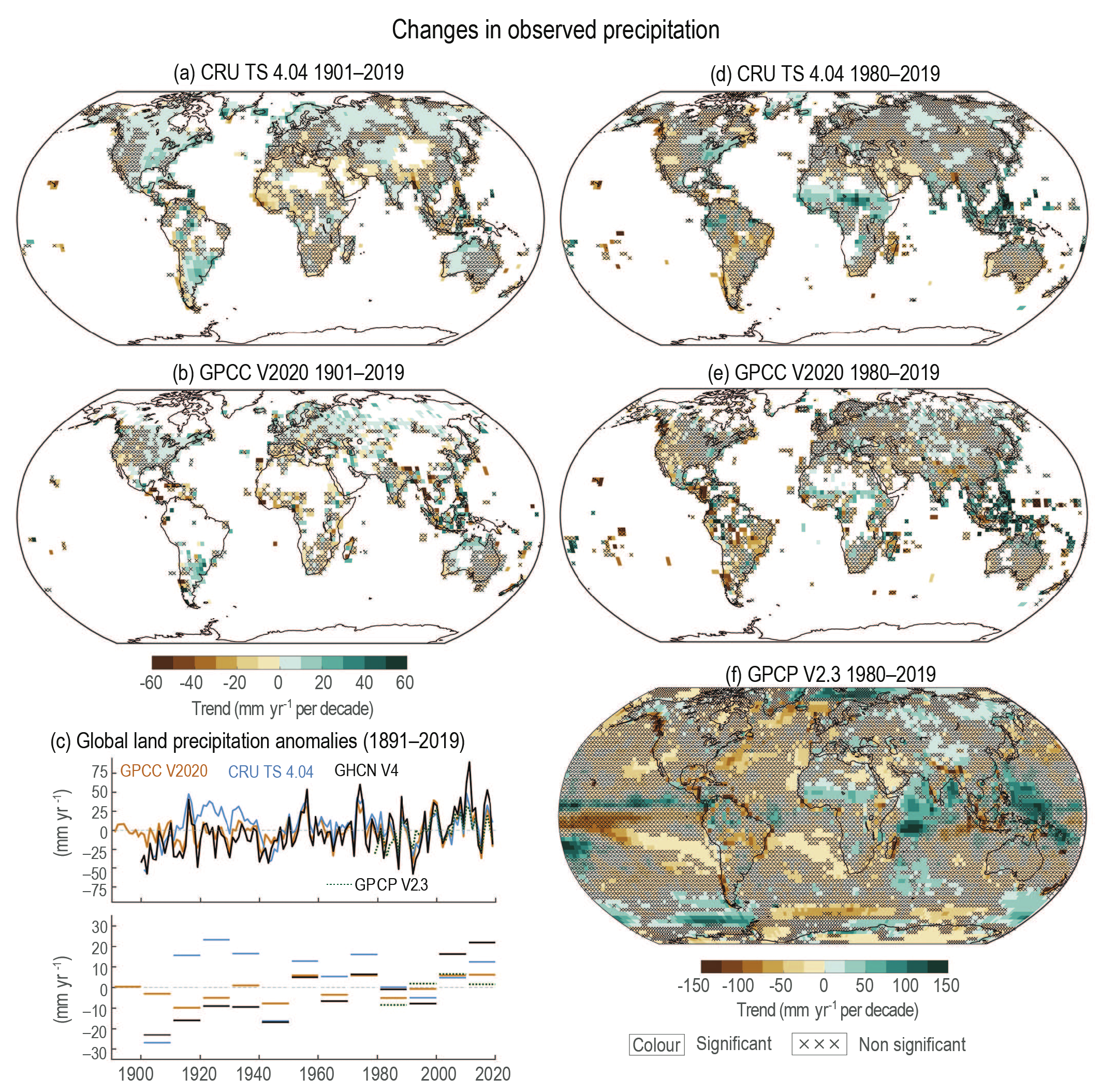
Changes in several components of the global hydrological cycle provide evidence for overall strengthening since at least 1980 (high confidence) . However, there is low confidence in comparing recent changes with past variations due to limitations in paleoclimate records at continental and global scales. Global land precipitation has likely increased since 1950, with a faster increase since the 1980s (medium confidence). Near-surface specific humidity has increased over both land (very likely) and the oceans (likely) since at least the 1970s. Relative humidity has very likely decreased over land areas since 2000. Global total column water vapour content hasvery likely increased during the satellite era. Observational uncertainty leads to low confidence in global trends in precipitation minus evaporation and river runoff. {2.3.1.3}
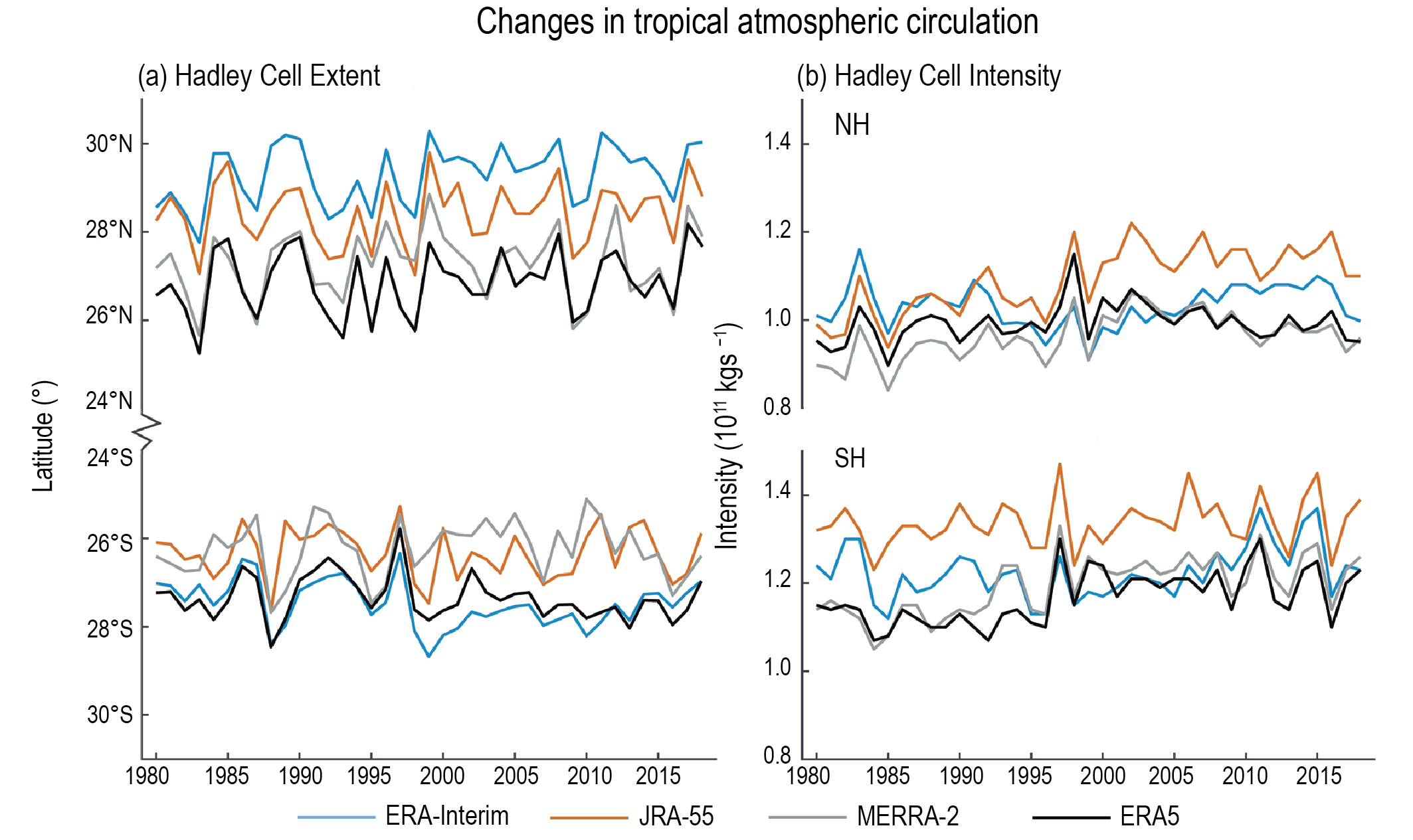
Several aspects of the large-scale atmospheric circulation have likely changed since the mid-20th century, but limited proxy evidence yields low confidence in how these changes compare to longer-term climate. The Hadley circulation has likely widened since at least the 1980s, and extratropical storm tracks have likely shifted poleward in both hemispheres. Global monsoon precipitation has likely increased since the 1980s, mainly in the Northern Hemisphere (medium confidence). Since the 1970s, near-surface winds have likely weakened over land. Over the oceans, near-surface winds likely strengthened over 1980–2000, but divergent estimates lead to low confidence in the sign (direction) of change thereafter. It is likely that the northern stratospheric polar vortex has weakened since the 1980s and experienced more frequent excursions toward Eurasia. {2.3.1.4}
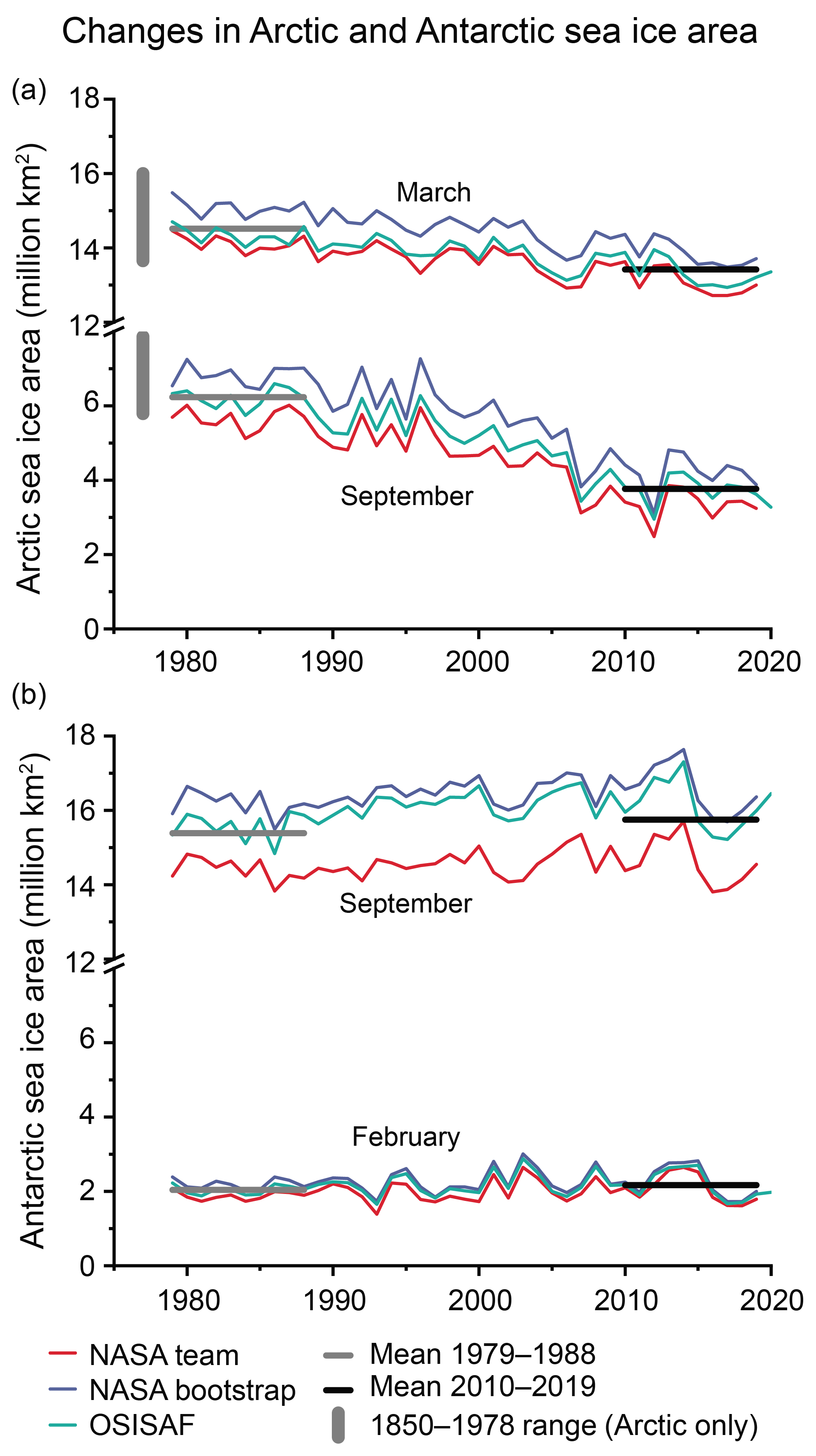
Current Arctic sea ice coverage levels are the lowest since at least 1850 for both annual mean and late-summer values (high confidence) and for the past 1000 years for late-summer values (medium confidence). Between 1979 and 2019, Arctic sea ice area has decreased in both summer and winter, with sea ice becoming younger, thinner and more dynamic (very high confidence). Decadal means for Arctic sea ice area decreased from 6.23 million km2 in 1979–1988 to 3.76 million km2 in 2010–2019 for September and from 14.52 to 13.42 million km2 for March. Antarctic sea ice area has experienced little net change since 1979 (high confidence), with only minor differences between sea ice area decadal means for 1979–1988 (2.04 million km2 for February, 15.39 million km2 for September) and 2010–2019 (2.17 million km2 for February, 15.75 million km2 for September). {2.3.2.1}
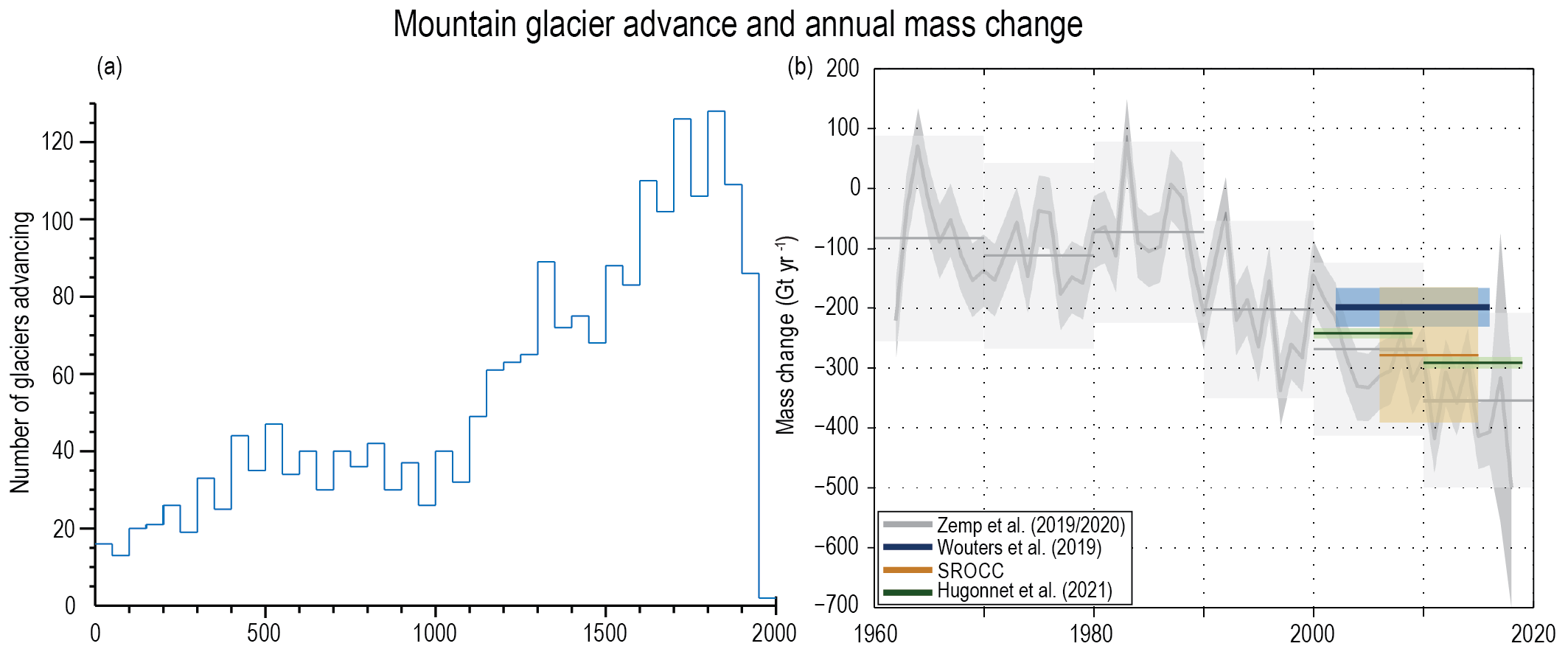
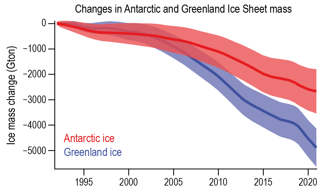
Changes across the terrestrial cryosphere are widespread, with several indicators now in states unprecedented in centuries to millennia (high confidence). Reductions in spring snow cover extent have occurred across the Northern Hemisphere since at least 1978 (very high confidence). With few exceptions, glaciers have retreated since the second half of the 19th century and have continued to retreat at increased rates since the 1990s (very high confidence); this behaviour is unprecedented in at least the last 2000 years (medium confidence). Greenland Ice Sheet (GrIS) mass loss has increased substantially since 2000 (high confidence). The Greenland Ice Sheet was smaller than at present during the Last Interglacial period (high confidence) and the mid-Holocene (high confidence). The Antarctic Ice Sheet (AIS) lost mass between 1992 and 2020 (very high confidence), with an increasing rate of mass loss over this period (medium confidence). Although permafrost persists in areas of the Northern Hemisphere where it was absent prior to 3000 years ago, increases in temperatures in the upper 30 m over the past three to four decades have been widespread (high confidence). {2.3.2}
Global mean sea level (GMSL) is rising, and the rate of GMSL rise since the 20th century is faster than over any preceding century in at least the last three millennia (high confidence). Since 1901, GMSL has risen by 0.20 [0.15 to 0.25] m, and the rate of rise is accelerating. The average rate of sea level rise was 1.3 [0.6 to 2.1] mm yr–1 between 1901 and 1971, increasing to 1.9 [0.8 to 2.9] mm yr–1 between 1971 and 2006, and further increasing to 3.7 [3.2 to 4.2] mm yr–1 between 2006 and 2018 (high confidence). Further back in time, there is medium confidence that GMSL was within –3.5 to +0.5 m (very likely) of present during the mid-Holocene (6000 years ago), 5 to 10 m (likely) higher during the Last Interglacial (125,000 years ago), and 5 to 25 m (very likely) higher during the mid-Pliocene Warm Period (MPWP) (3.3 million years ago). {2.3.3.3}
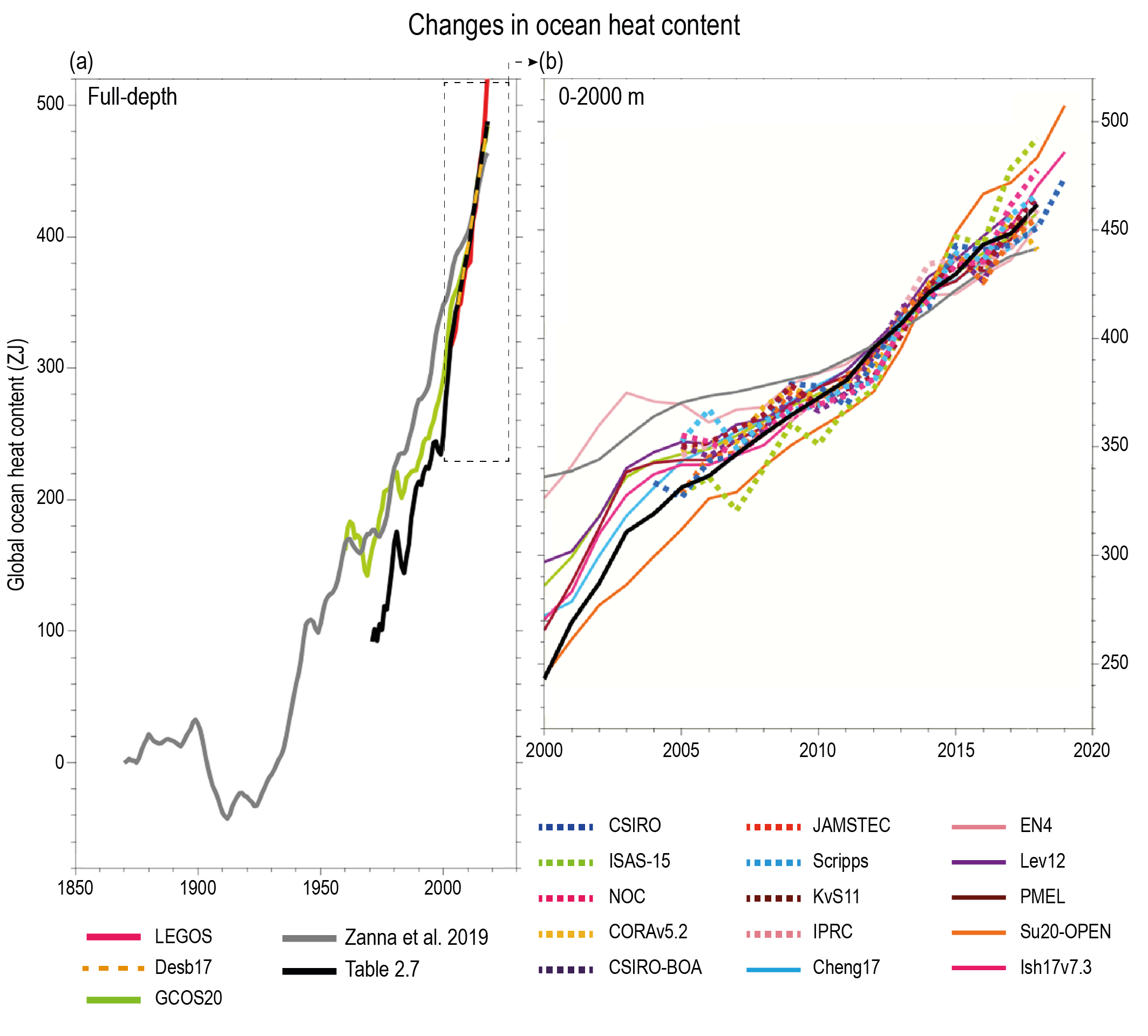
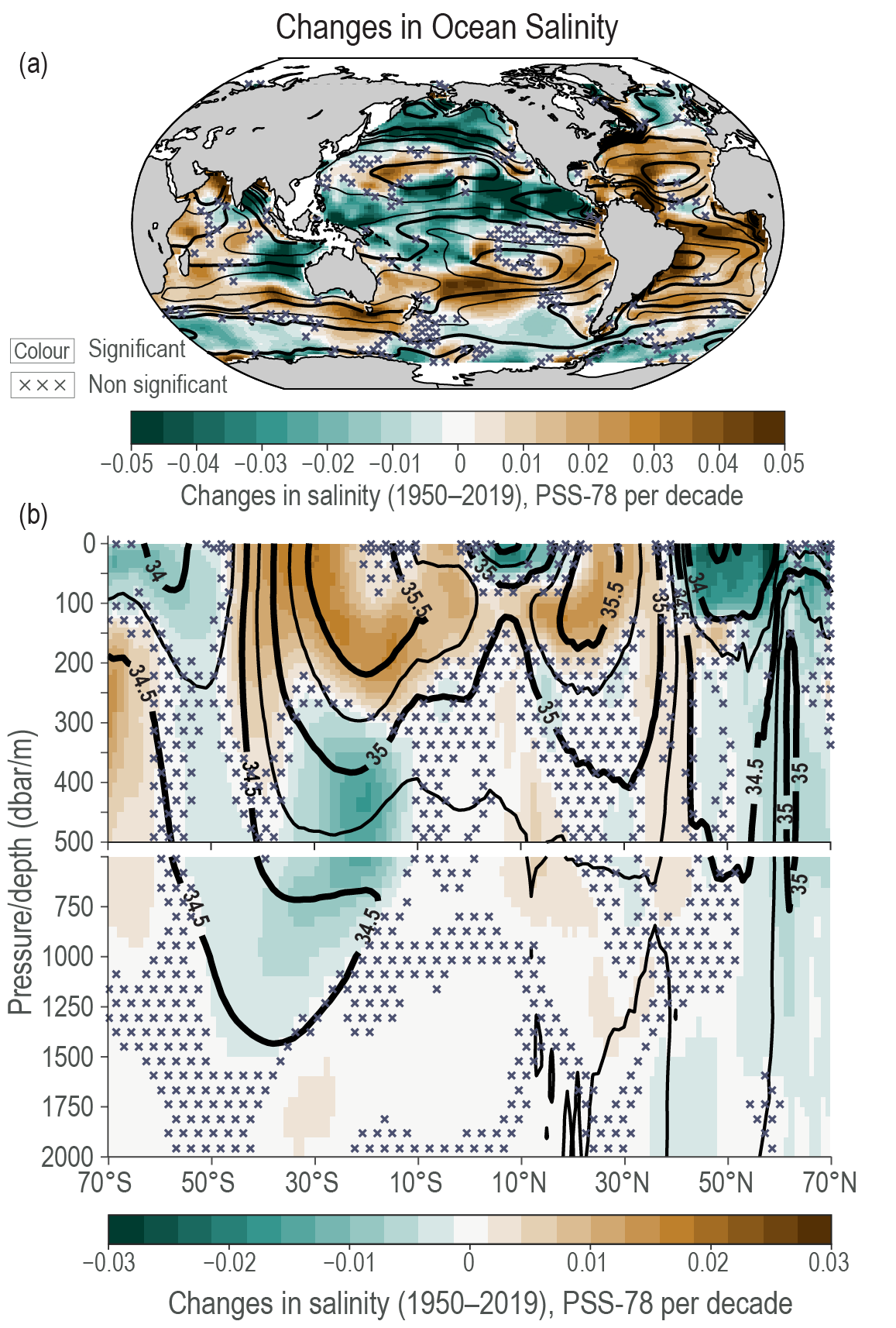
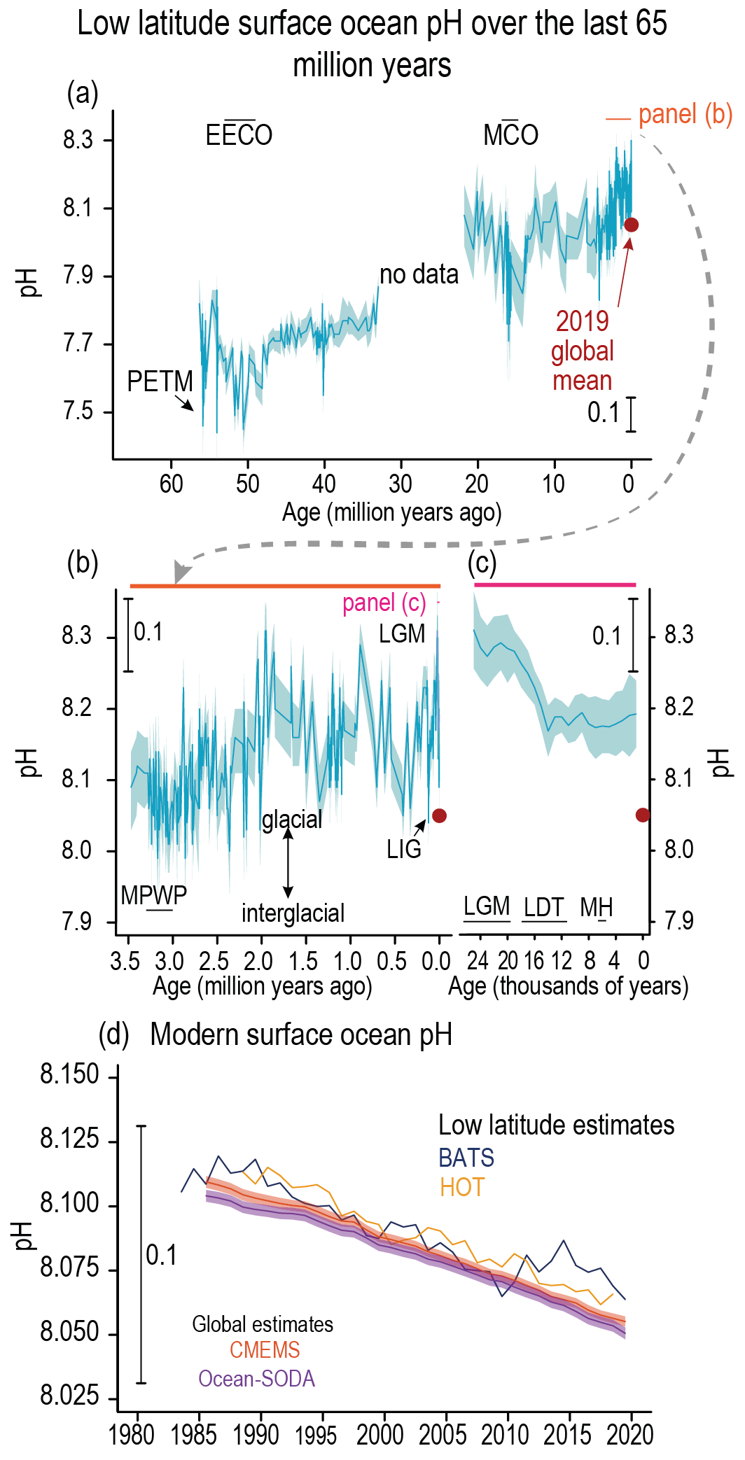
Recent ocean changes are widespread, and key ocean indicators are in states unprecedented for centuries to millennia (high confidence). Since 1971, it is virtually certain that global ocean heat content has increased for the upper (0–700 m) layer, very likely for the intermediate (700–2000 m) layer and likely below 2000 m, and is currently increasing faster than at any point since at least the last deglacial transition (18 to 11 thousand years ago) (medium confidence). It is virtually certain that large-scale near-surface salinity contrasts have intensified since at least 1950. The Atlantic Meridional Overturning Circulation (AMOC) was relatively stable during the past 8000 years (medium confidence) but declined during the 20th century (low confidence). Ocean pH has declined globally at the surface over the past four decades (virtually certain) and in all ocean basins in the ocean interior (high confidence) over the past 2–3 decades. A long-term increase in surface open ocean pH occurred over the past 50 million years (high confidence), and surface ocean pH as low as recent times is uncommon in the last 2 million years (medium confidence). Deoxygenation has occurred in most open ocean regions during the mid 20th to early 21st centuries (high confidence), with decadal variability (medium confidence). Oxygen minimum zones are expanding at many locations (high confidence). {2.3.3}
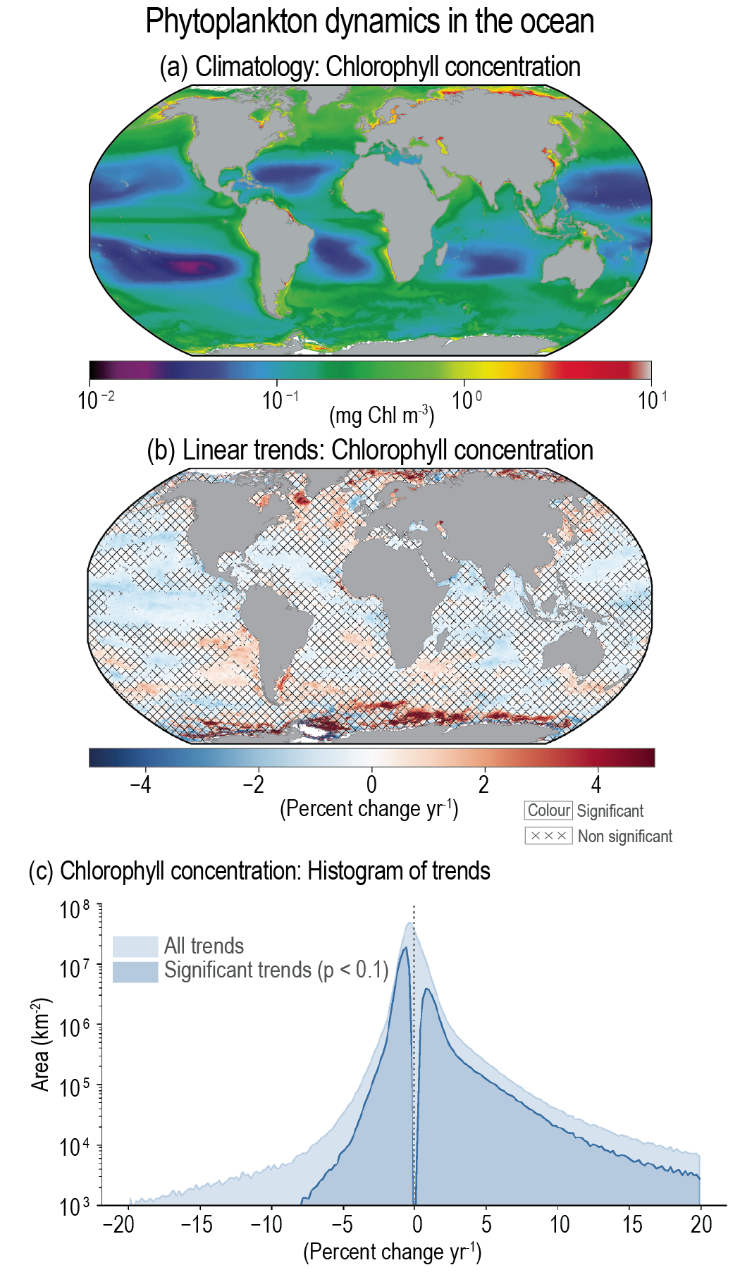
Changes in the marine biosphere are consistent with large-scale warming and changes in ocean geochemistry (high confidence). The ranges of many marine organisms are shifting towards the poles and towards greater depths (high confidence), but a minority of organisms are shifting in the opposite directions. This mismatch in responses across species means that the species composition of ecosystems is changing (medium confidence). At multiple locations, various phenological metrics for marine organisms have changed in the last 50 years, with the nature of the changes varying with location and with species (high confidence). In the last two decades, the concentration of phytoplankton at the base of the marine food web, as indexed by chlorophyll concentration, has shown weak and variable trends in low and mid-latitudes and an increase in high latitudes (medium confidence). Global marine primary production decreased slightly from 1998–2018, with increasing production in the Arctic (medium confidence). {2.3.4.2}
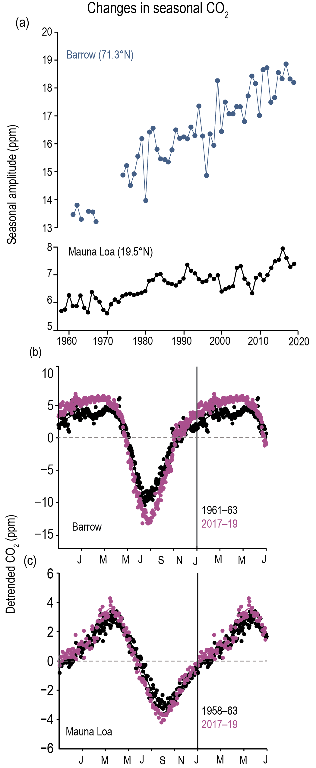
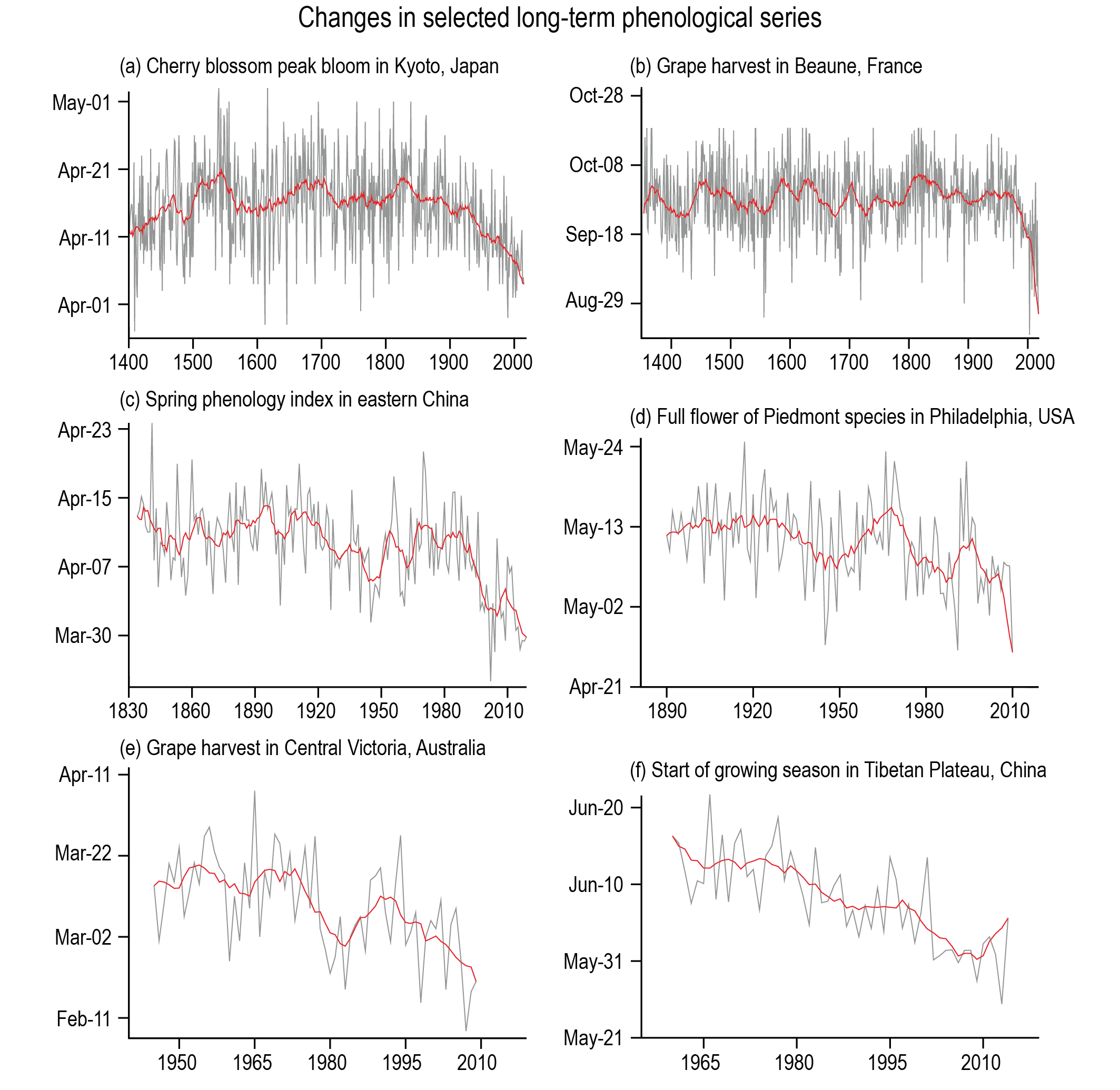
Changes in key global aspects of the terrestrial biosphere are consistent with large-scale warming (high confidence). Over the last century, there have been poleward and upslope shifts in the distributions of many land species (very high confidence) as well as increases in species turnover within many ecosystems (high confidence). Over the past half century, climate zones have shifted poleward, accompanied by an increase in the length of the growing season in the Northern Hemisphere extratropics and an increase in the amplitude of the seasonal cycle of atmospheric CO2 above 45°N (high confidence). Since the early 1980s, there has been a global-scale increase in the greenness of the terrestrial surface (high confidence). {2.3.4.1, 2.3.4.3}
During the mid-Pliocene warm period (MPWP, 3.3 to 3.0 million years ago) slowly changing large-scale indicators reflect a world that was warmer than present, with CO2 similar to current levels. CO2 levels during the MPWP were similar to present for a sustained period, within a range of 360–420 ppm (medium confidence). Relative to the present, GMST, GMSL and precipitation rate were all higher, the Northern Hemisphere latitudinal temperature gradient was lower, and major terrestrial biomes were shifted northward (very high confidence). There is high confidence that cryospheric indicators were diminished and medium confidence that the Pacific longitudinal temperature gradient weakened and monsoon systems strengthened. {2.3, Cross-Chapter Box 2.4, 9.6.2}
Inferences from past climate states based on proxy records can be compared with climate projections over coming centuries to place the range of possible futures into a longer-term context. There is medium confidence in the following mappings between selected paleo periods and future projections: during the Last Interglacial, GMST is estimated to have been 0.5°C–1.5°C warmer than the 1850–1900 reference for a sustained period, which overlaps the low end of the range of warming projected under SSP1-2.6, including its negative-emissions extension to the end of the 23rd century [1.0°C to 2.2°C]. During the mid-Pliocene Warm Period, the GMST estimate [2.5°C to 4.0°C] is similar to the range projected under SSP2-4.5 for the end of the 23rd century [2.3°C to 4.6°C]. GMST estimates for the Miocene Climatic Optimum [5°C to 10°C] and Early Eocene Climatic Optimum [10°C to 18°C], about 15 and 50 million years ago, respectively, overlap with the range projected for the end of the 23rd century under SSP5-8.5 [6.6°C to 14.1°C]. {Cross-Chapter Box 2.1, 2.3.1, 4.3.1.1, 4.7.1.1}
Changes in Modes of Variability
Since the late 19th century, major modes of climate variability show no sustained trends but do exhibit fluctuations in frequency and magnitude at inter-decadal time scales, with the notable exception of the Southern Annular Mode, which has become systematically more positive (high confidence). There is high confidencethat these modes of variability have existed for millennia or longer, but low confidence in detailed reconstructions of most modes prior to direct instrumental records. Both polar annular modes have exhibited strong positive trends toward increased zonality of mid-latitude circulation over multi-decadal periods, but these trends have not been sustained for the Northern Annular Mode since the early 1990s (high confidence). For tropical ocean modes, a sustained shift beyond multi-centennial variability has not been observed for El Niño–Southern Oscillation (medium confidence), but there is limited evidence and low agreement about the long-term behaviour of other tropical ocean modes. Modes of decadal and multi-decadal variability over the Pacific and Atlantic oceans exhibit no significant trends over the period of observational records (high confidence). {2.4}
2.1 Introduction
This chapter assesses the evidence basis for large-scale past changes in selected components of the climate system. As such, it combines much of the assessment performed in Chapters 2 through 5 of the Fifth Assessment Report (AR5) WGI contribution (IPCC, 2013) that, taken together, supported a finding of unequivocal recent warming of the climate system. The Sixth Assessment Report (AR6) WGI Report structure differs substantially from that in AR5 ( Section 1.1.2). This chapter focuses upon observed changes in climate system drivers and changes in key selected large-scale indicators of climate change and in important modes of variability (Cross-Chapter Box 2.2), which allow for an assessment of changes in the global climate system in an integrated manner. This chapter is complemented by Chapters 3 and 4, which respectively consider model assessment/detection and attribution, and future climate projections for subsets of these same indicators and modes. It does not consider changes in observed extremes, which are assessed in Chapter 11. The chapter structure is outlined in the visual abstract (Figure 2.1).
Use is made of paleoclimate, in situ, ground- and satellite-based remote sensing, and reanalysis data products where applicable (Section 1.5). All observational products used in the chapter are detailed in Annex I, and information on data sources and processing for each figure and table can be found in the associated chapter Table 2.SM.1 available as an electronic supplement to the chapter. Use of common periods ranging from 56 million years ago through to the recent past is applied to the extent permitted by available data (Section 1.4.1 and Cross-Chapter Box 2.1). In all cases, the narrative proceeds from as far in the past as the data permit through to the present. Each sub-section starts by highlighting the key findings from AR5 and any relevant AR6-cycle Special Reports (SROCC, SR1.5, SRCCL), and then outlines the new evidence-basis arising from a combination of: (i) new findings reported in the literature, including new datasets and new versions of existing datasets; and (ii) recently observed changes, before closing with a new summary assessment.
Trends, when calculated as part of this assessment, have wherever possible been calculated using a common approach following that adopted in Box 2.2 of Chapter 2 of AR5 (Hartmann et al., 2013). In addition to trends, consideration is also made of changes between various time slices/periods in performing the assessment (Section 1.4.1 and Cross-Chapter Box 2.1). Statistical significance of trends and changes are assessed at the two-tailed 90% confidence (very likely) level unless otherwise stated. Limited use is also made of published analyses that have employed a range of methodological choices. In each such case the method/metric is stated.
There exist a variety of inevitable and, in some cases, irreducible uncertainties in performing an assessment of the observational evidence for climate change. In some instances, a combination of sources of uncertainty is important. For example, the assessment of global surface temperature over the instrumental record in Section 2.3.1.1.3 considers a combination of observational-dataset and trend-estimate uncertainties. Furthermore, estimates of parametric uncertainty are often not comprehensive in their consideration of all possible factors and, when such estimates are constructed in distinct manners, there are often significant limitations to their direct comparability (Hartmann et al., 2013, their Box 2.1).
Cross-Chapter Box 2.1 | Paleoclimate Reference Periods in the Assessment Report
Contributing Authors: Darrell S. Kaufman (United States of America), Kevin D. Burke (United States of America), Samuel Jaccard (Switzerland), Christopher Jones (United Kingdom), Wolfgang Kiessling (Germany), Daniel J. Lunt (United Kingdom), Olaf Morgenstern (New Zealand/Germany), John W. Williams (United States of America)
Over the long evolution of the Earth’s climate system, several periods have been extensively studied as examples of distinct climate states. This Cross-Chapter Box places multiple paleoclimate reference periods into the unifying context of Earth’s long-term climate history, and points to sections in the report with additional information about each period. Other reference periods, including those of the industrialized era, are described in Section 1.4.1.
The reference periods represent times that were both colder and warmer than present, and periods of rapid climate change, many with informative parallels to projected climate (Cross-Chapter Box 2.1, Table 1). They are used to address a wide variety of questions related to natural climate variations in the past (FAQ 1.3). Most of them are used as targets to evaluate the performance of climate models under different climate forcings (Section 3.8.2), while also providing insight into the ocean-atmospheric circulation changes associated with various radiative forcings and geographical changes.
Global mean surface temperature (GMST) is a key indicator of the changing state of the climate system. Earth’s mean temperature history during the current geological era (Cenozoic, beginning 66 Ma (66 million years ago)) can be broadly characterized as follows (Cross-Chapter Box 2.1, Figure 1): (i) transient warming during the first 15 Myr (15 million years) of the Cenozoic, punctuated by the Paleocene–Eocene Thermal Maximum; (ii) a long-term cooling over tens of millions of years beginning around 50 Ma, driven by (among other factors) the slow drift of tectonic plates, which drove mountain building, erosion and volcanism, and reconfigured ocean passages, all of which ultimately moved carbon from the atmosphere to other reservoirs and led to the development of the Antarctic Ice Sheet (AIS) about 35–30 Ma; (iii) the intensification of cooling by climate feedbacks involving interactions among tectonics, ice albedo, ocean circulation, land cover and greenhouse gases, causing ice sheets to develop in the Northern Hemisphere (NH) by about 3 Ma; (iv) glacial-interglacial fluctuations paced by slow changes in Earth’s astronomical configuration (orbital forcing) and modulated by changes in the global carbon cycle and ice sheets on time scales of tens to hundreds of thousands of years, with particular prominence during the last 1 Myr; (v) a transition with both gradual and abrupt shifts from the Last Glacial Maximum to the present interglacial epoch (Holocene), with sporadic ice-sheet breakup disrupting ocean circulation; (vi) continued warming followed by minor cooling following the mid-Holocene, with superposed centennial- to decadal-scale fluctuations caused by volcanic activity, among other factors; (vii) recent warming related to the build-up of anthropogenic greenhouse gases (Sections 2.2.3 and 3.3.1).
GMST estimated for each of the reference periods based on proxy evidence (Section 2.3.1.1) can be compared with climate projections over coming centuries to place the range of possible futures into a longer-term context (Cross-Chapter Box 2.1, Figure 1). Here, the very likely range of GMST for the warmer world reference periods are compared with the very likely range of GSAT projected for the end the 21st century (2080–2100; Table 4.5) and the likely range for the end of the 23rd century (2300; Table 4.9) under multiple Shared Socio-economic Pathway (SSP) scenarios. From this comparison, there is medium confidence in the following: GMST estimated for the warmest long-term period of the Last Interglacial about 125 ka (125,000 years ago; 0.5°C–1.5°C relative to 1850–1900) overlaps with the low end of the range of temperatures projected under SSP1-2.6 including its negative emissions extension to the end of the 23rd century (1.0°Cto 2.2°C). GMST estimated for a period of prolonged warmth during the mid-Pliocene Warm Period about 3 Ma [2.5°C to 4.0°C] is similar to temperatures projected under SSP2-4.5 for the end of the 23rd century (2.3°C to 4.6°C). GMST estimated for the Miocene Climatic Optimum [5°C to 10°C] and Early Eocene Climatic Optimum [10°C to 18°C], about 15 and 50 Ma, respectively, overlap with the range projected for the end of the 23rd century under SSP5-8.5 (6.6°C to 14.1°C).
Cross-Chapter Box 2.1
Cross-Chapter Box 2.1, Table 1 | Paleo-reference periods, listed from oldest to youngest. See ‘AR6 Sections’ (right-hand column) for literature citations related to each ‘Sketch of the climate state.’ See WGII (Chapters 1, 2 and 3) for citations related to paleontological changes. See Interactive Atlas for simulated climate variables for MPWP, LIG, LGM and MH.
Period | Age/Yeara | Sketch of the Climate State (Relative to 1850–1900), andModel Experiment Protocols(italic). Values for large-scale climate indicators including global temperature, sea level and atmospheric CO2are shown in Figure 2.34. | AR6 Sections (partial list) |
Paleocene–Eocene Thermal Maximum (PETM) | 55.9–55.7 Ma (million years ago) | A geologically rapid, large-magnitude warming event at the start of the Eocene when a large pulse of carbon was released to the ocean-atmosphere system, decreasing ocean pH and oxygen content. Terrestrial plant and animal communities changed composition, and species distributions shifted poleward. Many deep-sea species went extinct and tropical coral reefs diminished. DeepMIP (Lunt et al., 2017) | 2.2.3.1 2.3.1.1.1 5.1.2.1 5.3.1.1 7.5.3.4 |
Early Eocene Climatic Optimumb (EECO) | 53–49 Ma | Prolonged ‘hothouse’ period with atmospheric CO2 concentration >1000 ppm, similar to SSP5-8.5 end-of-century values. Continental positions were somewhat different to present due to tectonic plate movements; polar ice was absent and there was more warming at high latitudes than in the equatorial regions. Near-tropical forests grew at 70°S, despite seasonal polar darkness. DeepMIP, about 50 Ma (Lunt et al., 2017, 2021) | 2.2.3.1 2.3.1.1.1 7.4.4.1.2 7.5.3.4 7.5.6 |
Miocene Climatic Optimumb (MCO) | 16.9–14.7 Ma | Prolonged warm period with atmospheric CO2 concentrations 400–600 ppm, similar to SSP2-4.5 end-of-century values. Continental geography was broadly similar to modern. At times, Arctic sea ice may have been absent, and the AIS was much smaller or perhaps absent. Peak in Cenozoic reef development. MioMIP1, Early and Middle Miocene (Steinthorsdottir et al., 2021) | 2.2.3.1 2.3.1.1.1 |
Mid-Pliocene Warm Period (MPWP) | 3.3–3.0 Ma | Warm period when atmospheric CO2 concentration was similar to present (Cross-Chapter Box 2.4). The Arctic was much warmer, but tropical temperatures were only slightly warmer. Sea level was higher than present. Treeline extended to the northern coastline of the NH continents. Also called, ‘Piacenzian warm period.’PMIP4midPliocene-eoi400, 3.2 Ma (Haywood et al., 2016, 2020) | CCB2.4 7.4.4.1.2 7.5.3.3 8.2.2.2 9.6.2 |
Last Interglacial (LIG) | 129–116 ka (thousand years ago) | Most recent interglacial period, similar to mid-Holocene, but with more pronounced seasonal insolation cycle. Northern high latitudes were warmer, with reduced sea ice. Greenland and West Antarctic ice sheets were smaller and sea level was higher. Monsoon was enhanced. Boreal forests extended into Greenland and subtropical animals such as Hippopotamusoccupied Britain. Coral reefs expanded latitudinally and contracted equatorially. PMIP4lig127k, 127 ka (Otto-Bliesner et al., 2017, 2021) | 2.2.3.2 2.3.1.1.1 2.3.3.3 9.2.2.1 9.6.2 |
Last Glacial Maximum (LGM) | 23–19 ka | Most recent glaciation when global temperatures were lower, with greater cooling toward the poles. Ice sheets covered much of North America and north-west Eurasia, and sea level was commensurately lower. Atmospheric CO2 was lower; more carbon was sequestered in the ocean interior. Precipitation was generally lower over most regions; the atmosphere was dustier, and ranges of many plant species contracted into glacial refugia; forest extent and coral reef distribution was reduced worldwide. PMIP4lgm, 21 ka (Kageyama et al., 2017, 2021a) | 2.2.3.2 2.3.1.1.1 3.3.1.1 3.8.2.1 5.1.2.2 7.4.4.1.2 7.5.3.1 8.3.2.4 9.6.2 |
Last Deglacial Transition (LDT) | 18–11 ka | Warming that followed the Last Glacial Maximum, with decreases in the extent of the cryosphere in both polar regions. Sea level, ocean meridional overturning circulation, and atmospheric CO2 increased during two main steps. Temperate and boreal species ranges expanded northwards. Community turnover was large. Megafauna populations declined or went extinct. | 2.2.3.2 5.1.2.2 5.3.1.2 8.6.1 9.6.2 |
Mid-Holocene (MH) | 6.5–5.5 ka | Middle of the present interglacial when the CO2 concentration was similar to the onset of the industrial era, but the orbital configuration led to warming and shifts in the hydrological cycle, especially NH monsoons. Approximate time during the current interglacial and before the onset of major industrial activities when GMST was highest. Biome-scale loss of North African grasslands caused by weakened monsoons and collapses of temperate tree populations linked to hydroclimate variability. PMIP4 mid-Holocene, 6 ka (Otto-Bliesner et al., 2017; Brierley et al., 2020) | 2.3.1.1.2 2.3.2.4 2.3.3.3 3.3.1.1 3.8.2.1 8.3.2.4 8.6.2.2 9.6.2 |
Last millenniumc | 850–1850 CE | Climate variability during this period is better documented on annual to centennial scales than during previous reference periods. Climate changes were driven by solar, volcanic, land cover, and anthropogenic forcings, including strong increases in greenhouse gasses since 1750. PMIP4 past1000, 850–1849 CE (Jungclaus et al., 2017) | 2.3.1.1.2 2.3.2.3 8.3.1.6 8.5.2.1 Box 11.3 |
aCE: Common Era; ka: thousands of years ago; Ma: millions of years ago.
b The word ‘optimum’ is traditionally used in geosciences to refer to the warmest interval of a geologic period.
c The terms ‘Little Ice Age’ and ‘Medieval Warm Period’ (or ‘Medieval Climate Anomaly’) are not used extensively in this report because the timing of these episodes is not well defined and varies regionally. Since AR5, new proxy records have improved climate reconstructions at decadal scale across the last millennium. Therefore, the dates of events within these two roughly defined periods are stated explicitly when possible.
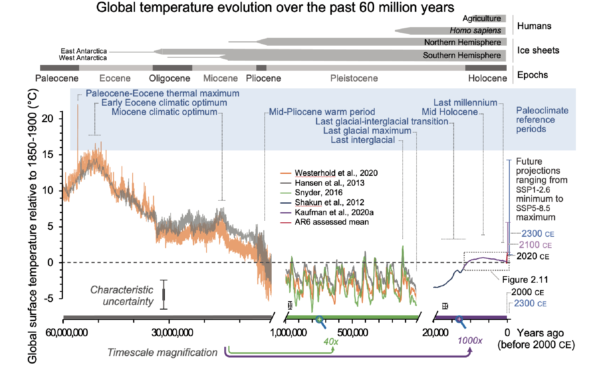
Cross-Chapter Box 2.1, Figure 1 | Global mean surface temperature (GMST) over the past 60 million years (60 Myr) relative to 1850–1900 shown on three time scales. Information about each of the nine paleo reference periods (blue font) and sections in AR6 that discuss these periods are listed in Cross-Chapter Box 2.1 Table 1. Grey horizontal bars at the top mark important events. Characteristic uncertainties are based on expert judgement and are representative of the approximate midpoint of their respective time scales; uncertainties decrease forward in time. GMST estimates for most paleo reference periods (Figure 2.34) overlap with this reconstruction, but take into account multiple lines of evidence. Future projections span the range of global surface air temperature best estimates for SSP1–2.6 and SSP5–8.5 scenarios described in Section 1.6. Range shown for 2100 is based on CMIP6 multi-model mean for 2081–2100 from Table 4.5; range for 2300 is based upon an emulator and taken from Table 4.9. Further details on data sources and processing are available in the chapter data table (Table 2.SM.1).
2.2 Changes in Climate Drivers
This section assesses the magnitude and rates of changes in both natural and anthropogenically mediated climate drivers over a range of time scales. First, changes in insolation (orbital and solar; Section 2.2.1), and volcanic stratospheric aerosol (Section 2.2.2) are assessed. Next, well-mixed greenhouse gases (GHGs; CO2, N2O and CH4) are covered in Section 2.2.3, with climate feedbacks and other processes involved in the carbon cycle assessed in Chapter 5. The section continues with the assessment of changes in halogenated GHGs (Section 2.2.4), stratospheric water vapour, stratospheric and tropospheric ozone (Section 2.2.5), and tropospheric aerosols (Section 2.2.6). Short-lived climate forcers (SLCFs), their precursor emissions and key processes are assessed in more detail in Chapter 6. Section 2.2.7 assesses the effect of historical land cover change on climate, including biophysical and biogeochemical processes. Section 2.2.8 summarizes the changes in the Earth’s energy balance since 1750 using the comprehensive assessment of effective radiative forcing (ERF) performed in Section 7.3. For some SLCFs with insufficient spatial or temporal observational coverage, ERFs are based on model estimates, but also reported here for completeness and context. Tabulated global mixing ratios of all well-mixed GHGs and ERFs from 1750–2019 are provided in Annex III.
2.2.1 Solar and Orbital Forcing
The AR5 assessed solar variability over multiple time scales, concluding that total solar irradiance (TSI) multi-millennial fluctuations over the past 9 kyr were <1 W m–2, but with no assessment of confidence provided. For multi-decadal to centennial variability over the last millennium, AR5 emphasized reconstructions of TSI that show little change (<0.1%) since the Maunder Minimum (1645–1715) when solar activity was particularly low, again without providing a confidence level. The AR5 further concluded that the best estimate of radiative forcing due to TSI changes for the period 1750–2011 was 0.05–0.10 W m–2 (medium confidence), and that TSIvery likely changed by –0.04 [–0.08 to 0.00] W m–2 between 1986 and 2008. Potential solar influences on climate due to feedbacks arising from interactions with galactic cosmic rays are assessed in Section 7.3.4.5.
Slow periodic changes in the Earth’s orbit around the Sun mainly cause variations in seasonal and latitudinal receipt of incoming solar radiation. Precise calculations of orbital variations are available for tens of millions of years (Berger and Loutre, 1991; Laskar et al., 2011). The range of insolation averaged over boreal summer at 65°N was about 83 W m−2 during the past million years, and 3.2 W m−2 during the past millennium, but there was no substantial effect upon global average radiative forcing (0.02 W m–2 during the past millennium).
A new reconstruction of solar irradiance extends back 9 kyr based upon updated cosmogenic isotope datasets and improved models for production and deposition of cosmogenic nuclides (Poluianov et al., 2016), and shows that solar activity during the second half of the 20th century was in the upper decile of the range. TSI features millennial-scale changes with typical magnitudes of 1.5 [1.4 to 2.1] W m–2 (C.-J. Wu et al., 2018). Although stronger variations in the deeper past cannot be ruled out completely (Egorova et al., 2018; Reinhold et al., 2019), there is no indication of such changes having happened over the last 9 kyr.
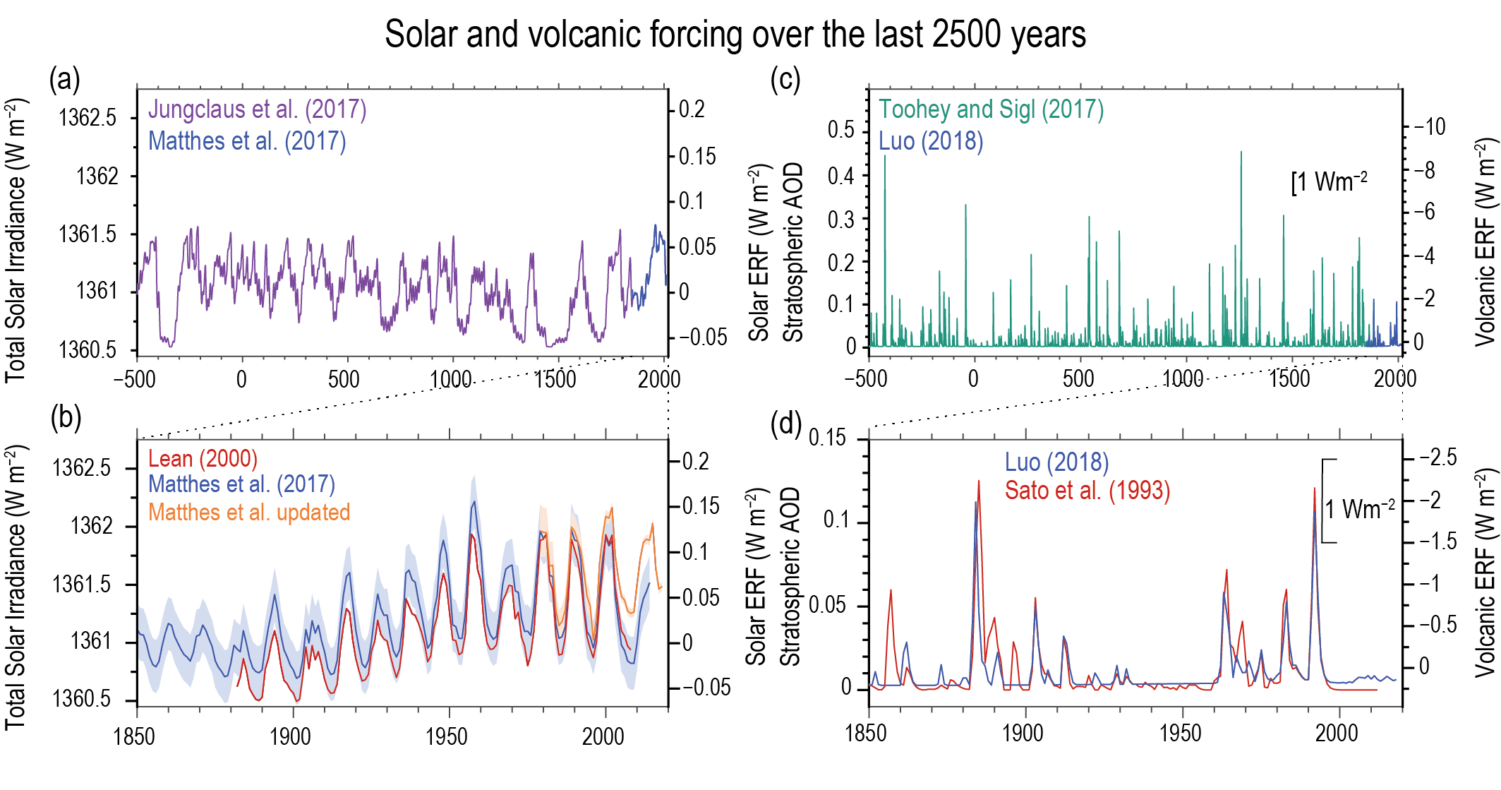
Recent estimates of TSI and spectral solar irradiance (SSI) for the past millennium are based upon updated irradiance models (e.g., Egorova et al., 2018; C.-J. Wu et al., 2018) and employ updated and revised direct sunspot observations over the last three centuries (Clette et al., 2014; Chatzistergos et al., 2017) as well as records of sunspot numbers reconstructed from cosmogenic isotope data prior to this (Usoskin et al., 2016). These reconstructed TSI time series (Figure 2.2a) feature little variation in TSI averaged over the past millennium. The TSI between the Maunder Minimum (1645–1715) and second half of the 20th century increased by 0.7–2.7 W m–2 (Jungclaus et al., 2017; Egorova et al., 2018; Lean, 2018; C.-J. Wu et al., 2018; Lockwood and Ball, 2020; Yeo et al., 2020). This TSI increase implies a change in ERF of 0.09–0.35 W m–2 (Section 7.3.4.4).

Estimation of TSI changes since 1900 (Figure 2.2b) has further strengthened, and confirms a small (less than about 0.1 W m–2) contribution to global climate forcing (Section 7.3.4.4). New reconstructions of TSI over the 20th century (Lean, 2018; C.-J. Wu et al., 2018) support previous results that the TSI averaged over the solar cycle very likely increased during the first seven decades of the 20th century and decreased thereafter (Figure 2.2b). TSI did not change significantly between 1986 and 2019. Improved insights (Krivova et al., 2006; Yeo et al., 2015, 2017; Coddington et al., 2016) show that variability in the 200–400 nm UV range was greater than previously assumed. Building on these results, the forcing proposed by Matthes et al. (2017) has a 16% stronger contribution to TSI variability in this wavelength range compared to the forcing used in the 5th Phase of the Coupled Model Intercomparison Project (CMIP5).
To conclude, solar activity since the late 19th century was relatively high but not exceptional in the context of the past 9 kyr (high confidence). The associated global mean ERF is in the range of –0.06 to +0.08 W m–2 (Section 7.3.4.4).
2.2.2 Volcanic Aerosol Forcing
The AR5 concluded that, on interannual time scales, the radiative effects of volcanic aerosols are a dominant natural driver of climate variability, with the greatest effects occurring within the first 2–5 years following a strong eruption. Reconstructions of radiative forcing by volcanic aerosols used in the Paleoclimate Modelling Intercomparison Project Phase III (PMIP3) simulations and in AR5 featured short-lived perturbations of a range of magnitudes, with events of greater magnitude than –1 W m–2 (annual mean) occurring on average every 35–40 years, although no associated assessment of confidence was given. This section focuses on advances in reconstructions of stratospheric aerosol optical depth (SAOD), whereas (Chapter 7 focuses on the ERF of volcanic aerosols, and Chapter 5 assesses volcanic emissions of CO2 and CH4; tropospheric aerosols are discussed in Section 2.2.6. Cross-Chapter Box 4.1 undertakes an integrative assessment of volcanic effects including potential for 21st century effects.
Advances in analysis of sulphate records from the Greenland Ice Sheet (GrIS) and AIS have resulted in improved dating and completeness of SAOD reconstructions over the past 2.5 kyr (Sigl et al., 2015), a more uncertain extension back to 10 ka (Kobashi et al., 2017; Toohey and Sigl, 2017), and a better differentiation of sulphates that reach high latitudes via stratospheric (strong eruptions) versus tropospheric pathways (A. Burke et al., 2019; Gautier et al., 2019). The PMIP4 volcanic reconstruction extends the period analysed in AR5 by 1 kyr (Figure 2.2c; Jungclaus et al., 2017) and features multiple strong events that were previously misdated, underestimated or not detected, particularly before about 1500 CE. The period between successive large volcanic eruptions (Negative ERF greater than –1 W m–2), ranges from 3–130 years, with an average of 43 ± 7.5 years between such eruptions over the past 2.5 kyr (data from Toohey and Sigl, 2017). The most recent such eruption was that of Mt Pinatubo in 1991. Century-long periods that lack such large eruptions occurred once every 400 years on average. Systematic uncertainties related to the scaling of sulphate abundance in glacier ice to radiative forcing have been estimated to be about 60% (Hegerl et al., 2006). Uncertainty in the timing of eruptions in the proxy record is ± 2 years (95% confidence interval) back to 1.5 ka and ± 4 years before (Toohey and Sigl, 2017).
SAOD averaged over the period 950–1250 CE (0.012) was lower than for the period 1450–1850 CE (0.017) and similar to the period 1850–1900 (0.011). Uncertainties associated with these inter-period differences are not well quantified but have little effect because the uncertainties are mainly systematic throughout the record. Over the past 100 years, SAOD averaged 14% lower than the mean of the previous 24 centuries (back to 2.5 ka), and well within the range of centennial-scale variability (Toohey and Sigl, 2017).
Direct observations of volcanic gas-phase sulphur emissions (mostly SO2), sulphate aerosols, and their radiative effects are available from a variety of sources (Kremser et al., 2016). New estimates of SO2 emissions from explosive eruptions have been derived from satellite (beginning in 1979) and in situ measurements (Höpfner et al., 2015; Carn et al., 2016; Neely III and Schmidt, 2016; Brühl, 2018). Satellite observations of aerosol extinction after recent eruptions have uncertainties of about 15–25% (Vernier et al., 2011; Bourassa et al., 2012). Additional uncertainties occur when gaps in the satellite records are filled by complementary observations or using statistical methods (Thomason et al., 2018). Merged datasets (Thomason et al., 2018) and sparse ground-based measurements (Stothers, 1997) allow for volcanic forcing estimates back to 1850. In contrast to the CMIP5 historical volcanic forcing datasets (Ammann et al., 2003), updated time series (Figure 2.2d; Luo, 2018) feature a more comprehensive set of optical properties including latitude-, height- and wavelength-dependent aerosol extinction, single scattering albedo and asymmetry parameters. A series of small-to-moderate eruptions since 2000 resulted in perturbations in SAOD of 0.004–0.006 (Andersson et al., 2015; Schmidt et al., 2018).
To conclude, strong individual volcanic eruptions cause multi-annual variations in radiative forcing. However, the average magnitude and variability of SAOD and its associated volcanic aerosol forcing since 1900 are not unusual in the context of at least the past 2.5 kyr (medium confidence).
2.2.3 Well-mixed Greenhouse Gases (WMGHGs)
Well-mixed greenhouse gases generally have lifetimes of more than several years. The AR5 assigned medium confidence to the values of atmospheric CO2 concentrations (mixing ratios) during the warm geological periods of the early Eocene and Pliocene. It concluded with very high confidence that, by 2011, the mixing ratios of CO2, CH4, and N2O in the atmosphere exceeded the range derived from ice cores for the previous 800 kyr, and that the observed rates of increase of the greenhouse gases were unprecedented on centennial timescales over at least the past 22 kyr. It reported that over 2005–2011 atmospheric burdens of CO2, CH4, and N2O increased, with 2011 levels of 390.5 parts per million (ppm), 1803.2 parts per billion (ppb) and 324.2 ppb, respectively. Increases of CO2 and N2O over 2005–2011 were comparable to those over 1996–2005, while CH4 resumed increasing in 2007, after remaining nearly constant over 1999–2006. A comprehensive process-based assessment of changes in CO2, CH4, and N2O is undertaken in Chapter 5.
2.2.3.1 CO2 During 450 Ma to 800 ka
Isotopes from continental and marine sediments using improved analytical techniques and sampling resolution have reinforced the understanding of long-term changes in atmospheric CO2 during the past 450 Myr (Table 2.1 and Figure 2.3). In particular, for the last 60 Myr, sampling resolution and accuracy of the boron isotope proxy in ocean sediments has improved (Penman et al., 2014; Anagnostou et al., 2016, 2020; Chalk et al., 2017; Gutjahr et al., 2017; Babila et al., 2018; Dyez et al., 2018; Raitzsch et al., 2018; Sosdian et al., 2018; Henehan et al., 2019, 2020; de la Vega et al., 2020; Harper et al., 2020), the understanding of the alkenone CO2 proxy has increased (e.g., Badger et al., 2019; Stoll et al., 2019; Y. Zhang et al., 2019; Zhang et al., 2020; Rae et al., 2021) and new phytoplankton proxies have been developed and applied (e.g., Witkowski et al., 2018). Understanding of the boron isotope CO2 proxy has improved since AR5 with studies showing very good agreement between boron-CO2 estimates and co-existing ice core CO2 (Hönisch and Hemming, 2005; Foster, 2008; Henehan et al., 2013; Chalk et al., 2017; Raitzsch et al., 2018; see Figure 2.3c). Such independent validation has proven difficult to achieve with the other available CO2 proxies (e.g., Badger et al., 2019; Da et al., 2019; Stoll et al., 2019; Y. Zhang et al., 2019). Remaining uncertainties in these ocean sediment based proxies (Hollis et al., 2019) partly limit the applicability of the alkenoneδ13C and boronδ11B proxies beyond the Cenozoic, although new records are emerging, for example, Jurikova et al. (2020). CO2 estimates from the terrestrial CO2 proxies, such as stomatal density in fossil plants and δ13C of palaeosol carbonates, are available for much of the last 420 Myr. Given the low sampling density, relatively large CO2 uncertainty, and high age uncertainty (relative to marine sediments) of the terrestrial proxies, preference here is given to the marine based proxies (and boron in particular) where possible.
Reference Period | CO2 Concentration (ppm) and Dataset Details | Rate of Change (ppm per century) |
Modern (1995–2014) | 359.6 to 360.4→396.7 to 397.5 (AR6) | 192.3 to 198.3a (AR6) |
Last 100 years (1919–2019) | 302.8 to 306.0→409.5 to 410.3 (AR6) | 103.9 to 107.1 (AR6) |
Approximate pre-industrial baseline (1850–1900; see Cross-Chapter Box 1.2) | 283.4 to 287.6→294.8 to 298.0 (AR6); 284.3b→295.7b (CMIP6) | 16.5 to 27.1a (AR6) 22.8b,a (CMIP6) |
Last millennium (1000–1750) | 278.0 to 285.0 (AR6; average of WAIS Divide, Law Dome and EDML core data) | –6.9 ~ 4.7b (Law Dome); –1.9 ~ 3.2b (EDML); –5.2 ~ 4.2b (WAIS Divide) |
MH | 260.1 to 268.1 (Dome C; CMIP6) | N/A |
LDT | 193.2b→271.2b (AR6); 195.2b→265.3b (Dome C); 191.2b→277.0b (WAIS Divide) | 9.6b (WAIS Divide); 7.1b (Dome C) |
LGM | 188.4 to 194.2 (AR6); 190.5 to 200.1 (WAIS Divide); 186.8 to 202.0 (Byrd); 184.9 to 193.1 (Dome C); 180.5 to 192.7 (Siple Dome); 190b (PMIP6); 174.2 to 205.8 (δ11B proxy) | N/A |
LIG | 265.9 to 281.5 (AR6); 259.4 to 283.8 (Vostok); 266.2 to 285.4 (Dome C); 275b (PMIP4) 282.2 to 305.8 (δ11B proxy) | N/A |
MPWP (KM5c) | 360 to 420 (AR6) | N/A |
EECO | 1150 to 2500 (AR6) | N/A |
PETM | 800 to 1000→1400 to 3150 (AR6) | 4 to 42 (AR6) |
a Centennial rate of change estimated by extrapolation of data from a shorter time period. The values (x to y) representvery likely ranges (90% CIs).
b Data uncertainty is not estimated.
Levels were close to 1750 values during at least one prolonged interval during the Carboniferous and Permian (350–252 Ma). During the Triassic (251.9–201.3 Ma), atmospheric CO2 mixing ratios reached a maximum of between 2000–5000 ppm (200–220 Ma). During the PETM (56 Ma) CO2 rapidly rose from about 900 ppm to about 2000 ppm (Table 2.1; Schubert and Jahren, 2013; Gutjahr et al., 2017; Anagnostou et al., 2020) in 3–20 kyr (Zeebe et al., 2016; Gutjahr et al., 2017; Turner, 2018). Estimated multi-millennial rates of CO2 accumulation during this event range from 0.3–1.5 PgC yr–1 (Gingerich, 2019), at least 4–5 times lower than current centennial rates (Section 5.3.1.1). Based on boron and carbon isotope data, supported by other proxies (Hollis et al., 2019), atmospheric CO2 during the EECO (50 Ma) was between 1150 and 2500 ppm (medium confidence), and then gradually declined over the last 50 Myr at a long-term rate of about 16 ppm Myr–1 (Figure 2.3). The last time the CO2 mixing ratio was as high as 1000 ppm (the level reached by some high emissions scenarios by 2100; Annex III) was prior to the Eocene-Oligocene transition (33.5 Ma; Figure 2.3) that was associated with the first major advance of the AIS (Pearson et al., 2009; Pagani et al., 2011; Anagnostou et al., 2016; Witkowski et al., 2018; Hollis et al., 2019). The compilation of Foster et al. (2017) constrained CO2 concentration to between 290 and 450 ppm during the MPWP, based primarily on the boron-isotope data reported by Martínez-Botí et al. (2015b), consistent with the AR5 range of 300–450 ppm. A more recent high-resolution boron isotope-based study revealed that CO2 cycled during the MPWP from about 330 to about 390 ppm on orbital timescales, with a mean of about 370 ppm (de la Vega et al., 2020). Although data from other proxy types (e.g., stomatal density orδ13C of alkenones) have too low resolution to resolve the orbital-related variability of CO2 during this interval (e.g., Kürschner et al., 1996; Stoll et al., 2019) there is general agreement among the different proxy types with the boron-derived mean (e.g., Stoll et al., 2019). High-resolution sampling (about 1 sample per 3 kyr) with the boron-isotope proxy indicates mean CO2 mixing ratios for the Marine Isotope Stage KM5c interglacial were 360–420 ppm (medium confidence) (de la Vega et al., 2020).
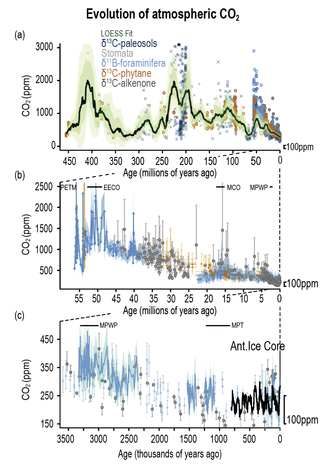 Figure 2.3 | The evolution of atmospheric CO2 through the last 450 million years (450 Myr). The periods covered are 0–450 Ma (a), 0–58 Ma (b), and 0–3500 ka (c), reconstructed from continental rock, marine sediment and ice core records. Note different time scales and axes ranges in panels (a), (b) and (c). Dark and light green bands in (a) are uncertainty envelopes at 68% and 95% uncertainty, respectively. 100 ppm in each panel is shown by the marker in the lower right-hand corner to aid comparison between panels. In panel (b) and (c) the major paleoclimate reference periods (CCB2.1) have been labelled, and in addition: MPT (Mid Pleistocene Transition), MCO (Miocene Climatic Optimum). Further details on data sources and processing are available in the chapter data table (Table 2.SM.1).
 Following the MPWP, the atmospheric CO2 mixing ratio generally decreased at a rate of about 30 ppm Myr–1. It is very likely that CO2 levels as high as the present were not experienced in the last 2 Myr (Hönisch et al., 2009; Bartoli et al., 2011; Martínez-Botí et al., 2015a; Chalk et al., 2017; Dyez et al., 2018; Da et al., 2019; Stoll et al., 2019). Related to the shift of glacial-interglacial cycle frequency from 40 to 100 kyr at 0.8–1.2 Ma, there was a decrease of glacial-period CO2 (Chalk et al., 2017; Dyez et al., 2018). These boron isotope-based CO2 results agree with available records based on ancient ice exposed near the surface of the AIS (Yan et al., 2019), however, direct comparison is limited due to a lack of ancient ice cores with sufficiently continuous stratigraphy (Higgins et al., 2015; Brook and Buizert, 2018).
To conclude, there is high confidence that average EECO and MPWP (KM5c) CO2 concentrations were higher than those preceding industrialization at 1150–2500 ppm and 360–420 ppm, respectively. Although there is some uncertainty due to the non-continuous nature of marine sediment records, the last time atmospheric CO2 mixing ratio was as high as present was very likely more than 2 Ma.
2.2.3.2 Glacial–Interglacial WMGHG Fluctuations from 800 Ka
Since AR5, the number of ice cores for the last 800 kyr has increased and their temporal resolution has improved (Figure 2.4), especially for the last 60 kyr and when combined with analyses of firn air, leading to improved quantification of greenhouse gas concentrations prior to the mid-20th century.
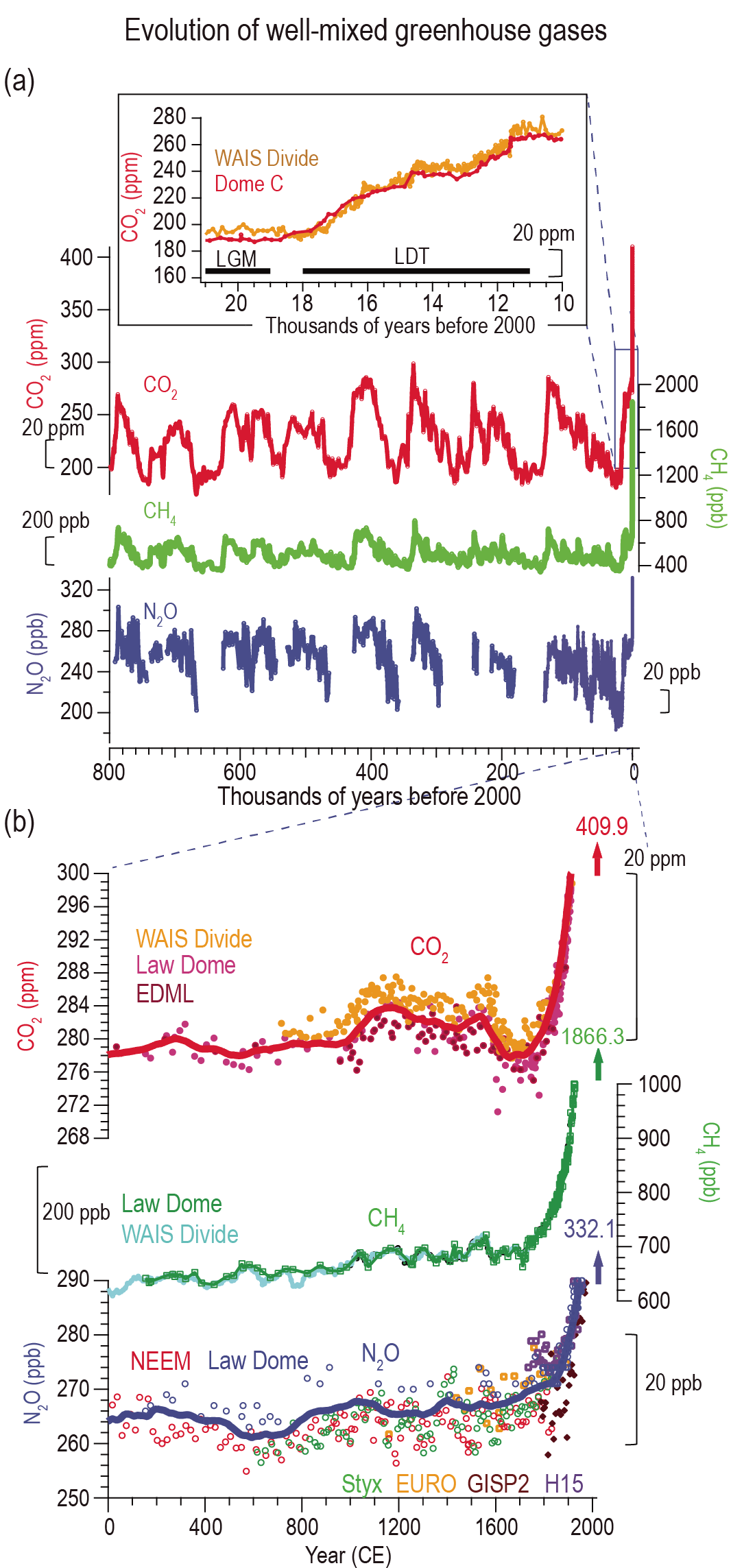 Figure 2.4 | Atmospheric well-mixed greenhouse gas (WMGHG) concentrations from ice cores. (a) Records during the last 800 kyr with the Last Glacial Maximum (LGM) to Holocene transition as inset. (b) Multiple high-resolution records over the CE. The horizontal black bars in panel (a) inset indicate LGM and Last Deglacial Termination (LDT) respectively. The red and blue lines in (b) are 100-year running averages for CO2 and N2O concentrations, respectively. The numbers with vertical arrows in (b) are instrumentally measured concentrations in 2019. Further details on data sources and processing are available in the chapter data table (Table 2.SM.1).
 2.2.3.2.1 Carbon dioxide (CO2)
Records of CO2 from the AIS formed during the last glacial period and the LDT show century-scale fluctuations of up to 9.6 ppm (Ahn et al., 2012; Ahn and Brook, 2014; Marcott et al., 2014; Bauska et al., 2015; Rubino et al., 2019). Although these rates are an order of magnitude lower than those directly observed over 1919–2019 CE (Section 2.2.3.3.1), they provide information on non-linear responses of climate-biogeochemical feedbacks (Section 5.1.2). Multiple records for 0–1850 CE show CO2 mixing ratios of 274–285 ppm. Offsets among ice core records are about 1%, but the long-term trends agree well and show coherent multi-centennial variations of about 10 ppm (Ahn et al., 2012; Bauska et al., 2015; Rubino et al., 2019). Multiple records show CO2 concentrations of 278.3 ± 2.9 ppm in 1750 and 285.5 ± 2.1 ppm in 1850 (Siegenthaler et al., 2005; MacFarling Meure et al., 2006; Ahn et al., 2012; Bauska et al., 2015). CO2 concentration increased by 5.0 ± 0.8 ppm during 970–1130 CE, followed by a decrease of 4.6 ± 1.7 ppm during 1580–1700 CE. The greatest rate of change over the CE prior to 1750 is observed at about 1600 CE, and ranges from –6.9 to +4.7 ppm per century in multiple high-resolution ice core records (Siegenthaler et al., 2005; MacFarling Meure et al., 2006; Ahn et al., 2012; Bauska et al., 2015; Rubino et al., 2019). Although ice core records present low-pass filtered time series due to gas diffusion and gradual bubble close-off in the snow layer over the ice sheet (Fourteau et al., 2020), the rate of increase since 1850 CE (about 125 ppm increase over about 170 years) is far greater than implied for any 170-year period by ice core records that cover the last 800 ka (very high confidence).
2.2.3.2.2 Methane (CH4)
CH4 concentrations over the past 110 kyr are higher in the Northern Hemisphere (NH) than in the Southern Hemisphere (SH), but closely correlated on centennial and millennial timescales (Buizert et al., 2015). On glacial to interglacial cycles, approximately 450 ppb oscillations in CH4 concentrations have occurred (Loulergue et al., 2008). On millennial timescales, most rapid climate changes observed in Greenland and other regions are coincident with rapid CH4 changes (Buizert et al., 2015; Rhodes et al., 2015, 2017). The variability of CH4 on centennial timescales during the early Holocene does not significantly differ from that of the late Holocene prior to about 1850 (Rhodes et al., 2013; Yang et al., 2017). The LGM concentration was 390.5 ± 6.0 ppb (Kageyama et al., 2017). The global mean concentrations during 0–1850 CE varied between 625 and 807 ppb. High-resolution ice core records from Antarctica and Greenland exhibit the same trends with an inter-polar difference of 36–47 ppb (Sapart et al., 2012; L. Mitchell et al., 2013). There is a long-term positive trend of about 0.5 ppb per decade during the CE until 1750 CE. The most rapid CH4 changes prior to industrialization were as large as 30–50 ppb on multi-decadal timescales. Global mean CH4 concentrations estimated from Antarctic and Greenland ice cores are 729.2 ± 9.4 ppb in 1750 and 807.6 ± 13.8 ppb in 1850 (L. Mitchell et al., 2013).
2.2.3.2.3 Nitrous oxide (N2O)
New records show that N2O concentration changes are associated with glacial-interglacial transitions (Schilt et al., 2014). The most rapid change during the last glacial termination is a 30 ppb increase in a 200-year period, which is an order of magnitude smaller than the modern rate (Section 2.2.3.3). During the LGM, N2O was 208.5 ± 7.7 ppb (Kageyama et al., 2017). Over the Holocene the lowest value was 257 ± 6.6 ppb during 6–8 ka, but millennial variation is not clearly detectable due to analytical uncertainty and insufficient ice core quality (Flückiger et al., 2002; Schilt et al., 2010). Recently acquired high-resolution records from Greenland and Antarctica for the last 2 kyr consistently show multi-centennial variations of about 5–10 ppb (Figure 2.4), although the magnitudes vary over time (Ryu et al., 2020). Three high temporal resolution records exhibit a short-term minimum at about 600 CE of 261 ± 4 ppb (MacFarling Meure et al., 2006; Ryu et al., 2020). It is very likely that industrial N2O increase started before 1900 CE (Machida et al., 1995; Sowers, 2001; MacFarling Meure et al., 2006; Ryu et al., 2020). Multiple ice cores show N2O concentrations of 270.1 ± 6.0 ppb in 1750 and 272.1 ± 5.7 ppb in 1850 (Machida et al., 1995; Flückiger et al., 1999; Sowers, 2001; Rubino et al., 2019; Ryu et al., 2020).
2.2.3.3 Modern Measurements of WMGHGs
In this section and for calculation of ERF, surface global averages are determined from measurements representative of the well-mixed lower troposphere. Global averages that include sites subject to significant anthropogenic activities or influenced by strong regional biospheric emissions are typically larger than those from remote sites, and require weighting accordingly (Table 2.2). This section focusses on global mean mixing ratios estimated from networks with global spatial coverage, and updated from the CMIP6 historical dataset (Meinshausen et al., 2017) for periods prior to the existence of global networks.
Species | Lifetime, AR6, ERF | 2011 | 2019 | Change | Network | Species | Lifetime, AR6, ERF | 2011 | 2019 | Change | Network | |
CO2 | # | 390.5 | 409.9 (0.17) | 5.0% | NOAA*a | HCFC-22 | 11.9 | 212.6 | 246.8 (0.5) | 16.1% | NOAA* | |
409.9 (0.4) | 389.7 | 409.5 (0.37) | 5.1% | SIO | 246.8 (0.6) | 213.7 | 246.7 (0.4) | 15.5% | AGAGE* | |||
2.156 | 390.2 | 409.6 (0.31) | 5.0% | CSIRO | 0.053 | 209.0 | 244.1 (3.0) | 22.0% | UCI | |||
390.9 | 410.5 (0.30) | 5.0% | WMO | HCFC-141b | 9.4 | 21.3 | 24.4 (0.1) | 14.4% | NOAA* | |||
390.9 | CMIP6 | 24.4 (0.3) | 21.4 | 24.3 (0.1) | 13.7% | AGAGE* | ||||||
CH4 | 9.1–11.8 | 1803.1 | 1866.6 (1.0) | 3.5% | NOAA* | 0.004 | 20.8 | 26.0 (0.3) | 25.0% | UCI | ||
1866.3 (3.3) | 1803.6 | 1866.1 (2.0) | 3.5% | AGAGE* | HCFC-142b | 18 | 20.9 | 22.0 (0.1) | 5.3% | NOAA* | ||
0.544 | 1791.8 | 1860.8 (3.5) | 3.9% | UCI | 22.3 (0.4) | 21.5 | 22.5 (0.1) | 5.0% | AGAGE* | |||
1802.3 | 1862.5 (2.4) | 3.3% | CSIRO | 0.004 | 21.0 | 22.8 (0.2) | 8.6% | UCI | ||||
1813 | 1877 (3) | 3.5% | WMO | HFC-134a | 14 | 62.7 | 107.8 (0.4) | 72% | NOAA* | |||
1813.1 | CMIP6 | 107.6 (1.0) | 62.8 | 107.4 (0.2) | 71% | AGAGE* | ||||||
N2O | 116–109 | 324.2 | 331.9 (0.2) | 2.4% | NOAA* | 0.018 | 63.4 | 107.6 (1.7) | 70% | UCI | ||
332.1 (0.4) | 324.7 | 332.3 (0.1) | 2.4% | AGAGE* | HFC-125 | 30 | 10.1 | 29.1 (0.3) | 187% | NOAA* | ||
0.208 | 324.0 | 331.6 (0.3) | 2.3% | CSIRO | 29.4 (0.6) | 10.4 | 29.7 (0.1) | 186% | AGAGE* | |||
324.3 | 332.0 (0.2) | 2.4% | WMO | 0.007 | ||||||||
324.2 | CMIP6 | HFC-23 | 228 | 24.1 | 32.4 (0.1) | 35% | AGAGE* | |||||
CFC-12 | 102 | 526.9 | 501.5 (0.3) | –4.8% | NOAA* | 32.4 (0.1) | ||||||
503.1 (3.2) | 529.6 | 504.6 (0.2) | –4.7% | AGAGE* | 0.006 | |||||||
0.180 | 525.3 | 508.4 (2.5) | –3.2% | UCI | HFC-143a | 51 | 11.9 | 23.8 (0.1) | 100% | NOAA* | ||
CFC-11 | 52 | 237.2 | 226.5 (0.2) | –4.5% | NOAA* | 24.0 (0.4) | 12.1 | 24.2 (0.1) | 100% | AGAGE* | ||
226.2 (1.1) | 237.4 | 225.9 (0.1) | –4.8% | AGAGE* | 0.004 | |||||||
0.066 | 237.9 | 224.9 (1.3) | –5.5% | UCI | HFC-32 | 5.4 | 4.27 | 19.2 (0.3) | 350% | NOAA* | ||
CFC-113 | 93 | 74.5 | 69.7 (0.1) | –6.4% | NOAA* | 20.0 (1.4) | 5.15 | 20.8 (0.2) | 304% | AGAGE* | ||
69.8 (0.3) | 74.6 | 69.9 (0.1) | –6.3% | AGAGE* | 0.002 | |||||||
0.021 | 74.9 | 70.0 (0.5) | –6.5% | UCI | CF4 | 50,000 | 79.0 | 85.5 (0.1) | 8.2% | AGAGE* | ||
CFC-114 | 189 | 16.36 | 16.28 (0.03) | –0.5% | AGAGE* | 85.5 (0.2) | ||||||
16.0 (0.05) | 0.005 | |||||||||||
0.005 | C2F6 | 10,000 | 4.17 | 4.85 (0.01) | 16.3% | AGAGE* | ||||||
CFC-115 | 540 | 8.39 | 8.67 (0.02) | 3.3% | AGAGE* | 4.85 (0.1) | ||||||
8.67 (0.02) | 0.001 | |||||||||||
0.002 | SF6 | About 1000 | 7.32 | 9.96 (0.02) | 36.1% | NOAA* | ||||||
CCl4 | 32 | 86.9 | 78.4 (0.1) | –9.8% | NOAA* | 9.95 (0.01) | 7.28 | 9.94 (0.02) | 36.5% | AGAGE* | ||
77.9 (0.7) | 85.3 | 77.3 (0.1) | –9.4% | AGAGE* | 0.006 | |||||||
0.013 | 87.8 | 77.7 (0.7) | –11.5% | UCI |
AGAGE: Advanced Global Atmospheric Gases Experiment; SIO: Scripps Institution of Oceanography; NOAA: National Oceanic and Atmospheric Administration, Global Monitoring Laboratory; UCI: University of California, Irvine; CSIRO: Commonwealth Scientific and Industrial Research Organization, Aspendale, Australia; WMO: World Meteorological Organization, Global Atmosphere Watch, CMIP6 (Climate Model Intercomparison Project Phase 6). Mixing ratios denoted by AR6 are representative of the remote, unpolluted troposphere, derived from one or more measurement networks (denoted by *). Minor differences between 2011 values reported here and in the previous Assessment Report (AR5) are due to updates in calibration and data processing. ERF in 2019 is taken from Table 7.5, and the difference with the AR5 assessment reflects updates in the estimates of AR6 global mixing ratios and updated radiative calculations. Uncertainties, in parenthesis, are estimated at 90% confidence interval. Networks use different methods to estimate uncertainties. Some uncertainties have been rounded up to be consistent with the number of decimal places shown. Lifetime is reported in years: # indicates multiple lifetimes for CO2. For CH4 and N2O the two values represent total atmospheric lifetime and perturbation lifetime.
2.2.3.3.1 Carbon dioxide (CO2)
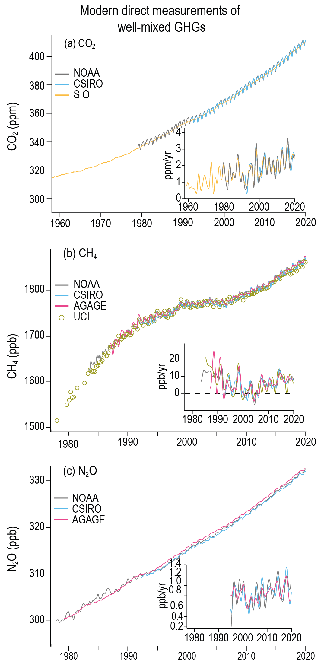
There has been a positive trend in globally averaged surface CO2 mixing ratios since 1958 (Figure 2.5a), that reflects the imbalance of sources and sinks (Section 5.2). The growth rate has increased overall since the 1960s (Figure 2.5a inset), while annual growth rates have varied substantially, for example, reaching a peak during the strong El Niño events of 1997–1998 and 2015–2016 (Bastos et al., 2013; Betts et al., 2016). The average annual CO2 increase from 2000 through 2011 was 2.0 ppm yr–1 (standard deviation 0.3 ppm yr–1), similar to what was reported in AR5. From 2011 through 2019 it was 2.4 ppm yr–1 (standard deviation 0.5 ppm yr–1), which is higher than that of any comparable time period since global measurements began. Global networks consistently show that the globally averaged annual mean CO2 has increased by 5.0% since 2011, reaching 409.9 ± 0.4 ppm in 2019 (NOAA measurements). Further assessment of changing seasonality is undertaken in Section 2.3.4.1.
 Figure 2.5 | Globally averaged dry-air mole fractions of greenhouse gases. (a) CO2 from SIO, CSIRO, and NOAA/GML (b) CH4 from NOAA, AGAGE, CSIRO, and UCI; and (c) N2O from NOAA, AGAGE, and CSIRO (Table 2.2). Growth rates, calculated as the time derivative of the global means after removing seasonal cycle are shown as inset figures. Note that the CO2 series is 1958–2019 whereas CH4, and N2O are 1979–2019. Units are parts per million (ppm) or parts per billion (ppb). Further details on data are in Annex III, and on data sources and processing are available in the chapter data table (Table 2.SM.1).
 2.2.3.3.2 Methane (CH4)
The globally averaged surface mixing ratio of CH4 in 2019 was 1866.3 ± 3.3 ppb, which is 3.5% higher than 2011, while observed increases from various networks range from 3.3–3.9% (Table 2.2 and Figure 2.5b). There are marked growth rate changes over the period of direct observations, with a decreasing rate from the late-1970s through the late-1990s, very little change in concentrations from 1999–2006, and resumed increases since 2006. Atmospheric CH4 fluctuations result from complex variations of sources and sinks. A detailed discussion of recent methane trends and our understanding of their causes is presented in Cross-Chapter Box 5.2.
2.2.3.3.3 Nitrous oxide (N2O)
The AR5 reported 324.2 ± 0.1 ppb for global surface annual mean N2O in 2011; since then, it has increased by 2.4% to 332.1 ± 0.4 ppb in 2019. Independent measurement networks agree well for both the global mean mixing ratio and relative change since 2011 (Table 2.2). Over 1995–2011, N2O increased at an average rate of 0.79 ± 0.05 ppb yr–1. The growth rate has been higher in recent years, amounting to 0.96 ± 0.05 ppb yr–1 from 2012 to 2019 (Figure 2.5c and Section 5.2.3.5).
2.2.3.4 Summary of Changes in WMGHGs
In summary, CO2 has fluctuated by at least 2000 ppm over the last 450 Myr (medium confidence). The last time CO2 concentrations were similar to the present-day was over 2 Ma (high confidence). Further, it is certain that WMGHG mixing ratios prior to industrialization were lower than present-day levels and the growth rates of the WMGHGs from 1850 are unprecedented on centennial timescales in at least the last 800 kyr. During the glacial-interglacial climate cycles over the last 800 kyr, the concentration variations of the WMGHG were 50–100 ppm for CO2, 210–430 ppb for CH4 and 60–90 ppb for N2O. Between 1750–2019 mixing ratios increased by 131.6 ± 2.9 ppm (47%), 1137 ± 10 ppb (156%), and 62 ± 6 ppb (23%), for CO2, CH4, and N2O, respectively (very high confidence). Since 2011 (AR5) mixing ratios of CO2, CH4, and N2O have further increased by 19 ppm, 63 ppb, and 7.7 ppb, reaching in 2019 levels of 409.9 (± 0.4) ppm, 1866.3 (± 3.3) ppb, and 332.1 (± 0.4) ppb, respectively. By 2019, the combined ERF (relative to 1750) of CO2, CH4 and N2O was 2.9 ± 0.5 W m–2 (Table 2.2; Section 7.3.2).
2.2.4 Halogenated Greenhouse Gases (CFCs, HCFCs, HFCs, PFCs, SF6 and others)
This category includes ozone depleting substances (ODS), their replacements, and gases used industrially or produced as by-products. Some have natural sources (Section 6.2.2.4). The AR5 reported that atmospheric abundances of chlorofluorocarbons (CFCs) were decreasing in response to controls on production and consumption mandated by the Montreal Protocol on Substances that Deplete the Ozone Layer and its amendments. In contrast, abundances of both hydrochlorofluorocarbons (HCFCs, replacements for CFCs) and hydrofluorocarbons (HFCs, replacements for HCFCs) were increasing. Atmospheric abundances of perfluorocarbons (PFCs), SF6, and NF3 were also increasing.
Further details on ODS and other minor greenhouse gases can be found in the Scientific Assessment of Ozone Depletion: 2018 (Engel et al., 2018; Montzka et al., 2018b). Updated mixing ratios of the most radiatively important gases (ERF >0.001 W m–2) are reported in Table 2.2, and additional gases (ERF <0.001 W m–2) are shown in Annex III.
2.2.4.1 Chlorofluorocarbons (CFCs)
Atmospheric abundances of most CFCs have continued to decline since 2011 (AR5). The globally-averaged abundance of CFC-12 decreased by 25 ppt (4.8%) from 2011 to 2019, while CFC-11 decreased by about 11 ppt (4.7%) over the same period (Table 2.2 and Figure 2.6). Atmospheric abundances of some minor CFCs (CFC-13, CFC-115, CFC-113a) have increased since 2011 (Annex III), possibly related to use of HFCs (Laube et al., 2014). Overall, as of 2019 the ERF from CFCs has declined by 9 ± 0.5% from its maximum in 2000, and 4.7 ± 0.6% since 2011 (Table 7.5).
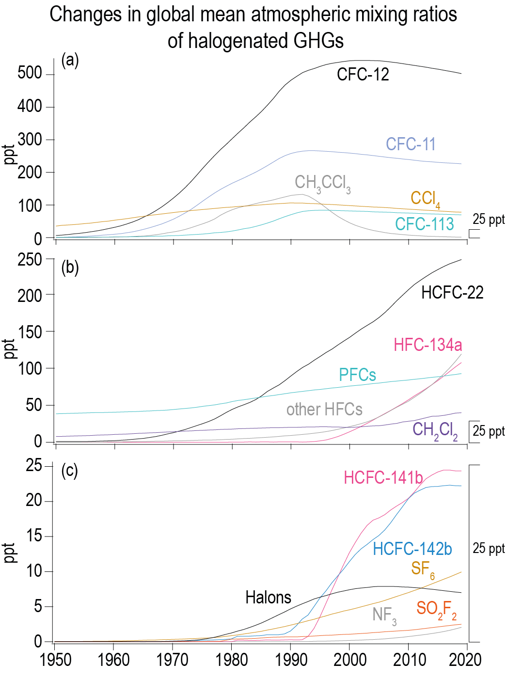 Figure 2.6 | Global mean atmospheric mixing ratios of select ozone-depletingsubstances and other greenhouse gases. Data shown are based on the CMIP6 historical dataset and data from NOAA and AGAGE global networks. PFCs include CF4, C2 f6, and C3F8, and c-C4F8; Halons include halon-1211, halon-1301, and halon-2402; other HFCs include HFC-23, HFC-32, HFC-125, HFC-143a, HFC-152a, HFC-227ea, HFC-236fa, HFC-245fa, and HFC-365mfc, and HFC-43-10mee. Note that the y-axis range is different for (a), (b) and (c) and a 25 parts per trillion (ppt) yardstick is given next to each panel to aid interpretation. Further data are in Annex III and details on data sources and processing are available in the chapter data table (Table 2.SM.1).
 While global reporting indicated that CFC-11 production had essentially ceased by 2010, and the atmospheric abundance of CFC-11 is still decreasing, emissions inferred from atmospheric observations began increasing in 2013–2014 and remained elevated for 5–6 years, suggesting renewed and unreported production (Montzka et al., 2018a, 2021; Rigby et al., 2019; Park et al., 2021). The global lifetimes of several ozone-depleting substances have been updated (SPARC, 2013), in particular for CFC-11 from 45 to 52 years.
2.2.4.2 Hydrochlorofluorocarbons (HCFCs)
The atmospheric abundances of the major HCFCs (HCFC-22, HCFC-141b, HCFC-142b), primarily used in refrigeration and foam blowing, are increasing, but rates of increase have slowed in recent years (Figure 2.6). Global mean mixing ratios (Table 2.2) showed good concordance at the time of AR5 for the period 2005–2011. For the period 2011–2019, the UCI network detected larger increases in HCFC-22, HCFC-141b, and HCFC-142b compared to the NOAA and AGAGE networks. Reasons for the discrepancy are presently unverified, but could be related to differences in sampling locations in the networks (Simpson et al., 2012). Emissions of HCFC-22, derived from atmospheric data, have remained relatively stable since 2012, while those of HCFC-141b and HCFC-142b have declined (Engel et al., 2018). Minor HCFCs, HCFC-133a and HCFC-31, have been detected in the atmosphere (currently less than 1 ppt) and may be unintentional by-products of HFC production (Engel et al., 2018).
2.2.4.3 Hydrofluorocarbons (HFCs), Perfluorocarbons (PFCs), Sulphur Hexafluoride (SF6) and Other Radiatively Important Halogenated Gases
Hydrofluorocarbons (HFCs) are replacements for CFCs and HCFCs. The atmospheric abundances of many HFCs increased between 2011 and 2019. HFC-134a (mobile air conditioning, foam blowing, and domestic refrigerators) increased by 71% from 63 ppt in 2011 to 107.6 ppt in 2019 (Table 2.2). The UCI network detected a slightly smaller relative increase (53%). HFC-23, which is emitted as a by-product of HCFC-22 production, increased by 8.4 ppt (35%) over 2011–2019. HFC-32 used as a substitute for HCFC-22, increased at least by 300%, and HFC-143a and HFC-125 showed increases of 100% and 187%, respectively. While the ERF of HFC-245fa is currently <0.001 W m–2, its atmospheric abundance doubled since 2011 to 3.1 ppt in 2019 (Annex III). In contrast, HFC-152a is showing signs of stable (steady-state) abundance.
Other radiatively important gases with predominantly anthropogenic sources also continue to increase in abundance. SF6, used in electrical distribution systems, magnesium production, and semi-conductor manufacturing, increased from 7.3 ppt in 2011 to 10.0 ppt in 2019 (+36%). Alternatives to SF6 or SF6-free equipment for electrical systems have become available in recent years, but SF6 is still widely in use in electrical switch gear (Simmonds et al., 2020). The global lifetime of SF6 has been revised from 3200 years to about 1000 years (Kovács et al., 2017; Ray et al., 2017) with implications for climate emissions metrics (Section 7.6.2). NF3, which is used in the semi-conductor industry, increased 147% over the same period to 2.05 ppt in 2019. Its contribution to ERF remains small, however, at 0.0004 W m–2. The atmospheric abundance of SO2 f2, which is used as a fumigant in place of ozone-depleting methyl bromide, reached 2.5 ppt in 2019, a 46% increase from 2011. Its ERF also remains small at 0.0005 W m–2.
The global abundance of CCl4 continues to decline, down about 9.6% since 2011. Following a revision of the global lifetime from 26 to 32 years, and discovery of previously unknown sources (e.g., biproducts of industrial emissions), knowledge of the CCl4 budget has improved. There is now better agreement between top-down emissions estimates (based on atmospheric measurements) and industry-based estimates (Engel et al., 2018). Halon-1211, mainly used for fire suppression, is also declining, and its ERF dropped below 0.001 W m–2 in 2019. While CH2 cl2 has a short atmospheric lifetime (6 months), and is not well-mixed, its abundance is increasing and its ERF is approaching 0.001 W m–2.
Perfluorocarbons CF4 and C2 f6, which have exceedingly long global lifetimes, showed modest increases from 2011 to 2019. CF4, which has both natural and anthropogenic sources, increased 8.2% to 85.5 ppt, and C2 f6 increased 16.3% to 4.85 ppt. c–C4F8, which is used in the electronics industry and may also be generated during the production of polytetrafluoroethylene (PTFE, also known as ‘Teflon’) and other fluoropolymers (Mühle et al., 2019), has increased 34% since 2011 to 1.75 ppt, although its ERF remains below 0.001 W m–2. Other PFCs, present at mixing ratios <1 ppt, have also been quantified (Droste et al., 2020; see Annex III).
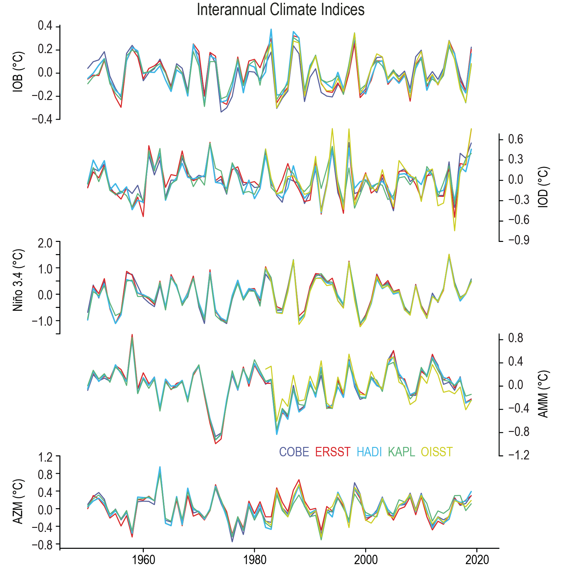 Figure 2.37 | Indices of interannual climate variability from 1950–2019 based upon several sea surface temperature data products. Shown are the following indices from top to bottom: IOB mode, IOD, Niño3.4, AMM and AZM. All indices are based on area-averaged annual data (see Annex IV). Further details on data sources and processing are available in the chapter data table (Table 2.SM.1).
 2.2.4.4 Summary of Changes in Halogenated Gases
In summary, by 2019 the ERF of halogenated GHGs had increased by 3.5% since 2011, reflecting predominantly a decrease in the atmospheric mixing ratios of CFCs and an increase in their replacements. However, average annual ERF growth rates associated with halogenated gases since 2011 are a factor of seven lower than in the 1970s and 1980s. Direct radiative forcings from CFCs, HCFCs, HFCs, and other halogenated greenhouse gases were 0.28, 0.06, 0.04, and 0.03 W m–2 respectively, totalling 0.41 ± 0.07 W m–2 in 2019 (see Table 7.5).
2.2.5 Other Short-lived Gases
2.2.5.1 Stratospheric Water Vapour
The AR5 assessed low confidence in stratospheric water vapour (SWV) trends based on substantial seasonal and interannual variability in satellite data from 1992 to 2011. The 1980–2010 record of balloon-borne frost point hygrometer measurements over Boulder, Colorado (40°N), showed an average net increase of 1.0 ± 0.2 ppm (27 ± 6%) in the 16–26 km layer.
Since AR5, bias-adjusted spatially comprehensive SWV measurements by different satellite sensors were merged to form continuous records (Hegglin et al., 2014; Froidevaux et al., 2015; Davis et al., 2016). These indicate no net global increase of SWV in the lower stratosphere since the late 1980s. Hegglin et al. (2014) reported a latitudinal dependence of SWV trends and suggested that the upward trend over Boulder should not be considered representative of the global stratosphere, while Lossow et al. (2018) showed insignificant differences between SWV trends at Boulder and those for the 35–45°N zonal mean from 1980 to 2010 using model simulations and satellite observations.
Recent studies of dynamical influences on SWV (Eguchi et al., 2015; Evan et al., 2015; Tao et al., 2015; Konopka et al., 2016; Diallo et al., 2018; Garfinkel et al., 2018) have demonstrated that the quasi-biennial oscillation (QBO), El Niño–Southern Oscillation (ENSO), Sudden Stratospheric Warming (SSW) events and possibly also Pacific Decadal Variability (PDV; W. Wang et al., 2016), can significantly influence SWV abundance and the tropical cold point tropopause temperatures that largely control water vapour entering the stratosphere. It has also been shown that the convective lofting of ice can moisten the lower stratosphere over large regions (Dessler et al., 2016; Anderson et al., 2017; Avery et al., 2017). Near-global observations of SWV have revealed unusually strong and abrupt interannual changes, especially in the tropical lower stratosphere. Between December 2015 and November 2016, the tropical mean SWV anomaly at 82 hPa dropped from 0.9 ± 0.1 ppm to –1.0 ± 0.1 ppm, accompanied by highly anomalous QBO-related dynamics in the tropical stratosphere (P.A. Newman et al., 2016; Tweedy et al., 2017) and the transition of ENSO from strong El Niño to La Niña conditions (Davis et al., 2017). The tropical mean SWV anomaly then rose sharply to 0.7 ± 0.1 ppm in June 2017 as warm westerlies returned to the tropical lower stratosphere and ENSO neutral conditions prevailed (Davis et al., 2017).
In summary, in situ measurements at a single mid-latitude location indicate about a 25% net increase in stratospheric water vapour since 1980, while merged satellite data records since the late 1980s suggest little net change. Recent studies of dynamical influences on SWV have highlighted their substantial roles in driving large interannual variability that complicates trend detection. There thus continues to be low confidence in trends of SWV over the instrumental period. Disregarding dynamic influences on SWV, an ERF of 0.05 ± 0.05 W m–2 is estimated for SWV produced by CH4 oxidation (Section 7.3.2.6), unchanged from AR5.
2.2.5.2 Stratospheric Ozone
The AR5 assessed that it was certain that global stratospheric ozone from the mid-1990s to 2011 was nearly constant and about 3.5% lower than in the reference period 1964–1980. Most of the declines occurred prior to the mid-1990s.
Global annual mean total ozone (Figure 2.7) significantly declined by about 3.5% during the 1980s and the early 1990s and by 2.5% over 60°S–60°N (near-global). Then, during 2000–2017, both global and near-global concentrations increased slightly, but not significantly, all in line with production and consumption limits of ODS regulated under the Montreal Protocol and its amendments. Near-global 2014–2017 mean total ozone is about 2.2% below the pre-ozone depletion 1964–1980 average (Braesicke et al., 2018). At southern and northern mid-latitudes, declines are 5.5% and 3.0% compared to the 1964–1980 average respectively. Total ozone remained practically unchanged in the tropics (Braesicke et al., 2018). Emission of ODS started before 1980 and some estimates suggest that as much as 40% of the long-term ozone loss occurred between 1960 and 1980 (Shepherd et al., 2014), lowering the 1964–1980 baseline values by about 1% (outside the polar regions), a value close to observational uncertainties. The world’s longest record of total ozone measurements from Arosa, Switzerland, initiated in 1926, does not show any substantial long-term changes before about 1980 (Staehelin et al., 2018).
 Figure 2.7 | Time series of annual mean total column ozone from 1964–2019. Values are in Dobson Units (DU), a good proxy for vertically integrated stratospheric ozone. Time series are shown for (a) near-global domain; (b–d) three zonal bands; and (e) polar (60°–90°) total ozone in March (Northern Hemisphere) and October (Southern Hemisphere): the months when polar ozone losses usually are largest. Further details on data sources and processing are available in the chapter data table (Table 2.SM.1).
 ERF depends strongly on the altitude of ozone changes. Two stratospheric regions are mainly responsible for long-term changes outside the polar regions. In the upper stratosphere (35–45 km), there was a strong decline (about 10%) from the start of observations in 1979 up to the mid-1990s and a subsequent increase by about 4% to present (SPARC/IO3C/GAW, 2019). In the lower stratosphere (20–25 km), there also was a statistically significant decline (7–8%) up to the mid-1990s, followed by stabilization or a small further decline (Ball et al., 2018, 2019), although the natural variability is too strong to make a conclusive statement (Chipperfield et al., 2018).
The strongest ozone loss in the stratosphere continues to occur in austral spring over Antarctica (ozone hole) with emergent signs of recovery after 2000 (Langematz et al., 2018). Interannual variability in polar stratospheric ozone is driven by large scale winds and temperatures, and, to a lesser extent, by the stratospheric aerosol loading and the solar cycle. This variability is particularly large in the Arctic, where the largest depletion events, comparable to a typical event in the Antarctic, occurred in 2011 (Manney et al., 2011; Langematz et al., 2018) and again in 2020 (Manney et al., 2020; Grooß and Müller, 2021). Further details on trends and ERF can be found in Sections 6.3.2 and 7.3.2.5.
In summary, compared to the 1964–1980 average, stratospheric ozone columns outside polar regions (60°S–60°N) declined by about 2.5% over 1980–1995, and stabilized after 2000, with 2.2% lower values in 2014–2017. Large ozone depletions continue to appear in spring in the Antarctic and, in particularly cold years, also in the Arctic. Model-based estimates disagree on the sign of the ERF due to stratospheric ozone changes, but agree that it is much smaller in magnitude than that due to tropospheric ozone changes (Section 7.3.2.5).
2.2.5.3 Tropospheric Ozone
The AR5 assessed medium confidence in large-scale increases of tropospheric ozone at rural surface sites across the NH (1970–2010), and in a doubling of European surface ozone during the 20th century, with the increases of surface ozone in the SH being of low confidence. Surface ozone likely increased in East Asia, but levelled off or decreased in the eastern USA and western Europe. Free tropospheric trends (1971–2010) from ozonesondes and aircraft showed positive trends in most, but not all, assessed regions, and for most seasons and altitudes. This section focuses on large scale ozone changes; chemical and physical processes and regional changes in tropospheric ozone are assessed in Section 6.3.2.1 and Section 7.3.2.5 assesses radiative forcing.
Prior to 1850 ozone observations do not exist, but a recent analysis using clumped-isotope composition of molecular oxygen (18O18O in O2) trapped in polar firn and ice, combined with atmospheric chemistry model simulations, constrains the global tropospheric ozone increase to less than 40% between 1850 and 2005, with most of this increase occurring between 1950 and 1980 (Yeung et al., 2019). Recently, the Tropospheric Ozone Assessment Report identified and evaluated 60 records of surface ozone observations collected at rural locations worldwide between 1896 and 1975, which were based on a range of measurement techniques with potentially large uncertainties (Tarasick et al., 2019). They found that from the mid-20th century (1930s to the early 1970s) to 1990–2014, rural surface ozone increased by 30–70% across the northern extra-tropics. This is smaller than the 100% 20th-century increase reported in AR5, which relied on far fewer measurement sites, all in Europe. In the northern tropics limited low-elevation historical data (1954–1975) provide no clear indication of surface ozone increases (Tarasick et al., 2019). However, similar to the northern mid-latitude increases, lower-free tropospheric ozone at Mauna Loa, Hawaii increased by approximately 50% from the late 1950s to present (Cooper et al., 2020). Historical observations are too limited to draw conclusions on surface ozone trends in the SH tropics and mid-latitudes since the mid-20th century, with tropospheric ozone exhibiting little change across Antarctica (Tarasick et al., 2019; Cooper et al., 2020). Based on reliable UV absorption measurements at remote locations (surface and lower troposphere), ozone trends since the mid-1990s varied spatially at northern mid-latitudes, but increased in the northern tropics (2–17%; 1–6 ppbv per decade; (Cooper et al., 2020; Gaudel et al., 2020). Across the SH these more recent observations are too limited to determine zonal trends (e.g., tropics, mid-latitudes, high latitudes).
The earliest observations of free tropospheric ozone (1934–1955) are available from northern mid-latitudes where limited data indicate a tropospheric column ozone increase of 48 ± 30% up to 1990–2012 (Tarasick et al., 2019). Starting in the 1960s, records from ozonesondes show no significant changes in the free troposphere over the Arctic and mid-latitude regions of Canada, but trends are mainly positive elsewhere in the northern mid-latitudes (Oltmans et al., 2013; Cooper et al., 2020). Tropospheric column and free tropospheric trends since the mid-1990s based on commercial aircraft, ozonesonde observations and satellite retrievals (Figure 2.8b,c), are overwhelmingly positive across the northern mid-latitudes (2–7%; 1–4 ppbv per decade) and tropics (2–14%; 1–5 ppbv per decade), with the largest increases (8–14%; 3–6 ppbv per decade) in the northern tropics in the vicinity of southern Asia and Indonesia. Observations in the SH are limited, but indicate average tropospheric column ozone increases of 2–12% (1–5 ppbv) per decade in the tropics (Figure 2.8c), and weak tropospheric column ozone increases (<5%, <1 ppbv per decade) at mid-latitudes (Cooper et al., 2020). Above Antarctica, mid-tropospheric ozone has increased since the late 20th century (Oltmans et al., 2013). The total ozone ERF from 1750 to 2019 best estimate is assessed as 0.47 W m–2 (Section 7.3.2.5) and this is dominated by increases in the troposphere. The underlying modelled global tropospheric ozone column increase (Skeie et al., 2020) from 1850 to 2010 of 40–60%, is somewhat higher than the isotope based upper-limit of Yeung et al. (2019). At mid-latitudes (30°–60°N) model increases of 30–40% since the mid-20th century are broadly consistent with observations.
 Figure 2.8 | Surface and tropospheric ozone trends. (a) Decadal ozone trends by latitude at 28 remote surface sites and in the lower free troposphere (650 hPa, about 3.5 km) as measured by IAGOS aircraft above 11 regions. All trends are estimated for the time series up to the most recently available year, but begin in 1995 or 1994. Colours indicate significance (p-value) as denoted in the in-line key. See Figure 6.5 for a depiction of these trends globally. (b) Trends of ozone since 1994 as measured by IAGOS aircraft in 11 regions in the mid-troposphere (700–300 hPa; about 3–9 km) and upper troposphere (about 10–12 km), as measured by IAGOS aircraft and ozonesondes. (c) Trends of average tropospheric column ozone mixing ratios from the TOST composite ozonesonde product and three composite satellite products based on TOMS, OMI/MLS (Sat1), GOME, SCIAMACHY, OMI, GOME-2A, GOME-2B (Sat2), and GOME, SCIAMACHY, GOME-II (Sat3). Vertical bars indicate the latitude range of each product, while horizontal lines indicate the very likely uncertainty range. Further details on data sources and processing are available in the chapter data table (Table 2.SM.1).
 In summary, limited available isotopicevidence constrains the global tropospheric ozone increase to less than 40% between 1850 and 2005 (low confidence). Based on sparse historical surface/low altitude data tropospheric ozone has increased since the mid-20th century by 30–70% across the NH (medium confidence). Surface/low altitude ozone trends since the mid-1990s are variable at northern mid-latitudes, but positive in the tropics [2 to 17% per decade] (high confidence). Since the mid-1990s, free tropospheric ozone has increased by 2–7% per decade in most regions of the northern mid-latitudes, and 2–12% per decade in the sampled regions of the northern and southern tropics (high confidence). Limited coverage by surface observations precludes identification of zonal trends in the SH, while observations of tropospheric column ozone indicate increases of less than 5% per decade at southern mid-latitudes (medium confidence).
2.2.6 Aerosols
The AR5 assessed large-scale aerosol optical depth (AOD) trends over 2000–2009, concluding that there was low confidence in a global trend, but that AODvery likely decreased from 1990 onwards over Europe and the eastern USA, and increased since 2000 over eastern and southern Asia. The ERF associated with aerosol–radiation interactions for 2011 (relative to 1750) was estimated to be –0.45 ± 0.5 W m–2 and of aerosol–cloud interaction estimated as –0.45 [–1.2 to 0.0] W m–2. Aerosol ERF uncertainty was assessed as the largest contributor to the overall ERF uncertainty since 1750.
This section assesses the observed large-scale temporal evolution of tropospheric aerosols. Aerosol-related processes, chemical and physical properties, and links to air quality, are assessed in Chapter 6. An in-depth assessment of aerosol interactions with radiation and clouds is provided in Section 7.3.3.
Aerosol proxy records of improved temporal resolution and quality are now available (Kylander et al., 2016; Stevens et al., 2016, 2018; Jacobel et al., 2017; Dornelas et al., 2018; Middleton et al., 2018), which further advance synthesis of new global compilations of aerosol loadings (Lambert et al., 2015; Albani et al., 2016). Estimates of the glacial/interglacial ratio in global dust deposition are within the range of 2–4 (Albani et al., 2015; Lambert et al., 2015). New reconstructions indicate a ratio of 3–5 for the glacial/interglacial loadings for mid- and high-latitude ocean of both hemispheres (Lamy et al., 2014; Martinez-Garcia et al., 2014; Serno et al., 2015). Improved quantification of changes in dust deposition from North Africa and North Atlantic sediment records confirms dust deposition rates lower by a factor 2–5 during the African Humid Period (10–5 ka) compared to the late Holocene (McGee et al., 2013; Albani et al., 2015; Middleton et al., 2018; Palchan and Torfstein, 2019). During the Holocene, biogenic emissions and volcanic activity drove significant variability (up to one order of magnitude) in sulphate concentrations (Schüpbach et al., 2018).
Ice cores allow for estimation of multi-centennial trends in mid- and high-latitude aerosol deposition, including those for sulphate and black carbon (Figure 2.9a,b). Sulphate in ice cores increased by a factor of 8 from the end of the 19th century to the 1970s in continental Europe, by a factor of 4 from the 1940s to the 1970s in Russia, and by a factor of 3 from the end of the 19th century to 1950 in the Arctic (Svalbard). In all regions studied, concentrations have declined by about a factor of 2 following their peak (around 1970 in Europe and Russia, and 1950 in the Arctic). Strong increases of black carbon (BC) were observed in the 20th century over Europe, Russia, Greenland (primarily originating from emissions from North America), and in the Arctic (Svalbard). South America exhibits a small positive trend (Figure 2.9). BC concentrations in various Antarctic ice cores were below 1 ng g–1 without a clear trend.
 Figure 2.9 | Aerosol evolution from ice-core measurements. Changes are shown as 10-year averaged time series (a, b) and trends in remote-sensing aerosol optical depth (AOD) and AODf (c, d). (a) Concentrations of non-sea salt (nss) sulphate (ng g–1). (b) Black carbon (BC) in glacier ice from the Arctic (Lomonosovfonna), Russia (Belukha), Europe (Colle Gnifetti), South America (Illimani), Antarctica (stacked sulphate record, and BC from the B40 core), and BC from Greenland (stacked rBC record from Greenland and eastern Europe (Elbrus)). (c) Linear trend in annual mean AOD retrieved from satellite data for the 2000–2019 period (% yr–1). The average trend from MODerate Resolution Imaging Spectroradiometer (MODIS) and Multi-Angle Imaging Spectroradiometer (MISR) is shown. Trends are calculated using OLS regression with significance assessed following AR(1) adjustment after Santer et al. (2008). Superimposed are the trends in annual-mean AOD from the AERONET surface sunphotometer network for 2000–2019. (d) Linear trend in 2000–2019 as in (c), but for fine-mode AOD, AODf, and using only MISR over land. ‘×’ marks denote non-significant trends. Further details on data sources and processing are available in the chapter data table (Table 2.SM.1).
 Spatially resolved trends of AOD derived from Aqua/Terra MISR and MODIS instruments over 2000–2019 range between –2% and +2% per year (Figure 2.9c). Ground-based solar attenuation networks help to constrain and improve the satellite-derived retrievals of AOD, and trends derived from the AERONET network (Figure 2.9c,d) corroborate satellite results (Georgoulias et al., 2016; Wei et al., 2019; Bauer et al., 2020; H. Yu et al., 2020) in particular for declines over Europe (Stjern et al., 2011; Cherian et al., 2014; Li et al., 2014) and the USA (Li et al., 2014; Jongeward et al., 2016). The tendency in AOD over East Asia reversed from positive (2000–2010) to negative (since 2010) (Sogacheva et al., 2018; Filonchyk et al., 2019; Ma et al., 2019; Samset et al., 2019). Over southern Asia, however, AOD from satellite (MODIS/MISR) and AERONET retrievals show continuing increases (Li et al., 2014; Zhao et al., 2017), with similar trends from UV-based aerosol retrievals from the Ozone Monitoring Instrument (OMI) on the Aura satellite (Dahutia et al., 2018; Hammer et al., 2018). A comparison of MODIS and MISR radiometric observations with the broadband CERES satellite instrument (Corbett and Loeb, 2015) showed that drifts in calibration are unlikely to affect the satellite derived trends. CERES shows patterns for clear-sky broadband radiation consistent with the aerosol spatio-temporal changes (Loeb et al., 2018; Paulot et al., 2018).
Satellite-derived trends are further supported by in situ regional surface concentration measurements, operational since the 1980s (sulphate) and 1990s (PM2.5) from a global compilation (Collaud Coen et al., 2020) of networks over Europe (Stjern et al., 2011), North America (Jongeward et al., 2016), and China (Zheng et al., 2018). Collaud Coen et al. (2020) report from surface observations across the NH mid-latitudes that aerosol absorption coefficients decreased since the first decade of the 21st century.
Anthropogenic aerosol is predominantly found in the fraction of particles with radii <1 µm that comprise the fine-mode AOD (AODf; Figure 2.9d; Kinne, 2019). A significant decline in AODf of more than 1.5% per year from 2000 to 2019 has occurred over Europe and North America, while there have been positive trends of up to 1.5% per year over Southern Asia and East Africa. The global-scale trend in AODf of –0.03% per year (Figure 2.9) is significant. The results are consistent with trend estimates from an aerosol reanalysis (Bellouin et al., 2020), and the trends in satellite-derived cloud droplet number concentrations are consistent with the aerosol trends (Cherian and Quaas, 2020). Cloudiness and cloud radiative properties trends are, however, less conclusive possibly due to their large variability (Norris et al., 2016; Cherian and Quaas, 2020). Further details on aerosol-cloud interactions are assessed in Section 7.3.3.2.
To conclude, atmospheric aerosols sampled by ice cores, influenced by northern mid-latitude emissions, show positive trends from 1700 until the last quarter of the 20th century and decreases thereafter (high confidence), but there is low confidence in observations of systematic changes in other parts of the world in these periods. Satellite data and ground-based records indicate that AOD exhibits predominantly negative trends since 2000 over NH mid-latitudes and SH continents, but increased over South Asia and East Africa (high confidence). A globally deceasing aerosol abundance is thus assessed with medium confidence. This implies increasing net positive ERF, since the overall negative aerosol ERF has become smaller.
2.2.7 Land Use and Land Cover
The AR5 assessed that land use change very likely increased the Earth’s albedo with a radiative forcing of –0.15 (± 0.10) W m–2. AR5 also assessed that a net cooling of the surface, accounting for processes that are not limited to the albedo, was about as likely as not . The SRCCL concluded with medium confidence that the biophysical effects of land cover change (mainly increased albedo) had a cooling effect on surface temperatures. The SRCCL also concluded with very high confidence that the biogeochemical effects of land cover change (i.e., GHG emissions) resulted in a mean annual surface warming.
Much of the global land surface has been modified or managed to some extent by human activities during the Holocene. Reconstructions based on pollen data indicate that natural vegetation probably covered most of the Earth’s ice-free terrestrial surface until roughly the mid-Holocene (Marquer et al., 2017; Harrison et al., 2020; F. Li et al., 2020). Reconstructions based on pollen, archaeological, and historical data indicate deforestation at the regional scale since at least 6 ka (Marquer et al., 2017; Stephens et al., 2019; Harrison et al., 2020; F. Li et al., 2020). From a global perspective, land-use forcing datasets (Lawrence et al., 2016) estimate that changes in land use (and related deforestation) were small on the global scale until the mid-19th century and accelerated markedly thereafter, with larger uncertainties prior to industrialization (Kaplan et al., 2017). Since the early 1980s, about 60% of all land cover changes have been associated with direct human activities, with spatial patterns emphasizing the regional character of land use and land management, including tropical deforestation, temperate afforestation, cropland intensification, and increased urbanization (Song et al., 2018; Zeng et al., 2018). At present, nearly three-quarters of the ice-free terrestrial surface is under some form of human use (Venter et al., 2016; Erb et al., 2017), particularly in agriculture and forest management.
The impact of historical land-cover change on global climate is assessed with model simulations that consider multiple climate and biophysical processes (e.g., changes in albedo, evapotranspiration, and roughness) and/or biogeochemical processes (e.g., changes in atmospheric composition such as carbon release from deforestation). The dominant biophysical response to land cover changes is albedo, which is estimated (using a MODIS albedo product and a historical land-use harmonization product) to have increased gradually prior to the mid-19th century and then strongly through the mid-20th century, with a slightly slower rise thereafter (Ghimire et al., 2014). Recent radiative forcing estimates arising from biophysical processes generally fall at the lower end of the AR5 assessed range. For instance, based on historical simulations from 13 CMIP6 models, C.J. Smith et al. (2020) estimated that the ERF from surface albedo changes (including snow cover and leaf area) was –0.08 [–0.22 to +0.06] W m–2 since 1850. Similarly, based on simulations from 13 CMIP5 models, Lejeune et al. (2020) estimated the radiative forcing from transitions between trees, crops, and grasslands was –0.11 [–0.16 to +0.04] W m–2 since 1860. Andrews et al. (2017) identified an ERF of –0.40 W m–2 since 1860, ascribing much of the effect to increases in albedo (including the unmasking of underlying snow cover); notably, however, the analysis was based on a single model with a known tendency to overestimate the ERF (Collins et al., 2011). Ward et al. (2014) examined the combined effects of biophysical and biogeochemical processes, obtaining an RF of 0.9 ± 0.5 W m–2 since 1850 that was driven primarily by increases in land-use related GHG emissions from deforestation and agriculture (Ward and Mahowald, 2015). According to a large suite of historical simulations, the biophysical effects of changes in land cover (i.e., increased surface albedo and decreased turbulent heat fluxes) led to a net global cooling of 0.10°C ± 0.14°C at the surface (SRCCL). Available model simulations suggest that biophysical and biogeochemical effects jointly may have contributed to a small global warming of 0.078°C ± 0.093°C at the surface over about the past two centuries (SRCCL), with a potentially even larger warming contribution over the Holocene as a whole (He et al., 2014).
In summary, biophysical effects from historical changes in land use have an overall negative ERF (medium confidence). The best-estimate ERF from the increase in global albedo is –0.15 W m–2 since 1700 and –0.12 W m–2 since 1850 (medium confidence) (Section 7.3.4.1). Biophysical effects of land-use change likely resulted in a net global cooling of about 0.1°C since 1750 (medium confidence) (Section 7.3.5.3).
2.2.8 Effective Radiative Forcing (ERF) Exerted by the Assessed Climate Drivers
The AR5 concluded that changes in climate drivers over the industrial period corresponded to a positive ERF which increased more rapidly after 1970 than before. There was very high confidence in the positive ERF due to WMGHG, with CO2 the single largest contributor. The AR5 concluded that there was high confidence that aerosols have offset a substantial portion of the WMGHG forcing.
This section reports the evolution in ERF with respect to 1750 as assessed in Section 7.3 and relies on the observed changes in climate drivers as assessed in Section 2.2 wherever possible, and models otherwise. The ERF is assessed using the methods and details described in Section 7.3.1 and includes, in addition to the radiative forcing, the rapid adjustments, especially implied by clouds. The time series are shown in Figure 2.10.
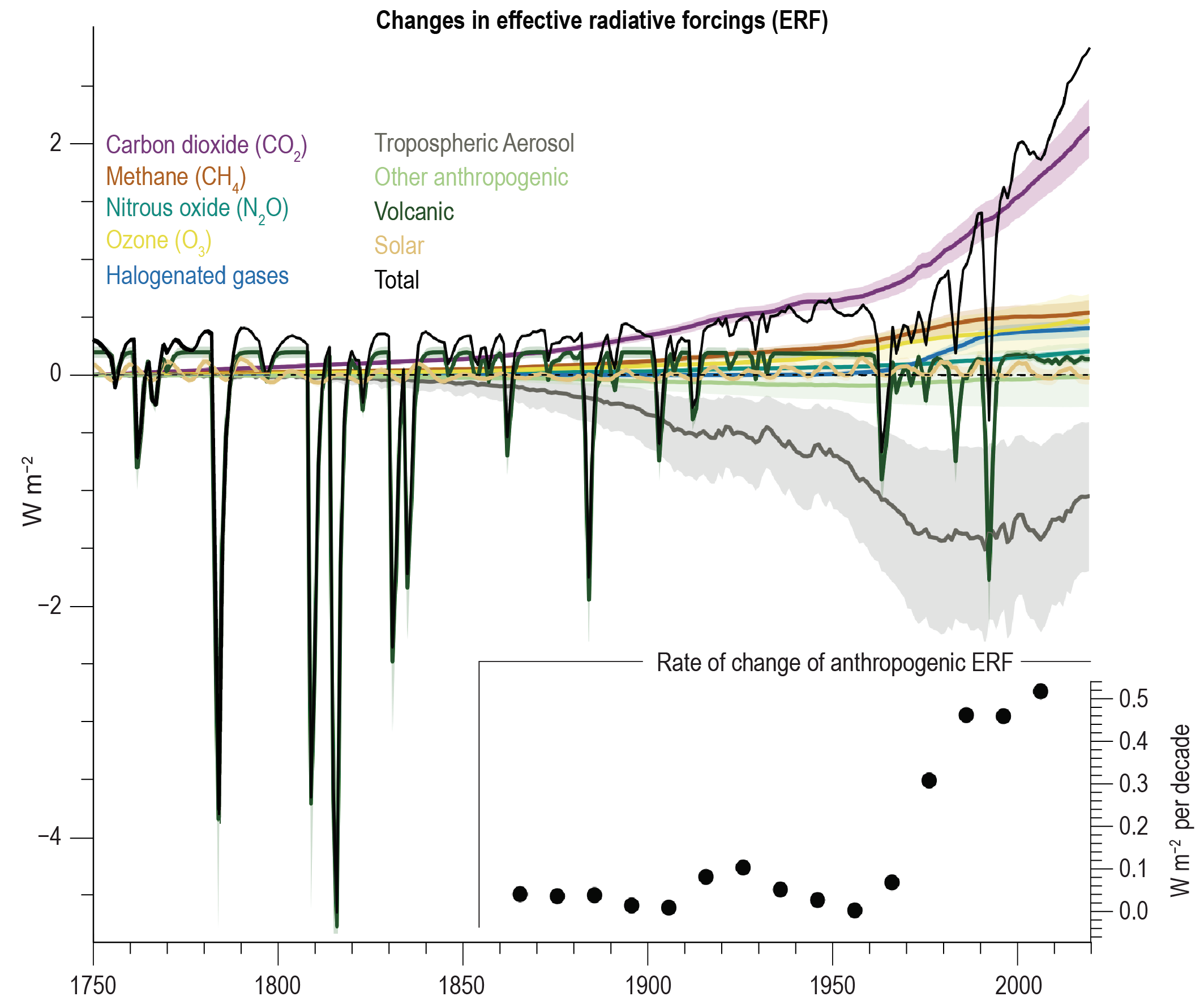 Figure 2.10 | Temporal evolution of effective radiative forcing (ERF) related to the drivers assessed in Section 2.2. ERFs are based upon the calculations described in Chapter 7, of which the global annual mean, central assessment values are shown as lines and the 5 to 95% uncertainty range as shading (Section 7.3, see Figures 7.6 to 7.8 for more detail on uncertainties). The inset plot shows the rate of change (linear trend) in total anthropogenic ERF (total without TSI and volcanic ERF) for 30-year periods centred at each dot. Further details on data sources and processing are available in the chapter data table (Table 2.SM.1).
 Increasing TSI (Section 2.2.1) implies a small ERF of less than 0.1 W m–2 between 1900 and 1980. TSI varies over the 11-year solar cycle with ERF of order ± 0.1 W m–2 in the assessed period. Strong volcanic eruptions (Section 2.2.2) with periods of strong negative ERF lasting 2–5 years in duration occurred in the late 19th and early 20th centuries. There followed a relatively quiescent period between about 1920 and 1960, and then three strong eruptions in 1963, 1982 and 1991, and only small-to-moderate eruptions thereafter (Schmidt et al., 2018).
The atmospheric concentrations of WMGHGs (Section 2.2.3) have continuously increased since the early 19th century, with CO2 contributing the largest share of the positive ERF. Compared to the last two decades of the 20th century, the growth rate of CO2 in the atmosphere increased in the 21st century, showed strong fluctuations for CH4, and was about constant for N2O. Mixing ratios of the most abundant CFCs declined (Section 2.2.4). Mixing ratios of HCFCs increased, but growth rates are starting to decelerate. Mixing ratios of HFCs and some other human-made components are increasing (Section 2.2.4). The ERF for CO2 alone is stronger than for all the other anthropogenic WMGHGs taken together throughout the industrial period, and its relative importance has increased in recent years (Figures 2.10 and 7.6).
Among the gaseous short-lived climate forcers (Chapter 6 and Sections 2.2.5 and 7.3; excluding CH4 here), ozone (O3) is the component with the largest (positive) ERF. Concentrations from direct observations have increased since the mid-20th century and, mostly based on models, this extends to since 1750. Other gaseous short-lived climate forcers have small contributions to total ERF.
The net effect of aerosols (Sections 2.2.6 and 6.4) on the radiation budget, including their effect on clouds, and cloud adjustments, as well as the deposition of black carbon on snow (Section 7.3.4.3), was negative throughout the industrial period (high confidence). The net effect strengthened (becoming more negative) over most of the 20th century, butmore likely than not weakened (becoming less negative) since the late 20th century. These trends are reflected in measurements of surface solar radiation (Section 7.2.2.3) and the Earth’s energy imbalance (Section 7.2.2.1). The relative importance of aerosol forcing compared to other forcing agents has decreased globally in the most recent 30 years (medium confidence) and the reduction of the negative forcing in the 21st century enhances the overall positive ERF.
Land use and land cover changes (Section 2.2.7) over the industrial period introduce a negative radiative forcing by increasing the surface albedo. This effect increased since 1750, reaching current values of about –0.20 W m–2 (medium confidence). This ERF value is taken from Section 7.3.4.1 and is different from the assessment in Section 2.2.7 in that it also includes the effect of irrigation. It also includes uncertain rapid adjustments and thus there is low confidence in its magnitude. Biogeochemical feedbacks can be substantial (Section 5.4) and are not included in ERF.
In conclusion, the net ERF due to all observed changes in climate drivers is positive, except for short periods (up to a few years in duration) following moderate to large volcanic eruptions, and has grown in magnitude since the late 19th century. The rate of change likely has increased in the last 30 years, since CO2 concentrations increased at an increasing rate due to growing CO2 emissions (very likely) , and since the aerosol forcing became less negative (more likely than not ).
2.3 Changes in Large-scale Climate
Cross-Chapter Box 2.2 | Large-scale Indicators of Climate Change
Contributing Authors: Veronika Eyring (Germany), Nathan P. Gillett (Canada), Sergey K. Gulev (Russian Federation), Jochem Marotzke (Germany), June-Yi Lee (Republic of Korea), Peter W. Thorne (Ireland/United Kingdom)
Chapters 2, 3 and 4 assess the current evidence basis for climatic changes, their causes, and their potential future under different possible emissions pathways using a combination of observations and state-of-the-art Earth system models (ESMs). The assessment in these chapters focuses on selected large-scale indicators and modes as defined in this Box. These indicators and modes of variability taken together characterize overall changes to the climate system as a whole.
Defining ‘large scale’
Understanding of large-scale climate variability and change requires knowledge of both the response to forcings and the role of internal variability. Many forcings have substantial hemispheric or continental scale variations. Modes of climate variability are generally driven by ocean basin scale processes. The climate system involves process interactions from the micro- to the global-scale and as such, any threshold for defining ‘large-scale’ is arbitrary, but, within these chapters on the basis of these considerations large-scale is defined to include ocean basin and continental scales as well as hemispheric and global scales.
Defining a key set of climate indicators
Key climate indicators should constitute a finite set of distinct variables and/or metrics that may collectively point to important overall changes in the climate system that provide a synthesis of climate system evolution and are of broad societal relevance. Key indicators have been selected across the atmospheric, oceanic, cryospheric and biospheric domains, with land as a cross-cutting component. These indicators, and their use across Chapters 2, 3 and 4, as well as the broader report, are summarized in Cross-Chapter Box 2.2, Table 1. All selected indicators are Essential Climate Variables as defined by the Global Climate Observing System (Bojinski et al., 2014).
Atmospheric indicators
Monitoring surface temperatures is integral to the negotiations of UNFCCC and the global mean temperature goals of the Paris Agreement. Upper-air temperatures are a key indicator of different causal mechanisms underlying climate change and underpinned the very first conclusion in the Second Assessment Report of a ‘discernible human influence’ (Santer et al., 1996). To ascertain large-scale changes of and human influence on the global hydrological cycle (which includes terrestrial and oceanic components), a small subset of indicators across this cycle are chosen: ocean and land precipitation–evaporation (P–E), global precipitation, total column water vapour, surface humidity (specific and relative), and global river runoff. Chapter 8 performs a substantive and holistic assessment of a much broader range of components. Finally, a warming world may be accompanied by a change in large-scale circulation patterns linked through energy/mass/momentum constraints such as the extent and strength of the Hadley circulation (HC), monsoon systems, and/or the position and strength of the sub-tropical and polar jets.
Cross-Chapter Box 2.2, Table 1 | Summary of the large-scale indicators used across Chapters 2 through 4 and their principal applications in remaining chapters. Indicators are sub-divided by Earth-system domain and their inclusion in individual chapters is indicated by a blue dot. The list of additional chapters is limited to those where the variable is a principal consideration.
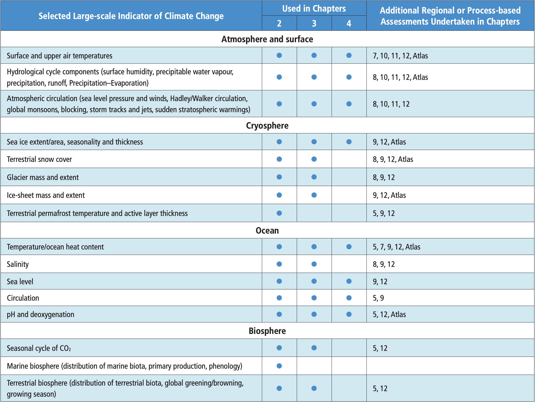
Cryospheric indicators
Changes in ice sheets are indicators of the longest-term impacts of climate change and associated with changes in global and regional sea level. Seasonal snow cover has many implications for mid- to high-latitude regions (albedo, hydrological cycle, etc.) with impacts on biospheric components of the system. Changes in sea ice extent, seasonality and thickness have potential impacts for hemispheric-scale circulation (Cross-Chapter Box 10.1). Changes in glacier mass balance contribute to changes in sea level but also have substantial implications for water supply for a substantial proportion of the global population. Finally, changes in permafrost and the seasonally thawed active layer have substantial implications in mid- to high-latitudes and have been hypothesized to be important in potential feedbacks through degassing of WMGHGs as the permafrost thaws.
Oceanic indicators
Most of the energy imbalance (Box 7.2) in the climate system is taken up by the ocean, resulting in changes in ocean temperature and heat content. Salinity changes indicate broad-scale hydrological cycle and circulation changes. Global-mean sea-level change is a key indicator of the impacts of both global warming and changes in global ice volume. Furthermore, it is integral to assessing the global energy budget (Cross-Chapter Box 9.1). The oceanic overturning circulation redistributes heat, carbon, oxygen and salinity within the ocean. Declines in ocean pH result from air-sea exchange of carbon dioxide and loss of ocean oxygen results from ocean warming; both lead to changes in marine ecosystems.
Biospheric indicators
The seasonal cycle of CO2 is an integrated measure of the biogeochemical activity across the global biosphere. Changes in marine and terrestrial ecosystems can also be observed directly at large scales. For small, free-floating organisms such as phytoplankton, the dynamics can be rapid in nature, whereas on land slower changes in plant assemblages may occur, with commensurate changes in altitude and latitude of the tree-line. Lengthening of the growing season and the associated changes in phenology, distribution and abundance of species would be expected in most of the extratropics. Biospheric indicators and their impacts are assessed in much greater detail in WGII Chapters 2 and 3.
Defining a selection of modes of variability
Many modes of climate variability affect global, hemispheric or regional climate across a range of timescales. Conversely, their behaviour may be influenced by global climate change. Modes were selected for inclusion that: (i) have effects at large spatial scales; and (ii) have substantial potential to modify interannual to multi-decadal climate. The selected modes are considered in multiple chapters (Cross-Chapter Box 2.2, Table 2) and are defined in Annex IV.
Cross-Chapter Box 2.2, Table 2 | Summary of the modes of variability used across Chapters 2 through 4 and their principal applications in remaining chapters. Inclusion in each of Chapters 2 through 4 is indicated by a blue dot of the relevant table cell. The list of remaining chapters is limited to those where the mode of variability is a principal consideration of that chapter and is not intended to be exhaustive.
2.3.1 Atmosphere and Earth’s Surface
2.3.1.1 Surface Temperatures
2.3.1.1.1 Temperatures of the deep past (65 Ma to 8 ka)
This assessment of the paleo reference periods (Cross-Chapter Box 2.1) draws from studies based mostly or entirely on indirect observational evidence from geological archives (i.e., proxy records) rather than reconstructions that rely more heavily on modelled parameters and those based on deep-ocean temperatures (e.g., Köhler et al., 2015; Friedrich et al., 2016). In contrast to AR5, temperature estimates from climate models are not included in the assessed values for paleo reference periods in this chapter. The AR5 concluded that the reconstructed GMST during the PETM was 4°C–7°C warmer than pre-PETM mean climate (low confidence), and that the EECO and the MPWP were 9°C–14°C and 1.9°C–3.6°C warmer than pre-industrial, respectively (medium confidence). The GMST during the LIG was assessed at 1°C–2°C warmer than pre-industrial (medium confidence), whereas SROCC narrowed the range to 0.5°C–1.0°C warmer, but did not state a confidence level. The AR5 further concluded that it was very likely that the LGM was 3°C–8°C colder than pre-industrial, and likely that the maximum rate of global warming during the subsequent deglacial period was 1°C–1.5°C kyr–1.
For the PETM, new reconstructions agree with those assessed by AR5. A major new compilation of proxy temperature data (Hollis et al., 2019) analysed using multiple statistical approaches (Inglis et al., 2020) indicates that GMST was 10°C–25°C (90% range) warmer than 1850–1900, or about 5°C warmer relative to the pre-PETM state. A related synthesis study also estimates that PETM warmed by 5°C (no uncertainty assigned; Zhu et al., 2019). A recent benthic isotope compilation (Westerhold et al., 2020) transformed to GMST based on the formulation by J. Hansen et al. (2013; Cross-Chapter Box 2.1, Figure 1), and adjusted to 1850–1900 by adding 0.36°C, shows an increase of GMST by about 10°C during the PETM. This reflects the expected higher variability at single sites that were used to splice together the composite time series, compared to the globally averaged composite time series of Zachos et al. (2008). The latter was originally used by J. Hansen et al. (2013) to reconstruct GMST, and is the preferred representation of the global average bottom water conditions, despite its less well-refined chronology.
For the EECO, new GMST reconstructions fall at the high end of the range assessed by AR5. These include estimates of 7°C–18°C (90% range; Inglis et al., 2020) and 12°C–18°C (95% range; Zhu et al., 2019) warmer than 1850–1900, and 10°C–16°C warmer than 1995–2014 ‘recent past’ conditions (2 standard error range; Caballero and Huber, 2013). Together, they indicate that GMST was 10°C–18°C warmer during the EECO compared with 1850–1900 (medium confidence).
The AR5 did not assess the GMST for the MCO. Reconstructions based on data from multiple study sites include estimates of about 4°C (uncertainty range not specified; You et al., 2009) and 5°C–10°C (2 standard error range; Goldner et al., 2014) warmer than 1850–1900. Together, these studies indicate that GMST was 4°C–10°C warmer during the MCO (medium confidence).
For the MPWP, new proxy-based estimates of global sea surface temperatures (SST) are about 2.0°C–3.5°C warmer than 1850–1900, depending on which proxy types are included in the analysis (Foley and Dowsett, 2019; McClymont et al., 2020). On the basis of model-derived relationships between land versus sea surface temperatures under different climate states (Figure 3.2b), the increase in GMST is estimated to have been roughly 15% greater than the increase in global SST. Therefore, GMST during the MPWP is estimated to have been 2.5°C–4.0°C warmer than 1850–1900 (medium confidence).
For the LIG (Cross-Chapter Box 2.1, Figure 1, and Figure 2.11), a major new compilation of marine proxy data (Turney et al., 2020) from 203 sites indicates that the average SST from 129–125 ka was 1.0°C ± 0.2°C (2 SD) warmer than 1850–1900 (reported relative to 1981–2010 and adjusted here by 0.8°C). These temperatures represent the time of peak warmth, which may not have been synchronous among these sites. This compares with two other SST estimates for 125 ka of 0.5°C ± 0.3°C (± 2 SD) warmer at 125 ka relative to 1870–1889 (Hoffman et al., 2017), and about 1.4°C (no uncertainty stated) warmer at 125 ka relative to 1850–1900 (Friedrich and Timmermann, 2020; reported relative to 10–5 ka and adjusted here by 0.4°C; Kaufman et al., 2020a). The average of these post-AR5 global SST anomalies is 1°C. Commensurately (Figure 3.2b), GMST is estimated to have been roughly 1.1°C above 1850–1900 values, although this value could be too high if peak warmth was not globally synchronous (Capron et al., 2017). A further estimate of peak GMST anomalies of 1.0°C–3.5°C (90% range; adjusted here to 1850–1900 by adding 0.2°C) based on 59 marine sediment cores (Snyder, 2016) is considerably warmer than remaining estimates and is therefore given less weight in the final assessment. The warmest millennium of the LIG GMST reconstruction in J. Hansen et al. (2013) is 1.5°C above 1850–1900. In summary, GMST during the warmest millennia of the LIG (within the interval of around 129–125 ka) is estimated to have reached 0.5°C–1.5°C higher values than the 1850–1990 reference period (medium confidence).
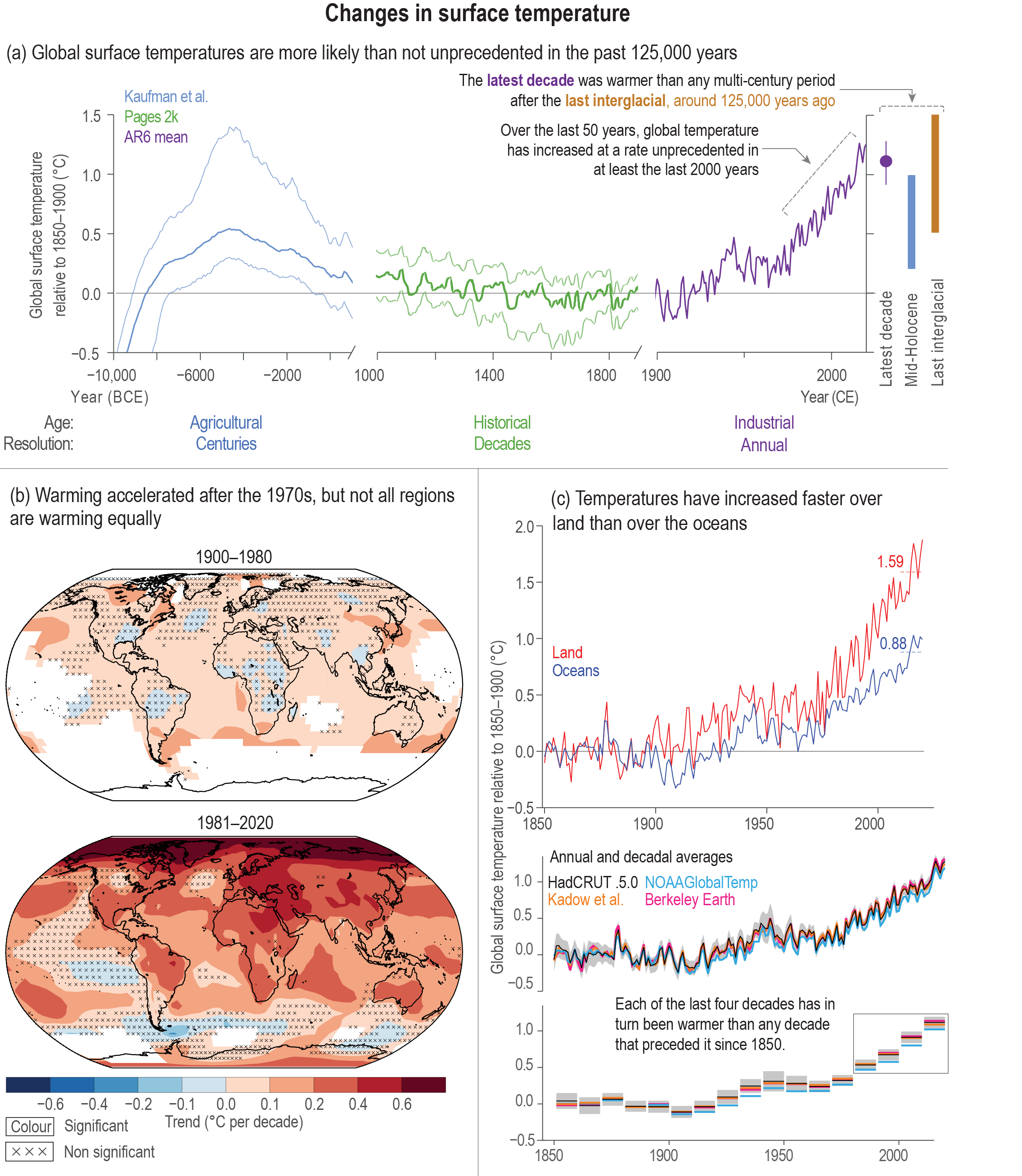 Figure 2.11 | Earth’s surface temperature history with key findings annotated within each panel. (a) GMST over the Holocene divided into three time scales: (i) 12 kyr–1 kyr in 100-year time steps; (ii) 1000–1900 CE, 10-year smooth; and (iii) 1900–2020 CE (from panel (c)). Median of the multi-method reconstruction (bold lines), with 5th and 95th percentiles of the ensemble members (thin lines). Vertical bars are the assessed medium confidence ranges of GMST for the Last Interglacial and mid-Holocene (Section 2.3.1.1). The last decade value and very likely range arises from Section 2.3.1.1.3. (b) Spatially resolved trends (°C per decade) for HadCRUTv5 over (upper map) 1900–1980, and (lower map) 1981–2020. Significance is assessed following AR(1) adjustment after Santer et al. (2008), ‘×’ marks denote non-significant trends. (c) Temperature from instrumental data for 1850–2020, including (upper panel) multi-product mean annual time series assessed in Section 2.3.1.1.3 for temperature over the oceans (blue line) and temperature over the land (red line) and indicating the warming to the most recent 10 years; and annually (middle panel) and decadally (bottom panel) resolved averages for the GMST datasets assessed in Section 2.3.1.1.3. The grey shading in each panel shows the uncertainty associated with the HadCRUT5 estimate (Morice et al., 2021). All temperatures relative to the 1850–1900 reference period. Further details on data sources and processing are available in the chapter data table (Table 2.SM.1).
 New GMST reconstructions for the LGM fall near the middle of AR5’s very likely range, which was based on a combination of proxy reconstructions and model simulations. Two of these new reconstructions use marine proxies to reconstruct global SST that were scaled to GMST based on different assumptions. One indicates that GMST was 6.2 [4.5 to 8.1] °C cooler than the late Holocene average (Snyder, 2016), and the other, 5.7°C ± 0.8°C (2 SD) cooler than the average of the first part of the Holocene (10–5 ka) (Friedrich and Timmermann, 2020). A third new estimate (Tierney et al., 2020) uses a much larger compilation of marine proxies along with a data-assimilation procedure, rather than scaling, to reconstruct a GMST of 6.1°C ± 0.4°C (2 SD) cooler than the late Holocene. Assuming that the 1850–1900 reference period was 0.2°C and 0.4°C cooler than the late and first part of the Holocene, respectively (Kaufman et al., 2020a), the midpoints of these three new GMST reconstructions average –5.8°C relative to 1850–1900. The coldest multi-century period of the LGM in the J. Hansen et al. (2013) reconstruction is 4.3°C colder than 1850–1900. This compares to land- and SST-only estimates of about –6.1°C ± 2°C and –2.2°C ± 1°C, respectively (2 SD), which are based on AR5-generation studies that imply a warmer GMST than more recent reconstructions (Figure 1c in Harrison et al., 2015; Figure 7 in Harrison et al., 2016). A major new pollen-based data-assimilation reconstruction averages 6.9°C cooler over northern extratropical land (Cleator et al., 2020). LGM temperature variability on centennial scales was about four times higher globally than during the Holocene, and even greater at high latitudes (Rehfeld et al., 2018). In summary, GMST is estimated to have been 5°C–7°C lower during the LGM (around 23–19 ka) compared with 1850–1900 (medium confidence).
For the LDT (Cross-Chapter Box 2.1, Figure 1), no new large-scale studies have been published since AR5 (Shakun et al., 2012) to further assess the rate of GMST change during this period of rapid global warming (estimated at 1°C–1.5°C per kyr). The reconstruction of Shakun et al. (2012) was based primarily on SST records and therefore underrepresents the change in GMST during the LDT. Temperature over Greenland increased by about ten times that rate during the centuries of most rapid warming (Jansen et al., 2020).
2.3.1.1.2 Temperatures of the post-glacial period (past 7000 years)
The AR5 did not include an assessment of large-scale temperature estimates for the MH, although it assigned high confidence to the long-term cooling trend over mid- to high-latitudes of the Northern Hemisphere (NH) during the 5 kyr that preceded recent warming. For average annual NH temperatures, the period 1983–2012 was assessed as very likely the warmest 30-year period of the past 800 years (high confidence) and likely the warmest 30-year period of the past 1.4 kyr (medium confidence); the warm multi-decadal periods prior to the 20th century were unsynchronized across regions, in contrast to the warming since the mid-20th century (high confidence), although only sparse information was available from the SH.
This section concerns the Holocene period prior to industrialization when GMST was overall highest. Whereas SR1.5 focussed upon the ‘Holocene thermal maximum’ when regional temperatures were up to 1°C higher than 1850–1900, though peak warming occurred regionally at different times between around 10 and 5 ka greatly complicating interpretation. A multi-method reconstruction (Kaufman et al., 2020a) based on a quality-controlled, multi-proxy synthesis of paleo-temperature records from 470 terrestrial and 209 marine sites globally (Kaufman et al., 2020b) indicates that the median GMST of the warmest two-century-long interval was 0.7 [0.3 to 1.8] °C warmer than 1800–1900 (which averaged 0.03°C colder than 1850–1900; PAGES 2k Consortium, 2019), and was centred around 6.5 ka. This is similar to Marcott et al. (2013), which is based on a smaller dataset (73 sites) and different procedures to estimate a maximum warmth of 0.8°C ± 0.3°C (2 SD) at around 7.0 ka, adjusted here by adding 0.3°C to account for differences in reference periods. These may be underestimates because averaging inherently smoothed proxy records with uncertain chronologies reduces the variability in the temperature reconstruction (e.g., Dolman and Laepple, (2018) for sedimentary archives). However, the general coincidence between peak warmth and astronomically driven boreal summer insolation might reflect a bias toward summer conditions (Liu et al., 2014; Hou et al., 2019; Bova et al., 2021), suggesting that the estimate is too high. This possibility is supported by AR5-generation proxy data focusing on 6 ka (Harrison et al., 2014), the long-standing MH modelling target (Cross-Chapter Box 2.1), that indicate surface temperatures for land and ocean were indistinguishable from ‘pre-industrial’ climate (Figure 1c in Harrison et al., 2015; Figure 7 in Harrison et al., 2016). In contrast, the GMST estimate from the multi-method global reconstruction (Kaufman et al., 2020a) for the millennium centred on 6 ka is only about 0.1°C colder than the warmest millennium.
Taking all lines of evidence into account, the GMST averaged over the warmest centuries of the current interglacial period (sometime between around 6 and 7 ka) is estimated to have been 0.2°C–1.0°C higher than 1850–1900 (medium confidence). It is therefore more likely than not that no multi-centennial interval during the post-glacial period was warmer globally than the most recent decade (which was 1.1°C warmer than 1850–1900; Section 2.3.1.1.3); the LIG (129–116 ka) is the next most recent candidate for a period of higher global temperature. Zonally averaged mean annual temperature reconstructions (Routson et al., 2019) indicate that MH warmth was most pronounced north of 30°N latitude, and that GMST subsequently decreased in general, albeit with multi-century variability, with greater cooling in the NH than in the SH (Kaufman et al., 2020a).
The temperature history of the last millennium and the methods used to reconstruct it have been studied extensively, both prior to and following AR5, as summarized recently by Smerdon and Pollack (2016) and Christiansen and Ljungqvist (2017). New regional (e.g., Shi et al., 2015; Stenni et al., 2017; Werner et al., 2018), global ocean (McGregor et al., 2015), quasi-hemispheric (Neukom et al., 2014; Schneider et al., 2015; Anchukaitis et al., 2017), and global (Tardif et al., 2019) temperature reconstructions, and new regional proxy data syntheses (Lüning et al., 2019a, b) have been published, extending back 1–2 kyr. In addition, a major new global compilation of multiproxy, annually resolved paleo-temperature records for the CE (PAGES 2k Consortium, 2017) has been analysed using a variety of statistical methods for reconstructing temperature (PAGES 2k Consortium, 2019). The median of the multi-method GMST reconstruction from this synthesis (Figure 2.11a) generally agrees with the AR5 assessment, while affording more robust estimates of the following major features of GMST during the CE: (i) an overall millennial-scale cooling trend of –0.18 [–0.28 to 0.00] °C kyr–1 prior to 1850; (ii) a multi-centennial period of relatively low temperature beginning around the 15th century, with GMST averaging –0.03 [–0.30 to 0.06] °C between 1450 and 1850 relative to 1850–1900; (iii) the warmest multi-decadal period occurring most recently; and (iv) the rate of warming during the second half of the 20th century (from instrumental data) exceeding the 99th percentile of all 51-year trends over the past 2 kyr. Moreover, the new proxy data compilation shows that the warming of the 20th century was more spatially uniform than any other century-scale temperature change of the CE (medium confidence) (Neukom et al., 2019). A new independent temperature reconstruction extending back to 1580 is based on an expanded database of subsurface borehole temperature profiles, along with refined methods for inverse modelling (Cuesta-Valero et al., 2021). The borehole data, converted to GMST based on the modelled relation between changes in land versus sea surface temperature outlined previously, indicate that average GMST for 1600–1650 was 0.12°C colder than 1850–1900, which is similar to the PAGES 2k reconstruction (0.09°C colder), although both estimates are associated with relatively large uncertainties (0.8°C (95% range) and 0.5°C (90% range), respectively).
To conclude, following approximately 6 ka, GMST generally decreased, culminating in the coldest multi-century interval of the post-glacial period (since 8 ka), which occurred between around 1450 and 1850 (high confidence). This multi-millennial cooling trend was reversed in the mid-19th century. Since around 1950, GMST has increased at an observed rate unprecedented for any 50-year period in at least the last 2000 years (high confidence).
2.3.1.1.3 Temperatures during the instrumental period – surface
The AR5 concluded that it was certain that GMST had increased since the late 19th century. Total warming in GMST was assessed as 0.85 [0.65 to 1.06] °C over 1880–2012, while the change from 1850–1900 to 2003–2012 was assessed at 0.78 [0.72 to 0.85] °C, and from 1850–1900 to 1986–2005 at 0.61 [0.55 to 0.67] °C. The SR1.5 reported warming of GMST from 1850–1900 to 2006–2015 of 0.87°C, with an 1880–2012 trend of 0.86°C and an 1880–2015 trend of 0.92°C. The SRCCL concluded that since the pre-industrial period, surface air temperature over land areas has risen nearly twice as much as the global mean surface temperature (high confidence).
Since AR5, there have been substantial improvements in the availability of instrumental archive data both over the ocean and on land. A new version of the International Comprehensive Ocean-Atmosphere Dataset (ICOADS Release 3.0, Freeman et al., 2017) comprises over 450 million in situ marine reports and incorporates newly digitized data, increasing coverage in data sparse regions and times (e.g., polar oceans and World War I). The International Surface Temperature Initiative released a much improved collection of fundamental land surface air temperature records (Rennie et al., 2014) comprising more than 35,000 station records. These advances, both of which have substantially improved spatial coverage, have reduced uncertainties in assessments of both land and marine data.
Marine domain
For SST analyses, three products – HadSST4 (1850–present, Kennedy et al., 2019), ERSSTv5 (1850–present, Huang et al., 2017) and COBE SST2 (1880–present, (Hirahara et al., 2014) – now have bias adjustments applied throughout the record. The new SST datasets account for two major issues previously identified in AR5: that globally averaged buoy SSTs are about 0.12°C cooler than ship-based SSTs (Kennedy et al., 2011; Huang et al., 2015), and that SSTs from ship engine room intakes may have biases for individual ships depending upon the sensor set-up (Kent and Kaplan, 2006) but have an overall warm bias when globally aggregated (Kennedy et al., 2019). The first issue primarily affects data since 1990, when buoys began to increasingly contribute to the observation network (Woodruff et al., 2011), and the second issue has its largest effect from the 1940s to the 1970s. From the standpoint of uncertainty, ERSSTv4 (W. Liu et al., 2015; Huang et al., 2016) and subsequent versions (Huang et al., 2017), and HadSST4 have estimates presented as ensembles that sample parametric uncertainty. Comparisons between these independently-derived analyses and the assessed uncertainties (Kennedy, 2014; Kent et al., 2017) show unambiguously that global mean SST increased since the start of the 20th century, a conclusion that is insensitive to the method used to treat gaps in data coverage (Kennedy, 2014).
A number of recent studies also corroborate important components of the SST record (Hausfather et al., 2017; Kent et al., 2017; Cowtan et al., 2018; Kennedy et al., 2019). In particular, ATSR SST satellite retrievals (Merchant et al., 2012; Berry et al., 2018), the near-surface records from hydrographical profiles (Gouretski et al., 2012; Huang et al., 2018), and coastal observations (Cowtan et al., 2018) have all been shown to be broadly consistent with the homogenized SST analyses. Hausfather et al. (2017) also confirmed the new estimate of the rate of warming seen in ERSSTv4 since the late 1990s through comparison with independent SST data sources such as Argo floats and satellite retrievals. Nevertheless, dataset differences remain in the mid-20th century when there were major, poorly-documented, changes in instrumentation and observational practices (Kent et al., 2017), particularly during World War II, when ship observations were limited and disproportionately originated from US naval sources (Thompson et al., 2008). Kennedy et al. (2019) also identify differences between the new HadSST4 dataset and other SST datasets in the 1980s and 1990s, indicating that some level of structural uncertainty remains during this period, whilst Chan et al. (2019) and Davis et al. (2019) document residual uncertainties in the early and later 20th century records respectively.
Historically, SST has been used as a basis for global temperature assessment on the premise that the less variable SST data provides a better estimate of marine temperature changes than marine air temperature (MAT) (Kent and Kennedy, 2021). However, MAT products are used to adjust SST biases in the NOAA SST product because they are assessed to be more homogeneous (Huang et al., 2017). Observational datasets exist for night-marine air temperature (NMAT) (e.g., Cornes et al., 2020; Junod and Christy, 2020; Rayner et al., 2020) and there are methods to adjust daytime MATs (Berry et al., 2004), but there is to date no regularly updated dataset which combines MAT with temperatures over land. MAT datasets are more sparse in recent decades than SST datasets as marine datasets have become increasingly dependent on drifting buoys (Centurioni et al., 2019) which generally measure SST but not MAT, and there are almost no recent winter MAT data south of 40°S (Swart et al., 2019). However, the situation reverses in the 19th century with a greater prevalence of MAT than SST measurements available in the ICOADS data repository (Freeman et al., 2017, 2019; Kent and Kennedy, 2021).
Land domain
The GHCNMv4 dataset (Menne et al., 2018) includes many more land stations than GHCNMv3, arising from the databank efforts of Rennie et al. (2014), and calculates a 100-member parametric uncertainty ensemble drawing upon the benchmarking analysis of Williams et al. (2012), as well as accounting for sampling effects. A new version of the CRUTEM dataset (CRUTEMv5, Osborn et al., 2021) has increased data completeness and additional quality control measures. A new global land dataset, the China Land Surface Air Temperature (CLSAT) dataset (Xu et al., 2018) has higher network density in some regions (particularly Asia) than previously existing datasets. Global trends derived from CLSAT are generally consistent with those derived from other land datasets through 2014 (Xu et al., 2018).
The AR5 identified diurnal temperature range (DTR) as a substantial knowledge gap. The most recent analysis of Thorne et al. (2016a, b) compared a broad range of gridded estimates of change in DTR, including a new estimate derived from the ISTI databank release using the pairwise homogenization algorithm used to create GHCNMv4, and estimates derived from Vose et al. (2005), HadEX2 (Donat et al., 2013a), HadGHCND (Donat et al., 2013b), GHCNDEX (Donat et al., 2013b), Berkeley Earth (Rohde et al., 2013), and CRU TS (Harris et al., 2014). The analysis highlighted substantial ambiguity in pre-1950 estimates arising from sparse data availability. After 1950 estimates agreed that DTR had decreased globally with most of that decrease occurring over the period 1960–1980. A subsequent DTR analysis using CLSAT further confirmed this behaviour (X. Sun et al., 2018).
No recent literature has emerged to alter the AR5 finding that it is unlikely that any uncorrected effects from urbanization (Box 10.3), or from changes in land use or land cover (Section 2.2.7), have raised global Land Surface Air Temperature (LSAT) trends by more than 10%, although larger signals have been identified in some specific regions, especially rapidly urbanizing areas such as eastern China (Y. Li et al., 2013; Liao et al., 2017; Z. Shi et al., 2019). There is also no clear indication that site-specific data homogeneity issues have had any significant impact on global trends since the early 20th century; there is more uncertainty in the 19th century, mainly arising from a lack of standardization of instrument shelters, which has been largely accounted for in data from central Europe (Jones et al., 2012), but less so elsewhere.
Combined data products
At the time of AR5 a limitation of conventional datasets was the lack of coverage, especially in high latitudes, which although recognized as an issue (Simmons et al., 2010) had not been addressed in most products. Interpolation involves the statistical imputation of values across regions with limited data and can add both systematic and random uncertainties (Lenssen et al., 2019). Cowtan and Way (2014) applied a kriging-based method to extend existing datasets to polar regions, while Kadow et al. (2020) used an artificial intelligence-based method, and Vaccaro et al. (2021) used gaussian random Markov fields, for the same purpose, although only Kadow et al. (2020) uses the most recent generation of datasets as its base. The Berkeley Earth merged product (Rohde and Hausfather, 2020), HadCRUT5 (Morice et al., 2021) and NOAA GlobalTemp-Interim (Vose et al., 2021) all include interpolation over reasonable distances across data sparse regions which results in quasi-global estimates from the late 1950s when continuous Antarctic observations commenced. Interpolated datasets with substantial coverage of high latitudes show generally stronger warming of GMST than those with limited data in polar regions (Vose et al., 2021), and their strong warming at high northern latitudes is consistent with independent estimates from reanalyses (Simmons et al., 2017; Lenssen et al., 2019) and satellites (Cowtan and Way, 2014). Given the spatial scales of surface temperature variations and the verification of the methods, it is extremely likely that interpolation results in a less-biased estimate of the actual global temperature change than ignoring regions with limited or no data.
In total there are five conventional datasets which meet spatial coverage requirements and draw from the most recent generation of SST analyses, four of which have sufficient data in the 1850–1900 period to allow an assessment of changes from that baseline (Table 2.3). A fifth dataset is added to the assessment for changes over land areas. Datasets share SST and LSAT data products and in several cases differ solely in the post-processing interpolation applied meaning that there are far fewer methodological degrees of freedom than implied by a straight count of the number of available estimates.
Dataset | Period of Record | Land Component | SST Component | Ensemble Uncertainties? | Meets all Inclusion Criteria? | Principal Reference |
HadCRUT5 | 1850–2020 | CRUTEM5 | HadSST4 | Yes | Yes | |
NOAA GlobalTemp – Interim | 1850–2020 | GHCNv4 | ERSSTv5 | Yes, on earlier version | Yes | |
Berkeley Earth | 1850–2020 | Berkeley | HadSST4 | No | Yes | |
Kadow et al. | 1850–2020 | CRUTEM5 | HadSST4 | No | Yes | |
China – MST | 1856–2020 | CLSAT | ERSSTv5 | No | Land only | |
GISTEMP | 1880–2020 | GHCNv4 | ERSSTv5 | Yes | Post-1880 only | |
Cowtan and Way | 1850–2020 | CRUTEM4 | HadSST3 | Yes | No | |
Vaccaro et al. | 1850–2020 | CRUTEM4 | HadSST3 | No | No |
Estimates of GMST have also benefitted from improved estimation of parametric uncertainties. New versions of three long-standing products from NASA GISTEMP v4 (Lenssen et al., 2019), NOAA GlobalTempv5 (B. Huang et al., 2019b) and HadCRUT5 (Morice et al., 2021) are all now available as ensemble estimates. These ensembles each account for a variety of systematic and random uncertainty effects in slightly different ways, giving broadly similar results, which are incorporated into the present assessment, with the total uncertainty generally declining up until the mid-20th century as data coverage improves.
Another significant development has been the incorporation of reanalysis products (Section 1.5.2) into operational monitoring of GSAT. It was reported in AR5 that various reanalyses were broadly consistent with conventional surface datasets in the representation of trends since the mid-20th century. Since that time, Simmons et al. (2017) found that the ERA-Interim (Dee et al., 2011) and JRA-55 (Kobayashi et al., 2015) reanalyses continued to be consistent, over the last 20 years, with those surface datasets which fully represented the polar regions. GSAT trends from ERA5 reanalysis (Hersbach et al., 2020) are also broadly consistent with GMST trends from conventional surface datasets. However, the MERRA-2 reanalysis (Gelaro et al., 2017) GSAT spuriously cooled sharply relative to ERA-Interim and JRA-55 in about 2007 (Funk et al., 2019). Since the early 2000s, analyses of surface temperature, from which near-surface temperature may be derived, have also been available from various satellites (Famiglietti et al., 2018; Prakash et al., 2018; Susskind et al., 2019), which have the potential to improve assessments of temperature changes over data-sparse regions.
Most land areas in the extratropical Northern Hemisphere (NH) have warmed faster than the GMST average over both the 1900–2020 and 1980–2020 periods (Figure 2.11b), although at more regional scales, particularly in data sparse regions, considerable uncertainty is introduced by sometimes large differences in trends between different LSAT datasets (Rao et al., 2018). Temperatures averaged over land areas globally have warmed by 1.59 [1.34 to 1.83] °C from 1850–1900 to 2011–2020, substantially higher than the SST warming of 0.88 [0.68 to 1.01] °C. The four conventional surface temperature products which meet all criteria to be included in the final assessment (Table 2.4) agree that each of the last four decades has consecutively been the warmest globally since the beginning of their respective records (Figure 2.11c and Table 2.4). Each of the six years 2015 to 2020 has very likely been at least 0.9°C warmer than the 1850–1900 average.
Diagnostic/ Dataset | 1850–1900 to 1995–2014(°C) | 1850–1900 to 2001–2020(°C) | 1850–1900 to 2011–2020(°C) | Trend 1880–2020(°C) | Trend 1960–2020(°C) | Trend 1980–2020(°C) | |
HadCRUT5 | GMST | 0.87 [0.81 to 0.94] | 1.01 [0.94 to 1.09] | 1.12 [1.06 to 1.18] | 1.10 [0.89 to 1.32] | 1.04 [0.93 to 1.14] | 0.76 [0.65 to 0.87] |
LSAT | 1.23 [1.06 to 1.38] | 1.44 [1.26 to 1.59] | 1.55 [1.39 to 1.70] | 1.43 [1.16 to 1.70] | 1.50 [1.33 to 1.67] | 1.20 [1.04 to 1.36] | |
SST | 0.73 [0.69 to 0.78] | 0.85 [0.81 to 0.90] | 0.94 [0.90 to 0.99] | 1.03 [0.80 to 1.25] | 0.90 [0.80 to 0.99] | 0.62 [0.51 to 0.72] | |
NOAA GlobalTemp – Interim | GMST | 0.76 | 0.91 | 1.02 | 1.06 [0.80 to 1.32] | 1.01 [0.90 to 1.11] | 0.75 [0.63 to 0.87] |
LSAT | 1.34 | 1.55 | 1.69 | 1.58 [1.32 to 1.84] | 1.54 [1.40 to 1.68] | 1.19 [1.04 to 1.35] | |
SST | 0.53 | 0.65 | 0.75 | 0.85 [0.59 to 1.12] | 0.79 [0.69 to 0.89] | 0.57 [0.44 to 0.70] | |
GISTEMP v4 | GMST | 1.07 [0.80 to 1.34] | 1.05 [0.94 to 1.16] | 0.79 [0.67 to 0.90] | |||
LSAT | 1.48 [1.19 to 1.78] | 1.56 [1.40 to 1.72] | 1.23 [1.07 to 1.39] | ||||
SST | 0.91 [0.65 to 1.17] | 0.84 [0.74 to 0.95] | 0.61 [0.49 to 0.72] | ||||
Berkeley Earth | GMST | 0.89 | 1.03 | 1.14 | 1.17 [0.94 to 1.40] | 1.09 [1.00 to 1.19] | 0.79 [0.68 to 0.90] |
LSAT | 1.28 | 1.49 | 1.60 | 1.50 [1.25 to 1.76] | 1.51 [1.36 to 1.66] | 1.16 [1.00 to 1.32] | |
SST | 0.73 | 0.85 | 0.96 | 1.04 [0.81 to 1.26] | 0.93 [0.84 to 1.01] | 0.64 [0.54 to 0.74] | |
China-MST | LSAT | 1.18 | 1.38 | 1.49 | 1.48 [1.21 to 1.75] | 1.48 [1.31 to 1.65] | 1.16 [1.00 to 1.32] |
Kadow et al. | GMST | 0.86 | 1.00 | 1.09 | 1.15 [0.95 to 1.35] | 1.01 [0.92 to 1.10] | 0.73 [0.63 to 0.82] |
LSAT | 1.29 | 1.49 | 1.61 | 1.60 [1.37 to 1.82] | 1.46 [1.30 to 1.61] | 1.14 [0.99 to 1.30] | |
SST | 0.69 | 0.80 | 0.88 | 0.97 [0.78 to 1.16] | 0.83 [0.76 to 0.90] | 0.56 [0.48 to 0.65] | |
Cowtan-Way | GMST | 0.82 [0.75 to 0.89] | 0.96 [0.89 to 1.03] | 1.04 [0.97 to 1.11] | 1.03 [0.84 to 1.22] | 0.94 [0.82 to 1.07] | 0.77 [0.67 to 0.87] |
LSAT | 1.23 | 1.43 | 1.54 | 1.42 [1.15 to 1.68] | 1.48 [1.31 to 1.65] | 1.20 [1.04 to 1.36] | |
SST | 0.66 | 0.76 | 0.84 | 0.88 [0.71 to 1.05] | 0.73 [0.61 to 0.84] | 0.61 [0.52 to 0.69] | |
Vaccaro et al. | GMST | 0.76 | 0.89 | 0.97 | 0.99 [0.81 to 1.17] | 0.89 [0.77 to 1.00] | 0.72 [0.63 to 0.81] |
LSAT | 1.15 | 1.35 | 1.47 | 1.40 [1.13 to 1.67] | 1.47 [1.29 to 1.64] | 1.21 [1.06 to 1.36] | |
SST | 0.60 | 0.70 | 0.77 | 0.82 [0.67 to 0.97] | 0.66 [0.55 to 0.76] | 0.53 [0.44 to 0.61] | |
ERA5 | GSAT | 0.78 [0.64 to 0.92] | |||||
LSAT | 1.21 [1.02 to 1.40] | ||||||
Average – GMST | 0.85 | 0.99 | 1.09 | 1.11 | 1.04 | 0.76 | |
Average – LSAT | 1.27 | 1.47 | 1.59 | 1.50 | 1.51 | 1.18 | |
Average – SST | 0.67 | 0.79 | 0.88 | 0.96 | 0.86 | 0.60 |
To conclude, from 1850–1900 to 1995–2014, GMST increased by 0.85 [0.69 to 0.95] °C, to the first two decades of the 21st century (2001–2020) by 0.99 [0.84 to 1.10] °C, and to the most recent decade (2011–2020) by 1.09 [0.95 to 1.20] °C. Each of the last four decades has in turn been warmer than any decade that preceded it since 1850. Temperatures have increased faster over land than over the oceans since 1850–1900, with warming to 2011–2020 of 1.59 [1.34 to 1.83] °C versus 0.88 [0.68 to 1.01] °C, respectively.
2.3.1.2 Temperatures During the Instrumental Period – Free Atmosphere
The AR5 reported that it was virtually certain that tropospheric temperatures have risen, and stratospheric temperatures fallen, since the mid-20th century, but that assessments of the rate of change and its vertical structure had only medium confidence in the NH extratropics and low confidence elsewhere. In particular there was low confidence in the vertical structure of temperature trends in the upper tropical troposphere.
2.3.1.2.1 Dataset developments
There have been updated radiosonde estimates from the University of Vienna (RAOBCORE and RICH; Haimberger et al., 2012) and a new dataset from the State University of New York (UAHRD, Zhou et al., 2020). There are new versions of AMSU products from the University of Alabama in Huntsville (UAHv6.0; Spencer et al., 2017) and Remote Sensing Systems (RSSv4.0; Mears and Wentz, 2017). These updates have led to convergence in the lower stratosphere layer (Maycock et al., 2018); in particular, the move to UAHv6.0 has addressed homogeneity issues identified by Seidel et al. (2016), although residual differences remain (Christy et al., 2018). Reanalyses products had identified limitations near the 300 hPa level where the contribution of aircraft observations has increased rapidly in recent years (Dee et al., 2011; Gelaro et al., 2017), leading to identified biases (Dee and Uppala, 2009), that have been addressed in ERA5 (Hersbach et al., 2020). Modern reanalyses are generally well aligned with radiosonde and satellite observations in the middle and lower troposphere and lower stratosphere. A new operational mid- and upper-stratospheric dataset (STAR) has been developed by Zou and Qian (2016), merging the previous 1979–2006 SSU dataset (Zou et al., 2014) with a dataset from 1998 onwards drawn from relevant AMSU channels (Wang and Zou, 2014). Further stratospheric satellite-based datasets from various combinations of satellites have been developed by McLandress et al. (2015) and Randel et al. (2016).
New assessments of free-atmosphere temperature are available through radio occultation (RO) and Atmospheric Infrared Sounder (AIRS) products which begin in the early 2000s (Section 1.5.1.1). Global Navigation Satellite System (GNSS)-RO datasets have been compared against AMSU data records, finding almost identical trends (Khaykin et al., 2017). Comparison of RO with collocated radiosondes, Vaisala RS90/92 and GCOS Reference Upper Air Network data (RS92-GDP; Dirksen et al., 2014), show very good correspondence with global annual mean differences of less than 0.2°C in the upper troposphere and lower stratosphere. Radiosonde daytime radiation biases were identified at higher altitudes (Ladstädter et al., 2015; Ho et al., 2017). The stability of RO makes this data a useful comparator for AMSU (Chen and Zou, 2014) and radiosondes (Ho et al., 2017; Tradowsky et al., 2017), as well as anchoring post-2006 reanalyses datasets and improving their consistency in the lower and middle stratosphere (Long et al., 2017; Ho et al., 2020). The effective vertical resolution of RO measurements in the upper troposphere and lower stratosphere was found to be up to 100 m at the tropical tropopause (Zeng et al., 2019a), which is favourable for resolving atmospheric variability (Scherllin-Pirscher et al., 2012; Wilhelmsen et al., 2018; Stocker et al., 2019). Temperature trends in RO products are most consistent with each other and with other observations between 8 km and 25 km (Ho et al., 2012; Steiner et al., 2013, 2020a). The uncertainty increases above 25 km for the early RO period, for which data are based on the single-satellite CHAMP mission, but data at higher altitudes become more reliable for later missions based on advanced receivers (Steiner et al., 2020a), along with the application of corrections for ionospheric effects (Danzer et al., 2020). The uncertainty due to the changing number of observations is reduced by correcting for the sampling uncertainty in RO climatological fields (e.g., Scherllin-Pirscher et al., 2011). For AIRS, thus far, stability of the instrument has been constrained to less than 0.03°C per decade for selected window channels in a comparison to SSTs measured by ocean buoys (Aumann et al., 2019). Trends were inter-compared with trends in RO data and reanalysis data to assess systematic uncertainties (Leroy et al., 2018).
2.3.1.2.2 Assessment of trends
Warming has continued in the lower troposphere according to all radiosonde, reanalyses and satellite datasets, with a rate over 1980–2019 similar to surface warming rates (Table 2.5; c.f. Table 2.4). Radiosonde-based products generally show greater warming rates for 1980–2019 than satellite-based products and reanalyses. They also extend further back to the 1950s and trends since quasi-global coverage around 1960 also show warming (Table 2.5). Trends in RO and AIRS data, supported by radiosonde datasets, exhibit a warming trend in most of the mid- to upper- troposphere at all non-polar latitudes over 2002–2019. These also exhibit faster warming rates in the tropics in the upper troposphere than those observed at or near the surface (Figure 2.12); with the lowermost stratosphere also warming while above it is cooling. There is some spread between different data types in the tropics near the 15km level, although these differences are reduced to near zero if a subset of radiosonde data, using only high-quality instruments, is used (Steiner et al., 2020b). AMSU tropical middle troposphere data also show that warming rates are near or above those in the lower troposphere, but they are measuring much broader layers which greatly complicates interpretation (Steiner et al., 2020b).
Temperatures averaged through the full lower stratosphere (roughly 10–25 km) have decreased over 1980–2019 in all data products, with the bulk of the decrease prior to 2000. The decrease holds even if the influence of the El Chichon (1982) and Pinatubo (1991) volcanic eruptions on the trend, found by Steiner et al. (2020a) to have increased the 1979–2018 cooling trend by 0.06°C per decade, is removed. Most datasets show no significant or only marginally significant trends over 2000–2019, and the results of Philipona et al. (2018) show weak increases over 2000–2015 in the very lowermost stratosphere sampled by radiosondes.
The STAR dataset shows cooling in the middle and upper stratosphere with a trend of –0.56°C ± 0.16°C per decade for the mid-stratosphere and –0.62°C ± 0.29°C per decade for the upper stratosphere over 1980–2019, although both cooling rates have slowed substantially since the mid-1990s. The overall post-1980 trend is reduced in magnitude by about 0.10°C per decade at both levels if the influences of the El Chichon and Pinatubo eruptions, and the solar cycle, are removed (Zou and Qian, 2016). The results obtained by McLandress et al. (2015) for 1980–2012, Randel et al. (2016) for 1979–2015, and Maycock et al. (2018) for 1979–2016 are broadly consistent with this.
A rise in the tropopause height of 40 to 120 m per decade between 1981 and 2015 was determined from both radiosonde and reanalysis datasets (Xian and Homeyer, 2019). Local studies (e.g., Tang et al., 2017; X. Chen et al., 2019) found stronger trends in some regions near the subtropical jet linked to tropical expansion (Section 2.3.1.4.1). Whilst Seidel and Randel (2006) found that the tropopause height was more closely coupled with temperatures in the stratosphere than those in the troposphere, it is not yet clear whether the rate of increase in tropopause height has experienced a similar recent slowdown to that of the cooling of the lower stratosphere, as short-period trends are typically inconclusive due to significant natural variability (Scherllin-Pirscher et al., 2021). RO data (Gao et al., 2015) indicate little change in tropopause height over the short period from 2006 to 2014, but a warming below the tropopause is observed over 2002 to 2019 (Figure 2.12).
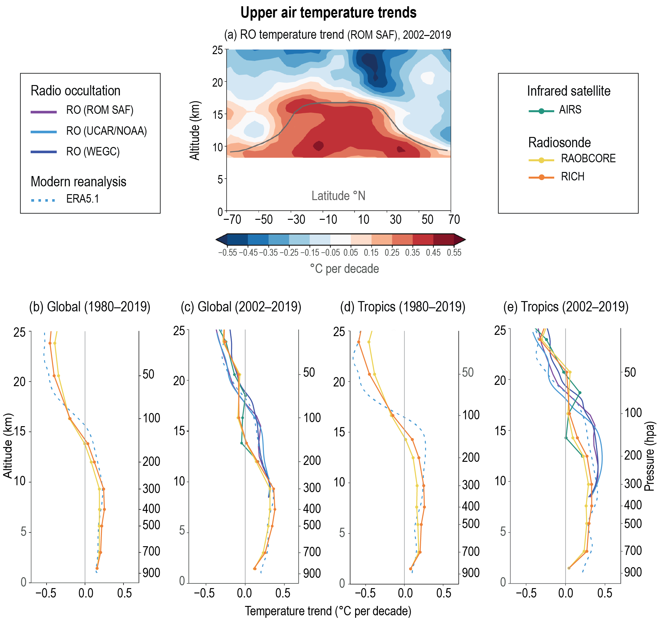 Figure 2.12 | Temperature trends in the upper air. (a) Zonal cross-section of temperature anomaly trends (2007–2016 baseline) for 2002–2019 in the upper troposphere and lower stratosphere region. The climatological tropopause altitude is marked by a grey line. Significance is not indicated due to the short period over which trends are shown, and because the assessment findings associated to this figure relate to difference between trends at different heights, not the absolute trends. (b, c) Trends in temperature at various atmospheric heights for 1980–2019 and 2002–2019 for the near-global (70°N–70°S) domain. (d, e) as for (b, c) but for the tropical (20°N–20°S) region. Further details on data sources and processing are available in the chapter data table (Table 2.SM.1).
 In summary, the troposphere has warmed since the mid-20th century. There is medium confidence that temperatures in the tropical upper troposphere have warmed faster than those at the surface since 2001, but low confidence in changes prior to 2001. It is virtually certain that the lower stratosphere has cooled since the mid-20th century. However, most datasets show that lower stratospheric temperatures have stabilized since the mid-1990s with no significant change over the last 20 years. It is likely that middle and upper stratospheric temperatures have decreased since 1980, but there is low confidence in the magnitude. It is virtually certain that the tropopause height has risen over 1980–2019 but there is low confidence in the magnitude of this rise, or whether the rate of change has reduced commensurate with stabilized lower stratospheric temperatures.
Diagnostic/Dataset | Trend 1960–2019 | Trend 1980–2019 | Trend 2000–2019 |
Lower troposphere | |||
RAOBCORE | 1.08 [0.94 to 1.23] | 0.74 [0.57 to 0.91] | 0.52 [0.26 to 0.78] |
RICH | 1.20 [1.06 to 1.34] | 0.79 [0.63 to 0.96] | 0.53 [0.28 to 0.77] |
UAHRD | 0.97 [0.80 to 1.13] | 0.91 [0.76 to 1.05] | 0.53 [0.35 to 0.72] |
UAH | 0.51 [0.37 to 0.65] | 0.29 [0.07 to 0.50] | |
RSS | 0.79 [0.66 to 0.92] | 0.41 [0.24 to 0.58] | |
ERA5.1 | 0.68 [0.52 to 0.84] | 0.55 [0.34 to 0.75] | |
Average | 1.08 | 0.74 | 0.47 |
Lower stratosphere | |||
RAOBCORE | –1.37 [–1.80 to –0.93] | –1.00 [–1.56 to –0.45] | –0.05 [–0.20 to 0.09] |
RICH | –1.45 [–1.99 to –0.92] | –1.19 [–1.95 to –0.42] | 0.02 [–0.20 to 0.23] |
UAHRD | −1.25 [−1.51 to −0.98] | −0.79 [−1.16 to −0.43] | −0.11 [−0.25 to 0.03] |
UAH | –1.14 [–1.61 to –0.67] | –0.24 [–0.37 to –0.12] | |
RSS | –0.90 [–1.37 to –0.43] | –0.14 [–0.26 to –0.03] | |
STAR | –0.97 [–1.45 to –0.49] | –0.17 [–0.29 to –0.04] | |
ERA5.1 | –1.19 [–1.87 to –0.50] | –0.01 [–0.13 to 0.10] | |
Average | –1.36 | –1.03 | –0.10 |
2.3.1.3 Global Hydrological Cycle
This section focuses on large-scale changes in a subset of components of the hydrological cycle (Cross-Chapter Box 2.2). Chapter 8 undertakes a holistic assessment of changes in the hydrological cycle integrating observations, modelling and theoretical understanding, while (Chapter 11 assesses hydrological cycle extremes such as droughts and floods.
2.3.1.3.1 Paleo perspective of the global hydrological cycle
The AR5 assessed large-scale indicators of terrestrial paleo hydroclimate, including as part of its assessment of paleo floods and droughts, but did not assess proxy evidence for paleo hydroclimate indicators over continental and larger scales. The paleoclimate evidence assessed in AR5 was broadly consistent with global hydroclimate scaling with temperature: warmer periods were wetter (e.g., the Pliocene; increased precipitation) with colder periods being drier (e.g., the LGM; decreased precipitation).
Substantial limitations exist in reconstructing the global hydrological cycle prior to the Quaternary, particularly during the Eocene, due to the lack of high-resolution proxy records and their sparsity. Spatial heterogeneity complicates identification of wetting and drying signals during the PETM and the EECO, with paleo data and model simulations suggesting an intensified global hydrological cycle (Carmichael et al., 2016, 2017; Hyland et al., 2017; West et al., 2020), in particular an increased specific humidity (Winnick et al., 2015; van Dijk et al., 2020). Conditions wetter than present were inferred for the MPWP (Cross Chapter Box 2.4), with intensified Asian monsoons (An et al., 2015) but with nevertheless drier conditions over tropical and subtropical SH locations (Pontes et al., 2020). A new global reconstruction of hydroclimate proxies for the LIG points to stronger boreal precipitation compared to 1850–1900 over high latitudes and especially over monsoon areas, with a more heterogeneous signal for the SH (Scussolini et al., 2019). This heterogeneity is also present in the tropics, characterized by large zonal differences in precipitation change due to the variations in the intensity of Walker circulation (Section 2.3.1.4.1). Available records indicate reduced global vegetation cover and abundant atmospheric dust deposition during the LGM (increased aridity), particularly over the tropics and high latitudes (Lamy et al., 2014; Újvári et al., 2017). This agrees with models and moisture-sensitive proxies, suggesting an overall decrease in global precipitation during the LGM relative to recent decades, albeit with regional-scale heterogeneity (Cao et al., 2019). Despite lower global precipitation amounts, research since AR5 has identified a wetting of mid-latitudes during the LGM (Putnam and Broecker, 2017; Lowry and Morrill, 2018; Morrill et al., 2018), thereby complicating the characterization of the LGM as a relatively ‘dry’ period. Low evaporation rates and increased top-soil moisture during the LGM may have contributed to elevated levels of large closed-basin lakes located in the 30°–45° latitudinal belts (Putnam and Broecker, 2017; Scheff et al., 2017), such as the south-west United States (e.g., Ibarra et al., 2018), southern Australia (Petherick et al., 2013; Fitzsimmons et al., 2015; Sniderman et al., 2019) and Patagonia (e.g., Quade and Kaplan, 2017).
New analyses suggest that during the Holocene, the NH mid-latitudes became increasingly wet, in phase with the strength of the latitudinal temperature and insolation gradients (Shuman and Marsicek, 2016; Routson et al., 2019). Nevertheless, there was also considerable spatial heterogeneity and variability on centennial to millennial timescales (Newby et al., 2014; Shuman and Marsicek, 2016; H. Zhang et al., 2018; Liefert and Shuman, 2020). The NH tropics and many regions of the SH deep tropics experienced wetting up until the early to mid-Holocene but drying thereafter (Shanahan et al., 2015; Nash et al., 2016; Muñoz et al., 2017; Quade et al., 2018). Evidence for the SH is limited, with a wetting trend during the Holocene in low latitudes of South America (Kanner et al., 2013; Mollier-Vogel et al., 2013) and parts of the African tropics (Schefuß et al., 2011; Chevalier and Chase, 2015) but a drying tendency over southern Australia and New Zealand (van den Bos et al., 2018; Barr et al., 2019) and South America (Quade and Kaplan, 2017; Moreno et al., 2018).
For the CE, new proxy records have led to the creation of continental drought atlases (Cook et al., 2015; Palmer et al., 2015; Stahle et al., 2016; Morales et al., 2020) and millennial reanalyses (Steiger et al., 2018; Tardif et al., 2019). These reconstructions highlighted the occurrence of multi-decadal regional mega-droughts in the NH before 1600 CE, particularly during 800–1200 CE, with a predominance of wet periods after 1700 CE (Cook et al., 2015; Rodysill et al., 2018; Shuman et al., 2018). In the SH, much of South America and the African tropics experienced a reduction of precipitation during 900–1200 CE and a wetting peak during 1500–1800 CE (Tierney et al., 2015; Nash et al., 2016; Fletcher et al., 2018; Lüning et al., 2018; Campos et al., 2019), with an opposite pattern in southern subtropical Africa (Woodborne et al., 2015; Lüning et al., 2018). Large multi-decadal variability was documented over Australia and New Zealand during the 800–1300 CE period, followed by a well-defined wet period during 1500–1800 CE (Barr et al., 2014; Evans et al., 2019).
To summarize, since AR5 there has been considerable progress in detecting the variations of the global hydrological cycle prior to the instrumental period. There are indications from multiple sources of a wetting trend during the Holocene, particularly for the NH and parts of the SH tropics (medium confidence). Hydroclimate during the CE is dominated by regional variability, generally precluding definitive statements on changes at continental and larger scales, with a general reduction of mega-drought occurrences over the last about 500 years (medium confidence). Availability of proxy data for assessing Holocene hydroclimate variability is biased towards the NH, with medium evidence butlow agreement for the assessment of SH changes.
2.3.1.3.2 Surface humidity
The AR5 reported very likely widespread increases in near-surface air specific humidity since the 1970s, abating from around 2000 to 2012 (medium confidence). This abatement resulted in a recent decline in relative humidity over the land.
Near surface humidity has been monitored using in-situ data (e.g., NOCSv2.0; Berry and Kent, 2011), satellite-derived estimations (e.g., HOAPS3, Liman et al., 2018; J-OFURO3, Tomita et al., 2019), global gridded products such as HadISDH (Willett et al., 2014, 2020), and reanalyses (e.g., ERA5, JRA-55 and 20CRv3). In-situ based humidity products suffer from uncertainties over poorly sampled regions particularly in the SH (Berry and Kent, 2011; Kent et al., 2014; Willett et al., 2014). There is general consensus in the inter-annual variability and sign of trends implying high confidence in increasing specific humidity since the 1970s and decreasing relative humidity since 2000, particularly over land (Simmons et al., 2010; Willett et al., 2014, 2020). Since 2012, specific humidity over land and ocean has remained well above the 1973–2019 average and reached record or near-record values (Figure 2.13b), with the strong 2015–2016 El Niño event boosting surface moisture levels (Byrne and O’Gorman, 2018). The abatement from around 2000 to 2012 reported in AR5 has not persisted. This is consistent with increases in total column water vapour (Section 2.3.1.3.3) and a resumption of rapid warming in surface temperatures (Section 2.3.1.1.3). The global averaged relative humidity however has remained depressed since 2000 (Figure 2.13d; Simmons et al., 2010; Willett et al., 2014, 2020; Dunn et al., 2017; Vicente-Serrano et al., 2018).
Since 1973, increases in specific humidity have been widespread and significant across the majority of the land and ocean regions where observations are available (Figure 2.13a). In contrast, trends in relative humidity show distinct spatial patterns with generally increasing trends over the higher latitudes and the tropics and generally decreasing trends over the sub-tropics and mid-latitudes, particularly over land areas (Figure 2.13c). Near-surface specific humidity over the oceans has increased since the 1970s according to several in-situ, satellite and reanalysis data records (Kent et al., 2014; Robertson et al., 2020; Willett et al., 2020). According to the HadISDH product, increases in specific humidity and decreases in relative humidity are significant particularly over the NH mid-latitudes (Figure 2.13a,c). Poor data coverage over the SH south of 20°S does not allow for the robust assessment of trends. Sources of uncertainty include the initial measurement accuracy, homogenization over land, observational height at ships and instrument bias adjustment over ocean, and sparse spatio-temporal sampling (Prytherch et al., 2015; Roberts et al., 2019; Willett et al., 2020).
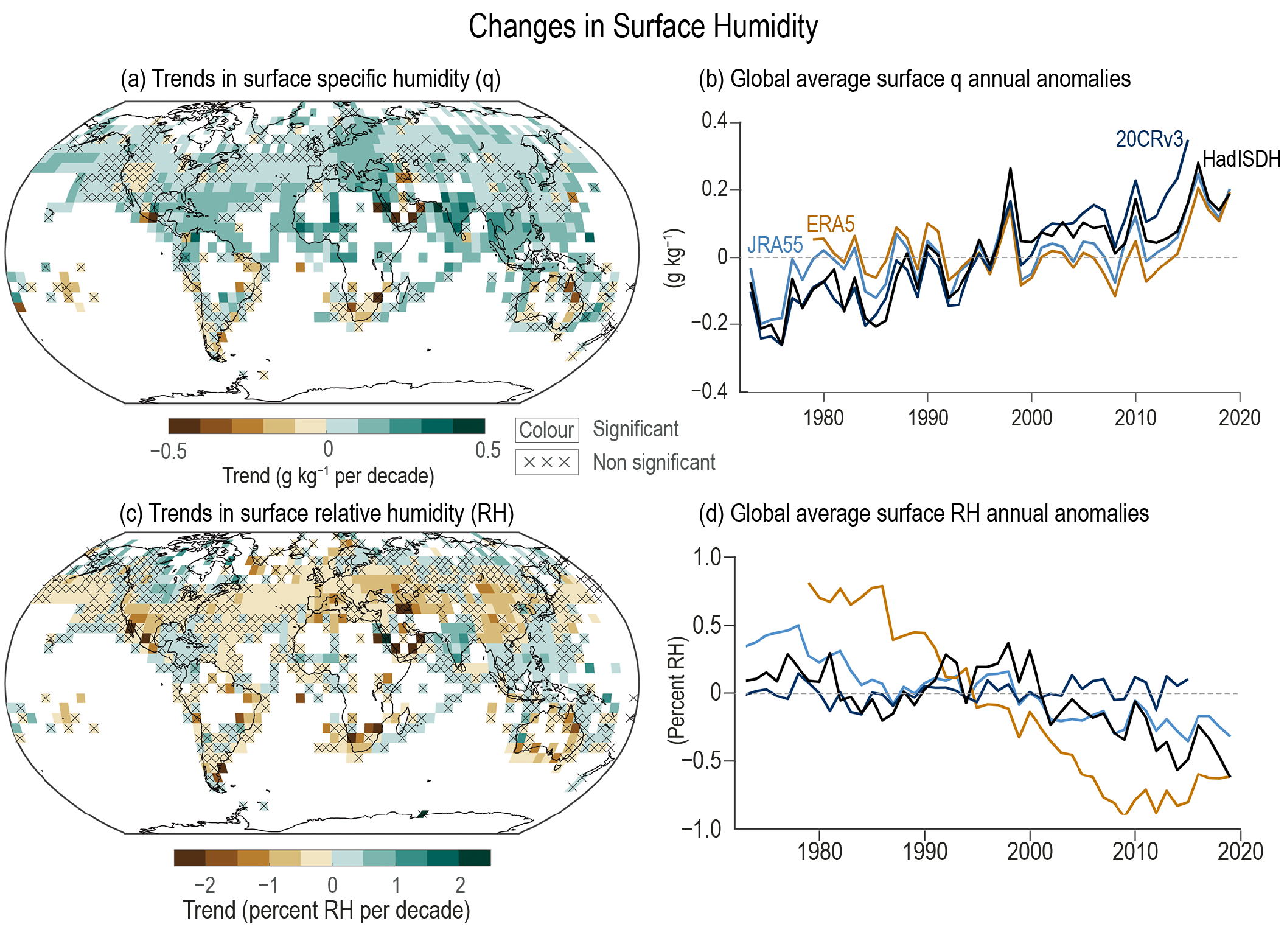
In summary, observations since the 1970s show avery likely increase in near surface specific humidity over both land and oceans. Avery likely decrease in relative humidity has occurred over much of the global land area since 2000, particularly over mid-latitude regions of the NH, with increases at northern high latitudes.
2.3.1.3.3 Total column water vapour (TCWV)
The AR5 concluded that total column water vapour (TCWV)very likely increased since the 1970s, at a rate that was overall consistent with the Clausius-Clapeyron relationship (about 7% per °C) given the observed increase in atmospheric temperature.
Records prior to the instigation of quasi-global coverage by radiosondes require the use of statistical relationships to infer TCWV from historical SST observations or the evaluation of centennial-scale reanalysis products (Smith and Arkin, 2015). These approaches reveal two periods of positive trends, one from 1910 to 1940 and the other from 1975 onwards (Zhang et al., 2013; Mieruch et al., 2014; Shi et al., 2018), concurrent with periods of positive SST trends (Figure 2.11). Potential sources of errors in the SST-based estimation of TCWV include both uncertainties in historical SST and uncertainties in the parameters that define the relationship between the variables (Smith and Arkin, 2015). Trends based on 20CRv2c, ERA-20C and ERA-20CM indicate an increase in TCWV over much of the global ocean since the beginning of the 20th century, particularly over the tropics (Bordi et al., 2015; Smith and Arkin, 2015; Poli et al., 2016). TCWV trends estimated since the middle of the 20th century from radiosonde observations show significant increases over North America and large portions of Eurasia, while decreases are restricted to Australia, eastern Asia and the Mediterranean region (Y. Zhang et al., 2018). Overall, there is a significant increase in TCWV over global land areas since 1979 (Chen and Liu, 2016).
Since the late 1970s a range of satellite missions permit a quasi-global assessment of TCWV. Several satellite products provide water vapour retrievals based upon distinct spectral domains, in addition to products from radiosondes, reanalyses and GNSS radio occultation. The GEWEX Water Vapour Assessment (G-VAP) provided an intercomparison of several TCWV data records, with global coverage but limited timespan (Schröder et al., 2018). The various global products generally exhibit a positive trend since 1979 (Figure 2.14; Allan et al., 2014; Mieruch et al., 2014; Schröder et al., 2016; J. Wang et al., 2016), most evident over the tropics (Gu and Adler, 2013; Chen and Liu, 2016; Mears et al., 2018; Wang and Liu, 2020; Salamalikis et al., 2021). The existence of apparent breakpoints in several products, which are generally coincident with changes in the observing system, lead to trend estimates that are not in line with theoretical expectations imposed by the Clausius-Clapeyron relationship (Schröder et al., 2019), although other factors such as regional moisture divergence/convergence could account for the observed TCWV-temperature scaling. Substantial potential inhomogeneities affect trend estimates based on satellite, reanalysis and merged products in particular over Central Africa, the Sahara and central South America (Schröder et al., 2016, 2019; J. Wang et al., 2016). Moreover, data gaps in observations from ground-based GNSS receivers and radiosondes lead to low confidence in TCWV estimation in these regions.
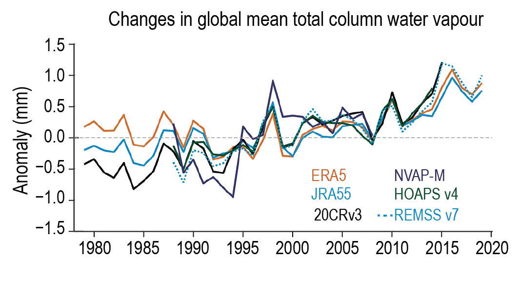 Figure 2.14 | Time series of global mean total column water vapour annual anomalies (mm) relative to a 1988–2008 base period. Further details on data sources and processing are available in the chapter data table (Table 2.SM.1).
 In summary, positive trends in global total column water vapour are very likely since 1979 when globally representative direct observations began, although uncertainties associated with changes in the observing system imply medium confidence in estimation of the trend magnitudes. Low confidence in longer-term trends arises from uncertainties in the SST-TCWV relationship and current centennial scale reanalyses, particularly during the first half of the 20th century.
2.3.1.3.4 Global precipitation
The AR5 concluded that there was low confidence in precipitation change averaged over global land areas prior to 1950, and medium confidence thereafter with no significant global trends. There was a likely overall increase in precipitation in the well-sampled NH mid-latitudes, with high confidence after 1951.
In situ precipitation records over land extend back for centuries in a few locations, and to the early to mid-20th century quasi-globally. Datasets differ in their input data, completeness of records, period covered, and the gridding procedures applied, which, given spatial clustering and the small spatial scales of precipitation, results in differences in global and regional estimates of precipitation changes (Q. Sun et al., 2018; Nogueira, 2020). The spatial variability of observed long-term trends (1901–2019) based on GPCC V2020 and CRU TS 4.04 (Figure 2.15a,b) indicates significant increases in precipitation mainly over eastern North America, northern Eurasia, southern South America and north-western Australia. Decreases are strongest across tropical western and equatorial Africa and southern Asia. The temporal evolution of global annual land precipitation anomalies exhibits little consistency between GPCC V2020, CRU TS 4.04 and GHCNv4 datasets, especially prior to 1950, that is associated with limitations in data coverage (Figure 2.15c; Wu et al., 2013; Shen et al., 2014; Gu and Adler, 2015). These disagreements between datasets prior to the 1950s result in differences in trend estimates over global land (Table 2.6). A qualitative consistency in decadal and interdecadal variations between the products is only observed since the 1950s, with primarily positive land precipitation anomalies during the 1950s, 1970s and during 2000 to 2019 (Figure 2.15c).
Dataset | Trends in annual precipitation (mm yr–1per decade) | ||
1901–2019 | 1960–2019 | 1980–2019 | |
GPCCv2020 | 1.01a± 0.99 | 1.67 ± 3.23 | 5.60 ± 6.38 |
CRU TS 4.04 | 0.57 ± 2.08 | 0.17 ± 3.12 | 5.75a± 5.09 |
GHCNv4 | 3.19a± 1.48 | 5.03a± 4.87 | 11.06a± 9.17 |
GPCPv2.3 | 5.41a± 5.20 | ||
aTrend values significant at the 10% level.
 Figure 2.15 | Changes in observed precipitation. (a, b) Spatial variability of observed precipitation trends over land for 1901–2019 for two global in-situ products. Trends are calculated using OLS regression with significance assessed following AR(1) adjustment after Santer et al. (2008) (‘×’ marks denote non-significant trends). (c) Annual time series and decadal means from 1891 to date relative to a 1981–2010 climatology (note that different products commence at distinct times). (d, e) as(a, b), but for the periods starting in 1980. (f) is for the same period for the globally complete merged GPCP v2.3 product. Further details on data sources and processing are available in the chapter data table (Table 2.SM.1).
 Several satellite-based precipitation datasets improve the representation of the spatio-temporal changes since the late 20th century. Some of these are based exclusively on satellite data (e.g., CMORPH, Joyce et al., 2004; GSMaP, Okamoto et al., 2005), with others being combinations of in situ observations, reanalyses and satellite retrievals (e.g., CMAP, Xie and Arkin, 1997; TRMM 3B43 V7, Huffman et al., 2007 ; PERSIANN-CDR, Ashouri et al., 2015; CHIRPS, Funk et al., 2015; GPCP V2.3, Adler et al., 2018). These can be affected by systematic and random uncertainties due to inhomogeneities in the satellite-derived precipitation and station data and the uncertainties of blending algorithms (Hegerl et al., 2015; Q. Sun et al., 2018). The spatial coverage of these products is near-global, with available estimations formally covering 60°S–60°N with decreasing quality from low to high latitudes, depending on the sensors and algorithms used (Hu et al., 2019). A detailed description of the most relevant satellite products is provided in section 10.2.1.1.
Recent trends (1980–2019) for GPCC V2020, CRU TS 4.04 and GPCP V2.3 show significant increases in land precipitation over tropical Africa, the eastern portions of Europe and North America, central Asia and the Maritime Continent (Figure 2.14d–f). Significant decreases are observed over central South America, western North America, northern Africa and the Middle East. A detailed assessment of the recent regional precipitation trends using the same datasets can be found in the Atlas. Global trends for 1980–2019 show a general increase in annual precipitation over land, which is particularly marked for CRU TS 4.04 and GHCNv4 (Table 2.6). These changes have been accompanied by a strengthening of precipitation seasonality over tropical land areas, although with broad spread between different satellite-based (GPCP, MSWEP_V1.2, PERSIANN-CDR) and in situ gridded datasets (GPCC, CRU TS; Chou et al., 2013; Li et al., 2016; Tan et al., 2020). Increasing trends since 1980, in contrast to longer-term declining trends since 1901, are particularly evident over much of Africa, while more widespread negative trends were observed over much of southern South America in the more recent period (Atlas 7.2; Knutson and Zeng, 2018). A faster recent increase in precipitation over global land is inferred comparing the precipitation trends over 1960–2019 with 1980–2019 (Table 2.6). Over the global ocean, the comparison between precipitation datasets is compromised by the different measurement periods, as well as the spatial coverage of the available products (Adler et al., 2017; Nguyen et al., 2018; Jaber and Abu-Allaban, 2020; Nogueira, 2020), limiting the ability to assess the sign and magnitude of precipitation trends. The GPCPv2.3 database (Adler et al., 2017, 2018) exhibits an increase of 2.94 mm yr–1 per decade over 1980–2019, principally due to the trends over the Indian ocean and in the tropical western Pacific (Figure 2.15f). The regional patterns of recent trends are consistent with the documented increase in precipitation over tropical wet regions and the decrease over dry areas, estimated through GPCP v2.2 data (Liu and Allan, 2013; Trammell et al., 2015; Kao et al., 2017; Polson and Hegerl, 2017).
In summary, globally averaged land precipitation has likely increased since the middle of the 20th century (medium confidence), with low confidence in trends prior to 1950. A faster increase in global land precipitation was observed since the 1980s (medium confidence), with large interannual variability and regional heterogeneity. Over the global ocean there is low confidence in the estimates of precipitation trends, linked to uncertainties in satellite retrievals, merging procedures and limited in situ observations.
2.3.1.3.5 Precipitation minus evaporation
The AR5 concluded that the pattern of precipitation minus evaporation (P–E) over the ocean had been enhanced since the 1950s (medium confidence). Saline surface waters had become saltier, while the relatively fresh surface waters had become fresher. The inferred changes in P–E were consistent with the observed increased TCWV, although uncertainties in the available products prevented identifying robust trends.
Estimating global-scale trends in P–E using direct observations alone is challenging due to limited evaporation measurements and inhomogeneities in satellite-derived precipitation and evaporation datasets (Hegerl et al., 2015; López et al., 2017). Hence, the assessment of global P–E trends is generally performed using reanalyses, although changes in the observing system imply considerable uncertainty (Skliris et al., 2014). Since the second half of the 20th century, several reanalyses and observational datasets have shown increases in P–E over global land, although 75% of land areas exhibit no significant changes and both internal variability and observational uncertainty are substantial (Greve et al., 2014; Robertson et al., 2016). The recently released ERA5 (Hersbach et al., 2020) showed improvements in the representation of tropical precipitation, although it overestimates global precipitation trends in comparison to ERA-Interim and GPCP (Nogueira, 2020), and suffers from temporal changes in the annual balance between precipitation and evaporation (Hersbach et al., 2020). The spatial pattern of P–E trends over 1980–2019 (Figure 2.16a) are largely consistent with the trends in the GPCP v2.3 precipitation dataset (Figure 2.15f and Section 2.3.1.3.4) and agrees in sign with the trends from other reanalyses such as JRA-55 and MERRA-2 (L. Yu et al., 2020).
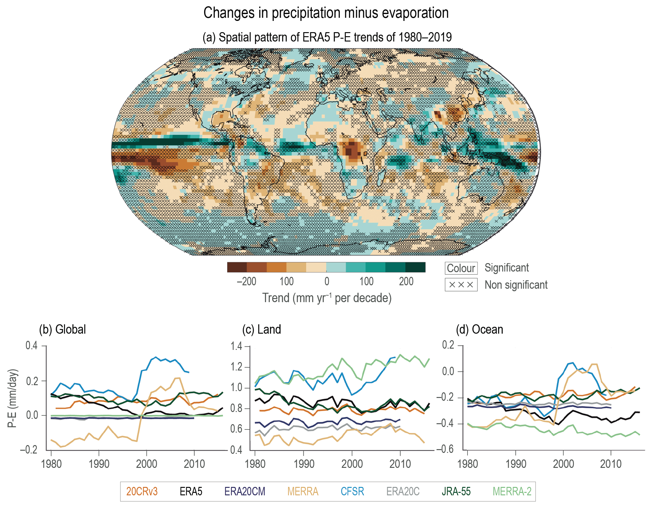 Figure 2. 16 | Changes in precipitation minus evaporation. (a) Trends in precipitation minus evaporation (P–E) between 1980 and 2019. Trends are calculated using OLS regression with significance assessed following AR(1) adjustment after Santer et al. (2008) (‘×’ marks denote non-significant trends). Time series of (b) global, (c) land-only and (d) ocean-only average annual P–E (mm day–1). Further details on data sources and processing are available in the chapter data table (Table 2.SM.1).
 A variety of reanalysis products exhibit diverse temporal evolutions of P–E (Figure 2.16b–d). Globally MERRA-2, ERA20C and ERA20CM exhibit little change whereas JRA-55, ERA5 and 20CRv3 all imply long-term changes (Figure 2.16d). A potential limitation in estimating P–E from some reanalysis products is readily apparent when considering the temporal evolution of global P–E from CFSR and MERRA (Figure 2.16d) which both exhibit strong discontinuities over the global ocean in the late 1990s. Over global land as a whole, precipitation exceeds evaporation (P–E >0) for all the reanalysis products (Figure 2.16c), with decreasing trends in P–E for ERA5 and JRA-55 and increasing trends for MERRA-2 and CFSR. The P–E over the global ocean is negative (evaporation exceeding precipitation) for most reanalyses (Figure 2.16d), with declining trends in ERA5 and MERRA-2 dominated by trends in evaporation (Bosilovich et al., 2017; Hersbach et al., 2020) (Figure 2.16d). The recent increase in ocean evaporation was also documented for several reanalyses (Craig et al., 2017) and in satellite data (Andersson et al., 2011; Robertson et al., 2014), although with considerable differences between available estimates (Chandanpurkar et al., 2017; L. Yu et al., 2020). An alternative indirect approach to estimate P–E changes is based on near-surface ocean salinity (Section 2.3.3.2), which is partially driven by the freshwater flux at the ocean surface. The near-surface salinity trends are more spatially coherent compared to those revealed by P–E estimates from reanalyses, with an intensification of the water cycle over oceans, especially in subtropical regions (Durack et al., 2012; Skliris et al., 2014; L. Yu et al., 2020). However, the precise rate of water cycle intensification implied by salinity trends is sensitive to methodological choices (e.g., Skliris et al., 2016; Zika et al., 2018).
In conclusion, observational uncertainty yields low confidence in globally averaged trends in P–E over the 20th century, with a spatial pattern dominated by precipitation changes over land and by evaporation increases over the ocean. Different reanalyses disagree on the sign of long-term changes in the global mean P–E.
2.3.1.3.6 Streamflow
The AR5 concluded that there was low confidence in a positive trend in global river discharge during the 20th century. It noted that many of the largest rivers with long term streamflow records have been impacted by non-climatic human influences such as dam construction or land-use change.
River discharge is monitored widely, although gaps remain at a subcontinental scale over central Asia and Africa (Wei et al., 2020). Substantial recent efforts have been made to generate new global streamflow datasets, consolidating observations from many stream gauges to create streamflow indices (Do et al., 2018; Gudmundsson et al., 2018) and gridded products using neural networks (Barbarossa et al., 2018) or combinations between observations and reanalyses (Suzuki et al., 2018; Ghiggi et al., 2019).
Human intervention on river discharge linked to increases in evapotranspiration and some reduction of intra-annual streamflow variability (Jaramillo and Destouni, 2015; Chai et al., 2020) might affect the detection of trends in extreme daily streamflow events (Do et al., 2017; Gudmundsson et al., 2019). However, these activities have a minor impact on annual streamflow compared to climate variations (Dai et al., 2009; Alkama et al., 2013). Available global studies post-1950 generally concur that there have been more rivers experiencing decreases than increases in runoff (Do et al., 2017; Su et al., 2018; Gudmundsson et al., 2019; X. Shi et al., 2019). Most of the rivers have not experienced statistically significant changes in streamflow, and when globally aggregated there is no significant change (Dai and Zhao, 2017). Global streamflow variability is strongly modulated by ENSO and PDV, with below-normal global streamflow as a response to El Niño events and vice-versa during La Niña episodes (Dai, 2016; Liang et al., 2016; Kim, 2019). The response of streamflow to changes in precipitation associated with ENSO and PDV has heterogeneous regional patterns at subcontinental scales (Section 8.3.2.9.1). No significant trends are found for reanalysis-based discharge estimates over 1993 to 2015 (Chandanpurkar et al., 2017). Uncertainties in global streamflow trends arise predominantly from changes in instrumentation, gauge restoration, recalibration of rating curves, flow regulation or channel engineering (Alkama et al., 2011; Gudmundsson et al., 2018; Ghiggi et al., 2019).
In summary, the sign of global streamflow trends remains uncertain, with slightly more globally gauged rivers experiencing significantly decreasing flows than significantly increasing flows since the 1950s (low confidence).
2.3.1.4 Atmospheric Circulation
This section focuses on large-scale changes in a subset of components of the atmospheric circulation (Cross-Chapter Box 2.2). Chapter 8 assesses large-scale as well as regional aspects of circulation components and their impact on the hydrological cycle, while (Chapter 11 assesses the association of circulation changes and variability with extreme events.
2.3.1.4.1The Hadley and Walker circulations
The AR5 reported low confidence in trends in the strength of the Hadley circulation (HC) and the Walker circulation (WC) due to uncertainties in available reanalysis datasets and the large interannual-to-decadal variability of associated circulation patterns. However, AR5 indicated a likely widening of the tropical belt since the 1970s, albeit with large uncertainty in the magnitude of this change. There was high confidence that the post-1990s strengthening of the Pacific WC reversed its weakening observed from the mid-19th century to the 1990s.
Paleo reconstructions of rainfall and trade winds extending over the last 100 kyr show an intensification of the NH HC concurrently with a weakening of the SH HC and a southward shift of the inter tropical convergence zone (ITCZ) during Heinrich stadials (Deplazes et al., 2013; McGee et al., 2018; Stríkis et al., 2018; Wendt et al., 2019). An intensification of the HC associated with conditions similar to La Niña (northward migrations of both the ITCZ and the SH westerlies) was found in reconstructions for the MH (McGee et al., 2014; Mollier-Vogel et al., 2019). Changes in insolation from the mid to late Holocene favoured a southward migration in the position of the ITCZ and the descending branch of the HC in the NH, approaching its current width and position (Wirth et al., 2013; Thatcher et al., 2020). Tree ring chronologies from the NH mid-latitudes over the last 800 years show that the northern edge of the HC tended to migrate southward during positive phases of ENSO and PDV, with northward shifts during negative phases (Alfaro-Sánchez et al., 2018). Between 1400 and 1850 CE the HC over both hemispheres and the ITCZ were displaced southward, consistent with occurrence of drought conditions in several NH regions (Wirth et al., 2013; Burn and Palmer, 2014; Lechleitner et al., 2017; Alfaro-Sánchez et al., 2018; Flores-Aqueveque et al., 2020). Moreover, several proxy records showed not only inter-hemispheric shifts in the ITCZ but a contraction of the tropical belt during 1400–1850 CE, which followed an expansion during 950–1250 CE (Denniston et al., 2016; Griffiths et al., 2016).
From centennial-scale reanalyses, Liu et al. (2012) and D’Agostino and Lionello (2017) found divergent results on HC extent over the last 150 years, although with unanimity upon an intensification of the SH HC. A substantial discrepancy between HC characteristics in centennial-scale reanalyses and in ERA-Interim (D’Agostino and Lionello, 2017) since 1979 yields significant questions regarding their ability to capture changes in HC behaviour. Taken together with the existence of apparent non-climatic artefacts in the datasets (Nguyen et al., 2015), this implies low confidence in changes in the extent and intensity of HC derived from centennial-scale reanalyses. However, using multiple observational datasets and centennial-scale reanalyses, Bronnimann et al. (2015) identified a southward shift in the NH HC edge from 1945 to 1980 of about 0.25° latitude per decade, consistent with observed changes in global land monsoon precipitation (Section 2.3.1.4.2).
Since AR5 several studies based upon a range of metrics and different reanalyses products have suggested that the annual mean HC extent has shifted poleward at an approximate rate of 0.1°–0.5° latitude per decade over the last about 40 years (Allen and Kovilakam, 2017; Davis and Birner, 2017; Grise et al., 2018; Staten et al., 2018, 2020; Studholme and Gulev, 2018; Grise and Davis, 2020). The observed widening of the annual mean HC, revealed by a variety of metrics, is primarily due to poleward shift of the Northern Hemisphere HC. There have been stronger upward trends in the NH extent of HC after 1992 (Figure 2.17a). The estimated magnitude of the recent changes based on modern-era reanalyses is not as large as that in AR5, due to apparent biases in older-generation reanalyses (Grise et al., 2019). Moreover, large interannual variability leads to uncertainties in estimates of long-term changes (Nguyen et al., 2013; Garfinkel et al., 2015b; Seviour et al., 2018; Staten et al., 2018), particularly for the NH given its zonal asymmetries (Staten et al., 2020; Wang et al., 2020). These large-scale features of the HC based on reanalyses agree with estimates revealed from the Integrated Global Radiosonde Archive (IGRA) during 1979–2012 (Lucas and Nguyen, 2015; Mathew et al., 2016). Recent trends based on reanalyses indicate a larger seasonal widening in the HC for summer and autumn in each hemisphere, although the magnitude of changes in HC extent is strongly dependent on dataset and metrics used (Grise et al., 2018; Y. Hu et al., 2018; Staten et al., 2018). The shifts in the HC position were accompanied by a narrowing ITCZ over the Atlantic and Pacific basins, with no significant change in its location and increases in the precipitation intensity (Byrne et al., 2018).
 Figure 2.17 | Time series of the annual mean Northern Hemisphere (NH, top curves) and Southern Hemisphere (SH, bottom curves) Hadley cell extent (a) and Hadley cell intensity (b) since 1979. Further details on data sources and processing are available in the chapter data table (Table 2.SM.1).
 Trends in the HC intensity since 1979 differ between reanalyses, although there is a tendency toward HC intensification (Figure 2.17b; Nguyen et al., 2013; Chen et al., 2014; D’Agostino and Lionello, 2017; R. Huang et al., 2019), which is more marked in the NH than the SH (Studholme and Gulev, 2018). However, the ability of reanalyses to represent the HC strength has been questioned due to inaccurate representation of latent heating distribution, which is directly related to tropical convection and influences the HC dynamics (Chemke and Polvani, 2019; Mathew and Kumar, 2019).
Paleo evidence during the LGM indicates a weaker WC over the Indian Ocean (DiNezio et al., 2018; Windler et al., 2019) with a stronger Pacific WC (DiNezio and Tierney, 2013). During the Holocene, a transition from a strong WC located more westward during the Early-to-Mid Holocene towards a weak and eastward shifted WC during the late Holocene was inferred from proxy records from the Pacific Warm Pool and South East Asia (Barr et al., 2019; Dang et al., 2020; Griffiths et al., 2020), in concurrence with changes in ENSO activity (Section 2.4.2). Reconstructions for the CE showed weakened WC during 1000–1250 and since 1850, with an intensified circulation during 1500–1850 CE (Xu et al., 2016; Deng et al., 2017).
Considering instrumental records, there is considerable interdecadal variability in the strength of the WC, resulting in time-period dependent magnitude and even sign of trends (Carilli et al., 2015; Bordbar et al., 2017; Hou et al., 2018), with some studies reporting weakening over the 20th century (e.g., Power and Kociuba, 2011; Liu et al., 2019), while others reported strengthening (Z. Li et al., 2020), particularly over the last 30–40 years (e.g., Hu et al., 2013; L’Heureux et al., 2013; Yim et al., 2017). Based on estimation of changes in mid-tropospheric velocity from changes in observed cloud cover, Bellomo and Clement (2015) suggest a weakening and eastward shift of the WC over 1920–2010, however the robustness of this signal is questionable due to high uncertainty in the ship-reported cloud data used before 1954. Using centennial-scale 20CR reanalysis Tseng et al. (2019) showed that the vertical westerly wind shear over the western Pacific does not indicate any long-term change during 1900–1980, but shows a marked increase since the 1980s that is not present in ERA-Interim and JRA-55, again calling into question the ability of centennial-scale reanalyses to capture tropical circulation changes. Recent strengthening together with a westward shift of the WC (Bayr et al., 2014; Ma and Zhou, 2016) was identified across several reanalysis products and observational datasets, and using different metrics for quantifying WC. Nevertheless, satellite observations of precipitation and analyses of upper tropospheric humidity suggest substantially weaker strengthening of the WC than implied by reanalyses (Chung et al., 2019). This recent strengthening in the WC is associated with enhanced precipitation in the tropical western Pacific, anomalous westerlies in the upper troposphere, strengthened downwelling in the central and eastern tropical Pacific, and anomalous surface easterlies in the western and central tropical Pacific (Dong and Lu, 2013; McGregor et al., 2014; Choi et al., 2016). Positive trends in sea level pressure over the eastern Pacific and concurrent negative trends over the Indonesian region result in a pattern implying a shift towards a La Niña-like WC regime, with strengthening of the Pacific Trade Winds mainly over 1979–2012 (L’Heureux et al., 2013; England et al., 2014; Sohn et al., 2016; Zhao and Allen, 2019). Seasonal assessment of the WC showed significant changes in the vertical westerly wind shear over the Pacific during the austral summer and autumn implying a strengthening (Clem et al., 2017).
In summary, there has been a likely widening of the Hadley circulation since the 1980s, mostly due to its extension in the NH, although there is only medium confidence in the extent of the changes. This has been accompanied by a strengthening of the Hadley circulation, particularly in the NH (medium confidence). There is low confidence in the estimation of long-term trends in the strength of the Walker circulation, which are time period dependent and subject to dataset uncertainties. Trends since 1980 are better characterized and consistent with avery likely strengthening that resembles a La Niña-like Walker circulation and a westward shift of the Walker circulation, although with medium confidence in the magnitude of the changes, arising from the differences between satellite observations and reanalysis products.
2.3.1.4.2 Global monsoon (GM) changes
The AR5 reported a weakening of the global monsoon (GM) circulation as well as a decrease of global land monsoon rainfall over the second half of the 20th century. Nevertheless, there was low confidence in the observed circulation trends due to uncertainties in reanalysis products and in the definition of the monsoon area. From a paleo perspective, AR5 only assessed regional monsoon changes.
New research based on high-resolution proxies reinforces previous findings on the influence of orbital cycles on GM variability on millennial time scales. The intensity of the monsoon systems is generally out of phase between hemispheres, being associated with the precession cycle (about 21–23 kyr) (An et al., 2015; P.X. Wang et al., 2017; Seth et al., 2019), with intensified NH monsoon systems during precession minima (Toucanne et al., 2015; Wagner et al., 2019). The eccentricity forcing (about 100 kyr cycle) shows stronger GM during interglacial periods (P.X. Wang et al., 2014, 2017; An et al., 2015; Mohtadi et al., 2016). Changes in obliquity (about 41 kyr cycle) modify the strength of monsoon systems, with increased summer monsoon rainfall when obliquity is maximal (Y. Liu et al., 2015b; Mohtadi et al., 2016). Millennial scale variability in GM during the LDT was also linked to the occurrences of Heinrich stadials, resulting in weakened NH monsoons and intensified SH monsoons (An et al., 2015; P.X. Wang et al., 2017; Margari et al., 2020).
An intensification of the NH monsoons in the early to mid-Holocene with increased precipitation and regional expansions of rainfall areas identified through a variety of proxy records is shown by Biasutti et al. (2018) and P.X. Wang et al. (2017). The response for the SH monsoons during this period indicates a weakening in both summer and winter precipitation (P.X. Wang et al., 2014, 2017; Sachs et al., 2018). A decline in GM precipitation and a retraction of the northern fringes of monsoon areas was inferred from the mid-Holocene onwards, with some regions experiencing wetter conditions during the mid to late Holocene compared with present and a strengthening of the SH monsoons (P.X. Wang et al., 2014, 2017; Sachs et al., 2018). For the CE, GM reconstructions exhibit inter-hemispheric contrast during the period 950–1250 CE, with intensified NH monsoons and weakened SH monsoons, and the opposite pattern during 1400–1850 CE (P.X. Wang et al., 2014; An et al., 2015).
Direct observations highlight that the GM land precipitation, particularly over the NH, experienced a slight increase from 1900 through the early 1950s, followed by an overall decrease from the 1950s to the 1980s, and then an increase to present (Kitoh et al., 2013; B. Wang et al., 2018, 2021; X. Huang et al., 2019b). This highlights the existence of multi-decadal variations in the NH monsoon circulation patterns and precipitation intensity (Wang et al., 2013; P.X. Wang et al., 2014, 2017; Monerie et al., 2019). An overall increase in monsoon precipitation during extended boreal summer (JJAS) over the NH since 1979 is revealed by GPCP (Deng et al., 2018; Han et al., 2019) and CMAP for 1980–2010 (Jiang et al., 2016). SH summer monsoon behaviour is dominated by strong interannual variability and large regional differences (Kitoh et al., 2013; Lin et al., 2014; Jiang et al., 2016; Kamae et al., 2017; Deng et al., 2018; Han et al., 2019), with no significant trends reported by GPCP and CMAP (Deng et al., 2018). Uncertainty predominantly arises from the observed increase in tropical precipitation seasonality (Feng et al., 2013) and the estimation of GM precipitation over the ocean areas, leading to a large apparent spread across datasets (Kitoh et al., 2013; Kamae et al., 2017).
In summary, observed trends during the last century indicate that the GM precipitation decline reported in AR5 has reversed since the 1980s, with a likely increase mainly due to a significant positive trend in the NH summer monsoon precipitation (medium confidence). However, GM precipitation has exhibited large multi-decadal variability over the last century, creating low confidence in the existence of centennial-length trends in the instrumental record. Proxy reconstructions show a likely NH monsoons weakening since the mid-Holocene, with opposite behaviour for the SH monsoons.
2.3.1.4.3Extratropical jets, storm tracks, and blocking
The AR5 reported a likely poleward shift of storm tracks and jet streams since the 1970s from different datasets, variables and approaches. These trends were consistent with the HC widening and the poleward shifting of the circulation features since the 1970s. There was low confidence in any large-scale change in blocking.
Proxy records consistent with modelling results imply a southward shift of the storm tracks over the North Atlantic during the LGM (Raible et al., 2021). A variety of proxies are available for the changes in the position of the extratropical jets/westerlies during the Holocene. Recent syntheses of moisture-sensitive proxy records indicate drier-than-present conditions over mid-latitudes of western North America (Hermann et al., 2018; Liefert and Shuman, 2020) during the MH, which together with a weakened Aleutian Low (Bailey et al., 2018) implies that the winter North Pacific jetstream was shifted northward. A synthesis of lines of evidence from the SH indicates that the westerly winds were stronger over 14–5 ka, followed by regional asymmetry after 5 ka (Fletcher and Moreno, 2012). There is no consensus on the shifts of the SH westerlies with some studies implying poleward migrations (Lamy et al., 2010; Voigt et al., 2015; Turney et al., 2017; Anderson et al., 2018) and others suggesting an equatorward shift (Kaplan et al., 2016) in the MH.
During 950–1400 CE, hydroclimate indicators suggest a northward shift of Pacific storm tracks over North America (McCabe-Glynn et al., 2013; Steinman et al., 2014) which was comparable in magnitude to that over 1979–2015 (J. Wang et al., 2017a). Storm tracks over the North Atlantic-European sector shifted northward as indicated by multi-proxy indicators over the North Atlantic (Wirth et al., 2013; Orme et al., 2017) and Mediterranean (Roberts et al., 2012). Reconstructed westerly winds in the SH suggest a poleward shift (Lamy et al., 2010; Schimpf et al., 2011; Goodwin et al., 2014; Koffman et al., 2014; Moreno et al., 2018), with latitudinal change comparable to that during recent decades (Swart and Fyfe, 2012; Manney and Hegglin, 2018).
Multiple reanalyses show that since 1979 the subtropical jet wind speeds have generally increased in winter and decreased in summer in both hemispheres, but the trends are regionally dependent (Pena-Ortiz et al., 2013; Manney and Hegglin, 2018; S.H. Lee et al., 2019). Over NH mid-latitudes, the summer zonal wind speeds have weakened in the mid-troposphere (Francis and Vavrus, 2012; Coumou et al., 2014, 2015; Haimberger and Mayer, 2017). Meanwhile there are indications of enhanced jetstream meandering in boreal autumn at the hemispheric scale (Francis and Vavrus, 2015; Di Capua and Coumou, 2016), whereas the regional arrangement of meandering depends on the background atmospheric state (Cohen et al., 2020). These meandering trends, however, are sensitive to the metrics used (Screen and Simmonds, 2013; Hassanzadeh et al., 2014; Cattiaux et al., 2016; Vavrus, 2018). Hypothesized links to Arctic warming are assessed in Cross-Chapter Box 10.1.
Multiple reanalyses and radiosonde observations show an increasing number of extratropical cyclones over the NH since the 1950s (Chang and Yau, 2016; X.L. Wang et al., 2016). The positive trends are generally consistent among reanalyses since 1979, though with considerable spread (Tilinina et al., 2013; X.L. Wang et al., 2016). In recent decades the number of deep extratropical cyclones has increased over the SH (Section 8.3.2.8.1 and Figure 8.12; Reboita et al., 2015; X.L. Wang et al., 2016), while the number of deep cyclones has decreased in the NH in both winter and summer (Neu et al., 2013; Coumou et al., 2015; Chang et al., 2016; J. Wang et al., 2017a; Gertler and O’Gorman, 2019). The regional changes for different intensity extratropical cyclones are assessed in Section 8.3.2.8.1. The assessment of trends is complicated by strong interannual to decadal variability, sensitivity to dataset choice and resolution (Tilinina et al., 2013; Lucas et al., 2014; X.L. Wang et al., 2016; Pepler et al., 2018; Rohrer et al., 2018) and cyclone identification/tracking methods (Neu et al., 2013; Grieger et al., 2018). Thus there is overall low confidence for recent changes in global extratropical storm tracks.
A consistent poleward shift of the tropospheric extratropical jets since 1979 is reported by multiple reanalyses (Figure 2.18; Davis and Rosenlof, 2012; Davis and Birner, 2013; Pena-Ortiz et al., 2013; Manney and Hegglin, 2018), and radiosonde winds (Allen et al., 2012). This is generally consistent with the previously reported shifts retrieved from satellite temperature observations (Fu and Lin, 2011; Davis and Rosenlof, 2012). After the 1960s the magnitude of meridional shifts in extratropical jets over both the North Atlantic and North Pacific in August is enhanced compared to multi-century variability (Trouet et al., 2018). Despite some regional differences (Woollings et al., 2014; Norris et al., 2016; J. Wang et al., 2017a; Xue and Zhang, 2017; Ma and Zhang, 2018; Melamed-Turkish et al., 2018), overall poleward deflection of storm tracks in boreal winter over both the North Atlantic and the North Pacific was identified during 1979–2010 (Tilinina et al., 2013). Over the SH extra-tropics there is a similarly robust poleward shift in the polar jet since 1979 (Pena-Ortiz et al., 2013; Manney and Hegglin, 2018; WMO, 2018), although after 2000 the December–January–February (DJF) tendency to poleward shift of the SH jet stream position ceased (Banerjee et al., 2020). The general poleward movement in midlatitude jet streams (Lucas et al., 2014) is consistent with the expansion of the tropical circulation (Section 2.3.1.4.1). The changes of extratropical jets and westerlies are also related to the annular modes of variability (Section 2.4 and Annex IV).
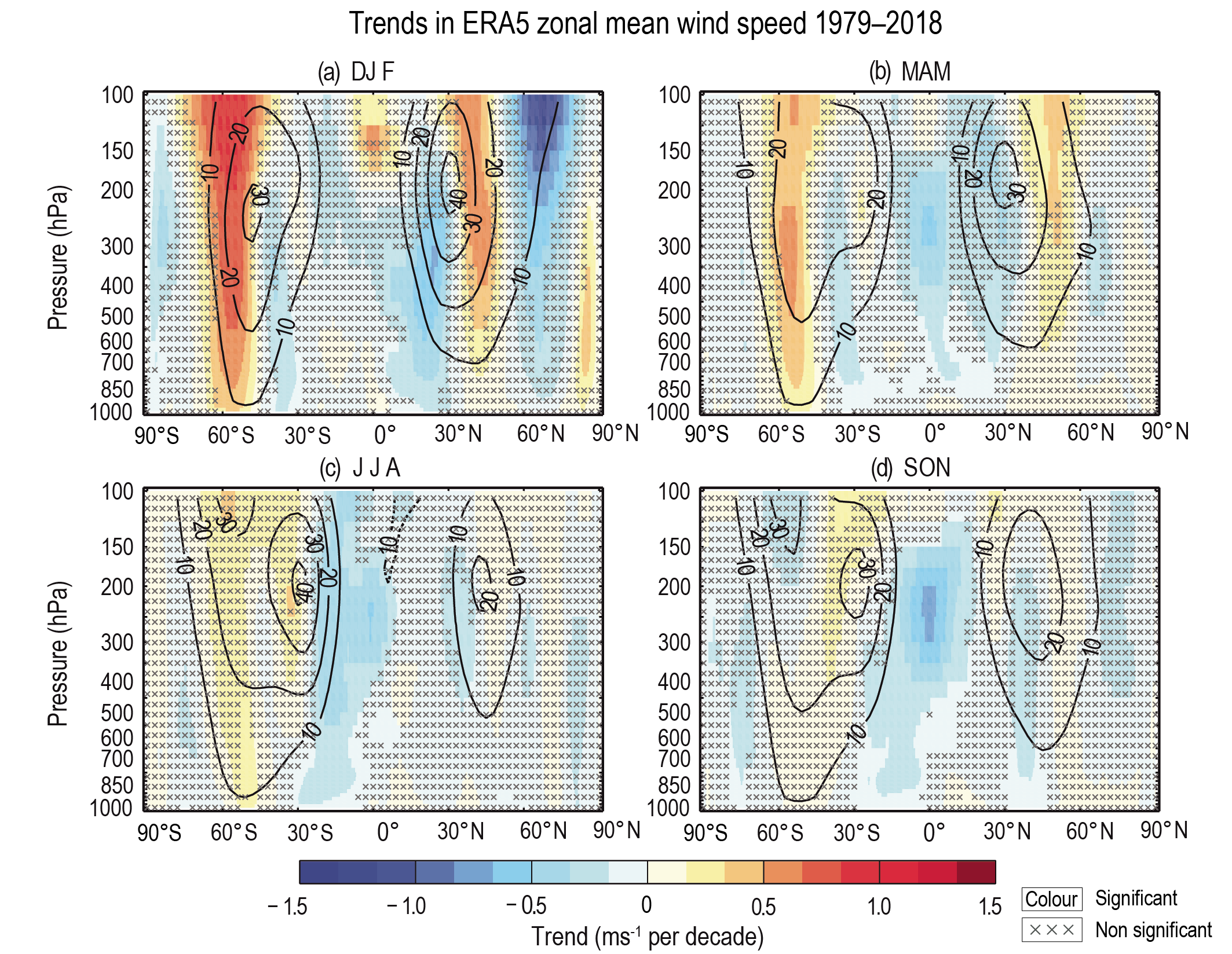
Robust trends in blocking have only been found in certain regions and specific seasons during recent decades. Increases in blocking frequency have occurred over low-latitude regions in the North Atlantic in boreal winter (Davini et al., 2012), the South Atlantic in austral summer (Dennison et al., 2016) and the southern Indian Ocean in austral spring (Schemm, 2018). Over the subpolar North Atlantic sustained periods of positive Greenland blocking were identified during 1870–1900 and from the late 1990s to 2015 (Hanna et al., 2015). Further analysis of association of Greenland blocking with the NAM is provided in Section 2.4.1.1. Meanwhile, a reduced blocking frequency has been found over winter in Siberia (Davini et al., 2012) and the south-western Pacific in austral spring (Schemm, 2018). Over eastern European Russia and western Siberia (40°E–100°E) a tendency towards longer blocking events was reported by Luo et al. (2016) for 2000–2013 and by Tyrlis et al. (2020) for 1979–2017. Inter-annual variance in the number of blocking events over the SH (Oliveira et al., 2014) and North Atlantic (Kim and Ha, 2015) has enhanced. Blocking events and their trends are sensitive to choice of datasets, calculation periods and methods (Cheung et al., 2013; Barnes et al., 2014; Pepler et al., 2018; Rohrer et al., 2018; Woollings et al., 2018b; Kononova and Lupo, 2020). As a result, hemispheric and global trends in blocking frequency have overall low confidence.
In summary, the total number of extratropical cyclones has likely increased since the 1980s in the NH (low confidence), but with fewer deep cyclones particularly in summer. The number of strong extratropical cyclones has likely increased in the SH (medium confidence). The extratropical jets and cyclone tracks have likely been shifting poleward in both hemispheres since the 1980s with marked seasonality in trends (medium confidence). There is low confidence in shifting of extratropical jets in the NH during the mid-Holocene and over 950–1400 CE to latitudes that likely were similar to those since 1979. There is low confidence in observed global-scale changes in the occurrence of blocking events.
2.3.1.4.4 Surface wind and sea level pressure
The AR5 concluded that surface winds over land had generally weakened. The confidence for both land and ocean surface wind trends was lowowing to uncertainties in datasets and measures used. Sea level pressure (SLP) was assessed to have likely decreased from 1979–2012 over the tropical Atlantic and increased over large regions of the Pacific and South Atlantic, but trends were sensitive to the period analysed.
Terrestrial in situ wind datasets have been updated and the quality-control procedures have been improved, with particular attention to homogeneity and to better retaining true extreme values (Dunn et al., 2012, 2014, 2016). Global mean land wind speed (excluding Australia) from HadISD for 1979–2018 shows a reduction (stilling) of 0.063 m s–1 per decade (Azorin-Molina et al., 2019). Trends are broadly insensitive to the subsets of stations used. Although the meteorological stations are unevenly distributed worldwide and sparse in South America and Africa, the majority exhibit stilling particularly in the NH (Figure 2.19). Regionally, strong decreasing trends are reported in central Asia and North America (–0.106 and –0.084 m s–1 per decade respectively) during 1979–2018 (McVicar et al., 2012; Vautard et al., 2012; J. Wu et al., 2018; Azorin-Molina et al., 2019). This stilling tendency has reversed after 2010 and the global mean surface winds have strengthened (Zeng et al., 2019b; Azorin-Molina et al., 2020), although the robustness of this reversal is unclear given the short period and interannual variability (Kousari et al., 2013; Kim and Paik, 2015; Azorin-Molina et al., 2019).
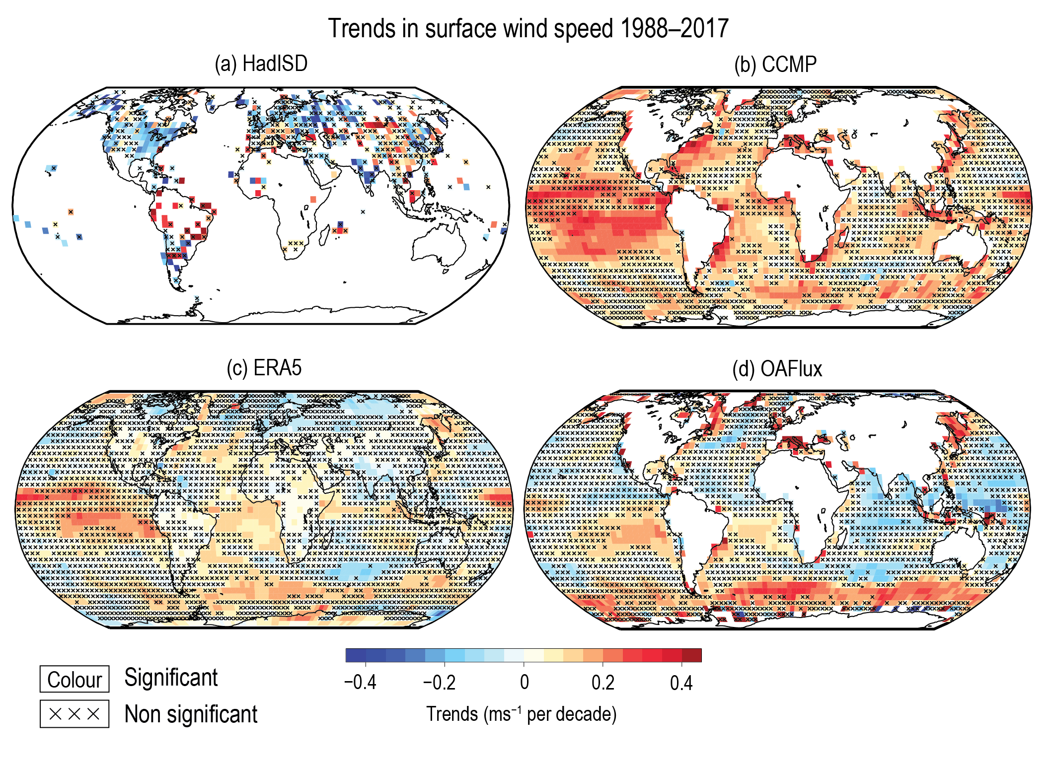
Over the ocean, datasets demonstrate considerable disagreement in surface wind speed trends and spatial features (Kent et al., 2013). Global ocean surface winds from NOCv2.0 demonstrate upward trends of about 0.11 m s–1 per decade (1979–2015) with somewhat smaller trends from WASwind for 1979–2011 (Azorin-Molina et al., 2017, 2019). The trends are consistent until 1998, but diverge thereafter. Both ERA5 and JRA-55 reanalyses show consistently increasing global marine wind speeds over 1979–2015, though flattening since 2000, whereas MERRA-2 agrees until 1998, but then exhibits increased variability and an overall decrease in the last two decades (Azorin-Molina et al., 2019). This agrees with estimates by Sharmar et al. (2021) showing upward ocean wind trends from 1979 to 2000 which are consistent in ERA-Interim, ERA5 and MERRA-2, but disagree with CFSR trends for the same period. Over 2000–2019 all reanalyses show diverging tendencies. An updated multiplatform satellite database (comprising data from altimeters, radiometers, and scatterometers) from 1985–2018 shows small increases in mean wind speed over the global ocean, with the largest increase observed in the Southern Ocean (Young and Ribal, 2019), consistent with signals in ERA-Interim, ERA5 and MERRA-2 (Sharmar et al., 2021). Overall, most products suggest positive trends over the Southern Ocean, western North Atlantic and the tropical eastern Pacific since the early 1980s.
The modern era reanalyses exhibit SLP increases over the SH subtropics with stronger increases in austral winter over 1979–2018. Over the NH, SLP increased over the mid-latitude Pacific in boreal winter and decreased over the eastern subtropical and mid-latitude North Atlantic in boreal summer. Discrepancies in the low-frequency variations during the first half of the 20th century exist in the centennial-scale reanalysis products (Befort et al., 2016). Overall, modern reanalysis datasets support the AR5 conclusion that there is no clear signal for trends in the strength and position of the permanent and quasi-permanent pressure centres of action since the 1950s. Instead, they highlight multi-decadal variations. Large-scale SLP is strongly associated with the changes in modes of variability (Section 2.4 and Annex IV).
In summary, since the 1970s a worldwide weakening of surface wind has likely occurred over land, particularly marked in the NH, with low confidence in a recent partial recovery since around 2010. Differences between available wind speed estimates lead to low confidence in trends over the global ocean as a whole but with most estimates showing strengthening globally over 1980–2000 and over the last four decades in the Southern Ocean, western North Atlantic and the tropical eastern Pacific.
2.3.1.4.5 Stratospheric polar vortex and sudden warming events
The AR5 assessed changes in the polar vortices and reported a likely decrease in the lower-stratospheric geopotential heights over Antarctica in spring and summer at least since 1979.
Multiple definitions for the polar vortex strength and sudden stratospheric warming (SSW) events have been proposed and compared (Butler et al., 2015; Palmeiro et al., 2015; Waugh et al., 2017; Butler and Gerber, 2018), and new techniques identifying daily vortex patterns and SSWs have been developed (D.M. Mitchell et al., 2013; Kretschmer et al., 2018). Errors in reanalysis stratospheric winds were assessed and discrepancies in stratospheric atmospheric circulation and temperatures between reanalyses, satellites and radiosondes have been reported (D.M. Mitchell et al., 2013; Duruisseau et al., 2017).
The northern stratospheric polar vortex has varied intra-seasonally and with altitude during recent decades. Multiple reanalysis and radiosonde datasets show that the midwinter lower stratospheric geopotential height (150 hPa) over the polar region north of 60°N has increased significantly since the early 1980s (Bohlinger et al., 2014; Garfinkel et al., 2017). This signal extends to the middle and upper stratosphere. In January-February zonal winds north of 60°N at 10 hPa have been weakening (Kim et al., 2014; Kretschmer et al., 2018). Daily atmospheric circulation patterns over the northern polar stratosphere exhibit a decreasing frequency of strong vortex events and commensurate increase in more-persistent weak events, which largely explains the observed significant weakening of the vortex during 1979–2015 (Kretschmer et al., 2018). The northern polar vortex has weakened in early winter but strengthened during late winter (Bohlinger et al., 2014; Garfinkel et al., 2015a, 2017; Ivy et al., 2016; Seviour, 2017; Kretschmer et al., 2018). In the middle and upper stratosphere, a strengthening trend of the northern polar vortex during DJF has occurred since 1998, contrasting the weakening trend beforehand (D. Hu et al., 2018). The position of the polar vortex also has long-term variations, exhibiting a persistent shift toward Northern Siberia and away from North America in February over the period 1979–2015 (Zhang et al., 2016; J. Zhang et al., 2018). Multiple measures show similar location changes (Seviour, 2017).
Sudden stratospheric warming (SSW), a phenomenon of rapid stratospheric air temperature increases (sometimes by more than 50°C in 1–2 days), is tightly associated with the reversal of upper stratospheric zonal winds, and a resulting collapse or substantial weakening of the stratospheric polar vortex (Butler et al., 2015; Butler and Gerber, 2018) and on average occurs approximately 6 times per decade in the NH winter (Charlton et al., 2007; Butler et al., 2015). The SSW record from all modern reanalyses is very consistent. There is a higher occurrence of major midwinter SSWs in the 1980s and 2000s with no SSW events during 1990–1997 (Reichler et al., 2012; Butler et al., 2015). An assessment of multi-decadal variability and change in SSW events is sensitive to both chosen metric and methods (Palmeiro et al., 2015). Due to the lack of assimilation of upper air data, the centennial-scale reanalyses do not capture SSW events, even for the most recent decades (Butler et al., 2015, 2017) and hence cannot inform on earlier behaviour. There has been considerably less study of trends in the SH stratosphere polar vortex strength despite the interest in the ozone hole and the potential impact of the SH stratosphere polar vortex strength on it. The occurrence of SSW events in the SH is not as frequent as in the NH, with only 3 documented events in the last 40 years (Shen et al., 2020).
In summary, it is likely that the northern lower stratospheric polar vortex has weakened since the 1980s in midwinter, and its location has shifted more frequently toward the Eurasian continent. The short record and substantial decadal variability yields low confidence in any trends in the occurrence of SSW events in the NH winter and such events in the SH are rare.
Cross-Chapter Box 2.3 | New Estimates of Global Warming to Date, and Key Implications
Contributing Authors: Peter W. Thorne (Ireland/United Kingdom), Blair Trewin (Australia), Richard P. Allan (United Kingdom), Richard Betts (United Kingdom), Lea Beusch (Switzerland), Chris Fairall (United States of America), Piers Forster (United Kingdom), Baylor Fox-Kemper (United States of America), Jan S. Fuglestvedt (Norway), John C. Fyfe (Canada), Nathan P. Gillett (Canada), Ed Hawkins (United Kingdom), Christopher Jones (United Kingdom), Elizabeth Kent (United Kingdom), Svitlana Krakovska (Ukraine), Elmar Kriegler (Germany), Jochem Marotzke (Germany), H. Damon Matthews (Canada), Thorsten Mauritsen (Germany/Denmark), Anna Pirani (Italy), Joeri Rogelj (United Kingdom, Austria/Belgium), Steven K. Rose (United States of America), Bjørn H. Samset (Norway), Sonia I. Seneviratne (Switzerland), Claudia Tebaldi (United States of America), Andrew Turner (United Kingdom), Russell S. Vose (United States of America), Rachel Warren (United Kingdom)
This Cross-Chapter Box presents the AR6 WGI assessment of observed global warming and describes improvements and updates since AR5 and subsequent Special Reports. The revised estimates result from: the availability of new and revised observational datasets; the occurrence of recent record warm years; and the evaluation of the two primary metrics used to estimate global warming in past IPCC reports: ‘Global mean surface temperature’ (GMST) and ‘Global surface air temperature’ (GSAT). Implications for threshold crossing times, remaining carbon budgets and impacts assessments across AR6 WGs are discussed.
Cross-Chapter Box 2.3
Dataset innovations
Since AR5, all major datasets used for assessing observed temperature change based upon GMST have been updated and improved (Section 2.3.1.1.3). A number of new products have also become available, including new datasets (e.g., Berkeley Earth, Rohde and Hausfather, 2020) and new interpolations based on existing datasets (e.g., Cowtan and Way, 2014 and Kadow et al., 2020). These various estimates are not fully independent.
Improvements in global temperature datasets since AR5 have addressed two major systematic issues. First, new SST datasets (Huang et al., 2017; Kennedy et al., 2019) address deficiencies previously identified in AR5 relating to the shift from predominantly ship-based to buoy-based measurements; these improvements result in larger warming trends, particularly in recent decades. Second, all datasets now employ interpolation to improve spatial coverage. This is particularly important in the Arctic, which has warmed faster than the rest of the globe in recent decades (Atlas 5.9.2.2); under-sampling of the Arctic leads to a cool bias in recent decades (Simmons et al., 2017; Benestad et al., 2019). Some datasets are now spatially complete (Cowtan and Way, 2014; Kadow et al., 2020) while others have expanded spatial coverage (Lenssen et al., 2019; Rohde and Hausfather, 2020; Morice et al., 2021; Vose et al., 2021). Several interpolation methods have been benchmarked against test cases (e.g., Lenssen et al., 2019), and comparisons with reanalyses further confirm the value of such interpolation (Simmons et al., 2017). It is extremely likely that interpolation produces an improved estimate of the changes in GMST compared to ignoring data-void regions.
Overall, dataset innovations and the availability of new datasets have led to an assessment of increased GMST change relative to the directly equivalent estimates reported in AR5 (Cross-Chapter Box 2.3, Table 1 and Figure 1).
Effects of warming since AR5 and choice of metrics of global mean temperature change
Each of the six years from 2015 to 2020 has likely been warmer than any prior year in the instrumental record. GMST for the decade 2011–2020 has been 0.19 [0.16 to 0.22] °C warmer than 2003–2012, the most recent decade used in AR5 (Cross-Chapter Box 2.3, Figure 1). A linear trend has become a poorer representation of observed change over time since most of the sustained warming has occurred after the 1970s (Cross-Chapter Box 2.3, Figure 1) and all values since 2012 are at least 0.2°C above a linear trendline for 1850–2020. For this reason, the primary method used to assess observed warming in this report is the change in temperature from 1850–1900 to the most recent decade (2011–2020) or the recent past (1995–2014), replacing the trend-based methods used in AR5 and earlier assessments. The effect of this change from trend-based to change-based metrics is currently relatively minor at –0.03°C (<5%) for the most recent decade, but this may not remain the case in future (high confidence).
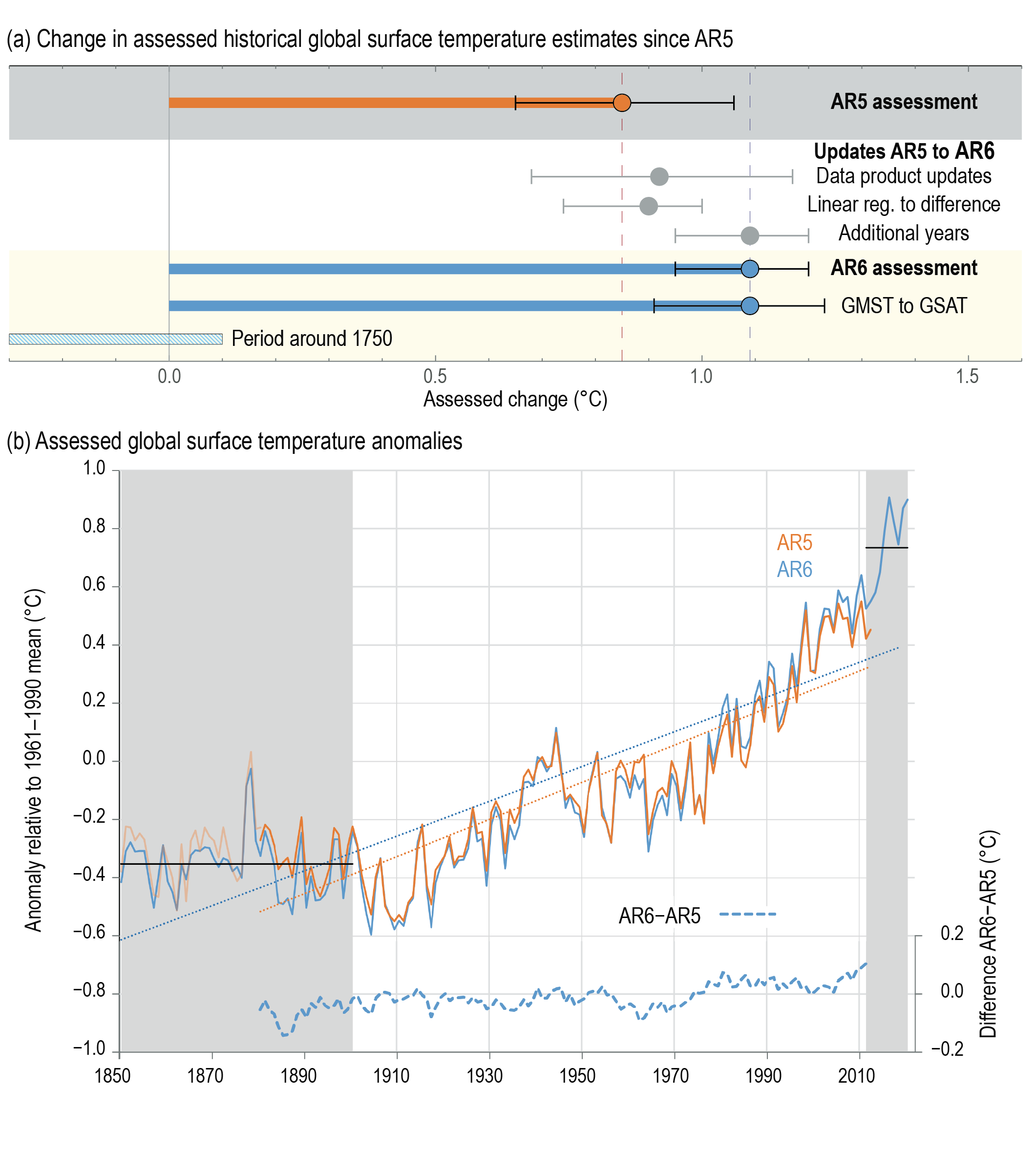
Cross-chapter Box 2.3, Figure 1 | Changes in assessed historical surface temperature changes since AR5. (a) Summary of the impact of various steps from AR5 assessment warming-to-date number for 1880–2012 using a linear trend fit to the AR6 assessment based upon the difference between 1850–1900 and 2011–2020. Whiskers provide 90% (very likely) ranges. AR6 assessment in addition denotes additional warming since the period around 1750 (Cross-Chapter Box 1.2). (b) Time series of the average of assessed AR5 series (orange, faint prior to 1880 when only HadCRUT4 was available) and AR6 assessed series (blue) and their differences (offset) including an illustration of the two trend fitting metrics used in AR5 and AR6. Further details on data sources and processing are available in the chapter data table (Table 2.SM.1).
Observed changes in global mean temperature since the pre-industrial era
AR5 used 1850–1900 as an approximate pre-industrial baseline for global temperature change, whilst using an earlier pre-industrial baseline of 1750 for radiative forcings. Cross-Chapter Box 1.2 assesses that there was an observed GMST change from the period around 1750 to 1850–1900 of around 0.1°C (likely range –0.1 to +0.3°C, medium confidence). This additional global temperature change before 1850–1900 is not included when making AR6 assessments on global warming to date, global temperature threshold crossing times, or remaining carbon budgets to ensure consistency with previous ARs.
Addressing the non-equivalence of GMST and GSAT
GMST is a combination of land surface air temperatures (LSAT) and SSTs, whereas GSAT is a combination of LSAT and marine air temperatures (MATs). Although GMST and GSAT are closely related, the two measures are physically distinct. The implications have become more apparent since AR5 (Merchant et al., 2013; Cowtan et al., 2015; Simmons et al., 2017; IPCC, 2018 (SR1.5); Richardson et al., 2018), and it has been shown (Rubino et al., 2020) that MAT and SST can show distinct multi-decadal-scale trends and patterns of interannual variability. Although SR1.5 used GMST for observational-based and GSAT for model-based headline warming statements, they noted the importance of the difference for their assessment (SR1.5Section 1.2.1.1). The SR1.5 used information from CMIP5 models to estimate a GSAT equivalent from observation-based GMST for certain applications such as remaining carbon budgets. The following subsections assess available lines of evidence related to the equivalence between GMST and GSAT.
Physical understanding
A well-understood physical constraint on the vertical gradient between the air and sea surface temperature is that it is approximately proportional to the turbulent sensible heat flux in the atmospheric surface layer (Chor et al., 2020). Similarly, the latent heat flux scales with the vertical humidity gradient and, in the global mean and in most oceanic regions, the latent heat flux is substantially larger than the sensible heat flux (Sections 7.2.1 and 9.2.1.3). If GSAT were to warm faster than GMST, the sensible surface heat flux would respond so as to reduce this difference. However, it is the sum of the sensible, latent, and radiative heat fluxes that controls GMST, so the sensible heat flux effect cannot be considered in isolation. Attempts to further constrain the combination of fluxes (e.g., Lorenz et al., 2010; Siler et al., 2019) rely on parameterizations or output from Earth system models (ESMs) or reanalyses and so are not considered independent. Apart from the above global considerations, regional and seasonal effects such as changes to the frequency and intensity of storms, sea state, cloudiness, sea ice cover, vegetation and land use may all affect the GSAT to GMST difference, either directly or by altering the relationships between gradients and energy fluxes. These changing energy flux relationships are monitored through observing the stratification of the upper ocean (Section 9.2.1.3) and the response of upper ocean processes (Cross-Chapter Box 5.3) in ESMs and reanalyses, but such monitoring tasks rival the observational challenge of directly observing SSTs and 2 m air temperature under a wide range of conditions. In summary, because of the lack of physical constraints and the complexity of processes driving changes in the GSAT to GMST temperature differences, there is no simple explanation based on physical grounds alone for how this difference responds to climate change.
Direct observational evidence
There is currently no regularly updated, entirely observation-based dataset for GSAT. The best available observations of near-surface air temperature over ocean are datasets of night-time marine air temperature (NMAT; e.g., Cornes et al., 2020; Junod and Christy, 2020), though spatial coverage is less extensive than for SST. Night-time measurements are used to avoid potential biases from daytime heating of ship superstructures. Kennedy et al. (2019) show little difference between HadNMAT2 and HadSST4 between 1920 and 1990, but a warming of SST relative to NMAT manifesting as a step change of 0.05°C–0.10°C in the early 1990s, which may reflect an actual change, the impact of increasingly divergent spatial coverage between SST and MAT measurements, or unresolved structural uncertainties in one or both datasets. This leads to NMAT warming around 10% more slowly than SST over the last century. In contrast, Junod and Christy (2020) find NMAT trends which are 8–17% larger than those for SST in the ERSSTv4 and HadISST datasets for the period 1900 to 2010, but 11–15% smaller than the SST trends for the same datasets from 1979 to 2010. However, ERSSTv4 uses NMAT data as a basis for homogeneity adjustment so is not fully independent. Kent and Kennedy (2021) note sensitivity to methodological choices in comparisons but find that NMAT is warming more slowly than SST products over most periods considered. Rubino et al. (2020) exploit tropical Pacific moored buoy arrays, available since the early 1980s, and find differences in NMAT and SST anomalies, which are sensitive to the choice of period and show spatio-temporal ENSO-related (Annex IV) signals in the differences.
Overall, with medium evidence and low agreement, available observational products suggest that NMAT is warming less than SST by up to 15%. Given that these ocean observations cover roughly two thirds of the globe, this implies that GMST is warming up to at most 10% faster than GSAT. Substantial uncertainty remains and the effect is highly sensitive to the choice of both time period and choice of NMAT and SST observational products to compare. Observed NMAT warming faster than observed SST cannot be precluded.
CMIP model-based evidence
CMIP historical simulations and projections agree that GSAT increases faster than GMST, the reverse of what is indicated by many marine observations. Several studies approximate the approach used to derive GMST from observations by blending SST over open ocean and SAT over land and sea ice from model output (Cowtan et al., 2015; Richardson et al., 2018; Beusch et al., 2020; Gillett et al., 2021). Cowtan et al. found that trends in GSAT are of the order of 9% larger than for GMST in CMIP5, based on data from 1850–2100 (historical + RCP8.5), if anomalies are blended and sea ice is allowed to vary over time (Cowtan et al., 2015). Broadly consistent numbers are found for both CMIP5 and CMIP6, across a range of SSP and RCP scenarios and time periods (Richardson et al., 2018; Beusch et al., 2020; Gillett et al., 2021). Blending monthly anomalies and allowing sea ice to vary, the change in GSAT for 2010–2019 relative to 1850–1900 is 2–8% larger than spatially-complete GMST in CMIP6 historical and SSP2-4.5 simulations (Gillett et al., 2021), and 6–12% larger in CMIP5 historical and RCP2.6 and 8.5 simulations for 2007–2016 relative to 1861–1880 (Richardson et al., 2018). However, a true like-for-like comparison to observational products is challenging because methodological choices have a large impact on the relationship between modelled GMST and GSAT and none of these studies fully reproduces the methods used to derive estimates of GMST in recent observational datasets, which use various ways to infill areas lacking in situ observations (Jones, 2020).
Marine boundary layer behaviour and parameterizations in all CMIP models are based upon Monin-Obukhov similarity theory (e.g., Businger et al., 1971), which informs assumptions around gradients in the near-surface boundary layer dependent upon temperature, wind speed and humidity. This leaves open the possibility of a common model bias, while Druzhinin et al. (2019) also point to departures of temperature profiles from theoretical predictions under certain conditions. There remain inadequacies in understanding and modelling of key processes (Edwards et al., 2020), and biases in the representation of the absolute SST-MAT difference have been identified in climate models and reanalyses (Găinuşă-Bogdan et al., 2015; Zhou et al., 2020).
Reanalysis-based evidence
Simmons et al. (2017) found that in JRA-55 and ERA-Interim (following an adjustment to account for an apparent discontinuity), GSAT increased 2–4% faster than GMST over the period 1979–2016. In atmospheric reanalyses, SST is given as a lower boundary condition from an observed globally interpolated product (such as HadISST; Rayner et al., 2003) whereas the air temperature is reliant upon model parameterizations and assimilated observations that do not include MAT observations (Simmons et al., 2017), thereby limiting their capability to constrain differences in GMST and GSAT trends. Furthermore, it is unclear what the lack of dynamic coupling at the ocean-atmosphere interface might imply for the representativeness of reanalysis-based estimates.
Representation of surface temperatures in sea ice regions
There is a significant issue in areas where sea ice melts or grows, where the quantity used in observational-based GMST estimates switches between air temperature and sea surface temperature. This primarily affects analyses combining SAT anomalies over land and ice with SST anomalies over ocean. In areas where sea ice has recently melted, the climatological value changes from an air-temperature based estimate to an SST estimate based upon the freezing point of seawater (–1.8°C). This switch in climatology to, in general, a warmer climatology, leads to a bias towards reduced warming in anomalies compared with analyses based on absolute temperatures. Richardson et al. (2018) found this underestimation to amount to approximately 3% of observed warming in historical model simulations. Given the projected future sea ice losses, the effect will grow in future (low confidence), with potential effects of the order of 0.1°C in the second half of the 21st century under high warming scenarios, although with some uncertainty arising from the large spread of sea ice loss in model projections (Tokarska et al., 2019).
Cross Chapter Box 2.3, Table 1 | Summary of key observationally based global warming estimates (in °C) to various reference periods in the present report and selected prior reports (AR5 WGI and SR1.5) and their principal applications (see Section 1.4.1 for further information on reference periods). Further details on data sources and processing are available in the chapter data table (Table 2.SM.1).
Reference Period | AR6 GMST (°C) | AR6 GSATa(°C) | AR5 and/orSR1.5(italics) – Only Where Reported (°C) | Principal Use of This Period in this Report and Previous Reports |
1850–1900 to 2011–2020 | 1.09 [0.95 to 1.20] | 1.09 [0.91 to 1.23] | Warming to present in AR6 WGI | |
1850–1900 to 2010–2019 | 1.06 [0.92 to 1.17] | 1.06 [0.88 to 1.21] | Attributable warming assessment period in AR6 WGI | |
1850–1900 to 2006–2019 | 1.03 [0.89 to 1.14] | 1.03 [0.86 to 1.18] | AR6 WGI warming estimate as a line of evidence for energy budget constraints to estimate ECS and TCR | |
1850–1900 to 2006–2015 | 0.94 [0.79 to 1.04] | 0.94 [0.76 to 1.08] | 0.87 [0.75 to 0.99] – GMST 0.97 [0.85 to 1.09] – GSATb | Warming to date in SR1.5 |
1850–1900 to 2003–2012 | 0.90 [0.74 to 1.00] | 0.90 [0.72 to 1.03] | 0.78 [0.72 to 0.85] | Warming to date in AR5 WGI |
1850–1900 to 2001–2020 | 0.99 [0.84 to 1.10] | 0.99 [0.81to 1.14] | Warming to first two decades of 21st century | |
1850–1900 to 1995–2014 | 0.85 [0.69 to 0.95] | 0.85 [0.67 to 0.98] | Warming to recent past in AR6 WGI | |
1850–1900 to 1986–2005 | 0.69 [0.54 to 0.79] | 0.69 [0.52 to 0.82] | 0.61 [0.55 to 0.67]c | Warming to recent past in AR5 WGI. This difference is used to report in this box the implications of the AR6 historical global surface temperature assessment in a way that is directly comparable to the AR5 estimate. |
1850–1900 to 1961–1990 | 0.36 [0.23 to 0.44] | 0.36 [0.22 to 0.45] | Warming to reference period recommended by WMO for national-level data sets used for climate change assessment (included in the AR6 WGI Atlas) | |
1880–2012 OLS trend | 0.92 [0.68 to 1.17] | 0.85 [0.65 to 1.06] | Warming trend to date in AR5 WGI Summary for Policymakers and AR5 Synthesis Report |
a As the uncertainty in the relationship between GMST and GSAT changes is independent of the uncertainty in the assessed change in GMST, these uncertainties are combined in quadrature.
b The SR1.5 derived a GSAT estimate by taking the CMIP5 ensemble mean GSAT change of 0.99°C, sub-sampling to HadCRUTv4.6, noting the offset in trends (0.84°C HadCRUT4 observed GMST vs. 0.86°C modelled GMST) and adjusting by this to arrive at an estimate of 0.97°C change in GSAT. The likely uncertainty range of ±0.12°C was not further adjusted.
c Note that the AR5 approach for the change from 1850–1900 to both 1986–2005 and 2003–2012 was based upon one dataset (HadCRUT4) and its parametric uncertainty estimates are known to underestimate the true uncertainty.
Summary of lines of evidence
GMST and GSAT are physically distinct. There is high confidence that long-term changes in GMST and GSAT differ by at most 10% in either direction. However, conflicting lines of evidence from models and direct observations combined with limitations in theoretical understanding lead to low confidence in the sign of any difference in long-term trends. The very likely range of estimated historical GMST warming is combined with the assessed ± 10% uncertainty in the relationship between GMST and GSAT changes to infer a GSAT equivalent, accounting for any possible real-world physical difference. Improvements in understanding may yield a robust basis to apply a scaling-factor to account for the difference in future assessments.
Mapping between AR5 and AR6 Assessments
The AR5 assessed estimate for historical warming between 1850–1900 and 1986–2005 is 0.61 [0.55 to 0.67] °C. The equivalent in AR6 is 0.69 [0.54 to 0.79] °C, and the 0.08 [-0.01 to 0.12] °C difference is an estimate of the contribution of changes in observational understanding alone (Cross-Chapter Box 2.3, Table 1). The exact value of this contribution depends upon the metric being compared (GMST/GSAT, the method used to calculate a trend or change between two periods, the exact reference period used), with the best estimates (with the exception of the SR1.5 GSAT estimate) falling between 0.07°C and 0.12°C. The choice of 1850–1900 to 1986–2005 as the basis is due to the widespread use of this period across AR5 and SR1.5 in several contexts. The AR6-assessed GMST warming between 1850–1900 and 2011–2020 is 1.09 [0.95 to 1.20] °C. An AR5-equivalent assessment using this estimated difference in observational understanding is thus 1.01 [0.94 to 1.08] °C. These updates and improvements in observational datasets affect other quantities that derive from the assessment of GSAT warming, including estimates of remaining carbon budgets and estimates of crossing times of 1.5°C and 2°C of global warming (see Cross Chapter Box 2.3, Table 1).
Updates to estimated Global Warming Level (GWL) crossing times
The updated estimate of historical warming is one contribution to the revised time of projected crossing of the threshold of 1.5°C global warming in comparison with SR1.5, but is not the only reason for this update. The AR6 assessment of future change in GSAT (Table 4.5) results in the following threshold-crossing times, based on 20-year moving averages. The threshold-crossing time is defined as the midpoint of the first 20-year period during which the average GSAT exceeds the threshold. During the near term (2021–2040), a 1.5°C GSAT increase relative to the average over the period 1850–1900 is very likely to occur in scenario SSP5-8.5, likely to occur in scenarios SSP2-4.5 and SSP3-7.0, and more likely than not to occur in scenarios SSP1-1.9 and SSP1-2.6. In all scenarios assessed here except SSP5-8.5, the central estimate of crossing the 1.5°C global warming level lies in the early 2030s. This is in the early part of the likely range (2030–2052) assessed in SR1.5, which assumed continuation of the then-reported warming rate; this estimated rate has been confirmed in AR6 (Section 3.3.1). Roughly half of this difference arises from the higher diagnosed historical warming in AR6. The other half arises because, for central estimates of climate sensitivity, most scenarios show stronger warming over the near term than was assessed as ‘current’ in SR1.5 (medium confidence). When considering scenarios similar to SSP1-1.9 instead of linear extrapolation, the SR1.5 estimate of when 1.5°C global warming is crossed is close to the central estimate reported here (SR1.5, Table 2.SM.12).
Implications for assessment of emissions scenarios and remaining carbon budgets
To estimate the global warming implications of emissions scenarios, AR5 and SR1.5 combined estimates of observed GMST changes from 1850–1900 to 1986–2005 (Cross-Chapter Box 2.3, Table 1) with GSAT projections of subsequent warming. AR6 undertakes three changes to this approach. First, the AR6 assessment of improved observational records is used. Second, the recent past baseline period is updated from 1986–2005 to 1995–2014, and, third, historical estimates are expressed in GSAT instead of GMST for consistency of historical estimates with future projections. The updated estimates of warming to date in AR6 lead to higher estimates of future warming, all else being equal. The temperature classification of emissions scenarios in the WGIII report adopts the definition of temperature classes as introduced in SR1.5, and assigns emissions scenarios to these classes based on their AR6 assessed GSAT outcomes (Cross-Chapter Box 7.1; WGIII Annex C.II.2.4).
In both AR5 and SR1.5, remaining carbon budgets were expressed as a function of GSAT warming, while also highlighting the implications of using historical warming estimates expressed in GMST. The AR5 reported total carbon budgets for GSAT warming relative to 1861–1880. The AR5 Synthesis Report (SYR) also includes remaining carbon budget estimates based on AR5 WGIII scenario projections that use the method for AR5 scenario projections described above. The SR1.5 integrated several methodological advancements to estimate remaining carbon budgets and reported budgets for additional GSAT warming since the 2006–2015 period, estimating, following the application of an adjustment (Richardson et al., 2016, Table 1.1, SR1.5) to GMST, that 0.97°C (± 0.12°C) of GSAT warming occurred historically between 1850–1900 and 2006–2015. The AR6 assessment, above, leads to an estimate of 0.94°C of warming between 1850–1900 and 2006–2015. All other factors considered equal, the AR6 estimate thus implies that 0.03°C more warming is considered for remaining carbon budgets compared to SR1.5. Combining this 0.03°C value with the SR1.5 transient climate response to cumulative emissions of CO2 (TCRE) translates into remaining carbon budgets about 70 [40–140] GtCO2 larger compared to SR1.5 on a like-for-like basis. Meanwhile, on the same like-for-like basis, updates to historical observational products would reduce remaining carbon budgets reported in AR5 SYR based on WGIII scenario projections by about 180 [120 to 370] GtCO2. Box 5.2 provides a further overview of updates to estimates of the remaining carbon budget since AR5.
Implications for assessment of impacts and adaptation
The assessment of global warming to date now being larger than previously assessed has no consequence on the assessment of past climate impacts, nor does it generally imply that projected climate impacts are now expected to occur earlier. The implications are mainly that the level of warming associated with a particular impact has been revised. This has very limited practical implications for the assessment of the benefits of limiting global warming to specific levels, as well as for the urgency of adaptation action. For example, impacts that occurred in the period 1986–2005 were previously associated with a GMST increase of 0.61°C relative to 1850–1900, relative to AR5 estimates. These impacts are now instead associated with a GMST increase of 0.69°C, relative to the assessment in this Report. The impacts themselves have not changed. Similarly, the impacts previously associated with a GMST or GSAT increase of 1.5°C will now generally be associated with a slightly different global warming level. This is because projections of future warming and its impacts relative to 1850–1900 are normally made by adding projected warming from a recent past baseline to an estimate of the observed warming from 1850–1900, as in AR5 and SR1.5.
Most of the previously projected impacts and risks associated with global warming of 1.5°C have therefore not changed and are still associated with the same level of future warming (0.89°C) relative to 1986–2005. With this warming now estimated as 0.08°C larger than in AR5, the future impacts previously associated with 1.5°C warming are now associated with 1.58°C warming. Similarly, the impacts now associated with 1.5°C warming would have previously been associated with 1.42°C warming. There are exceptions where impacts studies have used a baseline earlier than 1986–2005 (e.g., King et al., 2017), for which the new estimate of the historical warming would mean an earlier occurrence of the projected impacts. However, even in these cases, the ostensible difference in impacts associated with a 0.08°C difference in global mean temperature will be small in comparison with the uncertainties. There are also substantial uncertainties in regional climate changes and the magnitude of climate impact-drivers projected to occur with global warming of 1.5°C (Betts et al., 2018; Seneviratne et al., 2018). Furthermore, the time of reaching global warming of 1.5°C is subject to uncertainties of approximately ±10 years associated with uncertainties in climate sensitivity, and ±3 to 4 years associated with the different SSP forcing scenarios (Section 4.3.4, Table 4.5, and see discussion above).
There is therefore high confidence that assessment of the magnitude and timing of impacts-related climate quantities at 1.5°C is not substantially affected by the revised estimate of historical global warming. The assessment of the implications of limiting global warming to 1.5°C compared to 2°C will also remain broadly unchanged by the updated estimate of historical warming, as this depends on the relative impacts rather than the absolute impacts at any specific definition of global temperature anomaly (high confidence).
2.3.2 Cryosphere
This section focuses on large-scale changes in a subset of components of the cryosphere (Cross-Chapter Box 2.2). Chapter 9 undertakes a holistic assessment of past and possible future changes and understanding of key processes in the cryosphere, including those at regional scales, integrating observations, modelling and theoretical understanding, while, here in chapter 2, the focus is on past large-scale, observation-based cryospheric changes.
2.3.2.1 Sea Ice Coverage and Thickness
2.3.2.1.1 Arctic sea ice
The AR5 reported that the annual mean Arctic sea-ice extent (SIE)very likely decreased by 3.5–4.1% per decade between 1979 and 2012 with the summer sea-ice minimum (perennial sea ice)very likely decreasing by 9.4–13.6% per decade. This was confirmed by SROCC reporting the strongest reductions in September (12.8 ± 2.3% per decade; 1979–2018) and stating that these changes were likely unprecedented in at least 1 kyr (medium confidence). The spatial extent had decreased in all seasons, with the largest decrease for September (high confidence). The AR5 reported also that the average winter sea ice thickness within the Arctic Basin had likely decreased by between 1.3 m and 2.3 m from 1980 to 2008 (high confidence), consistent with the decline in multi-year and perennial ice extent. The SROCC stated further that it was virtually certain that Arctic sea ice had thinned, concurrent with a shift to younger ice. Lower sea ice volume in 2010–2012 compared to 2003–2008 was documented in AR5 (medium confidence). There was high confidence that, where the sea ice thickness had decreased, the sea-ice drift speed had increased.
Proxy records are used in combination with modelling to assess Arctic paleo sea ice conditions to the extent possible. For the Pliocene, limitedproxyevidence of a reduced sea ice cover compared to ‘modern’ winter conditions (Knies et al., 2014; Clotten et al., 2018) and model simulations of a largely ice-free Arctic Ocean during summer (Howell et al., 2016; Feng et al., 2019; F. Li et al., 2020) imply medium confidence that the Arctic Ocean was seasonally ice covered. Over the LIG, sparse proxy reconstructions (Stein et al., 2017; Kremer et al., 2018) and proxy evidence from marine sediments (Kageyama et al., 2021b) provide medium confidence of perennial sea ice cover.
Over the past 13 kyr proxy records suggest extensive sea-ice coverage during the Younger Dryas (at the end of the LDT), followed by a decrease in sea ice coverage during the Early Holocene, and increasing sea-ice coverage from the MH to the mid-15th century (De Vernal et al., 2013; Belt et al., 2015; Cabedo-Sanz et al., 2016; Armand et al., 2017; Belt, 2018). There is limited evidence that the Canadian Arctic had less multiyear sea ice during the Early Holocene than today (Spolaor et al., 2016). For more regional details on paleo arctic sea ice see Section 9.3.1.1.
Pan-Arctic SIE conditions (annual means and late summer) during the last decade were unprecedented since at least 1850 (Figure 2.20a; Walsh et al., 2017, 2019; Brennan et al., 2020), while, as reported in SROCC, there remains medium confidence that the September (late summer) Arctic sea ice loss during the last decade was unprecedented during the past 1 kyr. Sea-ice charts since 1850 (Walsh et al., 2017, 2019) suggest that there was no significant trend before the 1990s, but the uncertainty of these estimates is large and could mask a trend, a possibility illustrated by Brennan et al. (2020), who found a loss of Arctic sea ice between 1910 and 1940 in an estimate based on a data assimilation approach.
 Figure 2.20 | Changes in Arctic and Antarctic sea ice area. (a) Three time series of Arctic sea-ice area (SIA) for March and September from 1979 to 2020 (passive microwave satellite era). In addition, the range of SIA from 1850–1978 is indicated by the vertical bar to the left. (b) Three time series of Antarctic sea ice area for September and February (1979–2020). In both (a) and (b), decadal means for the three series for the first and most recent decades of observations are shown by horizontal lines in grey (1979–1988) and black (2010–2019). SIA values have been calculated from sea ice concentration fields. Available data for 2020 (OSISAF) is shown in both (a) and (b). Further details on data sources and processing are available in the chapter data table (Table 2.SM.1).
 There has been a continuing decline in SIE and Arctic sea ice area (SIA) in recent years (Figure 2.20a). To reduce grid-geometry associated biases and uncertainties (Notz, 2014; Ivanova et al., 2016; Meier and Stewart, 2019) SIA is used in addition to, or instead of SIE herein (see also section 9.3.1). A record-low Arctic SIA since the start of the satellite era (1979) occurred in September 2012 (Figure 2.20a). Decadal SIA means based on the average of three different satellite products decreased from 6.23 to 3.76 million km2 for September and 14.52 to 13.42 million km2 for March SIA (Figure 2.20a). Initial SIA data for 2020 (OSISAF) are within the range of these recent decadal means or slightly below (Figure 2.20a). SIA has declined since 1979 across the seasonal cycle (Figure 9.13). Most of this decline in SIA has occurred after 2000, and is superimposed by substantial interannual variability. The sharp decline in Arctic summer SIA coincides with earlier surface melt onset (Mortin et al., 2016; Bliss et al., 2017), later freeze-up, and thus a longer ice retreat and open water period (Stammerjohn et al., 2012; Parkinson, 2014; Peng et al., 2018).
Over the past two decades, first-year sea ice has become more dominant and the oldest multiyear ice (older than 4 years) which in March 1985 made up 33% of the Arctic sea-ice cover, has nearly disappeared, making up 1.2% in March 2019 (Perovich et al., 2020). The loss of older ice is indicative of a thinning overall of ice cover (Tschudi et al., 2016), but also the remaining older ice has become thinner (E. Hansen et al., 2013). Since in situ ice thickness measurements are sparse, information about ice thickness is mainly based on airborne and satellite surveys. Records from a combination of different platforms show for the central and western Arctic Ocean (Arctic Ocean north of Canada and Alaska) negative trends since the mid-1970s (Lindsay and Schweiger, 2015; Kwok, 2018), with a particularly rapid decline during the 2000s, which coincided with a large loss of multiyear sea ice. Direct observations from 2004 and 2017 indicate a decrease of modal ice thickness in the Arctic Ocean north of Greenland by 0.75 m, but with little thinning between 2014 and 2017 (Haas et al., 2017). This agrees with data based on satellite altimetry and airborne observations, showing no discernible thickness trend since 2010 (Kwok and Cunningham, 2015; Kwok, 2018; Kwok and Kacimi, 2018; see Figure 2.21). However, sea-ice thickness derived from airborne and spaceborne data is still subject to uncertainties imposed by snow loading. For radar altimeters, insufficient penetration of radar signal into the snowpack results in overestimation of ice thickness (e.g., Ricker et al., 2015; King et al., 2018; Nandan et al., 2020). Negative trends in ice thickness since the 1990s are also reported from the Fram Strait in the Greenland Sea, and north of Svalbard (E. Hansen et al., 2013; Renner et al., 2014; King et al., 2018; Rösel et al., 2018; Spreen et al., 2020). Thickness data collected in the Fram Strait originate from ice exported from the interior of the Arctic Basin and are representative of a larger geographical area upstream in the transpolar drift. A reduction of survival rates of sea ice exported from the Siberian shelves by 15% per decade has interrupted the transpolar drift and affected the long-range transport of sea ice (Krumpen et al., 2019). The thinner and on average younger ice has less resistance to dynamic forcing, resulting in a more dynamic ice cover (Hakkinen et al., 2008; Spreen et al., 2011; Vihma et al., 2012; Kwok et al., 2013).
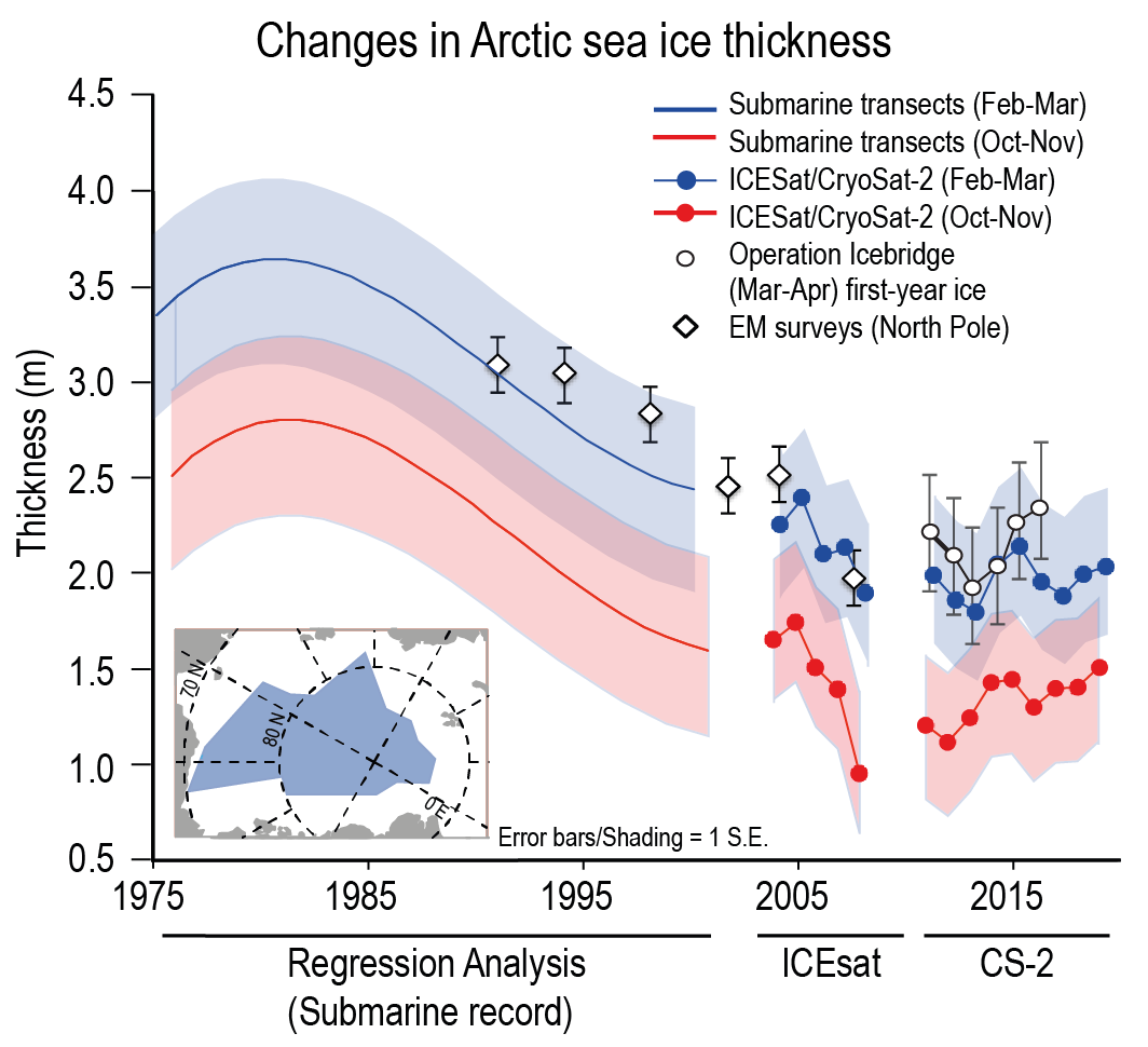 Figure 2.21 | Arctic sea ice thickness changes (means) for autumn (red/dotted red) and winter (blue/dotted blue). Shadings (blue and red) show 1 standard error (S.E.) ranges from the regression analysis of submarine ice thickness and expected uncertainties in satellite ice thickness estimates. Data release area of submarine data ice thickness data is shown in inset. Satellite ice thickness estimates are for the Arctic south of 88°N. Thickness estimates from more localized airborne/ground electromagnetic surveys near the North Pole (diamonds) and from Operation IceBridge (circles) are shown within the context of the larger scale changes in the submarine and satellite records. Further details on data sources and processing are available in the chapter data table (Table 2.SM.1).
 The SROCC noted the lack of continuous records of snow on sea ice. Nevertheless in recent decades, more snow on sea ice has been observed in the Atlantic sector in the Arctic than in the western Arctic Ocean (Webster et al., 2018). Previously, Warren et al. (1999) showed that over 1954–1991 there were weak trends towards declining snow depth on sea ice in the Pacific sector. Recent observations indicate a substantial thinning of the spring snowpack in the western Arctic (Cavalieri et al., 2012; Brucker and Markus, 2013; Kurtz et al., 2013; Laxon et al., 2013; Webster et al., 2018). In contrast, thick snow over Arctic sea ice in the Atlantic sector north of Svalbard (snow thickness around 0.4 m or more) has been observed in the 1970s and since the 1990s (Rösel et al., 2018), but data are too sparse to detect trends.
In summary, over 1979–2019 Arctic SIA has decreased for all months, with the strongest decrease in summer (very high confidence). Decadal means for SIA decreased from the first to the last decade in that period from 6.23 to 3.76 million km2 for September, and from 14.52 to 13.42 million km2 for March. Arctic sea ice has become younger, thinner and faster moving (very high confidence). Snow thickness on sea ice has decreased in the western Arctic Ocean (medium confidence). Since the Younger Dryas at the end of the LDT, proxy indicators show that Arctic sea ice has fluctuated on multiple time scales with a decrease in sea ice coverage during the Early Holocene and an increase from the MH to the mid-15th century. Current pan-Arctic sea ice coverage levels (annual mean and late summer) are unprecedentedly low since 1850 (high confidence), and with medium confidence for late summer for at least the past 1 kyr.
2.3.2.1.2 Antarctic sea ice
The AR5 reported a small but significant increase in the total annual mean Antarctic SIE that was very likely in the range of 1.2–1.8% per decade between 1979 and 2012 (0.13–0.20 million km2 per decade) (very high confidence), while SROCC reported that total Antarctic sea ice coverage exhibited no significant trend over the period of satellite observations (1979–2018) (high confidence). The SROCC noted that a significant positive trend in mean annual sea ice cover between 1979 and 2015 had not persisted, due to three consecutive years of below-average sea ice cover (2016–2018). The SROCC stated also that historical Antarctic sea ice data from different sources indicated a decrease in overall Antarctic sea ice cover since the early 1960s, but was too small to be separated from natural variability (high confidence).
There is onlylimited evidence from predominantly regional paleo proxies for the evolution of Southern Ocean sea ice before the instrumental record and estimates are not available for all proxy target periods (Section 9.3.2). Proxies from marine sediments for intervals preceding and following the MPWP indicate open water conditions with less sea ice than modern conditions (Taylor-Silva and Riesselman, 2018; Ishino and Suto, 2020). During the LGM, proxies indicate that austral winter sea ice coverage reached the polar ocean front (e.g., Nair et al., 2019). More recently, sea ice coverage appears to have fluctuated substantially throughout the Holocene (e.g., for the western Amundsen Sea, Lamping et al., 2020). At the beginning of the CE, regional summer sea ice coverage in the north-western Ross Sea was lower than today (Tesi et al., 2020). Crosta et al. (2021) suggest, based on different proxies, four different phases with 7–10 months periods of sea ice occurrence per year in the Antarctic region off Adelie Land during the CE, where each phase was several hundred years long.
More recent sea ice reconstructions are based on diverse sources including whaling records (de La Mare, 1997, 2009; Cotté and Guinet, 2007), old ship logbooks (Ackley et al., 2003; Edinburgh and Day, 2016), and ice core records (Curran et al., 2003; Abram et al., 2010; Sinclair et al., 2014), amongst other methods (e.g., Murphy et al., 2014). These reconstructions, in combination with recent satellite-based observations indicate: (i) a decrease in summer SIE across all Antarctic sectors since the early- to mid-20th century; (ii) a decrease in winter SIE in the East Antarctic and Amundsen-Bellingshausen Seas sectors starting in the 1960s; and (iii) small fluctuations in winter SIE in the Weddell Sea over the 20th century (Hobbs et al., 2016a, b). There are also ice-core indications that the pronounced Ross Sea increase dates back to the mid-1960s (Sinclair et al., 2014; Thomas and Abram, 2016). While there is reasonable broad-scale concurrence across these estimates, the uncertainties are large, there is considerable interannual variability, and reconstructions require further validation (Hobbs et al., 2016a, b). New reconstructions (Thomas et al., 2019) from Antarctic land ice cores show that SIE in the Ross Sea had increased between 1900 and 1990, while the Bellingshausen Sea had experienced a decline in SIE; this dipole pattern is consistent with satellite-based observations from 1979 to 2019 (Parkinson, 2019), but the recent rate of change then has been larger. Records of Antarctic SIE for the late 19th and early 20th centuries (Edinburgh and Day, 2016), show SIE comparable with the satellite era, although with marked spatial heterogeneity (e.g., Thomas et al., 2019).
Early Nimbus satellite visible and infrared imagery from the 1960s (Meier et al., 2013; Gallaher et al., 2014) indicate higher overall SIE compared to 1979–2013 (Hobbs et al., 2016a, b), but with large uncertainties and poorly quantified biases (NA SEM, 2017). The continuous satellite passive-microwave record shows that there was a modest increase in overall Antarctic SIA of 2.5% ± 0.2% per decade (1 standard error over 1979–2015; Comiso et al., 2017). For overall ice coverage and for this period, positive long-term trends were most pronounced during austral autumn advance (Maksym, 2019), being moderate in summer and winter, and lowest in spring (Holland, 2014; Turner et al., 2015; Hobbs et al., 2016a, b; Comiso et al., 2017). Since 2014, overall Antarctic SIE (and SIA) has exhibited major fluctuations from record-high to record-low satellite era extents (Massonnet et al., 2015; Reid and Massom, 2015; Reid et al., 2015; Comiso et al., 2017; Parkinson, 2019). After setting record-high extents each September from 2012 through 2014, Antarctic SIE (and SIA) dipped rapidly in mid-2016 and remained predominantly below average through 2019 (Reid et al., 2020). For the most recent decade of observations (2010–2019), the decadal means of three SIA products (Figure 2.20b) were 2.17 million km2 for February and 15.75 million km2 for September, respectively. The corresponding levels for the means for the first decade of recordings (1979–1988) were 2.04 million km2 for February and 15.39 million km2 for September indicating little overall change. Initial SIA data for 2020 (OSISAF) show SIA for September above, and for February slightly below the recent decadal means (Figure 2.20b). The 2020 September level (OSISAF) remains below the levels observed over 2012–2014.
In summary, Antarctic sea ice has experienced both increases and decreases in SIA over 1979–2019, and substantively lower levels since 2016, with only minor differences between decadal means of SIA for the first (for February 2.04 million km2, for September 15.39 million km2) and last decades (for February 2.17 million km2, for September 15.75 million km2) of satellite observations (high confidence). There remains low confidence in all aspects of Antarctic sea ice prior to the satellite era owing to a paucity of records that are highly regional in nature and often seemingly contradictory.
2.3.2.2 Terrestrial Snow Cover
The AR5 concluded that snow cover extent (SCE) had decreased in the NH, especially in spring (very high confidence). For 1967–2012, the largest change was in June and March–April SCEvery likely declined. No trends were identified for the SH due to limited records and large variability. The SROCC concluded with high confidence that Arctic June SCE declined between 1967 and 2018 and in nearly all mountain regions, snow cover declined in recent decades.
Analysis of the combined in situ observations (Brown, 2002) and the multi-observation product (Mudryk et al. 2020) indicates that since 1922, April SCE in the NH has declined by 0.29 million km2 per decade, with significant interannual variability (Figure 2.22) and regional differences (Section 9.5.3.1). The limited pre-satellite era data does not allow for a similar assessment for the entire spring-summer period. Assessment of SCE trends in the NH since 1978 indicates that for the October to February period there is substantial uncertainty in trends with the sign dependent on the observational product. Analysis using the NOAA Climate Data Record shows an increase in October to February SCE (Hernández-Henríquez et al., 2015; Kunkel et al., 2016) while analyses based on satellite borne optical sensors (Hori et al., 2017) or multi-observation products (Mudryk et al., 2020) show a negative trend for all seasons (Section 9.5.3.1 and Figure 9.23). The greatest declines in SCE have occurred during boreal spring and summer, although the estimated magnitude is dataset dependent (Rupp et al., 2013; Estilow et al., 2015; Bokhorst et al., 2016; Thackeray et al., 2016; Connolly et al., 2019).
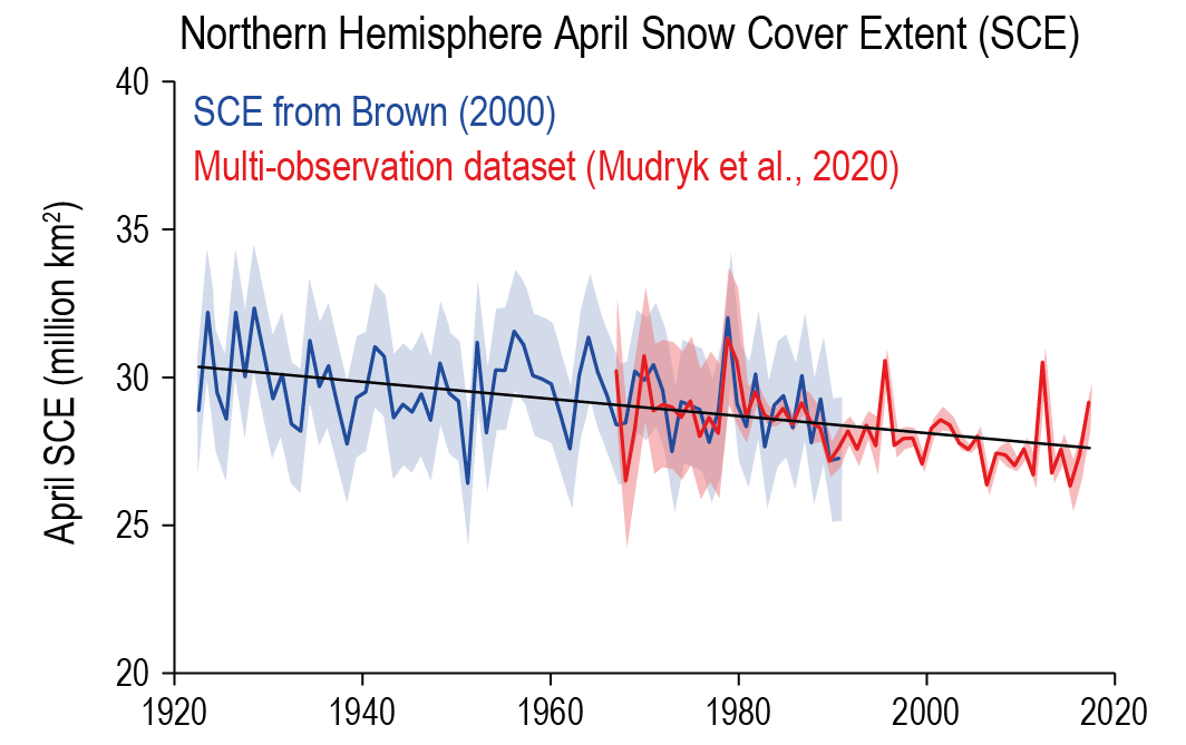 Figure 2.22 | April snow cover extent (SCE) for the Northern Hemisphere (1922–2018). Shading shows very likely range. The trend over the entire 1922–2018 period (black line) is –0.29 (± 0.07) million km2 per decade. Further details on data sources and processing are available in the chapter data table (Table 2.SM.1).
 There has been a commensurate decrease in the snow-cover duration and persistence, particularly in higher latitudes due to earlier spring melt and, in some cases, later autumn onset of snow cover (Chen et al., 2015; Derksen et al., 2015; Hori et al., 2017; Hammond et al., 2018). Arctic snow-cover duration has decreased by 2–4 days per decade since the 1970s (Brown et al., 2017). Significant decreases in snow-cover duration have been documented over western Eurasia since 1978 (Hori et al., 2017).
For the NH, maximum snow depth has generally decreased since the 1960s, with more robust trends for North America and greater uncertainty for Eurasia (Kunkel et al., 2016). Several satellite-based passive microwave and other products indicate general declines in pre-melt snow water equivalent since 1981 although there is regional and inter-dataset variability (Brown et al., 2017; Jeong et al., 2017; Marty et al., 2017; Mortimer et al., 2020; Mudryk et al., 2020; Pulliainen et al., 2020, Section 9.5.3).
In summary, substantial reductions in spring snow cover extent have occurred in the NH since 1978 (very high confidence) with limited evidence that this decline extends back to the early 20th century. Since 1981 there has been a general decline in NH spring snow water equivalent (high confidence).
2.3.2.3 Glacier Mass
The AR5 concluded with high confidence that, during the Holocene, glaciers were at times smaller than at the end of the 20th century. The AR5 stated further with very high confidence that most glaciers had been shrinking since the mid-1800s, and the mass loss from all glaciers worldwide very likely increased from 1970 to 2009. The SROCC reported a globally coherent picture of continued glacier recession in recent decades (very high confidence) based on in situ and satellite observations of changes in glacier area, length and mass, although there were considerable inter-annual and regional variations. Between 2006 and 2015 the global glacier mass change assessed by SROCC was –278 ± 113 Gt yr–1.
Two recent global reviews on glaciers over the Holocene (Solomina et al., 2015) and the past 2 kyr (Solomina et al., 2016) summarize the chronologies of respectively 189 and 275 glaciers. The former shows that glaciers retreated during the LDT and retracted to their minimum extent between 8 ka and 6 ka. Except for some glaciers in the SH and tropics, glaciers expanded thereafter, reaching their maximum extent beyond their present-day margins during the mid-15th to late 19th centuries CE. With few exceptions, glacier margins worldwide have retreated since the 19th century, with the rate of retreat and its global character since the late 20th century being unusual in the context of the Holocene (Solomina et al., 2016, Figure 2.23a). However, the areal extents of modern glaciers in most places in the NH are still larger than those of the early and/or middle Holocene (Solomina et al., 2015). When considering Holocene and present glaciers extents, it is important to account for the relatively long adjustment time of glaciers (often referred to as response time; Section 9.5.1.3); the majority of modern glaciers are currently out of equilibrium with current climate, even without further global warming (Mernild et al., 2013; Christian et al., 2018; Marzeion et al., 2018; Zekollari et al., 2020). The size of glaciers during other periods warmer than the Early to Mid-Holocene, such as the MPWP and LIG, is largely unknown because the deposits marking previous extents were in almost all cases over-ridden by later glaciations. For Arctic glaciers, different regional studies consistently indicate that in many places glaciers are now smaller than they have been in millennia (Lowell et al., 2013; Miller et al., 2013, 2017; Harning et al., 2016, 2018; Schweinsberg et al., 2017, 2018; Pendleton et al., 2019).
 Figure 2.23 | Mountain glacier advance and annual mass change. (a) Number of a finite selection of surveyed glaciers that advanced during the past 2000 years. (b) Annual and decadal global glacier mass change (Gt yr–1) from 1961 until 2018. In addition, mass change mean estimates are shown. Ranges show the 90% confidence interval. Further details on data sources and processing are available in the chapter data table (Table 2.SM.1).
 New glacier outline (RGI Consortium, 2017) and glacier mass compilations (Zemp et al., 2019, 2020; Ciracì et al., 2020; Hugonnet et al., 2021) improve, refine and update the quantification of glacier areal and mass changes based on observations from in situ and remote sensing data. Observations between the 1960s and 2019 indicate that mass loss has increased over recent decades (Figure 2.23b). The overall global glacier mass loss rate has increased from 240 ± 9 Gt yr–1 over 2000–2009 to 290 ± 10 Gt yr–1 over 2010–2019 (Hugonnet et al., 2021), confirming that the last decade exhibits the most negative glacier mass balance since the beginning of the observational record. Observations are in general consistent with trends revealed by global glacier mass change modelling for almost the entire 20th century (1901–1990) implying an estimated mass loss (without uncharted glaciers (Parkes and Marzeion, 2018) and excluding peripheral glaciers of Greenland and Antarctica) of very likely 210 ± 90 Gt yr–1 and very likely 170 ± 80 Gt yr–1 for the period 1971–2019 (Marzeion et al., 2015; Section 9.5.1 and Table 9.5).
In summary, there is very high confidence that, with few exceptions, glaciers worldwide have retreated since the second half of the 19th century, and continue to retreat. The current global character of glacier mass loss is highly unusual (almost all glaciers simultaneously receding) in the context of at least the last 2 kyr (medium confidence). Glacier mass loss rates have increased since the 1970s (high confidence). Although many surveyed glaciers are currently more extensive than during the MH (high confidence), they generally are in disequilibrium with respect to current climate conditions and hence are committed to further ice loss.
2.3.2.4 Ice-sheet Mass and Extent
During glacial periods, ice sheets were more extensive and the state of knowledge on their paleo-reconstruction can be found in recent publications (e.g., Stokes et al., 2015; Batchelor et al., 2019). This section focuses only on the large-scale aspects of those ice sheets, Greenland and Antarctic, that still exist today.
2.3.2.4.1 Greenland Ice Sheet (GrIS)
The AR5 concluded the volume of the Greenland Ice Sheet (GrIS) was reduced compared to present during periods of the past few million years that were globally warmer than present (high confidence). It reported that the GrIS had lost ice during the prior two decades (very high confidence), that the ice loss had occurred in several sectors, and that high rates of mass loss had both expanded to higher elevations (high confidence) and very likely accelerated since 1992. The SROCC concluded that it was extremely likely that ice loss increased through the early 21st century. The SROCC also found that summer melting rate had increased since the 1990s to a rate unprecedented over the last 350 years (very high confidence), being two to five times greater than the pre-industrial rates (medium confidence).
Details of the history of the GrIS fluctuations during warm interglacials continue to be elucidated. Oscillations over the past 7.5 Myr, including the Pliocene and through the glacial – interglacial cycles of the Pleistocene are not well-constrained, but most studies indicate that Greenland was at least partially glaciated over this time with extended periods when it was predominantly deglaciated (Bierman et al., 2016; Schaefer et al., 2016). Geological evidence and modelling studies suggest periods of glacial intensification during the Pliocene at 4.9 Myr, 4.0 Myr, 3.6 Myr and 3.3 Myr (De Schepper et al., 2014; Bierman et al., 2016; Bachem et al., 2017). Retreat of the GrIS occurred during the MPWP and GrIS extent was reduced compared to today with some studies suggesting that the ice sheet was limited to the highest elevations (De Schepper et al., 2014; Koenig et al., 2015; Haywood et al., 2016; Blake-Mizen et al., 2019). There is apparent glacial intensification following the MPWP, 2.75–2.72 Myr (Nielsen and Kuijpers, 2013; De Schepper et al., 2014; Blake-Mizen et al., 2019; Knutz et al., 2019). Several studies agree that during the LIG the total GrIS extent was likely less than present day (Section 9.4.1, Figure 9.17) with the total mass loss ranging from 0.3–6.2 m sea level equivalent (SLE), although timing and magnitude of this mass loss are not well constrained (Helsen et al., 2013; Stone et al., 2013; Vasskog et al., 2015; Goelzer et al., 2016; Sinclair et al., 2016; Yau et al., 2016; Clark et al., 2020). During the LGM, the GrIS reached a peak ice volume greater than present (2–5 m SLE), as revealed by the limited number of available geological records (Simpson et al., 2009; Lecavalier et al., 2014; Batchelor et al., 2019).
Recent studies of marine and lake sediments, glacier ice, and geomorphic features show that the GrIS retreated rapidly during the early Holocene but halted periodically, with a complex ice-margin chronology (Carlson et al., 2014; Larsen et al., 2014, 2015; Young and Briner, 2015; Briner et al., 2016; Young et al., 2020). It is probable that its total volume during 8–3 ka was smaller than today (Larsen et al., 2015; Young and Briner, 2015; Briner et al., 2016), but uncertainties exist regarding precisely when the minimum MH extent and volume was reached, due to uncertainties in reconstructions. The GrIS then re-advanced reaching its maximum extent in most places during 1450–1850 CE, although the timing and extent of this maximum differed by sector (Larsen et al., 2015; Briner et al., 2016).
Greenland-wide estimates of mass change based on direct observations were limited prior to 1992 at the time of AR5 (Kjeldsen et al., 2015). Combined records based on airborne observations, model-based estimates and geodetic approaches indicate an average mass loss of 75 ± 29.4 Gt yr–1 for 1900–1983 (Kjeldsen et al., 2015). Integration of proxies and modelling indicates that the last time the rate of mass loss of the GrIS was plausibly similar to 20th century rates was during the early Holocene (Buizert et al., 2018; Briner et al., 2020).
Since AR5, a combination of remote sensing, in situ observations and modelling has provided new insights regarding surface processes and their contribution to recent GrIS mass changes (AMAP, 2017; van den Broeke et al., 2017; Bamber et al., 2018; Mouginot et al., 2019; IMBIE Consortium, 2020; Khan et al., 2020). Estimates of total ice loss during the post-1850 period (Kjeldsen et al., 2015) and recent observations show that the rate of loss has increased since the beginning of the 21st century (IMBIE Consortium, 2020; Sasgen et al., 2020; Velicogna et al., 2020) (Section 9.4.1.1 and Figures 2.24 and 9.17).
The GrIS lost 4890 [4140 to 5640] Gt (SLE 13.5 [11.4 to 15.6] mm) of ice between 1992 and 2020 (Section 9.4.1 and Figure 2.24; IMBIE Consortium, 2020). The ice sheet was close to mass balance in the 1990s, but increases in mass loss have occurred since (Bamber et al., 2018; WCRP Global Sea Level Budget Group, 2018; Mouginot et al., 2019; IMBIE Consortium, 2020). The rate of ice-sheet (including peripheral glaciers) mass loss rose from 120 [70 to 170] Gt yr–1 (SLE 0.33 [0.18 to 0.47] mm yr–1) in 1901–1990 to 330 [290 to 370] Gt yr–1 (SLE 0.91 [0.79 to 1.02] mm yr–1) for 2006–2018 (Section 9.4.1, Table 9.5).
In summary, the GrIS was smaller than present during the MPWP (medium confidence), LIG (high confidence) and the MH (high confidence). GrIS mass loss began following a peak volume attained during the 1450–1850 period and the rate of loss has increased substantially since the turn of the 21st century (high confidence).
2.3.2.4.2 Antarctic Ice Sheet (AIS)
The AR5 reported that there was high confidence that the Antarctic Ice Sheet (AIS) was losing mass. The average ice mass loss from Antarctica was 97 [58 to 135] Gt yr–1 (GMSL equivalent of 0.27 [0.16 to 0.37] mm yr–1) over 1993–2010, and 147 [74 to 221] Gt yr–1 (0.41 [0.20 to 0.61] mm yr–1) over 2005–2010. These assessments included the Antarctic peripheral glaciers. The AR5 reported with high confidence that the volume of the West Antarctic Ice Sheet (WAIS) was reduced during warm periods of the past few million years. The SROCC concluded that over 2006–2015, the AIS lost mass at an average rate of 155 ± 19 Gt yr–1 (very high confidence). The SROCC also stated that it is virtually certain that the Antarctic Peninsula and WAIS combined have cumulatively lost mass since widespread measurements began in 1992, and that the rate of loss has increased since around 2006.
Process understanding and, to some extent, paleoclimate records show that changes in parts of the AIS can occur over multi-century time scales (<2kyr; Sections 9.4.2.3 and 9.6.2; e.g., Dowdeswell et al., 2020). Based on physical understanding, paleo evidence and numerical simulations, it is very likely that the AIS has been smaller than today during at least some past warm climates (such as MCO and LIG), in particular the WAIS (Figure 9.18; Golledge et al., 2014; de Boer et al., 2015; DeConto and Pollard, 2016; Levy et al., 2016). Results from sediment studies suggest a smaller AIS during the MPWP compared with current levels, with main differences in the WAIS (Section 9.6.2; SROCC, IPCC, 2019; Bertram et al., 2018; Shakun et al., 2018). Marine sediments indicate that during the Pleistocene repeated ungrounding and loss of large marine-based parts of the AIS occurred during interglacial periods, with at least seven transitions between floating and grounded ice in the Ross Sea during the last 780 kyr (McKay et al., 2012) and at least three reductions in ice volume in the Wilkes Basin during the last 500 kyr (Wilson et al., 2018). Proxies, modelling and process understanding (Rohling et al., 2019; Clark et al., 2020) indicate that the AIS was smaller during the LIG than present.
Geological evidence has been used to reconstruct Holocene glacial fluctuations of the ice sheet margin and lowerings of its surface, which occurred at different times in different places, as recently reviewed by Noble et al. (2020). In West Antarctica, marine sediments below the ice sheet (Kingslake et al., 2018) corroborate a previous glacial isostatic adjustment modelling study (Bradley et al., 2015), which suggests that ice had retreated behind the present grounding line prior to about 10 ka, and then readvanced. Geophysical imaging indicates a readvance in this area around 6 ± 2 ka (Wearing and Kingslake, 2019). Other studies from the region conclude that ice-sheet retreat and thinning was fastest from 9 to 8 ka (Johnson et al., 2014; McKay et al., 2016; Spector et al., 2017), or millennia later, during the MH (Hein et al., 2016; Johnson et al., 2019), with indications of a subsequent readvance (Venturelli et al., 2020). In East Antarctica, rapid ice-sheet thinning occurred between around 9 and 5 ka (Jones et al., 2015), consistent with previous work indicating that the ice sheet in many regions was at or close to its current position by 5 ka (Bentley et al., 2014). Overall, during the MH, the AIS was retreating, but remained more extensive than present, while some parts of the ice sheet might have been smaller than now (low confidence).
Improved estimates of surface mass balance (SMB) in Antarctica from 67 ice core records do not show any substantial changes in accumulation rates over most of Antarctica since 1200 CE (Frezzotti et al., 2013). The SMB growth rate in Antarctica is estimated to be 7.0 ± 0.1 Gt per decade between 1800 and 2010 and 14.0 ± 1.8 Gt per decade since 1900 (Thomas et al., 2017). For the period 1979–2000, an insignificant Antarctic-wide negative SMB trend has been estimated (Medley and Thomas, 2019). The Antarctic Ice Sheet lost 2670 [1800 to 3540]Gt (SLE 7.4 [5.0 to 9.8]mm) of ice between 1992 and 2020. The rate of ice-sheet (including peripheral glaciers) mass loss rose from 0 [–36 to +40] Gt yr–1 (SLE 0.0 [–0.10 to 0.11] mm yr–1) in 1901–1990 to 192 [145 to 239] Gt yr–1 (SLE 0.54 [0.47 to 0.61] mm yr–1) for 2006–2018 (Section 9.4.2, Figure 2.24, and Table 9.5). Within quantified uncertainties, this estimate agrees with other recent estimates (Rignot et al., 2019; B. Smith et al., 2020; Velicogna et al., 2020). There is therefore very high confidence that the AIS has been losing mass over 1992–2020 (Section 9.4.2.1 and Figure 2.24). Major contributions to recent AIS changes arise from West Antarctica and Wilkes Land in East Antarctica (Rignot et al., 2019). For the East Antarctic most studies suggest that the mass balance is not significantly different from zero (Bamber et al., 2018; IMBIE Consortium, 2018; Mohajerani et al., 2018; Rignot et al., 2019).
 Figure 2. 24 | Cumulative Antarctic Ice Sheet (AIS) and Greenland Ice Sheet (GrIS) mass changes. Values shown are in gigatons and come from satellite-based measurements (IMBIE Consortium, 2018, 2020) for the period 1992–2020. The estimated uncertainties, very likely range, for the respective cumulative changes are shaded. Further details on data sources and processing are available in the chapter data table (Table 2.SM.1).
 In summary, the AIS has lost mass between 1992 and 2020 (very high confidence), and there is medium confidence that this mass loss has increased. During the MPWP and LIG, the ice sheet was smaller than present (medium confidence). There is low confidence as to whether the total mass of the ice sheet was larger or smaller around 6 ka compared to now.
2.3.2.5 Terrestrial Permafrost
The AR5 concluded that in most regions and at most monitoring sites permafrost temperatures since the 1980s had increased (high confidence). Negligible change was observed at a few sites, mainly where permafrost temperatures were close to 0°C, with slight cooling at a limited number of sites. The AR5 also noted positive trends in active layer thickness (ALT; the seasonally thawed layer above the permafrost) since the 1990s for many high latitude sites (medium confidence). The SROCC concluded permafrost temperatures have increased to record high levels since the 1980s (very high confidence) with a recent increase by 0.29°C ± 0.12°C from 2007 to 2016 averaged across polar and high mountain regions globally.
Permafrost occurrence during the Pliocene has been inferred from pollen in lake sediments in NE Arctic Russia and permafrost-vegetation relationships which indicate that permafrost was absent during the MPWP in this region (Brigham-Grette et al., 2013; Herzschuh et al., 2016). Analysis of speleothem records in Siberian caves, indicates that permafrost was absent in the current continuous permafrost zone at 60°N at the start of the 1.5 Ma record, with aggradation occurring around 0.4 Ma (Vaks et al., 2020). There are indications of extensive permafrost thaw during subsequent interglacials especially further south in the current permafrost zone (Vaks et al., 2013). Reconstruction of permafrost distribution during the LGM indicates that permafrost was more extensive in exposed areas (Vandenberghe et al., 2014). In non-glaciated areas of the North American Arctic there is permafrost that survived the LIG (French and Millar, 2014). Trends and timing of permafrost aggradation and thaw over the last 6 kyr in peatlands of the NH were recently summarized (Hiemstra, 2018; Treat and Jones, 2018). Three multi-century periods (ending 1000 Before the Common Era (BCE), 500 CE and 1850 CE) of permafrost aggradation, associated with neoglaciation periods are inferred resulting in more extensive permafrost in peatlands of the present-day discontinuous permafrost zone, which reached a peak approximately 250 years ago, with thawing occurring concurrently with post 1850 warming (Treat and Jones, 2018). Although permafrost persists in peatlands at the southern extent of the permafrost zone where it was absent prior to 3 ka, there has been thawing since the 1960s (James et al., 2013; B.M. Jones et al., 2016; Holloway and Lewkowicz, 2020).
Records of permafrost temperature measured in several boreholes located throughout the northern polar regions indicate general warming of permafrost over the last 3–4 decades (Figure 2.25), with marked regional variations (Romanovsky et al., 2017a, b, 2020; Biskaborn et al., 2019). Recent (2018–2019) permafrost temperatures in the upper 20–30 m layer (at depths where seasonal variation is minimal) were the highest ever directly observed at most sites (Romanovsky et al., 2020), with temperatures in colder permafrost of northern North America being more than 1°C higher than they were in 1978. Increases in temperature of colder Arctic permafrost are larger (average 0.4°C–0.6°C per decade) than for warmer (temperature >–2°C) permafrost (average 0.17°C per decade) of sub-Arctic regions (Figures 2.25, 9.22).
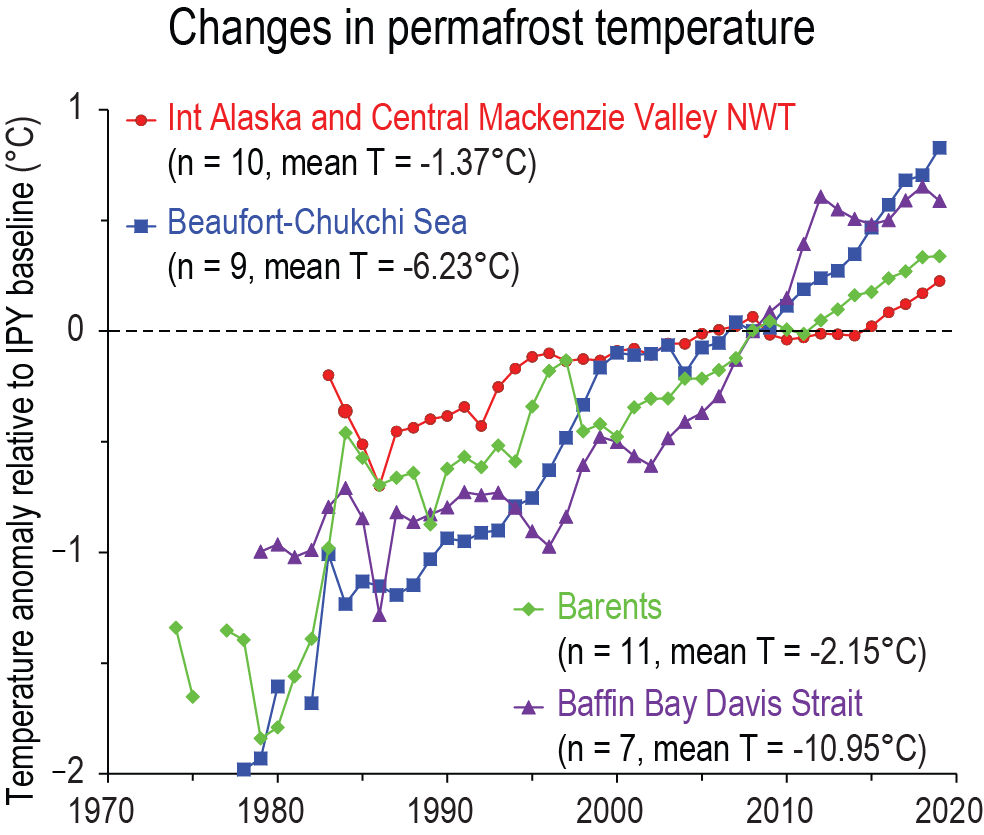 Figure 2.25 | Changes in permafrost temperature. Average departures of permafrost temperature (measured in the upper 20–30 m) from a baseline established during International Polar Year (2007–2009) for Arctic regions. Further details on data sources and processing are available in the chapter data table (Table 2.SM.1).
 Increases in permafrost temperature over the last 10–30 years of up to 0.3°C per decade have been documented at depths of about 20 m in high elevation regions in the NH (European Alps, the Tibetan Plateau and some other high elevation areas in Asia; G. Liu et al., 2017; Cao et al., 2018; Biskaborn et al., 2019; Noetzli et al., 2020; Zhao et al., 2020). In Antarctica, where records are limited and short (most <10 years) trends are less evident (Noetzli et al., 2019).
Assessment of trends in ALT is complicated by considerable ALT interannual variability. For example, in north-western North America during the extreme warm year of 1998, ALT was greater than in prior years. Although ALT decreased over the following few years, it has generally increased again since the late 2000s (Duchesne et al., 2015; Romanovsky et al., 2017b, 2020). However, at some sites there has been little change in ALT due to ground subsidence that accompanies thaw of ice-rich permafrost (Streletskiy et al., 2017; O’Neill et al., 2019). In the European and Russian Arctic there has been a broad-scale increase in ALT during the 21st century (Streletskiy et al., 2015; Romanovsky et al., 2020). In high elevation areas in Europe and Asia, increases in ALT have occurred since the mid-1990s (Y. Liu et al., 2017; Cao et al., 2018; Noetzli et al., 2019, 2020; Zhao et al., 2020). Limited and shorter records for Antarctica show marked interannual variability and no apparent trend with ALT being relatively stable or decreasing at some sites since 2006 (Hrbáček et al., 2018).
Observations of ground subsidence and other landscape change (e.g., thermokarst, slope instability) since the middle of the 20th century in the Arctic associated with ground ice melting have been documented in several studies and provide additional indications of thawing permafrost (Séjourné et al., 2015; Liljedahl et al., 2016; Borge et al., 2017; Kokelj et al., 2017; Nitze et al., 2017; Streletskiy et al., 2017; Derksen et al., 2019; Farquharson et al., 2019; Lewkowicz and Way, 2019; O’Neill et al., 2019; see Section 9.5.2.1). In mountain areas, destabilization and acceleration of rock glacier complexes that may be associated with warming permafrost have also been observed (Eriksen et al., 2018; Marcer et al., 2019).
In summary, increases in permafrost temperatures in the upper 30 m have been observed since the start of observational programs over the past three to four decades throughout the permafrost regions (high confidence). Limited evidence suggests that permafrost was less extensive during the MPWP (low confidence). Permafrost that formed after 3ka still persists in areas of the NH, but there are indications of thaw after the mid-1800s (medium confidence).
2.3.3 Ocean
This section focuses on large-scale changes in a subset of physical components of the ocean (Cross-Chapter Box 2.2). Chapter 7 assesses the role of the ocean in Earth system heating and evaluates the Earth’s energy budget. Chapter 9 undertakes a holistic assessment of changes in the ocean integrating observations, modelling and theoretical understanding. Chapter 11 assesses extremes such as marine heat waves and storm surges. SSTs are assessed in Section 2.3.1.1 as they constitute a critical component of GMST estimation.
2.3.3.1 Ocean Temperature, Heat Content and Thermal Expansion
AR5 assessed that since 1971, global ocean warming was virtually certain for the upper 700 m and likely for the 700–2000 m layer. The SROCC reported linear warming trends for the 0–700 m and 700–2000 m layers of the ocean, respectively, of 4.35 ± 0.8 and 2.25 ± 0.64 ZJ yr–1 over 1970–2017; 6.28 ± 0.48 and 3.86 ± 2.09 ZJ yr–1 over 1993–2017; and 5.31 ± 0.48 and 4.02 ± 0.97 ZJ yr–1 over 2005–2017. Both AR5 and SROCC assessed that the ocean below 2000 m had likely warmed since 1992. The SROCC reported global mean thermosteric sea level (ThSL) rise, associated with thermal expansion of the ocean, with a trend of 0.89 ± 0.05 mm yr–1 for 1970–2015; 1.36 ± 0.40 mm yr–1 for 1993–2015; and 1.40 ± 0.40 mm yr–1 for 2006–2015, and also reported that the rate of ocean warming over 1993–2017 had likely more than doubled since 1969–1992.
New ocean heat content (OHC) reconstructions derived from paleo proxies (Bereiter et al., 2018; Baggenstos et al., 2019; Shackleton et al., 2019; Gebbie, 2021) indicate that the global ocean warmed by 2.57°C ± 0.24°C, at an average rate of about 0.3°C ka–1 (equivalent to an OHC change rate of 1.3 ZJ yr–1) from the LGM (about 20 ka) to the early Holocene (about 10 ka; Section 9.2.2.1 and Figure 9.9). Over the LDT, ocean warming occurred in two stages, offset by some heat loss during the Antarctic Cold Reversal (14.58–12.75 ka). Only during a short period of rapid warming at the end of the Younger Dryas (12.75–11.55 ka) were rates comparable to those observed since the 1970s (Bereiter et al., 2018; Shackleton et al., 2019). Ice cores imply a small decrease in the global mean ocean temperature during the early Holocene (<0.4°C) (Bereiter et al., 2018; Baggenstos et al., 2019). Sediment cores from the equatorial Pacific and Atlantic Ocean (0–1000 m) indicate a stronger regional cooling (compared to mean ocean temperature) of 1.0°C ± 0.7°C to 1.8°C ± 0.4°C from the early/mid-Holocene to ca.1750 CE (Rosenthal et al., 2013, 2017; Morley et al., 2014; Kalansky et al., 2015). Sediment cores from the western equatorial Pacific suggest 0.8°C ± 0.1°C higher temperatures in the upper 700 m of the ocean during 950–1100 CE compared to 1400–1750 CE. These changes are consistent with a global estimate derived from combined surface and subsurface ocean temperature proxy records (PAGES 2k Consortium, 2013; McGregor et al., 2015). A combined study of model and observational data further confirmed these results, treating temperature as a passive tracer (Gebbie and Huybers, 2019) and addressing the role of circulation dynamics (Scheen and Stocker, 2020). Collectively, the proxy records indicate a global OHC decrease of about 400 ± 70 ZJ (about 170 ± 100 ZJ in the Pacific) in the upper 700 m between 950–1100 CE and 1400–1750 CE, and also suggest that the deep Pacific is still adjusting to this cooling (Rosenthal et al., 2013), partially offsetting the global increase since 1750 CE (Gebbie and Huybers, 2019; Gebbie, 2021).
For the instrumental era, since AR5 and SROCC, new and updated OHC and ThSL observation-based analyses (Johnson et al., 2020; von Schuckmann et al., 2020) enhance an existing large ensemble of direct and indirect OHC estimates (Figure 2.26), although some rely to varying degrees upon information from ocean-climate models. Direct estimates benefit from improved: bias adjustments (e.g., Cheng et al., 2018; Leahy et al., 2018; Palmer et al., 2018; Ribeiro et al., 2018; B. Wang et al., 2018; Bagnell and DeVries, 2020; Gouretski and Cheng, 2020); interpolation methods (Kuusela and Stein, 2018; Su et al., 2020); and characterization of sources of uncertainty (e.g., Good, 2017; Wunsch, 2018; Allison et al., 2019; Garry et al., 2019; Meyssignac et al., 2019; Palmer et al., 2021), including those originating from forced and intrinsic ocean variability (Penduff et al., 2018). After 2006 direct OHC estimates for the upper 2000 m layer benefit from the near-global ARGO array with its superior coverage over 60°S–60°N (Roemmich et al., 2019). Indirect estimates include OHC and ThSL series inferred from satellite altimetry and gravimetry since 2003 (Meyssignac et al., 2019), the passive uptake of OHC (ThSL) at centennial timescales inferred from observed SST anomalies, and time-invariant circulation processes from an ocean state estimation (e.g., Zanna et al., 2019). Resplandy et al. (2019) estimate the rate of global OHC uptake over 1991–2016 from changes in atmospheric composition and physical relationships based on CMIP5 model simulations. The uncertainties are broader than from direct estimates but the estimate is qualitatively consistent.
 Figure 2.26 | Changes in ocean heat content (OHC). Changes are shown over (a) full depth of the ocean from 1871–2019 from a selection of indirect and direct measurement methods. The series from Table 2.7 is shown in solid black in both (a) and (b) (see Table 2.7 caption for details). (b) as (a) but for 0–2000 m depths only and reflecting the broad range of available estimates over this period. For further details see chapter data table (Table 2.SM.1).
 Collectively, the new and updated analyses strengthen AR5 and SROCC findings of a sustained increase in global OHC (Figure 2.26 and Table 2.7) and associated ThSL rise. Larger warming rates are observed in the upper 700 m compared to deeper layers, with more areas exhibiting significant warming than significant cooling (Johnson and Lyman, 2020). There is an improved consistency among available estimates of OHC rates in the upper 2000 m since 2006. Cheng et al. (2020), von Schuckmann et al. (2020) and Johnson et al. (2020) have further confirmed that the central estimates of rates of OHC change in the upper 2000 m depths have increased after 1993 and particularly since 2010 (Section 3.5.1.3 and Figures 2.26 and 3.26), although uncertainties are large (Table 2.7). Ocean reanalyses support findings of continued upper ocean warming (Balmaseda et al., 2013; von Schuckmann et al., 2018; Meyssignac et al., 2019), albeit with higher spread than solely observational estimates, particularly in the poorly sampled deep ocean below 2000 m (Storto et al., 2017; Palmer et al., 2018).
Depth | Period | OHC Rate (ZJ y–1) | ThSL Rate (mm yr–1) | Relative Full Ocean Depth Contribution | |
OHC | ThSL | ||||
0–700 m | 1901–1990 | 2.50 [1.16 to 3.85] | 0.31 [0.16 to 0.45] | 81% | 86% |
1901–2018 | 3.11 [2.18 to 4.04] | 0.40 [0.30 to 0.50] | 66% | 74% | |
1971–2018 | 5.14 [3.46 to 6.82] | 0.71 [0.51 to 0.90] | 61% | 70% | |
1993–2018 | 6.06 [4.56 to 7.55] | 0.89 [0.69 to 1.10] | 58% | 68% | |
2006–2018 | 6.28 [4.06 to 8.50] | 0.91 [0.51 to 1.31] | 54% | 65% | |
700–2000 m | 1901–1990 | 0.50 [–0.59 to 1.60] | 0.04 [–0.07 to 0.16] | 16% | 11% |
1901–2018 | 1.26 [0.43 to 2.09] | 0.11 [0.02 to 0.19] | 27% | 20% | |
1971–2018 | 2.62 [2.04 to 3.20] | 0.23 [0.16 to 0.31] | 31% | 23% | |
1993–2018 | 3.31 [2.40 to 4.22] | 0.30 [0.19 to 0.41] | 32% | 23% | |
2006–2018 | 4.14 [2.41 to 5.86] | 0.36 [0.15 to 0.58] | 36% | 26% | |
>2000 m | 1901–1990 | 0.07 [0.02 to 0.12] | 0.01 [0.00 to 0.01] | 2% | 3% |
1901–2018 | 0.32 [0.18 to 0.46] | 0.03 [0.02 to 0.05] | 7% | 6% | |
1971–2018 | 0.66 [0.33 to 0.99] | 0.07 [0.03 to 0.10] | 8% | 7% | |
1993–2018 | 1.15 [0.58 to 1.72] | 0.12 [0.06 to 0.18] | 11% | 9% | |
2006–2018 | 1.15 [0.58 to 1.72] | 0.12 [0.06 to 0.18] | 10% | 9% | |
Full-depth | 1901–1990 | 3.08 [1.36 to 4.79] | 0.36 [0.17 to 0.54] | N/A | N/A |
1901–2018 | 4.68 [3.45 to 5.92] | 0.54 [0.40 to 0.68] | N/A | N/A | |
1971–2018 | 8.42 [6.08 to 10.77] | 1.01 [0.73 to 1.29] | N/A | N/A | |
1993–2018 | 10.52 [7.76 to 13.28] | 1.31 [0.95 to 1.66] | N/A | N/A | |
2006–2018 | 11.57 [7.20 to 15.94] | 1.39 [0.74 to 2.05] | N/A | N/A | |
In summary, current multi-decadal to centennial rates of OHC gain are greater than at any point since the last deglaciation (medium confidence). At multi-centennial timescales, changes in OHC based upon proxy indicators demonstrate a tight link with surface temperature changes during the last deglaciation (high confidence), as well as during the Holocene and CE (low confidence). It is likely the global ocean has warmed since 1871, consistent with the observed increase in sea surface temperature. It is virtually certain that OHC increased between 1971 and 2018 in the upper 700 m and very likely in the 700–2000 m layer, with high confidence since 2006. It is likely the OHC below 2000 m has increased since 1992. Confidence in the assessment of multi-decadal OHC increase is further strengthened by consistent closure of both global sea level and energy budgets (Section 7.2.2.2, Box 7.2, Cross-Chapter Box 9.1).
2.3.3.2 Ocean Salinity
The AR5 concluded that subtropical regions of high salinity (where evaporation dominates over precipitation) had become more saline, while regions of low salinity (mostly in the tropics and high latitudes) had very likely become fresher since the 1950s, both at the near-surface, and in the ocean interior along ventilation pathways. From 1950 to 2008, the mean surface contrast between high- and low-salinity regions increased by 0.13 [0.08 to 0.17] (PSS-78, UNESCO/ICES/SCOR/IAPSO, 1981). Across basins, the Atlantic Ocean had become saltier and the Pacific and Southern Oceans had freshened (very likely) .
Prior to the instrumental record, reconstructions of near-surface salinity change are accomplished by combining isotopic and elemental proxy data from microfossil plankton shells and skeletons preserved in deep-sea sediments. These data highlight changes in the salinity contrast between the Pacific and Atlantic oceans during past glacials (Broecker, 1989; Keigwin and Cook, 2007; Costa et al., 2018) and for repeated episodes of increased subtropical salinity (Schmidt et al., 2004, 2006) and subpolar freshening (Cortijo et al., 1997; Thornalley et al., 2011) in the North Atlantic ocean. These episodes were associated with disruptions to the large-scale deep ocean circulation (Buizert et al., 2015; Henry et al., 2016; Lynch-Stieglitz, 2017). Further quantification of paleo salinity changes is complicated by incomplete understanding of proxy-salinity relationships and the relative influence of atmospheric and ocean processes across regions and paleo periods (Rohling, 2007; LeGrande and Schmidt, 2011; Holloway et al., 2016; Conroy et al., 2017).
Since AR5, new and extended multi-decadal analyses have strengthened the observational support for increased contrast between high and low near-surface salinity regions and inter-basin contrast since the mid-20th century (Section 9.2.2.2; Durack and Wijffels, 2010; Good et al., 2013; Skliris et al., 2014; Aretxabaleta et al., 2017; Cheng et al., 2020). These analyses employ different statistical algorithms for interpolation, and only Cheng et al. (2020) use CMIP5 model simulations to constrain observation-based signals in data-sparse regions.
The 1950–2019 trends reveal near-surface freshening of the northern and western Warm (and fresh) Pool of the Pacific and increased salinity maxima in the subtropical Atlantic, strengthening the inter-basin contrast (Figure 2.27a). There are indications that the subpolar freshening and subtropical salinification of the Atlantic ocean may extend back to at least 1896 (Friedman et al., 2017). Over recent decades, new observations from Argo floats and ocean reanalyses provide general support that changes in the global patterns of near-surface salinity contrast are broadly associated with an intensification of the hydrological cycle (Sections 2.3.1.3.5 and 8.3.1.1). However, this assessment is complicated by changing observational techniques (Section 1.5.1), temporally and spatially inhomogeneous sampling and uncertainties in interpolation algorithms and the substantial influence of modes of natural variabiltity and ocean circulation processes over interannual timescales (Skliris et al., 2014; Durack, 2015; Grist et al., 2016; Aretxabaleta et al., 2017; Vinogradova and Ponte, 2017; Liu et al., 2020). Following AR5, based on the updated analysis from Durack and Wijffels (2010) which infills in situ gaps to recover large-scale patterns the mean salinity contrast between high- and low- near-surface salinity regions increased by 0.14 [0.07 to 0.20] from 1950 to 2019.
 Figure 2.27 | Changes in ocean salinity. Estimates of salinity trends using a total least absolute differences fitting method for (a) global near-surface salinity (SSS) changes and (b) global zonal mean subsurface salinity changes. Black contours show the associated climatological mean salinity (either near-surface (a) or subsurface (b)) for the analysis period (1950–2019). Both panels represent changes in Practical Salinity Scale 1978 [PSS-78], per decade. In both panels green denotes freshening regions and orange/brown denotes regions with enhanced salinities (‘×’ marks denote non-significant changes). Further details on data sources and processing are available in the chapter data table (Table 2.SM.1).
 Changes in the global patterns of near-surface salinity contrast are transferred to the ocean interior via ventilation pathways (Figure 2.27b). Large scale similarities in subsurface salinity changes across observational estimates point to decreasing (increasing) salinity in regions where salinity is lower (higher) than the global average, with freshening in subpolar regions and salinification in the subtropical gyres (Durack and Wijffels, 2010; Good et al., 2013; Skliris et al., 2014; Durack, 2015; Aretxabaleta et al., 2017; Cheng et al., 2020). Regional changes in salinity are assessed in Section 9.2.2.2.
In summary, it is virtually certain that since 1950 near-surface high salinity regions have become more saline, while low salinity regions have become fresher, and it is very likely that this extends to the ocean interior along ventilation pathways. Across basins, it is very likely that the Atlantic has become saltier and the Pacific and Southern oceans have freshened. The differences between high-salinity and low-salinity regions are linked to an intensification of the hydrological cycle (medium confidence).
2.3.3.3 Sea Level
The AR5 concluded based on proxy and instrumental data that the rate of global mean sea level (GMSL) rise since the mid-19th century was larger than the mean rate during the previous two millennia (high confidence). The SROCC reported with high confidence that GMSL increases were 1.5 [1.1 to 1.9] mm yr–1 for 1902–2010 (with an acceleration rate between –0.002 and +0.019 mm yr–2), 2.1 [1.8 to 2.3] mm yr–1 for 1970–2015, 3.2 [2.8 to 3.5] mm yr–1 for 1993–2015 and 3.6 [3.1 to 4.1] mm yr–1 for 2006–2015. AR5 reported that GMSL during the LIG was, over several thousand years, between 5 and 10 m higher than 1985–2004 (medium confidence) whereas SROCC concluded it was virtually certain that GMSL exceeded current levels (high confidence), and reached a peak that was likely 6–9 m higher than today, but did not exceed 10 m (medium confidence). The AR5 concluded with high confidence that there were two intra-LIG GMSL peaks and that the millennial-scale rate during these periods exceeded 2 mm yr–1. The AR5 had high confidence that GMSL during the MPWP did not exceed 20 m above present. Based on new understanding, SROCC placed the upper bound at 25 m but with low confidence.
The Earth was largely ice free during the EECO (Cramer et al., 2011; Miller et al., 2020, Section 9.6.2), and complete loss of current land ice reservoirs would raise GMSL by 65.6 ± 1.8 m (Morlighem et al., 2017, 2020; Farinotti et al., 2019). Given that GMSL change must be due to some combination of transient land ice growth and changes in terrestrial water storage, additional global mean thermosteric sea-level increase of 7 ± 2 m (Fischer et al., 2018) implies a peak EECO GMSL of 70–76 m (low confidence). Changes in ocean basin size driven by plate tectonics contributed a comparable amount to global mean geocentric sea level in the Eocene, but are definitionally excluded from GMSL assessment (Wright et al., 2020).
For the MPWP, several studies of coastal features have provided additional quantitative sea-level estimates of: 5.6–19.2 m from Spain (Dumitru et al., 2019), approximately 14 m from South Africa (Hearty et al., 2020), 15 m from the United States (Moucha and Ruetenik, 2017), and 25 m from New Zealand (Grant et al., 2019). Thus, consistent with SROCC, GMSL during the MPWP was higher than present by 5–25 m (medium confidence).
Reconstructions of GMSL from marine oxygen isotopes in foraminifera shells show variations of more than 100 m over intervals of 10–100 kyr during glacial-interglacial cycles of the Quaternary (Shackleton, 1987; McManus et al., 1999; Waelbroeck et al., 2002; Miller et al., 2020). Correction for past temperatures and a calibration for ice-volume changes implies uncertainty estimates of ± 10–13 m (1 SD) (Grant et al., 2014; Shakun et al., 2015; Spratt and Lisiecki, 2016). A recent marine oxygen-isotope-based GMSL reconstruction (Spratt and Lisiecki, 2016) agrees with previous reconstructions, while focusing on the past 800 kyr (Figure 2.28). It shows that GMSL during the Holocene was among the highest over this entire interval, and was surpassed only during the LIG (Marine Isotope Stage (MIS 5e)) and MIS 11 (medium confidence); however, relatively brief (about 2 kyr) highstands during other interglacial periods might be obscured by dating limitations.
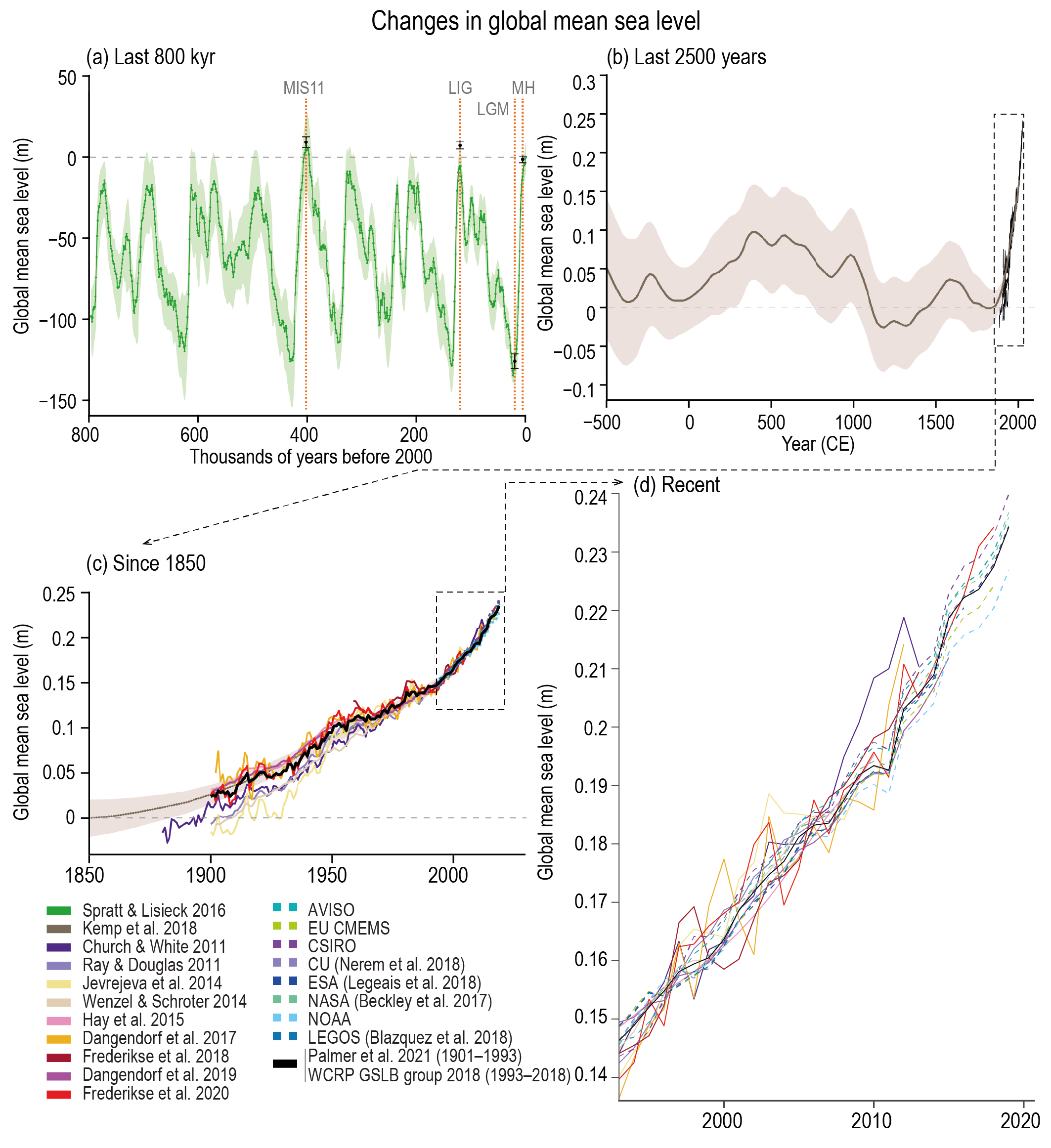 Figure 2.28 | Changes in global mean sea level. (a) Reconstruction of sea-level from ice core oxygen isotope analysis for the last 800 kyr. For target paleo periods (CCB2.1) and MIS11 the estimates based upon a broader range of sources are given as box whiskers. Note the much broader axis range (200 m) than for later panels (tenths of metres). (b) Reconstructions for the last 2500 years based upon a range of proxy sources with direct instrumental records superposed since the late 19th century. (c) Tide-gauge and, more latterly, altimeter-based estimates since 1850. The consensus estimate used in various calculations in Chapters 7 and 9 is shown in black. (d) The most recent period of record from tide-gauge and altimeter-based records. Further details on data sources and processing are available in the chapter data table (Table 2.SM.1).
 Few sites globally have well-preserved MIS 11 sea-level indicators (Dutton et al., 2015). As reported in AR5, Raymo and Mitrovica (2012) used glacial isostatic adjustment models to correct the elevation of MIS 11 sea-level proxies from Bermuda and Bahamas to estimate a peak MIS 11 GMSL between 6 and 13 m above present-day. This agrees with the elevation of 13 ± 2 m for the MIS 11 subtidal–intertidal transition in South Africa (Roberts et al., 2012). A revised glacial isostatic adjustment at this location resulted in a peak GMSL estimate of 8–11.5 m (Chen et al., 2014). In light of these data, and the review by Dutton et al. (2015), the AR5 estimate of 6–13 m for MIS 11 remains the best available (medium confidence).
Recent studies have highlighted uncertainties in estimates of GMSL during the LIG, including the extent of GMSL variability (Capron et al., 2019). Vertical land motions (Austermann et al., 2017) are starting to be considered quantitatively (e.g., Stephenson et al., 2019), but are still bounded by large uncertainties. The distribution and thickness of pre-LIG ice sheets (Dendy et al., 2017; Rohling et al., 2017) and isostasy driven by sediment loading since the LIG (Pico, 2020) add further uncertainty. In light of these recent studies and previous assessments, there is medium confidence that peak GMSL during the LIG was likely between 5 and 10 m higher than modern. Relative sea-level estimates from some sites (e.g., Bahamas and Seychelles) report ephemeral, metre-scale fluctuations (Vyverberg et al., 2018). Different generations of LIG reef growth at other sites (e.g., Yucatan Peninsula, Western Australia) suggest the occurrence of sudden accelerations in GMSL change (Blanchon et al., 2009; O’Leary et al., 2013). However, other sites (e.g., South Australia, Mediterranean), indicate that LIG sea level was substantially stable (T.-Y. Pan et al., 2018; Polyak et al., 2018). In addition, there are uncertainties in the interpretation of local relative sea level from some GMSL reconstructions (Barlow et al., 2018). Therefore, low confidence is assigned to any GMSL rate of change estimated within the LIG.
New geological proxies and glacial isostatic adjustment (GIA) modelling studies confirm that, at the LGM, GMSL was 125–134 m below present (Lambeck et al., 2014; Yokoyama et al., 2018). During the LDT, GMSL rose from approximately –120 m to –50 m, implying an average rate of about 10 mm yr–1 (Lambeck et al., 2014). The fastest rise occurred during Meltwater Pulse 1A, at about 14.6–14.3 ka (Deschamps et al., 2012; Sanborn et al., 2017), when GMSL rose by between 8 m and 15 m (medium confidence) (J. Liu et al., 2016) at an average rate of 24–44 mm yr–1.
Recent GIA modelling studies tuned to both near- and far-field relative sea level (RSL) data yield MH GMSL estimates of –3.8 to –1.0 m (Lambeck et al., 2014; Peltier et al., 2015; Bradley et al., 2016; Roy and Peltier, 2017). Estimates from relatively stable locations where the effects of GIA are small and relatively insensitive to parameters defining Earth rheology, and where RSL is expected to approximate GMSL to within about 1 m (e.g., Milne and Mitrovica, 2008), suggest that RSL was between about –6 to +1.5 m at around 6 ka at multiple locations (Camoin et al., 1997; Braithwaite et al., 2000; Frank et al., 2006; Montaggioni and Faure, 2008; Vacchi et al., 2016; Khan et al., 2017; Hibbert et al., 2018). The assessment of GMSL change at 6 kyr is challenging considering the proportionately large GIA effect (Kopp et al., 2016), insufficient resolution of marine geochemical proxies (δ18O, Mg/Ca) and uncertainties in the contribution of the Antarctic Ice Sheet during the MH (Section 2.3.2.4). The possibility that GMSL was at least somewhat higher than present cannot be excluded.
For the last 3 kyr, GMSL has been estimated from global databases of sea-level proxies, including numerous densely-sampled high-resolution salt-marsh records with decimetre scale vertical resolution and sub-centennial temporal resolution (Kopp et al., 2016; Kemp et al., 2018). Over the last about 1.5 kyr, the most prominent century-scale GMSL trends include average maximum rates of lowering and rising of –0.7 ± 0.5 mm yr–1 (2 SD) over 1020–1120 CE, and 0.3 ± 0.5 (2 SD) over 1460–1560, respectively. Between 1000 and 1750 CE, GMSL is estimated to have been within the range of about –0.11 to +0.09 m relative to 1900 (Kemp et al., 2018). This was followed by a sustained increase of GMSL that began between 1820 and 1860 and has continued to the present day. New analyses demonstrate that it is very likely that GMSL rise over the 20th century was faster than over any preceding century in at least 3 kyr (Kopp et al., 2016; Kemp et al., 2018) (Figure 2.28).
Since SROCC, two new tide gauge reconstructions of 20th century GMSL change have been published, although both rely upon CMIP models to varying degrees (Figure 2.28). Frederikse et al. (2020) used a ‘virtual station’ method and a probabilistic framework to estimate GMSL change and its uncertainties since 1900. Dangendorf et al. (2019) combined a Kalman Smoother (Hay et al., 2015) with Reduced Space Optimal Interpolation (Church and White, 2011; Ray and Douglas, 2011) in an effort to better represent both the long-term GMSL change while preserving information on sea-level variability. In addition, new ensemble-based methods for quantifying GMSL change have been presented that account for both structural and parametric uncertainty (Palmer et al., 2021). Altimeter time series of GMSL change (Figure 2.28) have been extended to 2019/2020 but bias adjustments (Watson et al., 2015; Beckley et al., 2017; Dieng et al., 2017; Ablain et al., 2019; Legeais et al., 2020) did not change since SROCC.
Based on the ensemble approach of Palmer et al. (2021) and an updated WCRP Global Sea Level Budget Group (2018) assessment (Figure 2.28) GMSL rose at a rate of 1.32 [0.58 to 2.06] mm yr–1 for the period 1901–1971, increasing to 1.87 [0.82 to 2.92] mm yr–1 between 1971 and 2006, and further increasing to 3.69 [3.21 to 4.17] mm yr–1 for 2006–2018 (high confidence). The average rate for 1901–2018 was 1.73 [1.28 to 2.17] mm yr–1 with a total rise of 0.20 [0.15 to 0.25] m (Table 9.5). The acceleration rate very likely is 0.094 [0.082 to 0.115] mm yr–2 for 1993–2018 (WCRP Global Sea Level Budget Group, 2018, updated), consistent with other estimates (Watson et al., 2015; X. Chen et al., 2017; Nerem et al., 2018; WCRP Global Sea Level Budget Group, 2018; Ablain et al., 2019; Legeais et al., 2020). For the period 1902–2010 the updated tide gauge reconstructions published since SROCC also show a robust acceleration over the 20th century and the ensemble estimate of Palmer et al. (2021) gives a value of 0.0053 [0.0042 to 0.0073] mm yr–2, based on an unweighted quadratic fit.
In summary, GMSL is rising, and the rate of GMSL rise since the 20th century is faster than over any preceding century in at least the last three millennia (high confidence). Since 1901, GMSL has risen by 0.20 [0.15 to 0.25] m at an accelerating rate. Further back in time, there is medium confidence that GMSL was within –3.5 to +0.5 m (very likely range) of present during the MH, 5–10 m higher (likely range) during the LIG, and 5–25 m higher (very likely range) during the MPWP.
2.3.3.4 Ocean Circulation
2.3.3.4.1 Atlantic Meridional Overturning Circulation (AMOC)
The AR5 concluded that there was no evidence of a trend in the AMOC during the period of instrumental observations. However, AR5 also stressed insufficient evidence to support a finding of change in the heat transport of the AMOC. SROCC assessed that there was emerging evidence in sustained observations, both in situ (2004–2017) and revealed from SST-based reconstructions, that the AMOC had weakened during the instrumental era relative to 1850–1900 (medium confidence), although there were insufficient data to quantify the magnitude of the weakening. SROCC also concluded with low confidence an increase of the Southern Ocean upper cell overturning circulation. SROCC also reported with medium confidence that the production of Antarctic Bottom Water had decreased since the 1950s consistent with a decreased lower cell overturning circulation, and potentially modulating the strength of the AMOC.
On multi-millennial timescales, proxy evidence indicates that the AMOC varied repeatedly in strength and vertical structure. During the last glacial period, particularly around the LGM, AMOC was estimated to be shallower than present, although there is continued debate about the magnitude of the shoaling (Lynch-Stieglitz et al., 2007; Gebbie, 2014), and whether this change was associated with a weaker overturning (Ritz et al., 2013; Menviel et al., 2017; Muglia et al., 2018). There are indications that substantial variations in AMOC were associated with abrupt climate changes during the glacial intervals, including Dansgaard-Oeschger and Heinrich events (14–70 ka) (McManus et al., 2004; Böhm et al., 2015; Henry et al., 2016; Lynch-Stieglitz, 2017). During these millennial-scale oscillations, weakened AMOC was associated with dramatic cooling in the NH and warming in the SH (Buizert et al., 2015; Henry et al., 2016), while hemispheric changes of opposite sign accompanied strengthened AMOC. After the final demise of the Laurentide ice sheet about 8 ka, the mean overall strength of AMOC has been relatively stable throughout the rest of the Holocene compared to the preceding 100 kyr (Hoffmann et al., 2018; Lippold et al., 2019). There are however indications of episodic variations in AMOC during the Holocene (Bianchi and McCave, 1999; Oppo et al., 2003; Thornalley et al., 2013; Ayache et al., 2018), and past interglacial intervals (Galaasen et al., 2014, 2020; Hayes et al., 2014; Mokeddem et al., 2014; H. Huang et al., 2020). Over the last 3 kyr, there are indications that AMOC variability was potentially linked to decreasing production of Labrador Sea Water (LSW), one of the water masses contributing to AMOC (Alonso-Garcia et al., 2017; Moffa-Sánchez and Hall, 2017; Moffa-Sánchez et al., 2019).
Numerous proxy records collectively imply that AMOC is currently at its weakest point in the past 1.6 ka (Rahmstorf et al., 2015; Caesar et al., 2018, 2021; Thibodeau et al., 2018; Thornalley et al., 2018). Caesar et al. (2021) analyse a compilation of various available indirect AMOC proxies from marine sediments, in situ-based reconstructions and terrestrial proxies, which show a decline beginning in the late 19th century and over the 20th century superimposed by large decadal variability in the second half of the 20th century. Indirect reconstructions of AMOC components based on coastal sea level records in the western North Atlantic (Ezer, 2013; McCarthy et al., 2015; Piecuch, 2020) show an AMOC decline since the late 1950s, with only a short period of recovery during the 1990s.
However, other studies highlight that proxy records do not show such clear signals (Moffa-Sánchez et al., 2019), and the use of SST- and coastal sea level-based proxies of AMOC places uncertainties on these results (Little et al., 2019; Jackson and Wood, 2020; Menary et al., 2020). For instance, SSTs are additionally influenced by atmospheric and non-AMOC related ocean variability (Josey et al., 2018; Keil et al., 2020; Menary et al., 2020), while sea level responds to a variety of factors (e.g., atmospheric pressure and local winds) independent of the AMOC (Woodworth et al., 2014; Piecuch and Ponte, 2015; Piecuch et al., 2016). Finally, large decadal variability is present in many reconstructions and obscures estimation of the long-term trend over the 20th century (Ezer, 2013; McCarthy et al., 2015; Yashayaev and Loder, 2016; Thornalley et al., 2018; Caesar et al., 2021). It is also noted that the proxy reported AMOC decline, beginning in the late 19th century, is not supported by model-based evidence (Sections 3.5.4.1 and 9.2.3.1).
Since the 1980s, multiple lines of observational evidence for AMOC change exist. Ship-based hydrographic estimates of AMOC as far back as the 1980s show no overall decline in AMOC strength (Fu et al., 2020; Worthington et al., 2021). Direct indications from in-situ observations report a –2.5 ± 1.4 Sv change between 1993 and 2010 across the OVIDE section, superimposed on large interannual to decadal variability (Mercier et al., 2015). At 41°N and 26°N, a decline of –3.1 ± 3.2 Sv per decade and –2.5 ± 2.1 Sv per decade respectively has been reported over 2004–2016 (Baringer et al., 2018; Smeed et al., 2018). However, Moat et al. (2020) report an increase in AMOC strength at 26°N over 2009–2018. Recent time series of moored observations at 11ºS (Hummels et al., 2015), 34°S (Meinen et al., 2018; Kersalé et al., 2020), and between 57 and 60ºN (Lozier et al., 2019) are currently too short to permit robust conclusions about changes. The directly observed AMOC weakening since 2004, while significant, is over too short a period to assess whether it is part of a longer term trend or dominated by decadal‐scale internal variability (Smeed et al., 2014; Collins et al., 2019; Moat et al., 2020). Notably an increase and subsequent decline in the 1990s is present in estimates of AMOC and associated heat transport constructed from reanalyses or auxiliary data (Section 9.2.3.1; Frajka-Williams, 2015; Jackson et al., 2016; Trenberth and Fasullo, 2017; Jackson and Wood, 2020).
Repeated full depth in situ measurements report that deep convection – a major driver for AMOC – has recently returned to the Labrador Sea, particularly in 2015 (Yashayaev and Loder, 2016; Rhein et al., 2017), and to the Irminger Sea (de Jong and de Steur, 2016; Gladyshev et al., 2016; de Jong et al., 2018) following an extended period with weak convection since 2000. An associated strengthening of the outflow from the Labrador Sea has not been observed (Zantopp et al., 2017; Lozier et al., 2019), while strengthening of the AMOC is tentative (Desbruyères et al., 2019; Moat et al., 2020). A long-term increase of the upper overturning cell in the Southern Ocean since the 1990s can be assessed with low confidence, and there is medium confidence of a decrease in Antarctic bottom water (AABW) volume and circulation, which has potential implications for the strength of the AMOC (Section 9.2.3.2).
In summary, proxy-based reconstructions suggest that the AMOC was relatively stable during the past 8 kyr (medium confidence), with a weakening beginning since the late 19th century (medium confidence), but due to a lack of direct observations, confidence in an overall decline of AMOC during the 20th centuryis low. From the mid-2000s to mid-2010s, the directly observed weakening in AMOC (high confidence) cannot be distinguished between decadal-scale variability or a long-term trend (high confidence).
2.3.3.4.2 Western boundary currents and inter-basin exchanges
Both AR5 and SROCC reported that western boundary currents (WBCs) have undergone an intensification, warming and poleward expansion, except for the Gulf Stream and the Kuroshio, but did not provide confidence statements. The AR5 reported with medium to high confidence intensification of the North Pacific subpolar gyre, the South Pacific subtropical gyre, and the subtropical cells, along with an expansion of the North Pacific subtropical gyre since the 1990s. It was pointed out that these changes are likely predominantly due to interannual-to-decadal variability, and in the case of the subtropical cells represent a reversal of earlier multi-decadal changes. SROCC concluded that it was unlikely that there has been a statistically significant net southward movement of the mean Antarctic Circumpolar Current (ACC) position over the past 20 years, in contrast to AR5, where this change had been assessed with medium confidence.
The intensity of the Kuroshio current system in the north-west Pacific varied in conjunction with the glaciation cycles over the last 1 Myr, with some limited glacial-interglacial variability in position (Jian et al., 2000; Gallagher et al., 2015). The Agulhas current has strengthened substantially during the warming associated with deglaciations of the past 1 Myr (Peeters et al., 2004; Bard and Rickaby, 2009; Martínez-Méndez et al., 2010; Marino et al., 2013; Ballalai et al., 2019). According to sediment core analyses, the Agulhas leakage varied by about 10 Sv during major climatic transitions over the past 640 kyr (Caley et al., 2014). Available data suggests that there was relatively little change in the net flow of the ACC during the LGM, with no consensus on the sign of changes (McCave et al., 2013; Lamy et al., 2015; Lynch-Stieglitz et al., 2016), except at one location at the northern edge of the Drake Passage where a 40% decrease of transport had been reported (Lamy et al., 2015). Longer time series from the northern entrance to Drake Passage suggest a consistent transport variability of 6–16% through glacial climate cycles, with higher current speeds during interglacial times and reduced current speeds during glacial intervals (Toyos et al., 2020). Inferred variability in the size and strength of the North Atlantic subpolar gyre was substantial, and included rapid changes on millennial time scales during both interglacial and glacial intervals over the last 150 kyr (Born and Levermann, 2010; Mokeddem et al., 2014; Irvalı et al., 2016; Mokeddem and McManus, 2016). North Atlantic – Arctic exchange has also varied in the past, with indications of an increasing inflow of Atlantic waters into the Arctic during the late Holocene (Ślubowska et al., 2005) with an acceleration to the recent inflow that is now the largest of the past 2 kyr (Spielhagen et al., 2011).
A latitudinal shift of subtropical/subpolar gyres on the order of 0.1 ± 0.04° per decade is derived by an indirect method using remote sensing data during 1993–2018 (Yang et al., 2020). Direct observations show a systematic poleward migration of WBCs (Wu et al., 2012; Yang et al., 2016, 2020; Bisagni et al., 2017). However, they do not support an intensification of WBCs, with a weakening, broadening, or little change reported for the Kuroshio (Y.-L. Wang et al., 2016; Wang and Wu, 2018; Collins et al., 2019), Gulf Stream (McCarthy et al., 2018; Collins et al., 2019; Dong et al., 2019; Andres et al., 2020), Agulhas (Beal and Elipot, 2016; Elipot and Beal, 2018) and East Australian (Sloyan and O’Kane, 2015) currents. The Gulf Stream has recently reversed a long-term poleward migration (Bisagni et al., 2017). Multidecadal variability of the strength and position of WBCs (Hsin, 2015; Bisagni et al., 2017; McCarthy et al., 2018) and short records from direct observations obscure the detection of any long-term trends (Yang et al., 2020).
The Pacific to Arctic exchange at the Bering Strait plays a minor role in the total Arctic exchange with the global ocean, which has increased from 0.8 Sv to 1.0 Sv over 1990–2015 (Woodgate, 2018). For Atlantic-Arctic exchange, major branches of Atlantic Water inflow from the North Atlantic into the Arctic across the Greenland–Scotland Ridge have remained stable since the mid-1990s (Berx et al., 2013; Hansen et al., 2015; Jochumsen et al., 2017; Østerhus et al., 2019), with only the smaller pathway of Atlantic Water north of Iceland showing a strengthening trend during 1993–2018 (Casanova-Masjoan et al., 2020), but with associated heat transport strengthening through the 1990s (Rossby et al., 2020; Tsubouchi et al., 2021). The Arctic outflow remained broadly stable from the mid-1990s to the mid 2010s (Østerhus et al., 2019).
The heat and mass transport of the Indonesian throughflow (ITF) shows substantial variability at seasonal to decadal time scales (Zhuang et al., 2013; Q.-Y. Liu et al., 2015; Susanto and Song, 2015; Feng et al., 2017, 2018; M. Li et al., 2018; Sprintall et al., 2019; Xie et al., 2019). Q.-Y. Liu et al. (2015) reported an increasing trend in the ITF geostrophic transport of 1 Sv per decade over 1984–2013, consistent with direct estimates (Sprintall et al., 2014), and results from reanalyses (M. Li et al., 2018), and this appears to be linked to multi-decadal scale variability rather than a long-term trend (Kosaka and Xie, 2013; England et al., 2014; Lee et al., 2015).
Southern Ocean circulation changes are assessed in SROCC (Meredith et al., 2019), and are confirmed and synthesized in Section 9.2.3.2 which shows that there is no indication of ACC transport change, and that it is unlikely that the mean meridional position of the ACC has moved southward in recent decades.
In summary, over the past 3–4 decades, the WBC strength is highly variable (high confidence), and WBCs and subtropical gyres have shifted poleward since 1993 (medium confidence). Net Arctic Ocean volume exchanges with the other ocean basins remained stable over the mid-1990s to the mid-2010s (high confidence). There is high confidence that the ITF shows strong multi-decadal scale variability since the 1980s.
2.3.3.5 Ocean pH
The AR5 assessed with high confidence that the pH of the ocean surface had decreased since preindustrial times, primarily as a result of ocean uptake of CO2. SROCC concluded that the global ocean absorbed 20–30% of total CO2 emissions since the 1980s, with virtually certainocean surface pH decline. The SROCC assessed a rate of surface pH decline of 0.017–0.027 pH units per decade across a range of time series of pH observations longer than 15 years. The decline in surface open ocean pH was assessed by SROCC as havingvery likely already emerged from background natural variability for more than 95% of the global surface open ocean.
Understanding of changes in surface pH at paleo time-scales has increased since AR5 (Clarkson et al., 2015; Foster and Rae, 2016; Zeebe et al., 2016; Gutjahr et al., 2017; Sosdian et al., 2018; Henehan et al., 2019; Anagnostou et al., 2020; Harper et al., 2020; Müller et al., 2020). Over the last 65 million years there have been several intervals when the pH of surface waters varied concurrently with climate change such as during the PETM, EECO, and MCO (Figure 2.29a and Section 5.3.1.1). However, only during the PETM is the change sufficiently well-constrained to allow for a direct comparison with recent and current trends (Kirtland Turner, 2018). This event was associated with profound perturbations of the global carbon cycle, ocean warming, deoxygenation and a surface ocean pH decrease likely ranging from 0.15 to 0.30 units (Penman et al., 2014; Gutjahr et al., 2017; Babila et al., 2018) – a rate that was likely at least an order of magnitude slower than today (Cui et al., 2011; Bowen et al., 2015; Frieling et al., 2016; Zeebe et al., 2016; Gutjahr et al., 2017; Kirtland Turner, 2018; Gingerich, 2019).
Paleo evidence suggests that surface ocean pH has gradually increased over the last 50 Myr (Anagnostou et al., 2016, 2020; Sosdian et al., 2018) (Figure 2.29a). Global mean surface pH values as low as observed during recent decades are uncommon in the last 2 Myr (Figure 2.29b) (Martínez-Botí et al., 2015a; Chalk et al., 2017; Dyez et al., 2018; Sosdian et al., 2018), and have not been experienced in at least the last 25 kyr (Figure 2.29c; Palmer and Pearson, 2003; Foster, 2008; Palmer et al., 2010; Henehan et al., 2013; Kirschke et al., 2013; Martínez-Botí et al., 2015a; Naik et al., 2015; Ezat et al., 2017; Gray et al., 2018; Shao et al., 2019). The magnitude of pH change during the Pleistocene glacial–interglacial cycles was 0.1–0.15 pH units – similar to recent changes in the modern era (Figure 2.29c and Section 5.3.1.2; Hönisch et al., 2009; Chalk et al., 2017; Shao et al., 2019). Maximum rates of pH change during the LDT, inferred from changes in atmospheric CO2 recorded in ice cores (Marcott et al., 2014) and the established relationships between pH and CO2 changes and the boron isotope proxy (Hain et al., 2018), reached –0.02 pH units per century at about 11.7 ka, about 14.8 ka and about 16.3 ka, as previously sequestered CO2 was transferred from the ocean interior to the subsurface ocean (Martínez-Botí et al., 2015a; Jaccard et al., 2016; Rae et al., 2018).
 Figure 2.29 | Low-latitude surface ocean pH over the last 65 million years (65 Myr). (a) Low-latitude (30°N–30°S) surface ocean pH over the last 65 Myr, reconstructed using boron isotopes in foraminifera. (b) as (a) but for the last 3.5 Myr. Double headed arrow shows the approximate magnitude of glacial-interglacial pH changes. (c) Multisite composite of surface pH. In (a, b, c) uncertainty is shown at 95% confidence as a shaded band. Relevant paleoclimate reference periods (CCB2.1) have been labelled. Period windows for succeeding panels are shown as horizontal black lines in (a) and (b). (d) Estimated low-latitude surface pH from direct observations (BATS, HOT) and global mean pH (65°S–65°N) from two indirect estimates (CMEMS, OCEAN-SODA). Further details on data sources and processing are available in the chapter data table (Table 2.SM.1).
 Since the 1980s, the global ocean has experienced a decline in surface pH of 0.016 ± 0.006 pH units per decade based on indirect pH products (Figure 2.29d; Lauvset et al., 2015; Hurd et al., 2018; IPCC, 2019; Gehlen et al., 2020) that agrees with the decline of 0.017–0.025 pH units per decade assessed in SROCC from direct time-series measurements of pH. Section 5.3.2.2 assesses a decline that ranges from 0.01 to 0.026 pH units per decade for the tropical and subtropical open ocean areas, and 0.003–0.026 pH units per decade for the polar and subpolar open ocean regions by using time series and ship-based datasets from the surface ocean CO2 measurement network (Bakker et al., 2016; Gehlen et al., 2020; Gregor and Gruber, 2021). There is general consensus that global surface ocean pH trends over the past two decades have exceeded the natural background variability (Lauvset et al., 2015; Bindoff et al., 2019; Gehlen et al., 2020). However, for some areas sparse data coverage, and large year-to-year variations hinders the detection of long-term surface ocean pH trends; for example in the Southern Ocean (Lauvset et al., 2015; Bindoff et al., 2019) and in the Arctic Ocean (Lauvset et al., 2015; Bindoff et al., 2019; Meredith et al., 2019).
For subsurface pH changes, estimates arise from direct ship measurements from repeated hydrography programs (Carter et al., 2019), indirect estimates of pH through calcite and aragonite saturation horizons (Osborne et al., 2020; Ross et al., 2020), and the very recent biogeochemical Argo floats equipped with pH sensors (Claustre et al., 2020). Global subsurface pH has decreased over the past 20 to 30 years, with signals observed to at least 1000 m depths (Lauvset et al., 2020). Global findings are supplemented by regional findings from the Pacific Ocean (Carter et al., 2019; Ross et al., 2020); the South Atlantic (Salt et al., 2015) and Southern Ocean (Jones et al., 2017); the North Atlantic Ocean and along the AMOC (Woosley et al., 2016; Perez et al., 2018), the Arctic Ocean (Qi et al., 2017) and marginal seas (C.-T.A. Chen et al., 2017). Further details are given in Section 5.3.3.1.
To conclude, it is virtually certain that surface open ocean pH has declined globally over the last 40 years by 0.003–0.026 pH per decade, and a decline in the ocean interior has been observed in all ocean basins over the past 2–3 decades (high confidence). A long-term increase in surface open ocean pH occurred over the past 50 Myr (high confidence), and surface open ocean pH as low as recent times is uncommon in the last 2 Myr (medium confidence). There is very high confidence that open ocean surface pH is now the lowest it has been for at least 26 kyr and current rates of pH change are unprecedented since at least that time.
2.3.3.6 Ocean Deoxygenation
SROCC concluded that there has very likely been a net loss of oxygen over all ocean depths since the 1960s linked to global ocean deoxygenation at a range of 0.3–2.0%, and that the oxygen levels in the global upper 1000 m of the ocean had decreased by 0.5–3.3% during 1970–2010 (medium confidence), alongside an expansion of oxygen minimum zones (OMZ) by 3–8%. For the surface ocean (0–100 m) and the thermocline at 100–600 m, the very likely range of oxygen decline was assessed to be 0.2–2.1% and 0.7–3.5%, respectively. Multidecadal rates of deoxygenation showed variability throughout the water column and across ocean basins (high confidence).
Since AR5 evidence for changes in oxygen content based on new proxy reconstructions has increased (Hoogakker et al., 2015, 2018; Gottschalk et al., 2016, 2020; Anderson et al., 2019). Paleo records point to past periods of reduced oceanic oxygen levels during the late Permian (about 250 Ma), the Jurassic and the Cretaceous (180–100 Ma), alongside associated global scale disturbances of the global carbon cycle. Emerging studies for the Cenozoic Era suggest more stable ocean oxygenation conditions throughout the interval on million-year time scales (X. Wang et al., 2016). Sedimentary proxy data indicate, however, that the seemingly stable Cenozoic was punctuated by transient, widespread deoxygenation during the PETM (Dickson et al., 2012; Winguth et al., 2012; Remmelzwaal et al., 2019), with parts of the ocean reaching anoxic levels (Section 5.3.1.1; Yao et al., 2018). Since the LGM, there was an overall emergence and expansion of low-oxygen waters into the ocean intermediate depths as a result of rapid warming and a reorganization of the global overturning circulation (Galbraith and Jaccard, 2015). The maximum expansion of oxygen-depleted waters during the LDT occurred coincidently with rapid warming in the NH at 14.7–12.9 ka (Jaccard and Galbraith, 2012; Moffitt et al., 2015; Hoogakker et al., 2018). Deep (>1500 m) ocean oxygen levels increased by 100–150 µmol kg–1 since the LGM, reaching modern oxygen levels at about 10 ka (Section 5.3.1.2; Hoogakker et al., 2015; Gottschalk et al., 2016; Anderson et al., 2019).
New findings for ocean oxygen content since SROCC are limited to regional scale assessments. The magnitude of change is difficult to compare across regions to arrive at a global assessment due to differences in depth range, time period, baseline climatology, methodology, and particularly the use of different units. To facilitate comparisons, data are presented as change per decade, and conversions of the SROCC global mean percentage of oxygen decline estimates are provided as a loss of 3.2 μmol kg−1 in the upper 1000 m of the global ocean (1.93%), 2.0 μmol kg−1 (0.8 μmol kg−1 per decade) in the upper 1000 m of the global ocean (1.93%), and 2.0 μmol kg−1 (0.5 μmol kg−1 per decade) in the entire water column (1.15%) between 1970 and 2010 (Bindoff et al., 2019). Oxygen change also shows decadal variability (Ito et al., 2016; Stramma et al., 2020) that can influence estimates of trends.
Subsurface (100–400 m) oxygen in the California Current system is estimated to have declined by 24 ± 2 μmol kg−1 (1.0 μmol kg−1 per decade) between 1993 and 2018, a rate similar to the global upper 1000 m average (Bindoff et al., 2019). In some locations, however, the magnitude of oxygen loss substantially exceeds global averages (Queste et al., 2018; Bronselaer et al., 2020; Cummins and Ross, 2020; Stramma et al., 2020). For example, a decline in oxygen content of 11.7 ± 3.5% in the upper 4000 m, including a decline of 20.4 ± 7.2% in the upper 1550 m, is reported in the North Pacific over the period 1958–2018 (Cummins and Ross, 2020) (equivalent to 2.3 μmol kg−1 per decade in the upper 1550 m and 2.0 μmol kg−1 decade− 1 throughout the 4000 m water column). In some regions of the Southern Ocean south of 65°S oxygen in the upper 2000 m has declined by 60 μmol kg−1 (~52 μmol kg−1 per decade) based on comparisons of 2014–2019 and 1985–2005 observations (Bronselaer et al., 2020). Within some OMZs regions of the Indian ocean, oxygen has declined from 6–12 to <2 μmol kg−1 between the 1960s and 2015–2016 (Bristow et al., 2017; Al-Said et al., 2018; Queste et al., 2018).
Findings since SROCC provide further support that the volume of severely oxygen-depleted water has expanded in some locations of the global ocean (Section 5.3.3.2). For example, vertical expansion of low oxygen zones is reported in the North Pacific at a rate of 3.1 ± 0.5 m yr–1 (Ross et al., 2020), and suboxic waters have increased by 20% at a rate of about 19 m per decade from 1982–2010 in the Arabian Sea (Al-Said et al., 2018; Lachkar et al., 2019), and expanded off the coast of Mexico (Sánchez-Velasco et al., 2019).
In summary, episodes of widespread and long-lasting (100 ka scales) open-ocean deoxygenation were related to warm climate intervals of the Permian-Cretaceous, with conditions becoming generally better oxygenated as the climate cooled over the course of the Cenozoic (high confidence). The largest expansions of oxygen depleted waters over the past 25 ka were strongly linked to rapid warming rates (medium confidence). Open-ocean deoxygenation has occurred in most regions of the open ocean during the mid-20th to early 21st centuries (high confidence), and shows decadal variability (medium confidence). Evidence further confirms SROCC that OMZs are expanding at many locations (high confidence).
2.3.4 Biosphere
This section is limited to a few biological indicators to demonstrate the close links between the biosphere and physical forcing. In selecting the indicators, we focussed on (i) those that are observable at large (global) spatial scales and over long (two decades or more) temporal scales, using standardized and consistent procedures; and (ii) those that are illustrative of the influence of the physical system on the biological realm. Chapters 2 and 3 of AR6 WGII undertake a more holistic assessment of biospheric impacts.
2.3.4.1 Seasonal Cycle of Atmospheric CO2
The AR5 noted that because CO2 uptake by photosynthesis occurs only during the growing season, the greater land mass in the NH imparts a characteristic ‘sawtooth’ seasonal cycle in atmospheric CO2. The SRCCL similarly stated that due to strong seasonal patterns of growth, NH terrestrial ecosystems are largely responsible for the seasonal variations in global atmospheric CO2 concentrations. Neither AR5 nor SRCCL made a confidence statement about observed changes in the amplitude of the seasonal cycle of CO2.
In situ observations of CO2 generally depict a rising amplitude of the seasonal cycle over the past half century, especially north of about 45°N (Figure 2.30). For example, an amplitude increase of 6 ± 2.6% per decade has been observed at the Barrow surface observatory in Alaska over 1961–2011 (Graven et al., 2013), with slightly slower increases thereafter. Aircraft data north of 45°N exhibit an amplitude increase of 57 ± 7% at 500 mb versus an increase of 26 ± 18% for 35°N–45°N between field campaigns in 1958–1961 and 2009–2011 (Graven et al., 2013). Increases in amplitude for the period 1980–2012 are apparent at eight surface observatories north of 50°N (Piao et al., 2018), related primarily to a larger drawdown in June and July. Trends in seasonal cycle amplitude at lower latitudes are smaller (if present at all); for instance, the increase at the Mauna Loa observatory in Hawaii since the early 1960s is only about half as large as at Barrow (Graven et al., 2013), and only one other low-latitude observatory has a significant increase from 1980–2012 (Piao et al., 2018). There is a weak signal of an increase in amplitude at the Sinhagad observatory in western India in recent years (Chakraborty et al., 2020). Generally speaking, larger increases in the Arctic and boreal regions are indicative of changes in vegetation and carbon cycle dynamics in northern ecosystems (Forkel et al., 2016), though increased carbon uptake can also result from other factors such as warmer- and wetter-than-normal conditions.
 Figure 2.30 | Changes in the amplitude of the seasonal cycle of CO2 . (a) Observed peak-to-trough seasonal amplitude given by the day of year of downward zero crossing, of CO2 concentration at Barrow (71°N, blue) and Mauna Loa (20°N, black). Seasonal CO2 cycles observed at (b) Barrow and (c) Mauna Loa for the 1961–1963 or 1958–1963 and 2017–2019 time periods. The first six months of the year are repeated. Reprinted with permission from AAAS. Further details on data sources and processing are available in the chapter data table (Table 2.SM.1).
 Recent satellite-based, global-scale estimates of seasonal variations in atmospheric CO2 for the period 2003–2018 show that the seasonal variations in the SH are out of phase with those in the NH (Reuter et al., 2020), which is consistent with the phenological shifts in primary productivity between hemispheres. The net effect of the phase shift between the two hemispheres is to dampen the amplitude of the global average seasonal cycle. These integrated results also show that the amplitude of the oscillations has been increasing in the SH, from about 2009, but comparison with data from Baring head suggests that periods of high seasonal oscillation had occurred at that location in the SH prior to 1995.
In summary, there is very high confidence that the amplitude of the seasonal cycle of atmospheric CO2 has increased at mid-to-high NH latitudes since the early 1960s. The observed increase is generally consistent with greater greening during the growing season and an increase in the length of the growing season over the high northern latitudes. Similarly, globally-integrated results from the SH also show an increase in seasonal amplitude of atmospheric CO2 signal, from around 2009 to 2018 (low confidence).
2.3.4.2 Marine Biosphere
2.3.4.2.1 Large-scale distribution of marine biota
SROCC pointed out that long-term global observations of many key ocean variables, including phytoplankton, have not reached the density and accuracy necessary for detecting change. But SROCC noted the good comparability between short time-scale single-sensor ocean-colour products and a longer time-scale, climate-quality time series of multi-sensor, inter-sensor-bias-corrected, and error-characterized, global data on chlorophyll-a concentration in the surface layers of the ocean. With respect to oligotrophic gyres, AR5 WGII concluded that the oligotrophic subtropical gyres of the Atlantic and Pacific Oceans are expanding and that they indicate declining phytoplankton stocks in these waters (limited evidence, low agreement). With respect to distributions of marine organisms, AR5 WGII reported range shifts of benthic, pelagic, and demersal species and communities (high confidence), though the shifts were not uniform.
Phytoplankton are responsible for marine primary production through photosynthesis; they are a major player in the ocean carbon cycle. They have a high metabolic rate and respond fast to changes in environmental conditions (light, temperature, nutrients, mixing), and as such, serve as a key indicator for change in marine ecosystems. Concentration of chlorophyll-a, the major photosynthetic pigment in all phytoplankton, is often used as a measure of phytoplankton biomass. As primary producers, they are also food for organisms at higher trophic levels. The multi-sensor time series of chlorophyll-a concentration has now been updated (Sathyendranath et al., 2019) to cover 1998–2018. Figure 2.31 shows that global trends in chlorophyll-a for the last two decades are insignificant over large areas of the global ocean (von Schuckmann et al., 2019), but some regions exhibit significant trends, with positive trends in parts of the Arctic and the Antarctic waters (>3% yr–1), and both negative and positive trends (within ± 3% yr–1) in parts of the tropics, subtropics and temperate waters. The interannual variability in chlorophyll-a data in many regions is strongly tied to indices of climate variability (Section 2.4 and Annex IV) and changes in total concentration are typically associated with changes in phytoplankton community structure (e.g., Brewin et al., 2012; Racault et al., 2017b). Variability in community structure related to El Niño has, in turn, been linked to variability in fisheries, for example in the catch of anchovy (Engraulis ringens) in the Humboldt current ecosystem (Jackson et al., 2011).

Since AR5 WGII, analysis of a longer time series of ocean-colour data (1998–2012) has shown (Aiken et al., 2017) that the expansion of the low nutrient part of the North Atlantic oligotrophic gyre was significant, at 0.27 × 10⁶km2 per decade, but that the rate was much lower than that reported earlier by Polovina et al. (2008). Furthermore, Aiken et al. (2017) reported no significant trend in the oligotrophic area of the South Atlantic Gyre. With the time series extended to 2016, von Schuckmann et al. (2018) reported that since 2007, there was a general decreasing trend in the areas of the North and South Pacific oligotrophic Gyres, while the North and South Atlantic oligotrophic Gyres remained stable, with little change in area, consistent with Aiken et al . (2017). The changing sign of trends in the areal extent of the oligotrophic gyres with increase in the length of the time series raises the possibility that these changes arise from interannual to multi-decadal variability. The time series of ocean-colour data is too short to discern any trend that might be superimposed on such variability.
Similarly, there is limited consistent and long-term information on large-scale distributions of marine organisms at higher trophic levels. But there are increased indications since AR5 and SROCC that the distributions of various higher trophic-level organisms are shifting both polewards and to deeper levels (Edwards et al., 2016; Haug et al., 2017; Atkinson et al., 2019; Lenoir et al., 2020; Pinsky et al., 2020), mostly consistent with changes in temperature. However observations also show a smaller set of counter-intuitive migrations towards warmer and shallower waters, which could be related to changes in phenology and in larval transport by currents (Fuchs et al., 2020). There are also strengthening indications of greater representation by species with warm-water affinity in marine communities, consistent with expectations under observed warming (Burrows et al., 2019). There are indications that pre-1850 CE plankton communities are different from their modern counterparts globally (Jonkers et al., 2019). Indicators of geographical distributions of species (mostly from coastal waters) suggest that the rates at which some species are leaving or arriving at an ecosystem are variable, leading to changes in community composition (Blowes et al., 2019), with likely greater representation of warm-water species in some locations (Burrows et al., 2019).
In summary, there is high confidence that the latitudinal and depth limits of the distribution of various organisms in the marine biome are changing. There is medium confidence that there are differences in the responses of individual species relative to each other, such that the species compositions of ecosystems are changing. There is medium confidence that chlorophyll concentration in the surface shows weak negative and positive trends in parts of low and mid latitudes, and weak positive trends in some high-latitude areas. There is medium confidence that the large-scale distribution of the oligotrophic gyre provinces is subject to significant inter-annual variations, but low confidence in the long-term trends in the areal extent of these provinces because of insufficient length of direct observations.
2.3.4.2.2 Marine primary production
SROCC expressed low confidence in satellite-based estimates of trends in marine primary production, citing insufficient length of the time series and lack of corroborating in situ measurements and independent validation time series. The report also cites significant mismatches in absolute values and decadal trends in primary production when different satellite-based products are compared.
Recent model-based results with assimilation of satellite data (Gregg and Rousseaux, 2019), show global annual mean marine primary production of around 38 (±1.13) PgC yr–1 over 1998–2015. This new result lies towards the low end of values reported in earlier, satellite-based, studies (range 36.5–67 PgC yr–1, reported in Sathyendranath et al. (2020)). Reconciling the results of Gregg and Rousseaux (2019) with earlier satellite-based studies leads to a mean of 47 (±7.8) PgC yr–1. There is a strong correlation between interannual regional variability in marine primary production and climate variability (Racault et al., 2017b; Gregg and Rousseaux, 2019). The increase in primary production in the Arctic has been associated with retreating sea ice and with increases in nutrient supply and chlorophyll concentration (Lewis et al., 2020). Gregg and Rousseaux (2019) reported a decreasing trend in marine primary production, of –0.8 PgC (–2.1%) per decade globally. There is low confidence in this trend because of the small number of studies and the short length of the time series (<20 years).
In conclusion, there is low confidence because of the small number of recent studies and the insufficient length of the time series analysed that marine primary production is 47 (± 7.8) PgC yr–1. A small decrease in productivity is evident globally for the period 1998–2015, but regional changes are larger and of opposing signs (low confidence).
2.3.4.2.3 Marine phenology
Phenology is the study of the timing of important events in the annual life cycle of organisms (plants or animals; see also Annex VII: Glossary). The AR5 WGII noted that the timing of various seasonal biological events in the ocean had advanced by more than four days per decade over the previous 50-year period and concluded that there was high confidence in observed changes in the phenological metrics of marine organisms. The AR5 WGII further reported that, of those observations that showed a response, 81% of changes in phenology, distribution and abundance were consistent with anticipated responses to climate warming according to theoretical expectations, corroborated by updates in SROCC. The consequent current and future impacts on interactions between species, including competition and predator-prey dynamics, were noted with high confidence.
There are additional indications that phenological metrics related to different species are changing, but not always in a similar manner. For example, many seabirds are breeding earlier, while others are breeding later (Sydeman et al., 2015). Planktonic organisms in the North Atlantic are also responding differently to each other when subjected to the same environmental changes (Edwards and Richardson, 2004). Furthermore, different factors could be responsible for triggering phenological responses in different stages in the life cycle of a single organism (Koeller et al., 2009). The shift in the distribution of many benthic invertebrates on the North-west Atlantic shelf, including some commercially important shellfish, could be explained by phenology and larval transport, and the shift and contraction of species range have been associated with higher mortality (Fuchs et al., 2020). Changes in phytoplankton phenological indicators globally (Racault et al., 2012; Sapiano et al., 2012) have been linked to indicators of climate variability, such as the multivariate ENSO Index (Racault et al., 2017a), with responses varying across ecological provinces of the ocean (Longhurst, 2007).
Phenological links between multiple components of an ecosystem have to be maintained intact, to retain system integrity. Since all higher pelagic organisms depend on phytoplankton for their food, either directly or indirectly, a match favours survival, and a mismatch is antagonistic to survival. Match represents synchronicity in the phenological events of both prey and predator. There are indications from ocean-colour data used in conjunction with fisheries data that the survival rate of various larger marine organisms depends on phenological metrics related to the seasonality of phytoplankton growth. Such links have been demonstrated, for example, for haddock (Melanogrammus aeglefinus) in the North-west Atlantic (Platt et al., 2003); northern shrimp in the North Atlantic (Koeller et al., 2009; Ouellet et al., 2011); sardine (Sardinella aurita) off the Ivory coast (Kassi et al., 2018); cod (Gadus morhua) and haddock (Melanogrammus aeglefinus) larvae in the North-West Atlantic (Trzcinski et al., 2013); and oil sardine (Sardinella longiceps) off the south-west coast of India. Borstad et al. (2011) showed that fledgling production rate of rhinoceros auklets (Cerorhinca monocerata) on a remote island in coastal north-eastern Pacific was related to seasonal values of chlorophyll-a biomass in the vicinity of the island.
In summary, new in situ data as well as satellite observations strengthen AR5 and SROCC findings that various phenological metrics for many species of marine organisms have changed in the last half century (high confidence), though many regions and many species of marine organisms remain under-sampled or even unsampled. The changes vary with location and with species (high confidence). There is a strong dependence of survival in higher trophic-level organisms (fish, exploited invertebrates, birds) on the availability of food at various stages in their life cycle, which in turn depends on phenologies of both (high confidence). There is a gap in our understanding of how the varied responses of marine organisms to climate change, from a phenological perspective, might threaten the stability and integrity of entire ecosystems.
2.3.4.3 Terrestrial Biosphere
2.3.4.3.1 Growing season and phenology changes
The AR5 WGII briefly discussed large-scale changes in the length of the growing season but made no confidence statement about observed trends. However, AR5 did conclude with high confidence that warming contributed to an overall spring advancement in the NH.
Recent in situ analyses document increases in the length of the thermal growing season (i.e., the period of the year when temperatures are warm enough to support growth) over much of the extratropical land surface since at least the mid-20th century. Over the NH as a whole, an increase of about 2.0 days per decade is evident for 1951–2018 (Dunn et al., 2020), with slightly larger increases north of 45°N (Barichivich et al., 2013). Over North America, a rise of about 1.3 days per decade is apparent in the United States for 1900–2014 (Kukal and Irmak, 2018), with larger increases after 1980 (McCabe et al., 2015); likewise, all ecozones in Canada experienced increases from 1950–2010 (Pedlar et al., 2015). Growing season length in China increased by at least 1.0 days per decade since 1960 (Xia et al., 2018) and by several days per decade in South Korea since 1970 (Jung et al., 2015). In general, changes in phenological indicators are consistent with the increase in growing season length documented by instrumental data (Parmesan and Hanley, 2015). Several long-term, site-specific records illustrate the unusualness of recent phenological changes relative to interannual variability; for example, peak bloom dates for cherry blossoms in Kyoto, Japan have occurred progressively earlier in the growing season in recent decades, as have grape harvest dates in Beaune, France (Figure 2.32).
 Figure 2.32 | Phenological indicators of changes in growing season. (a) Cherry blossom peak bloom in Kyoto, Japan; (b) grape harvest in Beaune, France; (c) spring phenology index in eastern China; (d) full flower of Piedmont species in Philadelphia, USA; (e) grape harvest in Central Victoria, Australia; (f) start of growing season in Tibetan Plateau, China. Red lines depict the 25-year moving average (top row) or the nine-year moving average (middle and bottom rows) with the minimum roughness boundary constraint of Mann (2004). Further details on data sources and processing are available in the chapter data table (Table 2.SM.1).
 Changes in the length of the photosynthetically active growing season (derived from the Normalized Difference Vegetation Index (NDVI)) are also evident over many land areas since the early 1980s. Increases of about 2.0 days per decade are apparent north of 45°N since the early 1980s (centred over mid-latitude Eurasia and north-eastern North America), with indications of a reversal to a decline in season length starting in the early 2000s (Barichivich et al., 2013; Zhao et al., 2015; Garonna et al., 2016; Q. Liu et al., 2016; Park et al., 2016). Satellite-based records suggest that most NH regions have experienced both an earlier start and a later end to the growing season, a finding supported by ground-based data (Piao et al., 2020). A number of studies also capture increases in growing season length over the Canadian Arctic (W. Chen et al., 2016), Fennoscandia (Høgda et al., 2013), most of Europe (Garonna et al., 2014), and parts of sub-Saharan Africa (Vrieling et al., 2013).
The general consistency between in situ and satellite estimates over the NH is noteworthy given that many factors independently contribute to uncertainty in observed changes. For example, there is no universally accepted definition of growing season length across in situ analyses; some define the growing season as the period based on a temperature threshold (e.g., 5°C) whereas others use the frost-free period. Spatial and temporal coverage can also affect conclusions based upon in situ studies (Donat et al., 2013b). For satellite analyses, uncertainties can be related to the satellite datasets themselves (e.g., satellite drift, sensor differences, calibration uncertainties, atmospheric effects); and to the methods for determining phenological metrics (e.g., start, end, and length of season; S. Wang et al., 2016).
In summary, based on multiple independent analyses of in situ, satellite, and phenological data, there is high confidence that the length of the growing season has increased over much of the extratropical NH since at least the mid-20th century.
2.3.4.3.2 Terrestrial ecosystems
The AR5 WGII concluded that many terrestrial species have shifted their geographic ranges in recent decades (high confidence). Similarly, SRCCL assessed that many land species have experienced range size and location changes as well as altered abundances over recent decades (high confidence). SROCC noted that species composition and abundance have markedly changed in high mountain ecosystems in recent decades (very high confidence).
Paleoclimate reconstructions document large-scale biome shifts from the deep past through the Holocene (e.g., Hoogakker et al., 2016). The northernmost location of the treeline is a representative indicator in this regard (Figure 2.34). During the MPWP, boreal forest extended to the Arctic coast, with the northernmost treeline being about 4° to 10° latitude further north than at present; temperate forests and grasslands were also shifted poleward (with reduced tundra extent), while savannahs and woodlands were more expansive in Africa and Australia at the expense of deserts (Cross-Chapter Box 2.4, Figure 1b; Salzmann et al., 2008, 2013; Sniderman et al., 2016; Andrae et al., 2018). During the LGM, tundra and steppe expanded whereas forests were globally reduced in extent (Prentice et al., 2000; Binney et al., 2017), the northern treeline being about 17° to 23° latitude south of its present-day location in most areas. During the LDT, pervasive ecosystem transformations occurred in response to warming and other climatic changes (Nolan et al., 2018; Fordham et al., 2020). By the MH, North Africa had experienced a widespread conversion from grasslands to desert (Hoelzmann et al., 1998; Prentice et al., 2000; Sha et al., 2019), and the northernmost treeline had shifted poleward again to about 1° to 3° latitude north of its current location (MacDonald et al., 2000; Binney et al., 2009; Williams et al., 2011). Over the past half century, there has been an increase in the spatial synchrony of annual tree growth across all continents that is unprecedented during the past millennium (Manzanedo et al., 2020). Elevated rates of vegetation change in the Holocene are consistent with climate variability (Shuman et al., 2019), intensified human land use (Fyfe et al., 2015; Marquer et al., 2017), and resulting increased ecosystem novelty (Finsinger et al., 2017; K.D. Burke et al., 2019).
Long-term ecological records capture extensive range shifts during the 20th and early 21st centuries (Lenoir and Svenning, 2015; Pecl et al., 2017). Research has been most extensive for North America and western Eurasia, with fewer studies for central Africa, eastern Asia, South America, Greenland, and Antarctica (Lenoir and Svenning, 2015). Most documented changes are toward cooler conditions – that is, poleward and upslope (Lenoir et al., 2008; Harsch et al., 2009; Elmendorf et al., 2015; Parmesan and Hanley, 2015; Evans and Brown, 2017). Notably, a large, quasi-global analysis (Chen et al., 2011) estimated that many insect, bird, and plant species had shifted by 17 (±3) km per decade toward higher latitudes and 11 (±2) m per decade toward higher elevations since the mid-20th century, with changes in both the leading and trailing edges of species ranges (Rumpf et al., 2018). Over the past century, long-term ecological surveys also show that species turnover (i.e., the total number of gains and losses of species within an area) has significantly increased across a broad array of ecosystems (Dornelas et al., 2014, 2019), including undisturbed montane areas worldwide (Gibson-Reinemer et al., 2015). Despite global losses to biodiversity, however, most local assemblages have experienced a change in biodiversity rather than a systematic loss (Pimm et al., 2014). With increased species turnover, the novelty of contemporary communities relative to historical baselines has risen (Hobbs et al., 2009; Radeloff et al., 2015) due to greater spatial homogenization, mixtures of exotic and native species, altered disturbance regimes, and legacies of current or historic land use (Olden and Rooney, 2006; Schulte et al., 2007; Thompson et al., 2013; Goring et al., 2016). In general, terrestrial species have had lower rates of turnover than marine species (Dornelas et al., 2018; Blowes et al., 2019).
There are exceptions to the general pattern of poleward/upslope migration. For some species, various biotic and abiotic factors (such as precipitation and land use) supersede the physiological effects of temperature (Vanderwal et al., 2013; Gibson-Reinemer and Rahel, 2015; Ordonez et al., 2016; Scheffers et al., 2016; Lenoir et al., 2020). For other species, poleward migration is slower than expectations from the observed temperature increases. Trees are one such example because of their long lifespan and gradual maturity (Renwick and Rocca, 2015); in fact, poleward advance is only evident at about half of the sites in a large global dataset of treeline dynamics for 1900-present (Harsch et al., 2009). Furthermore, the northernmost extent of treeline at present (roughly 73°N) is actually somewhat south of its location in the MH (MacDonald et al., 2008) despite an expanding growing season in the extratropical NH since the mid-20th century (Section 2.3.4.3.1).
Consistent with species range shifts, SRCCL noted that there have been changes in the geographical distribution of climate zones. Poleward shifts in temperate and continental climates are evident across the globe over 1950–2010, with decreases in the area (and increases in the average elevation) of polar climates (Chan and Wu, 2015). Zonal changes towards higher latitudes in winter plant hardiness regions are apparent since the 1970s over the central and eastern USA, with elevational changes also being important in the western USA (Daly et al., 2012). A clear northward shift in winter plant hardiness zones is detectable across western Canada since 1930, with somewhat lesser changes in the south-eastern part of the country (McKenney et al., 2014). A northward migration of agro-climate zones is also evident over Europe since the mid-1970s (Ceglar et al., 2019). In addition, a shift toward more arid climate zones is apparent in some areas, such as the Asian monsoon region (Son and Bae, 2015) as well as parts of South America and Africa (Spinoni et al., 2015).
In summary, there is very high confidence that many terrestrial species have shifted their geographic ranges poleward and/or upslope over the past century, with increased rates of species turnover. There is high confidence that the geographical distribution of climate zones has shifted in many parts of the world.
2.3.4.3.3 Global greening and browning
The AR5 WGII briefly discussed changes in global vegetation greenness derived from satellite proxies for photosynthetic activity. Observed trends varied in their strength and consistency, and AR5 thus made no confidence statement on observed changes. The SRCCL subsequently concluded that greening had increased globally over the past 2–3 decades (high confidence).
Vegetation index data derived from AVHRR and MODIS depicts increases in aspects of vegetation greenness (i.e., green leaf area and/or mass) over the past four decades (Piao et al., 2020). NDVI increased globally from the early 1980s through the early 2010s (Y. Liu et al., 2015a). N. Pan et al. (2018) found NDVI increases over about 70% of the Earth’s vegetated surface through 2013, and Osborne et al. (2018) noted strong upward changes in NDVI in the circumpolar Arctic through 2016. Globally integrated Leaf Area Index (LAI) also rose from the early 1980s through at least the early 2010s (Zhu et al., 2016; Forzieri et al., 2017; Jiang et al., 2017; Xiao et al., 2017) and probably through near-present; for example, C. Chen et al. (2019) documented an LAI increase over one-third of the global vegetated area from 2000–2017. Although less frequently analysed for temporal trends, Fraction of Absorbed Photosynthetically Active Radiation (FAPAR) likewise increased over many global land areas (particularly China, India, and eastern Europe) in the past two decades (Figure 2.33; Forkel et al., 2014; Gobron, 2018; Keenan and Riley, 2018). There are also documented changes in specific vegetation types, such as a 7% rise in global tree cover for 1982–2016 (Song et al., 2018) and an expansion of shrub extent in the Arctic tundra over 1982–2017 (Myers-Smith et al., 2020). The increased greening is largely consistent with CO2 fertilization at the global scale, with other changes being noteworthy at the regional level (Piao et al., 2020); examples include agricultural intensification in China and India (X. Chen et al., 2019; Gao et al., 2019) and temperature increases in the northern high latitudes (Kong et al., 2017; Keenan and Riley, 2018) and in other areas such as the Loess Plateau in central China (Y. Wang et al., 2018). Notably, some areas (such as parts of Amazonia, central Asia, and the Congo basin) have experienced browning (i.e., decreases in green leaf area and/or mass) (Hoogakker et al., 2015; Gottschalk et al., 2016; Anderson et al., 2019). Because rates of browning have exceeded rates of greening in some regions since the late 1990s, the increase in global greening has been somewhat slower in the last two decades (T.-Y. Pan et al., 2018).
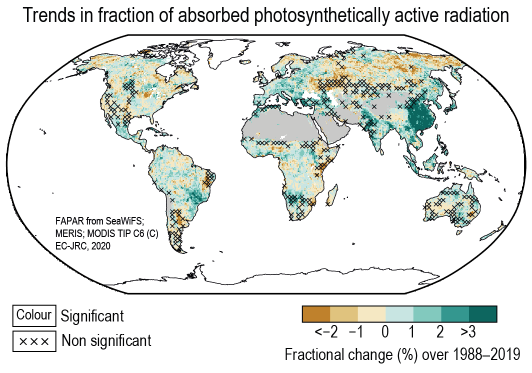 Figure 2. 33 | Satellite-based trends in fraction of absorbed photosynthetically active radiation (per decade) for 1998–2019. Trends are calculated using OLS regression with significance assessed following AR(1) adjustment after Santer et al. (2008); ‘×’ marks denote non-significant trend). Unvegetated areas such as barren deserts (grey) and ice sheets (white) have no trend in FAPAR. Further details on data sources and processing are available in the chapter data table (Table 2.SM.1).
 Global-scale linear trends differ substantially across products for the same periods and trend metrics used (Jiang et al., 2017). Several factors contribute to this large span in estimated changes. Remotely sensed vegetation products vary in their spatial and temporal completeness as well as resolution and are sensitive to contamination from atmospheric composition, clouds, snow cover, and anisotropy, as well as orbital changes and sensor degradations (de Jong et al., 2012; Zhu et al., 2016; Jiang et al., 2017; Xiao et al., 2017; N. Pan et al., 2018). Ground-based measurements suitable for calibration and validation are scarce before 2000 (Xiao et al., 2017), and the recalibration of satellite records (e.g., as in from MODIS Collection 5 to 6) can affect trends (Piao et al., 2020). It is possible that the increase in greenness over 2000–2015 is larger than the increase in gross primary production (based on flux tower measurements and MODIS Collection 6 data) (L. Zhang et al., 2018). Land use changes and altered disturbance regimes (e.g., floods, fires, diseases) may mask large-scale signals (Franklin et al., 2016). In addition, there is a plethora of models for the identification of phenological metrics from satellite data as well as a variety of statistical techniques for analysing historical changes (S. Wang et al., 2016).
In summary, there is high confidence that vegetation greenness (i.e., green leaf area and/or mass) has increased globally since the early 1980s. However, there is low confidence in the magnitude of this increase owing to the large range in available estimates.
2.3.5 Synthesis of Evidence for Past Changes
(Section 2.3 has assessed the observational evidence for changes in key indicators across the atmosphere, cryosphere, ocean and biosphere starting, where applicable, from paleoclimate proxy records and coming up to the present day. This synthesis serves as an assessment of the evidence for change across the climate system as represented by the instrumental record and its unusualness in the longer-term context. Building upon previous sections assessing the observational evidence for each key indicator individually, this section integrates the evidence across multiple indicators to arrive at a holistic and robust final assessment.
Climate has varied across a broad range of timescales (Figure 2.34). During the Cenozoic Era temperatures generally decreased over tens of millions of years, leading to the development of ice sheets. During the last two million years, climate has fluctuated between glacials and interglacials. Within the current Holocene interglacial and, with increasing detail in the CE, it is possible to reconstruct a history both of more indicators of the climate system and, with increasing fidelity, the rates of change. Solely for the last 150 years or so are instrumental observations of globally distributed climate indicators available. However, only since the late 20th century have observational systems attained essentially global monitoring capabilities. The direct observations point unequivocally to rapid change across many indicators of the climate system since the mid-19th century. These are all consistent in indicating a world that has warmed rapidly.
Assessing the long-term context of recent changes is key to understanding their potential importance and implications. The climate system consists of many observable aspects that vary over a very broad range of timescales. Some biogeochemical indicators of change such as atmospheric CO2 concentrations and ocean pH have shifted rapidly and CO2 concentrations are currently at levels unseen in at least 800 kyr (the period of continuous polar ice-core records) and very likely for millions of years. The GMST in the past decade is likely warmer than it has been on a centennially-averaged basis in the CE and more likely than not since the peak of the LIG. Many more integrative components of the climate system (e.g., glaciers, GMSL) are experiencing conditions unseen in millennia, whereas the most slowly responding components (e.g., ice-sheet extent, permafrost, tree line) are at levels unseen in centuries (high confidence). The rate at which several assessed climate indicators (e.g., GMSL, OHC, GSAT) have changed over recent decades is highly unusual in the context of preceding slower changes during the current post-glacial period (high confidence).
In summary, directly observed changes in the atmosphere, ocean, cryosphere and biosphere represent unequivocal evidence of a warming world. Key climate indicators are now at levels not experienced for centuries to millennia. Since the late 19th century many indicators of the global climate system have changed at a rate unprecedented over at least the last two thousand years.
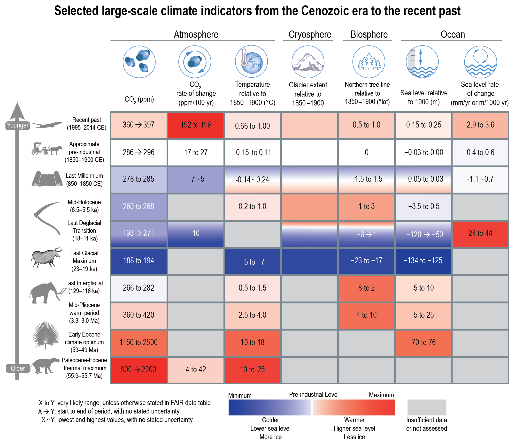 Figure 2.34 | Selected large-scale climate indicators during paleoclimate and recent reference periods of the Cenozoic Era. Values are based upon assessments carried out in this chapter, with confidence levels ranging fromlow tovery high. Refer to Cross-Chapter Box 2.1 for description of paleoclimate reference periods and Section 1.4.1 for recent reference periods. Values are reported as either the very likely range (x to y), or best estimates from beginning to end of the reference period with no stated uncertainty (x→y), or lowest and highest values with no stated uncertainty (x ~ y). Temperature is global mean surface temperature. Glacier extent is relative and colour scale is inverted so that more extensive glacier extent is intuitively blue.
 Cross-Chapter Box 2.4 | The Climate of the Pliocene (Around 3 Million Years Ago), When CO2Concentrations Were Last Similar to Those of the Present Day
Contributing Authors: Alan M. Haywood (United Kingdom), Darrell S. Kaufman (United States of America), Nicholas R. Golledge (New Zealand/United Kingdom), Dabang Jiang (China), Daniel J. Lunt (United Kingdom), Erin L. McClymont (United Kingdom), Ulrich Salzmann (United Kingdom/Germany, United Kingdom), Jessica Tierney (United States of America)
Throughout this Report, information about past climate states is presented in the context of specific climate variables, processes or regions. This Cross-Chapter Box focuses on a single paleoclimate reference period as an example of how proxy data, models and process understanding come together to form a more complete representation of a warm climate state that occurred during the relatively recent geologic past.
Introduction
The Pliocene Epoch is one of the best-documented examples of a warmer world during which the slow responding components of the climate system were approximately in balance with concentrations of atmospheric CO2, similar to present (e.g., Haywood et al., 2016). It provides a means to constrain Earth’s equilibrium climate sensitivity (Section 7.5.3) and to assess climate model simulations (Section 7.4.4.1.2). During the Pliocene, continental configurations were similar to present (Cross-Chapter Box 2.4 Figure 1a), and many plant and animal species living then also exist today. These similarities increase reliability of paleo-environmental reconstructions compared with those for older geological periods. Within the well-studied mid-Pliocene Warm Period (MPWP, also called the mid-Piacenzian Warm Period, 3.3–3.0 Ma), the interglacial period KM5c (3.212–3.187 Ma) has become a focus of research because its orbital configuration, and therefore insolation forcing, was similar to present (global mean insolation = –0.022 W m–2 relative to modern; Haywood et al., 2013), allowing for the climatic state associated with relatively high atmospheric CO2 to be assessed with fewer confounding variables.
Major global climate indicators
During the KM5c interglacial, atmospheric CO2 concentration was typically between 360 and 420 ppm (Section 2.2.3.1). New climate simulations of this interval from the Pliocene Model Intercomparison Project Phase 2 (PlioMIP2) show a multi-model mean global surface air temperature of 3.2 [2.1 to 4.8] °C warmer than control simulations (Cross-Chapter Box 2.4, Figure 1a; Haywood et al., 2020). This is consistent with proxy evidence for the broader MPWP, which indicates that global mean surface temperature was 2.5°C–4.0°C higher than 1850–1900 (Section 2.3.1.1.1). Global mean sea level was between 5 and 25 m higher than present (Section 2.3.3.3). Geological evidence (Section 2.3.2.4) and ice-sheet modelling (Section 9.6.2) indicate that both the Antarctic and Greenland Ice Sheets were substantially smaller than present (Cross-Chapter Box 2.4, Figure 1c). Attribution of sea level highstands to particular ice-sheet sources (Section 9.6.2) is challenging (DeConto and Pollard, 2016; Golledge, 2020), but improving (Berends et al., 2019; Grant et al., 2019).
Cross-Chapter Box 2.4
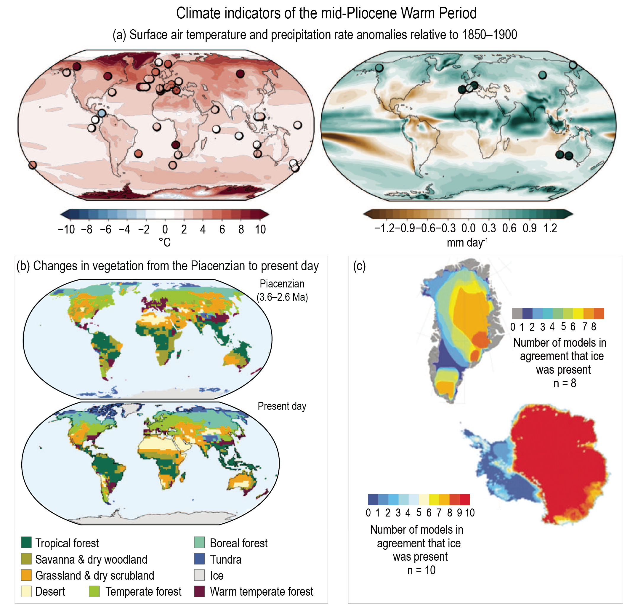
Cross-Chapter Box 2.4, Figure 1 | Climate indicators of the mid-Pliocene Warm Period (MPWP; 3.3–3.0 million years ago, Ma) from models and proxy data. (a) Simulated surface air temperature (left) and precipitation rate anomaly (right) anomaly (relative to 1850–1900) from the Pliocene Model Intercomparison Project Phase 2 multi-model mean, including CMIP6 (n = 4) and non-CMIP6 (n = 12) models. Symbols represent site-level proxy-based estimates of sea-surface temperature for KM5c (n = 32), and terrestrial temperature (n = 8) and precipitation rate for the MPWP (n = 8). (b) Distribution of terrestrial biomes was considerably different during the Piacenzian Stage (3.6–2.6 Ma) (upper) compared with present-day (lower). Biome distributions simulated with a model (BIOME4) in which Pliocene biome classifications are based on 208 locations, with model-predicted biomes filling spatial gaps, and the present day, with the model adjusted for CO2 concentration of 324 parts per million (ppm). (c) Ice-sheet extent predicted using modelled climate forcing and showing where multiple models consistently predict the former presence or absence of ice on Greenland (n = 8 total) and Antarctica (n = 10 total). Further details on data sources and processing are available in the chapter data table (Table 2.SM.1).
Northern high latitudes
The latitudinal temperature gradient during the MPWP was reduced relative to present-day and the consistency between proxy and modelled temperatures has improved since AR5 (Section 7.4.4.1.2). Northern high latitude (>60°N) SSTs were up to 7°C higher than 1850–1900 (Bachem et al., 2016; McClymont et al., 2020; Sánchez-Montes et al., 2020), and terrestrial biomes were displaced poleward (e.g., Dowsett et al., 2019) (Cross-Chapter Box 2.4, Figure 1b). Arctic tundra regions currently underlain by permafrost were warm enough to support boreal forests, which shifted northward by approximately 250 km in Siberia, and up to 2000 km in the Canadian Arctic Archipelago (Salzmann et al., 2013; Fletcher et al., 2017). The shift caused high-latitude surface albedo changes, which further amplified the Pliocene global warming (Zhang and Jiang, 2014). Vegetation changes in north-east Siberia indicate that MPWP summer temperatures were up to 6°C higher than present day (Brigham-Grette et al., 2013). Farther south, modern boreal forest regions in Russia and eastern North America were covered with temperate forests and grasslands, whereas highly diverse, warm-temperate forests with subtropical taxa were widespread in central and eastern Europe (Cross-Chapter Box 2.4, Figure 1). While seasonal sea ice was present in the North Atlantic and Arctic oceans, its winter extent was reduced relative to present (Knies et al., 2014; Clotten et al., 2018), and some models suggest that the Arctic was sea ice free during the summer (Howell et al., 2016; Feng et al., 2020).
Tropical Pacific
The average longitudinal temperature gradient in the tropical Pacific was weaker during the Pliocene than during 1850–1900 (Section 7.4.4.2.2). Changes in Pacific SSTs and SST gradients had far-reaching impacts on regional climates through atmospheric teleconnections, affecting rainfall patterns in western North America (Burls and Fedorov, 2017; Ibarra et al., 2018). The reduced zonal SST gradient has led to suggestions that the Pliocene Pacific experienced a ‘permanent El Niño’ state (Molnar and Cane, 2002; Fedorov, 2006). However, there is no direct geological evidence, nor support from climate models, that ENSO variability collapsed during the Pliocene. Although not located in the centre-of-action region for ENSO, Pliocene corals show temperature variability over 3–7 year timescales (Watanabe et al., 2011). In addition, a multi-model intercomparison indicates that ENSO existed, albeit with reduced variability (Brierley, 2015). Thus, there is high confidence that ENSO variability existed during the Pliocene.
Hydrological cycle
Vegetation reconstructions for the late Pliocene indicate regionally wetter conditions resulting in an expansion of tropical savannas and woodlands in Africa and Australia at the expense of deserts (Cross-Chapter Box 2.4, Figure 1b). PlioMIP2 climate models generally simulate higher rates of mean annual precipitation in the tropics and high latitudes, and a decrease in the subtropics, with a multi-model mean global increase of 0.19 [0.13–0.32] mm day–1 relative to control simulations (Cross-Chapter Box 2.4, Figure 1a; Haywood et al., 2020). Both simulations and limitedproxyevidence indicate stronger monsoons in northern Africa, Asia, and northern Australia relative to present, but trends are uncertain in other monsoon regions (X. Li et al., 2018; Yang et al., 2018; X. Huang et al., 2019a; R. Zhang et al., 2019). There is thus medium confidence that monsoon systems were stronger during the Pliocene. Simulations of MPWP climate show that global tropical cyclone intensity and duration increased during the MPWP (Yan et al., 2016); however, there is low confidence in this result because inter-model variability is high.
Summary
During the MPWP (3.3–3.0 Ma) the atmospheric CO2 concentration was similar to present, and the slow-response, large-scale indicators reflect a world that was warmer than present. With very high confidence, relative to present, global surface temperature, sea level, and precipitation rate were higher, NH latitudinal temperature gradient was lower, and major terrestrial biomes expanded poleward. With medium confidence from proxy-based evidence alone (Section 2.3.2), combined with numerical modelling, analysis of the sea-level budget, and process understanding (Section 9.6.2), there is high confidence that cryospheric indicators were diminished. There is medium confidence that the Pacific longitudinal temperature gradient was weaker and monsoon systems were stronger.
2.4 Changes in Modes of Variability
Modes of climate variability that are important for large-scale climate on interannual and longer timescales (Cross-Chapter Box 2.2) are assessed herein and defined and summarized in Annex IV. Though the modes of variability discussed here are assessed and classified on the basis of physical variables, it is important to recognize that the distribution and function of various components of the terrestrial and marine biospheres are modified in response to them.
2.4.1 Annular Modes
2.4.1.1 Northern Annular Mode (NAM)/North Atlantic Oscillation (NAO)
The AR5 reported that the shift towards a positive NAO, a mode of variability in the North Atlantic that is closely related to the hemispheric-scale NAM, from the 1950s to the 1990s was largely reversed by more recent changes (high confidence). Moreover, periods of persistent negative or positive NAO states observed during the latter part of the 20th century were not unusual, based on NAO reconstructions spanning the last half millennium (high confidence).
New multi-millennial-timescale NAO reconstructions are derived from marine and lake sediments, speleothems, tree rings and ice cores (Ortega et al., 2015; Faust et al., 2016; Sjolte et al., 2018). NAO variability over the past 8 kyr suggests the presence of a significant 1.5 kyr periodicity (Darby et al., 2012). Positive NAO conditions dominated during the MH, while the prevailing NAO sign during the early and late Holocene was negative according to most reconstructions (Olsen et al., 2012; Ait Brahim et al., 2019; Røthe et al., 2019; Hernández et al., 2020). For the CE, reconstructions developed since AR5 indicate no dominant NAO phase during 1000–1300 CE (Jones et al., 2014; Baker et al., 2015; Ortega et al., 2015; Lasher and Axford, 2019; Hernández et al., 2020), with either negative (Baker et al., 2015; Faust et al., 2016; Mellado-Cano et al., 2019) or a more variable phase of the NAO (Jones et al., 2014; Ortega et al., 2015; Sjolte et al., 2018; Cook et al., 2019) between 1400 and 1850 CE. Several instrument-based NAO reconstructions extending back to the 17th and 18th centuries highlight the presence of multi-decadal variations in the NAO phases (Cornes et al., 2013; Cropper et al., 2015), although these studies have limitations considering the seasonality of the centres of action and the locations of the stations used. Recent reconstructions of the large scale sea level pressure field yield more robust NAO analysis, showing a persistently negative NAO phase from the 1820s to the 1870s, with positive values dominating during the beginning of the 20th century followed by a declining trend over 1920–1970, with a recovery thereafter to a period of consistently high values between 1970 and the early 1990s (Delaygue et al., 2019; Mellado-Cano et al., 2019). Based on the evaluation of several NAO reconstructions for recent centuries, Hernández et al. (2020) highlighted that the strong positive NAO phases of the 1990s and early 21st century were not unusual.
The predominantly positive phase during the 1990s was followed by partial reversal and a tendency towards stronger variability in boreal winter NAM and NAO since the late 1990s (Pinto and Raible, 2012; Hanna et al., 2018). This is particularly evident in December NAO (Hanna et al., 2015) and NAM (Overland and Wang, 2015) indices, and is not unusual on multi-decadal time scales (Woollings et al., 2018a). Since the 1990s, a statistically significant summer NAO decline was reported, which is, to a lesser extent, also evident in the winter NAO, linked to an enhanced blocking activity over Greenland (Hanna et al., 2015, 2016; Wachowicz et al., 2021). However, this was moderated by persistent positive NAO values since 2015 (Annex IV.2.1). Based on observations and reanalysis datasets, multi-decadal variations were found for the NAM patterns: the Atlantic centre remained unchanged throughout 1920–2010, whereas the Pacific centre was stronger during 1920–1959 and 1986–2010 and weaker during 1960–1985 (Gong et al., 2018). Multidecadal changes were also observed in the position of the centres of action of the NAO (Moore et al., 2013; Zuo et al., 2016).
In summary, positive trends for the NAM/NAO winter indices were observed between the 1960s and the early 1990s, but these indices have become less positive or even negative thereafter (high confidence). The NAO variability in the instrumental record was very likely not unusual in the millennial and multi-centennial context.
2.4.1.2 Southern Annular Mode (SAM)
The AR5 concluded that it was likely that the SAM had become more positive since the 1950s and that this increase was unusual in the context of the prior 400 years (medium confidence). Both AR5 and SROCC reported statistically significant trends in the SAM during the instrumental period for the austral summer and autumn.
Several studies have attempted to reconstruct the evolution of the SAM during the Holocene using proxies of the position and strength of the SH zonal winds, although with no clear consensus regarding the timing and phase of the SAM (Hernández et al., 2020). The early Holocene was dominated by SAM positive phases (Moreno et al., 2018; Reynhout et al., 2019), consistent with increasing westerly wind strength (Lamy et al., 2010), with some reconstructions showing significant centennial and millennial variability but no consistent trend after 5 ka (Hernández et al., 2020). For the CE, enhanced westerly winds occurred over 0–1000 CE, as reflected in increased burning activity in Patagonia (Turney et al., 2016a) and tree ring records from southern New Zealand (Turney et al., 2016b) imply a predominantly positive SAM phase. Pollen records and lake sediments from Tasmania, southern mainland Australia, New Zealand and southern South America, inferred the period of 1000 to 1400 CE to be characterized by anomalously dry conditions south of 40°S, implying a positive SAM (Moreno et al., 2014; Fletcher et al., 2018; Evans et al., 2019; Matley et al., 2020). Nevertheless, proxy reconstructions of the SAM based on temperature-sensitive records from tree rings, ice cores, lake sediments and corals spanning the mid-to-polar latitudes show alternating positive and negative phases (Figure 2.35).
 Figure 2.35 | Southern Annular Mode (SAM) reconstruction over the last millennium. (a) SAM reconstructions as seven-year moving averages (thin lines) and 70-year LOESS filter (thick lines). (b) Observed SAM index during 1900–2019. Further details on data sources and processing are available in the chapter data table (Table 2.SM.1).
 Prolonged periods of negative SAM values were identified during the period 1400–1700 CE in several reconstructions (Figure 2.35, Villalba et al., 2012; Abram et al., 2014; Dätwyler et al., 2018), with a minimum identified during the 15th century (Hernández et al., 2020), although some disagreements exist between proxy records before 1800 CE (Hessl et al., 2017). Abram et al. (2014) concluded that the mean SAM index during recent decades is at its highest levels for at least the last 1 kyr. Similarly, the summer SAM reconstruction by Dätwyler et al. (2018) indicates a strengthening over the last 60 years that is outside the very likely range of the last millennium natural variability. The largest 30- and 50-year trends in the annual SAM index occurred at the end of the 20th century (after 1969 and 1950 respectively), indicating that the recent increase in the SAM is unprecedented in the context of at least the past three centuries (Yang and Xiao, 2018).
Before the mid-1950s, SAM indices derived from station-based datasets, and centennial reanalyses show pronounced interannual and decadal variability but no significant trends, with low correlation between SAM indices due to the diversity across different datasets and sensitivity to the definition used for the index calculation (Barrucand et al., 2018; Schneider and Fogt, 2018; J. Lee et al., 2019). Various SAM indices exhibit significant positive trends since the 1950s, particularly during austral summer and autumn (Barrucand et al., 2018; Schneider and Fogt, 2018; J. Lee et al., 2019), unprecedented for austral summer over the last 150 years (J.M. Jones et al., 2016; Fogt and Marshall, 2020). This indicates a strengthening of the surface westerly winds around Antarctica, related to both the position and intensity of the subpolar jet in the SH (Section 2.3.1.4.3; Ivy et al., 2017; IPCC, 2019). The SAM trends have slightly weakened after about 2000 (Fogt and Marshall, 2020).
In summary, historical station-based reconstructions of the SAM show that there has been a robust positive trend in the SAM index, particularly since 1950 and for the austral summer (high confidence). The recent positive trend in the SAM is likely unprecedented in at least the past millennium, although medium confidence arises due to the differences between proxy records before 1800 CE.
2.4.2 El Niño–Southern Oscillation (ENSO)
The AR5 reported with medium confidence that ENSO-like variability existed, at least sporadically, during the warm background state of the Pliocene. It was also found (high confidence) that ENSO has remained highly variable during the last 7 kyr with no discernible orbital modulation. The AR5 concluded that large variability on interannual to decadal timescales, and differences between datasets, precluded robust conclusions on any changes in ENSO during the instrumental period. The SROCC reported epochs of strong ENSO variability throughout the Holocene, with no indications of a systematic trend in ENSO amplitude, but with some indication that the ENSO amplitude over 1979–2009 was greater than at any point in the period from 1590–1880 CE. It was also reported that the frequency and intensity of El Niño events in the period from 1951–2000 was high relative to 1901–1950.
Manucharyan and Fedorov (2014) found that ENSO-like variability has been present, at least sporadically, during epochs of millions of years (including the MPWP; Cross-Chapter Box 2.4), with proxy records indicating that this was the case even when cross-Pacific SST gradients were much weaker than present. There is substantial disagreement between proxy records for ENSO activity during the early Holocene (Zhang et al., 2014; White et al., 2018), and for ENSO activity and mean state at the LGM (Leduc et al., 2009; Koutavas and Joanides, 2012; Sadekov et al., 2013; Ford et al., 2015, 2018; Zhu et al., 2017; Tierney et al., 2020). A number of studies (Cobb et al., 2013; H. McGregor et al., 2013; Carré et al., 2014; Emile-Geay et al., 2016; Thompson et al., 2017; Tian et al., 2017; White et al., 2018; Grothe et al., 2019) have found that ENSO was substantially weaker than at present at various times in the mid-Holocene within the period from 6 to 3 ka, with stronger decreases in variability revealed by remote proxies than by those close to the core region of ENSO activity. However, Karamperidou et al. (2015) find that weakening in ENSO-related variability in eastern Pacific proxies does not necessarily correspond to weakening in central Pacific proxies. Barrett et al. (2018) concluded that multi-proxy reconstructions are more efficient at identifying eastern Pacific than central Pacific events. This suggests that a weakening of proxy-based signals may indicate an along-equatorial shift in ENSO activity rather than a weakening of ENSO during some periods. Following the period of weak ENSO variability in the mid-Holocene, a number of studies find an increase in ENSO activity which, depending upon the study, commences between 4.4 and 3 ka (Koutavas and Joanides, 2012; Cobb et al., 2013; Zhang et al., 2014; S. Chen et al., 2016; Emile-Geay et al., 2016; Thompson et al., 2017; Du et al., 2021).
Numerous studies (J. Li et al., 2013; S. McGregor et al., 2013; Rustic et al., 2015; Hope et al., 2017; Y. Liu et al., 2017) find substantial variability in ENSO activity on multi-decadal to centennial timescales over the last 500 to 1 kyr (Figure 2.36). Different proxies show a wide spread in the specific timing and magnitude of events in the pre-instrumental period (e.g., Dätwyler et al., 2019). Most investigators find that ENSO activity in recent decades was higher than the most recent centuries prior to the instrumental period. Grothe et al. (2019) also found that ENSO variance of the last 50 years was 25% higher than the average of the last millennium, and was substantially higher than the average of the mid- to late-Holocene. S. McGregor et al., (2010, 2013) looked for common variance changes in pre-existing ENSO proxies, finding stronger ENSO variance for the 30-year period 1979–2009 compared to any 30-year period within the timespan 1590–1880 CE. This finding also holds when adding more recently developed ENSO proxies (Figure 2.36). Koutavas and Joanides (2012), Ledru et al. (2013) and Thompson et al. (2017) identify various periods within the range 1000 BCE to 1300 CE when ENSO activity was greater than in the following centuries, and more closely comparable to the mid-20th century onwards behaviour.
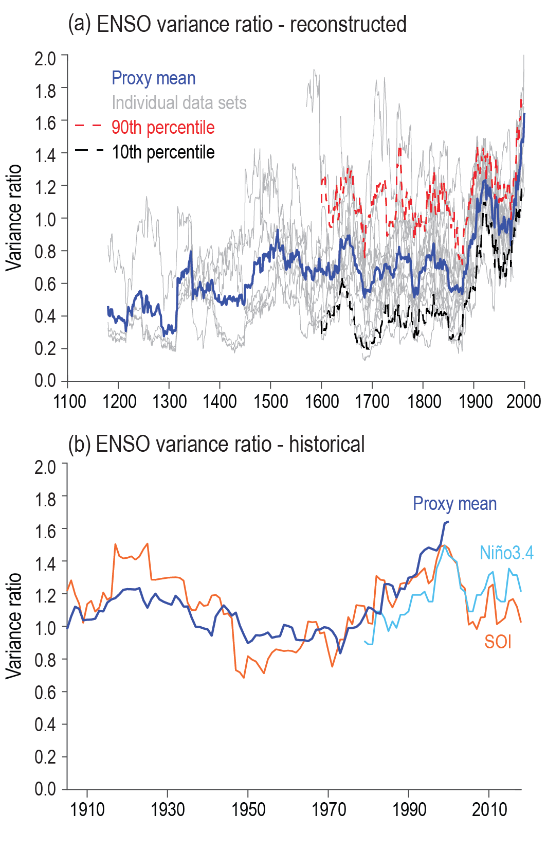 Figure 2.36 | Reconstructed and historical variance ratio of El Niño–Southern Oscillation (ENSO). (a) 30-year running variance of the reconstructed annual mean Niño 3.4 or related indicators from various published reconstructions. (b) Variance of June–November Southern Oscillation Index (SOI) and April–March mean Niño 3.4 (1981–2010 base period) along with the mean reconstruction from (a). Further details on data sources and processing are available in the chapter data table (Table 2.SM.1).
 Since AR5, updates to datasets used widely in prior ENSO assessments resulted in substantial and important revisions to observed tropical Pacific SST data (Section 2.3.1.1). In particular, ERSSTv4, and then ERSSTv5, addressed known SST biases in ERSSTv3 in the equatorial Pacific which affected the derived mean state and amplitude of indices based on that dataset (Huang et al., 2015). During the instrumental period, there is no robust indication of any significant century-scale trend in the east-west SST gradient across the equatorial Pacific Ocean, with periods when gradients have been stronger and weaker than the long-term average on decadal timescales, associated with a predominance of La Niña or El Niño events respectively. The frequency of El Niño and La Niña events is also subject to considerable decadal variability (e.g., Hu et al., 2013) but with no indication of a long-term signal in the frequency of events. The ENSO amplitude since 1950 has increased relative to the 1910–1950 period, as confirmed by independent proxy records (e.g., Gergis and Fowler, 2009), the Southern Oscillation Index (SOI) (Braganza et al., 2009) and SSTs (e.g., Ohba, 2013; Yu and Kim, 2013), although there is a spread between different proxy and instrumental sources as to the magnitude of that increase (Figure 2.36). The El Niño events of 1982–1983, 1997–1998 and 2015–2016 had the strongest anomalies in the Niño 3.4 SST index since 1950. Their predominance was less evident from indices based on de-trended data such as the Oceanic Niño Index (ONI) (which still ranked them as the three strongest events since 1950, but only by a small margin), and in the SOI. B. Huang et al. (2019a) also note that analyses based upon buoy and Argo data, which are only available since the 1990s, are more capable of resolving strong events than analyses which do not include such data.
Prior to the 1950s, SST observations in the tropical Pacific were much sparser and hence uncertainties in Niño indices are much larger (B. Huang et al., 2020). SOI data and some newer SST-based studies show high ENSO amplitude, comparable to the post-1950 period, in the period from the mid-late 19th century to about 1910, but proxy indicators generally indicate that the late 19th and early 20th century were less active than the late 20th century (Figure 2.36). Yu and Kim’s (2013) implementation of the ONI found a number of events with the ONI above 1.5°C between 1888 and 1905, then no such events until 1972, whilst the SOI indicates comparable or stronger events to the three strongest post-1950 events in 1896 and 1905. Giese and Ray (2011) also found a number of such events between 1890 and 1920 in the SODA ocean reanalysis, corroborated further by B. Huang et al. (2020) and Vaccaro et al. (2021), who found that the strength of the 1877–1878 event was comparable with that of the 1982–1983, 1997–1998 and 2015–2016 events. There have also been a number of strong La Niña events (e.g., 1973–1974, 1975–1976 and 2010–2011), with few clear analogues in the 1920–1970 period; the proxy-based analysis of McGregor et al. (2010) indicates that the mid-1970s La Niña period was also extreme in a multi-centennial context. There is no indication that the frequency of high-amplitude events since the 1970s reflects a long-term trend which can be separated from multi-decadal variability, given apparent presence of several high-amplitude events in the late 19th and early 20th centuries, and the relatively large uncertainty in pre-1950 SST data in the tropical Pacific region.
There is a distinction (Annex IV.2.3.1) between El Niño events centred in the eastern Pacific (‘Eastern Pacific’ (EP) or ‘classical’ events) and those centred in the Central Pacific (‘Central Pacific’ (CP) or ‘Modoki’ events), which have different typical teleconnections (e.g., Ashok et al., 2007; Ratnam et al., 2014; Capotondi et al., 2015; Timmermann et al., 2018). A number of studies, using a range of indicators, have found an increase in recent decades of the fraction of CP El Niño events, particularly after 2000 (Yu and Kim, 2013; Lübbecke and McPhaden, 2014; Pascolini-Campbell et al., 2015; Jiang and Zhu, 2018). Johnson (2013) found that the frequency of CP El Niño events had increased (although not significantly) over the 1950–2011 period, being accompanied by a significant increase in the frequency of La Niña events with a warm (as opposed to cool) western Pacific warm pool. A coral-based reconstruction starting in 1600 CE (Freund et al., 2019) found that the ratio of CP to EP events in the last 30 years was substantially higher than at any other time over the last 400 years. Variations in the proportion of CP and EP events have also been found in earlier periods, with Carré et al. (2014) finding a period of high CP activity around 7 ka.
There is no robust indicationof any changes in ENSO teleconnections over multi-centennial timescales (Hernández et al., 2020) despite multi-decadal variability. Shi and Wang (2018) found that teleconnections with the broader Asian summer monsoon, including the Indian and the East Asian monsoon, were generally stable since the 17th century during the developing phase of the monsoon, and showed substantial decadal variability, but no clear trend, during the decaying phase. They also found that the weakening of teleconnections between the Indian summer monsoon and ENSO in recent decades had numerous precedents over the last few centuries. Räsänen et al. (2016) also found substantial decadal variability, but little trend, in the strength of the relationship between ENSO and monsoon precipitation in South East Asia between 1650 and 2000. Dätwyler et al. (2019) identified a number of multi-decadal periods with apparently changed teleconnections at times over the last 400 years.
In the instrumental period, teleconnections associated with ENSO are well known to vary on decadal to multi-decadal timescales (e.g., He et al., 2013; Lee and Ha, 2015; Ashcroft et al., 2016; Jin et al., 2016; Wang et al., 2019). Yun and Timmermann (2018) found that decadal variations in teleconnections between ENSO and the Indian monsoon did not extend beyond what would be expected from a stochastic process. Many observed decadal changes in teleconnections in the instrumental period are consistent with a shift to more central Pacific El Niño events (Evtushevsky et al., 2018; Yeh et al., 2018; Yu and Sun, 2018; Zhao and Wang, 2019). Effects of the PDV (Kwon et al., 2013; S. Wang et al., 2014; Dong et al., 2018) and the AMV (Kayano et al., 2019) can also modulate ENSO teleconnections, and affect the frequency of CP versus EP events (Ashok et al., 2007). Chiodi and Harrison (2015) found that teleconnections over the most recent decades are broadly consistent with those over the last 100 years. Variability in teleconnections can also occur on timescales longer than characteristic PDV timescales (e.g., Gallant et al., 2013).
In summary, there is medium confidence that both ENSO amplitude and the frequency of high-magnitude events since 1950 are higher than over the period from 1850 and possibly as far back as 1400, but low confidence that they are outside the range of variability over periods prior to 1400, or higher than the average of the Holocene as a whole. Overall, there is no indication of a recent sustained shift in ENSO or associated features such as the Walker Circulation, or in teleconnections associated with these, being beyond the range of variability on decadal to millennial timescales. A high proportion of El Niño events in the last 20–30 years have been based in the central, rather than eastern Pacific, but there is low confidence that this represents a long-term change.
2.4.3 Indian Ocean Basin and Dipole Modes
The AR5 did not provide an assessment of the Indian Ocean Dipole (IOD) records based on paleo reconstructions. For the instrumental era, AR5 reported that there were no trends in the IOD behaviour. However, the strength of the Indian Ocean Basin-wide (IOB) mode, quantified by the basin-scale averaged SST index, increased in all assessed periods except 1979–2012, but the AR5 neither quantified trends nor provided a confidence statement.
For the LGM, enhanced equatorial Indian Ocean productivity in marine sediment records was associated with strengthened westerly jets, in line with a shallower central-western Indian Ocean thermocline and stronger negative IOD events (Punyu et al., 2014). The LGM Indian Ocean basin was substantially modified by the exposure of the tropical shelves (DiNezio et al., 2018) and this has been associated with an Indian Ocean ‘El Niño‘ (Thirumalai et al., 2019). Wurtzel et al. (2018) contend that during the LDT, including the Younger Dryas event, Indian Ocean precipitation did not mirror the zonal asymmetry observed in Indian Ocean SSTs in the Holocene based upon a speleothem record from Sumatra, but instead reflected shifts in moisture transport pathways and sources. Using Seychelles corals, representing the western pole of the IOD, spanning from the MH to present, Zinke et al. (2014) identified changes in seasonality, with the lowest seasonal SST range in the MH and then again around 2 ka, while the largest seasonal range occurred around 4.6 ka and then again during the near-present (1990–2003). Reconstructions from fossil corals for the eastern Indian Ocean point to stronger negative IOD SST anomalies due to the enhanced upwelling and cooling driven by a stronger monsoon with enhanced anomalous easterly winds in the eastern Indian Ocean during the MH (Abram et al., 2020b). Niedermeyer et al. (2014) from the analysis of stable isotopes in terrestrial plant waxes, suggest that the period 6.5 ka to 4.5 ka was characterized by an anomalously positive IOD mean state. During various parts of the Holocene, periods of a mean positive IOD-like state were associated with increased IOD variability, including events that exceed the magnitude of the strongest events during the instrumental period (Abram et al., 2020a).
From the coralδ18O record from the Seychelles over 1854–1994, Du et al. (2014) showed a 3–7 year dominant period associated with the IOB in response to ENSO forcing. They identified multi-decadal variability in the IOB, with more active IOB phases during 1870–1890, 1930–1955, and 1975–1992, while decadal variability in the IOB dominated during 1940–1975 (Du et al., 2014). Evidence for changes in IOB characteristics during earlier periods (e.g., MH, LGM) is limited.
The role of decadal to multi-decadal variability has recently emerged as an important aspect of the IOD with many indications of the effects of Pacific Ocean processes on IOD variability through atmospheric and oceanic mechanisms (Dong et al., 2016; Krishnamurthy and Krishnamurthy, 2016; Zhou et al., 2017; Jin et al., 2018). Positive events in the 1960s and 1990s were linked to a relatively shallow eastern Indian Ocean thermocline, and a primarily negative IOD state in the 1970s and 1980s was related to a deeper thermocline (Ummenhofer et al., 2016). Positive IOD events may have increased in frequency during the second half of the 20th century (Abram et al., 2020a, b). Earlier observations of apparent changes in the frequency and/or magnitude of the IOD events are considered unreliable, particularly prior to the 1960s (Hernández et al., 2020). Although the seasonal evolution and the type of ENSO (Section 2.4.2) may influence the character of the IOD (Guo et al., 2015; Zhang et al., 2015; Fan et al., 2016), the occurrence of some IOD events may be independent of ENSO (Sun et al., 2015).
To summarize, there is low confidence in any multi-decadal IOD variability trend in the instrumental period due to data uncertainties especially before the 1960s. In addition to data uncertainties, understanding of the IOB variability during the instrumental period is also limited by large-scale warming of the Indian Ocean. Neither the IOD nor the IOB have exhibited behaviour outside the range implied by proxy records (low confidence).
2.4.4 Atlantic Meridional (AMM) and Zonal Modes (AZM)
The AR5 reported no changes in the Atlantic Meridional Mode (AMM) during the 20th century or shorter periods thereof. For the Atlantic Zonal Mode (AZM), also referred as the Atlantic Niño, the AR5 reported increases during the 1950–2012 period but neither assessed trends nor provided a confidence statement. The AR5 did not assess paleo evidence for the AZM and AMM.
Paleo-reconstructions of these two modes remain rather limited. Nonetheless, the interhemispheric cross-equatorial SST gradients linked to changes in ITCZ locations characteristic of the AMM has been found during the LGM, Heinrich Stadial 1, and the MH, with the largest shift occurring during HS1 (McGee et al., 2014). Similarly, the dipole-like SST pattern in the South Atlantic subtropics, which is related to the AZM (Venegas et al., 1996; Morioka et al., 2011; Nnamchi et al., 2016, 2017; Lübbecke et al., 2018; Rouault et al., 2018; Foltz et al., 2019), has been reconstructed using SST proxies from marine sediment cores during the past 12 kyr (Wainer et al., 2014). The reconstructed index captures two significant cold events that occurred during the 12.9–11.6 ka and 8.6–8.0 ka periods in the South Atlantic (Wainer et al., 2014).
During the observational period the AZM and AMM (Figure 2.37) are related to the AMV largely controlling the interhemispheric gradient of the SST at decadal to multi-decadal timescales (Tokinaga and Xie, 2011; Polo et al., 2013; Svendsen et al., 2014a; Li et al., 2015; Lübbecke et al., 2018). The AZM interannual variability is enhanced (Lübbecke et al., 2018; Foltz et al., 2019), and is more strongly related to ENSO, during the negative phase of the AMV (Martín-Rey et al., 2014, 2018; Polo et al., 2015; Nnamchi et al., 2020). The AZM displayed a persistent weakened variability over the 1960–2009 period associated with declined cold tongue upwelling (Tokinaga and Xie, 2011), which became pronounced since 2000 (Prigent et al., 2020a, b). Despite these multi-decadal fluctuations, there is limited evidence for any sustained change in the AMM (Chang et al., 2011; Martín-Rey et al., 2018) and AZM (Martín-Rey et al., 2018; Nnamchi et al., 2020) during the instrumental period. The AZM and AMM interact on interannual timescales (Servain et al., 1999; Foltz and McPhaden, 2010; Pottapinjara et al., 2019) leading in 2009 to extremes of both modes in which the negative phase of the AMM (Foltz et al., 2012; Burmeister et al., 2016) preceded an equatorial cold tongue cold event that was unprecedented in the prior 30 years (Foltz and McPhaden, 2010; Burmeister et al., 2016).
In summary, confidence is low in any sustained changes to the AZM and AMM variability in instrumental observations. There is very low confidence in changes of the paleo AZM and AMM due to extremely limited availability of paleo reconstructions.
2.4.5 Pacific Decadal Variability (PDV)
Pacific Decadal Variability (PDV) refers to the ocean-atmosphere climate variability over the Pacific Ocean at decadal-to-interdecadal time scales and is usually described by the Pacific Decadal Oscillation (PDO) or the Inter-decadal Pacific Oscillation (IPO) indices. The AR5 and SROCC reported a large shift of the PDO in the late 1970s, with a predominantly positive phase until the end of the 1990s, being mainly negative afterwards. There was no significant change assessed in the PDO during the instrumental period as a whole, and no confidence level was assigned. Changes in the pre-instrumental era PDO were not assessed in AR5.
The existence of the PDV in the centuries prior to the instrumental period is evidenced by a variety of proxy records based on tree rings (Biondi et al., 2001; D’Arrigo and Ummenhofer, 2015), corals (Felis et al., 2010; Deng et al., 2013; Linsley et al., 2015) and sediments (Lapointe et al., 2017; O’Mara et al., 2019). There is little coherence between the various paleo-proxy indices prior to the instrumental record, and neither these nor the instrumental records provide indications of a clearly defined spectral peak (Chen and Wallace, 2015; M. Newman et al., 2016; Henley, 2017; L. Zhang et al., 2018; Buckley et al., 2019). For instance, spectral analysis from millennia length PDV reconstructions shows spectral peaks at multi-decadal, centennial and bi-centennial time scales (Beaufort and Grelaud, 2017), while only multi-decadal oscillations can be detected in the shorter (less than 400 years into the past) paleoclimate reconstructions. A variety of proxies suggest a shift in the PDV from the early-mid Holocene, which was characterized by a persistently negative phase of the PDO (i.e., weak Aleutian Low), to the late Holocene, and more variable and more positive PDO (i.e., strong Aleutian Low) conditions. This shift at around 4.5 ka is also evident in the PDO periodicities, changing from bidecadal and pentadecadal variability in the early Holocene to only pentadecadal periodicities in the late Holocene (Hernández et al., 2020). Several proxy records indicate that the strengthening in the Aleutian Low inferred since the late 17th century is unprecedented over the last millennium (Z. Liu et al., 2017; Osterberg et al., 2017; Winski et al., 2017), in line with an increase in PDV low-frequency variability (Williams et al., 2017; Hernández et al., 2020).
The PDO and IPO indices are significantly correlated during the instrumental period, showing regime shifts in the 1920s, 1940s, 1970s and around 1999. Positive PDV phases were observed from the 1920s to the mid-1940s and from the late 1970s to the late 1990s, while negative phases occurred from mid-1940s until the late 1970s, and since 1999 (Figure 2.38; Han et al., 2014; Chen and Wallace, 2015; M. Newman et al., 2016). The associated spatial patterns are quite similar, but the PDO pattern exhibits stronger SST anomalies in the extra-tropical North Pacific than the IPO (Chen and Wallace, 2015). The strength and structure of the SST patterns also differ among the periods (M. Newman et al., 2016).
 Figure 2.38 | Indices of multi-decadal climate variability from 1854–2019 based upon several sea surface temperature data products. Shown are the indices of the AMV and PDV based on area averages for the regions indicated in Annex IV. Further details on data sources and processing are available in the chapter data table (Table 2.SM.1).
 Instrumental observations are sparse prior to 1950, and thus the fidelity of any PDV index derived for the second part of the 19th century and early decades of the 20th century is relatively low (Figure 2.38; Deng et al., 2013; Wen et al., 2014). This results inlow agreement in the classification of the PDO/IPO phase among several indices, even during recent years with the availability of high-quality data. Nevertheless, the teleconnection patterns are robust regardless of the index used to characterize the PDO (McAfee, 2017). Analysis of time series of PDO and IPO highlights the (multi-) decadal nature of this mode of variability with no significant trends, but highlights a recent switch from a positive to a negative phase since 1999/2000 across all indicators (England et al., 2014; Henley, 2017).
In summary, the PDV in the instrumental record is dominated by (multi-)decadal-scale shifts between positive and negative phases over the last 150 years with no overall trend (high confidence). There is low confidence in paleo-PDV reconstructions due to discrepancies among the various available time series in terms of phasing and timing. However, there is high confidence in the occurrence of a shift from predominantly negative to positive PDO conditions from the middle to the late Holocene.
2.4.6 Atlantic Multi-decadal Variability
The AR5 reported no robust changes in Atlantic Multi-decadal Variability (AMV) reconstructions based on paleo records due to low consistency between different AMV reconstructions prior to 1900. AR5 concluded that there have been no significant trends in the AMV index during the instrumental period and there was difficulty in interpreting the AMV signal because of the long-term underlying SST warming trend.
The AR5 conclusions about large uncertainties in AMV paleo reconstructions (Hernández et al., 2020) have been reinforced by recent studies of tree rings (J. Wang et al., 2017b), Greenland ice (Chylek et al., 2012), and corals (Kilbourne et al., 2014; Svendsen et al., 2014b; J. Wang et al., 2017b). The AMV exhibited a generally positive state over the first millennium of the CE (Mann et al., 2009; Singh et al., 2018). Paleo reconstructions over the last millennium consistently show a negative AMV phase during 1400–1850 CE and a positive phase during 900–1200 CE (Mann et al., 2009; J. Wang et al., 2017b; Singh et al., 2018), consistent with warmer surface temperatures from tropical Atlantic records (Kilbourne et al., 2014).
Instrumental observations show that AMV is characterized by basin-wide warm and cool periods with an average variation in SST of about 0.4°C, but with larger variations in the North Atlantic subpolar gyre. Despite small differences in indices used to define the AMV (Annex IV), they all show warm periods occurring approximately between 1880–1900, 1940–1960, and from the mid-1990s to present, with cool periods in between (Figure 2.38) but no overall sustained change during the instrumental period (Booth et al., 2012; Gulev et al., 2013; Bellomo et al., 2018).
The oceanic changes are seen in salinity and temperature variations over the upper 3000 m of the North Atlantic (Polyakov et al., 2005; Keenlyside et al., 2015), and in sea level variations in the western North Atlantic along the Gulf Stream passage (McCarthy et al., 2015). The pattern and strength of the AMV differs among the periods (e.g., Svendsen et al., 2014b; Reynolds et al., 2018) and there are indications that there may have been a shift since 2005 toward a negative phase of the AMV (Robson et al., 2016).
In summary, no sustained change in AMV indices has been observed over the instrumental period (high confidence). However, instrumental records may not be long enough to distinguish any oscillatory behaviour from trends in the AMV. There is low confidence in the paleo AMV reconstructions due to a paucity of high-resolution records.
2.5 Final Remarks
The assessment in this chapter is based upon an ever-expanding volume of available proxy and observational records and a growing body of literature. Since AR5, improvements have been made in all aspects of data collection, data curation, data provision and data analysis permitting improved scientific insights. The chapter has also benefitted from the availability of new products from a range of emerging, mainly space-based, observing capabilities and new generations of reanalysis products. However, a number of key challenges still remain which, if addressed, would serve to strengthen future reports.
- Development of new techniques and exploitation of existing and new proxy sources may help address challenges around the low temporal resolution of most paleoclimate proxy records, particularly prior to the Common Era, and ambiguities around converting paleoclimate proxy data into estimates of climate-relevant variables. Conversions rely upon important proxy-specific assumptions and biases can be large due to limited accounting of seasonality, non-climatic effects, or the influence of multiple climate variables. These challenges currently limit the ability to ascertain the historical unusualness of recent directly observed climate changes for many indicators. {2.2, 2.3}
- Improved sharing of historical instrumental and proxy records (including metadata) along with significant efforts at data rescue of presently undigitized records would serve to significantly strengthen many aspects of the present assessment. Longer observational time series help to better understand variability, and any underlying periodicity in climate indicators and climate forcers, especially for components of the climate system where the dominant response is on multi-decadal and longer time scales. Targeted rescue of early marine data records, especially from waters of the tropical oceans and the Southern Ocean, could help constrain modes of variability and important teleconnection changes in, for example, the hydrological cycle and patterns of global temperature change. {2.2, 2.3, 2.4}
- Contemporary observing systems have limitations in parts of the Earth system with limited accessibility or coverage, for example coastal and shallow ocean, polar regions, marine biosphere, and the deep sea, leading to seasonal-dependency and regional variability in data coverage and uncertainty which serve to limit confidence in the present assessment of changes. {2.3}
- Contradictory lines of evidence exist between observations and models on the relationship between the rates of warming in GMST and GSAT, compounded by limitations in theoretical understanding. Improvements in air temperature datasets over the ocean and an improved understanding of the representation of the lowermost atmosphere over the ocean in models would reduce uncertainty in assessed changes in GSAT. {Cross-Chapter Box 2.3}
Acknowledgements
The authors of Chapter 2 would like to extend their gratitude to Sara Veasey, Deborah Riddle, Deborah Misch (all NOAA NCEI, USA) and Robert Fawcett (BoM, Australia) for providing substantial support in the production and finalization of all figures. We wish to acknowledge Raphael Neukom (University of Bern, Switzerland) and Michael Bosilovich (NASA/GFSC, USA) for their assistance in the provision of data.
Frequently Asked Questions
FAQ 2.1 | The Earth’s Temperature Has Varied Before. How Is the Current Warming Any Different?
Earth’s climate has always changed naturally, but both the global extent and rate of recent warming are unusual. The recent warming has reversed a slow, long-term cooling trend, and research indicates that global surface temperature is higher now than it has been for millennia.
While climate can be characterized by many variables, temperature is a key indicator of the overall climate state, and global surface temperature is fundamental to characterizing and understanding global climate change, including Earth’s energy budget. A rich variety of geological evidence shows that temperature has changed throughout Earth’s history. A variety of natural archives from around the planet, such as ocean and lake sediments, glacier ice and tree rings, shows that there were times in the past when the planet was cooler, and times when it was warmer. While our confidence in quantifying large-scale temperature changes generally decreases the farther back in time we look, scientists can still identify at least four major differences between the recent warming and those of the past.
It’s warming almost everywhere. During decades and centuries of the past 2000 years, some regions warmed more than the global average while, at the same time, other regions cooled. For example, between the 10th and 13th centuries, the North Atlantic region warmed more than many other regions. In contrast, the pattern of recent surface warming is globally more uniform than for other decadal to centennial climate fluctuations over at least the past two millennia.
It’s warming rapidly. Over the past 2 million years, Earth’s climate has fluctuated between relatively warm interglacial periods and cooler glacial periods, when ice sheets grew over vast areas of the northern continents. Intervals of rapid warming coincided with the collapse of major ice sheets, heralding interglacial periods such as the present Holocene Epoch, which began about 12,000 years ago. During the shift from the last glacial period to the current interglacial, the total temperature increase was about 5°C. That change took about 5000 years, with a maximum warming rate of about 1.5°C per thousand years, although the transition was not smooth. In contrast, Earth’s surface has warmed approximately 1.1°C since 1850–1900. However, even the best reconstruction of global surface temperature during the last deglacial period is too coarsely resolved for direct comparison with a period as short as the past 150 years. But for the past 2000 years, we have higher-resolution records that show that the rate of global warming during the last 50 years has exceeded the rate of any other 50-year period.
Recent warming reversed a long-term global cooling trend. Following the last major glacial period, global surface temperature peaked by around 6500 years ago, then slowly cooled. The long-term cooling trend was punctuated by warmer decades and centuries. These fluctuations were minor compared with the persistent and prominent warming that began in the mid-19th century when the millennial-scale cooling trend was reversed.
It’s been a long time since it’s been this warm. Averaged over the globe, surface temperatures of the past decade were probably warmer than when the long cooling trend began around 6500 years ago. If so, we need to look back to at least the previous interglacial period, around 125,000 years ago, to find evidence for multi-centennial global surface temperatures that were warmer than now.
Previous temperature fluctuations were caused by large-scale natural processes, while the current warming is largely due to human causes (see, for example, FAQ 1.3, FAQ 3.1). But understanding how and why temperatures have changed in the past is critical for understanding the current warming and how human and natural influences will interact to determine what happens in the future. Studying past climate changes also makes it clear that, unlike previous climate changes, the effects of recent warming are occurring on top of stresses that make humans and nature vulnerable to changes in ways that they have never before experienced (for example, see FAQ 11.2, FAQ12.3).
FAQ 2.1, Figure 1 | Evidence for the unusualness of recent warming.
FAQ 2.2 | What Is the Evidence for Climate Change?
The evidence for climate change rests on more than just increasing surface temperatures. A broad range of indicators collectively leads to the inescapable conclusion that we are witnessing rapid changes to many aspects of our global climate. We are seeing changes in the atmosphere, ocean, cryosphere, and biosphere. Our scientific understanding depicts a coherent picture of a warming world.
We have long observed our changing climate. From the earliest scientists taking meteorological observations in the 16th and 17th centuries to the present, we have seen a revolution in our ability to observe and diagnose our changing climate. Today we can observe diverse aspects of our climate system from space, from aircraft and weather balloons, using a range of ground-based observing technologies, and using instruments that can measure to great depths in the ocean.
Observed changes in key indicators point to warming over land areas. Global surface temperature over land has increased since the late 19th century, and changes are apparent in a variety of societally relevant temperature extremes. Since the mid-1950s the troposphere (i.e., the lowest few km of the atmosphere) has warmed, and precipitation over land has increased. Near-surface specific humidity (i.e., water vapour) over land has increased since at least the 1970s. Aspects of atmospheric circulation have also evolved since the mid-20th century, including a poleward shift of mid-latitude storm tracks.
Changes in the global ocean point to warming as well. Global average sea surface temperature has increased since the late 19th century. The heat content of the global ocean has increased since the 19th century, with more than 90% of the excess energy accumulated in the climate system being stored in the ocean. This ocean warming has caused ocean waters to expand, which has contributed to the increase in global sea level in the past century. The relative acidity of the ocean has also increased since the early 20th century, caused by the uptake of carbon dioxide from the atmosphere, and oxygen loss is evident in the upper ocean since the 1970s.
Significant changes are also evident over the cryosphere – the portion of the Earth where water is seasonally or continuously frozen as snow or ice. There have been decreases in Arctic sea ice area and thickness and changes in Antarctic sea ice extent since the mid-1970s. Spring snow cover in the Northern Hemisphere has decreased since the late-1970s, along with an observed warming and thawing of permafrost (perennially frozen ground). The Greenland and Antarctic ice sheets are shrinking, as are the vast majority of glaciers worldwide, contributing strongly to the observed sea level rise.
Many aspects of the biosphere are also changing. Over the last century, long-term ecological surveys show that many land species have generally moved poleward and to higher elevations. There have been increases in green leaf area and/or mass (i.e., global greenness) since the early 1980s, and the length of the growing season has increased over much of the extratropical Northern Hemisphere since at least the mid-20th century. There is also strong evidence that various phenological metrics (such as the timing of fish migrations) for many marine species have changed in the last half century.
Change is apparent across many components of the climate system. It has been observed using a very broad range of techniques and analysed independently by numerous groups around the world. The changes are consistent in pointing to a climate system that has undergone rapid warming since the industrial revolution.
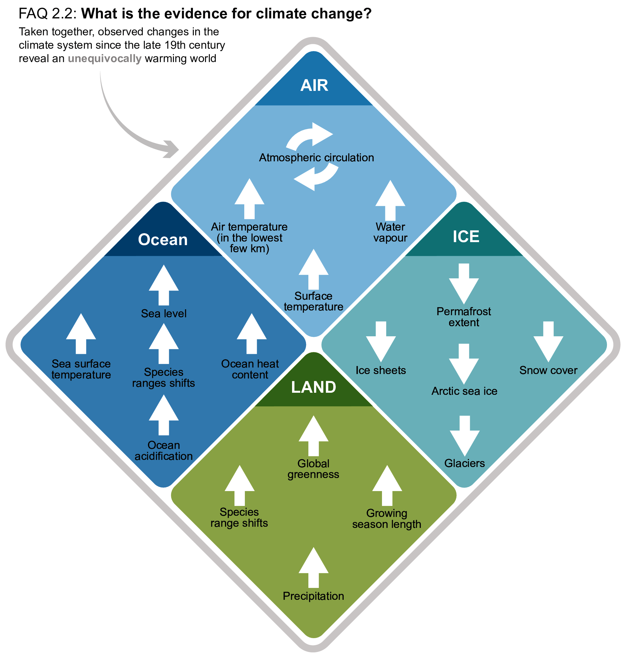
FAQ 2.2, Figure 1 | Synthesis of significant changes observed in the climate system over the past several decades. Upwards, downwards and circling arrows indicate increases, decreases and changes, respectively. Independent analyses of many components of the climate system that would be expected to change in a warming world exhibit trends consistent with warming. Note that this list is not comprehensive.
References
Ablain, M. et al., 2019: Uncertainty in satellite estimates of global mean sea-level changes, trend and acceleration. Earth System Science Data, 11(3), 1189–1202, doi: 10.5194/essd-11-1189-2019.
Abram, N.J. et al., 2010: Ice core evidence for a 20th century decline of sea ice in the Bellingshausen Sea, Antarctica. Journal of Geophysical Research: Atmospheres, 115, D23101, doi: 10.1029/2010jd014644.
Abram, N.J. et al., 2014: Evolution of the Southern Annular Mode during the past millennium. Nature Climate Change, 4(7), 564–569, doi: 10.1038/nclimate2235.
Abram, N.J. et al., 2020a: Palaeoclimate perspectives on the Indian Ocean Dipole (2020b). Quaternary Science Reviews, 237, 106302, doi: 10.1016/j.quascirev.2020.106302.
Abram, N.J. et al., 2020b: Coupling of Indo-Pacific climate variability over the last millennium (2020a). Nature, 579(7799), 385–392, doi: 10.1038/s41586-020-2084-4.
Ackley, S., P. Wadhams, J.C. Comiso, and A.P. Worby, 2003: Decadal decrease of Antarctic sea ice extent inferred from whaling records revisited on the basis of historical and modern sea ice records. Polar Research, 22, 19–25, doi: 10.1111/j.1751-8369.2003.tb00091.x.
Adler, R.F., G. Gu, M. Sapiano, J.J. Wang, and G.J. Huffman, 2017: Global Precipitation: Means, Variations and Trends During the Satellite Era (1979–2014). Surveys in Geophysics, 38(4), 679–699, doi: 10.1007/s10712-017-9416-4.
Adler, R.F. et al., 2018: The Global Precipitation Climatology Project (GPCP) monthly analysis (New Version 2.3) and a review of 2017 global precipitation. Atmosphere, 9(4), 138, doi: 10.3390/atmos9040138.
Ahn, J. and E.J. Brook, 2014: Siple Dome ice reveals two modes of millennial CO2 change during the last ice age. Nature Communications, 5(1), 3723, doi: 10.1038/ncomms4723.
Ahn, J., E.J. Brook, A. Schmittner, and K. Kreutz, 2012: Abrupt change in atmospheric CO2 during the last ice age. Geophysical Research Letters, 39, L18711, doi: 10.1029/2012gl053018.
Aiken, J. et al., 2017: A synthesis of the environmental response of the North and South Atlantic Sub-Tropical Gyres during two decades of AMT. Progress in Oceanography, 158, 236–254, doi: 10.1016/j.pocean.2016.08.004.
Ait Brahim, Y. et al., 2019: North Atlantic Ice-Rafting, Ocean and Atmospheric Circulation During the Holocene: Insights From Western Mediterranean Speleothems. Geophysical Research Letters, 46(13), 7614–7623, doi: 10.1029/2019gl082405.
Albani, S. et al., 2015: Twelve thousand years of dust: the Holocene global dust cycle constrained by natural archives. Climate of the Past, 11(6), 869–903, doi: 10.5194/cp-11-869-2015.
Albani, S. et al., 2016: Paleodust variability since the Last Glacial Maximum and implications for iron inputs to the ocean. Geophysical Research Letters, 43(8), 3944–3954, doi: 10.1002/2016gl067911.
Alfaro-Sánchez, R. et al., 2018: Climatic and volcanic forcing of tropical belt northern boundary over the past 800 years. Nature Geoscience, 11(12), 933–938, doi: 10.1038/s41561-018-0242-1.
Alkama, R., B. Decharme, H. Douville, and A. Ribes, 2011: Trends in Global and Basin-Scale Runoff over the Late Twentieth Century: Methodological Issues and Sources of Uncertainty. Journal of Climate, 24(12), 3000–3014, doi: 10.1175/2010jcli3921.1.
Alkama, R., L. Marchand, A. Ribes, and B. Decharme, 2013: Detection of global runoff changes: results from observations and CMIP5 experiments. Hydrology and Earth System Sciences, 17, 2967–2979, doi: 10.5194/hess-17-2967-2013.
Allan, R.P. et al., 2014: Physically Consistent Responses of the Global Atmospheric Hydrological Cycle in Models and Observations. Surveys in Geophysics, 35, 533–552, doi: 10.1007/s10712-012-9213-z.
Allen, R.J. and M. Kovilakam, 2017: The Role of Natural Climate Variability in Recent Tropical Expansion. Journal of Climate, 30, 6329–6350, doi: 10.1175/jcli-d-16-0735.1.
Allen, R.J., S.C. Sherwood, J.R. Norris, and C.S. Zender, 2012: Recent Northern Hemisphere tropical expansion primarily driven by black carbon and tropospheric ozone. Nature, 485, 350–354, doi: 10.1038/nature11097
Allison, L.C. et al., 2019: Towards quantifying uncertainty in ocean heat content changes using synthetic profiles. Environmental Research Letters, 14(8), 84037, doi: 10.1088/1748-9326/ab2b0b.
Alonso-Garcia, M. et al., 2017: Freshening of the Labrador Sea as a trigger for Little Ice Age development. Climate of the Past, 13(4), 317–331, doi: 10.5194/cp-13-317-2017.
Al-Said, T., S.W.A. Naqvi, F. Al-Yamani, A. Goncharov, and L. Fernandes, 2018: High total organic carbon in surface waters of the northern Arabian Gulf: Implications for the oxygen minimum zone of the Arabian Sea. Marine Pollution Bulletin, 129(1), 35–42, doi: 10.1016/j.marpolbul.2018.02.013.
AMAP, 2017: Snow, Water, Ice and Permafrost in the Arctic (SWIPA). Arctic Monitoring and Assessment Programme (AMAP), Oslo, Norway, 269 pp., www.amap.no/documents/doc/snow-water-ice-and-permafrost-in-the-arctic-swipa-2017/1610.
Ammann, C.M., G.A. Meehl, W.M. Washington, and C.S. Zender, 2003: A monthly and latitudinally varying volcanic forcing dataset in simulations of 20th century climate. Geophysical Research Letters, 30(12), doi: 10.1029/2003gl016875.
An, Z. et al., 2015: Global Monsoon Dynamics and Climate Change. Annual Review of Earth and Planetary Sciences, 43(1), 29–77, doi: 10.1146/annurev-earth-060313-054623.
Anagnostou, E. et al., 2016: Changing atmospheric CO2 concentration was the primary driver of early Cenozoic climate. Nature, 533, 380–384, doi: 10.1038/nature17423.
Anagnostou, E. et al., 2020: Proxy evidence for state-dependence of climate sensitivity in the Eocene greenhouse. Nature Communications, 11(1), 4436, doi: 10.1038/s41467-020-17887-x.
Anchukaitis, K.J. et al., 2017: Last millennium Northern Hemisphere summer temperatures from tree rings: Part II, spatially resolved reconstructions. Quaternary Science Reviews, 163, 1–22, doi: 10.1016/j.quascirev.2017.02.020.
Anderson, H.J. et al., 2018: Southern Hemisphere westerly wind influence on southern New Zealand hydrology during the Lateglacial and Holocene. Journal of Quaternary Science, 33(6), 689–701, doi: 10.1002/jqs.3045.
Anderson, J.G. et al., 2017: Stratospheric ozone over the United States in summer linked to observations of convection and temperature via chlorine and bromine catalysis. Proceedings of the National Academy of Sciences, 114(25), E4905-E4913, doi: 10.1073/pnas.1619318114.
Anderson, R.F. et al., 2019: Deep-Sea Oxygen Depletion and Ocean Carbon Sequestration During the Last Ice Age. Global Biogeochemical Cycles, 33(3), 301–317, doi: 10.1029/2018gb006049.
Andersson, A. et al., 2011: Evaluation of HOAPS-3 Ocean Surface Freshwater Flux Components. Journal of Applied Meteorology and Climatology, 50, 379–398, doi: 10.1175/2010jamc2341.1.
Andersson, S.M. et al., 2015: Significant radiative impact of volcanic aerosol in the lowermost stratosphere. Nature Communications, 6, 7692, doi: 10.1038/ncomms8692.
Andrae, J.W. et al., 2018: Initial Expansion of C4Vegetation in Australia During the Late Pliocene. Geophysical Research Letters, 45(10), doi: 10.1029/2018gl077833.
Andres, M., K.A. Donohue, and J.M. Toole, 2020: The Gulf Stream’s path and time-averaged velocity structure and transport at 68.5°W and 70.3°W. Deep-Sea Research Part I: Oceanographic Research Papers, 156, 103179, doi: 10.1016/j.dsr.2019.103179.
Andrews, T., R.A. Betts, B.B.B. Booth, C.D. Jones, and G.S. Jones, 2017: Effective radiative forcing from historical land use change. Climate Dynamics, doi: 10.1007/s00382-016-3280-7.
Aretxabaleta, A.L., K.W. Smith, and T.S. Kalra, 2017: Regime Changes in Global Sea Surface Salinity Trend. Journal of Marine Science and Engineering, 5(4), doi: 10.3390/jmse5040057.
Armand, L., A. Ferry, and A. Leventer, 2017: Advances in palaeo sea ice estimation. In: Sea Ice (Third Edition)[Thomas, D.N. (ed.)]. John Wiley & Sons, Ltd, Chichester, UK and Hoboken, NJ, USA, pp. 600–629, doi: 10.1002/9781118778371.ch26.
Ashcroft, L., J. Gergis, and D.J. Karoly, 2016: Long-term stationarity of El Niño–Southern Oscillation teleconnections in southeastern Australia. Climate Dynamics, 46(9), 2991–3006, doi: 10.1007/s00382-015-2746-3.
Ashok, K., S.K. Behera, S.A. Rao, H. Weng, and T. Yamagata, 2007: El Niño Modoki and its possible teleconnection. Journal of Geophysical Research: Oceans, 112(C11), doi: 10.1029/2006jc003798.
Ashouri, H. et al., 2015: PERSIANN-CDR: Daily Precipitation Climate Data Record from Multisatellite Observations for Hydrological and Climate Studies. Bulletin of the American Meteorological Society, 69–84, doi: 10.1175/bams-d-13-00068.1.
Atkinson, A. et al., 2019: Krill (Euphausia superba) distribution contracts southward during rapid regional warming. Nature Climate Change, 9(2), 142–147, doi: 10.1038/s41558-018-0370-z.
Aumann, H.H., S. Broberg, E. Manning, and T. Pagano, 2019: Radiometric Stability Validation of 17 Years of AIRS Data Using Sea Surface Temperatures. Geophysical Research Letters, 46(21), 12504–12510, doi: 10.1029/2019gl085098.
Austermann, J., J.X. Mitrovica, P. Huybers, and A. Rovere, 2017: Detection of a dynamic topography signal in last interglacial sea-level records. Science Advances, 3(7), doi: 10.1126/sciadv.1700457.
Avery, M.A., S.M. Davis, K.H. Rosenlof, H. Ye, and A.E. Dessler, 2017: Large anomalies in lower stratospheric water vapour and ice during the 2015–2016 El Ninõ. Nature Geoscience, 10(6), 405–409, doi: 10.1038/ngeo2961.
Ayache, M., D. Swingedouw, Y. Mary, F. Eynaud, and C. Colin, 2018: Multi-centennial variability of the AMOC over the Holocene: A new reconstruction based on multiple proxy-derived SST records. Global and Planetary Change, 170, 172–189, doi: 10.1016/j.gloplacha.2018.08.016.
Azorin-Molina, C., J.H. Dunn, C.A. Mears, P. Berrisford, and T.R. McVicar, 2017: Land surface wind speed [in “State of the Climate in 2016”]. Bulletin of the American Meteorological Society, 98(8), S37–S39, doi: 10.1175/2017bamsstateoftheclimate.1.
Azorin-Molina, C. et al., 2019: Surface winds [in “State of the Climate in 2018”]. Bulletin of the American Meteorological Society, 100(9), S43–S45, doi: 10.1175/2019bamsstateoftheclimate.1.
Azorin-Molina, C. et al., 2020: Land and ocean surface winds [in “State of the Climate in 2019”]. Bulletin of the American Meteorological Society, 101(8), S63–S65, doi: 10.1175/2020bamsstateoftheclimate.1.
Babila, T.L. et al., 2018: Capturing the global signature of surface ocean acidification during the Palaeocene-Eocene Thermal Maximum. Philosophical Transactions of the Royal Society A: Mathematical, Physical and Engineering Sciences, 376(2130), 20170072, doi: 10.1098/rsta.2017.0072.
Bachem, P.E., B. Risebrobakken, and E.L. McClymont, 2016: Sea surface temperature variability in the Norwegian Sea during the late Pliocene linked to subpolar gyre strength and radiative forcing. Earth and Planetary Science Letters, 446, 113–122, doi: 10.1016/j.epsl.2016.04.024.
Bachem, P.E., B. Risebrobakken, S. De Schepper, and E.L. McClymont, 2017: Highly variable Pliocene sea surface conditions in the Norwegian Sea. Climate of the Past, 13(9), 1153–1168, doi: 10.5194/cp-13-1153-2017.
Badger, M.P.S. et al., 2019: Insensitivity of alkenone carbon isotopes to atmospheric CO2 at low to moderate CO2 levels. Climate of the Past, 15(2), 539–554, doi: 10.5194/cp-15-539-2019.
Baggenstos, D. et al., 2019: Earth’s radiative imbalance from the Last Glacial Maximum to the present. Proceedings of the National Academy of Sciences, 116(30), 14881–14886, doi: 10.1073/pnas.1905447116.
Bagnell, A. and T. DeVries, 2020: Correcting Biases in Historical Bathythermograph Data Using Artificial Neural Networks. Journal of Atmospheric and Oceanic Technology, 37(10), 1781–1800, doi: 10.1175/jtech-d-19-0103.1.
Bailey, H.L. et al., 2018: Holocene atmospheric circulation in the central North Pacific: A new terrestrial diatom and δ18O dataset from the Aleutian Islands. Quaternary Science Reviews, 194, 27–38, doi: 10.1016/j.quascirev.2018.06.027.
Baker, A., J. C. Hellstrom, B.F.J. Kelly, G. Mariethoz, and V. Trouet, 2015: A composite annual-resolution stalagmite record of North Atlantic climate over the last three millennia. Scientific Reports, 5(1), 10307, doi: 10.1038/srep10307.
Bakker, D.C.E. et al., 2016: A multi-decade record of high-quality fCO2 data in version 3 of the Surface Ocean CO2 (Atlas (SOCAT). Earth System Science Data, 8(2), 383–413, doi: 10.5194/essd-8-383-2016.
Ball, W.T. et al., 2018: Evidence for a continuous decline in lower stratospheric ozone offsetting ozone layer recovery. Atmospheric Chemistry and Physics, 18(2), 1379–1394, doi: 10.5194/acp-18-1379-2018.
Ball, W.T. et al., 2019: Stratospheric ozone trends for 1985–2018: sensitivity to recent large variability. Atmospheric Chemistry and Physics, 19, 12731–12748, doi: 10.5194/acp-19-12731-2019.
Ballalai, J.M. et al., 2019: Tracking Spread of the Agulhas Leakage Into the Western South Atlantic and Its Northward Transmission During the Last Interglacial. Paleoceanography and Paleoclimatology, 34(11), 1744–1760, doi: 10.1029/2019pa003653.
Balmaseda, M.A., K.E. Trenberth, and E. Källén, 2013: Distinctive climate signals in reanalysis of global ocean heat content. Geophysical Research Letters, 40(9), 1754–1759, doi: 10.1002/grl.50382.
Bamber, J.L., R.M. Westaway, B. Marzeion, and B. Wouters, 2018: The land ice contribution to sea level during the satellite era. Environmental Research Letters, 13(6), 63008, doi: 10.1088/1748-9326/aac2f0.
Banerjee, A., F. J C, L.M. Polvani, D. Waugh, and K.-L. Chang, 2020: A pause in southern hemisphere circulation trends due to the Montreal Protocol. Nature, 579, 544–548, doi: 10.1038/s41586-020-2120-4.
Barbarossa, V. et al., 2018: Data Descriptor: FLO1K, global maps of mean, maximum and minimum annual streamflow at 1 km resolution from 1960 through 2015. Scientific Data, 5, 1–11, doi: 10.1038/sdata.2018.52.
Bard, E. and R.E.M. Rickaby, 2009: Migration of the subtropical front as a modulator of glacial climate. Nature, 460(7253), 380–383, doi: 10.1038/nature08189.
Barichivich, J. et al., 2013: Large-scale variations in the vegetation growing season and annual cycle of atmospheric CO2 at high northern latitudes from 1950 to 2011. Global Change Biology, 19(10), 3167-3183, doi: 10.1111/gcb.12283.
Baringer, M.O. et al., 2018: Meridional overturning and oceanic heat transport circulation observations in the North Atlantic Ocean [in “State of the Climate in 2017”]. Bulletin of the American Meteorological Society, 99(8), S91–S94, doi: 10.1175/2018bamsstateoftheclimate.1.
Barlow, N.L.M. et al., 2018: Lack of evidence for a substantial sea-level fluctuation within the Last Interglacial. Nature Geoscience, 11(9), 627–634, doi: 10.1038/s41561-018-0195-4.
Barnes, E.A., E. Dunn-Sigouin, G. Masato, and T. Woollings, 2014: Exploring recent trends in Northern Hemisphere blocking. Geophysical Research Letters, 41(2), 638–644, doi: 10.1002/2013gl058745.
Barr, C. et al., 2014: Climate variability in south-eastern Australia over the last 1500 years inferred from the high-resolution diatom records of two crater lakes. Quaternary Science Reviews, 95, 115–131, doi: 10.1016/j.quascirev.2014.05.001.
Barr, C. et al., 2019: Holocene El Niño–Southern Oscillation variability reflected in subtropical Australian precipitation. Scientific Reports, 9(1), 1627, doi: 10.1038/s41598-019-38626-3.
Barrett, H.G., J.M. Jones, and G.R. Bigg, 2018: Reconstructing El Niño Southern Oscillation using data from ships’ logbooks, 1815–1854. Part II: Comparisons with existing ENSO reconstructions and implications for reconstructing ENSO diversity. Climate Dynamics, 50(9), 3131–3152, doi: 10.1007/s00382-017-3797-4.
Barrucand, M.G., M.E. Zitto, R. Piotrkowski, P. Canziani, and A. O’Neill, 2018: Historical SAM index time series: linear and nonlinear analysis. International Journal of Climatology, 38, e1091–e1106, doi: 10.1002/joc.5435.
Bartoli, G., B. Hönisch, and R.E. Zeebe, 2011: Atmospheric CO2 decline during the Pliocene intensification of Northern Hemisphere glaciations. Paleoceanography, 26(4), doi: 10.1029/2010pa002055.
Bastos, A., S.W. Running, C. Gouveia, and R.M. Trigo, 2013: The global NPP dependence on ENSO: La Niña and the extraordinary year of 2011. Journal of Geophysical Research: Biogeosciences, 118, 1247–1255, doi: 10.1002/jgrg.20100.
Batchelor, C.L. et al., 2019: The configuration of Northern Hemisphere ice sheets through the Quaternary. Nature Communications, 10(1), 3713, doi: 10.1038/s41467-019-11601-2.
Bauer, S.E. et al., 2020: Historical (1850–2014) Aerosol Evolution and Role on Climate Forcing Using the GISS ModelE2.1 Contribution to CMIP6. Journal of Advances in Modeling Earth Systems, 12(8), e2019MS001978, doi: 10.1029/2019ms001978.
Bauska, T.K. et al., 2015: Links between atmospheric carbon dioxide, the land carbon reservoir and climate over the past millennium. Nature Geoscience, 8, 383–387, doi: 10.1038/ngeo2422.
Bayr, T., D. Dommenget, T. Martin, and S.B. Power, 2014: The eastward shift of the Walker Circulation in response to global warming and its relationship to ENSO variability. Climate Dynamics, 43(9–10), 2747–2763, doi: 10.1007/s00382-014-2091-y.
Beal, L.M. and S. Elipot, 2016: Broadening not strengthening of the Agulhas Current since the early 1990s. Nature, 540, 570–573, doi: 10.1038/nature19853.
Beaufort, L. and M. Grelaud, 2017: A 2700-year record of ENSO and PDO variability from the Californian margin based on coccolithophore assemblages and calcification. Progress in Earth and Planetary Science, 4(1), 5, doi: 10.1186/s40645-017-0123-z.
Beckley, B.D., P.S. Callahan, D.W. Hancock III, G.T. Mitchum, and R.D. Ray, 2017: On the “Cal-Mode” Correction to TOPEX Satellite Altimetry and Its Effect on the Global Mean Sea Level Time Series. Journal of Geophysical Research: Oceans, 122(11), 8371–8384, doi: 10.1002/2017jc013090.
Befort, D.J., S. Wild, T. Kruschke, U. Ulbrich, and G.C. Leckebusch, 2016: Different long-term trends of extra-tropical cyclones and windstorms in ERA-20C and NOAA-20CR reanalyses. Atmospheric Science Letters, 17, 586–595, doi: 10.1002/asl.694.
Bellomo, K. and A.C. Clement, 2015: Evidence for weakening of the Walker circulation from cloud observations. Geophysical Research Letters, 42(18), 7758–7766, doi: 10.1002/2015gl065463.
Bellomo, K., L.N. Murphy, M.A. Cane, A.C. Clement, and L.M. Polvani, 2018: Historical forcings as main drivers of the Atlantic multidecadal variability in the CESM large ensemble. Climate Dynamics, 50(9), 3687–3698, doi: 10.1007/s00382-017-3834-3.
Bellouin, N. et al., 2020: Radiative forcing of climate change from the Copernicus reanalysis of atmospheric composition. Earth System Science Data, 12(3), 1649–1677, doi: 10.5194/essd-12-1649-2020.
Belt, S.T., 2018: Source-specific biomarkers as proxies for Arctic and Antarctic sea ice. Organic Geochemistry, 125, 277–298, doi: 10.1016/j.orggeochem.2018.10.002.
Belt, S.T. et al., 2015: Identification of paleo Arctic winter sea ice limits and the marginal ice zone: Optimised biomarker-based reconstructions of late Quaternary Arctic sea ice. Earth and Planetary Science Letters, 431, 127–139, doi: 10.1016/j.epsl.2015.09.020.
Benestad, R.E., H.B. Erlandsen, A. Mezghani, and K.M. Parding, 2019: Geographical Distribution of Thermometers Gives the Appearance of Lower Historical Global Warming. Geophysical Research Letters, 46(13), 7654–7662, doi: 10.1029/2019gl083474.
Bentley, M.J. et al., 2014: A community-based geological reconstruction of Antarctic Ice Sheet deglaciation since the Last Glacial Maximum. Quaternary Science Reviews, 100, 1–9, doi: 10.1016/j.quascirev.2014.06.025.
Bereiter, B. et al., 2018: Mean global ocean temperatures during the last glacial transition. Nature, 553(39), 39, doi: 10.1038/nature25152.
Berends, C.J., B. de Boer, A.M. Dolan, D.J. Hill, and R.S.W. van de Wal, 2019: Modelling ice sheet evolution and atmospheric CO2 during the Late Pliocene. Climate of the Past, 15(4), 1603–1619, doi: 10.5194/cp-15-1603-2019.
Berger, A. and M.F. Loutre, 1991: Insolation values for the climate of the last 10 million years. Quaternary Science Reviews, 10(4), 297–317, doi: 10.1016/0277-3791(91)90033-q.
Berry, D.I. and E.C. Kent, 2011: Air-Sea fluxes from ICOADS: the construction of a new gridded dataset with uncertainty estimates. International Journal of Climatology, 31(7), 987–1001, doi: 10.1002/joc.2059.
Berry, D.I., E.C. Kent, and P.K. Taylor, 2004: An Analytical Model of Heating Errors in Marine Air Temperatures from Ships. Journal of Atmospheric and Oceanic Technology, 21(8), 1198–1215, doi: 10.1175/1520-0426(2004)021<1198:aamohe>2.0.co;2.
Berry, D.I., G.K. Corlett, O. Embury, and C.J. Merchant, 2018: Stability Assessment of the (A)ATSR Sea Surface Temperature Climate Dataset from the European Space Agency Climate Change Initiative. Remote Sensing, 10(1), doi: 10.3390/rs10010126.
Bertram, R.A. et al., 2018: Pliocene deglacial event timelines and the biogeochemical response offshore Wilkes Subglacial Basin, East Antarctica. Earth and Planetary Science Letters, 494, 109–116, doi: 10.1016/j.epsl.2018.04.054.
Berx, B. et al., 2013: Combining in situ measurements and altimetry to estimate volume, heat and salt transport variability through the Faroe–Shetland Channel. Ocean Science, 9(4), 639–654, doi: 10.5194/os-9-639-2013.
Betts, R.A., C.D. Jones, J.R. Knight, R.F. Keeling, and J.J. Kennedy, 2016: El Niño and a record CO2 rise. Nature Climate Change, 6, 806–810, doi: 10.1038/nclimate3063.
Betts, R.A. et al., 2018: Changes in climate extremes, fresh water availability and vulnerability to food insecurity projected at 1.5°C and 2°C global warming with a higher-resolution global climate model. Philosophical Transactions of the Royal Society A: Mathematical, Physical and Engineering Sciences, 376(2119), 20160452, doi: 10.1098/rsta.2016.0452.
Beusch, L., L. Gudmundsson, and S.I. Seneviratne, 2020: Crossbreeding CMIP6 Earth System Models With an Emulator for Regionally Optimized Land Temperature Projections. Geophysical Research Letters, 47(15), e2019GL086812, doi: 10.1029/2019gl086812.
Bianchi, G.G. and I.N. McCave, 1999: Holocene periodicity in North Atlantic climate and deep-ocean flow south of Iceland. Nature, 397(6719), 515–517, doi: 10.1038/17362.
Biasutti, M. et al., 2018: Global energetics and local physics as drivers of past, present and future monsoons. Nature Geoscience, 11(6), 392–400, doi: 10.1038/s41561-018-0137-1.
Bierman, P.R., J.D. Shakun, L.B. Corbett, S.R. Zimmerman, and D.H. Rood, 2016: A persistent and dynamic East Greenland Ice Sheet over the past 7.5 million years. Nature, 540(7632), 256–260, doi: 10.1038/nature20147.
Bindoff, N.L. et al., 2019: Changing Ocean, Marine Ecosystems, and Dependent Communities. In: IPCC Special Report on the Ocean and Cryosphere in a Changing Climate[Pörtner, H.-O., D.C. Roberts, V. Masson-Delmotte, P. Zhai, M. Tignor, E. Poloczanska, K. Mintenbeck, A. Alegría, M. Nicolai, and A. Okem (eds.)]. In Press, pp. 447–587, www.ipcc.ch/srocc/chapter/chapter-5/.
Binney, H.A. et al., 2009: The distribution of late-Quaternary woody taxa in northern Eurasia: evidence from a new macrofossil database. Quaternary Science Reviews, doi: 10.1016/j.quascirev.2009.04.016.
Binney, H.A. et al., 2017: Vegetation of Eurasia from the last glacial maximum to present: Key biogeographic patterns. Quaternary Science Reviews, 157, 80–97, doi: 10.1016/j.quascirev.2016.11.022.
Biondi, F., A. Gershunov, and D.R. Cayan, 2001: North Pacific Decadal Climate Variability since 1661. Journal of Climate, 14(1), 5–10, doi: 10.1175/1520-0442(2001)014<0005:npdcvs>2.0.co;2.
Bisagni, J.J., A. Gangopadhyay, and A. Sanchez-Franks, 2017: Secular change and inter-annual variability of the Gulf Stream position, 1993–2013, 70°–55°W. Deep-Sea Research Part I: Oceanographic Research Papers, 25, 1–10, doi: 10.1016/j.dsr.2017.04.001.
Biskaborn, B.K. et al., 2019: Permafrost is warming at a global scale. Nature Communications, 10(1), 264, doi: 10.1038/s41467-018-08240-4.
Blake-Mizen, K. et al., 2019: Southern Greenland glaciation and Western Boundary Undercurrent evolution recorded on Eirik Drift during the late Pliocene intensification of Northern Hemisphere glaciation. Quaternary Science Reviews, 209, 40–51, doi: 10.1016/j.quascirev.2019.01.015.
Blanchon, P., A. Eisenhauer, J. Fietzke, and V. Liebetrau, 2009: Rapid sea-level rise and reef back-stepping at the close of the last interglacial highstand. Nature, 458(7240), 881–884, doi: 10.1038/nature07933.
Bliss, A., J. Miller, and W. Meier, 2017: Comparison of Passive Microwave-Derived Early Melt Onset Records on Arctic Sea Ice. Remote Sensing, 9(3), 199, doi: 10.3390/rs9030199.
Blowes, S.A. et al., 2019: The geography of biodiversity change in marine and terrestrial assemblages. Science, 366(6463), 339–345, doi: 10.1126/science.aaw1620.
Bohlinger, P., B.M. Sinnhuber, R. Ruhnke, and O. Kirner, 2014: Radiative and dynamical contributions to past and future Arctic stratospheric temperature trends. Atmospheric Chemistry and Physics, 14(3), 1679–1688, doi: 10.5194/acp-14-1679-2014.
Böhm, E. et al., 2015: Strong and deep Atlantic meridional overturning circulation during the last glacial cycle. Nature, 517(7532), 73–76, doi: 10.1038/nature14059.
Bojinski, S. et al., 2014: The Concept of Essential Climate Variables in Support of Climate Research, Applications, and Policy. Bulletin of the American Meteorological Society, 95(9), 1431–1443, doi: 10.1175/bams-d-13-00047.1.
Bokhorst, S. et al., 2016: Changing Arctic snow cover: A review of recent developments and assessment of future needs for observations, modelling, and impacts. Ambio, 45, 516–537, doi: 10.1007/s13280-016-0770-0.
Booth, B.B.B., N.J. Dunstone, P.R. Halloran, T. Andrews, and N. Bellouin, 2012: Aerosols implicated as a prime driver of twentieth-century North Atlantic climate variability. Nature, 484(7393), 228–232, doi: 10.1038/nature10946.
Bordbar, M.H., T. Martin, M. Latif, and W. Park, 2017: Role of internal variability in recent decadal to multidecadal tropical Pacific climate changes. Geophysical Research Letters, 44(9), 4246–4255, doi: 10.1002/2016gl072355.
Bordi, I., R. Bonis, K. Fraedrich, and A. Sutera, 2015: Interannual variability patterns of the world’ s total column water content: Amazon River basin. Theoretical and Applied Climatology, 122, 441–455, doi: 10.1007/s00704-014-1304-y.
Borge, A.F., S. Westermann, I. Solheim, and B. Etzelmüller, 2017: Strong degradation of palsas and peat plateaus in northern Norway during the last 60 years. Cryosphere, 11(1), 1–16, doi: 10.5194/tc-11-1-2017.
Born, A. and A. Levermann, 2010: The 8.2 ka event: Abrupt transition of the subpolar gyre toward a modern North Atlantic circulation. Geochemistry, Geophysics, Geosystems, 11(6), doi: 10.1029/2009gc003024.
Borstad, G., W. Crawford, J.M. Hipfner, R. Thomson, and K. Hyatt, 2011: Environmental control of the breeding success of rhinoceros auklets at Triangle Island, British Columbia. Marine Ecology Progress Series, 424, 285–302, doi: 10.3354/meps08950.
Bosilovich, M.G., F.R. Robertson, L. Takacs, A. Molod, and D. Mocko, 2017: Atmospheric Water Balance and Variability in the MERRA-2 Reanalysis. Journal of Climate, 30, 1177–1196, doi: 10.1175/jcli-d-16-0338.1.
Bourassa, A.E., C.A. McLinden, A.F. Bathgate, B.J. Elash, and D.A. Degenstein, 2012: Precision estimate for Odin-OSIRIS limb scatter retrievals. Journal of Geophysical Research: Atmospheres, 117(D4), D04303, doi: 10.1029/2011jd016976.
Bova, S., Y. Rosenthal, Z. Liu, S.P. Godad, and M. Yan, 2021: Seasonal origin of the thermal maxima at the Holocene and the last interglacial. Nature, 589(7843), 548–553, doi: 10.1038/s41586-020-03155-x.
Bowen, G.J. et al., 2015: Two massive, rapid releases of carbon during the onset of the Palaeocene–Eocene thermal maximum. Nature Geoscience, 8(1), 44–47, doi: 10.1038/ngeo2316.
Bradley, S.L., G.A. Milne, B.P. Horton, and Y. Zong, 2016: Modelling sea level data from China and Malay-Thailand to estimate Holocene ice-volume equivalent sea level change. Quaternary Science Reviews, 137, 54–68, doi: 10.1016/j.quascirev.2016.02.002.
Bradley, S.L., R.C.A. Hindmarsh, P.L. Whitehouse, M.J. Bentley, and M.A. King, 2015: Low post-glacial rebound rates in the Weddell Sea due to Late Holocene ice-sheet readvance. Earth and Planetary Science Letters, 413, 79–89, doi: 10.1016/j.epsl.2014.12.039.
Braesicke, A.P. et al., 2018: Update on Global Ozone: Past, Present and Future. In: Scientific Assessment of Ozone Depletion: 2018. Global Ozone Research and Monitoring Project – Report No. 58, World Meteorological Organization (WMO), Geneva, Switzerland, pp. 3.1–3.74,https://csl.noaa.gov/assessments/ozone/2018/downloads/.
Braganza, K., J.L. Gergis, S.B. Power, J.S. Risbey, and A.M. Fowler, 2009: A multiproxy index of the El Niño–Southern Oscillation, A.D. 1525–1982. Journal of Geophysical Research: Atmospheres, 114(D5), doi: 10.1029/2008jd010896.
Braithwaite, C.J.R. et al., 2000: Origins and development of Holocene coral reefs: a revisited model based on reef boreholes in the Seychelles, Indian Ocean. International Journal of Earth Sciences, 89(2), 431–445, doi: 10.1007/s005310000078.
Brennan, M.K., G.J. Hakim, and E. Blanchard-Wrigglesworth, 2020: Arctic Sea-Ice Variability During the Instrumental Era. Geophysical Research Letters, 47(7), e2019GL086843, doi: 10.1029/2019gl086843.
Brewin, R.J.W. et al., 2012: The influence of the Indian Ocean Dipole on interannual variations in phytoplankton size structure as revealed by Earth Observation. Deep-Sea Research Part II: Topical Studies in Oceanography, 77–80, 117–127, doi: 10.1016/j.dsr2.2012.04.009.
Brierley, C.M., 2015: Interannual climate variability seen in the Pliocene Model Intercomparison Project. Climate of the Past, 11(3), 605–618, doi: 10.5194/cp-11-605-2015.
Brierley, C.M. et al., 2020: Large-scale features and evaluation of the PMIP4-CMIP6midHolocene simulations. Climate of the Past, 16(5), 1847–1872, doi: 10.5194/cp-16-1847-2020.
Brigham-Grette, J. et al., 2013: Pliocene Warmth, Polar Amplification, and Stepped Pleistocene Cooling Recorded in NE Arctic Russia. Science, 340(6139), 1421–1427, doi: 10.1126/science.1233137.
Briner, J.P. et al., 2016: Holocene climate change in Arctic Canada and Greenland. Quaternary Science Reviews, 147, 340–364, doi: 10.1016/j.quascirev.2016.02.010.
Briner, J.P. et al., 2020: Rate of mass loss from the Greenland Ice Sheet will exceed Holocene values this century. Nature, 586(7827), 70–74, doi: 10.1038/s41586-020-2742-6.
Bristow, L.A. et al., 2017: N2 production rates limited by nitrite availability in the Bay of Bengal oxygen minimum zone. Nature Geoscience, 10(1), 24–29, doi: 10.1038/ngeo2847.
Broecker, W.S., 1989: The salinity contrast between the Atlantic and Pacific oceans during glacial time. Paleoceanography, 4(2), 207–212, doi: 10.1029/pa004i002p00207.
Bronnimann, S. et al., 2015: Southward shift of the northern tropical belt from 1945 to 1980. Nature Geoscience, 8(12), 969–974, doi: 10.1038/ngeo2568.
Bronselaer, B. et al., 2020: Importance of wind and meltwater for observed chemical and physical changes in the Southern Ocean. Nature Geoscience, 13(1), 35–42, doi: 10.1038/s41561-019-0502-8.
Brook, E.J. and C. Buizert, 2018: Antarctic and global climate history viewed from ice cores. Nature, 558, 200–208, doi: 10.1038/s41586-018-0172-5.
Brown, R. et al., 2017: Arctic terrestrial snow cover. In: Snow, Water, Ice and Permafrost in the Arctic (SWIPA) 2017. Arctic Monitoring and Assessment Programme (AMAP), Oslo, Norway, pp. 25–64, www.amap.no/documents/doc/snow-water-ice-and-permafrost-in-the-arctic-swipa-2017/1610.
Brown, R.D., 2002: Reconstructed North American, Eurasian, and Northern Hemisphere Snow Cover Extent, 1915-1997, Version 1. National Snow and Ice Center, Boulder, CO, USA. Retrieved from: https://nsidc.org/data/g02131/versions/1.
Brucker, L. and T. Markus, 2013: Arctic-scale assessment of satellite passive microwave-derived snow depth on sea ice using Operation IceBridge airborne data. Journal of Geophysical Research: Oceans, doi: 10.1002/jgrc.20228.
Brühl, C., 2018: Volcanic SO2 data derived from limb viewing satellites for the lower stratosphere from 1998 to 2012, and from nadir viewing satellites for the troposphere. World Data Center for Climate (WDCC) at DKRZ. Retrieved from: https://doi.org/10.1594/wdcc/ssirc_1.
Buckley, B.M. et al., 2019: Interdecadal Pacific Oscillation reconstructed from trans-Pacific tree rings: 1350–2004 CE. Climate Dynamics, 53, 3181–3196, doi: 10.1007/s00382-019-04694-4.
Buizert, C. et al., 2015: Precise interpolar phasing of abrupt climate change during the last ice age. Nature, 520(7549), 661–665, doi: 10.1038/nature14401.
Buizert, C. et al., 2018: Greenland-Wide Seasonal Temperatures During the Last Deglaciation. Geophysical Research Letters, 45(4), 1905–1914, doi: 10.1002/2017gl075601.
Burke, A. et al., 2019: Stratospheric eruptions from tropical and extra-tropical volcanoes constrained using high-resolution sulfur isotopes in ice cores. Earth and Planetary Science Letters, 521, 113–119, doi: 10.1016/j.epsl.2019.06.006.
Burke, K.D. et al., 2019: Differing climatic mechanisms control transient and accumulated vegetation novelty in Europe and eastern North America. Philosophical Transactions of the Royal Society B: Biological Sciences, 374, 20190218, doi: 10.1098/rstb.2019.0218.
Burls, N.J. and A. Fedorov, 2017: Wetter subtropics in a warmer world: Contrasting past and future hydrological cycles. Proceedings of the National Academy of Sciences, 114(49), 12888–12893, doi: 10.1073/pnas.1703421114.
Burmeister, K., P. Brandt, and J.F. Lübbecke, 2016: Revisiting the cause of the eastern equatorial Atlantic cold event in 2009. Journal of Geophysical Research: Oceans, 121(7), 4777–4789, doi: 10.1002/2016jc011719.
Burn, M.J. and S.E. Palmer, 2014: Solar forcing of Caribbean drought events during the last millennium. Journal of Quaternary Science, 29(8), 827–836, doi: 10.1002/jqs.2660.
Burrows, M.T. et al., 2019: Ocean community warming responses explained by thermal affinities and temperature gradients. Nature Climate Change, 9(12), 959–963, doi: 10.1038/s41558-019-0631-5.
Businger, J.A., J.C. Wyngaard, Y. Izumi, and E.F. Bradley, 1971: Flux-Profile Relationships in the Atmospheric Surface Layer. Journal of the Atmospheric Sciences, 28(2), 181–189, doi: 10.1175/1520-0469(1971)028<0181:fprita>2.0.co;2.
Butler, A., J. Sjoberg, D. Seidel, and NOAA ESRL Chemical Science Division, 2017: Sudden Stratospheric Warming Compendium, Version 1.0. NOAA National Centers for Environmental Information (NCEI). Retrieved from: https://doi.org/10.7289/v5ns0rwp.
Butler, A.H. and E.P. Gerber, 2018: Optimizing the definition of a sudden stratospheric warming. Journal of Climate, 31(6), 2337–2344, doi: 10.1175/jcli-d-17-0648.1.
Butler, A.H. et al., 2015: Defining sudden stratospheric warmings. Bulletin of the American Meteorological Society, 96(11), 1913–1928, doi: 10.1175/bams-d-13-00173.1.
Byrne, M.P. and P.A. O’Gorman, 2018: Trends in continental temperature and humidity directly linked to ocean warming. Proceedings of the National Academy of Sciences, 115(19), 4863–4868, doi: 10.1073/pnas.1722312115.
Byrne, M.P., A.G. Pendergrass, A.D. Rapp, and K.R. Wodzicki, 2018: Response of the Intertropical Convergence Zone to Climate Change: Location, Width, and Strength. Current Climate Change Reports, 4(4), 355–370, doi: 10.1007/s40641-018-0110-5.
Caballero, R. and M. Huber, 2013: State-dependent climate sensitivity in past warm climates and its implications for future climate projections. Proceedings of the National Academy of Sciences, 110(35), 14162–7, doi: 10.1073/pnas.1303365110.
Cabedo-Sanz, P., S.T. Belt, A.E. Jennings, J.T. Andrews, and Geirsdóttir, 2016: Variability in drift ice export from the Arctic Ocean to the North Icelandic Shelf over the last 8000 years: A multi-proxy evaluation. Quaternary Science Reviews, 146, 99–115, doi: 10.1016/j.quascirev.2016.06.012.
Caesar, L., S. Rahmstorf, A. Robinson, G. Feulner, and V. Saba, 2018: Observed fingerprint of a weakening Atlantic Ocean overturning circulation. Nature, 556(7700), 191, doi: 10.1038/s41586-018-0006-5.
Caesar, L., G.D. McCarthy, D.J.R. Thornalley, N. Cahill, and S. Rahmstorf, 2021: Current Atlantic Meridional Overturning Circulation weakest in last millennium. Nature Geoscience, 14(3), 118–120, doi: 10.1038/s41561-021-00699-z.
Caley, T. et al., 2014: Quantitative estimate of the paleo-Agulhas leakage. Geophysical Research Letters, 41(4), 1238–1246, doi: 10.1002/2014gl059278.
Camoin, G.F. et al., 1997: Holocene sea level changes and reef development in the southwestern Indian Ocean. Coral Reefs, 16(4), 247–259, doi: 10.1007/s003380050080.
Campos, J.L.P.S. et al., 2019: Coherent South American Monsoon Variability During the Last Millennium Revealed Through High-Resolution Proxy Records. Geophysical Research Letters, 46(14), 8261–8270, doi: 10.1029/2019gl082513.
Cao, B. et al., 2018: Thermal Characteristics and Recent Changes of Permafrost in the Upper Reaches of the Heihe River Basin, Western China. Journal of Geophysical Research: Atmospheres, 123, 7935– 7949, doi: 10.1029/2018jd028442.
Cao, J., B. Wang, and J. Liu, 2019: Attribution of the Last Glacial Maximum climate formation. Climate Dynamics, 53(3), 1661–1679, doi: 10.1007/s00382-019-04711-6.
Capotondi, A. et al., 2015: Understanding ENSO Diversity. Bulletin of the American Meteorological Society, 96(6), 921–938, doi: 10.1175/bams-d-13-00117.1.
Capron, E., A. Govin, R. Feng, B.L. Otto-Bliesner, and E.W. Wolff, 2017: Critical evaluation of climate syntheses to benchmark CMIP6/PMIP4 127 ka Last Interglacial simulations in the high-latitude regions. Quaternary Science Reviews, 168, 137–150, doi: 10.1016/j.quascirev.2017.04.019.
Capron, E. et al., 2019: Challenges and research priorities to understand interactions between climate, ice sheets and global mean sea level during past interglacials. Quaternary Science Reviews, 219, 308–311, doi: 10.1016/j.quascirev.2019.06.030.
Carilli, J.E. et al., 2015: Reply to comment by Karnauskas et al. on “Equatorial Pacific coral geochemical records show recent weakening of the Walker circulation”. Paleoceanography, 30, 575–582, doi: 10.1002/2014pa002683.received.
Carlson, A.E. et al., 2014: Earliest Holocene south Greenland ice sheet retreat within its late Holocene extent. Geophysical Research Letters, 41(15), 5514–5521, doi: 10.1002/2014gl060800.
Carmichael, M.J. et al., 2016: A model–model and data–model comparison for the early Eocene hydrological cycle. Climate of the Past, 12(2), 455–481, doi: 10.5194/cp-12-455-2016.
Carmichael, M.J. et al., 2017: Hydrological and associated biogeochemical consequences of rapid global warming during the Paleocene–Eocene Thermal Maximum. Global and Planetary Change, 157, 114–138, doi: 10.1016/j.gloplacha.2017.07.014.
Carn, S.A., L. Clarisse, and A.J. Prata, 2016: Multi-decadal satellite measurements of global volcanic degassing. Journal of Volcanology and Geothermal Research, 311, 99–134, doi: 10.1016/j.jvolgeores.2016.01.002.
Carré, M. et al., 2014: Holocene history of ENSO variance and asymmetry in the eastern tropical Pacific. Science, 345(6200), 1045–1048, doi: 10.1126/science.1252220.
Carter, B.R. et al., 2019: Pacific Anthropogenic Carbon Between 1991 and 2017. Global Biogeochemical Cycles, 33(5), 597–617, doi: 10.1029/2018gb006154.
Casanova-Masjoan, M. et al., 2020: Along-Stream, Seasonal, and Interannual Variability of the North Icelandic Irminger Current and East Icelandic Current Around Iceland. Journal of Geophysical Research: Oceans, 125(9), e2020JC016283, doi: 10.1029/2020jc016283.
Cattiaux, J., Y. Peings, D. Saint-Martin, N. Trou-Kechout, and S.J. Vavrus, 2016: Sinuosity of midlatitude atmospheric flow in a warming world. Geophysical Research Letters, 43(15), 8259–8268, doi: 10.1002/2016gl070309.
Cavalieri, D.J. et al., 2012: A comparison of snow depth on sea ice retrievals using airborne altimeters and an AMSR-E simulator. IEEE Transactions on Geoscience and Remote Sensing, doi: 10.1109/tgrs.2011.2180535.
Ceglar, A., M. Zampieri, A. Toreti, and F. Dentener, 2019: Observed Northward Migration of Agro-Climate Zones in Europe Will Further Accelerate Under Climate Change. Earth’s Future, doi: 10.1029/2019ef001178.
Centurioni, L.R. et al., 2019: Global in situ Observations of Essential Climate and Ocean Variables at the Air-Sea Interface. Frontiers in Marine Science, 6, 419, doi: 10.3389/fmars.2019.00419.
Chai, Y. et al., 2020: Homogenization and polarization of the seasonal water discharge of global rivers in response to climatic and anthropogenic effects. Science of the Total Environment, 709, 136062, doi: 10.1016/j.scitotenv.2019.136062.
Chakraborty, S., Y.K. Tiwari, P.K.D. Burman, S.B. Roy, and V. Valsala, 2020: Observations and Modeling of GHG Concentrations and Fluxes Over India. In: Assessment of Climate Change over the Indian Region: A Report of the Ministry of Earth Sciences (MoES), Government of India[Krishnan, R., J. Sanjay, C. Gnanaseelan, M. Mujumdar, A. Kulkarni, and S. Chakraborty (eds.)]. Springer, Singapore, pp. 73–92, doi: 10.1007/978-981-15-4327-2_4.
Chalk, T.B. et al., 2017: Causes of ice age intensification across the Mid-Pleistocene Transition. Proceedings of the National Academy of Sciences, doi: 10.1073/pnas.1702143114.
Chan, D. and Q. Wu, 2015: Significant anthropogenic-induced changes of climate classes since 1950. Scientific Reports, 5(13487), doi: 10.1038/srep13487.
Chan, D., E.C. Kent, D.I. Berry, and P. Huybers, 2019: Correcting datasets leads to more homogeneous early-twentieth-century sea surface warming. Nature, 571(7765), 393–397, doi: 10.1038/s41586-019-1349-2.
Chandanpurkar, H.A., J.T. Reager, J.S. Famiglietti, and T.H. Syed, 2017: Satellite- and reanalysis-based mass balance estimates of global continental discharge (1993–2015). Journal of Climate, 30(21), 8481–8495, doi: 10.1175/jcli-d-16-0708.1.
Chang, C.-Y., J.C.H. Chiang, M.F. Wehner, A.R. Friedman, and R. Ruedy, 2011: Sulfate Aerosol Control of Tropical Atlantic Climate over the Twentieth Century. Journal of Climate, 24(10), 2540–2555, doi: 10.1175/2010jcli4065.1.
Chang, E.K.M. and A.M.W. Yau, 2016: Northern Hemisphere winter storm track trends since 1959 derived from multiple reanalysis datasets. Climate Dynamics, 47(5–6), 1435–1454, doi: 10.1007/s00382-015-2911-8.
Chang, E.K.M., C.G. Ma, C. Zheng, and A.M.W. Yau, 2016: Observed and projected decrease in Northern Hemisphere extratropical cyclone activity in summer and its impacts on maximum temperature. Geophysical Research Letters, 43(5), 2200–2208, doi: 10.1002/2016gl068172.
Charlton, A.J. et al., 2007: A New Look at Stratospheric Sudden Warmings. Part II: Evaluation of Numerical Model Simulations. Journal of Climate, 20(3), 470–488, doi: 10.1175/jcli3994.1.
Chatzistergos, T., I.G. Usoskin, G.A. Kovaltsov, N.A. Krivova, and S.K. Solanki, 2017: New reconstruction of the sunspot group numbers since 1739 using direct calibration and “backbone” methods. Astronomy & Astrophysics, 602, A69, doi: 10.1051/0004-6361/201630045.
Chemke, R. and L.M. Polvani, 2019: Opposite tropical circulation trends in climate models and in reanalyses. Nature Geoscience, 12(7), 528–532, doi: 10.1038/s41561-019-0383-x.
Chen, B. and Z. Liu, 2016: Global water vapor variability and trend from the latest 36 year (1979 to 2014) data of ECMWF and NCEP reanalyses, radiosonde, GPS, and microwave satellite. Journal of Geophysical Research: Atmospheres, 121, 11442–11462, doi: 10.1002/2016jd024917.
Chen, C. et al., 2019: China and India lead in greening of the world through land-use management. Nature Sustainability, 2, 122–129, doi: 10.1038/s41893-019-0220-7.
Chen, C.-T.A. et al., 2017: Deep oceans may acidify faster than anticipated due to global warming. Nature Climate Change, 7(12), 890–894, doi: 10.1038/s41558-017-0003-y.
Chen, I.C., J.K. Hill, R. Ohlemüller, D.B. Roy, and C.D. Thomas, 2011: Rapid range shifts of species associated with high levels of climate warming. Science, 333(6045), 1024–1026, doi: 10.1126/science.1206432.
Chen, S., K. Wei, W. Chen, and L. Song, 2014: Regional changes in the annual mean Hadley circulation in recent decades. Journal of Geophysical Research: Atmospheres, 119(13), 7815–7832, doi: 10.1002/2014jd021540.
Chen, S. et al., 2016: A high-resolution speleothem record of western equatorial Pacific rainfall: Implications for Holocene ENSO evolution. Earth and Planetary Science Letters, 442, 61–71, doi: 10.1016/j.epsl.2016.02.050.
Chen, W. et al., 2016: Decoupling between Plant Productivity and Growing Season Length under a Warming Climate in Canada’s Arctic. American Journal of Climate Change, 05(03), 334–359, doi: 10.4236/ajcc.2016.53026.
Chen, X. and X. Zou, 2014: Postlaunch calibration and bias characterization of AMSU-A upper air sounding channels using GPS RO Data. Journal of Geophysical Research: Atmospheres, 119(7), 3924–3941, doi: 10.1002/2013jd021037.
Chen, X. and J.M. Wallace, 2015: ENSO-Like Variability: 1900–2013. Journal of Climate, 28(24), 9623–9641, doi: 10.1175/jcli-d-15-0322.1.
Chen, X., S. Liang, Y. Cao, T. He, and D. Wang, 2015: Observed contrast changes in snow cover phenology in northern middle and high latitudes from 2001–2014. Scientific Reports, 5(1), 16820, doi: 10.1038/srep16820.
Chen, X. et al., 2017: The increasing rate of global mean sea-level rise during 1993–2014. Nature Climate Change, 7(7), 492–495, doi: 10.1038/nclimate3325.
Chen, X. et al., 2019: Tropopause trend across China from 1979 to 2016: A revisit with updated radiosonde measurements. International Journal of Climatology, 39(2), 1117–1127, doi: 10.1002/joc.5866.
Cheng, L. et al., 2017: Improved estimates of ocean heat content from 1960 to 2015. Science Advances, 3(3), e1601545, doi: 10.1126/sciadv.1601545.
Cheng, L. et al., 2018: How Well Can We Correct Systematic Errors in Historical XBT Data?Journal of Atmospheric and Oceanic Technology, 35(5), 1103–1125, doi: 10.1175/jtech-d-17-0122.1.
Cheng, L. et al., 2020: Improved estimates of changes in upper ocean salinity and the hydrological cycle. Journal of Climate, 33(23), 10357–10381, doi: 10.1175/jcli-d-20-0366.1.
Cherian, R. and J. Quaas, 2020: Trends in AOD, Clouds, and Cloud Radiative Effects in Satellite Data and CMIP5 and CMIP6 Model Simulations Over Aerosol Source Regions. Geophysical Research Letters, 47(9), e2020GL087132, doi: 10.1029/2020gl087132.
Cherian, R., J. Quaas, M. Salzmann, and M. Wild, 2014: Pollution trends over Europe constrain global aerosol forcing as simulated by climate models. Geophysical Research Letters, 41(6), 2176–2181, doi: 10.1002/2013gl058715.
Cheung, H.N., W. Zhou, H.Y. Mok, M.C. Wu, and Y. Shao, 2013: Revisiting the Climatology of Atmospheric Blocking in the Northern Hemisphere. Advances in Atmospheric Sciences, 30, 397–410, doi: 10.1007/s00376-012-2006-y.
Chevalier, M. and B.M. Chase, 2015: Southeast African records reveal a coherent shift from high- to low-latitude forcing mechanisms along the east African margin across last glacial-interglacial transition. Quaternary Science Reviews, 125, 117–130, doi: 10.1016/j.quascirev.2015.07.009.
Chiodi, A.M. and D.E. Harrison, 2015: Global Seasonal Precipitation Anomalies Robustly Associated with El Niño and La Niña Events – An OLR Perspective. Journal of Climate, 28(15), 6133–6159, doi: 10.1175/jcli-d-14-00387.1.
Chipperfield, M.P. et al., 2018: On the Cause of Recent Variations in Lower Stratospheric Ozone. Geophysical Research Letters, 45(11), 5718–5726, doi: 10.1029/2018gl078071.
Choi, J.-W., I.-G. Kim, J.-Y. Kim, and C.-H. Park, 2016: The Recent Strengthening of Walker Circulation. Sola, 12(0), 96–99, doi: 10.2151/sola.2016-022.
Chor, T., J.C. McWilliams, and M. Chamecki, 2020: Diffusive-Nondiffusive Flux Decompositions in Atmospheric Boundary Layers. Journal of the Atmospheric Sciences, 77(10), 3479–3494, doi: 10.1175/jas-d-20-0093.1.
Chou, C. et al., 2013: Increase in the range between wet and dry season precipitation. Nature Geoscience, 6(4), 263–267, doi: 10.1038/ngeo1744.
Christian, J.E., M. Koutnik, and G. Roe, 2018: Committed retreat: controls on glacier disequilibrium in a warming climate. Journal of Glaciology, 64(246), 675–688, doi: 10.1017/jog.2018.57.
Christiansen, B. and F.C. Ljungqvist, 2017: Challenges and perspectives for large-scale temperature reconstructions of the past two millennia. Reviews of Geophysics, 55(1), 40–96, doi: 10.1002/2016rg000521.
Christy, J.R., R.W. Spencer, W.D. Braswell, and R. Junod, 2018: Examination of space-based bulk atmospheric temperatures used in climate research. International Journal of Remote Sensing, 39(11), 3580–3607, doi: 10.1080/01431161.2018.1444293.
Chung, E.S. et al., 2019: Reconciling opposing Walker circulation trends in observations and model projections. Nature Climate Change, 9(5), 405–412, doi: 10.1038/s41558-019-0446-4.
Church, J.A. and N.J. White, 2011: Sea-level rise from the late 19th to the early 21st Century. Surveys in Geophysics, 32, 585, doi: 10.1007/s10712-011-9119-1.
Chylek, P. et al., 2012: Greenland ice core evidence for spatial and temporal variability of the Atlantic Multidecadal Oscillation. Geophysical Research Letters, 39(9), L09705, doi: 10.1029/2012gl051241.
Ciracì, E., I. Velicogna, and S. Swenson, 2020: Continuity of the Mass Loss of the World’s Glaciers and Ice Caps From the GRACE and GRACE Follow-On Missions. Geophysical Research Letters, 47(9), e2019GL086926, doi: 10.1029/2019gl086926.
Clark, P.U. et al., 2020: Oceanic forcing of penultimate deglacial and last interglacial sea-level rise. Nature, 577(7792), 660–664, doi: 10.1038/s41586-020-1931-7.
Clarkson, M.O. et al., 2015: Ocean acidification and the Permo-Triassic mass extinction. Science, 348(6231), 229, doi: 10.1126/science.aaa0193.
Claustre, H., K.S. Johnson, and Y. Takeshita, 2020: Observing the Global Ocean with Biogeochemical-Argo. Annual Review of Marine Science, 12(1), 23–48, doi: 10.1146/annurev-marine-010419-010956.
Cleator, S.F., S.P. Harrison, N.K. Nichols, I.C. Prentice, and I. Roulstone, 2020: A new multivariable benchmark for Last Glacial Maximum climate simulations. Climate of the Past, 16(2), 699–712, doi: 10.5194/cp-16-699-2020.
Clem, K.R., J.A. Renwick, and J. McGregor, 2017: Relationship between eastern tropical Pacific cooling and recent trends in the Southern Hemisphere zonal-mean circulation. Climate Dynamics, 49(1–2), 113–129, doi: 10.1007/s00382-016-3329-7.
Clette, F., L. Svalgaard, J.M. Vaquero, and E.W. Cliver, 2014: Revisiting the Sunspot Number. Space Science Reviews, 186(1–4), 35–103, doi: 10.1007/s11214-014-0074-2.
Clotten, C., R. Stein, K. Fahl, and S. De Schepper, 2018: Seasonal sea ice cover during the warm Pliocene: Evidence from the Iceland Sea (ODP Site 907). Earth and Planetary Science Letters, 481, 61–72, doi: 10.1016/j.epsl.2017.10.011.
Cobb, K.M. et al., 2013: Highly Variable El Niño-Southern Oscillation Throughout the Holocene. Science, 339(6115), 67–70, doi: 10.1126/science.1228246.
Coddington, O., J.L. Lean, P. Pilewskie, M. Snow, and D. Lindholm, 2016: A Solar Irradiance Climate Data Record. Bulletin of the American Meteorological Society, 97(7), 1265–1282, doi: 10.1175/bams-d-14-00265.1.
Cohen, J. et al., 2020: Divergent consensuses on Arctic amplification influence on midlatitude severe winter weather. Nature Climate Change, 10, 20–29, doi: 10.1038/s41558-019-0662-y.
Collaud Coen, M. et al., 2020: Multidecadal trend analysis of aerosol radiative properties at a global scale. Atmospheric Chemistry and Physics, 20(14), 8867–8908, doi: 10.5194/acp-20-8867-2020.
Collins, M., M. Sutherland, L. Bower, and S.-M. Cheong, 2019: Extremes, Abrupt Changes and Managing Risks. In: IPCC Special Report on the Ocean and Cryosphere in a Changing Climate[Pörtner, H.-O., D.C. Roberts, V. Masson-Delmotte, P. Zhai, M. Tignor, E. Poloczanska, K. Mintenbeck, A. Alegría, M. Nicolai, and A. Okem (eds.)]. In Press, pp. 589–656, www.ipcc.ch/srocc/chapter/chapter-6/.
Collins, W.J. et al., 2011: Development and evaluation of an Earth-System model – HadGEM2. Geoscientific Model Development, 4(4), 1051–1075, doi: 10.5194/gmd-4-1051-2011.
Comiso, J.C. et al., 2017: Positive Trend in the Antarctic Sea Ice Cover and Associated Changes in Surface Temperature. Journal of Climate, 30(6), 2251–2267, doi: 10.1175/jcli-d-16-0408.1.
Connolly, R. et al., 2019: Northern Hemisphere Snow-Cover Trends (1967–2018): A Comparison between Climate Models and Observations. Geosciences, 9(3), 135, doi: 10.3390/geosciences9030135.
Conroy, J.L. et al., 2017: Spatiotemporal variability in The δ18O-salinity relationship of seawater across the tropical Pacific Ocean. Paleoceanography, 32(5), 484–497, doi: 10.1002/2016pa003073.
Cook, E.R. et al., 2015: Old World megadroughts and pluvials during the Common Era. Science Advances, 1(10), e1500561, doi: 10.1126/sciadv.1500561.
Cook, E.R. et al., 2019: A Euro-Mediterranean tree-ring reconstruction of the winter NAO index since 910 C.E. Climate Dynamics, 53(3–4), 1567–1580, doi: 10.1007/s00382-019-04696-2.
Cooper, O.R. et al., 2020: Multi-decadal surface ozone trends at globally distributed remote locations. Elementa: Science of the Anthropocene, 8(1), 23, doi: 10.1525/elementa.420.
Corbett, J.G. and N.G. Loeb, 2015: On the relative stability of CERES reflected shortwave and MISR and MODIS visible radiance measurements during the Terra satellite mission. Journal of Geophysical Research: Atmospheres, 120(22), 11,608–11,616, doi: 10.1002/2015jd023484.
Cornes, R.C., P.D. Jones, K.R. Briffa, and T.J. Osborn, 2013: Estimates of the North Atlantic Oscillation back to 1692 using a Paris–London westerly index. International Journal of Climatology, 33(1), 228–248, doi: 10.1002/joc.3416.
Cornes, R.C., E.C. Kent, D.I. Berry, and J.J. Kennedy, 2020: CLASSnmat: A global night marine air temperature data set, 1880–2019. Geoscience Data Journal, 7(2), 170–184, doi: 10.1002/gdj3.100.
Cortijo, E. et al., 1997: Changes in sea surface hydrology associated with Heinrich event 4 in the North Atlantic Ocean between 40° and 60°N. Earth and Planetary Science Letters, 146(1–2), 29–45, doi: 10.1016/s0012-821x(96)00217-8.
Costa, K.M., J.F. McManus, and R.F. Anderson, 2018: Paleoproductivity and Stratification Across the Subarctic Pacific Over Glacial-Interglacial Cycles. Paleoceanography and Paleoclimatology, 33(9), 914–933, doi: 10.1029/2018pa003363.
Cotté, C. and C. Guinet, 2007: Historical whaling records reveal major regional retreat of Antarctic sea ice. Deep-Sea Research Part I: Oceanographic Research Papers, 57, 243–252, doi: 10.1016/j.dsr.2006.11.001.
Coumou, D., J. Lehmann, and J. Beckmann, 2015: The weakening summer circulation in the Northern Hemisphere mid-latitudes. Science, 348(6232), 324–327, doi: 10.1126/science.1261768.
Coumou, D., V. Petoukhov, S. Rahmstorf, S. Petri, and H.J. Schellnhuber, 2014: Quasi-resonant circulation regimes and hemispheric synchronization of extreme weather in boreal summer. Proceedings of the National Academy of Sciences, 111(34), 12331–12336, doi: 10.1073/pnas.1412797111.
Cowtan, K. and R.G. Way, 2014: Coverage bias in the HadCRUT4 temperature series and its impact on recent temperature trends. Quarterly Journal of the Royal Meteorological Society, 140(683), 1935–1944, doi: 10.1002/qj.2297.
Cowtan, K., R. Rohde, and Z. Hausfather, 2018: Evaluating biases in sea surface temperature records using coastal weather stations. Quarterly Journal of the Royal Meteorological Society, 144(712), 670–681, doi: 10.1002/qj.3235.
Cowtan, K. et al., 2015: Robust comparison of climate models with observations using blended land air and ocean sea surface temperatures. Geophysical Research Letters, 42(15), 6526–6534, doi: 10.1002/2015gl064888.
Craig, P.M., D. Ferreira, and J. Methven, 2017: The contrast between Atlantic and Pacific surface water fluxes. Tellus A: Dynamic Meteorology and Oceanography, 69(1), 1–15, doi: 10.1080/16000870.2017.1330454.
Cramer, B.S., K.G. Miller, P.J. Barrett, and J.D. Wright, 2011: Late Cretaceous-Neogene trends in deep ocean temperature and continental ice volume: Reconciling records of benthic foraminiferal geochemistry (δ18O and Mg/Ca) with sea level history. Journal of Geophysical Research: Oceans, 116(C12), doi: 10.1029/2011jc007255.
Cropper, T., E. Hanna, M.A. Valente, and T. Jónsson, 2015: A daily Azores-Iceland North Atlantic Oscillation index back to 1850. Geoscience Data Journal, 2(1), 12–24, doi: 10.1002/gdj3.23.
Crosta, X. et al., 2021: Multi-decadal trends in Antarctic sea-ice extent driven by ENSO-SAM over the last 2,000 years. Nature Geoscience, 14, 156–160, doi: 10.1038/s41561-021-00697-1.
Cuesta-Valero, F.J., A. Garcia-Garcia, H. Beltrami, J.F. González-Rouco, and E. Garcia-Bustamante, 2021: Long-Term Global Ground Heat Flux and Continental Heat Storage from Geothermal Data. Climate of the Past, 17(1), 451–468, doi: 10.5194/cp-17-451-2021.
Cui, Y. et al., 2011: Slow release of fossil carbon during the Palaeocene–Eocene Thermal Maximum. Nature Geoscience, 4(7), 481–485, doi: 10.1038/ngeo1179.
Cummins, P.F. and T. Ross, 2020: Secular trends in water properties at Station P in the northeast Pacific: An updated analysis. Progress in Oceanography, 186, 102329, doi: 10.1016/j.pocean.2020.102329.
Curran, M.A.J., T.D. Van Ommen, V.I. Morgan, K.L. Phillips, and A.S. Palmer, 2003: Ice Core Evidence for Antarctic Sea Ice Decline since the 1950s. Science, 302(5648), 1203–1206, doi: 10.1126/science.1087888.
D’Agostino, R. and P. Lionello, 2017: Evidence of global warming impact on the evolution of the Hadley Circulation in ECMWF centennial reanalyses. Climate Dynamics, 48(9–10), 3047–3060, doi: 10.1007/s00382-016-3250-0.
D’Arrigo, R. and C.C. Ummenhofer, 2015: The climate of Myanmar: evidence for effects of the Pacific Decadal Oscillation. International Journal of Climatology, 35(4), 634–640, doi: 10.1002/joc.3995.
Da, J., Y.G. Zhang, G. Li, X. Meng, and J. Ji, 2019: Low CO2 levels of the entire Pleistocene epoch. Nature Communications, 10(1), 4342, doi: 10.1038/s41467-019-12357-5.
Dahutia, P., B. Pathak, and P.K. Bhuyan, 2018: Aerosols characteristics, trends and their climatic implications over Northeast India and adjoining South Asia. International Journal of Climatology, 38(3), 1234–1256, doi: 10.1002/joc.5240.
Dai, A., 2016: Historical and Future Changes in Streamflow and Continental Runoff: A Review. In: Terrestrial Water Cycle and Climate Change: Natural and Human-Induced Impacts[Tang, Q. and T. Oki (eds.)]. pp. 17–37, doi: 10.1002/9781118971772.ch2.
Dai, A. and T. Zhao, 2017: Uncertainties in historical changes and future projections of drought. Part I: estimates of historical drought changes. Climatic Change, 144, 519–533, doi: 10.1007/s10584-016-1705-2.
Dai, A., T. Qian, K.E. Trenberth, and J.D. Milliman, 2009: Changes in continental freshwater discharge from 1948 to 2004. Journal of Climate, 22(10), 2773–2792, doi: 10.1175/2008jcli2592.1.
Daly, C., M.P. Widrlechner, M.D. Halbleib, J.I. Smith, and W.P. Gibson, 2012: Development of a new USDA plant hardiness zone map for the United States. Journal of Applied Meteorology and Climatology, 51(2), 242–264, doi: 10.1175/2010jamc2536.1.
Dang, H. et al., 2020: Pacific warm pool subsurface heat sequestration modulated Walker circulation and ENSO activity during the Holocene. Science Advances, 6(42), eabc0402, doi: 10.1126/sciadv.abc0402.
Dangendorf, S. et al., 2019: Persistent acceleration in global sea-level rise since the 1960s. Nature Climate Change, 9(9), 705–710, doi: 10.1038/s41558-019-0531-8.
Danzer, J., M. Schwaerz, G. Kirchengast, and S.B. Healy, 2020: Sensitivity Analysis and Impact of the Kappa-Correction of Residual Ionospheric Biases on Radio Occultation Climatologies. Earth and Space Science, 7(7), e2019EA000942, doi: 10.1029/2019ea000942.
Darby, D.A., J.D. Ortiz, C.E. Grosch, and S.P. Lund, 2012: 1,500-year cycle in the Arctic Oscillation identified in Holocene Arctic sea-ice drift. Nature Geoscience, 5(12), 897–900, doi: 10.1038/ngeo1629.
Dätwyler, C., N.J. Abram, M. Grosjean, E.R. Wahl, and R. Neukom, 2019: El Niño-Southern Oscillation variability, teleconnection changes and responses to large volcanic eruptions since AD 1000. International Journal of Climatology, 39(5), 2711–2724, doi: 10.1002/joc.5983.
Dätwyler, C. et al., 2018: Teleconnection stationarity, variability and trends of the Southern Annular Mode (SAM) during the last millennium. Climate Dynamics, 51(5–6), 2321–2339, doi: 10.1007/s00382-017-4015-0.
Davini, P., C. Cagnazzo, S. Gualdi, and A. Navarra, 2012: Bidimensional diagnostics, variability, and trends of Northern Hemisphere blocking. Journal of Climate, 25(19), 6496–6509, doi: 10.1175/jcli-d-12-00032.1.
Davis, L.L.B., D.W.J. Thompson, J.J. Kennedy, and E.C. Kent, 2019: The Importance of Unresolved Biases in Twentieth-Century Sea Surface Temperature Observations. Bulletin of the American Meteorological Society, 100(4), 621–629, doi: 10.1175/bams-d-18-0104.1.
Davis, N.A. and T. Birner, 2013: Seasonal to multidecadal variability of the width of the tropical belt. Journal of Geophysical Research: Atmospheres, 118(14), 7773–7787, doi: 10.1002/jgrd.50610.
Davis, N.A. and T. Birner, 2017: On the Discrepancies in Tropical Belt Expansion between Reanalyses and Climate Models and among Tropical Belt Width Metrics. Journal of Climate, 30, 1211–1231, doi: 10.1175/jcli-d-16-0371.1.
Davis, S.M. and K.H. Rosenlof, 2012: A multi-diagnostic intercomparison of tropical width time series using reanalyses and satellite observations. Journal of Climate, 25(4), 1061–1078, doi: 10.1175/jcli-d-11-00127.1.
Davis, S.M., K.H. Rosenlof, D.F. Hurst, H.B. Selkirk, and H. Vömel, 2017: Stratospheric Water Vapor [in “State of the Climate in 2016”]. Bulletin of the American Meteorological Society, 98(8), S51–S5, doi: 10.1175/2017bamsstateoftheclimate.1.
Davis, S.M. et al., 2016: The Stratospheric Water and Ozone Satellite Homogenized (SWOOSH) database: a long-term database for climate studies. Earth System Science Data, 8(2), 461–490, doi: 10.5194/essd-8-461-2016.
de Boer, B. et al., 2015: Simulating the Antarctic ice sheet in the late-Pliocene warm period: PLISMIP-ANT, an ice-sheet model intercomparison project. The Cryosphere, 9(3), 881–903, doi: 10.5194/tc-9-881-2015.
de Jong, M.F. and L. de Steur, 2016: Strong winter cooling over the Irminger Sea in winter 2014–2015, exceptional deep convection, and the emergence of anomalously low SST. Geophysical Research Letters, 43(13), 7106–7113, doi: 10.1002/2016gl069596.
de Jong, M.F., M. Oltmanns, J. Karstensen, and L. de Steur, 2018: Deep convection in the Irminger Sea observed with a dense mooring array. Oceanography, 31(1), 50–59, doi: 10.5670/oceanog.2018.109.
de Jong, R., J. Verbesselt, M.E. Schaepman, and S. de Bruin, 2012: Trend changes in global greening and browning: Contribution of short-term trends to longer-term change. Global Change Biology, 18(2), 642–655, doi: 10.1111/j.1365-2486.2011.02578.x.
de La Mare, W.K., 1997: Abrupt mid-twentieth-century decline in Antarctic sea-ice extent from whaling records. Nature, 389, 57–60, doi: 10.1038/37956.
de La Mare, W.K., 2009: Changes in Antarctic sea-ice extent from direct historical observations and whaling records. Climatic Change, 92, 461–493, doi: 10.1007/s10584-008-9473-2.
de la Vega, E., T.B. Chalk, P.A. Wilson, R.P. Bysani, and G.L. Foster, 2020: Atmospheric CO2 during the Mid-Piacenzian Warm Period and the M2 glaciation. Scientific Reports, 10(1), 11002, doi: 10.1038/s41598-020-67154-8.
De Schepper, S., P.L. Gibbard, U. Salzmann, and J. Ehlers, 2014: A global synthesis of the marine and terrestrial evidence for glaciation during the Pliocene Epoch. Earth-Science Reviews, 135, 83–102, doi: 10.1016/j.earscirev.2014.04.003.
De Vernal, A. et al., 2013: Dinocyst-based reconstructions of sea ice cover concentration during the Holocene in the Arctic Ocean, the northern North Atlantic Ocean and its adjacent seas. Quaternary Science Reviews, 79, 111–121, doi: 10.1016/j.quascirev.2013.07.006.
DeConto, R.M. and D. Pollard, 2016: Contribution of Antarctica to past and future sea-level rise. Nature, 531(7596), 591–597, doi: 10.1038/nature17145.
Dee, D.P. and S. Uppala, 2009: Variational bias correction of satellite radiance data in the ERA-Interim reanalysis. Quarterly Journal of the Royal Meteorological Society, 135(644), 1830–1841, doi: 10.1002/qj.493.
Dee, D.P. et al., 2011: The ERA-Interim reanalysis: configuration and performance of the data assimilation system. Quarterly Journal of the Royal Meteorological Society, 137(656), 553–597, doi: 10.1002/qj.828.
Delaygue, G., S. Brönnimann, P.D. Jones, J. Blanchet, and M. Schwander, 2019: Reconstruction of Lamb weather type series back to the eighteenth century. Climate Dynamics, 52, 6131–6148, doi: 10.1007/s00382-018-4506-7.
Dendy, S., J. Austermann, J.R. Creveling, and J.X. Mitrovica, 2017: Sensitivity of Last Interglacial sea-level high stands to ice sheet configuration during Marine Isotope Stage 6. Quaternary Science Reviews, 171, 234–244, doi: 10.1016/j.quascirev.2017.06.013.
Deng, K., S. Yang, M. Ting, Y. Tan, and S. He, 2018: Global Monsoon Precipitation: Trends, Leading Modes, and Associated Drought and Heat Wave in the Northern Hemisphere. Journal of Climate, 31(17), 6947–6966, doi: 10.1175/jcli-d-17-0569.1.
Deng, W. et al., 2013: Variations in the Pacific Decadal Oscillation since 1853 in a coral record from the northern South China Sea. Journal of Geophysical Research: Oceans, 118(5), 2358–2366, doi: 10.1002/jgrc.20180.
Deng, W. et al., 2017: A comparison of the climates of the Medieval Climate Anomaly, Little Ice Age, and Current Warm Period reconstructed using coral records from the northern South China Sea. Journal of Geophysical Research: Oceans, 122(1), 264–275, doi: 10.1002/2016jc012458.
Dennison, F.W., A.J. McDonald, and O. Morgenstern, 2016: The Influence of Ozone Forcing on Blocking in the Southern Hemisphere. Journal of Geophysical Research: Atmospheres, 121(24), 14358–14371, doi: 10.1002/2016jd025033.
Denniston, R.F. et al., 2016: Expansion and Contraction of the Indo-Pacific Tropical Rain Belt Over the Last Three Millennia. Scientific Reports, 6, 1–9, doi: 10.1038/srep34485.
Deplazes, G. et al., 2013: Links between tropical rainfall and North Atlantic climate during the last glacial period. Nature Geoscience, 6(3), 213–217, doi: 10.1038/ngeo1712.
Derksen, C., R. Brown, L. Mudryk, and K. Luojus, 2015: Terrestrial Snow Cover. In: Arctic Report Card 2015. pp. 17–21, www.arctic.noaa.gov/report-card/report-card-2015.
Derksen, C. et al., 2019: Changes in Snow, Ice and Permafrost Across Canada. In: Canada’s Changing Climate Report[Bush, E. and D.S. Lemmen (eds.)]. Government of Canada, Ottawa, ON, Canada, pp. 194–260,https://changingclimate.ca/cccr2019/chapter/5-0/.
Desbruyères, D.G., H. Mercier, G. Maze, and N. Daniault, 2019: Surface predictor of overturning circulation and heat content change in the subpolar North Atlantic. Ocean Science, 15(3), 809–817, doi: 10.5194/os-15-809-2019.
Deschamps, P. et al., 2012: Ice-sheet collapse and sea-level rise at the Bølling warming 14,600 years ago. Nature, 483(7391), 559–564, doi: 10.1038/nature10902.
Dessler, A.E. et al., 2016: Transport of ice into the stratosphere and the humidification of the stratosphere over the 21st century. Geophysical research letters, 43(5), 2323–2329, doi: 10.1002/2016gl067991.
Di Capua, G. and D. Coumou, 2016: Changes in meandering of the Northern Hemisphere circulation. Environmental Research Letters, 11(9), 094028, doi: 10.1088/1748-9326/11/9/094028.
Diallo, M. et al., 2018: Response of stratospheric water vapor and ozone to the unusual timing of El Niño and the QBO disruption in 2015–2016. Atmospheric Chemistry and Physics, 18(17), 13055–13073, doi: 10.5194/acp-18-13055-2018.
Dickson, A.J., A.S. Cohen, and A.L. Coe, 2012: Seawater oxygenation during the Paleocene-Eocene Thermal Maximum. Geology, 40(7), 639–642, doi: 10.1130/g32977.1.
Dieng, H.B., A. Cazenave, B. Meyssignac, and M. Ablain, 2017: New estimate of the current rate of sea level rise from a sea level budget approach. Geophysical Research Letters, 44(8), 3744–3751, doi: 10.1002/2017gl073308.
DiNezio, P.N. and J.E. Tierney, 2013: The effect of sea level on glacial Indo-Pacific climate. Nature Geoscience, 6(6), 485–491, doi: 10.1038/ngeo1823.
DiNezio, P.N. et al., 2018: Glacial changes in tropical climate amplified by the Indian Ocean. Science Advances, 4(12), 1–12, doi: 10.1126/sciadv.aat9658.
Dirksen, R.J. et al., 2014: Reference quality upper-air measurements: GRUAN data processing for the Vaisala RS92 radiosonde. Atmospheric Measurement Techniques, 7(12), 4463–4490, doi: 10.5194/amt-7-4463-2014.
Do, H.X., S. Westra, and M. Leonard, 2017: A global-scale investigation of trends in annual maximum streamflow. Journal of Hydrology, 552, 28–43, doi: 10.1016/j.jhydrol.2017.06.015.
Do, H.X., L. Gudmundsson, M. Leonard, and S. Westra, 2018: The Global Streamflow Indices and Metadata Archive (GSIM) – Part 1: The production of a daily streamflow archive and metadata. Earth System Science Data, 10(2), 765–785, doi: 10.5194/essd-10-765-2018.
Dolman, A.M. and T. Laepple, 2018: Sedproxy: a forward model for sediment-archived climate proxies. Climate of the Past, 14(12), 1851–1868, doi: 10.5194/cp-14-1851-2018.
Domingues, C.M. et al., 2008: Improved estimates of upper-ocean warming and multi-decadal sea-level rise. Nature, 453(7198), 1090–1093, doi: 10.1038/nature07080.
Donat, M.G. et al., 2013a: Updated analyses of temperature and precipitation extreme indices since the beginning of the twentieth century: The HadEX2 dataset. Journal of Geophysical Research: Atmospheres, 118(5), 2098–2118, doi: 10.1002/jgrd.50150.
Donat, M.G. et al., 2013b: Global Land-Based Datasets for Monitoring Climatic Extremes. Bulletin of the American Meteorological Society, 94(7), 997–1006, doi: 10.1175/bams-d-12-00109.1.
Dong, B. and R. Lu, 2013: Interdecadal enhancement of the walker circulation over the Tropical Pacific in the late 1990s. Advances in Atmospheric Sciences, 30(2), 247–262, doi: 10.1007/s00376-012-2069-9.
Dong, B., A. Dai, M. Vuille, and O.E. Timm, 2018: Asymmetric Modulation of ENSO Teleconnections by the Interdecadal Pacific Oscillation. Journal of Climate, 31(18), 7337–7361, doi: 10.1175/jcli-d-17-0663.1.
Dong, L. et al., 2016: The Footprint of the Inter-decadal Pacific Oscillation in Indian Ocean Sea Surface Temperatures. Scientific Reports, 6, 21251, doi: 10.1038/srep21251.
Dong, S., M.O. Baringer, and G.J. Goni, 2019: Slow Down of the Gulf Stream during 1993–2016. Scientific Reports, 9(1), 6672, doi: 10.1038/s41598-019-42820-8.
Dornelas, M. et al., 2014: Assemblage Time Series Reveal Biodiversity Change but Not Systematic Loss. Science, 344(6181), 296–299, doi: 10.1126/science.1248484.
Dornelas, M. et al., 2018: BioTIME: A database of biodiversity time series for the Anthropocene. Global Ecology and Biogeography, 27(7), 760–786, doi: 10.1111/geb.12729.
Dornelas, M. et al., 2019: A balance of winners and losers in the Anthropocene. Ecology Letters, 22(5), 847–854, doi: 10.1111/ele.13242.
Dowdeswell, J.A. et al., 2020: Delicate seafloor landforms reveal past Antarctic grounding-line retreat of kilometers per year. Science, 368(6494), 1020–1024, doi: 10.1126/science.aaz3059.
Dowsett, H.J. et al., 2019: The mid-Piacenzian of the North Atlantic Ocean. Stratigraphy, 16(3), 119–144, doi: 10.29041/strat.16.3.119-144.
Droste, E.S. et al., 2020: Trends and emissions of six perfluorocarbons in the Northern Hemisphere and Southern Hemisphere. Atmospheric Chemistry and Physics, 20(8), 4787–4807, doi: 10.5194/acp-20-4787-2020.
Druzhinin, O., Y. Troitskaya, and S. Zilitinkevich, 2019: The study of the unstably-stratified marine atmospheric boundary layer by direct numerical simulation. Journal of Physics: Conference Series, 1163, 12018, doi: 10.1088/1742-6596/1163/1/012018.
Du, X. et al., 2021: High-resolution interannual precipitation reconstruction of Southern California: Implications for Holocene ENSO evolution. Earth and Planetary Science Letters, 554, 116670, doi: 10.1016/j.epsl.2020.116670.
Du, Y., J.J. Xiao, and K.F. Yu, 2014: Tropical Indian Ocean Basin Mode recorded in coral oxygen isotope data from the Seychelles over the past 148 years. Science China Earth Sciences, 57(11), 2597–2605, doi: 10.1007/s11430-014-4956-7.
Duchesne, C., S.L. Smith, M. Ednie, and P.P. Bonnaventure, 2015: Active layer variability and Change in the Mackenzie Valley, Northwest Territories. In: 68th Canadian Geotechnical Conference and 7th Canadian Permafrost Conference. pp. 1–7.
Dumitru, O.A. et al., 2019: Constraints on global mean sea level during Pliocene warmth. Nature, 574(7777), 233–236, doi: 10.1038/s41586-019-1543-2.
Dunn, R.J.H., K.M. Willett, C.P. Morice, and D.E. Parker, 2014: Pairwise homogeneity assessment of HadISD. Climate of the Past, 10(4), 1501–1522, doi: 10.5194/cp-10-1501-2014.
Dunn, R.J.H., K.M. Willett, D.E. Parker, and L. Mitchell, 2016: Expanding HadISD: quality-controlled, sub-daily station data from 1931. Geoscientific Instrumentation, Methods and Data Systems, 5(2), 473–491, doi: 10.5194/cpd-11-4569-2015.
Dunn, R.J.H., K.M. Willett, A. Ciavarella, and P.A. Stott, 2017: Comparison of land surface humidity between observations and CMIP5 models. Earth System Dynamics, 8(3), 719–747, doi: 10.5194/esd-8-719-2017.
Dunn, R.J.H. et al., 2012: HadISD: A Quality Controlled global synoptic report database for selected variables at long-term stations from 1973–2011. Climate of the Past, 8(5), 1649–1679, doi: 10.5194/cp-8-1649-2012.
Dunn, R.J.H. et al., 2020: Development of an Updated Global Land In Situ-Based Data Set of Temperature and Precipitation Extremes: HadEX3. Journal of Geophysical Research: Atmospheres, 125(16), doi: 10.1029/2019jd032263.
Durack, P.J., 2015: Ocean salinity and the global water cycle. Oceanography, 28, 20–31, doi: 10.5670/oceanog.2015.03.
Durack, P.J. and S.E. Wijffels, 2010: Fifty-Year Trends in Global Ocean Salinities and Their Relationship to Broad-Scale Warming. Journal of Climate, 23(16), 4342–4362, doi: 10.1175/2010jcli3377.1.
Durack, P.J., S.E. Wijffels, and R.J. Matear, 2012: Ocean salinities reveal strong global water cycle intensification during 1950 to 2000. Science, 336(6080), 455–458, doi: 10.1126/science.1212222.
Duruisseau, F., N. Huret, A. Andral, and C. Camy-Peyret, 2017: Assessment of the ERA-Interim Winds Using High-Altitude Stratospheric Balloons. Journal of the Atmospheric Sciences, 74(6), 2065–2080, doi: 10.1175/jas-d-16-0137.1.
Dutton, A. et al., 2015: Sea-level rise due to polar ice-sheet mass loss during past warm periods. Science, 349(6244), doi: 10.1126/science.aaa4019.
Dyez, K.A., B. Hönisch, and G.A. Schmidt, 2018: Early Pleistocene Obliquity-Scale pCO2 Variability at ~1.5 Million Years Ago. Paleoceanography and Paleoclimatology, 33(11), 1270–1291, doi: 10.1029/2018pa003349.
Edinburgh, T. and J.J. Day, 2016: Estimating the extent of Antarctic summer sea ice during the Heroic Age of Antarctic exploration. Cryosphere, 10(6), 2721–2730, doi: 10.5194/tc-10-2721-2016.
Edwards, J.M., A.C.M. Beljaars, A.A.M. Holtslag, and A.P. Lock, 2020: Representation of Boundary-Layer Processes in Numerical Weather Prediction and Climate Models. Boundary-Layer Meteorology, 177, 511–539, doi: 10.1007/s10546-020-00530-z.
Edwards, M. and A.J. Richardson, 2004: Impact of climate change on marine pelagic phenology and trophic mismatch. Nature, 430(7002), 881–884, doi: 10.1038/nature02808.
Edwards, M. et al., 2016: Global Marine Ecological Status Report: results from the global CPR survey 2014/2015. Global Marine Ecological Status Report No. 11. Sir Alister Hardy Foundation for Continuous Plankton Recorder Survey, Plymouth, UK, 32 pp., www.cprsurvey.org/publications/scientific-reports/ecostatus-reports/.
Egorova, T. et al., 2018: Revised historical solar irradiance forcing. Astronomy & Astrophysics, 615, A85, doi: 10.1051/0004-6361/201731199.
Eguchi, N., K. Kodera, and T. Nasuno, 2015: A global non-hydrostatic model study of a downward coupling through the tropical tropopause layer during a stratospheric sudden warming. Atmospheric Chemistry and Physics, 15(1), 297–304, doi: 10.5194/acp-15-297-2015.
Elipot, S. and L.M. Beal, 2018: Observed Agulhas Current sensitivity to interannual and long-term trend atmospheric forcings. Journal of Climate, 31(8), 3077–3098, doi: 10.1175/jcli-d-17-0597.1.
Elmendorf, S.C. et al., 2015: Experiment, monitoring, and gradient methods used to infer climate change effects on plant communities yield consistent patterns. Proceedings of the National Academy of Sciences, 112(2), 448–452, doi: 10.1073/pnas.1410088112.
Emile-Geay, J. et al., 2016: Links between tropical Pacific seasonal, interannual and orbital variability during the Holocene. Nature Geoscience, 9, 168, doi: 10.1038/ngeo2608.
Engel, A. et al., 2018: Update on Ozone-Depleting Substances (ODSs) and Other Gases of Interest to the Montreal Protocol. In: Scientific Assessment of Ozone Depletion: 2018. Global Ozone Research and Monitoring Project – Report No. 58, World Meteorological Organization (WMO), Geneva, Switzerland, pp. 1.1–1.87, https://csl.noaa.gov/assessments/ozone/2018/downloads/.
England, M.H. et al., 2014: Recent intensification of wind-driven circulation in the Pacific and the ongoing warming hiatus. Nature Climate Change, 4(3), 222–227, doi: 10.1038/nclimate2106.
Erb, K.H. et al., 2017: Land management: data availability and process understanding for global change studies. Global Change Biology, 23(2), doi: 10.1111/gcb.13443.
Eriksen, H. et al., 2018: Recent Acceleration of a Rock Glacier Complex, Ádjet, Norway, Documented by 62 Years of Remote Sensing Observations. Geophysical Research Letters, 45(16), 8314–8323, doi: 10.1029/2018gl077605.
Estilow, T.W., A.H. Young, and D.A. Robinson, 2015: A long-term Northern Hemisphere snow cover extent data record for climate studies and monitoring. Earth System Science Data, 7(1), 137–142, doi: 10.5194/essd-7-137-2015.
Evan, S., K.H. Rosenlof, T. Thornberry, A. Rollins, and S. Khaykin, 2015: TTL cooling and drying during the January 2013 stratospheric sudden warming. Quarterly Journal of the Royal Meteorological Society, 141(693), 3030–3039, doi: 10.1002/qj.2587.
Evans, G., P. Augustinus, P. Gadd, A. Zawadzki, and A. Ditchfield, 2019: A multi-proxy μ-XRF inferred lake sediment record of environmental change spanning the last ca. 2230 years from Lake Kanono, Northland, New Zealand. Quaternary Science Reviews, 225, 106000, doi: 10.1016/j.quascirev.2019.106000.
Evans, P. and C.D. Brown, 2017: The boreal–temperate forest ecotone response to climate change. Environmental Reviews, 25(4), 423–431, doi: 10.1139/er-2017-0009.
Evtushevsky, O.M., A. Grytsai, and G.P. Milinevsky, 2018: Decadal changes in the central tropical Pacific teleconnection to the Southern Hemisphere extratropics. Climate Dynamics, 52, 4027–4055, doi: 10.1007/s00382-018-4354-5.
Ezat, M.M., T.L. Rasmussen, B. Hönisch, J. Groeneveld, and P. deMenocal, 2017: Episodic release of CO2 from the high-latitude North Atlantic Ocean during the last 135 kyr. Nature Communications, 8(1), 14498, doi: 10.1038/ncomms14498.
Ezer, T., 2013: Sea level rise, spatially uneven and temporally unsteady: why the US east coast, the global tide gauge record and the global altimeter data show different trends. Geophysical Research Letters, 40(20), 5439–5444, doi: 10.1002/2013gl057952.
Famiglietti, C.A., J.B. Fisher, G. Halverson, and E.E. Borbas, 2018: Global Validation of MODIS Near-Surface Air and Dew Point Temperatures. Geophysical Research Letters, 45(15), 7772–7780, doi: 10.1029/2018gl077813.
Fan, L., Q. Liu, C. Wang, and F. Guo, 2016: Indian Ocean Dipole Modes Associated with Different Types of ENSO Development. Journal of Climate, 30(6), 2233–2249, doi: 10.1175/jcli-d-16-0426.1.
Farinotti, D. et al., 2019: A consensus estimate for the ice thickness distribution of all glaciers on Earth. Nature Geoscience, 12, 168–173, doi: 10.1038/s41561-019-0300-3.
Farquharson, L.M. et al., 2019: Climate Change Drives Widespread and Rapid Thermokarst Development in Very Cold Permafrost in the Canadian High Arctic. Geophysical Research Letters, 46(12), 6681–6689, doi: 10.1029/2019gl082187.
Faust, J.C., K. Fabian, G. Milzer, J. Giraudeau, and J. Knies, 2016: Norwegian fjord sediments reveal NAO related winter temperature and precipitation changes of the past 2800 years. Earth and Planetary Science Letters, 435, 84–93, doi: 10.1016/j.epsl.2015.12.003.
Fedorov, A., 2006: The Pliocene Paradox (Mechanisms for a Permanent El Nino). Science, 312(5779), 1485–1489, doi: 10.1126/science.1122666.
Felis, T., A. Suzuki, H. Kuhnert, N. Rimbu, and H. Kawahata, 2010: Pacific Decadal Oscillation documented in a coral record of North Pacific winter temperature since 1873. Geophysical Research Letters, 37(14), doi: 10.1029/2010gl043572.
Feng, M., X. Zhang, B. Sloyan, and M. Chamberlain, 2017: Contribution of the deep ocean to the centennial changes of the Indonesian Throughflow. Geophysical Research Letters, 44(6), 2859–2867, doi: 10.1002/2017gl072577.
Feng, M., N. Zhang, Q. Liu, and S. Wijffels, 2018: The Indonesian throughflow, its variability and centennial change. Geoscience Letters, 5(1), 3, doi: 10.1186/s40562-018-0102-2.
Feng, R., B.L. Otto-Bliesner, E.C. Brady, and N. Rosenbloom, 2020: Increased Climate Response and Earth System Sensitivity From CCSM4 to CESM2 in Mid-Pliocene Simulations. Journal of Advances in Modeling Earth Systems, 12(8), e2019MS002033, doi: 10.1029/2019ms002033.
Feng, R. et al., 2019: Contributions of aerosol-cloud interactions to mid-Piacenzian seasonally sea ice-free Arctic Ocean. Geophysical Research Letters, 46(16), 9920–9929, doi: 10.1029/2019gl083960.
Feng, X., A. Porporato, and I. Rodriguez-Iturbe, 2013: Changes in rainfall seasonality in the tropics. Nature Climate Change, 3(6), 1–5, doi: 10.1038/nclimate1907.
Filonchyk, M. et al., 2019: Combined use of satellite and surface observations to study aerosol optical depth in different regions of China. Scientific Reports, 9(1), 6174, doi: 10.1038/s41598-019-42466-6.
Finsinger, W., T. Giesecke, S. Brewer, and M. Leydet, 2017: Emergence patterns of novelty in European vegetation assemblages over the past 15 000 years. Ecology Letters, 20, 336–346, doi: 10.1111/ele.12731.
Fischer, H. et al., 2018: Palaeoclimate constraints on the impact of 2°C anthropogenic warming and beyond. Nature Geoscience, 11(7), 474–485, doi: 10.1038/s41561-018-0146-0.
Fitzsimmons, K.E., N. Stern, C. Murray-Wallace, W. Truscott, and C. Pop, 2015: The Mungo mega-lake event, semi-arid Australia: Non-linear descent into the last ice age, implications for human behaviour. PLOS ONE, 10(6), 1–19, doi: 10.1371/journal.pone.0127008.
Fletcher, M.-S. and P.I. Moreno, 2012: Have the Southern Westerlies changed in a zonally symmetric manner over the last 14,000 years? A hemisphere-wide take on a controversial problem. Quaternary International, 253, 32–46, doi: 10.1016/j.quaint.2011.04.042.
Fletcher, M.-S. et al., 2018: Centennial-scale trends in the Southern Annular Mode revealed by hemisphere-wide fire and hydroclimatic trends over the past 2400 years. Geology, 46(4), 363–366, doi: 10.1130/g39661.1.
Fletcher, T., R. Feng, A.M. Telka, J. Matthews, and A. Ballantyne, 2017: Floral Dissimilarity and the Influence of Climate in the Pliocene High Arctic: Biotic and Abiotic Influences on Five Sites on the Canadian Arctic Archipelago. Frontiers in Ecology and Evolution, 5, 19, doi: 10.3389/fevo.2017.00019.
Flores-Aqueveque, V., M. Rojas, C. Aguirre, P.A. Arias, and C. González, 2020: South Pacific Subtropical High from the late Holocene to the end of the 21st century: insights from climate proxies and general circulation models. Climate of the Past, 16(1), 79–99, doi: 10.5194/cp-16-79-2020.
Flückiger, J. et al., 1999: Variations in atmospheric N2O concentration during abrupt climatic changes. Science, 285(5425), 227–230, doi: 10.1126/science.285.5425.227.
Flückiger, J. et al., 2002: High-resolution Holocene N2O ice core record and its relationship with CH4 and CO2. Global Biogeochemical Cycles, 16(1), 10–18, doi: 10.1029/2001gb001417.
Fogt, R.L. and G.J. Marshall, 2020: The Southern Annular Mode: Variability, trends, and climate impacts across the Southern Hemisphere. WIREs Climate Change, 11(4), 1–24, doi: 10.1002/wcc.652.
Foley, K.M. and H.J. Dowsett, 2019: Community sourced mid-Piacenzian sea surface temperature (SST) data. U.S. Geological Survey data release. Retrieved from: https://doi.org/10.5066/P9YP3DTV.
Foltz, G.R. and M.J. McPhaden, 2010: Abrupt equatorial wave-induced cooling of the Atlantic cold tongue in 2009. Geophysical Research Letters, 37(24), L24605, doi: 10.1029/2010gl045522.
Foltz, G.R., M.J. McPhaden, and R. Lumpkin, 2012: A Strong Atlantic Meridional Mode Event in 2009: The Role of Mixed Layer Dynamics. Journal of Climate, 25(1), 363–380, doi: 10.1175/jcli-d-11-00150.1.
Foltz, G.R. et al., 2019: The Tropical Atlantic Observing System. Frontiers in Marine Science, 6, 206, doi: 10.3389/fmars.2019.00206.
Ford, H.L., A.C. Ravelo, and P.J. Polissar, 2015: Reduced El Niño-Southern Oscillation during the last glacial maximum. Science, 347(6219), 255–258, doi: 10.1126/science.1258437.
Ford, H.L., C.L. McChesney, J.E. Hertzberg, and J.F. McManus, 2018: A Deep Eastern Equatorial Pacific Thermocline During the Last Glacial Maximum. Geophysical Research Letters, 45(21), 11806–11816, doi: 10.1029/2018gl079710.
Fordham, D.A. et al., 2020: Using paleo-archives to safeguard biodiversity under climate change. Science, 369(6507), eabc5654, doi: 10.1126/science.abc5654.
Forkel, M. et al., 2014: Identifying environmental controls on vegetation greenness phenology through model-data integration. Biogeosciences, 11(23), 7025–7050, doi: 10.5194/bg-11-7025-2014.
Forkel, M. et al., 2016: Enhanced seasonal CO2 exchange caused by amplified plant productivity in northern ecosystems. Science, 351(6274), 696–699, doi: 10.1126/science.aac4971.
Forzieri, G., R. Alkama, D.G. Miralles, and A. Cescatti, 2017: Satellites reveal contrasting responses of regional climate to the widespread greening of Earth. Science, 356(6343), 1180–1184, doi: 10.1126/science.aal1727.
Foster, G.L., 2008: Seawater pH, pCO2 and [CO32-] variations in the Caribbean Sea over the last 130 kyr: A boron isotope and B/Ca study of planktic foraminifera. Earth and Planetary Science Letters, 271(1), 254–266, doi: 10.1016/j.epsl.2008.04.015.
Foster, G.L. and J.W.B. Rae, 2016: Reconstructing Ocean pH with Boron Isotopes in Foraminifera. Annual Review of Earth and Planetary Sciences, 44(1), 207–237, doi: 10.1146/annurev-earth-060115-012226.
Foster, G.L., D.L. Royer, and D.J. Lunt, 2017: Future climate forcing potentially without precedent in the last 420 million years. Nature Communications, 8(14845), doi: 10.1038/ncomms14845.
Fourteau, K. et al., 2020: Estimation of gas record alteration in very low-accumulation ice cores. Climate of the Past, 16(2), 503–522, doi: 10.5194/cp-16-503-2020.
Frajka-Williams, E., 2015: Estimating the Atlantic overturning at 26°N using satellite altimetry and cable measurements. Geophysical Research Letters, 42(9), 3458–3464, doi: 10.1002/2015gl063220.
Francis, J.A. and S.J. Vavrus, 2012: Evidence linking Arctic amplification to extreme weather in mid-latitudes. Geophysical Research Letters, 39(6), L06801, doi: 10.1029/2012GL051000.
Francis, J.A. and S.J. Vavrus, 2015: Evidence for a wavier jet stream in response to rapid Arctic warming. Environmental Research Letters, 10(1), 014005, doi: 10.1088/1748-9326/10/1/014005.
Frank, N. et al., 2006: Open system U-series ages of corals from a subsiding reef in New Caledonia: Implications for sea level changes, and subsidence rate. Earth and Planetary Science Letters, 249(3), 274–289, doi: 10.1016/j.epsl.2006.07.029.
Franklin, J., J.M. Serra-Diaz, A.D. Syphard, and H.M. Regan, 2016: Global change and terrestrial plant community dynamics. Proceedings of the National Academy of Sciences, 113(14), 3725–3734, doi: 10.1073/pnas.1519911113.
Frederikse, T. et al., 2020: The causes of sea-level rise since 1900. Nature, 584(7821), 393–397, doi: 10.1038/s41586-020-2591-3.
Freeman, E. et al., 2017: ICOADS Release 3.0: a major update to the historical marine climate record. International Journal of Climatology, 37(5), 2211–2232, doi: 10.1002/joc.4775.
Freeman, E. et al., 2019: The International Comprehensive Ocean-Atmosphere Data Set – Meeting Users Needs and Future Priorities. Frontiers in Marine Science, 6, 435, doi: 10.3389/fmars.2019.00435.
French, H.M. and S.W.S. Millar, 2014: Permafrost at the time of the Last Glacial Maximum (LGM) in North America. Boreas, 43(3), 667–677, doi: 10.1111/bor.12036.
Freund, M.B. et al., 2019: Higher frequency of Central Pacific El Niño events in recent decades relative to past centuries. Nature Geoscience, 12(6), 450–455, doi: 10.1038/s41561-019-0353-3.
Frezzotti, M., C. Scarchilli, S. Becagli, M. Proposito, and S. Urbini, 2013: A synthesis of the Antarctic surface mass balance during the last 800 yr. Cryosphere, 7(1), 303–319, doi: 10.5194/tc-7-303-2013.
Friedman, A.R., G. Reverdin, M. Khodri, and G. Gastineau, 2017: A new record of Atlantic sea surface salinity from 1896 to 2013 reveals the signatures of climate variability and long-term trends. Geophysical Research Letters, 44(4), 1866–1876, doi: 10.1002/2017gl072582.
Friedrich, T. and A. Timmermann, 2020: Using Late Pleistocene sea surface temperature reconstructions to constrain future greenhouse warming. Earth and Planetary Science Letters, 530, 115911, doi: 10.1016/j.epsl.2019.115911.
Friedrich, T., A. Timmermann, M. Tigchelaar, O. Elison Timm, and A. Ganopolski, 2016: Nonlinear climate sensitivity and its implications for future greenhouse warming. Science Advances, 2(11), e1501923, doi: 10.1126/sciadv.1501923.
Frieling, J. et al., 2016: Thermogenic methane release as a cause for the long duration of the PETM. Proceedings of the National Academy of Sciences, 113(43), 12059-12064, doi: 10.1073/pnas.1603348113.
Froidevaux, L. et al., 2015: Global OZone Chemistry And Related trace gas Data records for the Stratosphere (GOZCARDS): methodology and sample results with a focus on HCl, H2O, and O3. Atmospheric Chemistry and Physics, 15(18), 10471–10507, doi: 10.5194/acp-15-10471-2015.
Fu, Q. and P. Lin, 2011: Poleward shift of subtropical jets inferred from satellite-observed lower-stratospheric temperatures. Journal of Climate, 24(21), 5597–5603, doi: 10.1175/jcli-d-11-00027.1.
Fu, Y., F. Li, J. Karstensen, and C. Wang, 2020: A stable Atlantic Meridional Overturning Circulation in a changing North Atlantic Ocean since the 1990s. Science Advances, 6(48), eabc7836, doi: 10.1126/sciadv.abc7836.
Fuchs, H.L. et al., 2020: Wrong-way migrations of benthic species driven by ocean warming and larval transport. Nature Climate Change, 10(11), 1052–1056, doi: 10.1038/s41558-020-0894-x.
Funk, C. et al., 2015: The climate hazards infrared precipitation with stations – a new environmental record for monitoring extremes. Scientific Data, 2(1), 150066, doi: 10.1038/sdata.2015.66.
Funk, C. et al., 2019: A High-Resolution 1983–2016 Tmax Climate Data Record Based on Infrared Temperatures and Stations by the Climate Hazard Center. Journal of Climate, 32(17), 5639–5658, doi: 10.1175/jcli-d-18-0698.1.
Fyfe, R.M., J. Woodbridge, and N. Roberts, 2015: From forest to farmland: Pollen-inferred land cover change across Europe using the pseudobiomization approach. Global Change Biology, 21(3), 1197–1212, doi: 10.1111/gcb.12776.
Găinuşă-Bogdan, A., P. Braconnot, and J. Servonnat, 2015: Using an ensemble data set of turbulent air-sea fluxes to evaluate the IPSL climate model in tropical regions. Journal of Geophysical Research: Atmospheres, 120(10), 4483–4505, doi: 10.1002/2014jd022985.
Galaasen, E.V. et al., 2014: Rapid Reductions in North Atlantic Deep Water During the Peak of the Last Interglacial Period. Science, 343(6175), 1129, doi: 10.1126/science.1248667.
Galaasen, E.V. et al., 2020: Interglacial instability of North Atlantic Deep Water ventilation. Science, 367(6485), 1485, doi: 10.1126/science.aay6381.
Galbraith, E.D. and S.L. Jaccard, 2015: Deglacial weakening of the oceanic soft tissue pump: Global constraints from sedimentary nitrogen isotopes and oxygenation proxies. Quaternary Science Reviews, 109, 38–48, doi: 10.1016/j.quascirev.2014.11.012.
Gallagher, S.J. et al., 2015: The Pliocene to recent history of the Kuroshio and Tsushima Currents: a multi-proxy approach. Progress in Earth and Planetary Science, 2(1), 17, doi: 10.1186/s40645-015-0045-6.
Gallaher, D.W., G.G. Campbell, and W.N. Meier, 2014: Anomalous variability in Antarctic sea ice extents during the 1960s with the use of Nimbus data. IEEE Journal of Selected Topics in Applied Earth Observations and Remote Sensing, 7(3), 881–887, doi: 10.1109/jstars.2013.2264391.
Gallant, A.J.E., S.J. Phipps, D.J. Karoly, A.B. Mullan, and A.M. Lorrey, 2013: Nonstationary Australasian Teleconnections and Implications for Paleoclimate Reconstructions. Journal of Climate, 26(22), 8827–8849, doi: 10.1175/jcli-d-12-00338.1.
Gao, P., X. Xu, and X. Zhang, 2015: Characteristics of the Trends in the Global Tropopause Estimated From COSMIC Radio Occultation Data. IEEE Transactions on Geoscience and Remote Sensing, 53(12), 6813–6822, doi: 10.1109/tgrs.2015.2449338.
Gao, X., S. Liang, and B. He, 2019: Detected global agricultural greening from satellite data. Agricultural and Forest Meteorology, 276–277, 107652, doi: 10.1016/j.agrformet.2019.107652.
Garfinkel, C.I., M.M. Hurwitz, and L.D. Oman, 2015a: Effect of recent sea surface temperature trends on the Arctic stratospheric vortex. Journal of Geophysical Research: Atmospheres, 120(11), 5404–5416, doi: 10.1002/2015jd023284.
Garfinkel, C.I., D.W. Waugh, and L.M. Polvani, 2015b: Recent Hadley cell expansion: The role of internal atmospheric variability in reconciling modeled and observed trends. Geophysical Research Letters, 42(24), 10824–10831, doi: 10.1002/2015gl066942.
Garfinkel, C.I., S.W. Son, K. Song, V. Aquila, and L.D. Oman, 2017: Stratospheric variability contributed to and sustained the recent hiatus in Eurasian winter warming. Geophysical Research Letters, 44(1), 374–382, doi: 10.1002/2016gl072035.
Garfinkel, C.I. et al., 2018: Nonlinear response of tropical lower-stratospheric temperature and water vapor to ENSO. Atmospheric Chemistry and Physics, 18(7), 4597–4615, doi: 10.5194/acp-18-4597-2018.
Garonna, I., R. de Jong, and M.E. Schaepman, 2016: Variability and evolution of global land surface phenology over the past three decades (1982–2012). Global Change Biology, 22(4), 1456–1468, doi: 10.1111/gcb.13168.
Garonna, I. et al., 2014: Strong contribution of autumn phenology to changes in satellite-derived growing season length estimates across Europe (1982–2011). Global Change Biology, 20(11), 3457–3470, doi: 10.1111/gcb.12625.
Garry, F.K. et al., 2019: Model-Derived Uncertainties in Deep Ocean Temperature Trends Between 1990 and 2010. Journal of Geophysical Research: Oceans, 124(2), 1155–1169, doi: 10.1029/2018jc014225.
Gaudel, A. et al., 2020: Aircraft observations since the 1990s reveal increases of tropospheric ozone at multiple locations across the Northern Hemisphere. Science Advances, 6(34), eaba8272, doi: 10.1126/sciadv.aba8272.
Gautier, E. et al., 2019: 2600-years of stratospheric volcanism through sulfate isotopes. Nature Communications, 10(1), 466, doi: 10.1038/s41467-019-08357-0.
Gebbie, G., 2014: How much did Glacial North Atlantic Water shoal?Paleoceanography, 29(3), 190–209, doi: 10.1002/2013pa002557.
Gebbie, G., 2021: Combining Modern and Paleoceanographic Perspectives on Ocean Heat Uptake. Annual Review of Marine Science, 13(1), 255–281, doi: 10.1146/annurev-marine-010419-010844.
Gebbie, G. and P. Huybers, 2019: The Little Ice Age and 20th-century deep Pacific cooling. Science, 363(6422), 70–74, doi: 10.1126/science.aar8413.
Gehlen, M. et al., 2020: Ocean acidification [in “Copernicus Marine Service Ocean State Report, Issue 4”]. Journal of Operational Oceanography, 13(sup1), S64–S67, doi: 10.1080/1755876x.2020.1785097.
Gelaro, R. et al., 2017: The Modern-Era Retrospective Analysis for Research and Applications, Version 2 (MERRA-2). Journal of Climate, 30(14), 5419–5454, doi: 10.1175/jcli-d-16-0758.1.
Georgoulias, A.K. et al., 2016: Spatiotemporal variability and contribution of different aerosol types to the aerosol optical depth over the Eastern Mediterranean. Atmospheric Chemistry and Physics, 16(21), 13853–13884, doi: 10.5194/acp-16-13853-2016.
Gergis, J.L. and A.M. Fowler, 2009: A history of ENSO events since A.D. 1525: implications for future climate change. Climatic Change, 92(3), 343–387, doi: 10.1007/s10584-008-9476-z.
Gertler, C.G. and P.A. O’Gorman, 2019: Changing available energy for extratropical cyclones and associated convection in Northern Hemisphere summer. Proceedings of the National Academy of Sciences, 116(10), 4105–4110, doi: 10.1073/pnas.1812312116.
Ghiggi, G., V. Humphrey, S.I. Seneviratne, and L. Gudmundsson, 2019: GRUN: An observations-based global gridded runoff dataset from 1902 to 2014. Earth System Science Data, 11, 1655–1674, doi: 10.5194/essd-2019-32.
Ghimire, B. et al., 2014: Global albedo change and radiative cooling from anthropogenic land cover change, 1700 to 2005 based on MODIS, land use harmonization, radiative kernels, and reanalysis. Geophysical Research Letters, 41(24), 9087–9096, doi: 10.1002/2014gl061671.
Gibson-Reinemer, D.K. and F.J. Rahel, 2015: Inconsistent range shifts within species highlight idiosyncratic responses to climate warming. PLOS ONE, 10(7), e0132103, doi: 10.1371/journal.pone.0132103.
Gibson-Reinemer, D.K., K.S. Sheldon, and F.J. Rahel, 2015: Climate change creates rapid species turnover in montane communities. Ecology and Evolution, 5(12), 2340–2347, doi: 10.1002/ece3.1518.
Giese, B.S. and S. Ray, 2011: El Niño variability in simple ocean data assimilation (SODA), 1871–2008. Journal of Geophysical Research: Oceans, 116(C2), doi: 10.1029/2010jc006695.
Gillett, N.P. et al., 2021: Constraining human contributions to observed warming since the pre-industrial period. Nature Climate Change, 11(3), 207–212, doi: 10.1038/s41558-020-00965-9.
Gingerich, P.D., 2019: Temporal Scaling of Carbon Emission and Accumulation Rates: Modern Anthropogenic Emissions Compared to Estimates of PETM-Onset Accumulation. Paleoceanography and Paleoclimatology, 34(3), 329–335, doi: 10.1029/2018pa003379.
Gladyshev, S., V.S. Gladyshev, S.K. Gulev, and A. Sokov, 2016: Anomalously deep convection in the Irminger Sea during the winter of 2014–2015. Doklady Earth Sciences, 469(1), 766–770, doi: 10.1134/s1028334x16070229.
Gobron, N., 2018: Terrestrial Vegetation Activity [in “State of the Climate in 2017”]. Bulletin of the American Meteorological Society, 99, S62–S63, doi: 10.1175/2018bamsstateoftheclimate.1.
Goelzer, H., P. Huybrechts, M.-F. Loutre, and T. Fichefet, 2016: Last Interglacial climate and sea-level evolution from a coupled ice sheet-climate model. Climate of the Past, 12(12), 2195–2213, doi: 10.5194/cp-12-2195-2016.
Goldner, A., N. Herold, and M. Huber, 2014: The challenge of simulating the warmth of the mid-Miocene climatic optimum in CESM1. Climate of the Past, 10(2), 523–536, doi: 10.5194/cp-10-523-2014.
Golledge, N.R., 2020: Long-term projections of sea-level rise from ice sheets. WIREs Climate Change, 11(2), e634, doi: 10.1002/wcc.634.
Golledge, N.R. et al., 2014: Antarctic contribution to meltwater pulse 1A from reduced Southern Ocean overturning. Nature Communications, 5(1), 5107, doi: 10.1038/ncomms6107.
Gong, H., L. Wang, W. Chen, and D. Nath, 2018: Multidecadal fluctuation of the wintertime Arctic Oscillation pattern and its implication. Journal of Climate, 31(14), 5595–5608, doi: 10.1175/jcli-d-17-0530.1.
Good, S.A., 2017: The impact of observational sampling on time series of global 0–700 m ocean average temperature: a case study. International Journal of Climatology, 37(5), 2260–2268, doi: 10.1002/joc.4654.
Good, S.A., M.J. Martin, and N.A. Rayner, 2013: EN4: Quality controlled ocean temperature and salinity profiles and monthly objective analyses with uncertainty estimates. Journal of Geophysical Research: Oceans, 118(12), 6704–6716, doi: 10.1002/2013jc009067.
Goodwin, I.D. et al., 2014: A reconstruction of extratropical Indo-Pacific sea-level pressure patterns during the Medieval Climate Anomaly. Climate Dynamics, 43(5–6), 1197–1219, doi: 10.1007/s00382-013-1899-1.
Goring, S.J. et al., 2016: Novel and lost forests in the upper Midwestern United States, from new estimates of settlement-era composition, stem density, and biomass. PLOS ONE, 11(12), e0151935, doi: 10.1371/journal.pone.0151935.
Gottschalk, J. et al., 2016: Biological and physical controls in the Southern Ocean on past millennial-scale atmospheric CO2 changes. Nature Communications, 7(1), 11539, doi: 10.1038/ncomms11539.
Gottschalk, J. et al., 2020: Southern Ocean link between changes in atmospheric CO2 levels and northern-hemisphere climate anomalies during the last two glacial periods. Quaternary Science Reviews, 230, 106067, doi: 10.1016/j.quascirev.2019.106067.
Gouretski, V. and L. Cheng, 2020: Correction for Systematic Errors in the Global Dataset of Temperature Profiles from Mechanical Bathythermographs. Journal of Atmospheric and Oceanic Technology, 37(5), 841–855, doi: 10.1175/jtech-d-19-0205.1.
Gouretski, V., J. Kennedy, T. Boyer, and A. Köhl, 2012: Consistent near-surface ocean warming since 1900 in two largely independent observing networks. Geophysical Research Letters, 39(19), L19606, doi: 10.1029/2012gl052975.
Grant, G.R. et al., 2019: The amplitude and origin of sea-level variability during the Pliocene epoch. Nature, 574(7777), 237–241, doi: 10.1038/s41586-019-1619-z.
Grant, K.M. et al., 2014: Sea-level variability over five glacial cycles. Nature Communications, 5(1), 5076, doi: 10.1038/ncomms6076.
Graven, H.D. et al., 2013: Enhanced Seasonal Exchange of CO2 by Northern Ecosystems Since 1960. Science, 341(6150), 1085–1089, doi: 10.1126/science.1239207.
Gray, A.R. et al., 2018: Autonomous Biogeochemical Floats Detect Significant Carbon Dioxide Outgassing in the High-Latitude Southern Ocean. Geophysical Research Letters, 45(17), 9049–9057, doi: 10.1029/2018gl078013.
Gregg, W.W. and C.S. Rousseaux, 2019: Global ocean primary production trends in the modern ocean color satellite record (1998–2015). Environmental Research Letters, 14(12), 124011, doi: 10.1088/1748-9326/ab4667.
Gregor, L. and N. Gruber, 2021: OceanSODA-ETHZ: a global gridded data set of the surface ocean carbonate system for seasonal to decadal studies of ocean acidification. Earth System Science Data, 13(2), 777–808, doi: 10.5194/essd-13-777-2021.
Greve, P. et al., 2014: Global assessment of trends in wetting and drying over land. Nature Geoscience, 7(10), 716–721, doi: 10.1038/ngeo2247.
Grieger, J., G.C. Leckebusch, C.C. Raible, I. Rudeva, and I. Simmonds, 2018: Subantarctic cyclones identified by 14 tracking methods, and their role for moisture transports into the continent. Tellus A: Dynamic Meteorology and Oceanography, 70(1), 1454808, doi: 10.1080/16000870.2018.1454808.
Griffiths, M.L. et al., 2016: Western Pacific hydroclimate linked to global climate variability over the past two millennia. Nature Communications, 7, 1–9, doi: 10.1038/ncomms11719.
Griffiths, M.L. et al., 2020: End of Green Sahara amplified mid- to late Holocene megadroughts in mainland Southeast Asia. Nature Communications, 11(1), 4204, doi: 10.1038/s41467-020-17927-6.
Grise, K.M. and S.M. Davis, 2020: Hadley cell expansion in CMIP6 models. Atmospheric Chemistry and Physics, 20(9), 5249–5268, doi: 10.5194/acp-20-5249-2020.
Grise, K.M., S.M. Davis, P.W. Staten, and O. Adam, 2018: Regional and Seasonal Characteristics of the Recent Expansion of the Tropics. Journal of Climate, 31(17), 6839–6856, doi: 10.1175/jcli-d-18-0060.1.
Grise, K.M. et al., 2019: Recent tropical expansion: Natural variability or forced response?Journal of Climate, 32(5), 1551–1571, doi: 10.1175/jcli-d-18-0444.1.
Grist, J.P., S.A. Josey, J.D. Zika, D.G. Evans, and N. Skliris, 2016: Assessing recent air-sea freshwater flux changes using a surface temperature-salinity space framework. Journal of Geophysical Research: Oceans, 121(12), 8787–8806, doi: 10.1002/2016jc012091.
Grooß, J.-U. and R. Müller, 2021: Simulation of Record Arctic Stratospheric Ozone Depletion in 2020. Journal of Geophysical Research: Atmospheres, 126(12), 17, doi: 10.1029/2020jd033339.
Grothe, P.R. et al., 2019: Enhanced El Niño-Southern Oscillation variability in recent decades. Geophysical Research Letters, 46(7), e2019GL083906, doi: 10.1029/2019gl083906.
Gu, G. and R.F. Adler, 2013: Interdecadal variability/long-term changes in global precipitation patterns during the past three decades: Global warming and/or pacific decadal variability?Climate Dynamics, 40(11–12), 3009–3022, doi: 10.1007/s00382-012-1443-8.
Gu, G. and R.F. Adler, 2015: Spatial patterns of global precipitation change and variability during 1901–2010. Journal of Climate, 28(11), 4431–4453, doi: 10.1175/jcli-d-14-00201.1.
Gudmundsson, L., H.X. Do, M. Leonard, and S. Westra, 2018: The Global Streamflow Indices and Metadata Archive (GSIM) - Part 2: Quality control, time-series indices and homogeneity assessment. Earth System Science Data, 10(2), 787–804, doi: 10.5194/essd-10-787-2018.
Gudmundsson, L., M. Leonard, H.X. Do, S. Westra, and S.I. Seneviratne, 2019: Observed Trends in Global Indicators of Mean and Extreme Streamflow. Geophysical Research Letters, 46(2), 756–766, doi: 10.1029/2018gl079725.
Gulev, S.K., M. Latif, N. Keenlyside, W. Park, and K.P. Koltermann, 2013: North Atlantic Ocean control on surface heat flux on multidecadal timescales. Nature, 499, 464, doi: 10.1038/nature12268.
Guo, F., Q. Liu, S. Sun, and J. Yang, 2015: Three Types of Indian Ocean Dipoles. Journal of Climate, 28(8), 3073–3092, doi: 10.1175/jcli-d-14-00507.1.
Gutjahr, M. et al., 2017: Very large release of mostly volcanic carbon during the Palaeocene–Eocene Thermal Maximum. Nature, 548(7669), 573–577, doi: 10.1038/nature23646.
Haas, C. et al., 2017: Ice and Snow Thickness Variability and Change in the High Arctic Ocean Observed by In Situ Measurements. Geophysical Research Letters, 44(20), 10,410–462,469, doi: 10.1002/2017gl075434.
Haimberger, L. and M. Mayer, 2017: Upper air winds [in “State of the Climate in 2016”]. Bulletin of the American Meteorological Society, 98(8), S39–S41, doi: 10.1175/2017bamsstateoftheclimate.1.
Haimberger, L., C. Tavolato, and S. Sperka, 2012: Homogenization of the Global Radiosonde Temperature Dataset through Combined Comparison with Reanalysis Background Series and Neighboring Stations. Journal of Climate, 25(23), 8108–8131, doi: 10.1175/jcli-d-11-00668.1.
Hain, M.P., G.L. Foster, and T. Chalk, 2018: Robust Constraints on Past CO2 Climate Forcing From the Boron Isotope Proxy. Paleoceanography and Paleoclimatology, 33(10), 1099–1115, doi: 10.1029/2018pa003362.
Hakkinen, S., A. Proshutinsky, and I. Ashik, 2008: Sea ice drift in the Arctic since the 1950s. Geophysical Research Letters, 35(19), L19704, doi: 10.1029/2008gl034791.
Hammer, M.S. et al., 2018: Insight into global trends in aerosol composition from 2005 to 2015 inferred from the OMI Ultraviolet Aerosol Index. Atmospheric Chemistry and Physics, 18(11), 8097–8112, doi: 10.5194/acp-18-8097-2018.
Hammond, J.C., F.A. Saavedra, and S.K. Kampf, 2018: Global snow zone maps and trends in snow persistence 2001–2016. International Journal of Climatology, 38(12), 4369–4383, doi: 10.1002/joc.5674.
Han, W. et al., 2014: Intensification of decadal and multi-decadal sea level variability in the western tropical Pacific during recent decades. Climate Dynamics, 43(5–6), 1357–1379, doi: 10.1007/s00382-013-1951-1.
Han, Z. et al., 2019: Changes in global monsoon precipitation and the related dynamic and thermodynamic mechanisms in recent decades. International Journal of Climatology, 39(3), 1490–1503, doi: 10.1002/joc.5896.
Hanna, E., T.E. Cropper, R.J. Hall, and J. Cappelen, 2016: Greenland Blocking Index 1851–2015: a regional climate change signal. International Journal of Climatology, 36(15), 4847–4861, doi: 10.1002/joc.4673.
Hanna, E., T.E. Cropper, P.D. Jones, A.A. Scaife, and R. Allan, 2015: Recent seasonal asymmetric changes in the NAO (a marked summer decline and increased winter variability) and associated changes in the AO and Greenland Blocking Index. International Journal of Climatology, 35(9), 2540–2554, doi: 10.1002/joc.4157.
Hanna, E. et al., 2018: Greenland blocking index daily series 1851–2015: Analysis of changes in extremes and links with North Atlantic and UK climate variability and change. International Journal of Climatology, 38(9), 3546–3564, doi: 10.1002/joc.5516.
Hansen, B. et al., 2015: Transport of volume, heat, and salt towards the Arctic in the Faroe Current 1993–2013. Ocean Science, 11(5), 743–757, doi: 10.5194/os-11-743-2015.
Hansen, E. et al., 2013: Thinning of Arctic sea ice observed in Fram Strait: 1990–2011. Journal of Geophysical Research: Oceans, 118(10), 5202–5221, doi: 10.1002/jgrc.20393.
Hansen, J., M. Sato, G. Russell, and P. Kharecha, 2013: Climate sensitivity, sea level and atmospheric carbon dioxide. Philosophical Transactions of the Royal Society A: Mathematical, Physical and Engineering Sciences, 371(2001), 20120294, doi: 10.1098/rsta.2012.0294.
Harning, D.J., Geirsdóttir, and G.H. Miller, 2018: Punctuated Holocene climate of Vestfirdir, Iceland, linked to internal/external variables and oceanographic conditions. Quaternary Science Reviews, 189, 31–42, doi: 10.1016/j.quascirev.2018.04.009.
Harning, D.J., Geirsdóttir, G.H. Miller, and L. Anderson, 2016: Episodic expansion of Drangajökull, Vestfirdir, Iceland, over the last 3 ka culminating in its maximum dimension during the Little Ice Age. Quaternary Science Reviews, 152, 118–131, doi: 10.1016/j.quascirev.2016.10.001.
Harper, D.T. et al., 2020: The Magnitude of Surface Ocean Acidification and Carbon Release During Eocene Thermal Maximum 2 (ETM-2) and the Paleocene–Eocene Thermal Maximum (PETM). Paleoceanography and Paleoclimatology, 35(2), e2019PA003699, doi: 10.1029/2019pa003699.
Harris, I., P.D. Jones, T.J. Osborn, and D.H. Lister, 2014: Updated high-resolution grids of monthly climatic observations – the CRU TS3.10 Dataset. International Journal of Climatology, 34(3), 623–642, doi: 10.1002/joc.3711.
Harrison, S.P., P.J. Bartlein, and I.C. Prentice, 2016: What have we learnt from palaeoclimate simulations?Journal of Quaternary Science, 31(4), 363–385, doi: 10.1002/jqs.2842.
Harrison, S.P. et al., 2014: Climate model benchmarking with glacial and mid-Holocene climates. Climate Dynamics, 43(3), 671–688, doi: 10.1007/s00382-013-1922-6.
Harrison, S.P. et al., 2015: Evaluation of CMIP5 palaeo-simulations to improve climate projections. Nature Climate Change, 5, 735, doi: 10.1038/nclimate2649.
Harrison, S.P. et al., 2020: Development and testing scenarios for implementing land use and land cover changes during the Holocene in Earth system model experiments. Geoscientific Model Development, 13(2), 805–824, doi: 10.5194/gmd-13-805-2020.
Harsch, M.A., P.E. Hulme, M.S. McGlone, and R.P. Duncan, 2009: Are treelines advancing? A global meta-analysis of treeline response to climate warming. Ecology Letters, 12(10), 1040–1049, doi: 10.1111/j.1461-0248.2009.01355.x.
Hartmann, D.L. et al., 2013: Observations: Atmosphere and surface. In: Climate Change 2013: The Physical Science Basis. Contribution of Working Group I to the Fifth Assessment Report of the Intergovernmental Panel on Climate Change[Stocker, T.F., D. Qin, G.K. Plattner, M. Tignor, S.K. Allen, J. Boschung, A. Nauels, Y. Xia, V. Bex, and P.M. Midgley (eds.)]. Cambridge University Press, Cambridge, United Kingdom and New York, NY, USA, pp. 159–254, doi: 10.1017/cbo9781107415324.008.
Hassanzadeh, P., Z. Kuang, and B.F. Farrell, 2014: Responses of midlatitude blocks and wave amplitude to changes in the meridional temperature gradient in an idealized dry GCM. Geophysical Research Letters, 41(14), 5223–5232, doi: 10.1002/2014gl060764.
Haug, T. et al., 2017: Future harvest of living resources in the Arctic Ocean north of the Nordic and Barents Seas: A review of possibilities and constraints. Fisheries Research, 188, 38–57, doi: 10.1016/j.fishres.2016.12.002.
Hausfather, Z. et al., 2017: Assessing recent warming using instrumentally homogeneous sea surface temperature records. Science Advances, 3(1), e1601207, doi: 10.1126/sciadv.1601207.
Hay, C.C., E. Morrow, R.E. Kopp, and J.X. Mitrovica, 2015: Probabilistic reanalysis of twentieth-century sea-level rise. Nature, 517(7535), 481–484, doi: 10.1038/nature14093.
Hayes, C.T. et al., 2014: A stagnation event in the deep South Atlantic during the last interglacial period. Science, 346(6216), 1514, doi: 10.1126/science.1256620.
Haywood, A.M., H.J. Dowsett, and A.M. Dolan, 2016: Integrating geological archives and climate models for the mid-Pliocene warm period. Nature Communications, 7, 10646, doi: 10.1038/ncomms10646.
Haywood, A.M. et al., 2013: On the identification of a Pliocene time slice for data–model comparison. Philosophical Transactions of the Royal Society A: Mathematical, Physical and Engineering Sciences, 371(2001), 20120515, doi: 10.1098/rsta.2012.0515.
Haywood, A.M. et al., 2020: The Pliocene Model Intercomparison Project Phase 2: large-scale climate features and climate sensitivity. Climate of the Past, 16(6), 2095–2123, doi: 10.5194/cp-16-2095-2020.
He, F. et al., 2014: Simulating global and local surface temperature changes due to Holocene anthropogenic land cover change. Geophysical Research Letters, 41(2), 623–631, doi: 10.1002/2013gl058085.
He, S., H. Wang, and J. Liu, 2013: Changes in the Relationship between ENSO and Asia–Pacific Midlatitude Winter Atmospheric Circulation. Journal of Climate, 26(10), 3377–3393, doi: 10.1175/jcli-d-12-00355.1.
Hearty, P.J. et al., 2020: Pliocene–Pleistocene Stratigraphy and Sea-Level Estimates, Republic of South Africa With Implications for a 400 ppmv CO2 World. Paleoceanography and Paleoclimatology, 35(7), e2019PA003835, doi: 10.1029/2019pa003835.
Hegerl, G.C., T.J. Crowley, W.T. Hyde, and D.J. Frame, 2006: Climate sensitivity constrained by temperature reconstructions over the past seven centuries. Nature, 440(7087), 1029–1032, doi: 10.1038/nature04679.
Hegerl, G.C. et al., 2015: Challenges in quantifying changes in the global water cycle. Bulletin of the American Meteorological Society, 96(7), 1097–1116, doi: 10.1175/bams-d-13-00212.1.
Hegglin, M.I. et al., 2014: Vertical structure of stratospheric water vapour trends derived from merged satellite data. Nature Geoscience, 7(10), 768–776, doi: 10.1038/ngeo2236.
Hein, A.S. et al., 2016: Mid-Holocene pulse of thinning in the Weddell Sea sector of the West Antarctic ice sheet. Nature Communications, 7(1), 12511, doi: 10.1038/ncomms12511.
Helsen, M.M., W.J. van de Berg, R.S.W. van de Wal, M.R. van den Broeke, and J. Oerlemans, 2013: Coupled regional climate-ice-sheet simulation shows limited Greenland ice loss during the Eemian. Climate of the Past, 9(4), 1773–1788, doi: 10.5194/cp-9-1773-2013.
Henehan, M.J. et al., 2013: Calibration of the boron isotope proxy in the planktonic foraminiferaGlobigerinoides ruber for use in palaeo-CO2 reconstruction. Earth and Planetary Science Letters, 364, 111–122, doi: 10.1016/j.epsl.2012.12.029.
Henehan, M.J. et al., 2019: Rapid ocean acidification and protracted Earth system recovery followed the end-Cretaceous Chicxulub impact. Proceedings of the National Academy of Sciences, 116(45), 22500, doi: 10.1073/pnas.1905989116.
Henehan, M.J. et al., 2020: Revisiting the Middle Eocene Climatic Optimum “Carbon Cycle Conundrum” With New Estimates of Atmospheric pCO2 From Boron Isotopes. Paleoceanography and Paleoclimatology, 35, e2019PA003713, doi: 10.1029/2019pa003713.
Henley, B.J., 2017: Pacific decadal climate variability: Indices, patterns and tropical-extratropical interactions. Global and Planetary Change, 155, 42–55, doi: 10.1016/j.gloplacha.2017.06.004.
Henry, L.G. et al., 2016: North Atlantic ocean circulation and abrupt climate change during the last glaciation. Science, 353(6298), 470–474, doi: 10.1126/science.aaf5529.
Hermann, N.W., J.L. Oster, and D.E. Ibarra, 2018: Spatial patterns and driving mechanisms of mid-Holocene hydroclimate in western North America. Journal of Quaternary Science, 33(4), 421–434, doi: 10.1002/jqs.3023.
Hernández, A. et al., 2020: Modes of climate variability: Synthesis and review of proxy-based reconstructions through the Holocene. Earth-Science Reviews, 209(103286), 103286, doi: 10.1016/j.earscirev.2020.103286.
Hernández-Henríquez, M.A., S.J. Déry, and C. Derksen, 2015: Polar amplification and elevation-dependence in trends of Northern Hemisphere snow cover extent, 1971-2014. Environmental Research Letters, 10(044010), doi: 10.1088/1748-9326/10/4/044010.
Hersbach, H. et al., 2020: The ERA5 global reanalysis. Quarterly Journal of the Royal Meteorological Society, 146, 1999–2049, doi: 10.1002/qj.3803.
Herzschuh, U. et al., 2016: Glacial legacies on interglacial vegetation at the Pliocene-Pleistocene transition in NE Asia. Nature Communications, 7(1), 11967, doi: 10.1038/ncomms11967.
Hessl, A., K.J. Allen, T. Vance, N.J. Abram, and K.M. Saunders, 2017: Reconstructions of the southern annular mode (SAM) during the last millennium. Progress in Physical Geography, 41(6), 834–849, doi: 10.1177/0309133317743165.
Hibbert, F.D., F.H. Williams, S.J. Fallon, and E.J. Rohling, 2018: A database of biological and geomorphological sea-level markers from the Last Glacial Maximum to present. Scientific Data, 5(1), 180088, doi: 10.1038/sdata.2018.88.
Hiemstra, J.F., 2018: Permafrost and environmental dynamics: A virtual issue of The Holocene. Holocene, 28(8), 1201–1204, doi: 10.1177/0959683618785835.
Higgins, J.A. et al., 2015: Atmospheric composition 1 million years ago from blue ice in the Allan Hills, Antarctica. Proceedings of the National Academy of Sciences, 112(22), 6887–6891, doi: 10.1073/pnas.1420232112.
Hirahara, S., M. Ishii, and Y. Fukuda, 2014: Centennial-Scale Sea Surface Temperature Analysis and Its Uncertainty. Journal of Climate, 27(1), 57–75, doi: 10.1175/jcli-d-12-00837.1.
Ho, S.-P., L. Peng, and H. Vömel, 2017: Characterization of the long-term radiosonde temperature biases in the upper troposphere and lower stratosphere using COSMIC and Metop-A/GRAS data from 2006 to 2014. Atmospheric Chemistry and Physics, 17(7), 4493–4511, doi: 10.5194/acp-17-4493-2017.
Ho, S.-P. et al., 2012: Reproducibility of GPS radio occultation data for climate monitoring: Profile-to-profile inter-comparison of CHAMP climate records 2002 to 2008 from six data centers. Journal of Geophysical Research: Atmospheres, 117(D18), D18111, doi: 10.1029/2012jd017665.
Ho, S.-P. et al., 2020: The COSMIC/FORMOSAT-3 Radio Occultation Mission after 12 years: Accomplishments, Remaining Challenges, and Potential Impacts of COSMIC-2. Bulletin of the American Meteorological Society, 101, E1107–E1136, doi: 10.1175/bams-d-18-0290.1.
Hobbs, R.J., E. Higgs, and J.A. Harris, 2009: Novel ecosystems: implications for conservation and restoration. Trends in Ecology and Evolution, 24(11), 599–605, doi: 10.1016/j.tree.2009.05.012.
Hobbs, W.R., M. Curran, N. Abram, and E.R. Thomas, 2016a: Century-scale perspectives on observed and simulated Southern Ocean sea ice trends from proxy reconstructions. Journal of Geophysical Research: Oceans, 121(10), 7804–7818, doi: 10.1002/2016jc012111.
Hobbs, W.R. et al., 2016b: A review of recent changes in Southern Ocean sea ice, their drivers and forcings. Global and Planetary Change, 143, 228–250, doi: 10.1016/j.gloplacha.2016.06.008.
Hoelzmann, P. et al., 1998: Mid-Holocene land-surface conditions in northern Africa and the Arabian peninsula: A data set for the analysis of biogeophysical feedbacks in the climate system. Global Biogeochemical Cycles, 12(1), 35–51, doi: 10.1029/97gb02733.
Hoffman, J.S., P.U. Clark, A.C. Parnell, and F. He, 2017: Regional and global sea-surface temperatures during the last interglaciation. Science, 355(6322), 276–279, doi: 10.1126/science.aai8464.
Hoffmann, S.S., J.F. McManus, and E. Swank, 2018: Evidence for Stable Holocene Basin-Scale Overturning Circulation Despite Variable Currents Along the Deep Western Boundary of the North Atlantic Ocean. Geophysical Research Letters, 45(24), 13427–13436, doi: 10.1029/2018gl080187.
Høgda, K., H. Tømmervik, and S. Karlsen, 2013: Trends in the Start of the Growing Season in Fennoscandia 1982–2011. Remote Sensing, 5(9), 4304–4318, doi: 10.3390/rs5094304.
Holland, P.R., 2014: The seasonality of Antarctic sea ice trends. Geophysical Research Letters, 41(12), 4230–4237, doi: 10.1002/2014gl060172.
Hollis, C.J. et al., 2019: The DeepMIP contribution to PMIP4: methodologies for selection, compilation and analysis of latest Paleocene and early Eocene climate proxy data, incorporating version 0.1 of the DeepMIP database. Geoscientific Model Development, 12(7), 3149–3206, doi: 10.5194/gmd-12-3149-2019.
Holloway, J.E. and A.G. Lewkowicz, 2020: Half a century of discontinuous permafrost persistence and degradation in western Canada. Permafrost and Periglacial Processes, 31(1), 85–96, doi: 10.1002/ppp.2017.
Holloway, M.D. et al., 2016: Antarctic last interglacial isotope peak in response to sea ice retreat not ice-sheet collapse. Nature Communications, 7, 1–9, doi: 10.1038/ncomms12293.
Hönisch, B. and N.G. Hemming, 2005: Surface ocean pH response to variations in pCO2 through two full glacial cycles. Earth and Planetary Science Letters, 236(1), 305–314, doi: 10.1016/j.epsl.2005.04.027.
Hönisch, B., N.G. Hemming, D. Archer, M. Siddall, and J.F. McManus, 2009: Atmospheric Carbon Dioxide Concentration Across the Mid-Pleistocene Transition. Science, 324(5934), 1551–1554, doi: 10.1126/science.1171477.
Hoogakker, B.A.A., H. Elderfield, G. Schmiedl, I.N. McCave, and R.E.M. Rickaby, 2015: Glacial-interglacial changes in bottom-water oxygen content on the Portuguese margin. Nature Geoscience, 8(1), 40–43, doi: 10.1038/ngeo2317.
Hoogakker, B.A.A. et al., 2016: Terrestrial biosphere changes over the last 120 kyr. Climate of the Past, 12(1), 51–73, doi: 10.5194/cp-12-51-2016.
Hoogakker, B.A.A. et al., 2018: Glacial expansion of oxygen-depleted seawater in the eastern tropical Pacific. Nature, 562(7727), 410–413, doi: 10.1038/s41586-018-0589-x.
Hope, P., B.J. Henley, J. Gergis, J. Brown, and H. Ye, 2017: Time-varying spectral characteristics of ENSO over the Last Millennium. Climate Dynamics, 49(5–6), 1705–1727, doi: 10.1007/s00382-016-3393-z.
Höpfner, M. et al., 2015: Sulfur dioxide SO2 from MIPAS in the upper troposphere and lower stratosphere 2002–2012. Atmospheric Chemistry and Physics, 15(12), 7017–7037, doi: 10.5194/acp-15-7017-2015.
Hori, M. et al., 2017: A 38-year (1978–2015) Northern Hemisphere daily snow cover extent product derived using consistent objective criteria from satellite-borne optical sensors. Remote Sensing of Environment, 191, 402–418, doi: 10.1016/j.rse.2017.01.023.
Hou, J., C.-G. Li, and S. Lee, 2019: The temperature record of the Holocene: progress and controversies. Science Bulletin, 64(9), 565–566, doi: 10.1016/j.scib.2019.02.012.
Hou, X., J. Cheng, S. Hu, and G. Feng, 2018: Interdecadal variations in the walker circulation and its connection to inhomogeneous air temperature changes from 1961–2012. Atmosphere, 9(12), 469, doi: 10.3390/atmos9120469.
Howell, F.W. et al., 2016: Arctic sea ice simulation in the PlioMIP ensemble. Climate of the Past, 12(3), 749–767, doi: 10.5194/cp-12-749-2016.
Hrbáček, F. et al., 2018: Active layer monitoring in Antarctica: an overview of results from 2006 to 2015. Polar Geography, 44(3), 217–231, doi: 10.1080/1088937x.2017.1420105.
Hsin, Y.C., 2015: Multidecadal variations of the surface Kuroshio between 1950s and 2000s and its impacts on surrounding waters. Journal of Geophysical Research: Oceans, 120(3), 1792–1808, doi: 10.1002/2014jc010582.
Hu, D., Z. Guan, W. Tian, and R. Ren, 2018: Recent strengthening of the stratospheric Arctic vortex response to warming in the central North Pacific. Nature Communications, 9(1), 1697, doi: 10.1038/s41467-018-04138-3.
Hu, Q. et al., 2019: Rainfall spatial estimations: A review from spatial interpolation to multi-source data merging. Water, 11(3), 1–30, doi: 10.3390/w11030579.
Hu, Y., H. Huang, and C. Zhou, 2018: Widening and weakening of the Hadley circulation under global warming. Science Bulletin, 63(10), 640–644, doi: 10.1016/j.scib.2018.04.020.
Hu, Z.-Z. et al., 2013: Weakened Interannual Variability in the Tropical Pacific Ocean since 2000. Journal of Climate, 26(8), 2601–2613, doi: 10.1175/jcli-d-12-00265.1.
Huang, B., C. Liu, G. Ren, H.M. Zhang, and L. Zhang, 2019a: The role of buoy and Argo observations in two SST analyses in the global and tropical Pacific Oceans. Journal of Climate, 32(9), 2517–2535, doi: 10.1175/jcli-d-18-0368.1.
Huang, B., M. L’Heureux, Z.-Z. Hu, X. Yin, and H.-M. Zhang, 2020: How Significant Was the 1877/78 El Niño?Journal of Climate, 33(11), 4853–4869, doi: 10.1175/jcli-d-19-0650.1.
Huang, B. et al., 2015: Extended Reconstructed Sea Surface Temperature Version 4 (ERSST.v4). Part I: Upgrades and Intercomparisons. Journal of Climate, 28(3), 911–930, doi: 10.1175/jcli-d-14-00006.1.
Huang, B. et al., 2016: Further Exploring and Quantifying Uncertainties for Extended Reconstructed Sea Surface Temperature (ERSST) Version 4 (v4). Journal of Climate, 29(9), 3119–3142, doi: 10.1175/jcli-d-15-0430.1.
Huang, B. et al., 2017: Extended Reconstructed Sea Surface Temperature, Version 5 (ERSSTv5): Upgrades, Validations, and Intercomparisons. Journal of Climate, 30(20), 8179–8205, doi: 10.1175/jcli-d-16-0836.1.
Huang, B. et al., 2018: Evaluating SST Analyses with Independent Ocean Profile Observations. Journal of Climate, 31(13), 5015–5030, doi: 10.1175/jcli-d-17-0824.1.
Huang, B. et al., 2019b: Uncertainty estimates for sea surface temperature and land surface air temperature in NOAAGlobalTemp version 5. Journal of Climate, 33(4), 1351–1379, doi: 10.1175/jcli-d-19-0395.1.
Huang, H., M. Gutjahr, A. Eisenhauer, and G. Kuhn, 2020: No detectable Weddell Sea Antarctic Bottom Water export during the Last and Penultimate Glacial Maximum. Nature Communications, 11(1), 424, doi: 10.1038/s41467-020-14302-3.
Huang, R., S. Chen, W. Chen, P. Hu, and B. Yu, 2019: Recent Strengthening of the Regional Hadley Circulation over the Western Pacific during Boreal Spring. Advances in Atmospheric Sciences, 36, 1251–1264, doi: 10.1007/s00376-019-9004-2.
Huang, X. et al., 2019a: Northwestward Migration of the Northern Edge of the East Asian Summer Monsoon During the Mid-Pliocene Warm Period: Simulations and Reconstructions. Journal of Geophysical Research: Atmospheres, 124(3), 1392–1404, doi: 10.1029/2018jd028995.
Huang, X. et al., 2019b: Northern Hemisphere land monsoon precipitation changes in the twentieth century revealed by multiple reanalysis datasets. Climate Dynamics, 53(11), 7131–7149, doi: 10.1007/s00382-019-04982-z.
Huffman, G.J. et al., 2007: The TRMM Multisatellite Precipitation Analysis (TMPA): Quasi-Global, Multiyear, Combined-Sensor Precipitation Estimates at Fine Scales. Journal of Hydrometeorology, 8(1), 38–55, doi: 10.1175/jhm560.1.
Hugonnet, R. et al., 2021: Accelerated global glacier mass loss in the early twenty-first century. Nature, 592(7856), 726–731, doi: 10.1038/s41586-021-03436-z.
Hummels, R. et al., 2015: Interannual to decadal changes in the western boundary circulation in the Atlantic at 11°S. Geophysical Research Letters, 42(18), 7615–7622, doi: 10.1002/2015gl065254.
Hurd, C.L., A. Lenton, B. Tilbrook, and P.W. Boyd, 2018: Current understanding and challenges for oceans in a higher-CO2 world. Nature Climate Change, 8(8), 686–694, doi: 10.1038/s41558-018-0211-0.
Hyland, E.g., N.D. Sheldon, and J.M. Cotton, 2017: Constraining the early Eocene climatic optimum: A terrestrial interhemispheric comparison. Geological Society of America Bulletin, 129(1–2), 244–252, doi: 10.1130/b31493.1.
Ibarra, D.E. et al., 2018: Warm and cold wet states in the western United States during the Pliocene-Pleistocene. Geology, 46(4), 355–358, doi: 10.1130/g39962.1.
IMBIE Consortium, 2018: Mass balance of the Antarctic Ice Sheet from 1992 to 2017. Nature, 558(7709), 219–222, doi: 10.1038/s41586-018-0179-y.
IMBIE Consortium, 2020: Mass balance of the Greenland Ice Sheet from 1992 to 2018. Nature, 579(7798), 233–239, doi: 10.1038/s41586-019-1855-2.
Inglis, G.N. et al., 2020: Global mean surface temperature and climate sensitivity of the EECO, PETM and latest Paleocene. Climate of the Past, 16(5), 1953–1968, doi: 10.5194/cp-16-1953-2020.
IPCC, 2013: Summary for Policymakers. In: Climate Change 2013: The Physical Science Basis. Contribution of Working Group I to the Fifth Assessment Report of the Intergovernmental Panel on Climate Change[Stocker, T.F., D. Qin, G.K. Plattner, M. Tignor, S.K. Allen, J. Boschung, A. Nauels, Y. Xia, V. Bex, and P.M. Midgley (eds.)]. Cambridge University Press, Cambridge, United Kingdom and New York, NY, USA, United Kingdom and New York, NY, USA, pp. 3–29, doi: 10.1017/cbo9781107415324.004.
IPCC, 2018: Global Warming of 1.5°C. An IPCC Special Report on the impacts of global warming of 1.5°C above pre-industrial levels and related global greenhouse gas emission pathways, in the context of strengthening the global response to the threat of climate change, sustainable development, and efforts to eradicate poverty, [Masson-Delmotte, V., P. Zhai, H.-O. Pörtner, D. Roberts, J. Skea, P.R. Shukla, A. Pirani, W. Moufouma-Okia, C. Péan, R. Pidcock, S. Connors, J.B.R. Matthews, Y. Chen, X. Zhou, M.I. Gomis, E. Lonnoy, T. Maycock, M. Tignor, and T. Waterfield (eds.)]. In Press, 616 pp., www.ipcc.ch/sr15.
IPCC, 2019: IPCC Special Report on the Ocean and Cryosphere in a Changing Climate [Pörtner, H.-O., D.C. Roberts, V. Masson-Delmotte, P. Zhai, M. Tignor, E. Poloczanska, K. Mintenbeck, A. Alegría, M. Nicolai, and A. Okem (eds.)]. In Press, 755 pp., www.ipcc.ch/srocc.
Irvalı, N. et al., 2016: Evidence for regional cooling, frontal advances, and East Greenland Ice Sheet changes during the demise of the last interglacial. Quaternary Science Reviews, 150, 184–199, doi: 10.1016/j.quascirev.2016.08.029.
Ishii, M. et al., 2017: Accuracy of Global Upper Ocean Heat Content Estimation Expected from Present Observational Data Sets. SOLA, 13, 163–167, doi: 10.2151/sola.2017-030.
Ishino, S. and I. Suto, 2020: Late Pliocene sea-ice expansion and its influence on diatom species turnover in the Southern Ocean. Marine Micropaleontology, 160, 101895, doi: 10.1016/j.marmicro.2020.101895.
Ito, T., A. Nenes, M.S. Johnson, N. Meskhidze, and C. Deutsch, 2016: Acceleration of oxygen decline in the tropical Pacific over the past decades by aerosol pollutants. Nature Geoscience, 9(6), 443–447, doi: 10.1038/ngeo2717.
Ivanova, D.P., P.J. Gleckler, K.E. Taylor, P.J. Durack, and K.D. Marvel, 2016: Moving beyond the total sea ice extent in gauging model biases. Journal of Climate, 29(24), 8965–8987, doi: 10.1175/jcli-d-16-0026.1.
Ivy, D.J., S. Solomon, and H.E. Rieder, 2016: Radiative and dynamical influences on polar stratospheric temperature trends. Journal of Climate, 29(13), 4927–4938, doi: 10.1175/jcli-d-15-0503.1.
Ivy, D.J. et al., 2017: Observed changes in the Southern Hemispheric circulation in May. Journal of Climate, 30(2), 527–536, doi: 10.1175/jcli-d-16-0394.1.
Jaber, S.M. and M.M. Abu-Allaban, 2020: TRMM 3B43 Product-Based Spatial and Temporal Anatomy of Precipitation Trends: Global Perspective. Environmental Monitoring and Assessment, 192(7), 437, doi: 10.1007/s10661-020-08405-z.
Jaccard, S.L. and E.D. Galbraith, 2012: Large climate-driven changes of oceanic oxygen concentrations during the last deglaciation. Nature Geoscience, 5(2), 151–156, doi: 10.1038/ngeo1352.
Jaccard, S.L., E.D. Galbraith, A. Martínez-Garciá, and R.F. Anderson, 2016: Covariation of deep Southern Ocean oxygenation and atmospheric CO2 through the last ice age. Nature, 530(7589), 207–210, doi: 10.1038/nature16514.
Jackson, L.C. and R.A. Wood, 2020: Fingerprints for Early Detection of Changes in the AMOC. Journal of Climate, 33(16), 7027–7044, doi: 10.1175/jcli-d-20-0034.1.
Jackson, L.C., K.A. Peterson, C.D. Roberts, and R.A. Wood, 2016: Recent slowing of Atlantic overturning circulation as a recovery from earlier strengthening. Nature Geoscience, 9(7), 518–522, doi: 10.1038/ngeo2715.
Jackson, T., H.A. Bouman, S. Sathyendranath, and E. Devred, 2011: Regional-scale changes in diatom distribution in the Humboldt upwelling system as revealed by remote sensing: implications for fisheries. ICES Journal of Marine Science, 68(4), 729–736, doi: 10.1093/icesjms/fsq181.
Jacobel, A.W., J.F. McManus, R.F. Anderson, and G. Winckler, 2017: Climate-related response of dust flux to the central equatorial Pacific over the past 150 kyr. Earth and Planetary Science Letters, 457, 160–172, doi: 10.1016/j.epsl.2016.09.042.
James, M., A.G. Lewkowicz, S.L. Smith, and C.M. Miceli, 2013: Multi-decadal degradation and persistence of permafrost in the Alaska Highway corridor, northwest Canada. Environmental Research Letters, 8(4), 045013, doi: 10.1088/1748-9326/8/4/045013.
Jansen, E. et al., 2020: Past perspectives on the present era of abrupt Arctic climate change. Nature Climate Change, 10(8), 714–721, doi: 10.1038/s41558-020-0860-7.
Jaramillo, F. and G. Destouni, 2015: Local flow regulation and irrigation raise global human water consumption and footprint. Science, 350(6265), 1248–1251, doi: 10.1126/science.aad1010.
Jeong, D., L. Sushama, and M. Naveed Khaliq, 2017: Attribution of spring snow water equivalent (SWE) changes over the northern hemisphere to anthropogenic effects. Climate Dynamics, 48, 3645–3658, doi: 10.1007/s00382-016-3291-4.
Jian, Z. et al., 2000: Holocene variability of the Kuroshio Current in the Okinawa Trough, northwestern Pacific Ocean. Earth and Planetary Science Letters, 184(1), 305–319, doi: 10.1016/s0012-821x(00)00321-6.
Jiang, C. et al., 2017: Inconsistencies of interannual variability and trends in long-term satellite leaf area index products. Global Change Biology, 23(10), 4133–4146, doi: 10.1111/gcb.13787.
Jiang, N. and C. Zhu, 2018: Asymmetric Changes of ENSO Diversity Modulated by the Cold Tongue Mode Under Recent Global Warming. Geophysical Research Letters, 45(22), 12,506–512,513, doi: 10.1029/2018gl079494.
Jiang, N., W. Qian, and J.C.H. Leung, 2016: The global monsoon division combining the k-means clustering method and low-level cross-equatorial flow. Climate Dynamics, 47(7–8), 2345–2359, doi: 10.1007/s00382-015-2967-5.
Jin, D., S.N. Hameed, and L. Huo, 2016: Recent Changes in ENSO Teleconnection over the Western Pacific Impacts the Eastern China Precipitation Dipole. Journal of Climate, 29(21), 7587–7598, doi: 10.1175/jcli-d-16-0235.1.
Jin, X. et al., 2018: Influences of Pacific Climate Variability on Decadal Subsurface Ocean Heat Content Variations in the Indian Ocean. Journal of Climate, 31(10), 4157–4174, doi: 10.1175/jcli-d-17-0654.1.
Jochumsen, K. et al., 2017: Revised transport estimates of the Denmark Strait overflow. Journal of Geophysical Research: Oceans, 122(4), 3434–3450, doi: 10.1002/2017jc012803.
Johnson, G.C. and J.M. Lyman, 2020: Warming trends increasingly dominate global ocean. Nature Climate Change, 10(8), 757–761, doi: 10.1038/s41558-020-0822-0.
Johnson, G.C. et al., 2020: Ocean heat content. In State of the Climate in 2019, Global Oceans. Bulletin of the American Meteorological Society, 101(8), S140–S144, doi: 10.1175/bams-d-20-0105.1.
Johnson, J.S., K.A. Nichols, B.M. Goehring, G. Balco, and J.M. Schaefer, 2019: Abrupt mid-Holocene ice loss in the western Weddell Sea Embayment of Antarctica. Earth and Planetary Science Letters, 518, 127–135, doi: 10.1016/j.epsl.2019.05.002.
Johnson, J.S. et al., 2014: Rapid Thinning of Pine Island Glacier in the Early Holocene. Science, 343(6174), 999–1001, doi: 10.1126/science.1247385.
Johnson, N.C., 2013: How Many ENSO Flavors Can We Distinguish?Journal of Climate, 26(13), 4816–4827, doi: 10.1175/jcli-d-12-00649.1.
Jones, B.M. et al., 2016: Presence of rapidly degrading permafrost plateaus in south-central Alaska. The Cryosphere, 10(6), 2673–2692, doi: 10.5194/tc-10-2673-2016.
Jones, E.M. et al., 2017: Ocean acidification and calcium carbonate saturation states in the coastal zone of the West Antarctic Peninsula. Deep-Sea Research Part II: Topical Studies in Oceanography, 139, 181–194, doi: 10.1016/j.dsr2.2017.01.007.
Jones, G.S., 2020: ‘Apples and Oranges’: On comparing simulated historic near-surface temperature changes with observations. Quarterly Journal of the Royal Meteorological Society, 146, 3747–3771, doi: 10.1002/qj.3871.
Jones, J.M. et al., 2016: Assessing recent trends in high-latitude Southern Hemisphere surface climate. Nature Climate Change, 6, 917, doi: 10.1038/nclimate3103.
Jones, P.D., C. Harpham, and B.M. Vinther, 2014: Winter-responding proxy temperature reconstructions and the North Atlantic Oscillation. Journal of Geophysical Research: Atmospheres, 119, 6497–6505, doi: 10.1002/2014jd021561.
Jones, P.D. et al., 2012: Hemispheric and large-scale land-surface air temperature variations: An extensive revision and an update to 2010. Journal of Geophysical Research: Atmospheres, 117(D5), D05127, doi: 10.1029/2011jd017139.
Jones, R.S. et al., 2015: Rapid Holocene thinning of an East Antarctic outlet glacier driven by marine ice sheet instability. Nature Communications, 6, 8910, doi: 10.1038/ncomms9910.
Jongeward, A.R., Z. Li, H. He, and X. Xiong, 2016: Natural and Anthropogenic Aerosol Trends from Satellite and Surface Observations and Model Simulations over the North Atlantic Ocean from 2002 to 2012. Journal of the Atmospheric Sciences, 73(11), 4469–4485, doi: 10.1175/jas-d-15-0308.1.
Jonkers, L., H. Hillebrand, and M. Kucera, 2019: Global change drives modern plankton communities away from the pre-industrial state. Nature, 570(7761), 372–375, doi: 10.1038/s41586-019-1230-3.
Josey, S.A. et al., 2018: The Recent Atlantic Cold Anomaly: Causes, Consequences, and Related Phenomena. Annual Review of Marine Science, 10, 475–501, doi: 10.1146/annurev-marine-121916-063102.
Joyce, R.J., J.E. Janowiak, P.A. Arkin, and P. Xie, 2004: CMORPH: A Method that Produces Global Precipitation Estimates from Passive Microwave and Infrared Data at High Spatial and Temporal Resolution. Journal of Hydrometeorology, 5(3), 487–503, doi: 10.1175/1525-7541(2004)005<0487:camtpg>2.0.co;2.
Jung, M.-P., K.-M. Shim, Y. Kim, and I.-T. Choi, 2015: Change of Climatic Growing Season in Korea. Korean Journal of Environmental Agriculture, 34, 192–195, doi: 10.5338/kjea.2015.34.3.27.
Jungclaus, J.H. et al., 2017: The PMIP4 contribution to CMIP6 – Part 3: The last millennium, scientific objective, and experimental design for the PMIP4 past1000 simulations. Geoscientific Model Development, 10(11), 4005–4033, doi: 10.5194/gmd-10-4005-2017.
Junod, R.A. and J.R. Christy, 2020: A new compilation of globally gridded night-time marine air temperatures: The UAHNMATv1 dataset. International Journal of Climatology, 40(5), 2609–2623, doi: 10.1002/joc.6354.
Jurikova, H. et al., 2020: Permian–Triassic mass extinction pulses driven by major marine carbon cycle perturbations. Nature Geoscience, 13(11), 745–750, doi: 10.1038/s41561-020-00646-4.
Kadow, C., D.M. Hall, and U. Ulbrich, 2020: Artificial intelligence reconstructs missing climate information. Nature Geoscience, 13(6), 408–413, doi: 10.1038/s41561-020-0582-5.
Kageyama, M. et al., 2017: The PMIP4 contribution to CMIP6 – Part 4: Scientific objectives and experimental design of the PMIP4-CMIP6 Last Glacial Maximum experiments and PMIP4 sensitivity experiments. Geoscientific Model Development, 10(11), 4035–4055, doi: 10.5194/gmd-10-4035-2017.
Kageyama, M. et al., 2021a: The PMIP4 Last Glacial Maximum experiments: preliminary results and comparison with the PMIP3 simulations. Climate of the Past, 17(3), 1065–1089, doi: 10.5194/cp-17-1065-2021.
Kageyama, M. et al., 2021b: A multi-model CMIP6-PMIP4 study of Arctic sea ice at 127ka: sea ice data compilation and model differences. Climate of the Past, 17(1), 37–62, doi: 10.5194/cp-17-37-2021.
Kalansky, J., Y. Rosenthal, T. Herbert, S. Bova, and M. Altabet, 2015: Southern Ocean contributions to the Eastern Equatorial Pacific heat content during the Holocene. Earth and Planetary Science Letters, 424, 158–167, doi: 10.1016/j.epsl.2015.05.013.
Kamae, Y., X. Li, S.P. Xie, and H. Ueda, 2017: Atlantic effects on recent decadal trends in global monsoon. Climate Dynamics, 49(9–10), 3443–3455, doi: 10.1007/s00382-017-3522-3.
Kanner, L.C., S.J. Burns, H. Cheng, R.L. Edwards, and M. Vuille, 2013: High-resolution variability of the South American summer monsoon over the last seven millennia: Insights from a speleothem record from the central Peruvian Andes. Quaternary Science Reviews, 75, 1–10, doi: 10.1016/j.quascirev.2013.05.008.
Kao, A., X. Jiang, L. Li, H. Su, and Y. Yung, 2017: Precipitation, circulation, and cloud variability over the past two decades. Earth and Space Science, 4, 597–606, doi: 10.1002/2017ea000319.
Kaplan, J. et al., 2017: Constraining the Deforestation History of Europe: Evaluation of Historical Land Use Scenarios with Pollen-Based Land Cover Reconstructions. Land, 6(4), 91, doi: 10.3390/land6040091.
Kaplan, M.R. et al., 2016: Patagonian and southern South Atlantic view of Holocene climate. Quaternary Science Reviews, 141, 112–125, doi: 10.1016/j.quascirev.2016.03.014.
Karamperidou, C., P.N. Di Nezio, A. Timmermann, F.-F. Jin, and K.M. Cobb, 2015: The response of ENSO flavors to mid-Holocene climate: Implications for proxy interpretation. Paleoceanography, 30(5), 527–547, doi: 10.1002/2014pa002742.
Kassi, J.-B. et al., 2018: Remotely Sensing the Biophysical Drivers of Sardinella auritaVariability in Ivorian Waters. Remote Sensing, 10(5), 785, doi: 10.3390/rs10050785.
Kaufman, D. et al., 2020a: Holocene global mean surface temperature, a multi-method reconstruction approach (2020a). Scientific Data, 7(1), 201, doi: 10.1038/s41597-020-0530-7.
Kaufman, D. et al., 2020b: A global database of Holocene paleotemperature records (2020b). Scientific Data, 7(1), 115, doi: 10.1038/s41597-020-0445-3.
Kayano, M.T., R.V. Andreoli, and R.A.F. Souza, 2019: El Niño–Southern Oscillation related teleconnections over South America under distinct Atlantic Multidecadal Oscillation and Pacific Interdecadal Oscillation backgrounds: La Niña. International Journal of Climatology, 39(3), 1359–1372, doi: 10.1002/joc.5886.
Keenan, T.F. and W.J. Riley, 2018: Greening of the land surface in the world’s cold regions consistent with recent warming. Nature Climate Change, 8, 825–828, doi: 10.1038/s41558-018-0258-y.
Keenlyside, N. et al., 2015: North Atlantic Multi-Decadal Variability – Mechanisms and Predictability. In: Climate Change: Multidecadal and Beyond[Chang, C.-P., M. Ghil, M. Latif, and J.M. Wallace (eds.)]. World Scientific, pp. 141–157, doi: 10.1142/9789814579933_0007.
Keigwin, L.D. and M.S. Cook, 2007: A role for North Pacific salinity in stabilizing North Atlantic climate. Paleoceanography, 22(3), PA3102, doi: 10.1029/2007pa001420.
Keil, P. et al., 2020: Multiple drivers of the North Atlantic warming hole. Nature Climate Change, 10(7), 667–671, doi: 10.1038/s41558-020-0819-8.
Kemp, A.C. et al., 2018: Relative sea-level change in Newfoundland, Canada, during the past ~3000 years. Quaternary Science Reviews, 201, 89–110, doi: 10.1016/j.quascirev.2018.10.012.
Kennedy, J.J., 2014: A review of uncertainty in in situ measurements and data sets of sea surface temperature. Reviews of Geophysics, 52(1), 1–32, doi: 10.1002/2013rg000434.
Kennedy, J.J., N.A. Rayner, C.P. Atkinson, and R.E. Killick, 2019: An ensemble data set of sea-surface temperature change from 1850: the Met Office 1 Hadley Centre HadSST.4.0.0.0 data set. Journal of Geophysical Research: Atmospheres, 124(14), 7719–7763, doi: 10.1029/2018jd029867.
Kennedy, J.J., N.A. Rayner, R.O. Smith, D.E. Parker, and M. Saunby, 2011: Reassessing biases and other uncertainties in sea surface temperature observations measured in situ since 1850: 1. Measurement and sampling uncertainties. Journal of Geophysical Research: Atmospheres, 116(D14), D14103, doi: 10.1029/2010jd015218.
Kent, E.C. and A. Kaplan, 2006: Toward Estimating Climatic Trends in SST. Part III: Systematic Biases. Journal of Atmospheric and Oceanic Technology, 23(3), 487–500, doi: 10.1175/jtech1845.1.
Kent, E.C. and J.J. Kennedy, 2021: Historical Estimates of Surface Marine Temperatures. Annual Review of Marine Science, 13(1), 283–311, doi: 10.1146/annurev-marine-042120-111807.
Kent, E.C., S. Fangohr, and D.I. Berry, 2013: A comparative assessment of monthly mean wind speed products over the global ocean. International Journal of Climatology, 33, 2520–2541, doi: 10.1002/joc.3606.
Kent, E.C., D.I. Berry, and J.B. Roberts, 2014: A comparison of global marine surface-specific humidity datasets from in situ observations and atmospheric reanalysis. International Journal of Climatology, 376, 355–376, doi: 10.1002/joc.3691.
Kent, E.C. et al., 2017: A Call for New Approaches to Quantifying Biases in Observations of Sea Surface Temperature. Bulletin of the American Meteorological Society, 98(8), 1601–1616, doi: 10.1175/bams-d-15-00251.1.
Kersalé, M. et al., 2020: Highly variable upper and abyssal overturning cells in the South Atlantic. Science Advances, 6(32), eaba7573, doi: 10.1126/sciadv.aba7573.
Khan, N.S. et al., 2017: Drivers of Holocene sea-level change in the Caribbean. Quaternary Science Reviews, 155, 13–36, doi: 10.1016/j.quascirev.2016.08.032.
Khan, S.A. et al., 2020: Centennial response of Greenland’s three largest outlet glaciers. Nature Communications, 11(1), 5718, doi: 10.1038/s41467-020-19580-5.
Khaykin, S.M. et al., 2017: Postmillennium changes in stratospheric temperature consistently resolved by GPS radio occultation and AMSU observations. Geophysical Research Letters, 44(14), 7510–7518, doi: 10.1002/2017gl074353.
Kilbourne, K.H., M.A. Alexander, and J.A. Nye, 2014: A low latitude paleoclimate perspective on Atlantic multidecadal variability. Journal of Marine Systems, 133, 4–13, doi: 10.1016/j.jmarsys.2013.09.004.
Kim, B.-M. et al., 2014: Weakening of the stratospheric polar vortex by Arctic sea-ice loss. Nature Communications, 5(1), 4646, doi: 10.1038/ncomms5646.
Kim, H., 2019: Hydrological cycle: river discharge and runoff [in “State of the Climate in 2018”]. Bulletin of the American Meteorological Society, 100(9), S35–S37, doi: 10.1175/2019bamsstateoftheclimate.1.
Kim, J.C. and K. Paik, 2015: Recent recovery of surface wind speed after decadal decrease: a focus on South Korea. Climate Dynamics, 45(5–6), 1699–1712, doi: 10.1007/s00382-015-2546-9.
Kim, S.-H. and K.-J. Ha, 2015: Two leading modes of Northern Hemisphere blocking variability in the boreal wintertime and their relationship with teleconnection patterns. Climate Dynamics, 44, 2479–2491, doi: 10.1007/s00382-014-2304-4.
King, A.D., D.J. Karoly, and B.J. Henley, 2017: Australian climate extremes at 1.5°C and 2°C of global warming. Nature Climate Change, 7(6), 412–416, doi: 10.1038/nclimate3296.
King, J. et al., 2018: Comparison of Freeboard Retrieval and Ice Thickness Calculation From ALS, ASIRAS, and CryoSat-2 in the Norwegian Arctic to Field Measurements Made During the N-ICE2015 Expedition. Journal of Geophysical Research: Oceans, 123(2), 1123–1141, doi: 10.1002/2017jc013233.
Kingslake, J. et al., 2018: Extensive retreat and re-advance of the West Antarctic Ice Sheet during the Holocene. Nature, 558(7710), 430–434, doi: 10.1038/s41586-018-0208-x.
Kinne, S., 2019: Aerosol radiative effects with MACv2. Atmospheric Chemistry and Physics, 19(16), 10919–10959, doi: 10.5194/acp-19-10919-2019.
Kirschke, S. et al., 2013: Three decades of global methane sources and sinks. Nature Geoscience, 6, 813–823, doi: 10.1038/ngeo1955.
Kirtland Turner, S., 2018: Constraints on the onset duration of the Paleocene–Eocene Thermal Maximum. Philosophical Transactions of the Royal Society A: Mathematical, Physical and Engineering Sciences, 376(2130), 20170082, doi: 10.1098/rsta.2017.0082.
Kitoh, A. et al., 2013: Monsoons in a changing world: A regional perspective in a global context. Journal of Geophysical Research: Atmospheres, 118(8), 3053–3065, doi: 10.1002/jgrd.50258.
Kjeldsen, K.K. et al., 2015: Spatial and temporal distribution of mass loss from the Greenland Ice Sheet since AD 1900. Nature, 528, 396–400, doi: 10.1038/nature16183.
Knies, J. et al., 2014: The emergence of modern sea ice cover in the Arctic Ocean. Nature Communications, 5(1), 5608, doi: 10.1038/ncomms6608.
Knutson, T.R. and F. Zeng, 2018: Model assessment of observed precipitation trends over land regions: Detectable human influences and possible low bias in model trends. Journal of Climate, 31(12), 4617–4637, doi: 10.1175/jcli-d-17-0672.1.
Knutz, P.C. et al., 2019: Eleven phases of Greenland Ice Sheet shelf-edge advance over the past 2.7 million years. Nature Geoscience, 12(5), doi: 10.1038/s41561-019-0340-8.
Kobashi, T. et al., 2017: Volcanic influence on centennial to millennial Holocene Greenland temperature change. Scientific Reports, 7(1), 1441, 361–368, doi: 10.1038/s41598-017-01451-7.
Ko, M.K.W., P.A. Newman, S. Reimann, and S.E. Strahan (eds.), 2013: SPARC Report on the Lifetimes of Stratospheric Ozone-Depleting Substances, Their Replacements, and Related Species. SPARC Report No. 6, WCRP-15/2013, 255 pp., www.sparc-climate.org/publications/sparc-reports/sparc-report-no-6/.
Kobayashi, S. et al., 2015: The JRA-55 reanalysis: General specifications and basic characteristics. Journal of the Meteorological Society of Japan. Series II, 93(1), 5–48, doi: 10.2151/jmsj.2015-001.
Koeller, P. et al., 2009: Basin-Scale Coherence in Phenology of Shrimps and Phytoplankton in the North Atlantic Ocean. Science, 324(5928), 791, doi: 10.1126/science.1170987.
Koenig, S.J. et al., 2015: Ice sheet model dependency of the simulated Greenland Ice Sheet in the mid-Pliocene. Climate of the Past, 11(3), doi: 10.5194/cp-11-369-2015.
Koffman, B.G. et al., 2014: Centennial-scale variability of the Southern Hemisphere westerly wind belt in the eastern Pacific over the past two millennia. Climate of the Past, 10(3), 112–125, doi: 10.5194/cp-10-1125-2014.
Köhler, P., B. de Boer, A.S. von der Heydt, L.B. Stap, and R.S.W. van de Wal, 2015: On the state dependency of the equilibrium climate sensitivity during the last 5 million years. Climate of the Past, 11(12), 1801–1823, doi: 10.5194/cp-11-1801-2015.
Kokelj, S., T.C. Lantz, J. Tunnicliffe, R. Segal, and D. Lacelle, 2017: Climate-driven thaw of permafrost preserved glacial landscapes, northwestern Canada. Geology, 45(4), 371–374, doi: 10.1130/g38626.1.
Kong, D., Q. Zhang, V.P. Singh, and P. Shi, 2017: Seasonal vegetation response to climate change in the Northern Hemisphere (1982–2013). Global and Planetary Change, 148, 1–8, doi: 10.1016/j.gloplacha.2016.10.020.
Kononova, N.K. and A.R. Lupo, 2020: Changes in the dynamics of the Northern Hemisphere atmospheric circulation and the relationship to surface temperature in the 20th and 21st centuries. Atmosphere, 11(3), 255, doi: 10.3390/atmos11030255.
Konopka, P., F. Ploeger, M. Tao, and M. Riese, 2016: Zonally resolved impact of ENSO on the stratospheric circulation and water vapor entry values. Journal of Geophysical Research: Atmospheres, 121(19), 11486–11501, doi: 10.1002/2015jd024698.
Kopp, R.E. et al., 2016: Temperature-driven global sea-level variability in the Common Era. Proceedings of the National Academy of Sciences, 113(11), E1434–E1441, doi: 10.1073/pnas.1517056113.
Kosaka, Y. and S.-P. Xie, 2013: Recent global-warming hiatus tied to equatorial Pacific surface cooling. Nature, 501(7467), 403–407, doi: 10.1038/nature12534.
Kousari, M.R., H. Ahani, and H. Hakimelahi, 2013: An investigation of near-surface wind speed trends in arid and semiarid regions of Iran. Theoretical and Applied Climatology, 114, 153–168, doi: 10.1007/s00704-012-0811-y.
Koutavas, A. and S. Joanides, 2012: El Niño–Southern Oscillation extrema in the Holocene and Last Glacial Maximum. Paleoceanography, 27(4), PA4208, doi: 10.1029/2012pa002378.
Kovács, T. et al., 2017: Determination of the atmospheric lifetime and global warming potential of sulfur hexafluoride using a three-dimensional model. Atmospheric Chemistry and Physics, 17(2), 883–898, doi: 10.5194/acp-17-883-2017.
Kremer, A. et al., 2018: Changes in sea ice cover and ice sheet extent at the Yermak Plateau during the last 160 ka – Reconstructions from biomarker records. Quaternary Science Reviews, 182, 93–108, doi: 10.1016/j.quascirev.2017.12.016.
Kremser, S. et al., 2016: Stratospheric aerosol – Observations, processes, and impact on climate. Reviews of Geophysics, 54(2), 278–335, doi: 10.1002/2015rg000511.
Kretschmer, M. et al., 2018: More-persistent weak stratospheric polar vortex States linked to cold extremes. Bulletin of the American Meteorological Society, 99(1), 49–60, doi: 10.1175/bams-d-16-0259.1.
Krishnamurthy, L. and V. Krishnamurthy, 2016: Decadal and interannual variability of the Indian Ocean SST. Climate Dynamics, 46(1), 57–70, doi: 10.1007/s00382-015-2568-3.
Krivova, N.A., S.K. Solanki, and L. Floyd, 2006: Reconstruction of solar UV irradiance in cycle 23. Astronomy & Astrophysics, 452(2), 631–639, doi: 10.1051/0004-6361:20064809.
Krumpen, T. et al., 2019: Arctic warming interrupts the Transpolar Drift and affects long-range transport of sea ice and ice-rafted matter. Scientific Reports, 9(1), 5459, doi: 10.1038/s41598-019-41456-y.
Kukal, M.S. and S. Irmak, 2018: U.S. Agro-Climate in 20th Century: Growing Degree Days, First and Last Frost, Growing Season Length, and Impacts on Crop Yields. Scientific Reports, 8, 6977, doi: 10.1038/s41598-018-25212-2.
Kunkel, K.E. et al., 2016: Trends and Extremes in Northern Hemisphere Snow Characteristics. Current Climate Change Reports, 2, 65–73, doi: 10.1007/s40641-016-0036-8.
Kürschner, W.M., J. van der Burgh, H. Visscher, and D.L. Dilcher, 1996: Oak leaves as biosensors of late neogene and early pleistocene paleoatmospheric CO2 concentrations. Marine Micropaleontology, 27(1–4), 299–312, doi: 10.1016/0377-8398(95)00067-4.
Kurtz, N.T. et al., 2013: Sea ice thickness, freeboard, and snow depth products from Operation IceBridge airborne data. Cryosphere, 7(4), 1035–1056, doi: 10.5194/tc-7-1035-2013.
Kuusela, M. and M.L. Stein, 2018: Locally stationary spatio-temporal interpolation of Argo profiling float data. Proceedings of the Royal Society A: Mathematical, Physical and Engineering Sciences, 474(2220), 20180400, doi: 10.1098/rspa.2018.0400.
Kwok, R., 2018: Arctic sea ice thickness, volume, and multiyear ice coverage: Losses and coupled variability (1958–2018). Environmental Research Letters, 13(10), 105005, doi: 10.1088/1748-9326/aae3ec.
Kwok, R. and G.F. Cunningham, 2015: Variability of arctic sea ice thickness and volume from CryoSat-2. Philosophical Transactions of the Royal Society A: Mathematical, Physical and Engineering Sciences, 373, 2045, doi: 10.1098/rsta.2014.0157.
Kwok, R. and S. Kacimi, 2018: Three years of sea ice freeboard, snow depth, and ice thickness of the Weddell Sea from Operation IceBridge and CryoSat-2. The Cryosphere, 12(8), 2789–2801, doi: 10.5194/tc-12-2789-2018.
Kwok, R., G. Spreen, and S. Pang, 2013: Arctic sea ice circulation and drift speed: Decadal trends and ocean currents. Journal of Geophysical Research: Oceans, 118(5), 2408–2425, doi: 10.1002/jgrc.20191.
Kwon, M.H., S.-W. Yeh, Y.-G. Park, and Y.-K. Lee, 2013: Changes in the linear relationship of ENSO–PDO under the global warming. International Journal of Climatology, 33(5), 1121–1128, doi: 10.1002/joc.3497.
Kylander, M.E. et al., 2016: Potentials and problems of building detailed dust records using peat archives: An example from Store Mosse (the “Great Bog”), Sweden. Geochimica et Cosmochimica Acta, 190, 156–174, doi: 10.1016/j.gca.2016.06.028.
L’Heureux, M.L., S. Lee, and B. Lyon, 2013: Recent multidecadal strengthening of the Walker circulation across the tropical Pacific. Nature Climate Change, 3(6), 571–576, doi: 10.1038/nclimate1840.
Lachkar, Z., M. Lévy, and K.S. Smith, 2019: Strong Intensification of the Arabian Sea Oxygen Minimum Zone in Response to Arabian Gulf Warming. Geophysical Research Letters, 46(10), 5420–5429, doi: 10.1029/2018gl081631.
Ladstädter, F., A.K. Steiner, M. Schwärz, and G. Kirchengast, 2015: Climate intercomparison of GPS radio occultation, RS90/92 radiosondes and GRUAN from 2002 to 2013. Atmospheric Measurement Techniques, 8(4), 1819–1834, doi: 10.5194/amt-8-1819-2015.
Lambeck, K., H. Rouby, A. Purcell, Y. Sun, and M. Sambridge, 2014: Sea level and global ice volumes from the Last Glacial Maximum to the Holocene. Proceedings of the National Academy of Sciences, 111(43), 15296–15303, doi: 10.1073/pnas.1411762111.
Lambert, F. et al., 2015: Dust fluxes and iron fertilization in Holocene and Last Glacial Maximum climates. Geophysical Research Letters, 42(14), 6014–6023, doi: 10.1002/2015gl064250.
Lamping, N. et al., 2020: Highly branched isoprenoids reveal onset of deglaciation followed by dynamic sea-ice conditions in the western Amundsen Sea, Antarctica. Quaternary Science Reviews, 228, 106103, doi: 10.1016/j.quascirev.2019.106103.
Lamy, F. et al., 2010: Holocene changes in the position and intensity of the southern westerly wind belt. Nature Geoscience, 3(10), 695–699, doi: 10.1038/ngeo959.
Lamy, F. et al., 2014: Increased Dust Deposition in the Pacific Southern Ocean During Glacial Periods. Science, 343(6169), 403–407, doi: 10.1126/science.1245424.
Lamy, F. et al., 2015: Glacial reduction and millennial-scale variations in Drake Passage throughflow. Proceedings of the National Academy of Sciences, 112(44), 13496, doi: 10.1073/pnas.1509203112.
Langematz, U. et al., 2018: Polar Stratospheric Ozone: Past, Present and Future. In: Scientific Assessment of Ozone Depletion: 2018. Global Ozone Research and Monitoring Project – Report No. 58, pp. 4.1–4.63, https://csl.noaa.gov/assessments/ozone/2018/downloads/.
Lapointe, F. et al., 2017: Influence of North Pacific decadal variability on the western Canadian Arctic over the past 700 years. Climate of the Past, 13(4), 411–420, doi: 10.5194/cp-13-411-2017.
Larsen, N.K. et al., 2014: Rapid early Holocene ice retreat in West Greenland. Quaternary Science Reviews, 92, 310–323, doi: 10.1016/j.quascirev.2013.05.027.
Larsen, N.K. et al., 2015: The response of the southern Greenland ice sheet to the Holocene thermal maximum. Geology, 43(4), 291–294, doi: 10.1130/g36476.1.
Lasher, G.E. and Y. Axford, 2019: Medieval warmth confirmed at the Norse Eastern Settlement in Greenland. Geology, 47(3), 267–270, doi: 10.1130/g45833.1.
Laskar, J., A. Fienga, M. Gastineau, and H. Manche, 2011: La2010: a new orbital solution for the long-term motion of the Earth. Astronomy & Astrophysics, 532, A89, doi: 10.1051/0004-6361/201116836.
Laube, J.C. et al., 2014: Newly detected ozone-depleting substances in the atmosphere. Nature Geoscience, 7, 266–269, doi: 10.1038/ngeo2109.
Lauvset, S.K., N. Gruber, P. Landschützer, A. Olsen, and J. Tjiputra, 2015: Trends and drivers in global surface ocean pH over the past 3 decades. Biogeosciences, 12(5), 1285–1298, doi: 10.5194/bg-12-1285-2015.
Lauvset, S.K. et al., 2020: Processes Driving Global Interior Ocean pH Distribution. Global Biogeochemical Cycles, 34(1), e2019GB006229, doi: 10.1029/2019gb006229.
Lawrence, D.M. et al., 2016: The Land Use Model Intercomparison Project (LUMIP) contribution to CMIP6: Rationale and experimental design. Geoscientific Model Development, 9(9), 2973–2998, doi: 10.5194/gmd-9-2973-2016.
Laxon, S.W. et al., 2013: CryoSat-2 estimates of Arctic sea ice thickness and volume. Geophysical Research Letters, 40(4), 732–737, doi: 10.1002/grl.50193.
Leahy, T.P., F.P. Llopis, M.D. Palmer, and N.H. Robinson, 2018: Using Neural Networks to Correct Historical Climate Observations. Journal of Atmospheric and Oceanic Technology, 35(10), 2053–2059, doi: 10.1175/jtech-d-18-0012.1.
Lean, J.L., 2018: Estimating Solar Irradiance Since 850 CE. Earth and Space Science, 5(4), 133–149, doi: 10.1002/2017ea000357.
Lecavalier, B.S. et al., 2014: A model of Greenland ice sheet deglaciation constrained by observations of relative sea level and ice extent. Quaternary Science Reviews, 102, 54–84, doi: 10.1016/j.quascirev.2014.07.018.
Lechleitner, F.A. et al., 2017: Tropical rainfall over the last two millennia: Evidence for a low-latitude hydrologic seesaw. Scientific Reports, 7, 1–9, doi: 10.1038/srep45809.
Ledru, M.-P. et al., 2013: The Medieval Climate Anomaly and the Little Ice Age in the eastern Ecuadorian Andes. Climate of the Past, 9(1), 307–321, doi: 10.5194/cp-9-307-2013.
Leduc, G., L. Vidal, O. Cartapanis, and E. Bard, 2009: Modes of eastern equatorial Pacific thermocline variability: Implications for ENSO dynamics over the last glacial period. Paleoceanography, 24(3), PA3202, doi: 10.1029/2008pa001701.
Lee, J., K.R. Sperber, P.J. Gleckler, C.J.W. Bonfils, and K.E. Taylor, 2019: Quantifying the agreement between observed and simulated extratropical modes of interannual variability. Climate Dynamics, 52, 4057–4089, doi: 10.1007/s00382-018-4355-4.
Lee, J.-Y. and K.-J. Ha, 2015: Understanding of Interdecadal Changes in Variability and Predictability of the Northern Hemisphere Summer Tropical–Extratropical Teleconnection. Journal of Climate, 28(21), 8634–8647, doi: 10.1175/jcli-d-15-0154.1.
Lee, S.H., P.D. William, and T.A. Frame, 2019: Increased shear in the North Atlantic upper-level jet stream over the past four decades. Nature, 572, 639–643, doi: 10.1038/s41586-019-1465-z.
Lee, S.-K. et al., 2015: Pacific origin of the abrupt increase in Indian Ocean heat content during the warming hiatus. Nature Geoscience, 8(6), 445–449, doi: 10.1038/ngeo2438.
Legeais, J.-F., W. Llovel, A. Melet, and B. Meyssignac, 2020: Evidence of the TOPEX-A Altimeter Instrumental Anomaly and Acceleration of the Global Mean Sea Level [In “Copernicus Marine Service Ocean State Report, Issue 4”]. Journal of Operational Oceanography, 13(sup1), S77–S81, doi: 10.1080/1755876x.2020.1785097.
LeGrande, A.N. and G.A. Schmidt, 2011: Water isotopologues as a quantitative paleosalinity proxy. Paleoceanography, 26(3), PA3225, doi: 10.1029/2010pa002043.
Lejeune, Q. et al., 2020: Biases in the albedo sensitivity to deforestation in CMIP5 models and their impacts on the associated historical Radiative Forcing. Earth System Dynamics, 11(4), 1209–1232, doi: 10.5194/esd-2019-94.
Lenoir, J. and J.C. Svenning, 2015: Climate-related range shifts – a global multidimensional synthesis and new research directions. Ecography, 38(1), 15–28, doi: 10.1111/ecog.00967.
Lenoir, J., J.C. Gégout, P.A. Marquet, P. De Ruffray, and H. Brisse, 2008: A significant upward shift in plant species optimum elevation during the 20th century. Science, 320 (5884), 1768–1771, doi: 10.1126/science.1156831.
Lenoir, J. et al., 2020: Species better track climate warming in the oceans than on land. Nature Ecology and Evolution, 4(8), 1044–1059, doi: 10.1038/s41559-020-1198-2.
Lenssen, N.J.L. et al., 2019: Improvements in the GISTEMP Uncertainty Model. Journal of Geophysical Research: Atmospheres, 124(12), 6307–6326, doi: 10.1029/2018jd029522.
Leroy, S.S., C.O. Ao, and O.P. Verkhoglyadova, 2018: Temperature Trends and Anomalies in Modern Satellite Data: Infrared Sounding and GPS Radio Occultation. Journal of Geophysical Research: Atmospheres, 123(20), 11431-11444, doi: 10.1029/2018jd028990.
Levitus, S. et al., 2012: World ocean heat content and thermosteric sea level change (0–2000 m), 1955–2010. Geophysical Research Letters, 39(10), doi: 10.1029/2012gl051106.
Levy, R. et al., 2016: Antarctic ice sheet sensitivity to atmospheric CO2 variations in the early to mid-Miocene. Proceedings of the National Academy of Sciences, 113(13), 3453–3458, doi: 10.1073/pnas.1516030113.
Lewis, K., G. Dijken, and K. Arrigo, 2020: Changes in phytoplankton concentration now drive increased Arctic Ocean primary production. Science, 369, 198–202, doi: 10.1126/science.aay8380.
Lewkowicz, A.G. and R.G. Way, 2019: Extremes of summer climate trigger thousands of thermokarst landslides in a High Arctic environment. Nature Communications, 10(1), 1329, doi: 10.1038/s41467-019-09314-7.
Li, F. et al., 2020: Towards quantification of Holocene anthropogenic land-cover change in temperate China: A review in the light of pollen-based REVEALS reconstructions of regional plant cover. Earth-Science Reviews, 203, 103119, doi: 10.1016/j.earscirev.2020.103119.
Li, J., B.E. Carlson, O. Dubovik, and A.A. Lacis, 2014: Recent trends in aerosol optical properties derived from AERONET measurements. Atmospheric Chemistry and Physics, 14(22), 12271–12289, doi: 10.5194/acp-14-12271-2014.
Li, J. et al., 2013: El Niño modulations over the past seven centuries. Nature Climate Change, 3, 822, doi: 10.1038/nclimate1936.
Li, M., A.L. Gordon, J. Wei, L.K. Gruenburg, and G. Jiang, 2018: Multi-decadal timeseries of the Indonesian throughflow. Dynamics of Atmospheres and Oceans, 81, 84–95, doi: 10.1016/j.dynatmoce.2018.02.001.
Li, X., D. Jiang, Z. Tian, and Y. Yang, 2018: Mid-Pliocene global land monsoon from PlioMIP1 simulations. Palaeogeography, Palaeoclimatology, Palaeoecology, 512, 56–70, doi: 10.1016/j.palaeo.2018.06.027.
Li, X. et al., 2015: Mid-Pliocene westerlies from PlioMIP simulations. Advances in Atmospheric Sciences, 32(7), 909–923, doi: 10.1007/s00376-014-4171-7.
Li, X. et al., 2016: Trend and seasonality of land precipitation in observations and CMIP5 model simulations. International Journal of Climatology, 36(11), 3781–3793, doi: 10.1002/joc.4592.
Li, Y., L. Zhu, X. Zhao, S. Li, and Y. Yan, 2013: Urbanization Impact on Temperature Change in China with Emphasis on Land Cover Change and Human Activity. Journal of Climate, 26(22), 8765–8780, doi: 10.1175/jcli-d-12-00698.1.
Li, Z., S. Yang, C.-Y. Tam, and C. Hu, 2020: Strengthening western equatorial Pacific and Maritime Continent atmospheric convection and its modulation on the trade wind during spring of 1901–2010. International Journal of Climatology, 41(2), 1455–1464, doi: 10.1002/joc.6856.
Liang, Y.C., C.C. Chou, J.Y. Yu, and M.H. Lo, 2016: Mapping the locations of asymmetric and symmetric discharge responses in global rivers to the two types of El Niño. Environmental Research Letters, 11(4), 044012 doi: 10.1088/1748-9326/11/4/044012.
Liao, W., D. Wang, X. Liu, G. Wang, and J. Zhang, 2017: Estimated influence of urbanization on surface warming in Eastern China using time-varying land use data. International Journal of Climatology, 37(7), 3197–3208, doi: 10.1002/joc.4908.
Liefert, D.T. and B.N. Shuman, 2020: Pervasive Desiccation of North American Lakes During the Late Quaternary. Geophysical Research Letters, 47, e2019GL086412, doi: 10.1029/2019gl086412.
Liljedahl, A.K. et al., 2016: Pan-Arctic ice-wedge degradation in warming permafrost and its influence on tundra hydrology. Nature Geoscience, 9, 312–318, doi: 10.1038/ngeo2674.
Liman, J., M. Schröder, K. Fennig, A. Andersson, and R. Hollmann, 2018: Uncertainty characterization of HOAPS 3.3 latent heat-flux-related parameters. Atmospheric Measurement Techniques, 11(3), 1793–1815, doi: 10.5194/amt-11-1793-2018.
Lin, R., T. Zhou, and Y. Qian, 2014: Evaluation of global monsoon precipitation changes based on five reanalysis datasets. Journal of Climate, 27(3), 1271–1289, doi: 10.1175/jcli-d-13-00215.1.
Lindsay, R. and A. Schweiger, 2015: Arctic sea ice thickness loss determined using subsurface, aircraft, and satellite observations. Cryosphere, 9(1), 269–283, doi: 10.5194/tc-9-269-2015.
Linsley, B.K., H.C. Wu, E.P. Dassié, and D.P. Schrag, 2015: Decadal changes in South Pacific sea surface temperatures and the relationship to the Pacific decadal oscillation and upper ocean heat content. Geophysical Research Letters, 42(7), 2358–2366, doi: 10.1002/2015gl063045.
Lippold, J. et al., 2019: Constraining the Variability of the Atlantic Meridional Overturning Circulation During the Holocene. Geophysical Research Letters, 46(20), 11338–11346, doi: 10.1029/2019gl084988.
Little, C.M. et al., 2019: The Relationship Between U.S. East Coast Sea Level and the Atlantic Meridional Overturning Circulation: A Review. Journal of Geophysical Research: Oceans, 124(9), 6435–6458, doi: 10.1029/2019jc015152.
Liu, C. and R.P. Allan, 2013: Observed and simulated precipitation responses in wet and dry regions 1850 – 2100. Environmental Research Letters, 8(3), 034002, doi: 10.1088/1748-9326/8/3/034002.
Liu, C., X. Liang, D.P. Chambers, and R.M. Ponte, 2020: Global Patterns of Spatial and Temporal Variability in Salinity from Multiple Gridded Argo Products. Journal of Climate, 33(20), 8751–8766, doi: 10.1175/jcli-d-20-0053.1.
Liu, G. et al., 2017: Permafrost Warming in the Context of Step-wise Climate Change in the Tien Shan Mountains, China. Permafrost and Periglacial Processes, 28(1), 130–139, doi: 10.1002/ppp.1885.
Liu, J., M. Song, Y. Hu, and X. Ren, 2012: Changes in the strength and width of the Hadley Circulation since 1871. Climate of the Past, 8(4), 1169–1175, doi: 10.5194/cp-8-1169-2012.
Liu, J., G.A. Milne, R.E. Kopp, P.U. Clark, and I. Shennan, 2016: Sea-level constraints on the amplitude and source distribution of Meltwater Pulse 1A. Nature Geoscience, 9(2), 130–134, doi: 10.1038/ngeo2616.
Liu, Q. et al., 2016: Delayed autumn phenology in the Northern Hemisphere is related to change in both climate and spring phenology. Global Change Biology, 22(11), 3702–3711, doi: 10.1111/gcb.13311.
Liu, Q.-Y., M. Feng, D. Wang, and S. Wijffels, 2015: Interannual variability of the Indonesian Throughflow transport: A revisit based on 30 year expendable bathythermograph data. Journal of Geophysical Research: Oceans, 120(12), 8270–8282, doi: 10.1002/2015jc011351.
Liu, W. et al., 2015: Extended Reconstructed Sea Surface Temperature Version 4 (ERSST.v4): Part II. Parametric and Structural Uncertainty Estimations. Journal of Climate, 28(3), 931–951, doi: 10.1175/jcli-d-14-00007.1.
Liu, Y., Y. Li, S. Li, and S. Motesharrei, 2015a: Spatial and temporal patterns of global NDVI trends: Correlations with climate and human factors. Remote Sensing, 7(10), 13233-13250, doi: 10.3390/rs71013233.
Liu, Y. et al., 2015b: Obliquity pacing of the western Pacific Intertropical Convergence Zone over the past 282,000 years. Nature Communications, 6(10018), 1–7, doi: 10.1038/ncomms10018.
Liu, Y. et al., 2017: Recent enhancement of central Pacific El Niño variability relative to last eight centuries. Nature Communications, 8, 15386, doi: 10.1038/ncomms15386.
Liu, Z., Z. Jian, C.J. Poulsen, and L. Zhao, 2019: Isotopic evidence for twentieth-century weakening of the Pacific Walker circulation. Earth and Planetary Science Letters, 507, 85–93, doi: 10.1016/j.epsl.2018.12.002.
Liu, Z. et al., 2014: The Holocene temperature conundrum. Proceedings of the National Academy of Sciences, 111(34), E3501–E3505, doi: 10.1073/pnas.1407229111.
Liu, Z. et al., 2017: Pacific North American circulation pattern links external forcing and North American hydroclimatic change over the past millennium. Proceedings of the National Academy of Sciences, 114(13), 3340–3345, doi: 10.1073/pnas.1618201114.
Lockwood, M. and W.T. Ball, 2020: Placing limits on long-term variations in quiet-Sun irradiance and their contribution to total solar irradiance and solar radiative forcing of climate. Proceedings of the Royal Society A: Mathematical, Physical and Engineering Sciences, 476(2238), 20200077, doi: 10.1098/rspa.2020.0077.
Loeb, N.G., T.J. Thorsen, J.R. Norris, H. Wang, and W. Su, 2018: Changes in Earth’s energy budget during and after the “Pause” in global warming: An observational perspective. Climate, 6(3), 62, doi: 10.3390/cli6030062.
Long, C.S., M. Fujiwara, S. Davis, D.M. Mitchell, and C.J. Wright, 2017: Climatology and interannual variability of dynamic variables in multiple reanalyses evaluated by the SPARC Reanalysis Intercomparison Project (S-RIP). Atmospheric Chemistry and Physics, 17(23), 14593–14629, doi: 10.5194/acp-17-14593-2017.
Longhurst, A.R., 2007: Ecological Geography of the Sea. Academic Press, 560 pp., doi: 10.1016/b978-0-12-455521-1.x5000-1.
López, O., R. Houborg, and M.F. McCabe, 2017: Evaluating the hydrological consistency of evaporation products using satellite-based gravity and rainfall data. Hydrology and Earth System Sciences, 21, 323–343, doi: 10.5194/hess-21-323-2017.
Lorenz, D.J., E.T. DeWeaver, and D.J. Vimont, 2010: Evaporation Change and Global Warming: The Role of Net Radiation and Relative Humidity. Journal of Geophysical Research: Atmospheres, 115(D20), D20118, doi: 10.1029/2010jd013949.
Lossow, S. et al., 2018: Trend differences in lower stratospheric water vapour between Boulder and the zonal mean and their role in understanding fundamental observational discrepancies. Atmospheric Chemistry and Physics, 18(11), 8331–8351, doi: 10.5194/acp-18-8331-2018.
Loulergue, L. et al., 2008: Orbital and millennial-scale features of atmospheric CH4 over the past 800,000 years. Nature, 453, 383, doi: 10.1038/nature06950.
Lowell, T. et al., 2013: Late Holocene expansion of Istorvet ice cap, Liverpool Land, east Greenland. Quaternary Science Reviews, 63, 128–140, doi: 10.1016/j.quascirev.2012.11.012.
Lowry, D.P. and C. Morrill, 2018: Is the Last Glacial Maximum a reverse analog for future hydroclimate changes in the Americas?Climate Dynamics, 52(8), 4407–4427, doi: 10.1007/s00382-018-4385-y.
Lozier, M.S. et al., 2019: A sea change in our view of overturning in the subpolar North Atlantic. Science, 363(6426), 516–521, doi: 10.1126/science.aau6592.
Lübbecke, J.F. and M.J. McPhaden, 2014: Assessing the Twenty-First-Century Shift in ENSO Variability in Terms of the Bjerknes Stability Index. Journal of Climate, 27(7), 2577–2587, doi: 10.1175/jcli-d-13-00438.1.
Lübbecke, J.F. et al., 2018: Equatorial Atlantic variability – Modes, mechanisms, and global teleconnections. WIREs Climate Change, 9(4), e527, doi: 10.1002/wcc.527.
Lucas, C. and H. Nguyen, 2015: Regional characteristics of tropical expansion and the role of climate variability. Journal of Geophysical Research: Atmospheres, 120(14), 6809–6824, doi: 10.1002/2015jd023130.
Lucas, C., B. Timbal, and H. Nguyen, 2014: The expanding tropics: A critical assessment of the observational and modeling studies. WIREs Climate Change, 5(1), 89–112, doi: 10.1002/wcc.251.
Lüning, S., M. Ga, I.B. Danladi, T.A. Adagunodo, and F. Vahrenholt, 2018: Hydroclimate in Africa during the Medieval Climate Anomaly. Palaeogeography, Palaeoclimatology, Palaeoecology, 495, 309–322, doi: 10.1016/j.palaeo.2018.01.025.
Lüning, S., M. Gałka, F.P. Bamonte, F.G. Rodríguez, and F. Vahrenholt, 2019a: The Medieval Climate Anomaly in South America. Quaternary International, 508, 70–87, doi: 10.1016/j.quaint.2018.10.041.
Lüning, S., L. Schulte, S. Garcés-Pastor, I.B. Danladi, and M. Gałka, 2019b: The Medieval Climate Anomaly in the Mediterranean Region. Paleoceanography and Paleoclimatology, 34(10), 1625–1649, doi: 10.1029/2019pa003734.
Lunt, D.J. et al., 2017: The DeepMIP contribution to PMIP4: experimental design for model simulations of the EECO, PETM, and pre-PETM (version 1.0). Geoscientific Model Development, 10(2), 889–901, doi: 10.5194/gmd-10-889-2017.
Lunt, D.J. et al., 2021: DeepMIP: Model intercomparison of early Eocene climatic optimum (EECO) large-scale climate features and comparison with proxy data. Climate of the Past, 17(1), 203–227, doi: 10.5194/cp-17-203-2021.
Luo, B., 2018: Aerosol Radiative Forcing and SAD version v4.0.0 1850–2016. Retrieved from: ftp://iacftp.ethz.ch/pub_read/luo/cmip6_sad_radforcing_v4.0.0.
Luo, D. et al., 2016: Impact of Ural blocking on winter warm Arctic–cold Eurasian anomalies. Part I: Blocking-induced amplification. Journal of Climate, 29, 3925–3947, doi: 10.1175/jcli-d-15-0611.1.
Lynch-Stieglitz, J., 2017: The Atlantic Meridional Overturning Circulation and Abrupt Climate Change. Annual Review of Marine Science, 9, 83–104, doi: 10.1146/annurev-marine-010816-060415.
Lynch-Stieglitz, J., T. Ito, and E. Michel, 2016: Antarctic density stratification and the strength of the circumpolar current during the Last Glacial Maximum. Paleoceanography, 31(5), 539–552, doi: 10.1002/2015pa002915.
Lynch-Stieglitz, J. et al., 2007: Atlantic Meridional Overturning Circulation During the Last Glacial Maximum. Science, 316(5821), 66, doi: 10.1126/science.1137127.
Ma, S. and T. Zhou, 2016: Robust Strengthening and westward shift of the tropical Pacific Walker circulation during 1979-2012: A comparison of 7 sets of reanalysis data and 26 CMIP5 models. Journal of Climate, 29(9), 3097–3118, doi: 10.1175/jcli-d-15-0398.1.
Ma, X. and Y. Zhang, 2018: Interannual variability of the North Pacific winter storm track and its relationship with extratropical atmospheric circulation. Climate Dynamics, 51, 3685–3698, doi: 10.1007/s00382-018-4104-8.
Ma, Z., R. Liu, Y. Liu, and J. Bi, 2019: Effects of air pollution control policies on PM2.5 pollution improvement in China from 2005 to 2017: a satellite-based perspective. Atmospheric Chemistry and Physics, 19(10), 6861–6877, doi: 10.5194/acp-19-6861-2019.
MacDonald, G.M., K. Kremenetski, and D.W. Beilman, 2008: Climate change and the northern Russian treeline zone. Philosophical Transactions of the Royal Society B: Biological Sciences, 363, 2283–2299, doi: 10.1098/rstb.2007.2200.
MacDonald, G.M. et al., 2000: Holocene treeline history and climate change across northern Eurasia. Quaternary Research, 53(3), 302 – 311, doi: 10.1006/qres.1999.2123.
MacFarling Meure, C. et al., 2006: Law Dome CO2, CH4 and N2O ice core records extended to 2000 years BP. Geophysical Research Letters, 33(14), L14810, doi: 10.1029/2006gl026152.
Machida, T., T. Nakazawa, Y. Fujii, S. Aoki, and O. Watanabe, 1995: Increase in the atmospheric nitrous oxide concentration during the last 250 years. Geophysical Research Letters, 22(21), 2921–2924, doi: 10.1029/95gl02822.
Maksym, T., 2019: Arctic and Antarctic Sea Ice Change: Contrasts, Commonalities, and Causes. Annual Review of Marine Science, 11(1), 187–213, doi: 10.1146/annurev-marine-010816-060610.
Mann, M.E. et al., 2009: Global Signatures and Dynamical Origins of the Little Ice Age and Medieval Climate Anomaly. Science, 326(5957), 1256, doi: 10.1126/science.1177303.
Manney, G.L. and M.I. Hegglin, 2018: Seasonal and regional variations of long-term changes in upper-tropospheric jets from reanalyses. Journal of Climate, 31(1), 423–448, doi: 10.1175/jcli-d-17-0303.1.
Manney, G.L. et al., 2011: Unprecedented Arctic ozone loss in 2011. Nature, 478(7370), 469–475, doi: 10.1038/nature10556.
Manney, G.L. et al., 2020: Record-low Arctic stratospheric ozone in 2020: MLS observations of chemical processes and comparisons with previous extreme winters. Geophysical Research Letters, 47(16), e2020GL089063, doi: 10.1029/2020gl089063.
Manucharyan, G.E. and A. Fedorov, 2014: Robust ENSO across a Wide Range of Climates. Journal of Climate, 27(15), 5836–5850, doi: 10.1175/jcli-d-13-00759.1.
Manzanedo, R.D., J. HilleRisLambers, T.T. Rademacher, and N. Pederson, 2020: Evidence of unprecedented rise in growth synchrony from global tree ring records. Nature Ecology and Evolution, 4, 1622–1629, doi: 10.1038/s41559-020-01306-x.
Marcer, M. et al., 2019: Evaluating the destabilization susceptibility of active rock glaciers in the French Alps. The Cryosphere, 13(1), 141–155, doi: 10.5194/tc-13-141-2019.
Marcott, S.A., J.D. Shakun, P.U. Clark, and A.C. Mix, 2013: A Reconstruction of Regional and Global Temperature for the Past 11,300 Years. Science, 339(6124), 1198–1201, doi: 10.1126/science.1228026.
Marcott, S.A. et al., 2014: Centennial-scale changes in the global carbon cycle during the last deglaciation. Nature, 514(7524), 616–619, doi: 10.1038/nature13799.
Margari, V. et al., 2020: Fast and slow components of interstadial warming in the North Atlantic during the last glacial. Communications Earth & Environment, 1(1), 1–9, doi: 10.1038/s43247-020-0006-x.
Marino, G. et al., 2013: Agulhas salt-leakage oscillations during abrupt climate changes of the Late Pleistocene. Paleoceanography, 28(3), 599–606, doi: 10.1002/palo.20038.
Marquer, L. et al., 2017: Quantifying the effects of land use and climate on Holocene vegetation in Europe. Quaternary Science Reviews, 171, 20–37, doi: 10.1016/j.quascirev.2017.07.001.
Martínez-Botí, M.A. et al., 2015a: Plio-Pleistocene climate sensitivity evaluated using high-resolution CO2 records. Nature, 518(7537), 49–54, doi: 10.1038/nature14145.
Martínez-Botí, M.A. et al., 2015b: Boron isotope evidence for oceanic carbon dioxide leakage during the last deglaciation. Nature, 518(7538), 219–222, doi: 10.1038/nature14155.
Martinez-Garcia, A. et al., 2014: Iron Fertilization of the Subantarctic Ocean During the Last Ice Age. Science, 343(6177), 1347–1350, doi: 10.1126/science.1246848.
Martínez-Méndez, G. et al., 2010: Contrasting multiproxy reconstructions of surface ocean hydrography in the Agulhas Corridor and implications for the Agulhas Leakage during the last 345,000 years. Paleoceanography, 25(4), PA4227, doi: 10.1029/2009pa001879.
Martín-Rey, M., B. Rodríguez-Fonseca, I. Polo, and F. Kucharski, 2014: On the Atlantic–Pacific Niños connection: a multidecadal modulated mode. Climate Dynamics, 43(11), 3163–3178, doi: 10.1007/s00382-014-2305-3.
Martín-Rey, M., I. Polo, B. Rodríguez-Fonseca, T. Losada, and A. Lazar, 2018: Is There Evidence of Changes in Tropical Atlantic Variability Modes under AMO Phases in the Observational Record?Journal of Climate, 31(2), 515–536, doi: 10.1175/jcli-d-16-0459.1.
Marty, C., A.-M. Tilg, and T. Jonas, 2017: Recent Evidence of Large-Scale Receding Snow Water Equivalents in the European Alps. Journal of Hydrometeorology, 18(4), 1021–1031, doi: 10.1175/jhm-d-16-0188.1.
Marzeion, B., P.W. Leclercq, J.G. Cogley, and A.H. Jarosch, 2015: Brief Communication: Global reconstructions of glacier mass change during the 20th century are consistent. The Cryosphere, 9(6), 2399–2404, doi: 10.5194/tc-9-2399-2015.
Marzeion, B., G. Kaser, F. Maussion, and N. Champollion, 2018: Limited influence of climate change mitigation on short-term glacier mass loss. Nature Climate Change, 8(4), 305–308, doi: 10.1038/s41558-018-0093-1.
Massonnet, F., V. Guemas, N.S. Fuèkar, and F.J. Doblas-Reyes, 2015: The 2014 high record of antarctic sea ice extent. Bulletin of the American Meteorological Society, 96(12), S163–S167, doi: 10.1175/bams-d-15-00093.1.
Mathew, S.S. and K.K. Kumar, 2019: On the role of precipitation latent heating in modulating the strength and width of the Hadley circulation. Theoretical and Applied Climatology, 136, 661–673, doi: 10.1007/s00704-018-2515-4.
Mathew, S.S., K.K. Kumar, and K.V. Subrahmanyam, 2016: Hadley cell dynamics in Japanese Reanalysis-55 dataset: evaluation using other reanalysis datasets and global radiosonde network observations. Climate Dynamics, 47(12), 3917–3930, doi: 10.1007/s00382-016-3051-5.
Matley, K.A., J.M.K. Sniderman, A.N. Drinnan, and J.C. Hellstrom, 2020: Late-Holocene environmental change on the Nullarbor Plain, southwest Australia, based on speleothem pollen records. Holocene, 30(5), 672–681, doi: 10.1177/0959683619895589.
Matthes, K. et al., 2017: Solar forcing for CMIP6 (v3.2). Geoscientific Model Development, 10(6), 2247–2302, doi: 10.5194/gmd-10-2247-2017.
Maycock, A.C. et al., 2018: Revisiting the Mystery of Recent Stratospheric Temperature Trends. Geophysical Research Letters, 45(18), 9919–9933, doi: 10.1029/2018gl078035.
McAfee, S.A., 2017: Uncertainty in Pacific decadal oscillation indices does not contribute to teleconnection instability. International Journal of Climatology, 37(8), 3509–3516, doi: 10.1002/joc.4918.
McCabe, G.J., J.L. Betancourt, and S. Feng, 2015: Variability in the start, end, and length of frost-free periods across the conterminous United States during the past century. International Journal of Climatology, 35(15), 4673–4680, doi: 10.1002/joc.4315.
McCabe-Glynn, S. et al., 2013: Variable North Pacific influence on drought in southwestern North America since AD 854. Nature Geoscience, 6(8), 617–621, doi: 10.1038/ngeo1862.
McCarthy, G.D., T.M. Joyce, and S.A. Josey, 2018: Gulf Stream variability in the context of quasi-decadal and multi-decadal Atlantic climate variability. Geophysical Research Letters, 45(20), 11257–11264, doi: 10.1029/2018gl079336.
McCarthy, G.D., I.D. Haigh, J.J.M. Hirschi, J.P. Grist, and D.A. Smeed, 2015: Ocean impact on decadal Atlantic climate variability revealed by sea-level observations. Nature, 521(7553), 508–510, doi: 10.1038/nature14491.
McCave, I.N., S.J. Crowhurst, G. Kuhn, C.-D. Hillenbrand, and M.P. Meredith, 2013: Minimal change in Antarctic Circumpolar Current flow speed between the last glacial and Holocene. Nature Geoscience, 7, 113, doi: 10.1038/ngeo2037.
McClymont, E.L. et al., 2020: Lessons from a high-CO2 world: an ocean view from ~3 million years ago. Climate of the Past, 16(4), 1599–1615, doi: 10.5194/cp-16-1599-2020.
McGee, D., A. Donohoe, J. Marshall, and D. Ferreira, 2014: Changes in ITCZ location and cross-equatorial heat transport at the Last Glacial Maximum, Heinrich Stadial 1, and the mid-Holocene. Earth and Planetary Science Letters, 390, 69–79, doi: 10.1016/j.epsl.2013.12.043.
McGee, D., P.B. DeMenocal, G. Winckler, J.B.W. Stuut, and L.I. Bradtmiller, 2013: The magnitude, timing and abruptness of changes in North African dust deposition over the last 20,000 yr. Earth and Planetary Science Letters, 371–372, 163–176, doi: 10.1016/j.epsl.2013.03.054.
McGee, D. et al., 2018: Hemispherically asymmetric trade wind changes as signatures of past ITCZ shifts. Quaternary Science Reviews, 180, 214–228, doi: 10.1016/j.quascirev.2017.11.020.
McGregor, H. et al., 2013: A weak El Niño/Southern Oscillation with delayed seasonal growth around 4,300 years ago. Nature Geoscience, 6(11), 949–953, doi: 10.1038/ngeo1936.
McGregor, H. et al., 2015: Robust global ocean cooling trend for the pre-industrial Common Era. Nature Geoscience, 8(9), 671–677, doi: 10.1038/ngeo2510.
McGregor, S., A. Timmermann, and O. Timm, 2010: A unified proxy for ENSO and PDO variability since 1650. Climate of the Past, 6(1), 1–17, doi: 10.5194/cp-6-1-2010.
McGregor, S., A. Timmermann, M.H. England, O. Elison Timm, and A.T. Wittenberg, 2013: Inferred changes in El Niño–Southern Oscillation variance over the past six centuries. Climate of the Past, 9(5), 2269–2284, doi: 10.5194/cp-9-2269-2013.
McGregor, S. et al., 2014: Recent Walker circulation strengthening and Pacific cooling amplified by Atlantic warming. Nature Climate Change, 4(10), 888–892, doi: 10.1038/nclimate2330.
McKay, R. et al., 2012: Pleistocene variability of Antarctic Ice Sheet extent in the Ross Embayment. Quaternary Science Reviews, 34, 93–112, doi: 10.1016/j.quascirev.2011.12.012.
McKay, R. et al., 2016: Antarctic marine ice-sheet retreat in the Ross Sea during the early Holocene. Geology, 44(1), 7–10, doi: 10.1130/g37315.1.
McKenney, D.W. et al., 2014: Change and evolution in the plant hardiness zones of Canada. BioScience, 64(4), 341–350, doi: 10.1093/biosci/biu016.
McLandress, C., T.G. Shepherd, A.I. Jonsson, T. von Clarmann, and B. Funke, 2015: A method for merging nadir-sounding climate records, with an application to the global-mean stratospheric temperature data sets from SSU and AMSU. Atmospheric Chemistry and Physics, 15(16), 9271–9284, doi: 10.5194/acp-15-9271-2015.
McManus, J.F., D.W. Oppo, and J.L. Cullen, 1999: A 0.5-Million-Year Record of Millennial-Scale Climate Variability in the North Atlantic. Science, 283(5404), 971–975, doi: 10.1126/science.283.5404.971.
McManus, J.F., R. Francois, J.-M. Gherardi, L.D. Keigwin, and S. Brown-Leger, 2004: Collapse and rapid resumption of Atlantic meridional circulation linked to deglacial climate changes. Nature, 428(6985), 834–837, doi: 10.1038/nature02494.
McVicar, T.R. et al., 2012: Global review and synthesis of trends in observed terrestrial near-surface wind speeds: Implications for evaporation. Journal of Hydrology, 416–417, 182–205, doi: 10.1016/j.jhydrol.2011.10.024.
Mears, C.A. and F.J. Wentz, 2017: A Satellite-Derived Lower-Tropospheric Atmospheric Temperature Dataset Using an Optimized Adjustment for Diurnal Effects. Journal of Climate, 30(19), 7695–7718, doi: 10.1175/jcli-d-16-0768.1.
Mears, C.A. et al., 2018: Construction and Uncertainty Estimation of a Satellite-Derived Total Precipitable Water Data Record Over the World’s Oceans. Earth and Space Science, 5(5), 197–210, doi: 10.1002/2018ea000363.
Medley, B. and E.R. Thomas, 2019: Increased snowfall over the Antarctic Ice Sheet mitigated twentieth-century sea-level rise. Nature Climate Change, 9(1), 34–39, doi: 10.1038/s41558-018-0356-x.
Meier, W.N. and J.S. Stewart, 2019: Assessing uncertainties in sea ice extent climate indicators. Environmental Research Letters, 14(3), 35005, doi: 10.1088/1748-9326/aaf52c.
Meier, W.N., D. Gallaher, and G.G. Campbell, 2013: New estimates of Arctic and Antarctic sea ice extent during September 1964 from recovered Nimbus I satellite imagery. The Cryosphere, 7(2), 699–705, doi: 10.5194/tc-7-699-2013.
Meinen, C.S. et al., 2018: Meridional Overturning Circulation Transport Variability at 34.5°S During 2009–2017: Baroclinic and Barotropic Flows and the Dueling Influence of the Boundaries. Geophysical Research Letters, 45(9), 4180–4188, doi: 10.1029/2018gl077408.
Meinshausen, M. et al., 2017: Historical greenhouse gas concentrations for climate modelling (CMIP6). Geoscientific Model Development, 10(5), 2057–2116, doi: 10.5194/gmd-10-2057-2017.
Melamed-Turkish, K., P.A. Taylor, and J. Liu, 2018: Upper-level winds over eastern North America: A regional jet stream climatology. International Journal of Climatology, 38(13), 4740-4757, doi: 10.1002/joc.5693.
Mellado-Cano, J., D. Barriopedro, R. García-Herrera, R.M. Trigo, and A. Hernández, 2019: Examining the North Atlantic Oscillation, East Atlantic pattern and jet variability since 1685. Journal of Climate, 32, 6285–6298, doi: 10.1175/jcli-d-18-0135.1.
Menary, M.B. et al., 2020: Aerosol-Forced AMOC Changes in CMIP6 Historical Simulations. Geophysical Research Letters, 47(14), e2020GL088166, doi: 10.1029/2020gl088166.
Menne, M.J., C.N. Williams, B.E. Gleason, J.J. Rennie, and J.H. Lawrimore, 2018: The Global Historical Climatology Network Monthly Temperature Dataset, Version 4. Journal of Climate, 31(24), 9835–9854, doi: 10.1175/jcli-d-18-0094.1.
Menviel, L. et al., 2017: Poorly ventilated deep ocean at the Last Glacial Maximum inferred from carbon isotopes: A data-model comparison study. Paleoceanography, 32(1), 2–17, doi: 10.1002/2016pa003024.
Merchant, C.J. et al., 2012: A 20 year independent record of sea surface temperature for climate from Along-Track Scanning Radiometers. Journal of Geophysical Research: Oceans, 117(C12), C12013, doi: 10.1029/2012jc008400.
Merchant, C.J. et al., 2013: The surface temperatures of Earth: steps towards integrated understanding of variability and change. Geoscientific Instrumentation, Methods and Data Systems, 2(2), 305–321, doi: 10.5194/gi-2-305-2013.
Mercier, H. et al., 2015: Variability of the meridional overturning circulation at the Greenland–Portugal OVIDE section from 1993 to 2010. Progress in Oceanography, 132, 250–261, doi: 10.1016/j.pocean.2013.11.001.
Meredith, M. et al., 2019: Polar Regions. In: IPCC Special Report on the Ocean and Cryosphere in a Changing Climate[Pörtner, H.-O., D.C. Roberts, V. Masson-Delmotte, P. Zhai, M. Tignor, E. Poloczanska, K. Mintenbeck, A. Alegría, M. Nicolai, A. Okem, J. Petzold, B. Rama, and N.M. Weyer (eds.)]. In Press, pp. 203–320, www.ipcc.ch/srocc/chapter/chapter-3-2/.
Mernild, S.H., W.H. Lipscomb, D.B. Bahr, V. Radić, and M. Zemp, 2013: Global glacier changes: a revised assessment of committed mass losses and sampling uncertainties. The Cryosphere, 7(5), 1565–1577, doi: 10.5194/tc-7-1565-2013.
Meyssignac, B. et al., 2019: Measuring Global Ocean Heat Content to Estimate the Earth Energy Imbalance. Frontiers in Marine Science, 6, 432, doi: 10.3389/fmars.2019.00432.
Middleton, J.L., S. Mukhopadhyay, C.H. Langmuir, J.F. McManus, and P.J. Huybers, 2018: Millennial-scale variations in dustiness recorded in Mid-Atlantic sediments from 0 to 70 ka. Earth and Planetary Science Letters, 482, 12–22, doi: 10.1016/j.epsl.2017.10.034.
Mieruch, S., M. Schröder, S. Noël, and J. Schulz, 2014: Comparison of decadal global water vapor changes derived from independent satellite time series. Journal of Geophysical Research: Atmospheres, 119(22), 12489–12499, doi: 10.1002/2014jd021588.
Miller, G.H., J.Y. Landvik, S.J. Lehman, and J.R. Southon, 2017: Episodic Neoglacial snowline descent and glacier expansion on Svalbard reconstructed from the14C ages of ice-entombed plants. Quaternary Science Reviews, 155, 67–78, doi: 10.1016/j.quascirev.2016.10.023.
Miller, G.H., S.J. Lehman, K.A. Refsnider, J.R. Southon, and Y. Zhong, 2013: Unprecedented recent summer warmth in Arctic Canada. Geophysical Research Letters, 40(21), 5745–5751, doi: 10.1002/2013gl057188.
Miller, K.G. et al., 2020: Cenozoic sea-level and cryospheric evolution from deep-sea geochemical and continental margin records. Science Advances, 6(20), eaaz1346, doi: 10.1126/sciadv.aaz1346.
Milne, G.A. and J.X. Mitrovica, 2008: Searching for eustasy in deglacial sea-level histories. Quaternary Science Reviews, 27(25), 2292–2302, doi: 10.1016/j.quascirev.2008.08.018.
Mitchell, D.M., L.J. Gray, J. Anstey, M.P. Baldwin, and A.J. Charlton-Perez, 2013: The influence of stratospheric vortex displacements and splits on surface climate. Journal of Climate, 26(8), 2668–2682, doi: 10.1175/jcli-d-12-00030.1.
Mitchell, L., E. Brook, J.E. Lee, C. Buizert, and T. Sowers, 2013: Constraints on the late Holocene anthropogenic contribution to the atmospheric methane budget (2013b). Science, 342(6161), 964–966, doi: 10.1126/science.1238920.
Moat, B.I. et al., 2020: Pending recovery in the strength of the meridional overturning circulation at 26°N. Ocean Science, 16(4), 863–874, doi: 10.5194/os-16-863-2020.
Moffa-Sánchez, P. and I.R. Hall, 2017: North Atlantic variability and its links to European climate over the last 3000 years. Nature Communications, 8(1), 1726, doi: 10.1038/s41467-017-01884-8.
Moffa-Sánchez, P. et al., 2019: Variability in the Northern North Atlantic and Arctic Oceans Across the Last Two Millennia: A Review. Paleoceanography and Paleoclimatology, 34(8), 1399–1436, doi: 10.1029/2018pa003508.
Moffitt, S.E. et al., 2015: Paleoceanographic Insights on Recent Oxygen Minimum Zone Expansion: Lessons for Modern Oceanography. PLOS ONE, 10(1), e0115246, doi: 10.1371/journal.pone.0115246.
Mohajerani, Y., I. Velicogna, and E. Rignot, 2018: Mass Loss of Totten and Moscow University Glaciers, East Antarctica, Using Regionally Optimized GRACE Mascons. Geophysical Research Letters, 45(14), 7010–7018, doi: 10.1029/2018gl078173.
Mohtadi, M., M. Prange, and S. Steinke, 2016: Review Palaeoclimatic insights into forcing and response of monsoon rainfall. Nature, 533(7602), 191–199, doi: 10.1038/nature17450.
Mokeddem, Z. and J.F. McManus, 2016: Persistent climatic and oceanographic oscillations in the subpolar North Atlantic during the MIS 6 glaciation and MIS 5 interglacial. Paleoceanography, 31(6), 758–778, doi: 10.1002/2015pa002813.
Mokeddem, Z., J.F. McManus, and D.W. Oppo, 2014: Oceanographic dynamics and the end of the last interglacial in the subpolar North Atlantic. Proceedings of the National Academy of Sciences, 111(31), 11263–11268, doi: 10.1073/pnas.1322103111.
Mollier-Vogel, E., G. Leduc, T. Böschen, P. Martinez, and R.R. Schneider, 2013: Rainfall response to orbital and millennial forcing in northern Peru over the last 18ka. Quaternary Science Reviews, 76, 29–38, doi: 10.1016/j.quascirev.2013.06.021.
Mollier-Vogel, E. et al., 2019: Mid-Holocene deepening of the Southeast Pacific oxycline. Global and Planetary Change, 172, 365–373, doi: 10.1016/j.gloplacha.2018.10.020.
Molnar, P. and M.A. Cane, 2002: El Niño’s tropical climate and teleconnections as a blueprint for pre-Ice Age climates. Paleoceanography, 17(2), 11, doi: 10.1029/2001pa000663.
Monerie, P.A., J. Robson, B. Dong, D.L.R. Hodson, and N.P. Klingaman, 2019: Effect of the Atlantic Multidecadal Variability on the Global Monsoon. Geophysical Research Letters, 46(3), 1765–1775, doi: 10.1029/2018gl080903.
Montaggioni, L.F. and G. Faure, 2008: Response of reef coral communities to sea-level rise: a Holocene model from Mauritius (Western Indian Ocean). Sedimentology, 44(6), 1053–1070, doi: 10.1111/j.1365-3091.1997.tb02178.x.
Montzka, S.A. et al., 2018a: An unexpected and persistent increase in global emissions of ozone-depleting CFC-11. Nature, 557(7705), 413–417, doi: 10.1038/s41586-018-0106-2.
Montzka, S.A. et al., 2018b: Hydrofluorocarbons (HFCs). In: Scientific Assessment of Ozone Depletion: 2018. Global Ozone Research and Monitoring Project – Report No. 58, World Meteorological Organization (WMO), Geneva, Switzerland, pp. 2.1–2.56, https://csl.noaa.gov/assessments/ozone/2018/downloads/
Montzka, S.A. et al., 2021: A decline in global CFC-11 emissions during 2018-2019. Nature, 590(7846), 428–432, doi: 10.1038/s41586-021-03260-5.
Moore, G.W.K., I.A. Renfrew, and R.S. Pickart, 2013: Multidecadal Mobility of the North Atlantic Oscillation. Journal of Climate, 26(8), 2453–2466, doi: 10.1175/jcli-d-12-00023.1.
Morales, M.S. et al., 2020: Six hundred years of South American tree rings reveal an increase in severe hydroclimatic events since mid-20th century. Proceedings of the National Academy of Sciences, 117(29), 16816–16823, doi: 10.1073/pnas.2002411117.
Moreno, P.I. et al., 2014: Southern Annular Mode-like changes in southwestern Patagonia at centennial timescales over the last three millennia. Nature Communications, 5(1), 4375, doi: 10.1038/ncomms5375.
Moreno, P.I. et al., 2018: Onset and evolution of southern annular mode-like changes at centennial timescale. Scientific Reports, 8(1), 3458, doi: 10.1038/s41598-018-21836-6.
Morice, C.P. et al., 2021: An updated assessment of near-surface temperature change from 1850: the HadCRUT5 dataset. Journal of Geophysical Research: Atmospheres, 126(3), e2019JD032361, doi: 10.1029/2019jd032361.
Morioka, Y., T. Tozuka, and T. Yamagata, 2011: On the Growth and Decay of the Subtropical Dipole Mode in the South Atlantic. Journal of Climate, 24(21), 5538–5554, doi: 10.1175/2011jcli4010.1.
Morley, A., Y. Rosenthal, P. DeMenocal, and P. Morley, A., Rosenthal, Y., deMenocal, 2014: Ocean–atmosphere climate shift during the mid-to-late Holocene transition. Earth and Planetary Science Letters, 388, 18–26, doi: 10.1016/j.epsl.2013.11.039.
Morlighem, M. et al., 2017: BedMachine v3: Complete Bed Topography and Ocean Bathymetry Mapping of Greenland From Multibeam Echo Sounding Combined With Mass Conservation. Geophysical Research Letters, 44(21), 11051–11061, doi: 10.1002/2017gl074954.
Morlighem, M. et al., 2020: Deep glacial troughs and stabilizing ridges unveiled beneath the margins of the Antarctic ice sheet. Nature Geoscience, 13(2), 132–137, doi: 10.1038/s41561-019-0510-8.
Morrill, C., D.P. Lowry, and A. Hoell, 2018: Thermodynamic and Dynamic Causes of Pluvial Conditions During the Last Glacial Maximum in Western North America. Geophysical Research Letters, 45, 335–345, doi: 10.1002/2017gl075807.
Mortimer, C. et al., 2020: Evaluation of long-term Northern Hemisphere snow water equivalent products. The Cryosphere, 14(5), 1579–1594, doi: 10.5194/tc-14-1579-2020.
Mortin, J. et al., 2016: Melt onset over Arctic sea ice controlled by atmospheric moisture transport. Geophysical Research Letters, 43(12), 6636–6642, doi: 10.1002/2016gl069330.
Moucha, R. and G.A. Ruetenik, 2017: Interplay between dynamic topography and flexure along the U.S. Atlantic passive margin: Insights from landscape evolution modeling. Global and Planetary Change, 149, 72–78, doi: 10.1016/j.gloplacha.2017.01.004.
Mouginot, J. et al., 2019: Forty-six years of Greenland Ice Sheet mass balance from 1972 to 2018. Proceedings of the National Academy of Sciences, 116(19), 9239–9244, doi: 10.1073/pnas.1904242116.
Mudryk, L. et al., 2020: Historical Northern Hemisphere snow cover trends and projected changes in the CMIP6 multi-model ensemble. The Cryosphere, 14(7), 2495–2514, doi: 10.5194/tc-14-2495-2020.
Muglia, J., L.C. Skinner, and A. Schmittner, 2018: Weak overturning circulation and high Southern Ocean nutrient utilization maximized glacial ocean carbon. Earth and Planetary Science Letters, 496, 47–56, doi: 10.1016/j.epsl.2018.05.038.
Mühle, J. et al., 2019: Perfluorocyclobutane (PFC-318, c-C4F8) in the global atmosphere. Atmospheric Chemistry and Physics, 19(15), 10335–10359, doi: 10.5194/acp-19-10335-2019.
Müller, T. et al., 2020: Ocean acidification during the early Toarcian extinction event: Evidence from boron isotopes in brachiopods. Geology, 48(12), 1184–1188, doi: 10.1130/g47781.1.
Muñoz, P. et al., 2017: Holocene climatic variations in the Western Cordillera of Colombia: A multiproxy high-resolution record unravels the dual influence of ENSO and ITCZ. Quaternary Science Reviews, 155, 159–178, doi: 10.1016/j.quascirev.2016.11.021.
Murphy, E.J., A. Clarke, N.J. Abram, and J. Turner, 2014: Variability of sea-ice in the northern Weddell Sea during the 20th century. Journal of Geophysical Research: Oceans, 119(7), 4549–4572, doi: 10.1002/2013jc009511.
Myers-Smith, I.H. et al., 2020: Complexity revealed in the greening of the Arctic. Nature Climate Change, 10(2), 106–117, doi: 10.1038/s41558-019-0688-1.
NA SEM, 2017: Antarctic Sea Ice Variability in the Southern Ocean-Climate System: Proceedings of a Workshop. National Academies of Sciences, Engineering, and Medicine. The National Academies Press, Washington, DC, USA, 82 pp., doi: 10.17226/24696.
Naik, S.S., P. Divakar Naidu, G.L. Foster, and M.A. Martínez-Botí, 2015: Tracing the strength of the southwest monsoon using boron isotopes in the eastern Arabian Sea. Geophysical Research Letters, 42(5), 1450–1458, doi: 10.1002/2015gl063089.
Nair, A. et al., 2019: Southern Ocean sea ice and frontal changes during the Late Quaternary and their linkages to Asian summer monsoon. Quaternary Science Reviews, 213, 93–104, doi: 10.1016/j.quascirev.2019.04.007.
Nandan, V. et al., 2020: Snow Property Controls on Modeled Ku-Band Altimeter Estimates of First-Year Sea Ice Thickness: Case Studies From the Canadian and Norwegian Arctic. IEEE Journal of Selected Topics in Applied Earth Observations and Remote Sensing, 13, 1082–1096, doi: 10.1109/jstars.2020.2966432.
Nash, D.J. et al., 2016: African hydroclimatic variability during the last 2000 years. Quaternary Science Reviews, 154, 1–22, doi: 10.1016/j.quascirev.2016.10.012.
Neely III, R.R. and A. Schmidt, 2016: VolcanEESM: Global volcanic sulphur dioxide (SO2) emissions database from 1850 to present – Version 1.0. Centre for Environmental Data Analysis, 04 February 2016. Retrieved from: https://dx.doi.org/10.5285/76ebdc0b-0eed-4f70-b89e-55e606bcd568.
Nerem, R.S. et al., 2018: Climate-change–driven accelerated sea-level rise detected in the altimeter era. Proceedings of the National Academy of Sciences, 115, 201717312, doi: 10.1073/pnas.1717312115.
Neu, U. et al., 2013: IMILAST: A Community Effort to Intercompare Extratropical Cyclone Detection and Tracking Algorithms. Bulletin of the American Meteorological Society, 94, 529–547, doi: 10.1175/bams-d-11-00154.1.
Neukom, R., N. Steiger, J.J. Gómez-Navarro, J. Wang, and J.P. Werner, 2019: No evidence for globally coherent warm and cold periods over the preindustrial Common Era. Nature, 571(7766), 550–554, doi: 10.1038/s41586-019-1401-2.
Neukom, R. et al., 2014: Inter-hemispheric temperature variability over the past millennium. Nature Climate Change, 4, 362, doi: 10.1038/nclimate2174.
Newby, P.E., B.N. Shuman, J.P. Donnelly, K.B. Karnauskas, and J. Marsicek, 2014: Centennial-to-millennial hydrologic trends and variability along the North Atlantic Coast, USA, during the Holocene. Geophysical Research Letters, 41, 4300–4307, doi: 10.1002/2014gl060183.
Newman, M. et al., 2016: The Pacific Decadal Oscillation, Revisited. Journal of Climate, 29(12), 4399–4427, doi: 10.1175/jcli-d-15-0508.1.
Newman, P.A., L. Coy, S. Pawson, and L.R. Lait, 2016: The anomalous change in the QBO in 2015–2016. Geophysical Research Letters, 43(16), 8791–8797, doi: 10.1002/2016gl070373.
Nguyen, H., A. Evans, C. Lucas, I. Smith, and B. Timbal, 2013: The Hadley Circulation in Reanalyses: Climatology, Variability, and Change. Journal of Climate, 26(10), 3357–3376, doi: 10.1175/jcli-d-12-00224.1.
Nguyen, H., C. Lucas, A. Evans, B. Timbal, and L. Hanson, 2015: Expansion of the Southern Hemisphere Hadley Cell in Response to Greenhouse Gas Forcing. Journal of Climate, 28, 8067–8077, doi: 10.1175/jcli-d-15-0139.1.
Nguyen, P. et al., 2018: Global precipitation trends across spatial scales using satellite observations. Bulletin of the American Meteorological Society, 99(4), 689–697, doi: 10.1175/bams-d-17-0065.1.
Niedermeyer, E.M., A.L. Sessions, S.J. Feakins, and M. Mohtadi, 2014: Hydroclimate of the western Indo-Pacific Warm Pool during the past 24,000 years. Proceedings of the National Academy of Sciences, 111(26), 9402, doi: 10.1073/pnas.1323585111.
Nielsen, T. and A. Kuijpers, 2013: Only 5 southern Greenland shelf edge glaciations since the early Pliocene. Scientific Reports, 3(1), 1875, doi: 10.1038/srep01875.
Nitze, I. et al., 2017: Landsat-based trend analysis of lake dynamics across Northern Permafrost Regions. Remote Sensing, 9(7), 640, doi: 10.3390/rs9070640.
Nnamchi, H.C., F. Kucharski, N.S. Keenlyside, and R. Farneti, 2017: Analogous seasonal evolution of the South Atlantic SST dipole indices. Atmospheric Science Letters, 18(10), 396–402, doi: 10.1002/asl.781.
Nnamchi, H.C., M. Latif, N.S. Keenlyside, and W. Park, 2020: A Satellite Era Warming Hole in the Equatorial Atlantic Ocean. Journal of Geophysical Research: Oceans, 125(4), e2019JC015834, doi: 10.1029/2019jc015834.
Nnamchi, H.C. et al., 2016: An Equatorial–Extratropical Dipole Structure of the Atlantic Niño. Journal of Climate, 29(20), 7295–7311, doi: 10.1175/jcli-d-15-0894.1.
Noble, T.L. et al., 2020: The Sensitivity of the Antarctic Ice Sheet to a Changing Climate: Past, Present, and Future. Reviews of Geophysics, 58(4), e2019RG000663, doi: 10.1029/2019rg000663.
Noetzli, J. et al., 2019: Permafrost Thermal State [in “State of the Climate in 2018”]. Bulletin of the American Meteorological Society, 100(9), S21–S22, doi: 10.1175/2019bamsstateoftheclimate.1.
Noetzli, J. et al., 2020: Permafrost Thermal State [in “State of the Climate in 2019”]. Bulletin of the American Meteorological Society, 101(8), S34–S36.
Nogueira, M., 2020: Inter-comparison of ERA-5, ERA-interim and GPCP rainfall over the last 40 years: Process-based analysis of systematic and random differences. Journal of Hydrology, 583, 124632, doi: 10.1016/j.jhydrol.2020.124632.
Nolan, C. et al., 2018: Past and future global transformation of terrestrial ecosystems under climate change. Science, 361(6405), 920–923, doi: 10.1126/science.aan5360.
Norris, J.R. et al., 2016: Evidence for climate change in the satellite cloud record. Nature, 536(7614), 72–75, doi: 10.1038/nature18273.
Notz, D., 2014: Sea-ice extent and its trend provide limited metrics of model performance. Cryosphere, 8(1), 229–243, doi: 10.5194/tc-8-229-2014.
O’Leary, M.J. et al., 2013: Ice sheet collapse following a prolonged period of stable sea level during the last interglacial. Nature Geoscience, 6(9), 796–800, doi: 10.1038/ngeo1890.
O’Mara, N.A. et al., 2019: Subtropical Pacific Ocean Temperature Fluctuations in the Common Era: Multidecadal Variability and Its Relationship With Southwestern North American Megadroughts. Geophysical Research Letters, 46(24), 14662–14673, doi: 10.1029/2019gl084828.
O’Neill, H.B., S.L. Smith, and C. Duchesne, 2019: Long-Term Permafrost Degradation and Thermokarst Subsidence in the Mackenzie Delta Area Indicated by Thaw Tube Measurements. Cold Regions Engineering 2019, 643–651, doi: 10.1061/9780784482599.074.
Ohba, M., 2013: Important factors for long-term change in ENSO transitivity. International Journal of Climatology, 33(6), 1495–1509, doi: 10.1002/joc.3529.
Okamoto, K., T. Ushio, T. Iguchi, N. Takahashi, and K. Iwanami, 2005: The Global Satellite Mapping of Precipitation (GSMaP) Project. Proceedings. 2005 IEEE International Geoscience and Remote Sensing Symposium, 2005. IGARSS ’05. , 5(3), 3414–3416, doi: 10.1109/igarss.2005.1526575.
Olden, J.D. and T.P. Rooney, 2006: On defining and quantifying biotic homogenization. Global Ecology and Biogeography, 15(2), 113–120, doi: 10.1111/j.1466-822x.2006.00214.x.
Oliveira, F.N.M., L.M. Carvalho, and T. Ambrizzi, 2014: A new climatology for Southern Hemisphere blockings in the winter and the combined effect of ENSO and SAM phases. International Journal of Climatology, 34(5), 1676–1692, doi: 10.1002/joc.3795.
Olsen, J., N.J. Anderson, and M.F. Knudsen, 2012: Variability of the North Atlantic Oscillation over the past 5,200 years. Nature Geoscience, 5(11), 808–812, doi: 10.1038/ngeo1589.
Oltmans, S.J. et al., 2013: Recent tropospheric ozone changes – A pattern dominated by slow or no growth. Atmospheric Environment, 67, 331–351, doi: 10.1016/j.atmosenv.2012.10.057.
Oppo, D.W., J.F. McManus, and J.L. Cullen, 2003: Deepwater variability in the Holocene epoch. Nature, 422(6929), 277, doi: 10.1038/422277b.
Ordonez, A., J.W. Williams, and J.C. Svenning, 2016: Mapping climatic mechanisms likely to favour the emergence of novel communities. Nature Climate Change, 6, 1104–1109, doi: 10.1038/nclimate3127.
Orme, L.C. et al., 2017: Past changes in the North Atlantic storm track driven by insolation and sea-ice forcing. Geology, 45(4), 335–338, doi: 10.1130/g38521.1.
Ortega, P. et al., 2015: A model-tested North Atlantic Oscillation reconstruction for the past millennium. Nature, 523(7558), 71–74, doi: 10.1038/nature14518.
Osborn, T.J. et al., 2021: Land Surface Air Temperature Variations Across the Globe Updated to 2019: The CRUTEM5 Data Set. Journal of Geophysical Research: Atmospheres, 126(2), e2019JD032352, doi: 10.1029/2019jd032352.
Osborne, E., J. Richter-Menge, and M. Jeffries (eds.), 2018: Arctic Report Card 2018. National Oceanic and Atmospheric Administration (NOAA), 113 pp., https://arctic.noaa.gov/report-card/report-card-2018.
Osborne, E.B., R.C. Thunell, N. Gruber, R.A. Feely, and C.R. Benitez-Nelson, 2020: Decadal variability in twentieth-century ocean acidification in the California Current Ecosystem. Nature Geoscience, 13(1), 43–49, doi: 10.1038/s41561-019-0499-z.
Osterberg, E.C. et al., 2017: The 1200 year composite ice core record of Aleutian Low intensification. Geophysical Research Letters, 44(14), 7447–7454, doi: 10.1002/2017gl073697.
Østerhus, S. et al., 2019: Arctic Mediterranean exchanges: a consistent volume budget and trends in transports from two decades of observations. Ocean Science, 15(2), 379–399, doi: 10.5194/os-15-379-2019.
Otto-Bliesner, B.L. et al., 2017: Amplified North Atlantic warming in the late Pliocene by changes in Arctic gateways: Arctic Gateways and Pliocene Climate. Geophysical Research Letters, 44(2), 957–964, doi: 10.1002/2016gl071805.
Otto-Bliesner, B.L. et al., 2021: Large-scale features of Last Interglacial climate: results from evaluating the lig127ksimulations for the Coupled Model Intercomparison Project (CMIP6)–Paleoclimate Modeling Intercomparison Project (PMIP4). Climate of the Past, 17(1), 63–94, doi: 10.5194/cp-17-63-2021.
Ouellet, P. et al., 2011: Ocean surface characteristics influence recruitment variability of populations of northern shrimp(Pandalus borealis) in the Northwest Atlantic. ICES Journal of Marine Science, 68(4), 737–744, doi: 10.1093/icesjms/fsq174.
Overland, J.E. and M. Wang, 2015: Increased variability in the early winter subarctic North American atmospheric circulation. Journal of Climate, 28(18), 7297–7305, doi: 10.1175/jcli-d-15-0395.1.
Pagani, M. et al., 2011: The Role of Carbon Dioxide During the Onset of Antarctic Glaciation. Science, 334(6060), 1261–1264, doi: 10.1126/science.1203909.
PAGES 2k Consortium, 2013: Continental-scale temperature variability during the past two millennia. Nature Geoscience, 6(5), 339–346, doi: 10.1038/ngeo1797.
PAGES 2k Consortium, 2017: A global multiproxy database for temperature reconstructions of the Common Era. Scientific Data, 4, 170088, doi: 10.1038/sdata.2017.88.
PAGES 2k Consortium, 2019: Consistent multidecadal variability in global temperature reconstructions and simulations over the Common Era. Nature Geoscience, 12(8), 643–649, doi: 10.1038/s41561-019-0400-0.
Palchan, D. and A. Torfstein, 2019: A drop in Sahara dust fluxes records the northern limits of the African Humid Period. Nature Communications, 10(1), 3803, doi: 10.1038/s41467-019-11701-z.
Palmeiro, F.M., D. Barriopedro, R. Garcia-Herrera, and N. Calvo, 2015: Comparing sudden stratospheric warming definitions in reanalysis data. Journal of Climate, 28(17), 6823–6840, doi: 10.1175/jcli-d-15-0004.1.
Palmer, J.G. et al., 2015: Drought variability in the eastern Australia and New Zealand summer drought atlas (ANZDA, CE 1500–2012) modulated by the Interdecadal Pacific Oscillation. Environmental Research Letters, 10(12), 124002, doi: 10.1088/1748-9326/10/12/124002.
Palmer, M.D., C.M. Domingues, A.B.A. Slangen, and F. Boeira Dias, 2021: An ensemble approach to quantify global mean sea-level rise over the 20th century from tide gauge reconstructions. Environmental Research Letters, 16(4), 044043, doi: 10.1088/1748-9326/abdaec.
Palmer, M.D. et al., 2018: An Algorithm for Classifying Unknown Expendable Bathythermograph (XBT) Instruments Based on Existing Metadata. Journal of Atmospheric and Oceanic Technology, 35(3), 429–440, doi: 10.1175/jtech-d-17-0129.1.
Palmer, M.R. and P.N. Pearson, 2003: A 23,000-Year Record of Surface Water pH and pCO2 in the Western Equatorial Pacific Ocean. Science, 300(5618), 480–482, doi: 10.1126/science.1080796.
Palmer, M.R. et al., 2010: Multi-proxy reconstruction of surface water pCO2 in the northern Arabian Sea since 29ka. Earth and Planetary Science Letters, 295(1), 49–57, doi: 10.1016/j.epsl.2010.03.023.
Pan, N. et al., 2018: Increasing global vegetation browning hidden in overall vegetation greening: Insights from time-varying trends (2018a). Remote Sensing of Environment, 214, 59–72, doi: 10.1016/j.rse.2018.05.018.
Pan, T.-Y., C. Murray-Wallace, A. Dosseto, and R.P. Bourman, 2018: The last interglacial (MIS 5e) sea level highstand from a tectonically stable far-field setting, Yorke Peninsula, southern Australia (2018b). Marine Geology, 398, 126–136, doi: 10.1016/j.margeo.2018.01.012.
Park, S. et al., 2021: A decline in emissions of CFC-11 and related chemicals from eastern China. Nature, 590(7846), 433–437, doi: 10.1038/s41586-021-03277-w.
Park, T. et al., 2016: Changes in growing season duration and productivity of northern vegetation inferred from long-term remote sensing data. Environmental Research Letters, 11(8), 084001, doi: 10.1088/1748-9326/11/8/084001.
Parkes, D. and B. Marzeion, 2018: Twentieth-century contribution to sea-level rise from uncharted glaciers. Nature, 563(7732), 551–554, doi: 10.1038/s41586-018-0687-9.
Parkinson, C.L., 2014: Spatially mapped reductions in the length of the Arctic sea ice season. Geophysical Research Letters, 41(12), 4316–4322, doi: 10.1002/2014gl060434.
Parkinson, C.L., 2019: A 40-y record reveals gradual Antarctic sea ice increases followed by decreases at rates far exceeding the rates seen in the Arctic. Proceedings of the National Academy of Sciences, 116(29), 14414–14423, doi: 10.1073/pnas.1906556116.
Parmesan, C. and M.E. Hanley, 2015: Plants and climate change: complexities and surprises. Annals of Botany, 116(6), 849–864, doi: 10.1093/aob/mcv169.
Pascolini-Campbell, M. et al., 2015: Toward a record of Central Pacific El Niño events since 1880. Theoretical and Applied Climatology, 119(1), 379–389, doi: 10.1007/s00704-014-1114-2.
Paulot, F., D. Paynter, P. Ginoux, V. Naik, and L.W. Horowitz, 2018: Changes in the aerosol direct radiative forcing from 2001 to 2015: observational constraints and regional mechanisms. Atmospheric Chemistry and Physics, 18(17), 13265–13281, doi: 10.5194/acp-18-13265-2018.
Pearson, P.N., G.L. Foster, and B.S. Wade, 2009: Atmospheric carbon dioxide through the Eocene–Oligocene climate transition. Nature, 461, 1110, doi: 10.1038/nature08447.
Pecl, G.T. et al., 2017: Biodiversity redistribution under climate change: Impacts on ecosystems and human well-being. Science, 355(6332), eaai9214, doi: 10.1126/science.aai9214.
Pedlar, J.H. et al., 2015: A comparison of two approaches for generating spatial models of growing-season variables for Canada. Journal of Applied Meteorology and Climatology, 54(2), 506–518, doi: 10.1175/jamc-d-14-0045.1.
Peeters, F.J.C. et al., 2004: Vigorous exchange between the Indian and Atlantic oceans at the end of the past five glacial periods. Nature, 430(7000), 661–665, doi: 10.1038/nature02785.
Peltier, W.R., D.F. Argus, and R. Drummond, 2015: Space geodesy constrains ice age terminal deglaciation: The global ICE-6G_C (VM5a) model. Journal of Geophysical Research: Solid Earth, 120(1), 450–487, doi: 10.1002/2014jb011176.
Pena-Ortiz, C., D. Gallego, P. Ribera, P. Ordonez, and M.D.C. Alvarez-Castro, 2013: Observed trends in the global jet stream characteristics during the second half of the 20th century. Journal of Geophysical Research: Atmospheres, 118, 2702–2713, doi: 10.1002/jgrd.50305.
Pendleton, S.L. et al., 2019: Rapidly receding Arctic Canada glaciers revealing landscapes continuously ice-covered for more than 40,000 years. Nature communications, 10(1), 445, doi: 10.1038/s41467-019-08307-w.
Penduff, T. et al., 2018: Chaotic variability of ocean heat content: Climate-relevant features and observational implications. Oceanography, 31(2), 63–71, doi: 10.5670/oceanog.2018.210.
Peng, G., M. Steele, A.C. Bliss, W.N. Meier, and S. Dickinson, 2018: Temporal means and variability of Arctic sea ice melt and freeze season climate indicators using a satellite climate data record. Remote Sensing, 10(9), 1328, doi: 10.3390/rs10091328.
Penman, D.E., B. Hönisch, R.E. Zeebe, E. Thomas, and J.C. Zachos, 2014: Rapid and sustained surface ocean acidification during the Paleocene-Eocene Thermal Maximum. Paleoceanography, 29(5), 357–369, doi: 10.1002/2014pa002621.
Pepler, A.S., A. Di Luca, and J.P. Evans, 2018: Independently assessing the representation of midlatitude cyclones in high-resolution reanalyses using satellite observed winds. International Journal of Climatology, 38(3), 1314–1327, doi: 10.1002/joc.5245.
Perez, F.F. et al., 2018: Meridional overturning circulation conveys fast acidification to the deep Atlantic Ocean. Nature, 554(7693), 515–518, doi: 10.1038/nature25493.
Perovich, D. et al., 2020: The Arctic: Sea ice [in “State of the Climate in 2019”]. Bulletin of the American Meteorological Society, 101(8), S251–S253, doi: 10.1175/bams-d-20-0086.1.
Petherick, L. et al., 2013: Climatic records over the past 30 ka from temperate Australia e a synthesis from the Oz-INTIMATE workgroup. Quaternary Science Reviews, 74, 58–77, doi: 10.1016/j.quascirev.2012.12.012.
Petropavlovskikh, I., S. Godin-Beekmann, D. Hubert, R. Damadeo, B. Hassler, and V. Sofieva (eds.), 2019: SPARC/IO3C/GAW Report on Long-term Ozone Trends and Uncertainties in the Stratosphere. SPARC Report No. 9, GAW Report No. 241, WCRP-17/2018, 78 pp., doi: 10.17874/f899e57a20b.
Philipona, R. et al., 2018: Radiosondes Show That After Decades of Cooling, the Lower Stratosphere Is Now Warming. Journal of Geophysical Research: Atmospheres, 123(22), 12509–512522, doi: 10.1029/2018jd028901.
Piao, S. et al., 2018: On the causes of trends in the seasonal amplitude of atmospheric CO2. Global Change Biology, 24(2), 608–616, doi: 10.1111/gcb.13909.
Piao, S. et al., 2020: Characteristics, drivers and feedbacks of global greening. Nature Reviews Earth & Environment, 1(1), 14–27, doi: 10.1038/s43017-019-0001-x.
Pico, T., 2020: Towards assessing the influence of sediment loading on Last Interglacial sea level. Geophysical Journal International, 220(1), 384–392, doi: 10.1093/gji/ggz447.
Piecuch, C.G., 2020: Likely weakening of the Florida Current during the past century revealed by sea-level observations. Nature Communications, 11(1), 3973, doi: 10.1038/s41467-020-17761-w.
Piecuch, C.G. and R.M. Ponte, 2015: Inverted barometer contributions to recent sea level changes along the northeast coast of North America. Geophysical Research Letters, 42(14), 5918–5925, doi: 10.1002/2015gl064580.
Piecuch, C.G., S. Dangendorf, R.M. Ponte, and M. Marcos, 2016: Annual sea level changes on the North American Northeast Coast: influence of local winds and barotropic motions. Journal of Climate, 29(13), 4801–4816, doi: 10.1175/jcli-d-16-0048.1.
Pimm, S.L. et al., 2014: The biodiversity of species and their rates of extinction, distribution, and protection. Science, 344(6187), 1246752, doi: 10.1126/science.1246752.
Pinsky, M.L., R.L. Selden, and Z.J. Kitchel, 2020: Climate-Driven Shifts in Marine Species Ranges: Scaling from Organisms to Communities. Annual Review of Marine Science, 12(1), 153–179, doi: 10.1146/annurev-marine-010419-010916.
Pinto, J.G. and C.C. Raible, 2012: Past and recent changes in the North Atlantic oscillation. WIREs Climate Change, 3(1), 79–90, doi: 10.1002/wcc.150.
Platt, T., C. Fuentes-Yaco, and K.T. Frank, 2003: Spring algal bloom and larval fish survival. Nature, 423(6938), 398–399, doi: 10.1038/423398b.
Poli, P. et al., 2016: ERA-20C: An Atmospheric Reanalysis of the Twentieth Century. Journal of Climate, 29(11), 4083–4097, doi: 10.1175/jcli-d-15-0556.1.
Polo, I., B.W. Dong, and R.T. Sutton, 2013: Changes in tropical Atlantic interannual variability from a substantial weakening of the meridional overturning circulation. Climate Dynamics, 41(9), 2765–2784, doi: 10.1007/s00382-013-1716-x.
Polo, I., M. Martin-Rey, B. Rodriguez-Fonseca, F. Kucharski, and C.R. Mechoso, 2015: Processes in the Pacific La Niña onset triggered by the Atlantic Niño. Climate Dynamics, 44(1), 115–131, doi: 10.1007/s00382-014-2354-7.
Polovina, J.J., E.A. Howell, and M. Abecassis, 2008: Ocean’s least productive waters are expanding. Geophysical Research Letters, 35(3), L03618, doi: 10.1029/2007gl031745.
Polson, D. and G.C. Hegerl, 2017: Strengthening contrast between precipitation in tropical wet and dry regions. Geophysical Research Letters, 44(1), 365–373, doi: 10.1002/2016gl071194.
Poluianov, S., G.A. Kovaltsov, A.L. Mishev, and I.G. Usoskin, 2016: Production of cosmogenic isotopes7Be, 10Be, 14C, 22Na, and36Cl in the atmosphere: Altitudinal profiles of yield functions. Journal of Geophysical Research: Atmospheres, 121(13), 8125–8136, doi: 10.1002/2016jd025034.
Polyak, V.J. et al., 2018: A highly resolved record of relative sea level in the western Mediterranean Sea during the last interglacial period. Nature Geoscience, 11(11), 860–864, doi: 10.1038/s41561-018-0222-5.
Polyakov, I. et al., 2005: Multidecadal Variability of North Atlantic Temperature and Salinity during the Twentieth Century. Journal of Climate, 18(21), 4562–4581, doi: 10.1175/jcli3548.1.
Pontes, G.M. et al., 2020: Drier tropical and subtropical Southern Hemisphere in the mid-Pliocene Warm Period. Scientific Reports, 10(1), 13458, doi: 10.1038/s41598-020-68884-5.
Pottapinjara, V., M.S. Girishkumar, R. Murtugudde, K. Ashok, and M. Ravichandran, 2019: On the Relation between the Boreal Spring Position of the Atlantic Intertropical Convergence Zone and Atlantic Zonal Mode. Journal of Climate, 32(15), 4767–4781, doi: 10.1175/jcli-d-18-0614.1.
Power, S.B. and G. Kociuba, 2011: What Caused the Observed Twentieth-Century Weakening of the Walker Circulation?Journal of Climate, 24(24), 6501–6514, doi: 10.1175/2011jcli4101.1.
Prakash, S., F. Shati, H. Norouzi, and R. Blake, 2018: Observed differences between near-surface air and skin temperatures using satellite and ground-based data. Theoretical and Applied Climatology, 137(1–2), 587–600, doi: 10.1007/s00704-018-2623-1.
Prentice, I.C. et al., 2000: Mid-Holocene and glacial-maximum vegetation geography of the northern continents and Africa. Journal of Biogeography, 27(3), 507–519, doi: 10.1046/j.1365-2699.2000.00425.x.
Prigent, A., R.A. Imbol Koungue, J.F. Lübbecke, P. Brandt, and M. Latif, 2020a: Origin of Weakened Interannual Sea Surface Temperature Variability in the Southeastern Tropical Atlantic Ocean. Geophysical Research Letters, 47(20), e2020GL089348, doi: 10.1029/2020gl089348.
Prigent, A., J.F. Lübbecke, T. Bayr, M. Latif, and C. Wengel, 2020b: Weakened SST variability in the tropical Atlantic Ocean since 2000. Climate Dynamics, 54(5), 2731–2744, doi: 10.1007/s00382-020-05138-0.
Prytherch, J., E.C. Kent, S. Fangohr, and D.I. Berry, 2015: A comparison of SSM/I-derived global marine surface-specific humidity datasets. International Journal of Climatology, 35(9), 2359–2381, doi: 10.1002/joc.4150.
Pulliainen, J. et al., 2020: Patterns and trends of Northern Hemisphere snow mass from 1980 to 2018. Nature, 581(7808), 294–298, doi: 10.1038/s41586-020-2258-0.
Punyu, V.R., V.K. Banakar, and A. Garg, 2014: Equatorial Indian Ocean productivity during the last 33kyr and possible linkage to Westerly Jet variability. Marine Geology, 348, 44–51, doi: 10.1016/j.margeo.2013.11.010.
Purkey, S.G. and G.C. Johnson, 2010: Warming of Global Abyssal and Deep Southern Ocean Waters between the 1990s and 2000s: Contributions to Global Heat and Sea Level Rise Budgets. Journal of Climate, 23(23), 6336–6351, doi: 10.1175/2010jcli3682.1.
Putnam, A.E. and W.S. Broecker, 2017: Human-induced changes in the distribution of rainfall. Science Advances, 3(5), e1600871, doi: 10.1126/sciadv.1600871.
Qi, D. et al., 2017: Increase in acidifying water in the western Arctic Ocean. Nature Climate Change, 7(3), 195–199, doi: 10.1038/nclimate3228.
Quade, J. and M.R. Kaplan, 2017: Lake-level stratigraphy and geochronology revisited at Lago (Lake) Cardiel, Argentina, and changes in the Southern Hemispheric Westerlies over the last 25 ka. Quaternary Science Reviews, 177, 173–188, doi: 10.1016/j.quascirev.2017.10.006.
Quade, J. et al., 2018: Megalakes in the Sahara? A Review. Quaternary Research, 90(2), 253–275, doi: 10.1017/qua.2018.46.
Queste, B.Y., C. Vic, K.J. Heywood, and S.A. Piontkovski, 2018: Physical Controls on Oxygen Distribution and Denitrification Potential in the North West Arabian Sea. Geophysical Research Letters, 45(9), 4143–4152, doi: 10.1029/2017gl076666.
Racault, M.-F., S. Sathyendranath, N. Menon, and T. Platt, 2017a: Phenological Responses to ENSO in the Global Oceans (2017a). Surveys in Geophysics, 38(1), 277–293, doi: 10.1007/s10712-016-9391-1.
Racault, M.-F., C. Le Quéré, E. Buitenhuis, S. Sathyendranath, and T. Platt, 2012: Phytoplankton phenology in the global ocean. Ecological Indicators, 14(1), 152–163, doi: 10.1016/j.ecolind.2011.07.010.
Racault, M.-F. et al., 2017b: Impact of El Niño Variability on Oceanic Phytoplankton. Frontiers in Marine Science, 4, 133, doi: 10.3389/fmars.2017.00133.
Radeloff, V.C. et al., 2015: The rise of novelty in ecosystems. Ecological Applications, 25(8), 2051–2068, doi: 10.1890/14-1781.1.
Rae, J.W.B. et al., 2018: CO2 storage and release in the deep Southern Ocean on millennial to centennial timescales. Nature, 562(7728), 569–573, doi: 10.1038/s41586-018-0614-0.
Rae, J.W.B. et al., 2021: Atmospheric CO2 over the Past 66 Million Years from Marine Archives. Annual Review of Earth and Planetary Sciences, 49(1), 609–641, doi: 10.1146/annurev-earth-082420-063026.
Rahmstorf, S. et al., 2015: Exceptional twentieth-century slowdown in Atlantic Ocean overturning circulation. Nature Climate Change, 5, 475–480, doi: 10.1038/nclimate2554.
Raible, C.C., J.G. Pinto, P. Ludwig, and M. Messmer, 2021: A review of past changes in extratropical cyclones in the northern hemisphere and what can be learned for the future. WIREs Climate Change, 12(1), e680, doi: 10.1002/wcc.680.
Raitzsch, M. et al., 2018: Boron isotope-based seasonal paleo-pH reconstruction for the Southeast Atlantic – A multispecies approach using habitat preference of planktonic foraminifera. Earth and Planetary Science Letters, 487, 138–150, doi: 10.1016/j.epsl.2018.02.002.
Randel, W.J., A.K. Smith, F. Wu, C.-Z. Zou, and H. Qian, 2016: Stratospheric Temperature Trends over 1979–2015 Derived from Combined SSU, MLS, and SABER Satellite Observations. Journal of Climate, 29(13), 4843–4859, doi: 10.1175/jcli-d-15-0629.1.
Rao, Y., S. Liang, and Y. Yu, 2018: Land Surface Air Temperature Data Are Considerably Different Among BEST-LAND, CRU-TEM4v, NASA-GISS, and NOAA-NCEI. Journal of Geophysical Research: Atmospheres, 123(11), 5881–5900, doi: 10.1029/2018jd028355.
Räsänen, T.A., V. Lindgren, J.H.A. Guillaume, B.M. Buckley, and M. Kummu, 2016: On the spatial and temporal variability of ENSO precipitation and drought teleconnection in mainland Southeast Asia. Climate of the Past, 12(9), 1889–1905, doi: 10.5194/cp-12-1889-2016.
Ratnam, J., S.K. Behera, Y. Masumoto, and T. Yamagata, 2014: Remote Effects of El Niño and Modoki Events on the Austral Summer Precipitation of Southern Africa. Journal of Climate, 27(10), 3802–3815, doi: 10.1175/jcli-d-13-00431.1.
Ray, E.A. et al., 2017: Quantification of the SF6 lifetime based on mesospheric loss measured in the stratospheric polar vortex. Journal of Geophysical Research: Atmospheres, 122(8), 4626–4638, doi: 10.1002/2016jd026198.
Ray, R.D. and B.C. Douglas, 2011: Experiments in reconstructing twentieth-century sea levels. Progress in Oceanography, 91(4), 496–515, doi: 10.1016/j.pocean.2011.07.021.
Raymo, M.E. and J.X. Mitrovica, 2012: Collapse of polar ice sheets during the stage 11 interglacial. Nature, 483(7390), 453–456, doi: 10.1038/nature10891.
Rayner, N.A. et al., 2003: Global analyses of sea surface temperature, sea ice, and night marine air temperature since the late nineteenth century. Journal of Geophysical Research: Atmospheres, 108(D14), doi: 10.1029/2002jd002670.
Rayner, N.A. et al., 2020: The EUSTACE project: delivering global, daily information on surface air temperature. Bulletin of the American Meteorological Society, 1–79, doi: 10.1175/bams-d-19-0095.1.
Reboita, M.S., R.P. da Rocha, T. Ambrizzi, and C.D. Gouveia, 2015: Trend and teleconnection patterns in the climatology of extratropical cyclones over the Southern Hemisphere. Climate Dynamics, 45, 1929–1944, doi: 10.1007/s00382-014-2447-3.
Rehfeld, K., T. Münch, S.L. Ho, and T. Laepple, 2018: Global patterns of declining temperature variability from the Last Glacial Maximum to the Holocene. Nature, 554, 356, doi: 10.1038/nature25454.
Reichler, T., J. Kim, E. Manzini, and J. Kröger, 2012: A stratospheric connection to Atlantic climate variability. Nature Geoscience, 5(11), 783–787, doi: 10.1038/ngeo1586.
Reid, P. and R.A. Massom, 2015: Successive Antarctic sea ice extent records during 2012, 2013 and 2014 [in “State of the Climate in 2014”]. Bulletin of the American Meteorological Society, 96(7), S163–S164, doi: 10.1175/2015BAMSStateoftheClimate.1.
Reid, P., S. Stammerjohn, R. Massom, T. Scambos, and J. Lieser, 2015: The record 2013 Southern Hemisphere sea-ice extent maximum. Annals of Glaciology, 56(69), 99–106, doi: 10.3189/2015aog69a892.
Reid, P. et al., 2020: Sea ice extent, concentration, and seasonality [in “State of the Climate in 2019”]. Bulletin of the American Meteorological Society, 101(8), S304–S306, doi: 10.1175/bams-d-20-0090.1.
Reinhold, T. et al., 2019: The Sun is less active than other solar-type stars. Science, 368(6490), 518–521, doi: 10.1126/science.aay3821.
Remmelzwaal, S.R.C. et al., 2019: Investigating Ocean Deoxygenation During the PETM Through the Cr Isotopic Signature of Foraminifera. Paleoceanography and Paleoclimatology, 34(6), 917–929, doi: 10.1029/2018pa003372.
Renner, A.H.H. et al., 2014: Evidence of Arctic sea ice thinning from direct observations. Geophysical Research Letters, 41(14), 5029–5036, doi: 10.1002/2014gl060369.
Rennie, J.J. et al., 2014: The international surface temperature initiative global land surface databank: monthly temperature data release description and methods. Geoscience Data Journal, 1(2), 75–102, doi: 10.1002/gdj3.8.
Renwick, K.M. and M.E. Rocca, 2015: Temporal context affects the observed rate of climate-driven range shifts in tree species. Global Ecology and Biogeography, 24(1), 44–51, doi: 10.1111/geb.12240.
Resplandy, L. et al., 2019: Quantification of ocean heat uptake from changes in atmospheric O2 and CO2 composition. Scientific Reports, 9(1), 20244, doi: 10.1038/s41598-019-56490-z.
Reuter, M. et al., 2020: Ensemble-based satellite-derived carbon dioxide and methane column-averaged dry-air mole fraction data sets (2003–2018) for carbon and climate applications. Atmospheric Measurement Techniques, 13(2), 789–819, doi: 10.5194/amt-13-789-2020.
Reynhout, S.A. et al., 2019: Holocene glacier fluctuations in Patagonia are modulated by summer insolation intensity and paced by Southern Annular Mode-like variability. Quaternary Science Reviews, 220, 178–187, doi: 10.1016/j.quascirev.2019.05.029.
Reynolds, D.J. et al., 2018: Isolating and Reconstructing Key Components of North Atlantic Ocean Variability From a Sclerochronological Spatial Network. Paleoceanography and Paleoclimatology, 33(10), 1086–1098, doi: 10.1029/2018pa003366.
RGI Consortium, 2017: Randolph Glacier Inventory – A Dataset of Global Glacier Outlines: Version 6.0. Technical Report, Global Land Ice Measurements from Space, CO, USA. Retrieved from: https://doi.org/10.7265/n5-rgi-60.
Rhein, M., R. Steinfeldt, D. Kieke, I. Stendardo, and I. Yashayaev, 2017: Ventilation variability of Labrador Sea Water and its impact on oxygen and anthropogenic carbon: a review. Philosophical Transactions of the Royal Society A: Mathematical, Physical and Engineering Sciences, 375(2102), 20160321, doi: 10.1098/rsta.2016.0321.
Rhodes, R.H. et al., 2013: Continuous methane measurements from a late Holocene Greenland ice core: Atmospheric and in-situ signals. Earth and Planetary Science Letters, 368, 9–19, doi: 10.1016/j.epsl.2013.02.034.
Rhodes, R.H. et al., 2015: Enhanced tropical methane production in response to iceberg discharge in the North Atlantic. Science, 348(6238), 1016–1019, doi: 10.1126/science.1262005.
Rhodes, R.H. et al., 2017: Atmospheric methane variability: Centennial-scale signals in the Last Glacial Period. Global Biogeochemical Cycles, 31(3), 575–590, doi: 10.1002/2016gb005570.
Ribeiro, N., M.M. Mata, J.L.L. De Azevedo, and M. Cirano, 2018: An assessment of the XBT fall-rate equation in the Southern Ocean. Journal of Atmospheric and Oceanic Technology, 35(4), 911–926, doi: 10.1175/jtech-d-17-0086.1.
Richardson, M., K. Cowtan, and R.J. Millar, 2018: Global temperature definition affects achievement of long-term climate goals. Environmental Research Letters, 13(5), 54004, doi: 10.1088/1748-9326/aab305.
Richardson, M., K. Cowtan, E. Hawkins, and M.B. Stolpe, 2016: Reconciled climate response estimates from climate models and the energy budget of Earth. Nature Climate Change, 6(10), 931–935, doi: 10.1038/nclimate3066.
Ricker, R., S. Hendricks, D.K. Perovich, V. Helm, and R. Gerdes, 2015: Impact of snow accumulation on CryoSat-2 range retrievals over Arctic sea ice: An observational approach with buoy data. Geophysical Research Letters, 42(11), 4447–4455, doi: 10.1002/2015gl064081.
Rigby, M. et al., 2019: Increase in CFC-11 emissions from eastern China based on atmospheric observations. Nature, 569(7757), 546–550, doi: 10.1038/s41586-019-1193-4.
Rignot, E. et al., 2019: Four decades of Antarctic Ice Sheet mass balance from 1979–2017. Proceedings of the National Academy of Sciences, 116(4), 1095–1103, doi: 10.1073/pnas.1812883116.
Ritz, S.P., T.F. Stocker, J.O. Grimalt, L. Menviel, and A. Timmermann, 2013: Estimated strength of the Atlantic overturning circulation during the last deglaciation. Nature Geoscience, 6(3), 208–212, doi: 10.1038/ngeo1723.
Roberts, J.B., C.A. Clayson, and F.R. Robertson, 2019: Improving Near-Surface Retrievals of Surface Humidity Over the Global Open Oceans From Passive Microwave Observations. Earth and Space Science, 6(7), 1220–1233, doi: 10.1029/2018ea000436.
Roberts, N. et al., 2012: Palaeolimnological evidence for an east–west climate see-saw in the Mediterranean since AD 900. Global and Planetary Change, 84–85(s1), 23–34, doi: 10.1016/j.gloplacha.2011.11.002.
Robertson, F.R., M.G. Bosilovich, and J.B. Roberts, 2016: Reconciling Land–Ocean Moisture Transport Variability in Reanalyses with P - ET in Observationally Driven Land Surface Models. Journal of Climate, 29, 8625–8646, doi: 10.1175/jcli-d-16-0379.1.
Robertson, F.R. et al., 2014: Consistency of Estimated Global Water Cycle Variations over the Satellite Era. Journal of Climate, 27, 6135–6154, doi: 10.1175/jcli-d-13-00384.1.
Robertson, F.R. et al., 2020: Uncertainties in Ocean Latent Heat Flux Variations Over Recent Decades in Satellite-Based Estimates and Reduced Observation Reanalyses. Journal of Climate, 33, 8415–8437, doi: 10.1175/jcli-d-19-0954.1.
Robson, J., P. Ortega, and R. Sutton, 2016: A reversal of climatic trends in the North Atlantic since 2005. Nature Geoscience, 9(7), 513–517, doi: 10.1038/ngeo2727.
Rodysill, J.R. et al., 2018: A North American Hydroclimate Synthesis (NAHS) of the Common Era. Global and Planetary Change, 162, 175–198, doi: 10.1016/j.gloplacha.2017.12.025.
Roemmich, D. et al., 2019: On the Future of Argo: A Global, Full-Depth, Multi-Disciplinary Array. Frontiers in Marine Science, 6, 439, doi: 10.3389/fmars.2019.00439.
Rohde, R.A. and Z. Hausfather, 2020: The Berkeley Earth Land/Ocean Temperature Record. Earth System Science Data, 12(4), 3469–3479, doi: 10.5194/essd-12-3469-2020.
Rohde, R.A. et al., 2013: Berkeley Earth Temperature Averaging Process. Geoinformatics & Geostatistics: An Overview, 1(2), doi: 10.4172/gigs.1000103.
Rohling, E.J., 2007: Progress in paleosalinity: Overview and presentation of a new approach. Paleoceanography, 22(3), PA3215, doi: 10.1029/2007pa001437.
Rohling, E.J. et al., 2017: Differences between the last two glacial maxima and implications for ice-sheet, δ18O, and sea-level reconstructions. Quaternary Science Reviews, 176, 1–28, doi: 10.1016/j.quascirev.2017.09.009.
Rohling, E.J. et al., 2019: Asynchronous Antarctic and Greenland ice-volume contributions to the last interglacial sea-level highstand. Nature Communications, 10(1), 5040, doi: 10.1038/s41467-019-12874-3.
Rohrer, M. et al., 2018: Representation of extratropical cyclones, blocking anticyclones, and alpine circulation types in multiple reanalyses and model simulations. Journal of Climate, 31(8), 3009–3031, doi: 10.1175/jcli-d-17-0350.1.
Romanovsky, V.E. et al., 2017a: Changing permafrost and its impacts. In: Snow, Water, Ice and Permafrost in the Arctic (SWIPA) 2017. Arctic Monitoring and Assessment Program (AMAP), Oslo, Norway, pp. 65–102, www.amap.no/documents/doc/snow-water-ice-and-permafrost-in-the-arctic-swipa-2017/1610.
Romanovsky, V.E. et al., 2017b: Terrestrial Permafrost. In: Arctic Report Card 2017. National Oceanic and Atmospheric Administration (NOAA), pp. 54–59, https://arctic.noaa.gov/report-card/report-card-2017.
Romanovsky, V.E. et al., 2020: The Arctic: Terrestrial Permafrost [in “State of the Climate in 2019”]. Bulletin of the American Meteorological Society, 101(8), S265–S269, doi: 10.1175/bams-d-20-0086.1.
Rösel, A. et al., 2018: Thin Sea Ice, Thick Snow, and Widespread Negative Freeboard Observed During N-ICE2015 North of Svalbard. Journal of Geophysical Research: Oceans, 123(2), 1156–1176, doi: 10.1002/2017jc012865.
Rosenthal, Y., B.K. Linsley, and D.W. Oppo, 2013: Pacific Ocean Heat Content During the Past 10,000 Years. Science, 342(6158), 617–621, doi: 10.1126/science.1240837.
Rosenthal, Y., J. Kalansky, A. Morley, and B. Linsley, 2017: A paleo-perspective on ocean heat content: Lessons from the Holocene and Common Era. Quaternary Science Reviews, 155, 1–12, doi: 10.1016/j.quascirev.2016.10.017.
Ross, T., C. Du Preez, and D. Ianson, 2020: Rapid deep ocean deoxygenation and acidification threaten life on Northeast Pacific seamounts. Global Change Biology, 26(11), 6424–6444, doi: 10.1111/gcb.15307.
Rossby, T., L. Chafik, and L. Houpert, 2020: What can Hydrography Tell Us About the Strength of the Nordic Seas MOC Over the Last 70 to 100 Years?Geophysical Research Letters, 47(12), e2020GL087456, doi: 10.1029/2020gl087456.
Røthe, T.O., J. Bakke, E.W.N. Støren, and S.O. Dahl, 2019: Wintertime extreme events recorded by lake sediments in Arctic Norway. The Holocene, 29(8), 1305–1321, doi: 10.1177/0959683619846983.
Rouault, M., S. Illig, J. Lübbecke, and R.A.I. Koungue, 2018: Origin, development and demise of the 2010–2011 Benguela Niño. Journal of Marine Systems, 188, 39–48, doi: 10.1016/j.jmarsys.2017.07.007.
Routson, C.C. et al., 2019: Mid-latitude net precipitation decreased with Arctic warming during the Holocene. Nature, 568, 83–87, doi: 10.1038/s41586-019-1060-3.
Roy, K. and W.R. Peltier, 2017: Space-geodetic and water level gauge constraints on continental uplift and tilting over North America: regional convergence of the ICE-6G_C (VM5a/VM6) models. Geophysical Journal International, 210(2), 1115–1142, doi: 10.1093/gji/ggx156.
Rubino, A., D. Zanchettin, F. De Rovere, and M.J. McPhaden, 2020: On the interchangeability of sea-surface and near-surface air temperature anomalies in climatologies. Scientific Reports, 10(1), 7433, doi: 10.1038/s41598-020-64167-1.
Rubino, M. et al., 2019: Revised records of atmospheric trace gases CO2, CH4, N2O, and δ13C-CO2 over the last 2000 years from Law Dome, Antarctica. Earth System Science Data, 11(2), 473–492, doi: 10.5194/essd-11-473-2019.
Rumpf, S.B., K. Hülber, N.E. Zimmermann, and S. Dullinger, 2018: Elevational rear edges shifted at least as much as leading edges over the last century. Global Ecology and Biogeography, 28(4), 533–543, doi: 10.1111/geb.12865.
Rupp, D.E., P.W. Mote, N.L. Bindoff, P.A. Stott, and D.A. Robinson, 2013: Detection and attribution of observed changes in northern hemisphere spring snow cover. Journal of Climate, 26(18), 6904–6914, doi: 10.1175/jcli-d-12-00563.1.
Rustic, G.T., A. Koutavas, T.M. Marchitto, and B.K. Linsley, 2015: Dynamical excitation of the tropical Pacific Ocean and ENSO variability by Little Ice Age cooling. Science, 350(6267), 1537–1541, doi: 10.1126/science.aac9937.
Ryu, Y. et al., 2020: Ice core nitrous oxide over the past 2000 years. PANGAEA. Retrieved from: 10.1594/pangaea.923434.
Sachs, J.P. et al., 2018: Southward Shift of the Pacific ITCZ During the Holocene. Paleoceanography and Paleoclimatology, 33, 1383–1395, doi: 10.1029/2018pa003469.
Sadekov, A.Y. et al., 2013: Palaeoclimate reconstructions reveal a strong link between El Niño–Southern Oscillation and Tropical Pacific mean state. Nature Communications, 4(1), 2692, doi: 10.1038/ncomms3692.
Salamalikis, V., I. Vamvakas, C.A. Gueymard, and A. Kazantzidis, 2021: Atmospheric water vapor radiative effects on shortwave radiation under clear skies: A global spatiotemporal analysis. Atmospheric Research, 251, 105418, doi: 10.1016/j.atmosres.2020.105418.
Salt, L.A., S.M.A.C. van Heuven, M.E. Claus, E.M. Jones, and H.J.W. de Baar, 2015: Rapid acidification of mode and intermediate waters in the southwestern Atlantic Ocean. Biogeosciences, 12(5), 1387–1401, doi: 10.5194/bg-12-1387-2015.
Salzmann, U., A.M. Haywood, D.J. Lunt, P.J. Valdes, and D.J. Hill, 2008: A new global biome reconstruction and data-model comparison for the Middle Pliocene. Global Ecology and Biogeography, 17(3), 432–447, doi: 10.1111/j.1466-8238.2008.00381.x.
Salzmann, U. et al., 2013: Challenges in quantifying Pliocene terrestrial warming revealed by data-model discord. Nature Climate Change, 3, 969–974, doi: 10.1038/nclimate2008.
Samset, B.H., M.T. Lund, M. Bollasina, G. Myhre, and L. Wilcox, 2019: Emerging Asian aerosol patterns. Nature Geoscience, 12(8), 582–584, doi: 10.1038/s41561-019-0424-5.
Sanborn, K.L. et al., 2017: New evidence of Hawaiian coral reef drowning in response to meltwater pulse-1A. Quaternary Science Reviews, 175, 60–72, doi: 10.1016/j.quascirev.2017.08.022.
Sánchez-Montes, M.L. et al., 2020: Late Pliocene Cordilleran Ice Sheet development with warm Northeast Pacific sea surface temperatures. Climate of the Past, 16(1), 299–313, doi: 10.5194/cp-2019-29.
Sánchez-Velasco, L. et al., 2019: Larval Fish Habitats and Deoxygenation in the Northern Limit of the Oxygen Minimum Zone off Mexico. Journal of Geophysical Research: Oceans, 124(12), 9690–9705, doi: 10.1029/2019jc015414.
Santer, B.D., T.M.L. Wigley, T.P. Barnett, and E. Anyamba, 1996: Detection of climate change and attribution of causes. In: Climate Change 1995: The Science of Climate Change. Contribution of Working Group I to the Second Assessment Report of the Intergovernmental Panel on Climate Change[Houghton, J.T., L.G.M. Filho, B.A. Callander, N. Harris, A. Kattenberg, and K. Maskell (eds.)]. Cambridge University Press, Cambridge, United Kingdom and New York, NY, USA, pp. 407–444, www.ipcc.ch/report/ar2/wg1.
Santer, B.D. et al., 2008: Consistency of modelled and observed temperature trends in the tropical troposphere. International Journal of Climatology, 28(13), 1703–1722, doi: 10.1002/joc.1756.
Sapart, C.J. et al., 2012: Natural and anthropogenic variations in methane sources during the past two millennia. Nature, 490, 85–88, doi: 10.1038/nature11461.
Sapiano, M.R.P., C.W. Brown, S. Schollaert Uz, and M. Vargas, 2012: Establishing a global climatology of marine phytoplankton phenological characteristics. Journal of Geophysical Research: Oceans, 117(C8), doi: 10.1029/2012jc007958.
Sasgen, I. et al., 2020: Return to rapid ice loss in Greenland and record loss in 2019 detected by the GRACE-FO satellites. Communications Earth & Environment, 1(1), 8, doi: 10.1038/s43247-020-0010-1.
Sathyendranath, S. et al., 2019: An Ocean-Colour Time Series for Use in Climate Studies: The Experience of the Ocean-Colour Climate Change Initiative (OC-CCI). Sensors, 19(19), 4285, doi: 10.3390/s19194285.
Sathyendranath, S. et al., 2020: Reconciling models of primary production and photoacclimation. Applied Optics, 59(10), C100–C114, doi: 10.1364/ao.386252.
Schaefer, J.M. et al., 2016: Greenland was nearly ice-free for extended periods during the Pleistocene. Nature, 540(7632), 252–255, doi: 10.1038/nature20146.
Scheen, J. and T.F. Stocker, 2020: Effect of changing ocean circulation on deep ocean temperature in the last millennium. Earth System Dynamics, 11(4), 925–951, doi: 10.5194/esd-11-925-2020.
Scheff, J., R. Seager, and H. Liu, 2017: Are Glacials Dry? Consequences for Paleoclimatology and for Greenhouse Warming. Journal of Climate, 30, 6593–6609, doi: 10.1175/jcli-d-16-0854.1.
Scheffers, B.R. et al., 2016: The broad footprint of climate change from genes to biomes to people. Science, 354(6313), aaf7671, doi: 10.1126/science.aaf7671.
Schefuß, E., H. Kuhlmann, G. Mollenhauer, M. Prange, and J. Pätzold, 2011: Forcing of wet phases in southeast Africa over the past 17,000 years. Nature, 480(7378), 509–512, doi: 10.1038/nature10685.
Schemm, S., 2018: Regional trends in weather systems help explain Antarctic sea ice trends. Geophysical Research Letters, 45, 7165–7175, doi: 10.1029/2018gl079109.
Scherllin-Pirscher, B., G. Kirchengast, A.K. Steiner, Y.-H. Kuo, and U. Foelsche, 2011: Quantifying uncertainty in climatological fields from GPS radio occultation: an empirical-analytical error model. Atmospheric Measurement Techniques, 4(9), 2019–2034, doi: 10.5194/amt-4-2019-2011.
Scherllin-Pirscher, B. et al., 2012: The vertical and spatial structure of ENSO in the upper troposphere and lower stratosphere from GPS radio occultation measurements. Geophysical Research Letters, 39(20), L20801, doi: 10.1029/2012gl053071.
Scherllin-Pirscher, B. et al., 2021: Tropical Temperature Variability in the UTLS: New Insights from GPS Radio Occultation Observations. Journal of Climate, 34(8), 2813–2838, doi: 10.1175/jcli-d-20-0385.1.
Schilt, A. et al., 2010: Glacial–interglacial and millennial-scale variations in the atmospheric nitrous oxide concentration during the last 800,000 years. Quaternary Science Reviews, 29(1), 182–192, doi: 10.1016/j.quascirev.2009.03.011.
Schilt, A. et al., 2014: Isotopic constraints on marine and terrestrial N2O emissions during the last deglaciation. Nature, 516, 234, doi: 10.1038/nature13971.
Schimpf, D. et al., 2011: The significance of chemical, isotopic, and detrital components in three coeval stalagmites from the superhumid southernmost Andes (53°S) as high-resolution palaeo-climate proxies. Quaternary Science Reviews, 30(3–4), 443–459, doi: 10.1016/j.quascirev.2010.12.006.
Schmidt, A. et al., 2018: Volcanic Radiative Forcing From 1979 to 2015. Journal of Geophysical Research: Atmospheres, 123(22), 12491–12508, doi: 10.1029/2018jd028776.
Schmidt, M.W., H.J. Spero, and D.W. Lea, 2004: Links between salinity variation in the Caribbean and North Atlantic thermohaline circulation. Nature, 428(6979), 160–163, doi: 10.1038/nature02346.
Schmidt, M.W., M.J. Vautravers, and H.J. Spero, 2006: Rapid subtropical North Atlantic salinity oscillations across Dansgaard-Oeschger cycles. Nature, 443(7111), 561–564, doi: 10.1038/nature05121.
Schneider, D.P. and R.L. Fogt, 2018: Artifacts in Century-Length Atmospheric and Coupled Reanalyses Over Antarctica Due To Historical Data Availability. Geophysical Research Letters, 45(2), 964–973, doi: 10.1002/2017gl076226.
Schneider, L. et al., 2015: Revising midlatitude summer temperatures back to A.D. 600 based on a wood density network. Geophysical Research Letters, 42(11), 4556–4562, doi: 10.1002/2015gl063956.
Schröder, M. et al., 2016: The GEWEX Water Vapor Assessment: Results from Intercomparison, Trend, and Homogeneity Analysis of Total Column Water Vapor. Journal of Applied Meteorology and Climatology, 55(7), 1633–1649, doi: 10.1175/jamc-d-15-0304.1.
Schröder, M. et al., 2018: The GEWEX Water Vapor Assessment archive of water vapour products from satellite observations and reanalyses. Earth System Science Data, 10(2), 1093–1117, doi: 10.5194/essd-10-1093-2018.
Schröder, M. et al., 2019: The GEWEX Water Vapor Assessment: Overview and Introduction to Results and Recommendations. Remote Sensing, 11, 1–28, doi: 10.3390/rs11030251.
Schubert, B.A. and A.H. Jahren, 2013: Reconciliation of marine and terrestrial carbon isotope excursions based on changing atmospheric CO2 levels. Nature Communications, 4(1), 1653, doi: 10.1038/ncomms2659.
Schulte, L.A., D.J. Mladenoff, T.R. Crow, L.C. Merrick, and D.T. Cleland, 2007: Homogenization of northern U.S. Great Lakes forests due to land use. Landscape Ecology, 22, 1089–1103, doi: 10.1007/s10980-007-9095-5.
Schüpbach, S. et al., 2018: Greenland records of aerosol source and atmospheric lifetime changes from the Eemian to the Holocene. Nature Communications, 9(1), 1476, doi: 10.1038/s41467-018-03924-3.
Schweinsberg, A.D., J.P. Briner, G.H. Miller, O. Bennike, and E.K. Thomas, 2017: Local glaciation in West Greenland linked to North Atlantic Ocean circulation during the Holocene. Geology, 45(3), 195–198, doi: 10.1130/g38114.1.
Schweinsberg, A.D. et al., 2018: Holocene mountain glacier history in the Sukkertoppen Iskappe area, southwest Greenland. Quaternary Science Reviews, 197, 142–161, doi: 10.1016/j.quascirev.2018.06.014.
Screen, J.A. and I. Simmonds, 2013: Exploring links between Arctic amplification and mid-latitude weather. Geophysical Research Letters, 40(5), 959–964, doi: 10.1002/grl.50174.
Scussolini, P. et al., 2019: Agreement between reconstructed and modeled boreal precipitation of the last interglacial. Science Advances, 5(11), 1–12, doi: 10.1126/sciadv.aax7047.
Seidel, D.J. and W.J. Randel, 2006: Variability and trends in the global tropopause estimated from radiosonde data. Journal of Geophysical Research: Atmospheres, 111(D21), D21101, doi: 10.1029/2006jd007363.
Seidel, D.J. et al., 2016: Stratospheric temperature changes during the satellite era. Journal of Geophysical Research: Atmospheres, 121(2), 664–681, doi: 10.1002/2015jd024039.
Séjourné, A. et al., 2015: Evolution of the banks of thermokarst lakes in Central Yakutia (Central Siberia) due to retrogressive thaw slump activity controlled by insolation. Geomorphology, 241, 31–40, doi: 10.1016/j.geomorph.2015.03.033.
Seneviratne, S.I. et al., 2018: The many possible climates from the Paris Agreement’s aim of 1.5°C warming. Nature, 558(7708), 41–49, doi: 10.1038/s41586-018-0181-4.
Serno, S. et al., 2015: Comparing dust flux records from the Subarctic North Pacific and Greenland: Implications for atmospheric transport to Greenland and for the application of dust as a chronostratigraphic tool. Paleoceanography, 30(6), 583–600, doi: 10.1002/2014pa002748.
Servain, J., I. Wainer, J.P. McCreary Jr., and A. Dessier, 1999: Relationship between the equatorial and meridional modes of climatic variability in the tropical Atlantic. Geophysical Research Letters, 26(4), 485–488, doi: 10.1029/1999gl900014.
Seth, A. et al., 2019: Monsoon Responses to Climate Changes – Connecting Past, Present and Future. Current Climate Change Reports, 5(2), 63–79, doi: 10.1007/s40641-019-00125-y.
Seviour, W.J.M., 2017: Weakening and shift of the Arctic stratospheric polar vortex: Internal variability or forced response?Geophysical Research Letters, 44(7), 3365–3373, doi: 10.1002/2017gl073071.
Seviour, W.J.M., S.M. Davis, K.M. Grise, and D.W. Waugh, 2018: Large Uncertainty in the Relative Rates of Dynamical and Hydrological Tropical Expansion. Geophysical Research Letters, 45(2), 1106–1113, doi: 10.1002/2017gl076335.
Sha, L. et al., 2019: How Far North Did the African Monsoon Fringe Expand During the African Humid Period? Insights From Southwest Moroccan Speleothems. Geophysical Research Letters, 46(23), 14093–14102, doi: 10.1029/2019gl084879.
Shackleton, N.J., 1987: Oxygen isotopes, ice volume and sea level. Quaternary Science Reviews, 6(3), 183–190, doi: 10.1016/0277-3791(87)90003-5.
Shackleton, S. et al., 2019: Is the Noble Gas-Based Rate of Ocean Warming During the Younger Dryas Overestimated?Geophysical Research Letters, 46(11), 5928–5936, doi: 10.1029/2019gl082971.
Shakun, J.D., D.W. Lea, L.E. Lisiecki, and M.E. Raymo, 2015: An 800-kyr record of global surface oceanδ18O and implications for ice volume-temperature coupling. Earth and Planetary Science Letters, 426, 58–68, doi: 10.1016/j.epsl.2015.05.042.
Shakun, J.D. et al., 2012: Global warming preceded by increasing carbon dioxide concentrations during the last deglaciation. Nature, 484, 49, doi: 10.1038/nature10915.
Shakun, J.D. et al., 2018: Minimal East Antarctic Ice Sheet retreat onto land during the past eight million years. Nature, 558(7709), 284–287, doi: 10.1038/s41586-018-0155-6.
Shanahan, T.M. et al., 2015: The time-transgressive termination of the African Humid Period. Nature Geoscience, 8(2), 140–144, doi: 10.1038/ngeo2329.
Shao, J. et al., 2019: Atmosphere-Ocean CO2 Exchange Across the Last Deglaciation From the Boron Isotope Proxy. Paleoceanography and Paleoclimatology, 34(10), 1650–1670, doi: 10.1029/2018pa003498.
Sharmar, V.D., M.Y. Markina, and S.K. Gulev, 2021: Global Ocean Wind-Wave Model Hindcasts Forced by Different Reanalyzes: A Comparative Assessment. Journal of Geophysical Research: Oceans, 126(1), e2020JC016710, doi: 10.1029/2020jc016710.
Shen, S.S.P., N. Tafolla, T.M. Smith, and P.A. Arkin, 2014: Multivariate Regression Reconstruction and Its Sampling Error for the Quasi-Global Annual Precipitation from 1900 to 2011. Journal of the Atmospheric Sciences, 71(9), 3250–3268, doi: 10.1175/jas-d-13-0301.1.
Shen, X., L. Wang, and S. Osprey, 2020: The Southern Hemisphere sudden stratospheric warming of September 2019. Science Bulletin, 65(21), 1800–1802, doi: 10.1016/j.scib.2020.06.028.
Shepherd, T.G. et al., 2014: Reconciliation of halogen-induced ozone loss with the total-column ozone record. Nature Geoscience, 7, 443–449, doi: 10.1038/ngeo2155.
Shi, F. et al., 2015: A multi-proxy reconstruction of spatial and temporal variations in Asian summer temperatures over the last millennium. Climatic Change, 131(4), 663–676, doi: 10.1007/s10584-015-1413-3.
Shi, H. and B. Wang, 2018: How does the Asian summer precipitation-ENSO relationship change over the past 544 years?Climate Dynamics, 52, 4583–4598, doi: 10.1007/s00382-018-4392-z.
Shi, L., C.J. Schreck, and M. Schröder, 2018: Assessing the Pattern Differences between Satellite-Observed Upper Tropospheric Humidity and Total Column Water Vapor during Major El Niño Events. Remote Sensing, 10(1188), 1–15, doi: 10.3390/rs10081188.
Shi, X., T. Qin, H. Nie, B. Weng, and S. He, 2019: Changes in Major Global River Discharges Directed into the Ocean. International Journal of Environmental Research and Public Health, 16(8), 1469, doi: 10.3390/ijerph16081469.
Shi, Z., G. Jia, Y. Hu, and Y. Zhou, 2019: The contribution of intensified urbanization effects on surface warming trends in China. Theoretical and Applied Climatology, 138(1), 1125–1137, doi: 10.1007/s00704-019-02892-y.
Shuman, B.N. and J. Marsicek, 2016: The structure of Holocene climate change in mid-latitude North America. Quaternary Science Reviews, 141, 38–51, doi: 10.1016/j.quascirev.2016.03.009.
Shuman, B.N., J. Marsicek, W.W. Oswald, and D.R. Foster, 2019: Predictable hydrological and ecological responses to Holocene North Atlantic variability. Proceedings of the National Academy of Sciences, 116(13), 5985–5990, doi: 10.1073/pnas.1814307116.
Shuman, B.N. et al., 2018: Placing the Common Era in a Holocene context: millennial to centennial patterns and trends in the hydroclimate of North America over the past 2000 years. Climate of the Past, 14(5), 665–686, doi: 10.5194/cp-14-665-2018.
Siegenthaler, U. et al., 2005: Supporting evidence from the EPICA Dronning Maud Land ice core for atmospheric CO2 changes during the past millennium. Tellus B: Chemical and Physical Meteorology, 57(1), 51–57, doi: 10.1111/j.1600-0889.2005.00131.x.
Sigl, M. et al., 2015: Timing and climate forcing of volcanic eruptions for the past 2,500 years. Nature, 523(7562), 543–549, doi: 10.1038/nature14565.
Siler, N., G.H. Roe, K.C. Armour, and N. Feldl, 2019: Revisiting the surface-energy-flux perspective on the sensitivity of global precipitation to climate change. Climate Dynamics, 52(7), 3983–3995, doi: 10.1007/s00382-018-4359-0.
Simmonds, P.G. et al., 2020: The increasing atmospheric burden of the greenhouse gas sulfur hexafluoride (SF6). Atmospheric Chemistry and Physics, 20(12), 7271–7290, doi: 10.5194/acp-20-7271-2020.
Simmons, A.J., K.M. Willett, P.D. Jones, P.W. Thorne, and D.P. Dee, 2010: Low-frequency variations in surface atmospheric humidity, temperature, and precipitation: Inferences from reanalyses and monthly gridded observational data sets. Journal of Geophysical Research: Atmospheres, 115(D1), D01110, doi: 10.1029/2009jd012442.
Simmons, A.J. et al., 2017: A reassessment of temperature variations and trends from global reanalyses and monthly surface climatological datasets. Quarterly Journal of the Royal Meteorological Society, 143(702), 101–119, doi: 10.1002/qj.2949.
Simpson, I.J. et al., 2012: Long-term decline of global atmospheric ethane concentrations and implications for methane. Nature, 488, 490–494, doi: 10.1038/nature11342.
Simpson, M.J.R., G.A. Milne, P. Huybrechts, and A.J. Long, 2009: Calibrating a glaciological model of the Greenland ice sheet from the Last Glacial Maximum to present-day using field observations of relative sea level and ice extent. Quaternary Science Reviews, 28(17), 1631–1657, doi: 10.1016/j.quascirev.2009.03.004.
Sinclair, G. et al., 2016: Diachronous retreat of the Greenland ice sheet during the last deglaciation. Quaternary Science Reviews, 145, 243–258, doi: 10.1016/j.quascirev.2016.05.040.
Sinclair, K.E., N.A.N. Bertler, M.M. Bowen, and K.R. Arrigo, 2014: Twentieth century sea-ice trends in the Ross Sea from a high-resolution, coastal ice-core record. Geophysical Research Letters, 41(10), 3510–3516, doi: 10.1002/2014gl059821.
Singh, H.K.A., G.J. Hakim, R. Tardif, J. Emile-Geay, and D.C. Noone, 2018: Insights into Atlantic multidecadal variability using the Last Millennium Reanalysis framework. Climate of the Past, 14(2), 157–174, doi: 10.5194/cp-14-157-2018.
Sjolte, J. et al., 2018: Solar and volcanic forcing of North Atlantic climate inferred from a process-based reconstruction. Climate of the Past, 14(8), 1179–1194, doi: 10.5194/cp-14-1179-2018.
Skeie, R.B. et al., 2020: Historical total ozone radiative forcing derived from CMIP6 simulations. npj Climate and Atmospheric Science, 3(1), 32, doi: 10.1038/s41612-020-00131-0.
Skliris, N., J.D. Zika, G. Nurser, S.A. Josey, and R. Marsh, 2016: Global water cycle amplifying at less than the Clausius-Clapeyron rate. Scientific Reports, 6(1), 38752, doi: 10.1038/srep38752.
Skliris, N. et al., 2014: Salinity changes in the World Ocean since 1950 in relation to changing surface freshwater fluxes. Climate Dynamics, 43(3–4), 709–736, doi: 10.1007/s00382-014-2131-7.
Sloyan, B.M. and T.J. O’Kane, 2015: Drivers of decadal variability in the Tasman Sea. Journal of Geophysical Research: Oceans, 120(5), 3193–3210, doi: 10.1002/2014jc010550.
Ślubowska, M.A., N. Koç, T.L. Rasmussen, and D. Klitgaard-Kristensen, 2005: Changes in the flow of Atlantic water into the Arctic Ocean since the last deglaciation: Evidence from the northern Svalbard continental margin, 80°N. Paleoceanography, 20(4), PA4014, doi: 10.1029/2005pa001141.
Smeed, D.A. et al., 2014: Observed decline of the Atlantic meridional overturning circulation 2004–2012. Ocean Science, 10(1), 29–38, doi: 10.5194/os-10-29-2014.
Smeed, D.A. et al., 2018: The North Atlantic Ocean is in a state of reduced overturning. Geophysical Research Letters, 45(3), 1527–1533, doi: 10.1002/2017gl076350.
Smerdon, J.E. and H.N. Pollack, 2016: Reconstructing Earth’s surface temperature over the past 2000 years: the science behind the headlines. WIREs Climate Change, 7(5), 746–771, doi: 10.1002/wcc.418.
Smith, B. et al., 2020: Pervasive ice sheet mass loss reflects competing ocean and atmosphere processes. Science, 368(6496), 1239–1242, doi: 10.1126/science.aaz5845.
Smith, C.J. et al., 2020: Effective radiative forcing and adjustments in CMIP6 models. Atmospheric Chemistry and Physics, 20(16), 9591–9618, doi: 10.5194/acp-20-9591-2020.
Smith, T.M. and P.A. Arkin, 2015: Improved historical analysis of oceanic total precipitable water. Journal of Climate, 28(8), 3099–3121, doi: 10.1175/jcli-d-14-00601.1.
Sniderman, J.M.K. et al., 2016: Pliocene reversal of late Neogene aridification. Proceedings of the National Academy of Sciences, 113(8), 1999–2004, doi: 10.1073/pnas.1520188113.
Sniderman, J.M.K. et al., 2019: Vegetation and Climate Change in Southwestern Australia During the Last Glacial Maximum. Geophysical Research Letters, 46(3), 1709–1720, doi: 10.1029/2018gl080832.
Snyder, C.W., 2016: Evolution of global temperature over the past two million years. Nature, 538, 226, doi: 10.1038/nature19798.
Sogacheva, L. et al., 2018: Spatial and seasonal variations of aerosols over China from two decades of multi-satellite observations – Part 1: ATSR (1995–2011) and MODIS C6.1 (2000–2017). Atmospheric Chemistry and Physics, 18(15), 11389–11407, doi: 10.5194/acp-18-11389-2018.
Sohn, B.J., S. Lee, E.S. Chung, and H.J. Song, 2016: The role of the dry static stability for the recent change in the Pacific Walker circulation. Journal of Climate, 29(8), 2765–2779, doi: 10.1175/jcli-d-15-0374.1.
Solomina, O.N. et al., 2015: Holocene glacier fluctuations. Quaternary Science Reviews, 111, 9–34, doi: 10.1016/j.quascirev.2014.11.018.
Solomina, O.N. et al., 2016: Glacier fluctuations during the past 2000 years. Quaternary Science Reviews, 149, 61–90, doi: 10.1016/j.quascirev.2016.04.008.
Son, K.-H. and D.-H. Bae, 2015: Drought analysis according to shifting of climate zones to arid climate zone over Asia monsoon region. Journal of Hydrology, 529, 1021–1029, doi: 10.1016/j.jhydrol.2015.09.010.
Song, X.-P. et al., 2018: Global land change from 1982 to 2016. Nature, 560(7720), 639–643, doi: 10.1038/s41586-018-0411-9.
Sosdian, S.M. et al., 2018: Constraining the evolution of Neogene ocean carbonate chemistry using the boron isotope pH proxy (2018a). Earth and Planetary Science Letters, 248, 362–376, doi: 10.1016/j.epsl.2018.06.017.
Sowers, T., 2001: N2O record spanning the penultimate deglaciation from the Vostok ice core. Journal of Geophysical Research: Atmospheres, 106(D23), 31903–31914, doi: 10.1029/2000jd900707.
Spector, P. et al., 2017: Rapid early-Holocene deglaciation in the Ross Sea, Antarctica. Geophysical Research Letters, 44(15), 7817–7825, doi: 10.1002/2017gl074216.
Spencer, R.W., J.R. Christy, and W.D. Braswell, 2017: UAH Version 6 Global Satellite Temperature Products: Methodology and Results. Asia-Pacific Journal of Atmospheric Science, 53(1), 121–130, doi: 10.1007/s13143-017-0010-y.
Spielhagen, R.F. et al., 2011: Enhanced Modern Heat Transfer to the Arctic by Warm Atlantic Water. Science, 331(6016), 450–453, doi: 10.1126/science.1197397.
Spinoni, J., J. Vogt, G. Naumann, H. Carrao, and P. Barbosa, 2015: Towards identifying areas at climatological risk of desertification using the Köppen-Geiger classification and FAO aridity index. International Journal of Climatology, 35(9), 2210–2222, doi: 10.1002/joc.4124.
Spolaor, A. et al., 2016: Canadian Arctic sea ice reconstructed from bromine in the Greenland NEEM ice core. Scientific Reports, 6(1), 33925, doi: 10.1038/srep33925.
Spratt, R.M. and L.E. Lisiecki, 2016: A Late Pleistocene sea level stack. Climate of the Past, 12(4), 1079–1092, doi: 10.5194/cp-12-1079-2016.
Spreen, G., R. Kwok, and D. Menemenlis, 2011: Trends in Arctic sea ice drift and role of wind forcing: 1992–2009. Geophysical Research Letters, 38(19), L19501, doi: 10.1029/2011gl048970.
Spreen, G. et al., 2020: Arctic Sea Ice Volume Export Through Fram Strait From 1992 to 2014. Journal of Geophysical Research: Oceans, 125(6), e2019JC016039, doi: 10.1029/2019jc016039.
Sprintall, J. et al., 2014: The Indonesian seas and their role in the coupled ocean–climate system. Nature Geoscience, 7(7), 487–492, doi: 10.1038/ngeo2188.
Sprintall, J. et al., 2019: Detecting Change in the Indonesian Seas. Frontiers in Marine Science, 6, 257, doi: 10.3389/fmars.2019.00257.
Staehelin, J., P. Viatte, R. Stübi, F. Tummon, and T. Peter, 2018: Stratospheric ozone measurements at Arosa (Switzerland): History and scientific relevance. Atmospheric Chemistry and Physics, 18(9), 6567–6584, doi: 10.5194/acp-18-6567-2018.
Stahle, D.W. et al., 2016: The Mexican Drought Atlas: Tree-ring reconstructions of the soil moisture balance during the late pre-Hispanic, colonial, and modern eras. Quaternary Science Reviews, 149, 34–60, doi: 10.1016/j.quascirev.2016.06.018.
Stammerjohn, S., R. Massom, D. Rind, and D. Martinson, 2012: Regions of rapid sea ice change: An inter-hemispheric seasonal comparison. Geophysical Research Letters, 39(6), L06501, doi: 10.1029/2012gl050874.
Staten, P.W., J. Lu, K.M. Grise, S.M. Davis, and T. Birner, 2018: Re-examining tropical expansion. Nature Climate Change, 8(9), 768–775, doi: 10.1038/s41558-018-0246-2.
Staten, P.W. et al., 2020: Tropical Widening: From Global Variations to Regional Impacts. Bulletin of the American Meteorological Society, 101(6), E897–E904, doi: 10.1175/bams-d-19-0047.1.
Steiger, N.J., J.E. Smerdon, E.R. Cook, and B.I. Cook, 2018: A reconstruction of global hydroclimate and dynamical variables over the Common Era. Scientific Data, 5, 1–15, doi: 10.1038/sdata.2018.86.
Stein, R., K. Fahl, P. Gierz, F. Niessen, and G. Lohmann, 2017: Arctic Ocean sea ice cover during the penultimate glacial and the last interglacial. Nature Communications, 8(1), 373, doi: 10.1038/s41467-017-00552-1.
Steiner, A.K. et al., 2013: Quantification of structural uncertainty in climate data records from GPS radio occultation. Atmospheric Chemistry and Physics, 13(3), 1469–1484, doi: 10.5194/acp-13-1469-2013.
Steiner, A.K. et al., 2020a: Consistency and structural uncertainty of multi-mission GPS radio occultation records. Atmospheric Measurement Techniques, 13(5), 2547–2575, doi: 10.5194/amt-13-2547-2020.
Steiner, A.K. et al., 2020b: Observed Temperature Changes in the Troposphere and Stratosphere from 1979 to 2018. Journal of Climate, 33(19), 8165–8194, doi: 10.1175/jcli-d-19-0998.1.
Steinman, B.A. et al., 2014: Ocean-atmosphere forcing of centennial hydroclimate variability in the Pacific Northwest. Geophysical Research Letters, 41(7), 2553–2560, doi: 10.1002/2014gl059499.
Steinthorsdottir, M. et al., 2021: The Miocene: The Future of the Past. Paleoceanography and Paleoclimatology, 36(4), e2020PA004037, doi: 10.1029/2020pa004037.
Stenni, B. et al., 2017: Antarctic climate variability on regional and continental scales over the last 2000 years. Climate of the Past, 13(11), 1609–1634, doi: 10.5194/cp-13-1609-2017.
Stephens, L. et al., 2019: Archaeological assessment reveals Earth’s early transformation through land use. Science, 365(6456), 897–902, doi: 10.1126/science.aax1192.
Stephenson, S.N., N.J. White, T. Li, and L.F. Robinson, 2019: Disentangling interglacial sea level and global dynamic topography: Analysis of Madagascar. Earth and Planetary Science Letters, 519, 61–69, doi: 10.1016/j.epsl.2019.04.029.
Stevens, T. et al., 2016: Mass accumulation rate and monsoon records from Xifeng, Chinese Loess Plateau, based on a luminescence age model. Journal of Quaternary Science, 31(4), 391–405, doi: 10.1002/jqs.2848.
Stevens, T. et al., 2018: Ice-volume-forced erosion of the Chinese Loess Plateau global Quaternary stratotype site. Nature Communications, 9(1), 983, doi: 10.1038/s41467-018-03329-2.
Stjern, C.W., A. Stohl, and J.E. Kristjánsson, 2011: Have aerosols affected trends in visibility and precipitation in Europe?Journal of Geophysical Research: Atmospheres, 116(D2), D02212, doi: 10.1029/2010jd014603.
Stocker, M., F. Ladstädter, H. Wilhelmsen, and A.K. Steiner, 2019: Quantifying Stratospheric Temperature Signals and Climate Imprints From Post-2000 Volcanic Eruptions. Geophysical Research Letters, 46(21), 12486–12494, doi: 10.1029/2019gl084396.
Stokes, C.R. et al., 2015: On the reconstruction of palaeo-ice sheets: Recent advances and future challenges. Quaternary Science Reviews, 125, 15–49, doi: 10.1016/j.quascirev.2015.07.016.
Stoll, H.M. et al., 2019: Upregulation of phytoplankton carbon concentrating mechanisms during low CO2 glacial periods and implications for the phytoplankton pCO2 proxy. Quaternary Science Reviews, 208, 1–20, doi: 10.1016/j.quascirev.2019.01.012.
Stone, E.J., D.J. Lunt, J.D. Annan, and J.C. Hargreaves, 2013: Quantification of the Greenland ice sheet contribution to Last Interglacial sea level rise. Climate of the Past, 9(2), 621–639, doi: 10.5194/cp-9-621-2013.
Storto, A. et al., 2017: Steric sea level variability (1993–2010) in an ensemble of ocean reanalyses and objective analyses. Climate Dynamics, 49(3), 709–729, doi: 10.1007/s00382-015-2554-9.
Stothers, R.B., 1997: Stratospheric aerosol clouds due to very large volcanic eruptions of the early twentieth century: Effective particle sizes and conversion from pyrheliometric to visual optical depth. Journal of Geophysical Research: Atmospheres, 102(D5), 6143–6151, doi: 10.1029/96jd03985.
Stramma, L. et al., 2020: Trends and decadal oscillations of oxygen and nutrients at 50 to 300m depth in the equatorial and North Pacific. Biogeosciences, 17(3), 813–831, doi: 10.5194/bg-17-813-2020.
Streletskiy, D.A., A.B. Sherstiukov, O.W. Frauenfeld, and F.E. Nelson, 2015: Changes in the 1963–2013 shallow ground thermal regime in Russian permafrost regions. Environmental Research Letters, 10(12), 125005, doi: 10.1088/1748-9326/10/12/125005.
Streletskiy, D.A. et al., 2017: Thaw Subsidence in Undisturbed Tundra Landscapes, Barrow, Alaska, 1962–2015. Permafrost and Periglacial Processes, 28(3), 566–572, doi: 10.1002/ppp.1918.
Stríkis, N.M. et al., 2018: South American monsoon response to iceberg discharge in the North Atlantic. Proceedings of the National Academy of Sciences, 115(15), 3788–3793, doi: 10.1073/pnas.1717784115.
Studholme, J. and S. Gulev, 2018: Concurrent Changes to Hadley Circulation and the Meridional Distribution of Tropical Cyclones. Journal of Climate, 31(11), 4367–4389, doi: 10.1175/jcli-d-17-0852.1.
Su, H. et al., 2020: OPEN: A New Estimation of Global Ocean Heat Content for Upper 2000 Meters from Remote Sensing Data. Remote Sensing, 12(14), 2294, doi: 10.3390/rs12142294.
Su, L. et al., 2018: Long-term trends in global river flow and the causal relationships between river flow and ocean signals. Journal of Hydrology, 563, 818–833, doi: 10.1016/j.jhydrol.2018.06.058.
Sun, Q. et al., 2018: A Review of Global Precipitation Data Sets: Data Sources, Estimation, and Intercomparisons. Reviews of Geophysics, 56(1), 79–107, doi: 10.1002/2017rg000574.
Sun, S., J. Lan, Y. Fang, Tana, and X. Gao, 2015: A Triggering Mechanism for the Indian Ocean Dipoles Independent of ENSO. Journal of Climate, 28(13), 5063–5076, doi: 10.1175/jcli-d-14-00580.1.
Sun, W. et al., 2021: The Assessment of Global Surface Temperature Change from 1850s: The C-LSAT2.0 Ensemble and the CMST-Interim Datasets. Advances in Atmospheric Sciences, 38(5), 875–888, doi: 10.1007/s00376-021-1012-3.
Sun, X. et al., 2018: Global diurnal temperature range (DTR) changes since 1901. Climate Dynamics, 52, 3343–3356, doi: 10.1007/s00382-018-4329-6.
Susanto, R.D. and Y.T. Song, 2015: Indonesian throughflow proxy from satellite altimeters and gravimeters. Journal of Geophysical Research: Oceans, 120(4), 2844–2855, doi: 10.1002/2014jc010382.
Susskind, J., G.A. Schmidt, J.N. Lee, and L. Iredell, 2019: Recent global warming as confirmed by AIRS. Environmental Research Letters, 14(4), 044030, doi: 10.1088/1748-9326/aafd4e.
Suzuki, T. et al., 2018: A dataset of continental river discharge based on JRA-55 for use in a global ocean circulation model. Journal of Oceanography, 74(4), 421–429, doi: 10.1007/s10872-017-0458-5.
Svendsen, L., N.G. Kvamstø, and N. Keenlyside, 2014a: Weakening AMOC connects Equatorial Atlantic and Pacific interannual variability. Climate Dynamics, 43(11), 2931–2941, doi: 10.1007/s00382-013-1904-8.
Svendsen, L., S. Hetzinger, N. Keenlyside, and Y. Gao, 2014b: Marine-based multiproxy reconstruction of Atlantic multidecadal variability. Geophysical Research Letters, 41(4), 1295–1300, doi: 10.1002/2013gl059076.
Swart, N.C. and J.C. Fyfe, 2012: Observed and simulated changes in the Southern Hemisphere surface westerly wind-stress. Geophysical Research Letters, 39(16), 6–11, doi: 10.1029/2012gl052810.
Swart, S. et al., 2019: Constraining Southern Ocean Air-Sea-Ice Fluxes Through Enhanced Observations. Frontiers in Marine Science, 6, 421, doi: 10.3389/fmars.2019.00421.
Sydeman, W.J., E. Poloczanska, T.E. Reed, and S.A. Thompson, 2015: Climate change and marine vertebrates. Science, 350(6262), 772–777, doi: 10.1126/science.aac9874.
Tan, X., Y. Wu, B. Liu, and S. Chen, 2020: Inconsistent changes in global precipitation seasonality in seven precipitation datasets. Climate Dynamics, 54(5–6), 3091–3108, doi: 10.1007/s00382-020-05158-w.
Tang, C. et al., 2017: Distribution and trends of the cold-point tropopause over China from 1979 to 2014 based on radiosonde dataset. Atmospheric Research, 193, 1–9, doi: 10.1016/j.atmosres.2017.04.008.
Tao, M. et al., 2015: Impact of the 2009 major sudden stratospheric warming on the composition of the stratosphere. Atmospheric Chemistry and Physics, 15(15), 8695–8715, doi: 10.5194/acp-15-8695-2015.
Tarasick, D. et al., 2019: Tropospheric Ozone Assessment Report: Tropospheric ozone from 1877 to 2016, observed levels, trends and uncertainties. Elementa: Science of the Anthropocene, 7(1), 39, doi: 10.1525/elementa.376.
Tardif, R. et al., 2019: Last Millennium Reanalysis with an expanded proxy database and seasonal proxy modeling. Climate of the Past, 15(4), 1251–1273, doi: 10.5194/cp-15-1251-2019.
Taylor-Silva, B.I. and C.R. Riesselman, 2018: Polar Frontal Migration in the Warm Late Pliocene: Diatom Evidence From the Wilkes Land Margin, East Antarctica. Paleoceanography and Paleoclimatology, 33(1), 76–92, doi: 10.1002/2017pa003225.
Tesi, T. et al., 2020: Resolving sea ice dynamics in the north-western Ross Sea during the last 2.6 ka: From seasonal to millennial timescales. Quaternary Science Reviews, 237, 106299, doi: 10.1016/j.quascirev.2020.106299.
Thackeray, C.W., C.G. Fletcher, L.R. Mudryk, and C. Derksen, 2016: Quantifying the Uncertainty in Historical and Future Simulations of Northern Hemisphere Spring Snow Cover. Journal of Climate, 29(23), 8647–8663, doi: 10.1175/jcli-d-16-0341.1.
Thatcher, D.L. et al., 2020: Hydroclimate variability from western Iberia (Portugal) during the Holocene: Insights from a composite stalagmite isotope record. Holocene, 30(7), 966–981, doi: 10.1177/0959683620908648.
Thibodeau, B. et al., 2018: Last Century Warming Over the Canadian Atlantic Shelves Linked to Weak Atlantic Meridional Overturning Circulation. Geophysical Research Letters, 45(22), 12376-12385, doi: 10.1029/2018gl080083.
Thirumalai, K., P.N. DiNezio, J.E. Tierney, M. Puy, and M. Mohtadi, 2019: An El Niño Mode in the Glacial Indian Ocean?Paleoceanography and Paleoclimatology, 34(8), 1316–1327, doi: 10.1029/2019pa003669.
Thomas, E.R. and N.J. Abram, 2016: Ice core reconstruction of sea ice change in the Amundsen-Ross Seas since 1702 A.D. Geophysical Research Letters, 43(10), 5309–5317, doi: 10.1002/2016gl068130.
Thomas, E.R. et al., 2017: Regional Antarctic snow accumulation over the past 1000 years. Climate of the Past, 13(11), 1491–1513, doi: 10.5194/cp-13-1491-2017.
Thomas, E.R. et al., 2019: Antarctic Sea Ice Proxies from Marine and Ice Core Archives Suitable for Reconstructing Sea Ice over the Past 2000 Years. Geosciences, 9(12), 506, doi: 10.3390/geosciences9120506.
Thomason, L.W. et al., 2018: A global space-based stratospheric aerosol climatology: 1979–2016. Earth System Science Data, 10(1), 469–492, doi: 10.5194/essd-10-469-2018.
Thompson, D.M. et al., 2017: Tropical Pacific climate variability over the last 6000 years as recorded in Bainbridge Crater Lake, Galápagos. Paleoceanography, 32(8), 903–922, doi: 10.1002/2017pa003089.
Thompson, D.W.J., J.J. Kennedy, J.M. Wallace, and P.D. Jones, 2008: A large discontinuity in the mid-twentieth century in observed global-mean surface temperature. Nature, 453, 646, doi: 10.1038/nature06982.
Thompson, J.R., D.N. Carpenter, C. Cogbill, and D.R. Foster, 2013: Four Centuries of Change in Northeastern United States Forests. PLOS ONE, 8(9), e72540, doi: 10.1371/journal.pone.0072540.
Thornalley, D.J.R., H. Elderfield, and I.N. McCave, 2011: Reconstructing North Atlantic deglacial surface hydrography and its link to the Atlantic overturning circulation. Global and Planetary Change, 79(3–4), 163–175, doi: 10.1016/j.gloplacha.2010.06.003.
Thornalley, D.J.R., S. Barker, J. Becker, I.R. Hall, and G. Knorr, 2013: Abrupt changes in deep Atlantic circulation during the transition to full glacial conditions. Paleoceanography, 28(2), 253–262, doi: 10.1002/palo.20025.
Thornalley, D.J.R. et al., 2018: Anomalously weak Labrador Sea convection and Atlantic overturning during the past 150 years. Nature, 556, 227–230, doi: 10.1038/s41586-018-0007-4.
Thorne, P.W. et al., 2016a: Reassessing changes in diurnal temperature range: Intercomparison and evaluation of existing global data set estimates (2016b). Journal of Geophysical Research: Atmospheres, 121(10), 5138–5158, doi: 10.1002/2015jd024584.
Thorne, P.W. et al., 2016b: Reassessing changes in diurnal temperature range: A new data set and characterization of data biases (2016a). Journal of Geophysical Research: Atmospheres, 121(10), 5115–5137, doi: 10.1002/2015jd024583.
Tian, Z., T. Li, D. Jiang, and L. Chen, 2017: Causes of ENSO weakening during the mid-Holocene. Journal of Climate, 30(17), 7049–7070, doi: 10.1175/jcli-d-16-0899.1.
Tierney, J.E., C.C. Ummenhofer, and P.B. DeMenocal, 2015: Past and future rainfall in the Horn of Africa. Science Advances, 1(9), e1500682, doi: 10.1126/sciadv.1500682.
Tierney, J.E. et al., 2020: Glacial cooling and climate sensitivity revisited. Nature, 584, 569–573, doi: 10.1038/s41586-020-2617-x.
Tilinina, N., S.K. Gulev, I. Rudeva, and P. Koltermann, 2013: Comparing Cyclone Life Cycle Characteristics and Their Interannual Variability in Different Reanalyses. Journal of Climate, 26, 6419–6438, doi: 10.1175/jcli-d-12-00777.1.
Timmermann, A. et al., 2018: El Niño–Southern Oscillation complexity. Nature, 559(7715), 535–545, doi: 10.1038/s41586-018-0252-6.
Tokarska, K.B. et al., 2019: Recommended temperature metrics for carbon budget estimates, model evaluation and climate policy. Nature Geoscience, 12(12), 964–971, doi: 10.1038/s41561-019-0493-5.
Tokinaga, H. and S.-P. Xie, 2011: Weakening of the equatorial Atlantic cold tongue over the past six decades. Nature Geoscience, 4(4), 222–226, doi: 10.1038/ngeo1078.
Tomita, H., T. Hihara, S. Kako, M. Kubota, and K. Kutsuwada, 2019: An introduction to J-OFURO3, a third-generation Japanese ocean flux data set using remote-sensing observations. Journal of Oceanography, 75(2), 171–194, doi: 10.1007/s10872-018-0493-x.
Toohey, M. and M. Sigl, 2017: Volcanic stratospheric sulfur injections and aerosol optical depth from 500 BCE to 1900 CE. Earth System Science Data, 9(2), 809–831, doi: 10.5194/essd-9-809-2017.
Toucanne, S. et al., 2015: Tracking rainfall in the northern Mediterranean borderlands during sapropel deposition. Quaternary Science Reviews, 129, 178–195, doi: 10.1016/j.quascirev.2015.10.016.
Toyos, M.H. et al., 2020: Antarctic Circumpolar Current Dynamics at the Pacific Entrance to the Drake Passage Over the Past 1.3 Million Years. Paleoceanography and Paleoclimatology, 35(7), e2019PA003773, doi: 10.1029/2019pa003773.
Tradowsky, J.S., C.P. Burrows, S.B. Healy, and J.R. Eyre, 2017: A New Method to Correct Radiosonde Temperature Biases Using Radio Occultation Data. Journal of Applied Meteorology and Climatology, 56(6), 1643–1661, doi: 10.1175/jamc-d-16-0136.1.
Trammell, J.H. et al., 2015: Investigation of Precipitation Variations over Wet and Dry Areas from Observation and Model. Advances in Meteorology, 2015(981092), 1–9, doi: 10.1155/2015/981092.
Treat, C.C. and M.C. Jones, 2018: Near-surface permafrost aggradation in Northern Hemisphere peatlands shows regional and global trends during the past 6000 years. Holocene, 28(6), 998–1010, doi: 10.1177/0959683617752858.
Trenberth, K.E. and J.T. Fasullo, 2017: Atlantic meridional heat transports computed from balancing Earth’s energy locally. Geophysical Research Letters, 44(4), 1919–1927, doi: 10.1002/2016gl072475.
Trouet, V., F. Babst, and M. Meko, 2018: Recent enhanced high-summer North Atlantic Jet variability emerges from three-century context. Nature Communications, 9(1), 180, doi: 10.1038/s41467-017-02699-3.
Trzcinski, M.K., E. Devred, T. Platt, and S. Sathyendranath, 2013: Variation in ocean colour may help predict cod and haddock recruitment. Marine Ecology Progress Series, 491, 187–197, doi: 10.3354/meps10451.
Tschudi, M.A., J.C. Stroeve, and J.S. Stewart, 2016: Relating the Age of Arctic Sea Ice to its Thickness, as Measured during NASA’s ICESat and IceBridge Campaigns. Remote Sensing, 8(6), 457, doi: 10.3390/rs8060457.
Tseng, W.L., S.Y. Simon Wang, H.-H. Hsu, and J.D.D. Meyer, 2019: Intensification of the decadal activity in Equatorial Rossby Waves and linkage to changing tropical circulation. Terrestrial, Atmospheric and Oceanic Sciences, 30(4), 563–574, doi: 10.3319/tao.2019.01.18.02.
Tsubouchi, T. et al., 2021: Increased ocean heat transport into the Nordic Seas and Arctic Ocean over the period 1993–2016. Nature Climate Change, 11(1), 21–26, doi: 10.1038/s41558-020-00941-3.
Turner, J., J.S. Hosking, T.J. Bracegirdle, G.J. Marshall, and T. Phillips, 2015: Recent changes in Antarctic Sea Ice. Philosophical Transactions of the Royal Society A: Mathematical, Physical and Engineering Sciences, 373(2045), 20140163, doi: 10.1098/rsta.2014.0163.
Turner, S.K., 2018: Constraints on the onset duration of the Paleocene-Eocene Thermal Maximum. Philosophical Transactions of the Royal Society A: Mathematical, Physical and Engineering Sciences, 376(2130), 20170082, doi: 10.1098/rsta.2017.0082.
Turney, C.S.M. et al., 2016a: A 250-year periodicity in Southern Hemisphere westerly winds over the last 2600 years (2016a). Climate of the Past, 12, 189–200, doi: 10.5194/cp-12-189-2016.
Turney, C.S.M. et al., 2016b: Intensification of Southern Hemisphere westerly winds 2000–1000 years ago: evidence from the subantarctic Campbell and Auckland Islands (52–50°S). Journal of Quaternary Science, 31(1), 12–19, doi: 10.1002/jqs.2828.
Turney, C.S.M. et al., 2017: Reconstructing atmospheric circulation over southern New Zealand: Establishment of modern westerly airflow 5500 years ago and implications for Southern Hemisphere Holocene climate change. Quaternary Science Reviews, 159, 77–87, doi: 10.1016/j.quascirev.2016.12.017.
Turney, C.S.M. et al., 2020: A global mean sea surface temperature dataset for the Last Interglacial (129–116 ka) and contribution of thermal expansion to sea level change. Earth System Science Data, 12(4), 3341–3356, doi: 10.5194/essd-12-3341-2020.
Tweedy, O. et al., 2017: Response of trace gases to the disrupted 2015–2016 quasi-biennial oscillation. Atmospheric Chemistry and Physics, 17(11), 6813–6823, doi: 10.5194/acp-17-6813-2017.
Tyrlis, E. et al., 2020: On the role of Ural Blocking in driving the Warm Arctic–Cold Siberia pattern. Quarterly Journal of the Royal Meteorological Society, 145, 2138–2153, doi: 10.1002/qj.3784.
Újvári, G. et al., 2017: Coupled European and Greenland last glacial dust activity driven by North Atlantic climate. Proceedings of the National Academy of Sciences, 114(50), E10632–E10638, doi: 10.1073/pnas.1712651114.
Ummenhofer, C.C., A. Biastoch, and C.W. Böning, 2016: Multidecadal Indian Ocean Variability Linked to the Pacific and Implications for Preconditioning Indian Ocean Dipole Events. Journal of Climate, 30(5), 1739–1751, doi: 10.1175/jcli-d-16-0200.1.
UNESCO/ICES/SCOR/IAPSO, 1981: Background papers and supporting data on the Practical Salinity Scale 1978. UNESCO Technical Papers in Marine Science No. 37. United Nations Educational, Scientific and Cultural Organization (UNESCO), Paris, France, 144 pp., www.jodc.go.jp/jodcweb/info/ioc_doc/UNESCO_tech/047932eb.pdf .
Usoskin, I.G., Y. Gallet, F. Lopes, G.A. Kovaltsov, and G. Hulot, 2016: Solar activity during the Holocene: the Hallstatt cycle and its consequence for grand minima and maxima. Astronomy & Astrophysics, 587, A150, doi: 10.1051/0004-6361/201527295.
Vaccaro, A. et al., 2021: Climate field completion via Markov random fields – Application to the HadCRUT4.6 temperature dataset. Journal of Climate, 34(10), 4169-4188, doi: 10.1175/jcli-d-19-0814.1.
Vacchi, M. et al., 2016: Multiproxy assessment of Holocene relative sea-level changes in the western Mediterranean: Sea-level variability and improvements in the definition of the isostatic signal. Earth-Science Reviews, 155, 172–197, doi: 10.1016/j.earscirev.2016.02.002.
Vaks, A. et al., 2013: Speleothems Reveal 500,000-Year History of Siberian Permafrost. Science, 340(6129), 183–186, doi: 10.1126/science.1228729.
Vaks, A. et al., 2020: Palaeoclimate evidence of vulnerable permafrost during times of low sea ice. Nature, 577(7789), 221–225, doi: 10.1038/s41586-019-1880-1.
van den Bos, V. et al., 2018: Holocene temperature, humidity and seasonality in northern New Zealand linked to Southern Hemisphere summer insolation. Quaternary Science Reviews, 201, 77–88, doi: 10.1016/j.quascirev.2018.10.008.
van den Broeke, M. et al., 2017: Greenland Ice Sheet Surface Mass Loss: Recent Developments in Observation and Modeling. Current Climate Change Reports, 3, 345–356, doi: 10.1007/s40641-017-0084-8.
van Dijk, J. et al., 2020: Spatial pattern of super-greenhouse warmth controlled by elevated specific humidity. Nature Geoscience, 13(11), 739–744, doi: 10.1038/s41561-020-00648-2.
Vandenberghe, J. et al., 2014: The Last Permafrost Maximum (LPM) map of the Northern Hemisphere: permafrost extent and mean annual air temperatures, 25–17 ka BP. Boreas, 43(3), 652–666, doi: 10.1111/bor.12070.
Vanderwal, J. et al., 2013: Focus on poleward shifts in species’ distribution underestimates the fingerprint of climate change. Nature Climate Change, 3, 239–243, doi: 10.1038/nclimate1688.
Vasskog, K., P.M. Langebroek, J.T. Andrews, J.E. Nilsen, and A. Nesje, 2015: The Greenland Ice Sheet during the last glacial cycle: Current ice loss and contribution to sea-level rise from a palaeoclimatic perspective. Earth-Science Reviews, 150, 45–67, doi: 10.1016/j.earscirev.2015.07.006.
Vautard, R., T.R. McVicar, J.N. Thepaut, and M.L. Roderic, 2012: Land surface winds and atmospheric evaporative demand [in “State of the Climate in 2011”]. Bulletin of the American Meteorological Society, 93(7), S36–S38, doi: 10.1175/2012bamsstateoftheclimate.1.
Vavrus, S.J., 2018: The Influence of Arctic Amplification on Mid-latitude Weather and Climate. Current Climate Change Reports, 4(3), 238–249, doi: 10.1007/s40641-018-0105-2.
Velicogna, I. et al., 2020: Continuity of Ice Sheet Mass Loss in Greenland and Antarctica From the GRACE and GRACE Follow-On Missions. Geophysical Research Letters, 47(8), e2020GL087291, doi: 10.1029/2020gl087291.
Venegas, S.A., L.A. Mysak, and D.N. Straub, 1996: Evidence for interannual and interdecadal climate variability in the South Atlantic. Geophysical Research Letters, 23(19), 2673–2676, doi: 10.1029/96gl02373.
Venter, O. et al., 2016: Sixteen years of change in the global terrestrial human footprint and implications for biodiversity conservation. Nature Communications, 7(1), 12558, doi: 10.1038/ncomms12558.
Venturelli, R.A. et al., 2020: Mid-Holocene Grounding Line Retreat and Readvance at Whillans Ice Stream, West Antarctica. Geophysical Research Letters, 47(15), e2020GL088476, doi: 10.1029/2020gl088476.
Vernier, J.-P. et al., 2011: Major influence of tropical volcanic eruptions on the stratospheric aerosol layer during the last decade. Geophysical Research Letters, 38(12), L12807, doi: 10.1029/2011gl047563.
Vicente-Serrano, S.M. et al., 2018: Recent changes of relative humidity: regional connections with land and ocean processes. Earth System Dynamics, 9(2), 915–937, doi: 10.5194/esd-9-915-2018.
Vihma, T., P. Tisler, and P. Uotila, 2012: Atmospheric forcing on the drift of Arctic sea ice in 1989–2009. Geophysical Research Letters, 39(2), L02501, doi: 10.1029/2011gl050118.
Villalba, R. et al., 2012: Unusual Southern Hemisphere tree growth patterns induced by changes in the Southern Annular Mode. Nature Geoscience, 5, 793–798, doi: 10.1038/ngeo1613.
Vinogradova, N.T. and R.M. Ponte, 2017: In Search of Fingerprints of the Recent Intensification of the Ocean Water Cycle. Journal of Climate, 30(14), 5513–5528, doi: 10.1175/jcli-d-16-0626.1.
Voigt, I. et al., 2015: Holocene shifts of the southern westerlies across the South Atlantic. Paleoceanography, 30(2), 39–51, doi: 10.1002/2014pa002677.
von Schuckmann, K. et al., 2018: Copernicus Marine Service Ocean State Report. Journal of Operational Oceanography, 11(sup1), S1–S142, doi: 10.1080/1755876x.2018.1489208.
von Schuckmann, K. et al., 2019: Copernicus Marine Service Ocean State Report, Issue 3. Journal of Operational Oceanography, 12(sup1), S1–S123, doi: 10.1080/1755876x.2019.1633075.
von Schuckmann, K. et al., 2020: Heat stored in the Earth system: where does the energy go?Earth System Science Data, 12(3), 2013–2041, doi: 10.5194/essd-12-2013-2020.
Vose, R.S., D.R. Easterling, and B. Gleason, 2005: Maximum and minimum temperature trends for the globe: An update through 2004. Geophysical Research Letters, 32(23), L23822, doi: 10.1029/2005gl024379.
Vose, R.S. et al., 2021: Implementing Full Spatial Coverage in NOAA’s Global Temperature Analysis. Geophysical Research Letters, 48(4), e2020GL090873, doi: 10.1029/2020gl090873.
Vrieling, A., J. de Leeuw, and M. Said, 2013: Length of Growing Period over Africa: Variability and Trends from 30 Years of NDVI Time Series. Remote Sensing, 5(2), 982–1000, doi: 10.3390/rs5020982.
Vyverberg, K. et al., 2018: Episodic reef growth in the granitic Seychelles during the Last Interglacial: Implications for polar ice sheet dynamics. Marine Geology, 399, 170–187, doi: 10.1016/j.margeo.2018.02.010.
Wachowicz, L.J., J.R. Preece, T.L. Mote, B.S. Barrett, and G.R. Henderson, 2021: Historical trends of seasonal Greenland blocking under different blocking metrics. International Journal of Climatology, 41(S1), joc.6923, doi: 10.1002/joc.6923.
Waelbroeck, C. et al., 2002: Sea-level and deep water temperature changes derived from benthic foraminifera isotopic records. Quaternary Science Reviews, 21(1), 295–305, doi: 10.1016/s0277-3791(01)00101-9.
Wagner, B. et al., 2019: Mediterranean winter rainfall in phase with African monsoons during the past 1.36 million years. Nature, 573, 256–260, doi: 10.1038/s41586-019-1529-0.
Wainer, I., L.F. Prado, M. Khodri, and B. Otto-Bliesner, 2014: Reconstruction of the South Atlantic Subtropical Dipole index for the past 12,000 years from surface temperature proxy. Scientific Reports, 4(1), 5291, doi: 10.1038/srep05291.
Walsh, J.E., F. Fetterer, J. Scott Stewart, and W.L. Chapman, 2017: A database for depicting Arctic sea ice variations back to 1850. Geographical Review, 107(1), 89–107, doi: 10.1111/j.1931-0846.2016.12195.x.
Walsh, J.E., W.L. Chapman, F. Fetterer, and J.S. Stewart, 2019: Gridded Monthly Sea Ice Extent and Concentration, 1850 Onward, Version 2. National Snow and Ice Data Center (NSIDC), Boulder, CO, USA. Retrieved from: https://nsidc.org/data/g10010.
Wang, B. et al., 2013: Northern Hemisphere summer monsoon intensified by mega-El Niño/southern oscillation and Atlantic multidecadal oscillation. Proceedings of the National Academy of Sciences, 110(14), 5347–5352, doi: 10.1073/pnas.1219405110.
Wang, B. et al., 2018: Toward predicting changes in the land monsoon rainfall a decade in advance. Journal of Climate, 31(7), 2699–2714, doi: 10.1175/jcli-d-17-0521.1.
Wang, B. et al., 2021: Monsoons Climate Change Assessment. Bulletin of the American Meteorological Society, 102(1), E1–E19, doi: 10.1175/bams-d-19-0335.1.
Wang, C., Y. Hu, X. Wen, C. Zhou, and J. Liu, 2020: Inter-model spread of the climatological annual mean Hadley circulation and its relationship with the double ITCZ bias in CMIP5. Climate Dynamics, 55(9–10), 2823–2834, doi: 10.1007/s00382-020-05414-z.
Wang, J., A. Dai, and C. Mears, 2016: Global water vapor trend from 1988 to 2011 and its diurnal asymmetry based on GPS, radiosonde, and microwave satellite measurements. Journal of Climate, 29(14), 5205–5222, doi: 10.1175/jcli-d-15-0485.1.
Wang, J., H.-M. Kim, and E.K.M. Chang, 2017a: Changes in Northern Hemisphere Winter Storm Tracks under the Background of Arctic Amplification. Journal of Climate, 30(10), 3705–3724, doi: 10.1175/jcli-d-16-0650.1.
Wang, J. et al., 2017b: Internal and external forcing of multidecadal Atlantic climate variability over the past 1,200 years. Nature Geoscience, 10(7), 512–517, doi: 10.1038/ngeo2962.
Wang, P.X. et al., 2014: The global monsoon across timescales: Coherent variability of regional monsoons. Climate of the Past, 10(6), 2007–2052, doi: 10.5194/cp-10-2007-2014.
Wang, P.X. et al., 2017: The global monsoon across time scales: Mechanisms and outstanding issues. Earth-Science Reviews, 174, 84–121, doi: 10.1016/j.earscirev.2017.07.006.
Wang, Q. et al., 2019: Response of Southern China Winter Rainfall to El Niño Diversity and Its Relevance to Projected Southern China Rainfall Change. Journal of Climate, 32(11), 3343–3356, doi: 10.1175/jcli-d-18-0571.1.
Wang, R. and Y. Liu, 2020: Recent declines in global water vapor from MODIS products: Artifact or real trend?Remote Sensing of Environment, 247, 111896, doi: 10.1016/j.rse.2020.111896.
Wang, S., J. Huang, Y. He, and Y. Guan, 2014: Combined effects of the Pacific Decadal Oscillation and El Niño-Southern Oscillation on Global Land Dry–Wet Changes. Scientific Reports, 4(1), 6651, doi: 10.1038/srep06651.
Wang, S. et al., 2016: Temporal trends and spatial variability of vegetation phenology over the Northern Hemisphere during 1982–2012. PLOS ONE, 11(6), e0157134, doi: 10.1371/journal.pone.0157134.
Wang, W. and C.-Z. Zou, 2014: AMSU-A-Only Atmospheric Temperature Data Records from the Lower Troposphere to the Top of the Stratosphere. Journal of Atmospheric and Oceanic Technology, 31(4), 808–825, doi: 10.1175/jtech-d-13-00134.1.
Wang, W., K. Matthes, N.E. Omrani, and M. Latif, 2016: Decadal variability of tropical tropopause temperature and its relationship to the Pacific Decadal Oscillation. Scientific Reports, 6, 29537, doi: 10.1038/srep29537.
Wang, X., N.J. Planavsky, C.T. Reinhard, J.R. Hein, and T.M. Johnson, 2016: A Cenozoic seawater redox record derived from238U/235U in ferromanganese crusts. American Journal of Science, 315(11), 64–83, doi: 10.2475/01.2016.02.
Wang, X.L., Y. Feng, R. Chan, and V. Isaac, 2016: Inter-comparison of extra-tropical cyclone activity in nine reanalysis datasets. Atmospheric Research, 181, 133–153, doi: 10.1016/j.atmosres.2016.06.010.
Wang, Y. et al., 2018: Major forest increase on the Loess Plateau, China (2001–2016). Land Degradation and Development, 29(11), 4080–4091, doi: 10.1002/ldr.3174.
Wang, Y.-L. and C.-R. Wu, 2018: Discordant multi-decadal trend in the intensity of the Kuroshio along its path during 1993–2013. Scientific Reports, 8(1), 14633, doi: 10.1038/s41598-018-32843-y.
Wang, Y.-L., C.-R. Wu, and S.-Y. Chao, 2016: Warming and weakening trends of the Kuroshio during 1993–2013. Geophysical Research Letters, 43(17), 9200–9207, doi: 10.1002/2016gl069432.
Ward, D.S. and N.M. Mahowald, 2015: Local sources of global climate forcing from different categories of land use activities. Earth System Dynamics, 6(1), 175–194, doi: 10.5194/esd-6-175-2015.
Ward, D.S., N.M. Mahowald, and S. Kloster, 2014: Potential climate forcing of land use and land cover change. Atmospheric Chemistry and Physics, 14(23), 12701–12724, doi: 10.5194/acp-14-12701-2014.
Warren, S.G. et al., 1999: Snow depth on Arctic sea ice. Journal of Climate, 12(6), 1814–1829, doi: 10.1175/1520-0442(1999)012<1814:sdoasi>2.0.co;2.
Watanabe, T. et al., 2011: Permanent El Niño during the Pliocene warm period not supported by coral evidence. Nature, 471, 209–211, doi: 10.1038/nature09777.
Watson, C.S. et al., 2015: Unabated global mean sea-level rise over the satellite altimeter era. Nature Climate Change, 5(6), 565–568, doi: 10.1038/nclimate2635.
Waugh, D.W., A.H. Sobel, and L.M. Polvani, 2017: What is the polar vortex and how does it influence weather?Bulletin of the American Meteorological Society, 98(1), 37–44, doi: 10.1175/bams-d-15-00212.1.
WCRP Global Sea Level Budget Group, 2018: Global sea-level budget 1993–present. Earth System Science Data, 10(3), 1551–1590, doi: 10.5194/essd-10-1551-2018.
Wearing, M.G. and J. Kingslake, 2019: Holocene Formation of Henry Ice Rise, West Antarctica, Inferred From Ice-Penetrating Radar. Journal of Geophysical Research: Earth Surface, 124(8), 2224–2240, doi: 10.1029/2018jf004988.
Webster, M. et al., 2018: Snow in the changing sea-ice systems. Nature Climate Change, 8(11), 946–953, doi: 10.1038/s41558-018-0286-7.
Wei, J., Y. Peng, R. Mahmood, L. Sun, and J. Guo, 2019: Intercomparison in spatial distributions and temporal trends derived from multi-source satellite aerosol products. Atmospheric Chemistry and Physics, 19(10), 7183–7207, doi: 10.5194/acp-19-7183-2019.
Wei, Z. et al., 2020: Identification of uncertainty sources in quasi-global discharge and inundation simulations using satellite-based precipitation products. Journal of Hydrology, 589, 125180, doi: 10.1016/j.jhydrol.2020.125180.
Wen, C., A. Kumar, and Y. Xue, 2014: Factors contributing to uncertainty in Pacific Decadal Oscillation index. Geophysical Research Letters, 41(22), 7980–7986, doi: 10.1002/2014gl061992.
Wendt, K.A. et al., 2019: Three-phased Heinrich Stadial 4 recorded in NE Brazil stalagmites. Earth and Planetary Science Letters, 510, 94–102, doi: 10.1016/j.epsl.2018.12.025.
Werner, J.P., D. Divine, F. Charpentier Ljungqvist, T. Nilsen, and P. Francus, 2018: Spatio-temporal variability of Arctic summer temperatures over the past 2 millennia. Climate of the Past, 14(4), 527–557, doi: 10.5194/cp-14-527-2018.
West, C.K. et al., 2020: Paleobotanical proxies for early Eocene climates and ecosystems in northern North America from middle to high latitudes. Climate of the Past, 16(4), 1387–1410, doi: 10.5194/cp-16-1387-2020.
Westerhold, T. et al., 2020: An astronomically dated record of Earth’s climate and its predictability over the last 66 million years. Science, 369(6509), 1383–1387, doi: 10.1126/science.aba6853.
White, S.M., A.C. Ravelo, and P.J. Polissar, 2018: Dampened El Niño in the Early and Mid-Holocene Due To Insolation-Forced Warming/Deepening of the Thermocline. Geophysical Research Letters, 45(1), 316–326, doi: 10.1002/2017gl075433.
Wilhelmsen, H., F. Ladstädter, B. Scherllin-Pirscher, and A.K. Steiner, 2018: Atmospheric QBO and ENSO indices with high vertical resolution from GNSS radio occultation temperature measurements. Atmospheric Measurement Techniques, 11(3), 1333–1346, doi: 10.5194/amt-11-1333-2018.
Willett, K.M., R.J.H. Dunn, J.J. Kennedy, and D.I. Berry, 2020: Development of the HadISDH.marine humidity climate monitoring dataset. Earth System Science Data, 12(4), 2853–2880, doi: 10.5194/essd-12-2853-2020.
Willett, K.M. et al., 2014: HadISDH land surface multi-variable humidity and temperature record for climate monitoring. Climate of the Past, 10, 1983–2006, doi: 10.5194/cp-10-1983-2014.
Williams, B. et al., 2017: North Pacific twentieth century decadal-scale variability is unique for the past 342 years. Geophysical Research Letters, 44, 3761–3769, doi: 10.1002/2017gl073138.
Williams, C.N., M.J. Menne, and P.W. Thorne, 2012: Benchmarking the performance of pairwise homogenization of surface temperatures in the United States. Journal of Geophysical Research: Atmospheres, 117(D5), D05116, doi: 10.1029/2011jd016761.
Williams, J.W., P. Tarasov, S. Brewer, and M. Notaro, 2011: Late Quaternary variations in tree cover at the northern forest-tundra ecotone. Journal of Geophysical Research: Biogeosciences, 116(G1), G01017, doi: 10.1029/2010jg001458.
Wilson, D.J. et al., 2018: Ice loss from the East Antarctic Ice Sheet during late Pleistocene interglacials. Nature, 561(7723), 383–386, doi: 10.1038/s41586-018-0501-8.
Windler, G., J.E. Tierney, P.N. DiNezio, K. Gibson, and R. Thunell, 2019: Shelf exposure influence on Indo-Pacific Warm Pool climate for the last 450,000 years. Earth and Planetary Science Letters, 516, 66–76, doi: 10.1016/j.epsl.2019.03.038.
Winguth, A.M.E., E. Thomas, and C. Winguth, 2012: Global decline in ocean ventilation, oxygenation, and productivity during the Paleocene-Eocene Thermal Maximum: Implications for the benthic extinction. Geology, 40(3), 263–266, doi: 10.1130/g32529.1.
Winnick, M.J., J.K. Caves, and C.P. Chamberlain, 2015: A mechanistic analysis of early Eocene latitudinal gradients of isotopes in precipitation. Geophysical Research Letters, 42(19), 8216–8224, doi: 10.1002/2015gl064829.
Winski, D. et al., 2017: Industrial-age doubling of snow accumulation in the Alaska Range linked to tropical ocean warming. Scientific Reports, 7(1), 1–12, doi: 10.1038/s41598-017-18022-5.
Wirth, S.B., L. Glur, A. Gilli, and F.S. Anselmetti, 2013: Holocene flood frequency across the Central Alps – solar forcing and evidence for variations in North Atlantic atmospheric circulation. Quaternary Science Reviews, 80, 112–128, doi: 10.1016/j.quascirev.2013.09.002.
Witkowski, C.R., J.W.H. Weijers, B. Blais, S. Schouten, and J.S. Sinninghe Damsté, 2018: Molecular fossils from phytoplankton reveal secular pCO2 trend over the phanerozoic. Science Advances, 4(11), eaat4556, doi: 10.1126/sciadv.aat4556.
WMO, 2018: Scientific Assessment of Ozone Depletion: 2018. Global Ozone Research and Monitoring Project – Report No. 58, World Meteorological Organization (WMO), Geneva, Switzerland, 588 pp., https://csl.noaa.gov/assessments/ozone/2018/downloads/.
Woodborne, S. et al., 2015: A 1000-year carbon isotope rainfall proxy record from South African baobab trees (Adansonia digitataL.). PLOS ONE, 10(5), e0124202, doi: 10.1371/journal.pone.0124202.
Woodgate, R.A., 2018: Increases in the Pacific inflow to the Arctic from 1990 to 2015, and insights into seasonal trends and driving mechanisms from year-round Bering Strait mooring data. Progress in Oceanography, 160, 124–154, doi: 10.1016/j.pocean.2017.12.007.
Woodruff, S.D. et al., 2011: ICOADS Release 2.5: extensions and enhancements to the surface marine meteorological archive. International Journal of Climatology, 31(7), 951–967, doi: 10.1002/joc.2103.
Woodworth, P.L., M.M. Maqueda, V.M. Roussenov, R.G. Williams, and C.W. Hughes, 2014: Mean sea-level variability along the northeast American Atlantic coast and the roles of the wind and the overturning circulation. Journal of Geophysical Research: Oceans, 119(12), 8916–8935, doi: 10.1002/2014jc010520.
Woollings, T., C. Czuchnicki, and C. Franzke, 2014: Twentieth century North Atlantic jet variability. Quarterly Journal of the Royal Meteorological Society, 140(680), 783–791, doi: 10.1002/qj.2197.
Woollings, T. et al., 2018a: Daily to Decadal Modulation of Jet Variability (2018a). Journal of Climate, 31, 1297–1314, doi: 10.1175/jcli-d-17-0286.1.
Woollings, T. et al., 2018b: Blocking and its Response to Climate Change (2018b). Current Climate Change Reports, 4(3), 287–300, doi: 10.1007/s40641-018-.
Woosley, R.J., F.J. Millero, and R. Wanninkhof, 2016: Rapid anthropogenic changes in CO2 and pH in the Atlantic Ocean: 2003–2014. Global Biogeochemical Cycles, 30(1), 70–90, doi: 10.1002/2015gb005248.
Worthington, E.L. et al., 2021: A 30-year reconstruction of the Atlantic meridional overturning circulation shows no decline. Ocean Science, 17(1), 285–299, doi: 10.5194/os-17-285-2021.
Wright, N.M., M. Seton, S.E. Williams, J.M. Whittaker, and R.D. Müller, 2020: Sea-level fluctuations driven by changes in global ocean basin volume following supercontinent break-up. Earth-Science Reviews, 208, 103293, doi: 10.1016/j.earscirev.2020.103293.
Wu, C.-J., N.A. Krivova, S.K. Solanki, and I.G. Usoskin, 2018: Solar total and spectral irradiance reconstruction over the last 9000 years. Astronomy & Astrophysics, 620, A120, doi: 10.1051/0004-6361/201832956.
Wu, J., J. Zha, D. Zhao, and Q. Yang, 2018: Changes in terrestrial near-surface wind speed and their possible causes: an overview. Climate Dynamics, 51, 2039–2078, doi: 10.1007/s00382-017-3997-y.
Wu, L. et al., 2012: Enhanced warming over the global subtropical western boundary currents. Nature Climate Change, 2(3), 161–166, doi: 10.1038/nclimate1353.
Wu, P., N. Christidis, and P. Stott, 2013: Anthropogenic impact on Earth’s hydrological cycle. Nature Climate Change, 3(9), 807–810, doi: 10.1038/nclimate1932.
Wunsch, C., 2018: Towards determining uncertainties in global oceanic mean values of heat, salt, and surface elevation. Tellus A: Dynamic Meteorology and Oceanography, 70(1), 1–14, doi: 10.1080/16000870.2018.1471911.
Wurtzel, J.B. et al., 2018: Tropical Indo-Pacific hydroclimate response to North Atlantic forcing during the last deglaciation as recorded by a speleothem from Sumatra, Indonesia. Earth and Planetary Science Letters, 492, 264–278, doi: 10.1016/j.epsl.2018.04.001.
Xia, J. et al., 2018: Shifts in timing of local growing season in China during 1961–2012. Theoretical and Applied Climatology, 137, 1637–1642, doi: 10.1007/s00704-018-2698-8.
Xian, T. and C.R. Homeyer, 2019: Global Tropopause Altitudes in Radiosondes and Reanalyses. Atmospheric Chemistry and Physics, 19(8), 5661–5678, doi: 10.5194/acp-19-5661-2019.
Xiao, Z., S. Liang, and B. Jiang, 2017: Evaluation of four long time-series global leaf area index products. Agricultural and Forest Meteorology, 246, 218–230, doi: 10.1016/j.agrformet.2017.06.016.
Xie, P. and P.A. Arkin, 1997: Global Precipitation: A 17-Year Monthly Analysis Based on Gauge Observations, Satellite Estimates, and Numerical Model Outputs. Bulletin of the American Meteorological Society, 78(11), 2539–2558, doi: 10.1175/1520-0477(1997)078<2539:gpayma>2.0.co;2.
Xie, T., R. Newton, P. Schlosser, C. Du, and M. Dai, 2019: Long-Term Mean Mass, Heat and Nutrient Flux Through the Indonesian Seas, Based on the Tritium Inventory in the Pacific and Indian Oceans. Journal of Geophysical Research: Oceans, 124(6), 3859–3875, doi: 10.1029/2018jc014863.
Xu, H. et al., 2016: Hydroclimatic contrasts over Asian monsoon areas and linkages to tropical Pacific SSTs. Scientific Reports, 6(1), 33177, doi: 10.1038/srep33177.
Xu, W. et al., 2018: A new integrated and homogenized global monthly land surface air temperature dataset for the period since 1900. Climate Dynamics, 50(7), 2513–2536, doi: 10.1007/s00382-017-3755-1.
Xue, D. and Y. Zhang, 2017: Concurrent variations in the location and intensity of the Asian winter jet streams and the possible mechanism. Climate Dynamics, 49(1), 37–52, doi: 10.1007/s00382-016-3325-y.
Yan, Q. et al., 2016: Enhanced intensity of global tropical cyclones during the mid-Pliocene warm period. Proceedings of the National Academy of Sciences, 113(46), 12963–12967, doi: 10.1073/pnas.1608950113.
Yan, Y. et al., 2019: Two-million-year-old snapshots of atmospheric gases from Antarctic ice. Nature, 574(7780), 663–666, doi: 10.1038/s41586-019-1692-3.
Yang, H. et al., 2016: Intensification and poleward shift of subtropical western boundary currents in a warming climate. Journal of Geophysical Research: Oceans, 121(7), 4928–4945, doi: 10.1002/2015jc011513.
Yang, H. et al., 2020: Poleward Shift of the Major Ocean Gyres Detected in a Warming Climate. Geophysical Research Letters, 47(5), e2019GL085868, doi: 10.1029/2019gl085868.
Yang, J. and C. Xiao, 2018: The evolution and volcanic forcing of the southern annular mode during the past 300 years. International Journal of Climatology, 38(4), 1706–1717, doi: 10.1002/joc.5290.
Yang, J.-W., J. Ahn, E.J. Brook, and Y. Ryu, 2017: Atmospheric methane control mechanisms during the early Holocene. Climate of the Past, 13(9), 1227–1242, doi: 10.5194/cp-13-1227-2017.
Yang, S. et al., 2018: A strengthened East Asian Summer Monsoon during Pliocene warmth: Evidence from ‘red clay’ sediments at Pianguan, northern China. Journal of Asian Earth Sciences, 155, 124–133, doi: 10.1016/j.jseaes.2017.10.020.
Yao, W., A. Paytan, and U.G. Wortmann, 2018: Large-scale ocean deoxygenation during the Paleocene-Eocene Thermal Maximum. Science, 361(6404), 804–806, doi: 10.1126/science.aar8658.
Yashayaev, I. and J.W. Loder, 2016: Recurrent replenishment of Labrador Sea Water and associated decadal-scale variability. Journal of Geophysical Research: Oceans, 121(11), 8095–8114, doi: 10.1002/2016jc012046.
Yau, A.M., M.L. Bender, A. Robinson, and E.J. Brook, 2016: Reconstructing the last interglacial at Summit, Greenland: Insights from GISP2. Proceedings of the National Academy of Sciences, 113(35), 9710–9715, doi: 10.1073/pnas.1524766113.
Yeh, S.-W. et al., 2018: ENSO Atmospheric Teleconnections and Their Response to Greenhouse Gas Forcing. Reviews of Geophysics, 56(1), 185–206, doi: 10.1002/2017rg000568.
Yeo, K.L., N.A. Krivova, and S.K. Solanki, 2017: EMPIRE: A robust empirical reconstruction of solar irradiance variability. Journal of Geophysical Research: Space Physics, 122(4), 3888–3914, doi: 10.1002/2016ja023733.
Yeo, K.L. et al., 2015: UV solar irradiance in observations and the NRLSSI and SATIRE-S models. Journal of Geophysical Research: Space Physics, 120(8), 6055–6070, doi: 10.1002/2015ja021277.
Yeo, K.L. et al., 2020: The Dimmest State of the Sun. Geophysical Research Letters, 47(19), e2020GL090243, doi: 10.1029/2020gl090243.
Yeung, L.Y. et al., 2019: Isotopic constraint on the twentieth-century increase in tropospheric ozone. Nature, 570(7760), 224–227, doi: 10.1038/s41586-019-1277-1.
Yim, B.Y., S.W. Yeh, H.J. Song, D. Dommenget, and B.J. Sohn, 2017: Land-sea thermal contrast determines the trend of Walker circulation simulated in atmospheric general circulation models. Geophysical Research Letters, 44(11), 5854–5862, doi: 10.1002/2017gl073778.
Yokoyama, Y. et al., 2018: Rapid glaciation and a two-step sea level plunge into the Last Glacial Maximum. Nature, 559(7715), 603–607, doi: 10.1038/s41586-018-0335-4.
You, Y., M. Huber, R.D. Müller, C.J. Poulsen, and J. Ribbe, 2009: Simulation of the Middle Miocene Climate Optimum. Geophysical Research Letters, 36(4), L04702, doi: 10.1029/2008gl036571.
Young, I.R. and A. Ribal, 2019: Multiplatform evaluation of global trends in wind speed and wave height. Science, 364(6440), 548–552, doi: 10.1126/science.aav9527.
Young, N.E. and J.P. Briner, 2015: Holocene evolution of the western Greenland Ice Sheet: Assessing geophysical ice-sheet models with geological reconstructions of ice-margin change. Quaternary Science Reviews, 114, 1–17, doi: 10.1016/j.quascirev.2015.01.018.
Young, N.E. et al., 2020: Deglaciation of the Greenland and Laurentide ice sheets interrupted by glacier advance during abrupt coolings. Quaternary Science Reviews, 229, 106091, doi: 10.1016/j.quascirev.2019.106091.
Yu, H. et al., 2020: Interannual variability and trends of combustion aerosol and dust in major continental outflows revealed by MODIS retrievals and CAM5 simulations during 2003–2017. Atmospheric Chemistry and Physics, 20(1), 139–161, doi: 10.5194/acp-20-139-2020.
Yu, J.-Y. and S.T. Kim, 2013: Identifying the types of major El Niño events since 1870. International Journal of Climatology, 33(8), 2105–2112, doi: 10.1002/joc.3575.
Yu, L., S.A. Josey, F.M. Bingham, and T. Lee, 2020: Intensification of the global water cycle and evidence from ocean salinity: a synthesis review. Annals of the New York Academy of Sciences, 1472(1), 76–94, doi: 10.1111/nyas.14354.
Yu, S. and J. Sun, 2018: Revisiting the relationship between El Niño-Southern Oscillation and the East Asian winter monsoon. International Journal of Climatology, 38(13), 4846–4859, doi: 10.1002/joc.5702.
Yun, K.-S. and A. Timmermann, 2018: Decadal Monsoon-ENSO Relationships Reexamined. Geophysical Research Letters, 45(4), 2014–2021, doi: 10.1002/2017gl076912.
Zachos, J.C., G.R. Dickens, and R.E. Zeebe, 2008: An early Cenozoic perspective on greenhouse warming and carbon-cycle dynamics. Nature, 451(7176), 279–283, doi: 10.1038/nature06588.
Zanna, L., S. Khatiwala, J.M. Gregory, J. Ison, and P. Heimbach, 2019: Global reconstruction of historical ocean heat storage and transport. Proceedings of the National Academy of Sciences, 116(4), 1126–1131, doi: 10.1073/pnas.1808838115.
Zantopp, R., J. Fischer, M. Visbeck, and J. Karstensen, 2017: From interannual to decadal: 17 years of boundary current transports at the exit of the Labrador Sea. Journal of Geophysical Research: Oceans, 122(3), 1724–1748, doi: 10.1002/2016jc012271.
Zeebe, R.E., A. Ridgwell, and J.C. Zachos, 2016: Anthropogenic carbon release rate unprecedented during the past 66 million years. Nature Geoscience, 9(4), 325–329, doi: 10.1038/ngeo2681.
Zekollari, H., M. Huss, and D. Farinotti, 2020: On the Imbalance and Response Time of Glaciers in the European Alps. Geophysical Research Letters, 47(2), e2019GL085578, doi: 10.1029/2019gl085578.
Zemp, M. et al., 2019: Global glacier mass changes and their contributions to sea-level rise from 1961 to 2016. Nature, 568(7752), 382–386, doi: 10.1038/s41586-019-1071-0.
Zemp, M. et al., 2020: Brief communication: Ad hoc estimation of glacier contributions to sea-level rise from the latest glaciological observations. Cryosphere, 14(3), 1043–1050, doi: 10.5194/tc-14-1043-2020.
Zeng, Z., S. Sokolovskiy, W.S. Schreiner, and D. Hunt, 2019a: Representation of vertical atmospheric structures by radio occultation observations in the UTLS: comparison to high resolution radiosonde profiles. Journal of Atmospheric and Oceanic Technology, 58(2), 199–211, doi: 10.1175/jtech-d-18-0105.1.
Zeng, Z. et al., 2018: Highland cropland expansion and forest loss in Southeast Asia in the twenty-first century. Nature Geoscience, 11(8), 556–562, doi: 10.1038/s41561-018-0166-9.
Zeng, Z. et al., 2019b: A reversal in global terrestrial stilling and its implications for wind energy production. Nature Climate Change, 9, 979–985, doi: 10.1038/s41558-019-0622-6.
Zhang, H. et al., 2018: East Asian hydroclimate modulated by the position of the westerlies during Termination I. Science, 362, 580–583, doi: 10.1126/science.aat9393.
Zhang, J., W. Tian, M.P. Chipperfield, F. Xie, and J. Huang, 2016: Persistent shift of the Arctic polar vortex towards the Eurasian continent in recent decades. Nature Climate Change, 6(12), 1094–1099, doi: 10.1038/nclimate3136.
Zhang, J. et al., 2018: Stratospheric ozone loss over the Eurasian continent induced by the polar vortex shift. Nature Communications, 9(1), 1–8, doi: 10.1038/s41467-017-02565-2.
Zhang, L., L. Wu, and B. Gan, 2013: Modes and mechanisms of global water vapor variability over the twentieth century. Journal of Climate, 26(15), 5578–5593, doi: 10.1175/jcli-d-12-00585.1.
Zhang, L., G. Kuczera, A.S. Kiem, and G. Willgoose, 2018: Using paleoclimate reconstructions to analyse hydrological epochs associated with Pacific decadal variability. Hydrology and Earth System Sciences, 22(12), 6399–6414, doi: 10.5194/hess-22-6399-2018.
Zhang, R. and D. Jiang, 2014: Impact of vegetation feedback on the mid-Pliocene warm climate. Advances in Atmospheric Sciences, 31(6), 1407–1416, doi: 10.1007/s00376-014-4015-5.
Zhang, R., D. Jiang, Z. Zhang, Q. Yan, and X. Li, 2019: Modeling the late Pliocene global monsoon response to individual boundary conditions. Climate Dynamics, 53(7), 4871–4886, doi: 10.1007/s00382-019-04834-w.
Zhang, W., Y. Wang, F.-F. Jin, M.F. Stuecker, and A.G. Turner, 2015: Impact of different El Niño types on the El Niño/IOD relationship. Geophysical Research Letters, 42(20), 8570–8576, doi: 10.1002/2015gl065703.
Zhang, Y., J. Xu, N. Yang, and P. Lan, 2018: Variability and Trends in Global Precipitable Water Vapor Retrieved from COSMIC Radio Occultation and Radiosonde Observations. Atmosphere, 9(5), 174, doi: 10.3390/atmos9050174.
Zhang, Y., C. Song, L.E. Band, and G. Sun, 2019: No Proportional Increase of Terrestrial Gross Carbon Sequestration From the Greening Earth. Journal of Geophysical Research: Biogeosciences, 124(8), 2540–2553, doi: 10.1029/2018jg004917.
Zhang, Y.G., J. Henderiks, and X. Liu, 2020: Refining the alkenone-pCO2 method II: Towards resolving the physiological parameter‘b’. Geochimica et Cosmochimica Acta, 281, 118–134, doi: 10.1016/j.gca.2020.05.002.
Zhang, Z., G. Leduc, and J.P. Sachs, 2014: El Niño evolution during the Holocene revealed by a biomarker rain gauge in the Galápagos Islands. Earth and Planetary Science Letters, 404, 420–434, doi: 10.1016/j.epsl.2014.07.013.
Zhao, H. and C. Wang, 2019: On the relationship between ENSO and tropical cyclones in the western North Pacific during the boreal summer. Climate Dynamics, 52(1–2), 275–288, doi: 10.1007/s00382-018-4136-0.
Zhao, J. et al., 2015: Spatial and temporal changes in vegetation phenology at middle and high latitudes of the northern hemisphere over the past three decades. Remote Sensing, 7(8), 10973–10995, doi: 10.3390/rs70810973.
Zhao, L. et al., 2020: Changing climate and the permafrost environment on the Qinghai–Tibet (Xizang) plateau. Permafrost and Periglacial Processes, 31(3), 396–405, doi: 10.1002/ppp.2056.
Zhao, S.-P., Z.-T. Nan, Y.-B. Huang, and L. Zhao, 2017: The Application and Evaluation of Simple Permafrost Distribution Models on the Qinghai-Tibet Plateau. Permafrost and Periglacial Processes, 28(2), 391–404, doi: 10.1002/ppp.1939.
Zhao, X. and R.J. Allen, 2019: Strengthening of the Walker Circulation in recent decades and the role of natural sea surface temperature variability. Environmental Research Communications, 1(2), 021003, doi: 10.1088/2515-7620/ab0dab.
Zheng, B. et al., 2018: Trends in China’s anthropogenic emissions since 2010 as the consequence of clean air actions. Atmospheric Chemistry and Physics, 18(19), 14095–14111, doi: 10.5194/acp-18-14095-2018.
Zhou, X., P. Ray, B.S. Barrett, and P.-C. Hsu, 2020: Understanding the bias in surface latent and sensible heat fluxes in contemporary AGCMs over tropical oceans. Climate Dynamics, 55(11), 2957–2978, doi: 10.1007/s00382-020-05431-y.
Zhou, X., O. Alves, S.J. Marsland, D. Bi, and A.C. Hirst, 2017: Multi-decadal variations of the South Indian Ocean subsurface temperature influenced by Pacific Decadal Oscillation. Tellus A: Dynamic Meteorology and Oceanography, 69(1), 1308055, doi: 10.1080/16000870.2017.1308055.
Zhu, J., C.J. Poulsen, and J.E. Tierney, 2019: Simulation of Eocene extreme warmth and high climate sensitivity through cloud feedbacks. Science Advances, 5(9), eaax1874, doi: 10.1126/sciadv.aax1874.
Zhu, J. et al., 2017: Reduced ENSO variability at the LGM revealed by an isotope-enabled Earth system model. Geophysical Research Letters, 44(13), 6984–6992, doi: 10.1002/2017gl073406.
Zhu, Z. et al., 2016: Greening of the Earth and its drivers. Nature Climate Change, 6, 791–795, doi: 10.1038/nclimate3004.
Zhuang, W., M. Feng, Y. Du, A. Schiller, and D. Wang, 2013: Low-frequency sea level variability in the southern Indian Ocean and its impacts on the oceanic meridional transports. Journal of Geophysical Research: Oceans, 118(3), 1302–1315, doi: 10.1002/jgrc.20129.
Zika, J.D. et al., 2018: Improved estimates of water cycle change from ocean salinity: the key role of ocean warming. Environmental Research Letters, 13(7), 074036, doi: 10.1088/1748-9326/aace42.
Zinke, J. et al., 2014: Corals record long-term Leeuwin current variability including Ningaloo Niño/Niña since 1795. Nature Communications, 5, 3607, doi: 10.1038/ncomms4607.
Zou, C.-Z. and H. Qian, 2016: Stratospheric Temperature Climate Data Record from Merged SSU and AMSU-A Observations. Journal of Atmospheric and Oceanic Technology, 33(9), 1967–1984, doi: 10.1175/jtech-d-16-0018.1.
Zou, C.-Z., H. Qian, W. Wang, L. Wang, and C. Long, 2014: Recalibration and merging of SSU observations for stratospheric temperature trend studies. Journal of Geophysical Research: Atmospheres, 119(23), 13180-13205, doi: 10.1002/2014jd021603.
Zuo, J., H.-L. Ren, W. Li, and L. Wang, 2016: Interdecadal Variations in the Relationship between the Winter North Atlantic Oscillation and Temperature in South-Central China. Journal of Climate, 29, 7477–7493, doi: 10.1175/jcli-d-15-0873.1.


