Chapter 3: Human Influence on the Climate System


This chapter should be cited as:
Eyring, V., N.P. Gillett, K.M. Achuta Rao, R. Barimalala, M. Barreiro Parrillo, N. Bellouin, C. Cassou, P.J. Durack, Y. Kosaka, S. McGregor, S. Min, O. Morgenstern, and Y. Sun, 2021: Human Influence on the Climate System. In Climate Change 2021: The Physical Science Basis. Contribution of Working Group I to the Sixth Assessment Report of the Intergovernmental Panel on Climate Change [Masson-Delmotte, V., P. Zhai, A. Pirani, S.L. Connors, C. Péan, S. Berger, N. Caud, Y. Chen, L. Goldfarb, M.I. Gomis, M. Huang, K. Leitzell, E. Lonnoy, J.B.R. Matthews, T.K. Maycock, T. Waterfield, O. Yelekçi, R. Yu, and B. Zhou (eds.)]. Cambridge University Press, Cambridge, United Kingdom and New York, NY, USA, pp. 423–552, doi: 10.1017/9781009157896.005.
Executive Summary
The evidence for human influence on recent climate change strengthened from the IPCC Second Assessment Report to the IPCC Fifth Assessment Report, and is now even stronger in this assessment. The IPCC Second Assessment Report (SAR, 1995) concluded ‘the balance of evidence suggests that there is a discernible human influence on global climate’. In subsequent assessments (TAR, 2001; AR4, 2007; and AR5, 2013), the evidence for human influence on the climate system was found to have progressively strengthened. The AR5 concluded that human influence on the climate system is clear, evident from increasing greenhouse gas concentrations in the atmosphere, positive radiative forcing, observed warming, and physical understanding of the climate system. This chapter updates the assessment of human influence on the climate system for large-scale indicators of climate change, synthesizing information from paleo records, observations and climate models. It also provides the primary evaluation of large-scale indicators of climate change in this Report, complemented by fitness-for-purpose evaluation in subsequent chapters.
Synthesis Across the Climate System
It is unequivocal that human influence has warmed the atmosphere, ocean and land since pre-industrial times. Combining the evidence from across the climate system increases the level of confidence in the attribution of observed climate change to human influence and reduces the uncertainties associated with assessments based on single variables. Large-scale indicators of climate change in the atmosphere, ocean, cryosphere and at the land surface show clear responses to human influence consistent with those expected based on model simulations and physical understanding. {3.8.1}
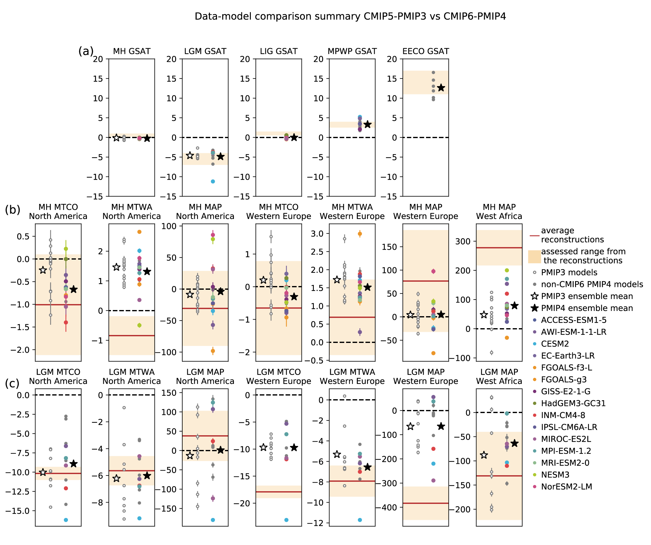
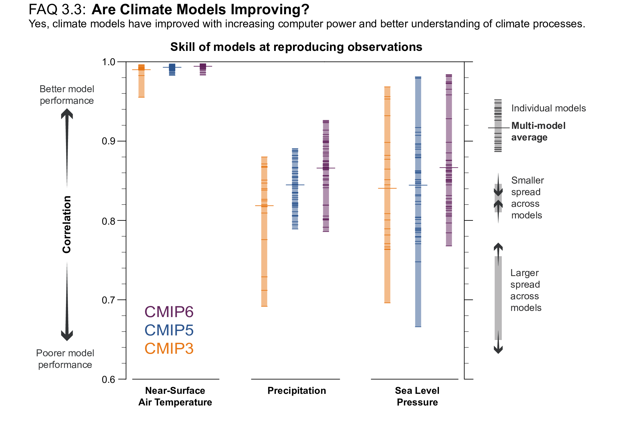
For most large-scale indicators of climate change, the simulated recent mean climate from the latest generation Coupled Model Intercomparison Project Phase 6 (CMIP6) climate models underpinning this assessment has improved compared to the Coupled Model Intercomparison Project Phase 5 (CMIP5) models assessed in AR5 (high confidence). Some differences from observations remain, for example in regional precipitation patterns. High-resolution models exhibit reduced biases in some but not all aspects of surface and ocean climate (medium confidence), and most Earth system models, which include biogeochemical feedbacks, perform as well as their lower-complexity counterparts (medium confidence). The multi-model mean captures most aspects of observed climate change well (high confidence). The multi-model mean captures the proxy-reconstructed global-mean surface air temperature (GSAT) change during past high- and low-CO2 climates (high confidence) and the correct sign of temperature and precipitation change in most assessed regions in the mid-Holocene (medium confidence). The simulation of paleoclimates on continental scales has improved compared to AR5 (medium confidence), but models often underestimate large temperature and precipitation differences relative to the present day (high confidence). {3.8.2}
Human Influence on the Atmosphere and Surface
The likely range of human-induced warming in global-mean surface air temperature (GSAT) in 2010–2019 relative to1850–1900 is 0.8°C–1.3°C, encompassing the observed warming of 0.9°C–1.2°C, while the change attributable to natural forcings is only −0.1°C to +0.1°C. The best estimate of human-induced warming is 1.07°C. Warming can now be attributed since 1850–1900, instead of since 1951 as done in AR5, thanks to a better understanding of uncertainties and because observed warming is larger. The likely ranges for human-induced GSAT and global mean surface temperature (GMST) warming are equal (medium confidence). Attributing observed warming to specific anthropogenic forcings remains more uncertain. Over the same period, forcing from greenhouse gases1 likely increased GSAT by 1.0°C–2.0°C, while other anthropogenic forcings including aerosols likely decreased GSAT by 0.0°C–0.8°C. It is very likely that human-induced greenhouse gas increases were the main driver2 of tropospheric warming since comprehensive satellite observations started in 1979, and extremely likely that human-induced stratospheric ozone depletion was the main driver of cooling in the lower stratosphere between 1979 and the mid-1990s. {3.3.1}
The CMIP6 model ensemble reproduces the observed historical global surface temperature trend and variability with biases small enough to support detection and attribution of human-induced warming (very high confidence). The CMIP6 historical simulations assessed in this report have an ensemble mean global surface temperature change within 0.2°C of the observations over most of the historical period, and observed warming is within the 5–95% range of the CMIP6 ensemble. However, some CMIP6 models simulate a warming that is either above or below the assessed 5–95% range of observed warming. CMIP6 models broadly reproduce surface temperature variations over the past millennium, including the cooling that follows periods of intense volcanism (medium confidence). For upper air temperature, there is medium confidence that most CMIP5 and CMIP6 models overestimate observed warming in the upper tropical troposphere by at least 0.1°C per decade over the period 1979 to 2014. The latest updates to satellite-derived estimates of stratospheric temperature have resulted in decreased differences between simulated and observed changes of global mean temperature through the depth of the stratosphere (medium confidence). {3.3.1}
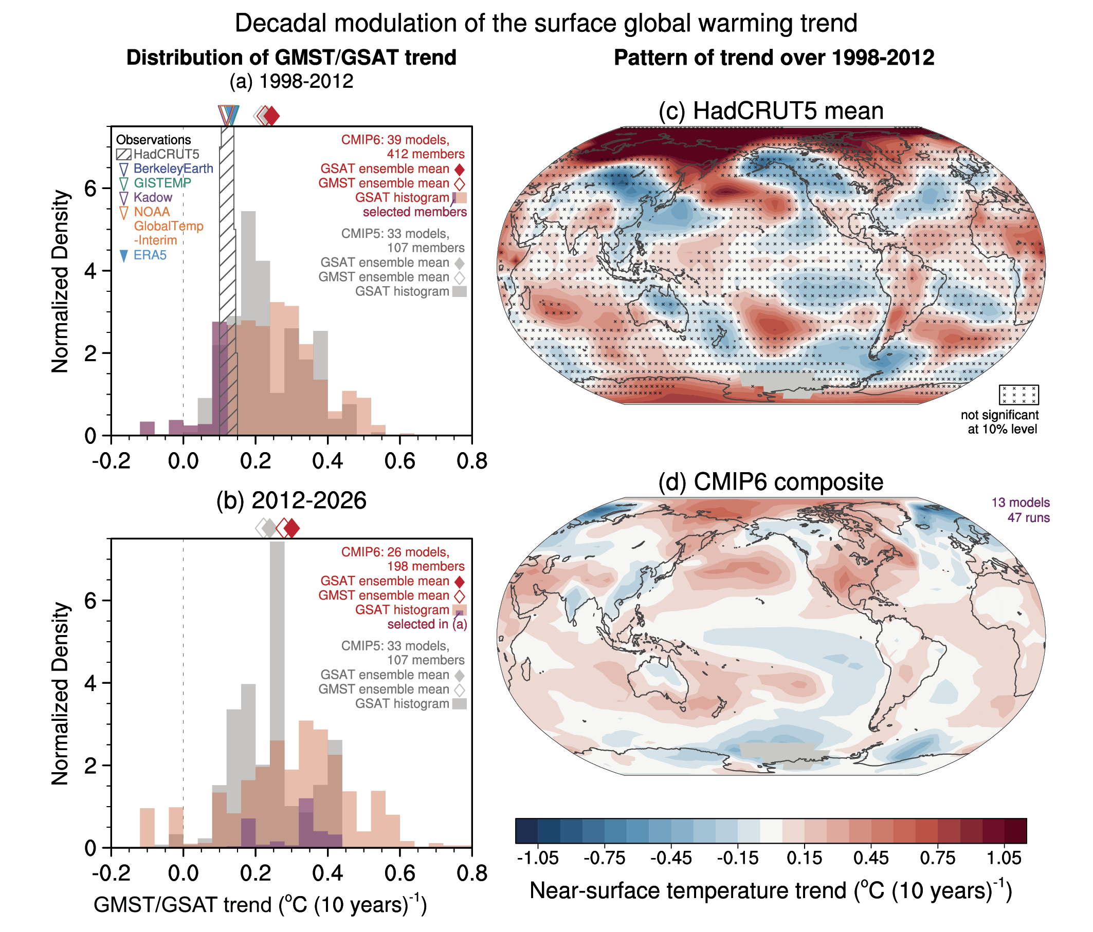
The slower rate of GMST increase observed over 1998–2012 compared to 1951–2012 was a temporary event followed by a strong GMST increase (very high confidence). Improved observational datasets since AR5 show a larger GMST trend over 1998–2012 than earlier estimates. All the observed estimates of the 1998–2012 GMST trend lie within the 10th–90th percentile range of CMIP6 simulated trends (high confidence). Internal variability, particularly Pacific Decadal Variability, and variations in solar and volcanic forcings partly offset the anthropogenic surface warming trend over the 1998–2012 period (high confidence). Global ocean heat content continued to increase throughout this period, indicating continuous warming of the entire climate system (very high confidence). Since 2012, GMST has warmed strongly, with the past five years (2016–2020) being the warmest five-year period in the instrumental record since at least 1850 (high confidence). {Cross-Chapter Box 3.1, 3.3.1; 3.5.1}
It is likely that human influence has contributed to3 moistening in the upper troposphere since 1979. Also, there is medium confidence that human influence contributed to a global increase in annual surface specific humidity, and medium confidence that it contributed to a decrease in surface relative humidity over mid-latitude Northern Hemisphere continents during summertime. {3.3.2}
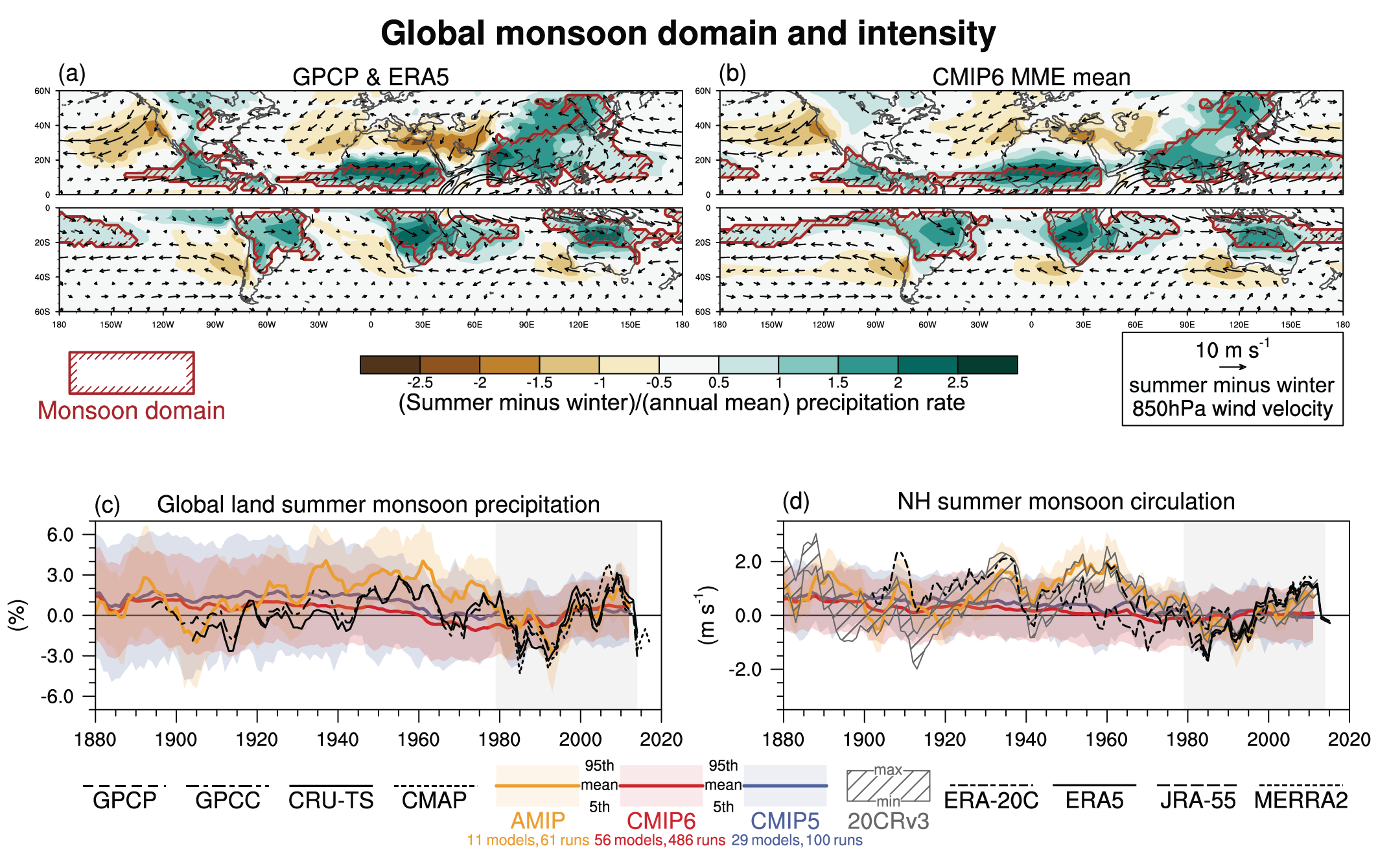
It is likely that human influence has contributed to observed large-scale precipitation changes since the mid-20th century. New attribution studies strengthen previous findings of a detectable increase in Northern Hemisphere mid- to high-latitude land precipitation (high confidence). Human influence has contributed to strengthening the zonal mean precipitation contrast between the wet tropics and dry subtropics (medium confidence). Yet, anthropogenic aerosols contributed to decreasing global land summer monsoon precipitation from the 1950s to 1980s (medium confidence). There is also medium confidence that human influence has contributed to high-latitude increases and mid-latitude decreases in Southern Hemisphere summertime precipitation since 1979 associated with the trend of the Southern Annular Mode toward its positive phase. Despite improvements, models still have deficiencies in simulating precipitation patterns, particularly over the tropical ocean (high confidence). {3.3.2, 3.3.3, 3.5.2}
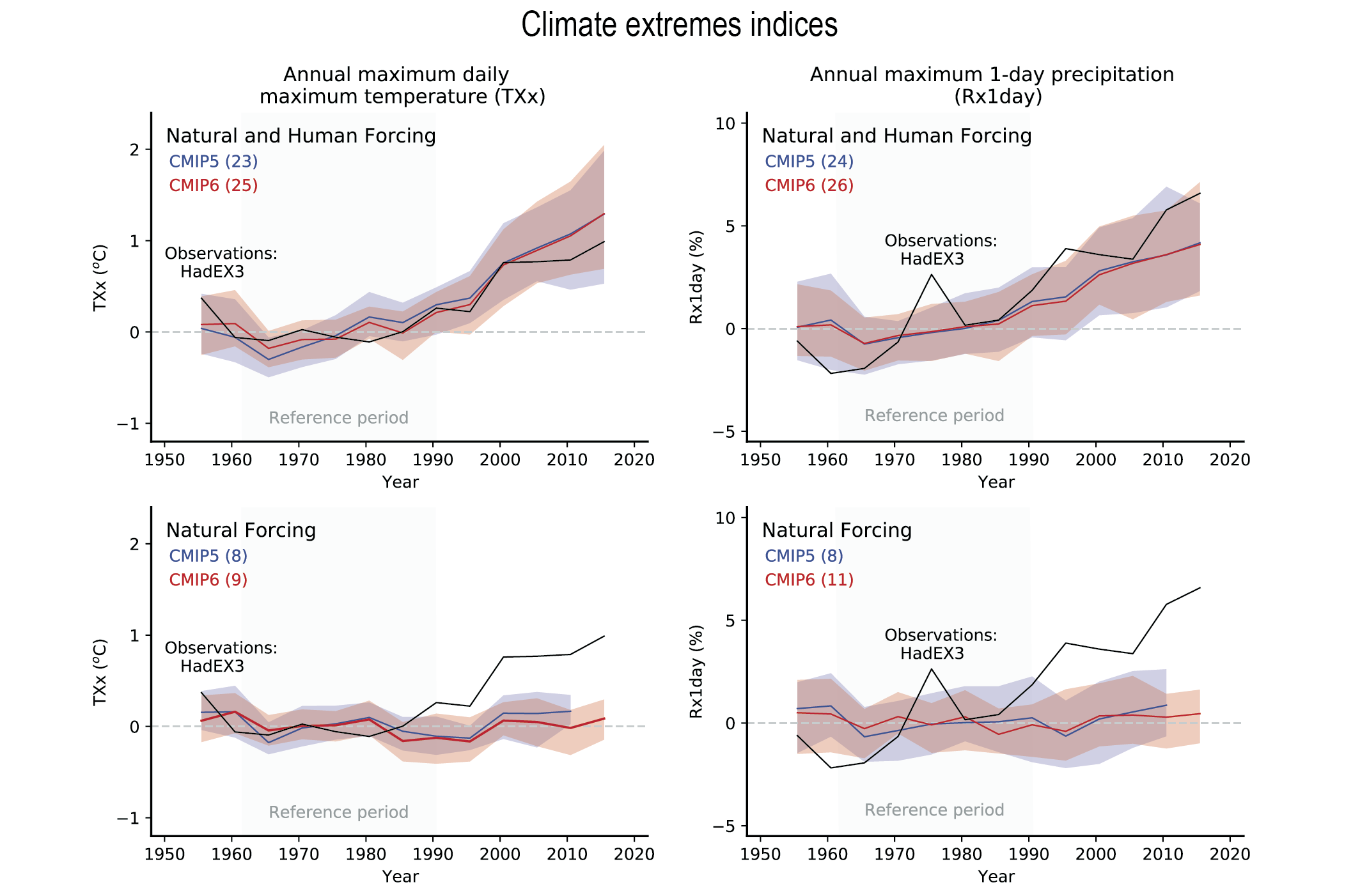
Human-induced greenhouse gas forcing is the main driver of the observed changes in hot and cold extremes on the global scale (virtually certain) and on most continents (very likely ). It is likely that human influence, in particular due to greenhouse gas forcing, is the main driver of the observed intensification of heavy precipitation in global land regions during recent decades. There is high confidence in the ability of models to capture the large-scale spatial distribution of precipitation extremes over land. The magnitude and frequency of extreme precipitation simulated by CMIP6 models are similar to those simulated by CMIP5 models (high confidence). {Cross-Chapter Box 3.2}
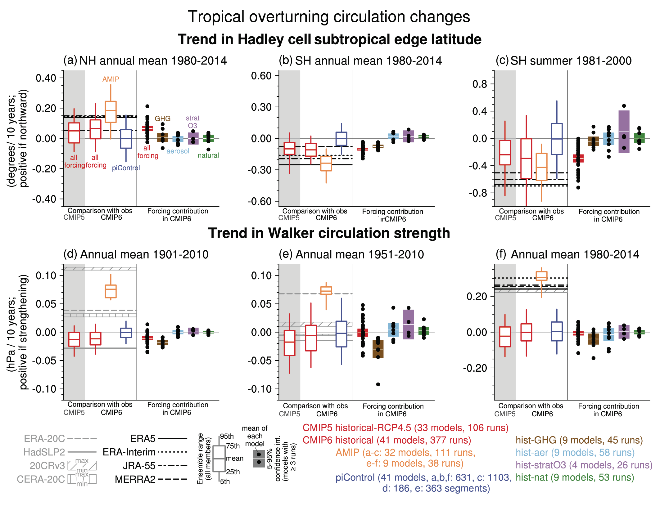
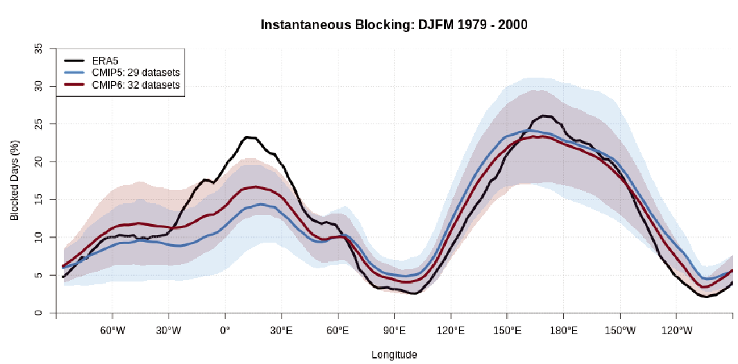
It is likely that human influence has contributed to the poleward expansion of the zonal mean Hadley cell in the Southern Hemisphere since the 1980s. There is medium confidence that the observed poleward expansion of the zonal mean Hadley cell in the Northern Hemisphere is within the range of internal variability. The causes of the observed strengthening of the Pacific Walker circulation since the 1980s are not well understood, and the observed strengthening trend is outside the range of trends simulated in the coupled models (medium confidence). While CMIP6 models capture the general characteristics of the tropospheric large-scale circulation (high confidence), systematic biases exist in the mean frequency of atmospheric blocking events, especially in the Euro-Atlantic sector, some of which reduce with increasing model resolution (medium confidence). {3.3.3}
Human Influence on the Cryosphere
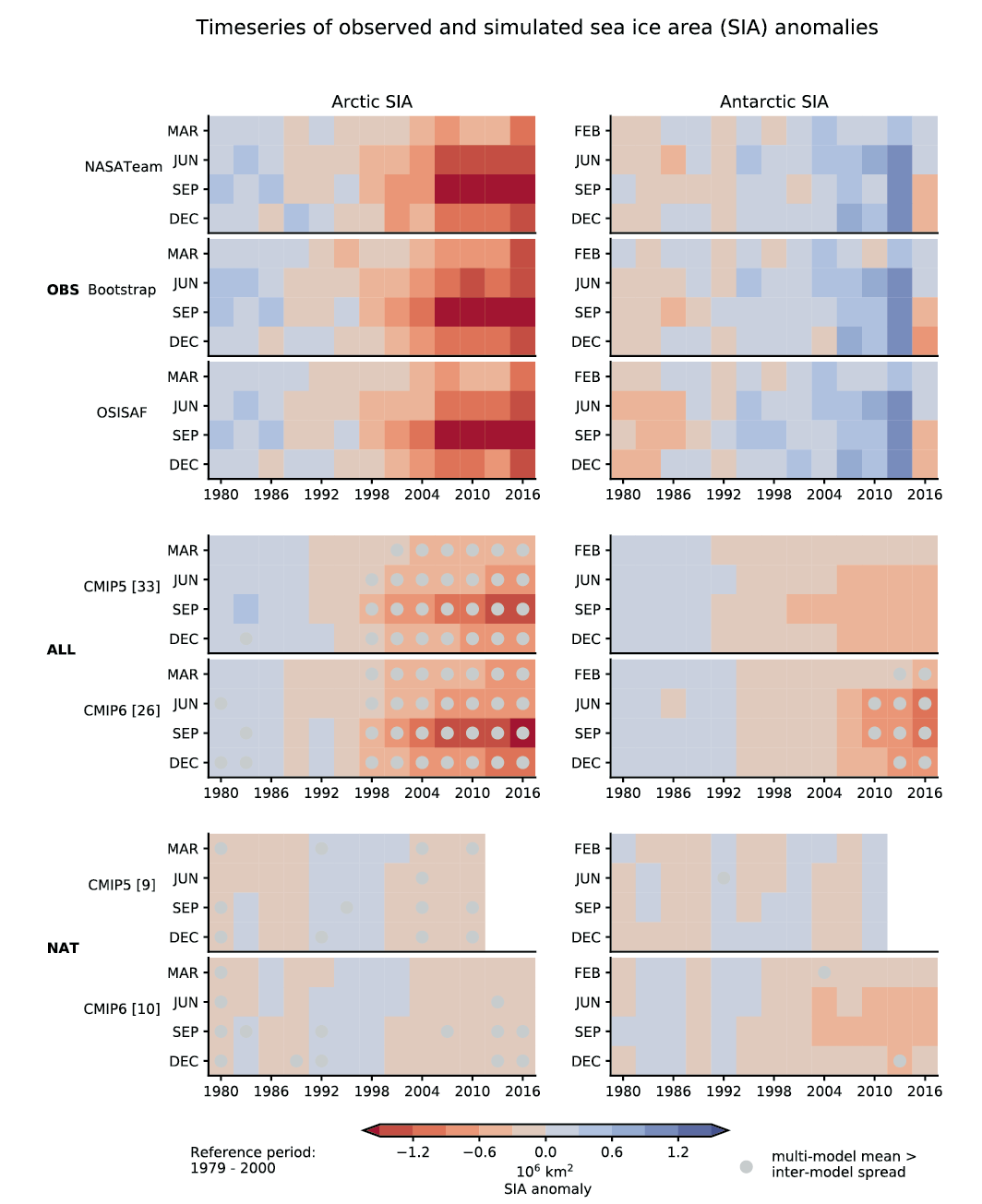
It is very likely that anthropogenic forcing, mainly due to greenhouse gas increases, was the main driver of Arctic sea ice loss since the late 1970s. There is new evidence that increases in anthropogenic aerosols have offset part of the greenhouse gas-induced Arctic sea ice loss since the 1950s (medium confidence). In the Arctic, despite large differences in the mean sea ice state, loss of sea ice extent and thickness during recent decades is reproduced in all CMIP5 and CMIP6 models (high confidence). By contrast, global climate models do not generally capture the small observed increase in Antarctic sea ice extent during the satellite era, and there is low confidence in attributing the causes of this change. {3.4.1}
It is very likely that human influence contributed to the observed reductions in Northern Hemisphere spring snow cover since 1950. The seasonal cycle in Northern Hemisphere snow cover is better reproduced by CMIP6 than by CMIP5 models (high confidence). Human influence was very likely the main driver of the recent global, near-universal retreat of glaciers. It is very likely that human influence has contributed to the observed surface melting of the Greenland Ice Sheet over the past two decades, and there is medium confidence in an anthropogenic contribution to recent overall mass loss from the Greenland Ice Sheet. However, there is only limited evidence, with medium agreement, of human influence on Antarctic Ice Sheet mass balance through changes in ice discharge. {3.4.2, 3.4.3}
Human Influence on the Ocean
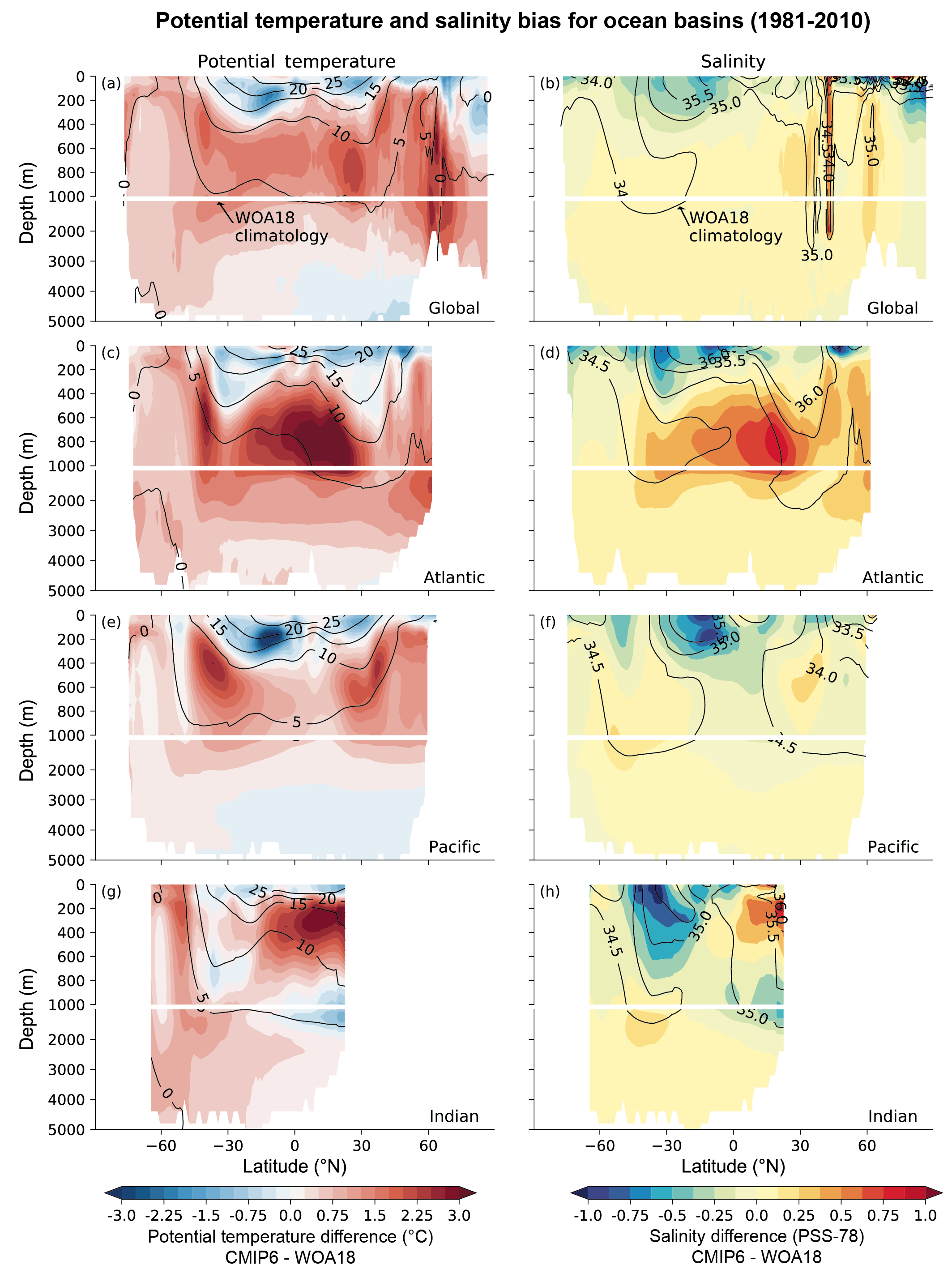
It is extremely likely that human influence was the main driver of the ocean heat content increase observed since the 1970s, which extends into the deeper ocean (very high confidence). Since AR5, there is improved consistency between recent observed estimates and model simulations of changes in upper (<700 m) ocean heat content, when accounting for both natural and anthropogenic forcings. Updated observations and model simulations show that warming extends throughout the entire water column (high confidence), with CMIP6 models simulating 58% of industrial-era heat uptake (1850–2014) in the upper layer (0–700 m), 21% in the intermediate layer (700–2000 m) and 22% in the deep layer (>2000 m). The structure and magnitude of multi-model mean ocean temperature biases have not changed substantially between CMIP5 and CMIP6 (medium confidence). {3.5.1}
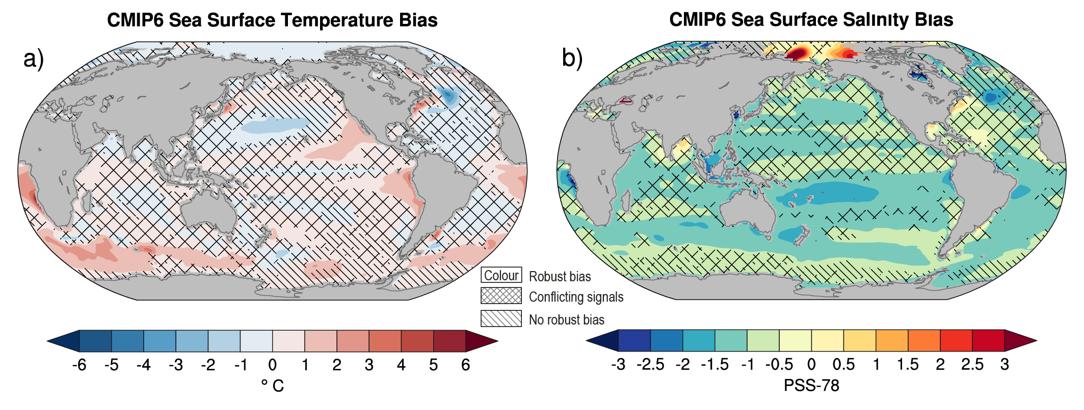
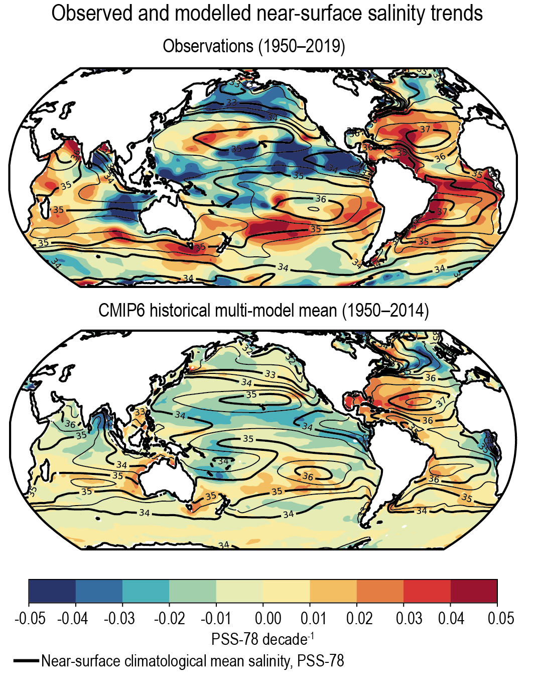
It is extremely likely that human influence has contributed to observed near-surface and subsurface ocean salinity changes since the mid-20th century. The associated pattern of change corresponds to fresh regions becoming fresher and salty regions becoming saltier (high confidence). Changes to the coincident atmospheric water cycle and ocean-atmosphere fluxes (evaporation and precipitation) are the primary drivers of the observed basin-scale salinity changes (high confidence). The observed depth-integrated basin-scale salinity changes have been attributed to human influence, with CMIP5 and CMIP6 models able to reproduce these patterns only in simulations that include greenhouse gas increases (medium confidence). The basin-scale changes are consistent across models and intensify through the historical period (high confidence). The structure of the biases in the multi-model mean has not changed substantially between CMIP5 and CMIP6 (medium confidence). {3.5.2}
Combining the attributable contributions from glaciers, ice-sheet surface mass balance and thermal expansion, it is very likely that human influence was the main driver of the observed global mean sea level rise since at least 1971. Since AR5, studies have shown that simulations that exclude anthropogenic greenhouse gases are unable to capture the sea level rise due to thermal expansion (thermosteric) during the historical period and that model simulations that include all forcings (anthropogenic and natural) most closely match observed estimates. It is very likely that human influence was the main driver of the observed global mean thermosteric sea level increase since 1970. {3.5.3, 3.5.1, 3.4.3}
While observations show that the Atlantic Meridional Overturning Circulation (AMOC) has weakened from the mid-2000s to the mid-2010s (high confidence) and the Southern Ocean upper overturning cell has strengthened since the 1990s (low confidence), observational records are too short to determine the relative contributions of internal variability, natural forcing, and anthropogenic forcing to these changes (high confidence). No changes in Antarctic Circumpolar Current transport or meridional position have been observed. The mean zonal and overturning circulations of the Southern Ocean and the mean overturning circulation of the North Atlantic (the Atlantic Meridional Overturning Circulation, AMOC) are broadly reproduced by CMIP5 and CMIP6 models. However, biases are apparent in the modelled circulation strengths (high confidence) and their variability (medium confidence). {3.5.4}
Human Influence on the Biosphere
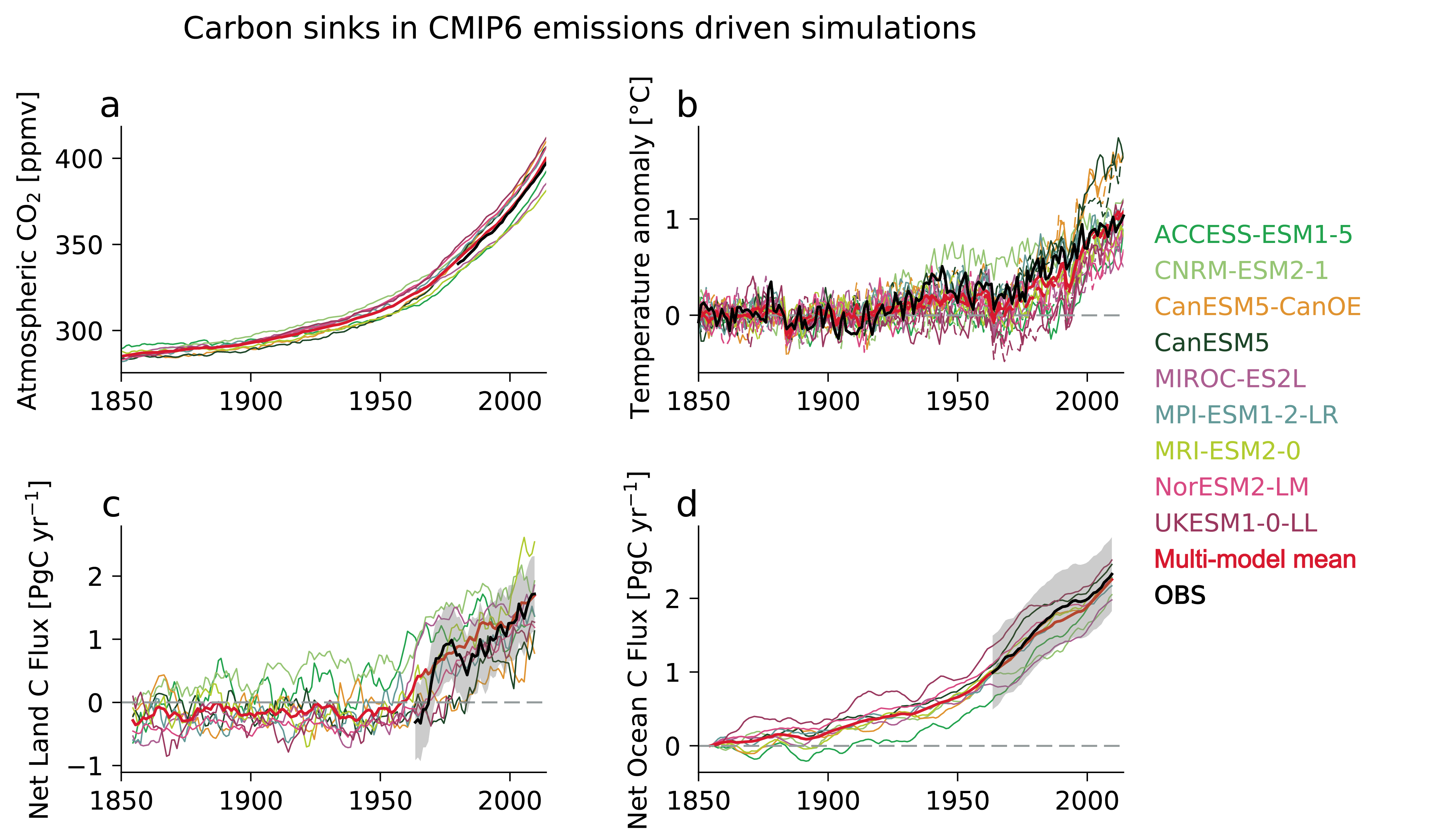
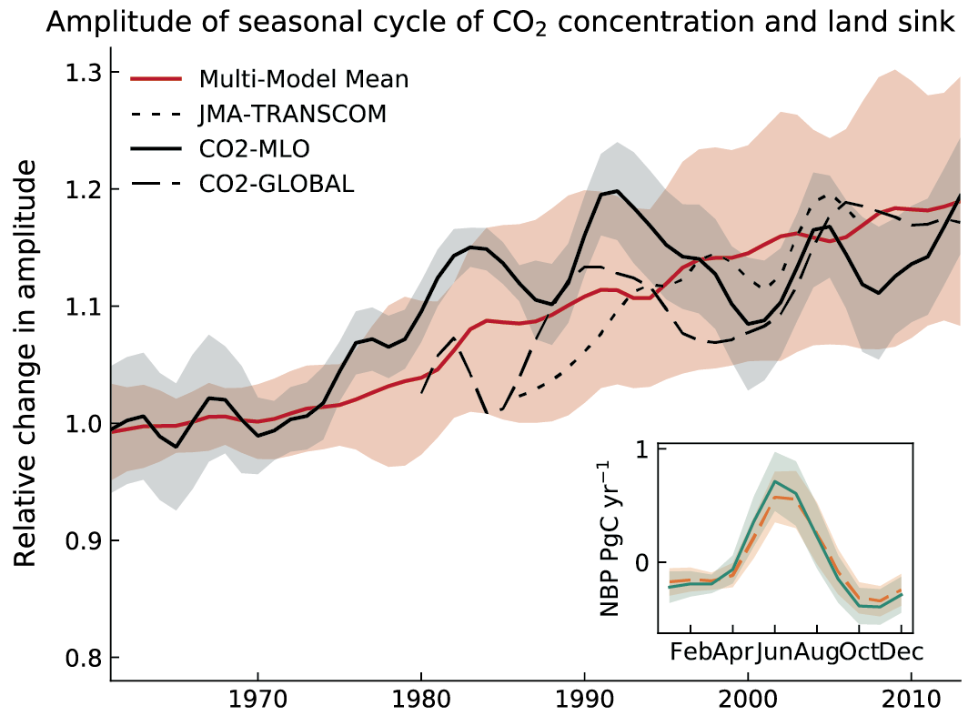
The main driver of the observed increase in the amplitude of the seasonal cycle of atmospheric CO2 is enhanced fertilization of plant growth by the increasing concentration of atmospheric CO2 (medium confidence) . However, there is only low confidence that this CO2 fertilization has also been the main driver of observed greening because land management is the dominating factor in some regions. Earth system models simulate globally averaged land carbon sinks within the range of observation-based estimates (high confidence), but global-scale agreement masks large regional disagreements. {3.6.1}
It is virtually certain that the uptake of anthropogenic CO2 was the main driver of the observed acidification of the global surface open ocean. The observed increase in CO2 concentration in the subtropical and equatorial North Atlantic since 2000 is likely associated in part with an increase in ocean temperature, a response that is consistent with the expected weakening of the ocean carbon sink with warming. Consistent with AR5 there is medium confidence that deoxygenation in the upper ocean is due in part to human influence. There is high confidence that Earth system models simulate a realistic time evolution of the global mean ocean carbon sink. {3.6.2}
Human Influence on Modes of Climate Variability
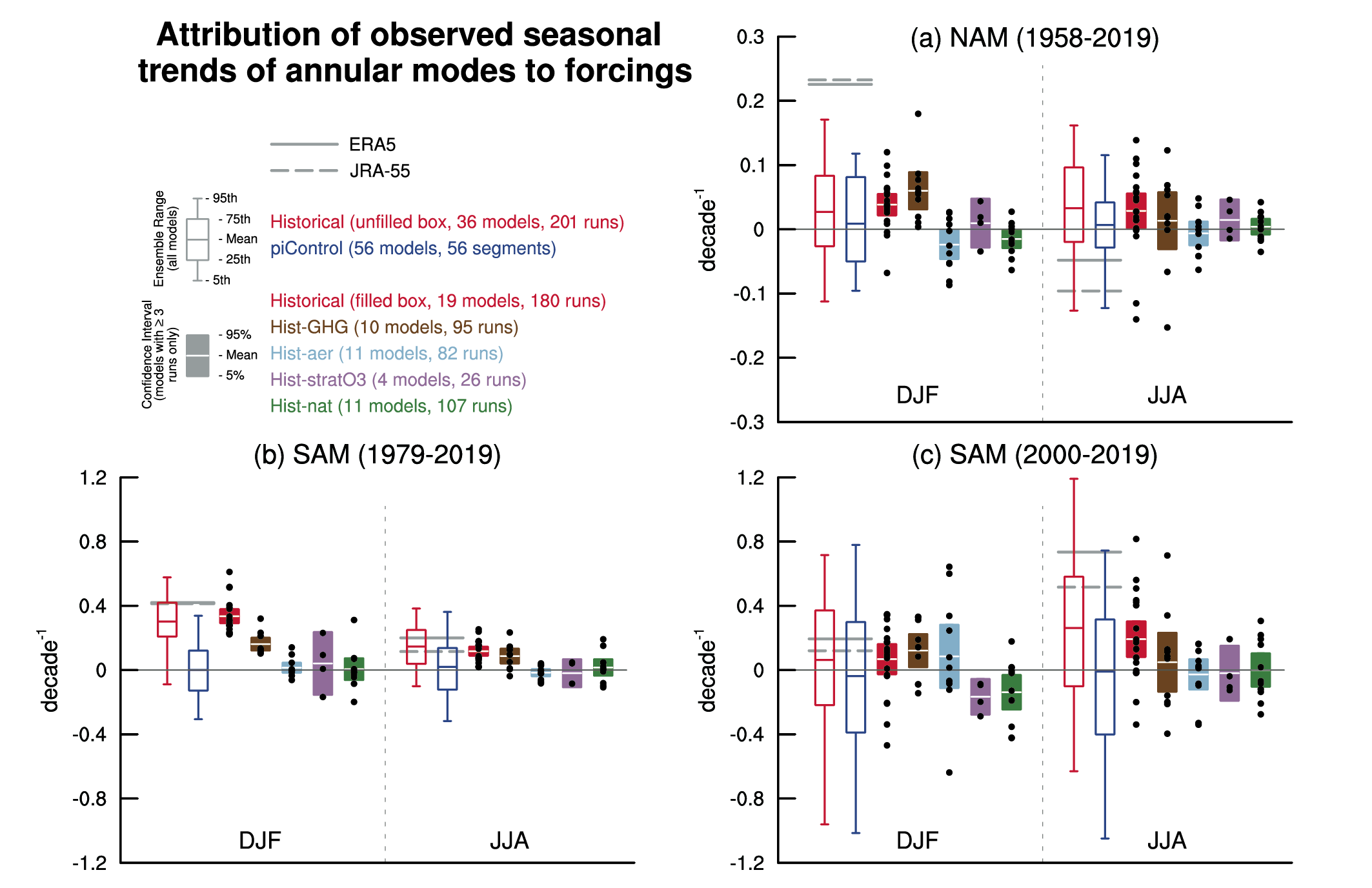
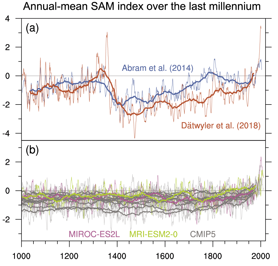
It is very likely that human influence has contributed to the observed trend towards the positive phase of the Southern Annular Mode (SAM) since the 1970s and to the associated strengthening and southward shift of the Southern Hemispheric extratropical jet in austral summer. The influence of ozone forcing on the SAM trend has been small since the early 2000s compared to earlier decades, contributing to a weaker SAM trend observed over 2000–2019 (medium confidence). Climate models reproduce the summertime SAM trend well, with CMIP6 models outperforming CMIP5 models (medium confidence). By contrast, the cause of the Northern Annular Mode (NAM) trend towards its positive phase since the 1960s and associated northward shifts of the Northern Hemispheric extratropical jet and storm track in boreal winter is not well understood. Models reproduce the observed spatial features and variance of the SAM and NAM very well (high confidence). {3.3.3, 3.7.1, 3.7.2}
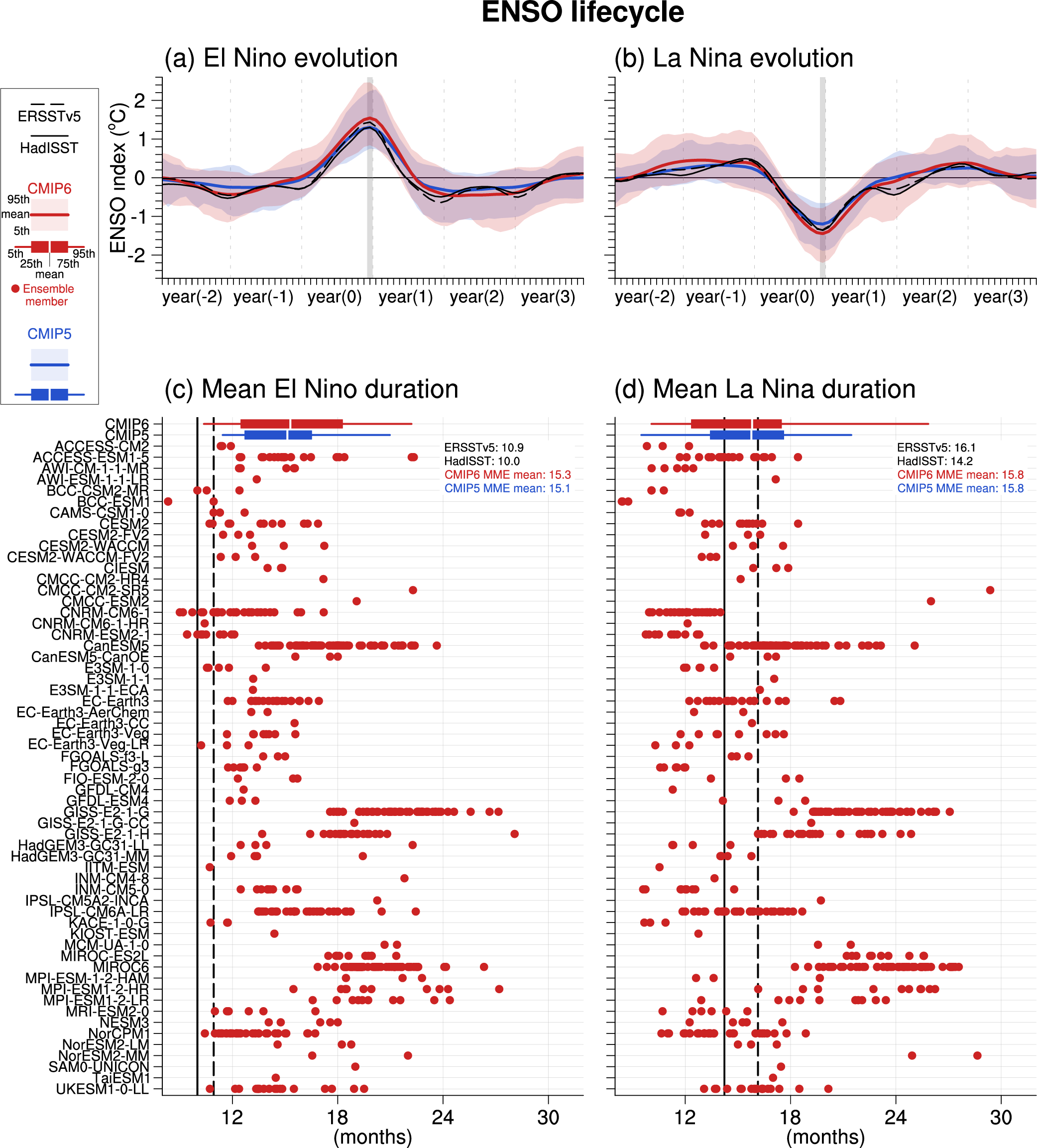
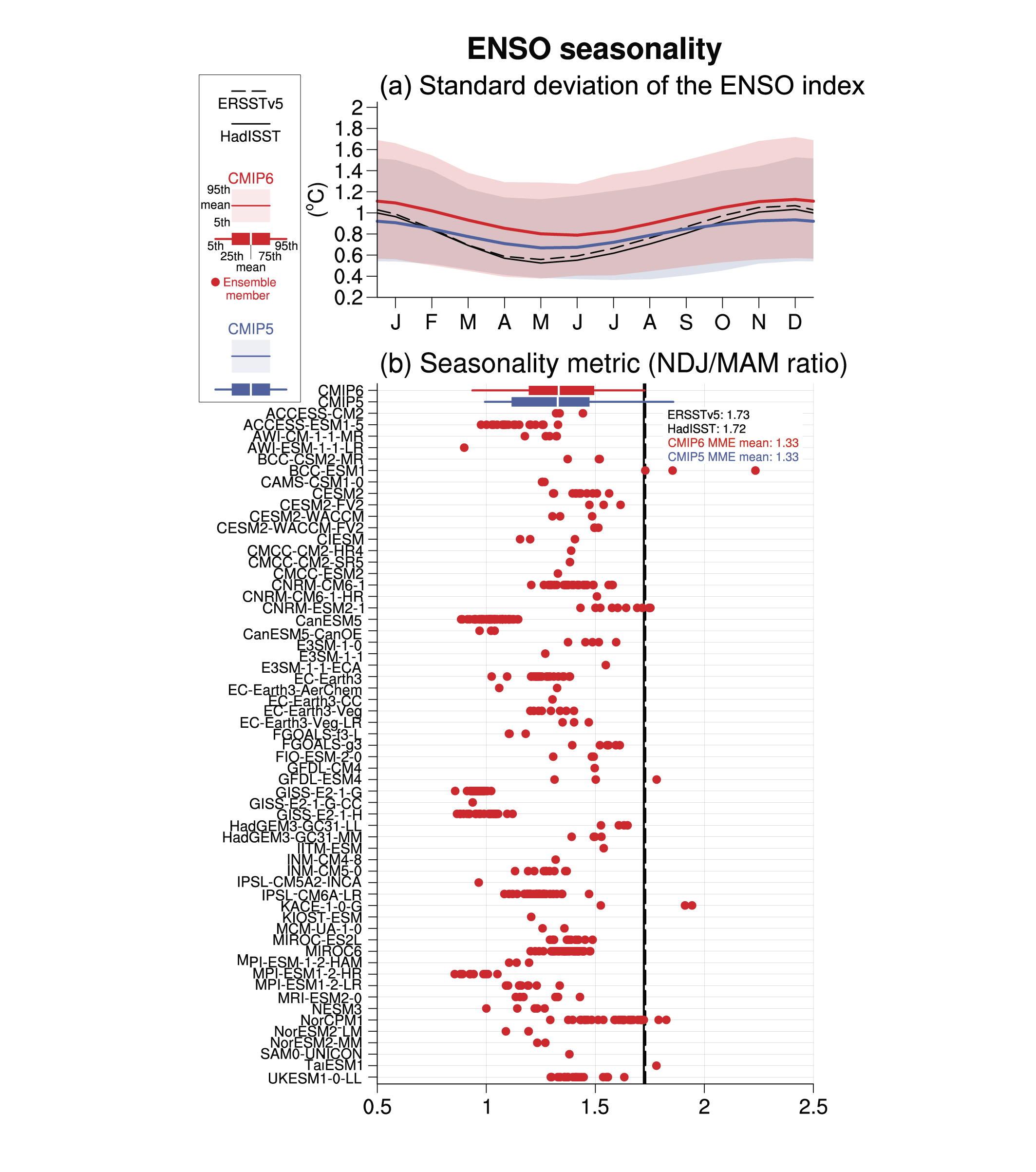
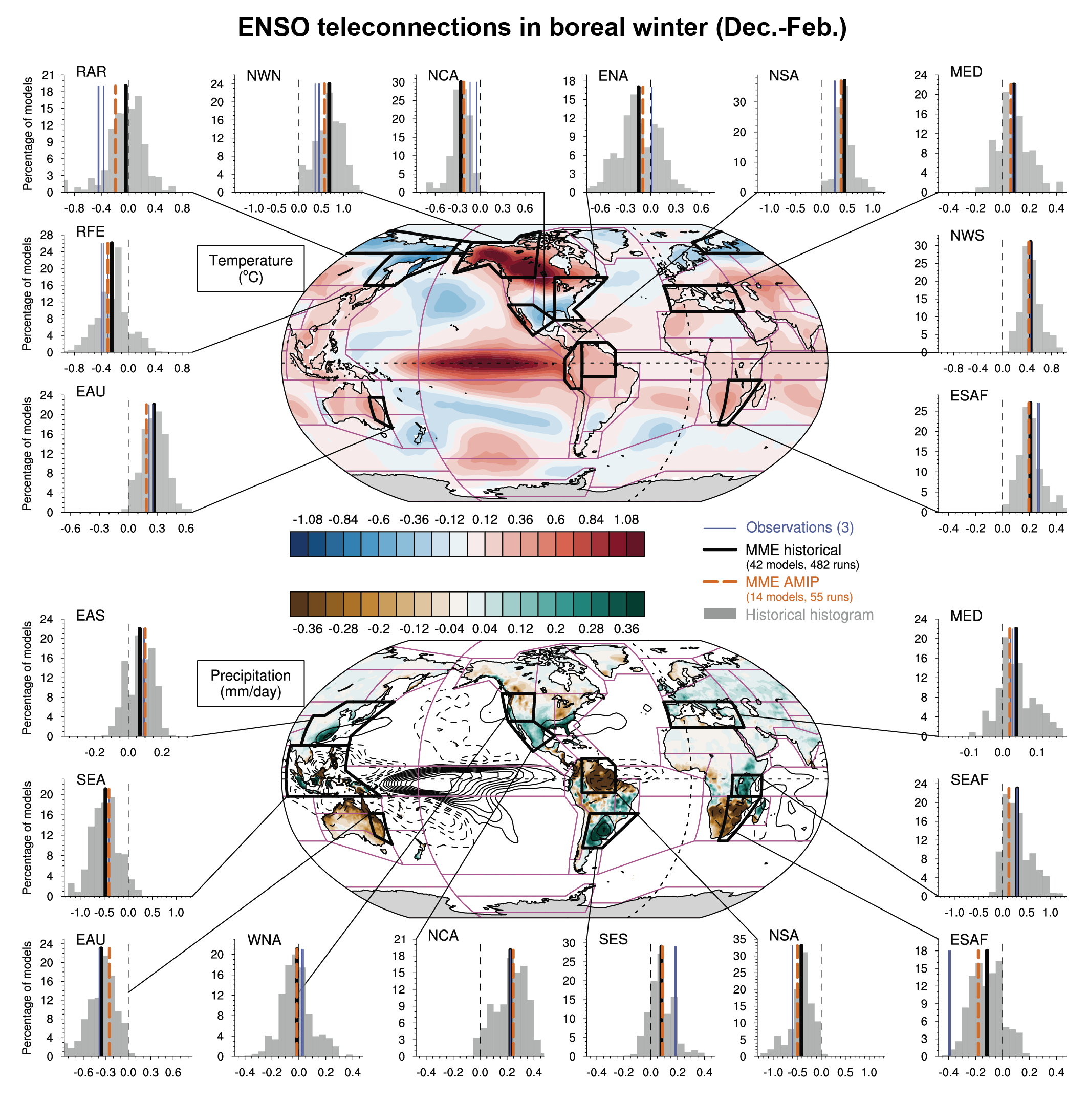
Human influence has not affected the principal tropical modes of interannual climate variability or their associated regional teleconnections beyond the range of internal variability (high confidence). Further assessment since AR5 confirms that climate and Earth system models are able to reproduce most aspects of the spatial structure and variance of the El Niño–Southern Oscillation and Indian Ocean Basin and Dipole modes (medium confidence). However, despite a slight improvement in CMIP6, some underlying processes are still poorly represented. In the Tropical Atlantic basin, which contains the Atlantic Zonal and Meridional modes, major biases in modelled mean state and variability remain. {3.7.3 to 3.7.5}
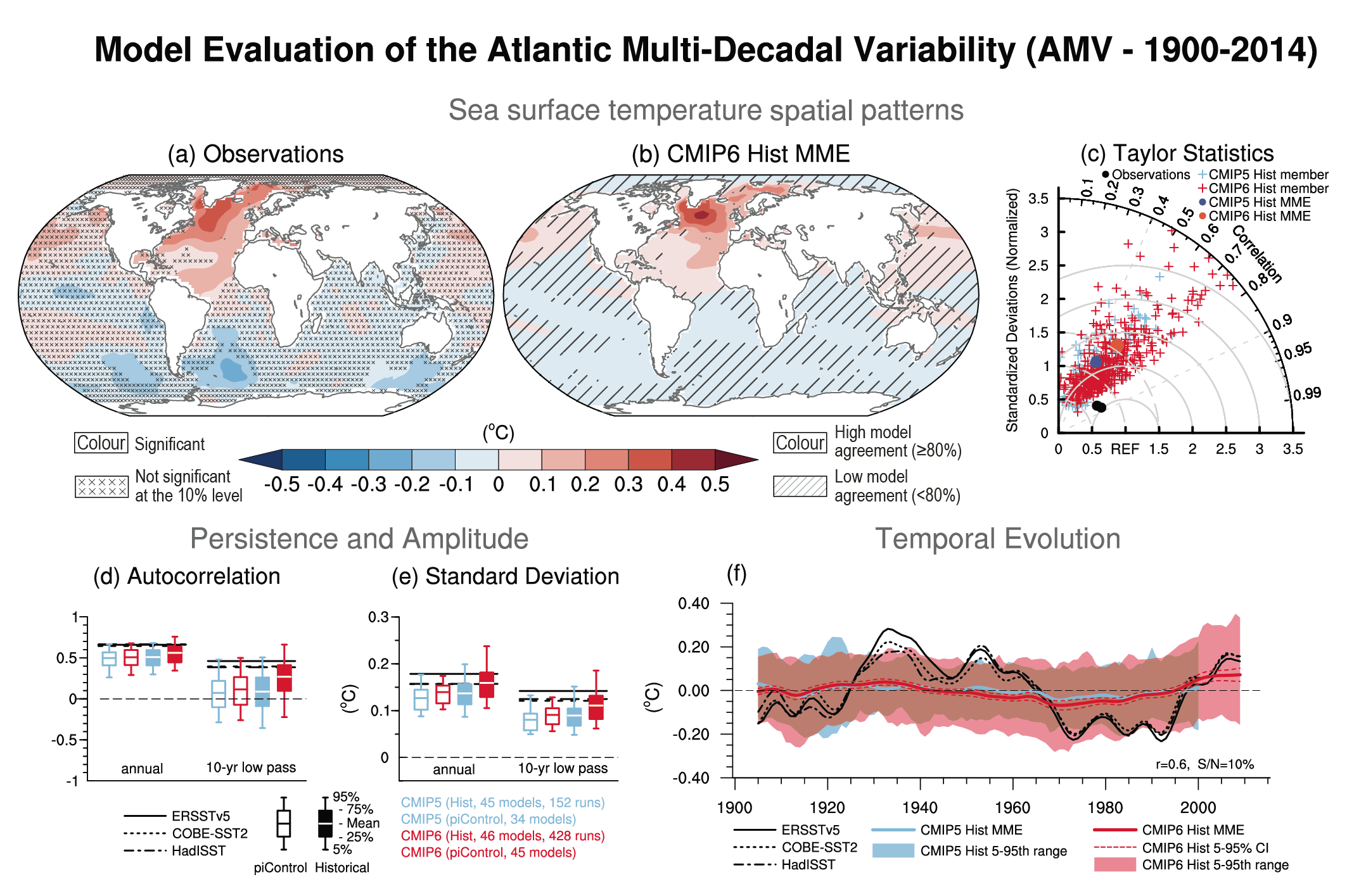
There is medium confidence that anthropogenic and volcanic aerosols contributed to observed changes in the Atlantic Multi-decadal Variability (AMV) index and associated regional teleconnections since the 1960s, but there is low confidence in the magnitude of this influence. There is high confidence that internal variability is the main driver of Pacific Decadal Variability (PDV) observed since pre-industrial times, despite some modelling evidence for potential human influence. Uncertainties remain in quantification of the human influence on AMV and PDV due to brevity of the observational records, limited model performance in reproducing related sea surface temperature (SST) anomalies despite improvements from CMIP5 to CMIP6 (medium confidence), and limited process understanding of their key drivers. {3.7.6, 3.7.7}
3.1 Scope and Overview
This chapter assesses the extent to which the climate system has been affected by human influence and to what extent climate models are able to simulate observed mean climate, changes and variability. This assessment is the basis for understanding what impacts of anthropogenic climate change may already be occurring and informs our confidence in climate projections. Moreover, an understanding of the amount of human-induced global warming to date is key to assessing our status with respect to the Paris Agreement goals of holding the increase in global average temperature to well below 2°C above pre-industrial levels and pursuing efforts to limit the temperature increase to 1.5°C (UNFCCC, 2016).
The evidence of human influence on the climate system has strengthened progressively over the course of the previous five IPCC assessments, from the Second Assessment Report that concluded ‘the balance of evidence suggests a discernible human influence on climate’ through to the Fifth Assessment Report (AR5) which concluded that ‘it is extremely likely that human influence caused more than half of the observed increase in global mean surface temperature (GMST) from 1951 to 2010’ (see also Sections 1.3.4 and 3.3.1.1). The AR5 concluded that climate models had been developed and improved since the Fourth Assessment Report (AR4) and were able to reproduce many features of observed climate. Nonetheless, several systematic biases were identified (Flato et al., 2013). This chapter additionally builds on the assessment of attribution of global temperatures contained in the IPCC Special Report on Global Warming of 1.5°C (SR1.5; IPCC, 2018), assessments of attribution of changes in the ocean and cryosphere in the IPCC Special Report on the Ocean and Cryosphere in a Changing Climate (SROCC; IPCC, 2019b), and assessments of attribution of changes in the terrestrial carbon cycle in the IPCC Special Report on Climate Change and Land (SRCCL, IPCC, 2019a).
This chapter assesses the evidence for human influence on observed large-scale indicators of climate change that are described in Cross-Chapter Box 2.2 and assessed in Chapter 2. It takes advantage of the longer period of record now available in many observational datasets. The assessment of the human-induced contribution to observed climate change requires an estimate of the expected response to human influence, as well as an estimate of the expected climate evolution due to natural forcings and an estimate of variability internal to the climate system (internal climate variability). For this we need high quality models, primarily climate and Earth system models. Since AR5, a new set of coordinated model results from the World Climate Research Programme (WCRP) Coupled Model Intercomparison Project Phase 6 (CMIP6; Eyring et al., 2016a) has become available. Together with updated observations of large-scale indicators of climate change (Chapter 2), CMIP simulations are a key resource for assessing human influence on the climate system. Pre-industrial control and historical simulations are of most relevance for model evaluation and assessment of internal variability, and these simulations are evaluated to assess fitness-for-purpose for attribution, which is the focus of this chapter (see also (Section 1.5.4). This chapter provides the primary evaluation of large-scale indicators of climate change in this Report, and is complemented by other fitness-for-purpose evaluations in subsequent chapters. CMIP6 also includes an extensive set of idealized and single forcing experiments for attribution (Eyring et al., 2016a; Gillett et al., 2016). In addition to the assessment of model performance and human influence on the climate system during the instrumental era up to the present-day, this chapter also includes evidence from paleo-observations and simulations over past millennia (Kageyama et al., 2018).
Whereas in previous IPCC assessment reports the comparison of simulated and observed climate change was done separately in a model evaluation chapter and a chapter on detection and attribution, in AR6 these comparisons are integrated together. This has the advantage of allowing a single discussion of the full set of explanations for any inconsistency in simulated and observed climate change, including missing forcings, errors in the simulated response to forcings, and observational errors, as well as an assessment of the application of detection and attribution techniques to model evaluation. Where simulated and observed changes are consistent, this can be interpreted both as supporting attribution statements, and as giving confidence in simulated future change in the variable concerned (see also Box 4.1). However, if a model’s simulation of historical climate change has been tuned to agree with observations, or if the models used in an attribution study have been selected or weighted on the basis of the realism of their simulated climate response, this information would need to be considered in the assessment and any attribution results correspondingly tempered. An integrated discussion of evaluation and attribution supports such a robust and transparent assessment.
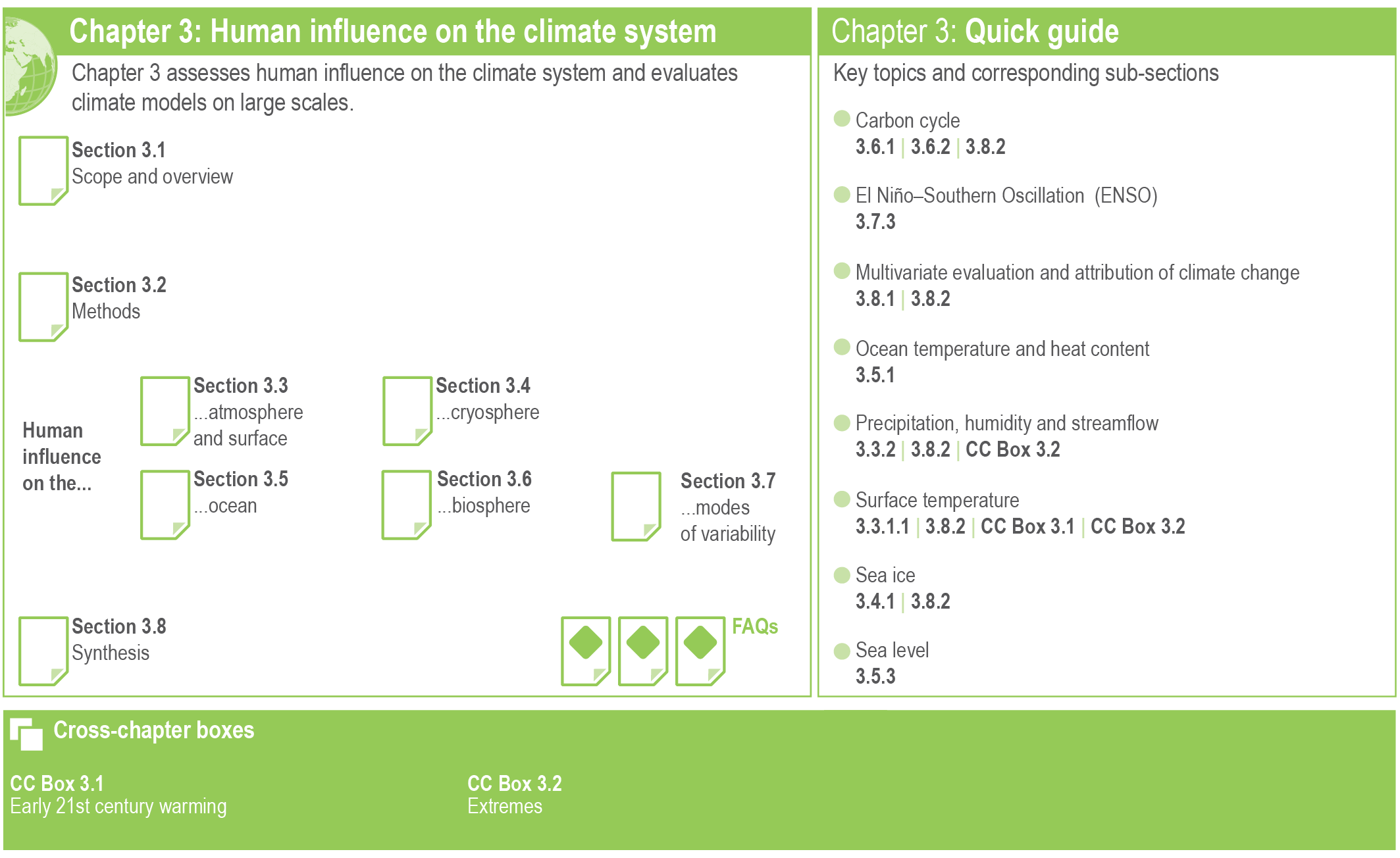
This chapter starts with a brief description of methods for detection and attribution of observed changes in Section 3.2, which builds on the more general introduction to attribution approaches in the Cross-Working Group Box on Attribution in Chapter 1. In this chapter we assess the detection of anthropogenic influence on climate on large spatial scales and long temporal scales, a concept related to, but distinct from, that of the emergence of anthropogenically-induced climate change from the range of internal variability on local scales and shorter time scales (Section 1.4.2.2). The following sections address the climate system component by component, in each case assessing human influence and evaluating climate models’ simulations of the relevant aspects of climate and climate change. This chapter assesses the evaluation and attribution of global, hemispheric, continental and ocean basin-scale indicators of climate change in the atmosphere and at the Earth’s surface (Section 3.3, cryosphere (Section 3.4, ocean (Section 3.5, and biosphere (Section 3.6, and the evaluation and attribution of modes of variability (Section 3.7), the period of slower warming in the early 21st century (Cross-Chapter Box 3.1) and large-scale changes in extremes (Cross-Chapter Box 3.2). Model evaluation and attribution on sub-continental scales are not covered here, since these are assessed in the Atlas and in Chapter 10, and extreme event attribution is not covered since it is assessed in Chapter 11. Section 3.8 assesses multivariate attribution and integrative measures of model performance based on multiple variables, as well as process representation in different classes of models. The chapter structure is summarized in Figure 3.1.
 Figure 3.1 | Visual guide to Chapter 3.
 3.2 Methods
New methods for model evaluation that are used in this chapter are described in Section 1.5.4. These include new techniques for process-based evaluation of climate and Earth system models against observations that have rapidly advanced since the publication of AR5 (Eyring et al., 2019) as well as newly developed CMIP evaluation tools that allow a more rapid and comprehensive evaluation of the models with observations (Eyring et al., 2016a, b).
In this chapter, we use the Earth System Model Evaluation Tool (ESMValTool, Eyring et al., 2020; Lauer et al., 2020; Righi et al., 2020) and the NCAR Climate Variability Diagnostic Package (CVDP, Phillips et al., 2014) that is included in the ESMValTool to produce most of the figures. This ensures traceability of the results and provides an additional level of quality control. The ESMValTool code to produce the figures in this chapter was released as open source software at the time of the publication of this Report (see details in the Chapter Data Table, Table SM.3.1). Figures in this chapter are produced either using one ensemble member from each model, or using all available ensemble members and weighting each simulation by 1/(NMi), where N is the number of models and Mi is the ensemble size of the i th model, prior to calculating means and percentiles. Both approaches ensure that each model used is given equal weight in the figures, and details on which approach is used are provided in the figure captions.
An introduction to recent developments in detection and attribution methods in the context of this Report is provided in the Cross-Working Group Box on Attribution in Chapter 1. Here we discuss new methods and improvements applicable to the attribution of changes in large-scale indicators of climate change which are used in this chapter.
3.2.1 Methods Based on Regression
Regression-based methods, also known as fingerprinting methods, have been widely used for detection of climate change and attribution of the change to different external drivers. Initially, these methods were applied to detect changes in global surface temperature, and were then extended to other climate variables at different time and spatial scales (e.g., Hegerl et al., 1996; Hasselmann, 1997; Allen and Tett, 1999; Gillett et al., 2003b; Zhang et al., 2007; Min et al., 2008a, 2011). These approaches are based on multivariate linear regression and assume that the observed change consists of a linear combination of externally forced signals plus internal variability, which generally holds for large-scale variables (Hegerl and Zwiers, 2011). The regressors are the expected space–time response patterns to different climate forcings (fingerprints), and the residuals represent internal variability. Fingerprints are usually estimated from climate model simulations following spatial and temporal averaging. A regression coefficient which is significantly greater than zero implies that a detectable change is identified in the observations. When the confidence interval of the regression coefficient includes unity and is inconsistent with zero, the magnitude of the model simulated fingerprints is assessed to be consistent with the observations, implying that the observed changes can be attributed in part to a particular forcing. Variants of linear regression have been used to address uncertainty in the fingerprints due to internal variability (Allen and Stott, 2003) as well as structural model uncertainty (Huntingford et al., 2006).
In order to improve the signal-to-noise ratio, observations and model-simulated responses are usually normalized by an estimate of internal variability derived from climate model simulations. This procedure requires an estimate of the inverse covariance matrix of the internal variability, and some approaches have been proposed for more reliable estimation of this (Ribes et al., 2009). A signal can be spuriously detected due to too-small noise, and hence simulated internal variability needs to be evaluated with care. Model-simulated variability is typically checked through comparing modelled variance from unforced simulations with the observed residual variance using a standard residual consistency test (Allen and Tett, 1999), or an improved one (Ribes and Terray, 2013). Imbers et al. (2014) tested the sensitivity of detection and attribution results to different representations of internal variability associated with short-memory and long-memory processes. Their results supported the robustness of previous detection and attribution statements for the global mean temperature change but they also recommended the use of a wider variety of robustness tests.
Some recent studies focused on the improved estimation of the scaling factor (regression coefficient) and its confidence interval. Hannart et al. (2014) described an inference procedure for scaling factors which avoids making the assumption that model error and internal variability have the same covariance structure. An integrated approach to optimal fingerprinting was further suggested in which all uncertainty sources (i.e., observational error, model error, and internal variability) are treated in one statistical model without a preliminary dimension reduction step (Hannart, 2016). Katzfuss et al. (2017) introduced a similar integrated approach based on a Bayesian model averaging. On the other hand, DelSole et al. (2019) suggested a bootstrap method to better estimate the confidence intervals of scaling factors even in a weak-signal regime. It is notable that some studies do not optimize fingerprints, as uncertainty in the covariance introduces a further layer of complexity, but results in only a limited improvement in detection (Polson and Hegerl, 2017).
Another fingerprinting approach uses pattern similarity between observations and fingerprints, in which the leading empirical orthogonal function obtained from the time-evolving multi-model forced simulation is usually defined as a fingerprint (e.g., Santer et al., 2013; Marvel et al., 2019; Bonfils et al., 2020). Observations and model simulations are then projected onto the fingerprint to measure the degree of spatial pattern similarity with the expected physical response to a given forcing. This projection provides the signal time series, which is in turn tested against internal variability, as estimated from long control simulations. As a way to extend this pattern-based approach to a high-dimensional detection variable at daily time scales, Sippel et al. (2019, 2020) proposed using the relationship pattern with a global climate change metric as a fingerprint. To solve the high-dimensional regression problem which makes regression coefficients not well constrained, they incorporated a statistical learning technique based on a regularized linear regression, which optimizes a global warming signal by giving lower weight to regions with large internal variability.
3.2.2 Other Probabilistic Approaches
Considering the difficulty in accounting for climate modelling uncertainties in the regression-based approaches, Ribes et al. (2017) introduced a new statistical inference framework based on an additivity assumption and likelihood maximization, which estimates climate model uncertainty based on an ensemble of opportunity and tests whether observations are inconsistent with internal variability and consistent with the expected response from climate models. The method was further developed by Ribes et al. (2021), who applied it to narrow the uncertainty range in the estimated human-induced warming. Hannart and Naveau (2018), on the other hand, extended the application of standard causal theory (Pearl, 2009) to the context of detection and attribution by converting a time series into an event, and calculating the probability of causation, an approach which maximizes the causal evidence associated with the forcing. On the other hand, Schurer et al. (2018) employed a Bayesian framework to explicitly consider climate modelling uncertainty in the optimal regression method. Application of these approaches to attribution of large-scale temperature changes supports a dominant anthropogenic contribution to the observed global warming.
Climate change signals can vary with time and discriminant analysis has been used to obtain more accurate estimates of time-varying signals, and has been applied to different variables such as seasonal temperatures (Jia and DelSole, 2012) and the South Asian monsoon (Srivastava and DelSole, 2014). The same approach was applied to separate aerosol forcing responses from other forcings (X. Yan et al., 2016) and results using climate model output indicated that detectability of the aerosol response is maximized by using a combination of temperature and precipitation data. Paeth et al. (2017) introduced a detection and attribution method applicable for multiple variables based on a discriminant analysis and a Bayesian classification method. Finally, a systematic approach has been proposed to translating quantitative analysis into a description of confidence in the detection and attribution of a climate response to anthropogenic drivers (Stone and Hansen, 2016).
Overall, these new fingerprinting and other probabilistic methods for detection and attribution as well as efforts to better incorporate the associated uncertainties have addressed a number of shortcomings in previously applied detection and attribution techniques. They further strengthen the confidence in attribution of observed large-scale changes to a combination of external forcings as assessed in the following sections.
3.3 Human Influence on the Atmosphere and Surface
3.3.1 Temperature
3.3.1.1 Surface Temperature
Surface temperature change is the aspect of climate in which the climate research community has had most confidence over past IPCC assessment reports. This confidence comes from the availability of longer observational records compared to other indicators, a large response to anthropogenic forcing compared to variability in the global mean, and a strong theoretical understanding of the key thermodynamics driving its changes (Collins et al., 2010; Shepherd, 2014). The AR5 assessed that it was extremely likely that human activities had caused more than half of the observed increase in global mean surface temperature from 1951 to 2010, and virtually certain that internal variability alone could not account for the observed global warming since 1951 (Bindoff et al., 2013). The AR5 also assessed with very high confidence that climate models reproduce the general features of the global-scale annual mean surface temperature increase over 1850–2011 and with high confidence that models reproduce global and Northern Hemisphere temperature variability on a wide range of time scales (Flato et al., 2013). This section assesses the performance of the new generation CMIP6 models (see Table AII.5) in simulating the patterns, trends, and variability of surface temperature, and the evidence from detection and attribution studies of human influence on large-scale changes in surface temperature.
3.3.1.1.1 Model evaluation
To be fit for detecting and attributing human influence on globally-averaged surface temperatures, climate models need to represent, based on physical principles, both the response of surface temperature to external forcings and the internal variability in surface temperature over various time scales. This section assesses the performance of those aspects in the latest generation CMIP6 climate models. See (Section 3.8 for evaluation at continental scales, Chapter 10 for model evaluation in the context of regional climate information, and the Atlas for region-by-region assessments of model performance.
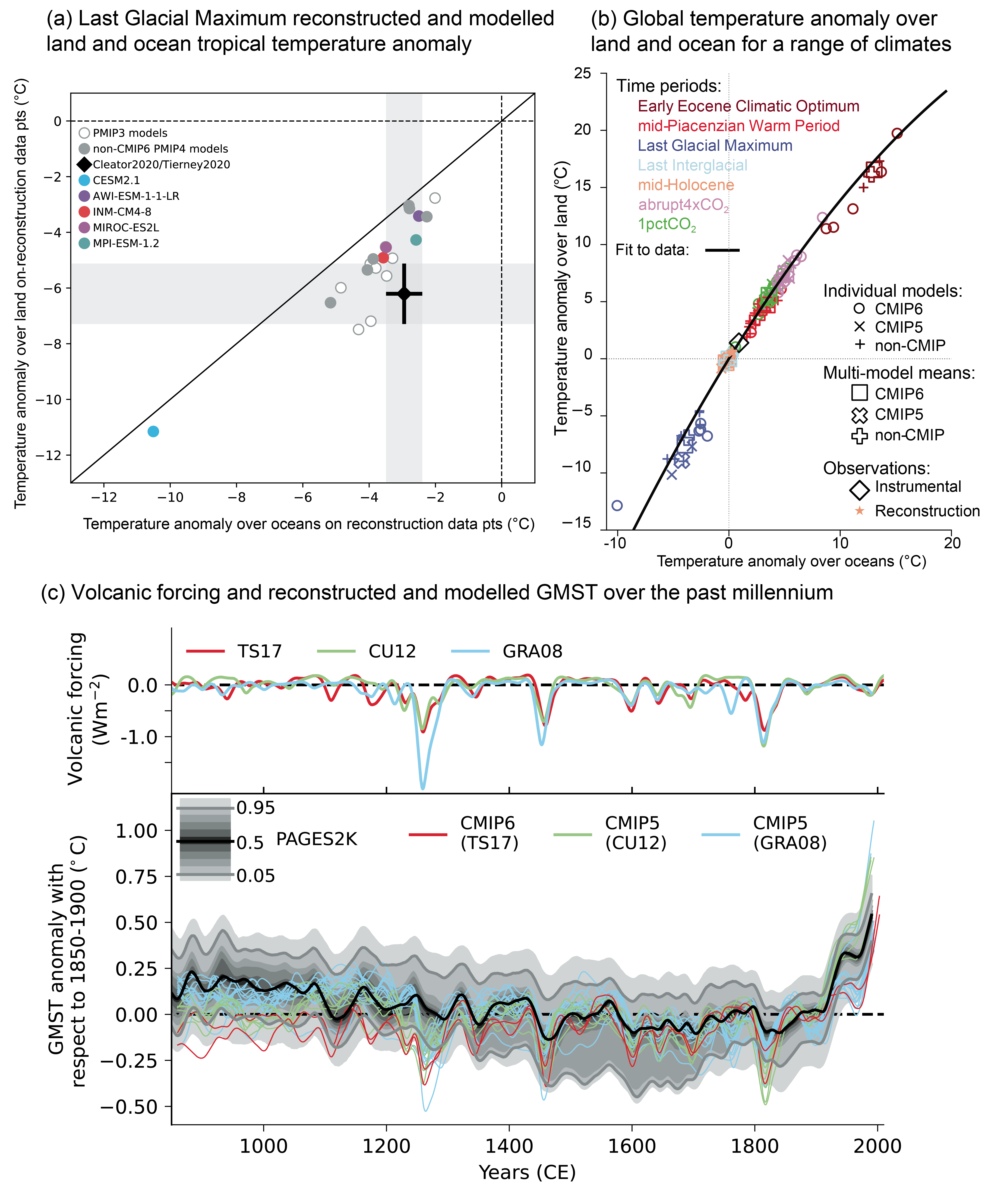
Reconstructions of past temperature from paleoclimate proxies (Section 2.3.1.1 and Cross-Chapter Box 2.1) have been used to evaluate modelled past climate temperature change patterns. The AR5 found that CMIP5 (Taylor et al., 2012) models were able to reproduce the large-scale patterns of temperature during the Last Glacial Maximum (LGM) (Flato et al., 2013) and simulated a polar amplification broadly consistent with reconstructions for warm (Pliocene and Eocene) and cold (LGM) periods (Masson-Delmotte et al., 2013). Since AR5, a better understanding of temperature proxies and their uncertainties and in some cases the forcing applied to model simulations has led to better agreement between models and reconstructions over a wide range of past climates. For the Pliocene and Eocene warm periods, understanding of uncertainties in temperature proxies (Hollis et al., 2019; McClymont et al., 2020) and the boundary conditions used in climate simulations (Haywood et al., 2016; Lunt et al., 2017) has improved, and some models now agree better with temperature proxies for these time periods compared to models assessed in AR5 (Sections 7.4.4.1.2, 7.4.4.2.2 and Cross-Chapter Box 2.4; Zhu et al., 2019; Haywood et al., 2020; Lunt et al., 2021). For the Last Interglacial (LIG), improved temporal resolution of temperature proxies (Capron et al., 2017) and better appreciation of the importance of freshwater forcing (Stone et al., 2016) have clarified the reasons behind apparent model-data inconsistencies. Regional LIG temperature responses simulated by CMIP6 are within the uncertainty ranges of reconstructed temperature responses, except in regions where unresolved changes in regional ocean circulation, meltwater, or vegetation changes may cause model mismatches (Otto-Bliesner et al., 2021). For the LGM, the CMIP5 and CMIP6 ensembles compare similarly to new sea surface temperature (SST) and surface air temperature (SAT) proxy reconstructions (Figure 3.2a; Cleator et al., 2020; Tierney et al., 2020b). The very cold CMIP6 LGM simulation by the Community Earth System Model Version 2.1 (CESM2.1) is an exception related to the high equilibrium climate sensitivity (ECS) of that model (Section 7.5.6; Kageyama et al., 2021a; Zhu et al., 2021). Figure 3.2a illustrates the wide range of simulated global LGM temperature responses in both ensembles. CMIP6 models tend to underestimate the cooling over land, but agree better with oceanic reconstructions. For the mid-Holocene, the regional biases found in CMIP5 simulations are similar to those in pre-industrial and historical simulations (Harrison et al., 2015; Ackerley et al., 2017), suggesting common causes. CMIP5 models underestimate Arctic warming in the mid-Holocene (Yoshimori and Suzuki, 2019). CMIP6 models simulate a mid-latitude, subtropical, and tropical cooling compared to the pre-industrial period, whereas temperature proxies indicate a warming (see Section 2.3.1.1.2; Brierley et al., 2020; Kaufman et al., 2020), although accounting for seasonal effects in the proxies may reduce the discrepancy (Bova et al., 2021). Over the past millennium, reconstructed and simulated temperature anomalies, internal variability, and forced response agree well over Northern Hemisphere continents, but those statistics disagree strongly in the Southern Hemisphere, where models seem to overestimate the response (PAGES 2k-PMIP3 group, 2015). That disagreement is partly explained by the lower quality of the reconstructions in the Southern Hemisphere, but model and/or forcing errors may also contribute (Neukom et al., 2018). Figure 3.2b shows that land/sea warming contrast behaves coherently in model simulations across multiple periods, with a slight non-linearity in land warming due to a smaller contribution of snow cover to temperature response in warmer climates. A multivariate assessment of paleoclimate model simulations is carried out in Section 3.8.2.

For the historical period, AR5 assessed with very high confidence that CMIP5 models reproduced observed large-scale mean surface temperature patterns, although errors of several degrees appear in elevated regions, like the Himalayas and Antarctica, near the edge of the sea ice in the North Atlantic, and in upwelling regions. This assessment is updated here for the CMIP6 simulations. Figure 3.3 shows the annual mean surface air temperature at 2 m for the CMIP5 and CMIP6 multi-model means, both compared to the fifth generation European Centre for Medium-Range Weather Forecasts (ECMWF) atmospheric reanalysis (ERA5; Section 1.5.2) for the period 1995–2014. The distribution of biases is similar in CMIP5 and CMIP6 models, as already noted by several studies (Crueger et al., 2018; Găinuşă-Bogdan et al., 2018; Kuhlbrodt et al., 2018; Lauer et al., 2018). Arctic temperature biases seem more widespread in both ensembles than assessed at the time of AR5. The fundamental causes of temperature biases remain elusive, with errors in clouds (Lauer et al., 2018), ocean circulation (Kuhlbrodt et al., 2018), winds (Lauer et al., 2018), and surface energy budget (Hourdin et al., 2015; Séférian et al., 2016; Găinuşă-Bogdan et al., 2018) being frequently cited candidates. Increasing horizontal resolution shows promise for decreasing long-standing biases in surface temperature over large regions (Bock et al., 2020). Panels e and f of Figure 3.3 show that biases in the mean High-Resolution Model Intercomparison Project (HighResMIP, Haarsma et al., 2016) models (see also Table AII.6) are smaller than those in the mean of the corresponding lower-resolution versions of the same models simulating the same period (see also (Section 3.8.2.2). However, the bias reduction is modest (Palmer and Stevens, 2019). In addition, the biases of the limited number of models participating in HighResMIP are not entirely representative of overall CMIP6 biases, especially in the Southern Ocean, as indicated by comparing panels b and f of Figure 3.3.
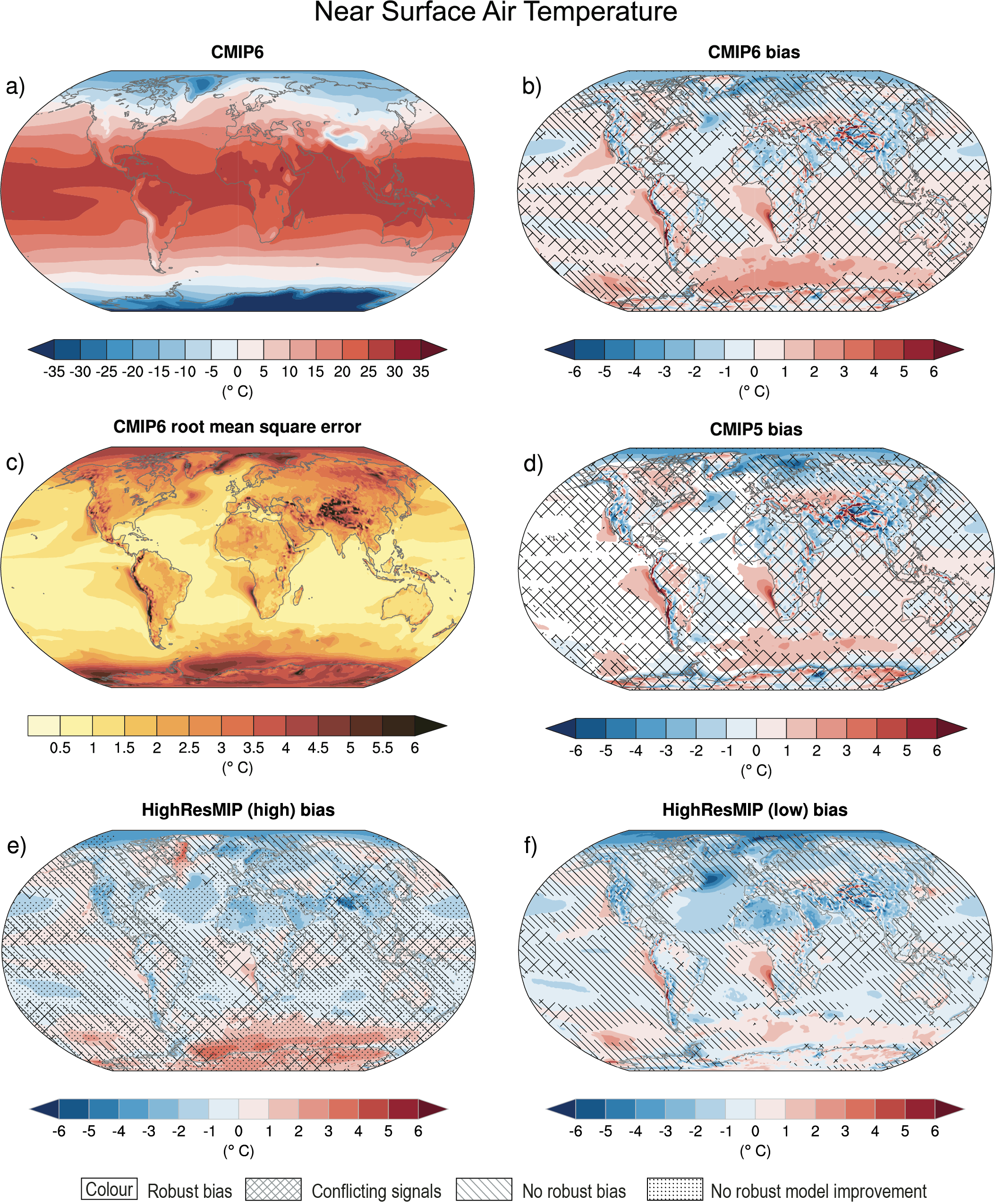 Figure 3.3 | Annual mean near-surface (2 m) air temperature (°C) for the period 1995–2014. (a) Multi-model (ensemble) mean constructed with one realization of the CMIP6 historical experiment from each model. (b) Multi-model mean bias, defined as the difference between the CMIP6 multi-model mean and the climatology of the fifth generation European Centre for Medium-Range Weather Forecasts (ECMWF) atmospheric reanalysis of the global climate (ERA5). (c) Multi-model mean of the root mean square error calculated over all months separately and averaged, with respect to the climatology from ERA5. (d) Multi-model mean bias defined as the difference between the CMIP6 multi-model mean and the climatology from ERA5. The difference between the multi-model mean of (e) high-resolution and (f) low-resolution simulations of four HighResMIP models and the climatology from ERA5 is also shown. Uncertainty is represented using the advanced approach: No overlay indicates regions with robust signal, where ≥66% of models show change greater than the variability threshold and ≥80% of all models agree on sign of change; diagonal lines indicate regions with no change or no robust signal, where <66% of models show a change greater than the variability threshold; crossed lines indicate regions with conflicting signal, where ≥66% of models show change greater than the variability threshold and <80% of all models agree on sign of change. For more information on the advanced approach, please refer to Cross-Chapter Box Atlas.1. Dots in panel (e) mark areas where the bias in high resolution versions of the HighResMIP models is not lower in at least three out of four models than in the corresponding low-resolution versions. Further details on data sources and processing are available in the chapter data table (Table 3.SM.1).
 The AR5 assessed with very high confidence that models reproduce the general history of the increase in global-scale annual mean surface temperature since the year 1850, although AR5 also reported that an observed reduction in the rate of warming over the period 1998–2012 was not reproduced by the models (Cross-Chapter Box 3.1; Flato et al., 2013). Figure 3.2c and Figure 3.4 show time series of anomalies in annually and globally averaged surface temperature simulated by CMIP5 and CMIP6 models for the past millennium and the period 1850 to 2020, respectively, with the baseline set to 1850–1900 (see Section 1.4.1). As also indicated by Figure 3.4, the spread in simulated absolute temperatures is large (Palmer and Stevens, 2019). However, the discussion is based on temperature anomaly time series instead of absolute temperatures because our focus is on evaluation of the simulation of climate change in these models, and also because anomalies are more uniformly distributed and are more easily deseasonalized to isolate long-term trends (see Section 1.4.1). CMIP6 models broadly reproduce surface temperature variations over the past millennium, including the cooling that follows periods of intense volcanism (medium confidence) (Figure 3.2c). Simulated GMST anomalies are well within the uncertainty range of temperature reconstructions (medium confidence) since about the year 1300, except for some short periods immediately following large volcanic eruptions, for which simulations driven by different forcing datasets disagree (Figure 3.2c). Before the year 1300, larger disagreements between models and temperature reconstructions are expected because forcing and temperature reconstructions are increasingly uncertain further back in time, but specific causes have not been identified conclusively (Ljungqvist et al., 2019; PAGES 2k Consortium, 2019) (medium confidence). For the historical period, results for CMIP6 shown in Figure 3.4 suggest that the qualitative history of surface temperature increase is well reproduced, including the increase in warming rates beginning in the 1960s and the temporary cooling that follows large volcanic eruptions.
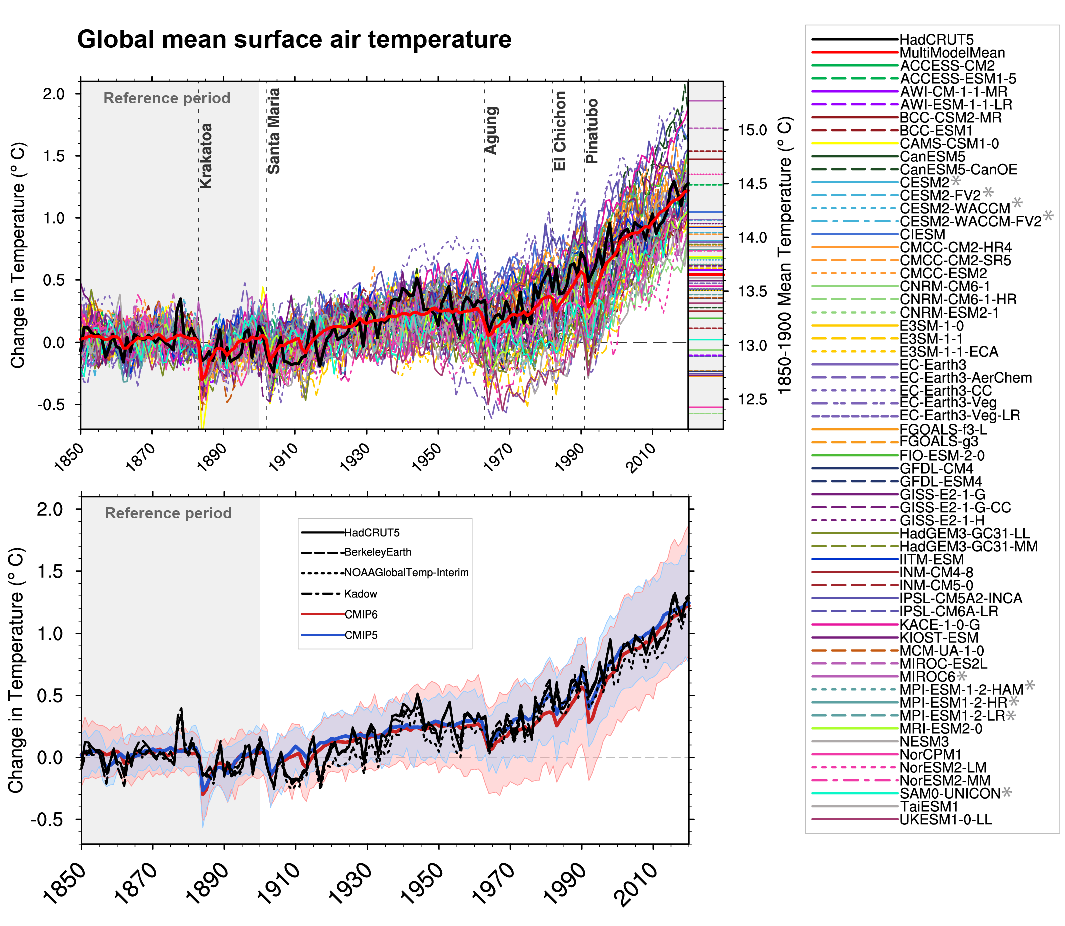
 Figure 3.4 | Observed and simulated time series of the anomalies in annual and global mean surface air temperature (GSAT). All anomalies are differences from the 1850–1900 time-mean of each individual time series. The reference period 1850–1900 is indicated by grey shading. (a) Single simulations from CMIP6 models (thin lines) and the multi-model mean (thick red line). Observational data (thick black lines) are from the Met Office Hadley Centre/Climatic Research Unit dataset (HadCRUT5), and are blended surface temperature (2 m air temperature over land and sea surface temperature over the ocean). All models have been subsampled using the HadCRUT5 observational data mask. Vertical lines indicate large historical volcanic eruptions. CMIP6 models which are marked with an asterisk are either tuned to reproduce observed warming directly, or indirectly by tuning equilibrium climate sensitivity. Inset: GSAT for each model over the reference period, not masked to any observations. (b) Multi-model means of CMIP5 (blue line) and CMIP6 (red line) ensembles and associated 5th to 95th percentile ranges (shaded regions). Observational data are HadCRUT5, Berkeley Earth, National Oceanic and Atmospheric Administration NOAAGlobalTemp-Interim and Kadow et al. (2020). Masking was done as in (a). CMIP6 historical simulations were extended with SSP2-4.5 simulations for the period 2015–2020 and CMIP5 simulations were extended with RCP4.5 simulations for the period 2006–2020. All available ensemble members were used (see Section 3.2). The multi-model means and percentiles were calculated solely from simulations available for the whole time span (1850–2020). Figure is updated from Bock et al. (2020), their Figures 1 and 2. CC BY 4.0https://creativecommons.org/licenses/by/4.0/. Further details on data sources and processing are available in the chapter data table (Table 3.SM.1).
 Although virtually all CMIP6 modelling groups report improvements in their model’s ability to simulate current climate compared to the CMIP5 version (Gettelman et al., 2019; Golaz et al., 2019; Mauritsen et al., 2019; Swart et al., 2019; Voldoire et al., 2019b; T. Wu et al., 2019b; Bock et al., 2020; Boucher et al., 2020; Dunne et al., 2020), it does not necessarily follow that the simulation of temperature trends is also improved (Bock et al., 2020; Fasullo et al., 2020). The CMIP6 multi-model ensemble encompasses observed warming and the multi-model mean tracks those observations within 0.2°C over most of the historical period. Figure 3.4 confirms the findings of Papalexiou et al. (2020), who highlighted based on 29 CMIP6 models that most models replicate the period of slow warming between 1942 and 1975 and the late twentieth century warming (1975–2014). The CMIP6 multi-model mean is cooler over the period 1980–2000 than both observations and CMIP5 (Figure 3.4; Bock et al., 2020; Flynn and Mauritsen, 2020; Gillett et al., 2021). Biases of several tenths of a degree in some CMIP6 models over that period may be due to an overestimate in aerosol radiative forcing (Sections 6.3.5 and 7.3.3, and Figure 6.8; Andrews et al., 2020; Dittus et al., 2020; Flynn and Mauritsen, 2020). Papalexiou et al. (2020), Tokarska et al. (2020) and Stolpe et al. (2021) all report that CMIP6 models on average overestimate warming from the 1970s or 1980s to the 2010s, although quantitative conclusions depend on which observational dataset is compared against (see also Table 2.4). However, Figure 3.4, which includes a larger number of models than available to those studies, indicates that the CMIP6 multi-model mean tracks observed warming better than the CMIP5 multi-model mean after the year 2000. The CMIP6 multi-model mean GSAT warming between 1850–1900 and 2010–2019 and associated 5–95% range is 1.09 [0.66 to 1.64] °C. Cross-Chapter Box 2.3 assessed GSAT warming over the same period at 1.06 [0.88 to 1.21] °C. So some CMIP6 models simulate a warming that is smaller than the assessed observed range, and other CMIP6 models simulate a warming that is larger. That overestimated warming may be an early symptom of overestimated ECS in some CMIP6 models (Section 7.5.6; Meehl et al., 2020; Schlund et al., 2020), and has implications for projections of GSAT changes (Chapter 4; Liang et al., 2020; Nijsse et al., 2020; Tokarska et al., 2020; Ribes et al., 2021). In some models, a large ECS and a strong aerosol forcing lead to too large a mid-20th century cooling followed by overestimated warming rates in the late 20th century when aerosol emissions decrease (Golaz et al., 2019; Flynn and Mauritsen, 2020). Temperature biases are driven by both model physics and prescribed forcing, which is a challenge for model development.
Chylek et al. (2020) argue that CMIP5 models overestimate the temperature response to volcanic eruptions. Lehner et al. (2016), Rypdal (2018) and Stolpe et al. (2021) point instead to missed compensating effects on surface temperature change associated with internal variability in the El Niño–Southern Oscillation (ENSO) or the Atlantic Multi-decadal Oscillation (AMO). An alternative view sees those ENSO and AMO responses as expressions of changes in climate feedbacks driven by the geographical pattern of SST changes (Andrews et al., 2018). At least one model is able to reproduce such pattern effects (Gregory and Andrews, 2016). Errors in the volcanic forcing prescribed in simulations, including for CMIP6 (Rieger et al., 2020), also introduce differences with the observed temperature response, independently of the quality of the model physics. In addition, comparisons of the modelled temperature response to large eruptions over the past millennium to temperature reconstructions based on tree rings show a much better agreement (Lücke et al., 2019; F. Zhu et al., 2020) than comparisons to the annual, multi-temperature proxy reconstructions shown in Figure 3.2c. These considerations, and Figures 3.2c and 3.4, suggest that CMIP6 models do not systematically overestimate the cooling that follows large volcanic eruptions (see also Cross-Chapter Box 4.1).
When interpreting model simulations of historical temperature change, it is important to keep in mind that some models are tuned towards representing the observed trend in global mean surface temperature over the historical period (Hourdin et al., 2017). In Figure 3.4 the CMIP6 models that are documented to have been tuned to reproduce observed warming, typically by tuning aerosol forcing or factors that influence the model’s ECS, are marked with an asterisk. Such tuning of a model can strongly impact its temperature projections (Mauritsen and Roeckner, 2020). However, Bock et al. (2020) reported that there is no statistically significant difference in multi-model mean GSAT between the models that had been tuned based on observed warming compared to those which had not. Moreover, only two of thirteen models used for the Detection and Attribution Model Intercomparison Project (DAMIP) simulations on which CMIP6 attribution studies are based were tuned towards historical warming (Bock et al., 2020; Gillett et al., 2021). Further, tuning is done on globally averaged quantities, so does not substantially change the spatio-temporal pattern of response on which many regression-based attribution studies are based (Bock et al., 2020). Therefore, we assess with high confidence that the tuning of a small number of CMIP6 models to observed warming has not substantially influenced attribution results assessed in this chapter.
The reliance of detection and attribution studies on climate models (see Section 3.2) requires that those models simulate realistic statistics of internal variability on multi-decadal time scales. An incorrect estimate of variability in models would affect confidence in the conclusions from detection and attribution. The AR5 found that CMIP5 models simulate realistic variability in global-mean surface temperature on decadal time scales, with variability on multi-decadal time scales being more difficult to evaluate because of the short observational record (Flato et al., 2013). Since AR5, new work has characterized the contributions of variability in different ocean areas to SST variability, with tropical modes of variability like ENSO dominant on time scales of five to ten years, while longer time scales see the variance maxima move poleward to the North Atlantic, North Pacific, and Southern oceans (Monselesan et al., 2015). There may, however, be sizeable, two-way interdependencies between ENSO and sea surface temperature variability in different basins (Kumar et al., 2014; Cai et al., 2019), and ENSO’s influence on global surface temperature variability may not be confined only to decadal time scales (Triacca et al., 2014). Studies based on large ensembles of 20th and 21st century climate change simulations confirm that internal variability has a substantial influence on global warming trends over periods shorter than 30–40 years (Kay et al., 2015; Dai and Bloecker, 2019). Although the equatorial Pacific seems to be the main source of internal variability on decadal time scales, Brown et al. (2016a) linked diversity in modelled oceanic convection, sea ice, and energy budget in high-latitude regions to overall diversity in modelled internal variability.
Interest in internal variability since the publication of AR5 stems in part from its importance in understanding the slower global surface temperature warming over the early 21st century (see Cross-Chapter Box 3.1). Evidence coming mostly from paleo studies is mixed on whether CMIP5 models underestimate decadal and multi-decadal variability in global mean temperature. Schurer et al. (2013) found good agreement between internal variability derived from paleo reconstructions, estimated as the fraction of variance that is not explained by forced responses, and modelled variability, although the subset of CMIP5 models they used may have been associated with larger variability than the full CMIP5 ensemble. PAGES 2k Consortium (2019) found that the largest 51-year trends in both reconstructions of global mean temperature and fully forced climate simulations over the period 850 to 1850 were almost identical. Zhu et al. (2019) showed agreement in the modelled and reconstructed temporal spectrum of global surface temperatures on annual to multi-millennial time scales. However, they suggest that decadal- to centennial variability is partly forced by slow orbital changes that predate the last millennium. This is consistent with Gebbie and Huybers (2019), who showed that the deep ocean has been out of equilibrium over that period. Laepple and Huybers (2014) found good agreement between modelled and proxy-derived decadal ocean temperature variability, but underestimates of variance by models by at least a factor of ten at centennial time scales because models underestimate the difference between the warm and cold periods of the last millennium. Parsons et al. (2020) found that some CMIP6 models exhibit much higher multi-decadal variability in GSAT than CMIP5 models, with indications that variability in these models is also higher than that from proxy reconstructions. CMIP6 models may not share the underestimation by CMIP5 models of variability in decadal to multi-decadal modes of variability, such as Pacific Decadal Variability (Section 3.7.6; England et al., 2014; Thompson et al., 2014; Schurer et al., 2015) and Atlantic Multi-decadal Variability (AMV), which may be partly forced, (see Section 3.7.7) but this assessment is limited by the small number of available studies. For the Southern Hemisphere, Hegerl et al. (2018) found an instance of internal variability in the early 20th century larger than that modelled, but indicated that could be an observational issue. Friedman et al. (2020) found biases in interhemispheric SST contrast in some models that may be consistent with underestimated cooling after early-20th century eruptions or underestimated Pacific Decadal Variability, but could also be due to an imperfect separation between internal variability and forced signal in the observations. Figure 3.2c, updated from PAGES 2k Consortium (2019), compares modelled temperatures to reconstructions over the last millennium. It indicates that models reproduce the observed variability well, at least for the time scales between 20 and 50 years that paleo reconstructions typically resolve and that the figure represents. In summary, decadal GMST variability simulated in CMIP6 models spans the range of residual decadal variability in large-scale reconstructions (medium evidence, low agreement).
In addition, new literature suggests that anthropogenic forcing itself may locally increase or decrease variability in surface temperatures (Screen et al., 2014; Qian and Zhang, 2015; Brown et al., 2017; Park et al., 2018; Santer et al., 2018; Weller et al., 2020). These studies imply limitations in the use of pre-industrial control simulations to quantify the role of unforced variability over the historical period. Some recent attribution studies (Gillett et al., 2021; Ribes et al., 2021) have estimated variability from ensembles of forced simulations instead, which would be expected to resolve any such changes in variability.
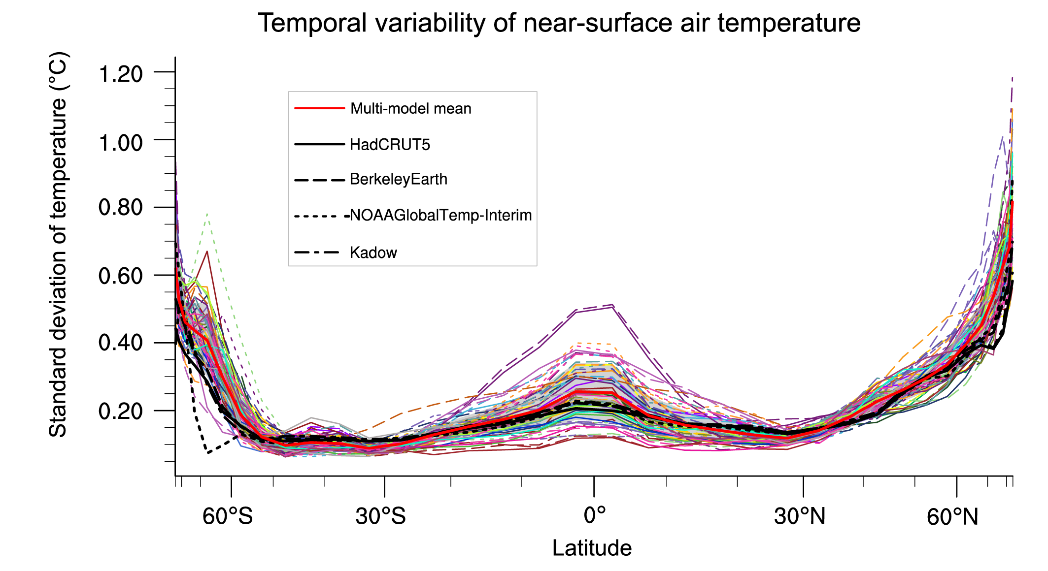
Figure 3.5 shows the standard deviation of zonal-mean surface temperature in CMIP6 pre-industrial control simulations and observed temperature datasets. Results are consistent with those based on CMIP5 models, which showed the largest model spread where variability is also large, in the tropics and mid- to high latitudes (Flato et al., 2013). Modelled variability is within a factor two of observed variability over most of the globe. The apparent overestimation of high latitude variability in models compared to observations may be due to interpolation and infilling over data sparse high latitude regions in the observational products shown here (Jones, 2016).
 Figure 3.5 | The standard deviation of annually averaged zonal-mean near-surface air temperature. This is shown for four detrended observed temperature datasets (HadCRUT5, Berkeley Earth, NOAAGlobalTemp-Interim and Kadow et al. (2020), for the years 1995-2014) and 59 CMIP6 pre-industrial control simulations (one ensemble member per model, 65 years) (after Jones et al., 2013). For line colours see the legend of Figure 3.4. Additionally, the multi-model mean (red) and standard deviation (grey shading) are shown. Observational and model datasets were detrended by removing the least-squares quadratic trend. Further details on data sources and processing are available in the chapter data table (Table 3.SM.1).
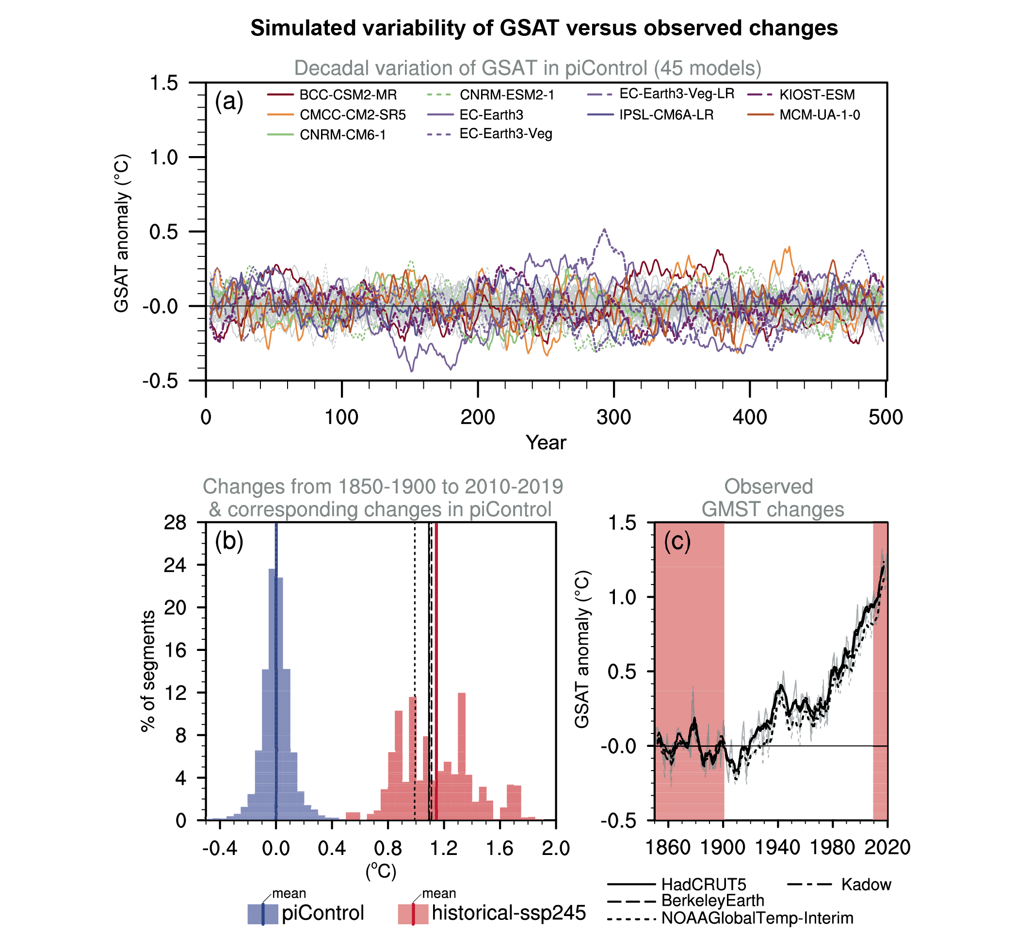
 The previous paragraph took an ensemble-mean view of model performance, but individual models disagree on unforced variability. Figure 3.6 illustrates the large differences in GSAT variability in unforced CMIP6 pre-industrial control simulations, following the method of Parsons et al. (2020). Surface temperatures in pre-industrial conditions are especially variable in the ten models highlighted in Figure 3.6a, and some models substantially exceed the variability seen in CMIP5 models (Parsons et al., 2020). Figure 3.6b shows that the distribution of warming trends simulated by CMIP6 models in historical simulations is clearly distinct from that simulated in unforced pre-industrial control simulations. Still, the unforced variability of the five most variable models approaches half that observed over the historical period under anthropogenically forced conditions (Figure 3.6c; Parsons et al., 2020; Ribes et al., 2021). For the Centre National de la Recherche Météorologique (CNRM) models, which are among the most variable, the large, low-frequency variability is attributed to strong simulated Atlantic Multi-decadal Variability (Séférian et al., 2019; Voldoire et al., 2019b), which is difficult to rule out because of the short observational record (Section 3.7.7; Cassou et al., 2018). But, importantly, patterns of temperature variability simulated by even the most variable models differ from the pattern of forced temperature change (Parsons et al., 2020). Taken together, this discussion and Figures 3.2, 3.5 and 3.6 indicate that the statistics of internal variability in models compare well in most cases to observational estimates and temperature proxy reconstructions, though some CMIP6 models appear to have higher multi-decadal variability than CMIP5 models or proxy reconstructions. When used in attribution studies, models with overestimated variability would increase estimated uncertainties and make results statistically conservative.
 Figure 3.6 | Simulated internal variability of global surface air temperature (GSAT) versus observed changes. (a) Time series of five-year running mean GSAT anomalies in 45 CMIP6 pre-industrial control (unforced) simulations. The 10 most variable models in terms of five-year running mean GSAT are coloured according to the legend on Figure 3.4. (b) Histograms of GSAT changes in CMIP6 historical simulations (extended by using SSP2-4.5 simulations) from 1850–1900 to 2010–2019 are shown by pink shading in (c), and GSAT changes between the average of the first 51 years and the average of the last 20 years of 170-year overlapping segments of the pre-industrial control simulations shown in (a) are shown by blue shading. GMST changes in observational datasets for the same period are indicated by black vertical lines. (c) Observed GMST anomaly time series relative to the 1850–1900 average. Black lines represent the five-year running means while grey lines show unfiltered annual time series. Further details on data sources and processing are available in the chapter data table (Table 3.SM.1).
 In summary, there is high confidence that CMIP6 models reproduce observed large-scale mean surface temperature patterns and internal variability as well as their CMIP5 predecessors, but with little evidence for reduced biases. CMIP6 models also reproduce historical GSAT changes similarly to their CMIP5 counterparts (medium confidence). However, in spite of model imperfections, there is very high confidence that biases in surface temperature trends and variability simulated by the CMIP5 and CMIP6 ensembles are small enough to support detection and attribution of human-induced warming.
3.3.1.1.2 Detection and attribution
Looking at periods preceding the instrumental record, AR5 assessed with high confidence that the 20th century annual mean surface temperature warming reversed a 5000-year cooling trend in Northern Hemisphere mid- to high latitudes caused by orbital forcing, and attributed the reversal to anthropogenic forcing with high confidence (see also (Section 2.3.1.1). Since AR5, the combined response to solar, volcanic and greenhouse gas forcing was detected in all Northern Hemisphere continents (PAGES 2k-PMIP3 group, 2015) over the period 864 to 1840. In contrast, the effect of those forcings was not detectable in the Southern Hemisphere (Neukom et al., 2018). Global and Northern Hemisphere temperature changes from reconstructions over this period have been attributed mostly to volcanic forcing (Schurer et al., 2014; McGregor et al., 2015; Otto-Bliesner et al., 2016; PAGES 2k Consortium, 2019; Büntgen et al., 2020), with a smaller role for changes in greenhouse gas forcing, and solar forcing playing a minor role (Schurer et al., 2014; PAGES 2k Consortium, 2019).
Focusing now on warming over the historical period, AR5 assessed that it was extremely likely that human influence was the dominant cause of the observed warming since the mid-20th century, and that it was virtually certain that warming over the same period could not be explained by internal variability alone. Since AR5 many new attribution studies of changes in global surface temperature have focused on methodological advances (see also (Section 3.2). Those advances include better accounting for observational and model uncertainties, and internal variability (Ribes and Terray, 2013; Hannart, 2016; Ribes et al., 2017; Schurer et al., 2018); formulating the attribution problem in a counterfactual framework (Hannart and Naveau, 2018); and reducing the dependence of the attribution on uncertainties in climate sensitivity and forcing (Otto et al., 2015; Haustein et al., 2017, 2019). Studies now account for uncertainties in the statistics of internal variability, either explicitly (Hannart, 2016; Hannart and Naveau, 2018; Ribes et al., 2021) or implicitly (Ribes and Terray, 2013; Schurer et al., 2018; Gillett et al., 2021), thus addressing concerns about over-confident attribution conclusions. Accounting for observational uncertainty increases the range of warming attributable to greenhouse gases by only 10 to 30% (Jones and Kennedy, 2017; Schurer et al., 2018). While some attribution studies estimate attributable changes in globally-complete GSAT (Schurer et al., 2018; Gillett et al., 2021; Ribes et al., 2021), others attribute changes in observational GMST, but this makes little difference to attribution conclusions (Schurer et al., 2018). Moreover, based on a synthesis of observational and modelling evidence, Cross-Chapter Box 2.3 assesses that the current best estimate of the scaling factor between GMST and GSAT is one, and therefore attribution studies of GMST and GSAT are here treated together in deriving assessed warming ranges. Studies also increasingly validate their multi-model approaches using imperfect model tests (Schurer et al., 2018; Gillett et al., 2021; Ribes et al., 2021). Alternative techniques, based purely on statistical or econometric approaches, without the need for climate modelling, have also been applied (Estrada et al., 2013; Stern and Kaufmann, 2014; Dergiades et al., 2016) and match the results of physically-based methods. The larger range of attribution techniques and improvements to those techniques increase confidence in the results compared to AR5.
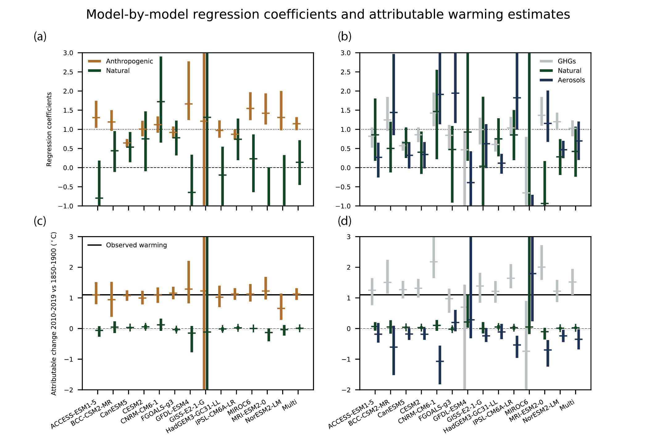
In contrast, studies published since AR5 indicate that closely constraining the separate contributions of greenhouse gas changes and aerosol changes to observed temperature changes remains challenging. Nonetheless, attribution of warming to greenhouse gas forcing has been found as early as the end of the 19th century (Schurer et al., 2014; Owens et al., 2017; PAGES 2k Consortium, 2019). Hegerl et al. (2019) found that volcanism cooled global temperatures by about 0.1°C between 1870 and 1910, then a lack of volcanic activity warmed temperatures by about 0.1°C between 1910 and 1950, with anthropogenic aerosols cooling temperatures throughout the 20th century, especially between 1950 and 1980 when the estimated range of aerosol cooling was about 0.1°C to 0.5°C. Jones et al. (2016) attributed a warming of 0.87 to 1.22°C per century over the period 1906 to 2005 to greenhouse gases, partially offset by a cooling of −0.54°C to −0.22°C per century attributed to aerosols. But they also found that detection of the greenhouse gas or the aerosol signal often fails, because of uncertainties in modelled patterns of change and internal variability. That point is illustrated by Figure 3.7, which shows two- and three-way fingerprinting regression coefficients for 13 CMIP6 models and the corresponding attributable warming ranges, derived using HadCRUT4 (Gillett et al., 2021). Regression coefficients with an uncertainty range that includes zero mean that detection has failed. Models with regression coefficients significantly less than one significantly overpredict the temperature response to the corresponding forcing. Conversely, models with regression coefficients significantly greater than one underpredict the response to these forcings. While estimates of warming attributable to anthropogenic influence derived using individual models are generally consistent, estimates of warming attributable to greenhouse gases and aerosols separately based on individual models are not all consistent, and detection of the aerosol influence fails more often than that of greenhouse gases. Hence, results of recent studies emphasize the need to use multi-model means to better constrain estimates of GSAT changes attributable to greenhouse gas and aerosol forcing (Schurer et al., 2018; Gillett et al., 2021; Ribes et al., 2021).
 Figure 3.7 | Regression coefficients and corresponding attributable warming estimates for individual CMIP6 models. Upper panels show regression coefficients based on a two-way regression (left) and three-way regression (right), of observed five-year mean, globally averaged, masked and blended surface temperature (HadCRUT4) onto individual model response patterns, and a multi-model mean, labelled ‘Multi’. Anthropogenic, natural, greenhouse gas, and other anthropogenic (aerosols, ozone, land-use change) regression coefficients are shown. Regression coefficients are the scaling factors by which the model responses must be multiplied to best match observations. Regression coefficients consistent with one indicate a consistent magnitude response in observations and models, and regression coefficients significantly greater than zero indicate a detectable response to the forcing concerned. Lower panels show corresponding observationally-constrained estimates of attributable warming in globally-complete GSAT for the period 2010–2019, relative to 1850–1900, and the horizontal black line shows an estimate of observed warming in GSAT for this period. Figure is adapted from Gillett et al. (2021), their Extended Data Figure 3. Further details on data sources and processing are available in the chapter data table (Table 3.SM.1).
 Figure 3.8 compares attributable changes in globally complete GSAT for the period 2010–2019 relative to 1850–1900 from three detection and attribution studies, two of which use CMIP6 multi-model means (Gillett et al., 2021; Ribes et al., 2021), and an estimate based on assessed effective radiative forcing and transient and equilibrium climate sensitivity (see Section 7.3.5.3). The reference period 1850–1900 is used to assess attributable temperature changes because this is when the earliest gridded surface temperature records start, this is when the CMIP6 historical simulations start, this is the earliest base period used in attribution literature, and this is a reference period used in IPCC SR1.5 and earlier reports. It should, however, be noted that Cross-Chapter Box 1.2 assesses with medium confidence that there was an anthropogenic warming with a likely range of 0.0°C–0.2°C between 1750 and 1850–1900. Figure 3.8 also shows the GSAT changes directly simulated in response to these forcings in thirteen CMIP6 models. In spite of their different methodologies and input datasets, the three attribution approaches yield very similar results, with the anthropogenic attributable warming range encompassing observed warming, and the natural attributable warming being close to zero. The warming driven by greenhouse gas increases is offset in part by cooling due to other anthropogenic forcing agents, mostly aerosols, although uncertainties in these contributions are larger than the uncertainty in the net anthropogenic warming, as discussed above. Estimates based on physical understanding of forcing and ECS made by (Chapter 7 are close to estimates from attribution studies, despite being the products of a different approach. This agreement enhances confidence in the magnitude and causes of attributable surface temperature warming.
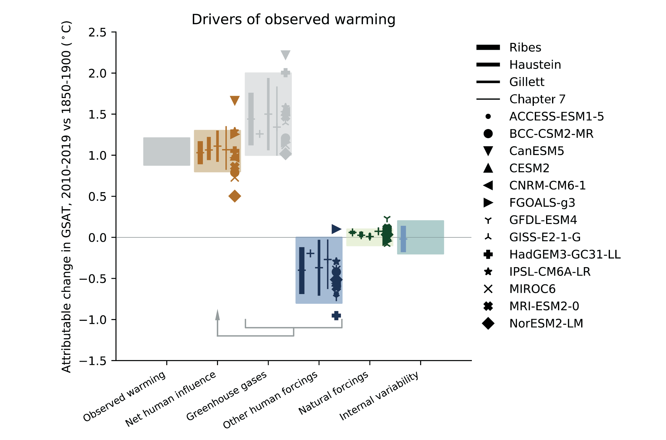 Figure 3.8 | Assessed contributions to observed warming, and supporting lines of evidence. Shaded bands show assessed likely ranges of temperature change in GSAT, 2010–2019 relative to 1850–1900, attributable to net human influence, well-mixed greenhouse gases, other human forcings (aerosols, ozone, and land-use change), natural forcings, and internal variability, and the 5–95% range of observed warming. Bars show 5–95% ranges based on (left to right) Haustein et al. (2017), Gillett et al. (2021) and Ribes et al. (2021), and crosses show the associated best estimates. No 5–95% ranges were provided for the Haustein et al. (2017) greenhouse gas or other human forcings contributions. The Ribes et al. (2021) results were updated using a revised natural forcing time series, and the Haustein et al. (2017) results were updated using HadCRUT5. The (Chapter 7 best estimates and ranges were derived using assessed forcing time series and a two-layer energy balance model as described in Section 7.3.5.3. Coloured symbols show the simulated responses to the forcings concerned in each of the models indicated. Further details on data sources and processing are available in the chapter data table (Table 3.SM.1).
 The AR5 found high confidence for a major role for anthropogenic forcing in driving warming over each of the inhabited continents, except for Africa where they found only medium confidence because of limited data availability (Bindoff et al., 2013). At the hemispheric scale, Friedman et al. (2020) and Bonfils et al. (2020) detected an anthropogenically forced response of inter-hemispheric contrast in surface temperature change, which has a complex time evolution but shows the Northern Hemisphere cooling relative to the Southern Hemisphere until around 1975 but then warming after that. Bonfils et al. (2020) attribute the Northern Hemisphere reversal to a combination of reduced aerosol forcing and greenhouse gas induced warming of Northern Hemisphere land masses. Friedman et al. (2020) found that CMIP5 models simulate the correct sign of the inter-hemispheric contrast when forced with all forcings but underestimate its magnitude. Figure 3.9 shows global surface temperature change in CMIP6 all-forcing and natural-only simulations globally, averaged over continents, and separately over land and ocean surfaces. All-forcing simulations encompass observed temperature changes for all regions, while natural-only simulations fail to do so in recent decades except in Antarctica, based on the annual means shown. As stated above, warming results from a partial offset of greenhouse gas warming by aerosol cooling. That offset is stronger over land than ocean. Regionally, models show a large range of possible temperature responses to greenhouse gas and aerosol forcing, which complicates single-forcing attribution. A more detailed discussion of regional attribution can be found in Section 10.4. Over global land surfaces, Chan and Wu (2015) used CMIP5 simulations to attribute a warming trend of 0.3 (2.5%–97.5% confidence interval: 0.2–0.36) °C per decade to anthropogenic forcing, with natural forcing only contributing 0.05 (0.02–0.06) °C per decade. Accounting for unsampled sources of uncertainty and the availability of only a single study, their result suggests that it is very likely that human influence is the main driver of warming over land.
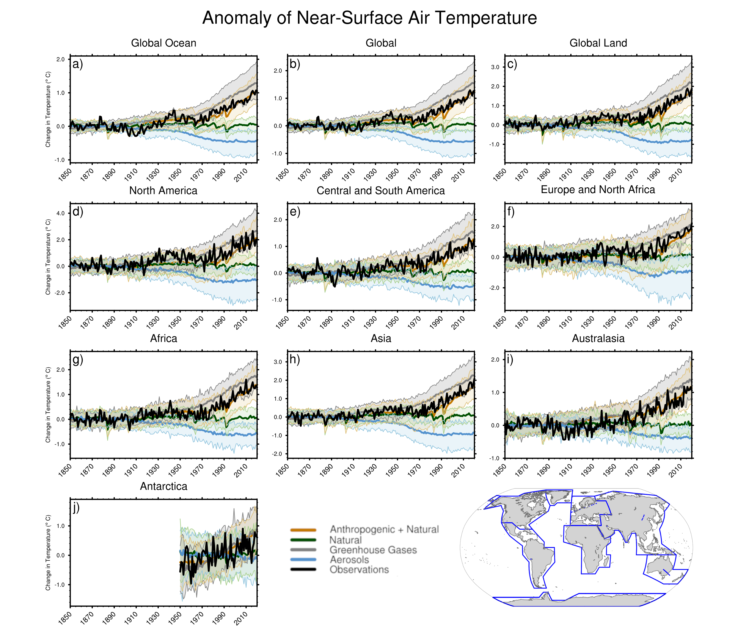 Figure 3.9 | Global, land, ocean and continental annual mean near-surface air temperatures anomalies in CMIP6 models and observations. Time series are shown for CMIP6 historical anthropogenic and natural (brown), natural-only (green), greenhouse gas only (grey) and aerosol only (blue) simulations (thick lines show multi-model means and shaded regions show the 5th to 95th percentile ranges) and for HadCRUT5 (black). All models have been subsampled using the HadCRUT5 observational data mask. Temperature anomalies are shown relative to 1950–2010 for Antarctica and relative to 1850–1900 for other continents. CMIP6 historical simulations are extended using the SSP2-4.5 scenario simulations. All available ensemble members were used (see Section 3.2). Regions are defined by Iturbide et al. (2020). Further details on data sources and processing are available in the chapter data table (Table 3.SM.1).
 In summary, since the publication of AR5, new literature has emerged that better accounts for methodological and climate model uncertainties in attribution studies (Ribes et al., 2017; Hannart and Naveau, 2018) and that concludes that anthropogenic warming is approximately equal to observed warming over the 1951–2010 period. The IPCC SR1.5 reached the same conclusion for 2017 relative to 1850–1900 based on anthropogenic warming and associated uncertainties calculated using the method of Haustein et al. (2017). Moreover, the improved understanding of the causes of the apparent slowdown in warming over the beginning of the 21st century and the difference in simulated and observed warming trends over this period (Cross-Chapter Box 3.1) further improve our confidence in the assessment of the dominant anthropogenic contribution to observed warming. In deriving our assessments, these considerations are balanced against new literature that raises questions about the ability of some models to simulate variability in surface temperatures over a range of time scales (Laepple and Huybers, 2014; Parsons et al., 2017; Friedman et al., 2020), and the finding that some CMIP6 models exhibit substantially higher multi-decadal internal variability than that seen in CMIP5, which remains to be fully understood (Parsons et al., 2020; Ribes et al., 2021). Further, uncertainties in simulated aerosol-cloud interactions are still large (Section 7.3.3.2.2), resulting in very diverse spatial responses of different climate models to aerosol forcing, and inter-model differences in the historical global mean temperature evolution and in diagnosed cooling attributable to aerosols (Figure 3.8). Moreover, like previous generations of coupled model simulations, historical and single forcing CMIP6 simulations follow a common experimental design (Eyring et al., 2016a; Gillett et al., 2016) and are thus all driven by the same common set of forcings, even though these forcings are uncertain. Hence, forcing uncertainty is not directly accounted for in most of the attribution and model evaluation studies assessed here, although this limitation can to some extent be addressed by comparing with previous generation multi-model ensembles or individual model studies using different sets of forcings.
The IPCC SR1.5 best estimate and likely range of anthropogenic attributable GMST warming was 1.0 ± 0.2°C in 2017 with respect to the period 1850–1900. Here, the best estimate is expressed in terms of GSAT and is calculated as the average of the three estimates shown in Figure 3.9, yielding a value of 1.07°C. Ranges for attributable GSAT warming are derived by finding the smallest ranges with a precision of 0.1°C which span all of the 5–95% ranges from the attribution studies shown in Figure 3.9. These ranges are then assessed as likely rather than very likely because the studies may underestimate the importance of the structural limitations of climate models, which probably do not represent all possible sources of internal variability; use too simple climate models, which may underestimate the role of internal variability; or underestimate model uncertainty, especially when using model ensembles of limited size and inter-dependent models, for example through common errors in forcings across models, as discussed above. This leads to a likely range for anthropogenic attributable warming in 2010–2019 relative to 1850–1900 of 0.8 to 1.3°C in terms of GSAT. This range encompasses the best estimate and very likely range of observed GSAT warming of 1.06 [0.88 to 1.21] °C over the same period (Cross-Chapter Box 2.3). There is medium confidence that the best estimate and likely ranges of attributable warming expressed in terms of GMST are equal to those for GSAT (Cross-Chapter Box 2.3). Repeating the process for other time periods leads to the best estimates and likely ranges listed in Table 3.1. GSAT change attributable to natural forcings is −0.1 to +0.1°C. The likely range of GSAT warming attributable to greenhouse gases is assessed in the same way to be 1.0 to 2.0°C while the GSAT change attributable to aerosols, ozone and land-use change is −0.8 to 0.0°C. Progress in attribution techniques allows the important advance of attributing observed surface temperature warming since 1850–1900, instead of since 1951 as was done in AR5.
1986–2005 | 1995–2014 | 2006–2015 | 2010–2019 | Warming Rate 2010–2019 | |
0.65 (0.52 to 0.77) | 0.82 (0.69 to 0.94) | 0.94 (0.8 to 1.08) | 1.03 (0.89 to 1.17) | 0.23 (0.18 to 0.29) | |
0.63 (0.32 to 0.94) | 0.84 (0.63 to 1.06) | 0.98 (0.74 to 1.22) | 1.11 (0.92 to 1.30) | 0.35 (0.30 to 0.41) | |
0.73 (0.58 to 0.82) | 0.88 (0.75 to 0.98) | 0.98 (0.87 to 1.10) | 1.06 (0.94 to 1.22) | 0.23 (0.19 to 0.35) | |
Assessment | 0.68 (0.3 to 1.0) | 0.85 (0.6 to 1.1) | 0.97 (0.7 to 1.3) | 1.07 (0.8 to 1.3) | 0.2 (0.1 to 0.3) |
The IPCC AR5 assessed the likely range of the contribution of internal variability to GMST warming to be −0.1 to +0.1°C over the period 1951–2010. Since then, several studies have downplayed the contribution of internal modes of variability to global temperature variability, often by arguing for a forced component to those internal modes (Mann et al., 2014; Folland et al., 2018; Haustein et al., 2019; Liguori et al., 2020). Haustein et al. (2017) found a 5–95% confidence interval of −0.09°C to +0.12°C for the contribution of internal variability to warming between 1850–1879 and 2017. Ribes et al. (2021) imply a contribution of internal variability of −0.02°C ± 0.16°C to warming between 2010–2019 and 1850–1900, assuming independence between errors in the observations and in the estimate of the forced response. Based on these studies, but allowing for unsampled sources of error, we assess the likely range of the contribution of internal variability to GSAT warming between 2010–2019 and 1850–1900 to be −0.2°C to +0.2°C.
The IPCC SR1.5 gave a likely range for the human-induced warming rate of 0.1°C to 0.3°C per decade in 2017, with a best estimate of 0.2°C per decade (Allen et al., 2018). Table 3.1 lists the estimates of attributable anthropogenic warming rate over the period 2010–2019 based on the three studies that underpin the assessment of GSAT warming (Haustein et al., 2017; Gillett et al., 2021; Ribes et al., 2021). Estimates from Haustein et al. (2017), based on observed warming, and Ribes et al. (2021), based on CMIP6 simulations constrained by observed warming, are in good agreement. The Gillett et al. (2021) estimate, also based on CMIP6 models, corresponds to a larger anthropogenic attributable warming rate, because of a smaller warming rate attributed to natural forcing than in Ribes et al. (2021). This disagreement does not support a decrease in uncertainty compared to the SR1.5 assessment. So the range for anthropogenic attributable surface temperature warming rate of 0.1°C to 0.3°C per decade is again assessed to be likely, with a best estimate of 0.2°C per decade.
3.3.1.2 Upper-air Temperature
(Chapter 2 assessed that the troposphere has warmed since at least the 1950s, that it is virtually certain that the stratosphere has cooled, and that there is medium confidence that the upper troposphere in the tropics has warmed faster than the near-surface since at least 2001 (Section 2.3.1.2). The AR5 assessed that anthropogenic forcings, dominated by greenhouse gases, likely contributed to the warming of the troposphere since 1961 and that anthropogenic forcings, dominated by the depletion of the ozone layer due to ozone-depleting substances, very likely contributed to the cooling of the lower stratosphere since 1979. Since AR5, understanding of observational uncertainties in the radiosonde and satellite data has improved with more available data and longer coverage, and differences between models and observations in the tropical atmosphere have been investigated further.
3.3.1.2.1 Tropospheric temperature
The AR5 assessed with low confidence that most, though not all, CMIP3 (Meehl et al., 2007) and CMIP5 (Taylor et al., 2012) models overestimated the observed warming trend in the tropical troposphere during the satellite period 1979–2012, and that a third to a half of this difference was due to an overestimate of the SST trend during this period (Flato et al., 2013). Since AR5, additional studies based on CMIP5 and CMIP6 models show that this warming bias in tropospheric temperatures remains. Recent studies have investigated the role of observational uncertainty, the model response to external forcings, the influence of the time period considered, and the role of biases in SST trends in contributing to this bias.
Several studies since AR5 have continued to demonstrate an inconsistency between simulated and observed temperature trends in the tropical troposphere, with models simulating more warming than observations (Mitchell et al., 2013, 2020; Santer et al., 2017a, b; McKitrick and Christy, 2018; Po-Chedley et al., 2021). Santer et al. (2017b) used updated and improved satellite retrievals to investigate model performance in simulating the tropical mid- to upper-troposphere trends, and removed the influence of stratospheric cooling by regression. These factors were found to reduce the size of the discrepancy in mid- to upper-tropospheric temperature trends between models and observations over the satellite era, but a discrepancy remained. Santer et al. (2017a) found that during the late 20th century, the discrepancies between simulated and satellite-derived mid- to upper-tropospheric temperature trends were consistent with internal variability, while during most of the early 21st century, simulated tropospheric warming was significantly larger than observed, which they related to systematic deficiencies in some of the external forcings used after year 2000 in the CMIP5 models. However, in CMIP6, differences between simulated and observed upper-tropospheric temperature trends persist despite updated forcing estimates (Mitchell et al., 2020). Figure 3.10 shows that CMIP6 models forced by combined anthropogenic and natural forcings overestimate temperature trends compared to radiosonde data (Haimberger et al., 2012) throughout the tropical troposphere (Mitchell et al., 2020). Over the 1979–2014 period, models are more consistent with observations in the lower troposphere, and least consistent in the upper troposphere around 200 hPa, where biases exceed 0.1°C per decade. Several studies using CMIP6 models suggest that differences in climate sensitivity may be an important factor contributing to the discrepancy between the simulated and observed tropospheric temperature trends (McKitrick and Christy, 2020; Po-Chedley et al., 2021), though it is difficult to deconvolve the influence of climate sensitivity, changes in aerosol forcing and internal variability in contributing to tropospheric warming biases (Po-Chedley et al., 2021). Another study found that the absence of a hypothesized negative tropical cloud feedback could explain half of the upper troposphere warming bias in one model (Mauritsen and Stevens, 2015).
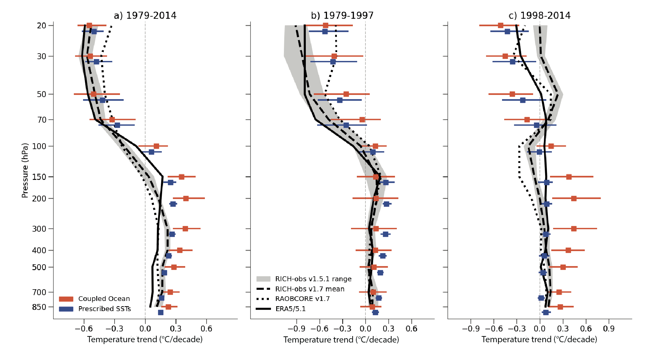 Figure 3.10 | Observed and simulated tropical mean temperature trends through the atmosphere. Vertical profiles of temperature trends in the tropics (20°S–20°N) for three periods: (a) 1979–2014, (b) 1979–1997 (ozone depletion era) and (c) 1998–2014 (ozone stabilization era). The black lines show trends in the Radiosonde Innovation Composite Homogenization (RICH) 1.7 (long dashed) and Radiosonde Observation Correction using Reanalysis (RAOBCORE) 1.7 (dashed) radiosonde datasets (Haimberger et al., 2012), and in the ERA5/5.1 reanalysis (solid). Grey envelopes are centred on the RICH 1.7 trends, but show the uncertainty based on 32 RICH-observations members of version 1.5.1 of the dataset, which used version 1.7.3 of the RICH software but with the parameters of version 1.5.1. ERA5 was used as reference for calculating the adjustments between 2010 and 2019, and ERA-Interim was used for the years before that. Red lines show trends in CMIP6 historical simulations from one realization of each of 60 models. Blue lines show trends in 46 CMIP6 models that used prescribed, rather than simulated, sea surface temperatures (SSTs). Figure is adapted from Mitchell et al. (2020), their Figure 1. Further details on data sources and processing are available in the chapter data table (Table 3.SM.1).
 Mitchell et al. (2013) and Mitchell et al. (2020) found a smaller discrepancy in tropical tropospheric temperature trends in models forced with observed SSTs (see also Figure 3.10a), and CMIP5 models and observations were found to be consistent below 150 hPa when viewed in terms of the ratio of temperature trends aloft to those at the surface (Mitchell et al., 2013). Flannaghan et al. (2014) and Tuel (2019) showed that most of the tropospheric temperature trend difference between CMIP5 models and the satellite-based observations over the 1970–2018 period is due to respective differences in SST warming trends in regions of deep convection, and Po-Chedley et al. (2021) showed that CMIP6 models with a more realistic SST simulation in the central and eastern Pacific show a better performance than other models. Though systematic biases still remain, this indicates that the bias in tropospheric temperature warming in models is in part linked to surface temperature warming biases, especially in the lower troposphere.
In summary, studies continue to find that CMIP5 and CMIP6 model simulations warm more than observations in the tropical mid- and upper-troposphere over the 1979–2014 period (Mitchell et al., 2013, 2020; Santer et al., 2017a, b; Suárez-Gutiérrez et al., 2017; McKitrick and Christy, 2018), and that overestimated surface warming is partially responsible (Mitchell et al., 2013; Po-Chedley et al., 2021). Some studies point to forcing errors in the CMIP5 simulations in the early 21st century as a possible contributor (Mitchell et al., 2013; Sherwood and Nishant, 2015; Santer et al., 2017a), but CMIP6 simulations use updated forcing estimates yet generally still warm more than observations. Although accounting for internal variability and residual observational errors can reconcile models with observations to some extent (Suárez-Gutiérrez et al., 2017; Mitchell et al., 2020), some studies suggest that climate sensitivity also plays a role (Mauritsen and Stevens, 2015; McKitrick and Christy, 2020; Po-Chedley et al., 2021). Hence, we assess with medium confidence that CMIP5 and CMIP6 models continue to overestimate observed warming in the upper tropical troposphere over the 1979–2014 period by at least 0.1°C per decade, in part because of an overestimate of the tropical SST trend pattern over this period.
The AR5 assessed as likely that anthropogenic forcings, dominated by greenhouse gases, contributed to the warming of the troposphere since 1961 (Bindoff et al., 2013). Since then, there has been further progress in detecting and attributing tropospheric temperature changes. Mitchell et al. (2020) used CMIP6 models to find that the main driver of tropospheric temperature changes is greenhouse gases. Previous detection of the anthropogenic influence on tropospheric warming may have overestimated uncertainties: Pallotta and Santer (2020) found that CMIP5 climate models overestimate the observed natural variability in global mean tropospheric temperature on time scales of 5–20 years. Nevertheless, Santer et al. (2019) found that stochastic uncertainty is greater for tropospheric warming than stratospheric cooling because of larger noise and slower recovery time from the Mount Pinatubo eruption in the troposphere. The detection time of the anthropogenic signal in the tropospheric warming can be affected by both the model climate sensitivity and the model response to aerosol forcing. Volcanic forcing is also important, as models that do not consider the influence of volcanic eruptions in the early 21st century overestimate the observed tropospheric warming since 1998 (Santer et al., 2014). Changes in the amplitude of the seasonal cycle of tropospheric temperatures have also been attributed to human influence. Santer et al. (2018) found that satellite data and climate models driven by anthropogenic forcing show consistent amplitude increases at mid-latitudes in both hemispheres, amplitude decreases at high latitudes in the Southern Hemisphere, and small changes in the tropics.
In summary, these studies confirm the dominant role of human activities in tropospheric temperature trends. We therefore assess that it is very likely that anthropogenic forcing, dominated by greenhouse gases, was the main driver of the warming of the troposphere since 1979.
3.3.1.2.2 Stratospheric temperature
The AR5 concluded that the CMIP5 models simulated a generally realistic evolution of lower-stratospheric temperatures (Bindoff et al., 2013; Flato et al., 2013), which was better than that of the CMIP3 models, in part because they generally include time-varying ozone concentrations, unlike many of the CMIP3 models. Nonetheless, it was noted that there was a tendency for the simulations to underestimate stratospheric cooling compared to observations. Bindoff et al. (2013) concluded that it was very likely that anthropogenic forcing, dominated by stratospheric ozone depletion by chemical reactions involving trace species known as ozone-depleting substances (ODS), had contributed to the cooling of the lower stratosphere since 1979. Increased greenhouse gases cause near-surface warming but cooling of stratospheric temperatures.
For the lower stratosphere, a debate has been ongoing since AR5 between studies finding that models underestimate the cooling of stratospheric temperature (Santer et al., 2017b), in part because of underestimated stratospheric ozone depletion (Eyring et al., 2013; Young et al., 2013), and studies finding that lower stratospheric temperature trends are within the range of observed trends (Young et al., 2013; Maycock et al., 2018). Different observational data and different time periods explain the different conclusions. Aquila et al. (2016) used forced chemistry-climate models with prescribed SST to investigate the influence of different forcings on global stratospheric temperature changes. They found that in the lower stratosphere, the simulated cooling trend due to increasing greenhouse gases was roughly constant over the satellite era, while changes in ODS concentrations amplified that stratospheric cooling trend during the era of increasing ozone depletion up until the mid-1990s, with a flattening of the temperature trend over the subsequent period over which stratospheric ozone has stabilized (Section 2.2.5.2). Mitchell et al. (2020) showed that while models simulate realistic trends in tropical lower-stratospheric temperature over the whole 1979–2014 period when compared with radiosonde data, they tend to overestimate the cooling trend over the ozone depletion era (1979–1997) and underestimate it over the ozone stabilization era (1998–2014; Figure 3.10b,c). They speculate that those disagreements are due to poor representations of stratospheric ozone forcing.
Upper stratospheric temperature changes were not assessed in the context of attribution or model evaluation in AR5, but this is an area where there has been considerable progress over recent years (Section 2.3.1.2.1). Simulated temperature changes in chemistry-climate models show good consistency with the reprocessed dataset from NOAA STAR but are less consistent with the revised UK Met Office record (Karpechko et al., 2018). The latter still shows stronger cooling than simulated in chemistry-climate models (Maycock et al., 2018). Reanalyses, which assimilate AMSU and SSU datasets, indicate an upper-stratospheric cooling from 1979 to 2009 of about 3°C at 5 hPa and 4°C at 1 hPa that agrees well with the cooling in simulations with prescribed SST and using CMIP5 forcings (Simmons et al., 2014). Mitchell (2016) used regularized optimal fingerprinting techniques to carry out an attribution analysis of annual mid- to upper-stratospheric temperature in response to external forcings. They found that anthropogenic forcing has caused a cooling of approximately 2°C–3°C in the upper stratosphere over the period of 1979–2015, with greenhouse gases contributing two thirds of this change and ozone depletion contributing one third. They found a large upper-stratospheric temperature change in response to volcanic forcing (0.4°C–0.6°C for Mount Pinatubo) but that change is still smaller than the lower-stratospheric signal. Aquila et al. (2016) found that the cooling of the middle and upper stratosphere after 1979 is mainly due to changes in greenhouse gas concentrations. Volcanic eruptions and the solar cycle were found not to affect long-term stratospheric temperature trends but to have short-term influences.
In summary, based on the latest updates to satellite observations of stratospheric temperature, we assess that simulated and observed trends in global mean temperature through the depth of the stratosphere are more consistent than based on previous datasets, but some differences remain (medium confidence). Studies published since AR5 increase our confidence in the simulated stratospheric temperature response to greenhouse gas and ozone changes, and support an assessment that it is extremely likely that stratospheric ozone depletion due to ozone-depleting substances was the main driver of the cooling of the lower stratosphere between 1979 and the mid-1990s, as expected from physical understanding. Similarly, revised observations and new studies support an assessment that it is extremely likely that anthropogenic forcing, both from increases in greenhouse gas concentrations and depletion of stratospheric ozone due to ozone-depleting substances, was the main driver of upper-stratospheric cooling since 1979.
Cross-Chapter Box 3.1 | Global Surface Warming Over the Early 21st Century
Contributors: Christophe Cassou (France), Yu Kosaka (Japan), John C. Fyfe (Canada), Nathan P. Gillett (Canada), Ed Hawkins (United Kingdom), Blair Trewin (Australia)
The AR5 found that the rate of global mean surface temperature (GMST) increase inferred from observations over the 1998–2012 period was lower than the rate of increase over the 1951–2012 period, and lower than the ensemble mean increase in historical simulations from CMIP5 climate models extended by Representative Concentration Pathway (RCP) scenario simulations beyond 2005
(Flato et al., 2013). This apparent slowdown of surface global warming compared to the 62-year rate was assessed with medium confidence to have been caused in roughly equal measure by a cooling contribution from internal variability and a reduced trend in external forcing (particularly associated with solar and volcanic forcing) in AR5 based on expert judgement (Flato et al., 2013). In AR5 it was assessed that almost all CMIP5 simulations did not reproduce the observed slower warming, and that there was medium confidence that the trend difference from the CMIP5 ensemble mean was to a substantial degree caused by internal variability with possible contributions from forcing error and model response uncertainty. This Cross-Chapter Box assesses new findings from observational products and statistical and physical models on trends over the 1998–2012 period considered in AR5.
Updated observational and reanalyses datasets and comparison with model simulations
Since AR5, there have been version updates and new releases of most observational GMST datasets (Cross-Chapter Box 2.3). All the updated products now available consistently find stronger positive trends for 1998–2012 than those assessed in AR5 (Cowtan and Way, 2014; Karl et al., 2015; Hausfather et al., 2017; Medhaug et al., 2017; Simmons et al., 2017; Risbey et al., 2018). Simmons et al. (2017) reported that the 1998–2012 GMST trends in the updated observational and reanalysis datasets available at that time ranged from 0.06°C to 0.14°C per decade, compared with the 0.05°C per decade on average reported in AR5, while the latest data products reported in Chapter 2 Table 2.4 show GMST or global mean near-surface air temperature (GSAT) trends over that period ranging from 0.12°C to 0.14°C per decade. The lowest trend in Simmons et al. (2017) is from HadCRUT4, now superseded by HadCRUT5, which shows a trend of 0.12°C per decade. The upward revision is mainly due to improved sea surface temperature (SST) datasets and infilling of surface temperature in locations with missing records in observational products, mainly in the Arctic (see Cross-Chapter Box 2.3 for details).
With these updates, all the observed trends assessed here lie within the 10th–90th percentile range of the simulated trends in the CMIP5 and CMIP6 simulations (Cross-Chapter Box 3.1, Figure 1a). This result is insensitive to whether model GSAT (based on surface air temperature) or GMST (based on a blend of surface air temperature over land and sea ice and SST over open ocean) is used, and to whether or not masking with the observational data coverage is applied. Therefore, the observed 1998–2012 trend is consistent with both the CMIP5 or CMIP6 multi-model ensemble of trends over the same period (high confidence).

Cross-Chapter Box 3.1, Figure 1 | 15-year trends of global surface temperature for 1998–2012 and 2012–2026. (a, b) GSAT and GMST trends for 1998–2012 (a) and 2012–2026 (b). Histograms are based on GSAT in historical simulations of CMIP6 (red shading, extended by SSP2-4.5) and CMIP5 (grey shading; extended by RCP4.5). Filled and open diamonds at the top represent multi-model ensemble means of GSAT and GMST trends, respectively. Diagonal lines show histograms of HadCRUT5.0.1.0. Triangles at the top of (a) represent GMST trends from Berkeley Earth, GISTEMP, Kadow et al. (2020) and NOAAGlobalTemp-Interim, and the GSAT trend from ERA5. Selected CMIP6 members whose 1998–2012 trends are lower than the HadCRUT5.0.1.0 mean trend are indicated by purple shading (a) and (b). In (a), model GMST and GSAT, and ERA5 GSAT are masked to match HadCRUT data coverage. (c–d) Trend maps of annual near-surface temperature for 1998–2012 based on HadCRUT5.0.1.0 mean (c), and composited surface air temperature trends of subsampled CMIP6 simulations (d) with GSAT trends in the purple shaded area in (a). In (c), cross marks indicate trends that are not significant at the 10% level based on t-tests with serial correlation taken into account. The ensemble size used for each of the histograms and the trend composite is indicated at the top right of each of the panels (a, b, d). Model ensemble members are weighted with the inverse of the ensemble size of the same model, so that each model is equally weighted. Further details on data sources and processing are available in the chapter data table (Table 3.SM.1).
Internal variability
All the observation-based GMST and GSAT trends are lower than the multi-model mean GMST and GSAT trends of both CMIP5 and CMIP6 for 1998–2012 (Cross-Chapter Box 3.1, Figure 1a). This suggests a possible cooling contribution from internal variability during this period. This is supported by initialized decadal hindcasts, which account for the phase of the multi-decadal modes of variability (Sections 3.7.6and 3.7.7), and which reproduce observed global mean SST and GSAT trends better than uninitialized historical simulations (Guemas et al., 2013; Meehl et al., 2014).
Studies since AR5 identify Pacific Decadal Variability (PDV) as the leading mode of variability associated with unforced decadal GSAT fluctuations, with additional influence from Atlantic Multi-decadal Variability (Annex IV.2.6, IV.2.7; Brown et al., 2015; Dai et al., 2015; Steinman et al., 2015; Pasini et al., 2017). PDV transitioned from positive (El Niño-like) to negative (La Niña-like) phases during the slow warming period (Figure 3.39f and Cross-Chapter Box 3.1, Figure 1c). Model ensemble members that capture the observed slower decadal warming under transient forcing, and time segments of model simulations that show decadal GSAT decreases under fixed radiative forcing, also feature negative PDV trends (Cross-Chapter Box 3.1, Figure 1d; Meehl et al., 2011, 2013, 2014; Maher et al., 2014; Middlemas and Clement, 2016), suggesting the influence of PDV. This is confirmed by statistical models with the PDV-GSAT relationship estimated from observations and model simulations (Schmidt et al., 2014; Meehl et al., 2016b; Hu and Fedorov, 2017), selected ensemble members and time segments from model simulations where PDV by chance evolves in phase with observations over the slow warming period (Huber and Knutti, 2014; Risbey et al., 2014), and coupled model experiments in which PDV evolution is constrained to follow the observations (Kosaka and Xie, 2013, 2016; England et al., 2014; Watanabe et al., 2014; Delworth et al., 2015). Part of the PDV trend may have been driven by anthropogenic aerosols (Smith et al., 2016); however, this result is model-dependent, and internally-driven PDV dominates the forced PDV signal in the CMIP6 multi-model ensemble (Section 3.7.6). It is also notable that there is large uncertainty in the magnitude of the PDV influence on GSAT across models (Deser et al., 2017a; C.-Y. Wang et al., 2017) and among the studies cited above. In addition to PDV, contributions to the reduced warming trend from wintertime Northern Hemisphere atmospheric internal variability, particularly associated with a trend towards the negative phase of the Northern Annular Mode/North Atlantic Oscillation (Annex IV.2.1; Guan et al., 2015; Saffioti et al., 2015; Iles and Hegerl, 2017) or the Cold Ocean–Warm Land (COWL) pattern (Molteni et al., 2017; Yang et al., 2020) have been suggested, leading to regional continental cooling over a large part of Eurasia and North America (Cross-Chapter Box 3.1, Figure 1c; C. Li et al., 2015; Deser et al., 2017a; Gan et al., 2019).
Such internally-driven variation of decadal GSAT trends is not unique to the 1998–2012 period (Section 1.4.2.1; Lovejoy, 2014; Roberts et al., 2015; Dai and Bloecker, 2019). Due to the nature of internal variability, surface temperature changes over the 1998–2012 period are regionally- and seasonally-varying (Cross-Chapter Box 3.1, Figure 1c; Trenberth et al., 2014; Zang et al., 2019). Further, there was no slowdown in the increasing occurrence of hot extremes over land (Kamae et al., 2014; Seneviratne et al., 2014; Imada et al., 2017). Thus, the internally-driven slowdown of GSAT increase does not correspond to slowdown of warming everywhere on the Earth’s surface.
Updated forcing
CMIP5 historical simulations driven by observed forcing variations ended in 2005 and were extended with RCP scenario simulations for model-observation comparisons beyond that date. Post AR5 studies based on updated external forcing show that while no net effect of updated anthropogenic aerosols is found on GSAT trends (Murphy, 2013; Gettelman et al., 2015; Oudar et al., 2018), natural forcing by moderate volcanic eruptions in the 21st century (Haywood et al., 2014; Ridley et al., 2014; Santer et al., 2014) and a prolonged solar irradiance minimum around 2009 compared to the normal 11-year cycle (Lean, 2018) yield a negative contribution to radiative forcing, which was missing in CMIP5 (Figure 2.2). This explains part of the difference between observed and CMIP5 trends, as shown based on EMIC simulations (Huber and Knutti, 2014; Ridley et al., 2014), statistical and mathematical models (Schmidt et al., 2014; Lean, 2018), and process-based climate models (Santer et al., 2014). However, in a single climate model study by Thorne et al. (2015), updating most forcings (greenhouse gas concentrations, solar irradiance, and volcanic and anthropogenic aerosols) available when the study was done made no significant difference to the 1998–2012 GMST trend from that obtained with original CMIP5 forcing. Potential underestimation of volcanic (negative) forcing may have played a role (Outten et al., 2015). In the multi-model ensemble mean, the 1998–2012 GMST trends are almost equal in CMIP5 and CMIP6 (Cross-Chapter Box 3.1, Figure 1a), suggesting compensation by a higher transient climate response and equilibrium climate sensitivity in CMIP6 than CMIP5 (Section 7.5.6). To summarize, while there is medium confidence that natural forcing that was missing in CMIP5 contributed to the difference of observed and simulated GMST trends, confidence remains low in the quantitative contribution of net forcing updates.
Energy budget and heat redistribution
The early 21st century slower warming was observed in atmospheric temperatures, but the heat capacity of the atmosphere is very small compared to that of the ocean. Although there is noticeable uncertainty among observational products (H. Su et al., 2017) and observation quality changes through time, global ocean heat content continued to increase during the slower surface warming period (very high confidence), at a rate consistent with CMIP5 and CMIP6 historical simulations (Sections 2.3.3.1, 3.5.1.3and 7.2.2.2). There is high confidence that the Earth’s energy imbalance was larger in the 2000s than in the 1985–1999 period (Section 7.2.2.1), consistent with accelerating ocean heat uptake in the past two decades (Section 3.5.1.3). Internal decadal variability is mainly associated with redistribution of heat within the climate system (X.H. Yan et al., 2016; Drijfhout, 2018) while associated top of the atmosphere radiation anomalies are weak (Palmer and McNeall, 2014). Heat redistribution in the top 350 m of the Indian and Pacific Oceans has been found to be the main contributor to reduced surface warming during the slower surface warming period (Lee et al., 2015; Nieves et al., 2015; F. Liu et al., 2016), consistent with the simulated signature of PDV (England et al., 2014; Maher et al., 2018a; Gastineau et al., 2019). Below 700 m, enhanced heat uptake over the slower surface warming period was observed mainly in the North Atlantic and Southern Ocean (Chen and Tung, 2014), though whether this was a response to forcing or a unique signature of the slow GMST warming has been questioned (W. Liu et al., 2016).
Summary and implications
With updated observation-based GMST datasets and forcing, improved analysis methods, new modelling evidence and deeper understanding of mechanisms, there is very high confidence that the slower GMST and GSAT increase inferred from observations in the 1998–2012 period was a temporary event induced by internal and naturally-forced variability that partly offset the anthropogenic warming trend over this period. Nonetheless, the heating of the climate system continued during this period, as reflected in the continued warming of the global ocean (very high confidence) and in the continued rise of hot extremes over land (medium confidence). Considering all the sources of uncertainties, it is impossible to robustly identify a single cause of the early 2000s slowdown (Hedemann et al., 2017; Power et al., 2017); rather, it should be interpreted as due to a combination of several factors (Huber and Knutti, 2014; Schmidt et al., 2014; Medhaug et al., 2017).
A major El Niño event in 2014–2016 led to three consecutive years of record annual GMST with unusually strong heat release from the North-western Pacific Ocean (Yin et al., 2018), which marked the end of the slower warming period (Hu and Fedorov, 2017; J. Su et al., 2017; Cha et al., 2018). The past five-year period (2016–2020) is the hottest five-year period in the instrumental record up to 2020 (high confidence). This rapid warming was accompanied by a PDV shift toward its positive phase (J. Su et al., 2017; Cha et al., 2018). A higher rate of warming following the 1998–2012 period is consistent with the predictions in AR5 Box 9.2 (Flato et al., 2013) and with a statistical prediction system (Sévellec and Drijfhout, 2018). Initialized decadal predictions show higher GMST trends in the early 2020s compared to uninitialized simulations (Thoma et al., 2015; Meehl et al., 2016a).
While some recent studies find that internal decadal GSAT variability may become weaker under GSAT warming, associated in part with reduced amplitude PDV (Section 4.5.3.5; Brown et al., 2017), the weakening is small under a realistic range of warming. A large volcanic eruption would temporarily cool GSAT (Cross-Chapter Box 4.1). Thus, there is very high confidence that reduced and increased GMST and GSAT trends at decadal time scales will continue to occur in the 21st century (Meehl et al., 2013; Roberts et al., 2015; Medhaug and Drange, 2016). However, such internal or volcanically forced decadal variations in GSAT trend have little effect on centennial warming (England et al., 2015; Cross-Chapter Box 4.1).
3.3.2 Precipitation, Humidity and Streamflow
3.3.2.1 Paleoclimate Context
A fact hindering detection and attribution studies in precipitation and other hydrological variables is the large internal variability of these fields relative to the anthropogenic signal. This low signal-to-noise ratio hinders the emergence of the anthropogenic signal from natural variability. Moreover, the sign of the change depends on location and time of the year. Paleoclimate records provide valuable context for observed trends in the 20th and 21st century and assist with the attribution of these trends to human influence (see also (Section 2.3.1.3.1). By nature, hydrological proxy data represent regional conditions, but taken together can represent large-scale patterns. As an example of how paleorecords have helped assessing the origin of changes, we consider some, mainly subtropical, regions which have experienced systematic drying in recent decades (see also Section 8.3.1.3). Paleoclimate simulations of monsoons are assessed in Section 3.3.3.2.
Records of tree ring width have provided evidence that recent prolonged dry spells in the Levant and Chile are unprecedented in the last millennium (high confidence) (Cook et al., 2016a; Garreaud et al., 2017). East Africa has also been drying in recent decades (Rowell et al., 2015; Hoell et al., 2017), a trend that is unusual in the context of the sedimentary paleorecord spanning the last millennium (Tierney et al., 2015). This may be a signature of anthropogenic forcing but cannot yet be distinguished from natural variability (Hoell et al., 2017; Philip et al., 2018). Likewise, tree rings indicate that the 2012–2014 drought in the south-western United States was exceptionally severe in the context of natural variability over the last millennium, and may have been exacerbated by the contribution of anthropogenic temperature rise (medium confidence) (Griffin and Anchukaitis, 2014; Williams et al., 2015). Furthermore, Williams et al. (2020) used a combination of hydrological modelling and tree-ring reconstructions to show that the period from 2000 to 2018 was the driest 19-year span in south-western North America since the late 1500s. Nonetheless, tree rings also indicate the presence of prolonged megadroughts in western North America throughout the last millennium that were more severe than 20th and 21st century events (high confidence) (Cook et al., 2004, 2010, 2015). These were associated with internal variability (Coats et al., 2016; Cook et al., 2016b) and indicate that large-magnitude changes in the water cycle may occur irrespective of anthropogenic influence (see also McKitrick and Christy, 2019).
Paleoclimate records also allow for model evaluation under conditions different from present-day. The AR5 concluded that models can successfully reproduce to first-order patterns of past precipitation changes during the Last Glacial Maximum (LGM) and mid-Holocene, though simulated precipitation changes during the mid-Holocene tended to be underestimated (Flato et al., 2013). Further analysis of CMIP5 models confirmed these results but has also revealed systematic offsets from the paleoclimate record (DiNezio and Tierney, 2013; Hargreaves and Annan, 2014; Harrison et al., 2014, 2015; Bartlein et al., 2017; Scheff et al., 2017; Tierney et al., 2017). Harrison et al. (2014) concluded that CMIP5 models do not perform better in simulating rainfall during the LGM and mid-Holocene than earlier model versions despite higher resolution and complexity. However, prescribing changes in vegetation and dust was found to improve the match to the paleoclimate record (Pausata et al., 2016; Tierney et al., 2017) suggesting that vegetation feedbacks in the CMIP5 models may be too weak (low confidence) (Hopcroft et al., 2017). Brierley et al. (2020) compared the latitudinal gradient of annual precipitation changes in the European–African sector simulated by CMIP6 models for the mid-Holocene with pollen-based reconstructions and showed that models generally reproduce the direction of changes seen in the reconstructions (Figure 3.11). They do not show a robust signal in area averaged rainfall over most European regions where quantitative reconstructions exist, which is not incompatible with reconstructions. Over the Sahara/Sahel and West Africa regions, where reconstructions suggest positive anomalies during the mid-Holocene, both CMIP5 and CMIP6 models also simulate a rainfall increase, but it is much weaker (see also (Section 3.3.3.2). Overall, however, large discrepancies remain between simulations and reconstructions.
 Figure 3.11 | Comparison between simulated annual precipitation changes and pollen-based reconstructions in the mid-Holocene (6000 years ago). The area-averaged changes relative to the pre-industrial control simulations over five regions (Iturbide et al., 2020) as simulated by CMIP6 models (individually identifiable, one ensemble member per model) and CMIP5 models (blue) are shown, stretching from the tropics to high-latitudes. All regions contain multiple quantitative reconstructions of changes relative to present day; their interquartile range are shown by boxes and with whiskers for their full range excluding outliers. Figure is adapted from Brierley et al. (2020). Further details on data sources and processing are available in the chapter data table (Table 3.SM.1).
 Liu et al. (2018) evaluated the soil moisture changes that occurred during the LGM and concluded that the multi-model median from CMIP5 is consistent with available paleo-records in some regions, but not in others. CMIP5 models accurately reproduce an increase in moisture in the western United States, related to an intensified winter storm track and decreased evaporative demand (Oster et al., 2015; Ibarra et al., 2018; Lora, 2018). On the other hand, CMIP5 models show a wide variety of responses in the tropical Indo-Pacific region, with only a few matching the pattern of change inferred from the paleoclimate record (DiNezio and Tierney, 2013; DiNezio et al., 2018). The variable response across models is related to the effect of the exposure of the tropical shelves during glacial times, which variously intensifies or weakens convection in the rising branch of the Walker cell, depending on model parameterization (DiNezio et al., 2011). For the Last Interglacial, CMIP6 models reproduce the proxy-based increased precipitation relative to pre-industrial in the North African, South Asian and North American regions, but not in Australia (Scussolini et al., 2019).
In summary, there is medium confidence that CMIP5 and CMIP6 models can reproduce broad aspects of precipitation changes during paleo reference periods, but large discrepancies remain. Further assessment of model performance and comparison between CMIP5 and CMIP6 during past climates can be found in Section 3.8.2.1.
3.3.2.2 Atmospheric Water Vapour
The AR5 concluded that an anthropogenic contribution to increases in specific humidity is found with medium confidence at and near the surface. A levelling off of atmospheric water vapour over land in the last two decades that needed better understanding, and remaining observational uncertainties, precluded a more confident assessment (Bindoff et al., 2013). Sections 4.5.1.3 and 8.3.1.4 show that there have been significant advances in the understanding of the processes controlling land surface humidity. In particular, there has been a focus on the role of oceanic moisture transport and land-atmosphere feedbacks in explaining the observed trends in relative humidity.
Water vapour is the most important natural greenhouse gas and its amount is expected to increase in a global warming context leading to further warming. Particularly important are changes in the upper troposphere because there water vapour regulates the strength of the water-vapour feedback (Section 7.4.2.2). CMIP5 models have been shown to have a wet bias in the tropical upper troposphere and a dry bias in the lower troposphere, with the former bias and model spread being larger than the latter (Jiang et al., 2012; Tian et al., 2013). Tian et al. (2013) also showed that in comparison to the AIRS specific humidity, CMIP5 models have the well-known double Inter-tropical Convergence Zone (ITCZ) bias in the troposphere from 1000 hPa to 300 hPa, especially in the tropical Pacific. Water vapour biases in models are dominated by errors in relative humidity throughout the troposphere, which are in turn closely related to errors in large scale circulation; temperature errors dominate near the tropopause (Takahashi et al., 2016). Section 7.4.2.2 discusses this topic in more detail for CMIP6 models. However, Schröder et al. (2019) show that the majority of well-established water vapour records are affected by inhomogeneity issues and thus should be used with caution (see also (Section 2.3.1.3.3). A comparison of trends in column water vapour path for 1998–2019 in satellite data, a reanalysis, CMIP5 and CMIP6 simulations averaged over the near-global ocean reveals that while on average model trends are higher than those in observations and a reanalysis, the latter lie within the multi-model range (Figure 3.12).
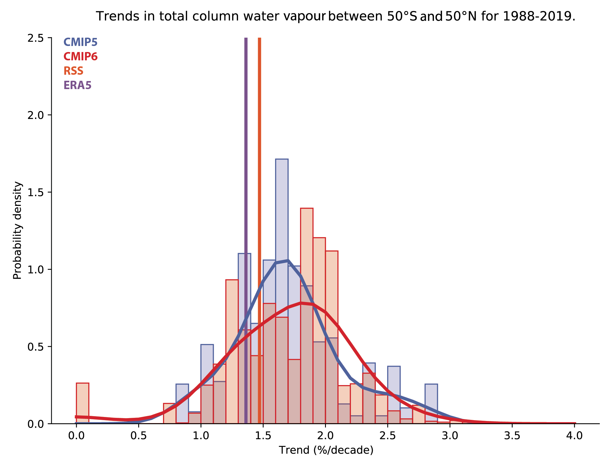 Figure 3.12 | Total column water vapour trends (% per decade) for the period 1988–2019 averaged over the near-global oceans (50°S–50°N). The figure shows satellite data (RSS) and ERA5.1 reanalysis, as well as CMIP5 (blue) and CMIP6 (red) historical simulations. All available ensemble members were used (see Section 3.2). Fits to the model trend probability distributions were performed with kernel density estimation. Figure is updated from Santer et al. (2007). Further details on data sources and processing are available in the chapter data table (Table 3.SM.1).
 The detection and attribution of tropospheric water vapour changes can be traced back to Santer et al. (2007), who used estimates of atmospheric water vapour from the satellite-based Special Sensor Microwave Imager (SSM/I) and from CMIP3 historical climate simulations. They provided evidence of human-induced moistening of the troposphere, and found that the simulated human fingerprint pattern was detectable at the 5% level by 2002 in water vapour satellite data (from 1988 to 2006). The observed changes matched the historical simulations forced by greenhouse gas changes and other anthropogenic forcings, and not those due to natural variability alone. Then, Santer et al. (2009) repeated this study with CMIP5 models, and found that the detection and attribution conclusions were not sensitive to model quality. These results demonstrate that the human fingerprint is governed by robust and basic physical processes, such as the water vapour feedback. Finally, Chung et al. (2014) extended this line of research by focusing on the global-mean water vapour content in the upper troposphere. Using satellite-based observations and sets of CMIP5 climate simulations run under various climate-forcing options, they showed that the observed moistening trend of the upper troposphere over the 1979–2005 period could not be explained by internal variability alone, but is attributable to a combination of anthropogenic and natural forcings. This increase in water vapour is accompanied by a reduction in mid-tropospheric relative humidity and clouds in the subtropics and mid-latitude in both models and observations related to changes in the Hadley cell (Section 3.3.3.1.1; Lau and Kim, 2015).
Dunn et al. (2017) confirmed earlier findings that global mean surface relative humidity increased between 1973 and 2000, followed by a steep decline (also reported in Willett et al., 2014) until 2013, and specific humidity correspondingly increased and then remained approximately constant (see also (Section 2.3.1.3.2), with none of the CMIP5 models capturing this behaviour. They noted biases in the mean state of the CMIP5 models’ surface relative humidity (and ascribed the failure to the representation of land surface processes and their response to CO2 forcing), concluding that these biases preclude any detection and attribution assessment. On the other hand, Byrne and O’Gorman (2018) showed that the positive trend in specific humidity continued in recent years and can be detected over land and ocean from 1979 to 2016. Moreover, they provided a theory suggesting that the increase in annual surface temperature and specific humidity as well as the decrease in relative humidity observed over land are linked to warming over the neighbouring ocean. They also pointed out that the negative trend in relative humidity over land regions is quite uncertain and requires further investigation. A recent study has also identified an anthropogenically-driven decrease in relative humidity over the Northern Hemisphere mid-latitude continents in summer between 1979 and 2014, which was underestimated by CMIP5 models (Douville and Plazzotta, 2017). Furthermore, in a modelling study Douville et al. (2020) showed that this decrease in boreal summer relative humidity over mid-latitudes is related not only to global ocean warming, but also to the physiological effect of CO2 on plants in the land surface model.
In summary, we assess that it is likely that human influence has contributed to moistening in the upper troposphere since 1979. Also, there is medium confidence that human influence contributed to a global increase in annual surface specific humidity, and medium confidence that it contributed to a decrease in surface relative humidity over mid-latitude Northern Hemisphere continents during summertime.
3.3.2.3 Precipitation
AR5 concluded that there was medium confidence that human influence had contributed to large-scale precipitation changes over land since 1950, including an increase in the Northern Hemisphere mid- to high latitudes. Moreover, AR5 concluded that observational uncertainties and challenges in precipitation modelling precluded a more confident assessment (Bindoff et al., 2013). Overall, it found that large-scale features of mean precipitation in CMIP5 models were in modest agreement with observations, but there were systematic errors in the tropics (Flato et al., 2013).
Since AR5, X. Li et al. (2016b) found that CMIP5 models simulate the large scale patterns of annual mean land precipitation and seasonality well, as well as reproducing qualitatively the observed zonal mean land precipitation trends for the period 1948–2005: models capture the drying trends in the tropics and at 45°S and the wetting trend in the Northern Hemisphere mid- to high latitudes, but the amplitudes of the changes are much smaller than observed. Land precipitation was found to show enhanced seasonality in observations (Chou et al., 2013), qualitatively consistent with the simulated response to anthropogenic forcing (Dwyer et al., 2014). However, models do not appear to reproduce the zonal mean trends in the magnitude of the seasonal cycle over the period 1948–2005, nor the two-dimensional distributions of trends of annual precipitation and seasonality over land, but differences may be explainable by internal variability (X. Li et al., 2016b). However, observed trends in seasonality depend on data set used (X. Li et al., 2016b; Marvel et al., 2017), and Marvel et al. (2017) found that observed changes in the annual cycle phase are consistent with model estimates of forced changes. These phase changes are mainly characterized by earlier onset of the wet season on the equatorward flanks of the extratropical storm tracks, particularly in the Southern Hemisphere. Box 8.2 assesses regional changes in water cycle seasonality.
The CMIP5 models have also been shown to adequately simulate the mean and interannual variability of the global monsoon (Section 3.3.3.2), but maintain the double ITCZ bias in the equatorial Pacific (Lee and Wang, 2014; Tian, 2015; Ni and Hsu, 2018). Despite the ITCZ bias, CMIP5 models have been used to detect in reanalysis a southward shift in the ITCZ prior to 1975, followed by a northward shift in the ITCZ after 1975, in response to forced changes in inter-hemispheric temperature contrast (Sections 3.3.1.1 and 8.3.2.1, and Figure 8.11; Bonfils et al., 2020; Friedman et al., 2020). CMIP5 models perform better than CMIP3 models, in particular regarding the global monsoon domain and intensity (Lee and Wang, 2014).
In observations at time scales less than a day intermittent rainfall fluctuations dominate variability, but CMIP5 models systematically underestimate them (Covey et al., 2018). Moreover, as noted in previous generation models, CMIP5 models produce rainfall too early in the day (Covey et al., 2016). Also, models overpredict precipitation frequency but have weaker intensity, although comparison with observed datasets is complex as there are large differences in intensity among them (Herold et al., 2016; Pendergrass and Deser, 2017; Trenberth et al., 2017). Regarding trends in precipitation intensity, models have also been shown to reproduce the compensation between increasing heavy precipitation and decreasing light to moderate rainfall (Thackeray et al., 2018b), a characteristic found in the observational record (Gu and Adler, 2018). Regional model performance is further assessed in Chapter 8 and the Atlas, while precipitation extremes are considered in Chapter 11.
The simulation of annual mean rainfall patterns in the CMIP6 models reveals minor improvements compared to those in CMIP5 models (Figure 3.13). The persistent biases include the double ITCZ in the tropical Pacific (seen as bands of excessive rainfall on both sides of the equatorial Pacific in Figure 3.13b,d) and the southward-shifted ITCZ in the equatorial Atlantic, which have been linked to the meridional pattern of SST bias (S. Zhou et al., 2020) and the reduced sensitivity of precipitation to local SST (Good et al., 2021). Tian and Dong (2020) also found that all three generations of CMIP models share similar systematic annual mean precipitation errors in the tropics, but that the double ITCZ bias is slightly reduced in CMIP6 models in comparison to CMIP3 and CMIP5 models. They also found some improvement in the overly intense Indian ocean ITCZ and the too dry South American continent except over the Andes. Fiedler et al. (2020) identified improvements in the tropical mean spatial correlations and root mean square error of the climatology as well as in the day-to-day variability, but found little change across CMIP phases in the double ITCZ bias and diurnal cycle. The CMIP6 models reproduce better the domain and intensity of the global monsoon (see Section 3.3.3.2). Moreover, CMIP6 models better represent the storm tracks (Priestley et al., 2020; also (Section 3.3.3.3), thereby reducing the precipitation biases in the North Atlantic and mid-latitudes of the Southern Hemisphere (Figure 3.13b,d). As a result, pattern correlations between simulated and observed annual mean precipitation range between 0.80 and 0.92 for CMIP6 models, compared to a range of 0.79 to 0.88 for CMIP5 (Bock et al., 2020). This relative improvement may be related to increased model resolution, as found when comparing biases in the mean of the HighResMIP models with the mean of the corresponding lower-resolution versions of the same models (see Figure 3.13e,f), particularly in the tropics and extratropical storm tracks. Consistent with this, a recent study using several coupled models showed that increasing the atmospheric resolution leads to a strong decrease in the precipitation bias in the tropical Atlantic ITCZ (see further discussion in Section 3.8.2.2; Vannière et al., 2019). Based on these results we assess that despite some improvements, CMIP6 models still have deficiencies in simulating precipitation patterns, particularly over the tropical ocean (high confidence).
 Figure 3.13 | Annual-mean precipitation rate (mm day–1) for the period 1995–2014. (a) Multi-model (ensemble) mean constructed with one realization of the CMIP6 historical experiment from each model. (b) Multi-model mean bias, defined as the difference between the CMIP6 multi-model mean and the precipitation analysis from the Global Precipitation Climatology Project (GPCP) version 2.3 (Adler et al., 2003). (c) Multi-model mean of the root mean square error calculated over all months separately and averaged with respect to the precipitation analysis from GPCP version 2.3. (d) Multi-model mean bias, calculated as the difference between the CMIP6 multi-model mean and the precipitation analysis from GPCP version 2.3. Also shown is the multi-model mean bias as the difference between the multi-model mean of (e) high resolution and (f) low-resolution simulations of four HighResMIP models and the precipitation analyses from GPCP version 2.3. Uncertainty is represented using the advanced approach. No overlay indicates regions with robust signal, where ≥66% of models show change greater than the variability threshold and ≥80% of all models agree on sign of change; diagonal lines indicate regions with no change or no robust signal, where <66% of models show a change greater than the variability threshold; crossed lines indicate regions with conflicting signal, where ≥66% of models show change greater than the variability threshold and <80% of all models agree on the sign of change. For more information on the advanced approach, please refer to the Cross-Chapter Box Atlas.1. Dots in panel (e) mark areas where the bias in high resolution versions of the HighResMIP models is not lower in at least three out of four models than in the corresponding low-resolution versions. Further details on data sources and processing are available in the chapter data table (Table 3.SM.1).
 Recent studies comparing observations and CMIP5 simulations have shown that tropical volcanic eruptions induce a significant reduction in global precipitation, particularly over the wet tropics, including the global monsoon regions (Iles and Hegerl, 2014; Paik and Min, 2017; Paik et al., 2020a). Reconstructions and modelling studies also suggest a distinct remote influence of volcanic forcing such that large volcanoes erupting in one hemisphere can enhance monsoon precipitation in the other hemisphere (F. Liu et al., 2016; Zuo et al., 2019). The climatic effect of volcanic eruptions is further assessed in Cross-Chapter Box 4.1.
An intensification of the wet–dry zonal mean patterns, consisting of the wet tropical and mid-latitude bands becoming wetter, and the dry subtopics becoming drier is expected in response to greenhouse gas and ozone changes (Section 8.2.2.2). However, detecting these changes is complicated by model errors in locating the main features of rainfall patterns. To deal with this issue, Marvel and Bonfils (2013) identified in each CMIP5 historical simulation the latitudinal peaks and troughs of the rainfall latitudinal patterns, measured the amplification and shift of these patterns in a pattern-based fingerprinting study, and found that the simultaneous amplification and shift in zonal precipitation patterns are detectable in Global Precipitation Climatology Project (GPCP) observations over the 1979–2012 period. Similarly, Bonfils et al. (2020) found that the intensification of wet–dry zonal patterns identified in CMIP5 historical simulations is detectable in reanalyses over the 1950–2014 period (see also Figure 8.11).
Based on long-term island precipitation records, Polson et al. (2016) identified significant increases in precipitation in the tropics and decreases in the subtropics, which are consistent with those simulated by the CMIP5 models. Moreover, results from Polson and Hegerl (2017) give support to an intensification of the water cycle according to the wet-gets-wetter, dry-gets-drier paradigm over tropical land areas as well. Other studies suggest that this paradigm does not necessarily hold over dry regions where moisture is limited (see also Section 8.2.2.1; Greve et al., 2014; Kumar et al., 2015). Polson and Hegerl (2017) explained this discrepancy by taking into account the seasonal and interannual movement of the regions (Allan, 2014). A follow-up study using CMIP6 models also found that the observed strengthening contrast of precipitation over wet and dry regions was detectable, although the increase was significantly larger in observations than in the multi-model mean. The change was attributed to a combination of anthropogenic and natural forcings, with anthropogenic forcings detectable in multi-signal analyses (Figure 3.14; Schurer et al., 2020).
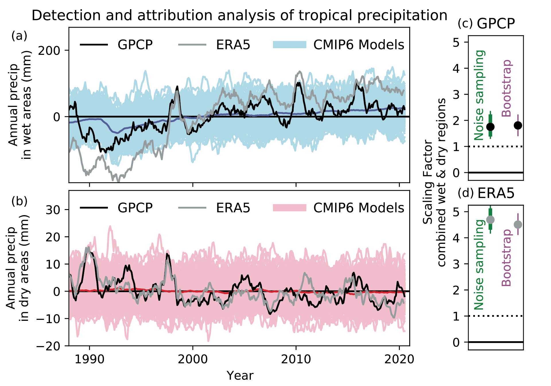 Figure 3.14 | Wet (a) and dry (b) region tropical mean (30°S–30°N) annual precipitation anomalies. Observed data are shown with black lines (GPCP), ERA5 reanalysis is shown in grey, single model simulations are shown with light blue/red lines (CMIP6), and multi-model mean results are shown with dark blue/red lines (CMIP6). Wet and dry region annual anomalies are calculated as the running mean over 12 months relative to a 1988–2020 base period. The regions are defined as the wettest third and driest third of the surface area, calculated for the observations and for each model separately for each season (following Polson and Hegerl, 2017). Scaling factors (c, d) are calculated for the combination of the wet and dry region mean, where the observations, reanalysis and all the model simulations are first standardized using the mean standard deviation of the pre-industrial control simulations. Two total least squares regression methods are used: noise in variables (following Polson and Hegerl, 2017) which estimates a best estimate and a 5–95% confidence interval using the pre-industrial controls (circle and thick green line) and the pre-industrial controls with double the variance (thin green line); and a bootstrap method (DelSole et al., 2019) (5–95% confidence interval shown with a purple line and best estimate with a circle). Panel (c) shows results for GPCP and panel (d) for ERA5. Figure is adapted from Schurer et al. (2020). Further details on data sources and processing are available in the chapter data table (Table 3.SM.1).
 Global land precipitation has likely increased since the middle of the 20th century (medium confidence), while there is low confidence in trends in land data prior to 1950 and over the ocean during the satellite era due to disagreement between datasets (Section 2.3.1.3.4). Figure 3.15a shows the time evolution of the global mean land precipitation since 1950, as well as the trend during the period. Adler et al. (2017) found no significant trend in the global mean precipitation during the satellite era, consistent with model simulations (Wu et al., 2013) and physical understanding of the energy budget (Section 8.2.1). This has been suggested to be due to the negative effect of anthropogenic sulphate aerosol that opposed the positive influence of rising global mean temperatures due to greenhouse gases (Salzmann, 2016; Richardson et al., 2018). The precipitation change expected from ocean warming is also partly offset by the fast atmospheric adjustment to increasing greenhouse gases (Section 8.2.1). Over the ocean, the negligible trend may be due to the cancelling effects of CO2 and aerosols (Richardson et al., 2018).
 Figure 3.15 | Observed and simulated time series of anomalies in zonal average annual mean precipitation. (a), (c–f) Evolution of global and zonal average annual mean precipitation (mm day–1) over areas of land where there are observations, expressed relative to the base period of 1961–1990, simulated by CMIP6 models (one ensemble member per model) forced with both anthropogenic and natural forcings (brown) and natural forcings only (green). Multi-model means are shown in thick solid lines and shading shows the 5–95% confidence interval of the individual model simulations. The data is smoothed using a low pass filter. Observations from three different datasets are included: gridded values derived from Global Historical Climatology Network (GHCN version 2) station data, updated from Zhang et al. (2007), data from the Global Precipitation Climatology Product (GPCP L3 version 2.3, Adler et al. (2003)) and from the Climate Research Unit (CRU TS4.02, Harris et al. (2014)). Also plotted are boxplots showing interquartile and 5–95% ranges of simulated trends over the period for simulations forced with both anthropogenic and natural forcings (brown) and natural forcings only (blue). Observed trends for each observational product are shown as horizontal lines. Panel (b) shows annual mean precipitation rate (mm day–1) of GHCN version 2 for the years 1950–2014 over land areas used to compute the plots. Further details on data sources and processing are available in the chapter data table (Table 3.SM.1).
 A gridpoint based analysis of annual precipitation trends over land regions since 1901 (Knutson and Zeng, 2018) comparing observed and simulated trends found that detectable anthropogenic increasing trends have occurred prominently over many mid- to high-latitude regions of the Northern Hemisphere and subtropics of the Southern Hemisphere. The observed trends in many cases are significantly stronger than modelled in the CMIP5 historical runs for the 1901–2010 period (though not for 1951–2010), which may be due to disagreement between observed datasets (Section 2.3.1.3.4), and/or suggest possible deficiencies in models.
The observed precipitation increase in the Northern Hemisphere high latitudes over the period 1966–2005 was attributed to anthropogenic forcing by a study using CMIP5 models (Wan et al., 2015) supporting the AR5 assessment. Initial results from CMIP6 also support the role of anthropogenic forcing in the precipitation increase observed in Northern Hemisphere high latitudes (see Figure 3.15c): the observed positive trend detected for the band 60°N–90°N can only be reproduced when anthropogenic forcing is included, although models tend to simulate overall a larger positive trend. A similar positive trend, but less significant, is also detected between 30°N–60°N, while in the southern mid-latitudes no trend is simulated (see Figure 3.15d, f).
For the Southern Hemisphere extratropics, Solman and Orlanski (2016) found that the observed summertime rainfall increase over high latitudes and decrease over mid-latitudes over the period 1979–2010 are quasi-zonally symmetric and related to changes in eddy activity. The latter were in turn found to be associated with the poleward shift of the westerlies due mostly to ozone depletion. Positive rainfall trends in the subtropics, particularly over south-eastern South America (see also Section 10.4.2.2) and northern and central Australia, have been also attributed to stratospheric ozone depletion (Kang et al., 2011; Gonzalez et al., 2014) and greenhouse gases (Vera and Díaz, 2015; Saurral et al., 2019). During austral winter, wetting at high latitudes and drying at mid-latitudes are not zonally homogenous, due to both changes in eddy activity and increased lower troposphere humidity. Solman and Orlanski (2016) associated these climate changes with increases in greenhouse gas concentration levels. Recently, Blazquez and Solman (2017) have shown that CMIP5 models represent very well the dynamical forcing and the frequency of frontal precipitation in the Southern Hemisphere winter extratropics, but the amount of precipitation due to fronts is overestimated. Chapters 10 and 11 validate in more detail the simulation of fronts in climate models (Sections 10.3.3.4.4 and 11.7.2.3).
Over the ocean, observations show coherent large-scale patterns of fresh ocean regions becoming fresher and salty ocean regions saltier across the globe, which has been related through modelling studies to changes in precipitation minus evaporation and is consistent with the wet-gets-wetter, dry-gets-drier paradigm (see Sections 3.5.2.2 and 8.2.2.1; Durack et al., 2012, 2013; Skliris et al., 2014; Durack, 2015; Hegerl et al., 2015; Levang and Schmitt, 2015; Zika et al., 2015; Grist et al., 2016; Cheng et al., 2020).
Overall, studies published since AR5 provide further evidence of an anthropogenic influence on precipitation, and therefore we now assess that it is likely that human influence has contributed to large-scale precipitation changes observed since the mid-20th century. New attribution studies strengthen previous findings of a detectable increase in mid to high latitude land precipitation over the Northern Hemisphere (high confidence). There is medium confidence that human influence has contributed to a strengthening of the zonal mean wet tropics-dry subtropics contrast, and that tropical rainfall changes follow the wet-gets-wetter, dry-gets-drier paradigm. There is also medium confidence that ozone depletion has increased precipitation over the southern high latitudes and decreased it over southern mid-latitudes during austral summer. Owing to observational uncertainties and inconsistent results between studies, we conclude that there is low confidence in the attribution of changes in the seasonality of precipitation.
3.3.2.4 Streamflow
Streamflow is to-date the only variable of the terrestrial water cycle with enough in-situ observations to allow for detection and attribution analysis at continental to global scales. Based on evidence from a few formal detection and attribution studies, particularly on the timing of peak streamflow, and the qualitative evaluation of studies reporting on observed and simulated trends, AR5 concluded that there is medium confidence that anthropogenic influence on climate has affected streamflow in some middle and high latitude regions (Bindoff et al., 2013). The AR5 also noted that observational uncertainties are large and that often only a limited number of models were considered.
(Section 2.3.1.3.6 assesses that there have not been significant trends in global average streamflow over the last century, though regional trends have been observed, driven in part by internal variability. Only a limited number of studies have systematically compared observed streamflow trends at continental to global scales with changes simulated by global circulation models in a detection and attribution setting. H. Yang et al. (2017) did not find a significant correlation between observed runoff changes and changes simulated in CMIP5 models in most grid cells, consistent with the assessment that observed changes are dominated by internal variability. In a pan-European assessment, Gudmundsson et al. (2017) attributed the spatio-temporal pattern of decreasing streamflow in southern Europe and increasing streamflow in northern Europe to anthropogenic climate change, but also concluded that additional effects of human water withdrawals could not be excluded. Focussing on continental runoff between 1958 and 2004, Alkama et al. (2013) found a significant change only when using reconstructed data over all rivers, and a large uncertainty in the estimate of the global streamflow trend due to opposing changes over different continents. Gedney et al. (2014) detected the influence of aerosols on streamflow in North America and Europe, with aerosols having driven an increase in streamflow due to reduced evaporation (see Section 8.3.1.5 for details on processes). There is also evidence for a detectable anthropogenic contribution toward earlier winter-spring streamflows in the north-central US (Kam et al., 2018) and in western Canada (Najafi et al., 2017). From a model evaluation perspective, Sheffield et al. (2013) reported that CMIP5 models reproduce spatial variations in runoff in North America well, though they tend to underestimate it.
Recently, Gudmundsson et al. (2021) performed a global detection and attribution study on streamflow and found that some regions are drying and others are wetting. Moreover, the simulated streamflow trends are consistent with observations only if externally forced climate change is considered, and the simulated effects of water and land management cannot reproduce the observed trends. The effects of volcanic eruptions in driving reduced streamflow have also been detected in the wet tropics (Iles and Hegerl, 2015; Zuo et al., 2019).
In summary, there is medium confidence that anthropogenic climate change has altered local and regional streamflow in various parts of the world and that the associated global-scale trend pattern is inconsistent with internal variability. Moreover, human interventions and water withdrawals, while affecting streamflow, cannot explain the observed spatio-temporal trends (medium confidence).
Cross-Chapter Box 3.2 | Human Influence on Large-scale Changes in Temperature and Precipitation Extremes
Contributors: Nathan P. Gillett (Canada), Seung-Ki Min (Republic of Korea), Krishnan Raghavan (India), Ying Sun (China), Xuebin Zhang (Canada)
Understanding how temperature and precipitation extremes have changed at large scales and the causes of these changes is an important part of our overall assessment of human influence on the climate system. Chapter 11 assesses changes in extremes and their causes, while this Cross-Chapter Box summarizes relevant assessments and supporting evidence in Chapters 8 and 11 and relates changes in extremes to mean changes on global and continental scales.
Attribution of temperature extremes
One important aspect of various indicators of temperature extremes is their connection to mean temperature at local, regional and global scales. For example, the highest daily temperature in a summer is often highly correlated with the summer mean temperature. Model projections show that changes in temperature extremes are often closely related to shifts in mean temperature (Seneviratne et al., 2016; Kharin et al., 2018). It is thus no surprise that changes in temperature extremes are consistent with warming mean temperature, with warming leading to more hot extremes and fewer cold extremes. Given the attribution of mean warming to human influence (Section 3.3.1), and the connection between changes in mean and extreme temperatures, it is to be expected that anthropogenic forcing has also influenced temperature extremes.
(Chapter 11 assesses that there is high confidence that climate models can reproduce the mean state and overall warming of temperature extremes observed globally and in most regions, although the magnitude of the trends may differ, and the ability of models to capture observed trends in temperature-related extremes depends on the metric evaluated, the way indices are calculated, and the time periods and spatial scales considered (Section 11.3.3). There has been widespread evidence of human influence on various aspects of temperature extremes, at global, continental, and regional scales. This includes attribution to human influence of observed changes in intensity, frequency, and duration and other relevant characteristics at global and continental scales (Section 11.3.4). The left-hand panel of Cross-Chapter Box 3.2, Figure 1 clearly shows that long-term changes in the global mean annual maximum daily maximum temperature can be reproduced by both CMIP5 and CMIP6 models forced with the combined effect of natural and anthropogenic forcings, but cannot be reproduced by simulations under natural forcing alone. Consistent with the assessment for global mean temperature (Section 3.3.1), aerosol changes are found to have offset part of the greenhouse gas induced increase in hot extremes globally and over most continents over the 1951–2015 period (Hu et al., 2020; Seong et al., 2021), though greenhouse gas and aerosol influences are less clearly separable in observed changes in cold extremes.
(Chapter 11 assesses that it is virtually certain that human-induced greenhouse gas forcing is the main contributor to the observed increase in the likelihood and severity of hot extremes and the observed decrease in the likelihood and severity of cold extremes on global scales, and very likely that this applies on most continents.
Attribution of precipitation extremes
An important piece of evidence supporting the SREX and AR5 assessment that there is medium confidence that anthropogenic forcing has contributed to a global scale intensification of heavy precipitation during the second half of the 20th century is the evidence for anthropogenic influence on other aspects of the global hydrological cycle. The most significant aspect of that is the increase in atmospheric moisture content associated with warming which should, in general, lead to enhanced extreme precipitation, particularly associated with enhanced convergence in tropical and extratropical cyclones (Sections 8.2.3.2 and 11.4.1). Such a connection is supported by the fact that annual maximum one-day precipitation increases with global mean temperature at a rate similar to the increase in the moisture holding capacity in response to warming, both in observations and in model simulations. Additionally, models project an increase in extreme precipitation across global land regions even in areas in which total annual or seasonal precipitation is projected to decrease.
The overall performance of CMIP6 models in simulating extreme precipitation intensity and frequency is similar to that of CMIP5 models (high confidence), and there is high confidence in the ability of models to capture the large-scale spatial distribution of precipitation extremes over land (Section 11.4.3). Evidence of human influence on extreme precipitation has become stronger since AR5. Considering changes in precipitation intensity averaged over all wet days, there is high confidence that daily mean precipitation intensities have increased since the mid-20th century in a majority of land regions, including Europe, North America and Asia, and it is likely that such an increase is mainly due to anthropogenic emissions of greenhouse gases (Sections 8.3.1.3 and 11.4.4). Section 11.4.4 also finds a larger fraction of land showing enhanced extreme precipitation and a larger probability of record-breaking one-day precipitation than expected by chance, which can only be explained when anthropogenic greenhouse gas forcing is considered. The right-hand
Cross-Chapter Box 3.2
panel of Cross-Chapter Box 3.2, Figure 1 demonstrates the consistency between changes in global average annual maximum daily precipitation in the observations and model simulations under combined anthropogenic and natural forcing, and inconsistency with simulations under natural forcing alone. While there is more evidence in the literature to quantify the net anthropogenic influence on extreme precipitation than the influence of individual forcing components, a dominant contribution of greenhouse gas forcing to the long-term intensification of extreme precipitation on global and continental scales has recently been quantified separately from the influence of anthropogenic aerosol and natural forcings (Dong et al., 2020; Paik et al., 2020b).
Chapter 11 assesses that it is likely that human influence, in particular due to greenhouse gas forcing, is the main driver of the observed intensification of heavy precipitation in global land regions during recent decades(Section 11.4.4).

Cross-Chapter Box 3.2, Figure 1 | Comparison of observed and simulated changes in global mean temperature and precipitation extremes. Time series of globally averaged five-year mean anomalies of the annual maximum daily maximum temperature (TXx in °C) and annual maximum 1-day precipitation (Rx1day as standardized probability index in %) between 1953 and 2017 from the HadEX3 observations and the CMIP5 and CMIP6 multi-model ensembles with natural and human forcing (top) and natural forcing only (bottom). For CMIP5, historical simulations for 1953–2005 are combined with corresponding RCP4.5 scenario runs for 2006–2017. For CMIP6, historical simulations for 1953–2014 are combined with SSP2-4.5 scenario simulations for 2015–2017. Numbers in brackets represent the number of models used. The time-fixed observational mask has been applied to model data throughout the whole period. Grid cells with more than 70% of data available between 1953 and 2017 plus data for at least three years between 2013 and 2017 are used. Coloured lines indicate multi-model means, while shading represents 5th–95th percentile ranges, based on all available ensemble members with equal weight given to each model (Section 3.2). Anomalies are relative to 1961–1990 means. Figure is updated from Seong et al. (2021), their Figure 3 and Paik et al. (2020b), their Figure 3. Further details on data sources and processing are available in the chapter data table (Table 3.SM.1).
3.3.3 Atmospheric Circulation
3.3.3.1 The Hadley and Walker Circulations
The tropical tropospheric circulation features meridional and zonal overturning circulations, called Hadley and Walker circulations. In the zonal mean, the downwelling branch of the Hadley circulation cell is located in the subtropics and is often used as an indicator of the meridional extent of the tropics. In the equatorial zonal-vertical section, the major rising branch of the Walker circulation is located over the Maritime continent with secondary ascending regions over northern South America and Africa. The zonal component of the surface trade winds over most of the equatorial Pacific and Atlantic is associated with the Walker circulation. This section assesses the zonal-mean Hadley cell extent and the Pacific Walker circulation strength. Regional and water cycle aspects of these circulations are assessed in more detail in Section 8.3.2.
AR5 found medium confidence that the depletion of stratospheric ozone had contributed to Hadley cell widening in the Southern Hemisphere in austral summer (Bindoff et al., 2013). It also noted that in contrast to a simulated weakening in response to greenhouse gas forcing, the Walker circulation had actually strengthened since the early 1990s, precluding any detection of human influence.
3.3.3.1.1 Hadley cell extent
Grise et al. (2019) found that a metric based on surface zonal winds, which are well constrained by surface observations, best compares reanalyses with CMIP5 models. With this method and new reanalysis products, the CMIP5 historical simulations exhibit comparable mean states and variability of the subtropical edge latitude of the Hadley cells to those observed (Grise et al., 2019).
(Chapter 2 assesses that there has very likely been a widening of the Hadley circulation since the 1980s (Section 2.3.1.4.1). The CMIP5 (Davis and Birner, 2017; Grise et al., 2018) and CMIP6 (Grise and Davis, 2020) historical simulation ensembles span the observed trends of the zonal-mean Hadley cell edges since the 1980s (Figure 3.16a–c). Studies based on CMIP5 models find a contribution from human influence to the observed widening trend, especially in the Southern Hemisphere (Gerber and Son, 2014; Staten et al., 2018, 2020; Grise et al., 2019; Jebri et al., 2020), which is confirmed based on CMIP6 (Figure 3.16b,c; Grise and Davis, 2020).
 Figure 3.16 | Model evaluation and attribution of changes in Hadley cell extent and Walker circulation strength. (a–c) Trends in subtropical edge latitude of the Hadley cells in (a) the Northern Hemisphere for 1980–2014 annual means and (b, c) Southern Hemisphere for (b) 1980–2014 annual means and (c) 1980/81–1999/2000 December–January–February means. Positive values indicate northward shifts. (d–f) Trends in the Pacific Walker circulation strength for (d) 1901–2010, (e) 1951–2010 and (f) 1980–2014. Positive values indicate strengthening. Based on CMIP5 historical (extended with RCP4.5), CMIP6 historical, AMIP, pre-industrial control, and single forcing simulations along with HadSLP2 and reanalyses. Pre-industrial control simulations are divided into non-overlapping segments of the same length as the other simulations. White boxes and whiskers represent means, interquartile ranges and 5th and 95th percentiles, calculated after weighting individual members with the inverse of the ensemble size of the same model, so that individual models are equally weighted (Section 3.2). The filled boxes represent the 5–95% confidence interval on the multi-model mean trends of the models with at least three ensemble members, with dots indicating the ensemble means of individual models. The edge latitude of the Hadley cell is where the surface zonal wind velocity changes sign from negative to positive, as described in the Appendix of Grise et al. (2018). The Pacific Walker circulation strength is evaluated as the annual mean difference of sea level pressure between 5°S–5°N, 160°W–80°W and 5°S–5°N, 80°E–160°E. Further details on data sources and processing are available in the chapter data table (Table 3.SM.1).
 In the annual mean, internal variability, including Pacific Decadal Variability (PDV; Annex IV.2.6), contributed to the observed zonal-mean Hadley cell expansion since 1980 comparably with human influence (Allen et al., 2014; Allen and Kovilakam, 2017; Mantsis et al., 2017; Amaya et al., 2018; Grise et al., 2018). Indeed, the ensemble-mean expansion in historical simulations is significantly weaker than in most of the reanalyses shown in Figure 3.16a–c, while the Atmospheric Model Intercomparison Project (AMIP) simulations forced by observed SSTs (Figure 3.16a–c) show stronger trends than historical coupled simulations on average (Nguyen et al., 2015; Davis and Birner, 2017; Grise et al., 2018). The human-induced change has not yet clearly emerged out of the internal variability range in the Northern Hemisphere (Quan et al., 2018; Grise et al., 2019), whereas the trend in the annual-mean Southern Hemisphere edge is outside the 5th–95th percentile range of internal variability in CMIP6 in three out of the four reanalyses (Figure 3.16b). For the Southern Hemisphere summer when the simulated human influence is strongest, the 1981–2000 trend in three out of the four reanalyses falls outside the 5th–95th percentile range of internal variability (Figure 3.16c; L. Tao et al., 2016; Grise et al., 2018, 2019).
In CMIP5 simulations, greenhouse gas increases and, in austral summer, stratospheric ozone depletion, contribute to the Southern Hemisphere expansion (Gerber and Son, 2014; Nguyen et al., 2015; L. Tao et al., 2016; Y.H. Kim et al., 2017), but the ozone influence is not significant in available CMIP6 simulations (Figure 3.16b–c). Since the 2000s, the stabilization or slight recovery of stratospheric ozone (Section 2.2.5.2) is consistent with the smaller observed trends (Banerjee et al., 2020). While many CMIP5 models under-represent the magnitude of the PDV, implying potential overconfidence on the detection of human influence on the Hadley cell expansion, this is less the case for the CMIP6 models (Section 3.7.6). However, the mechanism underlying the Hadley cell expansion remains unclear (Staten et al., 2018, 2020), precluding a process-based validation of the simulated human influence.
3.3.3.1.2 Walker circulation strength
CMIP5 models reproduce the mean state of the Walker circulation with reasonable fidelity, evidenced by the spatial pattern correlations of equatorial zonal mass stream function between models and observations being larger than 0.88 (Ma and Zhou, 2016). CMIP5 historical simulations on average simulate a significant weakening of the Pacific Walker circulation over the 20th century (DiNezio et al., 2013; Sandeep et al., 2014; Kociuba and Power, 2015), which is also seen in CMIP6 (Figure 3.16d). This weakening is accompanied by a reduction of convective activity over the Maritime Continent and an enhancement over the central equatorial Pacific (DiNezio et al., 2013; Sandeep et al., 2014; Kociuba and Power, 2015). In the CMIP6 simulations, greenhouse gas forcing induces this weakening (Figure 3.16d), which is consistent with theories based on radiative-convective equilibrium (Vecchi et al., 2006; Vecchi and Soden, 2007) and thermodynamic air-sea coupling (Xie et al., 2010), but inconsistent with a theory highlighting the ocean dynamical effect which suggests a strengthening in response to greenhouse gas increases (Clement et al., 1996; Seager et al., 2019; see also Section 7.4.4.2.1). Seager et al. (2019) attributed this inconsistency to equatorial Pacific SST biases in the models (Section 3.5.1.2.1). However, observational and reanalysis datasets disagree on the sign of trends in the Walker Circulation strength over the 1901–2010 period (Figure 3.16d), and Section 2.3.1.4.1 assesses low confidence in observed long-term Walker Circulation trends. The observational uncertainty remains high in the trends since the 1950s (Tokinaga et al., 2012; L’Heureux et al., 2013), though both CMIP5 and CMIP6 historical simulations span trends of all but one observational data set (Figure 3.16e). For this period, external influence simulated in CMIP6 is insignificant due to a partial compensation of forced responses to greenhouse gases and aerosols and large internal decadal variability (Figure 3.16e). It is notable that while AMIP simulations on average show strengthening over both the periods, those simulations are forced by one reconstruction of SST, which itself is subject to uncertainty before the 1970s (Deser et al., 2010; Tokinaga et al., 2012).
Observational SST products indicate that the equatorial zonal SST gradient from the western to the eastern equatorial Pacific has strengthened since 1870 (Section 7.4.4.2.1). While CMIP5 historical simulations on average simulate a weakening, large ensemble simulations span the observed strengthening since the 1950s (Watanabe et al., 2021) suggesting an important contribution from internal variability. Coats and Karnauskas (2017) also find that the anthropogenic influence on the SST gradient is yet to emerge out of internal variability even on centennial time scales.
Trends since the 1980s in in-situ and satellite observations and reanalyses exhibit strengthening of the Pacific Walker circulation and SST gradient (Section 2.3.1.4.1 and Figure 3.16f; L’Heureux et al., 2013; Boisséson et al., 2014; England et al., 2014; Kociuba and Power, 2015; Ma and Zhou, 2016). AMIP simulations reproduce this strengthening (Figure 3.16d; Boisséson et al., 2014; Ma and Zhou, 2016), indicating a dominant role of SST changes. However, all reanalysis trends lie outside the 5–95% range of simulated CMIP6 historical Walker circulation trends over this period (Figure 3.16f), consistent with CMIP5 results (England et al., 2014; Kociuba and Power, 2015). This may be in part caused by the underestimation of the PDV magnitude especially in CMIP5 models (Section 3.7.6; Kociuba and Power, 2015; Chung et al., 2019), but also suggests a potential error in simulating the forced changes of the Walker circulation. Specifically, anthropogenic and volcanic aerosol changes over this period may have driven a strengthening (DiNezio et al., 2013; Takahashi and Watanabe, 2016; Hua et al., 2018). This aerosol influence may be indirect via Atlantic Multi-decadal Variability (AMV; Annex IV.2.7) through inter-basin teleconnections (McGregor et al., 2014; Chikamoto et al., 2016; Kucharski et al., 2016; X. Li et al., 2016a; Ruprich-Robert et al., 2017), which may be underestimated in models due to SST biases in the equatorial Atlantic (Section 3.5.1.2.2; McGregor et al., 2018). Note also the large uncertainty in aerosol influence on the Walker circulation (Kuntz and Schrag, 2016; Hua et al., 2018; Oudar et al., 2018), which is also seen in CMIP6 (Figure 3.16f).
Paleoclimate data from the Pliocene epoch suggest that there was a reduction in the zonal SST gradient in the tropical Pacific under a similar CO2 concentration as today (Section 7.4.4.2.2 and Cross-Chapter Box 2.4). Tierney et al. (2019) found that this weaker gradient compared to pre-industrial, which suggests a weaker Walker circulation, is captured by climate models under Pliocene CO2 levels, in agreement with the CMIP6 response to greenhouse gas forcing (Figure 3.16d), though the magnitude of this effect varies strongly between models (Corvec and Fletcher, 2017).
3.3.3.1.3 Summary
It is likely that human influence has contributed to the poleward expansion of the zonal mean Hadley cell in the Southern Hemisphere since the 1980s. This assessment is supported by studies since AR5, which consistently find human influence from greenhouse gas increases on the expansion, with additional influence from ozone depletion in austral summer. For the strong ozone depletion period of 1981–2000, human influence is detectable in the summertime poleward expansion in the Southern Hemisphere (medium confidence). By contrast, there is medium confidence that the expansion of the zonal mean Hadley cell in the Northern Hemisphere is within the range of internal variability, with contributions from PDV and other internal variability. The causes of the observed strengthening of the Pacific Walker circulation over the 1980–2014 period are not well understood, since the observed strengthening trend is outside the range of variability simulated in the coupled models (medium confidence). Large observational uncertainty, lack of understanding of the mechanism underlying the poleward Hadley cell expansion, and contradicting theories on the greenhouse gas influence and uncertainty in the aerosol influence on the Walker circulation strength, limit confidence in these assessments.
3.3.3.2 Global Monsoon
Monsoons are seasonal transitions of regimes in atmospheric circulation and precipitation with the annual cycle of solar insolation, in association with redistribution of moist static energy (Wang and Ding, 2008; P.X. Wang et al., 2014; Biasutti et al., 2018). The global monsoon can be defined to encompasses all monsoon systems based on precipitation contrast in the solstice seasons (Wang and Ding, 2008; Figure 3.17). All regional monsoons are intimately connected to the global tropical atmospheric overturning by mass (Trenberth et al., 2000), momentum and energy budgets (Biasutti et al., 2018; Geen et al., 2020). Assessments of regional monsoon changes are made in Sections 8.3.2.4, 10.4.2.1 and 10.6.3.
 Figure 3.17 | Model evaluation of global monsoon domain, intensity, and circulation. (a, b) Climatological summer-winter range of precipitation rate, scaled by annual mean precipitation rate (shading) and 850 hPa wind velocity (arrows) based on (a) GPCP and ERA5 and (b) a multi-model ensemble mean of CMIP6 historical simulations for 1979–2014. The region enclosed by red lines is the monsoon domain based on the definition by Wang and Ding (2008). (c, d) Five-year running mean anomalies of (c) global land monsoon precipitation index defined as the percentage anomaly of the summertime precipitation rate averaged over the monsoon regions over land, relative to its average for 1979–2014 (the period indicated by light grey shading) and (d) the tropical monsoon circulation index defined as the vertical shear of zonal winds between 850 and 200 hPa levels averaged over 0°–20°N, from 120°W eastward to 120°E in Northern Hemisphere summer (Wang et al., 2013; m s–1) in CMIP5 historical and RCP4.5 simulations, and CMIP6 historical and AMIP simulations. Summer and winter are defined for individual hemispheres: May to September is defined as Northern Hemisphere summer and Southern Hemisphere winter, and November to March is defined as Northern Hemisphere winter and Summer Hemisphere summer. The numbers of models and simulations are given in the legend. The multi-model ensemble mean and percentiles are calculated after weighting individual ensemble members with the inverse of the ensemble size of the same model, so that individual models are equally weighted irrespective of ensemble size. Further details on data sources and processing are available in the chapter data table (Table 3.SM.1).
 AR5 assessed that CMIP5 models simulated monsoons better than CMIP3 models but that biases remained in domains and intensity (high confidence) (Flato et al., 2013). There were no detection and attribution assessment statements on the decreasing trend of global monsoon precipitation over land from the 1950s to the 1980s or the increasing trend of global monsoon precipitation afterwards. In the paleoclimate context, it was determined with high confidence that orbital forcing produces strong interhemispheric rainfall variability evident in multiple types of proxies (Masson-Delmotte et al., 2013).
Paleoclimate proxy evidence shows that the global monsoon has varied with orbital forcing and greenhouse gases (Section 2.3.1.4.2; Mohtadi et al., 2016; Seth et al., 2019). These large-magnitude intensifications and weakenings in the global monsoon involved in some cases orders-of-magnitude changes in precipitation locally (Harrison et al., 2014; Tierney et al., 2017). Paleoclimate modelling and limited data from past climate states with high CO2 suggest that precipitation intensifies in the monsoon domain under elevated greenhouse gases, providing context for present and future trends (Passey et al., 2009; Haywood et al., 2013; Zhang et al., 2013b). In model simulations of the mid-Pliocene, when globally averaged temperature was higher than present day, precipitation was larger in West African, South Asian and East Asian monsoons than under pre-industrial conditions, consistent with proxy evidence (Zhang et al., 2015; Sun et al., 2016, 2018; Corvec and Fletcher, 2017; X. Li et al., 2018). Prescott et al. (2019) and R. Zhang et al. (2019) find an important role for orbital forcing and CO2 in the mid-Pliocene monsoon expansion and intensification. Models are also able to capture interhemispherically contrasting monsoon changes in the Last Interglacial in response to orbital forcing and greenhouse gases, with wetter West African and Asian monsoons and a drier South American monsoon as seen in proxies (Govin et al., 2014; Gierz et al., 2017; Pedersen et al., 2017). In overall agreement with proxy evidence, a model with transient forcing simulates wetting and drying respectively of the Southern and Northern Hemisphere monsoons during the last deglaciation, with an important contribution from Atlantic Meridional Overturning Circulation (AMOC) slowdown (Otto-Bliesner et al., 2014; Mohtadi et al., 2016).
During the mid-Holocene, global monsoons were stronger especially in the Northern Hemisphere with an expansion of the West African monsoon domain in response to orbital forcing (Biasutti et al., 2018; Section 2.3.1.4.2). Simulations of the mid-Holocene with CMIP5 and CMIP6 models qualitatively capture the stronger Northern Hemisphere monsoon (Jiang et al., 2015; Brierley et al., 2020), mainly driven by atmospheric circulation changes (D’Agostino et al., 2019). However, the models underestimate the monsoon expansion found in proxy reconstructions (Perez-Sanz et al., 2014; Harrison et al., 2015; Tierney et al., 2017), which may be linked to mean biases in the monsoon domain (Brierley et al., 2020) and may be improved by imposing vegetation and dust changes (Pausata et al., 2016). The models simulate the weaker Southern Hemisphere monsoon during the mid-Holocene (D’Agostino et al., 2020), consistent with proxy evidence (Section 2.3.1.4.2). These studies indicate that models can qualitatively reproduce past global monsoon changes seen in proxies, though issues remain in quantitatively reproducing proxy observations. Studies of last millennium simulations show that simulated global monsoon precipitation increases with global mean temperature, while changes in monsoon circulation and hemispheric monsoon precipitation depend on forcing sources (Liu et al., 2012; Chai et al., 2018). Compared to greenhouse gas and solar variations, volcanic forcing is more effective in changing the global monsoon precipitation over the last millennium (Chai et al., 2018).
Reproducing monsoons in terms of domain, precipitation amount, and timings of onset and retreat over the historical period also remains difficult. While CMIP5 historical simulations broadly capture global monsoon domains and intensity based on summer and winter precipitation differences, they underestimate the extent and intensity of East Asian and North American monsoons while overestimating them over the tropical western North Pacific (Lee and Wang, 2014; M. Yan et al., 2016). B. Wang et al. (2020) reported that CMIP6 models simulate the global monsoon domain and precipitation better (Figure 3.17a,b), albeit with biases in annual mean precipitation and the timings of onset and withdrawal of the Southern Hemisphere monsoon. Notable inter-model differences were identified in CMIP5, with the multi-model ensemble mean outperforming individual models (Lee and Wang, 2014). Common biases were identified across CMIP5 models in moist static energy and upper-tropospheric temperature associated with the South Asian summer monsoon, which may arise from overly smoothed model topography (Boos and Hurley, 2012). However, in atmospheric models with increasing resolution approaching 20 km, improvements in monsoon precipitation are not universal across regions and models, and overall improvements are unclear (Johnson et al., 2016; Ogata et al., 2017; L. Zhang et al., 2018b).
In instrumental records, global summer monsoon precipitation intensity (measured by summer precipitation averaged over the monsoon domain) decreased from the 1950s to 1980s, followed by an increase (Section 2.3.1.4.2 and Figure 3.17c), arising mainly from variations in Northern Hemispheric land monsoons. A CMIP5 multi-model study by Y. Zhang et al. (2018) found that observed 1951–2004 trends of the global and Northern Hemisphere summer land monsoon precipitation intensity are well captured by historical simulations, and CMIP6 models show similar results for global land summer monsoon precipitation (Figure 3.17c). However, the 1960s peak in the Northern Hemisphere summer monsoon circulation is outside the 5th–95th percentile range of CMIP5 and CMIP6 historical simulations for two out of three reanalyses (Figure 3.17d). Modelling studies show that greenhouse gas increases act to enhance Northern Hemisphere summer monsoon precipitation intensity (Liu et al., 2012; Polson et al., 2014; Chai et al., 2018; L. Zhang et al., 2018b). Since the mid-20th century, however, modelling studies show that this effect was overwhelmed by the influence of anthropogenic aerosols in CMIP5 (Polson et al., 2014; Guo et al., 2015; Y. Zhang et al., 2018; Giannini and Kaplan, 2019) and in CMIP6 (T. Zhou et al., 2020). Weakening of the monsoon circulation and reduction of moisture availability are important in this aerosol influence (T. Zhou et al., 2020). Besides these human influences, the global monsoon is sensitive to internal variability and natural forcing including ENSO and volcanic aerosols on interannual time scales and PDV and AMV on decadal to multi-decadal time scales (Wang et al., 2013, 2018; F. Liu et al., 2016; Jiang and Zhou, 2019; Zuo et al., 2019); though AMV in the 20th century may have been partly driven by aerosols, see Section 3.7.7. Indeed, AMIP simulations better reproduce the observed multi-decadal variations of the global monsoon precipitation and circulation (Figure 3.17c,d). Y. Zhang et al. (2018) find that the multi-model ensemble mean trend of global land monsoon precipitation in historical simulations, dominated by anthropogenic aerosol forcing contributions, emerges out of the 90% range of internally-driven trends in pre-industrial control simulations. However, it should be noted that CMIP5 models tend to under-represent the PDV magnitude (Section 3.7.6), suggesting potential overconfidence in the detection of the forced signal. An observed enhancement in global summer monsoon precipitation since the 1980s is accompanied by an intensification of the Northern Hemisphere summer monsoon circulation (Figure 3.17c,d). These trends appear to be at the extreme of the range of the CMIP6 historical simulation ensemble but are well captured by AMIP simulations (Figure 3.17c,d). While the precipitation increase is consistent with greenhouse gas forcing, the circulation intensification is opposite to the simulated response to greenhouse gas forcing, and these enhancements have been attributed to PDV and AMV (Wang et al., 2013; Kamae et al., 2017).
In summary, while greenhouse gas increases acted to enhance the global land monsoon precipitation over the 20th century (medium confidence), consistent with projected future enhancement (Section 4.5.1.5), this tendency was overwhelmed by anthropogenic aerosols from the 1950s to the 1980s, which contributed to weakening of global land summer monsoon precipitation intensity for this period (medium confidence). There is medium confidence that the intensification of global monsoon precipitation and Northern Hemisphere summer monsoon circulation since the 1980s is dominated by internal variability. These assessments are supported respectively by multi-model detection and attribution studies which find an important role for anthropogenic aerosols in the weakening trend, and studies that identify a role for AMV and PDV in inducing the Northern Hemisphere summer monsoon circulation enhancement since the 1980s. Supported by multi-model simulations that are qualitatively consistent with proxy evidence, there is high confidence that orbital forcing contributed to higher Northern Hemisphere monsoon precipitation in the mid-Pliocene and mid-Holocene than pre-industrial. While CMIP5 models can capture the domain and precipitation intensity of the global monsoon, biases remain in their regional representations, and they are unsuccessful in quantitatively reproducing changes in paleo reconstructions (high confidence). CMIP6 models reproduce the domain and precipitation intensity of the global monsoon observed over the instrumental period better than CMIP5 models (medium confidence). However, CMIP5 and CMIP6 models fail to fully capture the variations of the Northern Hemisphere summer monsoon circulation (Figure 3.17d), but there is low confidence in this assessment due to a lack of evidence in the literature.
3.3.3.3 Extratropical Jets, Storm Tracks and Blocking
Extratropical jets are wind maxima in the upper troposphere which are often associated with storms, blocking, and weather extremes. Blocking refers to long-lived, stationary high-pressure systems that are often associated with a poleward displacement of the jet, causing cold spells in winter and heatwaves in summer (e.g., Sousa et al., 2018). Sections 2.3.1.4.3, 8.3.2.7, and 11.7.2 discuss these features in more detail.
AR5 concluded that models were able to capture the general characteristics of extratropical cyclones and storm tracks, although it also noted that most models underestimated cyclone intensity, that biases in cyclone frequency were linked to biases in sea surface temperatures, and that resolution can play a significant role in the quality of the simulation of storms (Flato et al., 2013). Similarly, AR5 found with high confidence that simulation of blocking was improved with increases in resolution. The AR5 did not specifically assess changes in Southern Hemisphere storm track characteristics or blocking.
Since AR5, new research using CMIP5 and CMIP6 models has confirmed that increasing the model resolution improves the simulation of cyclones and blocking in all seasons albeit with some exceptions and caveats (Zappa et al., 2013; Davini et al., 2017; Schiemann et al., 2017, 2020; Davini and D’Andrea, 2020; Priestley et al., 2020). New research also finds that model performance with respect to the simulation of cyclones and that of blocking events are correlated (Zappa et al., 2014), suggesting biases in both are aspects of the same underlying problems in models (Figure 3.18). In the North Pacific basin the annual mean blocking frequency is now well simulated compared to earlier evaluations, but substantial errors in the blocking frequency remain in the Euro-Atlantic sector (Figure 3.18; Dunn-Sigouin and Son, 2013; Davini and D’Andrea, 2016, 2020; Mitchell et al., 2017; Woollings et al., 2018b). While there is a resolution dependence in the size of this bias, even at very high resolution blocking in the Euro-Atlantic sector remains underestimated (Schiemann et al., 2017), and there is evidence of a compensation of errors as the resolution is increased (Davini et al., 2017). Davini and D’Andrea (2020) show that while the simulation of blocking improves with increasing resolution in CMIP3, CMIP5, and CMIP6 models, other factors contribute to biases, particularly to the underestimation of Euro-Atlantic blocking (Schiemann et al., 2020). The persistence of blocking events, typically underestimated, has not improved from CMIP5 to CMIP6 (Schiemann et al., 2020). Section 10.3.3.3 discusses the implications of the biases discussed here for regional climate.
 Figure 3.18 | Instantaneous Northern-Hemisphere blocking frequency (% of days) in the extended northern winter season (December–January–February–March – DJFM) for the years 1979–2000. Results are shown for the ERA5 reanalysis (black), CMIP5 (blue) and CMIP6 (red) models. Coloured lines show multi-model means and shaded ranges show corresponding 5–95% ranges constructed with one realization from each model. Figure is adapted from Davini and D’Andrea (2020), their Figure 12 and following the D’Andrea et al. (1998) definition of blocking. Further details on data sources and processing are available in the chapter data table (Table 3.SM.1).
 For the North Pacific storm track CMIP6 simulations exhibit large remaining underestimations of cyclone frequencies during summer (June to August), which for the low-resolution models have essentially remained unchanged versus CMIP5, and there is only a small resolution dependence of this bias (Priestley et al., 2020). During winter (December to February), both CMIP5 and CMIP6 models tend to place the North Pacific storm track too far equatorward (M. Yang et al., 2018; Priestley et al., 2020), leading to an overestimation of cyclones between 30°N and 40°N in the Pacific and an underestimation to the north of this. Both low- and high-resolution models show this pattern, but low-resolution models generally simulate fewer cyclones throughout the North Pacific (Priestley et al., 2020).
In winter, the North Atlantic storm track remains displaced to the south and east in many models (Harvey et al., 2020), leading to underestimation of cyclone frequencies near the North American coast and overestimation in the eastern North Atlantic. Higher-resolution CMIP6 models perform slightly better in this regard than low-resolution models. In summer (June to August), cyclone frequencies throughout the extratropical North Atlantic, which were substantially underestimated in CMIP5, have improved in CMIP6 high-resolution models. In low-resolution CMIP6 models, the problem is essentially unchanged (Priestley et al., 2020); this is associated with generally underestimated variability of sea level pressure in CMIP models (Harvey et al., 2020).
For the Southern Hemisphere (not considered in AR5), Priestley et al. (2020) find considerable improvement in the placement of the Southern Ocean storm track during summer (December to February) in CMIP6 models versus CMIP5, consistent with a more realistic annual mean surface wind maximum latitude in CMIP6 than in CMIP5 (Goyal et al., 2021). Relative to CMIP5, both low- and high-resolution CMIP6 models have increased track densities south of about 55°S and decreased track densities between about 40°S and 55°S, in better agreement with observations than CMIP5 models (Parsons et al., 2016; Patterson et al., 2019). CMIP5 models and high-resolution CMIP6 models simulate a storm track that is positioned too far equatorward, although the bias is smaller in the high-resolution models. By contrast, the low-resolution CMIP6 models simulate a storm track that is slightly too far poleward on average (Priestley et al., 2020). In winter (June to August), the biases found in CMIP5 are only slightly improved in CMIP6, with models continuing to underestimate the broad maximum cyclone track density in the south-eastern Indian Ocean and overestimate the minimum density in the south-western South Pacific (Priestley et al., 2020).
There is only one contiguous blocking region in the Southern Hemisphere, with the blocking frequency maximizing in the South Pacific and minimizing in the southern Indian Ocean regions (Parsons et al., 2016; Patterson et al., 2019). CMIP5 simulations agree relatively well with ERA-Interim in this region regarding the distribution of blocking events (Parsons et al., 2016). Individual models exhibit considerable biases in the blocking frequency; however only in austral summer do Patterson et al. (2019) find a systematic, multi-model underestimation of the blocking frequency in and around the Tasman Sea. The blocking frequency is anticorrelated with the amplitude of the SAM. Ozone depletion, through stratosphere-troposphere coupling, may have caused an increase in the blocking frequency in the South Atlantic sector (Dennison et al., 2016); this finding requires confirmation using a multi-model approach.
In addition to inadequate resolution, blocking and storm track biases in both hemispheres also result from mean state biases, in particular, biases related to the parameterization of orographic effects and to the misrepresentation of the Gulf Stream SST front (Anstey et al., 2013; Berckmans et al., 2013; Davini and D’Andrea, 2016; O’Reilly et al., 2016a; Pithan et al., 2016; Schiemann et al., 2017). Nonetheless overall SST biases have been suggested to have only a weak relevance to blocking (Davini and D’Andrea, 2016).
(Section 2.3.1.4.3 assesses that the total number of extratropical cyclones has likely increased since the 1980s in the Northern Hemisphere (low confidence), but with fewer deep cyclones particularly in summer. This observed reduction in cyclone activity by about 4% per decade in the Northern Hemisphere in summer (Chang et al., 2016; Section 2.3.1.4.3) may be associated with human-induced warming. CMIP5 historical simulations generally reproduce a reduction but underestimate its magnitude (Chang et al., 2016). Furthermore, feedback mechanisms associated with clouds may be responsible for substantial inter-model spread (Chang et al., 2016; Voigt and Shaw, 2016). In boreal winter, recent studies have suggested a potential influence of the rapid Arctic warming on observed intensification of Northern Hemisphere storm track activity in the past few decades, while other studies question this possibility (Cross-Chapter Box 10.1).
(Section 2.3.1.4.3 assesses that the extratropical jets and cyclone tracks have likely shifted poleward in both hemispheres since the 1980s with marked seasonality in trends (medium confidence). For the Southern Hemisphere, studies using CMIP5 and other models imply that both ozone depletion and increasing greenhouse gases have caused substantial atmospheric circulation change since the 1960s when concentrations of ozone-depleting substances started to increase (Eyring et al., 2013; Iglesias-Suarez et al., 2016; Karpechko et al., 2018; Son et al., 2018). In particular, ozone depletion, during austral summer, has been linked to a poleward shift of the westerly jet and Southern Hemisphere circulation zones and a southward expansion of the tropics (Kang et al., 2011), which is associated with a strengthening trend of the Southern Annular Mode (SAM; Section 3.7.2). This has been well reproduced by climate models with prescribed historical ozone concentration or interactive ozone chemistry (Gerber and Son, 2014; Son et al., 2018; Figure 3.19).
 Figure 3.19 | Long-term mean (thin black contours) and linear trend (colour) of zonal mean December–January–February zonal winds from 1985 to 2014 in the Southern Hemisphere. The figure shows (a) ERA5 and (b) the CMIP6 multi-model mean (58 CMIP6 models). The solid contours show positive (westerly) and zero long-term mean zonal wind, and the dashed contours show negative (easterly) long-term mean zonal wind. Only one ensemble member per model is included. Figure is modified from Eyring et al. (2013), their Figure 12. Further details on data sources and processing are available in the chapter data table (Table 3.SM.1).
 In summary, there is low confidence that an observed decrease in the frequency of Northern Hemisphere summertime extratropical cyclones is linked to anthropogenic influence. In the Southern Hemisphere, there is high confidence that human influence, in the form of ozone depletion, has contributed to the observed poleward shift of the jet in austral summer, while confidence is low for human influence on historical blocking activity. The low confidence statements are due to the limited number of studies available. The shift of the Southern Hemisphere jet is correlated with modulations of the SAM (Section 3.7.2). There is medium confidence in model performance regarding the simulation of the extratropical jets, storm track and blocking activity, with increased resolution sometimes corresponding to better performance, but important shortcomings remain, particularly for the Euro-Atlantic sector of the Northern Hemisphere. Nonetheless, synthesizing across Sections 3.3.3.1–3.3.3.3, there is high confidence that CMIP6 models capture the general characteristics of the tropospheric large-scale circulation.
3.3.3.4 Sudden Stratospheric Warming Activity
Sudden stratospheric warmings (SSWs) are stratospheric weather events associated with anomalously high temperatures at high latitudes persisting from days to weeks. Section 2.3.1.4.5 discusses the definition and observational aspects of SSWs. SSWs are often associated with anomalous weather conditions, for example, winter cold spells, in the lower atmosphere (e.g., Butler et al., 2015; Baldwin et al., 2021).
Seviour et al. (2016) found that stratosphere-resolving CMIP5 models, on average, reproduce the observed frequency of vortex splits (one form of SSWs) but with a wide range of model-specific biases. Models that produce a better mean state of the polar vortex also tend to produce a more realistic SSW frequency (Seviour et al., 2016). The mean sea level pressure anomalies occurring in CMIP5 model simulations when an SSW is underway, however, differ substantially from those in reanalyses (Seviour et al., 2016). Unlike stratosphere-resolving models, models with limited stratospheric resolution, which make up more than half of the CMIP5 ensemble, underestimate the frequency of SSWs (Osprey et al., 2013; J. Kim et al., 2017). Taguchi (2017) found a general underestimation in CMIP5 models of the frequency of ‘major’ SSWs (which are associated with a break-up of the polar vortex), an aspect of an under-representation in those models of dynamical variability in the stratosphere. Wu and Reichler (2020) found that finer vertical resolution in the stratosphere and a model top above the stratopause tend to be associated with a more realistic SSW frequency in CMIP5 and CMIP6 models.
Some studies find an increase in the frequency of SSWs under increasing greenhouse gases (e.g., Schimanke et al., 2013; Young et al., 2013; J. Kim et al., 2017). However, this behaviour is not robust across ensembles of chemistry-climate models (Mitchell et al., 2012; Ayarzagüena et al., 2018; Rao and Garfinkel, 2021). There is an absence of studies specifically focusing on simulated trends in SSWs during recent decades, and the short record and substantial decadal variability yields low confidence in any observed trends in the occurrence of SSW events in the Northern Hemisphere winter (Section 2.3.1.4.5). Such an absence of a trend and large variability would also be consistent with a recent reconstruction of SSWs extending back to 1850, based on sea level pressure observations (Domeisen, 2019), although this time series has limitations as it is not based on direct observations of SSWs.
In summary, an anthropogenic influence on the frequency or other aspects of SSWs has not yet been robustly detected. There is low confidence in the ability of models to simulate any such trends over the historical period because of large natural interannual variability and also due to substantial common biases in the simulated mean state affecting the simulated frequency of SSWs.
3.4 Human Influence on the Cryosphere
3.4.1 Sea Ice
3.4.1.1 Arctic Sea Ice
The AR5 concluded that ‘anthropogenic forcings are very likely to have contributed to Arctic sea ice loss since 1979’ (Bindoff et al., 2013), based on studies showing that models can reproduce the observed decline only when including anthropogenic forcings, and formal attribution studies. Since the beginning of the modern satellite era in 1979, Northern Hemisphere sea ice extent has exhibited significant declines in all months with the largest reduction in September (see Section 2.3.2.1.1, and Figures 3.20 and 3.21 for more details on observed changes). The recent Arctic sea ice loss during summer is unprecedented since 1850 (high confidence), but as in AR5 and SROCC there remains only medium confidence that the recent reduction is unique during at least the past 1000 years due to sparse observations (Sections 2.3.2.1.1 and 9.3.1.1). CMIP5 models also simulate Northern Hemisphere sea ice loss over the satellite era but with large differences among models (e.g., Massonnet et al., 2012; Stroeve et al., 2012). The envelope of simulated ice loss across model simulations encompasses the observed change, although observations fall near the low end of the CMIP5 and CMIP6 distributions of trends (Figure 3.20). CMIP6 models on average better capture the observed Arctic sea ice decline, albeit with large inter-model spread. Notz et al. (2020) found that CMIP6 models better reproduce the sensitivity of Arctic sea ice area to CO2 emissions and global warming than earlier CMIP models although the models’ underestimation of this sensitivity remains. Davy and Outten (2020) also found that CMIP6 models can simulate the seasonal cycle of Arctic sea ice extent and volume better than CMIP5 models. For the assessment of physical processes associated with changes in Arctic sea ice, see Section 9.3.1.1.
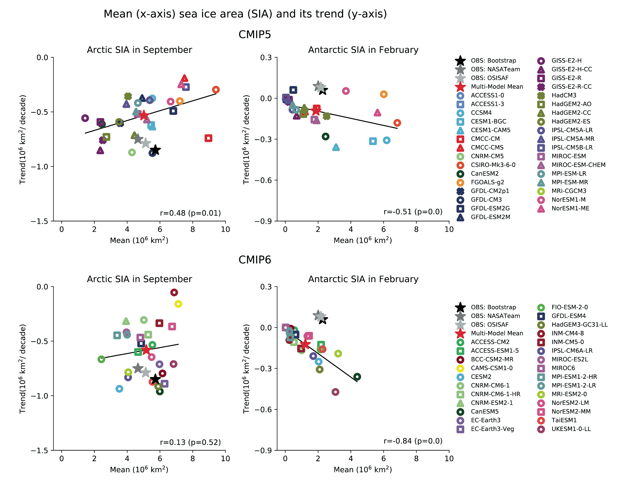 Figure 3.20 | Mean (x-axis) and trend (y-axis) of Arctic sea ice area (SIA) in September (left) and Antarctic SIA in February (right) for 1979–2017 from CMIP5 (upper) and CMIP6 (lower) models. All individual models (ensemble means) and the multi-model mean values are compared with the observations (OSISAF, NASA Team, and Bootstrap; see Figure 9.13). Solid line indicates a linear regression slope with corresponding correlation coefficient (r) and p-value provided. Note the different scales used on the y-axis for Arctic and Antarctic SIA. Results remain essentially the same when using sea ice extent (SIE; not shown). Further details on data sources and processing are available in the chapter data table (Table 3.SM.1).
 Since AR5, there have been several new detection and attribution studies on Arctic sea ice. While the attribution literature has mostly used sea ice extent (SIE), it is closely proportional to sea ice area (SIA; Notz, 2014), which is assessed in Chapters 2 and 9 and shown in Figures 3.20 and 3.21. Kirchmeier-Young et al. (2017) compared the observed time series of the September SIE over the period 1979–2012 with those from different large ensemble simulations which provide a robust sampling of internal climate variability (CanESM2, CESM1, and CMIP5) using an optimal fingerprinting technique. They detected anthropogenic signals which were separable from the response to natural forcing due to solar irradiance variations and volcanic aerosol, supporting previous findings (Figure 3.21; Min et al., 2008b; Kay et al., 2011; Notz and Marotzke, 2012; Notz and Stroeve, 2016). Using selected CMIP5 models and three independently derived sets of observations, Mueller et al. (2018) detected fingerprints from greenhouse gases, natural, and other anthropogenic forcings simultaneously in the September Arctic SIE over the period 1953–2012. They further showed that about a quarter of the greenhouse gas induced decrease in SIE has been offset by an increase due to other anthropogenic forcing (mainly aerosols). Similarly, Gagné et al. (2017b) suggested that the observed increase in Arctic sea ice concentration over the 1950–1975 period was primarily due to the cooling contribution of anthropogenic aerosol forcing based on single model simulations. Gagné et al. (2017a) identified a detectable increase in Arctic SIE in response to volcanic eruptions using CMIP5 models and four observational datasets. Polvani et al. (2020) suggested that ozone depleting substances played a substantial role in the Arctic sea ice loss over the 1955–2005 period.
 Figure 3.21 | Seasonal evolution of observed and simulated Arctic (left) and Antarctic (right) sea ice area (SIA) over 1979–2017. SIA anomalies relative to the 1979–2000 means from observations (OBS from OSISAF, NASA Team, and Bootstrap, top) and historical (ALL, middle) and natural only (NAT, bottom) simulations from CMIP5 and CMIP6 models. These anomalies are obtained by computing non-overlapping three-year mean SIA anomalies for March (February for Antarctic SIA), June, September, and December separately. CMIP5 historical simulations are extended by using RCP4.5 scenario simulations after 2005 while CMIP6 historical simulations are extended by using SSP2-4.5 scenario simulations after 2014. CMIP5 NAT simulations end in 2012. Numbers in brackets represent the number of models used. The multi-model mean is obtained by taking the ensemble mean for each model first and then averaging over models. Grey dots indicate multi-model mean anomalies stronger than inter-model spread (beyond ± 1 standard deviation). Results remain very similar when based on sea ice extent (SIE – not shown). Units: 106km2. Further details on data sources and processing are available in the chapter data table (Table 3.SM.1) and in the caption to Figure 9.13.
 Differences in sea ice loss among the models (Figure 3.20) have been attributed to a number of factors (see also Section 9.3.1.1). These factors include the late 20th century simulated sea ice state (Massonnet et al., 2012), the magnitude of changing ocean heat transport (Mahlstein and Knutti, 2011), and the rate of global warming (e.g., Gregory et al., 2002; Mahlstein and Knutti, 2012; Rosenblum and Eisenman, 2017). Sea ice thermodynamic considerations indicate that the magnitude of sea ice variability and loss depends on ice thickness (Bitz, 2008; Massonnet et al., 2018) and hence the climatology simulated by different models may influence their simulated sea ice trends (medium confidence), as indicated by the regression lines in Figure 3.20.
An important consideration in comparing Arctic sea ice loss in models and observations is the role of internal variability (medium confidence). Using ensemble simulations from a single model, Kay et al. (2011) suggested that internal variability could account for about half of the observed September ice loss. More recently, large ensemble simulations have been performed with many more ensemble members (Kay et al., 2015). These enable a more robust characterization of internal variability in the presence of forced anthropogenic change. Using such large ensembles, some studies discussed the influence of internal variability on Arctic sea ice trends (Swart et al., 2015). Song et al. (2016) also compared the trends in the forced and unforced simulations using multiple climate models and found that internal variability explains about 40% of the observed September sea ice melting trend, supporting previous studies (Stroeve et al., 2012). Based on the large ensembles of CESM1 and CanESM2, the September Arctic sea ice extent variance first increases and then decreases as SIE declines from its pre-industrial value (Kirchmeier-Young et al., 2017; Mueller et al., 2018) consistent with previous work (Goosse et al., 2009), but neither study found a strong sensitivity of detection and attribution results to the change in variability. Further work has indicated that internally-driven summer atmospheric circulation trends with enhanced atmospheric ridges over Greenland and the Arctic Ocean, which project on the negative phase of the North Atlantic Oscillation (Section 3.7.1), play an important role in the observed Arctic sea ice loss (Hanna et al., 2015; Ding et al., 2017). A fingerprint analysis using the CESM large ensemble suggests that this internal variability accounts for 40–50% of the observed September Arctic sea ice decline (Ding et al., 2019; England et al., 2019). Internally-generated decadal tropical variability and associated atmospheric teleconnections were suggested to have contributed to the changing atmospheric circulation in the Arctic and the associated rapid sea ice decline from 2000 to 2014 (Meehl et al., 2018).
Some recent studies evaluated the human contribution to recent record minimum SIE events in the Arctic. Analysing CMIP5 simulations, Zhang and Knutson (2013) found that the observed 2012 record low in September Arctic SIE is inconsistent with internal climate variability alone. Based on several large ensembles, Kirchmeier-Young et al. (2017) concluded that the observed 2012 SIE minimum cannot be reproduced in a simulation excluding human influence. Fučkar et al. (2016) showed that climate change contributed to the record low March Arctic SIE in 2015, which was accompanied by the record minimum SIE in the Sea of Okhotsk (Paik et al., 2017).
Based on the new attribution studies since AR5, we conclude that it is very likely that anthropogenic forcing mainly due to greenhouse gas increases was the main driver of Arctic sea ice loss since 1979. Increases in anthropogenic aerosols have offset part of the greenhouse gas induced Arctic sea ice loss since the 1950s (medium confidence). Despite large differences in the mean sea ice state in the Arctic, Arctic sea ice loss is captured by all CMIP5 and CMIP6 models. Nonetheless, large inter-model differences in the Arctic sea ice decline remain, limiting our ability to quantify forced changes and internal variability contributions.
3.4.1.2 Antarctic Sea Ice
AR5 concluded that ‘there is low confidence in the attribution of the observed increase in Antarctic SIE since 1979’ (Bindoff et al., 2013) due to the limited understanding of the external forcing contribution as well as the role of internal variability. Based on a difference between the first and last decades, Antarctic sea ice cover exhibited a small increase in summer and winter over the 1979–2017 period (Section 2.3.2.1.2, and Figures 3.20 and 3.21). However, these changes are not statistically significant and starting in late 2016, anomalously low sea ice area has been observed (Section 2.3.2.1.2). The mean hemispheric sea ice changes result from much larger, but partially compensating, regional changes with increases in the western Ross Sea and Weddell Sea and declines in the Bellingshausen and Amundsen Seas (Hobbs et al., 2016). Observed regional trends have been particularly large in austral autumn (see Section 2.3.2.1.2, and also Section 9.3.2.1 for more details of regional changes and related physical processes). Starting in austral spring of 2016, the ice extent decreased strongly (Turner et al., 2017) and has since remained anomalously low (Figure 3.21 and Figure 2.20). This decrease has been associated with anomalous atmospheric conditions associated with teleconnections from warming in the eastern Indian Ocean and a negative Southern Annular Mode (Chenoli et al., 2017; Stuecker et al., 2017; Schlosser et al., 2018; Meehl et al., 2019; Purich and England, 2019; G. Wang et al., 2019). A decadal-scale warming of the near-surface ocean that resulted from strengthened westerlies may also have contributed to and helped to sustain the sea ice loss (Meehl et al., 2019). Before satellites and on even longer time scales, very limited observational data and proxy coverage leads to low confidence in all aspects of Antarctic sea ice (Sections 2.3.2.1.2 and 9.3.2.1).
CMIP5 climate models generally simulate Antarctic sea ice loss over the satellite era since 1979 (Mahlstein et al., 2013; Turner et al., 2013) in contrast to the observed change, and CMIP6 models also simulate Antarctic ice loss (Roach et al., 2020; Figure 3.20 and 3.21). A number of studies have suggested that this discrepancy may be in part due to the role of internal variability in the observed change (Mahlstein et al., 2013; Polvani and Smith, 2013; Zunz et al., 2013; Meehl et al., 2016c; Turner et al., 2016), including teleconnections associated with tropical Pacific variability (Meehl et al., 2016c) and changing surface conditions resulting from multi-decadal ocean circulation variations (Singh et al., 2019). However, when the spatial pattern is considered, trends in the summer and autumn (from 1979–2005) appear outside the range of internal variability (Hobbs et al., 2015). This suggests that the models may exhibit an unrealistic simulation of the Antarctic sea ice forced response or the internal variability of the system. Discrepancies among the models in simulated sea ice variability (Zunz et al., 2013), the sea ice climatological state (Roach et al., 2018), upper ocean temperature trends (Schneider and Deser, 2018), Southern Hemisphere westerly wind trends (Purich et al., 2016), or the sea ice response to Southern Annular Mode variations (Ferreira et al., 2014; Holland et al., 2017; Kostov et al., 2017; Landrum et al., 2017) may all play some role in explaining these differences with the observed trends. Increased fresh water fluxes caused by mass loss of the Antarctic Ice Sheet (either by melting at the front of ice shelves or via iceberg calving) have been suggested as a possible mechanism driving the multi-decadal Antarctic sea ice expansion (Bintanja et al., 2015; Pauling et al., 2016) but there is a lack of consensus on this mechanism’s impacts (Pauling et al., 2017). A recent study based on a decadal prediction system suggests that initializing the state of the Antarctic Bottom Water cell allows the system to reproduce the observed Antarctic sea ice increase (Zhang et al., 2017), consistent with the suggestion that multi-decadal variability associated with variations in deep convection has contributed to the observed increase in Antarctic sea ice since 1979 (Latif et al., 2013; Zhang et al., 2017; L. Zhang et al., 2019) (see also Section 9.3.2.1).
There have been several studies that aimed to identify causes of the observed Antarctic SIE changes. Gagné et al. (2015) assessed the consistency of observed and simulated changes in Antarctic SIE for an extended period using recovered satellite-based estimates, and found that the observed trends since the mid-1960s are not inconsistent with model simulated trends. Studies based on the satellite period also indicate that the observed trends are largely within the range of simulated internal variability (Hobbs et al., 2016). A few distinct factors that led to the weak signal-to-noise ratio in Antarctic SIE trends have been further identified, which include large multi-decadal variability (Monselesan et al., 2015), the short observational record (e.g., Abram et al., 2013), and the limited model performance at representing the complex Antarctic climate system as discussed above (Bintanja et al., 2013; Uotila et al., 2014). The short period of comprehensive satellite observations, beginning in 1979, makes it challenging to set the observed increase between 1979 and 2015, or the subsequent decrease, in a long-term context, and to assess whether the difference in trend between observations and models, which mostly simulate long-term decreases, is systematic or a rare expression of internal variability on decadal to multi-decadal time scales.
In conclusion, the observed small increase in Antarctic sea ice extent during the satellite era is not generally captured by global climate models, and there is low confidence in attributing the causes of the change.
3.4.2 Snow Cover
Seasonal snow cover is a defining climate feature of the northern continents. It is therefore of considerable interest that climate models correctly simulate this feature. It is discussed in more detail in Section 9.5.3, and observational aspects of snow cover are assessed in Section 2.3.2.2.
The AR5 noted the strong linear correlation between Northern Hemisphere snow cover extent (SCE) and annual-mean surface air temperature in CMIP5 models. It was assessed as likely that there had been an anthropogenic contribution to observed reductions in Northern Hemisphere snow cover since 1970 (Bindoff et al., 2013). The AR5 assessed that CMIP5 models reproduced key features of observed snow cover well, including the seasonal cycle of snow cover over northern regions of Eurasia and North America, but had more difficulties in more southern regions with intermittent snow cover. The AR5 also found that CMIP5 models underestimated the observed reduction in spring snow cover over this period (Figure 3.22; see also Brutel-Vuilmet et al., 2013; Thackeray et al., 2016; Santolaria-Otín and Zolina, 2020). This behaviour has been linked to how the snow-albedo feedback is represented in models (Thackeray et al., 2018a). The CMIP5 multi-model ensemble has been shown to represent the snow-albedo feedback more realistically than CMIP3, although models from some individual modelling centres have not improved or have even got worse (Thackeray et al., 2018a). There is still a systematic overestimation of the albedo of boreal forest covered by snow (Thackeray et al., 2015; Y. Li et al., 2016). Consequently, the snow albedo feedback might have been overestimated by CMIP5 models (Section 9.5.3; Xiao et al., 2017).
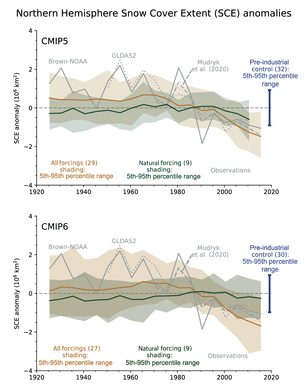 Figure 3.22 | Time series of Northern Hemisphere March–April mean snow cover extent (SCE) from observations, CMIP5 and CMIP6 simulations. The observations (grey lines) are updated Brown-NOAA (Brown and Robinson, 2011), Mudryk et al. (2020), and GLDAS2. CMIP5 (top) and CMIP6 (bottom) simulations of the response to natural plus anthropogenic forcing are shown in brown, natural forcing only in green, and the pre-industrial control simulation range is presented in blue. Five-year mean anomalies are shown for the 1923–2017 period with the x-axis representing the centre years of each five-year mean. CMIP5 all forcing simulations are extended by using RCP4.5 scenario simulations after 2005 while CMIP6 all forcing simulations are extended by using SSP2-4.5 scenario simulations after 2014. Shading indicates 5th–95th percentile ranges for CMIP5 and CMIP6 all and natural forcings simulations, and solid lines are ensemble means, based on all available ensemble members with equal weight given to each model (Section 3.2). The blue vertical bar indicates the mean 5th–95th percentile range of pre-industrial control simulation anomalies, based on non-overlapping segments. The numbers in brackets indicate the number of models used. Anomalies are relative to the average over 1971–2000. For models, SCE is restricted to grid cells with land fraction ≥50%. Greenland is excluded from the total area summation. Figure is modified from Paik and Min (2020), their Figure 1. Further details on data sources and processing are available in the chapter data table (Table 3.SM.1).
 CMIP6 models improve on CMIP5 models in producing slightly increased SCE versus CMIP5, correcting the low bias in CMIP5 (Mudryk et al., 2020). The linear relationship noted above between GSAT and SCE also exists in CMIP6 (Mudryk et al., 2020). Like CMIP5, the CMIP6 models capture the negative trend in spring snow cover that has occurred in recent decades (Figure 3.22). However, the median CMIP6 model now produces slightly stronger post-1981 declines in the March to April mean SCE than the CMIP5 median (Mudryk et al., 2020). Until about 1980, the models produce a generally stable March to April SCE, but after that a substantial decline, reaching a loss of about 2 × 10⁶km2 in 2012–2017 relative to the 1971–2000 average. Compared to earlier studies which found that models underestimate observed trends for the 1979–2005 period (Brutel-Vuilmet et al., 2013), both CMIP5 and CMIP6 models show improved agreement with the observations over the period to 2017 (Figure 3.22). One remaining concern is a failure of most CMIP6 models to correctly represent the relationship between snow cover extent and snow mass, reflecting too slow seasonal increases and decreases of SCE in the models (Mudryk et al., 2020).
Several CMIP5 and CMIP6 based studies have consistently attributed the observed Northern Hemisphere spring SCE changes (Section 2.3.2.2) to anthropogenic influences (Rupp et al., 2013; Najafi et al., 2016; Paik and Min, 2020), with the observed changes being found to be inconsistent with natural variability alone. Similarly, spring snow thickness (Snow Water Equivalent) changes on the scale of the Northern Hemisphere have been attributed to greenhouse gas forcing (Jeong et al., 2017). Using individual forcing simulations from multiple CMIP6 models, Paik and Min (2020) detected greenhouse gas influence in the observed decrease of early spring SCE between 1925 and 2019, which was found to be separable from the responses to other forcings.
In summary, it is very likely that anthropogenic influence contributed to the observed reductions in Northern Hemisphere springtime snow cover since 1950. CMIP6 models better represent the seasonality and geographical distribution of snow cover than CMIP5 simulations (high confidence). Both CMIP5 and CMIP6 models simulate strong declines in spring SCE during recent years, in general agreement with observations, causing the multi-model mean decreasing trend in spring SCE to now better agree with observations than in earlier evaluations. Evidence has yet to emerge that interactions between vegetation and snow, found problematic in CMIP5, have improved in CMIP6 models (Section 9.5.3). Such deficiencies in the representation of snow in climate models mean there is medium confidence in the simulation of snow cover over the northern continents in CMIP6 model simulations. The models consistently link snow extent to surface air temperature (Figure 9.24). With warming of near-surface air linked to anthropogenic influence, and particularly to greenhouse gas increases (Section 3.3.1.1), this provides additional evidence that reductions in snow cover are also caused by human activity.
3.4.3 Glaciers and Ice Sheets
While (Chapter 9 (Sections 9.4 and 9.5) discusses process understanding for glaciers and ice sheets, as well as evaluation of global and regional-scale glacier and ice-sheet models, our focus here is on the attribution of large-scale changes in glaciers and ice sheets. Land ice in the form of glaciers has been included in CMIP climate and Earth system models as components of the land surface models for many years. However, their representation is simplified and is omitted altogether in the less complex modelling systems. In CMIP3 (Meehl et al., 2007) and CMIP5 (Taylor et al., 2012) land ice area fraction, a component of land surface models, was defined as a time-independent quantity, and in most model configurations was preset at the simulation initialization as a permanent land feature. In CMIP6 considerable progress has been made in improving and evaluating the representation of modelled land ice. For glaciers, an example is the expansion of the Joint UK Land Environment Simulator (JULES) land surface model to enable elevated tiles, and hence more accurately simulate the altitudinal atmospheric effects on glaciers (Shannon et al., 2019). Moreover, standalone glacier models have now been systematically compared in GlacierMIP (Hock et al., 2019a; Marzeion et al., 2020). The Antarctic and Greenland Ice Sheets were absent in global climate models that pre-date CMIP6 (Eyring et al., 2016a), however some preliminary analyses that used results from CMIP5 to drive standalone ice-sheet models were included in AR5 (Church et al., 2013a). For the first time in CMIP, the latest CMIP6 phase includes a coordinated effort to simulate temporally evolving ice sheets within the Ice Sheet Model Intercomparison Project (ISMIP6; Box 9.3; Nowicki et al., 2016). Our understanding of aspects of the global water storage contained in glaciers and ice sheets, and their contribution to sea-level rise, has improved since AR5 and SROCC (Hock et al., 2019b; Meredith et al., 2019) both in models and observations (see assessment of observations and model evaluation for the Greenland Ice Sheet in Sections 2.3.2.4.1 and 9.4.1; Antarctica in Sections 2.3.2.4.2 and 9.4.2; and glaciers in Sections 2.3.2.3 and 9.5.1).
3.4.3.1 Glaciers
Glaciers are defined as perennial surface land ice masses independent of the Antarctic and Greenland Ice Sheets (Sections 9.5 and 2.3.2.3). The AR5 assessed that anthropogenic influence had likely contributed to the retreat of glaciers observed since the 1960s (Bindoff et al., 2013), based on a high level of scientific understanding and robust estimates of observed mass loss, internal variability, and glacier response to climatic drivers. The SROCC (Hock et al., 2019b) concluded that atmospheric warming was very likely the primary driver of glacier recession.
Simulations of glacier mass changes under climate change rely on glacier models driven by climate model output, often in collaborative research efforts such as GlacierMIP (Hock et al., 2019a; Marzeion et al., 2020). The GlacierMIP project is a systematic coordinated modelling effort designed to further understanding of glacier loss using global models. While the low resolution and remaining biases of climate model-derived boundary forcing data is a limitation, the release of the Randolph Glacier Inventory (Pfeffer et al., 2014; RGI Consortium, 2017) has supported more sophisticated, systematic and comprehensive modelling of glaciers worldwide (Hock et al., 2019a).
A regional study considering 85 Northern Hemisphere glacier systems concluded that there is a discernible human influence on glacier mass balance, with glacier model simulations driven by CMIP5 historical and greenhouse gas-only simulations showing a glacier mass loss, whereas those driven by natural-only forced simulations showed a net glacier growth (Hirabayashi et al., 2016). In addition, a study of the role of climate change in glacier retreat using a simple mass-balance model for 37 glaciers worldwide, concluded that observed length changes would not have occurred without anthropogenic climate change, with observed length variations exceeding those associated with internal variability by several standard deviations in many cases (Roe et al., 2017). Roe et al. (2021) used the same model to estimate that at least 85% of cumulative glacier mass loss since 1850 is attributable to anthropogenic influence. While Marzeion et al. (2014) found that anthropogenic influence contributed only 25 ± 35% of glacier mass loss for the period 1851–2010, their naturally-forced simulations exhibited a substantial negative mass balance, which Roe et al. (2021) argued is unrealistic. Moreover, Marzeion et al. (2014) estimated that anthropogenic influence contributed 69 ± 24% of glacier mass loss for the period 1991 to 2010, consistent with a progressively increasing fraction of mass loss attributable to anthropogenic influence found by Roe et al. (2021).
In summary, considering together the SROCC assessment that atmospheric warming was very likely the primary driver of glacier recession, the results of Roe et al. (2017, 2021) and our assessment of the dominant role of anthropogenic influence in driving atmospheric warming (Section 3.3.1), we conclude that human influence is very likely the main driver of the near-universal retreat of glaciers globally since the 1990s.
3.4.3.2 Ice Sheets
3.4.3.2.1 Greenland Ice Sheet
The AR5 assessed that it is likely that anthropogenic forcing contributed to the surface melting of the Greenland Ice Sheet since 1993 (Bindoff et al., 2013). The SROCC did not directly assess the attribution of Greenland Ice Sheet change to anthropogenic forcing, but it did assess with medium confidence that summer melting of the Greenland Ice Sheet has increased to a level unprecedented over at least the last 350 years, which is two-to-fivefold the pre-industrial level (see also Trusel et al., 2018).
(Section 2.3.2.4.1 assesses that Greenland Ice Sheet mass loss began in the latter half of the 19th century and that the rate of loss has increased substantially since the turn of the 21st century (high confidence), and also notes that integration of proxy evidence and modelling indicates that the last time the rate of mass loss was similar to the 20th century rate was during the early Holocene. Models of Greenland Ice Sheet evolution are evaluated in detail in Section 9.4.1.2, which assesses that there is overall medium confidence in these models. Model evaluation of surface mass balance changes over the Greenland Ice Sheet, including regional aspects, is also assessed in Atlas.11.2.3.
Detection and attribution studies of change in the Greenland Ice Sheet remain challenging (Kjeldsen et al., 2015; Bamber et al., 2019). This is in part due to the short observational record (Shepherd et al., 2012, 2018, 2020; Bamber et al., 2018; Cazenave et al., 2018; Mouginot et al., 2019; Rignot et al., 2019) and the challenges this poses to the evaluation of modelling efforts (Section 9.4.1.2). The latter require not only dynamic ice-sheet models, but also appropriate atmospheric and oceanic conditions to use as a boundary forcing to drive the models (Nowicki and Seroussi, 2018; Barthel et al., 2020). Nonetheless, new literature since AR5 finds that ice-sheet mass balance calculations using reanalysis-driven regional model simulations of surface mass balance are found to agree well with the observed decrease in ice-sheet mass over the past twenty years (Fettweis et al., 2020; Sasgen et al., 2020; Tedesco and Fettweis, 2020), consistent with earlier studies (Flato et al., 2013). These studies also show that the exceptional melt events observed in 2012 and 2019 were associated with exceptional atmospheric conditions (Sasgen et al., 2020; Tedesco and Fettweis, 2020). These results support the finding that increased surface melting is associated with warming, although atmospheric circulation anomalies, including the summer North Atlantic Oscillation (NAO) and variations in snowfall play an important role in driving interannual variations (Section 9.4.1.1; Sasgen et al., 2020; Tedesco and Fettweis, 2020). Further, a coupled ice-sheet-climate model study found emergence of decreased surface mass balance prior to the present day in coastal locations in Greenland, which dominate the integrated surface mass balance (Fyke et al., 2014), suggesting that observed variations in surface mass balance in these regions might be expected to be distinguishable from internal variability. A CMIP6 simulation of the historical period showed stable Greenland surface mass balance up to the 1990s, after which it declined due to increased melt and runoff, consistent with a downscaled reanalysis (van Kampenhout et al., 2020). Further, all experts surveyed in a structured expert judgement exercise examining the causes of the increase in mass loss from the Greenland Ice Sheet over the last two decades (Bamber et al., 2019) concluded that external forcing was responsible for at least 50% of the mass loss. A comparison of Greenland Ice Sheet mass loss trends from observations and AR5 model projections for the period 2007–2017 found that the magnitude of the observed surface mass balance trends was at the top of the AR5 assessed range, while mass loss due to changing ice dynamics was near the centre of the AR5 range (Slater et al., 2020), providing further evidence of consistent anthropogenically-forced mass loss trends in models and observations.
Drawing together the evidence from the continued and strengthened observed mass loss, the agreement between anthropogenically forced climate simulations and observations, and historical and paleo evidence for the unusualness of the observed rate of surface melting and mass loss, we assess that it is very likely that human influence has contributed to the observed surface melting of the Greenland Ice Sheet over the past two decades, and that there is medium confidence in an anthropogenic contribution to recent overall mass loss from Greenland.
3.4.3.2.2 Antarctic Ice Sheet
AR5 assessed that there was low confidence in attributing the causes of the observed mass loss from the Antarctic Ice Sheet since 1993 (Bindoff et al., 2013). The SROCC assessed that there is medium agreement but limited evidence of anthropogenic forcing of Antarctic mass balance through both surface mass balance and glacier dynamics. It further assessed that Antarctic ice loss is dominated by acceleration, retreat and rapid thinning of the major West Antarctic Ice Sheet outlet glaciers (very high confidence), driven by melting of ice shelves by warm ocean waters (high confidence). Based on updated observations, Chapter 2 assesses that there is very high confidence that the Antarctic Ice Sheet lost mass between 1992 and 2017, and that there is medium confidence that this mass loss has accelerated. Models of Antarctic Ice Sheet evolution are evaluated in detail in Section 9.4.2.2, which assesses that there is medium confidence in many ice-sheet processes in Antarctic Ice Sheet models, but low confidence in the ocean forcing affecting basal melt rates. CMIP5 and CMIP6 models perform similarly in their simulation of Antarctic surface mass balance (Section 9.4.2.2, Gorte et al., 2020). Model evaluation of surface mass balance over the Antarctic Ice Sheet, including regional aspects, is also assessed in Atlas.11.1.3.
Ice discharge around the West Antarctic Ice Sheet is strongly influenced by variability in basal melt (Jenkins et al., 2018; Hoffman et al., 2019), in particular at decadal and longer time scales (Snow et al., 2017). Basal melt rate variability can be induced by wind-driven ocean current changes, which may partly be of anthropogenic origin via greenhouse gas forcing (Holland et al., 2019). Moreover, ice discharge losses from the Antarctic Ice Sheet over the 2007–2017 period are close to the centre of the model-based range projected in AR5 (Slater et al., 2020). However, expert opinion differs as to whether recent Antarctic ice loss from the West Antarctic Ice Sheet has been driven primarily by external forcing or by internal variability, and there is no consensus (Bamber et al., 2019). Anthropogenic influence on the Antarctic surface mass balance, which is expected to partially compensate for ice discharge losses through increases in snowfall, is currently masked by strong natural variability (Previdi and Polvani, 2016; Bodart and Bingham, 2019), and observations suggest that it has been close to zero over recent years (see further discussion in Section 9.4.2.1; Slater et al., 2020).
Overall, there is medium agreement but limited evidence of anthropogenic influence on Antarctic mass balance through changes in ice discharge.
3.5 Human Influence on the Ocean
The global ocean plays an important role in the climate system, as it is responsible for transporting and storing large amounts of heat (Sections 3.5.1 and 9.2.2.1), freshwater (Sections 3.5.2 and 9.2.2.2) and carbon (Sections 3.6.2 and 5.2.1.3) that are exchanged with the atmosphere. Therefore, accurate ocean simulation in climate models is essential for the realistic representation of the climatic response to anthropogenic warming, including rates of warming, sea level rise and carbon uptake, and the representation of coupled modes of climate variability.
Ocean model development has advanced considerably since AR5 (Section 1.5.3.1). Ongoing model developments since AR5 have focused on improving the realism of the simulated ocean in coupled models, with horizontal resolutions increasing to 10–100 km (from about 200 km in CMIP5), and increased vertical resolutions in many modelling systems of 0–1 m for near-surface levels (from the highest resolution of 10 m in CMIP5). These developments are aimed at improving the representation of the diurnal cycle and coupling to the atmosphere (e.g., Bernie et al., 2005, 2007, 2008). General improvements to simulated ocean fidelity in response to increasing resolution are expected (Hewitt et al., 2017), and the effects of model resolution on the fidelity of ocean models are discussed in more detail in Sections 9.2.2 and 9.2.4.
In this section we assess the global and basin-scale properties of the simulated ocean, with a focus on evaluation of the realism of simulated ocean properties, and the detection and attribution of human-induced changes in the ocean over the period of observational coverage. Observed changes to ocean temperature (Section 2.3.3.1), salinity (Section 2.3.3.2), sea level (Section 2.3.3.3) and ocean circulation (Section 2.3.3.4) are reported in Chapter 2. A more process-based assessment of ocean changes, alongside the assessment of variability and changes in ocean properties with spatial scales smaller than ocean basins, is presented in Chapter 9.
3.5.1 Ocean Temperature
Ocean temperature and ocean heat content are key physical variables considered for climate model evaluation and are primary indicators of a changing ocean climate. This section assesses the performance of climate models in representing the mean state ocean temperature and heat content (Section 3.5.1.1), with a particular focus on the tropical oceans given the importance of air-sea coupling in these areas (Section 3.5.1.2). This is followed by an assessment of detection and attribution studies of changes in ocean temperature and heat content (Section 3.5.1.3). Changes in global surface temperature are assessed in Section 3.3.1.1.
3.5.1.1 Sea Surface and Zonal Mean Ocean Temperature Evaluation
In CMIP3 and CMIP5 models, large SST biases were found in the mid- and high latitudes (Flato et al., 2013). In CMIP6, the Northern Hemisphere mid-latitude surface temperature biases appear to be marginally improved in the multi-model mean when contrasted to CMIP5 despite large biases remaining in a few models (Figures 3.23a and 3.24). There is a decreased spread of the zonal mean SST error between 50°N and 30°S, relative to CMIP5 (Figure 3.24a). On the other hand, the Southern Ocean’s warm surface temperature bias remains (Figure 3.23a; Beadling et al., 2020), and is on average larger in CMIP6 than in CMIP5 models (Figures 3.23a and 3.24). This warm bias is often associated with persistent overlying atmospheric cloud biases (Hyder et al., 2018). Several other large biases also appear to remain largely unresolved in CMIP6, particularly warm biases in excess of 1°C along the equatorial eastern continental boundaries of the tropical Atlantic and Pacific Oceans (Figure 3.23a).
 Figure 3.23 | Multi-model mean bias of (a) sea surface temperature and (b) near-surface salinity, defined as the difference between the CMIP6 multi-model mean and the climatology from the World Ocean Atlas 2018. The CMIP6 multi-model mean is constructed with one realization of 46 CMIP6 historical experiments for the period 1995–2014 and the climatology from the World Ocean Atlas 2018 is an average over all available years (1955–2017). Uncertainty is represented using the advanced approach: No overlay indicates regions with robust signal, where ≥66% of models show change greater than the variability threshold and ≥80% of all models agree on sign of change; diagonal lines indicate regions with no change or no robust signal, where <66% of models show a change greater than the variability threshold; crossed lines indicate regions with conflicting signal, where ≥66% of models show change greater than the variability threshold and <80% of all models agree on sign of change. For more information on the advanced approach, please refer to Cross-Chapter Box Atlas.1. Further details on data sources and processing are available in the chapter data table (Table 3.SM.1).
Overall, the simulated and observed trends in SST patterns are generally consistent for the historical period (Olonscheck et al., 2020). The CMIP6 models generally represent the observed pattern of trends better than the CMIP5 models, and observed trends fall within the range of simulated trends over a larger area for CMIP6 models than for CMIP5 models (Olonscheck et al., 2020).
The CMIP5 multi-model mean zonally averaged subsurface ocean temperature showed warm biases between 200 m and 2000 m (mid-depth) over most latitudes, with exceptions in the Southern Ocean (>60°S, 100–2000 m) and upper (0–400 m) Arctic Ocean. Cold biases were simulated near the surface (0–200 m) at most latitudes (Flato et al., 2013). CMIP6 biases are broadly consistent with those reported in CMIP5 for the near-surface (<200 m) and mid-depth (200–2000 m) ocean (Voldoire et al., 2019b; Beadling et al., 2020; Y. Zhu et al., 2020). The warm bias begins between 100 and 400 m depth in all three basins, however, it is most prominent in the Atlantic Ocean, with a maximum magnitude in the equatorial latitudes, as in CMIP5 (Figure 3.25). In the Pacific, the large warm biases are mostly seen in the subtropical regions (30°N–60°N and 30°S–60°S). The cool near surface tropical bias is most prominent in the Pacific Ocean and also present in the Atlantic, with a smaller magnitude (Figure 3.25). Relative to CMIP5, the most prominent difference is an increase to the mid-depth (300–2000 m) warm bias in CMIP6 and a change in sign of the bias from cold to warm for the Southern Ocean mid-depth (>60°S) from CMIP5 to CMIP6 (Figure 3.25). Compared to CMIP3 and CMIP5, there is improved agreement between most CMIP6 models and observations in their representation of the zonal mean temperature of the upper 100 m of the Southern Ocean (Beadling et al., 2020).
 Figure 3.25 | CMIP6 potential temperature and salinity biases for the global ocean, Atlantic Ocean, Pacific Ocean and Indian Ocean. Shown in colour are the time-mean differences between the CMIP6 historical multi-model climatological mean and observations, zonally averaged for each basin (excluding marginal and regional seas). The observed climatological values are obtained from the World Ocean (Atlas 2018 (WOA18, 1981–2010; Prepared by the Ocean Climate Laboratory, National Oceanographic Data Center, Silver Spring, MD, USA), and are shown as labelled black contours for each of the basins. The simulated annual mean climatologies for 1981 to 2010 are calculated from available CMIP6 historical simulations, and the WOA18 climatology utilized synthesized observed data from 1981 to 2010. Output from a total of 30 available CMIP6 models is used for the temperature panels (left column) and 28 models for the salinity panels (right column). Potential temperature units are °C and salinity units are the Practical Salinity Scale 1978 [PSS-78]. Further details on data sources and processing are available in the chapter data table (Table 3.SM.1).
 Focusing on the deep ocean (>2000 m), the CMIP6 ensemble mean shows a prominent and consistent warm bias (Figure 3.25), in all basins except the equatorial and northern Pacific, which contrasts to a cold bias seen in CMIP5 (Flato et al., 2013). We note that while an updated observational temperature dataset is used in this assessment (WOA09 was used in AR5, while WOA18, 1981–2010 is used in AR6), the deep-ocean warm bias remains and is approaching double the magnitude (about 0.5°C) of the equivalent CMIP5 multi-model mean bias, a feature which is particularly prominent in the Atlantic and southern Indian Oceans. Increased horizontal resolution as well as the choice of the vertical coordinate are reported to partly improve these biases in some models (Adcroft et al., 2019; Rackow et al., 2019; Hewitt et al., 2020).
Since AR5, there has been growing evidence that the representation of mean surface and deeper ocean temperatures in coupled climate models can be improved by increasing the horizontal resolution both in the ocean and the atmosphere (e.g., Small et al., 2014; Hewitt et al., 2016; Iovino et al., 2016; Roberts et al., 2019). At an ocean resolution of around 1°, which is typical of CMIP6 models, some processes are parameterized rather than explicitly resolved, leading to a compromise in their dynamical representation. An increase in the model resolution allows for processes to be explicitly resolved, and can for example, enhance the simulation of eddies, thus improving simulated vertical eddy transport, and reducing temperature drifts in the deeper ocean (Griffies et al., 2015; von Storch et al., 2016). For some models, the mean absolute error in ocean temperature below 500 m is smaller in the high resolution version compared to the low resolution version, particularly in eddy-active regions such as the North Atlantic (Rackow et al., 2019). Increasing the horizontal resolution of individual climate models often leads to an overall decrease in the surface temperature biases over regions where they persisted through earlier CMIP generations, such as the central and western equatorial Pacific, as well as the North and tropical Atlantic (Figure 3.3e; Roberts et al., 2019; Hewitt et al., 2020). Despite this, as a group the four HighResMIP models included in Figures 3.3e and 3.24 do not on average show smaller SST biases than the CMIP6 multi-model mean, demonstrating the importance of factors other than resolution in contributing to SST biases.
In summary, there is little improvement in the multi-model mean sea surface and zonal mean ocean temperatures from CMIP5 to CMIP6 (medium confidence). Nevertheless, the CMIP6 models show a somewhat more realistic pattern of SST trends (low confidence).
3.5.1.2 Tropical Sea Surface Temperature Evaluation
3.5.1.2.1 Tropical Pacific Ocean
In CMIP5, mean state biases in the tropical Pacific Ocean including the excessive equatorial cold tongue, erroneous mean thermocline depth and slope along the equator remained but were improved relative to CMIP3 (Flato et al., 2013). Misrepresentation of the interaction between the atmosphere and ocean via the Bjerknes feedback and vertical mixing parameterizations, and a bias in winds were among the suggested reasons for the persistent biases (Li et al., 2014; Zhu and Zhang, 2018). Moving to CMIP6, a reduction of the cold bias in the equatorial cold tongue in the central Pacific is found on average in the CMIP6 models (Figure 3.24b; Grose et al., 2020; Planton et al., 2021), however, this reduced bias is not statistically significant when considered across the multi-model ensemble (Planton et al., 2021). It is also noteworthy that the longitude of the 28°C isotherm is closer to observed in CMIP6 than in CMIP5, with a coincident reduction in the CMIP6 inter-model standard deviation (Grose et al., 2020). The latter result implies that there is an improvement in the representation of the tropical Pacific mean state in CMIP6 models. Comparison of biases in individual HighResMIP models with biases in lower resolution versions of the same models indicates that there is no consistent improvement in SST biases in most of the equatorial Pacific with resolution (Figure 3.3e; Bock et al., 2020).
3.5.1.2.2 Tropical Atlantic Ocean
Fundamental features such as the mean zonal SST gradient in the tropical Atlantic were not reproduced in CMIP5 models. Studies have proposed that weaker than observed alongshore winds, underestimation of stratocumulus clouds, coarse model resolution, and insufficient oceanic cooling due to a deeper thermocline depth and weak vertical velocities at the base of the mixed layer in the eastern basin, underpinned these tropical Atlantic SST gradient biases (Hourdin et al., 2015; Richter, 2015). The SST gradient biases still remain in CMIP6. On average the cold bias in the western part of the basin is reduced while the warm bias in the eastern part has slightly increased (Figure 3.24b,c; Richter and Tokinaga, 2020). Several CMIP6 models, however, display large reductions in biases of the zonal SST gradient, such that the eastern equatorial Atlantic warm SST bias and associated westerly wind biases are mostly eliminated in these models (Richter and Tokinaga, 2020). The high resolution (HighResMIP) CMIP6 models show a better representation of the zonal SST gradient (Figure 3.24b,c), but some lower resolution models also perform well, suggesting that resolution is not the only factor responsible for biases in Tropical Atlantic SST (Richter and Tokinaga, 2020).
3.5.1.2.3 Tropical Indian Ocean
The tropical Indian Ocean mean state is reasonably well simulated both in CMIP5 and CMIP6 (Figure 3.24b,c). However, CMIP5 models show a large spread in the thermocline depth, particularly in the equatorial part of the basin (Saji et al., 2006; Fathrio et al., 2017b), which has been linked to the parameterization of the vertical mixing and the wind structure, leading to a misrepresentation of the ventilation process in some models (Schott et al., 2009; Richter, 2015; Shikha and Valsala, 2018). A common problem with the CMIP5 models is therefore a warm bias in the subsurface, mainly at depths around the thermocline, which is also apparent in the CMIP6 models (Figure 3.25g).
In the CMIP6 multi-model mean, the western tropical Indian Ocean shows a slightly larger warm bias compared to CMIP5 (Figure 3.24 b,c), which in part could be related to excessive supply of warm water from the Red Sea (Grose et al., 2020; Semmler et al., 2020). The HighResMIP models show decreases in SST bias across the Indian Ocean with increasing resolution (Figure 3.3e; Bock et al., 2020), though as a group the SST biases in the HighResMIP models are no smaller than those of the full CMIP6 ensemble.
3.5.1.2.4 Summary
In summary, the structure and magnitude of multi-model mean ocean temperature biases have not changed substantially between CMIP5 and CMIP6 (medium confidence). Although biases remain in the latest generation models, the broad consistency between the observed and simulated basin-scale ocean properties suggests that CMIP5 and CMIP6 models are appropriate tools for investigating ocean temperature and ocean heat content responses to forcing. This also provides high confidence in the utility of CMIP-class models for detection and attribution studies, for both ocean heat content (Section 3.5.1.3) and thermosteric sea level applications (Section 3.5.3.2).
3.5.1.3 Ocean Heat Content Change Attribution
The ocean plays an important role as the Earth’s primary energy store. The AR5 and SROCC assessed that the ocean accounted for more than 90% of the Earth’s energy change since the 1970s (Rhein et al., 2013; Bindoff et al., 2019). These assessments are consistent with recent studies assessed in Section 7.2 and Cross-Chapter Box 9.1, which find that 91% of the observed change in Earth’s total energy from 1971 to 2018 was stored in the ocean (von Schuckmann et al., 2020). The AR5 concluded that anthropogenic forcing has very likely made a substantial contribution to ocean warming above 700 m, whereas below 700 m, limited measurements restricted the assessment of ocean heat content changes in AR5 and prevented a robust comparison between observations and models (Bindoff et al., 2013).
With the recent increase in ocean sampling by Argo to 2000 m (Roemmich et al., 2015; Riser et al., 2016; von Schuckmann et al., 2016) and the resulting improvements in estimates of ocean heat content (Abraham et al., 2013; Balmaseda et al., 2013; Durack et al., 2014b; Cheng et al., 2017; von Schuckmann et al., 2020), a more quantitative assessment of the global ocean heat content changes that extends into the intermediate ocean (700–2000 m) over the more recent period (from 2005 to the present; Durack et al., 2018) can be performed. Observed ocean heat content changes are discussed in Section 2.3.3.1, where it is reported that it is virtually certain that the global upper ocean (0–700 m) and very likely that the global intermediate ocean (700–2000 m) warmed substantially from 1971 to the present. Further, ocean layer warming contributions are reported as 61% (0–700 m), 31% (700–2000 m) and 8% (>2000 m) for the 1971 to 2018 period (Table 2.7). CMIP5 model simulations replicate this partitioning fairly well for the industrial-era (1865 to 2017) throughout the upper (0–700 m, 65%), intermediate (700–2000 m, 20%) and deep (>2000 m, 15%) layers (Gleckler et al., 2016; Durack et al., 2018). The corresponding warming percentages for the multi-model mean of a subset of CMIP6 simulations over the 1850–2014 period are 58% for the upper, 21% for the intermediate, and 22% for the deep-ocean layers (Figure 3.26). These results are consistent with SROCC which assessed that it is virtually certain that both the upper and intermediate ocean warmed from 2004 to 2016, with an increased rate of warming since 1993 (Bindoff et al., 2019). The spatial distribution of these changes for different ocean depths is assessed in Section 9.2.2.1.
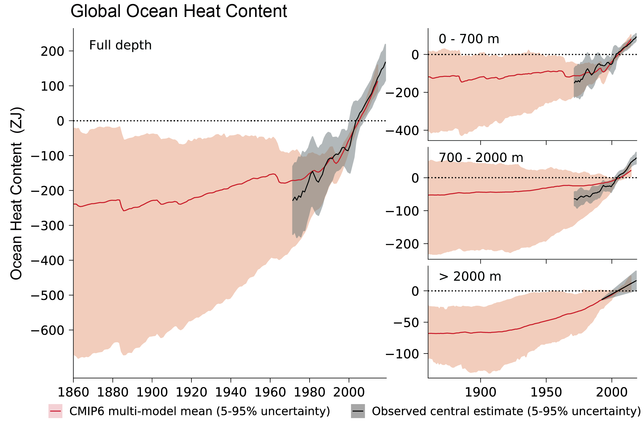 Figure 3.26 | Global ocean heat content in CMIP6 simulations and observations. Time series of observed (black) and simulated (red) global ocean heat content anomalies with respect to 1995–2014 for the full ocean depth (left-hand panel); upper layer: 0–700 m (top right-hand panel); intermediate layer: 700–2000 m (middle right-hand panel); and the abyssal ocean: >2000 m (bottom right-hand panel). The best estimate observations (black solid line) for the period of 1971–2018, along with very likely ranges (black shading) are from Section 2.3.3.1. For the models (1860–2014), ensemble members from 15 CMIP6 models are used to calculate the multi-model mean values (red solid line) after averaging across simulations for each independent model. The very likely ranges in the simulations are shown in red shading. Simulation drift has been removed from all CMIP6 historical runs using a contemporaneous portion of the linear fit to each corresponding pre-industrial control run (Gleckler et al., 2012). Units are zettajoules (ZJ; 1021 joule). Further details on data sources and processing are available in the chapter data table (Table 3.SM.1).
 The multi-model means of both CMIP5 and CMIP6 historical simulations forced with time varying natural and anthropogenic forcing shows robust increases in ocean heat content in the upper (0–700 m) and intermediate (700–2000 m) ocean (high confidence) (Figure 3.26; Cheng et al., 2016, 2019; Gleckler et al., 2016; Bilbao et al., 2019; Tokarska et al., 2019). Temporary (<10 years) surface and subsurface cooling during and after large volcanic eruptions is also captured in the upper-ocean, and global mean ocean heat content (Balmaseda et al., 2013). The ocean heat content increase is also reflected in the corresponding ocean thermal expansion which is a leading contributor to global mean sea level rise (Sections 3.5.3.2 and 9.2.4, and Box 9.1).
For the period 1971–2014, the rate of ocean heat uptake for the global ocean in the CMIP6 models is about 6.43 [2.08–8.66] ZJ yr–1, with the upper, intermediate and deeper layers respectively accounting for 68%, 16% and 16% of the full depth global heat uptake (Figure 3.26). Overall, the simulated ocean heat content changes are consistent with the updated and improved observational analyses, within the very likely uncertainty range defined for each (see also (Section 2.3.3.1, Table 2.7; Domingues et al., 2008; Purkey and Johnson, 2010; Levitus et al., 2012; Good et al., 2013; Cheng et al., 2017; Ishii et al., 2017; Zanna et al., 2019) as well as with the ocean components of total Earth heating assessed in Section 7.2.2.2, Table 7.1. Nevertheless, large uncertainties remain, particularly in the deeper layers due to the poor temporal and spatial sampling coverage, particularly in the Atlantic, Southern and Indian Oceans (Garry et al., 2019). The very likely ranges of the simulated trends for the full ocean depth and below 2000 m fall within the very likely range of observed uptake during the last two decades. In the intermediate layer, the multi-model ensemble mean mostly stays above the observed 5th–95th percentile range before the year 2000, and below that range after 2000. For the upper ocean, some individual model realizations show a reduced ocean heat content increase during the 1970s and 1980s, which is then compensated by a greater warming than the observations from the early 1990s. These discrepancies have been linked with a temporary increase in the Southern Ocean deep water formation rate, as well as with the models’ strong aerosol cooling effects and high equilibrium climate sensitivity (see also Section 7.5.6 and Box 7.2; Andrews et al., 2019, 2020; Golaz et al., 2019; Dunne et al., 2020; Winton et al., 2020).
Nevertheless, simulations show that the rate of ocean heat uptake has doubled in the past few decades, when contrasted to the rate over the complete 20th century (Figure 3.26), with over a third of the accumulated heat stored below 700 m (Cheng et al., 2016, 2019; Gleckler et al., 2016; Durack et al., 2018). The Southern Ocean shows the strongest ocean heat uptake that penetrates to deeper layers (Section 9.2.3.2), whereas ocean heat content increases in the Pacific and Indian Oceans largely occur in the upper layers (Bilbao et al., 2019).
Since AR5, the attribution of ocean heat content increases to anthropogenic forcing has been further supported by more detection and attribution studies. These studies have shown that contributions from natural forcing alone cannot explain the observed changes in ocean heat content in either the upper or intermediate ocean layers, and a response to anthropogenic forcing is clearly detectable in ocean heat content (Gleckler et al., 2016; Bilbao et al., 2019; Tokarska et al., 2019). Moreover, a response to greenhouse gas forcing is detectable independently of the response to other anthropogenic forcings (Bilbao et al., 2019; Tokarska et al., 2019), which has offset part of the greenhouse gas induced warming. Further evidence is provided by the agreement between observed and simulated changes in global thermal expansion associated with the ocean heat content increase when both natural and anthropogenic forcings are included in the simulations (Section 3.5.3.2), though internal variability plays a larger role in driving basin-scale thermosteric sea level trends (Bilbao et al., 2015). Over the Southern Ocean, warming is detectable over the late 20th century and is largely attributable to greenhouse gases (Swart et al., 2018; Hobbs et al., 2021), while other anthropogenic forcings such as ozone depletion have been shown to mitigate the warming in some of the CMIP5 simulations (Swart et al., 2018; Hobbs et al., 2021). The use of the mean temperature above a fixed isotherm rather than fixed depth further strengthens a robust detection of the anthropogenic response in the upper ocean (Weller et al., 2016), and better accounting for internal variability in the upper ocean (Rathore et al., 2020), helps explain reported hemispheric asymmetry in ocean heat content change (Durack et al., 2014b).
In summary, there is strong evidence for an improved understanding of the observed global ocean heat content increase. It is extremely likely that human influence was the main driver of the ocean heat content increase observed since the 1970s, which extends into the deeper ocean (very high confidence). Updated observations, like model simulations, show that warming extends throughout the entire water column (high confidence).
3.5.2 Ocean Salinity
While ocean assessments have primarily focused on temperature changes, improved observational salinity products since the early 2000s have supported more assessment of long-term ocean salinity change and variability from AR4 (Bindoff et al., 2007) to AR5 across both models and observations (Flato et al., 2013; Rhein et al., 2013). The AR5 assessed that it was very likely that anthropogenic forcings have made a discernible contribution to surface and subsurface ocean salinity changes since the 1960s. The SROCC augmented these insights, noting that observed high latitude freshening and warming have very likely made the surface ocean less dense with a stratification increase of between 2.18% and 2.42% from 1970 to 2017 (Bindoff et al., 2019). A recent observational analysis has expanded on these assessments, suggesting a very marked summertime density contrast enhancement across the mixed layer base of 6.2–11.6% per decade, driven by changes in temperature and salinity, which is more than six times larger than previous estimates (Sallée et al., 2021). An idealized ocean modelling study suggests that the enhanced stratification can account for a third of the salinity enhancement signal since 1990 (Zika et al., 2018). Thus, there has been an expansion of observed global- and basin-scale salinity change assessment literature since AR5, with many new studies reproducing the key patterns of long-term salinity change reported in AR5 (Rhein et al., 2013), and linking these through modelling studies to coincident changes in evaporation–precipitation patterns at the ocean surface (Sections 2.3.1.3, 3.3.2, 8.2.2.1 and 9.2.2).
Unlike SSTs, simulated sea surface salinity (SSS) does not provide a direct feedback to the atmosphere. However, some recent work has identified indirect radiative feedbacks through sea-salt aerosol interactions (Ayash et al., 2008; Amiri-Farahani et al., 2019; Z. Wang et al., 2019) that can act to strengthen tropical cyclones, and increase precipitation (Balaguru et al., 2012, 2016; Grodsky et al., 2012; Reul et al., 2014; Jiang et al., 2019). The absence of a direct feedback is one of the primary reasons why salinity simulation is difficult to constrain in ocean modelling systems, and why deviations from the observed near-surface salinity mean state between models and observations are often apparent (Durack et al., 2012; Shi et al., 2017).
3.5.2.1 Sea Surface and Depth-profile Salinity Evaluation
When compared to the routine assessment of simulated SST, simulated SSS has not received the same research attention at global- to basin-scales. For CMIP3, there was reasonable agreement between the basin-scale patterns of salinity, with a comparatively fresher Pacific when contrasted to the salty Atlantic, and basin salinity maxima features aligning well with the corresponding atmospheric evaporation minus precipitation field (Durack et al., 2012). Similar features are also reproduced in CMIP5 along with realistic variability in the upper layers, but less variability than observations at 300 m and deeper, especially in the poorly sampled Antarctic region (Pierce et al., 2012). In a regional study, only considering the Indian Ocean, CMIP5 SSS was assessed and it was shown that model biases were primarily linked to biases in the precipitation field, with ocean circulation biases playing a secondary role (Fathrio et al., 2017a). The sea surface salinity bias in CMIP6 models is shown in Figure 3.23b.
For the first time in AR5, alongside global zonal mean temperature, global zonal mean salinity bias with depth was assessed for the CMIP5 models. This showed a strong upper ocean (<300 m) negative salinity (fresh) bias of order 0.3 PSS-78, with a tendency toward a positive salinity (salty) bias (<0.25 PSS-78) in the Northern Hemisphere intermediate layers (200–3000 m) (Flato et al., 2013). These biases are also present in CMIP6, albeit with slightly smaller magnitudes (Figure 3.25). Here we expand the global zonal mean bias assessment to consider the three independent ocean basins individually, which allows for an assessment as to which basin biases are dominating the global zonal mean. The basin with the most pronounced biases is the Atlantic, with a strong upper ocean (<300 m) fresh bias, of order 0.3 PSS-78 just like the global zonal mean, and a marked subsurface salinity bias that exceeds 0.5 PSS-78 in equatorial waters between 400–1000 m.
The Pacific Ocean shares the strongest similarity to the global bias, with a similar upper ocean (<300 m) fresh bias. Lower magnitude positive salinity biases (about 0.3 PSS-78) are also present in both hemispheres between 200 and 3000 m, and deeper in the Southern Hemisphere (Figure 3.25). The Indian Ocean shows similar features to the Southern Hemisphere Pacific, with a marked upper ocean (<500 m) fresh bias of order 0.3 PSS-78, and a strong near-surface positive bias of order 0.4 PSS-78 associated with the Arabian Sea (Figure 3.25).
For the Southern Ocean in CMIP5, considerable fresh biases exist through the water column, and are most pronounced in the ventilated layers representing the subtropical mode and intermediate water masses (Sallée et al., 2013). A fresh bias in upper and intermediate layers of comparable magnitude is also seen in CMIP6 (Figure 3.25). The structure of the biases in the CMIP6 multi-model mean (which averages across many simulations with differing subsurface geographies and differing Southern Ocean salinity biases (Beadling et al., 2020)) is similar to that evident in the CMIP5 multi-model mean, but with slightly smaller magnitudes. The Arctic Ocean also on average exhibits a surface-enhanced fresh bias in the upper ocean (Figure 3.25), which is much larger than its Southern Hemisphere counterpart.
In summary, the structure of the salinity biases in the multi-model mean has not changed substantially between CMIP5 and CMIP6 (medium confidence), though there is limited evidence that the magnitude of subsurface biases has been reduced. Biases are sufficiently small to provide confidence in the utility of CMIP-class models for detection and attribution of ocean salinity.
3.5.2.2 Salinity Change Attribution
AR5 concluded that it was very likely that anthropogenic forcings had made a discernible contribution to surface and subsurface ocean salinity changes since the 1960s (Bindoff et al., 2013; Rhein et al., 2013). It highlighted that the spatial patterns of salinity trends, and the mean fields of salinity and evaporation minus precipitation are all similar, with an enhancement to Atlantic Ocean salinity and freshening in the Pacific and Southern Oceans. Since AR5 all subsequent work on assessing observed and modelled salinity changes has confirmed these results.
Considerable changes to observed broad- or basin-scale ocean near-surface salinity fields have been reported (see Section 2.3.3.2), and these have been linked to changes in the evaporation minus precipitation patterns at the ocean surface through model simulations, typically expressing a pattern of change where climatological mean fresh regions become fresher and corresponding salty regions becoming saltier (Durack et al., 2012, 2013; Zika et al., 2015; Lago et al., 2016; Skliris et al., 2016, 2018; Cheng et al., 2020), also broadly present in the CMIP6 multi-model mean (Figure 3.27). At basin-scales, the depth-integrated effect of mean salinity changes as captured in halosteric sea level for the top 0 to 2000 m has also been assessed based on observational products, and these results mirror near-surface patterns in the CMIP5 and CMIP6 models, with most areas that are becoming fresher at the surface exhibiting increases in halosteric sea level, and areas becoming saltier exhibiting decreases (Durack et al., 2014a; Figure 3.28). Further investigations using observations and models together have tied the long-term patterns of surface and subsurface salinity changes to coincident changes to the evaporation minus precipitation field over the ocean (Durack et al., 2012, 2013; Durack, 2015; Levang and Schmitt, 2015; Zika et al., 2015, 2018; Grist et al., 2016; Lago et al., 2016; Cheng et al., 2020), however the rate of these changes through time continues to be an active area of active research (Skliris et al., 2014; Zika et al., 2015, 2018; Cheng et al., 2020; Sallée et al., 2021).
 Figure 3.27 | Maps of multi-decadal salinity trends for the near-surface ocean. Units are Practical Salinity Scale 1978 [PSS-78] per decade. (Top) The best estimate (Section 2.3.3.2) observed trend (1950–2019, Durack and Wijffels, 2010). (Bottom) Simulated trend from the CMIP6 historical experiment multi-model mean (1950–2014). Black contours show the climatological mean salinity in increments of 0.5 PSS-78 (thick lines 1 PSS-78). Further details on data sources and processing are available in the chapter data table (Table 3.SM.1).
 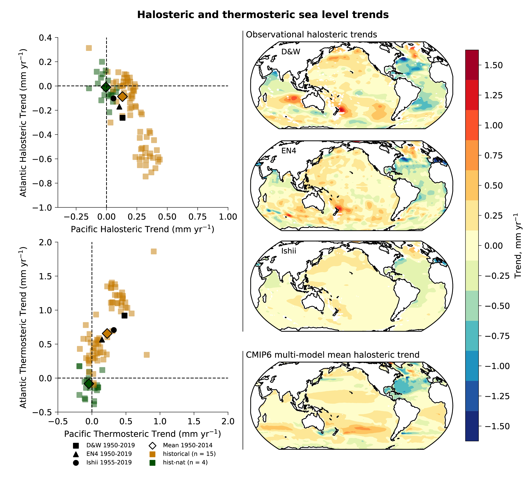 Figure 3.28 | Long-term trends in halosteric and thermosteric sea level in CMIP6 models and observations. Units are mm yr–1. In The right-hand column, three observed maps of 0 to 2000 m halosteric sea level trends are shown: top (D&W) from Durack and Wijffels (2010), 1950–2019, updated; upper-middle (EN4) from Good et al. (2013), 1950–2019, updated; and lower-middle (Ishii) from Ishii et al. (2017), 1955–2019, updated. Bottom-right: the CMIP6 historical multi-model mean (1950–2014). Red and orange colours show a halosteric contraction (enhanced salinity) and blue and green a halosteric expansion (reduced salinity). In The left-hand column , basin-integrated halosteric (top) and thermosteric (bottom) trends for the Atlantic and Pacific, the two largest ocean basins, are shown, where Pacific anomalies are presented on the x-axis and Atlantic on the y-axis. Observational estimates are presented in black, CMIP6 historical (all forcings) simulations are shown in orange squares, with the multi-model mean shown as a dark orange diamond with a black bounding box. CMIP6 hist-nat (historical natural forcings only) simulations are shown in green squares with the multi-model mean as a dark green diamond with a black bounding box. Further details on data sources and processing are available in the chapter data table (Table 3.SM.1).
 Climate change detection and attribution studies have considered salinity, with the first of these assessed in AR5 (Bindoff et al., 2013). Since that time, the positive detection conclusions (Stott et al., 2008; Pierce et al., 2012; Terray et al., 2012) have been supported by a number of more recent and independent assessments which have reproduced the multi-decadal basin-scale patterns of change in observations and models (Figures 3.27 and 3.28; Durack et al., 2014a; Durack, 2015; Levang and Schmitt, 2015; Skliris et al., 2016). Observed depth-integrated basin responses, contrasting the Pacific and Atlantic basins (freshening Pacific and enhanced salinity Atlantic) were also shown to be replicated in most historical (natural and anthropogenically forced) simulations, with this basin contrast absent in CMIP5 and CMIP6 natural-only simulations that exclude anthropogenic forcing (Durack et al., 2014a; Figure 3.28).
While observational sparsity considerably limits quantification of regional changes, a recent study by Friedman et al. (2017) assessed salinity changes in the Atlantic Ocean from 1896 to 2013 and confirmed the pattern of mid-to-low latitude enhanced salinity and high latitude North Atlantic freshening over this period exists even after accounting for the effects of the NAO and AMO.
Considering the bulk of evidence, it is extremely likely that human influence has contributed to observed near-surface and subsurface salinity changes across the globe since the mid-20th century. All available multi-decadal assessments have confirmed that the associated pattern of change corresponds to fresh regions becoming fresher and salty regions becoming saltier (high confidence). CMIP5 and CMIP6 models are only able to reproduce these patterns in simulations that include greenhouse gas increases (medium confidence). Changes to the coincident atmospheric water cycle and ocean-atmosphere fluxes (evaporation and precipitation) are the primary drivers of the basin-scale observed salinity changes (high confidence). This result is supported by all available observational assessments, along with a growing number of climate modelling studies targeted at assessing ocean and water cycle changes. The basin-scale changes are consistent across models and intensify on centennial scales from the historical period through to the projections of future climate (high confidence).
3.5.3 Sea Level
In keeping with the scope of this chapter, this section addresses global and basin-scale sea level changes, whereas regional and local sea level changes are assessed in Section 9.6. In AR5, the observed sea level budget was closed by considering all contributing factors including ocean warming, mass contributions from terrestrial storage, glaciers, and the Antarctic and Greenland ice sheets (Church et al., 2013b). The SROCC found that the observed global mean sea level (GMSL) rise is consistent within uncertainties with the sum of the estimated observed contributions for 1993–2015 and 2006–2015.
3.5.3.1 Sea Level Evaluation
The current generation of climate models do not fully resolve many of the components required to close the observed sea level budget, such as glaciers, ice sheets and land water storage (see Section 9.6 and Box 9.1). Consequently, most CMIP-based analyses of sea level change have focused on thermosteric sea level changes (i.e., thermal expansion due to warming) and ocean dynamic sea level change, both of which are simulated in the CMIP5-generation of models. The improved agreement between modelled thermal expansion and observed estimates during the historical period led the SROCC to assess a high confidence level in the simulated thermal expansion using climate models and high confidence in their ability to project future thermal expansion.
Since CMIP5 models do not include all necessary components of sea level change, this gap has been bridged by using offline models (for glacier melt and ice-sheet surface mass balance) driven by reanalyses and model output. Some studies have used offline mass inputs to account for dynamic ice-sheet and terrestrial contributions. Slangen et al. (2017) and Meyssignac et al. (2017) suggested including corrections to several contributions to sea level changes including to the Greenland surface mass balance and glacier contributions, based on differences between CMIP5-driven model results and reanalysis-driven results. This helps close the gap between models and observations for the 20th century globally, as well as providing better agreement with tide gauge observations in terms of interannual and multi-decadal variability at the regional scale.
In CMIP6, ice sheets (see Sections 3.4.3.2 and 9.4) are included for the first time in ISMIP6 (Nowicki et al., 2016). There is also scope for new insights into terrestrial water contributions from land surface (and sub-surface) modelling in the Land Surface, Snow and Soil moisture Model Intercomparison Project (LS3MIP; van den Hurk et al., 2016). In parallel, the GlacierMIP project (Hock et al., 2019a; Marzeion et al., 2020; see Sections 3.4.3.1 and 9.5) is also underway, and has provided more quantitative guidance and a comprehensive assessment of the uncertainties and best estimates of the current and future contributions of glaciers to the sea level budget.
3.5.3.2 Sea Level Change Attribution
The SROCC concluded with high confidence that the dominant cause of GMSL rise since 1970 is anthropogenic forcing. Prior to that, AR5 had concluded that it is very likely that there has been a substantial contribution from anthropogenic forcings to GMSL rise since the 1970s. Since AR5, several studies have identified a human contribution to observed sea level change resulting from a warming climate as manifest in thermosteric sea level change and the contribution from melting glaciers and ice sheets.
For the global mean thermosteric sea level change, Slangen et al. (2014) showed the importance of anthropogenic forcings (combined greenhouse gas and aerosol forcings) for explaining the magnitude of the observed changes between 1957 and 2005, considering the full depth of the ocean and natural forcings in order to capture the variability (see also Figure 3.29). Over the 1950–2005 period, Marcos and Amores (2014) found that human influence explains 87% of the 0–700 m global thermosteric sea level rise. Both thermosteric and regional dynamic patterns of sea level change in individual forcing experiments from CMIP5 were considered by Slangen et al. (2015) who showed that responses to anthropogenic forcings are significantly different from both internal variability and inter-model differences and that although greenhouse gas and anthropogenic aerosol forcings produce opposite GMSL responses, there are differences in the response on regional scales. Based on these studies, we conclude that it is very likely that anthropogenic forcing was the main driver of the observed global mean thermosteric sea level change since 1970.
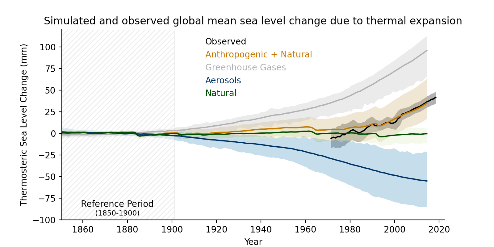 Figure 3.29 | Simulated and observed global mean sea level change due to thermal expansion for CMIP6 models and observations relative to the baseline period 1850–1900. Historical simulations are shown in brown, natural only in green, greenhouse gas only in grey, and aerosol only in blue (multi-model means shown as thick lines, and shaded ranges between the 5th and 95th percentile). The best estimate observations (black solid line) for the period of 1971–2018, along with very likely ranges (black shading) are from Section 2.3.3.1 and are shifted to match the multi-model mean of the historical simulations for the 1995–2014 period. Further details on data sources and processing are available in the chapter data table (Table 3.SM.1).
 In an attribution study of the sea-level contributions of glaciers, Marzeion et al. (2014) found that between 1991 and 2010, the anthropogenic fraction of global glacier mass loss was 69 ± 24% (see also Section 3.4.3.1). Slangen et al. (2016) considered all quantifiable components of the GMSL budget and showed that anthropogenically forced changes account for 69 ± 31% of the observed sea level rise over the period 1970 to 2005, whereas natural forcings combined with internal variability have a much smaller effect – only contributing 9 ± 18% of the change over the same period. These studies indicate that about 70% of the combined change in glaciers, ice-sheet surface mass balance and thermal expansion since 1970 can be attributed to anthropogenic forcing, and that this percentage has increased over the course of the 20th century. Detection studies on GMSL change in the 20th century (Becker et al., 2014; Dangendorf et al., (2015) found that observed total GMSL change in the 20th century was inconsistent with internal variability. Dangendorf et al. (2015) determined that for 1900 to 2011 at least 45% of GMSL change is human-induced. A study that developed a semi-empirical model to link sea-level change to observed GMST change concluded that at least 41% of the 20th century sea-level rise would not have happened in the absence of the century’s increasing GMST and that there was a 95% probability that by 1970 GMSL was higher than that which would have occurred in the absence of increasing GMST (Kopp et al., 2016). Richter et al. (2020) compared modelled sea level change with the satellite altimeter observations from 1993 to 2015; a period short enough that internal variability can dominate the spatial pattern of change. They found that when GMSL is not removed, model simulated zonally averaged sea level trends are consistent with altimeter observations globally as well as in each ocean basin and much larger than might be expected from internal variability. Using spatial correlation, Fasullo and Nerem (2018) showed that the satellite altimeter trend pattern is already detectable.
We note that current detection and attribution studies do not yet include all processes that are important for sea-level change (see Section 9.6). However, based on the body of literature available, we conclude that the main driver of the observed GMSL rise since at least 1971 is very likely anthropogenic forcing. The assessed period starts in 1971 for consistency with observations assessed in Cross-Chapter Box 9.1.
3.5.4 Ocean Circulation
Circulation of the ocean, whether it be wind or density driven, plays a prominent role in the heat and freshwater transport of the Earth system (Buckley and Marshall, 2016). Thus, its accurate representation is crucial for the realistic representation of water mass properties, and replication of observed changes driven by atmosphere-land-ocean coupling. Here, we assess the ability of CMIP models to reproduce the observed large-scale ocean circulation, along with assessment of the detection and attribution of any anthropogenically-driven changes. We also note that the process-based understanding of these circulation changes and circulation changes occurring at smaller scales is assessed in Section 9.2.3.
3.5.4.1 Atlantic Meridional Overturning Circulation (AMOC)
The Atlantic Meridional Overturning Circulation (AMOC) represents a large-scale flow of warm salty water northward at the surface and a return flow of colder water southward at depth. As such, its mean state plays an important role in transporting heat in the climate system, while its variability can act to redistribute heat (see Sections 2.3.3.4.1 and 9.2.3.1 for more details). Paleo-climatic and model evidence suggest that changes in AMOC strength have played a prominent role in past transitions between warm and cool climatic phases (e.g., Dansgaard et al., 1993; Ritz et al., 2013).
The AR5 concluded that while climate models suggested that an AMOC slowdown would occur in response to anthropogenic forcing, the short direct observational AMOC record precluded it from being used to support this model finding. Chapter 2 reports with high confidence, a weakening of the AMOC was observed in the mid-2000s to the mid-2010s, while again also noting that the observational record was too short to determine whether this is a significant trend or a manifestation of decadal and multi-decadal variability (Section 2.3.3.4.1). Indirect evidence of AMOC weakening since at least the 1950s is also presented, but confidence in this longer-term decrease was low Section 2.3.3.4.1).
Despite the additional six years or so of observations since AR5, the evaluation of the AMOC in models continues to be severely hampered by the geographically sparse and temporally short observational record. The longest continuous observational estimates of the AMOC are based on measurements taken at 26°N by the RAPID-MOCHA array (Smeed et al., 2018). Basic evaluation of the AMOC at 26°N shows that the CMIP5 and CMIP6 multi-model mean overturning strength is comparable with RAPID (Reintges et al., 2017; Weijer et al., 2020), but the model range is large (12–29 sverdrups (Sv)) for CMIP5 (Zhang and Wang, 2013); and 10–31 Sv for CMIP6 (Weijer et al., 2020) (Figure 3.30a). It is noted that deviations of AMOC strength in CMIP5 models have been related to global-scale sea surface temperature biases (C. Wang et al., 2014). Both coupled and ocean-only models also underestimate the depth of the AMOC cell (Danabasoglu et al., 2014; Weijer et al., 2020; Figure 3.30a). Paleo-climatic evidence has also raised questions regarding the accuracy of the representation of the strength and depth of the modelled AMOC during past periods (Otto-Bliesner et al., 2007; Muglia and Schmittner, 2015). Overall, however, both the CMIP5 and CMIP6 model ensembles simulate the general features of the AMOC mean state reasonably well, but there is a large spread in the latitude and depth of the maximum overturning, and the maximum AMOC strength (Figure 3.30a).
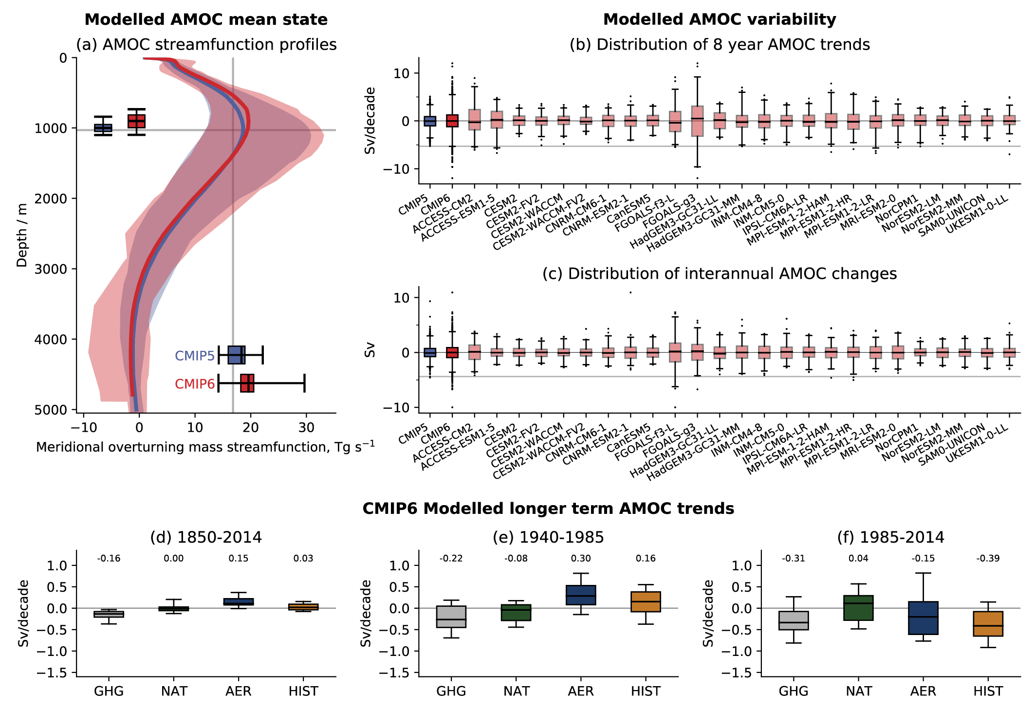 Figure 3.30 | Observed and CMIP6 simulated AMOC mean state, variability and long-term trends. (a) AMOC meridional stream function profiles at 26.5°N from the historical CMIP5 (1860–2004) and CMIP6 (1860–2014) simulations compared with the mean maximum overturning depth (horizontal grey line) and magnitude (vertical grey line) from the RAPID observations (2004–2018). The distributions of model ranges of AMOC maximum magnitude and depth are respectively displayed near the x- and y-axis. (b) Distributions of overlapping eight-year AMOC trends from individual CMIP6 historical simulations (pink box plots) are plotted along with the combined distributions of all available CMIP5 (blue boxplot) and CMIP6 (red boxplot) models. For reference, the observed eight-year trend calculated between 2004 and 2012 is also shown as a horizontal grey line (following Roberts et al., 2014). (c) Distributions of interannual AMOC variability from individual CMIP6 model historical simulations, along with the combined distributions of all available CMIP5 and CMIP6 models. Interannual variability in models and observations is estimated as annual mean (April–March) differences, and the horizontal grey line is the observed value for 2009/2010 minus 2008/2009 (following Roberts et al., 2014). (d–f) Distributions of linear AMOC trends calculated over various time periods (see panel titles) in CMIP6 simulations forced with: greenhouse gas forcing only (GHG), natural forcing only (NAT), anthropogenic aerosol forcing only (AER) and all forcing combined (Historical; HIST). (a–f) Boxes indicate the 25th to 75th percentile range, whiskers indicate 1st and 99th percentiles in (a-c) and 5th and 95th percentile in (d-f), and dots indicate outliers, while the horizontal black line is the multi-model mean trend. In (d–f) the multi-model mean trend is also written above each distribution. The multi-model distributions in (a–c) were produced with one historical ensemble member per model for which the AMOC variable was available (listed), while those in (d–f) were produced with the detection and attribution simulation datasets utilized by Menary et al. (2020). Further details on data sources and processing are available in the chapter data table (Table 3.SM.1).
 The short length of the observed time-series (RAPID has measured the AMOC since 2004), sparse observations, observational uncertainties (Sinha et al., 2018), as well as significant observed variability on interannual and longer time scales, makes comparison with modelled AMOC variability challenging. RAPID observations show that the overturning at 26°N was 2.9 Sv weaker in the multi-year average of 2008–2012 relative to 2004–2008 and 2.5 Sv weaker in 2012–2017 relative to 2004–2008 (Smeed et al., 2014, 2018) (see also (Section 2.3.3.4.1). As expected, this weakening was accompanied by a significant reduction in northward heat transport (Bryden et al., 2020). CMIP5 and CMIP6 models produce a forced weakening of the AMOC over the 2012–2017 period relative to 2004–2008, but at 26°N the multi-model mean response is substantially weaker than the observed AMOC decline over the same period. The discrepancy between the modelled multi-model mean (i.e., the forced response) and the RAPID observed AMOC changes has led studies to suggest that the observed weakening over 2004–2017 is largely due to internal variability (Yan et al., 2018). However, comparison of observed RAPID AMOC variability with modelled variability also reveals that most CMIP5 models appear to underestimate the interannual and decadal time scale AMOC variability (Roberts et al., 2014; Yan et al., 2018), and, although the overall variance is larger in CMIP6 than in CMIP5, similar results are found analysing the CMIP6 models (Figure 3.30b,c). It is currently unknown why most models underestimate this AMOC variability, or whether they are underestimating the internal or externally forced components. This underestimation of AMOC variability may also have potential implications for detection and attribution, the relationship between AMOC and AMV (see Section 3.7.7), and near-term predictions. There is also emerging evidence, based on analysis of freshwater transports, that the AMOC in CMIP5-era models is too stable, largely due to systematic biases in ocean salinity (W. Liu et al., 2017; Mecking et al., 2017). Such a systematic bias may potentially be linked with the underestimation of both simulated AMOC internal variability through eddy-mean flow interactions that are poorly represented in standard CMIP-class model resolution (Leroux et al., 2018), and externally forced change.
As reported in Section 2.3.3.4.1, estimates of AMOC since at least 1950, which are generated from observed surface temperatures or sea surface height, suggest the AMOC weakened through the 20th century (low confidence) (Ezer et al., 2013; Caesar et al., 2018). Over the same period, the CMIP5 multi-model mean showed no significant net forced response in AMOC (Cheng et al., 2013). However, a significant forced change is simulated in the CMIP6 multi-model mean, where a clear increase of the AMOC is seen over the 1940–1985 period (Figure 3.30e; Menary et al., 2020). Although there is general agreement that the influence of greenhouse gases acts to a weaken the modelled AMOC (Delworth and Dixon, 2006; Caesar et al., 2018), changes in solar, volcanic and anthropogenic aerosol emissions can lead to temporary changes in AMOC on decadal- to multi-decadal time scales (Delworth and Dixon, 2006; Menary et al., 2013; Menary and Scaife, 2014; Swingedouw et al., 2017; Undorf et al., 2018b). As such, the simulated net forced response in AMOC is a balance between the different forcing factors (Section 9.2.3.1; Delworth and Dixon, 2006; Menary et al., 2020). The differing AMOC response of CMIP5 and CMIP6 models during the historical period has been associated with stronger aerosol effective radiative forcing in the CMIP6 models (Menary et al., 2020), such that the aerosol-induced AMOC increase during the 1940–1985 period overcomes the greenhouse gas induced decline (Figure 3.30e). However, models simulate a range of anthropogenic aerosol effective radiative forcing and a range of historical AMOC trends in CMIP6 (Menary et al., 2020) and there remains considerable uncertainty over the realism of the CMIP6 AMOC response during the 20th century (Figure 3.30d–f) due to disagreement among the differing lines of evidence. For example, ocean reanalysis (Jackson et al., 2019) and forced ocean model simulations (Robson et al., 2012; Danabasoglu et al., 2016), which show AMOC changes that are broadly consistent with the CMIP6 response, appear to disagree with observational estimates of AMOC over the historical period (Ezer et al., 2013; Caesar et al., 2018). It is noted, however, that the relatively short length of the forced ocean simulations and ocean reanalysis precludes a comparable assessment of 20th century trends. Furthermore, despite the similar AMOC evolution seen in forced ocean model simulations and the CMIP6 models, it is unclear whether the same underlying mechanisms are responsible for the changes.
In summary, models do not support robust assessment of the role of anthropogenic forcing in the observed AMOC weakening between the mid-2000s and the mid-2010s, which is assessed to have occurred with high confidence in Section 2.3.3.4.1, as the changes are outside of the range of modelled AMOC trends (regardless of whether they are forced or internally generated) in most models. Thus, we have low confidence that anthropogenic forcing has influenced the observed changes in AMOC strength in the post-2004 period. In addition, there remains considerable uncertainty over the realism of the CMIP6 AMOC response during the 20th century due to disagreement among the differing lines of observational and modelled evidence (i.e., historical AMOC estimates, ocean reanalysis, forced ocean simulations and historical CMIP6 simulations). Thus, we have low confidence that anthropogenic forcing has had a significant influence on changes in AMOC strength during the 1860–2014 period.
3.5.4.2 Southern Ocean Circulation
The Southern Ocean circulation provides the principal connections between the world’s major ocean basins through the circulation of the Antarctic Circumpolar Current (ACC), while also largely controlling the connection between the deep and upper layers of the global ocean circulation, through its upper and lower overturning cells.
The assessment of observations presented in Sections 2.3.3.4.2 and 9.2.3.2 reports that there is no evidence of an ACC transport change, and it is unlikely that the mean meridional position of the ACC has moved southward in recent decades (Sections 2.3.3.4.2 and 9.2.3.2). This is despite observations of surface wind displaying an intensification and southward shift (Section 2.4.1.2). There is low confidence in an observed intensification of upper ocean overturning in the Southern Ocean and there is medium confidence for a slowdown of the Antarctic Bottom Water circulation and commensurate Antarctic Bottom Water volume decrease since the 1990s (Section 9.2.3.2). Section 9.2.3.2 presents new evidence, since SROCC, which assessed with medium confidence that the lower cell can episodically increase as a response to climatic anomalies, temporally counteracting the forced tendency for reduced bottom water formation.
The modelled strength of the ACC clearly improved from CMIP3, in which the models tended to underestimate the strength of the ACC, to CMIP5 (Meijers et al., 2012). This improvement in the realism of ACC strength continues from CMIP5 to CMIP6, with the modelled ACC strength converging toward the magnitude of observed estimates of net flow through the Drake Passage (Beadling et al., 2020). There is, however, a small number of models that still display an ACC that is much weaker than that observed, while several models also display much more pronounced ACC decadal variability than that observed (Beadling et al., 2020). The increased realism of the ACC was at least partly related to noted improvements in all metrics of the Southern Ocean’s surface wind stress forcing (Beadling et al., 2020). The most notable wind stress forcing improvements were found in the strength and the latitudinal position of the zonally-averaged westerly wind stress maximum (Beadling et al., 2020; Bracegirdle et al., 2020). While the two-cell structure of the overturning circulation appears to be well captured by CMIP5 models (Sallée et al., 2013; Russell et al., 2018), they tend to underestimate the intensity of the lower cell overturning, and overestimate the intensity of the upper cell overturning (Sallée et al., 2013). As the lower overturning cell is closely related to Antarctic Bottom Water formation and deep convection, both fields also display substantial errors in CMIP5 models (Heuzé et al., 2013, 2015). CMIP6 climate models show clear improvements compared to CMIP5 in their representation of Antarctic Bottom Water, which suggests an improved representation of the lower overturning cell (Heuzé, 2021).
Despite notable improvements of CMIP6 models compared to CMIP5 models, inherent limitations in the representation of important processes at play in the Southern Ocean’s horizontal and vertical circulation remain (Section 9.2.3.2). For instance, Southern Ocean mesoscale eddies are largely parameterized in the current generation of climate models and, despite their small spatial scales, they are a key element for establishing the ACC and upper overturning cell, as well as for their future evolution under changing atmospheric forcing (Kuhlbrodt et al., 2012; Downes and Hogg, 2013; Gent, 2016; Downes et al., 2018; Poulsen et al., 2018). The absence of ice-sheet coupling in the CMIP6 model suite is another important limitation, as basal meltwater and calving can influence the circulation, particularly the lower cell of the Southern Ocean (Bronselaer et al., 2018; Golledge et al., 2019; Lago and England, 2019; Jeong et al., 2020; Moorman et al., 2020). We note that early development of global climate models with interactive ice-shelf cavities has begun and is showing potential to be developed (Jeong et al., 2020).
In summary, while there have been improvements across successive CMIP phases (from CMIP3 to CMIP6) in the representation of the Southern Ocean circulation, such that the mean zonal and overturning circulations of the Southern Ocean are now broadly reproduced, substantial observational uncertainty and climate model challenges preclude attribution of Southern Ocean circulation changes (high confidence).
3.6 Human Influence on the Biosphere
3.6.1 Terrestrial Carbon Cycle
The AR5 did not make attribution statements on changes in global carbon sinks. The IPCC Special Report on Climate Change and Land (SRCCL) assessed with high confidence that global vegetation photosynthetic activity has increased over the last 2–3 decades (Jia et al., 2019). That increase was attributed to direct land use and management changes, as well as to CO2 fertilization, nitrogen deposition, increased diffuse radiation and climate change (high confidence). The AR5 assessed with high confidence that CMIP5 Earth System Models (ESMs) simulate the global mean land and ocean carbon sinks within the range of observation-based estimates (Flato et al., 2013). The IPCC SRCCL, however, noted the remaining shortcomings of carbon cycle schemes in ESMs (Jia et al., 2019), which for example do not properly incorporate thermal responses of respiration and photosynthesis, and frequently omit representations of permafrost thaw (Comyn-Platt et al., 2018), the nitrogen cycle (R.Q. Thomas et al., 2015) and its influence on vegetation dynamics (Jeffers et al., 2015), the phosphorus cycle (Fleischer et al., 2019), and accurate implications of carbon store changes for a range of land use and land management options (Erb et al., 2018; Harper et al., 2018) (see Sections 5.2.1.4.1 and 5.4, Figure 5.24 and Table 5.4 for details).
This section considers three main large-scale indicators of climate change relevant to the terrestrial carbon cycle: atmospheric CO2 concentration, atmosphere-land CO2 fluxes, and leaf area index. These indicators were chosen because they have been the target of attribution studies. Other indicators, like land use and management, and wildfires, relate to human influence but are discussed in Chapter 5. Chapter 7 discusses energetic consequences of changes in the terrestrial carbon cycle in Section 7.4.2.5.2. CMIP5 and CMIP6 ESMs are most often run with prescribed observed historical changes in atmospheric CO2 concentration and diagnose CO2 emissions consistent with these. Such calculations require that the models simulate realistic changes in the terrestrial carbon cycle over the historical period, as changes to land carbon stores will influence the size of CO2 emissions consistent with prescribed CO2 pathways, and associated remaining carbon budgets (Section 5.5). Such testing of existing models is needed while also recognising there are process representations still requiring inclusion.
Since AR5, atmospheric inversion studies have further tested or constrained models, while new datasets have been used to constrain specific parts of the terrestrial carbon cycle such as plant respiration (Huntingford et al., 2017). Figure 3.31 compares historical emissions-driven CMIP6 simulations of global mean atmospheric CO2 concentration and net ocean and land carbon fluxes to the assessed CO2 concentration and fluxes from the Global Carbon Project (Friedlingstein et al., 2019). For 2014, the CMIP6 models simulate a range of CO2 concentrations centred around the observed value of 397 ppmv, with a range of 381 to 412 ppmv. GSAT anomalies simulated over the historical period are very similar in models that simulate or prescribe changes in atmospheric CO2 concentrations (Figures 3.31b and 3.4a). Most models simulate realistic temporal evolution of the global net ocean and land carbon fluxes, although model spread is larger over land (Figure 3.31c,d; see also Sections 3.6.2 and 5.4.5.2, and Figure 5.24). Although literature published soon after AR5 highlighted the importance of representing nitrogen limitation on plant growth (Peng and Dan, 2015; R.Q. Thomas et al., 2015), more recent studies note that models without nitrogen limitation can still be consistent with the latest estimates of historical carbon cycle changes (Arora et al., 2020; Meyerholt et al., 2020). Uncertainties in the photosynthetic response to atmospheric CO2 concentrations at global scales, shifts in carbon allocation and turnover, land-use change (Hoffman et al., 2014; Wieder et al., 2019), and water limitation are also important influences on land carbon fluxes.
 Figure 3.31 | Evaluation of historical emissions-driven CMIP6 simulations for 1850–2014. Observations (black) are compared to simulations of global mean (a) atmospheric CO2 concentration (ppmv), with observations from the National Oceanic and Atmospheric Administration Earth System Research Laboratory (NOAA ESRL; Dlugokencky and Tans, 2020); (b) surface air temperature anomaly (°C) with respect to the 1850–1900 mean, with observations from HadCRUT4 (Morice et al., 2012); (c) land carbon uptake (PgC yr–1), (d) ocean carbon uptake (PgC yr–1), both with observations from the Global Carbon Project (GCP; Friedlingstein et al., 2019) and grey shading indicating the observational uncertainty. Land and ocean carbon uptakes are plotted using a 10-year running mean for better visibility. The ocean uptake is offset to 0 in 1850 to correct for pre-industrial riverine-induced carbon fluxes. Further details on data sources and processing are available in the chapter data table (Table 3.SM.1).
 All models and observational estimates agree that interannual variability in net CO2 uptake is much larger over land than over the ocean. Studies demonstrate that regional variations in both the trends and the yearly strength of the terrestrial carbon sink are considerable. Land carbon uptake is dominated by the extratropical northern latitudes (see also Section 5.4.5.3 and Figure 5.25; Ciais et al., 2019) because the tropics may have become a net source of carbon (Baccini et al., 2017). At local to regional scales, the dominant driver of yearly sink strength variations is water availability, but at continental to global scales, temperature anomalies are the dominant driver (Section 5.2.1.4.2; Jung et al., 2017). The major role of levels of water stored in the ground in influencing land-atmosphere CO2 exchange has also been confirmed through simultaneous analysis of satellite gravimetry and atmospheric CO2 levels (Humphrey et al., 2018). When considered globally, simulated land and ocean carbon sinks fall within the range of observation-based estimates with high confidence. But there is also high confidence that that apparent success arises for the wrong reasons, as models underestimate the Northern Hemisphere carbon sink, as discussed in Section 5.4.5.3.
The seasonal cycle in atmospheric CO2, which is driven by the drawdown of carbon by photosynthesis on land during the summer and release by respiration during the winter, has increased in amplitude since the start of systematic monitoring (Figure 3.32; see also (Section 2.3.4.1). This trend, which is larger at higher latitudes of the Northern Hemisphere, was first reported by Keeling et al. (1996) and has continued. Changes in vegetation productivity have also been observed, as well as longer growing seasons (Park et al., 2016). However, a slow down of the increasing trend has been noted, linked to a slow down of both vegetation greening and growing-season length increases (Buermann et al., 2018; Z. Li et al., 2018; K. Wang et al., 2020). Figure 3.32 shows that CMIP6 terrestrial carbon cycle models partially capture the increasing amplitude of the seasonal cycle of the land carbon sink, also seen in observational reconstructions. However, the identification of the human influence that contributes most strongly to these changes in the seasonal cycle is debated.
 Figure 3.32 | Relative change in the amplitude of the seasonal cycle of global land carbon uptake in the historical CMIP6 simulations from 1961–2014. Net biosphere production estimates from 19 CMIP6 models (red), the data-led reconstruction JMA-TRANSCOM (Maki et al., 2010; dotted) and atmospheric CO2 seasonal cycle amplitude changes from observations (global as dashed line, Mauna Loa Observatory (MLO) (Dlugokencky et al., 2020) in bold black). Seasonal cycle amplitude is calculated using the curve fit algorithm package from the National Oceanic and Atmospheric Administration Earth System Research Laboratory (NOAA ESRL). Relative changes are referenced to the 1961–1970 mean and for short time series adjusted to have the same mean as the model ensemble in the last 10 years. Interannual variation was removed with a nine-year Gaussian smoothing. Shaded areas show the one sigma model spread (grey) for the CMIP6 ensemble and the one sigma standard deviation of the smoothing (red) for the CO2 MLO observations. Inset: average seasonal cycle of ensemble mean net biosphere production and its one sigma model spread for 1961–1970 (orange dashed line, light orange shading) and 2005–2014 (solid green line, green shading). Further details on data sources and processing are available in the chapter data table (Table 3.SM.1).
 Proposed causes of the trend in the amplitude of the seasonal cycle of CO2, and its amplification at higher latitudes, include increases in the summer productivity and/or increases in the magnitude of winter respiration of northern ecosystems (Barichivich et al., 2013; Graven et al., 2013; Forkel et al., 2016; Wenzel et al., 2016), increases in productivity throughout the Northern Hemisphere by CO2 fertilization, and increases in the productivity of agricultural crops in northern mid-latitudes (Gray et al., 2014; Zeng et al., 2014). Recent studies have attempted to quantify the different contributions by comparing atmospheric CO2 observations with ensembles of land surface model simulations. Piao et al. (2017) found that CO2 fertilization of photosynthesis is the main driver of the increase in the amplitude of the seasonal cycle of atmospheric CO2 but noted that climate change drives the latitudinal differences in that increase. North of 40°N, Bastos et al. (2019) also found CO2 fertilization to be the most likely driver, with warming at northern high latitudes contributing a decrease in amplitude, in contrast to earlier conclusions (Graven et al., 2013; Forkel et al., 2016), and agricultural and land use changes making only a small contribution. For temperate regions of the Northern Hemisphere, K. Wang et al. (2020) found that the importance of CO2 fertilization is decreased by drought stress, but also found only a small contribution from agricultural and land use changes. However, many global models do not include nitrogen fertilization, changes to crop cultivars or irrigation effects, with the latter associated with deficiencies in simulated terrestrial water cycling (H. Yang et al., 2018). All these factors influence the capability of models to simulate accurately the seasonal cycle in atmosphere-land CO2 exchanges. Model comparisons to the atmospheric CO2 concentration record for Barrow, Alaska, suggest that models underestimate current levels of carbon fixation (Winkler et al., 2019) and have deficiencies in their phenological representation of greenness levels, particularly for autumn (Z. Li et al., 2018). Based on these studies and noting the uncertainty in the processes ultimately driving changes in atmospheric CO2 seasonal cycles (Section 5.2.1.4), we assess with medium confidence that fertilization by anthropogenic increases in atmospheric CO2 concentrations is the main driver of the increase in the amplitude of the seasonal cycle of atmospheric CO2.
Detection and attribution methods have been applied to leaf area index, which represents ‘greenness’ and general photosynthetic productivity (see Section 2.3.4.3). Nitrogen deposition and land cover change trends remain small compared to variability, so attributing changes in leaf area index to those processes is difficult. Using three satellite products and ten land models, Zhu et al. (2016) found increases in leaf area index (greening) over 25–50% of global vegetated areas, and they attributed 70% of this greening to CO2 fertilization, although they found that land use change can dominate regionally. This is consistent with the attribution study of observed greening of Mao et al. (2016), and with Mao et al. (2013) who found that CO2 fertilization was the dominant cause of enhanced vegetation growth, with latitudinal changes in leaf area index explained by the larger land surface warming in the Northern Hemisphere. These conclusions are also consistent with those of Zhu et al. (2017), who found a dominant role for CO2 fertilization in driving leaf area index changes in an attribution study in which land models were first weighted by performance. However, Chen et al. (2019) has challenged these results by showing that greening in India and China was driven by land-use change.
Leaf area index increases attributed to CO2 fertilization are due to a direct raised physiological response. However, for drylands, CO2-induced stomatal closure may act to conserve soil moisture and thereby indirectly drive higher photosynthesis through higher water use efficiency (Lu et al., 2016). In models with nitrogen deposition, there is evidence that this simulated effect also influences leaf area index trends, however, because of a lack of literature based on large-scale land simulations including both nutrient limitation and crop intensification, it is not yet possible to make an attribution statement about their individual roles in leaf area index changes.
In summary, Earth system models simulate globally averaged land carbon sinks within the range of observation-based estimates (high confidence), but global-scale agreement masks large regional disagreements. Based on new studies that attribute changes in atmospheric CO2 seasonal cycle to CO2 fertilization, albeit counteracted by other factors, combined with the medium confidence that models represent the processes driving changes in the seasonal cycle, we assess that there is medium confidence that CO2 fertilization is the main driver of the increase in the amplitude of the seasonal cycle of atmospheric CO2. Based on available literature, CO2 fertilization has been the main driver of the observed greening trend, but there is only low confidence in this assessment because of ongoing debate about the relative roles of CO2 fertilization, high latitude warming, and land management, and the low number of models that represent the whole suite of processes involved.
3.6.2 Ocean Biogeochemical Variables
Since CMIP5, there has been a general increase in ocean horizontal and vertical grid resolution in ocean model components (Arora et al., 2020; Séférian et al., 2020). The latter of these developments is particularly significant for projections of ocean stressors as it directly affects the representation of stratification. Updates in the representation of ocean biogeochemical processes between CMIP5 and CMIP6 have typically involved an increase in model complexity. Specific developments have been the more widespread inclusion of micronutrients, such as iron, variable stoichiometric ratios, more detailed representation of lower trophic levels including bacteria and the cycling and sinking of organic matter. CMIP6 biogeochemical model performance is generally an improvement on that of the parent CMIP5 generation of models (Séférian et al., 2020). The global representation of present-day air-sea carbon fluxes and surface chlorophyll concentrations show moderate improvements between CMIP5 and CMIP6. Similar improvements are seen in the representation of subsurface oxygen concentrations in most ocean basins, while the representation of surface macronutrient concentrations in CMIP6 is shown to have improved with respect to silicic acid but declined slightly with respect to nitrate. Model representation of the micronutrient iron has not improved substantially since CMIP5, but many more models are capable of representing iron. In addition, a comparison of the carbon concentration and carbon climate feedbacks shows no significant change between CMIP5 and CMIP6 (Arora et al., 2020).
Since AR5, research has also focused on the detection and attribution of regional patterns in ocean biogeochemical change relating to interior deoxygenation, air-sea CO2 flux, and ocean carbon uptake and associated acidification. Characterization of flux variability requires understanding of the suite of physical and biological processes including transport, heat fluxes, interior ventilation, biological production and gas exchange which can have very different controls on seasonal versus interannual time scales in both the North Pacific (Ayers and Lozier, 2012) and North Atlantic (Breeden and McKinley, 2016). In the Southern Ocean, models have difficulty reproducing the observed seasonal cycle and interannual variability, making attribution particularly challenging (Lovenduski et al., 2016; Mongwe et al., 2016, 2018).
The AR5 concluded that oxygen concentrations have decreased in the open ocean since 1960 and such decreases can be attributed in part to human influence with medium confidence. The decrease in ocean oxygen content in the upper 1000 m, between 1970 and 2010, is further confirmed in SROCC (medium confidence), with the oxygen minimum zone expanding in volume (see also Section 5.3.3.2). Observed oxygen declines over the last several decades (Stendardo and Gruber, 2012; Stramma et al., 2012; Schmidtko et al., 2017) match model estimates in the surface ocean (Oschlies et al., 2017) but are much larger than model derived estimates in the interior (Bopp et al., 2013; Cocco et al., 2013). Some of this difference has been interpreted as due to a lack of representation of coastal eutrophication in these models (Breitburg et al., 2018), but much of it remains unexplained. This disparity is particularly apparent in the eastern Pacific oxygen minimum zone, where some CMIP5 models showed increasing trends whereas observations show a strong decrease (Cabré et al., 2015). However, proxy reconstructions suggest that over the last century the ocean may have in fact undergone increases in oxygen in the most oxygen poor regions (Deutsch et al., 2014). As discussed in Section 5.3.1, ocean oxygen went through wide oscillations on multi-centennial time scales through the last deglaciation, with abrupt warming resulting in loss of oxygen in subsurface waters of the North Pacific (Praetorius et al., 2015). The global upper ocean oxygen inventory is negatively correlated with ocean heat content with a regression coefficient comparable to that found in ocean models (Ito et al., 2017). Variability and trends in the observed upper ocean oxygen concentration are mainly driven by the apparent oxygen utilization component with small contributions from oxygen solubility, suggesting that changing ocean circulation, mixing, and/or biochemical processes, rather than thermally induced solubility effects may be the main drivers of observed deoxygenation. The spatial distribution of the ocean deoxygenation in the interior of the ocean as well as over coastal areas is further assessed in Section 5.3.
As one of the most commonly observed surface parameters, the partial pressure of CO2 has been the topic of considerable detection and attribution work. In North Atlantic subtropical and equatorial biomes, warming has been shown to be a significant and persistent contributor to the observed increase in the partial pressure of CO2 since the mid‐2000s with long‐term warming leading to a reduction in ocean carbon uptake (Fay and McKinley, 2013), and with both the partial pressure of CO2 and associated carbon uptake demonstrating strong predictability as a function of interannual to decadal climate state (H. Li et al., 2016; Li and Ilyina, 2018). In the Southern Ocean however, detection and attribution of surface trends in the partial pressure of CO2 has proven more elusive and dependent on methodology, with some studies suggesting that Southern Ocean carbon uptake slowed from about 1990 to 2006 and subsequently strengthened from 2007 to 2010 (Lovenduski et al., 2008; Fay et al., 2014; Ritter et al., 2017). Other studies have suggested that poor representation of the seasonal cycle in the Southern Ocean may confound the models’ ability to represent changes in the partial pressure of CO2 in the Southern Ocean (Nevison et al., 2016; Mongwe et al., 2018).
Section 5.2.1.3 assesses that both observational reconstructions based on the partial pressure of CO2 and ocean biogeochemical models show a quasi-linear increase in the ocean sink of anthropogenic CO2 from 1.0 ± 0.3 PgC yr–1 to 2.5 ± 0.6 PgC yr–1 between 1960–1969 and 2010–2019 in response to global CO2 emissions (high confidence). During the 1990s, the global net flux of CO2 into the ocean is estimated to have weakened to 0.8 ± 0.5 PgC yr–1 while in 2000 and thereafter, it is estimated to have strengthened considerably to rates of 2.0 ± 0.5 PgC yr–1, associated with changes in SST, the surface concentration of dissolved inorganic carbon and alkalinity, and decadal variations in atmospheric forcing (Landschützer et al., 2016, see also Section 5.2).
Ocean acidification is one of the most detectible metrics of environmental change and was well covered in AR5, in which it was assessed that the uptake of anthropogenic CO2 had very likely resulted in acidification of surface waters (Bindoff et al., 2013). Since then, observations and simulations of multi-decadal trends in surface carbon chemistry have increased in robustness. The evidence on ocean pH decline had further strengthened in SROCC with good agreement found between CMIP5 models and observations and an assessment that the ocean was continuing to acidify in response to ongoing carbon uptake (Bindoff et al., 2019). An observed decrease in global surface open ocean pH is assessed in Section 2.3.3.5 to be virtually certain to have occurred with a rate of 0.003–0.026 per decade for the past 40 years. The ocean acidification has occurred not only in the surface layer but also in the interior of the ocean (Sections 2.3.3.5 and 5.3.3). Rates have been observed to be between −0.015 and −0.020 per decade in mode and intermediate waters of the North Atlantic through the combined effect of increased anthropogenic and remineralized carbon (Ríos et al., 2015) and acidification has been observed down to 3000 m in the deep water formation regions (Perez et al., 2018). There has also been considerable improvement in detection and attribution of anthropogenic CO2 versus eutrophication-based acidification in coastal waters (Wallace et al., 2014).
The increased evidence in recent studies supports an assessment that it is virtually certain that the uptake of anthropogenic CO2 was the main driver of the observed acidification of the global surface open ocean. The observed increase in acidification over the North Atlantic subtropical and equatorial regions since 2000 is likely associated in part with an increase in ocean temperature, a response which corresponds to the expected weakening of the ocean carbon sink with warming. Due to strong internal variability, systematic changes in carbon uptake in response to climate warming have not been observed in most other ocean basins at present. We further assess, consistent with AR5 and SROCC, that deoxygenation in the upper ocean is due in part to anthropogenic forcing, with medium confidence. There is high confidence that Earth system models simulate a realistic time evolution of the global mean ocean carbon sink.
3.7 Human Influence on Modes of Climate Variability
This section assesses model evaluation and attribution of changes in the modes of climate variability listed in Cross-Chapter Box 2.2, Table 2. The structure of the modes is described in Annex IV, observed changes in the modes and associated teleconnections are assessed in Section 2.4, and the role of the modes in shaping regional climate is assessed in Section 10.1.3.2.
3.7.1 North Atlantic Oscillation and Northern Annular Mode
The Northern Annular Mode (NAM; also known as the Arctic Oscillation) is an oscillation of atmospheric mass between the Arctic and northern mid-latitudes, analogous to the Southern Annular Mode (SAM; Section 3.7.2). It is the leading mode of variability of sea-level pressure in the northern extratropics but also has a clear fingerprint through the troposphere up to the lower stratosphere, with maximum expression in boreal winter (Kidston et al., 2015). The North Atlantic Oscillation (NAO) can be interpreted as the regional expression of the NAM and captures most of the related variance in the troposphere over a broad North Atlantic/Europe domain. Indices measuring the state of the NAO correlate highly with those of the NAM, and teleconnection patterns for both modes are rather similar (Feldstein and Franzke, 2006). A detailed description of the NAM and the NAO as well as their associated teleconnection over land is given in Annex IV.2.1.
AR5 found that while models simulated correctly most of the spatial properties of the NAM, substantial inter-model differences remained in the details of the associated teleconnection patterns over land (Flato et al., 2013). The AR5 reported that most models did not reproduce the observed positive trend of the NAO/NAM indices during the second half of the 20th century. It was unclear to what extent this failure reflected model shortcomings and/or if the observed trend could be simply related to pronounced internal climate variability. The AR5 accordingly did not make an attribution assessment for the NAO/NAM.
New studies since AR5 continue to find that CMIP5 models reproduce the spatial structure and magnitude of the NAM reasonably well (Lee and Black, 2013; Zuo et al., 2013; Davini and Cagnazzo, 2014; Ying et al., 2014; Ning and Bradley, 2016; Deser et al., 2017b; Gong et al., 2017) although the North Pacific SLP anomalies remain generally too strong (Zuo et al., 2013; Gong et al., 2017) and the subtropical North Atlantic lobe of SLP anomalies conversely too weak (Ning and Bradley, 2016) in many models. Such overall biases noted in both CMIP3 and CMIP5 (Davini and Cagnazzo, 2014) persist in CMIP6 historical simulations, even though the multi-model multi-member ensemble mean spatial correlation between modelled and observed NAM is slightly higher (Figure 3.33a,d,g). Regarding the NAO, the majority of CMIP5 models very successfully simulate its spatial structure (Lee et al., 2019) and its associations with extratropical jet, storm track and blocking variations over a broad North-Atlantic/Europe domain (Davini and Cagnazzo, 2014) and over land through teleconnections (Volpi et al., 2020). The good performance of the models is confirmed in CMIP6 with a marginal improvement of the averaged observation-model spatial correlation (Figure 3.33b,e,h) and better skill based on other evaluation metrics (Fasullo et al., 2020). The slight underestimation of the SLP anomalies related to the NAO centres of actions over the Azores and Greenland–Iceland–Norwegian Seas remain unchanged compared to CMIP5.
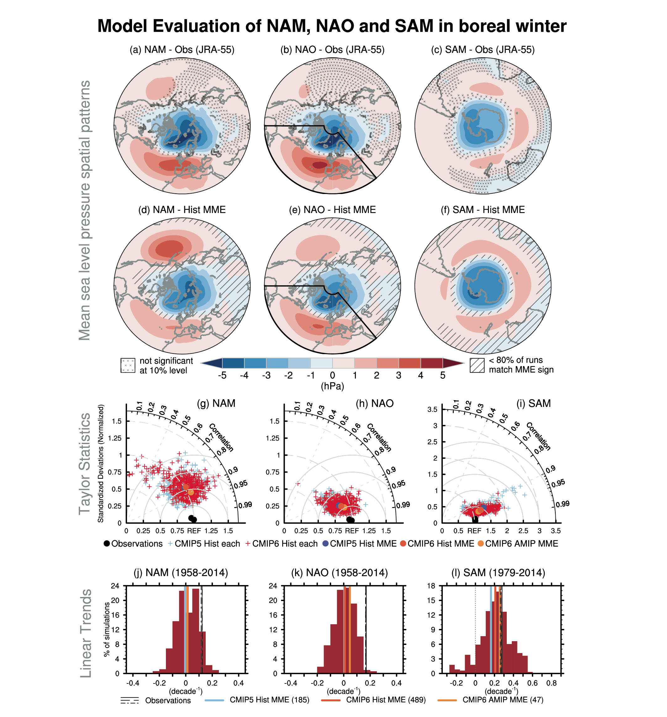 Figure 3.33 | Model evaluation of NAM, NAO and SAM in boreal winter. Regression of Mean Sea Level Pressure (MSLP) anomalies (in hPa) onto the normalized principal component (PC) of the leading mode of variability obtained from empirical orthogonal decomposition of the boreal winter (December–February) MSLP poleward of 20°N for the observed Northern Annular Mode (NAM, a), over 20°N–80°N, 90°W–40°E for the North Atlantic Oscillation as shown by the black sector (NAO, b), and poleward of 20°S for the Southern Annular Mode (SAM, c) for the JRA-55 reanalysis. Cross marks indicate regions where the anomalies are not significant at the 10% level based on a t-test. The period used to calculate the NAO/NAM is 1958–2014 but 1979–2014 for the SAM. (d–f) Same but for the multi-model ensemble (MME) mean from CMIP6 historical simulations. Models are weighted in compositing to account for differences in their respective ensemble size. Diagonal lines show regions where less than 80% of the runs agree in sign. (g–i) Taylor diagrams summarizing the representation of the modes in models and observations following Lee et al. (2019) for CMIP5 (light blue) and CMIP6 (red) historical simulations. The reference pattern is taken from JRA-55 (a–c). The ratio of standard deviation to that of the reference observations (radial distance), spatial correlation (radial angle) and resulting root-mean-squared errors (solid isolines) are given for individual ensemble members (crosses) and for other observational products (ERA5 and NOAA 20CR version 3, black dots). Coloured dots stand for weighted multi-model mean statistics for CMIP5 (blue) and CMIP6 (light red) as well as for AMIP simulations from CMIP6 (orange). (j–l) Histograms of the trends built from all individual ensemble members and all the models (brown bars). Vertical lines in black show all the observational estimates. The orange, light red, and light blue lines indicate the weighted multi-model mean of CMIP6 AMIP, CMIP6 and CMIP5 historical simulations, respectively. Further details on data sources and processing are available in the chapter data table (Table 3.SM.1).
 CMIP5 models with a model top within the stratosphere seriously underestimate the amplitude of the variability of the wintertime NAM expression in the stratosphere, in contrast to CMIP5 models which extend well above the stratopause (Lee and Black, 2015). However, even in the latter models, the stratospheric NAM events, and their downward influence on the troposphere, are insufficiently persistent (Charlton-Perez et al., 2013; Lee and Black, 2015). Increased vertical resolution does not show any significant added value in reproducing the structure and magnitude of the tropospheric NAM (Lee and Black, 2013) nor in the NAO predictability as assessed in a seasonal prediction context with a multi-model approach (Butler et al., 2016). On the other hand, there is mounting evidence that a correct representation of the Quasi Biennal Oscillation, extratropical stratospheric dynamics (the polar vortex and sudden stratospheric warmings), and related troposphere-stratosphere coupling, as well as their interplay with ENSO, are important for NAO/NAM timing (Scaife et al., 2016; Karpechko et al., 2017; Domeisen, 2019; Domeisen et al., 2019), in spite of underestimated troposphere–stratosphere coupling found in models compared to observations (O’Reilly et al., 2019b).
The observed trend of the NAM and NAO indices is positive in winter when calculated from the 1960s (Section 2.4.1.1) but it includes large multi-decadal variability, which means that the nature of the trend should be interpreted with caution (Gillett et al., 2013). The multi-model multi-member ensemble mean of the trend estimated from historical simulations over that period is very close to zero for both CMIP5 and CMIP6 (Figures 3.33j,k and 3.34a). Even if one cannot rule out that 1958–2014 was an exceptional period of variability, the observational estimates of the wintertime NAO trend lie outside the 5th–95th percentile range of the distribution of trends in the CMIP6 historical simulations, and the observed NAM trends over the same period lie above the 90th percentile. There is a tendency for the CMIP5 models to systematically underestimate the level of multi-decadal versus interannual variability of the winter NAO and jet stream compared to observations (X. Wang et al., 2017; Bracegirdle et al., 2018; Simpson et al., 2018). Results from CMIP6 (Figure 3.33j,k) and over the 1958–2019 period (Figure 3.34a) confirm this conclusion and seriously question the ability of the models to simulate long-term fluctuations of the NAO/NAM, independently of its forced or internal origins.
 Figure 3.34 | Attribution of observed seasonal trends in the annular modes to forcings. Simulated and observed trends in NAM indices over 1958–2019 (a) and in SAM indices over 1979–2019 (b) and over 2000–2019 (c) for boreal winter (December–February average; DJF) and summer (June–August average; JJA). The indices are based on the difference of the normalized zonally averaged monthly mean sea level pressure between 35°N and 65°N for the NAM and between 40°S and 65°S for the SAM as defined in Jianping and Wang (2003) and Gong and Wang (1999), respectively; the unit is decade–1. Ensemble mean, interquartile ranges and 5th and 95th percentiles are represented by empty boxes and whiskers for pre-industrial control simulations and historical simulations. The number of ensemble members and models used for computing the distribution is given in the upper-left legend. Grey lines show observed trends from the ERA5 and JRA-55 reanalyses. Multi-model multi-member ensemble means of the forced component of the trends as well as their 5–95% confidence intervals assessed from t-statistics, are represented by filled boxes, based on CMIP6 individual forcing simulations from DAMIP ensembles; greenhouse gases in brown, aerosols in light blue, stratospheric ozone in purple and natural forcing in green. Models with at least three ensemble members are used for the filled boxes, with black dots representing the ensemble means of individual models. Further details on data sources and processing are available in the chapter data table (Table 3.SM.1).
 Dedicated SST-forced stand-alone atmospheric model experiments (AMIP) suggest that ocean forcing appears to play a role in decadal variability of the NAO and associated fluctuations in the strength of the jet (Woollings et al., 2015). In particular, Atlantic and Indian Ocean SST anomalies (Fletcher and Cassou, 2015; Baker et al., 2019; Douville et al., 2019; Dhame et al., 2020) may have contributed to the long-term positive trend of the winter NAO/NAM over the 20th century, but there is only low confidence in such a causal relationship because of the limitation of the imposed SST approach in AMIP and the uncertainties in observed SST trends among datasets used as forcing of the atmospheric model. The representation of the NAM and NAO spatial structure is slightly improved in AMIP ensembles (Figure 3.33g,h), which also produce slightly larger trends than the historical simulations for the NAO, but not for the NAM.
When calculated over the most recent two decades, the wintertime NAM/NAO trend is weakly negative since the mid-1990s (Hanna et al., 2015). Recent studies based on observations (Gastineau and Frankignoul, 2015) and dedicated modelling experiments (Davini et al., 2015; Peings and Magnusdottir, 2016) suggest that the recent dominance of negative NAM/NAO could be partly related to the latest shift of the Atlantic Multi-decadal Variability (AMV) to a warm phase (Sections 2.4.4 and 3.7.7). Some recent modelling studies also find that the Arctic sea ice decline might be partly responsible for more recurrent negative NAM/NAO (Peings and Magnusdottir, 2013; B.M. Kim et al., 2014; Nakamura et al., 2015), while other studies do not robustly identify such responses in models (see also Cross-Chapter Box 10.1).
In contrast to winter, the observed trend of the NAO index over 1958–2014 is overall negative in summer and is associated with more recurrent blocking conditions over Greenland, in particular since the mid-1990s, thus contributing to the acceleration of melting of the Arctic sea ice (Section 3.4.1.1) and Greenland Ice Sheet (Section 3.4.3.2; Fettweis et al., 2013; Hanna et al., 2015; Ding et al., 2017). The origin of the negative trend of the summer NAO has not been clearly identified, and is hypothesized to be the result of combined influences (Lim et al., 2019), though trends in summertime NAO should also be interpreted with caution because of the presence of strong multi-decadal variability. The recent observed negative NAO prevalence and related blocking over Greenland is not present in any of the CMIP5 models (Hanna et al., 2018).
Regarding the influence of external forcings since pre-industrial times, AR5 noted that CMIP5 models tend to show an increase in the NAM in response to greenhouse gas increases (Bindoff et al., 2013). Based on the CMIP5 historical ensemble, Gillett and Fyfe (2013) however showed that such a trend is not significant in all seasons. A multi-model assessment of eight CMIP5 models found a NAM increase in response to greenhouse gases, but no robust influence of aerosol changes (Gillett et al., 2013). As for ozone depletion, there is no robust detectable influence on long-term trends of the NAO/NAM (Karpechko et al., 2018) in contrast to the SAM (Section 3.7.2), but there are indications that extreme Arctic ozone depletion events and their surface expression are linked to an anomalously strong NAM episodes (Calvo et al., 2015; Ivy et al., 2017). However, the direction of causality here is not clear.
Conclusions on external forcing influences on the NAM are supported by CMIP6 results based on single forcing ensembles (Figure 3.34a). Positive trends are found in historical simulations over 1958–2019 in boreal winter and are mainly driven by greenhouse gas increases. No significant trends are simulated in response to anthropogenic aerosols, stratospheric ozone or natural forcing. Albeit weak and not statistically significant, the sign of the multi-model mean forced response due to natural forcing is consistent with the observed reduction of solar activity since the 1980s (Section 2.2.1) whose influence would have favoured the negative phase of wintertime NAM/NAO based on the fingerprint of the nearly periodical 11-year solar cycle extracted from models (Scaife et al., 2013; Andrews et al., 2015; Thiéblemont et al., 2015) or observations (Gray et al., 2016; Lüdecke et al., 2020). But such an NAO response to solar forcing remains highly uncertain and controversial, being contradicted by longer proxy records over the last millennium (Sjolte et al., 2018) and modelling evidence (Gillett and Fyfe, 2013; Chiodo et al., 2019). For all seasons and for all individual forcings, uncertainties remain in the estimation of the forced response in the NAM trend as evidenced by considerable model spread (Figure 3.34a) and because the simulated forced component has small amplitude compared to internal variability.
Despite new efforts since AR5 to reconstruct the NAO beyond the instrumental record, it is still very challenging to assess the role of external forcings in the apparent multi-decadal to centennial variability present throughout the last millennium. Large uncertainties remain in the reconstructed NAO index that are sensitive to the types of proxies and statistical methods (Trouet et al., 2012; Ortega et al., 2015; Anchukaitis et al., 2019; Cook et al., 2019; Hernández et al., 2020; Michel et al., 2020) and reconstructed NAO variations are often not reproduced using pseudo-proxy approaches in models (Lehner et al., 2012; Landrum et al., 2013). At low frequency, it remains challenging to evaluate if the observed or reconstructed signal corresponds to an actual change in the NAO intraseasonal to interannual intrinsic properties or rather to a change in the mean background atmospheric circulation changes projecting on a specific phase of the mode. Consequently, conflicting results emerge in the attribution of reconstructed long-term variations in the NAO to solar forcing, whose influence thus remains controversial (Gómez-Navarro and Zorita, 2013; Moffa-Sánchez et al., 2014; Ortega et al., 2015; Ait Brahim et al., 2018; Sjolte et al., 2018; Xu et al., 2018). Influences from major volcanic eruptions appear to be more robust (Ortega et al., 2015; Swingedouw et al., 2017) even if some modelling experiments question the amplitude of the response, which mostly projects on the positive phase of the NAM/NAO (Bittner et al., 2016). The forced response is dependent on the strength, seasonal timing and location of the eruption but may also depend on the mean climate background state (Zanchettin et al., 2013) and/or the phases of the main modes of decadal variability such as the AMV (Section 3.7.7; Ménégoz et al., 2018).
Finally, there is some evidence of an apparent signal-to-noise problem referred to as ‘paradox’ in seasonal and decadal hindcasts of the NAO over the period 1979–2018 (Scaife and Smith, 2018), which suggests that the NAO response to external forcing, SST or sea ice anomalies could be too weak in models. The weakness of the signal has been related to troposphere-stratosphere coupling which is too intermittent (O’Reilly et al., 2019b) and to chronic model biases in the persistence of NAO/NAM daily regimes, which is critically underestimated in coupled models (Strommen and Palmer, 2019; Zhang and Kirtman, 2019), and which does not exhibit significant improvement when model resolution is increased (Fabiano et al., 2020). Note, however, that the apparent signal-to-noise problem may be dependent on the period analysed over the 20th century, which questions its interpretation as a general characteristic of coupled models (Weisheimer et al., 2020).
In summary, CMIP5 and CMIP6 models are skilful in simulating the spatial features and the variance of the NAM/NAO and associated teleconnections (high confidence). There is limited evidence for a significant role for anthropogenic forcings in driving the observed multi-decadal variations of the NAM/NAO from the mid 20th century. Confidence in attribution is low: (i) because there is a large spread in the modelled forced responses which is overwhelmed anyway by internal variability; (ii) because of the apparent signal-to-noise problem; and (iii) because of the chronic inability of models to produce a range of trends which encompasses the observed estimates over the last 60 years.
3.7.2 Southern Annular Mode
The Southern Annular Mode (SAM) consists of a meridional redistribution of atmospheric mass around Antarctica (Figure 3.33c,f), associated with a meridional shift of the jet and surface westerlies over the Southern Ocean. SAM indices are variously defined as the difference in zonal-mean sea level pressure or geopotential height between middle and high latitudes or via a principal-component analysis (Annex IV.2.2). Observational aspects of the SAM are assessed in Section 2.4.1.2.
AR5 assessed that CMIP5 models have medium performance in reproducing the SAM with biases in pattern (Flato et al., 2013). It also concluded that the trend of the SAM toward its positive phase in austral summer since the mid-20th century is likely to be due in part to stratospheric ozone depletion, and there was medium confidence that greenhouse gases have also played a role (Bindoff et al., 2013). Based on proxy reconstructions, AR5 found with medium confidence that the positive SAM trend since 1950 was anomalous compared to the last 400 years (Masson-Delmotte et al., 2013).
Additional research has shown that CMIP5 models reproduce the spatial structure of the SAM well, but tend to overestimate its variability in austral summer at interannual time scales, although this variability is within the observational uncertainty (Figure 3.33c,f,i; Zheng et al., 2013; Schenzinger and Osprey, 2015). This is related to the models’ tendency to simulate slightly more persistent SAM anomalies in summer compared to reanalyses (Schenzinger and Osprey, 2015; Bracegirdle et al., 2020). This may be due in part to too weak a negative feedback from tropospheric planetary waves (Simpson et al., 2013). CMIP6 models show improved performance in reproducing the spatial structure and interannual variance of the SAM in summer based on Lee et al. (2019) diagnostics (Figure 3.33i), with a better match of its trend with reanalyses over 1979–2014 (Figure 3.33l), more realistic persistence and improved positioning of the westerly jet, which in CMIP5 models on average is located too far equatorward (Bracegirdle et al., 2020; Grose et al., 2020). In CMIP5, it is also found that models which extend above the stratopause tend to simulate stronger summertime trends in the late 20th century than their counterparts with tops within the stratosphere (Rea et al., 2018; Son et al., 2018), though other differences between these sets of models, such as additional physical processes operating in the stratosphere or interactive ozone chemistry, may have also affected these results (Gillett et al., 2003a; Sigmond et al., 2008; Rea et al., 2018). At the surface, Ogawa et al. (2015) demonstrate with an atmospheric model the importance of sharp mid-latitude SST gradients for stratospheric ozone depletion to affect the SAM in summer. These studies imply that the well resolved stratosphere combined with finer ocean horizontal resolution has contributed to the stronger simulated trends in CMIP6 than in CMIP5.
CMIP6 historical simulations capture the observed positive trend of the summertime SAM when calculated from the 1970s to the 2010s (Figure 3.34b). J.L. Thomas et al. (2015) found that the chance of the observed 1980–2004 trend occurring only due to internal variability is less than 10% in many of the CMIP5 models, and results from CMIP6 models suggest that the chance of the 1979–2019 trend being due to internal variability could be even lower (Figure 3.34b). Although paleo-reconstructions of the SAM index are uncertain and vary in terms of long-term trends (Section 2.4.1.2), new reconstructions show that the 60-year summertime SAM trend since the mid-20th century is outside the 5th–95th percentile range of the trends in the pre-industrial variability, which matches the trend range of CMIP5 pre-industrial control simulations well (Dätwyler et al., 2018).
In general agreement with AR5, new research continues to indicate that both stratospheric ozone depletion and increasing greenhouse gases have contributed to the trend of the SAM during austral summer toward its positive phase in recent decades (Solomon and Polvani, 2016), with the ozone depletion influence dominating (Gerber and Son, 2014; Son et al., 2018). In CMIP6 historical simulations there are significant positive SAM trends over the 1979–2019 period in austral summer, although the contribution from ozone forcing evaluated with the four available models is not significant (Figure 3.34b). Three of these models share the same standard prescribed ozone forcing and produce significantly positive SAM trends over an extended period (1957–2019). The fourth model, MRI-ESM2-0, has the option of interactive ozone chemistry. Its ozone-only experiment is forced by prescribed ozone derived from its own historical simulations and produces a negative SAM trend associated with weak ozone depletion (Morgenstern et al., 2020). Morgenstern et al. (2014) and Morgenstern (2021) find an indirect influence of greenhouse gases on the SAM via induced ozone changes in coupled chemistry-climate simulations, which differ from the prescribed ozone simulations shown in Figure 3.34b. Since about 1997, the effective abundance of ozone-depleting halogen has been decreasing in the stratosphere (WMO, 2018), leading to a stabilization or even a reversal of stratospheric ozone depletion (Sections 2.2.5.2 and 6.3.2.2). The ozone stabilization and slight recovery since about 2000 may have caused a pause in the summertime SAM trend (Figure 3.34c; Saggioro and Shepherd, 2019; Banerjee et al., 2020), although some influence from internal variability cannot be ruled out. While some studies find an anthropogenic aerosol influence on the summertime SAM (Gillett et al., 2013; Rotstayn, 2013), recent studies with larger multi-model ensembles find that this effect is not robust (Steptoe et al., 2016; Choi et al., 2019), consistent with CMIP6 single forcing ensembles (Figure 3.34). In the CMIP5 simulations, volcanic stratospheric aerosol has a significant weakening effect on the SAM in autumn and winter (Cross-Chapter Box 4.1; Gillett and Fyfe, 2013), but there is no evidence that this effect leads to a significant multi-decadal trend since the late 20th century. Beyond external forcing, Fogt et al. (2017) show a significant association of tropical SST variability with the summertime SAM trend since the mid-20th century in agreement with Lim et al. (2016), who, however, demonstrate that such a teleconnection between the summertime SAM and El Niño–Southern Oscillation (Annex IV.2.3), found in observations, is missing in many CMIP5 models.
On longer time scales, last millennium experiments from CMIP5 models fail to capture multicentennial variability evident in the reconstructions for the pre-industrial era (Abram et al., 2014; Dätwyler et al., 2018), which is also the case in those from available CMIP6 models (Figure 3.35). However, there is large uncertainty among reconstructions (Section 2.4.1.2). It is therefore unclear whether this disagreement reflects this observational uncertainty, whether forcings such as variations in the imposed insolation may be too weak, whether models are insufficiently sensitive to such variations, or whether internal variability including that associated with tropical Pacific variability is under-represented (Abram et al., 2014). The explanation could be a combination of all these factors. However, despite the aforementioned limitations of the reconstructions, Section 2.4.1.2 assesses that the recent positive trend in the SAM is likely unprecedented in at least the past millennium (medium confidence). CMIP5 and CMIP6 last-millennium simulations only capture the present anomalous state during the final decades of the simulations which are dominated by human influence; this state is also outside the range of simulated variability characteristic of pre-industrial times.
 Figure 3.35 | Southern Annular Mode (SAM) indices in the last millennium. (a) Annual-mean SAM reconstructions by Abram et al. (2014) and Dätwyler et al. (2018). (b) The annual-mean SAM index defined by Gong and Wang (1999) in CMIP5 and CMIP6 last millennium simulations extended by historical simulations. All indices are normalized with respect to 1961–1990 means and standard deviations. Thin lines and thick lines show seven-year and 70-year moving averages, respectively. Further details on data sources and processing are available in the chapter data table (Table 3.SM.1).
 In summary, it is very likely that anthropogenic forcings have contributed to the observed trend of the summer SAM toward its positive phase since the 1970s. This assessment is supported by further model studies that confirm the human influence on the summertime SAM with improved models since AR5. While ozone depletion contributed to the trend from the 1970s to the 1990s (medium confidence), its influence has been small since 2000, leading to a weaker summertime SAM trend over 2000–2019 (medium confidence). Climate models reproduce the spatial structure of the summertime SAM observed since the late 1970s well (high confidence). CMIP6 models reproduce the spatiotemporal features and recent multi-decadal trend of the summertime SAM better than CMIP5 models (medium confidence). However, there is a large spread in the intensity of the SAM response to ozone and greenhouse gas changes in both CMIP5 and CMIP6 models (high confidence), which limits the confidence in the assessment of the ozone contribution to the observed trends. CMIP5 and CMIP6 models do not capture multicentennial variability of the SAM found in proxy reconstructions (low confidence). This confidence level reflects that it is unclear whether this is due to a model or an observational shortcoming.
3.7.3 El Niño–Southern Oscillation (ENSO)
The El Niño–Southern Oscillation (ENSO), which is generated via seasonally modulated interactions between the tropical Pacific ocean and atmosphere, influences severe weather, rainfall, river flow and agricultural production over large parts of the world (McPhaden et al., 2006). In fact, the remote climate influence of ENSO is so large that knowledge of its current phase and forecasts of its future phase largely underpin many seasonal rainfall and temperature forecasts worldwide (Annex IV.2.3).
AR5 noted that there have been clear improvements in the simulation of ENSO through previous generations of CMIP models (Flato et al., 2013), such that many CMIP5 models displayed behaviour that was qualitatively similar to that of the observed ENSO (Guilyardi et al., 2012). However, systematic errors were identified in the models’ representation of the tropical Pacific mean state and aspects of their interannual variability that affect quantitative comparisons. The AR5 assessment of ENSO concluded that the considerable observed inter-decadal modulations in ENSO amplitude and spatial pattern were largely consistent with unforced model simulations. Thus, there was low confidence in the role of a human-induced influence in these (Bindoff et al., 2013).
Observed ENSO amplitude, which is measured by the standard deviation of SST anomalies in a central equatorial Pacific region often referred to as the Nino 3.4 region, along with the lifecycle of events, are both reasonably well reproduced by most CMIP5 and CMIP6 models (Figure 3.36; Bellenger et al., 2014; Planton et al., 2021). The average CMIP5 model ENSO amplitude is slightly lower than that observed, while the average CMIP6 model ENSO amplitude is slightly higher than observed (Figure 3.36). The ENSO amplitude of the individual models, however, is highly variable across CMIP5 and CMIP6 models with many displaying either more or less variability than observed (Stevenson, 2012; Grose et al., 2020; Planton et al., 2021).
 Figure 3.36 | Life cycle of (left) El Niño and (right) La Niña events in observations (black) and historical simulations from CMIP5 (blue; extended with RCP4.5) and CMIP6 (red). An event is detected when the December ENSO index value in year zero exceeds 0.75 times its standard deviation for 1951–2010. (a, b) Composites of the ENSO index (°C). The horizontal axis represents month relative to the reference December (the grey vertical bar), with numbers in parentheses indicating relative years. Shading and lines represent 5th–95th percentiles and multi-model ensemble means, respectively. (c, d) Mean durations (months) of El Niño and La Niña events defined as number of months in individual events for which the ENSO index exceeds 0.5 times its December standard deviation. Each dot represents an ensemble member from the model indicated on the vertical axis. The boxes and whiskers represent multi-model ensemble means, interquartile ranges and 5th and 95th percentiles of CMIP5 and CMIP6. The CMIP5 and CMIP6 multi-model ensemble means and observational values are indicated at the top right of each panel. The multi-model ensemble means and percentile values are evaluated after weighting individual members with the inverse of the ensemble size of the same model, so that individual models are equally weighted irrespective of their ensemble sizes. The ENSO index is defined as the SST anomaly averaged over the Niño 3.4 region (5°S–5°N, 170°W–120°W). All results are based on five-month running mean SST anomalies with triangular-weights after linear detrending. Further details on data sources and processing are available in the chapter data table (Table 3.SM.1).
 ENSO events are often synchronized to the seasonal cycle in the observations, as the associated SST anomalies tend to peak in boreal winter (November to January) and be at their weakest in the boreal spring (March to April) (Harrison and Larkin, 1998; Larkin and Harrison, 2002). The majority of CMIP5 and CMIP6 models broadly reproduce the seasonality of ENSO SST variability in the central equatorial Pacific (Taschetto et al., 2014; Abellán et al., 2017; Grose et al., 2020; Planton et al., 2021) (Figure 3.37). However, CMIP5 models, while displaying an improvement on CMIP3 models, appear to under-represent the magnitude of the seasonal variance modulation (Bellenger et al., 2014). This under-representation of seasonal variance modulation continues in CMIP6 models, which display no statistically significant difference in this behaviour when compared to CMIP5 models (Planton et al., 2021) (Figure 3.37).
 Figure 3.37 | ENSO seasonality in observations (black) and historical simulations from CMIP5 (blue; extended with RCP4.5) and CMIP6 (red) for1951–2010. (a) Climatological standard deviation of the monthly ENSO index (SST anomaly averaged over the Niño 3.4 region; °C). Shading and lines represent 5th–95th percentiles and multi-model ensemble means, respectively. (b) Seasonality metric, which is defined for each model and each ensemble member as the ratio of the ENSO index climatological standard deviation in November–January (NDJ) to that in March–May (MAM). Each dot represents an ensemble member from the model indicated on the vertical axis. The boxes and whiskers represent the multi-model ensemble means, interquartile ranges and 5th and 95th percentiles of CMIP5 and CMIP6 individually. The CMIP5 and CMIP6 multi-model ensemble means and observational values are indicated at the top right of the panel. The multi-model ensemble means and percentile values are evaluated after weighting individual members with the inverse of the ensemble size of the same model, so that individual models are equally weighted irrespective of their ensemble sizes. All results are based on five-month running mean SST anomalies with triangular-weights after linear detrending. Further details on data sources and processing are available in the chapter data table (Table 3.SM.1).
 Observations show strong multi-decadal modulation of ENSO variance throughout the 20th century, with the most recent period displaying larger variability while the mid-century displayed relatively low ENSO variability (Figure 2.36; Li et al., 2013; McGregor et al., 2013; Hope et al., 2017). As assessed in Section 2.4.2, ENSO amplitude since 1950 is higher than over the pre-industrial period from 1850 as far back as 1400 (medium confidence), but there is low confidence that it is higher than the variability over periods prior to 1400. This reported variance increase suggests that external forcing plays a role in the ENSO variance changes (Hope et al., 2017). However, large ensembles of single model or multiple model simulations do not find strong trends in ENSO variability over the historical period, suggesting that external forcing has not yet modulated ENSO variability with a magnitude that exceeds the range of internal variability (Hope et al., 2017; Maher et al., 2018b; Stevenson et al., 2019). This is consistent with the Chapter 2 assessment that there is no clear evidence for a recent sustained shift in ENSO beyond the range of variability on decadal to millennial time scales (Section 2.4.2). CMIP5 and CMIP6 models show a decrease in ENSO variance in the mid-Holocene (Brown et al., 2020), though not to the extent seen in paleo-proxy records (Emile-Geay et al., 2016). This suggests that both modelled and observed ENSO respond to changes in external forcing, but not necessarily in the same manner.
Most CMIP5 and CMIP6 models are found to represent the general structure of observed SST anomalies during ENSO events well (Kim and Yu, 2012; Taschetto et al., 2014; Brown et al., 2020; Grose et al., 2020). However, the majority of CMIP5 models display SST anomalies that: i) extend too far to the west (Taschetto et al., 2014; Capotondi et al., 2015); and ii) have meridional widths that are too narrow (Zhang and Jin, 2012) compared to the observations. CMIP6 models display a statistically significant improvement in the longitudinal representation of ENSO SST anomalies relative to CMIP5 models (Planton et al., 2021), however, systematic biases in the zonal extent and meridional width remain in CMIP6 models (Fasullo et al., 2020; Planton et al., 2021). The ENSO phase asymmetry, where observed strong El Niño events are larger and have a shorter duration than strong La Niña events (Ohba and Ueda, 2009; Frauen and Dommenget, 2010), is also under-represented in both CMIP5 and CMIP6 models (Zhang and Sun, 2014; Planton et al., 2021). In this instance, both CMIP5 and CMIP6 models typically display El Niño events that have a longer duration than those observed, La Niña events that have a similar duration to those observed, and there is very little asymmetry in the duration of El Niño and La Niña phases (Figure 3.36). Roberts et al. (2018) find an improvement in amplitude asymmetry in a HighResMIP model, but the under-representation remains.
The continuum of El Niño events are typically stratified into two types (often termed ‘flavours’), Central Pacific and East Pacific, where the name denotes the location of the events’ largest SST anomalies (Annex IV.2.3; Capotondi et al., 2015). As discussed in Section 2.4.2, the different types of events tend to produce distinct teleconnections and climatic impacts (e.g., Taschetto et al., 2020). The characteristics of El Niño events of these two flavours in CMIP5 were generally comparable to the observations (Taschetto et al., 2014). CMIP6 models, however, display a statistically significant improvement in the representation of this ENSO event-to-event SST anomaly diversity when compared with CMIP5 models (Planton et al., 2021). In addition to this ENSO event diversity, the short observational record also displays an increase in the number of the Central Pacific-type events in recent decades (Ashok et al., 2007; McPhaden et al., 2011), which has also been identified as unusual in the context of the last 500–800 years based on recent paleo-climatic reconstructions (Section 2.4.2; Y. Liu et al., 2017; Freund et al., 2019). However, the short observational record combined with observational (L’Heureux et al., 2013) and paleo-climatic reconstruction uncertainties preclude firm conclusions being made about the long-term changes in the occurrence of different El Niño event types. Initial analysis with a selected number of CMIP3 models suggested that there may be a forced component to this recent prominence of Central Pacific-type events (Yeh et al., 2009), but analysis since then suggests that this behaviour is (i) consistent with that expected from internal variability (Newman et al., 2011); and (ii) not apparent across the full CMIP5 ensemble of historical simulations (Taschetto et al., 2014). Analysis of single-model large ensembles suggests that changes to ENSO event type in response to historical radiative forcing are not significant (e.g., Stevenson et al., 2019). These same results, however, also suggest that multiple forcings can have significant influences on ENSO type and that the net response will depend on the accurate representation of the balance of these forcings (Stevenson et al., 2019).
The climatic effects of ENSO outside the tropical Pacific largely arise through atmospheric teleconnections that are induced by ENSO-driven changes in deep tropical atmospheric convection and heating (Yeh et al., 2018). The teleconnections to higher latitudes are forced by waves that propagate into the extratropics (Hoskins and Karoly, 1981) and respectively excite the Pacific-North American pattern (Horel and Wallace, 1981) and Pacific-South American pattern (Karoly, 1989; Irving and Simmonds, 2016) in the Northern and Southern Hemispheres. Given the influence of these teleconnections on climate and extremes around the globe, it is important to understand how well they are reproduced in CMIP models. What has also become clear is that spatial correlations of ENSO’s teleconnections calculated over relatively short periods (<100 years) may not be the most effective way to assess these relationships (Langenbrunner and Neelin, 2013; Perry et al., 2020). This is because the spatial patterns are significantly affected by internal atmospheric variability on relatively short time scales (<100 years; Batehup et al., 2015; Perry et al., 2020). However, looking at simplified metrics like the agreement in the sign of the teleconnections (Langenbrunner and Neelin, 2013), regional average teleconnection strength over land (Perry et al., 2020), or a combination of both (Power and Delage, 2018) provides a more robust depiction of the teleconnection representation. Examining sign agreement for the teleconnection patterns, ensembles of CMIP5 AMIP simulations display broad spatial regions with high sign agreement with the observations, suggesting that the model ensemble is producing useful information regarding the teleconnected precipitation signal (Langenbrunner and Neelin, 2013). Looking at regional averages of CMIP5 historical simulations, Power and Delage (2018) show that the average coupled model teleconnection pattern reproduces the sign of the observed teleconnections in the majority of the 25 regions analysed. The sign agreement between the observed teleconnection and the multi-model mean teleconnection remains strong in CMIP6 (18 out of 20 displayed regions; Figure 3.38), and the observed DJF (December–January–February) teleconnection strength falls within the modelled range in all of the displayed regions for temperature and precipitation. Note, however, that while there is broad agreement in ENSO teleconnections between CMIP6 models and observations during DJF (e.g., Fasullo et al., 2020), there are regions and seasons where the modelled teleconnection strength is outside the observed range (Chen et al., 2020).
 Figure 3.38 | Model evaluation of ENSO teleconnection for near surface air temperature and precipitation in boreal winter (December–January–February). Teleconnections are identified by linear regression with the Niño 3.4 SST index based on Extended Reconstructed Sea Surface Temperature (ERSST) version 5 over the period 1958–2014. Maps show observed patterns for temperature from the Berkeley Earth dataset over land and from ERSST version 5 over ocean (°C, top) and for precipitation from GPCC over land (shading, mm day–1) and GPCP worldwide (contours, period: 1979–2014). Distributions of regression coefficients (grey histograms) are provided for a subset of AR6 reference regions defined in Atlas.1.3 for temperature (top) and precipitation (bottom). All fields are linearly detrended prior to computation. Multi-model multi-member ensemble means are indicated by thick vertical black lines. Blue vertical lines show three observational estimates of temperature, based on Berkeley Earth, GISTEMP and CRUTS datasets, and two observational estimates of precipitation, based on GPCC and CRUTS datasets. Further details on data sources and processing are available in the chapter data table (Table 3.SM.1).
 Most CMIP5 and CMIP6 models exhibit ENSO behaviour during the historical period that, to first order, is qualitatively similar to that of the observed ENSO. Many studies are now delving deeper into the models to understand if they are accurately producing the dynamics driving ENSO and its initiation (Jin et al., 2006; Bellenger et al., 2014; Vijayeta and Dommenget, 2018; Bayr et al., 2019; Planton et al., 2021). For both CMIP3 and CMIP5, diagnostics of ENSO event growth appear to show that the models, while producing ENSO variability that is qualitatively similar to that observed, do not represent the balance of the underlying dynamics well. The atmospheric Bjerknes feedback is too weak in the majority of models, while the surface heat flux feedback is also too weak in the majority of models. The former restricts event growth, while the latter restricts event damping, which when combined allow most models to produce variability in a range that is consistent with the observations (Bellenger et al., 2014; S.T. Kim et al., 2014; Vijayeta and Dommenget, 2018; Bayr et al., 2019). Analysis of ENSO representation in a subset of CMIP6 models by Planton et al. (2021) suggests that these issues remain.
To conclude, ENSO representation in CMIP5 models displayed a significant improvement from the representation of ENSO variability in CMIP3 models, which displayed much more intermodel spread in standard deviation, and stronger biennial periodicity (Guilyardi et al., 2012; Flato et al., 2013). In general, there has been no large step change in the representation of ENSO between CMIP5 and CMIP6, however, CMIP6 models appear to better represent some key ENSO characteristics (e.g., Brown et al., 2020; Planton et al., 2021). The instrumental record and paleo-proxy evidence through the Holocene all suggest that ENSO can display considerable modulations in amplitude, pattern and period (see also (Section 2.4.2). For the period since 1850, there is no clear evidence for a sustained shift in ENSO index beyond the range of internal variability. However, paleo-proxy evidence indicates with medium confidence that ENSO variability since 1950 is greater than at any time between 1400 and 1850 (Section 2.4.2). Coupled models display large changes of ENSO behaviour in the absence of external forcing changes, and little-to-no variance sensitivity to historical anthropogenic forcing. Thus, there is low confidence that anthropogenic forcing has led to the changes of ENSO variability inferred from paleo-proxy evidence.
Chapter 2 reports low confidence that the apparent change from East Pacific- to Central Pacific-type El Niño events that occurred in the last 20–30 years was representative of a long term change. While some climate models do suggest external forcing may affect the El Niño event type, most climate models suggest that what has been observed is well within the range of natural variability. Thus, there is low confidence that anthropogenic forcing has had an influence on the observed changes in El Niño event type.
3.7.4 Indian Ocean Basin and Dipole Modes
The Indian Ocean Basin (IOB) and Dipole (IOD) modes are the two leading modes of interannual SST variability over the tropical Indian Ocean, featuring basin-wide warming/cooling and an east–west dipole of SST anomalies, respectively (Annex IV.2.4). The IOD mode is anchored to boreal summer to autumn by the air–sea feedback, and often develops in concert with ENSO. Driven by matured ENSO events, the IOB mode peaks in boreal spring and often persists into the subsequent summer. Similar patterns of Indian Ocean SST variability also dominate its decadal and longer time scale variability (Han et al., 2014b).
AR5 concluded that models show high and medium performance in reproducing the IOB and IOD modes, respectively (medium confidence), with difficulty in reproducing the persistence of the IOB and the pattern and magnitude of the IOD (Flato et al., 2013). There was low confidence that changes in the IOD were detectable or attributable to human influence (Bindoff et al., 2013).
Since AR5, CMIP5 model representation of these modes has been analysed in detail, finding that most of the models qualitatively reproduce the spatial and seasonal features of the IOB and IOD modes (Chu et al., 2014; Liu et al., 2014; W. Tao et al., 2016). Improvements in simulating the IOB mode since CMIP3 have been identified in reduced multi-model mean biases and inter-model spread (W. Tao et al., 2016). CMIP5 models overall capture the transition from the IOD to IOB modes during an ENSO event (W. Tao et al., 2016). The IOB mode is forced in part through a cross-equatorial wind–evaporation–SST feedback triggered by ENSO-forced anomalous ocean Rossby waves that propagate to the shallow climatological thermocline dome in the tropical south-western Indian Ocean (Du et al., 2009). Consistently, models with a deeper climatological thermocline dome produce a weaker and less persistent IOB mode (G. Li et al., 2015a; Zheng et al., 2016). The deep thermocline bias remains in the ensemble mean of CMIP5 models due to a common surface easterly wind bias over the equatorial Indian Ocean (Lee et al., 2013) associated with weaker South Asian summer monsoon circulation (G. Li et al., 2015b). However, the influence of this systematic bias may be compensated by other biases, resulting in a realistic IOB magnitude (W. Tao et al., 2016). Halder et al. (2021) found that CMIP6 models reproduce the IOB mode reasonably well, but did not evaluate the progress since CMIP5.
By contrast, the IOD magnitude is overestimated by CMIP5 models on average, though with noticeable improvements from CMIP3 models (Liu et al., 2014). The overestimation of the IOD magnitude remains in most of 34 CMIP6 models examined in McKenna et al. (2020) with worsening on average in July and August. A too steep climatological thermocline slope along the equator due to the surface easterly wind bias in boreal summer and autumn contributes to this IOD magnitude bias through an excessively strong Bjerknes feedback in CMIP5 (Liu et al., 2014; G. Li et al., 2015b; Hirons and Turner, 2018). The surface easterly bias and associated east–west SST gradient bias are not improved in CMIP6 (Long et al., 2020; Section 3.5.1.2.3), suggesting that the thermocline bias also remains. McKenna et al. (2020) additionally find degradation in the positive-negative asymmetry of the IOD but an improvement in IOD frequency in a subset of CMIP6 models compared to CMIP5. In terms of teleconnections, the equatorial surface easterly wind bias also affects the IOD-associated moisture transport anomalies toward tropical eastern Africa (Hirons and Turner, 2018) where the IOD is associated with strong precipitation anomalies in boreal autumn (Annex IV.2.4). CMIP5 and CMIP6 models capture the IOD teleconnection to Southern and Central Australian precipitation although it is weaker on average than observed, with no clear improvements from CMIP5 to CMIP6 (Grose et al., 2020). Strong IOD events could also influence the Northern Hemisphere extratropical circulation in winter and in particular the NAM (Section 3.7.1), based on interference between forced Rossby waves emerging from the Indian Ocean and climatological stationary waves (Fletcher and Cassou, 2015). The record positive phase of the NAO/NAM in winter 2019–2020 assessed over the instrumental era has been accordingly linked to the record IOD event of autumn 2019 (Hardiman et al., 2020), which has been associated with the devastating record fire season in Australia (Wang and Cai, 2020).
The observed Indian Ocean basin-average SST increase on multi-decadal and centennial time scales is well represented by CMIP5 historical simulations, and has been attributed to the effects of greenhouse gases offset in part by the effects of anthropogenic aerosols mainly through aerosol-cloud interactions (Dong and Zhou, 2014; Dong et al., 2014b). The observed SST trend is larger in the western than eastern tropical Indian Ocean, which leads to an apparent upward trend of the IOD index, but this trend is statistically insignificant (Section 2.4.3). CMIP5 models capture this warming pattern, which may be associated with Walker circulation weakening over the Indian Ocean due to greenhouse gas forcing (Dong and Zhou, 2014). However, strong internal decadal IOD-like variability and observational uncertainty preclude attribution (Cai et al., 2013; Han et al., 2014b; Gopika et al., 2020). Such a positive IOD-like change in equatorial zonal SST gradient suggests an increase in the frequency of extreme positive events (Cai et al., 2014) and skewness (Cowan et al., 2015) of the IOD mode. While there is some evidence of an increase in frequency of positive IOD events during the second half of the 20th century, the current level of IOD variability is not unprecedented in a proxy reconstruction for the last millennium (Section 2.4.3; Abram et al., 2020). Besides, the IOD magnitude in the late 20th century is not significantly different between CMIP5 simulations forced by historical and natural-only forcings, though this conclusion is based on only five selected ensemble members that realistically reproduce statistical features of the IOD (Blau and Ha, 2020). While selected CMIP5 models show weakening (Thielke and Mölg, 2019) and seasonality changes (Blau and Ha, 2020) in IOD-induced rainfall anomalies in tropical eastern Africa, no comparison with observational records has been made. Likewise, while a strengthening tendency of the ENSO-IOB mode correlation and resultant intensification of the IOB mode are found in historical or future simulations in selected CMIP5 models (Hu et al., 2014; Tao et al., 2015), such a change has not been detected in observational records.
After linear detrending, Pacific Decadal Variability (PDV; Annex IV.2.6; Section 3.7.6) has been suggested as a driver of decadal to multi-decadal variations in the IOB mode (Dong et al., 2016). However, correlation between the PDV and a decadal IOB index, defined from linearly detrended SST, changed from positive to negative during the 1980s (Han et al., 2014a). The increase in anthropogenic forcing and recovery from the eruptions of El Chichón in 1982 and Pinatubo in 1991 may have overwhelmed the PDV influence, and explain this change (Dong and McPhaden, 2017; L. Zhang et al., 2018a). However, the low statistical degrees of freedom hamper clear detection of human influence in this correlation change.
To summarize, there is medium confidence that changes in the interannual IOD variability in the late 20th century inferred from observations and proxy records are within the range of internal variability. There is no evidence of anthropogenic influence on the interannual IOB. On decadal- to multi-decadal time scales, there is low confidence that human influence has caused a reversal of the correlation between PDV and decadal variations in the IOB mode. The low confidence in this assessment is due to the short observational record, limited number of models used for the attribution, lack of model evaluation of the decadal IOB mode, and uncertainty in the contribution from volcanic aerosols. Nevertheless, CMIP5 models have medium overall performance in reproducing both the interannual IOB and IOD modes, with an apparently good performance in reproducing the IOB magnitude arising from compensation of biases in the formation process, and overly high IOD magnitude due to the mean state bias (high confidence). There is no clear improvement in the simulation of the IOD from CMIP5 to CMIP6 models, though there is only medium confidence in this assessment, since only a subset of CMIP6 models have been examined. There is no evidence for performance changes in simulating the IOB from CMIP5 to CMIP6 models.
3.7.5 Atlantic Meridional and Zonal Modes
The Atlantic Zonal Mode (AZM), often referred to as the Atlantic Equatorial Mode or Atlantic Niño, and the Atlantic Meridional Mode (AMM) are the two leading basin-wide patterns of interannual to decadal variability in the tropical Atlantic. Akin to ENSO in the Pacific, the term Atlantic Niño is broadly used to refer to years when the SSTs in the tropical eastern Atlantic basin along the cold tongue are significantly warmer than the climatological average. The AMM is characterized by anomalous cross-equatorial gradients in SST. Both modes are associated with altered strength of the Inter-tropical Convergence Zone (ITCZ) and/or latitudinal shifts in the ITCZ, which locally affect African and American monsoon systems and remotely affect tropical Pacific and Indian Ocean variability through inter-basins teleconnections. A detailed description of both AZM and AMM, as well as their associated teleconnection over land, is given in Annex IV.2.5
AR5 mentioned the considerable difficulty in simulating both Atlantic Niño and AMM despite some improvements in CMIP5 for some models (Flato et al., 2013). Severe biases in mean state and variance for both SST and atmospheric dynamics including rainfall (e.g., a double ITCZ) as well as teleconnections were reported. The AR5 highlighted the complexity of the tropical Atlantic biases, which were explained by multiple factors both in the ocean and atmosphere.
Since AR5, further analysis of the major persistent biases in models has been reported (Xu et al., 2014; Jouanno et al., 2017; Y. Yang et al., 2017; Dippe et al., 2018; Lübbecke et al., 2018; Voldoire et al., 2019a). Errors in equatorial and basin wide trade winds, cloud cover and ocean vertical mixing and dynamics both locally and in remote subtropical upwelling regions, key thermodynamic ocean–atmosphere feedbacks, and tropical land–atmosphere interaction have been shown to be detrimental to the representation of both the Atlantic Niño and AMM leading to poor teleconnectivity over land (Rodríguez-Fonseca et al., 2015; Wainwright et al., 2019) and between tropical basins (Ott et al., 2015).
Despite some improvements (Richter et al., 2014; Nnamchi et al., 2015), biases in the mean state are so large that the mean east–west temperature gradient at the equator along the thermocline remains opposite to observed in two thirds of the CMIP5 models (Section 3.5.1.2.2), which clearly affects the simulation of the Atlantic Niño and associated dynamics (Muñoz et al., 2012; Ding et al., 2015; Deppenmeier et al., 2016). The interhemispheric SST gradient is also systematically underestimated in models, with a too cold mean state in the northern part of the tropical Atlantic ocean and too warm conditions in the South Atlantic basin. The seasonality is poorly reproduced and the wind–SST coupling is weaker than observed so that altogether, and despite AMM-like variability in 20th century climate simulations, AMM is not the dominant Atlantic mode in all CMIP5 models (Liu et al., 2013; Amaya et al., 2017). These biases in mean state translate into biases in modelling the mean ITCZ (Flato et al., 2013). Similar biases were found in experiments using CMIP5 models but with different climate background states, such as Last Glacial Maximum, mid-Holocene and future scenario simulations (Brierley and Wainer, 2018). Analyses of CMIP6 show encouraging results in the representation of Atlantic Niño and AMM modes of variability in terms of amplitude and seasonality. Some models now display reduced biases in the spatial structure of the modes and related explained variance but persistent errors still remain on average in the timing of the modes and in the coupled nature of the modes, that is, the strength of the link between ocean (SST, mixed layer depth) and atmospheric (wind) anomalies (Richter and Tokinaga, 2020), as well as in the Atlantic Ocean equatorial east–west temperature gradient (Section 3.5.1.2.2, Figure 3.24).
There are some recent indications that increasing model resolution both vertically and horizontally, in the ocean and atmospheric component (Richter, 2015; Small et al., 2015; Harlaß et al., 2018), could partly alleviate some tropical Atlantic biases in mean state (Section 3.5.1.2.2), seasonality, interannual- to decadal-variability and associated teleconnectivity over land, such as with the West African monsoon (Steinig et al., 2018). Results from CMIP6 tend to confirm that increasing resolution is not the unique way to address the biases in the tropical Atlantic (Richter and Tokinaga, 2020). For instance, the inclusion of a stochastic physics scheme has a nearly equivalent effect in the improvement of the mean number and the strength distribution of tropical Atlantic cyclones (Vidale et al., 2021).
(Section 2.4.4 assess that there is low confidence in any sustained changes to the AZM and AMM variability in instrumental observations. Moreover, any attribution of possible human influence on the Atlantic modes and associated teleconnections is limited by the poor fidelity of CMIP5 and CMIP6 models in reproducing the mean tropical Atlantic climate, its seasonality and variability, despite hints of some improvement in CMIP6, as well as other sources of uncertainties related to limited process understanding in the observations (Foltz et al., 2019), the response of the tropical Atlantic climate to anthropogenic aerosol forcing (Booth et al., 2012; Zhang et al., 2013a) and the presence of strong multi-decadal fluctuations related to AMV (Section 3.7.7) and cross-tropical basin interactions (Martín-Rey et al., 2018; Cai et al., 2019). The fact that most models poorly represent the climatology and variability of the tropical Atlantic combined with the short observational record makes it difficult to place the recent observed changes in the context of internal multi-annual variability versus anthropogenic forcing.
In summary, based on CMIP5 and CMIP6 results, there is no robust evidence that the observed changes in either the Atlantic Niño or AMM modes and associated teleconnections over the second half of the 20th century are beyond the range of internal variability or have been influenced by natural or anthropogenic forcing. Considering the physical processes responsible for model biases in these modes, increasing resolution in both ocean and atmosphere components may be an opportunity for progress in the simulation of the tropical Atlantic changes as evidenced by some individual model studies (Roberts et al., 2018), but this needs confirmation from a multi-model perspective.
3.7.6 Pacific Decadal Variability
Pacific Decadal Variability (PDV) is the generic term for the modes of variability in the Pacific Ocean that vary on decadal to inter-decadal time scales. PDV and its related teleconnections encompass the Pacific Decadal Oscillation (PDO; Mantua et al., 1997; Zhang et al., 1997; Mantua and Hare, 2002), and an anomalous SST pattern in the North Pacific, as well as a broader structure associated with Pacific-wide SSTs termed the Inter-decadal Pacific Oscillation (IPO; Power et al., 1999; Folland et al., 2002; Henley et al., 2015). Since the PDO and IPO indices are highly correlated, this section assesses them together as the PDV (Annex IV.2.6).
AR5 mentioned an overall limited level of evidence for both CMIP3 and CMIP5 evaluation of the Pacific modes at inter-decadal time scales, leading to low confidence statements about the models’ performance in reproducing PDV (Flato et al., 2013) and similarly low confidence in the attribution of observed PDV changes to human influence (Bindoff et al., 2013).
The implication of PDV in the observed slowdown of the GMST warming rate in the early 2000s (Cross-Chapter Box 3.1) has triggered considerable research on decadal climate variability and predictability since AR5 (Meehl et al., 2013, 2016b; England et al., 2014; Dai et al., 2015; Steinman et al., 2015; Kosaka and Xie, 2016; Cassou et al., 2018). Many studies find that the broad spatial characteristics of PDV are reasonably well represented in unforced climate models (Newman et al., 2016; Henley, 2017) and in historical simulations in CMIP5 and CMIP6 (Figure 3.39), although there is sensitivity to the methodology used to remove the externally-forced component of the SST (Bonfils and Santer, 2011; Xu and Hu, 2018). Compared with CMIP3 models, CMIP5 models exhibit overall slightly better performance in reproducing PDV and associated teleconnections (Polade et al., 2013; Joshi and Kucharski, 2017), and also smaller inter-model spread (Lyu et al., 2016). CMIP6 models on average show slightly improved reproduction of the PDV spatial structure than CMIP5 models (Figure 3.39a–c; Fasullo et al., 2020). SST anomalies in the subtropical South Pacific lobe are, however, too weak relative to the equatorial and North Pacific lobes in CMIP5 pre-industrial control and historical simulations (Henley et al., 2017), a bias that remains in CMIP6 (Figure 3.39b).
Biases in the PDV temporal properties and amplitude are present in CMIP5 (Cheung et al., 2017; Henley, 2017). While model evaluation is severely hampered by short observational records and incomplete observational coverage before satellite measurements started, the duration of PDV phases appears to be shorter in coupled models than in observations, and correspondingly the ratio of decadal to interannual variance is underestimated (Figure 3.39e,f; Henley et al., 2017). This apparent bias may be associated with overly biennial behaviour of Pacific trade wind variability and related ENSO activity, leaving too weak variability on decadal time scales (Kociuba and Power, 2015). ENSO influence on the extratropical North Pacific Ocean at decadal time scales is also very diverse among both CMIP3 and CMIP5 models, being controlled by multiple factors (Nidheesh et al., 2017). In terms of amplitude, the variance of the PDV index after decadal filtering is significantly weaker in the concatenated CMIP5 ensemble than the three observational estimates used in Figure 3.39e (p<0.1 with an F-test). Consequently, the observed PDV fluctuations over the historical period often lie in the tails of the model distributions (Figure 3.39e,f). Even if one cannot rule out that the observed PDV over the instrumental era represents an exceptional period of variability, it is plausible that the tendency of the CMIP5 models to systematically underestimate the low frequency variance is due to an incomplete representation of decadal-scale mechanisms in these models. This situation is slightly improved in CMIP6 historical simulations but remains a concern (Fasullo et al., 2020). The results of McGregor et al. (2018) suggest that the under-representation of the variability stems from Atlantic mean SST biases (Section 3.5.1.2.2) through inter-basin coupling.
While PDV is primarily understood as an internal mode of variability (Si and Hu, 2017), there are some indications that anthropogenically induced SST changes project onto PDV and have contributed to its past evolution (Bonfils and Santer, 2011; Dong et al., 2014a; Boo et al., 2015; Xu and Hu, 2018). However, the level of evidence is limited because of the difficulty in correctly separating internal versus externally forced components of the observed SST variations, and because it is unclear whether the dynamics of the PDV are operative in this forced SST change pattern. Over the last two to three decades which encompass the period of slower GMST increase (Cross-Chapter Box 3.1), Smith et al. (2016) found that anthropogenic aerosols have driven part of the PDV change toward its negative phase. A similar result is shown in Takahashi and Watanabe (2016) who found intensification of the Pacific Walker circulation in response to aerosol forcing (Section 3.3.3.1.2). Indeed, CMIP6 models simulate a negative PDV trend since the 1980s (Figure 3.39f), which is much weaker than internal variability. However, a response to anthropogenic aerosols is not robustly identified in a large ensemble of a model (Oudar et al., 2018), across CMIP5 models (Hua et al., 2018), or in idealized model simulations (Kuntz and Schrag, 2016). Alternatively, inter-basin teleconnections associated with the warming of the North Atlantic Ocean related to the mid-1990s phase shift of the AMV (McGregor et al., 2014; Chikamoto et al., 2016; Kucharski et al., 2016; X. Li et al., 2016a; Ruprich-Robert et al., 2017), and also warming in the Indian Ocean (Luo et al., 2012; Mochizuki et al., 2016), could have favoured a PDV transition to its negative phase in the 2000s. Considering the possible influence of external forcing on Indian Ocean decadal variability (Section 3.7.4) and AMV (Section 3.7.7), any such human influence on PDV would be indirect through changes in these ocean basins, and then imported to the Pacific via inter-basin coupling. However, this human influence on AMV, and how consistently such inter-basin processes affect PDV phase shifts, are uncertain. Other modelling studies find that anthropogenic aerosols can influence the PDV (Verma et al., 2019; Amiri-Farahani et al., 2020; Dow et al., 2020). It is however unclear whether and how much those forcings contributed to the observed variations of PDV. In CMIP6 models, the temporal correlation of the multi-model ensemble mean PDV index with its observational counterpart is insignificant and negligible (Figure 3.39f), suggesting that any externally-driven component in historical PDV variations was weak. Lastly, the multi-model ensemble mean computed from CMIP6 historical simulations shows slightly stronger variation than the CMIP5 counterpart, suggesting a greater simulated influence from external forcings in CMIP6. Still, the fraction of the forced signal to the total PDV is very low (Figure 3.39f), in contrast to AMV (Section 3.7.7). Consistently, Liguori et al. (2020) estimate that the variance fraction of the externally-driven to total PDV is up to only 15% in a multi-model large ensemble of historical simulations. These findings support an assessment that PDV is mostly driven by internal variability since the pre-industrial era. The sensitivity of ensemble-mean PDV trends to the ensemble size (Oudar et al., 2018), and the dominance of the ensemble spread over the ensemble mean in the 60-year trend of the equatorial Pacific zonal SST gradient in large ensemble simulations (Watanabe et al., 2021), also support this statement.
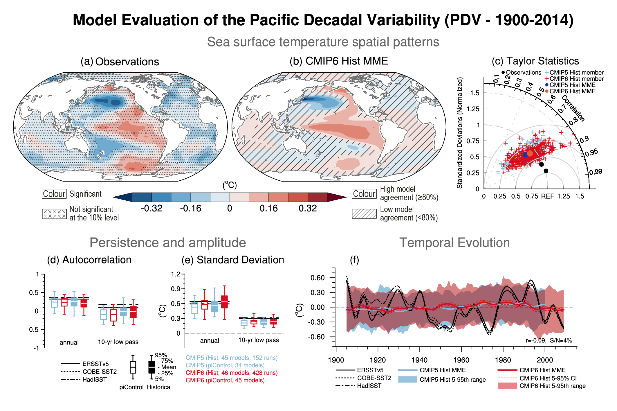 Figure 3.39 | Model evaluation of the Pacific Decadal Variability (PDV). (a, b) Sea surface temperature (SST) anomalies (°C) regressed onto the Tripole Index (TPI; Henley et al., 2015) for 1900–2014 in (a) ERSST version 5 and (b) CMIP6 multi-model ensemble (MME) mean composite obtained by weighting ensemble members by the inverse of the model ensemble size. A 10-year low-pass filter was applied beforehand. Cross marks in (a) represent regions where the anomalies are not significant at the 10% level based on a t-test. Diagonal lines in (b) indicate regions where less than 80% of the runs agree in sign. (c) A Taylor diagram summarizing the representation of the PDV pattern in CMIP5 (each ensemble member is shown as a cross in light blue, and the weighted multi-model mean as a dot in dark blue), CMIP6 (each ensemble member is shown as a cross in red, and the weighted multi-model mean as a dot in orange) and observations over 40°S–60°N and 110°E–70°W. The reference pattern is taken from ERSST version 5 and black dots indicate other observational products: Hadley Centre Sea Ice and Sea Surface Temperature data set version 1 (HadISST version 1) and Centennial in situ Observation-Based Estimates of Sea Surface Temperature version 2 (COBE-SST2). (d) Autocorrelation of unfiltered annual TPI at lag one year and 10-year low-pass filtered TPI at lag 10 years for observations over 1900–2014 (horizontal lines), 115-year chunks of pre-industrial control simulations (open boxes) and individual historical simulations over 1900–2014 (filled boxes) from CMIP5 (blue) and CMIP6 (red). (e) As in (d), but showing standard deviation of the unfiltered and filtered TPI (°C). Boxes and whiskers show weighted multi-model means, interquartile ranges and 5th and 95th percentiles. (f) Time series of the 10-year low-pass filtered TPI (°C) in ERSST version 5, HadISST version 1 and COBE-SST2 observational estimates (black) and CMIP5 and CMIP6 historical simulations. The thick red and light blue lines are the weighted multi-model mean for the historical simulations in CMIP5 and CMIP6, respectively, and the envelopes represent the 5th–95th percentile ranges across ensemble members. The 5–95% confidence interval for the CMIP6 multi-model mean is given in thin dashed lines. Further details on data sources and processing are available in the chapter data table (Table 3.SM.1).
 In CMIP5 last millennium simulations, there is no consistency in temporal variations of PDV across the ensemble (Fleming and Anchukaitis, 2016). This supports the notion that PDV is internal in nature. However, this issue remains difficult to assess because paleoclimate reconstructions of PDV have too poor a level of agreement for a rigorous model evaluation in past millennia (Henley, 2017).
To conclude, there is high confidence that internal variability has been the main driver of the PDV since pre-industrial times, despite some modelling evidence for potential external influence. This assessment is supported by studies based on large ensemble simulations that found the dominance of internally-driven PDV, and the CMIP6-based assessment (Figure 3.39). As such, PDV is an important driver of decadal internal climate variability which limits detection of human influence on various aspects of decadal climate change on global to regional scales (high confidence). Model evaluation of PDV is hampered by short observational records, spatial incompleteness of observations before the satellite observation era, and poor agreement among paleoclimate reconstructions. Despite the limitations of these model-observation comparisons, CMIP5 models, on average, simulate broadly realistic spatial structures of the PDV, but with a clear bias in the South Pacific (medium confidence). CMIP5 models also very likely underestimate PDV magnitude. CMIP6 models tend to show better overall performance in spatial structure and magnitude of PDV, but there is low confidence in this assessment due to the lack of literature.
3.7.7 Atlantic Multi-decadal Variability
Atlantic Multi-decadal Variability (AMV) refers to a climate mode representing basin-wide multi-decadal fluctuations in surface temperatures in the North Atlantic (Figure 3.40a,f), with teleconnections particularly pronounced over the adjacent continents and the Arctic. The AMV phenomenon is usually assessed through SST anomalies averaged over the entire North Atlantic basin, hereafter the AMV index, but it is associated with many physical processes including three-dimensional ocean circulation, such as AMOC fluctuations (Section 3.5.4.1), gyre adjustments, and salt and heat transport in the entire North Atlantic and subarctic Atlantic basins. The AMV, together with the PDV, has been shown to have modulated GSAT on multi-decadal time scales since pre-industrial times (Cross-Chapter Box 3.1; T. Wu et al., 2019a; Li et al., 2020). A detailed description of the AMV as well as its associated teleconnection over land is given in Annex IV.2.7.
 Figure 3.40 | Model evaluation of Atlantic Multi-decadal Variability (AMV). (a, b) Sea surface temperature (SST) anomalies (°C) regressed onto the AMV index defined as the 10-year low-pass filtered North Atlantic (0°–60°N, 80°W–0°E) area-weighted SST* anomalies over 1900–2014 in (a) ERSST version 5 and (b) the CMIP6 multi-model ensemble (MME) mean composite obtained by weighting ensemble members by the inverse of each model’s ensemble size. The asterisk denotes that the global mean SST anomaly has been removed at each time step of the computation. Cross marks in (a) represent regions where the anomalies are not significant at the 10% level based on a t-test. Diagonal lines in (b) show regions where less than 80% of the runs agree in sign. (c) A Taylor diagram summarizing the representation of the AMV pattern in CMIP5 (each ensemble member is shown as a cross in light blue, and the weighted multi-model mean is shown as a dot in dark blue), CMIP6 (each ensemble member is shown as a cross in red, and the weighted multi-model mean is shown as a dot in orange) and observations over [0°–60°N, 80°W–0°E]. The reference pattern is taken from ERSST version 5 and black dots indicate other observational products (HadISST version 1 and COBE-SST2). (d) Autocorrelation of unfiltered annual AMV index at lag one year and 10-year low-pass filtered AMV index at lag 10 years for observations over 1900–2014 (horizontal lines), 115-year chunks of pre-industrial control simulations (open boxes) and individual historical simulations over 1900–2014 (filled boxes) from CMIP5 (blue) and CMIP6 (red). (e) As in (d), but showing standard deviation of the unfiltered and filtered AMV indices (°C). Boxes and whiskers show the weighted multi-model means, interquartile ranges and 5th and 95th percentiles. (f) Time series of the AMV index (°C) in ERSST version 5, HadISST version 1 and COBE-SST2 observational estimates (black) and CMIP5 and CMIP6 historical simulations. The thick red and light blue lines are the weighted multi-model mean for the historical simulations in CMIP5 and CMIP6, respectively, and the envelopes represent the 5th–95th percentile ranges obtained from all ensemble members. The 5–95% confidence interval for the CMIP6 multi-model mean is shown by the thin dashed line. Further details on data sources and processing are available in the chapter data table (Table 3.SM.1).
 AR5 assessed, based on climate models, that the AMV was primarily internally-driven alongside some contribution from external forcings (mainly anthropogenic aerosols) over the late 20th century (Bindoff et al., 2013; Flato et al., 2013). But AR5 also concluded that models show medium performance in reproducing the observed AMV, with difficulties in simulating the time scale, the spatial structure and the coherency between all the physical processes involved (Flato et al., 2013).
Climate models analysed since AR5 continue to simulate AMV-like variability as part of their internal variability. This statement is mostly based on CMIP5 pre-industrial control and historical simulations (Wouters et al., 2012; Schmith et al., 2014; Menary et al., 2015; Ruprich-Robert and Cassou, 2015; Brown et al., 2016b; Chen et al., 2016; Kim et al., 2018a) and is also true for the CMIP6 models (Menary et al., 2018; Voldoire et al., 2019b). Models also continue to support links to a wide array of remote climate influences through atmospheric teleconnections (Martin et al., 2014; Ruprich-Robert et al., 2017, 2018; Monerie et al., 2019; Qasmi et al., 2020; Ruggieri et al., 2021). Even if debate remains (Clement et al., 2015; Cane et al., 2017; Mann et al., 2020), there is now stronger evidence for a crucial role of oceanic dynamics in internal AMV that is primarily linked to the AMOC and its interplay with the NAO (Zhang et al., 2013a; Müller et al., 2015; O’Reilly et al., 2016b, 2019a; Delworth et al., 2017; Zhang, 2017; Sun et al., 2019; Kim et al., 2020). However, considerable diversity in the spatio-temporal properties of the simulated AMV is found in both pre-industrial control and historical CMIP5 experiments (Zhang and Wang, 2013; Wills et al., 2019). Such model diversity is presumably associated with the wide range of coupled processes associated with AMV (Baker et al., 2017; Woollings et al., 2018a) including large-scale atmospheric teleconnections and regional feedbacks relating to tropical clouds, Arctic sea ice in the subarctic basins and Saharan dust, whose relative importance and interactions across time scales are specific to each model (Martin et al., 2014; Brown et al., 2016b).
Additional studies since AR5 corroborate that CMIP5-era models tend to underestimate many aspects of observed AMV and its SST fingerprint. On average, the duration of modelled AMV episodes is too short, the magnitude of AMV is too weak and its basin-wide SST spatial structure is limited by the poor representation of the link between the tropical North Atlantic and the subpolar North Atlantic/Nordic seas (Martin et al., 2014; Qasmi et al., 2017). Such mismatches between observed and simulated AMV (Figure 3.40c–e) have been associated with intrinsic model biases in both mean state (Menary et al., 2015; Drews and Greatbatch, 2016) and variability in the ocean and overlying atmosphere. For instance, compared to available observational data CMIP5 models underestimate the ratio of decadal to interannual variability of the main drivers of AMV, namely the AMOC, NAO and related North Atlantic jet variations (Section 3.7.1; Bracegirdle et al., 2018; Kim et al., 2018b; Simpson et al., 2018; Yan et al., 2018), which has strong implications for the simulated temporal statistics of AMV, AMV-induced teleconnections (Ault et al., 2012; Menary et al., 2015) and AMV predictability.
The increase of AMV variance in CMIP6 models (stronger magnitude and longer duration) seems to be explained by the enhanced variability in the subpolar North Atlantic SST (Figure 3.40b,c), which is particularly pronounced in some models, associated with greater variability in the AMOC (Section 3.5.4.1; Voldoire et al., 2019a; Boucher et al., 2020) and greater GMST multi-decadal variability (Section 3.3.1 and Figure 3.40c–f; Voldoire et al., 2019b; Parsons et al., 2020). The decadal variance in SST in the subpolar North Atlantic seems now to be slightly overestimated in CMIP6 compared to observational estimates, while the AMV-related tropical SST anomalies remain weaker in line with CMIP5 (Figure 3.40b). The mechanisms producing the tropical-extratropical relationship at decadal time scales remain poorly understood despite stronger evidence since AR5 for the importance of the subpolar gyre SST anomalies in generating tropical changes through atmospheric teleconnection (Caron et al., 2015; Ruprich-Robert et al., 2017; Kim et al., 2020). Significant discrepancies remain in the simulated AMV spatial pattern when historical simulations are compared to multivariate observations (Yan et al., 2018; Robson et al., 2020).
There is additional evidence since AR5 that external forcing has been playing an important role in shaping the timing and intensity of the observed AMV since pre-industrial times (Bellomo et al., 2018; Andrews et al., 2020). The time synchronisation between observed and multi-model mean AMV SST indices is significant in both CMIP5 and CMIP6 historical simulations, while the explained variance of the forced response in CMIP6 appears stronger (Figure 3.40d–f). The competition between greenhouse gas warming and anthropogenic sulphate aerosol cooling has been proposed to be particularly important over the latter half of the 20th century (Booth et al., 2012; Steinman et al., 2015; Murphy et al., 2017; Undorf et al., 2018a; Haustein et al., 2019). The latest observed AMV shift from the cold to the warm phase in the mid-1990s at the surface ocean is well captured in the CMIP6 forced component and may be associated with the lagged response to increased AMOC due to strong anthropogenic aerosol forcing over 1955–1985 (Menary et al., 2020) in combination with the rapid response through surface flux processes to declining aerosol forcing and increasing greenhouse gas influence since then. However, natural forcings may have also played a significant role. For instance, volcanic forcing has been shown to contribute in part to the cold phases of the AMV-related SST anomalies observed in the 20th century (Terray, 2012; Bellucci et al., 2017; Swingedouw et al., 2017; Birkel et al., 2018). Over the last millennium, natural forcings including major volcanic eruptions and fluctuations in solar activity are thought to have driven a larger fraction of the multi-decadal variations in the AMV than in the industrial era, with some interplay with internal processes (Otterå et al., 2010; Knudsen et al., 2014; Moffa-Sánchez et al., 2014; J. Wang et al., 2017; Malik et al., 2018; Mann et al., 2021), but other studies question the role of natural forcings over this period (Zanchettin et al., 2014; Lapointe et al., 2020).
Model evaluation of the AMV phenomenon remains difficult because of short observational records (especially of detailed process-based observations), the lack of stationarity in the variance, spatial patterns and frequency of the AMV assessed from modelled SST (Qasmi et al., 2017), difficulties in estimating the forced signals in both historical simulations and observations (Tandon and Kushner, 2015), and because of probable interplay between internally and externally-driven processes (Watanabe and Tatebe, 2019). Furthermore, models simulate a large range of historical anthropogenic aerosol forcing (Smith et al., 2020) and questions often referred to as signal-to-noise paradox have been raised concerning the models’ ability to correctly simulate the magnitude of the response of AMV-related atmospheric circulation phenomena, such as the NAO (Section 3.7.1), to both internally and externally generated changes (Scaife and Smith, 2018). Related methodological and epistemological uncertainties also call into question the relevance of the traditional basin-average SST index to assessing the AMV phenomenon (Zanchettin et al., 2014; Frajka-Williams et al., 2017; Haustein et al., 2019; Wills et al., 2019).
To summarize, results from CMIP5 and CMIP6 models together with new statistical techniques to evaluate the forced component of modelled and observed AMV, provide robust evidence that external forcings have modulated AMV over the historical period. In particular, anthropogenic and volcanic aerosols are thought to have played a role in the timing and intensity of the negative (cold) phase of AMV recorded from the mid-1960s to mid-1990s and subsequent warming (medium confidence). However, there is low confidence in the estimated magnitude of the human influence. The limited level of confidence is primarily explained by difficulties in accurately evaluating model performance in simulating AMV. The evaluation is severely hampered by short instrumental records but also, equally importantly, by the lack of detailed and coherent long-term process-based observations (for example of the AMOC, aerosol optical depth, surface fluxes and cloud changes), which limit our process understanding. In addition, studies often rely solely on simplistic SST indices that may be hard to interpret (Zhang et al., 2016) and may mask critical physical inconsistencies in simulations of the AMV compared to observations (Zhang, 2017).
3.8 Synthesis Across Earth System Components
3.8.1 Multivariate Attribution of Climate Change
The AR5 concluded that human influence on the climate system is clear (IPCC, 2013), based on observed increasing greenhouse gas concentrations in the atmosphere, positive radiative forcing, observed warming, and physical understanding of the climate system. The AR5 also assessed that it was virtually certain that internal variability alone could not account for observed warming since 1951 (Bindoff et al., 2013). Evidence has grown since AR5 that observed changes since the 1950s in many parts of the climate system are attributable to anthropogenic influence. So far, this chapter has focused on examining individual aspects of the climate system in separate sections. The results presented in Sections 3.3 to 3.7 substantially strengthen our assessment of the role of human influence on climate since pre-industrial times. In this section we look across the whole climate system to assess to what extent a physically consistent picture of human induced change emerges across the climate system (Figure 3.41).
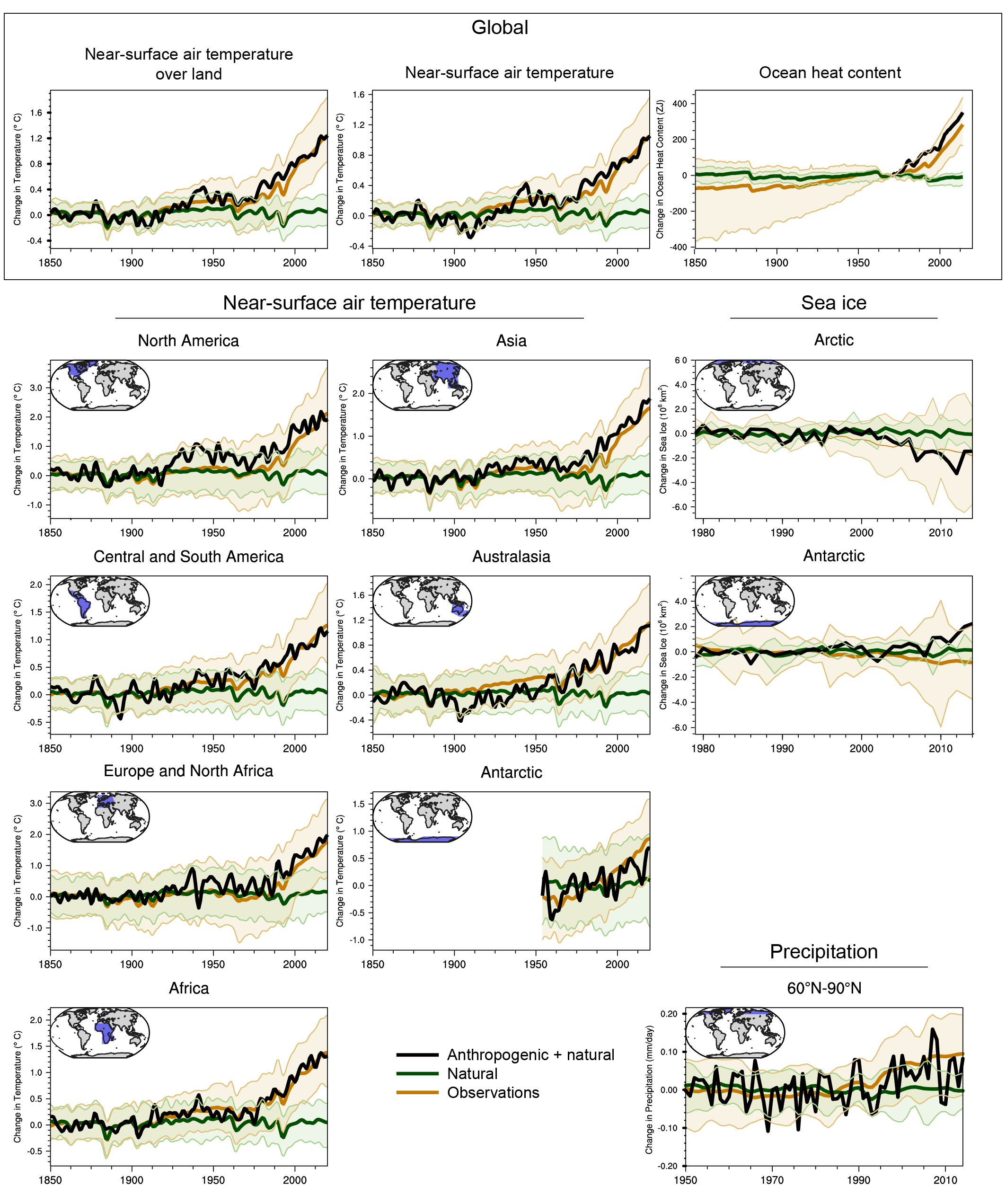 Figure 3.41 | Summary figure showing simulated and observed changes in key large-scale indicators of climate change across the climate system, for continental, ocean basin and larger scales. Black lines show observations, brown lines and shading show the multi-model mean and 5th–95th percentile ranges for CMIP6 historical simulations including anthropogenic and natural forcing, and blue lines and shading show corresponding ensemble means and 5th–95th percentile ranges for CMIP6 natural-only simulations. Temperature time series are as in Figure 3.9, but with smoothing using a low pass filter. Precipitation time series are as in Figure 3.15 and ocean heat content as in Figure 3.26. Further details on data sources and processing are available in the chapter data table (Table 3.SM.1).
 The observed global surface air temperature warming of 0.9°C to 1.2°C in 2010–2019 is much greater than can be explained by internal variability (likely –0.2°C to +0.2°C) or natural forcings (likely –0.1°C to +0.1°C) alone, but consistent with the assessed anthropogenic warming (likely 0.8°C to 1.3°C; Section 3.3.1.1). It is very likely that human influence is the main driver of warming over land Section 3.3.1.1). Moreover, the atmosphere as a whole has warmed (Table 7.1), and it is very likely that human-induced greenhouse gas increases were the main driver of tropospheric warming since 1979 (Section 3.3.1.2). It is virtually certain that greenhouse gas forcing was the main driver of the observed changes in hot and cold extremes over land at the global scale (Cross-Chapter Box 3.2).
As might be expected from a warming atmosphere, moisture in the troposphere has increased and precipitation patterns have changed. Human influence has likely contributed to the observed changes in humidity and precipitation (Section 3.3.2). It is likely that human influence, in particular due to greenhouse gas forcing, is the main driver of the observed intensification of heavy precipitation in global land regions during recent decades (Cross-Chapter Box 3.2). The pattern of ocean salinity changes indicate that fresh regions are becoming fresher and that salty regions are becoming saltier as a result of changes in ocean-atmosphere fluxes through evaporation and precipitation (high confidence) making it extremely likely that human influence has contributed to observed near-surface and subsurface salinity changes since the mid-20th century (Section 3.5.2.2). Taken together, this evidence indicates a human influence on the water cycle.
It is very likely that human influence was the main driver of Arctic sea ice loss since the late 1970s (Section 3.4.1.1), and very likely that it contributed to the observed reductions in Northern Hemisphere springtime snow cover since 1950 (Section 3.4.2). Human influence was very likely the main driver of the recent global, near-universal retreat of glaciers and it is very likely that it contributed to the observed surface melting of the Greenland Ice Sheet over the past two decades (Section 3.4.3.2.1). It is extremely likely that human influence was the main driver of the ocean heat content increase observed since the 1970s (Section 3.5.1.3), and very likely that human influence was the main driver of the observed GMSL rise since at least 1970 (Section 3.5.3.2).
Combining the evidence from across the climate system (Sections 3.3–3.7) increases the level of confidence in the attribution of observed climate change to human influence and reduces the uncertainties associated with assessments based on a single variable. From this combined evidence, it is unequivocal that human influence has warmed the atmosphere, ocean and land components of the global climate system, taken together.
3.8.2 Multivariate Model Evaluation
Similar to the assessment of multivariate attribution of climate change in the previous section, this section covers the performance of the models across different variables (Sections 3.8.2.1) and different classes of models (Section 3.8.2.2). Here the focus is on a system-wide assessment using integrative measures of model performance that characterize model performance using multiple diagnostic fields derived from multi-model ensembles.
3.8.2.1 Integrative Measures of Model Performance
The purpose of this section is to use multivariate analyses to address how well models simulate present-day and historical climate. For every diagnostic field considered, model performance is compared to one or multiple observational references, and the quality of the simulation is expressed as a single number, for example a correlation coefficient or a root mean square difference versus the observational reference. By simultaneously assessing different performance indices, model improvements can be quantified, similarities in behaviour between different models become apparent, and dependencies between various indices become evident (Gleckler et al., 2008; Waugh and Eyring, 2008).
AR5 found significant differences between models in the simulation of mean climate in the CMIP5 ensemble when measured against meteorological reanalyses and observations (Flato et al., 2013), see also Stouffer et al. (2017). The AR5 determined that for the diagnostic fields analysed, the models usually compared similarly against two different reference datasets, suggesting that model errors were generally larger than observational uncertainties or other differences between the observational references. In agreement with previous assessments, the CMIP5 multi-model mean generally performed better than individual models (Annan and Hargreaves, 2011; Rougier, 2016). The AR5 considered 13 atmospheric fields in its assessment for the instrumental period but did not assess multi-variate model performance in other climate domains (e.g., ocean, land, and sea ice). The AR5 found only modest improvement regarding the simulation of climate for two periods of the Earth’s history (the Last Glacial Maximum and the mid-Holocene) between CMIP5 and previous paleoclimate simulations. Similarly, for the modern period only modest, incremental progress was found between CMIP3 and CMIP5 regarding the simulation of precipitation and radiation. The representation of clouds also showed improvement, but remained a key challenge in climate modelling (Flato et al., 2013).
The type of multi-variate analysis of models presented in AR5 remains critical to building confidence for example in projections of climate change. It is expanded here to the previous-generation CMIP3 and present-generation CMIP6 models and also to more variables and more climate domains, covering land and ocean as well as sea ice. The multi-variate evaluation of these three generations of models is performed relative to the observational datasets listed in Annex I, Table AI.1. For many of these datasets, a rigorous characterization of the observational uncertainty is not available, see discussion in Chapter 2. Here, as much as possible, multiple independent observational datasets are used. Disagreements among them would cause differences in model scoring, indicating that observational uncertainties may be substantial compared to model errors. Conversely, similar scores against different observational datasets would suggest model biases may be larger than the observational uncertainty.
An analysis of a basket of 16 atmospheric variables (Figure 3.42a) assessed across CMIP3, CMIP5, and CMIP6 models but excluding high-resolution models participating in HighResMIP, reveals the progress made between these three generations of models (Bock et al., 2020). Progress is evidenced by the increasing prevalence of blue colours (indicating a performance better than the median) for the more recent model versions. Additionally, a few CMIP6 models outperform the best-performing CMIP5 models. Progress is evident across all 16 variables. As noted in AR5, the models typically score similarly against both observational reference datasets, indicating that indeed uncertainties in these reference datasets are smaller than model biases. Several models and model families perform better compared to observational references than the median, across a majority of the climate variables assessed, and conversely some other models or model families compare more poorly against these reference datasets. Such a good correspondence across a range of diagnostic fields probing different aspects of climate enhances confidence that the improved performances reflect progress in the physical realism of these simulations. An alternative explanation, that progress is due to a cancellation of errors achieved by model tuning, appears improbable given the large number of diagnostic fields involved here. However, several instances of poor model performance (red colours in Figure 3.42) still exist in the CMIP6 ensemble. Family relationships (i.e. various degrees of shared formulations; Knutti et al., 2013) between the models are apparent, for example, the GISS, GFDL, CESM, CNRM, and HadGEM/UKESM1/ACCESS families score similarly across all atmospheric variables, both for the CMIP5 and CMIP6 generations. In the cases of CESM2/CESM2(WACCM), CNRM-CM6-1/CNRM-ESM2-1, NorCPM1/NorESM2-LM, and HadGEM3-GC31-LL/UKESM1-0-LL, the high-complexity model scores as well or better than its lower-complexity counterpart, indicating that increasing complexity by adding Earth system features, which by removing constraints could be expected to degrade a model’s performance, does not necessarily do so. Several high climate-sensitivity models (Section 7.5; Meehl et al., 2020), in particular CanESM5, CESM2, CESM2-WACCM, HadGEM3-GC31-LL, and UKESM1-0-LL, score well against the benchmarks. In accordance with AR5 and earlier assessments, the multi-model mean, with some notable exceptions, is better than any individual model (Annan and Hargreaves, 2011; Rougier, 2016).
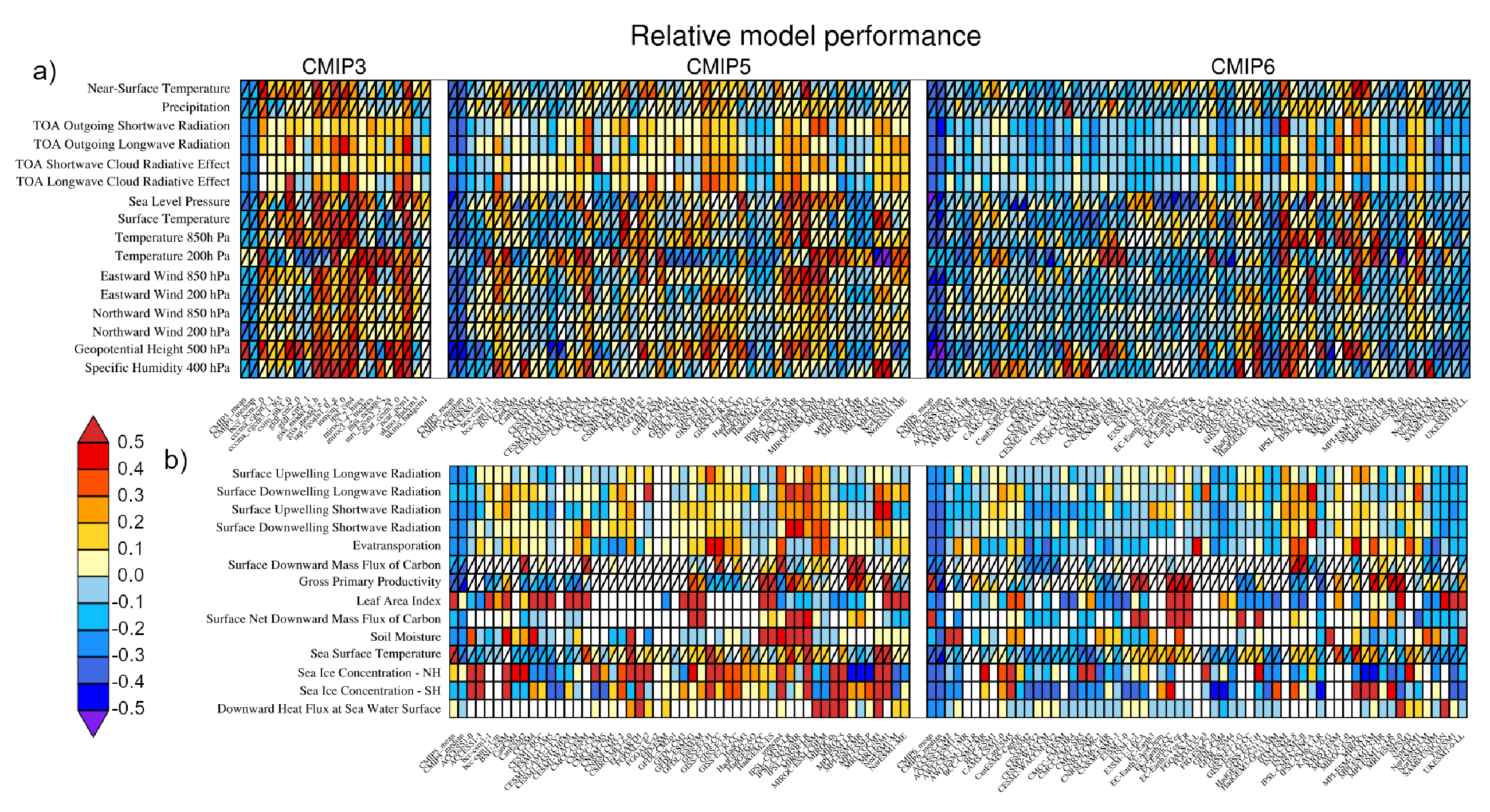
Regarding model performance for the ocean and the cryosphere (Figure 3.42b), it is apparent that for many models there are substantial differences between the scores for Arctic and Antarctic sea ice concentration. This might suggest that it is not sea ice physics directly that is driving such differences in performance but rather other influences, such as differences in geography, the role of large ice shelves (which are absent in the Arctic), or large-scale ocean dynamics. As for atmospheric variables, progress is evident also across all four ocean and ten land variables from CMIP5 to CMIP6.
In summary, CMIP6 models perform generally better for a basket of variables covering mean historical climate across the atmosphere, ocean, and land domains than previous-generation and older models (high confidence). Earth System models characterized by additional biogeochemical feedbacks often perform at least as well as related more constrained, lower-complexity models lacking these feedbacks (medium confidence). In many cases, the models score similarly against both observational references, indicating that model errors are usually larger than observational uncertainties (high confidence). Moreover, synthesizing across Sections 3.3–3.7, we assess that the CMIP6 multi-model mean captures most aspects of observed climate change well (high confidence).
Using centred pattern correlations (quantifying pattern similarity on a scale of –1 to 1, with 1 expressing perfect similarity and 0 no relationship) for selected fields, AR5 documented improvements between CMIP3 and CMIP5 in surface air temperature, outgoing longwave radiation, and precipitation (Figure 9.6 of Flato et al., 2013). Little further progress between CMIP3 and CMIP5 was found for fields that were already quite well simulated in CMIP3 (such as surface air temperature and outgoing longwave radiation). For precipitation, the spread reduced because the worst-performing models improved. The shortwave cloud radiative effect remained relatively poorly simulated with significant inter-model spread (e.g., Calisto et al., 2014). This comparison of centred pattern correlations is designed to help determine the quality of simulation of different diagnostics relative to each other, and also to examine progress between generations of models. Figure 3.43 shows the centred pattern correlations for 16 variables for CMIP3, CMIP5 and CMIP6 models. In the ensemble averages, CMIP6 performs better than CMIP5 and CMIP3 for near-surface temperature, precipitation, mean sea-level pressure, and many other variables. For the variables shown, the uncertainties in observational datasets, in particular for precipitation and northward wind at 850 hPa, remain substantial relative to mean model errors (see grey dots in Figure 3.43).
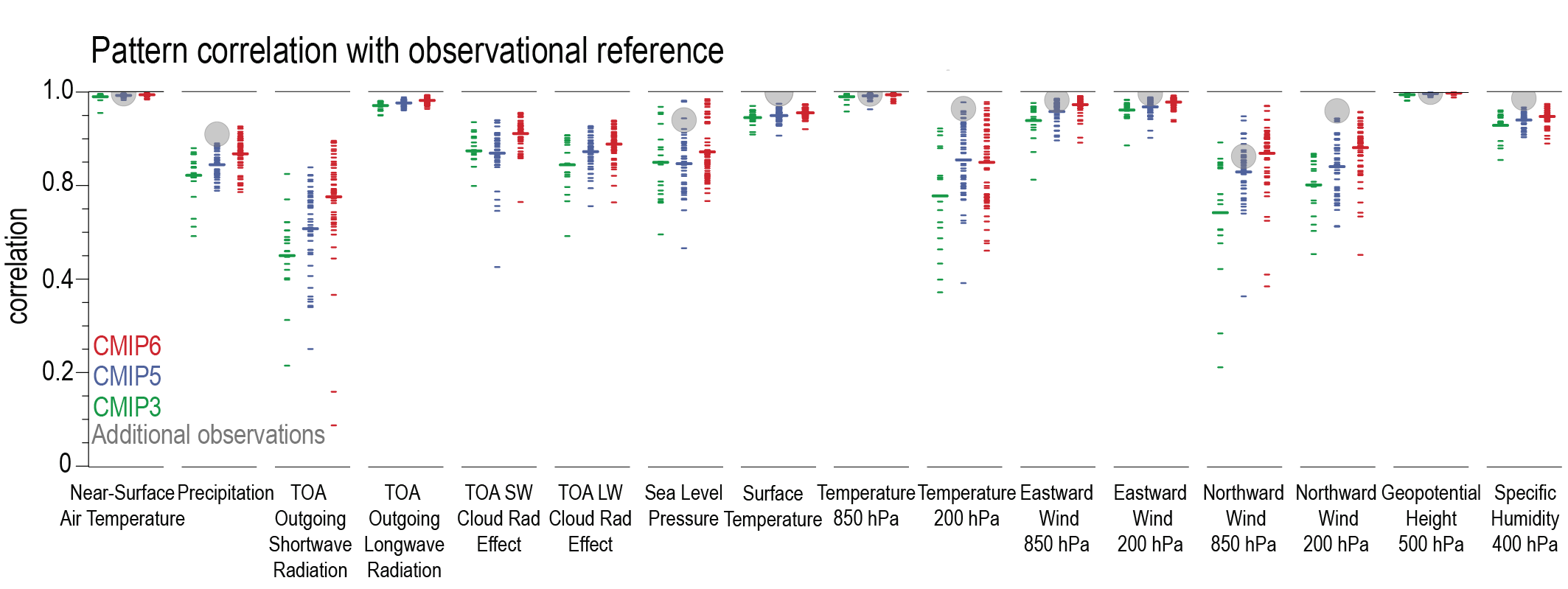 Figure 3.43 | Centred pattern correlations between models and observations for the annual mean climatology over the period 1980–1999. Results are shown for individual CMIP3 (green), CMIP5 (blue) and CMIP6 (red) models (one ensemble member from each model is used) as short lines, along with the corresponding multi-model ensemble averages (long lines). Correlations are shown between the models and the primary reference observational data set (from left to right: ERA5, GPCP-SG, CERES-EBAF, CERES-EBAF, CERES-EBAF, CERES-EBAF, JRA-55, ESACCI-SST, ERA5, ERA5, ERA5, ERA5, ERA5, ERA5, AIRS, ERA5). In addition, the correlation between the primary reference and additional observational datasets (from left to right: NCEP, GHCN, -, -, -, -, ERA5, HadISST, NCEP, NCEP, NCEP, NCEP, NCEP, NCEP, ERA5, NCEP) are shown (solid grey circles) if available. To ensure a fair comparison across a range of model resolutions, the pattern correlations are computed after regridding all datasets to a resolution of 4° in longitude and 5° in latitude. Figure is updated and expanded from Bock et al. (2020), their Figure 7 CC BY 4.0https://creativecommons.org/licenses/by/4.0/. Further details on data sources and processing are available in the chapter data table (Table 3.SM.1).
 In addition to the multivariate assessments of simulations of the recent historical period, simulations of selected periods of the Earth’s more distant history can be used to benchmark climate models by exposing them to climate forcings that are radically different from the present and recent past (Harrison et al., 2015, 2016; Kageyama et al., 2018; Tierney et al., 2020a). These time periods provide an out-of-sample test of models because they are not in general used in the process of model development. They encompass a range of climate drivers, such as volcanic and solar forcing for the Last Millennium, orbital forcing for the mid-Holocene and Last Interglacial, and changes in greenhouse gases and ice sheets for the LGM, mid-Pliocene Warm Period, and early Eocene (Sections 2.2 and 2.3). These drivers led to climate changes, including in surface temperature (Section 2.3.1.1) and the hydrological cycle (Section 2.3.1.3.1), which are described by paleoclimate proxies that have been synthesized to support evaluations of models on a global and regional scale. However, the more sparse, indirect, and regionally incomplete climate information available from paleo-archives motivates a different form of the multivariate analysis of simulations covering these periods versus the equivalent for the historical period, as described below.
AR5 found that reconstructions and simulations of past climates both show similar responses in terms of large-scale patterns of climate change, such as polar amplification (Flato et al., 2013; Masson-Delmotte et al., 2013). However, for several regional signals (e.g., the north–south temperature gradient in Europe and regional precipitation changes), the magnitude of change seen in the proxies relative to the pre-industrial period was underestimated by the models. When benchmarking CMIP5/PMIP3 models against reconstructions of the mid-Holocene and LGM, AR5 found only a slight improvement compared with earlier model versions across a range of variables. For the Last Interglacial, it was noted that the magnitude of observed annual mean warming in the Northern Hemisphere was only reached in summer in the models. For the mid-Pliocene Warm Period, it was noted that both proxies and models showed a polar amplification of temperature compared with the pre-industrial period, but a formal model evaluation was not carried out.
Since AR5, new simulation protocols have been developed in PMIP4 (Kageyama et al., 2018), which are further described for the mid-Holocene and the Last Interglacial by Otto-Bliesner et al. (2017), for the LGM by Kageyama et al. (2017), for the Pliocene by Haywood et al. (2016), and for the early Eocene by Lunt et al. (2017). These have resulted in new model simulations for these time periods (Brierley et al., 2020; Haywood et al., 2020; Kageyama et al., 2021a; Lunt et al., 2021; Otto-Bliesner et al., 2021). These time periods span an assessed temperature range of 20°C (Section 2.3.1.1), and for all periods the PMIP4 multi-model ensemble mean is within 0.5°C of the assessed range of GSAT (Figure 3.44a). Those time periods for which the multi-model ensemble mean is outside the assessed range of GSAT, the mid-Holocene and the Last Interglacial, are primarily forced by orbital changes not greenhouse gas forcing, and as a result the forcing as well as the assessed and modelled response are relatively close to zero in the global annual mean. During these periods, climate change therefore is a consequence of more poorly understood Earth System feedbacks acting on the response to orbital differences versus the present-day, affecting the seasonality of insolation.
 Figure 3.44 | Multivariate synopsis of paleoclimate model results compared to observational references. Data-model comparisons for (a) GSAT anomalies for five PMIP4 periods and for regional features for the (b) mid-Holocene and (c) LGM periods, for PMIP3 and PMIP4 models. The results from CMIP6 models are shown as coloured dots. In (a) the light orange shading shows the very likely assessed ranges presented in Section 2.3.1.1. In (b) and (c), the regions and variables are defined as follows: North America (20°N–50°N, 140°W–60°W), Western Europe (35°N–70°N, 10°W–30°E) and West Africa (0°–30°N, 10°W–30°E); mean temperature of the coldest month (MTCO; °C), mean temperature of the warmest month (MTWA; °C), mean annual precipitation (MAP; mm yr–1). In (b) and (c) the ranges shown for the reconstructions (Bartlein et al. (2011) for mid-Holocene and Cleator et al. (2020) for LGM) are based on the standard error given at each site: the average and associated standard deviation over each area is obtained by computing 1000 times the average of randomly drawn values from the Gaussian distributions defined at each site by the reconstruction mean and standard error; the light orange colour shows the ±1 standard deviation of these 1000 estimates. The dots on (b) and (c) show the average of the model output for grid points for which there are reconstructions. The ranges for the model results are based on an ensemble of 1000 averages over 50 years randomly picked in the model output time series for each region and each variable: the mean ± one standard deviation is plotted for each model. Figure is adapted from Brierley et al. (2020), their Figure S3 for the mid-Holocene; and from Kageyama et al. (2021b), their Figure 12 for the LGM. Further details on data sources and processing are available in the chapter data table (Table 3.SM.1).
 Polar amplification in the LGM, mid-Pliocene Warm Period, and Early Eocene Climatic Optimum (EECO) simulations is assessed in Section 7.4.4.1.2. Here we focus on the mid-Holocene and the LGM, which have been a part of AMIP or CMIP through several assessment cycles, and as such serve as a reference to quantify regional model-data agreement from one IPCC assessment to another. We compare the results from 15 CMIP6 models using the PMIP4 protocol (CMIP6-PMIP4), with non-CMIP6 models using the PMIP4 protocol, with PMIP3 models, and with regional temperature and precipitation changes from proxies for the mid-Holocene (Figure 3.44b). For six out of seven variables shown, the CMIP6 multi-model mean captures the correct sign of the change. For five out of seven of them the CMIP6 ensemble mean is within the reconstructed range. For the other two variables (changes in the mean temperature of the warmest month over North America and in the mean annual precipitation over West Africa) nearly all PMIP4 and PMIP3 models are outside the reconstructed range. CMIP6 models show regional patterns of temperature changes similar to the PMIP3 ensemble (Brierley et al., 2020), but the slight mid-Holocene cooling in PMIP4 compared with PMIP3, probably associated with lower imposed mid-Holocene carbon dioxide concentrations (Otto-Bliesner et al., 2017), improves the regional model performance for summer and winter temperatures (Figure 3.44b). However, this cooling also results in a CMIP6 mid-Holocene GSAT that lies further from the assessed range (Figure 3.44a). All models show an expansion of the monsoon areas from the pre-industrial to the mid-Holocene simulations in the Northern Hemisphere, but this expansion in some cases is only large enough to cancel out the bias in the pre-industrial control simulations (Section 3.3.3.2; Brierley et al., 2020). There is a slight improvement in representing the northward expansion of the West African monsoon region in PMIP4 compared with PMIP3 (Figures 3.11 and 3.44b).
Fourteen simulations of the LGM climate have been produced following the CMIP6-PMIP4 protocol using 11 models, five of which are from the latest CMIP6 generation. The multi-model-mean global cooling simulated by these models is close to that simulated by the CMIP5-PMIP3 ensemble, but the range of results is larger. The increase in the range is largely due to the inclusion of CESM2 which simulates a much larger cooling than the other PMIP4 models (Figure 3.44a). This is consistent with its larger climate sensitivity (see also (Section 3.3.1.1; Zhu et al., 2021). The other models on average also simulate slightly larger cooling in PMIP4 versus PMIP3 (Kageyama et al., 2017, 2021a). The PMIP4 multi-model mean is within the range of reconstructed regional averages for four out of seven regional variables; this is unchanged from PMIP3 but for different variables (Figure 3.44c). For all fields, the results of many individual models are outside the reconstructed range. For two variables out of seven (changes in the mean temperature of the warmest month and mean annual precipitation over Western Europe) no model is within the range of the reconstructions. This analysis is strengthened compared with the equivalent analysis in AR5 because it is based on larger and improved reconstructions (Cleator et al., 2020). Most CMIP6-PMIP4 models simulate a slightly stronger AMOC in the LGM, but no strong deepening of the AMOC (Kageyama et al., 2021a), while most other PMIP4 models simulate a strengthening and strong deepening of the AMOC, as was the case for the PMIP3 models (Muglia and Schmittner, 2015; Sherriff-Tadano et al., 2018). Only one model (CESM1.2) shows a shoaling of LGM AMOC which is consistent with reconstructions (Marzocchi and Jansen, 2017; Sherriff-Tadano et al., 2018).
17 PMIP4 models completed Last Interglacial simulations (Otto-Bliesner et al., 2021). The comparison to reconstructions is generally good, except for some discrepancies, such as for upwelling systems in the South East Atlantic or discrepancies which may result from local melting of remnant ice sheets absent in the Last Interglacial simulation protocol. All models simulate a decrease in Arctic sea ice in summer, commensurate with increased summer insolation, while some models even simulate a large or complete loss (Guarino et al., 2020; Kageyama et al., 2021b). Sea ice reconstructions for the central Arctic are, however, too uncertain to evaluate this behaviour. The Last Interglacial simulations indicate a clear relationship between simulated sea ice loss and model responses to increased greenhouse gas forcing (Kageyama et al., 2021b; Otto-Bliesner et al., 2021).
Overall, the PMIP multi-model means agree very well (within 0.5°C of the assessed range) with GSAT reconstructed from proxies across multiple time periods, spanning a range from 6°C colder than pre-industrial (Last Glacial Maximum) to 14°C warmer than pre-industrial (Early Eocene Climate Optimum) (high confidence). During the orbitally-forced mid-Holocene, the CMIP6 multi-model mean captures the sign of the regional changes in temperature and precipitation in most regions assessed, and there have been some regional improvements compared to AR5 (medium confidence). The limited number of CMIP6 simulations of the LGM hinders model evaluation of the multi-model mean, but for both LGM and mid-Holocene, models tend to underestimate the magnitude of large changes (high confidence). Some long-standing model-data discrepancies, such as a dry bias in North Africa in the mid-Holocene, have not improved in CMIP6 compared with PMIP3 (high confidence).
3.8.2.2 Process Representation in Different Classes of Models
Based on new scientific insights and newly available observations, many improvements have been made to models from CMIP5 to CMIP6, including changes in the representation of physics of the atmosphere, ocean, sea ice, and land surface. In many cases, changes in the detailed representation of cloud and aerosol processes have been implemented. The new generation of CMIP6 climate models also features increases in spatial resolution, as well as inclusion of additional Earth system processes and new components (see further details in Section 1.5.3.1 and in Tables AII.5 and AII.6). Such changes to model physics and resolution are often designed to improve the fitness-for-purpose of a model such as for projecting regional aspects of climate (Section 10.3) or to more fully represent feedbacks to make the models more fit for long-term climate projections affected for example by carbon cycle feedbacks (see also (Section 1.5.3.1).
Factors affecting model performance include resolution, the type of dynamical core (spectral, finite difference or finite volume), physics parameters and parameterisations, model structure, for example, many of the coupled HighResMIP models (Haarsma et al., 2016) use the NEMO ocean model, affecting model diversity, and the range and degree of process realism (e.g., for aerosols, atmospheric chemistry and other Earth System components). This section particularly explores the influence of model resolution and of complexity on model performance (see also Section 8.5.1).
A key advance in CMIP6 compared to CMIP5 is the presence of high-resolution models that have participated in HighResMIP. Resolution alone can significantly affect a model’s performance, with some effects propagating to the global scale. Recent studies have shown that enhancing the horizontal resolution of models is seen to significantly affect aspects of large-scale circulation as well as improve the simulation of small-scale processes and extremes when compared to CMIP3 and CMIP5 models (see also Section 11.4.3; Haarsma et al., 2016), with some models approaching 10 km resolution in the atmosphere (Kodama et al., 2021) or ocean (Caldwell et al., 2019; Gutjahr et al., 2019; Roberts et al., 2019; Chang et al., 2020; Semmler et al., 2020).
As discussed in Section 3.3, CMIP6 models reproduce observed large-scale mean surface temperature patterns as well as their CMIP5 predecessors, but biases in surface temperature in the mean of HighResMIP models are smaller than those in the mean of the corresponding standard resolution CMIP6 configurations of the same models (Section 3.3.1.1 and Figure 3.3). The extent and causes of improvements due to increased horizontal resolutions in the atmosphere and ocean domains depend on the model (Kuhlbrodt et al., 2018; Roberts et al., 2018, 2019; Sidorenko et al., 2019), although they typically involve better process representation (for example of ocean currents and atmospheric storms) which can lead to reduced biases in top of atmosphere radiation and cloudiness. Precipitation has likewise improved in CMIP6 versus CMIP5 models, but biases remain. The high resolution (<25 km) class of models participating in HighResMIP compares regionally better against observations than the standard resolution CMIP6 models (of order 100 km, Figure 3.13; Section 3.3.2), partly because of an improved representation of orographic (mountain-induced) precipitation which constitutes a major fraction of precipitation on land, but other processes also play an important role (Vannière et al., 2019). However, there are also large parts of the tropical ocean where precipitation in high-resolution models is not improved compared to standard resolution CMIP6 models (Vannière et al., 2019).
Additionally, the representation of surface and deeper ocean mean temperature is improved in models with higher horizontal resolution (Sections 3.5.1.1 and 3.5.1.2) with systematic improvements in coupled tropical Atlantic sea surface temperature and precipitation biases at higher resolutions (Roberts et al., 2019, single model; Vannière et al., 2019, multi-model), the North Atlantic cold bias (Bock et al., 2020, multi-model; Roberts et al., 2018, 2019; Caldwell et al., 2019; all single models) as well as deep-ocean biases (Small et al., 2014; Griffies et al., 2015; Caldwell et al., 2019; Gutjahr et al., 2019; Roberts et al., 2019; Chang et al., 2020, all single model studies). Atlantic ocean transports (heat and volume) are also generally improved compared to observations (Grist et al., 2018; Caldwell et al., 2019; Docquier et al., 2019; Roberts et al., 2019, 2020c; Chang et al., 2020), as well as some aspects of air-sea interactions (P. Wu et al., 2019, single model; Bellucci et al., 2021, multi-model). However, warm-biased sea surface temperatures in the Southern Ocean are worse in comparison to standard resolution CMIP6 models (Bock et al., 2020). The AR5 noted problems with the simulation of clouds in this region which were later attributed to a lack of supercooled liquid clouds (Bodas-Salcedo et al., 2016). Mesoscale ocean processes are critical to maintaining the Southern Ocean stratification and response to wind forcing (Marshall and Radko, 2003; Hallberg and Gnanadesikan, 2006), and their explicit representation requires even higher ocean resolution (Hallberg, 2013). Similarly, atmospheric convection remains unresolved even in the highest-resolution climate models participating in HighResMIP. However, there is also evidence of improvements in the frequency, distribution and interannual variability of tropical cyclones in HighResMIP (Roberts et al., 2020a, b), particularly in the Northern Hemisphere (see further discussion in Section 11.7.1.3), and their interaction with the ocean (Scoccimarro et al., 2017, single model), as well as the global moisture budget (Vannière et al., 2019). At higher resolution the track density of tropical cyclones is increased practically everywhere where tropical cyclones occur. Simulation of some climate extremes is shown to be improved at higher resolution including explosively developing extra-tropical cyclones (Vries et al., 2019; Jiaxiang et al., 2020), blocking (Section 3.3.3.3; Fabiano et al., 2020; Schiemann et al., 2020) and European extreme precipitation due to a better representation of the North Atlantic storm track (van Haren et al., 2015) and orographic boundary conditions (Schiemann et al., 2018).
In CMIP6 a number of Earth system models have increased the realism by which key biogeochemical aspects of the coupled Earth system are represented, affecting, for example, the carbon and nitrogen cycles, aerosols, and atmospheric chemistry (e.g., Cao et al., 2018; Gettelman et al., 2019; Lin et al., 2019; Mauritsen et al., 2019; Séférian et al., 2019; Sellar et al., 2019; Sidorenko et al., 2019; Swart et al., 2019; Dunne et al., 2020; Seland et al., 2020; Wu et al., 2020; Ziehn et al., 2020). In addition to increased process realism, the level of coupling between the physical climate and biogeochemical components of the Earth system has also been enhanced in some models (Mulcahy et al., 2020) as well as across different biogeochemical components (see Section 5.4 for a discussion and Table 5.4 for an overview). For example, the nitrogen cycle is now simulated in several ESMs (Zaehle et al., 2015; Davies-Barnard et al., 2020). This advance accounts for the fertilization effect nitrogen availability has on vegetation and carbon uptake, reducing uncertainties in the simulations of the carbon uptake responses to physical climate change (Section 3.6.1) and to CO2 increases (Arora et al., 2020), thus improving confidence in the simulated airborne fraction of CO2 emissions (Jones and Friedlingstein, 2020) and better constraining remaining carbon budgets (Section 5.5). Such advances also allow investigation of land-based climate change mitigation options (e.g., through changes in land management and associated terrestrial carbon uptake (Mahowald et al., 2017; Pongratz et al., 2018)) or interactions between different facets of the managed Earth system, such as interactions between mitigation efforts targeting climate warming and air quality (West et al., 2013). A number of developments also explicitly target improved simulation of the past.
Further such ESM developments include: (i) Apart from the nitrogen cycle, extending terrestrial carbon cycle models to simulate interactions between the carbon cycle and other nutrient cycles, such as phosphorus, that are known to play an important role in limiting future plant uptake of CO2 (Zaehle et al., 2015). (ii) Introducing explicit coupling between interactive atmospheric chemistry and aerosol schemes (Gettelman et al., 2019; Sellar et al., 2019), which has been shown to affect estimates of historical aerosol radiative forcing (Karset et al., 2018). Furthermore, interactive treatment of atmospheric chemistry in a full ESM supports investigation of interactions between climate and air quality mitigation efforts, such as in AerChemMIP (Collins et al., 2017), as well as interactions between stratospheric ozone recovery and global warming (Morgenstern et al., 2018). (iii) Coupling between components of Earth system models has been extended to increase their utility for studying future interactions across the full Earth system, such as between ocean biogeochemistry and cloud-aerosol processes (Mulcahy et al., 2020), and vegetation and impacts on dust production (Kok et al., 2018), production of secondary organic aerosols (SOA, Zhao et al., 2017) and Equilibrium Climate Sensitivity (ECS), whereby enhanced CO2 fertilization of land vegetation causes changes in regional surface albedo (Andrews et al., 2019). Increased coupling between physical climate and biogeochemical processes in a single ESM, along with an increased number of interactively represented processes, such as permafrost thaw, vegetation, wildfires and continental ice sheets increases our ability to investigate the potential for abrupt and interactive changes in the Earth system (see Sections 4.7.3 and 5.4.9, and Box 5.1). Table 5.4 provides an overview of recent advances in representing the carbon cycle in ESMs.
In summary, both high-resolution and high-complexity models have been evaluated as part of CMIP6. In comparison with standard resolution CMIP6 models, higher resolution probed under the HighResMIP activity (Haarsma et al., 2016) improves aspects of the simulation of climate (particularly concerning sea surface temperature) but discrepancies remain and there are some regions, such as parts of the Southern Ocean, where currently attainable resolution produces inferior performance (high confidence). Such model behaviour can indicate deficiencies in model physics that are not simply associated with resolution. In several cases, high-complexity ESMs that include additional interactions between Earth system components and thus have potential for additional associated model errors nevertheless perform as well as their low-complexity counterparts, illustrating that interactively simulating these Earth System components as part of the climate system is now well established.
Acknowledgements
Graphic developers: Bettina K. Gier (Germany), Birgit Hassler (Germany), Soufiane Karmouche (Germany, Morocco), Seungmok Paik (Republic of Korea), Min-Gyu Seong (Republic of Korea)
Data providers: Leopold Haimberger (Austria), Lawrence Mudryk (Canada), Dirk Notz (Germany)
Frequently Asked Questions
FAQ 3.1 | How Do We Know Humans Are Responsible for Climate Change?
The dominant role of humans in driving recent climate change is clear. This conclusion is based on a synthesis of information from multiple lines of evidence, including direct observations of recent changes in Earth’s climate; analyses of tree rings, ice cores, and other long-term records documenting how the climate has changed in the past; and computer simulations based on the fundamental physics that governs the climate system.
Climate is influenced by a range of factors. There are two main natural drivers of variations in climate on time scales of decades to centuries. The first is variations in the sun’s activity, which alter the amount of incoming energy from the sun. The second is large volcanic eruptions, which increase the number of small particles (aerosols) in the upper atmosphere that reflect sunlight and cool the surface–an effect that can last for several years (see also FAQ 3.2). The main human drivers of climate change are increases in the atmospheric concentrations of greenhouse gases and of aerosols from burning fossil fuels, land use and other sources. The greenhouse gases trap infrared radiation near the surface, warming the climate. Aerosols, like those produced naturally by volcanoes, on average cool the climate by increasing the reflection of sunlight. Multiple lines of evidence demonstrate that human drivers are the main cause of recent climate change.
The current rates of increase of the concentration of the major greenhouse gases (carbon dioxide, methane and nitrous oxide) are unprecedented over at least the last 800,000 years. Several lines of evidence clearly show that these increases are the results of human activities. The basic physics underlying the warming effect of greenhouse gases on the climate has been understood for more than a century, and our current understanding has been used to develop the latest generation climate models (see FAQ 3.3). Like weather forecasting models, climate models represent the state of the atmosphere on a grid and simulate its evolution over time based on physical principles. They include a representation of the ocean, sea ice and the main processes important in driving climate and climate change.
Results consistently show that such climate models can only reproduce the observed warming (black line in FAQ 3.1, Figure 1) when including the effects of human activities (grey band in FAQ 3.1, Figure 1), in particular the increasing concentrations of greenhouse gases. These climate models show a dominant warming effect of greenhouse gas increases (red band, which shows the warming effects of greenhouse gases by themselves), which has been partly offset by the cooling effect of increases in atmospheric aerosols (blue band). By contrast, simulations that include only natural processes, including internal variability related to El Niño and other similar variations, as well as variations in the activity of the sun and emissions from large volcanoes (green band in FAQ 3.1, Figure 1), are not able to reproduce the observed warming. The fact that simulations including only natural processes show much smaller temperature increases indicates that natural processes alone cannot explain the strong rate of warming observed. The observed rate can only be reproduced when human influence is added to the simulations.
Moreover, the dominant effect of human activities is apparent not only in the warming of global surface temperature, but also in the pattern of warming in the lower atmosphere and cooling in the stratosphere, warming of the ocean, melting of sea ice, and many other observed changes. An additional line of evidence for the role of humans in driving climate change comes from comparing the rate of warming observed over recent decades with that which occurred prior to human influence on climate. Evidence from tree rings and other paleoclimate records shows that the rate of increase of global surface temperature observed over the past fifty years exceeded that which occurred in any previous 50-year period over the past 2000 years (see FAQ 2.1).
Taken together, this evidence shows that humans are the dominant cause of observed global warming over recent decades.
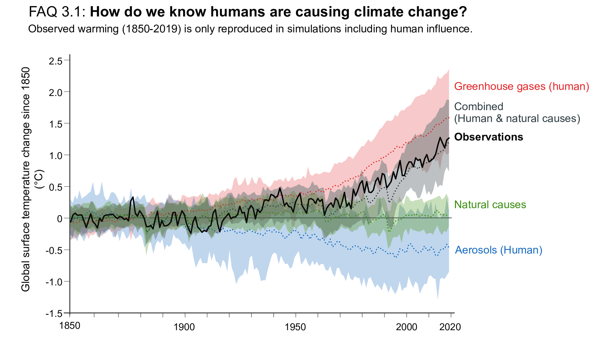
FAQ 3.1, Figure 1 | Observed warming (1850–2019) is only reproduced in simulations including human influence. Global surface temperature changes in observations, compared to climate model simulations of the response to all human and natural forcings (grey band), greenhouse gases only (red band), aerosols and other human drivers only (blue band) and natural forcings only (green band). Solid coloured lines show the multi-model mean, and coloured bands show the 5–95% range of individual simulations.
FAQ 3.2 | What is Natural Variability and How Has it Influenced Recent Climate Changes?
Natural variability refers to variations in climate that are caused by processes other than human influence. It includes variability that is internally generated within the climate system and variability that is driven by natural external factors. Natural variability is a major cause of year-to-year changes in global surface climate and can play a prominent role in trends over multiple years or even decades. But the influence of natural variability is typically small when considering trends over periods of multiple decades or longer. When estimated over the entire historical period (1850–2020), the contribution of natural variability to global surface warming of –0.23°C to +0.23°C is small compared to the warming of about 1.1°C observed during the same period, which has been almost entirely attributed to the human influence.
Paleoclimatic records (indirect measurements of climate that can extend back many thousands of years) and climate models all show that global surface temperatures have changed significantly over a wide range of time scales in the past. One of these reasons is natural variability, which refers to variations in climate that are either internally generated within the climate system or externally driven by natural changes. Internal natural variability corresponds to a redistribution of energy within the climate system (for example via atmospheric circulation changes similar to those that drive the daily weather) and is most clearly observed as regional, rather than global, fluctuations in surface temperature. External natural variability can result from changes in the Earth’s orbit, small variations in energy received from the sun, or from major volcanic eruptions. Although large orbital changes are related to global climate changes of the past, they operate on very long time scales (i.e., thousands of years). As such, they have displayed very little change over the past century and have had very little influence on temperature changes observed over that period. On the other hand, volcanic eruptions can strongly cool the Earth, but this effect is short-lived and their influence on surface temperatures typically fades within a decade of the eruption.
To understand how much of observed recent climate change has been caused by natural variability (a process referred to as attribution), scientists use climate model simulations. When only natural factors are used to force climate models, the resulting simulations show variations in climate on a wide range of time scales in response to volcanic eruptions, variations in solar activity, and internal natural variability. However, the influence of natural climate variability typically decreases as the time period gets longer, such that it only has mild effects on multi-decadal and longer trends (FAQ 3.2, Figure 1).
Consequently, over periods of a couple of decades or less, natural climate variability can dominate the human-induced surface warming trend – leading to periods with stronger or weaker warming, and sometimes even cooling (FAQ 3.2, Figure 1, left and centre). Over longer periods, however, the effect of natural variability is relatively small (FAQ 3.2, Figure 1, right). For instance, over the entire historical period (1850–2019), natural variability is estimated to have caused between –0.23°C and +0.23°C of the observed surface warming of about 1.1°C. This means that the bulk of the warming has been almost entirely attributed to human activities, particularly emissions of greenhouse gases (FAQ 3.1).
Another way to picture natural variability and human influence is to think of a person walking a dog. The path of the walker represents the human-induced warming, while their dog represents natural variability. Looking at global surface temperature changes over short periods is akin to focusing on the dog. The dog sometimes moves ahead of the owner and other times behind. This is similar to natural variability that can weaken or amplify warming on the short term. In both cases it is difficult to predict where the dog will be or how the climate will evolve in the near future. However, if we pull back and focus on the slow steady steps of the owner, the path of the dog is much clearer and more predictable, as it follows the path of its owner. Similarly, human influence on the climate is much clearer over longer time periods.
 FAQ 3.2, Figure 1 | Annual (left), decadal (middle) and multi-decadal (right) variations in average global surface temperature. The thick black line is an estimate of the human contribution to temperature changes, based on climate models, whereas the green lines show the combined effect of natural variations and human-induced warming, different shadings of green represent different simulations, which can be viewed as showing a range of potential pasts. The influence of natural variability is shown by the green bars, and it decreases on longer time scales. The data is sourced from the CESM1 large ensemble.
FAQ 3.3 | Are Climate Models Improving?
Yes, climate models have improved and continue to do so, becoming better at capturing complex and small-scale processes and at simulating present-day mean climate conditions. This improvement can be measured by comparing climate simulations against historical observations. Both the current and previous generations of models show that increases in greenhouse gases cause global warming. While past warming is well simulated by the new generation models as a group, some individual models simulate past warming that is either below or above what is observed. The information about how well models simulate past warming, as well as other insights from observations and theory, are used to refine this Report’s projections of global warming.
Climate models are important tools for understanding past, present and future climate change. They are sophisticated computer programs that are based on fundamental laws of physics of the atmosphere, ocean, ice, and land. Climate models perform their calculations on a three-dimensional grid made of small bricks or ‘gridcells’ of about 100 km across. Processes that occur on scales smaller than the model grid cells (such as the transformation of cloud moisture into rain) are treated in a simplified way. This simplification is done differently in different models. Some models include more processes and complexity than others; some represent processes in finer detail (smaller grid cells) than others. Hence the simulated climate and climate change vary between models.
Climate modelling started in the 1950s and, over the years, models have become increasingly sophisticated as computing power, observations and our understanding of the climate system have advanced. The models used in the IPCC First Assessment Report published in 1990 correctly reproduced many aspects of climate (FAQ 1.1). The actual evolution of the climate since then has confirmed these early projections, when accounting for the differences between the simulated scenarios and actual emissions. Models continue to improve and get better and better at simulating the large variety of important processes that affect climate. For example, many models now simulate complex interactions between different aspects of the Earth system, such as the uptake of carbon dioxide by vegetation on land and by the ocean, and the interaction between clouds and air pollutants. While some models are becoming more comprehensive, others are striving to represent processes at higher resolution, for example to better represent the vortices and swirls in currents responsible for much of the transport of heat in the ocean.
Scientists evaluate the performance of climate models by comparing historical climate model simulations to observations. This evaluation includes comparison of large-scale averages as well as more detailed regional and seasonal variations. There are two important aspects to consider: (i) how models perform individually and (ii) how they perform as a group. The average of many models often compares better against observations than any individual model, since errors in representing detailed processes tend to cancel each other out in multi-model averages.
As an example, FAQ 3.3 Figure 1 compares simulations from the three most recent generations of models (available around 2008, 2013 and 2021) with observations of three climate variables. It shows the correlation between simulated and observed patterns, where a value of 1 represents perfect agreement. Many individual models of the new generation perform significantly better, as indicated by values closer to 1. As a group, each generation out-performs the previous generation: the multi-model average (shown by the longer lines) is progressively closer to 1. The vertical extent of the colored bars indicates the range of model performance across each group. The top of the bar moves up with each generation, indicating improved performance of the best performing models from one generation to the next. In the case of precipitation, the performance of the worst performing models is similar in the two most recent model generations, increasing the spread across models.
Developments in the latest generation of climate models, including new and better representation of physical, chemical and biological processes, as well as higher resolution, have improved the simulation of many aspects of the Earth system. These simulations, along with the evaluation of the ability of the models to simulate past warming as well as the updated assessment of the temperature response to a doubling of CO2 in the atmosphere, are used to estimate the range of future global warming (FAQ 7.3).

FAQ 3.3, Figure 1 | Pattern correlations between models and observations of three different variables: surface air temperature, precipitation and sea level pressure. Results are shown for the three most recent generations of models, from the Coupled Model Intercomparison Project (CMIP): CMIP3 (orange), CMIP5 (blue) and CMIP6 (purple). Individual model results are shown as short lines, along with the corresponding ensemble average (long line). For the correlations the yearly averages of the models are compared with the reference observations for the period 1980–1999, with 1 representing perfect similarity between the models and observations. CMIP3 simulations performed in 2004-2008 were assessed in the IPCC Fourth Assessment, CMIP5 simulations performed in 2011–2013 were assessed in the IPCC Fifth Assessment, and CMIP6 simulations performed in 2018–2021 are assessed in this Report.
References
Abellán, E., S. McGregor, and M.H. England, 2017: Analysis of the southward wind shift of ENSO in CMIP5 models. Journal of Climate, 30(7), 2415–2435, doi: 10.1175/jcli-d-16-0326.1.
Abraham, J.P. et al., 2013: A review of global ocean temperature observations: Implications for ocean heat content estimates and climate change. Reviewsof Geophysics, 51(3), 450–483, doi: 10.1002/rog.20022.
Abram, N.J., E.W. Wolff, and M.A.J. Curran, 2013: A review of sea ice proxy information from polar ice cores. Quaternary Science Reviews, 79, 168–183, doi: 10.1016/j.quascirev.2013.01.011.
Abram, N.J. et al., 2014: Evolution of the Southern Annular Mode during the past millennium. Nature Climate Change, 4(7), 564–569, doi: 10.1038/nclimate2235.
Abram, N.J. et al., 2020: Coupling of Indo-Pacific climate variability over the last millennium. Nature, 579(7799), 385–392, doi: 10.1038/s41586-020-2084-4.
Ackerley, D. et al., 2017: Evaluation of PMIP2 and PMIP3 simulations of mid-Holocene climate in the Indo-Pacific, Australasian and Southern Ocean regions. Climate of the Past, 13(11), 1661–1684, doi: 10.5194/cp-13-1661-2017.
Adcroft, A. et al., 2019: The GFDL Global Ocean and Sea Ice Model OM4.0: Model Description and Simulation Features. Journal of Advances inModeling Earth Systems, doi: 10.1029/2019ms001726.
Adler, R.F., G. Gu, M. Sapiano, J.-J. Wang, and G.J. Huffman, 2017: Global Precipitation: Means, Variations and Trends During the Satellite Era (1979–2014). Surveys in Geophysics, 38(4), 679–699, doi: 10.1007/s10712-017-9416-4.
Adler, R.F. et al., 2003: The Version-2 Global Precipitation Climatology Project (GPCP) Monthly Precipitation Analysis (1979–Present). Journalof Hydrometeorology, 4(6), 1147–1167, doi: 10.1175/1525-7541(2003)004<1147:tvgpcp>2.0.co;2.
Ait Brahim, Y. et al., 2018: Multi-decadal to centennial hydro-climate variability and linkage to solar forcing in the Western Mediterranean during the last 1000 years. Scientific Reports, 8(1), 17446, doi: 10.1038/s41598-018-35498-x.
Alkama, R., L. Marchand, A. Ribes, and B. Decharme, 2013: Detection of global runoff changes: results from observations and CMIP5 experiments. Hydrology and Earth System Sciences, 17(7), 2967–2979, doi: 10.5194/hess-17-2967-2013.
Allan, R.P., 2014: Dichotomy of drought and deluge. Nature Geoscience, 7(10), 700–701, doi: 10.1038/ngeo2243.
Allen, M.R. and S.F.B. Tett, 1999: Checking for model consistency in optimal fingerprinting. Climate Dynamics, 15(6), 419–434, doi: 10.1007/s003820050291.
Allen, M.R. and P.A. Stott, 2003: Estimating signal amplitudes in optimal fingerprinting, part I: theory. Climate Dynamics, 21(5), 477–491, doi: 10.1007/s00382-003-0313-9.
Allen, M.R. et al., 2018: Framing and Context. In: Global Warming of 1.5°C. An IPCC Special Report on the impacts of global warming of 1.5°C above pre-industrial levels and related global greenhouse gas emission pathways, in the context of strengthening the global response to the threat of climate change, sustainable development, and efforts to eradicate poverty[Masson-Delmotte, V., P. Zhai, H.-O. Pörtner, D. Roberts, J. Skea, P.R. Shukla, A. Pirani, W. Moufouma-Okia, C. Péan, R. Pidcock, S. Connors, J.B.R. Matthews, Y. Chen, X. Zhou, M.I. Gomis, E. Lonnoy, T. Maycock, M. Tignor, and T. Waterfield (eds.)]. In Press, pp. 49–92, www.ipcc.ch/sr15/chapter/chapter-1.
Allen, R.J. and M. Kovilakam, 2017: The role of natural climate variability in recent tropical expansion. Journal of Climate, 30(16), 6329–6350, doi: 10.1175/jcli-d-16-0735.1.
Allen, R.J., J.R. Norris, and M. Kovilakam, 2014: Influence of anthropogenic aerosols and the Pacific Decadal Oscillation on tropical belt width. Nature Geoscience, 7(4), 270–274, doi: 10.1038/ngeo2091.
Amaya, D.J., M.J. DeFlorio, A.J. Miller, and S.-P. Xie, 2017: WES feedback and the Atlantic Meridional Mode: observations and CMIP5 comparisons. Climate Dynamics, 49(5), 1665–1679, doi: 10.1007/s00382-016-3411-1.
Amaya, D.J., N. Siler, S.-P. Xie, and A.J. Miller, 2018: The interplay of internal and forced modes of Hadley Cell expansion: lessons from the global warming hiatus. Climate Dynamics, 51(1), 305–319, doi: 10.1007/s00382-017-3921-5.
Amiri-Farahani, A., R.J. Allen, K.F. Li, and J.E. Chu, 2019: The Semidirect Effect of Combined Dust and Sea Salt Aerosols in a Multimodel Analysis. GeophysicalResearch Letters, 46(17–18), 10512–10521, doi: 10.1029/2019gl084590.
Amiri-Farahani, A., R.J. Allen, K.F. Li, P. Nabat, and D.M. Westervelt, 2020: A La Niña-Like Climate Response to South African Biomass Burning Aerosol in CESM Simulations. Journal of Geophysical Research: Atmospheres, 125(6), doi: 10.1029/2019jd031832.
Anchukaitis, K.J. et al., 2019: Coupled Modes of North Atlantic Ocean–Atmosphere Variability and the Onset of the Little Ice Age. Geophysical Research Letters, 46(21), 12417–12426, doi: 10.1029/2019gl084350.
Andrews, M.B., J.R. Knight, and L.J. Gray, 2015: A simulated lagged response of the North Atlantic Oscillation to the solar cycle over the period 1960–2009. Environmental Research Letters, 10(5), 054022, doi: 10.1088/1748-9326/10/5/054022.
Andrews, M.B. et al., 2020: Historical Simulations With HadGEM3-GC3.1 for CMIP6. Journal of Advances in Modeling Earth Systems, 12(6), e2019MS001995, doi: 10.1029/2019ms001995.
Andrews, T. et al., 2018: Accounting for Changing Temperature Patterns Increases Historical Estimates of Climate Sensitivity. Geophysical Research Letters, 45(16), doi: 10.1029/2018gl078887.
Andrews, T. et al., 2019: Forcings, Feedbacks, and Climate Sensitivity in HadGEM3-GC3.1 and UKESM1. Journal of Advances in Modeling Earth Systems, 11(12), 4377–4394, doi: 10.1029/2019ms001866.
Annan, J.D. and J.C. Hargreaves, 2011: Understanding the CMIP3 Multimodel Ensemble. Journal of Climate, 24(16), 4529–4538, doi: 10.1175/2011jcli3873.1.
Anstey, J.A. et al., 2013: Multi-model analysis of Northern Hemisphere winter blocking: Model biases and the role of resolution. Journal of Geophysical Research: Atmospheres, 118(10), 3956–3971, doi: 10.1002/jgrd.50231.
Aquila, V. et al., 2016: Isolating the roles of different forcing agents in global stratospheric temperature changes using model integrations with incrementally added single forcings. Journal of Geophysical Research: Atmospheres, 121(13), 8067–8082, doi: 10.1002/2015jd023841.
Arora, V.K. et al., 2020: Carbon-concentration and carbon-climate feedbacks in CMIP6 models and their comparison to CMIP5 models. Biogeosciences, 17(16), 4173–4222, doi: 10.5194/bg-17-4173-2020.
Ashok, K., S.K. Behera, S.A. Rao, H. Weng, and T. Yamagata, 2007: El Niño Modoki and its possible teleconnection. Journal of Geophysical Research: Oceans, 112(11), 1–27, doi: 10.1029/2006jc003798.
Ault, T.R., J.E. Cole, and S. St George, 2012: The amplitude of decadal to multidecadal variability in precipitation simulated by state-of-the-art climate models. Geophysical Research Letters, 39(21), L21705, doi: 10.1029/2012gl053424.
Ayarzagüena, B. et al., 2018: No robust evidence of future changes in major stratospheric sudden warmings: a multi-model assessment from CCMI. Atmospheric Chemistry and Physics, 18(15), 11277–11287, doi: 10.5194/acp-18-11277-2018.
Ayash, T., S. Gong, and C.Q. Jia, 2008: Direct and Indirect Shortwave Radiative Effects of Sea Salt Aerosols. Journal of Climate, 21(13), 3207–3220, doi: 10.1175/2007jcli2063.1.
Ayers, J.M. and M.S. Lozier, 2012: Unraveling dynamical controls on the North Pacific carbon sink. Journal of Geophysical Research: Oceans, 117(C1), C01017, doi: 10.1029/2011jc007368.
Baccini, A. et al., 2017: Tropical forests are a net carbon source based on aboveground measurements of gain and loss. Science, 358(6360), 230–234, doi: 10.1126/science.aam5962.
Baker, H.S., T. Woollings, and C. Mbengue, 2017: Eddy-Driven Jet Sensitivity to Diabatic Heating in an Idealized GCM. Journal of Climate, 30(16), 6413–6431, doi: 10.1175/jcli-d-16-0864.1.
Baker, H.S., T. Woollings, C.E. Forest, and M.R. Allen, 2019: The Linear Sensitivity of the North Atlantic Oscillation and Eddy-Driven Jet to SSTs. Journal of Climate, 32(19), 6491–6511, doi: 10.1175/jcli-d-19-0038.1.
Balaguru, K., G.R. Foltz, L.R. Leung, and K.A. Emanuel, 2016: Global warming-induced upper-ocean freshening and the intensification of super typhoons. Nature Communications, 7(1), 13670, doi: 10.1038/ncomms13670.
Balaguru, K. et al., 2012: Ocean barrier layers’ effect on tropical cyclone intensification. Proceedings of the National Academy of Sciences, 109(36), 14343–14347, doi: 10.1073/pnas.1201364109.
Baldwin, M.P. et al., 2021: Sudden Stratospheric Warmings. Reviews ofGeophysics, 59(1), e2020RG000708, doi: 10.1029/2020rg000708.
Balmaseda, M.A., K.E. Trenberth, and E. Källén, 2013: Distinctive climate signals in reanalysis of global ocean heat content. Geophysical Research Letters, 40(9), 1754–1759, doi: 10.1002/grl.50382.
Bamber, J.L., R.M. Westaway, B. Marzeion, and B. Wouters, 2018: The land ice contribution to sea level during the satellite era. Environmental Research Letters, 13(6), 063008, doi: 10.1088/1748-9326/aac2f0.
Bamber, J.L., M. Oppenheimer, R.E. Kopp, W.P. Aspinall, and R.M. Cooke, 2019: Ice sheet contributions to future sea-level rise from structured expert judgment. Proceedings of the National Academy of Sciences, 116(23), 11195–11200, doi: 10.1073/pnas.1817205116.
Banerjee, A., J.C. Fyfe, L.M. Polvani, D. Waugh, and K.-L. Chang, 2020: A pause in Southern Hemisphere circulation trends due to the Montreal Protocol. Nature, 579(7800), 544–548, doi: 10.1038/s41586-020-2120-4.
Barichivich, J. et al., 2013: Large-scale variations in the vegetation growing season and annual cycle of atmospheric CO2 at high northern latitudes from 1950 to 2011. Global Change Biology, 19(10), 3167–3183, doi: 10.1111/gcb.12283.
Barthel, A. et al., 2020: CMIP5 model selection for ISMIP6 ice sheet model forcing: Greenland and Antarctica. The Cryosphere, 14(3), 855–879, doi: 10.5194/tc-14-855-2020.
Bartlein, P.J., S.P. Harrison, and K. Izumi, 2017: Underlying causes of Eurasian midcontinental aridity in simulations of mid-Holocene climate. GeophysicalResearch Letters, 44(17), 9020–9028, doi: 10.1002/2017gl074476.
Bartlein, P.J. et al., 2011: Pollen-based continental climate reconstructions at 6 and 21 ka: A global synthesis. Climate Dynamics, 37(3), 775–802, doi: 10.1007/s00382-010-0904-1.
Bastos, A. et al., 2019: Contrasting effects of CO2 fertilization, land-use change and warming on seasonal amplitude of Northern Hemisphere CO2 exchange. Atmospheric Chemistry and Physics, 19(19), 12361–12375, doi: 10.5194/acp-19-12361-2019.
Batehup, R., S. McGregor, and A.J.E. Gallant, 2015: The influence of non-stationary teleconnections on palaeoclimate reconstructions of ENSO variance using a pseudoproxy framework. Climate of the Past, 11(12), 1733–1749, doi: 10.5194/cp-11-1733-2015.
Bayr, T. et al., 2019: Error compensation of ENSO atmospheric feedbacks in climate models and its influence on simulated ENSO dynamics. Climate Dynamics, 53(1), 155–172, doi: 10.1007/s00382-018-4575-7.
Beadling, R.L. et al., 2020: Representation of Southern Ocean Properties across Coupled Model Intercomparison Project Generations: CMIP3 to CMIP6. Journal of Climate, 33(15), 6555–6581, doi: 10.1175/jcli-d-19-0970.1.
Becker, M., M. Karpytchev, and S. Lennartz-Sassinek, 2014: Long-term sea level trends: Natural or anthropogenic?Geophysical Research Letters, 41(15), 5571–5580, doi: 10.1002/2014gl061027.
Bellenger, H., E. Guilyardi, J. Leloup, M. Lengaigne, and J. Vialard, 2014: ENSO representation in climate models: From CMIP3 to CMIP5. Climate Dynamics, 42(7–8), 1999–2018, doi: 10.1007/s00382-013-1783-z.
Bellomo, K., L.N. Murphy, M.A. Cane, A.C. Clement, and L.M. Polvani, 2018: Historical forcings as main drivers of the Atlantic multidecadal variability in the CESM large ensemble. Climate Dynamics, 50(9), 3687–3698, doi: 10.1007/s00382-017-3834-3.
Bellucci, A., A. Mariotti, and S. Gualdi, 2017: The Role of Forcings in the Twentieth-Century North Atlantic Multidecadal Variability: The 1940–75 North Atlantic Cooling Case Study. Journal of Climate, 30(18), 7317–7337, doi: 10.1175/jcli-d-16-0301.1.
Bellucci, A. et al., 2021: Air-Sea interaction over the Gulf Stream in an ensemble of HighResMIP present climate simulations. Climate Dynamics, 56(7–8), 2093–2111, doi: 10.1007/s00382-020-05573-z.
Berckmans, J., T. Woollings, M.-E. Demory, P.-L. Vidale, and M. Roberts, 2013: Atmospheric blocking in a high resolution climate model: influences of mean state, orography and eddy forcing. Atmospheric Science Letters, 14(1), 34–40, doi: 10.1002/asl2.412.
Bernie, D.J., S.J. Woolnough, J.M. Slingo, and E. Guilyardi, 2005: Modeling diurnal and intraseasonal variability of the ocean mixed layer. Journal ofClimate, 18(8), 1190–1202, doi: 10.1175/jcli3319.1.
Bernie, D.J., E. Guilyardi, G. Madec, J.M. Slingo, and S.J. Woolnough, 2007: Impact of resolving the diurnal cycle in an ocean–atmosphere GCM. Part 1: A diurnally forced OGCM. Climate Dynamics, 29(6), 575–590, doi: 10.1007/s00382-007-0249-6.
Bernie, D.J. et al., 2008: Impact of resolving the diurnal cycle in an ocean–atmosphere GCM. Part 2: A diurnally coupled CGCM. Climate Dynamics, 31(7–8), 909–925, doi: 10.1007/s00382-008-0429-z.
Biasutti, M. et al., 2018: Global energetics and local physics as drivers of past, present and future monsoons. Nature Geoscience, 11(6), 392–400, doi: 10.1038/s41561-018-0137-1.
Bilbao, R.A.F., J.M. Gregory, and N. Bouttes, 2015: Analysis of the regional pattern of sea level change due to ocean dynamics and density change for 1993–2099 in observations and CMIP5 AOGCMs. Climate Dynamics, 45(9), 2647–2666, doi: 10.1007/s00382-015-2499-z.
Bilbao, R.A.F., J.M. Gregory, N. Bouttes, M.D. Palmer, and P. Stott, 2019: Attribution of ocean temperature change to anthropogenic and natural forcings using the temporal, vertical and geographical structure. Climate Dynamics, 53(9–10), 5389–5413, doi: 10.1007/s00382-019-04910-1.
Bindoff, N.L. et al., 2007: Observations: Oceanic Climate Change and Sea Level. In: Climate Change 2007: The Physical Science Basis. Contribution of Working Group I to the Fourth Assessment Report of the Intergovernmental Panel on Climate Change[Solomon, S., D. Qin, M. Manning, Z. Chen, M. Marquis, K.B. Averyt, M. Tignor, and H.L. Miller (eds.)]. Cambridge University Press, Cambridge, United Kingdom and New York, NY, USA, pp. 385–432, www.ipcc.ch/report/ar4/wg1.
Bindoff, N.L. et al., 2013: Detection and attribution of climate change: From global to regional. In: Climate Change 2013: The Physical Science Basis. Contribution of Working Group I to the Fifth Assessment Report of the Intergovernmental Panel on Climate Change[Stocker, T.F., D. Qin, G.-K. Plattner, M. Tignor, S.K. Allen, J. Boschung, A. Nauels, Y. Xia, V. Bex, and P.M. Midgley (eds.)]. Cambridge University Press, Cambridge University Press, Cambridge, United Kingdom and New York, pp. 867–952, doi: 10.1017/cbo9781107415324.022.
Bindoff, N.L. et al., 2019: Changing Ocean, Marine Ecosystems, and Dependent Communities. In: IPCC Special Report on the Ocean and Cryosphere in a Changing Climate[Pörtner, H.-O., D.C. Roberts, V. Masson-Delmotte, P. Zhai, M. Tignor, E. Poloczanska, K. Mintenbeck, A. Alegría, M. Nicolai, A. Okem, J. Petzold, B. Rama, and N.M. Weyer (eds.)]. In Press, pp. 447–588, www.ipcc.ch/srocc/chapter/chapter-5.
Bintanja, R., G.J. van Oldenborgh, and C.A. Katsman, 2015: The effect of increased fresh water from Antarctic ice shelves on future trends in Antarctic sea ice. Annals of Glaciology, 56(69), 120–126, doi: 10.3189/2015aog69a001.
Bintanja, R., G.J. van Oldenborgh, S.S. Drijfhout, B. Wouters, and C.A. Katsman, 2013: Important role for ocean warming and increased ice-shelf melt in Antarctic sea-ice expansion. Nature Geoscience, 6(5), 376–379, doi: 10.1038/ngeo1767.
Birkel, S.D., P.A. Mayewski, K.A. Maasch, A. Kurbatov, and B. Lyon, 2018: Evidence for a volcanic underpinning of the Atlantic multidecadal oscillation. npj Climate and Atmospheric Science, 1(1), 24, doi: 10.1038/s41612-018-0036-6.
Bittner, M., H. Schmidt, C. Timmreck, and F. Sienz, 2016: Using a large ensemble of simulations to assess the Northern Hemisphere stratospheric dynamical response to tropical volcanic eruptions and its uncertainty. Geophysical Research Letters, 43(17), 9324–9332, doi: 10.1002/2016gl070587.
Bitz, C.M., 2008: Some Aspects of Uncertainty in Predicting Sea Ice Thinning. In: Arctic Sea Ice Decline: Observations, Projections, Mechanisms, and Implications[DeWeaver, E.T., C.M. Bitz, and L.-B. Tremblay (eds.)]. American Geophysical Union (AGU), Washington, DC, USA, pp. 63–76, doi: 10.1029/180gm06.
Blau, M.T. and K.-J. Ha, 2020: The Indian Ocean Dipole and its Impact on East African Short Rains in Two CMIP5 Historical Scenarios With and Without Anthropogenic Influence. Journal of Geophysical Research: Atmospheres, 125(16), e2020JD033121, doi: 10.1029/2020jd033121.
Blazquez, J. and S. Solman, 2017: Fronts and precipitation in CMIP5 models for the austral winter of the Southern Hemisphere. Climate Dynamics, 50(7–8), 2705–2717, doi: 10.1007/s00382-017-3765-z.
Bock, L. et al., 2020: Quantifying Progress Across Different CMIP Phases With the ESMValTool. Journal of Geophysical Research: Atmospheres, 125(21), e2019JD032321, doi: 10.1029/2019jd032321.
Bodart, J.A. and R.J. Bingham, 2019: The Impact of the Extreme 2015–2016 El Niño on the Mass Balance of the Antarctic Ice Sheet. Geophysical Research Letters, 46(23), 13862–13871, doi: 10.1029/2019gl084466.
Bodas-Salcedo, A. et al., 2016: Large Contribution of Supercooled Liquid Clouds to the Solar Radiation Budget of the Southern Ocean. Journal of Climate, 29(11), 4213–4228, doi: 10.1175/jcli-d-15-0564.1.
Boisséson, E., M.A. Balmaseda, S. Abdalla, E. Källén, and P.A.E.M. Janssen, 2014: How robust is the recent strengthening of the Tropical Pacific trade winds?Geophysical Research Letters, 41(12), 4398–4405, doi: 10.1002/2014gl060257.
Bonfils, C.J.W. and B.D. Santer, 2011: Investigating the possibility of a human component in various pacific decadal oscillation indices. Climate Dynamics, 37(7–8), 1457–1468, doi: 10.1007/s00382-010-0920-1.
Bonfils, C.J.W. et al., 2020: Human influence on joint changes in temperature, rainfall and continental aridity. Nature Climate Change, 10(8), 726–731, doi: 10.1038/s41558-020-0821-1.
Boo, K.-O. et al., 2015: Influence of aerosols in multidecadal SST variability simulations over the North Pacific. Journal of Geophysical Research: Atmospheres, 120(2), 517–531, doi: 10.1002/2014jd021933.
Boos, W.R. and J. Hurley, 2012: Thermodynamic Bias in the Multimodel Mean Boreal Summer Monsoon. Journal of Climate, 26(7), 2279–2287, doi: 10.1175/jcli-d-12-00493.1.
Booth, B.B.B., N.J. Dunstone, P.R. Halloran, T. Andrews, and N. Bellouin, 2012: Aerosols implicated as a prime driver of twentieth-century North Atlantic climate variability. Nature, 484(7393), 228–232, doi: 10.1038/nature10946.
Bopp, L. et al., 2013: Multiple stressors of ocean ecosystems in the 21st century: projections with CMIP5 models. Biogeosciences, 10(10), 6225–6245, doi: 10.5194/bg-10-6225-2013.
Boucher, O. et al., 2020: Presentation and Evaluation of the IPSL-CM6A-LR Climate Model. Journal of Advances in Modeling Earth Systems, 12(7), e2019MS002010, doi: 10.1029/2019ms002010.
Bova, S., Y. Rosenthal, Z. Liu, S.P. Godad, and M. Yan, 2021: Seasonal origin of the thermal maxima at the Holocene and the last interglacial. Nature, 589(7843), 548–553, doi: 10.1038/s41586-020-03155-x.
Bracegirdle, T.J., H. Lu, R. Eade, and T. Woollings, 2018: Do CMIP5 Models Reproduce Observed Low-Frequency North Atlantic Jet Variability?GeophysicalResearch Letters, 45(14), 7204–7212, doi: 10.1029/2018gl078965.
Bracegirdle, T.J. et al., 2020: Improvements in Circumpolar Southern Hemisphere Extratropical Atmospheric Circulation in CMIP6 Compared to CMIP5. Earthand Space Science, 7(6), e2019EA001065, doi: 10.1029/2019ea001065.
Breeden, M.L. and G.A. McKinley, 2016: Climate impacts on multidecadal pCO2 variability in the North Atlantic: 1948–2009. Biogeosciences, 13(11), 3387–3396, doi: 10.5194/bg-13-3387-2016.
Breitburg, D. et al., 2018: Declining oxygen in the global ocean and coastal waters. Science, 359(6371), eaam7240, doi: 10.1126/science.aam7240.
Brierley, C.M. and I. Wainer, 2018: Inter-annual variability in the tropical Atlantic from the Last Glacial Maximum into future climate projections simulated by CMIP5/PMIP3. Climate of the Past, 14(10), 1377–1390, doi: 10.5194/cp-14-1377-2018.
Brierley, C.M. et al., 2020: Large-scale features and evaluation of the PMIP4-CMIP6midHolocenesimulations. Climate of the Past, 16(5), 1847–1872, doi: 10.5194/cp-16-1847-2020.
Bronselaer, B. et al., 2018: Change in future climate due to Antarctic meltwater. Nature, 564(7734), 53–58, doi: 10.1038/s41586-018-0712-z.
Brown, J.R. et al., 2020: Comparison of past and future simulations of ENSO in CMIP5/PMIP3 and CMIP6/PMIP4 models. Climate of the Past, 16(5), 1777–1805, doi: 10.5194/cp-16-1777-2020.
Brown, P.T., W. Li, and S.-P. Xie, 2015: Regions of significant influence on unforced global mean surface air temperature variability in climate models. Journal of Geophysical Research: Atmospheres, 120(2), 480–494, doi: 10.1002/2014jd022576.
Brown, P.T., W. Li, J.H. Jiang, and H. Su, 2016a: Spread in the magnitude of climate model interdecadal global temperature variability traced to disagreements over high-latitude oceans. Geophysical Research Letters, 43(24), 12543–12549, doi: 10.1002/2016gl071442.
Brown, P.T., M.S. Lozier, R. Zhang, and W. Li, 2016b: The necessity of cloud feedback for a basin-scale Atlantic Multidecadal Oscillation. Geophysical Research Letters, 43(8), 3955–3963, doi: 10.1002/2016gl068303.
Brown, P.T., Y. Ming, W. Li, and S.A. Hill, 2017: Change in the magnitude and mechanisms of global temperature variability with warming. Nature Climate Change, 7(10), doi: 10.1038/nclimate3381.
Brutel-Vuilmet, C., M. Ménégoz, and G. Krinner, 2013: An analysis of present and future seasonal Northern Hemisphere land snow cover simulated by CMIP5 coupled climate models. The Cryosphere, 7(1), 67–80, doi: 10.5194/tc-7-67-2013.
Bryden, H.L. et al., 2020: Reduction in ocean heat transport at 26°N since 2008 cools the eastern subpolar gyre of the North Atlantic Ocean. Journal of Climate, 33(5), 1677–1689, doi: 10.1175/jcli-d-19-0323.1.
Buckley, M.W. and J. Marshall, 2016: Observations, inferences, and mechanisms of the Atlantic Meridional Overturning Circulation: A review. Reviews of Geophysics, 54(1), 5–63, doi: 10.1002/2015rg000493.
Buermann, W. et al., 2018: Widespread seasonal compensation effects of spring warming on northern plant productivity. Nature, 562(7725), 110–114, doi: 10.1038/s41586-018-0555-7.
Büntgen, U. et al., 2020: Prominent role of volcanism in Common Era climate variability and human history. Dendrochronologia, 64, 125757, doi: 10.1016/j.dendro.2020.125757.
Butler, A.H. et al., 2015: Defining Sudden Stratospheric Warmings. Bulletin of the American Meteorological Society, 96(11), 1913–1928, doi: 10.1175/bams-d-13-00173.1.
Butler, A.H. et al., 2016: The Climate-system Historical Forecast Project: do stratosphere-resolving models make better seasonal climate predictions in boreal winter?Quarterly Journal of the Royal Meteorological Society, 142(696), 1413–1427, doi: 10.1002/qj.2743.
Byrne, M.P. and P.A. O’Gorman, 2018: Trends in continental temperature and humidity directly linked to ocean warming. Proceedings of the NationalAcademy of Sciences, 115(19), 4863–4868, doi: 10.1073/pnas.1722312115.
Cabré, A., I. Marinov, R. Bernardello, and D. Bianchi, 2015: Oxygen minimum zones in the tropical Pacific across CMIP5 models: mean state differences and climate change trends. Biogeosciences, 12(18), 5429–5454, doi: 10.5194/bg-12-5429-2015.
Caesar, L., S. Rahmstorf, A. Robinson, G. Feulner, and V. Saba, 2018: Observed fingerprint of a weakening Atlantic Ocean overturning circulation. Nature, 556(7700), 191–196, doi: 10.1038/s41586-018-0006-5.
Cai, W. et al., 2013: Projected response of the Indian Ocean Dipole to greenhouse warming. Nature Geoscience, 6(12), 999–1007, doi: 10.1038/ngeo2009.
Cai, W. et al., 2014: Increased frequency of extreme Indian Ocean Dipole events due to greenhouse warming. Nature, 510(7504), 254–258, doi: 10.1038/nature13327.
Cai, W. et al., 2019: Pantropical climate interactions. Science, 363(6430), eaav4236, doi: 10.1126/science.aav4236.
Caldwell, P.M. et al., 2019: The DOE E3SM Coupled Model Version 1: Description and Results at High Resolution. Journal of Advances in Modeling Earth Systems, 11(12), 4095–4146, doi: 10.1029/2019ms001870.
Calisto, M., D. Folini, M. Wild, and L. Bengtsson, 2014: Cloud radiative forcing intercomparison between fully coupled CMIP5 models and CERES satellite data. Annales Geophysicae, 32(7), 793–807, doi: 10.5194/angeo-32-793-2014.
Calvo, N., L.M. Polvani, and S. Solomon, 2015: On the surface impact of Arctic stratospheric ozone extremes. Environmental Research Letters, 10(9), 094003, doi: 10.1088/1748-9326/10/9/094003.
Cane, M.A., A.C. Clement, L.N. Murphy, and K. Bellomo, 2017: Low-Pass Filtering, Heat Flux, and Atlantic Multidecadal Variability. Journal ofClimate, 30(18), 7529–7553, doi: 10.1175/jcli-d-16-0810.1.
Cao, J. et al., 2018: The NUIST Earth System Model (NESM) version 3: description and preliminary evaluation. Geoscientific Model Development, 11(7), 2975–2993, doi: 10.5194/gmd-11-2975-2018.
Capotondi, A. et al., 2015: Understanding ENSO Diversity. Bulletin of the American Meteorological Society, 96(6), 921–938, doi: 10.1175/bams-d-13-00117.1.
Capron, E., A. Govin, R. Feng, B.L. Otto-Bliesner, and E.W. Wolff, 2017: Critical evaluation of climate syntheses to benchmark CMIP6/PMIP4 127 ka Last Interglacial simulations in the high-latitude regions. Quaternary Science Reviews, 168, 137–150, doi: 10.1016/j.quascirev.2017.04.019.
Caron, L.-P., L. Hermanson, and F.J. Doblas-Reyes, 2015: Multiannual forecasts of Atlantic U.S. tropical cyclone wind damage potential. GeophysicalResearch Letters, 42(7), 2417–2425, doi: 10.1002/2015gl063303.
Cassou, C. et al., 2018: Decadal Climate Variability and Predictability: Challenges and Opportunities. Bulletin of the American MeteorologicalSociety, 99(3), 479–490, doi: 10.1175/bams-d-16-0286.1.
Cha, S.-C., J.-H. Moon, and Y.T. Song, 2018: A Recent Shift Toward an El Niño-Like Ocean State in the Tropical Pacific and the Resumption of Ocean Warming. Geophysical Research Letters, 45(21), 11885–11894, doi: 10.1029/2018gl080651.
Chai, J., F. Liu, J. Liu, and X. Shen, 2018: Enhanced Global Monsoon in Present Warm Period Due to Natural and Anthropogenic Forcings. Atmosphere, 9(4), 136, doi: 10.3390/atmos9040136.
Chan, D. and Q. Wu, 2015: Attributing observed SST trends and subcontinental land warming to anthropogenic forcing during 1979–2005. Journal ofClimate, 28(8), 3152–3170, doi: 10.1175/jcli-d-14-00253.1.
Chang, E.K.M., C.-G. Ma, C. Zheng, and A.M.W. Yau, 2016: Observed and projected decrease in Northern Hemisphere extratropical cyclone activity in summer and its impacts on maximum temperature. Geophysical Research Letters, 43(5), 2200–2208, doi: 10.1002/2016gl068172.
Chang, P. et al., 2020: An Unprecedented Set of High-Resolution Earth System Simulations for Understanding Multiscale Interactions in Climate Variability and Change. Journal of Advances in Modeling Earth Systems, 12(12), e2020MS002298, doi: 10.1029/2020ms002298.
Charlton-Perez, A.J. et al., 2013: On the lack of stratospheric dynamical variability in low-top versions of the CMIP5 models. Journal of GeophysicalResearch: Atmospheres, 118(6), 2494–2505, doi: 10.1002/jgrd.50125.
Chen, C. et al., 2019: China and India lead in greening of the world through land-use management. Nature Sustainability, 2(2), 122–129, doi: 10.1038/s41893-019-0220-7.
Chen, H., E.K. Schneider, and Z. Wu, 2016: Mechanisms of internally generated decadal-to-multidecadal variability of SST in the Atlantic Ocean in a coupled GCM. Climate Dynamics, 46(5–6), 1517–1546, doi: 10.1007/s00382-015-2660-8.
Chen, R., I.R. Simpson, C. Deser, and B. Wang, 2020: Model Biases in the Simulation of the Springtime North Pacific ENSO Teleconnection. Journal of Climate, 33(23), 9985–10002, doi: 10.1175/jcli-d-19-1004.1.
Chen, X. and K.-K. Tung, 2014: Varying planetary heat sink led to global-warming slowdown and acceleration. Science, 345(6199), 897–903, doi: 10.1126/science.1254937.
Cheng, L., J. Abraham, Z. Hausfather, and K.E. Trenberth, 2019: How fast are the oceans warming?Science, 363(6423), 128–129, doi: 10.1126/science.aav7619.
Cheng, L., K.E. Trenberth, M.D. Palmer, J. Zhu, and J.P. Abraham, 2016: Observed and simulated full-depth ocean heat-content changes for 1970-2005. Ocean Science, 12(4), 925–935, doi: 10.5194/os-12-925-2016.
Cheng, L. et al., 2017: Improved estimates of ocean heat content from 1960 to 2015. Science Advances, 3(3), e1601545, doi: 10.1126/sciadv.1601545.
Cheng, L. et al., 2020: Improved estimates of changes in upper ocean salinity and the hydrological cycle. Journal of Climate, 33(23), 10357–10381, doi: 10.1175/jcli-d-20-0366.1.
Cheng, W., J.C.H. Chiang, and D. Zhang, 2013: Atlantic meridional overturning circulation (AMOC) in CMIP5 Models: RCP and historical simulations. Journal of Climate, 26(18), 7187–7197, doi: 10.1175/jcli-d-12-00496.1.
Chenoli, S.N., M.Y.A. Mazuki, J. Turner, and A. Abu Samah, 2017: Historical and projected changes in the Southern Hemisphere Sub-tropical Jet during winter from the CMIP5 models. Climate Dynamics, 48(1–2), 661–681, doi: 10.1007/s00382-016-3102-y.
Cheung, A.H. et al., 2017: Comparison of low-frequency internal climate variability in CMIP5 models and observations. Journal of Climate, 30(12), 4763–4776, doi: 10.1175/jcli-d-16-0712.1.
Chikamoto, Y., T. Mochizuki, A. Timmermann, M. Kimoto, and M. Watanabe, 2016: Potential tropical Atlantic impacts on Pacific decadal climate trends. Geophysical Research Letters, 43(13), 7143–7151, doi: 10.1002/2016gl069544.
Chiodo, G., J. Oehrlein, L.M. Polvani, J.C. Fyfe, and A.K. Smith, 2019: Insignificant influence of the 11-year solar cycle on the North Atlantic Oscillation. Nature Geoscience, 12(2), 94–99, doi: 10.1038/s41561-018-0293-3.
Choi, J., S.-W. Son, and R.J. Park, 2019: Aerosol versus greenhouse gas impacts on Southern Hemisphere general circulation changes. Climate Dynamics, 52(7–8), 4127–4142, doi: 10.1007/s00382-018-4370-5.
Chou, C. et al., 2013: Increase in the range between wet and dry season precipitation. Nature Geoscience, 6(4), 263–267, doi: 10.1038/ngeo1744.
Chu, J.-E. et al., 2014: Future change of the Indian Ocean basin-wide and dipole modes in the CMIP5. Climate Dynamics, 43(1), 535–551, doi: 10.1007/s00382-013-2002-7.
Chung, E.-S., B. Soden, B.J. Sohn, and L. Shi, 2014: Upper-tropospheric moistening in response to anthropogenic warming. Proceedings of theNational Academy of Sciences, 111(32), 11636–11641, doi: 10.1073/pnas.1409659111.
Chung, E.-S. et al., 2019: Reconciling opposing Walker circulation trends in observations and model projections. Nature Climate Change, 9(5), 405–412, doi: 10.1038/s41558-019-0446-4.
Church, J.A., D. Monselesan, J.M. Gregory, and B. Marzeion, 2013a: Evaluating the ability of process based models to project sea-level change. Environmental Research Letters, 8(1), 014051, doi: 10.1088/1748-9326/8/1/014051.
Church, J.A. et al., 2013b: Sea Level Change. In: Climate Change 2013: The Physical Science Basis. Contribution of Working Group I to the Fifth Assessment Report of the Intergovernmental Panel on Climate Change[Stocker, T.F., D. Qin, G.-K. Plattner, M. Tignor, S.K. Allen, J. Boschung, A. Nauels, Y. Xia, V. Bex, and P.M. Midgley (eds.)]. Cambridge University Press, Cambridge, United Kingdom and New York, NY, USA, pp. 1137–1216, doi: 10.1017/cbo9781107415324.026.
Chylek, P., C. Folland, J.D. Klett, and M.K. Dubey, 2020: CMIP5 Climate Models Overestimate Cooling by Volcanic Aerosols. Geophysical Research Letters, 47(3), e2020GL087047, doi: 10.1029/2020gl087047.
Ciais, P. et al., 2019: Five decades of northern land carbon uptake revealed by the interhemispheric CO2 gradient. Nature, 568(7751), 221–225, doi: 10.1038/s41586-019-1078-6.
Cleator, S.F., S.P. Harrison, N.K. Nichols, I.C. Prentice, and I. Roulstone, 2020: A new multi-variable benchmark for Last Glacial Maximum climate simulations. Climate of the Past, 16, 699–712, doi: 10.5194/cp-2019-55.
Clement, A.C., R. Seager, M.A. Cane, and S.E. Zebiak, 1996: An Ocean Dynamical Thermostat. Journal of Climate, 9(9), 2190–2196, doi: 10.1175/1520-0442 (1996)009<2190:aodt>2.0.co;2.
Clement, A.C. et al., 2015: The Atlantic Multidecadal Oscillation without a role for ocean circulation. Science, 350(6258), 320–324, doi: 10.1126/science.aab3980.
Coats, S. and K.B. Karnauskas, 2017: Are Simulated and Observed Twentieth Century Tropical Pacific Sea Surface Temperature Trends Significant Relative to Internal Variability?Geophysical Research Letters, 44(19), 9928–9937, doi: 10.1002/2017gl074622.
Coats, S. et al., 2016: Internal ocean-atmosphere variability drives megadroughts in Western North America. Geophysical Research Letters, 43(18), 9886–9894, doi: 10.1002/2016gl070105.
Cocco, V. et al., 2013: Oxygen and indicators of stress for marine life in multi-model global warming projections. Biogeosciences, 10(3), 1849–1868, doi: 10.5194/bg-10-1849-2013.
Collins, M. et al., 2010: The impact of global warming on the tropical Pacific Ocean and El Niño. Nature Geoscience, 3(6), 391–397, doi: 10.1038/ngeo868.
Collins, W.J. et al., 2017: AerChemMIP: quantifying the effects of chemistry and aerosols in CMIP6. Geoscientific Model Development, 10(2), 585–607, doi: 10.5194/gmd-10-585-2017.
Comyn-Platt, E. et al., 2018: Carbon budgets for 1.5 and 2°C targets lowered by natural wetland and permafrost feedbacks. Nature Geoscience, 11(8), 568–573, doi: 10.1038/s41561-018-0174-9.
Cook, B.I., K.J. Anchukaitis, R. Touchan, D.M. Meko, and E.R. Cook, 2016a: Spatiotemporal drought variability in the Mediterranean over the last 900 years. Journal of Geophysical Research: Atmospheres, 121(5), 2060–2074, doi: 10.1002/2015jd023929.
Cook, B.I. et al., 2016b: North American megadroughts in the Common Era: reconstructions and simulations. WIREs Climate Change, 7(3), 411–432, doi: 10.1002/wcc.394.
Cook, E.R., C.A. Woodhouse, C.M. Eakin, D.M. Meko, and D.W. Stahle, 2004: Long-Term Aridity Changes in the Western United States. Science, 306(5698), 1015–1018, doi: 10.1126/science.1102586.
Cook, E.R. et al., 2010: Asian Monsoon Failure and Megadrought During the Last Millennium. Science, 328(5977), 486–489, doi: 10.1126/science.1185188.
Cook, E.R. et al., 2015: Old World megadroughts and pluvials during the Common Era. Science Advances, 1(10), e1500561, doi: 10.1126/sciadv.1500561.
Cook, E.R. et al., 2019: A Euro-Mediterranean tree-ring reconstruction of the winter NAO index since 910 C.E. Climate Dynamics, 53(3–4), 1567–1580, doi: 10.1007/s00382-019-04696-2.
Corvec, S. and C.G. Fletcher, 2017: Changes to the tropical circulation in the mid-Pliocene and their implications for future climate. Climate of the Past, 13(2), 135–147, doi: 10.5194/cp-13-135-2017.
Covey, C. et al., 2016: Metrics for the Diurnal Cycle of Precipitation: Toward Routine Benchmarks for Climate Models. Journal of Climate, 29(12), 4461–4471, doi: 10.1175/jcli-d-15-0664.1.
Covey, C. et al., 2018: High-Frequency Intermittency in Observed and Model-Simulated Precipitation. Geophysical Research Letters, 45(22), 12514–12522, doi: 10.1029/2018gl078926.
Cowan, T., W. Cai, B. Ng, and M. England, 2015: The Response of the Indian Ocean Dipole Asymmetry to Anthropogenic Aerosols and Greenhouse Gases. Journal of Climate, 28(7), 2564–2583, doi: 10.1175/jcli-d-14-00661.1.
Cowtan, K. and R.G. Way, 2014: Coverage bias in the HadCRUT4 temperature series and its impact on recent temperature trends. Quarterly Journal of the Royal Meteorological Society, 140(683), 1935–1944, doi: 10.1002/qj.2297.
Crowley, T.J. and M.B. Unterman, 2013: Technical details concerning development of a 1200 yr proxy index for global volcanism. Earth SystemScience Data, 5(1), 187–197, doi: 10.5194/essd-5-187-2013.
Crueger, T. et al., 2018: ICON-A, The Atmosphere Component of the ICON Earth System Model: II. Model Evaluation. Journal of Advances in ModelingEarth Systems, 10(7), 1638–1662, doi: 10.1029/2017ms001233.
D’Agostino, R., J. Bader, S. Bordoni, D. Ferreira, and J. Jungclaus, 2019: Northern Hemisphere Monsoon Response to Mid-Holocene Orbital Forcing and Greenhouse Gas-Induced Global Warming. Geophysical Research Letters, 46(3), 1591–1601, doi: 10.1029/2018gl081589.
D’Agostino, R. et al., 2020: Contrasting Southern Hemisphere Monsoon Response: MidHolocene Orbital Forcing versus Future Greenhouse Gas–Induced Global Warming. Journal of Climate, 33(22), 9595–9613, doi: 10.1175/jcli-d-19-0672.1.
D’Andrea, F. et al., 1998: Northern Hemisphere atmospheric blocking as simulated by 15 atmospheric general circulation models in the period 1979–1988. Climate Dynamics, 14(6), 385–407, doi: 10.1007/s003820050230.
Dai, A. and C.E. Bloecker, 2019: Impacts of internal variability on temperature and precipitation trends in large ensemble simulations by two climate models. Climate Dynamics, 52(1–2), 289–306, doi: 10.1007/s00382-018-4132-4.
Dai, A., J.C. Fyfe, S.-P. Xie, and X. Dai, 2015: Decadal modulation of global surface temperature by internal climate variability. Nature Climate Change, 5(6), 555–559, doi: 10.1038/nclimate2605.
Danabasoglu, G. et al., 2014: North Atlantic Simulations in Coordinated Ocean-ice Reference Experiments phase 2 (CORE-II). Part 1: Mean States. Ocean Modelling, 73, 76–107, doi: 10.1016/j.ocemod.2013.10.005.
Danabasoglu, G. et al., 2016: North Atlantic simulations in Coordinated Ocean-ice Reference Experiments phase II (CORE-II). Part II: Inter-annual to decadal variability. Ocean Modelling, 97, 65–90, doi: 10.1016/j.ocemod.2015.11.007.
Dangendorf, S. et al., 2015: Detecting anthropogenic footprints in sea level rise. Nature Communications, 6(1), 7849, doi: 10.1038/ncomms8849.
Dansgaard, W. et al., 1993: Evidence for general instability of past climate from a 250-kyr ice-core record. Nature, 364(6434), 218–220, doi: 10.1038/364218a0.
Dätwyler, C. et al., 2018: Teleconnection stationarity, variability and trends of the Southern Annular Mode (SAM) during the last millennium. Climate Dynamics, 51(5–6), 2321–2339, doi: 10.1007/s00382-017-4015-0.
Davies-Barnard, T. et al., 2020: Nitrogen cycling in CMIP6 land surface models: progress and limitations. Biogeosciences, 17(20), 5129–5148, doi: 10.5194/bg-17-5129-2020.
Davini, P. and C. Cagnazzo, 2014: On the misinterpretation of the North Atlantic Oscillation in CMIP5 models. Climate Dynamics, 43(5), 1497–1511, doi: 10.1007/s00382-013-1970-y.
Davini, P. and F. D’Andrea, 2016: Northern Hemisphere Atmospheric Blocking Representation in Global Climate Models: Twenty Years of Improvements?Journal of Climate, 29(24), 8823–8840, doi: 10.1175/jcli-d-16-0242.1.
Davini, P. and F. D’Andrea, 2020: From CMIP3 to CMIP6: Northern hemisphere atmospheric blocking simulation in present and future climate. Journal of Climate, 33(23), 10021–10038, doi: 10.1175/jcli-d-19-0862.1.
Davini, P., J. Hardenberg, and S. Corti, 2015: Tropical origin for the impacts of the Atlantic Multidecadal Variability on the Euro-Atlantic climate. Environmental Research Letters, 10(9), 94010, doi: 10.1088/1748-9326/10/ 9/094010.
Davini, P., S. Corti, F. D’Andrea, G. Rivière, and J. von Hardenberg, 2017: Improved Winter European Atmospheric Blocking Frequencies in High-Resolution Global Climate Simulations. Journal of Advances in Modeling Earth Systems, 9(7), 2615–2634, doi: 10.1002/2017ms001082.
Davis, N. and T. Birner, 2017: On the Discrepancies in Tropical Belt Expansion between Reanalyses and Climate Models and among Tropical Belt Width Metrics. Journal of Climate, 30(4), 1211–1231, doi: 10.1175/jcli-d-16-0371.1.
Davy, R. and S. Outten, 2020: The Arctic Surface Climate in CMIP6: Status and Developments since CMIP5. Journal of Climate, 33(18), 8047–8068, doi: 10.1175/jcli-d-19-0990.1.
DelSole, T., L. Trenary, X. Yan, and M.K. Tippett, 2019: Confidence intervals in optimal fingerprinting. Climate Dynamics, 52(7–8), 4111–4126, doi: 10.1007/s00382-018-4356-3.
Delworth, T.L. and K.W. Dixon, 2006: Have anthropogenic aerosols delayed a greenhouse gas-induced weakening of the North Atlantic thermohaline circulation?Geophysical Research Letters, 33(2), L02606, doi: 10.1029/2005gl024980.
Delworth, T.L., F. Zeng, A. Rosati, G.A. Vecchi, and A.T. Wittenberg, 2015: A Link between the Hiatus in Global Warming and North American Drought. Journal of Climate, 28(9), 3834–3845, doi: 10.1175/jcli-d-14-00616.1.
Delworth, T.L. et al., 2017: The Central Role of Ocean Dynamics in Connecting the North Atlantic Oscillation to the Extratropical Component of the Atlantic Multidecadal Oscillation. Journal of Climate, 30(10), 3789–3805, doi: 10.1175/jcli-d-16-0358.1.
Dennison, F.W., A. McDonald, and O. Morgenstern, 2016: The influence of ozone forcing on blocking in the Southern Hemisphere. Journalof Geophysical Research: Atmospheres, 121(24), 14358–14371, doi: 10.1002/2016jd025033.
Deppenmeier, A.-L., R.J. Haarsma, and W. Hazeleger, 2016: The Bjerknes feedback in the tropical Atlantic in CMIP5 models. Climate Dynamics, 47(7–8), 2691–2707, doi: 10.1007/s00382-016-2992-z.
Dergiades, T., R.K. Kaufmann, and T. Panagiotidis, 2016: Long-run changes in radiative forcing and surface temperature: The effect of human activity over the last five centuries. Journal of Environmental Economics and Management, 76, 67–85, doi: 10.1016/j.jeem.2015.11.005.
Deser, C., A.S. Phillips, and M.A. Alexander, 2010: Twentieth century tropical sea surface temperature trends revisited. Geophysical Research Letters, 37(10), L10701, doi: 10.1029/2010gl043321.
Deser, C., R. Guo, and F. Lehner, 2017a: The relative contributions of tropical Pacific sea surface temperatures and atmospheric internal variability to the recent global warming hiatus. Geophysical Research Letters, 44(15), 7945–7954, doi: 10.1002/2017gl074273.
Deser, C., J.W. Hurrell, and A.S. Phillips, 2017b: The role of the North Atlantic Oscillation in European climate projections. Climate Dynamics, 49(9), 3141–3157, doi: 10.1007/s00382-016-3502-z.
Deutsch, C. et al., 2014: Oceanography. Centennial changes in North Pacific anoxia linked to tropical trade winds. Science, 345(6197), 665–668, doi: 10.1126/science.1252332.
Dhame, S., A.S. Taschetto, A. Santoso, and K.J. Meissner, 2020: Indian Ocean warming modulates global atmospheric circulation trends. Climate Dynamics, 55(7–8), 2053–2073, doi: 10.1007/s00382-020-05369-1.
DiNezio, P.N. and J.E. Tierney, 2013: The effect of sea level on glacial Indo-Pacific climate. Nature Geoscience, 6(6), 485–491, doi: 10.1038/ngeo1823.
DiNezio, P.N., G.A. Vecchi, and A.C. Clement, 2013: Detectability of Changes in the Walker Circulation in Response to Global Warming. Journal of Climate, 26(12), 4038–4048, doi: 10.1175/jcli-d-12-00531.1.
DiNezio, P.N. et al., 2011: The response of the Walker circulation to Last Glacial Maximum forcing: Implications for detection in proxies. Paleoceanography, 26(3), PA3217, doi: 10.1029/2010pa002083.
DiNezio, P.N. et al., 2018: Glacial changes in tropical climate amplified by the Indian Ocean. Science Advances, 4(12), eaat9658, doi: 10.1126/sciadv.aat9658.
Ding, H., R.J. Greatbatch, M. Latif, and W. Park, 2015: The impact of sea surface temperature bias on equatorial Atlantic interannual variability in partially coupled model experiments. Geophysical Research Letters, 42(13), 5540–5546, doi: 10.1002/2015gl064799.
Ding, Q. et al., 2017: Influence of high-latitude atmospheric circulation changes on summertime Arctic sea ice. Nature Climate Change, 7(4), 289–295, doi: 10.1038/nclimate3241.
Ding, Q. et al., 2019: Fingerprints of internal drivers of Arctic sea ice loss in observations and model simulations. Nature Geoscience, 12(1), 28–33, doi: 10.1038/s41561-018-0256-8.
Dippe, T., R.J. Greatbatch, and H. Ding, 2018: On the relationship between Atlantic Niño variability and ocean dynamics. Climate Dynamics, 51(1–2), 597–612, doi: 10.1007/s00382-017-3943-z.
Dittus, A.J. et al., 2020: Sensitivity of Historical Climate Simulations to Uncertain Aerosol Forcing. Geophysical Research Letters, 47(13), doi: 10.1029/2019gl085806.
Dlugokencky, E.J. and P.P. Tans, 2020: Trends in Atmospheric Carbon Dioxide. National Oceanic and Atmospheric Administration (NOAA) Global Monitoring Laboratory (GML), Boulder, CO, USA. Retrieved from: ww w.esrl.noaa.gov/gmd/ccgg/trends/gl_data.html.
Dlugokencky, E.J., J.W. Mund, A.M. Crotwell, M.J. Crotwell, and K.W. Thoning, 2020: Atmospheric Carbon Dioxide Dry Air Mole Fractions from the NOAA GML Carbon Cycle Cooperative Global Air Sampling Network, 1968–2019. National Oceanic and Atmospheric Administration (NOAA) Global Monitoring Laboratory (GML), Boulder, CO, USA. Retrieved from: htt ps://doi.org/10.15138/wkgj-f215.
Docquier, D. et al., 2019: Impact of model resolution on Arctic sea ice and North Atlantic Ocean heat transport. Climate Dynamics, 53(7), 4989–5017, doi: 10.1007/s00382-019-04840-y.
Domeisen, D.I.V., 2019: Estimating the Frequency of Sudden Stratospheric Warming Events From Surface Observations of the North Atlantic Oscillation. Journal of Geophysical Research: Atmospheres, 124(6), 3180–3194, doi: 10.1029/2018jd030077.
Domeisen, D.I.V., C.I. Garfinkel, and A.H. Butler, 2019: The Teleconnection of El Niño Southern Oscillation to the Stratosphere. Reviews of Geophysics, 57(1), 5–47, doi: 10.1029/2018rg000596.
Domingues, C.M. et al., 2008: Improved estimates of upper-ocean warming and multi-decadal sea-level rise. Nature, 453(7198), 1090–1093, doi: 10.1038/nature07080.
Dong, L. and T. Zhou, 2014: The Indian Ocean Sea Surface Temperature Warming Simulated by CMIP5 Models during the Twentieth Century: Competing Forcing Roles of GHGs and Anthropogenic Aerosols. Journal of Climate, 27(9), 3348–3362, doi: 10.1175/jcli-d-13-00396.1.
Dong, L. and M.J. McPhaden, 2017: Why has the relationship between Indian and Pacific Ocean decadal variability changed in recent decades?Journal of Climate, 30(6), 1971–1983, doi: 10.1175/jcli-d-16-0313.1.
Dong, L., T. Zhou, and X. Chen, 2014a: Changes of Pacific decadal variability in the twentieth century driven by internal variability, greenhouse gases, and aerosols. Geophysical Research Letters, 41(23), 8570–8577, doi: 10.1002/2014gl062269.
Dong, L., T. Zhou, and B. Wu, 2014b: Indian Ocean warming during 1958-2004 simulated by a climate system model and its mechanism. ClimateDynamics, 42(1–2), 203–217, doi: 10.1007/s00382-013-1722-z.
Dong, L. et al., 2016: The Footprint of the Inter-decadal Pacific Oscillation in Indian Ocean Sea Surface Temperatures. Scientific Reports, 6, 21251, doi: 10.1038/srep21251.
Dong, S. et al., 2020: Attribution of Extreme Precipitation with Updated Observations and CMIP6 Simulations. Journal of Climate, 34(3), 871–881, doi: 10.1175/jcli-d-19-1017.1.
Douville, H. and M. Plazzotta, 2017: Midlatitude Summer Drying: An Underestimated Threat in CMIP5 Models?Geophysical Research Letters, 44(19), 9967–9975, doi: 10.1002/2017gl075353.
Douville, H., A. Ribes, and S. Tyteca, 2019: Breakdown of NAO reproducibility into internal versus externally-forced components: a two-tier pilot study. Climate Dynamics, 52(1–2), 29–48, doi: 10.1007/s00382-018-4141-3.
Douville, H. et al., 2020: Drivers of the enhanced decline of land near-surface relative humidity to abrupt 4xCO2 in CNRM-CM6-1. Climate Dynamics, 55, doi: 10.1007/s00382-020-05351-x.
Dow, W.J., A.C. Maycock, M. Lofverstrom, and C.J. Smith, 2020: The Effect of Anthropogenic Aerosols on the Aleutian Low. Journal of Climate, 34(5), 1725–1741, doi: 10.1175/jcli-d-20-0423.1.
Downes, S.M. and A.M.C. Hogg, 2013: Southern Ocean Circulation and Eddy Compensation in CMIP5 Models. Journal of Climate, 26(18), 7198–7220, doi: 10.1175/jcli-d-12-00504.1.
Downes, S.M., P. Spence, and A.M. Hogg, 2018: Understanding variability of the Southern Ocean overturning circulation in CORE-II models. Ocean Modelling, 123, 98–109, doi: 10.1016/j.ocemod.2018.01.005.
Drews, A. and R.J. Greatbatch, 2016: Atlantic Multidecadal Variability in a model with an improved North Atlantic Current. Geophysical Research Letters, 43(15), 8199–8206, doi: 10.1002/2016gl069815.
Drijfhout, S., 2018: The relation between natural variations in ocean heat uptake and global mean surface temperature anomalies in CMIP5. Scientific Reports, 8(1), 7402, doi: 10.1038/s41598-018-25342-7.
Du, Y., S.-P. Xie, G. Huang, and K. Hu, 2009: Role of Air–Sea Interaction in the Long Persistence of El Niño–Induced North Indian Ocean Warming. Journalof Climate, 22(8), 2023–2038, doi: 10.1175/2008jcli2590.1.
Dunn, R.J.H., K.M. Willett, A. Ciavarella, and P.A. Stott, 2017: Comparison of land surface humidity between observations and CMIP5 models. Earth System Dynamics, 8(3), 719–747, doi: 10.5194/esd-8-719-2017.
Dunne, J.P. et al., 2020: The GFDL Earth System Model Version 4.1 (GFDL-ESM 4.1): Overall Coupled Model Description and Simulation Characteristics. Journal of Advances in Modeling Earth Systems, 12(11), e2019MS002015, doi: 10.1029/2019ms002015.
Dunn-Sigouin, E. and S.-W. Son, 2013: Northern Hemisphere blocking frequency and duration in the CMIP5 models. Journal of Geophysical Research: Atmospheres, 118(3), 1179–1188, doi: 10.1002/jgrd.50143.
Durack, P.J., 2015: Ocean salinity and the global water cycle. Oceanography, 28(1), 20–31, doi: 10.5670/oceanog.2015.03.
Durack, P.J. and S.E. Wijffels, 2010: Fifty-Year trends in global ocean salinities and their relationship to broad-scale warming. Journal of Climate, 23(16), 4342–4362, doi: 10.1175/2010jcli3377.1.
Durack, P.J., S.E. Wijffels, and R.J. Matear, 2012: Ocean salinities reveal strong global water cycle intensification during 1950 to 2000. Science, 336(6080), 455–458, doi: 10.1126/science.1212222.
Durack, P.J., S.E. Wijffels, and T.P. Boyer, 2013: Long-term salinity changes and implications for the global water cycle. International Geophysics, 103, 727–757, doi: 10.1016/b978-0-12-391851-2.00028-3.
Durack, P.J., S.E. Wijffels, and P.J. Gleckler, 2014a: Long-term sea-level change revisited: The role of salinity. Environmental Research Letters, 9(11), 114017, doi: 10.1088/1748-9326/9/11/114017.
Durack, P.J., P.J. Gleckler, F.W. Landerer, and K.E. Taylor, 2014b: Quantifying underestimates of long-term upper-ocean warming. Nature Climate Change, 4(11), 999–1005, doi: 10.1038/nclimate2389.
Durack, P.J. et al., 2018: Ocean Warming: From the Surface to the Deep in Observations and Models. Oceanography, 31(2), 41–51, doi: 10.5670/oceanog.2018.227.
Dwyer, J.G., M. Biasutti, and A.H. Sobel, 2014: The Effect of Greenhouse Gas–Induced Changes in SST on the Annual Cycle of Zonal Mean Tropical Precipitation. Journal of Climate, 27(12), 4544–4565, doi: 10.1175/jcli-d-13-00216.1.
Emile-Geay, J. et al., 2016: Links between tropical Pacific seasonal, interannual and orbital variability during the Holocene. Nature Geoscience, 9(2), 168–173, doi: 10.1038/ngeo2608.
England, M., A. Jahn, and L. Polvani, 2019: Nonuniform Contribution of Internal Variability to Recent Arctic Sea Ice Loss. Journal of Climate, 32(13), 4039–4053, doi: 10.1175/jcli-d-18-0864.1.
England, M.H., J.B. Kajtar, and N. Maher, 2015: Robust warming projections despite the recent hiatus. Nature Climate Change, 5(5), 394–396, doi: 10.1038/nclimate2575.
England, M.H. et al., 2014: Recent intensification of wind-driven circulation in the Pacific and the ongoing warming hiatus. Nature Climate Change, 4(3), 222–227, doi: 10.1038/nclimate2106.
Erb, K.-H. et al., 2018: Unexpectedly large impact of forest management and grazing on global vegetation biomass. Nature, 553(7686), 73–76, doi: 10.1038/nature25138.
Estrada, F., P. Perron, and B. Martínez-López, 2013: Statistically derived contributions of diverse human influences to twentieth-century temperature changes. Nature Geoscience, 6(12), 1050–1055, doi: 10.1038/ngeo1999.
Eyring, V. et al., 2013: Long-term ozone changes and associated climate impacts in CMIP5 simulations. Journal of Geophysical Research: Atmospheres, 118(10), 5029–5060, doi: 10.1002/jgrd.50316.
Eyring, V. et al., 2016a: Overview of the Coupled Model Intercomparison Project Phase 6 (CMIP6) experimental design and organization. Geoscientific Model Development, 9(5), 1937–1958, doi: 10.5194/gmd-9-1937-2016.
Eyring, V. et al., 2016b: Towards improved and more routine Earth system model evaluation in CMIP. Earth System Dynamics, 7(4), 813–830, doi: 10.5194/esd-7-813-2016.
Eyring, V. et al., 2019: Taking climate model evaluation to the next level. Nature Climate Change, 9(2), 102–110, doi: 10.1038/s41558-018-0355-y.
Eyring, V. et al., 2020: Earth System Model Evaluation Tool (ESMValTool) v2.0 – an extended set of large-scale diagnostics for quasi-operational and comprehensive evaluation of Earth system models in CMIP. Geoscientific Model Development, 13(7), 3383–3438, doi: 10.5194/gmd-13-3383-2020.
Ezer, T., L.P. Atkinson, W.B. Corlett, and J.L. Blanco, 2013: Gulf Stream’s induced sea level rise and variability along the U.S. mid-Atlantic coast. Journal of Geophysical Research: Oceans, 118(2), 685–697, doi: 10.1002/jgrc.20091.
Fabiano, F. et al., 2020: Euro-Atlantic weather Regimes in the PRIMAVERA coupled climate simulations: impact of resolution and mean state biases on model performance. Climate Dynamics, 54, 5031–5048, doi: 10.1007/s00382-020-05271-w.
Fasullo, J.T. and R.S. Nerem, 2018: Altimeter-era emergence of the patterns of forced sea-level rise in climate models and implications for the future. Proceedings of the National Academy of Sciences, 115(51), 12944–12949, doi: 10.1073/pnas.1813233115.
Fasullo, J.T., A.S. Phillips, and C. Deser, 2020: Evaluation of Leading Modes of Climate Variability in the CMIP Archives. Journal of Climate, 33(13), 5527–5545, doi: 10.1175/jcli-d-19-1024.1.
Fathrio, I., A. Manda, S. Iizuka, Y.M. Kodama, and S. Ishida, 2017a: Evaluation of CMIP5 models on sea surface salinity in the Indian Ocean. IOP Conference Series: Earth and Environmental Science, 54(1), 012039, doi: 10.1088/1755-1315/54/1/012039.
Fathrio, I. et al., 2017b: Assessment of western Indian Ocean SST bias of CMIP5 models. Journal of Geophysical Research: Oceans, 122(4), 3123–3140, doi: 10.1002/2016jc012443.
Fay, A.R. and G.A. McKinley, 2013: Global trends in surface ocean pCO2 from in situ data. Global Biogeochemical Cycles, 27(2), 541–557, doi: 10.1002/gbc.20051.
Fay, A.R., G.A. McKinley, and N.S. Lovenduski, 2014: Southern Ocean carbon trends: Sensitivity to methods. Geophysical Research Letters, 41(19), 6833–6840, doi: 10.1002/2014gl061324.
Feldstein, S.B. and C. Franzke, 2006: Are the North Atlantic Oscillation and the Northern Annular Mode Distinguishable?Journal of the Atmospheric Sciences, 63(11), 2915–2930, doi: 10.1175/jas3798.1.
Ferreira, D., J. Marshall, C.M. Bitz, S. Solomon, and A. Plumb, 2014: Antarctic Ocean and Sea Ice Response to Ozone Depletion: A Two-Time-Scale Problem. Journal of Climate, 28(3), 1206–1226, doi: 10.1175/jcli-d-14-00313.1.
Fettweis, X. et al., 2013: Brief communication “Important role of the mid-tropospheric atmospheric circulation in the recent surface melt increase over the Greenland ice sheet”. The Cryosphere, 7(1), 241–248, doi: 10.5194/tc-7-241-2013.
Fettweis, X. et al., 2020: GrSMBMIP: intercomparison of the modelled 1980–2012 surface mass balance over the Greenland Ice Sheet. The Cryosphere, 14(11), 3935–3958, doi: 10.5194/tc-14-3935-2020.
Fiedler, S. et al., 2020: Simulated tropical precipitation assessed across three major phases of the coupled model intercomparison project (CMIP). Monthly Weather Review, 148(9), 3653–3680, doi: 10.1175/mwr-d-19-0404.1.
Flannaghan, T.J. et al., 2014: Tropical temperature trends in Atmospheric General Circulation Model simulations and the impact of uncertainties in observed SSTs. Journal of Geophysical Research: Atmospheres, 119(23), 13327–13337, doi: 10.1002/2014jd022365.
Flato, G. et al., 2013: Evaluation of climate models. In: Climate Change 2013: The Physical Science Basis. Contribution of Working Group I to the Fifth Assessment Report of the Intergovernmental Panel on Climate Change[Stocker, T.F., D. Qin, G.-K. Plattner, M. Tignor, S.K. Allen, J. Boschung, A. Nauels, Y. Xia, V. Bex, and P.M. Midgley (eds.)]. Cambridge University Press, Cambridge, United Kingdom and New York, NY, USA, pp. 741–866, doi: 10.1017/cbo9781107415324.020.
Fleischer, K. et al., 2019: Amazon forest response to CO2 fertilization dependent on plant phosphorus acquisition. Nature Geoscience, 12(9), 736–741, doi: 10.1038/s41561-019-0404-9.
Fleming, L.E. and K.J. Anchukaitis, 2016: North Pacific decadal variability in the CMIP5 last millennium simulations. Climate Dynamics, 47(12), 3783–3801, doi: 10.1007/s00382-016-3041-7.
Fletcher, C.G. and C. Cassou, 2015: The dynamical influence of separate teleconnections from the Pacific and Indian oceans on the northern annular mode. Journal of Climate, 28(20), 7985–8002, doi: 10.1175/jcli-d-14-00839.1.
Flynn, C.M. and T. Mauritsen, 2020: On the climate sensitivity and historical warming evolution in recent coupled model ensembles. Atmospheric Chemistry and Physics, 20(13), 7829–7842, doi: 10.5194/acp-20-7829-2020.
Fogt, R.L. et al., 2017: A twentieth century perspective on summer Antarctic pressure change and variability and contributions from tropical SSTs and ozone depletion. Geophysical Research Letters, 44(19), 9918–9927, doi: 10.1002/2017gl075079.
Folland, C.K., J.A. Renwick, M.J. Salinger, and A.B. Mullan, 2002: Relative influences of the Interdecadal Pacific Oscillation and ENSO on the South Pacific Convergence Zone. Geophysical Research Letters, 29(13), 2–5, doi: 10.1029/2001gl014201.
Folland, C.K., O. Boucher, A. Colman, and D.E. Parker, 2018: Causes of irregularities in trends of global mean surface temperature since the late 19th century. Science Advances, 4(6), eaao5297, doi: 10.1126/sciadv.aao5297.
Foltz, G.R. et al., 2019: The Tropical Atlantic Observing System. Frontiers in Marine Science, 6, 206, doi: 10.3389/fmars.2019.00206.
Forkel, M. et al., 2016: Enhanced seasonal CO2 exchange caused by amplified plant productivity in northern ecosystems. Science, 351(6274), 696–699, doi: 10.1126/science.aac4971.
Frajka-Williams, E., C. Beaulieu, and A. Duchez, 2017: Emerging negative Atlantic Multidecadal Oscillation index in spite of warm subtropics. Scientific Reports, 7(1), 11224, doi: 10.1038/s41598-017-11046-x.
Frauen, C. and D. Dommenget, 2010: El Niño and La Niña amplitude asymmetry caused by atmospheric feedbacks. Geophysical Research Letters, 37(18), L18801, doi: 10.1029/2010gl044444.
Freund, M.B. et al., 2019: Higher frequency of Central Pacific El Niño events in recent decades relative to past centuries. Nature Geoscience, 12(6), 450–455, doi: 10.1038/s41561-019-0353-3.
Friedlingstein, P. et al., 2019: Global Carbon Budget 2019. Earth System Science Data, 11(4), 1783–1838, doi: 10.5194/essd-11-1783-2019.
Friedman, A.R., G. Reverdin, M. Khodri, and G. Gastineau, 2017: A new record of Atlantic sea surface salinity from 1896 to 2013 reveals the signatures of climate variability and long-term trends. Geophysical Research Letters, 44(4), 1866–1876, doi: 10.1002/2017gl072582.
Friedman, A.R. et al., 2020: Forced and Unforced Decadal Behavior of the Interhemispheric SST Contrast during the Instrumental Period (1881–2012): Contextualizing the Late 1960s–Early 1970s Shift. Journal of Climate, 33(9), 3487–3509, doi: 10.1175/jcli-d-19-0102.1.
Fučkar, N.S. et al., 2016: Record Low Northern Hemisphere Sea Ice Extent in March 2015. Bulletin of the American Meteorological Society, 97(12), S136–S140, doi: 10.1175/bams-d-16-0153.1.
Fyke, J.G., M. Vizcaíno, and W.H. Lipscomb, 2014: The pattern of anthropogenic signal emergence in Greenland Ice Sheet surface mass balance. Geophysical Research Letters, 41(16), 6002–6008, doi: 10.1002/2014gl060735.
Gagné, M.-È., N.P. Gillett, and J.C. Fyfe, 2015: Observed and simulated changes in Antarctic sea ice extent over the past 50 years. Geophysical Research Letters, 42(1), 90–95, doi: 10.1002/2014gl062231.
Gagné, M.-È., M.C. Kirchmeier-Young, N.P. Gillett, and J.C. Fyfe, 2017a: Arctic sea ice response to the eruptions of Agung, El Chichón, and Pinatubo. Journal of Geophysical Research: Atmospheres, 122(15), 8071–8078, doi: 10.1002/2017jd027038.
Gagné, M.-È., J.C. Fyfe, N.P. Gillett, I. Polyakov, and G.M. Flato, 2017b: Aerosol-driven increase in Arctic sea ice over the middle of the twentieth century. Geophysical Research Letters, 44(14), 7338–7346, doi: 10.1002/2016gl071941.
Găinuşă-Bogdan, A., F. Hourdin, A.K. Traore, and P. Braconnot, 2018: Omens of coupled model biases in the CMIP5 AMIP simulations. Climate Dynamics, 51(7–8), 2927–2941, doi: 10.1007/s00382-017-4057-3.
Gan, Z. et al., 2019: The Key Role of Atlantic Multidecadal Oscillation in Minimum Temperature Over North America During Global Warming Slowdown. Earthand Space Science, 6(3), 387–397, doi: 10.1029/2018ea000443.
Gao, C., A. Robock, and C. Ammann, 2008: Volcanic forcing of climate over the past 1500 years: An improved ice core-based index for climate models. Journal of Geophysical Research, 113(D23), D23111, doi: 10.1029/2008jd010239.
Garreaud, R.D. et al., 2017: The 2010–2015 megadrought in central Chile: impacts on regional hydroclimate and vegetation. Hydrology and Earth System Sciences, 21(12), 6307–6327, doi: 10.5194/hess-21-6307-2017.
Garry, F.K. et al., 2019: Model-Derived Uncertainties in Deep Ocean Temperature Trends Between 1990 and 2010. Journal of Geophysical Research: Oceans, 124(2), 1155–1169, doi: 10.1029/2018jc014225.
Gastineau, G. and C. Frankignoul, 2015: Influence of the North Atlantic SST variability on the atmospheric circulation during the twentieth century. Journal of Climate, 28(4), 1396–1416, doi: 10.1175/jcli-d-14-00424.1.
Gastineau, G., A.R. Friedman, M. Khodri, and J. Vialard, 2019: Global ocean heat content redistribution during the 1998–2012 Interdecadal Pacific Oscillation negative phase. Climate Dynamics, 53(1–2), 1187–1208, doi: 10.1007/s00382-018-4387-9.
Gebbie, G. and P. Huybers, 2019: The Little Ice Age and 20th-century deep Pacific cooling. Science, 363(6422), 70–74, doi: 10.1126/science.aar8413.
Gedney, N. et al., 2014: Detection of solar dimming and brightening effects on Northern Hemisphere river flow. Nature Geoscience, 7(11), 796–800, doi: 10.1038/ngeo2263.
Geen, R., S. Bordoni, D.S. Battisti, and K. Hui, 2020: Monsoons, ITCZs, and the Concept of the Global Monsoon. Reviews of Geophysics, 58(4), e2020RG000700, doi: 10.1029/2020rg000700.
Gent, P.R., 2016: Effects of Southern Hemisphere Wind Changes on the Meridional Overturning Circulation in Ocean Models. Annual Review of Marine Science, 8(1), 79–94, doi: 10.1146/annurev-marine-122414-033929.
Gerber, E.P. and S.-W. Son, 2014: Quantifying the Summertime Response of the Austral Jet Stream and Hadley Cell to Stratospheric Ozone and Greenhouse Gases. Journal of Climate, 27(14), 5538–5559, doi: 10.1175/jcli-d-13-00539.1.
Gettelman, A., D.T. Shindell, and J.F. Lamarque, 2015: Impact of aerosol radiative effects on 2000–2010 surface temperatures. Climate Dynamics, 45(7–8), 2165–2179, doi: 10.1007/s00382-014-2464-2.
Gettelman, A. et al., 2019: The Whole Atmosphere Community Climate Model Version 6 (WACCM6). Journal of Geophysical Research: Atmospheres, 124(23), 12380–12403, doi: 10.1029/2019jd030943.
Giannini, A. and A. Kaplan, 2019: The role of aerosols and greenhouse gases in Sahel drought and recovery. Climatic Change, 152(3–4), 449–466, doi: 10.1007/s10584-018-2341-9.
Gierz, P., M. Werner, and G. Lohmann, 2017: Simulating climate and stable water isotopes during the Last Interglacial using a coupled climate-isotope model. Journal of Advances in Modeling Earth Systems, 9(5), 2027–2045, doi: 10.1002/2017ms001056.
Gillett, N.P. and J.C. Fyfe, 2013: Annular mode changes in the CMIP5 simulations. Geophysical Research Letters, 40(6), 1189–1193, doi: 10.1002/grl.50249.
Gillett, N.P., M.R. Allen, and K.D. Williams, 2003a: Modelling the atmospheric response to doubled CO2 and depleted stratospheric ozone using a stratosphere-resolving coupled GCM. Quarterly Journal of the Royal Meteorological Society, 129(589), 947–966, doi: 10.1256/qj.02.102.
Gillett, N.P., J.C. Fyfe, and D.E. Parker, 2013: Attribution of observed sea level pressure trends to greenhouse gas, aerosol, and ozone changes. Geophysical Research Letters, 40(10), 2302–2306, doi: 10.1002/grl.50500.
Gillett, N.P., F.W. Zwiers, A.J. Weaver, and P.A. Stott, 2003b: Detection of human influence on sea-level pressure. Nature, 422(6929), 292–294, doi: 10.1038/nature01487.
Gillett, N.P. et al., 2016: The Detection and Attribution Model Intercomparison Project (DAMIP v1.0) contribution to CMIP6. Geoscientific Model Development, 9(10), 3685–3697, doi: 10.5194/gmd-9-3685-2016.
Gillett, N.P. et al., 2021: Constraining human contributions to observed warming since the pre-industrial period. Nature Climate Change, 11(3), 207–212, doi: 10.1038/s41558-020-00965-9.
Gleckler, P.J., K.E. Taylor, and C. Doutriaux, 2008: Performance metrics for climate models. Journal of Geophysical Research: Atmospheres, 113(D6), D06104, doi: 10.1029/2007jd008972.
Gleckler, P.J., P.J. Durack, R.J. Stouffer, G.C. Johnson, and C.E. Forest, 2016: Industrial-era global ocean heat uptake doubles in recent decades. Nature Climate Change, 6(4), 394–398, doi: 10.1038/nclimate2915.
Gleckler, P.J. et al., 2012: Human-induced global ocean warming on multidecadal timescales. Nature Climate Change, 2(7), 524–529, doi: 10.1038/nclimate1553.
Golaz, J.-C. et al., 2019: The DOE E3SM Coupled Model Version 1: Overview and Evaluation at Standard Resolution. Journal of Advances in Modeling Earth Systems, 11(7), 2089–2129, doi: 10.1029/2018ms001603.
Golledge, N.R. et al., 2019: Global environmental consequences of twenty-first-century ice-sheet melt. Nature, 566(7742), 65–72, doi: 10.1038/s41586-019-0889-9.
Gong, D. and S. Wang, 1999: Definition of Antarctic Oscillation index. Geophysical Research Letters, 26(4), 459–462, doi: 10.1029/1999gl900003.
Gong, H., L. Wang, W. Chen, X. Chen, and D. Nath, 2017: Biases of the wintertime Arctic Oscillation in CMIP5 models. Environmental Research Letters, 12(1), 014001, doi: 10.1088/1748-9326/12/1/014001.
Gonzalez, P.L.M., L.M. Polvani, R. Seager, and G.J.P. Correa, 2014: Stratospheric ozone depletion: a key driver of recent precipitation trends in Southeastern South America. Climate Dynamics, 42(7–8), 1775–1792, doi: 10.1007/s00382-013-1777-x.
Good, P. et al., 2021: High sensitivity of tropical precipitation to local sea surface temperature. Nature, 589(7842), 408–414, doi: 10.1038/s41586-020-2887-3.
Good, S.A., M.J. Martin, and N.A. Rayner, 2013: EN4: Quality controlled ocean temperature and salinity profiles and monthly objective analyses with uncertainty estimates. Journal of Geophysical Research: Oceans, 118(12), 6704–6716, doi: 10.1002/2013jc009067.
Goosse, H., O. Arzel, C.M. Bitz, A. de Montety, and M. Vancoppenolle, 2009: Increased variability of the Arctic summer ice extent in a warmer climate. Geophysical Research Letters, 36(23), L23702, doi: 10.1029/2009gl040546.
Gopika, S. et al., 2020: Aliasing of the Indian Ocean externally-forced warming spatial pattern by internal climate variability. Climate Dynamics, 54(1–2), 1093–1111, doi: 10.1007/s00382-019-05049-9.
Gorte, T., J.T.M. Lenaerts, and B. Medley, 2020: Scoring Antarctic surface mass balance in climate models to refine future projections. The Cryosphere, 14(12), 4719–4733, doi: 10.5194/tc-14-4719-2020.
Govin, A., V. Varma, and M. Prange, 2014: Astronomically forced variations in western African rainfall (21°N-20°S) during the Last Interglacial period. Geophysical Research Letters, 41(6), 2117–2125, doi: 10.1002/2013gl058999.
Goyal, R., A. Sen Gupta, M. Jucker, and M.H. England, 2021: Historical and Projected Changes in the Southern Hemisphere Surface Westerlies. Geophysical Research Letters, 48(4), e2020GL090849, doi: 10.1029/2020gl090849.
Graven, H.D. et al., 2013: Enhanced Seasonal Exchange of CO2 by Northern Ecosystems Since 1960. Science, 341(6150), 1085–1089, doi: 10.1126/science.1239207.
Gray, J.M. et al., 2014: Direct human influence on atmospheric CO2 seasonality from increased cropland productivity. Nature, 515(7527), 398–401, doi: 10.1038/nature13957.
Gray, L.J., T.J. Woollings, M. Andrews, and J. Knight, 2016: Eleven-year solar cycle signal in the NAO and Atlantic/European blocking. Quarterly Journal of the Royal Meteorological Society, 142(698), 1890–1903, doi: 10.1002/qj.2782.
Gregory, J.M. and T. Andrews, 2016: Variation in climate sensitivity and feedback parameters during the historical period. Geophysical Research Letters, 43(8), 3911–3920, doi: 10.1002/2016gl068406.
Gregory, J.M. et al., 2002: Recent and future changes in Arctic sea ice simulated by the HadCM3 AOGCM. Geophysical Research Letters, 29(24), 24–28, doi: 10.1029/2001gl014575.
Greve, P. et al., 2014: Global assessment of trends in wetting and drying over land. Nature Geoscience, 7(10), 716–721, doi: 10.1038/ngeo2247.
Griffies, S.M. et al., 2015: Impacts on ocean heat from transient mesoscale eddies in a hierarchy of climate models. Journal of Climate, 28(3), 952–977, doi: 10.1175/jcli-d-14-00353.1.
Griffin, D. and K.J. Anchukaitis, 2014: How unusual is the 2012–2014 California drought?Geophysical Research Letters, 41(24), 9017-9023, doi: 10.1002/2014gl062433.
Grise, K.M. and S.M. Davis, 2020: Hadley cell expansion in CMIP6 models. Atmospheric Chemistry and Physics, 20(9), 5249–5268, doi: 10.5194/acp-20-5249-2020.
Grise, K.M., S.M. Davis, P.W. Staten, and O. Adam, 2018: Regional and Seasonal Characteristics of the Recent Expansion of the Tropics. Journal of Climate, 31(17), 6839–6856, doi: 10.1175/jcli-d-18-0060.1.
Grise, K.M. et al., 2019: Recent Tropical Expansion: Natural Variability or Forced Response?Journal of Climate, 32(5), 1551–1571, doi: 10.1175/jcli-d-18-0444.1.
Grist, J.P., S.A. Josey, J.D. Zika, D.G. Evans, and N. Skliris, 2016: Assessing recent air–sea freshwater flux changes using a surface temperature–salinity space framework. Journal of Geophysical Research: Oceans, 121(12), 8787–8806, doi: 10.1002/2016jc012091.
Grist, J.P. et al., 2018: Increasing Atlantic Ocean Heat Transport in the Latest Generation Coupled Ocean–Atmosphere Models: The Role of Air–Sea Interaction. Journal of Geophysical Research: Oceans, 123(11), 8624–8637, doi: 10.1029/2018jc014387.
Grodsky, S.A. et al., 2012: Haline hurricane wake in the Amazon/Orinoco plume: AQUARIUS/SACD and SMOS observations. Geophysical Research Letters, 39(20), 2012GL053335, doi: 10.1029/2012gl053335.
Grose, M.R. et al., 2020: Insights From CMIP6 for Australia’s Future Climate. Earth’s Future, 8(5), e2019EF001469, doi: 10.1029/2019ef001469.
Gu, G. and R.F. Adler, 2018: Precipitation Intensity Changes in the Tropics from Observations and Models. Journal of Climate, 31, 4775–4790, doi: 10.1175/jcli-d-17-0550.1.
Guan, X., J. Huang, R. Guo, and P. Lin, 2015: The role of dynamically induced variability in the recent warming trend slowdown over the Northern Hemisphere. Scientific Reports, 5(1), 12669, doi: 10.1038/srep12669.
Guarino, M.-V. et al., 2020: Sea-ice-free Arctic during the Last Interglacial supports fast future loss. Nature Climate Change, 10(10), 928–932, doi: 10.1038/s41558-020-0865-2.
Gudmundsson, L., S.I. Seneviratne, and X. Zhang, 2017: Anthropogenic climate change detected in European renewable freshwater resources. Nature Climate Change, 7, 813, doi: 10.1038/nclimate3416.
Gudmundsson, L. et al., 2021: Globally observed trends in mean and extreme river flow attributed to climate change. Science, 371(6534), 1159–1162, doi: 10.1126/science.aba3996.
Guemas, V., F.J. Doblas-Reyes, I. Andreu-Burillo, and M. Asif, 2013: Retrospective prediction of the global warming slowdown in the past decade. Nature Climate Change, 3, 649, doi: 10.1038/nclimate1863.
Guilyardi, E. et al., 2012: A first look at ENSO in CMIP5. Clivar Exchanges, 17(58), 29–32, www.clivar.org/sites/default/files/documents/Exchanges58.pdf .
Guo, L., A.G. Turner, and E.J. Highwood, 2015: Impacts of 20th century aerosol emissions on the South Asian monsoon in the CMIP5 models. AtmosphericChemistry and Physics, 15(11), 6367–6378, doi: 10.5194/acp-15-6367-2015.
Gutjahr, O. et al., 2019: Max Planck Institute Earth System Model (MPI-ESM1.2) for the High-Resolution Model Intercomparison Project (HighResMIP). Geoscientific Model Development, 12(7), 3241–3281, doi: 10.5194/gmd-12-3241-2019.
Haarsma, R.J. et al., 2016: High Resolution Model Intercomparison Project (HighResMIP v1.0) for CMIP6. Geoscientific Model Development, 9(11), 4185–4208, doi: 10.5194/gmd-9-4185-2016.
Haimberger, L., C. Tavolato, and S. Sperka, 2012: Homogenization of the global radiosonde temperature dataset through combined comparison with reanalysis background series and neighboring stations. Journal of Climate, 25(23), 8108–8131, doi: 10.1175/jcli-d-11-00668.1.
Halder, S., A. Parekh, J.S. Chowdary, C. Gnanaseelan, and A. Kulkarni, 2021: Assessment of CMIP6 models’ skill for tropical Indian Ocean sea surface temperature variability. International Journal of Climatology, 41(4), 2568–2588, doi: 10.1002/joc.6975.
Hallberg, R., 2013: Using a resolution function to regulate parameterizations of oceanic mesoscale eddy effects. Ocean Modelling, 72, 92–103, doi: 10.1016/j.ocemod.2013.08.007.
Hallberg, R. and A. Gnanadesikan, 2006: The Role of Eddies in Determining the Structure and Response of the Wind-Driven Southern Hemisphere Overturning: Results from the Modeling Eddies in the Southern Ocean (MESO) Project. Journal of Physical Oceanography, 36(12), 2232–2252, doi: 10.1175/jpo2980.1.
Han, W. et al., 2014a: Intensification of decadal and multi-decadal sea level variability in the western tropical Pacific during recent decades. Climate Dynamics, 43(5), 1357–1379, doi: 10.1007/s00382-013-1951-1.
Han, W. et al., 2014b: Indian ocean decadal variability: A review. Bulletin of the American Meteorological Society, 95(11), 1679–1703, doi: 10.1175/bams-d-13-00028.1.
Hanna, E., X. Fettweis, and R.J. Hall, 2018: Brief communication: Recent changes in summer Greenland blocking captured by none of the CMIP5 models. The Cryosphere, 12(10), 3287–3292, doi: 10.5194/tc-12-3287-2018.
Hanna, E., T.E. Cropper, P.D. Jones, A.A. Scaife, and R. Allan, 2015: Recent seasonal asymmetric changes in the NAO (a marked summer decline and increased winter variability) and associated changes in the AO and Greenland Blocking Index. International Journal of Climatology, 35(9), 2540–2554, doi: 10.1002/joc.4157.
Hannart, A., 2016: Integrated optimal fingerprinting: Method description and illustration. Journal of Climate, 29(6), 1977–1998, doi: 10.1175/jcli-d-14-00124.1.
Hannart, A. and P. Naveau, 2018: Probabilities of causation of climate changes. Journal of Climate, 31(14), 5507–5524, doi: 10.1175/jcli-d-17-0304.1.
Hannart, A., A. Ribes, and P. Naveau, 2014: Optimal fingerprinting under multiple sources of uncertainty. Geophysical Research Letters, 41(4), 1261–1268, doi: 10.1002/2013gl058653.
Hardiman, S.C. et al., 2020: Predictability of European winter 2019/20: Indian Ocean dipole impacts on the NAO. Atmospheric Science Letters, 21(12), e1005, doi: 10.1002/asl.1005.
Hargreaves, J.C. and J. Annan, 2014: Can we trust climate models?WIREs Climate Change, 5, 435–440, doi: 10.1002/wcc.288.
Harlaß, J., M. Latif, and W. Park, 2018: Alleviating tropical Atlantic sector biases in the Kiel climate model by enhancing horizontal and vertical atmosphere model resolution: climatology and interannual variability. Climate Dynamics, 50(7–8), 2605–2635, doi: 10.1007/s00382-017-3760-4.
Harper, A.B. et al., 2018: Land-use emissions play a critical role in land-based mitigation for Paris climate targets. Nature Communications, 9(1), 2938, doi: 10.1038/s41467-018-05340-z.
Harris, I., P.D. Jones, T.J. Osborn, and D.H. Lister, 2014: Updated high-resolution grids of monthly climatic observations – the CRU TS3.10 Dataset. International Journal of Climatology, 34(3), 623–642, doi: 10.1002/joc.3711.
Harrison, D.E. and N.K. Larkin, 1998: El Niño-Southern Oscillation sea surface temperature and wind anomalies, 1946–1993. Reviews of Geophysics, 36(3), 353–399, doi: 10.1029/98rg00715.
Harrison, S.P., P.J. Bartlein, and I.C. Prentice, 2016: What have we learnt from palaeoclimate simulations?Journal of Quaternary Science, 31(4), 363–385, doi: 10.1002/jqs.2842.
Harrison, S.P. et al., 2014: Climate model benchmarking with glacial and mid-Holocene climates. Climate Dynamics, 43(3–4), 671–688, doi: 10.1007/s00382-013-1922-6.
Harrison, S.P. et al., 2015: Evaluation of CMIP5 palaeo-simulations to improve climate projections. Nature Climate Change, 5(8), 735–743, doi: 10.1038/nclimate2649.
Harvey, B.J., P. Cook, L.C. Shaffrey, and R. Schiemann, 2020: The Response of the Northern Hemisphere Storm Tracks and Jet Streams to Climate Change in the CMIP3, CMIP5, and CMIP6 Climate Models. Journal of Geophysical Research: Atmospheres, 125(23), e2020JD032701, doi: 10.1029/2020jd032701.
Hasselmann, K., 1997: Multi-pattern fingerprint method for detection and attribution of climate change. Climate Dynamics, 13(9), 601–611, doi: 10.1007/s003820050185.
Hausfather, Z. et al., 2017: Assessing recent warming using instrumentally homogeneous sea surface temperature records. Science Advances, 3(1), e1601207, doi: 10.1126/sciadv.1601207.
Haustein, K. et al., 2017: A real-time Global Warming Index. Scientific Reports, 7(1), 15417, doi: 10.1038/s41598-017-14828-5.
Haustein, K. et al., 2019: A limited role for unforced internal variability in twentieth-century warming. Journal of Climate, 32(16), 4893–4917, doi: 10.1175/jcli-d-18-0555.1.
Haywood, A.M. et al., 2013: Large-scale features of Pliocene climate: results from the Pliocene Model Intercomparison Project. Climate of the Past, 9(1), 191–209, doi: 10.5194/cp-9-191-2013.
Haywood, A.M. et al., 2016: The Pliocene Model Intercomparison Project (PlioMIP) Phase 2: scientific objectives and experimental design. Climate of the Past, 12(3), 663–675, doi: 10.5194/cp-12-663-2016.
Haywood, A.M. et al., 2020: The Pliocene Model Intercomparison Project Phase 2: large-scale climate features and climate sensitivity. Climate of the Past, 16(6), 2095–2123, doi: 10.5194/cp-16-2095-2020.
Haywood, J.M., A. Jones, and G.S. Jones, 2014: The impact of volcanic eruptions in the period 2000–2013 on global mean temperature trends evaluated in the HadGEM2-ES climate model. Atmospheric Science Letters, 15(2), 92–96, doi: 10.1002/asl2.471.
Hedemann, C., T. Mauritsen, J. Jungclaus, and J. Marotzke, 2017: The subtle origins of surface-warming hiatuses. Nature Climate Change, 7(5), 336–339, doi: 10.1038/nclimate3274.
Hegerl, G. and F. Zwiers, 2011: Use of models in detection and attribution of climate change. WIREs Climate Change, 2(4), 570–591, doi: 10.1002/wcc.121.
Hegerl, G.C., S. Brönnimann, A. Schurer, and T. Cowan, 2018: The early 20th century warming: Anomalies, causes, and consequences. WIREs Climate Change, 9(4), e522, doi: 10.1002/wcc.522.
Hegerl, G.C. et al., 1996: Detecting Greenhouse-Gas-Induced Climate Change with an Optimal Fingerprint Method. Journal of Climate, 9(10), 2281–2306, doi: 10.1175/1520-0442(1996)009<2281:dggicc>2.0.co;2.
Hegerl, G.C. et al., 2015: Challenges in quantifying changes in the global water cycle. Bulletin of the American Meteorological Society, 96(7), 1097–1115, doi: 10.1175/bams-d-13-00212.1.
Hegerl, G.C. et al., 2019: Causes of climate change over the historical record. Environmental Research Letters, 14(12), 123006, doi: 10.1088/1748-9326/ab4557.
Henley, B.J., 2017: Pacific decadal climate variability: Indices, patterns and tropical-extratropical interactions. Global and Planetary Change, 155, 42–55, doi: 10.1016/j.gloplacha.2017.06.004.
Henley, B.J. et al., 2015: A Tripole Index for the Interdecadal Pacific Oscillation. Climate Dynamics, 45(11–12), 3077–3090, doi: 10.1007/s00382-015-2525-1.
Henley, B.J. et al., 2017: Spatial and temporal agreement in climate model simulations of the Interdecadal Pacific Oscillation. Environmental Research Letters, 12(4), 44011, doi: 10.1088/1748-9326/aa5cc8.
Hernández, A. et al., 2020: A 2,000-year Bayesian NAO reconstruction from the Iberian Peninsula. Scientific Reports, 10(1), 14961, doi: 10.1038/s41598- 020-71372-5.
Herold, N., L. Alexander, M.G. Donat, S. Contractor, and A. Becker, 2016: How much does it rain over land?Geophysical Research Letters, 43(1), 341–348, doi: 10.1002/2015gl066615.
Heuzé, C., 2021: Antarctic Bottom Water and North Atlantic Deep Water in CMIP6 models. Ocean Science, 17(1), 59–90, doi: 10.5194/os-17-59-2021.
Heuzé, C., K.J. Heywood, D.P. Stevens, and J.K. Ridley, 2013: Southern Ocean bottom water characteristics in CMIP5 models. Geophysical Research Letters, 40(7), 1409–1414, doi: 10.1002/grl.50287.
Heuzé, C., K.J. Heywood, D.P. Stevens, and J.K. Ridley, 2015: Changes in Global Ocean Bottom Properties and Volume Transports in CMIP5 Models under Climate Change Scenarios. Journal of Climate, 28(8), 2917–2944, doi: 10.1175/jcli-d-14-00381.1.
Hewitt, H.T. et al., 2016: The impact of resolving the Rossby radius at mid-latitudes in the ocean: results from a high-resolution version of the Met Office GC2 coupled model. Geoscientific Model Development, 9(10), 3655–3670, doi: 10.5194/gmd-9-3655-2016.
Hewitt, H.T. et al., 2017: Will high-resolution global ocean models benefit coupled predictions on short-range to climate timescales?Ocean Modelling, 120, 120–136, doi: 10.1016/j.ocemod.2017.11.002.
Hewitt, H.T. et al., 2020: Resolving and Parameterising the Ocean Mesoscale in Earth System Models. Current Climate Change Reports, 6(4), 137–152, doi: 10.1007/s40641-020-00164-w.
Hirabayashi, Y. et al., 2016: Contributions of natural and anthropogenic radiative forcing to mass loss of Northern Hemisphere mountain glaciers and quantifying their uncertainties. Scientific Reports, 6(1), 29723, doi: 10.1038/srep29723.
Hirons, L. and A. Turner, 2018: The Impact of Indian Ocean Mean-State Biases in Climate Models on the Representation of the East African Short Rains. Journal of Climate, 31(16), 6611–6631, doi: 10.1175/jcli-d-17-0804.1.
Hobbs, W.R., N.L. Bindoff, and M.N. Raphael, 2015: New Perspectives on Observed and Simulated Antarctic Sea Ice Extent Trends Using Optimal Fingerprinting Techniques. Journal of Climate, 28(4), 1543–1560, doi: 10.1175/jcli-d-14-00367.1.
Hobbs, W.R., C. Roach, T. Roy, J.B. Sallée, and N. Bindoff, 2021: Anthropogenic temperature and salinity changes in the Southern ocean. Journal of Climate, 34(1), 215–228, doi: 10.1175/jcli-d-20-0454.1.
Hobbs, W.R. et al., 2016: A review of recent changes in Southern Ocean sea ice, their drivers and forcings. Global and Planetary Change, 143, 228–250, doi: 10.1016/j.gloplacha.2016.06.008.
Hock, R. et al., 2019a: GlacierMIP - A model intercomparison of global-scale glacier mass-balance models and projections. Journal of Glaciology, 65(251), 453–467, doi: 10.1017/jog.2019.22.
Hock, R. et al., 2019b: High Mountain Areas. In: IPCC Special Report on the Ocean and Cryosphere in a Changing Climate[Pörtner, H.-O., D.C. Roberts, V. Masson-Delmotte, P. Zhai, M. Tignor, E. Poloczanska, K. Mintenbeck, A. Alegría, M. Nicolai, A. Okem, J. Petzold, B. Rama, and N.M. Weyer (eds.)]. In Press, pp. 131–202, www.ipcc.ch/srocc/chapter/chapter-2.
Hoell, A., M. Hoerling, J. Eischeid, X.-W. Quan, and B. Liebmann, 2017: Reconciling Theories for Human and Natural Attribution of Recent East Africa Drying. Journal of Climate, 30(6), 1939–1957, doi: 10.1175/jcli-d-16-0558.1.
Hoffman, F.M. et al., 2014: Causes and implications of persistent atmospheric carbon dioxide biases in Earth System Models. Journal of Geophysical Research: Biogeosciences, 119(2), 141–162, doi: 10.1002/2013jg002381.
Hoffman, M.J., X. Asay-Davis, S.F. Price, J. Fyke, and M. Perego, 2019: Effect of Subshelf Melt Variability on Sea Level Rise Contribution From Thwaites Glacier, Antarctica. Journal of Geophysical Research: Earth Surface, 124(12), 2798–2822, doi: 10.1029/2019jf005155.
Holland, M.M., L. Landrum, Y. Kostov, and J. Marshall, 2017: Sensitivity of Antarctic sea ice to the Southern Annular Mode in coupled climate models. Climate Dynamics, 49(5), 1813–1831, doi: 10.1007/s00382-016-3424-9.
Holland, P.R., T.J. Bracegirdle, P. Dutrieux, A. Jenkins, and E.J. Steig, 2019: West Antarctic ice loss influenced by internal climate variability and anthropogenic forcing. Nature Geoscience, 12(9), 718–724, doi: 10.1038/s41561-019-0420-9.
Hollis, C.J. et al., 2019: The DeepMIP contribution to PMIP4: methodologies for selection, compilation and analysis of latest Paleocene and early Eocene climate proxy data, incorporating version 0.1 of the DeepMIP database. Geoscientific Model Development, 12(7), 3149–3206, doi: 10.5194/gmd-12-3149-2019.
Hopcroft, P.O., P.J. Valdes, A.B. Harper, and D.J. Beerling, 2017: Multi vegetation model evaluation of the Green Sahara climate regime. Geophysical Research Letters, 44(13), 6804–6813, doi: 10.1002/2017gl073740.
Hope, P., B.J. Henley, J. Gergis, J. Brown, and H. Ye, 2017: Time-varying spectral characteristics of ENSO over the Last Millennium. Climate Dynamics, 49(5–6), 1705–1727, doi: 10.1007/s00382-016-3393-z.
Horel, J.D. and J.M. Wallace, 1981: Planetary-Scale Atmospheric Phenomena Associated with the Southern Oscillation. Monthly Weather Review, 109(4), 813–829, doi: 10.1175/1520-0493(1981)109<0813:psapaw>2.0.co;2.
Hoskins, B.J. and D.J. Karoly, 1981: The Steady Linear Response of a Spherical Atmosphere to Thermal and Orographic Forcing. Journal of the AtmosphericSciences, 38(6), 1179–1196, doi: 10.1175/1520-0469(1981)038<1179:tslroa>2.0.co;2.
Hourdin, F. et al., 2015: Air moisture control on ocean surface temperature, hidden key to the warm bias enigma. Geophysical Research Letters, 42(24), 10885–10893, doi: 10.1002/2015gl066764.
Hourdin, F. et al., 2017: The art and science of climate model tuning. Bulletin of the American Meteorological Society, 98(3), 589–602, doi: 10.1175/bams-d-15-00135.1.
Hu, K. et al., 2014: Interdecadal Variations in ENSO Influences on Northwest Pacific–East Asian Early Summertime Climate Simulated in CMIP5 Models. Journal of Climate, 27(15), 5982–5998, doi: 10.1175/jcli-d-13-00268.1.
Hu, S. and A. Fedorov, 2017: The extreme El Niño of 2015–2016 and the end of global warming hiatus. Geophysical Research Letters, 44(8), 3816–3824, doi: 10.1002/2017gl072908.
Hu, T., Y. Sun, X. Zhang, S.-K. Min, and Y.-H. Kim, 2020: Human influence on frequency of temperature extremes. Environmental Research Letters, 15(6), 064014, doi: 10.1088/1748-9326/ab8497.
Hua, W., A. Dai, and M. Qin, 2018: Contributions of Internal Variability and External Forcing to the Recent Pacific Decadal Variations. Geophysical Research Letters, 45(14), 7084–7092, doi: 10.1029/2018gl079033.
Huber, M. and R. Knutti, 2014: Natural variability, radiative forcing and climate response in the recent hiatus reconciled. Nature Geoscience, 7(9), 651–656, doi: 10.1038/ngeo2228.
Humphrey, V. et al., 2018: Sensitivity of atmospheric CO2 growth rate to observed changes in terrestrial water storage. Nature, 560(7720), 628–631, doi: 10.1038/s41586-018-0424-4.
Huntingford, C., P.A. Stott, M.R. Allen, and F.H. Lambert, 2006: Incorporating model uncertainty into attribution of observed temperature change. Geophysical Research Letters, 33(5), L05710, doi: 10.1029/2005gl024831.
Huntingford, C. et al., 2017: Implications of improved representations of plant respiration in a changing climate. Nature Communications, 8(1), 1602, doi: 10.1038/s41467-017-01774-z.
Hyder, P. et al., 2018: Critical Southern Ocean climate model biases traced to atmospheric model cloud errors. Nature Communications, 9(1), 3625, doi: 10.1038/s41467-018-05634-2.
Ibarra, D.E. et al., 2018: Warm and cold wet states in the western United States during the Pliocene–Pleistocene. Geology, 46(4), 355–358, doi: 10.1130/g39962.1.
Iglesias-Suarez, F., P.J. Young, and O. Wild, 2016: Stratospheric ozone change and related climate impacts over 1850–2100 as modelled by the ACCMIP ensemble. Atmospheric Chemistry and Physics, 16(1), 343–363, doi: 10.5194/acp-16-343-2016.
Iles, C.E. and G.C. Hegerl, 2014: The global precipitation response to volcanic eruptions in the CMIP5 models. Environmental Research Letters, 9(10), 104012, doi: 10.1088/1748-9326/9/10/104012.
Iles, C.E. and G.C. Hegerl, 2015: Systematic change in global patterns of streamflow following volcanic eruptions. Nature Geoscience, 8(11), 838–842, doi: 10.1038/ngeo2545.
Iles, C.E. and G. Hegerl, 2017: Role of the North Atlantic Oscillation in decadal temperature trends. Environmental Research Letters, 12(11), 114010, doi: 10.1088/1748-9326/aa9152.
Imada, Y. et al., 2017: Recent Enhanced Seasonal Temperature Contrast in Japan from Large Ensemble High-Resolution Climate Simulations. Atmosphere, 8(12), 57, doi: 10.3390/atmos8030057.
Imbers, J., A. Lopez, C. Huntingford, and M. Allen, 2014: Sensitivity of Climate Change Detection and Attribution to the Characterization of Internal Climate Variability. Journal of Climate, 27(10), 3477–3491, doi: 10.1175/jcli-d-12-00622.1.
Iovino, D., S. Masina, A. Storto, A. Cipollone, and V.N. Stepanov, 2016: A 1/16° eddying simulation of the global NEMO sea-ice–ocean system. Geoscientific Model Development, 9(8), 2665–2684, doi: 10.5194/gmd-9-2665-2016.
IPCC, 2013: Summary for Policymakers. In: Climate Change 2013: The Physical Science Basis. Contribution of Working Group I to the Fifth Assessment Report of the Intergovernmental Panel on Climate Change[Stocker, T.F., D. Qin, G.K. Plattner, M. Tignor, S.K. Allen, J. Boschung, A. Nauels, Y. Xia, V. Bex, and P.M. Midgley (eds.)]. Cambridge University Press, Cambridge, United Kingdom and New York, NY, USA, pp. 3–29, doi: 10.1017/cbo9781107415324.004.
IPCC, 2018: Global Warming of 1.5°C. An IPCC Special Report on the impacts of global warming of 1.5°C above pre-industrial levels and related global greenhouse gas emission pathways, in the context of strengthening the global response to the threat of climate change, sustainable development, and efforts to eradicate poverty [Masson-Delmotte, V., P. Zhai, H.-O. Pörtner, D. Roberts, J. Skea, P.R. Shukla, A. Pirani, W. Moufouma-Okia, C. Péan, R. Pidcock, S. Connors, J.B.R. Matthews, Y. Chen, X. Zhou, M.I. Gomis, E. Lonnoy, T. Maycock, M. Tignor, and T. Waterfield (eds.)]. In Press, 616 pp., www.ipcc.ch/sr15.
IPCC, 2019a: Climate Change and Land: an IPCC special report on climate change, desertification, land degradation, sustainable land management, food security, and greenhouse gas fluxes in terrestrial ecosystems [Shukla, P.R., J. Skea, E.C. Buendia, V. Masson-Delmotte, H.-O. Pörtner, D.C. Roberts, P. Zhai, R. Slade, S. Connors, R. Diemen, M. Ferrat, E. Haughey, S. Luz, S. Neogi, M. Pathak, J. Petzold, J.P. Pereira, P. Vyas, E. Huntley, K. Kissick, M. Belkacemi, and J. Malley (eds.)]. In Press, 896 pp., www.ipcc.ch/srccl.
IPCC, 2019b: IPCC Special Report on the Ocean and Cryosphere in a Changing Climate [Pörtner, H.-O., D.C. Roberts, V. Masson-Delmotte, P. Zhai, M. Tignor, E. Poloczanska, K. Mintenbeck, A. Alegría, M. Nicolai, A. Okem, J. Petzold, B. Rama, and N.M. Weyer (eds.)]. In Press, 755 pp., www.ipcc.ch/report/srocc.
Irving, D. and I. Simmonds, 2016: A New Method for Identifying the Pacific–South American Pattern and Its Influence on Regional Climate Variability. Journal of Climate, 29(17), 6109–6125, doi: 10.1175/jcli-d-15-0843.1.
Ishii, M. et al., 2017: Accuracy of Global Upper Ocean Heat Content Estimation Expected from Present Observational Data Sets. SOLA, 13, 163–167, doi: 10.2151/sola.2017-030.
Ito, T., S. Minobe, M.C. Long, and C. Deutsch, 2017: Upper ocean O2 trends: 1958–2015. Geophysical Research Letters, 44(9), 4214–4223, doi: 10.1002/2017gl073613.
Iturbide, M. et al., 2020: An update of IPCC climate reference regions for subcontinental analysis of climate model data: definition and aggregated datasets. Earth System Science Data, 12(4), 2959–2970, doi: 10.5194/essd-12-2959-2020.
Ivy, D.J., S. Solomon, N. Calvo, and D.W.J. Thompson, 2017: Observed connections of Arctic stratospheric ozone extremes to Northern Hemisphere surface climate. Environmental Research Letters, 12(2), 024004, doi: 10.1088/1748-9326/aa57a4.
Jackson, L.C. et al., 2019: The Mean State and Variability of the North Atlantic Circulation: A Perspective From Ocean Reanalyses. Journal of Geophysical Research: Oceans, 124(12), 9141–9170, doi: 10.1029/2019jc015210.
Jebri, B. et al., 2020: Contributions of Internal Variability and External Forcing to the Recent Trends in the Southeastern Pacific and Peru–Chile Upwelling System. Journal of Climate, 33(24), 10555–10578, doi: 10.1175/jcli-d-19-0304.1.
Jeffers, E.S., M.B. Bonsall, C.A. Froyd, S.J. Brooks, and K.J. Willis, 2015: The relative importance of biotic and abiotic processes for structuring plant communities through time. Journal of Ecology, 103(2), 459–472, doi: 10.1111/1365-2745.12365.
Jenkins, A. et al., 2018: West Antarctic Ice Sheet retreat in the Amundsen Sea driven by decadal oceanic variability. Nature Geoscience, 11(10), 733–738, doi: 10.1038/s41561-018-0207-4.
Jeong, D., L. Sushama, and M. Naveed Khaliq, 2017: Attribution of spring snow water equivalent (SWE) changes over the northern hemisphere to anthropogenic effects. Climate Dynamics, 48(11), 3645–3658, doi: 10.1007/s00382-016-3291-4.
Jeong, H. et al., 2020: Impacts of Ice-Shelf Melting on Water-Mass Transformation in the Southern Ocean from E3SM Simulations. Journal of Climate, 33(13), 5787–5807, doi: 10.1175/jcli-d-19-0683.1.
Jia, G. et al., 2019: Land–climate interactions. In: Climate Change and Land: an IPCC special report on climate change, desertification, land degradation, sustainable land management, food security, and greenhouse gas fluxes interrestrial ecosystems[P.R. Shukla, J. Skea, E. Calvo Buendia, V. Masson-Delmotte, H.-O. Pörtner, D.C. Roberts, P. Zhai, R. Slade, S. Connors, R. Diemen, M. Ferrat, E. Haughey, S. Luz, S. Neogi, M. Pathak, J. Petzold, J.P. Pereira, P. Vyas, E. Huntley, K. Kissick, M. Belkacemi, and J. Malley (eds.)]. In Press, pp. 131–248, www.ipcc.ch/srccl/chapter/chapter-2.
Jia, L. and T. DelSole, 2012: Optimal Determination of Time-Varying Climate Change Signals. Journal of Climate, 25(20), 7122–7137, doi: 10.1175/jcli- d-11-00434.1.
Jiang, B., D. Wang, X. Shen, J. Chen, and W. Lin, 2019: Effects of sea salt aerosols on precipitation and upper troposphere/lower stratosphere water vapour in tropical cyclone systems. Scientific Reports, 9(1), 15105, doi: 10.1038/s41598-019-51757-x.
Jiang, D., Z. Tian, and X. Lang, 2015: Mid-Holocene global monsoon area and precipitation from PMIP simulations. Climate Dynamics, 44(9–10), 2493–2512, doi: 10.1007/s00382-014-2175-8.
Jiang, J. and T. Zhou, 2019: Global Monsoon Responses to Decadal Sea Surface Temperature Variations during the Twentieth Century: Evidence from AGCM Simulations. Journal of Climate, 32(22), 7675–7695, doi: 10.1175/jcli-d-18-0890.1.
Jiang, J.H. et al., 2012: Evaluation of cloud and water vapor simulations in CMIP5 climate models using NASA “A-Train” satellite observations. Journal of Geophysical Research: Atmospheres, 117(D14), D14105, doi: 10.1029/2011jd017237.
Jianping, L. and J.X.L. Wang, 2003: A new North Atlantic Oscillation index and its variability. Advances in Atmospheric Sciences, 20(5), 661–676, doi: 10.1007/bf02915394.
Jiaxiang, G. et al., 2020: Influence of model resolution on bomb cyclones revealed by HighResMIP-PRIMAVERA simulations. Environmental ResearchLetters, 15(8), 084001, doi: 10.1088/1748-9326/ab88fa.
Jin, F.-F., S.T. Kim, and L. Bejarano, 2006: A coupled-stability index for ENSO. Geophysical Research Letters, 33(23), L23708, doi: 10.1029/2006gl027221.
Johnson, S.J. et al., 2016: The resolution sensitivity of the South Asian monsoon and Indo-Pacific in a global 0.35° AGCM. Climate Dynamics, 46(3–4), 807–831, doi: 10.1007/s00382-015-2614-1.
Jones, C.D. and P. Friedlingstein, 2020: Quantifying process-level uncertainty contributions to TCRE and carbon budgets for meeting Paris Agreement climate targets. Environmental Research Letters, 15(7), 74019, doi: 10.1088/1748-9326/ab858a.
Jones, G.S. and J.J. Kennedy, 2017: Sensitivity of attribution of anthropogenic near-surface warming to observational uncertainty. Journal of Climate, 30(12), 4677–4691, doi: 10.1175/jcli-d-16-0628.1.
Jones, G.S., P.A. Stott, and N. Christidis, 2013: Attribution of observed historical near-surface temperature variations to anthropogenic and natural causes using CMIP5 simulations. Journal of Geophysical Research: Atmospheres, 118(10), 4001–4024, doi: 10.1002/jgrd.50239.
Jones, G.S., P.A. Stott, and J.F.B. Mitchell, 2016: Uncertainties in the attribution of greenhouse gas warming and implications for climate prediction. Journalof Geophysical Research, 121(12), 6969–6992, doi: 10.1002/2015jd024337.
Jones, P., 2016: The reliability of global and hemispheric surface temperature records. Advances in Atmospheric Sciences, 33(3), 269–282, doi: 10.1007/s00376-015-5194-4.
Joshi, M.K. and F. Kucharski, 2017: Impact of Interdecadal Pacific Oscillation on Indian summer monsoon rainfall: an assessment from CMIP5 climate models. Climate Dynamics, 48(7–8), 2375–2391, doi: 10.1007/s00382-016-3210-8.
Jouanno, J., O. Hernandez, and E. Sanchez-Gomez, 2017: Equatorial Atlantic interannual variability and its relation to dynamic and thermodynamic processes. Earth System Dynamics, 8(4), 1061–1069, doi: 10.5194/esd-8-1061-2017.
Jung, M. et al., 2017: Compensatory water effects link yearly global land CO2 sink changes to temperature. Nature, 541(7638), 516–520, doi: 10.1038/nature20780.
Kadow, C., D.M. Hall, and U. Ulbrich, 2020: Artificial intelligence reconstructs missing climate information. Nature Geoscience, 13(6), 408–413, doi: 10.1038/s41561-020-0582-5.
Kageyama, M. et al., 2017: The PMIP4 contribution to CMIP6 – Part 4: Scientific objectives and experimental design of the PMIP4-CMIP6 Last Glacial Maximum experiments and PMIP4 sensitivity experiments. Geoscientific Model Development, 10(11), 4035–4055, doi: 10.5194/gmd-10-4035-2017.
Kageyama, M. et al., 2018: The PMIP4 contribution to CMIP6 – Part 1: Overview and over-arching analysis plan. Geoscientific Model Development, 11(3), 1033–1057, doi: 10.5194/gmd-11-1033-2018.
Kageyama, M. et al., 2021a: The PMIP4 Last Glacial Maximum experiments: preliminary results and comparison with the PMIP3 simulations. Climate of the Past, 17(3), 1065–1089, doi: 10.5194/cp-17-1065-2021.
Kageyama, M. et al., 2021b: A multi-model CMIP6-PMIP4 study of Arctic sea ice at 127 ka: sea ice data compilation and model differences. Climate of the Past, 17(1), 37–62, doi: 10.5194/cp-17-37-2021.
Kam, J., T.R. Knutson, and P.C.D. Milly, 2018: Climate Model Assessment of Changes in Winter–Spring Streamflow Timing over North America. Journal of Climate, 31(14), 5581–5593, doi: 10.1175/jcli-d-17-0813.1.
Kamae, Y., H. Shiogama, M. Watanabe, and M. Kimoto, 2014: Attributing the increase in Northern Hemisphere hot summers since the late 20th century. Geophysical Research Letters, 41(14), 5192–5199, doi: 10.1002/2014gl061062.
Kamae, Y., X. Li, S.-P. Xie, and H. Ueda, 2017: Atlantic effects on recent decadal trends in global monsoon. Climate Dynamics, 49(9–10), 3443–3455, doi: 10.1007/s00382-017-3522-3.
Kang, S.M., L.M. Polvani, J.C. Fyfe, and M. Sigmond, 2011: Impact of Polar Ozone Depletion on Subtropical Precipitation. Science, 332(6032), 951–954, doi: 10.1126/science.1202131.
Karl, T.R. et al., 2015: Possible artifacts of data biases in the recent global surface warming hiatus. Science, 348(6242), 1469–1472, doi: 10.1126/science.aaa5632.
Karoly, D.J., 1989: Southern Hemisphere Circulation Features Associated with El Niño-Southern Oscillation Events. Journal of Climate, 2(11), 1239–1252, doi: 10.1175/1520-0442(1989)002<1239:shcfaw>2.0.co;2.
Karpechko, A.Y., P. Hitchcock, D.H.W. Peters, and A. Schneidereit, 2017: Predictability of downward propagation of major sudden stratospheric warmings. Quarterly Journal of the Royal Meteorological Society, 143(704), 1459–1470, doi: 10.1002/qj.3017.
Karpechko, A.Y. et al., 2018: Stratospheric Ozone Changes and Climate. In: Scientific Assessment of Ozone Depletion: 2018. Global Ozone Research and Monitoring Project – Report No. 58, World Meteorological Organization (WMO), Geneva, Switzerland, pp. 5.1–5.69, https://csl.noaa.gov/assessments/ozone/2018/downloads/.
Karset, I.H.H. et al., 2018: Strong impacts on aerosol indirect effects from historical oxidant changes. Atmospheric Chemistry and Physics, 18(10), 7669–7690, doi: 10.5194/acp-18-7669-2018.
Katzfuss, M., D. Hammerling, and R.L. Smith, 2017: A Bayesian hierarchical model for climate change detection and attribution. Geophysical Research Letters, 44(11), 5720–5728, doi: 10.1002/2017gl073688.
Kaufman, D. et al., 2020: Holocene global mean surface temperature, a multi-method reconstruction approach. Scientific Data, 7(1), 201, doi: 10.1038/s41597-020-0530-7.
Kay, J.E., M.M. Holland, and A. Jahn, 2011: Inter-annual to multi-decadal Arctic sea ice extent trends in a warming world. Geophysical Research Letters, 38(15), L15708, doi: 10.1029/2011gl048008.
Kay, J.E. et al., 2015: The Community Earth System Model (CESM) Large Ensemble Project: A Community Resource for Studying Climate Change in the Presence of Internal Climate Variability. Bulletin of the American Meteorological Society, 96(8), 1333–1349, doi: 10.1175/bams-d-13-00255.1.
Keeling, C.D., J.F.S. Chin, and T.P. Whorf, 1996: Increased activity of northern vegetation inferred from atmospheric CO2 measurements. Nature, 382(6587), 146–149, doi: 10.1038/382146a0.
Kharin, V. et al., 2018: Risks from Climate Extremes Change Differently from 1.5°C to 2.0°C Depending on Rarity. Earth’s Future, 6(5), 704–715, doi: 10.1002/2018ef000813.
Kidston, J. et al., 2015: Stratospheric influence on tropospheric jet streams, storm tracks and surface weather. Nature Geoscience, 8(6), 433–440, doi: 10.1038/ngeo2424.
Kim, B.M. et al., 2014: Weakening of the stratospheric polar vortex by Arctic sea-ice loss. Nature Communications, 5(1), 4646, doi: 10.1038/ncomms5646.
Kim, J., S.-W. Son, E.P. Gerber, and H.-S. Park, 2017: Defining Sudden Stratospheric Warming in Climate Models: Accounting for Biases in Model Climatologies. Journal of Climate, 30(14), 5529–5546, doi: 10.1175/jcli-d-16-0465.1.
Kim, S.T. and J.Y. Yu, 2012: The two types of ENSO in CMIP5 models. Geophysical Research Letters, 39(11), 1–6, doi: 10.1029/2012gl052006.
Kim, S.T., W. Cai, F.F. Jin, and J.Y. Yu, 2014: ENSO stability in coupled climate models and its association with mean state. Climate Dynamics, 42(11–12), 3313–3321, doi: 10.1007/s00382-013-1833-6.
Kim, W.M., S.G. Yeager, and G. Danabasoglu, 2018a: Key Role of Internal Ocean Dynamics in Atlantic Multidecadal Variability During the Last Half Century. Geophysical Research Letters, 45(24), 13449–13457, doi: 10.1029/2018gl080474.
Kim, W.M., S. Yeager, and G. Danabasoglu, 2020: Atlantic Multidecadal Variability and Associated Climate Impacts Initiated by Ocean Thermohaline Dynamics. Journal of Climate, 33(4), 1317–1334, doi: 10.1175/jcli-d-19-0530.1.
Kim, W.M., S. Yeager, P. Chang, and G. Danabasoglu, 2018b: Low-Frequency North Atlantic Climate Variability in the Community Earth System Model Large Ensemble. Journal of Climate, 31(2), 787–813, doi: 10.1175/jcli-d-17-0193.1.
Kim, Y.H., S.K. Min, S.W. Son, and J. Choi, 2017: Attribution of the local Hadley cell widening in the Southern Hemisphere. Geophysical Research Letters, 44(2), 1015–1024, doi: 10.1002/2016gl072353.
Kirchmeier-Young, M.C., F.W. Zwiers, and N.P. Gillett, 2017: Attribution of Extreme Events in Arctic Sea Ice Extent. Journal of Climate, 30(2), 553–571, doi: 10.1175/jcli-d-16-0412.1.
Kjeldsen, K.K. et al., 2015: Spatial and temporal distribution of mass loss from the Greenland Ice Sheet since AD 1900. Nature, 528(7582), 396–400, doi: 10.1038/nature16183.
Knudsen, M.F., B.H. Jacobsen, M.-S. Seidenkrantz, and J. Olsen, 2014: Evidence for external forcing of the Atlantic Multidecadal Oscillation since termination of the Little Ice Age. Nature Communications, 5(1), 3323, doi: 10.1038/ncomms4323.
Knutson, T.R. and F. Zeng, 2018: Model Assessment of observed precipitation trends over land regions: Detectable human influences and possible low bias in model trends. Journal of Climate, 31(12), 4617–4637, doi: 10.1175/jcli-d-17-0672.1.
Knutti, R., D. Masson, and A. Gettelman, 2013: Climate model genealogy: Generation CMIP5 and how we got there. Geophysical Research Letters, 40(6), 1194–1199, doi: 10.1002/grl.50256.
Kociuba, G. and S.B. Power, 2015: Inability of CMIP5 models to simulate recent strengthening of the walker circulation: Implications for projections. Journal of Climate, 28(1), 20–35, doi: 10.1175/jcli-d-13-00752.1.
Kodama, C. et al., 2021: The Nonhydrostatic ICosahedral Atmospheric Model for CMIP6 HighResMIP simulations (NICAM16-S): experimental design, model description, and impacts of model updates. Geoscientific Model Development, 14(2), 795–820, doi: 10.5194/gmd-14-795-2021.
Kok, J.F., D.S. Ward, N.M. Mahowald, and A.T. Evan, 2018: Global and regional importance of the direct dust–climate feedback. Nature communications, 9(1), 241, doi: 10.1038/s41467-017-02620-y.
Kopp, R.E. et al., 2016: Temperature-driven global sea-level variability in the Common Era. Proceedings of the National Academy of Sciences, 113(11), E1434–E1441, doi: 10.1073/pnas.1517056113.
Kosaka, Y. and S.-P. Xie, 2013: Recent global-warming hiatus tied to equatorial Pacific surface cooling. Nature, 501(7467), 403–407, doi: 10.1038/nature12534.
Kosaka, Y. and S.-P. Xie, 2016: The tropical Pacific as a key pacemaker of the variable rates of global warming. Nature Geoscience, 9(9), 669–673, doi: 10.1038/ngeo2770.
Kostov, Y. et al., 2017: Fast and slow responses of Southern Ocean sea surface temperature to SAM in coupled climate models. Climate Dynamics, 48(5), 1595–1609, doi: 10.1007/s00382-016-3162-z.
Kucharski, F. et al., 2016: Atlantic forcing of Pacific decadal variability. Climate Dynamics, 46(7), 2337–2351, doi: 10.1007/s00382-015-2705-z.
Kuhlbrodt, T., R.S. Smith, Z. Wang, and J.M. Gregory, 2012: The influence of eddy parameterizations on the transport of the Antarctic Circumpolar Current in coupled climate models. Ocean Modelling, 52–53, 1–8, doi: 10.1016/j.ocemod.2012.04.006.
Kuhlbrodt, T. et al., 2018: The Low-Resolution Version of HadGEM3 GC3.1: Development and Evaluation for Global Climate. Journal of Advances in Modeling Earth Systems, 10(11), 2865–2888, doi: 10.1029/2018ms001370.
Kumar, A., B. Jha, and H. Wang, 2014: Attribution of SST variability in global oceans and the role of ENSO. Climate Dynamics, 43(1–2), 209–220, doi: 10.1007/s00382-013-1865-y.
Kumar, S., R.P. Allan, F.W. Zwiers, D.M. Lawrence, and P.A. Dirmeyer, 2015: Revisiting trends in wetness and dryness in the presence of internal climate variability and water limitations over land. Geophysical Research Letters, 42, 10867–10875, doi: 10.1002/2015gl066858.
Kuntz, L.B. and D.P. Schrag, 2016: Impact of Asian aerosol forcing on tropical Pacific circulation and the relationship to global temperature trends. Journal of Geophysical Research: Atmospheres, 121(24), 14403–14413, doi: 10.1002/2016jd025430.
L’Heureux, M.L., S. Lee, and B. Lyon, 2013: Recent multidecadal strengthening of the Walker circulation across the tropical Pacific. Nature Climate Change, 3(6), 571–576, doi: 10.1038/nclimate1840.
Laepple, T. and P. Huybers, 2014: Ocean surface temperature variability: Large model-data differences at decadal and longer periods. Proceedings of the National Academy of Sciences, 111(47), 16682–16687, doi: 10.1073/pnas.1412077111.
Lago, V. and M.H. England, 2019: Projected Slowdown of Antarctic Bottom Water Formation in Response to Amplified Meltwater Contributions. Journal of Climate, 32(19), 6319–6335, doi: 10.1175/jcli-d-18-0622.1.
Lago, V. et al., 2016: Simulating the role of surface forcing on observed multidecadal upper-ocean salinity changes. Journal of Climate, 29(15), 5575–5588, doi: 10.1175/jcli-d-15-0519.1.
Landrum, L.L., M.M. Holland, M.N. Raphael, and L.M. Polvani, 2017: Stratospheric Ozone Depletion: An Unlikely Driver of the Regional Trends in Antarctic Sea Ice in Austral Fall in the Late Twentieth Century. Geophysical Research Letters, 44(21), 11062-11070, doi: 10.1002/2017gl075618.
Landrum, L.L. et al., 2013: Last Millennium Climate and Its Variability in CCSM4. Journal of Climate, 26(4), 1085–1111, doi: 10.1175/jcli-d-11-00326.1.
Landschützer, P., N. Gruber, and D.C.E. Bakker, 2016: Decadal variations and trends of the global ocean carbon sink. Global Biogeochemical Cycles, 30(10), 1396–1417, doi: 10.1002/2015gb005359.
Langenbrunner, B. and J.D. Neelin, 2013: Analyzing ENSO Teleconnections in CMIP Models as a Measure of ModelFidelity in Simulating Precipitation. Journal of Climate, 26(13), 4431–4446, doi: 10.1175/jcli-d-12-00542.1.
Lapointe, F. et al., 2020: Annually resolved Atlantic sea surface temperature variability over the past 2,900 y. Proceedings of the National Academy of Sciences, 117(44), 27171–27178, doi: 10.1073/pnas.2014166117.
Larkin, N.K. and D.E. Harrison, 2002: ENSO warm (El Niño) and cold (La Niña) event life cycles: Ocean surface anomaly patterns, their symmetries, asymmetries, and implications. Journal of Climate, 15(10), 1118–1140, doi: 10.1175/1520-0442(2002)015<1118:ewenoa>2.0.co;2.
Latif, M., T. Martin, and W. Park, 2013: Southern ocean sector centennial climate variability and recent decadal trends. Journal of Climate, 26(19), 7767–7782, doi: 10.1175/jcli-d-12-00281.1.
Lau, W.K.M. and K.-M. Kim, 2015: Robust Hadley Circulation changes and increasing global dryness due to CO2 warming from CMIP5 model projections. Proceedings of the National Academy of Sciences, 112(12), 3630–3635, doi: 10.1073/pnas.1418682112.
Lauer, A. et al., 2018: Process-level improvements in CMIP5 models and their impact on tropical variability, the Southern Ocean, and monsoons. Earth System Dynamics, 9(1), 33–67, doi: 10.5194/esd-9-33-2018.
Lauer, A. et al., 2020: Earth System Model Evaluation Tool (ESMValTool) v2.0 – diagnostics for emergent constraints and future projections from Earth system models in CMIP. Geoscientific Model Development, 13(9), 4205–4228, doi: 10.5194/gmd-13-4205-2020.
Lean, J.L., 2018: Observation-based detection and attribution of 21st century climate change. WIREs Climate Change, 9(2), e511, doi: 10.1002/wcc.511.
Lee, J., K.R. Sperber, P.J. Gleckler, C.J.W. Bonfils, and K.E. Taylor, 2019: Quantifying the agreement between observed and simulated extratropical modes of interannual variability. Climate Dynamics, 52(7–8), 4057–4089, doi: 10.1007/s00382-018-4355-4.
Lee, J.-Y. and B. Wang, 2014: Future change of global monsoon in the CMIP5. Climate Dynamics, 42(1), 101–119, doi: 10.1007/s00382-012-1564-0.
Lee, S.K. et al., 2015: Pacific origin of the abrupt increase in Indian Ocean heat content during the warming hiatus. Nature Geoscience, 8(6), 445–449, doi: 10.1038/ngeo2438.
Lee, T., D.E. Waliser, J.-L.F. Li, F.W. Landerer, and M.M. Gierach, 2013: Evaluation of CMIP3 and CMIP5 Wind Stress Climatology Using Satellite Measurements and Atmospheric Reanalysis Products. Journal of Climate, 26(16), 5810–5826, doi: 10.1175/jcli-d-12-00591.1.
Lee, Y.-Y. and R.X. Black, 2013: Boreal winter low-frequency variability in CMIP5 models. Journal of Geophysical Research: Atmospheres, 118(13), 6891–6904, doi: 10.1002/jgrd.50493.
Lee, Y.-Y. and R.X. Black, 2015: The Structure and Dynamics of the Stratospheric Northern Annular Mode in CMIP5 Simulations. Journal of Climate, 28(1), 86–107, doi: 10.1175/jcli-d-13-00570.1.
Lehner, F., C.C. Raible, and T.F. Stocker, 2012: Testing the robustness of a precipitation proxy-based North Atlantic Oscillation reconstruction. Quaternary Science Reviews, 45, 85–94, doi: 10.1016/j.quascirev. 2012. 04.025.
Lehner, F., A.P. Schurer, G.C. Hegerl, C. Deser, and T.L. Frölicher, 2016: The importance of ENSO phase during volcanic eruptions for detection and attribution. Geophysical Research Letters, 43(6), 2851–2858, doi: 10.1002/2016gl067935.
Leroux, S. et al., 2018: Intrinsic and Atmospherically Forced Variability of the AMOC: Insights from a Large-Ensemble Ocean Hindcast. Journal of Climate, 31(3), 1183–1203, doi: 10.1175/jcli-d-17-0168.1.
Levang, S.J. and R.W. Schmitt, 2015: Centennial changes of the global water cycle in CMIP5 models. Journal of Climate, 28(16), 6489–6502, doi: 10.1175/jcli-d-15-0143.1.
Levitus, S. et al., 2012: World ocean heat content and thermosteric sea level change (0–2000m), 1955–2010. Geophysical Research Letters, 39(10), L10603, doi: 10.1029/2012gl051106.
Li, C., B. Stevens, and J. Marotzke, 2015: Eurasian winter cooling in the warming hiatus of 1998–2012. Geophysical Research Letters, 42(19), 8131–8139, doi: 10.1002/2015gl065327.
Li, G., S.-P. Xie, and Y. Du, 2015a: Climate Model Errors over the South Indian Ocean Thermocline Dome and Their Effect on the Basin Mode of Interannual Variability. Journal of Climate, 28(8), 3093–3098, doi: 10.1175/jcli-d-14-00810.1.
Li, G., S.-P. Xie, and Y. Du, 2015b: Monsoon-Induced Biases of Climate Models over the Tropical Indian Ocean. Journal of Climate, 28(8), 3058–3072, doi: 10.1175/jcli-d-14-00740.1.
Li, G., S.-P. Xie, G. Li, and S.-P. Xie, 2014: Tropical Biases in CMIP5 Multimodel Ensemble: The Excessive Equatorial Pacific Cold Tongue and Double ITCZ Problems. Journal of Climate, 27(4), 1765–1780, doi: 10.1175/jcli-d-13-00337.1.
Li, H. and T. Ilyina, 2018: Current and Future Decadal Trends in the Oceanic Carbon Uptake Are Dominated by Internal Variability. Geophysical Research Letters, 45(2), 916–925, doi: 10.1002/2017gl075370.
Li, J. et al., 2013: El Niño modulations over the past seven centuries. Nature Climate Change, 3(9), 822–826, doi: 10.1038/nclimate1936.
Li, H., T. Ilyina, W.A. Müller, and F. Sienz, 2016: Decadal predictions of the North Atlantic CO2uptake. Nature Communications, 7, 11076, doi: 10.1038/ncomms11076.
Li, X., S.-P. Xie, S.T. Gille, and C. Yoo, 2016a: Atlantic-induced pan-tropical climate change over the past three decades. Nature Climate Change, 6(3), 275–279, doi: 10.1038/nclimate2840.
Li, X., D. Jiang, Z. Tian, and Y. Yang, 2018: Mid-Pliocene global land monsoon from PlioMIP1 simulations. Palaeogeography, Palaeoclimatology, Palaeoecology, 512, 56–70, doi: 10.1016/j.palaeo.2018.06.027.
Li, X. et al., 2016b: Trend and seasonality of land precipitation in observations and CMIP5 model simulations. International Journal of Climatology, 36(11), 3781–3793, doi: 10.1002/joc.4592.
Li, Y. et al., 2016: Evaluating biases in simulated land surface albedo from CMIP5 global climate models. Journal of Geophysical Research: Atmospheres, 121(11), 6178–6190, doi: 10.1002/2016jd024774.
Li, Z. et al., 2018: Non-uniform seasonal warming regulates vegetation greening and atmospheric CO2 amplification over northern lands. Environmental Research Letters, 13(12), 124008, doi: 10.1088/1748-9326/aae9ad.
Li, Z. et al., 2020: A robust relationship between multidecadal global warming rate variations and the Atlantic Multidecadal Variability. Climate Dynamics, 55(7–8), 1945–1959, doi: 10.1007/s00382-020-05362-8.
Liang, Y., N.P. Gillett, and A.H. Monahan, 2020: Climate Model Projections of 21st Century Global Warming Constrained Using the Observed Warming Trend. Geophysical Research Letters, 47(12), e2019GL086757, doi: 10.1029/2019gl086757.
Liguori, G., S. McGregor, J.M. Arblaster, M.S. Singh, and G.A. Meehl, 2020: A joint role for forced and internally-driven variability in the decadal modulation of global warming. Nature Communications, 11(1), 3827, doi: 10.1038/s41467-020-17683-7.
Lim, E.-P. et al., 2016: The impact of the Southern Annular Mode on future changes in Southern Hemisphere rainfall. Geophysical Research Letters, 43(13), 7160–7167, doi: 10.1002/2016gl069453.
Lim, Y.-K., R.I. Cullather, S.M.J. Nowicki, and K.-M. Kim, 2019: Inter-relationship between subtropical Pacific sea surface temperature, Arctic sea ice concentration, and North Atlantic Oscillation in recent summers. Scientific Reports, 9(1), 3481, doi: 10.1038/s41598-019-39896-7.
Lin, Y.-L. et al., 2019: The Community Integrated Earth System Model (CIESM) from Tsinghua University and its plan for CMIP6 experiments. Advances in Climate Change Research, 15(5), 545–550, doi: 10.12006/j.issn.1673-1719.2019.166.
Liu, F. et al., 2016: Global monsoon precipitation responses to large volcanic eruptions. Scientific Reports, 6(1), 24331, doi: 10.1038/srep24331.
Liu, H., C. Wang, S.-K. Lee, and D. Enfield, 2013: Atlantic Warm Pool Variability in the CMIP5 Simulations. Journal of Climate, 26(15), 5315–5336, doi: 10.1175/jcli-d-12-00556.1.
Liu, J. et al., 2012: What drives the global summer monsoon over the past millennium?Climate Dynamics, 39(5), 1063–1072, doi: 10.1007/s00382-012-1360-x.
Liu, L. et al., 2014: Indian Ocean variability in the CMIP5 multi-model ensemble: the zonal dipole mode. Climate Dynamics, 43(5), 1715–1730, doi: 10.1007/s00382-013-2000-9.
Liu, S., D. Jiang, and X. Lang, 2018: A multi-model analysis of moisture changes during the last glacial maximum. Quaternary Science Reviews, 191, 363–377, doi: 10.1016/j.quascirev.2018.05.029.
Liu, W., S.P. Xie, and J. Lu, 2016: Tracking ocean heat uptake during the surface warming hiatus. Nature Communications, 7, 1–9, doi: 10.1038/ncomms10926.
Liu, W., S.-P. Xie, Z. Liu, and J. Zhu, 2017: Overlooked possibility of a collapsed Atlantic Meridional Overturning Circulation in warming climate. Science Advances, 3(1), e1601666, doi: 10.1126/sciadv.1601666.
Liu, Y. et al., 2017: Recent enhancement of central Pacific El Niño variability relative to last eight centuries. Nature Communications, 8(1), 15386, doi: 10.1038/ncomms15386.
Ljungqvist, F.C. et al., 2019: Centennial-scale temperature change in last millennium simulations and proxy-based reconstructions. Journal of Climate, 32(9), 2441–2482, doi: 10.1175/jcli-d-18-0525.1.
Long, S.-M., G. Li, K. Hu, and J. Ying, 2020: Origins of the IOD-like Biases in CMIP Multimodel Ensembles: The Atmospheric Component and Ocean–Atmosphere Coupling. Journal of Climate, 33(24), 10437–10453, doi: 10.1175/jcli-d-20-0459.1.
Lora, J.M., 2018: Components and mechanisms of hydrologic cycle changes over North America at the Last Glacial Maximum. Journal of Climate, 31(17), 7035–7051, doi: 10.1175/jcli-d-17-0544.1.
Lovejoy, S., 2014: Return periods of global climate fluctuations and the pause. Geophysical Research Letters, 41(13), 4704–4710, doi: 10.1002/2014gl060478.
Lovenduski, N.S., N. Gruber, and S.C. Doney, 2008: Toward a mechanistic understanding of the decadal trends in the Southern Ocean carbon sink. Global Biogeochemical Cycles, 22(3), GB3016, doi: 10.1029/2007gb003139.
Lovenduski, N.S., G.A. McKinley, A.R. Fay, K. Lindsay, and M.C. Long, 2016: Partitioning uncertainty in ocean carbon uptake projections: Internal variability, emission scenario, and model structure. Global Biogeochemical Cycles, 30(9), 1276–1287, doi: 10.1002/2016gb005426.
Lu, X., L. Wang, and M.F. McCabe, 2016: Elevated CO2 as a driver of global dryland greening. Scientific Reports, 6(1), 20716, doi: 10.1038/srep20716.
Lübbecke, J.F. et al., 2018: Equatorial Atlantic variability – Modes, mechanisms, and global teleconnections. WIREs Climate Change, 9(4), e527, doi: 10.1002/wcc.527.
Lücke, L.J., G.C. Hegerl, A.P. Schurer, and R. Wilson, 2019: Effects of memory biases on variability of temperature reconstructions. Journal of Climate, 32(24), 8713–8731, doi: 10.1175/jcli-d-19-0184.1.
Lüdecke, H.-J., R. Cina, H.-J. Dammschneider, and S. Lüning, 2020: Decadal and multidecadal natural variability in European temperature. Journal of Atmospheric and Solar-Terrestrial Physics, 205, 105294, doi: 10.1016/j.jastp.2020.105294.
Lunt, D.J. et al., 2017: The DeepMIP contribution to PMIP4: experimental designfor model simulations of the EECO, PETM, and pre-PETM (version 1.0). Geoscientific Model Development, 10(2), 889–901, doi: 10.5194/gmd-10-889-2017.
Lunt, D.J. et al., 2021: DeepMIP: model intercomparison of early Eocene climatic optimum (EECO) large-scale climate features and comparison with proxy data. Climate of the Past, 17(1), 203–227, doi: 10.5194/cp-17-203-2021.
Luo, B., 2018: Aerosol Radiative Forcing and SAD version v4.0.0 1850–2016. Retrieved from: ftp://iacftp.ethz.ch/pub_read/luo/cmip6_sad_radforcing_v4.0.0.
Luo, J.-J., W. Sasaki, and Y. Masumoto, 2012: Indian Ocean warming modulates Pacific climate change. Proceedings of the National Academy of Sciences, 109(46), 18701–18706, doi: 10.1073/pnas.1210239109.
Lyu, K., X. Zhang, J.A. Church, and J. Hu, 2016: Evaluation of the interdecadal variability of sea surface temperature and sea level in the Pacific in CMIP3 and CMIP5 models. International Journal of Climatology, 36(11), 3723–3740, doi: 10.1002/joc.4587.
Ma, S. and T. Zhou, 2016: Robust Strengthening and Westward Shift of the Tropical Pacific Walker Circulation during 1979–2012: A Comparison of 7 Sets of Reanalysis Data and 26 CMIP5 Models. Journal of Climate, 29(9), 3097–3118, doi: 10.1175/jcli-d-15-0398.1.
Maher, N., A. Gupta, and M.H. England, 2014: Drivers of decadal hiatus periods in the 20th and 21st centuries. Geophysical Research Letters, 41(16), 5978–5986, doi: 10.1002/2014gl060527.
Maher, N., M.H. England, A. Gupta, and P. Spence, 2018a: Role of Pacific trade winds in driving ocean temperatures during the recent slowdown and projections under a wind trend reversal. Climate Dynamics, 51(1–2), 321–336, doi: 10.1007/s00382-017-3923-3.
Maher, N., D. Matei, S. Milinski, and J. Marotzke, 2018b: ENSO Change in Climate Projections: Forced Response or Internal Variability?Geophysical Research Letters, 45(20), 11390–11398, doi: 10.1029/2018gl079764.
Mahlstein, I. and R. Knutti, 2011: Ocean Heat Transport as a Cause for Model Uncertainty in Projected Arctic Warming. Journal of Climate, 24(5), 1451–1460, doi: 10.1175/2010jcli3713.1.
Mahlstein, I. and R. Knutti, 2012: September Arctic sea ice predicted to disappear near 2°C global warming above present. Journal of Geophysical Research: Atmospheres, 117(D6), D06104, doi: 10.1029/2011jd016709.
Mahlstein, I., P.R. Gent, and S. Solomon, 2013: Historical Antarctic mean sea ice area, sea ice trends, and winds in CMIP5 simulations. Journal of Geophysical Research: Atmospheres, 118(11), 5105–5110, doi: 10.1002/jgrd.50443.
Mahowald, N.M. et al., 2017: Interactions between land use change and carbon cycle feedbacks. Global Biogeochemical Cycles, 31(1), 96–113, doi: 10.1002/2016gb005374.
Maki, T. et al., 2010: New technique to analyse global distributions of CO2 concentrations and fluxes from non-processed observational data. Tellus B: Chemical and Physical Meteorology, 62(5), 797–809, doi: 10.1111/j.1600-0889.2010.00488.x.
Malik, A., S. Brönnimann, and P. Perona, 2018: Statistical link between external climate forcings and modes of ocean variability. Climate Dynamics, 50(9–10), 3649–3670, doi: 10.1007/s00382-017-3832-5.
Mann, M.E., B.A. Steinman, and S.K. Miller, 2014: On forced temperature changes, internal variability, and the AMO. Geophysical Research Letters, 41(9), 3211–3219, doi: 10.1002/2014gl059233.
Mann, M.E., B.A. Steinman, and S.K. Miller, 2020: Absence of internal multidecadal and interdecadal oscillations in climate model simulations. Nature Communications, 11(1), 49, doi: 10.1038/s41467-019-13823-w.
Mann, M.E., B.A. Steinman, D.J. Brouillette, and S.K. Miller, 2021: Multidecadal climate oscillations during the past millennium driven by volcanic forcing. Science, 371(6533), 1014–1019, doi: 10.1126/science.abc5810.
Mantsis, D.F., S. Sherwood, R. Allen, and L. Shi, 2017: Natural variations of tropical width and recent trends. Geophysical Research Letters, 44(8), 3825–3832, doi: 10.1002/2016gl072097.
Mantua, N.J. and S.R. Hare, 2002: The Pacific Decadal Oscillation. Journal of Oceanography, 58(1), 35–44, doi: 10.1023/a:1015820616384.
Mantua, N.J., S.R. Hare, Y. Zhang, J.M. Wallace, and R.C. Francis, 1997: A Pacific Interdecadal Climate Oscillation with Impacts on Salmon Production. Bulletin of the American Meteorological Society, 78(6), 1069–1080, doi: 10.1175/1520-0477(1997)078<1069:apicow>2.0.co;2.
Mao, J. et al., 2013: Global Latitudinal-Asymmetric Vegetation Growth Trends and Their Driving Mechanisms: 1982–2009. Remote Sensing, 5(3), 1484–1497, doi: 10.3390/rs5031484.
Mao, J. et al., 2016: Human-induced greening of the northern extratropical land surface. Nature Climate Change, 6, 959, doi: 10.1038/nclimate3056.
Marcos, M. and A. Amores, 2014: Quantifying anthropogenic and natural contributions to thermosteric sea level rise. Geophysical Research Letters, 41(7), 2502–2507, doi: 10.1002/2014gl059766.
Marshall, J. and T. Radko, 2003: Residual-mean solutions for the Antarctic Circumpolar Current and its associated overturning circulation. Journal of Physical Oceanography, 33(11), 2341–2354, doi: 10.1175/1520-0485(2003)033<2341:rsftac>2.0.co;2.
Martin, E.R., C. Thorncroft, and B.B.B. Booth, 2014: The Multidecadal Atlantic SST-Sahel Rainfall Teleconnection in CMIP5 Simulations. Journal of Climate, 27(2), 784–806, doi: 10.1175/jcli-d-13-00242.1.
Martín-Rey, M., I. Polo, B. Rodríguez-Fonseca, T. Losada, and A. Lazar, 2018: Is There Evidence of Changes in Tropical Atlantic Variability Modes under AMO Phases in the Observational Record?Journal of Climate, 31(2), 515–536, doi: 10.1175/jcli-d-16-0459.1.
Marvel, K. and C. Bonfils, 2013: Identifying external influences on global precipitation. Proceedings of the National Academy of Sciences, 110(48), 19301–19306, doi: 10.1073/pnas.1314382110.
Marvel, K. et al., 2017: Observed and Projected Changes to the Precipitation Annual Cycle. Journal of Climate, 30(13), 4983–4995, doi: 10.1175/jcli-d-16-0572.1.
Marvel, K. et al., 2019: Twentieth-century hydroclimate changes consistent with human influence. Nature, 569(7754), 59–65, doi: 10.1038/s41586-019-1149-8.
Marzeion, B., J.G. Cogley, K. Richter, and D. Parkes, 2014: Attribution of global glacier mass loss to anthropogenic and natural causes. Science, 345(6199), 919–921, doi: 10.1126/science.1254702.
Marzeion, B. et al., 2020: Partitioning the Uncertainty of Ensemble Projections of Global Glacier Mass Change. Earth’s Future, 8(7), e2019EF001470, doi: 10.1029/2019ef001470.
Marzocchi, A. and M.F. Jansen, 2017: Connecting Antarctic sea ice to deep-ocean circulation in modern and glacial climate simulations. Geophysical Research Letters, 44(12), 6286–6295, doi: 10.1002/2017gl073936.
Masson-Delmotte, V. et al., 2013: Information from Paleoclimate Archives. In: Climate Change 2013: The Physical Science Basis. Contribution of Working Group I to the Fifth Assessment Report of the Intergovernmental Panel on Climate Change[Stocker, T.F., D. Qin, G.-K. Plattner, M. Tignor, S.K. Allen, J. Boschung, A. Nauels, Y. Xia, V. Bex, and P.M. Midgley (eds.)]. Cambridge University Press, Cambridge, United Kingdom and New York, NY, USA, pp. 383–464, doi: 10.1017/cbo9781107415324.013.
Massonnet, F. et al., 2012: Constraining projections of summer Arctic sea ice. The Cryosphere, 6(6), 1383–1394, doi: 10.5194/tc-6-1383-2012.
Massonnet, F. et al., 2018: Arctic sea-ice change tied to its mean state through thermodynamic processes. Nature Climate Change, 8(7), 599–603, doi: 10.1038/s41558-018-0204-z.
Mauritsen, T. and B. Stevens, 2015: Missing iris effect as a possible cause of muted hydrological change and high climate sensitivity in models. Nature Geoscience, 8(5), 346–351, doi: 10.1038/ngeo2414.
Mauritsen, T. and E. Roeckner, 2020: Tuning the MPI-ESM1.2 Global Climate Model to Improve the Match With Instrumental Record Warming by Lowering Its Climate Sensitivity. Journal of Advances in Modeling Earth Systems, 12(5), e2019MS002037, doi: 10.1029/2019ms002037.
Mauritsen, T. et al., 2019: Developments in the MPI-M Earth System Model version 1.2 (MPI-ESM1.2) and Its Response to Increasing CO2. Journal of Advances in Modeling Earth Systems, 11(4), 998-1038, doi: 10.1029/2018ms001400.
Maycock, A.C. et al., 2018: Revisiting the Mystery of Recent Stratospheric Temperature Trends. Geophysical Research Letters, 45(18), 9919–9933, doi: 10.1029/2018gl078035.
McClymont, E.L. et al., 2020: Lessons from a high-CO2 world: An ocean view from ~3 million years ago. Climate of the Past, 16(4), doi: 10.5194/cp-16-1599-2020.
McGregor, H.V. et al., 2015: Robust global ocean cooling trend for the pre-industrial Common Era. Nature Geoscience, 8(9), 671–677, doi: 10.1038/ngeo2510.
McGregor, S., A. Timmermann, M.H. England, O. Elison Timm, and A.T. Wittenberg, 2013: Inferred changes in El Niño–Southern Oscillation variance over the past six centuries. Climate of the Past, 9(5), 2269–2284, doi: 10.5194/cp-9-2269-2013.
McGregor, S., M.F. Stuecker, J.B. Kajtar, M.H. England, and M. Collins, 2018: Model tropical Atlantic biases underpin diminished Pacific decadal variability. Nature Climate Change, 8(6), 493–498, doi: 10.1038/s41558-018-0163-4.
McGregor, S. et al., 2014: Recent Walker circulation strengthening and Pacific cooling amplified by Atlantic warming. Nature Climate Change, 4(10), 888–892, doi: 10.1038/nclimate2330.
McKenna, S., A. Santoso, A. Gupta, A.S. Taschetto, and W. Cai, 2020: Indian Ocean Dipole in CMIP5 and CMIP6: characteristics, biases, and links to ENSO. Scientific Reports, 10(1), 11500, doi: 10.1038/s41598-020-68268-9.
McKitrick, R. and J. Christy, 2018: A Test of the Tropical 200- to 300-hPa Warming Rate in Climate Models. Earth and Space Science, 5(9), 529–536, doi: 10.1029/2018ea000401.
McKitrick, R. and J. Christy, 2019: Assessing changes in US regional precipitation on multiple time scales. Journal of Hydrology, 578, 124074, doi: 10.1016/j.jhydrol.2019.124074.
McKitrick, R. and J. Christy, 2020: Pervasive Warming Bias in CMIP6 Tropospheric Layers. Earth and Space Science, 7(9), 1–8, doi: 10.1029/2020ea001281.
McPhaden, M.J., S.E. Zebiak, and M.H. Glantz, 2006: ENSO as an Integrating Concept in Earth Science. Science, 314(5806), 1740–1745, doi: 10.1126/science.1132588.
McPhaden, M.J., T. Lee, and D. McClurg, 2011: El Niño and its relationship to changing background conditions in the tropical Pacific Ocean. Geophysical Research Letters, 38(15), 2–5, doi: 10.1029/2011gl048275.
Mecking, J., S.S. Drijfhout, L.C. Jackson, and M.B. Andrews, 2017: The effect of model bias on Atlantic freshwater transport and implications for AMOC bi-stability. Tellus A: Dynamic Meteorology and Oceanography, 69(1), 1299910, doi: 10.1080/16000870.2017.1299910.
Medhaug, I. and H. Drange, 2016: Global and regional surface cooling in a warming climate: a multi-model analysis. Climate Dynamics, 46(11–12), 3899–3920, doi: 10.1007/s00382-015-2811-y.
Medhaug, I., M.B. Stolpe, E.M. Fischer, and R. Knutti, 2017: Reconciling controversies about the ‘global warming hiatus’. Nature, 545, 41, doi: 10.1038/nature22315.
Meehl, G.A., H. Teng, and J.M. Arblaster, 2014: Climate model simulations of the observed early-2000s hiatus of global warming. Nature Climate Change, 4(10), 898–902, doi: 10.1038/nclimate2357.
Meehl, G.A., A. Hu, and H. Teng, 2016a: Initialized decadal prediction for transition to positive phase of the Interdecadal Pacific Oscillation. Nature Communications, 7(1), 11718, doi: 10.1038/ncomms11718.
Meehl, G.A., A. Hu, B.D. Santer, and S.P. Xie, 2016b: Contribution of the Interdecadal Pacific Oscillation to twentieth-century global surface temperature trends. Nature Climate Change, 6(11), 1005–1008, doi: 10.1038/nclimate3107.
Meehl, G.A., J.M. Arblaster, J.T. Fasullo, A. Hu, and K.E. Trenberth, 2011: Model-based evidence of deep-ocean heat uptake during surface-temperature hiatus periods. Nature Climate Change, 1(7), 360–364, doi: 10.1038/nclimate1229.
Meehl, G.A., A. Hu, J.M. Arblaster, J. Fasullo, and K.E. Trenberth, 2013: Externally Forced and Internally Generated Decadal Climate Variability Associated with the Interdecadal Pacific Oscillation. Journal of Climate, 26(18), 7298–7310, doi: 10.1175/jcli-d-12-00548.1.
Meehl, G.A., J.M. Arblaster, C.M. Bitz, C.T.Y. Chung, and H. Teng, 2016c: Antarctic sea-ice expansion between 2000 and 2014 driven by tropical Pacific decadal climate variability. Nature Geoscience, 9(8), 590–595, doi: 10.1038/ngeo2751.
Meehl, G.A., C.T.Y. Chung, J.M. Arblaster, M.M. Holland, and C.M. Bitz, 2018: Tropical Decadal Variability and the Rate of Arctic Sea Ice Decrease. Geophysical Research Letters, 45(20), 11326–11333, doi: 10.1029/2018gl079989.
Meehl, G.A. et al., 2007: The WCRP CMIP3 multimodel dataset: A new era in climatic change research. Bulletin of the American Meteorological Society, 88(9), 1383–1394, doi: 10.1175/bams-88-9-1383.
Meehl, G.A. et al., 2019: Sustained ocean changes contributed to sudden Antarctic sea ice retreat in late 2016. Nature Communications, 10(1), 14, doi: 10.1038/s41467-018-07865-9.
Meehl, G.A. et al., 2020: Context for interpreting equilibrium climate sensitivity and transient climate response from the CMIP6 Earth system models. Science Advances, 6(26), eaba1981, doi: 10.1126/sciadv.aba1981.
Meijers, A.J.S. et al., 2012: Representation of the Antarctic Circumpolar Current in the CMIP5 climate models and future changes under warming scenarios. Journal of Geophysical Research: Oceans, 117(12), C12008, doi: 10.1029/2012jc008412.
Menary, M.B. and A.A. Scaife, 2014: Naturally forced multidecadal variability of the Atlantic meridional overturning circulation. Climate Dynamics, 42(5), 1347–1362, doi: 10.1007/s00382-013-2028-x.
Menary, M.B. et al., 2013: Mechanisms of aerosol-forced AMOC variability in a state of the art climate model. Journal of Geophysical Research: Oceans, 118(4), 2087–2096, doi: 10.1002/jgrc.20178.
Menary, M.B. et al., 2015: Exploring the impact of CMIP5 model biases on the simulation of North Atlantic decadal variability. Geophysical Research Letters, 42(14), 5926–5934, doi: 10.1002/2015gl064360.
Menary, M.B. et al., 2018: Preindustrial Control Simulations With HadGEM3-GC3.1 for CMIP6. Journal of Advances in Modeling Earth Systems, 10(12), 3049–3075, doi: 10.1029/2018ms001495.
Menary, M.B. et al., 2020: Aerosol-Forced AMOC Changes in CMIP6 Historical Simulations. Geophysical Research Letters, 47(14), e2020GL088166, doi: 10.1029/2020gl088166.
Ménégoz, M. et al., 2018: Role of the Atlantic Multidecadal Variability in modulating the climate response to a Pinatubo-like volcanic eruption. Climate Dynamics, 51(5–6), 1863–1883, doi: 10.1007/s00382-017-3986-1.
Meredith, M. et al., 2019: Polar Regions. In: IPCC Special Report on the Ocean and Cryosphere in a Changing Climate[Pörtner, H.-O., D.C. Roberts, V. Masson-Delmotte, P. Zhai, M. Tignor, E. Poloczanska, K. Mintenbeck, A. Alegría, M. Nicolai, A. Okem, J. Petzold, B. Rama, and N.M. Weyer (eds.)]. In Press, pp. 203–320, www.ipcc.ch/srocc/chapter/chapter-3-2.
Meyerholt, J., K. Sickel, and S. Zaehle, 2020: Ensemble projections elucidate effects of uncertainty in terrestrial nitrogen limitation on future carbon uptake. Global Change Biology, 26(7), doi: 10.1111/gcb.15114.
Meyssignac, B. et al., 2017: Evaluating model simulations of twentieth-century sea-level rise. Part II: Regional sea-level changes. Journal of Climate, 30(21), 8565–8593, doi: 10.1175/jcli-d-17-0112.1.
Michel, S. et al., 2020: Reconstructing climatic modes of variability from proxy records using ClimIndRec version 1.0. Geoscientific Model Development, 13(2), 841–858, doi: 10.5194/gmd-13-841-2020.
Middlemas, E.A. and A.C. Clement, 2016: Spatial Patterns and Frequency of Unforced Decadal-Scale Changes in Global Mean Surface Temperature in Climate Models. Journal of Climate, 29(17), 6245–6257, doi: 10.1175/jcli-d-15-0609.1.
Min, S.-K., X. Zhang, and F. Zwiers, 2008a: Human-induced Arctic moistening. Science, 320(5875), 518–520, doi: 10.1126/science.1153468.
Min, S.-K., X. Zhang, F.W. Zwiers, and T. Agnew, 2008b: Human influence on Arctic sea ice detectable from early 1990s onwards. Geophysical Research Letters, 35(21), L21701, doi: 10.1029/2008gl035725.
Min, S.-K., X. Zhang, F.W. Zwiers, and G.C. Hegerl, 2011: Human contribution to more-intense precipitation extremes. Nature, 470, 378–381, doi: 10.1038/nature09763.
Mitchell, D.M., 2016: Attributing the forced components of observed stratospheric temperature variability to external drivers. Quarterly Journal of the Royal Meteorological Society, 142(695), 1041–1047, doi: 10.1002/qj.2707.
Mitchell, D.M., P.W. Thorne, P.A. Stott, and L.J. Gray, 2013: Revisiting the controversial issue of tropical tropospheric temperature trends. Geophysical Research Letters, 40(11), 2801–2806, doi: 10.1002/grl.50465.
Mitchell, D.M., Y.T.E. Lo, W.J.M. Seviour, L. Haimberger, and L.M. Polvani, 2020: The vertical profile of recent tropical temperature trends: Persistent model biases in the context of internal variability. Environmental ResearchLetters, 15(10), 1040b4, doi: 10.1088/1748-9326/ab9af7.
Mitchell, D.M. et al., 2012: The Effect of Climate Change on the Variability of the Northern Hemisphere Stratospheric Polar Vortex. Journal of the Atmospheric Sciences, 69(8), 2608–2618, doi: 10.1175/jas-d-12-021.1.
Mitchell, D.M. et al., 2017: Assessing mid-latitude dynamics in extreme event attribution systems. Climate Dynamics, 48(11–12), 3889–3901, doi: 10.1007/s00382-016-3308-z.
Mochizuki, T., M. Kimoto, M. Watanabe, Y. Chikamoto, and M. Ishii, 2016: Interbasin effects of the Indian Ocean on Pacific decadal climate change. Geophysical Research Letters, 43(13), 7168–7175, doi: 10.1002/2016gl069940.
Moffa-Sánchez, P., A. Born, I.R. Hall, D.J.R. Thornalley, and S. Barker, 2014: Solar forcing of North Atlantic surface temperature and salinity over the past millennium. Nature Geoscience, 7(4), 275–278, doi: 10.1038/ngeo2094.
Mohtadi, M., M. Prange, and S. Steinke, 2016: Palaeoclimatic insights into forcing and response of monsoon rainfall. Nature, 533(7602), 191–199, doi: 10.1038/nature17450.
Molteni, F., R. Farneti, F. Kucharski, and T.N. Stockdale, 2017: Modulation of air-sea fluxes by extratropical planetary waves and its impact during the recent surface warming slowdown. Geophysical Research Letters, 44(3), 1494–1502, doi: 10.1002/2016gl072298.
Monerie, P.-A., J. Robson, B. Dong, D.L.R. Hodson, and N.P. Klingaman, 2019: Effect of the Atlantic Multidecadal Variability on the Global Monsoon. Geophysical Research Letters, 46(3), 1765–1775, doi: 10.1029/2018gl080903.
Mongwe, N.P., N. Chang, and P.M.S. Monteiro, 2016: The seasonal cycle as a mode to diagnose biases in modelled CO2 fluxes in the Southern Ocean. Ocean Modelling, 106, 90–103, doi: 10.1016/j.ocemod.2016.09.006.
Mongwe, N.P., M. Vichi, and P.M.S. Monteiro, 2018: The seasonal cycle of pCO2 and CO2 fluxes in the Southern Ocean: diagnosing anomalies in CMIP5 Earth system models. Biogeosciences, 15(9), 2851–2872, doi: 10.5194/bg-15-2851-2018.
Monselesan, D.P., T.J. O’Kane, J.S. Risbey, and J. Church, 2015: Internal climate memory in observations and models. Geophysical Research Letters, 42(4), 1232–1242, doi: 10.1002/2014gl062765.
Moorman, R., A.K. Morrison, and A. McC. Hogg, 2020: Thermal Responses to Antarctic Ice Shelf Melt in an Eddy-Rich Global Ocean–Sea Ice Model. Journal of Climate, 33(15), 6599–6620, doi: 10.1175/jcli-d-19-0846.1.
Morgenstern, O., 2021: The Southern Annular Mode in 6th Coupled Model Intercomparison Project Models. Journal of Geophysical Research: Atmospheres, 126(5), e2020JD034161, doi: 10.1029/2020jd034161.
Morgenstern, O. et al., 2014: Direct and ozone-mediated forcing of the Southern Annular Mode by greenhouse gases. Geophysical Research Letters, 41(24), 9050–9057, doi: 10.1002/2014gl062140.
Morgenstern, O. et al., 2018: Ozone sensitivity to varying greenhouse gases and ozone-depleting substances in CCMI-1 simulations. Atmospheric Chemistry and Physics, 18(2), 1091–1114, doi: 10.5194/acp-18-1091-2018.
Morgenstern, O. et al., 2020: Reappraisal of the Climate Impacts of Ozone-Depleting Substances. Geophysical Research Letters, 47(20), e2020GL088295, doi: 10.1029/2020gl088295.
Morice, C.P., J.J. Kennedy, N.A. Rayner, and P.D. Jones, 2012: Quantifying uncertainties in global and regional temperature change using an ensemble of observational estimates: The HadCRUT4 data set. Journal of Geophysical Research: Atmospheres, 117(D8), D08101, doi: 10.1029/2011jd017187.
Mouginot, J. et al., 2019: Forty-six years of Greenland Ice Sheet mass balance from 1972 to 2018. Proceedings of the National Academy of Sciences, 116(19), 9239–9244, doi: 10.1073/pnas.1904242116.
Mudryk, L. et al., 2020: Historical Northern Hemisphere snow cover trends and projected changes in the CMIP6 multi-model ensemble. Cryosphere, 14(7), 2495–2514, doi: 10.5194/tc-14-2495-2020.
Mueller, B.L., N.P. Gillett, A.H. Monahan, and F.W. Zwiers, 2018: Attribution of Arctic Sea Ice Decline from 1953 to 2012 to Influences from Natural, Greenhouse Gas, and Anthropogenic Aerosol Forcing. Journal of Climate, 31(19), 7771–7787, doi: 10.1175/jcli-d-17-0552.1.
Muglia, J. and A. Schmittner, 2015: Glacial Atlantic overturning increased by wind stress in climate models. Geophysical Research Letters, 42(22), 9862–9868, doi: 10.1002/2015gl064583.
Mulcahy, J.P. et al., 2020: Description and evaluation of aerosol in UKESM1 and HadGEM3-GC3.1 CMIP6 historical simulations. Geoscientific Model Development, 13(12), 6383–6423, doi: 10.5194/gmd-13-6383-2020.
Müller, W.A. et al., 2015: A twentieth-century reanalysis forced ocean model to reconstruct the North Atlantic climate variation during the 1920s. Climate Dynamics, 44(7–8), 1935–1955, doi: 10.1007/s00382-014-2267-5.
Muñoz, E., W. Weijer, S.A. Grodsky, S.C. Bates, and I. Wainer, 2012: Mean and variability of the tropical Atlantic Ocean in the CCSM4. Journal of Climate, 25(14), 4860–4882, doi: 10.1175/jcli-d-11-00294.1.
Murphy, D.M., 2013: Little net clear-sky radiative forcing from recent regional redistribution of aerosols. Nature Geoscience, 6, 258, doi: 10.1038/ngeo1740.
Murphy, L.N., K. Bellomo, M. Cane, and A. Clement, 2017: The role of historical forcings in simulating the observed Atlantic multidecadal oscillation. Geophysical Research Letters, 44(5), 2472–2480, doi: 10.1002/2016gl071337.
Najafi, M.R., F.W. Zwiers, and N.P. Gillett, 2016: Attribution of the spring snow cover extent decline in the Northern Hemisphere, Eurasia and North America to anthropogenic influence. Climatic Change, 136(3), 571–586, doi: 10.1007/s10584-016-1632-2.
Najafi, M.R., F.W. Zwiers, and N.P. Gillett, 2017: Attribution of observed streamflow changes in key British Columbia drainage basins. Geophysical Research Letters, 44(21), 11–12, doi: 10.1002/2017gl075016.
Nakamura, T. et al., 2015: A negative phase shift of the winter AO/NAO due to the recent Arctic sea-ice reduction in late autumn. Journal of Geophysical Research: Atmospheres, 120(8), 3209–3227, doi: 10.1002/2014jd022848.
Neukom, R., A.P. Schurer, N.J. Steiger, and G.C. Hegerl, 2018: Possible causes of data model discrepancy in the temperature history of the last Millennium. Scientific Reports, 8(1), 7572, doi: 10.1038/s41598-018-25862-2.
Nevison, C.D. et al., 2016: Evaluating CMIP5 ocean biogeochemistry and Southern Ocean carbon uptake using atmospheric potential oxygen: Present-day performance and future projection. Geophysical Research Letters, 43(5), 2077–2085, doi: 10.1002/2015gl067584.
Newman, M., S.-I. Shin, and M.A. Alexander, 2011: Natural variation in ENSO flavors. Geophysical Research Letters, 38(14), L14705, doi: 10.1029/2011gl047658.
Newman, M. et al., 2016: The Pacific decadal oscillation, revisited. Journal of Climate, 29(12), 4399–4427, doi: 10.1175/jcli-d-15-0508.1.
Nguyen, H., C. Lucas, A. Evans, B. Timbal, and L. Hanson, 2015: Expansion of the Southern Hemisphere Hadley Cell in Response to Greenhouse Gas Forcing. Journal of Climate, 28(20), 8067–8077, doi: 10.1175/jcli-d-15-0139.1.
Ni, Y. and P.-C. Hsu, 2018: Inter-annual variability of global monsoon precipitation in present-day and future warming scenarios based on 33 Coupled Model Intercomparison Project Phase 5 models. International Journal of Climatology, 38(13), 4875–4890, doi: 10.1002/joc.5704.
Nidheesh, A.G. et al., 2017: Influence of ENSO on the Pacific decadal oscillation in CMIP models. Climate Dynamics, 49(9–10), 3309–3326, doi: 10.1007/s00382-016-3514-8.
Nieves, V., J.K. Willis, and W.C. Patzert, 2015: Recent hiatus caused by decadal shift in Indo-Pacific heating. Science, 349(6247), 532–535, doi: 10.1126/science.aaa4521.
Nijsse, F.J.M.M., P.M. Cox, and M.S. Williamson, 2020: Emergent constraints on transient climate response (TCR) and equilibrium climate sensitivity (ECS) from historical warming in CMIP5 and CMIP6 models. Earth System Dynamics, 11(3), 737–750, doi: 10.5194/esd-11-737-2020.
Ning, L. and R.S. Bradley, 2016: NAO and PNA influences on winter temperature and precipitation over the eastern United States in CMIP5 GCMs. Climate Dynamics, 46(3), 1257–1276, doi: 10.1007/s00382-015-2643-9.
Nnamchi, H.C. et al., 2015: Thermodynamic controls of the Atlantic Niño. Nature Communications, 6(1), 8895, doi: 10.1038/ncomms9895.
Notz, D., 2014: Sea-ice extent and its trend provide limited metrics of model performance. The Cryosphere, 8(1), 229–243, doi: 10.5194/tc-8-229-2014.
Notz, D. and J. Marotzke, 2012: Observations reveal external driver for Arctic sea-ice retreat. Geophysical Research Letters, 39(8), L08502, doi: 10.1029/2012gl051094.
Notz, D. and J. Stroeve, 2016: Observed Arctic sea-ice loss directly follows anthropogenic CO2 emission. Science, 354(6313), 747–750, doi: 10.1126/science.aag2345.
Notz, D. et al., 2020: Arctic Sea Ice in CMIP6. Geophysical Research Letters, 47(10), e2019GL086749, doi: 10.1029/2019gl086749.
Nowicki, S.M.J. and H. Seroussi, 2018: Projections of Future Sea Level Contributions from the Greenland and Antarctic Ice Sheets: Challenges Beyond Dynamical Ice Sheet Modeling. Oceanography, 31(2), 109–117, doi: 10.5670/oceanog.2018.216.
Nowicki, S.M.J. et al., 2016: Ice Sheet Model Intercomparison Project (ISMIP6) contribution to CMIP6. Geoscientific Model Development, 9(12), 4521–4545, doi: 10.5194/gmd-9-4521-2016.
O’Reilly, C.H., S. Minobe, and A. Kuwano-Yoshida, 2016a: The influence of the Gulf Stream on wintertime European blocking. Climate Dynamics, 47(5), 1545–1567, doi: 10.1007/s00382-015-2919-0.
O’Reilly, C.H., L. Zanna, and T. Woollings, 2019a: Assessing External and Internal Sources of Atlantic Multidecadal Variability Using Models, Proxy Data, and Early Instrumental Indices. Journal of Climate, 32(22), 7727–7745, doi: 10.1175/jcli-d-19-0177.1.
O’Reilly, C.H., M. Huber, T. Woollings, and L. Zanna, 2016b: The signature of low-frequency oceanic forcing in the Atlantic Multidecadal Oscillation. Geophysical Research Letters, 43(6), 2810–2818, doi: 10.1002/2016gl067925.
O’Reilly, C.H., A. Weisheimer, T. Woollings, L.J. Gray, and D. MacLeod, 2019b: The importance of stratospheric initial conditions for winter North Atlantic Oscillation predictability and implications for the signal-to-noise paradox. Quarterly Journal of the Royal Meteorological Society, 145(718), 131–146, doi: 10.1002/qj.3413.
Ogata, T. et al., 2017: The resolution sensitivity of the Asian summer monsoon and its inter-model comparison between MRI-AGCM and MetUM. Climate Dynamics, 49(9–10), 3345–3361, doi: 10.1007/s00382-016-3517-5.
Ogawa, F., N.-E. Omrani, K. Nishii, H. Nakamura, and N. Keenlyside, 2015: Ozone-induced climate change propped up by the Southern Hemisphere oceanic front. Geophysical Research Letters, 42(22), 10056–10063, doi: 10.1002/2015gl066538.
Ohba, M. and H. Ueda, 2009: Role of Nonlinear Atmospheric Response to SST on the Asymmetric Transition Process of ENSO. Journal of Climate, 22(1), 177–192, doi: 10.1175/2008jcli2334.1.
Olonscheck, D., M. Rugenstein, and J. Marotzke, 2020: Broad Consistency Between Observed and Simulated Trends in Sea Surface Temperature Patterns. Geophysical Research Letters, 47(10), e2019GL086773, doi: 10.1029/2019gl086773.
Ortega, P. et al., 2015: A model-tested North Atlantic Oscillation reconstruction for the past millennium. Nature, 523(7558), 71–74, doi: 10.1038/nature14518.
Oschlies, A. et al., 2017: Patterns of deoxygenation: sensitivity to natural and anthropogenic drivers. Philosophical Transactions of the Royal Society A: Mathematical, Physical and Engineering Sciences, 375(2102), 20160325, doi: 10.1098/rsta.2016.0325.
Osprey, S.M., L.J. Gray, S.C. Hardiman, N. Butchart, and T.J. Hinton, 2013: Stratospheric Variability in Twentieth-Century CMIP5 Simulations of the Met Office Climate Model: High Top versus Low Top. Journal of Climate, 26(5), 1595–1606, doi: 10.1175/jcli-d-12-00147.1.
Oster, J.L., D.E. Ibarra, M.J. Winnick, and K. Maher, 2015: Steering of westerly storms over western North America at the Last Glacial Maximum. Nature Geoscience, 8(3), 201–205, doi: 10.1038/ngeo2365.
Ott, I., K. Romberg, and J. Jacobeit, 2015: Teleconnections of the tropical Atlantic and Pacific Oceans in a CMIP5 model ensemble. Climate Dynamics, 44(11–12), 3043–3055, doi: 10.1007/s00382-014-2394-z.
Otterå, O.H., M. Bentsen, H. Drange, and L. Suo, 2010: External forcing as a metronome for Atlantic multidecadal variability. Nature Geoscience, 3(10), 688–694, doi: 10.1038/ngeo955.
Otto, F.E.L., D.J. Frame, A. Otto, and M.R. Allen, 2015: Embracing uncertainty in climate change policy. Nature Climate Change, 5(10), 917–921, doi: 10.1038/nclimate2716.
Otto-Bliesner, B.L. et al., 2007: Last Glacial Maximum ocean thermohaline circulation: PMIP2 model intercomparisons and data constraints. Geophysical Research Letters, 34(12), L12706, doi: 10.1029/2007gl029475.
Otto-Bliesner, B.L. et al., 2014: Coherent changes of southeastern equatorial and northern African rainfall during the last deglaciation. Science, 346(6214), 1223–1227, doi: 10.1126/science.1259531.
Otto-Bliesner, B.L. et al., 2016: Climate Variability and Change since 850 CE: An Ensemble Approach with the Community Earth System Model. Bulletin of the American Meteorological Society, 97(5), 735–754, doi: 10.1175/bams-d-14-00233.1.
Otto-Bliesner, B.L. et al., 2017: The PMIP4 contribution to CMIP6 – Part 2: Two interglacials, scientific objective and experimental design for Holocene and Last Interglacial simulations. Geoscientific Model Development, 10(11), 3979–4003, doi: 10.5194/gmd-10-3979-2017.
Otto-Bliesner, B.L. et al., 2021: Large-scale features of Last Interglacial climate: results from evaluating the lig127ksimulations for the Coupled Model Intercomparison Project (CMIP6)–Paleoclimate Modeling Intercomparison Project (PMIP4). Climate of the Past, 17(1), 63–94, doi: 10.5194/cp-17-63-2021.
Oudar, T., P.J. Kushner, J.C. Fyfe, and M. Sigmond, 2018: No Impact of Anthropogenic Aerosols on Early 21st Century Global Temperature Trends in a Large Initial-Condition Ensemble. Geophysical Research Letters, 45(17), 9245–9252, doi: 10.1029/2018gl078841.
Outten, S., P. Thorne, I. Bethke, and Seland, 2015: Investigating the recent apparent hiatus in surface temperature increases: 1. Construction of two 30-member Earth System Model ensembles. Journal of Geophysical Research: Atmospheres, 120(17), 8575–8596, doi: 10.1002/2015jd023859.
Owens, M.J. et al., 2017: The Maunder minimum and the Little Ice Age: an update from recent reconstructions and climate simulations. Journal of Space Weather and Space Climate, 7, A33, doi: 10.1051/swsc/2017034.
Paeth, H., F. Pollinger, and C. Ring, 2017: Detection and Attribution of Multivariate Climate Change Signals Using Discriminant Analysis and Bayesian Theorem. Journal of Climate, 30(19), 7757–7776, doi: 10.1175/jcli-d-16-0850.1.
PAGES 2k Consortium, 2019: Consistent multi-decadal variability in global temperature reconstructions and simulations over the Common Era. Nature geoscience, 12(8), 643–649, doi: 10.1038/s41561-019-0400-0.
PAGES 2k-PMIP3 group, 2015: Continental-scale temperature variability in PMIP3 simulations and PAGES 2k regional temperature reconstructions over the past millennium. Climate of the Past, 11(12), 1673–1699, doi: 10.5194/cp-11-1673-2015.
Paik, S. and S.-K. Min, 2017: Climate responses to volcanic eruptions assessed from observations and CMIP5 multi-models. Climate Dynamics, 48(3), 1017–1030, doi: 10.1007/s00382-016-3125-4.
Paik, S. and S.K. Min, 2020: Quantifying the anthropogenic greenhouse gas contribution to the observed spring snow-cover decline using the CMIP6 multimodel ensemble. Journal of Climate, 33(21), 9261–9269, doi: 10.1175/jcli-d-20-0002.1.
Paik, S., S.-K. Min, C.E. Iles, E.M. Fischer, and A.P. Schurer, 2020a: Volcanic-induced global monsoon drying modulated by diverse El Niño responses. Science Advances, 6(21), eaba1212, doi: 10.1126/sciadv.aba1212.
Paik, S. et al., 2017: Attributing Causes of 2015 Record Minimum Sea-Ice Extent in the Sea of Okhotsk. Journal of Climate, 30(12), 4693–4703, doi: 10.1175/jcli-d-16-0587.1.
Paik, S. et al., 2020b: Determining the Anthropogenic Greenhouse Gas Contribution to the Observed Intensification of Extreme Precipitation. Geophysical Research Letters, 47(12), e2019GL086875, doi: 10.1029/ 2019gl086875.
Pallotta, G. and B.D. Santer, 2020: Multi-frequency analysis of simulated versus observed variability in tropospheric temperature. Journal of Climate, 33(23), 10383–10402, doi: 10.1175/jcli-d-20-0023.1.
Palmer, M.D. and D.J. McNeall, 2014: Internal variability of Earth’s energy budget simulated by CMIP5 climate models. Environmental Research Letters, 9(3), 34016, doi: 10.1088/1748-9326/9/3/034016.
Palmer, T. and B. Stevens, 2019: The scientific challenge of understanding and estimating climate change. Proceedings of the National Academy of Sciences, 116(49), doi: 10.1073/pnas.1906691116.
Papalexiou, S.M., C.R. Rajulapati, M.P. Clark, and F. Lehner, 2020: Robustness of CMIP6 Historical Global Mean Temperature Simulations: Trends, Long-Term Persistence, Autocorrelation, and Distributional Shape. Earth’s Future, 8(10), e2020EF001667, doi: 10.1029/2020ef001667.
Park, B.J., Y.H. Kim, S.K. Min, and E.P. Lim, 2018: Anthropogenic and natural contributions to the lengthening of the summer season in the Northern Hemisphere. Journal of Climate, 31(17), 6803–6819, doi: 10.1175/jcli-d-17-0643.1.
Park, T. et al., 2016: Changes in growing season duration and productivity of northern vegetation inferred from long-term remote sensing data. Environmental Research Letters, 11(8), 084001, doi: 10.1088/1748-9326/11/8/084001.
Parsons, L.A., M.K. Brennan, R.C.J. Wills, and C. Proistosescu, 2020: Magnitudes and Spatial Patterns of Interdecadal Temperature Variability in CMIP6. Geophysical Research Letters, 47(7), e2019GL086588, doi: 10.1029/2019gl086588.
Parsons, L.A. et al., 2017: Temperature and Precipitation Variance in CMIP5 Simulations and Paleoclimate Records of the Last Millennium. Journal of Climate, 30(22), 8885–8912, doi: 10.1175/jcli-d-16-0863.1.
Parsons, S., J.A. Renwick, and A.J. McDonald, 2016: An Assessment of Future Southern Hemisphere Blocking Using CMIP5 Projections from Four GCMs. Journal of Climate, 29(21), 7599–7611, doi: 10.1175/jcli-d-15-0754.1.
Pasini, A., U. Triacca, and A. Attanasio, 2017: Evidence for the role of the Atlantic multidecadal oscillation and the ocean heat uptake in hiatus prediction. Theoretical and Applied Climatology, 129(3–4), 873–880, doi: 10.1007/s00704-016-1818-6.
Passey, B.H. et al., 2009: Strengthened East Asian summer monsoons during a period of high-latitude warmth? Isotopic evidence from Mio-Pliocene fossil mammals and soil carbonates from northern China. Earth and Planetary Science Letters, 277(3–4), 443–452, doi: 10.1016/j.epsl.2008.11.008.
Patterson, M., T. Bracegirdle, and T. Woollings, 2019: Southern Hemisphere Atmospheric Blocking in CMIP5 and Future Changes in the Australia-New Zealand Sector. Geophysical Research Letters, 46(15), 9281–9290, doi: 10.1029/2019gl083264.
Pauling, A.G., C.M. Bitz, I.J. Smith, and P.J. Langhorne, 2016: The Response of the Southern Ocean and Antarctic Sea Ice to Freshwater from Ice Shelves in an Earth System Model. Journal of Climate, 29(5), 1655–1672, doi: 10.1175/jcli-d-15-0501.1.
Pauling, A.G., I.J. Smith, P.J. Langhorne, and C.M. Bitz, 2017: Time-Dependent Freshwater Input From Ice Shelves: Impacts on Antarctic Sea Ice and the Southern Ocean in an Earth System Model. Geophysical Research Letters, 44(20), 10454–10461, doi: 10.1002/2017gl075017.
Pausata, F.S.R., G. Messori, and Q. Zhang, 2016: Impacts of dust reduction on the northward expansion of the African monsoon during the Green Sahara period. Earth and Planetary Science Letters, 434, 298–307, doi: 10.1016/j.epsl.2015.11.049.
Pearl, J., 2009: Causality: models, reasoning and inference. Cambridge University Press, Cambridge, UK, 465 pp., doi: 10.1017/cbo9780511803161.
Pedersen, R.A., P.L. Langen, and B.M. Vinther, 2017: The last interglacial climate: comparing direct and indirect impacts of insolation changes. Climate Dynamics, 48(9–10), 3391–3407, doi: 10.1007/s00382-016-3274-5.
Peings, Y. and G. Magnusdottir, 2013: Response of the Wintertime Northern Hemisphere Atmospheric Circulation to Current and Projected Arctic Sea Ice Decline: A Numerical Study with CAM5. Journal of Climate, 27(1), 244–264, doi: 10.1175/jcli-d-13-00272.1.
Peings, Y. and G. Magnusdottir, 2016: Wintertime atmospheric response to Atlantic multidecadal variability: effect of stratospheric representation and ocean–atmosphere coupling. Climate Dynamics, 47(3–4), 1029–1047, doi: 10.1007/s00382-015-2887-4.
Pendergrass, A.G. and C. Deser, 2017: Climatological characteristics of typical daily precipitation. Journal of Climate, 30(15), 5985–6003, doi: 10.1175/jcli-d-16-0684.1.
Peng, J. and L. Dan, 2015: Impacts of CO2 concentration and climate change on the terrestrial carbon flux using six global climate–carbon coupled models. Ecological modelling, 304, 69–83, doi: 10.1016/j.ecolmodel.2015.02.016.
Perez, F.F. et al., 2018: Meridional overturning circulation conveys fast acidification to the deep Atlantic Ocean. Nature, 554(7693), 515–518, doi: 10.1038/nature25493.
Perez-Sanz, A., G. Li, P. Gonzalez-Samperiz, and S.P. Harrison, 2014: Evaluation of modern and mid-Holocene seasonal precipitation of the Mediterranean and northern Africa in the CMIP5 simulations. Climate of the Past, 10, 551–568, doi: 10.5194/cp-10-551-2014.
Perry, S.J., S. McGregor, A. Sen Gupta, M.H. England, and N. Maher, 2020: Projected late 21st century changes to the regional impacts of the El Niño-Southern Oscillation. Climate Dynamics, 54(1–2), 395–412, doi: 10.1007/s00382-019-05006-6.
Pfeffer, W.T. et al., 2014: The Randolph Glacier Inventory: a globally complete inventory of glaciers. Journal of Glaciology, 60(221), 537–552, doi: 10.3189/2014jog13j176.
Philip, S. et al., 2018: Attribution Analysis of the Ethiopian Drought of 2015. Journal of Climate, 31(6), 2465–2486, doi: 10.1175/jcli-d-17-0274.1.
Phillips, A.S., C. Deser, and J. Fasullo, 2014: Evaluating Modes of Variability in Climate Models. Eos, Transactions American Geophysical Union, 95(49), 453–455, doi: 10.1002/2014eo490002.
Piao, S. et al., 2017: On the causes of trends in the seasonal amplitude of atmospheric CO2. Global Change Biology, 24(2), 608–616, doi: 10.1111/gcb.13909.
Pierce, D.W., P.J. Gleckler, T.P. Barnett, B.D. Santer, and P.J. Durack, 2012: The fingerprint of human-induced changes in the ocean’s salinity and temperature fields. Geophysical Research Letters, 39(21), L21704, doi: 10.1029/2012gl053389.
Pithan, F., T.G. Shepherd, G. Zappa, and I. Sandu, 2016: Climate model biases in jet streams, blocking and storm tracks resulting from missing orographic drag. Geophysical Research Letters, 43(13), 7231–7240, doi: 10.1002/2016gl069551.
Planton, Y.Y. et al., 2021: Evaluating Climate Models with the CLIVAR 2020 ENSO Metrics Package. Bulletin of the American Meteorological Society, 102(2), E193–E217, doi: 10.1175/bams-d-19-0337.1.
Po-Chedley, S. et al., 2021: Natural variability contributes to model–satellite differences in tropical tropospheric warming. Proceedings of the NationalAcademy of Sciences, 118(13), e2020962118, doi: 10.1073/pnas.2020962118.
Polade, S.D., A. Gershunov, D.R. Cayan, M.D. Dettinger, and D.W. Pierce, 2013: Natural climate variability and teleconnections to precipitation over the Pacific-North American region in CMIP3 and CMIP5 models. Geophysical Research Letters, 40(10), 2296–2301, doi: 10.1002/grl.50491.
Polson, D. and G.C. Hegerl, 2017: Strengthening contrast between precipitation in tropical wet and dry regions. Geophysical Research Letters, 44, 365–373, doi: 10.1002/2016gl071194.
Polson, D., G.C. Hegerl, and S. Solomon, 2016: Precipitation sensitivity to warming estimated from long island records. Environmental Research Letters, 11(7), 074024, doi: 10.1088/1748-9326/11/7/074024.
Polson, D., M. Bollasina, G.C. Hegerl, and L.J. Wilcox, 2014: Decreased monsoon precipitation in the Northern Hemisphere due to anthropogenic aerosols. Geophysical Research Letters, 41, 6023–6029, doi: 10.1002/2014gl060811.
Polvani, L.M. and K.L. Smith, 2013: Can natural variability explain observed Antarctic sea ice trends? New modeling evidence from CMIP5. Geophysical Research Letters, 40(12), 3195–3199, doi: 10.1002/grl.50578.
Polvani, L.M., M. Previdi, M.R. England, G. Chiodo, and K.L. Smith, 2020: Substantial twentieth-century Arctic warming caused by ozone-depleting substances. Nature Climate Change, 10(2), 130–133, doi: 10.1038/s41558-019-0677-4.
Pongratz, J. et al., 2018: Models meet data: Challenges and opportunities in implementing land management in Earth system models. Global Change Biology, 24(4), 1470–1487, doi: 10.1111/gcb.13988.
Poulsen, M.B., M. Jochum, and R. Nuterman, 2018: Parameterized and resolved Southern Ocean eddy compensation. Ocean Modelling, 124, 1–15, doi: 10.1016/j.ocemod.2018.01.008.
Power, S.B. and F.P.D. Delage, 2018: El Niño-Southern oscillation and associated climatic conditions around the world during the latter half of the twenty-first century. Journal of Climate, 31(15), 6189–6207, doi: 10.1175/jcli-d-18-0138.1.
Power, S.B., T. Casey, C. Folland, A. Colman, and V. Mehta, 1999: Inter-decadal modulation of the impact of ENSO on Australia. Climate Dynamics, 15(5), 319–324, doi: 10.1007/s003820050284.
Power, S.B., F. Delage, G. Wang, I. Smith, and G. Kociuba, 2017: Apparent limitations in the ability of CMIP5 climate models to simulate recent multi-decadal change in surface temperature: implications for global temperature projections. Climate Dynamics, 49(1–2), 53–69, doi: 10.1007/s00382-016-3326-x.
Praetorius, S.K. et al., 2015: North Pacific deglacial hypoxic events linked to abrupt ocean warming. Nature, 527(7578), 362–366, doi: 10.1038/nature15753.
Prescott, C.L., A.M. Haywood, A.M. Dolan, S.J. Hunter, and J.C. Tindall, 2019: Indian monsoon variability in response to orbital forcing during the late Pliocene. Global and Planetary Change, 173, 33–46, doi: 10.1016/j.gloplacha.2018.12.002.
Previdi, M. and L.M. Polvani, 2016: Anthropogenic impact on Antarctic surface mass balance, currently masked by natural variability, to emerge by mid-century. Environmental Research Letters, 11(9), 094001, doi: 10.1088/1748-9326/11/9/094001.
Priestley, M.D.K. et al., 2020: An Overview of the Extratropical Storm Tracks in CMIP6 Historical Simulations. Journal of Climate, 33(15), 6315–6343, doi: 10.1175/jcli-d-19-0928.1.
Purich, A. and M.H. England, 2019: Tropical Teleconnections to Antarctic Sea Ice During Austral Spring 2016 in Coupled Pacemaker Experiments. Geophysical Research Letters, 46(12), 6848–6858, doi: 10.1029/2019gl082671.
Purich, A., W. Cai, M.H. England, and T. Cowan, 2016: Evidence for link between modelled trends in Antarctic sea ice and underestimated westerly wind changes. Nature Communications, 7, 10409, doi: 10.1038/ncomms10409.
Purkey, S.G. and G.C. Johnson, 2010: Warming of global abyssal and deep Southern Ocean waters between the 1990s and 2000s: Contributions to global heat and sea level rise budgets. Journal of Climate, 23(23), 6336–6351, doi: 10.1175/2010jcli3682.1.
Qasmi, S., C. Cassou, and J. Boé, 2017: Teleconnection Between Atlantic Multidecadal Variability and European Temperature: Diversity and Evaluation of the Coupled Model Intercomparison Project Phase 5 Models. Geophysical Research Letters, 44(21), 11140–11149, doi: 10.1002/2017gl074886.
Qasmi, S., C. Cassou, and J. Boé, 2020: Teleconnection Processes Linking the Intensity of the Atlantic Multidecadal Variability to the Climate Impacts over Europe in Boreal Winter. Journal of Climate, 33(7), 2681–2700, doi: 10.1175/jcli-d-19-0428.1.
Qian, C. and X. Zhang, 2015: Human Influences on Changes in the Temperature Seasonality in Mid- to High-Latitude Land Areas. Journal of Climate, 28(15), 5908–5921, doi: 10.1175/jcli-d-14-00821.1.
Quan, X.-W., M.P. Hoerling, J. Perlwitz, and H.F. Diaz, 2018: On the Time of Emergence of Tropical Width Change. Journal of Climate, 31(18), 7225–7236, doi: 10.1175/jcli-d-18-0068.1.
Rackow, T. et al., 2019: Sensitivity of deep ocean biases to horizontal resolution in prototype CMIP6 simulations with AWI-CM1.0. Geoscientific Model Development, 12(7), 2635–2656, doi: 10.5194/gmd-12-2635-2019.
Rao, J. and C.I. Garfinkel, 2021: CMIP5/6 models project little change in the statistical characteristics of sudden stratospheric warmings in the 21st century. Environmental Research Letters, 16(3), 034024, doi: 10.1088/1748-9326/abd4fe.
Rathore, S., N.L. Bindoff, H.E. Phillips, and M. Feng, 2020: Recent hemispheric asymmetry in global ocean warming induced by climate change and internal variability. Nature Communications, 11(1), 2008, doi: 10.1038/s41467-020-15754-3.
Rayner, N.A. et al., 2003: Global analyses of sea surface temperature, sea ice, and night marine air temperature since the late nineteenth century. Journal of Geophysical Research: Atmospheres, 108(D14), 4407, doi: 10.1029/2002jd002670.
Rea, G., A. Riccio, F. Fierli, F. Cairo, and C. Cagnazzo, 2018: Stratosphere-resolving CMIP5 models simulate different changes in the Southern Hemisphere. Climate Dynamics, 50(5–6), 2239–2255, doi: 10.1007/s00382-017-3746-2.
Reintges, A., T. Martin, M. Latif, and N.S. Keenlyside, 2017: Uncertainty in twenty-first century projections of the Atlantic Meridional Overturning Circulation in CMIP3 and CMIP5 models. Climate Dynamics, 49(5), 1495–1511, doi: 10.1007/s00382-016-3180-x.
Reul, N. et al., 2014: Multisensor observations of the Amazon-Orinoco river plume interactions with hurricanes. Journal of Geophysical Research: Oceans, 119(12), 8271–8295, doi: 10.1002/2014jc010107.
RGI Consortium, 2017: Randolph Glacier Inventory – A Dataset of Global Glacier Outlines: Version 6.0. Technical Report. Global Land Ice Measurements from Space, CO, USA. Retrieved from: www.glims.org/rgi/randolph60.html.
Rhein, M. et al., 2013: Observations: Ocean. In: Climate Change 2013: The Physical Science Basis. Contribution of Working Group I to the Fifth Assessment Report of the Intergovernmental Panel on Climate Change[Stocker, T.F., D. Qin, G.-K. Plattner, M. Tignor, S.K. Allen, J. Boschung, A. Nauels, Y. Xia, V. Bex, and P.M. Midgley (eds.)]. Cambridge University Press, Cambridge, United Kingdom and New York, NY, USA, pp. 255–316, doi: 10.1017/cbo9781107415324.010.
Ribes, A. and L. Terray, 2013: Application of regularised optimal fingerprinting to attribution. Part II: Application to global near-surface temperature. Climate Dynamics, 41(11–12), 2837–2853, doi: 10.1007/s00382-013-1736-6.
Ribes, A., J.-M. Azaïs, and S. Planton, 2009: Adaptation of the optimal fingerprint method for climate change detection using a well-conditioned covariance matrix estimate. Climate Dynamics, 33(5), 707–722, doi: 10.1007/s00382-009-0561-4.
Ribes, A., S. Qasmi, and N.P. Gillett, 2021: Making climate projections conditional on historical observations. Science Advances, 7(4), eabc0671, doi: 10.1126/sciadv.abc0671.
Ribes, A., F.W. Zwiers, J.-M. Azaïs, and P. Naveau, 2017: A new statistical approach to climate change detection and attribution. Climate Dynamics, 48(1–2), 367–386, doi: 10.1007/s00382-016-3079-6.
Richardson, T.B. et al., 2018: Drivers of Precipitation Change: An Energetic Understanding. Journal of Climate, 31(23), 9641–9657, doi: 10.1175/jcli-d-17-0240.1.
Richter, I., 2015: Climate model biases in the eastern tropical oceans: causes, impacts and ways forward. WIREs Climate Change, 6(3), 345–358, doi: 10.1002/wcc.338.
Richter, I. and H. Tokinaga, 2020: An overview of the performance of CMIP6 models in the tropical Atlantic: mean state, variability, and remote impacts. Climate Dynamics, 55(9–10), 2579–2601, doi: 10.1007/s00382-020-05409-w.
Richter, I., S.P. Xie, S.K. Behera, T. Doi, and Y. Masumoto, 2014: Equatorial Atlantic variability and its relation to mean state biases in CMIP5. Climate Dynamics, 42(1–2), 171–188, doi: 10.1007/s00382-012-1624-5.
Richter, K. et al., 2020: Detecting a forced signal in satellite-era sea-level change. Environmental Research Letters, 15(9), 094079, doi: 10.1088/1748-9326/ab986e.
Ridley, D.A. et al., 2014: Total volcanic stratospheric aerosol optical depths and implications for global climate change. Geophysical Research Letters, 41, 7763–7769, doi: 10.1002/2014gl061541.
Rieger, L.A. et al., 2020: Quantifying CanESM5 and EAMv1 sensitivities to Mt. Pinatubo volcanic forcing for the CMIP6 historical experiment. Geoscientific Model Development, 13(10), 4831–4843, doi: 10.5194/gmd-13-4831-2020.
Righi, M. et al., 2020: Earth System Model Evaluation Tool (ESMValTool) v2.0 – technical overview. Geoscientific Model Development, 13(3), 1179–1199, doi: 10.5194/gmd-13-1179-2020.
Rignot, E. et al., 2019: Four decades of Antarctic Ice Sheet mass balance from 1979-2017. Proceedings of the National Academy of Sciences, 116(4), 1–9, doi: 10.1073/pnas.1812883116.
Ríos, A.F. et al., 2015: Decadal acidification in the water masses of the Atlantic Ocean. Proceedings of the National Academy of Sciences, 112(32), 9950–9955, doi: 10.1073/pnas.1504613112.
Risbey, J.S. et al., 2014: Well-estimated global surface warming in climate projections selected for ENSO phase. Nature Climate Change, 4(9), 835–840, doi: 10.1038/nclimate2310.
Risbey, J.S. et al., 2018: A fluctuation in surface temperature in historical context: reassessment and retrospective on the evidence. Environmental Research Letters, 13(12), 123008, doi: 10.1088/1748-9326/aaf342.
Riser, S.C. et al., 2016: Fifteen years of ocean observations with the global Argo array. Nature Climate Change, 6(2), 145–153, doi: 10.1038/nclimate2872.
Ritter, R. et al., 2017: Observation-Based Trends of the Southern Ocean Carbon Sink. Geophysical Research Letters, 44(24), 12339–12348, doi: 10.1002/2017gl074837.
Ritz, S.P., T.F. Stocker, J.O. Grimalt, L. Menviel, and A. Timmermann, 2013: Estimated strength of the Atlantic overturning circulation during the last deglaciation. Nature Geoscience, 6(3), 208–212, doi: 10.1038/ngeo1723.
Roach, L.A., S.M. Dean, and J.A. Renwick, 2018: Consistent biases in Antarctic sea ice concentration simulated by climate models. The Cryosphere, 12(1), 365–383, doi: 10.5194/tc-12-365-2018.
Roach, L.A. et al., 2020: Antarctic Sea Ice in CMIP6. Geophysical Research Letters, 47(9), e2019GL086729, doi: 10.1029/2019gl086729.
Roberts, C.D., L. Jackson, and D. McNeall, 2014: Is the 2004–2012 reduction of the Atlantic meridional overturning circulation significant?Geophysical Research Letters, 41(9), 3204–3210, doi: 10.1002/2014gl059473.
Roberts, C.D., M.D. Palmer, D. McNeall, and M. Collins, 2015: Quantifying the likelihood of a continued hiatus in global warming. Nature Climate Change, 5(4), 337–342, doi: 10.1038/nclimate2531.
Roberts, C.D. et al., 2018: Climate model configurations of the ECMWF Integrated Forecasting System (ECMWF-IFS cycle 43r1) for HighResMIP. Geoscientific Model Development, 11(9), 3681–3712, doi: 10.5194/gmd-11-3681-2018.
Roberts, M.J. et al., 2019: Description of the resolution hierarchy of the global coupled HadGEM3-GC3.1 model as used in CMIP6 HighResMIP experiments. Geoscientific Model Development, 12(12), 4999–5028, doi: 10.5194/gmd-12-4999-2019.
Roberts, M.J. et al., 2020a: Impact of model resolution on tropical cyclone simulation using the HighResMIP-PRIMAVERA multimodel ensemble. Journal of Climate, 33(7), 2557–2583, doi: 10.1175/jcli-d-19-0639.1.
Roberts, M.J. et al., 2020b: Projected Future Changes in Tropical Cyclones Using the CMIP6 HighResMIP Multimodel Ensemble. Geophysical Research Letters, 47(14), e2020GL088662, doi: 10.1029/2020gl088662.
Roberts, M.J. et al., 2020c: Sensitivity of the Atlantic Meridional Overturning Circulation to Model Resolution in CMIP6 HighResMIP Simulations and Implications for Future Changes. Journal of Advances in Modeling Earth Systems, 12(8), e2019MS002014, doi: 10.1029/2019ms002014.
Robson, J., R. Sutton, K. Lohmann, D. Smith, and M.D. Palmer, 2012: Causes of the Rapid Warming of the North Atlantic Ocean in the Mid-1990s. Journal of Climate, 25(12), 4116–4134, doi: 10.1175/jcli-d-11-00443.1.
Robson, J. et al., 2020: The Evaluation of the North Atlantic Climate System in UKESM1 Historical Simulations for CMIP6. Journal of Advances in Modeling Earth Systems, 12(9), e2020MS002126, doi: 10.1029/2020ms002126.
Rodríguez-Fonseca, B. et al., 2015: Variability and Predictability of West African Droughts: A Review on the Role of Sea Surface Temperature Anomalies. Journal of Climate, 28(10), 4034–4060, doi: 10.1175/jcli-d-14-00130.1.
Roe, G.H., M.B. Baker, and F. Herla, 2017: Centennial glacier retreat as categorical evidence of regional climate change. Nature Geoscience, 10(2), 95–99, doi: 10.1038/ngeo2863.
Roe, G.H., J.E. Christian, and B. Marzeion, 2021: On the attribution of industrial-era glacier mass loss to anthropogenic climate change. The Cryosphere, 15(4), 1889–1905, doi: 10.5194/tc-15-1889-2021.
Roemmich, D. et al., 2015: Unabated planetary warming and its ocean structure since 2006. Nature Climate Change, 5(3), 240–245, doi: 10.1038/nclimate2513.
Rosenblum, E. and I. Eisenman, 2017: Sea Ice Trends in Climate Models Only Accurate in Runs with Biased Global Warming. Journal of Climate, 30(16), 6265–6278, doi: 10.1175/jcli-d-16-0455.1.
Rotstayn, L.D., 2013: Projected effects of declining anthropogenic aerosols on the southern annular mode. Environmental Research Letters, 8(4), 044028, doi: 10.1088/1748-9326/8/4/044028.
Rougier, J., 2016: Ensemble Averaging and Mean Squared Error. Journal of Climate, 29(24), 8865–8870, doi: 10.1175/jcli-d-16-0012.1.
Rowell, D.P., B.B.B. Booth, S.E. Nicholson, and P. Good, 2015: Reconciling Past and Future Rainfall Trends over East Africa. Journal of Climate, 28(24), 9768–9788, doi: 10.1175/jcli-d-15-0140.1.
Ruggieri, P. et al., 2021: Atlantic Multidecadal Variability and North Atlantic Jet: A Multimodel View from the Decadal Climate Prediction Project. Journal of Climate, 34(1), 347–360, doi: 10.1175/jcli-d-19-0981.1.
Rupp, D.E., P.W. Mote, N.L. Bindoff, P.A. Stott, and D.A. Robinson, 2013: Detection and Attribution of Observed Changes in Northern Hemisphere Spring Snow Cover. Journal of Climate, 26(18), 6904–6914, doi: 10.1175/jcli-d-12-00563.1.
Ruprich-Robert, Y. and C. Cassou, 2015: Combined influences of seasonal East Atlantic Pattern and North Atlantic Oscillation to excite Atlantic multidecadal variability in a climate model. Climate Dynamics, 44(1–2), 229–253, doi: 10.1007/s00382-014-2176-7.
Ruprich-Robert, Y. et al., 2017: Assessing the Climate Impacts of the Observed Atlantic Multidecadal Variability Using the GFDL CM2.1 and NCAR CESM1 Global Coupled Models. Journal of Climate, 30(8), 2785–2810, doi: 10.1175/jcli-d-16-0127.1.
Ruprich-Robert, Y. et al., 2018: Impacts of the Atlantic Multidecadal Variability on North American Summer Climate and Heat Waves. Journal of Climate, 31(9), 3679–3700, doi: 10.1175/jcli-d-17-0270.1.
Russell, J.L. et al., 2018: Metrics for the Evaluation of the Southern Ocean in Coupled Climate Models and Earth System Models. Journal of Geophysical Research: Oceans, 123(5), 3120–3143, doi: 10.1002/2017jc013461.
Rypdal, K., 2018: The life and death of the recent global surface warming hiatus parsimoniously explained. Climate, 6(3), 64, doi: 10.3390/cli6030064.
Saffioti, C., E.M. Fischer, and R. Knutti, 2015: Contributions of atmospheric circulation variability and data coverage bias to the warming hiatus. Geophysical Research Letters, 42(7), 2385–2391, doi: 10.1002/2015gl063091.
Saggioro, E. and T.G. Shepherd, 2019: Quantifying the Timescale and Strength of Southern Hemisphere Intraseasonal Stratosphere-troposphere Coupling. Geophysical Research Letters, 46(22), 13479–13487, doi: 10.1029/2019gl084763.
Saji, N.H. et al., 2006: Tropical Indian Ocean Variability in the IPCC Twentieth-Century Climate Simulations. Journal of Climate, 19(17), 4397–4417, doi: 10.1175/jcli3847.1.
Sallée, J.-B. et al., 2013: Assessment of Southern Ocean water mass circulation and characteristics in CMIP5 models: Historical bias and forcing response. Journal of Geophysical Research: Oceans, 118(4), 1830–1844, doi: 10.1002/jgrc.20135.
Sallée, J.-B. et al., 2021: Summertime increases in upper-ocean stratification and mixed-layer depth. Nature, 591(7851), 592–598, doi: 10.1038/s41586-021-03303-x.
Salzmann, M., 2016: Global warming without global mean precipitation increase?Science Advances, 2(6), e1501572, doi: 10.1126/sciadv.1501572.
Sandeep, S., F. Stordal, P.D. Sardeshmukh, and G.P. Compo, 2014: Pacific Walker Circulation variability in coupled and uncoupled climate models. Climate Dynamics, 43(1–2), 103–117, doi: 10.1007/s00382-014-2135-3.
Santer, B.D. et al., 2007: Identification of human-induced changes in atmospheric moisture content. Proceedings of the National Academy of Sciences, 104(39), 15248–15253, doi: 10.1073/pnas.0702872104.
Santer, B.D. et al., 2009: Incorporating model quality information in climate change detection and attribution studies. Proceedings of the National Academy of Sciences, 106(35), 14778–14783, doi: 10.1073/pnas.0901736106.
Santer, B.D. et al., 2013: Human and natural influences on the changing thermal structure of the atmosphere. Proceedings of the National Academy of Sciences, 110(43), 17235–17240, doi: 10.1073/pnas.1305332110.
Santer, B.D. et al., 2014: Volcanic contribution to decadal changes in tropospheric temperature. Nature Geoscience, 7(3), 185–189, doi: 10.1038/ngeo2098.
Santer, B.D. et al., 2017a: Causes of differences in model and satellite tropospheric warming rates. Nature Geoscience, 10(7), 478–485, doi: 10.1038/ngeo2973.
Santer, B.D. et al., 2017b: Comparing tropospheric warming in climate models and satellite data. Journal of Climate, 30(1), 373–392, doi: 10.1175/jcli-d-16-0333.1.
Santer, B.D. et al., 2018: Human influence on the seasonal cycle of tropospheric temperature. Science, 361(6399), eaas8806, doi: 10.1126/science.aas8806.
Santer, B.D. et al., 2019: Quantifying stochastic uncertainty in detection time of human-caused climate signals. Proceedings of the National Academy of Sciences, 116(40), 19821–19827, doi: 10.1073/pnas.1904586116.
Santolaria-Otín, M. and O. Zolina, 2020: Evaluation of snow cover and snow water equivalent in the continental Arctic in CMIP5 models. Climate Dynamics, 55(11), 2993–3016, doi: 10.1007/s00382-020-05434-9.
Sasgen, I. et al., 2020: Return to rapid ice loss in Greenland and record loss in 2019 detected by the GRACE-FO satellites. Communications Earth & Environment, 1(1), 8, doi: 10.1038/s43247-020-0010-1.
Saurral, R.I., F. Kucharski, and G.A. Raggio, 2019: Variations in ozone and greenhouse gases as drivers of Southern Hemisphere climate in a medium-complexity global climate model. Climate Dynamics, 53(11), 6645–6663, doi: 10.1007/s00382-019-04950-7.
Scaife, A.A. and D. Smith, 2018: A signal-to-noise paradox in climate science. npj Climate and Atmospheric Science, 1(1), 28, doi: 10.1038/s41612-018-0038-4.
Scaife, A.A. et al., 2013: A mechanism for lagged North Atlantic climate response to solar variability. Geophysical Research Letters, 40(2), 434–439, doi: 10.1002/grl.50099.
Scaife, A.A. et al., 2016: Seasonal winter forecasts and the stratosphere. Atmospheric Science Letters, 17(1), 51–56, doi: 10.1002/asl.598.
Scheff, J., R. Seager, H. Liu, and S. Coats, 2017: Are glacials dry? Consequences for paleoclimatology and for greenhouse warming. Journal of Climate, 30(17), 6593–6609, doi: 10.1175/jcli-d-16-0854.1.
Schenzinger, V. and S.M. Osprey, 2015: Interpreting the nature of Northern and Southern Annular Mode variability in CMIP5 Models. Journalof Geophysical Research: Atmospheres, 120(21), 11203–11214, doi: 10.1002/2014jd022989.
Schiemann, R. et al., 2017: The Resolution Sensitivity of Northern Hemisphere Blocking in Four 25-km Atmospheric Global Circulation Models. Journal of Climate, 30(1), 337–358, doi: 10.1175/jcli-d-16-0100.1.
Schiemann, R. et al., 2018: Mean and extreme precipitation over European river basins better simulated in a 25km AGCM. Hydrology and Earth System Sciences, 22(7), 3933–3950, doi: 10.5194/hess-22-3933-2018.
Schiemann, R. et al., 2020: Northern Hemisphere blocking simulation in current climate models: evaluating progress from the Climate Model Intercomparison Project Phase 5 to 6 and sensitivity to resolution. Weather and Climate Dynamics, 1, 277–292, doi: 10.5194/wcd-1-277-2020.
Schimanke, S., T. Spangehl, H. Huebener, and U. Cubasch, 2013: Variability and trends of major stratospheric warmings in simulations under constant and increasing GHG concentrations. Climate Dynamics, 40(7–8), 1733–1747, doi: 10.1007/s00382-012-1530-x.
Schlosser, E., F.A. Haumann, and M.N. Raphael, 2018: Atmospheric influences on the anomalous 2016 Antarctic sea ice decay. The Cryosphere, 12(3), 1103–1119, doi: 10.5194/tc-12-1103-2018.
Schlund, M., A. Lauer, P. Gentine, S.C. Sherwood, and V. Eyring, 2020: Emergent constraints on equilibrium climate sensitivity in CMIP5: do they hold for CMIP6?Earth System Dynamics, 11(4), 1233–1258, doi: 10.5194/esd-11-1233-2020.
Schmidt, G.A., D.T. Shindell, and K. Tsigaridis, 2014: Reconciling warming trends. Nature Geoscience, 7(3), 158–160, doi: 10.1038/ngeo2105.
Schmidt, G.A. et al., 2011: Climate forcing reconstructions for use in PMIP simulations of the last millennium (v1.0). Geoscientific Model Development, 4(1), 33–45, doi: 10.5194/gmd-4-33-2011.
Schmidtko, S., L. Stramma, and M. Visbeck, 2017: Decline in global oceanic oxygen content during the past five decades. Nature, 542(7641), 335–339, doi: 10.1038/nature21399.
Schmith, T., S. Yang, E. Gleeson, and T. Semmler, 2014: How Much Have Variations in the Meridional Overturning Circulation Contributed to Sea Surface Temperature Trends since 1850? A Study with the EC-Earth Global Climate Model. Journal of Climate, 27(16), 6343–6357, doi: 10.1175/jcli-d-13-00651.1.
Schneider, D.P. and C. Deser, 2018: Tropically driven and externally forced patterns of Antarctic sea ice change: reconciling observed and modeled trends. Climate Dynamics, 50(11), 4599–4618, doi: 10.1007/s00382-017-3893-5.
Schott, F.A., S.-P. Xie, and J.P. McCreary, 2009: Indian Ocean circulation and climate variability. Reviews of Geophysics, 47(1), RG1002, doi: 10.1029/2007rg000245.
Schröder, M. et al., 2019: The GEWEX Water Vapor Assessment: Overview and Introduction to Results and Recommendations. Remote Sensing, 11(3), 251, doi: 10.3390/rs11030251.
Schurer, A.P., S.F.B. Tett, and G.C. Hegerl, 2014: Small influence of solar variability on climate over the past millennium. Nature Geoscience, 7(2), 104–108, doi: 10.1038/ngeo2040.
Schurer, A.P., G.C. Hegerl, and S.P. Obrochta, 2015: Determining the likelihood of pauses and surges in global warming. Geophysical Research Letters, 42(14), 5974–5982, doi: 10.1002/2015gl064458.
Schurer, A.P., A.P. Ballinger, A.R. Friedman, and G.C. Hegerl, 2020: Human influence strengthens the contrast between tropical wet and dry regions. Environmental Research Letters, 15(10), 104026, doi: 10.1088/1748-9326/ab83ab.
Schurer, A.P., G.C. Hegerl, M.E. Mann, S.F.B. Tett, and S.J. Phipps, 2013: Separating Forced from Chaotic Climate Variability over the Past Millennium. Journal of Climate, 26(18), 6954–6973, doi: 10.1175/jcli-d-12-00826.1.
Schurer, A.P. et al., 2018: Estimating the transient climate response from observed warming. Journal of Climate, 31(20), 8645–8663, doi: 10.1175/jcli-d-17-0717.1.
Scoccimarro, E. et al., 2017: Tropical Cyclone Interaction with the Ocean: The Role of High-Frequency (Subdaily) Coupled Processes. Journal of Climate, 30(1), 145–162, doi: 10.1175/jcli-d-16-0292.1.
Screen, J.A., C. Deser, I. Simmonds, and R. Tomas, 2014: Atmospheric impacts of Arctic sea-ice loss, 1979–2009: separating forced change from atmospheric internal variability. Climate Dynamics, 43(1), 333–344, doi: 10.1007/s00382-013-1830-9.
Scussolini, P. et al., 2019: Agreement between reconstructed and modeled boreal precipitation of the Last Interglacial. Science Advances, 5(11), eaax7047, doi: 10.1126/sciadv.aax7047.
Seager, R. et al., 2019: Strengthening tropical Pacific zonal sea surface temperature gradient consistent with rising greenhouse gases. Nature Climate Change, 9(7), 517–522, doi: 10.1038/s41558-019-0505-x.
Séférian, R. et al., 2016: Development and evaluation of CNRM Earth system model – CNRM-ESM1. Geoscientific Model Development, 9(4), 1423–1453, doi: 10.5194/gmd-9-1423-2016.
Séférian, R. et al., 2019: Evaluation of CNRM Earth System Model, CNRM-ESM2-1: Role of Earth System Processes in Present-Day and Future Climate. Journal of Advances in Modeling Earth Systems, 11(12), 4182–4227, doi: 10.1029/2019ms001791.
Séférian, R. et al., 2020: Tracking Improvement in Simulated Marine Biogeochemistry Between CMIP5 and CMIP6. Current Climate Change Reports, 6(3), 95–119, doi: 10.1007/s40641-020-00160-0.
Seland, Ø. et al., 2020: Overview of the Norwegian Earth System Model (NorESM2) and key climate response of CMIP6 DECK, historical, and scenario simulations. Geoscientific Model Development, 13(12), 6165–6200, doi: 10.5194/gmd-13-6165-2020.
Sellar, A.A. et al., 2019: UKESM1: Description and Evaluation of the U.K. Earth System Model. Journal of Advances in Modeling Earth Systems, 11(12), 4513–4558, doi: 10.1029/2019ms001739.
Semmler, T. et al., 2020: Simulations for CMIP6 With the AWI Climate Model AWI-CM-1-1. Journal of Advances in Modeling Earth Systems, 12(9), doi: 10.1029/2019ms002009.
Seneviratne, S.I., M.G. Donat, B. Mueller, and L. Alexander, 2014: No pause in the increase of hot temperature extremes. Nature Climate Change, 4(3), 161–163, doi: 10.1038/nclimate2145.
Seneviratne, S.I., M.G. Donat, A.J. Pitman, R. Knutti, and R.L. Wilby, 2016: Allowable CO2 emissions based on regional and impact-related climate targets. Nature, 529(7587), 477–483, doi: 10.1038/nature16542.
Seong, M.G., S.K. Min, Y.H. Kim, X. Zhang, and Y. Sun, 2021: Anthropogenic greenhouse gas and aerosol contributions to extreme temperature changes during 1951–2015. Journal of Climate, 34(3), 857–870, doi: 10.1175/jcli-d-19-1023.1.
Seth, A. et al., 2019: Monsoon Responses to Climate Changes – Connecting Past, Present and Future. Current Climate Change Reports, 5(2), 63–79, doi: 10.1007/s40641-019-00125-y.
Sévellec, F. and S.S. Drijfhout, 2018: A novel probabilistic forecast system predicting anomalously warm 2018–2022 reinforcing the long-term global warming trend. Nature Communications, 9(1), 3024, doi: 10.1038/s41467-018-05442-8.
Seviour, W.J.M., L.J. Gray, and D.M. Mitchell, 2016: Stratospheric polar vortex splits and displacements in the high-top CMIP5 climate models. Journal of Geophysical Research: Atmospheres, 121(4), 1400–1413, doi: 10.1002/2015jd024178.
Shannon, S. et al., 2019: Global glacier volume projections under high-end climate change scenarios. The Cryosphere, 13(1), 325–350, doi: 10.5194/tc-13-325-2019.
Sheffield, J. et al., 2013: North American Climate in CMIP5 Experiments. Part I: Evaluation of Historical Simulations of Continental and Regional Climatology. Journal of Climate, 26(23), 9209–9245, doi: 10.1175/jcli-d-12-00592.1.
Shepherd, A. et al., 2012: A reconciled estimate of ice-sheet mass balance. Science, 338(6111), 1183–1189, doi: 10.1126/science.1228102.
Shepherd, A. et al., 2018: Mass balance of the Antarctic Ice Sheet from 1992 to 2017. Nature, 558(7709), 219–222, doi: 10.1038/s41586-018-0179-y.
Shepherd, A. et al., 2020: Mass balance of the Greenland Ice Sheet from 1992 to 2018. Nature, 579(7798), 233–239, doi: 10.1038/s41586-019-1855-2.
Shepherd, T.G., 2014: Atmospheric circulation as a source of uncertainty in climate change projections. Nature Geoscience, 7(10), 703–708, doi: 10.1038/ngeo2253.
Sherriff-Tadano, S., A. Abe-Ouchi, M. Yoshimori, A. Oka, and W.-L. Chan, 2018: Influence of glacial ice sheets on the Atlantic meridional overturning circulation through surface wind change. Climate Dynamics, 50(7), 2881–2903, doi: 10.1007/s00382-017-3780-0.
Sherwood, S.C. and N. Nishant, 2015: Atmospheric changes through 2012 as shown by iteratively homogenized radiosonde temperature and wind data (IUKv2). Environmental Research Letters, 10(5), 054007, doi: 10.1088/1748-9326/10/5/054007.
Shi, L. et al., 2017: An assessment of upper ocean salinity content from the Ocean Reanalyses Inter-comparison Project (ORA-IP). Climate Dynamics, 49(3), 1009–1029, doi: 10.1007/s00382-015-2868-7.
Shikha, S. and V. Valsala, 2018: Subsurface ocean biases in climate models and its implications in the simulated interannual variability: A case study for Indian Ocean. Dynamics of Atmospheres and Oceans, 84, 55–74, doi: 10.1016/j.dynatmoce.2018.10.001.
Si, D. and A. Hu, 2017: Internally Generated and Externally Forced Multidecadal Oceanic Modes and Their Influence on the Summer Rainfall over East Asia. Journal of Climate, 30(20), 8299–8316, doi: 10.1175/jcli-d-17-0065.1.
Sidorenko, D. et al., 2019: Evaluation of FESOM2.0 Coupled to ECHAM6.3: Preindustrial and HighResMIP Simulations. Journal of Advances in Modeling Earth Systems, 11(11), 3794–3815, doi: 10.1029/2019ms001696.
Sigmond, M., J.F. Scinocca, and P.J. Kushner, 2008: Impact of the stratosphere on tropospheric climate change. Geophysical Research Letters, 35(12), L12706, doi: 10.1029/2008gl033573.
Simmons, A.J. et al., 2014: Estimating low-frequency variability and trends in atmospheric temperature using ERA-Interim. Quarterly Journal of the Royal Meteorological Society, 140(679), 329–353, doi: 10.1002/qj.2317.
Simmons, A.J. et al., 2017: A reassessment of temperature variations and trends from global reanalyses and monthly surface climatological datasets. Quarterly Journal of the Royal Meteorological Society, 143(702), 101–119, doi: 10.1002/qj.2949.
Simpson, I.R., T.G. Shepherd, P. Hitchcock, and J.F. Scinocca, 2013: Southern Annular Mode Dynamics in Observations and Models. Part II: Eddy Feedbacks. Journal of Climate, 26(14), 5220–5241, doi: 10.1175/jcli-d-12-00495.1.
Simpson, I.R., C. Deser, K.A. McKinnon, and E.A. Barnes, 2018: Modeled and Observed Multidecadal Variability in the North Atlantic Jet Stream and Its Connection to Sea Surface Temperatures. Journal of Climate, 31(20), 8313–8338, doi: 10.1175/jcli-d-18-0168.1.
Singh, H.A., L.M. Polvani, and P.J. Rasch, 2019: Antarctic Sea Ice Expansion, Driven by Internal Variability, in the Presence of Increasing Atmospheric CO2. Geophysical Research Letters, 46(24), 14762–14771, doi: 10.1029/2019gl083758.
Sinha, B. et al., 2018: The accuracy of estimates of the overturning circulation from basin-wide mooring arrays. Progress in Oceanography, 160, 101–123, doi: 10.1016/j.pocean.2017.12.001.
Sippel, S., N. Meinshausen, E.M. Fischer, E. Székely, and R. Knutti, 2020: Climate change now detectable from any single day of weather at global scale. Nature Climate Change, 10(1), 35–41, doi: 10.1038/s41558-019-0666-7.
Sippel, S. et al., 2019: Uncovering the Forced Climate Response from a Single Ensemble Member Using Statistical Learning. Journal of Climate, 32(17), 5677–5699, doi: 10.1175/jcli-d-18-0882.1.
Sjolte, J. et al., 2018: Solar and volcanic forcing of North Atlantic climate inferred from a process-based reconstruction. Climate of the Past, 14(8), 1179–1194, doi: 10.5194/cp-14-1179-2018.
Skliris, N., J.D. Zika, G. Nurser, S.A. Josey, and R. Marsh, 2016: Global water cycle amplifying at less than the Clausius-Clapeyron rate. Scientific Reports, 6(1), 38752, doi: 10.1038/srep38752.
Skliris, N., J.D. Zika, L. Herold, S.A. Josey, and R. Marsh, 2018: Mediterranean sea water budget long-term trend inferred from salinity observations. Climate Dynamics, 51(7–8), 2857–2876, doi: 10.1007/s00382-017-4053-7.
Skliris, N. et al., 2014: Salinity changes in the World Ocean since 1950 in relation to changing surface freshwater fluxes. Climate Dynamics, 43(3–4), 709–736, doi: 10.1007/s00382-014-2131-7.
Slangen, A.B.A., J.A. Church, X. Zhang, and D. Monselesan, 2014: Detection and attribution of global mean thermosteric sea level change. Geophysical Research Letters, 41(16), 5951–5959, doi: 10.1002/2014gl061356.
Slangen, A.B.A., J.A. Church, X. Zhang, and D.P. Monselesan, 2015: The sea level response to external forcings in historical simulations of CMIP5 climate models. Journal of Climate, 28(21), 8521–8539, doi: 10.1175/jcli-d-15-0376.1.
Slangen, A.B.A. et al., 2016: Anthropogenic forcing dominates global mean sea-level rise since 1970. Nature Climate Change, 6(7), 701–705, doi: 10.1038/nclimate2991.
Slangen, A.B.A. et al., 2017: Evaluating Model Simulations of Twentieth-Century Sea Level Rise. Part I: Global Mean Sea Level Change. Journal of Climate, 30(21), 8539–8563, doi: 10.1175/jcli-d-17-0110.1.
Slater, T., A.E. Hogg, and R. Mottram, 2020: Ice-sheet losses track high-end sea-level rise projections. Nature Climate Change, 10(10), 879–881, doi: 10.1038/s41558-020-0893-y.
Small, R.J., E. Curchitser, K. Hedstrom, B. Kauffman, and W.G. Large, 2015: The Benguela Upwelling System: Quantifying the Sensitivity to Resolution and Coastal Wind Representation in a Global Climate Model. Journal of Climate, 28(23), 9409–9432, doi: 10.1175/jcli-d-15-0192.1.
Small, R.J. et al., 2014: A new synoptic scale resolving global climate simulation using the Community Earth System Model. Journal of Advances in Modeling Earth Systems, 6(4), 1065–1094, doi: 10.1002/2014ms000363.
Smeed, D.A. et al., 2014: Observed decline of the Atlantic meridional overturning circulation 2004–2012. Ocean Science, 10(1), 29–38, doi: 10.5194/os-10-29-2014.
Smeed, D.A. et al., 2018: The North Atlantic Ocean Is in a State of Reduced Overturning. Geophysical Research Letters, 45(3), 1527–1533, doi: 10.1002/2017gl076350.
Smith, C.J. et al., 2020: Effective radiative forcing and adjustments in CMIP6 models. Atmospheric Chemistry and Physics, 20(16), 9591–9618, doi: 10.5194/acp-20-9591-2020.
Smith, D.M. et al., 2016: Role of volcanic and anthropogenic aerosols in the recent global surface warming slowdown. Nature Climate Change, 6(10), 936–940, doi: 10.1038/nclimate3058.
Snow, K. et al., 2017: The Response of Ice Sheets to Climate Variability. Geophysical Research Letters, 44(23), 11878–11885, doi: 10.1002/2017gl075745.
Solman, S.A. and I. Orlanski, 2016: Climate Change over the Extratropical Southern Hemisphere: The Tale from an Ensemble of Reanalysis Datasets. Journal of Climate, 29(5), 1673–1687, doi: 10.1175/jcli-d-15-0588.1.
Solomon, A. and L.M. Polvani, 2016: Highly Significant Responses to Anthropogenic Forcings of the Midlatitude Jet in the Southern Hemisphere. Journal of Climate, 29(9), 3463–3470, doi: 10.1175/jcli-d-16-0034.1.
Son, S.-W. et al., 2018: Tropospheric jet response to Antarctic ozone depletion: An update with Chemistry-Climate Model Initiative (CCMI) models. Environmental Research Letters, 13(5), 054024, doi: 10.1088/1748-9326/aabf21.
Song, M., L. Wei, and Z. Wang, 2016: Quantifying the contribution of natural variability to September Arctic sea ice decline. Acta Oceanologica Sinica, 35(5), 49–53, doi: 10.1007/s13131-016-0854-5.
Sousa, P.M., R.M. Trigo, D. Barriopedro, P.M.M. Soares, and J.A. Santos, 2018: European temperature responses to blocking and ridge regional patterns. Climate Dynamics, 50(1), 457–477, doi: 10.1007/s00382-017-3620-2.
Srivastava, A.K. and T. DelSole, 2014: Robust Forced Response in South Asian Summer Monsoon in a Future Climate. Journal of Climate, 27(20), 7849–7860, doi: 10.1175/jcli-d-13-00599.1.
Staten, P.W., J. Lu, K.M. Grise, S.M. Davis, and T. Birner, 2018: Re-examining tropical expansion. Nature Climate Change, 8(9), 768–775, doi: 10.1038/s41558-018-0246-2.
Staten, P.W. et al., 2020: Tropical Widening: From Global Variations to Regional Impacts. Bulletin of the American Meteorological Society, 101(6), E897–E904, doi: 10.1175/bams-d-19-0047.1.
Steinig, S., J. Harlaß, W. Park, and M. Latif, 2018: Sahel rainfall strength and onset improvements due to more realistic Atlantic cold tongue development in a climate model. Scientific Reports, 8(1), 2569, doi: 10.1038/s41598-018-20904-1.
Steinman, B.A., M.E. Mann, and S.K. Miller, 2015: Atlantic and Pacific multidecadal oscillations and Northern Hemisphere temperatures. Science, 347(6225), 988–991, doi: 10.1126/science.1257856.
Stendardo, I. and N. Gruber, 2012: Oxygen trends over five decades in the North Atlantic. Journal of Geophysical Research: Oceans, 117(C11), C11004, doi: 10.1029/2012jc007909.
Steptoe, H., L.J. Wilcox, and E.J. Highwood, 2016: Is there a robust effect of anthropogenic aerosols on the Southern Annular Mode?Journal of Geophysical Research: Atmospheres, 121(17), 10029–10042, doi: 10.1002/2015jd024218.
Stern, D.I. and R.K. Kaufmann, 2014: Anthropogenic and natural causes of climate change. Climatic Change, 122(1–2), 257–269, doi: 10.1007/s10584-013-1007-x.
Stevenson, S.L., 2012: Significant changes to ENSO strength and impacts in the twenty-first century: Results from CMIP5. Geophysical Research Letters, 39(17), 1–5, doi: 10.1029/2012gl052759.
Stevenson, S.L., A. Capotondi, J. Fasullo, and B. Otto-Bliesner, 2019: Forced changes to twentieth century ENSO diversity in a last Millennium context. Climate Dynamics, 52(12), 7359–7374, doi: 10.1007/s00382-017-3573-5.
Stolpe, M.B., K. Cowtan, I. Medhaug, and R. Knutti, 2021: Pacific variability reconciles observed and modelled global mean temperature increase since 1950. Climate Dynamics, 56(1–2), 613–634, doi: 10.1007/s00382-020-05493-y.
Stone, D.A. and G. Hansen, 2016: Rapid systematic assessment of the detection and attribution of regional anthropogenic climate change. Climate Dynamics, 47(5–6), 1399–1415, doi: 10.1007/s00382-015-2909-2.
Stone, E.J. et al., 2016: Impact of meltwater on high-latitude early Last Interglacial climate. Climate of the Past, 12(9), 1919–1932, doi: 10.5194/cp-12-1919-2016.
Stott, P.A., R.T. Sutton, and D.M. Smith, 2008: Detection and attribution of Atlantic salinity changes. Geophysical Research Letters, 35(21), L21702, doi: 10.1029/2008gl035874.
Stouffer, R.J. et al., 2017: CMIP5 scientific gaps and recommendations for CMIP6. Bulletin of the American Meteorological Society, 98(1), 95–105, doi: 10.1175/bams-d-15-00013.1.
Stramma, L., A. Oschlies, and S. Schmidtko, 2012: Mismatch between observed and modeled trends in dissolved upper-ocean oxygen over the last 50 yr. Biogeosciences, 9(10), 4045–4057, doi: 10.5194/bg-9-4045-2012.
Stroeve, J.C. et al., 2012: Trends in Arctic sea ice extent from CMIP5, CMIP3 and observations. Geophysical Research Letters, 39(16), L16502, doi: 10.1029/2012gl052676.
Strommen, K. and T.N. Palmer, 2019: Signal and noise in regime systems: A hypothesis on the predictability of the North Atlantic Oscillation. Quarterly Journal of the Royal Meteorological Society, 145(718), 147–163, doi: 10.1002/qj.3414.
Stuecker, M.F., C.M. Bitz, and K.C. Armour, 2017: Conditions leading to the unprecedented low Antarctic sea ice extent during the 2016 austral spring season. Geophysical Research Letters, 44(17), 9008–9019, doi: 10.1002/2017gl074691.
Su, H., X. Wu, W. Lu, W. Zhang, and X.H. Yan, 2017: Inconsistent Subsurface and Deeper Ocean Warming Signals During Recent Global Warming and Hiatus. Journal of Geophysical Research: Oceans, 122(10), 8182–8195, doi: 10.1002/2016jc012481.
Su, J., R. Zhang, and H. Wang, 2017: Consecutive record-breaking high temperatures marked the handover from hiatus to accelerated warming. Scientific Reports, 7, 43735, doi: 10.1038/srep43735.
Suárez-Gutiérrez, L., C. Li, P.W. Thorne, and J. Marotzke, 2017: Internal variability in simulated and observed tropical tropospheric temperature trends. Geophysical Research Letters, 44(11), 5709–5719, doi: 10.1002/2017gl073798.
Sun, C., J. Li, F. Kucharski, J. Xue, and X. Li, 2019: Contrasting spatial structures of Atlantic Multidecadal Oscillation between observations and slab ocean model simulations. Climate Dynamics, 52(3–4), 1395–1411, doi: 10.1007/s00382-018-4201-8.
Sun, Y., T. Zhou, G. Ramstein, C. Contoux, and Z. Zhang, 2016: Drivers and mechanisms for enhanced summer monsoon precipitation over East Asia during the mid-Pliocene in the IPSL-CM5A. Climate Dynamics, 46(5–6), 1437–1457, doi: 10.1007/s00382-015-2656-4.
Sun, Y. et al., 2018: Quantifying East Asian Summer Monsoon Dynamics in the ECP4.5 Scenario With Reference to the Mid-Piacenzian Warm Period. Geophysical Research Letters, 45(22), 12523–12533, doi: 10.1029/2018gl080061.
Swart, N.C., S.T. Gille, J.C. Fyfe, and N.P. Gillett, 2018: Recent Southern Ocean warming and freshening driven by greenhouse gas emissions and ozone depletion. Nature Geoscience, 11(11), 836–841, doi: 10.1038/s41561-018-0226-1.
Swart, N.C., J.C. Fyfe, E. Hawkins, J.E. Kay, and A. Jahn, 2015: Influence of internal variability on Arctic sea-ice trends. Nature Climate Change, 5, 86, doi: 10.1038/nclimate2483.
Swart, N.C. et al., 2019: The Canadian Earth System Model version 5 (CanESM5.0.3). Geoscientific Model Development, 12(11), 4823–4873, doi: 10.5194/gmd-12-4823-2019.
Swingedouw, D. et al., 2017: Impact of explosive volcanic eruptions on the main climate variability modes. Global and Planetary Change, 150, 24–45, doi: 10.1016/j.gloplacha.2017.01.006.
Taguchi, M., 2017: A study of different frequencies of major stratospheric sudden warmings in CMIP5 historical simulations. Journal of Geophysical Research: Atmospheres, 122(10), 5144–5156, doi: 10.1002/2016jd025826.
Takahashi, C. and M. Watanabe, 2016: Pacific trade winds accelerated by aerosol forcing over the past two decades. Nature Climate Change, 6(8), 768–772, doi: 10.1038/nclimate2996.
Takahashi, H., H. Su, and J.H. Jiang, 2016: Error analysis of upper tropospheric water vapor in CMIP5 models using “A-Train” satellite observations and reanalysis data. Climate Dynamics, 46(9–10), 2787–2803, doi: 10.1007/s00382-015-2732-9.
Tandon, N.F. and P.J. Kushner, 2015: Does External Forcing Interfere with the AMOC’s Influence on North Atlantic Sea Surface Temperature?Journal of Climate, 28(16), 6309–6323, doi: 10.1175/jcli-d-14-00664.1.
Tao, L., Y. Hu, and J. Liu, 2016: Anthropogenic forcing on the Hadley circulation in CMIP5 simulations. Climate Dynamics, 46(9–10), 3337–3350, doi: 10.1007/s00382-015-2772-1.
Tao, W. et al., 2015: Interdecadal modulation of ENSO teleconnections to the Indian Ocean Basin Mode and their relationship under global warming in CMIP5 models. International Journal of Climatology, 35(3), 391–407, doi: 10.1002/joc.3987.
Tao, W. et al., 2016: A study of biases in simulation of the Indian Ocean basin mode and its capacitor effect in CMIP3/CMIP5 models. Climate Dynamics, 46(1–2), 205–226, doi: 10.1007/s00382-015-2579-0.
Taschetto, A.S. et al., 2014: Cold tongue and warm pool ENSO Events in CMIP5: Mean state and future projections. Journal of Climate, 27(8), 2861–2885, doi: 10.1175/jcli-d-13-00437.1.
Taschetto, A.S. et al., 2020: ENSO atmospheric teleconnections. In: El Niño Southern Oscillation in a Changing Climate[McPhaden, M.J., A. Santoso, and W. Cai (eds.)]. American Geophysical Union (AGU), Washington DC, USA, pp. 309–335, doi: 10.1002/9781119548164.ch14.
Taylor, K.E., R.J. Stouffer, and G.A. Meehl, 2012: An overview of CMIP5 and the experiment design. Bulletin of the American Meteorological Society, 93(4), 485–498, doi: 10.1175/bams-d-11-00094.1.
Tedesco, M. and X. Fettweis, 2020: Unprecedented atmospheric conditions (1948–2019) drive the 2019 exceptional melting season over the Greenland ice sheet. The Cryosphere, 14(4), 1209–1223, doi: 10.5194/tc-14-1209-2020.
Terray, L., 2012: Evidence for multiple drivers of North Atlantic multi-decadal climate variability. Geophysical Research Letters, 39(19), L19712, doi: 10.1029/2012gl053046.
Terray, L. et al., 2012: Near-surface salinity as nature’s rain gauge to detect human influence on the Tropical water cycle. Journal of Climate, 25(3), 958–977, doi: 10.1175/jcli-d-10-05025.1.
Thackeray, C.W., C.G. Fletcher, and C. Derksen, 2015: Quantifying the skill of CMIP5 models in simulating seasonal albedo and snow cover evolution. Journal of Geophysical Research: Atmospheres, 120(12), 5831–5849, doi: 10.1002/2015jd023325.
Thackeray, C.W., X. Qu, and A. Hall, 2018a: Why Do Models Produce Spread in Snow Albedo Feedback?Geophysical Research Letters, 45(12), 6223–6231, doi: 10.1029/2018gl078493.
Thackeray, C.W., C.G. Fletcher, L.R. Mudryk, and C. Derksen, 2016: Quantifying the Uncertainty in Historical and Future Simulations of Northern Hemisphere Spring Snow Cover. Journal of Climate, 29(23), 8647–8663, doi: 10.1175/jcli-d-16-0341.1.
Thackeray, C.W., A.M. DeAngelis, A. Hall, D.L. Swain, and X. Qu, 2018b: On the Connection Between Global Hydrologic Sensitivity and Regional Wet Extremes. Geophysical Research Letters, 45(20), 11343–11351, doi: 10.1029/2018gl079698.
Thiéblemont, R., K. Matthes, N.-E. Omrani, K. Kodera, and F. Hansen, 2015: Solar forcing synchronizes decadal North Atlantic climate variability. Nature Communications, 6(1), 8268, doi: 10.1038/ncomms9268.
Thielke, A. and T. Mölg, 2019: Observed and simulated Indian Ocean Dipole activity since the mid-19th century and its relation to East African short rains. International Journal of Climatology, 39(11), 4467–4478, doi: 10.1002/joc.6085.
Thoma, M., R.J. Greatbatch, C. Kadow, and R. Gerdes, 2015: Decadal hindcasts initialized using observed surface wind stress: Evaluation and prediction out to 2024. Geophysical Research Letters, 42(15), 6454–6461, doi: 10.1002/2015gl064833.
Thomas, J.L., D.W. Waugh, and A. Gnanadesikan, 2015: Southern Hemisphere extratropical circulation: Recent trends and natural variability. Geophysical Research Letters, 42(13), 5508–5515, doi: 10.1002/2015gl064521.
Thomas, R.Q., E.N.J. Brookshire, and S. Gerber, 2015: Nitrogen limitation on land: how can it occur in Earth system models?Global Change Biology, 21(5), 1777–1793, doi: 10.1111/gcb.12813.
Thompson, D.M., J.E. Cole, G.T. Shen, A.W. Tudhope, and G.A. Meehl, 2014: Early twentieth-century warming linked to tropical Pacific wind strength. Nature Geoscience, 8, 117, doi: 10.1038/ngeo2321.
Thorne, P., S. Outten, I. Bethke, and Seland, 2015: Investigating the recent apparent hiatus in surface temperature increases: 2. Comparison of model ensembles to observational estimates. Journal of Geophysical Research: Atmospheres, 120(17), 8597–8620, doi: 10.1002/2014jd022805.
Tian, B., 2015: Spread of model climate sensitivity linked to double-Intertropical Convergence Zone bias. Geophysical Research Letters, 42(10), 4133–4141, doi: 10.1002/2015gl064119.
Tian, B. and X. Dong, 2020: The Double-ITCZ Bias in CMIP3, CMIP5, and CMIP6 Models Based on Annual Mean Precipitation. Geophysical Research Letters, 47(8), e2020GL087232, doi: 10.1029/2020gl087232.
Tian, B. et al., 2013: Evaluating CMIP5 models using AIRS tropospheric air temperature and specific humidity climatology. Journal of Geophysical Research: Atmospheres, 118(1), 114–134, doi: 10.1029/2012jd018607.
Tierney, J.E., C.C. Ummenhofer, and P.B. DeMenocal, 2015: Past and future rainfall in the Horn of Africa. Science Advances, 1(9), e1500682, doi: 10.1126/sciadv.1500682.
Tierney, J.E., F.S.R. Pausata, and P.B. DeMenocal, 2017: Rainfall regimes of the Green Sahara. Science Advances, 3(1), e1601503, doi: 10.1126/sciadv.1601503.
Tierney, J.E., A.M. Haywood, R. Feng, T. Bhattacharya, and B.L. Otto-Bliesner, 2019: Pliocene warmth consistent with greenhouse gas forcing. Geophysical Research Letters, 46(15), 9136–9144, doi: 10.1029/2019gl083802.
Tierney, J.E. et al., 2020a: Past climates inform our future. Science, 370(6517), eaay3701, doi: 10.1126/science.aay3701.
Tierney, J.E. et al., 2020b: Glacial cooling and climate sensitivity revisited. Nature, 584(7822), 569–573, doi: 10.1038/s41586-020-2617-x.
Tokarska, K.B., G.C. Hegerl, A.P. Schurer, A. Ribes, and J.T. Fasullo, 2019: Quantifying human contributions to past and future ocean warming and thermosteric sea level rise. Environmental Research Letters, 14(7), 074020, doi: 10.1088/1748-9326/ab23c1.
Tokarska, K.B. et al., 2020: Past warming trend constrains future warming in CMIP6 models. Science Advances, 6(12), eaaz9549, doi: 10.1126/sciadv.aaz9549.
Tokinaga, H., S.-P. Xie, C. Deser, Y. Kosaka, and Y.M. Okumura, 2012: Slowdown of the Walker circulation driven by tropical Indo-Pacific warming. Nature, 491, 439, doi: 10.1038/nature11576.
Toohey, M. and M. Sigl, 2017: Volcanic stratospheric sulfur injections and aerosol optical depth from 500 BCE to 1900 CE. Earth System Science Data, 9(2), 809–831, doi: 10.5194/essd-9-809-2017.
Trenberth, K.E., D.P. Stepaniak, and J.M. Caron, 2000: The Global Monsoon as Seen through the Divergent Atmospheric Circulation. Journal of Climate, 13(22), 3969–3993, doi: 10.1175/1520-0442(2000)013<3969:tgmast>2.0.co;2.
Trenberth, K.E., Y. Zhang, and M. Gehne, 2017: Intermittency in Precipitation: Duration, Frequency, Intensity, and Amounts Using Hourly Data. Journal of Hydrometeorology, 18(5), 1393–1412, doi: 10.1175/jhm-d-16-0263.1.
Trenberth, K.E., J.T. Fasullo, G. Branstator, and A.S. Phillips, 2014: Seasonal aspects of the recent pause in surface warming. Nature Climate Change, 4(10), 911–916, doi: 10.1038/nclimate2341.
Triacca, U., A. Pasini, A. Attanasio, A. Giovannelli, and M. Lippi, 2014: Clarifying the roles of greenhouse gases and ENSO in recent global warming through their prediction performance. Journal of Climate, 27(20), 7903–7910, doi: 10.1175/jcli-d-13-00784.1.
Trouet, V., J.D. Scourse, and C.C. Raible, 2012: North Atlantic storminess and Atlantic Meridional Overturning Circulation during the last Millennium: Reconciling contradictory proxy records of NAO variability. Global and Planetary Change, 84–85, 48–55, doi: 10.1016/j.gloplacha.2011.10.003.
Trusel, L.D. et al., 2018: Nonlinear rise in Greenland runoff in response to post-industrial Arctic warming. Nature, 564(7734), 104-108, doi: 10.1038/s41586-018-0752-4.
Tuel, A., 2019: Explaining differences between recent model and satellite tropospheric warming rates with tropical SSTs. Geophysical Research Letters, 46, 9023–9030, doi: 10.1029/2019gl083994.
Turner, J., T.J. Bracegirdle, T. Phillips, G.J. Marshall, and J. Scott Hosking, 2013: An Initial Assessment of Antarctic Sea Ice Extent in the CMIP5 Models. Journal of Climate, 26(5), 1473–1484, doi: 10.1175/jcli-d-12-00068.1.
Turner, J., J.S. Hosking, G.J. Marshall, T. Phillips, and T.J. Bracegirdle, 2016: Antarctic sea ice increase consistent with intrinsic variability of the Amundsen Sea Low. Climate Dynamics, 46(7), 2391–2402, doi: 10.1007/s00382-015-2708-9.
Turner, J. et al., 2017: Unprecedented springtime retreat of Antarctic sea ice in 2016. Geophysical Research Letters, 44(13), 6868–6875, doi: 10.1002/2017gl073656.
Undorf, S., M.A. Bollasina, B.B.B. Booth, and G.C. Hegerl, 2018a: Contrasting the Effects of the 1850–1975 Increase in Sulphate Aerosols from North America and Europe on the Atlantic in the CESM. Geophysical Research Letters, 45(21), 11930–11940, doi: 10.1029/2018gl079970.
Undorf, S. et al., 2018b: Detectable Impact of Local and Remote Anthropogenic Aerosols on the 20th Century Changes of West African and South Asian Monsoon Precipitation. Journal of Geophysical Research: Atmospheres, 123(10), 4871–4889, doi: 10.1029/2017jd027711.
UNFCCC, 2016: Decision 1/CP.21: Adoption of the Paris Agreement. In: Report of the Conference of the Parties on its twenty-first session, held in Paris from 30 November to 13 December 2015. Addendum: Part two: Action taken by the Conference of the Parties at its twenty-first session. FCCC/CP/2015/10/Add.1, United Nations Framework Convention on Climate Change (UNFCCC), pp. 1–36, unfccc.int/documents/9097.
Uotila, P., P.R. Holland, T. Vihma, S.J. Marsland, and N. Kimura, 2014: Is realistic Antarctic sea-ice extent in climate models the result of excessive ice drift?Ocean Modelling, 79, 33–42, doi: 10.1016/j.ocemod.2014.04.004.
van den Hurk, B. et al., 2016: LS3MIP (v1.0) contribution to CMIP6: the Land Surface, Snow and Soil moisture Model Intercomparison Project – aims, setup and expected outcome. Geoscientific Model Development, 9(8), 2809–2832, doi: 10.5194/gmd-9-2809-2016.
van Haren, R., R.J. Haarsma, G.J. Van Oldenborgh, and W. Hazeleger, 2015: Resolution Dependence of European Precipitation in a State-of-the-Art Atmospheric General Circulation Model. Journal of Climate, 28(13), 5134–5149, doi: 10.1175/jcli-d-14-00279.1.
van Kampenhout, L. et al., 2020: Present-Day Greenland Ice Sheet Climate and Surface Mass Balance in CESM2. Journal of Geophysical Research: Earth Surface, 125(2), e2019JF005318, doi: 10.1029/2019jf005318.
Vannière, B. et al., 2019: Multi-model evaluation of the sensitivity of the global energy budget and hydrological cycle to resolution. Climate Dynamics, 52(11), 6817–6846, doi: 10.1007/s00382-018-4547-y.
Vecchi, G.A. and B.J. Soden, 2007: Global Warming and the Weakening of the Tropical Circulation. Journal of Climate, 20(17), 4316–4340, doi: 10.1175/jcli4258.1.
Vecchi, G.A. et al., 2006: Weakening of tropical Pacific atmospheric circulation due to anthropogenic forcing. Nature, 441(1), 73–76, doi: 10.1038/nature04744.
Vera, C.S. and L. Díaz, 2015: Anthropogenic influence on summer precipitation trends over South America in CMIP5 models. International Journal of Climatology, 35(10), 3172–3177, doi: 10.1002/joc.4153.
Verma, T., R. Saravanan, P. Chang, and S. Mahajan, 2019: Tropical Pacific Ocean Dynamical Response to Short-Term Sulfate Aerosol Forcing. Journalof Climate, 32(23), 8205–8221, doi: 10.1175/jcli-d-19-0050.1.
Vidale, P.L. et al., 2021: Impact of Stochastic Physics and Model Resolution on the Simulation of Tropical Cyclones in Climate GCMs. Journal of Climate, 34(11), 4315–4341, doi: 10.1175/jcli-d-20-0507.1.
Vijayeta, A. and D. Dommenget, 2018: An evaluation of ENSO dynamics in CMIP simulations in the framework of the recharge oscillator model. Climate Dynamics, 51(5–6), 1753–1771, doi: 10.1007/s00382-017-3981-6.
Voigt, A. and T.A. Shaw, 2016: Impact of Regional Atmospheric Cloud Radiative Changes on Shifts of the Extratropical Jet Stream in Response to Global Warming. Journal of Climate, 29(23), 8399–8421, doi: 10.1175/jcli-d-16-0140.1.
Voldoire, A. et al., 2019a: Role of wind stress in driving SST biases in the Tropical Atlantic. Climate Dynamics, 53(5–6), 3481–3504, doi: 10.1007/s00382-019-04717-0.
Voldoire, A. et al., 2019b: Evaluation of CMIP6 DECK Experiments With CNRM-CM6-1. Journal of Advances in Modeling Earth Systems, 11(7), 2177–2213, doi: 10.1029/2019ms001683.
Volpi, D., L. Batté, J.-F. Guérémy, and M. Déqué, 2020: Teleconnection-based evaluation of seasonal forecast quality. Climate Dynamics, 55(5–6), 1353–1365, doi: 10.1007/s00382-020-05327-x.
von Schuckmann, K. et al., 2016: An imperative to monitor Earth’s energy imbalance. Nature Climate Change, 6(2), 138–144, doi: 10.1038/nclimate2876.
von Schuckmann, K. et al., 2020: Heat stored in the Earth system: where does the energy go?Earth System Science Data, 12(3), 2013–2041, doi: 10.5194/essd-12-2013-2020.
von Storch, J.-S., H. Haak, E. Hertwig, and I. Fast, 2016: Vertical heat and salt fluxes due to resolved and parameterized meso-scale Eddies. Ocean Modelling, 108, 1–19, doi: 10.1016/j.ocemod.2016.10.001.
Vries, H., S. Scher, R. Haarsma, S. Drijfhout, and A. Delden, 2019: How Gulf-Stream SST-fronts influence Atlantic winter storms. Climate Dynamics, 52(9), 5899–5909, doi: 10.1007/s00382-018-4486-7.
Wainwright, C.M. et al., 2019: The impact of air–sea coupling and ocean biases on the seasonal cycle of southern West African precipitation. Climate Dynamics, 53(11), 7027–7044, doi: 10.1007/s00382-019-04973-0.
Wallace, R.B., H. Baumann, J.S. Grear, R.C. Aller, and C.J. Gobler, 2014: Coastal ocean acidification: The other eutrophication problem. Estuarine, Coastal and Shelf Science, 148, 1–13, doi: 10.1016/j.ecss.2014.05.027.
Wan, H., X. Zhang, F. Zwiers, and S.-K. Min, 2015: Attributing northern high-latitude precipitation change over the period 1966–2005 to human influence. Climate Dynamics, 45(7), 1713–1726, doi: 10.1007/s00382-014-2423-y.
Wang, B. and Q. Ding, 2008: Global monsoon: Dominant mode of annual variation in the tropics. Dynamics of Atmospheres and Oceans, 44(3–4), 165–183, doi: 10.1016/j.dynatmoce.2007.05.002.
Wang, B., C. Jin, and J. Liu, 2020: Understanding Future Change of Global Monsoons Projected by CMIP6 Models. Journal of Climate, 33(15), 6471–6489, doi: 10.1175/jcli-d-19-0993.1.
Wang, B. et al., 2013: Northern Hemisphere summer monsoon intensified by mega-El Niño/southern oscillation and Atlantic multidecadal oscillation. Proceedings of the National Academy of Sciences, 110(14), 5347–5352, doi: 10.1073/pnas.1219405110.
Wang, B. et al., 2018: Toward Predicting Changes in the Land Monsoon Rainfall a Decade in Advance. Journal of Climate, 31(7), 2699–2714, doi: 10.1175/jcli-d-17-0521.1.
Wang, C., L. Zhang, S.-K. Lee, L. Wu, and C.R. Mechoso, 2014: A global perspective on CMIP5 climate model biases. Nature Climate Change, 4(3), 201–205, doi: 10.1038/nclimate2118.
Wang, C.-Y., S.-P. Xie, Y. Kosaka, Q. Liu, and X.-T. Zheng, 2017: Global Influence of Tropical Pacific Variability with Implications for Global Warming Slowdown. Journal of Climate, 30(7), 2679–2695, doi: 10.1175/jcli-d-15-0496.1.
Wang, G. and W. Cai, 2020: Two-year consecutive concurrences of positive Indian Ocean Dipole and Central Pacific El Niño preconditioned the 2019/2020 Australian “black summer” bushfires. Geoscience Letters, 7(1), 19, doi: 10.1186/s40562-020-00168-2.
Wang, G. et al., 2019: Compounding tropical and stratospheric forcing of the record low Antarctic sea-ice in 2016. Nature Communications, 10(1), 13, doi: 10.1038/s41467-018-07689-7.
Wang, J. et al., 2017: Internal and external forcing of multidecadal Atlantic climate variability over the past 1,200 years. Nature Geoscience, 10(7), 512–517, doi: 10.1038/ngeo2962.
Wang, K. et al., 2020: Causes of slowing-down seasonal CO2 amplitude at Mauna Loa. Global Change Biology, 26(8), 4462–4477, doi: 10.1111/gcb.15162.
Wang, P.X. et al., 2014: The global monsoon across timescales: coherent variability of regional monsoons. Climate of the Past, 10(6), 2007–2052, doi: 10.5194/cp-10-2007-2014.
Wang, X., J. Li, C. Sun, and T. Liu, 2017: NAO and its relationship with the Northern Hemisphere mean surface temperature in CMIP5 simulations. Journal of Geophysical Research: Atmospheres, 122(8), 4202–4227, doi: 10.1002/2016jd025979.
Wang, Z., L. Bi, B. Yi, and X. Zhang, 2019: How the Inhomogeneity of Wet Sea Salt Aerosols Affects Direct Radiative Forcing. Geophysical Research Letters, 46(3), 1805–1813, doi: 10.1029/2018gl081193.
Watanabe, M. and H. Tatebe, 2019: Reconciling roles of sulphate aerosol forcing and internal variability in Atlantic multidecadal climate changes. Climate Dynamics, 53(7–8), 4651–4665, doi: 10.1007/s00382-019-04811-3.
Watanabe, M., J.-L. Dufresne, Y. Kosaka, T. Mauritsen, and H. Tatebe, 2021: Enhanced warming constrained by past trends in equatorial Pacific sea surface temperature gradient. Nature Climate Change, 11(1), 33–37, doi: 10.1038/s41558-020-00933-3.
Watanabe, M. et al., 2014: Contribution of natural decadal variability to global warming acceleration and hiatus. Nature Climate Change, 4(10), 893–897, doi: 10.1038/nclimate2355.
Waugh, D.W. and V. Eyring, 2008: Quantitative performance metrics for stratospheric-resolving chemistry-climate models. Atmospheric Chemistry and Physics, 8(18), 5699–5713, doi: 10.5194/acp-8-5699-2008.
Weijer, W., W. Cheng, O.A. Garuba, A. Hu, and B.T. Nadiga, 2020: CMIP6 Models Predict Significant 21st Century Decline of the Atlantic Meridional Overturning Circulation. Geophysical Research Letters, 47(12), e2019GL086075, doi: 10.1029/2019gl086075.
Weisheimer, A. et al., 2020: Seasonal Forecasts of the Twentieth Century. Bulletin of the American Meteorological Society, 101(8), E1413–E1426, doi: 10.1175/bams-d-19-0019.1.
Weller, E., B.-J. Park, and S.-K. Min, 2020: Anthropogenic and Natural Contributions to the Lengthening of the Southern Hemisphere Summer Season. Journal of Climate, 33(24), 10539–10553, doi: 10.1175/jcli-d-20-0084.1.
Weller, E. et al., 2016: Multi-model attribution of upper-ocean temperature changes using an isothermal approach. Scientific Reports, 6(1), 26926, doi: 10.1038/srep26926.
Wenzel, S., P.M. Cox, V. Eyring, and P. Friedlingstein, 2016: Projected land photosynthesis constrained by changes in the seasonal cycle of atmospheric CO2. Nature, 538(7626), 499–501, doi: 10.1038/nature19772.
West, J.J. et al., 2013: Co-benefits of mitigating global greenhouse gas emissions for future air quality and human health. Nature Climate Change, 3(10), 885–889, doi: 10.1038/nclimate2009.
Wieder, W.R. et al., 2019: Beyond Static Benchmarking: Using Experimental Manipulations to Evaluate Land Model Assumptions. Global Biogeochemical Cycles, 33(10), 1289–1309, doi: 10.1029/2018gb006141.
Willett, K.M. et al., 2014: HadISDH land surface multi-variable humidity and temperature record for climate monitoring. Climate of the Past, 10(6), 1983–2006, doi: 10.5194/cp-10-1983-2014.
Williams, A.P. et al., 2015: Contribution of anthropogenic warming to California drought during 2012–2014. Geophysical Research Letters, 42(16), 6819–6828, doi: 10.1002/2015gl064924.
Williams, A.P. et al., 2020: Large contribution from anthropogenic warming to an emerging North American megadrought. Science, 368(6488), 314–318, doi: 10.1126/science.aaz9600.
Wills, R.C.J., K.C. Armour, D.S. Battisti, and D.L. Hartmann, 2019: Ocean–Atmosphere Dynamical Coupling Fundamental to the Atlantic Multidecadal Oscillation. Journal of Climate, 32(1), 251–272, doi: 10.1175/jcli-d-18-0269.1.
Winkler, A.J., R.B. Myneni, G.A. Alexandrov, and V. Brovkin, 2019: Earth system models underestimate carbon fixation by plants in the high latitudes. Nature Communications, 10(1), 885, doi: 10.1038/s41467-019-08633-z.
Winton, M. et al., 2020: Climate Sensitivity of GFDL’s CM4.0. Journal of Advances in Modeling Earth Systems, 12(1), e2019MS001838, doi: 10.1029/2019ms001838.
WMO, 2018: Executive Summary. In: Scientific Assessment of Ozone Depletion: 2018. Global Ozone Research and Monitoring Project – Report No. 58, World Meteorological Organization (WMO), Geneva, Switzerland, pp. ES.1–ES.67, https://csl.noaa.gov/assessments/ozone/2018/downloads/.
Woollings, T. et al., 2015: Contrasting interannual and multidecadal NAO variability. Climate Dynamics, 45(1–2), 539–556, doi: 10.1007/s00382-014-2237-y.
Woollings, T. et al., 2018a: Daily to Decadal Modulation of Jet Variability. Journal of Climate, 31(4), 1297–1314, doi: 10.1175/jcli-d-17-0286.1.
Woollings, T. et al., 2018b: Blocking and its Response to Climate Change. Current Climate Change Reports, 4(3), 287–300, doi: 10.1007/s40641-018-0108-z.
Wouters, B., S. Drijfhout, and W. Hazeleger, 2012: Interdecadal North-Atlantic meridional overturning circulation variability in EC-EARTH. Climate Dynamics, 39(11), 2695–2712, doi: 10.1007/s00382-012-1366-4.
Wu, P., N. Christidis, and P. Stott, 2013: Anthropogenic impact on Earth’s hydrological cycle. Nature Climate Change, 3(9), 807–810, doi: 10.1038/nclimate1932.
Wu, P. et al., 2019: The impact of horizontal atmospheric resolution in modelling air–sea heat fluxes. Quarterly Journal of the Royal Meteorological Society, 145(724), 3271–3283, doi: 10.1002/qj.3618.
Wu, T., A. Hu, F. Gao, J. Zhang, and G.A. Meehl, 2019a: New insights into natural variability and anthropogenic forcing of global/regional climate evolution. npj Climate and Atmospheric Science, 2(1), 18, doi: 10.1038/s41612-019-0075-7.
Wu, T. et al., 2019b: The Beijing Climate Center Climate System Model (BCC-CSM): the main progress from CMIP5 to CMIP6. Geoscientific Model Development, 12(4), 1573–1600, doi: 10.5194/gmd-12-1573-2019.
Wu, T. et al., 2020: Beijing Climate Center Earth System Model version 1 (BCC-ESM1): model description and evaluation of aerosol simulations. Geoscientific Model Development, 13(3), 977–1005, doi: 10.5194/gmd-13-977-2020.
Wu, Z. and T. Reichler, 2020: Variations in the Frequency of Stratospheric Sudden Warmings in CMIP5 and CMIP6 and Possible Causes. Journal of Climate, 33(23), 10305–10320, doi: 10.1175/jcli-d-20-0104.1.
Xiao, L., T. Che, L. Chen, H. Xie, and L. Dai, 2017: Quantifying Snow Albedo Radiative Forcing and Its Feedback during 2003–2016. Remote Sensing, 9(9), 883, doi: 10.3390/rs9090883.
Xie, S.-P. et al., 2010: Global Warming Pattern Formation: Sea Surface Temperature and Rainfall. Journal of Climate, 23(4), 966–986, doi: 10.1175/2009jcli3329.1.
Xu, T., Z. Shi, and Z. An, 2018: Responses of ENSO and NAO to the external radiative forcing during the last millennium: Results from CCSM4 and MPI-ESM-P simulations. Quaternary International, 487, 99–111, doi: 10.1016/j.quaint.2017.12.038.
Xu, Y. and A. Hu, 2018: How Would the Twenty-First-Century Warming Influence Pacific Decadal Variability and Its Connection to North American Rainfall: Assessment Based on a Revised Procedure for the IPO/PDO. Journal of Climate, 31(4), 1547–1563, doi: 10.1175/jcli-d-17-0319.1.
Xu, Z., P. Chang, I. Richter, W. Kim, and G. Tang, 2014: Diagnosing southeast tropical Atlantic SST and ocean circulation biases in the CMIP5 ensemble. Climate Dynamics, 43(11), 3123–3145, doi: 10.1007/s00382-014-2247-9.
Yan, M., B. Wang, and J. Liu, 2016: Global monsoon change during the Last Glacial Maximum: a multi-model study. Climate Dynamics, 47(1–2), 359–374, doi: 10.1007/s00382-015-2841-5.
Yan, X., T. DelSole, and M.K. Tippett, 2016: What Surface Observations Are Important for Separating the Influences of Anthropogenic Aerosols from Other Forcings?Journal of Climate, 29(11), 4165–4184, doi: 10.1175/jcli-d-15-0667.1.
Yan, X., R. Zhang, and T.R. Knutson, 2018: Underestimated AMOC Variability and Implications for AMV and Predictability in CMIP Models. Geophysical Research Letters, 45(9), 4319–4328, doi: 10.1029/2018gl077378.
Yan, X.H. et al., 2016: The global warming hiatus: Slowdown or redistribution?Earth’s Future, 4(11), 472–482, doi: 10.1002/2016ef000417.
Yang, H. et al., 2017: Regional patterns of future runoff changes from Earth system models constrained by observation. Geophysical Research Letters, 44(11), 5540–5549, doi: 10.1002/2017gl073454.
Yang, H. et al., 2018: Changing the retention properties of catchments and their influence on runoff under climate change. Environmental Research Letters, 13(9), 094019, doi: 10.1088/1748-9326/aadd32.
Yang, J.-C. et al., 2020: Synchronized tropical Pacific and extratropical variability during the past three decades. Nature Climate Change, 10(5), 422–427, doi: 10.1038/s41558-020-0753-9.
Yang, M., X. Li, R. Zuo, X. Chen, and L. Wang, 2018: Climatology and Interannual Variability of Winter North Pacific Storm Track in CMIP5 Models. Atmosphere, 9(3), 79, doi: 10.3390/atmos9030079.
Yang, Y., S.-P. Xie, L. Wu, Y. Kosaka, and J. Li, 2017: Causes of Enhanced SST Variability over the Equatorial Atlantic and Its Relationship to the Atlantic Zonal Mode in CMIP5. Journal of Climate, 30(16), 6171–6182, doi: 10.1175/jcli-d-16-0866.1.
Yeh, S.-W. et al., 2009: El Niño in a changing climate. Nature, 461, 511, doi: 10.1038/nature08316.
Yeh, S.-W. et al., 2018: ENSO Atmospheric Teleconnections and Their Response to Greenhouse Gas Forcing. Reviews of Geophysics, 56(1), 185–206, doi: 10.1002/2017rg000568.
Yin, J., J. Overpeck, C. Peyser, and R. Stouffer, 2018: Big Jump of Record Warm Global Mean Surface Temperature in 2014–2016 Related to Unusually Large Oceanic Heat Releases. Geophysical Research Letters, 45(2), 1069–1078, doi: 10.1002/2017gl076500.
Ying, K.-R., T.-B. Zhao, and X.-G. Zheng, 2014: Slow and Intraseasonal Modes of the Boreal Winter Atmospheric Circulation Simulated by CMIP5 Models. Atmospheric and Oceanic Science Letters, 7(1), 34–41, doi: 10.3878/j.issn.1674-2834.13.0058.
Yoshimori, M. and M. Suzuki, 2019: The relevance of mid-Holocene Arctic warming to the future. Climate of the Past, 15(4), 1375–1394, doi: 10.5194/cp-15-1375-2019.
Young, P.J. et al., 2013: Agreement in late twentieth century southern hemisphere stratospheric temperature trends in observations and ccmval-2, CMIP3, and CMIP5 models. Journal of Geophysical Research: Atmospheres, 118(2), 605–613, doi: 10.1002/jgrd.50126.
Zaehle, S., C.D. Jones, B. Houlton, J.-F. Lamarque, and E. Robertson, 2015: Nitrogen availability reduces CMIP5 projections of twenty-first-century land carbon uptake. Journal of Climate, 28(6), 2494–2511.
Zanchettin, D., O. Bothe, W. Müller, J. Bader, and J.H. Jungclaus, 2014: Different flavors of the Atlantic Multidecadal Variability. Climate Dynamics, 42(1–2), 381–399, doi: 10.1007/s00382-013-1669-0.
Zanchettin, D. et al., 2013: Background conditions influence the decadal climate response to strong volcanic eruptions. Journal of Geophysical Research: Atmospheres, 118(10), 4090–4106, doi: 10.1002/jgrd.50229.
Zang, C.S., S. Jochner-Oette, J. Cortés, A. Rammig, and A. Menzel, 2019: Regional trend changes in recent surface warming. Climate Dynamics, 52(11), 6463–6473, doi: 10.1007/s00382-018-4524-5.
Zanna, L., S. Khatiwala, J.M. Gregory, J. Ison, and P. Heimbach, 2019: Global reconstruction of historical ocean heat storage and transport. Proceedings of the National Academy of Sciences, 116(4), 1126–1131, doi: 10.1073/pnas.1808838115.
Zappa, G., L.C. Shaffrey, and K.I. Hodges, 2013: The ability of CMIP5 models to simulate North Atlantic extratropical cyclones. Journal of Climate, 26(15), 5379–5396, doi: 10.1175/jcli-d-12-00501.1.
Zappa, G., G. Masato, L. Shaffrey, T. Woollings, and K. Hodges, 2014: Linking Northern Hemisphere blocking and storm track biases in the CMIP5 climate models. Geophysical Research Letters, 41(1), 135–139, doi: 10.1002/2013gl058480.
Zeng, N. et al., 2014: Agricultural Green Revolution as a driver of increasing atmospheric CO2 seasonal amplitude. Nature, 515(7527), 394–397, doi: 10.1038/nature13893.
Zhang, L. and C. Wang, 2013: Multidecadal North Atlantic sea surface temperature and Atlantic meridional overturning circulation variability in CMIP5 historical simulations. Journal of Geophysical Research: Oceans, 118(10), 5772–5791, doi: 10.1002/jgrc.20390.
Zhang, L., W. Han, and F. Sienz, 2018a: Unraveling Causes for the Changing Behavior of the Tropical Indian Ocean in the Past Few Decades. Journal of Climate, 31(6), 2377–2388, doi: 10.1175/jcli-d-17-0445.1.
Zhang, L., T.L. Delworth, W. Cooke, and X. Yang, 2019: Natural variability of Southern Ocean convection as a driver of observed climate trends. Nature Climate Change, 9(1), 59–65, doi: 10.1038/s41558-018-0350-3.
Zhang, L., T. Zhou, N.P. Klingaman, P. Wu, and M. Roberts, 2018b: Effect of Horizontal Resolution on the Representation of the Global Monsoon Annual Cycle in AGCMs. Advances in Atmospheric Sciences, 35(8), 1003–1020, doi: 10.1007/s00376-018-7273-9.
Zhang, L. et al., 2017: Estimating Decadal Predictability for the Southern Ocean Using the GFDL CM2.1 Model. Journal of Climate, 30(14), 5187–5203, doi: 10.1175/jcli-d-16-0840.1.
Zhang, R., 2017: On the persistence and coherence of subpolar sea surface temperature and salinity anomalies associated with the Atlantic multidecadal variability. Geophysical Research Letters, 44(15), 7865–7875, doi: 10.1002/2017gl074342.
Zhang, R. and T.R. Knutson, 2013: The role of global climate change in the extreme low summer Arctic sea ice extent in 2012 [in “Explaining Extreme Events of 2012 from a Climate Perspective”]. Bulletin of the American Meteorological Society, 94(9), S23–S26, doi: 10.1175/BAMS-D-13-00085.1.
Zhang, R., D. Jiang, and Z. Zhang, 2015: Causes of mid-Pliocene strengthened summer and weakened winter monsoons over East Asia. Advances inAtmospheric Sciences, 32(7), 1016–1026, doi: 10.1007/s00376-014-4183-3.
Zhang, R., D. Jiang, Z. Zhang, Q. Yan, and X. Li, 2019: Modeling the late Pliocene global monsoon response to individual boundary conditions. Climate Dynamics, 53(7–8), 4871–4886, doi: 10.1007/s00382-019-04834-w.
Zhang, R. et al., 2013a: Have Aerosols Caused the Observed Atlantic Multidecadal Variability?Journal of the Atmospheric Sciences, 70(4), 1135–1144, doi: 10.1175/jas-d-12-0331.1.
Zhang, R. et al., 2013b: Mid-Pliocene East Asian monsoon climate simulated in the PlioMIP. Climate of the Past, 9(5), 2085–2099, doi: 10.5194/cp-9-2085-2013.
Zhang, R. et al., 2016: Comment on “The Atlantic Multidecadal Oscillation without a role for ocean circulation”. Science, 352(6293), 1527–1527, doi: 10.1126/science.aaf1660.
Zhang, T. and D.Z. Sun, 2014: ENSO asymmetry in CMIP5 models. Journal of Climate, 27(11), 4070–4093, doi: 10.1175/jcli-d-13-00454.1.
Zhang, W. and F.F. Jin, 2012: Improvements in the CMIP5 simulations of ENSO-SSTA meridional width. Geophysical Research Letters, 39(23), 1–5, doi: 10.1029/2012gl053588.
Zhang, W. and B. Kirtman, 2019: Understanding the Signal-to-Noise Paradox with a Simple Markov Model. Geophysical Research Letters, 46(22), 13308–13317, doi: 10.1029/2019gl085159.
Zhang, X. et al., 2007: Detection of human influence on twentieth-century precipitation trends. Nature, 448(7152), 461–465, doi: 10.1038/nature06025.
Zhang, Y., J.M. Wallace, and D.S. Battisti, 1997: ENSO-like Interdecadal Variability: 1900–93. Journal of Climate, 10(5), 1004–1020, doi: 10.1175/ 1520-0442(1997)010<1004:eliv>2.0.co;2.
Zhang, Y., Y. Guo, W. Dong, and C. Li, 2018: What drives the decadal variation of global land monsoon precipitation over the past 50 years?InternationalJournal of Climatology, 38(13), 4818–4829, doi: 10.1002/joc.5699.
Zhao, D.F. et al., 2017: Environmental conditions regulate the impact of plants on cloud formation. Nature Communications, 8(1), 14067, doi: 10.1038/ncomms14067.
Zheng, F., J. Li, R.T. Clark, and H.C. Nnamchi, 2013: Simulation and Projection of the Southern Hemisphere Annular Mode in CMIP5 Models. Journal of Climate, 26(24), 9860–9879, doi: 10.1175/jcli-d-13-00204.1.
Zheng, X.-T., L. Gao, G. Li, and Y. Du, 2016: The Southwest Indian Ocean thermocline dome in CMIP5 models: Historical simulation and future projection. Advances in Atmospheric Sciences, 33(4), 489–503, doi: 10.1007/s00376-015-5076-9.
Zhou, S., G. Huang, and P. Huang, 2020: Excessive ITCZ but Negative SST Biases in the Tropical Pacific Simulated by CMIP5/6 Models: The Role of the Meridional Pattern of SST Bias. Journal of Climate, 33(12), 5305–5316, doi: 10.1175/jcli-d-19-0922.1.
Zhou, T. et al., 2020: The dynamic and thermodynamic processes dominating the reduction of global land monsoon precipitation driven by anthropogenic aerosols emission. Science China Earth Sciences, 63(7), 919–933, doi: 10.1007/s11430-019-9613-9.
Zhu, F., J. Emile-Geay, G.J. Hakim, J. King, and K.J. Anchukaitis, 2020: Resolving the Differences in the Simulated and Reconstructed Temperature Response to Volcanism. Geophysical Research Letters, 47(8), e2019GL086908, doi: 10.1029/2019gl086908.
Zhu, F. et al., 2019: Climate models can correctly simulate the continuum of global-average temperature variability. Proceedings of the National Academy of Sciences, 116(18), 8728–8733, doi: 10.1073/pnas.1809959116.
Zhu, J. et al., 2021: Assessment of Equilibrium Climate Sensitivity of the Community Earth System Model Version 2 Through Simulation of the Last Glacial Maximum. Geophysical Research Letters, 48(3), e2020GL091220, doi: 10.1029/2020gl091220.
Zhu, Y. and R.H. Zhang, 2018: An Argo-Derived Background Diffusivity Parameterization for Improved Ocean Simulations in the Tropical Pacific. Geophysical Research Letters, 45(3), 1509–1517, doi: 10.1002/2017gl076269.
Zhu, Y., R.-H. Zhang, and J. Sun, 2020: North Pacific Upper-Ocean Cold Temperature Biases in CMIP6 Simulations and the Role of Regional Vertical Mixing. Journal of Climate, 33(17), 7523–7538, doi: 10.1175/jcli-d-19-0654.1.
Zhu, Z. et al., 2016: Greening of the Earth and its drivers. Nature Climate Change, 6(8), 791–795, doi: 10.1038/nclimate3004.
Zhu, Z. et al., 2017: Attribution of seasonal leaf area index trends in the northern latitudes with “optimally” integrated ecosystem models. Global Change Biology, 23(11), 4798–4813, doi: 10.1111/gcb.13723.
Ziehn, T. et al., 2020: The Australian Earth System Model: ACCESS-ESM1.5. Journal of Southern Hemisphere Earth Systems Science, 70, 193–214, doi: 10.1071/es19035.
Zika, J.D. et al., 2015: Maintenance and broadening of the ocean’s salinity distribution by the water cycle. Journal of Climate, 28(24), 9550–9560, doi: 10.1175/jcli-d-15-0273.1.
Zika, J.D. et al., 2018: Improved estimates of water cycle change from ocean salinity: The key role of ocean warming. Environmental Research Letters, 13(7), 074036, doi: 10.1088/1748-9326/aace42.
Zunz, V., H. Goosse, and F. Massonnet, 2013: How does internal variability influence the ability of CMIP5 models to reproduce the recent trend in Southern Ocean sea ice extent?The Cryosphere, 7(2), 451–468, doi: 10.5194/tc-7-451-2013.
Zuo, J.-Q., W.-J. Li, and H.-L. Ren, 2013: Representation of the Arctic Oscillation in the CMIP5 Models. Advances in Climate Change Research, 4(4), 242–249, doi: 10.3724/sp.j.1248.2013.242.
Zuo, M., T. Zhou, and W. Man, 2019: Hydroclimate Responses over Global Monsoon Regions Following Volcanic Eruptions at Different Latitudes. Journal of Climate, 32(14), 4367–4385, doi: 10.1175/jcli-d-18-0707.1.
1In this chapter, ‘greenhouse gases’ refers to well-mixed greenhouse gases.
2In this chapter, ‘main driver’ means responsible for more than 50% of the change.
3In this chapter the phrase ‘human influence has contributed to’ an observed change means that the response to human influence is non-zero and consistent in sign with the observed change.


