Chapter 9: Ocean, Cryosphere and Sea Level Change


This chapter should be cited as:
Fox-Kemper, B., H.T. Hewitt, C. Xiao, G. Aðalgeirsdóttir, S.S. Drijfhout, T.L. Edwards, N.R. Golledge, M. Hemer, R.E. Kopp, G. Krinner, A. Mix, D. Notz, S. Nowicki, I.S. Nurhati, L. Ruiz, J.-B. Sallée, A.B.A. Slangen, and Y. Yu, 2021: Ocean, Cryosphere and Sea Level Change. In Climate Change 2021: The Physical Science Basis. Contribution of Working Group I to the Sixth Assessment Report of the Intergovernmental Panel on Climate Change [Masson-Delmotte, V., P. Zhai, A. Pirani, S.L. Connors, C. Péan, S. Berger, N. Caud, Y. Chen, L. Goldfarb, M.I. Gomis, M. Huang, K. Leitzell, E. Lonnoy, J.B.R. Matthews, T.K. Maycock, T. Waterfield, O. Yelekçi, R. Yu, and B. Zhou (eds.)]. Cambridge University Press, Cambridge, United Kingdom and New York, NY, USA, pp. 1211–1362, doi: 10.1017/9781009157896.011.
Executive Summary
This chapter assesses past and projected changes in the ocean, cryosphere and sea level using paleoreconstructions, instrumental observations and model simulations. In the following summary, we update and expand the related assessments from the IPCC Fifth Assessment Report (AR5), the Special Report on Global Warming of 1.5°C (SR1.5) and the Special Report on Ocean and Cryosphere in a Changing Climate (SROCC). This chapter covers major advances since SROCC, including the synthesis of extended and new observations. These advances allow for improved assessment of past change, processes and budgets for the last century, and the use of a hierarchy of models and emulators, which provide improved projections and uncertainty estimates of future change. In addition, the systematic use of model emulators makes our projections of ocean heat content, land ice loss and sea level rise fully consistent with each other and with the assessed equilibrium climate sensitivity and projections of global surface air temperature across the entire report. In this executive summary, uncertainty ranges are reported as very likely ranges and expressed by square brackets, unless otherwise noted.
Ocean Heat and Salinity
At the ocean surface, temperature has, on average, increased by 0.88 [0.68 to 1.01] °C between 1850–1900 and 2011–2020, with 0.60 [0.44 to 0.74] °C of this warming having occurred since 1980. The ocean surface temperature is projected to increase between 1995 to 2014 and 2081 to 2100 on average by 0.86 [0.43 to 1.47, likely range] °C in SSP1-2.6 and by 2.89 [2.01 to 4.07, likely range] °C in SSP5-8.5. Since the 1950s, the fastest surface warming has occurred in the Indian Ocean and in western boundary currents, while ocean circulation has caused slow warming or surface cooling in the Southern Ocean, equatorial Pacific, North Atlantic, and coastal upwelling systems (very high confidence). At least 83% of the ocean surface will very likely warm over the 21st century in all Shared Socio-economic Pathways (SSP) scenarios. {2.3.3, 9.2.1}
The heat content of the global ocean has increased since at least 1970, and will continue to increase over the 21st century (virtually certain). The associated warming will likely continue until at least 2300, even for low-emissions scenarios, because of the slow circulation of the deep ocean. Ocean heat content has increased from 1971 to 2018 by 0.396 [0.329 to 0.463, likely range] yottajoules and will likely increase until 2100 by two to four times that amount under SSP1-2.6 and four to eight times that amount under SSP5-8.5. The long time scale also implies that the amount of deep-ocean warming will only become scenario-dependent after about 2040 (medium confidence), and that the warming is irreversible over centuries to millennia (very high confidence). On annual to decadal time scales, the redistribution of heat by the ocean circulation dominates spatial patterns of temperature change (high confidence). At longer time scales, the spatial patterns are dominated by additional heat, primarily stored in water masses formed in the Southern Ocean, and by weaker warming in the North Atlantic where heat redistribution caused by changing circulation counteracts the additional heat input through the surface (high confidence). {9.2.2, 9.2.4, 9.6.1, Cross-Chapter Box 9.1}
Marine heatwaves – sustained periods of anomalously high near-surface temperatures that can lead to severe and persistent impacts on marine ecosystems – have become more frequent over the 20th century (high confidence). Since the 1980s, they have approximately doubled in frequency (high confidence) and have become more intense and longer (medium confidence). This trend will continue, with marine heatwaves at global scale becoming four times [2 to 9, likely range] more frequent in 2081–2100 compared to 1995–2014 under SSP1-2.6, and eight times [3 to 15, likely range] more frequent under SSP5-8.5. The largest changes will occur in the tropical ocean and the Arctic (medium confidence). {Box 9.2}
The upper ocean has become more stably stratified since at least 1970 over the vast majority of the globe (virtually certain), primarily due to surface-intensified warming and high-latitude surface freshening (very high confidence). Changes in ocean stability affect vertical exchanges of surface waters with the deep ocean and large-scale ocean circulation. Based on recent refined analyses of the available observations, the global 0–200 m stratification is now assessed to have increased about twice as much as reported by SROCC, with a 4.9 ± 1.5% increase from 1970 to 2018 (high confidence) and even higher increases at the base of the surface mixed layer. Upper-ocean stratification will continue to increase throughout the 21st century (virtually certain). {9.2.1}
Ocean Circulation
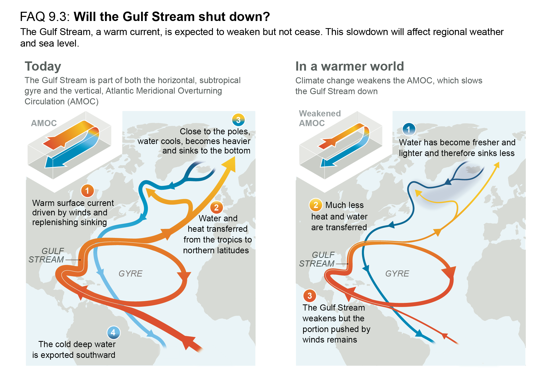
The Atlantic Meridional Overturning Circulation (AMOC) will very likely decline over the 21st century for all SSP scenarios. There is medium confidencethat the decline will not involve an abrupt collapse before 2100. For the 20th century, there is low confidence in reconstructed and modelled AMOC changes because of their low agreement in quantitative trends. The low confidence also arises from new observations that indicate missing key processes in both models and measurements used for formulating proxies and from new evaluations of modelled AMOC variability. This results in low confidence in quantitative projections of AMOC decline in the 21st century, despite the high confidence in the future decline as a qualitative feature based on process understanding. {9.2.3}
Southern Ocean circulation and associated temperature changes in Antarctic ice-shelf cavities are sensitive to changes in wind patterns and increased ice shelf melt (high confidence). However, limitations in understanding feedback mechanisms involving the ocean, atmosphere and cryosphere, which are not fully represented in the current generation of climate models, generally limit our confidence in future projections of the Southern Ocean and of its forcing on Antarctic sea ice and ice shelves. {9.2.3, 9.3.2, 9.4.2}
Many ocean currents will change in the 21st century as a response to changes in wind stress associated with anthropogenic warming (high confidence). Western boundary currents have shifted poleward since 1993 (medium confidence), consistent with a poleward shift of the subtropical gyres. Of the four eastern boundary upwelling systems, only the California Current system has experienced some large-scale upwelling-favourable wind intensification since the 1980s (medium confidence). In the 21st century, consistent with projected changes in the surface winds, the East Australian Current Extension and Agulhas Current Extension will intensify, while the Gulf Stream and Indonesian Throughflow will weaken (medium confidence). Eastern boundary upwelling systems will change, with a dipole spatial pattern within each system of reduction at low latitude and enhancement at high latitude (high confidence). {9.2.1, 9.2.3}
Sea Ice
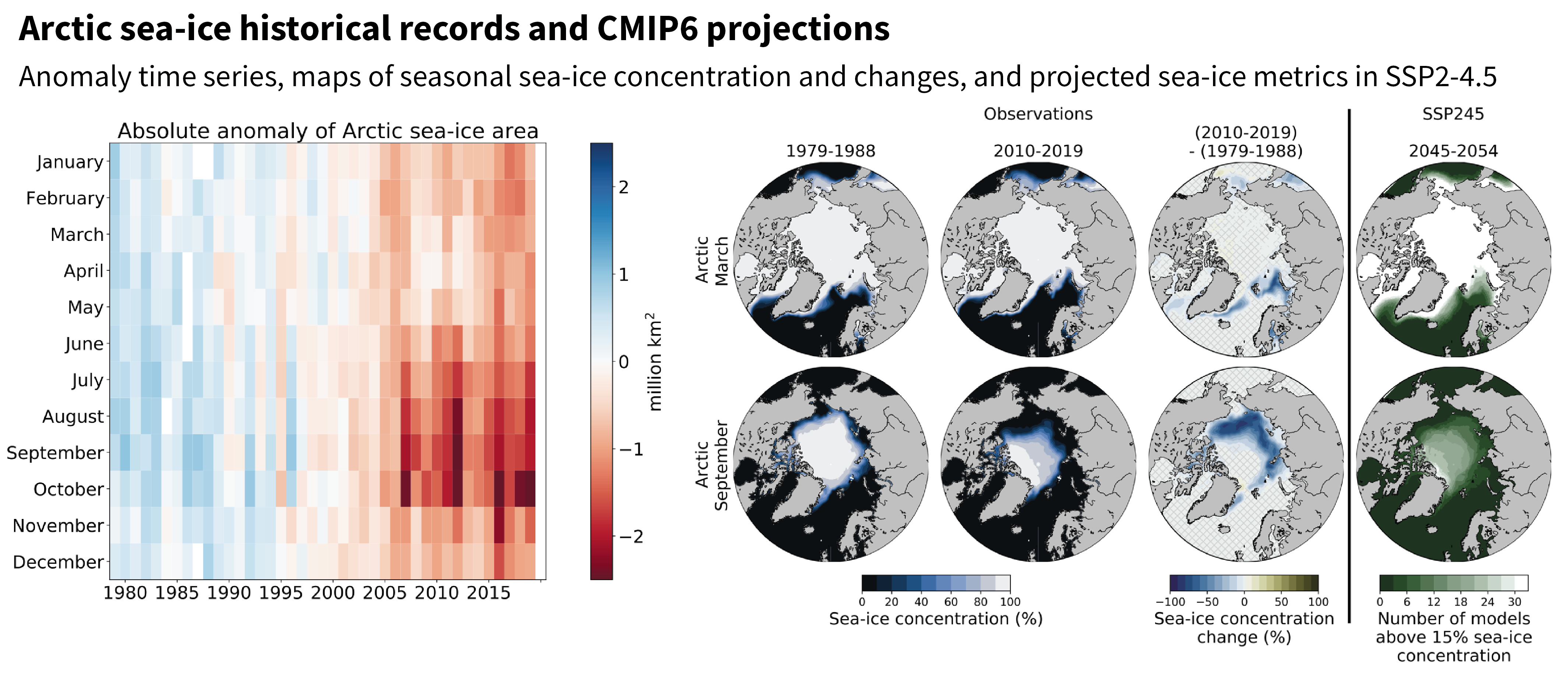
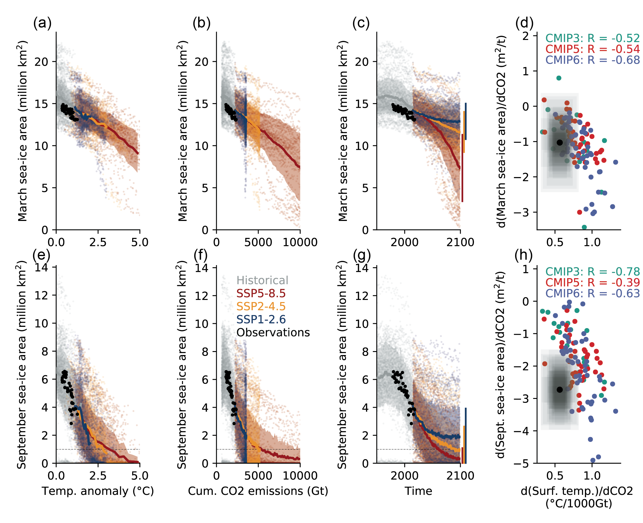
The Arctic Ocean will likely become practically sea ice free1during the seasonal sea ice minimum for the first time before 2050 in all considered SSP scenarios. There is no tipping point for this loss of Arctic summer sea ice (high confidence). The practically ice-free state is projected to occur more often with higher greenhouse gas concentrations, and it will become the new normal for high-emissions scenarios by the end of this century (high confidence). Based on observational evidence, Coupled Model Intercomparison Project Phase 6 (CMIP6) models and conceptual understanding, the substantial satellite-observed decrease of Arctic sea ice area over the period 1979–2019 is well described as a linear function of global mean surface temperature, and thus of cumulative anthropogenic carbon dioxide (CO2) emissions, with superimposed internal variability (high confidence). According to both process understanding and CMIP6 simulations, a practically sea ice-free state will likely be observed some years before additional (post-2020) cumulative anthropogenic CO2 emissions reach 1000 GtCO2. {4.3.2, 9.3.1}
For Antarctic sea ice, regionally opposing trends and large interannual variability result in no significant trend in satellite-observed sea ice area from 1979 to 2020 in both winter and summer (high confidence). The regionally opposing trends result primarily from changing regional wind forcing (medium confidence). There is low confidence in model simulations of future Antarctic sea ice decrease, and lack of decrease, due to deficiencies of process representation, in particular at the regional level. {2.3.2, 9.2.3, 9.3.2}
Sea Level
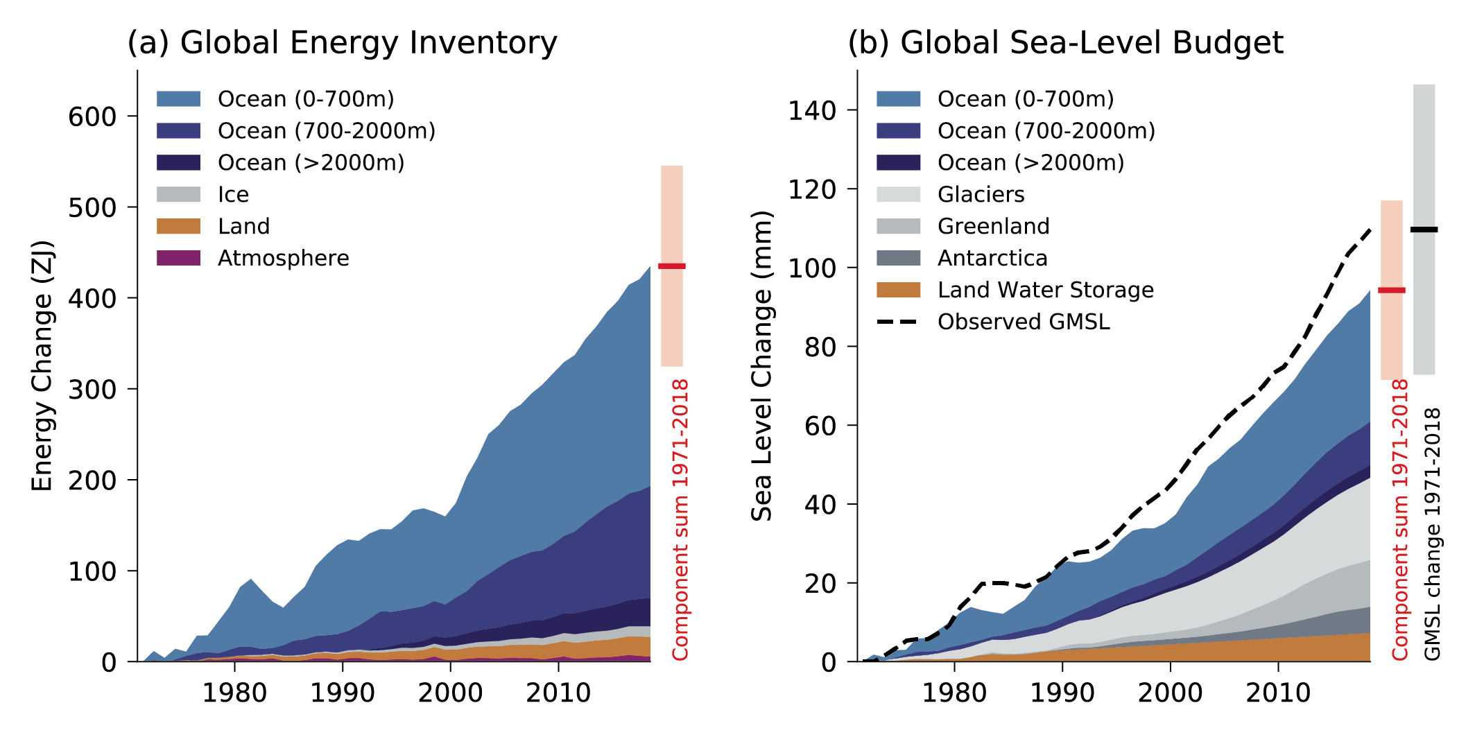
Global mean sea level (GMSL) rose faster in the 20th century than in any prior century over the last three millennia (high confidence), with a 0.20 [0.15 to 0.25] m rise over the period 1901–2018 (high confidence). GMSL rise has accelerated since the late 1960s, with an average rate of 2.3 [1.6 to 3.1] mm yr–1 over the period 1971–2018 increasing to 3.7 [3.2 to 4.2] mm yr–1 over the period 2006–2018 (high confidence). New observation-based estimates published since SROCC lead to an assessed sea level rise over the period 1901–2018 that is consistent with the sum of individual components. Ocean thermal expansion (38%) and mass loss from glaciers (41%) dominate the total change from 1901 to 2018. The contribution of Greenland and Antarctica to GMSL rise was four times larger during 2010–2019 than during 1992–1999 (high confidence). Because of the increased ice-sheet mass loss, the total loss of land ice (glaciers and ice sheets) was the largest contributor to global mean sea level rise over the period 2006–2018 (high confidence). {2.3.3, 9.6.1, 9.6.2, Cross-Chapter Box 9.1, Table 9.A.1, Box 7.2}
At the basin scale, sea levels rose fastest in the Western Pacific and slowest in the Eastern Pacific over the period 1993–2018 (medium confidence). Regional differences in sea level arise from: ocean dynamics; changes in Earth gravity, rotation and deformation due to land ice and land-water changes; and vertical land motion. Temporal variability in ocean dynamics dominates regional patterns on annual to decadal time scales (high confidence). The anthropogenic signal in regional sea level change will emerge in most regions by 2100 (medium confidence). {9.2.4, 9.6.1}
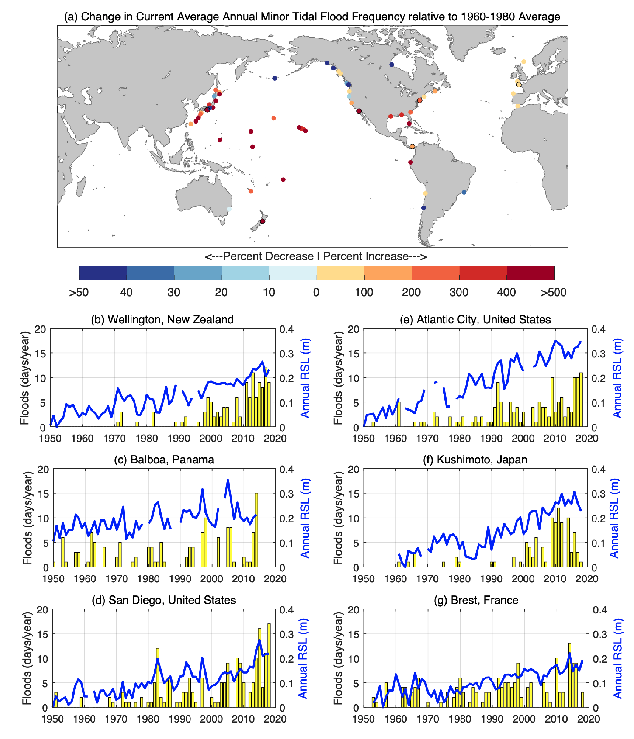
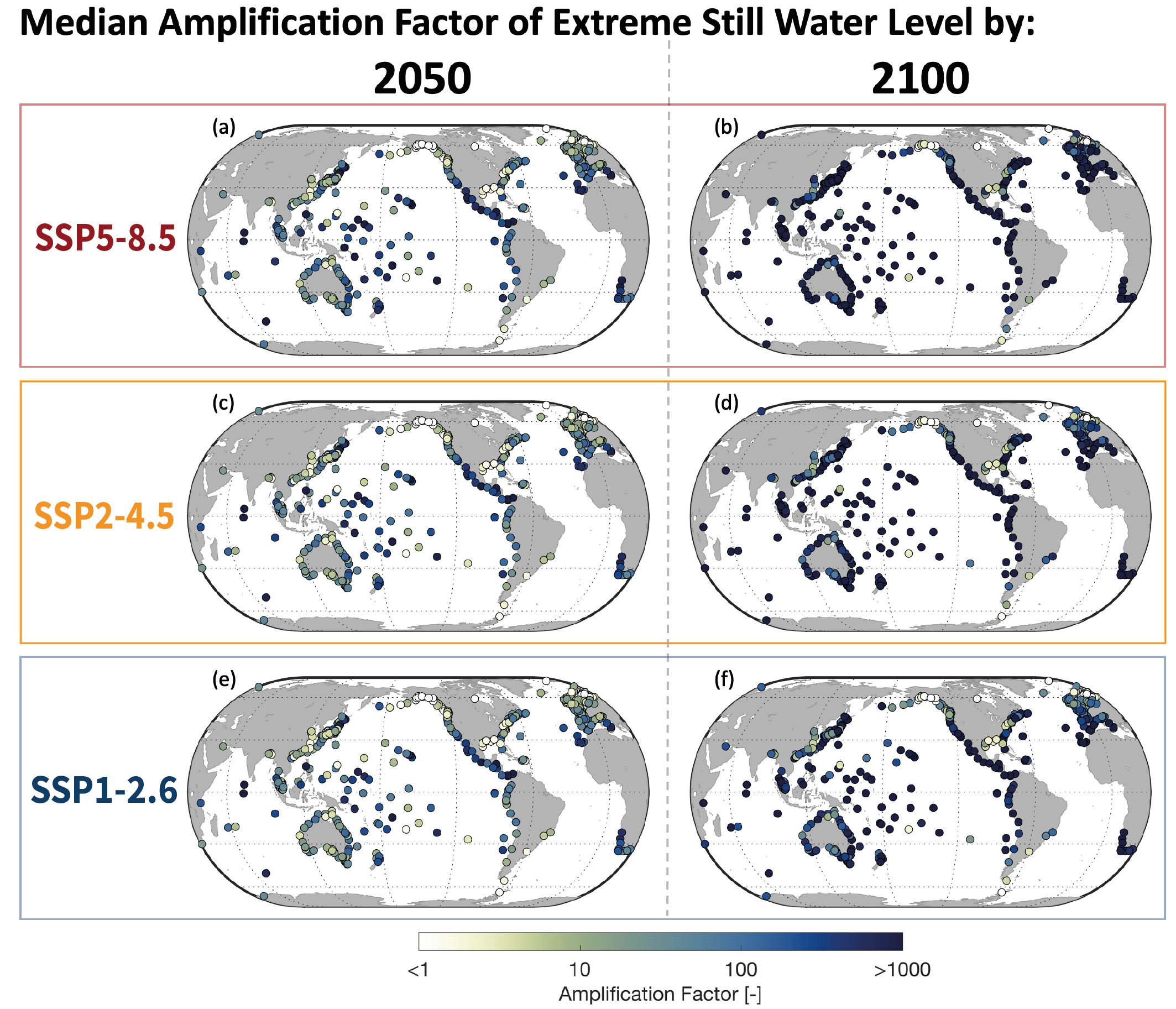
Regional sea level change has been the main driver of changes in extreme still water levels across the quasi-global tide gauge network over the 20th century (high confidence) and will be the main driver of a substantial increase in the frequency of extreme still water levels over the next century (medium confidence). Observations show that high-tide flooding events that occurred five times per year during the period 1960–1980 occurred, on average, more than eight times per year during the period 1995–2014 (high confidence). Under the assumption that other contributors to extreme sea levels remain constant (e.g., stationary tides, storm-surge, and wave climate), extreme sea levels that occurred once per century in the recent past will occur annually or more frequently at about 19–31% of tide gauges by 2050 and at about 60% (SSP1-2.6) to 82% (SSP5-8.5) of tide gauges by 2100 (medium confidence). In total, such extreme sea levels will occur about 20 to 30 times more frequently by 2050 and 160 to 530 times more frequently by 2100 compared to the recent past, as inferred from the median amplification factors for SSP1-2.6, SSP2-4.5, and SSP5-8.5 (medium confidence). Over the 21st century, the majority of coastal locations will experience a median projected regional sea level rise within ±20% of the median projected GMSL change (medium confidence). {9.6.3, 9.6.4}
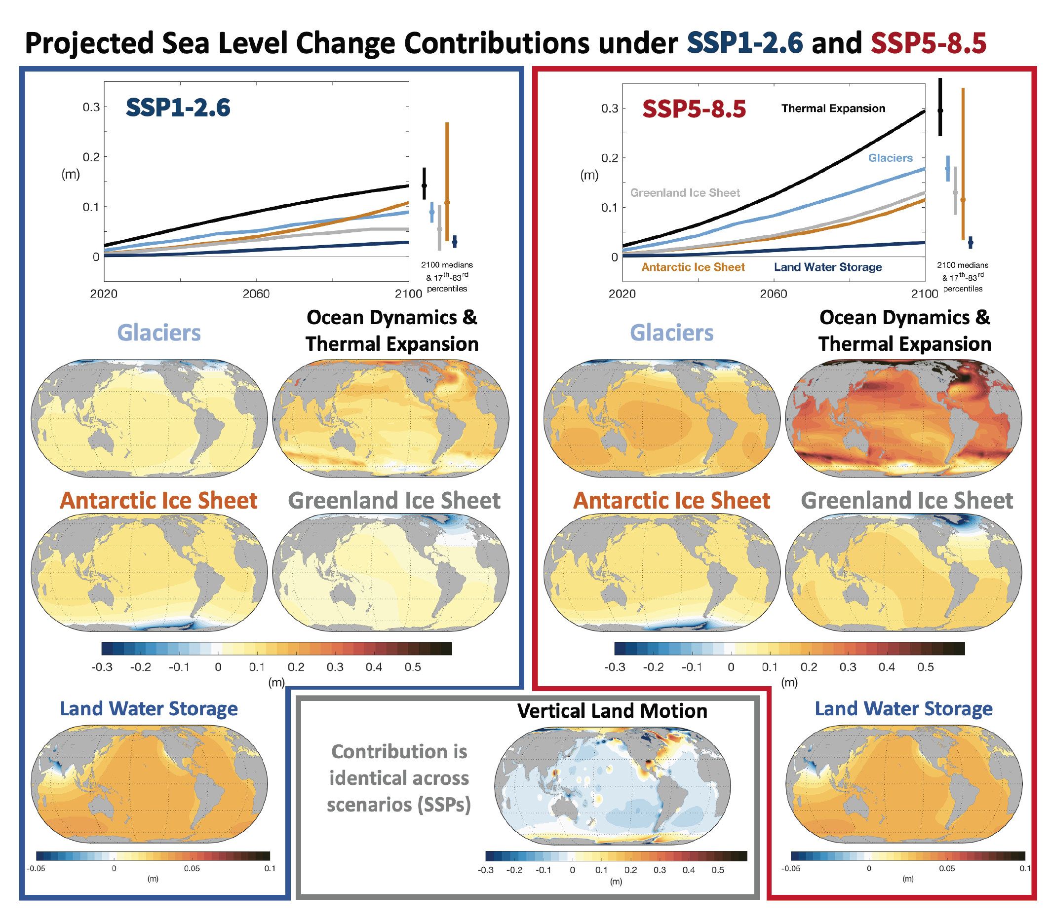
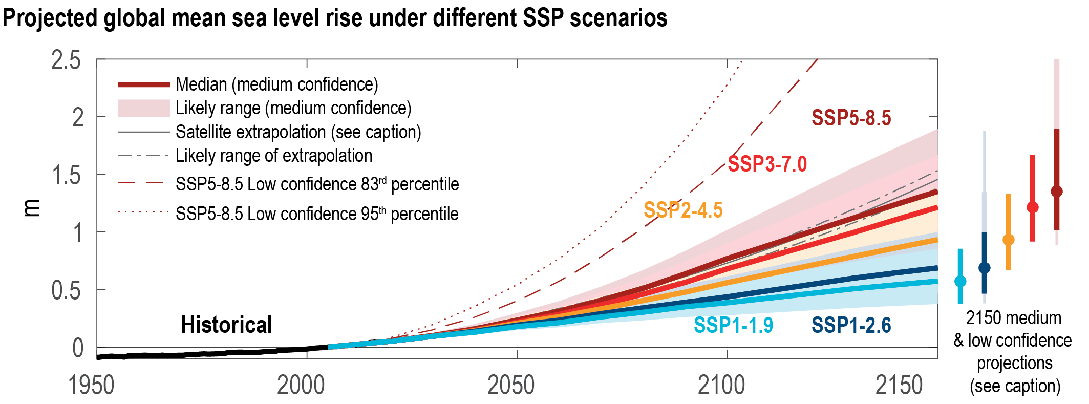
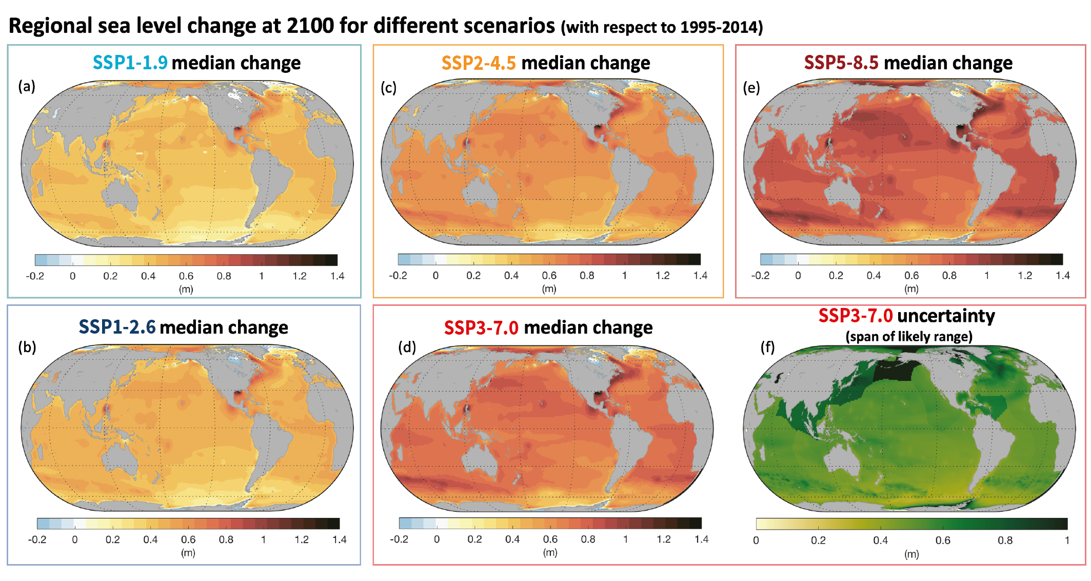
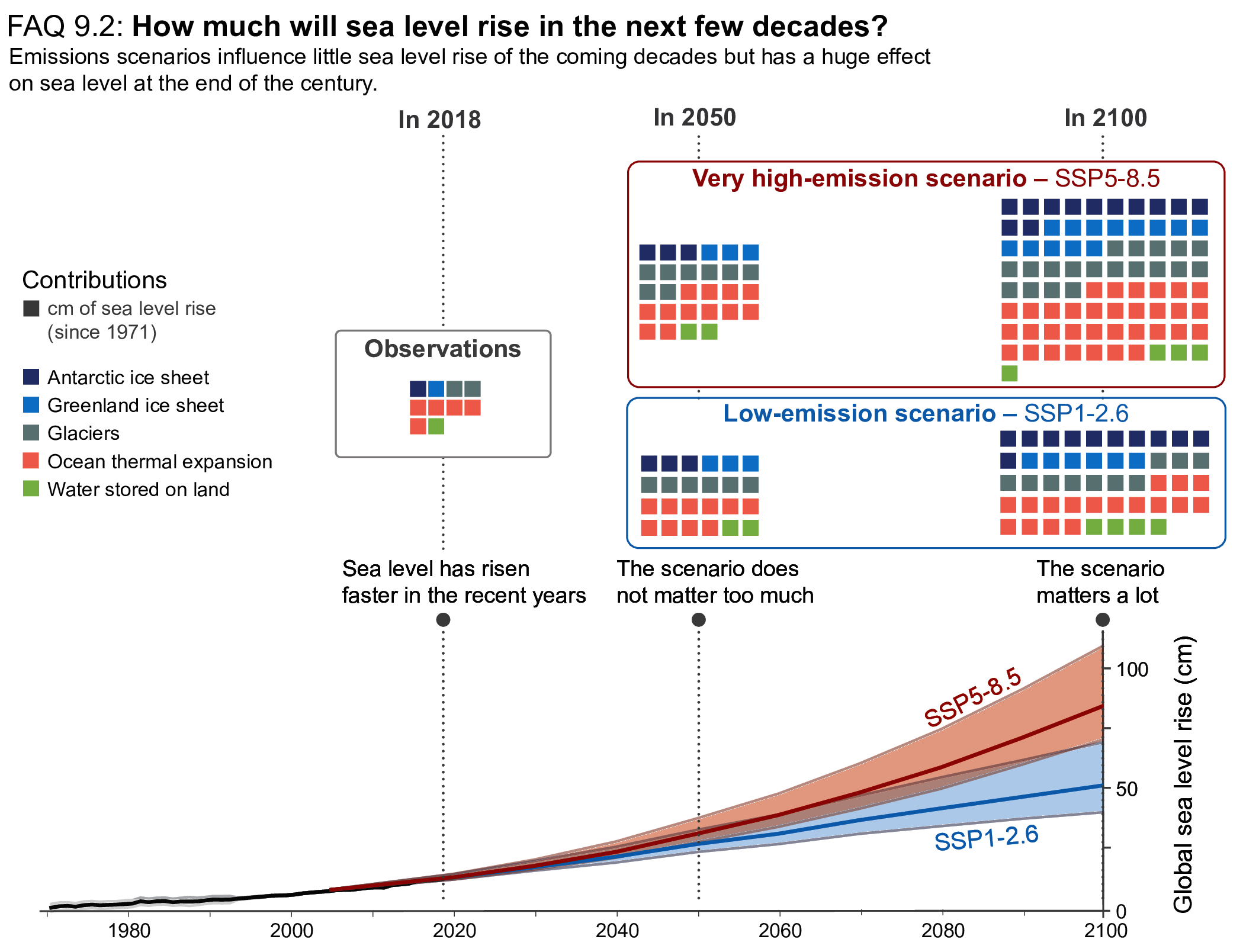
It is virtually certainthat GMSL will continue to rise until at least 2100, because all assessed contributors to GMSL are likely to virtually certainto continue contributing throughout this century. Considering only processes for which projections can be made with at least medium confidence, relative to the period 1995–2014, GMSL will rise by 2050 between 0.18 [0.15 to 0.23, likely range] m (SSP1-1.9) and 0.23 [0.20 to 0.29, likely range] m (SSP5-8.5), and by 2100 between 0.38 [0.28 to 0.55, likely range] m (SSP1-1.9) and 0.77 [0.63 to 1.01, likely range] m (SSP5-8.5) . This GMSL rise is primarily caused by thermal expansion and mass loss from glaciers and ice sheets, with minor contributions from changes in land-water storage. These likely range projections do not include those ice-sheet-related processes that are characterized by deep uncertainty. {9.6.3}
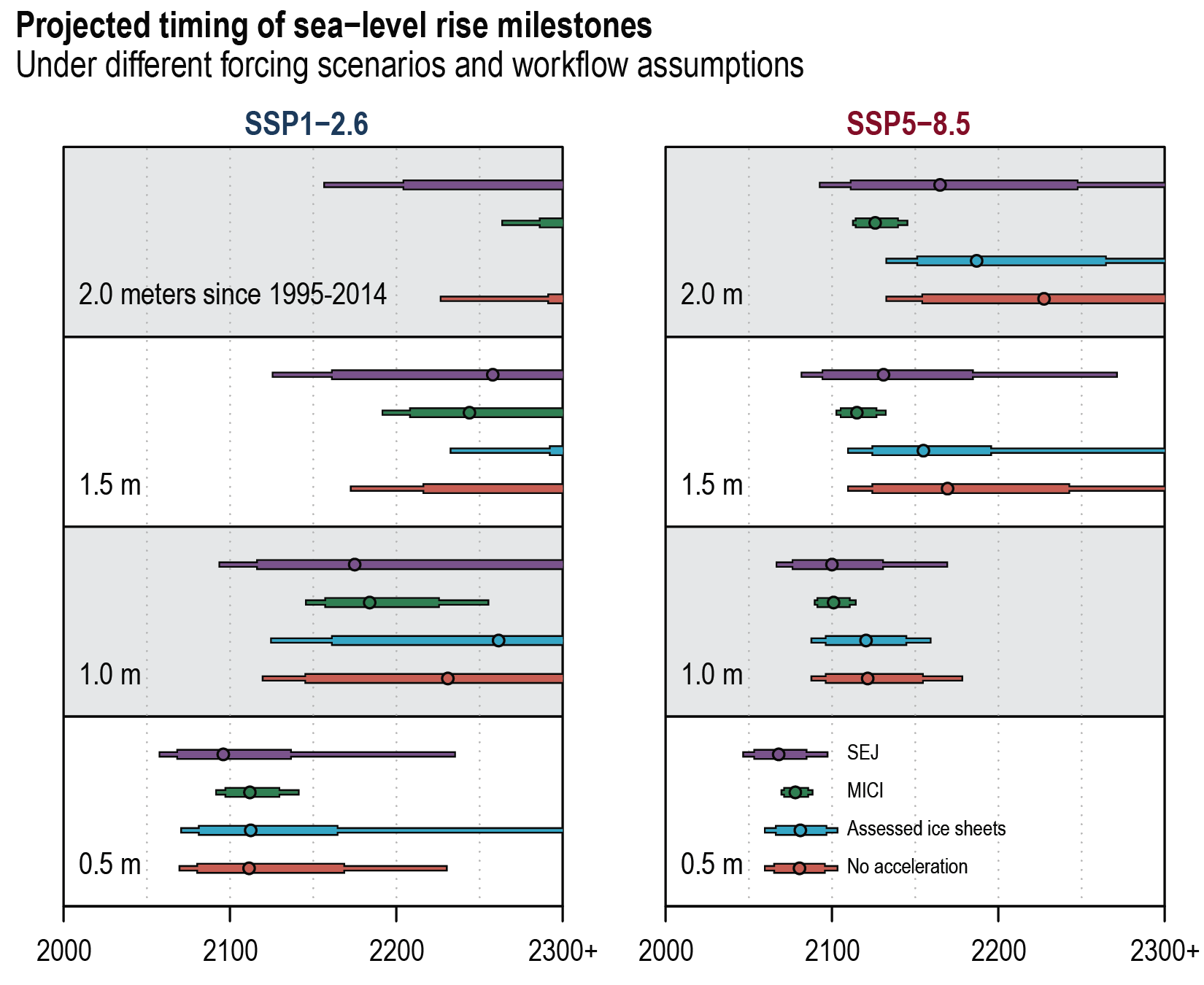
Higher amounts of GMSL rise before 2100 could be caused by earlier-than-projected disintegration of marine ice shelves, the abrupt, widespread onset of marine ice sheet instability and marine ice cliff instability around Antarctica, and faster-than-projected changes in the surface mass balance and discharge from Greenland. These processes are characterized by deep uncertainty arising from limited process understanding, limited availability of evaluation data, uncertainties in their external forcing and high sensitivity to uncertain boundary conditions and parameters. In a low-likelihood, high-impact storyline, under high emissions such processes could in combination contribute more than one additional metre of sea level rise by 2100. {9.6.3, Box 9.4}
Beyond 2100, GMSL will continue to rise for centuries due to continuing deep-ocean heat uptake and mass loss of the Greenland and Antarctic ice sheets, and will remain elevated for thousands of years (high confidence). Considering only processes for which projections can be made with at least medium confidence and assuming no increase in ice-mass flux after 2100, relative to the period 1995–2014, by 2150, GMSL will rise between 0.6 [0.4 to 0.9, likely range] m (SSP1-1.9) and 1.4 [1.0 to 1.9, likely range] m (SSP5-8.5). By 2300, GMSL will rise between 0.3 m and 3.1 m under SSP1-2.6, between 1.7 m and 6.8 m under SSP5-8.5 in the absence of marine ice cliff instability, and by up to 16 m under SSP5-8.5 considering marine ice cliff instability (low confidence). {9.6.3}
Ice Sheets
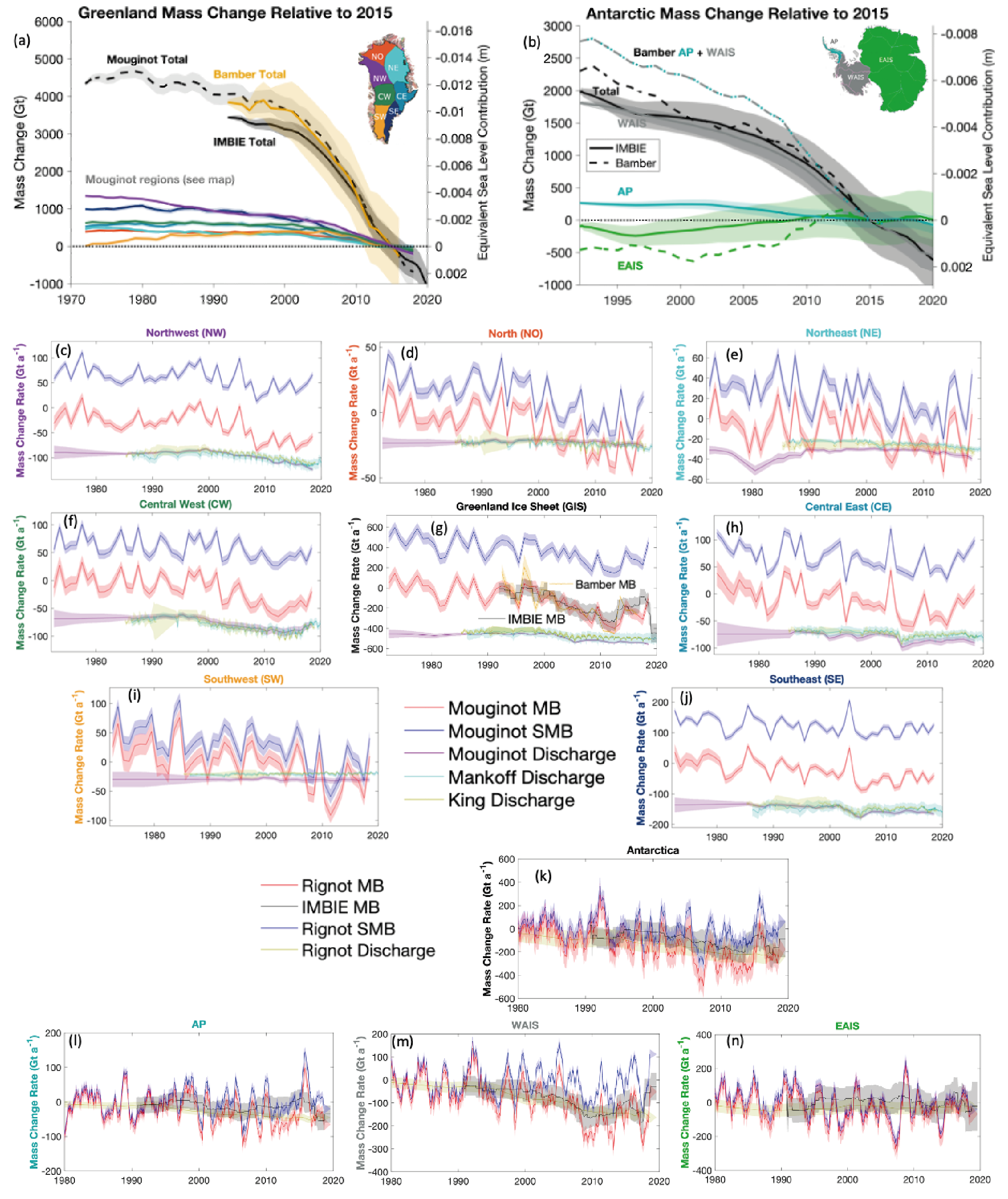
The Greenland Ice Sheet has lost 4890 [4140 to 5640] Gt mass over the period 1992–2020, equivalent to 13.5 [11.4 to 15.6] mm global mean sea level rise. The mass-loss rate was on average 39 [–3 to +80] Gt yr–1 over the period 1992–1999, 175 [131 to 220] Gt yr–1 over the period 2000–2009 and 243 [197 to 290] Gt yr–1 over the period 2010–2019. This mass loss is driven by both discharge and surface melt, with the latter increasingly becoming the dominating component of mass loss with high interannual variability in the last decade (high confidence). The largest mass losses occurred in the north-west and the south-east of Greenland (high confidence). {2.3.2, 9.4.1}
The Antarctic Ice Sheet has lost 2670 [1800 to 3540] Gt mass over the period 1992–2020, equivalent to 7.4 [5.0 to 9.8] mm global mean sea level rise. The mass-loss rate was, on average, 49 [–2 to +100] Gt yr–1 over the period 1992–1999, 70 [22 to 119] Gt yr–1 over the period 2000–2009 and 148 [94 to 202] Gt yr–1 over the period 2010–2019. Mass losses from West Antarctic outlet glaciers outpaced mass gain from increased snow accumulation on the continent and dominated the ice-sheet mass losses since 1992 (very high confidence). These mass losses from the West Antarctic outlet glaciers were mainly induced by ice-shelf basal melt (high confidence) and locally by ice-shelf disintegration preceded by strong surface melt (high confidence). Parts of the East Antarctic Ice Sheet have lost mass in the last two decades (high confidence). {2.3.2, 9.4.2, Atlas.11.1}
Both the Greenland Ice Sheet (virtually certain) and the Antarctic Ice Sheet (likely ) will continue to lose mass throughout this century under all considered SSP scenarios. The related contribution to global mean sea level rise until 2100 from the Greenland Ice Sheet will likely be 0.01 to 0.10 m under SSP1-2.6, 0.04 to 0.13 m under SSP2-4.5 and 0.09–0.18 m under SSP5-8.5, while the Antarctic Ice Sheet will likely contribute 0.03 to 0.27 m under SSP1-2.6, 0.03 to 0.29 m under SSP2-4.5, and 0.03 to 0.34 m under SSP5-8.5. The loss of ice from Greenland will become increasingly dominated by surface melt, as marine margins retreat and the ocean-forced dynamic response of ice-sheet margins diminishes (high confidence). In the Antarctic, dynamic losses driven by ocean warming and ice-shelf disintegration will likely continue to outpace increasing snowfall this century (medium confidence). Beyond 2100, total mass loss from both ice sheets will be greater under high-emissions scenarios than under low-emissions scenarios (high confidence). The assessed likely ranges consider those ice-sheet processes in whose representation in current models we have at least medium confidence, including surface mass balance and grounding-line retreat in the absence of instabilities. Under high-emissions scenarios, poorly understood processes related to marine ice sheet instability and marine ice cliff instability, characterized by deep uncertainty, have the potential to strongly increase Antarctic mass loss on century to multi-century time scales. {9.4.1, 9.4.2, 9.6.3, Box 9.3, Box 9.4}
Glaciers
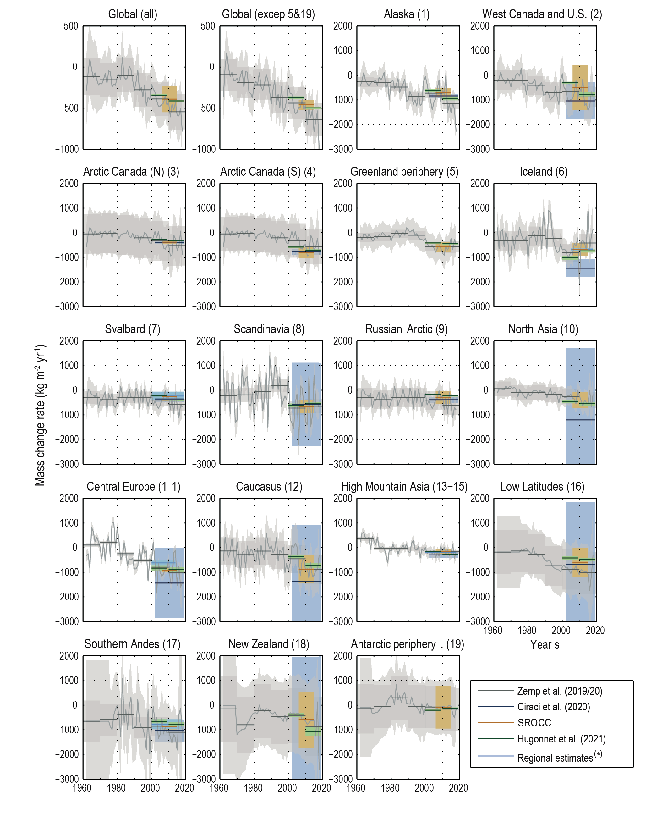
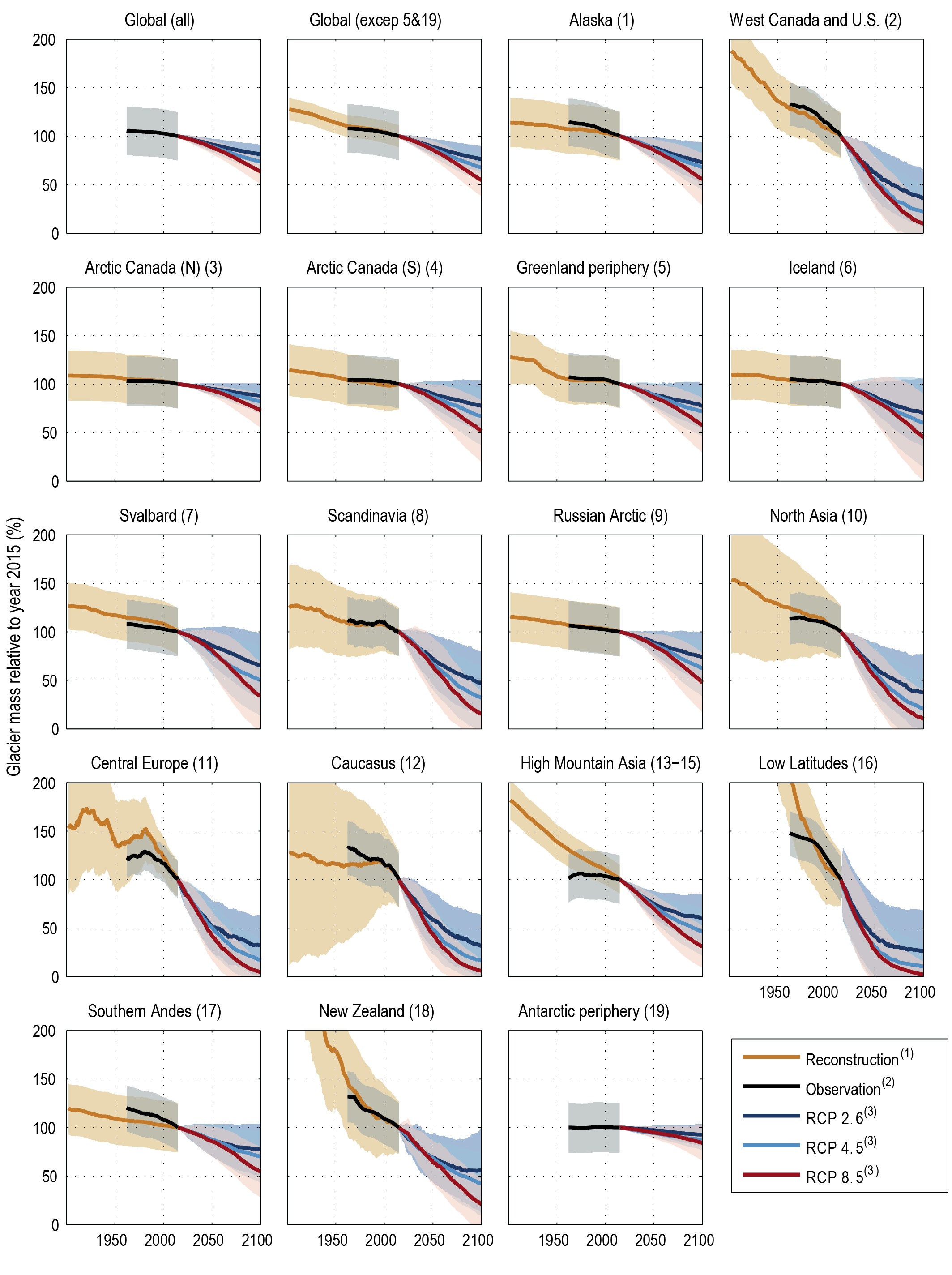
Glaciers lost 6200 [4600 to 7800] Gt of mass (17.1 [12.7 to 21.5] mm global mean sea level equivalent) over the period 1993–2019 and will continue losing mass under all SSP scenarios (very high confidence). During the decade 2010–2019, glaciers lost more mass than in any other decade since the beginning of the observational record (very high confidence). For all regions with long-term observations, glacier mass in the decade 2010–2019 is the smallest since at least the beginning of the 20th century (medium confidence). Because of their lagged response, glaciers will continue to lose mass at least for several decades even if global temperature is stabilized (very high confidence). Glaciers will lose 29,000 [9000 to 49,000] Gt and 58,000 [28,000 to 88,000] Gt over the period 2015–2100 for RCP2.6 and RCP8.5, respectively (medium confidence), which represents 18 [5 to 31] % and 36 [16 to 56] % of their early-21st-century mass, respectively. {2.3.2, 9.5.1, 9.6.1, 9.6.3, 12.4}
Permafrost
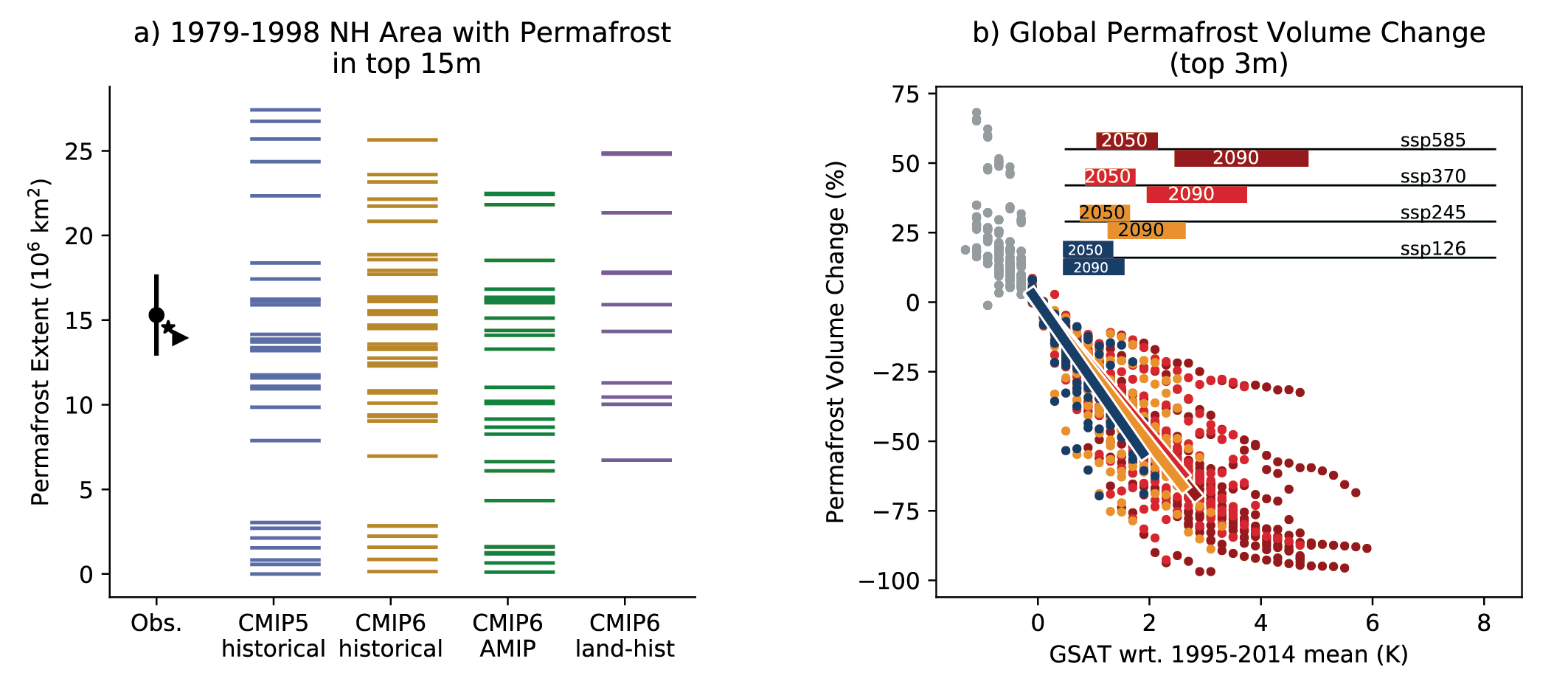
Increases in permafrost temperature have been observed over the past three to four decades throughout the permafrost regions (high confidence), and further global warming will lead to near-surface permafrost volume loss (high confidence). Complete permafrost thaw in recent decades is a common phenomenon in discontinuous and sporadic permafrost regions (medium confidence). Permafrost warmed globally by 0.29 [0.17 to 0.41, likely range] °C between 2007 and 2016 (medium confidence). An increase in the active layer thickness is a pan-Arctic phenomenon (medium confidence), subject to strong heterogeneity in surface conditions. The volume of perennially frozen soil within the upper 3 m of the ground will decrease by about 25% per 1°C of global surface air temperature change (up to 4°C above pre-industrial temperature) (medium confidence). {9.5.2}
Snow
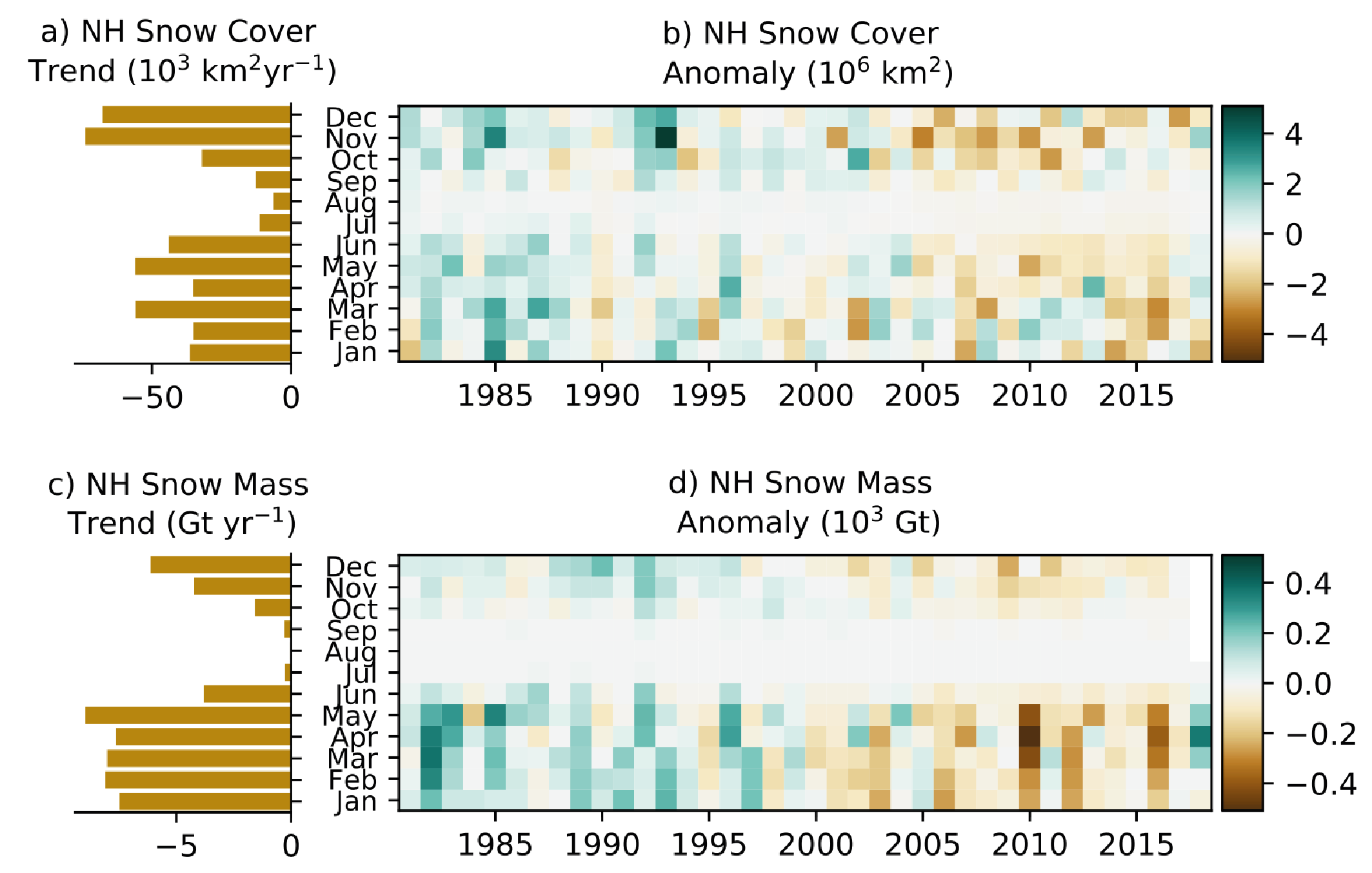
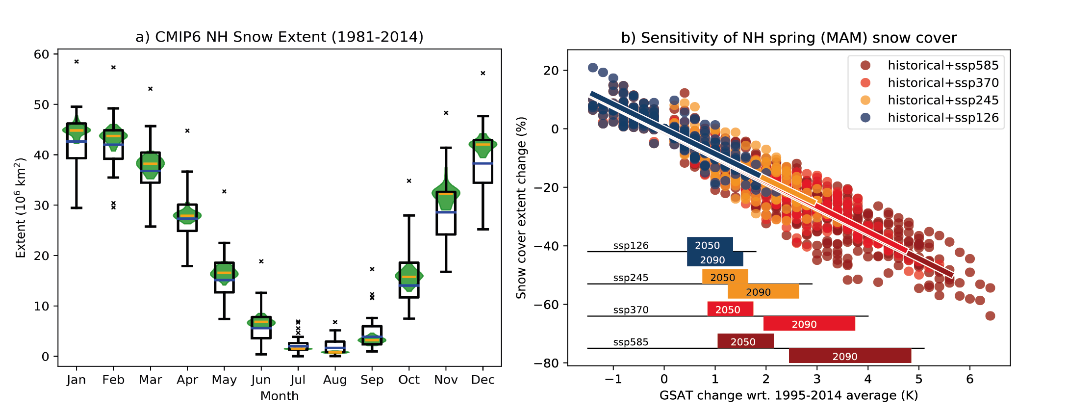
Northern Hemisphere spring snow cover extent has been decreasing since 1978 (very high confidence), and there is high confidencethat this trend extends back to 1950. Further decrease of Northern Hemisphere seasonal snow cover extent is virtually certainunder further global warming. The observed sensitivity of Northern Hemisphere snow cover extent to Northern Hemisphere land surface air temperature for 1981–2010 is –1.9 [–2.8 to –1.0, likely range] million km2 per 1°C throughout the snow season. It is virtually certain that Northern Hemisphere snow cover extent will continue to decrease as global climate continues to warm, and process understanding strongly suggests that this also applies to Southern Hemisphere seasonal snow cover (high confidence). Northern Hemisphere spring snow cover extent will decrease by about 8% per 1°C of global surface air temperature change (up to 4°C above pre-industrial temperature) (medium confidence). {9.5.3}
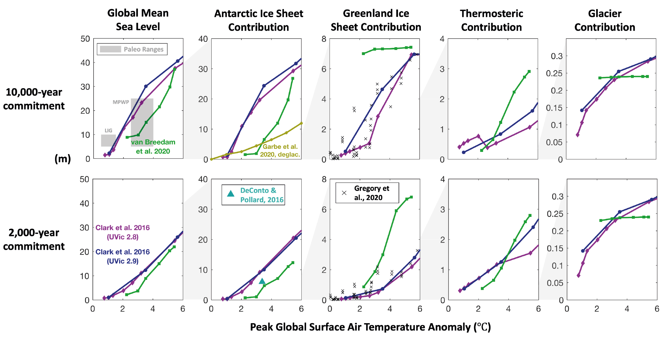
Cryospheric Changes and Sea Level Rise at Specific Levels of Global Warming
At sustained warming levels between 1.5°C and 2°C, the Arctic Ocean will become practically sea ice-free in September in some years (medium confidence); the ice sheets will continue to lose mass (high confidence), but will not fully disintegrate on time scales of multiple centuries (medium confidence); there is limited evidence that the Greenland and West Antarctic ice sheets will be lost almost completely and irreversibly over multiple millennia; about 50 to 60% of current glacier mass excluding the two ice sheets and the glaciers peripheral to the Antarctic Ice Sheet will remain, predominantly in the polar regions (low confidence); Northern Hemisphere spring snow cover extent will decrease by up to 20% relative to 1995–2014 (medium confidence); the permafrost volume in the top 3 m will decrease by up to 50% relative to 1995–2014 (medium confidence). Committed GMSL rise over 2000 years will be about 2 to 6 m with 2°C of peak warming (medium agreement, limited evidence). {9.3.1, 9.4.1, 9.4.2, 9.5.1, 9.5.2, 9.5.3, 9.6.3}
At sustained warming levels between 2°C and 3°C, The Arctic Ocean will be practically sea ice free throughout September in most years (medium confidence); there is limited evidence that the Greenland and West Antarctic ice sheets will be lost almost completely and irreversibly over multiple millennia; both the probability of their complete loss and the rate of mass loss will increase with higher temperatures (high confidence); about 50 to 60% of current glacier mass outside Antarctica will be lost (low confidence); Northern Hemisphere spring snow cover extent will decrease by up to 30% relative to 1995–2014 (medium confidence); permafrost volume in the top 3 m will decrease by up to 75% relative to 1995–2014 (medium confidence). Committed GMSL rise over 2000 years will be about 4 to 10 m with 3°C of peak warming (medium agreement, limited evidence). {9.3.1, 9.4.1, 9.4.2, 9.5.1, 9.5.2, 9.5.3, 9.6.3}
At sustained warming levels between 3°C and 5°C, the Arctic Ocean will become practically sea ice free throughout several months in most years (high confidence); near-complete loss of the Greenland Ice Sheet and complete loss of the West Antarctic Ice Sheet will occur irreversibly over multiple millennia (medium confidence); substantial parts or all of Wilkes Subglacial Basin in East Antarctica will be lost over multiple millennia (low confidence); 60 to 75% of current glacier mass outside Antarctica will disappear (low confidence); nearly all glacier mass in low latitudes, Central Europe, Caucasus, western Canada and the USA, North Asia, Scandinavia and New Zealand will likely disappear; Northern Hemisphere spring snow cover extent will decrease by up to 50% relative to 1995–2014 (medium confidence); permafrost volume in the top 3 m will decrease by up to 90% compared to 1995–2014 (medium confidence). Committed GMSL rise over 2000 years will be about 12 to 16 m with 4°C of peak warming and 19 to 22 m with 5°C of peak warming (medium agreement, limited evidence). {9.3.1, 9.4.1, 9.4.2, 9.5.1, 9.5.2, 9.5.3, 9.6.3}
9.1 Introduction
This chapter provides a holistic assessment of the physical processes underlying global and regional changes in the ocean, cryosphere and sea level, as well as improved understanding of observed, attributed and projected future changes since the IPCC Fifth Assessment Report (AR5) and the Special Report on the Ocean and Cryosphere in a Changing Climate (SROCC; see outline in Figure 9.1). The ocean and cryosphere (defined as the frozen components of the Earth system such as sea ice, ice sheets, glaciers, permafrost and snow) exchange heat and freshwater with the atmosphere and each other (Figure 9.2). In a warming climate, the combined effects of thermal expansion of seawater and melting of the terrestrial cryosphere result in global mean sea level rise (Box 9.1).
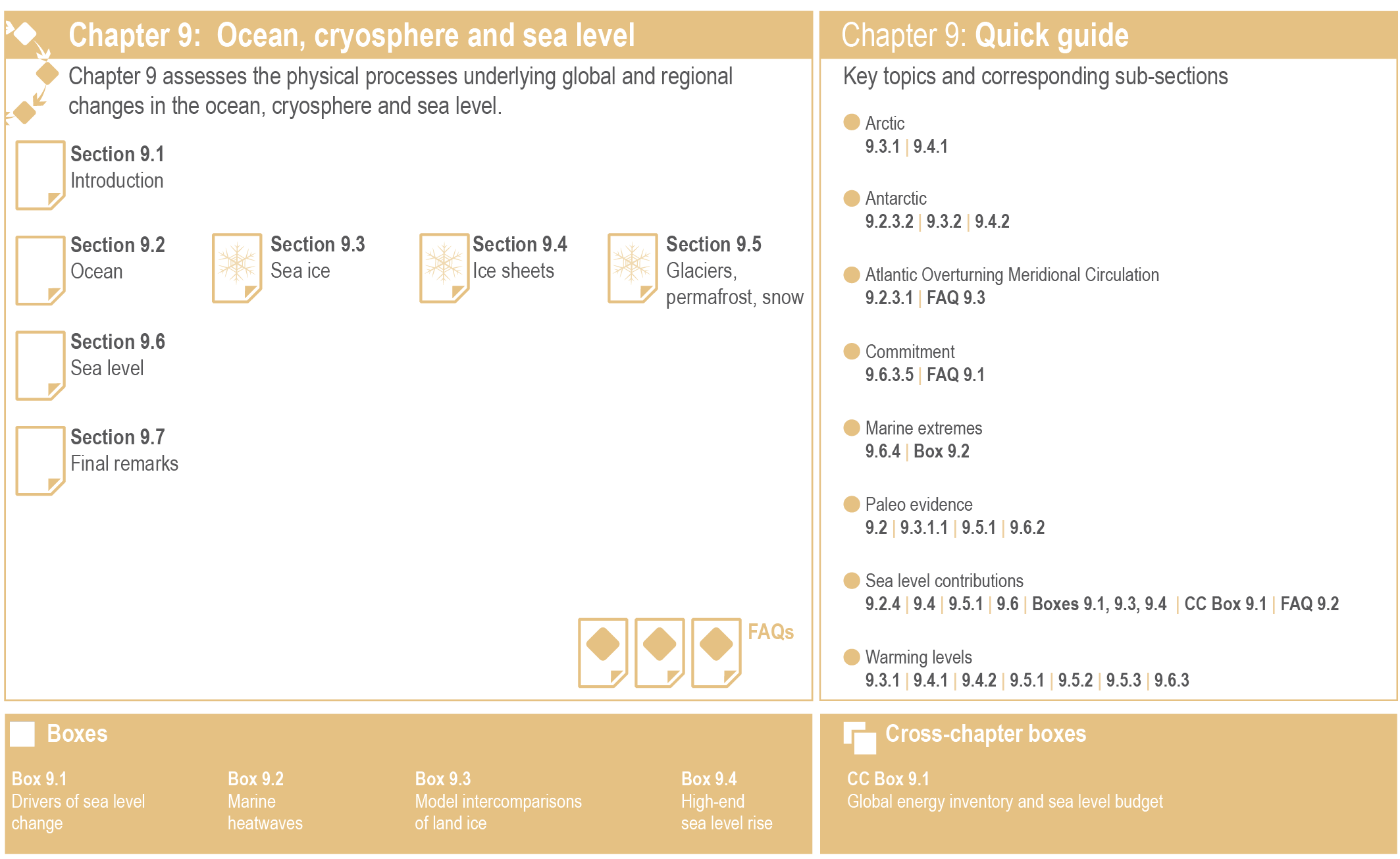 Figure 9.1 | Visual guide to Chapter 9. Sections dealing with the cryosphere are highlighted with a snowflake.
 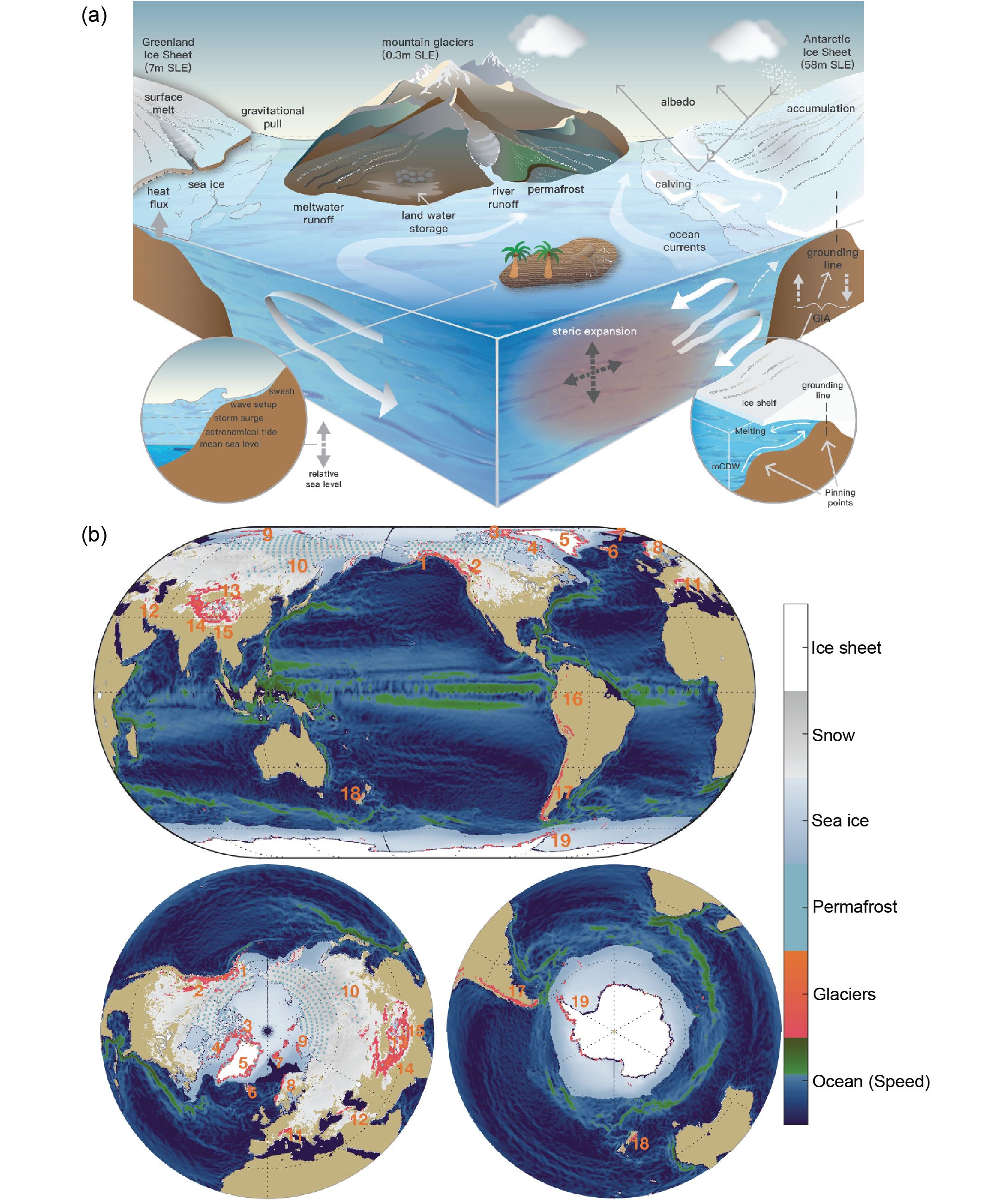 Figure 9.2 | Components of ocean, cryosphere and sea level assessed in this chapter. (a) Schematic of processes (mCDW=modified Circumpolar Deep Water, GIA=Glacial Isostatic Adjustment). White arrows indicate ocean circulation. Pinning points indicate where the grounding line is most stable and ice-sheet retreat will slow. (b) Geographic distribution of ocean and cryosphere components (numbers indicate glacierized regions (RGI Consortium, 2017)). See Figures 9.20 and 9.21 for labels. Sea ice shaded to indicate the annual mean concentration. Green ocean colours indicate larger surface current speed. Further details on data sources and processing are available in the chapter data table (Table 9.SM.9).
 Ocean acidification and deoxygenation are covered in Chapter 5, and regional changes to the ocean and cryosphere are covered in Chapter 12 and the Atlas. Ecosystem range shifts and climate risk for marine biodiversity associated with ocean change are assessed in AR6 Working Group II (WGII). The notion of ‘climate velocity’ often used in impact studies, which is defined as the speed and direction at which a climate variable moves across a corresponding spatial field, is underpinned by the assessment of changes in the physical characteristics of the ocean provided in this chapter.
There are two major advances of this chapter compared with AR5 and SROCC facilitated by community efforts. The first is the temporal and spatial increase in observations of both the ocean and the cryosphere (Section 1.5.1.1). In particular, extended observations have allowed for improved assessment of past change and closure of both the energy and sea level budgets in a consistent way (Cross-Chapter Box 9.1) and the sea level budget for the last century (Section 9.6.1.1). Higher resolution observations have revealed the details of the Atlantic Meridional Overturning Circulation (AMOC; Section 9.2.3.1) and globally resolved glacier changes for the first time (Section 9.5.1.1). Improved methodology has resulted in a doubling of the assessed level of observed increase in global ocean 0–200 m stratification compared to SROCC assessment (Section 9.2.1.3).
The second advance is the use of a hierarchy of models and emulators to update projections of oceanic, cryospheric and sea level change arising from Coupled Model Intercomparison Project Phase 6 (CMIP6) and related projects (Section 1.5.4.3, Table 1.3, and Annex II). 2The CMIP6 included an ice-sheet modelling intercomparison for the first time. Particular modelling advances relevant to this chapter are the increase in ocean resolution in the High Resolution Model Intercomparison Project (HighResMIP) and Ocean Model Intercomparison Project phase 2 (OMIP-2) experiments (Sections 1.5.3.1 and 9.2), projections of future glacier (GlacierMIP) and ice sheet (ISMIP6) and Linear Antarctic Response Model Intercomparison Project (LARMIP-2) response from multi-model studies (Sections 9.5.1 and 9.4, and Box 9.3), and new methods to synthesize ocean and cryosphere models into sea level projections for all Shared Socieo-economic Pathway scenarios (SSPs; Sections 1.6.1, 9.4.1.3, 9.4.2.5 and 9.6.3, and Cross-Chapter Box 1.4) and warming levels (Sections 9.6.3 and 1.6.2, and Cross-Chapter Box 11.1). In particular, sea level projections and the individual contributions (Section 9.6.3.3) are consistent with equilibrium climate sensitivity and surface temperature assessments across this Report (Box 4.1 and Cross-Chapter Box 7.1).
There are other advances in scientific understanding. In the cryosphere, this chapter assesses how fast-responding elements (sea ice, permafrost and snow; Sections 9.3, 9.5.2 and 9.5.3) track warming levels across observations and projections independent of scenario, process understanding of uncertainty in Antarctic Ice Sheet projections (Section 9.4.2 and Box 9.4) and new insight into thresholds for Arctic sea ice (Section 9.3.1.1) and Greenland and West Antarctic ice sheets (Sections 9.4.1.4 and 9.4.2.6). In the ocean, process understanding of ocean heat uptake (Section 9.2.2.1 and Cross-Chapter Box 5.3) and observed changes in ocean stratification (Section 9.2.1.3) have implications for ocean biogeochemistry are also important.
Box 9.1 | Key Processes Driving Sea Level Change
Sea level changearises from processes acting on a range of spatial and temporal scales, in the ocean, cryosphere, solid Earth, atmosphere and on land (Figure 9.2). Relative sea level (RSL) change is the change in local mean sea surface height relative to the sea floor, as measured by instruments that are fixed to the Earth’s surface (e.g., tide gauges). This reference frame is used when considering coastal impacts, hazards and adaptation needs. In contrast, geocentric sea level change is the change in local mean sea surface height with respect to the terrestrial reference frame, and is the sea level change observed with instruments from space. This box provides a brief summary of sea level processes using standard terminology (Gregory et al., 2019).
Global processes
Global mean sea level change (Sections 9.6 and 2.3.3.3) is the change in volume of the ocean divided by the ocean surface area. It is the sum of changes in ocean density (‘global mean thermosteric sea level change’) and changes in the ocean mass as a result of changes in the cryosphere or land-water storage (‘barystatic sea level change’).
Steric sea level change is caused by changes in the ocean density and is composed of ‘thermosteric sea level change’ and ‘halosteric sea level change’. Thermosteric sea level change (also referred to as ‘thermal expansion’) occurs as a result of changes in ocean temperature: increasing temperature reduces ocean density and increases the volume per unit of mass. Halosteric sea level change occurs as a result of salinity variations: higher salinity leads to higher density and decreases the volume per unit of mass. Although both processes can be relevant on regional to local scales, thermosteric changes contribute to global mean sea level change, whereas global mean halosteric change is negligible (Gregory et al., 2019). There is high confidence in the understanding of processes causing thermosteric sea level change (Section 9.2.4.1).
The Greenland and Antarctic ice sheets are the largest reservoirs of frozen freshwater and therefore potentially the largest contributors to sea level rise. Fluctuations in ice-sheet volume arise from the imbalance between accumulation (either at the ice-sheet surface or on the underside of ice shelves) and loss from sublimation, surface and basal melting, and iceberg calving. Ice sheets discharge the majority of their mass through marine-terminating ice streams that are in some cases buttressed by floating ice shelves. Changes in the thickness and extent of the ice shelves due to melt from below, calving, or disintegration, as a result of surface meltwater penetrating crevasses, can affect the flow of the inland ice streams. There is medium confidence in ice-sheet processes but low confidence in their forcing (ocean changes and ice-shelf collapse) and in instability processes (Sections 9.4.1 and 9.4.2). 3
Glaciers contribute to sea level change via an imbalance between mass gain and mass loss processes, which leads to adjustments in the glacier geometry over an extended period of time, called the response time. The response time may range from a few years to a few hundred years. The glacial meltwater does not all flow immediately into the ocean: it can refreeze, feed rivers (where it may be extracted for domestic use), evaporate, or be stored in (proglacial) lakes or closed basins. There is medium to high confidence in the understanding of processes leading to sea level contributions from glaciers (Section 9.5.1).
Land-water storage includes surface water, soil moisture, groundwater storage and snow, but excludes water stored in glaciers and ice sheets. Changes in land-water storage can be caused either by direct human intervention in the water cycle (e.g., storage of water in reservoirs by building dams in rivers, groundwater extraction for consumption and irrigation, or deforestation) or by climate variations (e.g., changes in the amount of water in internally drained lakes and wetlands, the canopy, the soil, the permafrost and
the snowpack). Land-water storage changes caused by climate variations may be indirectly affected by anthropogenic influences. It is difficult to assign a single confidence level to land-water storage as understanding can vary from low confidence in groundwater recharge processes to high confidence in water storage via snowpack changes (Sections 8.2.3 and 8.3.1.7).
Regional and local processes
Ocean dynamic sea level change refers to the change in mean sea level relative to the geoid and is associated with the circulation and density-driven changes in the ocean. Ocean dynamic sea level change varies regionally but by definition has a zero global mean. It includes the depression of the sea surface by atmospheric pressure. There is medium confidence in the understanding of ocean processes leading to dynamic sea level change (Section 9.2.4.2).
Changes in Earth gravity, Earth rotation and viscoelastic solid Earth deformation (GRD) – result from the redistribution of mass between terrestrial ice and water reservoirs and the ocean. Contemporary terrestrial mass loss leads to elastic solid Earth uplift and a nearby RSL fall. (For a single source of terrestrial mass loss, this is within about 2000 km; for multiple sources, the distance depends on the interaction of the different RSL patterns.) Farther away (around more than 7000 km for a single source of terrestrial mass loss), RSL rises more than the global average, due to first-order gravitational effects. Earth deformation associated with adding water to the ocean and a shift of the Earth’s rotation axis towards the source of terrestrial mass loss leads to second-order effects that increase spatial variability of the pattern globally. GRD effects due to the redistribution of ocean water within the ocean itself are referred to asself-attraction and loading effects. There is high confidence in the understanding of GRD processes.
Glacial isostatic adjustment is ongoing GRD in response to past changes in the distribution of ice and water on Earth’s surface. On a time scale of decades to tens of millennia following mass redistribution, Earth’s mantle flows viscously as it evolves toward isostatic equilibrium, causing solid Earth movement and geoid changes, which can result in regional to local sea level variations. There is medium confidence in the understanding of glacial isostatic adjustment processes.
Vertical land motion is the change in height of the land surface or the sea floor and can have several causes in addition to elastic deformation associated with contemporary GRD and viscoelastic deformation associated with glacial isostatic adjustment. Subsidence (sinking of the land surface or sea floor) can occur through compaction of alluvial sediments in deltaic regions, removal of fluids such as gas, oil, and water, or drainage of peatlands. Tectonic deformation of the Earth’s crust can occur as a result of earthquakes and volcanic eruptions. There is medium confidence in the understanding of vertical land motion processes.
Extreme sea level is an exceptionally low or high local sea surface height arising from combined short-term phenomena (e.g., storm surges, tides and waves). RSL changes affect extreme sea levels directly by shifting the mean water levels, and indirectly by modulating the depth for propagation of tides, waves and/or surges. Extreme sea levels can be influenced by changes in the frequency, tracks, or strength of weather systems, or anthropogenic changes such as dredging. Extreme still water level refers to the combined contribution of RSL change, tides and storm surges. Wind-generated waves also contribute to coastal sea level. Extreme total water level is the extreme still water level plus wave setup (time-mean sea level elevation due to wave energy dissipation). When considering coastal impacts, swash (vertical displacement up the shore-face induced by individual waves) is also important and included in Extreme coastal water level. There is low to medium confidence in the understanding of extreme sea level processes (Sections 9.6.4 and 12.4).
9.2 Oceans
9.2.1 Ocean Surface
9.2.1.1 Sea Surface Temperature
The IPCC Fifth Assessment Report (AR5; Hartmann et al., 2013) assessed that it is virtually certain that global sea surface temperature (SST) has increased since the beginning of the 20th century (very high confidence). The Special Report on Ocean and Cryosphere in a Changing Climate (SROCC) did not assess past SST change. Since AR5, improvements in the understanding of recent SST biases in the observational records, especially extending ship-based observations with buoy-based observations and improved treatment of sea ice, have had important consequences for key climate change indicators such as global mean surface temperature (GMST), global surface air temperature (GSAT), and SST (Cross-Chapter Box 2.3). The AR5 assessment is confirmed, and it is nowvery likely that global mean SST changed by 0.88 [0.68 to 1.01] °C from 1850–1900 to 2011–2020, and 0.60 [0.44 to 0.74] °C from 1980 to 2020 (Figure 9.3 and Table 2.4).
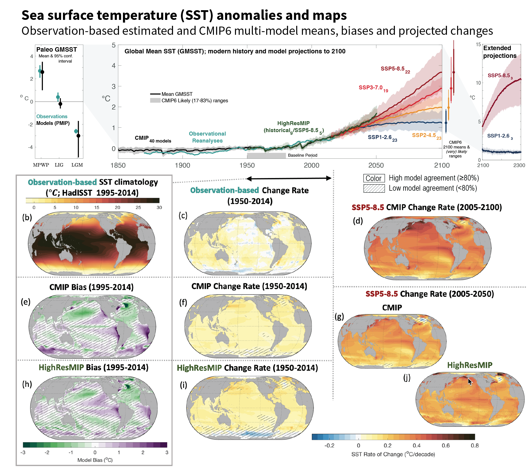 Figure 9.3 | Sea surface temperature (SST) and its changes with time. (a) Time series of global mean SST anomaly relative to 1950–1980 climatology. Shown are paleoclimate reconstructions and PMIP models, observational reanalyses (HadISST) and multi-model means from the Coupled Model Intercomparison Project (CMIP) historical simulations, CMIP projections, and HighResMIP experiment. (b) Map of observed SST (1995–2014 climatology HadISST). (c) Historical SST changes from observations. (d) CMIP 2005–2100 SST change rate. (e) Bias of CMIP. (f) CMIP change rate. (g) 2005–2050 change rate for SSP5-8.5 for the CMIP ensemble. (h) Bias of HighResMIP (bottom left) over 1995–2014. (i) HighResMIP change rate for 1950–2014. (j) 2005–2050 change rate for SSP5-8.5 for the HighResMIP ensemble. No overlay indicates regions with high model agreement, where ≥80% of models agree on sign of change. Diagonal lines indicate regions with low model agreement, where <80% of models agree on sign of change (see Cross-Chapter Box Atlas.1 for more information). Further details on data sources and processing are available in the chapter data table (Table 9.SM.9).
 Regions vary in the rate of SST warming, with slight cooling in some regions (Figure 9.3). The SROCC (Collins et al., 2019) and Section 7.4.4 assess SST changes over specific regions, which are consistent with the changes reported here. The tropical ocean has been warming faster than other regions since 1950, with the fastest warming in regions of the tropical Indian and western Pacific oceans (Figure 9.3), due to a combination of local atmosphere–ocean coupling, the Indonesian Throughflow (Section 9.2.3.4 and Figure 9.11), and trends in the Walker circulation (Sections 2.3.1.4.1 and 3.3.3.1, and Figure 3.16). The western boundary currents of the subtropical gyres have warmed faster than the global mean over the past century. There remains low agreement in the changes of the location and the dynamical changes in western boundary current extensions (Sections 2.3.3.4.2 and 9.2.3.4, and Figure 9.3). In the Arctic, the mean SST increase over the last two decades is similar to, or only slightly higher than, the global average (J.-L Chen et al., 2019). In contrast, the eastern Pacific Ocean, subpolar North Atlantic Ocean and Southern Ocean have warmed more slowly than the global average or cooled (Figure 9.3). Surface warming in the subpolar Southern Ocean has been slower than the global average since the 1950s, and this pattern is consistent with the upwelling around Antarctica renewing surface water with pre-industrial, deeper water masses (Section 9.2.3.2; Frölicher et al., 2015; J. Marshall et al., 2015; Armour et al., 2016). New evidence since SROCC (Meredith et al., 2019) confirms slight cooling since the 1980s around the subpolar Southern Ocean, contrasting with marked warming directly northward of it (Section 9.2.3.2; Haumann et al., 2020; Rye et al., 2020; Auger et al., 2021). In eastern boundary upwelling systems, SROCC (Bindoff et al., 2019) reported low agreement between SST trends in recent decades, due to varying spatio-temporal resolution and interannual to multi-decadal variability. Satellite evidence not included in SROCC shows that 92% of these regions warmed more slowly than neighbouring offshore locations between 1982 and 2015, so upwelling may buffer the near shore from warming (Section 9.2.3.5; Varela et al., 2018). Coupled ocean-atmospheric modes of variability strongly affect regional SST (Cross-Chapter Box 3.1 and Annex IV). In summary, a positive SST trend since 1950 is evident globally, but there is very high confidence that the Indian Ocean, western equatorial Pacific Ocean, and western boundary currents have warmed faster than the global average, while the Southern Ocean, the eastern equatorial Pacific, and the North Atlantic Ocean have warmed more slowly, or have slightly cooled.
In AR5 (Flato et al., 2013), a marginal improvement was noted in Coupled Model Intercomparison Project Phase 5 (CMIP5) climate model SST biases compared to Phase 3 (CMIP3) models in AR4, with a reduction in the magnitude of biases. The AR5 noted that, in several regions, large SST biases are symptomatic of errors in the representation of important processes, such as dynamics in the equatorial Pacific and North Atlantic, and Southern Ocean. Common regional biases in SST or historical SST trends are not exclusively linked to the representation of the ocean (high confidence), but can have multiple causes, including: errors in the representation of long-term historical trends in equatorial winds (Section 9.2.1.2); misrepresentation of the forced equatorial ocean response (Karnauskas et al., 2012; Kohyama et al., 2017; Coats and Karnauskas, 2018); thermocline depth errors (Linz et al., 2014); errors in atmospheric model cloud-related shortwave radiation (Hyder et al., 2018); biases in ocean circulation variability (C. Wang et al., 2014); and deficiencies in upper ocean (Q. Li et al., 2019) and atmospheric (Bates et al., 2012) boundary layer parametrizations. In CMIP6, the mid-latitude biases in the Northern Hemisphere are improved in the multi-model mean, and the inter-model standard deviation of the zonal mean SST error is significantly decreased in the northern Hemisphere south of 50°N compared to CMIP5, though biases in equatorial regions remain essentially unchanged (Section 3.5.1.1 and Figures 3.23, 3.24 and 9.3). Some long-standing ocean model biases have been reduced through increases in model resolution in CMIP6 (Bock et al., 2020) and improved parametrizations (Fox-Kemper et al., 2011; Q. Li et al., 2016; Qiao et al., 2016; Reichl and Hallberg, 2018). The High Resolution Model Intercomparison Project (HighResMIP) ensemble (Figure 9.3) has smaller cold biases in the North Atlantic and the tropical Pacific, and smaller warm biases in the upwelling regions off the western coasts of Africa, North and South America (Roberts et al., 2018, 2019; Caldwell et al., 2019; Docquier et al., 2019). In summary, CMIP6 models show persistent regional biases in representing the climatological SST state (very high confidence), but higher resolution reduces some biases, particularly in the North Atlantic and eastern boundary upwelling systems (Figure 9.3; high confidence).
The CMIP6 models represent the observed trends in SST patterns with greater fidelity than CMIP5, with the ocean area that is inconsistent with the observed trends decreasing by about three quarters from CMIP5 to CMIP6 (Olonscheck et al., 2020). In some regions, the direction of SST changes in observations are consistent with CMIP6 only when including internal variability (Olonscheck et al., 2020). This is notably the case in the equatorial Pacific, North Atlantic, and Southern Ocean, which are regions where SST is of known importance in controlling heat uptake (Section 9.2.2.1) and the global radiative feedback parameter (Section 7.4.4.3). Overall, despite some persistent regional biases, CMIP6 coupled climate models reproduce the observed SST trends or high internal variability over the past century over a range of different multi-decadal periods (Figure 9.3; Olonscheck et al., 2020; Watanabe et al., 2021), highlighting their skill to inform future large-scale SST changes at regional scale. Warming is projected at varying rates in all regions by 2050, except the North Atlantic Subpolar Region, the equatorial Pacific, and the Southern Ocean where models disagree (high confidence).
It is virtually certain that SST will continue to increase in the 21st century, at a rate depending on future emissions scenarios. The future global mean SST increase projected by CMIP6 models for the period 1995–2014 to 2081–2100 is 0.86 [5–95% range: 0.43–1.47] °C under SSP1-2.6, 1.51 [1.02 to 2.19] °C under SSP2-4.5, 2.19 [1.56 to 3.30] °C under SSP3-7.0, and 2.89 [2.01 to 4.07] °C under SSP5-8.5 (Figure 9.3). While under SSP1-2.6, the CMIP6 ensemble consistently projects that it is very likely at least 83% of the world ocean surface will have warmed by 2100, and under SSP5-8.5, at least 98% of the world ocean surface will have warmed. The spatial pattern of future change is consistent with observed SST change over the 20th century, though with notable regional differences (Figure 9.3). Long-term change in SST patterns is important for regional impacts but also affects radiative feedbacks, and therefore long-term change in climate sensitivity (Section 7.4.4.3). In the Southern Ocean, CMIP6 models project that SSTs will eventually consistently increase in the 21st century, at a rate dependent on future scenarios (Figure 9.3 and Section 9.2.3.2; Bracegirdle et al., 2020). Yet, there is only low confidence that this Southern Ocean warming will emerge by the end of the century (Section 7.4.4.1), due to the inconsistent historical and near-term simulations and observations over the 20th century (Figure 9.3). Furthermore, the equilibrium SST pattern from proxy records or simulated by climate models under CO2 forcing stand in contrast with the cooling trends in the Southern Ocean observed over the past decades (Section 7.4.4.1.2). Similarly, the SST change pattern observed in the tropical Pacific Ocean will transition on centennial time scales to a mean pattern resembling the El Niño pattern (medium confidence) (Annex IV). However, it is difficult to delineate a climate change trend ressembling an El Niño pattern and El Niño variability (Wittenberg, 2009; Collins et al., 2010) without large ensembles (Kay et al., 2015). Several Pliocene SST reconstructions indicate enhanced warming in the centre of the eastern Pacific equatorial cold tongue upwelling region, consistent with reconstruction of enhanced subsurface warming and enhanced warming in coastal upwelling regions (Section 7.4.4.2.2). The North Atlantic subpolar gyre is projected to continue to warm more slowly than surrounding regions (Suo et al., 2017), as the Gulf Stream concurrently warms rapidly (Figure 9.3; Cheng et al., 2013) and the Atlantic Meridional Overturning Circulation further declines under greenhouse gas forcing, although models disagree about the rate of change (Figure 9.3 and Section 9.2.3.1). In summary, CMIP6 models show a future pattern of SST change comparable to historical trends with intensity depending on future emissions scenario, and some of the observed cooling trends over the 20th century will eventually transition to a warming SST on centennial time scales, in particular in the Southern Ocean (high confidence) and in the equatorial Pacific (medium confidence), while the North Atlantic subpolar gyre will continue to warm more slowly than the global average (high confidence).
9.2.1.2 Air–Sea Fluxes
Air–sea fluxes of energy, freshwater, and momentum (wind stresses) are difficult to observe directly (Cronin et al., 2019), so estimates of the global mean net air–sea heat flux are inferred from observed ocean warming (Section 2.3.3.1, Box 7.2, and Cross-Chapter Box 9.1). Air–sea heat fluxes resemble the warming patterns of CMIP3 (Domingues et al., 2008; Levitus et al., 2012) and are consistent with the ensemble mean warming rate of CMIP5 (Cheng et al., 2017, 2019) and CMIP6 models (Section 3.5.1.3). Regional air–sea fluxes in models remain a key driver of uncertainty (Huber and Zanna, 2017; Tsujino et al., 2020). A substantial part of the upper 700 m energy increase is very likely attributed to anthropogenic forcing via increasing radiative forcing (Sections 3.5.1.3, 7.2 and 7.3).
The SROCC (Abram et al., 2019) and AR5 (Rhein et al., 2013) assessed that observations of air–sea fluxes had not yet reached the density or accuracy to directly detect trends beyond the noise. New evidence since SROCC confirms that direct heat and freshwater flux trends have not emerged yet as spatial (Figure 9.4), annual (Yu, 2019), and decadal (Zanna et al., 2019) variability overwhelm detection. Since AR5, comprehensive comparisons (Bentamy et al., 2017; Valdivieso et al., 2017; Yu et al., 2017) have used updated and new surface flux products to improve surface flux uncertainty estimates, and these comparisons note that implied global energy imbalances often exceed the observed ocean warming. Flux estimates using top of atmosphere observations and atmospheric fluxes from reanalysis have improved over past products (Trenberth and Fasullo, 2018) but require consistency adjustments (Trenberth et al., 2019) as the energy budget is not closed. Adjustments are needed for all flux products, and they remain less accurate than direct ocean heat content change measurements (Cheng et al., 2017). Some regional changes are likely robust in both satellite observations and projections (Figure 9.4). Recent satellite-based surface flux products with improved retrieval algorithms and new satellites, for example, J-OFURO3 (Tomita et al., 2019) and OAFlux-HR (Yu, 2019), provide a complete suite of turbulent fluxes including heat, moisture, and momentum. When combined with satellite-based surface radiation from Clouds and the Earth’s Radiant Energy System (CERES) Energy Balanced and Filled (EBAF; Kato et al., 2018) and precipitation from Global Precipitation Climatology Project (GPCP; Adler et al., 2003), full ocean-surface forcing is available since 1987 (Figure 9.4). These products agree with sparse buoy and ship observations within 30 W m–2(Bentamy et al., 2017; Cronin et al., 2019). While patterns agree between models and satellites in net fluxes (Figure 9.4), the trend magnitudes are substantially weaker in models. The fluxes tending to warm the North Atlantic and Southern Ocean are consistent with the largest changes observed in the surface properties and water masses (Sections 9.2.1.1, 9.2.2.1 and 9.2.2.3). The observed trend toward a saltier Atlantic Ocean and a fresher Indian Ocean, as well as trends in evaporation minus precipitation (E-P) patterns in the equatorial Pacific (see also Section 8.3.1) enhance the present mean pattern of wetting and drying. Elsewhere patterns are less clear, with only partial, large-scale agreement with the ‘wet gets wetter’ simplification (Sections 3.3.2.3, 4.4.1 and 4.5.1). In summary, globally integrated and large-scale fluxes are more reliably inferred from heat content and salinity change, while regional trends are rarely robust in observations; where they are robust, they tend to be underestimated or in disagreement in models (very high confidence).
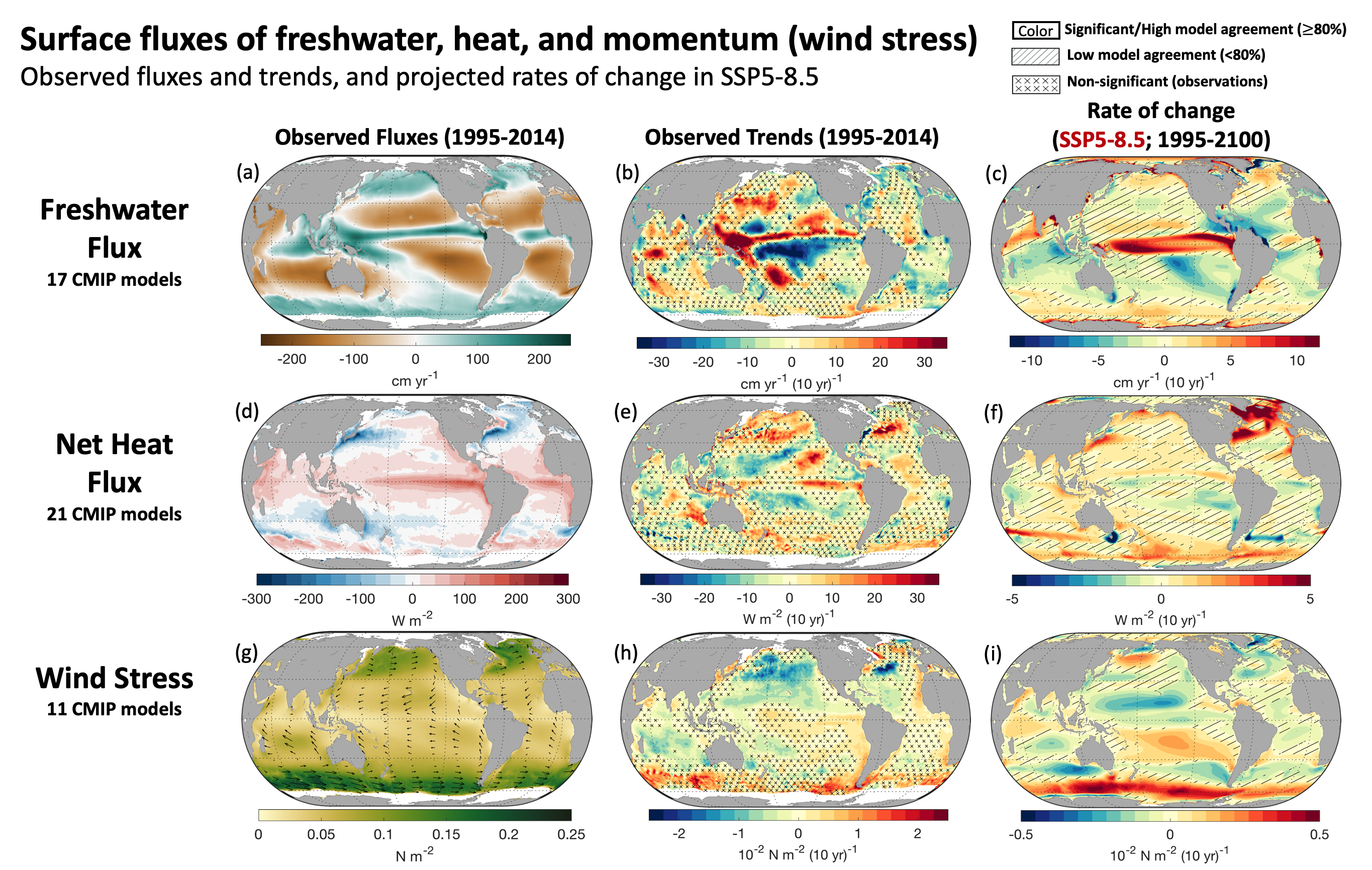
 Figure 9.4 | Global maps of observed mean fluxes (a, d, g), the observed trends in these fluxes (b, e, h) and the projected rate of change in these fluxes from SSP5-8.5 (c, f, i). Shown are the freshwater flux (a–c), net heat flux (d–f), and momentum flux or wind stress magnitude (g–i), with positive numbers indicating ocean freshening, warming, and accelerating respectively. The means and observed trends are calculated between 1995–2014 (freshwater and wind stress) or 2001–2014 (heat). The SSP5-8.5 projected rates are between 1995–2100 using 20-year averages at each end of the time period. Observations show objective interpolation from Clouds and the Earth’s Radiant Energy System (CERES) Energy Balanced and Filled (EBAF) v4 (Kato et al., 2018), Objectively Analyzed air–sea Fluxes-High Resolution (OAFlux-HR) (Yu, 2019), and Global Precipitation Climatology Project (GPCP) (Adler et al., 2003) of fluxes and flux trends (b, e, h). Observed trends with no overlay indicate regions where the trends are significant at p = 0.34 level. Crosses indicate regions where trends are not significant. For (c, f, i) projections, no overlay indicates regions with high model agreement, where ≥80% of models agree on the sign of change. Diagonal lines indicate regions with low model agreement, where <80% of models agree on the sign of change (see Cross-Chapter Box Atlas.1 for more information). Further details on data sources and processing are available in the chapter data table (Table 9.SM.9).
 There is low confidence in long-term wind stress trends in most regions, but a few locations have likely trends over the scatterometer era and in projections, as shown in Figure 9.4 (Desbiolles et al., 2017; Young and Ribal, 2019; Yu, 2019). The AR5 (Rhein et al., 2013) assessed with medium confidence that zonal wind stress over the Southern Ocean increased from the early 1980s to the 1990s (medium confidence) (Figure 9.4). Over 1995–2014, the zonal wind stress over the Southern Ocean continued to increase, westerly winds in the North Pacific and North Atlantic weakened, while the easterly equatorial Pacific winds of the Walker circulation strengthened (Figure 9.4). In historical simulations, CMIP5 models projected annular modes (Annex IV) to move poleward and strengthen in both hemispheres (Yang et al., 2016), while in CMIP6 models westerlies only strengthen over the Southern Ocean, with a weaker trend than recently observed (Figure 9.4 and Sections 4.5.1 and 4.5.3). In the tropical Pacific Ocean, a weakening trend in easterly winds and Walker circulation in the 20th century has been inferred based on observed sea level pressure data (Vecchi et al., 2006; Vecchi and Soden, 2007) and coral proxies (Carilli et al., 2014) and is projected to continue by CMIP6 models (Figure 9.4). Yet, over 1995–2014 observed winds have strengthened (Figure 9.4). The observed strengthening may have been influenced by a combination of factors (Section 7.4.4.2.1), but there is low confidence in the attribution of this signal to anthropogenic warming (Section 3.3.3.1) and medium confidence that it reflects internal variability (Section 8.3.2.3). Near-term projected changes over the Southern Ocean result from ozone recovery and greenhouse gases (Sections 4.3.3 and 4.4.3). Overall, there is only low confidence in observed and projected wind stress trends in most regions because trends in oceanic wind stresses during the satellite era have not emerged or are inconsistent with historical simulated changes.
Air–sea flux biases result from common causes in most models, and many are the same as during AR5 (Rhein et al., 2013). Important currents (e.g., Gulf Stream, Kuroshio, Antarctic Circum-polar Current patterns) are often found in erroneous locations in models, affecting SST and flux signatures (Bates et al., 2012; Beadling et al., 2020; J.-L.F. Li et al., 2020), but their locations are improved in high-resolution ocean models (Chassignet et al., 2017, 2020; Hewitt et al., 2020), and high-resolution coupled models reduce the mean air–sea flux biases (Delworth et al., 2012; Sakamoto et al., 2012; Small et al., 2014; Haarsma et al., 2016; Caldwell et al., 2019; L.C Jackson et al., 2020). Oceanic variability stems either from internal chaotic variability or atmospheric forcing (Hasselmann, 1976; Sérazin et al., 2016, 2017). Large-scale variability in the ocean tends to follow atmospheric forcing in low-resolution models, while in high-resolution coupled models ocean variability drives atmospheric variability on small scales (Bishop et al., 2017; Small et al., 2019), allowing these high-resolution models to mimic the coupling with clouds, precipitation, and atmospheric and oceanic boundary layers apparent in observations (Chelton and Xie, 2010; Frenger et al., 2013). Even coarse-resolution models, such as the ocean and sea ice components used in CMIP6, show significant sensitivity in the mean and variability of SST and sea ice to modest changes in flux forcing (Tsujino et al., 2020). Finally, there is still considerable disagreement between different parametrizations of air–sea fluxes used in models and strong scatter in direct observations (Renault et al., 2016; Brodeau et al., 2017). In summary, there is very high confidence that air–sea heat flux and stress biases are reduced in coupled models with high ocean resolution over coarse-resolution models, although the effect on trends remain unclear.
9.2.1.3 Upper-ocean Stratification and Surface Mixed Layers
The density difference from surface to deep ocean is the upper-ocean stratification. The AR5 (Rhein et al., 2013) assessed that it is very likely that the thermal contribution to stratification over the fixed 0–200 m layer increased by about 1% per decade between 1971 and 2010 (based on linear trend consistently across reports). The SROCC (Bindoff et al., 2019) found it very likely that density stratification increased by 0.46–0.51% per decade between 60°S and 60°N from 1970 to 2017). New published estimates based on a variety of different interpolated observations show that SROCC assessed rate is too low, even using the same data and methods (Li et al., 2020). The 1960–2018 stratification increase is estimated at 1.2 ± 0.1% per decade from the IAP dataset, 1.2 ± 0.4% per decade from the Ishii product, 0.7 ± 0.5% per decade from the EN4 dataset, 0.9 ± 0.5% per decade from ORAS4, and 1.2 ±0.3% per decade from the National Centers for Environmental Information (NCEI) dataset (G. Li et al., 2020). The improved methodology for computing stratification change on individual profiles before gridding yields a global annual mean increase of 0–200 m stratification change of 0.8 ± 0.2% per decade between 1960 and 2018 (Yamaguchi and Suga, 2019) and a global summer mean increase of 0–200 m stratification change of 1.3 ± 0.3% per decade between 1970 and 2018 (Sallée et al., 2021) is of a similar magnitude to the long-term trend (Yamaguchi and Suga, 2019; G. Li et al., 2020). In summary, there is limited evidence that focusing on changes over a fixed depth range might hide larger increases occurring at the seasonally and regionally variable pycnocline depth. There is also limited evidence that summer stratification change within the pycnocline has occurred at a rate of 8.9 ± 2.7% per decade from 1970 to 2018, and limited evidence of a winter pycnocline stratification increase (Cummins and Ross, 2020; Sallée et al., 2021).
While AR5 and SROCC did not assess change in mixed-layer depth, the reported changes in stratification can modulate the surface mixed-layer depth, which is set by a balance between fluxes and dynamical mixing (winds, tides, waves, convection) acting against the background stratification and restratification processes (solar and dynamical). Despite the large stratification increase observed at a global scale, new evidence shows that summer mixed-layer depth deepened consistently over the globe at a rate of 2.9 ± 0.5% per decade from 1970 to 2018, with the largest deepening observed in the Southern Ocean, corresponding to overall deepening from 3–15 m per decade depending on region (Somavilla et al., 2017; Sallée et al., 2021). While the shorter observational record in winter (compared to summer) does not allow global winter mixed-layer trends to be reliably assessed (Sallée et al., 2021), winter mixed-layer depths deepening at rates of 10 m per decade have been reported at individual long-term mid-latitude monitoring sites (Somavilla et al., 2017). Projections agree that shoaling of mixed-layer depth is expected in the 21st century, but only for strong emissions scenarios, and only in some regions (Figure 9.5). In summary, there is limited observational evidence that the mixed layer is globally deepening, while models show no emergence of a trend until later in the 21st century under strong emissions.
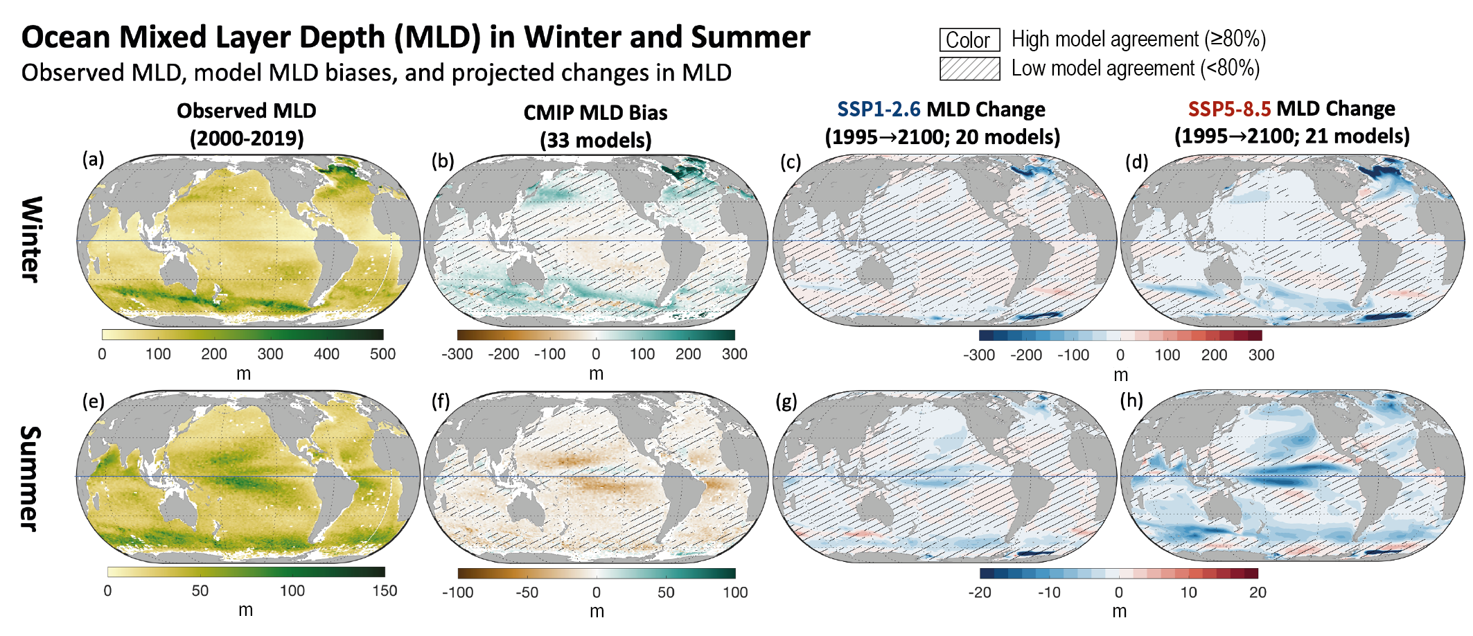
 Figure 9.5 | Mixed-layer depth in (a–d) winter and (e–h) summer. (a, e) Observed climatological mean mixed-layer depth (based on density threshold) from the Argo Mixed Layer Depth Climatology (Holte et al., 2017) usingobservations for 2000–2019. (b, f) Bias between the observation-based estimate (2000–2019) and the 1995–2014 Coupled Model Intercomparison Project Phase 6 (CMIP6) climatological mean mixed-layer depth. (c, d, g, h) Projected mixed-layer depth (MLD) change from 1995–2014 to 2081–2100 under (c, g) SSP1-2.6 and (d, h) SSP5-8.5 scenarios. The (a–d) winter row shows December–January–February (DJF) in the Northern Hemisphere and June–July–August (JJA) in the Southern Hemisphere; The (e–h) summer row shows JJA in the Northern Hemisphere and DJF in the Southern Hemisphere. The mixed-layer depth is the depth where the potential density is 0.03 kg m–3denser than at 10 m. No overlay indicates regions with high model agreement, where ≥80% of models agree on the sign of change. Diagonal lines indicate regions with low model agreement, where <80% of models agree on the sign of change (see Cross-Chapter Box Atlas.1 for more information). Further details on data sources and processing are available in the chapter data table (Table 9.SM.9).
 The SROCC assessed that upper-ocean stratification will continue to increase in the 21st century under increased radiative forcing (high confidence), due to increased surface temperature and high-latitude surface freshening (Bindoff et al., 2019). New climate model simulations concur with SROCC assessment of a future increase of the 0–200 m stratification under increased radiative forcing in all regions of the world ocean (Kwiatkowski et al., 2020). In addition, CMIP6 climate models project a shallowing of the mixed-layer in summer and winter by the end of the century under increased radiative forcing (Figure 9.5; Kwiatkowski et al., 2020), with the exception of the Arctic showing deepening of the mixed layer as a result of sea ice retreat (Figure 9.5; Lique et al., 2018). The regions of largest shallowing are associated with the deepest climatological mixed layer, in both winter and summer, particularly affecting the North Atlantic and the Southern Ocean basins (Figure 9.5). While CMIP6 models tend to project shallowing mixed layers under a warming climate, except at high latitudes (Figure 9.5; Lique et al., 2018; Kwiatkowski et al., 2020), a deepening in the summer mixed-layer depth by intensification of the surface winds and storms may explain inconsistency among models in many regions (Figure 9.5; Young and Ribal, 2019), although model mixed-layer biases are large in the summer in the Southern Ocean (Belcher et al., 2012; Sallée et al., 2013a; Q. Li et al., 2016; Tsujino et al., 2020). Lack of observed ocean turbulence and climate model limitations do not allow for direct assessment of ocean surface turbulence change and limit confidence in past and future mixed-layer change. Understanding of turbulent processes, their representation in ocean and climate models, and their effect on mixed-layer biases have been an active and rapidly evolving topic of research since AR5 (Buckingham et al., 2019; Q. Li et al., 2019). Small-scale mixed-layer processes are not resolved in climate models (D’Asaro, 2014; Buckingham et al., 2019; McWilliams, 2019) and despite significant improvements in their parametrization over the last decade (Fox-Kemper et al., 2011; Jochum et al., 2013; Q. Li et al., 2016, 2019; Qiao et al., 2016) and significant improvement in some models (Li and Fox-Kemper, 2017; Dunne et al., 2020), biases in mixed-layer representation generally persist (Heuzé, 2017; Williams et al., 2018; Cherchi et al., 2019; Golaz et al., 2019; Voldoire et al., 2019; Yukimoto et al., 2019; Boucher et al., 2020; Danabasoglu et al., 2020; Dunne et al., 2020; Kelley et al., 2020). In summary, the representation of upper-ocean stratification and mixed layers has improved in CMIP6 compared to CMIP5. While it is virtually certain that the global mean upper ocean will continue to stratify in the 21st century, there is only low confidence in the future evolution of mixed-layer depth, which is projected to mostly shoal under high emissions, except in high-latitude regions where sea ice retreats.
Box 9.2 | Marine Heatwaves
Marine heatwaves (MHW) are periods of extreme high sea temperature relative to the long-term mean seasonal cycle (Hobday et al., 2016). Studies since the Special Report on the Ocean and Cryosphere in a Changing Climate (SROCC; Collins et al., 2019) confirm the assessment that MHW can lead to severe and persistent impacts on marine ecosystems – from mass mortality of benthic communities, including coral bleaching, changes in phytoplankton blooms, shifts in species composition and geographical distribution, and toxic algal blooms, to decline in fisheries catch and mariculture (Smale et al., 2019; Cheung and Frölicher, 2020; Hayashida et al., 2020; Piatt et al., 2020). Unlike synoptic atmospheric heatwaves Section 11.3), MHWs can extend for millions of square kilometres, persist for weeks to months, and occur at subsurface (Bond et al., 2015; Schaeffer and Roughan, 2017; Perkins-Kirkpatrick et al., 2019; Laufkötter et al., 2020).
The SROCC established that MHWs have occurred in all basins over the last decades. Additional evidence documenting widespread occurrence of marine heat waves in all basins and marginal seas continues to accumulate (Y. Li et al., 2019; Yao et al., 2020). The SROCC highlighted the role of large-scale climate modes of variability in amplifying or suppressing MHW occurrences, which has since been further corroborated, increasing confidence in climate modes as important drivers of MHWs (Holbrook et al., 2019; Sen Gupta et al., 2020). More generally, understanding of processes leading to MHWs has increased since SROCC, including air–sea heat flux Section 9.2.1.2), increased horizontal heat advection, shoaling of the mixed-layer and suppressed mixing processes Section 9.2.1.3), reduced coastal upwelling and Ekman pumping Section 9.2.3.5), changes in eddy activities and planetary waves, and the re-emergence of warm subsurface anomalies (Holbrook et al., 2020; Sen Gupta et al., 2020).
The SROCC reported with high confidence that MHWs – defined as days exceeding the 99th percentile in sea surface temperature (SST) from 1982 to 2016 – have very likely doubled in frequency between 1982 and 2016. Additional observation-based evidence and acquisition of longer observation time series since SROCC have confirmed and expanded on this assessment: since the 1980s MHWs have also become more intense and longer (Frölicher and Laufkötter, 2018; Smale et al., 2019; Laufkötter et al., 2020). Satellite observations and reanalyses of SST show an increase in intensity of 0.04°C per decade from 1982 to 2016, an increase in spatial extent of 19% per decade from 1982 to 2016, and an increase in annual MHW days of 54% between the 1987–2016 period compared to 1925–1954 (Frölicher et al., 2018; Oliver, 2019). The SROCC assessed that 84–90% of all MHWs that occurred between 2006 and 2015 are very likely caused by anthropogenic warming. There is new evidence since SROCC that the frequency of the most impactful marine heatwaves over the last few decades has increased more than 20-fold because of anthropogenic global warming (Laufkötter et al., 2020). In summary, there is high confidence that MHWs have increased in frequency over the 20th century, with an approximate doubling from 1982 to 2016, and medium confidence that they have become more intense and longer since the 1980s.
Consistent with SROCC, future MHWs are defined with reference to the historical climate conditions. The SROCC assessed that MHWs willvery likely further increase in frequency, duration, spatial extent and intensity under future global warming in the 21st century. The CMIP6 projections allow us to confirm this assessment and quantify future change based on global mean probability ratio change (Box 9.2, Figure 1): they project MHWs willbecome four times (5–95% range: 2–9 times] more frequent in 2081–2100 compared to 1995–2014 under SSP1-2.6, or eight times (3–15 times) more frequent under SSP5-8.5. The SROCC highlighted that future change of MHWs will not be globally uniform, with the largest changes in the frequency of marine heatwaves being projected to occur in the western tropical Pacific and the Arctic Ocean (medium confidence). New evidence from the latest generation of climate models confirms and complements SROCC assessment (Box 9.2, Figure 1). Moderate increases are projected for mid-latitudes, and only small increases are projected for the Southern Ocean (medium confidence) (Hayashida et al., 2020). While under the SSP5-8.5 scenario, permanent MHWs (more than 360 days per year) are projected to occur in the 21st century in parts of the tropical ocean, the Arctic Ocean and around 45°S, the occurrence of such permanent MHWs can largely be avoided under the SSP1-2.6 scenario (Frölicher et al., 2018; Oliver et al., 2019; Plecha and Soares, 2020). The resolution of current climate models (CMIP5 and CMIP6) capture the broad features of MHWs, but they may have a bias towards weaker and longer MHWs in the historical period (medium confidence) (Frölicher et al., 2018; Pilo et al., 2019; Plecha and Soares, 2020) and greater intensification in western boundary current regions (Hayashida et al., 2020).
Box 9.2
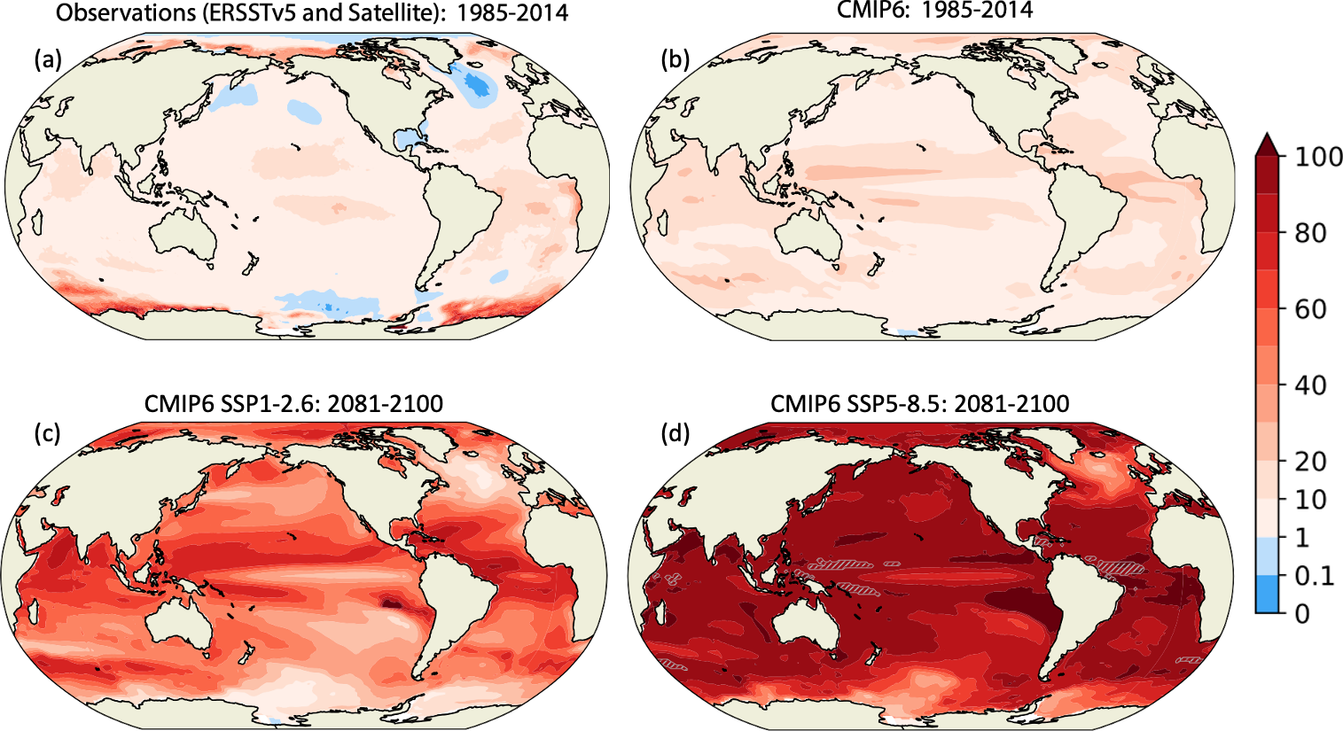
Box 9.2, Figure 1 | Observed and simulated regional probability ratio of marine heatwaves (MHWs) for the 1985–2014 period and for the end of the 21st century under two different greenhouse gas emissions scenarios. The probability ratio is the proportion by which the number of MHW days per year has increased relative to pre-industrial times. An MHW is defined as a deviation beyond the daily 99th percentile (11-day window) in the deseasonalized sea surface temperature. (a)The MHW probability ratio from satellite observations (NOAA OISST V2.1; Huang et al. 2020) during 1985–2014. The mean warming pattern (difference in ERSST5 (Huang et al. 2017) sea surface temperature between the 1985–2014 and 1854–1900 periods) has been added to the satellite observations to calculate the probability ratio. (b–d)Coupled Model Intercomparison Project Phase 6 (CMIP6) simulated multi-model mean probability ratio of the(b)1985–2014 period, and 2081–2100 period in the(c) SSP1 2.6 and(d) SSP5 8.5 scenarios. The areas with grey diagonal lines in (d) indicate permanent MHWs (>360 heatwave days per year). These 14 CMIP6 models are included in the analysis: ACCESS-CM2, CESM2, CESM2-WACCM, CMCCCM2-SR5, CNRM-CM6-1, CNRM-ESM2-1, CanESM5, EC-Earth3, IPSL-CM6A-LR, MIROC6, MRI-ESM2-0, NESM3, NorESM2-LM, NorESM2-MM. Further details on data sources and processing are available in the chapter data table (Table 9.SM.9).
9.2.2 Changes in Heat and Salinity
9.2.2.1 Ocean Heat Content and Heat Transport
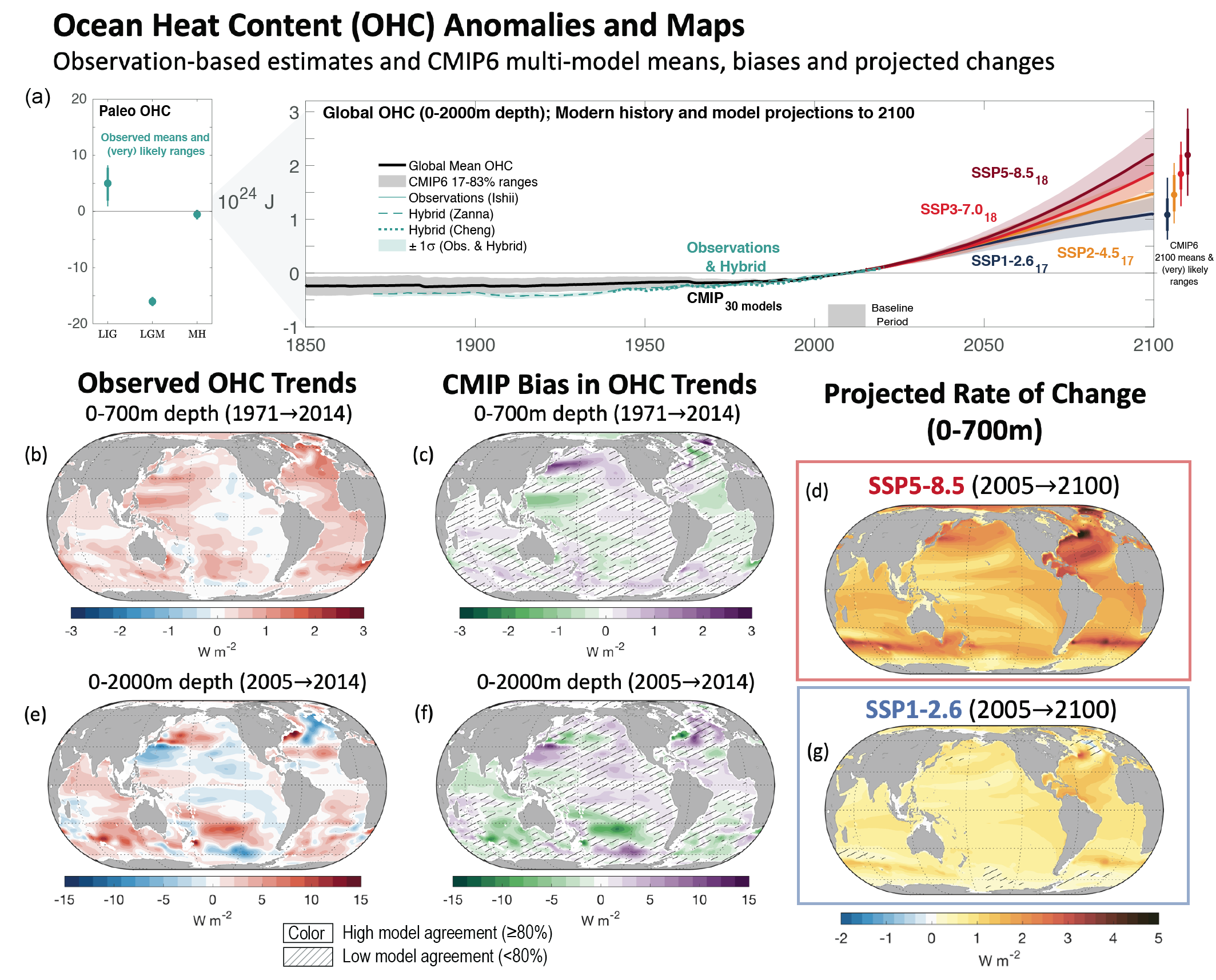
Ocean warming – that is, increasing ocean heat content (OHC) – is an important aspect of energy on Earth: SROCC (Bindoff et al., 2019) reported that there is high confidence that ocean warming during 1971–2010 dominated the increase in the Earth’s energy inventory, which is confirmed by the Box 7.2 assessment that the ocean has stored 91% of the total energy gained from 1971 to 2018. As reported in Sections 2.3.3.1, 3.5.1.3 and 7.2.2.2, Box 7.2 and Cross-Chapter Box 9.1, confidence in the assessment of global OHC change since 1971 is strengthened compared to previous reports, and extended backward to include likely warming since 1871. Table 7.1 updates the estimates of total ocean heat gains from 1971 to 2018, 1993 to 2018 and 2006 to 2018. Section 3.5.1.3 assesses that it is extremely likely that anthropogenic forcing was the main driver of the OHC increase over the historical period. Section 2.3.3.1 reports that current multi-decadal to centennial rates of OHC gain are greater than at any point since the last deglaciation (medium confidence).
Ocean warming is not uniform with depth. The AR5 (Rhein et al., 2013) assessed that, since 1971, ocean warming was virtually certain for the upper 700 m and likely for the 700–2000 m layer. Both AR5 and SROCC (Bindoff et al., 2019) assessed that the deep ocean below 2000 m had likely warmed since 1992, especially in the Southern Ocean. Section 2.3.3.1 provides an updated assessment of ocean temperature change for different depth layers, time periods and observation-based reconstructions (Table 2.7). Section 2.3.3.1 confirms the previous assessment that it is virtually certain that the upper ocean (0–700 m) has warmed since 1971, that ocean warming at intermediate depths (700–2000 m) is very likely since 2006, and that it is likely that ocean warming has occurred below 2000 m since 1992. Section 3.5.1.3 assessed that it is extremely likely that human influence was the main driver of the ocean heat content increase observed since the 1970s, which extends into the deeper ocean (very high confidence), and shows that biases in potential temperature have a complex pattern (Figure 3.25). In the present section, we assess the regional patterns of this warming and associated processes driving regional ocean warming.
The rate of ocean warming varies regionally, with some regions having experienced slight cooling (Figure 9.6). The SROCC (Bindoff et al., 2019) assessed that ocean warming in the 0–700 m depth is globally widespread, with slower than global average warming in the subpolar North Atlantic. The SROCC (Meredith et al., 2019) also estimated that the Southern Ocean accounted for around 75% of global ocean heat uptake during 1870–1995 and that 35–43% of the upper 2000 m global ocean warming occurred in the Southern Ocean over 1970–2017 (45–62% for 2005–2017). The SROCC noted that this interhemispheric asymmetry might (at least partially) be explained by high concentrations of aerosols in the Northern Hemisphere. Here, we confirm these assessments, bring new evidence attributing these regional trends, and discuss the role of decadal ocean circulation variability in redistributing heat, driving interhemispheric asymmetry of the recent rate of ocean warming (Rathore et al., 2020; L. Wang et al., 2021). Since SROCC, one new study shows that the subpolar North Atlantic ‘warming hole’ observed since the 1980s has emerged from internal climate variability and can be attributed to greenhouse gas emissions (Chemke et al., 2020). A new analysis of a suite of climate models (Hobbs et al., 2021) confirms SROCC assessment, based on one paper (Swart et al., 2018), attributing the observed Southern Ocean warming to anthropogenic forcing. Given the large fraction of global ocean warming in the Southern Ocean and the sparse observations there before 2005, there is limited evidence that global OHC increase since 1971 might have been underestimated (Cheng and Zhu, 2014; Durack et al., 2014). Cross-Chapter Box 9.1 accounts for an increased error before 2005 in global OHC change. In summary, in the upper 2000 m since the 1970s, the subpolar North Atlantic has been slowly warming, and the Southern Ocean has stored a disproportionally large amount of anthropogenic heat (medium confidence).
 Figure 9.6 | Ocean heat content (OHC) and its changes with time. (a) Time series of global OHC anomaly relative to a 2005–2014 climatology in the upper 2000 m of the ocean. Shown are observations (Ishii et al., 2017; Baggenstos et al., 2019; Shackleton et al., 2020), model-observation hybrids (Cheng et al., 2019; Zanna et al., 2019), and multi-model means from the Coupled Model Intercomparison Project Phase 6 (CMIP6) historical (29 models) and Shared Socio-economic Pathway (SSP) scenarios (label subscripts indicate number of models per SSP). (b–g) Maps of OHC across different time periods, in different layers, and from different datasets/experiments. Maps show the CMIP6 ensemble bias and observed (Ishii et al., 2017) trends of OHC for (b, c) 0–700 m for the period 1971–2014, and (e, f) 0–2000 m for the period 2005–2017. CMIP6 ensemble mean maps show projected rate of change 2015–2100 for (d) SSP5-8.5 and (g) SSP1-2.6 scenarios. Also shown are the projected change in 0–700 m OHC for (d) SSP1-2.6 and (g) SSP5-8.5 in the CMIP6 ensembles, for the period 2091–2100 versus 2005–2014. No overlay indicates regions with high model agreement, where ≥80% of models agree on the sign of change. Diagonal lines indicate regions with low model agreement, where <80% of models agree on the sign of change (see Cross-Chapter Box Atlas.1 for more information). Further details on data sources and processing are available in the chapter data table (Table 9.SM.9).
 Below 2000 m, direct observations of full-depth ocean temperature change are limited to ship-based, high-quality deep-ocean temperature measurements. Such high-quality full-depth ship-based sampling has improved from 1990 to the present due to the World Ocean Circulation Experiment (WOCE) and the Global Ocean Ship-based Hydrographic Investigations Program (GO-SHIP; Sloyan et al., 2019). The SROCC (Bindoff et al., 2019) assessed that the likely warming of the ocean since the 1990s below 2000 m is associated with a marked regional pattern, with larger warming in the Southern Ocean. In the deep North Atlantic, warming has reversed to cooling over the past decade, possibly due to internal variability fed by North Atlantic Deep Water (Section 9.2.2.3). Over the past decade, the warming rate of Antarctic Bottom Water (AABW; Section 9.2.2.3) has been dependent on origin: slower from the Weddell Sea and faster from the Ross Sea and Adélie Land. One new study (Purkey et al., 2019) strengthens confidence in AABW warming: below 4000 m a monotonic, basin‐wide, and multi-decadal temperature change is found in the southern Pacific basin, with larger warming rates near the bottom water formation sites than further downstream. New analysis of one model provides limited evidence that the sparse observational record may underestimate the rate of deep-ocean warming from 1990 to 2010 by about 20% (Garry et al., 2019) which is included in the assessed OHC error (Cross-Chapter Box 9.1). There is still low agreement in deep-ocean changes from ocean data assimilation reanalyses (Palmer et al., 2017) and low confidence in such inferences. In summary, while observational coverage below 2000 m is sparser than in the upper 2000 m, there is high confidence that deep-ocean warming below 2000 m has been larger in the Southern Ocean than in other ocean basins due to widespread AABW warming.
Different processes drive OHC patterns over a range of time scales. Recent literature has highlighted the role of ocean circulation variability in driving OHC patterns by decomposing the global pattern of OHC change into a combination of added heat due to climate change taken up under fixed ocean circulation (‘added heat’), and redistribution of heat associated with changing ocean currents (‘redistributed heat’; Gregory et al., 2016; Bronselaer and Zanna, 2020; Couldrey et al., 2021). Redistributed heat alters regional patterns of heat storage and carbon storage (Cross-Chapter Box 5.3; Bronselaer and Zanna, 2020; Todd et al., 2020; Couldrey et al., 2021) but does not affect the global OHC. There is medium confidence that decadal variability of the ocean circulation strengthened the rate of ocean warming in the Southern Hemisphere compared to the Northern Hemisphere in the decade from 2005 (Rathore et al., 2020; L. Wang et al., 2021; Zika et al., 2021). More generally, since 2005, the OHC pattern observed is predominantly due to heat redistribution with regions of both warming and cooling (Figure 9.6; Zika et al., 2021); however, extending analysis back to 1972 shows the importance of added heat setting a large-scale warming pattern with mid-latitude maxima consistent with subduction of water masses, particularly in Southern Hemisphere Mode Waters (Section 9.2.2.3, and Figures 9.6 and 9.8; Bronselaer and Zanna, 2020). The longer the analysis window, the more added heat dominates over redistributed heat. This translates into more ocean area with statistically significant warming trends and less area with statistically significant cooling trends (Johnson and Lyman, 2020). The region where added heat is most compensated for by redistributed cooling is in the northern North Atlantic basin, where changes in the subpolar gyre circulation and Atlantic Meridional Overturning Circulation (AMOC) result in cooling (Section 9.2.3.1; Williams et al., 2015; Piecuch et al., 2017; Zanna et al., 2019; Bronselaer and Zanna, 2020). In summary, and strengthening SROCC assessment, ocean warming is not globally uniform due to patterns of uptake predominantly along known water mass pathways, and due to changing ocean circulation redistributing heat within the ocean (high confidence).
While heat redistribution reflects changes in ocean circulation and is a useful concept to understand the underlying processes driving OHC patterns, change in ocean heat transport (OHT) arises due to changes in ocean circulation and ocean temperature and affects regional OHC change. The AR5 did not assess change in OHT and SROCC (Meredith et al., 2019) only assessed projected OHT increases into the Nordic Seas and the Arctic Ocean. New evidence of increasing northward OHT into the Arctic has been observed in recent decades (Muilwijk et al., 2018; Q. Wang et al., 2019; Tsubouchi et al., 2021), similar to SROCC assessment, and consistent with observed increase in OHC in the ice-free Arctic ocean (Mayer et al., 2019). It is estimated that an increase of 0.021 PW of OHT occurred after 2001 into the Arctic, which is sufficient to account for the recent OHC change in the northern seas (Tsubouchi et al., 2021). However, these trends cannot yet be attributed to anthropogenic forcing due to potential internal variability (Muilwijk et al., 2018; Wang et al., 2019). New evidence strengthens the case that El Niño–Southern Oscillation (ENSO) and the Northern Annular Mode affect interannual OHT variability (Trenberth et al., 2019) and shows that a slowing AMOC reduces northward OHT in the Atlantic at 26.5°N (Section 9.2.3.1 and Figure 9.8; Bryden et al., 2020). Despite a decrease of AMOC northward heat (0.17 PW) and mass (2.5 Sverdrup (Sv); 1 Sv = 109kg s–1) transport, OHT has increased toward the Arctic through increased upper northern North Atlantic temperatures and stronger wind-driven gyres (medium confidence) (Section 9.2.3.4 and Figure 9.11; Singh et al., 2017; Oldenburg et al., 2018). In summary, OHT has increased toward the Arctic in recent decades, which at least partially explains the recent OHC change in the Arctic (medium confidence).
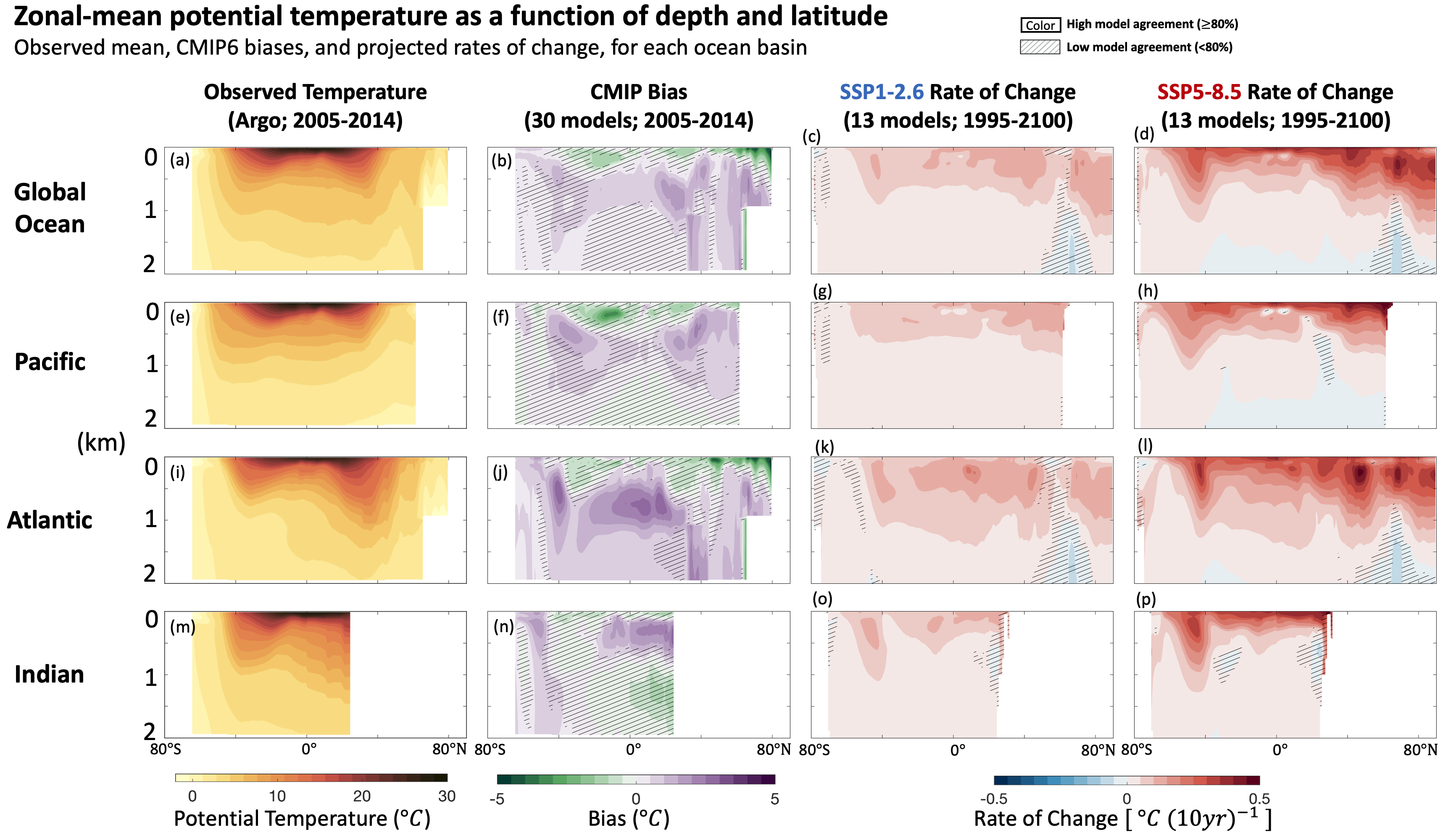 Figure 9.7 | Meridional-depth profiles of zonal-mean potential temperature in the ocean and its rate of change in the upper 2000 m of the Global, Pacific, Atlantic and Indian oceans. Shown are (a, e, i, m) observed temperature (Argo climatology 2005–2014), (b, f, j, n) bias of the Coupled Model Intercomparison Project Phase 6 (CMIP6) ensemble over this period, and future changes under (c, g, k, o) SSP1-2.6 and (d, h, l, p) SSP5-8.5. No overlay indicates regions with high model agreement, where ≥80% of models agree on the sign of change. Diagonal lines indicate regions with low model agreement, where <80% of models agree on the sign of change (see Cross-Chapter Box Atlas.1 for more information). Further details on data sources and processing are available in the chapter data table (Table 9.SM.9).
 Major volcanic eruptions have caused interannual to decadal cooling phases within the marked long-term increase in global OHC – Mount Agung in 1963, El Chichón in 1982 and Mount Pinatubo in 1991 (Cross-Chapter Box 4.1; Church et al., 2005; Fasullo et al., 2016; Stevenson et al., 2016; Fasullo and Nerem, 2018). In the first few years following an eruption, heat exchange with the subsurface ocean allows atmospheric cooling to be sequestered into the seasonal thermocline, therefore reducing the magnitude of the peak atmospheric temperature anomaly (Gupta and Marshall, 2018). However, while explosive volcanic eruptions only disturb the Earth’s radiative budget and surface fluxes for a few years, the ocean preserves an anomaly in OHC in the upper 500 m (also affecting thermosteric sea level) many years after the eruption (Gupta and Marshall, 2018; Bilbao et al., 2019). The anomaly affects the atmosphere through air–sea heat fluxes with surface conditions returning to normal only after several decades (Gupta and Marshall, 2018; Bilbao et al., 2019), or on centennial time scales in the case of repeated eruptions (G.H. Miller et al., 2012; Atwood et al., 2016; Gupta and Marshall, 2018). In summary, there is medium confidence that oceanic mechanisms buffer the atmospheric response to volcanic eruptions on annual time scales by storing volcanic cooling in the subsurface ocean, affecting OHC and thermosteric sea level on decadal to centennial time scales.
CMIP5 and CMIP6 models simulate OHC changes that are consistent with the updated observational and improved estimates of OHC over the period 1960 to 2018 (Figures 9.6, 9.7 and 9.8), and they replicate the vertical partitioning of OHC change for the industrial era, although with a tendency to underestimate OHC gain shallower than 2000 m and overestimate it deeper than 2000 m (Section 3.5.1.3). The AR5 (Flato et al., 2013) assessed that climate models transport heat downward more than the real ocean. Since AR5, studies have shown that increasing the horizontal resolution of ocean models tends to increase agreement of vertical heat transport with observations as the dependency on ad-hoc choices of eddy parametrizations is relaxed (Griffies et al., 2015; Chassignet et al., 2020). The magnitude of the AMOC and Indonesian Throughflow affect future OHC change – for example, through overestimated modelled downward heat pumping (Kostov et al., 2014) – and there are indications of greater model consistency in these transports at higher resolution (Figure 9.10; Chassignet et al., 2020; L.C. Jackson et al., 2020). Climate models tend to reproduce the observed added heat, but redistributed heat is less well represented (Figure 9.8; Bronselaer and Zanna, 2020; Dias et al., 2020; Couldrey et al., 2021). Since redistributed heat dominates historical OHC change, historical simulations poorly reproduce regional patterns, but as future OHC change will become dominated by added heat, more skill in future modelled OHC patterns is expected (Bronselaer and Zanna, 2020). In summary, climate models have more skill in representing OHC change from added heat than from ocean circulation change (high confidence). Since added heat dominates over redistributed heat on a centennial scale (especially under high-emissions scenarios) confidence in future modelled OHC patterns at the end of the 21st century is greater than at decadal scale.
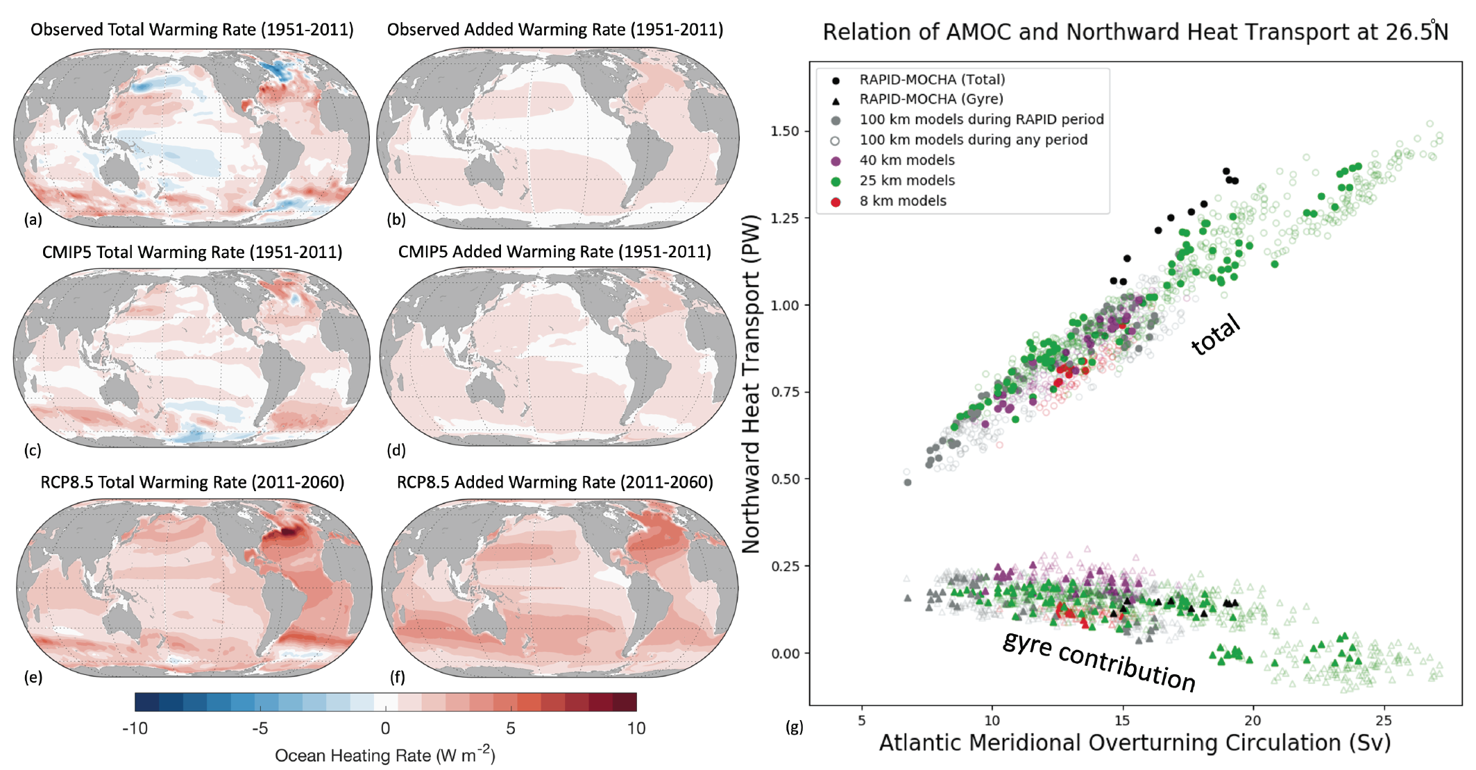 Figure 9.8 | Decomposition of simulated ocean heat content and northward ocean heat transport. (a, c, e) Total ocean heat content (0–2000 m) warming rate as observed and simulated by Coupled Model Intercomparison Project Phase 5 (CMIP5) models over the historical period (1972–2011) and under the RCP8.5 future (2021–2060) versus the associated decomposed (b, d, f) added heat contribution (neglecting changes in ocean circulation) to the total(Bronselaer and Zanna, 2020). (g) Relationship between northward heat transport and Atlantic Meridional Overturning Circulation (AMOC) in HighResMIP models (1950–2050) and observations during the RAPID period (2004–2018). Further details on data sources and processing are available in the chapter data table (Table 9.SM.9).
 The SROCC (Bindoff et al., 2019) assessed that the ocean will continue to take up heat in the coming decades for all plausible scenarios, and here this assessment is confirmed with very high confidence. The SROCC reported that, compared with the observed changes since the 1970s, the warming of the ocean by 2100 would very likely double to quadruple for low-emissions scenarios (RCP2.6) and increase five to seven times for high-emissions scenarios (RCP8.5). The SROCC also concluded with high confidence that the overall warming of the ocean would continue this century, even after radiative forcing and mean surface temperatures stabilize. The SROCC projected that OHC in the 0–2000 m layer will increase from 2017 to 2100 by 0.900 ± 0.345 YJ (1 YJ = 1024Joules) under RCP2.6 and 2.150 ± 0.540 YJ under RCP8.5. Updating SROCC estimates with CMIP6 projections gives heat content increases and 17–83% ranges in the 0–2000 m layer between 1995–2014 and 2081–2100 of 1.06 (0.80–1.31) YJ, 1.35 (1.08–1.67) YJ, 1.62 (1.37–1.91) YJ, 1.89 (1.60–2.29) YJ under scenarios SSP1-2.6, SSP2-4.5, SSP3-7.0, and SSP5-8.5, respectively (Figure 9.6 and Table 9.1). The two-layer model used here to calculate thermosteric sea level rise (9.SM.4) and tuned for AR6-assessed equilibrium climate sensitivity (ECS; Section 7.SM.2), provides consistent 17–83% ranges of 1.18 (0.99–1.42) YJ, 1.56 (1.33–1.86) YJ, 1.90 (1.63–2.21) YJ, 2.23 (1.92–2.64) YJ under scenarios SSP1-2.6, SSP2-4.5, SSP3-7.0, and SSP5-8.5, respectively (Table 9.1). Based on CMIP6 models and the two-layer model, it is likely that, between 1995–2014 and 2081–2100, OHC will increase two to four times the amount of the 1971–2018 OHC increase under SSP1-2.6, and four to eight times that amount under SSP5-8.5. The CMIP6 models show that OHC dependence on scenarios begins only after about 2040 (Figure 9.6).
The OHC patterns projected by CMIP6 models (Figures 9.6 and 9.7) are similar to the CMIP5 projections assessed in SROCC (Bindoff et al., 2019): faster warming in all water mass subduction regions (e.g., subtropical cells and mode waters); deeper penetration in the centre of subtropical gyres; slower northern North Atlantic warming due to slowing AMOC; and slower subpolar Southern Ocean warming due upwelled pre-industrial water masses. Decreased aerosol forcing will allow Northern Hemisphere ocean warming to be faster and less dominated by Southern Hemisphere change (Shi et al., 2018; Irving et al., 2019). Since SROCC, distinguishing between added and redistributed heat has aided in understanding projections (Bronselaer and Zanna, 2020; Dias et al., 2020; Couldrey et al., 2021). The near-term decades will feature patterns strongly influenced by heat redistribution and internal variability (Rathore et al., 2020). Strengthening Southern Hemisphere westerlies are projected, except for stringent mitigation scenarios (Bracegirdle et al., 2020), and will cause a northward and downward OHT. There is low agreement in future Southern Ocean warming across model results due to uncertainties in the magnitude of westerly wind changes (Figure 9.4; Liu et al., 2018; He et al., 2019; Dias et al., 2020; Lyu et al., 2020b) and the degree of eddy compensation of overturning across different parametrizations and resolutions (Section 9.2.3.2; Beal and Elipot, 2016; Mak et al., 2017; Roberts et al., 2020). By 2100, however, the OHC change will be dominated by the added heat response, particularly for strong warming scenarios (Garuba and Klinger, 2018; Bronselaer and Zanna, 2020) with added heat following unperturbed water mass pathways in the North Atlantic and Southern Ocean (Figure 9.8; Dias et al., 2020; Couldrey et al., 2021). There is high confidence that projected weakening of the AMOC (Section 9.2.3.1) will cause a decrease in northward OHT in the Northern Hemisphere mid-latitudes (Figure 9.8 and Sections 9.2.3.1 and 4.3.2.3; Weijer et al., 2020) associated with a dipole pattern of Atlantic OHC redistributed from northern to low latitudes that may override added heating in the northern North Atlantic (Figures 9.6, 9.7 and 9.8). Variations in the degree of AMOC redistributed heat (Menary and Wood, 2018) causes large intermodel spread in SST (Figure 9.3) and OHC change (Figure 9.6; Kostov et al., 2014; Bronselaer and Zanna, 2020; Todd et al., 2020; Couldrey et al., 2021). In the 700–2000 m depth range, CMIP5 and CMIP6 models project the largest warming to be in the North Atlantic Deep Water and Antarctic Intermediate Water (Figure 9.7) while below 2000 m, the North Atlantic cools in many models, and Antarctic Bottom Waters warm (Sallée et al., 2013b; Heuzé et al., 2015). In summary, on decadal time scales, redistribution will dominate regional patterns of OHC change without affecting the globally integrated OHC; however, by 2100, particularly under strong warming scenarios, there is high confidence that regional patterns of OHC change will be dominated by added heat entering the sea surface, primarily in water mass formation regions in the subtropics; and reduced aerosols will increase the relative rate of Northern Hemisphere heat uptake (medium confidence).
The SROCC assessed that the warming of the deep ocean is slow to manifest, with multi-century or longer response times, so global OHC (and global mean thermosteric sea level) will continue to rise for centuries (Figures 9.9 and 9.30). New studies show that this continuation persists, even after cessation of greenhouse gas emissions (Ehlert and Zickfeld, 2018). Ocean warming will continue, even after emissions reach zero because of slow ocean circulation (Larson et al., 2020). OHC will increase until at least 2300, even for low-emissions scenarios, but with a scenario-dependent rate (Nauels et al., 2017; Palmer et al., 2018) and depends on cumulative CO2 emissions, as well as the time profile of emissions (Bouttes et al., 2013). Past long-term changes in total OHC illustrate adjustment relevant to expected future changes (Figure 9.9). Observational data from ice core rare gas elemental and isotopic ratios document a rise in global OHC relative to the Last Glacial Maximum of >17,000 ZJ (change in mean ocean temperature >3.1°C; 1 ZJ = 1021Joules) (Figure 9.9; Bereiter et al., 2018; Baggenstos et al., 2019; Shackleton et al., 2019, 2020). This temperature increase is significantly larger than the modelled OHC changes associated with collapse of AMOC alone, and tracks rising Southern Ocean SST (Uemura et al., 2018), strengthening of the deep abyssal overturning cell (Du et al., 2020) and increased North Atlantic water in the Southern Ocean (Wilson et al., 2020). This underscores the importance of Antarctic abyssal ventilation on long-term oceanic heat budgets (Section 9.2.3.2). An ensemble of four intermediate-complexity models project 10,000-year future responses to CO2 emissions (Clark et al., 2016) with SST change peaking around 2300 and a varying scenario-dependent magnitude approaching the scale of glacial-to-interglacial changes in paleodata (Figure 9.9). Long-term OHC commitments relative to 1850–1900 conditions are 2.6, 9.7, 15.2, 21.6, and 28.0 YJ (with mean ocean temperature change as much as 5.1°C) for emissions of 0, 1280, 2560, and 3840 and 5120 Gt after 2000 CE respectively, with OHC peaking near 4000 CE, reflecting whole-ocean warming lagging SST by thousands of years. The exact timing is uncertain, subject to rates of high-latitude meltwater input (Van Breedam et al., 2020) and circulation time (Gebbie and Huybers, 2019). In summary, there is very high confidence that there is a long-term commitment to increased OHC in response to anthropogenic CO2 emissions, which is essentially irreversible on human time scales.
 Figure 9.9 | Long-term trends of ocean heat content (OHC) and surface temperature. (a, b) Ice-core rare gas estimates of past mean OHC (ZJ), scaled to global mean ocean temperature (°C), and to steric global mean sea level (GMSL) (m) per CCB-2 (red dashed line), compared to surface temperatures (black solid line, gold solid line; °C rightmost axis). Southern Ocean sea surface temperature (SST) from multiple proxies in 11 sediment cores and from ice core deuterium excess (Uemura et al., 2018). (a) Penultimate glacial interval to last interglacial, 150,000–100,000 yr B2K (before 2000) (Shackleton et al., 2020). (b) Last glacial interval to modern interglacial, 40,000–0 yr B2K (Baggenstos et al., 2019; Shackleton et al., 2019). Changes in OHC (dashed lines) track changes in Southern Ocean SST (solid lines). (c) Long-term projected (2000 to 12000 CE) changes of OHC (dashed lines) in response to four greenhouse gas emissions scenarios (Clark et al., 2016) scale similarly to large-scale paleo changes but lag projected global mean SST (solid lines). (d) model simulated 1500–1999 OHC (Gregory et al., 2006) and 1955–2019 observations (Levitus et al., 2012) updated by NOAA NODC. All data expressed as anomalies relative to pre-industrial time. Further details on data sources and processing are available in the chapter data table (Table 9.SM.9).
 9.2.2.2 Ocean Salinity
The AR5 (Rhein et al., 2013) assessed that it was very likely that subsurface salinity changes reflect surface salinity change, and that basin-scale regions of high salinity and evaporation had trended more saline, while regions of low salinity and more precipitation had trended fresher since the 1950s. The SROCC (Bindoff et al., 2019) assessment was consistent with AR5. Section 2.3.3.2 strengthens evidence that subsurface salinity trends are connected to surface trends (very likely) , which are, in turn, linked to an intensifying hydrological cycle (medium confidence). Increasing evidence from updated observational records indicates that it is nowvirtually certain that surface salinity contrasts are increasing. At basin scale, Section 2.3.3.2 and AR5 concur that it is very likely that the Pacific and Southern Ocean have freshened, and the Atlantic has become more saline. Figures 3.25 and 3.27 compare CMIP6 models to salinity observations.
Globally the mean salinity contrast at near-surface between high- and low-salinity regions increased 0.14 [0.07 to 0.20] from 1950 to 2019 (Section 2.3.3.2). At regional scale, SROCC (Meredith et al., 2019) assessed an Arctic liquid freshwater trend of 600 ± 300 km3yr–1(600 ± 200 Gt yr–1) between 1992 and 2012, reflecting changes associated with continental freshwater imports that affect ocean mass (land ice, rivers) as well as changes in sea ice volume. Since AR5, regional observation-based analyses not assessed in SROCC further confirm the long-term, large-scale and regional patterns of salinity change, both at the ocean surface and in the subsurface ocean, including almost 120 years of changes in the North Atlantic (Friedman et al., 2017) and 60 years of monitoring in the subpolar North Pacific (Cummins and Ross, 2020). These longer time series also provide context to detect large multi-annual change from 2012 to 2016 in the subpolar North Atlantic, unprecedented over the centennial record (Holliday et al., 2020). In summary, there is high confidence that salinity trends have extended for more than 60 to 100 years in the regions with long historical observation records, such as the North Pacific and the North Atlantic basin.
While there is low confidence in direct estimates of trends in surface freshwater fluxes (Sections 2.3.1.3.5, 8.3.1.1 and 9.2.1.2), as discussed in SROCC (Meredith et al., 2019), observational studies coupled with modelling studies suggest that surface flux changes drive many observed near-surface salinity changes, on top of changes specific to polar regions. Advances in salinity observations – for example, the Argo program (Riser et al., 2016); Soil Moisture and Ocean Salinity (SMOS), Aquarius and Soil Moisture Active Passive (SMAP; Supply et al., 2018; Vinogradova et al., 2019) – combined with process studies (SPURS-1/2; Lindstrom et al., 2015; SPURS-2 Planning Group 2015) and methodological and numerical advances, have increased understanding of how subsurface salinity anomalies link to surface fluxes, and thus increase confidence that near-surface and subsurface salinity pattern changes since the 1950s are linked to changing surface freshwater fluxes (Zika et al., 2018; Cheng et al., 2020) with an additional contribution from changes in sea ice and land ice discharge at high latitudes (Haumann et al., 2016; Purich et al., 2018; Dukhovskoy et al., 2019; Rye et al., 2020). There is therefore medium confidence in the processes linking surface fluxes to surface and subsurface salinity change.
Ocean circulation changes also affect salinity, largely on annual to decadal time scales (Du et al., 2019; Liu et al., 2019; Holliday et al., 2020). For instance, in the subpolar North Atlantic, increasing northward transport of Atlantic waters entering the subpolar gyre from the South have compensated the salinity decrease expected from increased Greenland meltwater flux since the early 1990s (Dukhovskoy et al., 2016, 2019; Stendardo et al., 2020). After the mid-2010s the trend reversed towards a broad freshening, the largest in 120 years, in the North Atlantic (Holliday et al., 2020). The long-term freshening in the Pacific Ocean has also been subject to decadal variability, such as a marked salinification since 2005 associated with increased surface fluxes (G. Li et al., 2019). Local salinity anomalies forced by water cycle intensification can be weakened by rapid exchange between basins with opposing trends, such as by water mass exchange in shallow wind-driven cells between the tropics and the subtropics (Levang and Schmitt, 2020). Similarly, eddy exchanges between neighbouring gyres can partly counterbalance decadal time scale long-term subpolar freshening and affect deep convection (Levang and Schmitt, 2020). There is high confidence that, at annual to decadal time scales, regional salinity changes are driven by ocean circulation change superimposed on longer-term trends.
The CMIP5 historical simulations have patterns similar to, but with greater spatial variability than, observed estimates and correspondingly smaller amplitudes in the multi-model mean (Durack, 2015; Cheng et al., 2020; Silvy et al., 2020). Section 3.5.2.1reports, however, that the fidelity of ocean salinity simulation has improved in CMIP6, and near-surface and subsurface biases have been reduced (medium confidence), though the structure of the biases strongly reflects those of CMIP5. At regional scale, salinity biases are at least partially a result of inaccurate ocean dynamics (Levang and Schmitt, 2020). Despite the regional limitations, Section 3.5.2.2assesses that, at the global scale, it is extremely likely that human influence has contributed to observed surface and subsurface salinity changes since the mid-20th century (strengthened from the very likely AR5 assessment).
The SROCC (Bindoff et al., 2019) assessed that projected salinity changes in the subsurface ocean reflect changes in the rates of formation of water masses or their newly formed properties. Additional consistent newer evidence based on CMIP5 and regional climate models confirms that 21st century projections adhere to the ‘fresh gets fresher, salty gets saltier’ paradigm, through subduction of freshening high-latitude waters into the ventilated water masses in both hemispheres in the Pacific, Indian and Southern Ocean – especially the Arctic and upper Southern Ocean, and saltier subtropical and Mediterranean surface waters – lead to saltier pycnoclines and North Atlantic mode water (Metzner et al., 2020; Parras-Berrocal et al., 2020; Silvy et al., 2020; Soto-Navarro et al., 2020). Overall, projections confirm SROCC assessment that fresh ocean regions will continue to get fresher and salty ocean regions will continue to get saltier in the 21st century (medium confidence).
9.2.2.3 Water Masses
Water masses refer to connected bodies of ocean water, formed at the ocean surface with identifiable properties (temperature, salinity, density, chemical tracers) resulting from the unique formation conditions of the overlying atmosphere and/or ice, before being transferred (subducted) to the deeper ocean below the surface turbulent layer. As water masses subduct, they ventilate the subsurface ocean, transferring characteristics acquired at the ocean surface to the subsurface. By integrating surface flux changes, water masses provide higher signal-to-noise ratios for detecting and monitoring climate change than surface fluxes (Bindoff and McDougall, 2000; Durack and Wijffels, 2010; Silvy et al., 2020).
Subtropical mode waters (STMW) ventilate the main thermocline of the ocean at mid- to low-latitudes and have circulation time scales away from the surface of the order of years to decades. The SROCC (Bindoff et al., 2019) reported that warming in the subtropical gyres penetrates deeper than in other gyres, following the density surfaces in these gyres. Consistently, we assess that STMW have deepened worldwide, with greatest deepening in the Southern Hemisphere (high confidence) (Häkkinen et al., 2016; Desbruyères et al., 2017). Subsurface warming in the Northern Hemisphere STMW is larger than at the surface (Sugimoto et al., 2017) because they are formed in winter western boundary current extensions, where surface warming is larger than the global average (Section 9.2.1.1). Variability in STMW thickness or temperature has a large imprint on OHC (Section 9.2.2.1; Kolodziejczyk et al., 2019). STMW are observed to be freshening in the North Pacific and associated with increased salinity in the North Atlantic (Oka et al., 2017; Silvy et al., 2020), with large decadal variability (Oka et al., 2019; Wu et al., 2020). Anthropogenic temperature and salinity changes in the STMW layer are projected to intensify in the future, with emergence from natural variability around 2020 to 2040 (Silvy et al., 2020).
Subantarctic mode water (SAMW) and Antarctic intermediate water (AAIW) form at the Southern Ocean surface directly north of the Antarctic Circumpolar Current and ventilate the upper 1000 m of the Southern Hemisphere subtropics. The SROCC (Meredith et al., 2019) reported a freshening of these water masses between 1950 and 2018, and they are projected to have the largest subsurface temperature increase of the Southern Hemisphere oceans, along with a continued freshening, in the 21st century. The SROCC connected SAMW and AAIW to Southern Ocean temperature changes as the large Southern Ocean surface heat uptake is circulated and mixed along with these water masses (high confidence). Close to its formation region, SAMW is predominantly affected by air–sea flux changes, while further northward it is influenced by wind-forced changes (Meredith et al., 2019). New evidence shows that a change in SAMW heat content over the last decade is primarily attributable to its thickening (Kolodziejczyk et al., 2019). Over the past decade, the SAMW and AAIW volumes have changed by thickening of the lighter and thinning of the denser parts of SAMW and AAIW, leading to lightening of these ventilated ocean layers overall (Hong et al., 2020; Portela et al., 2020). Over the last decade, there is limited evidence of increased subduction of SAMW due to deepening mixed layers in the SAMW formation region (Section 9.2.1.3; Qu et al., 2020). Climate models from CMIP3 to CMIP5 generally simulated shallower and lighter SAMW and AAIW than is observed (Flato et al., 2013). New analysis of CMIP5 models suggests that the freshening of these water masses is one of the most prominent projected salinity changes in the world ocean, and that this freshening emerged from internal variability as early as the 1980s to 1990s (Silvy et al., 2020).
Trends in North Atlantic Deep Water (NADW) are obscured by decadal variability (Rhein et al., 2013; Bindoff et al., 2019). The AR5 (Rhein et al., 2013) assessed that it is very likely that the temperature, salinity, and formation rate of the Upper NADW (formed by deep convection in the Labrador and Irminger Seas) is dominated by strong decadal variability related to the North Atlantic Oscillation (NAO) and it is likely that Lower NADW (formed in the Nordic Seas and supplied to the North Atlantic by deep overflows over the sills between Scotland and Greenland) cooled from 1955 to 2005. New insights from observations have emphasized the stability of the deep overflows associated with Lower NADW (Hansen et al., 2016; Jochumsen et al., 2017; Østerhus et al., 2019) and even slight warming in the Faroe Bank Channel (Hansen et al., 2016). As a result, the AR5 assessment that Lower NADWlikely cooled between 1955 and 2005 is revised to: it is likely that any observed changes in temperature, salinity, and formation rate of the Lower NADW are dominated by decadal variability. For CMIP5 models, it was shown that AMOC variability is linked to variability in NADW formation (Heuzé, 2017) and projected AMOC decline to decreased NADW formation (both Lower NADW and Upper NADW; Heuzé et al., 2015). For CMIP6 models, projected AMOC decline is also associated with a decline in NADW formation (Reintges et al., 2017; Weijer et al., 2020). The link between AMOC and NADW formation appears insensitive to the large range in model bias in NADW water mass characteristics (Heuzé, 2017). Many models may overestimate deep water formation in the Labrador Sea, but at least one new model is consistent with recent Overturning in the Subpolar North Atlantic Program (OSNAP) observations showing very weak overturning in the western subpolar gyre, where Labrador Sea water is formed (Menary et al., 2020a). The CMIP6 models show a reduced bias in NADW properties compared to CMIP5 models, but still feature varying locations of deep convection in the subpolar gyre: some convect only in the Labrador Sea (6/35 models), most in both the Labrador and Irminger Seas (26/35 models; as is observed), and some only in the Irminger Sea (3/35 models), but in general, the area where deep convection takes place has expanded relative to CMIP5, which appears unrealistic (Heuzé, 2021). Models with most deep convection in the subpolar gyre feature the smallest bias in NADW characteristics, partly associated with NADW formed in the Nordic Seas (as observed) being largely unable to leave the area (Heuzé, 2021) due to inaccurate overflows (Danabasoglu et al., 2010; Deshayes et al., 2014; Wang et al., 2015). Despite the wide range in model bias, it remains very likely that any long-term (multi-decadal or longer) decrease in AMOC is accompanied by a decline in NADW formation, associated with lighter densities in the northern North Atlantic and Arctic basins.
The SROCC (Meredith et al., 2019) assessed that the global volume of Antarctic Bottom Water (AABW) had decreased and warmed since the 1980s, most noticeably near Antarctica. The SROCC also noted freshening in the Indian and Pacific sectors of the Southern Ocean and a higher rate of freshening in the Indian Sector from the 2000s to 2010s than from the 1990s to 2000s (low confidence). Since SROCC, freshening of Indian Ocean AABW from 1974 to 2016 has been revealed (Aoki et al., 2020). Additionally, interannual to decadal variability in AABW has been quantified to be larger than previously thought in terms of temperature, salinity and thickness, and in volume transport (Abrahamsen et al., 2019; Purkey et al., 2019; Gordon et al., 2020; Silvano et al., 2020). Multi-decadal to centennial modes of variability could have driven the observed trends of the lower cell over the past decades via the opening of a Weddell Sea Polynya (L. Zhang et al., 2019), although other studies find it contributed minimally to the observed abyssal warming (Zanowski et al., 2015; Zanowski and Hallberg, 2017). Therefore, there is limited evidence and low agreement in the role of open ocean polynyas in driving past decadal observed trends of AABW. Beyond variability, all observational, theoretical, and numerical evidence supports SROCC assessment that formation and export of AABW will continue to decrease due to warming and freshening of surface source waters near the Antarctic continent. Consistent with Section 9.2.3.2, confidence in this assessment is increased to medium confidence compared to SROCC.
Circumpolar Deep Water (CDW) lies in the Southern Ocean and forms by the mixing of NADW and AABW (Talley, 2013). The SROCC (Meredith et al., 2019) assessed with low confidence that mean southward and upward CDW transport is linked to decadal wind variability (Section 9.2.3.2), and that CDW has warmed south of the Antarctic Circumpolar Current (ACC) in the past decades. New evidence reinforces SROCC assessment: changes in Southern Ocean wind stress have been confirmed to drive variability and increase the large-scale southward CDW transport (Waugh et al., 2019). In addition, growing evidence suggests that the upper-ocean stratification increase in the subpolar Southern Ocean since the 1970s (Section 9.2.1.3) has reduced the volume of CDW that is mixed to the surface, causing subsurface CDW warming (Bronselaer et al., 2020; Haumann et al., 2020; Jeong et al., 2020; Moorman et al., 2020). Large regions of the Antarctic shelves are currently isolated from warm CDW (Thompson et al., 2018; Jourdain et al., 2020). The SROCC (Meredith et al., 2019) assessed that subsurface warming extends close to Antarctica and has co-occurred with shoaling of the CDW since the 1980s, influencing the continental shelf most in the Amundsen-Bellingshausen Seas, Wilkes Land, and the Antarctic Peninsula. New evidence since SROCC reinforces confidence in the importance of the role of winds in transporting heat associated with CDW to continental shelves and ice cavities in the Amundsen-Bellingshausen Seas (Dotto et al., 2019) and via variable small-scale undercurrents to the Shirase Glacier Tongue in East Antarctica (Hirano et al., 2020; Kusahara et al., 2021). There is limited evidence that increased greenhouse gas forcing has caused a slight mean change of the local winds from 1920 to 2018, facilitating CDW heat intrusion onto the Amundsen-Bellingshausen continental shelf and ice shelf melt (Holland et al., 2019). Multiple lines of observational, numerical, theoretical, and paleo evidence provide high confidence that changes in wind pattern (Spence et al., 2014; Dotto et al., 2019; Holland et al., 2019), increased ice-shelf melt (Golledge et al., 2019; Moorman et al., 2020), reduction in sea ice production (Timmermann and Hellmer, 2013; Obase et al., 2017), and eddies (Stewart and Thompson, 2015; Thompson et al., 2018) can facilitate access of CDW to the sub-ice-shelf cavities (Section 9.4.2.1). However, there is low confidence in the quantitification, importance and the ability of present models, especially at coarse resolution, to project changes in each of these processes (Section 9.4.2.2). Some studies have projected a possible shift from cold to warm sub-ice-shelf cavities causing a sudden flush of warm water underneath ice shelves, but there is low confidence in the driving processes and the threshold to trigger the shift (Box 9.4; Hellmer et al., 2012, 2017; Silvano et al., 2018; Hazel and Stewart, 2020).
9.2.3 Regional Ocean Circulation
9.2.3.1 Atlantic Meridional Overturning Circulation
Atlantic Meridional Overturning Circulation (AMOC) is the main overturning current system in the South and North Atlantic oceans. It transports warm upper-ocean water northwards, and cold, deep water southwards, as part of the global ocean circulation system (Section 2.3.3.4.1). Changes in AMOC influence global ocean heat content (OHC) and transport (Section 9.2.2.1); global ocean anthropogenic carbon uptake changes and climate sensitivity (Cross-Chapter Box 5.3); and dynamical sea level change (Section 9.2.4). Since AR5/SROCC, confidence in modelled and reconstructed AMOC has decreased due to new observations and model disagreement. Confidence levels have been revisited in modelled AMOC evolution during the 20th century, the magnitude of 21st-century AMOC decline, and the possibility of an abrupt collapse before 2100.
The AR5 (Flato et al., 2013) found that the mean AMOC strength in CMIP5 models ranges from 15 to 30 Sv for the historical period. The multi-model mean overturning at 26°N in CMIP5 and CMIP6 is comparable to the RAPID array measurements (Reintges et al., 2017), but the inter-model spread in CMIP6 is as large (10–31 Sv) as in CMIP5 (Section 3.5.4; Weijer et al., 2020). Biases in simulations of the present-day AMOC and associated deep convection in the subpolar gyre and Nordic Seas were large in CMIP5 models, with many models exhibiting ocean convection that is too deep, over too large an area, too far south, and occurring too frequently (Section 9.2.1.3 and Figure 9.5; Heuzé, 2017) related to biases in sea ice extent, overflows, and freshwater forcing (Deshayes et al., 2014; H. Wang et al., 2015). As a result, the AMOC in CMIP5 was nearly always too shallow, with too weak a temperature contrast between the northward and southward flowing branches. Deep convection errors are still large in CMIP6, and the shallow bias in AMOC persists (Weijer et al., 2020; Heuzé, 2021). Since AR5, there is emerging evidence that enhancing horizontal resolution can reduce long-standing climate model biases in AMOC strength, where the magnitude and profile of northward heat transport at 26°N become more comparable to observations (Chassignet et al., 2020; Roberts et al., 2020). The sensitivity of the AMOC to ocean resolution, however, is model-dependent and can be positive as well as negative (Roberts et al., 2020). An increase in AMOC strength at 26°N, with higher resolution in the ocean component, has been associated with too strong (deep) convection in the subpolar gyre and too deep winter mixed layers (L.C. Jackson et al., 2020), which occurs in most CMIP6 models that are unable to overflow deep water formed in the Nordic Seas across the Greenland–Iceland–Scotland Ridge. Models with a correct AMOC strength may do so by compensating a lack of deep-water outflow from the Nordic Seas through too much deep convection and deep-water formation in the Labrador and Irminger Seas (Heuzé, 2021).
Models and paleoreconstructions have often assumed a close relation between the AMOC and deep convection in the Labrador Sea; the Labrador Sea convection variability has been interpreted as connecting to AMOC variability. Observational studies have been inconclusive on whether this relation exists (Buckley and Marshall, 2016). New insight from observed overturning in the eastern and western subpolar gyre in the North Atlantic in OSNAP (Lozier et al., 2019; Petit et al., 2020) reveals that 15.6 ± 3.1Sv takes place north of the OSNAP array between Greenland and Scotland, with only 2.1 ± 0.9 Sv of overturning occurring across the Labrador Sea, as found with the OSNAP 53°N array spanning the mouth, calling into question the validity of the Labrador Sea convection–AMOC link (Lozier et al., 2019). Although these results are derived from only the first 21 months of data from monitoring since 2014, hydrographic observations during 1990–1997 previously found small overturning (1–2 Sv) in the Labrador Sea (Pickart and Spall, 2007). However, previous estimates of Labrador Sea Water formation (obtained with different techniques) suggest larger overturning (Haine et al., 2008). Part of this controversy could be explained if a large fraction of newly formed Labrador Sea Water is not exported from the Labrador Sea. The OSNAP observations are supported by previous hydrographic measurements in showing strong east–west symmetry in isopycnal slope in the Labrador Sea in periods of both strong and weak convection; this implies compensating northward and southward transport above and below the potential density surface that separates the upper and lower overturning limbs (Lozier et al., 2019), despite large deep convection variability (Yashayaev, 2007; Yashayaev and Loder, 2016). New observations of deep winter mixing in the Irminger Basin (de Jong et al., 2018; Josey et al., 2019) support the assertion that the Irminger Sea, in addition to the Nordic Seas (Chafik and Rossby, 2019), are the main sources of overturning in the eastern subpolar gyre, consistent with OSNAP (Petit et al., 2020). It is unclear to what extent models are in disagreement with this view of overturning in the subpolar gyre, as a direct comparison with OSNAP of model analyses partitioning the overturning into a western and eastern part is mostly lacking, with a notable exception (Menary et al., 2020a). Other results give rise to considerable uncertainty over veracity of the models in simulating the overturning partitioning between east and west and the role of various drivers of AMOC variability, including: the analysis of water mass formation in CMIP6 models (Heuzé, 2021); the analysis between Labrador Sea Water formation and AMOC in a suite of ocean-only models (Danabasoglu et al., 2014); and the fact that when the OSNAP observing system design was tested in an eddy-permitting ocean model comparable amounts of overturning in the western and eastern subpolar gyre were found (Susan Lozier et al., 2017). Disagreement between models and OSNAP observations may decrease in higher-resolution models (Menary et al., 2020a). In summary, multiple lines of evidence provide medium agreement between models and observations on drivers of change and variability in the AMOC and, in particular, the role of Labrador Sea deep convection in constituting AMOC variability.
The AMOC is a potential driver of Atlantic Multi-decadal Variability (AMV), but there is new evidence that anthropogenic aerosol changes have contributed to observed AMV changes, and that underestimation of the magnitude and duration of AMV changes in CMIP5 is tempered in CMIP6 (Section 3.7.7 and Annex IV.2.7). Comparison of observed AMOC variability at the RAPID section with modelled variability reveals that CMIP5 models appear to largely underestimate the interannual and decadal time scale variability (Roberts et al., 2014; Yan et al., 2018), and similar results are found when analysing CMIP6 models (Section 3.5.4.1). By underestimating the multi-decadal AMOC–AMV link and other low-frequency AMOC variability, climate models also underestimate internal variability in subpolar SSTs that feed back on the North Atlantic Oscillation (NAO). This causes the NAO to lack variability on multi-decadal time scales (Kim et al., 2018). Despite the role of the AMOC in generating AMV through subsurface temperatures in antiphase with SST and downward heat fluxes into the ocean that anticorrelate with SSTs (R. Zhang et al., 2019), it is generally accepted that AMOC forcing of SST variability exists alongside stochastic wind forcing and external forcing by aerosols (Bellomo et al., 2018; Haustein et al., 2019; O’Reilly et al., 2019; Wills et al., 2019).
The SROCC (Collins et al., 2019) assessed that in situ observations (2004–2017) and sea surface temperature reconstructions indicate that AMOC has weakened relative to 1850–1900 (medium confidence). However, SROCC also assessed that there is insufficient data to quantify the magnitude of the weakening, or to properly attribute it to anthropogenic forcing, due to the limited length of the observational record. Here, this assessment is adjusted to low confidence in the weakening (as also discussed in Sections 2.3.3.4.1 and 3.5.4.1). The CMIP5 multi-model mean showed no 20th century trend in AMOC (Cheng et al., 2013). The CMIP6 multi-model mean slightly opposes the reconstructed decline due to a strong increase in the 1940–1985 period (Menary et al., 2020b; Weijer et al., 2020), thought to be in response to aerosol forcing (Section 3.5.4.1), followed by a smaller decline since the 1990s. Also, agreement between different proxy-based reconstructions is weak in many details (Moffa-Sánchez et al., 2019) and questions can be raised regarding various proxies used in reconstructions (Section 2.3.3.4.1). For instance, SST-based proxies can be influenced by atmospheric and other processes acting on different time scales (Moffa-Sánchez et al., 2019; Jackson and Wood, 2020). In addition, many proxies are indirect and based on AMOC-related processes assumed to be similar to those found in models, such as the link between AMOC and Labrador Sea convection, which has been questioned recently (see above). In addition, the subpolar gyre from which many AMOC proxies are taken may vary independently of AMOC, with similar patterns in SST and OHC driven by wind variability (Williams et al., 2014; Piecuch et al., 2017). Finally, a new dynamic reconstruction of the Atlantic inflow to the Nordic Seas suggests no slowdown over the past 70 to 100 years (Rossby et al., 2020), in contrast to a new compilation of proxy reconstructions which suggests that AMOC is presently in its weakest state in the last millennium (Caesar et al., 2021), reinforcing the evidence that motivated the previous SROCC assessment. Section 3.5.4.1 also questions the veracity of the models’ forced AMOC response during the 20th century. Given the large discrepancy between modelled and reconstructed AMOC in the 20th century, and the uncertainty over the realism of the 20th century modelled AMOC response (Section 3.5.4.1), we have low confidence in both.
The strength of AMOC has been measured directly since 2004 using the RAPID Array (Section 2.3.3.4.1; Smeed et al., 2018). RAPID-based estimates show a large amount of variability compared to CMIP models (Roberts et al., 2014). Observed changes since 2004 are too short for the evaluation of a long-term trend given the decadal scale internal variability (Section 2.3.3.4.1). Nevertheless, Smeed et al. (2018) argue that, between 2007 and 2011, AMOC shifted to a state of reduced overturning – decreasing from 18.8 Sv between 2004 and 2008 to 16.1 Sv after 2008. A shift in AMOC strength of this magnitude is not captured by CMIP5 and CMIP6 models, which generally underestimate interannual to decadal AMOC variability (Section 3.5.4.1). Additional evidence since SROCC also raises the inconsistency between the RAPID weakening in the 3000–5000 m depth range and the relative constancy of deep overflows from the Arctic (Østerhus et al., 2019), implying that the recent decrease in AMOC at 26.5°N (Smeed et al., 2018) is not caused by overflow weakening or reduced overturning in the Nordic Seas, although the weakening occurred almost exclusively in the 3000–5000 m depth range associated with a reduction of Lower NADW (Section 9.2.2.3). It is unclear what causes a weakening of the deepest limb of AMOC at 26.5°N, if the main sources for this flow farther north remain constant. Various estimates of AMOC and associated heat transport suggest an increase since the 1940s with a subsequent decrease since the 1990s (Section 2.3.3.4.1), supported by ocean reanalysis (Jackson et al., 2019), forced ocean model simulations (Robson et al., 2012; Danabasoglu et al., 2016) and CMIP6 simulations (Menary et al., 2020a). This suggests that the observed AMOC-shift between 2007 and 2011 may be part of a longer-term decrease (medium confidence), which has been attributed to be part of multiannual variability (Rhein et al., 2019).
The SROCC (Collins et al., 2019) found that AMOC will very likely weaken over the 21st century. In CMIP6 projections, the modelled decline starting in the 1990s continues in all future projections, almost independent of the forcing scenario until about 2060, after which low-emissions scenarios show stabilization, while high-emissions scenarios continue to exhibit AMOC decline (Figure 9.10; Menary et al., 2020b; Weijer et al., 2020). Despite differences in overall AMOC strength, location and latitude of deep convection, sea ice and SST bias and representation of deep overflows, the model projections are qualitatively similar. This agreement suggests that AMOC decline may be governed by large-scale constraints independent of the details of the models. In theoretical models of the thermohaline circulation, the circulation strength is proportional to a density or pressure difference between the subpolar North Atlantic and subtropical South Atlantic (Kuhlbrodt et al., 2007; Weijer et al., 2019). In all models, the north-south pressure gradient decreases in the 21st century, as subpolar waters warm faster than subtropical waters, and an enhanced hydrological cycle drives freshening at subpolar latitudes, while subtropical latitudes feature more evaporation and salinification (Section 9.2.1). As a result, surface waters at subpolar latitudes become more buoyant and more stable, so that deep water formation driving the AMOC declines (Section 9.2.1.3). Projected AMOC decline by 2100 ranges from 24 [4 to 46] % in SSP1-2.6 to 39 [17–55] % in SSP5-8.5 (medium confidence) (Section 4.3.2.3). Note that these ranges are based on ensemble means of individual models, largely smoothing out internal variability. If single realizations are considered, the ranges become wider, especially by lowering the low end of the range (Section 4.3.2.3). In summary, it is very likely that AMOC will decline in the 21st century, but there is low confidence in the model’s projected timing and magnitude. In addition, freshwater from the melting of the Greenland Ice Sheet (Sections 9.4.1.3 and 9.4.1.4) could further enhance the future weakening of AMOC in the 21st century (Collins et al., 2019; Golledge et al., 2019).
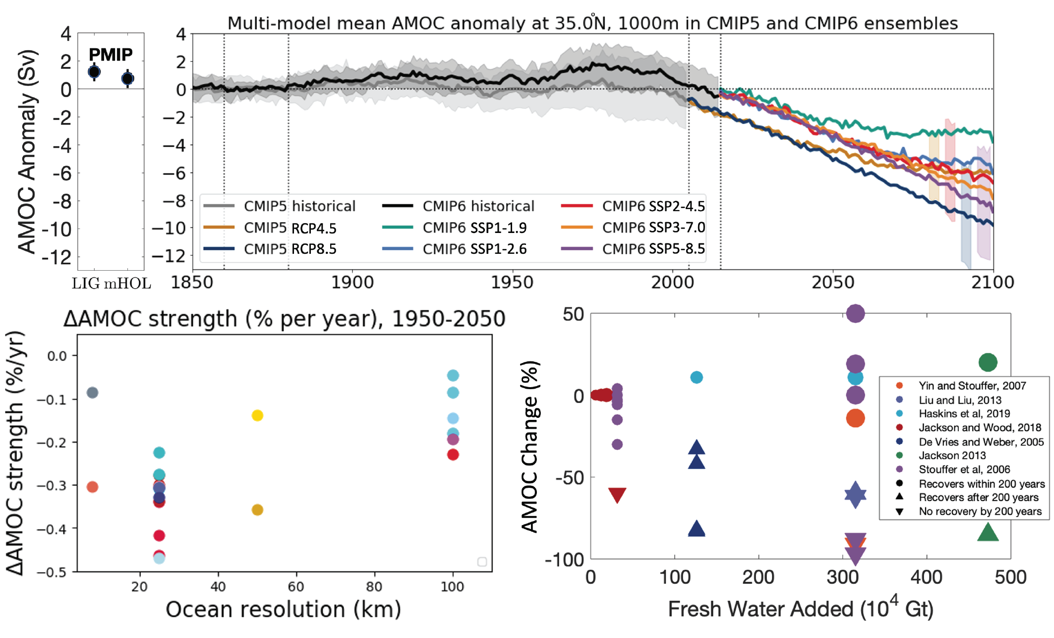 Figure 9.10 | Atlantic Meridional Overturning Circulation (AMOC) strength in simulations and sensitivity to resolution and forcing. (Top left) AMOC magnitude (units: Sverdrup (Sv) = 109kgs–1) in Paleoclimate Modelling Intercomparison Project (PMIP) experiments. (Top right) Time series of AMOC from Coupled Model Intercomparison Project Phase 5 and 6 (CMIP5 and CMIP6) based on (Menary et al., 2020b). (Bottom left) Percent change in AMOC strength per year at different resolutions over the 1950–2050 period with colours for model families (Roberts et al., 2020). (Bottom right) A compilation of percentage changes in the simulated AMOC after applying an additional freshwater flux in the subpolar North Atlantic at the surface for a limited time (de Vries and Weber, 2005; Stouffer et al., 2006; Yin and Stouffer, 2007; Jackson, 2013; Liu and Liu, 2013; Jackson and Wood, 2018; Haskins et al., 2019). Symbols indicate whether the AMOC recovers within 200 years (circles), is starting to recover (upwards arrow), or does not recover within 200 years (downwards arrow). Symbol size indicates rate of freshwater input. Further details on data sources and processing are available in the chapter data table (Table 9.SM.9).
 Both AR5(Collins et al., 2013)and SROCC (Collins et al., 2019) assessed that an abrupt collapse of AMOC before 2100 was very unlikely , but SROCC added that, by 2300, an AMOC collapse was as likely asnot for high-emissions scenarios. The SROCC also assessed that model bias may considerably affect the sensitivity of the modelled AMOC to freshwater forcing. Tuning towards stability and model biases (Valdes, 2011; Liu et al., 2017; Mecking et al., 2017; Weijer et al., 2019) provides CMIP models a tendency toward unrealistic stability (medium confidence). By correcting for existing salinity biases, Liu et al. (2017) demonstrated that AMOC behaviour may change dramatically on centennial to millennial time scales, and that the probability of a collapsed state increases. None of the CMIP6 models features an abrupt AMOC collapse in the 21st century, but they neglect meltwater release from the Greenland Ice Sheet. Also, a recent process study reveals that a collapse of AMOC can be induced, even by small-amplitude changes in freshwater forcing (Lohmann and Ditlevsen, 2021). As a result, we change the assessment of an abrupt collapse before 2100 to medium confidence that it will not occur.
9.2.3.2 Southern Ocean
The changing Southern Ocean circulation system exerts a strong influence on the global climate by modulating: (i) global OHC (Section 9.2.2.1); (ii) global ocean anthropogenic carbon uptake (Cross-chapter Box 5.3); global ocean overturning circulation (Section 9.2.3.1); (iii) climate sensitivity (Section 7.4.4 and Cross-chapter Box 5.3); (iv) sea level through basal melt of ice shelves (9.4.2); and (v) Southern Hemisphere sea ice cover (Section 9.3.2).
The SROCC (Meredith et al., 2019) had low confidence in all CMIP5-based model projections due to their inability to explicitly resolve eddy processes, and their inability to properly consider future meltwater change from the Antarctic Ice Sheet. These limitations of climate models to represent the Southern Ocean persist due to most CMIP6 models still using parameterized mesoscale eddy processes, which are limited in projecting the future response of the horizontal and vertical circulation under climate warming, and also because of the continued absence of active ice-shelf and ice-sheet coupling in the CMIP6 model suite, therefore ignoring basal meltwater and calving feedback on the circulation (Meredith et al., 2019). In addition, two important limitations of CMIP6 models of the Southern Ocean involve processes that were not assessed in SROCC. First, the poor representation of dense overflows causes most of the Antarctic Bottom Water (AABW) to be formed by spurious open ocean convection rather than by dense overflows from the Antarctic continental shelves that feed the lower overturning cell (Snow et al., 2015; Dufour et al., 2017; Heuzé, 2021). Second, Antarctic continental shelf waters are poorly simulated because potentially important controlling mechanisms tend to be too small and transient to observe and resolve in CMIP ocean models. These small processes include: the heterogeneity of observed sub-ice-shelf melt with warm water driving narrow basal channels that cut underneath the ice (Drews, 2015; Alley et al., 2016; Marsh et al., 2016; Milillo et al., 2019); eddies and tides (Stewart et al., 2018; Jourdain et al., 2019; Hausmann et al., 2020), which can drive Circumpolar Deep Water (CDW) onto the continental shelves or dynamically increase melting (Section 9.2.3.6); and feedback mechanisms between ocean, atmosphere and cryosphere that can weaken or amplify initial perturbations (Donat-Magnin et al., 2017; Spence et al., 2017; Turner et al., 2017; Silvano et al., 2018; Webber et al., 2019; Hazel and Stewart, 2020). In addition, the Southern Ocean in CMIP5 and CMIP6 models exhibit surface temperature biases (Section 9.2.1.1), which have been linked in CMIP5 models to errors in atmospheric model cloud-related shortwave radiation (Hyder et al., 2018) and are somewhat improved in High Resolution Model Intercomparison Project (HighResMIP) models (Figure 9.3). In summary, there is high confidence that future change in the subpolar Southern Ocean region, including sea ice cover and ocean temperature change on Antarctic continental shelves, depends on feedback mechanisms involving the ocean, atmosphere and cryosphere that are poorly understood and not represented in the current generation of climate models. This results in large uncertainty and low confidence in the future sea ice cover (Section 9.3.2) and in ocean temperature change on the Antarctic continental shelf (Section 9.4.2.3).
Despite these challenges, the CMIP6 ensemble does represent the main Southern Ocean circulation characteristics: the simulated Antarctic Circumpolar Current (ACC) transport is generally lower than observation-based values but consistent when considering ensemble spread, and the inter-model spread in ACC transport has greatly reduced from previous generations of climate models from CMIP3 to CMIP6 (Beadling et al., 2019, 2020). The structure (but not the magnitude) of the two-cell zonally averaged overturning is captured by most CMIP6 models (Russell et al., 2018; Beadling et al., 2019). In addition, while issues remain, CMIP6 climate models show clear improvements in their representation of AABW compared to CMIP5: several models correctly represent or parameterize Antarctic shelf processes, fewer models exhibit Southern Ocean deep convection, bottom density biases are reduced, and abyssal overturning is more realistic (Heuzé, 2021). In terms of atmospheric wind forcing, CMIP6 models show an improvement compared to CMIP5 models, with an overall reduction in the equatorward bias of the annual mean westerly jet from 1.9° in CMIP5 to 0.4° in CMIP6, but in contrast, they show no such overall improvements for their representation of the Amundsen Sea Low (Bracegirdle et al., 2020; Lyu et al., 2020a), which can be critical in driving variability of water masses on the Antarctic continental shelf in west Antarctica, the Weddell Sea or the Ross Sea (Holland et al., 2019; Silvano et al., 2020).
The SROCC (Meredith et al., 2019) established that, while trends in the atmospheric forcing of the Southern Ocean have been dominated by a strengthening of the Southern Hemisphere westerly winds in recent decades, there is medium confidence that ACC transport is weakly sensitive to changes in winds. It also reported that, instead of increasing the mean ACC transport, additional energy input associated with increased wind stress cascades into the eddy field (medium confidence). In contrast with the AR5 assessment (Rhein et al., 2013), SROCC evaluated that it was unlikely that there has been a net southward migration of the mean ACC position over the past 20 years. There is no additional evidence to revisit SROCC assessment on wind sensitivity. However, new evidence does suggest that air–sea buoyancy forcing associated with idealized 4×CO2 forcing leads to an increase in ACC transport (limited evidence) (Shi et al., 2020). The SROCC noted that, if the general strengthening in westerly winds is sustained, then it is very likely that the eddy field will continue to increase in intensity, and it is likely that the mean position and strength of the ACC will remain only weakly sensitive to winds. In the future, the strength of the Southern Hemisphere westerly wind jet results from a competition between decrease due to ozone hole recovery and increase due to increased radiative forcing (Section 4.3.3.1). This competition results in an increased atmospheric jet by 2100 compared to present day under SSP2-4.5, SSP3-7.0, and SSP5-8.5, but a decreased jet by 2100 under SSP1-2.6 (Bracegirdle et al., 2020). There is little inter-model spread in the CMIP6 future response of the atmospheric westerly jet, providing high confidence in this assessment (in contrast, CMIP6 models show no consistency in their future projection of easterly wind change along the Antarctic continental shelf break; Bracegirdle et al., 2020). Paleo-oceanographic evidence suggests that ACC flow through Drake Passage was consistently stronger during warm intervals of the past (both during interstadials and interglacials), but with relatively little change and no consensus on the sign of change in other regions (Lamy et al., 2015; Toyos et al., 2020). In summary, additional evidence since SROCC confirms that there is medium confidence that the ACC has been weakly sensitive to Southern Hemisphere atmospheric jet increase in the past decades. New evidence since SROCC suggests that there is high confidence that the Southern Hemisphere atmospheric jet will increase in the 21st century for all scenarios (except for SSP1-1.9 and SSP1-2.6; Section 4.3.3.1) with a greater increase for larger radiative forcing. An increase in westerly winds will very likely force an increase of the eddy field in the ACC, and while there is medium confidence that the ACC is weakly sensitive to wind change, new advances since SROCC provide limited evidence that the ACC transport will nevertheless increase in response to wind and buoyancy fluxes.
For the upper cell overturning circulation, SROCC concluded that: its transport has experienced significant inter-decadal variability in response to wind forcing since the 1990s; and there is low confidence in the assessments of a long-term increase in upper-ocean overturning. Consistent with SROCC, the importance of eddy processes and winds in driving long-term change and variability have been reinforced, with a potential fast wind response partially counteracted by a slower eddy response (Doddridge et al., 2019; Waugh et al., 2019; Stewart et al., 2020). Eddy parametrizations affect the strength of overturning, its sensitivity to winds and the ACC transport (Mak et al., 2017). Even in eddy-resolving simulations, sub-gridscale dissipation affects the overturning and ACC (Pearson et al., 2017). In addition, there has been progress in understanding the importance of Antarctic Ice Shelf meltwater and sea ice, in driving the observed changes in the near surface and in the upper overturning cell over the past decades, on top of changes induced by winds and eddies (Bronselaer et al., 2020; Haumann et al., 2020; Jeong et al., 2020; Rye et al., 2020). In particular, increased stratification caused by increased freshwater flux to the surface ocean (Section 9.2.1.3) can cause a shoaling and warming of the CDW layer, and create a positive feedback, enhancing basal melt of the Antarctic Ice Sheet (Section 9.4.2.1; Bronselaer et al., 2018; Golledge et al., 2019; Schloesser et al., 2019; Sadai et al., 2020). There is medium confidence in the existence of this feedback mechanism but low agreement on the magnitude of the feedback. The SROCC reported that CMIP5 models project that the overall transport of upper-ocean overturning cell will increase by up to 20% in the 21st century, and no new studies alter that assessment.
For the lower cell overturning circulation, SROCC assessed that a slowdown of its transport is consistent with the observed decrease in volume (medium confidence) of AABW in the global ocean (Section 9.2.2.3). Additional evidence since SROCC strengthens confidence that increased glacial meltwater flux will reduce the density of bottom waters during the 21st century. It will eventually reach a point where deep convection will be curtailed, and shelf water will become too buoyant to sink to the ocean interior, thereby slowing the lower cell overturning circulation (Bronselaer et al., 2018; Golledge et al., 2019; Lago and England, 2019; Moorman et al., 2020). While such changes are consistent with the observed freshening and decreased volume of the AABW layer reported in SROCC (as discussed in Section 9.2.2.3), new observation-based studies have highlighted how the lower cell overturning can episodically increase as a response to climate anomalies, temporally counteracting the tendency for melt to reduce AABW formation (Abrahamsen et al., 2019; Castagno et al., 2019; Gordon et al., 2020; Silvano et al., 2020). In addition, while the opening of open ocean polynyas can affect the lower cell on decadal to centennial time scales, there is limited evidence and low agreement in the role of open ocean polynyas in driving observed trends of the lower cell in the last decade (Section 9.2.2.3). Based on CMIP5 models, SROCC reported with low confidence that formation and export of AABW associated with the lower overturning cell will decrease in the 21st century, and there is no new evidence to revisit that assessment from climate models. However, additional paleo evidence from marine sediments suggests that AABW formation/ventilation was vulnerable to freshwater fluxes during past interglacials (Hayes et al., 2014; Huang et al., 2020; Turney et al., 2020) and that AABW formation was strongly reduced (Skinner et al., 2010; Gottschalk et al., 2016; Jaccard et al., 2016) or possibly totally curtailed (Huang et al., 2020) during the Last Glacial Maximum (LGM) and transient cold intervals of marine isotope stages 2 and 3 (MIS2 and MIS3). Specifically, sedimentary reconstructions show a transient reduction in AABW ventilation in the Atlantic sector of the Southern Ocean during MIS5e, which is assessed to have been warmer than modern climate (Thomas et al., 2020). However, long multi-centennial or millennial model runs under higher-than-pre-industrial CO2 concentrations show that, after 500–1000 years, ventilation in the Southern Ocean resumes, and possibly overshoots with enhanced convection in the Weddell and Ross seas, leading to enhanced bottom water ventilation globally (Yamamoto et al., 2015; Frölicher et al., 2020). AABW ventilation increased at the onset of the last deglacial transition, promoting the release of previously sequestered CO2 to the atmosphere on centennial to millennial time scales (Bauska et al., 2016; Jaccard et al., 2016; Rae et al., 2018), concomitant with a southward shift of the Southern Hemisphere westerly wind belt (Denton et al., 2010; Jaccard et al., 2016) and reduced sea ice cover (Ferrari et al., 2014; Stein et al., 2020). In summary, the combination of observational, numerical and paleoclimate evidence provides us with medium confidence that the lower cell will continue decreasing in the 21st century as a result of increased basal melt from the Antarctic Ice Sheet.
9.2.3.3 Tropical Oceans
The tropics are a tightly coupled ocean-atmosphere system with tightly interconnected basins (Cai et al., 2019). The zonal atmospheric Walker Circulation and the Indonesian Throughflow (Figure 9.11) are key connections between the Pacific and Indian oceans, and variations in the Walker and Hadley Circulations are tightly linked to the tropical Pacific SST and currents. The tropics have a profound influence on the climate system through the multiple modes of variability they host, which have widespread global influence at seasonal to annual time scale (Annex IV).
The effect of tropical modes of variability on climate and their long-term changes are reviewed in detail in Annex IV, while changes to the tropical ocean are assessed throughout the report and briefly summarized here. Section 2.4 concludes that a sustained shift beyond multi-centennial variability has not been observed for El Niño–Southern Oscillation (ENSO) (medium confidence) and that there is limited evidence and limited agreement about the long-term behaviour of other tropical modes. Section 3.7 assesses with high confidence that human influence has not affected the principal tropical modes of interannual climate variability and their associated regional teleconnections beyond the range of internal variability. Section 4.3.3.2 assesses with medium confidence that there is no consensus from models for a systematic change in the amplitude of ENSO sea surface temperature variability over the 21st century. The related change in tropical SSTs is covered in Section 9.2.1.1. The projected changes in SST have implications for marine heat wave characteristics, which are assessed in Box 9.2. SST changes in the tropics are related to changes in the atmospheric circulation, including surface equatorial easterly trade winds and Walker Circulation (Section 4.5.3.2), and the weakening Indonesian Throughflow and strengthening Agulhas Extension and leakage (Section 9.2.3.4). Weakening trade winds under climate change (Vecchi and Soden, 2007) will tend to decrease upwelling, along isopycnals in the eastern Pacific and diapycnal upwelling in the central Pacific, and thus the meridional temperature gradients that drive tropical instability waves (Terada et al., 2020), along with a weakening, flattening and shoaling of the tropical thermocline and equatorial undercurrent (Luo and Rothstein, 2011). A weak or absent equatorial undercurrent (Kuntz and Schrag, 2020) and a too-diffuse and incorrectly sloped tropical thermocline (Zhu et al., 2020) remain issues in most CMIP6 models. In summary, while future changes in tropical modes of variability remain unclear, change in atmospheric and ocean circulation will drive continued change in tropical ocean temperature in the 21st century (medium confidence), with part of the region experiencing drastic marine heat wave conditions (high confidence).
9.2.3.4 Gyres, Western Boundary Currents and Inter-basin Exchanges
The AR5 (Rhein et al., 2013) assessed with medium to high confidence that the North Pacific subpolar gyre, the South Pacific subtropical gyre, and the subtropical cells have intensified. They also reported that the North Pacific subtropical gyre had expanded since the 1990s, and that, overall, the changes in gyre systems were likely predominantly due to interannual-to-decadal variability. The SROCC (Meredith et al., 2019) complemented the AR5 assessment by reporting that the polar Beaufort Gyre in the Arctic expanded to the north-west between 2003 and 2014, contemporaneous with changes in its freshwater accumulation and alterations in wind forcing. Consistent with the reported change over the gyres, both AR5 and SROCC (Bindoff et al., 2019; Collins et al., 2019) reported that western boundary currents (WBCs) have intensified (Figure 9.11), and expanded poleward, except for the Gulf Stream and the Kuroshio. Section 2.3.3.4 provides an overall assessment of gyres and WBCs, including an assessment of change from paleoclimate archives. Section 2.3.3.4 assesses that, while WBC strength is highly variable at multi-decadal scale (high confidence), WBCs and subtropical gyres have shifted poleward since 1993 (medium confidence), at a rate on the order of 0.04–0.1 degree per decade during 1993–2018. Figure 9.11 shows that CMIP5 and CMIP6 models agree in projecting a weaker Gulf Stream and Gulf Stream Extension, while the Kuroshio changes less (Sen Gupta et al., 2016).
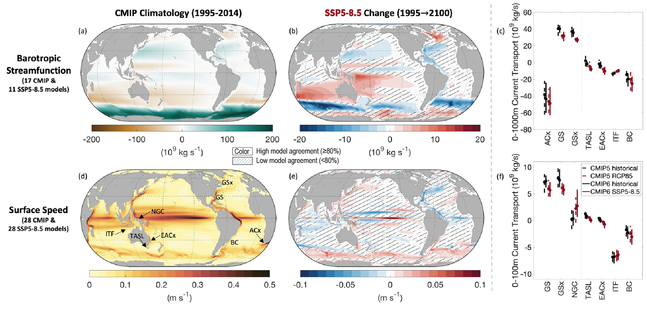 Figure 9.11 | Simulated barotropic streamfunction, surface speed and major current transport in Coupled Model Intercomparison Project Phase 5 and 6 (CMIP5 and CMIP6). (a) Mean barotropic streamfunction (unit: 109kgs–1; 1995–2014) and projected barotropic streamfunction change (109kgs–1; 2018–2100 vs 1995–2014) under (b) SSP5-8.5. (d) Mean surface (0–100 m) speed (m s–1) and projected surface speed change (m s–1, 2081–2100) versus 1995–2014 under (e) SSP5-8.5. (c, f) Median and likely range of 1995–2014 and 2081–2100 transport of three currents with the largest transport change and four with the largest fractional change (Sen Gupta et al., 2016). (c) Deep currents: Agulhas Extension (ACx), Gulf Stream (GS), Gulf Stream Extension (GSx), Tasman Leakage (TASL), East Australia Current Extension (EACx), Indonesian Throughflow (ITF), and Brazil Current (BC). (f) Shallow currents: as for deep but with New Guinea Current (NGC), and without ACx. No overlay indicates regions with high model agreement, where ≥80% of models agree on the sign of change. Diagonal lines indicate regions with low model agreement, where <80% of models agree on the sign of change (see Cross-Chapter Box Atlas.1 for more information). Further details on data sources and processing are available in the chapter data table (Table 9.SM.9).
 Although the observed wind stress curl shows systematic poleward shift in each basin as a result of anthropogenic warming (Section 2.3.1.4; Chen and Wu, 2012; Wu et al., 2012; Zhai et al., 2014), which has caused a systematic shift of the WBCs and subtropical gyres since 1993 (Wu et al., 2012; Yang et al., 2016, 2020), the response of current strength is more complex and inconsistent across regions (Sloyan and O’Kane, 2015; Y.-L. Wang et al., 2016; Elipot and Beal, 2018; McCarthy et al., 2018; Wang and Wu, 2018; Dong et al., 2019). The strength of WBCs and gyres exhibit inconsistent responses because they are dependent on wind stress forcing and because multi-scale interaction and air–sea interaction have an important role in their long-term trends and variability (Zhang et al., 2020). Observed changes in gyre circulation are dominated by interannual and decadal modes of variability globally (Qiu and Chen, 2012; Melzer and Subrahmanyam, 2017; McCarthy et al., 2018; Hu et al., 2020). The North Atlantic subpolar gyre is strongly modulated by variability associated with the NAO and AMV (Annex IV; Robson et al., 2016). Subpolar gyre systems can change abruptly due to a positive feedback between convective mixing and salinity transport (Born et al., 2013, 2016) and air–sea interaction (Moffa-Sánchez et al., 2014; Moreno-Chamarro et al., 2017) within the gyre. In the Arctic, both the Beaufort gyre and mesoscale eddies strengthened between 2003 and 2014 (Armitage et al., 2017), which might be partly due to increased wind stress (Oldenburg et al., 2018) or reduced sea ice thickness and changes in sea ice pack morphology (van der Linden et al., 2019). Presently, there is limited evidence in attributing causality to these changes for any of the proposed mechanisms. In the North Pacific, there has been an increasing trend in the Alaska Gyre from 1993 to 2017 (Cummins and Masson, 2018), which might be attributed to Pacific Decadal Oscillation (low confidence) (Hristova et al., 2019). In the Southern Ocean, limited evidence indicates that the subpolar gyres respond to Southern Hemisphere atmospheric modes of variability at interannual time scale (Armitage et al., 2018; Dotto et al., 2018).
All climate models reproduce WBCs and gyres, but eddy-present or eddy-rich models (roughly 10–25 km and about 10 km resolution, respectively) represent these currents more realistically than eddy-parameterized models (very high confidence) (Small et al., 2014; Griffies et al., 2015; Chassignet et al., 2017, 2020; Hewitt et al., 2017, 2020; Roberts et al., 2018). Compared to observations or to eddy-present and eddy-rich models, the eddy-parameterized models from CMIP5 and CMIP6 simulate weaker and wider WBCs, as well as less realistic locations of subtropical and subpolar gyre boundaries (Figure 9.11). Increased resolution admits mesoscale eddies, and also improves simulation of the strength and position of WBCs such as the Kuroshio Current, Gulf Stream, and East Australian Current (very high confidence) (Sasaki et al., 2004; Chassignet and Marshall, 2008; Delworth et al., 2012; Yu et al., 2012; Small et al., 2014; Haarsma et al., 2016; Chassignet et al., 2017, 2020; Hewitt et al., 2020). Improved boundary current location relates to improved recirculation regions (Jayne et al., 2009), mean path and variability, and existence of multiple stable paths (Qiu et al., 2005; Delman et al., 2015), air–sea fluxes (Small et al., 2014), and related coastal weather patterns (Kaspi and Schneider, 2011). The wind-current feedback, implemented by considering relative velocity of currents and wind, realistically dampens mesoscale eddies and WBCs, through mesoscale air–sea interaction (Ma et al., 2016; Renault et al., 2016, 2019), even though sub-mesoscale wind-current damping feedback is missing in these models (medium confidence) (Z. Zhang et al., 2016). As eddies potentially play a role in determining the strength of gyre circulations and their low-frequency variability (Fox-Kemper and Pedlosky, 2004; Berloff et al., 2007), it is expected that eddy-present and eddy-rich models will differ in their decadal variability and sensitivity to changes in the wind stress of gyres from eddy-parameterized models (medium confidence). Nonetheless, important aspects of gyre strength depend primarily on forcing and not resolution, allowing long-term changes in gyre strength to be investigated with low-resolution climate models (Hughes and de Cuevas, 2001; Yeager, 2015).
Under future scenarios RCP4.5 and RCP8.5, AR5 (Collins et al., 2013) assessed an intensification and poleward extension of the southern Hemisphere subtropical gyres in the 21st century. New evidence since AR5 further reinforces their conclusions, which are now extended to all subtropical gyre systems in the Northern and Southern hemispheres (Yang et al., 2016, 2020). CMIP6 models project changes in WBCs that are consistent with projected changes in the surface winds. Under strong radiative forcing, in scenario SSP5-8.5, CMIP6 models project that the East Australian Current Extension, Agulhas Current Extension and Brazil Current will intensify in the 21st century, while the Gulf Stream will weaken (Figure 9.11). Although CMIP5/CMIP6 are limited in resolution, medium confidence is given to changes in WBCs due to consistency across generations of climate models, including CMIP6, despite changes in model structure, resolution and parametrizations.
The SROCC (Collins et al., 2019) concluded with high confidence that Indonesian Throughflow (ITF) transport from the Pacific Ocean to the Indian Ocean has increased in the past two decades as a result (medium confidence) of an unprecedented intensification of the equatorial Pacific trade wind system. Section 2.3.3.4 assesses that there is high confidence that the increase in the ITF over the past two decades is linked to multi-decadal scale variability rather than a longer-term trend. Consistently, in the future, as winds change under increased radiative forcing, most models project a decline of the ITF on the centennial time scale (Figure 9.11). One of the clearest changes of ocean current transport simulated by climate models is a weakening of the Indonesian Throughflow, projected in CMIP5 simulations under RCP4.5 and RCP8.5 scenarios (Sen Gupta et al., 2016; Stellema et al., 2019), and in CMIP6 simulations under the SSP5-8.5 scenario (high confidence, Figure 9.11).
The SROCC reports with high confidence that the Agulhas leakage from the Indian to the Atlantic Ocean has increased in the past two decades (Collins et al., 2019), and there is no additional evidence since then allowing this assessment to be revisited (Biastoch et al., 2015; Loveday et al., 2015; Lübbecke et al., 2015). There is low confidence in future projections of Agulhas leakage because most CMIP models cannot directly simulate it, due to coarse resolution. However, there is medium evidence that the strength of the Southern Hemisphere westerlies controls Agulhas leakage (Durgadoo et al., 2013; Biastoch et al., 2015; Loveday et al., 2015), and high confidence that the strength of the Southern Hemisphere westerlies will increase under increased radiative forcing, except in lower warming scenarios (SSP1-1.9, SSP1.2-6; Section 4.3.3.1; Bracegirdle et al., 2020). There is also evidence that increasing Agulhas leakage is consistent with observed change of the temperature and salinity structure in the Atlantic ocean, and with variability of the AMOC (Section 9.2.3.1; Biastoch et al., 2015). This range of indirect evidence provides medium confidence that the Agulhas leakage will increase in the 21st century, except for the strongest mitigation scenario (Figure 9.11).
The SROCC assessed that the annual Bering Strait volume transport from the Pacific to the Arctic Ocean increased from 2001–2014, consistent with an estimated increased northward heat transport of about 60% from 2001–2014, and an increased freshwater transport of 30 ± 20 km3yr–1from 1991 to 2015 (Meredith et al., 2019). Section 2.3.3.4 assesses that volume transport from the Pacific to the Arctic has increased since the 1990s from 0.8 Sv to 1.0 Sv over 1990–2015. Realistic representation of the Bering Strait transport in the current generation of climate models is challenging because the strait is narrow compared to the resolution of climate models (Clement Kinney et al., 2014; Aksenov et al., 2016). For the Atlantic to Arctic transport, Section 2.3.3.4 reports that the major branches of Atlantic Water inflow across the Greenland–Scotland Ridge have remained stable, with only the smaller pathway of Atlantic Water north of Iceland showing a strengthening trend during 1993–2018. Section 2.3.3.4 also assesses that the Arctic outflow remained stable from the mid-1990s to the mid-2010s. Future changes in these currents have not yet been studied in CMIP6 models.
9.2.3.5 Eastern Boundary Upwelling Systems
Eastern boundary upwelling systems (EBUS) exist where trade winds draw cold and generally low-pH/low-oxygen waters upward. Coastal upwelling plays a key role in supplying the food chain with nutrients, hence the richness and productivity of EBUS (Bindoff et al., 2019). The SROCC (Bindoff et al., 2019) assessed with high confidence that three out of the four major EBUS have experienced large-scale wind intensification in the past 60 years (only the trend for the Canary Current is considered uncertain). However, it also emphasized that various processes can also modulate, or even reverse, wind trends locally (Bindoff et al., 2019). Here we revisit SROCC assessment (Bindoff et al., 2019) based on evidence showing low agreement between studies that have investigated trends over past decadess of upwelling-favourable winds (Varela et al., 2015). This low agreement has been related to differences in wind products, season of interest, and length of the considered time series (Varela et al., 2015). Based on this, we assess that only the California Current system has experienced large-scale upwelling-favorable wind intensification over the period 1982–2010, albeit with regional differences (García-Reyes and Largier, 2010; Seo et al., 2012). In the Benguela, Canary, and Humboldt systems, large-scale, upwelling-favourable wind trends are ambiguous, owing to low confidence in long-term in situ marine wind data (Cardone et al., 1990; Bakun et al., 2010) and low agreement among available studies (Narayan et al., 2010; Sydeman et al., 2014; Varela et al., 2015). Our assessment confirms SROCC assessment (Bindoff et al., 2019) in that high natural variability of EBUS and their inadequate representation by most climate models gives low confidence in attribution of observed changes, while anthropogenic changes are projected to emerge primarily in the second half of the 21st century (limited evidence: one model and one study) (Brady et al., 2017).
Under increased radiative forcing, SROCC (Bindoff et al., 2019) assessed that climate models project, in the 21st century, a reduction of wind and upwelling intensity in EBUS at low latitudes, and enhancement at high latitudes, under scenario RCP8.5, with an overall reduction in either upwelling intensity or extension. It also highlighted that coastal warming and wind intensification may lead to variable countervailing responses to upwelling intensification at local scales. Despite differences among EBUS (D. Wang et al., 2015), there is growing evidence since SROCC in this pattern of change. While it has long been hypothesized that, for upwelling winds, change is linked to air temperature contrast between ocean and land (Bakun, 1990), this hypothesis has increasingly been challenged. Changes in sea level pressure and wind fields in EBUS appear to be primarily tied to those affecting subtropical highs (García-Reyes et al., 2013). Poleward expansion of the Hadley cell (Section 2.3.1.4.1; Staten et al., 2018) and the related poleward migration of subtropical highs (He et al., 2017; Cherchi et al., 2018), produce robust patterns of changes of reduced upwelling at low latitude and enhanced upwelling at high latitude (Echevin et al., 2012; Belmadani et al., 2014; Bettencourt et al., 2015; Rykaczewski et al., 2015; Sousa et al., 2017; Lamont et al., 2018; Sylla et al., 2019). These patterns are most apparent in summer in both hemispheres. Synoptic variability of upwelling winds, important to the functioning of upwelling ecosystems (García-Reyes et al., 2014), may also be affected by climate change (Aguirre et al., 2019). However, coarse resolution model projections of winds in upwelling regions may be more consistent than higher-resolution projections, as these regions are highly sensitive to resolution (Small et al., 2015).
Projected future annual cumulative upwelling wind changes at most locations, and seasons remain within ±10–20% of present-day values in the 21st century, even in the context of high-end emissions scenarios (4×CO2 or RCP8.5) (medium confidence). Changes due to wind stress curl and alongshore pressure gradients tend to agree with alongshore wind changes (Oerder et al., 2015; Sylla et al., 2019). Direct estimation of oceanic upward transport (Oyarzún and Brierley, 2019; Sylla et al., 2019) and nutrient flux into the euphotic layer (Jacox et al., 2018) provide a meaningful estimator of upwelling, integrating all relevant processes, including changes in wind stress curl. However, there is limited evidence from vertical velocity of climate models and missing processes in coarse-resolution climate models that presently limit this approach. Change in upper-ocean stratification (Section 9.2.1.3) is projected to increase confinement of upwelling vertical velocities to near the ocean surface (high confidence) (Oerder et al., 2015; Oyarzún and Brierley, 2019).
In summary, SROCC and this Report conclude that the California Current system has experienced some upwelling-favourable wind intensification since the 1980s (high confidence), while low agreement among reported wind changes in the Benguela, Canary, and Humboldt systems prevent a similar assessment. As in SROCC, there is low confidence in attribution of observed changes to anthropogenic or natural causes. New evidence reinforces our confidence in SROCC assessment that, under increased radiative forcing, EBUS winds will change with a dipole spatial pattern within each EBUS of reduction (weaker and/or shorter) at low latitude, and enhancement (stronger and/or longer) at high latitude (high confidence). There is medium confidence that, across all scenarios, upwelling wind changes in EBUS will remain moderate in the 21st century, within ±10–20% from present-day values.
9.2.3.6 Coastal Systems and Marginal Seas
Beyond the world’s coastlines lie the shoreline, shallow estuaries, continental shelves, and deeper fjords and slopes, where depths increase rapidly from the shelves to the deep-ocean floor. It is more difficult to transport fluid across (rather than along) the shelf-break or slope (Brink, 2016), and estuaries and shelves have complex circulations and mixing, leading to indirect connections between the inner shelves and coastlines and offshore conditions. Coastal processes link to large-scale metrics of climate and regional effects, from changing rivers and estuaries, melt and runoff to deep water, to how changes offshore affect regional and coastal conditions.
Shelf-deep ocean exchanges involve eddying, tidal, or turbulent motions and small-scale topography such as submarine canyons; high-resolution observations and models are needed to capture these effects (Greenberg et al., 2007; Capet et al., 2008; Allen and Durrieu de Madron, 2009; Colas et al., 2012; Trotta et al., 2017). Example coastal processes that introduce uncertainty into large-scale projections are exchange of CDW across the Antarctic shelf-break, which affects AABW formation and Antarctic ice-shelf–ocean interaction (Sections 9.2.2.3 and 9.2.3.2; Stewart and Thompson, 2013, 2015), river and estuarine plumes and their responses to water level and hydrology change (Banas et al., 2009; Sun et al., 2017), fjord dynamics linked to glacial outflows (Straneo and Cenedese, 2015; Torsvik et al., 2019), and changing formation of water masses in marginal seas (Kim et al., 2001; Greene and Pershing, 2007; Giorgi and Lionello, 2008; Renner et al., 2009). Downscaling projections to the local level allows process detail (Foreman et al., 2014; Mathis and Pohlmann, 2014; Meier, 2015; Tinker et al., 2016). Some processes can only be simulated when coastal models are forced by larger-scale models of the atmosphere, cryosphere, or hydrosphere (Seo et al., 2007, 2008; Somot et al., 2008; Oerder et al., 2015; Renault et al., 2016; Y. Zhang et al., 2016; Wåhlin et al., 2020), including the addition of tides (Janeković and Powell, 2012; Timko et al., 2013; Tinker et al., 2015; Pickering et al., 2017; Hausmann et al., 2020). Due to coastal process complexity and small scale, linking the effects of coastal ocean changes to global ocean changes requires high-resolution modelling (Holt et al., 2017, 2018), two-way nesting, or local mesh refinement (Fringer et al., 2006; Zhang and Baptista, 2008; Mason et al., 2010; Dietrich et al., 2012; Hellmer et al., 2012; Ringler et al., 2013; Q. Wang et al., 2014; Zängl et al., 2015; Y.J. Zhang et al., 2016; Soto-Navarro et al., 2020). Coarse climate models and HighResMIP models do not represent some coastal phenomena such as cross-shelf exchanges and sub-mesoscale eddies, which require 1 km or finer resolution. Thus, there is low confidence in projecting centennial scale coastal climate change where regional downscaling or refinement is lacking. There is high confidence in the ability of regional coupled models to improve coastal climate change process understanding and provide regional information (Section 12.4), but many sites globally await such projections.
9.2.4 Steric and Dynamic Sea Level Change
9.2.4.1 Global Mean Thermosteric Sea Level Change
Changes in globally averaged ocean heat content (OHC) cause global mean thermosteric sea level (GMTSL) change (Box 9.1). The observed increased OHC for 1971–2018 of 325 to 546 ZJ (very likely range) (Section 7.2, Box 7.2) has led to a GMTSL rise of 0.03 to 0.06 m out of a total global mean sea level (GMSL) of 0.07 to 0.15 m (very likely range) (Section 2.3.3.3, Tables 2.7 and 9.5, and Cross-Chapter Box 9.1).
Projections of GMTSL rise in AR5 (Church et al., 2013b) and SROCC (Oppenheimer et al., 2019) were derived from the CMIP5 ensemble, after removing drift estimated based on pre-industrial control simulations. Differences between removing a linear and a quadratic drift are small (Hobbs et al., 2016a; Hermans et al., 2021). These prior assessments filled in projections for models that did not provide GMTSL rise for all scenarios, by calculating the heat content of the climate system from global surface air temperature and net radiative flux, then converting this to GMTSL rise using each model’s diagnosed expansion efficiency coefficient. In AR5, the associated uncertainties were derived by assuming a normal distribution, with the 5th–95th percentile CMIP5 ensemble range taken as the likely range (±1 standard deviation).
In this Report, global surface air temperature projections are not derived directly from the CMIP6 ensemble (Box 4.1). Therefore, to produce projections of OHC and GMTSL rise consistent with the Report’s assessment of equilibrium climate sensitivity and transient climate response (Section 7.5.2.2), this chapter employs a two-layer energy budget emulator (Supplementary Materials 7.SM.2, 9.SM.4.3). Since AR5, climate model emulators have been increasingly used to predict GMTSL (Cross-Chapter Box 7.1; Kostov et al., 2014; Palmer et al., 2018, 2020; Nauels et al., 2019). The expansion efficiency coefficient that relates GMTSL and OHC for the two-layer emulator has a mean and standard deviation of 0.113 ± 0.013 m YJ–1(Supplementary Material 9.SM.4.3). This approach yields a likely thermosteric contribution between 1995–2014 and 2100 that represents a minimal change from AR5 and SROCC (Table 9.8). The two-layer emulator GMTSL projected median and 17th–83rd percentile, or likely , range is 0.12 (0.09 to 0.15) m for SSP1-1.9, 0.14 (0.11 to 0.18) m for SSP1-2.6, 0.20 (0.16 to 0.24) m for SSP2-4.5, 0.25 (0.21 to 0.30) m for SSP3-7.0, and 0.30 (0.24 to 0.36) m for SSP5-8.5 by 2100 (Section 9.6.3.2 and Tables 9.1, 9.8 and 9.9). The two-layer model heat content increases slightly faster than that of the total depth CMIP6 ensemble, which is related to its role in the assessed energy balance (Section 7.SM.2), but with a similar ensemble spread (Table 9.1). Projecting the likely factor by which 1995–2014 to 2081–2100 OHC change exceeds change over 1971 to 2018 in CMIP6 yields 3 to 5 for SSP1-2.6, 4 to 6 for SSP2-4.5, 5 to 7 for SSP3-7.0, and 5 to 8 for SSP5-8.5. The two-layer model likely equivalents are 2 to 3 for SSP1-2.6, 3 to 4 for SSP2-4.5, 4 to 5 for SSP3-7.0, and 4 to 6 for SSP5-8.5.
For reconstructions, the expansion efficiency coefficient is required for the conversion between ocean temperature and steric sea level over a specific time scale. Combining the assessed sea level and energy data over 1995 to 2014 (drawn from the analysis in Cross-Chapter Box 9.1) results in a coefficient of 0.1210 ± 0.0014 m YJ–1, or 0.6607 ± 0.0076 m °C–1in terms of mean ocean temperature. The two-layer emulator assessment used in AR6 results in 0.113 ± 0.013 m YJ–1, or 0.617 ± 0.071 m °C–1(Appendices 7.SM.2, 9.SM.4). Both of these estimates are in line with an independent estimate of 0.70 m/°C (Hieronymus, 2019) and other estimates, for example, 0.116 ± 0.011 m YJ–1(Kuhlbrodt and Gregory, 2012), but are significantly larger than the temperature to sea level conversion used in AR5 (0.42 m °C–1based on SST and the estimated range from Levermann et al., 2013). The expansion coefficient is not fixed across models, nor in time, as it varies depending on which water masses are storing the added heat, and the commitment time scale (Hallberg et al., 2013). For paleoclimate, a scaling for sea surface temperature (0.6 m °C–1) or global surface air temperature (GSAT; see Cross-Chapter Box 2.3) can be estimated, but mean ocean temperature is in phase with steric sea level change, while sea surface temperatures are not (Figure 9.9; Shakun et al., 2012; Tierney et al., 2020). Thus, while conversions between OHC, mean ocean temperature and GMTSL across applications are within uncertainty ranges (medium confidence) (Table 9.1), little consistency is found when correlating these variables to SST or GSAT, which may vary independently.
Short-lived climate forcers (Sections 6.3 and 6.6.3) are associated with a sea level commitment, due to an OHC and mean ocean temperature response that lasts substantially longer than their atmospheric forcing and SST response, although not as long as the sea level commitment associated with CO2 emissions (Sections 9.2.1.1 and 4.4.4). For example, Zickfeld et al. (2017) find that about 70% of the thermosteric sea level rise associated with methane forcing would persist 100 years after the elimination of methane emissions, and 40% would persist for more than 500 years.
In summary, consistent relationships between OHC (Section 9.2.2.1), mean ocean temperature and GMTSL are found using two-layer emulators, CMIP6 models, and modern and paleo observations to provide medium confidence in the 0.113 ± 0.013 m YJ–1, or 0.617 ± 0.071 m °C–1likely ranges of assessed conversion values. It is possible to estimate relationships between SST or GSAT change and GMTSL rise, but conversions are not generally applicable and depend on time scale and application.
Study | RCP2.6/SSP1-2.6 | RCP4.5/SSP2-4.5 | RCP8.5/SSP5-8.5 |
IPCC AR5 and SROCC GMTSL | 0.13 [0.09 to 0.17] m | 0.18 [0.13 to 0.22] m | 0.26 [0.20 to 0.32] m |
CMIP6 5–95% GMTSL | 0.14 [0.08 to 0.17] m | 0.18 [0.11 to 0.23] m | 0.26 [0.17 to 0.33] m |
CMIP6 5–95% GMTSL | – | 0.19 [0.13 to 0.24] m | 0.27 [0.19 to 0.35] m |
Assessed GMTSL based on two-layer model 17–83% and 5–95% (Sections7.SM.2, 9.SM.4) | 0.13 (0.11 to 0.16) [0.09 to 0.19] m | 0.17 (0.14 to 0.21) [0.12 to 0.25] m | 0.25 (0.20 to 0.30) [0.18 to 0.35] m |
Total OHC 17–83% and 5–95% from assessed two-layer model (Sections7.SM.2, 9.SM.4) | 1.18 (0.99 to 1.42) [0.86 to 1.65] YJ | 1.56 (1.33 to 1.86) [1.19 to 2.12] YJ | 2.23 (1.92 to 2.64) [1.71 to 3.00] YJ |
0–2000 m OHC 17–83% and 5–95% from CMIP6 (Figure 9.6) | 1.06 (0.80 to 1.31) [0.66 to 1.64] YJ | 1.35 (1.08 to 1.67) [0.90 to 1.84] YJ | 1.89 (1.60 to 2.29) [1.28 to 2.58] YJ |
9.2.4.2 Ocean Dynamic Sea Level Change
Projections of ocean dynamic sea level change (Box 9.1) on multi-annual time scales resemble the patterns of steric sea level change in the open ocean (Figures 9.11 and 9.12; Lowe and Gregory, 2006; Pardaens et al., 2011; Couldrey et al., 2021). On shorter time scales, especially in extratropical coastal areas, there may be an important barotropic component (also called bottom pressure change) due mostly to changes in wind-driven circulation and eddies apparent in the variance of ocean dynamic sea level (Figure 9.12; Roberts et al., 2016; Hughes et al., 2018). This component is highly sensitive to ocean model resolution (Chassignet et al., 2020). Steric sea level change is associated with local changes in temperature and salinity, which come about through changes in surface fluxes of heat and freshwater (Section 9.2.1.2) and through redistribution of existing water masses by changed ocean circulation and mixing processes (Figure 9.12 and Sections 9.2.2.1 and 9.2.3). Redistribution of water masses often involves anticorrelated thermosteric and halosteric changes (Figure 9.12), especially in the Atlantic (Pardaens et al., 2011; Bouttes et al., 2014; Durack et al., 2014; Griffies et al., 2014; Han et al., 2017).
 Figure 9.12 | (a–f) Coupled Model Intercomparison Project Phase 6 (CMIP6) multi-model mean projected change contributions to relative sea level change in (a, d) steric sea level anomaly, (b, e) thermosteric sea level anomaly, and (c, f) halosteric sea level anomaly between 1995–2014 and 2081–2100 using a method that does not require a reference level (Landerer et al., 2007). Global mean change has been removed from these figures, consistent with the methods in Sections 9.6.3 and 9.SM.4 and the definitions of Gregory et al. (2019). (Gregory et al., 2019). See Figure 9.27 for global mean sea level (GMSL). (g–i) Standard deviation of ocean dynamic sea level change from (g) Aviso observations (10-day high-pass filter); (h) five-day mean of high-resolution Ocean Model Intercomparison Project phase 2 (OMIP-2) models forced with observed fluxes; and (i) five-day mean of low-resolution OMIP-2 models which are comparable in resolution to the models in (a–f). No overlay indicates regions with high model agreement, where ≥80% of models agree on the sign of change. Diagonal lines indicate regions with low model agreement, where <80% of models agree on the sign of change (see Cross-Chapter Box Atlas.1 for more information). Further details on data sources and processing are available in the chapter data table (Table 9.SM.9).
 Ocean dynamic sea level change is strongly affected by internal variability (Section 9.6.1.4), partly from interannual to decadal coupled atmosphere–ocean modes of variability via wind-driven redistribution (Annex IV; Griffies et al., 2014; Han et al., 2017) and partly from intrinsic ocean variability, particularly in higher-resolution simulations (such as HighResMIP), which statistically resemble observations, even on short time scales (Figure 9.12; Griffies et al., 2014; Sérazin et al., 2016; Llovel et al., 2018; Chassignet et al., 2020). High-resolution simulations are not used in relative sea level projections (Section 9.6.3) due to the limited range of forcing scenarios. The most marked feature of long-term regional sea level change in the continuous satellite altimetry record, beginning in 1992, is the east–west dipole in the Pacific Ocean (rising more rapidly in the east, see also Section 9.6.1.3), which persisted until 2015, and can be explained by anomalously strong trade winds (Merrifield et al., 2012; England et al., 2014; Griffies et al., 2014; Takahashi and Watanabe, 2016; Han et al., 2017) together with associated changes in surface heat flux (Piecuch et al., 2019). The most notable features of sub-annual variability in altimetry are eddies and tides, which are directly simulated only in high-resolution models (Haigh et al., 2019; Chassignet et al., 2020).
Projections of the pattern and amplitude of regional ocean dynamic sea level change in CMIP6 and previous model generations show a large model spread, of a similar size to the geographical spread (Figure 9.12). The model spread derives from model dependence of changes both in surface fluxes (Section 9.2.1.2) and in the ocean response (Section 9.2.2). The spread is similar in CMIP6 and CMIP5, and is largest in regions with large projected variations in ensemble-mean ocean dynamic sea level change (Lyu et al., 2020a), such as the Southern Ocean Dipole with an ocean dynamic sea level rise north of the ACC and a fall to the south, the Atlantic Dipole with a sea level rise north of 40°N and a fall in 20°N–40°N, the Northwest Pacific Dipole, and the large sea level rise in the Arctic (Church et al., 2013b; Slangen et al., 2014a, 2015; Bilbao et al., 2015; Gregory et al., 2016; C. Chen et al., 2019; Lyu et al., 2020a; Couldrey et al., 2021). Patterns of change are consistent between model simulations and observations (medium confidence). The major model ensemble-mean features resemble thermosteric sea level change, as expected from altered input of heat to the ocean without changing circulation, while model spread results from the diversity in redistribution of the heat content of the unperturbed ocean (Section 9.2.2.1; Bouttes and Gregory, 2014; Gregory et al., 2016; Huber and Zanna, 2017; Lyu et al., 2020b; Todd et al., 2020; Couldrey et al., 2021).
The Southern Ocean Meridional Dipole is driven by a northward advection of excess heat (from changes in surface fluxes) by the wind-driven circulation followed by subduction or diffusive uptake in mid-latitudes, northward redistribution of existing heat by the strengthening of that circulation, and the meridional contrast in thermal expansivity due to its temperature-dependence (Armour et al., 2016; Gregory et al., 2016; Lyu et al., 2020b; Todd et al., 2020; Couldrey et al., 2021).
The positive Arctic ocean dynamic sea level change is driven by increased freshwater input (Couldrey et al., 2021). The Northwest Pacific Dipole is driven by the intensification of the Kuroshio Current in response to reduced heat loss and in some models to wind stress change (C. Chen et al., 2019; Couldrey et al., 2021).
The North Atlantic sea level change dipole is forced by a reduction in heat loss from the ocean north of 40°N (i.e., net heat uptake), which in all Earth system models leads to a weakening of the AMOC, although the magnitude has a large model spread (Section 9.2.3.1; Gregory et al., 2016; Huber and Zanna, 2017). The reduced northward transport of warm, salty water (Section 9.2.2) causes further ocean dynamic sea level change, whose details are model-dependent. North of 40°N, this redistribution leads to a sea level rise, predominantly halosteric, reinforcing the thermosteric effect of heat uptake (Couldrey et al., 2021). Comparison of observed Atlantic OHC for 1955–2017 with a reconstruction assuming no change in circulation indicates that the thermosteric sea level change resulting from southward redistribution of heat may be detectable (Zanna et al., 2019). This redistribution causes a tendency for SST cooling north of 40°N and anomalous heat input from the atmosphere, and thus a positive feedback on AMOC weakening (Winton et al., 2013; Gregory et al., 2016; Todd et al., 2020; Couldrey et al., 2021). Many climate and ocean models agree that the AMOC weakening is associated with pronounced thermosteric sea level rise along the American coast around 40°N (Figures 9.12 and 9.26), leading to a relatively large ocean dynamic sea level rise in this region (Yin, 2012; Bouttes et al., 2014; Slangen et al., 2014b; Little et al., 2019; Lyu et al., 2020a).
In summary, ocean dynamic sea level change involves changes to temperature and salinity and responses of currents to changing forcing, with significant variability driven by unforced oceanic variability. Projections of dynamic sea level variability require fully three-dimensional ocean models, and only high-resolution ocean models are statistically consistent on short time scales with satellite altimeter observations (very high confidence).
9.3 Sea Ice
9.3.1 Arctic Sea Ice
9.3.1.1 Arctic Sea Ice Coverage
The observed decrease of Arctic sea ice area is a key indicator of large-scale climate change (Section 2.3.2.1.1, Cross-Chapter Box 2.2). The SROCC (Meredith et al., 2019) assesses that sea ice extent, which is the total area of all grid cells with at least 15% sea ice concentration, has declined since 1979 in each month of the year (very high confidence). In contrast to SROCC, we assess changes in sea ice area (the actual area of the ocean covered by sea ice) rather than sea ice extent, because sea ice area is geophysically more relevant and not grid-dependent (Notz, 2014; Ivanova et al., 2016; Notz et al., 2016; Notz and SIMIP Community, 2020). Arctic sea ice area is calculated based on measurements by passive microwave satellite sensors that provide near-continuous measurements of gridded, pan-Arctic sea ice concentration from 1979 onwards. Irreducible uncertainties in the conversion of thermal microwave brightness temperature to sea ice concentration, and choices in algorithm design, cause uncertainties in observed Arctic sea ice area, which are far smaller than the observed sea ice loss (e.g., Comiso et al., 2017a; Niederdrenk and Notz, 2018; Alekseeva et al., 2019; Kern et al., 2019; Meier and Stewart, 2019). Sea ice area has decreased in every month of the year from 1979 to the present (very high confidence) (Figure 9.13). The absolute and the relative ice losses are highest in late summer-early autumn (high confidence) (Figure 9.13). Averaged over the decade 2010–2019, the monthly Arctic sea ice area from August to October has been around 2 million km² (or about 25%) smaller than during 1979–1988 (high confidence) (Figure 9.13).
 Figure 9.13 | Arctic sea ice historical records and Coupled Model Intercomparison Project Phase 6 (CMIP6) projections. (Left) Absolute anomaly of monthly-mean Arctic sea ice area during the period 1979 to 2019 relative to the average monthly-mean Arctic sea ice area during the period 1979 to 2008. (Right) Sea ice concentration in the Arctic for March and September, which usually are the months of maximum and minimum sea ice area, respectively. First column: Satellite-retrieved mean sea ice concentration during the decade 1979–1988. Second column: Satellite-retrieved mean sea ice concentration during the decade 2010–2019. Third column: Absolute change in sea ice concentration between these two decades, with grid lines indicating non-significant differences. Fourth column: Number of available CMIP6 models that simulate a mean sea ice concentration above 15 % for the decade 2045–2054. The average observational record of sea ice area is derived from the UHH sea ice area product (Doerr et al., 2021), based on the average sea ice concentration of OSISAF/CCI (OSI-450 for 1979–2015, OSI-430b for 2016–2019) (Lavergne et al., 2019), NASA Team (version 1, 1979–2019) (Cavalieri et al., 1996) and Bootstrap (version 3, 1979–2019) (Comiso, 2017) that is also used for the figure panels showing observed sea ice concentration. Further details on data sources and processing are available in the chapter data table (Table 9.SM.9).
 The SROCC discussed the regional distribution of Arctic sea ice loss, and the findings remain valid for the updated time series covering 2019 (Figure 9.13). Sea ice loss in winter is strongest in the Barents Sea, while summer losses occur primarily at the summer sea ice region margins, in particular in the East Siberian, Chukchi, Kara and Beaufort Seas (Frey et al., 2015; Chen et al., 2016; Onarheim et al., 2018; Peng and Meier, 2018; Maksym, 2019). In the Bering Sea, expanding winter sea ice cover was observed until 2017 (Frey et al., 2015; Onarheim et al., 2018; Peng and Meier, 2018), but a marked reduction in sea ice concentration has occurred since then (high confidence) (Stabeno and Bell, 2019).
With respect to seasonal changes in the sea ice cover, the winter sea ice loss causes a decrease in the average sea ice age and fraction of multi-year ice, as assessed by SROCC (very high confidence), and also of the ocean area covered intermittently by sea ice (Bliss et al., 2019). In contrast, the seasonal ice zone (covered by sea ice in winter but not in summer) has expanded regionally (Bliss et al., 2019) and over the whole Arctic (Steele and Ermold, 2015), because the loss of summer sea ice area is larger than the loss of winter sea ice area. Arctic sea ice retreat includes an earlier onset of surface melt in spring and a later freeze up in autumn, lengthening the open water season in the seasonal sea ice zone (Stroeve and Notz, 2018). However, there is low agreement in quantification of regional trends of melt and freeze onset between different observational products (Bliss et al., 2017; Smith and Jahn, 2019).
Reconstructions of Arctic sea ice coverage put the satellite period changes into centennial context. Direct observational data coverage (Walsh et al., 2017) and model reconstructions (Brennan et al., 2020) warrant high confidence that the low Arctic sea ice area of summer 2012 is unprecedented since 1850, and that the summer sea ice loss is significant in all Arctic regions except for the Central Arctic (Cai et al., 2021). Direct winter observational data coverage before 1953 is too sparse to reliably assess Arctic sea ice area. Since 1953, the years 2015 to 2018 had the four lowest values of maximum Arctic sea ice area, which usually occurs in March (high confidence) (Figure 2.20). Reconstructions of Arctic sea ice area before 1850 remain sparse, and as in SROCC, there remains medium confidence that the current sea ice levels in late summer are unique during the past 1 kyr (Section 2.3.2.1.1; Kinnard et al., 2011; De Vernal et al., 2013b).
The observed fluctuations and trends of the Arctic sea ice cover arise from a combination of changes in natural external forcing and anthropogenic forcing, internal variability and internal feedbacks (e.g., Notz and Stroeve, 2018; Halloran et al., 2020). New paleo-proxy techniques indicate regional sea ice changes over epochs and millennia and allow possible drivers to be assessed. Biomarker IP25 (Belt et al., 2007) together with other sedimentary biomarkers (Belt, 2018) provide local temporal information on seasonal sea ice coverage, permanent sea ice coverage and ice-free waters, with occasional ambiguous contrasting results (Belt, 2019). These records and other proposed paleo proxies, including bromine in ice cores (Spolaor et al., 2016), dinocyst assemblages (e.g., De Vernal et al., 2013b) and driftwood (e.g., Funder et al., 2011), provide evidence of sea ice fluctuations that exceed internal variability (high confidence).
The inferred sea ice fluctuations over millennia can be related to Northern Hemisphere temperature evolution and give rise to Arctic-wide fluctuations in sea ice coverage in the paleorecord (Section 2.3.2.1.1). On a regional scale, fluctuations include decreased sea ice cover during the Allerød warm period (14.7–12.9 ka) in the Laptev (Hörner et al., 2016) and Bering Seas (Méheust et al., 2018); an extensive sea ice cover during the Younger Dryas (around 12 ka) in the Bering (Méheust et al., 2018), Kara (Hörner et al., 2018), Laptev (Hörner et al., 2016) and Barents (Belt et al., 2015) Seas, and at the Yermak Plateau (Kremer et al., 2018); little sea ice during the early Holocene, when Northern Hemisphere summer insolation was higher than today (8000 to 9000 years before present), in the North Icelandic Shelf area (Cabedo-Sanz et al., 2016; Xiao et al., 2017), Sea of Okhotsk (Lo et al., 2018), Canadian Arctic (Spolaor et al., 2016), Barents (Berben et al., 2017), Bering (Méheust et al., 2018), and Chukchi (Stein et al., 2017) Seas, at the Yermak Plateau (Kremer et al., 2018) and north of Greenland (Funder et al., 2011); increasing sea ice cover throughout much of the middle and late Holocene around Svalbard (Knies et al., 2017), in the North Icelandic Shelf area (Cabedo-Sanz et al., 2016; Harning et al., 2019; Halloran et al., 2020), north of Greenland (Funder et al., 2011), and in the Western Greenland (Kolling et al., 2018), Barents (Belt et al., 2015; Berben et al., 2017), Chukchi (De Vernal et al., 2013a; Stein et al., 2017) and Laptev (Hörner et al., 2016) Seas. The consistent, Arctic-wide changes give high confidence in millennial-scale co-variability of the sea ice cover with temperature fluctuation.
The SROCC assessed that approximately half of the satellite-observed Arctic summer sea ice loss is driven by increased concentrations of atmospheric greenhouse gases (medium confidence). Recent attribution studies now allow the strengthened assessment that it is very likely that more than half of the observed Arctic sea ice loss in summer is anthropogenic (Section 3.4.1.1). This assessment is confirmed by process-based analyses of Arctic sea ice loss not assessed by SROCC. Similar to the paleorecord, the satellite record of Arctic sea ice area from 1979 onwards is strongly and linearly correlated with global mean temperature on decadal and longer time scales (Figures 9.14a,e) (e.g., Gregory et al., 2002; Rosenblum and Eisenman, 2017). The correlation holds across all months with R2 ranging from 0.61 to 0.81 (Niederdrenk and Notz, 2018). However, in contrast to paleorecords, sea ice fluctuations during the satellite period are only weakly correlated with Northern Hemisphere insolation (Notz and Marotzke, 2012); modern Northern Hemisphere sea ice area is more strongly correlated with atmospheric carbon dioxide (CO2) concentration (Johannessen, 2008; Notz and Marotzke, 2012) and cumulative anthropogenic CO2 emissions (Figures 9.14b,f; Zickfeld et al., 2012; Herrington and Zickfeld, 2014; Notz and Stroeve, 2016). The R2 values of the correlation between sea ice area and cumulative CO2 emissions range across all months from 0.76 to 0.92 (Stroeve and Notz, 2018). In summary, there is high confidence that satellite-observed Arctic sea ice area is strongly correlated with global mean temperature, CO2 concentration and cumulative anthropogenic CO2 emissions.
In addition to changes in the external forcing, internal variability substantially affects Arctic sea ice, evidenced from both paleorecords (e.g., Chan et al., 2017; Hörner et al., 2017; Kolling et al., 2018) and satellites after 1979 (e.g., Notz and Stroeve, 2018; Roberts et al., 2020) (high confidence). Most of the internal variability on annual time scales is related to atmospheric temperature fluctuations, for example linked to cyclone activities (Wernli and Papritz, 2018; Olonscheck et al., 2019), while multi-decadal internal variability is primarily related to changes in oceanic heat transport (Zhang, 2015; Halloran et al., 2020). These mechanisms are represented in current climate models (Olonscheck et al., 2019; Halloran et al., 2020), but the resulting internal variability of September sea ice area in CMIP5 and CMIP6 models, as given by the ensemble mean standard deviationΣSIA,Sep= 0.5 million km² (Olonscheck and Notz, 2017; Notz and SIMIP Community, 2020), exceeds the estimated internal variability for the period 1850 to 1979 from both reanalyses (ΣSIA,Sep= 0.3 million km2) and direct observational reconstructions (ΣSIA,Sep= 0.2 million km2) (medium confidence because of limited reliability of longer-term sea ice reconstructions) (Brennan et al., 2020). Internal variability has been estimated to have contributed 30 to 50% of the observed Arctic summer sea ice loss since 1979 (Kay et al., 2011; Stroeve et al., 2012; Ding et al., 2017, 2019; England et al., 2019). However, this estimate from models might be biased towards internal over forced variability because of the models’ high internal variability and because the CMIP5 simulated September sea ice sensitivity to forcing is lower than observed, even if internal variability is taken into account (Notz and Stroeve, 2016; Rosenblum and Eisenman, 2017). Most CMIP6 models fail to simulate the observed sensitivity of sea ice loss to CO2 emissions (as a proxy for time) and to temperature simultaneously. However, they better capture the observed sensitivity of sea ice loss to CO2 emissions than CMIP5 models (Section 3.4.1; Figure 9.14h; Notz and SIMIP Community, 2020).
 Figure 9.14 | Monthly mean March (a–d) and September (e–h) sea ice area as a function of global surface air temperature (GSAT) anomaly (a, e); cumulative anthropogenic CO2 emissions (b, f); year (c, g) in Coupled Model Intercomparison Project Phase 6 (CMIP6) model simulations (shading, ensemble mean as bold line) and in observations (black dots). Panels (d) and (h) show the sensitivity of sea ice loss to anthropogenic CO2 emissions as a function of the modelled sensitivity of GSAT to anthropogenic CO2 emissions. In panels (d) and (h), the black dot denotes the observed sensitivity, while the shading around it denotes internal variability as inferred from CMIP6 simulations (after Notz and SIMIP Community, 2020). Further details on data sources and processing are available in the chapter data table (Table 9.SM.9).
 The SROCC examined the different atmospheric and oceanic processes that caused the observed sea ice loss, with recent studies providing new evidence for the importance of variations in air temperature (Olonscheck et al., 2019; Dahlke et al., 2020), wind patterns (Graham et al., 2019), oceanic heat flux (Docquier et al., 2021) and riverine heat influx (Park et al., 2020). As in SROCC, the relative contribution of each physical cause to the sea ice loss cannot be robustly quantified because of disagreement among models (Burgard and Notz, 2017), sparse observations, and limited understanding of the variation of each factor with global mean temperature. This is addressed by new diagnostics available from CMIP6 simulations, which now allow for more detailed analyses of the drivers of sea ice loss at a process level (Keen et al., 2021).
In examining temperature thresholds for the loss of Arctic summer sea ice, the Special Report on Global Warming of 1.5°C (SR1.5; Hoegh-Guldberg et al., 2018) and SROCC assess that a reduction of September mean sea ice area to below 1 million km2, practically a sea ice-free Arctic Ocean, is more probable for a global mean warming of 2°C compared to global mean warming of 1.5°C (high confidence). Analyses of CMIP6 simulations (Notz and SIMIP Community, 2020) confirm this result, as they show that, on decadal and longer time scales, Arctic summer sea ice area will remain highly correlated with global mean temperature until the summer sea ice has vanished (Figure 9.14a,e). Quantitatively, existing studies (Screen and Williamson, 2017; Jahn, 2018; Ridley and Blockley, 2018; Sigmond et al., 2018; Notz and SIMIP Community, 2020) also show that, for a warming between 1.5 and 2°C, the Arctic will only be practically sea ice free in September in some years, while at 3°C warming, the Arctic is practically sea ice free in September in most years, with longer practically sea ice-free periods at higher warming levels (medium confidence). However, because of the CMIP5 and CMIP6 models’ generally too low sensitivity of sea ice loss to global warming, there is only low confidence regarding the specific warming level at which the Arctic Ocean first becomes practically sea ice free (Section 4.3.2.1; Notz and SIMIP Community, 2020).
In contrast, CMIP6 models capture the observed sensitivity of Arctic sea ice area to cumulative anthropogenic CO2 emissions well, providing high confidence that the Arctic Ocean will likely become practically sea ice free in the September mean for the first time for future CO2 emissions of less than 1000 Gt and before the year 2050 in all SSP scenarios (Notz and SIMIP Community, 2020). This new assessment is consistent with an observation-based projection of a practically sea ice-free Arctic Ocean in September for additional anthropogenic CO2 emissions of 800 ± 330 GtCO2 beyond the year 2018 (Notz and Stroeve, 2018; Stroeve and Notz, 2018). This estimate may, however, be too high due to neglecting possible future reduction in atmospheric aerosol load that would cause additional warming (Gagné et al., 2015a; Wang et al., 2018), and is subject to the same constraints as the carbon budget analysis for global mean temperature (see section 5.5 for details). Based on CMIP6 simulations, it is very likely that the Arctic Ocean will remain sea ice covered in winter in all scenarios throughout this century (Sections 4.3.2 and 4.4.2).
There is an indication that CMIP6 simulations of Arctic sea ice have improved relative to CMIP5 (Section 3.4.1.1), but detailed evaluation studies exist mainly for CMIP5 models. These studies found that CMIP5 model projections and reanalyses show a large spread of simulated regional Arctic sea ice concentration (Laliberté et al., 2016; Chevallier et al., 2017), which remains true for CMIP6 models (Shu et al., 2020; Wei et al., 2020). In addition, both CMIP5 and CMIP6 models show a large spread in the simulated seasonal cycle of Arctic sea ice area, with too high a sea ice area in March in the ensemble mean (Notz and SIMIP Community, 2020). The CMIP5 models have also had difficulty simulating realistic landfast sea ice (Laliberté et al., 2018). These findings imply that both CMIP5 and CMIP6 models do not realistically capture the regional and seasonal processes governing observed Arctic sea ice evolution, causing low confidence in the models’ projections of future regional sea ice evolution, including updated projections for shipping routes across the Northern Sea Route and Northwest Passage (Wei et al., 2020).
The CMIP5 models also have issues with capturing the seasonal cycle of observed changes in Arctic sea ice drift speed, which affects their simulation of regional sea ice concentration patterns. Direct measurements of Arctic sea ice from drift buoys and satellites show that drift speed of Arctic sea ice has increased over the satellite period in all seasons (e.g., Rampal et al., 2009; Docquier et al., 2017). In summer, CMIP5 models show a slowdown of Arctic sea ice drift rather than the observed acceleration (Tandon et al., 2018). In winter, CMIP5 models generally capture the observed acceleration of Arctic drift speed. The drift acceleration is primarily caused by the decrease in concentration and thickness in the observational record (Rampal et al., 2009; Spreen et al., 2011; Olason and Notz, 2014; Docquier et al., 2017) and, for winter, in CMIP5 models (Tandon et al., 2018). Changes in wind speed are less important for the observed large-scale changes (Spreen et al., 2011; Vihma et al., 2012; Olason and Notz, 2014; Docquier et al., 2017; Tandon et al., 2018). In summary, there is high confidence that Arctic sea ice drift has accelerated because of the decrease in sea ice concentration and thickness.
The SR1.5 assessed with high confidence that there is no hysteresis in the loss of Arctic summer sea ice. In addition, there is no tipping point or critical threshold in global mean temperature beyond which the loss of summer sea ice becomes self-accelerating and irreversible (high confidence). This is because stabilizing feedbacks during winter related to increased heat loss through thin ice and thin snow, and increased emission of longwave radiation from open water, dominate over the amplifying ice albedo feedback (see Section 7.4.2 for details on the individual feedbacks; e.g., Eisenman, 2012; Wagner and Eisenman, 2015; Notz and Stroeve, 2018). Observed and modelled Arctic summer sea ice and global mean temperature are linked with little temporal delay, and the summer sea ice loss is reversible on decadal time scales (Armour et al., 2011; Ridley et al., 2012; Li et al., 2013; Jahn, 2018). The loss of winter sea ice is reversible as well, but the loss of winter sea ice area per degree of warming in CMIP5 and CMIP6 projections increases as the ice retreats from the continental shore lines, because these limit the possible areal fluctuations (high confidence) (Section 4.3.2.1; Bathiany et al., 2016, 2020; Meccia et al., 2020).
9.3.1.2 Arctic Sea Ice Volume and Thickness
The SROCC assessed with very high confidence that Arctic sea ice has become thinner over the satellite period from 1979 onwards, and this assessment is confirmed for the updated time series (Section 2.3.2.1.1). Sea ice area has also decreased substantially over this period (Section 9.3.1.1), leading to the assessment that Arctic sea ice volume has also decreased with very high confidence over the satellite period since 1979. There is, however, only low confidence in quantitative estimates of the sea ice volume loss over this period because of a lack of reliable, long-term, pan-Arctic observations and substantial spread in available reanalyses (Chevallier et al., 2017). Current best estimates from reanalyses suggest a reduction of September Arctic sea ice volume of 55 to 65% over the period 1979–2010, and of about 72% over the period 1979–2016, with the latter deemed a conservative estimate (Schweiger et al., 2019).
For the more recent past, ice thickness can be directly estimated from satellite retrievals of sea ice freeboard (Kwok and Cunningham, 2015; Kwok, 2018). Based on these retrievals, there is medium confidence that Arctic sea ice volume has decreased since 2003. There is low confidence in the amount of decrease over this period and over the CryoSat-2 period from 2011 onwards, primarily because of snow-induced uncertainties in the retrieval algorithms, the shortness of the record, and the small identified trend (e.g., Bunzel et al., 2018; Petty et al., 2018, 2020).
Observations of regional changes in sea ice thickness vary in quality. Analysis of submarine data in the central Arctic Ocean suggests that its sea ice has thinned by about 75 cm compared to the mid-1970s (Section 2.3.2.1.1). For smaller regions, data are too sparse to allow for quantitative estimates of long-term trends (King et al., 2017; Rösel et al., 2018), but a clear thinning signal over 10 to 20 years has been found for sea ice in the Fram Strait (Spreen et al., 2020), north of Canada (Haas et al., 2017) and for landfast ice in the Kongsfjorden/Svalbard Arctic border (Pavlova et al., 2019). The CMIP5 models and reanalyses fail to capture the observed distribution (Stroeve et al., 2014; Shu et al., 2015) and evolution (Chevallier et al., 2017) of Arctic sea ice thickness. Most CMIP6 models do not capture the observed spatial distribution of sea ice thickness realistically (Wei et al., 2020). This leads to low confidence in estimates of thickness from reanalyses and from CMIP5 and CMIP6 models and in their projections of sea ice volume.
9.3.2 Antarctic Sea Ice
9.3.2.1 Antarctic Sea Ice Coverage
The SROCC (Meredith et al., 2019) assessed that there was no significant trend in annual mean Antarctic sea ice area over the period of reliable satellite retrievals starting in 1979 (high confidence). The updated time series is consistent with this assessment. It includes a maximum sea ice area in 2014, then a substantial decline until the minimum sea ice area in 2017, and an increase in sea ice area since 2017 (Figures 2.20 and 9.15; Schlosser et al., 2018; Maksym, 2019; Parkinson, 2019). As assessed in Section 2.3.2.1.2, the possible significance of the increase in mean Antarctic sea ice area over the shorter period 1979 to 2014 (Figure 2.20; Simmonds, 2015; Comiso et al., 2017b) is unclear. This is because of observational uncertainty (see Section 9.3.1.1), large year-to-year fluctuations in all months (Figure 9.15), and limited understanding of the processes and reliability of year-to-year correlation of Antarctic sea ice area (Yuan et al., 2017).
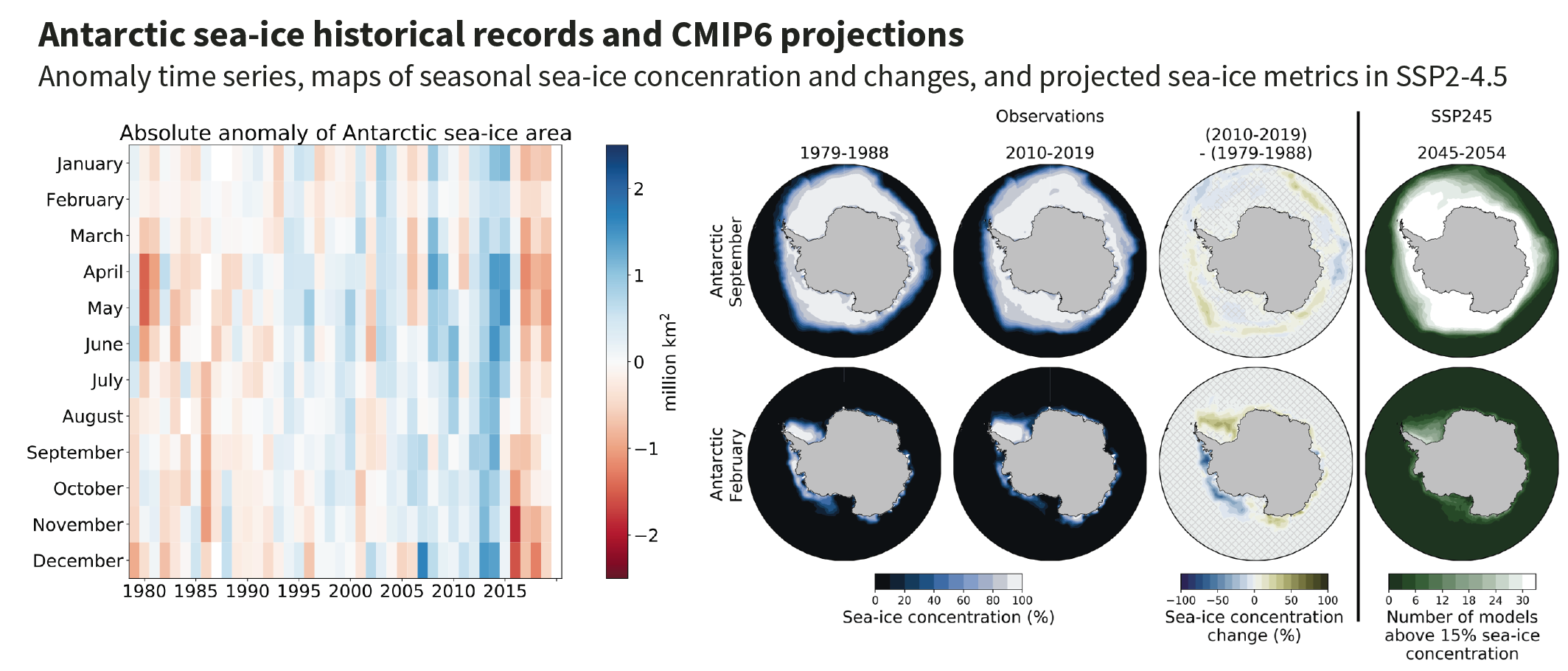 Figure9.15 | Antarctic sea ice historical records and Coupled Model Intercomparison Project Phase 6 (CMIP6) projections. (Left) Absolute anomaly of observed monthly mean Antarctic sea ice area during the period 1979–2019 relative to the average monthly mean Antarctic sea ice area during the period 1979–2008. (Right) Sea ice coverage in the Antarctic as given by the average of the three most widely used satellite-based estimates for September and February, which usually are the months of maximum and minimum sea ice coverage, respectively. First column: Mean sea ice coverage during the decade 1979–1988. Second column: Mean sea ice coverage during the decade 2010–2019. Third column: Absolute change in sea ice concentration between these two decades, with grid lines indicating non-significant differences. Fourth column: Number of available CMIP6 models that simulate a mean sea ice concentration above 15% for the decade 2045–2054. The average observational record of sea ice area is derived from the UHH sea ice area product (Doerr et al., 2021), based on the average sea ice concentration of OSISAF/CCI (OSI-450 for 1979–2015, OSI-430b for 2016–2019) (Lavergne et al., 2019), NASA Team (version 1, 1979–2019) (Cavalieri et al., 1996) and Bootstrap (version 3, 1979–2019) (Comiso, 2017) that is also used for the figure panels showing observed sea ice concentration. Further details on data sources and processing are available in the chapter data table (Table 9.SM.9).
 As assessed by SROCC, the evolution of mean Antarctic sea ice area is the result of opposing regional trends (high confidence), with slightly decreasing sea ice cover during the period 1979 to 2019 in the Amundsen and Bellingshausen Seas, particularly during summer, and slightly increasing sea ice cover in the eastern parts of the Weddell and Ross Seas (Figure 9.15). With the exception of the Ross Sea, these trends are not significant, considering the large variability of the time series (Yuan et al., 2017).
The SROCC assessed that the regional trends are closely related to meridional wind trends (high confidence). This is the case as the regional trends in the maximum northward extent of the ice cover (Figure 9.15) are determined by the balance between the northward advection of the ice that is formed in polynyas near the continental margin, and the lateral and subsurface melting through oceanic heat fluxes. The advection of the sea ice is strongly correlated with winds and cyclones (Schemm, 2018; Vichi et al., 2019; Alberello et al., 2020). Accordingly, the increasing sea ice area in the Ross Sea can be linked to a strengthening of the Amundsen Sea low (e.g., Holland et al., 2017b, 2018), while other regional sea ice trends in the austral autumn can be linked to changes in westerly winds, cyclone activity and the Southern Annular Mode (SAM) in summer and spring (Doddridge and Marshall, 2017; Holland et al., 2017a; Schemm, 2018). In addition to the wind-driven changes, increased near-surface ocean stratification (Section 9.2.1.3) has contributed to the observed increase in sea ice coverage (e.g., Purich et al., 2018; L. Zhang et al., 2019) as it tends to cool the surface ocean (Sections 9.2.1.1 and 9.2.3.2). The changes in stratification result partly from surface freshening (De Lavergne et al., 2014), associated with increased northward sea ice advection (Haumann et al., 2020) and/or melting of the Antarctic ice sheet (medium confidence) (e.g., Haumann et al., 2020; Jeong et al., 2020; Mackie et al., 2020), and amplified by local ice–ocean feedbacks (Goosse and Zunz, 2014; Lecomte et al., 2017; Goosse et al., 2018). In the Amundsen Sea, strong ice shelf melting can cause local sea ice melt next to the ice shelf front by entraining warm circumpolar deep water to the ice shelf cavity and surface ocean (medium confidence) (Sections 9.2.3.2 and 9.4.2.2; Jourdain et al., 2017; Merino et al., 2018). It has also been suggested that the observed regional increase in sea ice coverage since 1979 results from a long-term Southern Ocean surface cooling trend (e.g., Kusahara et al., 2019; Jeong et al., 2020) but the importance of this mechanism for the observed sea ice evolution is unclear owing to intricate feedbacks between sea ice change and surface cooling (Haumann et al., 2020). The importance of changing wave activity (Section 9.6.4.2; Kohout et al., 2014; Bennetts et al., 2017; Roach et al., 2018b) on sea ice is unclear due to limited process understanding. In summary, there is high confidence that regional Antarctic trends are primarily caused by changes in sea ice drift and decay, with medium confidence in a dominating role of changing wind pattern. The precise relative contribution of individual drivers remains uncertain because of limited observations, disagreement between models, unresolved processes, and temporal and spatial remote linkages caused by sea ice drift (Section 9.2.3.2; Pope et al., 2017).
Recent research has confirmed SROCC assessment of atmospheric and oceanic drivers of the sea ice decline from 2014 to 2017, which can be linked to changes in both subsurface ocean heat flux (Meehl et al., 2019; Purich and England, 2019) and atmospheric circulation, with the latter partly related to teleconnections with the tropics (Meehl et al., 2019; Purich and England, 2019; G. Wang et al., 2019). In the Weddell Sea, these changes caused in 2017 the re-emergence of the largest polynya over the Maud Rise since the 1970s (Section 9.2.3.2; Campbell et al., 2019; Jena et al., 2019; Turner et al., 2020).
The AR5 (Collins et al., 2013) and SROCC found low confidence in future projections of Antarctic sea ice. This includes the projected mitigation of the sea ice loss by stratospheric ozone recovery (Smith et al., 2012) and by an increased freshwater input from melting of the Antarctic Ice Sheet (Bronselaer et al., 2018). Compared to the interannual variability during the satellite record from 1979 onwards, models simulate too much variability in both CMIP5 (Zunz et al., 2013) and CMIP6 (Roach et al., 2020). The seasonal cycle in sea ice coverage is misrepresented in most CMIP5 (e.g., Holmes et al., 2019) and CMIP6 models (Roach et al., 2020), but the multi-model mean seasonal cycle in CMIP5 and CMIP6 agrees well with observations (Shu et al., 2015; Roach et al., 2020). Most CMIP5 models do not realistically simulate the evolution of Antarctic sea ice volume (Shu et al., 2015) and consistently overestimate the amount of low concentration sea ice, and underestimate the amount of high concentration sea ice (Roach et al., 2018a). In contrast, CMIP6 models simulate a more realistic distribution of regional sea ice coverage (Roach et al., 2020). Most CMIP5 models poorly represent Antarctic sea ice drift (e.g., Schroeter et al., 2018; Holmes et al., 2019), affecting simulated historical trends, with models that simulate a strong sea ice motion showing more variability in sea ice coverage than models with weaker sea ice motion (Schroeter et al., 2018). Owing to limited agreement between model simulations and observations, limited reliable observations on a process level, and a lack of process understanding of the substantial spread in CMIP5 and CMIP6 model simulations, there remains low confidence in existing future projections of Antarctic sea ice decrease and lack of decrease.
The discrepancy between the modelled and observed evolution of Antarctic sea ice has been related by SROCC to deficiencies in modelled stratification, freshening by ice-shelf meltwater, clouds, and other wind- and ocean-driven processes. Recent studies highlight the possible mis-representation of freshwater fluxes from ice shelves (Jeong et al., 2020), and the possible effect of the low resolution of most models (Sidorenko et al., 2019), even though lower-resolution models are, in principle, capable of a realistic simulation of the seasonal sea ice budgets in the Southern Ocean (Holmes et al., 2019). The relative importance of these possible reasons for the models’ shortcomings remains unclear (see Section 3.4.1.2 for details).
The analysis and understanding of the long-term evolution of the Antarctic sea ice cover is hindered by the scarcity of observational records before the satellite period, and the scarcity of paleorecords (see Section 2.3.2.1.2 for further details). Such long records are particularly relevant given that the Southern Ocean response to external forcing takes longer than the length of the available direct observational record (Goosse and Renssen, 2001; Armour et al., 2016). There is only limited evidence for large-scale decadal fluctuations in sea ice coverage caused by large-scale temperature and wind forcing. Sparse direct pre-satellite observations suggest a decrease in sea ice coverage from the 1950s to the 1970s (Fan et al., 2014). Paleo-proxy data indicate that, on multi-decadal to multi-centennial time scales, sea ice coverage of the Southern Ocean follows large-scale temperature trends (e.g., Crosta et al., 2018; Chadwick et al., 2020; Lamping et al., 2020), for example linked to fluctuations in the El Niño–Southern Oscillation and Southern Annular Mode (Crosta et al., 2021), and that during the Last Glacial Maximum, Antarctic sea ice extended to about the polar front latitude in most regions during winter, whereas the extent during summer is less well understood (e.g., Benz et al., 2016; Xiao et al., 2016; Nair et al., 2019).
Regionally, proxy data from ice cores consistently indicate that the increase of sea ice area in the Ross Sea and the decrease of sea ice area in the Bellingshausen Sea are part of longer centennial trends and exceed internal variability on multi-decadal time scales (medium confidence) (e.g., Thomas et al., 2019; Tesi et al., 2020). These centennial trends are consistent with simulations from CMIP5 models (Hobbs et al., 2016b; J.M. Jones et al., 2016; Kimura et al., 2017).
There is low confidence in the attribution of the observed changes in Antarctic sea ice area (Section 3.4.1.2). Based on the available evidence, the lack of a negative trend of Antarctic sea ice area, despite substantial global warming in recent decades, has been attributed to internal variability in analyses of the observational record (Meier et al., 2013; Gallaher et al., 2014; Gagné et al., 2015b), reconstructions from early observations (Fan et al., 2014; Edinburgh and Day, 2016) and proxy data (Hobbs et al., 2016b) in model simulations (Turner et al., 2013; Zunz et al., 2013; L. Zhang et al., 2019). Nonetheless, without accurate simulations of observed changes, the possible contribution of anthropogenic forcing to the regional changes in sea ice area remains unclear (Hosking et al., 2013; Turner et al., 2013; Haumann et al., 2014; L. Zhang et al., 2019).
The attribution of the observed trends in atmospheric and oceanic forcing is also uncertain because of limited observational records and discrepancies between modelled and observed evolution of the sea ice cover. More specifically, there is contrasting evidence for a direct role of stratospheric ozone depletion on the observed changes in atmospheric circulation (Haumann et al., 2014; England et al., 2016; Landrum et al., 2017). In contrast, there is high confidence that multi-decadal variations in the tropical Pacific and in the Atlantic affect the Amundsen Sea low (Li et al., 2014; Kwok et al., 2016; Meehl et al., 2016; Purich et al., 2016; Simpkins et al., 2016), while other modes of climate variability (Annex IV) affect, for example, Southern Ocean cyclone activity (Simpkins et al., 2012; Cerrone et al., 2017; Schemm, 2018).
9.3.2.2 Antarctic Sea Ice Thickness
The SROCC assessed that observations are too sparse to reliably estimate long-term trends in Antarctic sea ice thickness. This remains true, and only qualitative statements on prevailing thicknesses are possible. Data from ICESat-1 laser altimetry (Kurtz and Markus, 2012), from Operation IceBridge (Kwok and Kacimi, 2018), and long-term shipboard observations collected in the Antarctic Sea Ice Processes and Climate (ASPeCt) dataset (Worby et al., 2008) suggest that sea ice thicker than 1 m prevails in regions of multi-year ice along the eastern coast of the Antarctic Peninsula in the Weddell Sea, in the high-latitude embayment of the Weddell Sea, and along the coast of the Amundsen Sea, with remaining regions dominated by thinner first-year sea ice (high confidence). Regional patterns in ice thickness are affected by areas of high snow deposition and resulting snow-ice formation (Massom et al., 2001; Maksym and Markus, 2008), and deformation, ridging, and rafting that regionally cause formation of very thick sea ice (Massom et al., 2006; G. Williams et al., 2015). In addition, near ice shelves a sub-ice platelet layer from supercooled water can significantly increase sea ice thickness (Hoppmann et al., 2020; Haas et al., 2021). Regarding snow thickness, observations are too sparse in space and time to reliably estimate changes across Southern Ocean sea ice (Webster et al., 2018).
There is low confidence in the long-term trend of Antarctic sea ice thickness. Both ASPeCt and ICESat-1 measurements are biased low in regions with thick ice (Kern and Spreen, 2015), compared to results from reanalyses (Massonnet et al., 2013; Haumann et al., 2016) and observations with autonomous vehicles under sea ice (G. Williams et al., 2015). Estimates of sea ice thickness from CryoSat-2 do not substantially reduce uncertainty, primarily because of the unknown snow thickness and radar scattering above the snow–ice interface (Bunzel et al., 2018; Kwok and Kacimi, 2018; Kacimi and Kwok, 2020). Isolated in situ time series show no clear long-term trend in landfast ice thickness in the Weddell Sea (Arndt et al., 2020). Reanalyses suggest overall increasing sea ice thickness and volume between 1980 and 2010 (Holland et al., 2014; Zhang, 2014; Massonnet et al., 2015), while CMIP5 (Shu et al., 2015; Schroeter et al., 2018) and CMIP6 models simulate a decrease in Antarctic sea ice volume over the historical period. Because of this discrepancy, and the unclear reliability of the reanalyses (Uotila et al., 2019), there is low confidence in CMIP5 and CMIP6 simulated future Antarctic sea ice thickness.
9.4 Ice Sheets
9.4.1 Greenland Ice Sheet
9.4.1.1 Recent Observed Changes
In this section we present regional mass change time series for the Greenland Ice Sheet and assess the different processes that are causing the increase in mass loss. The vast increase in observational products from various platforms (e.g, GRACE, PROMICE, ESA-CCI, NASA MEaSUREs) provide a consistent and clear picture of a shrinking Greenland Ice Sheet (Colgan et al., 2019; Mottram et al.,2019; Mouginot et al., 2019; King et al., 2020; Mankoff et al., 2020; Moon et al., 2020; Sasgen et al., 2020; Velicogna et al., 2020; The IMBIE Team, 2020). Section 2.3.2.4.1 provides an updated estimate of the total Greenland Ice Sheet mass change in a global context (Figure 2.24). The estimated ice-sheet extent at different times is shown in Figure 9.17, and the paleo perspective on Greenland Ice Sheet evolution is presented in Section 9.6.2.
 Figure 9.16 | Mass changes and mass change rates for Greenland and Antarctic ice sheet regions. (a) Time series of mass changes in Greenland for each of the major drainage basins shown in the inset figure (Bamber et al., 2018b; Mouginot et al., 2019; The IMBIE Team, 2021) for the periods 1972–2016, 1992–2018, and 1992–2020. (b) Time series of mass changes for three portions of Antarctica (Bamber et al., 2018b; The IMBIE Team, 2021) for the period 1992–2016 and 1992–2020. Estimates of mass change rates of surface mass balance, discharge and mass balance in (g) all of Greenland and (c–f, h–j) in seven Greenland regions (Bamber et al., 2018b; Mankoff et al., 2019; Mouginot et al., 2019; King et al., 2020). Estimates of mass change rates of surface mass balance, discharge and mass balance for (k) all of Antarctica and (l–n) for three regions of Antarctica (Bamber et al., 2018b; The IMBIE Team, 2018; Rignot et al., 2019). Further details on data sources and processing are available in the chapter data table (Table 9.SM.9).
 For the 20th century, SROCC (Meredith et al., 2019) presented one reconstruction for 1900–1983 and estimated mass change for the Greenland Ice Sheet and its peripheral glaciers for the period 1901–1990. Since SROCC, a comprehensive new study has extended the satellite record back to 1972 (Figure 9.16; Mouginot et al., 2019). The rate of ice-sheet mass change was positive (i.e., it gained mass) in 1972–1980 (47 ± 21 Gt yr–1) and then negative (i.e., it lost mass; –51 ± 17 Gt yr–1and –41 ± 17 Gt yr–1) in 1980–1990 and 1990–2000, respectively. Other ice discharge time series starting in 1985 (King et al., 2018, 2020; Mankoff et al., 2019, 2020) agree with Mouginot et al. (2019) (see also Figure 9.16). There is limited evidence of temporally and spatially heterogeneous Greenland outlet glacier evolution during the 20th century (Lea et al., 2014; Lüthi et al., 2016; Andresen et al., 2017; Khan et al., 2020; Vermassen et al., 2020). Historical photographs (Khan et al., 2020) show large mass losses of Jakobshavn and Kangerlussuaq Glaciers in West Greenland from 1880 until the 1940s, exceeding their 21st-century mass loss, whereas the Helheim Glacier in East Greenland remained stable, gained mass in the 1990s, then rapidly lost mass after 2000. Together, these three large outlet glaciers, draining about 12% of the ice sheet surface area, have lost 22 ± 3 Gt yr–1in the period 1880–2012 (Khan et al., 2020). Overall, these studies provide a variable picture of the Greenland Ice Sheet mass change in the 20th century. The updated mass loss of Greenland Ice Sheet, including peripheral glaciers for the period 1901–1990, is 120 [70–170] Gt yr–1(see Table 9.5 and Figures 9.16 and 9.17).
Post-1992, SROCC stated that it is extremely likely that the rate of mass change of Greenland Ice Sheet was more negative during 2012–2016 than during 1992–2001, with very high confidence that summer melting has increased since the 1990s to a level unprecedented over at least the last 350 years. Since SROCC, the updated synthesis of satellite observations by the Ice Sheet Mass Balance Intercomparison Exercise (The IMBIE Team, 2020) and the GRACE Follow-On (GRACE-FO) Mission (Abich et al., 2019; Kornfeld et al., 2019), have confirmed the mass change record, and the record has been extended to 2020 (The IMBIE Team, 2021) as presented in 2.3.2.4. The Greenland Ice Sheet lost 4890 [4140–5640] Gt of ice between 1992 and 2020, causing sea level to rise by 13.5 [11.4 to 15.6] mm (The IMBIE Team, 2021; see also Section 2.3.2.4.1, Figure 9.16 and Table 9.5). The IMBIE Team’s (2020) estimates are consistent with other post-AR5 reviews (Figure 9.17, Table 9.SM.1; Bamber et al., 2018a; Cazenave et al., 2018; Mouginot et al., 2019; Slater et al., 2021). Recent GRACE-FO data (Sasgen et al., 2020; Velicogna et al., 2020) show that, after two cold summers in 2017 and 2018, with relatively moderate mass change of about –100 Gt yr–1, the 2019 mass change (–532 ± 58 Gt yr–1) was the largest annual mass loss in the record. The high agreement across a variety of methods confirms SROCC and Chapter 2 assessments. The mass-loss rate was, on average, 39 [–3 to 80] Gt yr–1over the period 1992–1999, 175 [131 to 220] Gt yr–1over the period 2000–2009 and 243 [197 to 290] Gt yr–1over the period 2010–2019 (see Table 9.SM.1).
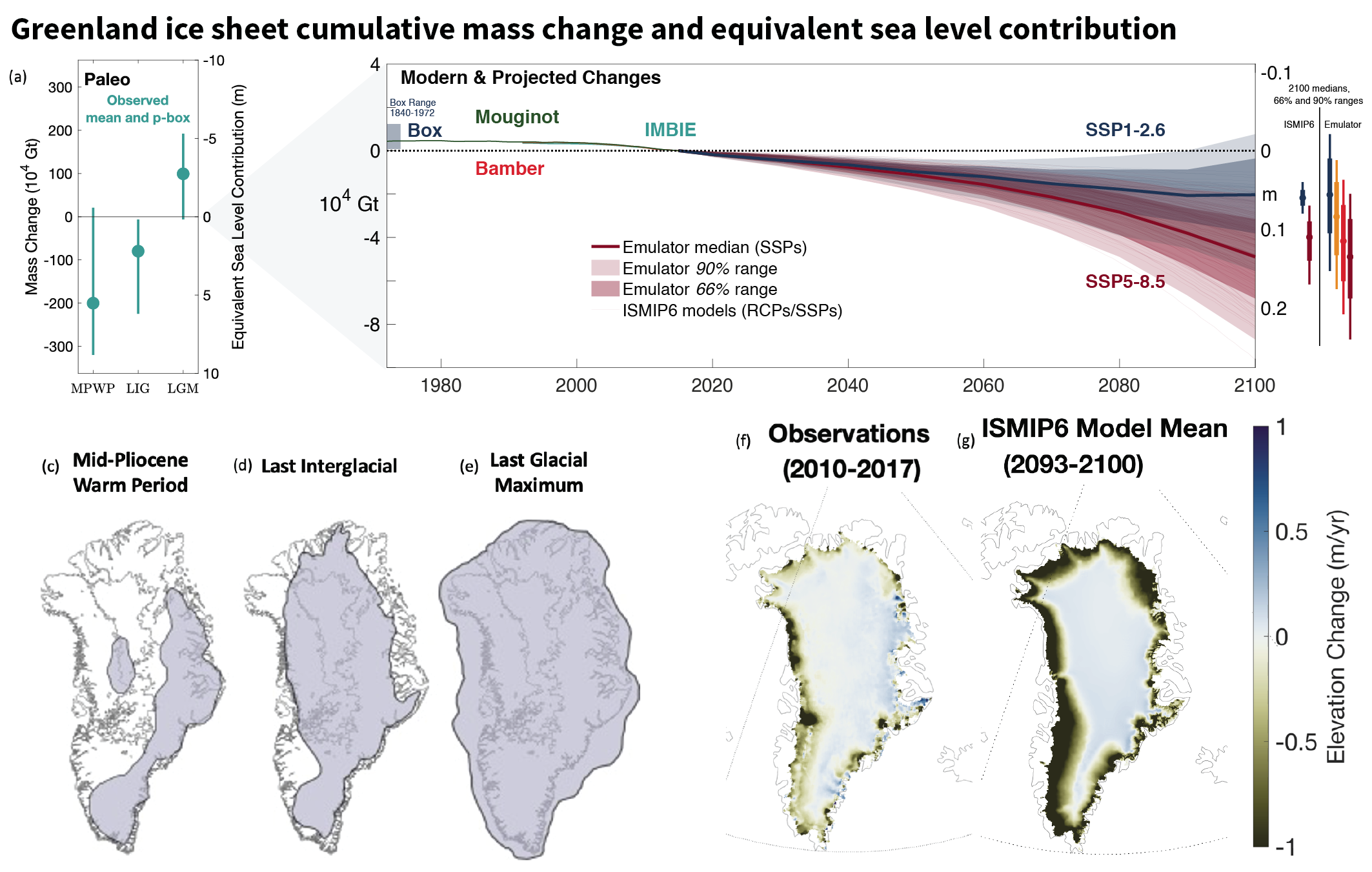 Figure 9.17 | Greenland Ice Sheet cumulative mass change and equivalent sea level contribution. (a) A p-box (Section 9.6.3.2) based estimate of the range of values of paleo Greenland Ice Sheet mass and sea level equivalents relative to present day and the median over all central estimates (Simpson et al., 2009; Argus and Peltier, 2010; Colville et al., 2011; Dolan et al., 2011; Fyke et al., 2011; Robinson et al., 2011; Born and Nisancioglu, 2012; K.G. Miller et al., 2012; Dahl-Jensen et al., 2013; Helsen et al., 2013; Nick et al., 2013; Quiquet et al., 2013; Stone et al., 2013; Colleoni et al., 2014; Lecavalier et al., 2014; Robinson and Goelzer, 2014; Calov et al., 2015, 2018; Dutton et al., 2015; Koenig et al., 2015; Peltier et al., 2015; Stuhne and Peltier, 2015; Vizcaino et al., 2015; Goelzer et al., 2016; Khan et al., 2016; Yau et al., 2016; de Boer et al., 2017; Simms et al., 2019); (b, left) cumulative mass loss (and sea level equivalent) since 2015 from 1972 (Mouginot et al., 2019) and 1992 (Bamber et al., 2018b; The IMBIE Team, 2020), the estimated mass loss from 1840 (Box and Colgan, 2013; Kjeldsen et al., 2015) indicated with a shaded box, and projections from Ice Sheet Model Intercomparison Project for CMIP6 (ISMIP6) to 2100 under RCP8.5/SSP5-8.5 and RCP2.6/SSP1-2.6 scenarios (thin lines from Goelzer et al. (2020); Edwards et al. (2021); Payne et al. (2021)) and ISMIP6 emulator under SSP5-8.5 and SSP1-2.6 to 2100 (shades and bold line; Edwards et al., 2021); (b, right) 17th–83rd and 5th–95th percentile ranges for ISMIP6 and ISMIP6 emulator at 2100. Schematic interpretations of individual reconstructions (Lecavalier et al., 2014; Goelzer et al., 2016; Berends et al., 2019) of the spatial extent of the Greenland Ice Sheet are shown for the: (c) mid-Pliocene Warm Period; (d) the Last Interglacial; and (e) the Last Glacial Maximum: grey shading shows extent of grounded ice. Maps of mean elevation changes (f) 2010–2017 derived from CryoSat 2 radar altimetry (Bamber et al., 2018b) and (g) ISMIP6 model mean (2093–2100) projected changes for the MIROC5 climate model under the RCP8.5 scenario (Goelzer et al., 2020). Further details on data sources and processing are available in the chapter data table (Table 9.SM.9).
 The SROCC assessed with high confidence that surface mass balance (SMB),rather than discharge, has started to dominate the mass loss of the Greenland Ice Sheet (due to increased surface melting and runoff), increasing from 42% of the total mass loss for 2000–2005 to 68% for 2009–2012. While these estimates have been confirmed since SROCC (Mouginot et al., 2019), the new longer record, as well as further comprehensive studies(Khan et al., 2015; Colgan et al., 2019; Mottram et al., 2019; The IMBIE Team, 2020)and detailed discharge records(King et al., 2020; Mankoff et al., 2020)reveal a more complex picture than the continuous trajectory this statement may have implied. Discharge was relatively constant from 1972–1999, varying by around 6% for the whole ice sheet, while SMB varied by a factor of over two interannually, leading to either mass gain or loss in a given year (Figure 9.16). During 2000–2005, the rate of discharge increased by 18%, then remained fairly constant again (increasing by 6% from 2006–2018). After 2000, SMB decreased more rapidly than discharge increased. In summary, the consistent temporal pattern in these longer datasets leads to high confidence that the Greenland Ice Sheet mass losses are increasingly dominated by SMB, but there is high confidence that mass loss varies strongly, due to large interannual variability in SMB.
On a regional scale, the surface elevation is lowering in all regions, and widespread terminus and calving front retreats have been observed (with no glaciers advancing; Mottram et al., 2019; Moon et al., 2020). The largest mass losses have occurred along the west coast and in south-east Greenland (Figure 9.16), concentrated at a few major outlet glaciers (Mouginot et al., 2019; Khan et al., 2020). This regional pattern is consistent with independent Global Navigation Satellite System (GNSS) observations from the Greenland Global Positioning System (GPS) network which show elastic bedrock uplift of tens of centimetres between 2007–2019 as a result of ongoing ice mass loss (Bevis et al., 2019). The regional time series (Figures 9.16; Atlas.30) show that SMB has been gradually decreasing in all regions, while the increase in discharge in the south-east, central east, north-west and central west has been linked to retreating tidewater glaciers (Figure 9.16). In summary, the detailed regional records show an increase in mass loss in all regions after the 1980s, caused by both increases in discharge and decreases in SMB (high confidence), although the timing and patterns vary between regions. The largest mass loss occurred in the north-west and the south-east of Greenland (high confidence).
The SROCC stated with high confidence that variability in large-scale atmospheric circulation is an important driver of short-term SMB changes for the Greenland Ice Sheet. This effect of atmospheric circulation variability on both precipitation and melt rates (and SROCC assessment) is confirmed by more recent publications (Välisuo et al., 2018; B. Zhang et al., 2019; Velicogna et al., 2020). The strong mass loss in 2019 (Cullather et al., 2020; Hanna et al., 2020; Tedesco and Fettweis, 2020) was driven by highly anomalous atmospheric circulation patterns, both on daily (Cullather et al., 2020) and seasonal time scales (Tedesco and Fettweis, 2020). Although surface melt is anticorrelated with the summer North Atlantic Oscillation Index (Välisuo et al., 2018; Ruan et al., 2019; Sherman et al., 2020), especially in West Greenland (Bevis et al., 2019), Greenland Ice Sheet melt is more strongly correlated with the Greenland Blocking Index (Hanna et al., 2016, 2018) than with the summer North Atlantic Oscillation index (Huai et al., 2020).
The SROCC did not assess the role of cloud changes in detail. Studies since AR5 have shown that higher incident shortwave radiation in conjunction with reduced cloud cover leads to increased melt rates, particularly over the low-albedo ablation zone in the southern part of the Greenland Ice Sheet (Hofer et al., 2017; Niwano et al., 2019; Ruan et al., 2019). Conversely, an increase in cloud cover over the high-albedo central parts of the ice sheet, leading to higher downwelling longwave radiation, was shown to lead either to increased melt (Bennartz et al., 2013) or reduced refreezing of meltwater (van Tricht et al., 2016). The elevation dependence of the cloud radiative effect and its control on surface meltwater generation and refreezing (W. Wang et al., 2019; Hahn et al., 2020) can induce a spatially consistent response of the integrated Greenland Ice Sheet melt to dominant patterns of cloud and atmospheric variability. The shortwave and longwave radiation effects on surface melt by clouds have been shown to compensate for each other during strong atmospheric river events, and the increase in melt is caused by increased sensible heat fluxes during such events (Mattingly et al., 2020). In summary, there is medium confidence that cloud cover changes are an important driver of the increasing melt rates in the southern and western part of the Greenland Ice Sheet.
The SROCC stated with high confidence that positive albedo feedbacks contributed substantially to the post-1990s Greenland Ice Sheet melt increase. Several (mostly positive) feedbacks involving surface albedo operate on ice sheets (e.g., Fyke et al., 2018). Melt amplification by the observed increase of bare ice exposure through snowline migration to higher parts of the ice sheet since 2000 (Shimada et al., 2016; Ryan et al., 2019) was five times stronger than the effect of hydrological and biological processes that lead to reduced bare ice albedo (Ryan et al., 2019). Impurities, in part biologically active (Ryan et al., 2018), have been observed to lead to albedo reduction (Stibal et al., 2017) and are estimated to have increased runoff from bare ice in the southwestern sector of the Greenland Ice Sheet by about 10% (Cook et al., 2020). In summary, new studies confirm that there is high confidence that the Greenland Ice Sheet melt increase since about 2000 has been amplified by positive albedo feedbacks, with the expansion of bare ice extent being the dominant factor, and albedo in the bare ice zone being primarily controlled by distributed biologically active impurities (see also Section 7.3.4.3).
The SROCC reported with medium confidence that around half of the 1960–2014 Greenland Ice Sheet surface meltwater ran off, while most of the remainder infiltrated firn and snow, where it either refroze or accumulated in firn aquifers. Studies since SROCC show a decrease of firn air content between 1998–2008 and 2010–2017 (Vandecrux et al., 2019) in the low-accumulation percolation area of western Greenland, reducing meltwater retention capacity. Moreover, meltwater infiltration into firn can be strongly limited by low-permeability ice slabs created by refreezing of infiltrated meltwater (Machguth et al., 2016). Recent observations and modelling efforts indicate that rapidly expanding low-permeability layers have led to an increase in runoff area since 2001 (MacFerrin et al., 2019). In summary, there is medium confidence that meltwater storage and refreezing can temporarily buffer a large-scale melt increase, but limiting factors have been identified.
The SROCC reported that there was medium confidence that ocean temperatures near the grounding zone of tidewater glaciers are critically important to their calving rate, but there was low confidence in understanding their response to ocean forcing. The increase in ice discharge in the late 1990s and early 2000s (Mouginot et al., 2019; King et al., 2020; Mankoff et al., 2020) has been associated with a period of widespread tidewater glacier retreat (Murray et al., 2015; Wood et al., 2021) and speed up (Moon et al., 2020). Since SROCC, new studies provide strong evidence for rapid submarine melting at tidewater glaciers (Sutherland et al., 2019; Wagner et al., 2019; Bunce et al., 2020; R.H. Jackson et al., 2020). Changes in submarine melting and subglacial meltwater discharge can trigger increased ice discharge by reducing the buttressing to ice flow and promoting calving (Benn et al., 2017; Todd et al., 2018; Ma and Bassis, 2019; Mercenier et al., 2020); through undercutting (Rignot et al., 2015; D.A. Slater et al., 2017; Wood et al., 2018; Fried et al., 2019) and frontal incision (Cowton et al., 2019). Warming ocean waters have been implicated in the recent thinning and breakup of floating ice tongues in north-eastern and north-western Greenland (Mouginot et al., 2015; Wilson et al., 2017; Mayer et al., 2018; Washam et al., 2018; An et al., 2021; Wood et al., 2021). On decadal time scales, tidewater glacier terminus position correlates with submarine melting (Slater et al., 2019). Over shorter time scales, individual glaciers or clusters of glaciers can behave differently and asynchronously (Bunce et al., 2018; Vijay et al., 2019; An et al., 2021), and there are not always clear associations between water temperature and glacier calving rates (Motyka et al., 2017), retreat or speed-up (Joughin et al., 2020; Solgaard et al., 2020). Variations in ice mélange at the front of a glacier, associated with changes in ocean and air temperature, have also emerged as a plausible control on calving (Burton et al., 2018; Xie et al., 2019; Joughin et al., 2020). In summary, there is high confidence that warmer ocean waters and increased subglacial discharge of surface melt at the margins of marine-terminating glaciers increase submarine melt, which leads to increased ice discharge. There is medium confidence that this contributed to the increased rate of mass loss from Greenland, particularly in the period 2000–2010 when increased discharge was observed in the south-east and north-west.
The SROCC reported that accurate bedrock topography is required for understanding and projecting the glacier response to ocean forcing. Accurate bathymetry is essential for establishing which water masses enter glacial fjords, and for reliable estimates of the submarine melt rates experienced by tidewater glaciers (Schaffer et al., 2020; T. Slater et al., 2020; Wood et al., 2021). Subglacial and lateral topography is known to strongly modulate tidewater glacier dynamics and the sensitivity of tidewater glaciers to climatic forcing (Enderlin et al., 2013; Catania et al., 2018). Bathymetric mapping around the ice sheet has greatly improved with direct and gravimetric surveys (Millan et al., 2018; An et al., 2019a, b; Jakobsson et al., 2020) leading to the improvement of Greenland-wide bathymetric and topographic mapping (e.g., Morlighem et al., 2017). However, large uncertainties in ice thickness remain for around half of the outlet glaciers (Mouginot et al., 2019; Wood et al., 2021) and sea ice covered and iceberg-packed regions remain poorly sampled near glacier termini (Morlighem et al., 2017). There is high confidence that bathymetry (governing the water masses that flow into fjord cavities) and fjord geometry and bedrock topography (controlling ice dynamics) modulate the response of individual glaciers to climate forcing.
The AR5 assessed that it is likely that anthropogenic forcing has contributed to the surface melting of Greenland since 1993 (Bindoff et al., 2013). Section 3.4.3.2 assesses that it is very likely that human influence has contributed to the observed surface melting of the Greenland Ice Sheet over the past two decades. There is medium confidence of an anthropogenic contribution to recent mass loss from Greenland.
9.4.1.2 Model Evaluation
The SROCC (Oppenheimer et al., 2019) stated that substantial challenges remained for modelling of the Greenland SMB and the dynamical ice sheet. Since SROCC, further insights into modelling of the Greenland ice sheet has come from model intercomparison studies of the SMB (Fettweis et al., 2020) and dynamical ice sheets (Goelzer et al., 2020; Payne et al., 2021). Further aspects relevant to the forcing of the ice sheet from large scale global climate models and regional climate models are discussed in Box 9.3 and Section Atlas.11.2.
The SROCC stated that climate model simulations of Greenland SMB had improved since AR5, giving medium confidence in the ability of climate models to simulate changes in Greenland SMB. Since SROCC, a multi-model intercomparison study (Fettweis et al., 2020) of regional and global climate models has shown that the greatest inter-model spread occurs in the ablation zone, due to deficiencies in an accurate model representation of the ablation zone extent and processes related to surface melt and runoff, confirming SROCC statement that there is large uncertainty in the bare ice model (Ryan et al., 2019). This intercomparison showed that simple, well-tuned SMB models using positive degree day melt schemes can perform as well as more complex physically based models (Figure (Atlas 30). Furthermore, the ensemble mean of the models produced the best estimate of the present-day SMB relative to observations (particularly in the ablation zone). Further assessment of Greenland Ice Sheet regional SMB can be found in Section Atlas.11.2.3. Recent progress confirms SROCC assessment that there is medium confidence in the ability of climate models to simulate changes in Greenland SMB.
The SROCC noted increased use of coupled climate–ice sheet models for simulating the Greenland ice sheet, but it also noted that remaining deficiencies in coupling between models of climate and ice sheets (e.g., low spatial resolution) limited the adequate representation of the feedbacks between them. Some Earth system models (ESMs) now incorporate multi-layer snow models and full energy balance models (Punge et al., 2012; Cullather et al., 2014; van Kampenhout et al., 2017, 2020; Alexander et al., 2019) or use elevation classes to compensate for their coarser resolution (Lipscomb et al., 2013; Sellevold et al., 2019; Gregory et al., 2020; Muntjewerf et al., 2020a, b). Resulting SMB simulations compare better with regional climate models and observations (Alexander et al., 2019; van Kampenhout et al., 2020), but the remaining shortcomings lead to problems reproducing a present-day ice-sheet state close to observations. In summary, there is medium confidence in quantitative simulations of the present-day state of the Greenland Ice Sheet in ESMs.
The SROCC (Meredith et al., 2019) stated that there is low confidence in understanding coastal glacier response to ocean forcing because submarine melt rates, calving rates, bed and fjord geometry and the roles of ice mélange and subglacial discharge are poorly understood. Ice–ocean interactions remain poorly understood and difficult to model, with parametrizations often used for calving of marine-terminating glaciers (Mercenier et al., 2018) and submarine and plume-driven melt (Beckmann et al., 2019). Due to the difficulties of modelling the large number of marine-terminating glaciers and limited availability of high-resolution bedrock data, the majority of recent modelling work on Greenland outlet glaciers is focused on individual or a limited number of glaciers (Krug et al., 2014; Bondzio et al., 2016, 2017; Morlighem et al., 2016b; Muresan et al., 2016; Choi et al., 2017; Beckmann et al., 2019), or a specific region (Morlighem et al., 2019). Since SROCC, using a flowline model that includes calving and submarine melting, Beckmann et al. (2019) concluded that the AR5 upscaling of contributions from four of the largest glaciers (Nick et al., 2013) overestimated the total glacier contribution from the Greenland Ice Sheet, due to differences in response between large and small glaciers. The regional study of Morlighem et al. (2019) confirms that ice–ocean interactions have the potential to trigger extensive glacier retreat over decadal time scales, as indicated by observations (Section 9.4.1.1). One focus of continental ice-sheet models has been the improved treatment of marine-terminating glaciers via the inclusion of calving processes and freely moving calving fronts (Aschwanden et al., 2019; Choi et al., 2021). An improved bedrock topographic dataset (Morlighem et al., 2017) allows for ice discharge to be better captured for outlet glaciers in continental ice-sheet models, and simulations indicate that bedrock topography controls the magnitude and rate of retreat (Aschwanden et al., 2019; Rückamp et al., 2020). Overall, although there is high confidence that the dynamic response of Greenland outlet glaciers is controlled by bedrock topography, there is low confidence in quantification of future mass loss from Greenland triggered by warming ocean conditions, due to limitations in the current understanding of ice–ocean interactions, its implementation in ice-sheet models, and knowledge of bedrock topography.
The SROCC (Oppenheimer et al., 2019) noted the progress made in Greenland Ice Sheet models since AR5. New since SROCC is a focus on improved representation of the present-day state of the ice sheet (Box 9.3; Goelzer et al., 2018, 2020). Improvements are closely linked to the growing number and quality of observations (Section 9.4.1.1), new techniques to generate internally consistent input datasets (Morlighem et al., 2014, 2016a), wider use of data assimilation techniques (Larour et al., 2014, 2016; Perego et al., 2014; Goldberg et al., 2015; Lee et al., 2015; Schlegel et al., 2015; Mosbeux et al., 2016), increased model resolution (Aschwanden et al., 2016) and tuning of key processes such as calving (Choi et al., 2021). A remaining challenge is low confidence in reproducing historical mass changes of the Greenland Ice Sheet (Box 9.3). However, there is medium confidence in ice-sheet models reproducing the present state of the Greenland Ice Sheet, leading to medium confidence in the current ability to accurately project its future evolution.
9.4.1.3 Projections to 2100
The AR5 and SROCC projected that changes in Greenland SMB will contribute to sea level in 2100 by 0.03 (0.01 to 0.07) m sea level equivalent (SLE) under RCP2.6, and 0.07 (0.03 to 0.16) m SLE under RCP8.5. New since SROCC are the projections of SMB obtained by an ESM, two regional climate models, and reconstructions based on temperature from the CMIP5 and CMIP6 ensembles (Hofer et al., 2020; Noël et al., 2021). The range of sea level contribution from Greenland SMB in Noël et al. (2021) is comparable to the AR5 assessment when either CMIP5 or CMIP6 models are used, while Hofer et al. (2020) find a greater mass loss across all CMIP6 emissions scenarios when compared to CMIP5 scenarios. Using SSP5-8.5 instead of RCP8.5 increases the mean projected sea level from 2005–2100 by up to 0.06 m in the regional climate model simulations of Hofer et al. (2020) who attribute the difference mainly to a greater Arctic amplification and associated cloud and sea ice feedbacks in the CMIP6 SSP5-8.5 simulations. In summary, these new projections with fixed ice-sheet topography do not provide sufficient evidence to change the AR5 and SROCC assessments.
Reviewing modelling studies since AR5 (Church et al., 2013b), SROCC (Oppenheimer et al., 2019) assessed Greenland’s contribution to future sea level to be relatively similar to AR5 (Table 9.2). The baseline for projections has shifted from 1986–2005 in SROCC, to 1995–2014 in this Report. Adjusted to the new 1995–2014 baseline by subtracting 0.01 m, SROCC projected a likely contribution of 0.07 (0.0–0.11) m SLE under RCP2.6, and 0.14 (0.08–0.27) m SLE under RCP8.5 by 2100. Since SROCC, new projections for the 21st century have included dynamic ice sheets coupled to ESMs (Muntjewerf et al., 2020a; Van Breedam et al., 2020) or regional atmospheric models (Table 9.2; Le clec’h et al., 2019). The coupled ESM–ice-sheet model CESM2–CISM2 (Community Earth System Model Version 2 and Community Ice Sheet Model 2) projects a sea level rise of 0.109 m in 2100 relative to 2015 under SSP5-8.5 (Muntjewerf et al., 2020a) and a similar contribution under the idealized 1% yr–1increase in CO2 scenario (Muntjewerf et al., 2020b). The CESM2–CISM2 simulations include ice-sheet–atmosphere interactions and ice-sheet surface meltwater routed to the ocean. The coupled regional atmospheric model and ice-sheet model MAR-GRISLI (Modèle Atmosphérique Régional and Grenoble ice sheet and land ice model) projects a sea level rise of 0.079 m in 2100 relative to 2000 under RCP8.5 (Le Clec’h et al., 2019). An ESM of lower complexity coupled to an ice-sheet model gives a sea level contribution of 0.025 to 0.064 m under RCP2.6 and 0.056 to 0.12 m under RCP8.5 (the range is due to four simulations with different parameter sets for the atmosphere model) (Van Breedam et al., 2020). Van Breedam et al. (2020) identify a simulation with a preferred parameter set that projects 0.034 m for RCP2.6 and 0.073 m for RCP8.5. Although the ocean does not directly force the ice-sheet models in these simulations, the new coupled models allow for interactions between ice-sheet dynamics, SMB and local climate. The coupled projections fall within the lower bounds of AR5 and SROCC and, as these studies do not prescribe ocean forcing directly, it is possible that the dynamic response is underestimated.
Representative Concentration Pathways (RCPs) | ||||
Study | RCP2.6 | RCP4.5 | RCP8.5 | Notes |
IPCC AR5 and SROCC (Oppenheimer et al., 2019) | 0.07 (0.03 to 0.11) | 0.08 (0.04 to 0.15) | 0.14 (0.08 to 0.27) | Median and likely (66%range) contributions in 2100 relative to 1995–2014. Median of multiple studies |
ISMIP6 CMIP5-forced (Goelzer et al., 2020); excludes historical dynamic response | 0.01 to 0.05 | n/a | 0.04 to 0.14 | Range of multi-model contributions in 2100 relative to 2015 from 1 ESM for RCP2.6 and 6 ESMs for RCP8.5 (see caption) |
Coupled regional atmosphere–ice sheet model (Le clec’h et al., 2019) | n/a | n/a | 0.079 | Contribution in 2100 relative to 2000 from AR-GRISLI model |
Coupled Earth system model (ESM) of lower complexity-ice-sheet model (Van Breedam et al., 2020) | 0.034 (0.025 to 0.064) | n/a | 0.073 (0.056 to 0.12) | Contribution in 2100 relative to 2000 from LOVECLIM-AGISM model; preferred parameter set and range from four simulations with different parameters for atmosphereodel |
Shared Socio-economic Pathways (SSPs) | ||||
Study | SSP1-2.6 | SSP2-4.5 | SSP5-8.5 | Notes |
Coupled ESM–ice sheet model (Muntjewerf et al., 2020a) | n/a | n/a | 0.109 | Contribution in 2100 relative to 2015 from coupled CESM2–CISM2 |
ISMIP6 CMIP6-forced (Payne et al., 2021); excludes historical dynamic response | 0.02 to 0.06 | n/a | 0.08 to 0.25 | Range of multi-model contributions in 2100 relative to 2015 from one ESM for SSP1-2.6 and four ESMs for SSP5-8.5 |
ISMIP6 CMIP5 and CMIP6 forced ensemble including historical dynamic response | 0.06 (0.05 to 0.07) [0.04 to 0.08] | n/a | 0.11 (0.09 to 0.14) [0.07 to 0.17] | Median (66% range) [90% range] contribution from ISMIP6 CMIP5- and CMIP6-forced multi-model ensembles |
ISMIP6 with AR5 parametric fit: used to estimate rates (Supplementary Material 9.SM.4.4) including historical dynamic response | 0.08 (0.06 to 0.10) [0.05 to 0.12] | 0.10 (0.08 to 0.13) [0.07 to 0.15] | 0.14 (0.11 to 0.18) [0.10 to 0.22] | Median (66% range) [90% range] contribution from AR5 parametric fit to ISMIP6 ensemble, relative to 1995–2014 |
Emulated ISMIP6; excludes historical dynamic response (Edwards et al., 2021) | 0.03 (–0.01 to 0.08) [–0.04 to 0.12] | 0.06 (0.01 to 0.10) [–0.02 to 0.15] | 0.11 (0.06 to 0.16) [0.03 to 0.21] | Median (66% range) [90% range] contribution in 2100 relative to 2015 from emulator of ISMIP6 used with Chapter 7: Climate Forcing |
This assessment: emulated ISMIP6 total | 0.06 (0.01 to 0.10) [–0.02 to 0.15] | 0.08 (0.04 to 0.13) [0.01 to 0.18] | 0.13 (0.09 to 0.18) [0.05 to 0.23] | As above, but relative to 1995–2014 and including historical dynamic response |
Since SROCC, projections of the Greenland Ice Sheet are also available from The Ice Sheet Model Intercomparison Project for CMIP6 (ISMIP6) (Box 9.3; Annex II; Figure 9.17; Nowicki et al., 2016, 2020a). ISMIP6 multi-model projections are corrected with an assessment of the historical dynamical response to pre-2015 climate forcing (Box 9.3). For the period 2015–2100, the ISMIP6 uncorrected multi-model ensemble projects sea level contributions ranging from 0.01 to 0.05 m under RCP2.6, 0.04 to 0.14 m under RCP8.5 (Goelzer et al., 2020), 0.02 to 0.06 m under SSP1-2.6, and 0.08 to 0.25 m under SSP5-8.5 (Table 9.2; Payne et al., 2021). The higher mass loss in the SSPs is attributed to a larger decrease in SMB due to the high climate sensitivity of the models used (Payne et al., 2021). This finding is confirmed by Choi et al. (2021), where CMIP6 SSP5-8.5 SMB leads to larger ice loss than CMIP5 RCP8.5, while ice discharge is similar. As the ISMIP6 framework considers a subset of the RCPs/SSPs and CMIP models, SSP-based projections have been inferred from multiple approaches. First, the ISMIP6 CMIP5-forced (Goelzer et al., 2020) and CMIP6-forced (Payne et al., 2021) combined ensemble projections were corrected with the historical trend (Box 9.3) using bootstrapping. Second, an emulator of the ISMIP6 projections (Box 9.3; Edwards et al., 2021) is forced by distributions of global surface air temperature for each SSP from a two-layer energy budget emulator (Supplementary Material 7.SM.2) and then corrected with the historical trend in the same way. These two approaches result in projections that are similar in their median values to AR5 and SROCC projections (Table 9.2), but differ in their range. Similar results are obtained when the AR5 parametric fit is applied to the ISMIP6 models (Table 9.2, Supplementary Material 9.SM.4.4), which is used to estimate rates of change and post-2100 projections (Sections 9.4.1.4 and 9.6.3.2).
The SROCC noted that the study by Aschwanden et al. (2019) projects a significantly higher Greenland contribution to sea level than the assessed likely range in AR5 and SROCC. Under RCP8.5, Aschwanden et al. (2019) found that Greenland could contribute up to 0.33 m to sea level by 2100 relative to 2000 (the ensemble member that best reproduces the 2000–2015 mean SMB from a regional climate model projects Greenland mass losses of 0.08 m SLE under RCP2.6 and 0.18 m SLE under RCP8.5). The SROCC noted that the potentially high sea level contribution in this study could be due to the assumption of spatially uniform warming, which can overestimate surface melt rates. However, it also reflects the deep uncertaintysurrounding atmospheric forcing, surface processes, submarine melt, calving and ice dynamics. Goelzer et al. (2020) ascribe 40% of the ISMIP6 multi-model ensemble spread to ice-sheet model uncertainty, 40% to climate model uncertainty and 20% to ocean forcing uncertainty. We note that this finding reflects the current challenges associated with the representation of ice–ocean interactions in models, and the uncertainty in basal conditions (Section 9.4.1.2). However, this finding is consistent with the work of Aschwanden et al. (2019) and thus, there is medium confidence that uncertainty in mass loss from the Greenland Ice Sheet is dominated by uncertainty in climate scenario and surface processes, whereas uncertainty in calving and frontal melt play a minor role.
The SROCC stated that surface processes, rather than ice discharged into the ocean, will dominate Greenland ice loss over the 21st century, regardless of the emissions scenario (high confidence). This is confirmed by the ISMIP6 projections (Goelzer et al., 2020; Payne et al., 2021). The projected mass loss of Greenland is predominantly due to increased surface meltwater and loss in refreezing capacity resulting in decreasing SMB (high confidence), concurrent with rising temperatures and darkening of the ice-sheet surface (Fettweis et al., 2013; Vizcaino et al., 2015; Le Clec’h et al., 2019; Muntjewerf et al., 2020a, b; Sellevold and Vizcaíno, 2020). Mass changes due to SMB and outlet glacier dynamics are linked (Goelzer et al., 2013; Fürst et al., 2015; Rückamp et al., 2020), as mass loss by one process decreases mass loss by the other – for example, SMB removes ice before it can reach the marine glacier terminus. There is medium confidence that the mass loss through ice discharge will decrease in the future (Fürst et al., 2015; Aschwanden et al., 2019; Golledge et al., 2019), because an increase in mass loss (via increased discharge or surface runoff) leads, in most areas, to a retreat of the glacier margin onto land above sea level, isolating the ice sheet from marine influence.
In summary, it is virtually certain that the Greenland Ice Sheet will continue to lose mass this century under all emissions scenarios, and high confidence that total mass loss by 2100 will increase with cumulative emissions. The sea level assessment (Section 9.6.3.3) is based on the emulated ISMIP6 projections, allowing a more consistent approach to a wider range of climate and ocean forcings. The Greenland Ice Sheet is likely to contribute 0.06 (0.01 to 0.10) m under SSP1-2.6 and 0.13 (0.09 to 0.18) m under SSP5-8.5 by 2100 relative to 1995–2014. These projections (as well as those of AR5 and SROCC) are lower than the study of Aschwanden et al. (2019) or the range of possible sea level changes resulting from Structured Expert Judgement (SEJ; Section 9.6.3.2; Bamber et al., 2019), contributing to the deep uncertainty in projected sea level (Box 9.4). There is, however, high confidence that the loss from Greenland will become increasingly dominated by SMB and surface melt, as the ocean-forced dynamic response of glaciers will diminish as marine margins retreat to higher grounds.
9.4.1.4 Projections Beyond 2100
The AR5 (Church et al., 2013b) assessed the contribution from Greenland to sea level projections in 2300 as 0.15 m SLE in low-emissions scenarios (about RCP2.6) and 0.31–1.19 m in high scenarios (approximately RCP6.0/RCP8.5). The SROCC (Oppenheimer et al., 2019) did not update AR5 estimates, given limited evidence and low agreement from three new studies (Vizcaino et al., 2015; Calov et al., 2018; Aschwanden et al., 2019). Since SROCC, a new study gives a sea level contribution of 0.11 to 0.20 m in low-emissions scenarios and 0.61 to 1.29 m in high-emissions scenarios (Van Breedam et al., 2020). The low-emissions projections by Van Breedam et al. (2020) encompass AR5’s assessed contribution, while the high emissions projections are higher than that from AR5. The ‘optimal’ ensemble member of Aschwanden et al. (2019) (see also Section 9.4.1.3) indicates that Greenland could contribute 0.25 m under RCP2.6 and 1.74 m under RCP8.5. Structured expert judgement (Bamber et al., 2019) projects Greenland losses of 0.54 (0.28–1.28) m under 2°C warming and 0.97 (0.4–2.23) m under 5°C warming. These studies therefore agree that the AR5 and SROCC assessments are at the low end of the range of projections. In addition, observations suggest that Greenland Ice Sheet losses are tracking the upper range of AR5 projections (T. Slater et al., 2020). Therefore, we update the likely range for the contribution of the Greenland Ice Sheet to global mean sea level (GMSL) by 2300 to 0.11–0.25 m under RCP2.6/SSP1-2.6 and 0.31–1.74 m under RCP8.5/SSP5-8.5. However, given the uncertainty in climatic drivers used to project ice-sheet change over the 21st century (Goelzer et al., 2020; Hofer et al., 2020; Noël et al., 2021) and the large range in simulations since AR5 extending beyond 2100, we only have low confidence in the contribution to GMSL by 2300 and beyond.
The role of the elevation–mass feedback for future projections of Greenland can be assessed from paleo simulations. Ice-sheet model simulations of the Laurentide (Gomez et al., 2015; Gregoire et al., 2016) and Eurasian (Alvarez-Solas et al., 2019) ice sheets invoke at least some contribution to last glacial termination mass loss from SMB reduction, as a consequence of an elevation–mass balance feedback (Levermann and Winkelmann, 2016). In a model spanning Meltwater Pulse 1A, this mechanism increased mass loss by approximately 66% (Gregoire et al., 2016) but in Last Interglacial simulations, the effect of this feedback is shown to depend on the surface scheme of the climate model employed (Plach et al., 2019). Given the agreement between theoretical analyses and paleo-ice-sheet model experiments, there is high confidence that the elevation–mass balance feedback is most relevant at multi-centennial and millennial time scales, consistent with future-focused studies (Aschwanden et al. 2019, Le Clec’h et al., 2019, Gregory et al., 2020).
The SROCC adopted the AR5 assessment that complete loss of Greenland ice, contributing about 7 m to sea level, over a millennium or more would occur for a sustained global mean surface temperature (GMST) between 1°C (low confidence) and 4°C (medium confidence) above pre-industrial levels. New studies since SROCC (Gregory et al., 2020; Van Breedam et al., 2020) confirm this assessment (see also Figure 9.30). Clark et al. (2016) estimate a complete loss to take about 8000 years at 5.5°C and about 3000 years at 8.6°C. Based on the agreement between new and previous studies, there is therefore high confidence that the rate at which Greenland Ice Sheet commitment is realized depends on the amount of warming.
Accounting for more detailed feedbacks between the atmosphere and the ice sheet (Gregory et al., 2020) found a gradual relationship between sustained global mean warming and the corresponding near-equilibrium ice-sheet volume, in contrast to a sharp threshold as found by Robinson et al. (2012). Rather than a climatically controlled tipping point for irreversible loss of the Greenland Ice Sheet, Gregory et al. (2020) found a threshold of irreversibility linked to ice-sheet size, similar to previous work (Ridley et al., 2010). The results of Gregory et al. (2020) show that, if the ice sheet loses mass equivalent to about 3–3.5 m of sea level rise, it would not regrow to its present state, and 2 m of the sea level rise would be irreversible. The point in time at which the current ice sheet might reach this critical volume depends on oceanic and atmospheric conditions, ice dynamics, and climate–ice sheet feedbacks (Gregory et al., 2020; Van Breedam et al., 2020). Therefore, projections differ in the magnitude and rate of temperature change to cross the threshold for irreversible loss. Projections from a large ensemble indicate that the mass threshold may be reached in as early as 400 years under extended RCP8.5 if warming reaches 10°C or more above present levels (Aschwanden et al., 2019). In summary, there is high confidence in the existence of threshold behaviour of the Greenland Ice Sheet in a warmer climate; however, there is low agreement on the nature of the thresholds and the associated tipping points.
Box 9.3 | Insights into Land Ice Evolution From Model Intercomparison Projects
Projections of ice sheets and glaciers in AR5 (Church et al., 2013b) and SROCC (Oppenheimer et al., 2019) were assessed by collecting single model studies – with the exception of glaciers in SROCC (Hock et al., 2019b). Community benchmark experiments (ISMIP-HOM; Pattyn et al., 2008) or Marine Ice Sheet Model Intercomparison Projects (MISMIP; Pattyn et al., 2012); MISMIP3d, (Pattyn and Durand, 2013); MISMIP+ (Asay-Davis et al., 2016; Cornford et al., 2020) have substantially advanced ice-sheet modelling since AR5. Model Intercomparison Projects (MIPs) now inform projections of both ice sheets and glaciers: the Ice Sheet MIP for CMIP6 (ISMIP6; Sections 9.4.1.3 and 9.4.2.5), the Linear Antarctic Response MIP (LARMIP-2; Section 9.4.2.5) and GlacierMIP (Section 9.5.1.3).
Regional forcing for land ice intercomparison projects
Simulations of ice sheets and glaciers are dependent on forcing provided by atmosphere and ocean models. Despite progress in representing processes, reducing biases and increasing resolution, regional and global models still have difficulties reproducing observed regional air temperature, surface mass balance (SMB) and ocean changes (Sections 9.4.1.2 and 9.4.2.2, and Atlas.11). An assessment of CMIP5 and CMIP6 climate models, as forcing for land ice models, has been undertaken (Walsh et al., 2018; Barthel et al., 2020; Marzeion et al., 2020; Nowicki et al., 2020b) with the aim of selecting the best available historical forcings and sampling potential regional future climate changes. Despite improvement in simulation of atmospheric forcing, persistent biases remain in CMIP5 and CMIP6, which reduces the fidelity of historical and future simulations of land ice.
Box 9.3
ISMIP6 initial state intercomparison projects
The ISMIP6 initial state intercomparison projects (initMIP) for the Greenland (Goelzer et al., 2018) and Antarctic (Seroussi et al., 2019) ice sheets were designed to understand the uncertainty in sea level projections resulting from the choice of initialization procedures used for projections of sea level (Nowicki et al., 2016). Participating modelling groups (Annex II) were free to decide on the initialization method used to bring ice-sheet models to a present-day state, with the effect of these choices captured in a control simulation (starting from the present-day state, with no further climate forcing applied), which measures intrinsic model drift. Compared to the earlier SeaRISE intercomparison project (Bindschadler et al., 2013; Nowicki et al., 2013), the modelled present-day ice sheets are in closer agreement with observations, and the model drift has been reduced (Goelzer et al., 2018; Seroussi et al., 2019). Nonetheless, historical simulations remain challenging for ice-sheet models, due to limited ice-sheet observations prior to the satellite era and biases in the historical atmospheric and oceanic forcings from climate models (Nowicki and Seroussi, 2018). ISMIP6 and LARMIP-2 therefore did not provide a protocol for the historical runs used to bring the ice sheets to present day, nor criteria for sub-selecting models from the multi-model ensemble based on the ability to reproduce historical changes (Levermann et al., 2020; Nowicki et al., 2020a).
ISMIP6 projections for the Greenland and Antarctic ice sheets
The ISMIP6 projection protocol (Nowicki et al., 2016, 2020a) was designed to sample the uncertainty in future sea level due to climate scenarios (via the use of high- and low-emissions scenarios and multiple climate models), ice–ocean interactions and inland response to ice-shelf collapse, and ice-sheet model diversity. The participating ice-sheet models are listed in Annex II. For each ice sheet, forcing was selected (Barthel et al., 2020) from the CMIP5 (Taylor et al., 2012) and CMIP6 (Eyring et al., 2016) models. Atmospheric forcing fields consisted of anomalies in SMB and surface air temperatures; these were generated directly from the CMIP models for the Antarctic Ice Sheet and downscaled using the regional climate model (MAR) for the Greenland Ice Sheet (Hofer et al., 2020). To sample the uncertainty due to ocean forcings, models used either a model-specific scheme with the ISMIP6-provided oceanic dataset or a standard ISMIP6 approach. For the Greenland Ice Sheet, the oceanic dataset consists of thermal forcing (temperature minus freezing temperature) extrapolated into fjords and subglacial runoff. The standard approach uses timelines of tidewater glacier retreat (D.A. Slater et al., 2019, 2020). For the Antarctic Ice Sheet, the oceanic dataset consists of salinity, thermal forcing and temperature added to an observationally derived climatology and extrapolated under ice shelves. The standard approach is a basal melt rate that depends quadratically on thermal forcing, adapted from Favier et al. (2019), with two different calibrations (Figure 9.19, Jourdain et al., 2020) that reproduce observed basal melt rates across Antarctica or Pine Island Glacier, respectively (Sections 9.4.2.2, 9.4.2.3). Antarctic ice-shelf disintegration datasets (Nowicki et al., 2020a) assume that ice shelves disintegrate when annual surface melt reaches a threshold (Trusel et al., 2015).
The ISMIP6 projections (Goelzer et al.,2020; Seroussi et al., 2020; Payne et al., 2021) are reported as experiment minus control and represent the sea level resulting from future climate change only. The control simulation, which has constant climate conditions starting in 2015 from the historical run, captures drift associated with the choices made for the initialization method and historical run. Subtraction of this control removes any long-term dynamic response of the ice sheet to pre-2015 climate change. This response has been assessed using dynamic discharge derived from observations over the last 40 years (Mouginot et al., 2019; Rignot et al., 2019), under an assumption that it persists at the past rate until 2100, rather than diminishing. The dynamic response to historical forcing is estimated as 0.19 ± 0.10 mm yr–1for the Greenland Ice Sheet (Section 9.4.1.3) and 0.33 ± 0.16 mm yr–1for the Antarctic Ice Sheet (Section 9.4.2.5). Over the period 2015–2100, this leads to an additional sea level contribution of 1.7 cm for Greenland and 2.8 cm for Antarctica.
LARMIP-2 projections for the Antarctic Ice Sheet
LARMIP-2 is focused on the uncertainty in the ocean forcing and associated ice-shelf melting (Levermann et al., 2014, 2020) with the majority of the models also participating in ISMIP6 (Annex II). The experiments start from present day and impose an additional basal ice-shelf melting of 8 m yr–1at the beginning of the 100-year simulation. A control run is used to remove drift resulting from initialization. The time derivative of the ice-sheet response yields a linear response function, which is then convoluted with a forcing of basal shelf melt time series for five Antarctic regions. The forcing time series for RCP2.6, 4.5, 6.0 and 8.5 were obtained from a random combination of global mean temperature for each Representative Concentration Pathway (RCP) from MAGICC-6.0 (Meinshausen et al., 2011), a scaling factor and time delay for the relationship between global surface air temperature and subsurface ocean warming in a given sector of the Southern Ocean from one of 19 CMIP5 models (Taylor et al., 2012) and a basal melting sensitivity from the interval [7–16] m yr–1°C–1to convert the regional subsurface warming into basal ice-shelf melting. This process is repeated 20,000 times to obtain a probability distribution of the sea level contribution for five Antarctic sectors. The linear response framework captures complex temporal responses of the ice sheets resulting from an increase in basal ice-shelf melting, but neglects the response to SMB and any self-dampening or self-amplifying processes, such as marine ice shelf instability (MISI). The LARMIP-2 method is applied to temperature projections for the Shared Socio-economic Pathways (SSPs; Supplementary Material 7.SM.2) and an estimate of SMB change from the AR5 parametric Antarctic Ice Sheet SMB model (Church et al., 2013b) is added to the results (Sections 9.4.2.4, 9.4.2.5 and 9.6.3.2). It is not necessary to add a long-term dynamic response to the LARMIP-2 projections, as this is incorporated in the basal melt time series.
GlacierMIP projections
GlacierMIP (Marzeion et al., 2020) was designed to estimate the glacier contribution to sea level rise, including from peripheral glaciers in Greenland and Antarctica that can be considered to be dynamically decoupled, or entirely separate, from the ice sheets. Glacier models are described in Annex II. Initial conditions were based on Randolph Glacier Inventory Version 6 (RGI Consortium, 2017) and initial ice thickness and volume were provided from an update of Huss and Farinotti (2012), although some glacier models used their own estimates. Forcings were taken from 10 different CMIP5 general circulation models, selected based on availability of multiple RCPs, the choice in a previous model intercomparison (Hock et al., 2019a), and performance in glacier-covered regions according to Walsh et al. (2018). In addition, two global glacier models performed the same experiment with 13 CMIP6 models (Section 9.5.1.3).
Use of an emulator with ISMIP6 and GlacierMIP projections
The ISMIP6 and GlacierMIP projections are primarily based on a limited number of CMIP5 RCPs and CMIP6 SSPs, and a limited sampling of ice–ocean interaction parameters and ice-shelf collapse simulations. Emulators provide a method for expanding these projections to a range of SSPs with more comprehensive sampling of climate, ice-sheet and glacier modelling uncertainties. Sections 9.4.1.3, 9.4.2.5 and 9.5.1.3 show estimates from the emulator of Edwards et al. (2021). This is a Gaussian Process, rather than a physically based (Cross-Chapter Box 7.1) model derived from the ISMIP6 and GlacierMIP simulations; projections use distributions of global surface air temperature (GSAT) from the two-layer emulator (Supplementary Material 7.SM.2) and ice-sheet parameters as inputs, and include estimates of the emulator uncertainty. Therefore, probability intervals are not inflated by a further factor, as is often the case for multi-model ensemble projections, to account for missing uncertainties (Section 9.6.3.2). The emulator is used in Section 9.6.3 to provide projections of the land ice contribution to sea level that are fully consistent with each other, ocean heat content, and the assessed equilibrium climate sensitivity and projections of GSAT across the entire report.
9.4.2 Antarctic Ice Sheet
9.4.2.1 Recent Observed Changes
As stated in Section 2.3.2.4, satellite observations by Ice Sheet Mass Balance Intercomparison Exercise (IMBIE) combining multi-team estimates based on altimetry, gravity anomalies (GRACE) and the input-output method, already presented in SROCC (Meredith et al., 2019), are updated and extended to 2020 (The IMBIE Team, 2021). The Antarctic Ice Sheet (AIS) lost 2670 [1800 to 3540]Gt mass over the period 1992–2020, equivalent to 7.4 [5.0 to 9.8]mm GMSL rise (for contribution to sea level budget, see Figures 9.16 and 9.18, and Table 9.5). Within uncertainties, this estimate agrees with a review of post-AR5 studies up to 2016 (Bamber et al., 2018b) and is consistent with recent single studies based on satellite laser altimetry (Smith et al., 2020), the input-output method (Rignot et al., 2019) and gravimetry (Velicogna et al., 2020). The mass-loss rate was on average 49 [–2 to 100] Gt yr–1over the period 1992–1999, 70 [22 to 119] Gt yr–1over the period 2000–2009, and 148 [94 to 202] Gt yr–1over the period 2010–2016 (see Figures 9.16 and 9.18, and Table 9.SM.1). However, recent work suggests that the mass loss has not further increased since 2016 because of regional mass gains in Dronning Maud Land (Velicogna et al., 2020). Mass loss of the West Antarctic and Antarctic Peninsula ice sheets has increased since about 2000 (very high confidence), essentially due to increased ice discharge (Harig and Simons, 2015; Paolo et al., 2015; Forsberg et al., 2017; Bamber et al., 2018b; Gardner et al., 2018; The IMBIE Team, 2018; Rignot et al., 2019).
The SROCC reported with very high confidence that the acceleration, retreat and thinning of the principal West Antarctic outlet glaciers has dominated the observed Antarctic mass loss over the last decades, and stated with high confidence that these losses were driven by melting of ice shelves by warm ocean waters. The average West Antarctic Ice Sheet (WAIS) mass loss of 82 ± 9 Gt yr–1between 1992 and 2017 (The IMBIE Team, 2021) leads to substantial observed surface lowering (e.g., Schröder et al., 2019; Shepherd et al., 2019), particularly in coastal regions (Figure 9.18). Recent studies using satellite altimetry (Schröder et al., 2019) and the input-output method (Rignot et al., 2019) consistently show mass loss in these coastal regions since the late 1970s (Figure 9.16). Because of consistent multiple lines of evidence, there is high confidence in mass loss of the Totten Glacier in East Antarctica (Miles et al., 2013; X. Li et al., 2016; Mohajerani et al., 2018; Rignot et al., 2019; Schröder et al., 2019; Shepherd et al., 2019) since about 2000, dominated by changes in coastal ice dynamics (X. Li et al., 2016). It is currently unclear whether mass loss of the EAIS over the last three decades has been significant (Rignot et al., 2019) or, at 5 ± 46 Gt yr–1between 1992 and 2017, essentially zero within uncertainties (The IMBIE Team, 2018). In summary, WAIS losses, through acceleration, retreat and thinning of the principal outlet glaciers, dominated the AIS mass losses over the last decades (very high confidence) and there is high confidence that this is the case since the late 1970s. Furthermore, parts of the EAIS have lost mass in the last two decades (high confidence).
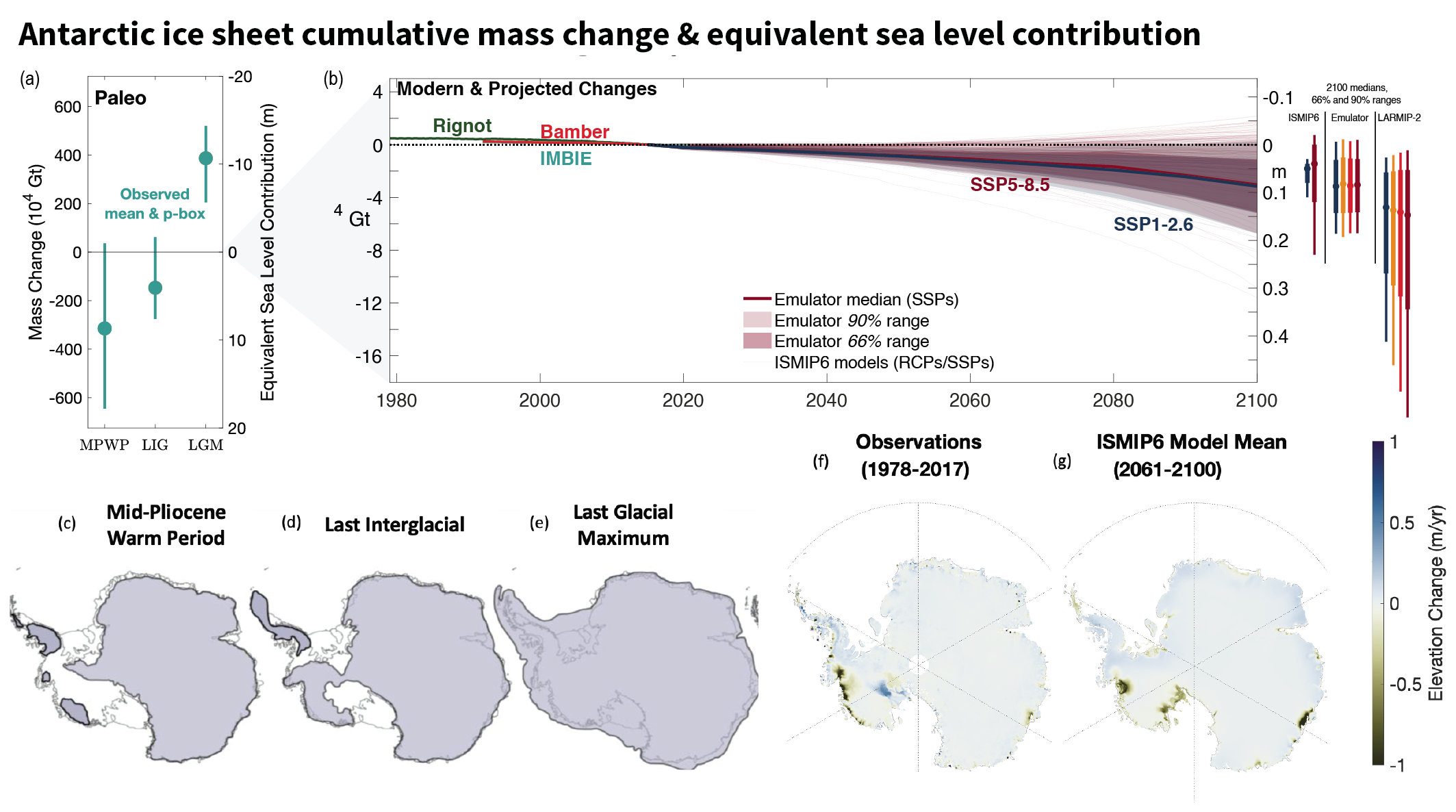 Figure 9.18 | Antarctic Ice Sheet cumulative mass change and equivalent sea level contribution. (a) A p-box (Section 9.6.3.2) based estimate of the range of values of paleo Antarctic ice sheet mass and sea level equivalents relative to present day and the median over all central estimates (Bamber et al., 2009; Argus and Peltier, 2010; Dolan et al., 2011; Mackintosh et al., 2011; Golledge et al., 2012, 2013, 2014, 2015, 2017b; K.G. Miller et al., 2012; Whitehouse et al., 2012; Ivins et al., 2013; Argus et al., 2014; Briggs et al., 2014; Maris et al., 2014; de Boer et al., 2015, 2017; Dutton et al., 2015; Pollard et al., 2015; DeConto and Pollard, 2016; Gasson et al., 2016; Goelzer et al., 2016; Yan et al., 2016; Kopp et al., 2017; Simms et al., 2019); (b left) cumulative mass loss (and sea level equivalent) since 2015, with satellite observations shown from 1993 (Bamber et al., 2018a; The IMBIE Team, 2018; WCRP Global Sea Level Budget Group, 2018) and observations from 1979 (Rignot et al., 2019), and projections from Ice Sheet Model Intercomparison Project for CMIP6 (ISMIP6) to 2100 under RCP8.5/SSP5-8.5 and RCP2.6/SSP1-2.6 scenarios (thin lines from Seroussi et al., 2020; Edwards et al., 2021; Payne et al., 2021)and ISMIP6 emulator under SSP5-8.5 and SSP1-2.6 to 2100 (shades and bold line; Edwards et al., 2021); (b, right) 17th–83rd, 5th–95th percentile ranges for ISMIP6, ISMIP6 emulator, and LARMIP-2 including surface mass balance (SMB) at 2100. (c–e) Schematic interpretations of individual reconstructions (Anderson et al., 2002; Bentley et al., 2014; de Boer et al., 2015; Goelzer et al., 2016) of the spatial extent of the Antarctic Ice Sheet are shown for the: (c) mid-Pliocene Warm Period, (d) Last Interglacial; and (e) Last Glacial Maximum (Fretwell et al., 2013): grey shading shows extent of grounded ice. (f –g) Maps of mean elevation changes (f) 1978–2017 derived from multi-mission satellite altimetry (Schröder et al., 2019) and (g) ISMIP6: 2061–2100 projected changes for an ensemble using the Norwegian Climate Center’s Earth System Model (NorESM1-M) climate model under the RCP8.5 scenario (Seroussi et al., 2020). Further details on data sources and processing are available in the chapter data table (Table 9.SM.9).
 As stated in SROCC, snowfall and glacier flow are the largest components determining AIS mass changes, with glacier flow acceleration (dynamic thinning) on the WAIS and the Antarctic Peninsula driving total loss trends in recent decades (very high confidence), and a partial offset of the dominating dynamic-thinning losses by increased snowfall (high confidence). The SROCC attributed medium confidence to estimates of 20th-century snowfall increases equivalent to a sea level change of –7.7 ± 4.0 mm on the EAIS, and –2.8 ± 1.7 mm on the WAIS, respectively (Medley and Thomas, 2019). Loss of buttressing, which can be caused by ice-shelf thinning, gradual ice-shelf front retreat or ice-shelf disintegration, has been linked to instantaneous ice velocity increases, and thus dynamic thinning, since the early 1990s. This link is clearly evident in the Amundsen and, to a lesser degree, Bellingshausen sectors (Gudmundsson et al., 2019), where passive shelf ice (ice that can be removed without major effects on the ice-shelf dynamics) is very limited or absent (Fürst et al., 2016). Surface mass balance (SMB) changes, dominated by snowfall, exhibit strong regional and temporal variability, for example with multi-decadal increases in the Antarctic Peninsula inferred since the 1930s (Medley and Thomas, 2019), and dominate the interannual to decadal variability of the AIS mass balance (Rignot et al., 2019). However, no significant continent-wide SMB trend is inferredsince 1979 (The IMBIE Team, 2018; Medley and Thomas, 2019; regional changes of Antarctic SMB are assessed further in AtlasSection 11.1). In summary, there is very high confidence that the observed AIS mass loss since the early 1990s is primarily linked to ice-shelf changes.
The SROCC stated with high confidence that melting of ice shelves by warm ocean waters, leading to reduction of ice-shelf buttressing, has driven the observed ongoing thinning of major WAIS outlet glaciers. Since SROCC, digitized radar measurements have shown that the eastern ice shelf of Thwaites Glacier in the Amundsen Sea Embayment thinned between 10 and 33% during the three decades after 1978 (Schroeder et al., 2019), and the role of basal ice-shelf melting has been emphasized (Smith et al., 2020). Strong surface meltwater production has been noted as a precursor of ice-shelf disintegration in and since SROCC (Bell et al., 2018), and recent work placed strong meltwater production events (Lenaerts et al., 2017; Nicolas et al., 2017; Wille et al., 2019) and seasons (Robel and Banwell, 2019) in this context. Antarctic ice-shelf basal meltwater flux varied between about 1100 ± 150 Gt yr–1in the mid-1990s and about 1570 ± 140 Gt yr–1in the late 2000s before decreasing to 1160 ± 150 Gt yr–1in 2018, and basal melt rates strongly vary with geographical position and depth, as a function of the surrounding water temperature (Adusumilli et al., 2020). Section 9.2.2.3 assesses that the intrusion of warm Circumpolar Deep Water (CDW), which has warmed and shoaled since the 1980s, has been at least partially controlled by forcing with significant decadal variability . Limited evidence suggests that, beyond strong internal decadal wind variability, increased greenhouse gas forcing has slightly modified the mean local winds between 1920 and 2018, facilitating the intrusion of CDW heat on the Amundsen-Bellingshausen continental shelf, and increased ice shelf melt (Section 9.2.2.3). However, theoretical understanding is still incomplete and in situ measurements within the ice–ocean boundary layer are sparse (Wåhlin et al., 2020). Modelling, and therefore attribution of ice shelf basal melt, remains challenging because of insufficient process understanding, required spatial resolution, the paucity of in situ observations (Dinniman et al., 2016; Asay-Davis et al., 2017; Turner et al., 2017), and uncertainties of bathymetric datasets under ice-shelf cavities (Goldberg et al., 2019, 2020; Morlighem et al., 2020). In summary, ice-shelf thinning, mainly driven by basal melt, is widespread around the Antarctic coast and particularly strong around the WAIS (high confidence), although basal melt rates show substantial spatio-temporal variability.
Satellite observations suggest that changes in sea ice coverage and thickness can modulate iceberg calving, ice shelf flow and glacier terminus position around Antarctica (Miles et al., 2013, 2016, 2017; Massom et al., 2015; Greene et al., 2018; Bevan et al., 2019), either through mechanical coupling or via changes to ocean stratification, influencing basal melting. A combined observational and modelling study (Massom et al., 2018) showed that regional loss of a protective sea ice buffer played a role in the rapid disintegration events of the Larsen A and B and Wilkins ice shelves in the Antarctic Peninsula between 1995 and 2009, by exposing damaged (rifted) outer ice shelf margins to enhanced flexure by storm-generated ocean swells. One observational study (Sun et al., 2019) suggests that the absence of sea ice in front of ice shelves, which leads to strengthened topographic waves, favours higher ice-shelf basal melt rates by increasing the baroclinic (depth varying) ocean heat flux which can enter the cavity (Wåhlin et al., 2020). Paleo evidence for sea ice control on ice sheets is lacking, but geologic evidence shows a concordance between periods of ice-sheet growth and the expansion of sea ice (Patterson et al., 2014; Levy et al., 2019), both being favoured by reduced sea surface temperatures. Modelling confirms that sea ice controls the strength of ice mélange (Robel, 2017; Schlemm and Levermann, 2021) and thus influences ice-shelf flexure and calving rates and stability of floating ice margins, but one model shows this had negligible effect on AIS retreat rates during past warm periods (Pollard et al., 2018). Loss of ice-shelf-proximal sea ice is also associated with increased solar heating of surface waters and increased sub-shelf melting (Bendtsen et al., 2017; Stewart et al., 2019). In summary, although in some cases sea ice decrease and glacier and ice-shelf flow and terminus position changes can have the same common cause, there is medium confidence that sea ice decrease ultimately favours the mass loss of nearby ice shelves through a variety of processes.
The SROCC stated with high confidence that ice-shelf disintegration has driven dynamic thinning in the northern Antarctic Peninsula over recent decades, and expressed high confidence in current ongoing mass loss from glaciers that fed now-disintegrated ice shelves. However, the mass loss rate has decreased in the 20 years since the immediate speed-up following ice-shelf disintegration in 1995 and 2002. Observed flow speed of these tributary glaciers is still 26% higher than before the ice shelf disintegration (Seehaus et al., 2018). Conversely, one study interpreted the increased flow speed of the Scar Inlet Ice Shelf’s tributary glaciers as a sign of evolving instability of the currently intact ice shelf (Qiao et al., 2020).
Ongoing grounding line retreat, indicating dynamic thinning, is observed with high confidence in many areas of Antarctica, and particularly on the WAIS, with the highest rates being in the Amundsen and Bellingshausen Sea areas, and around Totten Glacier in East Antarctica, as stated in SROCC. Research published since SROCC has evidenced grounding line retreat of the West Antarctic Berry Glacier on the Getz Coast (Millan et al., 2020) and on the East Antarctic Denman Glacier (Brancato et al., 2020), both since 1996. Furthermore observed grounding line retreat in excess of 1.5 km between 2003 and 2015 has been reported for parts of Marie Byrd Land (Christie et al., 2018). In summary, there is high confidence that grounding lines of marine-terminating glaciers are currently retreating in many areas around Antarctica, particularly around the WAIS, and additional areas of grounding line retreat have been evidenced since SROCC.
The SROCC stated with medium confidence that sustained mass losses of several major glaciers in the Amundsen Sea Embayment (ASE) are compatible with the onset of marine ice sheet instability (MISI). However, whether unstable WAIS retreat had begun, or was imminent, remained a critical uncertainty. New publications since SROCC have not substantially clarified this question. One study that combined satellite measurements with a numerical model and prescribed ice-shelf thinning (Gudmundsson et al., 2019) suggests that MISI is not required to explain the observed current mass loss rates of the WAIS, because they are consistent with external climate drivers. Furthermore, the fast grounding line retreat of the Pine Island Glacier in the ASE, which was triggered in the 1940s (Smith et al., 2017), observed after 1992 (Rignot et al., 2014) and previously interpreted as a sign of MISI (Favier et al., 2014), seems to have stabilized recently (Milillo et al., 2017; Konrad et al., 2018), and its current flow patterns do not suggest ongoing or imminent MISI (Bamber and Dawson, 2020). However, sustained fast grounding line retreat has been observed for the Smith Glacier in the ASE (Scheuchl et al., 2016), and an analysis of flow patterns and grounding line retreat of the ASE Thwaites Glacier between 1992 and 2017 (Milillo et al., 2019) showed sustained, albeit spatially heterogeneous, grounding line retreat, highlighting ice–ocean interactions that lead to increased basal melt. In addition, Denman Glacier in East Antarctica was shown to hold potential for unstable retreat (Brancato et al., 2020). In summary, the observed evolution of the ASE glaciers is compatible with, but not unequivocally indicating an ongoing MISI (medium confidence).
The SROCC reported limited evidence and medium agreement for anthropogenic forcing of the observed AIS mass balance changes. As stated in Section 3.4.3.2, there remains low confidence in attributing the causes of the observed mass of loss from the AIS since 1993, in spite of some additional process-based evidence to support attribution to anthropogenic forcing.
9.4.2.2 Model Evaluation
The AR5 (Church et al., 2013b; Flato et al., 2013) stated that regional climate models and global models with bias-corrected SST and sea ice concentration tended to produce more accurate simulations of Antarctic SMB than coupled climate models. It also noted strong climate model temperature biases over the Antarctic, though the latter may reflect known biases in the reanalysis used (Fréville et al., 2014). Section Atlas.11.1 assesses that there is medium confidence in the capacity of climate models to simulate Antarctic climatology and SMB changes.
(Section 9.2.3.2 assesses that there is low confidence in simulations of Southern Ocean temperature. Few ocean models resolve ice-shelf cavities, and biases in present-day melt rates can be substantial in some sectors, including the key region of the Amundsen Sea (e.g., an exception is the FESOM simulation in Figure 9.19 includes ice-shelf cavities and simulates ice-shelf basal melting and refreezing) (Naughten et al., 2018). An increasing number of observational studies from which basal melt rates are calculated (Huhn et al., 2018; Adusumilli et al., 2020; Das et al., 2020; Hirano et al., 2020; Stevens et al., 2020), combined with improved understanding of influences specific to water-masses and modes of melting or dissolving (Silvano et al., 2018; Adusumilli et al., 2020; Malyarenko et al., 2020; Wåhlin et al., 2020), may help to refine these models in the future. However, given the limited number of available models and their biases, there is currently low confidence in the sub-shelf melt rates simulated by ocean models.
Improvements in the representation of grounding line evolution in ice-sheet models since AR5 (such as sub-grid schemes for basal friction and ice-shelf melt, and local grid refinement) means that most of the model simulations presented in SROCC were dominated by physical processes. Since then, these advances have been applied in several model intercomparison projects – such as ISMIP6 and LARMIP-2 (see Box 9.3); MISMIP+ (Cornford et al. 2020); and ABUMIP (Sun et al. 2020). All models participating in ISMIP6 and LARMIP-2 simulate ice-shelf and grounding-line evolution, and include sub-shelf melt parametrization, which was not the case in the Sea-level Response to Ice Sheet Evolution (SeaRISE) project intercomparison (Bindschadler et al., 2013; Nowicki et al., 2013). Simulations of grounding line evolution (Seroussi et al., 2017, 2020) have benefitted from improved bedrock topography (Morlighem et al., 2020). Treatment of sub-shelf melting, however, remains one of the causes of large differences in AIS models, particularly for partially floating grid cells in models with coarse resolution (Levermann et al., 2020; Edwards et al., 2021). Due to the limitations in resolving cavities in ocean models, as described above, basal melt rates are generally parameterized at the ice shelf base, based on ocean model simulations of temperatures and salinity instead (Nowicki et al., 2020b; Seroussi et al., 2020). While this has the advantage of connecting melt rates to emissions scenarios, a large variety of melt parametrizations exist (DeConto and Pollard, 2016; Lazeroms et al., 2018; Reese et al., 2018; Hoffman et al., 2019; Pelle et al., 2019; Jourdain et al., 2020), and there is low agreement due to limited observational constraints (ocean temperature, salinity, velocity, and ice shelf draft)(Jourdain et al., 2020), uncertainty in the physics of parametrized processes, missing processes (e.g., tides), and uncertainty in the treatment of ice-sheet–climate feedbacks (Donat-Magnin et al., 2017; Bronselaer et al., 2018; Golledge et al., 2019). Parametrizations are usually calibrated to present-day melt rates, but can respond differently to projected ocean warming (Favier et al., 2019; Jourdain et al., 2020). Two different calibrations were used in ISMIP6 (Box 9.3; Jourdain et al., 2020; Nowicki et al., 2020b): one reproducing melt rates averaged around the whole continent (MeanAnt: Figure 9.19), and the other reproducing melt rates near the grounding line of Pine Island Glacier (PIGL; see Figure 9.19), leading to large differences in melt rates. Evaluation with observations and two cavity-resolving models suggests that the MeanAnt parametrization better reproduces observed melt rates and projected increases in both the warm Amundsen Sea Embayment and cold Ronne-Filchner shelf cavity, as well as total Antarctic melting (Jourdain et al., 2020). The PIGL calibration represents the upper end for increased basal melt sensitivity that would be caused by continent-wide changes to ocean water properties and circulation under strong future forcing (Jourdain et al., 2020). The basal sliding law also has a strong influence on grounding line retreat and glacier acceleration in response to perturbations, and varies spatially (Sun et al., 2020). Sliding laws (Joughin et al., 2019) can only be constrained with observations in regions experiencing significant change, and with sufficiently long observational records.
 Figure 9.19 | Ice-shelf basal melt rates for present-day (upper panels) and changes from present-day to the end of the 21st century under the RCP8.5 scenario (lower panels). Present-day melt rates were estimated through: the input-output method constrained by satellite observations and atmosphere/snow simulations (Rignot et al., 2013) and representative of 2003–2008 (upper left); the Ice Sheet Model Intercomparison Project for CMIP6 (ISMIP6) non-local-PIGL parametrization constrained by observation-based ocean properties (Jourdain et al., 2020) and representative of 1995–2014 (upper centre); the Finite Element Sea ice/Ice Shelf Ocean Model (FESOM) simulation over 2006–2015, forced by atmospheric conditions from a Coupled Model Intercomparison Project Phase 5 (CMIP5) multi-model mean (MMM) under the RCP8.5 scenario (Naughten et al., 2018) (upper right). Future anomalies are calculated as 2081–2100 minus present-day using the ISMIP6 non-local-MeanAnt and non-local-PIGL parametrizations (Jourdain et al., 2020) (lower left and centre, respectively) based on projections from the Norwegian Climate Center’s Earth System Model (NorESM1-M) CMIP5 model, and the FESOM-MMM projection (lower right). Note the symmetric-log colour bar (linear around zero, logarithmic for stronger negative and positive values). Inset highlights the Amundsen Sea Region. Further details on data sources and processing are available in the chapter data table (Table 9.SM.9).
 The SROCC noted that AIS simulations are increasingly evaluated or formally calibrated with modern observations and/or paleodata – to obtain more realistic initial conditions (ice-sheet geometry, velocity and forcing) and to constrain uncertainty in probabilistic projections. This trend continues (Nias et al., 2019; Gilford et al., 2020; Hamlington et al., 2020b; Wernecke et al., 2020). However, while the large-scale characteristics of the initial ice-sheet state have improved significantly (Box 9.3), capturing the smaller-scale rates of change, including mass trends, remains challenging for many models (Goldberg et al., 2015; Reese et al., 2020; Seroussi et al., 2020; Siegert et al., 2020). This increases uncertainty in projections, especially for the 21st century (Section 9.4.2.5). However, uncertainties in ice-sheet model simulations have been much better quantified since AR5, through model intercomparison projects (in particular, ISMIP6 and LARMIP-2; see Box 9.3), perturbed parameter ensembles, and increasing use of statistical emulation (Gilford et al., 2020; Levermann et al., 2020; Wernecke et al., 2020; DeConto et al., 2021; Edwards et al., 2021) to better sample the parameter space. By exploring uncertainties more fully, these methods have the potential to identify better simulations of the historical period.
An important difficulty is how to evaluate simulations of processes that are: not currently observed; or rare; or indirectly deduced – in particular, the ice-shelf disintegrations and cliff failures that would drive the proposed marine ice cliff instability (MICI; Section 9.4.2.4 and Box 9.4; DeConto and Pollard, 2016; DeConto et al., 2021). Models of ice-cliff failure can only be indirectly and partially evaluated, using existing (i.e., static) cliffs and laboratory experiments (Clerc et al., 2019). The SROCC stated that there was low agreement on the exact MICI mechanism and limited evidence of its occurrence in the present or the past, and that the validity of MICI remains unproven. Only one ice-sheet model represents MICI (Pollard et al., 2015; DeConto and Pollard, 2016; DeConto et al., 2021). The mechanism has not been found to be essential for reproducing Mid Pliocene Warm Period and Last Interglacial reconstructions or satellite observations, though Last Interglacial data slightly favours it in this model (Edwards et al., 2019; Gilford et al., 2020; DeConto et al., 2021).
In summary, there is nowmedium confidence in many ice-sheet processes in ice-sheet models, including grounding line evolution. However, there remains low confidence in the ocean forcing affecting the basal melt rates, and low confidence in simulating mechanisms that have the potential to cause widespread, sustained and very rapid ice loss from Antarctica through MICI.
9.4.2.3 Drivers of Future Antarctic Ice Sheet Change
9.4.2.3.1 Surface mass balance
The AR5 projected a negative contribution from Antarctic surface mass balance (SMB) changes to sea level over the 21st century (i.e., mitigating sea level rise), due to increased snowfall associated with warmer air temperatures. Sensitivity of SMB to Antarctic surface air temperature change varied from 3.7 to 7% °C–1, and the sea level projections assumed a sensitivity of 5.1 ± 1.5% °C–1from CMIP3 era models (Gregory and Huybrechts, 2006) to estimate SMB changes from Antarctic temperatures in the CMIP5 ensemble. Since the AR5, analyses of CMIP5 and CMIP6 models have found Antarctic temperature sensitivity for accumulation (precipitation minus sublimation) of 3.5 to 8.7% °C–1(Frieler et al., 2015), for SMB of 6.0 to 9.9% °C–1(Previdi and Polvani, 2016) and for precipitation of around 4 to 9% °C–1(±1 standard deviation ranges; Bracegirdle et al., 2020). An accumulation sensitivity estimate derived from ice core data lies in the middle of the range, around 6% °C–1(Frieler et al., 2015). These are consistent, within uncertainties, with each other and AR5, under the approximation that SMB is dominated by snowfall.
The AR5 found that the median and likely sea level contributions due to SMB from 1986–2005 to 2100 were –0.05 (–0.09 to –0.02) m under RCP8.5 and –0.02 (–0.05 to 0.00) m under RCP2.6. The SROCC did not present a separate SMB contribution, instead showing total Antarctic projections derived from ice-sheet models (Section 9.4.2.5). Projections of the SMB contribution to sea level tend to be slightly more negative since AR5, due at least in part to the higher range in equilibrium climate sensitivity values in CMIP6 (Payne et al., 2021). Mean and ±1 standard deviation ranges for grounded Antarctic Ice Sheet SMB changes from 2000 to 2100 computed from CMIP5 models are –0.08 (–0.13 to –0.04) m sea level equivalent (SLE) for RCP8.5 and, similarly for CMIP6 models, are –0.07 (–0.11 to –0.03) m for SSP5-8.5 (Gorte et al., 2020). The general circulation models (GCMs) used to drive ice-sheet models in ISMIP6 (Box 9.3) project mean grounded AIS SMB changes from 2005 to 2100 of –0.06 (range –0.08 to –0.03) m SLE under RCP8.5 for the six CMIP5 models (Seroussi et al., 2020) and –0.09 (range –0.10 to –0.07) m SLE under SSP5-8.5 for the four CMIP6 models, which have climate sensitivity values of 4.8°C –5.3°C (Payne et al., 2021). We apply the AR5 parametric AIS SMB model (Section 9.6.3.2) to updated projections of global mean temperature from a two-layer energy budget emulator (Supplementary Material 7.SM.2), which gives a median –0.05 (5–95% range –0.07 to –0.02) m SLE for SSP5-8.5 (Section 9.4.2.5, Table 9.3), that is, similar to the AR5 assessment and slightly smaller than the CMIP6 estimate. This estimate is used to augment the LARMIP-2 dynamic projections (Box 9.3) in Sections 9.4.2.5 and 9.4.2.6. Overall, CMIP5 and CMIP6 GCM simulations of sea level fall by 2100 due to Antarctic SMB increases are around 2–4 cm greater than estimates derived with the statistical method used in AR5. Further details about projections of Antarctic temperature, precipitation and SMB are provided in Section Atlas.11.1.4, which assesses that, due to the challenges of model evaluation (Section 9.4.2.2) and the possibility of increased meltwater runoff (Kittel et al., 2021), there is only medium confidence that the future contribution of Antarctic SMB to sea level this century will be negative under all greenhouse gas emissions scenarios. Longer time scales are discussed in 9.4.2.6.
9.4.2.3.2 Sub-shelf melting
The SROCC highlighted that an important ongoing deficiency in projections of Antarctic sub-shelf melting is the lack of ice–ocean coupling in most continental-scale studies. Increased basal melting is mainly caused by warmer CDW (Section 9.2.2.3) on the continental shelves, and warming surface waters intruding under ice shelves (Naughten et al., 2018). Predicting whether or not open ocean water masses will freely penetrate ice shelf cavities, or will be partially blocked by ocean density gradients, is complex (Wåhlin et al., 2020); while melting related to CDW inflow is currently dominant in the Amundsen Sea Embayment, melt in other embayments is limited by deep inflows of high-salinity shelf water or seasonally warmed shallow incursions of Antarctic Surface Water (Stewart et al., 2019; Adusumilli et al., 2020). There is little consensus regarding future change in CDW (Section 9.2.2.3), and more generally low confidence in future change in the temperature of Antarctic ice-shelf cavities (Section 9.2.3.2).
The response of sub-shelf melting to ocean warming is also poorly constrained. A key unknown is whether, and when, cold ice-shelf cavities might become more similar to the Amundsen Sea Embayment, not only in ocean temperature but also ice–ocean heat exchange, which depends on the cavity geometry and ocean circulation (Little et al., 2009). Only two ocean models with ice-shelf cavities have been used to make sub-shelf basal melting projections for Special Report on Emissions Scenarios and Representative Concentration Pathway (RCP) scenarios (Hellmer et al., 2012; Timmermann and Hellmer, 2013; Timmermann and Goeller, 2017; Naughten et al., 2018). The FESOM simulation, forced by a CMIP5 multi-model mean under RCP8.5, projects a 90% increase in melting (Figure 9.19), although this could be overestimated due to an underestimation of present-day melt rates (Section 9.4.2.2; Naughten et al., 2018). The temperature–melt relationship was parameterized by ISMIP6 in terms of heat exchange velocity in m a–1, and by LARMIP-2 as basal melt sensitivity in m a–1°C–1(Box 9.3; Jourdain et al., 2020; Levermann et al., 2020; Reese et al., 2020), and both vary widely around the continent, depending on cavity type. Median values of ISMIP6 heat exchange velocity vary by a factor of 5–10 when calibrating to either mean Antarctic or high Pine Island Glacier observed melt rates (Section 9.4.2.2; Box 9.3; Jourdain et al., 2020). Basal melt sensitivities near the grounding line estimated by Reese et al. (2020) with a box model of ocean overturning range from 3.9 m a–1°C–1for the Weddell Sea to 10.5 m a–1°C–1for the Amundsen Sea region, with a continental mean of 5.3 m a–1°C–1. Similarly high Amundsen Sea sensitivities are estimated in coupled ice–ocean simulations of Thwaites Glacier (mean 9.4 m a–1°C–1; range 6–16 m a–1°C–1) (Seroussi et al., 2017). These large variations lead to large differences in basal melt rates and projected sea level contributions when applied to the whole ice sheet in ISMIP6 and LARMIP-2 (Box 9.3). Projections of melt rates from the two ISMIP6 calibrations are higher than those from FESOM, driven by a CMIP5 multi-model mean (Figure 9.19; Jourdain et al., 2020). The ISMIP6 ensemble mostly uses the mean Antarctic calibration, but includes some simulations with the Pine Island Glacier calibration, and the ISMIP6 emulator samples more of these higher values; LARMIP-2 uses basal melt sensitivities (7–16 m a–1°C–1) consistent with estimates for the Amundsen Sea Embayment. Due to the limited availability of cavity-resolving ocean models, and the wide regional variation in estimates of basal melt sensitivity to ocean temperature, there is only low confidence in projected future sub-ice-shelf melt rates. The impact of this uncertainty on AIS model projections to 2100 is discussed in Section 9.4.2.5.
9.4.2.3.3 Ice-shelf disintegration
Antarctic ice shelves modulate grounded ice flow through buttressing, so their weakening or disintegration is crucial for the timing and magnitude of ice loss and onset of instabilities (Section 9.4.2.4; Box 9.4). Projections of ice-shelf disintegration are uncertain in terms of atmospheric warming and the response of the shelf surface – that is, surface melting, and whether shelves then disintegrate due to hydrofracturing and flexing, or are resilient through refreezing or drainage (Bell et al., 2018). The SROCC stated it is not expected that widespread ice-shelf loss will occur before the end of the 21st century, but this was based on only one study, using a regional climate model forced by five GCMs (Trusel et al., 2015), so there was low confidence in this assessment. The study of DeConto and Pollard (2016) projected the appearance of extensive surface meltwater several decades earlier than Trusel et al. (2015) and was therefore assessed to be too uncertain to include in SROCC projections of the AIS.
Since SROCC, further studies have highlighted the modelling uncertainties in this area. Coastal surface air temperature projections in CMIP6 models show large inter-model differences driven by sea ice retreat and exhibit more warming relative to global mean temperature under low emissions than high, due to delayed response of the Southern Ocean to stabilized emissions and stratospheric ozone recovery (Bracegirdle et al., 2020). The updated study of DeConto et al. (2021) includes improvements to the climate simulations relative to those in DeConto and Pollard (2016), and the resulting surface meltwater projections are now consistent with Trusel et al. (2015). However, the net effect of meltwater feedbacks on ice shelves is uncertain. Ice discharge is expected to lead to surface ocean and atmosphere cooling: this increases ocean stratification and sub-shelf melting, but also reduces ice-shelf surface melting and delays hydrofracturing (Golledge et al., 2019; Sadai et al., 2020; DeConto et al., 2021). The new studies are insufficient to change SROCC’s low confidence assessment on ice-shelf loss. The consequence of this uncertainty on projections is discussed in Section 9.4.2.5 and Box 9.4.
9.4.2.4 Ice-sheet Instabilities
A major uncertainty in future Antarctic mass losses is the possibility of rapid and/or irreversible ice losses through instability of marine parts of the ice sheet, via the proposed mechanisms of marine ice sheet instability (MISI) and marine ice cliff instability (MICI), and whether these processes will lead to a collapse of the West Antarctic Ice Sheet (WAIS).
MISI is a proposed self-reinforcing mechanism within marine ice sheets that lie on a bed that slopes down towards the interior of the ice sheet, whereby, in the absence of ice-shelf buttressing, the position of the grounding line is inherently unstable until reaching an upward sloping bed. The SROCC (Meredith et al., 2019) noted advances in modelling MISI since AR5, but that ‘significant discrepancies’ remained in projections due to poor understanding of mechanisms, and lack of observational data to constrain the models. Since SROCC, modelling uncertainties have been more thoroughly explored, rather than constrained (compatibility of current observations in the Amundsen Sea Embayment with MISI is assessed in Section 9.4.2.1). Internal climate variability might either slow (Hoffman et al., 2019) or amplify (Robel et al., 2019) MISI, and stable grounding line positions can be reached on downward sloping beds if ice shelves provide buttressing (Sergienko and Wingham, 2019; Cornford et al., 2020). Ice-sheet model simulations that remove all Antarctic ice shelves (and prevent them from reforming) show 2–10 m SLE Antarctic mass loss after 500 years due to MISI, of which WAIS collapse contributes 2–5 m (Sun et al., 2020), with the majority of the mass loss in the first one to two centuries. Much of the multi-model variation is due to the sliding law (Section 9.4.2.2). However, it is not expected that widespread ice-shelf loss will occur before the end of the 21st century (Section 9.4.2.3; Box 9.4). A recent update of bed topography that unveiled large and overdeepened subglacial troughs in East Antarctica potentially vulnerable to MISI (Morlighem et al., 2020) has only been used by a few models (Seroussi et al., 2020; Sun et al., 2020), so current projections could underestimate vulnerability in these regions. The sea level rise contribution of the AIS therefore crucially depends on the behaviour of individual ice shelves and outlet glacier systems and whether they enter MISI for a given level of warming (Box 9.4; Pattyn and Morlighem, 2020). As for Antarctic simulations generally (Sections 9.4.2.2 and 9.4.2.3), there is medium confidence in simulating MISI but low confidence in projecting the sub-shelf melting and ice-shelf disintegration that drive it.
The SROCC noted limited evidence from geological records and ice-sheet modelling, suggesting that parts of the AIS experienced rapid (centennial) retreat likely due to MISI between 20,000 and 9,000 years ago, and also described more uncertain evidence for the Last Interglacial (LIG) and mid-Pliocene Warm Period (MPWP). Recent support for past MISI is provided by model simulations of the WAIS during the LIG (Clark et al., 2020), the British Ice Sheet during the last termination (Gandy et al., 2018) and the Laurentide Ice Sheet during the Younger Dryas (Pico et al., 2019), which show progressive retreat despite declining temperatures, indicative of a true (ice dynamic) instability. Direct observational evidence of rapid paleo ice-sheet grounding line retreat is rare but, on the Larsen continental shelf, retreat rates of >10 km yr–1during the deglaciation have been estimated (Dowdeswell et al., 2020). MISI has also been inferred from sedimentological evidence of ice loss from Wilkes Subglacial Basin, East Antarctica (Bertram et al., 2018; Wilson et al., 2018; Blackburn et al., 2020) but these reconstructions cannot unambiguously identify unstable from progressive retreat. Therefore, there is limited evidence to identify the operation of instability mechanisms such as MISI in paleo ice-sheet retreat.
The SROCC assessed that ice-sheet interactions with the solid Earth are not expected to substantially slow sea level rise from marine-based ice in Antarctica over the 21st century (medium confidence), but that these processes could become important on multi-century and longer time scales. More recent modelling of deglaciation of the Ross Embayment by Lowry et al. (2020) is consistent with this assessment. However, new projections for Pine Island Glacier (Kachuck et al., 2020) support previous work (Barletta et al., 2018) suggesting that lower mantle viscosity in this region leads to a negative feedback on decadal time scales. Grounding line stabilization by the solid Earth response may therefore occur over the 21st century in the Amundsen Sea Embayment, where most mass loss is occurring (Section 9.4.2.1), but more generally occurs over multi-centennial to millennial time scales (medium confidence).
The MICI hypothesis describes rapid, unmitigated calving triggered by ice-shelf collapse (Pollard et al., 2015). The SROCC noted that the MICI mechanism led one model (DeConto and Pollard, 2016) to lose mass far more rapidly, but excluded the mechanism from its projections due to uncertainty in the timing of the ice-shelf disintegration (Section 9.4.2.3). They stated that MICI could lead to sea level contributions beyond 2100 considerably higher than the likely range projected by other models. However, given the low agreement on the exact MICI mechanism and limited evidence of its occurrence in the present or the past (Section 9.4.2.2), its potential to affect future sea level rise was very uncertain. Since SROCC, new simulations show later ice-shelf disintegration, in agreement with other models (Section 9.4.2.3; DeConto et al., 2021), and therefore lower projections at 2100 (Section 9.4.2.5). New theoretical evidence suggests that ice-cliff collapse may only occur after very rapid ice shelf disintegration caused by unusually high meltwater production (Clerc et al., 2019; Robel and Banwell, 2019), and that the subsequent rate of retreat depends on the terminus geometry (Bassis and Ultee, 2019). As SROCC noted, only Crane Glacier on the Peninsula has shown retreat consistent with MICI, after the Larsen B ice shelf collapsed, and MICI-style behaviour at Jakobshavn and Helheim Glaciers in Greenland might not be representative of wider Antarctic glaciers. Observations from Greenland show that steep cliffs commonly evolve into short floating extensions, rather than collapsing catastrophically (Joughin et al., 2020). As assessed in Section 9.4.2.2 and 9.4.2.3, there is therefore low confidence in simulating mechanisms that have the potential to cause widespread, sustained and very rapid ice loss from Antarctica this century through MICI, and low confidence in projecting the driver of ice-shelf disintegration.
In summary, poorly understood processes of instabilities, characterized by deep uncertainty, have the potential to strongly increase Antarctic mass loss under high greenhouse gas emissions on century-to-multicentury time scales (Box 9.4). These instabilities are therefore considered separately in assessments of the future contribution to global mean sea level (GMSL; Sections 9.4.2.5, 9.4.2.6, 9.6.3.2 and 9.6.3.5).
9.4.2.5 Projections to 2100
The AR5 assessed the median and likely (66–100% probability) sea level contributions of the AIS in 2100 relative to 1986–2005 to be 0.06 (–0.04 to +0.16) m SLE under RCP2.6 and 0.04 (–0.08 to +0.14) m SLE under RCP8.5 (Table 9.3; no change when using the AR6 baseline). The AR5 stated that only the collapse of the marine-based sectors of the AIS, if initiated, could cause GMSL to rise substantially above the likely range during the 21st century, with medium confidence that this would not exceed several tenths of a metre during this period. The assessment of the dynamical contribution had no dependence on emissions scenarios, due to the lack of literature, so the decrease in sea level contribution in the higher-emissions scenario was solely due to increased SMB (Section 9.4.2.3). The SROCC (Oppenheimer et al., 2019) assessed the total contribution based on five new ice-sheet modelling studies that incorporated marine ice-sheet dynamics, combining their estimates and interpreting the 5–95th percentile range of the resulting distribution as the likely range (17–83% probability interval, i.e., not open-ended as in the AR5). The median and likely range contributions by 2100 were 0.04 (0.01–0.11) m under RCP2.6 and 0.12 (0.03–0.28) m under RCP8.5 (Table 9.3). The positive scenario-dependence in SROCC – where increases in dynamic losses driven by ocean warming and ice-shelf disintegration under higher emissions (Section 9.4.2.3) dominate over increases in SMB – arose from a combination of physical processes and model limitations. Modelling improvements in these studies included improved representations of grounding line response to drivers, more extensive exploration of uncertainties, and inclusion of a positive feedback of meltwater on climate (Golledge et al., 2019). However, two of the projections did not include SMB changes that would offset dynamic losses (Levermann et al., 2014; Ritz et al., 2015), and the scenario dependence may have been further amplified by highly sensitive sub-shelf melt parametrizations and use of simplified SMB schemes (Golledge et al., 2015, 2019; Bulthuis et al., 2019; Oppenheimer et al., 2019).
Since SROCC, new projections have arisen from multi-model intercomparison projects ISMIP6 and LARMIP-2 (Box 9.3) and one model that includes MICI (Section 9.4.2.4; Table 9.3; DeConto et al., 2021). Corrections are added to allow comparison: all ISMIP6-derived projections have an estimate of the historical dynamical response to pre-2015 climate forcing added, which increases contributions (Box 9.3; Figure 9.18); the LARMIP-2 dynamic projections are combined with an estimate of SMB, which decreases contributions (Sections 9.4.2.3 and 9.6.3.2); and the ISMIP6 emulated and LARMIP-2 projections were re-estimate using the global surface air temperature distributions from the two-layer energy budget emulator described in Supplementary Material 7.SM.2. The majority of the new projections indicate that, under all emissions scenarios, the AIS will lose mass overall and contribute to sea level rise. Most thinning occurs in the Amundsen Sea sector in WAIS and Totten Glacier in EAIS (Figure 9.18). The most negative contribution is –0.02 m (5th percentile of ISMIP6 combined RCP8.5 and SSP5-8.5 projections after correction) and the largest contribution is 0.57 m SLE (95th percentile; Levermann et al., 2020), or 0.63 m SLE with MICI (95th percentile; DeConto et al., 2021). ISMIP6 ensemble ranges are wider for the high scenarios (RCP8.5/SSP5-8.5) than the low (RCP2.6/SSP1-2.6), in part because more simulations were available. The ISMIP6 simulations that apply an ice-shelf collapse scenario based on exceedance of a surface meltwater threshold (Trusel et al., 2015), driven by CMIP5 models, show only a small increase in mass loss (around 0–0.04 m), mostly from the Peninsula, due in part to the small number of ice shelves predicted to collapse this century (Seroussi et al., 2020). Simulations driven by the CMIP5 model HadGEM2-ES, which has unusually extreme warming in the Ross Sea (Barthel et al., 2020), show a larger mass loss (up to about 0.05 m) in East Antarctica under ice-shelf collapse (Edwards et al., 2021). The ISMIP6 projections do not include the efficient meltwater drainage or atmospheric feedbacks that could reduce mass loss further (Seroussi et al., 2020).
The relationship between emissions scenario and AIS response varies across the studies, with emulated ISMIP6 projections showing a slight negative scenario dependence in the median (–0.01 m) from SSP1-2.6 to SSP5-8.5, and LARMIP-2-based projections showing a slight positive scenario-dependence in the median (0.02 m; Table 9.3). A lack of clear scenario dependence in the median masks large individual variations across climate and ice-sheet models, whereby the net AIS contribution response to emissions scenario depends on the relative magnitudes of the atmosphere, ocean and ice-sheet responses (Barthel et al., 2020; Seroussi et al., 2020; Edwards et al., 2021). Climate and ice-sheet models do not project that the AIS response will be the same under high or low greenhouse gas emissions in 2100; rather, there is no consensus on the sign of the change. In contrast, strong scenario dependence is seen from RCP4.5 to RCP8.5 in projections that allow MICI (Section 9.4.2.4; DeConto et al., 2021), though less so than earlier projections (DeConto and Pollard, 2016) due to later ice-shelf disintegrations. A negative or positive scenario dependence of the AIS response this century cannot be deduced from recent observations, because there is still low confidence in attributing the causes of observed mass loss (Section 9.4.2.1), and neither regional mass increases by SMB nor regional mass losses by ice flow have a linear relationship with global mean temperature (Sections 9.4.2.1, 9.4.2.2, 9.4.2.3). There is therefore low agreement on the relationship between emissions scenario and AIS response. However, in the longer term, mass loss is expected to dominate (Section 9.4.2.6).
The LARMIP-2 median projections are higher than those of the ISMIP6 emulator (by 0.04–0.07 m), and the 95th percentiles are two to three times higher. Two possible reasons for the differences between the emulated ISMIP6 and LARMIP-2 projections are assessed: the set of ice-sheet models (Annex II) and the parameter values determining sub-shelf melt sensitivity to ocean temperature (Section 9.4.2.3; Box 9.3). Using only the 13 ice-sheet models common to ISMIP6 and LARMIP-2 reduces the LARMIP-2 median projections by 0.02–0.03 m SLE and the 95th percentiles by 0.04–0.08 m SLE (Table 9.3). This approximately halves the difference in medians, but has a relatively small effect on the upper end. Sub-shelf melt sensitivity has a larger effect, due to the wide variation of estimates from different regions and methods. Using only the Pine Island Glacier sub-shelf melt distribution (Sections 9.4.2.2 and 9.4.2.3) in the ISMIP6 emulator gives a median Antarctic projection of about 0.08 m in 2100 in all scenarios before historical correction, compared with around 0 m using only the mean Antarctic distribution; the published projections use a joint distribution (Edwards et al., 2021). Reese et al. (2020) find that using the basal melt sensitivities of LARMIP-2 yields an order of magnitude greater mass loss under RCP8.5 than with the ISMIP6 mean Antarctic values. Halving the basal melt sensitivity parameter range (i.e., in line with a continental mean estimate: Section 9.4.2.3) would lead to a halving of the LARMIP-2 dynamic contribution. This would reconcile the LARMIP-2 and ISMIP6 emulator median and 95th percentile projections using the common subset of models within about 0.02–0.05 m. There is therefore limited evidence that the ISMIP6 and LARMIP-2 projections could be reconciled by using common ice-sheet models and basal melt sensitivity values.
It is not possible to distinguish which of ISMIP6 and LARMIP-2 is more realistic, due to limitations in historical simulations (Box 9.3) and understanding of basal melting (Section 9.4.2.3.2), so the projections are combined using a ‘p-box’ approach (Section 9.6.3.2). The mean of the ISMIP6 emulated and LARMIP-2 medians gives the assessed median projections, and the outer edges of the 17–83% ranges give the outer edges of the assessed likely (17–83%) ranges – that is, encompassing the structural and parametric uncertainties of both methods, giving medium confidence in their combined projections. The main difference between this assessment and SROCC is to increase the medians of the lower scenarios by 0.05–0.07 m, so that all SSPs are similar to SROCC assessment of RCP8.5, and to substantially increase the upper ends of the likely ranges: by 0.14–0.16 m for RCP2.6/SSP1-2.6 and RCP4.5/SSP2-4.5, and 0.06 m for RCP8.5/SSP5-8.5. The increase relative to SROCC is partly due to the increase in LARMIP-2 projections relative to the original LARMIP study (Levermann et al., 2014), arising from the larger number of participating ice-sheet models (Levermann et al., 2020). The historical dynamic response to pre-2015 climate forcing applied to the ISMIP6 emulator could be overestimated, due to the assumption of a constant future rate (Box 9.3). This assessment encompasses SROCC and all projections since, except the 83rd percentiles of projections that allow MICI under RCP8.5 (DeConto et al., 2021) and the Structured Expert Judgement (SEJ) under 5°C shown in SROCC (Bamber et al., 2019). Both are used in further p-box estimates to give the outer limits of low confidence assessments (Section 9.6.3.2).
In summary, it is likely that the AIS will continue to lose mass throughout this century under all emissions scenarios – that is, dynamic losses driven by ocean warming and ice-shelf disintegration will likely continue to outpace increasing snowfall (medium confidence). The upper end of projections is not well constrained, due to different assumptions about the future sensitivity of sub-shelf basal melting to ocean warming and the proposed marine ice cliff instability triggered by ice-shelf disintegration (Sections 9.4.2.3 and 9.4.2.4; Box 9.4).
Representative Concentration Pathways (RCPs) | ||||
Study | RCP2.6 | RCP4.5 | RCP8.5 | Notes |
IPCC AR5 (Church et al., 2013b) | 0.06 (–0.04 to +0.16) | 0.05 (–0.05 to +0.15) | 0.04 (–0.08 to +0.14) | Median and likely (≥ 66%range) contribution |
IPCC SROCC (Oppenheimer et al., 2019) | 0.04 (0.01 to 0.11) | 0.06 (0.01 to 0.15) | 0.12 (0.03 to 0.28) | Median and likely (66%range) contribution. Combination of five studies |
ISMIP6 CMIP5-forced (Seroussi et al., 2020); excludes historical dynamic response | –0.01 to +0.16 | – | –0.08 to +0.30 | Range of ISMIP6 multi-model contributions in 2100 relative to 2015 from 2 ESMs for RCP2.6 and 6 ESMs for RCP8.5 |
LARMIP-2; excludes surface mass balance (SMB) (Levermann et al., 2020) | 0.13 (0.07 to 0.24) [0.04 to 0.37] | 0.14 (0.07 to 0.28) [0.05 to 0.44] | 0.17 (0.09 to 0.36) [0.06 to 0.58] | Median (67% range) [90% range] LARMIP-2 multi-model dynamic contribution in 2100 relative to 1900 |
MICI (DeConto et al., 2021) | 0.08 (0.06 to 0.12) [0.06 to 0.15] | 0.09 (0.07 to 0.11) [0.07 to 0.15] | 0.34 (0.19 to 0.53) [0.11 to 0.63] | Median (66% range) [90% range] |
Shared Socio-economic Pathways (SSPs) | ||||
Study | SSP1-2.6 | SSP2-4.5 | SSP5-8.5 | Notes |
Multi-model ensemble projections | ||||
ISMIP6 CMIP6-forced (Payne et al., 2021); excludes historical dynamic response | –0.05 to +0.01 | – | –0.09 to +0.11 | Range of ISMIP6 multi-model contributions in 2100 relative to 2015 from 1 ESM for SSP1-2.6 and 4 ESMs for SSP5-8.5 |
ISMIP6 all (CMIP5 and CMIP6-forced) including historical dynamic response | –0.05 (0.04 to 0.08) [0.03 to 0.11] | – | 0.04 (0.00 to 0.12) [–0.02 to +0.23] | Median (66% range) [90% range] contribution from ISMIP6 CMIP5 and CMIP5-forced multi-model ensembles, (see caption) |
Emulated ISMIP6; excludes historical dynamic response (Edwards et al., 2021) | 0.04 (–0.01 to +0.10) [–0.05 to +0.14] | 0.04 (–0.02 to +0.10) [–0.06 to +0.14] | 0.04 (–0.01 to +0.09) [–0.05 to +0.14] | Median (66% range) [90% range] contribution in 2100 relative to 2015 from emulator of ISMIP6 used with Chapter 7 climate forcing |
Emulated ISMIP6 total | 0.09 (0.03 to 0.14) [–0.01 to +0.19] | 0.09 (0.03 to 0.14) [–0.01 to +0.18] | 0.08 (0.03 to 0.14) [0.00 to 0.18] | Emulated ISMIP6, but relative to 1995–2014 and including historical dynamic response (see caption) |
SMB | –0.02 (–0.03 to –0.01) [–0.04 to –0.01] | –0.03 (–0.04 to –0.02) [–0.06 to –0.01] | –0.05 (–0.07 to –0.03) [–0.09 to –0.02] | Median (66% range) [90% range] SMB estimated for the AR5, used to correct LARMIP-2 below |
LARMIP-2; excludes SMB | 0.15 (0.08 to 0.29) [0.05 to 0.44] | 0.17 (0.09 to 0.33) [0.06 to 0.49] | 0.20 (0.10 to 0.39) [0.07 to 0.61] | Median (66% range) [90% range] dynamic contribution from LARMIP-2 multi-model method used with Chapter 7 climate forcing |
LARMIP-2 subset of models; excludes SMB | 0.14 (0.08 to 0.26) [0.05 to 0.39] | 0.15 (0.08 to 0.29) [0.05 to 0.45] | 0.17 (0.10 to 0.35) [0.06 to 0.54] | As above, but using only the 13 of 16 ice-sheet models common to both ISMIP6 and LARMIP-2 |
LARMIP-2 subset of models; includes SMB | 0.11 (0.05 to 0.24) [0.03 to 0.37] | 0.12 (0.05 to 0.26) [0.02 to 0.42] | 0.12 (0.05 to 0.30) [0.01 to 0.49] | As above, but including the SMB estimate |
LARMIP-2 total | 0.13 (0.06 to 0.27) [0.03 to 0.41] | 0.14 (0.06 to 0.29) [0.02 to 0.46] | 0.15 (0.05 to 0.34) [0.01 to 0.57] | Median (66% range) [90% range] dynamic contribution from LARMIP-2 multi-model method used with Chapter 7 climate forcing, including the SMB estimate |
This assessment: combination of emulated ISMIP6 and LARMIP-2 | 0.11 (0.03 to 0.27) [–0.01 to +0.41] | 0.11 (0.03 to 0.29) [–0.01 to +0.46] | 0.12 (0.03 to 0.34) [0.00 to 0.57] | Median (66% range) [90% range] assessment combining emulated ISMIP6 and LARMIP-2 |
9.4.2.6 Projections Beyond 2100
The SROCC assessed the median and likely range of Antarctic SLE contributions at 2300 as 0.16 (0.07–0.37) m under RCP2.6 and 1.46 (0.60–2.89) m under RCP8.5, based on three studies. It was noted that deep uncertaintyremained beyond 2100: while solid Earth feedbacks could reduce ice loss over multi-century time scales, MICI (Section 9.4.2.4) might give contributions higher than the likely ranges. The SROCC also presented structured expert judgement (SEJ) projections for comparison (Bamber et al., 2019), which give higher values. Since SROCC, three studies have made projections to 2300: (i) Rodehacke et al. (2020) assessed two methods for implementing precipitation changes (based on repeating 2071–2100 forcings beyond 2100), which both gave negative projections at 2300 because the dynamic response was very small (–0.11 to –0.01 m SLE for RCP2.6; –0.25 to –0.07 m for RCP8.5 forcing); (ii) In contrast, simulations forced by 2081–2100 ocean-only projections under RCP8.5/SSP5-8.5 beyond 2100, using two implementations of the ISMIP6 ‘non-local’ basal melt parametrizations (Box 9.3 and Section 9.4.2.2) and two sliding laws, are all positive (0.08 m to 0.96 m SLE by 2300), though these do not include the negative contribution from SMB changes (Lipscomb et al., 2021); (iii) Finally, DeConto et al. (2021) update projections for the MICI hypothesis (Section 9.4.2.4) using the extensions of the RCPs to 2300, and obtain far higher contributions: median (17–83%) ranges of 1.09 (0.71–1.35) m SLE under RCP2.6 and 9.60 (6.87–13.54) m SLE under RCP8.5. These are larger than previous estimates (DeConto and Pollard, 2016), particularly at the upper end: 0.68 (0.29–1.13) m SLE for RCP2.6 and 8.40 (7.47–9.76) m for RCP8.5 (Edwards et al., 2019), which can largely be explained by the higher maximum ice cliff calving rate. LARMIP-2 dynamic projections (Box 9.3) are also estimated under the extended SSPs and corrected with SMB (as in Section 9.4.2.5), giving median (17–83%) ranges of 0.40 (0.18–0.78) m SLE at 2300 under SSP1-2.6 and 1.57 (0.68–3.14) m under SSP5-8.5. The longer time scale may invalidate the linear response assumption of LARMIP-2, which neglects any self-dampening or self-amplifying processes. The ranges of projections for 2300 without MICI (Golledge et al., 2015; Bulthuis et al., 2019; Levermann et al., 2020; Rodehacke et al., 2020; Lipscomb et al., 2021; ‘assessed ice-sheet contributions’ in Section 9.6.3.5 are –0.14 to +0.78 m SLE under RCP2.6/SSP1-2.6, and –0.27 to 3.14 m SLE under RCP8.5/SSP5-8.5). The lower bounds are the 5th percentile of Bulthuis et al. (2019) and the lowest mean/median from Rodehacke et al. (2020), respectively; the upper bounds are the 83% percentiles of the LARMIP-2 estimates. These ranges are wider than SROCC likely ranges, and more consistent with the SEJ (Bamber et al., 2019). However, projections in which Antarctica contributes much more than the assessed ranges under sustained very high greenhouse gas emissions – that is, around 7–14 m to GMSL by 2300 (DeConto et al., 2021), cannot be ruled out, and are taken as a sensitivity case (Section 9.6.3.5; Table 9.11). In summary, there is high confidence that Antarctic mass loss will be greater beyond 2100 under high greenhouse gas emissions, but the large range of projections mean we have only low confidence in the likely AIS contribution to GMSL by 2300 for a given scenario. Deep uncertaintyremains in the role of AIS instabilities under very high emissions.
The West and East Antarctic ice sheets are considered to be tipping elements – that is, susceptible to critical thresholds. The SR1.5 (Hoegh-Guldberg et al., 2018) assessed that a threshold for WAIS instability may be close to 1.5°C–2°C (medium confidence), as only RCP2.6 led to long-term projections of less than 1 m (Golledge et al., 2015; DeConto and Pollard, 2016). Based on the agreement of a further study (Bulthuis et al., 2019), SROCC confirmed that low emissions would limit Antarctic ice loss over multi-century time scales (high confidence), but it was not possible to determine whether this was sufficient to prevent substantial ice loss (medium confidence). Since SROCC, new studies have revisited this topic (Garbe et al., 2020; Rodehacke et al., 2020; Van Breedam et al., 2020; DeConto et al., 2021; Lipscomb et al., 2021), allowing a more complete assessment along with other studies (Feldmann and Levermann, 2015; Clark et al., 2016; Golledge et al., 2017a; Edwards et al., 2019) and the extension to LARMIP-2 above. The majority project 0–1.3 m SLE on multi-century time scales under scenarios of 1°C–2°C warming. Projections can increase up to 2 m SLE under high basal melt sensitivity to ocean warming (Section 9.4.2.3; Lipscomb et al., 2021) or MICI (Section 9.4.2.4). On multi-millennial time scales (≥2,000 years), many projections remain below 1.6 m SLE under 1°C–2°C warming – that is, less than about half of the WAIS in SLE (see also Section 9.6.3.5 and Figure 9.30). Other studies project majority or total loss of WAIS under 1°C–2°C warming, exceeding 2 m SLE, under the higher end of the warming range (≥1.5°C), or high ocean warming (≥0.5°C) and/or high basal melting around WAIS, or MICI. All but two of these multi-millennial studies use variants of the same ice-sheet model, though different modelling choices mean they can be considered quasi-independent. Simulations of previous interglacial periods often show near or total WAIS disintegration, with mass loss exceeding 3 m SLE (e.g. Figure 9.18), although limitations of these studies or inferences that can be drawn under different forcings limit confidence in the robustness of these as quantitative analogues (Sections 9.4.2.4 and 9.6.2). Overall, increased evidence and agreement on the time scales and drivers of mass loss confirm the SR1.5 assessment that a threshold for WAIS instability may be close to 1.5°C–2°C (medium confidence), and that the probability of passing a threshold is larger for 2°C warming than for 1.5°C (medium confidence), particularly under strong ocean warming. New projections agree with previous studies that only part of WAIS would be lost on multi-century time scales if warming remains less than 2°C (medium confidence). There is limited agreement about whether complete disintegration would eventually occur at this level of warming, but medium confidence this would take millennia.
Under around 2°C–3°C peak warming, complete or near-complete loss of the WAIS is projected in most studies after multiple millennia (low confidence), with continent-wide mass losses of around 2–5 m SLE or more; this could occur on multi-century time scales under very high basal melting (Lipscomb et al., 2021) or widespread ice-shelf loss and/or MICI (low confidence) (Sun et al., 2020; DeConto et al., 2021). Mass losses under around 2°C–3°C warming could be less than 2 m SLE, particularly for multi-century time scales, low basal melting, or less responsive sliding laws. If warming exceeds around 3°C above pre-industrial, part of the EAIS (typically the Wilkes Subglacial Basin) is projected to be lost on multi-millennial time scales (low confidence), with total AIS mass loss equivalent to around 6–12 m or more sea level rise; mass loss could be much smaller if the dynamic response is small (Bulthuis et al., 2019; Rodehacke et al., 2020), or much faster under widespread ice-shelf loss and/or MICI (Sun et al., 2020; DeConto et al., 2021). A study by Garbe et al. (2020) suggests that 6°C sustained warming and associated mass loss of about 12 m SLE may be a critical threshold beyond which the ice sheet reorganizes to a new state, leading to large losses from East Antarctica (including the Aurora Subglacial Basin) and leading to a further 10 m sea level contribution per degree of warming; other studies also show much higher mass loss per °C at higher levels of warming (Section 9.6.3.5 and Figure 9.30; Van Breedam et al., 2020; DeConto et al., 2021).
The SROCC (Meredith et al., 2019; Oppenheimer et al., 2019) assessed that Antarctic mass losses could be irreversible over decades to millennia (low confidence). Garbe et al. (2020) show that the AIS is always volumetrically smaller when regrowing under a given warming level than when it retreats under the same forcing. Even if retreat followed by regrowth results in a net zero change in volume, the spatial distribution of mass may be altered, especially in parts of West Antarctica vulnerable to MISI. Projections that start reducing CO2 concentrations from 2030 onwards, reaching pre-industrial levels around 2300, show sea level contributions exceeding 1 m by 2500 when including MICI (DeConto et al., 2021). New research therefore confirms SROCC assessment that mass loss from the AIS is irreversible on decadal to millennial time scales (low confidence) (FAQ 9.1), and suggests that reducing atmospheric CO2 concentrations or temperatures to pre-industrial levels may not be sufficient to prevent or reverse substantial Antarctic mass losses (low confidence).
9.5 Glaciers, Permafrost and Seasonal Snow Cover
9.5.1 Glaciers
9.5.1.1 Observed and Reconstructed Glacier Extent and Mass Changes
9.5.1.1.1 Global glacier contribution
The IPCC’s Fifth Assessment Report (AR5; Vaughan et al., 2013) assessed glacier changes from studies based on the regions defined in the Randolph Glacier Inventory (RGI; RGI version 2.0): a satellite observation-based, global inventory of glacier outlines for the year 2000. Following Special Report on the Ocean and Cryosphere in a Changing Climate (SROCC; Hock et al., 2019b; Meredith et al., 2019), we report on studies based on RGI version 6.0 (RGI Consortium, 2017). Increased volume of satellite observations and the inclusion of detailed regional glacier inventories has resulted in an improved inventory (RGI Consortium, 2017). A new consensus estimate for the ice thickness distribution of all glaciers in RGI 6.0 was obtained from an ensemble of five numerical models. However, only one out of five models covered all regions (Farinotti et al., 2019), and was, where possible, calibrated and validated with the worldwide Glacier Thickness Database (GlaThiDa 3.0: GlaThiDa Consortium, 2019; Welty et al., 2020). The updated inventory shows decreases in estimated glacier volume in the Arctic, High Mountain Asia and Southern Andes, partially compensated by increases in Antarctica. 15% of the total glacier volume is estimated to be below sea level and would not contribute to sea level rise if melted (Farinotti et al., 2019). Supplementary Material Table 9.SM.2 shows the inventory glacier area and mass for each region in the year 2000.
The SROCC found a globally coherent trend of glacier decline in the last decades, despite large annual variability and regional differences (very high confidence). Section 2.3.2.3 assesses the global glacier mass changes for the whole 20th century (see Table 9.5 for contribution to the sea level budget. Note that the peripheral glaciers in Greenland and Antarctica are added to the ice sheets for the budget). The AR6 assessment is based on Marzeion et al. (2015), using glacier-length reconstructions (Leclercq et al., 2011) and a glacier model forced by gridded climate observations (Marzeion et al., 2012), and not considering the estimated mass loss of uncharted glaciers (100 ± 50 Gt yr–1; Parkes and Marzeion, 2018). The time series are assumed independent, resulting in larger uncertainty than presented in SROCC (see also Section 9.6.1). The rate of global glacier mass loss (excluding the periphery of ice sheets) for the period 1901–1990 is estimated to be very likely 210 ± 90 Gt yr–1, representing 16 [28 to 7] % of the glacier mass in 1901, in agreement with SROCC within uncertainty estimates.
Since SROCC, new regional estimates for the Andes (Dussaillant et al., 2019), High Mountain Asia (Shean et al., 2020), Iceland (Aðalgeirsdóttir et al., 2020), the European Alps (Davaze et al., 2020; Sommer et al., 2020) and Svalbard (Schuler et al., 2020), two new global (Ciracì et al., 2020; Hugonnet et al., 2021) and an ad hoc estimate for the latest glaciological observations (Zemp et al., 2020) have extended the glacier mass change time series up to 2018–2019 (Figure 9.21 and Supplementary Material Table 9.SM.3). A reconciled global estimate for the period 1962–2019 has been compiled by Slater et al. (2021). However, in contrast to Slater et al. (2021), after 2000 this assessment is based on the first globally complete and consistent estimate of 21st-century glacier mass change from differencing of digital elevation models (Hugonnet et al., 2021) covering 94.7% of glacier area with glacier mass change for each glacier in the inventory produced with unprecedented accuracy. The estimates from Hugonnet et al. (2021) agree within uncertainties with new and previous estimates at global (Hock et al., 2019b; Wouters et al., 2019; Zemp et al., 2019; Ciracì et al., 2020; Slater et al., 2021) and regional scale (Dussaillant et al., 2019; Aðalgeirsdóttir et al., 2020; Schuler et al., 2020; Shean et al., 2020). Excluding peripheral glaciers of ice sheets (RGI regions 5 and 19), glacier mass loss rate was very likely 170 ± 80 Gt yr–1for the period 1971 to 2019 (8 [4 to 14] % of 1971 glacier mass), 210 ± 50 Gt yr–1over the period 1993–2019 (6 [4 to 8] % of 1993 glacier mass) and 240 ± 40 Gt yr–1over the period 2006–2019 (3 [2 to 4] % of 2006 glacier mass; Sections 2.3.2.3 and 9.6.1, Table 9.5, 4and Cross-Chapter Box 9.1). Including the peripheral glaciers of the ice sheets, the global glacier mass loss rate in the period 2000–2019 is very likely 266 ± 16 Gt yr–1(4 [3 to 6] % of glacier mass in 2000) with an increase in the mass loss rate from 240 ± 9 Gt yr–1in 2000–2009 to 290 ± 10 Gt yr–1in 2010–2019 (high confidence). These estimates are in agreement with SROCC estimate and extend the period to 2018–2019. In summary, new evidence published since SROCC shows that, during the decade 2010–2019, glaciers lost more mass than in any other decade since the beginning of the observational record (very high confidence) (Section 8.3.1.7.1 and Figure 9.20).
 Figure 9.20 | Global and regional glacier mass change rate between 1960 and 2019. The time series of annual and decadal mean mass change are based on glaciological and geodetic balances (Zemp et al., 2019, 2020). Superimposed are the 2002–2019 average rates by (Ciracì et al., 2020) based on the Gravity Recovery and Climate Experiment (GRACE), 2006–2015 estimated rates as assessed in Special Report on Ocean and Cryosphere in a Changing Climate (SROCC) and the new decadal averages (2000–2009 and 2010–2019) by Hugonnet et al. (2021). * New regional estimates for the Andes (Dussaillant et al., 2019), High Mountain Asia (Shean et al., 2020), Iceland (Aðalgeirsdóttir et al., 2020), Central Europe (Sommer et al., 2020) and Svalbard (Schuler et al., 2020) are also shown. The uncertainty reported in each study is shown. See Figure 9.2 for the location of each region. Further details on data sources and processing are available in the chapter data table (Table 9.SM.9).
 9.5.1.1.2 Regional glacier changes
A major advance since SROCC is the availability of high-accuracy mass loss estimates for individual glaciers (Hugonnet et al., 2021). These results show that, during the last 20 years, the highest regional mass loss rates (>720 kg m–2yr–1) were observed in the Southern Andes, New Zealand, Alaska, Central Europe, and Iceland. Meanwhile, the lowest regional mass loss rates (<250 kg m–2yr–1) were observed in High Mountain Asia, the Russian Arctic, and the periphery of Antarctica. Glacier mass loss in Alaska (25% of 2000–2019 total mass loss), the periphery of Greenland (13%), Arctic Canada North (11%), Arctic Canada South (10%), the periphery of Antarctica (8%), the Southern Andes (8%) and High Mountain Asia (8%), represent the majority (83%) of the total glacier mass loss during the last 20 years (2000–2019).
The glacier mass loss rate from geodetic mass balance assessments in the Southern Andes during 2006–2015 was smaller (720 ± 70 kg m–2yr–1; Braun et al., 2019; Dussaillant et al., 2019; Hugonnet et al., 2021) than previously assessed in SROCC (860 ± 160 kg m–2yr–1), though within uncertainties. In the Central and Desert regions of the Southern Andes, an increase in mass loss from 2000–2009 to 2010–2018, and a high loss rate in Patagonia for the whole period, are observed (Dussaillant et al., 2019). Records of glacier mass loss in Peru (Seehaus et al., 2019a) and Bolivia (Seehaus et al., 2019b) in the period 2000–2016 show an increase in mass loss towards the end of the observation period. In western North America, outside of Alaska and western Yukon, there was a fourfold increase in mass loss for 2009–2018 (860 ± 320 kg m–2yr–1) compared to 2000–2009 (203 ± 214 kg m–2yr–1; Menounos et al., 2019), and in the Canadian Arctic there was a doubling of mass loss in the last two decades compared with pre-1996 (Noël et al., 2018; Cook et al., 2019). The peripheral glaciers in NE Greenland experienced a 23% increase in mass loss in 1980–2014 compared to the period 1910 to 1978–1987 (Carrivick et al., 2019). In Iceland, 16 ± 4% of the around 1890 glacier mass has been lost; about half of that loss occurred in the period 1994–2019 (Aðalgeirsdóttir et al., 2020). Glacier records starting in 1960 in Norway show that half of the observed glaciers advanced in the 1990s but all have retreated since 2000 (Andreassen et al., 2020). In Svalbard, glaciers have been losing mass since the 1960s, with a tendency towards more negative mass balance since 2000 (Deschamps-Berger et al., 2019; Van Pelt et al., 2019; Morris et al., 2020; Noël et al., 2020; Schuler et al., 2020). A similar increase in mass loss has been observed for Franz Josef Land in the Russian Arctic (Zheng et al., 2018). Rapid retreat and downwasting throughout the European Alps in the early 21st century is reported (Sommer et al., 2020) and long-term records, although limited, indicate sustained glacier mass loss in High Mountain Asia since around 1850, with increased mass loss in recent decades (Shean et al., 2020). In summary, although interannual variability is high in many regions, glacier mass records throughout the world show with very high confidence that the loss rate has been increasing in the last two decades (see also Section 8.3.1.7.1 and 12.4 for regional glacier assessment).
Section 2.3.2.3 assesses that the rate and global character of glacier retreat in the latter part of 20th century, and finds that the first decades of the 21st century appear to be unusual in the context of the Holocene (medium confidence) and the global glacier recession in the beginning of the 21st century to be unprecedented in the last 2000 years (medium confidence). These assessments are supported by regional evidence. New reconstructions of the Patagonian Ice Sheet suggest that 20th-century glacial recession occurred faster than at any time during the Holocene (Davies et al., 2020). The reconstructions of glacier variations show that the glaciers in some regions are now smaller than previously recorded: since the mid-16th century in the Mont Blanc and Grindelwald regions of the European Alps (Nussbaumer and Zumbühl, 2012), since the 9th century in Norway (Nesje et al., 2012), and for the past 1800 years in north-west Iceland (Harning et al., 2016, 2018). In Arctic Canada and Svalbard, many glaciers are now smaller than they have been in at least 4000 years (Lowell et al., 2013; Miller et al., 2013, 2017; Schweinsberg et al., 2017, 2018) and more than 40,000 years in Baffin Island (Pendleton et al., 2019). Although the millennial glacier length variation records are incomplete and discontinuous, and glacier fluctuations depend on multiple factors (e.g., temperature, precipitation, topography, internal glacial dynamics), there is a coherent relationship between rising temperatures, negative mass balance and glacier retreat on centennial time scales across most of the world. Glaciological and geodetic observations show that the rates of early 21st-century mass loss are the highest since 1850 (Zemp et al., 2015). For all regions with long-term observations, glacier mass in the decade 2010–2019 was the smallest since at least the beginning of the 20th century (medium confidence).
In contrast to the global glacier mass decline (Figure 9.21, Table 9.5, and Supplementary Material 9.SM.2), a few glaciers have gained mass or advanced due to internal glacier dynamics or locally restricted climatic causes. The SROCC discusses the ‘Karakoram anomaly’ (centred on the western Kunlun range (at about 80°E, 35°N), but also covering part of the Pamir and Karakoram ranges), where glaciers have been close to balance since at least the 1970s, and had a slightly positive mass balance since the 2000s. Since SROCC, new evidence suggests that this anomaly is related to a combination of low-temperature sensitivity of debris-covered glaciers, a decrease of summer air temperatures (Cross-Chapter Box 10.3), and an increase in snowfall, possibly caused by increases in evapotranspiration from irrigated agriculture (Bonekamp et al., 2019; de Kok et al., 2020; Farinotti et al., 2020; Shean et al., 2020). However, a recent geodetic mass balance estimate suggests substantially increased thinning rates of High Mountain Asian glaciers after about 2010 (Hugonnet et al., 2021). There is limited evidence to assess whether the Karakoram anomaly will persist in coming decades but, due to the projected increase in air temperature throughout the region, its long-term persistence is unlikely (high confidence) (Cross-Chapter Box 10.3; Kraaijenbrink et al., 2017; de Kok et al., 2020; Farinotti et al., 2020).
9.5.1.1.3 Drivers of glacier change
The AR5 (Masson-Delmotte et al., 2013) noted that early-to-mid-Holocene glacier minima could be attributed to high summer insolation (high confidence), unlike the current situation. Since AR5, new and improved chronologies of glacier size variations from the end of the last glacial period and the Holocene (e.g., Solomina et al., 2015, 2016; Eaves et al., 2019; Hall et al., 2019; Marcott et al., 2019; Bohleber et al., 2020; Davies et al., 2020; Palacios et al., 2020) confirm the dominant role of orbital forcing for millennial-scale glacier fluctuations, but emphasize the role of other forcings – solar and volcanic activity, ocean circulation, sea ice and internal climate variability – in explaining the regional variability of glacier fluctuations at shorter time scales. Shakun et al. (2015) demonstrated that, during the last deglacial transition (18–11 ka), the mid-to-low-latitude glacier retreat was driven by an increase in atmospheric CO2 and global temperature.
In the Northern Hemisphere, where summer insolation decreased during the Holocene (Section 2.2.1), glaciers generally waxed (Briner et al., 2016; Kaufman et al., 2016; Lecavalier et al., 2017; Zhang et al., 2017; Axford et al., 2019; Geirsdóttir et al., 2019; Larsen et al., 2019; Luckman et al., 2020). Conversely, in the Southern Hemisphere, where summer insolation increased during the Holocene, glaciers generally waned (Solomina et al., 2015; Kaplan et al., 2016; Reynhout et al., 2019). However, these general global trends were modulated by regional climate variations in temperature and precipitation (Murari et al., 2014; Kaplan et al., 2016; Batbaatar et al., 2018; Saha et al., 2018) and there are a number of examples of this. A precipitation increase led to a local early Holocene (7–8 ka) glacier maximum in arid Mongolia (Gichginii Range). Glacier advances at about 9 ka in south-west Greenland have been suggested to be a consequence of the freshwater pulse from the Laurentide Ice Sheet, which led to cooling in the Baffin Bay area (Schweinsberg et al., 2018). Lake sediments indicate that the glaciers in the region were smaller than today, or absent between 8.6 and 1.4 ka (Larocca et al., 2020). Glaciers on the Antarctic Peninsula and in Patagonia during the Holocene were strongly affected by the southern westerly winds, sea ice extent, and ocean circulation (García et al., 2020). Recent studies indicate that explosive volcanism can drive glacier advances (Solomina et al., 2015, 2016; Schweinsberg et al., 2018; Brönnimann et al., 2019). In summary, on millennial time scales over the Holocene, there is high confidence that orbital forcing drove hemispheric-scale glacier variations, but new studies provide a nuanced picture of responses to a variety of regional-scale forcings.
(Section 3.4.3.1 assesses new attribution studies for glaciers and finds that human influence is very likely the main driver of the global, near-universal retreat of glaciers since the 1990s. The SROCC assessed that it is very likely that atmospheric warming is the primary driver for the global glacier recession. Since SROCC, a study of glaciers in New Zealand used event attribution to confirm a connection between extreme glacier mass loss years and anthropogenic warming (Vargo et al., 2020).
The SROCC stated with high confidence that, besides temperature, other factors, such as precipitation changes or internal glacier dynamics, have modified the temperature-induced glacier response in some regions. Deposition of a thin layer (<2 cm) of light-absorbing particles (e.g., black carbon, brown carbon, algae, mineral dust or volcanic ash) can exert an important control on glacier mass balance, by decreasing surface albedo and thus increasing absorbed shortwave radiation and melt (see also Section 7.3.4.3). The SROCC found limited evidence and low agreement that this process has had a significant effect on observed long-term glacier changes. Several studies have shown melt increases due to the deposition of light-absorbing particles (Schmale et al., 2017; Wittmann et al., 2017; Sigl et al., 2018; Di Mauro et al., 2019, 2020; Magalhães et al., 2019; Constantin et al., 2020). Conversely, increasingly thick debris cover (>2–5 cm) on retreating glaciers can slow down glacier melt (Pratap et al., 2015; Brun et al., 2016). Although debris covers only about 4–7% of the total glacier area globally (Scherler et al., 2018; Herreid and Pellicciotti, 2020), many glaciers are heavily debris-covered in their lower reaches, especially in High Mountain Asia, the Caucasus, the European Alps, Southern Andes and Alaska, resulting in different responses to warming than similar clean-ice glaciers. A shift in regional meteorological conditions, driven by the location and strength of the upper level zonal wind, has been found to have forced recent high mass loss rates in Western North America (Menounos et al., 2019). High geothermal heat flux areas underneath glaciers and high energy dissipation in the flow of water and ice causes additional mass loss of the glaciers in Iceland (Jóhannesson et al., 2020), accounting for 20% of the mass loss since 1994 (Aðalgeirsdóttir et al. 2020). Glacier lake volume in front of retreating glaciers, has increased globally by around 48% between 1990 and 2018 (Shugar et al., 2020), which can increase both subaqueous melt and calving. In summary, there is high confidence that non-climatic drivers have and will continue to modulate the first-order temperature response of glaciers in some regions.
 Figure 9.21 | Global and regional glacier mass evolution between 1901 and 2100 relative to glacier mass in 2015. Reconstructed glacier mass change through the 20th century (Marzeion et al., 2015) and observed during 1961–2016 (Zemp et al., 2019). Projected (2015–2100) glacier mass evolution is based on the median of three RCP emissions scenarios (Marzeion et al., 2020). In all cases, uncertainties are the 90% confidence interval. For a better comparison between regions, the maximum relative mass change was set to 200%, although for three regions, the volume changes between 1901 and 2015 exceeded that value. For the Low Latitude, New Zealand, and High Mountain Asia glaciers, the changes were larger than 1000%, 350%, and 250%, respectively. See Figure 9.2 for the location of each region. Further details on data sources and processing are available in the chapter data table (Table 9.SM.9).
9.5.1.2 Model Evaluation
Since AR5, glacier mass projections have been coordinatedby the Glacier Model Intercomparison Project (GlacierMIP; Hock et al., 2019a; Marzeion et al., 2020). The SROCC (Hock et al., 2019b) relied on six global-scale glacier models based on previously published glacier model projections (Hock et al., 2019a). It found with high confidence that glaciers will lose substantial mass by the end of the century, but assigned medium confidence to the magnitude and timing of the projected glacier mass loss, because of the simplicity of the models, the limited observations in some regions to calibrate them, and the diverging initial glacier volumes.
Since SROCC, Marzeion et al. (2020) projected 21st century global-scale glacier mass changes based on seven global-scale and four regional-scale glacier models (Annex II). All models used the same initial and boundary conditions, forming a more coherent ensemble of projections compared to SROCC. Nevertheless, challenges remain because of scarcity of glacier thickness, surface mass balance (SMB) and frontal ablation data for model calibration, but also due to uncertainties in glacier outlines, surface elevations and ice velocities. The global SMB models are of varying complexity, including mass balance sensitivity approaches (van de Wal and Wild, 2001), temperature-index methods (Anderson and Mackintosh, 2012; Marzeion et al., 2012; Radić et al., 2014; Huss and Hock, 2015; Kraaijenbrink et al., 2017; Maussion et al., 2019; Zekollari et al., 2019; Rounce et al., 2020) and simplified energy balance calculations (Sakai and Fujita, 2017; Shannon et al., 2019). Compared to simpler, empirical parametrizations, full energy-balance models are not necessarily the most appropriate choice for simulating future glacier response to climate change, even at the local scale (Réveillet et al., 2017, 2018), because of parameter and forcing uncertainties. All models account for glacier retreat and advance, but only two models (Anderson and Mackintosh, 2012; Huss and Hock, 2015) include frontal ablation.
Secondary processes such as debris-cover thickening (e.g., Herreid and Pellicciotti, 2020), albedo changes due to light-absorbing particles (e.g., Magalhães et al., 2019; Williamson et al., 2019), trends of refreezing and water storage in firn (e.g., Ochwat et al., 2021), dynamic instabilities such as surges (e.g., Thøgersen et al., 2019) or glacier collapse (e.g., Kääb et al., 2018), are not represented in global glacier models, resulting in both underestimated and overestimated sensitivity to warming that is currently not possible to quantify. Furthermore, challenges for future projections are caused by the low-resolution and high-spatial variability at sub-grid scale of the precipitation amount provided by general circulation models (GCMs), which requires downscaling to the spatial scale of a glacier (Maussion et al., 2019; Zekollari et al., 2019; Marzeion et al., 2020). In summary, in agreement with SROCC, progress in global scale glacier modelling efforts allows medium confidence in the capability of current-generation glacier models to simulate the magnitude and timing of glacier mass changes as a response to climatic forcing.
9.5.1.3 Projections
The AR5 (Vaughan et al., 2013) and SROCC (Hock et al., 2019b) stated with high confidence that the world’s glaciers are presently in imbalance due to the warming of recent decades. The observed retreat of glaciers is only a partial response to the already realized warming (Christian et al., 2018), and they are committed to losing considerable mass in the future, even without further change in air temperature (Mernild et al., 2013; Trüssel et al., 2013; Zekollari and Huybrechts, 2015; Huss and Fischer, 2016; Marzeion et al., 2018; Jouvet and Huss, 2019). One model estimates that 36 ± 8 % of global glacier mass is already committed to be lost due to past greenhouse gas emissions (Marzeion et al., 2018). Although accumulation and ablation instantly determine the SMB, the glacier geometries adjust to changed atmospheric conditions over a longer time (Zekollari et al., 2020). The adjustment time, often referred to as the response time, is variable from one glacier to another, depending on the glacier geometry (thickness and steepness), SMB and gradient (e.g., Jóhannesson et al., 1989; Harrison et al., 2001; Lüthi, 2009; Zekollari et al., 2020). Response time is variable: years for smaller and steeper glaciers (Beedle et al., 2009; Lüthi and Bauder, 2010; Rabatel et al., 2013), up to tens or hundreds of years for larger and gentle-sloped glaciers (e.g., Burgess and Sharp, 2004; Lüthi et al., 2010; Zekollari et al., 2020). The models indicate that the disequilibrium between the glaciers and present atmospheric conditions (1995 to 2014) reduces and then disappears at around year 2070 (Marzeion et al., 2020). There is therefore very high confidence that the disequilibrium of glaciers will persist as warming continues, and that glacierswill continue to lose mass for at least several decades because of their lagged response, even if global temperature is stabilized.
The SROCC assessed that global glacier mass loss by 2100, relative to 2015 will be 18 [likely range 11 to 25] % for scenario RCP2.6 and 36 [likely range 26 to 47] % for RCP8.5, and that many glaciers will disappear regardless of the emissions scenario (very high confidence). Since SROCC, new results from Marzeion et al. (2020) have been published (Box 9.3, Figure 9.21 and Table 9.4, including peripheral glaciers in Greenland and Antarctica). Glaciers will lose 29,000 [9000 to 49,000] Gt and 58,000 [28,000 to 88,000] Gt over the period 2015–2100 for RCP2.6 and RCP8.5, respectively (medium confidence), which represents 18 [5 to 31] % and 36 [16 to 56] % of their early 21st century mass, respectively (Table 9.4). Within uncertainties, these agree with SROCC estimates, although with a slightly smaller mass loss due to the inclusion of models with lower sensitivity to changing climate conditions (Marzeion et al., 2020). The greatest source of uncertainty in glacier mass loss until the middle of the 21st century is the disagreement between glacier models, with emissions scenario becoming the dominant cause of uncertainty by the end of the 21st century (Marzeion et al., 2020).
Representative Concentration Pathways (RCPs) | ||||
Study | RCP2.6 | RCP4.5 | RCP8.5 | Notes |
IPCC AR5 and SROCC | 0.10 (0.04–0.16) m | 0.12 (0.06–0.19) m | 0.17 (0.09–0.25) m | Median and likely (66% range) contributions in 2100 relative to 1995–2014 |
GlacierMIP | 0.094 (0.069–0.119) m | 0.142 (107–177) m | 0.200 (0.156–0.240) m | Mean (±1 standard deviation range) contributions |
GlacierMIP | 0.079 [0.023–0.135] m | 0.119 [0.053–0.185] m | 0.159 [0.073–0.245] m | Median [90% range] |
Shared Socio-economic Pathways (SSPs) | ||||
Study | SSP1-2.6 | SSP2-4.5 | SSP5-8.5 | Notes |
GlacierMIP experimental protocol (Marzeion et al., 2020) with CMIP6 forcing | 0.111 (0.077–0.145) [0.05–0.167] m | 0.136 (0.096–0.176) [0.07–0.201] m | 0.190 (0.133–0.247) [0.09–0.283] m | Mean (66% range) [90% range] using 13 GCMs and 2 glacier modelsa |
GlacierMIP (Marzeion et al., 2020) with AR5 parametric fit: used for rates and post-2100 projections (Supplementary Material 9.SM.4.5) | 0.102 (0.076–0.134) [0.059–0.154] m | 0.128 (0.095–0.167) [0.076–0.192] m | 0.171 (0.124–0.224) [0.098–0.259] m | Median (66% range) [90% range] contribution from AR5 parametric fit to GlacierMIP ensemble, relative to 1995–2014 |
Emulated (Marzeion et al., 2020; Edwards et al., 2021) | 0.080 (0.059–0.101) [0.046–0.116]m | 0.115 (0.093–0.137) [0.077–0.155] m | 0.170 (0.144–0.196) [0.124–0.218]m | Median (66% range) [90% range] contribution in 2100 relative to 2015 from emulator of GlacierMIP6 used with Chapter 7: Climate Forcing |
aOGGM (Maussion et al., 2019) and GloGEM (Huss and Hock, 2015).
Although the GlacierMIP projections (Hock et al., 2019a; Marzeion et al., 2020) were forced by RCP scenarios, two global glacier models (Huss and Hock, 2015; Maussion et al., 2019) were also run with 13 GCMs and SSP scenarios (Table 9.4). These results show increased mass loss compared to the RCP forced simulations, although with fewer global glacier models. To enable the glacier contribution to future sea level rise to be estimated under the full range of SSP scenarios (Section 9.6.3.3), the GlacierMIP results are emulated using a Gaussian process model (Box 9.3 and Table 9.4; Edwards et al., 2021). The emulated projections show a narrower range than the roughly equivalent RCP projections, which may be explained by not accounting for covariance in the regional uncertainties (Marzeion et al., 2020) and by the fact that the emulator caps sea level contribution for each region at the volume above floatation estimated by Farinotti et al. (2019) (Table 9.SM.2). Comparison of simulated and emulated regional sea level contributions support this explanation. Rates of change and post-2100 sea level projections are estimated with the AR5 parametric fit (Supplementary Material 9.SM.4.5; Church et al., 2013b) applied to the GlacierMIP results (Marzeion et al., 2020), and these are also shown in Table 9.4 for comparison.
The mass loss rates vary between regions and there are distinctively different patterns between scenarios (Marzeion et al., 2020). The global models agree that regions characterized by relatively little glacier-covered area (Low Latitude, Central Europe, Caucasus, Western Canada and USA, North Asia, Scandinavia and New Zealand) will lose nearly all (>80%) glacier mass by 2100 in the RCP8.5 scenario, but their corresponding contribution to sea level rise will be small. A study using detailed ice dynamics for the largest glacier of the European Alps, Great Aletsch Glacier, projects 60% of present ice volume will be lost by 2100 in RCP2.6 and an almost complete wastage of the ice in RCP8.5 (Jouvet and Huss, 2019). Due to their larger mass, the largest contribution to sea level rise comes from glaciers in the Arctic and Antarctic regions (Antarctic, Arctic Canada, Alaska, Greenland, Svalbard and Russian Arctic), in spite of having the smallest relative mass loss, and it is expected that they will continue to contribute to sea level rise beyond 2100. The regions with intermediate glacier mass (Southern Andes, High Mountain Asia and Iceland) show decreasing mass loss rates for RCP2.6 throughout the 21st century, and increasing rates for RCP8.5 that peak in the mid-to-late 21st century (Figure 9.21). The peak in mass loss rate followed by reduction is due to decreasing glacier volume and stabilizing mass balance (Marzeion et al., 2020). Vatnajökull, the largest glacier in Iceland, is projected to lose about 50% of its mass by 2300 in extended RCP4.5 and 80–100% in extended RCP8.5 scenarios (Schmidt et al., 2019). In summary, both global and regional studies agree that glacier mass loss will continue in all regions, with larger mass loss for high-emissions scenarios (high confidence) (see also Section 8.4.1.7.1).
In AR5 and SROCC, glacier mass loss beyond 2100 was calculated using a parametric fit to available model simulations. In section 9.6.3.5, that same parametric fit is applied to Marzeion et al. (2020) projections, resulting in complete glacier mass loss at year 2300 under SSP5-8.5 and 40–100% mass loss under SSP1-2.6. Clark et al. (2016) simulate glacier mass evolution, not including glaciers peripheral to the Antarctic Ice Sheet (AIS), for different warming levels for the next 10,000 years. There is limited evidence and low confidence that, at sustained warming levels between 1.5 and 2°C, about 50–60% of glacier mass will remain, predominantly in the polar regions. At sustained warming levels between 2 and 3°C, about 50–60% of glacier mass outside Antarctica will be lost and, at sustained warming levels, between 3 and 5°C, 60–75% of glacier mass outside Antarctica will disappear. Based on Marzeion et al. (2020), there is medium confidence that nearly all glacier mass in low latitudes, Central Europe, the Caucasus, western Canada and the USA, North Asia, Scandinavia and New Zealand will disappear at this high warming level.
9.5.2 Permafrost
This section focuses on the physical aspects of permafrost (perennially frozen ground) as an element of the climate system, drawing on the assessment of observed global permafrost changes provided in Section 2.3.2.5, and more specifically model evaluation and projections. The permafrost carbon feedback is assessed in Box 5.1. Section 12.4 of this Report provides permafrost information relevant to impacts and risk on regional scales.
9.5.2.1 Observed and Reconstructed Changes
The current extent of the global permafrost region is about 22 ± 3×10⁶km2(Gruber, 2012). Permafrost underlies about 15% of Northern Hemisphere land and more than 50% of the unglacierized land north of 60°N (Zhang et al., 1999; Gruber, 2012; Obu et al., 2019). It is also found in high-altitude areas of mountain ranges in both hemispheres – estimated in SROCC (Hock et al., 2019b) as representing about 27–29% of the global permafrost area (medium confidence) and most unglacierized areas in Antarctica (Vieira et al., 2010; Obu et al., 2020). Ground ice volume in permafrost is variable, reaching up to 90% in syngenetic permafrost deposits (Kanevskiy et al., 2013; Gilbert et al., 2016). The SROCC (Meredith et al., 2019) reported medium confidence in the estimation that Earth’s total perennial ground ice volume is equivalent to 2–10 cm of global sea level (Zhang et al., 2000). There is no evidence suggesting that a large part of this volume, if melted, would run off and contribute to global sea level. Therefore, and because of the modest total volume of mobilizable water, the contribution of permafrost thaw to past and future sea level budgets is usually neglected (see Section 9.6.3.2).
Permafrost changes mostly refer to changes in extent, temperature and active layer thickness (ALT). The SROCC (Hock et al., 2019b; Meredith et al., 2019) reported with very high confidence that record high permafrost temperatures at the depth of the zero annual amplitude (the depth about 10–20 m below the surface where the seasonal soil temperature cycle vanishes) were attained in recent decades in the Northern circumpolar permafrost region, high confidence that permafrost has warmed over recent decades in many mountain ranges, and overall very high confidence that global warming over the last decades has led to widespread permafrost warming. As reported in SROCC, the global (polar and mountain) permafrost temperature has increased at 0.29°C ± 0.12°C near the depth of zero annual amplitude between 2007 and 2016 (Biskaborn et al., 2019). Stronger warming has been observed in the continuous permafrost zone (0.39°C ± 0.15°C) compared to the discontinuous zone (0.20°C ± 0.10°C), consistent with the fact that, near the melting point, a large amount of energy is required for melting the ice (Figure 9.22), and because of the reduced effect of Arctic amplification in more southerly locations (Romanovsky et al., 2017). This is consistent with longer-term Arctic trends from deep boreholes shown in Figure 2.22. Mountain permafrost temperature trends are heterogeneous, reflecting variations in local conditions such as topography, surface type, soil texture and snow cover, but again, generally weaker warming rates are observed in warmer permafrost at temperatures close to 0°C, particularly when ice content is high (e.g., Mollaret et al., 2019; Noetzli et al., 2019; PERMOS, 2019). In summary, strong variability in recent permafrost temperature trends is linked to local conditions, regionally varying temperature trends, and the thermal state of permafrost itself. However, as discussed in Section 2.3.2.5, there is overall high confidence in the observed increases in permafrost temperature over the past three to four decades throughout the permafrost regions.
Closer to the surface, the active layer undergoes annual cycles of freeze and thaw. The SROCC reported medium confidence in ALT increase as a pan-Arctic phenomenon. Recent evidence presented in Section 2.3.2.5 shows pervasive ALT increase in the European and Russian Arctic in the 21st century, and in high elevation areas in Europe and Asia since the mid-1990s. Emergence of a clearer global picture is hampered by: (i) uneven distribution of observing sites; (ii) substantial variability among the existing sites, strongly influenced by local conditions (soil constituents and moisture, snow cover, vegetation); (iii) interannual variability; and (iv) thaw settlement in ice-rich terrain (Streletskiy et al., 2017; O’Neill et al., 2019). In summary, in agreement with SROCC and recent evidence presented in Section 2.3.2.5, there is medium confidence that ALT increase is a pan-Arctic phenomenon.
There is medium confidence that the observed acceleration and destabilization of rock glaciers is related to warming temperatures and increase in water content at the permafrost table in recent decades (Deline et al., 2015; Cicoira et al., 2019; Marcer et al., 2019; PERMOS, 2019; Kenner et al., 2020). There is also medium confidence that observed increases in size and frequency of rock avalanches are linked to permafrost degradation in rock walls (Ravanel et al., 2017; Patton et al., 2019; Tapia Baldis and Trombotto Liaudat, 2019). In summary, there is medium confidence that mountain permafrost degradation at high altitude has increased the instability of mountain slopes in the past decade.
The SROCC assessed with high confidence that the extent of subsea permafrost, formed before submersion on Arctic continental shelves during the last deglaciation, is much reduced compared to older studies that had estimated the entire formerly exposed Arctic shelf area to be underlain by permafrost. This is supported by observations (Shakhova et al., 2017) that show rapid thaw of recently submerged permafrost on the East Siberian Shelf. A modelling study (Overduin et al., 2019) estimates that 97% of permafrost under Arctic shelves is currently thinning.
Based on multiple studies, there is medium confidence that widespread retreat of coastal permafrost is accelerating in the Arctic (Günther et al., 2015; Cunliffe et al., 2019; Isaev et al., 2019). There is also consistent evidence of complete permafrost thaw in areas of discontinuous and sporadic permafrost since about 1980, but this evidence is geographically scattered (Camill, 2005; Kirpotin et al., 2011; James et al., 2013; B.M. Jones et al., 2016; Borge et al., 2017; Chasmer and Hopkinson, 2017; Gibson et al., 2018). In spite of increasing evidence of landscape changes from site studies and remote sensing, quantifying permafrost extent change remains challenging because it is a subsurface phenomenon that cannot be observed directly (Jorgenson and Grosse, 2016; Trofaier et al., 2017). A modelling study for the Qinghai-Tibet Plateau between the 1960s and the 2000s (Ran et al., 2018) suggests transition from permafrost to seasonally frozen ground over an area of more than 400,000 km2. In summary, there is medium confidence that complete permafrost thaw in recent decades is a common phenomenon in discontinuous and sporadic permafrost regions. In addition, paleoclimatic evidence presented in Section 2.3.2.5 confirms a long-term sensitivity of permafrost extent to climatic variations, although an analysis of North American speleothem records over the last two glacial cycles indicates that this apparent high sensitivity could be a consequence of regional-scale variability (Batchelor et al., 2019).
There is a lack of formal studies attributing observed permafrost changes (thaw depth, thermal state) or associated landscape changes to anthropogenic forcing. However, the observed Arctic warming has been attributed to anthropogenic forcing (e.g., Najafi et al., 2015) and an obvious physical link exists between ground temperatures (and thus permafrost) and surface air temperatures. Therefore, physically consistent and convergent lines of evidence lead to medium confidence in anthropogenic forcing being the dominant cause of the observed pan-Arctic permafrost changes. Added to this, local permafrost change by soil and ecosystem disturbance is induced by increasing human industrial activities in the Arctic (e.g., Raynolds et al., 2014).
9.5.2.2 Evaluation of Permafrost in Climate Models
As stated in AR5 (Flato et al., 2013), coupled models contributing to CMIP5 showed large inter-model variability of permafrost extent due to deficiencies in reproducing surface characteristics and processes (Koven et al., 2013), particularly thermal properties of the ground and snow. These deficiencies led SROCC (Meredith et al., 2019) to express only medium confidence in the models’ capacity to correctly project the magnitude of future permafrost changes, in spite of high confidence in the models’ projection of a general thaw depth increase and a substantial loss of shallow permafrost. The SROCC further noted that several types of physical ‘pulse’ disturbances, in particular fire and thermokarst formation, are usually not represented in coupled climate models. This has been discussed in detail in SROCC, which assessed that there is high confidence that permafrost degradation through fire (Jones et al., 2015; Gibson et al., 2018) is currently occurring faster in some well-studied regions than during the first half of the 20th century, and medium confidence that thermokarst formation, to which about 20% of the northern permafrost region is vulnerable (Olefeldt et al., 2016), can lead to faster large-scale permafrost degradation in response to climate change.
Since SROCC, dedicated modelling of the evolution of ice- and organic-rich permafrost in the north-east Siberian lowlands (Nitzbon et al., 2020) has shown that not representing thermokarst-inducing processes in ice-rich terrain leads to a systematic underestimation of the rapidity and magnitude of permafrost thaw. Simplified inventory-based modelling (Turetsky et al., 2020) points towards similar conclusions. Although these pulse disturbances still need to be represented in CMIP-type models, there have been many new developments to that type of model since CMIP5 and AR5. Soil freezing and its thermal and hydrological effects are now included in a large number of land-surface modules that are part of the CMIP6 ensemble (S. Chadburn et al., 2015; Hagemann et al., 2016; Cuntz and Haverd, 2018; Guimberteau et al., 2018; Yokohata et al., 2020), sometimes allowing for the effects of excess ice (Lee et al., 2014). Improved representation of snow insulation in models has led to more realistic simulated permafrost extents (e.g., Paquin and Sushama, 2015). In a post-CMIP5 ensemble of land-surface models driven by observed meteorological conditions (McGuire et al., 2016), inter-model spread was substantially reduced when the ensemble was restricted to models that appropriately represented the effect of snow insulation on the underlying soil (W. Wang et al., 2016). More detailed descriptions of high-latitude vegetation characteristics, vegetation dynamics, and snow-vegetation interactions have been included in several models since AR5 (S.E. Chadburn et al., 2015; Porada et al., 2016; Druel et al., 2017).
A total soil column depth of at least about 10 m is required to adequately represent the dampening effect of seasonal-scale heat exchanges between shallow and deeper ground, and thus to correctly simulate ALT (Lawrence et al., 2008; Ekici et al., 2015). However, many CMIP6 models still have shallower total soil columns (Burke et al., 2020) and the proportion of models with deeper total soil columns has not increased since CMIP5 (Koven et al., 2013). Another recently identified process, usually not represented in the current (CMIP6) generation of climate models (Zhu et al., 2019), is warming-driven decomposition and burning of organic material that provides strong thermal insulation of underlying ground. Decay of the insulating organic material can lead to increased permafrost thaw, creating a positive feedback loop.
In spite of the aforementioned structural improvements to many models, the simulated current permafrost extent from available CMIP6 models shows no substantial improvement with respect to CMIP5 (see Figure 9.22a). The extent of the region where permafrost is simulated within the top 15 m in the Northern Hemisphere for the 1979–1998 period is characterized by very large scatter in the coupled CMIP5 and CMIP6 historical simulations compared to estimates of the present permafrost extent based on multiple observational lines of evidence (Zhang et al., 1999) and models based on satellite observations and reanalyses (Gruber, 2012; Obu et al., 2019). Outliers with very low simulated permafrost extent are models that have only a very shallow soil column (leading to an underestimate of thermal inertia at depth) and do not take into account soil water phase changes. These inadequacies lead to an overestimate of seasonal thaw depth, exceeding the total thickness of the models’ soil columns (Burke et al., 2020). Excessive simulated permafrost extent can in several cases be traced to insufficient thermal insulation by the winter snow cover (Burke et al., 2020).
Figure 9.22a also shows that the corresponding land-atmosphere simulations with prescribed observed sea surface temperatures and sea ice concentrations, and the land-only simulations with prescribed reanalysis-based meteorological forcing, do not provide an improved simulation of the current permafrost extent, although, by construction, they can be expected to exhibit lower land surface climate biases. This further points to deficiencies in the land modules as the main reason for biases, consistent with conclusions drawn from the analysis of CMIP5 output (Koven et al., 2013), as reported in SROCC and AR5.
In spite of more realistic description of permafrost-related processes in many coupled climate models, the CMIP6 models still produce a very scattered ensemble of estimates of current permafrost extent, and there is high confidence that this is strongly linked to deficiencies of the representation of soil processes. Furthermore, current-generation climate models tend to neglect several physical disturbances that can lead to faster permafrost thaw. Because of large uncertainties in the future evolution of these drivers (see SROCC), there is limited evidence that these shortcomings lead to an underestimate of permafrost degradation rates in response to climate change in the CMIP6 ensemble. In summary, there is high confidence that coupled models correctly simulate the sign of future permafrost changes linked to surface climate changes, but only medium confidence in the amplitude and timing of the transient response.
 Figure 9.22 | Simulated versus observed permafrost extent and volume change by warming level. (a) Diagnosed Northern Hemisphere permafrost extent (area with perennially frozen ground at 15 m depth, or at the deepest model soil level if this is above 15 m) for 1979–1998, for available Coupled Model Intercomparison Project Phase 5 and 6 (CMIP5 and CMIP6) models, from the first ensemble member of the historical coupled run, and for CMIP6 Atmospheric Model Intercomparison Project (AMIP) (atmosphere+land surface, prescribed ocean) and land-hist (land only, prescribed atmospheric forcing) runs. Estimates of current permafrost extents based on physical evidence and reanalyses are indicated as black symbols – triangle: Obu et al. (2018); star: Zhang et al. (1999); circle: central value and associated range from Gruber (2012). (b) Simulated global permafrost volume change between the surface and 3 m depth as a function of the simulated global surface air temperature (GSAT) change, from the first ensemble members of a selection of scenarios, for available CMIP6 models. Further details on data sources and processing are available in the chapter data table (Table 9.SM.9).
 9.5.2.3 Projected Permafrost Changes
The AR5 (Collins et al., 2013) and SROCC (Meredith et al., 2019) (based on available CMIP5 output) both expressed high confidence that future pan-Arctic thaw depth will increase and near-surface permafrost extent will decrease under future global warming, and medium confidence in the magnitude of the simulated changes because of model deficiencies and the large spread of the results.
The equilibrium sensitivity of permafrost extent to stabilized global mean warming has been inferred (by constraining CMIP5 output with diagnosed relationships between the observed present-day spatial distribution of permafrost and air temperature) to be about 4.0×10⁶km2°C–1(Chadburn et al., 2017) for global surface air temperature (GSAT) changes with respect to the present below about +3°C. This equilibrium permafrost sensitivity, relevant for assessing long-term permafrost changes at a stabilized warming level, is about 20% higher than the transient centennial-scale near-surface permafrost extent sensitivity (diagnosed from seasonal thaw down to 3 m depth) suggested by direct analysis of CMIP5 output (Slater and Lawrence, 2013). Compared to these and other studies reported in AR5 and SROCC (Koven et al., 2013), the recently suggested equilibrium extent sensitivity to GSAT changes of about 1.5×10⁶km2°C–1based on idealized ground temperature modelling (Liu et al., 2021) appears unrealistically low.
A strong transient temperature sensitivity of the volume of perennially frozen soil in the top 3 m below the surface is consistently suggested by the available CMIP6 models (Figure 9.22b). Relative to the current volume, the transient sensitivity of the modelled permafrost volume in the top 3 m to GSAT changes (with respect to the 1995–2014 average and up to +3°C change, that is, about up to +4°C with respect to pre-industrial levels) is about 25 ± 5 % °C–1(Burke et al., 2020), but there is only medium confidence in this value and 1 standard deviation uncertainty range because of the model deficiencies discussed in 9.5.2.2. It is important to note that permafrost loss will not be limited to the top 3 m, with delayed response of deeper permafrost. The simulated transient temperature sensitivity of permafrost volume is slightly stronger in the SSP1-2.6 scenario than in other SSPs because subsurface temperature lag increases with higher atmospheric warming rates, particularly when ground ice melting induces additional delays.
Due to the role of air temperature as a major driver of permafrost change, SROCC (Hock et al., 2019b) expressed very high confidence that permafrost in high mountain regions is expected to undergo increasing thaw and degradation during the 21st century, with stronger consequences expected for higher greenhouse gas emissions scenarios. Recently published studies (e.g., Zhao et al., 2019) support this SROCC assessment.
In summary, based on high agreement across CMIP6 and older model projections, fundamental process understanding, and paleoclimate evidence, it is virtually certain that permafrost extent and volume will shrink as global climate warms.
9.5.3 Seasonal Snow Cover
Mean snow cover extent in January and February, the usual months of maximum extent, covers about 45% of the Northern Hemisphere (NH) land surface – more than 45 million km2 over the 1967–2014 period (Estilow et al., 2015). In contrast, maximum seasonal snow cover in South America, the dominant ice-free land mass in the Southern Hemisphere in terms of seasonal snow cover extent, remains well below 1 million km2(Foster et al., 2009) or less than 2% of the Southern Hemisphere land surface.
Terrestrial snow cover is characterized via three variables: (i) areal snow cover extent (SCE); (ii) the time period of continuous snow cover – snow cover duration (SCD) that reflects snow-on and snow-off dates (i.e., the first and last days of observed snow cover); and (iii) snow accumulation – expressed either as snow depth (SD) or snow water equivalent (SWE), the depth of water stored by the snowpack.
Observed large-scale snow cover changes, their attribution to human activity, and their effects on the hydrological cycle are also discussed in Chapter 2 (Section 2.3.2.2), Chapter 3 (Section 3.4.2) and Chapter 8 (Section 8.2.3.1) of this Report. The role of snow in the global surface albedo feedback is assessed in Section 7.4.2.3. The effect of aerosol deposition on snow albedo and associated climate forcing is assessed in Section 7.3.4.3.
9.5.3.1 Observed Changes of Seasonal Snow Cover
The AR5 (Vaughan et al., 2013) reported that NH SCE in June very likely decreased by 11.7 [8.8 to 14.6] % per decade over the 1967–2012 period, exceeding the absolute and relative reductions observed in March and April. The AR5 further reported very high confidence that NH March and April SCE decreased over the 90 years after 1922. The SROCC only assessed snow cover changes for the Arctic and mountain areas. For the Arctic (north of 60°N), SROCC (Meredith et al., 2019) expressed high confidence in SCE decreases of –3.5 ± 1.9% per decade in May and –13.4 ± 5.4% per decade in June, based on a combination of multiple datasets (Mudryk et al., 2017). Concerning mountain snow cover, SROCC (Hock et al., 2019b) reported with high confidence that mountain snow cover (both in terms of SCE and maximum SWE) has generally declined since the middle of the 20th century at lower elevations. At higher elevations, SROCC reported medium confidence in generally insignificant snow cover trends (where these were available). The large-scale assessment provided in Section 2.3.2.2 of this Report reports very high confidence in substantial reductions of NH SCE (particularly in spring) since 1978, and states that there is limited evidence that this decline extends back to the early 20th century.
Since SROCC, progress has been made in characterizing seasonal NH snow cover changes through the combined analysis of datasets from multiple sources (surface observations, remote sensing, land surface models and reanalysis products). A recent combined dataset (Mudryk et al., 2020) identified negative NH SCE trends in all months between 1981 and 2018, exceeding –50 × 103km2yr–1in November, December, March and May (Figure 9.23a,b). The loss of spring SCE is also reflected in earlier spring snow melt, derived from surface observations (Bulygina et al., 2011; Brown et al., 2017), satellite observations (Wang et al., 2013; Estilow et al., 2015; Anttila et al., 2018), and model-based analyses (Liston and Hiemstra, 2011). There is considerable inter-dataset and regional variability, but the continental-scale trends of snow-off dates from these datasets are consistently negative (Brown et al., 2017; Kouki et al., 2019).
 Figure 9.23 | Observed monthly Northern Hemisphere snow cover (a) trends and (b) anomalies, and snow mass (c) trends and (d) anomalies. From the observation-based ensemble discussed in the text (Mudryk et al., 2020). Trends and anomalies are calculated over the 1981–2018 period. Further details on data sources and processing are available in the chapter data table (Table 9.SM.9).
 Satellite-derived estimates of NH SCE compiled within the National Oceanic and Atmospheric Administration Climate Data Record (NOAA CDR) snow chart extend back to 1967, providing one of the longest environmental data records from spaceborne measurements (Estilow et al., 2015). Continental trends from these coarse resolution estimates (about 200 km) show declining snow cover during the spring period, consistent with surface warming (Hernández-Henríquez et al., 2015; Mudryk et al., 2017). Therefore, as assessed in Section 2.3.2.2, there is very high confidence that the NH spring SCE has been decreasing since 1978.
Hemispheric reconstructions with simple snow models and in situ observations have extended a pre-satellite record to precede the satellite record and extend back to 1922 (Brown and Robinson, 2011), putting the satellite era in historical context. This study, also assessed in AR5, suggests an increase in North American spring (March–April) SCE from 1915 to about 1950, followed by a decrease of the same total magnitude afterwards. In Eurasia, a negative trend in April is visible over the entire 1922–2010 period of record, while in March, a step decrease at about 1985 separates two periods with insignificant trends. Overall, combining March and April, consistency between the continental trends since 1950, and agreement in sign with the NOAA satellite record since 1967, provides high confidence in Northern Hemisphere spring snow cover decrease since about 1950. Analysis of paleoclimate records (Pederson et al., 2011; Belmecheri et al., 2016) suggests that recent snowpack reductions in western North America are exceptional on a millennial time scale (medium confidence).
Recent remote sensing global-scale studies (Hammond et al., 2018; Notarnicola, 2020) report that, since 2000, snow cover area and/or duration decreased in 78% of global mountain areas (Notarnicola, 2020). Due to the shortness of these records and high spatial variability, they only provide limited evidence in medium agreement that snow cover area and duration changes over that recent period are more consistently negative at higher (>4000 m) than at lower elevations, and do not alter the high confidence in longer-term mountain snow cover decrease at lower elevations since the middle of the 20th century that was already reported in SROCC.
As assessed in detail in Section 3.4.2, it is very likely that anthropogenic influence contributed to the observed reductions in Northern Hemisphere spring snow cover since the mid-20th century. The reasons for this assessment are: (i) physical consistency of the observed spring snowpack and surface temperature changes in observations and models; (ii) the strong observed hemispheric and regional spring SCE and SWE trends; and (iii) the general attribution of hemispheric temperature changes to human influence. Consistent between multiple observational products and historical climate model simulations, the observed NH SCE sensitivity to NH land (>30°N) warming (Mudryk et al., 2017) is approximately –1.9×10⁶km2°C–1(95% confidence range of ±0.9×10⁶km2°C–1) throughout the snow season.
Compared to numerous studies on spring SCE changes, less attention has been paid to changes in NH snow cover during the onset period in the autumn, a challenging period to retrieve snow information from optical satellite imagery due to persistent clouds and decreased solar illumination at higher latitudes. Positive trends in October and November SCE in the NOAA CDR (Hernández-Henríquez et al., 2015) are not replicated in other surface, satellite, and model datasets (Brown and Derksen, 2013; Peng et al., 2013; Hori et al., 2017; Mudryk et al., 2017). The positive trends from the NOAA CDR are also inconsistent with later autumn snow-on dates since 1980 (–0.6 to –1.4 days per decade), based on historical surface observations, model-derived analyses and independent satellite datasets (updated from Derksen et al., 2017). The SCE trend sensitivity to surface temperature forcing in the NOAA CDR is anomalous compared to other datasets during October and November (Mudryk et al., 2017). There is therefore medium confidence that the NH SCE trend for the 1981–2016 period was also negative during these two months (Mudryk et al., 2020).
In the low-to-mid latitude (18°S–40°S) South American Andes, a dry-season snow cover decrease of about 12% per decade has been reported for the 1986–2018 period (Cordero et al., 2019), linked to El Niño–Southern Oscillation (ENSO) changes dominant in the northern part, and an additional influence of poleward migration of the westerly wind zone in the southern part of the study area. Further south, long-term warming has been identified as the dominant cause of observed winter snow cover reduction over the 1972–2016 period at about 53°S in Brunswick Peninsula (Aguirre et al., 2018).
The AR5 (Hock et al., 2019b) reported on SWE and SD in situ observations mostly from mountain areas, the majority of which showed negative trends over their respective observational periods. However, AR5 did not provide an assessment of large-scale snow mass changes across the Northern Hemisphere. The SROCC attributed medium confidence to reports of negative SWE trends in the Russian Arctic between 1966 and 2014, and stated that seasonal maximum SD trends in the North American Arctic were mostly insignificant and inconsistently positive or negative. It further attributed medium confidence to gridded products that suggest negative pan-Arctic SWE trends between 1981 and 2016, and high confidence in a general decline of mountain snow mass at lower elevations, albeit with regional variations.
Since AR5, the number of global or hemispheric-scale gridded SWE products has substantially increased. A validation and intercomparison (Mortimer et al., 2020) of datasets – derived from: (i) reanalysis-based products; (ii) a combined surface observation – passive microwave remote sensing product; and (iii) stand-alone passive microwave products – has led to better understanding of the strengths and limitations of each. These gridded products consistently identify negative trends in maximum pre-melt SWE across the 1981–2016 period over Eurasia and North America (Figure 9.23c,d; Mudryk et al., 2020). To further constrain SWE uncertainty, Pulliainen et al. (2020) implemented a bias correction based on snow course observations which yielded a current best estimate for the average 1980–2018 March SWE over NH non-alpine land north of 40°N of 2938 [likely range 2846–3062] Gt. Using this method, the bias-corrected GlobSnow v3.0 dataset suggests a 4.6 Gt yr–1decrease of March SWE over this 39-year period across North America, and a negligible trend across Eurasia. These SWE trends are consistent with the continental SCE trends over this period, as assessed above, but strong regional and temporal variability only allows medium confidence in the signs and magnitudes of these trends. However, there is high confidence in a general decline of NH spring SWE since 1981 (Section 2.3.2.2). In the longer term (see also Section 2.3.2.2), annual maximum SD trends from site measurements confirm mostly negative trends in North America (Kunkel et al., 2016) between 1960–1961 and 2014–2015, and strong spatial variability in Eurasia (Zhong et al., 2018) between 1966 and 2012, with spatial patterns bearing some resemblance to the shorter satellite-based trends reported by Pulliainen et al. (2020). However, over this longer period, the Eurasian measurements (Zhong et al., 2018) exhibit, on average, a positive trend. On the Qinghai-Tibet Plateau, site measurements between 1961 and 2010 (Xu et al., 2017) suggest a shift from an initial increase of spring SD until about 1980 to a decreasing trend afterwards.
Concerning the assessment of SWE trends in mountainous regions, SROCC noted a need for observations spanning several decades because of very strong temporal variability. Moreover, determining SWE trends in mountain regions is challenging because the coarse resolution (typically 25 to 50 km) of gridded SWE products is inadequate in areas of mountainous terrain (Snauffer et al., 2016). Based on a compilation of a large number of studies of SWE trends in mountain regions, SROCC noted strong regional variations, but a general consistency in greater reductions in SWE at lower elevations associated with shifts from solid to liquid precipitation. A recent synthesis of snow observations in the European Alps (Matiu et al., 2021) shows a 1971–2019 seasonal (November to May) SD trend of –8.4% per decade, along with negative maximum SD and seasonal snow cover duration trends. The trends are stronger and more significant during transitional seasons and at transitional (from no snow to snow) altitudes, and exhibit strong regional variations, consistent with earlier reports for the Swiss and Austrian Alps (Schöner et al., 2019) and the Pyrenees (López‐Moreno et al., 2020).
In summary, since AR5, intercomparison, dataset blending of gridded products, and bias correction using snow course measurements contributed to an improved estimate of the average 1980–2018 March SWE over NH non-alpine land north of 40°N of 2938 [likely range 2846–3062] Gt, with medium confidence in the magnitudes of continental-scale trends over that period. However, there is high confidence in a general decline of NH spring SWE since 1981 (Section 2.3.2.2). In mountain areas, in situ observations tend to suggest that annual maximum SWE reductions are generally stronger at elevation bands where shifts from solid to liquid precipitation affected the snow mass.
9.5.3.2 Evaluation of Seasonal Snow in Climate Models
Building on AR5 (Flato et al., 2013) and subsequent published work, SROCC (Meredith et al., 2019) stated that CMIP5 models tended to underestimate the observed decrease of Northern Hemisphere spring SCE due to inappropriate parametrization of snow processes, misrepresentation of the snow-albedo feedback, underestimated temperature sensitivity, and biased climatological spring snow cover. Since AR5, progress in the observation, description and understanding of snow microstructure (Kinar and Pomeroy, 2015; Calonne et al., 2017) and its links to physical (thermal and radiative) properties (Löwe et al., 2013; Calonne et al., 2014) has prompted efforts to represent physical properties as a function of the evolving snow microstructure in models (Carmagnola et al., 2014; Calonne et al., 2015). However, even state-of-the-art snow models intended for meteorological and climate applications still struggle to correctly represent the time evolution of the snow thermal properties, particularly of cold and dry tundra snow (Domine et al., 2016). Moreover, most, if not all, CMIP6 climate models do not explicitly represent the darkening of snow by deposition of black carbon and other light-absorbing aerosol species known to influence snow melt rates (Section 7.3.4.3). Regardless of these shortcomings, snow modules of climate models continue to be improved. Recent progress includes the incorporation of multiple energy balances within the canopy and between sub-grid tiles with different snow heights (Aas et al., 2017; Boone et al., 2017) and inclusion of advanced specific snow models in coupled climate models (Niwano et al., 2018; Voldoire et al., 2019), opening the prospect of future progress in quantifying snow-related feedbacks in a changing climate. Recently developed multi-physics snow models (Essery, 2015; Lafaysse et al., 2017), which are able to emulate the behaviour of a large number of models in a broad range of climates, allow model shortcomings and key parameter uncertainties, for example, concerning snow masking by vegetation or snow thermal conductivity, to be identified. Guidance for future model improvement can be provided by improved diagnostics, such as a concise metric of snow insulation (A.G. Slater et al., 2017), which builds on an observed relation between effective seasonal mean SD and the dampening of winter season temperature decrease within the soil, and allows an efficient quantification of inaccuracies in the simulated snow insulation effect.
There is high confidence that large inter-model variations in the snow-cover sensitivity to temperature can largely be explained by inaccuracies in the simulated snow-albedo feedback (Qu and Hall, 2014); a multi-model sub-ensemble of CMIP5 models that simulate a correct magnitude of this feedback presents a 40% reduced spread in the projected 21st century Northern Hemisphere land warming trend (Thackeray and Fletcher, 2016). Errors of the simulated feedback strength were linked to: (i) systematic positive albedo biases over the boreal forest belt, mostly due to unrealistic treatment of vegetation masking (Thackeray and Fletcher, 2016); (ii) inaccurate prescribed tree cover fraction and inappropriate parametrization of leaf area index in some models (Loranty et al., 2014; L. Wang et al., 2016); and (iii) low spatial resolution leading to inaccuracies in the strength of the simulated snow albedo feedback in mountainous regions (Letcher and Minder, 2015). Although the representation of snow-albedo feedback improved in many CMIP5 models over CMIP3, some models deteriorated (Thackeray et al., 2018).
Analysis of the available CMIP6 historical simulations for the 1981–2014 period shows that, on average, CMIP6 models simulate well the observed SCE (Mudryk et al., 2020), except for outliers and a median low bias during the winter months (Figure 9.24a). This is an improvement over CMIP5 (Mudryk et al., 2020), where many snow-related biases were linked to inadequacies of the vegetation masking of snow cover over the boreal forests (Thackeray et al., 2015). A comparison between CMIP5 and CMIP6 results (Mudryk et al., 2020) shows that there is no notable progress in the quality of the representation of the observed 1981–2014 monthly snow cover trends.
 Figure 9.24 | Simulated Coupled Model Intercomparison Project Phase 6 (CMIP6) and observed snow cover extent (SCE). (a) Simulated CMIP6 and observed (Mudryk et al., 2020) SCE (in millions of km2) for 1981–2014. Boxes and whiskers with outliers represent monthly mean values for the individual CMIP6 models averaged over 1981–2014, with the red bar indicating the median of the CMIP6 multi-model ensemble for that period. The observed interannual distribution over the period is represented in green, with the yellow bar indicating the median. (b) Spring (March to May) Northern Hemisphere SCE against global surface air temperature (GSAT) (relative to the 1995–2014 average) for the CMIP6 Tier 1 scenarios (SSP1-2.6, SSP2-4.5, SSP3-7.0 and SSP5-8.5), with linear regressions. Each data point is the mean for one CMIP6 simulation (first ensemble member for each available model) in the corresponding temperature bin. Further details on data sources and processing are available in the chapter data table (Table 9.SM.9).
 9.5.3.3 Projected Snow Cover Changes
The AR5 (Collins et al., 2013) stated that substantial NH spring snow cover reductions at the end of the 21st century were very likely under strong emissions scenarios, and expressed medium confidence in the projected geographic patterns of annual maximum SWE changes. Based on studies using downscaled CMIP5 or regional climate model output, either directly or via snowpack models driven by such output, SROCC (Hock et al., 2019b) reported likely SD or mass decreases at lower elevations in many mountain ranges over the 21st century and high confidence in smaller future changes at higher elevations.
Since AR5, one study (Brown et al., 2017), applying a method developed by de Elía et al. (2013) to a CMIP5 sub-ensemble, suggested that over most of the Northern Hemisphere, the projected decrease of SCD will exceed natural variability before this will be the case for annual maximum SWE. The same study reports that, over large parts of Eastern and Western North America and Europe, forced SCD changes are projected to exceed natural variability in the 2020s in spring and autumn, while the signals tend to emerge later in the Arctic regions and particularly late, after 2060, in Eastern Siberia under the RCP8.5 scenario. Thackeray and Fletcher (2016) have shown that inter-model spread in projected spring SCE trends could be reduced through improved simulation of spring season warming because of the tight coupling between temperature and SCE linked to the snow-albedo feedback (Qu and Hall, 2014; Thackeray and Fletcher, 2016).
Across all emissions scenarios, and with negligible scenario dependence (Figure 9.24b), CMIP6 models consistently (all models and all months) simulate Northern Hemisphere snow cover decrease in response to future GSAT change over the 21st century (Mudryk et al., 2020). The simulated SCE decrease is close to a linear function of global temperature change for all months (shown in Figure 9.24b for spring, with medium confidence in an average sensitivity of about –8% per °C of GSAT increase), except when snow cover vanishes. This occurs at about +2°C of GSAT change above the 1995–2014 level (that is, about +3°C above the pre-industrial level) for the months of July and August, and at about +3°C above the 1995–2014 level for June and September. Possible effects of such changes on the hydrological cycle are assessed in Section 8.2.3.1.
In summary, consistent projections from all generations of global climate models, elementary process understanding and strong covariance between snow cover and temperature on several time scales make it virtually certain that future Northern Hemisphere snow cover extent and duration will continue to decrease as global climate continues to warm, and process understanding strongly suggests that this also applies to Southern Hemisphere seasonal snow cover (high confidence).
Seasonal snow cover, by definition, has a clear annual cycle with usually complete disappearance in spring and summer and re-formation in autumn or winter. Therefore, there is very high confidence that the current and projected changes to seasonal snow cover are reversible (Verfaillie et al., 2018). In the case of global or regional cooling, abrupt large-scale snow-cover changes, with a transition from seasonal to persistent snow cover due to a strong snow-albedo feedback, are a typical feature of glacial inceptions (e.g., Baum and Crowley, 2003; Calov et al., 2005), and these can be irreversible on centennial or longer time scales because of this feedback. In summary, based on physical understanding and the absence of occurrence of such events in climate model projections, abrupt future changes of seasonal snow cover on large scales in the absence of concomitant abrupt atmospheric change as a driver appear very unlikely in the context of current and projected warming.
9.6 Sea Level Change
9.6.1 Global and Regional Sea Level Change in the Instrumental Era
9.6.1.1 Global Mean Sea Level Change Budget in the Pre-satellite Era
The SROCC (Oppenheimer et al., 2019) discussed the development and application of new statistical methodologies for reconstructing global mean sea level (GMSL) from tide gauge data over the 20th century (Box 9.1). Based on an ensemble of tide gauge reconstructions, SROCC assessed an average rate of GMSL rise of 1.38 [0.81 to 1.95, very likely range] mm yr–1for the period 1901–1990. Since SROCC, two new GMSL reconstructions have been published (Dangendorf et al., 2019; Frederikse et al., 2020b) and are included in an updated ensemble estimate of GMSL change (Section 2.3.3.3; Palmer et al., 2021). Based on these updated data and methods, the GMSL change over the (pre-satellite) period 1901–1990 is assessed to be 0.12 [0.07 to 0.17, very likely range] m with an average rate of 1.35 [0.78 to 1.92, very likely range] mm yr–1(high confidence) (Table 9.5; Section 2.3.3.3) in agreement with SROCC assessment. Both this assessment and SROCC have substantially larger uncertainties than the AR5 assessment, which was based on a single tide gauge reconstruction and did not account for structural uncertainty (see Palmer et al., 2021 for a discussion).
The SROCC found that four of the five available tide gauge reconstructions that extend back to at least 1902 showed a robust acceleration (high confidence) of GMSL rise over the 20th century, with estimates for the period 1902–2010 (–0.002 to +0.019 mm yr–2) that were consistent with AR5. New tide gauge reconstructions published since SROCC (Dangendorf et al., 2019; Frederikse et al., 2020b) support this assessment and suggest that increased ocean heat uptake related to changes in Southern Hemisphere winds and increased mass loss from Greenland are the primary physical mechanisms for the acceleration (Section 2.3.3.3). Therefore, the SROCC assessment on the acceleration of GMSL rise over the 20th century is maintained.
The evaluation of the sea level budget presented here, and in Section 9.6.1.2, draws on assessments of the individual components (Sections 2.3.3.1 and 9.2.4.1 for global-mean thermosteric and Sections 9.5.1.1, 9.4.1.1 and 9.4.2.1 for ice mass loss contributions to GMSL change from glaciers and ice sheets). Following SROCC approach, the mass loss from ice sheet peripheral glaciers is included in the ice-sheet contributions to GMSL change (glacier mass loss from regions 5 and 19 of the Randolph Glacier Inventory 6.0 (RGI Consortium, 2017) are added to ice-sheet mass loss where applicable, with uncertainties added in quadrature). The total change in GMSL for each component, and their sum, is summarized in Table 9.5 (uncertainties added in quadrature). For consistency across the report, and to simplify the treatment of uncertainties, all budget calculations are based on the difference between the first and last year in each period (Palmer et al., 2021), rather than a linear fit to the underlying time series as used in SROCC and AR5.
The sea level budget in SROCC included the anthropogenic contribution of land-water storage (LWS; Box 9.1) change from a single estimate (Wada, 2016). Since SROCC, two studies have combined estimates of natural LWS change with anthropogenic LWS changes from reservoir impoundment and groundwater depletion (Cáceres et al., 2020; Frederikse et al., 2020b). For Cáceres et al. (2020), zero change is assumed for the period 1901–1948, since their LWS change estimates are not available before 1948. Given the large year-to-year changes associated with hydrological variability, the assessed changes in LWS (Table 9.5) are based on linear trends for each period, following Palmer et al. (2021). Structural uncertainty is estimated from the standard deviation of the trends across the two studies, and parametric uncertainty is estimated based on the Monte Carlo simulations of Frederikse et al. (2020b). These two sources of uncertainty are combined in quadrature, and the assessed central estimate is taken as the average of the ensemble mean trends. Compared to SROCC-assessed LWS trend of -0.12 mm yr–1for the period 1901–1990, the updated assessment leads to a more negative trend of –0.16 [–0.35 to 0.04] mm yr–1, although the two are consistent within the estimated uncertainties. Previous studies and SROCC have highlighted the large uncertainty in estimates of LWS change over the 20th century (Gregory et al., 2013), and therefore SROCC assessment of low confidence in the estimated LWS contribution to GMSL change is maintained.
Since SROCC, a new ocean heat content reconstruction (Section 2.3.3.1; Zanna et al., 2019) has allowed global thermosteric sea level change to be estimated over the 20th century. As a result, the sea level budget for the 20th century can now be assessed for the first time. For the periods 1901–1990 and 1901–2018, the assessed very likely range for the sum of components is found to be consistent with the assessed very likely range of observed GMSL change (medium confidence), in agreement with Frederikse et al. (2020b; Table 9.5). This represents a major step forward in the understanding of observed GMSL change over the 20th century, which is dominated by glacier (52%) and Greenland Ice Sheet mass loss (29%) and the effect of ocean thermal expansion (32%), with a negative contribution from the LWS change (–14%). While the combined mass loss for Greenland and glaciers is consistent with SROCC, updates in the underlying datasets lead to differences in partitioning of the mass loss.
9.6.1.2 Global Mean Sea Level Change Budget in the Satellite Era
The SROCC (Oppenheimer et al., 2019) concluded that GMSL increased at a rate of 3.16 [2.79 to 3.53, very likely range] mm yr–1in the period 1993–2015 (the satellite altimetry era), and a rate of 3.58 [3.10 to 4.06, very likely range] mm yr–1in the period 2006–2015 – the Gravity Recovery and Climate Experiment (GRACE)/Argo data era (high confidence). An updated assessment for the periods 1993–2018 and 2006–2018 yields values of 3.25 [2.88 to 3.61] and 3.69 [3.21 to 4.17] mm yr–1(high confidence) (Table 9.5), with the slightly larger central estimates consistent with the observed acceleration in GMSL rise since the late 1960s (Dangendorf et al., 2019), given the longer assessment periods. Based on the GMSL assessed time series presented in Section 2.3.3.3, GMSL acceleration is estimated as 0.075 [0.066 to 0.080] mm yr–2 for 1971–2018 and 0.094 [0.082–0.115] mm yr–2 for 1993–2018 (high confidence). For the common period of 1993–2010, the assessed rate of GMSL rise based on tide gauge reconstructions (3.19 [1.18 to 5.20] mm yr–1) is consistent with the assessment based on satellite altimetry (2.77 [2.26 to 3.28] mm yr–1), within the estimated uncertainties.
Since SROCC, two new estimates of the LWS contribution have been published (Section 9.6.1.1; Cáceres et al., 2020; Frederikse et al., 2020b). For the early 21st century (the periods 1993–2018 and 2006–2018) both publications find a positive LWS contribution (Table 9.5), based on the most recent GRACE-derived estimates. This contrasts with the negative LWS contribution presented for the same periods in SROCC based on World Climate Research Programme (WCRP) Global Sea Level Budget Group (2018), and reinforces the low confidence assessment of the LWS contribution.
For both periods in the satellite era – that is, 1993–2018 and 2006–2018 – the sum of contributions is consistent with the total observed GMSL change (high confidence) (Table 9.5). However, the latter period, which is characterized by improved data quality and coverage associated with satellite and Argo observations, shows much closer agreement in the central estimates. The marginal sea level budget closure for the period 1993–2018 may indicate underestimated uncertainty, which may be structural as well as parametric. The sea level budget assessments across the various periods in Table 9.5 demonstrate that the acceleration in GMSL rise (Section 2.3.3.3) since the late 1960s is mostly the result of increased ice-sheet mass loss. However, all contributions to GMSL rise show their largest rate during 2006–2018, with the ice sheets accounting for 27% of the total change during this period. Because of the increased ice-sheet mass loss, the total loss of land ice (glaciers and ice sheets) was the largest contributor to GMSL rise over the period 2006–2018 (high confidence).
Observed contribution to GMSL change | 1901–1990 {9.6.1.1} | 1971–2018 {CCBox 9.1} | 1993–2 018 {9.6.1.2} | 2006–2018 {9.6.1.2} | 1901–2018 {9.6.1.1} | |
Thermal expansion (Section 2.3.3.1; Table 2.7) | Δ (mm) | 31.6 [14.7 to 48.5] (31.9%) | 47.5 [34.3 to 60.7] (50.4%) | 32.7 [23.8 to 41.6] (45.9%) | 16.7 [8.9 to 24.6] (38.6%) | 63.2 [47.0 to 79.4] (38.4%) |
mm yr–1 | 0.36 [0.17 to 0.54] | 1.01 [0.73 to 1.29] | 1.31 [0.95 to 1.66] | 1.39 [0.74 to 2.05] | 0.54 [0.40 to 0.68] | |
Glaciers (excluding peripheral glaciers) (Sections 2.3.2.3, 9.5.1.1) | Δ (mm) | 51.8 [30.4 to 73.2] (52.3%) | 20.9 [10.0 to 31.7] (22.2%) | 13.8 [10.0 to 17.6] (19.4%) | 7.5 [6.8 to 8.2] (17.3%) | 67.2 [41.8 to 92.6] (40.8%) |
mm yr–1 | 0.58 [0.34 to 0.82] | 0.44 [0.21 to 0.67] | 0.55 [0.40 to 0.70] | 0.62 [0.57 to 0.68] | 0.57 [0.36 to 0.79] | |
Greenland Ice Sheet (including peripheral glaciers) (Sections 2.3.2.4.1, 9.4.1.1) | Δ (mm) | 29.0 [16.3 to 41.7] (29.3%) | 11.9 [7.7 to 16.1] (12.6%) | 10.8 [8.9 to 12.7] (15.2%) | 7.5 [6.2 to 8.9] (17.3%) | 40.4 [27.2 to 53.5] (24.5%) |
mm yr–1 | 0.33 [0.18 to 0.47] | 0.25 [0.16 to 0.34] | 0.43 [0.36 to 0.51] | 0.63 [0.51 to 0.74] | 0.35 [0.23 to 0.46] | |
Antarctic Ice Sheet (including peripheral glaciers) (Sections 2.3.2.4.2, 9.4.2.1) | Δ (mm) | 0.4 [–8.8 to 9.6] (0.4%) | 6.7 [–4.0 to 17.3] (7.1%) | 6.1 [4.0 to 8.3] (8.6%) | 4.4 [2.9 to 6.0] (10.2%) | 6.7 [–4.0 to 17.4] (4.1%) |
mm yr–1 | 0.00 [–0.10 to 0.11] | 0.14 [–0.09 to 0.37] | 0.25 [0.16 to 0.33] | 0.37 [0.24 to 0.50] | 0.06 [–0.03 to 0.15] | |
Land-water storagea | Δ (mm) | –13.8 [–31.4 to 3.8] (-13.9%) | 7.3 [–2.4 to 16.9] (7.7%) | 7.8 [3.3 to 12.2] (10.9%) | 7.2 [3.8 to 10.6] (16.6%) | –12.9 [–45.8 to 20.0] (–7.8%) |
mm yr–1 | –0.15 [–0.35 to 0.04] | 0.15 [–0.05 to 0.36] | 0.31 [0.13 to 0.49] | 0.60 [0.32 to 0.88] | –0.11 [–0.39 to 0.17] | |
Sum of observed contributions | Δ (mm) | 99.0 [63.0 to 135.1] | 94.2 [71.5 to 117.0] | 71.2 [60.2 to 82.3] | 43.4 [34.5 to 52.2] | 164.6 [116.9 to 212.4] |
mm yr–1 | 1.11 [0.71 to 1.52] | 2.00 [1.52 to 2.49] | 2.85 [2.41 to 3.29] | 3.61 [2.88 to 4.35] | 1.41 [1.00 to 1.82] | |
Observed GMSL change | Δ (mm) | 120.1T [69.3 to 170.8] | 109.6T&A [72.8 to 146.4] | 81.2A [72.1 to 90.2] | 44.3A [38.6 to 50.0] | 201.9T&A [150.3 to 253.5] |
mm yr–1 | 1.35T [0.78 to 1.92] | 2.33T&A [1.55 to 3.12] | 3.25A [2.88 to 3.61] | 3.69A [3.21 to 4.17] | 1.73T&A [1.28 to 2.17] |
T, A and T&Aindicate assessments based on tide gauge reconstructions (T), satellite altimetry (A), or a combination of both (T&A). The assessment uses tide gauge reconstructions before 1993 and satellite altimetry after 1993.
aFor the periods 1971–2018, 1993–2018, 2006–2018 and 1901–2018 the Cáceres et al. (2020) linear trends are based on the period up to 2016.
9.6.1.3 Regional Sea Level Change in the Satellite Era
Regional sea level changes are resolved by both tide gauge and satellite altimetry observations (Hamlington et al., 2020a). Altimeters have the advantage of quasi-global coverage but are limited to a period (1993–present) in which the forced trend response is just emerging on regional scales (Section 9.6.1.4). An analysis of the local altimetry error budget to estimate 90% confidence intervals on regional sea level trends and accelerations reports that 98% of the ocean surface has experienced significant sea level rise over the satellite era (Prandi et al., 2021). The same study finds that sea level accelerations display a less uniform pattern, with an east–west dipole in the Pacific, a north–south dipole in the Southern Ocean and in the North Atlantic, and 85% of the ocean surface experiencing significant sea level acceleration or deceleration, above instrumental and post-processing noise. Longer records are available from tide gauges, albeit with variable coverage by basin. Regional departures from GMSL rise are primarily driven by ocean transport divergences that result from wind stress anomalies and spatial variability in atmospheric heat and freshwater fluxes (Section 9.2.4).
The SROCC (Oppenheimer et al., 2019) noted the occurrence of large multiannual sea level variations in the Pacific, associated with the Pacific Decadal Oscillation (PDO) in particular, and involving the El Niño Southern Oscillation (ENSO), North Pacific Gyre Oscillation (NPGO) and Indian Ocean Dipole (IOD; Annex IV; Royston et al., 2018; Hamlington et al., 2020b). There was intensified sea level rise during the 1990s and 2000s, with 10-year trends exceeding 20 mm yr–1in the western tropical Pacific Ocean, while sea level trends were negative on the North American west coast. During the 2010s, the situation reversed, with western Pacific sea level falling at more than 10 mm yr–1(Hamlington et al., 2020b). For the Atlantic Ocean, SROCC described regional sea level variability as being driven primarily by wind and heat flux variations associated with the North Atlantic Oscillation (NAO) and heat transport changes associated with Atlantic Meridional Overturning Circulation (AMOC) variability . During periods of subpolar North Atlantic warming, winds along the European coast are predominantly from the south and may communicate steric anomalies onto the continental shelf, driving regional sea level rise, with the reverse during periods of cooling (Chafik et al., 2019). High rates of sea level rise in the North Indian Ocean are accompanied by a weakening summer South Asian monsoon circulation (Swapna et al., 2017).
The Arctic ocean is typically excluded from global sea level studies, owing to the uncertainties associated with resolving sea level in ice-covered regions, strong variations in gravitational, rotational, and deformational (GRD) effects, and uncertain glacial isostatic adjustment (GIA) estimates (Box 9.1). Spanning 1991–2018, a very likely sea level rise of 1.16–1.81 mm yr–1is observed (Rose et al., 2019). Since SROCC, the forced response in regional sea level varies in time with the relative influence of different forcing agents (Fasullo et al., 2020).
The SROCC estimated regional sea level changes from combinations of the various contributions to sea level change from CMIP5 climate model outputs, allowing comparison with satellite altimeter and tide gauge observations. Closure of the regional sea level budget is complicated by the fact that regional sea level variability is larger than GMSL variability. Also, there are more processes that need to be considered, such as vertical land movement and ocean dynamical changes (Box 9.1). A number of observation-based studies have focused on specific areas, such as the Mediterranean (García et al., 2006), the South China Sea (Feng et al., 2012), the east coast of the USA (Frederikse et al., 2017; Piecuch et al., 2018), the North Atlantic basin (Kleinherenbrink et al., 2016) and the north-western European continental shelf seas (Frederikse et al., 2016). Studies using tide gauge data and observation-based estimates of the contributions find that, while local agreement is not yet possible, the observational sea level budget can be closed on a basin scale (Slangen et al., 2014b; Frederikse et al., 2016, 2018, 2020b). A budget analysis for the GRACE era found that the budget closes in some, but not all, coastal regions: substantial parts of the sea level change signal in the North Atlantic could not be explained by steric or barystatic changes (Rietbroek et al., 2016). This is in agreement with other work comparing climate model estimates to 20th-century tide gauge observations (Meyssignac et al., 2017), where the majority of local spatial variability is determined by the ocean dynamic component. Vertical land movement is another major cause of local spatial variability in sea level change and, for instance, relevant for oceanic islands (Forbes et al., 2013; Martínez-Asensio et al., 2019). In summary, the regional sea level budget, using either observations or models, can currently only be closed on basin scales (medium confidence), with large uncertainties remaining on smaller scales .
9.6.1.4 Attribution and Time of Emergence of Regional Sea Level Change
The SROCC (Oppenheimer et al., 2019) attributed anthropogenic forcing to be the dominant cause of GMSL rise since 1970 (see also Section 3.5.3.2), but detection and attribution (Cross-Working Group Box: Attribution in Chapter 1) of 20th century externally forced regional sea level changes is more challenging, as regional variability is larger (Section 9.6.1.3), and therefore the signal-to-noise ratio is smaller (Richter and Marzeion, 2014; Monselesan et al., 2015; Palanisamy et al., 2015). Whereas SROCC assessed with high confidence that GMSL rise is attributable to anthropogenic greenhouse gas emissions, they assessed with medium confidence that the regional anomalies in ocean basins are a combination of the response to anthropogenic greenhouse gas emissions and internal variability.
The simulated ocean dynamic and thermosteric response to external forcings during 1861–2005 is only larger than simulated internal variability in the Southern Ocean and North Pacific on a 1° grid (Slangen et al., 2015). However, on spatial scales exceeding 2000 km, a detectable signal is revealed in the last 45 years in 63% of the global ocean area (Richter et al., 2017). The thermosteric change in the upper 700 m in the period 1970–2005 shows similar observed and simulated forced geographical patterns, and anthropogenic forcing accounts for part (North Atlantic, 65%) or all (tropical Pacific, Southern Ocean) of the observed regional mean (Marcos and Amores, 2014). The influences of greenhouse gases and anthropogenic aerosols can be partially distinguished by considering geographical or vertical ocean temperature variations (Slangen et al., 2015; Bilbao et al., 2019; Fasullo et al., 2020). Zonal-mean forced ocean dynamic sea level change alone is not detectable but, using spatial correlation, the global geographical pattern during the altimeter period is detectable in sea level trends (Fasullo and Nerem, 2018). This patternmay already or will soon be detectable in individual years, based on an analysis of CMIP5 climate model simulations (Bilbao et al., 2015). Anthropogenic forcing, dominated by greenhouse gases, has strengthened the meridional sea level gradient in the Southern Ocean since the 1960s (Slangen et al., 2015; Bilbao et al., 2019; Fasullo et al., 2020). New evidence finds that observed zonal-mean total sea level trends during 1993–2018 in all basins are inconsistent with unforced variability alone, but are consistent with the modelled response to external forcing (Richter et al., 2020).
A region that has been studied intensely in the context of sea level detection and attribution is the tropical Pacific. Observed sea level trends in the tropical Pacific show a PDO-like (Annex IV) east–west dipole (with a greater rate of rise in the west, see Section 9.6.1.3). This dipole does not occur in CMIP5 simulations with the magnitude and duration that was observed in the 1990s and 2000s, neither in response to historical forcing, nor as internal variability after removing the variability associated with the PDO (Bilbao et al., 2015). Hamlington et al. (2014) did obtain a residual trend pattern for 1993–2010 in the tropical Pacific that may link to anthropogenic warming of the tropical Indian Ocean. Allowing for PDO and ENSO variations, (Royston et al., 2018) describe patches of the Pacific Ocean where the sea level trend for 1993–2015 is distinguishable from temporally correlated noise. The acceleration in eastern Pacific sea level rise is largely accounted for by variations resembling PDO and ENSO (Hamlington et al., 2020a).
In the future, the anthropogenic signal in regional sea level change from ocean density and dynamics is projected to emerge first in regions with relatively small internal variability, such as the tropical Atlantic Ocean and the tropical Indian Ocean (Jordà, 2014; Lyuet al., 2014; Richter and Marzeion, 2014; Bilbao et al., 2015). The signal is projected to emerge over 50% of the ocean area by the 2040s (Lyu et al., 2014), but in regions where variability is large and projected changes are small, such as the Southern Ocean, the signal will not emerge before late in the century. Adding the projected sea level change from land ice mass loss and groundwater extraction strengthens and modifies the forced signal, leading to times of emergence 10 to 20 years earlier in most parts of the ocean, except in regions close to sources of mass loss, with emergence over 50% of the ocean area by 2020, and nearly everywhere by 2100 (medium confidence) (Lyu et al., 2014; Richter et al., 2017).
In summary, detection of forced regional changes for some ocean areas in recent decades is possible (medium confidence), but attribution of regional sea level change to forcings over longer periods (20th century) and for all ocean basins is not yet possible.
Cross-Chapter Box 9.1 | Global Energy Inventory and Sea Level Budget
Coordinators: Matthew D. Palmer (United Kingdom), Aimée B.A. Slangen (The Netherlands)
Contributors: Guðfinna Aðalgeirsdóttir (Iceland), Fábio Boeira Dias (Finland/Brazil), Catia M. Domingues (Australia, United Kingdom/Brazil), Gerhard Krinner (France/Germany, France), Johannes Quaas (Germany), Lucas Ruiz (Argentina)
Increased atmospheric greenhouse gas emissions since the 19th century have led to a net positive radiative forcing of Earth’s climate (Sections 2.2 and 7.3) and a corresponding accumulation of energy in the Earth system. Quantification of this energy gain is essential to our understanding of observed climate change, and for estimates of climate sensitivity (Section 7.5). The global energy inventory is closely linked to our understanding of observed global sea level change, through the energy associated with loss of land-based ice and the effect of thermal expansion associated with ocean warming (Box 9.1, Sections 2.3.3.1 and 9.6.1; Table 9.5).

Cross-Chapter 9.1, Figure 1 | Global Energy Inventory and Sea Level Budget. (a) Observed changes in the global energy inventory for 1971–2018 (shaded time series) with component contributions as indicated in the figure legend. Earth System Heating for the whole period and associated uncertainty is indicated to the right of the plot (red bar = central estimate; shading =very likely range); (b) Observed changes in components of global mean sea level for 1971–2018 (shaded time series) as indicated in the figure legend. Observed global mean sea level change from tide gauge reconstructions (1971–1993) and satellite altimeter measurements (1993–2018) is shown for comparison (dashed line) as a three-year running mean to reduce sampling noise. Closure of the global sea level budget for the whole period is indicated to the right of the plot (red bar = component sum central estimate; red shading =very likely range; black bar = total sea level central estimate; grey shading =very likely range). Full details of the datasets and methods used are available in Annex I. Further details on energy and sea level components are reported in Table 7.1 and Table 9.5.
The Earth system gained substantial energy over the period 1971–2018 (high confidence), with an assessed very likely range of 325–546 ZJ or 0.43–0.72 W m–2 expressed per unit area of the Earth’s surface (Cross-Chapter Box 9.1, Figure 1a; Section 7.2, Box 7.2). Ocean warming dominates the energy inventory change (high confidence), accounting for 91% of the observed energy increase for the period 1971–2018, with upper-ocean warming (0–700 m) accounting for 56% (Section 7.2). Much smaller amounts went into melting of ice (3%) and heating of the land (5%) and atmosphere (1%). Overall, the percentage contributions are similar to those reported in IPCC’s Fifth Assessment Report (AR5) for the period 1971–2010 (Rhein et al., 2013).
The observed global mean sea level (GMSL) budget is assessed through comparison of the sum of individual components of GMSL change with independent observations of total GMSL change from tide gauge and satellite altimeter observations (Cross-Chapter Box 9.1, Figure 1b; Sections 2.3.3 and 9.6.1 and Table 9.5). The assessed sum of the observed components indicates that GMSL very likely increased by 72 mm to 117 mm over the period 1971–2018 (Table 9.5), with the largest contributions from ocean thermal expansion (50%) and melting of ice sheets and glaciers (42%). The assessed total GMSL change (Section 2.3.3) for the period 1971–2018 has a very likely range of 73–146 mm and, as a result, the sea level budget is closed for this period (Cross-Chapter Box 9.1, Figure 1b; Section 9.6.1, Table 9.5).
The sea level budget closure demonstrates improved quantification of the processes of observed GMSL change for this period relative to previous IPCC assessments (Church et al., 2013b; Oppenheimer et al., 2019). A related assessment presented in Chapter 7 demonstrates closure of the global energy budget (high confidence) (Box 7.2) and strengthens the confidence in scientific understanding of both of these key aspects of climate change.
9.6.2 Paleo Context of Global and Regional Sea Level Change
As SROCC (Oppenheimer et al., 2019) noted, paleo sea level records provide information on past ice-sheet changes, and process-based ice-sheet models of past warm periods inform equilibrium responses. However, given uncertainties in paleo sea level and polar paleoclimate, and limited temporal resolution of paleo sea level records, there is low confidence in the utility of paleo sea level records for quantitatively informing near-term GMSL change. Nonetheless, the paleorecord does contextualize sea level and can test projection models (see also FAQ 1.3). Proxy constraints on GMSL and global ice volume are assessed in Sections 2.3.2.4. and 2.3.3.3 (see also FAQ 9.1). This section updates prior assessments of drivers of past GMSL changes and climatically coherent areas of relative sea level (RSL) variability. GMSL changes are framed in terms of global mean surface temperature (GMST) but noting that amplified high-latitude warming is a robust equilibrium response to elevated CO2 (Masson-Delmotte et al., 2013): polar air temperatures during past warm periods were up to twice the GMST changes shown in Table 9.6. The SROCC assessment that past multi-metre sea level changes have resulted from significant ice-sheet changes beyond those presently observed is confirmed (very high confidence).
Paleo Period | Years Cross-Chapter Box 2.1 | GMST relative to 1850–1900 Section 2.3.1.1 | CO2 Sections 2.2.3.1 and 2.2.3.2 | Global Mean Sea Level (GMSL) Section 2.3.3.3 |
Early Eocene Climatic Optimum (EECO) | 53–49 Ma | +10°C to +18°C | 1150 to 2500 ppm | +70 to +76 m |
Mid-Pliocene Warm Period (MPWP) | 3.3–3.0 Ma | +2.5°C to +4°C | 360 to 420 ppm | +5 to +25 m |
Marine Isotope Stage (MIS) 11 | about 424–395 ka | 0.5°C ± 1.6°Ca | 265 to 286 ppm | +6 to +13 m |
Last Interglacial (LIG) | about 129–116 ka | +0.5°C to +1.5°C | 266 to 282 ppm | +5 to +10 m |
Last Glacial Maximum (LGM) | 21–19 ka | –5°C to –7°C | 188 to 194 ppm | –125 to –134 m |
Last Deglacial Transition | 18–11 ka | n/a | 193 to 271 ppm | –120 to –50 m |
Early Holocene | 11.65–6.5 ka | n/a | 250 to 268 ppm | –50 to –3.5 m |
Mid-Holocene | 6.5–5.5 ka | +0.2°C to +1.0°C | 260 to 268 ppm | –3.5 to +0.5 m |
Last Millennium | 850–1850 CE | –0.14°C to +0.24°C | 278 to 285 ppm | –0.05 to +0.03 m |
aBased on one study (Irvalı et al., 2020) relative to SST values around year 2000.
9.6.2.1 Mid-Pliocene Warm Period
During the mid-Pliocene Warm Period (MPWP), GMST was 2.5°C–4°C warmer than 1850–1900 (medium confidence) and GMSL was between 5 and 25 m higher than today (medium confidence) (Table 9.6 and Section 2.3.3.3). The AR5 (Masson-Delmotte et al., 2013) concluded that ice-sheet models consistently produce near-complete deglaciation of the Greenland and West Antarctic ice sheets, and multi-meter loss of the East Antarctic Ice Sheet (EAIS) in response to MPWP climate conditions. Studies since AR5 have yielded a consistent but broader range, due in part to larger ensembles exploring more parameters (DeConto and Pollard, 2016; Yan et al., 2016; DeConto et al., 2021). Partly on the basis of these studies, SROCC proposed a ‘plausible’ upper bound on GMSL of 25 m (low confidence) with evidence suggesting an Antarctic contribution of anywhere between 5.4 and 17.8 m.
The MPWP climate had substantial polar amplification, up to 8°C above pre-industrial levels in Arctic Russia (Section 7.4.4.1; Fischer et al., 2018). Ice-sheet model simulations indicate that Northern Hemisphere glaciation was limited to high-elevation regions in eastern and southern Greenland (medium confidence) (Figure 9.17; De Schepper et al., 2014; Yan et al., 2014; Koenig et al., 2015; Dowsett et al., 2016; Berends et al., 2019) with Northern Hemisphere glaciation only becoming more widespread from the (cooler) late Pliocene (Bachem et al., 2017; Blake-Mizen et al., 2019; Knutz et al., 2019; Sánchez-Montes et al., 2020). Southern Hemisphere glaciation was characterized by an Antarctic Ice Sheet (AIS) reduced in volume from the present (medium confidence) (Figure 9.18; Dowsett et al., 2016; Berends et al., 2019; Grant et al., 2019; Miller et al., 2020) with mountain ice fields in the Andes of South America (De Schepper et al., 2014). Ice-sheet models are inconsistent in the magnitude of the sea level contribution from Antarctica (DeConto and Pollard, 2016; Yan et al., 2016; Golledge et al., 2017b; Berends et al., 2019; DeConto et al., 2021) but near-field sedimentological reconstructions support precessionally modulated and eccentricity-paced multi-metre sea level contributions from the Wilkes Subglacial Basin over 3–5 kyr (Patterson et al., 2014; Bertram et al., 2018). Insummary, under a past warming level of around 2.5°C–4°C, ice sheets in both hemispheres were reduced in extent compared to present (high confidence). Proxy-based evidence (Section 2.3.3.3) combined with numerical modelling indicates that, on millennial time scales, the GMSL contribution arising from ice sheets was >5 m (high confidence) or >10 m (medium confidence) (Figures 9.17 and 9.18; Moucha and Ruetenik, 2017; Berends et al., 2019; Dumitru et al., 2019).
9.6.2.2 Marine Isotope Stage 11
The SROCC (Meredith et al., 2019) noted that Greenland may have been ice-free for extensive periods during Pleistocene interglaciations, implying a high sensitivity of the Greenland Ice Sheet to warming levels close to present day. The AR5 (Church et al., 2013b) assigned medium confidence to a Marine Isotope Stage 11 (MIS 11) GMSL of 6–15 m above present, requiring a loss of much of the Greenland and West Antarctic ice sheets, and a possible contribution from East Antarctica. High-resolution multi-proxy sea surface temperature reconstructions and climate model simulations concur that MIS 11 was an extremely long interglacial that exhibited positive annual at 0.5°C ± 1.6 °C (Irvalı et al., 2020) and summer at 2.1°C–3.4 °C (Robinson et al., 2017) temperature anomalies (de Wet et al., 2016). The GMSL was 6–13 m above present (medium confidence) (Section 2.3.3.3). The Greenland Ice Sheet lost 4.5–6 m (Reyes et al., 2014) or about 6.1 m (3.9–7 m, 95% confidence) sea level equivalent (SLE) by about 7 kyr after peak summer warmth (Robinson et al., 2017), with marine-based ice from AIS (Blackburn et al., 2020) contributing 6.4–8.8 m SLE at this time (Mas e Braga et al., 2021). Agreement between GMSL and ice-sheet reconstructions gives high confidence in identifying a high sensitivity of both ice sheets to the protracted duration of thermal forcing, even at low warming levels (Reyes et al., 2014; Robinson et al., 2017; Irvalı et al., 2020; Mas e Braga et al., 2021). Modelled mean mass loss rates for the Greenland Ice Sheet of 0.4 m kyr–1during MIS 11 (Robinson et al., 2017) are indistinguishable from recent mass loss rates averaged over 1992–2018 (Section 9.4.1.1). In summary, geological reconstructions and numerical simulations consistently show that past warming levels of <2°C (GMST) are sufficient to trigger multi-metre mass loss from both the Greenland and Antarctic ice sheets if maintained for millennia (high confidence), in agreement with SROCC findings for comparable warming levels during MIS 5e, the Last Interglacial.
9.6.2.3 Last Interglacial
The AR5 found that the Last Interglacial (LIG) GMSL was >5 m (very high confidence) but <10 m (high confidence). Their best estimate of 6 m was based on two studies (Kopp et al., 2009; Dutton and Lambeck, 2012). The SROCC concluded that, during the LIG, Greenland’s contribution to the GMSL highstand (the highest sea levels during the LIG) of 6–9 m increased gradually, whereas the Antarctic contribution occurred early, from about 129 ka. Due to widely varying reconstructions from model studies (Greenland) and the paucity of direct evidence of ice-sheet change (Antarctic), the magnitude of sea level contributions from both ice sheets was assigned low confidence.
Since AR5, information has improved about the LIG, when GMST was about 0.5°C–1.5°C above 1850–1900 (medium confidence) (Section 2.3.1.1). The LIG had higher summer insolation than present and polar amplified sea surface and surface air temperatures that reached >1°C–4°C and >3°C–11 °C in the Arctic respectively (Landais et al., 2016; Capron et al., 2017; Fischer et al., 2018). Mean annual and maximum summer ocean temperatures peaked early (129–125 ka) in the interglacial period, reaching 1.1 ± 0.3 °C above the modern global mean (Shackleton et al., 2020) with summer anomalies of 2.5°C–3.5 °C in the Southern Ocean (Bianchi and Gersonde, 2002) and spatially variable timing (Chadwick et al., 2020). It is virtually certain that GMSL was higher than today, likely by 5–10 m (medium confidence) (Section 2.3.3.3). Global mean thermal expansion peaked at about 0.9 ± 0.3 m early in the LIG (about 129 ka), declining to modern levels by about 127 ka (Shackleton et al., 2020). With no more than 0.3 ± 0.1 m of GMSL rise from glaciers (Section 9.5.1), at most 1.0 ± 0.3 m of the GMSL rise originated from sources other than the polar ice sheets.
Recent LIG ice-sheet simulations agree that peak loss from the Greenland Ice Sheet occurred late (125–120 ka; Goelzer et al., 2016; Tabone et al., 2018; Plach et al., 2019) when Northern Hemisphere insolation was greater than at present (medium confidence) (Capron et al., 2017), consistent with inferences from marine sediment records (Hatfield et al., 2016; Irvalı et al., 2020) and far-field GMSL indicators (Rohling et al., 2019). Best estimates of the GMSL contribution from Greenland (Figure 9.17) differ between models: ≤1 m (Albrecht et al., 2020; Clark et al., 2020), 1–2 m (Calov et al., 2015; Goelzer et al., 2016; Bradley et al., 2018), up to 3 m (Tabone et al., 2018; Plach et al., 2019), and >5 m (Yau et al., 2016). There is high confidence that the response time of the Greenland Ice Sheet to LIG warming was multi-millennial, and high confidence that it contributed to LIG GMSL change, but low agreement in the contribution magnitude.
Far-field GMSL records suggest that the AIS contributed to LIG sea level from 129.5–125 ka (Figure 9.18) but direct evidence is sparse. Thinning of part of the WAIS is interpreted from a 130–80 ka hiatus in the Patriot Hills horizontal ice core record (Turney et al., 2020). Marine sediment records suggest a dynamic response of the Wilkes Subglacial Basin (WSB) of the EAIS during this period, indicating a response time scale of 1000–2500 yr (Wilson et al., 2018), consistent with modelling studies (Mengel and Levermann, 2014; Golledge et al., 2017b; Sutter et al., 2020). Isotopic changes in the Talos Dome ice core are inconsistent with local surface lowering, limiting retreat to 0.4–0.8 m SLE from this sector (Sutter et al., 2020). Ice-sheet models forced with unmodified atmosphere–ocean models (Goelzer et al., 2016; Clark et al., 2020) simulate 3–4.4 m SLE mass loss, primarily from the WAIS, with no retreat in WSB (e.g., Figure 9.18). Models forced with proxy-based or ad hoc LIG ocean temperature anomalies (DeConto and Pollard, 2016; Sutter et al., 2016) indicate collapse of West Antarctica under 2°C–3°C ocean forcing yielding 3–7.5 m sea level contribution, but modest or no retreat in the WSB. Based on limited evidence and limited agreement between models, there is low confidence in both the magnitude and timing of LIG mass loss from the AIS.
In summary, paleo-environmental and modelling studies indicate that, under past warming of the level achieved during the LIG (ca. 0.5°C–1.5°C), it is likely that both the Greenland and Antarctic ice sheets responded dynamically over multiple millennia (high confidence).
9.6.2.4 Last Glacial Maximum
At the Last Glacial Maximum (LGM) geological proxies and GIA models indicate that GMSL was 125–134 m below present (Section 2.3.3.3 and Figures 9.17 and 9.18). New studies have not changed AR5’s conclusions regarding the size or timing of the LGM and last glacial termination, but have further examined the LGM sea level budget. Based on a synthesis of multiple prior studies, (Simms et al., 2019) estimated central 67% probability contributions to the LGM lowstand (i.e., lowest levels during the LGM) of 76 ± 7 m from the North American Laurentide Ice Sheet, 18 ± 5 m from the Eurasian Ice Sheet, 10 ± 2 m from Antarctica, 4 ± 1 m from Greenland, 5.5 ± 0.5 m from glaciers, and 2.4 ± 0.3 m due to an increase in ocean density. Of the residual, up to about 1.4 m may be ascribed to groundwater, leaving a shortfall of 16 ± 10 m yet to be allocated among land ice reservoirs or lakes.
9.6.2.5 Last Deglacial Transition: Meltwater pulse 1A
During Meltwater pulse 1A (MWP-1A), GMSL very likely (medium confidence) rose by 8–15 m (Liu et al., 2016). Consistent with AR5, the drivers of this rapid rise remain ambiguous. The spatial patterns of RSL change over this interval are inadequately observed to constrain the relative contributions of the North American and Antarctic ice sheets (Liu et al., 2016). Modelling studies of the North American Ice Sheet permit a 3–6 m (Gregoire et al., 2016) or 6–9 m contribution over the duration of MWP-1A (Tarasov et al., 2012). Sedimentological evidence (Weber et al., 2014; Bart et al., 2018) provides near-field evidence for an Antarctic contribution, consistent with modelling studies (Golledge et al., 2014; Stuhne and Peltier, 2015), but does not constrain the magnitude of the contribution. A recent statistical analysis of Norwegian Sea and Arctic Ocean sediments suggests a 3–7 m contribution from the Eurasian Ice Sheet (Brendryen et al., 2020), a possibility not considered in AR5 or the meta-analysis of Liu et al. (2016). In summary, MWP-1A appears to have been driven by a combination of melt in North America (high confidence), Eurasia (low confidence), and Antarctica (low confidence), but the budget is not closed.
9.6.2.6 Holocene
Around half (50–60 m) of the GMSL rise since the LGM occurred during the early Holocene at a sustained rate of about 15 m kyr–1from around 11.4–8.2 ka (Lambeck et al., 2014), possibly punctuated by abrupt meltwater pulses (Smith et al., 2011; Carlson and Clark, 2012; Törnqvist and Hijma, 2012; Harrison et al., 2019). An abrupt (about 1.1 m) sea level rise around 8.2 ka was associated with drainage of the pro-glacial Agassiz and Ojibway lakes, attributed to accelerated melt from collapsing Laurentide Ice Sheet ice saddles (Matero et al., 2017). The Laurentide Ice Sheet provided the greatest contribution (27 m) to early Holocene GMSL (Peltier et al., 2015; Roy and Peltier, 2017), the Scandinavian Ice Sheet contributed about 2 m from the beginning of the Holocene until its demise by around 10.5 ka, (Cuzzone et al., 2016), while the Barents Sea Ice Sheet contributed a small but unknown amount (Patton et al., 2015, 2017; Auriac et al., 2016). The Greenland Ice Sheet contributed about 4 m, consistent with ice thinning rates inferred from the Camp Century ice core (Lecavalier et al., 2017; McFarlin et al., 2018). Recent estimates of Antarctic contributions during the early Holocene vary considerably from about 1.2 m to 8.5 m (Whitehouse et al., 2012; Ivins et al., 2013; Argus et al., 2014; Briggs et al., 2014; Golledge et al., 2014; Pollard et al., 2016; Roy and Peltier, 2017; Albrecht et al., 2020). In summary, the early Holocene was characterized by steadily rising GMSL as global ice sheets continued to retreat from their LGM extents. This steady rise was punctuated by abrupt pulses during episodes of rapid meltwater discharge.
In the middle Holocene, GMST peaked at 0.2°C–1.0°C higher than 1850–1900 temperature between 7 and 6 ka (Section 2.3.1.1.2). GMSL rise slowed coincidently with final melting of the Laurentide ice sheet by 6.7 ± 0.4 ka (Ullman et al., 2016), after which only Greenland and Antarctic ice sheets could have contributed significantly. At 6 ka, GMSL was –3.5 to +0.5 m (medium confidence) (Section 2.3.3.3). Simulations of the Holocene Thermal Maximum give a Greenland Ice Sheet broadly consistent with geological reconstructions so, despite uncertainties regarding the timing of minimum ice-sheet volume and extent, there is medium confidence that minima were reached at different times in different areas during the period 8–3 ka BP (Larsen et al., 2015; Young and Briner, 2015; Briner et al., 2016). Geochronological and numerical modelling studies indicate that it is likely (medium confidence) that the period of smaller-than-present ice extent in all sectors of Greenland persisted for at least 2000 to 3000 years (Larsen et al., 2015; Young and Briner, 2015; Briner et al., 2016; Nielsen et al., 2018). Based on ice-sheet modelling and carbon-14 (14C) dating (Kingslake et al., 2018) suggested that West Antarctic grounding lines retreated prior to around 10 ka BP, followed by a readvance. Other studies from the same region conclude that retreat was fastest from 9–8 ka BP (Spector et al., 2017), or from 7.5–4.8 ka BP (Venturelli et al., 2020). Marine geological evidence indicates open marine conditions east of Ross Island by 8.6 ± 0.2 ka BP (McKay et al., 2016). In the western Weddell Sea, Johnson et al. (2019) reported rapid glacier thinning from 7.5–6 ka BP. Hein et al. (2016) concluded that the fastest thinning further south took place from 6.5–3.5 ka BP, potentially contributing 1.4–2 m to GMSL. Geophysical data indicate stabilization or readvance in this area around 6 ± 2 ka BP (Wearing and Kingslake, 2019). In coastal Dronning Maud Land (East Antarctica) rapid thinning occurred 9–5 ka BP (Kawamata et al., 2020), whereas glaciers in the Northern Antarctic Peninsula receded during the period 11–8 ka BP and readvanced to their maximal extents by 7–4 ka BP (Kaplan et al., 2020). In summary, higher-than-pre-industrial GMST during the mid-Holocene coincided with recession of the Greenland Ice Sheet to a smaller-than-present extent (high confidence). Multiple lines of evidence give high confidence that thinning or retreat in parts of Antarctica during the Holocene took place at different times in different places. However, limited data means there is only low confidence in whether or not the ice sheet as a whole was smaller than present during the mid-Holocene.
In summary, both proxies and model simulations indicate that GMSL changes during the early to mid-Holocene were the result of episodic pulses, due to drainage of meltwater lakes, superimposed on a trend of steady rise due to continued ice-sheet retreat (high confidence).
The combination of tide gauge observations and geological reconstructions indicates that a sustained increase of GMSL began between 1820–1860 and led to a 20th-century GMSL rise that was very likely (high confidence) faster than in any preceding century in the last 3000 years (Section 2.3.3.3). At a regional level, tide gauge and geological data from the North Atlantic and Australasia show inflections in RSL trends between 1895–1935, with an increase of 0.8 to 2.5 mm yr–1across the inflection (Gehrels and Woodworth, 2013). A statistical meta-analysis of globally distributed geological and tide gauge data (Kopp et al., 2016) found that, in all 20 examined regions with geological records stretching back at least 2000 years, the rate of RSL rise in the 20th century was greater than the local average over 0–1700 CE. In four of the 20 regions, all in the North Atlantic (Connecticut, New Jersey, North Carolina, and Iceland), the 19th century rate was also greater than the 0–1700 CE average (90% confidence interval). In summary, rates of RSL rise exceeding the pre-industrial background rate of rise are apparent in parts of the North Atlantic in the 19th century (medium confidence), and in most of the world in the 20th century (high confidence).
9.6.3 Future Sea Level Changes
This section first assesses sea level projections since AR5 (Church et al., 2013b) and including SROCC (Oppenheimer et al., 2019) based on Representative Concentration Pathways (RCPs; Section 9.6.3.1). Process-level assessments in sections 9.2.4, 9.4.1.3, 9.4.1.4, 9.4.2.5, 9.4.2.6 and 9.5.1.3 are synthesized (Section 9.6.3.2) to produce new global mean and regional sea level projections based on the Shared Socio-economic Pathways up to 2150 (Section 9.6.3.3) and on global warming levels up to 2100 (Section 9.6.3.4). Long-term global mean sea level (GMSL) projections, both at 2300 and on multimillennial time scales, are also assessed (Section 9.6.3.5).
Sections 9.6.3.3 and 9.6.3.4 present likely ranges of the new global mean sea levels, incorporating only processes in whose projections there is at least medium confidence, consistent with headline projections in AR5 and SROCC. As emphasized by SROCC, there is a substantial likelihood that sea level rise will be outside the likely range. As described in Box 1.1, since the definition of ‘likely ’ refers to at least 66% probability, there may be as much as a 34% probability that the processes in which there is at least medium confidence will generate outcomes outside the likely range. Furthermore, additional processes in which there is low confidenceSection 9.4.2.4; Box 9.4) may also contribute to sea level change. The presentation of likely sea level change (Tables 9.8–9.9 and in Figures 9.27, 9.29) is therefore accompanied by a low confidence range intended to reflect potential contributions from additional processes under high-emissions scenarios. The low confidence range incorporates ice-sheet projections based on Structured Expert Judgement (SEJ) – that is, a formal, calibrated method of combining quantified expert assessments that incorporates all potential processes – and projections from an AIS model that includes the marine ice cliff instability (a specific uncertain process not generally included in ice-sheet models; Section 9.4.2.4).
9.6.3.1 Global Mean Sea Level Projections Based on the Representative Concentration Pathways
The AR5 (Church et al., 2013b) generated GMSL projections for the RCPs by combining information from CMIP5 climate models with glacier and ice-sheet surface mass balance (SMB) models and assessments of projected ice-sheet dynamic and land-water storage contributions (Section 9.6.3.2). The SROCC (Oppenheimer et al., 2019) updated AR5 projections based on a revised assessment of the AIS contribution to GMSL rise. The AR5 and SROCC employ a baseline period of 1986 to 2005, which is updated in this Report to a baseline period of 1995 to 2014 (Section 1.4.1). Between these two periods, GMSL rose by 3 cm, and this correction is applied to projections from previous reports to allow comparison (Table 9.8). Accounting for this shift, SROCC concludes that, with medium confidence, GMSL will rise between 0.40 (0.26–0.56, likely range) m (RCP2.6) and 0.81 (0.58–1.07 m, likely range) m (RCP8.5) by 2100 relative to 1995–2014. The AR5 and SROCC GMSL projections for the 2007–2018 period have been shown to be consistent with observed trends in GMSL and regional weighted mean tide gauges (J. Wang et al., 2021).
Since AR5, a number of projections of GMSL rise have been published based on the RCPs (Kopp et al., 2014, 2017; Slangen et al., 2014b; Grinsted et al., 2015; Jackson et al., 2016; Mengel et al., 2016; Bakker et al., 2017; Bittermann et al., 2017; Le Bars et al., 2017; Nauels et al., 2017; Wong et al., 2017; Goodwin et al., 2018; Nicholls et al., 2018; Le Cozannet et al., 2019; Palmer et al., 2020). See Garner et al. (2018) or a database (Tables 9.SM.5, 9.SM.6). Some studies also produced associated global sets of regional projections (Kopp et al., 2014, 2017; Slangen et al., 2014b; Le Cozannet et al., 2019; Palmer et al., 2020). Since SROCC (Le Cozannet et al., 2019) focused on the low end of the probability distribution of GMSL rise, Palmer et al. (2020) extended projections beyond 2100 using a climate model emulator (Cross-Chapter Box 7.1), and Horton et al. (2020) conducted a survey of 106 sea level experts, providing additional context for interpreting sea level rise projections for 2100 and 2300.
As noted by SROCC, the largest differences between projections of GMSL in 2100 are due to the ice-sheet projection method, which generally fall into one of three categories: (i) projections from ice-sheet models that represent processes where there is at least medium confidence (Sections 9.4.1.2 and 9.4.2.2); (ii) projections from an Antarctic ice-sheet model that incorporates the marine ice cliff instability (MICI; Section 9.4.2.4; DeConto and Pollard, 2016); or (iii) projections based on SEJ (Sections 9.4.1.3, 9.4.1.4, 9.4.2.5 and 9.4.2.6; Bamber and Aspinall, 2013; Bamber et al., 2019). Low confidence is ascribed to projections incorporating MICI because there is low confidence in the current ability to quantify MICI (Section 9.4.2.4). Low confidence is also ascribed to projections based on SEJ, because individual experts participating in the SEJ study may have incorporated processes in whose quantification there is low confidence, and the experts’ reasoning has not been examined in detail. In general, the range of GMSL projections based on ice-sheet models not incorporating MICI overlaps with, but is lower than, projections incorporating MICI or employing SEJ (Figure 9.25).
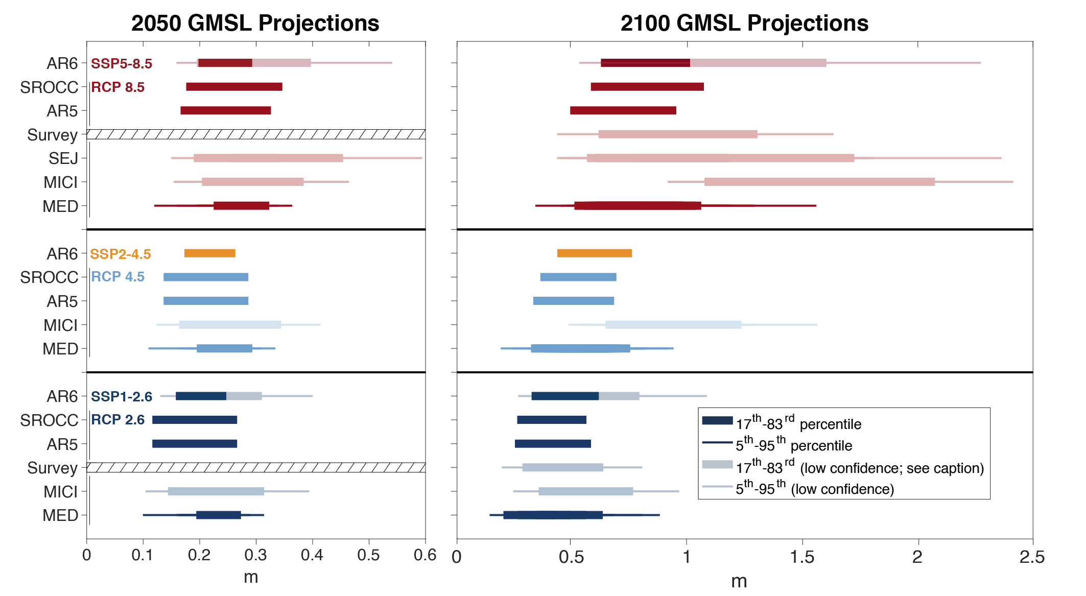 Figure 9.25 | Literature global mean sea level (GMSL) projections (m) for 2050 (left) and 2100 (right) since 1995–2014, for RCP8.5/SSP5-8.5 (top set), RCP4.5/SSP2-4.5 (middle set), and RCP2.6/SSP1-2.6 (bottom set). Projections are standardized to account for minor differences in time periods. Thick bars span from the 17th–83rd percentile projections, and thin bars span the 5th–95th percentile projections. The different assessments of ice-sheet contributions are indicated by ‘MED’ (ice-sheet projections include only processes in whose quantification there is medium confidence), ‘MICI’ (ice-sheet projections which incorporate marine ice cliff instability), and ‘SEJ’ (structured expert judgement) to assess the central range of the ice-sheet projection distributions. ‘Survey’ indicates the results of a 2020 survey of sea level experts on global mean sea level (GMSL) rise from all sources (Horton et al., 2020). Projection categories incorporating processes in which there is low confidence (MICI and SEJ) are lightly shaded. Dispersion among the different projections represents deep uncertainty, which arises as a result of low agreement regarding appropriate conceptual models describing ice-sheet behaviour and low agreement regarding probability distributions used to represent key uncertainties. Individual studies are shown in Tables 9.SM.5 and 9.SM.6. Further details on data sources and processing are available in the chapter data table (Table 9.SM.9).
 There is high agreement across published GMSL projections for 2050, and there is little sensitivity to emissions scenario (Figure 9.25, left panel). Up to 2050, projections are broadly consistent with extrapolation of the observed acceleration of GMSL rise (Sections 2.3.3.3, 9.6.1.1 and 9.6.1.2). Considering only projections incorporating ice-sheet processes in whose quantification there is at least medium confidence, the GMSL projections for 2050, across all emissions scenarios, fall between 0.1 and 0.4 m (5th–95th percentile range). Projections incorporating MICI or SEJ do not extend this range under RCP2.6 or RCP4.5 but do extend the upper part of the range to 0.6 m under RCP8.5. On the basis of these studies, we therefore have high confidence that GMSL in 2050 will be between 0.1 and 0.4 m higher than in 1995–2014 under low- and moderate-emissions scenarios, and between 0.1 and 0.6 m under high-emissions scenarios.
Conversely, there is low agreement across published GMSL projections for 2100, particularly for higher-emissions scenarios, as well as a higher degree of sensitivity to the choice of emissions scenario (Figure 9.25, right panel). Considering only projections representing processes in whose quantification there is at least medium confidence, the GMSL projections for 2100 fall between 0.2 and 1.0 m (5th–95th percentile range) under RCP2.6 and RCP4.5, and between 0.3 and 1.6 m under RCP8.5. Considering also projections incorporating MICI or SEJ (low confidence), the projections for 2100 fall between 0.2 and 1.0 m (5th–95th percentile range) under RCP2.6, 0.2, and 1.6 m under RCP4.5, and 0.4 and 2.4 m under RCP8.5. In summary, RCP-based projections published since AR5 show high agreement for 2050, but exhibit broad ranges and low agreement for 2100, particularly under RCP8.5.
9.6.3.2 Drivers of Projected Sea Level Change
This section describes the choices made for the contributions to the updated global mean and regional sea level projections (Section 9.6.3.3) based on assessments in this Report and compares the updated projections to AR5 (Church et al., 2013b) and SROCC (Oppenheimer et al., 2019) (Tables 9.7 and 9.8). Since there is no single model that can directly compute all of the contributions to sea level change (Box 9.1), the contributions to sea level are computed separately and then combined (Tables 9.8 and 9.9). For consistency with global surface air temperature (GSAT) projections (Section 4.3.1.1), and assessment of equilibrium climate sensitivity (ECS) and transient climate response (TCR; Section 7.5), temperature-dependent projections (thermal expansion, ice sheets, glaciers) are forced by GSAT projections from a two-layer energy budget emulator (Smith et al., 2018) that is calibrated to be consistent with the assessment of ECS and TCR (Box 7.1, Supplementary Material 7.SM.2). Throughout, likely ranges are assessed based on the combination of uncertainty in the GSAT distribution and uncertainty in the relationships between GSAT and changes to individual components. In general, 17th–83rd percentile results, incorporating both GSAT and sea level process uncertainty, are interpreted as likely ranges. This is distinct from the approach used by AR5, which interpreted the 5th–95th percentile range of CMIP5 projections, and therefore of GMSL projections driven by them, as likely ranges. The shift in interpretation is consistent with the use of the emulator for GSAT (Box 4.1, Cross-Chapter Box 7.1). Very likely ranges are not assessed because of the potential for processes in whose projections there is currently low confidence to substantially augment total projected GMSL change.
Driver of Global Mean or Regional Sea Level change | SROCC Projection Method | AR6 Projection method |
Thermal expansion (Section 9.2.4.1) | CMIP5 ensemble drift-corrected zostoga, with surrogates derived from climate system heat content where not available | Two-layer emulator with climate sensitivity calibrated to AR6 assessment (Supplementary Material 7.SM.2) and expansion coefficients calibrated to emulate CMIP6 models (Supplementary Material 9.SM.4.2 and 9.SM.4.3) |
Greenland Ice Sheet (excluding peripheral glaciers) (Sections 9.4.1.3 and 9.4.1.4) | Surface mass balance: scaled cubic polynomial fit to global mean surface temperature (GMST) Dynamics: Quadratic function of time, calibrated based on multi-model assessment | Medium confidence processes up to 2100: Emulated Ice Sheet Model Intercomparison Project for CMIP6 (ISMIP6) simulations (Box 9.3; Edwards et al., 2021) Medium confidence processes after 2100: Parametric model fit to ISMIP6 simulations up to 2100, extrapolated based on either constant post-2100 rates or a quadratic interpolation to the multi-model assessed 2300 range (Supplementary Material 9.SM.4.4) Low confidence processes: Structured expert judgement (Bamber et al., 2019) |
Antarctic Ice Sheet (excluding peripheral glaciersa) (Sections 9.4.2.5 and 9.4.2.6) | Multi-model assessment | Medium confidence processes up to 2100: p-box including: (i) Emulated ISMIP6 simulations (Edwards et al., 2021); and (ii) Linear Antarctic Response Model Intercomparison Project (LARMIP-2) simulations (Levermann et al., 2020) augmented by AR5 surface mass balance model (Box 9.3) Medium confidence processes after 2100: p-box including: (i) AR5 parametric AIS model; and (ii) LARMIP-2 simulations augmented by AR5 surface mass balance model applied to CMIP6 models, with both methods extrapolated based on either constant post-2100 rates or a quadratic interpolation to the multi-model assessed 2300 range (Section 9.6.3.2) Low confidence processes: (i) Single-ice-sheet-model ensemble simulations incorporating marine ice cliff instability (DeConto et al., 2021); and (ii) structured expert judgement (Bamber et al., 2019) |
Glaciers (including peripheral glaciers) (Section 9.5.1.3) | Power law function of integrated GMST fit to glacier models | Up to 2100: Emulated GlacierMIP (Marzeion et al., 2020; Edwards et al., 2021) simulations (Box 9.3) Beyond 2100: AR5 parametric model re-fit to GlacierMIP (Supplementary Material 9.SM.4.5; Marzeion et al., 2020) |
Land-water storage (Section 9.6.3.2) | Groundwater depletion: combination of: (i) continuation of early 21st-century trends; and (ii) land-surface hydrology models (Wada et al., 2012) Water impoundment: combination of: (i) continuation of historical rate; and (ii) assumption of no net impoundment after 2010 | Groundwater depletion: Population/groundwater depletion relationship calibrated based on Konikow (2011) and Wada et al. (2012, 2016) Water impoundment: Population/dam impoundment relationship calibrated based on Chao et al. (2008), adjusted for new construction following Hawley et al. (2020) for 2020 to 2040 |
Ocean dynamic sea level (Section 9.2.4.2) | CMIP5 ensemble zosfield after polynomial drift removal | Distribution derived from CMIP6 ensemble zosfield after linear drift removal (Supplementary Material 9.SM.4.2 and 9.SM.4.3) |
Gravitational, rotational, and deformational effects (Section 9.6.3.2) | Sea level equation solver (Slangen et al., 2014b) driven by projections of ice-sheet, glacier, and land-water storage changes | |
Glacial isostatic adjustment and other drivers of vertical land motion Section 9.6.3.2) | Glacial Isostatic Adjustment model, with ice history from mean of the Australian National University (ANU) and ICE-5G reconstructions | Spatio-temporal statistical model of tide gauge data (updated from Kopp et al., 2014) (Supplementary Material 9.SM.4.6) |
aIce-sheet models include some of the larger islands in the Antarctic periphery, so there is some overlap in the projected glacier contribution and the projected Antarctic contribution, but the effect is estimated to be on the order of 0.5–1 cm or less (Edwards et al., 2021).
9.6.3.2.1 Global mean thermosteric sea level rise
In AR5 and SROCC, global mean thermosteric sea level rise was derived from the 21 members of the CMIP5 ensemble that provided the required variables (Section 9.2.4.1). The AR5 and SROCC removed drift estimated based on a pointwise polynomial fit to pre-industrial control simulations. They extended projections to scenarios not provided by the models by calculating the heat content of the climate system from GMST and net radiative flux, and converting this to global mean thermosteric sea level rise using each model’s diagnosed expansion efficiency coefficient. The AR5 and SROCC derived the associated uncertainties by assuming a normal distribution, with the 5th–95th percentile CMIP5 ensemble interpreted as the likely range. In this Report, global mean thermosteric sea level rise is derived from a two-layer energy budget emulator consistent with the assessment of ECS and TCR (Section 9.2.4.1; Supplementary Material 9.SM.4.2 and 9.SM.4.3). Despite the change in methodology, this leads to a likely global mean thermosteric contribution (17th–83rd percentile) between 1995–2014 and 2100 that represents a minimal change from AR5 and SROCC (Table 9.8).
9.6.3.2.2 Greenland Ice Sheet
The AR5 and SROCC projected the Greenland surface-mass balance using a cubic polynomial fit to a regional climate model as a function of global mean surface temperature (with a log-normal scaling factor reflecting uncertainty in surface-mass balance models, and another scaling factor reflecting the positive feedback of ice-sheet elevation changes on mass loss), and the dynamic contribution was estimated based on a multi-model assessment interpolated as a quadratic function of time.
For processes whose projections we have at least medium confidence in, the updated projections use emulated Ice Sheet Model Intercomparison Project for CMIP6 (ISMIP6) projections of the Greenland Ice Sheet (Section 9.4.1.3; Figure 9.17; Tables 9.2 and 9.7; Box 9.3). Since the ISMIP6 emulator does not account for temporal correlation, a parametric fit to the ISMIP6 results is used to calculate rates of change (Supplementary Material 9.SM.4.4). For projections beyond 2100 (when the ISMIP6 simulations end), the polynomial fit is extrapolated based on two alternate approaches: (i) an assumption of constant rates of mass change after 2100; and (ii) for SSP1-2.6 and SSP5-8.5, a quadratic function of time extending to 2300 based on the multi-model assessment of contributions under RCP2.6 and RCP8.5 at 2300 (Section 9.4.1.4). Differences between the two approaches are small up to 2150, and since the latter approach is not available for all scenarios, only the former (constant rates) is used for time series projections up to 2150. Both approaches are used for examining uncertainty in the timing of different levels of GMSL rise and to inform projections for the year 2300 (Section 9.4.1.4). For 2100, the ISMIP6 emulator yields the likely contribution from the Greenland Ice Sheet shown in Table 9.2 and Figure 9.17, representing a slight narrowing from AR5 projections.
9.6.3.2.3 Antarctic Ice Sheet
For the Antarctic Ice Sheet (AIS), AR5 applied a temperature-based scaling approach for SMB and a quadratic function of time, calibrated to a multi-model assessment, for dynamic contributions. The SROCC used a new assessment based on the results of five process-based studies (Section 9.4.2.5). For processes in whose projections we have at least medium confidence, the likely rangeprojections for the AIS are based on: (i) the emulated ISMIP6 ensemble; and (ii) the LARMIP-2 ensemble, augmented with AR5 parametric Antarctic SMB model. The GMSL projections are produced with both distributions and combined in a ‘p-box’ (Kriegler and Held, 2005; Le Cozannet et al., 2017), which represents the upper and lower bounds of the distribution (Section 9.4.2.5, Box 9.3 and Table 9.3). A likely range is then identified, spanning the lower of the two 17th percentile projections and the higher of the two 83rd percentile projections, 5 with the median taken as the mean of the medians of the two projections. Since the ISMIP6 emulator does not account for temporal correlation, the AR5 parametric AIS model is substituted for the emulator in the p-box for rates of change. As AR5 projections are modestly lower than those from the ISMIP6 emulator, this substitution modestly broadens the likely range at the low end for projections of rate and changes beyond 2100. For projections beyond 2100 (when the ISMIP6 and LARMIP-2 simulations end), the AIS simulations are extrapolated using the same two approaches as the Greenland Ice Sheet (GrIS) projections (Section 9.4.1.4). The likely ranges to 2100 are consistent with SROCC (Table 9.8).
9.6.3.2.4 Low confidence ice-sheet projections
To test the possible effect of additional ice-sheet processes for which there is low confidence (Sections 9.4.1.3, 9.4.1.4, 9.4.2.5, 9.4.2.6 and 9.6.3.1, and Box 9.4), two additional approaches are considered. For both the Greenland and Antarctic ice sheets, we produce sensitivity cases employing the SEJ projections of Bamber et al. (2019), mapping 2°C and 5°C stabilization scenarios to SSP1-2.6 and SSP5-8.5, respectively. For the AIS, we produce an additional sensitivity case using projections, which incorporate MICI (DeConto et al., 2021), mapping projections for RCP2.6 and RCP8.5 to SSP1-2.6 and SSP5-8.5. For the Greenland Ice Sheet, the SEJ projections indicate the potential for outcomes outside the corresponding likely ranges (Table 9.8). For the AIS, there is no evidence from these studies to suggest an important role under lower-emissions scenarios for processes in whose projections we have low confidence. By contrast, for SSP5-8.5, the SEJ and MICI projections exhibit 17th–83rd percentile ranges of 0.02–0.56 m and 0.19–0.53 m by 2100, consistent with one another but considerably broader than the likely contribution for medium confidence processes of 0.03–0.34 m. This lower level of agreement for higher-emissions scenarios reflects the deep uncertainty in the AIS contribution to GMSL change under higher-emissions scenarios (Box 9.4). This deep uncertaintygrows after 2100: by 2150, under SSP5-8.5, medium confidence processes likely lead to a –0.1–0.7 m AIS contribution, while SEJ- and MICI-based projections indicate 0.0–1.1 m and 1.4–3.7 m, respectively.
9.6.3.2.5 Glaciers
In AR5 and SROCC, global glacier mass changes were derived from a power law of integrated global mean surface temperature change fit to results from four different glacier models. The updated projections use emulated GlacierMIP projections (Section 9.5.1.3; Box 9.3). Since the GlacierMIP emulator does not account for temporal correlation and terminates, along with the GlacierMIP simulations, in 2100, we employ a parametric fit to the GlacierMIP simulations, with a functional form similar to that employed by AR5, to calculate rates of change and extrapolate changes beyond 2100 (up to a maximum potential contribution of 0.32 m; see Supplementary Material 9.SM.4.5). This approach leads to a median glacier contribution that is a minimal change (Table 9.8) from AR5 and SROCC and a modest narrowing of likely ranges (Section 9.5.1.3). For RCP2.6, AR5 projected 0.10 (0.04 to 0.16, likely range) m, compared to 0.09 (0.07 to 0.11) m projected for SSP1-2.6. For RCP8.5, AR5 projected a likely contribution of 0.17 (0.09 to 0.25) m, compared to 0.18 (0.15 to 0.21) m projected here.
9.6.3.2.6 Land-water storage
In AR5 and SROCC, the groundwater depletion contribution to GMSL rise was based on combining results from two approaches: one assuming a continuation of early 21st-century trends (Konikow, 2011); and the other using land-surface hydrology models (Wada et al., 2012). Together, these yielded a range of about 0.02–0.09 m of GMSL rise by 2080–2099. The rate of water impoundment in reservoirs was likewise based on two approaches: one assuming the continuation of the average rate over 1971–2010 (and thus –0.01 to –0.03 m by 2080–2099; Chao et al., 2008); and the other assuming no net impoundment after 2010 (Lettenmaier and Milly, 2009). Together, these yield a GMSL contribution from groundwater impoundment of –0.03 to 0 m. Combining groundwater depletion and water impoundment led AR5 and SROCC to infer a projected range of –0.01 to +0.11 m by 2100.
In the updated projections, a statistical relationship is applied, linking historical and future SSP global population to dam impoundment and groundwater extraction (Rahmstorf et al., 2012; Kopp et al., 2014). The population/groundwater depletion relationship is calibrated based on the same studies used in AR5 (Konikow, 2011; Wada et al., 2012), reduced by about 20% to account for water retained on land (Wada et al., 2016). The population/dam impoundment relationship is calibrated based on Chao et al. (2008). However, while historically dam impoundment has been declining with population, recent literature shows that planned dam construction considerably exceeds the historical trend (Zarfl et al., 2015; Hawley et al., 2020). Over 2020–2040, the impoundment contribution to GMSL rise based on past trends would be about –0.1 mm yr–1, compared to about –0.5 mm yr–1if all currently planned dams are built (Hawley et al., 2020) and the statistical projection is therefore augmented by an additional –0.4 to 0.0 mm yr–1over 2020–2040 to account for the possible effects of planned dam construction. As in AR5 and SROCC, climatically driven changes to land-water storage (LWS) have not been included in published sea level projections, as they are not well quantified (e.g., Jensen et al., 2019) or are considered negligible (e.g., permafrost, Section 9.5.2). This approach yields a likely global-mean land-water storage contribution (Figure 9.27, Table 9.8) that is slightly lower and narrower than the AR5 and SROCC likely ranges. Since the projections are explicitly population driven, these projections also exhibit a weak scenario dependence, with a contribution around 0.01 m higher under SSP3 than under other scenarios.
RCP2.6 | SSP1-2.6 | ||||
m relative to 1995–2014 | AR5 | SROCC | Medium confidence processes | MICI | SEJ |
Thermal expansion (Section 9.2.4.1) | 0.14 (0.10–0.19) m | 0.14 (0.11–0.18) m | |||
Greenland Section 9.4.1.3) | 0.07 (0.03–0.11) m | 0.06 (0.01–0.10) m | 0.13 (0.07–0.30) m | ||
Antarctica (Section 9.4.2.5) | 0.06 (–0.04 to +0.16) m | 0.04 (0.01–0.11) m | 0.11 (0.03–0.27) m | 0.08 (0.06–0.12) m | 0.09 (–0.01 to +0.25) m |
Glaciers (Section 9.5.1.3) | 0.10 (0.04–0.16) m | 0.09 (0.07–0.11) m | |||
Land-water storage (Section 9.6.3.2) | 0.05 (–0.01 to +0.11) m | 0.03 (0.01–0.04) m | |||
Total (2100) | 0.41 (0.25–0.58) m | 0.40 (0.26–0.56) m | 0.44 (0.33–0.62) m | 0.41 (0.35–0.48) m | 0.53 (0.38–0.79) m |
Total (2150) | 0.29–0.63 m | 0.56 (0.40–0.73) m | 0.68 (0.46–0.99) m | 0.74 (0.62–0.91) m | 0.84 (0.56–1.34) m |
GMSL rate, 2080–2100 (mmyr–1) | 4.4 (2.0–6.8) mm yr–1 | 4 (2–6) mm yr–1 | 5.2 (3.2–8.0) mm yr–1 | 5.1 (4.3–6.2) mm yr–1 | 5.9 (2.8–11.0) mm yr–1 |
RCP8.5 | SSP5-8.5 | ||||
m relative to 1995–2014 | AR5 | SROCC | Medium confidence processes | MICI | SEJ |
Thermal expansion (Section 9.2.4.1) | 0.31 (0.24–0.38) m | 0.30 (0.24–0.36) m | |||
Greenland Section 9.4.1.3) | 0.14 (0.08–0.27) m | 0.13 (0.09–0.18) m | 0.23 (0.10–0.59) m | ||
Antarctica (Section 9.4.2.5) | 0.04 (–0.08 to +0.14) m | 0.12 (0.03–0.28) m | 0.12 (0.03–0.34) m | 0.34 (0.19–0.53) m | 0.21 (0.02–0.56) m |
Glaciers (Section 9.5.1.3) | 0.17 (0.09–0.25) m | 0.18 (0.15–0.20) m | |||
Land-water storage (Section 9.6.3.2) | 0.05 (–0.01 to +0.11) m | 0.03 (0.01–0.04) m | |||
Total (2100) | 0.71 (0.49–0.95) m | 0.81 (0.58–1.07) m | 0.77 (0.63–1.01) m | 0.99 (0.82–1.19) m | 1.00 (0.70–1.60) m |
Total (2150) | 0.34–1.35 m | 1.27 (0.80–1.79) m | 1.32 (0.98–1.88) m | 3.48 (2.57–4.82) m | 1.79 (1.22–2.94) m |
GMSL rate, 2080–2100 (mmyr–1) | 11.2 (7.5–15.7) mm yr–1 | 15 (10–20) mm yr–1 | 12.1 (8.6–17.6) mm yr–1 | 23.1 (17.5–30.1) mm yr–1 | 16.0 (9.8–28.9) mm yr–1 |
9.6.3.2.7 Ocean dynamic sea level
In AR5 and SROCC, the ocean dynamic sea level contribution to RSL projections was derived from the CMIP5 ensemble, after removing the drift estimate based on pre-industrial control simulations. This Report uses updated simulations from the CMIP6 ensemble (Section 9.2.4.2; Supplementary Material 9.SM.4.2) to project the ocean dynamic sea level contribution to RSL change (Section 9.2.4.2; Figure 9.26). To produce ocean dynamic sea level projections consistent with the global mean thermosteric projections from the two-layer energy budget emulator, we follow the approach of Kopp et al. (2014), employing a correlation between global-mean thermosteric sea level change and ocean dynamic sea level derived from the CMIP6 ensemble (Supplementary Material 9.SM.4.3). Since CMIP6 models are of fairly coarse resolution (typically about 100 km), and even the models participating in HighResMIP (near 10 km resolution) do not capture all the phenomena that contribute to coastal ocean dynamic sea level change, there is low confidence in the details of ocean dynamic sea level change along the coast (Section 9.2.3.6) and in semi-enclosed basins, such as the Mediterranean, where coarse models can misrepresent key dynamic processes. Regional high-resolution models can improve projections of coastal ocean dynamic sea level change (Section 12.4; Hermans et al., 2020), but have not been implemented at a global scale.
 Figure 9.26 | Median global mean and regional relative sea level projections (m) by contribution for the SSP1-2.6 and SSP5-8.5 scenarios. Upper time series: Global mean contributions to sea level change as a function of time, relative to 1995–2014. Lower maps: Regional projections of the sea level contributions in 2100 relative to 1995–2014 for SSP5-8.5 and SSP1-2.6. Vertical land motion is common to both Shared Socio-economic Pathways (SSPs). Further details on data sources and processing are available in the chapter data table (Table 9.SM.9).
 9.6.3.2.8 Gravitational, rotational and deformational effects
Gravitational, rotational, and deformational (GRD) effects (Box 9.1) lead to distinct variations in the RSL change pattern, which are similar across a range of benchmarked GRD solvers (Martinec et al., 2018; Palmer et al., 2020). There is high confidence in the understanding of GRD processes. RSL rise associated with GRD is very likely to be largest in the Pacific, due to the combined effects of projected GrIS, AIS and glacier mass loss (high confidence) (e.g., Kopp et al., 2014; Slangen et al., 2014b; Larour et al., 2017; Mitrovica et al., 2018). The GRD effect associated with mass loss from an ice sheet is sensitive to the spatial distribution of that mass loss. For example, the GRD contribution to RSL rise in Australia will be larger for Antarctic mass loss sourced fromthe Antarctic Peninsula than for Antarctic mass loss sourced fromThwaites Glacier. In parts of north-eastern North America and north-western Europe, GRD effects associated with mass loss from southern Greenland will lead to an RSL fall, whereas mass loss from northern Greenland will lead to an RSL rise (high confidence) (Figure 9.26; Larour et al., 2017; Mitrovica et al., 2018). The AR5 and SROCC computed RSL patterns using a gravitationally self-consistent GRD solver given the amounts, locations and timing of the projected barystatic sea level changes driven by glaciers, ice sheets and LWS (Church et al., 2013b). A similar GRD solver is used in the updated projections (following Slangen et al., 2014b). The Earth model used is based on the Preliminary reference Earth model (PREM: Dziewonski and Anderson, 1981), and is elastic, compressible and radially stratified.
9.6.3.2.9 Glacial isostatic adjustment and other drivers of vertical land motion
Glacial Isostatic Adjustment (GIA) leads to vertical land motion (VLM; see Box 9.1) and changes in sea surface height, both of which contribute to RSL change. GIA uncertainty is caused by uncertainty in the rheological structure of the solid Earth, which drives the longer-term viscous Earth deformation, as well as uncertainty in the modelled global ice history (e.g., Whitehouse, 2018). In AR5 and SROCC, GIA contributions to RSL change were calculated using a sea level equation solver with an ice-sheet history taken as the mean of the ICE5G (Peltier et al., 2015) and ANU (Lambeck et al., 2014) ice-sheet models. Since AR5, new global models are emerging that more rigorously treat ice and Earth structure uncertainty (Caron et al., 2018). However, there is also a growing recognition that lateral variations in Earth structure limit the utility of global models that treat the solid Earth as though it were laterally uniform (Love et al., 2016; Huang et al., 2019; T. Li et al., 2020).
As noted by SROCC, VLM from sources other than GIA – including tectonics and mantle dynamic topography, volcanism, compaction, and anthropogenic subsidence – can be locally important, producing VLM rates comparable to or greater than rates of GMSL change. Complete global projections of these processes are not available because of the small spatial scales, the sensitivity of subsidence to local human activities, and the stochasticity of tectonics (Wöppelmann and Marcos, 2016; Oppenheimer et al., 2019). Therefore, integrated RSL projections to date have either included only the component of VLM associated with GIA (as in AR5 and SROCC), or used a constant long-term background rate of change (including both GIA and other long-term drivers of VLM) estimated from historical tide gauge trends (e.g., Kopp et al., 2014). The updated projections use the second approach and extrapolate the field of long-term background rates of RSL change, including long-term VLM derived from tide gauges, to global coverage using a spatio-temporal statistical approach (Supplementary Material 9.SM.4.6; Kopp et al., 2014). The combined GIA and long-term VLM is assumed to be scenario independent and constant over the projected period. In areas where rapid subsidence occurs in a cluster of tide gauges (e.g., the western Gulf of Mexico), the associated rates are interpolated between the tide gauges. In areas where the available tide gauges exhibit large, tectonically driven VLM that changes considerably in rate over short distances (e.g., Alaska and the Bering Strait), a sizable uncertainty propagates into the RSL projections (Figure 9.26). Rates of RSL rise are likely to be underestimated due to subsidence in shallow strata that are not recorded by tide gauges (Keogh and Törnqvist, 2019) and in some locations may therefore be minimum values, especially if anomalously high subsidence rates associated with fluid extraction are also considered (e.g., Minderhoud et al., 2017). Therefore, depending on location, there is low to medium confidence in the GIA and VLM projections employed in this Report. In many regions, higher-fidelity projections would require more detailed regional analysis.
9.6.3.3 Sea Level Projections to 2150 Based on Shared Socio-economic Pathway Scenarios
Up to 2050, consistent with AR5 and SROCC, GMSL projections exhibit little scenario dependence (high confidence) (Figure 9.27 and Table 9.9) with likely (medium confidence)sea level rise between the baseline period (1995–2014) and 2050 of 0.19 (0.16–0.25) m under SSP1-2.6 and 0.23 (0.20–0.30) m under SSP5-8.5. These projections fall centrally within the range of published projections for RCP2.6 and RCP8.5 (Section 9.6.3.1).
SSP1-1.9 | SSP1-2.6 | SSP2-4.5 | SSP3-7.0 | SSP5-8.5 | SSP5-8.5 Low Confidence | |
Thermal expansion | 0.12 (0.09–0.15) | 0.14 (0.11–0.18) | 0.20 (0.16–0.24) | 0.25 (0.21–0.30) | 0.30 (0.24–0.36) | 0.30 (0.24–0.36) |
Greenland | 0.05 (0.00–0.09) | 0.06 (0.01–0.10) | 0.08 (0.04–0.13) | 0.11 (0.07–0.16) | 0.13 (0.09–0.18) | 0.18 (0.09–0.59) |
Antarctica | 0.10 (0.03–0.25) | 0.11 (0.03–0.27) | 0.11 (0.03–0.29) | 0.11 (0.03–0.31) | 0.12 (0.03–0.34) | 0.19 (0.02–0.56) |
Glaciers | 0.08 (0.06–0.10) | 0.09 (0.07–0.11) | 0.12 (0.10–0.15) | 0.16 (0.13–0.18) | 0.18 (0.15–0.21) | 0.17 (0.11–0.21) |
Land-water Storage | 0.03 (0.01–0.04) | 0.03 (0.01–0.04) | 0.03 (0.01–0.04) | 0.03 (0.02–0.04) | 0.03 (0.01–0.04) | 0.03 (0.01–0.04) |
Total (2030) | 0.09 (0.08–0.12) | 0.09 (0.08–0.12) | 0.09 (0.08–0.12) | 0.10 (0.08–0.12) | 0.10 (0.09–0.12) | 0.10 (0.09–0.15) |
Total (2050) | 0.18 (0.15–0.23) | 0.19 (0.16–0.25) | 0.20 (0.17–0.26) | 0.22 (0.18–0.27) | 0.23 (0.20–0.29) | 0.24 (0.20–0.40) |
Total (2090) | 0.35 (0.26–0.49) | 0.39 (0.30–0.54) | 0.48 (0.38–0.65) | 0.56 (0.46–0.74) | 0.63 (0.52–0.83) | 0.71 (0.52–1.30) |
Total (2100) | 0.38 (0.28–0.55) | 0.44 (0.32–0.62) | 0.56 (0.44–0.76) | 0.68 (0.55–0.90) | 0.77 (0.63–1.01) | 0.88 (0.63–1.60) |
Total (2150) | 0.57 (0.37–0.86) | 0.68 (0.46–0.99) | 0.92 (0.66–1.33) | 1.19 (0.89–1.65) | 1.32 (0.98–1.88) | 1.98 (0.98–4.82) |
Rate (2040–2060) | 4.1 (2.8–6.0) | 4.8 (3.5–6.8) | 5.8 (4.4–8.0) | 6.4 (5.0–8.7) | 7.2 (5.6–9.7) | 7.9 (5.6–16.1) |
Rate (2080–2100) | 4.2 (2.4–6.6) | 5.2 (3.2–8.0) | 7.7 (5.2–11.6) | 10.4 (7.4–14.8) | 12.1 (8.6–17.6) | 15.8 (8.6–30.1) |
Beyond 2050, the scenarios increasingly diverge. Between the baseline period (1995–2014) and 2100, processes in whose projection there is medium confidence drive likely GMSL rise of 0.44 (0.32–0.62) m and 0.77 (0.63–1.01) m under SSP1-2.6 and SSP5-8.5, respectively (Tables 9.8, 9.9). While derived using substantially updated methods, these projections are broadly consistent with SROCC, which projected likely GMSL rise of 0.41 (0.26–0.56) m and 0.81 (0.58–1.07) m under RCP2.6 and RCP8.5, respectively, over this period. They are modestly higher than those of AR5, which projected likely GMSL rise of 0.41 (0.25–0.58) m under RCP2.6 and 0.71 (0.49–0.95) m under RCP8.5 (Figure 9.25, Table 9.8). They are also broadly consistent with projections produced by driving AR5 methods with CMIP6 temperature and thermal expansion projections, which leads to 0.44 (0.27–0.61) m under SSP1-2.6 and 0.73 (0.49–1.02) m under SSP5-8.5 (Hermans et al., 2021). The SSP1-2.6 and SSP5-8.5 projections are consistent with the ranges of published projections for RCP2.6 and RCP8.5 that do not incorporate MICI or SEJ (Section 9.6.3.1).
 Figure 9.27 | Projected global mean sea level rise under different Shared Socio-economic Pathway (SSP) scenarios. Likely global mean sea level (GMSL) change for SSP scenarios resulting from processes in whose projection there is medium confidence. Projections and likely ranges at 2150 are shown on right. Lightly shaded ranges and thinner lightly shaded ranges on the right show the 17th–83rd and 5th–95th percentile ranges for projections including low confidence processes for SSP1-2.6 and SSP5-8.5 only, derived from a p-box including structured expert judgement and marine ice-cliff instability projections. Black lines show historical GMSL change, and thick solid and dash-dotted black lines show the mean and likely range extrapolating the 1993–2018 satellite altimeter trend and acceleration. Further details on data sources and processing are available in the chapter data table (Table 9.SM.9).
 The likely GMSL projections for SSP3-7.0 and SSP5-8.5 are consistent with a continuation of the GMSL satellite-observed rate (very likely 3.25 [2.88–3.61] mm yr–1) and acceleration (very likely 0.094 [0.082–0.115] mm yr–2) of GMSL rise over 1993–2018 (Table 9.5 and Section 2.3.3.3), which would imply a likely GMSL rise of 0.24 m (0.23–0.25 m) by 2050 and 0.73 m (0.69–0.77 m) by 2100. This extrapolation would also imply a likely rate of GMSL rise of 7.5 (7.4–7.6) mm yr–1over 2040–2060 and 11.2 (10.6–11.8) mm yr–1over 2080–2100. Over the satellite period, the observed acceleration has been driven primarily by ice-sheet contributions (Section 9.6.1.2 and Table 9.5); in the median projections for SSP3-7.0 and SSP5-8.5, these accelerations are projected to continue at a slightly lower level, while the GMSL acceleration is augmented by an acceleration of thermal expansion and glacier loss associated with rising global temperature. Overall, these extrapolations imply that, under SSP1-1.9, SSP1-2.6, and SSP2-4.5, the GMSL acceleration is projected to decrease from its current level.
While ice-sheet processes in whose projection there is low confidence have little influence up to 2100 on projections under SSP1-1.9 and SSP1-2.6 (Table 9.9), this is not the case under higher emissions scenarios, where they could lead to GMSL rise well above the likely range. In particular, under SSP5-8.5, low-confidence processes could lead to a total GMSL rise of 0.6–1.6 m over this time period (17th–83rd percentile range of p-box, including SEJ- and MICI-based projections), with 5th–95th percentile projections extending to 0.5–2.3 m (low confidence). The assessed low confidence range is slightly narrower than, but broadly consistent with, the full 0.4–2.4 m range of published 5th–95th percentile projections for RCP8.5 since AR5 (Section 9.6.3.1) – including those based on SEJ or incorporating MICI – and highlights the deep uncertainty in GMSL rise under the highest emissions scenarios (Box 9.4). The assessment of the potential contribution of processes in which there is low confidence to GMSL rise by 2100 is broadly consistent with the AR5’s assessment (Church et al., 2013b), which concluded that collapse of marine-based sectors of the AIS could cause several tenths of a metre of GMSL rise above the likely range.
While prior assessment reports, starting with the First Assessment Report (Warrick et al., 1990), have focused on projecting GMSL up to the year 2100, time has progressed, and the year 2100 is now within the time frame of some long-term infrastructure decisions. For this reason, projections up to the year 2150 are also highlighted (Table 9.9). Over this time period, assuming no acceleration in ice-sheet mass fluxes after 2100, processes in which there is medium confidence lead to GMSL rise of 0.5–1.0 m under SSP1-2.6 and 1.0–1.9 m under SSP5-8.5. Processes in which there is low confidence could drive GMSL rise under SSP5-8.5 to 1.0–4.8 m (17th–83rd percentile) or even 0.9–5.4 m (5th–95th percentile).
Median projected RSL changes are shown in Figure 9.28, with driving factors highlighted in Figure 9.26. Approximately 60% (SSP1-1.9) to 70% (SSP5-8.5) of the global coastline has a projected median 21st century regional RSL rise within ±20% of the global mean increase (medium confidence). Consistent with AR5, loss of land ice mass will be an important contributor to spatial patterns in RSL change (high confidence), with ocean dynamic sea level being particularly important as a dipolar contributor in the north-west Atlantic, a positive contributor in the Arctic Ocean, and a negative contributor in the Southern Ocean south of the Antarctic Circumpolar Current (medium confidence)Section 9.2.4.2). As today, VLM will remain a major driver of RSL change (high confidence). Uncertainty in RSL projections is greatest in tectonically active areas in which VLM varies over short distances (e.g., Alaska) and in areas potentially subject to large ocean dynamic sea level change (e.g., the north-western Atlantic) (high confidence).
 Figure 9.28 | Regional sea level change at 2100 for different scenarios (with respect to 1995–2014). Median regional relative sea level change from 1995–2014 up to 2100 for: (a) SSP1-1.9; (b) SSP1-2.6; (c) SSP2-4.5; (d) SSP3-7.0; (e) SSP5-8.5; and (f) width of the likely range for SSP3-7.0. The high uncertainty in projections around Alaska and the Aleutian Islands arises from the tectonic contribution to vertical land motion, which varies greatly over short distances in this region. Further details on data sources and processing are available in the chapter data table (Table 9.SM.9).
 An alternative perspective on uncertainty in future sea level rise is provided by looking at uncertainty in time rather than elevation; that is, looking at the range of dates when specific thresholds of sea level rise are projected to be crossed (Figure 9.29). Considering only medium confidence processes, GMSL rise is likely to exceed 0.5 m between about 2080 and 2170 under SSP1-2.6 and between about 2070 and 2090 under SSP5-8.5. It is likely to exceed 1.0 m between about 2150 and some point after 2300 under SSP1-2.6, and between about 2100 and 2150 under SSP5-8.5. It is unlikely to exceed 2.0 m until after 2300 under SSP1-2.6, while it is likely to do so between about 2160 and 2300 under SSP5-8.5. However, processes in whose projections there is low confidence could lead to substantially earlier exceedances under higher emissions scenarios: under SSP5-8.5, 1.0 m could be exceeded by about 2080 and 2.0 m could be exceeded by about 2110 (17th percentile of p-box, incorporating projections based on SEJ and MICI), with 5th percentile projections as early as about 2070 for 1.0 m and 2090 for 2.0 m.
 Figure 9.29 | Timing of when global mean sea level (GMSL) thresholds of 0.5, 1.0, 1.5 and 2.0 m are exceeded, based on four different ice-sheet projection methods informing post-2100 projections. Methods are labelled based on their treatment of ice sheets. ‘No acceleration’ assumes constant rates of mass change after 2100. ‘Assessed ice sheet’ models post-2100 ice-sheet losses using a parametric fit (Supplementary Material 9.SM.4) extending to 2300 based on a multi-model assessment of contributions under RCP2.6 and RCP8.5 at 2300. Structured expert judgement (SEJ) employs ice-sheet projections from Bamber et al. (2019). Marine ice-cliff instability (MICI) combines the parametric fit (Supplementary Material 9.SM3.4) for Greenland with Antarctic projections based on DeConto et al. (2021). Circles, thick bars and thin bars represent the 50th, 17th–83rd and 5th–95th percentiles of the exceedance timing for the indicated projection method. Further details on data sources and processing are available in the chapter data table (Table 9.SM.9).
 9.6.3.4 Sea Level Projections up to 2100 Based on Global Warming Levels
Global warming levels represent a new dimension of integration in the AR6 cycle (Section 1.6.2, Cross-Chapter Box 11.1). The SR1.5 (Hoegh-Guldberg et al., 2018) concluded that, based on an assessment of GMSL projections published for 1.5°C and 2.0°C scenarios, there is medium agreement that GMSL in 2100 would be 0.04–0.16 m higher in a 2°C warmer world, compared to a 1.5°C warmer world based on 17–84% confidence interval projections (0.00–0.24 m based on 5–95% confidence interval projections) with a central value of around 0.1 m. The SR1.5 did not attempt to standardize the definition of warming-level scenarios, or to examine additional warming levels. No new integrated GMSL projections for 1.5°C or 2.0°C scenarios have been published since SR1.5.
Most of the contributors to GMSL are more closely tied to time-integrated GSAT than instantaneous GSAT (Hermans et al., 2021), which means that sea level projections by warming level can only be interpreted if the warming levels are linked to a specific time frame. Here, the warming level projections are defined based on the 2081–2100 GSAT anomaly (Supplementary Material 9.SM.4.7). Different pathways in GSAT can be followed to reach a certain temperature level, which affects the temporal evolution of the different contributors to sea level change. For instance, there will be different ice-sheet and glacier responses to a fast increase to a peak warming of 2°C in 2050, followed by a plateau or a decrease, compared to a gradual increase to the same level of warming in 2100. The sea level projections presented might include different pathways to the same warming level in 2100, which is reflected in the uncertainty ranges, and should therefore be interpreted as illustrative of sea level scenarios under a certain warming level.
Projections of likely 21st-century GMSL rise along climate trajectories leading to different increases in GSAT between 1850–1900 and 2081–2100 are shown in Table 9.10, along with the SSPs for which the temperature-level projections are most closely aligned. For example, considering only processes in which there is medium confidence, from the baseline period (1995–2014) up to 2100, GMSL in a 2°C scenario is likely to rise by 0.40–0.69, which is intermediate between the projections for SSP1-2.6 and SSP2-4.5. GMSL in a 4°C scenario is likely to rise by 0.58–0.92 m, similar to the projection for SSP3-7.0. Consistent with the discussion in Section 9.6.3.3, there is deep uncertainty in the projections for temperature levels above 3°C, and alternative approaches to projecting ice-sheet changes may yield substantially different projections in 4°C and 5°C futures. For example, employing SEJ ice-sheet projections (Bamber et al., 2019) instead of the projections for medium confidence processes only leads to a 17th–83rd percentile rise between the baseline period (1995–2014) and 2100 of 0.7–1.6 m, rather than 0.7–1.1 m in a 5°C scenario.
1.5°C | 2.0°C | 3.0°C | 4.0°C | 5.0°C | SSP5-8.5 Low Confidence | |
Closest SSPs | SSP1-2.6 | SSP1-2.6/SSP2-4.5 | SSP2-4.5/SSP3-7.0 | SSP3-7.0 | SSP5-8.5 | |
Total (2050) | 0.18 (0.16–0.24) m | 0.20 (0.17–0.26) m | 0.21 (0.18–0.27) m | 0.22 (0.19–0.28) m | 0.25 (0.22–0.31) m | 0.24 (0.20–0.40) m |
Total (2100) | 0.44 (0.34–0.59) m | 0.51 (0.40–0.69) m | 0.61 (0.50–0.81) m | 0.70 (0.58–0.92) m | 0.81 (0.69–1.05) m | 0.88 (0.63–1.60) m |
Rate (2040–2060) | 4.1 (2.9–5.7) mm yr–1 | 5.0 (3.7–7.0) mm yr–1 | 6.0 (4.6–8.1) mm yr–1 | 6.4 (5.0–8.6) mm yr–1 | 7.2 (5.7–9.8) mm yr–1 | 7.9 (5.6–16.1) mm yr–1 |
Rate (2080–2100) | 4.3 (2.6–6.4) mm yr–1 | 5.5 (3.4–8.4) mm yr–1 | 7.8 (5.3-–11.6) mm yr–1 | 9.9 (7.1–14.3) mm yr–1 | 11.7 (8.5–17.0) mm yr–1 | 15.8 (8.6–30.1) mm yr–1 |
2000-yr commitment | 2 to 3 m | 2 to 6 m | 4 to 10 m | 12 to 16 m | 19 to 22 m | |
10,000-yr commitment | 6 to 7 m | 8 to 13 m | 10 to 24 m | 19 to 33 m | 28 to 37 m |
9.6.3.5 Multi-century and Multi-millennial Sea Level Rise
Neither AR5 nor SROCC discussed the sea level commitment associated with historical emissions. Since AR5, new evidence has suggested that historical emissions up to 2016 will lead to a likely committed sea level rise (i.e., the rise that would occur in the absence of additional emissions) of 0.7–1.1 m up to 2300, while pledged emissions through 2030 increase the committed rise to 0.8–1.4 m (Nauels et al., 2019).
Between the baseline period (1995–2014) and 2300, AR5 projected a GMSL rise of 0.38–0.82 m under a non-specific low-emissions scenario and 0.9–3.6 m under a non-specific high-emissions scenario (Table 9.11). The SROCC projected 0.6–1.0 m under RCP2.6 and 2.3–5.3 m under RCP8.5 (low confidence). RCP-based projections for 2300 published since AR5 span a broader range, even excluding studies employing SEJ or MICI, with 17th–83rd percentile projections ranging from 0.3–2.9 m for RCP2.6 and 1.7–6.8 m for RCP8.5 (Table 9.SM.8; Kopp et al., 2014, 2017; Nauels et al., 2017, 2019; Bamber et al., 2019; Palmer et al., 2020). Conservatively extending the ISMIP6- and LARMIP-2-based projections beyond 2100 by assuming no subsequent change in ice-sheet mass flux rates (an approach similar to that adopted by Palmer et al. (2020) for the Greenland Ice Sheet and for the Antarctic Ice Sheet dynamics) leads to a GMSL change up to 2300 of 0.8–2.0 m under SSP1-2.6 and 1.9–4.1 m under SSP5-8.5 (17th–83rd percentile), while incorporating the ice-sheet contributions for 2300 assessed in Section 9.4.1.4 and Section 9.4.2.6 leads to 0.6–1.5 m and 2.2–5.9 m, respectively. Incorporating Antarctic results from a model with MICI (Section 9.4.2.4), using RCP forcing to inform SSP-based projections, leads to 1.4–2.1 m for SSP1-2.6 and 9.5–16.2 m for SSP5-8.5 (DeConto et al., 2021). Incorporating the SEJ-based ice-sheet projections of Bamber et al. (2019) for 2°C and 5°C stabilization scenarios yields 1.0–3.1 m for SSP1-2.6, and 2.4–6.3 m for SSP5-8.5, although because of the differences in scenarios, the SSP1-2.6 estimates may be overestimated and the SSP5-8.5 may be underestimated. The eightfold uncertainty range across projection methods under SSP5-8.5 reflects deep uncertainty in the multi-century response of ice sheets to strong climate forcing.
Taking into account all these approaches, including published projections for RCP2.6, under SSP1-2.6 GMSL will rise between 0.3 and 3.1 m by 2300 (low confidence). This projection range indicates that, while SROCC projections under low emissions to 2300 are consistent with no ice-sheet acceleration after 2100, there is the possibility of a much broader range of outcomes at the high end, reflected in the range of published GMSL projections. Under SSP5-8.5, GMSL will rise between 1.7 and 6.8 m by 2300 in the absence of MICI and by up to 16 m considering MICI, a wider range than AR5 or SROCC assessments, but consistent with published projections (low confidence).
On still longer time scales, AR5 concluded with low confidence that the multi-millennial GMSL commitment sensitivity to warming was about 1–3 m °C–1GSAT increase. Two process-model studies since AR5 (Clark et al., 2016; Van Breedam et al., 2020) indicate higher commitments (Figure 9.30). Ice sheets dominate the multi-millennial sea level commitment (Sections 9.4.1.4 and 9.4.2.6), but the two studies disagree on the relative contribution of the Greenland and Antarctic ice sheets. Notably, processes such as MICI (Section 9.4.2.4) that are a major factor behind the deep uncertainty in century-scale AIS response do not appear to have a substantial effect on the multi-millennial magnitude (DeConto and Pollard, 2016). Only one of the studies of multimillennial GMSL commitments includes scenarios consistent with 1.5°C of peak warming (Clark et al., 2016); this study suggests a 2000-year commitment at 1.5°C of about 2.3–3.1 m, with approximately an additional 1.4–2.3 m commitment between 1.5°C and 2.0°C (i.e., about 3 to 5 m °C–1). Taken together, both studies show a 2000-year GMSL commitment of about 2–6 m for peak warming of about 2°C, 4–10 m for 3°C, 12–16 m for 4°C, and 19–22 m for 5°C (medium agreement, limited evidence) (Table 9.10). GMSL rise continues after 2000 years, leading to a 10,000-year commitment of about 6–7 m for 1.5°C of peak warming (based on Clark et al., 2016), and based on both studies of about 8–13 m for 2.0°C, 10–24 m for 3.0°C, 19–33 m for 4.0°C, and 28–37 m for 5°C (medium agreement, limited evidence) (Table 9.10).
An indicative metric for the equilibrium sea level response can be provided by comparing paleo GSAT and GMSL during past multimillennial warm periods (Sections 2.3.1.1, 2.3.3.3 and 9.6.2; Figure 9.9). However, caution is needed as the present and past warm periods differ in astronomical and other forcings (Cross-chapter Box 2.1) and in terms of polar amplification. The Last Interglacial (likely 5–10 m higher GMSL than today and 0.5°C–1.5°C warmer than 1850–1900; Section 9.6.2; Table 9.6) is consistent with the Clark et al. (2016) projections for the 10,000-year commitment associated with 1.5°C of warming. Similarly, the Mid-Pliocene Warm Period (very likely 5–25 m higher GMSL than today and very likely 2.5°C–4°C warmer) (Section 9.6.2; Table 9.6) is consistent with the range of 10,000-year commitments associated with 2.5–4°C of warming, but GMSL reconstructions provide only a weak, broad constraint on model-based projections. An additional paleo constraint comes from the Early Eocene Climatic Optimum, which indicates that 10–18°C of warming is associated with ice-free conditions and a likely GMSL rise of 70–76 m (Sections 2.3.3 and 9.6.2). Together with model-based projections (Clark et al., 2016; Van Breedam et al., 2020), this period suggests that commitment to ice-free conditions would occur for peak warming of about 7°C–13°C (medium agreement, limited evidence).
On the basis of modelling studies, paleo constraints, single-ice-sheet studies finding multimillennial nonlinear responses from both the Greenland and Antarctic ice sheets (Sections 9.4.1.4 and 9.4.2.6), and the underlying physics, we conclude that GMSL commitment is nonlinear in peak warming on time scales of both 2,000 and 10,000 years (medium confidence) and exceeds the AR5 assessment of 1–3 m °C–1(medium agreement, limited evidence) (Table 9.9). Although thermosteric sea level will start to decline slowly about 2,000 years after emissions cease, the slower responses from the Greenland and Antarctic ice sheets mean that GMSL will continue to rise for 10,000 years under most scenarios (medium confidence).
Since AR5, a small number of modelling studies have examined the reversibility of the multimillennial sea level commitment under carbon dioxide (CO2) removal, solar radiation modification or local ice shelf engineering. The slow response of the deep ocean to forcing leads to global-mean thermosteric sea level fall occurring long afterward, even if CO2 levels are restored after a transient increase: global mean thermosteric sea level rise takes more than a millennium to reverse (Ehlert and Zickfeld, 2018). Rapid reversion to pre-industrial CO2 concentrations has been found to be ineffective at fostering regrowth of the AIS (DeConto et al., 2021) but may reduce the multimillennial sea level commitment (DeConto and Pollard, 2016). Altering sub-ice-shelf bathymetry (Wolovick and Moore, 2018) or triggering ice shelf advance through massive snow deposition (Feldmann et al., 2019) might interrupt marine ice sheet instability (Section 9.4.2.4) and thus reduce sea level commitment. A reversion to pre-industrial Greenland Ice Sheet temperatures with solar radiation modification is projected to stop mass loss in Greenland but leads to minimal regrowth (Applegate and Keller, 2015). Based on limited evidence, carbon dioxide removal, solar radiation modification, and local ice-shelf engineering may be effective at reducing the yet-to-be-realized sea level commitment, but ineffective at reversing GMSL rise (low confidence).
Low | RCP2.6 | SSP1-2.6 | |||||
m relative to 1995–2014 | AR5 | SROCC | Post-AR5 Published Range | No Ice-sheet Acceleration After 2100 | Assessed Ice-sheet Contribution | MICI | SEJ |
Thermal expansion | 0.07–0.46 m | 0.19–0.35 m | |||||
Greenland | 0.14 m | 0.22–0.39 m | 0.11–0.25 m | 0.28–1.28 m | |||
Antarctica | 0.21–0.25 m | –0.05 to +1.14 m | –0.14 to +0.78 m | 0.71–1.35 m | –0.11 to +1.56 m | ||
Glaciers | n/a | 0.12–0.29 m | |||||
Land-water storage | –0.03 m | 0.07–0.37 m | 0.05–0.10 m | ||||
Total (2300) | 0.38–0.82 m | 0.57–1.04 m | 0. 3–2.9 m | 0.8–2.0 m | 0.6–1.5 m | 1.4–2.1 m | 1. 0–3.1 m |
High | RCP8.5 | SSP5-8.5 | |||||
m relative to 1995–2014 | AR5 | SROCC | Post-AR5 Published Range Without (with) MICI | No Ice-Sheet Acceleration after 2100 | Assessed Ice-sheet Contribution | MICI | SEJ |
Thermal expansion | 0.28–1.80 m | 0.92–1.51 m | |||||
Greenland | 0.30–1.18 m | 0.53–0.88 m | 0.32–1.75 m | 0.40–2.23 m | |||
Antarctica | 0.02–0.19 m | 0.60–2.89 m | –0.39 to +1.55 m | –0.28 to +3.13 m | 6.87–13.54 m | 0.03–3.05 m | |
Glaciers | 0.29–0.39 m | 0.32 m | |||||
Land-water storage | n/a | 0.05–0.10 m | |||||
Total (2300) | 0.89–3.56 m | 2.25–5.34 m | 1.7–6.8 (up to 14.1) m | 1.7–4.0 m | 2.2–5.9 m | 9.5–16.2 m | 2.4–6.3 m |
 Figure 9.30 | Global mean sea level (GMSL) commitment as a function of peak global surface air temperature. From models (Clark et al., 2016; DeConto and Pollard, 2016; Garbe et al., 2020; Van Breedam et al., 2020) and paleo data on 2000-year (lower row) and 10,000 year (upper row) time scales. Columns indicate different contributors to GMSL rise (from left to right: total GMSL change, Antarctic Ice Sheet, Greenland Ice Sheet, global mean thermosteric sea level rise, and glaciers). Further details on data sources and processing are available in the chapter data table (Table 9.SM.9).
 Box 9.4 | High-end Storyline of 21st-century Sea Level Rise
In this box, we outline a storyline (Glossary, Box 10.2; Shepherd et al., 2018) for high-end sea level projections for 2100. This storyline considers processes whose quantification is highly uncertain regarding the timing of their possible onset and/or their potential to accelerate sea level rise. These processes are therefore not considered for the assessed upper bound of likely sea level rise by 2100 in section 9.6.3.3, as the likely range includes only processes that can be projected skilfully with at least medium confidence (based on agreement and evidence).
As noted by SROCC, stakeholders with a low risk tolerance (e.g., those planning for coastal safety in cities and long-term investment in critical infrastructure) may wish to consider global-mean sea level rise above the assessed likely range by the year 2100, because ‘likely ’ implies an assessed likelihood of up to 16% that sea level rise by 2100 will be higher (see also Siegert et al., 2020). Because of our limited understanding of the rate at which some of the governing processes contribute to long-term sea level rise, we cannot currently robustly quantify the likelihood with which they can cause higher sea level rise before 2100 (Stammer et al., 2019).
In light of such deep uncertainty, we employ a storyline approach in examining the potential for, and early warning signals of a high-end sea level scenario unfolding within this century. In doing so, we note upfront that the main uncertainty related to high-end sea level rise is ‘when’ rather than ‘if’ it arises: the upper limit of 1.01 m of likely sea level range by 2100 for the SSP5-8.5 scenario will be exceeded in any future warming scenario on time scales of centuries to millennia (high confidence), but it is uncertain how quickly the long-term committed sea level will be reached (Section 9.6.3.5). Hence, global mean sea level might rise well above the likely range before 2100, which is reflected by assessments of ice-sheet contributions based on structured expert judgement (Bamber et al., 2019) leading to a 95th percentile of projected future sea level rise as high as 2.3 m in 2100 (Section 9.6.3.3).
A plausible storyline for such high-end sea level rise in 2100 assumes a strong warming scenario (Section 4.8). The storyline considers faster-than-projected disintegration of marine ice shelves and the abrupt, widespread onset of marine ice cliff instability (MICI) and marine ice sheet instability (MISI) in Antarctica (Section 9.4.2.4), and faster-than-projected changes in both the surface mass balance and dynamical ice loss in Greenland. While conceptual studies provide medium evidence of these processes, substantial uncertainties and low agreement in quantifying their future evolution arise from limited process understanding, limited availability of evaluation data, missing or crude representation in model simulations, their high sensitivity to uncertain boundary conditions and parameters, and/or uncertain atmosphere and ocean forcing (Sections 9.4.1.2; 9.4.2.2).
In Antarctica, high warming might lead to floating ice shelves starting to break up earlier than expected due to processes not yet accounted for in ice-sheet models or in current climate models used to force ice-sheet projections. Such processes include hydrofracturing driven by surface meltwater, and increase in ocean thermal forcing driven by ocean circulation changes (Sections 9.2.2.3, 9.2.3.2 and 9.4.2.3; Hellmer et al., 2012, 2017; Silvano et al., 2018; Hazel and Stewart, 2020). In particular, the Thwaites and Pine Island Glacier ice shelves could potentially disintegrate this century, which might trigger MICI before 2100 (DeConto and Pollard, 2016; DeConto et al., 2021). MISI could potentially develop earlier and faster than simulated by the majority of models if fast flowing ice streams follow plastic, instead of currently assumed more viscous, sliding laws (Sun et al., 2020). Oceanic feedbacks could drive high-end sea level rise by changes in the meltwater-driven overturning circulation in ice cavities that cause additional melting (Jeong et al., 2020); by a warming of the ocean water in contact with the ice shelves due to increased stratification and thus reduced vertical mixing (Sections 9.2.2.3 and 9.2.3.2; Golledge et al., 2019; Moorman et al., 2020; Sadai et al., 2020); or by an increase in sea ice cover due to increased ocean stratification (Section 9.3.2.1), which could reduce the amount of warm, moist air that reaches the continent, and limit the mass gain from snowfall over the ice sheet (Sadai et al., 2020).
In Greenland, stronger mass loss than currently projected might also occur (Aschwanden et al., 2019; Khan et al., 2020; T. Slater et al., 2020). For example, warming-induced dynamical changes in atmospheric circulation could enhance summer blocking and produce more frequent extreme melt events over Greenland similar to the record mass loss of more than 500 Gt in summer 2019 (Section 9.4.1.1; Delhasse et al., 2018; Sasgen et al., 2020). Cloud processes in polar areas that are not well represented in models could further enhance surface melt (Hofer et al., 2019), as could feedbacks between surface melt and the increasing albedo from meltwater, detritus and pigmented algae (Section 9.4.1.1; Cook et al., 2020). The same ice dynamical processes associated with basal melt and MISI discussed for Antarctica could also occur in Greenland, as long as the ice sheet is in contact with the ocean.
The strength of all these processes is currently understood to depend strongly on global mean temperature and polar amplification, with additional linkages through feedback from global mean sea level (Gomez et al., 2020). These dependencies on a joint forcing imply that processes are strongly correlated. Hence, both their uncertainties and their possible cascading contribution to high-end sea level rise are expected to combine. Therefore, high-end sea level rise can occur if one or two processes related to ice-sheet collapse in Antarctica result in an additional sea level rise at the maximum of their plausible ranges (Sections 9.4.2.5 and 9.6.3.3; Table 9.7) or if several of the processes described in this box result in individual contributions to additional sea level rise at moderate levels. In both cases, global-mean sea level rise by 2100 would be substantially higher than the assessed likely range, as indicated by the projections including low confidence processes reaching in 2100 as high as 1.6 m at the 83rd percentile and 2.3 m at the 95th percentile (Section 9.6.3.3).
Identifying the potential drivers of a high-end sea level rise allows identification of sites and observables that can provide early warnings of a much faster sea level rise than the likely range of this and previous reports. One potential site for such monitoring is Thwaites Glacier, which is melting faster in some places and slower in others than models simulate. At this glacier, the effect of tides and channelling of warm water flows on the melting is evident (Milillo et al., 2019), making the floating ice shelf potentially vulnerable to breakup from hydrofracturing, driven by surface meltwater, much earlier than expected. In addition, the glacier is retreating towards a zone with deeper bedrock, which at its present rate of retreat would be reached in 30 years (Yu et al., 2019). Thwaites Glacier is therefore a strong candidate to experience large-scale MISI and/or MICI (Golledge et al., 2019; DeConto et al., 2021), making it the ideal site for monitoring early warning signals of accelerated sea level rise from Antarctica. Such signals could possibly be observed within the next few decades (Scambos et al., 2017).
9.6.4 Extreme Sea Levels:Tides, Surges and Waves
An extreme sea level (ESL) refers to an occurrence of exceptionally high or low local sea surface height (Box 9.1). This section focuses on oceanographic-driven changes in ESL (Box 9.1).
9.6.4.1 Past Changes
The AR5 (Church et al., 2013b) concluded that changes in extreme still water levels (ESWL), combining RSL, tide and surge as observed by tide gauges (Box 9.1) are very likely to be caused by observed increases in RSL, but noted low confidence in region-specific results owing to the limited number of studies considering localized contributions from storm surge, tide or wave effects. Influences from dominant modes of climate variability, particularly ENSO and NAO (Annex IV), were also noted. Climate modes affect sea level extremes in many regions, as a result of both sea level anomalies (Sections 9.2.4.2 and 9.6.1.3) and changes in storminess (Section 11.7). The SROCC (Oppenheimer et al., 2019) concluded with high confidence that inclusion of local processes (wave effects, storm surges, tides plus other regional morphology changes due to erosion, sedimentation and compaction) is essential for estimation of changes in ESL events.
As in AR5 and SROCC, tide gauge observations show that RSL rise (Section 9.6.1.3) is the primary driver of changes in ESWL at most locations and, across tide gauges, has led to a median 165% increase in high-tide flooding over 1995–2014 relative to those over 1960–1980 (high confidence) (Figure 9.31). Some locations exhibit substantial differences between long-term RSL trends and ESWL (high confidence), particularly given decadal to multi-decadal variations of other ESWL contributors (Rashid and Wahl, 2020). Since SROCC, RSL rise has been shown to be the dominant contributor to ESWL rise at most gauge sites along the Chinese coast, but, at some locations, the surge contribution dominates (Feng et al., 2019). Trends in the difference between ESWL and mean RSL rise can result from changes (either positive or negative) in the surge or tidal components, and can include non-linear interactions between tide, surge, and RSL (Arns et al., 2015; Schindelegger et al., 2018). The positive phase of the 18.6-year nodal cycle of the astronomical tide is a further consideration, contributing to an increased flood hazard relative to the long-term average (Talke et al., 2018; Peng et al., 2019; Baranes et al., 2020). Failing to consider the non-linear interactions between tide, surge and RSL may overestimate trends in ESWL (low confidence) (Arns et al., 2020). In some regions, changes in ESWL depend more on changes in surge or tide than on sea level trends.
 Figure 9.31 | Historical occurrences of minor extreme still water levels. Defined as the 99th percentile of daily observed water levels over 1995–2014. (a) Percent change in occurrences over 1995–2014 relative to those over 1960–1980. (b–g) Annual mean sea level (blue) and annual occurrences of extreme still water levels over the 1995–2014 99th percentile daily maximum (yellow) at six selected tide gauge locations. Further details on data sources and processing are available in the chapter data table (Table 9.SM.9).
 Ongoing development of the Global Extreme Sea Level Analysis (GESLA) tide gauge database (Woodworth et al., 2016) along with data archaeology (Talke and Jay, 2013) extends availability of tide gauge records back to the mid 19th century (or earlier). Dynamical datasets used to assess trends in ESL at global or regional scales – for example, tide and surge contributions from the Global Tide and Surge Reanalysis (GTSR; Muis et al., 2016, 2020), or wave setup/swash contributions from available wave hindcasts/reanalyses (Melet et al., 2018) – have model biases introduced with resolution and parametrization limitations, incomplete atmospheric data, and currently span only a few decades, so they are not yet long or accurate enough to assess long-term trends in ESLs. Therefore, there is medium confidence in observed trends in ESWL, but only low confidence in modelled ESL trends.
The AR5 indicated that the amplitude and phase of major tidal constituents have exhibited long-term change, but that their effects on ESL were not well understood. The SROCC (Bindoff et al., 2019) reported changes in tides (amplification and dampening) at some locations to be of comparable importance to changes in mean sea level for explaining changes in high water levels, with the sign of change being dependent on stability of shoreline position. RSL rise causes water depth-based alterations to the resonant characteristics of the basin, changes the bottom friction and increases the wave speed (Pickering et al., 2012) and remains the primary hypothesis for observed tidal changes. Other contributing processes include strong localized anthropogenic drivers (e.g., port development, dredging, flood defences, land reclamation), changes in stratification associated with ocean warming (Section 9.2.1.3), and changes in seabed roughness associated with ecological change (e.g., Haigh et al., 2019). Tide gauge data show that, although principal tidal components have varied in amplitude on the order of 2% to 10% per century (Jay, 2009; Ray, 2009), identifying direct causality remains challenging (Haigh et al., 2019). Combined, observations and models indicate RSL rise and direct anthropogenic factors are the primary drivers of observed tidal changes at tide gauge stations (medium confidence).
The SROCC (Oppenheimer et al., 2019) reported variations in storm surge not related to changes in RSL, and concluded with high confidence that consideration of localized storm surge processes was essential to monitor trends in ESL. SL events driven by storm surge are a response to tropical and extratropical cyclones. While historical trends in extra-tropical cyclones are less clear (Section 11.7.2.1), there is mounting evidence for an increasing proportion of stronger tropical cyclones globally, with an associated poleward migration (Section 11.7.1.2). These changes are captured in the ESL record, for example, via increasing intensity and poleward shift in the location of typhoon-driven storm surges reported across 64 years (1950–2013) in the western North Pacific (Oey and Chou, 2016). Along the east coast of the USA, there has been an increase in frequency of ESL events due to tropical cyclone changes since 1923 that can be statistically linked to changes in global average temperature (Grinsted et al., 2013), and the signal is projected to emerge around 2030 (Lee et al., 2017). At century and longer time scales, geological proxies such as overwash deposits in coastal lagoons or sinkholes can be used to reconstruct past changes in storm activity (e.g., Brandon et al., 2013; Lin et al., 2014) and put recent events into historical perspective (e.g., Brandon et al., 2015). However, there is low confidence in the current ability to quantitatively compare geological proxies with gauge data. Historical storm surge activity is being increasingly assessed with use of hydrodynamic model simulations and data-driven global reconstructions to supplement tide gauge observations to investigate historical changes at centennial to millennial time scales (e.g., Ji et al., 2020; Muis et al., 2020; Tadesse et al., 2020). Large regional variations and limited observational data lead to low confidence in observed trends in the surge contribution to increasing ESL.
Waves contribute to ESL via wave setup, infra-gravity waves and swash processes (Dodet et al., 2019), with Extreme Total Water Level (ETWL; Box 9.1) used to represent ESWL with addition of wave setup, and Extreme Coastal Water Level (ECWL; Box 9.1) also including contributions from swash. The SROCC (Oppenheimer et al., 2019) reported the dependency of these processes on nearshore geomorphology and deep-water wave climate, and thus sensitivity to internal climate variability and climate change. Few long-term deployments of in situ measurements in the very dynamic surf zone means that long-term records of ETWL or ECWL are limited to a few sites; tidal gauges are typically located in sheltered locations (e.g., harbours) where wave contributions are absent (Lambert et al., 2020). Consequently, trends in wave contributions to ESL are typically derived from trends in wave conditions observed offshore. On the basis of satellite altimeter observations, SROCC reported increasing extreme wave heights in the Southern and North Atlantic oceans of around 1.0 and 0.8 cm yr–1, respectively, over the period 1985–2018 (medium confidence). The SROCC (Collins et al., 2019) also identified sea ice loss in the Arctic as leading to increased wave heights over the period 1992–2014 (medium confidence). Since SROCC, the satellite wave record has been shown to be sensitive to alternate processing techniques, leading to important differences in reported trends (Timmermans et al., 2020). The most common observation platforms for surface waves over the past 30 years are in situ buoys. However, evolving biases associated with changing instrument type, configuration and sampling methodology introduce artificial trends (e.g., Gemmrich et al., 2011; Timmermans et al., 2020). Accurate metadata is required to address these issues, and, while available locally, are only beginning to be globally coordinated (Centurioni et al., 2019). Wave reanalysis and hindcast products have also been used to investigate total water level at global scale (Melet et al., 2018; Reguero et al., 2019). Their applicability for trend analysis is limited by inhomogeneous data for assimilation (Stopa et al., 2019), but they inform relationships between seasonal, interannual to inter-decadal variability of climate indices and wind-wave characteristics (A.G. Marshall et al., 2015, 2018; Kumar et al., 2016; Stopa et al., 2016). To summarize, satellite era trends in wave heights of order 0.5 cm yr–1have been reported, most pronounced in the Southern Ocean. However, sensitivity of processing techniques, inadequate spatial distribution of observations, and homogeneity issues in available records limit confidence in reported trends (medium confidence).
Only a few studies have attempted to quantify the role of anthropogenic climate change in ESL events (e.g., Mori et al., 2014; Takayabu et al., 2015; Turki et al., 2019). Detection and attribution of the human influence on climatic changes in surges, and waves remains a challenge (Ceres et al., 2017), with limited evidence to suggest in some instances – for example, poleward migration of tropical cyclones in the Western North Pacific (Section 11.7.1.2), changes in surges and waves can be attributed to anthropogenic climate change (low confidence). With RSL change being considered the primary driver of observed tidal changes, there is medium confidence that these changes can be attributed to human influence. The close relationship between local ESL and long-term RSL change, combined with the robust attribution of GMSL change (Section 9.6.1.4), implies that observed global changes in ESL can be attributed, at least in part, to human-caused climate change (medium confidence), but reconciling regional variation in these changes is not yet possible (Section 9.6.1.4).
9.6.4.2 Future Changes
There are two distinct methods used to project future ESL changes: (i) The static, or mean sea level offset, approach employs historical distributions of tidal, surge and wave components and adjusts future ESL distributions for mean RSL rise; (ii) The dynamic approach employs hydrodynamic and/or wave models forced with atmospheric fields derived from general circulation models (GCMs) to project changes in tidal, storm surge and wave distributions, which are then combined with RSL projections to project future ESLs; and (iii) The dynamic approach is computationally expensive. Use of the dynamic approach on large spatial or global scales has only recently been successful to project 21st-century changes in ETWL (Vousdoukas et al., 2017, 2018) and ECWL(Melet et al., 2020). Kirezci et al. (2020) assume stationarity in global wave and storm surge simulations to assess projected 21st-century changes in episodic coastal ETWL-driven flooding under global sea level rise scenarios.
The SROCC (Oppenheimer et al., 2019) presents projections of ESL derived using a static approach. Such projections often quantify changes in ESL event frequency, expressed as ‘frequency amplification factors’ (Hunter, 2010, 2012). Like RSL projections, frequency amplification factors increase under higher-emissions scenarios, and differences between scenarios increase over time. The SROCC concludes that even small to moderate changes in mean RSL can lead to hundred- to thousand-fold increases in the frequencies with which certain thresholds are exceeded – for example, what is currently a 1-in-100-year ESL height (1% annual probability or 0.01 expected annual events) will be expected once or even multiple times per year in future at many locations (Figure 9.32). The SROCC showed that currently rare ESL events (e.g., with an average return period of 100 years) will occur annually or more frequently at most available locations for RCP4.5 by the end of the century (high confidence). Results from these assessments are sensitive to the type of ESL probability distribution assumed (Buchanan et al., 2016; Wahl et al., 2017), as well as the magnitude and uncertainty of projected RSL change (Slangen et al., 2017; Wahl et al., 2017; Frederikse et al., 2020a). Frequency amplification factors tend to be largest in tropical regions due in part to higher RSL rise projections, but primarily to the relative rarity of high ESLs in areas with little historical exposure to tropical or extratropical cyclones. Alternative representation of changes in ESL, such as presenting changes in exceedances per year (Sweet and Park, 2014), are subject to similar sensitivities, and lead to medium confidence in projected changes of event frequency using these methods.
 Figure 9.32 | Projected median frequency amplification factors for the 1% average annual probability extreme still water level in 2050 (a, c, e) and 2100 (b, d, f). Based on a peak-over-threshold (99.7%) method applied to the historical extreme still water levels of Global Extreme Sea Level Analysis version 2 (GESLA2) following Special Report on Ocean and Cryosphere in a Changing Climate (SROCC) and additionally fitting a Gumbel distribution between Mean Higher High Water (MHHW) and the threshold following Buchanan et al. (2016), using the regional sea level projections of (Section 9.6.3.3 for (a, b) SSP5-8.5, (c, d) SSP2-4.5 and (e, f) SSP1-2.6. Further details on data sources and processing are available in the chapter data table (Table 9.SM.9).
 Employing a similar static approach – fitting a Gumbel distribution between Mean Higher High Water (average of higher high water height of each tidal day) and a threshold following Buchanan et al. (2016) – this Report updates SROCC projections of ESL with the RSL projections from Section 9.6.3.3 (see also Supplementary Material 9.SM.4). By 2050, the median increase in frequency amplification factor at 634 tide gauge stations is 19 for SSP1-2.6, 22 for SSP2-4.5, and 30 for SSP5-8.5 (Figure 9.32). This means that, by 2050, a historical (1995–2014) 1% annual probability ESL will have increased to an 19–30% annual probability. The 1% historical annual probability event is expected to become an annual event at 19–31% of the 634 stations by 2050, consistent with SROCC. By 2100, the median frequency amplification factor is projected to be 163 for SSP1-2.6, 325 for SSP2-4.5, and 532 for SSP5-8.5, with respectively 60%, 71%, and 82% of the stations experiencing a currently 1% annual probability event at least yearly (medium confidence) (Figure 9.32).
In the dynamic approach, the low resolution of the forcing fields arising from GCMs limits the ability to resolve historical and future changes in tropical and extra-tropical storm frequency and intensity, and resolution of local geography and morphology limit ability to represent ECWL (Box 9.1). Not all relevant processes – such as river discharge – are included in the dynamic models, and ESL events are typically a combination of multiple contributing processes, which are often not independent (Jevrejeva et al., 2019). In both static and dynamical approaches, global assessment of the performance of modelled storm surge and wave contributions to ESL is limited by poor coverage of observations (limited to tide gauges for ESWL, Muis et al., 2020), and unavailable for the wave dependent ETWL and ECWL estimates (Vitousek et al., 2017; Vousdoukas et al., 2018; Kirezci et al., 2020; Lambert et al., 2020; Melet et al., 2020). In studies to date, individual models are used to simulate different contributions to ESL, non-linear interactions are not well captured, and uncertainties associated with downscaling methodology are poorly resolved, leading to low confidence in available ESL projections that include these modelled wave and surge contributions.
Assessment of dynamic ETWL changes for regions is presented in Chapter 12, following the methods of Vousdoukas et al. (2018) and Kirezci et al. (2020). Consistent with studies using the static approach, Vousdoukas et al. (2018) finds that by 2050 the historical 1% average annual probability ETWL will have increased to a 2–50% average annual probability for most high latitude regions, and more often (up to multiple times a year, >100% annual probability) in the tropics, under both RCP4.5 and RCP8.5. For 2100, present-day 1% average annual probability extreme sea levels will be exceeded multiple times each year almost everywhere. In summary, despite waves and surges being non-negligible contributors to projected ETWL and ECWL changes (Vousdoukas et al., 2018; Melet et al., 2020), RSL change is expected to be the main driver in changes in future ESL return periods in most areas (medium confidence).
The SROCC (Bindoff et al., 2019) concluded that the majority of coastal regions will experience statistically significant changes in tidal amplitudes through the 21st century. Comprehensive high-resolution (of the order 10 km) numerical modelling studies provide evidence for spatially coherent changes in tidal amplitudes in shelf seas as a result of RSL rise (Haigh et al., 2019, and references therein). There is high confidence that GMSL rise will be the primary driver of global tidal amplitude increases and decreases over the next 100–200 years, changing the baseline tide that ESLs are imposed on. At local and regional scales, anthropogenic factors such as major land reclamation efforts, as in the East China Sea (Song et al., 2013) or differing national coastal management strategies (maintaining the present coastline position or managed retreat) will locally modulate the influence of GMSL rise on tidal amplitude (medium confidence).
The SROCC (Oppenheimer et al., 2019) concluded that the intensity of severe tropical cyclones will increase in a warmer climate (Section 11.7.1), but low confidence remains in the future frequency of tropical cyclones. Changes in tropical cyclone climatology will contribute to variations in frequency and magnitude of future ESL surge events, although estimates of this contribution range widely (Lin et al., 2012; McInnes et al., 2014, 2016; Little et al., 2015; Garner et al., 2017; Mori et al., 2019; Muis et al., 2020). In the Gulf of Mexico, changes in ESL due to tropical cyclone activity may be as important as SLR in enhancing future flood hazards (Marsooli et al., 2019). For the Korean Peninsula, a maximum change in 100-year return height associated with typhoon-induced storm surges of 10% under 4°C warming is found (Yang et al., 2018). The effects of projected changes in tropical cyclone intensity may be enhanced or offset in different locations by effects of changes in tracks (Section 11.7.1; Garner et al., 2017). There is low confidence in projected changes in ESL driven by changes in tropical cyclone climatology.
Changes in surface wave conditions occur in response to changes in frequency; intensity and position of forcing winds and storms (Morim et al., 2018, 2019); reduction in sea ice and associated changes in fetch conditions (Thomson and Rogers, 2014; Casas-Prat and Wang, 2020); and changes in coastal morphology associated with RSL rise (Wandres et al., 2017; Storlazzi et al., 2018). A few studies considering the contribution of a non-stationary wave climate on future changes in ESL infer a small but non-negligible contribution (Vousdoukas et al., 2018; Melet et al., 2020). The SROCC presented qualitative assessments of projected changes in wave conditions. Since SROCC, a quantitative assessment of a community ensemble of global wind-wave projections (Morim et al., 2019) found robust projected changes of around 5–10% (positive or negative, depending on region) in annual mean significant wave height, mean wave period, and/or mean wave directions along about 52% of the world’s coastline that exceed internal climate variability under RCP8.5 by 2100. Continued retreat of sea ice cover in the Arctic will lead to more energetic wind-wave conditions (Casas-Prat and Wang, 2020). Wave climate modelling methods introduce up to around 50% of the ensemble variance in mean wave climate projections (Morim et al., 2019). GCMs do not typically resolve the higher-resolution tropical and extratropical storm features required to accurately determine the contribution of extreme waves to ESLs and individual studies have sought to improve resolution to address these issues (e.g., Timmermans et al., 2017). To date, projections of wave height extremes have been constrained to single wave model configurations (e.g., Timmermans et al., 2017; Meucci et al., 2020). In summary, there is medium confidence in projections of changes in mean wave climate but low confidence in the projected changes in extreme wave conditions due to limited evidence.
Correlations between changes in sea level-forced (mean sea level and tidal) and atmospherically-forced drivers (ocean surface waves and surges) of ESLs have only been considered in a few studies, although high surge and high waves co-occur along a majority of the world’s coastlines (Marcos et al., 2019). Along the east coast fo the USA, ocean dynamic sea level change and change in power dissipation index (a proxy for North Atlantic tropical cyclone activity) are correlated across CMIP5 GCMs, resulting in an increase in ESLs relative to analyses assuming independence of these changes (Little et al., 2015). In the Irish Sea, dynamically coupled wave-tide modelling results in high water wave heights up to 20% higher than in an uncoupled analysis (Lewis et al., 2019). In the German Bight, RSL rise relaxes the breaking criterion of nearshore waves (assuming no geomorphological response), allowing larger waves to propagate closer to shore, leading to increased wave runup (Arns et al., 2017). In south-western Australia, the influence of projected SLR was found to exceed the influence of projected changes in forcing winds on wave characteristics at the coast (Wandres et al., 2017). Thus, projections of ESL that do not consider correlations between and among sea level forced and atmospherically forced drivers can differ strongly from coupled projections (medium confidence).
The SROCC (Collins et al., 2019)highlighted compound events, or coincident occurrence of multiple hazards, as an example of deep uncertainty, and noted that failing to account for multiple factors contributing to extreme events will lead to underestimation of the probabilities of occurrence (high confidence). Statistical studies have shown that high rain or streamflow often co-occurs with storm surge as examples of ‘compound’ surge-rain or surge-discharge events (Sections 11.8.1 and 12.4.5.6; Wahl and Chambers, 2015; Moftakhari et al., 2017; Ward et al., 2018; Wu et al., 2018; Couasnon et al., 2020). Dynamical modelling studies show that co-occurrence of flood drivers raises ESLs at some locations in estuaries, such as the Rhine Delta (Zhong et al., 2013), the Netherlands (van den Hurk et al., 2015), Taiwan, China (Chen and Liu, 2016), and the Hudson River, USA (Orton et al., 2020), particularly when hydrologic catchments are steep and cause high rainfall near the coast, such as in south-west UK (Svensson and Jones, 2004). The compound effect of storm surge and rainfall contributes greater projected flood risk than climate-induced amplification (Hsiao et al., 2021). However, at other locations, co-occurrence was unimportant because streamflow timing did not coincide with the coastal peak storm surge (Hudson River, Orton et al., 2012; Rhine delta, Klerk et al., 2015). The SROCC (Oppenheimer et al., 2019) detailed the complexity of interactions in deltaic environments. Direct increases in flooding driven by increasing RSL and storm surge, rain, or correlations between these flood-drivers (e.g., Moftakhari et al., 2017; Orton et al., 2020) are expected to be further accompanied by increases in flooding due to subsidence (vertical land movement) and sedimentation (RSL-driven blockage of river flows). The probability of concurrent surge, wave and precipitation events has been projected to increase by more than 25% by 2100 compared to present, with high northern latitudes displaying compound flooding becoming more than 2.5 times as frequent, and weakening in the subtropics (Bevacqua et al., 2020). However, the number of studies on compound events is still limited and so there is low confidence in understanding the extent by which compound events of surge with rain will change in response to RSL rise and climate change.
9.7 Final Remarks
The process-based assessment of observed and projected change in the ocean, cryosphere and sea level undertaken here reveals advances and gaps in reconstructions, observations, models and process understanding. Revisiting the updated assessments since AR5 and SROCC helps to gauge the robustness of understanding and quantitative assessments. The CMIP6 family of models builds on the experience of the CMIP5 models, and the projections of ISMIP6, LARMIP-2 and GlacierMIP strengthen understanding. Taken together with emulators of these simulations (Box 9.3) and transparent statistical approaches (Section 9.6.3), this chapter provides projections that are consistent with the assessment of equilibrium climate sensitivity in this Report and that have improved estimates of uncertainty.
The largest uncertainties in future sea level and cryosphere change are related to the Greenland and Antarctic ice sheets (Sections 9.4.1.3, 9.4.1.4, 9.4.2.5 and 9.4.2.6). While the ISMIP6 and LARMIP-2 protocols provide simulations permitting uncertainty estimation and probabilistic inferences, remaining deep uncertaintyrelates to ice-sheet processes and the atmospheric and oceanic conditions simulated by CMIP models in polar regions (Sections 9.4.2.3 and 9.4.2.4). ISMIP6 and LARMIP-2 have not been simulated beyond 2100, which greatly reduces the amount and variety of state-of-the-art projections available to make ice-sheet and sea level projections beyond 2150. After 2150, limited agreement causes us to consider all projections as low confidence. Critically, the uncertainty in ice-sheet projections is the leading uncertainty in projections of future global sea level for the second half of this century and beyond (Section 9.6.3).
Glacier inventory and projection uncertainty has been a significant source of past sea level budget uncertainty and remains a dominant uncertainty until mid-century. Emissions scenario becomes the largest source of glacier change uncertainty by 2100, just as the relative importance of glacier loss is projected to decrease (Section 9.5.1).
New high-resolution climate models show that sea surface temperature, overturning circulation, ocean heat content change and sea ice cover are considerably improved in most models when compared to the coarser resolution models. Change in the Southern Ocean and adjacent shelves (Section 9.2.3.2) is intimately linked to the future of the Antarctic Ice Sheet (Section 9.4.2.3), and projection of the Southern Ocean depends on oceanic and atmospheric drivers affecting heat (and carbon) uptake and sea ice. However, resolution remains a factor, as most CMIP6 models are far from resolutions that directly represent coastal and regional shallow-water processes, such as those beneath Antarctic ice shelves, in Greenland fjords and the eddying convection found by the Overturning in the Subpolar North Atlantic Program.
Processes that change on long time scales – particularly Atlantic Meridional Overturning Circulation, ocean heat content, and ice sheets – require additional projections beyond the CMIP scenarios to explore longer-term commitment, post-forcing recovery measured in centuries rather than years or decades, and potential tipping points and thresholds. Only a few new studies focused on longer time scales, and none based on CMIP6 models.
Acknowledgements
We acknowledge the contribution of invited expert reviewers and the Ice Sheet Mass Balance Intercomparison Exercise (IMBIE) Team. Their valuable input and advice have significantly improved the chapter. We thank colleagues, institutions and, in particular, our families for their support. Thanks to the Technical Support Unit and especially Sophie Berger for her support.
Frequently Asked Questions
FAQ 9.1 | Can Continued Melting of the Greenland and Antarctic Ice Sheets Be Reversed? How Long Would It Take for Them to Grow Back?
Evidence from the distant past shows that some parts of the Earth system might take hundreds to thousands of years to fully adjust to changes in climate. This means that some of the consequences of human-induced climate change will continue for a very long time, even if atmospheric heat-trapping gas levels and global temperatures are stabilized or reduced in the future. This is especially true for the Greenland and Antarctic ice sheets, which grow much more slowly than they retreat. If the current melting of these ice sheets continues for long enough, it becomes effectively irreversible on human time scales, as does the sea level rise caused by that melting.
Humans are changing the climate and there are mechanisms that amplify the warming in the polar regions (Arctic and Antarctic). The Arctic is already warming faster than anywhere else (see FAQ 4.3). This is significant because these colder high latitudes are home to our two remaining ice sheets: Antarctica and Greenland. Ice sheets are huge reservoirs of frozen freshwater, built up by tens of thousands of years of snowfall. If they were to completely melt, the water released would raise global sea level by about 65 m. Understanding how these ice sheets are affected by warming of nearby ocean and atmosphere is therefore critically important. The Greenland and Antarctic ice sheets are already slowly responding to recent changes in climate, but it takes a long time for these huge masses of ice to adjust to changes in global temperature. That means that the full effects of a warming climate may take hundreds or thousands of years to play out. An important question is whether these changes can eventually be reversed, once levels of greenhouse gases in the atmosphere are stabilized or reduced by humans and natural processes. Records from the past can help us answer this question.
For at least the last 800,000 years, the Earth has followed cycles of gradual cooling followed by rapid warming caused by natural processes. During cooling phases, more and more ocean water is gradually deposited as snowfall, causing ice sheets to grow and sea level to slowly decrease. During warming phases, the ice sheets melt more quickly, resulting in more rapid rises in sea level (FAQ 9.1, Figure 1). Ice sheets build up very slowly because growth relies on the steady accumulation of falling snow that eventually compacts into ice. As the climate cools, areas that can accumulate snow expand, reflecting back more sunlight that otherwise would keep the Earth warmer. This means that, once started, glacial climates develop rapidly. However, as the climate cools, the amount of moisture that the air can hold tends to decrease. As a result, even though glaciations begin quite quickly, it takes tens of thousands of years for ice sheets to grow to a point where they are in balance with the colder climate.
Ice sheets retreat more quickly than they grow because of processes that, once triggered, drive self-reinforcing ice loss. For ice sheets that are mostly resting on bedrockabovesea level – like the Greenland Ice Sheet – the main self-reinforcing loop that affects them is the ‘elevation–mass balance feedback’ (FAQ 9.1, Figure 1, right). In this situation, the altitude of the ice-sheet surface decreases as it melts, exposing the sheet to warmer air. The lowered surface then melts even more, lowering it faster still, until eventually the whole ice sheet disappears. In places where the ice sheet rests instead on bedrock that is belowsea level, and which also deepens inland, including many parts of the Antarctic Ice Sheet, an important process called ‘marine ice sheet instability’ is thought to drive rapid retreat (FAQ 9.1, Figure 1, left). This happens when the part of the ice sheet that is surrounded by sea water melts. That leads to additional thinning, which in turn accelerates the motion of the glaciers that feed into these areas. As the ice sheet flows more quickly into the ocean, more melting takes place, leading to more thinning and even faster flow that brings ever-more glacier ice into the ocean, ultimately driving rapid deglaciation of whole ice-sheet drainage basins.
These (and other) self-reinforcing processes explain why relatively small increases in temperature in the past led to very substantial sea level rise over centuries to millennia, compared to the many tens of thousands of years it takes to grow the ice sheets that lowered the sea level in the first place. These insights from the past imply that, if human-induced changes to the Greenland and Antarctic ice sheets continue for the rest of this century, it will take thousands of years to reverse that melting, even if global air temperatures decrease within this or the next century. In this sense, these changes are therefore irreversible, since the ice sheets would take much longer to regrow than the decades or centuries for which modern society is able to plan.
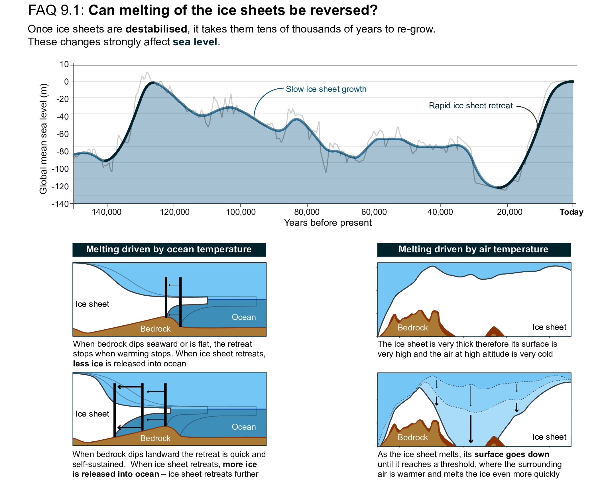
FAQ 9.1, Figure 1 | Ice sheets growth and decay. (Top) Changes in ice-sheet volume modulate sea level variations. The grey line depicts data from a range of physical environmental sea level recorders such as coral reefs while the blue line is a smoothed version of it. (Bottom left) Example of destabilization mechanism in Antarctica. (Bottom right) Example of destabilization mechanism in Greenland.
FAQ 9.2 | How Much Will Sea Level Rise in the Next Few Decades?
As of 2018, global average sea level was about 15–25 cm higher than in 1900, and 7–15 cm higher than in 1971. Sea level will continue to rise by an additional 10–25 cm by 2050. The major reasons for this ongoing rise in sea level are the thermal expansion of seawater as its temperature increases, and the melting of glaciers and ice sheets. Local sea level changes can be larger or smaller than the global average, with the smallest changes in formerly glaciated areas, and the largest changes in low-lying river delta regions.
Across the globe, sea level is rising, and the rate of increase has accelerated. Sea level increased by about 4 mm per year from 2006 to 2018, which was more than double the average rate over the 20th century. Rise during the early 1900s was due to natural factors, such as glaciers catching up to warming that occurred in the Northern Hemisphere during the 1800s. However, since at least 1970, human activities have been the dominant cause of global average sea level rise, and they will continue to be for centuries into the future.
Sea level rises either through warming of ocean waters or the addition of water from melting ice and bodies of water on land. Expansion due to warming caused about 50% of the rise observed from 1971 to 2018. Melting glaciers contributed about 22% over the same period. Melting of the two large ice sheets in Greenland and Antarctica has contributed about 13% and 7%, respectively, during 1971 to 2018, but melting has accelerated in the recent decades, increasing their contribution to 22% and 14% since 2016. Another source is changes in land-water storage: reservoirs and aquifers on land have reduced, which contributed about an 8% increase in sea level.
By 2050, sea level is expected to rise an additional 10–25 cm whether or not greenhouse gas emissions are reduced (FAQ 9.2, Figure 1). Beyond 2050, the amount by which sea level will rise is more uncertain. The accumulated total emissions of greenhouse gases over the upcoming decades will play a big role beyond 2050, especially in determining where sea level rise and ice-sheet changes eventually level off.
Even if net zero emissions are reached, sea level rise will continue because the deep ocean will continue to warm and ice sheets will take time to catch up to the warming caused by past and present emissions: ocean and ice sheets are slow to respond to environmental changes (see FAQ 5.3). Some projections under low emissions show sea level rise continuing as net zero is approached at a rate comparable to today (3–8 mm per year by 2100 versus 3–4 mm per year in 2015), while others show substantial acceleration to more than five times the present rate by 2100, especially if emissions continue to be high and processes that accelerate retreat of the Antarctic Ice Sheet occur widely (FAQ 9.1).
Sea level rise will increase the frequency and severity of extreme sea level events at coasts (see FAQ 8.2), such as storm surges, wave inundation and tidal floods: risk can be increased by even small changes in global average sea level. Scientists project that, in some regions, extreme sea level events that were recently expected once in 100 years will occur annually at 20–25% of locations by 2050 regardless of emissions, but by 2100 emissions choice will matter: annually at 60% of locations for low emissions, and at 80% of locations under strong emissions.
In many places, local sea level change will be larger or smaller than the global average. From year to year and place to place, changes in ocean circulation and wind can lead to local sea level change. In regions where large ice sheets, such as the Fennoscandian in Eurasia and the Laurentide and Cordilleran in North America, covered the land during the last ice age, the land is still slowly rising up now that the extra weight of the ice sheets is gone. This local recovery is compensating for global sea level rise in these regions and can even lead to local decrease in sea level. In regions just beyond where the former ice sheets reached and the Earth bulged upwards, the land is now falling and, as a result, local sea level rise is faster than the global rate. In many regions within low-lying delta regions (such as New Orleans and the Ganges–Brahmaputra delta), the land is rapidly subsiding (sinking) because of human activities such as building dams or groundwater and fossil fuel extraction. Further, when an ice sheet melts, it has less gravitational pull on the ocean water nearby. This reduction in gravitational attraction causes sea level to fall close to the (now less-massive) ice sheet while causing sea level to rise farther away. Melt from a polar ice sheet therefore raises sea level most in the opposite hemisphere or in low latitudes – amounting to tens of centimetres difference in rise between regions by 2100.

FAQ 9.2, Figure 1 | Observed and projected global mean sea level rise and the contributions from its major constituents.
FAQ 9.3 | Will the Gulf Stream Shut Down?
The Gulf Stream is part of two circulation patterns in the North Atlantic: the Atlantic Meridional Overturning Circulation (AMOC) and the North Atlantic subtropical gyre. Based on models and theory, scientific studies indicate that, while the AMOC is expected to slow in a warming climate, the Gulf Stream will not change much and would not shut down totally, even if the AMOC did. Most climate models project that the AMOC slows in the later 21st century under most emissions scenarios, with some models showing it slowing even sooner. The Gulf Stream affects the weather and sea level, so if it slows, North America will see higher sea levels and Europe’s weather and rate of relative warming will be affected.
The Gulf Stream is the biggest current in the North Atlantic Ocean. It transports about 30 billion kilograms of water per second northward past points on the east coast of North America. It is a warm current, with temperatures 5°C to 15°C warmer than surrounding waters, so it carries warmer water (thermal energy) from its southern origins and releases warmth to the atmosphere and surrounding water.
The Gulf Stream is part of two major circulation patterns, the Atlantic Meridional Overturning Circulation (AMOC) and the North Atlantic Subtropical Gyre (FAQ 9.3, Figure 1). The rotation of the Earth causes the big currents in both circulations to stay on the western side of their basin, which in the Atlantic means the circulations combine to form the Gulf Stream. Other large currents contribute to gyres, such as the Kuroshio in the North Pacific and the East Australian Current in the South Pacific, but the Gulf Stream is special in its dual role. There is no comparable deep overturning circulation in the North Pacific to the AMOC, so the Kuroshio plays only one role as part of a gyre.
The gyres circulate surface waters and result primarily from winds driving the circulation. These winds are not expected to change much and so neither will the gyres, which means the gyre portion of the Gulf Stream and the Kuroshio will continue to transport thermal energy poleward from the equator much as they do now. The gyre contribution to the Gulf Stream is 2 to 10 times larger than the AMOC contribution.
The Gulf Stream’s role in the AMOC is supplying surface source water that cools, becomes denser and sinks to form cold, deep waters that travel back equatorward, spilling over features on the ocean floor and mixing with other deep Atlantic waters to form a southward current at a depth of about 1500 metres beneath the Gulf Stream. This overturning flow is the AMOC, with the Gulf Stream in the upper kilometre flowing northward, and the colder deep water flowing southward.
The AMOC is expected to slow over the coming centuries. One reason why is freshening of the ocean waters: by meltwater from Greenland, changing Arctic sea ice, and increased precipitation over warmer northern seas. An array of moorings across the Atlantic has been monitoring the AMOC since 2004, with recently expanded capabilities. The monitoring of the AMOC has not been long enough for a trend to emerge from variability and detect long-term changes that may be underway (see FAQ 1.2). Other indirect signs may indicate slowing overturning – for example, slower warming where the Gulf Stream’s surface waters sink. Climate models show that this ‘cold spot’ of slower-than-average warming occurs as the AMOC weakens, and they project that this will continue. Paleoclimate evidence indicates that the AMOC changed significantly in the past, especially during transitions from colder climates to warmer ones, but that it has been stable for 8000 years.
What happens if the AMOC slows in a warming world? The atmosphere adjusts somewhat by carrying more heat, compensating partly for the decreases in heat carried by AMOC. But the ‘cold spot’ makes parts of Europe warm more slowly. Models indicate that weather patterns in Greenland and around the Atlantic will be affected, with reduced precipitation in the mid-latitudes, changing strong precipitation patterns in the tropics and Europe, and stronger storms in the North Atlantic storm track. The slowing of this current combined with the rotation of the Earth means that sea level along North America rises as the AMOC contribution to the Gulf Stream slows.
The North Atlantic is not the only site of sensitive meridional overturning. Around Antarctica, the world’s densest seawater is formed by freezing into sea ice, leaving behind salty, cold water that sinks to the bottom and spreads northward. Recent studies show that melting of the Antarctic Ice Sheet and changing winds over the Southern Ocean can affect this southern meridional overturning, affecting regional weather.

FAQ 9.3, Figure 1 | Horizontal (gyre) and vertical (Atlantic Meridional Overturning Circulation, AMOC) circulations in the Atlantic today (left) and in a warmer world (right). The Gulf Stream is a warm current composed of both circulations.
References
Aas, K.S., K. Gisnås, S. Westermann, and T.K. Berntsen, 2017: A Tiling Approach to Represent Subgrid Snow Variability in Coupled Land Surface–Atmosphere Models. Journal of Hydrometeorology, 18(1), 49–63, doi: 10.1175/jhm-d-16-0026.1.
Abich, K. et al., 2019: In-Orbit Performance of the GRACE Follow-on Laser Ranging Interferometer. Physical Review Letters, 123(3), 031101, doi: 10.1103/physrevlett.123.031101.
Abrahamsen, E.P. et al., 2019: Stabilization of dense Antarctic water supply to the Atlantic Ocean overturning circulation. Nature Climate Change, 9(10), 742–746, doi: 10.1038/s41558-019-0561-2.
Abram, N. et al., 2019: Framing and Context of the Report. In: IPCC Special Report on the Ocean and Cryosphere in a Changing Climate[Pörtner, H.-O., D.C. Roberts, V. Masson-Delmotte, P. Zhai, M. Tignor, E. Poloczanska, K. Mintenbeck, A. Alegría, M. Nicolai, A. Okem, J. Petzold, B. Rama, and N.M. Weyer (eds.)]. In Press, pp. 73–129, www.ipcc.ch/srocc/chapter/chapter-1-framing-and-context-of-the-report .
Aðalgeirsdóttir, G. et al., 2020: Glacier changes in Iceland from ~1890 to 2019. Frontiers in Earth Science, 8, 520, doi: 10.3389/feart.2020.523646.
Adler, R.F. et al., 2003: The Version-2 Global Precipitation Climatology Project (GPCP) Monthly Precipitation Analysis (1979–Present). Journal of Hydrometeorology, 4(6), 1147–1167, doi: 10.1175/1525-7541(2003)004<1147:tvgpcp>2.0.co;2.
Adusumilli, S., H.A. Fricker, B. Medley, L. Padman, and M.R. Siegfried, 2020: Interannual variations in meltwater input to the Southern Ocean from Antarctic ice shelves. Nature Geoscience, 13, 616–620, doi: 10.1038/s41561-020-0616-z.
Aguirre, C., M. Rojas, R.D. Garreaud, and D.A. Rahn, 2019: Role of synoptic activity on projected changes in upwelling-favourable winds at the ocean’s eastern boundaries. npj Climate and Atmospheric Science, 2(1), 44, doi: 10.1038/s41612-019-0101-9.
Aguirre, F. et al., 2018: Snow Cover Change as a Climate Indicator in Brunswick Peninsula, Patagonia. Frontiers in Earth Science, 6, 130, doi: 10.3389/feart.2018.00130.
Aksenov, Y. et al., 2016: Arctic pathways of Pacific Water: Arctic Ocean Model Intercomparison experiments. Journal of Geophysical Research: Oceans, 121(1), 27–59, doi: 10.1002/2015jc011299.
Alberello, A. et al., 2020: Drift of Pancake Ice Floes in the Winter Antarctic Marginal Ice Zone During Polar Cyclones. Journal of Geophysical Research: Oceans, 125(3), e2019JC015418, doi: 10.1029/2019jc015418.
Albrecht, T., R. Winkelmann, and A. Levermann, 2020: Glacial-cycle simulations of the Antarctic Ice Sheet with the Parallel Ice Sheet Model (PISM) – Part 1: Boundary conditions and climatic forcing. Cryosphere, 14(2), 599–632, doi: 10.5194/tc-14-599-2020.
Alekseeva, T. et al., 2019: Comparison of Arctic Sea Ice Concentrations from the NASA Team, ASI, and VASIA2 Algorithms with Summer and Winter Ship Data. Remote Sensing, 11(21), 2481, doi: 10.3390/rs11212481.
Alexander, P.M. et al., 2019: Simulated Greenland Surface Mass Balance in the GISS ModelE2 GCM: Role of the Ice Sheet Surface. Journal of Geophysical Research: Earth Surface, 124(3), 750–765, doi: 10.1029/2018jf004772.
Allen, S.E. and X. Durrieu de Madron, 2009: A review of the role of submarine canyons in deep-ocean exchange with the shelf. Ocean Science, 5(4), 607–620, doi: 10.5194/os-5-607-2009.
Alley, K.E., T.A. Scambos, M.R. Siegfried, and H.A. Fricker, 2016: Impacts of warm water on Antarctic ice shelf stability through basal channel formation. Nature Geoscience, 9(4), 290–293, doi: 10.1038/ngeo2675.
Alvarez-Solas, J., R. Banderas, A. Robinson, and M. Montoya, 2019: Ocean-driven millennial-scale variability of the Eurasian ice sheet during the last glacial period simulated with a hybrid ice-sheet–shelf model. Climate of the Past, 15(3), 957–979, doi: 10.5194/cp-15-957-2019.
An, L., E. Rignot, R. Millan, K. Tinto, and J. Willis, 2019a: Bathymetry of Northwest Greenland Using “Ocean Melting Greenland” (OMG) High-Resolution Airborne Gravity and Other Data. Remote Sensing, 11(2), 131, doi: 10.3390/rs11020131.
An, L. et al., 2019b: Bathymetry of Southeast Greenland From Oceans Melting Greenland (OMG) Data. Geophysical Research Letters, 46(20), 11197–11205, doi: 10.1029/2019gl083953.
An, L. et al., 2021: Ocean melting of the Zachariae Isstrøm and Nioghalvfjerdsfjorden glaciers, northeast Greenland. Proceedings of the National Academy of Sciences, 118(2), e2015483118, doi: 10.1073/pnas.2015483118.
Anderson, B. and A. Mackintosh, 2012: Controls on mass balance sensitivity of maritime glaciers in the Southern Alps, New Zealand: The role of debris cover. Journal of Geophysical Research: Earth Surface, 117(F1), F01003, doi: 10.1029/2011jf002064.
Anderson, J.B., S.S. Shipp, A.L. Lowe, J.S. Wellner, and A.B. Mosola, 2002: The Antarctic Ice Sheet during the Last Glacial Maximum and its subsequent retreat history: A review. Quaternary Science Reviews, 21(1–3), 49–70, doi: 10.1016/s0277-3791(01)00083-x.
Andreassen, L.M., H. Elvehøy, B. Kjøllmoen, and J.M.C. Belart, 2020: Glacier change in Norway since the 1960s – an overview of mass balance, area, length and surface elevation changes. Journal of Glaciology, 66(256), 313–328, doi: 10.1017/jog.2020.10.
Andresen, C.S. et al., 2017: Exceptional 20th century glaciological regime of a major SE Greenland outlet glacier. Scientific Reports, 7(1), 13626, doi: 10.1038/s41598-017-13246-x.
Anttila, K., T. Manninen, E. Jääskeläinen, A. Riihelä, and P. Lahtinen, 2018: The role of climate and land use in the changes in surface albedo prior to snow melt and the timing of melt season of seasonal snow in northern land areas of 40°N–80°N during 1982–2015. Remote Sensing, 10(10), doi: 10.3390/rs10101619.
Aoki, S. et al., 2020: Freshening of Antarctic Bottom Water off Cape Darnley, East Antarctica. Journal of Geophysical Research: Oceans, 125, e2020JC016374, doi: 10.1029/2020jc016374.
Applegate, P.J. and K. Keller, 2015: How effective is albedo modification (solar radiation management geoengineering) in preventing sea-level rise from the Greenland Ice Sheet?Environmental Research Letters, 10(8), 84018, doi: 10.1088/1748-9326/10/8/084018.
Argus, D.F. and W.R. Peltier, 2010: Constraining models of postglacial rebound using space geodesy: A detailed assessment of model ICE-5G (VM2) and its relatives. Geophysical Journal International, 181(2), 697–723, doi: 10.1111/j.1365-246x.2010.04562.x.
Argus, D.F., W.R. Peltier, R. Drummond, and A.W. Moore, 2014: The Antarctica component of postglacial rebound model ICE-6G_C (VM5a) based on GPS positioning, exposure age dating of ice thicknesses, and relative sea level histories. Geophysical Journal International, 198(1), 537–563, doi: 10.1093/gji/ggu140.
Armitage, T.W.K., R. Kwok, A.F. Thompson, and G. Cunningham, 2018: Dynamic Topography and Sea Level Anomalies of the Southern Ocean: Variability and Teleconnections. Journal of Geophysical Research: Oceans, 123(1), 613–630, doi: 10.1002/2017jc013534.
Armitage, T.W.K. et al., 2017: Arctic Ocean surface geostrophic circulation 2003–2014. The Cryosphere, 11(4), 1767–1780, doi: 10.5194/tc-11-1767-2017.
Armour, K.C., I. Eisenman, E. Blanchard-Wrigglesworth, K.E. McCusker, and C.M. Bitz, 2011: The reversibility of sea ice loss in a state-of-the-art climate model. Geophysical Research Letters, 38(16), L16705, doi: 10.1029/2011gl048739.
Armour, K.C., J. Marshall, J.R. Scott, A. Donohoe, and E.R. Newsom, 2016: Southern Ocean warming delayed by circumpolar upwelling and equatorward transport. Nature Geoscience, 9, 549, doi: 10.1038/ngeo2731.
Arndt, S., M. Hoppmann, H. Schmithüsen, A.D. Fraser, and M. Nicolaus, 2020: Seasonal and interannual variability of landfast sea ice in Atka Bay, Weddell Sea, Antarctica. The Cryosphere, 14(9), 2775–2793, doi: 10.5194/tc-14-2775-2020.
Arns, A., T. Wahl, I.D. Haigh, and J. Jensen, 2015: Determining return water levels at ungauged coastal sites: A case study for northern Germany. Ocean Dynamics, 65(4), 539–554, doi: 10.1007/s10236-015-0814-1.
Arns, A. et al., 2017: Sea-level rise induced amplification of coastal protection design heights. Scientific reports, 7(1), 40171, doi: 10.1038/srep40171.
Arns, A. et al., 2020: Non-linear interaction modulates global extreme sea levels, coastal flood exposure, and impacts. Nature Communications, 11(1), 1–9, doi: 10.1038/s41467-020-15752-5.
Asay-Davis, X.S., N.C. Jourdain, and Y. Nakayama, 2017: Developments in Simulating and Parameterizing Interactions Between the Southern Ocean and the Antarctic Ice Sheet. Current Climate Change Reports, 3(4), 316–329, doi: 10.1007/s40641-017-0071-0.
Asay-Davis, X.S. et al., 2016: Experimental design for three interrelated marine ice sheet and ocean model intercomparison projects: MISMIP v. 3 (MISMIP +), ISOMIP v. 2 (ISOMIP +) and MISOMIP v. 1 (MISOMIP1). Geoscientific Model Development, 9(7), 2471–2497, doi: 10.5194/gmd-9-2471-2016.
Aschwanden, A., M.A. Fahnestock, and M. Truffer, 2016: Complex Greenland outlet glacier flow captured. Nature Communications, 7, 10524, doi: 10.1038/ncomms10524.
Aschwanden, A. et al., 2019: Contribution of the Greenland Ice Sheet to sea level over the next millennium. Science Advances, 5(6), eaav9396, doi: 10.1126/sciadv.aav9396.
Atwood, A.R., E. Wu, D.M.W. Frierson, D.S. Battisti, and J.P. Sachs, 2016: Quantifying Climate Forcings and Feedbacks over the Last Millennium in the CMIP5–PMIP3 Models. Journal of Climate, 29(3), 1161–1178, doi: 10.1175/jcli-d-15-0063.1.
Auger, M., R. Morrow, E. Kestenare, J.-B. Sallée, and R. Cowley, 2021: Southern Ocean in-situ temperature trends over 25 years emerge from interannual variability. Nature Communications, 12(1), 514, doi: 10.1038/s41467-020-20781-1.
Auriac, A. et al., 2016: Glacial isostatic adjustment associated with the Barents Sea ice sheet: A modelling inter-comparison. Quaternary Science Reviews, 147, 122–135, doi: 10.1016/j.quascirev.2016.02.011.
Axford, Y. et al., 2019: Holocene temperature history of northwest Greenland – With new ice cap constraints and chironomid assemblages from Deltasø. Quaternary Science Reviews, 215, 160–172, doi: 10.1016/j.quascirev.2019.05.011.
Bachem, P.E., B. Risebrobakken, S. De Schepper, and E.L. Mcclymont, 2017: Highly variable Pliocene sea surface conditions in the Norwegian Sea. Climate of the Past, 13(9), 1153–1168, doi: 10.5194/cp-13-1153-2017.
Baggenstos, D. et al., 2019: Earth’s radiative imbalance from the Last Glacial Maximum to the present. Proceedings of the National Academy of Sciences, 116(30), 14881–14886, doi: 10.1073/pnas.1905447116.
Bakker, A.M.R., T.E. Wong, K.L. Ruckert, and K. Keller, 2017: Sea-level projections representing the deeply uncertain contribution of the West Antarctic ice sheet. Scientific Reports, 7(1), 3880, doi: 10.1038/s41598-017-04134-5.
Bakun, A., 1990: Global climate change and intensification of coastal ocean upwelling. Science, 247(4939), 198–201, www.jstor.org/stable/2873492.
Bakun, A., D.B. Field, A. Redondo-Rodriguez, and S.J. Weeks, 2010: Greenhouse gas, upwelling-favorable winds, and the future of coastal ocean upwelling ecosystems. Global Change Biology, 16(4), 1213–1228, doi: 10.1111/j.1365-2486.2009.02094.x.
Bamber, J.L. and W.P. Aspinall, 2013: An expert judgement assessment of future sea level rise from the ice sheets. Nature Climate Change, 3, 424–427, doi: 10.1038/nclimate1778.
Bamber, J.L. and G.J. Dawson, 2020: Complex evolving patterns of mass loss from Antarctica’s largest glacier. Nature Geoscience, 13(2), 127–131, doi: 10.1038/s41561-019-0527-z.
Bamber, J.L., R.E.M. Riva, B.L.A. Vermeersen, and A.M. LeBrocq, 2009: Reassessment of the Potential Sea-Level Rise from a Collapse of the West Antarctic Ice Sheet. Science, 324(5929), 901–903, doi: 10.1126/science.1169335.
Bamber, J.L., R.M. Westaway, B. Marzeion, and B. Wouters, 2018a: A new synthesis of annual land ice mass trends 1992 to 2016. PANGAEA. Retrieved from: https://doi.org/10.1594/pangaea.890030.
Bamber, J.L., R.M. Westaway, B. Marzeion, and B. Wouters, 2018b: The land ice contribution to sea level during the satellite era. Environmental Research Letters, 13, 063008, doi: 10.1088/1748-9326/aac2f0.
Bamber, J.L., M. Oppenheimer, R.E. Kopp, W.P. Aspinall, and R.M. Cooke, 2019: Ice sheet contributions to future sea-level rise from structured expert judgment. Proceedings of the National Academy of Sciences, 116(23), 11195–11200, doi: 10.1073/pnas.1817205116.
Banas, N.S., P. MacCready, and B.M. Hickey, 2009: The Columbia River plume as cross-shelf exporter and along-coast barrier. Continental Shelf Research, 29(1), 292–301, doi: 10.1016/j.csr.2008.03.011.
Baranes, H.E. et al., 2020: Tidally Driven Interannual Variation in Extreme Sea Level Frequencies in the Gulf of Maine. Journal of Geophysical Research: Oceans, 125(10), e2020JC016291, doi: 10.1029/2020jc016291.
Barletta, V.R. et al., 2018: Observed rapid bedrock uplift in Amundsen Sea Embayment promotes ice-sheet stability. Science, 360(6395), 1335–1339, doi: 10.1126/science.aao1447.
Bart, P.J., M. DeCesare, B.E. Rosenheim, W. Majewski, and A. McGlannan, 2018: A centuries-long delay between a paleo-ice-shelf collapse and grounding-line retreat in the Whales Deep Basin, eastern Ross Sea, Antarctica. Scientific Reports, 12392, doi: 10.1038/s41598-018-29911-8.
Barthel, A. et al., 2020: CMIP5 model selection for ISMIP6 ice sheet model forcing: Greenland and Antarctica. The Cryosphere, 14, 855–879, doi: 10.5194/tc-14-855-2020.
Bassis, J.N. and L. Ultee, 2019: A Thin Film Viscoplastic Theory for Calving Glaciers: Toward a Bound on the Calving Rate of Glaciers. Journal of Geophysical Research: Earth Surface, 124(8), 2036–2055, doi: 10.1029/2019jf005160.
Batbaatar, J., A. Gillespie, D. Fink, A. Matmon, and T. Fujioka, 2018: Asynchronous glaciations in arid continental climate. Quaternary Science Reviews, 182, 1–19, doi: 10.1016/j.quascirev.2017.12.001.
Batchelor, C.J. et al., 2019: Distinct Permafrost Conditions Across the Last Two Glacial Periods in Midlatitude North America. Geophysical Research Letters, 46, 13318–13326, doi: 10.1029/2019gl083951.
Bates, S.C. et al., 2012: Mean Biases, Variability, and Trends in Air–Sea Fluxes and Sea Surface Temperature in the CCSM4. Journal of Climate, 25(22), 7781–7801, doi: 10.1175/jcli-d-11-00442.1.
Bathiany, S., J. Hidding, and M. Scheffer, 2020: Edge Detection Reveals Abrupt and Extreme Climate Events. Journal of Climate, 33(15), 6399–6421, doi: 10.1175/jcli-d-19-0449.1.
Bathiany, S., D. Notz, T. Mauritsen, G. Raedel, and V. Brovkin, 2016: On the Potential for Abrupt Arctic Winter Sea Ice Loss. Journal of Climate, 29(7), 2703–2719, doi: 10.1175/jcli-d-15-0466.1.
Baum, S.K. and T.J. Crowley, 2003: The snow/ice instability as a mechanism for rapid climate change: A Neoproterozoic Snowball Earth model example. Geophysical Research Letters, 30(20), 2030, doi: 10.1029/2003gl017333.
Bauska, T.K. et al., 2016: Carbon isotopes characterize rapid changes in atmospheric carbon dioxide during the last deglaciation. Proceedings of the National Academy of Sciences, 113(13), 3465–3470, doi: 10.1073/pnas.1513868113.
Beadling, R.L., J.L. Russell, R.J. Stouffer, P.J. Goodman, and M. Mazloff, 2019: Assessing the quality of Southern Ocean circulation in CMIP5 AOGCM and Earth System Model simulations. Journal of Climate, 32, 5915–5940, doi: 10.1175/jcli-d-19-0263.1.
Beadling, R.L. et al., 2020: Representation of Southern Ocean properties across Coupled Model Intercomparison Project generations: CMIP3 to CMIP6. Journal of Climate, 33, 6555–6581, doi: 10.1175/jcli-d-19-0970.1.
Beal, L.M. and S. Elipot, 2016: Broadening not strengthening of the Agulhas Current since the early 1990s. Nature, 540(7634), 570–573, doi: 10.1038/nature19853.
Beckmann, J. et al., 2019: Modeling the response of Greenland outlet glaciers to global warming using a coupled flowline-plume model. The Cryosphere, 13, 2281–2301, doi: 10.5194/tc-2018-89.
Beedle, M.J., B. Menounos, B.H. Luckman, and R. Wheate, 2009: Annual push moraines as climate proxy. Geophysical Research Letters, 36(20), L20501, doi: 10.1029/2009gl039533.
Belcher, S.E. et al., 2012: A global perspective on Langmuir turbulence in the ocean surface boundary layer. Geophysical Research Letters, 39(18), L18605, doi: 10.1029/2012gl052932.
Bell, R.E., A.F. Banwell, L.D. Trusel, and J. Kingslake, 2018: Antarctic surface hydrology and impacts on ice-sheet mass balance. Nature Climate Change, 8(12), 1044–1052, doi: 10.1038/s41558-018-0326-3.
Bellomo, K., L.N. Murphy, M.A. Cane, A.C. Clement, and L.M. Polvani, 2018: Historical forcings as main drivers of the Atlantic multidecadal variability in the CESM large ensemble. Climate Dynamics, 50(9–10), 3687–3698, doi: 10.1007/s00382-017-3834-3.
Belmadani, A., V. Echevin, F. Codron, K. Takahashi, and C. Junquas, 2014: What dynamics drive future wind scenarios for coastal upwelling off Peru and Chile?Climate dynamics, 43(7–8), 1893–1914.
Belmecheri, S., F. Babst, E.R. Wahl, D.W. Stahle, and V. Trouet, 2016: Multi-century evaluation of Sierra Nevada snowpack. Nature Climate Change, 6, 2–3, doi: 10.1038/nclimate2809.
Belt, S.T., 2018: Source-specific biomarkers as proxies for Arctic and Antarctic sea ice. Organic Geochemistry, 125, 277–298, doi: 10.1016/j.orggeochem.2018.10.002.
Belt, S.T., 2019: What do IP25 and related biomarkers really reveal about sea ice change?Quaternary Science Reviews, 204, 216–219, doi: 10.1016/j.quascirev.2018.11.025.
Belt, S.T. et al., 2007: A novel chemical fossil of palaeo sea ice: IP25. Organic Geochemistry, 38(1), 16–27, doi: 10.1016/j.orggeochem.2006.09.013.
Belt, S.T. et al., 2015: Identification of paleo Arctic winter sea ice limits and the marginal ice zone: Optimised biomarker-based reconstructions of late Quaternary Arctic sea ice. Earth and Planetary Science Letters, 431, 127–139, doi: 10.1016/j.epsl.2015.09.020.
Bendtsen, J. et al., 2017: Sea ice breakup and marine melt of a retreating tidewater outlet glacier in northeast Greenland (81°N). Scientific Reports, 7(1), 1–11, doi: 10.1038/s41598-017-05089-3.
Benn, D.I., T. Cowton, J. Todd, and A. Luckman, 2017: Glacier Calving in Greenland. Current Climate Change Reports, 3(4), 282–290, doi: 10.1007/s40641-017-0070-1.
Bennartz, R. et al., 2013: July 2012 Greenland melt extent enhanced by low-level liquid clouds. Nature, 496, 83–86, doi: 10.1038/nature12002.
Bennetts, L.G., S. O’Farrell, and P. Uotila, 2017: Brief communication: Impacts of ocean-wave-induced breakup of Antarctic sea ice via thermodynamics in a stand-alone Version of the CICE sea-ice model. The Cryosphere, 11(3), 1035–1040, doi: 10.5194/tc-11-1035-2017.
Bentamy, A. et al., 2017: Review and assessment of latent and sensible heat flux accuracy over the global oceans. Remote Sensing of Environment, 201, 196–218, doi: 10.1016/j.rse.2017.08.016.
Bentley, M.J. et al., 2014: A community-based geological reconstruction of Antarctic Ice Sheet deglaciation since the Last Glacial Maximum. Quaternary Science Reviews, 100, 1–9, doi: 10.1016/j.quascirev.2014.06.025.
Benz, V., O. Esper, R. Gersonde, F. Lamy, and R. Tiedemann, 2016: Last Glacial Maximum sea surface temperature and sea-ice extent in the Pacific sector of the Southern Ocean. Quaternary Science Reviews, 146, 216–237, doi: 10.1016/j.quascirev.2016.06.006.
Berben, S.M.P., K. Husum, A. Navarro-Rodriguez, S.T. Belt, and S. Aagaard-Sørensen, 2017: Semi-quantitative reconstruction of early to late Holocene spring and summer sea ice conditions in the northern Barents Sea. Journal of Quaternary Science, 32(5), 587–603, doi: 10.1002/jqs.2953.
Bereiter, B., S. Shackleton, D. Baggenstos, K. Kawamura, and J. Severinghaus, 2018: Mean global ocean temperatures during the last glacial transition. Nature, 553(7686), 39–44, doi: 10.1038/nature25152.
Berends, C.J., B. de Boer, A.M. Dolan, D.J. Hill, and R.S.W. van de Wal, 2019: Modelling ice sheet evolution and atmospheric CO2 during the Late Pliocene. Climate of the Past, 15, 1603–1619, doi: 10.5194/cp-2019-34.
Berloff, P. et al., 2007: The Turbulent Oscillator: A Mechanism of Low-Frequency Variability of the Wind-Driven Ocean Gyres. Journal of Physical Oceanography, 37(9), 2363–2386, doi: 10.1175/jpo3118.1.
Bertram, R.A. et al., 2018: Pliocene deglacial event timelines and the biogeochemical response offshore Wilkes Subglacial Basin, East Antarctica. Earth and Planetary Science Letters, 494, 109–116, doi: 10.1016/j.epsl.2018.04.054.
Bettencourt, J.H. et al., 2015: Boundaries of the Peruvian oxygen minimum zone shaped by coherent mesoscale dynamics. Nature Geoscience, 8(12), 937–940, doi: 10.1038/ngeo2570.
Bevacqua, E. et al., 2020: More meteorological events that drive compound coastal flooding are projected under climate change. Communications Earth & Environment, 1(1), 47, doi: 10.1038/s43247-020-00044-z.
Bevan, S.L., A.J. Luckman, D.I. Benn, T. Cowton, and J. Todd, 2019: Impact of warming shelf waters on ice mélange and terminus retreat at a large SE Greenland glacier. Cryosphere, 13(9), 2303–2315, doi: 10.5194/tc-13-2303-2019.
Bevis, M. et al., 2019: Accelerating changes in ice mass within Greenland, and the ice sheet’s sensitivity to atmospheric forcing. Proceedings of the National Academy of Sciences, 116(6), 1934–1939, doi: 10.1073/pnas.1806562116.
Bianchi, C. and R. Gersonde, 2002: The Southern Ocean surface between Marine Isotope Stages 6 and 5d: Shape and timing of climate changes. Palaeogeography, Palaeoclimatology, Palaeoecology, 187(1–2), 151–177, doi: 10.1016/s0031-0182(02)00516-3.
Biastoch, A. et al., 2015: Atlantic multi-decadal oscillation covaries with Agulhas leakage. Nature Communications, 6(1), 10082, doi: 10.1038/ncomms10082.
Bilbao, R.A.F., J.M. Gregory, and N. Bouttes, 2015: Analysis of the regional pattern of sea level change due to ocean dynamics and density change for 1993–2099 in observations and CMIP5 AOGCMs. Climate Dynamics, 45( 9–10), 2647–2666, doi: 10.1007/s00382-015-2499-z.
Bilbao, R.A.F., J.M. Gregory, N. Bouttes, M.D. Palmer, and P. Stott, 2019: Attribution of ocean temperature change to anthropogenic and natural forcings using the temporal, vertical and geographical structure. Climate Dynamics, 53(9), 5389–5413, doi: 10.1007/s00382-019-04910-1.
Bindoff, N.L. and T.J. McDougall, 2000: Decadal Changes along an Indian Ocean Section at 32°S and Their Interpretation. Journal of Physical Oceanography, 30(6), 1207–1222, doi: 10.1175/1520-0485(2000)030<1207:dcaaio>2.0.co;2.
Bindoff, N.L. et al., 2013: Detection and Attribution of Climate Change: from Global to Regional. In: Climate Change 2013: The Physical Science Basis. Contribution of Working Group I to the Fifth Assessment Report of the Intergovernmental Panel on Climate Change[Stocker, T.F., D. Qin, G.-K. Plattner, M. Tignor, S.K. Allen, J. Boschung, A. Nauels, Y. Xia, V. Bex, and P.M. Midgley (eds.)]. Cambridge University Press, pp. 867–952, doi: 10.1017/cbo9781107415324.022.
Bindoff, N.L. et al., 2019: Changing Ocean, Marine Ecosystems, and Dependent Communities. In: IPCC Special Report on the Ocean and Cryosphere in a Changing Climate[Pörtner, H.-O., D.C. Roberts, V. Masson-Delmotte, P. Zhai, M. Tignor, E. Poloczanska, K. Mintenbeck, M. Nicolai, A. Okem, J. Petzold, B. Rama, and N. Weyer (eds.)]. In Press, pp. 447–588, www.ipcc.ch/srocc/chapter/chapter-5.
Bindschadler, R.A. et al., 2013: Ice-sheet model sensitivities to environmental forcing and their use in projecting future sea level (the SeaRISE project). Journal of Glaciology, 59(214), 195–224, doi: 10.3189/2013jog12j125.
Bishop, S.P. et al., 2017: Scale Dependence of Midlatitude Air–Sea Interaction. Journal of Climate, 30(20), 8207–8221, doi: 10.1175/jcli-d-17-0159.1.
Biskaborn, B.K. et al., 2019: Permafrost is warming at a global scale. Nature Communications, 10(1), 264, doi: 10.1038/s41467-018-08240-4.
Bittermann, K., S. Rahmstorf, R.E. Kopp, and A.C. Kemp, 2017: Global mean sea-level rise in a world agreed upon in Paris. Environmental Research Letters, 12(12), 124010, doi: 10.1088/1748-9326/aa9def .
Blackburn, T. et al., 2020: Ice retreat in Wilkes Basin of East Antarctica during a warm interglacial. Nature, 583(7817), 554–559, doi: 10.1038/s41586-020-2484-5.
Blake-Mizen, K. et al., 2019: Southern Greenland glaciation and Western Boundary Undercurrent evolution recorded on Eirik Drift during the late Pliocene intensification of Northern Hemisphere glaciation. Quaternary Science Reviews, 209, 40–51, doi: 10.1016/j.quascirev.2019.01.015.
Bliss, A.C., J. Miller, and W. Meier, 2017: Comparison of Passive Microwave-Derived Early Melt Onset Records on Arctic Sea Ice. Remote Sensing, 9(3), 199, doi: 10.3390/rs9030199.
Bliss, A.C., M. Steele, G. Peng, W.N. Meier, and S. Dickinson, 2019: Regional variability of Arctic sea ice seasonal change climate indicators from a passive microwave climate data record. Environmental Research Letters, 14(4), 045003, doi: 10.1088/1748-9326/aafb84.
Bock, L. et al., 2020: Quantifying Progress Across Different CMIP Phases With the ESMValTool. Journal of Geophysical Research: Atmospheres, 125(21), e2019JD032321, doi: 10.1029/2019jd032321.
Bohleber, P., M. Schwikowski, M. Stocker-Waldhuber, L. Fang, and A. Fischer, 2020: New glacier evidence for ice-free summits during the life of the Tyrolean Iceman. Scientific Reports, 10(1), 20513, doi: 10.1038/s41598-020-77518-9.
Bond, N.A., M.F. Cronin, H. Freeland, and N. Mantua, 2015: Causes and impacts of the 2014 warm anomaly in the NE Pacific. Geophysical Research Letters, 42, 3414–3420, doi: 10.1002/2015gl063306.
Bondzio, J.H. et al., 2016: Modelling calving front dynamics using a level-set method: application to Jakobshavn Isbræ, West Greenland. The Cryosphere, 10(2), 497–510, doi: 10.5194/tc-10-497-2016.
Bondzio, J.H. et al., 2017: The mechanisms behind Jakobshavn Isbræ’s acceleration and mass loss: A 3-D thermomechanical model study. Geophysical Research Letters, 44(12), 6252–6260, doi: 10.1002/2017gl073309.
Bonekamp, P.N.J., R.J. de Kok, E. Collier, and W.W. Immerzeel, 2019: Contrasting Meteorological Drivers of the Glacier Mass Balance Between the Karakoram and Central Himalaya. Frontiers in Earth Science, 7, 107, doi: 10.3389/feart.2019.00107.
Boone, A. et al., 2017: The interactions between soil–biosphere–atmosphere land surface model with a multi-energy balance (ISBA-MEB) option in SURFEXv8 – Part 1: Model description. Geoscientific Model Development, 10(2), 843–872, doi: 10.5194/gmd-10-843-2017.
Borge, A.F., S. Westermann, I. Solheim, and B. Etzelmüller, 2017: Strong degradation of palsas and peat plateaus in northern Norway during the last 60 years. Cryosphere, 11(1), 1–16, doi: 10.5194/tc-11-1-2017.
Born, A. and K.H. Nisancioglu, 2012: Melting of Northern Greenland during the last interglaciation. The Cryosphere, 6, 1239–1250, doi: 10.5194/tc-6-1239-2012.
Born, A., T.F. Stocker, and A.B. Sandø, 2016: Transport of salt and freshwater in the Atlantic Subpolar Gyre. Ocean Dynamics, 66(9), 1051–1064, doi: 10.1007/s10236-016-0970-y.
Born, A., T.F. Stocker, C.C. Raible, and A. Levermann, 2013: Is the Atlantic subpolar gyre bistable in comprehensive coupled climate models?Climate Dynamics, 40(11–12), 2993–3007, doi: 10.1007/s00382-012-1525-7.
Boucher, O. et al., 2020: Presentation and Evaluation of the IPSL-CM6A-LR Climate Model. Journal of Advances in Modeling Earth Systems, 12(7), e2019MS002010, doi: 10.1029/2019ms002010.
Bouttes, N. and J.M. Gregory, 2014: Attribution of the spatial pattern of CO2-forced sea level change to ocean surface flux changes. Environmental Research Letters, 9(3), 034004, doi: 10.1088/1748-9326/9/3/034004.
Bouttes, N., J.M. Gregory, and J.A. Lowe, 2013: The reversibility of sea level rise. Journal of Climate, 26(8), 2502–2513, doi: 10.1175/jcli-d-12-00285.1.
Bouttes, N., J.M. Gregory, T. Kuhlbrodt, and R.S. Smith, 2014: The drivers of projected North Atlantic sea level change. Climate Dynamics, 43(5–6), 1531–1544, doi: 10.1007/s00382-013-1973-8.
Box, J.E. and W. Colgan, 2013: Greenland Ice Sheet Mass Balance Reconstruction. Part III: Marine Ice Loss and Total Mass Balance (1840–2010). Journal of Climate, 26(18), 6990–7002, doi: 10.1175/jcli-d-12-00546.1.
Bracegirdle, T. et al., 2020: Twenty-first century changes in Antarctic and Southern Ocean surface climate in CMIP6. Atmospheric Science Letters, 21(9), asl984, doi: 10.1002/asl.984.
Bradley, S.L., T.J. Reerink, R.S.W. Van De Wal, and M.M. Helsen, 2018: Simulation of the Greenland Ice Sheet over two glacial–interglacial cycles: investigating a sub-ice-shelf melt parameterization and relative sea level forcing in an ice-sheet-ice–shelf model. Climate of the Past, 14(5), 619–635, doi: 10.5194/cp-14-619-2018.
Brady, R.X., M.A. Alexander, N.S. Lovenduski, and R.R. Rykaczewski, 2017: Emergent anthropogenic trends in California Current upwelling. Geophysical Research Letters, 44(10), 5044–5052, doi: 10.1002/2017gl072945.
Brancato, V. et al., 2020: Grounding Line Retreat of Denman Glacier, East Antarctica, Measured With COSMO-SkyMed Radar Interferometry Data. Geophysical Research Letters, 47(7), e2019GL086291, doi: 10.1029/2019gl086291.
Brandon, C.M., J.D. Woodruff, D. Lane, and J.P. Donnelly, 2013: Tropical cyclone wind speed constraints from resultant storm surge deposition: A 2500 year reconstruction of hurricane activity from St. Marks, FL. Geochemistry, Geophysics, Geosystems, 14(8), 2993–3008, doi: 10.1002/ggge.20217.
Brandon, C.M., J.D. Woodruff, J.P. Donnelly, and R.M. Sullivan, 2015: How Unique was Hurricane Sandy? Sedimentary Reconstructions of Extreme Flooding from New York Harbor. Scientific Reports, 4(1), 7366, doi: 10.1038/srep07366.
Braun, M.H. et al., 2019: Constraining glacier elevation and mass changes in South America. Nature Climate Change, 9(2), 130–136, doi: 10.1038/s41558-018-0375-7.
Brendryen, J., H. Haflidason, Y. Yokoyama, K.A. Haaga, and B. Hannisdal, 2020: Eurasian Ice Sheet collapse was a major source of Meltwater Pulse 1A 14,600 years ago. Nature Geoscience, 13(5), 363–368, doi: 10.1038/s41561-020-0567-4.
Brennan, M.K., G.J. Hakim, and E. Blanchard-Wrigglesworth, 2020: Arctic Sea-Ice Variability During the Instrumental Era. Geophysical Research Letters, 47(7), e2019GL086843, doi: 10.1029/2019gl086843.
Briggs, R.D., D. Pollard, and L. Tarasov, 2014: A data-constrained large ensemble analysis of Antarctic evolution since the Eemian. Quaternary Science Reviews, 103, 91–115, doi: 10.1016/j.quascirev.2014.09.003.
Briner, J.P. et al., 2016: Holocene climate change in Arctic Canada and Greenland. Quaternary Science Reviews, 147, 340–364, doi: 10.1016/j.quascirev.2016.02.010.
Brink, K.H., 2016: Cross-shelf exchange. Annual review of marine science, 8, 59–78, doi: 10.1146/annurev-marine-010814-015717.
Brodeau, L., B. Barnier, S.K. Gulev, and C. Woods, 2017: Climatologically Significant Effects of Some Approximations in the Bulk Parameterizations of Turbulent Air–Sea Fluxes. Journal of Physical Oceanography, 47(1), 5–28, doi: 10.1175/jpo-d-16-0169.1.
Brönnimann, S. et al., 2019: Last phase of the Little Ice Age forced by volcanic eruptions. Nature Geoscience, 12(8), 650–656, doi: 10.1038/s41561-019-0402-y.
Bronselaer, B. and L. Zanna, 2020: Heat and carbon coupling reveals ocean warming due to circulation changes. Nature, 584, 227–233, doi: 10.1038/s41586-020-2573-5.
Bronselaer, B. et al., 2018: Change in future climate due to Antarctic meltwater. Nature, 564(7734), 53–58, doi: 10.1038/s41586-018-0712-z.
Bronselaer, B. et al., 2020: Importance of wind and meltwater for observed chemical and physical changes in the Southern Ocean. Nature Geoscience, 13(1), 35–42, doi: 10.1038/s41561-019-0502-8.
Brown, R.D. and D.A. Robinson, 2011: Northern Hemisphere spring snow cover variability and change over 1922–2010 including an assessment of uncertainty. The Cryosphere, 5(1), 219–229, doi: 10.5194/tc-5-219-2011.
Brown, R.D. and C. Derksen, 2013: Is Eurasian October snow cover extent increasing?Environmental Research Letters, 8(2), 024006, doi: 10.1088/1748-9326/8/2/024006.
Brown, R.D. et al., 2017: Arctic terrestrial snow cover. In: Snow, Water, Ice and Permafrost in the Arctic (SWIPA) 2017. Arctic Monitoring and Assessment Programme (AMAP), Oslo, Norway, pp. 25–64, www.amap.no/documents/doc/snow-water-ice-and-permafrost-in-the-arctic-swipa-2017/1610.
Brun, F. et al., 2016: Quantifying volume loss from ice cliffs on debris-covered glaciers using high-resolution terrestrial and aerial photogrammetry. Journal of Glaciology, 62(234), 684–695, doi: 10.1017/jog.2016.54.
Bryden, H.L. et al., 2020: Reduction in ocean heat transport at 26°N since 2008 cools the eastern subpolar gyre of the North Atlantic Ocean. Journal of Climate, 33(5), 1677–1689, doi: 10.1175/jcli-d-19-0323.1.
Buchanan, M.K., R.E. Kopp, M. Oppenheimer, and C. Tebaldi, 2016: Allowances for evolving coastal flood risk under uncertain local sea-level rise. Climatic Change, 137(3–4), 347–362, doi: 10.1007/s10584-016-1664-7.
Buckingham, C.E. et al., 2019: The Contribution of Surface and Submesoscale Processes to Turbulence in the Open Ocean Surface Boundary Layer. Journal of Advances in Modeling Earth Systems, 11(12), 4066–4094, doi: 10.1029/2019ms001801.
Buckley, M.W. and J. Marshall, 2016: Observations, inferences, and mechanisms of the Atlantic Meridional Overturning Circulation: A review. Reviews of Geophysics, 54(1), 5–63, doi: 10.1002/2015rg000493.
Bulthuis, K., M. Arnst, S. Sun, and F. Pattyn, 2019: Uncertainty quantification of the multi-centennial response of the Antarctic ice sheet to climate change. Cryosphere, 13, 1349–1380, doi: 10.5194/tc-13-1349-2019.
Bulygina, O.N., P.Y. Groisman, V.N. Razuvaev, and N.N. Korshunova, 2011: Changes in snow cover characteristics over Northern Eurasia since 1966. Environmental Research Letters, 6(4), 0452204, doi: 10.1088/1748-9326/6/4/045204.
Bunce, C., J.R. Carr, P.W. Nienow, N. Ross, and R. Killick, 2018: Ice front change of marine-terminating outlet glaciers in northwest and southeast Greenland during the 21st century. Journal of Glaciology, 64(246), 523–535, doi: 10.1017/jog.2018.44.
Bunce, C., P. Nienow, A. Sole, T. Cowton, and B. Davison, 2020: Influence of glacier runoff and near-terminus subglacial hydrology on frontal ablation at a large Greenlandic tidewater glacier. Journal of Glaciology, 1–10, doi: 10.1017/jog.2020.109.
Bunzel, F., D. Notz, and L.T. Pedersen, 2018: Retrievals of Arctic Sea-Ice Volume and Its Trend Significantly Affected by Interannual Snow Variability. Geophysical Research Letters, 45(21), 11751–11759, doi: 10.1029/2018gl078867.
Burgard, C. and D. Notz, 2017: Drivers of Arctic Ocean warming in CMIP5 models. Geophysical Research Letters, 44(9), 4263–4271, doi: 10.1002/2016gl072342.
Burgess, D.O. and M.J. Sharp, 2004: Recent Changes in Areal Extent of the Devon Ice Cap, Nunavut, Canada. Arctic, Antarctic, and Alpine Research, 36(2), 261–271, doi: 10.1657/1523-0430(2004)036[0261:rciaeo]2.0.co;2.
Burke, E., Y. Zhang, and G. Krinner, 2020: Evaluating permafrost physics in the Coupled Model Intercomparison Project 6 (CMIP6) models and their sensitivity to climate change. The Cryosphere, 14, 3155–3174, doi: 10.5194/tc-14-3155-2020.
Burton, J.C., J.M. Amundson, R. Cassotto, C.-C. Kuo, and M. Dennin, 2018: Quantifying flow and stress in ice mélange, the world’s largest granular material. Proceedings of the National Academy of Sciences, 115(20), 5105–5110, doi: 10.1073/pnas.1715136115.
Cabedo-Sanz, P., S.T. Belt, A.E. Jennings, J.T. Andrews, and Geirsdóttir, 2016: Variability in drift ice export from the Arctic Ocean to the North Icelandic Shelf over the last 8000 years: A multi-proxy evaluation. Quaternary Science Reviews, 146, 99–115, doi: 10.1016/j.quascirev.2016.06.012.
Cáceres, D. et al., 2020: Assessing global water mass transfers from continents to oceans over the period 1948–2016. Hydrology and Earth System Sciences, 24(10), 4831–4851, doi: 10.5194/hess-24-4831-2020.
Caesar, L., G.D. McCarthy, D.J.R. Thornalley, N. Cahill, and S. Rahmstorf, 2021: Current Atlantic Meridional Overturning Circulation weakest in last millennium. Nature Geoscience, 14(3), 118–120, doi: 10.1038/s41561-021-00699-z.
Cai, Q. et al., 2021: Accelerated decline of summer Arctic sea ice during 1850–2017 and the amplified Arctic warming during the recent decades. Environmental Research Letters, 16(3), 034015, doi: 10.1088/1748-9326/abdb5f .
Cai, W. et al., 2019: Pantropical climate interactions. Science, 363(6430), doi: 10.1126/science.aav4236.
Caldwell, P.M. et al., 2019: The DOE E3SM Coupled Model Version 1: Description and Results at High Resolution. Journal of Advances in Modeling Earth Systems, 11(12), 4095–4146, doi: 10.1029/2019ms001870.
Calonne, N., C. Geindreau, and F. Flin, 2015: Macroscopic modeling of heat and water vapor transfer with phase change in dry snow based on an upscaling method: Influence of air convection. Journal of Geophysical Research: Earth Surface, 120(12), 2476–2497, doi: 10.1002/2015jf003605.
Calonne, N., M. Montagnat, M. Matzl, and M. Schneebeli, 2017: The layered evolution of fabric and microstructure of snow at Point Barnola, Central East Antarctica. Earth and Planetary Science Letters, 460, 293–301, doi: 10.1016/j.epsl.2016.11.041.
Calonne, N., F. Flin, C. Geindreau, B. Lesaffre, and S. Rolland Du Roscoat, 2014: Study of a temperature gradient metamorphism of snow from 3-D images: Time evolution of microstructures, physical properties and their associated anisotropy. The Cryosphere, 8, 2255–2274, doi: 10.5194/tc-8-2255-2014.
Calov, R., A. Robinson, M. Perrette, and A. Ganopolski, 2015: Simulating the Greenland ice sheet under present-day and palaeo constraints including a new discharge parameterization. The Cryosphere, 9(1), 179–196, doi: 10.5194/tc-9-179-2015.
Calov, R., A. Ganopolski, M. Claussen, V. Petoukhov, and R. Greve, 2005: Transient simulation of the last glacial inception. Part I: Glacial inception as a bifurcation in the climate system. Climate Dynamics, 24(6), 545–561, doi: 10.1007/s00382-005-0007-6.
Calov, R. et al., 2018: Simulation of the future sea level contribution of Greenland with a new glacial system model. The Cryosphere, 12(10), 3097–3121, doi: 10.5194/tc-12-3097-2018.
Camill, P., 2005: Permafrost thaw accelerates in boreal peatlands during late-20th century climate warming. Climatic Change, 68, 135–152, doi: 10.1007/s10584-005-4785-y.
Campbell, E.C. et al., 2019: Antarctic offshore polynyas linked to Southern Hemisphere climate anomalies. Nature, 570(7761), 319–325, doi: 10.1038/s41586-019-1294-0.
Capet, X., E.J. Campos, and A.M. Paiva, 2008: Submesoscale activity over the Argentinian shelf. Geophysical Research Letters, 35(15), L15605, doi: 10.1029/2008gl034736.
Capron, E., A. Govin, R. Feng, B.L. Otto-Bliesner, and E.W. Wolff, 2017: Critical evaluation of climate syntheses to benchmark CMIP6/PMIP4 127 ka Last Interglacial simulations in the high-latitude regions. Quaternary Science Reviews, 168, 137–150, doi: 10.1016/j.quascirev.2017.04.019.
Cardone, V.J., J.G. Greenwood, and M.A. Cane, 1990: On Trends in Historical Marine Wind Data. Journal of Climate, 3(1), 113–127, doi: 10.1175/1520-0442(1990)003<0113:otihmw>2.0.co;2.
Carilli, J.E. et al., 2014: Equatorial Pacific coral geochemical records show recent weakening of the Walker Circulation. Paleoceanography, 29(11), 1031–1045, doi: 10.1002/2014pa002683.
Carlson, A.E. and P.U. Clark, 2012: Ice sheet sources of sea level rise and freshwater discharge during the last deglaciation. Reviews of Geophysics, 50(4), RG4007, doi: 10.1029/2011rg000371.
Carmagnola, C.M. et al., 2014: Implementation and evaluation of prognostic representations of the optical diameter of snow in the SURFEX/ISBA-Crocus detailed snowpack model. The Cryosphere, 8(2), 417–437, doi: 10.5194/tc-8-417-2014.
Caron, L. et al., 2018: GIA Model Statistics for GRACE Hydrology, Cryosphere, and Ocean Science. Geophysical Research Letters, 45(5), 2203–2212, doi: 10.1002/2017gl076644.
Carrivick, J.L. et al., 2019: Accelerated Volume Loss in Glacier Ablation Zones of NE Greenland, Little Ice Age to Present. Geophysical Research Letters, 46(3), 1476–1484, doi: 10.1029/2018gl081383.
Casas-Prat, M. and X.L. Wang, 2020: Projections of Extreme Ocean Waves in the Arctic and Potential Implications for Coastal Inundation and Erosion. Journal of Geophysical Research: Oceans, 125(8), e2019JC015745, doi: 10.1029/2019jc015745.
Castagno, P. et al., 2019: Rebound of shelf water salinity in the Ross Sea. Nature Communications, 10(1), 5441, doi: 10.1038/s41467-019-13083-8.
Catania, G.A. et al., 2018: Geometric Controls on Tidewater Glacier Retreat in Central Western Greenland. Journal of Geophysical Research: Earth Surface, 123(8), 2024–2038, doi: 10.1029/2017jf004499.
Cavalieri, D.J., C.L. Parkinson, P. Gloersen, and H.J. Zwally, 1996: Sea Ice Concentrations from Nimbus-7 SMMR and DMSP SSM/I-SSMIS Passive Microwave Data, Version 1. NASA National Snow and Ice Data Center Distributed Active Archive Center, Boulder, CO, USA. Retrieved from: https://nsidc. org/data/nsidc-0051.
Centurioni, L.R. et al., 2019: Global in situ Observations of Essential Climate and Ocean Variables at the Air–Sea Interface. Frontiers in Marine Science, 6, 419, doi: 10.3389/fmars.2019.00419.
Ceres, R.L., C.E. Forest, and K. Keller, 2017: Understanding the detectability of potential changes to the 100-year peak storm surge. Climatic Change, 145(1–2), 221–235, doi: 10.1007/s10584-017-2075-0.
Cerrone, D., G. Fusco, I. Simmonds, G. Aulicino, and G. Budillon, 2017: Dominant Covarying Climate Signals in the Southern Ocean and Antarctic Sea Ice Influence During the Last Three Decades. Journal of Climate, 30(8), 3055–3072, doi: 10.1175/jcli-d-16-0439.1.
Chadburn, S. et al., 2015: An improved representation of physical permafrost dynamics in the JULES land-surface model. Geoscientific Model Development, 8(5), 1493–1508, doi: 10.5194/gmd-8-1493-2015.
Chadburn, S.E. et al., 2015: Impact of model developments on present and future simulations of permafrost in a global land-surface model. The Cryosphere, 9(4), 1505–1521, doi: 10.5194/tc-9-1505-2015.
Chadburn, S.E. et al., 2017: An observation-based constraint on permafrost loss as a function of global warming. Nature Climate Change, 7(5), 340–344, doi: 10.1038/nclimate3262.
Chadwick, M., C.S. Allen, L.C. Sime, and C.D. Hillenbrand, 2020: Analysing the timing of peak warming and minimum winter sea-ice extent in the Southern Ocean during MIS 5e. Quaternary Science Reviews, 229, 106134, doi: 10.1016/j.quascirev.2019.106134.
Chafik, L. and T. Rossby, 2019: Volume, Heat, and Freshwater Divergences in the Subpolar North Atlantic Suggest the Nordic Seas as Key to the State of the Meridional Overturning Circulation. Geophysical Research Letters, 46(9), 4799–4808, doi: 10.1029/2019gl082110.
Chafik, L., J.E. Nilsen, S. Dangendorf, G. Reverdin, and T. Frederikse, 2019: North Atlantic Ocean Circulation and Decadal Sea Level Change During the Altimetry Era. Scientific Reports, 9(1), 1041, doi: 10.1038/s41598-018-37603-6.
Chan, P. et al., 2017: Multicentennial record of Labrador Sea primary productivity and sea-ice variability archived in coralline algal barium. Nature Communications, 8, 15543, doi: 10.1038/ncomms15543.
Chao, B.F., Y.H. Wu, and Y.S. Li, 2008: Impact of Artificial Reservoir Water Impoundment on Global Sea Level. Science, 320(5873), 212–214, doi: 10.1126/science.1154580.
Chasmer, L. and C. Hopkinson, 2017: Threshold loss of discontinuous permafrost and landscape evolution. Global Change Biology, 23, 2672–2686, doi: 10.1111/gcb.13537.
Chassignet, E.P. and D.P. Marshall, 2008: Gulf Stream separation in numerical ocean models. In: Ocean Modeling in an Eddying Regime[Hecht, M.W. and H. Hasumi (eds.)]. American Geophysical Union (AGU), Washington, DC, USA, pp. 39–61, doi: 10.1029/177gm05.
Chassignet, E.P., X. Xu, E.P. Chassignet, and X. Xu, 2017: Impact of Horizontal Resolution (1/12° to 1/50°) on Gulf Stream Separation, Penetration, and Variability. Journal of Physical Oceanography, 47(8), 1999–2021, doi: 10.1175/jpo-d-17-0031.1.
Chassignet, E.P. et al., 2020: Impact of horizontal resolution on global ocean–sea ice model simulations based on the experimental protocols of the Ocean Model Intercomparison Project phase 2 (OMIP-2). Geoscientific Model Development, 13(9), 4595–4637, doi: 10.5194/gmd-13-4595-2020.
Chelton, D.B. and S.-P. Xie, 2010: Coupled Ocean–Atmosphere Interaction at Oceanic Mesoscales. Oceanography, 23, 52–69, doi: 10.2307/24860862.
Chemke, R., L. Zanna, and L.M. Polvani, 2020: Identifying a human signal in the North Atlantic warming hole. Nature Communications, 11(1), 1540, doi: 10.1038/s41467-020-15285-x.
Chen, C., W. Liu, and G. Wang, 2019: Understanding the Uncertainty in the 21st Century Dynamic Sea Level Projections: The Role of the AMOC. Geophysical Research Letters, 46(1), 210–217, doi: 10.1029/2018gl080676.
Chen, H.W., R.B. Alley, and F. Zhang, 2016: Interannual Arctic sea ice variability and associated winter weather patterns: A regional perspective for 1979–2014. Journal of Geophysical Research: Atmospheres, 121(24), 14433–14455, doi: 10.1002/2016jd024769.
Chen, J.-L., S.-C. Kang, X.-H. Meng, and Q.-L. You, 2019: Assessments of the Arctic amplification and the changes in the Arctic sea surface. Advances in Climate Change Research, 10(4), 193–202, doi: 10.1016/j.accre.2020.03.002.
Chen, W.-B. and W.-C. Liu, 2016: Assessment of storm surge inundation and potential hazard maps for the southern coast of Taiwan. Natural Hazards, 82(1), 591–616, doi: 10.1007/s11069-016-2199-y.
Chen, Z. and L. Wu, 2012: Long-term change of the Pacific North Equatorial Current bifurcation in SODA. Journal of Geophysical Research: Oceans, 117(C6), C06016, doi: 10.1029/2011jc007814.
Cheng, L. and J. Zhu, 2014: Artifacts in variations of ocean heat content induced by the observation system changes. Geophysical Research Letters, 41(20), 7276–7283, doi: 10.1002/2014gl061881.
Cheng, L., J. Abraham, Z. Hausfather, and K.E. Trenberth, 2019: How fast are the oceans warming?Science, 363(6423), 128–129, doi: 10.1126/science.aav7619.
Cheng, L. et al., 2017: Improved estimates of ocean heat content from 1960 to 2015. Science Advances, 3(3), e1601545, doi: 10.1126/sciadv.1601545.
Cheng, L. et al., 2020: Improved Estimates of Changes in Upper Ocean Salinity and the Hydrological Cycle. Journal of Climate, 33(23), 10357–10381, doi: 10.1175/jcli-d-20-0366.1.
Cheng, W., J.C.H.H. Chiang, and D. Zhang, 2013: Atlantic Meridional Overturning Circulation (AMOC) in CMIP5 Models: RCP and Historical Simulations. Journal of Climate, 26(18), 7187–7197, doi: 10.1175/jcli-d-12-00496.1.
Cherchi, A. et al., 2018: The Response of Subtropical Highs to Climate Change. Current Climate Change Reports, 4(4), 371–382, doi: 10.1007/s40641-018-0114-1.
Cherchi, A. et al., 2019: Global Mean Climate and Main Patterns of Variability in the CMCC-CM2 Coupled Model. Journal of Advances in Modeling Earth Systems, 11(1), 185–209, doi: 10.1029/2018ms001369.
Cheung, W.W.L. and T.L. Frölicher, 2020: Marine heatwaves exacerbate climate change impacts for fisheries in the northeast Pacific. Scientific Reports, 10(1), 6678, doi: 10.1038/s41598-020-63650-z.
Chevallier, M. et al., 2017: Intercomparison of the Arctic sea ice cover in global ocean–sea ice reanalyses from the ORA-IP project. Climate Dynamics, 49(3), 1107–1136, doi: 10.1007/s00382-016-2985-y.
Choi, Y., M. Morlighem, E. Rignot, and M. Wood, 2021: Ice dynamics will remain a primary driver of Greenland ice sheet mass loss over the next century. Communications Earth & Environment, 2(1), 26, doi: 10.1038/s43247-021-00092-z.
Choi, Y., M. Morlighem, E. Rignot, J. Mouginot, and M. Wood, 2017: Modeling the Response of Nioghalvfjerdsfjorden and Zachariae Isstrøm Glaciers, Greenland, to Ocean Forcing Over the Next Century. Geophysical Research Letters, 44(21), 11071–11079, doi: 10.1002/2017gl075174.
Christian, J.E., M. Koutnik, and G. Roe, 2018: Committed retreat: controls on glacier disequilibrium in a warming climate. Journal of Glaciology, 64(246), 675–688, doi: 10.1017/jog.2018.57.
Christie, F.D.W. et al., 2018: Glacier change along West Antarctica’s Marie Byrd Land Sector and links to inter-decadal atmosphere–ocean variability. The Cryosphere, 12, 2461–2479, doi: 10.5194/tc-12-2461-2018.
Church, J.A., N.J. White, and J.M. Arblaster, 2005: Significant decadal-scale impact of volcanic eruptions on sea level and ocean heat content. Nature, 438(7064), 74–77, doi: 10.1038/nature04237.
Church, J.A., D. Monselesan, J.M. Gregory, and B. Marzeion, 2013a: Evaluating the ability of process based models to project sea-level change. Environmental Research Letters, 8(1), 14051, doi: 10.1088/1748-9326/8/1/014051.
Church, J.A. et al., 2013b: Sea Level Change. In: Climate Change 2013: The Physical Science Basis. Contribution of Working Group I to the Fifth Assessment Report of the Intergovernmental Panel on Climate Change[Stocker, T.F., D. Qin, G.-K. Plattner, M. Tignor, S.K. Allen, J. Boschung, A. Nauels, Y. Xia, V. Bex, and P.M. Midgley (eds.)]. Cambridge University Press, Cambridge, United Kingdom and New York, NY, USA, pp. 1137–1216, doi: 10.1017/cbo9781107415324.026.
Cicoira, A., J. Beutel, J. Faillettaz, and A. Vieli, 2019: Water controls the seasonal rhythm of rock glacier flow. Earth and Planetary Science Letters, 528, 115844, doi: 10.1016/j.epsl.2019.115844.
Ciracì, E., I. Velicogna, and S. Swenson, 2020: Continuity of the Mass Loss of the World’s Glaciers and Ice Caps From the GRACE and GRACE Follow-On Missions. Geophysical Research Letters, 47(9), e2019GL086926, doi: 10.1029/2019gl086926.
Clark, P.U. et al., 2016: Consequences of twenty-first-century policy for multi-millennial climate and sea-level change. Nature Climate Change, 6(4), 360–369, doi: 10.1038/nclimate2923.
Clark, P.U. et al., 2020: Oceanic forcing of penultimate deglacial and last interglacial sea-level rise. Nature, 577, 660–664, doi: 10.1038/s41586-020-1931-7.
Clement Kinney, J. et al., 2014: On the Flow Through Bering Strait: A Synthesis of Model Results and Observations. In: The Pacific Arctic Region: Ecosystem Status and Trends in a Rapidly Changing Environment[Grebmeier, J.M. and W. Maslowski (eds.)]. Springer, Dordrecht, The Netherlands, pp. 167–198, doi: 10.1007/978-94-017-8863-2_7.
Clerc, F., B.M. Minchew, and M.D. Behn, 2019: Marine Ice Cliff Instability Mitigated by Slow Removal of Ice Shelves. Geophysical Research Letters, 46(21), 12108–12116, doi: 10.1029/2019gl084183.
Coats, S. and K.B. Karnauskas, 2018: A Role for the Equatorial Undercurrent in the Ocean Dynamical Thermostat. Journal of Climate, 31(16), 6245–6261, doi: 10.1175/jcli-d-17-0513.1.
Colas, F., J.C. McWilliams, X. Capet, and J. Kurian, 2012: Heat balance and eddies in the Peru-Chile current system. Climate Dynamics, 39(1–2), 509–529, doi: 10.1007/s00382-011-1170-6.
Colgan, W. et al., 2019: Programme for monitoring of the Greenland ice sheet (PROMICE): Ice sheet mass balance (1995–2015). Geological Survey of Denmark and Greenland Bulletin.
Colleoni, F. et al., 2014: Modeling Northern Hemisphere ice-sheet distribution during MIS 5 and MIS 7 glacial inceptions. Climate of the Past, 10(1), 269–291, doi: 10.5194/cp-10-269-2014.
Collins, M. et al., 2010: The impact of global warming on the tropical Pacific Ocean and El Niño. Nature Geoscience, 3(6), 391–397, doi: 10.1038/ngeo868.
Collins, M. et al., 2013: Long-term Climate Change: Projections, Commitments and Irreversibility. In: Climate Change 2013: The Physical Science Basis. Contribution of Working Group I to the Fifth Assessment Report of the Intergovernmental Panel on Climate Change[Stocker, T.F., D. Qin, G.-K. Plattner, M. Tignor, S.K. Allen, J. Boschung, A. Nauels, Y. Xia, V. Bex, and P.M. Midgley (eds.)]. Cambridge Univeristy Press, Cambridge, United Kingdom and New York, USA, pp. 1029–1136, doi: 10.1017/cbo9781107415324.024.
Collins, M. et al., 2019: Extremes, Abrupt Changes and Managing Risks. In: IPCC Special Report on the Ocean and Cryosphere in a Changing Climate[Pörtner, H.-O., D.C. Roberts, V. Masson-Delmotte, P. Zhai, M. Tignor, E. Poloczanska, K. Mintenbeck, M. Nicolai, A. Okem, J. Petzold, B. Rama, and N. Weyer (eds.)]. In Press, pp. 589-655, www.ipcc.ch/srocc/chapter/chapter-6.
Colville, E.J. et al., 2011: Sr-Nd-Pb Isotope Evidence for Ice-Sheet Presence on Southern Greenland During the Last Interglacial. Science, 333(6042), 620–623, doi: 10.1126/science.1204673.
Comiso, J.C., 2017: Bootstrap Sea Ice Concentrations from Nimbus-7 SMMR and DMSP SSM/I-SSMIS, Version 3. NASA National Snow and Ice Data Center Distributed Active Archive Center, Boulder, CO, USA. Retrieved from: https://nsidc.org/data/nsidc-0079.
Comiso, J.C., W.N. Meier, and R. Gersten, 2017a: Variability and trends in the Arctic Sea ice cover: Results from different techniques. Journal of Geophysical Research: Oceans, 122(8), 6883–6900, doi: 10.1002/2017jc012768.
Comiso, J.C. et al., 2017b: Positive Trend in the Antarctic Sea Ice Cover and Associated Changes in Surface Temperature. Journal of Climate, 30(6), 2251–2267, doi: 10.1175/jcli-d-16-0408.1.
Constantin, J.G. et al., 2020: Measurements and modeling of snow albedo at Alerce Glacier, Argentina: Effects of volcanic ash, snow grain size, and cloudiness. Cryosphere, 14(12), 4581–4601, doi: 10.5194/tc-14-4581-2020.
Cook, A.J. et al., 2019: Atmospheric forcing of rapid marine-terminating glacier retreat in the Canadian Arctic Archipelago. Science Advances, 5(3), eaau8507, doi: 10.1126/sciadv.aau8507.
Cook, J.M. et al., 2020: Glacier algae accelerate melt rates on the south-western Greenland Ice Sheet. The Cryosphere, 14, 309–330, doi: 10.5194/tc-14-309-2020.
Cordero, R.R. et al., 2019: Dry-Season Snow Cover Losses in the Andes (18°–40°S) driven by Changes in Large-Scale Climate Modes. Scientific Reports, 9, 16945, doi: 10.1038/s41598-019-53486-7.
Cornford, S.L. et al., 2020: Results of the third Marine Ice Sheet Model Intercomparison Project (MISMIP+). The Cryosphere, 14(7), 2283–2301, doi: 10.5194/tc-14-2283-2020.
Couasnon, A. et al., 2020: Measuring compound flood potential from river discharge and storm surge extremes at the global scale and its implications for flood hazard. Natural Hazards and Earth System Sciences, 20, 489–504, doi: 10.5194/nhess-20-489-2020.
Couldrey, M.P. et al., 2021: What causes the spread of model projections of ocean dynamic sea-level change in response to greenhouse gas forcing?Climate Dynamics, 56(1–2), 155–187, doi: 10.1007/s00382-020-05471-4.
Cowton, T.R., J.A. Todd, and D.I. Benn, 2019: Sensitivity of Tidewater Glaciers to Submarine Melting Governed by Plume Locations. Geophysical Research Letters, 46, 11219–11227, doi: 10.1029/2019gl084215.
Cronin, M.F. et al., 2019: Air–Sea Fluxes With a Focus on Heat and Momentum. Frontiers in Marine Science, 6, 430, doi: 10.3389/fmars.2019.00430.
Crosta, X. et al., 2018: Ocean as the main driver of Antarctic ice sheet retreat during the Holocene. Global and Planetary Change, 166, 62–74, doi: 10.1016/j.gloplacha.2018.04.007.
Crosta, X. et al., 2021: Multi-decadal trends in Antarctic sea-ice extent driven by ENSO–SAM over the last 2,000 years. Nature Geoscience, 14(3), 156–160, doi: 10.1038/s41561-021-00697-1.
Cullather, R.I., S.M.J. Nowicki, B. Zhao, and M.J. Suarez, 2014: Evaluation of the Surface Representation of the Greenland Ice Sheet in a General Circulation Model. Journal of Climate, 27(13), 4835–4856, doi: 10.1175/jcli-d-13-00635.1.
Cullather, R.I. et al., 2020: Anomalous Circulation in July 2019 Resulting in Mass Loss on the Greenland Ice Sheet. Geophysical Research Letters, 47, e2020GL087263, doi: 10.1029/2020gl087263.
Cummins, P.F. and D. Masson, 2018: Low-frequency isopycnal variability in the Alaska Gyre from Argo. Progress in Oceanography, 168, 310–324, doi: 10.1016/j.pocean.2018.09.014.
Cummins, P.F. and T. Ross, 2020: Secular trends in water properties at Station P in the northeast Pacific: An updated analysis. Progress in Oceanography, 186, 102329, doi: 10.1016/j.pocean.2020.102329.
Cunliffe, A. et al., 2019: Rapid retreat of permafrost coastline observed with aerial drone photogrammetry. Cryosphere, 13(5), 1513–1528, doi: 10.5194/tc-13-1513-2019.
Cuntz, M. and V. Haverd, 2018: Physically Accurate Soil Freeze-Thaw Processes in a Global Land Surface Scheme. Journal of Advances in Modeling Earth Systems, 10(1), 54–77, doi: 10.1002/2017ms001100.
Cuzzone, J.K. et al., 2016: Final deglaciation of the Scandinavian Ice Sheet and implications for the Holocene global sea-level budget. Earth and Planetary Science Letters, 448, 34–41, doi: 10.1016/j.epsl.2016.05.019.
D’Asaro, E.A., 2014: Turbulence in the Upper-Ocean Mixed Layer. Annual Review of Marine Science, 6(1), 101–115, doi: 10.1146/annurev-marine-010213-135138.
Dahl-Jensen, D. et al., 2013: Eemian interglacial reconstructed from a Greenland folded ice core. Nature, 493(7433), 489–494, doi: 10.1038/nature11789.
Dahlke, S. et al., 2020: The observed recent surface air temperature development across Svalbard and concurring footprints in local sea ice cover. International Journal of Climatology, 40(12), 5246–5265, doi: 10.1002/joc.6517.
Danabasoglu, G., W.G. Large, and B.P. Briegleb, 2010: Climate impacts of parameterized Nordic Sea overflows. Journal of Geophysical Research: Oceans, 115(C11), C11005, doi: 10.1029/2010jc006243.
Danabasoglu, G. et al., 2014: North Atlantic simulations in Coordinated Ocean-ice Reference Experiments phase II (CORE-II). Part I: Mean states. Ocean Modelling, 73, 76–107, doi: 10.1016/j.ocemod.2013.10.005.
Danabasoglu, G. et al., 2016: North Atlantic simulations in Coordinated Ocean-ice Reference Experiments phase II (CORE-II). Part II: Inter-annual to decadal variability. Ocean Modelling, 97, 65–90, doi: 10.1016/j.ocemod.2015.11.007.
Danabasoglu, G. et al., 2020: The Community Earth System Model Version 2 (CESM2). Journal of Advances in Modeling Earth Systems, 12(2), e2019MS001916, doi: 10.1029/2019ms001916.
Dangendorf, S. et al., 2019: Persistent acceleration in global sea-level rise since the 1960s. Nature Climate Change, 9(9), 705–710, doi: 10.1038/s41558-019-0531-8.
Das, I. et al., 2020: Multidecadal Basal Melt Rates and Structure of the Ross Ice Shelf, Antarctica, Using Airborne Ice Penetrating Radar. Journal of Geophysical Research: Earth Surface, 125(3), e2019JF005241, doi: 10.1029/2019jf005241.
Davaze, L., A. Rabatel, A. Dufour, R. Hugonnet, and Y. Arnaud, 2020: Region-Wide Annual Glacier Surface Mass Balance for the European Alps From 2000 to 2016. Frontiers in Earth Science, 8, 149, doi: 10.3389/feart.2020.00149.
Davies, B.J. et al., 2020: The evolution of the Patagonian Ice Sheet from 35 ka to the present day (PATICE). Earth-Science Reviews, 204, 103152, doi: 10.1016/j.earscirev.2020.103152.
de Boer, B., A.M. Haywood, A.M. Dolan, S.J. Hunter, and C.L. Prescott, 2017: The transient response of ice volume to orbital forcing during the warm late Pliocene. Geophysical Research Letters, 44(20), 10486–10494, doi: 10.1002/2017gl073535.
de Boer, B. et al., 2015: Simulating the Antarctic ice sheet in the late-Pliocene warm period: PLISMIP-ANT, an ice-sheet model intercomparison project. Cryosphere, 9(3), 881–903, doi: 10.5194/tc-9-881-2015.
de Elía, R., S. Biner, and A. Frigon, 2013: Interannual variability and expected regional climate change over North America. Climate Dynamics, 41(5–6), 1245–1267, doi: 10.1007/s00382-013-1717-9.
de Jong, M.F., M. Oltmanns, J. Karstensen, and L. de Steur, 2018: Deep Convection in the Irminger Sea Observed with a Dense Mooring Array. Oceanography, 31(1), 50–59, doi: 10.5670/oceanog.2018.109.
de Kok, R.J., P.D.A. Kraaijenbrink, O.A. Tuinenburg, P.N.J. Bonekamp, and W.W. Immerzeel, 2020: Towards understanding the pattern of glacier mass balances in High Mountain Asia using regional climatic modelling. The Cryosphere, 14(9), 3215–3234, doi: 10.5194/tc-14-3215-2020.
De Lavergne, C., J.B. Palter, E.D. Galbraith, R. Bernardello, and I. Marinov, 2014: Cessation of deep convection in the open Southern Ocean under anthropogenic climate change. Nature Climate Change, 4, 278, doi: 10.1038/nclimate2132.
De Schepper, S., P.L. Gibbard, U. Salzmann, and J. Ehlers, 2014: A global synthesis of the marine and terrestrial evidence for glaciation during the Pliocene Epoch. Earth-Science Reviews, 135, 83–102, doi: 10.1016/j.earscirev.2014.04.003.
De Vernal, A., R. Gersonde, H. Goosse, M.S. Seidenkrantz, and E.W. Wolff, 2013a: Sea ice in the paleoclimate system: The challenge of reconstructing sea ice from proxies – an introduction. Quaternary Science Reviews, 79, 1–8, doi: 10.1016/j.quascirev.2013.08.009.
De Vernal, A. et al., 2013b: Dinocyst-based reconstructions of sea ice cover concentration during the Holocene in the Arctic Ocean, the northern North Atlantic Ocean and its adjacent seas. Quaternary Science Reviews, 79, 111–121, doi: 10.1016/j.quascirev.2013.07.006.
de Vries, P. and S.L. Weber, 2005: The Atlantic freshwater budget as a diagnostic for the existence of a stable shut down of the meridional overturning circulation. Geophysical Research Letters, 32(9), L09606, doi: 10.1029/2004gl021450.
de Wet, G.A., I.S. Castañeda, R.M. DeConto, and J. Brigham-Grette, 2016: A high-resolution mid-Pleistocene temperature record from Arctic Lake El’gygytgyn: A 50 kyr super interglacial from MIS 33 to MIS 31?Earth and Planetary Science Letters, 436, 56–63, doi: 10.1016/j.epsl.2015.12.021.
DeConto, R.M. and D. Pollard, 2016: Contribution of Antarctica to past and future sea-level rise. Nature, 531(7596), 591–597, doi: 10.1038/nature17145.
DeConto, R.M. et al., 2021: The Paris Climate Agreement and future sea-level rise from Antarctica. Nature, 593(7857), 83–89, doi: 10.1038/s41586-021-03427-0.
Delhasse, A., X. Fettweis, C. Kittel, C. Amory, and C. Agosta, 2018: Brief communication: Impact of the recent atmospheric circulation change in summer on the future surface mass balance of the Greenland Ice Sheet. The Cryosphere, 12(11), 3409–3418, doi: 10.5194/tc-12-3409-2018.
Deline, P. et al., 2015: Ice Loss and Slope Stability in High-Mountain Regions. In: Snow and Ice-Related Hazards, Risks, and Disasters[John F. Shroder, W. Haeberli, and C. Whiteman (eds.)]. Academic Press, pp. 521–561, doi: 10.1016/b978-0-12-394849-6.00015-9.
Delman, A.S. et al., 2015: Effects of Eddy Vorticity Forcing on the Mean State of the Kuroshio Extension. Journal of Physical Oceanography, 45(5), 1356–1375, doi: 10.1175/jpo-d-13-0259.1.
Delworth, T.L. et al., 2012: Simulated Climate and Climate Change in the GFDL CM2.5 High-Resolution Coupled Climate Model. Journal of Climate, 25(8), 2755–2781, doi: 10.1175/jcli-d-11-00316.1.
Denton, G.H. et al., 2010: The Last Glacial Termination. Science, 328(5986), 1652–1656, doi: 10.1126/science.1184119.
Derksen, C., R. Brown, L. Mudryk, and K. Luojus, 2017: Terrestrial snow cover. State of the Climate in 2016. Bulletin of the American Meteorological Society, 98(8), S143–S145, doi: 10.1175/2017bamsstateoftheclimate.1.
Desbiolles, F. et al., 2017: Two decades [1992–2012] of surface wind analyses based on satellite scatterometer observations. Journal of Marine Systems, 168, 38–56, doi: 10.1016/j.jmarsys.2017.01.003.
Desbruyères, D., E.L. McDonagh, B.A. King, and V. Thierry, 2017: Global and Full-Depth Ocean Temperature Trends during the Early Twenty-First Century from Argo and Repeat Hydrography. Journal of Climate, 30(6), 1985–1997, doi: 10.1175/jcli-d-16-0396.1.
Deschamps-Berger, C. et al., 2019: Closing the mass budget of a tidewater glacier: The example of Kronebreen, Svalbard. Journal of Glaciology, 65(249), 136–148, doi: 10.1017/jog.2018.98.
Deshayes, J. et al., 2014: CMIP5 Model Intercomparison of Freshwater Budget and Circulation in the North Atlantic. Journal of Climate, 27(9), 3298–3317, doi: 10.1175/jcli-d-12-00700.1.
Di Mauro, B. et al., 2019: Saharan dust events in the European Alps: role in snowmelt and geochemical characterization. The Cryosphere, 13(4), 1147–1165, doi: 10.5194/tc-13-1147-2019.
Di Mauro, B. et al., 2020: Glacier algae foster ice-albedo feedback in the European Alps. Scientific Reports, 10(1), 4739, doi: 10.1038/s41598-020-61762-0.
Dias, F.B. et al., 2020: Ocean Heat Storage in Response to Changing Ocean Circulation Processes. Journal of Climate, 33(21), 9065–9082, doi: 10.1175/jcli-d-19-1016.1.
Dietrich, J.C. et al., 2012: Performance of the Unstructured-Mesh, SWAN+ADCIRC Model in Computing Hurricane Waves and Surge. Journal of Scientific Computing, 52(2), 468–497, doi: 10.1007/s10915-011-9555-6.
Ding, Q. et al., 2017: Influence of high-latitude atmospheric circulation changes on summertime Arctic sea ice. Nature Climate Change, 7(4), 289–295, doi: 10.1038/nclimate3241.
Ding, Q. et al., 2019: Fingerprints of internal drivers of Arctic sea ice loss in observations and model simulations. Nature Geoscience, 12(1), 28, doi: 10.1038/s41561-018-0256-8.
Dinniman, M. et al., 2016: Modeling Ice Shelf/Ocean Interaction in Antarctica: A Review. Oceanography, 29(4), 144–153, doi: 10.5670/oceanog.2016.106.
Docquier, D., T. Koenigk, R. Fuentes-Franco, M.P. Karami, and Y. Ruprich-Robert, 2021: Impact of ocean heat transport on the Arctic sea-ice decline: A model study with EC-Earth3. Climate Dynamics, 56(5–6), 1407–1432, doi: 10.1007/s00382-020-05540-8.
Docquier, D. et al., 2017: Relationships between Arctic sea ice drift and strength modelled by NEMO-LIM3.6. The Cryosphere, 11(6), 2829–2846, doi: 10.5194/tc-11-2829-2017.
Docquier, D. et al., 2019: Impact of model resolution on Arctic sea ice and North Atlantic Ocean heat transport. Climate Dynamics, 53(7), 4989–5017, doi: 10.1007/s00382-019-04840-y.
Doddridge, E.W. and J. Marshall, 2017: Modulation of the Seasonal Cycle of Antarctic Sea Ice Extent Related to the Southern Annular Mode. Geophysical Research Letters, 44(19), 9761–9768, doi: 10.1002/2017gl074319.
Doddridge, E.W. et al., 2019: Eddy Compensation Dampens Southern Ocean Sea Surface Temperature Response to Westerly Wind Trends. Geophysical Research Letters, 46(8), 4365–4377, doi: 10.1029/2019gl082758.
Dodet, G. et al., 2019: The Contribution of Wind-Generated Waves to Coastal Sea-Level Changes. Surveys in Geophysics, 40(6), 1563–1601, doi: 10.1007/s10712-019-09557-5.
Doerr, J., D. Notz, and S. Kern, 2021: UHH Sea Ice Area Product (Version 2019_fv0.01) [Data set]. University of Hamburg, Hamburg, Germany. Retrieved from: https://doi.org/10.25592/uhhfdm.8559.
Dolan, A.M. et al., 2011: Sensitivity of Pliocene ice sheets to orbital forcing. Palaeogeography, Palaeoclimatology, Palaeoecology, 309(1–2), 98–110, doi: 10.1016/j.palaeo.2011.03.030.
Domine, F., M. Barrere, and D. Sarrazin, 2016: Seasonal evolution of the effective thermal conductivity of the snow and the soil in high Arctic herb tundra at Bylot Island, Canada. The Cryosphere, 10(6), 2573–2588, doi: 10.5194/tc-10-2573-2016.
Domingues, C.M. et al., 2008: Improved estimates of upper-ocean warming and multi-decadal sea-level rise. Nature, 453(7198), 1090–1093, doi: 10.1038/nature07080.
Donat-Magnin, M. et al., 2017: Ice-Shelf Melt Response to Changing Winds and Glacier Dynamics in the Amundsen Sea Sector, Antarctica. Journal of Geophysical Research: Oceans, 122(12), 10206–10224, doi: 10.1002/2017jc013059.
Dong, S., M.O. Baringer, and G.J. Goni, 2019: Slow Down of the Gulf Stream during 1993–2016. Scientific Reports, 9(1), 6672, doi: 10.1038/s41598-019-42820-8.
Dotto, T.S. et al., 2018: Variability of the Ross Gyre, Southern Ocean: Drivers and Responses Revealed by Satellite Altimetry. Geophysical Research Letters, 45(12), 6195–6204, doi: 10.1029/2018gl078607.
Dotto, T.S. et al., 2019: Wind-Driven Processes Controlling Oceanic Heat Delivery to the Amundsen Sea, Antarctica. Journal of Physical Oceanography, 49(11), 2829–2849, doi: 10.1175/jpo-d-19-0064.1.
Dowdeswell, J.A. et al., 2020: Delicate seafloor landforms reveal past Antarctic grounding-line retreat of kilometers per year. Science, 368(6494), 1020–1024, doi: 10.1126/science.aaz3059.
Dowsett, H. et al., 2016: The PRISM4 (mid-Piacenzian) paleoenvironmental reconstruction. Climate of the Past, 12(7), 1519–1538, doi: 10.5194/cp-12-1519-2016.
Drews, R., 2015: Evolution of ice-shelf channels in Antarctic ice shelves. The Cryosphere, 9(3), 1169–1181, doi: 10.5194/tc-9-1169-2015.
Druel, A. et al., 2017: Towards a more detailed representation of high-latitude vegetation in the global land surface model ORCHIDEE (ORC-HL-VEGv1.0). Geoscientific Model Development, 10(12), 4693–4722, doi: 10.5194/gmd-10-4693-2017.
Du, J., B.A. Haley, and A.C. Mix, 2020: Evolution of the Global Overturning Circulation since the Last Glacial Maximum based on marine authigenic neodymium isotopes. Quaternary Science Reviews, 241, 106396, doi: 10.1016/j.quascirev.2020.106396.
Du, Y., Y. Zhang, and J. Shi, 2019: Relationship between sea surface salinity and ocean circulation and climate change. Science China Earth Sciences, 62(5), 771–782, doi: 10.1007/s11430-018-9276-6.
Dufour, C.O. et al., 2017: Preconditioning of the Weddell Sea Polynya by the Ocean Mesoscale and Dense Water Overflows. Journal of Climate, 30(19), 7719–7737, doi: 10.1175/jcli-d-16-0586.1.
Dukhovskoy, D.S. et al., 2016: Greenland freshwater pathways in the sub-Arctic Seas from model experiments with passive tracers. Journal of Geophysical Research: Oceans, 121(1), 877–907, doi: 10.1002/2015jc011290.
Dukhovskoy, D.S. et al., 2019: Role of Greenland Freshwater Anomaly in the Recent Freshening of the Subpolar North Atlantic. Journal of Geophysical Research: Oceans, 124(5), 3333–3360, doi: 10.1029/2018jc014686.
Dumitru, O.A. et al., 2019: Constraints on global mean sea level during Pliocene warmth. Nature, 574(7777), 233–236, doi: 10.1038/s41586-019-1543-2.
Dunne, J.P. et al., 2020: The GFDL Earth System Model Version 4.1 (GFDL-ESM 4.1): Overall Coupled Model Description and Simulation Characteristics. Journal of Advances in Modeling Earth Systems, 12(11), e2019MS002015, doi: 10.1029/2019ms002015.
Durack, P.J., 2015: Ocean Salinity and the Global Water Cycle. Oceanography, 28(1), 20–31, doi: 10.5670/oceanog.2015.03.
Durack, P.J. and S.E. Wijffels, 2010: Fifty-Year Trends in Global Ocean Salinities and Their Relationship to Broad-Scale Warming. Journal of Climate, 23(16), 4342–4362, doi: 10.1175/2010jcli3377.1.
Durack, P.J., S.E. Wijffels, and P.J. Gleckler, 2014: Long-term sea-level change revisited: The role of salinity. Environmental Research Letters, 9(11), 114017, doi: 10.1088/1748-9326/9/11/114017.
Durgadoo, J., B.R. Loveday, C.J.C. Reason, P. Penven, and A. Biastoch, 2013: Agulhas Leakage Predominantly Responds to the Southern Hemisphere Westerlies. Journal of Physical Oceanography, 43(10), 2113–2131, doi: 10.1175/jpo-d-13-047.1.
Dussaillant, I. et al., 2019: Two decades of glacier mass loss along the Andes. Nature Geoscience, 12(10), 802–808, doi: 10.1038/s41561-019-0432-5.
Dutton, A. and K. Lambeck, 2012: Ice Volume and Sea Level During the Last Interglacial. Science, 337(6091), 216–219, doi: 10.1126/science.1205749.
Dutton, A., J.M. Webster, D. Zwartz, K. Lambeck, and B. Wohlfarth, 2015: Tropical tales of polar ice: evidence of Last Interglacial polar ice sheet retreat recorded by fossil reefs of the granitic Seychelles islands. Quaternary Science Reviews, 107, 182–196, doi: 10.1016/j.quascirev.2014.10.025.
Dziewonski, A.M. and D.L. Anderson, 1981: Preliminary reference Earth model (PREM). Physics of the Earth and Planetary Interiors, 25(4), 297–356, doi: 10.1016/0031-9201(81)90046-7.
Eaves, S.R. et al., 2019: Late-glacial and Holocene glacier fluctuations in North Island, New Zealand. Quaternary Science Reviews, 223, 105914, doi: 10.1016/j.quascirev.2019.105914.
Echevin, V., K. Goubanova, A. Belmadani, and B. Dewitte, 2012: Sensitivity of the Humboldt Current system to global warming: A downscaling experiment of the IPSL-CM4 model. Climate Dynamics, 38(3–4), 761–774, doi: 10.1007/s00382-011-1085-2.
Edinburgh, T. and J.J. Day, 2016: Estimating the extent of Antarctic summer sea ice during the Heroic Age of Antarctic Exploration. The Cryosphere, 10(6), 2721–2730, doi: 10.5194/tc-10-2721-2016.
Edwards, T.L. et al., 2019: Revisiting Antarctic ice loss due to marine ice-cliff instability. Nature, 566(7742), 58–64, doi: 10.1038/s41586-019-0901-4.
Edwards, T.L. et al., 2021: Projected land ice contributions to twenty-first-century sea level rise. Nature, 593(7857), 74–82, doi: 10.1038/s41586-021-03302-y.
Ehlert, D. and K. Zickfeld, 2018: Irreversible ocean thermal expansion under carbon dioxide removal. Earth System Dynamics, 9, 197–210, doi: 10.5194/esd-9-197-2018.
Eisenman, I., 2012: Factors controlling the bifurcation structure of sea ice retreat. Journal of Geophysical Research: Atmospheres, 117(1), D01111, doi: 10.1029/2011jd016164.
Ekici, A. et al., 2015: Site-level model intercomparison of high latitude and high altitude soil thermal dynamics in tundra and barren landscapes. Cryosphere, 9(4), 1343–1361, doi: 10.5194/tc-9-1343-2015.
Elipot, S. and L.M. Beal, 2018: Observed Agulhas Current sensitivity to interannual and long-term trend atmospheric forcings. Journal of Climate, 3077–3098, doi: 10.1175/jcli-d-17-0597.1.
Enderlin, E.M., I.M. Howat, and A. Vieli, 2013: High sensitivity of tidewater outlet glacier dynamics to shape. The Cryosphere, 7(3), 1007–1015, doi: 10.5194/tc-7-1007-2013.
England, M.H. et al., 2014: Recent intensification of wind-driven circulation in the Pacific and the ongoing warming hiatus. Nature Climate Change, 4(3), 222–227, doi: 10.1038/nclimate2106.
England, M.R., A. Jahn, and L. Polvani, 2019: Nonuniform Contribution of Internal Variability to Recent Arctic Sea Ice Loss. Journal of Climate, 32(13), 4039–4053, doi: 10.1175/jcli-d-18-0864.1.
England, M.R., L.M. Polvani, K.L. Smith, L. Landrum, and M.M. Holland, 2016: Robust response of the Amundsen Sea Low to stratospheric ozone depletion. Geophysical Research Letters, 43(15), 8207–8213, doi: 10.1002/2016gl070055.
Essery, R., 2015: A factorial snowpack model (FSM 1.0). Geoscientific Model Development, 8(12), 3867–3876, doi: 10.5194/gmd-8-3867-2015.
Estilow, T.W., A.H. Young, and D.A. Robinson, 2015: A long-term Northern Hemisphere snow cover extent data record for climate studies and monitoring. Earth System Science Data, 7(1), 137–142, doi: 10.5194/essd-7-137-2015.
Eyring, V. et al., 2016: Overview of the Coupled Model Intercomparison Project Phase 6 (CMIP6) experimental design and organization. Geoscientific Model Development, 9(5), 1937–1958, doi: 10.5194/gmd-9-1937-2016.
Fan, T., C. Deser, and D.P. Schneider, 2014: Recent Antarctic sea ice trends in the context of Southern Ocean surface climate variations since 1950. Geophysical Research Letters, 41(7), 2419–2426, doi: 10.1002/2014gl059239.
Farinotti, D., W.W. Immerzeel, R.J. Kok, D.J. Quincey, and A. Dehecq, 2020: Manifestations and mechanisms of the Karakoram glacier Anomaly. Nature Geoscience, 13, 8–16, doi: 10.1038/s41561-019-0513-5.
Farinotti, D. et al., 2019: A consensus estimate for the ice thickness distribution of all glaciers on Earth. Nature Geoscience, 12(3), 168–173, doi: 10.1038/s41561-019-0300-3.
Fasullo, J.T. and R.S. Nerem, 2018: Altimeter-era emergence of the patterns of forced sea-level rise in climate models and implications for the future. Proceedings of the National Academy of Sciences, 115(51), 12944–12949, doi: 10.1073/pnas.1813233115.
Fasullo, J.T., R.S. Nerem, and B. Hamlington, 2016: Is the detection of accelerated sea level rise imminent?Scientific Reports, 6(1), 31245, doi: 10.1038/srep31245.
Fasullo, J.T., P.R. Gent, and R. Steven Nerem, 2020: Sea level rise in the CESM large ensemble: The role of individual climate forcings and consequences for the coming decades. Journal of Climate, 33(16), 6911–6927, doi: 10.1175/jcli-d-19-1001.1.
Favier, L. et al., 2014: Retreat of Pine Island Glacier controlled by marine ice-sheet instability. Nature Climate Change, 5(2), 117–121, doi: 10.1038/nclimate2094.
Favier, L. et al., 2019: Assessment of sub-shelf melting parameterisations using the ocean–ice-sheet coupled model NEMO(v3.6)–Elmer/Ice(v8.3). Geoscientific Model Development, 12(6), 2255–2283, doi: 10.5194/gmd-12-2255-2019.
Feldmann, J. and A. Levermann, 2015: Collapse of the West Antarctic Ice Sheet after local destabilization of the Amundsen Basin. Proceedings of the National Academy of Sciences, 112(46), 14191–14196, doi: 10.1073/pnas.1512482112.
Feldmann, J., A. Levermann, and M. Mengel, 2019: Stabilizing the West Antarctic Ice Sheet by surface mass deposition. Science advances, 5(7), eaaw4132, doi: 10.1126/sciadv.aaw4132.
Feng, J. et al., 2019: Acceleration of the Extreme Sea Level Rise Along the Chinese Coast. Earth and Space Science, 6(10), 1942–1956, doi: 10.1029/2019ea000653.
Feng, W., M. Zhong, and H.Z. Xu, 2012: Sea level variations in the South China Sea inferred from satellite gravity, altimetry, and oceanographic data. Science China Earth Sciences, 55(10), 1696–1701, doi: 10.1007/s11430-012-4394-3.
Ferrari, R. et al., 2014: Antarctic sea ice control on ocean circulation in present and glacial climates. Proceedings of the National Academy of Sciences, 111(24), 8753–8758, doi: 10.1073/pnas.1323922111.
Fettweis, X. et al., 2013: Estimating the Greenland ice sheet surface mass balance contribution to future sea level rise using the regional atmospheric climate model MAR. The Cryosphere, 7(2), 469–489, doi: 10.5194/tc-7-469-2013.
Fettweis, X. et al., 2020: GrSMBMIP: Intercomparison of the modelled 1980–2012 surface mass balance over the Greenland Ice sheet. The Cryosphere, 14, 3935–3958, doi: 10.5194/tc-14-3935-2020.
Fischer, H. et al., 2018: Palaeoclimate constraints on the impact of 2°C anthropogenic warming and beyond. Nature Geoscience, 11(7), 474–485, doi: 10.1038/s41561-018-0146-0.
Flato, G. et al., 2013: Evaluation of Climate Models. In: Climate Change 2013: The Physical Science Basis. Contribution of Working Group I to the Fifth Assessment Report of the Intergovernmental Panel on Climate Change[Stocker, T.F., D. Qin, G.-K. Plattner, M. Tignor, S.K. Allen, J. Boschung, A. Nauels, Y. Xia, V. Bex, and P.M. Midgley (eds.)]. Cambridge University Press, Cambridge, United Kingdom and New York, USA, pp. 741–866, doi: 10.1017/cbo9781107415324.020.
Forbes, D.L., T.S. James, M. Sutherland, and S.E. Nichols, 2013: Physical basis of coastal adaptation on tropical small islands. Sustainability Science, 8(3), 327–344, doi: 10.1007/s11625-013-0218-4.
Foreman, M.G.G., W. Callendar, D. Masson, J. Morrison, and I. Fine, 2014: A Model Simulation of Future Oceanic Conditions along the British Columbia Continental Shelf. Part II: Results and Analyses. Atmosphere-Ocean, 52(1), 20–38, doi: 10.1080/07055900.2013.873014.
Forsberg, R., L. Sørensen, and S. Simonsen, 2017: Greenland and Antarctica Ice Sheet Mass Changes and Effects on Global Sea Level. Surveys in Geophysics, 38(1), 89–104, doi: 10.1007/s10712-016-9398-7.
Foster, J.L., D.K. Hall, R.E.J. Kelly, and L. Chiu, 2009: Seasonal snow extent and snow mass in South America using SMMR and SSM/I passive microwave data (1979–2006). Remote Sensing of Environment, 113(2), 291–305, doi: 10.1016/j.rse.2008.09.010.
Fox-Kemper, B. and J. Pedlosky, 2004: Wind-driven barotropic gyre I: Circulation control by eddy vorticity fluxes to an enhanced removal region. Journal of Marine Research, 62(2), 169–193, doi: 10.1357/002224004774201681.
Fox-Kemper, B. et al., 2011: Parameterization of mixed layer eddies. III: Implementation and impact in global ocean climate simulations. Ocean Modelling, 39(1), 61–78, doi: 10.1016/j.ocemod.2010.09.002.
Frederikse, T., K. Simon, C.A. Katsman, and R. Riva, 2017: The sea-level budget along the Northwest Atlantic coast: GIA, mass changes, and large-scale ocean dynamics. Journal of Geophysical Research: Oceans, 122(7), 5486–5501, doi: 10.1002/2017jc012699.
Frederikse, T. et al., 2016: Closing the sea level budget on a regional scale: Trends and variability on the Northwestern European continental shelf. Geophysical Research Letters, 43(20), 10864–10872, doi: 10.1002/2016gl070750.
Frederikse, T. et al., 2018: A Consistent Sea-Level Reconstruction and Its Budget on Basin and Global Scales over 1958–2014. Journal of Climate, 31(3), 1267–1280, doi: 10.1175/jcli-d-17-0502.1.
Frederikse, T. et al., 2020a: Antarctic Ice Sheet and emission scenario controls on 21st-century extreme sea-level changes. Nature Communications, 11(1), 390, doi: 10.1038/s41467-019-14049-6.
Frederikse, T. et al., 2020b: The causes of sea-level rise since 1900. Nature, 584(7821), 393–397, doi: 10.1038/s41586-020-2591-3.
Frenger, I., N. Gruber, R. Knutti, and M. Münnich, 2013: Imprint of Southern Ocean eddies on winds, clouds and rainfall. Nature Geoscience, 6(8), 608–612, doi: 10.1038/ngeo1863.
Fretwell, P. et al., 2013: Bedmap2: improved ice bed, surface and thickness datasets for Antarctica. Cryosphere, 7(1), 375–393, doi: 10.5194/tc-7-375-2013.
Fréville, H. et al., 2014: Using MODIS land surface temperatures and the Crocus snow model to understand the warm bias of ERA-Interim reanalyses at the surface in Antarctica. The Cryosphere, 8(4), 1361–1373, doi: 10.5194/tc-8-1361-2014.
Frey, K.E., G.W.K. Moore, L.W. Cooper, and J.M. Grebmeier, 2015: Divergent patterns of recent sea ice cover across the Bering, Chukchi, and Beaufort seas of the Pacific Arctic Region. Progress in Oceanography, 136, 32–49, doi: 10.1016/j.pocean.2015.05.009.
Fried, M.J. et al., 2019: Distinct Frontal Ablation Processes Drive Heterogeneous Submarine Terminus Morphology. Geophysical Research Letters, 46, 12083–12091, doi: 10.1029/2019gl083980.
Friedman, A.R., G. Reverdin, M. Khodri, and G. Gastineau, 2017: A new record of Atlantic sea surface salinity from 1896 to 2013 reveals the signatures of climate variability and long-term trends. Geophysical Research Letters, 44(4), 1866–1876, doi: 10.1002/2017gl072582.
Frieler, K. et al., 2015: Consistent evidence of increasing Antarctic accumulation with warming. Nature Climate Change, 5(4), 348–352, doi: 10.1038/nclimate2574.
Fringer, O.B., M. Gerritsen, and R.L. Street, 2006: An unstructured-grid, finite-volume, nonhydrostatic, parallel coastal ocean simulator. Ocean Modelling, 14(3–4), 139–173, doi: 10.1016/j.ocemod.2006.03.006.
Frölicher, T.L. and C. Laufkötter, 2018: Emerging risks from marine heat waves. Nature Communications, 9(1), 650, doi: 10.1038/s41467-018-03163-6.
Frölicher, T.L., E.M. Fischer, and N. Gruber, 2018: Marine heatwaves under global warming. Nature, 560(7718), 360–364, doi: 10.1038/s41586-018-0383-9.
Frölicher, T.L. et al., 2015: Dominance of the Southern Ocean in Anthropogenic Carbon and Heat Uptake in CMIP5 Models. Journal of Climate, 28(2), 862–886, doi: 10.1175/jcli-d-14-00117.1.
Frölicher, T.L. et al., 2020: Contrasting Upper and Deep Ocean Oxygen Response to Protracted Global Warming. Global Biogeochemical Cycles, 34(8), e2020GB006601, doi: 10.1029/2020gb006601.
Funder, S. et al., 2011: A 10,000-year record of Arctic Ocean Sea-ice variability – View from the beach. Science, 333(6043), 747–750, doi: 10.1126/science.1202760.
Fürst, J.J., H. Goelzer, and P. Huybrechts, 2015: Ice-dynamic projections of the Greenland ice sheet in response to atmospheric and oceanic warming. The Cryosphere, 9(3), 1039–1062, doi: 10.5194/tc-9-1039-2015.
Fürst, J.J. et al., 2016: The safety band of Antarctic ice shelves. Nature Climate Change, 6(5), 479–482, doi: 10.1038/nclimate2912.
Fyke, J.G., O. Sergienko, M. Löfverström, S. Price, and J.T.M. Lenaerts, 2018: An Overview of Interactions and Feedbacks Between Ice Sheets and the Earth System. Reviews of Geophysics, 56(2), 361–408, doi: 10.1029/2018rg000600.
Fyke, J.G. et al., 2011: A new coupled ice sheet/climate model: description and sensitivity to model physics under Eemian, Last Glacial Maximum, late Holocene and modern climate conditions. Geoscientific Model Development, 4(1), 117–136, doi: 10.5194/gmd-4-117-2011.
Gagné, M., N.P. Gillett, and J.C. Fyfe, 2015a: Impact of aerosol emission controls on future Arctic sea ice cover. Geophysical Research Letters, 42(20), 8481–8488, doi: 10.1002/2015gl065504.
Gagné, M., N.P. Gillett, and J.C. Fyfe, 2015b: Observed and simulated changes in Antarctic sea ice extent over the past 50 years. Geophysical Research Letters, 42(1), 90–95, doi: 10.1002/2014gl062231.
Gallaher, D.W., G.G. Campbell, and W.N. Meier, 2014: Anomalous Variability in Antarctic Sea Ice Extents During the 1960s With the Use of Nimbus Data. IEEE Journal of Selected Topics in Applied Earth Observations and Remote Sensing, 7(3), 881–887, doi: 10.1109/jstars.2013.2264391.
Gandy, N. et al., 2018: Marine Ice Sheet Instability and Ice Shelf Buttressing Influenced Deglaciation of the Minch Ice Stream, Northwest Scotland. The Cryosphere, 12(11), 3635–3651, doi: 10.5194//tc-12-3635-2018.
Garbe, J., T. Albrecht, A. Levermann, J.F. Donges, and R. Winkelmann, 2020: The hysteresis of the Antarctic Ice Sheet. Nature, 585(7826), 538–544, doi: 10.1038/s41586-020-2727-5.
García, D., B.F. Chao, J. Del Río, I. Vigo, and J. García-Lafuente, 2006: On the steric and mass-induced contributions to the annual sea level variations in the Mediterranean Sea. Journal of Geophysical Research: Oceans, 111(C9), C09030, doi: 10.1029/2005jc002956.
García, J.-L. et al., 2020: 14C and10Be dated Late Holocene fluctuations of Patagonian glaciers in Torres del Paine (Chile, 51°S) and connections to Antarctic climate change. Quaternary Science Reviews, 246, 106541, doi: 10.1016/j.quascirev.2020.106541.
García-Reyes, M. and J. Largier, 2010: Observations of increased wind-driven coastal upwelling off central California. Journal of Geophysical Research: Oceans, 115(C4), doi: 10.1029/2009jc005576.
García-Reyes, M., J.L. Largier, and W.J. Sydeman, 2014: Synoptic-scale upwelling indices and predictions of phyto- and zooplankton populations. Progress in Oceanography, 120, 177–188, doi: 10.1016/j.pocean.2013.08.004.
García-Reyes, M. et al., 2013: Relative influence of oceanic and terrestrial pressure systems in driving upwelling-favorable winds. Geophysical Research Letters, 40(19), 5311–5315, doi: 10.1002/2013gl057729.
Gardner, A.S. et al., 2018: Increased West Antarctic and unchanged East Antarctic ice discharge over the last 7 years. Cryosphere, 12, 521–547, doi: 10.5194/tc-12-521-2018.
Garner, A.J. et al., 2017: Impact of climate change on New York City’s coastal flood hazard: Increasing flood heights from the preindustrial to 2300 CE. Proceedings of the National Academy of Sciences, 114(45), doi: 10.1073/pnas.1703568114.
Garner, A.J. et al., 2018: Evolution of 21st Century Sea Level Rise Projections. Earth’s Future, 6(11), 1603–1615, doi: 10.1029/2018ef000991.
Garry, F.K. et al., 2019: Model-Derived Uncertainties in Deep Ocean Temperature Trends Between 1990 and 2010. Journal of Geophysical Research: Oceans, 124(2), 1155–1169, doi: 10.1029/2018jc014225.
Garuba, O.A. and B.A. Klinger, 2018: The Role of Individual Surface Flux Components in the Passive and Active Ocean Heat Uptake. Journal of Climate, 31(15), 6157–6173, doi: 10.1175/jcli-d-17-0452.1.
Gasson, E., R.M. DeConto, and D. Pollard, 2016: Modeling the oxygen isotope composition of the Antarctic ice sheet and its significance to Pliocene sea level. Geology, 44(10), 827–830, doi: 10.1130/g38104.1.
Gebbie, G. and P. Huybers, 2019: The Little Ice Age and 20th Century Deep Pacific Cooling. Science, 363(6422), 70–74, doi: 10.1126/science.aar8413.
Gehrels, W.R. and P.L. Woodworth, 2013: When did modern rates of sea-level rise start?Global and Planetary Change, 100, 263–277, doi: 10.1016/j.gloplacha.2012.10.020.
Geirsdóttir, Á et al., 2019: The onset of neoglaciation in Iceland and the 4.2 ka event. Climate of the Past, 15(1), 25–40, doi: 10.5194/cp-15-25-2019.
Gemmrich, J., B. Thomas, and R. Bouchard, 2011: Observational changes and trends in northeast Pacific wave records. Geophysical Research Letters, 38(22), L22601, doi: 10.1029/2011gl049518.
Gibson, C.M. et al., 2018: Wildfire as a major driver of recent permafrost thaw in boreal peatlands. Nature Communications, 9(1), 3041, doi: 10.1038/s41467-018-05457-1.
Gilbert, G.L., M. Kanevskiy, and J.B. Murton, 2016: Recent Advances (2008–2015) in the Study of Ground Ice and Cryostratigraphy. Permafrost and Periglacial Processes, 27(4), 377–389, doi: 10.1002/ppp.1912.
Gilford, D.M. et al., 2020: Could the Last Interglacial Constrain Projections of Future Antarctic Ice Mass Loss and Sea-Level Rise?Journal of Geophysical Research: Earth Surface, 125(10), e2019JF005418, doi: 10.1029/2019jf005418.
Giorgi, F. and P. Lionello, 2008: Climate change projections for the Mediterranean region. Global and Planetary Change, 63(2–3), 90–104, doi: 10.1016/j.gloplacha.2007.09.005.
GlaThiDa Consortium, 2019: Glacier Thickness Database 3.0.1. World Glacier Monitoring Service (WGMS), Zurich, Switzerland. Retrieved from: https://doi.org/10.5904/wgms-glathida-2019-03.
Goelzer, H., P. Huybrechts, M.-F.M.-F. Loutre, and T. Fichefet, 2016: Last Interglacial climate and sea-level evolution from a coupled ice sheet–climate model. Climate of the Past, 12(12), 2195–2213, doi: 10.5194/cp-12-2195-2016.
Goelzer, H. et al., 2013: Sensitivity of Greenland Ice Sheet Projections to Model Formulations. Journal of Glaciology, 59(216), 733–749, doi: 10.3189/2013jog12j182.
Goelzer, H. et al., 2018: Design and results of the ice sheet model initialisation experiments initMIP-Greenland: an ISMIP6 intercomparison. The Cryosphere, 12(4), 1433–1460, doi: 10.5194/tc-12-1433-2018.
Goelzer, H. et al., 2020: The future sea-level contribution of the Greenland ice sheet: A multi-model ensemble study of ISMIP6. The Cryosphere, 14(9), 3071–3096, doi: 10.5194/tc-14-3071-2020.
Golaz, J.-C. et al., 2019: The DOE E3SM Coupled Model Version 1: Overview and Evaluation at Standard Resolution. Journal of Advances in Modeling Earth Systems, 11(7), 2089–2129, doi: 10.1029/2018ms001603.
Goldberg, D.N., P. Heimbach, I. Joughin, and B. Smith, 2015: Committed retreat of Smith, Pope, and Kohler Glaciers over the next 30 years inferred by transient model calibration. The Cryosphere, 9(6), 2429–2446, doi: 10.5194/tc-9-2429-2015.
Goldberg, D.N., N. Gourmelen, S. Kimura, R. Millan, and K. Snow, 2019: How Accurately Should We Model Ice Shelf Melt Rates?Geophysical Research Letters, 46(1), 189–199, doi: 10.1029/2018gl080383.
Goldberg, D.N., T.A. Smith, S.H.K. Narayanan, P. Heimbach, and M. Morlighem, 2020: Bathymetric Influences on Antarctic Ice-Shelf Melt Rates. Journal of Geophysical Research: Oceans, 125(11), e2020JC016370, doi: 10.1029/2020jc016370.
Golledge, N.R., C.J. Fogwill, A.N. Mackintosh, and K.M. Buckley, 2012: Dynamics of the last glacial maximum Antarctic ice-sheet and its response to ocean forcing. Proceedings of the National Academy of Sciences, 109(40), doi: 10.1073/pnas.1205385109.
Golledge, N.R., R.H. Levy, R.M. McKay, and T.R. Naish, 2017a: East Antarctic ice sheet most vulnerable to Weddell Sea warming. Geophysical Research Letters, 44(5), 2343–2351, doi: 10.1002/2016gl072422.
Golledge, N.R. et al., 2013: Glaciology and geological signature of the Last Glacial Maximum Antarctic ice sheet. Quaternary Science Reviews, 78, 225–247, doi: 10.1016/j.quascirev.2013.08.011.
Golledge, N.R. et al., 2014: Antarctic contribution to meltwater pulse 1A from reduced Southern Ocean overturning. Nature Communications, 5(1), 5107, doi: 10.1038/ncomms6107.
Golledge, N.R. et al., 2015: The multi-millennial Antarctic commitment to future sea-level rise. Nature, 526(7573), 421–425, doi: 10.1038/nature15706.
Golledge, N.R. et al., 2017b: Antarctic climate and ice-sheet configuration during the early Pliocene interglacial at 4.23 Ma. Climate of the Past, 13(7), 959–975, doi: 10.5194/cp-13-959-2017.
Golledge, N.R. et al., 2019: Global environmental consequences of twenty-first-century ice-sheet melt. Nature, 566(7742), 65–72, doi: 10.1038/s41586-019-0889-9.
Gomez, N., D. Pollard, and D. Holland, 2015: Sea-level feedback lowers projections of future Antarctic Ice-Sheet mass loss. Nature Communications, 6(1), 8798, doi: 10.1038/ncomms9798.
Gomez, N., M.E. Weber, P.U. Clark, J.X. Mitrovica, and H.K. Han, 2020: Antarctic ice dynamics amplified by Northern Hemisphere sea-level forcing. Nature, 587(7835), 600–604, doi: 10.1038/s41586-020-2916-2.
Goodwin, P., S. Brown, I.D. Haigh, R.J. Nicholls, and J.M. Matter, 2018: Adjusting Mitigation Pathways to Stabilize Climate at 1.5°C and 2.0°C Rise in Global Temperatures to Year 2300. Earth’s Future, 6(3), 601–615, doi: 10.1002/2017ef000732.
Goosse, H. and H. Renssen, 2001: A two-phase response of the Southern Ocean to an increase in greenhouse gas concentrations. Geophysical Research Letters, 28(18), 3469–3472, doi: 10.1029/2001gl013525.
Goosse, H. and V. Zunz, 2014: Decadal trends in the Antarctic sea ice extent ultimately controlled by ice–ocean feedback. The Cryosphere, 8(2), 453–470, doi: 10.5194/tc-8-453-2014.
Goosse, H. et al., 2018: Quantifying climate feedbacks in polar regions. Nature Communications, 9(1), 1919, doi: 10.1038/s41467-018-04173-0.
Gordon, A.L., B.A. Huber, and E.P. Abrahamsen, 2020: Interannual Variability of the Outflow of Weddell Sea Bottom Water. Geophysical Research Letters, 47(4), e2020GL087014, doi: 10.1029/2020gl087014.
Gorte, T., J.T.M. Lenaerts, and B. Medley, 2020: Scoring Antarctic surface mass balance in climate models to refine future projections. The Cryosphere, 14, 4719–4733, doi: 10.5194/tc-14-4719-202.
Gottschalk, J. et al., 2016: Biological and physical controls in the Southern Ocean on past millennial-scale atmospheric CO2 changes. Nature Communications, 7, 11539, doi: 10.1038/ncomms11539.
Graham, R.M. et al., 2019: Winter storms accelerate the demise of sea ice in the Atlantic sector of the Arctic Ocean. Scientific Reports, 9(1), 9222, doi: 10.1038/s41598-019-45574-5.
Grant, G.R. et al., 2019: The amplitude and origin of sea-level variability during the Pliocene epoch. Nature, 574(7777), 237–241, doi: 10.1038/s41586-019-1619-z.
Greenberg, D.A., F. Dupont, F.H. Lyard, D.R. Lynch, and F.E. Werner, 2007: Resolution issues in numerical models of oceanic and coastal circulation. Continental Shelf Research, 27(9), 1317–1343, doi: 10.1016/j.csr.2007.01.023.
Greene, C.A., D.A. Young, D.E. Gwyther, B.K. Galton-Fenzi, and D.D. Blankenship, 2018: Seasonal dynamics of Totten Ice Shelf controlled by sea ice buttressing. The Cryosphere, 12, 2869–2882, doi: 10.5194/tc-12-2869-2018.
Greene, C.H. and A.J. Pershing, 2007: Climate Drives Sea Change. Science, 315(5815), 1084–1085, doi: 10.1126/science.1136495.
Gregoire, L.J., B. Otto-Bliesner, P.J. Valdes, and R. Ivanovic, 2016: Abrupt Bølling warming and ice saddle collapse contributions to the Meltwater Pulse 1a rapid sea level rise. Geophysical Research Letters, 43(17), 9130–9137, doi: 10.1002/2016gl070356.
Gregory, J.M. and P. Huybrechts, 2006: Ice-sheet contributions to future sea-level change. Philosophical Transactions of the Royal Society A: Mathematical, Physical and Engineering Sciences, 364(1844), 1709–1732, doi: 10.1098/rsta.2006.1796.
Gregory, J.M., J.A. Lowe, and S.F.B. Tett, 2006: Simulated Global-Mean Sea Level Changes over the Last Half-Millennium. Journal of Climate, 19(18), 4576–4591, doi: 10.1175/jcli3881.1.
Gregory, J.M., S.E. George, and R.S. Smith, 2020: Large and irreversible future decline of the Greenland ice sheet. The Cryosphere, 14(12), 4299–4322, doi: 10.5194/tc-14-4299-2020.
Gregory, J.M. et al., 2002: Recent and future changes in Arctic sea ice simulated by the HadCM3 AOGCM. Geophysical Research Letters, 29(24), 28-1–28-4, doi: 10.1029/2001gl014575.
Gregory, J.M. et al., 2013: Twentieth-century global-mean sea level rise: Is the whole greater than the sum of the parts?Journal of Climate, 26(13), 4476–4499, doi: 10.1175/jcli-d-12-00319.1.
Gregory, J.M. et al., 2016: The Flux-Anomaly-Forced Model Intercomparison Project (FAFMIP) contribution to CMIP6: investigation of sea-level and ocean climate change in response to CO2 forcing. Geoscientific Model Development, 9(11), 3993–4017, doi: 10.5194/gmd-9-3993-2016.
Gregory, J.M. et al., 2019: Concepts and Terminology for Sea Level: Mean, Variability and Change, Both Local and Global. Surveys in Geophysics, 40(6), 1251–1289, doi: 10.1007/s10712-019-09525-z.
Griffies, S.M. et al., 2014: An assessment of global and regional sea level for years 1993–2007 in a suite of interannual CORE-II simulations. Ocean Modelling, 78, 35–89, doi: 10.1016/j.ocemod.2014.03.004.
Griffies, S.M. et al., 2015: Impacts on ocean heat from transient mesoscale eddies in a hierarchy of climate models. Journal of Climate, 28(3), 952–977, doi: 10.1175/jcli-d-14-00353.1.
Grinsted, A., J.C. Moore, and S. Jevrejeva, 2013: Projected Atlantic hurricane surge threat from rising temperatures. Proceedings of the National Academy of Sciences, 110(14), 5369–5373, doi: 10.1073/pnas.1209980110.
Grinsted, A., S. Jevrejeva, R.E.M. Riva, and D. Dahl-Jensen, 2015: Sea level rise projections for northern Europe under RCP8.5. Climate Research, 64(1), 15–23, doi: 10.3354/cr01309.
Gruber, S., 2012: Derivation and analysis of a high-resolution estimate of global permafrost zonation. The Cryosphere, 6, 221–233, doi: 10.5194/tc-6-221-2012.
Gudmundsson, G.H., F.S. Paolo, S. Adusumilli, and H.A. Fricker, 2019: Instantaneous Antarctic ice sheet mass loss driven by thinning ice shelves. Geophysical Research Letters, 46(23), 13903–13909, doi: 10.1029/2019gl085027.
Guimberteau, M. et al., 2018: ORCHIDEE-MICT (v8.4.1), a land surface model for the high latitudes: model description and validation. Geoscientific Model Development, 11, 121–163, doi: 10.5194/gmd-11-121-2018.
Günther, F. et al., 2015: Observing Muostakh disappear: Permafrost thaw subsidence and erosion of a ground-ice-rich Island in response to arctic summer warming and sea ice reduction. Cryosphere, 9(1), 151–178, doi: 10.5194/tc-9-151-2015.
Gupta, M. and J. Marshall, 2018: The Climate Response to Multiple Volcanic Eruptions Mediated by Ocean Heat Uptake: Damping Processes and Accumulation Potential. Journal of Climate, 31(21), 8669–8687, doi: 10.1175/jcli-d-17-0703.1.
Haarsma, R.J. et al., 2016: High Resolution Model Intercomparison Project (HighResMIP v1.0) for CMIP6. Geoscientific Model Development, 9(11), 4185–4208, doi: 10.5194/gmd-9-4185-2016.
Haas, C. et al., 2017: Ice and Snow Thickness Variability and Change in the High Arctic Ocean Observed by In Situ Measurements. Geophysical Research Letters, 44(20), 10462–10469, doi: 10.1002/2017gl075434.
Haas, C. et al., 2021: Airborne mapping of the sub-ice platelet layer under fast ice in McMurdo Sound, Antarctica. The Cryosphere, 15(1), 247–264, doi: 10.5194/tc-15-247-2021.
Hagemann, S., T. Blome, A. Ekici, and C. Beer, 2016: Soil-frost-enabled soil-moisture–precipitation feedback over northern high latitudes. Earth System Dynamics, 7(3), 611–625, doi: 10.5194/esd-7-611-2016.
Hahn, L.C., T. Storelvmo, S. Hofer, R. Parfitt, and C.C. Ummenhofer, 2020: Importance of orography for Greenland cloud and melt response to atmospheric blocking. Journal of Climate, 33(10), 4187–4206, doi: 10.1175/jcli-d-19-0527.1.
Haigh, I.D. et al., 2019: The Tides They Are a-Changin’: A comprehensive review of past and future non-astronomical changes in tides, their driving mechanisms and future implications. Reviews of Geophysics, 58(1), 2018RG000636, doi: 10.1029/2018rg000636.
Haine, T. et al., 2008: North Atlantic Deep Water Formation in the Labrador Sea, Recirculation Through the Subpolar Gyre, and Discharge to the Subtropics. In: Arctic–Subarctic Ocean Fluxes[Dickson, R.R., J. Meincke, and P. Rhines (eds.)]. Springer, Dordrecht, The Netherlands, pp. 653–701, doi: 10.1007/978-1-4020-6774-7_28.
Häkkinen, S., P.B. Rhines, and D.L. Worthen, 2016: Warming of the Global Ocean: Spatial Structure and Water-Mass Trends. Journal of Climate, 29(13), 4949–4963, doi: 10.1175/jcli-d-15-0607.1.
Hall, B.L., T. Lowell, G.R.M. Bromley, G.H. Denton, and A.E. Putnam, 2019: Holocene glacier fluctuations on the northern flank of Cordillera Darwin, southernmost South America. Quaternary Science Reviews, 222, 105904, doi: 10.1016/j.quascirev.2019.105904.
Hallberg, R., A. Adcroft, J.P. Dunne, J.P. Krasting, and R.J. Stouffer, 2013: Sensitivity of Twenty-First-Century Global-Mean Steric Sea Level Rise to Ocean Model Formulation. Journal of Climate, 26(9), 2947–2956, doi: 10.1175/jcli-d-12-00506.1.
Halloran, P.R. et al., 2020: Natural drivers of multidecadal Arctic sea ice variability over the last millennium. Scientific Reports, 10(1), 688, doi: 10.1038/s41598-020-57472-2.
Hamlington, B.D., T. Frederikse, R.S. Nerem, J.T. Fasullo, and S. Adhikari, 2020a: Investigating the Acceleration of Regional Sea Level Rise During the Satellite Altimeter Era. Geophysical Research Letters, 47(5), e2019GL086528, doi: 10.1029/2019gl086528.
Hamlington, B.D. et al., 2014: Uncovering an anthropogenic sea-level rise signal in the Pacific Ocean. Nature Climate Change, 4(9), 782–785, doi: 10.1038/nclimate2307.
Hamlington, B.D. et al., 2020b: Understanding of Contemporary Regional Sea-Level Change and the Implications for the Future. Reviews of Geophysics, 58(3), e2019RG000672, doi: 10.1029/2019rg000672.
Hammond, J.C., F.A. Saavedra, and S.K. Kampf, 2018: Global snow zone maps and trends in snow persistence 2001–2016. International Journal of Climatology, 38, 4369–4383, doi: 10.1002/joc.5674.
Han, W. et al., 2017: Spatial Patterns of Sea Level Variability Associated with Natural Internal Climate Modes. Surveys in Geophysics, 38(1), 217–250, doi: 10.1007/s10712-016-9386-y.
Hanna, E., X. Fettweis, and R.J. Hall, 2018: Brief communication: Recent changes in summer Greenland blocking captured by none of the CMIP5 models. The Cryosphere, 12(10), 3287–3292, doi: 10.5194/tc-12-3287-2018.
Hanna, E., T.E. Cropper, R.J. Hall, and J. Cappelen, 2016: Greenland Blocking Index 1851–2015: A regional climate change signal. International Journal of Climatology, 36(15), 4847–4861, doi: 10.1002/joc.4673.
Hanna, E. et al., 2020: Greenland surface air temperature changes from 1981 to 2019 and implications for ice-sheet melt and mass-balance change. International Journal of Climatology, 41(S1), E1336–E1352, doi: 10.1002/joc.6771.
Hansen, B., K.M. Húsgarð Larsen, H. Hátún, and S. Østerhus, 2016: A stable Faroe Bank Channel overflow 1995–2015. Ocean Science, 12(6), 1205–1220, doi: 10.5194/os-12-1205-2016.
Harig, C. and F.J. Simons, 2015: Accelerated West Antarctic ice mass loss continues to outpace East Antarctic gains. Earth and Planetary Science Letters, 415, 134–141, doi: 10.1016/j.epsl.2015.01.029.
Harning, D.J., Geirsdóttir, and G.H. Miller, 2018: Punctuated Holocene climate of Vestfirðir, Iceland, linked to internal/external variables and oceanographic conditions. Quaternary Science Reviews, 189, 31–42, doi: 10.1016/j.quascirev.2018.04.009.
Harning, D.J., Geirsdóttir, G.H. Miller, and L. Anderson, 2016: Episodic expansion of Drangajökull, Vestfirðir, Iceland, over the last 3 ka culminating in its maximum dimension during the Little Ice Age. Quaternary Science Reviews, 152, 118–131, doi: 10.1016/j.quascirev.2016.10.001.
Harning, D.J. et al., 2019: Sea Ice Control on Winter Subsurface Temperatures of the North Iceland Shelf During the Little Ice Age: A TEX86 Calibration Case Study. Paleoceanography and Paleoclimatology, 34(6), 1006–1021, doi: 10.1029/2018pa003523.
Harrison, S., D.E. Smith, and N.F. Glasser, 2019: Late Quaternary meltwater pulses and sea level change. Journal of Quaternary Science, 34(1), 1–15, doi: 10.1002/jqs.3070.
Harrison, W.D., D.H. Elsberg, K.A. Echelmeyer, and R.M. Krimmel, 2001: On the characterization of glacier response by a single time-scale. Journal of Glaciology, 47(159), 659–664, doi: 10.3189/172756501781831837.
Hartmann, D.L. et al., 2013: Observations: Atmosphere and Surface. In: Climate Change 2013: the Physical Science Basis. Contribution of Working Group I to the Fifth Assessment Report of the Intergovernmental Panel on Climate Change[Stocker, T.F., D. Qin, G.-K.Plattner, M. Tignor, S.K. Allen, A. J. Boschung, Nauels, Y. Xia, V. Bex, and P.M. Midgley (eds.)]. Cambridge University Press, Cambridge, United Kingdom and New York, NY, USA, pp. 159–254, doi: 10.1017/cbo9781107415324.008.
Haskins, R.K., K.I.C. Oliver, L.C. Jackson, S.S. Drijfhout, and R.A. Wood, 2019: Explaining asymmetry between weakening and recovery of the AMOC in a coupled climate model. Climate Dynamics, 53(1), 67–79, doi: 10.1007/s00382-018-4570-z.
Hasselmann, K., 1976: Stochastic climate models Part I. Theory. Tellus, 28(6), 473–485, doi: 10.1111/j.2153-3490.1976.tb00696.x.
Hatfield, R.G. et al., 2016: Interglacial responses of the southern Greenland ice sheet over the last 430,000 years determined using particle-size specific magnetic and isotopic tracers. Earth and Planetary Science Letters, 454, 225–236, doi: 10.1016/j.epsl.2016.09.014.
Haumann, F.A., D. Notz, and H. Schmidt, 2014: Anthropogenic influence on recent circulation-driven Antarctic sea ice changes. Geophysical Research Letters, 41(23), 8429–8437, doi: 10.1002/2014gl061659.
Haumann, F.A., N. Gruber, and M. Münnich, 2020: Sea-Ice Induced Southern Ocean Subsurface Warming and Surface Cooling in a Warming Climate. AGU Advances, 1(2), e2019AV000132, doi: 10.1029/2019av000132.
Haumann, F.A., N. Gruber, M. Münnich, I. Frenger, and S. Kern, 2016: Sea-ice transport driving Southern Ocean salinity and its recent trends. Nature, 537(7618), 89–92, doi: 10.1038/nature19101.
Hausmann, U. et al., 2020: The Role of Tides in Ocean-Ice Shelf Interactions in the Southwestern Weddell Sea. Journal of Geophysical Research: Oceans, 125(6), e2019JC015847, doi: 10.1029/2019jc015847.
Haustein, K. et al., 2019: A Limited Role for Unforced Internal Variability in Twentieth-Century Warming. Journal of Climate, 32(16), 4893–4917, doi: 10.1175/jcli-d-18-0555.1.
Hawley, W.B., C.C. Hay, J.X. Mitrovica, and R.E. Kopp, 2020: A Spatially Variable Time Series of Sea Level Change Due to Artificial Water Impoundment. Earth’s Future, 8(7), e2020EF001497, doi: 10.1029/2020ef001497.
Hayashida, H., R.J. Matear, P.G. Strutton, and X. Zhang, 2020: Insights into projected changes in marine heatwaves from a high-resolution ocean circulation model. Nature Communications, 11(1), 4352, doi: 10.1038/s41467-020-18241-x.
Hayes, C.T. et al., 2014: A stagnation event in the deep South Atlantic during the last interglacial period. Science, 346(6216), 1514–1517, doi: 10.1126/science.1256620.
Hazel, J.E. and A.L. Stewart, 2020: Bistability of the Filchner-Ronne Ice Shelf Cavity Circulation and Basal Melt. Journal of Geophysical Research: Oceans, 125(4), e2019JC015848, doi: 10.1029/2019jc015848.
He, C., Z. Liu, and A. Hu, 2019: The transient response of atmospheric and oceanic heat transports to anthropogenic warming. Nature Climate Change, 9(3), 222–226, doi: 10.1038/s41558-018-0387-3.
He, C., B. Wu, L. Zou, and T. Zhou, 2017: Responses of the Summertime Subtropical Anticyclones to Global Warming. Journal of Climate, 30(16), 6465–6479, doi: 10.1175/jcli-d-16-0529.1.
Hein, A.S. et al., 2016: Mid-Holocene pulse of thinning in the Weddell Sea sector of the West Antarctic ice sheet. Nature Communications, 7, 1–8, doi: 10.1038/ncomms12511.
Hellmer, H.H., F. Kauker, R. Timmermann, and T. Hattermann, 2017: The fate of the Southern Weddell sea continental shelf in a warming climate. Journal of Climate, 30(12), 4337–4350, doi: 10.1175/jcli-d-16-0420.1.
Hellmer, H.H., F. Kauker, R. Timmermann, J. Determann, and J. Rae, 2012: Twenty-first-century warming of a large Antarctic ice-shelf cavity by a redirected coastal current. Nature, 485(7397), 225, doi: 10.1038/nature11064.
Helsen, M.M., W.J. Van De Berg, R.S.W. van de Wal, M.R. van den Broeke, and J. Oerlemans, 2013: Coupled regional climate–ice-sheet simulation shows limited Greenland ice loss during the Eemian. Climate of the Past, 9(4), 1773–1788, doi: 10.5194/cp-9-1773-2013.
Hermans, T.H.J. et al., 2020: Improving sea-level projections on the Northwestern European shelf using dynamical downscaling. Climate Dynamics, 54(3), 1987–2011, doi: 10.1007/s00382-019-05104-5.
Hermans, T.H.J. et al., 2021: Projecting Global Mean Sea-Level Change Using CMIP6 Models. Geophysical Research Letters, 48(5), e2020GL092064, doi: 10.1029/2020gl092064.
Hernández-Henríquez, M.A., S.J. Déry, and C. Derksen, 2015: Polar amplification and elevation-dependence in trends of Northern Hemisphere snow cover extent, 1971–2014. Environmental Research Letters, 10(4), 044010, doi: 10.1088/1748-9326/10/4/044010.
Herreid, S. and F. Pellicciotti, 2020: The state of rock debris covering Earth’s glaciers. Nature Geoscience, 13(9), 621–627, doi: 10.1038/s41561-020-0615-0.
Herrington, T. and K. Zickfeld, 2014: Path independence of climate and carbon cycle response over a broad range of cumulative carbon emissions. Earth System Dynamics, 5(2), 409–422, doi: 10.5194/esd-5-409-2014.
Heuzé, C., 2017: North Atlantic deep water formation and AMOC in CMIP5 models. Ocean Science, 13(4), 609–622, doi: 10.5194/os-13-609-2017.
Heuzé, C., 2021: Antarctic Bottom Water and North Atlantic Deep Water in CMIP6 models. Ocean Science, 17(1), 59–90, doi: 10.5194/os-17-59-2021.
Heuzé, C., K.J. Heywood, D.P. Stevens, and J.K. Ridley, 2015: Changes in Global Ocean Bottom Properties and Volume Transports in CMIP5 Models under Climate Change Scenarios. Journal of Climate, 28(8), 2917–2944, doi: 10.1175/jcli-d-14-00381.1.
Hewitt, H.T. et al., 2017: Will high-resolution global ocean models benefit coupled predictions on short-range to climate timescales?Ocean Modelling, 120, 120–136, doi: 10.1016/j.ocemod.2017.11.002.
Hewitt, H.T. et al., 2020: Resolving and Parameterising the Ocean Mesoscale in Earth System Models. Current Climate Change Reports, 6(4), 137–152, doi: 10.1007/s40641-020-00164-w.
Hieronymus, M., 2019: An update on the thermosteric sea level rise commitment to global warming. Environmental Research Letters, 14(5), 054018, doi: 10.1088/1748-9326/ab1c31.
Hirano, D. et al., 2020: Strong ice–ocean interaction beneath Shirase Glacier Tongue in East Antarctica. Nature Communications, 11(1), 4221, doi: 10.1038/s41467-020-17527-4.
Hobbs, W., M.D. Palmer, and D. Monselesan, 2016a: An Energy Conservation Analysis of Ocean Drift in the CMIP5 Global Coupled Models. Journal of Climate, 29(5), 1639–1653, doi: 10.1175/jcli-d-15-0477.1.
Hobbs, W., M. Curran, N. Abram, and E.R. Thomas, 2016b: Century-scale perspectives on observed and simulated Southern Ocean sea ice trends from proxy reconstructions. Journal of Geophysical Research: Oceans, 121(10), 7804–7818, doi: 10.1002/2016jc012111.
Hobbs, W.R., C. Roach, T. Roy, J.-B. Sallée, and N. Bindoff, 2021: Anthropogenic Temperature and Salinity Changes in the Southern Ocean. Journal of Climate, 34(1), 215–228, doi: 10.1175/jcli-d-20-0454.1.
Hobday, A.J. et al., 2016: A hierarchical approach to defining marine heatwaves. Progress in Oceanography, 141, 227–238, doi: 10.1016/j.pocean.2015.12.014.
Hock, R. et al., 2019a: GlacierMIP – a model intercomparison of global-scale glacier mass-balance models and projections. Journal of Glaciology, 65(251), 453–467, doi: 10.1017/jog.2019.22.
Hock, R. et al., 2019b: High Mountain Areas. In: IPCC Special Report on the Ocean and Cryosphere in a Changing Climate[Pörtner, H.-O., D.C. Roberts, V. Masson-Delmotte, P. Zhai, M. Tignor, E. Poloczanska, K. Mintenbeck, A. Alegría, M. Nicolai, A. Okem, J. Petzold, B. Rama, and N.M. Weyer (eds.)]. In Press, pp. 131–202, www.ipcc.ch/srocc/chapter/chapter-2.
Hoegh-Guldberg, O. et al., 2018: Impacts of 1.5°C Global Warming on Natural and Human Systems. In: Global Warming of 1.5°C. An IPCC Special Report on the impacts of global warming of 1.5°C above pre-industrial levels and related global greenhouse gas emission pathways, in the context of strengthening the global response to the threat of climate change, sustainable development, and efforts to eradicate poverty[Masson-Delmotte, V., P. Zhai, H.-O. Pörtner, D. Roberts, J. Skea, P.R. Shukla, A. Pirani, W. Moufouma-Okia, C. Péan, R. Pidcock, S. Connors, J.B.R. Matthews, Y. Chen, X. Zhou, M.I. Gomis, E. Lonnoy, T. Maycock, M. Tignor, and T. Waterfield (eds.)]. In Press, pp. 175–311, www.ipcc.ch/sr15/chapter/chapter-3.
Hofer, S., A.J. Tedstone, X. Fettweis, and J.L. Bamber, 2017: Decreasing cloud cover drives the recent mass loss on the Greenland Ice Sheet. Science Advances, 3(6), e1700584, doi: 10.1126/sciadv.1700584.
Hofer, S., A.J. Tedstone, X. Fettweis, and J.L. Bamber, 2019: Cloud microphysics and circulation anomalies control differences in future Greenland melt. Nature Climate Change, 9(7), 523–528, doi: 10.1038/s41558-019-0507-8.
Hofer, S. et al., 2020: Greater Greenland Ice Sheet contribution to global sea level rise in CMIP6. Nature Communications, 11(1), 6289, doi: 10.1038/s41467-020-20011-8.
Hoffman, M.J., X. Asay-Davis, S.F. Price, J. Fyke, and M. Perego, 2019: Effect of Subshelf Melt Variability on Sea Level Rise Contribution From Thwaites Glacier, Antarctica. Journal of Geophysical Research: Earth Surface, 124(12), 2798–2822, doi: 10.1029/2019jf005155.
Holbrook, N.J. et al., 2019: A global assessment of marine heatwaves and their drivers. Nature Communications, 10(1), 2624, doi: 10.1038/s41467-019-10206-z.
Holbrook, N.J. et al., 2020: Keeping pace with marine heatwaves. Nature Reviews Earth & Environment, 1(9), 482–493, doi: 10.1038/s43017-020-0068-4.
Holland, M.M., L. Landrum, Y. Kostov, and J. Marshall, 2017a: Sensitivity of Antarctic sea ice to the Southern Annular Mode in coupled climate models. Climate Dynamics, 49(5–6), 1813–1831, doi: 10.1007/s00382-016-3424-9.
Holland, M.M., L. Landrum, M. Raphael, and S. Stammerjohn, 2017b: Springtime winds drive Ross Sea ice variability and change in the following autumn. Nature Communications, 8(1), 731, doi: 10.1038/s41467-017-00820-0.
Holland, M.M., L. Landrum, M.N. Raphael, and R. Kwok, 2018: The Regional, Seasonal, and Lagged Influence of the Amundsen Sea Low on Antarctic Sea Ice. Geophysical Research Letters, 45(20), 11227–11234, doi: 10.1029/2018gl080140.
Holland, P.R., T.J. Bracegirdle, P. Dutrieux, A. Jenkins, and E.J. Steig, 2019: West Antarctic ice loss influenced by internal climate variability and anthropogenic forcing. Nature Geoscience, 12(9), 718–724, doi: 10.1038/s41561-019-0420-9.
Holland, P.R. et al., 2014: Modeled trends in Antarctic sea ice thickness. Journal of Climate, 27(10), 3784–3801, doi: 10.1175/jcli-d-13-00301.1.
Holliday, N.P. et al., 2020: Ocean circulation causes the largest freshening event for 120 years in eastern subpolar North Atlantic. Nature Communications, 11(1), 585, doi: 10.1038/s41467-020-14474-y.
Holmes, C.R., P.R. Holland, and T.J. Bracegirdle, 2019: Compensating Biases and a Noteworthy Success in the CMIP5 Representation of Antarctic Sea Ice Processes. Geophysical Research Letters, 46(8), 4299–4307, doi: 10.1029/2018gl081796.
Holt, J. et al., 2017: Prospects for improving the representation of coastal and shelf seas in global ocean models. Geoscientific Model Development, 10(1), 499–523, doi: 10.5194/gmd-10-499-2017.
Holt, J. et al., 2018: Climate-Driven Change in the North Atlantic and Arctic Oceans Can Greatly Reduce the Circulation of the North Sea. Geophysical Research Letters, 45(21), 11827–11836, doi: 10.1029/2018gl078878.
Holte, J., L.D. Talley, J. Gilson, and D. Roemmich, 2017: An Argo mixed layer climatology and database. Geophysical Research Letters, 44(11), 5618–5626, doi: 10.1002/2017gl073426.
Hong, Y., Y. Du, T. Qu, Y. Zhang, and W. Cai, 2020: Variability of the Subantarctic Mode Water Volume in the South Indian Ocean During 2004–2018. Geophysical Research Letters, 47(10), e2020GL087830, doi: 10.1029/2020gl087830.
Hoppmann, M. et al., 2020: Platelet ice, the Southern Ocean’s hidden ice: A review. Annals of Glaciology, 61(83), 341–368, doi: 10.1017/aog.2020.54.
Hori, M. et al., 2017: A 38-year (1978–2015) Northern Hemisphere daily snow cover extent product derived using consistent objective criteria from satellite-borne optical sensors. Remote Sensing of Environment, 191, 402–418, doi: 10.1016/j.rse.2017.01.023.
Hörner, T., R. Stein, and K. Fahl, 2017: Evidence for Holocene centennial variability in sea ice cover based on IP25biomarker reconstruction in the southern Kara Sea (Arctic Ocean). Geo-Marine Letters, 37(5), 515–526, doi: 10.1007/s00367-017-0501-y.
Hörner, T., R. Stein, and K. Fahl, 2018: Paleo-sea ice distribution and polynya variability on the Kara Sea shelf during the last 12 ka. Arktos, 4(1), 6, doi: 10.1007/s41063-018-0040-4.
Hörner, T., R. Stein, K. Fahl, and D. Birgel, 2016: Post-glacial variability of sea ice cover, river run-off and biological production in the western Laptev Sea (Arctic Ocean) – a high-resolution biomarker study. Quaternary Science Reviews, 143, 133–149, doi: 10.1016/j.quascirev.2016.04.011.
Horton, B.P. et al., 2020: Estimating global mean sea-level rise and its uncertainties by 2100 and 2300 from an expert survey. npj Climate and Atmospheric Science, 3(1), 18, doi: 10.1038/s41612-020-0121-5.
Hosking, J.S., A. Orr, G.J. Marshall, J. Turner, and T. Phillips, 2013: The Influence of the Amundsen–Bellingshausen Seas Low on the Climate of West Antarctica and Its Representation in Coupled Climate Model Simulations. Journal of Climate, 26(17), 6633–6648, doi: 10.1175/jcli-d-12-00813.1.
Hristova, H.G., C. Ladd, and P.J. Stabeno, 2019: Variability and Trends of the Alaska Gyre From Argo and Satellite Altimetry. Journal of Geophysical Research: Oceans, 124(8), 5870–5887, doi: 10.1029/2019jc015231.
Hsiao, S.C. et al., 2021: Flood risk influenced by the compound effect of storm surge and rainfall under climate change for low-lying coastal areas. Science of the Total Environment, 764, 144439, doi: 10.1016/j.scitotenv.2020.144439.
Hu, S. et al., 2020: Deep-reaching acceleration of global mean ocean circulation over the past two decades. Science Advances, 6(6), eaax7727, doi: 10.1126/sciadv.aax7727.
Huai, B., M.R. van den Broeke, and C.H. Reijmer, 2020: Long-term surface energy balance of the western Greenland ice sheet and the role of large-scale circulation variability. The Cryosphere, 14, 4181–4199, doi: 10.5194/tc-14-4181-2020.
Huang, H., M. Gutjahr, A. Eisenhauer, and G. Kuhn, 2020: No detectable Weddell Sea Antarctic Bottom Water export during the Last and Penultimate Glacial Maximum. Nature Communications, 11(1), 424, doi: 10.1038/s41467-020-14302-3.
Huang, P.P., P. Wu, and H. Steffen, 2019: In search of an ice history that is consistent with composite rheology in Glacial Isostatic Adjustment modelling. Earth and Planetary Science Letters, 517, 26–37, doi: 10.1016/j.epsl.2019.04.011.
Huber, M.B. and L. Zanna, 2017: Drivers of uncertainty in simulated ocean circulation and heat uptake. Geophysical Research Letters, 44(3), 1402–1413, doi: 10.1002/2016gl071587.
Hughes, C.W. and B.A. de Cuevas, 2001: Why Western Boundary Currents in Realistic Oceans are Inviscid: A Link between Form Stress and Bottom Pressure Torques. Journal of Physical Oceanography, 31(10), 2871–2885, doi: 10.1175/1520-0485(2001)031<2871:wwbcir>2.0.co;2.
Hughes, C.W., J. Williams, A. Blaker, A. Coward, and V. Stepanov, 2018: A window on the deep ocean: The special value of ocean bottom pressure for monitoring the large-scale, deep-ocean circulation. Progress in Oceanography, 161, 19–46, doi: 10.1016/j.pocean.2018.01.011.
Hugonnet, R. et al., 2021: Accelerated global glacier mass loss in the early twenty-first century. Nature, 592(7856), 726–731, doi: 10.1038/s41586-021-03436-z.
Huhn, O. et al., 2018: Basal Melt and Freezing Rates From First Noble Gas Samples Beneath an Ice Shelf. Geophysical Research Letters, 45(16), 8455–8461, doi: 10.1029/2018gl079706.
Hunter, J., 2010: Estimating sea-level extremes under conditions of uncertain sea-level rise. Climatic Change, 99(3), 331–350, doi: 10.1007/s10584-009-9671-6.
Hunter, J., 2012: A simple technique for estimating an allowance for uncertain sea-level rise. Climatic Change, 113(2), 239–252, doi: 10.1007/s10584-011-0332-1.
Huss, M. and D. Farinotti, 2012: Distributed ice thickness and volume of all glaciers around the globe. Journal of Geophysical Research: Earth Surface, 117(F4), F04010, doi: 10.1029/2012jf002523.
Huss, M. and R. Hock, 2015: A new model for global glacier change and sea-level rise. Frontiers in Earth Science, 3, 54, doi: 10.3389/feart.2015.00054.
Huss, M. and M. Fischer, 2016: Sensitivity of Very Small Glaciers in the Swiss Alps to Future Climate Change. Frontiers in Earth Science, 4, 34, doi: 10.3389/feart.2016.00034.
Hyder, P. et al., 2018: Critical Southern Ocean climate model biases traced to atmospheric model cloud errors. Nature Communications, 9(1), 3625, doi: 10.1038/s41467-018-05634-2.
Irvalı, N. et al., 2020: A low climate threshold for south Greenland Ice Sheet demise during the Late Pleistocene. Proceedings of the National Academy of Sciences, 117(1), 190–195, doi: 10.1073/pnas.1911902116.
Irving, D.B., S. Wijffels, and J.A. Church, 2019: Anthropogenic Aerosols, Greenhouse Gases, and the Uptake, Transport, and Storage of Excess Heat in the Climate System. Geophysical Research Letters, 46(9), 4894–4903, doi: 10.1029/2019gl082015.
Isaev, V.S. et al., 2019: Cliff retreat of permafrost coast in south-west Baydaratskaya Bay, Kara Sea, during 2005–2016. Permafrost and Periglacial Processes, 30(1), 35–47, doi: 10.1002/ppp.1993.
Ishii, M. et al., 2017: Accuracy of Global Upper Ocean Heat Content Estimation Expected from Present Observational Data Sets. SOLA, 13, 163–167, doi: 10.2151/sola.2017-030.
Ivanova, D.P., P.J. Gleckler, K.E. Taylor, P.J. Durack, and K.D. Marvel, 2016: Moving beyond the Total Sea Ice Extent in Gauging Model Biases. Journal of Climate, 29(24), 8965–8987, doi: 10.1175/jcli-d-16-0026.1.
Ivins, E.R. et al., 2013: Antarctic contribution to sea level rise observed by GRACE with improved GIA correction. Journal of Geophysical Research: Solid Earth, 118(6), 3126–3141, doi: 10.1002/jgrb.50208.
Jaccard, S.L., E.D. Galbraith, A. Martínez-García, and R.F. Anderson, 2016: Covariation of deep Southern Ocean oxygenation and atmospheric CO2 through the last ice age. Nature, 530(7589), 207–210, doi: 10.1038/nature16514.
Jackson, L.C., 2013: Shutdown and recovery of the AMOC in a coupled global climate model: The role of the advective feedback. Geophysical Research Letters, 40(6), 1182–1188, doi: 10.1002/grl.50289.
Jackson, L.C. and R.A. Wood, 2018: Timescales of AMOC decline in response to fresh water forcing. Climate Dynamics, 51(4), 1333–1350, doi: 10.1007/s00382-017-3957-6.
Jackson, L.C. and R.A. Wood, 2020: Fingerprints for Early Detection of Changes in the AMOC. Journal of Climate, 33(16), 7027–7044, doi: 10.1175/jcli-d-20-0034.1.
Jackson, L.C., K.A. Peterson, C.D. Roberts, and R.A. Wood, 2016: Recent slowing of Atlantic overturning circulation as a recovery from earlier strengthening. Nature Geoscience, 9(7), 518–522, doi: 10.1038/ngeo2715.
Jackson, L.C. et al., 2019: The Mean State and Variability of the North Atlantic Circulation: A Perspective From Ocean Reanalyses. Journal of Geophysical Research: Oceans, 124(12), 9141–9170, doi: 10.1029/2019jc015210.
Jackson, L.C. et al., 2020: Impact of ocean resolution and mean state on the rate of AMOC weakening. Climate Dynamics, 55(7–8), 1711–1732, doi: 10.1007/s00382-020-05345-9.
Jackson, R.H. et al., 2020: Meltwater Intrusions Reveal Mechanisms for Rapid Submarine Melt at a Tidewater Glacier. Geophysical Research Letters, 47(2), e2019GL085335, doi: 10.1029/2019gl085335.
Jacox, M.G., C.A. Edwards, E.L. Hazen, and S.J. Bograd, 2018: Coastal Upwelling Revisited: Ekman, Bakun, and Improved Upwelling Indices for the U.S. West Coast. Journal of Geophysical Research: Oceans, 123(10), 7332–7350, doi: 10.1029/2018jc014187.
Jahn, A., 2018: Reduced probability of ice-free summers for 1.5°C compared to 2°C warming. Nature Climate Change, 8(5), 409–413, doi: 10.1038/s41558-018-0127-8.
Jakobsson, M. et al., 2020: The International Bathymetric Chart of the Arctic Ocean Version 4.0. Scientific Data, 7(1), 176, doi: 10.1038/s41597-020-0520-9.
James, M., A.G. Lewkowicz, S.L. Smith, and C.M. Miceli, 2013: Multi-decadal degradation and persistence of permafrost in the Alaska Highway corridor, northwest Canada. Environmental Research Letters, 8(4), 045013, doi: 10.1088/1748-9326/8/4/045013.
Janeković, I. and B. Powell, 2012: Analysis of imposing tidal dynamics to nested numerical models. Continental Shelf Research, 34, 30–40, doi: 10.1016/j.csr.2011.11.017.
Jay, D.A., 2009: Evolution of tidal amplitudes in the eastern Pacific Ocean. Geophysical Research Letters, 36(4), L04603, doi: 10.1029/2008gl036185.
Jayne, S.R. et al., 2009: The Kuroshio Extension and its recirculation gyres. Deep Sea Research Part I: Oceanographic Research Papers, 56(12), 2088–2099, doi: 10.1016/j.dsr.2009.08.006.
Jena, B., M. Ravichandran, and J. Turner, 2019: Recent Reoccurrence of Large Open-Ocean Polynya on the Maud Rise Seamount. Geophysical Research Letters, 46(8), 4320–4329, doi: 10.1029/2018gl081482.
Jensen, L., A. Eicker, H. Dobslaw, T. Stacke, and V. Humphrey, 2019: Long-term wetting and drying trends in land water storage derived from GRACE and CMIP5 models. Journal of Geophysical Research: Atmospheres, 1 24(17–18), 9808–9823, doi: 10.1029/2018jd029989.
Jeong, H. et al., 2020: Impacts of Ice-Shelf Melting on Water-Mass Transformation in the Southern Ocean from E3SM Simulations. Journal of Climate, 33(13), 5787–5807, doi: 10.1175/jcli-d-19-0683.1.
Jevrejeva, S., H. Palanisamy, and L.P. Jackson, 2020: Global mean thermosteric sea level projections by 2100 in CMIP6 climate models. Environmental Research Letters, 16(1), 14028, doi: 10.1088/1748-9326/abceea.
Jevrejeva, S. et al., 2019: Probabilistic Sea Level Projections at the Coast by 2100. Surveys in Geophysics, 40(6), 1673–1696, doi: 10.1007/s10712-019-09550-y.
Ji, T., G. Li, and R. Liu, 2020: Historical Reconstruction of Storm Surge Activity in the Southeastern Coastal Area of China for the Past 60 Years. Earth and Space Science, 7(8), e2019EA001056, doi: 10.1029/2019ea001056.
Jochum, M. et al., 2013: The Impact of Oceanic Near-Inertial Waves on Climate. Journal of Climate, 26(9), 2833–2844, doi: 10.1175/jcli-d-12-00181.1.
Jochumsen, K. et al., 2017: Revised transport estimates of the Denmark Strait overflow. Journal of Geophysical Research: Oceans, 122(4), 3434–3450, doi: 10.1002/2017jc012803.
Johannessen, O.M., 2008: Decreasing Arctic Sea Ice Mirrors Increasing CO2 on Decadal Time Scale. Atmospheric and Oceanic Science Letters, 1(1), 51–56, doi: 10.1080/16742834.2008.11446766.
Jóhannesson, T., C. Raymond, and E. Waddington, 1989: Time-Scale for Adjustment of Glaciers to Changes in Mass Balance. Journal of Glaciology, 35(121), 355–369, doi: 10.3189/s002214300000928x.
Jóhannesson, T. et al., 2020: Non-surface mass balance of glaciers in Iceland. Journal of Glaciology, 66(258), 685–697, doi: 10.1017/jog.2020.37.
Johnson, G.C. and J.M. Lyman, 2020: Warming trends increasingly dominate global ocean. Nature Climate Change, 10(8), 757–761, doi: 10.1038/s41558-020-0822-0.
Johnson, J.S., K.A. Nichols, B.M. Goehring, G. Balco, and J.M. Schaefer, 2019: Abrupt mid-Holocene ice loss in the western Weddell Sea Embayment of Antarctica. Earth and Planetary Science Letters, 518, 127–135, doi: 10.1016/j.epsl.2019.05.002.
Jones, B.M. et al., 2015: Recent Arctic tundra fire initiates widespread thermokarst development. Scientific Reports, 5(1), 15865, doi: 10.1038/srep15865.
Jones, B.M. et al., 2016: Presence of rapidly degrading permafrost plateaus in south-central Alaska. The Cryosphere, 10, 2673–2692, doi: 10.5194/tc-10-2673-2016.
Jones, J.M. et al., 2016: Assessing recent trends in high-latitude Southern Hemisphere surface climate. Nature Climate Change, 6, 917, doi: 10.1038/nclimate3103.
Jordà, G., 2014: Detection time for global and regional sea level trends and accelerations. Journal of Geophysical Research: Oceans, 119(10), 7164–7174, doi: 10.1002/2014jc010005.
Jorgenson, M.T. and G. Grosse, 2016: Remote Sensing of Landscape Change in Permafrost Regions. Permafrost and Periglacial Processes, 27(4), 324–338, doi: 10.1002/ppp.1914.
Josey, S.A., M.F. Jong, M. Oltmanns, G.K. Moore, and R.A. Weller, 2019: Extreme Variability in Irminger Sea Winter Heat Loss Revealed by Ocean Observatories Initiative Mooring and the ERA5 Reanalysis. Geophysical Research Letters, 46(1), 293–302, doi: 10.1029/2018gl080956.
Joughin, I., B.E. Smith, and C.G. Schoof, 2019: Regularized Coulomb Friction Laws for Ice Sheet Sliding: Application to Pine Island Glacier, Antarctica. Geophysical Research Letters, 46(9), 4764–4771, doi: 10.1029/2019gl082526.
Joughin, I., D. E. Shean, B. E. Smith, and D. Floricioiu, 2020: A decade of variability on Jakobshavn Isbræ: Ocean temperatures pace speed through influence on mélange rigidity. Cryosphere, 14(1), 211–227, doi: 10.5194/tc-14-211-2020.
Jourdain, N.C. et al., 2017: Ocean circulation and sea-ice thinning induced by melting ice shelves in the Amundsen Sea. Journal of Geophysical Research: Oceans, 122(3), 2550–2573, doi: 10.1002/2016jc012509.
Jourdain, N.C. et al., 2019: Simulating or prescribing the influence of tides on the Amundsen Sea ice shelves. Ocean Modelling, 133, 44–55, doi: 10.1016/j.ocemod.2018.11.001.
Jourdain, N.C. et al., 2020: A protocol for calculating basal melt rates in the ISMIP6 Antarctic ice sheet projections. The Cryosphere, 14(9), 3111–3134, doi: 10.5194/tc-2019-277.
Jouvet, G. and M. Huss, 2019: Future retreat of Great Aletsch Glacier. Journal of Glaciology, 65(253), 869–872, doi: 10.1017/jog.2019.52.
Kääb, A. et al., 2018: Massive collapse of two glaciers in western Tibet in 2016 after surge-like instability. Nature Geoscience, 11(2), 114–120, doi: 10.1038/s41561-017-0039-7.
Kachuck, S.B., D.F. Martin, J.N. Bassis, and S.F. Price, 2020: Rapid Viscoelastic Deformation Slows Marine Ice Sheet Instability at Pine Island Glacier. Geophysical Research Letters, 47(10), 1–12, doi: 10.1029/2019gl086446.
Kacimi, S. and R. Kwok, 2020: The Antarctic sea ice cover from ICESat-2 and CryoSat-2: freeboard, snow depth, and ice thickness. The Cryosphere, 14(12), 4453–4474, doi: 10.5194/tc-14-4453-2020.
Kanevskiy, M. et al., 2013: Ground ice in the upper permafrost of the Beaufort Sea coast of Alaska. Cold Regions Science and Technology, 85, 56–70, doi: 10.1016/j.coldregions.2012.08.002.
Kaplan, M.R. et al., 2016: Patagonian and southern South Atlantic view of Holocene climate. Quaternary Science Reviews, 141, 112–125, doi: 10.1016/j.quascirev.2016.03.014.
Kaplan, M.R. et al., 2020: Holocene glacier behavior around the northern Antarctic Peninsula and possible causes. Earth and Planetary Science Letters, 534, 116077, doi: 10.1016/j.epsl.2020.116077.
Karnauskas, K.B., G.C. Johnson, and R. Murtugudde, 2012: An Equatorial Ocean Bottleneck in Global Climate Models. Journal of Climate, 25(1), 343–349, doi: 10.1175/jcli-d-11-00059.1.
Kaspi, Y. and T. Schneider, 2011: Winter cold of eastern continental boundaries induced by warm ocean waters. Nature, 471(7340), 621–624, doi: 10.1038/nature09924.
Kato, S. et al., 2018: Surface Irradiances of Edition 4.0 Clouds and the Earth’s Radiant Energy System (CERES) Energy Balanced and Filled (EBAF) Data Product. Journal of Climate, 31(11), 4501–4527, doi: 10.1175/jcli-d-17-0523.1.
Kaufman, D.S. et al., 2016: Holocene climate changes in eastern Beringia (NW North America) – a systematic review of multi-proxy evidence. Quaternary Science Reviews, 147, 312–339, doi: 10.1016/j.quascirev.2015.10.021.
Kawamata, M. et al., 2020: Abrupt Holocene ice-sheet thinning along the southern Soya Coast, Lützow-Holm Bay, East Antarctica, revealed by glacial geomorphology and surface exposure dating. Quaternary Science Reviews, 247, 106540, doi: 10.1016/j.quascirev.2020.106540.
Kay, J.E., M.M. Holland, and A. Jahn, 2011: Inter-annual to multi-decadal Arctic sea ice extent trends in a warming world. Geophysical Research Letters, 38(15), doi: 10.1029/2011gl048008.
Kay, J.E. et al., 2015: The community earth system model (CESM) large ensemble project: A community resource for studying climate change in the presence of internal climate variability. Bulletin of the American Meteorological Society, 96(8), 1333–1349, doi: 10.1175/bams-d-13-00255.1.
Keen, A. et al., 2021: An inter-comparison of the mass budget of the Arctic sea ice in CMIP6 models. The Cryosphere, 15(2), 951–982, doi: 10.5194/tc-15-951-2021.
Kelley, M. et al., 2020: GISS-E2.1: Configurations and Climatology. Journal of Advances in Modeling Earth Systems, 12(8), e2019MS002025, doi: 10.1029/2019ms002025.
Kenner, R., L. Pruessner, J. Beutel, P. Limpach, and M. Phillips, 2020: How rock glacier hydrology, deformation velocities and ground temperatures interact: Examples from the Swiss Alps. Permafrost and Periglacial Processes, 31(1), 3–14, doi: 10.1002/ppp.2023.
Keogh, M.E. and T.E. Törnqvist, 2019: Measuring rates of present-day relative sea-level rise in low-elevation coastal zones: A critical evaluation. Ocean Science, 15(1), 61–73, doi: 10.5194/os-15-61-2019.
Kern, S. and G. Spreen, 2015: Uncertainties in Antarctic sea-ice thickness retrieval from ICESat. Annals of Glaciology, 56(69), 107–119, doi: 10.3189/2015aog69a736.
Kern, S. et al., 2019: Satellite passive microwave sea-ice concentration data set intercomparison: closed ice and ship-based observations. The Cryosphere, 13(12), 3261–3307, doi: 10.5194/tc-13-3261-2019.
Khan, S.A. et al., 2015: Greenland ice sheet mass balance: A review. Reports on Progress in Physics, 78(4), 46801, doi: 10.1088/0034-4885/78/4/046801.
Khan, S.A. et al., 2016: Geodetic measurements reveal similarities between post–Last Glacial Maximum and present-day mass loss from the Greenland ice sheet. Science Advances, 2(9), e1600931, doi: 10.1126/sciadv.1600931.
Khan, S.A. et al., 2020: Centennial response of Greenland’s three largest outlet glaciers. Nature Communications, 11(1), 5718, doi: 10.1038/s41467-020-19580-5.
Kim, K. et al., 2001: Warming and structural changes in the east (Japan) Sea: A clue to future changes in global oceans?Geophysical Research Letters, 28(17), 3293–3296, doi: 10.1029/2001gl013078.
Kim, W.M., S. Yeager, P. Chang, and G. Danabasoglu, 2018: Low-Frequency North Atlantic Climate Variability in the Community Earth System Model Large Ensemble. Journal of Climate, 31(2), 787–813, doi: 10.1175/jcli-d-17-0193.1.
Kimura, S. et al., 2017: Oceanographic Controls on the Variability of Ice-Shelf Basal Melting and Circulation of Glacial Meltwater in the Amundsen Sea Embayment, Antarctica. Journal of Geophysical Research: Oceans, 122(12), 10131–10155, doi: 10.1002/2017jc012926.
Kinar, N.J. and J.W. Pomeroy, 2015: Measurement of the physical properties of the snowpack. Reviews of Geophysics, 53, 481–544, doi: 10.1002/2015rg000481.
King, J. et al., 2017: Sea-ice thickness from field measurements in the northwestern Barents Sea. Journal of Geophysical Research: Oceans, 122(2), 1497–1512, doi: 10.1002/2016jc012199.
King, M.D. et al., 2018: Seasonal to decadal variability in ice discharge from the Greenland Ice Sheet. The Cryosphere, 12(12), 3813–3825, doi: 10.5194/tc-12-3813-2018.
King, M.D. et al., 2020: Dynamic ice loss from the Greenland Ice Sheet driven by sustained glacier retreat. Communications Earth & Environment, 1(1), 1, doi: 10.1038/s43247-020-0001-2.
Kingslake, J. et al., 2018: Extensive retreat and re-advance of the West Antarctic Ice Sheet during the Holocene. Nature, 558(7710), 430–434, doi: 10.1038/s41586-018-0208-x.
Kinnard, C. et al., 2011: Reconstructed changes in Arctic sea ice over the past 1,450 years. Nature, 479(7374), 509–512, doi: 10.1038/nature10581.
Kirezci, E. et al., 2020: Projections of global-scale extreme sea levels and resulting episodic coastal flooding over the 21st Century. Scientific Reports, 10(1), 1–12, doi: 10.1038/s41598-020-67736-6.
Kirpotin, S. et al., 2011: West Siberian palsa peatlands: Distribution, typology, cyclic development, present day climate-driven changes, seasonal hydrology and impact on CO2 cycle. International Journal of Environmental Studies, 68(5), 603–623, doi: 10.1080/00207233.2011.593901.
Kittel, C. et al., 2021: Diverging future surface mass balance between the Antarctic ice shelves and grounded ice sheet. The Cryosphere, 15(3), 1215–1236, doi: 10.5194/tc-15-1215-2021.
Kjeldsen, K.K. et al., 2015: Spatial and temporal distribution of mass loss from the Greenland Ice Sheet since AD 1900. Nature, 528, 396, doi: 10.1038/nature16183.
Kleinherenbrink, M., R. Riva, and Y. Sun, 2016: Sub-basin-scale sea level budgets from satellite altimetry, Argo floats and satellite gravimetry: A case study in the North Atlantic Ocean. Ocean Science, 12(6), 1179–1203, doi: 10.5194/os-12-1179-2016.
Klerk, W.J., H.C. Winsemius, W.J. van Verseveld, A.M.R. Bakker, and F.L.M. Diermanse, 2015: The co-incidence of storm surges and extreme discharges within the Rhine–Meuse Delta. Environmental Research Letters, 10(3), 035005, doi: 10.1088/1748-9326/10/3/035005.
Knies, J. et al., 2017: Sea-ice dynamics in an Arctic coastal polynya during the past 6500 years. Arktos, 3(1), 1, doi: 10.1007/s41063-016-0027-y.
Knutz, P.C. et al., 2019: Eleven phases of Greenland Ice Sheet shelf-edge advance over the past 2.7 million years. Nature Geoscience, 12(5), 361–368, doi: 10.1038/s41561-019-0340-8.
Koenig, S.J. et al., 2015: Ice sheet model dependency of the simulated Greenland Ice Sheet in the mid-Pliocene. Climate of the Past, 11, 369–381, doi: 10.5194/cp-11-369-2015.
Kohout, A.L., M.J.M. Williams, S.M. Dean, and M.H. Meylan, 2014: Storm-induced sea-ice breakup and the implications for ice extent. Nature, 509(7502), 604–607, doi: 10.1038/nature13262.
Kohyama, T., D.L. Hartmann, and D.S. Battisti, 2017: La Niña–like Mean-State Response to Global Warming and Potential Oceanic Roles. Journal of Climate, 30(11), 4207–4225, doi: 10.1175/jcli-d-16-0441.1.
Kolling, H.M., R. Stein, K. Fahl, K. Perner, and M. Moros, 2018: New insights into sea ice changes over the past 2.2 kyr in Disko Bugt, West Greenland. Arktos, 4(1), 11, doi: 10.1007/s41063-018-0045-z.
Kolodziejczyk, N., W. Llovel, and E. Portela, 2019: Interannual Variability of Upper Ocean Water Masses as Inferred From Argo Array. Journal of Geophysical Research: Oceans, 124(8), 6067–6085, doi: 10.1029/2018jc014866.
Konikow, L.F., 2011: Contribution of global groundwater depletion since 1900 to sea-level rise. Geophysical Research Letters, 38(17), L17401, doi: 10.1029/2011gl048604.
Konrad, H. et al., 2018: Net retreat of Antarctic glacier grounding lines. Nature Geoscience, 11(4), 258–262, doi: 10.1038/s41561-018-0082-z.
Kopp, R.E., F.J. Simons, J.X. Mitrovica, A.C. Maloof, and M. Oppenheimer, 2009: Probabilistic assessment of sea level during the last interglacial stage. Nature, 462(7275), 863–867, doi: 10.1038/nature08686.
Kopp, R.E. et al., 2014: Probabilistic 21st and 22nd century sea-level projections at a global network of tide gauge sites. Earth’s Future, 2, 383–406, doi: 10.1002/2014ef000239.
Kopp, R.E. et al., 2016: Temperature-driven global sea-level variability in the Common Era. Proceedings of the National Academy of Sciences, 113(11), E1434–E1441, doi: 10.1073/pnas.1517056113.
Kopp, R.E. et al., 2017: Evolving Understanding of Antarctic Ice-Sheet Physics and Ambiguity in Probabilistic Sea-Level Projections. Earth’s Future, 5(12), 1217–1233, doi: 10.1002/2017ef000663.
Kornfeld, R.P. et al., 2019: GRACE-FO: The Gravity Recovery and Climate Experiment Follow-On Mission. Journal of Spacecraft and Rockets, 56(3), 931–951, doi: 10.2514/1.a34326.
Kostov, Y., K.C. Armour, and J. Marshall, 2014: Impact of the Atlantic meridional overturning circulation on ocean heat storage and transient climate change. Geophysical Research Letters, 41(6), 2108–2116, doi: 10.1002/2013gl058998.
Kouki, K. et al., 2019: Intercomparison of Snow Melt Onset Date Estimates From Optical and Microwave Satellite Instruments Over the Northern Hemisphere for the Period 1982–2015. Journal of Geophysical Research: Atmospheres, 124(21), 11205–11219, doi: 10.1029/2018jd030197.
Koven, C.D., W.J. Riley, and A. Stern, 2013: Analysis of Permafrost Thermal Dynamics and Response to Climate Change in the CMIP5 Earth System Models. Journal of Climate, 26(6), 1877–1900, doi: 10.1175/jcli-d-12-00228.1.
Kraaijenbrink, P.D.A., M.F.P. Bierkens, A.F. Lutz, and W.W. Immerzeel, 2017: Impact of a global temperature rise of 1.5 degrees Celsius on Asia’s glaciers. Nature, 549(7671), 257–260, doi: 10.1038/nature23878.
Kremer, A. et al., 2018: Changes in sea ice cover and ice sheet extent at the Yermak Plateau during the last 160 ka – Reconstructions from biomarker records. Quaternary Science Reviews, 182, 93–108, doi: 10.1016/j.quascirev.2017.12.016.
Kriegler, E. and H. Held, 2005: Utilizing belief functions for the estimation of future climate change. International Journal of Approximate Reasoning, 39(2), 185–209, doi: 10.1016/j.ijar.2004.10.005.
Krug, J., J. Weiss, O. Gagliardini, and G. Durand, 2014: Combining damage and fracture mechanics to model calving. The Cryosphere, 8(6), 2101–2117, doi: 10.5194/tc-8-2101-2014.
Kuhlbrodt, T. and J.M. Gregory, 2012: Ocean heat uptake and its consequences for the magnitude of sea level rise and climate change. Geophysical Research Letters, 39(18), L18608, doi: 10.1029/2012gl052952.
Kuhlbrodt, T. et al., 2007: On the driving processes of the Atlantic meridional overturning circulation. Reviews of Geophysics, 45(2), RG2001, doi: 10.1029/2004rg000166.
Kumar, P., S.-K. Min, E. Weller, H. Lee, and X.L. Wang, 2016: Influence of Climate Variability on Extreme Ocean Surface Wave Heights Assessed from ERA-Interim and ERA-20C. Journal of Climate, 29(11), 4031–4046, doi: 10.1175/jcli-d-15-0580.1.
Kunkel, K.E. et al., 2016: Trends and Extremes in Northern Hemisphere Snow Characteristics. Current Climate Change Reports, 2, 65–73, doi: 10.1007/s40641-016-0036-8.
Kuntz, L.B. and D.P. Schrag, 2020: Representation of the Equatorial Undercurrent in CMIP5 Models. Journal of Physical Oceanography, 50(10), 2997–3007, doi: 10.1175/jpo-d-20-0007.1.
Kurtz, N.T. and T. Markus, 2012: Satellite observations of Antarctic sea ice thickness and volume. Journal of Geophysical Research: Oceans, 117(C8), C08025, doi: 10.1029/2012jc008141.
Kusahara, K., G.D. Williams, R. Massom, P. Reid, and H. Hasumi, 2019: Spatiotemporal dependence of Antarctic sea ice variability to dynamic and thermodynamic forcing: A coupled ocean–sea ice model study. Climate Dynamics, 52(7), 3791–3807, doi: 10.1007/s00382-018-4348-3.
Kusahara, K., D. Hirano, M. Fujii, A.D. Fraser, and T. Tamura, 2021: Modeling intensive ocean–cryosphere interactions in Lützow-Holm Bay, East Antarctica. The Cryosphere, 15(4), 1697–1717, doi: 10.5194/tc-15-1697-2021.
Kwiatkowski, L. et al., 2020: Twenty-first century ocean warming, acidification, deoxygenation, and upper-ocean nutrient and primary production decline from CMIP6 model projections. Biogeosciences, 17(13), 3439–3470, doi: 10.5194/bg-17-3439-2020.
Kwok, R., 2018: Arctic sea ice thickness, volume, and multiyear ice coverage: Losses and coupled variability (1958–2018). Environmental Research Letters, 13(10), 105005, doi: 10.1088/1748-9326/aae3ec.
Kwok, R. and G.F. Cunningham, 2015: Variability of Arctic sea ice thickness and volume from CryoSat-2. Philosophical Transactions of the Royal Society A: Mathematical, Physical and Engineering Sciences, 373(2045), 20140157, doi: 10.1098/rsta.2014.0157.
Kwok, R. and S. Kacimi, 2018: Three years of sea ice freeboard, snow depth, and ice thickness of the Weddell Sea from Operation IceBridge and CryoSat-2. The Cryosphere, 12(8), 2789–2801, doi: 10.5194/tc-12-2789-2018.
Kwok, R., J.C. Comiso, T. Lee, and P.R. Holland, 2016: Linked trends in the South Pacific sea ice edge and Southern Oscillation Index. Geophysical Research Letters, 43(19), 10295–10302, doi: 10.1002/2016gl070655.
Lafaysse, M. et al., 2017: A multiphysical ensemble system of numerical snow modelling. The Cryosphere, 11, 1173–1198, doi: 10.5194/tc-11-1173-2017.
Lago, V. and M.H. England, 2019: Projected Slowdown of Antarctic Bottom Water Formation in Response to Amplified Meltwater Contributions. Journal of Climate, 32(19), 6319–6335, doi: 10.1175/jcli-d-18-0622.1.
Laliberté, F., S.E.L. Howell, and P.J. Kushner, 2016: Regional variability of a projected sea ice-free Arctic during the summer months. Geophysical Research Letters, 43(1), 256–263, doi: 10.1002/2015gl066855.
Laliberté, F., S.E.L. Howell, J.-F. Lemieux, F. Dupont, and J. Lei, 2018: What historical landfast ice observations tell us about projected ice conditions in Arctic archipelagoes and marginal seas under anthropogenic forcing. The Cryosphere, 12(11), 3577–3588, doi: 10.5194/tc-12-3577-2018.
Lambeck, K., H. Rouby, A. Purcell, Y. Sun, and M. Sambridge, 2014: Sea level and global ice volumes from the Last Glacial Maximum to the Holocene. Proceedings of the National Academy of Sciences, 111(43), 15296–15303, doi: 10.1073/pnas.1411762111.
Lambert, E., J. Rohmer, G. Le Cozannet, and R.S.W. van de Wal, 2020: Adaptation time to magnified flood hazards underestimated when derived from tide gauge records. Environmental Research Letters, 15(7), 074015, doi: 10.1088/1748-9326/ab8336.
Lamont, T., M. García-Reyes, S.J. Bograd, C.D. van der Lingen, and W.J. Sydeman, 2018: Upwelling indices for comparative ecosystem studies: Variability in the Benguela Upwelling System. Journal of Marine Systems, 188, 3–16, doi: 10.1016/j.jmarsys.2017.05.007.
Lamping, N. et al., 2020: Highly branched isoprenoids reveal onset of deglaciation followed by dynamic sea-ice conditions in the western Amundsen Sea, Antarctica. Quaternary Science Reviews, 228, 106103, doi: 10.1016/j.quascirev.2019.106103.
Lamy, F. et al., 2015: Glacial reduction and millennial-scale variations in Drake Passage throughflow. Proceedings of the National Academy of Sciences, 112(44), 13496–13501, doi: 10.1073/pnas.1509203112.
Landais, A. et al., 2016: How warm was Greenland during the last interglacial period?Climate of the Past, 12(9), 1933–1948, doi: 10.5194/cp-12-1933-2016.
Landerer, F.W., J.H. Jungclaus, and J. Marotzke, 2007: Regional Dynamic and Steric Sea Level Change in Response to the IPCC-A1B Scenario. Journal of Physical Oceanography, 37(2), 296–312, doi: 10.1175/jpo3013.1.
Landrum, L.L., M.M. Holland, M.N. Raphael, and L.M. Polvani, 2017: Stratospheric Ozone Depletion: An Unlikely Driver of the Regional Trends in Antarctic Sea Ice in Austral Fall in the Late Twentieth Century. Geophysical Research Letters, 44(21), 11062–11070, doi: 10.1002/2017gl075618.
Larocca, L.J., Y. Axford, S.A. Woodroffe, G.E. Lasher, and B. Gawin, 2020: Holocene glacier and ice cap fluctuations in southwest Greenland inferred from two lake records. Quaternary Science Reviews, 246, 106529, doi: 10.1016/j.quascirev.2020.106529.
Larour, E., E.R. Ivins, and S. Adhikari, 2017: Should coastal planners have concern over where land ice is melting?Science Advances, 3(11), e1700537, doi: 10.1126/sciadv.1700537.
Larour, E., J. Utke, A. Bovin, M. Morlighem, and G. Perez, 2016: An approach to computing discrete adjoints for MPI-parallelized models applied to Ice Sheet System Model 4.11. Geoscientific Model Development, 9(11), 3907–3918, doi: 10.5194/gmd-9-3907-2016.
Larour, E. et al., 2014: Inferred basal friction and surface mass balance of the Northeast Greenland Ice Stream using data assimilation of ICESat (Ice Cloud and land Elevation Satellite) surface altimetry and ISSM (Ice Sheet System Model). The Cryosphere, 8(6), 2335–2351, doi: 10.5194/tc-8-2335-2014.
Larsen, N.K. et al., 2015: The response of the southern Greenland ice sheet to the Holocene thermal maximum. Geology, 43(4), 291–294, doi: 10.1130/g36476.1.
Larsen, N.K. et al., 2019: Local ice caps in Finderup Land, North Greenland, survived the Holocene Thermal Maximum. Boreas, 48(3), 551–562, doi: 10.1111/bor.12384.
Larson, E.J.L., R.W. Portmann, S. Solomon, and D.M. Murphy, 2020: Decadal Attribution of Historic Temperature and Ocean Heat Content Change to Anthropogenic Emissions. Geophysical Research Letters, 47(3), e2019GL085905, doi: 10.1029/2019gl085905.
Laufkötter, C., J. Zscheischler, and T.L. Frölicher, 2020: High-impact marine heatwaves attributable to human-induced global warming. Science, 369(6511), 1621–1625, doi: 10.1126/science.aba0690.
Lavergne, T. et al., 2019: Version 2 of the EUMETSAT OSI SAF and ESA CCI sea-ice concentration climate data records. The Cryosphere, 13(1), 49–78, doi: 10.5194/tc-13-49-2019.
Lawrence, D.M., A.G. Slater, V.E. Romanovsky, and D.J. Nicolsky, 2008: Sensitivity of a model projection of near-surface permafrost degradation to soil column depth and representation of soil organic matter. Journal of Geophysical Research: Earth Surface, 113(2), F02011, doi: 10.1029/2007jf000883.
Lazeroms, W.M.J., A. Jenkins, G.H. Gudmundsson, and R.S.W. van de Wal, 2018: Modelling present-day basal melt rates for Antarctic ice shelves using a parametrization of buoyant meltwater plumes. The Cryosphere, 12(1), 49–70, doi: 10.5194/tc-12-49-2018.
Le Bars, D., S. Drijfhout, and H. de Vries, 2017: A high-end sea level rise probabilistic projection including rapid Antarctic ice sheet mass loss. Environmental Research Letters, 12(4), 044013, doi: 10.1088/1748-9326/aa6512.
Le clec’h, S. et al., 2019: Assessment of the Greenland ice sheet–atmosphere feedbacks for the next century with a regional atmospheric model coupled to an ice sheet model. The Cryosphere, 13(1), 373–395, doi: 10.5194/tc-13-373-2019.
Le Cozannet, G., J.-C. Manceau, and J. Rohmer, 2017: Bounding probabilistic sea-level projections within the framework of the possibility theory. Environmental Research Letters, 12(1), 014012, doi: 10.1088/1748-9326/aa5528.
Le Cozannet, G. et al., 2019: Low-End Probabilistic Sea-Level Projections. Water, 11(7), 1507, doi: 10.3390/w11071507.
Lea, J.M. et al., 2014: Terminus-driven retreat of a major southwest Greenland tidewater glacier during the early 19th century: insights from glacier reconstructions and numerical modelling. Journal of Glaciology, 60(220), 333–344, doi: 10.3189/2014jog13j163.
Lecavalier, B.S. et al., 2014: A model of Greenland ice sheet deglaciation constrained by observations of relative sea level and ice extent. Quaternary Science Reviews, 102, 54–84, doi: 10.1016/j.quascirev.2014.07.018.
Lecavalier, B.S. et al., 2017: High Arctic Holocene temperature record from the Agassiz ice cap and Greenland ice sheet evolution. Proceedings of the National Academy of Sciences, 114(23), 5952–5957, doi: 10.1073/pnas.1616287114.
Leclercq, P.W., J. Oerlemans, and J.G. Cogley, 2011: Estimating the Glacier Contribution to Sea-Level Rise for the Period 1800–2005. Surveys in Geophysics, 32(4–5), 519–535, doi: 10.1007/s10712-011-9121-7.
Lecomte, O. et al., 2017: Vertical ocean heat redistribution sustaining sea-ice concentration trends in the Ross Sea. Nature Communications, 8(1), 258, doi: 10.1038/s41467-017-00347-4.
Lee, B.S., M. Haran, and K. Keller, 2017: Multidecadal Scale Detection Time for Potentially Increasing Atlantic Storm Surges in a Warming Climate. Geophysical Research Letters, 44(20), 10617–10623, doi: 10.1002/2017gl074606.
Lee, H., S.C. Swenson, A.G. Slater, and D.M. Lawrence, 2014: Effects of excess ground ice on projections of permafrost in a warming climate. Environmental Research Letters, 9(12), 124006, doi: 10.1088/1748-9326/9/12/124006.
Lee, V., S.L. Cornford, and A.J. Payne, 2015: Initialization of an ice-sheet model for present-day Greenland. Annals of Glaciology, 56(70), 129–140, doi: 10.3189/2015aog70a121.
Lenaerts, J.T.M. et al., 2017: Meltwater produced by wind-albedo interaction stored in an East Antarctic ice shelf. Nature Climate Change, 7(1), 58–62, doi: 10.1038/nclimate3180.
Letcher, T.W. and J.R. Minder, 2015: Characterization of the simulated regional snow albedo feedback using a regional climate model over complex terrain. Journal of Climate, 28(19), 7576–7595, doi: 10.1175/jcli-d-15-0166.1.
Lettenmaier, D.P. and P.C.D. Milly, 2009: Land waters and sea level. Nature Geoscience, 2(7), 452–454, doi: 10.1038/ngeo567.
Levang, S.J. and R.W. Schmitt, 2020: Intergyre Salt Transport in the Climate Warming Response. Journal of Physical Oceanography, 50(1), 255–268, doi: 10.1175/jpo-d-19-0166.1.
Levermann, A. and R. Winkelmann, 2016: A simple equation for the melt elevation feedback of ice sheets. Cryosphere, 10(4), 1799–1807, doi: 10.5194/tc-10-1799-2016.
Levermann, A. et al., 2013: The multimillennial sea-level commitment of global warming. Proceedings of the National Academy of Sciences, 110(34), 13745–13750, doi: 10.1073/pnas.1219414110.
Levermann, A. et al., 2014: Projecting Antarctic ice discharge using response functions from SeaRISE ice-sheet models. Earth System Dynamics, 5(2), 271–293, doi: 10.5194/esd-5-271-2014.
Levermann, A. et al., 2020: Projecting Antarctica’s contribution to future sea level rise from basal ice shelf melt using linear response functions of 16 ice sheet models (LARMIP-2). Earth System Dynamics, 11(1), 35–76, doi: 10.5194/esd-11-35-2020.
Levitus, S. et al., 2012: World ocean heat content and thermosteric sea level change (0–2000 m), 1955–2010. Geophysical Research Letters, 39(10), L10603, doi: 10.1029/2012gl051106.
Levy, R.H. et al., 2019: Antarctic ice-sheet sensitivity to obliquity forcing enhanced through ocean connections. Nature Geoscience, 12(2), 132–137, doi: 10.1038/s41561-018-0284-4.
Lewis, M.J. et al., 2019: Wave–tide interaction modulates nearshore wave height. Ocean Dynamics, 69(3), 367–384, doi: 10.1007/s10236-018-01245-z.
Li, C., D. Notz, S. Tietsche, and J. Marotzke, 2013: The transient versus the equilibrium response of sea ice to global warming. Journal of Climate, 26(15), 5624–5636, doi: 10.1175/jcli-d-12-00492.1.
Li, G. et al., 2019: Examining the salinity change in the upper Pacific Ocean during the Argo period. Climate Dynamics, 53(9), 6055–6074, doi: 10.1007/s00382-019-04912-z.
Li, G. et al., 2020: Increasing ocean stratification over the past half-century. Nature Climate Change, 10(12), 1116–1123, doi: 10.1038/s41558-020-00918-2.
Li, J.-L.F. et al., 2020: An Overview of CMIP5 and CMIP6 Simulated Cloud Ice, Radiation Fields, Surface Wind Stress, Sea Surface Temperatures, and Precipitation Over Tropical and Subtropical Oceans. Journal of Geophysical Research: Atmospheres, 125(15), e2020JD032848, doi: 10.1029/2020jd032848.
Li, Q. and B. Fox-Kemper, 2017: Assessing the effects of Langmuir turbulence on the entrainment buoyancy flux in the ocean surface boundary layer. Journal of Physical Oceanography, 47(12), 2863–2886, doi: 10.1175/jpo-d-17-0085.1.
Li, Q. et al., 2016: Langmuir mixing effects on global climate: WAVEWATCH III in CESM. Ocean Modelling, 103, 145–160, doi: 10.1016/j.ocemod.2015.07.020.
Li, Q. et al., 2019: Comparing Ocean Surface Boundary Vertical Mixing Schemes Including Langmuir Turbulence. Journal of Advances in Modeling Earth Systems, 11(11), 3545–3592, doi: 10.1029/2019ms001810.
Li, T. et al., 2020: Uncertainties of Glacial Isostatic Adjustment Model Predictions in North America Associated With 3D Structure. Geophysical Research Letters, 47(10), e2020GL087944, doi: 10.1029/2020gl087944.
Li, X., D.M. Holland, E.P. Gerber, and C. Yoo, 2014: Impacts of the north and tropical Atlantic Ocean on the Antarctic Peninsula and sea ice. Nature, 505(7484), 538–542, doi: 10.1038/nature12945.
Li, X., E. Rignot, J. Mouginot, and B. Scheuchl, 2016: Ice flow dynamics and mass loss of Totten Glacier, East Antarctica, from 1989 to 2015. Geophysical Research Letters, 43(12), 6366–6373, doi: 10.1002/2016gl069173.
Li, Y., G. Ren, Q. Wang, and Q. You, 2019: More extreme marine heatwaves in the China Seas during the global warming hiatus. Environmental Research Letters, 14(10), 104010, doi: 10.1088/1748-9326/ab28bc.
Lin, N., K. Emanuel, M. Oppenheimer, and E. Vanmarcke, 2012: Physically based assessment of hurricane surge threat under climate change. Nature Climate Change, 2(6), 462, doi: 10.1038/nclimate1389.
Lin, N., P. Lane, K.A. Emanuel, R.M. Sullivan, and J.P. Donnelly, 2014: Heightened hurricane surge risk in northwest Florida revealed from climatological–hydrodynamic modeling and paleorecord reconstruction. Journal of Geophysical Research: Atmospheres, 119(14), 8606–8623, doi: 10.1002/2014jd021584.
Lindstrom, E., F. Bryan, and R. Schmitt, 2015: SPURS: Salinity Processes in the Upper-ocean Regional Study – The North Atlantic Experiment. Oceanography, 28(1), 14–19, doi: 10.5670/oceanog.2015.01.
Linz, M., E. Tziperman, and D.G. MacMartin, 2014: Process-based analysis of climate model ENSO simulations: Intermodel consistency and compensating errors. Journal of Geophysical Research: Atmospheres, 119(12), 7396–7409, doi: 10.1002/2013jd021415.
Lipscomb, W.H. et al., 2013: Implementation and Initial Evaluation of the Glimmer Community Ice Sheet Model in the Community Earth System Model. Journal of Climate, 26(19), 7352–7371, doi: 10.1175/jcli-d-12-00557.1.
Lipscomb, W.H. et al., 2021: ISMIP6-based projections of ocean-forced Antarctic Ice Sheet evolution using the Community Ice Sheet Model. The Cryosphere, 15, 633–661, doi: 10.5194/tc-15-633-2021.
Lique, C., H.L. Johnson, and Y. Plancherel, 2018: Emergence of deep convection in the Arctic Ocean under a warming climate. Climate Dynamics, 50(9), 3833–3847, doi: 10.1007/s00382-017-3849-9.
Liston, G.E. and C.A. Hiemstra, 2011: The changing cryosphere: Pan-Arctic snow trends (1979–2009). Journal of Climate, 24(21), 5691–5712, doi: 10.1175/jcli-d-11-00081.1.
Little, C.M., A. Gnanadesikan, and M. Oppenheimer, 2009: How ice shelf morphology controls basal melting. Journal of Geophysical Research, 114(C12), C12007, doi: 10.1029/2008jc005197.
Little, C.M. et al., 2015: Joint projections of US East Coast sea level and storm surge. Nature Climate Change, 5(12), 1114–1120, doi: 10.1038/nclimate2801.
Little, C.M. et al., 2019: The Relationship Between U.S. East Coast Sea Level and the Atlantic Meridional Overturning Circulation: A Review. Journal of Geophysical Research: Oceans, 124(9), 6435–6458, doi: 10.1029/2019jc015152.
Liu, C., X. Liang, R.M. Ponte, N. Vinogradova, and O. Wang, 2019: Vertical redistribution of salt and layered changes in global ocean salinity. Nature Communications, 10(1), 3445, doi: 10.1038/s41467-019-11436-x.
Liu, J., G.A. Milne, R.E. Kopp, P.U. Clark, and I. Shennan, 2016: Sea-level constraints on the amplitude and source distribution of Meltwater Pulse 1A. Nature Geoscience, 9(2), 130–134, doi: 10.1038/ngeo2616.
Liu, L. et al., 2021: Permafrost sensitivity to global warming of 1.5°C and 2°C in the Northern Hemisphere. Environmental Research Letters, 16(3), 034038, doi: 10.1088/1748-9326/abd6a8.
Liu, W. and Z. Liu, 2013: A Diagnostic Indicator of the Stability of the Atlantic Meridional Overturning Circulation in CCSM3. Journal of Climate, 26(6), 1926–1938, doi: 10.1175/jcli-d-11-00681.1.
Liu, W., J. Lu, and S.-P. Xie, 2018: Southern Ocean Heat Uptake, Redistribution, and Storage in a Warming Climate: The Role of Meridional Overturning Circulation. Journal of Climate, 31, 4727–4743, doi: 10.1175/jcli-d-17.
Liu, W., S.-P. Xie, Z. Liu, and J. Zhu, 2017: Overlooked possibility of a collapsed Atlantic Meridional Overturning Circulation in warming climate. Science Advances, 3(1), e1601666, doi: 10.1126/sciadv.1601666.
Llovel, W. et al., 2018: Contributions of Atmospheric Forcing and Chaotic Ocean Variability to Regional Sea Level Trends Over 1993–2015. Geophysical Research Letters, 45(24), 13405–13413, doi: 10.1029/2018gl080838.
Lo, L. et al., 2018: Precession and atmospheric CO2 modulated variability of sea ice in the central Okhotsk Sea since 130,000 years ago. Earth and Planetary Science Letters, 488, 36–45, doi: 10.1016/j.epsl.2018.02.005.
Lohmann, J. and P.D. Ditlevsen, 2021: Risk of tipping the overturning circulation due to increasing rates of ice melt. Proceedings of the National Academy of Sciences, 118(9), e2017989118, doi: 10.1073/pnas.2017989118.
López-Moreno, J.I. et al., 2020: Long-term trends (1958–2017) in snow cover duration and depth in the Pyrenees. International Journal of Climatology, 40(14), 6122–6136, doi: 10.1002/joc.6571.
Loranty, M.M., L.T. Berner, S.J. Goetz, Y. Jin, and J.T. Randerson, 2014: Vegetation controls on northern high latitude snow-albedo feedback: Observations and CMIP5 model simulations. Global Change Biology, 20(2), 594–606, doi: 10.1111/gcb.12391.
Love, R. et al., 2016: The contribution of glacial isostatic adjustment to projections of sea-level change along the Atlantic and Gulf coasts of North America. Earth’s Future, 4(10), 440–464, doi: 10.1002/2016ef000363.
Loveday, B.R., P. Penven, and C.J.C. Reason, 2015: Southern Annular Mode and westerly-wind-driven changes in Indian–Atlantic exchange mechanisms. Geophysical Research Letters, 42(12), 4912–4921, doi: 10.1002/2015gl064256.
Lowe, J.A. and J.M. Gregory, 2006: Understanding projections of sea level rise in a Hadley Centre coupled climate model. Journal of Geophysical Research: Oceans, 111(C11), C11014, doi: 10.1029/2005jc003421.
Löwe, H., F. Riche, and M. Schneebeli, 2013: A general treatment of snow microstructure exemplified by an improved relation for thermal conductivity. Cryosphere, 7(5), 1473–1480, doi: 10.5194/tc-7-1473-2013.
Lowell, T. et al., 2013: Late Holocene expansion of Istorvet ice cap, Liverpool Land, east Greenland. Quaternary Science Reviews, 63, 128–140, doi: 10.1016/j.quascirev.2012.11.012.
Lowry, D.P. et al., 2020: Geologic controls on ice sheet sensitivity to deglacial climate forcing in the Ross Embayment, Antarctica. Quaternary Science Advances, 1, 100002, doi: 10.1016/j.qsa.2020.100002.
Lozier, M.S. et al., 2019: A sea change in our view of overturning in the subpolar North Atlantic. Science, 363(6426), 516–521, doi: 10.1126/science.aau6592.
Lübbecke, J.F., J. Durgadoo, and A. Biastoch, 2015: Contribution of Increased Agulhas Leakage to Tropical Atlantic Warming. Journal of Climate, 28(24), 9697–9706, doi: 10.1175/jcli-d-15-0258.1.
Luckman, B.H., B.J.R. Sperling, and G.D. Osborn, 2020: The Holocene history of the Columbia Icefield, Canada. Quaternary Science Reviews, 242, 106436, doi: 10.1016/j.quascirev.2020.106436.
Luo, Y. and L.M. Rothstein, 2011: Response of the Pacific Ocean Circulation to Climate Change. Atmosphere-Ocean, 49(3), 235–244, doi: 10.1080/07055900.2011.602325.
Lüthi, M.P., 2009: Transient response of idealized glaciers to climate variations. JournalofGlaciology, 55(193), 918–930, doi: 10.3189/002214309790152519.
Lüthi, M.P. and A. Bauder, 2010: Analysis of Alpine glacier length change records with a macroscopic glacier model. Geographica Helvetica, 65(2), 92–102, doi: 10.5194/gh-65-92-2010.
Lüthi, M.P., A. Bauder, and M. Funk, 2010: Volume change reconstruction of Swiss glaciers from length change data. Journal of Geophysical Research: Earth Surface, 115(F4), F04022, doi: 10.1029/2010jf001695.
Lüthi, M.P. et al., 2016: A century of geometry and velocity evolution at Eqip Sermia, West Greenland. Journal of Glaciology, 62(234), 640–654, doi: 10.1017/jog.2016.38.
Lyu, K., X. Zhang, and J.A. Church, 2020a: Regional Dynamic Sea Level Simulated in the CMIP5 and CMIP6 Models: Mean Biases, Future Projections, and Their Linkages. Journal of Climate, 33(15), 6377–6398, doi: 10.1175/jcli-d-19-1029.1.
Lyu, K., X. Zhang, J.A. Church, and Q. Wu, 2020b: Processes Responsible for the Southern Hemisphere Ocean Heat Uptake and Redistribution under Anthropogenic Warming. Journal of Climate, 33(9), 3787–3807, doi: 10.1175/jcli-d-19-0478.1.
Lyu, K., X. Zhang, J.A. Church, A.B.A. Slangen, and J. Hu, 2014: Time of emergence for regional sea-level change. Nature Climate Change, 4, 1006–1010, doi: 10.1038/nclimate2397.
Ma, X. et al., 2016: Western boundary currents regulated by interaction between ocean eddies and the atmosphere. Nature, 535(7613), 533–537, doi: 10.1038/nature18640.
Ma, Y. and J.N. Bassis, 2019: The Effect of Submarine Melting on Calving From Marine Terminating Glaciers. Journal of Geophysical Research: Earth Surface, 124, 334–346, doi: 10.1029/2018jf004820.
MacFerrin, M. et al., 2019: Rapid expansion of Greenland’s low-permeability ice slabs. Nature, 573(7774), 403–407, doi: 10.1038/s41586-019-1550-3.
Machguth, H. et al., 2016: Greenland meltwater storage in firn limited by near-surface ice formation. Nature Climate Change, 6, 390, doi: 10.1038/nclimate2899.
Mackie, S., I.J. Smith, J.K. Ridley, D.P. Stevens, and P.J. Langhorne, 2020: Climate response to increasing Antarctic iceberg and ice shelf melt. Journal of Climate, 33(20), 8917–8938, doi: 10.1175/jcli-d-19-0881.1.
Mackintosh, A. et al., 2011: Retreat of the East Antarctic ice sheet during the last glacial termination. Nature Geoscience, 4(3), 195–202, doi: 10.1038/ngeo1061.
Magalhães, N., H. Evangelista, T. Condom, A. Rabatel, and P. Ginot, 2019: Amazonian Biomass Burning Enhances Tropical Andean Glaciers Melting. Scientific Reports, 9(1), 16914, doi: 10.1038/s41598-019-53284-1.
Mak, J., D.P. Marshall, J.R. Maddison, and S.D. Bachman, 2017: Emergent eddy saturation from an energy constrained eddy parameterisation. Ocean Modelling, 112, 125–138, doi: 10.1016/j.ocemod.2017.02.007.
Maksym, T., 2019: Arctic and Antarctic Sea Ice Change: Contrasts, Commonalities, and Causes. Annual Review of Marine Science, 11(1), 187–213, doi: 10.1146/annurev-marine-010816-060610.
Maksym, T. and T. Markus, 2008: Antarctic sea ice thickness and snow-to-ice conversion from atmospheric reanalysis and passive microwave snow depth. Journal of Geophysical Research: Oceans, 113(2), C02S12, doi: 10.1029/2006jc004085.
Malyarenko, A. et al., 2020: A synthesis of thermodynamic ablation at ice–ocean interfaces from theory, observations and models. Ocean Modelling, 154, 101692, doi: 10.1016/j.ocemod.2020.101692.
Mankoff, K.D. et al., 2019: Greenland Ice Sheet discharge from 2000 to 2018. Earth System Science Data, 11, 769–786, doi: 10.5194/essd-11-769-2019.
Mankoff, K.D. et al., 2020: Greenland Ice Sheet solid ice discharge from 1986 through March 2020. Earth System Science Data, 12(2), 1367–1383, doi: 10.5194/essd-12-1367-2020.
Marcer, M. et al., 2019: Evaluating the destabilization susceptibility of active rock glaciers in the French Alps. The Cryosphere, 13(1), 141–155, doi: 10.5194/tc-13-141-2019.
Marcos, M. and A. Amores, 2014: Quantifying anthropogenic and natural contributions to thermosteric sea level rise. Geophysical Research Letters, 41(7), 2502–2507, doi: 10.1002/2014gl059766.
Marcos, M. et al., 2019: Coastal Sea Level and Related Fields from Existing Observing Systems. Surveys in Geophysics, 40(6), 1293–1317, doi: 10.1007/s10712-019-09513-3.
Marcott, S.A. et al., 2019: 10Be age constraints on latest Pleistocene and Holocene cirque glaciation across the western United States. npj Climate and Atmospheric Science, 2(1), 5, doi: 10.1038/s41612-019-0062-z.
Maris, M.N.A. et al., 2014: Modelling the evolution of the Antarctic ice sheet since the last interglacial. The Cryosphere, 8(4), 1347–1360, doi: 10.5194/tc-8-1347-2014.
Marsh, O.J. et al., 2016: High basal melting forming a channel at the grounding line of Ross Ice Shelf, Antarctica. Geophysical Research Letters, 43(1), 250–255, doi: 10.1002/2015gl066612.
Marshall, A.G., H.H. Hendon, T.H. Durrant, and M.A. Hemer, 2015: Madden Julian Oscillation impacts on global ocean surface waves. Ocean Modelling, 96, 136–147, doi: 10.1016/j.ocemod.2015.06.002.
Marshall, A.G., M.A. Hemer, H.H. Hendon, and K.L. McInnes, 2018: Southern annular mode impacts on global ocean surface waves. Ocean Modelling, 129, 58–74, doi: 10.1016/j.ocemod.2018.07.007.
Marshall, J. et al., 2015: The ocean’s role in the transient response of climate to abrupt greenhouse gas forcing. Climate Dynamics, 44(7–8), 2287–2299, doi: 10.1007/s00382-014-2308-0.
Marsooli, R., N. Lin, K. Emanuel, and K. Feng, 2019: Climate change exacerbates hurricane flood hazards along US Atlantic and Gulf Coasts in spatially varying patterns. Nature Communications, 10(1), 3785, doi: 10.1038/s41467-019-11755-z.
Martinec, Z. et al., 2018: A benchmark study of numerical implementations of the sea level equation in GIA modelling. Geophysical Journal International, 215(1), 389–414, doi: 10.1093/gji/ggy280.
Martínez-Asensio, A. et al., 2019: Relative sea-level rise and the influence of vertical land motion at Tropical Pacific Islands. Global and Planetary Change, 176, 132–143, doi: 10.1016/j.gloplacha.2019.03.008.
Marzeion, B., A.H. Jarosch, and M. Hofer, 2012: Past and future sea-level change from the surface mass balance of glaciers. The Cryosphere, 6(6), 1295–1322, doi: 10.5194/tc-6-1295-2012.
Marzeion, B., P.W. Leclercq, J.G. Cogley, and A.H. Jarosch, 2015: Brief Communication: Global reconstructions of glacier mass change during the 20th century are consistent. The Cryosphere, 9(6), 2399–2404, doi: 10.5194/tc-9-2399-2015.
Marzeion, B., G. Kaser, F. Maussion, and N. Champollion, 2018: Limited influence of climate change mitigation on short-term glacier mass loss. Nature Climate Change, 8(4), 305–308, doi: 10.1038/s41558-018-0093-1.
Marzeion, B. et al., 2020: Partitioning the Uncertainty of Ensemble Projections of Global Glacier Mass Change. Earth’s Future, 8(7), e2019EF001470, doi: 10.1029/2019ef001470.
Mas e Braga, M., J. Bernales, M. Prange, A. Stroeven, and I. Rogozhina, 2021: Sensitivity of the Antarctic ice sheets to the peak warming of Marine Isotope Stage 11. The Cryosphere, 15, 459–478, doi: 10.5194/tc-15-459-2021.
Mason, E. et al., 2010: Procedures for offline grid nesting in regional ocean models. Ocean Modelling, 35(1–2), 1–15, doi: 10.1016/j.ocemod.2010.05.007.
Massom, R.A. et al., 2001: Snow on Antarctic sea ice. Reviews of Geophysics, 39(3), 413–445, doi: 10.1029/2000rg000085.
Massom, R.A. et al., 2006: Extreme Anomalous Atmospheric Circulation in the West Antarctic Peninsula Region in Austral Spring and Summer 2001/02, and Its Profound Impact on Sea Ice and Biota. Journal of Climate, 19(15), 3544–3571, doi: 10.1175/jcli3805.1.
Massom, R.A. et al., 2015: External influences on the Mertz Glacier Tongue (East Antarctica) in the decade leading up to its calving in 2010. Journal of Geophysical Research: Earth Surface, 120(3), 490–506, doi: 10.1002/2014jf003223.
Massom, R.A. et al., 2018: Antarctic ice shelf disintegration triggered by sea ice loss and ocean swell. Nature, 558(7710), 383–389, doi: 10.1038/s41586-018-0212-1.
Masson-Delmotte, V. et al., 2013: Information from Paleoclimate Archives. In: Climate Change 2013: The Physical Science Basis. Contribution of Working Group I to the Fifth Assessment Report of the Intergovernmental Panel on Climate Change[Stocker, T.F., D. Qin, G.-K. Plattner, M. Tignor, S.K. Allen, J. Boschung, A. Nauels, Y. Xia, V. Bex, and P.M. Midgley (eds.)]. Cambridge University Press, Cambridge, United Kingdom and New York, USA, pp. 383–464, doi: 10.1017/cbo9781107415324.013.
Massonnet, F., V. Guemas, N.S. Fučkar, and F.J. Doblas-Reyes, 2015: The 2014 High Record of Antarctic Sea Ice Extent [in “Explaining Extreme Events of 2014 from a Climate Perspective”]. Bulletin of the American Meteorological Society, 96(12), S163–S167, doi: 10.1175/bams-d-15-00093.1.
Massonnet, F. et al., 2013: A model reconstruction of the Antarctic sea ice thickness and volume changes over 1980–2008 using data assimilation. Ocean Modelling, 64, 67–75, doi: 10.1016/j.ocemod.2013.01.003.
Matero, I.S.O., L.J. Gregoire, R.F. Ivanovic, J.C. Tindall, and A.M. Haywood, 2017: The 8.2 ka cooling event caused by Laurentide ice saddle collapse. Earth and Planetary Science Letters, 473, 205–214, doi: 10.1016/j.epsl.2017.06.011.
Mathis, M. and T. Pohlmann, 2014: Projection of physical conditions in the North Sea for the 21st century. Climate Research, 61(1), 1–17, doi: 10.3354/cr01232.
Matiu, M. et al., 2021: Observed snow depth trends in the European Alps: 1971 to 2019. The Cryosphere, 15(3), 1343–1382, doi: 10.5194/tc-15-1343-2021.
Mattingly, K.S. et al., 2020: Strong Summer Atmospheric Rivers Trigger Greenland Ice Sheet Melt through Spatially Varying Surface Energy Balance and Cloud Regimes. Journal of Climate, 33(16), 6809–6832, doi: 10.1175/jcli-d-19-0835.1.
Maussion, F. et al., 2019: The Open Global Glacier Model (OGGM) v1.1. Geoscientific Model Development, 12(3), 909–931, doi: 10.5194/gmd-12-909-2019.
Mayer, C. et al., 2018: Large ice loss variability at Nioghalvfjerdsfjorden Glacier, Northeast-Greenland. Nature Communications, 9(1), 2768, doi: 10.1038/s41467-018-05180-x.
Mayer, M. et al., 2019: An Improved Estimate of the Coupled Arctic Energy Budget. Journal of Climate, 32(22), 7915–7934, doi: 10.1175/jcli-d-19-0233.1.
McCarthy, G.D., T.M. Joyce, and S.A. Josey, 2018: Gulf Stream Variability in the Context of Quasi-Decadal and Multidecadal Atlantic Climate Variability. Geophysical Research Letters, 45(20), 11257–11264, doi: 10.1029/2018gl079336.
McFarlin, J.M. et al., 2018: Pronounced summer warming in northwest Greenland during the Holocene and Last Interglacial. Proceedings of the National Academy of Sciences, 115(25), 6357–6362, doi: 10.1073/pnas.1720420115.
McGuire, A.D. et al., 2016: Variability in the sensitivity among model simulations of permafrost and carbon dynamics in the permafrost region between 1960 and 2009. Global Biogeochemical Cycles, 30(7), 1015–1037, doi: 10.1002/2016gb005405.
McInnes, K.L., R.K. Hoeke, K.J.E. Walsh, J.G. O’Grady, and G.D. Hubbert, 2016: Application of a synthetic cyclone method for assessment of tropical cyclone storm tides in Samoa. Natural Hazards, 80(1), 425–444, doi: 10.1007/s11069-015-1975-4.
McInnes, K.L. et al., 2014: Quantifying storm tide risk in Fiji due to climate variability and change. Global and Planetary Change, 116, 115–129, doi: 10.1016/j.gloplacha.2014.02.004.
McKay, R. et al., 2016: Antarctic marine ice-sheet retreat in the Ross Sea during the early Holocene. Geology, 44(1), 7–10, doi: 10.1130/g37315.1.
McWilliams, J.C., 2019: A survey of submesoscale currents. Geoscience Letters, 6(1), 1–15, doi: 10.1186/s40562-019-0133-3.
Meccia, V.L., F. Fabiano, P. Davini, and S. Corti, 2020: Stochastic Parameterizations and the Climate Response to External Forcing: An Experiment With EC-Earth. Geophysical Research Letters, 47(3), e2019GL085951, doi: 10.1029/2019gl085951.
Mecking, J.V., S.S. Drijfhout, L.C. Jackson, and M.B. Andrews, 2017: The effect of model bias on Atlantic freshwater transport and implications for AMOC bi-stability. Tellus A: Dynamic Meteorology and Oceanography, 69(1), 1299910, doi: 10.1080/16000870.2017.1299910.
Medley, B. and E.R. Thomas, 2019: Increased snowfall over the Antarctic Ice Sheet mitigated twentieth-century sea-level rise. Nature Climate Change, 9(1), 34–39, doi: 10.1038/s41558-018-0356-x.
Meehl, G.A., J.M. Arblaster, C.M. Bitz, C.T.Y. Chung, and H. Teng, 2016: Antarctic sea-ice expansion between 2000 and 2014 driven by tropical Pacific decadal climate variability. Nature Geoscience, 9(8), 590–595, doi: 10.1038/ngeo2751.
Meehl, G.A. et al., 2019: Sustained ocean changes contributed to sudden Antarctic sea ice retreat in late 2016. Nature Communications, 10(1), 14, doi: 10.1038/s41467-018-07865-9.
Méheust, M., R. Stein, K. Fahl, and R. Gersonde, 2018: Sea-ice variability in the subarctic North Pacific and adjacent Bering Sea during the past 25 ka: new insights from IP25 and Uk’37 proxy records. Arktos, 4(1), 8, doi: 10.1007/s41063-018-0043-1.
Meier, H.E.M., 2015: Projected Change – Marine Physics. In: Second Assessment of Climate Change for the Baltic Sea Basin[The BACC II Author Team (ed.)]. Springer, Cham, Switzerland, pp. 243–252, doi: 10.1007/978-3-319-16006-1_13.
Meier, W.N. and J.S. Stewart, 2019: Assessing uncertainties in sea ice extent climate indicators. Environmental Research Letters, 14(3), 035005, doi: 10.1088/1748-9326/aaf52c.
Meier, W.N., D. Gallaher, and G.G. Campbell, 2013: New estimates of Arctic and Antarctic sea ice extent during September 1964 from recovered Nimbus I satellite imagery. The Cryosphere, 7(2), 699–705, doi: 10.5194/tc-7-699-2013.
Meinshausen, M. et al., 2011: The RCP greenhouse gas concentrations and their extensions from 1765 to 2300. Climatic Change, 109(1–2), 213–241, doi: 10.1007/s10584-011-0156-z.
Melet, A., B. Meyssignac, R. Almar, and G. Le Cozannet, 2018: Under-estimated wave contribution to coastal sea-level rise. Nature Climate Change, 8(3), 234–239, doi: 10.1038/s41558-018-0088-y.
Melet, A. et al., 2020: Contribution of Wave Setup to Projected Coastal Sea Level Changes. Journal of Geophysical Research: Oceans, 125(8), e2020JC016078, doi: 10.1029/2020jc016078.
Melzer, B.A. and B. Subrahmanyam, 2017: Decadal changes in salinity in the oceanic subtropical gyres. Journal of Geophysical Research: Oceans, 122(1), 336–354, doi: 10.1002/2016jc012243.
Menary, M.B. and R.A. Wood, 2018: An anatomy of the projected North Atlantic warming hole in CMIP5 models. Climate Dynamics, 50(7–8), 3063–3080, doi: 10.1007/s00382-017-3793-8.
Menary, M.B., L.C. Jackson, and M.S. Lozier, 2020a: Reconciling the Relationship Between the AMOC and Labrador Sea in OSNAP Observations and Climate Models. Geophysical Research Letters, 47(18), e2020GL089793, doi: 10.1029/2020gl089793.
Menary, M.B. et al., 2020b: Aerosol-Forced AMOC Changes in CMIP6 Historical Simulations. Geophysical Research Letters, 47(14), e2020GL088166, doi: 10.1029/2020gl088166.
Mengel, M. and A. Levermann, 2014: Ice plug prevents irreversible discharge from East Antarctica. Nature Climate Change, 4, 451–455, doi: 10.1038/nclimate2226.
Mengel, M. et al., 2016: Future sea level rise constrained by observations and long-term commitment. Proceedings of the National Academy of Sciences, 113(10), 2597–2602, doi: 10.1073/pnas.1500515113.
Menounos, B. et al., 2019: Heterogeneous Changes in Western North American Glaciers Linked to Decadal Variability in Zonal Wind Strength. Geophysical Research Letters, 46(1), 200–209, doi: 10.1029/2018gl080942.
Mercenier, R., M.P. Lüthi, and A. Vieli, 2018: Calving relation for tidewater glaciers based on detailed stress field analysis. The Cryosphere, 12(2), 721–739, doi: 10.5194/tc-12-721-2018.
Mercenier, R., M.P. Lüthi, and A. Vieli, 2020: How Oceanic Melt Controls Tidewater Glacier Evolution. Geophysical Research Letters, 47, e2019GL086769, doi: 10.1029/2019gl086769.
Meredith, M. et al., 2019: Polar Regions. In: IPCC Special Report on the Ocean and Cryosphere in a Changing Climate[Pörtner, H.-O., D.C. Roberts, V. Masson-Delmotte, P. Zhai, M. Tignor, E. Poloczanska, K. Mintenbeck, M. Nicolai, A. Okem, J. Petzold, B. Rama, and N. Weyer (eds.)]. In Press, pp. 203–320, www.ipcc.ch/srocc/chapter/chapter-3-2.
Merino, N. et al., 2018: Impact of increasing antarctic glacial freshwater release on regional sea-ice cover in the Southern Ocean. Ocean Modelling, 121, 76–89, doi: 10.1016/j.ocemod.2017.11.009.
Mernild, S.H., W.H. Lipscomb, D.B. Bahr, V. Radić, and M. Zemp, 2013: Global glacier changes: A revised assessment of committed mass losses and sampling uncertainties. The Cryosphere, 7(5), 1565–1577, doi: 10.5194/tc-7-1565-2013.
Merrifield, M.A., P.R. Thompson, and M. Lander, 2012: Multidecadal sea level anomalies and trends in the western tropical Pacific. Geophysical Research Letters, 39(13), L13602, doi: 10.1029/2012gl052032.
Metzner, E.P., M. Salzmann, and R. Gerdes, 2020: Arctic Ocean Surface Energy Flux and the Cold Halocline in Future Climate Projections. Journal of Geophysical Research: Oceans, 125(2), e2019JC015554, doi: 10.1029/2019jc015554.
Meucci, A., I.R. Young, M. Hemer, E. Kirezci, and R. Ranasinghe, 2020: Projected 21st century changes in extreme wind-wave events. Science Advances, 6(24), 7295–7305, doi: 10.1126/sciadv.aaz7295.
Meyssignac, B. et al., 2017: Evaluating model simulations of twentieth-century sea-level rise. Part II: Regional sea-level changes. Journal of Climate, 30(21), 8565–8593, doi: 10.1175/jcli-d-17-0112.1.
Miles, B.W.J., C.R. Stokes, and S.S.R. Jamieson, 2016: Pan–ice-sheet glacier terminus change in East Antarctica reveals sensitivity of Wilkes Land to sea-ice changes. Science Advances, 2(5), e1501350, doi: 10.1126/sciadv.1501350.
Miles, B.W.J., C.R. Stokes, and S.S.R. Jamieson, 2017: Simultaneous disintegration of outlet glaciers in Porpoise Bay (Wilkes Land), East Antarctica, driven by sea ice break-up. The Cryosphere, 11(1), 427–442, doi: 10.5194/tc-11-427-2017.
Miles, B.W.J., C.R. Stokes, A. Vieli, and N.J. Cox, 2013: Rapid, climate-driven changes in outlet glaciers on the Pacific coast of East Antarctica. Nature, 500(7464), 563–566, doi: 10.1038/nature12382.
Milillo, P. et al., 2017: On the Short-term Grounding Zone Dynamics of Pine Island Glacier, West Antarctica, Observed With COSMO-SkyMed Interferometric Data. Geophysical Research Letters, 44(20), 10436–10444, doi: 10.1002/2017gl074320.
Milillo, P. et al., 2019: Heterogeneous retreat and ice melt of thwaites glacier, West Antarctica. Science Advances, 5(1), eaau3433, doi: 10.1126/sciadv.aau3433.
Millan, R. et al., 2018: Vulnerability of Southeast Greenland Glaciers to Warm Atlantic Water From Operation IceBridge and Ocean Melting Greenland Data. Geophysical Research Letters, 45(6), 2688–2696, doi: 10.1002/2017gl076561.
Millan, R. et al., 2020: Constraining an Ocean Model Under Getz Ice Shelf, Antarctica, Using a Gravity-Derived Bathymetry. Geophysical Research Letters, 47(13), e2019GL086522, doi: 10.1029/2019gl086522.
Miller, G.H., J.Y. Landvik, S.J. Lehman, and J.R. Southon, 2017: Episodic Neoglacial snowline descent and glacier expansion on Svalbard reconstructed from the14C ages of ice-entombed plants. Quaternary Science Reviews, 155, 67–78, doi: 10.1016/j.quascirev.2016.10.023.
Miller, G.H., S.J. Lehman, K.A. Refsnider, J.R. Southon, and Y. Zhong, 2013: Unprecedented recent summer warmth in Arctic Canada. Geophysical Research Letters, 40(21), 5745–5751, doi: 10.1002/2013gl057188.
Miller, G.H. et al., 2012: Abrupt onset of the Little Ice Age triggered by volcanism and sustained by sea-ice/ocean feedbacks. Geophysical Research Letters, 39(2), L02708, doi: 10.1029/2011gl050168.
Miller, K.G. et al., 2012: High tide of the warm Pliocene: Implications of global sea level for Antarctic deglaciation. Geology, 40(5), 407–410, doi: 10.1130/g32869.1.
Miller, K.G. et al., 2020: Cenozoic sea-level and cryospheric evolution from deep-sea geochemical and continental margin records. Science Advances, 6(20), eaaz1346, doi: 10.1126/sciadv.aaz1346.
Minderhoud, P.S.J. et al., 2017: Impacts of 25 years of groundwater extraction on subsidence in the Mekong delta, Vietnam. Environmental Research Letters, 12(6), 64006, doi: 10.1088/1748-9326/aa7146.
Mitrovica, J.X., C.C. Hay, R.E. Kopp, C. Harig, and K. Latychev, 2018: Quantifying the sensitivity of sea level change in coastal localities to the geometry of polar ice mass flux. Journal of Climate, 31(9), 3701–3709, doi: 10.1175/jcli-d-17-0465.1.
Moffa-Sánchez, P., A. Born, I.R. Hall, D.J.R. Thornalley, and S. Barker, 2014: Solar forcing of North Atlantic surface temperature and salinity over the past millennium. Nature Geoscience, 7(4), 275–278, doi: 10.1038/ngeo2094.
Moffa-Sánchez, P. et al., 2019: Variability in the Northern North Atlantic and Arctic Oceans Across the Last Two Millennia: A Review. Paleoceanography and Paleoclimatology, 34(8), 1399–1436, doi: 10.1029/2018pa003508.
Moftakhari, H.R., G. Salvadori, A. AghaKouchak, B.F. Sanders, and R.A. Matthew, 2017: Compounding effects of sea level rise and fluvial flooding. Proceedings of the National Academy of Sciences, 114(37), 9785–9790, doi: 10.1073/pnas.1620325114.
Mohajerani, Y., I. Velicogna, and E. Rignot, 2018: Mass Loss of Totten and Moscow University Glaciers, East Antarctica, Using Regionally Optimized GRACE Mascons. Geophysical Research Letters, 45(14), 7010–7018, doi: 10.1029/2018gl078173.
Mollaret, C. et al., 2019: Mountain permafrost degradation documented through a network of permanent electrical resistivity tomography sites. The Cryosphere, 13(10), 2557–2578, doi: 10.5194/tc-13-2557-2019.
Monselesan, D.P., T.J. O’Kane, J.S. Risbey, and J. Church, 2015: Internal climate memory in observations and models. Geophysical Research Letters, 42(4), 1232–1242, doi: 10.1002/2014gl062765.
Moon, T.A., A.S. Gardner, B. Csatho, I. Parmuzin, and M.A. Fahnestock, 2020: Rapid reconfiguration of the Greenland Ice Sheet coastal margin. Journal of Geophysical Research: Earth Surface, 125, e2020JF005585, doi: 10.1029/2020jf005585.
Moorman, R., A.K. Morrison, and A. McC. Hogg, 2020: Thermal Responses to Antarctic Ice Shelf Melt in an Eddy-Rich Global Ocean–Sea Ice Model. Journal of Climate, 33(15), 6599–6620, doi: 10.1175/jcli-d-19-0846.1.
Moreno-Chamarro, E., D. Zanchettin, K. Lohmann, and J.H. Jungclaus, 2017: An abrupt weakening of the subpolar gyre as trigger of Little Ice Age-type episodes. Climate Dynamics, 48(3–4), 727–744, doi: 10.1007/s00382-016-3106-7.
Mori, N. et al., 2014: Local amplification of storm surge by Super Typhoon Haiyan in Leyte Gulf. Geophysical Research Letters, 41(14), 5106–5113, doi: 10.1002/2014gl060689.
Mori, N. et al., 2019: Future changes in extreme storm surges based on mega-ensemble projection using 60-km resolution atmospheric global circulation model. Coastal Engineering Journal, 61(3), 295–307, doi: 10.1080/21664250.2019.1586290.
Morim, J., M. Hemer, N. Cartwright, D. Strauss, and F. Andutta, 2018: On the concordance of 21st century wind-wave climate projections. Global and Planetary Change, 167, 160–171, doi: 10.1016/j.gloplacha.2018.05.005.
Morim, J. et al., 2019: Robustness and uncertainties in multivariate wind-wave climate projections. Nature Climate Change, 9, 711–718, doi: 10.1038/s41558-019-0542-5.
Morlighem, M., E. Rignot, and J.K. Willis, 2016a: Improving Bed Topography Mapping of Greenland Glaciers Using NASA’s Oceans Melting Greenland (OMG) Data. Oceanography, 29(4), 62–71, doi: 10.5670/oceanog.2016.99.
Morlighem, M., E. Rignot, J. Mouginot, H. Seroussi, and E. Larour, 2014: Deeply incised submarine glacial valleys beneath the Greenland ice sheet. Nature Geoscience, 7(6), 418–422, doi: 10.1038/ngeo2167.
Morlighem, M., M. Wood, H. Seroussi, Y. Choi, and E. Rignot, 2019: Modeling the response of northwest Greenland to enhanced ocean thermal forcing and subglacial discharge. The Cryosphere, 13(2), 723–734, doi: 10.5194/tc-13-723-2019.
Morlighem, M. et al., 2016b: Modeling of Store Gletscher’s calving dynamics, West Greenland, in response to ocean thermal forcing. Geophysical Research Letters, 43(6), 2659–2666, doi: 10.1002/2016gl067695.
Morlighem, M. et al., 2017: BedMachine v3: Complete Bed Topography and Ocean Bathymetry Mapping of Greenland From Multibeam Echo Sounding Combined With Mass Conservation. Geophysical Research Letters, 44(21), 11051–11061, doi: 10.1002/2017gl074954.
Morlighem, M. et al., 2020: Deep glacial troughs and stabilizing ridges unveiled beneath the margins of the Antarctic ice sheet. Nature Geoscience, 13(2), 132–137, doi: 10.1038/s41561-019-0510-8.
Morris, A., G. Moholdt, and L. Gray, 2020: Spread of Svalbard Glacier Mass Loss to Barents Sea Margins Revealed by CryoSat-2. Journal of Geophysical Research: Earth Surface, 125(8), e2019JF005357, doi: 10.1029/2019jf005357.
Mortimer, C. et al., 2020: Evaluation of long-term Northern Hemisphere snow water equivalent products. The Cryosphere, 14(5), 1579–1594, doi: 10.5194/tc-14-1579-2020.
Mosbeux, C., F. Gillet-Chaulet, and O. Gagliardini, 2016: Comparison of adjoint and nudging methods to initialise ice sheet model basal conditions. Geoscientific Model Development, 9(7), 2549–2562, doi: 10.5194/gmd-9-2549-2016.
Mottram, R. et al., 2019: An Integrated View of Greenland Ice Sheet Mass Changes Based on Models and Satellite Observations. Remote Sensing, 11(12), 1407, doi: 10.3390/rs11121407.
Motyka, R.J. et al., 2017: Asynchronous behavior of outlet glaciers feeding Godthåbsfjord (Nuup Kangerlua) and the triggering of Narsap Sermia’s retreat in SW Greenland. Journal of Glaciology, 63(238), 288–308, doi: 10.1017/jog.2016.138.
Moucha, R. and G.A. Ruetenik, 2017: Interplay between dynamic topography and flexure along the U.S. Atlantic passive margin: Insights from landscape evolution modeling. Global and Planetary Change, 149, 72–78, doi: 10.1016/j.gloplacha.2017.01.004.
Mouginot, J. et al., 2015: Fast retreat of Zachariæ Isstrøm, northeast Greenland. Science, 350(6266), 1357–1361, doi: 10.1126/science.aac7111.
Mouginot, J. et al., 2019: Forty-six years of Greenland Ice Sheet mass balance from 1972 to 2018. Proceedings of the National Academy of Sciences, 116(19), 9239–9244, doi: 10.1073/pnas.1904242116.
Mudryk, L. et al., 2020: Historical Northern Hemisphere snow cover trends and projected changes in the CMIP6 multi-model ensemble. The Cryosphere, 14(7), 2495–2514, doi: 10.5194/tc-14-2495-2020.
Mudryk, L.R., P.J. Kushner, C. Derksen, and C. Thackeray, 2017: Snow cover response to temperature in observational and climate model ensembles. Geophysical Research Letters, 44(2), 919–926, doi: 10.1002/2016gl071789.
Muilwijk, M., L.H. Smedsrud, M. Ilicak, and H. Drange, 2018: Atlantic Water Heat Transport Variability in the 20th Century Arctic Ocean From a Global Ocean Model and Observations. Journal of Geophysical Research: Oceans, 123(11), 8159–8179, doi: 10.1029/2018jc014327.
Muis, S., M. Verlaan, H.C. Winsemius, J.C.J.H. Aerts, and P.J. Ward, 2016: A global reanalysis of storm surges and extreme sea levels. Nature Communications, 7, 11969, doi: 10.1038/ncomms11969.
Muis, S. et al., 2020: A High-Resolution Global Dataset of Extreme Sea Levels, Tides, and Storm Surges, Including Future Projections. Frontiers in Marine Science, 7, 263, doi: 10.3389/fmars.2020.00263.
Muntjewerf, L. et al., 2020a: Greenland Ice Sheet Contribution to 21st Century Sea Level Rise as Simulated by the Coupled CESM2.1-CISM2.1. Geophysical Research Letters, 47(9), e2019GL086836, doi: 10.1029/2019gl086836.
Muntjewerf, L. et al., 2020b: Accelerated Greenland Ice Sheet Mass Loss Under High Greenhouse Gas Forcing as Simulated by the Coupled CESM2.1-CISM2.1. Journal of Advances in Modeling Earth Systems, 12(10), e2019MS002031, doi: 10.1029/2019ms002031.
Murari, M.K. et al., 2014: Timing and climatic drivers for glaciation across monsoon-influenced regions of the Himalayan–Tibetan orogen. Quaternary Science Reviews, 88, 159–182, doi: 10.1016/j.quascirev.2014.01.013.
Muresan, I.S. et al., 2016: Modelled glacier dynamics over the last quarter of a century at Jakobshavn Isbræ. The Cryosphere, 10(2), 597–611, doi: 10.5194/tc-10-597-2016.
Murray, T. et al., 2015: Extensive retreat of Greenland tidewater glaciers, 2000–2010. Arctic, Antarctic, and Alpine Research, 47(3), 427–447, doi: 10.1657/aaar0014-049.
Nair, A. et al., 2019: Southern Ocean sea ice and frontal changes during the Late Quaternary and their linkages to Asian summer monsoon. Quaternary Science Reviews, 213, 93–104, doi: 10.1016/j.quascirev.2019.04.007.
Najafi, M.R., F.W. Zwiers, and N.P. Gillett, 2015: Attribution of Arctic temperature change to greenhouse-gas and aerosol influences. Nature Climate Change, 5(3), 246–249, doi: 10.1038/nclimate2524.
Narayan, N., A. Paul, S. Mulitza, and M. Schulz, 2010: Trends in coastal upwelling intensity during the late 20th century. Ocean Science, 6(3), 815–823, doi: 10.5194/os-6-815-2010.
Nauels, A., M. Meinshausen, M. Mengel, K. Lorbacher, and T.M.L. Wigley, 2017: Synthesizing long-term sea level rise projections – the MAGICC sea level model v2.0. Geoscientific Model Development, 10(6), 2495–2524, doi: 10.5194/gmd-10-2495-2017.
Nauels, A. et al., 2019: Attributing long-term sea-level rise to Paris Agreement emission pledges. Proceedings of the National Academy of Sciences, 116(47), 23487–23492, doi: 10.1073/pnas.1907461116.
Naughten, K.A. et al., 2018: Future Projections of Antarctic Ice Shelf Melting Based on CMIP5 Scenarios. Journal of Climate, 31(13), 5243–5261, doi: 10.1175/jcli-d-17-0854.1.
Nesje, A. et al., 2012: The climatic significance of artefacts related to prehistoric reindeer hunting exposed at melting ice patches in southern Norway. The Holocene, 22(4), 485–496, doi: 10.1177/0959683611425552.
Nias, I.J., S.L. Cornford, T.L. Edwards, N. Gourmelen, and A.J. Payne, 2019: Assessing Uncertainty in the Dynamical Ice Response to Ocean Warming in the Amundsen Sea Embayment, West Antarctica. Geophysical Research Letters, 46(20), 11253–11260, doi: 10.1029/2019gl084941.
Nicholls, R.J. et al., 2018: Stabilization of global temperature at 1.5°C and 2.0°C: Implications for coastal areas. Philosophical Transactions of the Royal Society A: Mathematical, Physical and Engineering Sciences, 376(2119), 20160448, doi: 10.1098/rsta.2016.0448.
Nick, F.M. et al., 2013: Future sea-level rise from Greenland’s main outlet glaciers in a warming climate. Nature, 497(7448), 235–238, doi: 10.1038/nature12068.
Nicolas, J.P. et al., 2017: January 2016 extensive summer melt in West Antarctica favoured by strong El Niño. Nature Communications, 8(1), 15799, doi: 10.1038/ncomms15799.
Niederdrenk, A.L. and D. Notz, 2018: Arctic Sea Ice in a 1.5°C Warmer World. Geophysical Research Letters, 45(4), 1963–1971, doi: 10.1002/2017gl076159.
Nielsen, L.T., G. Aðalgeirsdóttir, V. Gkinis, R. Nuterman, and C.S. Hvidberg, 2018: The effect of a Holocene climatic optimum on the evolution of the Greenland ice sheet during the last 10 kyr. Journal of Glaciology, 64(245), 477–488, doi: 10.1017/jog.2018.40.
Nitzbon, J. et al., 2020: Fast response of cold ice-rich permafrost in northeast Siberia to a warming climate. Nature Communications, 11(1), 2201, doi: 10.1038/s41467-020-15725-8.
Niwano, M., A. Hashimoto, and T. Aoki, 2019: Cloud-driven modulations of Greenland ice sheet surface melt. Scientific Reports, 9, 10380, doi: 10.1038/s41598-019-46152-5.
Niwano, M. et al., 2018: NHM–SMAP: Spatially and temporally high-resolution nonhydrostatic atmospheric model coupled with detailed snow process model for Greenland Ice Sheet. Cryosphere, 12(2), 635–655, doi: 10.5194/tc-12-635-2018.
Noël, B., L. van Kampenhout, J.T.M. Lenaerts, W.J. van de Berg, and M.R. van den Broeke, 2021: A 21st Century Warming Threshold for Sustained Greenland Ice Sheet Mass Loss. Geophysical Research Letters, 48, e2020GL090471, doi: 10.1029/2020gl090471.
Noël, B. et al., 2018: Six Decades of Glacial Mass Loss in the Canadian Arctic Archipelago. Journal of Geophysical Research: Earth Surface, 123(6), 1430–1449, doi: 10.1029/2017jf004304.
Noël, B. et al., 2020: Low elevation of Svalbard glaciers drives high mass loss variability. Nature Communications, 11(1), 4597, doi: 10.1038/s41467-020-18356-1.
Noetzli, J. et al., 2019: Permafrost thermal state [in “State of the Climate in 2018”]. Bulletin of the American Meteorological Society, 100(9), S21–S22, doi: 10.1175/2019bamsstateoftheclimate.1.
Notarnicola, C., 2020: Hotspots of snow cover changes in global mountain regions over 2000–2018. Remote Sensing of Environment, 243, 111781, doi: 10.1016/j.rse.2020.111781.
Notz, D., 2014: Sea-ice extent and its trend provide limited metrics of model performance. Cryosphere, 8(1), 229–243, doi: 10.5194/tc-8-229-2014.
Notz, D. and J. Marotzke, 2012: Observations reveal external driver for Arctic sea-ice retreat. Geophysical Research Letters, 39(8), L08502, doi: 10.1029/2012gl051094.
Notz, D. and J. Stroeve, 2016: Observed Arctic sea-ice loss directly follows anthropogenic CO2 emission. Science, 354(6313), 747–750, doi: 10.1126/science.aag2345.
Notz, D. and J. Stroeve, 2018: The Trajectory Towards a Seasonally Ice-Free Arctic Ocean. Current Climate Change Reports, 4(4), 407–416, doi: 10.1007/s40641-018-0113-2.
Notz, D. and SIMIP Community, 2020: Arctic Sea Ice in CMIP6. Geophysical Research Letters, 47(10), e2019GL086749, doi: 10.1029/2019gl086749.
Notz, D. et al., 2016: The CMIP6 Sea-Ice Model Intercomparison Project (SIMIP): Understanding sea ice through climate-model simulations. Geoscientific Model Development, 9(9), 3427–3446, doi: 10.5194/gmd-9-3427-2016.
Nowicki, S. and H. Seroussi, 2018: Projections of Future Sea Level Contributions from the Greenland and Antarctic Ice Sheets: Challenges Beyond Dynamical Ice Sheet Modeling. Oceanography, 31(2), 109–117, doi: 10.5670/oceanog.2018.216.
Nowicki, S.M.J. et al., 2013: Insights into spatial sensitivities of ice mass response to environmental change from the SeaRISE ice sheet modeling project II: Greenland. Journal of Geophysical Research: Earth Surface, 118(2), 1025–1044, doi: 10.1002/jgrf.20076.
Nowicki, S.M.J. et al., 2016: Ice Sheet Model Intercomparison Project (ISMIP6) contribution to CMIP6. Geoscientific Model Development, 9(12), 4521–4545, doi: 10.5194/gmd-9-4521-2016.
Nowicki, S.M.J. et al., 2020a: Experimental protocol for sea level projections from ISMIP6 stand-alone ice sheet models. Cryosphere, 14(7), 2331–2368, doi: 10.5194/tc-14-2331-2020.
Nowicki, S.M.J. et al., 2020b: Experimental protocol for sea level projections from ISMIP6 stand-alone ice sheet models. The Cryosphere, 14(7), 2331–2368, doi: 10.5194/tc-14-2331-2020.
Nussbaumer, S.U. and H.J. Zumbühl, 2012: The Little Ice Age history of the Glacier des Bossons (Mont Blanc massif, France): A new high-resolution glacier length curve based on historical documents. Climatic Change, 111(2), 301–334, doi: 10.1007/s10584-011-0130-9.
O’Neill, H.B., S.L. Smith, and C. Duchesne, 2019: Long-Term Permafrost Degradation and Thermokarst Subsidence in the Mackenzie Delta Area Indicated by Thaw Tube Measurements. In: Cold Regions Engineering 2019. pp. 643–651, doi: 10.1061/9780784482599.074.
O’Reilly, C.H., L. Zanna, and T. Woollings, 2019: Assessing External and Internal Sources of Atlantic Multidecadal Variability Using Models, Proxy Data, and Early Instrumental Indices. Journal of Climate, 32(22), 7727–7745, doi: 10.1175/jcli-d-19-0177.1.
Obase, T., A. Abe-Ouchi, K. Kusahara, H. Hasumi, and R. Ohgaito, 2017: Responses of Basal Melting of Antarctic Ice Shelves to the Climatic Forcing of the Last Glacial Maximum and CO2 Doubling. Journal of Climate, 30(10), 3473–3497, doi: 10.1175/jcli-d-15-0908.1.
Obu, J., S. Westermann, A. Kääb, and A. Bartsch, 2018: Ground Temperature Map, 2000–2016, Northern Hemisphere Permafrost. Alfred Wegener Institute, Helmholtz Centre for Polar and Marine Research, Bremerhaven, Germany, PANGAEA. Retrieved from: https://doi.org/10.1594/pangaea.888600.
Obu, J. et al., 2019: Northern Hemisphere permafrost map based on TTOP modelling for 2000–2016 at 1 km2 scale. Earth-Science Reviews, 193, 299–316, doi: 10.1016/j.earscirev.2019.04.023.
Obu, J. et al., 2020: Pan-Antarctic map of near-surface permafrost temperatures at 1 km2 scale. The Cryosphere, 14, 497–519, doi: 10.5194/tc-14-497-2020.
Ochwat, N.E., S.J. Marshall, B.J. Moorman, A.S. Criscitiello, and L. Copland, 2021: Evolution of the firn pack of Kaskawulsh Glacier, Yukon: meltwater effects, densification, and the development of a perennial firn aquifer. The Cryosphere, 15(4), 2021–2040, doi: 10.5194/tc-15-2021-2021.
Oerder, V. et al., 2015: Peru-Chile upwelling dynamics under climate change. Journal of Geophysical Research: Oceans, 120(2), 1152–1172, doi: 10.1002/2014jc010299.
Oey, L.-Y. and S. Chou, 2016: Evidence of rising and poleward shift of storm surge in western North Pacific in recent decades. Journal of Geophysical Research: Oceans, 121(7), 5181–5192, doi: 10.1002/2016jc011777.
Oka, E. et al., 2017: Long-term change and variation of salinity in the western North Pacific subtropical gyre revealed by 50-year long observations along 137°E. Journal of Oceanography, 73(4), 479–490, doi: 10.1007/s10872-017-0416-2.
Oka, E. et al., 2019: Remotely Forced Decadal Physical and Biogeochemical Variability of North Pacific Subtropical Mode Water Over the Last 40 Years. Geophysical Research Letters, 46(3), 1555–1561, doi: 10.1029/2018gl081330.
Olason, E. and D. Notz, 2014: Drivers of variability in Arctic sea-ice drift speed. Journal of Geophysical Research: Oceans, 119(9), 5755–5775, doi: 10.1002/2014jc009897.
Oldenburg, D., K.C. Armour, L.A. Thompson, and C.M. Bitz, 2018: Distinct Mechanisms of Ocean Heat Transport Into the Arctic Under Internal Variability and Climate Change. Geophysical Research Letters, 45(15), 7692–7700, doi: 10.1029/2018gl078719.
Olefeldt, D. et al., 2016: Circumpolar distribution and carbon storage of thermokarst landscapes. Nature Communications, 7(1), 13043, doi: 10.1038/ncomms13043.
Oliver, E.C.J., 2019: Mean warming not variability drives marine heatwave trends. Climate Dynamics, 53(3), 1653–1659, doi: 10.1007/s00382-019-04707-2.
Oliver, E.C.J. et al., 2019: Projected Marine Heatwaves in the 21st Century and the Potential for Ecological Impact. Frontiers in Marine Science, 6, 734, doi: 10.3389/fmars.2019.00734.
Olonscheck, D. and D. Notz, 2017: Consistently estimating internal climate variability from climate model simulations. Journal of Climate, 30(23), 9555–9573, doi: 10.1175/jcli-d-16-0428.1.
Olonscheck, D., T. Mauritsen, and D. Notz, 2019: Arctic sea-ice variability is primarily driven by atmospheric temperature fluctuations. Nature Geoscience, 12(6), 430–434, doi: 10.1038/s41561-019-0363-1.
Olonscheck, D., M. Rugenstein, and J. Marotzke, 2020: Broad Consistency Between Observed and Simulated Trends in Sea Surface Temperature Patterns. Geophysical Research Letters, 47(10), e2019GL086773, doi: 10.1029/2019gl086773.
Onarheim, I.H., T. Eldevik, L.H. Smedsrud, and J.C. Stroeve, 2018: Seasonal and regional manifestation of Arctic sea ice loss. Journal of Climate, 31(12), 4917–4932, doi: 10.1175/jcli-d-17-0427.1.
Oppenheimer, M. et al., 2019: Sea Level Rise and Implications for Low Lying Islands, Coasts and Communities. In: IPCC Special Report on the Ocean and Cryosphere in a Changing Climate[Pörtner, H.-O., D.C. Roberts, V. Masson-Delmotte, P. Zhai, M. Tignor, E. Poloczanska, K. Mintenbeck, M. Nicolai, A. Okem, J. Petzold, B. Rama, and N. Weyer (eds.)]. In Press, pp. 321–445, www.ipcc.ch/srocc/chapter/chapter-4-sea-level-rise-and-implications-for-low-lying-islands-coasts-and-communities/.
Orton, P.M., N. Georgas, A. Blumberg, and J. Pullen, 2012: Detailed modeling of recent severe storm tides in estuaries of the New York City region. Journal of Geophysical Research: Oceans, 117(C9), C09030, doi: 10.1029/2012jc008220.
Orton, P.M. et al., 2020: Flood hazard assessment from storm tides, rain and sea level rise for a tidal river estuary. Natural Hazards, 102(2), 729–757, doi: 10.1007/s11069-018-3251-x.
Østerhus, S. et al., 2019: Arctic Mediterranean exchanges: A consistent volume budget and trends in transports from two decades of observations. Ocean Science, 15(2), 379–399, doi: 10.5194/os-15-379-2019.
Overduin, P.P. et al., 2019: Submarine Permafrost Map in the Arctic Modeled Using 1-D Transient Heat Flux (SuPerMAP). Journal of Geophysical Research: Oceans, 124(6), 3490–3507, doi: 10.1029/2018jc014675.
Oyarzún, D. and C.M. Brierley, 2019: The future of coastal upwelling in the Humboldt current from model projections. Climate Dynamics, 52(1–2), 599–615, doi: 10.1007/s00382-018-4158-7.
Palacios, D. et al., 2020: Climate sensitivity and geomorphological response of cirque glaciers from the late glacial to the Holocene, Sierra Nevada, Spain. Quaternary Science Reviews, 248, 106617, doi: 10.1016/j.quascirev.2020.106617.
Palanisamy, H., B. Meyssignac, A. Cazenave, and T. Delcroix, 2015: Is anthropogenic sea level fingerprint already detectable in the Pacific Ocean?Environmental Research Letters, 10(8), 084024, doi: 10.1088/1748-9326/10/8/084024.
Palmer, M.D., G.R. Harris, and J.M. Gregory, 2018: Extending CMIP5 projections of global mean temperature change and sea level rise due to thermal expansion using a physically-based emulator. Environmental Research Letters, 13(8), 084003, doi: 10.1088/1748-9326/aad2e4.
Palmer, M.D., C.M. Domingues, A.B.A. Slangen, and F. Boeira Dias, 2021: An ensemble approach to quantify global mean sea-level rise over the 20th century from tide gauge reconstructions. Environmental Research Letters, 16(4), 044043, doi: 10.1088/1748-9326/abdaec.
Palmer, M.D. et al., 2017: Ocean heat content variability and change in an ensemble of ocean reanalyses. Climate Dynamics, 49(3), 909–930, doi: 10.1007/s00382-015-2801-0.
Palmer, M.D. et al., 2020: Exploring the Drivers of Global and Local Sea-Level Change Over the 21st Century and Beyond. Earth’s Future, 8(9), e2019EF001413, doi: 10.1029/2019ef001413.
Paolo, F.S., H.A. Fricker, and L. Padman, 2015: Volume loss from Antarctic ice shelves is accelerating. Science, 348(6232), 327–331, doi: 10.1126/science.aaa0940.
Paquin, J.P. and L. Sushama, 2015: On the Arctic near-surface permafrost and climate sensitivities to soil and snow model formulations in climate models. Climate Dynamics, 44(1–2), 203–228, doi: 10.1007/s00382-014-2185-6.
Pardaens, A.K., J.M. Gregory, and J.A. Lowe, 2011: A model study of factors influencing projected changes in regional sea level over the twenty-first century. Climate Dynamics, 36(9), 2015–2033, doi: 10.1007/s00382-009-0738-x.
Park, H. et al., 2020: Increasing riverine heat influx triggers Arctic sea ice decline and oceanic and atmospheric warming. Science Advances, 6(45), eabc4699, doi: 10.1126/sciadv.abc4699.
Parkes, D. and B. Marzeion, 2018: Twentieth-century contribution to sea-level rise from uncharted glaciers. Nature, 563(7732), 551–554, doi: 10.1038/s41586-018-0687-9.
Parkinson, C.L., 2019: A 40-y record reveals gradual Antarctic sea ice increases followed by decreases at rates far exceeding the rates seen in the Arctic. Proceedings of the National Academy of Sciences, 116(29), 14414–14423, doi: 10.1073/pnas.1906556116.
Parras-Berrocal, I.M. et al., 2020: The climate change signal in the Mediterranean Sea in a regionally coupled atmosphere–ocean model. Ocean Science, 16(3), 743–765, doi: 10.5194/os-16-743-2020.
Patterson, M.O. et al., 2014: Orbital forcing of the East Antarctic ice sheet during the Pliocene and Early Pleistocene. Nature Geoscience, 7(11), 841–847, doi: 10.1038/ngeo2273.
Patton, A.I., S.L. Rathburn, and D.M. Capps, 2019: Landslide response to climate change in permafrost regions. Geomorphology, 340, 116–128, doi: 10.1016/j.geomorph.2019.04.029.
Patton, H. et al., 2015: Geophysical constraints on the dynamics and retreat of the Barents Sea ice sheet as a paleobenchmark for models of marine ice sheet deglaciation. Reviews of Geophysics, 53(4), 1051–1098, doi: 10.1002/2015rg000495.
Patton, H. et al., 2017: Deglaciation of the Eurasian ice sheet complex. Quaternary Science Reviews, 169, 148–172, doi: 10.1016/j.quascirev.2017.05.019.
Pattyn, F. and G. Durand, 2013: Why marine ice sheet model predictions may diverge in estimating future sea level rise. Geophysical Research Letters, 40(16), 4316–4320, doi: 10.1002/grl.50824.
Pattyn, F. and M. Morlighem, 2020: The uncertain future of the Antarctic Ice Sheet. Science, 367(6484), 1331–1335, doi: 10.1126/science.aaz5487.
Pattyn, F. et al., 2008: Benchmark experiments for higher-order and full-Stokes ice sheet models (ISMIP-HOM). Cryosphere, 2(2), 95–108, doi: 10.5194/tc-2-95-2008.
Pattyn, F. et al., 2012: Results of the Marine Ice Sheet Model Intercomparison Project, MISMIP. The Cryosphere, 6(3), 573–588, doi: 10.5194/tc-6-573-2012.
Pavlova, O., S. Gerland, and H. Hop, 2019: Changes in Sea-Ice Extent and Thickness in Kongsfjorden, Svalbard (2003–2016). In: The Ecosystem of Kongsfjorden, Svalbard[Hop, H. and C. Wiencke (eds.)]. Advances in Polar Ecology Vol. 2, Springer, Cham, Switzerland, pp. 105–136, doi: 10.1007/978-3-319-46425-1_4.
Payne, A.J. et al., 2021: Future Sea Level Change Under Coupled Model Intercomparison Project Phase 5 and Phase 6 Scenarios From the Greenland and Antarctic Ice Sheets. Geophysical Research Letters, 48(16), e2020GL091741, doi: 10.1029/2020gl091741.
Pearson, B., B. Fox-Kemper, S. Bachman, and F. Bryan, 2017: Evaluation of scale-aware subgrid mesoscale eddy models in a global eddy-rich model. Ocean Modelling, 115, 42–58, doi: 10.1016/j.ocemod.2017.05.007.
Pederson, G.T. et al., 2011: The unusual nature of recent snowpack declines in the North American Cordillera. Science, 333(6040), 332–335, doi: 10.1126/science.1201570.
Pelle, T., M. Morlighem, and J. Bondzio, 2019: Brief communication: PICOP, a new ocean melt parameterization under ice shelves combining PICO and a plume model. Cryosphere, 13, 1043–1049, doi: 10.5194/tc-13-1043-2019.
Peltier, W.R., D.F. Argus, and R. Drummond, 2015: Space geodesy constrains ice age terminal deglaciation: The global ICE-6G_C (VM5a) model. Journal of Geophysical Research: Solid Earth, 120(1), 450–487, doi: 10.1002/2014jb011176.
Pendleton, S.L. et al., 2019: Rapidly receding Arctic Canada glaciers revealing landscapes continuously ice-covered for more than 40,000 years. Nature Communications, 10(1), 445, doi: 10.1038/s41467-019-08307-w.
Peng, D., E.M. Hill, A.J. Meltzner, and A.D. Switzer, 2019: Tide Gauge Records Show That the 18.61-Year Nodal Tidal Cycle Can Change High Water Levels by up to 30 cm. Journal of Geophysical Research: Oceans, 124(1), 736–749, doi: 10.1029/2018jc014695.
Peng, G. and W.N. Meier, 2018: Temporal and regional variability of Arctic sea-ice coverage from satellite data. Annals of Glaciology, 59(76pt2), 191–200, doi: 10.1017/aog.2017.32.
Peng, S. et al., 2013: Change in snow phenology and its potential feedback to temperature in the Northern Hemisphere over the last three decades. Environmental Research Letters, 8, 014008, doi: 10.1088/1748-9326/8/1/014008.
Perego, M., S. Price, and G. Stadler, 2014: Optimal initial conditions for coupling ice sheet models to Earth system models. Journal of Geophysical Research: Earth Surface, 119(9), 1894–1917, doi: 10.1002/2014jf003181.
Perkins-Kirkpatrick, S.E. et al., 2019: The Role of Natural Variability and Anthropogenic Climate Change in the 2017/18 Tasman Sea Marine Heatwave. Bulletin of the American Meteorological Society, 100(1), S105–S110, doi: 10.1175/bams-d-18-0116.1.
PERMOS, 2019: Permafrost in Switzerland 2014/2015 to 2017/2018. [Noetzli, J., C. Pellet, and B. Staub (eds.). Glaciological Report (Permafrost) No. 16–19, Cryospheric Commission of the Swiss Academy of Sciences, 104 pp., doi: 10.13093/permos-rep-2019-16-19.
Petit, T., M.S. Lozier, S.A. Josey, and S.A. Cunningham, 2020: Atlantic Deep Water Formation Occurs Primarily in the Iceland Basin and Irminger Sea by Local Buoyancy Forcing. Geophysical Research Letters, 47(22), doi: 10.1029/2020gl091028.
Petty, A.A., M.M. Holland, D.A. Bailey, and N.T. Kurtz, 2018: Warm Arctic, Increased Winter Sea Ice Growth?Geophysical Research Letters, 45(23), 12922–12930, doi: 10.1029/2018gl079223.
Petty, A.A., N.T. Kurtz, R. Kwok, T. Markus, and T.A. Neumann, 2020: Winter Arctic Sea Ice Thickness From ICESat-2 Freeboards. Journal of Geophysical Research: Oceans, 125(5), e2019JC015764, doi: 10.1029/2019jc015764.
Piatt, J.F. et al., 2020: Extreme mortality and reproductive failure of common murres resulting from the northeast Pacific marine heatwave of 2014–2016. PLOS ONE, 15(1), doi: 10.1371/journal.pone.0226087.
Pickart, R.S. and M.A. Spall, 2007: Impact of Labrador Sea convection on the North Atlantic meridional overturning circulation. Journal of Physical Oceanography, 37(9), 2207–2227, doi: 10.1175/jpo3178.1.
Pickering, M.D., N.C. Wells, K.J. Horsburgh, and J.A.M. Green, 2012: The impact of future sea-level rise on the European Shelf tides. Continental Shelf Research, 35, 1–15, doi: 10.1016/j.csr.2011.11.011.
Pickering, M.D. et al., 2017: The impact of future sea-level rise on the global tides. Continental Shelf Research, 142, 50–68, doi: 10.1016/j.csr.2017.02.004.
Pico, T., A. Robel, E. Powell, A.C. Mix, and J.X. Mitrovica, 2019: Leveraging the Rapid Retreat of the Amundsen Gulf Ice Stream 13,000 Years Ago to Reveal Insight Into North American Deglaciation. Geophysical Research Letters, 46(21), 12101–12107, doi: 10.1029/2019gl084789.
Piecuch, C.G., R.M. Ponte, C.M. Little, M.W. Buckley, and I. Fukumori, 2017: Mechanisms underlying recent decadal changes in subpolar North Atlantic Ocean heat content. Journal of Geophysical Research: Oceans, 122(9), 7181–7197, doi: 10.1002/2017jc012845.
Piecuch, C.G., P.R. Thompson, R.M. Ponte, M.A. Merrifield, and B.D. Hamlington, 2019: What Caused Recent Shifts in Tropical Pacific Decadal Sea-Level Trends?Journal of Geophysical Research: Oceans, 124(11), 7575–7590, doi: 10.1029/2019jc015339.
Piecuch, C.G. et al., 2018: Origin of spatial variation in US East Coast sea-level trends during 1900–2017. Nature, 564(7736), 400–404, doi: 10.1038/s41586-018-0787-6.
Pilo, G.S., N.J. Holbrook, A.E. Kiss, and A.M.C. Hogg, 2019: Sensitivity of Marine Heatwave Metrics to Ocean Model Resolution. Geophysical Research Letters, 46(24), 14604–14612, doi: 10.1029/2019gl084928.
Plach, A., K.H. Nisancioglu, P.M. Langebroek, A. Born, and S. Le Clec’h, 2019: Eemian Greenland ice sheet simulated with a higher-order model shows strong sensitivity to surface mass balance forcing. Cryosphere, 13(8), 2133–2148, doi: 10.5194/tc-13-2133-2019.
Plecha, S.M. and P.M.M. Soares, 2020: Global marine heatwave events using the new CMIP6 multi-model ensemble: from shortcomings in present climate to future projections. Environmental Research Letters, 15(12), 124058, doi: 10.1088/1748-9326/abc847.
Pollard, D., R.M. DeConto, and R.B. Alley, 2015: Potential Antarctic Ice Sheet retreat driven by hydrofracturing and ice cliff failure. Earth and Planetary Science Letters, 412, 112–121, doi: 10.1016/j.epsl.2014.12.035.
Pollard, D., N. Gomez, R.M. DeConto, and H.K. Han, 2018: Estimating Modern Elevations of Pliocene Shorelines Using a Coupled Ice Sheet–Earth–Sea Level Model. Journal of Geophysical Research: Earth Surface, 123(9), 2279–2291, doi: 10.1029/2018jf004745.
Pollard, D., W. Chang, M. Haran, P. Applegate, and R. DeConto, 2016: Large ensemble modeling of the last deglacial retreat of the West Antarctic Ice Sheet: comparison of simple and advanced statistical techniques. Geoscientific Model Development, 9(5), 1697–1723, doi: 10.5194/gmd-9-1697-2016.
Pope, J.O., P.R. Holland, A. Orr, G.J. Marshall, and T. Phillips, 2017: The impacts of El Niño on the observed sea ice budget of West Antarctica. Geophysical Research Letters, 44(12), 6200–6208, doi: 10.1002/2017gl073414.
Porada, P., A. Ekici, and C. Beer, 2016: Effects of bryophyte and lichen cover on permafrost soil temperature at large scale. The Cryosphere, 10(5), 2291–2315, doi: 10.5194/tc-10-2291-2016.
Portela, E., N. Kolodziejczyk, C. Maes, and V. Thierry, 2020: Interior water-mass variability in the Southern-Hemisphere oceans during the last decade. Journal of Physical Oceanography, 50(2), 361–381, doi: 10.1175/jpo-d-19-0128.1.
Prandi, P. et al., 2021: Local sea level trends, accelerations and uncertainties over 1993–2019. Scientific Data, 8(1), 1–12, doi: 10.1038/s41597-020-00786-7.
Pratap, B., D.P. Dobhal, M. Mehta, and R. Bhambri, 2015: Influence of debris cover and altitude on glacier surface melting: A case study on Dokriani Glacier, central Himalaya, India. Annals of Glaciology, 56(70), 9–16, doi: 10.3189/2015aog70a971.
Previdi, M. and L.M. Polvani, 2016: Anthropogenic impact on Antarctic surface mass balance, currently masked by natural variability, to emerge by mid-century. Environmental Research Letters, 11(9), 094001, doi: 10.1088/1748-9326/11/9/094001.
Pulliainen, J. et al., 2020: Patterns and trends of Northern Hemisphere snow mass from 1980 to 2018. Nature, 581(7808), 294–298, doi: 10.1038/s41586-020-2258-0.
Punge, H.J., H. Gallée, M. Kageyama, and G. Krinner, 2012: Modelling snow accumulation on Greenland in Eemian, glacial inception, and modern climates in a GCM. Climate of the Past, 8, 1801–1819, doi: 10.5194/cp-8-1801-2012.
Purich, A. and M.H. England, 2019: Tropical Teleconnections to Antarctic Sea Ice During Austral Spring 2016 in Coupled Pacemaker Experiments. Geophysical Research Letters, 46(12), 6848–6858, doi: 10.1029/2019gl082671.
Purich, A., M.H. England, W. Cai, A. Sullivan, and P.J. Durack, 2018: Impacts of broad-scale surface freshening of the Southern Ocean in a coupled climate model. Journal of Climate, 31(7), 2613–2632, doi: 10.1175/jcli-d-17-0092.1.
Purich, A. et al., 2016: Tropical Pacific SST Drivers of Recent Antarctic Sea Ice Trends. Journal of Climate, 29(24), 8931–8948, doi: 10.1175/jcli-d-16-0440.1.
Purkey, S.G. et al., 2019: Unabated Bottom Water Warming and Freshening in the South Pacific Ocean. Journal of Geophysical Research: Oceans, 124(3), 1778–1794, doi: 10.1029/2018jc014775.
Qiao, F., Y. Yuan, J. Deng, D. Dai, and Z. Song, 2016: Wave–turbulence interaction-induced vertical mixing and its effects in ocean and climate models. Philosophical Transactions of the Royal Society A: Mathematical, Physical and Engineering Sciences, 374(2065), 20150201, doi: 10.1098/rsta.2015.0201.
Qiao, G., Y. Li, S. Guo, and W. Ye, 2020: Evolving Instability of the Scar Inlet Ice Shelf based on Sequential Landsat Images Spanning 2005–2018. Remote Sensing, 12(1), 36, doi: 10.3390/rs12010036.
Qiu, B. and S. Chen, 2012: Multidecadal Sea Level and Gyre Circulation Variability in the Northwestern Tropical Pacific Ocean. Journal of Physical Oceanography, 42(1), 193–206, doi: 10.1175/jpo-d-11-061.1.
Qiu, B., S. Chen, B. Qiu, and S. Chen, 2005: Variability of the Kuroshio Extension Jet, Recirculation Gyre, and Mesoscale Eddies on Decadal Time Scales. Journal of Physical Oceanography, 35(11), 2090–2103, doi: 10.1175/jpo2807.1.
Qu, T., S. Gao, and R.A. Fine, 2020: Variability of the Sub-Antarctic Mode Water Subduction Rate During the Argo Period. Geophysical Research Letters, 47(13), e2020GL088248, doi: 10.1029/2020gl088248.
Qu, X. and A. Hall, 2014: On the persistent spread in snow-albedo feedback. Climate Dynamics, 42(1–2), 69–81, doi: 10.1007/s00382-013-1774-0.
Quiquet, A., C. Ritz, H.J. Punge, and D. y Mélia, 2013: Greenland ice sheet contribution to sea level rise during the last interglacial period: A modelling study driven and constrained by ice core data. Climate of the Past, 9(1), 353–366, doi: 10.5194/cp-9-353-2013.
Rabatel, A. et al., 2013: Current state of glaciers in the tropical Andes: A multi-century perspective on glacier evolution and climate change. The Cryosphere, 7(1), 81–102, doi: 10.5194/tc-7-81-2013.
Radić, V. et al., 2014: Regional and global projections of twenty-first century glacier mass changes in response to climate scenarios from global climate models. Climate Dynamics, 42(1–2), 37–58, doi: 10.1007/s00382-013-1719-7.
Rae, J.W.B. et al., 2018: CO2 storage and release in the deep Southern Ocean on millennial to centennial timescales. Nature, 562(7728), 569–573, doi: 10.1038/s41586-018-0614-0.
Rahmstorf, S., M. Perrette, and M. Vermeer, 2012: Testing the robustness of semi-empirical sea level projections. Climate Dynamics, 39(3–4), 861–875, doi: 10.1007/s00382-011-1226-7.
Rampal, P., J. Weiss, and D. Marsan, 2009: Positive trend in the mean speed and deformation rate of Arctic sea ice, 1979–2007. Journal of Geophysical Research: Oceans, 114(5), C05013, doi: 10.1029/2008jc005066.
Ran, Y., X. Li, and G. Cheng, 2018: Climate warming over the past half century has led to thermal degradation of permafrost on the Qinghai–Tibet Plateau. Cryosphere, 12, 595–608, doi: 10.5194/tc-12-595-2018.
Rashid, M.M. and T. Wahl, 2020: Predictability of Extreme Sea Level Variations Along the U.S. Coastline. Journal of Geophysical Research: Oceans, 125(9), e2020JC016295, doi: 10.1029/2020jc016295.
Rathore, S., N.L. Bindoff, H.E. Phillips, and M. Feng, 2020: Recent hemispheric asymmetry in global ocean warming induced by climate change and internal variability. Nature Communications, 11(1), 2008, doi: 10.1038/s41467-020-15754-3.
Ravanel, L., F. Magnin, and P. Deline, 2017: Impacts of the 2003 and 2015 summer heatwaves on permafrost-affected rock-walls in the Mont Blanc massif. Science of the Total Environment, 609, 132–143, doi: 10.1016/j.scitotenv.2017.07.055.
Ray, R.D., 2009: Secular changes in the solar semidiurnal tide of the western North Atlantic Ocean. Geophysical Research Letters, 36(19), L19601, doi: 10.1029/2009gl040217.
Raynolds, M.K. et al., 2014: Cumulative geoecological effects of 62 years of infrastructure and climate change in ice-rich permafrost landscapes, Prudhoe Bay Oilfield, Alaska. Global Change Biology, 20(4), 1211–1224, doi: 10.1111/gcb.12500.
Reese, R., A. Levermann, T. Albrecht, H. Seroussi, and R. Winkelmann, 2020: The role of history and strength of the oceanic forcing in sea level projections from Antarctica with the Parallel Ice Sheet Model. Cryosphere, 14(9), 3097–3110, doi: 10.5194/tc-14-3097-2020.
Reese, R. et al., 2018: The far reach of ice-shelf thinning in Antarctica. Nature Climate Change, 8(1), 53–57, doi: 10.1038/s41558-017-0020-x.
Reguero, B.G., I.J. Losada, and F.J. Méndez, 2019: A recent increase in global wave power as a consequence of oceanic warming. Nature Communications, 10(1), 205, doi: 10.1038/s41467-018-08066-0.
Reichl, B.G. and R. Hallberg, 2018: A simplified energetics based planetary boundary layer (ePBL) approach for ocean climate simulations. Ocean Modelling, 132, 112–129, doi: 10.1016/j.ocemod.2018.10.004.
Reintges, A., T. Martin, M. Latif, and N.S. Keenlyside, 2017: Uncertainty in twenty-first century projections of the Atlantic Meridional Overturning Circulation in CMIP3 and CMIP5 models. Climate Dynamics, 49(5–6), 1495–1511, doi: 10.1007/s00382-016-3180-x.
Renault, L., P. Marchesiello, S. Masson, and J.C. McWilliams, 2019: Remarkable Control of Western Boundary Currents by Eddy Killing, a Mechanical Air–Sea Coupling Process. Geophysical Research Letters, 46(5), 2743–2751, doi: 10.1029/2018gl081211.
Renault, L. et al., 2016: Modulation of Wind Work by Oceanic Current Interaction with the Atmosphere. Journal of Physical Oceanography, 46(6), 1685–1704, doi: 10.1175/jpo-d-15-0232.1.
Renner, A.H.H., K.J. Heywood, and S.E. Thorpe, 2009: Validation of three global ocean models in the Weddell Sea. Ocean Modelling, 30(1), 1–15, doi: 10.1016/j.ocemod.2009.05.007.
Réveillet, M., C. Vincent, D. Six, and A. Rabatel, 2017: Which empirical model is best suited to simulate glacier mass balances?Journal of Glaciology, 63(237), 39–54, doi: 10.1017/jog.2016.110.
Réveillet, M. et al., 2018: Relative performance of empirical and physical models in assessing the seasonal and annual glacier surface mass balance of Saint-Sorlin Glacier (French Alps). Cryosphere, 12(4), 1367–1386, doi: 10.5194/tc-12-1367-2018.
Reyes, A. et al., 2014: South Greenland ice-sheet collapse during Marine Isotope Stage 11. Nature, 510(7506), 525–528, doi: 10.1038/nature13456.
Reynhout, S.A. et al., 2019: Holocene glacier fluctuations in Patagonia are modulated by summer insolation intensity and paced by Southern Annular Mode-like variability. Quaternary Science Reviews, 220, 178–187, doi: 10.1016/j.quascirev.2019.05.029.
RGI Consortium, 2017: Randolph Glacier Inventory – a Dataset of Global Glacier Outlines: Version 6.0: Technical Report. Global Land Ice Measurements from Space, CO, USA. Retrieved from: https://doi.org/10.7265/n5-rgi-60.
Rhein, M., C. Mertens, and A. Roessler, 2019: Observed Transport Decline at 47°N, Western Atlantic. Journal of Geophysical Research: Oceans, 124(7), 4875–4890, doi: 10.1029/2019jc014993.
Rhein, M. et al., 2013: Observations: Ocean. In: Climate Change 2013: The Physical Science Basis. Contribution of Working Group I to the Fifth Assessment Report of the Intergovernmental Panel on Climate Change[Stocker, T.F., D. Qin, G.-K. Plattner, M. Tignor, S.K. Allen, J. Boschung, A. Nauels, Y. Xia, V. Bex, and P.M. Midgley (eds.)]. Cambridge University Press, Cambridge, United Kingdom and New York, NY, USA, pp. 255–316, doi: 10.1017/cbo9781107415324.010.
Richter, K. and B. Marzeion, 2014: Earliest local emergence of forced dynamic and steric sea-level trends in climate models. Environmental Research Letters, 9(11), 114009, doi: 10.1088/1748-9326/9/11/114009.
Richter, K., B. Marzeion, and R. Riva, 2017: The effect of spatial averaging and glacier melt on detecting a forced signal in regional sea level. Environmental Research Letters, 12(3), 034004, doi: 10.1088/1748-9326/aa5967.
Richter, K. et al., 2020: Detecting a forced signal in satellite-era sea-level change. Environmental Research Letters, 15(9), 094079, doi: 10.1088/1748-9326/ab986e.
Ridley, J.K. and E.W. Blockley, 2018: Brief communication: Solar radiation management not as effective as CO2 mitigation for Arctic sea ice loss in hitting the 1.5 and 2°C COP climate targets. Cryosphere, 12(10), 3355–3360, doi: 10.5194/tc-12-3355-2018.
Ridley, J.K., J.A. Lowe, and H.T. Hewitt, 2012: How reversible is sea ice loss?Cryosphere, 6(1), 193–198, doi: 10.5194/tc-6-193-2012.
Ridley, J.K., J.M. Gregory, P. Huybrechts, and J. Lowe, 2010: Thresholds for irreversible decline of the Greenland ice sheet. Climate Dynamics, 35(6), 1065–1073, doi: 10.1007/s00382-009-0646-0.
Rietbroek, R., S.-E. Brunnabend, J. Kusche, J. Schröter, and C. Dahle, 2016: Revisiting the contemporary sea-level budget on global and regional scales. Proceedings of the National Academy of Sciences, 113(6), 1504–1509, doi: 10.1073/pnas.1519132113.
Rignot, E., S. Jacobs, J. Mouginot, and B. Scheuchl, 2013: Ice-shelf melting around Antarctica. Science, 341(6143), 266–270, doi: 10.1126/science.1235798.
Rignot, E., J. Mouginot, M. Morlighem, H. Seroussi, and B. Scheuchl, 2014: Widespread, rapid grounding line retreat of Pine Island, Thwaites, Smith, and Kohler glaciers, West Antarctica, from 1992 to 2011. Geophysical Research Letters, 41(10), 3502–3509, doi: 10.1002/2014gl060140.
Rignot, E., I. Fenty, Y. Xu, C. Cai, and C. Kemp, 2015: Undercutting of marine-terminating glaciers in West Greenland. Geophysical Research Letters, 42(14), 5909–5917, doi: 10.1002/2015gl064236.
Rignot, E. et al., 2019: Four decades of Antarctic Ice Sheet mass balance from 1979–2017. Proceedings of the National Academy of Sciences, 116(4), 1–9, doi: 10.1073/pnas.1812883116.
Ringler, T. et al., 2013: A multi-resolution approach to global ocean modeling. Ocean Modelling, 69, 211–232, doi: 10.1016/j.ocemod.2013.04.010.
Riser, S.C. et al., 2016: Fifteen years of ocean observations with the global Argo array. Nature Climate Change, 6(2), 145–153, doi: 10.1038/nclimate2872.
Ritz, C. et al., 2015: Potential sea-level rise from Antarctic ice-sheet instability constrained by observations. Nature, 528(7580), 115–118, doi: 10.1038/nature16147.
Roach, L.A., S.M. Dean, and J.A. Renwick, 2018a: Consistent biases in Antarctic sea ice concentration simulated by climate models. The Cryosphere, 12(1), 365–383, doi: 10.5194/tc-12-365-2018.
Roach, L.A., C. Horvat, S.M. Dean, and C.M. Bitz, 2018b: An Emergent Sea Ice Floe Size Distribution in a Global Coupled Ocean–Sea Ice Model. Journal of Geophysical Research: Oceans, 123(6), 4322–4337, doi: 10.1029/2017jc013692.
Roach, L.A. et al., 2020: Antarctic Sea Ice Area in CMIP6. Geophysical Research Letters, 47(9), e2019GL086729, doi: 10.1029/2019gl086729.
Robel, A.A., 2017: Thinning sea ice weakens buttressing force of iceberg mélange and promotes calving. Nature Communications, 8, 1–7, doi: 10.1038/ncomms14596.
Robel, A.A. and A.F. Banwell, 2019: A Speed Limit on Ice Shelf Collapse Through Hydrofracture. Geophysical Research Letters, 46(21), 12092–12100, doi: 10.1029/2019gl084397.
Robel, A.A., H. Seroussi, and G.H. Roe, 2019: Marine ice sheet instability amplifies and skews uncertainty in projections of future sea-level rise. Proceedings of the National Academy of Sciences, 116(30), 14887–14892, doi: 10.1073/pnas.1904822116.
Roberts, C.D., L. Jackson, and D. McNeall, 2014: Is the 2004–2012 reduction of the Atlantic meridional overturning circulation significant?Geophysical Research Letters, 41(9), 3204–3210, doi: 10.1002/2014gl059473.
Roberts, C.D. et al., 2016: On the Drivers and Predictability of Seasonal-to-Interannual Variations in Regional Sea Level. Journal of Climate, 29(21), 7565–7585, doi: 10.1175/jcli-d-15-0886.1.
Roberts, M.J. et al., 2018: The Benefits of Global High Resolution for Climate Simulation: Process Understanding and the Enabling of Stakeholder Decisions at the Regional Scale. Bulletin of the American Meteorological Society, 99(11), 2341–2359, doi: 10.1175/bams-d-15-00320.1.
Roberts, M.J. et al., 2019: Description of the resolution hierarchy of the global coupled HadGEM3-GC3.1 model as used in CMIP6 HighResMIP experiments. Geoscientific Model Development, 12(12), 4999–5028, doi: 10.5194/gmd-12-4999-2019.
Roberts, M.J. et al., 2020: Sensitivity of the Atlantic Meridional Overturning Circulation to Model Resolution in CMIP6 HighResMIP Simulations and Implications for Future Changes. Journal of Advances in Modeling Earth Systems, 12(8), e2019MS002014, doi: 10.1029/2019ms002014.
Robinson, A. and H. Goelzer, 2014: The importance of insolation changes for paleo ice sheet modeling. Cryosphere, 8(4), 1419–1428, doi: 10.5194/tc-8-1419-2014.
Robinson, A., R. Calov, and A. Ganopolski, 2011: Greenland ice sheet model parameters constrained using simulations of the Eemian Interglacial. Climate of the Past, 7(2), 381–396, doi: 10.5194/cp-7-381-2011.
Robinson, A., R. Calov, and A. Ganopolski, 2012: Multistability and critical thresholds of the Greenland ice sheet. Nature Climate Change, 2(6), 429–432, doi: 10.1038/nclimate1449.
Robinson, A., J. Alvarez-Solas, R. Calov, A. Ganopolski, and M. Montoya, 2017: MIS-11 duration key to disappearance of the Greenland ice sheet. Nature Communications, 8(1), 16008, doi: 10.1038/ncomms16008.
Robson, J., P. Ortega, and R. Sutton, 2016: A reversal of climatic trends in the North Atlantic since 2005. Nature Geoscience, 9(7), 513–517, doi: 10.1038/ngeo2727.
Robson, J., R. Sutton, K. Lohmann, D. Smith, and M.D. Palmer, 2012: Causes of the Rapid Warming of the North Atlantic Ocean in the Mid-1990s. Journal of Climate, 25(12), 4116–4134, doi: 10.1175/jcli-d-11-00443.1.
Rodehacke, C.B., M. Pfeiffer, T. Semmler, Gurses, and T. Kleiner, 2020: Future sea level contribution from Antarctica inferred from CMIP5 model forcing and its dependence on precipitation ansatz. Earth System Dynamics, 11(4), 1153–1194, doi: 10.5194/esd-11-1153-2020.
Rohling, E.J. et al., 2019: Asynchronous Antarctic and Greenland ice-volume contributions to the last interglacial sea-level highstand. Nature Communications, 10(1), 5040, doi: 10.1038/s41467-019-12874-3.
Romanovsky, V. et al., 2017: Changing Permafrost and its Impacts. In: Snow, Water, Ice and Permafrost in the Arctic (SWIPA) 2017. Arctic Monitoring and Assessment Programme (AMAP), Oslo, Norway, pp. 65–136, www.amap.no/documents/doc/snow-water-ice-and-permafrost-in-the-arctic-swipa-2017/1610.
Rose, S.K., O.B. Andersen, M. Passaro, C.A. Ludwigsen, and C. Schwatke, 2019: Arctic Ocean Sea Level Record from the Complete Radar Altimetry Era: 1991–2018. Remote Sensing, 11(14), 1672, doi: 10.3390/rs11141672.
Rösel, A. et al., 2018: Thin Sea Ice, Thick Snow, and Widespread Negative Freeboard Observed During N-ICE2015 North of Svalbard. Journal of Geophysical Research: Oceans, 123(2), 1156–1176, doi: 10.1002/2017jc012865.
Rosenblum, E. and I. Eisenman, 2017: Sea ice trends in climate models only accurate in runs with biased global warming. Journal of Climate, 30(16), 6265–6278, doi: 10.1175/jcli-d-16-0455.1.
Rossby, T., L. Chafik, and L. Houpert, 2020: What can Hydrography Tell Us About the Strength of the Nordic Seas MOC Over the Last 70 to 100 Years?Geophysical Research Letters, 47(12), e2020GL087456, doi: 10.1029/2020gl087456.
Rounce, D.R., R. Hock, and D.E. Shean, 2020: Glacier Mass Change in High Mountain Asia Through 2100 Using the Open-Source Python Glacier Evolution Model (PyGEM). Frontiers in Earth Science, 7, 331, doi: 10.3389/feart.2019.00331.
Roy, K. and W.R. Peltier, 2017: Space-geodetic and water level gauge constraints on continental uplift and tilting over North America: regional convergence of the ICE-6G_C (VM5a/VM6) models. Geophysical Journal International, 210(2), 1115–1142, doi: 10.1093/gji/ggx156.
Royston, S. et al., 2018: Sea-Level Trend Uncertainty With Pacific Climatic Variability and Temporally-Correlated Noise. Journal of Geophysical Research: Oceans, 123(3), 1978–1993, doi: 10.1002/2017jc013655.
Ruan, R. et al., 2019: Decelerated Greenland Ice Sheet Melt Driven by Positive Summer North Atlantic Oscillation. Journal of Geophysical Research: Atmospheres, 124(14), 7633–7646, doi: 10.1029/2019jd030689.
Rückamp, M., H. Goelzer, and A. Humbert, 2020: Sensitivity of Greenland ice sheet projections to spatial resolution in higher-order simulations: the Alfred Wegener Institute (AWI) contribution to ISMIP6 Greenland using the Ice-sheet and Sea-level System Model (ISSM). The Cryosphere, 14(10), 3309–3327, doi: 10.5194/tc-14-3309-2020.
Russell, J.L. et al., 2018: Metrics for the Evaluation of the Southern Ocean in Coupled Climate Models and Earth System Models. Journal of Geophysical Research: Oceans, 123(5), 3120–3143, doi: 10.1002/2017jc013461.
Ryan, J.C. et al., 2018: Dark zone of the Greenland Ice Sheet controlled by distributed biologically-active impurities. Nature Communications, 9(1), 1065, doi: 10.1038/s41467-018-03353-2.
Ryan, J.C. et al., 2019: Greenland Ice Sheet surface melt amplified by snowline migration and bare ice exposure. Science Advances, 5(3), eaav3738, doi: 10.1126/sciadv.aav3738.
Rye, C.D. et al., 2020: Antarctic Glacial Melt as a Driver of Recent Southern Ocean Climate Trends. Geophysical Research Letters, 47(11), e2019GL086892, doi: 10.1029/2019gl086892.
Rykaczewski, R.R. et al., 2015: Poleward displacement of coastal upwelling-favorable winds in the ocean’s eastern boundary currents through the 21st century. Geophysical Research Letters, 42(15), 6424–6431, doi: 10.1002/2015gl064694.
Sadai, S., A. Condron, R. DeConto, and D. Pollard, 2020: Future climate response to Antarctic Ice Sheet melt caused by anthropogenic warming. Science Advances, 6(39), eaaz1169, doi: 10.1126/sciadv.aaz1169.
Saha, S., L. Owen, E. Orr, and M. Caffee, 2018: Timing and nature of Holocene glacier advances at the northwestern end of the Himalayan-Tibetan orogen. Quaternary Science Reviews, 187, 177–202, doi: 10.1016/j.quascirev.2018.03.009.
Sakai, A. and K. Fujita, 2017: Contrasting glacier responses to recent climate change in high-mountain Asia. Scientific Reports, 7(1), 13717, doi: 10.1038/s41598-017-14256-5.
Sakamoto, T. et al., 2012: MIROC4h: A New High-Resolution Atmosphere–Ocean Coupled General Circulation Model. Journal of the Meteorological Society of Japan. Series II, 90(3), 325–359, doi: 10.2151/jmsj.2012-301.
Sallée, J.-B. et al., 2013a: Assessment of Southern Ocean mixed-layer depths in CMIP5 models: Historical bias and forcing response. Journal of Geophysical Research: Oceans, 118(4), 1845–1862, doi: 10.1002/jgrc.20157.
Sallée, J.-B. et al., 2013b: Assessment of Southern Ocean water mass circulation and characteristics in CMIP5 models: Historical bias and forcing response. Journal of Geophysical Research: Oceans, 118(4), 1830–1844, doi: 10.1002/jgrc.20135.
Sallée, J.-B. et al., 2021: Summertime increases in upper-ocean stratification and mixed-layer depth. Nature, 591(7851), 592–598, doi: 10.1038/s41586-021-03303-x.
Sánchez-Montes, M.L. et al., 2020: Late Pliocene Cordilleran Ice Sheet development with warm northeast Pacific sea surface temperatures. Climate of the Past, 16(1), 299–313, doi: 10.5194/cp-16-299-2020.
Sasaki, H. et al., 2004: A series of eddy-resolving ocean simulations in the world ocean – OFES (OGCM for the Earth Simulator) project. In: Oceans ‘04 MTS/IEEE Techno-Ocean ‘04. IEEE, pp. 1535–1541, doi: 10.1109/oceans.2004.1406350.
Sasgen, I. et al., 2020: Return to rapid ice loss in Greenland and record loss in 2019 detected by the GRACE-FO satellites. Communications Earth & Environment, 1(1), 8, doi: 10.1038/s43247-020-0010-1.
Scambos, T.A. et al., 2017: How much, how fast?: A science review and outlook for research on the instability of Antarctica’s Thwaites Glacier in the 21st century. Global and Planetary Change, 153, 16–34, doi: 10.1016/j.gloplacha.2017.04.008.
Schaeffer, A. and M. Roughan, 2017: Subsurface intensification of marine heatwaves off southeastern Australia: The role of stratification and local winds. Geophysical Research Letters, 44(10), 5025–5033, doi: 10.1002/2017gl073714.
Schaffer, J. et al., 2020: Bathymetry constrains ocean heat supply to Greenland’s largest glacier tongue. Nature Geoscience, 13(3), 227–231, doi: 10.1038/s41561-019-0529-x.
Schemm, S., 2018: Regional Trends in Weather Systems Help Explain Antarctic Sea Ice Trends. Geophysical Research Letters, 45(14), 7165–7175, doi: 10.1029/2018gl079109.
Scherler, D., H. Wulf, and N. Gorelick, 2018: Global Assessment of Supraglacial Debris-Cover Extents. Geophysical Research Letters, 45(21), 11798–11805, doi: 10.1029/2018gl080158.
Scheuchl, B., J. Mouginot, E. Rignot, M. Morlighem, and A. Khazendar, 2016: Grounding line retreat of Pope, Smith, and Kohler Glaciers, West Antarctica, measured with Sentinel-1a radar interferometry data. Geophysical Research Letters, 43(16), 8572–8579, doi: 10.1002/2016gl069287.
Schindelegger, M., J.A.M. Green, S.-B. Wilmes, and I.D. Haigh, 2018: Can We Model the Effect of Observed Sea Level Rise on Tides?Journal of Geophysical Research: Oceans, 123(7), 4593–4609, doi: 10.1029/2018jc013959.
Schlegel, N.-J., E. Larour, H. Seroussi, M. Morlighem, and J.E. Box, 2015: Ice discharge uncertainties in Northeast Greenland from boundary conditions and climate forcing of an ice flow model. Journal of Geophysical Research: Earth Surface, 120(1), 29–54, doi: 10.1002/2014jf003359.
Schlemm, T. and A. Levermann, 2021: A simple model of mélange buttressing for calving glaciers. The Cryosphere, 15, 531–545, doi: 10.5194/tc-2020-50.
Schloesser, F., T. Friedrich, A. Timmermann, R.M. DeConto, and D. Pollard, 2019: Antarctic iceberg impacts on future Southern Hemisphere climate. Nature Climate Change, 9(9), 672–677, doi: 10.1038/s41558-019-0546-1.
Schlosser, E., F.A. Haumann, and M.N. Raphael, 2018: Atmospheric influences on the anomalous 2016 Antarctic sea ice decay. The Cryosphere, 12(3), 1103–1119, doi: 10.5194/tc-12-1103-2018.
Schmale, J. et al., 2017: Modulation of snow reflectance and snowmelt from Central Asian glaciers by anthropogenic black carbon. Scientific Reports, 7(1), 40501, doi: 10.1038/srep40501.
Schmidt, L.S. et al., 2019: Dynamic simulations of Vatnajökull ice cap from 1980 to 2300. Journal of Glaciology, 66(255), 97–112, doi: 10.1017/jog.2019.90.
Schöner, W., R. Koch, C. Matulla, C. Marty, and A.M. Tilg, 2019: Spatiotemporal patterns of snow depth within the Swiss-Austrian Alps for the past half century (1961 to 2012) and linkages to climate change. International Journal of Climatology, 39(3), 1589–1603, doi: 10.1002/joc.5902.
Schröder, L. et al., 2019: Four decades of Antarctic surface elevation changes from multi-mission satellite altimetry. The Cryosphere, 13, 427–449, doi: 10.5194/tc-13-427-2019.
Schroeder, D.M. et al., 2019: Multidecadal observations of the Antarctic ice sheet from restored analog radar records. Proceedings of the National Academy of Sciences, 116(38), 18867–18873, doi: 10.1073/pnas.1821646116.
Schroeter, S., W. Hobbs, N.L. Bindoff, R. Massom, and R. Matear, 2018: Drivers of Antarctic sea ice volume change in CMIP5 models. Journal of Geophysical Research: Oceans, 123, 1–25, doi: 10.1029/2018jc014177.
Schuler, T. et al., 2020: Reconciling Svalbard Glacier Mass Balance. Frontiers in Earth Science, 8, 156, doi: 10.3389/feart.2020.00156.
Schweiger, A.J., K.R. Wood, and J. Zhang, 2019: Arctic Sea Ice Volume Variability over 1901–2010: A Model-Based Reconstruction. Journal of Climate, 32(15), 4731–4752, doi: 10.1175/jcli-d-19-0008.1.
Schweinsberg, A.D., J.P. Briner, G.H. Miller, O. Bennike, and E.K. Thomas, 2017: Local glaciation in West Greenland linked to North Atlantic Ocean circulation during the Holocene. Geology, 45(3), 195–198, doi: 10.1130/g38114.1.
Schweinsberg, A.D. et al., 2018: Holocene mountain glacier history in the Sukkertoppen Iskappe area, southwest Greenland. Quaternary Science Reviews, 197, 142–161, doi: 10.1016/j.quascirev.2018.06.014.
Screen, J.A. and D. Williamson, 2017: Ice-free Arctic at 1.5°C?Nature Climate Change, 7(4), 230–231, doi: 10.1038/nclimate3248.
Seehaus, T., A.J. Cook, A.B. Silva, and M. Braun, 2018: Changes in glacier dynamics in the northern Antarctic Peninsula since 1985. Cryosphere, 12, 577–594, doi: 10.5194/tc-12-577-2018.
Seehaus, T. et al., 2019a: Changes of the tropical glaciers throughout Peru between 2000 and 2016 – mass balance and area fluctuations. The Cryosphere, 13(10), 2537–2556, doi: 10.5194/tc-13-2537-2019.
Seehaus, T. et al., 2019b: Mass balance and area changes of glaciers in the Cordillera Real and Tres Cruces, Bolivia, between 2000 and 2016. Journal of Glaciology, 66(255), 124–136, doi: 10.1017/jog.2019.94.
Sellevold, R. and M. Vizcaíno, 2020: Global Warming Threshold and Mechanisms for Accelerated Greenland Ice Sheet Surface Mass Loss. Journal of Advances in Modeling Earth Systems, 12(9), e2019MS002029, doi: 10.1029/2019ms002029.
Sellevold, R. et al., 2019: Surface mass balance downscaling through elevation classes in an Earth system model: application to the Greenland ice sheet. The Cryosphere, 13, 3193–3208, doi: 10.5194/tc-13-3193-2019.
Sen Gupta, A. et al., 2016: Future changes to the Indonesian Throughflow and Pacific circulation: The differing role of wind and deep circulation changes. Geophysical Research Letters, 43(4), 1669–1678, doi: 10.1002/2016gl067757.
Sen Gupta, A. et al., 2020: Drivers and impacts of the most extreme marine heatwaves events. Scientific Reports, 10(1), 19359, doi: 10.1038/s41598-020-75445-3.
Seo, H., R. Murtugudde, M. Jochum, and A.J. Miller, 2008: Modeling of mesoscale coupled ocean–atmosphere interaction and its feedback to ocean in the western Arabian Sea. Ocean Modelling, 25(3–4), 120–131, doi: 10.1016/j.ocemod.2008.07.003.
Seo, H., K.H. Brink, C.E. Dorman, D. Koracin, and C.A. Edwards, 2012: What determines the spatial pattern in summer upwelling trends on the U.S. West Coast?Journal of Geophysical Research: Oceans, 117(C8), C08012, doi: 10.1029/2012jc008016.
Seo, H. et al., 2007: The Scripps Coupled Ocean–Atmosphere Regional (SCOAR) Model, with Applications in the Eastern Pacific Sector. Journal of Climate, 20(3), 381–402, doi: 10.1175/jcli4016.1.
Sérazin, G. et al., 2016: Quantifying uncertainties on regional sea level change induced by multidecadal intrinsic oceanic variability. Geophysical Research Letters, 43(15), 8151–8159, doi: 10.1002/2016gl069273.
Sérazin, G. et al., 2017: A global probabilistic study of the ocean heat content low-frequency variability: Atmospheric forcing versus oceanic chaos. Geophysical Research Letters, 44(11), 5580–5589, doi: 10.1002/2017gl073026.
Sergienko, O. and D.J. Wingham, 2019: Grounding line stability in a regime of low driving and basal stresses. Journal of Glaciology, 65(253), 833–849, doi: 10.1017/jog.2019.53.
Seroussi, H. et al., 2017: Continued retreat of Thwaites Glacier, West Antarctica, controlled by bed topography and ocean circulation. Geophysical Research Letters, 44(12), 6191–6199, doi: 10.1002/2017gl072910.
Seroussi, H. et al., 2019: initMIP-Antarctica: An ice sheet model initialization experiment of ISMIP6. The Cryosphere, 13, 1441–1471, doi: 10.5194/tc-13-1441-2019.
Seroussi, H. et al., 2020: ISMIP6 Antarctica: A multi-model ensemble of the Antarctic ice sheet evolution over the 21st century. Cryosphere, 14(9), 3033–3070, doi: 10.5194/tc-14-3033-2020.
Shackleton, S. et al., 2019: Is the Noble Gas-Based Rate of Ocean Warming During the Younger Dryas Overestimated?Geophysical Research Letters, 46(11), 5928–5936, doi: 10.1029/2019gl082971.
Shackleton, S. et al., 2020: Global ocean heat content in the Last Interglacial. Nature Geoscience, 13(1), 77–81, doi: 10.1038/s41561-019-0498-0.
Shakhova, N. et al., 2017: Current rates and mechanisms of subsea permafrost degradation in the East Siberian Arctic Shelf. Nature Communications, 8, 15872, doi: 10.1038/ncomms15872.
Shakun, J.D. et al., 2012: Global warming preceded by increasing carbon dioxide concentrations during the last deglaciation. Nature, 484, 49–54, doi: 10.1038/nature10915.
Shakun, J.D. et al., 2015: Regional and global forcing of glacier retreat during the last deglaciation. Nature Communications, 6, 8059, doi: 10.1038/ncomms9059.
Shannon, S. et al., 2019: Global glacier volume projections under high-end climate change scenarios. The Cryosphere, 13(1), 325–350, doi: 10.5194/tc-13-325-2019.
Shean, D.E. et al., 2020: A Systematic, Regional Assessment of High Mountain Asia Glacier Mass Balance. Frontiers in Earth Science, 7, 363, doi: 10.3389/feart.2019.00363.
Shepherd, A. et al., 2019: Trends in Antarctic Ice Sheet Elevation and Mass. Geophysical Research Letters, 46(14), 8174–8183, doi: 10.1029/2019gl082182.
Shepherd, T.G. et al., 2018: Storylines: an alternative approach to representing uncertainty in physical aspects of climate change. Climatic Change, 151(3), 555–571, doi: 10.1007/s10584-018-2317-9.
Sherman, P., E. Tziperman, C. Deser, and M. McElroy, 2020: Historical and Future Roles of Internal Atmospheric Variability in Modulating Summertime Greenland Ice Sheet Melt. Geophysical Research Letters, 47(6), e2019GL086913, doi: 10.1029/2019gl086913.
Shi, J.-R., S.-P. Xie, and L.D. Talley, 2018: Evolving Relative Importance of the Southern Ocean and North Atlantic in Anthropogenic Ocean Heat Uptake. Journal of Climate, 31(18), 7459–7479, doi: 10.1175/jcli-d-18-0170.1.
Shi, J.-R., L.D. Talley, S.-P. Xie, W. Liu, and S.T. Gille, 2020: Effects of Buoyancy and Wind Forcing on Southern Ocean Climate Change. Journal of Climate, 33(23), 10003–10020, doi: 10.1175/jcli-d-19-0877.1.
Shimada, R., N. Takeuchi, and T. Aoki, 2016: Inter-annual and geographical variations in the extent of bare ice and dark ice on the Greenland ice sheet derived from MODIS satellite images. Frontiers in Earth Science, 4, 43, doi: 10.3389/feart.2016.00043.
Shu, Q., Z. Song, and F. Qiao, 2015: Assessment of sea ice simulations in the CMIP5 models. Cryosphere, 9(1), 399–409, doi: 10.5194/tc-9-399-2015.
Shu, Q. et al., 2020: Assessment of Sea Ice Extent in CMIP6 With Comparison to Observations and CMIP5. Geophysical Research Letters, 47(9), e2020GL087965, doi: 10.1029/2020gl087965.
Shugar, D.H. et al., 2020: Rapid worldwide growth of glacial lakes since 1990. Nature Climate Change, 10(10), 939–945, doi: 10.1038/s41558-020-0855-4.
Sidorenko, D. et al., 2019: Evaluation of FESOM2.0 Coupled to ECHAM6.3: Preindustrial and HighResMIP Simulations. Journal of Advances in Modeling Earth Systems, 11(11), 3794–3815, doi: 10.1029/2019ms001696.
Siegert, M., R.B. Alley, E. Rignot, J. Englander, and R. Corell, 2020: Twenty-first century sea-level rise could exceed IPCC projections for strong-warming futures. One Earth, 3(6), 691–703, doi: 10.1016/j.oneear.2020.11.002.
Sigl, M. et al., 2018: 19th century glacier retreat in the Alps preceded the emergence of industrial black carbon deposition on high-alpine glaciers. The Cryosphere, 12(10), 3311–3331, doi: 10.5194/tc-12-3311-2018.
Sigmond, M., J.C. Fyfe, and N.C. Swart, 2018: Ice-free Arctic projections under the Paris Agreement. Nature Climate Change, 8(5), 404–408, doi: 10.1038/s41558-018-0124-y.
Silvano, A. et al., 2018: Freshening by glacial meltwater enhances melting of ice shelves and reduces formation of Antarctic Bottom Water. Science Advances, 4(4), eaap9467, doi: 10.1126/sciadv.aap9467.
Silvano, A. et al., 2020: Recent recovery of Antarctic Bottom Water formation in the Ross Sea driven by climate anomalies. Nature Geoscience, 13(12), 780–786, doi: 10.1038/s41561-020-00655-3.
Silvy, Y., E. Guilyardi, J.-B. Sallée, and P.J. Durack, 2020: Human-induced changes to the global ocean water masses and their time of emergence. Nature Climate Change, 10(11), 1030–1036, doi: 10.1038/s41558-020-0878-x.
Simmonds, I., 2015: Comparing and contrasting the behaviour of Arctic and Antarctic sea ice over the 35 year period 1979–2013. Annals of Glaciology, 56(69), 18–28, doi: 10.3189/2015aog69a909.
Simms, A.R., L. Lisiecki, G. Gebbie, P.L. Whitehouse, and J.F. Clark, 2019: Balancing the last glacial maximum (LGM) sea-level budget. Quaternary Science Reviews, 205, 143–153, doi: 10.1016/j.quascirev.2018.12.018.
Simpkins, G.R., Y. Peings, and G. Magnusdottir, 2016: Pacific Influences on Tropical Atlantic Teleconnections to the Southern Hemisphere High Latitudes. Journal of Climate, 29(18), 6425–6444, doi: 10.1175/jcli-d-15-0645.1.
Simpkins, G.R., L.M. Ciasto, D.W.J. Thompson, and M.H. England, 2012: Seasonal Relationships Between Large-Scale Climate Variability and Antarctic Sea Ice Concentration. Journal of Climate, 25(16), 5451–5469, doi: 10.1175/jcli-d-11-00367.1.
Simpson, M.J.R., G.A. Milne, P. Huybrechts, and A.J. Long, 2009: Calibrating a glaciological model of the Greenland ice sheet from the Last Glacial Maximum to present-day using field observations of relative sea level and ice extent. Quaternary Science Reviews, 28, 1631–1657, doi: 10.1016/j.quascirev.2009.03.004.
Singh, H.A., P.J. Rasch, and B.E.J. Rose, 2017: Increased Ocean Heat Convergence Into the High Latitudes With CO2 Doubling Enhances Polar-Amplified Warming. Geophysical Research Letters, 44(20), 10583–10591, doi: 10.1002/2017gl074561.
Skinner, L.C., S. Fallon, C. Waelbroeck, E. Michel, and S. Barker, 2010: Ventilation of the Deep Southern Ocean and Deglacial CO2 Rise. Science, 328(5982), 1147–1151, doi: 10.1126/science.1183627.
Slangen, A.B.A., J.A. Church, X. Zhang, and D. Monselesan, 2014a: Detection and attribution of global mean thermosteric sea-level change. Geophysical Research Letters, 41(16), 5951–5959, doi: 10.1002/2014gl061356.
Slangen, A.B.A., J.A. Church, X. Zhang, and D.P. Monselesan, 2015: The sea level response to external forcings in historical simulations of CMIP5 climate models. Journal of Climate, 28(21), 8521–8539, doi: 10.1175/jcli-d-15-0376.1.
Slangen, A.B.A. et al., 2014b: Projecting twenty-first century regional sea-level changes. Climatic Change, 124(1–2), 317–332, doi: 10.1007/s10584-014-1080-9.
Slangen, A.B.A. et al., 2017: Evaluating model simulations of twentieth-century sea level rise. Part I: Global mean sea level change. Journal of Climate, 30(21), 8539–8563, doi: 10.1175/jcli-d-17-0110.1.
Slater, A.G. and D.M. Lawrence, 2013: Diagnosing present and future permafrost from climate models. Journal of Climate, 26(15), 5608–5623, doi: 10.1175/jcli-d-12-00341.1.
Slater, A.G., D.M. Lawrence, and C.D. Koven, 2017: Process-level model evaluation: A snow and heat transfer metric. The Cryosphere, 11(2), 989–996, doi: 10.5194/tc-11-989-2017.
Slater, D.A., P.W. Nienow, D.N. Goldberg, T.R. Cowton, and A.J. Sole, 2017: A model for tidewater glacier undercutting by submarine melting. Geophysical Research Letters, 44(5), 2360–2368, doi: 10.1002/2016gl072374.
Slater, D.A. et al., 2019: Estimating Greenland tidewater glacier retreat driven by submarine melting. The Cryosphere, 13(9), 2489–2509, doi: 10.5194/tc-13-2489-2019.
Slater, D.A. et al., 2020: Twenty-first century ocean forcing of the Greenland ice sheet for modelling of sea level contribution. Cryosphere, 14(3), 985–1008, doi: 10.5194/tc-14-985-2020.
Slater, T., A.E. Hogg, and R. Mottram, 2020: Ice-sheet losses track high-end sea-level rise projections. Nature Climate Change, 10(10), 879–881, doi: 10.1038/s41558-020-0893-y.
Slater, T. et al., 2021: Review article: Earth’s ice imbalance. The Cryosphere, 15(1), 233–246, doi: 10.5194/tc-15-233-2021.
Sloyan, B.M. and T.J. O’Kane, 2015: Drivers of decadal variability in the Tasman Sea. Journal of Geophysical Research: Oceans, 120(5), 3193–3210, doi: 10.1002/2014jc010550.
Sloyan, B.M. et al., 2019: The Global Ocean Ship-Based Hydrographic Investigations Program (GO-SHIP): A Platform for Integrated Multidisciplinary Ocean Science. Frontiers in Marine Science, 6, 445, doi: 10.3389/fmars.2019.00445.
Smale, D.A. et al., 2019: Marine heatwaves threaten global biodiversity and the provision of ecosystem services. Nature Climate Change, 9(4), 306, doi: 10.1038/s41558-019-0412-1.
Small, R.J., F.O. Bryan, S.P. Bishop, and R.A. Tomas, 2019: Air-sea turbulent heat fluxes in climate models and observational analyses: What drives their variability?Journal of Climate, 32(8), 2397–2421, doi: 10.1175/jcli-d-18-0576.1.
Small, R.J. et al., 2014: A new synoptic scale resolving global climate simulation using the Community Earth System Model. Journal of Advances in Modeling Earth Systems, 6(4), 1065–1094, doi: 10.1002/2014ms000363.
Small, R.J. et al., 2015: The Benguela Upwelling System: Quantifying the Sensitivity to Resolution and Coastal Wind Representation in a Global Climate Model. Journal of Climate, 28(23), 9409–9432, doi: 10.1175/jcli-d-15-0192.1.
Smeed, D.A. et al., 2018: The North Atlantic Ocean Is in a State of Reduced Overturning. Geophysical Research Letters, 45(3), 1527–1533, doi: 10.1002/2017gl076350.
Smith, A. and A. Jahn, 2019: Definition differences and internal variability affect the simulated Arctic sea ice melt season. Cryosphere, 13(1), 1–20, doi: 10.5194/tc-13-1-2019.
Smith, B. et al., 2020: Pervasive ice sheet mass loss reflects competing ocean and atmosphere processes. Science, 368(6496), 1239–1242, doi: 10.1126/science.aaz5845.
Smith, C.J. et al., 2018: FAIR v1.3: A simple emissions-based impulse response and carbon cycle model. Geoscientific Model Development, 11(6), 2273–2297, doi: 10.5194/gmd-11-2273-2018.
Smith, D.E., S. Harrison, C.R. Firth, and J.T. Jordan, 2011: The early Holocene sea level rise. Quaternary Science Reviews, 30(15), 1846–1860, doi: 10.1016/j.quascirev.2011.04.019.
Smith, J.A. et al., 2017: Sub-ice-shelf sediments record history of twentieth-century retreat of Pine Island Glacier. Nature, 541(7635), 77–80, doi: 10.1038/nature20136.
Smith, K.L., L.M. Polvani, and D.R. Marsh, 2012: Mitigation of 21st century Antarctic sea ice loss by stratospheric ozone recovery. Geophysical Research Letters, 39(20), 2012GL053325, doi: 10.1029/2012gl053325.
Snauffer, A.M., W.W. Hsieh, and A.J. Cannon, 2016: Comparison of gridded snow water equivalent products with in situ measurements in British Columbia, Canada. Journal of Hydrology, 541, 714–726, doi: 10.1016/j.jhydrol.2016.07.027.
Snow, K. et al., 2015: Sensitivity of abyssal water masses to overflow parameterisations. Ocean Modelling, 89, 84–103, doi: 10.1016/j.ocemod.2015.03.004.
Solgaard, A.M. et al., 2020: Hagen Bræ: A Surging Glacier in North Greenland – 35 Years of Observations. Geophysical Research Letters, 47(6), e2019GL085802, doi: 10.1029/2019gl085802.
Solomina, O.N. et al., 2015: Holocene glacier fluctuations. Quaternary Science Reviews, 111, 9–34, doi: 10.1016/j.quascirev.2014.11.018.
Solomina, O.N. et al., 2016: Glacier fluctuations during the past 2000 years. Quaternary Science Reviews, 149, 61–90, doi: 10.1016/j.quascirev.2016.04.008.
Somavilla, R., C. González-Pola, and J. Fernández-Diaz, 2017: The warmer the ocean surface, the shallower the mixed layer. How much of this is true?Journal of Geophysical Research: Oceans, 122(9), 7698–7716, doi: 10.1002/2017jc013125.
Sommer, C. et al., 2020: Rapid glacier retreat and downwasting throughout the European Alps in the early 21st century. Nature Communications, 11(1), 1–10, doi: 10.1038/s41467-020-16818-0.
Somot, S., F. Sevault, M. Déqué, and M. Crépon, 2008: 21st century climate change scenario for the Mediterranean using a coupled atmosphere–ocean regional climate model. Global and Planetary Change, 63(2–3), 112–126, doi: 10.1016/j.gloplacha.2007.10.003.
Song, D., X.H. Wang, X. Zhu, and X. Bao, 2013: Modeling studies of the far-field effects of tidal flat reclamation on tidal dynamics in the East China Seas. Estuarine, Coastal and Shelf Science, 133, 147–160, doi: 10.1016/j.ecss.2013.08.023.
Sousa, M.C., M. DeCastro, I. Alvarez, M. Gomez-Gesteira, and J.M. Dias, 2017: Why coastal upwelling is expected to increase along the western Iberian Peninsula over the next century?Science of The Total Environment, 592, 243–251, doi: 10.1016/j.scitotenv.2017.03.046.
Spector, P. et al., 2017: Rapid early-Holocene deglaciation in the Ross Sea, Antarctica. Geophysical Research Letters, 44(15), 7817–7825, doi: 10.1002/2017gl074216.
Spence, P. et al., 2014: Rapid subsurface warming and circulation changes of Antarctic coastal waters by poleward shifting winds. Geophysical Research Letters, 41(13), 4601–4610, doi: 10.1002/2014gl060613.
Spence, P. et al., 2017: Localized rapid warming of West Antarctic subsurface waters by remote winds. Nature Climate Change, 7(8), 595–603, doi: 10.1038/nclimate3335.
Spolaor, A. et al., 2016: Canadian arctic sea ice reconstructed from bromine in the Greenland NEEM ice core. Scientific Reports, 6, 33925, doi: 10.1038/srep33925.
Spreen, G., R. Kwok, and D. Menemenlis, 2011: Trends in Arctic sea ice drift and role of wind forcing: 1992–2009. Geophysical Research Letters, 38(19), L19501, doi: 10.1029/2011gl048970.
Spreen, G. et al., 2020: Arctic Sea Ice Volume Export Through Fram Strait From 1992 to 2014. Journal of Geophysical Research: Oceans, 125(6), e2019JC016039, doi: 10.1029/2019jc016039.
Stabeno, P.J. and S.W. Bell, 2019: Extreme Conditions in the Bering Sea (2017–2018): Record-Breaking Low Sea-Ice Extent. Geophysical Research Letters, 46(15), 8952–8959, doi: 10.1029/2019gl083816.
Stammer, D. et al., 2019: Ocean Climate Observing Requirements in Support of Climate Research and Climate Information. Frontiers in Marine Science, 6, 444, doi: 10.3389/fmars.2019.00444.
Staten, P.W., J. Lu, K.M. Grise, S.M. Davis, and T. Birner, 2018: Re-examining tropical expansion. Nature Climate Change, 8(9), 768–775, doi: 10.1038/s41558-018-0246-2.
Steele, M. and W. Ermold, 2015: Loitering of the retreating sea ice edge in the Arctic Seas. Journal of Geophysical Research: Oceans, 120(12), 7699–7721, doi: 10.1002/2015jc011182.
Stein, K., A. Timmermann, E.Y. Kwon, and T. Friedrich, 2020: Timing and magnitude of Southern Ocean sea ice/carbon cycle feedbacks. Proceedings of the National Academy of Sciences, 117(9), 4498–4504, doi: 10.1073/pnas.1908670117.
Stein, R. et al., 2017: Holocene variability in sea ice cover, primary production, and Pacific-Water inflow and climate change in the Chukchi and East Siberian Seas (Arctic Ocean). Journal of Quaternary Science, 32(3), 362–379, doi: 10.1002/jqs.2929.
Stellema, A., A. Sen Gupta, and A.S. Taschetto, 2019: Projected slow down of South Indian Ocean circulation. Scientific Reports, 9(1), 17705, doi: 10.1038/s41598-019-54092-3.
Stendardo, I., M. Rhein, and R. Steinfeldt, 2020: The North Atlantic Current and its Volume and Freshwater Transports in the Subpolar North Atlantic, Time Period 1993–2016. Journal of Geophysical Research: Oceans, 125(9), e2020JC016065, doi: 10.1029/2020jc016065.
Stevens, C. et al., 2020: Ocean mixing and heat transport processes observed under the Ross Ice Shelf control its basal melting. Proceedings of the National Academy of Sciences, 117(29), 16799-16804, doi: 10.1073/pnas.1910760117.
Stevenson, S., B. Otto-Bliesner, J. Fasullo, and E. Brady, 2016: “El Niño Like” hydroclimate responses to last millennium volcanic eruptions. Journal of Climate, 29(8), 2907–2921, doi: 10.1175/jcli-d-15-0239.1.
Stewart, A.L. and A.F. Thompson, 2013: Connecting Antarctic Cross-Slope Exchange with Southern Ocean Overturning. Journal of Physical Oceanography, 43(7), 1453–1471, doi: 10.1175/jpo-d-12-0205.1.
Stewart, A.L. and A.F. Thompson, 2015: Eddy-mediated transport of warm Circumpolar Deep Water across the Antarctic Shelf Break. Geophysical Research Letters, 42(2), 432–440, doi: 10.1002/2014gl062281.
Stewart, A.L., A. Klocker, and D. Menemenlis, 2018: Circum-Antarctic Shoreward Heat Transport Derived From an Eddy- and Tide-Resolving Simulation. Geophysical Research Letters, 45(2), 834–845, doi: 10.1002/2017gl075677.
Stewart, C.L., P. Christoffersen, K.W. Nicholls, M.J.M. Williams, and J.A. Dowdeswell, 2019: Basal melting of Ross Ice Shelf from solar heat absorption in an ice-front polynya. Nature Geoscience, 12, 435–440, doi: 10.1038/s41561-019-0356-0.
Stewart, K.D., A.M.C. Hogg, M.H. England, and D.W. Waugh, 2020: Response of the Southern Ocean Overturning Circulation to Extreme Southern Annular Mode Conditions. Geophysical Research Letters, 47(22), e2020GL091103, doi: 10.1029/2020gl091103.
Stibal, M. et al., 2017: Algae Drive Enhanced Darkening of Bare Ice on the Greenland Ice Sheet. Geophysical Research Letters, 44(22), 11463–11471, doi: 10.1002/2017gl075958.
Stone, E.J., D.J. Lunt, J.D. Annan, and J.C. Hargreaves, 2013: Quantification of the Greenland ice sheet contribution to Last Interglacial sea level rise. Climate of the Past, 9(2), 621–639, doi: 10.5194/cp-9-621-2013.
Stopa, J.E., F. Ardhuin, and F. Girard-Ardhuin, 2016: Wave climate in the Arctic 1992–2014: seasonality and trends. The Cryosphere, 10(4), 1605–1629, doi: 10.5194/tc-10-1605-2016.
Stopa, J.E., F. Ardhuin, E. Stutzmann, and T. Lecocq, 2019: Sea State Trends and Variability: Consistency Between Models, Altimeters, Buoys, and Seismic Data (1979–2016). Journal of Geophysical Research: Oceans, 124(6), 3923–3940, doi: 10.1029/2018jc014607.
Storlazzi, C.D. et al., 2018: Most atolls will be uninhabitable by the mid-21st century because of sea-level rise exacerbating wave-driven flooding. Science Advances, 4(4), eaap9741, doi: 10.1126/sciadv.aap9741.
Stouffer, R.J. et al., 2006: Investigating the Causes of the Response of the Thermohaline Circulation to Past and Future Climate Changes. Journal of Climate, 19(8), 1365–1387, doi: 10.1175/jcli3689.1.
Straneo, F. and C. Cenedese, 2015: The Dynamics of Greenland’s Glacial Fjords and Their Role in Climate. Annual Review of Marine Science, 7(1), 89–112, doi: 10.1146/annurev-marine-010213-135133.
Streletskiy, D.A. et al., 2017: Thaw Subsidence in Undisturbed Tundra Landscapes, Barrow, Alaska, 1962–2015. Permafrost and Periglacial Processes, 28(3), 566–572, doi: 10.1002/ppp.1918.
Stroeve, J.C. and D. Notz, 2018: Changing state of Arctic sea ice across all seasons. Environmental Research Letters, 13(10), 103001, doi: 10.1088/1748-9326/aade56.
Stroeve, J.C., A. Barrett, M. Serreze, and A. Schweiger, 2014: Using records from submarine, aircraft and satellites to evaluate climate model simulations of Arctic sea ice thickness. The Cryosphere, 8(5), 1839–1854, doi: 10.5194/tc-8-1839-2014.
Stroeve, J.C. et al., 2012: Trends in Arctic sea ice extent from CMIP5, CMIP3 and observations. Geophysical Research Letters, 39(16), L16502, doi: 10.1029/2012gl052676.
Stuhne, G.R. and W.R. Peltier, 2015: Reconciling the ICE-6G_C reconstruction of glacial chronology with ice sheet dynamics: The cases of Greenland and Antarctica. Journal of Geophysical Research: Earth Surface, 120(9), 1841–1865, doi: 10.1002/2015jf003580.
Sugimoto, S., K. Hanawa, T. Watanabe, T. Suga, and S.-P. Xie, 2017: Enhanced warming of the subtropical mode water in the North Pacific and North Atlantic. Nature Climate Change, 7, 656, doi: 10.1038/nclimate3371.
Sun, Q., M.M. Whitney, F.O. Bryan, and Y.- Tseng, 2017: A box model for representing estuarine physical processes in Earth system models. Ocean Modelling, 112, 139–153, doi: 10.1016/j.ocemod.2017.03.004.
Sun, S. et al., 2019: Topographic Shelf Waves Control Seasonal Melting Near Antarctic Ice Shelf Grounding Lines. Geophysical Research Letters, 46(16), 9824–9832, doi: 10.1029/2019gl083881.
Sun, S. et al., 2020: Antarctic ice sheet response to sudden and sustained ice-shelf collapse (ABUMIP). Journal of Glaciology, 66(260), 891–904, doi: 10.1017/jog.2020.67.
Suo, L., Y. Gao, D. Guo, and I. Bethke, 2017: Sea-ice free Arctic contributes to the projected warming minimum in the North Atlantic. Environmental Research Letters, 12(7), 74004, doi: 10.1088/1748-9326/aa6a5e.
Supply, A. et al., 2018: Precipitation Estimates from SMOS Sea-Surface Salinity. Quarterly Journal of the Royal Meteorological Society, 144(S1), 103–119, doi: 10.1002/qj.3110.
Susan Lozier, M. et al., 2017: Overturning in the Subpolar North Atlantic Program: A New International Ocean Observing System. Bulletin of the American Meteorological Society, 98(4), 737–752, doi: 10.1175/bams-d-16-0057.1.
Sutherland, D.A. et al., 2019: Direct observations of submarine melt and subsurface geometry at a tidewater glacier. Science, 365(6451), 369–374, doi: 10.1126/science.aax3528.
Sutter, J., P. Gierz, K. Grosfeld, M. Thoma, and G. Lohmann, 2016: Ocean temperature thresholds for Last Interglacial West Antarctic Ice Sheet collapse. Geophysical Research Letters, 43(6), 2675–2682, doi: 10.1002/2016gl067818.
Sutter, J. et al., 2020: Limited Retreat of the Wilkes Basin Ice Sheet During the Last Interglacial. Geophysical Research Letters, 47(13), 1–8, doi: 10.1029/2020gl088131.
Svensson, C. and D.A. Jones, 2004: Dependence between sea surge, river flow and precipitation in south and west Britain. Hydrology and Earth System Sciences, 8(5), 973–992, doi: 10.5194/hess-8-973-2004.
Swapna, P., J. Jyoti, R. Krishnan, N. Sandeep, and S.M. Griffies, 2017: Multidecadal Weakening of Indian Summer Monsoon Circulation Induces an Increasing Northern Indian Ocean Sea Level. Geophysical Research Letters, 44(20), 10560–10572, doi: 10.1002/2017gl074706.
Swart, N.C., S.T. Gille, J.C. Fyfe, and N.P. Gillett, 2018: Recent Southern Ocean warming and freshening driven by greenhouse gas emissions and ozone depletion. Nature Geoscience, 11(11), 836–841, doi: 10.1038/s41561-018-0226-1.
Sweet, W. and J. Park, 2014: From the extreme to the mean: Acceleration and tipping points of coastal inundation from sea level rise. Earth’s Future, 2(12), 579–600, doi: 10.1002/2014ef000272.
Sydeman, W.J. et al., 2014: Climate change and wind intensification in coastal upwelling ecosystems. Science, 345(6192), 77–80, doi: 10.1126/science.1251635.
Sylla, A., J. Mignot, X. Capet, and A.T. Gaye, 2019: Weakening of the Senegalo–Mauritanian upwelling system under climate change. Climate Dynamics, 53(7–8), 4447–4473, doi: 10.1007/s00382-019-04797-y.
Tabone, I., J. Blasco, A. Robinson, J. Alvarez-Solas, and M. Montoya, 2018: The sensitivity of the Greenland Ice Sheet to glacial–interglacial oceanic forcing. Climate of the Past, 14(4), 455–472, doi: 10.5194/cp-14-455-2018.
Tadesse, M., T. Wahl, and A. Cid, 2020: Data-Driven Modeling of Global Storm Surges. Frontiers in Marine Science, 7, 260, doi: 10.3389/fmars.2020.00260.
Takahashi, C. and M. Watanabe, 2016: Pacific trade winds accelerated by aerosol forcing over the past two decades. Nature Climate Change, 6(8), 768–772, doi: 10.1038/nclimate2996.
Takayabu, I. et al., 2015: Climate change effects on the worst-case storm surge: A case study of Typhoon Haiyan. Environmental Research Letters, 10(6), 064011, doi: 10.1088/1748-9326/10/6/064011.
Talke, S.A. and D.A. Jay, 2013: Nineteenth century North American and Pacific tidal data: Lost or just forgotten?Journal of Coastal Research, 29(6a), 118–127, doi: 10.2112/jcoastres-d-12-00181.1.
Talke, S.A., A.C. Kemp, and J. Woodruff, 2018: Relative Sea Level, Tides, and Extreme Water Levels in Boston Harbor From 1825 to 2018. Journal of Geophysical Research: Oceans, 123(6), 3895–3914, doi: 10.1029/2017jc013645.
Talley, L.D., 2013: Closure of the Global Overturning Circulation Through the Indian, Pacific, and Southern Oceans: Schematics and Transports. Oceanography, 26(1), 80–97, doi: 10.5670/oceanog.2013.07.
Tandon, N.F., P.J. Kushner, D. Docquier, J.J. Wettstein, and C. Li, 2018: Reassessing Sea Ice Drift and Its Relationship to Long-Term Arctic Sea Ice Loss in Coupled Climate Models. Journal of Geophysical Research: Oceans, 123(6), 4338–4359, doi: 10.1029/2017jc013697.
Tapia Baldis, C. and D. Trombotto Liaudat, 2019: Rockslides and rock avalanches in the Central Andes of Argentina and their possible association with permafrost degradation. Permafrost and Periglacial Processes, 30(4), 330–347, doi: 10.1002/ppp.2024.
Tarasov, L., A.S. Dyke, R.M. Neal, and W.R. Peltier, 2012: A data-calibrated distribution of deglacial chronologies for the North American ice complex from glaciological modeling. Earth and Planetary Science Letters, 315, 30–40, doi: 10.1016/j.epsl.2011.09.010.
Taylor, K.E., R.J. Stouffer, and G.A. Meehl, 2012: An Overview of CMIP5 and the Experiment Design. Bulletin of the American Meteorological Society, 93(4), 485–498, doi: 10.1175/bams-d-11-00094.1.
Tedesco, M. and X. Fettweis, 2020: Unprecedented atmospheric conditions (1948–2019) drive the 2019 exceptional melting season over the Greenland ice sheet. The Cryosphere, 14, 1209–1223, doi: 10.5194/tc-14-1209-2020.
Terada, M., S. Minobe, and C. Deutsch, 2020: Mechanisms of future changes in equatorial upwelling: CMIP5 intermodel analysis. Journal of Climate, 33(2), 497–510, doi: 10.1175/jcli-d-19-0128.1.
Tesi, T. et al., 2020: Resolving sea ice dynamics in the north-western Ross Sea during the last 2.6 ka: From seasonal to millennial timescales. Quaternary Science Reviews, 237, 106299, doi: 10.1016/j.quascirev.2020.106299.
Thackeray, C.W. and C.G. Fletcher, 2016: Snow albedo feedback: Current knowledge, importance, outstanding issues and future directions. Progress in Physical Geography, 40(3), 392–408, doi: 10.1177/0309133315620999.
Thackeray, C.W., C.G. Fletcher, and C. Derksen, 2015: Quantifying the skill of CMIP5 models in simulating seasonal albedo and snow cover evolution. Journal of Geophysical Research: Atmospheres, 120(12), 5831–5849, doi: 10.1002/2015jd023325.
Thackeray, C.W., X. Qu, and A. Hall, 2018: Why Do Models Produce Spread in Snow Albedo Feedback?Geophysical Research Letters, 45(12), 6223–6231, doi: 10.1029/2018gl078493.
The IMBIE Team, 2018: Mass balance of the Antarctic Ice Sheet from 1992 to 2017. Nature, 558(7709), 219–222, doi: 10.1038/s41586-018-0179-y.
The IMBIE Team, 2020: Mass balance of the Greenland Ice Sheet from 1992 to 2018. Nature, 579(7798), 233–239, doi: 10.1038/s41586-019-1855-2.
The IMBIE Team, 2021: Antarctic and Greenland Ice Sheet mass balance 1992–2020 for IPCC AR6 (Version 1.0) [Data set]. UK Polar Data Centre, Natural Environment Research Council, UK Research & Innovation, doi: 10.5285/77B64C55-7166-4A06-9DEF-2E400398E452.
Thøgersen, K., A. Gilbert, T.V. Schuler, and A. Malthe-Sørenssen, 2019: Rate-and-state friction explains glacier surge propagation. Nature Communications, 10(1), 2823, doi: 10.1038/s41467-019-10506-4.
Thomas, E.R. et al., 2019: Antarctic Sea Ice Proxies from Marine and Ice Core Archives Suitable for Reconstructing Sea Ice over the Past 2000 Years. Geosciences, 9(12), 506, doi: 10.3390/geosciences9120506.
Thomas, Z.A. et al., 2020: Tipping elements and amplified polar warming during the Last Interglacial. Quaternary Science Reviews, 233, 106222, doi: 10.1016/j.quascirev.2020.106222.
Thompson, A.F., A.L. Stewart, P. Spence, and K.J. Heywood, 2018: The Antarctic Slope Current in a Changing Climate. Reviews of Geophysics, 56(4), 741–770, doi: 10.1029/2018rg000624.
Thomson, J. and W.E. Rogers, 2014: Swell and sea in the emerging Arctic Ocean. Geophysical Research Letters, 41(9), 3136–3140, doi: 10.1002/2014gl059983.
Tierney, J.E. et al., 2020: Glacial cooling and climate sensitivity revisited. Nature, 584(7822), 569–573, doi: 10.1038/s41586-020-2617-x.
Timko, P.G. et al., 2013: Skill testing a three-dimensional global tide model to historical current meter records. Journal of Geophysical Research: Oceans, 118(12), 6914–6933, doi: 10.1002/2013jc009071.
Timmermann, R. and H.H. Hellmer, 2013: Southern Ocean warming and increased ice shelf basal melting in the twenty-first and twenty-second centuries based on coupled ice-ocean finite-element modelling. Ocean Dynamics, 63(9), 1011–1026, doi: 10.1007/s10236-013-0642-0.
Timmermann, R. and S. Goeller, 2017: Response to Filchner-Ronne Ice Shelf cavity warming in a coupled ocean-ice sheet model – Part 1: The ocean perspective. Ocean Science, 13(5), 765–776, doi: 10.5194/os-13-765-2017.
Timmermans, B.W., D. Stone, M. Wehner, and H. Krishnan, 2017: Impact of tropical cyclones on modeled extreme wind-wave climate. Geophysical Research Letters, 44(3), 1393–1401, doi: 10.1002/2016gl071681.
Timmermans, B.W., C.P. Gommenginger, G. Dodet, and J.-R. Bidlot, 2020: Global Wave Height Trends and Variability from New Multimission Satellite Altimeter Products, Reanalyses, and Wave Buoys. Geophysical Research Letters, 47(9), e2019GL086880, doi: 10.1029/2019gl086880.
Tinker, J., J. Lowe, J. Holt, A. Pardaens, and A. Wiltshire, 2015: Validation of an ensemble modelling system for climate projections for the northwest European shelf seas. Progress in Oceanography, 138, 211–237, doi: 10.1016/j.pocean.2015.07.002.
Tinker, J., J. Lowe, A. Pardaens, J. Holt, and R. Barciela, 2016: Uncertainty in climate projections for the 21st century northwest European shelf seas. Progress in Oceanography, 148, 56–73, doi: 10.1016/j.pocean.2016.09.003.
Todd, A. et al., 2020: Ocean-Only FAFMIP: Understanding Regional Patterns of Ocean Heat Content and Dynamic Sea Level Change. Journal of Advances in Modeling Earth Systems, 12, e2019MS002027, doi: 10.1029/2019ms002027.
Todd, J. et al., 2018: A Full-Stokes 3-D Calving Model Applied to a Large Greenlandic Glacier. Journal of Geophysical Research: Earth Surface, 123(3), 410–432, doi: 10.1002/2017jf004349.
Tomita, H., T. Hihara, S. Kako, M. Kubota, and K. Kutsuwada, 2019: An introduction to J-OFURO3, a third-generation Japanese ocean flux data set using remote-sensing observations. Journal of Oceanography, 75(2), 171–194, doi: 10.1007/s10872-018-0493-x.
Törnqvist, T.E. and M.P. Hijma, 2012: Links between early Holocene ice-sheet decay, sea-level rise and abrupt climate change. Nature Geoscience, 5(9), 601–606, doi: 10.1038/ngeo1536.
Torsvik, T. et al., 2019: Impact of tidewater glacier retreat on the fjord system: Modeling present and future circulation in Kongsfjorden, Svalbard. Estuarine, Coastal and Shelf Science, 220, 152–165, doi: 10.1016/j.ecss.2019.02.005.
Toyos, M.H. et al., 2020: Antarctic Circumpolar Current Dynamics at the Pacific Entrance to the Drake Passage Over the Past 1.3 Million Years. Paleoceanography and Paleoclimatology, 35(7), e2019PA003773, doi: 10.1029/2019pa003773.
Trenberth, K.E. and J.T. Fasullo, 2018: Applications of an updated atmospheric energetics formulation. Journal of Climate, 31(16), 6263–6279, doi: 10.1175/jcli-d-17-0838.1.
Trenberth, K.E., Y. Zhang, J.T. Fasullo, and L. Cheng, 2019: Observation-Based Estimates of Global and Basin Ocean Meridional Heat Transport Time Series. Journal of Climate, 32(14), 4567–4583, doi: 10.1175/jcli-d-18-0872.1.
Trofaier, A.M., S. Westermann, and A. Bartsch, 2017: Progress in space-borne studies of permafrost for climate science: Towards a multi-ECV approach. Remote Sensing of Environment, 203, 55–70, doi: 10.1016/j.rse.2017.05.021.
Trotta, F., N. Pinardi, E. Fenu, A. Grandi, and V. Lyubartsev, 2017: Multi-nest high-resolution model of submesoscale circulation features in the Gulf of Taranto. Ocean Dynamics, 67(12), 1609–1625, doi: 10.1007/s10236-017-1110-z.
Trusel, L.D. et al., 2015: Divergent trajectories of Antarctic surface melt under two twenty-first-century climate scenarios. Nature Geoscience, 8, 927–932, doi: 10.1038/ngeo2563.
Trüssel, B.L., R.J. Motyka, M. Truffer, and C.F. Larsen, 2013: Rapid thinning of lake-calving Yakutat Glacier and the collapse of the Yakutat Icefield, southeast Alaska, USA. Journal of Glaciology, 59(213), 149–161, doi: 10.3189/2013j0g12j081.
Tsubouchi, T. et al., 2021: Increased ocean heat transport into the Nordic Seas and Arctic Ocean over the period 1993–2016. Nature Climate Change, 11(1), 21–26, doi: 10.1038/s41558-020-00941-3.
Tsujino, H. et al., 2020: Evaluation of global ocean–sea-ice model simulations based on the experimental protocols of the Ocean Model Intercomparison Project phase 2 (OMIP-2). Geoscientific Model Development, 13(8), 3643–3708, doi: 10.5194/gmd-13-3643-2020.
Turetsky, M.R. et al., 2020: Carbon release through abrupt permafrost thaw. Nature Geoscience, 13(2), 138–143, doi: 10.1038/s41561-019-0526-0.
Turki, I., N. Massei, and B. Laignel, 2019: Linking sea level dynamic and exceptional events to large-scale atmospheric circulation variability: A case of the Seine Bay, France. Oceanologia, 61(3), 321–330, doi: 10.1016/j.oceano.2019.01.003.
Turner, J., T.J. Bracegirdle, T. Phillips, G.J. Marshall, and J.S. Hosking, 2013: An Initial Assessment of Antarctic Sea Ice Extent in the CMIP5 Models. Journal of Climate, 26(5), 1473–1484, doi: 10.1175/jcli-d-12-00068.1.
Turner, J. et al., 2017: Atmosphere–ocean–ice interactions in the Amundsen Sea Embayment, West Antarctica. Reviews of Geophysics, 55, 235–276, doi: 10.1002/2016rg000532.
Turner, J. et al., 2020: Recent Decrease of Summer Sea Ice in the Weddell Sea, Antarctica. Geophysical Research Letters, 47(11), e2020GL087127, doi: 10.1029/2020gl087127.
Turney, C.S.M. et al., 2020: Early Last Interglacial ocean warming drove substantial ice mass loss from Antarctica. Proceedings of the National Academy of Sciences, 117(8), 3996–4006, doi: 10.1073/pnas.1902469117.
Uemura, R. et al., 2018: Asynchrony between Antarctic temperature and CO2 associated with obliquity over the past 720,000 years. Nature communications, 9(1), 1–11, doi: 10.1038/s41467-018-03328-3.
Ullman, D.J. et al., 2016: Final Laurentide ice-sheet deglaciation and Holocene climate-sea level change. Quaternary Science Reviews, 152, 49–59, doi: 10.1016/j.quascirev.2016.09.014.
Uotila, P. et al., 2019: An assessment of ten ocean reanalyses in the polar regions. Climate Dynamics, 52(3), 1613–1650, doi: 10.1007/s00382-018-4242-z.
Valdes, P., 2011: Built for stability. Nature Geoscience, 4(7), 414–416, doi: 10.1038/ngeo1200.
Valdivieso, M. et al., 2017: An assessment of air–sea heat fluxes from ocean and coupled reanalyses. Climate Dynamics, 49(3), 983–1008, doi: 10.1007/s00382-015-2843-3.
Välisuo, I., T. Vihma, R. Pirazzini, and M. Schäfer, 2018: Interannual Variability of Atmospheric Conditions and Surface Melt in Greenland in 2000–2014. Journal of Geophysical Research: Atmospheres, 123(18), 10443–10463, doi: 10.1029/2018jd028445.
Van Breedam, J., H. Goelzer, and P. Huybrechts, 2020: Semi-equilibrated global sea-level change projections for the next 10 000 years. Earth System Dynamics, 11(4), 953–976, doi: 10.5194/esd-11-953-2020.
Van de Wal, R.S.W. and M. Wild, 2001: Modelling the response of glaciers to climate change by applying volume–area scaling in combination with a high resolution GCM. Climate Dynamics, 18(3), 359–366, doi: 10.1007/s003820100184.
van den Hurk, B., E. van Meijgaard, P. de Valk, K.-J. van Heeringen, and J. Gooijer, 2015: Analysis of a compounding surge and precipitation event in the Netherlands. Environmental Research Letters, 10(3), 035001, doi: 10.1088/1748-9326/10/3/035001.
van der Linden, E.C., D. Le Bars, R. Bintanja, and W. Hazeleger, 2019: Oceanic heat transport into the Arctic under high and low CO2 forcing. Climate Dynamics, 53(7–8), 4763–4780, doi: 10.1007/s00382-019-04824-y.
van Kampenhout, L. et al., 2017: Improving the Representation of Polar Snow and Firn in the Community Earth System Model. Journal of Advances in Modeling Earth Systems, 9(7), 2583–2600, doi: 10.1002/2017ms000988.
van Kampenhout, L. et al., 2020: Present-Day Greenland Ice Sheet Climate and Surface Mass Balance in CESM2. Journal of Geophysical Research: Earth Surface, 125(2), e2019JF005318, doi: 10.1029/2019jf005318.
Van Pelt, W. et al., 2019: A long-term dataset of climatic mass balance, snow conditions, and runoff in Svalbard (1957–2018). Cryosphere, 13(9), 2259–2280, doi: 10.5194/tc-13-2259-2019.
van Tricht, K. et al., 2016: Clouds enhance Greenland ice sheet meltwater runoff. Nature Communications, 7, 10266, doi: 10.1038/ncomms10266.
Vandecrux, B. et al., 2019: Firn data compilation reveals widespread decrease of firn air content in western Greenland. The Cryosphere, 13(3), 845–859, doi: 10.5194/tc-13-845-2019.
Varela, R., I. Álvarez, F. Santos, M. Gómez-Gesteira, and others, 2015: Has upwelling strengthened along worldwide coasts over 1982–2010?Scientific reports, 5, 10016, doi: 10.1038/srep10016.
Varela, R., F.P. Lima, R. Seabra, C. Meneghesso, and M. Gómez-Gesteira, 2018: Coastal warming and wind-driven upwelling: A global analysis. Science of The Total Environment, 639, 1501–1511, doi: 10.1016/j.scitotenv.2018.05.273.
Vargo, L.J. et al., 2020: Anthropogenic warming forces extreme annual glacier mass loss. Nature Climate Change, 10(9), 856–861, doi: 10.1038/s41558-020-0849-2.
Vaughan, D.G. et al., 2013: Observations: Cryosphere. In: Climate Change 2013: The Physical Science Basis. Contribution of Working Group I to the Fifth Assessment Report of the Intergovernmental Panel on Climate Change[Stocker, T.F., G.-K. D. Qin, M. Plattner, S.K. Tignor, J. Allen, A. Boschung, Y. Nauels, V.B. Xia, and P.M. Midgley (eds.)]. Cambridge University Press, Cambridge, United Kingdom and New York, NY, USA, pp. 317–382, doi: 10.1017/cbo9781107415324.012.
Vecchi, G.A. and B.J. Soden, 2007: Global Warming and the Weakening of the Tropical Circulation. Journal of Climate, 20(17), 4316–4340, doi: 10.1175/jcli4258.1.
Vecchi, G.A. et al., 2006: Weakening of tropical Pacific atmospheric circulation due to anthropogenic forcing. Nature, 441(7089), 73–76, doi: 10.1038/nature04744.
Velicogna, I. et al., 2020: Continuity of Ice Sheet Mass Loss in Greenland and Antarctica From the GRACE and GRACE Follow-On Missions. Geophysical Research Letters, 47(8), e2020GL087291, doi: 10.1029/2020gl087291.
Venturelli, R.A. et al., 2020: Mid-Holocene Grounding Line Retreat and Readvance at Whillans Ice Stream, West Antarctica. Geophysical Research Letters, 47(15), e2020GL088476, doi: 10.1029/2020gl088476.
Verfaillie, D. et al., 2018: Multi-component ensembles of future meteorological and natural snow conditions for 1500 m altitude in the Chartreuse mountain range, Northern French Alps. Cryosphere, 12(4), 1249–1271, doi: 10.5194/tc-12-1249-2018.
Vermassen, F. et al., 2020: A Major Collapse of Kangerlussuaq Glacier’s Ice Tongue Between 1932 and 1933 in East Greenland. Geophysical Research Letters, 47(4), e2019GL085954, doi: 10.1029/2019gl085954.
Vichi, M. et al., 2019: Effects of an Explosive Polar Cyclone Crossing the Antarctic Marginal Ice Zone. Geophysical Research Letters, 46(11), 5948–5958, doi: 10.1029/2019gl082457.
Vieira, G. et al., 2010: Thermal state of permafrost and active-layer monitoring in the antarctic: Advances during the international polar year 2007–2009. Permafrost and Periglacial Processes, 21(2), 182–197, doi: 10.1002/ppp.685.
Vihma, T., P. Tisler, and P. Uotila, 2012: Atmospheric forcing on the drift of Arctic sea ice in 1989–2009. Geophysical Research Letters, 39(2), L02501, doi: 10.1029/2011gl050118.
Vijay, S. et al., 2019: Resolving Seasonal Ice Velocity of 45 Greenlandic Glaciers With Very High Temporal Details. Geophysical Research Letters, 46(3), 1485–1495, doi: 10.1029/2018gl081503.
Vinogradova, N. et al., 2019: Satellite Salinity Observing System: Recent Discoveries and the Way Forward. Frontiers in Marine Science, 6, 243, doi: 10.3389/fmars.2019.00243.
Vitousek, S. et al., 2017: Doubling of coastal flooding frequency within decades due to sea-level rise. Scientific Reports, 7(1), 1–9, doi: 10.1038/s41598-017-01362-7.
Vizcaino, M. et al., 2015: Coupled simulations of Greenland Ice Sheet and climate change up to A.D. 2300. Geophysical Research Letters, 42(10), 3927–3935, doi: 10.1002/2014gl061142.
Voldoire, A. et al., 2019: Evaluation of CMIP6 DECK Experiments With CNRM-CM6-1. Journal of Advances in Modeling Earth Systems, 11, 2177–2213, doi: 10.1029/2019ms001683.
Vousdoukas, M.I., L. Mentaschi, E. Voukouvalas, M. Verlaan, and L. Feyen, 2017: Extreme sea levels on the rise along Europe’s coasts. Earth’s Future, 5(3), 304–323, doi: 10.1002/2016ef000505.
Vousdoukas, M.I. et al., 2018: Global probabilistic projections of extreme sea levels show intensification of coastal flood hazard. Nature Communications, 9(1), 2360, doi: 10.1038/s41467-018-04692-w.
Wada, Y., 2016: Modeling Groundwater Depletion at Regional and Global Scales: Present State and Future Prospects. Surveys in Geophysics, 37(2), 419–451, doi: 10.1007/s10712-015-9347-x.
Wada, Y. et al., 2012: Past and future contribution of global groundwater depletion to sea-level rise. Geophysical Research Letters, 39(9), L09402, doi: 10.1029/2012gl051230.
Wada, Y. et al., 2016: Fate of water pumped from underground and contributions to sea-level rise. Nature Climate Change, 6(8), 777–780, doi: 10.1038/nclimate3001.
Wagner, T.J.W. and I. Eisenman, 2015: How Climate Model Complexity Influences Sea Ice Stability. Journal of Climate, 28(10), 3998–4014, doi: 10.1175/jcli-d-14-00654.1.
Wagner, T.J.W. et al., 2019: Large spatial variations in the flux balance along the front of a Greenland tidewater glacier. Cryosphere, 13(3), 911–925, doi: 10.5194/tc-13-911-2019.
Wahl, T. and D.P. Chambers, 2015: Evidence for multidecadal variability in US extreme sea level records. Journal of Geophysical Research: Oceans, 120(3), 1527–1544, doi: 10.1002/2014jc010443.
Wahl, T. et al., 2017: Understanding extreme sea levels for broad-scale coastal impact and adaptation analysis. Nature Communications, 8(1), 16075, doi: 10.1038/ncomms16075.
Wåhlin, A.K. et al., 2020: Ice front blocking of ocean heat transport to an Antarctic ice shelf. Nature, 578, 568–571, doi: 10.1038/s41586-020-2014-5.
Walsh, J.E., F. Fetterer, J. Scott Stewart, and W.L. Chapman, 2017: A database for depicting Arctic sea ice variations back to 1850. Geographical Review, 107(1), 89–107, doi: 10.1111/j.1931-0846.2016.12195.x.
Walsh, J.E. et al., 2018: Downscaling of climate model output for Alaskan stakeholders. Environmental Modelling & Software, 110, 38–51, doi: 10.1016/j.envsoft.2018.03.021.
Wandres, M., C. Pattiaratchi, and M.A. Hemer, 2017: Projected changes of the southwest Australian wave climate under two atmospheric greenhouse gas concentration pathways. Ocean Modelling, 117, 70–87, doi: 10.1016/j.ocemod.2017.08.002.
Wang, C., L. Zhang, S.-K.K. Lee, L. Wu, and C.R. Mechoso, 2014: A global perspective on CMIP5 climate model biases. Nature Climate Change, 4(3), 201–205, doi: 10.1038/nclimate2118.
Wang, D., T.C. Gouhier, B.A. Menge, and A.R. Ganguly, 2015: Intensification and spatial homogenization of coastal upwelling under climate change. Nature, 518(7539), 390–394, doi: 10.1038/nature14235.
Wang, G. et al., 2019: Compounding tropical and stratospheric forcing of the record low Antarctic sea-ice in 2016. Nature Communications, 10(1), 13, doi: 10.1038/s41467-018-07689-7.
Wang, H., S.A. Legg, and R.W. Hallberg, 2015: Representations of the Nordic Seas overflows and their large scale climate impact in coupled models. Ocean Modelling, 86, 76–92, doi: 10.1016/j.ocemod.2014.12.005.
Wang, J., J.A. Church, X. Zhang, and X. Chen, 2021: Reconciling global mean and regional sea level change in projections and observations. Nature Communications, 12, 990, doi: 10.1038/s41467-021-21265-6.
Wang, L., C. Derksen, R. Brown, and T. Markus, 2013: Recent changes in pan-Arctic melt onset from satellite passive microwave measurements. Geophysical Research Letters, 40(3), 522–528, doi: 10.1002/grl.50098.
Wang, L. et al., 2016: Investigating the spread in surface albedo for snow-covered forests in CMIP5 models. Journal of Geophysical Research: Atmospheres, 121(3), 1104–1119, doi: 10.1002/2015jd023824.
Wang, L. et al., 2021: Recent Shift in the Warming of the Southern Oceans Modulated by Decadal Climate Variability. Geophysical Research Letters, 48(3), e2020GL090889, doi: 10.1029/2020gl090889.
Wang, Q. et al., 2014: The Finite Element Sea Ice–Ocean Model (FESOM) v.1.4: formulation of an ocean general circulation model. Geoscientific Model Development, 7(2), 663–693, doi: 10.5194/gmd-7-663-2014.
Wang, Q. et al., 2019: Ocean Heat Transport Into the Barents Sea: Distinct Controls on the Upward Trend and Interannual Variability. Geophysical Research Letters, 46(22), 13180–13190, doi: 10.1029/2019gl083837.
Wang, W., C.S. Zender, D. van As, and N.B. Miller, 2019: Spatial Distribution of Melt Season Cloud Radiative Effects Over Greenland: Evaluating Satellite Observations, Reanalyses, and Model Simulations Against In Situ Measurements. Journal of Geophysical Research: Atmospheres, 124, 57–71, doi: 10.1029/2018jd028919.
Wang, W. et al., 2016: Evaluation of air–soil temperature relationships simulated by land surface models during winter across the permafrost region. The Cryosphere, 10(4), 1721–1737, doi: 10.5194/tc-10-1721-2016.
Wang, Y. et al., 2018: Elucidating the Role of Anthropogenic Aerosols in Arctic Sea Ice Variations. Journal of Climate, 31(1), 99–114, doi: 10.1175/jcli-d-17-0287.1.
Wang, Y.-L. and C.-R. Wu, 2018: Discordant multi-decadal trend in the intensity of the Kuroshio along its path during 1993–2013. Scientific Reports, 8(1), 14633, doi: 10.1038/s41598-018-32843-y.
Wang, Y.-L., C.-R. Wu, and S.-Y. Chao, 2016: Warming and weakening trends of the Kuroshio during 1993–2013. Geophysical Research Letters, 43(17), 9200–9207, doi: 10.1002/2016gl069432.
Ward, P.J. et al., 2018: Dependence between high sea-level and high river discharge increases flood hazard in global deltas and estuaries. Environmental Research Letters, 13(8), 084012, doi: 10.1088/1748-9326/aad400.
Warrick, R. et al., 1990: Sea Level Rise. In: Climate Change: The IPCC Scientific Assessment[Houghton, J.T., G.J. Jenkins, and J.J. Ephraums (eds.)]. Cambridge University Press, Cambridge, United Kingdom and New York, NY, USA, pp. 259–281, www.ipcc.ch/report/ar1/wg1.
Washam, P., A. Münchow, and K.W. Nicholls, 2018: A Decade of Ocean changes impacting the ice shelf of Petermann Gletscher, Greenland. Journal of Physical Oceanography, 48(10), 2477–2493, doi: 10.1175/jpo-d-17-0181.1.
Watanabe, M., J.L. Dufresne, Y. Kosaka, T. Mauritsen, and H. Tatebe, 2021: Enhanced warming constrained by past trends in equatorial Pacific sea surface temperature gradient. Nature Climate Change, 11, 33–37, doi: 10.1038/s41558-020-00933-3.
Waugh, D.W., A. McC. Hogg, P. Spence, M.H. England, and T.W.N. Haine, 2019: Response of Southern Ocean Ventilation to Changes in Midlatitude Westerly Winds. Journal of Climate, 32(17), 5345–5361, doi: 10.1175/jcli-d-19-0039.1.
WCRP Global Sea Level Budget Group, 2018: Global sea-level budget 1993–present. Earth System Science Data, 10(3), 1551–1590, doi: 10.5194/essd-10-1551-2018.
Wearing, M.G. and J. Kingslake, 2019: Holocene Formation of Henry Ice Rise, West Antarctica, Inferred From Ice-Penetrating Radar. Journal of Geophysical Research: Earth Surface, 124(8), 2224–2240, doi: 10.1029/2018jf004988.
Webber, B.G.M., K.J. Heywood, D.P. Stevens, and K.M. Assmann, 2019: The Impact of Overturning and Horizontal Circulation in Pine Island Trough on Ice Shelf Melt in the Eastern Amundsen Sea. Journal of Physical Oceanography, 49(1), 63–83, doi: 10.1175/jpo-d-17-0213.1.
Weber, M.E. et al., 2014: Millennial-scale variability in Antarctic ice-sheet discharge during the last deglaciation. Nature, 510(7503), 134–138, doi: 10.1038/nature13397.
Webster, M. et al., 2018: Snow in the changing sea-ice systems. Nature Climate Change, 8(11), 946–953, doi: 10.1038/s41558-018-0286-7.
Wei, T., Q. Yan, W. Qi, M. Ding, and C. Wang, 2020: Projections of Arctic sea ice conditions and shipping routes in the twenty-first century using CMIP6 forcing scenarios. Environmental Research Letters, 15(10), 104079, doi: 10.1088/1748-9326/abb2c8.
Weijer, W., W. Cheng, O.A. Garuba, A. Hu, and B.T. Nadiga, 2020: CMIP6 Models Predict Significant 21st Century Decline of the Atlantic Meridional Overturning Circulation. Geophysical Research Letters, 47(12), e2019GL086075, doi: 10.1029/2019gl086075.
Weijer, W. et al., 2019: Stability of the Atlantic Meridional Overturning Circulation: A Review and Synthesis. Journal of Geophysical Research: Oceans, 124(8), 5336–5375, doi: 10.1029/2019jc015083.
Welty, E. et al., 2020: Worldwide version-controlled database of glacier thickness observations. Earth System Science Data, 12, 3039–3055, doi: 10.5194/essd-2020-87.
Wernecke, A., T.L. Edwards, I.J. Nias, P.B. Holden, and N.R. Edwards, 2020: Spatial probabilistic calibration of a high-resolution Amundsen Sea Embayment ice sheet model with satellite altimeter data. Cryosphere, 14(5), 1459–1474, doi: 10.5194/tc-14-1459-2020.
Wernli, H. and L. Papritz, 2018: Role of polar anticyclones and mid-latitude cyclones for Arctic summertime sea-ice melting. Nature Geoscience, 11(2), 108–113, doi: 10.1038/s41561-017-0041-0.
Whitehouse, P.L., 2018: Glacial isostatic adjustment modelling: Historical perspectives, recent advances, and future directions. Earth Surface Dynamics, 6(2), 401–429, doi: 10.5194/esurf-6-401-2018.
Whitehouse, P.L., M.J. Bentley, and A.M. Le Brocq, 2012: A deglacial model for Antarctica: geological constraints and glaciological modelling as a basis for a new model of Antarctic glacial isostatic adjustment. Quaternary Science Reviews, 32, 1–24, doi: 10.1016/j.quascirev.2011.11.016.
Wille, J.D. et al., 2019: West Antarctic surface melt triggered by atmospheric rivers. Nature Geoscience, 12(11), 911–916, doi: 10.1038/s41561-019-0460-1.
Williams, G. et al., 2015: Thick and deformed Antarctic sea ice mapped with autonomous underwater vehicles. Nature Geoscience, 8(1), 61–67, doi: 10.1038/ngeo2299.
Williams, K.D. et al., 2018: The Met Office Global Coupled Model 3.0 and 3.1 (GC3.0 and GC3.1) Configurations. Journal of Advances in Modeling Earth Systems, 10(2), 357–380, doi: 10.1002/2017ms001115.
Williams, R.G., V. Roussenov, D. Smith, and M.S. Lozier, 2014: Decadal Evolution of Ocean Thermal Anomalies in the North Atlantic: The Effects of Ekman, Overturning, and Horizontal Transport. Journal of Climate, 27(2), 698–719, doi: 10.1175/jcli-d-12-00234.1.
Williams, R.G., V. Roussenov, M.S. Lozier, and D. Smith, 2015: Mechanisms of Heat Content and Thermocline Change in the Subtropical and Subpolar North Atlantic. Journal of Climate, 28(24), 9803–9815, doi: 10.1175/jcli-d-15-0097.1.
Williamson, C.J. et al., 2019: Glacier Algae: A Dark Past and a Darker Future. Frontiers in Microbiology, 10, 524, doi: 10.3389/fmicb.2019.00524.
Wills, R.C.J., K.C. Armour, D.S. Battisti, and D.L. Hartmann, 2019: Ocean–Atmosphere Dynamical Coupling Fundamental to the Atlantic Multidecadal Oscillation. Journal of Climate, 32(1), 251–272, doi: 10.1175/jcli-d-18-0269.1.
Wilson, D.J. et al., 2018: Ice loss from the East Antarctic Ice Sheet during late Pleistocene interglacials. Nature, 561(7723), 383–386, doi: 10.1038/s41586-018-0501-8.
Wilson, D.J. et al., 2020: Sea-ice control on deglacial lower cell circulation changes recorded by Drake Passage deep-sea corals. Earth and Planetary Science Letters, 544, 116405, doi: 10.1016/j.epsl.2020.116405.
Wilson, N., F. Straneo, and P. Heimbach, 2017: Satellite-derived submarine melt rates and mass balance (2011–2015) for Greenland’s largest remaining ice tongues. Cryosphere, 11(6), 2773–2782, doi: 10.5194/tc-11-2773-2017.
Winton, M., S.M. Griffies, B.L. Samuels, J.L. Sarmiento, and T.L.F. Licher, 2013: Connecting changing ocean circulation with changing climate. Journal of Climate, 26(7), 2268–2278, doi: 10.1175/jcli-d-12-00296.1.
Wittenberg, A.T., 2009: Are historical records sufficient to constrain ENSO simulations?Geophysical Research Letters, 36(12), L12702, doi: 10.1029/2009gl038710.
Wittmann, M. et al., 2017: Impact of dust deposition on the albedo of Vatnajökull ice cap, Iceland. The Cryosphere, 11, 741–754, doi: 10.5194/tc-11-741-2017.
Wolovick, M.J. and J.C. Moore, 2018: Stopping the flood: could we use targeted geoengineering to mitigate sea level rise?The Cryosphere, 12(9), 2955–2967, doi: 10.5194/tc-12-2955-2018.
Wong, T.E., A.M.R. Bakker, and K. Keller, 2017: Impacts of Antarctic fast dynamics on sea-level projections and coastal flood defense. Climatic Change, 144(2), 347–364, doi: 10.1007/s10584-017-2039-4.
Wood, M. et al., 2018: Ocean-Induced Melt Triggers Glacier Retreat in Northwest Greenland. Geophysical Research Letters, 45(16), 8334–8342, doi: 10.1029/2018gl078024.
Wood, M. et al., 2021: Ocean forcing drives glacier retreat in Greenland. Science Advances, 7(1), eaba7282, doi: 10.1126/sciadv.aba7282.
Woodworth, P.L. et al., 2016: Towards a global higher-frequency sea level dataset. Geoscience Data Journal, 3(2), 50–59, doi: 10.1002/gdj3.42.
Wöppelmann, G. and M. Marcos, 2016: Vertical land motion as a key to understanding sea level change and variability. Reviews of Geophysics, 54(1), 64–92, doi: 10.1002/2015rg000502.
Worby, A.P. et al., 2008: Thickness distribution of Antarctic sea ice. Journal of Geophysical Research: Oceans, 113(C5), C05S92, doi: 10.1029/2007jc004254.
Wouters, B., A.S. Gardner, and G. Moholdt, 2019: Global Glacier Mass Loss During the GRACE Satellite Mission (2002–2016). Frontiers in Earth Science, 7, 96, doi: 10.3389/feart.2019.00096.
Wu, B., X. Lin, and L. Yu, 2020: North Pacific subtropical mode water is controlled by the Atlantic Multidecadal Variability. Nature Climate Change, 10(3), 238–243, doi: 10.1038/s41558-020-0692-5.
Wu, L. et al., 2012: Enhanced warming over the global subtropical western boundary currents. Nature Climate Change, 2(3), 161–166, doi: 10.1038/nclimate1353.
Wu, W. et al., 2018: Mapping Dependence Between Extreme Rainfall and Storm Surge. Journal of Geophysical Research: Oceans, 123(4), 2461–2474, doi: 10.1002/2017jc013472.
Xiao, W., O. Esper, and R. Gersonde, 2016: Last Glacial – Holocene climate variability in the Atlantic sector of the Southern Ocean. Quaternary Science Reviews, 135, 115–137, doi: 10.1016/j.quascirev.2016.01.023.
Xiao, X. et al., 2017: Deglacial and Holocene sea-ice variability north of Iceland and response to ocean circulation changes. Earth and Planetary Science Letters, 472, 14–24, doi: 10.1016/j.epsl.2017.05.006.
Xie, S., T.H. Dixon, D.M. Holland, D. Voytenko, and I. Vaňková, 2019: Rapid iceberg calving following removal of tightly packed pro-glacial mélange. Nature Communications, 10(1), 3250, doi: 10.1038/s41467-019-10908-4.
Xu, W., L. Ma, M. Ma, H. Zhang, and W. Yuan, 2017: Spatial-temporal variability of snow cover and depth in the Qinghai–Tibetan plateau. Journal of Climate, 30, 1521–1533, doi: 10.1175/jcli-d-15-0732.1.
Yamaguchi, R. and T. Suga, 2019: Trend and Variability in Global Upper-Ocean Stratification Since the 1960s. Journal of Geophysical Research: Oceans, 124(12), 8933–8948, doi: 10.1029/2019jc015439.
Yamamoto, A. et al., 2015: Global deep ocean oxygenation by enhanced ventilation in the Southern Ocean under long-term global warming. Global Biogeochemical Cycles, 29(10), 1801–1815, doi: 10.1002/2015gb005181.
Yan, Q., Z. Zhang, and H. Wang, 2016: Investigating uncertainty in the simulation of the Antarctic ice sheet during the mid-Piacenzian. Journal of Geophysical Research: Atmospheres, 121(4), 1559–1574, doi: 10.1002/2015jd023900.
Yan, Q., Z. Zhang, H. Wang, and R. Zhang, 2014: Simulation of Greenland ice sheet during the mid-Pliocene warm period. Chinese Science Bulletin, 59(2), 201–211, doi: 10.1007/s11434-013-0001-z.
Yan, X., R. Zhang, and T.R. Knutson, 2018: Underestimated AMOC Variability and Implications for AMV and Predictability in CMIP Models. Geophysical Research Letters, 45(9), 4319–4328, doi: 10.1029/2018gl077378.
Yang, H. et al., 2016: Intensification and poleward shift of subtropical western boundary currents in a warming climate. Journal of Geophysical Research: Oceans, 121(7), 4928–4945, doi: 10.1002/2015jc011513.
Yang, H. et al., 2020: Poleward Shift of the Major Ocean Gyres Detected in a Warming Climate. Geophysical Research Letters, 47(5), e2019GL085868, doi: 10.1029/2019gl085868.
Yang, J.-A., S. Kim, N. Mori, and H. Mase, 2018: Assessment of long-term impact of storm surges around the Korean Peninsula based on a large ensemble of climate projections. Coastal Engineering, 142, 1–8, doi: 10.1016/j.coastaleng.2018.09.008.
Yao, Y., J. Wang, J. Yin, and X. Zou, 2020: Marine Heatwaves in China’s Marginal Seas and Adjacent Offshore Waters: Past, Present, and Future. Journal of Geophysical Research: Oceans, 125(3), e2019JC015801, doi: 10.1029/2019jc015801.
Yashayaev, I., 2007: Hydrographic changes in the Labrador Sea, 1960–2005. Progress in Oceanography, 73(3–4), 242–276, doi: 10.1016/j.pocean.2007.04.015.
Yashayaev, I. and J.W. Loder, 2016: Recurrent replenishment of Labrador Sea Water and associated decadal-scale variability. Journal of Geophysical Research: Oceans, 121(11), 8095–8114, doi: 10.1002/2016jc012046.
Yau, A.M., M.L. Bender, A. Robinson, and E.J. Brook, 2016: Reconstructing the last interglacial at Summit, Greenland: Insights from GISP2. Proceedings of the National Academy of Sciences, 113(35), 9710–9715, doi: 10.1073/pnas.1524766113.
Yeager, S., 2015: Topographic Coupling of the Atlantic Overturning and Gyre Circulations. Journal of Physical Oceanography, 45(5), 1258–1284, doi: 10.1175/jpo-d-14-0100.1.
Yin, J., 2012: Century to multi-century sea level rise projections from CMIP5 models. Geophysical Research Letters, 39(17), L17709, doi: 10.1029/2012gl052947.
Yin, J. and R.J. Stouffer, 2007: Comparison of the Stability of the Atlantic Thermohaline Circulation in Two Coupled Atmosphere–Ocean General Circulation Models. Journal of Climate, 20(17), 4293–4315, doi: 10.1175/jcli4256.1.
Yokohata, T. et al., 2020: Model improvement and future projection of permafrost processes in a global land surface model. Progress in Earth and Planetary Science, 7(1), 69, doi: 10.1186/s40645-020-00380-w.
Young, I.R. and A. Ribal, 2019: Multiplatform evaluation of global trends in wind speed and wave height. Science, 364(6440), 548–552, doi: 10.1126/science.aav9527.
Young, N.E. and J.P. Briner, 2015: Holocene evolution of the western Greenland Ice Sheet: Assessing geophysical ice-sheet models with geological reconstructions of ice-margin change. Quaternary Science Reviews, 114, 1–17, doi: 10.1016/j.quascirev.2015.01.018.
Yu, H., E. Rignot, H. Seroussi, M. Morlighem, and Y. Choi, 2019: Impact of Iceberg Calving on the Retreat of Thwaites Glacier, West Antarctica Over the Next Century With Different Calving Laws and Ocean Thermal Forcing. Geophysical Research Letters, 46(24), 14539–14547, doi: 10.1029/2019gl084066.
Yu, L., 2019: Global Air–Sea Fluxes of Heat, Fresh Water, and Momentum: Energy Budget Closure and Unanswered Questions. Annual Review of Marine Science, 11(1), 227–248, doi: 10.1146/annurev-marine-010816-060704.
Yu, L. et al., 2017: The Global Ocean Water Cycle in Atmospheric Reanalysis, Satellite, and Ocean Salinity. Journal of Climate, 30(10), 3829–3852, doi: 10.1175/jcli-d-16-0479.1.
Yu, Y.Q., H.L. Liu, and P.F. Lin, 2012: A quasi-global 1/10° eddy-resolving ocean general circulation model and its preliminary results. Chinese Science Bulletin, 57(30), 3908–3916, doi: 10.1007/s11434-012-5234-8.
Yuan, N. et al., 2017: Increase of the Antarctic Sea Ice Extent is highly significant only in the Ross Sea. Scientific Reports, 7, 41096, doi: 10.1038/srep41096.
Yukimoto, S. et al., 2019: The Meteorological Research Institute Earth System Model Version 2.0, MRI-ESM2.0: Description and Basic Evaluation of the Physical Component. Journal of the Meteorological Society of Japan. Series II, 97(5), 931–965, doi: 10.2151/jmsj.2019-051.
Zängl, G., D. Reinert, P. Rípodas, and M. Baldauf, 2015: The ICON (ICOsahedral Non-hydrostatic) modelling framework of DWD and MPI-M: Description of the non-hydrostatic dynamical core. Quarterly Journal of the Royal Meteorological Society, 141(687), 563–579, doi: 10.1002/qj.2378.
Zanna, L., S. Khatiwala, J.M. Gregory, J. Ison, and P. Heimbach, 2019: Global reconstruction of historical ocean heat storage and transport. Proceedings of the National Academy of Sciences, 116(4), 1126–1131, doi: 10.1073/pnas.1808838115.
Zanowski, H. and R. Hallberg, 2017: Weddell Polynya Transport Mechanisms in the Abyssal Ocean. Journal of Physical Oceanography, 47(12), 2907–2925, doi: 10.1175/jpo-d-17-0091.1.
Zanowski, H., R. Hallberg, and J.L. Sarmiento, 2015: Abyssal Ocean Warming and Salinification after Weddell Polynyas in the GFDL CM2G Coupled Climate Model. Journal of Physical Oceanography, 45(11), 2755–2772, doi: 10.1175/jpo-d-15-0109.1.
Zarfl, C., A.E. Lumsdon, J. Berlekamp, L. Tydecks, and K. Tockner, 2015: A global boom in hydropower dam construction. Aquatic Sciences, 77(1), 161–170, doi: 10.1007/s00027-014-0377-0.
Zekollari, H. and P. Huybrechts, 2015: On the climate–geometry imbalance, response time and volume–area scaling of an alpine glacier: insights from a 3-D flow model applied to Vadret da Morteratsch, Switzerland. Annals of Glaciology, 56(70), 51–62, doi: 10.3189/2015aog70a921.
Zekollari, H., M. Huss, and D. Farinotti, 2019: Modelling the future evolution of glaciers in the European Alps under the EURO-CORDEX RCM ensemble. The Cryosphere, 13(4), 1125–1146, doi: 10.5194/tc-13-1125-2019.
Zekollari, H., M. Huss, and D. Farinotti, 2020: On the Imbalance and Response Time of Glaciers in the European Alps. Geophysical Research Letters, 47(2), e2019GL085578, doi: 10.1029/2019gl085578.
Zemp, M. et al., 2015: Historically unprecedented global glacier decline in the early 21st century. Journal of Glaciology, 61(228), 745–762, doi: 10.3189/2015jog15j017.
Zemp, M. et al., 2019: Global glacier mass changes and their contributions to sea-level rise from 1961 to 2016. Nature, 568(7752), 382–386, doi: 10.1038/s41586-019-1071-0.
Zemp, M. et al., 2020: Brief communication: Ad hoc estimation of glacier contributions to sea-level rise from the latest glaciological observations. The Cryosphere, 14(3), 1043–1050, doi: 10.5194/tc-14-1043-2020.
Zhai, F., D. Hu, Q. Wang, and F. Wang, 2014: Long-term trend of Pacific South Equatorial Current bifurcation over 1950–2010. Geophysical Research Letters, 41(9), 3172–3180, doi: 10.1002/2014gl059934.
Zhang, B. et al., 2019: Geodetic and model data reveal different spatio-temporal patterns of transient mass changes over Greenland from 2007 to 2017. Earth and Planetary Science Letters, 515, 154–163, doi: 10.1016/j.epsl.2019.03.028.
Zhang, J., 2014: Modeling the impact of wind intensification on Antarctic sea ice volume. Journal of Climate, 27(1), 202–214, doi: 10.1175/jcli-d-12-00139.1.
Zhang, L., T.L. Delworth, W. Cooke, and X. Yang, 2019: Natural variability of Southern Ocean convection as a driver of observed climate trends. Nature Climate Change, 9(1), 59–65, doi: 10.1038/s41558-018-0350-3.
Zhang, R., 2015: Mechanisms for low-frequency variability of summer Arctic sea ice extent. Proceedings of the National Academy of Sciences, 112(15), 4570–4575, doi: 10.1073/pnas.1422296112.
Zhang, R. et al., 2019: A Review of the Role of the Atlantic Meridional Overturning Circulation in Atlantic Multidecadal Variability and Associated Climate Impacts. Reviews of Geophysics, 57(2), 316–375, doi: 10.1029/2019rg000644.
Zhang, T., J.A. Heginbottom, R.G. Barry, and J. Brown, 2000: Further statistics on the distribution of permafrost and ground ice in the Northern Hemisphere. Polar Geography, 24(2), 126–131, doi: 10.1080/10889370009377692.
Zhang, T., R.G. Barry, K. Knowles, J.A. Heginbottom, and J. Brown, 1999: Statistics and characteristics of permafrost and ground-ice distribution in the Northern Hemisphere. Polar Geography, 23(2), 132–154, doi: 10.1080/10889379909377670.
Zhang, Y. and A.M. Baptista, 2008: SELFE: A semi-implicit Eulerian–Lagrangian finite-element model for cross-scale ocean circulation. Ocean Modelling, 21(3–4), 71–96, doi: 10.1016/j.ocemod.2007.11.005.
Zhang, Y., H. Renssen, H. Seppä, and P.J. Valdes, 2017: Holocene temperature evolution in the Northern Hemisphere high latitudes – Model-data comparisons. Quaternary Science Reviews, 173, 101–113, doi: 10.1016/j.quascirev.2017.07.018.
Zhang, Y., Z. Zhang, D. Chen, B. Qiu, and W. Wang, 2020: Strengthening of the Kuroshio current by intensifying tropical cyclones. Science, 368(6494), 988–993, doi: 10.1126/science.aax5758.
Zhang, Y. et al., 2016: Studies of the Canadian Arctic Archipelago water transport and its relationship to basin-local forcings: Results from AO-FVCOM. Journal of Geophysical Research: Oceans, 121(6), 4392–4415, doi: 10.1002/2016jc011634.
Zhang, Y.J., F. Ye, E. Stanev, and S. Grashorn, 2016: Seamless cross-scale modeling with SCHISM. Ocean Modelling, 102, 64–81, doi: 10.1016/j.ocemod.2016.05.002.
Zhang, Z. et al., 2016: Observed 3D Structure, Generation, and Dissipation of Oceanic Mesoscale Eddies in the South China Sea. Scientific Reports, 6(1), 24349, doi: 10.1038/srep24349.
Zhao, S., S. Zhang, W. Cheng, and C. Zhou, 2019: Model Simulation and Prediction of Decadal Mountain Permafrost Distribution Based on Remote Sensing Data in the Qilian Mountains from the 1990s to the 2040s. Remote Sensing, 11(2), 183, doi: 10.3390/rs11020183.
Zheng, W. et al., 2018: Accelerating glacier mass loss on Franz Josef Land, Russian Arctic. Remote Sensing of Environment, 211, 357–375, doi: 10.1016/j.rse.2018.04.004.
Zhong, H., P.-J. van Overloop, and P.H.A.J.M. van Gelder, 2013: A joint probability approach using a 1-D hydrodynamic model for estimating high water level frequencies in the Lower Rhine Delta. Natural Hazards and Earth System Sciences, 13(7), 1841–1852, doi: 10.5194/nhess-13-1841-2013.
Zhong, X. et al., 2018: Spatiotemporal variability of snow depth across the Eurasian continent from 1966 to 2012. Cryosphere, 12, 227–245, doi: 10.5194/tc-12-227-2018.
Zhu, D. et al., 2019: Controls of soil organic matter on soil thermal dynamics in the northern high latitudes. Nature Communications, 10(1), 3172, doi: 10.1038/s41467-019-11103-1.
Zhu, Y., R.-H. Zhang, D. Li, and D. Chen, 2020: The thermocline biases in the tropical North Pacific and their attributions. Journal of Climate, 34(5), 1–17, doi: 10.1175/jcli-d-20-0675.1.
Zickfeld, K., V.K. Arora, and N.P. Gillett, 2012: Is the climate response to CO2 emissions path dependent?Geophysical Research Letters, 39(5), L05703, doi: 10.1029/2011gl050205.
Zickfeld, K., S. Solomon, and D.M. Gilford, 2017: Centuries of thermal sea-level rise due to anthropogenic emissions of short-lived greenhouse gases. Proceedings of the National Academy of Sciences, 114(4), 657–662, doi: 10.1073/pnas.1612066114.
Zika, J.D., J.M. Gregory, E.L. McDonagh, A. Marzocchi, and L. Clément, 2021: Recent Water Mass Changes Reveal Mechanisms of Ocean Warming. Journal of Climate, 34(9), 3461–3479, doi: 10.1175/jcli-d-20-0355.1.
Zika, J.D. et al., 2018: Improved estimates of water cycle change from ocean salinity: the key role of ocean warming. Environmental Research Letters, 13(7), 74036, doi: 10.1088/1748-9326/aace42.
Zunz, V., H. Goosse, and F. Massonnet, 2013: How does internal variability influence the ability of CMIP5 models to reproduce the recent trend in Southern Ocean sea ice extent?The Cryosphere, 7(2), 451–468, doi: 10.5194/tc-7-451-2013.
1Sea ice area below 1 million km2.
2In particular, this range of tools leads to advances in the evaluation of confidence in projections. When CMIP6 models are used without additional evidence, the 5–95% confidence range of projections is assigned to a likely range to acknowledge that there are uncertainty sources not reflected by model spread, consistent with Chapter 4.
3The conversion of land ice mass loss to global mean sea level rise used in this Report – the sea level equivalent (SLE) – is 362.5 gigatonnes (Gt) of ice loss for 1 mm of sea level rise.
4The periods in Table 9.5 end in 2018, leading to a slight difference in the values.
5Note that the use of this approach implies that the likely ranges are likely in the use of the term to mean 66–100% probable; this is distinct from usage in SROCC, where the likely range was defined to have a precise 66% probability.


