Chapter 2: Emissions trends and drivers


This chapter should be cited as:
Dhakal, S., J.C. Minx, F.L. Toth, A. Abdel-Aziz, M.J. Figueroa Meza, K. Hubacek, I.G.C. Jonckheere, Yong-Gun Kim, G.F. Nemet, S. Pachauri, X.C. Tan, T. Wiedmann, 2022: Emissions Trends and Drivers. In IPCC, 2022: Climate Change 2022: Mitigation of Climate Change. Contribution of Working Group III to the Sixth Assessment Report of the Intergovernmental Panel on Climate Change[P.R. Shukla, J. Skea, R. Slade, A. Al Khourdajie, R. van Diemen, D. McCollum, M. Pathak, S. Some, P. Vyas, R. Fradera, M. Belkacemi, A. Hasija, G. Lisboa, S. Luz, J. Malley, (eds.)]. Cambridge University Press, Cambridge, UK and New York, NY, USA. doi: 10.1017/9781009157926.004
Executive Summary 
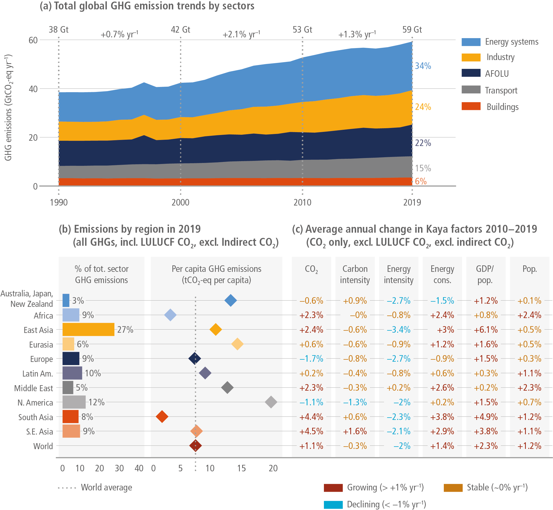
Global net anthropogenic greenhouse gas (GHG) emissions during the last decade (2010–2019) were higher than at any previous time in human history (high confidence). Since 2010, GHG emissions have continued to grow, reaching 59 ± 6.6 GtCO2-eq in 2019, 1 but the average annual growth in the last decade (1.3%, 2010–2019) was lower than in the previous decade (2.1%, 2000–2009) ( high confidence). Average annual GHG emissions were 56 ± 6.0 GtCO2-eq yr –1 for the decade 2010–2019 growing by about 9.1 GtCO2-eq yr –1 from the previous decade (2000–2009) – the highest decadal average on record ( high confidence). {2.2.2, Table 2.1, Figure 2.2, Figure 2.5}
Emissions growth has varied, but persisted across all groups of GHGs (high confidence). The average annual emission levels of the last decade (2010–2019) were higher than in any previous decade for each group of GHGs ( high confidence). In 2019, CO2 emissions were 45 ± 5.5 GtCO2, 2 CH411 ± 3.2 GtCO2-eq, N2O 2.7 ± 1.6 GtCO2-eq and fluorinated gases (F-gases: HFCs, PFCs, SF6, NF3) 1.4 ± 0.41 GtCO2-eq. Compared to 1990, the magnitude and speed of these increases differed across gases: CO2 from fossil fuel and industry (FFI) grew by 15 GtCO2-eq yr –1 (67%), CH4 by 2.4 GtCO2-eq yr –1 (29%), F-gases by 0.97 GtCO2-eq yr –1 (254%), and N2O by 0.65 GtCO2-eq yr –1 (33%). CO2 emissions from net land use, land-use change and forestry (LULUCF) have shown little long-term change, with large uncertainties preventing the detection of statistically significant trends. F-gases excluded from GHG emissions inventories such as chlorofluorocarbons and hydrochlorofluorocarbons are about the same size as those included ( high confidence). {2.2.1, 2.2.2, Table 2.1, Figures 2.2, 2.3 and 2.5}
Globally, gross domestic product (GDP) per capita and population growth remained the strongest drivers of CO2 emissions from fossil fuel combustion in the last decade (robust evidence, high agreement). Trends since 1990 continued in the years 2010 to 2019 with GDP per capita and population growth increasing emissions by 2.3% and 1.2% yr –1, respectively. This growth outpaced the reduction in the use of energy per unit of GDP (–2% yr –1, globally) as well as improvements in the carbon intensity of energy (–0.3% yr –1) ( high confidence). {2.4.1, Figure 2.16}
The global COVID-19 pandemic led to a steep drop in CO2 emissions from fossil fuel and industry (high confidence). Global CO2-FFI emissions dropped in 2020 by about 5.8% (5.1–6.3%) or about 2.2 (1.9–2.4) GtCO2 compared to 2019. Emissions, however, have rebounded globally by the end of December 2020 (medium confidence). {2.2.2, Figure 2.6}
Cumulative net CO2 emissions of the last decade (2010–2019) are about the same size as the remaining carbon budget for keeping warming to 1.5°C (medium confidence). Cumulative net CO2 emissions since 1850 are increasing at an accelerating rate: about 62% of total cumulative CO2 emissions from 1850 to 2019 occurred since 1970 (1500 ± 140 GtCO2); about 43% since 1990 (1000 ± 90 GtCO2); and about 17% since 2010 (410 ± 30 GtCO2). For comparison, the remaining carbon budget for keeping warming to 1.5°C with a 67% (50%) probability is about 400 (500) ± 220 GtCO2 (medium confidence). {2.2.2, Figure 2.7; AR6 WGI 5.5; AR6 WGI Table 5.8}
A growing number of countries have achieved GHG emission reductions longer than 10 years – a few at rates that are broadly consistent with climate change mitigation scenarios that limit warming to well below 2°C (high confidence). There are at least 18 countries that have reduced CO2 and GHG emissions for longer than 10 years. Reduction rates in a few countries have reached 4% in some years, in line with rates observed in pathways that limit warming to 2°C (>67%). However, the total reduction in annual GHG emissions of these countries is small (about 3.2 GtCO2-eq yr –1) compared to global emissions growth observed over the last decades. Complementary evidence suggests that countries have decoupled territorial CO2 emissions from GDP, but fewer have decoupled consumption-based emissions from GDP. This decoupling has mostly occurred in countries with high per capita GDP and high per capita CO2 emissions. {2.2.3, 2.3.3, Figure 2.11, Table 2.3, Table 2.4}
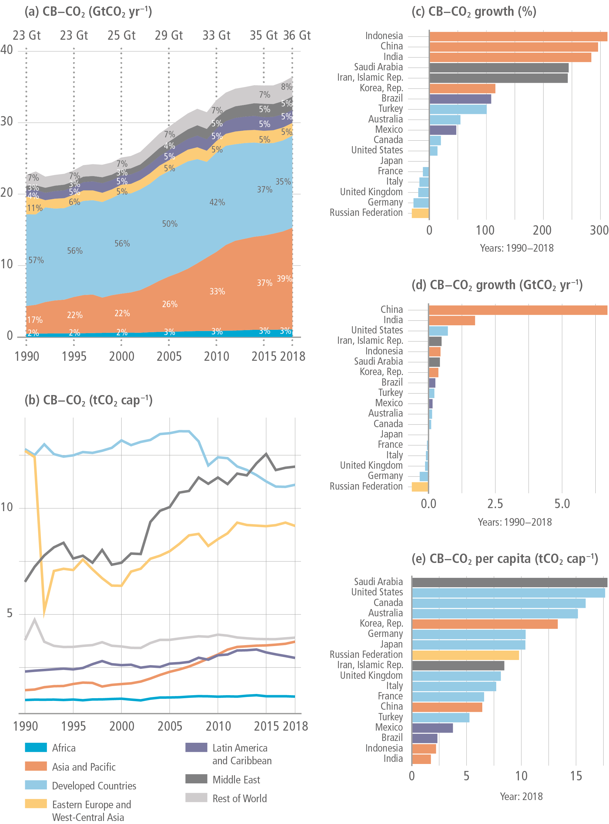
Consumption-based CO2 emissions in Developed Countries and the Asia and Pacific region are higher than in other regions (high confidence). In Developed Countries, consumption-based CO2 emissions peaked at 15 GtCO2 in 2007, declining to about 13 GtCO2 in 2018. The Asia and Pacific region, with 52% of current global population, has become a major contributor to consumption-based CO2 emission growth since 2000 (5.5% yr –1 for 2000–2018); it exceeded the Developed Countries region, which accounts for 16% of current global population, as the largest emitter of consumption-based CO2. {2.3.2, Figure 2.14}
Carbon intensity improvements in the production of traded products have led to a net reduction in CO2 emissions embodied in international trade (robust evidence, high agreement). A decrease in the carbon intensity of traded products has offset increased trade volumes between 2006 and 2016. Emissions embodied in internationally traded products depend on the composition of the global supply chain across sectors and countries and the respective carbon intensity of production processes (emissions per unit of economic output). {2.3, 2.4}
Developed Countries tend to be net CO2 emission importers, whereas developing countries tend to be net emission exporters (robust evidence, high agreement). Net CO2 emission transfers from developing to Developed Countries via global supply chains have decreased between 2006 and 2016. Between 2004 and 2011, CO2 emission embodied in trade between developing countries have more than doubled (from 0.47 to 1.1 Gt) with the centre of trade activities shifting from Europe to Asia. {2.3.4, Figure 2.15}
Emissions from developing countries have continued to grow, starting from a low base of per capita emissions and with a lower contribution to cumulative emissions than Developed Countries (robust evidence, high agreement). Average 2019 per capita CO2-FFI emissions in three developing regions – Africa (1.2 tCO2 per capita), Asia and Pacific (4.4 tCO2 per capita), and Latin America and Caribbean (2.7 tCO2 per capita) – remained less than half that of Developed Countries (9.5 tCO2 per capita) in 2019. CO2-FFI emissions in the three developing regions together grew by 26% between 2010 and 2019, compared to 260% between 1990 and 2010, while in Developed Countries emissions contracted by 9.9% between 2010 and 2019, and by 9.6% between 1990 and 2010. Historically, the three developing regions together contributed 28% to cumulative CO2-FFI emissions between 1850 and 2019, whereas Developed Countries contributed 57% and Least-Developed Countries contributed 0.4%. {2.2.3, Figures 2.9 and 2.10}
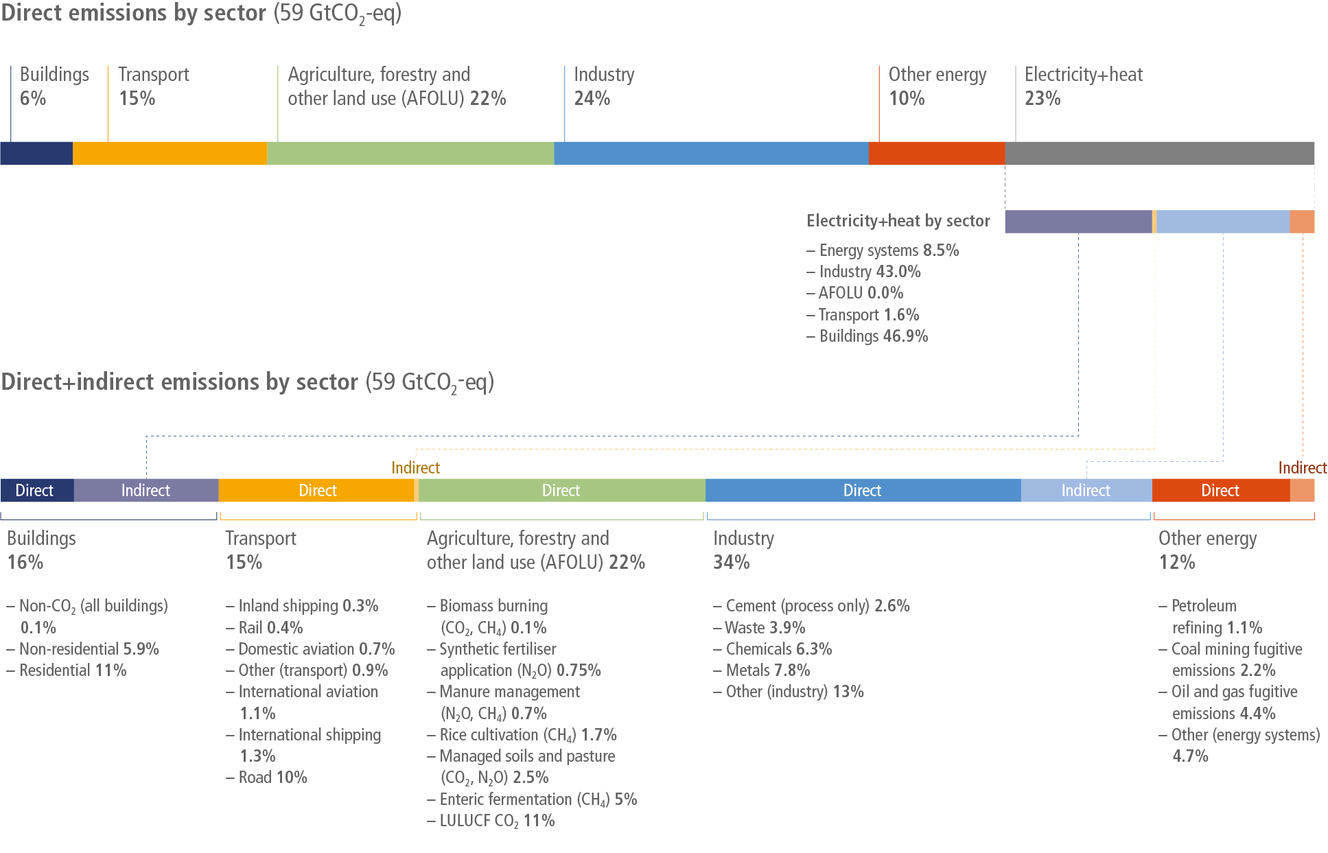
Globally, GHG emissions continued to rise across all sectors and subsectors; most rapidly in transport and industry (high confidence). In 2019, 34% (20 GtCO2-eq) of global GHG emissions came from the energy sector, 24% (14 GtCO2-eq) from industry, 22% (13 GtCO2-eq) from agriculture, forestry and other land use (AFOLU), 15% (8.7 GtCO2-eq) from transport and 5.6% (3.3 GtCO2-eq) from buildings. Once indirect emissions from energy use are considered, the relative shares of industry and buildings emissions rise to 34% and 16%, respectively. Average annual GHG emissions growth during 2010 to 2019 slowed compared to the previous decade in energy supply (from 2.3% to 1.0%) and industry (from 3.4% to 1.4%, direct emissions only), but remained roughly constant at about 2% per year in the transport sector ( high confidence). Emission growth in AFOLU is more uncertain due to the high share of CO2-LULUCF emissions (medium confidence). {2.4.2, Figure 2.13, Figures 2.16 to 2.21}
Average annual growth in GHG emissions from energy supply decreased from 2.3% for 2000–2009 to 1.0% for 2010–2019 (high confidence). This slowing of growth is attributable to further improvements in energy efficiency (annually, 1.9% less energy per unit of GDP was used globally between 2010 and 2019). Reductions in global carbon intensity by –0.2% yr –1 contributed further – reversing the trend during 2000 to 2009 (+0.2% yr –1) (medium confidence). These carbon intensity improvements were driven by fuel switching from coal to gas, reduced expansion of coal capacity, particularly in Eastern Asia, and the increased use of renewables. {2.2.4, 2.4.2.1, Figure 2.17}
GHG emissions in the industry, buildings and transport sectors continue to grow, driven by an increase in the global demand for products and services (high confidence). These final demand sectors make up 44% of global GHG emissions, or 66% when the emissions from electricity and heat production are reallocated as indirect emissions to related sectors, mainly to industry and buildings. Emissions are driven by the large rise in demand for basic materials and manufactured products, a global trend of increasing floor space per capita, building energy service use, travel distances, and vehicle size and weight. Between 2010 and 2019, domestic and international aviation were particularly fast growing at average annual rates of +3.3% and +3.4%. Global energy efficiencies have improved in all three demand sectors, but carbon intensities have not. {2.2.4; Figures 2.18 to 2.20}
Providing access to modern energy services universally would increase global GHG emissions by, at most, a few percent (medium confidence). The additional energy demand needed to support decent living standards 3 for all is estimated to be well below current average energy consumption (medium evidence, high agreement ). More equitable income distributions can reduce carbon emissions, but the nature of this relationship can vary by level of income and development (limited evidence, medium agreement ). {2.4.3}
Evidence of rapid energy transitions exists, but only at sub-global scales (medium evidence, medium agreement). Emerging evidence since the Fifth Assessment Report of the Intergovernmental Panel on Climate Change (IPCC AR5) on past energy transitions identifies a growing number of cases of accelerated technology diffusion at sub-global scales and describes mechanisms by which future energy transitions may occur more quickly than those in the past. Important drivers include technology transfer and cooperation, intentional policy and financial support, and harnessing synergies among technologies within a sustainable energy system perspective (medium evidence, medium agreement ). A fast global low-carbon energy transition enabled by finance to facilitate low-carbon technology adoption in developing, and particularly in least-developed countries, can facilitate achieving climate stabilisation targets (robust evidence, high agreement ). {2.5.2, Table 2.5}
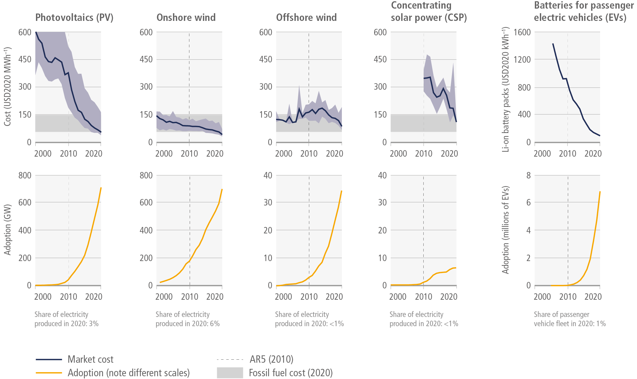
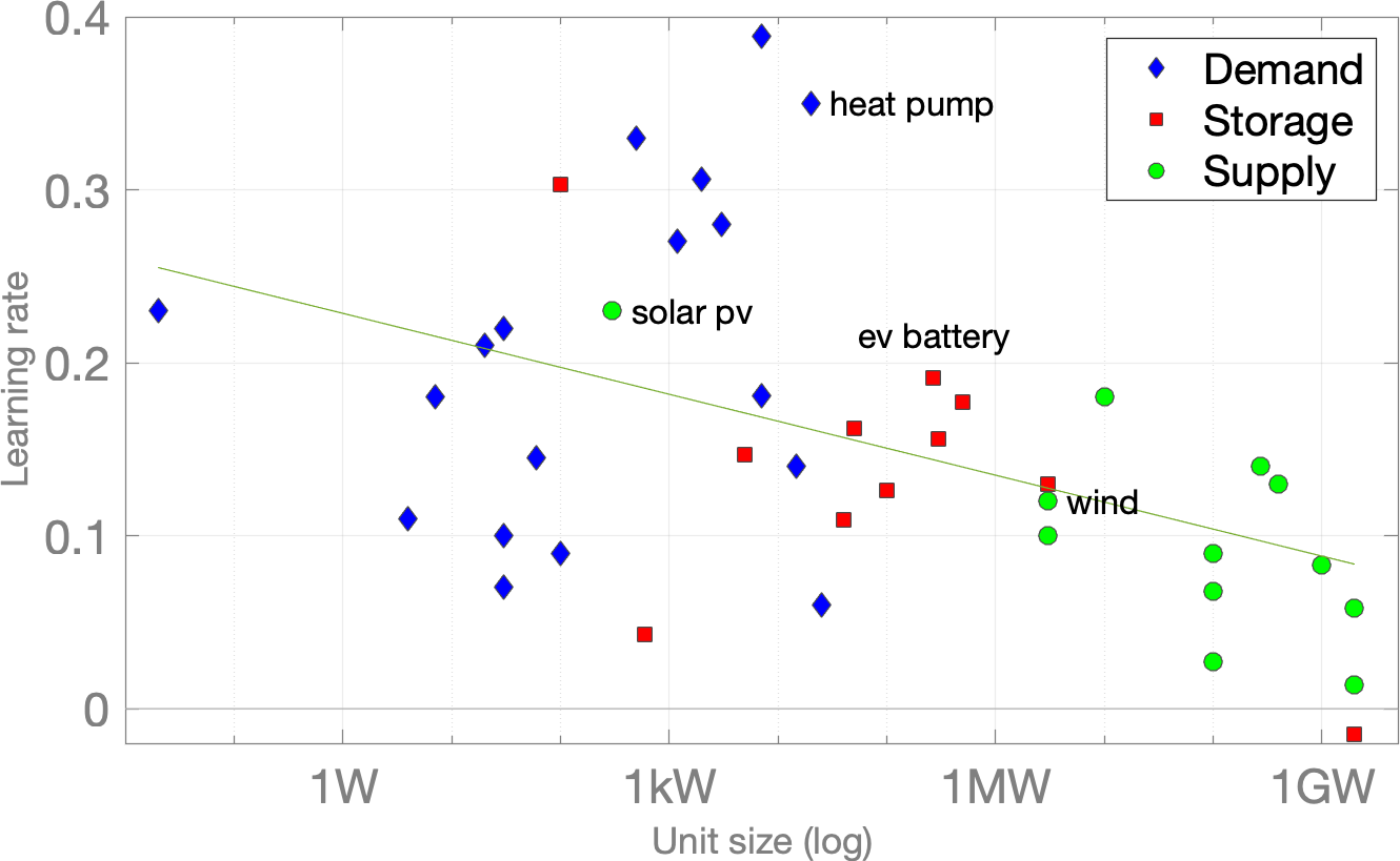
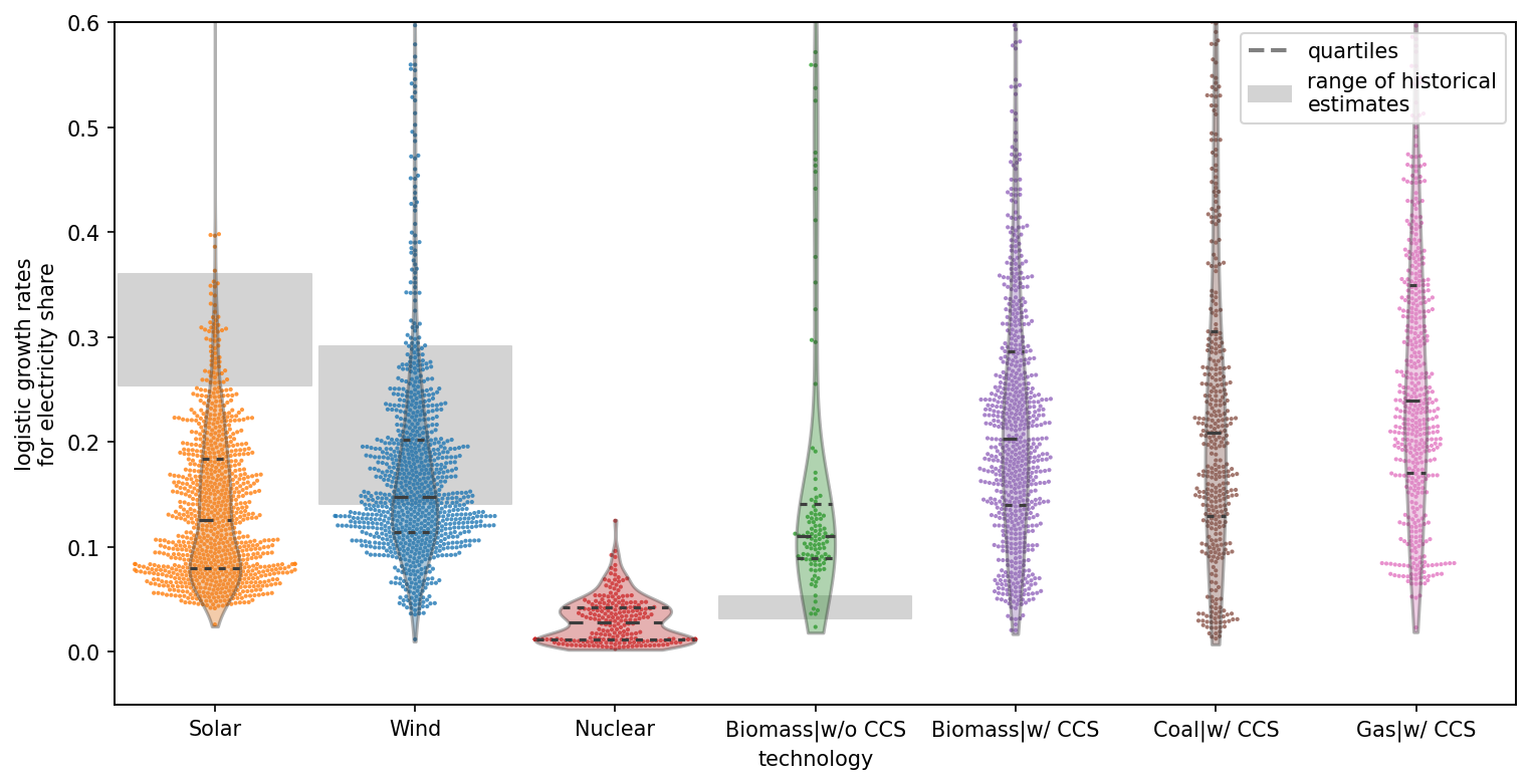
Multiple low-carbon technologies have shown rapid progress since AR5 – in cost, performance, and adoption – enhancing the feasibility of rapid energy transitions (robust evidence, high agreement). The rapid deployment and cost decrease of modular technologies like solar, wind, and batteries have occurred much faster than anticipated by experts and modelled in previous mitigation scenarios (robust evidence, high agreement ). The political, economic, social, and technical feasibility of solar energy, wind energy and electricity storage technologies has improved dramatically over the past few years. In contrast, the adoption of nuclear energy and carbon capture and storage (CCS) in the electricity sector has been slower than the growth rates anticipated in stabilisation scenarios. Emerging evidence since AR5 indicates that small-scale technologies (e.g., solar, batteries) tend to improve faster and be adopted more quickly than large-scale technologies (nuclear, CCS) (medium evidence, medium agreement ). {2.5.3, 2.5.4, Figures 2.22 and 2.23}
Robust incentives for investment in innovation, especially incentives reinforced by national policy and international agreements, are central to accelerating low-carbon technological change (robust evidence, medium agreement). Policies have driven innovation, including instruments for technology push (e.g., scientific training, research and development) and demand pull (e.g., carbon pricing, adoption subsidies), as well as those promoting knowledge flows and especially technology transfer. The magnitude of the scale-up challenge elevates the importance of rapid technology development and adoption. This includes ensuring participation of developing countries in an enhanced global flow of knowledge, skills, experience, and equipment. Also, technology itself requires strong financial, institutional, and capacity-building support (robust evidence, high agreement ). {2.5.4, 2.5, 2.8}
The global wealthiest 10% contribute about 36–45% of global GHG emissions (robust evidence, high agreement). The global 10% wealthiest consumers live in all continents, with two-thirds in high-income regions and one-third in emerging economies (robust evidence, medium agreement ). The lifestyle consumption emissions of the middle-income and poorest citizens in emerging economies are between 5 and 50 times below their counterparts in high-income countries (medium evidence, medium agreement ). Increasing inequality within a country can exacerbate dilemmas of redistribution and social cohesion, and affect the willingness of rich and poor to accept lifestyle changes for mitigation and policies to protect the environment (medium evidence, medium agreement ) {2.6.1, 2.6.2, Figure 2.25}
Estimates of future CO2 emissions from existing fossil fuel infrastructures already exceed remaining cumulative net CO2 emissions in pathways limiting warming to 1.5°C with no or limited overshoot (high confidence). Assuming variations in historical patterns of use and decommissioning, estimated future CO2 emissions from existing fossil fuel infrastructure alone are 660 (460–890) GtCO2 and from existing and currently planned infrastructure 850 (600–1100) GtCO2. This compares to overall cumulative netCO2 emissions until reaching net zero CO2 of 510 (330–710) Gt in pathways that limit warming to 1.5°C with no or limited overshoot, and 890 (640–1160) Gt in pathways that limit warming to 2°C (<67%) ( high confidence). While most future CO2 emissions from existing and currently planned fossil fuel infrastructure are situated in the power sector, most remaining fossil fuel CO2 emissions in pathways that limit warming to 2°C (<67%) and below are from non-electric energy – most importantly from the industry and transportation sectors ( high confidence). Decommissioning and reduced utilisation of existing fossil fuel installations in the power sector as well as cancellation of new installations are required to align future CO2 emissions from the power sector with projections in these pathways ( high confidence). {2.7.2, 2.7.3, Figure 2.26, Table 2.6, Table 2.7}
A broad range of climate policies, including instruments like carbon pricing, play an increasing role in GHG emissions reductions. The literature is in broad agreement, but the magnitude of the reduction rate varies by the data and methodology used, country, and sector (robust evidence, high agreement). Countries with a lower carbon pricing gap (higher carbon price) tend to be less carbon intensive (medium confidence). {2.8.2, 2.8.3}
Climate-related policies have also contributed to decreasing GHG emissions. Policies such as taxes and subsidies for clean and public transportation, and renewable policies have reduced GHG emissions in some contexts (robust evidence, high agreement). Pollution control policies and legislations that go beyond end-of-pipe controls have also had climate co-benefits, particularly if complementarities with GHG emissions are considered in policy design (medium evidence, medium agreement ). Policies on AFOLU and sector-related policies such as afforestation can have important impacts on GHG emissions (medium evidence, medium agreement ). {2.8.4}
2.1Introduction
As demonstrated by the contribution of Working Group I to the Sixth Assessment Report of the Intergovernmental Panel on Climate Change (AR6 WGI) (IPCC 2021a), greenhouse gas 4 (GHG) concentrations in the atmosphere and annual anthropogenic GHG emissions continue to grow and have reached a historic high, driven mainly by continued fossil fuels use (Jackson et al. 2019; Friedlingstein et al. 2020; Peters et al. 2020). Unsurprisingly, a large volume of new literature has emerged since AR5 on the trends and underlying drivers of anthropogenic GHG emissions. This chapter provides a structured assessment of this new literature and establishes the most important thematic links to other chapters in this report.
While AR5 has mostly assessed GHG emissions trends and drivers between 1970 and 2010, this assessment focuses on the period 1990–2019 with the main emphasis on changes since 2010. Compared to Chapter 5 in the contribution of WG III to AR5 (Blanco et al. 2014), the scope of the present chapter is broader. It presents the historical background of global progress in climate change mitigation for the rest of the report and serves as a starting point for the assessment of long-term as well as near- and medium-term mitigation pathways in Chapters 3 and 4, respectively. It also provides a systemic perspective on past emissions trends in different sectors of the economy (Chapters 6–12), and relates GHG emissions trends to past policies (Chapter 13) and observed technological development (Chapter 16). There is also a greater focus on the analysis of consumption-based sectoral emissions trends, empirical evidence of emissions consequences of behavioural choices and lifestyles, and the social aspects of mitigation (Chapter 5). Finally, a completely new section discusses the mitigation implications of existing and planned long-lived infrastructure and carbon lock-in.
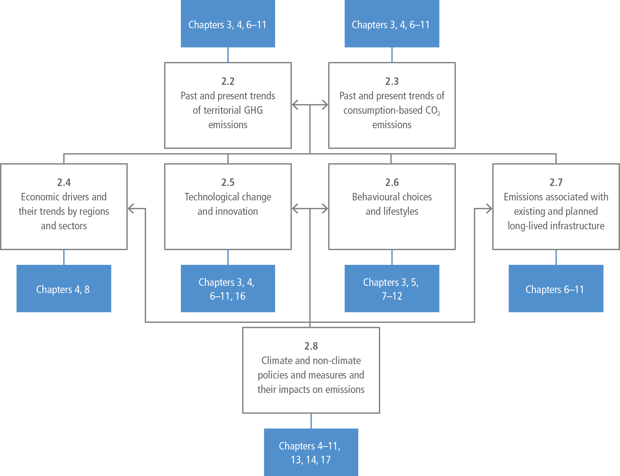
Figure 2.1 presents the road map of this chapter. It is a simplified illustration of the causal chain driving emissions along the black arrows. It also highlights the most important linkages to other chapters in this volume (blue lines). The logic of the figure is that the main topic of this chapter is GHG emissions trends (discussed only in this chapter at such level of detail), hence they are at the top of the figure in grey-outlined boxes. The secondary theme is the drivers behind these trends, depicted in the second line of grey-outlined boxes. Four categories of drivers highlight key issues and guide readers to chapters in which more details are presented. Finally, in addition to their own motivations and objectives, climate and non-climate policies and measures shape the aspirations and activities of actors in the main driver categories, as shown in the grey-outlined box below.

Figure 2.1 | Chapter 2 road map and linkages toother chapters. Black arrows show the causal chain driving emissions. Blue lines indicate key linkages to other chapters in this report.
Accordingly, the grey-outlined boxes at the top of Figure 2.1 show that the first part of the chapter presents GHG emissions from two main perspectives: their geographical locations; and the places where goods are consumed and services are utilised. A complicated chain of drivers underlie these emissions. They are linked across time, space, and various segments of the economy and society in complex non-linear relationships. Sections shown in the second row of grey-outlined boxes assess the latest literature and improve the understanding of the relative importance of these drivers in mitigating GHG emissions. A huge mass of physical capital embodying immense financial assets and potentially operating over a long lifetime produces vast GHG emissions. This long-lived infrastructure can be a significant hindrance to fast and deep reductions of emissions; it is therefore also shown as an important driver. A large range of economic, social, environmental, and other policies has been shaping these drivers of GHG emissions in the past and are anticipated to influence them in the future, as indicated by the grey-outlined policies box and its manifold linkages. As noted, blue lines show linkages of sections to other chapters that discuss these drivers and their operating mechanisms in detail.
2.2Past and Present Trends of Territorial GHG Emissions
Total anthropogenic greenhouse gas (GHG) emissions as discussed in this chapter comprise CO2 emissions from fossil fuel combustion and industrial (FFI) processes, 5 net CO2 emissions from land use, land-use change, and forestry (CO2-LULUCF) (often named FOLU – forestry and other land-use – in previous IPCC reports), methane (CH4), nitrous oxide (N2O) and fluorinated gases (F-gases) comprising hydrofluorocarbons (HFCs), perfluorocarbons (PFCs), sulphur hexafluoride (SF6) as well as nitrogen trifluoride (NF3). There are other major sources of F-gas emissions that are regulated under the Montreal Protocol such as chlorofluorocarbons (CFCs) and hydrochlorofluorocarbons (HCFCs) that also have considerable warming impacts (Figure 2.4), however they are not considered here. Other substances, including ozone and aerosols, that further contribute climate forcing are only treated very briefly, but a full chapter is devoted to this subject in the Working Group I contribution to AR6 (Szopa et al. 2021a; 2021b).
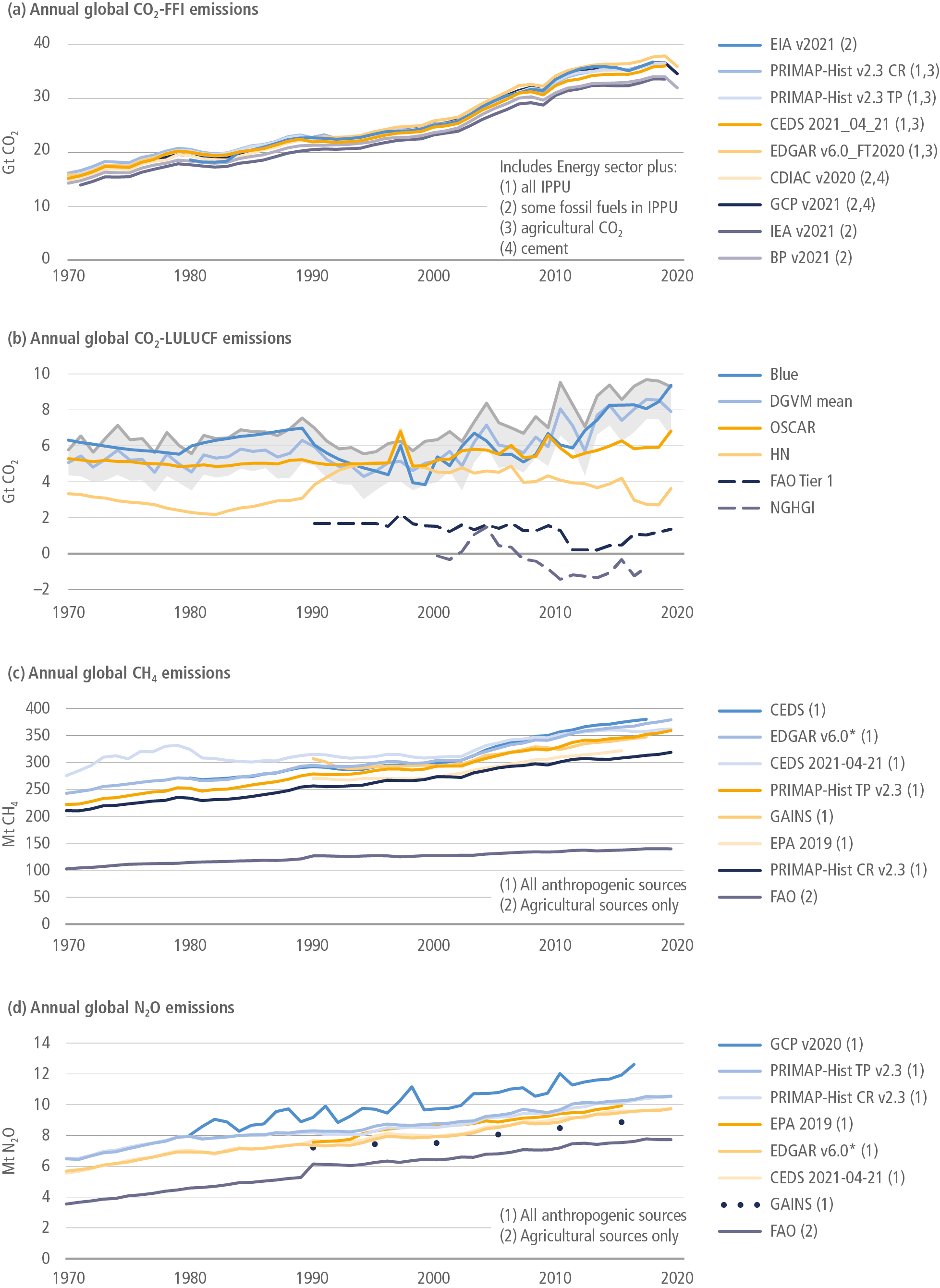
A growing number of global GHG emissions inventories have become available since AR5 (Minx et al. 2021). However, only a few are comprehensive in their coverage of sectors, countries and gases – namely EDGAR (Emissions Database for Global Atmospheric Research) (Crippa et al. 2021), PRIMAP (Potsdam Real-time Integrated Model for probabilistic Assessment of emissions Paths) (Gütschow et al. 2021a), CAIT (Climate Analysis Indicators Tool) (WRI 2019) and CEDS (A Community Emissions Data System for Historical Emissions) (Hoesly et al. 2018). None of these inventories presently cover CO2-LULUCF, while CEDS excludes F-gases. For individual gases and sectors, additional GHG inventories are available, as shown in Figure 2.2, but each has varying system boundaries leading to important differences between their respective estimates (Section 2.2.1). Some inventories are compiled bottom-up, while others are produced synthetically and are dependent on other inventories. A more comprehensive list and discussion of different datasets is provided in the Chapter 2 Supplementary Material (2.SM.1) and in Minx et al. (2021).

Figure 2.2: Estimates of global anthropogenic greenhouse gasemissions from different data sources 1970–2019. Panel (a): CO2FFI emissions from: EDGAR – Emissions Database for Global Atmospheric Research (this dataset) (Crippa et al. 2021); GCP – Global Carbon Project (Friedlingstein et al. 2020; Andrew and Peters 2021); CEDS – Community Emissions Data System (Hoesly et al. 2018; O’Rourke et al. 2021); CDIAC Global, Regional, and National Fossil-Fuel CO2 Emissions (Gilfillan et al. 2020); PRIMAP-hist – Potsdam Real-time Integrated Model for probabilistic Assessment of emissions Paths (Gütschow et al. 2016, 2021b); EIA – Energy Information Administration International Energy Statistics (EIA 2021); BP – BP Statistical Review of World Energy (BP 2021); IEA – International Energy Agency (IEA 2021a, 2021b); IPPU refers to emissions from industrial processes and product use. Panel (b): Net anthropogenic CO2-LULUCF emissions from: BLUE – Bookkeeping of land-use emissions (Hansis et al. 2015; Friedlingstein et al. 2020); DGVM-mean – multi-model mean of CO2-LULUCF emissions from dynamic global vegetation models (Friedlingstein et al. 2020); OSCAR – an earth system compact model (Friedlingstein et al. 2020; Gasser et al. 2020); HN – Houghton and Nassikas Bookkeeping Model (Houghton and Nassikas 2017; Friedlingstein et al. 2020); for comparison, the net CO2 flux from FAOSTAT (FAO Tier 1) is plotted, which comprises net emissions and removals on forest land and from net forest conversion (FAOSTAT 2021; Tubiello et al. 2021), emissions from drained organic soils under cropland/grassland (Conchedda and Tubiello 2020), and fires in organic soils (Prosperi et al. 2020), as well as a net CO2 flux estimate from National Greenhouse Gas Inventories (NGHGI) based on country reports to the UNFCCC, which include land-use change, and fluxes in managed lands (Grassi et al. 2021). Panel (c): Anthropogenic CH4 emissions from: EDGAR (above); CEDS (above); PRIMAP-hist (above); GAINS – The Greenhouse gas – Air pollution Interactions and Synergies Model (Höglund-Isaksson et al. 2020); EPA-2019: Greenhouse gas emission inventory (US-EPA, 2019); FAO –FAOSTAT inventory emissions (Tubiello et al. 2013; Tubiello 2018; FAOSTAT 2021); Panel (d): Anthropogenic N2O emissions from: GCP – global nitrous oxide budget (Tian et al. 2020); CEDS (above); EDGAR (above); PRIMAP-hist (above); GAINS (Winiwarter et al. 2018); EPA-2019 (above); FAO (above). Differences in emissions across different versions of the EDGAR dataset are shown in the Supplementary Material (Figure 2.SM.2). Source: Minx et al. (2021).
Across this report, version 6 of EDGAR (Crippa et al. 2021) provided by the Joint Research Centre of the European Commission, is used for a consistent assessment of GHG emissions trends and drivers. It covers anthropogenic releases of CO2-FFI, CH4, N2O, and F-gas (HFCs, PFCs, SF6, NF3) emissions by 228 countries and territories and across five sectors and 27 subsectors. EDGAR is chosen because it provides the most comprehensive global dataset in its coverage of sources, sectors and gases. For transparency, and as part of the uncertainty assessment, EDGAR is compared to other global datasets in Section 2.2.1 as well as in the Chapter 2 Supplementary Material (2.SM.1). For individual country estimates of GHG emissions, it may be more appropriate to use inventory data submitted to the United Nations Framework Convention on Climate Change (UNFCCC) under the common reporting format (CRF) (UNFCCC 2021). However, these inventories are only up to date for Annex I countries and cannot be used to estimate global or regional totals. As part of the regional analysis, a comparison of EDGAR and CRF estimates at the country-level is provided, where the latter is available (Figure 2.9).
Net CO2-LULUCF estimates are added to the dataset as the average of estimates from three bookkeeping models of land-use emissions (Hansis et al. 2015; Houghton and Nassikas 2017; Gasser et al. 2020) following the Global Carbon Project (Friedlingstein et al. 2020). This is different to AR5, where land-based CO2 emissions from forest fires, peat fires, and peat decay, were used as an approximation of the net-flux of CO2-LULUCF (Blanco et al. 2014). Note that the definition of CO2-LULUCF emissions by global carbon cycle models, as used here, differs from IPCC definitions (IPCC 2006) applied in national greenhouse gas inventories (NGHGI) for reporting under the climate convention (Grassi et al. 2018, 2021) and, similarly, from estimates by the Food and Agriculture Organization of the United Nations (FAO) for carbon fluxes on forest land (Tubiello et al. 2021). The conceptual difference in approaches reflects different scopes. We use the global carbon cycle models’ approach for consistency with Working Group I (Canadell et al. 2021) and to comprehensively distinguish natural from anthropogenic drivers, while NGHGI generally report as anthropogenic all CO2 fluxes from lands considered managed (Section 7.2.2). Finally, note that the CO2-LULUCF estimate from bookkeeping models as provided in this chapter is indistinguishable from the CO2 from agriculture, forestry and other land use (AFOLU) as reported in Chapter 7, because the CO2 emissions component from agriculture is negligible.
The resulting synthetic dataset used here has undergone additional peer review and is publicly available (Minx et al. 2021). Comprehensive information about the dataset as well as underlying uncertainties (including a comparison with other datasets) can be found in the Supplementary Material to this chapter and in Minx et al. (2021).
In this chapter and the report as a whole, different GHGs are frequently converted into common units of CO2 equivalent (CO2-eq) emissions using 100-year global warming potentials (GWP100) from AR6 WGI (Forster et al. 2021a). This reflects the dominant use in the scientific literature and is consistent with decisions made by Parties to the Paris Agreement for reporting and accounting of emissions and removals (UNFCCC 2019). Other GHG emissions metrics exist, all of which, like GWP100, are designed for specific purposes and have limitations and uncertainties. The appropriate choice of GHG emissions metrics depends on policy objective and context (Myhre et al. 2013; Kolstad et al. 2015). A discussion of GHG metrics is provided in a Cross-Chapter Box later in the chapter (Cross-Chapter Box 2) and at length in the Chapter 2 Supplementary Material. Throughout the chapter GHG emissions are reported (in GtCO2-eq) at two significant digits to reflect prevailing uncertainties in emissions estimates. Estimates are subject to uncertainty, which we report for a 90% confidence interval.
2.2.1Uncertainties in GHG Emissions
Estimates of historical GHG emissions – CO2, CH4, N2O and F-gases – are uncertain to different degrees. Assessing and reporting uncertainties is crucial in order to understand whether available estimates are sufficiently robust to answer policy questions – for example, if GHG emissions are still rising, or if a country has achieved an emission reduction goal (Marland 2008). These uncertainties can be of scientific nature, such as when a process is not sufficiently understood. They also arise from incomplete or unknown parameter information (e.g., activity data, or emission factors), as well as estimation uncertainties from imperfect modelling techniques. There are at least three major ways to examine uncertainties in emission estimates (Marland et al. 2009): (i) by comparing estimates made by independent methods and observations (e.g., comparing atmospheric measurements with bottom-up emissions inventory estimates) (Saunois et al. 2020; Petrescu et al. 2020 a and 2020b; Tian et al. 2020); (ii) by comparing estimates from multiple sources and understanding sources of variation (Macknick 2011; Andres et al. 2012; Andrew 2020; Ciais et al. 2021); and (iii) by evaluating estimates from a single source (Hoesly and Smith 2018), for instance via statistical sampling across parameter values (e.g., Monni et al. 2007; Robert J. Andres et al. 2014; Tian et al. 2019; Solazzo et al. 2021).
Uncertainty estimates can be rather different depending on the method chosen. For example, the range of estimates from multiple sources is bounded by their interdependency; they can be lower than true structural plus parameter uncertainty, or than estimates made by independent methods. In particular, it is important to account for potential bias in estimates, which can result from using common methodological or parameter assumptions, or from missing sources (systemic bias). It is further crucial to account for differences in system boundaries – that is, which emissions sources are included in a dataset and which are not, otherwise direct comparisons can exaggerate uncertainties (Macknick 2011; Andrew 2020). Independent top-down observational constraints are, therefore, particularly useful to bound total emission estimates, but are not yet capable of verifying emission levels or trends (Petrescu et al. 2021a, 2021b). Similarly, uncertainties estimates are influenced by specific modelling choices. For example, uncertainty estimates from studies on the propagation of uncertainties associated with key input parameters (activity data, emissions factors) following the IPCC Guidelines (IPCC 2006) are strongly determined by assumptions on how these parameters are correlated between sectors, countries, and regions (Janssens-Maenhout et al. 2019; Solazzo et al. 2021). Assuming (full) covariance between source categories, and therefore dependence between them, increases uncertainty estimates. Estimates allowing for some covariance as in Sollazo et al. (2021) also tend to yield higher estimates than the range of values from ensemble of dependent inventories (Saunois et al. 2016, 2020).
For this report, a comprehensive assessment of uncertainties is provided in the Supplementary Material (2.SM.2) to this chapter based on Minx et al. (2021). The uncertainties reported here combine statistical analysis, comparisons of global emissions inventories and an expert judgement of the likelihood of results lying outside a defined confidence interval, rooted in an understanding gained from the relevant literature. This literature has improved considerably since AR5, with a growing number of studies that assess uncertainties based on multiple lines of evidence (Saunois et al. 2016, 2020; Tian et al. 2020; Petrescu et al. 2021a, 2021b).
To report the uncertainties in GHG emissions estimates, a 90% confidence interval (5th–95th percentile) is adopted – that is, there is a 90% likelihood that the true value will be within the provided range if the errors have a Gaussian distribution, and no bias is assumed. This is in line with previous reporting in IPCC AR5 (Blanco et al. 2014; Ciais et al. 2014). Note that national emissions inventory submissions to the UNFCCC are requested to report uncertainty using a 95% confidence interval. The use of this broader uncertainty interval implies, however, a relatively high degree of knowledge about the uncertainty structure of the associated data, particularly regarding the distribution of uncertainty in the tails of the probability distributions. Such a high degree of knowledge is not present over all regions, emission sectors and species considered here.
Based on the assessment of relevant uncertainties above, a constant, relative, global uncertainty estimates for GHGs are applied at a 90% confidence interval that range from relatively low values for CO2-FFI (±8%), to intermediate values for CH4 and F-gases (±30%), to higher values for N2O (±60%) and CO2-LULUCF (±70%). Uncertainties for aggregated total GHG emissions in terms of CO2-eq emissions are calculated as the square root of the squared sums of absolute uncertainties for individual gases (taking F-gases together), using GWP100 to weight emissions of non-CO2 gases but excluding uncertainties in the metric itself.
This assessment of uncertainties is broadly in line with AR5 WGIII (Blanco et al. 2014), but revises individual uncertainty judgements in line with the more recent literature (Saunois et al. 2016, 2020; Janssens-Maenhout et al. 2019; Friedlingstein et al. 2020; Tian et al. 2020; Solazzo et al. 2021) as well as the underlying synthetic analysis provided here (e.g., Figures 2.2 and 2.3 in this chapter; and Minx et al. 2021). As such, reported changes in these estimates do not reflect changes in the underlying uncertainties, but rather a change in expert judgement based on an improved evidence base in the scientific literature. Uncertainty estimates for CO2-FFI and N2O remain unchanged compared to AR5. The change in the uncertainty estimates for CH4 from 20% to 30% is justified by larger uncertainties reported for EDGAR emissions (Janssens-Maenhout et al. 2019; Solazzo et al. 2021) as well as the wider literature (Kirschke et al. 2013; Tubiello et al. 2015; Saunois et al. 2016, 2020). As AR6 – in contrast to AR5 – uses CO2-LULUCF data from global bookkeeping models, the respective uncertainty estimate is based on the reporting in the underlying literature (Friedlingstein et al. 2020) as well as Working Group I (Canadell et al. 2021). The 70% uncertainty value is at the higher end of the range considered in AR5 (Blanco et al. 2014).
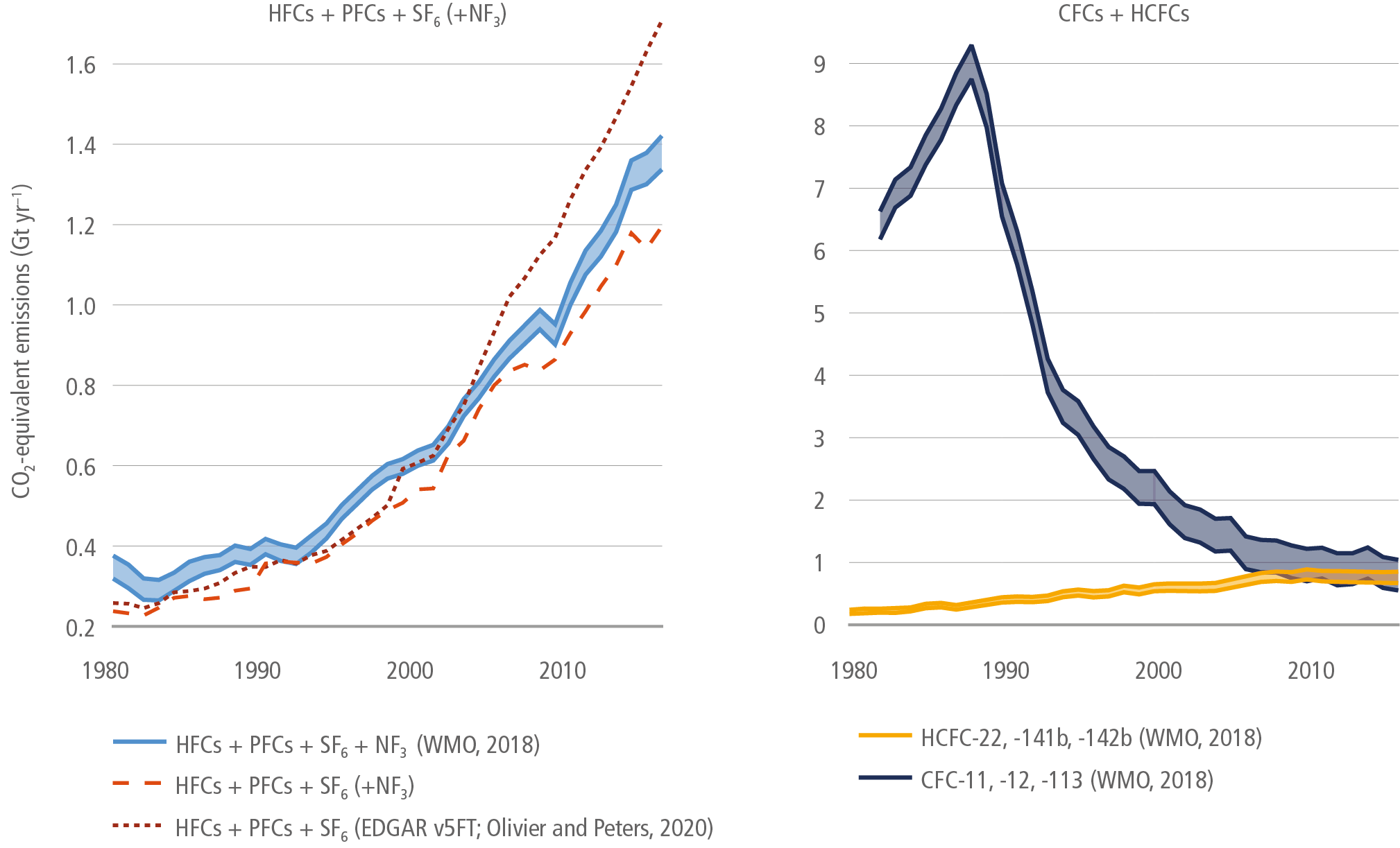
Finally, for F-gas emissions top-down atmospheric measurements from the 2018 World Meteorological Organization’s (WMO) Scientific Assessment of Ozone Depletion (Engel and Rigby 2018; Montzka and Velders 2018) are compared to the data used in this report (Crippa et al. 2021; Minx et al. 2021) as shown in Figure 2.3. Due to the general absence of natural F-gas fluxes, there is a sound understanding of global and regional F-gas emissions from top-down estimates of atmospheric measurements with small and well-understood measurement, lifetime and transport model uncertainties (Engel and Rigby 2018; Montzka and Velders 2018). However, when species are aggregated into total F-gas emissions, EDGARv6.0 emissions are around 10% lower than the WMO 2018 values throughout, with larger differences for individual F-gas species, and further discrepancies when comparing to older EDGAR versions. Based on this, the overall uncertainties for aggregate F-gas emissions is judged conservatively at 30% – 10 percentage points higher than in AR5 (Blanco et al. 2014).

Figure 2.3 | Comparison between top-down estimates and bottom-up EDGAR inventory data on GHG emissions for 1980–2016. Left panel: Total GWP100-weighted emissions based on IPCC AR6 (Forster et al. 2021a) of F-gases in Olivier and Peters (2020) [EDGARv5FT] (dark-red dotted line, excluding C4F10, C5F12, C6F14 and C7F16) and EDGARv6 (bright red dashed line) compared to top-down estimates based on AGAGE and NOAA data from WMO (2018) (blue lines; Engel and Rigby (2018); Montzka and Velders (2018)). Right panel: Top-down aggregated emissions for the three most abundant CFCs (–11, –12 and –113) and HCFCs (–22, –141b, –142b) not covered in bottom-up emissions inventories are shown in dark blue and yellow. For top-down estimates the shaded areas between two respective lines represent 1σ uncertainties. Source: Minx et al. (2021).
Aggregate uncertainty across all GHGs is approximately ±11% depending on the composition of gases in a particular year. AR5 applied a constant uncertainty estimates of ±10% for total GHG emissions. The upwards revision applied to the uncertainties of CO2-LULUCF, CH4 and F-gas emissions therefore has a limited overall effect on the assessment of GHG emissions.
GHG emissions metrics such as GWP100 have their own uncertainties, which has been largely neglected in the literature so far. Minx et al. (2021) report the uncertainty in GWP100 metric values as ±50% for methane and other short-lived climate forcers (SLCFs), and ±40% for non-CO2 gases with longer atmospheric lifetimes (specifically, those with lifetimes longer than 20 years). If uncertainties in GHG metrics are considered, and are assumed independent (which may lead to an underestimate) the overall uncertainty of total GHG emissions in 2019 increases from ±11% to ±13%. Metric uncertainties are not further considered in this chapter, but are referred to in Cross-Chapter Box 2 in this chapter, and Chapter 2 Supplementary Material on GHG metrics (2.SM.3).
The most appropriate metric to aggregate GHG emissions depends on the objective (Cross-Chapter Box 2). One such objective can be to understand the contribution of emissions in any given year to warming, while another can be to understand the contribution of cumulative emissions over an extended time period to warming. In Figure 2.4 the modelled warming from emissions of each gas or group of gases is also shown – calculated using the reduced-complexity climate model Finite Amplitude Impulse Response (FaIR) model v1.6, which has been calibrated to match several aspects of the overall WGI assessment (Forster et al. 2021a; specifically Cross-Chapter Box 7 in Chapter 10 therein). Additionally, its temperature response to emissions with shorter atmospheric lifetimes such as aerosols, methane or ozone has been adjusted to broadly match those presented in Szopa et al. (2021a). There are some differences in actual warming compared to the GWP100 weighted emissions of each gas (Figure 2.4), in particular a greater contribution from CH4 emissions to historical warming. This is consistent with warming from CH4 being short-lived and hence having a more pronounced effect in the near-term during a period of rising emissions. Nonetheless, Figure 2.4 highlights that emissions weighted by GWP100 do not provide a fundamentally different information about the contribution of individual gases than modelled actual warming over the historical period, when emissions of most GHGs have been rising continuously, with CO2 being the dominant and CH4 being the second most important contributor to GHG-induced warming. Other metrics such as GWP* (or GWP star) (Cain et al. 2019) offer an even closer resemblance between cumulative CO2-eq emissions and temperature change. Such a metric may be more appropriate when the key objective is to track temperature change when emissions are falling, as in mitigation scenarios.
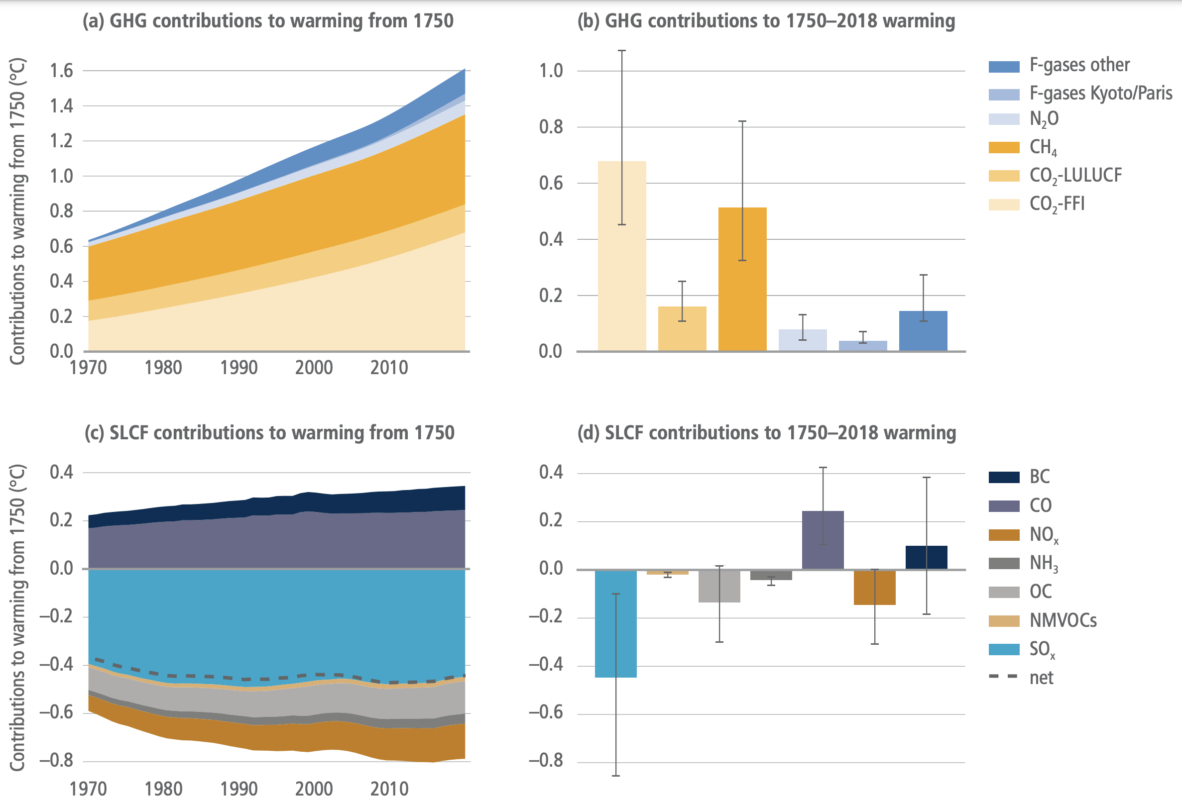
Figure 2.4 | Contribution of different GHGs to global warming over the period 1750 to 2018. Top row: contributions estimated with the FaIR reduced-complexity climate model. Major GHGs and aggregates of minor gases as a timeseries in (a) and as a total warming bar chart with 90% confidence interval added in (b). Bottom row: contribution from short-lived climate forcers as a time series in (c) and as a total warming bar chart with 90% confidence interval added in (d). The dotted line in (c) gives the net temperature change from short-lived climate forcers other than CH4. F-Kyoto/Paris includes the gases covered by the Kyoto Protocol and Paris Agreement, while F-other includes the gases covered by the Montreal Protocol but excluding the HFCs. Source: Minx et al. (2021).
Cross-Chapter Box 2 | GHG Emissions Metrics
Authors: Andy Reisinger (New Zealand), Alaa Al Khourdajie (United Kingdom/Syria), Kornelis Blok (the Netherlands), Harry Clark (New Zealand), Annette Cowie (Australia), Jan S. Fuglestvedt (Norway), Oliver Geden (Germany), Veronika Ginzburg (the Russian Federation), Céline Guivarch (France), Joanna I. House (United Kingdom), Jan Christoph Minx (Germany), Rachid Mrabet (Morocco), Gert-Jan Nabuurs (the Netherlands), Glen P. Peters (Norway/Australia), Keywan Riahi (Austria), Roberto Schaeffer (Brazil), Raphael Slade (United Kingdom), Anders Hammer Strømman (Norway), Detlef P. van Vuuren (the Netherlands)
Comprehensive mitigation policy relies on consideration of all anthropogenic forcing agents, which differ widely in their atmospheric lifetimes and impacts on the climate system. GHG emission metrics 6 provide simplified information about the effects that emissions of different GHGs have on global temperature or other aspects of climate, usually expressed relative to the effect of emitting CO2 (see emission metrics in Annex I: Glossary). This information can inform prioritisation and management of trade-offs in mitigation policies and emission targets for non-CO2 gases relative to CO2, as well as for baskets of gases expressed in CO2-eq. This assessment builds on the evaluation of GHG emission metrics from a physical science perspective by WGI (Forster et al. 2021b). For additional details and supporting references, see Chapter 2 Supplementary Material (2.SM.3) and Annex II.8.
The global warming potential (GWP) and the global temperature change potential (GTP) werethe main metrics assessed in AR5 (Myhre et al. 2013; Kolstad et al. 2014). The GWP with a lifetime of 100 years (GWP100) continues to be the dominant metric used in the scientific literature on mitigation assessed by WGIII. The assessment by WGI (Forster et al. 2021) includes updated values for these metrics based on updated scientific understanding of the response of the climate system to emissions of different gases, including changing background concentrations. It also assesses new metrics published since AR5. Metric values in AR6 include climate-carbon cycle feedbacks by default; this provides an important update and clarification from AR5 which reported metric values both with and without such feedbacks.
The choice of metric, including time horizon, should reflect the policy objectives for which the metric is applied (Plattner et al. 2009). Recent studies confirm earlier findings that the GWP is consistent with a cost-benefit framework (Kolstad et al. 2014), which implies weighting each emission based on the economic damages that this emission will cause over time, or conversely, the avoided damages from avoiding that emission. The GWP time horizon can be linked to the discount rate used to evaluate economic damages from each emission. For methane, GWP100 implies a social discount rate of about 3–5% depending on the assumed damage function, whereas GWP20 implies a much higher discount rate, greater than 10% (medium confidence) (Mallapragada and Mignone 2019; Sarofim and Giordano 2018). The dynamic GTP is aligned with a cost-effectiveness framework, as it weights each emission based on its contribution to global warming in a specified future year (e.g., the expected year of peak warming for a given temperature goal). This implies a shrinking time horizon and increasing relative importance of SLCF emissions as the target year is approached (Johansson 2011; Aaheim and Mideksa 2017). The GTP with a static time horizon (e.g., GTP100) is not well-matched to either a cost-benefit or a cost-effectiveness framework, as the year for which the temperature outcome is evaluated would not match the year of peak warming, nor the overall damages caused by each emission (Edwards and Trancik 2014; Strefler et al. 2014; Mallapragada and Mignone 2017).
A number of studies since AR5 have evaluated the impact of various GHG emission metrics and time horizons on the global economic costs of limiting global average temperature change to a pre-determined level (e.g. Strefler et al. 2014; Harmsen et al. 2016; Tanaka et al. 2021) (see 2.SM.3 for additional detail). These studies indicate that, for mitigation pathways that limit warming to 2°C (<67%) above pre-industrial levels or lower, using GWP100 to inform cost-effective abatement choices between gases would achieve such long-term temperature goals at close to least global cost within a few percent ( high confidence). Using the dynamic GTP instead of GWP100 could reduce global mitigation costs by a few percent in theory ( high confidence), but the ability to realise those cost savings depends on the temperature limit, policy foresight and flexibility in abatement choices as the weighting of SLCF emissions increases over time (medium confidence) (van den Berg et al. 2015; Huntingford et al. 2015). Similar benefits as for the dynamic GTP might be obtained by regularly reviewing and potentially updating the time horizon used for GWP in light of actual emissions trends compared to climate goals (Tanaka et al. 2020).
The choice of metric and time horizon can affect the distribution of costs and the timing of abatement between countries and sectors in cost-effective mitigation strategies. Sector-specific lifecycle assessments find that different emission metrics and different time horizons can lead to divergent conclusions about the effectiveness of mitigation strategies that involve reductions of one gas but an increase of another gas with a different lifetime (e.g., Tanaka et al. 2019). Assessing the sensitivity of conclusions to different emission metrics and time horizons can support more robust decision-making (Levasseur et al. 2016; Balcombe et al. 2018) (see 2.SM.3 for details). Sectoral and national perspectives on GHG emission metrics may differ from a global least-cost perspective, depending on other policy objectives and equity considerations, but the literature does not provide a consistent framework for assessing GHG emission metrics based on equity principles.
Literature since AR5 has emphasised that the GWP100 is not well-suited to estimating the warming effect at specific points in time from sustained SLCF emissions (e.g., Allen et al. 2016; Cain et al. 2019; Collins et al. 2019). This is because the warming caused by an individual SLCF emission pulse diminishes over time and hence, unlike CO2, the warming from SLCF emissions that are sustained over multiple decades to centuries depends mostly on their ongoing rate of emissions rather than their cumulative emissions. Treating all gases interchangeably based on GWP100 within a stated emissions target therefore creates ambiguity about actual global temperature outcomes (Fuglestvedt et al. 2018; Denison et al. 2019). Supplementing economy-wide emission targets with information about the expected contribution from individual gases to such targets would reduce the ambiguity in global temperature outcomes.
Recently developed step/pulse metrics such as the combined global temperature change potential (CGTP) (Collins et al. 2019) and GWP* (Allen et al. 2018; Cain et al. 2019) recognise that a sustained increase/decrease in the rate of SLCF emissions has a similar effect on global surface temperature over multiple decades as a one-off pulse emission/removal of CO2. These metrics use this relationship to calculate the CO2 emissions or removals that would result in roughly the same temperature change as a sustained change in the rate of SLCF emissions (CGTP) over a given time period, or as a varying time series of CH4 emissions (GWP*). From a mitigation perspective, these metrics indicate greater climate benefits from rapid and sustained methane reductions over the next few decades than if such reductions are weighted by GWP100, while conversely, sustained methane increases have greater adverse climate impacts (Collins et al. 2019; Lynch et al. 2020). The ability of these metrics to relate changes in emission rates of short-lived gases to cumulative CO2 emissions makes them well-suited, in principle, to estimating the effect on the remaining carbon budget from more, or less, ambitious SLCF mitigation over multiple decades compared to a given reference scenario ( high confidence) (Collins et al. 2019; Forster et al. 2021).
The potential application of GWP* in wider climate policy (e.g., to inform equitable and ambitious emission targets or to support sector-specific mitigation policies) is contested, although relevant literature is still limited (Rogelj and Schleussner 2019, 2021; Schleussner et al. 2019; Allen et al. 2021; Cain et al. 2021). Whereas GWP and GTP describe the marginal effect of each emission relative to the absence of that emission, GWP* describes the equivalent CO2 emissions that would give the same temperature change as an emissions trajectory of the gas considered, starting at a (user-determined) reference point. The warming based on those cumulative CO2-equivalent emission at any point in time is relative to the warming caused by emissions of that gas before the reference point. Because of their different focus, GWP* and GWP100 can equate radically different CO2 emissions to the same CH4 emissions: rapidly declining CH4 emissions have a negative CO2-warming-equivalent value based on GWP* (rapidly declining SLCF emissions result in declining temperature, relative to the warming caused by past SLCF emissions at a previous point in time) but a positive CO2-equivalent value based on GWP or GTP (each SLCF emission from any source results in increased future radiative forcing and global average temperature than without this emission, regardless of whether the rate of SLCF emissions is rising or declining). The different focus in these metrics can have important distributional consequences, depending on how they are used to inform emission targets (Lynch et al. 2021; Reisinger et al. 2021), but this has only begun to be explored in the scientific literature.
A key insight from WGI is that, for a given emissions scenario, different metric choices can alter the time at which net zero GHG emissions are calculated to be reached, or whether net zero GHG emissions are reached at all (2.SM.3). From a mitigation perspective, this implies that changing GHG emission metrics but retaining the same numerical CO2-equivalent emissions targets would result in different climate outcomes. For example, achieving a balance of global anthropogenic GHG emissions and removals, as stated in Article 4.1 of the Paris Agreement could, depending on the GHG emission metric used, result in different peak temperatures and in either stable, or slowly or rapidly declining temperature after the peak (Allen et al. 2018; Fuglestvedt et al. 2018; Tanaka and O’Neill 2018; Schleussner et al. 2019). A fundamental change in GHG emission metrics used to monitor achievement of existing emission targets could therefore inadvertently change their intended climate outcomes or ambition, unless existing emission targets are re-evaluated at the same time (very high confidence).
The WGIII contribution to AR6 reports aggregate emissions and removals using updated GWP100 values from AR6 WGI unless stated otherwise. This choice was made on both scientific grounds (the alignment of GWP100 with a cost-benefit perspective under social discount rates and its performance from a global cost-effectiveness perspective) and for procedural reasons, including continuity with past IPCC reports and alignment with decisions under the Paris Agreement Rulebook (Annex II.8). A key constraint in the choice of metric is also that the literature assessed by WGIII predominantly uses GWP100 and often does not provide sufficient detail on emissions and abatement of individual gases to allow translation into different metrics. Presenting such information routinely in mitigation studies would enable the application of more diverse GHG emission metrics in future assessments to evaluate their contribution to different policy objectives.
All metrics have limitations and uncertainties, given that they simplify the complexity of the physical climate system and its response to past and future GHG emissions. No single metric is well-suited to all applications in climate policy. For this reason, the WGIII contribution to AR6 reports emissions and mitigation options for individual gases where possible; CO2-equivalent emissions are reported in addition to individual gas emissions where this is judged to be policy-relevant. This approach aims to reduce the ambiguity regarding mitigation potentials for specific gases and actual climate outcomes over time arising from the use of any specific GHG emission metric.
2.2.2Trends in the Global GHG Emissions Trajectories and Short-lived Climate Forcers
2.2.2.1Anthropogenic Greenhouse Gas Emissions Trends
Global GHG emissions continued to rise since AR5, but the rate of emissions growth slowed ( high confidence). GHG emissions reached 59 ± 6.6 GtCO2-eq in 2019 (Table 2.1 and Figure 2.5). In 2019, CO2 emissions from the FFI were 38 (±3.0) Gt, CO2 from LULUCF 6.6 ± 4.6 Gt, CH411 ± 3.2 GtCO2-eq, N2O 2.7 ± 1.6 GtCO2-eq and F-gases 1.4 ± 0.41 GtCO2-eq. There is high confidence that average annual GHG emissions for the last decade (2010–2019) were the highest on record in terms of aggregate CO2-eq emissions, but low confidence for annual emissions in 2019 as uncertainties are large considering the size and composition of observed increases in the most recent years (UNEP 2020a; Minx et al. 2021).
Table 2.1 | Total anthropogenic GHG emissions (GtCO2-eq yr–1) 1990–2019. CO2 from fossil fuel combustion and industrial processes (FFI); CO2 from Land Use, Land Use Change and Forestry (LULUCF); methane (CH4); nitrous oxide (N2O); fluorinated gases (F-gases: HFCs, PFCs, SF6, NF3). Aggregate GHG emissions trends by groups of gases reported in GtCO2- eq converted based on global warming potentials with a 100-year time horizon (GWP100) from the IPCC Sixth Assessment Report (AR6). Uncertainties are reported for a 90% confidence interval. Source: Minx et al. (2021).
Average annual emissions (GtCO2-eq) | ||||||
CO2FFI | CO2LULUCF | CH4 | N2O | Fluorinated gases | GHG | |
2019 | 38 ± 3.0 | 6.6 ± 4.6 | 11 ± 3.2 | 2.7 ± 1.6 | 1.4 ± 0.41 | 59 ± 6.6 |
2010–2019 | 36 ± 2.9 | 5.7 ± 4.0 | 10 ± 3.0 | 2.6 ± 1.5 | 1.2 ± 0.35 | 56 ± 6.0 |
2000–2009 | 29 ± 2.4 | 5.3 ± 3.7 | 9.0 ± 2.7 | 2.3 ± 1.4 | 0.81 ± 0.24 | 47 ± 5.3 |
1990–1999 | 24 ± 1.9 | 5.0 ± 3.5 | 8.2 ± 2.5 | 2.1 ± 1.2 | 0.49 ± 0.15 | 40 ± 4.9 |
1990 | 23 ± 1.8 | 5.0 ± 3.5 | 8.2 ± 2.5 | 2.0 ± 1.2 | 0.38 ± 0.11 | 38 ± 4.8 |
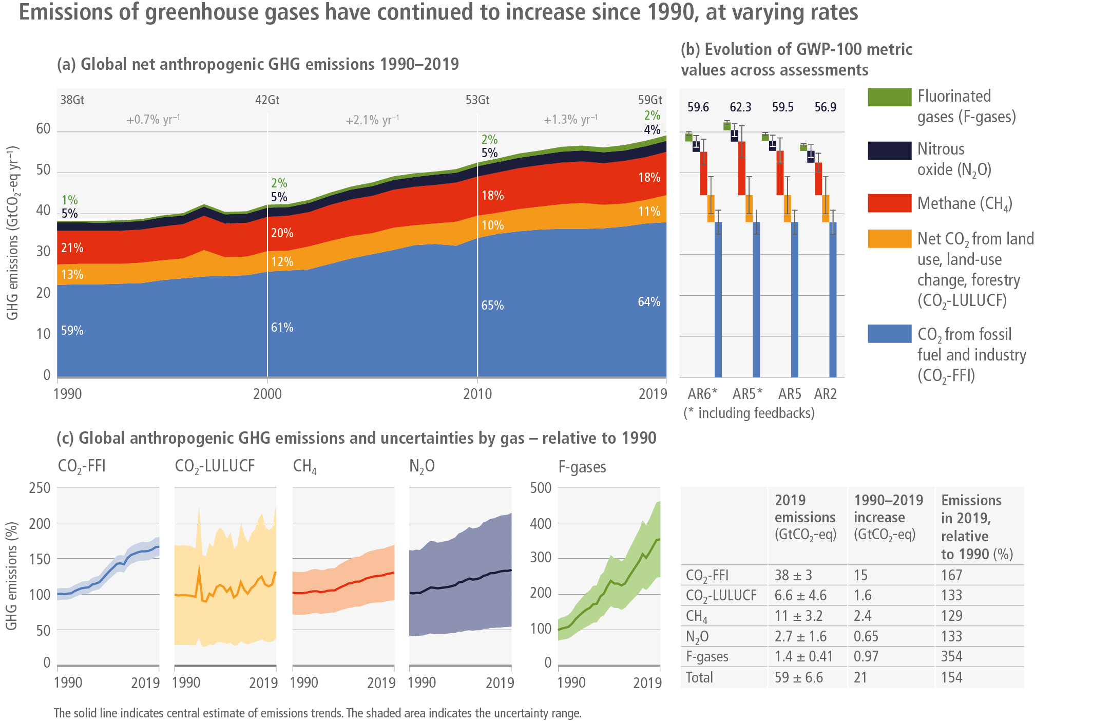
Figure 2.5 | Total anthropogenic GHG emissions (GtCO2-eq yr–1) 1990–2019. CO2 from fossil fuel combustion and industrial processes (FFI); net CO2 from land use, land use change and forestry (LULUCF); methane (CH4); nitrous oxide (N2O); fluorinated gases (F-gases: HFCs, PFCs, SF6, NF3). Panel (a): Aggregate GHG emissions trends by groups of gases reported in GtCO2-eq converted based on global warming potentials with a 100-year time horizon (GWP100) from the IPCC Sixth Assessment Report. Panel (b): Waterfall diagrams juxtaposes GHG emissions for the most recent year (2019) in CO2 equivalent units using GWP100 values from the IPCC’s Second, Fifth, and Sixth Assessment Reports, respectively. Error bars show the associated uncertainties at a 90% confidence interval. Panel (c): individual trends in CO2-FFI, CO2-LULUCF, CH4, N2O and F-gas emissions for the period 1990–2019, normalised to 1 in 1990. Source: data from Minx et al. (2021).
GHG emissions levels in 2019 were higher compared to 10 and 30 years earlier ( high confidence): about 12% (6.5 GtCO2-eq) higher than in 2010 (53 ± 5.7 GtCO2-eq) (the last year of AR5 reporting) and about 54% (21 GtCO2-eq) higher than in 1990 (38 ± 4.8 GtCO2-eq) (the baseline year of the Kyoto Protocol and frequent nationally determined contribution (NDC) reference). GHG emissions growth slowed compared to the previous decade ( high confidence): From 2010 to 2019, GHG emissions grew on average by about 1.3% per year compared to an average annual growth of 2.1% between 2000 and 2009. Nevertheless the absolute increase in average annual GHG emissions for 2010–2019 compared to 2000–2009 was 9.1 GtCO2-eq and, as such, the largest observed in the data since 1970 (Table 2.1) – and most likely in human history (Friedlingstein et al. 2020; Gütschow et al. 2021b). Decade-by-decade growth in average annual GHG emissions was observed across all (groups of) gas as shown in Table 2.1, but for N2O and CO2-LULUCF emissions this is much more uncertain.
Reported total annual GHG emission estimates differ between the WGIII contributions in AR5 (Blanco et al. 2014) and AR6 (this chapter) mainly due to differing global warming potentials ( high confidence). For the year 2010, total GHG emissions were estimated at 49 ± 4.9 GtCO2-eq in AR5 (Blanco et al. 2014), while we report 53 ± 5.7 GtCO2-eq here. However, in AR5 total GHG emissions were weighted based on GWP100 values from IPCC’s Second Assessment Report. Applying those GWP values to the 2010 emissions from AR6 yields 50 GtCO2-eq (Forster et al. 2021a). Hence, observed differences are mainly due to the use of most recent GWP values, which have higher warming potentials for methane (29% higher for biogenic and 42% higher for fugitive methane) and 12% lower values for nitrous oxide (Cross-Chapter Box 2 in this chapter).
Emissions growth has been persistent but varied in pace across gases. The average annual emission levels of the last decade (2010–2019) were higher than in any previous decade for each group of GHGs: CO2, CH4, N2O, and F-gases ( high confidence). Since 1990, CO2-FFI have grown by 67% (15 GtCO2-eq), CH4 by 29% (2.4 GtCO2-eq), and N2O by 33% (0.65 GtCO2-eq), respectively (Figure 2.5). Growth in fluorinated gases (F-gas) has been by far the highest with about 254% (1.0 GtCO2-eq), but it occurred from low levels. In 2019, total F-gas levels were no longer negligible with a share of 2.3% of global GHG emissions. Note that the F-gases reported here do not include CFCs and HCFCs, which are groups of substances regulated under the Montreal Protocol. The aggregate CO2-eq emissions of HFCs, HCFCs and CFCs were each approximately equal in 2016, with a smaller contribution from PFCs, SF6, NF3 and some more minor F-gases. Therefore, the GWP-weighted F-gas emissions reported here (HFCs, PFCs, SF6, NF3), which are dominated by the HFCs, represent less than half of the overall CO2-eq F-gas emissions in 2016 (Figure 2.3).
The only exception to these patterns of GHG emissions growth is net anthropogenic CO2-LULUCF emissions, where there is no statistically significant trend due to high uncertainties in estimates (Figures 2.2 and 2.5; Chapter 2 Supplementary Material). While the average estimate from the bookkeeping models report a slightly increasing trend in emissions, NGHGI and FAOSTAT estimates show a slightly decreasing trend, which diverges in recent years (Figure 2.2). Similarly, trends in CO2-LULUCF estimates from individual bookkeeping models differ: while two models (BLUE and OSCAR) show a sustained increase in emissions levels since the mid-1990s, emissions from the third model (Houghton and Nassikas (HN)) declined (Figure 2.2 in this chapter; Friedlingstein et al. 2020). Differences in accounting approaches and their impacts CO2 emissions estimates from land use is covered in Chapter 7 and in the Chapter 2 Supplementary Material (2.SM.2). Note that anthropogenic net emissions from bioenergy are covered by the CO2-LULUCF estimates presented here.
The CO2-FFI share in total CO2-eq emissions has plateaued at about 65% in recent years and its growth has slowed considerably since AR5 ( high confidence). The CO2-FFI emissions grew at 1.1% during the 1990s and 2.5% during the 2000s. For the last decade (2010s) – not covered by AR5 – this rate dropped to 1.2%. This included a short period between 2014 and 2016 with little or no growth in CO2-FFI emissions, mainly due to reduced emissions from coal combustion (Jackson et al. 2016; Qi et al. 2016; Peters et al. 2017a; Canadell et al. 2021). Subsequently, CO2-FFI emissions started to rise again (Peters et al. 2017b; Figueres et al. 2018; Peters et al. 2020).
Starting in the spring of 2020 a major break in global emissions trends was observed due to lockdown policies implemented in response to the COVID-19 pandemic ( high confidence) (Forster et al. 2020; Le Quéré et al. 2020, 2021; Z. Liu et al. 2020b ; Bertram et al. 2021). Overall, global CO2-FFI emissions are estimated to have declined by 5.8% (5.1%–6.3%) in 2020, or about 2.2 (1.9–2.4) GtCO2 in total (Friedlingstein et al. 2020; Z. Liu et al. 2020b ; BP 2021; Crippa et al. 2021; IEA 2021a). This exceeds any previous global emissions decline since 1970, both in relative and absolute terms (Figure 2.6). Daily emissions, estimated based on activity and power-generation data, declined substantially compared to 2019 during periods of economic lockdown, particularly in April 2020 – as shown in Figure 2.6 – but rebounded by the end of 2020 (medium confidence) (Le Quéré et al. 2020, 2021; Z. Liu et al. 2020b ). Impacts were differentiated by sector, with road transport and aviation particularly affected. Inventories estimate the total power sector CO2 reduction from 2019 to 2020 at 3% (IEA 2021a) and 4.5% (Crippa et al. 2021). Approaches that predict near real-time estimates of the power sector reduction are more uncertain and estimates range more widely, between 1.8% (Le Quéré et al. 2020, 2021), 4.1% (Z. Liu et al. 2020b ) and 6.8% (Bertram et al. 2021); the latter taking into account the over-proportional reduction of coal generation due to low gas prices and merit order effects. Due to the very recent nature of this event, it remains unclear what the exact short- and long-term impacts on future global emissions trends will be.
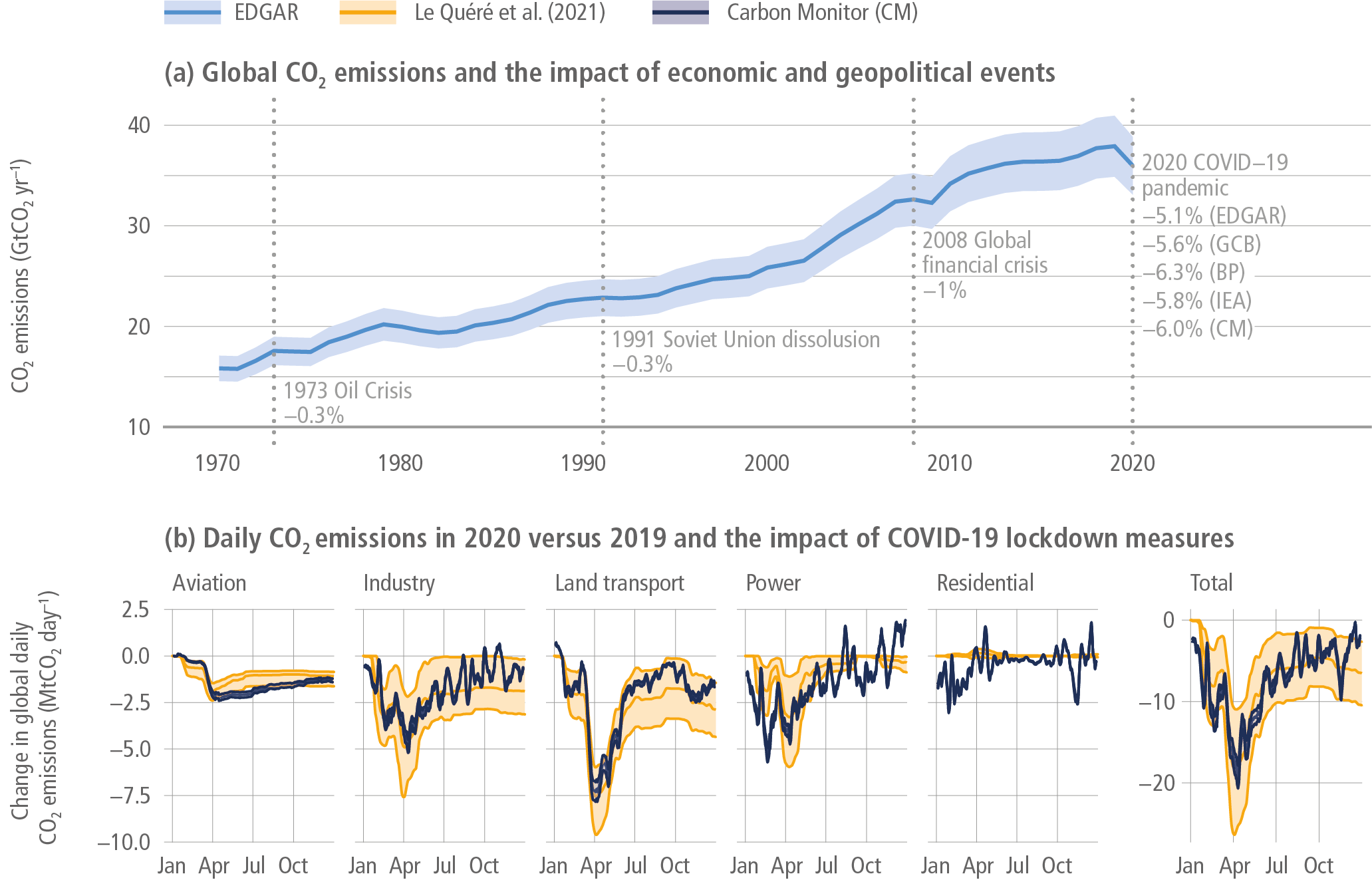
Figure 2.6 | Global CO2 emissions from fossil fuel combustion and industry (FFI) in 2020 and the impact of COVID-19. Panel (a) depicts CO2-FFI emissions over the past five decades (GtCO2 yr –1). The single year declines in emissions following major economic and geopolitical events are shown, as well as the decline recorded in five different datasets for emissions in 2020 (COVID-19) compared to 2019 (no COVID-19). Panel (b) depicts the change in global daily carbon emissions (MtCO2 per day) in 2020 compared to 2019, showing the impact of COVID-19 lockdown policies. Source: Friedlingstein et al. (2020), Le Quéré et al. (2020), Carbon Monitor (Liu et al. 2020b ), BP (2021), Crippa et al. (2021), IEA (2021a).
From 1850 until around 1950, anthropogenic CO2 emissions were mainly (>50%) from land use, land-use change and forestry (Figure 2.7). Over the past half-century CO2 emissions from LULUCF have remained relatively constant around 5.1 ± 3.6 GtCO2 but with a large spread across estimates (Le Quéré et al. 2018 a; Friedlingstein et al. 2019, 2020). By contrast, global annual FFI-CO2 emissions have continuously grown since 1850, and since the 1960s from a decadal average of 11 ± 0.9 GtCO2 to 36 ± 2.9 GtCO2 during 2010–2019 (Table 2.1).
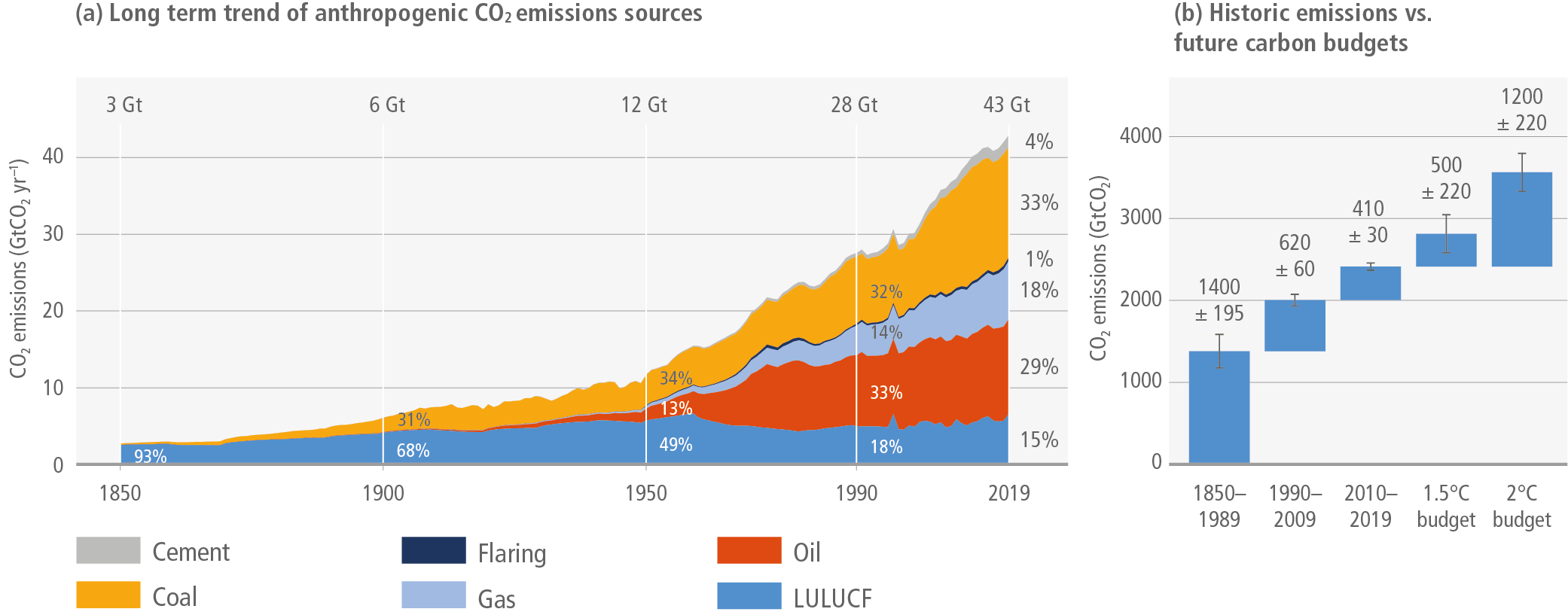
Figure 2.7 | Historic anthropogenic CO2 emission and cumulative CO2 emissions (1850–2019) as well as remaining carbon budgets for limiting warming to 1.5°C and 2°C. Panel (a) shows historic annual anthropogenic CO2 emissions (GtCO2 yr –1) by fuel type and process. Panel (b) shows historic cumulative anthropogenic CO2 emissions for the periods 1850–1989, 1990–2009, and 2010–2019 as well as remaining future carbon budgets as of 1 January 2020 to limit warming to 1.5°C and 2°C at the 67th percentile of the transient climate response to cumulative CO2 emissions. The whiskers indicate a budget uncertainty of ±220 GtCO2-eq for each budget and the aggregate uncertainty range at one standard deviation for historical cumulative CO2 emissions, consistent with Working Group 1. Sources: Friedlingstein et al. (2020) and Canadell et al. (2021).
Cumulative CO2 emissions since 1850 reached 2400 ± 240 GtCO2 in 2019 ( high confidence). 7 More than half (62%) of total emissions from 1850 to 2019 occurred since 1970 (1500 ± 140 GtCO2), about 42% since 1990 (1000 ± 90 GtCO2) and about 17% since 2010 (410 ± 30 GtCO2) (Friedlingstein et al. 2019; Friedlingstein et al. 2020; Canadell et al. 2021) (Figure 2.7). Emissions in the last decade are about the same size as the remaining carbon budget of 400 ± 220 (500, 650) GtCO2 for limiting global warming to 1.5°C and between one-third and half the 1150 ± 220 (1350, 1700) GtCO2 for limiting global warming below 2°C with a 67% (50%, 33%) probability, respectively (medium confidence) (Canadell et al. 2021). At current (2019) levels of emissions, it would only take 8 (2–15) and 25 (18–35) years to emit the equivalent amount of CO2 for a 67th percentile 1.5°C and 2°C remaining carbon budget, respectively. Related discussions of carbon budgets, short-term ambition in the context of Nationally Determined Contributions (NDCs), pathways to limiting warming to well below 2°C and carbon dioxide removals are mainly discussed in Chapters 3, 4, and 12, but also Section 2.7 of this chapter.
Even when taking uncertainties into account, historical emissions between 1850 and 2019 constitute a large share of total carbon budgets from 2020 onwards for limiting warming to 1.5°C with a 50% probability as well as for limiting warming to 2°C with a 67% probability. Based on central estimates only, historical cumulative net CO2 emissions between 1850–2019 amount to about four fifths of the total carbon budget for a 50% probability of limiting global warming to 1.5°C (central estimate about 2900 GtCO2), and to about two thirds of the total carbon budget for a 67% probability to limit global warming to 2°C (central estimate about 3550 GtCO2). The carbon budget is the maximum amount of cumulative net global anthropogenic CO2 emissions that would result in limiting global warming to a given level with a given likelihood, taking into account the effect of other anthropogenic climate forcers. This is referred to as the total carbon budget when expressed starting from the pre-industrial period, and as the remaining carbon budget when expressed from a recent specified date. The total carbon budgets reported here are the sum of historical emissions from 1850 to 2019 and the remaining carbon budgets from 2020 onwards, which extend until global net zero CO2 emissions are reached. Uncertainties for total carbon budgets have not been assessed and could affect the specific calculated fractions (IPCC 2021 [Working Group 1 SPM], Canadell et al., 2021 [Working Group 1 Ch5]).
Comparisons between historic GHG emissions and baseline projections provide increased evidence that global emissions are not tracking high-end scenarios (Hausfather and Peters 2020), and rather followed ‘middle-of-the-road’ scenario narratives in the earlier series, and by combinations of ‘global-sustainability’ and ‘middle-of-the-road’ narratives in the most recent series (IPCC Special Report on Emissions Scenarios (SRES) and Shared Socioeconomic Pathways (SSP)-baselines) (Pedersen et al. 2020; Strandsbjerg Tristan Pedersen et al. 2021). As countries increasingly implement climate policies and technology costs continue to evolve, it is expected that emissions will continually shift away from scenarios that assume no climate policy but remain insufficient to limit warming to below 2°C (Vrontisi et al. 2018; Hausfather and Peters 2020; Roelfsema et al. 2020; UNEP 2020b).
The literature since AR5 suggests that compared to historical trends baseline scenarios might be biased towards higher levels of fossil fuel use compared to what is observed historically (Cross-Chapter Box 1 in Chapter 1; Ritchie and Dowlatabadi 2017, 2018; Ritchie 2019; Creutzig et al. 2021;). Ritchie and Dowlatabadi (2017) show that per-capita primary energy consumption in baseline scenarios tends to increase at rates faster than those observed in the long-term historical evidence – particularly in terms of coal use. For example, SSP5 envisions a six-fold increase in per capita coal use by 2100 – against flat long-term historical observations – while the most optimistic baseline scenario SSP1-Sustainability is associated with coal consumption that is broadly in line with historical long-term trends (Ritchie and Dowlatabadi 2017). In contrast, models have struggled to reproduce historical upscaling of wind and solar and other granular energy technologies (Wilson et al. 2013; van Sluisveld et al. 2015; Creutzig et al. 2017; Shiraki and Sugiyama 2020; Sweerts et al. 2020; Wilson et al. 2020b).
2.2.2.2Other Short-lived Climate Forcers (SLCFs)
There are other emissions with shorter atmospheric lifetimes that contribute to climate changes. Some of them (aerosols, sulphur emissions or organic carbon) reduce forcing, while others – such as black carbon, carbon monoxide or non-methane volatile organic compounds (NMVOC) – contribute to warming (Figure 2.4) as assessed in WGI (Forster et al. 2021c; Szopa et al. 2021a). Many of these other SLCFs are co-emitted during combustion processes in power plants, cars, trucks, airplanes, but also during wildfires and household activities such as traditional cooking with open biomass burning. As these co-emissions have implications for net warming, they are also considered in long-term emission reduction scenarios as covered in the literature (Harmsen et al. 2020; Rauner et al. 2020b; Smith et al. 2020; Vandyck et al. 2020) as well as Chapter 3 of this report. These air pollutants are also detrimental to human health (e.g., Lelieveld et al. 2015, 2018; Vohra et al. 2021). For example, Lelieveld et al. (2015) estimate a total of 3.3 (1.6–4.8) million premature deaths in 2010 from outdoor air pollution. Reducing air pollutants in the context of climate policies therefore leads to substantial co-benefits of mitigation efforts (Von Stechow et al. 2015; Rao et al. 2017; Lelieveld et al. 2019; Rauner et al. 2020a). Here we briefly outline the major trends in emissions of SLCFs.
Conventional air pollutants that are subject to significant emission controls in many countries include sulphur dioxide (SO2), nitrogen oxides (NOx), black carbon (BC) and carbon monoxide (CO). From 2015 to 2019, global SO2 and NOx emissions declined, mainly due to reductions in energy systems (Figure 2.8). Reductions in BC and CO emissions appear to have occurred over the same period, but trends are less certain due to the large contribution of emissions from poorly quantified traditional biofuel use. Emissions of CH4, OC and NMVOC have remained relatively stable in the past five years. OC and NMVOC may have plateaued, although there is additional uncertainty due to sources of NMVOCs that may be missing in current inventories (McDonald et al. 2018).
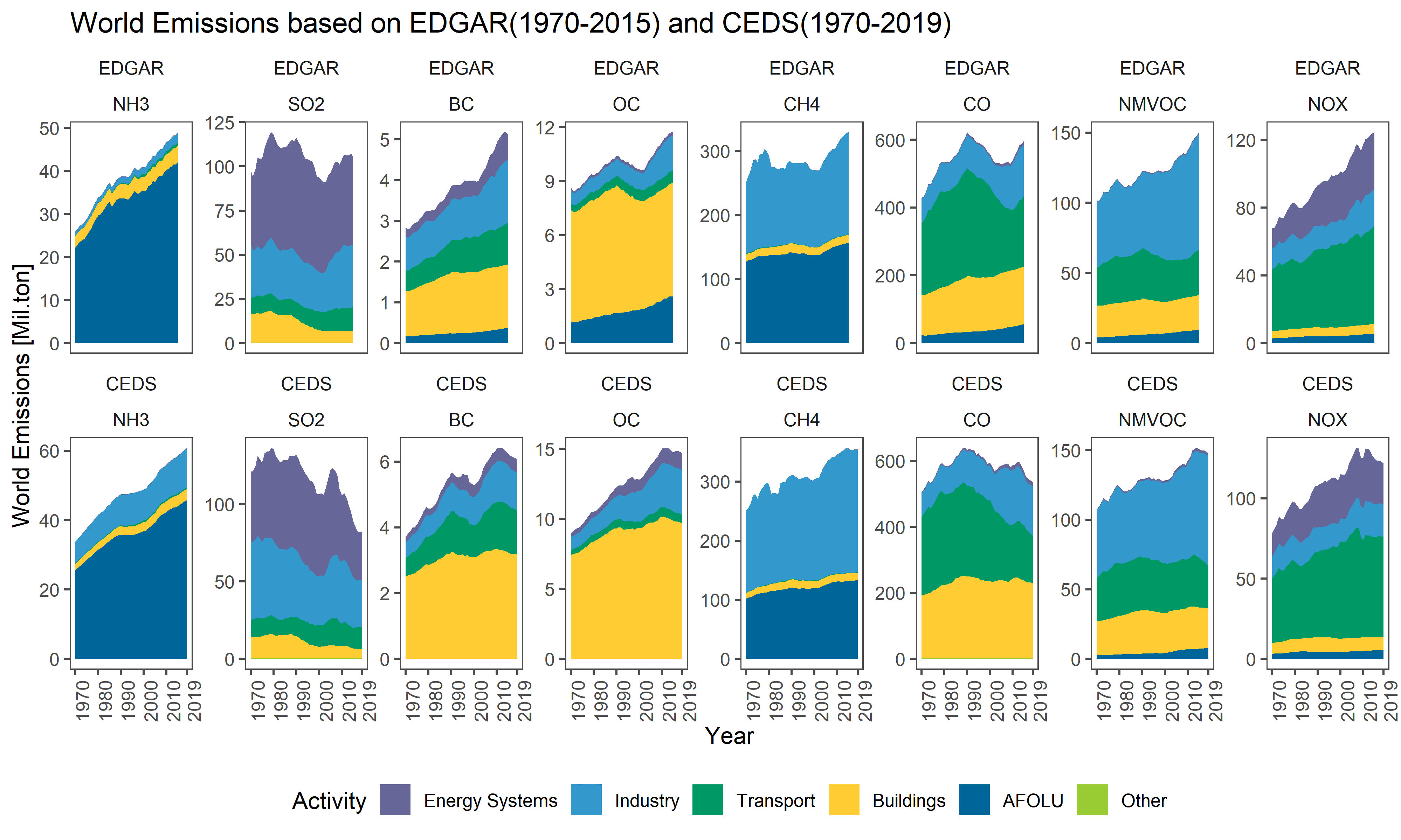
Figure 2.8 | Air pollution emissionsby major sectors from CEDS (1970–2019) and EDGAR (1970–2015) inventories. Source: Crippa et al. (2019a, 2018); O’Rourke et al. (2020); McDuffie et al. (2020).
2.2.3Regional GHG Emissions Trends
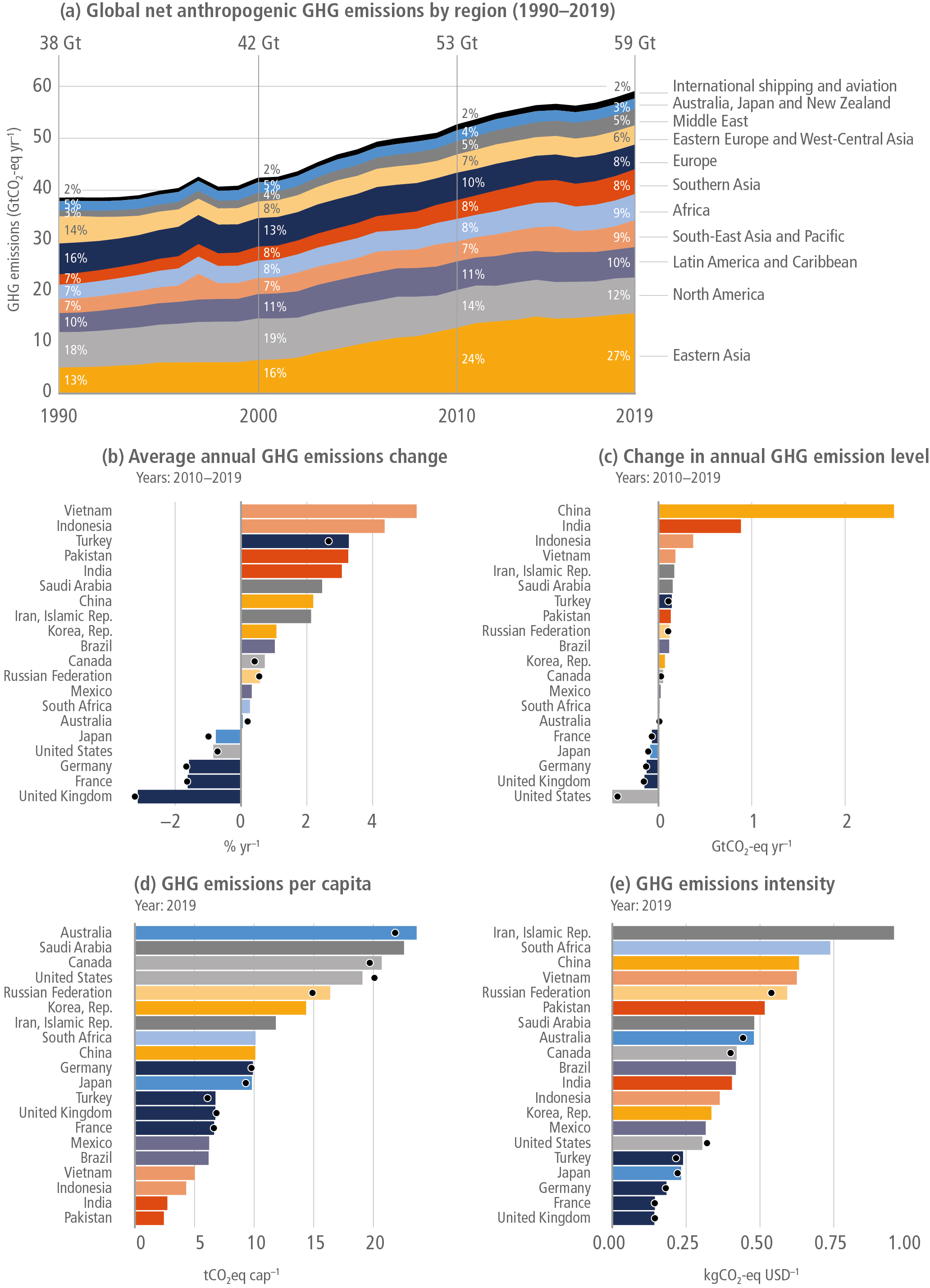
Regional contributions to global GHG emissions have shifted since the beginning of the international climate negotiations in the 1990s ( high confidence). As shown in Figure 2.9, developed countries (North America, Europe, and Australia, Japan, New Zealand) as a group have not managed to reduce GHG emissions substantially, with fairly stable levels at about 15 GtCO2-eq yr –1 between 1990 and 2010, while countries in Asia and Pacific (Eastern Asia, Southern Asia, and South-East Asia and Pacific) have rapidly increased their share of global GHG emissions – particularly since the 2000s (Jackson et al. 2019; Peters et al. 2020; UNEP 2020c; Crippa et al. 2021; IEA 2021b).

Figure 2.9: Change in regional GHGs from multiple perspectives and their underlying drivers. Panel (a): Regional GHG emissions trends (in GtCO2-eq yr –1) for the time period 1990–2019. GHG emissions from international aviation and shipping are not assigned to individual countries and shown separately. Panels (b) and (c): Changes in GHG emissions for the 20 largest emitters (as of 2019) for the post-AR5 reporting period 2010–2019 in relative (% annual change) and absolute terms (GtCO2-eq). Panels (d) and (e): GHG emissions per capita and per GDP in 2019 for the 20 largest emitters (as of 2019). GDP estimated using constant international purchasing power parity (USD2017). Emissions are converted into CO2-equivalents based on global warming potentials with a 100-year time horizon (GWP100) from the IPCC Sixth Assessment Report (Forster et al. 2021a). The black dots represent the emissions data from UNFCCC-CRFs (2021) that were accessed through Gütschow et al. (2021a). Net LULUCF CO2 emissions are included in panel (a), based on the average of three bookkeeping models (Section 2.2), but are excluded in panels (b–e) due to a lack of country resolution.
Most global GHG emission growth occurred in Asia and Pacific, which accounted for 77% of the net 21 GtCO2-eq increase in GHG emissions since 1990, and 83% of the net 6.5 GtCO2-eq increase since 2010. 8 Africa contributed 11% of GHG emissions growth since 1990 (2.3 GtCO2-eq) and 10% (0.7 GtCO2-eq) since 2010. The Middle East contributed 10% of GHG emissions growth since 1990 (2.1 GtCO2-eq) and also 10% (0.7 GtCO2-eq) since 2010. Latin America and the Caribbean contributed 11% of GHG emissions growth since 1990 (2.2 GtCO2-eq), and 5% (0.3 GtCO2-eq) since 2010. Two regions, Developed Countries, and Eastern Europe and West Central Asia, reduced emissions overall since 1990, by –1.6 GtCO2-eq and –0.8 GtCO2-eq, respectively. However, emissions in the latter started to grow again since 2010, contributing to 5% of the global GHG emissions change (0.3 GtCO2-eq).
Average annual GHG emission growth across all regions slowed between 2010 and 2019 compared to 1990–2010, with the exception of Eastern Europe and West Central Asia. Global emissions changes tend to be driven by a limited number of countries, principally the G20 Group (Friedlingstein et al. 2020; UNEP 2020c; Xia et al. 2021). For instance, the slowing of global GHG emissions between 2010 and 2019, compared to the previous decade, was primarily triggered by substantial reductions in GHG emissions growth in China. Ten countries jointly contributed about 75% of the net 6.5 GtCO2-eq yr –1 increase in GHG emissions during 2010–2019, of which two countries contributed more than 50% (Figure 2.9) (see also Minx et al., 2021; Crippa et al., 2021).
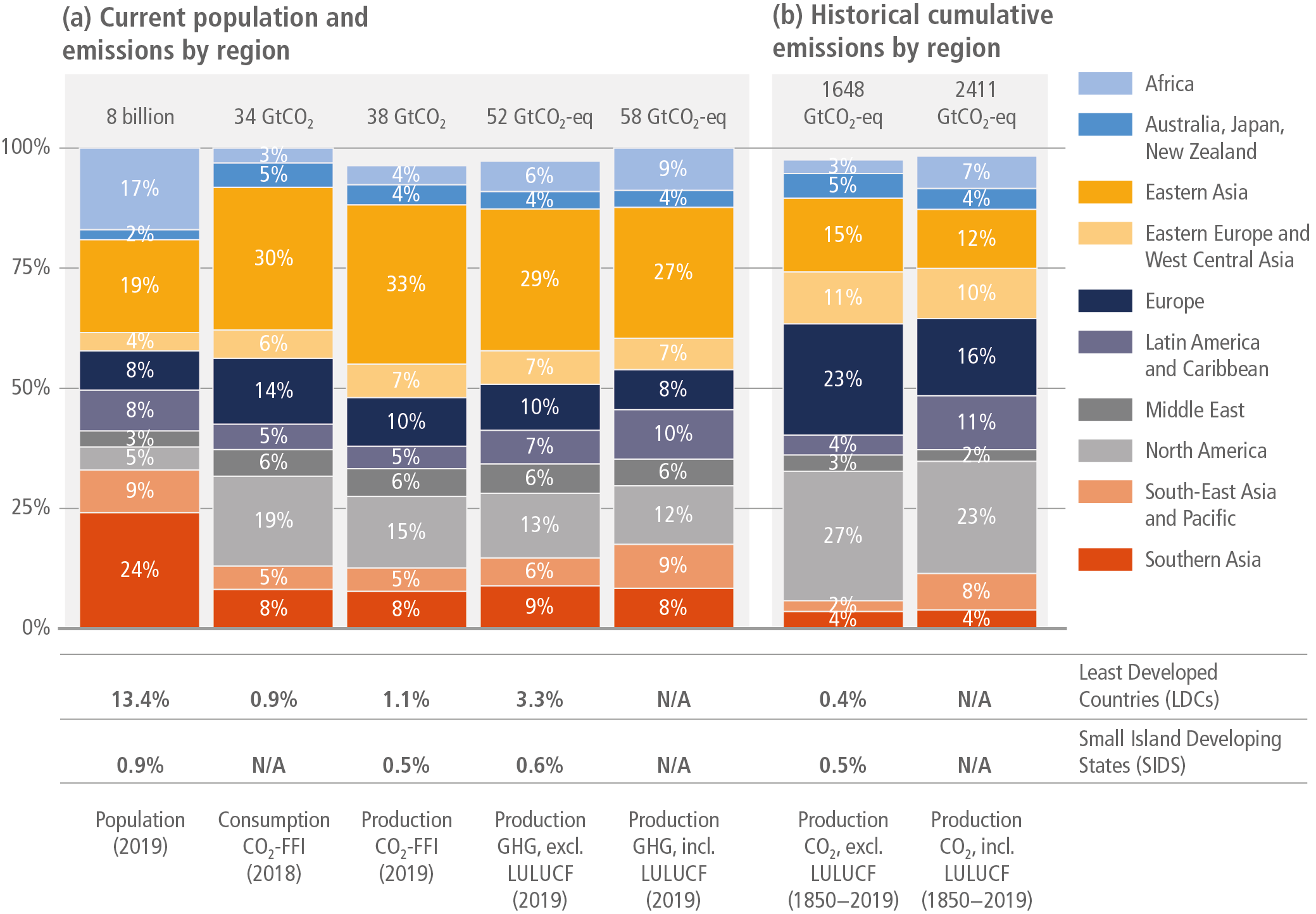
GHG and CO2-FFI levels diverge starkly between countries and regions ( high confidence) (Jackson et al. 2019; Friedlingstein et al. 2020; UNEP 2020c; Crippa et al. 2021). Developed Countries sustained high levels of per capita CO2-FFI emissions at 9.5 tCO2 per capita in 2019 (but with a wide range of 1.9–16 tCO2 per capita). This is more than double that of three developing regions: 4.4 (0.3–12.8) tCO2 per capita in Asia and Pacific; 1.2 (0.03–8.5) tCO2 per capita in Africa; and 2.7 (0.3–24) tCO2 per capita in Latin America. 9 Per capita CO2-FFI emissions were 9.9 (0.89–15) tCO2 per capita in Eastern Europe and West Central Asia, and 8.6 (0.36–38) tCO2 per capita in the Middle East. CO2-FFI emissions in the three developing regions together grew by 26% between 2010 and 2019, compared to 260% between 1990 and 2010, while in Developed Countries emissions contracted by 9.9% between 2010–2019 and by 9.6% between 1990–2010.
Least-Developed Countries and Small Island Developing States contributed only a negligible proportion of historic GHG emissions growth and have the lowest per capita emissions. As of 2019 Least Developed Countries contribute 3.3% of global GHG emissions, excluding LULUCF CO2, despite making up 13% of the global population. Small Island Developing States contributed 0.6% of global GHG emissions in 2019, excluding LULUCF CO2, with 0.9% of the global population. Since the start of the industrial revolution in 1850 up until 2019, Least Developed Countries contributed 0.4% of total cumulative CO2 emissions, while Small Island Developing States contributed 0.5% (Figure 2.10). Conversely, Developed Countries have the highest share of historic cumulative emissions (Rocha et al. 2015; Gütschow et al. 2016; Matthews 2016), contributing approximately 57% (Figure 2.10), followed by Asia and Pacific (21%), Eastern Europe and West Central Asia (9%), Latin America and the Caribbean (4%), the Middle East (3%), and Africa (3%). Developed Countries still have the highest share of historic cumulative emissions (45%) when CO2-LULUCF emissions are included, which typically account for a higher proportion of emissions in developing regions (Figure 2.10).

Figure 2.10 | Different perspectives on historic emissions andequity. Panel (a) shows the regional proportion (%) of total global population or emissions in 2018 or 2019, for five categories: population (persons); consumption-based CO2-FFI emissions (GtCO2); production-based CO2-FFI emissions (GtCO2); production-based GHG emissions excluding CO2-LULUCF (GtCO2-eq); and production-based GHG emissions including CO2-LULUCF (GtCO2-eq). Panel (b) shows the regional proportion (%) of total cumulative production-based CO2 emissions from 1850 to 2019, including and excluding CO2-LULUCF (GtCO2). In the lower panels, the proportion of each population or emissions category attributable to Least-Developed Countries and Small Island Developing States (SIDS) are shown, where available (CO2-LULUCF data is not available for these regions). GHG emissions are converted into CO2-equivalents based on global warming potentials with a 100-year time horizon (GWP100) from the IPCC Sixth Assessment Report (Forster et al. 2021a). Source: data from Friedglinstein et al. (2020).
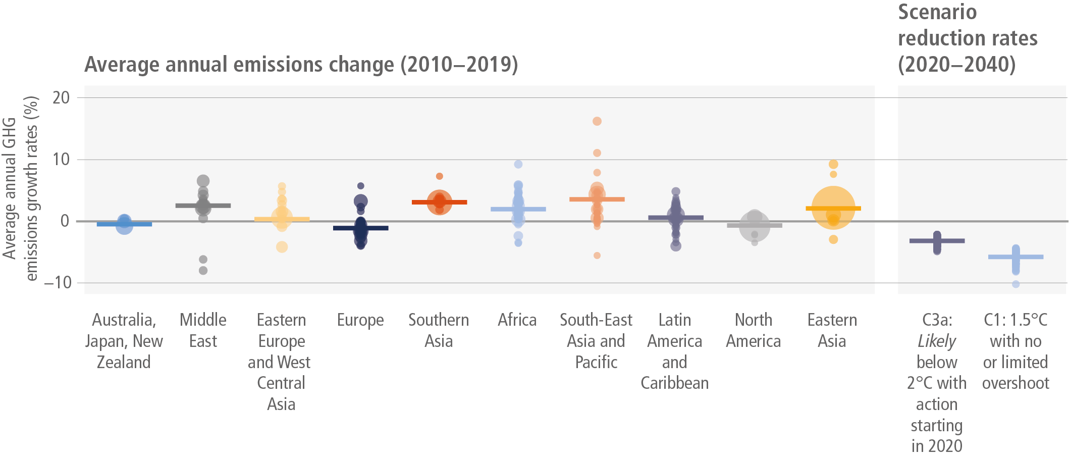
Figure 2.11 | Recent average annual GHG emissions changes of countries (left panel) versus rates of reduction in 1.5°C and 2°C mitigation scenarios. Scenario data is taken from Chapter 3 of this report with the scenario categories defined and summarised in Table 3.2 in Chapter 3. Emissions are converted into CO2-equivalents based on global warming potentials with a 100-year time horizon (GWP100) from the IPCC Sixth Assessment Report (Forster et al. 2021a). Circles indicate countries (left panel) or individual scenarios (right panel), the former scaled by total emissions in 2019. Horizontal lines indicate the region average emissions change (left panel), or scenario category average emissions change (right panel). Source: data from Minx et al. (2021).
A growing number of countries have reduced CO2 and GHG emissions for longer than 10 years ( high confidence) (Le Quéré et al. 2019; Burck et al. 2021; Lamb et al. 2021a; Wu et al. 2021). Data up to 2018 indicates that about 24 countries have reduced territorial CO2 and GHG emissions (excluding LULUCF CO2), as well as consumption-based CO2 emissions, for at least 10 years (Lamb et al. 2021a). Uncertainties in emissions levels and changes over time prevents a precise assessment of reductions in some cases. Of these 24 countries, 12 peaked emissions in the 2000s; six have sustained longer reductions since the 1970s; and six are former members of the Eastern Bloc, where emissions dropped rapidly in the 1990s and continued declining at a slower pace thereafter. Country emissions reductions have been driven by both climate and non-climate policies and factors, including structural changes. To date, most territorial emissions reductions were realised in the electricity and heat sector, followed by industry and buildings, while in many cases transport emissions have increased since countries reached their overall emissions peak (Climate Transparency 2021; Lamb et al. 2021a). One estimate of the total reduction in annual GHG emissions – from peak years to 2018 – sums to 3.2 GtCO2-eq across all decarbonising countries (Lamb et al. 2021a). These reductions have therefore been far outweighed by recent emissions growth. However, climate policy related reductions may be even larger when compared against a counterfactual case of emissions growth across different sectors (Eskander and Fankhauser 2020) (Cross-Chapter Box 1 in Chapter 1; Section 2.8).
The recent (2010–2019) emissions changes of some countries are in line with pathways that limit warming to below 2°C (<67%) ( e.g., –4% average annual reductions) (Figure 2.10). Overall, there are first country cases emerging that highlight the feasibility of sustained emission reductions outside of periods of economic disruption (Lamb et al. 2021a). However, such pathways will need to be taken by many more countries to keep the goals of the Paris Agreement in reach (Höhne et al. 2020; Roelfsema et al. 2020; Kriegler et al. 2018a; den Elzen et al. 2019) as analysed by Chapter 4 of this report. Moreover, observed reductions are not yet consistent and long-term, nor achieved across all sectors, nor fully aligned with country NDC targets (Le Quéré et al. 2019; Lamb et al. 2021a; den Elzen et al. 2019; Burck et al. 2021; Climate Transparency 2021).
2.2.4 Sectoral GHG Emissions Trends
In 2019, 34% (20 GtCO2-eq) of the 59 GtCO2-eq GHG emissions came from the energy sector, 24% (14 GtCO2-eq) from industry, 22% (13 GtCO2-eq) from AFOLU, 15% (8.7 GtCO2-eq) from transport and 6% (3.3 GtCO2-eq) from buildings (Figure 2.12). The relative size of each sector depends on the exact definition of sector boundaries (de la Rue du Can et al. 2015; Lamb et al. 2021b). The largest individual subsector contributing to global GHG emissions in 2019 was electricity and heat generation at 14 GtCO2-eq. This subsector can be reallocated to consuming sectors as indirect (scope 2) emissions to emphasise the role of final energy demand and demand-side solutions in climate change mitigation (Creutzig et al. 2018) (Chapter 5). This increases the emission share of the industry sector to 34% and of the buildings sector to 16%.

Figure 2.12 | Total anthropogenic direct and indirect GHG emissions for the year 2019 (in GtCO2-eq) by sector and subsector. Direct emissions estimates assign emissions to the sector in which they arise (scope 1 reporting). Indirect emissions – as used here – refer to the reallocation of emissions from electricity and heat to the sector of final use (scope 2 reporting). Note that cement refers to process emissions only, as a lack of data prevents the full reallocation of indirect emissions to this sector. More comprehensive conceptualisations of indirect emissions including all products and services (scope 3 reporting) are discussed in Section 2.3 of this chapter. Emissions are converted into CO2-equivalents based on global warming potentials with a 100-year time horizon (GWP100) from the IPCC Sixth Assessment Report. Percentages may not add up to 100 across categories due to rounding at the second significant digit. Source: based on Lamb et al. (2021b); data: Minx et al. (2021).
Average annual GHG emissions growth has been fastest in the transport sector with about 1.8% for the most recent period 2010–2019, followed by direct emissions in the industry sector (1.4%) and the energy sector (1%) (Figure 2.13). This is different to growth patterns observed in the previous decade as reported in AR5 (IPCC 2014a; Blanco et al. 2014). Between 2000 and 2009 fastest GHG emissions growth was observed for industry with 3.4% followed by the energy sector with 2.3%. GHG emissions growth in the transport sector has been stable across both periods at about 1.8%, while direct building emissions growth averaged below 1% during 2010–2019. Ranking of high-emitting subsectors by direct emissions highlights the importance of CO2 emissions from LULUCF (6.6 GtCO2-eq; but with low confidence in magnitude and trend), road transport (6.1 GtCO2-eq), metals (3.1 GtCO2-eq), and other industry (4.4 GtCO2-eq). Overall, some of the fastest growing sources of subsector emissions from 2010 to 2019 have been international aviation (+3.4%), 10 domestic aviation (+3.3%), inland shipping (+2.9%), metals (+2.3%), international shipping (+1.7%), and road transport (+1.7%).
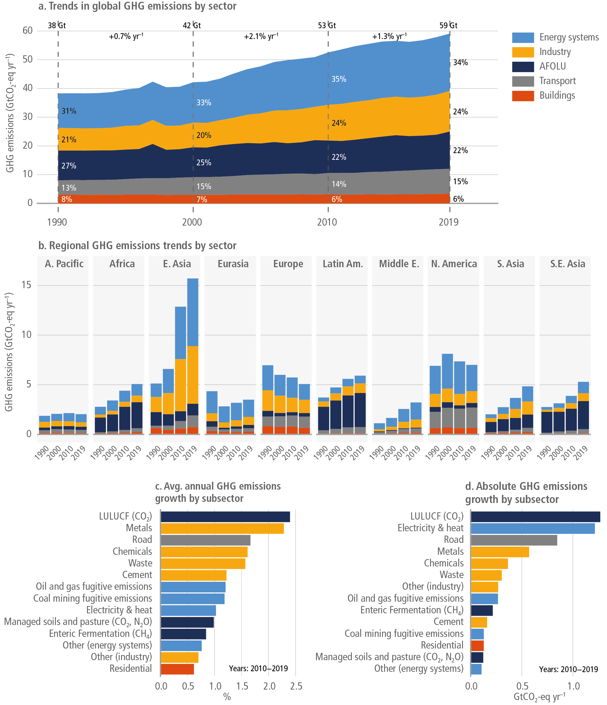
Figure 2.13 | Total annual anthropogenic GHG emissions by major economic sector and their underlying trends by region. Panel (a): Trends in total annual anthropogenic GHG emissions (in GtCO2-eq yr –1) by major economic sector. Panel (b): Trends in total annual anthropogenic GHG emissions (in GtCO2-eq yr –1) by major economic sector and region. Panels c and d: Largest subsectoral changes in GHG emissions for the reporting period 2010–2019 in relative (% annual change) and absolute terms (GtCO2-eq yr –1). Emissions are converted into CO2-equivalents based on global warming potentials with a 100-year time horizon (GWP100) from the IPCC Sixth Assessment Report. Source: based on Lamb et al. (2021b); Data: Crippa et al. (2021); Minx et al. (2021).
2.3Past and Present Trends of Consumption-based CO2 Emissions (CBEs) and Emissions Embodied in Trade
2.3.1 Scope, Variability and Uncertainty of CBEs
Consumption is increasingly met by global supply chains often involving large geographical distances and causing emissions in producing countries (Hubacek et al. 2014, 2016; Wiedmann and Lenzen 2018). Therefore, accounting for emissions from production along the entire supply chain to fulfil final demand, – so-called consumption-based emissions (CBEs), – is necessary to understand why emissions occur and to what extent consumption choices and associated supply chains contribute to total emissions, and ultimately how to influence consumption to achieve climate mitigation targets and environmental justice (Vasconcellos 2020).
Production-based emissions (PBEs) and territorial emissions resulting from the production and consumption of goods and services within a region (for both domestic use and export) are often used by authorities to report carbon emissions (Peters 2008) (Section 2.2). PBEs also include emissions from international activities (e.g., international aviation/shipping and non-resident activities), which are excluded from territorial emissions (Karstensen et al. 2018; Shan et al. 2018). In contrast, CBEs refer to emissions along the entire supply chains induced by consumption, irrespective of the place of production (Liu et al. 2015 b). This reflects a shared understanding that a wider system boundary going beyond territorial emissions is important to avoid outsourcing of pollution and to achieve global decarbonisation. CBEs allow for the identification of new policy levers through information on a country’s trade balance of embodied emissions, households’ carbon implications of their lifestyle choices, companies’ upstream emissions as input for supply chain management, and cities’ footprints outside their administrative boundaries (Davis and Caldeira 2010; Feng et al. 2013). Kander et al. (2015) proposed a technology-adjusted consumption-based emission accounting (TCBA) approach to address the issue of carbon intensity in exports. TCBA incorporates emissions embodied in trade but also adjusted for differences in carbon efficiency in exports of different countries. Unlike PBEs, there are no internationally agreed approaches to calculate CBEs, making it a major drawback for mainstreaming the use of this indicator in policymaking.
There are other proposed emission accounting approaches used in different circumstances. Historical cumulative emissions (HCEs) are used when analysing countries’ historic contribution to emissions and responsibility for emission reduction. HCEs account for a country’s cumulative past emissions, which may be different from the country’s current annual emissions (Botzen et al. 2008; Ritchie 2019), but are sensitive to the choice of cut-off period. For example, the USA and EU-27 countries plus the UK contributed respectively 13.3% and 8.7% to global PBEs in 2019 (Crippa et al. 2020), however, they emitted around 25% and 22% of global historical PBEs since 1751 (Ritchie 2019). Extraction-based emissions (EBEs) accounting allocates all emissions from burning fossil fuels throughout the supply chains to the country where the fuels were extracted (Steininger and Schinko 2015). EBEs can be calculated by multiplying primary energy extraction of fossil fuels with their respective carbon content (Erickson and Lazarus 2013). Another approach for accounting emissions is income-based emission (IBE), which traces emissions throughout all supply chains and allocates emissions to primary inputs (e.g., capital and labour). In other words, IBEs investigate a country’s direct and indirect downstream GHG emissions enabled by its primary inputs (Liang et al. 2017 a). All these approaches provide complementary information and different angles to assigning responsibility for emissions reductions.
Box 2.1 | Policy Applications of Consumption-based Emissions
Consumption-based emissions provide additional or complementary information to production-based emissions that can be used for a variety of policy applications. These include:
•Complementary national-level emissions accounting and target or budget setting
•Raising awareness and increasing understanding of the GHG effects of consumption
•Accounting for and understanding of distributional and responsibility issues in GHG emissions mitigation, both nationally and internationally
•Incentives to change consumption patterns or reduce consumption (e.g., through taxation policies)
•Accounting for and understanding of carbon leakage and emissions embodied in trade*
•International emissions trading schemes or linked national schemes
•Trade policies addressing emissions embodied in trade and international supply chains (e.g., border tax adjustments and clean technology transfers, carbon offsetting or financing, etc.)
•Including embodied emissions in product performance standards and labelling
•Policies of public and private procurement
•Agreements with international suppliers
•Discussing the climate impacts of lifestyles and inequalities in consumption and associated emissions.
The points above are based on a synopsis of studies (Steininger et al. 2014; Afionis et al. 2017; Hubacek et al. 2017b; Wang and Zhou 2018; Bolea et al. 2020).
* Note, however, that comparing embodied emissions in trade between countries is further complicated by the fact that emission intensities differ across countries. Approaches to adjust for these differences and facilitate comparisons have been suggested (Kander et al. 2015; Baumert et al. 2019; Dietzenbacher et al. 2020; Jakob 2021). Many different approaches on how to share responsibility between producers and consumers have been proposed in designing effective integrated global climate policies (Liu and Fan 2017; Khajehpour et al. 2019; Jakob et al. 2021). Ultimately, assigning responsibility is normative.
The dominant method for calculating nations’ CBEs is global multi-region input-output (GMRIO) analysis (Wiedmann and Lenzen 2018). Other frequently used approaches include analysing bilateral trade flows of products and their lifecycle emission factors (Sato 2014). Generally, the uncertainties associated with CBEs depends on the choice of the dataset/model used for calculation, which differs according to: (i) the national economic and trade data used; (ii) the emissions data used; (iii) the sector or product-level aggregation; (iv) the regional aggregation; (v) the conceptual scope (e.g., residential vs territorial accounting principle); and (vi) the model construction techniques, which include table-balancing algorithms and ways of dealing with missing or conflicting data (Moran and Wood 2014; Owen, 2017; Wieland et al. 2018; Wood et al. 2018, 2019). When excluding systematic error sources, research has shown that the stochastic relative standard deviation (RSD) of total national CBEs is not significantly different to that from PBEs accounts and in the region of 5–15% (Wood et al. 2018, 2019).
Six global accounts for consumption-based GHG emissions at the country level are widely used (Table 2.2). Each dataset has been constructed by different teams of researchers, covering different time periods and containing CBEs estimates for different sets of countries and regions (Owen 2017).
Wood et al. (2019) present a comprehensive and systematic model intercomparison and find a variation of 5–10% for both PBE and CBE accounts of major economies and country groups (e.g., EU-28, OECD). The estimates for the USA were the most closely aligned, with 3.7% RSD. For smaller countries, variability is in the order of 20–30% and can reach more than 40% in cases of very small, highly trade-exposed countries such as Singapore and Luxembourg (Wood et al. 2019). It is recommended that CBEs results for such countries be interpreted with care.
Overall, production accounts showed a slightly higher convergence (8% average of RSD) than consumption-based accounts (12%). The variation across model results can be approximately halved, when normalising national totals to one common value for a selected base year. The difference between PBEs result variation (4% average RSD after normalisation) and CBEs results (7%) remains after normalisation.
In general, the largest contributors to uncertainty of CBEs results are – in descending order of priority – the total of territorial GHG emission accounts, the allocation of emissions to economic sectors, the total and composition of final demand, and lastly the structure of the economy. Harmonising territorial emissions across GMRIO datasets is the single most important factor that reduces uncertainty by about 50% (Tukker et al. 2020). More work is required to optimise or even institutionalise the compilation of multi-region input-output data and models to enhance the accuracy of consumption-based accounting (Tukker et al. 2018; Wood et al. 2018).
2.3.2Trends in Global and Regional CBEs Trajectories
In comparison to territorial emissions discussed in Section 2.2, Figure 2.14 shows the trends of global and regional CBEs from 1990 to 2018. This section uses the PBEs and CBEs data from the Global Carbon Budget 2020 (Friedlingstein et al. 2020), which are slightly different from the PBEs used in Section 2.2. The Global Carbon Budget only includes CO2 emissions from fossil fuels and cement production.

Figure 2.14 | Consumption-based CO2 emissions trends for the period 1990–2018. The CBEs of countries are collected from the Global Carbon Budget 2020 (Friedlingstein et al. 2020). Source: this figure is modified based on Hubacek et al. (2021).
The two panels at left in Figure 2.14 show total and per capita CBEs for six regions. The three panels on the right show additional information for the 18 top-emitting countries with the highest CBEs in 2018. In Developed Countries, consumption-based CO2 emissions peaked at 15 GtCO2 in 2007 with a subsequent 16% decline until 2016 (to 12.7 GtCO2) and a slight rebound of 1.6% until 2018 (to 12.9 GtCO2). Asia and Pacific has been a major contributor to consumption-based CO2 emissions growth since 2000 and exceeded Developed Countries as the global largest emissions source in 2015. From 1990 to 2018, the average growth rate of Asia and Pacific was 4.8% per year, while in other regions emissions declined by –1.1%–4.3% per year on average. In 2018, 35% of global consumption-based CO2 emissions were from Developed Countries and 39% from Asia and Pacific, 5% from Latin American and Caribbean, 5% from Eastern Europe and West Central Asia, 5% from Middle East, and 3% from Africa (Hubacek et al. 2021). Global CBEs kept growing over the period with a short-lived decline in 2008 due to the global financial crisis. In 2020, lockdowns associated with COVID-19 significantly reduced global emissions (Section 2.2.2), including CBEs (Shan et al. 2021a).
2.3.3 Decoupling of Emissions from Economic Growth
There has been a long-standing discussion on whether environmental impacts such as carbon emissions and use of natural resources can be decoupled from economic growth. It is controversial whether absolute decoupling can be achieved at a global scale (Ward et al. 2016; Hickel and Kallis 2020; Haberl et al. 2020). However, a number of studies found that it is feasible to achieve decoupling at the national level, and they have explored the reasons for such decoupling (Schandl et al. 2016; Ward et al. 2016; Deutch 2017; Roinioti and Koroneos 2017; Vadén et al. 2020; Habimana Simbi et al. 2021; Shan et al. 2021b).
Table 2.3 shows the extent of decoupling of CBEs and GDP of countries based on CBEs from the Global Carbon Budget (Friedlingstein et al. 2020) and GDP data from the World Bank. Table 2.4 also presents countries’ degree of decoupling of PBEs and GDP. These data allow a comparison of decoupling between GDP and both PBEs and CBEs.
Table 2. 4 | Country groups with different degree of PBE–GDP decoupling from 2015 to 2018.
Number of countries | Absolute decoupling | Relative decoupling | No decoupling | Economic recession | |
32 | 41 | 36 | 6 | ||
CBEs (gigatonnes) | Total | 6.41 | 23.43 | 2.83 | 0.85 |
Global share | 19.1% | 69.9% | 8.4% | 2.5% | |
PBEs (gigatonnes) | Total | 5.33 | 24.36 | 3.04 | 0.84 |
Global share | 15.9% | 72.6% | 9.1% | 2.5% | |
Population (million) | Total | 857 | 4518 | 1213 | 270 |
Global share | 12.5% | 65.9% | 17.7% | 3.9% | |
GDP (billion) | Total | 27091 | 45255 | 4086 | 2997 |
Global share | 34.1% | 57.0% | 5.1% | 3.8% | |
Per capita GDP (1000 USD2010) | Average | 28.83 | 19.53 | 6.00 | 17.78 |
Median | 26.36 | 12.04 | 3.64 | 13.12 | |
Max | 79.23 | 110.70 | 63.93 | 33.11 | |
Min | 1.09 | 0.57 | 0.49 | 5.80 | |
Per capita CBEs (tonnes) | Average | 7.70 | 6.98 | 3.99 | 12.55 |
Median | 6.78 | 6.00 | 1.95 | 11.33 | |
Max | 23.22 | 37.95 | 25.35 | 23.21 | |
Min | 0.43 | 0.09 | 0.18 | 2.33 | |
CBEs intensity (tonnes per 1000 USD2010) | Average | 0.41 | 0.50 | 0.77 | 0.66 |
Median | 0.31 | 0.44 | 0.52 | 0.69 | |
Max | 2.41 | 1.68 | 4.10 | 1.22 | |
Min | 0.12 | 0.10 | 0.20 | 0.21 | |
Per capita PBEs (tonnes) | Average | 6.02 | 5.69 | 4.33 | 14.15 |
Median | 5.36 | 4.88 | 1.67 | 13.22 | |
Max | 20.13 | 16.65 | 39.27 | 27.24 | |
Min | 0.30 | 0.09 | 0.01 | 2.23 | |
PBEs intensity (tonnes per 1000 USD2010) | Average | 0.33 | 0.45 | 0.71 | 0.75 |
Median | 0.20 | 0.31 | 0.44 | 0.68 | |
Max | 1.47 | 1.76 | 4.83 | 1.80 | |
Min | 0.05 | 0.10 | 0.13 | 0.20 | |
Note: CBEs are obtained from the Global Carbon Budget 2020 (Friedlingstein et al. 2020), GDP and population are from the World Bank. One country (Venezuela) does not have GDP data after 2015, so the degree of decoupling was only calculated for 115 countries. In order to be consistent with the results of CBEs, we calculate the decoupling of PBE until 2018.
Absolute decoupling refers to a decline of emissions in absolute terms or as being stable while GDP grows (i.e., a decoupling index 11 greater than 1); relative decoupling refers to growth of emissions being lower than growth of GDP (a decoupling index between 0 and 1); and no decoupling, which refers to a situation where emissions grow to the same extent or faster than GDP (a decoupling index of less than 0) (Wu et al. 2018).
During the most recent three-year period from 2015 to 2018, 23 countries (or 20% of the 116 sample countries) have achieved absolute decoupling of CBEs and GDP, while 32 countries (or 28%) achieved absolute decoupling of PBEs and GDP: 14 of them (e.g., the UK, Japan, and the Netherlands) also decoupled PBEs and GDP. Countries with absolute decoupling of CBEs tend to achieve decoupling at relatively high levels of economic development and high per capita emissions. Most of EU and North American countries are in this group. Decoupling was not only achieved by outsourcing carbon-intensive production, but also improvements in production efficiency and energy mix, leading to a decline of emissions. Structural Decomposition Analysis shows that the main driver for decoupling has been a reduction in carbon intensity (i.e., change in energy mix and energy efficiency) from both domestic production and imports (Hubacek et al. 2021). Similarly, Wood et al. (2020b) found that EU countries have reduced their overall consumption-based GHG emissions by 8% between 1995 and 2016, mainly due to the use of more efficient technology. The literature also shows that changes in the structure of economy with a shift to tertiary sectors of production may contribute to such decoupling (Kanitkar et al. 2015; Jiang et al. 2021).
A total of 67 (or 58%) countries, including China and India, have relatively decoupled GDP and CBEs between 2015 and 2018, reflecting a slower growth in emissions than GDP. It is worth noting that the USA shows relative decoupling of emissions (both CBEs and PBEs) and GDP over the most recent period, although it strongly decoupled economic growth from emissions between 2005 and 2015. Thus decoupling can be temporary and countries’ emissions may again increase after a period of decoupling.
Another 19 (or 16%) countries, such as South Africa and Nepal, have experienced no decoupling between GDP and CBEs from 2015 to 2018, meaning the growth of their GDP is closely tied with the consumption of emission-intensive goods. As a result, a further increase of GDP in these countries will likely lead to higher emissions, if they follow the historical trend without substantive improvement in efficiency of production and energy use.
It is important to note that a country’s degree of decoupling changes over time. For example, 32countries achieved absolute decoupling from 2010 to 2015 but only 10 of them remained decoupled over the next three years. More importantly, although absolute decoupling has reduced annual emissions, the remaining emissions are still contributing to an increase in atmospheric carbon concentration. Absolute decoupling is not sufficient to avoid consuming the remaining CO2 emission budget under the global warming limit of 1.5°C or 2°C and to avoid climate breakdown (Stoknes and Rockström 2018; Hickel and Kallis 2020). Even if all countries decouple in absolute terms this might still not be sufficient and thus can only serve as one of the indicators and steps toward fully decarbonising the economy and society.
2.3.4Emissions Embodied in Trade (EET)
As global trade patterns have changed over recent decades, so have emissions embodied in trade (EET) (Jiang & Green 2017). EET refers to emissions associated with production of traded goods and services and is equal to the difference between PBEs and CBEs (Wiebe and Yamano 2016). EET includes two parts: emissions embodied in imports (EEI); and emissions embodied in exports (EEE). For a given country or region with CBEs higher than PBEs, it is a net importer with a higher EEI than EEE, and vice versa.
EET have been rising faster since the 1980s due to an increase in trade volume (Xu and Dietzenbacher 2014; Wood et al. 2018). CO2 emissions from the production of internationally traded products peaked in 2006 at about 26% of global CO2 emissions. Since then, international CO2 emissions transfers declined but are likely to remain an important part of the climate policy agenda (Wood et al. 2020a). About 24% of global economic output and 25% of global CO2 emissions are embodied in the international trade of goods and services as of 2014 (Hubacek et al. 2021).
2.3.4.1Net Emission Transfers
Located downstream in global supply chains, developed countries (mostly in Western Europe and North America) tend to be net emission importers, that is, EEI are larger than EEE. For example, over 40% of national CO2 footprints in France, Germany, Italy, and Spain are from imports (Fan et al. 2017). Developing countries tend to be net emission exporters with higher PBEs than their CBEs (Peters et al. 2011a), especially for Asia and Pacific (as shown in Figure 2.15). That is to say, there is a net emission transfer and outsourcing of carbon-intensive production from developed to developing economies via global trade (Jiang et al. 2018 ), mainly caused by cheap labour costs (Tate and Bals 2017) and cheap raw materials (Mukherjee 2018). Increasing openness to trade (Fernández-Amador et al. 2016) and less stringent environmental legislation (acting as so-called pollution havens) are also possible reasons (Hoekstra et al. 2016; Malik and Lan 2016; Banerjee and Murshed 2020).
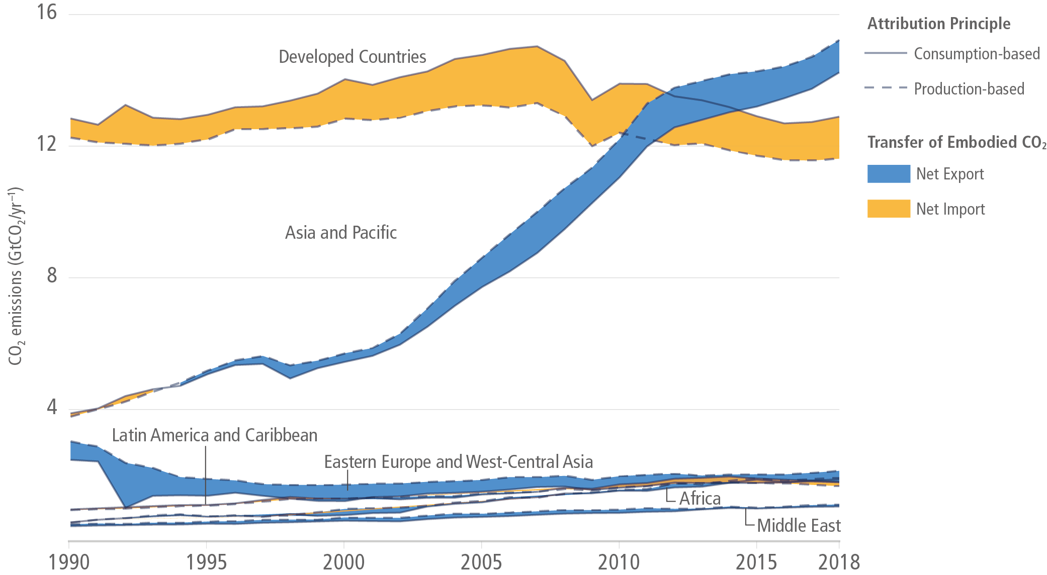
Figure 2.15 | Total annual CO2 emissions for 116 countries by global region based on consumption- and production-based emissions. The shaded areas are the net CO2 trade balances (differences) between each of the regions. Yellow shading indicates that the region is a net importer of embodied CO2 emissions, leading to consumption-based emission estimates that are higher than traditional territorial emission estimates. Blue shading indicates the reverse. Production-based emissions are collected from EDGAR and consumption-based emissions from the Global Carbon Budget 2020 (Friedlingstein et al. 2020). Source: this figure is modified based on Hubacek et al. (2021).
Net emissions transferred between developing and developed countries peaked at 7.3% of global CO2 emissions in 2006 and then subsequently declined (Wood et al. 2020a). The main reason for the decline was an improvement in the carbon intensity of traded products, rather than a decline in trade volume (Wood et al. 2020a). Despite continued improvements, developing economies tend to have higher emission intensity than developed economies due to less efficient technologies and a carbon-intensive fuel mix (Jiang and Guan 2017).
2.3.4.2Geographical Shifts of Emissions Embodied in Trade
With the rapid growth of developing countries, the geographical centre of global trade as well as emissions embodies in trade is changing. The fast growth of Asian countries is shifting the global trade centre from Europe to Asia (Zhang et al. 2019). Asian exports in monetary units increased by 235% from 1996 to 2011, and its share in global exports increased from 25% to 46%, whereas Europe’s share in global exports decreased from 51% in 1996 to 39% in 2011. After 2011, global trade has stalled, but Asia’s share of global exports further increased to 42% in 2020 (UNCTAD 2021).
In addition to changes in trade volume, trading patterns have also been changing significantly in Asian countries. These countries are replacing traditional trading hubs (such as Russia and Germany) due to the fast growth in trade flows, especially with countries of the Global South (Zhang et al. 2019). The largest geographical shifts in trade-embodied emissions between 1995 and 2011 occurred in high-tech, electronics, and machinery (Malik and Lan 2016; Jiang et al. 2018 ). For example, China is shifting its exports to include more low-carbon and higher value-added goods and services. As a result, China’s exported emissions declined by 20% from 2008 to 2015 (Mi et al. 2018).
Developing countries are increasingly playing an important role in global trade. EET between developing countries, so-called South-South trade, has more than doubled between 2004 (0.47 Gt) and 2011 (1.11 Gt), which is seen as a reflection of a new phase of globalisation (Meng et al. 2018). Developing countries, therefore, have gained importance as global suppliers of goods and services and have also become more relevant as global consumers as they grow their domestic demand (Fernández-Amador et al. 2016). Since 2014, CO2 emission transfer between developing countries has plateaued and then slightly declined and seems to have stabilised at around the same level of transfers between non-OECD and OECD countries at around 2.4 GtCO2 yr –1 (Wood et al. 2020a). In both cases, a decrease in carbon intensity of trade just about offset increased trade volumes (Wood et al. 2020a).
2.4 Economic Drivers and Their Trends by Regions and Sectors
This section provides a summary of the main economic drivers of GHG emissions (mostly territorial) by regions and sectors, including those that are more indirect drivers related to economic activity, such as inequality and rapid urbanisation. Trade as a driver of global GHG emissions is described in the Chapter 2 Supplementary Material. Socio-demographic drivers are described in Section 2.6. The Kaya decomposition presented in this section is based on the International Energy Agency (IEA) and Emissions Database for Global Atmospheric Research (EDGAR) v6 databases and tracks global, regional, and sectoral GHG emissions from 1990 to 2019 (Crippa et al. 2021; IEA 2021c; Lamb et al. 2021b; Minx et al. 2021). It shows main contributors to GHG emissions as independent factors, although these factors also interact with each other.
2.4.1Economic Drivers at Global and Regional Levels
Economic growth (measured as GDP) and its main components – GDP per capita and population growth – remained the strongest drivers of GHG emissions in the last decade, following a long-term trend (robust evidence, high agreement ) (Liddle 2015; Malik et al. 2016; Sanchez and Stern 2016; Chang et al. 2019; Dong et al. 2019; Liobikiene and Butkus 2019; Liu et al. 2019a; Mardani et al. 2019; Pan et al. 2019; Dong et al. 2020; Parker and Bhatti 2020; Xia et al. 2021). Globally, GDP per capita remained by far the strongest upward driver, increasing almost in tandem with energy consumption and CO2 emissions up until 2015, after which some modest decoupling occurred (Deutch 2017; Wood et al. 2018) (Section 2.3.3). The main counteracting, yet insufficient, factor that led to emissions reductions was decreased energy use per unit of GDP in almost all regions (–2.0% yr –1 between 2010 and 2019 globally) (see also Lamb et al. 2021b) (Figure 2.16) (robust evidence, high agreement ). These reductions in energy intensity are a result of technological innovation, structural changes, regulation, fiscal support, and direct investment, as well as increased economic efficiency in underlying sectors (Yao et al. 2015; Sanchez and Stern 2016; Chang et al. 2019; Dong et al. 2019a; Mohmmed et al. 2019; Stern 2019; Azhgaliyeva et al. 2020; Goldemberg 2020; Gao et al. 2021; Liddle and Huntington 2021; Liu et al. 2019b; Xia et al. 2021).

Figure 2.16 | Trends and drivers of global GHG emissions, including: (a) trends of GHG emissions by sectors 1990–2019; (b) share of total and per capita GHG emissions by world region in 2019; and (c) Kaya decomposition of CO2 emissions drivers. The Kaya decomposition is based on the equation F = P(G/P)(E/G)(F/E), where F is CO2 emissions, P is population, G/P is GDP per capita, E/G is the energy intensity of GDP and F/E is the carbon intensity of energy. The indicated annual growth rates are averaged across the years 2010–2019 (in panel (c), these are for fossil fuel CO2 emissions only, in order to ensure compatibility with underlying energy data). Note that the energy consumption by itself (primary energy supply) is not part of the decomposition, but is listed here for comparison with the Kaya factors. Source: data from Crippa et al. (2021), IEA (2021c), Minx et al. (2021).
The decades-long trend that efficiency gains were outpaced by an increase in worldwide GDP (or income) per capita continued unabated in the last 10 years (robust evidence, high agreement ) (Wiedmann et al. 2020; Xia et al. 2021). In addition, the emissions-reducing effects of energy efficiency improvements are diminished by the energy rebound effect, which has been found in several studies to largely offset any energy savings (robust evidence, high agreement ) (Rausch and Schwerin 2018; Colmenares et al. 2020; Stern 2020; Brockway et al. 2021; Bruns et al. 2021). The rebound effect is discussed extensively in Section 9.9.2.
A significant decarbonisation of the energy system was only noticeable in North America, Europe and Eurasia. Globally, the amount of CO2 per unit of energy used has practically remained unchanged over the last three decades (Tavakoli 2018; Chang et al. 2019), although it is expected to decrease more consistently in the future (Xia et al. 2021). Population growth has also remained a strong and persistent upward driver in almost all regions (+1.2% yr –1 globally from 2010 to 2019) (Lamb et al. 2021) (Figure 2.16), although per capita emission levels are very uneven across world regions. Therefore, modest population increases in wealthy countries may have a similar impact on emissions as high population increases in regions with low per capita emission levels.
Developing countries remained major accelerators of global CO2 emissions growth since 2010, mostly driven by increased consumption and production, in particular in East Asia (robust evidence, high agreement ) (Jiborn et al. 2020). While energy intensity declined to a similar extent in countries of the Organisation for Economic Co-operation and Development (OECD) and non-OECD countries over the last 30 years, economic growth has been much stronger in non-OECD countries (González-Torres et al. 2021). This led to an average annual growth rate of 2.8% of CO2 emissions in these countries, whereas they decreased by 0.3% yr –1 in OECD countries (UNEP 2019). The majority of developed economies reduced both production-based and consumption-based CO2 emissions modestly (Jiborn et al. 2020; Xia et al. 2021). This was due to slower economic growth, increased energy efficiency (less energy per unit of GDP), fuel switching from coal to gas (mostly in North America) (Wang et al. 2020 b), and the use of less and cleaner energy from renewables in Europe (Peters et al. 2017; Karstensen et al. 2018; Chang et al. 2019; Wood et al. 2019 c).
Economic growth as the main driver of GHG emissions is particularly strong in China and India (robust evidence, high agreement ) (Liu et al. 2019b; Ortega-Ruiz et al. 2020; Z. Wang et al. 2020 b; Yang et al. 2020; Zheng et al. 2020; Xia et al. 2021), although both countries show signs of relative decoupling because of structural changes (Marin and Mazzanti 2019). A change in China’s production structure (with relatively less heavy industry and lower-carbon manufacturing) and consumption patterns (i.e., the type of goods and services consumed) has become the main moderating factor of emissions after 2010, while economic growth, consumption levels, and investment remain the dominating factors driving up emissions (Wang and Jiang 2019; Jiborn et al. 2020; Zheng et al. 2020). In India, an expansion of production and trade as well as a higher energy intensity between 2010 and 2014 caused increased emissions (Kanitkar et al. 2015; Wang and Zhou 2020; Z. Wang et al. 2020 b).
2.4.2Sectoral Drivers
GHG emissions continued to rise since 2010 across all sectors and subsectors, most rapidly in electricity production, industry, and transport. Decarbonisation gains from improvements in energy efficiency across different sectors and worldwide have been largely wiped out by increases in demand for goods and services. Prevailing consumption patterns have also tended to aggravate energy use and emissions, with the long-term trend led by developed regions. Decarbonisation trends in some developed regions are limited in size and geographically. Globally, there are enormous unexploited mitigation potentials from adopting best available technologies.
The following subsections discuss main emissions drivers by sector. More detailed analyses of sectoral emissions and mitigation options are presented in Chapters 6–11.
2.4.2.1Energy Systems
Global energy system emissions growth has slowed down in recent years, but global oil and gas use was still growing (Jackson et al. 2019) and the sector remained the single largest contributor to global GHG emissions in 2019 with 20 GtCO2-eq (34%) ( high confidence) (Figure 2.17). Most of the 14 GtCO2-eq from electricity and heat generation (23% of global GHG emissions in 2019) were due to energy use in industry and in buildings, making these two sectors also prominent targets for mitigation (Davis et al. 2018; Crippa et al. 2019) (see subsections 2.4.2.2 and 2.4.2.3 below).
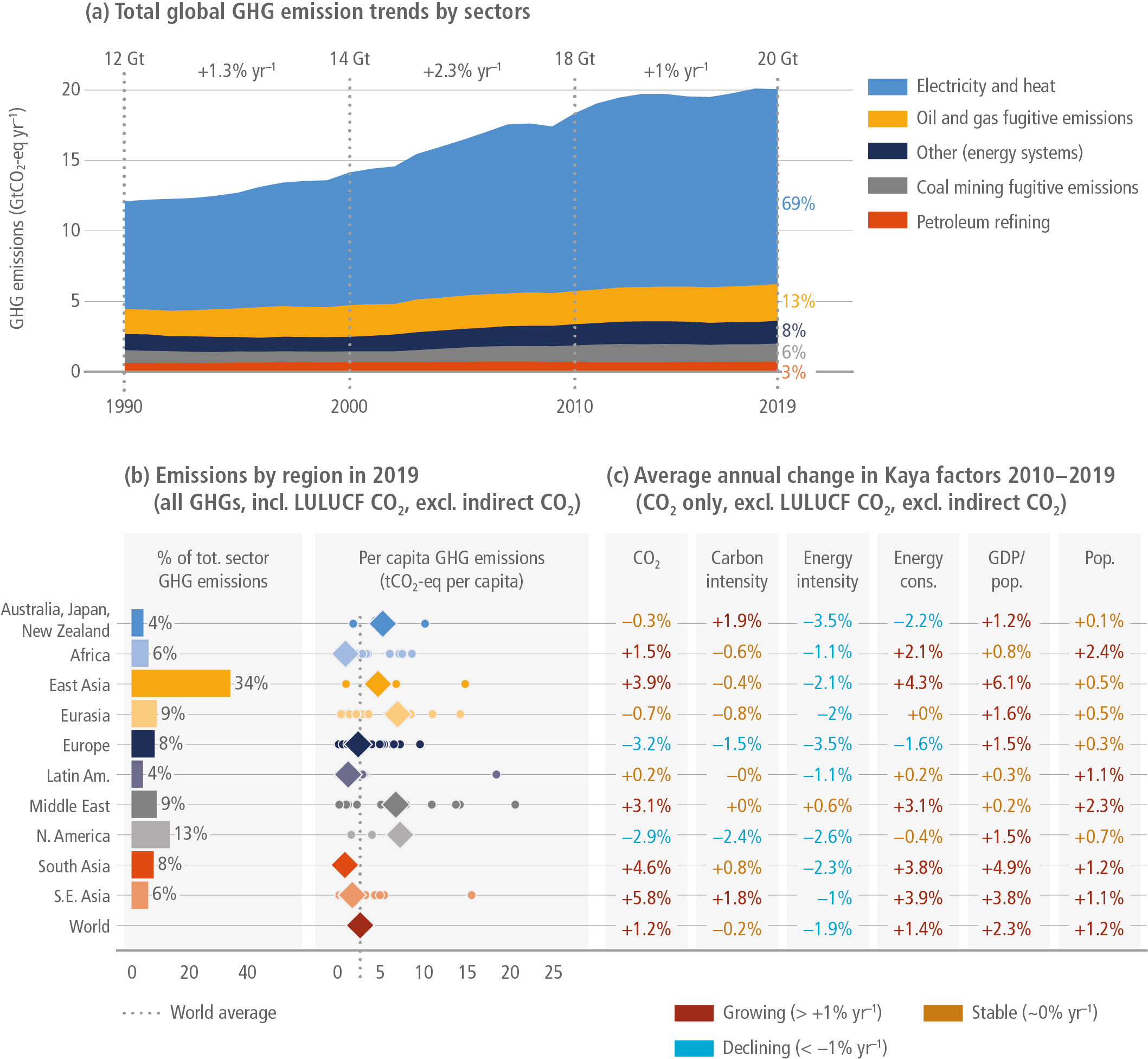
Figure 2.17 | Trends and drivers of global energy sector emissions (see Figure 2.16 caption for details) with energy measured as primary energy supply.
Growth in CO2 emissions from energy systems has closely tracked rising GDP per capita globally (Lamb et al. 2021b), affirming the substantial literature describing the mutual relationship between economic growth and demand for energy and electricity (robust evidence, high agreement ) (Khanna and Rao 2009; Stern, 2011). This relationship has played out strongly in developing regions, particularly in Asia, where a massive scale up of energy supply has accompanied economic growth – with average annual increases of energy demand between 3.8–4.3% in 2010–2019 (Figure 2.17). The key driver for slowing the growth of energy systems CO2 emissions has been declining energy intensities in almost all regions. Annually, 1.9% less energy per unit of GDP was used globally between 2010 and 2019.
The carbon intensity of power generation varies widely between (and also within) regions (Chapter 6). In North America, a switch from coal to gas for power generation (Peters et al. 2017, 2020; Feng 2019; Mohlin et al. 2019) as well as an overall decline in the share of fossil fuels in electricity production (from 66% in 2010 to 59% in 2018) (Mohlin et al. 2019) has decreased carbon intensity and CO2 emissions. Since 2007, Europe’s carbon intensity improvements have been driven by the steady expansion of renewables in the share of electricity generation (medium evidence, high agreement ) (Peters et al. 2017, 2020; Le Quéré et al. 2019; Rodrigues et al. 2020). Some studies attribute these effects to climate policies, such as the carbon floor price in the UK, the EU emissions trading scheme, and generous renewable energy subsidies across the continent (Dyrstad et al. 2019; H. Wang et al. 2020). South-East Asian developed countries and Australia, Japan and New Zealand stand out in contrast to other developed regions, with an increase of regional carbon intensity of 1.8 and 1.9% yr –1, respectively (Figure 2.17). Generally, the use of natural gas for electricity production is growing strongly in most countries and gas has contributed to the largest increase in global fossil CO2 emissions in recent years (Jackson et al. 2019; Peters et al. 2020). Furthermore, gas brings the risk of increased methane (CH4) emissions from fugitive sources, as well as large cumulative emissions over the lifetime of new gas power plants that may erase early carbon intensity reductions (Shearer et al. 2020).
The growth of emissions from coal power slowed after 2010, and even declined between 2011 and 2019, primarily due to a slowdown of economic growth and fewer coal capacity additions in China (Friedlingstein et al. 2019; Peters et al. 2020). Discussions of a global ‘peak coal’, however, may be premature, as further growth was observed in 2019 (Friedlingstein et al. 2019; Peters et al. 2020). Large ongoing and planned capacity increases in India, Turkey, Indonesia, Vietnam, South Africa, and other countries has become a driver of thermal coal use after 2014 (UNEP 2017; Edenhofer et al. 2018; Steckel et al. 2019).
2.4.2.2Industry Sector
When indirect emissions from electricity and heat production are included, industry becomes the single highest emitting sector of GHGs (20.0 GtCO2-eq in 2019) ( high confidence). Facilitated by globalisation, East Asia has been the main source and primary driver of global industry emissions growth since 2000 (robust evidence, high agreement ) (Lamb et al. 2021). However, while East Asia has emitted 45% of the world’s industry GHG emissions in 2019, a remarkable decrease of 5.0% yr –1 in energy intensity and 1.6% in carbon intensity helped to stabilise direct industrial CO2 emissions in this region (–0.3% yr –1 between 2010 and 2019; Figure 2.18). Direct industry CO2 emissions have also declined in Latin America, Europe and Australia, Japan and New Zealand, and – to a smaller extent – in North America. In all other regions, they were growing – most rapidly in southern Asia (+4.3% annually for direct CO2 emissions since 2010) (Figure 2.18).
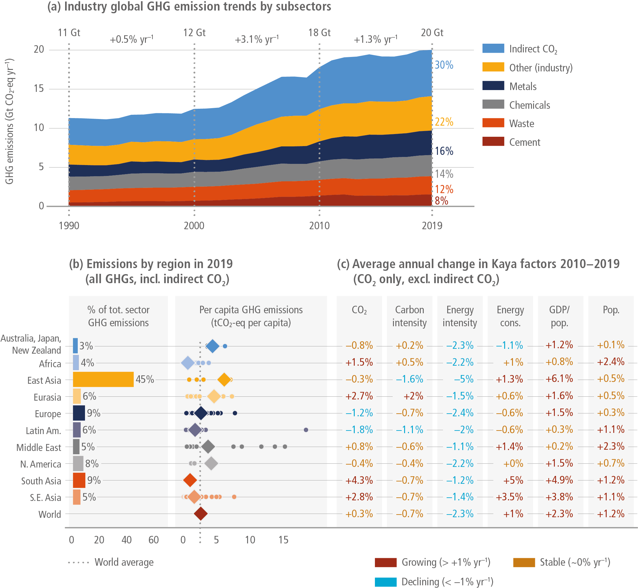
Figure 2.18 | Trends and drivers of global industry sector emissions (see Figure 2.16 caption for details) with energy measured as total final energy consumption.
The main global driver of industry emissions has been a massive rise in the demand for products that are indirectly used in production, such as cement, chemicals, steel, aluminium, wood, paper, plastics, lubricants, fertilisers, and so on. This demand was driven by economic growth, rising affluence, and consumption, as well as a rapid rise in urban populations and associated infrastructure development (robust evidence, high agreement ) (Krausmann et al. 2018). There is strong evidence that the growing use of concrete, steel, and other construction materials is particularly tightly coupled to these drivers (Pauliuk et al. 2013; Cao et al. 2017; Krausmann et al. 2017; Plank et al. 2018; Haberl et al. 2020). Per capita stocks of cement and steel show a typical pattern of rapid take-off as countries urbanise and industrialise, before slowing down to low growth at high levels of GDP. Hence, in countries that have recently been industrialising and urbanising – that is Eastern, Southern and South-Eastern Asia – a particularly strong increase of emissions from these subsectors can be observed. Selected wealthy countries seem to stabilise at high per capita levels of stocks, although it is unclear if these stabilisations persist and if they result in significant absolute reductions of material use (Wiedenhofer et al. 2015; Cao et al. 2017; Krausmann et al. 2018). Opportunities for prolonging lifetimes and improving end of life recycling in order to achieve absolute reductions in extraction activities are as yet unexploited (Krausmann et al. 2017; Zink and Geyer, 2017).
On the production side, improvements in the efficiency of material extraction, processing, and manufacturing have reduced industrial energy use per unit of output (J. Wang et al. 2019 ). These measures, alongside improved material substitution, lightweight designs, extended product and servicing lifetimes, improved service efficiency, and increased reuse and recycling will enable substantial emissions reductions in the future (Hertwich et al. 2019). In absence of these improvements in energy intensity, the growth of population and GDP per capita would have driven the industrial CO2 emissions to rise by more than 100% by 2017 compared with 1990, instead of 56% (Lamb et al. 2021b). Nonetheless, many studies point to deep regional differences in efficiency levels and large globally unexploited potentials to improve industrial energy efficiency by adopting best available technologies and practices for metal, cement, and chemical production (Gutowski et al. 2013; Schulze et al. 2016; Hernandez et al. 2018; Talaei et al. 2018).
2.4.2.3Buildings Sector
Global direct and indirect GHG emissions from the buildings sector reached 9.7 GtCO2-eq in 2019, or 16% of global emissions). Most of these emissions (66%, or 6.4 GtCO2-eq) were upstream emissions from power generation and commercial heat (Figure 2.19). The remaining 33% (3.3 GtCO2-eq) of emissions were directly produced in buildings, for instance by gas and coal boilers, and cooking and lighting devices that burn kerosene, biomass, and other fuels (Lamb et al. 2021). Residential buildings accounted for the majority of this sector’s emissions (64%, 6.3 GtCO2-eq, including both direct and indirect emissions), followed by non-residential buildings (35%, 3.5 GtCO2-eq) ( high confidence).

Figure 2.19 | Trends and drivers of global buildings sector emissions (see Figure 2.16 caption for details) with energy measured as total final energy consumption.
Global buildings sector GHG emissions increased by 0.7% yr –1 between 2010 and 2019 (Figure 2.19), growing the most in absolute terms in East and South Asia, whereas they declined the most in Europe, mostly due to the expansion of renewables in the energy sector and increased energy efficiency (Lamb et al. 2021). North America has the highest per capita GHG emissions from buildings and the second highest absolute level after East Asia (Figure 2.19).
Rising wealth has been associated with more floor space being required to service growing demand in the retail, office, and hotel sectors (medium evidence, high agreement ) (Daioglou et al. 2012; Deetman et al. 2020). In addition, demographic and social factors have driven a cross-national trend of increasing floor space per capita. As populations age and decrease in fertility, and as individuals seek greater privacy and autonomy, households declined in size, at least before the COVID-19 pandemic (Ellsworth-Krebs 2020). These factors led to increased floor space per capita, even as populations stabilise. This in turn is a key driver for building sector emissions, because building characteristics such as size and type, rather than occupant behaviour, tend to explain the majority of energy use within dwellings (Guerra Santin et al. 2009; Ürge-Vorsatz et al. 2015; Huebner and Shipworth 2017) (Chapter 9).
Energy activity levels further drive regional differences. In Eurasia, Europe and North America, thermal demands for space heating dominate building energy use, at 66%, 62% and 48% of residential energy demand, respectively (IEA 2020a). In contrast, cooking has a much higher share of building energy use in regions of the Global South, including China (Cao et al. 2016). And, despite temperatures being on average warmer in the Global South, electricity use for cooling is a more prominent factor in the Global North (Waite et al. 2017). This situation is changing, however, as rapid income growth and demographic changes in the Global South enable households to heat and cool their homes (Ürge-Vorsatz et al. 2015, 2020).
Steady improvements in building energy intensities across regions can be attributed to baseline improvements in building fabrics, appliance efficiencies, energy prices, and fuel shifts. Many countries have adopted a mix of relevant policies, such as energy labelling, building energy codes, and mandatory energy performance requirements (Nie and Kemp 2014; Nejat et al. 2015; Economidou et al. 2020). Efforts towards building refurbishments and retrofits have also been pursued in several nations, especially for historical buildings in Europe, but evidence suggests that the recent retrofit rates have not made a significant dent on emissions (Corrado and Ballarini 2016). The Chinese central government launched various policies, including command and control, economic incentives, and technology measures, but a big gap remains between the total rate of building green retrofit in the nation and the future retrofit potential (G. Liu et al. 2020a, 2020b). Still, one major global factor driving down energy intensities has been the global transition from inefficient coal and biomass use in buildings for heating and cooking, towards natural gas and electricity, in part led by concerted policy action in Asian countries (Ürge-Vorsatz et al. 2015; Kerimray et al. 2017; Thoday et al. 2018). As developing countries construct new buildings, there is sizable potential to reduce and use less carbon-intensive building materials and adopt building designs and standards that lower lifecycle buildings energy use and allow for passive comfort. Chapter 9 describes the mitigation options of the buildings sector.
2.4.2.4Transport Sector
With a steady, average annual growth of +1.8% yr –1 between 2010 and 2019, global transport GHG emissions reached 8.9 GtCO2-eq in 2019 and accounted for 15% of all direct and indirect emissions (Figure 2.20). Road transport passenger and freight emissions represented by far the largest component and source of this growth (6.1 GtCO2-eq, 69% of all transport emissions in 2019) ( high confidence). National plus international shipping and aviation emissions together accounted for 2.0 GtCO2-eq or 22% of the sector’s total in 2019. North America, Europe and Eastern Asia stand out as the main regional contributors to global transport emissions and together account for 50% of the sector’s total.
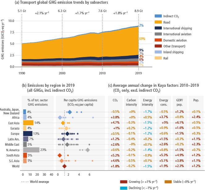
Figure 2.20 | Trends and drivers of global transport sector emissions (see Figure 2.16 caption for details) with energy measured as total final energy consumption.
The proportion of total final energy used in transport (28%) and its fast expansion over time weighs heavily on climate mitigation efforts, as 92% of transport energy comes from oil-based fuels (IEA 2020b). These trends situate transport as one of the most challenging sectors for climate change mitigation – no country has so far been able to realise significant emissions reductions in the sector. North America’s absolute and per capita transport emissions are the highest amongst world regions, but those of South, South-East and East Asia are growing the fastest ( high confidence) (between +4.6% and +5.2% yr –1 for CO2 between 2010 and 2019) (Figure 2.20).
More so than any other sector, transport energy use has tracked GDP per capita growth (Figure 2.20), (Lamb et al. 2021). With the exception of road gasoline demand in OECD countries, the demand for all road fuels generally increases at least as fast as the rate at which GDP per capita increases (Liddle and Huntington 2020). Developments since 1990 continue a historical trend of increasing travel distances and a shift from low- to high-speed transport modes that goes along with GDP growth (Schäfer et al. 2009; Gota et al. 2019). Modest improvements in energy efficiency have been realised between 2010 and 2019, averaging –1.5% yr –1 in energy intensity globally, while carbon intensities of the transport sector have remained stable in all world regions (Figure 2.20). Overall, global increases in passenger and freight travel activity levels have outpaced energy efficiency and fuel economy improvements, continuing a long-term trend for the transport sector (medium evidence, high agreement ) (Gucwa and Schäfer 2013; Grübler 2015; McKinnon 2016).
Despite some policy achievements, energy use in the global transport system remains to the present deeply rooted in fossil fuels (robust evidence, high agreement ) (Figueroa et al. 2014; IEA 2019). In part this is due to the increasing adoption of larger, heavier combustion-based vehicles in some regions, which have tended to far outpace electric and hybrid vehicle sales (Chapter 10). Yet, stringent material efficiency and lightweight design of passenger vehicles alone would have the potential to cut cumulative global GHG emissions until 2060 by 16–39 GtCO2-eq (Pauliuk et al. 2021).
While global passenger activity has expanded in all world regions, great disparities exist between low- and high-income regions, and within countries between urban and rural areas (ITF 2019). While private car use is dominant in OECD countries (EC 2019), the growth of passenger-km (the product of number of travellers and distance travelled) has considerably slowed there, down to an increase of just 1% yr –1 between 2000 and 2017 (SLoCaT 2018) (Chapter 10). Meanwhile, emerging economies in the Global South are becoming more car-dependent, with rapidly growing motorisation, on-demand private transport services, urban sprawl, and the emergence of local automotive production, while public transport struggles to provide adequate services (Dargay et al. 2007; Hansen and Nielsen 2017; Pojani and Stead 2017).
Freight travel activity grew across the globe by 68% in the last two decades, driven by global GDP increases, together with the proliferation of online commerce and rapid (i.e., same-day and next-day) delivery (SLoCaT 2018). Growth has been particularly rapid in heavy-duty road freight transport.
While accounting for a small share of total GHG emissions, domestic and international aviation have been growing faster than road transport emissions, with average annual growth rates of +3.3% and +3.4%, respectively, between 2010 and 2019 (Crippa et al. 2021; Minx et al. 2021;). Energy efficiency improvements in aviation were considerably larger than in road transport, but were outpaced by even larger increases in activity levels (SLoCaT 2018; Lee et al. 2021) (Chapter 10).
2.4.2.5AFOLU Sector
GHG emissions from agriculture, forestry and other land use (AFOLU) reached 13 GtCO2-eq globally in 2019 (medium confidence) (Figure 2.21). AFOLU trends, particularly those for CO2-LULUCF, are subject to a high degree of uncertainty (Section 2.2.1). Overall, the AFOLU sector accounts for 22% of total global GHG emissions, and in several regions – Africa, Latin America, and South-East Asia – it is the single largest emitting sector, which is also significantly affected itself by climate change (AR6 WGI Chapters 8, 11, and 12; and AR6 WGII Chapter 5). Latin America has the highest absolute and per capita AFOLU GHG emissions of any world region (Figure 2.21). CO2 emissions from land-use change and CH4 emissions from enteric fermentation together account for 74% of sector-wide GHGs. Note that CO2-LULUCF estimates included in this chapter are not necessarily comparable with country GHG inventories, due to different approaches to estimating anthropogenic CO2 sinks (Grassi et al. 2018) (Chapter 7).
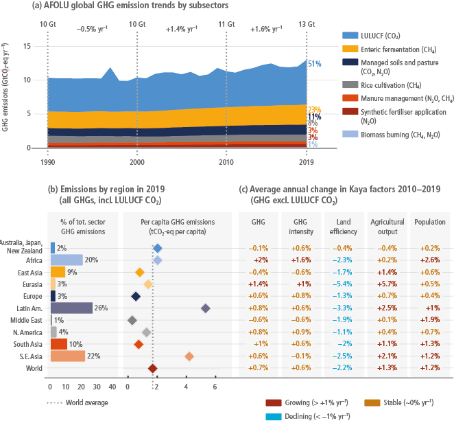
Figure 2.21 | Trends and drivers of global AFOLU sector emissions: (a) trends of GHG emissions by subsectors 1990–2019; (b) share of total sector and per capita GHG emissions by world region in 2019; and (c) Kaya decomposition of GHG emissions drivers. Based on the equation H=P(A/P)(L/A)(H/L), where P is population, A/P is agricultural output per capita, L/A is the land required per unit of agricultural output (land efficiency), and H/L is GHG emissions per unit of land (GHG intensity) (Hong et al. 2021). GHG emissions H comprise agricultural CH4 and N2O emissions from EDGAR v6.0. The indicated annual growth rates are averaged across the years 2010–2019 – LULUCF CO2 emissions are excluded in panel (c). (Note: due to different datasets, the population breakdown for AFOLU emissions is slightly different than that in the other sector figures above).
Unlike all other sectors, AFOLU emissions are typically higher in developing compared to developed regions (medium confidence). In Africa, Latin America, and South-East Asia, CO2 emissions associated with land-use change and management predominate, dwarfing other AFOLU and non-AFOLU sources and making AFOLU the single largest sector with more than 50% of emissions in these regions (Lamb et al. 2021b). Land-use and land-management emissions are associated with the expansion of agriculture into carbon-dense tropical forest areas (Vancutsem et al. 2021), where large quantities of CO2 emissions result from the removal and burning of biomass and draining of carbon rich soils (Pearson et al. 2017; IPCC 2018; Hong et al. 2021). Ruminant livestock rearing takes place on vast tracts of pasture land worldwide, contributing to large quantities of CH4 emissions from enteric fermentation in Latin America (0.8 GtCO2-eq in 2018), Southern Asia (0.6 GtCO2-eq), and Africa (0.5 GtCO2-eq), while also playing a sizable role in the total AFOLU emissions of most other regions (Lamb et al. 2021b).
In all regions, the amount of land required per unit of agricultural output has decreased significantly from 2010 to 2019, with a global average of –2.2% yr –1 (land efficiency metric in Figure 2.21). This reflects agricultural intensification and technological progress. However, in most regions this was mirrored by an increase in output per capita, meaning that absolute GHG emissions in most regions increased over the last decade. A significant increase in total AFOLU emissions occurred in Africa, driven by both increased GHG emissions per unit of land and increased populations (Figure 2.21).
The AFOLU sector and its emissions impacts are closely tied to global supply chains, with countries in Latin America and South-East Asia using large portions of their land for agricultural and forestry products exported to other countries (Chapter 7). The strong increases in production per capita and associated GHG emissions seen in these regions are at least partly attributable to growing exports and not national food system or dietary changes. At the same time, efforts to promote environmental sustainability in regions such as the EU and the USA (but also fast-growing emerging economies such as China) can take place at the cost of increasing land displacement elsewhere to meet their own demand (Meyfroidt et al. 2010; Yu et al. 2013; Creutzig et al. 2019).
Global diets are a key driver of production per capita, and thus land pressure and AFOLU emissions (Chapter 7). As per capita incomes rise and populations urbanise, traditional, low-calorie diets that emphasise starchy foods, legumes, and vegetables transition towards energy-intensive products such as refined sugars, fats, oils, and meat (Pradhan et al. 2013; Tilman and Clark 2014). At a certain point in national development, affluence and associated diets thus override population growth as the main driver of AFOLU emissions (Kastner et al. 2012). Very high calorie diets have high total GHG emissions per capita (Heller and Keoleian 2015) and are common in the developed world (Pradhan et al. 2013). Over the last few decades, a ‘westernisation’ of diets has also been occurring in developing countries (Pradhan et al. 2013). Low- and middle-income countries such as India, Brazil, Egypt, Mexico, and South Africa have experienced a rapid dietary shift towards western-style diets (De Carvalho et al. 2013; Pradhan et al. 2013; Popkin 2015). Another driver of higher food requirements per capita is food waste, which has increased more or less continuously since the 1960s in all regions but Europe (Porter and Reay 2016).
2.4.3Poverty and Inequality
Increasing economic inequality globally has given rise to concern that unequal societies may be more likely to pollute and degrade their environments (Masud et al. 2018; Chancel 2020; Hailemariam et al. 2020; Millward-Hopkins and Oswald 2021). The nature of this relationship has important implications for the design of income redistribution policies aiming to reduce inequalities (Section 2.6 presents evidence on how affluence and high consumption relate to emissions). Income inequality and carbon intensity of consumption differs across countries and individuals (Baležentis et al. 2020) (Section 2.3.3). Reduced income inequality between nations can reduce emissions intensity of global income growth, if energy intensity reductions from income growth in some nations offset increases in energy and emissions from higher growth in other nations (Rao and Min 2018). Increasing income inequality between individuals can translate into larger energy and emissions inequality if higher incomes are spent on more energy-intensive consumption and affluent lifestyles (Oswald et al. 2020; Wiedmann et al. 2020) (Section 2.6).
Literature shows that more equitable income distributions can improve environmental quality, but the nature of this relationship can vary by level of development (low evidence, medium agreement ) (Knight et al. 2017; Chen et al. 2020; Hailemariam et al. 2020; Huang and Duan 2020; Liobikienė and Rimkuvienė 2020; Rojas-Vallejos and Lastuka 2020; Uddin et al. 2020). Differences in the energy and carbon intensities of consumption and the composition of consumption baskets across populations and nations matter for emissions. (Jorgenson et al. 2016; Grunewald et al. 2017). There is evidence to suggest that more equal societies place a higher value on environmental public goods (Baumgärtner et al. 2017; Drupp et al. 2018). Additional research shows that reducing top income inequality in OECD countries can reduce carbon emissions and improve environmental quality (Hailemariam et al. 2020) and that the effect of wealth inequality, measured as the wealth share of the top decile, on per capita emissions in high-income countries, is positive (Knight et al. 2017). Evidence from 40 sub-Saharan African countries suggests that a rise in income inequality contributed to increasing CO2 emissions between 2010 and 2016, controlling for other drivers such as economic growth, population size, and inflation (Baloch et al. 2020).
The key development objective of eradicating extreme poverty (Chakravarty and Tavoni 2013; Hubacek et al. 2017a; Malerba 2020) and providing universal access to modern energy services (Pachauri et al. 2013, 2018; Pachauri 2014; Singh et al. 2017) only marginally affects GHG emissions (medium evidence, high agreement ). Shifts from biomass to more efficient energy sources and collective provisioning systems for safe water, health, and education are associated with reduced energy demand (Baltruszewicz et al. 2021). Efforts to alleviate multi-dimensional poverty by providing minimum decent living standards universally, however, may require more energy and resources. Recent estimates of the additional energy needed are still within bounds of projections of energy demand under climate stabilisation scenarios (Hubacek et al. 2017a, 2017b; Rao et al. 2019; Pascale et al. 2020; Kikstra et al. 2021). Bottom-up estimates suggest that achieving decent living standards requires 13–40 GJ per capita annually, much less than the current world average energy consumption of 80 GJ per capita in 2020 (Millward-Hopkins et al. 2020) (medium evidence, high agreement ). Aggregate top-down estimates suggest that achieving a high Human Development Index (HDI) score above 0.8 requires energy consumption between 30–100 GJ per capita yr –1 (Lamb and Rao 2015). There is some evidence, however, of a decoupling between energy consumption and HDI over time (Akizu-Gardoki et al. 2018). The emissions consequences of poverty alleviation and decent living also depend on whether improvements in well-being occur via energy- and carbon-intensive industrialisation or low-carbon development (Semieniuk and Yakovenko 2020; Fu et al. 2021; Huang and Tian 2021).
2.4.4Rapid and Large-scale Urbanisation as a Driver of GHG Emissions
Economic growth and urbanisation go hand in hand and are both influencing GHG emissions. However, the exact role of urban development in driving emissions is multi-faceted and heterogeneous, depending on development status and other regional factors (medium evidence, high agreement ) (Jorgenson et al. 2014; Lamb et al. 2014; Liddle and Lung 2014; Creutzig et al. 2015; Pincetl 2017; Azizalrahman and Hasyimi 2019; Muñoz et al. 2020). This calls for a differentiated assessment. This section assesses the process of rapid urban growth in developing countries and how emissions change over time when cities’ urban populations and infrastructure expand at fast speed and at a massive scale (Seto et al. 2017; Elmqvist et al. 2021). To distinguish, Section 2.6 includes the carbon footprint of urban lifestyles and the difference in emissions profiles between already urbanised and less urbanised areas. Chapter 8 deals with urban strategies for climate change mitigation.
Urban development is most significant and rapid in developing and transition countries, accompanied by a substantial migration of rural populations to urban areas (Apergis and Li 2016; Azizalrahman and Hasyimi 2019; Z. Wang et al. 2019 ) and associated impacts on land use (Richardson et al. 2015). If the trend of developing countries following infrastructure stock patterns in industrialised nations continues until 2050, this could cause approximately 350 GtCO2 from the production of materials (Müller et al. 2013). This would be equivalent to 70% of the 500 GtCO2 estimated remaining carbon budget from the beginning of 2020 to limit global warming to 1.5°C with a likelihood of 50% (IPCC 2021b).
In many developing countries across the world, the process of urban expansion leads to higher per capita consumption-based GHG emissions (medium evidence, high agreement ) (Jorgenson et al. 2014; Yao et al. 2015; Zhang et al. 2016; Wood et al. 2018 a; Muñoz et al. 2020). The high disparity between rural and urban personal carbon footprints in these countries (Wiedenhofer et al. 2017) (Section 2.6) means that migration to urban areas increases overall emissions as levels of income and expenditure rise, leading to further economic growth and infrastructure development in urban areas (Müller et al. 2013; Li et al. 2015; Wang and Yang 2016; Zhang et al. 2016; Wiedenhofer et al. 2017; Cetin and Bakirtas 2019; Fan et al. 2019; Li and Zhou 2019; Xia et al. 2019; Sarkodie et al. 2020).
For total production-based emissions in general, urbanisation is thought to have a smaller effect than changes in population, GDP per capita, and energy and emissions intensities, which are all more influential (Lin et al. 2017). Another driver of urban emissions is rising ambient air temperature caused by urban land expansion, which will likely drive a substantive increase in air conditioning use and cold storage for food (Huang et al. 2019). Specific emission drivers, however, depend on city- and place-specific circumstances such as income, household size, density, or local climate (Baiocchi et al. 2015; H. Wang et al. 2019 ). Geographical factors, urban form, and transport/fuel costs are dependent on each other, and, together with economic activity, have been found to explain 37% of urban direct energy use and 88% of urban transport energy use in a global sample of 274 cities (Creutzig et al. 2015).
2.5Technological Change is Key to Reducing Emissions
Technological change for climate change mitigation involves improvement in and adoption of technologies, primarily those associated with energy production and use. Technological change has had a mitigating effect on emissions over the long term and is central to efforts to achieving climate goals ( high confidence). Progress since AR5 shows that multiple low-carbon technologies are improving and falling in cost ( high confidence); technology adoption is reaching substantial shares, and small-scale technologies are particularly promising on both (medium confidence). Faster adoption and continued technological progress can play a crucial role in accelerating the energy transition. However, the historical pace of technological change is still insufficient to catalyse a complete and timely transition to a low-carbon energy system: technological change needs to accelerate ( high confidence). This section assesses the role of technological change in driving emissions reductions and the factors that drive technological change, with an emphasis on the speed of transitions. Incentives and support for technological change affect technology outcomes (Sivaram et al. 2018; Wilson et al. 2020a). Work since AR5 has focused on evaluating the effectiveness of policies: those that accelerate technological change by enhancing knowledge (technology push) and those that increase market opportunities for successful technologies (demand pull) (Nemet 2013); as well as the importance of tailoring support to country contexts (Barido et al. 2020; Rosenbloom et al. 2020), including the limits of carbon-pricing policies to date (Lilliestam et al. 2020). Section 2.8 and Chapter 13 describe how these polices affect emissions; Chapter 14 and Cross-Chapter Box 12 in Chapter 16 discuss transition dynamics; and Chapter 16 provides a more detailed assessment of the evolution and mitigation impacts of technology development, innovation, and transfer.
2.5.1Technological Change Has Reduced Emissions
Technological change that facilitates efficient energy utilisation from production to its final conversion into end-use services is a critical driver of carbon emissions reductions ( high confidence). Technological change can facilitate stringent mitigation, but it can also reduce these effects by changing consumer behaviour, such as through rebound effects (Section 2.6 and Chapter 16). AR6 includes an entire chapter on innovation, technology development, and transfer (Chapter 16). A focus gained in this section is the extent to which aligned, credible, and durable policies can accelerate technological change factors to put emissions reductions on a trajectory compatible with reaching United Nations Framework Convention on Climate Change (UNFCCC) goals.
Technological change has facilitated the provision of more diverse and efficient energy services (heating, cooling, lighting, and mobility) while generating fewer emissions per unit of service. As seen in Section 2.4, in Kaya identity terms (Lima et al. 2016) (see ‘Kaya identity’ in Glossary): population and economic growth are factors that have increased emissions, while technological change has reduced emissions (Peters et al. 2017). These Kaya statistics show that, while technological change can facilitate the transition to a low-carbon economy, it needs to proceed at a much faster pace than historical trends (Peters et al. 2017).
Multiple challenges exist in accelerating the past rate of technological change. First, an array of physical assets in the energy system are long-lived and thus involve substantial committed carbon (Section 2.7) (Knapp 1999; Cui et al. 2019). A process of ‘exnovation’, accelerating the phase-out of incumbent technology through intentional policy (such as by pricing carbon), provides a means to address long lifetimes (Davidson 2019; Rosenbloom and Rinscheid 2020). Second, countries may not have the capacity to absorb the flows of ideas and research results from international knowledge spillovers due to weak infrastructure, limited research capacity, lack of credit facilities (Chapter 15, Section 15.5), and other barriers to technology transfer (Adenle et al. 2015). In a developing country context, processes of innovation and diffusion need to include competence-building systems (Lema et al. 2015; Perrot and Sanni 2018; Stender et al. 2020). Third, public policy is central to stimulating technological change to reduce emissions; policy depends on creating credible expectations of future market opportunities (Alkemade and Suurs 2012), but the historical evidence shows that, despite recent progress, policies related to energy and climate over the long term have been inconsistent (Taylor 2012; Nemet et al. 2013; Koch et al. 2016). Bolstering the credibility and durability of policies related to low-carbon technology are crucial to accelerating technological change and inducing the private sector investment required (Helm et al. 2003; Habermacher et al. 2020).
2.5.2A Low-carbon Energy Transition Needs to Occur Faster Than Previous Transitions
An illuminating debate on the possibility of faster transitions has emerged since AR5 – with diverging assumptions about future technological change at the core of the discourse (Bazilian et al. 2020; Lu and Nemet 2020). Table 2.5 summarises these arguments.
Table2.5 | Summary of reasons to expect a fast energy transition/slow transition.
Fast transition | Slow transition | |
Evidentiary basis | Technology and country cases over 50 years | Historical global system over 200 years |
Systems | Complementary technologies enable integration | Difficult integration with existing infrastructure |
Economics | Falling costs of nascent technology | Mature incumbent technologies Upfront costs and capital constraints |
Technology | Digitalisation and global supply chains More abundant innovation Granular technology | Long lifetimes of capital stock Difficult to decarbonise sectors |
Actors | Proactive efforts for transition Bottom-up public concern Mobilised low-carbon interest groups | Risk-averse adopters Attributes do not appeal to consumers Rent-seeking by powerful incumbents |
Governance | Leaders catalyse faster change | Collective action problems |
2.5.2.1Energy Transitions Can Occur Faster Than in the Past
Recent studies have identified examples supporting fast energy transitions (Sovacool 2016; Bond et al. 2019; Reed et al. 2019). One describes five rapid national-scale transitions in end-use technologies, including lighting in Sweden, cook-stoves in China, liquefied petroleum gas stoves in Indonesia, ethanol vehicles in Brazil, and air conditioning in the USA (Sovacool 2016). Adoption of electric vehicles in Norway and in cities in China have also been rapid (Rietmann and Lieven 2019; Li et al. 2020; Fridstrøm 2021). Examples in energy supply, include electrification in Kuwait, natural gas in the Netherlands, nuclear electricity in France and Sweden, combined heat and power in Denmark, renewable energy in Uruguay, and coal retirements in Ontario, Canada (Qvist and Brook 2015). Reasons that these exemplars could be applied more broadly in the future include: growing urgency on climate change, shifting motivation from price response to proactive resource scarcity, and an increase in the likelihood of technological breakthroughs (medium confidence) (Sovacool 2016; Bazilian et al. 2020). The emergence of smaller unit scale, granular technologies (described below) also creates the potential for faster system change (Trancik 2006; Grubler et al. 2018; Wilson et al. 2020a). Energy service prices and government actions that affect demand are critical to the speed and extent of energy transitions (Kramer and Haigh 2009). Reasons scholars consider for expecting a fast transition include: intentional policy and alignment with goals; globalisation which diversifies sources and integrates supply chains; collective action via the Paris Agreement; as well as bottom-up grassroots movements and private sector initiatives (Kern and Rogge 2016). Political support for change can also speed transitions (Burke and Stephens 2017; Stokes and Breetz 2018), as can the credibility of transition-related targets (Li and Pye 2018; Rogge and Dütschke 2018).
The important role of leader countries is often missed when looking only at global aggregates (Meckling and Hughes 2018); leaders accumulate important knowledge, provide scaled market, and set positive examples for followers (medium confidence) (Schwerhoff 2016; Buchholz et al. 2019). In recent years, the conception of where leadership, climate-relevant innovation, and technology transfer originate has shifted to considering more meaningfully direct South-South and South-North forms of technology transfer, flows of capital, drivers for market access, origins of innovation, and other forms of cooperation (Urban 2018; Köhler et al. 2019). Recent evidence shows that South-South trade is enabling clean technology transfer (Gosens 2020). Leaders can initiate a process of ‘catalytic cooperation’ in which they overcome collective action problems and stimulate rapid change (Hale 2018). Similarly, ‘sensitive intervention points’ – targeted support of social movements, technologies, or policies themselves – can lead to rapid and self-sustaining change (Farmer et al. 2019), such as support for photovoltaics in Germany in the 2000s and student climate activism in Europe in 2019. The focus on leadership, catalysts, and intervention points reflects a systemic view of transitions that emphasises interactions and interdependence (Geels 2018; Meckling and Hughes 2018). Technological change has been at the core of transitions, but is best understood as part of a system in which social aspects are crucial (medium confidence) (Cherp et al. 2018; Köhler et al. 2019; Overland and Sovacool 2020).
2.5.2.2Reasons Why Transitions Will Occur at Historical Rates of Change
Recent work has also reasserted previous claims that the speed of a low-carbon transition will follow historical patterns (low confidence). Broad transitions involve technological complexity, time-consuming technological development, risk-averse adopters, high upfront costs, and low immediate individual adoption benefits, attributes that are not all present in the examples of rapid change described above (Grubler et al. 2016). Additional factors that slow transitions include: the need for the transition to occur globally, thus requiring nations with unequal economic resources and development circumstances to engage in near-universal participation; slow progress in recent decades; intermittence of renewables, and the time involved in building supporting infrastructure (Smil 2016); difficulty in decarbonising transportation and industry (Rissman et al. 2020); and material resource constraints (Davidsson et al. 2014).
2.5.3Improvements in Technologies Enable Faster Adoption
Since AR5, multiple low-carbon technologies have shown dramatic improvement, particularly solar photovoltaic (PV), wind, and batteries ( high confidence). The observed pace of these changes and the likelihood of their continuation support the arguments in the previous section that future energy transitions are likely to occur more quickly than in the past (medium confidence).
2.5.3.1Technological Change Has Produced Dramatic Cost Reductions
A wide array of technologies shows long-term improvements in performance, efficiency, and cost. Among the most notable are solar PV, wind power, and batteries ( high confidence) (Chapters 6 and 16). The dynamics for PVs are the most impressive, having fallen in cost by a factor of 10,000 from the first commercial application on a satellite in 1958 (Maycock and Wakefield 1975) to power purchase agreements signed in 2019 (IRENA 2020). Wind has been on a nearly as steep trajectory (Wiser and Bolinger 2019) as are lithium-ion battery packs for electric vehicles (Nykvist and Nilsson 2015; Service 2019). The future potential for PV and batteries seems especially promising given that neither industry has yet begun to adopt alternative materials with attractive properties as the cost reductions and performance improvements associated with the current generation of each technology continue (medium confidence) (Kwade et al. 2018). A key challenge is improving access to finance, especially in developing country contexts, where the costs of financing are of crucial importance (Creutzig et al. 2017; Schmidt 2019).
2.5.3.2Technological Change has Accelerated Since AR5
Figure 2.22 shows changes in the costs of four dynamic energy technologies. One can see rapid changes since AR5, cost data for which ended in 2010. Solar PV is by far the most dynamic technology, and its cost since AR5 has continued on its steep decline at about the same rate of change as before AR5, but now costs are well within the range of fossil fuels ( high confidence) (Chapter 6). Very few concentrating solar power (CSP) plants had been built between the 1980s and 2012. Since AR5, 4GW have been built and costs have fallen by half. Onshore wind has continued its pace of cost reductions such that it is well within the range of fossil fuels. Offshore wind has changed the most since AR5. Whereas costs were increasing before AR5, they have decreased by 50% since. None of these technologies shows indications of reaching a limit in their cost reductions. Crucial to their impact will be extending these gains in the electricity and transportation sectors to the industrial sector (Davis et al. 2018).

Figure 2.22 | Unit cost reductions and use in some rapidly changing mitigation technologies. The top panel shows global costs per unit of energy (USD per MWh) for some rapidly changing mitigation technologies. Solid blue lines indicate average unit cost in each year. Light blue shaded areas show the range between the 5th and 95th percentiles in each year. Grey shading indicates the range of unit costs for new fossil fuel (coal and gas) power in 2020 (corresponding to USD55–148 per MWh). In 2020, the levelised costs of energy (LCOE) of the four renewable energy technologies could compete with fossil fuels in many places. For batteries, costs shown are for 1 kWh of battery storage capacity; for the others, costs are LCOE, which includes installation, capital, operations, and maintenance costs per MWh of electricity produced. The literature uses LCOE because it allows consistent comparisons of cost trends across a diverse set of energy technologies to be made. However, it does not include the costs of grid integration or climate impacts. Further, LCOE does not take into account other environmental and social externalities that may modify the overall (monetary and non-monetary) costs of technologies and alter their deployment. The bottom panel shows cumulative global adoption for each technology, in GW of installed capacity for renewable energy and in millions of vehicles for battery-electric vehicles. A vertical dashed line is placed in 2010 to indicate the change since AR5. Shares of electricity produced and share of passenger vehicle fleet are indicated in text for 2020 based on provisional data, i.e., percentage of total electricity production (for PV, onshore wind, offshore wind, CSP) and of total stock of passenger vehicles (for EVs). The electricity production share reflects different capacity factors; for example, for the same amount of installed capacity, wind produces about twice as much electricity as solar PV. {2.5, 6.4} Renewable energy and battery technologies were selected as illustrative examples because they have recently shown rapid changes in costs and adoption, and because consistent data are available. Other mitigation options assessed in the report are not included as they do not meet these criteria.
2.5.3.3Granular Technologies Improve Faster
The array of evidence of technology learning that has accumulated both before and since AR5 (Thomassen et al. 2020) has prompted investigations about the factors that enable rapid technology learning. From the wide variety of factors considered, unit size has generated the strongest and most robust results. Smaller unit sizes, sometimes referred to as ‘granularity’, tend to be associated with faster learning rates (medium confidence) (Sweerts et al. 2020; Wilson et al. 2020). Examples include solar PV, batteries, heat pumps, and to some extent wind power. The explanatory mechanisms for these observations are manifold and well established: more iterations are available with which to make improvements (Trancik 2006); mass production can be more powerful than economies of scale (Dahlgren et al. 2013); project management is simpler and less risky (Wilson et al. 2020); the ease of early retirement can enable risk-taking for innovative designs (Sweerts et al. 2020); and they tend to be less complicated (Malhotra and Schmidt 2020; Wilson et al. 2020). Small technologies often involve iterative production processes with many opportunities for learning by doing, and have much of the most advanced technology in the production equipment than in the product itself. In contrast, large unit scale technologies – such as full-scale nuclear power, carbon capture and storage (CCS), low-carbon steel making, and negative emissions technologies such as bioenergy with carbon capture and storage (BECCS) – are often primarily built on site and include thousands to millions of parts, such that complexity and system integration issues are paramount (Nemet 2019). Despite the accumulating evidence of the benefits of granularity, these studies are careful to acknowledge the role of other factors in explaining learning. In a study of 41 energy technologies (Figure 2.23), unit size explained 22% of the variation in learning rates (Sweerts et al. 2020) and a study of 31 low-carbon technologies showed that unit size explained 33% (Wilson et al. 2020). Attributing that amount of variation to a single factor is rare in studies of technological change. The large residual has motivated studies, which find that small-scale technologies provide opportunities for rapid change, but they do not make rapid change inevitable; a supportive context, including supportive policy and complementary technologies, can stimulate more favourable technology outcomes ( high confidence).

Figure 2.23 | Learning rates for 41 energy demand, supply, and storage technologies. Source: Sweerts et al. (2020).
There is also evidence that small technologies not only learn but become adopted faster than large technologies (medium confidence) (Wilson et al. 2020b). Some of the mechanisms related to the adoption rate difference are associated with cost reductions; for example, smaller, less lumpy investments involve lower risk for adopters (Dahlgren et al. 2013; Wilson et al. 2020b). The shorter lifetimes of small technologies allow users to take advantage of new performance improvements (Knapp 1999) and access a large set of small adopters (Finger et al. 2019). Other mechanisms for faster adoption are distinctly related to markets: modular technologies can address a wide variety of niche markets (Geels 2018) with different willingness to pay (Nemet 2019) and strategically find protected niches while technology is maturing (Coles et al. 2018).
2.5.4Rapid Adoption Accelerates Energy Transitions
The transition to a more sustainable energy system depends not just on improvement in technologies, but also on their widespread adoption. Work since AR5 has also substantiated the bidirectional causal link between technology improvement and adoption. Cost reductions facilitate adoption, which generates opportunities for further cost reductions through a process of learning by doing (medium confidence). The rate of adoption is thus closely related to the speed at which an energy transition is possible.
Results of integrated assessment models (IAMs) show that scale-up needs are massive for 2°C scenarios. Using logistic growth rates of energy shares as in previous work (Wilson 2012; Cherp et al. 2021), most of these technologies include annual adoption growth rates of 20% in the 2020s and 2030s, and are in line with recent adoption of wind and solar. However, it is important to realise that IAMs include faster adoption rates for some mitigation technologies than for others (Peters et al. 2017). Growth rates in IAMs for large-scale CCS – biomass, coal, and gas – are between 15–30% (25th and 75th percentiles) (Figure 2.24). So few plants have been built that there is little historical data to analyse expected growth; with only two full-scale CCS power plants built and a 7% growth rate, if including industrial CCS. In contrast, IAMs indicate that they expect much lower rates of growth in future years for the technologies that have been growing fastest in recent years (wind and solar), without strong evidence for why this should occur.

Figure 2.24 | Growth of key technologies (2020–2040) in Paris-consistent mitigation scenarios compared to historical growth. Comparisons of historical growth (grey bars) to growth in 2020–2040 mitigation scenarios (dots). Values on the vertical axis are logistic annual growth rates for share of each technology in electricity supply. Horizontal arrangement of dots within technology categories indicates the count of scenarios at each growth rate. Source: data on scenarios from Chapter 3; historical data from BP (2021).
The overall pattern shows that IAMs expect growth in small-scale renewables to fall to less than half of their recent pace, and large-scale CCS to more than double from the limited deployment assessed ( high confidence). The emerging work since AR5 showing the rapid adoption and faster learning in small-scale technologies should prompt a keener focus on what technologies the world can depend on to scale up quickly (Grubb et al. 2021). The scenario results make it quite clear that climate stabilisation depends on rapid adoption of low-carbon technologies throughout the 2020–2040 period.
2.6Behavioural Choices and Lifestyles
2.6.1Introduction
This section synthesises how behavioural choices, lifestyles, and consumption preferences affect energy use and emissions. Household consumption is the largest component of a country’s gross domestic product (GDP) and the main contributor to greenhouse gas (GHG) emissions through direct energy consumption for heating and cooling or private transportation, and indirectly through carbon emitted during production of final consumption items. There is great variation in individual, group and household behaviour and consumption patterns within and between countries and over time. A number of factors affect people’s consumption patterns and associated carbon emissions, such as: socio-demographics; socio-economic status; infrastructure and access to public services; the regulatory framework; availability, affordability and accessibility of more or less sustainable choices on markets; and individual values and preferences (Dietz et al. 2009).
Carbon footprints vary between and within countries and show an uneven distribution because of differences in development levels, economic structure, economic cycle, available public infrastructure, climate and residential lifestyles (Bruckner et al. 2021). Similar emission characteristics can also be found within a country – see, for China; Feng et al. (2013); for the USA: Pizer et al. (2010); Feng et al. (2013); Miehe et al. (2016); Hubacek et al. (2017b); Wang et al. (2018); for Brazil: Sanches-Pereira et al. (2016); and for Latin American countries: Zhong et al. (2020).
In western countries, the largest contribution to the household carbon footprint is from transportation, housing, and consumption of food (Druckman and Jackson 2015). The joint contribution of these three items varies in different countries, depending on consumption patterns, and account for 58.5%, on average, in EU25 countries (Tukker and Jansen 2006). However, different countries, and regions within countries, may have different emission patterns due to differences in income, lifestyle, geography, infrastructure, political and economic situation. For example, the main contributors to the average US household is private transport (19.6%), followed by electricity (14.8%) and meat (5.2%) (Jones and Kammen 2011), while UK households have 24.6% emissions on energy and housing, 13.7% emissions on food, and 12.2% emissions on consumables (Gough et al. 2011). A study of 49 Japanese cities found that energy (31%), food (27%), and accommodation (15%) were the largest sources of household emissions (Long et al. 2017). An investigation of Japan’s household emissions found that energy, food, and utility are the three main emissions sources, but their shares are dependent on age (Shigetomi et al. 2014). See Section 12.4 (Chapter 12) and Box 5.4 (Chapter 5) for a more in-depth discussion on food systems and dietary shifts towards lower emission food.
In terms of rapidly growing economies, China is the most extensively researched country. China’s household emissions were primarily derived from electricity and coal consumption, as well as residents’ consumption of emission-intensive products, such as housing (33.4%), food (23.6%), private transportation and communication (14.8%) (Wang et al. 2018). Space heating was the largest contributor among various daily energy uses in northern cities (Yang and Liu 2017). In comparison, Indonesian rural households have a larger emission share on food and a much smaller share on services and recreation than urban households (Irfany and Klasen 2017). Urban Indonesian households have a much larger share of transport-related emissions (Irfany and Klasen 2017). Analysis from the Philippines shows that, on average, households in urban areas emit twice as much as rural ones because of much lower direct energy use in homes and for transport in rural areas (Serino 2017). In other emerging economies, such as India, Brazil, Turkey and South Africa, a high share of transport-related carbon emissions among urban middle- and high-income households is evident (Huang and Tian 2021).
2.6.2Factors Affecting Household Consumption Patterns and Behavioural Choices
Households’ carbon emissions are closely linked to activities and consumption patterns of individuals and as a group in households. Individual and group behaviour, in turn, is shaped by economic, technological, and psychological factors, social contexts (such as family ties, friends and peer pressure) and cultural contexts (social identity, status, and norms) as well as the natural environment (number of hot and cold days) and physical infrastructure, or geography (Jorgenson et al. 2019). For example, a city with an excellent bicycle infrastructure will make it safer and easier for citizens to become highly mobile by using their bikes; a city that has less density and is dominated by automobile infrastructure induces more people to travel by car (Chapters 8 and 10). As a consequence, many climate relevant consumption acts are not consciously decided on or deliberately made part of a lifestyle, but are strongly influenced by the factors listed above. Chapter 5 provides a more in-depth discussion on behavioural drivers and examples of behavioural interventions and policies that can be used to reduce emissions.
Demographic characteristics such as age, sex, and education constitute an important set of determinants influencing emissions patterns. People of different genders have different consumption patterns. For example, men tend to consume more food (especially meat) than women, leading to higher food-related emissions. Also, men spend more money on vehicles and driving (Wang et al. 2018). Similar evidence has been found in Germany, Greece, Norway, and Sweden, where men’s energy use is 8%, 39%, 6%, and 22% higher than women’s, respectively (Räty and Carlsson-Kanyama 2010).
Income. Due to the differences that shape individuals’ consumption patterns, there are enormous differences in the associated carbon footprints – with income being one of the most important predictors. Globally, households with income in the top 10% – income higher than USD23.03 purchasing power parity (PPP) per capita per day – are responsible for 34–45% of GHG emissions, while those in the bottom 50% – income less than USD2.97 PPP per capita per day – are responsible for only 13–15% of emissions, depending on the study (Chancel and Piketty 2015; Hubacek et al. 2017b) (Figure 2.25). The average carbon footprint of the high household incomes is more than an order of magnitudes larger than that of the lowest expenditure group (Feng et al. 2021). For example, Zhang et al. (2016) analysed the impact of household consumption across different income households on CO2 emissions in China and concluded that the impact on CO2 emissions generated by urban households’ consumption is 1.8 times as much as that of rural ones. High-income households have higher emissions related to transport and entertainment – such as recreational expenditure, travel, and eating out – than low-income households. Low-income households tend to have a larger share on necessities such as fuel for heating and cooking (Kerkhof et al. 2009). Figure 2.25 shows the carbon footprint per capita ranked by per capita income.
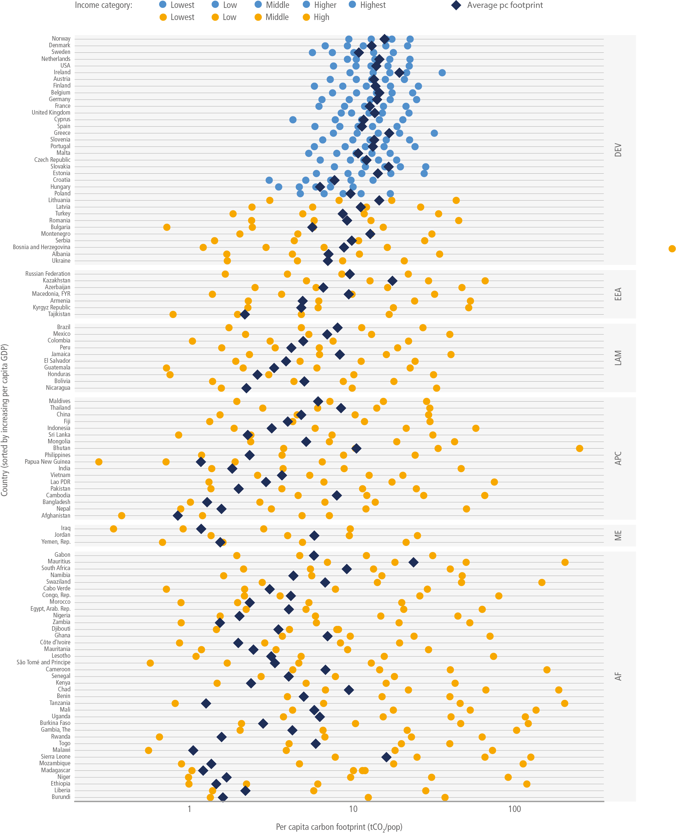
Figure 2.25 | Carbon footprints per capita income and expenditure category for 109 countries ranked by per capita income (consumption-based emissions).
Age. The effect of population ageing on emissions is contested in the literature. Ageing when accompanied by shrinking household size and more energy-intensive consumption and activity patterns results in increased emissions. However, an ageing labour force can also dampen economic growth and result in less energy-intensive activity such as driving, which decreases emissions (Liddle and Lung 2010; Liddle 2011). Ageing of the population characterises the demographic transition in both developed and developing countries. The implications of ageing for emissions depend on labour force participation of the elderly and differences in the consumption and investment patterns of different age groups (O’Neill et al. 2012). Analysis using panel macro data from OECD countries suggests that shifts in age and cohort composition have contributed to rising GHG emissions since the 1960s (Menz and Welsch 2012; Nassen 2014). Household-level data over time for the USA provides evidence that residential energy consumption increases over the lifetime of household members, largely due to accompanying changes in household size (Estiri and Zagheni 2019). Similar insights emerge from Japan, where analysis shows that those in their 70s or older, a group that is growing in size in Japan, have higher emissions than other age groups (Shigetomi et al. 2014, 2018, 2019). Recent analysis from China suggests that the shift to smaller and ageing households is resulting in higher carbon emissions because of the accompanying time-use and consumption shifts (Yu et al. 2018; Li and Zhou 2019). An increase in the dependency ratio – that is, the proportion of children aged under 15 and people over 65 relative to the working-age population – in other analyses, has been shown to lead to reduced CO2 emissions in China (Wei et al. 2018; Li and Zhou 2019). Implications of the nature of this relationship are important to policy discussions of working hours and retirement age that are likely to have an influence on emissions. For example, children and youth tend to emit more education-related emissions than adults (Han et al. 2015). Older people tend to have higher emissions related to heating and cooling being more sensitive to temperature (Meier and Rehdanz 2010).
Household size. Per capita emissions tend to decrease with family size, as living together becomes more energy efficient (Qu et al. 2013). The household size in most countries is decreasing (Liu et al. 2011), but the degree differs across countries – for example, there is a higher decrease rate in China than in Canada and the UK (Maraseni et al. 2015). The evidence shows that shifts to smaller households are associated with larger per-capita footprints (Liddle and Lung 2014; Underwood and Zahran 2015; Ivanova et al. 2017; Wiedenhofer et al. 2018), at least in developed countries (Meangbua et al. 2019).
Urban living. The carbon footprint of individuals and households is also significantly influenced by urban-rural differences (Ivanova et al. 2018; Wiedenhofer et al. 2018). In some cases, the difference can be explained by the effect of locational and spatial configuration characteristics, such as levels of compactness/density, centrality, proximity and ease of access to services. In all these parameters, urban areas score higher compared with rural or peri-urban (outlying and suburban) areas, thus influencing household emissions in different ways. Urban households tend to have higher emissions than rural households (O’Neill et al. 2010; Liu et al. 2011), but with adifferent energy and consumption structures. For example, rural households have more diverse energy inputs, such as biomass, biogas, solar, wind, small hydro and geothermal in addition to coal (Maraseni et al. 2016).
In terms of indirect emissions, urban households have more service-related emissions – such as from education and entertainment – than rural households, while rural households tend to have higher emissions related to food consumption or transportation (Büchs and Schnepf 2013; Maraseni et al. 2016) but this is strongly dependent on the specific situation of the respective country, as in poorer regions, rural transport might be mainly based on public transport with lower carbon emissions per capita. Centrality and location also play a role on the level of urban household emissions. Studies on US households found that residents in the urban core have 20% lower household emissions than residents in suburbs, which show a large range of household emissions (from –50% to +60%) (Kahn 2000; Jones and Kammen 2014). Higher population density tends to be associated with lower per capita emissions (Liddle and Lung 2014; Liu et al. 2017).
Location choices are a significant contributor to household emissions. Suburbanites tend to own larger, spacious homes with larger heating and cooling requirements. Commuting distance and access to public transportation, recreation areas, city centres, public services, and shops are other important neighbourhood-specific determinants of carbon emissions (Baiocchi et al. 2010) (see more on this in Chapters 8 and 10).
Time use. A study on the emissions implications of time use (Wiedenhofer et al. 2018) found that the most carbon-intensive activities are personal care, eating and drinking and commuting. Indirect emissions are also high for repairs and gardening. In contrast, home-based activities, such as sleep and resting, cleaning and socialising at home, have low carbon intensities per hour of time use. The same study also found that households in cities and areas with higher incomes tend to substitute personal activities for contracted services, thus shifting away from households to the service sector (Wiedenhofer et al. 2018). Improvements in the efficiency of time or resource use are diminished by rebound effects that have been shown to reduce emissions savings by 20–40% on average (Gillingham et al. 2015), while other authors argue that, potentially, the size of the rebound effect could be larger (Saunders 2015) (see more coverage of the rebound effect in Chapters 9 and 16). Lifestyle shifts brought about by using information technologies and socio-technological changes are inducing alterations in people’s daily activities and time-use patterns.
The reduction of working hours is increasingly discussed as an approach to improve well-being and reduce emissions (Fitzgerald et al. 2015, 2018; Melo et al. 2018; Wiedenhofer et al. 2018; Smetschka et al. 2019). For instance, analysis of differences in working hours across the USA for the period 2007–2013 shows that there is a strong positive relationship between carbon emissions and working hours. This relationship holds, even after controlling for other differences in political, demographic and economic drivers of emissions (Fitzgerald et al. 2018). In other analyses, this relationship is seen to hold in both developed and developing countries (Fitzgerald et al. 2015). One recent study, however, finds evidence of nonlinear relationships between working time and environmental pressure in EU15 countries between 1970 and 2010, in cases where non-work time is spent instead in carbon-intensive leisure activities (Shao and Shen 2017).
Social norms. Evidence from experiments in the US shows that social norms cannot only help in reducing a household’s absolute level of electricity use but also shift the time of use to periods when more renewable electricity is in the system (Horne and Kennedy, 2017). Analysis from Sweden shows that adoption of sustainable innovations like solar panels is influenced by perceived behaviour and expectations of others (Palm, 2017). Similar conclusions emerge from analysis in the Netherlands on the adoption of electric vehicles and smart energy systems (Noppers et al. 2019).
Broader contextual factors and cultural trends towards consumerism, individualisation and defining self-worth through conspicuous consumption can drive emissions up (Chancel and Piketty, 2015). However, cohort and generational shifts can drive emissions down. For instance, evidence, from millennials in the OECD shows that fewer younger people have driving licenses compared to older generations (Kuhnimhof et al. 2012). Similar, findings are evident from analysis for the US, where changing attitudes, decreased employment and rising virtual mobility explain decreased travel by Millennials (McDonald, 2015). Analysis for France shows that baby boomers are higher emitters than other generations (Chancel, 2014). A change in social norms is taking place with the spread of the sharing economy by which consumers share or borrow goods from other consumers. Sharing opportunities are more advanced within the mobility sector (Greenblatt and Shaheen, 2015). Successful car and bike sharing have rapidly expanded in countries such as China, Indonesia, Mexico, Brazil and Turkey. Technology and data advances are currently barriers to spreading of sharing in low- and lower middle-income cities but the potential offered by these technologies to allow poor countries to leapfrog to more integrated, efficient, multimodal transport systems is important (Yanocha et al. 2020). Despite this potential it is unclear how much shared mobility contributes to transport decarbonisation or to make it worse as it takes away riders from public transit (ITF, 2019). The evidence so far shows that the potential positive impacts of shared mobility with pooled rides in lowering travel costs, abating congestion, and reduced GHG emissions have not materialised to date (Merlin, 2019) (Chapter 5).
Education and environmental knowledge. A positive relationship was found between general and carbon-specific knowledge and the attitude towards carbon-specific behaviours in US consumers (Polonsky et al. 2012). One example, pertaining to students, found that the gain of environmental knowledge resulted in more environmentally favourable attitude among these high school students (Bradley et al. 1999). A comparison across states in the USA, for example, shows that environmental awareness can be a mitigating factor of territorial GHG emissions (Dietz et al. 2015). A 1% increase in ‘environmentalism’ – defined as the ‘environmental voting record of the state’s Congressional delegation’ (Dietz et al. 2015) – leads to a 0.45% decrease in emissions.
Environmental knowledge is not always directly translating into decreased ecological footprint (Csutora 2012). While pro-environmental action is lagging behind, research shows that this is not caused by people undervaluing the environment, but rather by people structurally underestimating how much others care (Bouman and Steg 2019). Other evidence shows that there are multiple causal pathways through which a more educated population can effect emissions, some of which may be positive and others negative (Lutz et al. 2019). A more educated population is more productive and can drive higher economic growth and therefore emissions (Lenzen and Cummins 2013). Moreover, education that is designed to specifically inform decision makers of the impacts of their decisions and provide behavioural nudges can be a way to reduce emissions (Duarte et al. 2016).
Status competition. As part of a larger consumer society and consumer culture, based on consumer-oriented lifestyles, products frequently provide a source for identity and fulfilment (Stearns 2001; Baudrillard 2017; Jorgenson et al. 2019). People pursue cultural constructs such as status, comfort, convenience, hygiene, nutrition, and necessity. Consumption is, by and large, not an end in itself but a means to achieve some other end, and those ends are diverse and not necessarily connected to one another (Wilk 2010). This shows that consumption patterns cannot be sufficiently understood without also considering the context – for example, the cultural and social contexts leading to status competition and status-related consumption (Veblen 2009; Ehrhardt-Martinez, K. et al. 2015; Wilk 2017). Status seeking can work to reduce emissions when ‘green products’ such as an electric car or photovoltaics on the roof become a sign for high-status (Griskevicius et al. 2010). It also can work to increase emissions through visible and high-carbon intensive consumption items, such a larger homes, fuel-inefficient sport utility vehicles (SUVs), and long-distance vacations (Schor 1998), driven by a notion of having ‘to keep up with the Joneses’ (Hamilton 2011). This can lead to formation of new habits and needs, where products and services become normalised and are quickly perceived as needed, reinforced through social networks and advertisement, making it psychologically easy to convert a luxury item to a perceived necessity (Assadour 2012). For example, the share of adults who consider a microwave a necessity was about one-third in 1996 but had increased to more than two-thirds in 2006, but retreated in importance during the recession years 2008–2009 (Morin and Taylor 2009). Similar ups and downs have been observed for television sets, air conditioning, dishwashers or clothes dryers. (Druckman and Jackson 2009). Basic needs and luxury items are subject to change over one’s lifetime and in relation to others (Horowitz 1988). This shows that the boundaries of the public’s luxury-versus-necessity perceptions are malleable (Morin and Taylor 2009).
Inequality. Global inequality within and between countries has shifted over the last decade’s expanding consumption and consumer culture (Castilhos and Fonseca 2016; Alvaredo et al. 2018; Short and Martínez 2020). The rise of income of middle-class in countries, mostly in Asia – for example, China, India, Indonesia and Vietnam – and the stagnating incomes of the middle classes in developed economies reduced between countries’ income differences; meanwhile, the population under extreme poverty (a threshold of USD1.9 per person per day) is now concentrated in Sub-Saharan Africa and South Asia (Milanović 2016). A major gap between top and bottom incomes occurred in parallel within countries. Since 1980, the top 1% richest individuals in the world captured twice as much growth as the bottom 50% individuals (Friedman and Savage 2017; Alvaredo et al. 2018). The influence of these dual inequality trends on lifestyles, new consumption patterns and carbon emissions at regional, local and global scale are large and have led to the fastest growth of global carbon emissions, in particular, for fast emerging economies (Sections 2.2. and 2.3). Emissions remain highly concentrated, with the top 10% per capita emitters contributing to between 35–45% of global emissions, while the bottom 50% emitters contribute to 13–15% of global emissions (Hubacek et al. 2017a). Furthermore, the top 1% of income earners by some estimates could have an average carbon footprint 175 times that of an average person in the bottom 10% (Otto et al. 2020). The top 10% high emitters live in all continents, and one-third of them live in emerging countries (Chancel and Piketty 2015; Hubacek et al. 2017a; Semieniuk and Yakovenko 2020). Mitigation pathways need to consider how to minimise the impacts of inequality on climate change and the different mechanisms and effects coming into play between the inequality of income and emissions (Baek and Gweisah 2013; Berthe and Elie 2015; Hao et al. 2016; Grunewald et al. 2017) (Section 2.4.3).
Inequality trends catalyse impact at a demand level, mobilising rapid lifestyles changes, symbolic consumption and ideals of material improvements and upward mobility (Castilhos et al. 2017) and emulation of high-carbon emissions intensive lifestyle of the wealthy (Gough 2017). Decoupling energy use and emissions from income growth and the decarbonisation of energy services have not counteracted these trends (Section 2.4.1). Alternative options to deal with carbon inequality, such as sharing global carbon emissions among high emitters (Chakravarty et al. 2009; Chakravarty and Tavoni 2013) or addressing the discourse of income distribution and the carbon intensity of high emitters lifestyles (Hubacek et al., 2017b; Gössling 2019; Otto et al. 2019) are met with caution that such alternatives may necessitate hard-to-implement institutional changes (Semieniuk and Yakovenko 2020). Growing inequality within countries may make recomposition of emission intensive consumption more difficult and, it may also exacerbate redistribution and social cohesion dilemmas (Gough 2017; Römpke et al. 2019). Climate mitigation action has different motivational departures in unequal context. An emerging global ‘middle class’ strengthens consumption at the margin as evidence by first-time purchases of white goods with likely impacts on energy demand (Wolfram et al. 2012), and with a warming climate, the increased use of air conditioning (Davis and Gertler 2015). Inequality may affect the willingness of rich and poor to pay for environmental goods or accept policies to protect the environment (Baumgärtner et al. 2017). Unequal departure for action is strongly manifested in cities of all sizes in developing countries with low-income urban residents hardest hit in lock-in situations such as lack of access to transportation and jobs (Altshuler 2013; Mattioli 2017), lack of green spaces (Joassart-Marcelli et al. 2011), poor access to waste collection (King and Gutberlet 2013) and to energy and clean water provision. The exacerbation of these conditions constrains the feasibility for achieving emissions reductions through lifestyle or behavioural changes alone (Baiocchi et al. 2010; Oxfam 2015). High inequality limits mitigation efforts and conversely, advancing mitigation should not contribute to deepen existing inequalities (Rao and Min 2018; Saheb et al. 2019). It is critically important to account for varying demands and affordability across heterogeneous household groups in access to quality energy, education, health, decent jobs and services, while recomposing consumption and balancing societal trade-offs via policies to boost the inclusion of low-income and energy-poor population groups (Pachauri et al. 2013). Further, there is a need to reduce inequalities and improve the capabilities people have to live the lives they value (Sen 1999; Gough et al. 2011; Gough, 2017; Aranoff et al. 2019).
2.7Emissions Associated With Existing and Planned Long-lived Infrastructure
2.7.1Introduction: Clarification of Concepts
Carbon lock-in can be understood as inertia in a system that limits the rate of transformation by a path-dependent process (Seto et al. 2016). For example, long lifetimes of infrastructures such as power plants, roads, buildings or industrial plants may influence the rate of transformation substantially and lock societies into carbon-intensive lifestyles and practices for many decades (Unruh 2000, 2002; Unruh and Carrillo-Hermosilla 2006; Grubler 2012; Seto et al. 2016; Sovacool 2016). Infrastructure stock evolution depends on technological and economic factors, but also on institutional and behavioural ones that are often mutually reinforcing. That is, physical infrastructure such as the built environment of urban areas can shape people’s behaviour and practices, which in turn change the demand for such infrastructure and lock-in energy demand patterns (Banister et al. 1997; Makido et al. 2012; Creutzig et al. 2016; Seto et al. 2016; Shove and Trentmann 2018).
There is a broad literature on carbon lock-in related to infrastructure that has analysed different geographical scales and sectors, with a strong focus on the power sector (Fisch-Romito et al. 2020). Available quantifications differ in the time frames of analysis that can be classified as backward-looking, static for a given year, or forward-looking using scenarios (Fisch-Romito et al. 2020). Quantifications also differ in the indicators used to describe carbon lock-in. Literature has assessed how delays in climate policy affect the evolution of fossil-fuel infrastructure stock in the short term (Bertram et al. 2015; Kefford et al. 2018; McGlade et al. 2018), overall mitigation costs (Riahi et al. 2015; Luderer et al. 2016), or the transition risks from premature retirements or underutilisation of existing assets (Iyer et al. 2015; Johnson et al. 2015; Lane et al. 2016; Luderer et al. 2016; Farfan and Breyer 2017; van Soest et al. 2017; Kefford et al. 2018; Cui et al. 2019; Fofrich et al. 2020; Malik et al. 2020; H. Wang et al. 2020; Pradhan et al. 2021). Only a few authors have relied on indicators related to institutional factors such as technology scale or employment (Erickson et al. 2015; Spencer et al. 2018). Complementary literature has explored how the sheer size of the world’s fossil fuel reserves (and resources) and owners’ financial interests could contribute to supply-side dynamics that sustain the use of fossil fuels (Jewell et al. 2013; Jakob and Hilaire 2015; McGlade and Ekins 2015; Bauer et al. 2016; Heede and Oreskes 2016; Welsby et al. 2021).
One way of quantifying potential carbon lock-in is to estimate the future CO2 emissions from existing and planned infrastructure (Davis et al. 2010; Davis and Socolow 2014) based on historic patterns of use and decommissioning. Such estimates focus on CO2 emissions from operating infrastructure and do not comprise any upstream or downstream emissions across the lifecycle, which are provided elsewhere in the literature (Müller et al. 2013; Creutzig et al. 2016; Krausmann et al. 2020; Fisch-Romito 2021). Estimates tend to focus on energy, while other areas, such as the agricultural sector are usually not covered. Another strand of literature quantifies lock-in by estimating fossil-fuel related CO2 emissions that are hard to avoid in future scenarios using integrated assessment models (IAMs) (Kriegler et al. 2018b; Luderer et al. 2018). The remainder of this chapter will assess potential carbon lock-in through those two related strands of literature.
2.7.2Estimates of Future CO2 Emissions From Long-lived Infrastructures
Table 2.6 summarises studies that apply an accounting approach based on plant-level data to quantify future CO2 emissions from long-lived fossil fuel infrastructure (Davis et al. 2010; Davis and Socolow 2014; Rozenberg et al. 2015; Edenhofer et al. 2018; Pfeiffer et al. 2018; Cui et al. 2019; Smith et al. 2019; Tong et al. 2019; Pradhan et al. 2021). Differences between studies arise in the scope of the infrastructure covered (including resolution), the inclusion of new infrastructure proposals, the exact estimation methodology applied as well as their assessments of uncertainties. Other studies provide analysis with a sectoral focus (Bullock et al. 2020; Vogl et al. 2021) or with a regional focus on the power sector (Shearer et al. 2017, 2020; González-Mahecha et al. 2019; Grubert 2020; Tao et al. 2020).
Assuming variations in historic patterns of use and decommissioning, comprehensive estimates of cumulative future CO2 emissions from current fossil fuel infrastructures are 720 (550–910) GtCO2 (Smith et al. 2019) and 660 (460–890) ( high confidence) (Tong et al. 2019) (Table 2.6 and Figure 2.26). This is about the same size as the overall cumulative net CO2 emissions until reaching net zero CO2 of 510 (330–710) Gt in pathways that limit warming to 1.5°C with no or limited overshoot (Chapter 3). About 50% of cumulative future CO2 emissions from current fossil fuel infrastructures come from the power sector and 70% of these (or about 40% of the total) are from coal plants only. Like global annual CO2 emissions (Friedlingstein et al. 2020; Peters et al. 2020), future CO2 emissions from fossil fuel infrastructures have increased over time – that is, future CO2 emissions from fossil fuel infrastructure additions in a given year still outgrow ‘savings’ from infrastructure retirements (Davis and Socolow 2014; Tong et al. 2019). This could add further inertia to the system as it may require more and faster retirement of fossil-fuel based infrastructures later, and lead to higher costs for meeting climate goals (e.g., Bertram et al. 2015; Johnson et al. 2015).
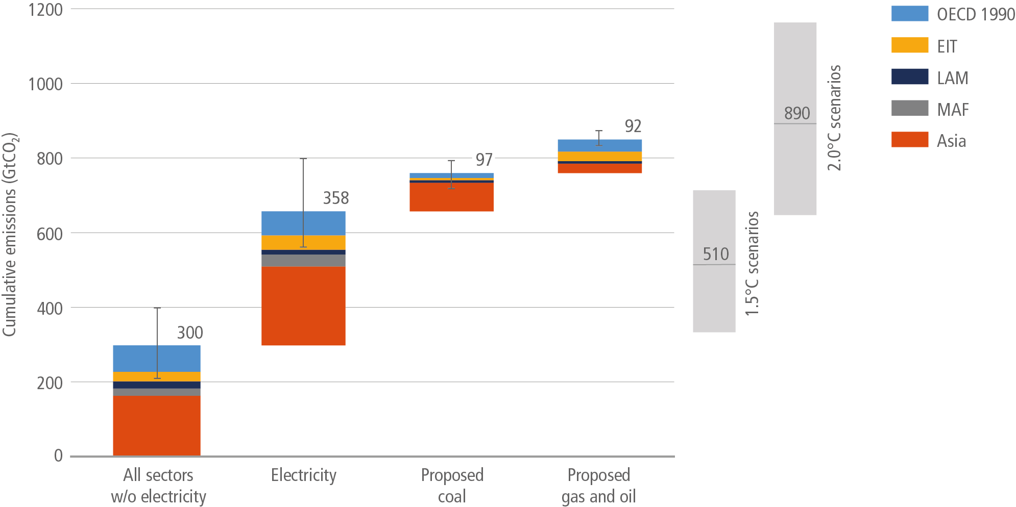
Figure 2.26 | Future CO2 emissions from existing and currently planned fossil fuel infrastructure in the context of Paris carbon budgets in GtCO2based on historic patterns of infrastructure lifetimes and capacity utilisation. Future CO2 emissions estimates of existing infrastructure for the electricity sector as well as all other sectors (industry, transport, buildings, other fossil fuel infrastructures) and of proposed infrastructures for coal power as well as gas and oil power. Grey bars on the right depict the range (5th–95th percentile) in overall cumulative net CO2 emissions until reaching net zero CO2 in pathways that limit warming to 1.5°C with no or limited overshoot (1.5°C scenarios), and in pathways that limit warming to 2°C (<67%) (2°C scenarios). Source: based on Edenhofer et al. (2018) and Tong et al. (2019).
Estimates of total cumulative future CO2 commitments from proposed infrastructure focus only on the power sector due to data availability (Table 2.6 and Figure 2.26). Infrastructure proposals can be at various stages of development involving very different probabilities of implementation. About one-third of the currently proposed projects are more probable as they are already under construction (Cui et al. 2019). Pfeiffer et al. (2018) and Tong et al. (2019) assess the cumulated CO2 emissions from proposed infrastructure in the entire power sector at 270 GtCO2 and 190 GtCO2 respectively. Estimates of CO2 emissions implications for new coal power infrastructure plans are more frequent (Edenhofer et al. 2018; Pfeiffer et al. 2018; Cui et al. 2019; Tong et al. 2019) ranging between 100 and 210 GtCO2. Differences across estimates of future CO2 emissions from proposed power infrastructure mostly reflect substantial cancellations of coal infrastructure proposals in 2017 and 2018 (Tong et al. 2019).
The global estimate of future CO2 emissions from current and planned fossil-fuel infrastructures is 850 (600–1100) GtCO2 (Tong et al. 2019). This already exceeds total cumulative net CO2 emissions in pathways that limit warming to 1.5°C with no or limited overshoot (see above). It is about the same size as the total cumulative net CO2 emissions of 890 (640–1160) GtCO2 from pathways that limit warming to 2°C (<67%) (Chapter 3). Hence, cumulative net CO2 emissions to limit warming to 2°C (<67%) or lower could already be exhausted by current and planned fossil fuel infrastructure ( high confidence) even though this estimate only covers a fraction of all infrastructure developments over the 21st century as present in mitigation pathways, does not cover all sectors (e.g., AFOLU) and does not include currently infrastructure development plans in transport, buildings, and industry due to a lack of data.
Hence, the Paris climate goals could move out of reach unless there are dedicated efforts for early decommissioning, and reduced utilisation of existing fossil fuel infrastructures, cancellation of plans for new fossil fuel infrastructures, or compensation efforts by removing some of the CO2 emissions from the atmosphere (Cui et al. 2019; Smith et al. 2019; Tong et al. 2019; Pradhan et al. 2021). For example, Fofrich et al. (2020) suggest in a multi-model study that coal and gas power infrastructure would need to be retired 30 (19–34) and 24 (21–26) years earlier than the historical averages of 39 and 36 years when following 1.5°C pathways and 23 (11–33) and 19 (11–16) years earlier when following 2°C pathways. Cui et al. (2019) arrive at more conservative estimates for coal power plants, but only consider the existing and currently proposed capacity. Premature retirement of power plants pledged by members of the Powering Past Coal Alliance would cut emissions by 1.6 GtCO2, which is 150 times less than future CO2 emissions from existing coal power plants (Jewell et al. 2019).
Few quantifications of carbon lock-in from urban infrastructure, in particular urban form, have been attempted, in part because they also relate to behaviours that are closely tied to routines and norms that co-evolve with ‘hard infrastructures’ and technologies, as well as ‘soft infrastructure‘ such as social networks and markets (Seto et al. 2016). There are some notable exceptions providing early attempts (Guivarch and Hallegatte 2011; Driscoll 2014; Seto et al.2014; Lucon et al. 2014; Erickson and Tempest 2015; Creutzig et al. 2016). Creutzig et al. (2016) attempt a synthesis of this literature and estimate the total cumulative future CO2 emissions from existing urban infrastructure at 210 Gt, and from new infrastructures at 495 Gt for the period 2010–2030.
2.7.3 Synthesis – Comparison with Estimates of Residual Fossil Fuel CO2 Emissions
A complementary strand of literature uses IAMs to assess the cumulative gross amount of unabated CO2 emissions from fossil fuels across decarbonisation pathways that are not removed from the system, even under strong (short- and long-term) climate policy ambitions. Lower bound estimates for such a minimum amount of unabated residual CO2 emissions across the 21st century that is not removed from the system, even under very ambitious climate policy assumptions, may be around 600–700 GtCO2 (Kriegler et al. 2018b). This range increases to 650–1800 GtCO2 (Table 2.7) as soon as a broader set of policy assumptions are considered, including delayed action in scenarios that limit warming to 1.5°C and 2°C respectively (Luderer et al. 2018).
Notably, the lower end of residual fossil fuel emissions in IAM scenarios (Luderer et al. 2018) is remarkably similar to global estimates from the accounting studies of the previous section, as shown in Table 2.6. Yet, there are important conceptual and interpretative differences that are also reflected in the very different distribution of reported future CO2 emissions attached to current and future fossil fuel infrastructures (Table 2.7). Accounting studies start from granular, plant-based data for existing fossil fuel infrastructure and make statements about their future CO2 emissions, assuming variations of historic patterns of use and decommissioning. Expansions to the future are limited to proposals for new infrastructures that we know of today. Scenario studies quantifying residual fossil fuel emissions start from aggregate infrastructure descriptions, but dynamically update those through new investment decisions in each time step across the 21st century based on the development of energy and energy service demands, as well as technology availability, guided by defined climate policy goals (or their absence).
In accounting studies, estimates of future CO2 emissions from current fossil fuel infrastructures are dominated by the power sector with its large fossil fuel capacities. In contrast, scenario studies highlight residual emissions from non-electric energy – particularly in the transport and industry sectors. Fossil-fuel infrastructure in the power sector can be much more easily retired than in those sectors, where there are fewer and more costly alternatives. IAMs therefore account for continued investments into fossil-based energy technologies in areas with limited decarbonisation potential, such as some areas of transportation (in particular aviation, shipping and road-based freight) or some industrial processes (such as cement production or feedstocks for chemicals). This explains the key discrepancies observable in Table 2.7. Therefore, our overall assessment of these available lines of evidence strongly emphasises the importance of decommissioning, reduced utilisation of existing power sector infrastructure, as well as continued cancellation of new power sector infrastructures in order to limit warming to well below 2°C ( high confidence) (Kriegler et al. 2018b; Luderer et al. 2018; Chen et al. 2019; Cui et al. 2019; Fofrich et al. 2020). This is important as the power sector is comparatively easy to decarbonise (IPCC 2014a; Krey et al. 2014; Davis et al. 2018; Méjean et al. 2019) and it is crucial to make space for residual emissions from non-electric energy end uses that are more difficult to mitigate ( high confidence). Any further delay in climate policy substantially increases carbon lock-in and mitigation challenges as well as a dependence on carbon dioxide removal technologies for meeting the Paris climate goals (Kriegler et al. 2018b; Luderer et al. 2018).
2.8Climate and Non-Climate Policies and Measures and their Impacts on Emissions
2.8.1Introduction
The key to achieving climate change mitigation targets includes crafting environmentally effective, economically efficient and socially equitable policies. For the purposes of this section, policies are defined broadly as actions to guide decisions to reach explicit goals and, accordingly, climate (mitigation) policies are the ones whose primary objective is to reduce GHG emissions. They include a range of domains from economic and institutional to research and development (R&D) and social policies, and are implemented by various instruments (e.g., market-based and regulatory in the economic domain) and measures (e.g., legal provisions and governance arrangements in the institutional domain) (Chapter 13, and see ‘mitigation policies’ in Glossary). Yet GHG emissions are also affected by policies enacted in various social, economic and environmental areas to pursue primarily non-climatic objectives. This section presents succinct assessments of the outcomes and effectiveness of a few selected policy instruments applied in the last two decades that target climate protection (Sections 2.8.2 and 2.8.3) and GHG emissions impacts of selected other policies primarily aimed at improvements in environmental quality and natural resource management (Section 2.8.4). 12
It is rather difficult, though not impossible, to discern the genuine impacts of climate and non-climate policies on GHG emissions. Most current and past policies target only a small part of global emissions in a limited geographical area and/or from a small number of economic sectors. However, in addition to the targeted region or sector, policies and measures tend to affect GHG emissions in other parts of the world. Emissions leakage is the key channel by which such phenomena and complex interactions occur. 13 Uncertainties in impacts, synergies, and trade-offs between policies and measures also complicate the evaluation of emissions impacts. These make it challenging to identify the impacts of any specific policy or measure on emissions of any specific region or sector. Rigorous statistical analyses are necessary for building strong empirical evidence, but the experience with climate-related policy experiments to date is limited.
2.8.2Comprehensive Multinational Assessments
Comprehensive multinational evaluations with wider regional and sectoral coverage enable the assessment of emissions impacts without distortions from emissions leakage. Among the wide range of climate policy instruments, pricing carbon – such as a carbon tax or an emissions trading system – has been one of the most widely used and effective options to reduce GHG emissions (robust evidence, high agreement ). In a comparison of 142 countries with and without carbon pricing, countries with a carbon price show annual CO2 emission growth rates of 2 percentage points lower than countries without such policies (Best et al. 2020). A more comprehensive evaluation of carbon prices shows that countries with a lower carbon pricing gap (a higher carbon price) tend to be more carbon-efficient, that is, they have a lower carbon intensity of GDP (OECD 2018). 14 An empirical analysis of the effects of environmental regulation and innovation on the carbon emissions of OECD countries during the period 1999–2014 indicates that a 1% increase in environmentally friendly patents reduced carbon emissions by 0.017%, and a 1% increase in environmental tax revenue per capita reduced carbon emissions by 0.03% (Hashmi and Alam 2019).
Domestic and international climate legislation have also contributed to the reduction of GHG emissions. An empirical analysis of legislative activity in 133 countries over the period 1999–2016 based on panel data indicates that each new law reduced annual CO2 emissions per unit of GDP by 0.78% nationally in the first three years, and by 1.79% beyond three years. Additionally, climate laws as of 2016 were associated with an annual reduction in global CO2 emissions of 5.9 GtCO2 and 38 GtCO2 cumulatively since 1999 (Eskander and Fankhauser 2020). It is notable that 36 countries that accepted legally binding targets under the Kyoto Protocol all complied (Shishlov et al. 2016). It is impossible to disentangle precisely the contribution of individual mitigation policies, but it is clear that the participating countries, especially those in the OECD, did make substantial policy efforts with material impact (Grubb 2016). An ex-post evaluation shows a significant impact of the Protocol on emissions reductions (Maamoun 2019).
Renewable energy policies, such as Renewable Portfolio Standards and Feed-in-Tariff, have played an essential role in the massive expansion of renewable energy capacities, another key driver of GHG emissions reductions (robust evidence, high agreement ). Drivers of decreasing CO2 emissions seen in a group of 18 developed economies that decarbonised over the period 2005–2015 are the displacement of fossil fuels by renewable energy and decreases in energy use (Le Quéré et al. 2019). Renewable energy policies both at the EU and member states level have played an essential role in abating GHG emissions (ICF International 2016).
2.8.3National, Sectoral, and Cross-sectoral Policies
2.8.3.1National and Regional Carbon Pricing
Carbon prices – such as carbon taxes and GHG emissions trading schemes (ETSs) – are among the most widely used climate policy instruments across the globe, together with technology support instruments (IRENA 2018). As of May 2020, there were 61 carbon pricing schemes in place or scheduled for implementation, consisting of 31 ETSs and 30 carbon tax regimes, covering 12 GtCO2-eq or about 22% of annual global GHG emissions (World Bank 2020). The performance of carbon pricing in practice varies by countries and sectors, and depends on the policy environment (robust evidence, high agreement ).
The European Union Emissions Trading Scheme (EU ETS), the longest-standing regional climate policy instrument to date, has reduced emissions, though the estimates of the amount vary by study, by country, and by sector; ranging from 3–28% (McGuinness and Ellerman 2008; Ellerman et al. 2010; Abrell et al. 2011; Anderson and Di Maria 2011; Egenhofer et al. 2011; Petrick and Wagner 2014; Arlinghaus 2015; Martin et al. 2016). The EU ETS avoided emitting about 1.2 GtCO2 between 2008 and 2016 (3.8%), almost half of what EU governments promised to reduce under their Kyoto Protocol commitments (Bayer and Aklin 2020).
China’s emission trading pilots have resulted in a decline in carbon intensity in the pilot provinces by adjusting the industrial structure (Zhou et al. 2019). The Regional Greenhouse Gas Initiative (RGGI) in the USA has induced leakage in emissions through increases in electricity generation in surrounding non-RGGI areas, but it has led to the reduction of emissions by way of changes in the fuel mix from coal to gas (Fell and Maniloff 2018). Actual emissions declined in six of the 10 ETSs for which data is available, although other factors, such as the 2009 recession, have had significant impacts on those emissions as well (Haites et al. 2018).
The evidence of environmental effectiveness of carbon taxes in Western European countries is varied depending on country and study (robust evidence, high agreement ). A significant impact is found in Finland but insignificant impacts are found in Denmark and the Netherlands, and there are mixed results for Sweden (Lin and Li 2011; Brännlund et al. 2014). Only six of the 17 taxes, where data are available, have reduced actual emissions subject to the tax. Tax rates tend to be too low in many cases and the scale and frequency of the rate changes has not been sufficient to stimulate further emissions reductions (Haites et al. 2018).
2.8.3.2 Selected Sectoral Climate Policy Instruments
Many governments have implemented sector-specific policies, in addition to nationwide measures, to reduce GHG emissions ( high confidence). Examples of sectoral climate policies include carbon taxes on transportation fuels, low-carbon fuel standards, and regulation of coal power generation.
The implementation of a carbon tax and value-added tax on gasoline and diesel in Sweden resulted in significant reductions of CO2 emissions in the transportation sector (Shmelev and Speck 2018; Andersson 2019). An assessment of a variety of carbon tax schemes across various sectors in the EU shows a negative relationship between CO2 emissions and a CO2 tax (Hájek et al. 2019). In British Columbia (Canada), the carbon tax resulted in a decrease in demand for gasoline and a reduction in total GHG emissions (not exclusive to the transportation sector) estimated to be between 5–15% (Murray and Rivers 2015; Rivers and Schaufele 2015). The Low Carbon Fuel Standard in California has contributed to reducing carbon emissions in the transportation sector by approximately 9.85–13.28% during 1997–2014 (Huseynov and Palma 2018).
The power sector typically accounts for a large portion of countries’ CO2 emissions. Market-based regulation and government subsidies in China contributed to improving operational efficiency and reducing emissions (Zhao et al. 2015). In addition, the implementation of ultra-low emission standards has also resulted in a significant reduction in emissions from China’s power plants (Tang et al. 2019). Mandatory climate and energy policies, including the California Global Warming Solutions Act, reduced CO2 emissions by 2.7–25% of the average state-level annual emissions from the power sector over the period 1990–2014 in the USA. Mandatory GHG registry/reporting, electric decoupling and a public benefit fund have been effective in further decreasing power sector emissions in the USA (Martin and Saikawa 2017). In the UK electricity sector, a carbon price floor, combined with electricity market reform (competitive auctions for both firm capacity and renewable energy), displaced coal, whose share fell from 46% in 1995 to 7% in 2017, halving CO2 emissions, while renewables grew from under 4% in 2008 to 22% by 2017 (Grubb and Newbery 2018). See Chapter 13 for more information.
An alternative approach to a carbon tax is an indirect emissions tax on fuels such as an excise tax, or on vehicles, based on the expected CO2 intensity of new passenger vehicles. Vehicle purchase taxes can result in a reduction in GHG emissions through reducing the CO2 emissions intensity of vehicles, while also discouraging new vehicle purchases (Aydin and Esen 2018). For example, a vehicle tax policy in Norway resulted in a reduction of average CO2 intensity per kilometre of 7.5 gCO2 km –1 (Ciccone 2018; Steinsland et al. 2018). Despite such evidence, studies of carbon pricing find that additional policies are often needed to stimulate sufficient emissions reductions in transportation (medium confidence) (Tvinnereim and Mehling 2018).
Electric vehicles (EVs) powered by clean electricity can reduce GHG emissions, and such policies are important for spurring adoption of such vehicles (Kumar and Alok 2020; Thiel et al. 2020). The extent to which EV deployment can decrease emissions by replacing internal combustion engine-based vehicles depends on the generation mix of the electric grid (Abdul-Manan 2015; Nichols et al. 2015; Canals Casals et al. 2016; Hofmann et al. 2016; Choi et al. 2018; Teixeira and Sodré 2018) although, even with current grids, EVs reduce emissions in almost all cases (Knobloch et al. 2020). Policy incentives for EV adoption can be an effective mechanism to increase EV sales (Langbroek et al. 2016) and may include discounts, purchase subsidies, regulations, and government leadership (medium confidence) (Bakker and Jacob Trip 2013; Silvia and Krause 2016; Teixeira and Sodré 2018; Qiu et al. 2019; Santos and Davies 2020). The presence of charging infrastructure and publicly available charging increases the adoption rate of EVs (Vergis and Chen 2015; Javid et al. 2019). A comparison of EV adoption rates across 30 countries shows a positive correlation between charging stations and EV market share (Sierzchula et al. 2014). A rollout of 80,000 DC fast chargers across the USA is estimated to have resulted in a 4% reduction in emissions compared to a baseline of no additional fast chargers (Levinson and West 2018). More recently, bans on internal combustion engine vehicles have provided a much more direct approach to stimulating the adoption of EVs and its supporting infrastructure; however, the efficacy of such measures depends on enforcement (Plötz et al. 2019).
Public transit can reduce vehicle travel and lower GHG emissions by reducing the number of trips taken by private vehicles and the length of those trips (medium confidence). Changes to the operation of public transportation systems (such as density of bus stops, distance from stops to households, duration and frequency of trip times, and lowering ridership costs) can result in a mode shift from private car trips to public transit trips (Cats et al. 2017; Choi 2018; Carroll et al. 2019). These changes in the public transit system operation and network optimisation have been shown to have reduced GHG emissions in cases such as San Francisco, where the cost optimisation of the transit network was estimated to decrease emissions by a factor of three (Cheng et al. 2018) and Barcelona, where the optimisation of the urban bus system was estimated to reduce GHG emissions by 50% (Griswold et al. 2017). For every 1% increase in investment in transit services and transit-oriented design, there is an estimated 0.16% reduction in private vehicle kilometres travelled per capita (McIntosh et al. 2014).
Bike- and car-sharing programmes can reduce GHG emissions (medium confidence). Albeit a study of eight cities in the USA with larger bike share systems and higher ridership found that their potential to reduce total emissions is limited to <0.1% of total GHG emissions from the transportation sectors of these cities (Kou et al. 2020). The emissions reductions effects of car-sharing programmes depends on the specifics of programmes: the mode shift from public transit to car-sharing services can outweigh the decreases in GHG emissions associated with a reduced number of cars on the road (Jung and Koo 2018), whereas car-sharing programmes with EV fleets may reduce GHG emissions (Luna et al. 2020).
2.8.4Emission Impacts of Other Related Policies
Policies other than those intended directly to mitigate GHGs can also influence these emissions. Policies to protect the stratospheric ozone layer is a case in point. Implementing the Montreal Protocol and its amendments, emissions of controlled ozone-depleting substances (ODSs) (those covered by the protocol) declined to a very low level of about 1.4 GtCO2-eq yr –1 by 2010, avoiding GHG emissions of an estimated 13.3–16.7 GtCO2-eq yr –1 (9.7–12.5 GtCO2-eq yr –1 when accounting for the ozone depletion and hydrofluorocarbons (HFCs) offsets) (Velders et al. 2007). Yet fluorinated gases (F-gases), the substances introduced to substitute ODSs are also potent GHGs. See Section 2.2 for emissions data, and Chapter 13 on current policies to mitigate HFCs and other F-gases. GHG implications of two other categories of non-climate policies are briefly assessed in this section.
2.8.4.1Co-impacts of Air Quality, Sector-specific and Energy Policies on Climate Mitigation
Co-impacts of local or regional air pollution abatement policies for climate mitigation are widely studied in the literature. Cross-border externalities of air pollution have also made these a focus of several international agreements (Mitchell et al. 2020). Evaluating the effectiveness of such treaties and policies is difficult because deriving causal inferences and accurate attribution requires accounting for several confounding factors, and direct and indirect spillovers (Isaksen 2020). Nevertheless, several studies assess the effectiveness of such treaties and regulations (De Foy et al. 2016; Li et al. 2017a, 2017b; Morgenstern 2018; Mardones and Cornejo 2020). However, there is little ex-post empirical analysis and a greater focus on ex-ante studies in the literature.
At a local scale, air pollutants are often co-emitted with GHGs in combustion processes. Many air quality policies and regulations focus on local pollution from specific sources that can potentially either substitute or complement global GHG emissions in production and generation processes. Also, policies that reduce certain air pollutants, such as sulphur dioxide (SO2), have a positive radiative forcing effect (Navarro et al. 2016). The evidence on individual air pollution control regulation and policies for GHG emissions is therefore mixed (medium evidence, medium agreement ). Evidence from the USA suggests that increased stringency of local pollution regulation had no statistically detectable co-benefits or costs on GHG emissions (Brunel and Johnson 2019). Evidence from China suggests that the effectiveness of policies addressing local point sources differed from those of non-point sources and the co-benefits for climate are mixed, though policies addressing large industrial point sources have been easier to implement and have had significant impact (Huang and Wang 2016; Xu et al. 2016; van der A et al. 2017; Dang and Liao 2019; Fang et al. 2019; Yu et al. 2019). Legislation to reduce emissions of air pollutants in Europe have significantly improved air quality and health but have had an unintended warming effect on the climate (Turnock et al. 2016).
Often, the realisation of potential co-benefits depends on the type of pollutant addressed by the specific policy, and whether complementarities between local pollution and global GHG emissions are considered in policy design (medium evidence, high agreement ) (Rafaj et al. 2014; Li et al. 2017a). Effective environmental regulations that also deliver co-benefits for climate mitigation require integrated policies (Schmale et al. 2014; Haines et al. 2017). Uncoordinated policies can have unintended consequences and even increase emissions (Holland et al. 2015). Many studies suggest that policies that target both local and global environmental benefits simultaneously may be more effective (medium evidence, medium agreement ) (Klemun et al. 2020). Furthermore, air pollution policies aimed at inducing structural changes – for example, closure of polluting coal power plants or reducing motorised miles travelled – are more likely to have potential positive spillover effects for climate mitigation, as compared to policies incentivising end-of-pipe controls (Wang 2021).
Other policies that typically have potential co-benefits for climate mitigation include those specific to certain sectors and are discussed in Chapters 5–11. Examples of such policies include those that encourage active travel modes, which have been found to have ancillary benefits for local air quality, human health, and GHG emissions (Fujii et al. 2018). Policies to reduce energy use through greater efficiency have also been found to have benefits for air quality and the climate (robust evidence, medium agreement ) (Tzeiranaki et al. 2019; Bertoldi and Mosconi 2020). Important air quality and climate co-benefits of renewable or nuclear energy policies have also been found (medium evidence, medium agreement ) (Lee et al. 2017; Apergis et al. 2018; Sovacool and Monyei 2021).
Policies specific to other sectors, such as encouraging green building design, can also reduce GHG emissions (Eisenstein et al. 2017). Evidence from several countries also shows that replacing polluting solid biomass cooking with cleaner gas-burning or electric alternatives have strong co-benefits for health, air quality, and climate change (robust evidence, high agreement ) (Anenberg et al. 2017; Singh et al. 2017; Tao et al. 2018).
2.8.4.2Climate Impacts of Agricultural, Forestry, Land Use, and AFOLU-related Policies
Policies on agriculture, forestry, and other land use (AFOLU), and AFOLU sector-related policies have had a long history in many developing and developed countries. Co-impacts of these policies on the climate have been only marginally studied, although their impacts might be quite important because the AFOLU sector is responsible for 22% of total GHG emissions (robust evidence, high agreement ). The results of afforestation policies around the world and the contribution to CCS are also important.
Private and governmental policies can have a major impact on the climate. Experience indicates that ‘climate proofing’ a policy is likely to require some stimulus, resources, and expertise from agencies or organisations from outside the country. Stimulus and support for adaptation and mitigation can come from the UN system and from international development institutions (FAO 2009). These findings are also valid for small/organic farmers vis-à-vis large-scale agro-industry. For example, small/medium and environmentally concerned farmers in Europe are often asking for more policies and regulations, and see it as necessary from a climate perspective, and also to maintain competitiveness relative to large agro-industrial complexes. Therefore, the need for governmental support for small producers in regulations encompasses all AFOLU sectors.
Forestry case: zero deforestation
Forest is generally defined as land spanning more than 0.5 hectares with trees higher than 5 metres and a canopy cover of more than 10%, or trees able to reach these thresholds in situ (FAO 1998). Zero-deforestation (i.e., both gross and net zero deforestation) initiatives generate results at multiple levels (Meijer 2014). Efforts to achieve zero-deforestation (and consequently emissions) are announced by non-governmental organisations (NGOs), companies, governments, and other stakeholder groups. NGOs engage through their campaigning, but also propose tools and approaches for companies (Leijten et al. 2020). The extent to which companies can actually monitor actions conducive to zero-deforestation pledges depends on their position in the supply chain. Beyond the business practices of participating companies, achieving long-term positive societal impacts requires upscaling from supply chains towards landscapes, with engagement of all stakeholders, and in particular small producers. The various success indicators for zero deforestation mirror the multiple levels at which such initiatives develop: progress towards certification, improved traceability, and legality are apparent output measures, whereas direct-area monitoring and site selection approaches target the business practices themselves.
Such efforts have led to the development of the High Carbon Stock (HCS) approach that combines carbon stock values with the protection of HCS areas (including peatlands and riparian zones) and areas important for the livelihoods of local communities (Rosoman et al. 2017). Long-term positive impacts, however, will need to be assessed with hindsight and focus on national and global statistics. Successful initiatives targeting zero deforestation at jurisdictional level would also need to improve the enforcement of forest laws and regulations (EII 2015; Meyer and Miller 2015).
Large-scale agribusiness, banks, and consumer goods companies dominate supply chain-focused zero-deforestation initiatives, but only the producers, including local communities and smallholders, can change the production circumstances (TFD 2014). Producers shoulder much of the burden for meeting environmental requirements of pledges. And local communities and small producers are vulnerable to being cut out when supply chains reorient. The zero-deforestation pledges do not always devise programmes for introducing new sourcing strategies, and governments may have an important contribution to make, particularly in safeguarding the interests of small producers.
Other than in Brazil and Indonesia, beyond individual supply chains, there is still little evidence on positive results of zero-deforestation commitments, as information available for companies to judge their progress is scarce. Moreover, many zero-deforestation pledges set targets to be achieved by 2020 or 2030, and, consequently, many companies have not yet reported publicly on their progress. Similarly, only a few governments have yet shown progress in reducing deforestation, but the New York Declaration on Forests, the Sustainable Development Goals (SDGs) and the Paris Agreement were adopted relatively recently. The effectiveness of private-sector zero-deforestation pledges depends on the extent to which they can be supported by governmental action and foster a cooperative environment with the engagement of all stakeholders. Where the pledges are coordinated with regulation, multi-stakeholder dialogues, and technical and financial support, a true paradigm shift becomes possible. Many governments are still building the capacity to improve overall forest governance, but implementing ambitious international targets is likely to depend on technical and major financial support that has not yet been mobilised.
2.9Knowledge Gaps
•Global GHG emissions estimates are published less frequently and with greater reporting lags than, for example, CO2 from fossil fuel and industry. Data quality and reporting frequency remains an issue, particularly in developing countries where the statistical infrastructure is not well developed. Efforts to compile a global GHG emissions inventory by country, sector, and across time, that is annually updated based on the best-available inventory information, similar to ongoing activities for carbon dioxide (CO2), methane (CH4) or nitrous oxide (N2O), could fill this gap. Uncertainties and their methodological treatment in GHG emissions estimates are still not comprehensively understood.
•There is a more fundamental data gap for F-gas emissions, where data quality in global inventories is poor due to considerable gaps in the underlying activity data – particularly in developing countries. Comprehensive tracking of fluorinated gases (F-gas) emissions would also imply the inclusion of other gases not covered under the Paris Agreement, such as chlorofluorocarbons, hydrochlorofluorocarbons and others.
•Currently, despite advances in terms of data availability, sectoral and spatial resolution, the results in consumption-based emission estimates are dependent on the database used, the level of sectoral aggregation and country resolution. More fine-grained data at spatial resolution as well as the product level would support exploring the mitigation options at the sub-national level, companies and households.
•Consumption-based emission accounts suffer from lack of quantification of uncertainties at the subnational level and especially in data-scarce environments, such as for developing countries. A better understanding of drivers that caused decoupling of emissions at the national and especially sub-national level are important to explore.
•Understanding how socio-economic drivers modulate emission mitigation is crucial. Technological improvements (e.g., improved energy or land-use intensity of the economy) have shown a persistent pattern over the last few decades, but gains have been outpaced by increases in affluence (GDP per capita) and population growth, leading to continued emissions growth. Therefore the key gap in knowledge is how these drivers of emissions can be mitigated by demand management, alternative economic models, population control and rapid technological transition to different extents and in different settings. More research on decoupling and sustainability transformations would help to answer these questions. Key knowledge gaps also remain in the role of trade – in particular, how supporting low-carbon technologies in developing and exporting countries can counteract the upward-driving effect of trade, and how to achieve decoupling without outsourcing emissions to others and often to less developed regions.
•Understanding of how inequality affects emissions is in a nascent stage. Less is known about the causal mechanisms by which different dimensions of inequality – such as income, socio-economic, spatial, socio-cultural-gender and ethnicity – affect emissions. In particular, limited knowledge exists on the linkages between dimensions of inequality other than income or wealth and emissions arising from different service demands. Research gaps are apparent on how inequalities in living standards relate to emissions and how changes in inequalities between genders, social groups, and other marginalised communities impact emissions trends.
•Digitalisation of the economy is often quoted as providing new mitigation opportunities, but knowledge and evidences are yet limited – such as understanding of the role of smart apps and the potential and influence of disruptive technologies at the demand and supply side on GHG emissions.
•Despite growing evidence of technological progress across a variety of mitigation areas and the availability of increasingly precise datasets, knowledge gaps remain on technological change and innovation and evidence on speed of transitions to clarify what would make them fast or slow. Innovation is an inherently uncertain process and there will always be imperfect ex ante knowledge on technological outcomes and their effects on mitigation. The extent to which a low-carbon transition can proceed faster than historical examples is crucial to aid future mitigation. That depends on a better understanding of the speed of building, updating and replacing infrastructure. Additionally, how and whether financing for low-carbon technology investment in low- and middle-income countries can be delivered at low-cost and sustained over time are important questions. The emerging findings that small-scale technologies learn faster and are adopted more quickly need to be tested against a broader set of cases, and in particular against the large dispersion in data.
•Future CO2 emissions from existing and planned infrastructure is not well understood and quantified outside the power sector. Further integration of bottom-up accounting and scenario approaches from integrated assessment seems promising. Comprehensive assessments of hard-to-abate residual fossil fuel emissions and their relationship to CO2 removal activities are lacking, but will be important for informing net-zero emissions strategies.
•Empirical evidence of emission impacts from climate policies, including carbon pricing, is not sufficient for unambiguous attribution assessment, mainly due to the limited experience with climate-related policy experiments to date. More attention to the methodology for comprehensive evaluation of climate policies and measures, such as effective carbon rates is apparent. Key knowledge gaps also exist on ex-post evaluations of climate and non-climate policies and measures for their impact on emissions, particularly at the global scale, considering national circumstances and priorities.
Frequently Asked Questions (FAQs)
FAQ 2.1 | Are emissions still increasing or are they falling?
Global greenhouse gas (GHG) emissions continued to rise and reached 59 ±6.6 GtCO2-eq in 2019, although the rate of growth has fallen compared to the previous decade. However, emissions were higher than at any point in human history before. Emissions were around 12% and 54% higher than in 2010 and 1990, respectively. Average annual GHG emissions for 2009–2019 were higher compared to the periods 2000–2009 and 1990–1999, respectively. GHG emissions growth slowed since 2010: while average annual GHG emissions growth was 2.1% for 2000–2010, it was only 1.3% for 2010–2019. In order to stop the temperature increase, however, net emissions must be zero.
FAQ 2.2 | Are there countries that have reduced emissions and grown economically at the same time?
About 24 countries have reduced territorial CO2 and GHG emissions for more than 10 years. Uncertainties in emission levels and changes over time prevent a precise assessment in some country cases. In the short observation period of 2010–2015, 43 out of 166 countries have achieved absolute decoupling of consumption-based CO2 emissions from economic growth, which means that these countries experienced GDP growth while their emissions have stabilised or declined. A group of developed countries, such as some EU countries and the USA, and some developing countries, such as Cuba, have successfully achieved an absolute decoupling of consumption-based CO2 emissions and GDP growth. Decoupling has been achieved at various levels of per capita income and per capita emissions. Overall, the absolute reduction in annual emissions achieved by some countries has been outweighed by growth in emissions elsewhere in the world.
FAQ 2.3 | How much time do we have to act to keep global warming below 1.5 degrees?
If global CO2 emissions continue at current rates, the remaining carbon budget for keeping warming to 1.5°C will likely be exhausted before 2030. Between 1850 and 2019, total cumulative CO2 emissions from the fossil fuel industry (FFI) and agriculture, forestry, and other land use (AFOLU) were 2400 (±240 GtCO2). Of these, about 410 ± 30 GtCO2 were added since 2010. This is about the same size as the remaining carbon budget for keeping global warming to 1.5°C and between one-third and one-half of the 1150 ± 220 (1350, 1700) GtCO2 for limiting global warming below 2°C with a 67% (50%, 33%) probability, respectively (Canadell et al. 2021). At current (2019) rates of emissions, it would only take 8 (2–15) and 25 (18–35) years to emit the equivalent amount of CO2 for a 67th percentile 1.5°C and 2°C remaining carbon budget, respectively. This highlights the dependence of 1.5°C pathways on the availability of substantial CO2 removal capacities, as discussed in Chapters 3, 4, and 12, but also Section 2.7 of this chapter.
References
Aaheim, A. and T. Mideksa, 2017: Requirements to metrics of greenhouse gas emissions, given a cap on temperature. Ecol. Econ. , 131, 460–467, doi:10.1016/j.ecolecon.2016.09.026.
Abdul-Manan, A.F.N., 2015: Uncertainty and differences in GHG emissions between electric and conventional gasoline vehicles with implications for transport policy making. Energy Policy, 87, 1–7, doi:10.1016/j.enpol.2015.08.029.
Abrell, J., A. Ndoye Faye, and G. Zachmann, 2011: Assessing the impact of the EU ETS using firm level data. Bruegel, Brussels, Belgium, 23 pp.
Adenle, A.A., H. Azadi, and J. Arbiol, 2015: Global assessment of technological innovation for climate change adaptation and mitigation in developing world. J. Environ. Manage. , 161, 261–275, doi:10.1016/j.jenvman.2015.05.040.
Afionis, S., M. Sakai, K. Scott, J. Barrett, and A. Gouldson, 2017: Consumption‐based carbon accounting: does it have a future?WIREs Clim. Change, 8(1) , e438, doi:10.1002/wcc.438.
Aguiar, A., M. Chepeliev, E.L. Corong, R. McDougall, and D. van der Mensbrugghe, 2019: The GTAP Data Base: Version 10. J. Glob. Econ. Anal. , 4(1) , 1–27, doi:10.21642/JGEA.040101AF.
Akizu-Gardoki, O. et al., 2018: Decoupling between human development and energy consumption within footprint accounts. J. Clean. Prod. , 202, 1145–1157, doi:10.1016/j.jclepro.2018.08.235.
Alkemade, F. and R.A.A. Suurs, 2012: Patterns of expectations for emerging sustainable technologies. Technol. Forecast. Soc. Change, 79(3) , 448–456, doi:10.1016/j.techfore.2011.08.014.
Allen, M. et al., 2021: Ensuring that offsets and other internationally transferred mitigation outcomes contribute effectively to limiting global warming. Environ. Res. Lett. , 16(7) , 074009, doi:10.1088/1748-9326/abfcf9.
Allen, M.R. et al., 2016: New use of global warming potentials to compare cumulative and short-lived climate pollutants. Nat. Clim. Change. , 6(8) , 773–776, doi:10.1038/nclimate2998.
Allen, M.R. et al., 2018: A solution to the misrepresentations of CO2-equivalent emissions of short-lived climate pollutants under ambitious mitigation. npj Clim. Atmos. Sci. , 1(1) , 16, doi:10.1038/s41612-018-0026-8.
Altshuler, A., 2013: Equity as a Factor in Urban Transportation Politics. Access, 42, 2–9.
Alvaredo, F., L. Chancel, T. Piketty, E. Saez, and G. Zucman, 2018: World Inequality Report 2018. Belknap Press of Harvard University Press, Cambridge, MA, USA, 344 pp.
Anderson, B. and C. Di Maria, 2011: Abatement and Allocation in the Pilot Phase of the EU ETS. Environ. Resour. Econ. , 48(1) , 83–103, doi:10.1007/s10640-010-9399-9.
Andersson, J.J., 2019: Carbon Taxes and CO2 Emissions: Sweden as a Case Study. Am. Econ. J. Econ. Policy, 11(4) , 1–30, doi:10.1257/pol.20170144.
Andres, R.J. et al., 2012: A synthesis of carbon dioxide emissions from fossil-fuel combustion. Biogeosciences, 9(5) , 1845–1871, doi:10.5194/bg-9-1845-2012.
Andres, R.J., T.A. Boden, and D. Higdon, 2014: A new evaluation of the uncertainty associated with CDIAC estimates of fossil fuel carbon dioxide emission. Tellus B: Chem. Phys. Meteorol. , 66(1) , 23616, doi:10.3402/tellusb.v66.23616.
Andrew, R. and G. Peters, 2021: The Global Carbon Project’s fossil CO2 emissions dataset. doi:10.5281/zenodo.5569235.
Andrew, R.M., 2020: A comparison of estimates of global carbon dioxide emissions from fossil carbon sources. Earth Syst. Sci. Data, 12(2) , 1437–1465, doi:10.5194/essd-12-1437-2020.
Anenberg, S.C. et al., 2017: Air pollution-related health and climate benefits of clean cookstove programs in Mozambique. Environ. Res. Lett. , 12(2) , 025006, doi:10.1088/1748-9326/aa5557.
Apergis, N. and J. Li, 2016: Population and lifestyle trend changes in China: implications for environmental quality. Appl. Econ. , 48(54) , 5246–5256, doi:10.1080/00036846.2016.1173184.
Apergis, N., M. Ben Jebli, and S. Ben Youssef, 2018: Does renewable energy consumption and health expenditures decrease carbon dioxide emissions? Evidence for sub-Saharan Africa countries. Renew. Energy, 127, 1011–1016, doi:10.1016/j.renene.2018.05.043.
Aranoff, K., A. Battistonii, D. Aldana Cohen, and T. Riofrancos, 2019: A Planet to Win: Why We Need a New Green Deal. Verso, London UK and New York, NY, USA, 208 pp.
Arlinghaus, J., 2015: Impacts of Carbon Prices on Indicators of Competitiveness: A Review of Empirical Findings. OECD Environment Working Paper No. 87, OECD Publishing, Paris, France, 36 pp.
Assadour, E., 2012: The Path to Degrowth in Overdeveloped Countries. In: State of the World 2012[Starke, L., (ed.)], Island Press/Center for Resource Economics, Washington DC, USA, pp. 22–37.
Aydin, C. and Ö. Esen, 2018: Reducing CO2 emissions in the EU member states: Do environmental taxes work?J. Environ. Plan. Manag. , 61(13) , 2396–2420, doi:10.1080/09640568.2017.1395731.
Azhgaliyeva, D., Y. Liu, and B. Liddle, 2020: An empirical analysis of energy intensity and the role of policy instruments. Energy Policy, 145, 111773, doi:10.1016/j.enpol.2020.111773.
Azizalrahman, H. and V. Hasyimi, 2019: A model for urban sector drivers of carbon emissions. Sustain. Cities Soc. , 44, 46–55, doi:10.1016/j.scs.2018.09.035.
Baek, J. and G. Gweisah, 2013: Does income inequality harm the environment?: Empirical evidence from the United States. Energy Policy, 62, 1434–1437, doi:10.1016/j.enpol.2013.07.097.
Baiocchi, G., J. Minx, and K. Hubacek, 2010: The Impact of Social Factors and Consumer Behavior on Carbon Dioxide Emissions in the United Kingdom. J. Ind. Ecol. , 14(1) , 50–72, doi:10.1111/j.1530-9290.2009.00216.x.
Baiocchi, G., F. Creutzig, J. Minx, and P.-P. Pichler, 2015: A spatial typology of human settlements and their CO2 emissions in England. Glob. Environ. Change, 34, 13–21, doi:10.1016/j.gloenvcha.2015.06.001.
Bakker, S. and J. Jacob Trip, 2013: Policy options to support the adoption of electric vehicles in the urban environment. Transp. Res. Part D Transp. Environ. , 25, 18–23, doi:10.1016/j.trd.2013.07.005.
Balcombe, P., J.F. Speirs, N.P. Brandon, and A.D. Hawkes, 2018: Methane emissions: choosing the right climate metric and time horizon. Environ. Sci. Process. Impacts, 20(10) , 1323–1339, doi:10.1039/C8EM00414E.
Baležentis, T., G. Liobikienė, D. Štreimikienė, and K. Sun, 2020: The impact of income inequality on consumption-based greenhouse gas emissions at the global level: A partially linear approach. J. Environ. Manage. , 267, 110635, doi:10.1016/j.jenvman.2020.110635.
Baloch, M.A., Danish, S.U.-D. Khan, Z.Ş. Ulucak, and A. Ahmad, 2020: Analyzing the relationship between poverty, income inequality, and CO2 emission in Sub-Saharan African countries. Sci. Total Environ. , 740, 139867, doi:10.1016/j.scitotenv.2020.139867.
Baltruszewicz, M. et al., 2021: Household final energy footprints in Nepal, Vietnam and Zambia: composition, inequality and links to well-being. Environ. Res. Lett. , 16(2) , 025011, doi:10.1088/1748-9326/abd588.
Banerjee, S. and M. Murshed, 2020: Do emissions implied in net export validate the pollution haven conjecture? Analysis of G7 and BRICS countries. Int. J. Sustain. Econ. , 12(3) , 297, doi:10.1504/IJSE.2020.111539.
Banister, D., S. Watson, and C. Wood, 1997: Sustainable cities: transport, energy, and urban form. Environ. Plan. B Plan. Des. , 24(1) , 125–143, doi:10.1068/b240125.
Barido, D.P. de L., N. Avila, and D.M. Kammen, 2020: Exploring the Enabling Environments, Inherent Characteristics and Intrinsic Motivations Fostering Global Electricity Decarbonization. Energy Res. Soc. Sci. , 61, 101343, doi:10.1016/j.erss.2019.101343.
Baudrillard, J., 2017: The consumer society: Myths and structures. SAGE Publications Ltd, Los Angeles, USA, 224 pp.
Bauer, N. et al., 2016: Global fossil energy markets and climate change mitigation – an analysis with REMIND. Clim. Change, 136(1) , 69–82, doi:10.1007/s10584-013-0901-6.
Baumert, N., A. Kander, M. Jiborn, V. Kulionis, and T. Nielsen, 2019: Global outsourcing of carbon emissions 1995–2009: A reassessment. Environ. Sci. Policy, 92, 228–236, doi:10.1016/j.envsci.2018.10.010.
Baumgärtner, S., M.A. Drupp, J.N. Meya, J.M. Munz, and M.F. Quaas, 2017: Income inequality and willingness to pay for environmental public goods. J. Environ. Econ. Manage. , 85, 35–61, doi:10.1016/j.jeem.2017.04.005.
Bayer, P. and M. Aklin, 2020: The European Union Emissions Trading System reduced CO2 emissions despite low prices. Proc. Natl. Acad. Sci. , 117(16) , 8804–8812, doi:10.1073/pnas.1918128117.
Bazilian, M., M. Bradshaw, J. Gabriel, A. Goldthau, and K. Westphal, 2020: Four scenarios of the energy transition: Drivers, consequences, and implications for geopolitics. WIREs Clim. Change, 11(2) , doi:10.1002/wcc.625.
Berthe, A. and L. Elie, 2015: Mechanisms explaining the impact of economic inequality on environmental deterioration. Ecol. Econ. , 116, 191–200, doi:10.1016/j.ecolecon.2015.04.026.
Bertoldi, P. and R. Mosconi, 2020: Do energy efficiency policies save energy? A new approach based on energy policy indicators (in the EU Member States). Energy Policy, 139 (January), 111320, doi:10.1016/j.enpol.2020.111320.
Bertram, C. et al., 2015: Carbon lock-in through capital stock inertia associated with weak near-term climate policies. Technol. Forecast. Soc. Change, 90(PA) , 62–72, doi:10.1016/j.techfore.2013.10.001.
Bertram, C. et al., 2021: COVID-19-induced low power demand and market forces starkly reduce CO2 emissions. Nat. Clim. Change, 11(3) , 193–196, doi:10.1038/s41558-021-00987-x.
Best, R., P.J. Burke, and F. Jotzo, 2020: Carbon Pricing Efficacy: Cross-Country Evidence. Environ. Resour. Econ. , 77(1) , 69–94, doi:10.1007/s10640-020-00436-x.
Blanco G., R. Gerlagh, S. Suh, J. Barrett, H.C. de Coninck, C.F. Diaz Morejon, R. Mathur, N. Nakicenovic, A. Ofosu Ahenkora, J. Pan, H. Pathak, J. Rice, R. Richels, S.J. Smith, D.I. Stern, F.L. Toth, and P. Zhou, 2014: Drivers, Trends and Mitigation. In: Climate Change 2014: Mitigation of Climate Change. Contribution of Working Group III to the Fifth Assessment Report of the Intergovernmental Panel on Climate Change[Edenhofer, O., R. Pichs-Madruga, Y. Sokona, E. Farahani, S. Kadner, K. Seyboth, A. Adler, I. Baum, S. Brunner, P. Eickemeier, B. Kriemann, J. Savolainen, S. Schlömer, C. von Stechow, T. Zwickel and J.C. Minx (eds.)]. Cambridge University Press, Cambridge, UK and New York, NY, USA, pp. 351–411.
Bolea, L., R. Duarte, and J. Sánchez-Chóliz, 2020: Exploring carbon emissions and international inequality in a globalized world: A multiregional-multisectoral perspective. Resour. Conserv. Recycl. , 152, 104516, doi:10.1016/j.resconrec.2019.104516.
Bond, K., A. McCrone, and J. Kortenhorst, 2019: The Speed of the Energy Transition Gradual or Rapid Change. World Economic Forum, Cologny/Geneva, Switzerland, 32 pp.
Botzen, W.J.W., J.M. Gowdy, and J.C.J.M. Van Den Bergh, 2008: Cumulative CO2 emissions: shifting international responsibilities for climate debt. Clim. Policy, 8(6) , 569–576, doi:10.3763/cpol.2008.0539.
Bouman, T. and L. Steg, 2019: Motivating Society-wide Pro-environmental Change. One Earth, 1(1) , 27–30, doi:10.1016/j.oneear.2019.08.002.
BP, 2021: Statistical Review of World Energy. BP, London, UK, pp. 8–20.
Bradley, J.C., T.M. Waliczek, and J.M. Zajicek, 1999: Relationship Between Environmental Knowledge and Environmental Attitude of High School Students. J. Environ. Educ. , 30(3) , 17–21, doi:10.1080/00958969909601873.
Brännlund, R., T. Lundgren, and P.-O. Marklund, 2014: Carbon intensity in production and the effects of climate policy – Evidence from Swedish industry. Energy Policy, 67, 844–857, doi:10.1016/j.enpol.2013.12.012.
Brockway, P.E., S. Sorrell, G. Semieniuk, M.K. Heun, and V. Court, 2021: Energy efficiency and economy-wide rebound effects: A review of the evidence and its implications. Renew. Sustain. Energy Rev. , 141, 110781, doi:10.1016/j.rser.2021.110781.
Bruckner, B., K. Hubacek, Y. Shan, H. Zhong, and K. Feng, 2021: Impacts of poverty alleviation on national and global carbon emissions. Nat. Sustain. , 5(4) , 311–320, doi:10.1038/s41893-021-00842-z.
Brunel, C. and E.P. Johnson, 2019: Two birds, one stone? Local pollution regulation and greenhouse gas emissions. Energy Econ. , 78, 1–12, doi:10.1016/j.eneco.2018.10.011.
Bruns, S.B., A. Moneta, and D.I. Stern, 2021: Estimating the economy-wide rebound effect using empirically identified structural vector autoregressions. Energy Econ. , 97, 105158, doi:10.1016/j.eneco.2021.105158.
Buchholz, W., L. Dippl, and M. Eichenseer, 2019: Subsidizing renewables as part of taking leadership in international climate policy: The German case. Energy Policy, 129, 765–773, doi:10.1016/j.enpol.2019.02.044.
Büchs, M. and S.V. Schnepf, 2013: Who emits most? Associations between socio-economic factors and UK households’ home energy, transport, indirect and total CO2 emissions. Ecol. Econ. , 90, 114–123, doi:10.1016/j.ecolecon.2013.03.007.
Bullock, S., J. Mason, J. Broderick, and A. Larkin, 2020: Shipping and the Paris climate agreement: a focus on committed emissions. BMC Energy, 2(1) , 5, doi:10.1186/s42500-020-00015-2.
Burck, J., U. Hagen, C. Bals, N. Höhne, and L. Nascimento, 2021: Climate Change Performance Index 2021. Germanwatch, New Climate Institute, Climate Action Network, Bonn, Germany, 13 pp. https://ccpi.org/download/the-climate-change-performance-index-2021/.
Burke, M.J. and J.C. Stephens, 2017: Energy democracy: Goals and policy instruments for sociotechnical transitions. Energy Res. Soc. Sci. , 33, 35–48, doi:10.1016/j.erss.2017.09.024.
Cain, M. et al., 2019: Improved calculation of warming-equivalent emissions for short-lived climate pollutants. Clim. Atmos. Sci. , 2(1) , 29, doi:10.1038/s41612-019-0086-4.
Cain, M. et al., 2021: Comment on ‘Unintentional unfairness when applying new greenhouse gas emissions metrics at country level.’Environ. Res. Lett. , 16(6) , 068001, doi:10.1088/1748-9326/ac02eb.
Cao, X., X. Dai, and J. Liu, 2016: Building energy-consumption status worldwide and the state-of-the-art technologies for zero-energy buildings during the past decade. Energy Build. , 128, 198–213, doi:10.1016/j.enbuild.2016.06.089.
Cao, Z., L. Shen, A.N. Løvik, D.B. Müller, and G. Liu, 2017: Elaborating the History of Our Cementing Societies: An In-Use Stock Perspective. Environ. Sci. Technol. , 51(19) , 11468–11475, doi:10.1021/acs.est.7b03077.
Carroll, P., B. Caulfield, and A. Ahern, 2019: Measuring the potential emission reductions from a shift towards public transport. Transp. Res. Part D Transp. Environ. , 73, 338–351, doi:10.1016/j.trd.2019.07.010.
Carvalho, A.M. de, C.L.G. César, R.M. Fisberg, and D.M.L. Marchioni, 2013: Excessive meat consumption in Brazil: diet quality and environmental impacts. Public Health Nutr. , 16(10) , 1893–1899, doi:10.1017/S1368980012003916.
Casals, L.C., E. Martinez-Laserna, B. Amante García, and N. Nieto, 2016: Sustainability analysis of the electric vehicle use in Europe for CO2 emissions reduction. J. Clean. Prod. , 127, 425–437, doi:10.1016/j.jclepro.2016.03.120.
Castilhos, R.B. and M.J. Fonseca, 2016: Pursuing upward transformation: The construction of a progressing self among dominated consumers. J. Bus. Res. , 69(1) , 6–17, doi:10.1016/j.jbusres.2015.07.015.
Castilhos, R.B., M.J. Fonseca, and V. Bavaresco, 2017: Consumption, crisis, and coping strategies of lower class families in Brazil: A sociological account. Int. J. Consum. Studies, 41(4) , 379–388, doi:10.1111/ijcs.12341.
Cats, O., Y.O. Susilo, and T. Reimal, 2017: The prospects of fare-free public transport: evidence from Tallinn. Transportation (Amst). , 44(5) , 1083–1104, doi:10.1007/s11116-016-9695-5.
Cetin, M.A. and I. Bakirtas, 2020: The long-run environmental impacts of economic growth, financial development, and energy consumption: Evidence from emerging markets. Energy Environ. , 31(4) , 634–655, doi:10.1177/0958305X19882373.
Chakravarty, S. and M. Tavoni, 2013: Energy Poverty Alleviation and Climate Change Mitigation: Is There a Trade Off?Energy Economics., 40, 67–73, doi:10.1016/j.eneco.2013.09.022
Chakravarty, S. et al., 2009: Sharing global CO2 emission reductions among one billion high emitters. Proc. Natl. Acad. Sci. , 106(29) , 11884–11888, doi:10.1073/pnas.0905232106.
Chancel, L., 2014: Are younger generations higher carbon emitters than their elders?Ecol. Econ. , 100, 195–207, doi:10.1016/j.ecolecon.2014.02.009.
Chancel, L., 2020: 1 Economic Inequality as a Component of Unsustainability. In: Unsustainable Inequalities, Harvard University Press, Cambridge MA, USA and London, UK, pp. 11–35.
Chancel, L. and T. Piketty, 2015: Carbon and inequality: from Kyoto to Paris. Paris School of Economics, Paris, France, 48pp, doi:10.13140/RG.2.1.3536.0082.
Chang, C.-P., M. Dong, B. Sui, and Y. Chu, 2019: Driving forces of global carbon emissions: From time- and spatial-dynamic perspectives. Econ. Model. , 77, 70–80, doi:10.1016/j.econmod.2019.01.021.
Chen, G. et al., 2019: Review on City-Level Carbon Accounting. Environ. Sci. Technol. , 53(10) , 5545–5558, doi:10.1021/acs.est.8b07071.
Chen, J., Q. Xian, J. Zhou, and D. Li, 2020: Impact of income inequality on CO2 emissions in G20 countries. J. Environ. Manage. , 271, 110987, doi:10.1016/j.jenvman.2020.110987.
Cheng, H., C. Mao, S. Madanat, and A. Horvath, 2018: Minimizing the total costs of urban transit systems can reduce greenhouse gas emissions: The case of San Francisco. Transp. Policy, 66 (March), 40–48, doi:10.1016/j.tranpol.2018.02.009.
Cherp, A., V. Vinichenko, J. Jewell, E. Brutschin, and B. Sovacool, 2018: Integrating techno-economic, socio-technical and political perspectives on national energy transitions: A meta-theoretical framework. Energy Res. Soc. Sci. , 37 (January 2017), 175–190, doi:10.1016/j.erss.2017.09.015.
Cherp, A., V. Vinichenko, J. Tosun, J.A. Gordon, and J. Jewell, 2021: National growth dynamics of wind and solar power compared to the growth required for global climate targets. Nat. Energy, 6(7) , 742–754, doi:10.1038/s41560-021-00863-0.
Choi, H., J. Shin, and J. Woo, 2018: Effect of electricity generation mix on battery electric vehicle adoption and its environmental impact. Energy Policy, 121 (October 2017), 13–24, doi:10.1016/j.enpol.2018.06.013.
Choi, K., 2018: The influence of the built environment on household vehicle travel by the urban typology in Calgary, Canada. Cities, 75, 101–110, doi:10.1016/j.cities.2018.01.006.
Ciais, P., C. Sabine, G. Bala, L. Bopp, V. Brovkin, J. Canadell, A. Chhabra, R. DeFries, J. Galloway, M. Heimann, C. Jones, C. Le Quéré, R.B. Myneni, S. Piao and P. Thornton, 2013: Carbon and Other Biogeochemical Cycles. In: Climate Change 2013: The Physical Science Basis. Contribution of Working Group I to the Fifth Assessment Report of the Intergovernmental Panel on Climate Change[Stocker, T.F., D. Qin, G.-K. Plattner, M. Tignor, S.K. Allen, J. Boschung, A. Nauels, Y. Xia, V. Bex and P.M. Midgley (eds.)]. Cambridge University Press, Cambridge, UK, and New York, NY, USA, 465–570.
Ciais, P. et al., 2021: Empirical estimates of regional carbon budgets imply reduced global soil heterotrophic respiration. Natl. Sci. Rev. , 8(2) , doi:10.1093/nsr/nwaa145.
Ciccone, A., 2018: Environmental effects of a vehicle tax reform: Empirical evidence from Norway. Transp. Policy, 69 (April 2017), 141–157, doi:10.1016/j.tranpol.2018.05.002.
Climate Transparency, 2021: Climate Transparency Report . 16 pp. https://www.climate-transparency.org/wp-content/uploads/2021/10/CT2021-Highlights-Report.pdf .
Clarke L., K. Jiang, K. Akimoto, M. Babiker, G. Blanford, K. Fisher-Vanden, J.-C. Hourcade, V. Krey, E. Kriegler, A. Löschel, D. McCollum, S. Paltsev, S. Rose, P.R. Shukla, M. Tavoni, B.C.C. van der Zwaan, and D.P. van Vuuren, 2014: Assessing Transformation Pathways. In: Climate Change 2014: Mitigation of Climate Change. Contribution of Working Group III to the Fifth Assessment Report of the Intergovernmental Panel on Climate Change[Edenhofer, O., R. Pichs-Madruga, Y. Sokona, E. Farahani, S. Kadner, K. Seyboth, A. Adler, I. Baum, S. Brunner, P. Eickemeier, B. Kriemann, J. Savolainen, S. Schlömer, C. von Stechow, T. Zwickel and J.C. Minx (eds.)]. Cambridge University Press, Cambridge, UK, and New York, NY, USA, pp 413–510.
Coles, A.-M., A. Piterou, and A. Sentić, 2018: Is small really beautiful? A review of the concept of niches in innovation. Technol. Anal. Strateg. Manag. , 30(8) , 895–908, doi:10.1080/09537325.2017.1408907.
Collins, W.J., D.J. Frame, J.S. Fuglestvedt, and K.P. Shine, 2019: Stable climate metrics for emissions of short and long-lived species – combining steps and pulses. Environ. Res. Lett. , 15(2) , 024018, doi:10.1088/1748-9326/ab6039.
Colmenares, G., A. Löschel, and R. Madlener, 2020: The rebound effect representation in climate and energy models. Environ. Res. Lett. , 15(12) , 123010, doi:10.1088/1748-9326/abc214.
Conchedda, G. and F.N. Tubiello, 2020: Drainage of organic soils and GHG emissions: validation with country data. Earth Syst. Sci. Data, 12(4) , 3113–3137, doi:10.5194/essd-12-3113-2020.
Corrado, V. and I. Ballarini, 2016: Refurbishment trends of the residential building stock: Analysis of a regional pilot case in Italy. Energy Build. , 132 (March 2013), 91–106, doi:10.1016/j.enbuild.2016.06.022.
Creutzig, F., G. Baiocchi, R. Bierkandt, P.-P. Pichler, and K.C. Seto, 2015: Global typology of urban energy use and potentials for an urbanization mitigation wedge. Proc. Natl. Acad. Sci. , 112(20) , 6283–6288, doi:10.1073/pnas.1315545112.
Creutzig, F. et al., 2016: Urban infrastructure choices structure climate solutions. Nat. Clim. Change, 6(12) , 1054–1056, doi:10.1038/nclimate3169.
Creutzig, F. et al., 2017: The underestimated potential of solar energy to mitigate climate change. Nat. Energy, 2(9) , 17140, doi:10.1038/nenergy.2017.140.
Creutzig, F. et al., 2018: Towards demand-side solutions for mitigating climate change. Nat. Clim. Change, 8(4) , 260–263, doi:10.1038/s41558-018-0121-1.
Creutzig, F. et al., 2019: Assessing human and environmental pressures of global land-use change 2000–2010. Glob. Sustain. , 2 (e1), e1, doi:10.1017/sus.2018.15.
Creutzig, F., J. Hilaire, G.F. Nemet, F. Müller-hansen, and J.C. Minx, 2021: Climate change mitigation easier than suggested by models 1. Earth Sp. Sci. Open Arch. , doi:10.1002/essoar.10506825.1.
Crippa, M. et al., 2018: Gridded emissions of air pollutants for the period 1970–2012 within EDGAR v4.3.2. Earth Syst. Sci. Data, 10(4) , 1987–2013, doi:10.5194/essd-10-1987-2018.
Crippa, M. et al., 2019a: Fossil CO2and GHG emissions of all world countries: 2019 report. Publications Office of the European Union, Luxembourg, 251 pp.
Crippa, M., D. Guizzardi, M. Muntean, and E. Schaaf, 2019b: EDGAR v5.0 Global Air Pollutant Emissions, European Commission, JRC122516.
Crippa, M. et al., 2020: Fossil CO2 emissions of all world countries – 2020 Report . European Commission Publications Office, Luxembourg, 244 pp.
Crippa, M. et al., 2021: GHG emissions of all world countries – 2021 Report . European Commission Publications Office, Luxembourg, 263 pp.
Csutora, M., 2012: One More Awareness Gap? The Behaviour –Impact Gap Problem. J. Consum. Policy, 35(1) , 145–163, doi:10.1007/s10603-012-9187-8.
Cui, R.Y. et al., 2019: Quantifying operational lifetimes for coal power plants under the Paris goals. Nat. Commun. , 10(1) , 4759, doi:10.1038/s41467-019-12618-3.
Dahlgren, E., C. Göçmen, K. Lackner, and G. van Ryzin, 2013: Small Modular Infrastructure. Eng. Econ. , 58(4) , 231–264, doi:10.1080/0013791X.2013.825038.
Daioglou, V., B.J. van Ruijven, and D.P. van Vuuren, 2012: Model projections for household energy use in developing countries. Energy, 37(1) , 601–615, doi:10.1016/j.energy.2011.10.044.
Dang, R. and H. Liao, 2019: Radiative Forcing and Health Impact of Aerosols and Ozone in China as the Consequence of Clean Air Actions over 2012–2017. Geophys. Res. Lett. , 46(21) , 12511–12519, doi:10.1029/2019GL084605.
Dargay, J., D. Gately, and M. Sommer, 2007: Vehicle Ownership and Income Growth, Worldwide: 1960–2030. Energy J. , 28(4) , 143–170, doi:10.5547/ISSN0195-6574-EJ-Vol28-No4-7.
Davidson, D.J., 2019: Exnovating for a renewable energy transition. Nat. Energy, 4(4) , 254–256, doi:10.1038/s41560-019-0369-3.
Davidsson, S., L. Grandell, H. Wachtmeister, and M. Höök, 2014: Growth curves and sustained commissioning modelling of renewable energy: Investigating resource constraints for wind energy. Energy Policy, 73, 767–776, doi:10.1016/j.enpol.2014.05.003.
Davis, L.W. and P.J. Gertler, 2015: Contribution of air conditioning adoption to future energy use under global warming. Proc. Natl. Acad. Sci. , 112(19) , 5962–5967, doi:10.1073/pnas.1423558112.
Davis, S.J. and K. Caldeira, 2010: Consumption-based accounting of CO2 emissions. Proc. Natl. Acad. Sci. , 107(12) , 5687–5692, doi:10.1073/pnas.0906974107.
Davis, S.J. and R.H. Socolow, 2014: Commitment accounting of CO2 emissions. Environ. Res. Lett. , 9(8) , 084018, doi:10.1088/1748-9326/9/8/084018.
Davis, S.J., K. Caldeira, and H.D. Matthews, 2010: Future CO2 Emissions and Climate Change from Existing Energy Infrastructure. Science, 329(5997) , 1330–1333, doi:10.1126/science.1188566.
Davis, S.J. et al., 2018: Net-zero emissions energy systems. Science, 360(6396) , doi:10.1126/science.aas9793.
de Foy, B., Z. Lu, and D.G. Streets, 2016: Satellite NO2 retrievals suggest China has exceeded its NOx reduction goals from the twelfth Five-Year Plan. Sci. Rep. , 6(1) , 35912, doi:10.1038/srep35912.
de la Rue du Can, S., L. Price, and T. Zwickel, 2015: Understanding the full climate change impact of energy consumption and mitigation at the end-use level: A proposed methodology for allocating indirect carbon dioxide emissions. Appl. Energy, 159, 548–559, doi:10.1016/j.apenergy.2015.08.055.
Deetman, S. et al., 2020: Modelling global material stocks and flows for residential and service sector buildings towards 2050. J. Clean. Prod. , 245(118658) , 118658, doi:10.1016/j.jclepro.2019.118658.
den Elzen, M. et al., 2019: Are the G20 economies making enough progress to meet their NDC targets?Energy Policy, 126, 238–250, doi:10.1016/j.enpol.2018.11.027.
Denison, S., P.M. Forster, and C.J. Smith, 2019: Guidance on emissions metrics for nationally determined contributions under the Paris Agreement. Environ. Res. Lett. , 14(12) , 124002, doi:10.1088/1748-9326/ab4df4.
Deutch, J., 2017: Decoupling Economic Growth and Carbon Emissions. Joule, 1(1) , 3–5, doi:10.1016/j.joule.2017.08.011.
Dietz, T., G.T. Gardner, J. Gilligan, P.C. Stern, and M.P. Vandenbergh, 2009: Household actions can provide a behavioral wedge to rapidly reduce US carbon emissions. Proc. Natl. Acad. Sci. , 106(44) , 18452–18456, doi:10.1073/pnas.0908738106.
Dietz, T., K.A. Frank, C.T. Whitley, J. Kelly, and R. Kelly, 2015: Political influences on greenhouse gas emissions from US states. Proc. Natl. Acad. Sci. , 112(27) , 8254–8259, doi:10.1073/pnas.1417806112.
Dietzenbacher, E., B. Los, R. Stehrer, M. Timmer, and G. de Vries, 2013: The Construction of World Input–Output Tables in the WIOD Project. Econ. Syst. Res. , 25(1) , 71–98, doi:10.1080/09535314.2012.761180.
Dietzenbacher, E., V. Kulionis, and F. Capurro, 2020: Measuring the effects of energy transition: A structural decomposition analysis of the change in renewable energy use between 2000 and 2014. Appl. Energy, 258, 114040, doi:10.1016/j.apenergy.2019.114040.
Dong, K., X. Dong, and C. Dong, 2019a: Determinants of the global and regional CO2 emissions: What causes what and where?Appl. Econ. , 51(46) , 5031–5044, doi:10.1080/00036846.2019.1606410.
Dong, K., H. Jiang, R. Sun, and X. Dong, 2019b: Driving forces and mitigation potential of global CO2 emissions from 1980 through 2030: Evidence from countries with different income levels. Sci. Total Environ. , 649, 335–343, doi:10.1016/j.scitotenv.2018.08.326.
Dong, K., G. Hochman, and G.R. Timilsina, 2020: Do drivers of CO2 emission growth alter overtime and by the stage of economic development?Energy Policy, 140, 111420, doi:10.1016/j.enpol.2020.111420.
Driscoll, P.A., 2014: Breaking Carbon Lock-In: Path Dependencies in Large-Scale Transportation Infrastructure Projects. Plan. Pract. Res. , 29(3) , 317–330, doi:10.1080/02697459.2014.929847.
Druckman, A. and T. Jackson, 2009: The carbon footprint of UK households 1990–2004: A socio-economically disaggregated, quasi-multi-regional input–output model. Ecol. Econ. , 68(7) , 2066–2077, doi:10.1016/j.ecolecon.2009.01.013.
Druckman, A. and T. Jackson, 2016: Understanding Households as Drivers of Carbon Emissions. In: Taking Stock of Industrial Ecology[Clift, R. and A. Druckman, (eds.)], Springer International Publishing, Cham, Switzerland, pp. 181–203.
Drupp, M.A., J.N. Meya, S. Baumgärtner, and M.F. Quaas, 2018: Economic Inequality and the Value of Nature. Ecol. Econ. , 150, 340–345, doi:10.1016/j.ecolecon.2018.03.029.
Duarte, R. et al., 2016: Modeling the carbon consequences of pro-environmental consumer behavior. Appl. Energy, 184, 1207–1216, doi:10.1016/j.apenergy.2015.09.101.
Dyrstad, J.M., A. Skonhoft, M.Q. Christensen, and E.T. Ødegaard, 2019: Does economic growth eat up environmental improvements? Electricity production and fossil fuel emission in OECD countries 1980–2014. Energy Policy, 125, 103–109, doi:10.1016/j.enpol.2018.10.051.
EC, 2019: EU Transport in figures 2019. Publications Office of the European Union, Luxembourg, 164 pp.
Economidou, M. et al., 2020: Review of 50 years of EU energy efficiency policies for buildings. Energy Build. , 225, 110322, doi:10.1016/j.enbuild.2020.110322.
Edenhofer, O., J.C. Steckel, M. Jakob, and C. Bertram, 2018: Reports of coal’s terminal decline may be exaggerated. Environ. Res. Lett. , 13(2) , 024019, doi:10.1088/1748-9326/aaa3a2.
Edwards, M.R. and J.E. Trancik, 2014: Climate impacts of energy technologies depend on emissions timing. Nat. Clim. Change, 4(5) , 347–352, doi:10.1038/nclimate2204.
Egenhofer, C., M. Alessi, A. Georgiev, and N. Fujiwara, 2011: The EU Emissions Trading System and Climate Policy Towards 2050: Real incentives to reduce emissions and drive innovation? Special Report by CEPS. Centre for European Policy Studies, Brussels, Belgium, 40 pp (Accessed May 2, 2021).
EIA, 2021: International Energy Statistics. https://www.eia.gov/beta/international/data/browser/ (Accessed July 8, 2019).
EII, 2015: Territorial performance system., San Francisco, CA, USA. https://static1.squarespace.com/static/561fed9fe4b02e8febd96de0/t/ 564bafc0e4b06a249688ac05/1447800768039/EII_TPS_EN_ 2015.pdf (Accessed 10 May, 2021).
Eisenstein, W. et al., 2017: Climate co-benefits of green building standards: water, waste and transportation. Build. Res. Inf. , 45(8) , 828–844, doi:10.1080/09613218.2016.1204519.
Ellerman, A.D., F.J. Conery, and C. de Perthuis, 2010: Pricing Carbon: The European Union Emissions Trading Scheme. Cambridge University Press, Cambridge, UK, 390 pp.
Ellsworth-Krebs, K., 2020: Implications of declining household sizes and expectations of home comfort for domestic energy demand. Nat. Energy, 5(1) , 20–25, doi:10.1038/s41560-019-0512-1.
Elmqvist, T. et al., 2021: Urbanization in and for the Anthropocene. npj Urban Sustain. , 1(1) , 6, doi:10.1038/s42949-021-00018-w.
Engel, A. et al., 2018: Chapter 1: Update on Ozone Depleting Substances (ODSs) and Other Gases of Interest to the Montreal Protocol. In: Scientific Assessment of Ozone Depletion: 2018, World Meterological Organization, Geneva, Switzerland, 91 pp.
Ehrhardt-Martinez, K., 2015: Consumption and climate change. In: Climate change and society: Sociological perspectives[Dunlap, R. and R. Brulle (eds.)], Oxford University Press, Oxford, UK, doi:10.1093/acprof:oso/9780199356102.001.0001.
Erickson, P. and M. Lazarus, 2013: Accounting for Greenhouse Gas Emissions Associated with the Supply of Fossil Fuels. Stockholm Environment Institute, Stockholm, Sweden, 1 pp.
Erickson, P. and K. Tempest, 2015: Keeping cities green: Avoiding carbon lock-in due to urban development . Stockholm Environment Institute, Seattle, USA, 28 pp.
Erickson, P., S. Kartha, M. Lazarus, and K. Tempest, 2015: Assessing carbon lock-in. Environ. Res. Lett. , 10(8) , 084023, doi:10.1088/1748-9326/10/8/084023.
Eskander, S.M.S.U. and S. Fankhauser, 2020: Reduction in greenhouse gas emissions from national climate legislation. Nat. Clim. Change, 10(8) , 750–756, doi:10.1038/s41558-020-0831-z.
Estiri, H. and E. Zagheni, 2019: Age matters: Ageing and household energy demand in the United States. Energy Res. Soc. Sci. , 55, 62–70, doi:10.1016/j.erss.2019.05.006.
Fan, J.-L., Q. Wang, S. Yu, Y.-B. Hou, and Y.-M. Wei, 2017: The evolution of CO2 emissions in international trade for major economies: a perspective from the global supply chain. Mitig. Adapt. Strateg. Glob. Change, 22(8) , 1229–1248, doi:10.1007/s11027-016-9724-x.
Fan, Z., Y. Lei, and S. Wu, 2019: Research on the changing trend of the carbon footprint of residents’ consumption in Beijing. Environ. Sci. Pollut. Res. , 26(4) , 4078–4090, doi:10.1007/s11356-018-3931-9.
Fang, D. et al., 2019: Clean air for some: Unintended spillover effects of regional air pollution policies. Sci. Adv. , 5(4) , doi:10.1126/sciadv.aav4707.
FAO, 1998: Terms and Definitions. Forest Resources Assessment Programme Working Paper 1., FRA 2000, FAO, Rome.
FAO, 2009: Climate Change and Agriculture Policies: How to mainstream climate change adaptation and mitigation into agriculture policies. FAO, Rome, 76 pp.
FAOSTAT, 2021: Emissions Totals. http://www.fao.org/faostat/en/#data/GT/visualize (Accessed September 30, 2021).
Farfan, J. and C. Breyer, 2017: Structural changes of global power generation capacity towards sustainability and the risk of stranded investments supported by a sustainability indicator. J. Clean. Prod. , 141, 370–384, doi:10.1016/j.jclepro.2016.09.068.
Farmer, J.D. et al., 2019: Sensitive intervention points in the post-carbon transition. Science, 364(6436) , 132–134, doi:10.1126/science.aaw7287.
Fell, H. and P. Maniloff, 2018: Leakage in regional environmental policy: The case of the regional greenhouse gas initiative. J. Environ. Econ. Manage. , 87, 1–23, doi:10.1016/j.jeem.2017.10.007.
Feng, K., 2019: Drivers of peak and decline. Nat. Clim. Change, 9(3) , 188–189, doi:10.1038/s41558-019-0421-0.
Feng, K. et al., 2013: Outsourcing CO2 within China. Proc. Natl. Acad. Sci. , 110(28) , 11654–11659, doi:10.1073/pnas.1219918110.
Feng, K., K. Hubacek, and K. Song, 2021: Household carbon inequality in the U.S. J. Clean. Prod. , 278, 123994, doi:10.1016/j.jclepro.2020.123994.
Fernández-Amador, O., J.F. Francois, and P. Tomberger, 2016: Carbon dioxide emissions and international trade at the turn of the millennium. Ecol. Econ. , 125, 14–26, doi:10.1016/j.ecolecon.2016.01.005.
Figueres, C. et al., 2018: Emissions are still rising: ramp up the cuts. Nature, 564(7734) , 27–30, doi:10.1038/d41586-018-07585-6.
Figueroa, M., O. Lah, L.M. Fulton, A. McKinnon, and G. Tiwari, 2014: Energy for Transport. Annu. Rev. Environ. Resour. , 39(1) , 295–325, doi:10.1146/annurev-environ-031913-100450.
Finger, R., S.M. Swinton, N. El Benni, and A. Walter, 2019: Precision Farming at the Nexus of Agricultural Production and the Environment. Annu. Rev. Resour. Econ. , 11(1) , 313–335, doi:10.1146/annurev-resource-100518-093929.
Fisch-Romito, V., 2021: Embodied carbon dioxide emissions to provide high access levels to basic infrastructure around the world. Glob. Environ. Change, 70, 102362, doi:10.1016/j.gloenvcha.2021.102362.
Fisch-Romito, V., C. Guivarch, F. Creutzig, J.C. Minx, and M.W. Callaghan, 2021: Systematic map of the literature on carbon lock-in induced by long-lived capital. Environ. Res. Lett. , 16(5) , 053004, doi:10.1088/1748-9326/aba660.
Fitzgerald, J.B., A.K. Jorgenson, and B. Clark, 2015: Energy consumption and working hours: a longitudinal study of developed and developing nations, 1990–2008. Environ. Sociol. , 1(3) , 213–223, doi:10.1080/23251042.2015.1046584.
Fitzgerald, J.B., J.B. Schor, and A.K. Jorgenson, 2018: Working Hours and Carbon Dioxide Emissions in the United States, 2007–2013. Soc. Forces, 96(4) , 1851–1874, doi:10.1093/sf/soy014.
Fofrich, R. et al., 2020: Early retirement of power plants in climate mitigation scenarios. Environ. Res. Lett. , 15(9) , 094064, doi:10.1088/1748-9326/ab96d3.
Forster, P.M. et al., 2020: Current and future global climate impacts resulting from COVID-19. Nat. Clim. Change, 10(10) , 913–919, doi:10.1038/s41558-020-0883-0.
Fridstrøm, L., 2021: The Norwegian Vehicle Electrification Policy and Its Implicit Price of Carbon. Sustainability, 13(3) , 1346, doi:10.3390/su13031346.
Friedlingstein, P. et al., 2019: Global Carbon Budget 2019. Earth Syst. Sci. Data, 11(4) , 1783–1838, doi:10.5194/essd-11-1783-2019.
Friedlingstein, P. et al., 2020: Global Carbon Budget 2020. Earth Syst. Sci. Data, 12(4) , 3269–3340, doi:10.5194/essd-12-3269-2020.
Fu, R., G. Jin, J. Chen, and Y. Ye, 2021: The effects of poverty alleviation investment on carbon emissions in China based on the multiregional input–output model. Technol. Forecast. Soc. Change, 162, 120344, doi:10.1016/j.techfore.2020.120344.
Fuglestvedt, J. et al., 2018: Implications of possible interpretations of ‘greenhouse gas balance’ in the Paris Agreement. Philos. Trans. R. Soc. A Math. Phys. Eng. Sci. , 376(2119) , 20160445, doi:10.1098/rsta.2016.0445.
Fujii, H., K. Iwata, A. Chapman, S. Kagawa, and S. Managi, 2018: An analysis of urban environmental Kuznets curve of CO2 emissions: Empirical analysis of 276 global metropolitan areas. Appl. Energy, 228, 1561–1568, doi:10.1016/j.apenergy.2018.06.158.
Gao, J., B. Peng, and R. Smyth, 2021: On income and price elasticities for energy demand: A panel data study. Energy Econ. , 96, 105168, doi:10.1016/ j.eneco.2021.105168.
Gasser, T. et al., 2020: Historical CO2 emissions from land use and land cover change and their uncertainty. Biogeosciences, 17(15) , 4075–4101, doi:10.5194/bg-17-4075-2020.
Geels, F.W., 2018: Disruption and low-carbon system transformation: Progress and new challenges in socio-technical transitions research and the Multi-Level Perspective. Energy Res. Soc. Sci. , 37, 224–231, doi:10.1016/j.erss.2017.10.010.
Gilfillan, D., G. Marland, T. Boden, and R. Andres, 2020: Global, Regional, and National Fossil-Fuel CO2 Emissions: 1751–2017. Zenodo, doi:10.5281/ZENODO.4281271.
Gillingham, K., D. Rapson, and G. Wagner, 2016: The Rebound Effect and Energy Efficiency Policy. Rev. Environ. Econ. Policy, 10(1) , 68–88, doi:10.1093/reep/rev017.
Goldemberg, J., 2020: The evolution of the energy and carbon intensities of developing countries. Energy Policy, 137, 111060, doi:10.1016/j.enpol.2019.111060.
González-Mahecha, E., O. Lecuyer, M. Hallack, M. Bazilian, and A. Vogt-Schilb, 2019: Committed emissions and the risk of stranded assets from power plants in Latin America and the Caribbean. Environ. Res. Lett. , 14(12) , 124096, doi:10.1088/1748-9326/ab5476.
González-Torres, M., L. Pérez-Lombard, J.F. Coronel, and I.R. Maestre, 2021: Revisiting Kaya Identity to define an Emissions Indicators Pyramid. J. Clean. Prod. , 317, 128328, doi:10.1016/j.jclepro.2021.128328.
Gosens, J., 2020: The greening of South-South trade: Levels, growth, and specialization of trade in clean energy technologies between countries in the global South. Renew. Energy, 160, 931–943, doi:10.1016/j.renene.2020.06.014.
Gössling, S., 2019: Celebrities, air travel, and social norms. Ann. Tour. Res. , 79, 102775, doi:10.1016/j.annals.2019.102775.
Gota, S., C. Huizenga, K. Peet, N. Medimorec, and S. Bakker, 2019: Decarbonising transport to achieve Paris Agreement targets. Energy Effic. , 12(2) , 363–386, doi:10.1007/s12053-018-9671-3.
Gough, I., 2017: Decarbonising consumption: needs, necessities and eco-social policies. In: Heat, greed and human need: climate change, capitalism and sustainable wellbeing, Edward Elgar Publishing Ltd, Cheltenham, UK, pp. 146–170.
Gough, I., S. Abdallah, V. Johnson, J. Ryan, and C. Smith, 2011: The distribution of total greenhouse gas emissions by households in the UK, and some implications for social policy. Centre for Analysis of Social Exclusion, London, UK, 57 pp.
Grassi, G. et al., 2018: Reconciling global-model estimates and country reporting of anthropogenic forest CO2 sinks. Nat. Clim. Change, 8(10) , 914–920, doi:10.1038/s41558-018-0283-x.
Grassi, G. et al., 2021: Critical adjustment of land mitigation pathways for assessing countries’ climate progress. Nat. Clim. Change, 11(5) , 425–434, doi:10.1038/s41558-021-01033-6.
Greenblatt, J.B. and S. Shaheen, 2015: Automated Vehicles, On-Demand Mobility, and Environmental Impacts. Curr. Sustain. Energy Reports, 2(3) , 74–81, doi:10.1007/s40518-015-0038-5.
Grimm, N.B. et al., 2008: Global Change and the Ecology of Cities. Science, 319(5864) , 756–760, doi:10.1126/science.1150195.
Griskevicius, V., J.M. Tybur, and B. Van den Bergh, 2010: Going green to be seen: Status, reputation, and conspicuous conservation. J. Pers. Soc. Psychol. , 98(3) , 392–404, doi:10.1037/a0017346.
Griswold, J.B., T. Sztainer, J. Lee, S. Madanat, and A. Horvath, 2017: Optimizing Urban Bus Transit Network Design Can Lead to Greenhouse Gas Emissions Reduction. Front. Built Environ. , 3 (February), 1–7, doi:10.3389/fbuil.2017.00005.
Grubb, M., 2016: Full legal compliance with the Kyoto Protocol’s first commitment period – some lessons. Clim. Policy, 16(6) , 673–681, doi:10.1080/14693062.2016.1194005.
Grubb, M. and D. Newbery, 2018: UK Electricity Market Reform and the Energy Transition: Emerging Lessons. Energy J. , 39(01) , 1–25, doi:10.5547/01956574.39.6.mgru.
Grubb, M. et al., 2021: Induced innovation in energy technologies and systems: a review of evidence and potential implications for CO2 mitigation. Environ. Res. Lett. , 16(4) , 043007, doi:10.1088/1748-9326/abde07.
Grubert, E., 2020: Fossil electricity retirement deadlines for a just transition. Science, 370(6521) , 1171–1173, doi:10.1126/science.abe0375.
Grübler, A., 1998: Technology and Global Change. Cambridge University Press, Cambridge, UK, 452 pp.
Grubler, A., 2012: Energy transitions research: Insights and cautionary tales. Energy Policy, 50, 8–16, doi:10.1016/j.enpol.2012.02.070.
Grubler, A., C. Wilson, and G. Nemet, 2016: Apples, oranges, and consistent comparisons of the temporal dynamics of energy transitions. Energy Res. Soc. Sci. , 22, 18–25, doi:10.1016/j.erss.2016.08.015.
Grubler, A. et al., 2018: A low energy demand scenario for meeting the 1.5°C target and sustainable development goals without negative emission technologies. Nat. Energy, 3(6) , 515–527, doi:10.1038/s41560-018-0172-6.
Grunewald, N., S. Klasen, I. Martínez-Zarzoso, and C. Muris, 2017: The Trade-off Between Income Inequality and Carbon Dioxide Emissions. Ecol. Econ. , 142, 249–256, doi:10.1016/j.ecolecon.2017.06.034.
Gucwa, M. and A. Schäfer, 2013: The impact of scale on energy intensity in freight transportation. Transp. Res. Part D Transp. Environ. , 23, 41–49, doi:10.1016/j.trd.2013.03.008.
Guerra Santin, O., L. Itard, and H. Visscher, 2009: The effect of occupancy and building characteristics on energy use for space and water heating in Dutch residential stock. Energy Build. , 41(11) , 1223–1232, doi:10.1016/j.enbuild.2009.07.002.
Guivarch, C. and S. Hallegatte, 2011: Existing infrastructure and the 2°C target. Clim. Change, 109(3–4) , 801–805, doi:10.1007/s10584-011-0268-5.
Gutowski, T.G., J.M. Allwood, C. Herrmann, and S. Sahni, 2013: A Global Assessment of Manufacturing: Economic Development, Energy Use, Carbon Emissions, and the Potential for Energy Efficiency and Materials Recycling. Annu. Rev. Environ. Resour. , 38(1) , 81–106, doi:10.1146/annurev-environ-041112-110510.
Gütschow, J. et al., 2016: The PRIMAP-hist national historical emissions time series. Earth Syst. Sci. Data, 8(2) , 571–603, doi:10.5194/essd-8-571-2016.
Gütschow, J., A. Günther, and M. Pflüger, 2021a: The PRIMAP-hist national historical emissions time series (1750–2019) v2.3. Earth Syst. Sci. Data, 8, 571-603, doi:10.5194/essd-8-571-2016.
Gütschow, J., M.L. Jeffery, and A. Günther, 2021b: PRIMAP-crf: UNFCCC CRF data in IPCC categories (PRIMAP-crf-2021-v1). 10, 1427–1438, doi:10.5281/ZENODO.4723476.
Haberl, H. et al., 2020: A systematic review of the evidence on decoupling of GDP, resource use and GHG emissions, part II: synthesizing the insights. Environ. Res. Lett. , 15(6) , 065003, doi:10.1088/1748-9326/ab842a.
Habermacher, F. and P. Lehmann, 2020: Commitment Versus Discretion in Climate and Energy Policy. Environ. Resour. Econ. , 76(1) , 39–67, doi:10.1007/s10640-020-00414-3.
Habimana Simbi, C. et al., 2021: Decomposition and decoupling analysis of carbon dioxide emissions in African countries during 1984–2014. J. Environ. Sci. , 102, 85–98, doi:10.1016/j.jes.2020.09.006.
Hailemariam, A., R. Dzhumashev, and M. Shahbaz, 2020: Carbon emissions, income inequality and economic development. Empir. Econ. , 59(3) , 1139–1159, doi:10.1007/s00181-019-01664-x.
Haines, A. et al., 2017: Short-lived climate pollutant mitigation and the Sustainable Development Goals. Nat. Clim. Change, 7(12) , 863–869, doi:10.1038/s41558-017-0012-x.
Haites, E. et al., 2018: Experience with Carbon Taxes and Greenhouse Gas Emissions Trading Systems. SSRN Electron. J. , XXIX, 109, doi:10.2139/ssrn.3119241.
Hájek, M., J. Zimmermannová, K. Helman, and L. Rozenský, 2019: Analysis of carbon tax efficiency in energy industries of selected EU countries. Energy Policy, 134 (June 2018), 110955, doi:10.1016/j.enpol.2019.110955.
Hale, T., 2020: Catalytic Cooperation. Glob. Environ. Polit. , 20(4) , 73–98, doi:10.1162/glep_a_00561.
Hamilton, J., 2011: Keeping Up with the Joneses in the Great British Refurb: The Impacts and Limits of Social Learning in Eco-renovation. In: Engaging the Public with Climate Change: Behaviour Change and Communication[Whitmarsh, L., I. Lorenzoni, and S. O’Neill, (eds.)], Routledge, London, UK, pp. 20.
Han, L., X. Xu, and L. Han, 2015: Applying quantile regression and Shapley decomposition to analyzing the determinants of household embedded carbon emissions: evidence from urban China. J. Clean. Prod. , 103, 219–230, doi:10.1016/j.jclepro.2014.08.078.
Hansen, A. and K.B. Nielsen, (eds.) 2017: Cars, automobility and development in Asia: wheels of change. Taylor & Francis, London UK and New York, USA, 202 pp.
Hansis, E., S.J. Davis, and J. Pongratz, 2015: Relevance of methodological choices for accounting of land use change carbon fluxes. Global Biogeochem. Cycles, 29(8) , 1230–1246, doi:10.1002/2014GB004997.
Hao, Y., H. Chen, and Q. Zhang, 2016: Will income inequality affect environmental quality? Analysis based on China’s provincial panel data. Ecol. Indic. , 67, 533–542, doi:10.1016/j.ecolind.2016.03.025.
Harmsen, M. et al., 2020: The role of methane in future climate strategies: mitigation potentials and climate impacts. Clim. Change, 163(3) , 1409–1425, doi:10.1007/s10584-019-02437-2.
Harmsen, M.J.H.M. et al., 2016: How climate metrics affect global mitigation strategies and costs: a multi-model study. Clim. Change, 136(2) , 203–216, doi:10.1007/s10584-016-1603-7.
Hashmi, R. and K. Alam, 2019: Dynamic relationship among environmental regulation, innovation, CO2 emissions, population, and economic growth in OECD countries: A panel investigation. J. Clean. Prod. , 231, 1100–1109, doi:10.1016/j.jclepro.2019.05.325.
Hausfather, Z. and G.P. Peters, 2020: Emissions – the ‘business as usual’ story is misleading. Nature, 577(7792) , 618–620, doi:10.1038/d41586-020-00177-3.
Heede, R. and N. Oreskes, 2016: Potential emissions of CO2 and methane from proved reserves of fossil fuels: An alternative analysis. Glob. Environ. Change, 36, 12–20, doi:10.1016/j.gloenvcha.2015.10.005.
Heller, M.C. and G.A. Keoleian, 2015: Greenhouse Gas Emission Estimates of U.S. Dietary Choices and Food Loss. J. Ind. Ecol. , 19(3) , 391–401, doi:10.1111/jiec.12174.
Helm, D., C. Hepburn, and R. Mash, 2003: Credible carbon policy. Oxford Rev. Econ. Policy, 19(3) , 438–450, doi:10.1093/oxrep/19.3.438.
Hernandez, A.G., S. Cooper-Searle, A.C.H. Skelton, and J. M. Cullen, 2018: Leveraging material efficiency as an energy and climate instrument for heavy industries in the EU. Energy Policy, 120, 533–549, doi:10.1016/j.enpol.2018.05.055.
Hertwich, E.G. et al., 2019: Material efficiency strategies to reducing greenhouse gas emissions associated with buildings, vehicles, and electronics – a review. Environ. Res. Lett. , 14(4) , 043004, doi:10.1088/1748-9326/ab0fe3.
Hickel, J. and G. Kallis, 2020: Is Green Growth Possible?New Polit. Econ. , 25(4) , 469–486, doi:10.1080/13563467.2019.1598964.
Hoekstra, R., B. Michel, and S. Suh, 2016: The emission cost of international sourcing: using structural decomposition analysis to calculate the contribution of international sourcing to CO2 emission growth. Econ. Syst. Res. , 28(2) , 151–167, doi:10.1080/09535314.2016.1166099.
Hoesly, R.M. and S.J. Smith, 2018: Informing energy consumption uncertainty: an analysis of energy data revisions. Environ. Res. Lett. , 13(12) , 124023, doi:10.1088/1748-9326/aaebc3.
Hoesly, R.M. et al., 2018: Historical (1750–2014) anthropogenic emissions of reactive gases and aerosols from the Community Emissions Data System (CEDS). Geosci. Model Dev. , 11(1) , 369–408, doi:10.5194/gmd-11-369-2018.
Hofmann, J., D. Guan, K. Chalvatzis, and H. Huo, 2016: Assessment of electrical vehicles as a successful driver for reducing CO2 emissions in China. Appl. Energy, 184, 995–1003, doi:10.1016/j.apenergy.2016.06.042.
Höglund-Isaksson, L., A. Gómez-Sanabria, Z. Klimont, P. Rafaj, and W. Schöpp, 2020: Technical potentials and costs for reducing global anthropogenic methane emissions in the 2050 timeframe –results from the GAINS model. Environ. Res. Commun. , 2(2) , 025004, doi:10.1088/2515-7620/ab7457.
Höhne, N. et al., 2020: Emissions: world has four times the work or one-third of the time. Nature, 579(7797) , 25–28, doi:10.1038/d41586-020-00571-x.
Holland, S.P., J.E. Hughes, C.R. Knittel, and N.C. Parker, 2015: Unintended Consequences of Carbon Policies: Transportation Fuels, Land-Use, Emissions, and Innovation. Energy J. , 36(3) , 35–74, doi:10.5547/01956574.36.3.shol.
Hong, C. et al., 2021: Global and regional drivers of land-use emissions in 1961–2017. Nature, 589(7843) , 554–561, doi:10.1038/s41586-020-03138-y.
Horne, C. and E.H. Kennedy, 2017: The power of social norms for reducing and shifting electricity use. Energy Policy, 107, 43–52, doi:10.1016/j.enpol.2017.04.029.
Horowitz, D., 1988: The Morality of Spending. Johns Hopkins University Press, Baltimore, Maryland, USA.
Houghton, R.A. and A.A. Nassikas, 2017: Global and regional fluxes of carbon from land use and land cover change 1850–2015. Global Biogeochem. Cycles, 31(3) , 456–472, doi:10.1002/2016GB005546.
Huang, K., X. Li, X. Liu, and K.C. Seto, 2019: Projecting global urban land expansion and heat island intensification through 2050. Environ. Res. Lett. , 14(11) , 114037, doi:10.1088/1748-9326/ab4b71.
Huang, M. and B. Wang, 2016: Factors influencing CO2 emissions in China based on grey relational analysis. Energy Sources, Part A Recover. Util. Environ. Eff. , 38(4) , 555–561, doi:10.1080/15567036.2013.802073.
Huang, R. and L. Tian, 2021: CO2 emissions inequality through the lens of developing countries. Appl. Energy, 281, 116043, doi:10.1016/j.apenergy.2020.116043.
Huang, Z. and H. Duan, 2020: Estimating the threshold interactions between income inequality and carbon emissions. J. Environ. Manage. , 263, 110393, doi:10.1016/j.jenvman.2020.110393.
Hubacek, K., K. Feng, J.C. Minx, S. Pfister, and N. Zhou, 2014: Teleconnecting Consumption to Environmental Impacts at Multiple Spatial Scales. J. Ind. Ecol. , 18(1) , 7–9, doi:10.1111/jiec.12082.
Hubacek, K., K. Feng, B. Chen, and S. Kagawa, 2016: Linking Local Consumption to Global Impacts. J. Ind. Ecol. , 20(3) , 382–386, doi:10.1111/jiec.12463.
Hubacek, K., G. Baiocchi, K. Feng, and A. Patwardhan, 2017a: Poverty eradication in a carbon constrained world. Nat. Commun. , 8(1) , 912, doi:10.1038/s41467-017-00919-4.
Hubacek, K. et al., 2017b: Global carbon inequality. Energy, Ecol. Environ. , 2(6) , 361–369, doi:10.1007/s40974-017-0072-9.
Hubacek, K., X. Chen, K. Feng, T. Wiedmann, and Y. Shan, 2021: Evidence of decoupling consumption-based CO2 emissions from economic growth. Adv. Appl. Energy, 4, 100074, doi:10.1016/j.adapen.2021.100074.
Huebner, G.M. and D. Shipworth, 2017: All about size? – The potential of downsizing in reducing energy demand. Appl. Energy, 186, 226–233, doi:10.1016/j.apenergy.2016.02.066.
Huntingford, C. et al., 2015: The implications of carbon dioxide and methane exchange for the heavy mitigation RCP2.6 scenario under two metrics. Environ. Sci. Policy, 51, 77–87, doi:10.1016/j.envsci.2015.03.013.
Huseynov, S. and M.A. Palma, 2018: Does California’s Low Carbon Fuel Standards reduce carbon dioxide emissions?PLoS One, 13(9) , e0203167, doi:10.1371/journal.pone.0203167.
ICF International, 2016: Decomposition analysis of the changes in GHG emissions in the EU and Member States. Publication Office of the European Union, Luxembourg, 112 pp.
IEA, 2019: Fuel Economy in Major Car Markets: Technology and Policy Drivers 2005–2017. International Energy Agency, Paris, France, pp. 87–88.
IEA, 2020a: World energy outlook 2020 – event . International Energy Agency, Paris, France, 464 pp.
IEA, 2020b: World Energy Balances. International Energy Agency, Paris, France, 59 pp.
IEA, 2021a: CO2 emissions from fossil fuel combustion 2018. International Energy Agency, Paris, France.
IEA, 2021b: Global Energy Review 2021. International Energy Agency, Paris, France, pp. 1–36.
IEA, 2021c: World Energy Balances. International Energy Agency, Paris, France.
IPCC 2006: 2006 IPCC Guidelines for National Greenhouse Gas Inventories, Prepared by the National Greenhouse Gas Inventories Programme, Eggleston H.S., Buendia L., Miwa K., Ngara T. and Tanabe K. (eds). Published: IGES, Japan.
IPCC, 2018: Summary for Policymakers. In: Global Warming of 1.5°C. An IPCC Special Report on the impacts of global warming of 1.5°C above pre-indust rial levels and related global greenhouse gas emission pathways, in the context of strengthening the global response to the threat of climate change, sustainable development, and efforts to eradicate poverty[Masson-Delmotte, V., P. Zhai, H.-O. Pörtner, D. Roberts, J. Skea, P.R. Shukla, A. Pirani, W. Moufouma-Okia, C. Péan, R. Pidcock, S. Connors, J.B.R. Matthews, Y. Chen, X. Zhou, M.I. Gomis, E. Lonnoy, T. Maycock, M. Tignor, and T. Waterfield (eds.)]. Cambridge University Press, Cambridge, UK and New York, NY, USA.
IPCC, 2021a: Climate Change 2021a: The Physical Science Basis. Contribution of Working Group I to the Sixth Assessment Report of the Intergovernmental Panel on Climate Change[Masson-Delmotte, V., P. Zhai, A. Pirani, S.L. Connors, C. Péan, S. Berger, N. Caud, Y. Chen, L. Goldfarb, M.I. Gomis, M. Huang, K. Leitzell, E. Lonnoy, J.B.R. Matthews, T.K. Maycock, T. Waterfield, O. Yelekçi, R. Yu, and B. Zhou (eds.)]. Cambridge University Press, Cambridge, UK and New York, NY, USA.
IPCC, 2021b: Summary for Policymakers. In: Climate Change 2021: The Physical Science Basis. Contribution of Working Group I to the Sixth Assessment Report of the Intergovernmental Panel on Climate Change[MassonDelmotte, V., P. Zhai, A. Pirani, S.L. Connors, C. Péan, S. Berger, N. Caud, Y. Chen, L. Goldfarb, M.I. Gomis, M. Huang, K. Leitzell, E. Lonnoy, J.B.R. Matthews, T.K. Maycock, T. Waterfield, O. Yelekçi, R. Yu, and B. Zhou (eds.)]. Cambridge University Press, Cambridge, UK and New York, NY, USA.
IRENA, 2020: Renewable Capacity Statistics 2020. IRENA, Abu Dhabi, United Arab Emirates, 66 pp.
IRENA, IEA, and REN21, 2018: Renewable Energy Policies in a Time of Transition. IRENA, REN21, IEA, 112 pp.
Irfany, M.I. and S. Klasen, 2017: Affluence and emission tradeoffs: evidence from Indonesian households’ carbon footprint. Environ. Dev. Econ. , 22(5) , 546–570, doi:10.1017/S1355770X17000262.
Isaksen, E.T., 2020: Have international pollution protocols made a difference?J. Environ. Econ. Manage. , 103, 102358, doi:10.1016/j.jeem.2020.102358.
ITF, 2019: ITF Transport Outlook 2019. OECD Publishing, Paris, France, 200 pp.
Ivanova, D. et al., 2017: Mapping the carbon footprint of EU regions. Environ. Res. Lett. , 12(5) , 054013, doi:10.1088/1748-9326/aa6da9.
Ivanova, D. et al., 2018: Carbon mitigation in domains of high consumer lock-in. Glob. Environ. Change, 52, 117–130, doi:10.1016/j.gloenvcha.2018.06.006.
Iyer, G.C. et al., 2015: The contribution of Paris to limit global warming to 2°C. Environ. Res. Lett. , 10(12) , 125002, doi:10.1088/1748-9326/10/12/125002.
Jackson, R.B. et al., 2016: Reaching peak emissions. Nat. Clim. Change, 6(1) , 7–10, doi:10.1038/nclimate2892.
Jackson, R.B. et al., 2019: Persistent fossil fuel growth threatens the Paris Agreement and planetary health. Environ. Res. Lett. , 14(12) , 121001, doi:10.1088/1748-9326/ab57b3.
Jakob, M., 2021: Climate policy and international trade – A critical appraisal of the literature. Energy Policy, 156, 112399, doi:10.1016/j.enpol.2021.112399 Jakob, M. and J. Hilaire, 2015: Unburnable fossil-fuel reserves. Nature, 517(7533) , 150–151, doi:10.1038/517150a.
Jakob, M., H. Ward, and J.C. Steckel, 2021: Sharing responsibility for trade-related emissions based on economic benefits. Glob. Environ. Change, 66, 102207, doi:10.1016/j.gloenvcha.2020.102207.
Janssens-Maenhout, G. et al., 2019: EDGAR v4.3.2 Global Atlas of the three major greenhouse gas emissions for the period 1970–2012. Earth Syst. Sci. Data, 11(3) , 959–1002, doi:10.5194/essd-11-959-2019.
Javid, R.J., M. Salari, and R. Jahanbakhsh Javid, 2019: Environmental and economic impacts of expanding electric vehicle public charging infrastructure in California’s counties. Transp. Res. Part D Transp. Environ. , 77 (November), 320–334, doi:10.1016/j.trd.2019.10.017.
Jewell, J. et al., 2013: Energy Security of China, India, the E.U. and the U.S. Under Long-Term Scenarios: Results FROM Six IAMs. Clim. Change Econ. , 04(04) , 1340011, doi:10.1142/S2010007813400113.
Jewell, J., V. Vinichenko, L. Nacke, and A. Cherp, 2019: Prospects for powering past coal. Nat. Clim. Change, 9(8) , 592–597, doi:10.1038/s41558-019-0509-6.
Jiang, M. H. An X. Gao N. Jia S. Liu and H. Zheng, 2021: Structural decomposition analysis of global carbon emissions: The contributions of domestic and international input changes. J. Environ. Manage. , 294, 112942, doi: 10.1016/j.jenvman.2021.112942.
Jiang, X. and C. Green, 2017: The Impact on Global Greenhouse Gas Emissions of Geographic Shifts in Global Supply Chains. Ecol. Econ. , 139, 102–114, doi:10.1016/j.ecolecon.2017.04.027.
Jiang, X. and D. Guan, 2017: The global CO2 emissions growth after international crisis and the role of international trade. Energy Policy, 109, 734–746, doi:10.1016/j.enpol.2017.07.058.
Jiang, K., C. He, H. Dai, J. Liu, and X. Xu, 2018: Emission scenario analysis for China under the global 1.5°C target. Carbon Manag. , 9(5) , 481–491, doi:10.1080/17583004.2018.1477835.
Jiang, X., D. Guan, and L.A. López, 2018: The global CO2 emission cost of geographic shifts in international sourcing. Energy Econ. , 73, 122–134, doi:10.1016/j.eneco.2018.05.015.
Jiborn, M., V. Kulionis, and A. Kander, 2020: Consumption versus Technology: Drivers of Global Carbon Emissions 2000–2014. Energies, 13(2) , 339, doi:10.3390/en13020339.
Joassart-Marcelli, P., J. Wolch, and Z. Salim, 2011: Building the Healthy City: The Role of Nonprofits in Creating Active Urban Parks. Urban Geogr. , 32(5) , 682–711, doi:10.2747/0272-3638.32.5.682.
Johansson, D.J.A., 2012: Economics- and physical-based metrics for comparing greenhouse gases. Clim. Change, 110(1–2) , 123–141, doi:10.1007/s10584-011-0072-2.
Johnson, N. et al., 2015: Stranded on a low-carbon planet: Implications of climate policy for the phase-out of coal-based power plants. Technol. Forecast. Soc. Change, 90 (PA), 89–102, doi:10.1016/j.techfore.2014.02.028.
Jones, C. and D.M. Kammen, 2014: Spatial Distribution of U.S. Household Carbon Footprints Reveals Suburbanization Undermines Greenhouse Gas Benefits of Urban Population Density. Environ. Sci. Technol. , 48(2) , 895–902, doi:10.1021/es4034364.
Jones, C.M. and D.M. Kammen, 2011: Quantifying Carbon Footprint Reduction Opportunities for U.S. Households and Communities. Environ. Sci. Technol. , 45(9) , 4088–4095, doi:10.1021/es102221h.
Jorgenson, A.K., D. Auerbach, and B. Clark, 2014: The (De-) carbonization of urbanization, 1960–2010. Clim. Change, 127(3–4) , 561–575, doi:10.1007/s10584-014-1267-0.
Jorgenson, A.K., J.B. Schor, K.W. Knight, and X. Huang, 2016: Domestic Inequality and Carbon Emissions in Comparative Perspective. Sociol. Forum, 31 (September), 770–786, doi:10.1111/socf.12272.
Jorgenson, A.K. et al., 2019: Social science perspectives on drivers of and responses to global climate change. WIREs Clim. Change, 10(1) , 1–17, doi:10.1002/wcc.554.
Jung, J. and Y. Koo, 2018: Analyzing the Effects of Car Sharing Services on the Reduction of Greenhouse Gas (GHG) Emissions. Sustainability, 10(2) , 539, doi:10.3390/su10020539.
Kahn, M.E., 2000: The environmental impact of suburbanization. J. Policy Anal. Manag. , 19(4) , 569–586, doi:10.1002/1520-6688 (200023) 19:4<569::AID-PAM3>3.0.CO;2-P.
Kander, A., M. Jiborn, D.D. Moran, and T.O. Wiedmann, 2015: National greenhouse-gas accounting for effective climate policy on international trade. Nat. Clim. Change, 5(5) , 431–435, doi:10.1038/nclimate2555.
Kanitkar, T., R. Banerjee, and T. Jayaraman, 2015: Impact of economic structure on mitigation targets for developing countries. Energy Sustain. Dev. , 26, 56–61, doi:10.1016/j.esd.2015.03.003.
Karstensen, J., G.P. Peters, and R.M. Andrew, 2018: Trends of the EU’s territorial and consumption-based emissions from 1990 to 2016. Clim. Change, 151(2) , 131–142, doi:10.1007/s10584-018-2296-x.
Kastner, T., M.J.I. Rivas, W. Koch, and S. Nonhebel, 2012: Global changes in diets and the consequences for land requirements for food. Proc. Natl. Acad. Sci. , 109(18) , 6868–6872, doi:10.1073/pnas.1117054109.
Kefford, B.M., B. Ballinger, D.R. Schmeda-Lopez, C. Greig, and S. Smart, 2018: The early retirement challenge for fossil fuel power plants in deep decarbonisation scenarios. Energy Policy, 119, 294–306, doi:10.1016/j.enpol.2018.04.018.
Kerimray, A., L. Rojas-Solórzano, M. Amouei Torkmahalleh, P.K. Hopke, and B.P. Ó Gallachóir, 2017: Coal use for residential heating: Patterns, health implications and lessons learned. Energy Sustain. Dev. , 40, 19–30, doi:10.1016/j.esd.2017.05.005.
Kerkhof, A.C., R.M.J. Benders, and H.C. Moll, 2009: Determinants of variation in household CO2 emissions between and within countries. Energy Policy, 37(4) , 1509–1517, doi:10.1016/j.enpol.2008.12.013.
Kern, F. and K.S. Rogge, 2016: The pace of governed energy transitions: Agency, international dynamics and the global Paris agreement accelerating decarbonisation processes?Energy Res. Soc. Sci. , 22, 13–17, doi:10.1016/j.erss.2016.08.016.
Khajehpour, H., Y. Saboohi, and G. Tsatsaronis, 2019: Exergy-Based Responsibility Allocation of Climate Change. In: University Initiatives in Climate Change Mitigation and Adaptation[Leal Filho, W. and R. Leal-Arcas, (eds.)], Springer International Publishing, Cham, Switzerland, pp. 291–315.
Khanna, M. and N.D. Rao, 2009: Supply and Demand of Electricity in the Developing World. Annu. Rev. Resour. Econ. , 1(1) , 567–596, doi:10.1146/annurev.resource.050708.144230.
Kikstra, J.S., A. Mastrucci, J. Min, K. Riahi, and N.D. Rao, 2021: Decent living gaps and energy needs around the world. Environ. Res. Lett. , 16(9) , 095006, doi:10.1088/1748-9326/ac1c27.
King, M.F. and J. Gutberlet, 2013: Contribution of cooperative sector recycling to greenhouse gas emissions reduction: A case study of Ribeirão Pires, Brazil. Waste Manag. , 33(12) , 2771–2780, doi:10.1016/j.wasman.2013.07.031.
Kirschke, S. et al., 2013: Three decades of global methane sources and sinks. Nat. Geosci. , 6(10) , 813–823, doi:10.1038/ngeo1955.
Klemun, M.M., M.R. Edwards, and J.E. Trancik, 2020: Research priorities for supporting subnational climate policies. WIREs Clim. Change, 11, 1–9, doi:10.1002/wcc.646.
Knapp, K.E., 1999: Exploring Energy Technology Substitution for Reducing Atmospheric Carbon Emissions. Energy J. , 20(2) , 121–143, doi:10.5547/ISSN0195-6574-EJ-Vol20-No2-5.
Knight, K.W., J.B. Schor, and A.K. Jorgenson, 2017: Wealth Inequality and Carbon Emissions in High-income Countries. Soc. Curr. , 4(5) , 403–412, doi:10.1177/2329496517704872.
Knobloch, F. et al., 2020: Net emission reductions from electric cars and heat pumps in 59 world regions over time. Nat. Sustain. , 3(6) , 437–447, doi:10.1038/s41893-020-0488-7.
Koch, N., G. Grosjean, S. Fuss, and O. Edenhofer, 2016: Politics matters: Regulatory events as catalysts for price formation under cap-and-trade. J. Environ. Econ. Manage. , 78, 121–139, doi:10.1016/j.jeem.2016.03.004.
Köhler, J. et al., 2019: An agenda for sustainability transitions research: State of the art and future directions. Environ. Innov. Soc. Transitions, 31 (January), 1–32, doi:10.1016/j.eist.2019.01.004.
Kolstad C., K. Urama, J. Broome, A. Bruvoll, M. Cariño Olvera, D. Fullerton, C. Gollier, W.M. Hanemann, R. Hassan, F. Jotzo, M.R. Khan, L. Meyer, and L. Mundaca, 2014: Social, Economic and Ethical Concepts and Methods. In: Climate Change 2014: Mitigation of Climate Change. Contribution of Working Group III to the Fifth Assessment Report of the Intergovernmental Panel on Climate Change[Edenhofer, O., R. Pichs-Madruga, Y. Sokona, E. Farahani, S. Kadner, K. Seyboth, A. Adler, I. Baum, S. Brunner, P. Eickemeier, B. Kriemann, J. Savolainen, S. Schlömer, C. von Stechow, T. Zwickel and J.C. Minx (eds.)]. Cambridge University Press, Cambridge, UK and New York, NY, USA.
Kou, Z.-S. pd., X. Wang, S.F. (Anthony) Chiu, and H. Cai, 2020: Quantifying greenhouse gas emissions reduction from bike share systems: a model considering real-world trips and transportation mode choice patterns. Resour. Conserv. Recycl. , 153 (October 2019), 104534, doi:10.1016/j.resconrec.2019.104534.
Kramer, G.J. and M. Haigh, 2009: No quick switch to low-carbon energy. Nature, 462(7273) , 568–569, doi:10.1038/462568a.
Krausmann, F. et al., 2017: Global socioeconomic material stocks rise 23-fold over the 20th century and require half of annual resource use. Proc. Natl. Acad. Sci. , 114(8) , 1880–1885, doi:10.1073/pnas.1613773114.
Krausmann, F., C. Lauk, W. Haas, and D. Wiedenhofer, 2018: From resource extraction to outflows of wastes and emissions: The socioeconomic metabolism of the global economy, 1900–2015. Glob. Environ. Change, 52, 131–140, doi:10.1016/j.gloenvcha.2018.07.003.
Krausmann, F., D. Wiedenhofer, and H. Haberl, 2020: Growing stocks of buildings, infrastructures and machinery as key challenge for compliance with climate targets. Glob. Environ. Change, 61, 102034, doi:10.1016/j.gloenvcha.2020.102034.
Krey, V., G. Luderer, L. Clarke, and E. Kriegler, 2014: Getting from here to there – energy technology transformation pathways in the EMF27 scenarios. Clim. Change, 123(3–4) , 369–382, doi:10.1007/s10584-013-0947-5.
Kriegler, E. et al., 2018a: Short term policies to keep the door open for Paris climate goals. Environ. Res. Lett. , 13(7) , 074022, doi:10.1088/1748-9326/aac4f1.
Kriegler, E. et al., 2018b: Pathways limiting warming to 1.5°C: a tale of turning around in no time?Philos. Trans. R. Soc. A Math. Phys. Eng. Sci. , 376(2119) , 20160457, doi:10.1098/rsta.2016.0457.
Kuhnimhof, T. et al., 2012: Men Shape a Downward Trend in Car Use among Young Adults – Evidence from Six Industrialized Countries. Transp. Rev. , 32(6) , 761–779, doi:10.1080/01441647.2012.736426.
Kumar, R.R. and K. Alok, 2020: Adoption of electric vehicle: A literature review and prospects for sustainability. J. Clean. Prod. , 253, 119911, doi:10.1016/j.jclepro.2019.119911.
Kwade, A. et al., 2018: Current status and challenges for automotive battery production technologies. Nat. Energy, 3(4) , 290–300, doi:10.1038/s41560-018-0130-3.
Lamb, W.F. and N.D. Rao, 2015: Human development in a climate-constrained world: What the past says about the future. Glob. Environ. Change, 33, 14–22, doi:10.1016/j.gloenvcha.2015.03.010.
Lamb, W.F. et al., 2014: Transitions in pathways of human development and carbon emissions. Environ. Res. Lett. , 9(1) , 014011, doi:10.1088/1748-9326/9/1/014011.
Lamb, W.F. et al., 2021a: A review of trends and drivers of greenhouse gas emissions by sector from 1990 to 2018. Environ. Res. Lett. , 16(7) , 073005, doi:10.1088/1748-9326/abee4e.
Lamb, W.F., M. Grubb, F. Diluiso, and J.C. Minx, 2021b: Countries with sustained greenhouse gas emissions reductions: an analysis of trends and progress by sector. Clim. Policy, 22(1) , 1–17, doi:10.1080/14693062.2021.1990831.
Lane, J.L. et al., 2016: Understanding constraints to the transformation rate of global energy infrastructure. WIREs Energy Environ. , 5(1) , 33–48, doi:10.1002/wene.177.
Langbroek, J.H.M., J.P. Franklin, and Y.O. Susilo, 2016: The effect of policy incentives on electric vehicle adoption. Energy Policy, 94, 94–103, doi:10.1016/j.enpol.2016.03.050.
Le Quéré, C. et al., 2018: Global Carbon Budget 2018. Earth Syst. Sci. Data, 10(4) , 2141–2194, doi:10.5194/essd-10-2141-2018.
Le Quéré, C. et al., 2019: Drivers of declining CO2 emissions in 18 developed economies. Nat. Clim. Change, 9(3) , 213–217, doi:10.1038/s41558-019-0419-7.
Le Quéré, C. et al., 2020: Temporary reduction in daily global CO2 emissions during the COVID-19 forced confinement. Nat. Clim. Change, 10(7) , 647–653, doi:10.1038/s41558-020-0797-x.
Le Quéré, C. et al., 2021: Fossil CO2 emissions in the post-COVID-19 era. Nat. Clim. Change, 11(3) , 197–199, doi:10.1038/s41558-021-01001-0.
Lee, D.S. et al., 2021: The contribution of global aviation to anthropogenic climate forcing for 2000 to 2018. Atmos. Environ. , 244, 117834, doi:10.1016/j.atmosenv.2020.117834.
Lee, S., M. Kim, and J. Lee, 2017: Analyzing the Impact of Nuclear Power on CO2 Emissions. Sustainability, 9(8) , 1428, doi:10.3390/su9081428.
Leijten, F., S. Sim, H. King, and P.H. Verburg, 2020: Which forests could be protected by corporate zero deforestation commitments? A spatial assessment. Environ. Res. Lett. , 15(6) , 064021, doi:10.1088/1748-9326/ab8158.
Lelieveld, J., J.S. Evans, M. Fnais, D. Giannadaki, and A. Pozzer, 2015: The contribution of outdoor air pollution sources to premature mortality on a global scale. Nature, 525(7569) , 367–371, doi:10.1038/nature15371.
Lelieveld, J., A. Haines, and A. Pozzer, 2018: Age-dependent health risk from ambient air pollution: a modelling and data analysis of childhood mortality in middle-income and low-income countries. Lancet Planet. Heal. , 2(7) , e292–e300, doi:10.1016/S2542-5196 (18) 30147-5.
Lelieveld, J. et al., 2019: Effects of fossil fuel and total anthropogenic emission removal on public health and climate. Proc. Natl. Acad. Sci. , 116(15) , 7192–7197, doi:10.1073/pnas.1819989116.
Lema, R., M. Iizuka, and R. Walz, 2015: Introduction to low-carbon innovation and development: insights and future challenges for research. Innov. Dev. , 5(2) , 173–187, doi:10.1080/2157930X.2015.1065096.
Lenzen, M. and R. Cummins, 2013: Happiness versus the Environment – A Case Study of Australian Lifestyles. Challenges, 4(1) , 56–74, doi:10.3390/challe4010056.
Lenzen, M., R. Wood, and T. Wiedmann, 2010: Uncertainty Analysis for Multi-Region Input–Output Models – A Case Study of the UK’S Carbon Footprint. Econ. Syst. Res. , 22(1) , 43–63, doi:10.1080/09535311003661226.
Lenzen, M., D. Moran, K. Kanemoto, and A. Geschke, 2013: Building EORA: A Global Multi-Region Input–Output Database at High Country and Sector Resolution. Econ. Syst. Res. , 25(1) , 20–49, doi:10.1080/09535314.2013.769938.
Levasseur, A. et al., 2016: Enhancing life cycle impact assessment from climate science: Review of recent findings and recommendations for application to LCA. Ecol. Indic. , 71, 163–174, doi:10.1016/j.ecolind.2016.06.049.
Levinson, R.S. and T.H. West, 2018: Impact of public electric vehicle charging infrastructure. Transp. Res. Part D Transp. Environ. , 64 (October 2017), 158–177, doi:10.1016/j.trd.2017.10.006.
Li, F.G.N. and S. Pye, 2018: Uncertainty, politics, and technology: Expert perceptions on energy transitions in the United Kingdom. Energy Res. Soc. Sci. , 37, 122–132, doi:10.1016/j.erss.2017.10.003.
Li, H., J. Strauss, and L. Lu, 2019: The impact of high-speed rail on civil aviation in China. Transp. Policy, 74, 187–200, doi:10.1016/j.tranpol.2018.11.015.
Li, M., H. Ye, X. Liao, J. Ji, and X. Ma, 2020: How Shenzhen, China pioneered the widespread adoption of electric vehicles in a major city: Implications for global implementation. WIREs Energy Environ. , 9(4) , doi:10.1002/wene.373.
Li, S. and C. Zhou, 2019: What are the impacts of demographic structure on CO2 emissions? A regional analysis in China via heterogeneous panel estimates. Sci. Total Environ. , 650, 2021–2031, doi:10.1016/j.scitotenv.2018.09.304.
Li, X., Y. Qiao, and L. Shi, 2017a: The aggregate effect of air pollution regulation on CO2 mitigation in China’s manufacturing industry: an econometric analysis. J. Clean. Prod. , 142, 976–984, doi:10.1016/j.jclepro.2016.03.015.
Li, X., Y. Qiao, J. Zhu, L. Shi, and Y. Wang, 2017b: The “APEC blue” endeavor: Causal effects of air pollution regulation on air quality in China. J. Clean. Prod. , 168, 1381–1388, doi:10.1016/j.jclepro.2017.08.164.
Li, Y., R. Zhao, T. Liu, and J. Zhao, 2015: Does urbanization lead to more direct and indirect household carbon dioxide emissions? Evidence from China during 1996–2012. J. Clean. Prod. , 102, 103–114, doi:10.1016/j.jclepro.2015.04.037.
Liang, S., S. Qu, Z. Zhu, D. Guan, and M. Xu, 2017: Income-Based Greenhouse Gas Emissions of Nations. Environ. Sci. Technol. , 51(1) , 346–355, doi:10.1021/acs.est.6b02510.
Liddle, B., 2011: Consumption-Driven Environmental Impact and Age Structure Change in OECD Countries. Demogr. Res. , 24, 749–770, doi:10.4054/DemRes.2011.24.30.
Liddle, B., 2013: Urban density and climate change: a STIRPAT analysis using city-level data. J. Transp. Geogr. , 28, 22–29, doi:10.1016/j.jtrangeo.2012.10.010.
Liddle, B., 2015: What are the carbon emissions elasticities for income and population? Bridging STIRPAT and EKC via robust heterogeneous panel estimates. Glob. Environ. Change, 31, 62–73, doi:10.1016/j.gloenvcha.2014.10.016.
Liddle, B. and S. Lung, 2010: Age-structure, urbanization, and climate change in developed countries: Revisiting STIRPAT for disaggregated population and consumption-related environmental impacts. Popul. Environ. , 31(5) , 317–343, doi:10.1007/s11111-010-0101-5.
Liddle, B. and S. Lung, 2014: Might electricity consumption cause urbanization instead? Evidence from heterogeneous panel long-run causality tests. Glob. Environ. Change, 24, 42–51, doi:10.1016/j.gloenvcha.2013.11.013.
Liddle, B. and H. Huntington, 2020: ‘On the Road Again’: A 118 country panel analysis of gasoline and diesel demand. Transp. Res. Part A Policy Pract. , 142, 151–167, doi:10.1016/j.tra.2020.10.015.
Liddle, B. and H. Huntington, 2021: There’s Technology Improvement, but is there Economy-wide Energy Leapfrogging? A Country Panel Analysis. World Dev. , 140, 105259, doi:10.1016/j.worlddev.2020.105259.
Lilliestam, J., A. Patt, and G. Bersalli, 2021: The effect of carbon pricing on technological change for full energy decarbonization: A review of empirical ex‐post evidence. WIREs Clim. Change, 12(1) , doi:10.1002/wcc.681.
Lima, F., M.L. Nunes, J. Cunha, and A.F.P. Lucena, 2016: A cross-country assessment of energy-related CO2 emissions: An extended Kaya Index Decomposition Approach. Energy, 115, 1361–1374, doi:10.1016/j.energy.2016.05.037.
Lin, B. and X. Li, 2011: The effect of carbon tax on per capita CO2 emissions. Energy Policy, 39(9) , 5137–5146, doi:10.1016/j.enpol.2011.05.050.
Lin, S., S. Wang, D. Marinova, D. Zhao, and J. Hong, 2017: Impacts of urbanization and real economic development on CO2 emissions in non-high income countries: Empirical research based on the extended STIRPAT model. J. Clean. Prod. , 166, 952–966, doi:10.1016/j.jclepro.2017.08.107.
Liobikienė, G. and M. Butkus, 2019: Scale, composition, and technique effects through which the economic growth, foreign direct investment, urbanization, and trade affect greenhouse gas emissions. Renew. Energy, 132, 1310–1322, doi:10.1016/j.renene.2018.09.032.
Liobikienė, G. and D. Rimkuvienė, 2020: The role of income inequality on consumption-based greenhouse gas emissions under different stages of economic development. Environ. Sci. Pollut. Res. , 27(34) , 43067–43076, doi:10.1007/s11356-020-10244-x.
Liu, D., X. Guo, and B. Xiao, 2019a: What causes growth of global greenhouse gas emissions? Evidence from 40 countries. Sci. Total Environ. , 661, 750–766, doi:10.1016/j.scitotenv.2019.01.197.
Liu, G., C.E. Bangs, and D.B. Müller, 2013: Stock dynamics and emission pathways of the global aluminium cycle. Nat. Clim. Change, 3(4) , 338–342, doi:10.1038/nclimate1698.
Liu, G., Y. Tan, and X. Li, 2020a: China’s policies of building green retrofit: A state-of-the-art overview. Build. Environ. , 169 (September 2019), 106554, doi:10.1016/j.buildenv.2019.106554.
Liu, G., X. Li, Y. Tan, and G. Zhang, 2020b: Building green retrofit in China: Policies, barriers and recommendations. Energy Policy, 139 (May 2019), 111356, doi:10.1016/j.enpol.2020.111356.
Liu, H. and X. Fan, 2017: Value-Added-Based Accounting of CO2 Emissions: A Multi-Regional Input-Output Approach. Sustainability, 9(12) , 2220, doi:10.3390/su9122220.
Liu, H., W. Liu, X. Fan, and W. Zou, 2015: Carbon emissions embodied in demand–supply chains in China. Energy Econ. , 50, 294–305, doi:10.1016/j.eneco.2015.06.006.
Liu, L.-C., G. Wu, J.-N. Wang, and Y.-M. Wei, 2011: China’s carbon emissions from urban and rural households during 1992–2007. J. Clean. Prod. , 19(15) , 1754–1762, doi:10.1016/j.jclepro.2011.06.011.
Liu, X. et al., 2019b: Low-carbon developments in Northeast China: Evidence from cities. Appl. Energy, 236, 1019–1033, doi:10.1016/j.apenergy.2018.12.060.
Liu, Y., S. Chen, B. Chen, and W. Yang, 2017: Analysis of CO2 emissions embodied in China’s bilateral trade: a non-competitive import input–output approach. J. Clean. Prod. , 163, S410–S419, doi:10.1016/j.jclepro.2016.02.085.
Liu, Z. et al., 2015: Four system boundaries for carbon accounts. Ecol. Modell. , 318, 118–125, doi:10.1016/j.ecolmodel.2015.02.001.
Liu, Z. et al., 2020b: Near-real-time monitoring of global CO2 emissions reveals the effects of the COVID-19 pandemic. Nat. Commun. , 11(1) , 5172, doi:10.1038/s41467-020-18922-7.Liu 209.
Long, Y., Y. Yoshida, and L. Dong, 2017: Exploring the indirect household carbon emissions by source: Analysis on 49 Japanese cities. J. Clean. Prod. , 167, 571–581, doi:10.1016/j.jclepro.2017.08.159.
Lu, J. and G.F. Nemet, 2020: Evidence map: topics, trends, and policy in the energy transitions literature. Environ. Res. Lett. , 15(12) , 123003, doi:10.1088/1748-9326/abc195.
Lucon O., D. Ürge-Vorsatz, A. Zain Ahmed, H. Akbari, P. Bertoldi, L.F. Cabeza, N. Eyre, A. Gadgil, L.D.D. Harvey, Y. Jiang, E. Liphoto, S. Mirasgedis, S. Murakami, J. Parikh, C. Pyke, and M.V. Vilariño, 2014: Buildings. In: Climate Change 2014: Mitigation of Climate Change. Contribution of Working Group III to the Fifth Assessment Report of the Intergovernmental Panel on Climate Change[Edenhofer, O., R. Pichs-Madruga, Y. Sokona, E. Farahani, S. Kadner, K. Seyboth, A. Adler, I. Baum, S. Brunner, P. Eickemeier, B. Kriemann, J. Savolainen, S. Schlömer, C. von Stechow, T. Zwickel and J.C. Minx (eds.)]. Cambridge University Press, Cambridge, UK and New York, NY, USA.
Luderer, G., C. Bertram, K. Calvin, E. De Cian, and E. Kriegler, 2016: Implications of weak near-term climate policies on long-term mitigation pathways. Clim. Change, 136(1) , 127–140, doi:10.1007/s10584-013-0899-9.
Luderer, G. et al., 2018: Residual fossil CO2 emissions in 1.5–2°C pathways. Nat. Clim. Change, 8(7) , 626–633, doi:10.1038/s41558-018-0198-6.
Luna, T.F., M. Uriona-Maldonado, M.E. Silva, and C.R. Vaz, 2020: The influence of e-carsharing schemes on electric vehicle adoption and carbon emissions: An emerging economy study. Transp. Res. Part D Transp. Environ. , 79 (July 2019), 102226, doi:10.1016/j.trd.2020.102226.
Lutz, W. et al., 2019: Education rather than age structure brings demographic dividend. Proc. Natl. Acad. Sci. , 116(26) , 12798–12803, doi:10.1073/pnas.1820362116.
Lynch, J., M. Cain, R. Pierrehumbert, and M. Allen, 2020: Demonstrating GWP: a means of reporting warming-equivalent emissions that captures the contrasting impacts of short- and long-lived climate pollutants. Environ. Res. Lett. , 15(4) , 044023, doi:10.1088/1748-9326/ab6d7e.
Lynch, J., M. Cain, D. Frame, and R. Pierrehumbert, 2021: Agriculture’s Contribution to Climate Change and Role in Mitigation Is Distinct From Predominantly Fossil CO2-Emitting Sectors. Front. Sustain. Food Syst. , 4, 1–9, doi:10.3389/fsufs.2020.518039.
Maamoun, N., 2019: The Kyoto protocol: Empirical evidence of a hidden success. J. Environ. Econ. Manage. , 95, 227–256, doi:10.1016/j.jeem.2019.04.001.
Macknick, J., 2011: Energy and CO2 emission data uncertainties. Carbon Manag. , 2(2) , 189–205, doi:10.4155/cmt.11.10.
Makido, Y., S. Dhakal, and Y. Yamagata, 2012: Relationship between urban form and CO2 emissions: Evidence from fifty Japanese cities. Urban Clim. , 2, 55–67, doi:10.1016/j.uclim.2012.10.006.
Malerba, D., 2020: The Trade-off Between Poverty Reduction and Carbon Emissions, and the Role of Economic Growth and Inequality: An Empirical Cross-Country Analysis Using a Novel Indicator. Soc. Indic. Res. , 150(2) , 587–615, doi:10.1007/s11205-020-02332-9.
Malhotra, A. and T.S. Schmidt, 2020: Accelerating Low-Carbon Innovation. Joule, 4(11) , 2259–2267, doi:10.1016/j.joule.2020.09.004.
Malik, A. and J. Lan, 2016: The role of outsourcing in driving global carbon emissions. Econ. Syst. Res. , 28(2) , 168–182, doi:10.1080/09535314.2016.1172475.
Malik, A., J. Lan, and M. Lenzen, 2016: Trends in Global Greenhouse Gas Emissions from 1990 to 2010. Environ. Sci. Technol. , 50(9) , 4722–4730, doi:10.1021/acs.est.5b06162.
Malik, A. et al., 2020: Reducing stranded assets through early action in the Indian power sector. Environ. Res. Lett. , 15(9) , 094091, doi:10.1088/1748-9326/ab8033.
Mallapragada, D. and B.K. Mignone, 2017: A consistent conceptual framework for applying climate metrics in technology life cycle assessment. Environ. Res. Lett. , 12(7) , 074022, doi:10.1088/1748-9326/aa7397.
Mallapragada, D.S. and B.K. Mignone, 2020: A theoretical basis for the equivalence between physical and economic climate metrics and implications for the choice of Global Warming Potential time horizon. Clim. Change, 158(2) , 107–124, doi:10.1007/s10584-019-02486-7.
Maraseni, T.N., J. Qu, and J. Zeng, 2015: A comparison of trends and magnitudes of household carbon emissions between China, Canada and UK. Environ. Dev. , 15, 103–119, doi:10.1016/j.envdev.2015.04.001.
Maraseni, T.N., J. Qu, B. Yue, J. Zeng, and J. Maroulis, 2016: Dynamism of household carbon emissions (HCEs) from rural and urban regions of northern and southern China. Environ. Sci. Pollut. Res. , 23(20) , 20553–20566, doi:10.1007/s11356-016-7237-5.
Mardani, A., D. Streimikiene, F. Cavallaro, N. Loganathan, and M. Khoshnoudi, 2019: Carbon dioxide (CO2) emissions and economic growth: A systematic review of two decades of research from 1995 to 2017. Sci. Total Environ. , 649, 31–49, doi:10.1016/j.scitotenv.2018.08.229.
Mardones, C. and N. Cornejo, 2020: Ex - post evaluation of a program to reduce critical episodes due to air pollution in southern Chile. Environ. Impact Assess. Rev. , 80, 106334, doi:10.1016/j.eiar.2019.106334.
Marin, G. and M. Mazzanti, 2019: Structural Change and the Environment. In: New Perspectives on Structural Change: Causes and Consequences of Structural Change in the Global Economy[Alcorta, L., N. Foster-McGregor, B. Verspagen, and A. Szirmai, (eds.)], Oxford University Press, Oxford, UK, pp. 622–647.
Marland, G., 2008: Uncertainties in Accounting for CO2From Fossil Fuels. J. Ind. Ecol. , 12(2) , 136–139, doi:10.1111/j.1530-9290.2008.00014.x.
Marland, G., K. Hamal, and M. Jonas, 2009: How Uncertain Are Estimates of CO2 Emissions?J. Ind. Ecol. , 13(1) , 4–7, doi:10.1111/j.1530-9290.2009.00108.x.
Martin, G. and E. Saikawa, 2017: Effectiveness of state climate and energy policies in reducing power-sector CO2 emissions. Nat. Clim. Change, 7(12) , 912–919, doi:10.1038/s41558-017-0001-0.
Martin, R., M. Muûls, and U.J. Wagner, 2016: The Impact of the European Union Emissions Trading Scheme on Regulated Firms: What Is the Evidence after Ten Years?Rev. Environ. Econ. Policy, 10(1) , 129–148, doi:10.1093/reep/rev016.
Masud, M.M., F.B. Kari, H. Banna, and M.K. Saifullah, 2018: Does income inequality affect environmental sustainability? Evidence from the ASEAN-5. J. Asia Pacific Econ. , 23(2) , 213–228, doi:10.1080/13547860.2018.1442146.
Matthews, H.D., 2016: Quantifying historical carbon and climate debts among nations. Nat. Clim. Change, 6(1) , 60–64, doi:10.1038/nclimate2774.
Mattioli, G., 2017: ‘Forced Car Ownership’ in the UK and Germany: Socio-Spatial Patterns and Potential Economic Stress Impacts. Soc. Incl. , 5(4) , 147–160, doi:10.17645/si.v5i4.1081.
Maycock, P.D. and G.F. Wakefield, 1975: Business Analysis of Solar Photovoltaic Energy Conversion. In: Photovoltaic Specialists Conference, 11th, Scottsdale, Ariz., May 6–8, 1975, Conference Record. (A76-14727 04-44) Institute of Electrical and Electronics Engineers, Inc., New York, NY, USA, pp. 252–255.
McDonald, B.C. et al., 2018: Volatile chemical products emerging as largest petrochemical source of urban organic emissions. Science, 359(6377) , 760–764, doi:10.1126/science.aaq0524.
McDonald, N.C., 2015: Are Millennials Really the “Go-Nowhere” Generation?J. Am. Plan. Assoc. , 81(2) , 90–103, doi:10.1080/01944363.2015.1057196.
McDuffie, E.E. et al., 2020: A global anthropogenic emission inventory of atmospheric pollutants from sector- and fuel-specific sources (1970–2017) : an application of the Community Emissions Data System (CEDS). Earth Syst. Sci. Data, 12(4) , 3413–3442, doi:10.5194/essd-12-3413-2020.
McGlade, C. and P. Ekins, 2015: The geographical distribution of fossil fuels unused when limiting global warming to 2°C. Nature, 517(7533) , 187–190, doi:10.1038/nature14016.
McGlade, C., S. Pye, P. Ekins, M. Bradshaw, and J. Watson, 2018: The future role of natural gas in the UK: A bridge to nowhere?Energy Policy, 113, 454–465, doi:10.1016/j.enpol.2017.11.022.
McGuinness, M. and A.D. Ellerman, 2008: CO2Abatement in the UK Power Sector: Evidence from the EU ETS Trial Period. Vasa, (September), 16.
McIntosh, J., R. Trubka, J. Kenworthy, and P. Newman, 2014: The role of urban form and transit in city car dependence: Analysis of 26 global cities from 1960 to 2000. Transp. Res. Part D Transp. Environ. , 33, 95–110, doi:10.1016/j.trd.2014.08.013.
McKinnon, A.C., 2016: Freight Transport Deceleration: Its Possible Contribution to the Decarbonisation of Logistics. Transp. Rev. , 36(4) , 418–436, doi:10.1080/01441647.2015.1137992.
Meangbua, O., S. Dhakal, and J.K.M. Kuwornu, 2019: Factors influencing energy requirements and CO2 emissions of households in Thailand: A panel data analysis. Energy Policy, 129, 521–531, doi:10.1016/j.enpol.2019.02.050.
Meckling, J. and L. Hughes, 2018: Global interdependence in clean energy transitions. Bus. Polit. , 20(4) , 467–491, doi:10.1017/bap.2018.25.
Meier, H. and K. Rehdanz, 2010: Determinants of residential space heating expenditures in Great Britain. Energy Econ. , 32(5) , 949–959, doi:10.1016/j.eneco.2009.11.008.
Meijer, K., 2014: Can supply chain initiatives reduce deforestation? A comparative analysis of cases from Brazil and Indonesia. German Development Institute, Bonn, Germany, 39 pp.
Méjean, A., C. Guivarch, J. Lefèvre, and M. Hamdi-Cherif, 2019: The transition in energy demand sectors to limit global warming to 1.5°C. Energy Effic. , 12(2) , 441–462, doi:10.1007/s12053-018-9682-0.
Melo, P.C., J. Ge, T. Craig, M.J. Brewer, and I. Thronicker, 2018: Does Work-life Balance Affect Pro-environmental Behaviour? Evidence for the UK Using Longitudinal Microdata. Ecol. Econ. , 145, 170–181, doi:10.1016/j.ecolecon.2017.09.006.
Meng, J. et al., 2018: The rise of South–South trade and its effect on global CO2 emissions. Nat. Commun. , 9(1) , 1871, doi:10.1038/s41467-018-04337-y.
Menz, T. and H. Welsch, 2012: Population aging and carbon emissions in OECD countries: Accounting for life-cycle and cohort effects. Energy Econ. , 34(3) , 842–849, doi:10.1016/j.eneco.2011.07.016.
Merlin, L. A., 2019: Transportation Sustainability Follows From More People in Fewer Vehicles, Not Necessarily Automation. J. Am. Plan. Assoc. , 85(4) , 501–510, doi:10.1080/01944363.2019.1637770.
Meyer, C. and D. Miller, 2015: Zero Deforestation Zones: The Case for Linking Deforestation-Free Supply Chain Initiatives and Jurisdictional REDD+. J. Sustain. For. , 34(6–7) , 559–580, doi:10.1080/10549811.2015.1036886.
Meyfroidt, P., T.K. Rudel, and E.F. Lambin, 2010: Forest transitions, trade, and the global displacement of land use. Proc. Natl. Acad. Sci. , 107(49) , 20917–20922, doi:10.1073/pnas.1014773107.
Mi, Z., J. Meng, F. Green, D.M. Coffman, and D. Guan, 2018: China’s “Exported Carbon” Peak: Patterns, Drivers, and Implications. Geophys. Res. Lett. , 45(9) , 4309–4318, doi:10.1029/2018GL077915.
Miehe, R., R. Scheumann, C.M. Jones, D.M. Kammen, and M. Finkbeiner, 2016: Regional carbon footprints of households: a German case study. Environ. Dev. Sustain. , 18(2) , 577–591, doi:10.1007/s10668-015-9649-7.
Milanović, B., 2016: Global inequality: a new approach for the age of globalization. The Belknap Press of Harvard University Press, Cambridge, Massachusetts, USA, 299 pp.
Millward-Hopkins, J. and Y. Oswald, 2021: ‘Fair’ inequality, consumption and climate mitigation. Environ. Res. Lett. , 16(3) , 034007, doi:10.1088/1748-9326/abe14f.
Millward-Hopkins, J., J.K. Steinberger, N.D. Rao, and Y. Oswald, 2020: Providing decent living with minimum energy: A global scenario. Glob. Environ. Change, 65, 102168, doi:10.1016/j.gloenvcha.2020.102168.
Minx, J.C. et al., 2021: A comprehensive and synthetic dataset for global, regional, and national greenhouse gas emissions by sector 1970–2018 with an extension to 2019. Earth Syst. Sci. Data, 13(11) , 5213–5252, doi:10.5194/essd-13-5213-2021.
Mitchell, R.B. et al., 2020: What We Know (and Could Know) About International Environmental Agreements. Glob. Environ. Polit. , 20(1) , 103–121, doi:10.1162/glep_a_00544.
Mohlin, K., A. Bi, S. Brooks, J. Camuzeaux, and T. Stoerk, 2019: Turning the corner on US power sector CO2 emissions – a 1990–2015 state level analysis. Environ. Res. Lett. , 14(8) , 084049, doi:10.1088/1748-9326/ab3080.
Mohmmed, A. et al., 2019: Driving factors of CO2 emissions and nexus with economic growth, development and human health in the Top Ten emitting countries. Resour. Conserv. Recycl. , 148, 157–169, doi:10.1016/j.resconrec.2019.03.048.
Monni, S., P. Perälä, and K. Regina, 2007: Uncertainty in Agricultural CH4AND N2O Emissions from Finland – Possibilities to Increase Accuracy in Emission Estimates. Mitig. Adapt. Strateg. Glob. Change, 12(4) , 545–571, doi:10.1007/s11027-006-4584-4.
Montzka, S.A. and G.J.M. Velders, 2018: Chapter 2: Hydrofluorocarbons (HFCs). In: Scientific Assessment of Ozone Depletion: 2018, World Meterological Organization, Geneva, Switzerland.
Moran, D. and R. Wood, 2014: Convergence Between the EORA, WIOD, EXIOBASE, and OPENEU’S Consumption-Based Carbon Accounts. Econ. Syst. Res. , 26(3) , 245–261, doi:10.1080/09535314.2014.935298.
Moran, D. et al., 2018: Carbon footprints of 13 000 cities. Environ. Res. Lett. , 13(6) , 064041, doi:10.1088/1748-9326/aac72a.
Morgenstern, R., 2018: Retrospective Analysis of U.S. Federal Environmental Regulation. J. Benefit-Cost Anal. , 9(2) , 285–304, doi:10.1017/bca.2017.17.
Morin, R. and P. Taylor, 2009: Luxury or Necessity? The Public Makes a U-Turn, Pew Research Centre, Washington, DC, USA, 21 pp.
Mukherjee, S., 2018: Services Outsourcing and Productivity Growth. South Asia Econ. J. , 19(2) , 192–209, doi:10.1177/1391561418794693.
Müller, D.B. et al., 2013: Carbon Emissions of Infrastructure Development. Environ. Sci. Technol. , 47(20) , 11739–11746, doi:10.1021/es402618m.
Muñoz, P., S. Zwick, and A. Mirzabaev, 2020: The impact of urbanization on Austria’s carbon footprint. J. Clean. Prod. , 263, 121326, doi:10.1016/j.jclepro.2020.121326.
Myhre, G., D. Shindell, F.-M. Bréon, W. Collins, J. Fuglestvedt, J. Huang, D. Koch, J.-F. Lamarque, D. Lee, B. Mendoza, T. Nakajima, A. Robock, G. Stephens, T. Takemura and H. Zhang, 2013: Anthropogenic and Natural Radiative Forcing. In: Climate Change 2013: The Physical Science Basis. Contribution of Working Group I to the Fifth Assessment Report of the Intergovernmental Panel on Climate Change[Stocker, T.F., D. Qin, G.-K. Plattner, M. Tignor, S.K. Allen, J. Boschung, A. Nauels, Y. Xia, V. Bex and P.M. Midgley (eds.)]. Cambridge University Press, Cambridge, UK and New York, NY, USA.
Murray, B. and N. Rivers, 2015: British Columbia’s revenue-neutral carbon tax: A review of the latest “grand experiment” in environmental policy. Energy Policy, 86, 674–683, doi:10.1016/j.enpol.2015.08.011.
Nässén, J., 2014: Determinants of greenhouse gas emissions from Swedish private consumption: Time-series and cross-sectional analyses. Energy, 66, 98–106, doi:10.1016/j.energy.2014.01.019.
Nejat, P., F. Jomehzadeh, M.M. Taheri, M. Gohari, and M.Z. Abd. Majid, 2015: A global review of energy consumption, CO2 emissions and policy in the residential sector (with an overview of the top ten CO2 emitting countries). Renew. Sustain. Energy Rev. , 43, 843–862, doi:10.1016/j.rser.2014.11.066.
Nemet, G., 2013: Technological change and climate change policy. In: Encyclopedia of Energy, Natural Resource and Environmental Economics[Shogren, J., (ed.)], Elsevier, Amsterdam, Netherlands, pp. 107–116.
Nemet, G.F., P. Braden, and E. Cubero, 2013: Credibility, ambition, and discretion in long-term U.S. energy policy targets from 1973 to 2011. University of Wisconsin-Madison La Follette School of Public Affairs, Working Paper 2013-007, Madison, WI, USA, 30 pp.
Nemet, G.G.F., 2019: How solar became cheap: A model for low-carbon innovation. Earthscan Routledge, New York City, NY, USA, 223 pp.
Nichols, B.G., K.M. Kockelman, and M. Reiter, 2015: Air quality impacts of electric vehicle adoption in Texas. Transp. Res. Part D Transp. Environ. , 34, 208–218, doi:10.1016/j.trd.2014.10.016.
Nie, H. and R. Kemp, 2014: Index decomposition analysis of residential energy consumption in China: 2002–2010. Appl. Energy, 121, 10–19, doi:10.1016/j.apenergy.2014.01.070.
Noppers, E., K. Keizer, M. Milovanovic, and L. Steg, 2019: The role of adoption norms and perceived product attributes in the adoption of Dutch electric vehicles and smart energy systems. Energy Res. Soc. Sci. , 57 (October 2018), 101237, doi:10.1016/j.erss.2019.101237.
Nykvist, B. and M. Nilsson, 2015: Rapidly falling costs of battery packs for electric vehicles. Nat. Clim. Change, 5(4) , 329–332, doi:10.1038/nclimate2564.
O’Neill, B.C. et al., 2010: Global demographic trends and future carbon emissions. Proc. Natl. Acad. Sci. , 107(41) , 17521–17526, doi:10.1073/pnas.1004581107.
O’Neill, B.C. et al., 2012: Demographic change and carbon dioxide emissions. Lancet , 380(9837) , 157–164, doi:10.1016/S0140-6736 (12) 60958-1.
O’Rourke, P.R. et al., 2020: CEDS v-2020-09-11 Pre-Release Emission Data 1975–2019. Zenodo, doi:10.5281/zenodo.4025316.
O’Rourke, P.R. and S.J. Smith et al., 2021: CEDS v_2021_04_21 Release Emission Data. Zenodo, doi:10.5281/ZENODO.4741285.
OECD, 2021: Effective Carbon Rates 2021: Pricing Carbon Emissions through Taxes and Emissions Trading. OECD Publishing, Paris, France, 40 pp.
Ortega-Ruiz, G., A. Mena-Nieto, and J.E. García-Ramos, 2020: Is India on the right pathway to reduce CO2 emissions? Decomposing an enlarged Kaya identity using the LMDI method for the period 1990–2016. Sci. Total Environ. , 737, 139638, doi:10.1016/j.scitotenv.2020.139638.
Oswald, Y., A. Owen, and J.K. Steinberger, 2020: Large inequality in international and intranational energy footprints between income groups and across consumption categories. Nat. Energy, 5(3) , 231–239, doi:10.1038/s41560-020-0579-8.
Otto, I.M., K.M. Kim, N. Dubrovsky, and W. Lucht, 2019: Shift the focus from the super-poor to the super-rich. Nat. Clim. Change, 9(2) , 82–84, doi:10.1038/s41558-019-0402-3.
Overland, I. and B.K. Sovacool, 2020: The misallocation of climate research funding. Energy Res. Soc. Sci. , 62, 101349, doi:10.1016/j.erss.2019.101349.
Owen, A., 2017: Techniques for Evaluating the Differences in Multiregional Input-Output Databases: A Comparative Evaluation of CO2Consumption-Based Accounts Calculated Using Eora, GTAP and WIOD. Springer International Publishing, Cham, Switzerland, 217 pp.
Oxfam, 2015: Extreme Carbon Inequality: Why the Paris climate deal must put the poorest, lowest emitting and most vulnerable people first . Oxfam International, London, UK, 14 pp. https://oxfamilibrary.openrepository.com/handle/10546/582545.
Pachauri, S., 2014: Household electricity access a trivial contributor to CO2 emissions growth in India. Nat. Clim. Change, 4(12) , 1073–1076, doi:10.1038/nclimate2414.
Pachauri, S. et al., 2013: Pathways to achieve universal household access to modern energy by 2030. Environ. Res. Lett. , 8(2) , 024015, doi:10.1088/1748-9326/8/2/024015.
Pachauri, S., N.D. Rao, and C. Cameron, 2018: Outlook for modern cooking energy access in Central America. PLoS One, 13(6) , e0197974, doi:10.1371/journal.pone.0197974.
Palm, A., 2017: Peer effects in residential solar photovoltaics adoption – A mixed methods study of Swedish users. Energy Res. Soc. Sci. , 26, 1–10, doi:10.1016/j.erss.2017.01.008.
Pan, X., M.K. Uddin, B. Ai, X. Pan, and U. Saima, 2019: Influential factors of carbon emissions intensity in OECD countries: Evidence from symbolic regression. J. Clean. Prod. , 220, 1194–1201, doi:10.1016/j.jclepro.2019.02.195.
Parker, S. and M.I. Bhatti, 2020: Dynamics and drivers of per capita CO2 emissions in Asia. Energy Econ. , 89, 104798, doi:10.1016/j.eneco.2020.104798.
Pascale, A., S. Chakravarty, P. Lant, S. Smart, and C. Greig, 2020: The rise of (sub)nations? Sub-national human development, climate targets, and carbon dioxide emissions in 163 countries. Energy Res. Soc. Sci. , 68, 101546, doi:10.1016/j.erss.2020.101546.
Pathak, H., N. Jain, A. Bhatia, J. Patel, and P.K. Aggarwal, 2010: Carbon footprints of Indian food items. Agric. Ecosyst. Environ. , 139(1–2) , 66–73, doi:10.1016/j.agee.2010.07.002.
Pauliuk, S., T. Wang, and D.B. Müller, 2013: Steel all over the world: Estimating in-use stocks of iron for 200 countries. Resour. Conserv. Recycl. , 71, 22–30, doi:10.1016/j.resconrec.2012.11.008.
Pauliuk, S. et al., 2021: Global scenarios of resource and emission savings from material efficiency in residential in buildings and cars. Nat. Commun. , 12(1) , 5097, doi:10.1038/s41467-021-25300-4.
Pearson, T.R.H., S. Brown, L. Murray, and G. Sidman, 2017: Greenhouse gas emissions from tropical forest degradation: an underestimated source. Carbon Balance Manag. , 12(1) , 3, doi:10.1186/s13021-017-0072-2.
Pedersen, J.S.T. et al., 2020: Variability in historical emissions trends suggests a need for a wide range of global scenarios and regional analyses. Commun. Earth Environ. , 1(1) , 41, doi:10.1038/s43247-020-00045-y.
Pedersen, J.S.T. et al., 2021: An assessment of the performance of scenarios against historical global emissions for IPCC reports. Glob. Environ. Change, 66, 102199, doi:10.1016/j.gloenvcha.2020.102199.
Perrot, R. and M. Sanni, 2018: Building low-carbon energy innovation systems in Africa. African J. Sci. Technol. Innov. Dev. , 10(5) , 519–524, doi:10.1080/20421338.2018.1523033.
Peters, G.P., 2008: From production-based to consumption-based national emission inventories. Ecol. Econ. , 65(1) , 13–23, doi:10.1016/j.ecolecon.2007.10.014.
Peters, G.P., R. Andrew, and J. Lennox, 2011b: Constructing an Environmentally-Extended Multi-Regional Input–Output Table Using the GTAP Database. Econ. Syst. Res. , 23(2) , 131–152, doi:10.1080/09535314.2011.563234.
Peters, G.P., J.C. Minx, C.L. Weber, and O. Edenhofer, 2011a: Growth in emission transfers via international trade from 1990 to 2008. Proc. Natl. Acad. Sci. , 108(21) , 8903–8908, doi:10.1073/pnas.1006388108.
Peters, G.P. et al., 2017a: Towards real-time verification of CO2 emissions. Nat. Clim. Change, 7(12) , 848–850, doi:10.1038/s41558-017-0013-9.
Peters, G.P. et al., 2017b: Key indicators to track current progress and future ambition of the Paris Agreement. Nat. Clim. Change, 7(2) , 118–122, doi:10.1038/nclimate3202.
Peters, G.P. et al., 2020: Carbon dioxide emissions continue to grow amidst slowly emerging climate policies. Nat. Clim. Change, 10(1) , 3–6, doi:10.1038/s41558-019-0659-6.
Petrescu, A.M.R. et al., 2020: European anthropogenic AFOLU greenhouse gas emissions: a review and benchmark data. Earth Syst. Sci. Data, 12(2) , 961–1001, doi:10.5194/essd-12-961-2020.
Petrescu, A.M.R. et al., 2021a: The consolidated European synthesis of CO2 emissions and removals for the European Union and United Kingdom: 1990–2018. Earth Syst. Sci. Data, 13(5) , 2363–2406, doi:10.5194/essd-13-2363-2021.
Petrescu, A.M.R. et al., 2021b: The consolidated European synthesis of CH4 and N2O emissions for the European Union and United Kingdom: 1990–2017. Earth Syst. Sci. Data, 13(5) , 2307–2362, doi:10.5194/essd-13-2307-2021.
Petrick, S. et al., 2014: The Impact of Carbon Trading on Industry: Evidence from German Manufacturing Firms. Kiel Institute for the World Economy, Kiel, Germany, pp. 1–52.
Pfeiffer, A., C. Hepburn, A. Vogt-Schilb, and B. Caldecott, 2018: Committed emissions from existing and planned power plants and asset stranding required to meet the Paris Agreement. Environ. Res. Lett. , 13(5) , 054019, doi:10.1088/1748-9326/aabc5f.
Pincetl, S., 2017: Cities in the age of the Anthropocene: Climate change agents and the potential for mitigation. Anthropocene, 20, 74–82, doi:10.1016/j.ancene.2017.08.001.
Pizer, W., J.N. Sanchirico, and M. Batz, 2010: Regional patterns of U.S. household carbon emissions. Clim. Change, 99(1–2) , 47–63, doi:10.1007/s10584-009-9637-8.
Plank, B., N. Eisenmenger, A. Schaffartzik, and D. Wiedenhofer, 2018: International Trade Drives Global Resource Use: A Structural Decomposition Analysis of Raw Material Consumption from 1990–2010. Environ. Sci. Technol. , 52(7) , 4190–4198, doi:10.1021/acs.est.7b06133.
Plattner, G.-K., T.F. Stocker, P. Midgley, and M. Tignor, (eds.) 2009: Meeting Report of the IPCC Expert Meeting on the Science of Alternative Metrics. IPCC WGI Technical Support Unit, Bern, Switzerland, 82 pp.
Plötz, P., J. Axsen, S.A. Funke, and T. Gnann, 2019: Designing car bans for sustainable transportation. Nat. Sustain. , 2(7) , 534–536, doi:10.1038/s41893-019-0328-9.
Pojani, D. and D. Stead, 2017: The urban transport crisis in emerging economies. Springer Nature, Cham, Switzerland, 301 pp.
Polonsky, M.J., A. Vocino, S.L. Grau, R. Garma, and A.S. Ferdous, 2012: The impact of general and carbon-related environmental knowledge on attitudes and behaviour of US consumers. J. Mark. Manag. , 28(3–4) , 238–263, doi:10.1080/0267257X.2012.659279.
Popkin, B.M., 2015: Nutrition Transition and the Global Diabetes Epidemic. Curr. Diab. Rep. , 15(9) , 64, doi:10.1007/s11892-015-0631-4.
Porter, S.D. and D.S. Reay, 2016: Addressing food supply chain and consumption inefficiencies: potential for climate change mitigation. Reg. Environ. Change, 16(8) , 2279–2290, doi:10.1007/s10113-015-0783-4.
Pradhan, P., D.E. Reusser, and J.P. Kropp, 2013: Embodied Greenhouse Gas Emissions in Diets. PLoS One, 8(5) , e62228, doi:10.1371/journal.pone.0062228.
Pradhan, S. et al., 2021: Effects of Direct Air Capture Technology Availability on Stranded Assets and Committed Emissions in the Power Sector. Front. Clim. , 3, 1–12, doi:10.3389/fclim.2021.660787.
Prosperi, P. et al., 2020: New estimates of greenhouse gas emissions from biomass burning and peat fires using MODIS Collection 6 burned areas. Clim. Change, 161(3) , 415–432, doi:10.1007/s10584-020-02654-0.
Qi, Y., N. Stern, T. Wu, J. Lu, and F. Green, 2016: China’s post-coal growth. Nat. Geosci. , 9(8) , 564–566, doi:10.1038/ngeo2777.
Qiu, Y.Q., P. Zhou, and H.C. Sun, 2019: Assessing the effectiveness of city-level electric vehicle policies in China. Energy Policy, 130, 22–31, doi:10.1016/j.enpol.2019.03.052.
Qu, J. et al., 2013: Household carbon dioxide emissions from peasants and herdsmen in northwestern arid-alpine regions, China. Energy Policy, 57, 133–140, doi:10.1016/j.enpol.2012.12.065.
Qvist, S.A. and B.W. Brook, 2015: Potential for Worldwide Displacement of Fossil-Fuel Electricity by Nuclear Energy in Three Decades Based on Extrapolation of Regional Deployment Data. PLoS One, 10(5) , e0124074, doi:10.1371/journal.pone.0124074.
Rafaj, P., M. Amann, J. Siri, and H. Wuester, 2014: Changes in European greenhouse gas and air pollutant emissions 1960–2010: decomposition of determining factors. Clim. Change, 124(3) , 477–504, doi:10.1007/s10584-013-0826-0.
Rao, N.D. and J. Min, 2018: Less global inequality can improve climate outcomes. WIREs Clim. Change, 9(2) , doi:10.1002/wcc.513.
Rao, N.D., J. Min, and A. Mastrucci, 2019: Energy requirements for decent living in India, Brazil and South Africa. Nat. Energy, 4(12) , 1025–1032, doi:10.1038/s41560-019-0497-9.
Rao, S. et al., 2017: Future air pollution in the Shared Socio-economic Pathways. Glob. Environ. Change, 42, 346–358, doi:10.1016/j.gloenvcha.2016.05.012.
Räty, R. and A. Carlsson-Kanyama, 2010: Energy consumption by gender in some European countries. Energy Policy, 38(1) , 646–649, doi:10.1016/j.enpol.2009.08.010.
Rauner, S. et al., 2020a: Coal-exit health and environmental damage reductions outweigh economic impacts. Nat. Clim. Change, 10(4) , 308–312, doi:10.1038/s41558-020-0728-x.
Rauner, S., J. Hilaire, D. Klein, J. Strefler, and G. Luderer, 2020b: Air quality co-benefits of ratcheting up the NDCs. Clim. Change, 163(3) , 1481–1500, doi:10.1007/s10584-020-02699-1.
Rausch, S. and H. Schwerin, 2018: Does Higher Energy Efficiency Lower Economy-Wide Energy Use?CER-ETH – Center of Economic Research at ETH Zurich, Zurich, Switzerland.
Reed, A. et al., 2019: Interrogating uncertainty in energy forecasts: the case of the shale gas boom. Energy Transitions, 3(1–2) , 1–11, doi:10.1007/s41825-019-00015-9.
Reisinger, A. et al., 2021: How necessary and feasible are reductions of methane emissions from livestock to support stringent temperature goals?Philos. Trans. R. Soc. A Math. Phys. Eng. Sci. , 379(2210) , 20200452, doi:10.1098/rsta.2020.0452.
Riahi, K. et al., 2015: Locked into Copenhagen pledges – Implications of short-term emission targets for the cost and feasibility of long-term climate goals. Technol. Forecast. Soc. Change, 90, 8–23, doi:10.1016/j.techfore.2013.09.016.
Richardson, R.B., L.S. Olabisi, N. Sakana, K. Waldman, and P. Grabowski, 2015: The impact of sustainable intensification on landscapes and livelihoods (SILL) in Zambia. International Institute of Tropical Agriculture, Ibadan, Nigeria, 76 pp.
Rietmann, N. and T. Lieven, 2019: How policy measures succeeded to promote electric mobility – Worldwide review and outlook. J. Clean. Prod. , 206, 66–75, doi:10.1016/j.jclepro.2018.09.121.
Rissman, J. et al., 2020: Technologies and policies to decarbonize global industry: Review and assessment of mitigation drivers through 2070. Appl. Energy, 266, 114848, doi:10.1016/j.apenergy.2020.114848.
Ritchie, H., 2019: Who has contributed most to global CO2 emissions? Our World in Data, https://ourworldindata.org/contributed-most-global-co2#:~:text=The%20USA%20has%20emitted%20most,over%20the%20last%20266%20years.
Ritchie, J. and H. Dowlatabadi, 2017: Why do climate change scenarios return to coal?Energy, 140, 1276–1291, doi:10.1016/j.energy.2017.08.083.
Ritchie, J. and H. Dowlatabadi, 2018: Defining climate change scenario characteristics with a phase space of cumulative primary energy and carbon intensity. Environ. Res. Lett. , 13(2) , 024012, doi:10.1088/1748-9326/aaa494.
Rivers, N. and B. Schaufele, 2015: Salience of carbon taxes in the gasoline market. J. Environ. Econ. Manage. , 74, 23–36, doi:10.1016/j.jeem.2015.07.002.
Rocha, M. et al., 2015: Historical Responsibility for Climate Change – from countries emissions to contribution to temperature increase. Climate Analytics and Potsdam Institute for Climate Impact Research, 51 pp.
Rodrigues, J.F.D., J. Wang, P. Behrens, and P. de Boer, 2020: Drivers of CO2 emissions from electricity generation in the European Union 2000–2015. Renew. Sustain. Energy Rev. , 133, 110104, doi:10.1016/j.rser.2020.110104.
Roelfsema, M. et al., 2020: Taking stock of national climate policies to evaluate implementation of the Paris Agreement. Nat. Commun. , 11(1) , 2096, doi:10.1038/s41467-020-15414-6.
Rogelj, J. and C.-F. Schleussner, 2019: Unintentional unfairness when applying new greenhouse gas emissions metrics at country level. Environ. Res. Lett. , 14(11) , 114039, doi:10.1088/1748-9326/ab4928.
Rogelj, J. and C.-F. Schleussner, 2021: Reply to Comment on ‘Unintentional unfairness when applying new greenhouse gas emissions metrics at country level.’Environ. Res. Lett. , 16(6) , 068002, doi:10.1088/1748-9326/ac02ec.
Rogge, K.S. and E. Dütschke, 2018: What makes them believe in the low-carbon energy transition? Exploring corporate perceptions of the credibility of climate policy mixes. Environ. Sci. Policy, 87, 74–84, doi:10.1016/j.envsci.2018.05.009.
Roinioti, A. and C. Koroneos, 2017: The decomposition of CO2 emissions from energy use in Greece before and during the economic crisis and their decoupling from economic growth. Renew. Sustain. Energy Rev. , 76, 448–459, doi:10.1016/j.rser.2017.03.026.
Rojas-Vallejos, J. and A. Lastuka, 2020: The income inequality and carbon emissions trade-off revisited. Energy Policy, 139, 111302, doi:10.1016/j.enpol.2020.111302.
Römpke, A.-K., I. Fritsche, and G. Reese, 2019: Get together, feel together, act together: International personal contact increases identification with humanity and global collective action. J. Theor. Soc. Psychol. , 3(1) , 35–48, doi:10.1002/jts5.34.
Rosenbloom, D. and A. Rinscheid, 2020: Deliberate decline: An emerging frontier for the study and practice of decarbonization. WIREs Clim. Change, 11(6) , doi:10.1002/wcc.669.
Rosenbloom, D., J. Markard, F.W. Geels, and L. Fuenfschilling, 2020: Why carbon pricing is not sufficient to mitigate climate change – and how “sustainability transition policy” can help. Proc. Natl. Acad. Sci. , 117(16) , 8664–8668, doi:10.1073/pnas.2004093117.
Rosoman, G., S.S. Sheun, C. Opal, P. Anderson, and R. Trapshah, (eds.) 2017: The HCS Approach – Putting no deforestation into practice. HCS Approach Toolkit Version 2.0, (August). HSCA Foundation, Kuala Lumpur, Malaysia.
Rozenberg, J., S.J. Davis, U. Narloch, and S. Hallegatte, 2015: Climate constraints on the carbon intensity of economic growth. Environ. Res. Lett. , 10(9) , 095006, doi:10.1088/1748-9326/10/9/095006.
Saheb, Y. et al., 2019: The European Energy Poverty Index (EEPI). OpenExp, 29 pp. https://www.openexp.eu/sites/default/files/publication/files/european_energy_poverty_index-eepi_en.pdf .
Sanches-Pereira, A., L.G. Tudeschini, and S.T. Coelho, 2016: Evolution of the Brazilian residential carbon footprint based on direct energy consumption. Renew. Sustain. Energy Rev. , 54, 184–201, doi:10.1016/j.rser.2015.09.024.
Sanchez, L.F. and D.I. Stern, 2016: Drivers of industrial and non-industrial greenhouse gas emissions. Ecol. Econ. , 124, 17–24, doi:10.1016/j.ecolecon. 2016.01.008.
Santos, G. and H. Davies, 2020: Incentives for quick penetration of electric vehicles in five European countries: Perceptions from experts and stakeholders. Transp. Res. Part A Policy Pract. , 137, 326–342, doi:10.1016/j.tra.2018.10.034.
Sarkodie, S.A., P.A. Owusu, and T. Leirvik, 2020: Global effect of urban sprawl, industrialization, trade and economic development on carbon dioxide emissions. Environ. Res. Lett. , 15(3) , 034049, doi:10.1088/1748-9326/ab7640.
Sarofim, M.C. and M.R. Giordano, 2018: A quantitative approach to evaluating the GWP timescale through implicit discount rates. Earth Syst. Dyn. , 9(3) , 1013–1024, doi:10.5194/esd-9-1013-2018.
Sato, M., 2014: Product level embodied carbon flows in bilateral trade. Ecol. Econ. , 105, 106–117, doi:10.1016/j.ecolecon.2014.05.006.
Saunders, H.D., 2015: Recent Evidence for Large Rebound: Elucidating the Drivers and their Implications for Climate Change Models. Energy J. , 36(1) , 23–48, doi:10.5547/01956574.36.1.2.
Saunois, M. et al., 2016: The global methane budget 2000–2012. Earth Syst. Sci. Data, 8(2) , 697–751, doi:10.5194/essd-8-697-2016.
Saunois, M. et al., 2020: The Global Methane Budget 2000–2017. Earth Syst. Sci. Data, 12(3) , 1561–1623, doi:10.5194/essd-12-1561-2020.
Schäfer, A., J.B. Heywood, H.D. Jacoby, and I.A. Waitz, 2009: Transportation in a Climate-Constrained World. The MIT Press, Cambridge, Massachusetts, USA, 357 pp.
Schandl, H. et al., 2016: Decoupling global environmental pressure and economic growth: scenarios for energy use, materials use and carbon emissions. J. Clean. Prod. , 132, 45–56, doi:10.1016/j.jclepro.2015.06.100.
Schleussner, C.-F., A. Nauels, M. Schaeffer, W. Hare, and J. Rogelj, 2019: Inconsistencies when applying novel metrics for emissions accounting to the Paris agreement. Environ. Res. Lett. , 14(12) , 124055, doi:10.1088/1748-9326/ab56e7.
Schmale, J., D. Shindell, E. von Schneidemesser, I. Chabay, and M. Lawrence, 2014: Air pollution: Clean up our skies. Nature, 515(7527) , 335–337, doi:10.1038/515335a.
Schmidt, T.S., 2019: Making electrification models more realistic by incorporating differences in institutional quality and financing cost. Prog. Energy, 2(1) , 013001, doi:10.1088/2516-1083/ab43a3.
Schor, J.B., 1998: The Overspent American. Basic Books, New York, NY, USA, pp 272.
Schulze, M., H. Nehler, M. Ottosson, and P. Thollander, 2016: Energy management in industry – a systematic review of previous findings and an integrative conceptual framework. J. Clean. Prod. , 112, 3692–3708, doi:10.1016/j.jclepro.2015.06.060.
Schwerhoff, G., 2016: The economics of leadership in climate change mitigation. Clim. Policy, 16(2) , 196–214, doi:10.1080/14693062.2014.992297.
Semieniuk, G. and V.M. Yakovenko, 2020: Historical evolution of global inequality in carbon emissions and footprints versus redistributive scenarios. J. Clean. Prod. , 264, 121420, doi:10.1016/j.jclepro.2020.121420.
Sen, A., 1999: Development as freedom. Oxford University Press, Oxford, UK, 84 pp.
Seriño, M.N.V., 2017: Is Decoupling Possible? Association between Affluence and Household Carbon Emissions in the Philippines. Asian Econ. J. , 31(2) , 165–185, doi:10.1111/asej.12119.
Service, R.F., 2019: Solar plus batteries is now cheaper than fossil power. Science, 365(6449) , 108–108, doi:10.1126/science.365.6449.108.
Seto K.C., S. Dhakal, A. Bigio, H. Blanco, G.C. Delgado, D. Dewar, L. Huang, A. Inaba, A. Kansal, S. Lwasa, J.E. McMahon, D.B. Müller, J. Murakami, H. Nagendra, and A. Ramaswami, 2014: Human Settlements, Infrastructure and Spatial Planning. In: Climate Change 2014: Mitigation of Climate Change. Contribution of Working Group III to the Fifth Assessment Report of the Intergovernmental Panel on Climate Change[Edenhofer, O., R. Pichs-Madruga, Y. Sokona, E. Farahani, S. Kadner, K. Seyboth, A. Adler, I. Baum, S. Brunner, P. Eickemeier, B. Kriemann, J. Savolainen, S. Schlömer, C. von Stechow, T. Zwickel and J.C. Minx (eds.)]. Cambridge University Press, Cambridge, UK and New York, NY, USA.
Seto, K.C. et al., 2016: Carbon Lock-In: Types, Causes, and Policy Implications. Annu. Rev. Environ. Resour. , 41(1) , 425–452, doi:10.1146/annurev-environ-110615-085934.
Seto, K.C., J.S. Golden, M. Alberti, and B.L. Turner, 2017: Sustainability in an urbanizing planet. Proc. Natl. Acad. Sci. , 114(34) , 8935–8938, doi:10.1073/pnas.1606037114.
Shan, Y. et al., 2018: China CO2 emission accounts 1997–2015. Sci. Data, 5(1) , 170201, doi:10.1038/sdata.2017.201.
Shan, Y. et al. 2021a: Impacts of COVID-19 and fiscal stimuli on global emissions and the Paris Agreement. Nat. Clim. Chang, 11, 200–206. doi:10.1038/s41558-020-00977-5.
Shan, Y. et al., 2021b: Chinese cities exhibit varying degrees of decoupling of economic growth and CO2 emissions between 2005 and 2015. One Earth, 4(1) , 124–134, doi:10.1016/j.oneear.2020.12.004.
Shao, Q. and S. Shen, 2017: When reduced working time harms the environment: A panel threshold analysis for EU-15, 1970–2010. J. Clean. Prod. , 147, 319–329, doi:10.1016/j.jclepro.2017.01.115.
Shearer, C., R. Fofrich, and S.J. Davis, 2017: Future CO2 emissions and electricity generation from proposed coal-fired power plants in India. Earth’s Futur. , 5(4) , 408–416, doi:10.1002/2017EF000542.
Shearer, C., D. Tong, R. Fofrich, and S.J. Davis, 2020: Committed Emissions of the U.S. Power Sector, 2000–2018. AGU Adv. , 1(3) , doi:10.1029/2020AV000162.
Shigetomi, Y., K. Nansai, S. Kagawa, and S. Tohno, 2014: Changes in the Carbon Footprint of Japanese Households in an Aging Society. Environ. Sci. Technol. , 48(11) , 6069–6080, doi:10.1021/es404939d.
Shigetomi, Y. et al., 2018: Driving forces underlying sub-national carbon dioxide emissions within the household sector and implications for the Paris Agreement targets in Japan. Appl. Energy, 228, 2321–2332, doi:10.1016/j.apenergy.2018.07.057.
Shigetomi, Y. et al., 2019: Clarifying Demographic Impacts on Embodied and Materially Retained Carbon toward Climate Change Mitigation. Environ. Sci. Technol. , 53(24) , 14123–14133, doi:10.1021/acs.est.9b02603.
Shiraki, H. and M. Sugiyama, 2020: Back to the basic: toward improvement of technoeconomic representation in integrated assessment models. Clim. Change, 162(1) , 13–24, doi:10.1007/s10584-020-02731-4.
Shishlov, I., R. Morel, and V. Bellassen, 2016: Compliance of the Parties to the Kyoto Protocol in the first commitment period. Clim. Policy, 16(6) , 768–782, doi:10.1080/14693062.2016.1164658.
Shmelev, S.E. and S.U. Speck, 2018: Green fiscal reform in Sweden: Econometric assessment of the carbon and energy taxation scheme. Renew. Sustain. Energy Rev. , 90, 969–981, doi:10.1016/j.rser.2018.03.032.
Short, J.R. and L. Martínez, 2020: The urban effects of the emerging middle class in the global south. Geogr. Compass, 14(4) , doi:10.1111/gec3.12484.
Shove, E. and F. Trentmann, (eds.) 2018: Infrastructures in Practice: The Dynamics of Demand in Networked Societies. Routledge, Abingdon, Oxon; New York, NY, USA, 236 pp.
Sierzchula, W., S. Bakker, K. Maat, and B. van Wee, 2014: The influence of financial incentives and other socio-economic factors on electric vehicle adoption. Energy Policy, 68(0) , 183–194, doi:10.1016/j.enpol.2014.01.043.
Silvia, C. and R.M. Krause, 2016: Assessing the impact of policy interventions on the adoption of plug-in electric vehicles: An agent-based model. Energy Policy, 96, 105–118, doi:10.1016/j.enpol.2016.05.039.
Singh, D., S. Pachauri, and H. Zerriffi, 2017: Environmental payoffs of LPG cooking in India. Environ. Res. Lett. , 12(11) , 115003, doi:10.1088/1748-9326/aa909d.
Sivaram, V., J.O. Dabiri, and D.M. Hart, 2018: The Need for Continued Innovation in Solar, Wind, and Energy Storage. Joule, 2(9) , 1639–1642, doi:10.1016/j.joule.2018.07.025.
SLoCaT, 2018: Transport and Climate Change: Global Status Report 2018. SLoCaT, 184 pp. http://slocat.net/tcc-gsr.
Smetschka, B. et al., 2019: Time Matters: The Carbon Footprint of Everyday Activities in Austria. Ecol. Econ. , 164, 106357, doi:10.1016/j.ecolecon.2019.106357.
Smil, V., 2016: Examining energy transitions: A dozen insights based on performance. Energy Res. Soc. Sci. , 22, 194–197, doi:10.1016/j.erss.2016.08.017.
Smith, C.J. et al., 2019: Current fossil fuel infrastructure does not yet commit us to 1.5°C warming. Nat. Commun. , 10(1) , 101, doi:10.1038/s41467-018-07999-w.
Smith, S.J. et al., 2020: The Energy Modeling Forum (EMF)-30 study on short-lived climate forcers: introduction and overview. Clim. Change, 163(3) , 1399–1408, doi:10.1007/s10584-020-02938-5.
Solazzo, E. et al., 2021: Uncertainties in the Emissions Database for Global Atmospheric Research (EDGAR) emission inventory of greenhouse gases. Atmos. Chem. Phys. , 21(7) , 5655–5683, doi:10.5194/acp-21-5655-2021.
Sovacool, B.K., 2016: How long will it take? Conceptualizing the temporal dynamics of energy transitions. Energy Res. Soc. Sci. , 13, 202–215, doi:10.1016/j.erss.2015.12.020.
Sovacool, B.K. and C.G. Monyei, 2021: Positive Externalities of Decarbonization: Quantifying the Full Potential of Avoided Deaths and Displaced Carbon Emissions from Renewable Energy and Nuclear Power. Environ. Sci. Technol. , 55(8) , 5258–5271, doi:10.1021/acs.est.1c00140.
Spencer, T. et al., 2018: The 1.5°C target and coal sector transition: at the limits of societal feasibility. Clim. Policy, 18(3) , 335–351, doi:10.1080/14693062.2017.1386540.
Stadler, K. et al., 2018: EXIOBASE 3: Developing a Time Series of Detailed Environmentally Extended Multi-Regional Input-Output Tables. J. Ind. Ecol. , 22(3) , 502–515, doi:10.1111/jiec.12715.
Stearns, P., 2001: Consumerismin World History: The Global Transformation of Desire. Routledge, New York, USA, 180 pp.
Steckel, J.C., J. Hilaire, M. Jakob, and O. Edenhofer, 2020: Coal and carbonization in sub-Saharan Africa. Nat. Clim. Change, 10(1) , 83–88, doi:10.1038/s41558-019-0649-8.
Steininger, K. et al., 2014: Justice and cost effectiveness of consumption-based versus production-based approaches in the case of unilateral climate policies. Glob. Environ. Change, 24, 75–87, doi:10.1016/j.gloenvcha.2013.10.005.
Steininger, K.W. and T. Schinko, 2015: Environmental Policy in an Open Economy: Refocusing Climate Policy to Address International Trade Spillovers. In: Dynamic Approaches to Global Economic Challenges, Springer International Publishing, Cham, Switzerland, pp. 171–190.
Steinsland, C., L. Fridstrøm, A. Madslien, and H. Minken, 2018: The climate, economic and equity effects of fuel tax, road toll and commuter tax credit. Transp. Policy, 72 (April), 225–241, doi:10.1016/j.tranpol.2018.04.019.
Stender, F., U. Moslener, and W.P. Pauw, 2020: More than money: does climate finance support capacity building?Appl. Econ. Lett. , 27(15) , 1247–1251, doi:10.1080/13504851.2019.1676384.
Stern, D.I., 2011: The role of energy in economic growth. Ann. N. Y. Acad. Sci. , 1219(1) , 26–51, doi:10.1111/j.1749-6632.2010.05921.x.
Stern, D.I., 2019: Energy and economic growth. In: Routledge Handbook of Energy Economics[Soytaş, U. and R. Sarı, (eds.)], Routledge, London, UK, pp. 28–46.
Stern, D.I., 2020: How large is the economy-wide rebound effect?Energy Policy, 147, 111870, doi:10.1016/j.enpol.2020.111870.
Stokes, L.C. and H.L. Breetz, 2018: Politics in the U.S. energy transition: Case studies of solar, wind, biofuels and electric vehicles policy. Energy Policy, 113, 76–86, doi:10.1016/j.enpol.2017.10.057.
Stoknes, P.E. and J. Rockström, 2018: Redefining green growth within planetary boundaries. Energy Res. Soc. Sci. , 44, 41–49, doi:10.1016/j.erss.2018.04.030.
Strefler, J., G. Luderer, T. Aboumahboub, and E. Kriegler, 2014: Economic impacts of alternative greenhouse gas emission metrics: a model-based assessment. Clim. Change, 125(3–4) , 319–331, doi:10.1007/s10584-014-1188-y.
Su, B. and B.W. Ang, 2016: Multi-region comparisons of emission performance: The structural decomposition analysis approach. Ecol. Indic. , 67, 78–87, doi:10.1016/j.ecolind.2016.02.020.
Sweerts, B., R.J. Detz, and B. van der Zwaan, 2020: Evaluating the Role of Unit Size in Learning-by-Doing of Energy Technologies. Joule, 4(5) , 967–970, doi:10.1016/j.joule.2020.03.010.
Szopa, S., V. Naik, B. Adhikary, P. Artaxo, T. Berntsen, W.D. Collins, S. Fuzzi, L. Gallardo, A. Kiendler-Scharr, Z. Klimont, H. Liao, N. Unger, and P. Zanis, 2021a: Short-Lived Climate Forcers. In Climate Change 2021: The Physical Science Basis. Contribution of Working Group I to the Sixth Assessment Report of the Intergovernmental Panel on Climate Change[Masson-Delmotte, V., P. Zhai, A. Pirani, S.L. Connors, C. Péan, S. Berger, N. Caud, Y. Chen, L. Goldfarb, M.I. Gomis, M. Huang, K. Leitzell, E. Lonnoy, J.B.R. Matthews, T.K. Maycock, T. Waterfield, O. Yelekçi, R. Yu, and B. Zhou (eds.)]. Cambridge University Press, Cambridge, United Kingdom and New York, NY, USA, pp. 817–922, doi:10.1017/9781009157896.008.
Szopa, S., V. Naik, B. Adhikary, P. Artaxo, T. Berntsen, W.D. Collins, S. Fuzzi, L. Gallardo, A. Kiendler-Scharr, Z. Klimont, H. Liao, N. Unger, and P. Zanis, 2021b: Short-Lived Climate Forcers Supplementary Material. In Climate Change 2021: The Physical Science Basis. Contribution of Working Group I to the Sixth Assessment Report of the Intergovernmental Panel on Climate Change[Masson-Delmotte, V., P. Zhai, A. Pirani, S.L. Connors, C. Péan, S. Berger, N. Caud, Y. Chen, L. Goldfarb, M.I. Gomis, M. Huang, K. Leitzell, E. Lonnoy, J.B.R. Matthews, T.K. Maycock, T. Waterfield, O. Yelekçi, R. Yu, and B. Zhou (eds.)]. Available fromhttps://www.ipcc.ch/.
Talaei, A., M. Ahiduzzaman, and A. Kumar, 2018: Assessment of long-term energy efficiency improvement and greenhouse gas emissions mitigation potentials in the chemical sector. Energy, 153, 231–247, doi:10.1016/j.energy.2018.04.032.
Tanaka, K. and B.C. O’Neill, 2018: The Paris Agreement zero-emissions goal is not always consistent with the 1.5°C and 2°C temperature targets. Nat. Clim. Change, 8, 319-324, doi:10.1038/s41558-018-0097-x.
Tanaka, K., O. Cavalett, W.J. Collins, and F. Cherubini, 2019: Asserting the climate benefits of the coal-to-gas shift across temporal and spatial scales. Nat. Clim. Change, 9(5) , 389–396, doi:10.1038/s41558-019-0457-1.
Tanaka, K., O. Boucher, P. Ciais, and D.J.A. Johansson, 2020: Cost-effective implementation of the Paris Agreement using flexible greenhouse gas metrics. Nat. Commun. (in press).
Tang, L. et al., 2019: Substantial emission reductions from Chinese power plants after the introduction of ultra-low emissions standards. Nat. Energy, 4(11) , doi:10.1038/s41560-019-0468-1.
Tao, S. et al., 2018: Quantifying the rural residential energy transition in China from 1992 to 2012 through a representative national survey. Nat. Energy, 3(7) , 567–573, doi:10.1038/s41560-018-0158-4.
Tao, Y., H. Liang, and M.A. Celia, 2020: Electric power development associated with the Belt and Road Initiative and its carbon emissions implications. Appl. Energy, 267, 114784, doi:10.1016/j.apenergy.2020.114784.
Tate, W.L. and L. Bals, 2017: Outsourcing/offshoring insights: going beyond reshoring to rightshoring. Int. J. Phys. Distrib. Logist. Manag. , 47(2/3) , 106–113, doi:10.1108/IJPDLM-11-2016-0314.
Tavakoli, A., 2018: A journey among top ten emitter country, decomposition of “Kaya Identity.”Sustain. Cities Soc. , 38, 254–264, doi:10.1016/j.scs.2017.12.040.
Taylor, M.R., 2012: Innovation under cap-and-trade programs. Proc. Natl. Acad. Sci. , 109(13) , 4804–4809, doi:10.1073/pnas.1113462109.
Teixeira, A.C.R. and J.R. Sodré, 2018: Impacts of replacement of engine powered vehicles by electric vehicles on energy consumption and CO2 emissions. Transp. Res. Part D Transp. Environ. , 59 (February), 375–384, doi:10.1016/j.trd.2018.01.004.
TFD, 2014: Scoping dialogue on understanding deforestation-free (UDF)., New Haven, Connecticut, USA, 14 pp.
Thiel, C., A. Tsakalidis, and A. Jäger-Waldau, 2020: Will Electric Vehicles Be Killed (again) or Are They the Next Mobility Killer App?Energies, 13(7) , 1828, doi:10.3390/en13071828.
Thoday, K., P. Benjamin, M. Gan, and E. Puzzolo, 2018: The Mega Conversion Program from kerosene to LPG in Indonesia: Lessons learned and recommendations for future clean cooking energy expansion. Energy Sustain. Dev. , 46, 71–81, doi:10.1016/j.esd.2018.05.011.
Thomassen, G., S. Van Passel, and J. Dewulf, 2020: A review on learning effects in prospective technology assessment. Renew. Sustain. Energy Rev. , 130, 109937, doi:10.1016/j.rser.2020.109937.
Tian, H. et al., 2019: Global soil nitrous oxide emissions since the preindustrial era estimated by an ensemble of terrestrial biosphere models: Magnitude, attribution, and uncertainty. Glob. Change Biol. , 25(2) , 640–659, doi:10.1111/gcb.14514.
Tilman, D. and M. Clark, 2014: Global diets link environmental sustainability and human health. Nature, 515(7528) , 518–522, doi:10.1038/nature13959.
Timmer, M.P., E. Dietzenbacher, B. Los, R. Stehrer, and G.J. de Vries, 2015: An Illustrated User Guide to the World Input-Output Database: the Case of Global Automotive Production. Rev. Int. Econ. , 23(3) , 575–605, doi:10.1111/roie.12178.
Tong, D. et al., 2019: Committed emissions from existing energy infrastructure jeopardize 1.5°C climate target. Nature, 572(7769) , 373–377, doi:10.1038/s41586-019-1364-3.
Trancik, J.E., 2006: Scale and innovation in the energy sector: a focus on photovoltaics and nuclear fission. Environ. Res. Lett. , 1(1) , 014009, doi:10.1088/1748-9326/1/1/014009.
Tubiello, F.N., 2019: Greenhouse Gas Emissions Due to Agriculture. In: Encyclopedia of Food Security and Sustainability, Elsevier, New York, NY, USA, pp. 196–205.
Tubiello, F.N. et al., 2013: The FAOSTAT database of greenhouse gas emissions from agriculture. Environ. Res. Lett. , 8(1) , 015009, doi:10.1088/1748-9326/8/1/015009.
Tubiello, F.N. et al., 2015: The Contribution of Agriculture, Forestry and other Land Use Activities to Global Warming, 1990-2012. Glob. Change Biol. , 21(7) , 2655–2660, doi:10.1111/gcb.12865.
Tubiello, F.N. et al., 2021: Carbon emissions and removals from forests: new estimates, 1990–2020. Earth Syst. Sci. Data, 13(4) , 1681–1691, doi:10.5194/essd-13-1681-2021.
Tukker, A. and B. Jansen, 2006: Environmental Impacts of Products: A Detailed Review of Studies. J. Ind. Ecol. , 10(3) , 159–182, doi:10.1162/jiec.2006.10.3.159.
Tukker, A. et al., 2018: Towards Robust, Authoritative Assessments of Environmental Impacts Embodied in Trade: Current State and Recommendations. J. Ind. Ecol. , 22(3) , 585–598, doi:10.1111/jiec.12716.
Tukker, A., R. Wood, and S. Schmidt, 2020: Towards accepted procedures for calculating international consumption-based carbon accounts. Clim. Policy, 20(sup1) , S90–S106, doi:10.1080/14693062.2020.1722605.
Turnock, S.T. et al., 2016: The impact of European legislative and technology measures to reduce air pollutants on air quality, human health and climate. Environ. Res. Lett. , 11(2) , 024010, doi:10.1088/1748-9326/11/2/024010.
Tvinnereim, E. and M. Mehling, 2018: Carbon pricing and deep decarbonisation. Energy Policy, 121, 185–189, doi:10.1016/j.enpol.2018.06.020.
Tzeiranaki, S.T. et al., 2019: Analysis of the EU Residential Energy Consumption: Trends and Determinants. Energies, 12(6) , 1065, doi:10.3390/en12061065.
Uddin, M.M., V. Mishra, and R. Smyth, 2020: Income inequality and CO2 emissions in the G7, 1870–2014: Evidence from non-parametric modelling. Energy Econ. , 88, 104780, doi:10.1016/j.eneco.2020.104780.
UNCTAD, 2021: Merchandise: Total trade and share, annual. https://unctadstat.unctad.org/EN/BulkDownload.html.
Underwood, A. and S. Zahran, 2015: The carbon implications of declining household scale economies. Ecol. Econ. , 116, 182–190, doi:10.1016/j.ecolecon.2015.04.028.
UNEP, 2017: The Emissions Gap Report 2017. United Nations Environment Programme, Nairobi, Kenya, 116 pp.
UNEP, 2019: Emissions Gap Report 2019. Executive summary. United Nations Environment Programme, Nairobi, Kenya, pp. XIV–XXV.
UNEP, 2020a: Emissions Gap Report 2020. United Nations Environment Programme, Nairobi, Kenya, 128 pp.
UNEP, 2020b: Global emissions trends and G20 status and outlook. In: Emissions Gap Report 2020, United Nations Environment Programme, Nairobi, Kenya, pp. 3–24.
UNFCCC, 2019: Report of the Conference of the Parties serving as the meeting of the Parties to the Paris Agreement on the third part of its first session, held in Katowice from 2 to 15 December 2018. Addendum, Part 2: Action taken by the Conference of the Parties. UNFCCC, Bonn, Germany, 37 pp.
UNFCCC, 2021: National Inventory Submissions 2021. https://unfccc.int/ghg-inventories-annex-i-parties/2021 (Accessed September 30, 2021).
Unruh, G.C., 2000: Understanding carbon lock-in. Energy Policy, 28(12) , 817–830, doi:10.1016/S0301-4215 (00) 00070-7.
Unruh, G.C., 2002: Escaping carbon lock-in. Energy Policy, 30(4) , 317–325, doi:10.1016/S0301-4215 (01) 00098-2.
Unruh, G.C. and J. Carrillo-Hermosilla, 2006: Globalizing carbon lock-in. Energy Policy, 34(10) , 1185–1197, doi:10.1016/j.enpol.2004.10.013.
Urban, F., 2018: China’s rise: Challenging the North-South technology transfer paradigm for climate change mitigation and low carbon energy. Energy Policy, 113, 320–330, doi:10.1016/j.enpol.2017.11.007.
Ürge-Vorsatz, D., L.F. Cabeza, S. Serrano, C. Barreneche, and K. Petrichenko, 2015: Heating and cooling energy trends and drivers in buildings. Renew. Sustain. Energy Rev. , 41, 85–98, doi:10.1016/j.rser.2014.08.039.
Ürge-Vorsatz, D. et al., 2020: Advances Toward a Net-Zero Global Building Sector. Annu. Rev. Environ. Resour. , 45(1) , 227–269, doi:10.1146/annurev-environ-012420-045843.
US-EPA, 2019: Global Non-CO2Greenhouse Gas Emission Projections & Mitigation., Washington D.C., USA, 84 pp. https://www.epa.gov/global-mitigation-non-co2-greenhouse-gases.
Vadén, T. et al., 2020: Decoupling for ecological sustainability: A categorisation and review of research literature. Environ. Sci. Policy, 112, 236–244, doi:10.1016/j.envsci.2020.06.016.
van den Berg, M., A.F. Hof, J. van Vliet, and D.P. van Vuuren, 2015: Impact of the choice of emission metric on greenhouse gas abatement and costs. Environ. Res. Lett. , 10(2) , 024001, doi:10.1088/1748-9326/10/2/024001.
van der A, R.J. et al., 2017: Cleaning up the air: effectiveness of air quality policy for SO2 and NOx emissions in China. Atmos. Chem. Phys. , 17(3) , 1775–1789, doi:10.5194/acp-17-1775-2017.
van Sluisveld, M.A.E. et al., 2015: Comparing future patterns of energy system change in 2°C scenarios with historically observed rates of change. Glob. Environ. Change, 35, 436–449, doi:10.1016/j.gloenvcha.2015.09.019.
van Soest, H.L. et al., 2017: Early action on Paris Agreement allows for more time to change energy systems. Clim. Change, 144(2) , 165–179, doi:10.1007/s10584-017-2027-8.
Vancutsem, C. et al., 2021: Long-term (1990–2019) monitoring of forest cover changes in the humid tropics. Sci. Adv. , 7(10) , eabe1603–eabe1603, doi:10.1126/sciadv.abe1603.
Vandyck, T., K. Keramidas, S. Tchung-Ming, M. Weitzel, and R. Van Dingenen, 2020: Quantifying air quality co-benefits of climate policy across sectors and regions. Clim. Change, 163(3) , 1501–1517, doi:10.1007/s10584-020-02685-7.
Vasconcellos Oliveira, R., 2020: A Methodological Framework for Developing More Just Footprints: The Contribution of Footprints to Environmental Policies and Justice. Sci. Eng. Ethics, 26(1) , 405–429, doi:10.1007/s11948-019-00100-8.
Veblen, T., 2009: The Theory of the Leisure Class. Oxford University Press, Oxford, UK, 300 pp.
Velders, G.J.M., S.O. Andersen, J.S. Daniel, D.W. Fahey, and M. McFarland, 2007: The importance of the Montreal Protocol in protecting climate. Proc. Natl. Acad. Sci. , 104(12) , 4814–4819, doi:10.1073/pnas.0610328104.
Vergis, S. and B. Chen, 2015: Comparison of plug-in electric vehicle adoption in the United States: A state by state approach. Res. Transp. Econ. , 52 (December 2010), 56–64, doi:10.1016/j.retrec.2015.10.003.
Vermeulen, S.J., B.M. Campbell, and J.S.I. Ingram, 2012: Climate Change and Food Systems. Annu. Rev. Environ. Resour. , 37(1) , 195–222, doi:10.1146/annurev-environ-020411-130608.
Vogl, V., O. Olsson, and B. Nykvist, 2021: Phasing out the blast furnace to meet global climate targets. Joule, 5(10) , 2646–2662, doi:10.1016/j.joule.2021.09.007.
Vohra, K. et al., 2021: Global mortality from outdoor fine particle pollution generated by fossil fuel combustion: Results from GEOS-Chem. Environ. Res. , 195, 110754, doi:10.1016/j.envres.2021.110754.
von Stechow, C. et al., 2015: Integrating Global Climate Change Mitigation Goals with Other Sustainability Objectives: A Synthesis. Annu. Rev. Environ. Resour. , 40(1) , 363–394, doi:10.1146/annurev-environ-021113-095626.
Vrontisi, Z. et al., 2018: Enhancing global climate policy ambition towards a 1.5°C stabilization: a short-term multi-model assessment. Environ. Res. Lett. , 13(4) , 044039, doi:10.1088/1748-9326/aab53e.
Waite, M. et al., 2017: Global trends in urban electricity demands for cooling and heating. Energy, 127, 786–802, doi:10.1016/j.energy.2017.03.095.
Wang, H. and P. Zhou, 2018: Assessing Global CO2 Emission Inequality From Consumption Perspective: An Index Decomposition Analysis. Ecol. Econ. , 154, 257–271, doi:10.1016/j.ecolecon.2018.08.008.
Wang, H. et al., 2019: China’s CO2 peak before 2030 implied from characteristics and growth of cities. Nat. Sustain. , 2(8) , 748–754, doi:10.1038/s41893-019-0339-6.
Wang, H. et al., 2020: Early transformation of the Chinese power sector to avoid additional coal lock-in. Environ. Res. Lett. , 15(2) , 024007, doi:10.1088/1748-9326/ab5d99.
Wang, J., J.F.D. Rodrigues, M. Hu, P. Behrens, and A. Tukker, 2019: The evolution of Chinese industrial CO2 emissions 2000–2050: A review and meta-analysis of historical drivers, projections and policy goals. Renew. Sustain. Energy Rev. , 116, 109433, doi:10.1016/j.rser.2019.109433.
Wang, P., 2021: China’s air pollution policies: Progress and challenges. Curr. Opin. Environ. Sci. Heal. , 19, 100227, doi:10.1016/j.coesh.2020.100227.
Wang, Q. and R. Jiang, 2019: Is China’s economic growth decoupled from carbon emissions?J. Clean. Prod. , 225, 1194–1208, doi:10.1016/j.jclepro.2019.03.301.
Wang, Q. and Y. Zhou, 2020a: Evolution and drivers of production-based carbon emissions in China and India: Differences and similarities. J. Clean. Prod. , 277, 123958, doi:10.1016/j.jclepro.2020.123958.
Wang, Q., S. Li, and Z. Pisarenko, 2020b: Heterogeneous effects of energy efficiency, oil price, environmental pressure, R&D investment, and policy on renewable energy – evidence from the G20 countries. Energy, 209, 118322, doi:10.1016/j.energy.2020.118322.
Wang, Y., G. Yang, Y. Dong, Y. Cheng, and P. Shang, 2018: The Scale, Structure and Influencing Factors of Total Carbon Emissions from Households in 30 Provinces of China – Based on the Extended STIRPAT Model. Energies, 11(5) , 1125, doi:10.3390/en11051125.
Wang, Z. and Y. Yang, 2016: Features and influencing factors of carbon emissions indicators in the perspective of residential consumption: Evidence from Beijing, China. Ecol. Indic. , 61, 634–645, doi:10.1016/j.ecolind.2015.10.015.
Wang, Z., C. Cui, and S. Peng, 2019: How do urbanization and consumption patterns affect carbon emissions in China? A decomposition analysis. J. Clean. Prod. , 211, 1201–1208, doi:10.1016/j.jclepro.2018.11.272.
Wang, Z., Q. Jiang, K. Dong, M.S. Mubarik, and X. Dong, 2020a: Decomposition of the US CO2 emissions and its mitigation potential: An aggregate and sectoral analysis. Energy Policy, 147, 111925, doi:10.1016/j.enpol.2020.111925.
Wang, Z., J. Meng, and D. Guan, 2020b: Dynamic Driving Forces of India’s Emissions From Production and Consumption Perspectives. Earth’s Futur. , 8(8) , e2020EF001485, doi:10.1029/2020EF001485.
Ward, J.D. et al., 2016: Is Decoupling GDP Growth from Environmental Impact Possible?PLoS One, 11(10) , e0164733, doi:10.1371/journal.pone.0164733.
Wei, T., Q. Zhu, and S. Glomsrød, 2018: How Will Demographic Characteristics of the Labor Force Matter for the Global Economy and Carbon Dioxide Emissions?Ecol. Econ. , 147, 197–207, doi:10.1016/j.ecolecon.2018.01.017.
Welsby, D., J. Price, S. Pye, and P. Ekins, 2021: Unextractable fossil fuels in a 1.5°C world. Nature, 597(7875) , 230–234, doi:10.1038/s41586-021-03821-8.
Wiebe, K.S. and N. Yamano, 2016: Estimating CO2 Emissions Embodied in Final Demand and Trade Using the OECD ICIO 2015: Methodology and Results. OECD Sci. Technol. Ind. Work. Pap. No. 2016/05, doi:10.1787/5jlrcm216xkl-en.
Wiedenhofer, D., J.K. Steinberger, N. Eisenmenger, and W. Haas, 2015: Maintenance and Expansion: Modeling Material Stocks and Flows for Residential Buildings and Transportation Networks in the EU25. J. Ind. Ecol. , 19(4) , 538–551, doi:10.1111/jiec.12216.
Wiedenhofer, D. et al., 2017: Unequal household carbon footprints in China. Nat. Clim. Change, 7(1) , 75–80, doi:10.1038/nclimate3165.
Wiedenhofer, D., B. Smetschka, L. Akenji, M. Jalas, and H. Haberl, 2018: Household time use, carbon footprints, and urban form: a review of the potential contributions of everyday living to the 1.5°C climate target. Curr. Opin. Environ. Sustain. , 30, 7–17, doi:10.1016/j.cosust.2018.02.007.
Wiedmann, T. and M. Lenzen, 2018: Environmental and social footprints of international trade. Nat. Geosci. , 11(5) , 314–321, doi:10.1038/s41561-018-0113-9.
Wiedmann, T., M. Lenzen, L.T. Keyßer, and J.K. Steinberger, 2020: Scientists’ warning on affluence. Nat. Commun. , 11(1) , 3107, doi:10.1038/s41467-020-16941-y.
Wieland, H., S. Giljum, M. Bruckner, A. Owen, and R. Wood, 2018: Structural production layer decomposition: a new method to measure differences between MRIO databases for footprint assessments. Econ. Syst. Res. , 30(1) , 61–84, doi:10.1080/09535314.2017.1350831.
Wilk, R., 2010: Consumption embedded in culture and language: implications for finding sustainability. Sustain. Sci. Pract. Policy, 6(2) , 38–48, doi:10.1080/15487733.2010.11908048.
Wilk, R., 2017: Without Consumer Culture, There is No Environmental Crisis. In: Panel contribution to the Population-Environment Research Network Cyberseminar, Population-Environment Research Network, p. 4.
Wilson, C., 2012: Up-scaling, formative phases, and learning in the historical diffusion of energy technologies. Energy Policy, 50, 81–94, doi:10.1016/j.enpol.2012.04.077.
Wilson, C., A. Grubler, N. Bauer, V. Krey, and K. Riahi, 2013: Future capacity growth of energy technologies: are scenarios consistent with historical evidence?Clim. Change, 118(2) , 381–395, doi:10.1007/s10584-012-0618-y.
Wilson, C. et al., 2020a: Granular technologies to accelerate decarbonization. Science, 368(6486) , 36–39, doi:10.1126/science.aaz8060.
Wilson, C., L. Kerr, F. Sprei, E. Vrain, and M. Wilson, 2020b: Potential Climate Benefits of Digital Consumer Innovations. Annu. Rev. Environ. Resour. , 45(1) , 113–144, doi:10.1146/annurev-environ-012320-082424.
Winiwarter, W., L. Höglund-Isaksson, Z. Klimont, W. Schöpp, and M. Amann, 2018: Technical opportunities to reduce global anthropogenic emissions of nitrous oxide. Environ. Res. Lett. , 13(1) , 014011, doi:10.1088/1748-9326/aa9ec9.
Wiser, R.H. and M. Bolinger, 2019: 2018 Wind Technologies Market Report. In: Wind Power Market and Economic Trends, Nova Science Publishers, Inc., Hauppauge, NY, USA, pp. 199–261.
WMO, 2018: Scientific Assessment of Ozone Depletion: 2018. Global Ozo. World Meterological Organization, Geneva, Switzerland.
Wolfram, C., O. Shelef, and P. Gertler, 2012: How Will Energy Demand Develop in the Developing World?J. Econ. Perspect. , 26(1) , 119–138, doi:10.1257/jep.26.1.119.
Wood, R. et al., 2018: Growth in Environmental Footprints and Environmental Impacts Embodied in Trade: Resource Efficiency Indicators from EXIOBASE3. J. Ind. Ecol. , 22(3) , 553–564, doi:10.1111/jiec.12735.
Wood, R., D.D. Moran, J.F.D. Rodrigues, and K. Stadler, 2019: Variation in trends of consumption based carbon accounts. Sci. Data, 6(1) , 99, doi:10.1038/s41597-019-0102-x.
Wood, R. et al., 2020a: Beyond peak emission transfers: historical impacts of globalization and future impacts of climate policies on international emission transfers. Clim. Policy, 20(sup1) , S14–S27, doi:10.1080/14693062.2019.1619507.
Wood, R. et al., 2020b: The structure, drivers and policy implications of the European carbon footprint. Clim. Policy, 20(sup1) , S39–S57, doi:10.1080/14693062.2019.1639489.
World Bank, 2020: State and Trends of Carbon Pricing 2020. The World Bank, Wasgington DC, USA, 109 pp.
WRI, 2019: CAIT – Country Greenhouse Gas Emissions Data. https://www.wri. org/resources/data-sets/cait-country-greenhouse-gas-emissions-data (Accessed July 8, 2019).
Wu, R., J. Wang, S. Wang, and K. Feng, 2021: The drivers of declining CO2 emissions trends in developed nations using an extended STIRPAT model: A historical and prospective analysis. Renew. Sustain. Energy Rev. , 149, 111328, doi:10.1016/j.rser.2021.111328.
Wu, Y., Q. Zhu, and B. Zhu, 2018: Comparisons of decoupling trends of global economic growth and energy consumption between developed and developing countries. Energy Policy, 116, 30–38, doi:10.1016/j.enpol.2018.01.047.
Xia, Q., H. Wang, X. Liu, and X. Pan, 2021: Drivers of global and national CO2 emissions changes 2000–2017. Clim. Policy, 21(5) , 604–615, doi:10.1080/14693062.2020.1864267.
Xia, Y., H. Wang, and W. Liu, 2019: The indirect carbon emission from household consumption in China between 1995–2009 and 2010–2030: A decomposition and prediction analysis. Comput. Ind. Eng. , 128, 264–276, doi:10.1016/j.cie.2018.12.031.
Xu, S.-C., Z.-X. He, R.-Y. Long, and H. Chen, 2016: Factors that influence carbon emissions due to energy consumption based on different stages and sectors in China. J. Clean. Prod. , 115, 139–148, doi:10.1016/j.jclepro.2015.11.050.
Xu, X.Y. and B.W. Ang, 2013: Index decomposition analysis applied to CO2 emission studies. Ecol. Econ. , 93, 313–329, doi:10.1016/j.ecolecon.2013.06.007.
Xu, Y. and E. Dietzenbacher, 2014: A structural decomposition analysis of the emissions embodied in trade. Ecol. Econ. , 101, 10–20, doi:10.1016/j.ecolecon.2014.02.015.
Yamano, N. and J. Guilhoto, 2020: CO2 emissions embodied in international trade and domestic final demand – Methodology and results using the OECD Inter-Country Input-Output Database. OECD Publishing, Paris, France, 57 pp.
Yang, J. et al., 2020: Driving forces of China’s CO2 emissions from energy consumption based on Kaya-LMDI methods. Sci. Total Environ. , 711, 134569, doi:10.1016/j.scitotenv.2019.134569.
Yang, T. and W. Liu, 2017: Inequality of household carbon emissions and its influencing factors: Case study of urban China. Habitat Int. , 70, 61–71, doi:10.1016/j.habitatint.2017.10.004.
Yang, W., Z. Wang, J. Cui, Z. Zhu, and X. Zhao, 2015: Comparative study of the thermal performance of the novel green (planting) roofs against other existing roofs. Sustain. Cities Soc. , 16 (C), 1–12, doi:10.1016/j.scs.2015.01.002.
Yanocha, D., J. Mason, and J. Hagen, 2020: Using data and technology to integrate mobility modes in low-income cities. Transp. Rev. , 41(3) , 262–284, doi:10.1080/01441647.2020.1834006.
Yao, C., K. Feng, and K. Hubacek, 2015: Driving forces of CO2 emissions in the G20 countries: An index decomposition analysis from 1971 to 2010. Ecol. Inform. , 26, 93–100, doi:10.1016/j.ecoinf.2014.02.003.
Yu, B., Y.-M. Wei, G. Kei, and Y. Matsuoka, 2018: Future scenarios for energy consumption and carbon emissions due to demographic transitions in Chinese households. Nat. Energy, 3(2) , 109–118, doi:10.1038/s41560-017-0053-4.
Yu, M. et al., 2019: Effects of air pollution control measures on air quality improvement in Guangzhou, China. J. Environ. Manage. , 244, 127–137, doi:10.1016/j.jenvman.2019.05.046.
Yu, Y., K. Feng, and K. Hubacek, 2013: Tele-connecting local consumption to global land use. Glob. Environ. Change, 23(5) , 1178–1186, doi:10.1016/j.gloenvcha.2013.04.006.
Zhang, C., X. Cao, and A. Ramaswami, 2016: A novel analysis of consumption-based carbon footprints in China: Unpacking the effects of urban settlement and rural-to-urban migration. Glob. Environ. Change, 39, 285–293, doi:10.1016/j.gloenvcha.2016.06.003.
Zhang, Y., Y. Li, K. Hubacek, X. Tian, and Z. Lu, 2019: Analysis of CO2 transfer processes involved in global trade based on ecological network analysis. Appl. Energy, 233–234, 576–583, doi:10.1016/j.apenergy.2018.10.051.
Zhao, X., H. Yin, and Y. Zhao, 2015: Impact of environmental regulations on the efficiency and CO2 emissions of power plants in China. Appl. Energy, 149, 238–247, doi:10.1016/j.apenergy.2015.03.112.
Zhao, Y., T. Ercan, and O. Tatari, 2016: Life cycle based multi-criteria optimization for optimal allocation of commercial delivery truck fleet in the United States. Sustain. Prod. Consum. , 8, 18–31, doi:10.1016/j.spc.2016.04.003.
Zheng, X. et al., 2020: Drivers of change in China’s energy-related CO2 emissions. Proc. Natl. Acad. Sci. , 117(1) , 29–36, doi:10.1073/pnas.1908513117.
Zhong, H., K. Feng, L. Sun, L. Cheng, and K. Hubacek, 2020: Household carbon and energy inequality in Latin American and Caribbean countries. J. Environ. Manage. , 273, 110979, doi:10.1016/j.jenvman.2020.110979.
Zhong, X.Y., J.X. Gao, H. Ren, and W.G. Cai, 2018: EKC Analysis and Decomposition of Influencing Factors in Building Energy Consumption of Three Municipalities in China. IOP Conf. Ser. Earth Environ. Sci. , 143, 012011, doi:10.1088/1755-1315/143/1/012011.
Zhou, B., C. Zhang, H. Song, and Q. Wang, 2019: How does emission trading reduce China’s carbon intensity? An exploration using a decomposition and difference-in-differences approach. Sci. Total Environ. , 676, 514–523, doi:10.1016/j.scitotenv.2019.04.303.
Zhu, K., J. Zhang, S. Niu, C. Chu, and Y. Luo, 2018: Limits to growth of forest biomass carbon sink under climate change. Nat. Commun. , 9(1) , 2709, doi:10.1038/s41467-018-05132-5.
Zink, T. and R. Geyer, 2017: Circular Economy Rebound. J. Ind. Ecol. , 21(3) , 593–602, doi:10.1111/jiec.12545.
1 Emissions of GHGs are weighed by global warming potentials with a 100-year time horizon (GWP100) from the Sixth Assessment Report (Forster et al. 2021). GWP100 is commonly used in wide parts of the literature on climate change mitigation and is required for reporting emissions under the United Nations Framework Convention on Climate Change (UNFCCC). All metrics have limitations and uncertainties. (Cross-Chapter Box 2 in Chapter 2 and Annex II, Part II, Section 8).
2 In 2019, CO2 from fossil fuel and industry (FFI) were 38 ± 3.0 Gt, CO2 from net land use, land-use change and forestry (LULUCF) 6.6 ± 4.6 Gt.
3 Decent Living Standards (DLS) – a benchmark of material conditions for human well-being – overlaps with many Sustainable Development Goals (SDGs). Minimum requirements of energy use consistent with enabling well-being for all is between 20 and 50 GJ per capita yr –1 depending on the context. {5.2.2, 5.2.2, Box 5.3, Figure 5.6}
4 Greenhouse gases are gaseous constituents of the atmosphere that absorb and emit radiation at specific wavelengths within the spectrum of radiation emitted by the Earth’s surface, by the atmosphere itself, and by clouds. This property causes the greenhouse effect. Water vapour (H2O), carbon dioxide (CO2), nitrous oxide (N2O), methane (CH4), and ozone (O3) are the primary GHGs in the Earth’s atmosphere. Human-made GHGs include sulphur hexafluoride (SF6), hydrofluorocarbons (HFCs), chlorofluorocarbons (CFCs), and perfluorocarbons (PFCs); see Annex I: Glossary.
5 Industrial processes relate to CO2 releases from fossil fuel oxidation and carbonate decomposition.
6 Emission metrics also exist for aerosols, but these are not commonly used in climate policy. This assessment focuses on GHG emission metrics only.
7 For consistency with WGI, uncertainties in this paragraph are reported at a 68% confidence interval. This reflects the difficulty in the WGI context of characterising the uncertainty in the CO2 fluxes between the atmosphere and the ocean and land reservoirs individually, particularly on an annual basis, as well as the difficulty of updating the emissions from land-use change.
8 Note that GHG emissions from international aviation and shipping could not be attributed to individual regions, while CO2 emissions from AFOLU could not be attributed to individual countries. Change in GHG emissions that can be easily assigned to regions is 20.3 of 20.8 GtCO2-eq for 1990–2019 and 6.3 of 6.5 GtCO2-eq for 2010–2019.
9 In all cases, constraining countries within the emissions range to those larger than 1 million population.
10 Note that this does not include the additional warming impacts from aviation due to short-lived climate forcers, which are assessed in Chapter 10 (Section 10.5).
11 The decoupling index can be calculated based on changes of a country’s GDP and CO2 emissions (Akizu-Gardoki et al. 2018; Wu et al. 2018). See the equation below. DI refers to decoupling index; G1 refers to the GDP of reporting year while G0 refers to the base year; E1 refers to emissions of the reporting year while E0 refers to emissions of the base year.

12 This section only reviews the emission impacts of selected policy instruments. Other important aspects such as equity and cost-effectiveness are assessed in Chapter 13, presenting comprehensive evaluations of policies and measures.
13 Refer to Chapter 13 on policies and institutions for a detailed discussion of emissions leakages and complex interactions from policy mixes.
14 The OECD (2018) measures carbon prices using the effective carbon rate (ECR), which is the sum of three components: specific taxes on fossil fuels; carbon taxes; and prices of tradable emissions permits. The carbon pricing gap measures the difference between actual ECRs and benchmark rates. The carbon pricing gap indicates the extent to which polluters do not pay for the damage from carbon emissions.
Table 2.2 | Features of six global datasets for consumption-based emissions accounts.
Name of consumption-based account datasets (and references) | Years available | Number of countries/regions | Number of sectors |
Eora (Lenzen et al. 2013); (https://worldmrio.com) | 1990–2015 | 190 | Varies from 25 to >500 |
EXIOBASE (Stadler et al. 2018); (https://www.exiobase.eu) | 1995–2016 | 49 | 200 products and 163 industries |
GTAP (Peters, et al. 2011b; Aguiar et al. 2019); (https://www.gtap.agecon.purdue.edu) | 2004, 2007, 2011, 2014 | 140 | 57 |
OECD/ICIO (Yamano and Guilhoto, 2020); (http://oe.cd/io-co2) | 1995–2015 | 67 | 36 |
WIOD (Dietzenbacher et al. 2013; Timmer et al. 2015); (http://wiod.org) | 2000–2014 | 44 | 56 |
Global Carbon Budget (Friedlingstein et al. 2020) | 1990–2018 | 118 | N/A |
Table 2. 3| Country groups with different degree of CBE–GDP decoupling from 2015 to 2018.
Number of countries | Absolute decoupling | Relative decoupling | No decoupling | Economic recession | |
23 | 67 | 19 | 6 | ||
CBEs (gigatonnes) | Total | 5.40 | 25.33 | 1.93 | 0.85 |
Global share | 16.1% | 75.6% | 5.8% | 2.5% | |
PBEs (gigatonnes) | Total | 4.84 | 25.73 | 2.16 | 0.84 |
Global share | 14.4% | 76.6% | 6.4% | 2.5% | |
Population (million) | Total | 625 | 5195 | 768 | 270 |
Global share | 9.1% | 75.7% | 11.2% | 3.9% | |
GDP (billion) | Total | 19,891 | 54,240 | 2300 | 2997 |
Global share | 25.0% | 68.3% | 2.9% | 3.8% | |
Per capita GDP (1000 USD2010) | Average | 31.45 | 16.29 | 6.57 | 17.78 |
Median | 23.55 | 8.03 | 2.56 | 13.12 | |
Max | 110.70 | 79.23 | 63.93 | 33.11 | |
Min | 1.31 | 0.49 | 0.52 | 5.80 | |
Per capita CBEs (tonnes) | Average | 10.27 | 5.30 | 4.47 | 12.55 |
Median | 8.87 | 4.13 | 1.67 | 11.33 | |
Max | 37.95 | 17.65 | 25.35 | 23.21 | |
Min | 0.64 | 0.09 | 0.18 | 2.33 | |
CBE intensity (tonnes per 1000 USD2010) | Average | 0.45 | 0.50 | 0.93 | 0.66 |
Median | 0.36 | 0.42 | 0.62 | 0.69 | |
Max | 1.16 | 2.41 | 4.10 | 1.22 | |
Min | 0.11 | 0.10 | 0.28 | 0.21 | |
Per capita PBEs (tonnes) | Average | 8.20 | 4.36 | 5.32 | 14.15 |
Median | 6.79 | 3.02 | 1.19 | 13.22 | |
Max | 19.58 | 20.13 | 39.27 | 27.24 | |
Min | 0.49 | 0.09 | 0.08 | 2.23 | |
PBE intensity (tonnes per 1000 USD2010) | Average | 0.42 | 0.40 | 0.94 | 0.75 |
Median | 0.28 | 0.31 | 0.58 | 0.68 | |
Max | 1.57 | 1.47 | 4.83 | 1.80 | |
Min | 0.10 | 0.05 | 0.16 | 0.20 | |
Note: CBEs are obtained from the Global Carbon Budget 2020 (Friedlingstein et al. 2020), GDP and population are from the World Bank. One country (Venezuela) does not have GDP data after 2015, so the degree of decoupling was only calculated for 115 countries. This table is modified from Hubacek et al. (2021).
Figure 2.25: Carbon footprints per capita income and expenditure category for 109 countries ranked by per capita income (consumption-based emissions). Notes: countries and income categories are dependent on data availability. Light blue dots represent income quintiles (lowest, low, middle, higher, and highest) of EU countries and the USA. Yellow dots are for the developing country group provided by the World Bank for four expenditure categories: lowest, low, middle and higher (Hubacek et al. 2017b). Dark blue diamonds represent average per capita carbon footprints. Countries are ranked from the lowest per capita income (bottom) to the highest income (top) within each country group. Countries are grouped using the IPCC’s six high-level classification categories. Footprint values for higher income groups in the World Bank data are less reliable.
Table 2.6 | Comparing cumulative future CO2 emissions estimates from existing andproposed long-lived infrastructures by sector. Future CO2 emissions estimates are reported from the ‘year of dataset’. Note that, in some cases, the totals may not correspond to the sum of underlying sectors due to rounding (based on Tong et al. 2019). Initial estimates of future CO2 emissions from fossil fuel infrastructures by Davis et al. (2010) are considerably lower than more recent estimates by Smith et al. (2019) and Tong et al. (2019) due to substantial growth in fossil energy infrastructure, as represented by more recent data. Estimates presented here are rounded to two significant digits.
Davis et al. (2010) | Davis and Socolow (2014) | Pfeiffer et al. (2018) | Smith et al. (2019) | ||||||||||||||
GtCO2 | Year of dataset | GtCO2 | Year of dataset | GtCO2 | Year of dataset | GtCO2 | Year of dataset | GtCO2 | Year of dataset | GtCO2 | Year of dataset | GtCO2 | Year of dataset | GtCO2 | Year of dataset | ||
Existing | Electricity | 220 | 2009 | 310 | 2012 | – | – | – | – | 310 | 2016 | 350 (260–450) | 2009* | 360 (240–490) | 2018 | – | – |
Coal | 2009 | 210 | 2012 | – | – | 190 | 2016 | 220 | 2016 | – | – | 260 (180–360) | 2018 | 340 | 2017 | ||
Gas, oil, and other fuels | 2009 | 100 | 2012 | – | – | – | – | 88 | 2016 | – | – | 98 (65–140) | 2018 | – | – | ||
Industry | 100 | 2009 | – | – | – | – | – | – | 150 (120–190) | 2009 | 160 (110–220) | 2017 | – | – | |||
Transport | 120 | 2009 | – | – | – | – | – | – | 92 (73–110) | 2017 | 64 (53–75) | 2017 | – | – | |||
Residential, commercial, and other energy | 53 | 2009 | – | – | – | – | – | – | 120 (91–160) | 2009* | 74 (52–110) | 2018 | – | – | |||
All sectors | 500 (280–700) | 660 (370–890) | 2013 | – | – | – | – | 720 (550–910) | – | 660 (460–890) | – | – | – | ||||
Proposed | Electricity | – | – | – | – | 270 | 2016 | – | – | 190 (140–230) | 2018 | – | – | ||||
Coal | – | – | 150 | 2016 | 210 | 2016 | – | – | 97 (74–120) | 2018 | 180 | 2017 | |||||
Gas, oil, and other fuels | – | – | – | – | 60 | 2016 | – | – | 91 (68–110) | 2018 | – | – | |||||
All sectors + proposed electricity | 850 (600–1100) | ||||||||||||||||
Table 2.7 | Residual (gross) fossil fuel emissions (GtCO2) in climate change mitigation scenarios strengthening mitigation action after 2020 (‘early strengthening’), compared to scenarios that keep Nationally Determined Contribution (NDC) ambition level until 2030 and only strengthen thereafter. Cumulative gross CO2 emissions from fossil fuel and industry until reaching net zero CO2 emissions are given in terms of the mean as well as minimum and maximum (in parentheses) across seven participating models: AIM/CGE, GCAM, IMAGE, MESSAGES, POLES, REMIND, WITCH. Scenario design prescribes a harmonised, global carbon price in line with long-term carbon budget. Delay scenarios follow the same price trajectory, but 10 years later. Carbon dioxide removal requirements represent ex-post calculations that subtract gross fossil fuel emissions from the carbon budget associated with the respective long-term warming limit. We take the carbon budget for limiting warming to 1.5°C with a 50% probability and to 2°C with a 67% probability (Canadell et al. 2021). Hence, carbon dioxide removal (CDR) requirements reflect a minimum amount of CDR for a given mitigation trajectory. Results are reported at two significant digits. Sources: Luderer et al. (2018); Tong et al. (2019).
Future CO2 emissions from existing and planned fossil fuel infrastructure (accounting studies) | Residual fossil fuel emissions – cumulative gross CO2 emissions from fossil fuel and industry until reaching net zero CO2 emissions (in GtCO2) | |||||||||
Early strengthening from (2020) | Delayed strengthening from 2030 | |||||||||
GtCO2 | Year | Well below 2°C | Below 1.5°C in 2100 | Well below 2°C | Below 1.5°C in 2100 | |||||
Existing and proposed | Electricity | 550 (380–730) | 2018 | Existing AND future instalments | Electricity | 180 (140–310) | 130 (90–160) | 250 (220–340) | 200 (190–230) | |
Non-electric supply | Non-electric supply | 100 (42–130) | 59 (27–83) | 120 (55–150) | 75 (40–100) | |||||
Existing | Industry | 160 (110–220) | 2017 | Industry | 260 (160–330) | 140 (86–180) | 290 (200–370) | 200 (130–250) | ||
Transportation | 64 (53–75) | 2017 | Transportation | 310 (190–370) | 170 (110–220) | 310 (250–400) | 200 (140–260) | |||
Buildings | 74 (52–110) | 2018 | Buildings | 110 (75–110) | 58 (35–77) | 120 (80–150) | 73 (51–93) | |||
All sectors and proposed electricity | 850 (600–1100) | All sectors (2021 – net zero CO2) | 960 (730–1100) | 570 (400–640) | 1100 (900–1200) | 770 (590–860) | ||||
All sectors (2021–2100) | 1300 (970–1500) | 850 (650–1100) | 1400 (1200–1600) | 1000 (860–1300) | ||||||
Implied minimum requirement for carbon dioxide removal until 2100 | 150 (0–350) | 350 (150–600) | 250 (50–450) | 500 (360–800) | ||||||


