Chapter 2: Terrestrial and Freshwater Ecosystems and Their Services


This chapter should be cited as:
Parmesan, C., M.D. Morecroft, Y. Trisurat, R. Adrian, G.Z. Anshari, A. Arneth, Q. Gao, P. Gonzalez, R. Harris, J. Price, N. Stevens, and G.H. Talukdarr, 2022: Terrestrial and Freshwater Ecosystems and Their Services. In: Climate Change 2022: Impacts, Adaptation and Vulnerability. Contribution of Working Group II to the Sixth Assessment Report of the Intergovernmental Panel on Climate Change [H.-O. Pörtner, D.C. Roberts, M. Tignor, E.S. Poloczanska, K. Mintenbeck, A. Alegría, M. Craig, S. Langsdorf, S. Löschke, V. Möller, A. Okem, B. Rama (eds.)]. Cambridge University Press, Cambridge, UK and New York, NY, USA, pp. 197–377, doi:10.1017/9781009325844.004.
Executive Summary 
Chapter 2, building on prior assessments 1 , provides a global assessment of the observed impacts and projected risks of climate change to terrestrial and freshwater ecosystems, including their component species and the services they provide to people. Where possible, differences among regions, taxonomic groups and ecosystem types are presented. Adaptation options to reduce risks to ecosystems and people are assessed.
Observed Impacts
Multiple lines of evidence, combined with the strong and consistent trends observed on every continent, make it very likely 2 that manyobserved changes in the ranges, phenology, physiology and morphology of terrestrial and freshwater species can be attributed to regional and global climate changes, particularly increases in the frequency and severity of extreme events (very high confidence3 ) {2.3.1; 2.3.3.5; 2.4.2; 2.4.5; Table 2.2; Table 2.3; Table SM2.1; Cross-Chapter Box EXTREMES in this chapter}. The most severe impacts are occurring in the most vulnerable species and ecosystems, characterised by inherent physiological, ecological or behavioural traits that limit their abilities to adapt, as well as those most exposed to climatic hazards (high confidence){2.4.2.2; 2.4.2.6; 2.4.2.8; 2.4.5; 2.6.1; Cross-Chapter Box EXTREMES in this chapter}.
New studies since the IPCC 5th Assessment Report (AR5) and the Special Report on Global Warming of 1.5°C (SR1.5) (with data for >12,000 species globally) show changes consistent with climate change. Where attribution was assessed (>4,000 species globally), approximately half of the species had shifted their ranges to higher latitudes or elevations and two-thirds of spring phenological events had advanced, driven by regional climate changes (very high confidence) . Shifts in species ranges are altering community make-up, with exotic species exhibiting a greater ability to adapt to climate change than natives, especially in more northern latitudes, potentially leading to new invasive species (medium confidence) {2.4.2.3.3; 2.4.2.7}. New analyses demonstrate that prior reports underestimated impacts due to the complexity of biological responses to climate change (high confidence). {2.4.2.1; 2.4.2.3; 2.4.2.4; 2.4.2.5; 2.4.5; Table 2.2; Table SM2.1; Table 2.3}
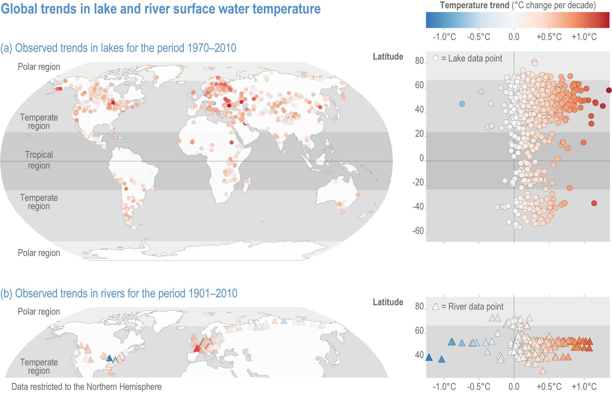
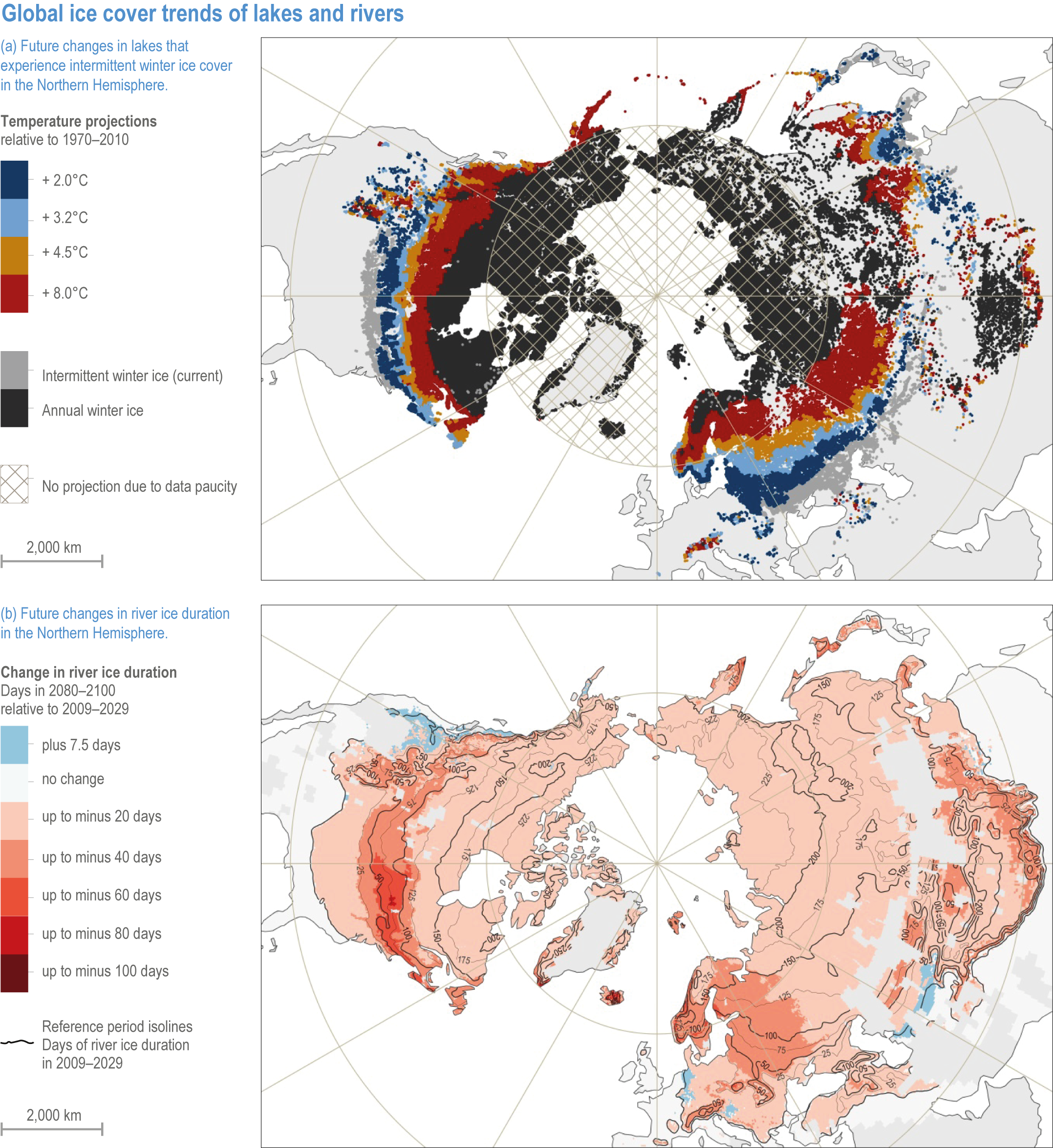
Responses of freshwater species are strongly related to changes in the physical environment (high confidence) {2.3.3; 2.4.2.3.2}. Global coverage of quantitative observations in freshwater ecosystems has increased since AR5. Water temperature has increased in rivers (up to 1°C per decade) and lakes (up to 0.45°C per decade) {2.3.3.1; Figure 2.2}. The extent of ice cover has declined by 25% and duration by >2 weeks {2.3.3.4; Figure 2.4}. Changes in flow have led to reduced connectivity in rivers (high confidence) {2.3.3.2; Figure 2.3}. Indirect changes include alterations in river morphology, substrate composition, oxygen concentrations and thermal regime in lakes (very high confidence) {2.3.3.2; 2.3.3.3}. Dissolved oxygen concentrations have typically declined and primary productivity has increased with warming. Warming and browning (increase in organic matter) have occurred in boreal freshwaters, with both positive and negative repercussions on water temperature profiles (lower vs. upper water) (high confidence) and primary productivity (medium confidence) as well as reduced water quality (high confidence) {2.4.4.1; Figure 2.5}.
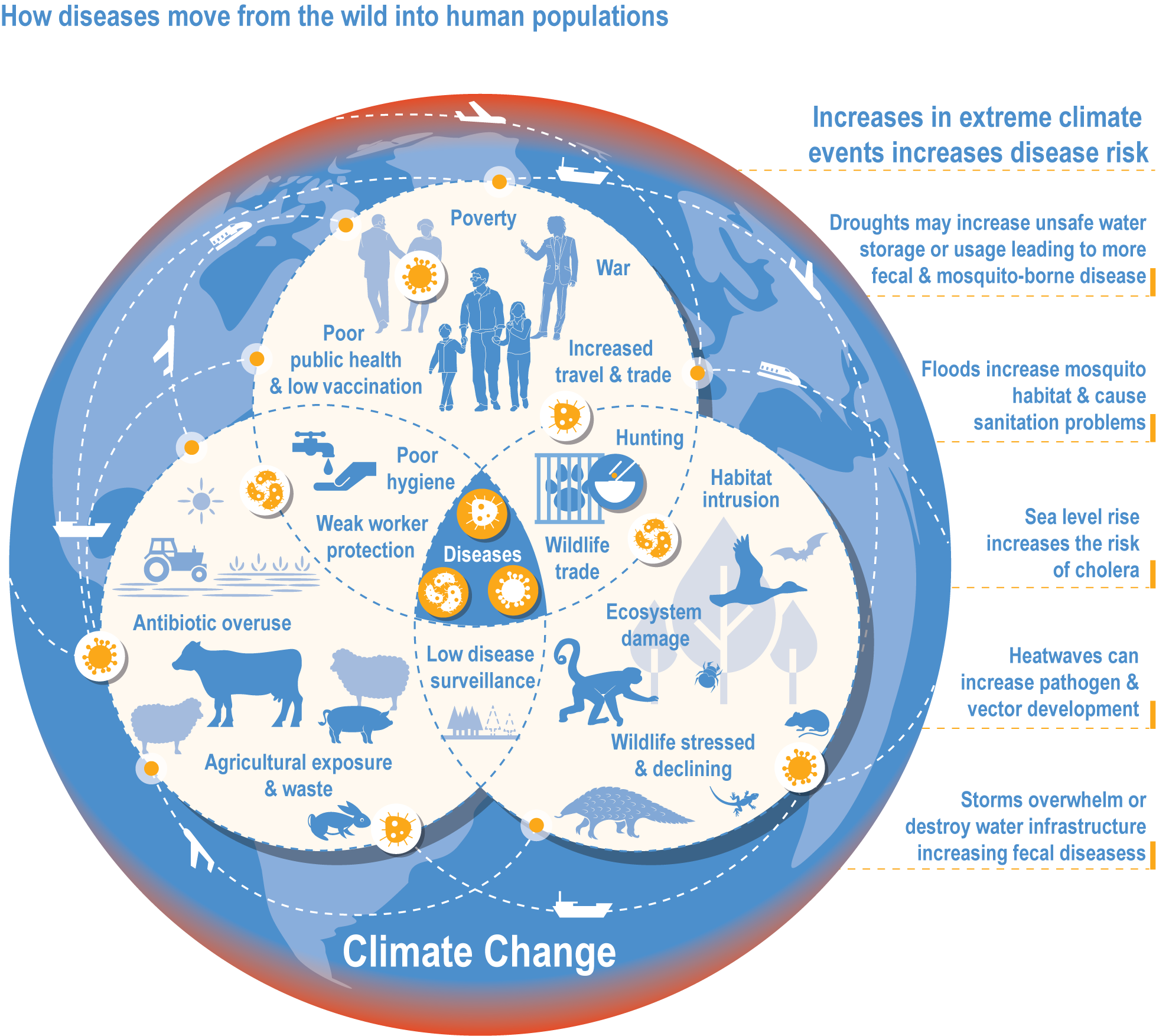
Climate change has increased wildlife diseases (high confidence). Experimental studies provide high confidence in the attribution of observed increased disease severity, outbreak frequency and the emergence of novel vectors and their diseases into new areas to recent trends in climate and extreme events. Many vector-borne diseases and those caused by ticks, helminth worms and the chytrid fungus (Batrachochytrium dendrobatidis, Bd) have shifted polewards and upwards and are emerging in new regions (high confidence). In the high Arctic and at high elevations in Nepal, there is high confidence that climate change has driven the expansion of vector-borne diseases (VBDs) that infect humans. {2.4.2.7, 7.2.2.1, 9.8.2.4, 10.4.7.1, 12.3.1.4, 13.7.1.2, 14.4.6.4; Cross-Chapter Box ILLNESS in this chapter}
Forest insect pests have expanded northward, and the severity and extent of outbreaks have increased in northern North America and northern Eurasia due to warmer winters reducing insect mortality and longer growing seasons favouring more generations per year (high confidence) {2.4.2.1; 2.4.4.3.3}.
Local population extinctions caused by climate change have been widespread among plants and animals, detected in 47% of 976 species examined and associated with increases in the hottest yearly temperatures (very high confidence) {2.4.2.2}. Climate-driven population extinctions have been higher in tropical (55%) than in temperate (39%) regions, higher in freshwater (74%) than in marine (51%) or terrestrial (46%) habitats, and higher in animals (50%) than in plants (39%). Extreme heat waves have led to local fish dying out in lakes and mass mortality events in birds, bats, mammals and fish {2.3.3.5, 2.4.2.7.2, Cross-Chapter Box EXTREMES in this chapter}. Intensification of droughts contributes to the disappearance of small or ephemeral ponds that often harbour rare and endemic species. {2.4.2.2; Cross-Chapter Box EXTREMES in this chapter}
Global extinctions or near-extinctions have been linked to regional climate change in three documented cases{2.4.2.2}. The cloud forest-restricted golden toad (Incilius periglenes) was extinct by 1990 in a nature preserve in Costa Rica following successive extreme droughts (medium confidence). The white sub-species of the lemuroid ringtail possum (Hemibelideus lemuroides) in Queensland, Australia, disappeared after heat waves in 2005 (high confidence): intensive censuses found only 2 individuals in 2009. The Bramble Cay melomys (BC melomys, Melomys rubicola) was not seen after 2009 and was declared extinct in 2016, with sea-level rise (SLR) and increased storm surge associated with climate change being the most probable drivers (high confidence). Additionally, the interaction of climate change and chytrid fungus (Bd) has driven many of the observed global declines in amphibian populations and the extinction of many species (high confidence) {2.4.2.7.1}.
A growing number of studies have documented genetic evolution within populations in response to recent climate change (very high confidence). To date, genetic changes remain within the limits of known variation for species (high confidence). Controlled selection experiments and field observations indicate that evolution would not prevent a species becoming extinct if its climate space disappears globally (high confidence) . Climate hazards outside of those to which species have adapted are occurring on all continents (high confidence). More frequent and intense extreme events, superimposed on longer-term climate trends, have pushed sensitive species and ecosystems towards tipping points that are beyond the ecological and evolutionary capacity to adapt, causing abrupt and possibly irreversible changes (medium confidence). {2.3.1; 2.3.3; 2.4.2.6; 2.4.2.8; 2.6.1; Cross-Chapter Boxes ILLNESS and EXTREMES in this chapter}
Since AR5, biome shifts and structural changes within ecosystems have been detected at an increasing number of locations, consistent with climate change and increasing atmospheric CO2 (high confidence) . New studies are documenting the changes that were projected in prior IPCC reports have now been observed, including upward shifts in the forest/alpine tundra ecotone, northward shifts in the deciduous/boreal forest ecotones, increased woody vegetation in the sub-Arctic tundra and shifts in the thermal habitat in lakes (high confidence). A combination of changes in grazing, browsing, fire, climate and atmospheric CO2 is leading to observed woody encroachment into grasslands and savannah, consistent with projections from process-based models driven by precipitation, atmospheric CO2 and wildfires (high confidence) {2.4.3; Table 2.3; Table SM2.1; Box 2.1; Figure Box 2.1.1; Table Box 2.1.1}. There is high agreement between the projected changes in earlier reports and the recent trends observed for areas of increased tree death in temperate and boreal forests and woody encroachment in savannas, grasslands and tundra {2.5.4; Box 2.1; Figure Box 2.1.1; Table Box 2.1.1}. Observed changes impact the structure, functioning and resilience of ecosystems as well as ecosystem services, such as climate regulation (high confidence) {2.3; 2.4.2; 2.4.3; 2.4.4, 2.5.4, Figure 2.11, Table 2.5, Box 2.1; Figure Box 2.1.1; Table Box 2.1.1}.
Regional increases in the area burned by wildfire (up to double natural levels), tree mortality of up to 20%, and biome shifts of up to 20 km latitudinally and 300 m up-slope have been attributed to anthropogenic climate change in tropical, temperate and boreal ecosystems around the world (high confidence), damaging key aspects of ecological integrity. This degrades the survival of vegetation, habitat for biodiversity, water supplies, carbon sequestration, and other key aspects of the integrity of ecosystems and their ability to provide services for people (high confidence). {2.4.3.1; 2.4.4.2; 2.4.4.3; 2.4.4.4; Table 2.3; Table SM2.1}
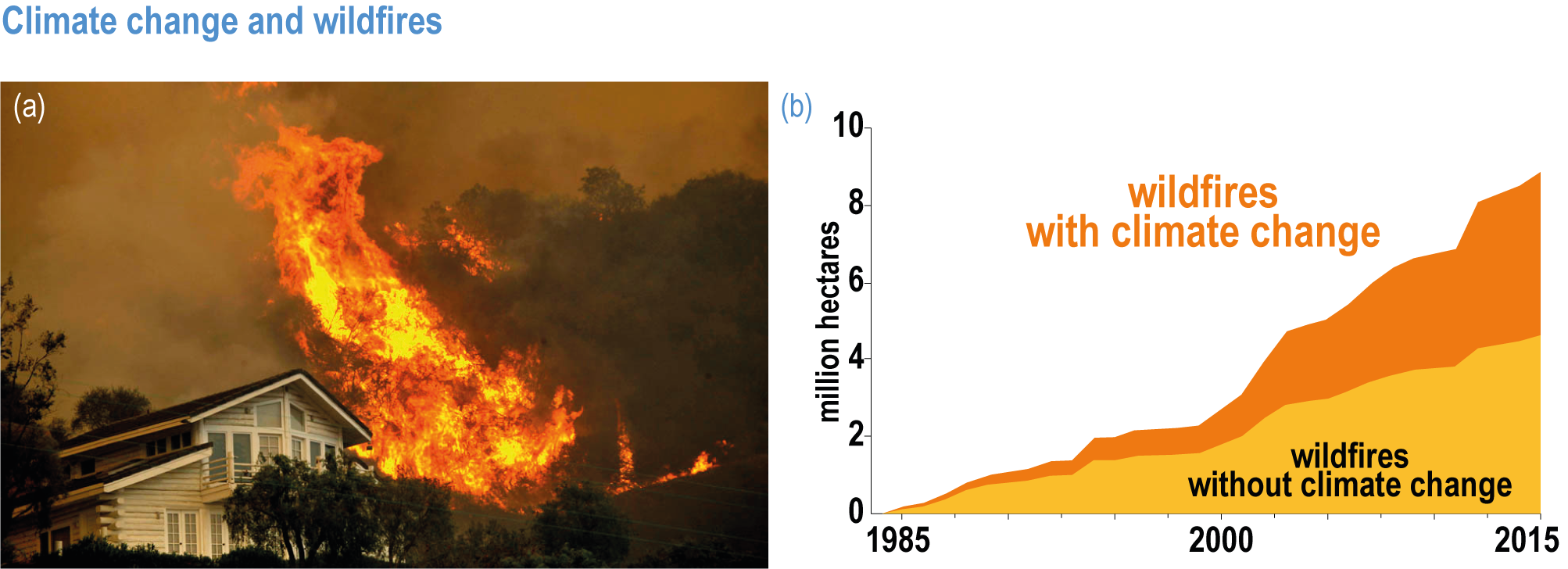
Fire seasons have lengthened on one-quarter of vegetated areas since 1979 as a result of increasing temperature, aridity and drought (medium confidence). Field evidence shows that anthropogenic climate change increased area burned by wildfire above natural levels in western North America in the period 1984–2017: a doubling above natural for the western USA and 11 times higher than natural in one extreme year in British Columbia (high confidence) . In the Amazon, the Arctic, Australia and parts of Africa and Asia, burned area has increased, consistent with, although not formally attributed to, anthropogenic climate change. Wildfires generate up to one-third of ecosystem carbon emissions globally, a feedback that exacerbates climate change (high confidence). Deforestation, draining of peatlands, agricultural expansion or abandonment, fire suppression, and inter-decadal cycles such as the El Niño-Southern Oscillation (ENSO), can exert a stronger influence than climate change on increasing or decreasing wildfire in some regions {2.4.4.2; Table 2.3; Table SM2.1; FAQ 2.3}. Increase in wildfire from the levels to which ecosystems are adapted degrades vegetation, habitat for biodiversity, water supplies and other key aspects of the integrity of ecosystems and their ability to provide services for people (high confidence). {2.4.3.1, 2.4.4.2, 2.4.4.3, 2.4.4.4; Table 2.3; Table SM2.1}
Drought-induced tree mortality attributed to anthropogenic climate change has caused up to 20% loss of trees in the period 1945–2007 in three regions in Africa and North America (high confidence) . It has also potentially contributed to over 100 other cases of drought-induced tree mortality across Africa, Asia, Australia, Europe, and North and South America (high confidence). Field observations have documented post-mortality vegetation shifts (high confidence). Timber cutting, agricultural expansion, air pollution and other non-climate factors also contribute to tree death. Increases in forest insect pests driven by climate change have contributed to tree mortality and shifts in carbon dynamics in many temperate and boreal forest areas (very high confidence). The direction of changes in carbon balance and wildfires following insect outbreaks depends on the local forest insect communities (medium confidence). {2.4.4.3; Table 2.3; Table SM2.1}
Terrestrial ecosystems currently remove more carbon from the atmosphere, 2.5–4.3 Gt yr-1, than they emit (+1.6 ± 0.7 Gt y-1), and so are currently a net sink of -1.9 ± 1.1 Gt y-1. Intact tropical rainforests, Arctic permafrost, peatlands and other healthy high-carbon ecosystems provide a vital global ecosystem service of preventing the release of stored carbon (high confidence) . Terrestrial ecosystems contain stocks of ~3500 GtC in vegetation, permafrost, and soils, three to five times the amount of carbon in unextracted fossil fuels (high confidence) and >4 times the carbon currently in the atmosphere (high confidence). Tropical forests and Arctic permafrost contain the highest ecosystem carbon stocks in aboveground vegetation and in soil, respectively, in the world (high confidence). Deforestation, draining, burning or drying of peatlands, and thawing of Arctic permafrost, due to climate change, has already shifted some areas of these ecosystems from carbon sinks to carbon sources (high confidence). {2.4.3.6; 2.4.3.8; 2.4.3.9; 2.4.4.4}
Evidence indicates that climate change is affecting many species, ecosystems and ecological processes that provide ecosystem services connected to human health, livelihoods, and well-being (medium confidence). These services include climate regulation, water and food provisioning, pollination of crops, tourism and recreation. It is difficult to establish full end-to-end attribution from climatic changes to changes in a given ecosystem service and to identify the location and timing of impacts. The lack of attribution studies may delay specific adaptation planning, but there is evidence that protection and restoration of ecosystems builds resilience of service provision. {2.2; 2.3; 2.4.2.7; 2.4.4; 2.4.5; 2.5.3; 2.5.4; 2.6.3; 2.6.4; 2.6.5; 2.6.6; 2.6.7; Cross-Chapter Boxes NATURAL, ILLNESS and EXTREMES in this chapter; Cross-Chapter Box COVID in Chapter 7; Cross-Chapter Box MOVING PLATE in Chapter 5; Box 5.3; section 5.4.3.4}
Projected Risks
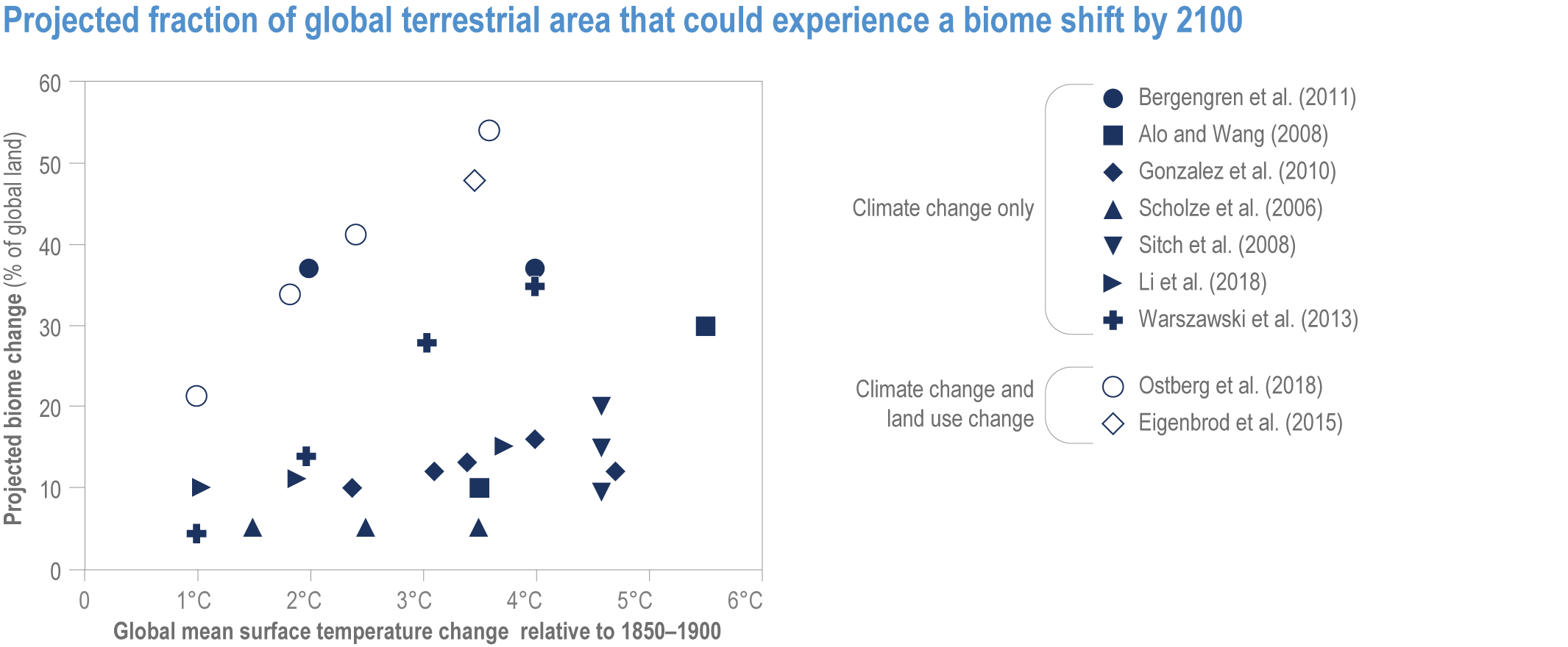
Climate change increases risks to fundamental aspects of terrestrial and freshwater ecosystems, with the potential for species’ extinctions to reach 60% at 5°C global mean surface air temperature (GSAT) warming (high confidence), biome shifts (changes in the major vegetation form of an ecosystem) on 15% (at 2°C warming) to 35% (at 4°C warming) of global land (medium confidence), and increases in the area burned by wildfire of 35% (at 2°C warming) to 40% (at 4°C warming) of global land (medium confidence). {2.5.1; 2.5.2; 2.5.3; 2.5.4; Figure 2.6; Figure 2.7; Figure 2.8; Figure 2.9; Figure 2.11; Table 2.5; Table SM2.2; TableSM2.5; Cross-Chapter Box DEEP in Chapter 17; Cross-Chapter Paper 1}
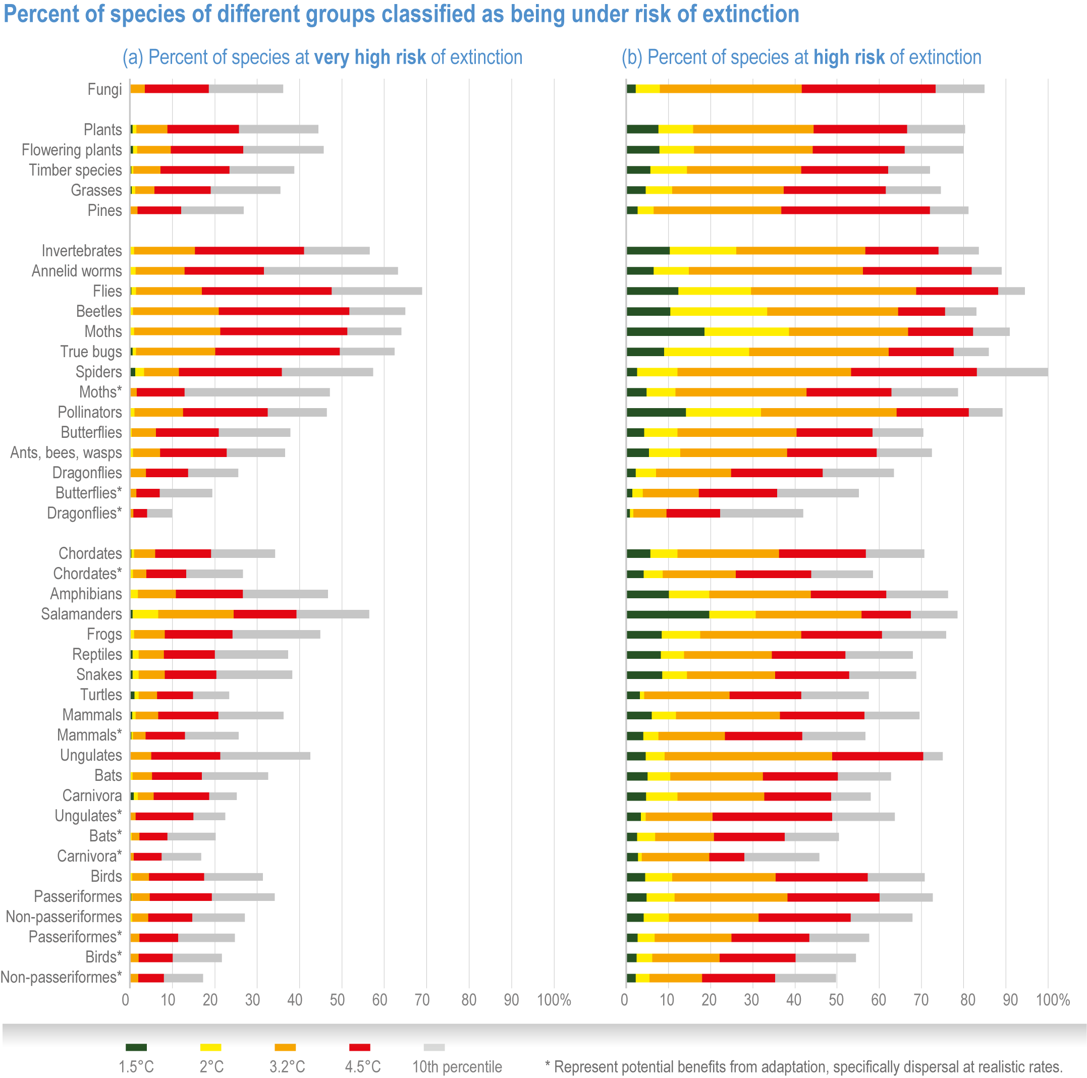
Extinction of species is an irreversible impact of climate change, with increasing risk as global temperatures rise (very high confidence) . The median values for percentage of species at very high risk of extinction (categorized as “critically endangered” by IUCN Red List categories)(IUCN, 2001) are 9% at 1.5°C rise in GSAT, 10% at 2°C, 12% at 3.0°C, 13% at 4°C and 15% at 5°C (high confidence) , with the likely range of estimates having a maximum of 14% at 1.5°C and rising to a maximum of 48% at 5°C (Figure 2.7). Among the groups containing the largest numbers of species at a very high risk of extinction for mid-levels of warming (3.2°C) are: invertebrates (15%, and specifically pollinators at 12%), amphibians (11% overall, but salamanders are at 24%) and flowering plants (10%). All groups fare substantially better at lower warming of 2°C, with extinction projections reducing to <3% for all groups, except salamanders that reduced to 7% (medium confidence) (Figure 2.8a). Even the lowest estimates of species’ extinctions (median of 9% at 1.5°C rise GSAT’) are 1000 times the natural background rates. Projected species’ extinctions at future global warming levels are consistent with projections from AR4, but assessed for many more species with much greater geographic coverage and a broader range of climate models. {2.5.1.3; Figure 2.6; Figure 2.7; Figure 2.8; Cross-Chapter Box DEEP in Chapter 17; Cross-Chapter Paper 1}
Species are the fundamental unit of ecosystems, and the increasing risk of local losses of species increases the risks of reduced ecosystem integrity, functioning and resilience with increasing warming (high confidence). As species become rare, their role in the functioning of the ecosystem diminishes (high confidence). Loss of species locally reduces the ability of an ecosystem to provide services and lowers its resilience to climate change (high confidence). At 1.58°C GSAT warming, >10% of species are projected to become endangered (median estimate, with “endangered” equating to a high risk of extinction, sensu IUCN), and at 2.07°C this rises to >20% of species, representing a high and very high risk of biodiversity loss, respectively (medium confidence) {2.5.4; Figure 2.8b, Figure 2.11; Table 2.5; Table SM2.5}. Biodiversity loss is projected for more regions with increasing warming, and will be worst in northern South America, southern Africa, most of Australia and at northern high latitudes (medium confidence) {2.5.1.3; Figure 2.6}.
Climate change increases risks of biome shifts on up to 35% of global land at ≥4°C GSAT warming, that emission reductions could limit to <15% for <2°C warming (medium confidence). Under high-warming scenarios, models indicate shifts of extensive parts of the Amazon rainforest to drier and lower-biomass vegetation (medium confidence), poleward shifts of boreal forest into treeless tundra across the Arctic, and upslope shifts of montane forests into alpine grassland (high confidence). Area at high risk of biome shifts from changes in climate and land use combined can double or triple compared to climate change alone (medium confidence). Novel ecosystems, with no historical analogue, are expected to become increasingly common in the future (medium confidence). {2.3, 2.4.2.3.3, 2.5.2; 2.5.4, Figure 2.11; Table 2.5; Table SM2.4; Table SM2.5}
The risk of wildfire increases along with an increase in global temperatures (high confidence) . With 4°C GSAT warming by 2100, wildfire frequency is projected to have a net increase of ~30% (medium confidence) . Increased wildfire, combined with soil erosion due to deforestation, could degrade water supplies (medium confidence). For ecosystems with an historically low frequency of fires, a projected 4°C global temperature rise increases the risk of fires, with potential increases in tree mortality and the conversion of extensive parts of the Amazon rainforest to drier and lower-biomass vegetation (medium confidence). {2.5.3.2; 2.5.3.3}
Continued climate change substantially increases the risk of carbon stored in the biosphere being released into the atmosphere due to increases in processes such as wildfire, tree mortality, insect pest outbreaks, peatland drying and permafrost thaw (high confidence). These phenomena exacerbate self-reinforcing feedbacks between emissions from high-carbon ecosystems (that currently store ~3000–4000 GtC) and increasing global temperatures. Complex interactions of climate change, land use change (LUC), carbon dioxide fluxes and vegetation changes, combined with insect outbreaks and other disturbances, will regulate the future carbon balance of the biosphere. These processes are incompletely represented in current earth system models (ESMs). The exact timing and magnitude of climate–biosphere feedbacks and potential tipping points of carbon loss are characterised by large uncertainty, but studies of feedbacks indicate that increased ecosystem carbon losses can cause large temperature increases in the future (medium confidence). (section 5.4, Figure 5.29 and Table 5.4 in (Canadell et al., 2021)), {2.5.2.7; 2.5.2.8; 2.5.2.9; 2.5.3.2; 2.5.3.3; 2.5.3.4; 2.5.3.5; Figure 2.10; Figure 2.11; Table 2.4; Table 2.5; Table SM2.2 Table SM2.5}
Contributions of Adaptation Measures to Solutions
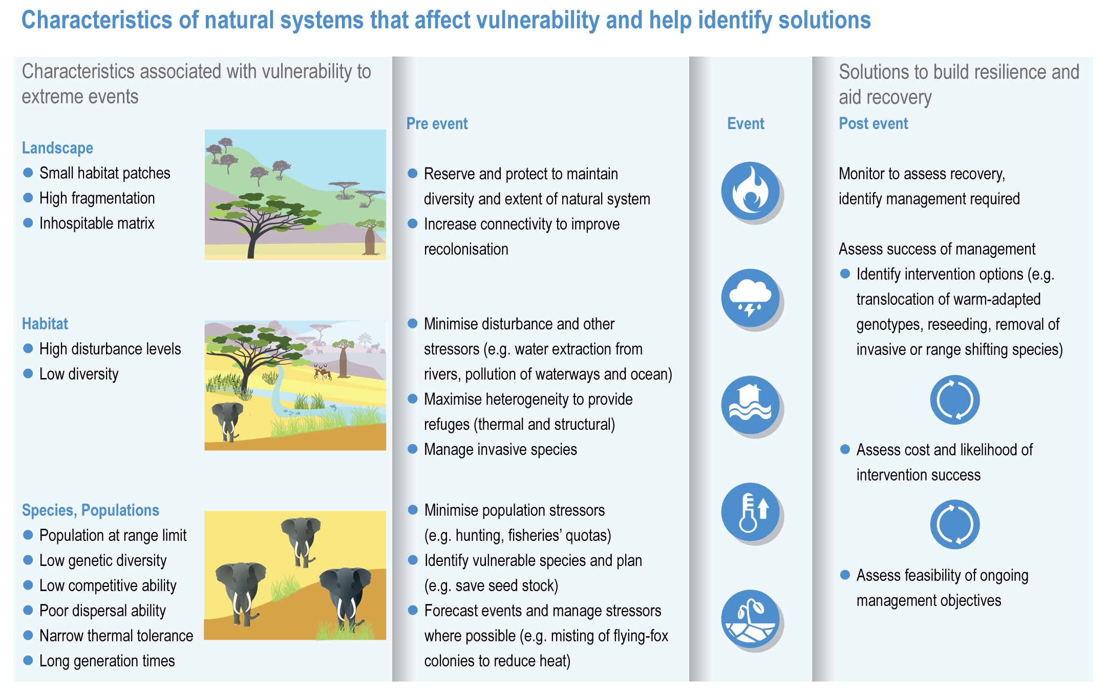
The resilience of biodiversity and ecosystem services to climate change can be increased by human adaptation actions including ecosystem protection and restoration (high confidence). Ecological theory and observations show that a wide range of actions can reduce risks to species and ecosystem integrity. This includes minimising additional stresses or disturbances; reducing fragmentation; increasing natural habitat extent, connectivity and heterogeneity; maintaining taxonomic, phylogenetic, and functional diversity and redundancy; and protecting small-scale refugia where micro-climate conditions can allow species to persist (high confidence). Adaptation also includes actions to aid the recovery of ecosystems following extreme events. Understanding the characteristics of vulnerable species can assist in early warning systems to minimise negative impacts and inform management intervention. {2.3; Figure 2.1; 2.5.3.1, 2.6.2, Table 2.6, 2.6.5, 2.6.7, 2.6.8}
There is new evidence that species can persist in refugia where conditions are locally cooler, when populations of the same species may be declining elsewhere (high confidence) {2.6.2}. Protecting refugia, for example, where soils remain wet during drought or fire risk is reduced, and in some cases creating cooler micro-climates, are promising adaptation measures {2.6.3; 2.6.5; Cross-Chapter Paper 1; CCP5.2.1 }. There is also new evidence that species can persist locally because of plasticity including changes in phenology or behavioural changes that move an individual into cooler micro-climates, and genetic adaptation may allow species to persist for longer than might be expected from local climatic changes (high confidence) {2.4.2.6; 2.4.2.8, 2.6.1}. There is no evidence to indicate that these mechanisms will prevent global extinctions of rare, very localised species already near their climatic limits or species inhabiting climate/habitat zones that are disappearing (high confidence). {2.4.2.8, 2.5.1, 2.5.3.1, 2.5.4, 2.6.1, 2.6.2, 2.6.5}
Since AR5, many adaptation plans and strategies have been developed to protect ecosystems and biodiversity, but there is limited evidence of the extent to which adaptation is taking place and virtually no evaluation of the effectiveness of adaptation measures in the scientific literature (medium confidence). This is an important evidence gap that needs to be addressed, to ensure a baseline is available against which to judge effectiveness and develop and refine adaptation in future. Many proposed adaptation measures have not been implemented (low confidence). {2.6.2; 2.6.3; 2.6.4; 2.6.5; 2.6.6; 2.6.8; 2.7}
Ecosystem restoration and resilience building cannot prevent all impacts of climate change, and adaptation planning needs to manage inevitable changes to species distributions, ecosystem structure and processes (veryhigh confidence). Actions to manage inevitable change include the local modification of micro-climate or hydrology, adjustment of site management plans and facilitating the dispersal of vulnerable species to new locations by increasing habitat connectivity and by active translocation of species. Adaptation can reduce risks but cannot prevent all damaging impacts so is not a substitute for reductions in greenhouse gas (GHG) emissions (high confidence). {2.2; 2.3; 2.3.1; 2.3.2; 2.4.5; 2.5.1.3; 2.5.1.4; 2.5.2; 2.5.3.1; 2.5.3.5; 2.5.4; 2.6.1; 2.6.2; 2.6.3; 2.6.4; 2.6.5; 2.6.6; 2.6.8; Cross-Chapter Box NATURAL in this chapter}
Ecosystem-based adaptation (EbA) can deliver climate change adaptation for people, with multiple additional benefits including those for biodiversity (high confidence). An increasing body of evidence demonstrates that climatic risks to people including floods, drought, fire and overheating, can be lowered by a range of EbA techniques in urban and rural areas (medium confidence). EbA forms part of a wider range of nature-based solutions (NbS); some have mitigation co-benefits, including the protection and restoration of forests and other high-carbon ecosystems as well as agro-ecological farming (AF) practices. However, EbA and other NbS are still not widely implemented. {2.2; 2.5.3.1; 2.6.2; 2.6.3; 2.6.4; 2.6.5; 2.6.6, 2.6.7; Table 2.7; Cross-Chapter Box NATURAL in this chapter; Cross-Chapter Paper 1}
To realise potential benefits and avoid harm, it is essential that EbA is deployed in the right places and with the right approaches for that area, with inclusive governance (high confidence) . Interdisciplinary scientific information and practical expertise, including Indigenous and local knowledge (IKLK), are essential to effectiveness (high confidence). There is a large risk of maladaptation where this does not happen (high confidence). {1.4.2; 2.2; 2.6; Table 2.7; Box 2.2; Figure Box 2.2.1; Cross-Chapter Box NATURAL in this chapter; Cross-Chapter Paper 1; 5.14.2}
EbA and other NbS are themselves vulnerable to climate change impacts (high confidence). They need to take account of climate change if they are to remain effective and they will be increasingly under threat at higher warming levels. NbS cannot be regarded as an alternative to, or a reason to delay, deep cuts in GHG emissions. (high confidence) {2.6.3, 2.6.5; 2.6.7; Cross-Chapter Box NATURAL in this chapter}
Climate Resilient Development
Protection and restoration of natural and semi-natural ecosystems are key adaptation measures in view of the clear evidence that damage and degradation of ecosystems exacerbates the impacts of climate change on biodiversity and people (high confidence). Ecosystem services that are under threat from a combination of climate change and other anthropogenic pressures include climate change mitigation, flood risk management, food provisioning and water supply (high confidence). Adaptation strategies that treat climate, biodiversity and human society as coupled systems will be most effective. {2.3; Figure 2.1; 2.5.4; 2.6.2; 2.6.3; 2.6.7; Cross-Chapter Boxes NATURAL and ILLNESS in this chapter}
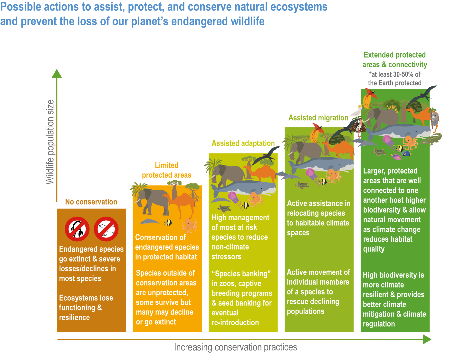
A range of analyses have concluded that ~30–50% of Earth’s surface needs to be effectively conserved to maintain biodiversity and ecosystem services (high confidence). Climate change places additional stress on ecosystem integrity and functioning, adding urgency to taking action. Low-intensity sustainable management, including that performed by Indigenous Peoples, is an integral part of some protected areas, and can support effective adaptation and maintain ecosystem health. Food and fibre production in other areas will need to be efficient, sustainable and adapted to climate change to meet the needs of the human population. (high confidence) {Figure 2.1; 2.5.4; 2.6.2; 2.6.3; 2.6.7}
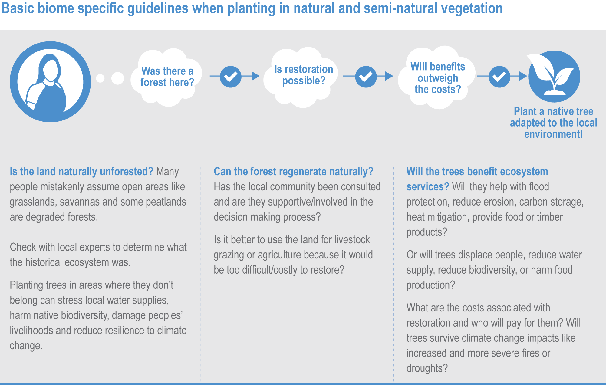
Natural ecosystems can provide the storage and sequestration of carbon at the same time as providing multiple other ecosystem services, including EbA (high confidence), but there are risks of maladaptation and environmental damage from some approaches to land-based mitigation (high confidence). Plantation, single-species forests in areas which would not naturally support forest, including savanna, natural grasslands and temperate peatlands, and replacing native tropical forests on peat soils, have destroyed local biodiversity and created a range of problems regarding water supply, food supply, fire risk and GHG emissions. Large-scale deployment of bioenergy, including bioenergy with carbon capture and storage (BECCS) through dedicated herbaceous or woody bioenergy crops and non-native production forests, can damage ecosystems directly or through increasing competition for land, with substantial risks to biodiversity. {2.6.3, 2.6.5, 2.6.6, 2.6.7; Box 2.2; Cross-Chapter Box NATURAL in this chapter; CCP7.3.2; Cross-Working Group Box BIOECONOMY in Chapter 5}
Terrestrial and aquatic ecosystems and species are often less degraded on land managed by Indigenous Peoples and local communities than on other land (medium confidence) . Involving indigenous and local institutions is a key element for developing successful adaptation strategies. IKLK includes a wide variety of resource-use practices and ecosystem stewardship strategies that conserve and enhance both wild and domestic biodiversity. {2.6.5; 2.6.7; Cross-Chapter Box NATURAL in this chapter; Chapter 15; Box 18.6; CCP2.4.1; CCP2.4.3; Box CCP7.1 }
Increases in the frequency and severity of extreme events, that WGI has attributed to human greenhouse gas emissions, are compressing the timeline available for natural systems to adapt and also impeding our ability to identify, develop and implement solutions (medium confidence). There is now an urgent need to build resilience and assist recovery following extreme events. This, combined with long-term changes in baseline conditions, means that implementing adaptation and mitigation measures cannot be delayed if these are to be fully effective. {2.3; Cross-Chapter Box EXTREMES in this chapter}
2.1 Introduction
2.1.1 Overview
We provide assessments of observed and projected impacts of climate change across species, biomes (vegetation types), ecosystems and ecosystem services, highlighting the processes that are emerging on a global scale. Where sufficient evidence exists, differences in biological responses across regions, taxonomic groups or types of ecosystems are presented, particularly when such differences provide meaningful insights into current or potential future autonomous or human-mediated adaptations. Human interventions that might build the resilience of ecosystems and minimise the negative impacts of climate change on biodiversity and ecosystem functioning are assessed. Such interventions include adaptation strategies and programmes to support biodiversity conservation and Ecosystem-based Adaptation (EbA). The assessments were done in the context of the Convention on Biological Diversity (CBD) and sustainable development goals (SDGs), whose contributions to climate resilient development (CRD) pathways are assessed. This chapter highlights both the successes and failures of adaptation attempts and considers potential synergies and conflicts with land-based climate change mitigation. Knowledge gaps and sources of uncertainty are included to encourage additional research.
The Working Group II Summary for Policymakers of the AR5 stated that ‘many terrestrial and freshwater species have shifted their geographic ranges, seasonal activities, migration patterns, abundances, and species interactions in response to ongoing climate change’ (IPCC, 2014d). Based on long-term observed changes across the regions, it was estimated that approximately 20–30% of plant and animal species are at risk of extinction when global mean temperatures rise 2–3°C above pre-industrial levels (Fischlin et al., 2007). In addition, the WGII AR5 Synthesis Report (IPCC, 2014e) broadly suggested that autonomous adaptation by ecosystems and wild species might occur, and proposed human-assisted adaptations to minimise negative climate change impacts.
Risk assessments for species, communities, key ecosystems and their services were based on the risk assessment framework introduced in the IPCC AR5 (IPCC, 2014b). Assessments of observed changes in biological systems emphasise detecting and attributing the impacts of climate change on ecological and evolutionary processes, particularly freshwater ecosystems, and ecosystem processes such as wildfires, that were superficially assessed in previous reports. Where appropriate, assessment of interactions between climate change and other human activities is provided.
Land use and land cover change (LULCC) as well as the unsustainable exploitation of resources in terrestrial and freshwater systems continue to be major factors contributing to the loss of natural ecosystems and biodiversity (high confidence). Fertiliser input, pollution of waterways, dam construction and the extraction of freshwater for irrigation put additional pressure on biodiversity and alter ecosystem function (Shin et al., 2019). Likewise, for biodiversity, invasive alien species have been identified as a major threat, especially in freshwater systems, on islands and in coastal regions (high confidence) (IPBES, 2018b; IPBES, 2018e; IPBES, 2018c; IPBES, 2018d; IPBES, 2019). Climate change and CO2 are expected to become increasingly important as drivers of change over the coming decades (Ciais et al., 2013; Settele et al., 2014; IPBES, 2019; IPCC, 2019c).
2.1.2 Points of Departure
Species diversity and ecosystem function influence each other reciprocally, while the latter forms the necessary basis for ecosystem services (Hooper et al., 2012; Mokany et al., 2016). Drivers of impacts on biodiversity, ecosystem function and ecosystem services have been assessed in reports by the IPCC, the Food and Agriculture Organization (FAO), the Intergovernmental Platform on Biodiversity and Ecosystem Services (IPBES) and the Global Environmental Outlook (Settele et al., 2014; FAO, 2018; IPBES, 2018b; IPBES, 2018e; IPBES, 2018c; IPBES, 2018d; IPBES, 2019; UNEP, 2019; Secretariat of the Convention on Biological Diversity, 2020). Most recently, the IPCC Special Report on Climate Change and Land (SRCCL) provided an assessment on land degradation and desertification, GHG emissions and food security in the context of global warming (IPCC, 2019c), and the IPBES–IPCC joint report on biodiversity and climate change provided a synthesis of the current understanding of the interactions, synergies and feedbacks between biodiversity and climate change (Pörtner et al., 2021). This chapter builds on and expands the results of these assessments.
Assessment of the impacts of climate change on freshwater systems has been limited in previous assessments, and inter-linkages between terrestrial and freshwater processes have not been fully explored (Settele et al., 2014; IPBES, 2019). Improved treatment of impacts on terrestrial and freshwater systems is critical, considering the revisions of international sustainability goals and targets, especially the conclusion that many of the proposed post-2020 targets of the CBD cannot be met due to climate change impacts (Arneth et al., 2020).
Previous reports highlighted the possibility of new ecosystem states stemming from shifts in thermal regimes, species composition, and energy and matter flows (Settele et al., 2014; Shin et al., 2019). Projecting such “tipping points” (see Glossary Appendix II) has been identified in previous reports as a challenge since monitoring programmes, field studies, and ecosystem and biodiversity modelling tools do not capture the underlying species–species and species–climate interactions sufficiently well to identify how biological interactions within and across trophic levels may amplify or dampen shifts in ecosystem states (Settele et al., 2014; Shin et al., 2019). Building on these previous analyses and the recent literature, Chapter 2 of AR6 provides new insights compared to those of previous assessments by (i) emphasising freshwater aspects and the interlinkages between freshwater and terrestrial systems, (ii) assessing more clearly the link between biodiversity and ecosystem functioning, (iii) assessing the impacts associated with climate change mitigation scenarios versus those of climate change including interactions with adaptation, and (iv) where possible, places findings in the context of the United Nations (UN) SDGs 2030 and services for human societies.
2.1.3 Guide to Attribution and Traceability of Uncertainty Assessments
For biological systems, we use the framework for detection and attribution outlined in AR5, in which biological changes observed are not attributed to global but rather to local or regional climate changes (Parmesan et al., 2013; Cramer et al., 2014). However, global distribution of regional responses is desirable to achieve generality, and data in prior reports were concentrated from the Northern Hemisphere. The critique of ‘global’ studies by (Feeley et al., 2017) argues that their naming is misleading, that most of them are far from global, and that a considerable geographic and taxonomic bias remains. This bias is diminishing, as regional data from the Southern Hemisphere is added and there is now representation from every continent.
Overall confidence in attributing biological changes to climate change can be increased in multiple ways (Parmesan et al., 2013), four of which we list here. First, confidence rises when the time span of biological records is long, such that decadal trends in climate can be compared with decadal trends in biological response, and long-term trends can be statistically distinguished from natural variability. Second, confidence can be increased by examining a large geographic area, which tends to diminish the effects of local confounding factors (Parmesan et al., 2013; Daskalova et al., 2021). Third, confidence is increased when there is experimental or empirical evidence of a mechanistic link between particular climate metrics and a biological response. Fourth, confidence is increased when particular fingerprints of climate change are documented that uniquely implicate climate change as the causal driver of the biological change (Parmesan and Yohe, 2003). These conditions constitute multiple lines of evidence, which, when they converge, can provide very high confidence that climate change is the causal driver of an observed change in a particular biological species or system (Parmesan et al., 2013).
Important factors that may confound or obscure effects of climate change are the presence of invasive species, changes in land use (LULCC) and, in freshwater systems, eutrophication (IPCC, 2019a). The temporal and spatial scale of studies also affects estimates of impacts. The most extreme published estimates of biological change tend to be derived from smaller areas and/or shorter time frames (Daskalova et al., 2021); a recent large global analysis of data for 12,415 species found that differences in study methodology accounted for most of the explained variance in reported range shifts (Lenoir et al., 2020). The importance of LULCC is frequently stressed, but there is a paucity of studies actually quantifying the relative effects of climate change and LULCC on species and communities. (Sirami et al., 2017) found only 13 such studies: four concluded that effects of LULCC overrode those of climate change, four found that the two drivers independently affected different species and five found that they acted in synergy.
2.2 Connections of Ecosystem Services to Climate Change
Ecosystems provide services essential for human survival and well-being. The Millennium Ecosystem Assessment defined ecosystem services as ‘the benefits people obtain from ecosystems’ including ‘provisioning services such as food and water; regulating services such as regulation of floods, drought, land degradation, and disease; supporting services such as soil formation and nutrient cycling; and cultural services such as recreational, spiritual, religious, and other nonmaterial benefits’ (Millennium Ecosystem Assessment, 2005).
The IPBES renamed the concept ‘nature’s contributions to people’ and broadened the definition to ‘the contributions, both positive and negative, of living nature (i.e., diversity of organisms, ecosystems, and their associated ecological and evolutionary processes) to the quality of life for people. Beneficial contributions from nature include such things as food provision, water purification, flood control, and artistic inspiration, whereas detrimental contributions include disease transmission and predation that damages people or their assets’ (IPBES, 2019). The concept was modified to include more social viewpoints and broaden the analyses beyond narrow economic stock-and-flow valuation approaches (Díaz et al., 2018). IPBES developed a classification of 18 categories of ecosystem services (see Table 2.1).
When anthropogenic climate change affects ecosystems, it can also affect ecosystem services for people. Climate change connects to ecosystem services by means of three links, i.e., climate change–species–ecosystems–ecosystem services. This chapter assesses these connections via all three links when end-to-end published scientific analyses are available for terrestrial and freshwater ecosystems. This type of robust evidence exists for some key ecosystem services (Section 2.5.3, 2.5.4), and is assessed in specific report sections: biodiversity habitat creation and maintenance (Sections 2.4, 2.5), regulation of detrimental organisms and biological processes (Sections 2.4.2.3, 2.4.2.7, 2.4.4, 2.5.3, 2.6.4, Cross-Chapter Box ILLNESS in this chapter), regulation of climate through ecosystem feedbacks in terms of carbon storage (Sections 2.4.4.4, 2.5.2.10, 2.5.3.4, 2.5.3.5) and albedo (Section 2.5.3.5) and the provision of freshwater from ecosystems to people (Section 2.5.3.6).
For ecosystem services that do not have published scientific information to establish unambiguous links to climate change, the climate–species–ecosystem links are assessed. Global ecological assessments, including the Global Biodiversity Assessment (Heywood et al., 1995), the Millennium Ecosystem Assessment (Millennium Ecosystem Assessment, 2005), and the IPBES Global Assessment Report (IPBES, 2019) have synthesised scientific information on the ecosystem–ecosystem services link, but a full assessment from climate change to ecosystem services is often impeded by limited quantitative studies that span this entire spectrum (see Mengist et al., 2020) for a review of this gap in montane regions).
IPCC and IPBES are collaborating to address gaps in the knowledge about the effects of climate change on ecosystem services (Pörtner et al., 2021). Table 2.1 provides a guide for finding information on climate change and individual ecosystem services in the AR6.
Table 2.1 | Connections of ecosystem services to climate change, indicating the 18 categories of nature’s contributions to people (IPBES, 2019), the most relevant sections in the AR6, and the level of evidence in this report for attribution to anthropogenic climate change of observed impacts on ecosystem services. The order of services in the table follows the order presented by IPBES and does not denote importance or priority. Connections denote observed impacts, future risks and adaptation. The order of connections follows the relevance or the order of sections. Numbers in parentheses refer to sections in this chapter.
Ecosystem service | Connections to climate change |
Habitat creation and maintenance | Species extinctions (2.4.2.2, 2.5.1.3), species range shifts (2.4.2.1, 2.4.2.5), ecological changes in freshwater ecosystems (2.3.3, 2.4.2.3.2, 2.4.4.1, 2.4.4.5.2, 2.5.1.3.2, 2.5.3.5, 2.5.4, 2.5.3.6, 2.5.5.8), vegetation changes (2.4.3, 2.4.4.2.5, 2.4.4.3, 2.4.4.4, 2.4.4.5.1, 2.5.2, 2.5.3.3), biome shifts (2.4.3.2, 2.5.4), wildfire (2.4.4.2, 2.5.3.2), tree mortality (2.4.4.3, 2.5.3.3) (robust evidence) |
Pollination and dispersal of seeds and other propagules | Species extinctions (2.4.2.2, 2.5.1.3), species range shifts (2.4.2.1, 2.4.2.5), phenology changes (2.4.2.4, 2.4.2.5). See also Box 5.3. (medium evidence) |
Regulation of air quality | Wildfire (2.4.4.2, 2.5.3.2, Chapter 7), tree mortality (2.4.4.3, 2.5.3.3) (medium evidence) |
Regulation of climate | Ecosystem carbon stocks, emissions, and removals (2.4.4.4, 2.5.3.4, (Canadell et al., 2021), Amazon rainforest dieback (2.4.3.6, 2.4.4.3.2, 2.4.4.4.2, 2.5.2.6, 2.5.2.10, 2.5.3.3), tundra permafrost thaw (2.4.4.4.4, 2.5.2.8, 2.5.3.5, 2.5.4), biome shifts (2.4.3, 2.5.2, 2.5.3.2.2), wildfire (2.4.4.2, 2.5.3.2), tree mortality (2.4.4.3, 2.5.3.3), primary productivity changes (2.4.4.5, 2.5.3.5) (robust evidence) |
Regulation of ocean acidification | Ocean acidification (Canadell et al., 2021), changes in marine species distribution and abundance (Chapter 3) (robust evidence) |
Regulation of freshwater quantity, location and timing | Physical changes in freshwater systems (2.3.3), ecological changes in freshwater ecosystems (2.4.2.3.2, 2.4.4.1, 2.4.4.5.2, 2.5.1.3.2, 2.5.3.7), tree mortality (2.4.4.3, 2.5.3.3), freshwater supply from ecosystems (2.5.3.6) (medium evidence) |
Regulation of freshwater and coastal-water quality | Coastal ecosystem changes (Chapter 3), physical changes in freshwater systems (2.3.3), ecological changes in freshwater ecosystems (2.4.2.3.2; 2.4.4.1, 2.4.4.5.2, 2.5.1.3.2, 2.5.3.7) (robust evidence) |
Formation, protection and decontamination of soils and sediments | Agricultural ecosystem changes (Chapter 5), physical changes in freshwater systems (2.3.1), vegetation changes (2.4.3, 2.5.4), wildfire (2.4.4.2, 2.5.3.2) (medium evidence) |
Regulation of hazards and extreme events | Coastal ecosystem changes (Chapter 3), vegetation changes (2.4.3, 2.5.2), wildfire (2.4.4.2, 2.5.3.2), Summary of hazards (2.3), Cross-Chapter Box EXTREMES in this chapter (medium evidence) |
Regulation of detrimental organisms and biological processes | Inter-species interactions (2.4.2), control of disease vectors (2.4.2.7, 2.5.1, 2.6.4), insect-pest infestations (2.4.4.3), Cross-Chapter Box ILLNESS in this chapter (medium evidence) |
Energy | Forestry plantation changes (Chapter 5), biomass changes in natural ecosystems (2.4.4.4), bioeconomy (Cross-Working Group Box BIOECONOMY in Chapter 5), tree mortality (2.4.4.3, 2.5.3.3) (limited evidence) |
Food and feed | Agricultural ecosystem changes (Chapter 5), species extinctions (2.4.2.2, 2.5.1.3), species range shifts (2.4.2.1), nature-based services from natural ecosystems (Cross-Chapter Box NATURAL in this chapter), shifts in commercial food species (Cross-Chapter Box MOVING PLATE in Chapter 5) (medium evidence) |
Materials, companionship and labour | Forestry plantation changes (Chapter 5), species extinctions (2.4.2.2, 2.5.1.3), species range shifts (2.4.2.1), tree mortality (2.4.4.3, 2.5.3.3) (limited evidence) |
Medicinal, biochemical and genetic resources | Species extinctions (2.4.2.2, 2.5.1.3), species range shifts (2.4.2.1) (limited evidence) |
Learning and inspiration | All observed impacts (2.4) and future risks (2.5) in terrestrial and freshwater ecosystems (limited evidence) |
Physical and psychological experiences | All observed impacts (2.4) and future risks (2.5) in terrestrial and freshwater ecosystems. See also 5.4.3.4, Chapter 15, CCP6. (limited evidence) |
Supporting identities | All observed impacts (2.4) and future risks (2.5) in terrestrial and freshwater ecosystems. See also 5.4.3.4, Chapter 15, CCP6 (limited evidence) |
Maintenance of options | All observed impacts (2.4) and future risks (2.5) in terrestrial and freshwater ecosystems, nature-based services from natural ecosystems (Cross-Chapter Box NATURAL in this chapter, Cross-Chapter Box DEEP in Chapter 17, Cross-Chapter Box MOVING PLATE in Chapter 5. (limited evidence) |
2.3 Hazards and Exposure
In AR6, Working Group I (IPCC, 2021a) describes changes in physical climate systems using the term ‘climatic impact-drivers’ (CIDs), which can have detrimental, beneficial or neutral effects on a system. In contrast, the literature on natural systems tends to focus on hazards, which include natural or human-induced physical events, impacts, or trends with the potential to cause negative effects on ecosystems and environmental resources. Hazards are affected by current and future changes in climate, including altered climate variability and extreme events (Ranasinghe et al., 2021). Hazards can occur suddenly (e.g., a heat wave or heavy rain event), or more slowly (e.g., land loss, degradation and erosion linked to multiple climate hazards compounding). Observed exposure and risks to protected areas are assessed in Section 2.5.3.1.1. See also Cross-Chapter Box EXTREMES in this chapter.
Non-climatic hazards such as LUC, habitat fragmentation, pollution and invasive species have been the primary drivers of change in terrestrial and freshwater ecosystems in the past (high confidence) (Figure 2.1). These impacts have been extensively documented in reports by the IPBES (2021). However, while climate change has not been the predominant influence to date, its relative impact is increasing (IPCC SRCCL), with greater interactive effects of non-climate and climate hazards now occurring (Birk et al., 2020).
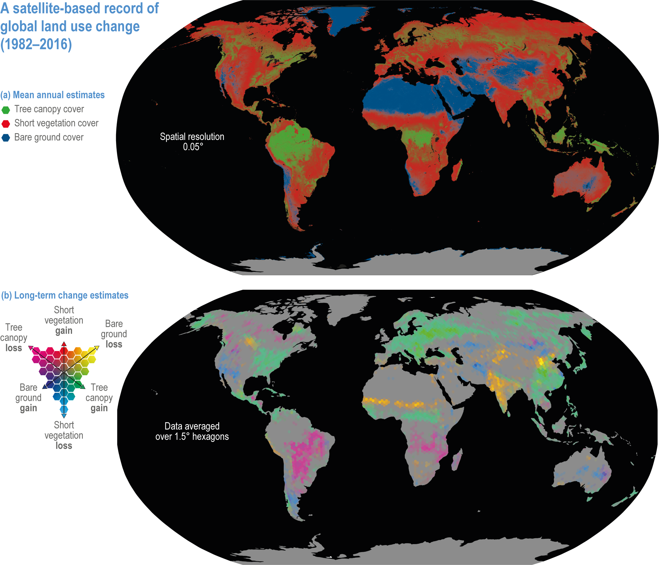
Figure 2.1 | Map of global land use change from 1982 to 2016. Based on satellite records of global tree canopy (TC), short vegetation (SV) and bare ground (BG) cover (from Song et al., 2018).
(a) Mean annual estimates of cover (% of pixel area at 0.05° resolution).
(b) Long-term change estimates (% of pixel area at 1.5° resolution), with pixels showing a statistically significant trend (n= 35 years, two-sided Mann–Kendall test, P < 0.05) in TC, SV or BG. The dominant changes are TC gain with SV loss; BG gain with SV loss; TC gain with BG loss; BG gain with TC loss; SV gain with BG loss; and SV gain with TC loss. Grey indicates areas with no significant change between 1982 and 2016.
2.3.1 Observed Changes to Hazards and Extreme Events
The major climate hazards at the global level are generally well understood (Ranasinghe et al., 2021) (WGI AR6 Interactive Atlas). Increased temperatures and changes to rainfall and runoff patterns; greater variability in temperature, rainfall, river flow and water levels; and rising sea levels and the increased frequency of extreme events means that greater areas of the world are being exposed to climate hazards outside of those to which they are adapted (high confidence) (Lange et al., 2020).
Extreme events are a natural and important part of many ecosystems, and many organisms have adapted to cope with long-term and short-term climate variability within the disturbance regime experienced during their evolutionary history (high confidence). However, climate changes, disturbance regime changes and the magnitude and frequency of extreme events such as floods, droughts, cyclones, heat waves and fire have increased in many regions (high confidence). These disturbances affect ecosystem functioning, biodiversity and ecosystem services (high confidence), but are, in general, poorly captured in impact models (Albrich et al., 2020b), although this should improve as higher-resolution climate models that better capture smaller-scale processes and extreme events become available (Seneviratne et al., 2021). Extreme events pose huge challenges for EbA (IPCC, 2012). Ecosystem functionality, on which such adaptation measures rely, may be altered or destroyed by extreme episodic events (Handmer et al., 2012; Lal et al., 2012; Pol et al., 2017).
There is high confidence that the combination of internal variability, superimposed on longer-term climate trends, is pushing ecosystems to tipping points, beyond which abrupt and possibly irreversible changes are occurring (Harris et al., 2018a; Jones et al., 2018; Hoffmann et al., 2019b; Prober et al., 2019; Berdugo et al., 2020; Bergstrom et al., 2021). Increases in the frequency and severity of heat waves, droughts and aridity, floods, fires and extreme storms have been observed in many regions (Seneviratne et al., 2012; Ummenhofer and Meehl, 2017), and these trends are projected to continue (high confidence) (Section 3.2.2.1, Cross-Chapter Box EXTREMES this Chapter) (Hoegh-Guldberg et al., 2018; Seneviratne et al., 2021).
While the major climate hazards at the global level are generally well described with high confidence, there is less understanding about the importance of hazards on ecosystems when they are superimposed (Allen et al., 2010; Anderegg et al., 2015; Seidl et al., 2017; Dean et al., 2018), and the outcomes are difficult to quantify in future projections (Handmer et al., 2012). Simultaneous or sequential events (coincident or compounding events) can lead to an extreme event or impact, even if each event is not in themselves extreme (Denny et al., 2009; Hinojosa et al., 2019). For example, the compounding effects of SLR, extreme coastal high tide, storm surge, and river flow can substantially increase flooding hazard and impacts on freshwater systems (Moftakhari et al., 2017). On land, changing rainfall patterns and repeated heat waves may interact with biological factors such as altered plant growth and nutrient allocation under elevated CO2, affecting herbivore rates and insect outbreaks leading to the widespread dieback of some forests (e.g., in Australian eucalypt forests) (Gherlenda et al., 2016; Hoffmann et al., 2019a). Risk assessments typically only consider a single climate hazard with no changing variability, thereby potentially underestimating the actual risk (Milly et al., 2008; Sadegh et al., 2018; Zscheischler et al., 2018; Terzi et al., 2019; Stockwell et al., 2020).
Understanding impacts associated with the rapid rate of climate change is less developed and more uncertain than changes in mean climate. High climate velocity (Loarie et al., 2009) is expected to be associated with distribution shifts, incomplete range filling and species extinctions (high confidence) (Sandel et al., 2011; Burrows et al., 2014), although not all species are equally at risk from high velocity (see Sections 2.4.2.2, 2.5.1.3). It is generally assumed that the more rapid the rate of change, the greater the impact on species and ecosystems, but responses are taxonomically and geographically variable (high confidence) (Kling et al., 2020).
For example, strong dispersers are less at risk, while species with low dispersal ability, small ranges and long lifespans (e.g., many plants, especially trees, many amphibians and some small mammals) are more at risk (IPCC, 2014b; Hamann et al., 2015) . This is likely to favour generalist and invasive species, altering species composition, ecosystem structure and function (Clavel et al., 2011; Büchi and Vuilleumier, 2014). The ability to track suitable climates is substantially reduced by habitat fragmentation and human modifications of the landscape such as dams on rivers and urbanisation (high confidence). Freshwater systems are particularly at risk of rapid warming, given their naturally fragmented distribution. Velocity of changes in surface temperature of inland standing waters globally was estimated as being 3.5 ± 2.3 km per decade from 1861 to 2005. From 2006 to 2099, this is projected to increase from 8.7 ± 5.5 km (representative concentration pathway, RCP2.6) to 57.0 ± 17.0 km (RCP8.5) per decade (Woolway and Maberly, 2020). Although the dispersal of the aerial adult stage of some aquatic insects can surpass these climate velocities, rates of change under mid- and high-emission scenarios (RCP4.5, RCP6.0, RCP8.5) are substantially higher than the known rates of the active dispersal of many species (Woolway and Maberly, 2020). Many species, both terrestrial and freshwater, are not expected to be able to disperse fast enough to track suitable climates under mid- and high-emission scenarios (medium confidence) (RCP4.5, RCP6.0, RCP8.5; (Brito-Morales et al., 2018).
2.3.2 Projected Impacts of Increases in Extreme Events
Understanding of the large-scale drivers and the local-to-regional feedback processes that lead to extreme events is still limited, and projections of extremes and coincident or compounding events remain uncertain (Prudhomme et al., 2014; Sillmann et al., 2017; Hao et al., 2018; Miralles et al., 2019). Extreme events are challenging to model because they are, by definition, rare, and often occur at spatial and temporal scales much finer than the resolution of climate models (Sillmann et al., 2017; Zscheischler et al., 2018). Additionally, the processes that cause extreme events often interact, as is the case for drought and heat events, and they are spatially and temporally dependent, for example, soil moisture and temperature (Vogel et al., 2017). Understanding feedbacks between land and atmosphere also remains limited. For example, positive feedbacks between soil and vegetation, or between evaporation, radiation and precipitation, are important in the preconditioning of extreme events such as heat waves and droughts, and can increase the severity and impact of such events (Miralles et al., 2019).
Despite recent improvements in observational studies and climate modelling (Santanello et al., 2015; Stegehuis et al., 2015; PaiMazumder and Done, 2016; Basara and Christian, 2018; Knelman et al., 2019), the potential to quantify or infer formal causal relationships between multiple drivers and/or hazards remains limited (Zscheischler and Seneviratne, 2017; Kleinman et al., 2019; Miralles et al., 2019; Yokohata et al., 2019; Harris et al., 2020). The mechanisms underlying the response are difficult to identify (e.g., responses to heat stress, drought and insects), effects vary among species and at different life stages, and an initial stress may influence the response to further stress (Nolet and Kneeshaw, 2018). Additionally, hazards such as drought are often exacerbated by societal, industrial and agricultural water demands, requiring more sophisticated modelling of the physical and human systems (Mehran et al., 2017; Wan et al., 2017). Observations of past compound events may not provide reliable guides as to how future events may evolve, because human activity and recent climate change continue to interact to influence both system functioning and a climate state not previously experienced (Seneviratne et al., 2021)
2.3.3 Biologically Important Physical Changes in Freshwater Systems
Physical changes are fundamental drivers of change at all levels of biological organisation, from individual species, to communities, whole ecosystems. The climate hazards specific to freshwater systems not documented elsewhere in AR6 are summarised here.
2.3.3.1 Observed Change in Thermal Habitat and Oxygen Availability
Since AR5, evidence of changes in the temperature of lakes and rivers has continued to increase. Global warming rates for lake surface waters were estimated as 0.21°C–0.45°C per decade between 1970 and 2010, exceeding sea-surface temperature (SST) trends of 0.09°C per decade between 1980 and 2017 (robust evidence, high agreement ) (Figure 2.2; (Schneider and Hook, 2010; Kraemer et al., 2015; O’Reilly et al., 2015; Woolway et al., 2020b). Warming of lake surface water temperatures was variable within regions (O’Reilly et al., 2015) but more homogeneous than deep-water temperature changes (Pilla et al., 2020). Because temperature trends in lakes can vary vertically, horizontally and seasonally, complex changes have occurred in the amount of habitat available to aquatic organisms at particular depths and temperatures (Kraemer et al., 2021).

Figure 2.2 | Observed global trends in lake and river surface water temperature.
(a) Left panel: map of temperatures of lakes (1970–2010).
(b) Left panel: map of temperatures of rivers (1901–2010). Note that the trends of river water temperatures are not directly comparable within rivers or to lakes, since time periods are not consistent across river studies. Right panels (a) and (b) depict water temperature trends along a latitudinal gradient highlighting the above average warming rates in northern Polar Regions (polar amplification). Data sources for lakes: (O’Reilly et al., 2015; Carrea and Merchant, 2019; Woolway et al., 2020a; Woolway et al., 2020b). Data sources for rivers: (Webb and Walling, 1992; Langan et al., 2001; Daufresne et al., 2004; Moatar and Gailhard, 2006; Lammers et al., 2007; Patterson et al., 2007; Webb and Nobilis, 2007; Durance and Ormerod, 2009; Kaushal et al., 2010; Pekárová et al., 2011; Jurgelėnaitė et al., 2012; Markovic et al., 2013; Arora et al., 2016; Latkovska and Apsīte, 2016; Marszelewski and Pius, 2016; Jurgelėnaitė et al., 2017).
Changes in river water temperatures ranged from −1.21°C to +1.076°C per decade between 1901 and 2010 (medium evidence, medium agreement ) (Hari et al., 2006; Kaushal et al., 2010; Jurgelėnaitė et al., 2012; Li et al., 2012; Latkovska and Apsīte, 2016; Marszelewski and Pius, 2016). The more rapid increase in surface water temperature in lakes and rivers in regions with cold winters (O’Reilly et al., 2015) can, in part, be attributed to the amplified warming in polar and high-latitude regions (robust evidence, high agreement ) (Screen and Simmonds, 2010; Stuecker et al., 2018).
Shifts in thermal regime: Since AR5, the trend that lake waters mix less frequently continues (Butcher et al., 2015; Adrian et al., 2016; Richardson et al., 2017; Woolway et al., 2017). This results from greater warming of surface temperatures relative to deep-water temperatures, and the loss of ice during winter which prevents inverse thermal stratification in north temperate lakes (robust evidence, high agreement ) (Adrian et al., 2009; Winslow et al., 2015; Adrian et al., 2016; Schwefel et al., 2016; Richardson et al., 2017).
Oxygen availability: increased water temperature and reduced mixing cause a decrease in dissolved oxygen. In 400 lakes, dissolved oxygen in surface and deep waters declined by 4.1 and 16.8%, respectively, between 1980 and 2017 (Jane et al., 2021). The deepest water layers are expected to experience an increase in hypoxic conditions by >25% due to fewer complete mixing events, with strong repercussions for nutrient dynamics and the loss of thermal habitat (robust evidence, high agreement ) (Straile et al., 2010; Zhang et al., 2015; Schwefel et al., 2016).
2.3.3.2 Observed Changes in Water Level
Depending on how the intensification of the global water cycle affects individual lake water budgets, the amount of water stored in specific lakes may increase, decrease or have no substantial cumulative effect (Notaro et al., 2015; Pekel et al., 2016; Rodell et al., 2018; Busker et al., 2019; Woolway et al., 2020b). The magnitude of hydrological changes that can be assuredly attributed to climate change remains uncertain (Hegerl et al., 2015; Gronewold and Rood, 2019; Kraemer et al., 2020). Attribution of water storage variation in lakes due to climate change is facilitated when such variations occur coherently across broad geographic regions and long time scales, preferably absent of other anthropogenic hydrological influences (Watras et al., 2014; Kraemer et al., 2020). There is increasing awareness that climate change contributes to the loss of small temporary ponds which cover a greater global area than lakes (Bagella et al., 2016).
Lakes fed by glacial melt water are growing in response to climate change and glacier retreat (robust evidence, high agreement ) (Shugar et al., 2020). Water storage increases on the Tibetan Plateau (Figure 2.3a) have been attributed to changes in glacier melt, permafrost thaw, precipitation and runoff, in part as a result of climate change (Huang et al., 2011; Meng et al., 2019; Wang et al., 2020a). High confidence in attribution of these trends to climate change is supported by long-term ground survey data and observations from the Gravity Recovery and Climate Experiment (GRACE) satellite mission (Ma et al., 2010; Rodell et al., 2018; Kraemer et al., 2020).
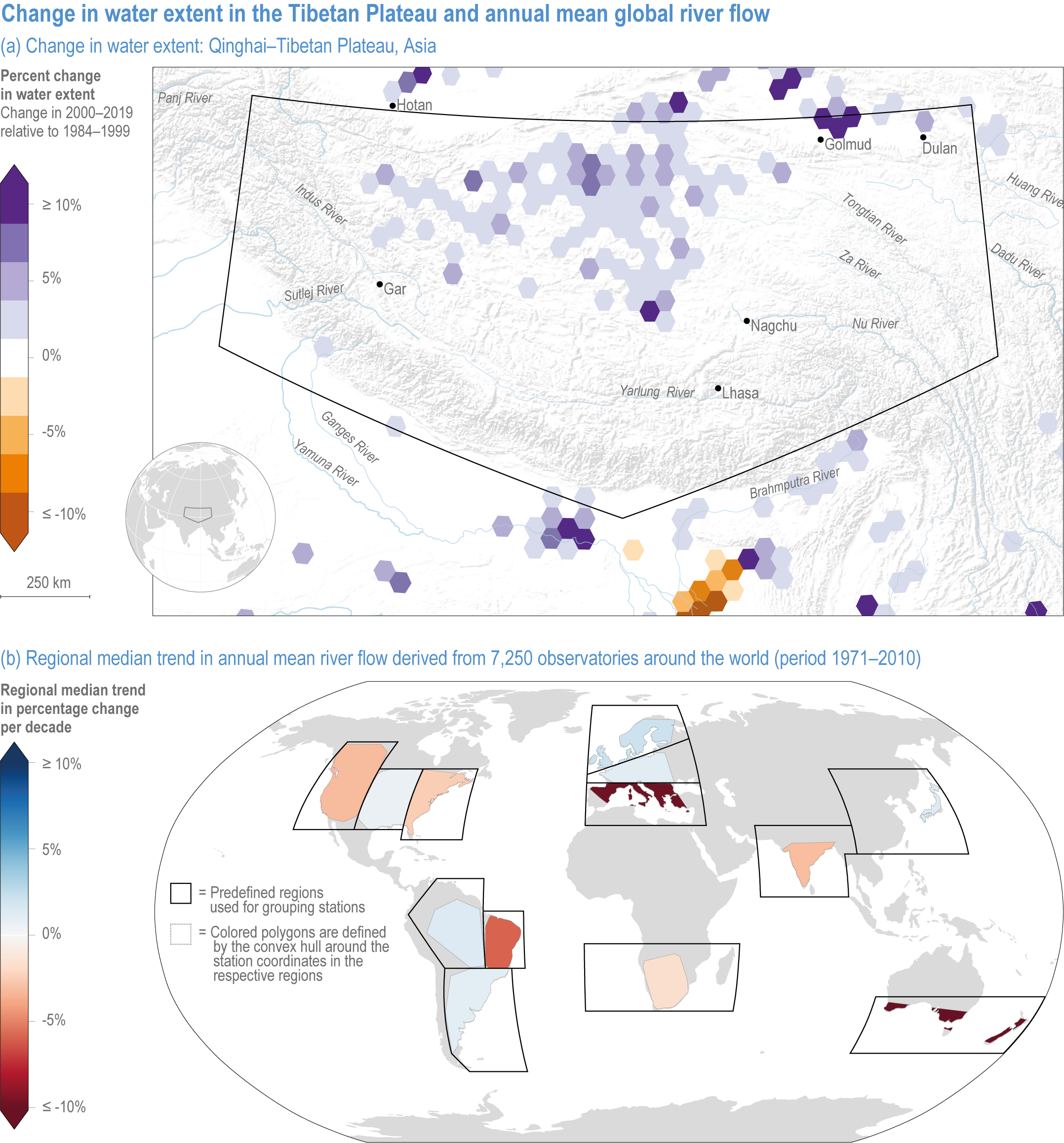
Figure 2.3 | Change in water extent in the Tibetan Plateau and annual mean global river flow.
(a) Changes in water storage on the Tibetan Plateau. Map of the Qinghai–Tibetan Plateau, Asia, showing the percent change in surface water extent from 1984 to 2019 based on LANDSAT imagery. Increases in surface water extent in this region are mainly caused by climate change-mediated increases in precipitation and glacial melt (Source: EC JRC/Google; (Pekel et al., 2016).
(b) Global map of the median trend in annual mean river flow derived from 7250 observatories around the world (in 1971–2010). Some regions are drying (northeast Brazil, southern Australia and the Mediterranean) and others are wetting (northern Europe), mainly caused by large-scale shifts in precipitation, changes in factors that influence evapotranspiration and alterations of the timing of snow accumulation and melt driven by rising temperatures (Source: (Gudmundsson et al., 2021).
In the Arctic, lake area has increased in regions with continuous permafrost, and decreased in regions where permafrost is thinner and discontinuous (robust evidence, high agreement ) (See Chapter 4) (Smith et al., 2005; Andresen and Lougheed, 2015; Nitze et al., 2018; Mekonnen et al., 2021).
2.3.3.3 Observed Changes in Discharge
Analysis of river flows from 7250 observatories around the world covering the years 1971–2010 and identified spatially complex patterns, with reductions in northeastern Brazil, southern Australia and the Mediterranean, and increases in northern Europe (medium evidence, medium agreement ) (Gudmundsson et al., 2021). More than half of global rivers undergo periodic drying that reduces river connectivity (medium evidence, medium agreement ). Increased frequency and intensity of droughts may cause perennial rivers to become intermittent and intermittent rivers to disappear (medium evidence, medium agreement ), threatening freshwater fish in habitats already characterised by heat and droughts (Datry et al., 2016; Schneider et al., 2017; Jaric et al., 2019). In high-altitude/latitude streams, reduced glacier and snowpack extent, earlier snowmelt and altered precipitation patterns, attributed to climate change, have increased flow intermittency (Siebers et al., 2019; Gudmundsson et al., 2021). Patterns in flow regimes can be directly linked to a variety of processes shaping freshwater biodiversity, so any climate change-induced changes in flow regimes and river connectivity are expected to alter species composition as well as having societal impacts (See Chapter 3 in (IPCC, 2018b)) (Bunn and Arthington, 2002; Thomson et al., 2012; Chessman, 2015; Kakouei et al., 2018).
2.3.3.4 Observed Loss of Ice
Studies since AR5 have confirmed ongoing and accelerating loss of lake and river ice in the Northern Hemisphere (robust evidence, high agreement ) (Figure 2.4). In recent decades, systems have been freezing later in winter and thawing earlier in spring, reducing ice duration by >2 weeks per year and leading to an increasing numbers of years with a loss of perennial ice cover, intermittent ice cover or even an absence of ice (Adrian et al., 2009; Kirillin et al., 2012; Paquette et al., 2015; Adrian et al., 2016; Park et al., 2016; Roberts et al., 2017; Sharma et al., 2019). The global extent of river ice declined by 25% between 1984 and 2018 (Yang et al., 2020). This trend has been more pronounced at higher latitudes, consistent with enhanced polar warming (large geographic coverage) (Du et al., 2017). Empirical long-term and remote-sensing data gathered in an increasingly large number of freshwater systems supports very high confidence in attributing these trends to climate change. For the decline of glaciers, snow and permafrost, see Chapter 4 (this report) and the Special Report on the Ocean and Cryosphere in a Changing Climate (IPCC, 2019b).

Figure 2.4 | Global ice cover trends of lakes and rivers.
(a) Spatial distribution of current (light grey areas) and future (coloured areas) Northern Hemisphere lakes that may experience intermittent winter ice cover with climate warming. Projections were based on current conditions (1970–2010) and four established air temperature projections (Data source: (Sharma et al., 2019).
(b) Spatial distribution of projected change in Northern Hemisphere river ice duration under the RCP4.5 emission scenario by 2080–2100 relative to the period 2009–2029. White areas refer to rivers without ice cover in the period 2009–2029 (zero days). Reference period isolines indicate river ice duration in the period 2009–2029. Coloured areas depict loss of ice duration in days. Blue areas depict a projected increase in river ice duration. Grey land areas indicate a lack of Landsat-observable rivers (Data source: (Yang et al., 2020).
2.3.3.5 Extreme Weather Events and Freshwater Systems
Since AR5, numerous drastic short-term responses have been observed in lakes and rivers, to both expected seasonal extreme events and unexpected supra-seasonal extremes extending over multiple seasons. Consequences for ecosystem functioning are not well understood (Bogan et al., 2015; Death et al., 2015; Stockwell et al., 2020). Increasing frequencies of severe floods and droughts attributed to climate change are major threats for river ecosystems (Peters et al., 2016; Alfieri et al., 2017). While extreme floods cause massive physical disturbance, moderate floods can have positive effects, providing woody debris that contributes to habitat complexity and diversity, flushing fine sediments, dissolving organic carbon and providing important food sources from terrestrial origins (Peters et al., 2016; Talbot et al., 2018). Droughts reduce river habitat diversity and connectivity, threatening aquatic species, especially in deserts and arid regions (Bogan et al., 2015; Death et al., 2015; Ledger and Milner, 2015; Jaric et al., 2019).
Rivers already under stress from human activities such as urban development and farming on floodplains are prone to reduced resilience to future extreme events (medium confidence) (Woodward et al., 2016; Talbot et al., 2018). Thus, the potential for floods to become catastrophic for ecosystem services is exacerbated by LULCC (Peters et al., 2016; Talbot et al., 2018). However, biota can recover rapidly from extreme flood events if river geomorphology is not greatly altered. If instream habitat is strongly affected, recovery, if it occurs, takes much longer, resulting in a decline of biodiversity (medium confidence) (Thorp et al., 2010; Death et al., 2015; Poff et al., 2018).
However, not all extreme events will have a biological impact, depending, in particular, on the timing, magnitude and frequency of events and the antecedent conditions (Bailey and van de Pol, 2016; Stockwell et al., 2020; Jennings et al., 2021; Thayne et al., 2021). For instance, an extreme wind event may have little impact on phytoplankton in a lake that was fully mixed prior to the event. Conversely, the effects of a storm on phytoplankton communities may compound when lakes have not yet recovered from a previous storm or if periods of drought alternate with periods of intense precipitation (limited evidence) (Leonard et al., 2014; Stockwell et al., 2020).
In summary, extreme events (heat waves, storms and loss of ice) affect lakes in terms of water temperature, water level, light, oxygen concentrations and nutrient dynamics, which, in turn, affect primary production, fish communities and GHG emissions (high confidence). These impacts are modified by levels of solar radiation, wind speed and precipitation (Woolway et al., 2020a). Droughts have a negative impact on water quality in streams and lakes by increasing water temperature, salinity, the frequency of algal blooms and contaminant concentrations, and reducing concentrations of nutrients and dissolved oxygen (medium confidence) (Peters et al., 2016; Alfieri et al., 2017; Woolway et al., 2020a). Understanding how these pressures subsequently cascade through freshwater ecosystems will be essential for future projections of their resistance and resilience towards extreme events (Leonard et al., 2014; Stockwell et al., 2020). See Table SM2.1 for specific examples of observed changes.
2.3.3.6 Projected Changes in Physical Characteristics of Lakes and Rivers
Given the strength of relationship between past GSAT and warming trends at lake surfaces (Figure 2.2; Section 2.3.3.1) and projected increases in heat waves, surface water temperatures are projected to continue to increase (Woolway et al., 2021). Mean May to October lake surface temperatures in 46,557 European lakes were projected to be 2.9°C, 4.5°C and 6.5°C warmer by 2081–2099 compared to the historic period (1981–1999) under RCP2.0, RCP6.0 and RCP8.5, respectively (Woolway et al., 2020a). Under RCP2.6, the average intensity of lake heat waves increases from 3.7°C to 4.0°C and the average duration from 7.7 to 27.0 days, relative to the historic period (1970–1999). For RCP8.5, warming increases to 5.4°C and duration increases dramatically to 95.5 days (medium confidence) (Woolway et al., 2021).
Worldwide alterations in lake mixing regimes in response to climate change are projected (Kirillin, 2010). Most prominently, monomictic lakes—undergoing one mixing event in most years—will become permanently stratified, while lakes that are currently dimictic—mixing twice per year—will become monomictic by 2080–2100 (medium confidence) (Woolway and Merchant, 2019). Nevertheless, predicting mixing behaviour remains an important challenge and attribution to climate change remains difficult (Schwefel et al., 2016; Bruce et al., 2018).
Under climate projections of 3.2°C warming, 4.6% of the ice-covered lakes in the Northern Hemisphere could switch to intermittent winter ice cover (Figure 2.4a; (Sharma et al., 2019). Unfrozen and warmer lakes lose more water to evaporation (Wang et al., 2018b). By 2100, global annual lake evaporation will increase by 16%, relative to 2006–2015, under RCP8.5 (Woolway et al., 2020b). Moreover, melting of ice decreases the ratio of sensible to latent heat flux, thus channelling more energy into evaporation (medium confidence) (Wang et al., 2018b). In the periods 2009–2029 and 2080–2100, average duration of river ice is projected to decline by 7.3 and 16.7 days under RCP4.5 and RCP8.5, respectively (Figure 2.4b; Yang et al., 2020).
Projections of lake water storage are limited by the absence of reliable, long-term, homogenous and spatially resolved hydrologic observations (Hegerl et al., 2015). This uncertainty is reflected in the widely divergent projections in response to future climate changes in individual lakes (Angel and Kunkel, 2010; MacKay and Seglenieks, 2012; Malsy et al., 2012; Notaro et al., 2015) . Selecting models that perform well when comparing hindcasted to observed past water storage variation often does little to reduce water storage projection uncertainty (Angel and Kunkel, 2010). This wide range of potential changes complicates lake management. For information on observed and projected changes in the global water cycle and hydrological regimes for streams, lakes, wetland, groundwater and their implications on water quality and societies, see Chapter 4, this report, and (Douville et al., 2021). For the role of weather and climate extremes on the global water cycle, see (Seneviratne et al., 2021).
In summary, with ongoing climate warming and an increase in the frequency and intensity of extreme events, observed increases in water temperature, losses of ice and shifts in thermal regime are projected to continue (high confidence).
Cross-Chapter Box EXTREMES | Ramifications of Climatic Extremes for Marine, Terrestrial, Freshwater and Polar Natural Systems
Authors: Rebecca Harris (Australia, Chapter 2, CCP3), Philip Boyd (Australia, Chapter 3), Rita Adrian (Germany, Chapter 2), Jörn Birkmann (Germany, Chapter 8), Sarah Cooley (USA, Chapter 3), Simon Donner (Canada, Chapter 3), Mette Mauritzen (Norway, Chapter 3), Guy Midgley (South Africa, Chapter 16); Camille Parmesan (France/USA/UK, Chapter 2), Dieter Piepenburg (Germany, Chapter 13, CCP6), Marie-Fanny Racault (UK/France, Chapter 3), Björn Rost (Germany, Chapter 3, CCP6), David Schoeman (Australia, Chapter 3), Stavana E. Strutz (USA/Chapter 2), Maarten van Aalst (the Netherlands, Chapter 16).
Introduction
Increases in the frequency and magnitudes of extreme events, attributed to anthropogenic climate change by WGI (IPCC, 2021a), are now causing profound negative effects across all realms of the world (marine, terrestrial, freshwater and polar) (medium confidence) (Fox-Kemper et al., 2021; Seneviratne et al., 2021) (Sections 2.3.1, 2.3.2, 2.3.3.5, 2.4.2.2, Chapter 3, Chapters 9–12, this report). Changes to population abundance, species distributions, local extirpations, and global extinctions are leading to long-term, potentially irreversible shifts in the composition, structure and function of natural systems (medium confidence) (Frolicher and Laufkotter, 2018; Harris et al., 2018a; Maxwell et al., 2019; Smale et al., 2019). These effects have widespread ramifications for ecosystems and the services they provide—physical habitat, erosion control, carbon storage, nutrient cycling and water quality—with knock-on effects for tourism, fisheries, forestry and other natural resources (2.4.3, 2.4.4, 2.5.1, 2.5.2, 2.5.3, 2.5.4) (Kaushal et al., 2018; Heinze et al., 2021; Pörtner et al., 2021).
Increasingly, the magnitude of extreme events is exceeding the values projected for mean conditions for 2100, regardless of emissions scenario (Figure Cross-Chapter Box EXTREMES.1). This has collapsed the timeline that organisms and natural communities have to acclimate or adapt to climate change (medium confidence). Consequently, rather than having decades to identify, develop and adopt solutions, actions to build resilience and assist recovery following extreme events are required quickly if they are to be effective.
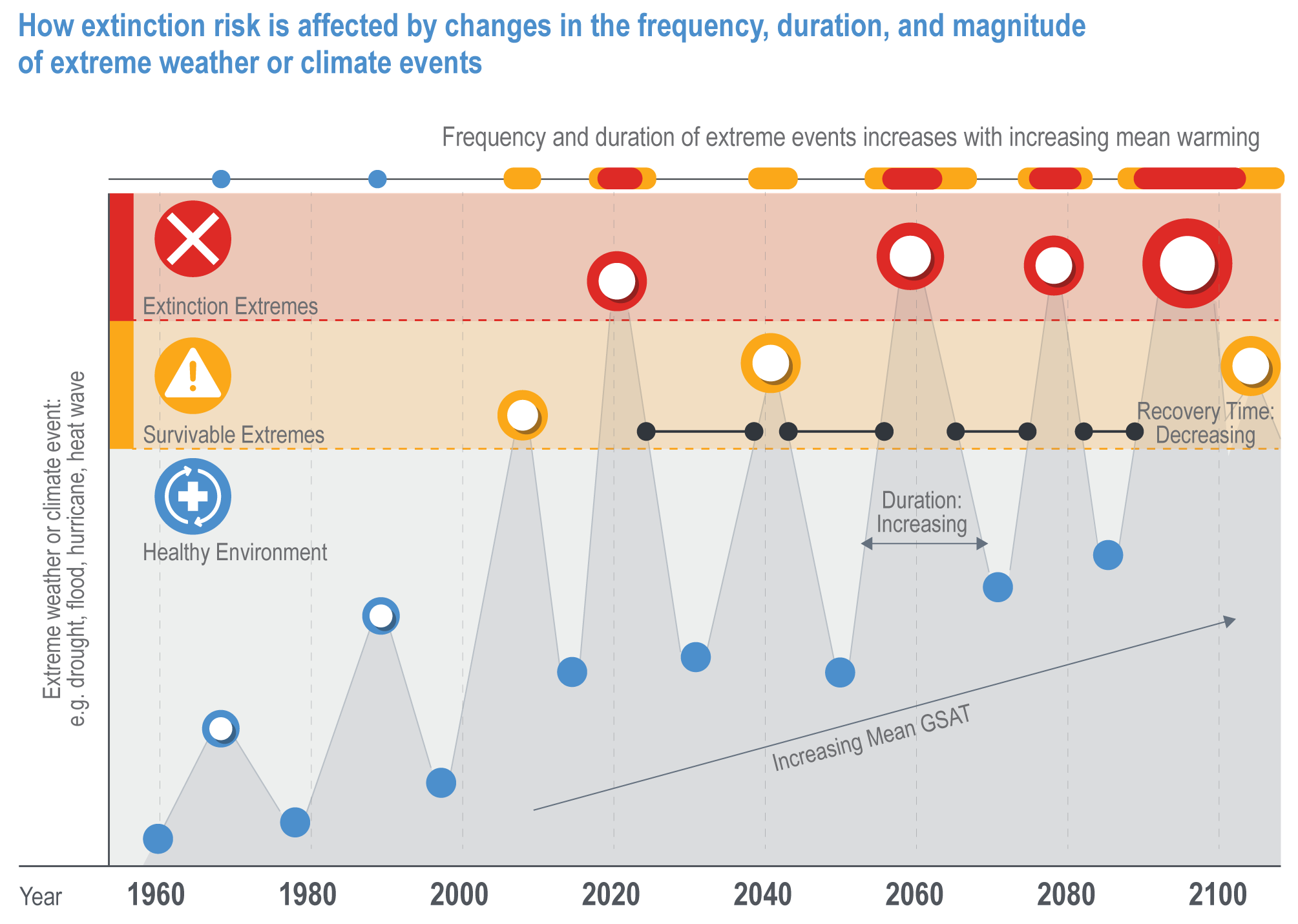
Figure Cross-Chapter Box EXTREMES.1 | A conceptual illustration of how extinction risk is affected by changes in the frequency, duration and magnitude of extreme weather or climate events (e. g,. drought, fire, flood and heat waves). Many organisms have adapted to cope with long- and short-term climate variability, but as the magnitude and frequency of extreme events increases, superimposed on the long-term climate trend, the threshold between survivable extreme weather events (yellow) and extremes that carry a high risk of causing population or species extinctions (red) is crossed more frequently. This can lead to local extinction events with insufficient time between to enable recovery, resulting in long-term, irreversible changes to the composition, structure and function of natural systems. When the extreme event occurs over a large area relative to the distribution of a species (e.g., a hurricane impacting an island which is the only place a given species occurs), a single extreme event can drive the global extinction of a species.
Recent extremes highlight the characteristics that enable natural systems to resist or recover from events, helping natural resource managers to develop solutions to improve the resilience of natural communities and identify the limits to adaptation (Bergstrom et al., 2021).
Marine Heat Waves
Consensus is emerging that anthropogenic climate change has significantly increased the likelihood of recent marine heat waves (MHWs) (medium confidence) (Oliver et al., 2018; Fox-Kemper et al., 2021). A widespread MHW occurred in the northeast Pacific in 2013–2015, with upper ocean temperature anomalies of up to 6.2°C relative to 2002–2012 (Gentemann et al., 2017). This event, termed the ‘Blob’, enhanced surface water stratification, decreasing nutrient supply, primary and community production and leading to widespread changes to open ocean and coastal ecosystems, with geographical shifts of key species across trophic levels, mass strandings of marine mammals, seabird mortalities and the closure of commercially important fisheries (Cavole et al., 2016; Piatt et al., 2020). The MHW reappeared in 2019 (‘Blob 2.0’) (Amaya et al., 2020), with similarly high temperature anomalies extending from Alaska to California, but the ecological effects of this event are expected to differ because the Blob originated in winter, and Blob2.0 intensified in summer (Amaya et al., 2020). Modelling suggests rapid shifts in the geographic distributions of important fish species in response to MHWs (Cheung and Frolicher, 2020), with projected decreased biomass and distributional shifts of fish at least four times faster and larger than the effects of decadal-scale mean changes throughout the 21st century under RCP8.5 (high confidence) (Cheung and Frolicher, 2020). MHWs can also dramatically increase CH4 emissions from oceans, a significant positive feedback to global warming (see also Chapter 3, this report) (Borges et al., 2019).
The Arctic region is warming more than twice as fast as the global mean, and polar organisms and ecosystems are likely to be particularly vulnerable to heat waves due to their specific thermal niches and physiological thresholds and also the lack of poleward ‘refugia’ (high confidence). The consequences of MHWs are exacerbated by concomitant sea ice melting and the freshening of surface waters, leading to secondary effects due to osmotic stress and failing pH homeostasis. Since sea ice-associated organisms are often critical components of polar food chains, cascading effects up to the top predators are expected. In 2015–2016, a MHW occurred in the Gulf of Alaska/Bering Sea (Walsh et al., 2018) which was unprecedented in terms of surface temperatures and ocean heat content, geographical extent, depth range and persistence, impacting the entire marine food web. Persistent warming favoured some phytoplankton species and triggered one of the largest algal blooms recorded in this region, with concomitant oyster farm closures due to uncommon paralytic shellfish-poisoning events (Walsh et al., 2018). There were also massive die-offs of common guillemots (Uria aalge) and puffins (Fratercula cirrhata) , attributed to starvation resulting from warming-induced effects on food supply (Jones et al., 2019). A 2017 survey found a 71% decline in the abundance of Pacific cod (Gadus macrocephalus) since 2015, likely due to an increase in metabolic demand and reduced prey supply during the MHWs (Barbeaux et al., 2020).
Terrestrial Heat Waves
Heat waves are now regularly occurring that exceed the physiological thresholds of some species, including birds and other small endotherms such as flying foxes (high confidence) (Sections 2.4.2.2, 2.4.2.6). Heat waves in Australia, North America and southern Africa have caused mass mortality events due to lethal hyperthermia and dehydration (Saunders et al., 2011; Conradie et al., 2020; McKechnie et al., 2021), reducing fitness (du Plessis et al., 2012; Andrew et al., 2017; Sharpe et al., 2019; van de Ven et al., 2019; van de Ven et al., 2020), breeding success, and recruitment (Kennedy et al., 2013; Wiley and Ridley, 2016; Ratnayake et al., 2019) and affecting daily activity and geographic distributions (Albright et al., 2017). They also place enormous demands on wildlife management agencies and pose risks to human health (Welbergen et al., 2008).
Cross-Chapter Box EXTREMES
Recent mortality events affected 14 species of bird and fruit bats (Epomophorus wahlbergi) in South Africa when maximum air temperatures exceeded 43–45°C in 2020 (McKechnie et al., 2021). Passerine birds seem more vulnerable to lethal hyperthermia, due to the relative inefficiency of panting to lose heat (McKechnie et al., 2021) and also their small size, as heat tolerance generally increases with body mass (McKechnie et al., 2021). Several mass mortality events of flying foxes (Pteropus poliocephalus, P. alecto) have occurred in eastern Australia when maximum air temperatures exceeded 42° (Welbergen et al., 2008). Nineteen such events occurred between 1994 and 2008, compared to three events prior to 1994. In January 2002, maximum temperatures exceeded the 30-year average mean daily maximum by up to 16.5° and killed >3500 individuals (Welbergen et al., 2008). In 2014, an estimated 45,500 flying foxes died in a single day, when average maximum temperatures were ≥8°C above average (Bureau of Meteorology, 2014). Drought compounds the impacts, as mortality increases when water availability is low (Welbergen et al., 2008; Mo and Roache, 2020; McKechnie et al., 2021).
Antarctica encountered its first recorded heat wave in 2020. Record high temperatures occurred in East Antarctica (Robinson et al., 2020), with a maximum (9.2°) temperature ~7° above the mean maximum, and minimum temperatures > 0°. Record high temperatures (18.3°) were also recorded in West Antarctica (Robinson et al., 2020). It is too soon to know the impact on polar life, but such abrupt heating is expected to have wide-ranging effects on biota, from flash-flooding and dislodgement of plants, to excess meltwater supplying moisture to arid polar ecosystems ( Cross-Chapter Paper 6 Polar). Heat waves in Siberia in 2016, 2018 and 2020, with air temperature anomalies >6°, were associated with extensive wildfires, pest infestations and melting permafrost (Overland and Wang, 2021).
Freshwater Extremes
Heat waves, storms and floods affect the thermal regime and biogeochemical functioning of lakes and rivers (Woolway and Merchant, 2017; Vicente-Serrano et al., 2020). Extreme heat waves lead to abnormally high water temperatures (Till et al., 2019) and reduce the mixing of lakes (Woolway et al., 2021), causing a decrease in oxygen and deep-water oxygen renewal (Zhang et al., 2015). Ectotherms such as fish and invertebrates are particularly susceptible to such temperature and oxygen stress (Stoks et al., 2014). Their metabolic demands increase with rising temperature and a suitable habitat is eroded due to both high temperatures and lower oxygen concentrations in lakes and rivers. Till et al. (2019) attributed 502 fish kill events in the Wisconsin lakes (USA) to warmer summers in lakes that experienced abnormally high water temperatures. Such events are predicted to double by 2041–2059 and increase four-fold by 2081–2099 compared to historical levels (Till et al., 2019). This anticipated increase in die-offs may facilitate warm-water fish species displacing cool-water species (Hansen et al., 2017; Jennings et al., 2021). Floods mobilise nutrients and sediment, and aid dispersal of invasive species in rivers (Death et al., 2015), while drought extremes reduce river connectivity, threatening biodiversity in rivers (section 2.3.3.5) (Tickner et al., 2020).
Cross-Chapter Box EXTREMES
Learnings from Recent Extremes
These examples show that the impact of an extreme event is a function of its characteristics and those of the exposed ecosystem. The timing, frequency, absolute magnitude and geographic extent of the extreme event, relative to antecedent conditions and the life cycle, resistance and resilience of the natural community, all determine the biological response (Figure Cross-Chapter Box Extremes.1) (Hillebrand et al., 2018; Gruber et al., 2021). The impact appears to be greater when extreme events occur more frequently, particularly when the interval between events is insufficient to allow recovery to previous population sizes (e.g., frequent fires and coral bleaching) or coincides with vulnerable life-cycle stages, even when populations are adapted to cope with such disturbances. Events occurring over large spatial areas reduce the potential for recolonisation from nearby populations (e.g., regional droughts causing widespread declines). Often the magnitude of extreme events exceeds historical levels, so organisms are less likely to be adapted to them, particularly when several extremes coincide (e.g., high water temperature and drought) (Duke et al., 2017). When hazards occur simultaneously (compound events), the impacts of extremes can be substantially aggravated, triggering a cascade of effects in ecosystems (Gruber et al., 2021).
Several characteristics of natural systems are associated with greater vulnerability to extreme events (Figure Cross-Chapter Box EXTREMES.2), knowledge of which can inform solutions to build resilience and aid recovery (Robinson et al., 2020). Resilience can be built prior to an event by minimising additional disturbances, such as water extraction from river systems, pollution of aquatic systems, fragmentation of land and LULCCs. Managing landscapes to reduce fragmentation and increase habitat extent, connectivity and heterogeneity, by increasing the number and extent of reserves, may provide local refugia from extreme events and enhance post-event recolonisation, but may be less effective for marine systems (Section 3.6). Maintaining taxonomic, phylogenetic and functional diversity is important, as more diverse systems may be more stable in the face of disturbances (Pimm, 1984; García-Palacios et al., 2018).
 Figure Cross-Chapter Box EXTREMES.2 | Characteristics of natural systems that affect vulnerability and help identify solutions—both prior to and after extreme events—to build resistance, resilience and recovery
Several characteristics increase vulnerability: low or narrow thermal tolerance, high habitat specificity, low dispersal ability, long generation times, low competitive ability and life-cycle constraints that limit recovery or recolonisation. Populations living close to one or more limiting factors near range edges are also vulnerable (Arafeh-Dalmau et al., 2019). Understanding these characteristics can inform management intervention to aid recovery following an extreme event. For instance, knowledge of the flying fox’s physiological temperature threshold led to successful interventions, including misting populations to reduce mortality (Mo and Roache, 2020), and the development of a ‘heat stress forecaster’, an online tool which uses weather forecasts to identify roosts at risk of extreme heat events (Ratnayake et al., 2019). This early warning system increases the preparedness of wildlife management and conservation agencies, enabling efficient allocation of management resources towards the locations that are likely to be the most affected.
Monitoring following extreme events can help identify immediate impacts and the potential for cascading interactions, such as changes to competitive interactions following range shifts, impacts on freshwater ecosystems following wildfires and the spread of invasive species. Ongoing monitoring of recovery and effectiveness of management intervention is important, focussing on habitat-forming species (e.g., kelp, corals and dominant tree species) and keystone species (e.g., filter-feeders, macrophytes and top predators), as the loss of these species can lead to ecosystem tipping points, beyond which the system may not recover (Collins et al., 2019) (Sections 2.5.3; 3.4.4.1; 3.4.4.1.4; chapters 9–15, this report).
The acute impacts of extreme events, in addition to the chronic stress of changing mean conditions, are accelerating and amplifying the biological effects of climate change. This amplification is being observed globally and in all realms where life exists. Extreme events are compressing the timeline available for natural systems to adapt, and impeding our ability to identify, develop and adopt solutions. Recent events highlight the urgent need to mitigate global GHG emissions and identify solutions to halt accelerating impacts on natural systems (Díaz et al., 2020).
Cross-Chapter Box EXTREMES
2.4 Observed Impacts of Climate Change on Species, Communities, Biomes, Key Ecosystems and Their Services
2.4.1 Overview
Global meta-analyses of terrestrial systems in AR3 and AR4 concentrated on long time frames (>20 years) and findings from relatively undisturbed areas, where confidence in attributing observed changes to climate change is high. Recent global and regional meta-analyses (AR5 and later) have been broader, including data from degraded and disturbed areas and studies with shorter time frames (Tables 2.2a,b).
By the time of AR5, >4000 species with long-term observational data had been studied in the context of climate change (Parmesan, 2006; Parmesan and Hanley, 2015). Since then, thousands of new studies and additional species have been added, leading to higher confidence in climate change attribution (Table 2.2) (Scheffers et al., 2016; Wiens, 2016; Cohen et al., 2018; Feeley et al., 2020). Freshwater habitats have been under-represented in prior reports, but new long-term datasets, coupled with laboratory and field experiments, are improving our understanding. This assessment stresses observations from lakes and streams. As numbers of studies increase and data is increasingly extracted from areas with high LULCC, attribution is more difficult as habitat loss and fragmentation are known major drivers of changes in terrestrial and freshwater species (Ramsar Convention on Wetlands, 2018; IPBES, 2019; Tickner et al., 2020). Due to the overwhelming volume of literature, the assessments for chapter 2 concentrates on results from large continental or global-scale reviews and meta-analyses. Most of the assessment of studies conducted in individual countries can be found in Regional chapters, but this chapter does include studies across very large countries or political entities that occupy much of a continent (e.g., Canada, the USA, Australia or Europe), or studies that provide rare or uniquely-relevant information.
2.4.2 Observed Responses to Climate Change by Species and Communities (Freshwater and Terrestrial)
2.4.2.1 Observed Range Shifts Driven by Climate Change
Poleward and upward range shifts were already attributable to climate warming with high confidence in AR5. Publication of observed range shifts in accord with climate change have accelerated since AR5 and strengthened attribution. Ongoing latitudinal and elevational range shifts driven by regional climate trends are now well-established globally across many groups of organisms, and attributable to climate change with very high confidence due to very high consistency across a now very large body of species and studies and an in-depth understanding of mechanisms underlying physiological and ecological responses to climate drivers (Table 2.2; Table 2.3, Table SM2.1) (Pöyry et al., 2009; Chen et al., 2011; Grewe et al., 2013; Gibson-Reinemer and Rahel, 2015; MacLean and Beissinger, 2017; Pacifici et al., 2017; Anderegg et al., 2019). Range shifts stem from local population extinctions along warm-range boundaries (Anderegg et al., 2019) as well as from the colonisation of new regions at cold-range boundaries (Ralston et al., 2017).
Many studies since AR4 have tended not to be designed as attribution studies, particularly recent large-scale, multi-species meta-analyses. That is to say, all the data available was included in such studies (from both undisturbed and highly degraded lands and including very short-term data sets of <20 years), with little attempt to design the studies to differentiate the effects of climate change from those of other potential confounding variables. These studies tended to find greater lag and a lower proportion of species changing in the directions expected from climate change, with the authors concluding that LULCC, particularly habitat loss and fragmentation, was impeding wild species from effectively tracking climate change (Lenoir and Svenning, 2015; Rumpf et al., 2019; Lenoir et al., 2020).
Attribution is strong for species and species-interactions for which there is a robust mechanistic understanding of the role of climate on biological processes (high confidence). Unprecedented outbreaks of spruce beetles occurring from Alaska to Utah in the 1990s were attributed to warm weather that, in Alaska, facilitated a halving of the insect’s life cycle from two years to one (Logan et al., 2003). Milder winters and warmer growing seasons were likewise implicated in poleward expansions and increasing outbreaks of several forest pests (Weed et al., 2013), leading to the current prediction that 41% of major insect pest species will further increase their damage as climate warms, and only 4% will reduce their impacts, while the rest will show mixed responses (Lehmann et al., 2020).
During their range shifts, forest pests remain climate-sensitive. For example, the distribution of the western spruce budworm is limited at its warm range edges by the adverse effects of mild winters on overwinter survival, and at its cool range by the ability to arrive at a cold-resistant stage before winter arrives (Régnière and Nealis, 2019). We might therefore expect tree mortality from insect outbreaks to be most severe at sites climatically less suitable for the plants, where plants would be under more stress. However, (Jaime et al., 2019), using separate species distribution models (SDMs) (MaxEnt) for the insects and plants, found that observed mortality of Scots pine from bark beetles was highest at sites that were most climatically suitable for the trees as well as for the insects. In a study of tree mortality in California, bark beetles selectively killed highly stressed fir trees, but killed pines according to their size irrespective of stress status (Stephenson et al., 2019).
Range shifts in a poleward and upward direction, following expected trajectories according to local and regional climate trends, are strongly occurring in freshwater fish populations in North America (Lynch et al., 2016b), Europe (Comte and Grenouillet, 2013; Gozlan et al., 2019) and Central Asia (Gozlan et al., 2019) (medium evidence, high agreement). Cold-water fish, such as coregonids and smelt have been negatively affected at the equatorial borders of their distributions (Jeppesen et al., 2012). Upward elevational range shifts in rivers and streams have been observed. Systematic shifts towards higher elevation and upstream were found for 32 stream-fish species in France following regional variation in climate change (Comte and Grenouillet, 2013). Bull trout (Salvelinus confluentus) in Idaho (USA), were estimated to have lost 11–20% (8–16% per decade) of the headwater stream lengths necessary for cold-water spawning and early juvenile rearing, with the largest losses occurring in the coldest habitats (Isaak et al., 2010). Range contractions of the same species have been found in the Rocky Mountains watershed (Eby et al., 2014). Likewise, the distribution of the stonefly Zapada glacier, endemic to the alpine streams of the Glacier National Park in Montana (USA), has been reduced over several decades by an upstream retreat to higher, cooler sites as water temperatures have increased and glacial masses have decreased (Giersch et al., 2015).
The melting of glaciers has led to a change in water discharge associated with community turnover in glacier-fed streams (Cauvy-Fraunié and Dangles, 2019). For instance, glacier-obligate macro-invertebrates have started disappearing when glacial cover drops below approximately 50% (robust evidence, high agreement ), reviewed in (Hotaling et al., 2017). For freshwater invertebrates, no meaningful trends have been detected in geographic extent or population size for most species (Gozlan et al., 2019).
An invasive freshwater cyanobacterium in lakes, Cylindrospermopsis raciborskii, originating from the tropics, has spread to temperate zones over the last few decades due to the climate change-induced earlier increase of water temperature in spring (Wiedner et al., 2007), aided by a competitive advantage in eutrophic systems (Ekvall et al., 2013; Urrutia-Cordero et al., 2016).
2.4.2.2 Observed Local Population and Global Species’ Extinctions Driven by Climate Change
Disappearances of local populations within a species range are more frequent and better documented than whole species’ extinctions, and attribution to climate change is possible for sites with minimal confounding non-climatic stressors. Changes of temperature extremes are often more important to these local extinction rates than changes of mean annual temperature (high confidence) (see Sections 2.3.1, 2.3.2, 2.3.3.5, 2.4.2.6, Cross-Chapter Box EXTREMES in this chapter) (Parmesan et al., 2013). A global meta-analysis of 236 species of birds, mammals, amphibians, fish, invertebrates and plants across 132 independent studies found that changes in population abundances were strongly related to temperature variability globally, and significantly related to precipiation variability in lower latitudes (Pearce-Higgins et al., 2015). In a global study of 538 diverse plant and animal species, sites with local extinctions were associated with smaller changes of mean annual temperature but larger and faster changes of hottest yearly temperatures than sites where populations persisted (Román-Palacios and Wiens, 2020). Near warm range limits, 44% of species had suffered local extinctions. In both temperate and tropical regions, sites with local extinction had greater increases in maximum temperatures than those without: a Tmax increase of 0.456°C and 0.316°C versus a Tmean increase of 0.153°C and 0.061°C for temperate (n= 505 sites) and tropical (n= 76 sites), respectively (P < 0.001) (Román-Palacios and Wiens, 2020).
Wiens (2016) assumed that population extinctions were primarily driven by climate change when they occurred at elevational or latitudinal ‘warm edge’ range limits, and were at relatively undisturbed sites stated by the authors to be under increasing climatic stress. By this criterion, climate-caused local extinctions were widespread among plants and animals globally, detected in 47% of 976 species examined. The percentage of species suffering these extinctions was higher in the Tropics (55%) than in temperate habitats (39%), higher in freshwater (74%) than in marine (51%) or terrestrial (46%) habitats, and higher in animals (50%) than in plants (39%). The difference between plants and animals varied with latitude; in the temperate zone, a much higher proportion of animals than plants suffered range-limit extinctions (38.6% of 207 animal species vs. 8.6% of 105 plants, P < 0.0001) while at tropical sites, local extinction rates were (nonsignificantly) higher in plants (59% of 155 species) than in animals (52% of 349 species), the reverse of their temperate-zone relationship. Rates varied across animal groups from 35% in mammals, to 43% in birds, 56% in insects and 59% in fish (Wiens, 2016).
Freshwater population extinctions are mainly due to habitat loss, the introduction of alien species, pollution, over-harvesting (Gozlan et al., 2019; IPBES, 2019) and climate change-induced epidemic diseases (Pounds et al., 2006)(see Section 2.4.2.7.1). Climate warming, particularly through the intensification and severity of droughts, contributes to the disappearance of small ponds which hold rare and endemic species (Bagella et al., 2016). Systematic data on the extent and biology of small ponds is, however, lacking on the global scale. Extreme heat waves can lead to large local fish kills in lakes (see Section 2.3.3.5), when water temperature and oxygen concentrations surpass critical thresholds and threatening cold-water fish and amphibians (Thompson et al., 2012). Evidence of a local extinction of some invertebrate species with a 1.4°C–1.7°C rise in mean annual stream winter temperature from 1981 to 2005 was reported in Abrahams et al. (2013). Population declines of specialist species in glacier-fed streams, such as the non-biting midge Diamesa davisi (Chironomidae), can be attributed to climate-change-driven glacier retreat (Cauvy-Fraunié and Dangles, 2019), and the flatworm Crenobia alpina (Planariidae) has been reported as locally extinct in the Welsh Llyn Brianne river (Durance and Ormerod, 2010; Larsen et al., 2018).
Many high montane possums in Australia have low physiological tolerance to heat waves, with death occuring due to heat-driven dehydration at temperatures exceeding 29°C–30°C for >4–5 h over several days (Meade et al., 2018; Turner, 2020). Major declines have been recorded for several species, population extinctions have occured at lower elevations since the early 2000s, and the white sub-species of the lemuroid ringtail possum (Hemibelideus lemuroides) in Queensland, Australia, disappeared after heat waves in 2005 (high confidence): intensive censuses found only 2 individuals in 2009 (Chandler, 2014; Weber et al., 2021).
Two terrestrial and freshwater species have become extinct in the wild, with climate change implicated as a key driver. The cloud forest-restricted golden toad (Incilius periglenes) was extinct by 1990 in a nature preserve in Costa Rica, driven by successive extreme droughts. This occurred in the absence of chytridiomycosis infection, caused by the fungal pathogen Bd, verified during field censuses of golden toad populations in the process of extinction as well as genetic analyses of museum specimens, although Bd was present in other frog species in the region (medium evidence, high agreement ) (Pounds et al., 1999; Pounds et al., 2006; Puschendorf et al., 2006; Richards-Hrdlicka, 2013). The interaction between expansion of chytrid fungus globally and local climate change is implicated in the extinction of a wide range of tropical amphibians (high confidence) (see Section 2.4.2.7.1 Case Study 2 Chytrid fungus and climate change).
The BC melomys (Melomys rubicola), the only mammal endemic to the Great Barrier Reef, inhabited a small (5-hectare) low-lying (<3-m-high) cay in the Torres Strait Islands, Australia. Recorded as having a population size of several hundred in 1978, this mammal has not been seen since 2009 and was declared extinct in 2016 (Gynther et al., 2016). SLR and documented increases in storm surge and in tropical cyclones, driven by climate change, led to multiple inundations of the island in the 2000s. Between 1998 and 2014, herbacious vegetation, the food resource for the BC melomys, declined by 97% in area (from 2.2 down to 0.065 hectares), and from 11 plant species down to two (Gynther et al., 2016; Watson, 2016; Woinarski, 2016; Woinarski et al., 2017). The island was unihabited with few non-climatic threats, providing high confidence in the attribution of extinction of the BC melomys to climate change-driven increases in the frequency and duration of island inundation (Turner and Batianoff, 2007; Woinarski et al., 2014; Gynther et al., 2016; Watson, 2016; Woinarski et al., 2017).
In the IUCN Red List (IUCN, 2019), 16.2% of terrestrial and freshwater species (n= 3,777 species) that are listed as endangered, critically endangered or extinct in the wild (n= 23,251 species) list climate change or severe weather as one of their threats.
In summary, local population extinctions caused by climate-change-driven increases in extreme weather and climate events have been widespread among plants and animals (very high confidence), and the first clear documentations of entire species driven extinct by recent climate change is emerging (medium confidence).
2.4.2.3 Observed Changes in Community Composition Driven by Climate Change
2.4.2.3.1 Overall patterns of community change
The most common type of community change takes the form of in situ decreases in cold-adapted species and increases in warm-adapted species (Bowler et al., 2017; Hughes et al., 2018; Kuhn and Gégout, 2019; Feeley et al., 2020). This process has lead to increases of species richness on mountaintops and decreased richness at adjacent lower elevations (medium evidence, high agreement ) (Forister et al., 2010; Steinbauer et al., 2018). While it is also expected from observed range shifts of individual species that species richness should increase along tropical/temperate ecotones and along temperate/boreal ecotones, to date this has not been well documented. Lewthwaite et al (Lewthwaite and Mooers, 2022) documented a small increase in local richness across Canada for 265 species of butterflies, but the stronger effect was an homogenization across the region, with generalist species generally expanding into new sites and leading to lower Beta-diversity (lower diversity among sites). In a study of 66 bumble bee species across North America and Europe, Soroye et al (Soroye et al., 2020) did not find the expected pattern, with most sites, regardless of latitude, declining in species richness, even when individual species benefited from warming or increased precipitation at some sites. Observed shifts in community composition have consequences for species’ interactions. Such indirect effects of climate change have been shown to often have greater impacts on species than the direct effects of climate itself, particularly for higher-level consumers (Cahill et al., 2013; Ockendon et al., 2014).
Analyses indicated that responses in range shifts and timing were lagging behind the changes expected from regional warming. This type of lag, where biological response is less than expected from known underlying physiology or general climatic limits, is called ‘climate debt’. Examples of climate debt, measured from community composition changes, come from birds and butterflies in Europe (Devictor et al., 2012) and lowland forest herbaceous plants in France (Bertrand et al., 2011). The French study found that larger debts occurred in communities with warmer baseline conditions and that some of the apparent debt stemmed from the ability of species to tolerate warming in situ, so no range shift was observed.
Prominent changes in freshwater community composition, such as increases in cyanobacteria and warm-tolerant zooplankton species, the loss of cold-water fish, gains in thermo-tolerant fish, macro-invertebrates, and floating macrophytes, are occurring (medium evidence, high agreement , medium confidence) (Adrian et al., 2016; Hossain et al., 2016; Short et al., 2016; Huisman et al., 2018; Gozlan et al., 2019). Geothermal streams have provided evidence about community structure and ecosystem function at high temperatures. A study of 14 such habitats reported simplified food web structures and shortened pathways of energy flux between consumers and resources (high confidence) (O’Gorman et al., 2019). Changes in the relative abundance of species, species composition and biodiversity due to warming trends, and non-climate-driven changes are to be expected in lakes and rivers globally. However, thus far, empirical evidence and mechanistic understanding to inform modelling is too limited to draw general conclusions about the nature of current and future climate change-driven changes within entire food webs on a global scale (Urban et al., 2016).
2.4.2.3.2 Freshwater systems: mechanistic drivers and responses
Physical changes in lakes (see Section 2.3.3) have affected primary production (see Section 2.4.4.5.2), algal-bloom formation and composition, zooplankton and fish size distribution, and species composition (Urrutia-Cordero et al., 2017; Gozlan et al., 2019; Seltmann et al., 2019). Declines in the abundance of cold-stenothermal species, particularly the Arctic charr (Salvelinus alpinus), coregonids and smelt, and increases in eurythermal fish (e.g., the thermo-tolerant carp Cyprinus carpio, common bream, pike perch, roach and shad) have been observed in northern temperate lakes associated with warming trends (medium evidence, high agreement ) (Jeppesen et al., 2012; Jeppesen et al., 2014). These changes increase predation pressure on zooplankton and reduce grazing pressure on phytoplankton, which may result in higher phytoplankton biomass (De Senerpont Domis et al., 2013; Jeppesen et al., 2014; Adrian et al., 2016). Reduction in lake mixing lowers the concentration of nutrients in the epilimnion and may lead to higher silicon-to-phosphorous ratios that negatively affect diatom growth (Yankova et al., 2017) or overall primary productivity (see Section 2.4.4.5.2).
In a study of 1567 lakes across Europe and North America, Kakouei (2021) identified climate change as the major driver of increases in phytoplankton biomass in remote areas with minimal LULCC. Greater temperature variability can be more important than long-term temperature trends as a driver of zooplankton biodiversity (Shurin et al., 2010). Reductions of winter severity attributed to anthropogenic climate change are increasing winter algal biomass, and motile and phototropic species, at the expense of mixotrophic species (Özkundakci et al., 2016; Hampton et al., 2017).
Tropical lakes are prone to loss of deep-water oxygen due to lake warming, with negative consequences for their fisheries and their biodiversity (Lewis Jr, 2000; Van Bocxlaer et al., 2012). Many ancient tropical lakes (Malawi, Tanganyika, Victoria, Titicaca, Towuti and Matano) hold thousands of endemic animal species (Vadeboncoeur et al., 2011).
Observed effects of climate change on freshwater invertebrates are variable (Knouft and Ficklin, 2017). In glacier-fed streams globally, climate change has caused community turnover and changes in abundances in terms of increased generalist and decreased specialist species (Lencioni, 2018; Cauvy-Fraunié and Dangles, 2019). In turn, dragonflies in flowing waters, monitored during the warming period from 1988 through 2006 in Europe, did not show consistent changes in their distribution (Grewe et al., 2013), reviewed in Knouft and Ficklin (2017). Long-term trends in the species composition and community structure of stream macro-invertebrates, specifically a general trend for decreases in species characteristic of cold, fast-flowing waters and increases of thermophilic species typical of stagnant or slow-moving waters, have been attributed to climate change (robust evidence, high agreement ) (Daufresne et al., 2007; Chessman, 2015). A study of 14 geothermal streams reported simplified food web structures and shortened pathways of energy flux between consumers and resources (O’Gorman et al., 2019). Macrophytes benefit from rising water temperatures, but increased shading from increased phytoplankton biomass could offset this (Hossain et al., 2016; Short et al., 2016; Zhang et al., 2017a).
2.4.2.3.3 Emergence of novel communities and invasive species
As climate change is increasing the movements of species into new areas, there is concern about how exotic species are being impacted, either by becoming invasive or by already invasive species gaining even more advantage over native species. Modelling predicts that the effects of climate warming on food web structure and stability favour the success of invading species (Sentis et al., 2021). Both simulated warming experiments (Zettlemoyer et al., 2019) and long-term observations (Willis et al., 2010) have found phenologies of exotic species to respond more adaptively to warming than those of natives; in the long-term observations, the success of exotics was attributed to their greater phenological responsiveness. In an expert assessment of the future relative importance of different drivers of the impacts of biological invasions, climate change was named as the most important driver in polar regions, second-most important in temperate regions (after trade/transport), and third-most important in the tropics (after trade/transport and human demography/migration) (Essl et al., 2020).
However, not all exotic species become invasive. As novel climate conditions develop, novel communities made up of new combinations of species are emerging as populations and species adapt and shift their ranges differentially, not always with negative consequences (high confidence) (Dornelas et al., 2014; Evers et al., 2018; Teixeira and Fernandes, 2020). Novel communities differ in composition, structure, function and evolutionary trajectories, as the proportions of specialists and generalists, native, introduced and range-shifting species change and species interactions are altered, ultimately affecting ecosystem dynamics and functioning (Lurgi et al., 2012; Hobbs et al., 2014; Heger and van Andel, 2019). The exact nature of novel communities is difficult to predict because species-level uncertainties propagate at the community level due to ecological interactions (Williams and Jackson, 2007). However, observations, experimental mesocosms (Bastazini et al., 2021), and theoretical models (Lurgi et al., 2012; Sentis et al., 2021) provide support that novel communities will continue to emerge with climate change (medium confidence).
2.4.2.4 Observed Phenological Responses to Climate Change
Since AR5, the number of studies of changes in phenology (timing of biological events) has increased substantially, aided by advances in remote sensing (Piao et al., 2019). Phenological studies have documented particularly consistent conclusions on responses of plants and animals to warming, including the advancement of spring events and the lengthening of growing seasons in temperate regions (via a combination of advancement of spring events and, to a lesser extent, the retardation of autumn events) (robust evidence, high agreement ) (Table 2.2, Table 2.3, Table SM2.1) (Menzel et al., 2020). In the Tropics, by contrast, changes in precipitation have more strongly influenced animal phenology than have temperature changes (Cohen et al., 2018). A meta-analysis compared observed phenological advances in birds with expectations due to warming local climates, and concluded that the observed advances fell short of what was expected and that a substantial phenological climate debt had been generated (Radchuk et al., 2019).
Taxonomic groups have differed in their responses (Parmesan, 2007; Thackeray et al., 2010), and a few have completely diverged from general trends. For example, seabirds continue to breed with their pre-climate-change phenologies (Keogan et al., 2018). Newer reviews and analyses reveal differences in responses across continents and time intervals (Piao et al., 2019). Mean advance in days per decade for plants was 5.5 in China and 3.0–4.2 in Europe, but only 0.9 in North America (Piao et al., 2019). Mean values for the retardation of autumn leaf fall, which can be more influenced by photoperiod and less by temperature than spring leaf-out, were 0.36 days per decade in Europe (Menzel et al., 2020), 2.6 days per decade in China and around 3 days per decade in the USA (medium evidence, high agreement ) (Piao et al., 2019).
The rapid rate of the advancement of spring events in the 1990s slowed down in the 2000s, and stalled or even reversed in some regions (Menzel et al., 2020). Wang et al. (2019) noted, from remote sensing, that during the ‘global warming hiatus’ from 1998 to 2012, there were no global trends in either spring green-up or autumn colouring. Annual crops, the timing of which is determined by farmers, were an exception. When natural systems were advancing fast prior to 1998, farmers advanced more slowly, but during the natural ‘hiatus’, farmed crops advanced faster than wild plants and cultivated trees (Menzel et al., 2020). In a long (67 years) European time series (Menzel et al., 2020), autumn leaf colouring showed delays attributed to winter and spring warming in 57% of observations (mean delay of 0.36 days per decade); spring and summer phenologies advanced in 89% of wild plants, despite decreased winter chilling, with around 60% of trends significant and ‘strongly attributable’ to winter and spring warming; and the growing season lengthened in 84% of cases (mean lengthening 0.26 days yr -1) (Table 2.2).
Table 2.2 | Global fingerprints of climate change impacts across wild species. (Updated from (Parmesan and Hanley, 2015). For each study for which data were made available, a response for an individual species or functional group was classified as (1) no response (i.e., no significant change in the measured trait over time), (2) if a significant change was found, the response was classified as either consistent or not consistent with expectations according to local or regional climate trends. Percentages are approximate and estimated for the studies as a whole. Individual analyses within the studies may differ. The specific metrics of climate change analysed for associations with biological change vary somewhat across studies, but most use changes in local or regional temperatures (e.g., mean monthly T or mean annual T), with some using precipitation metrics (e.g., total annual rainfall). For example, a consistent response would be poleward range shifts in areas that are warming. Probability (P) of getting the observed ratio of consistent-to-not consistent responses by chance was <10–13 for (Parmesan and Yohe, 2003; Root et al., 2003; Root et al., 2005; Poloczanska et al., 2013) and <0.001 for Rosenzweig et al. (2008). The last collumn distinguishes studies that were designed for attribution to climate change (e.g. by analysing only long-term data from relatively undisturbed habitats (see section 2.1.3 and 2.4.1)(Parmesan et al., 2013; Cramer et al., 2014) from those that analysed all available data, including data from areas highly-impacted by non-climate drivers (e.g. LULCC).
Study | N: total numbers of species, functional groups or studies | Species in given system: Terrestrial (T) Marine (M) Freshwater (F) | Types of change | Changes documented | Geographical region | Study allows for attribution to climate change |
2.2a Observed phenological changes | ||||||
677 species | T: 461 plants, 168 birds, 35 insects; T/F: 9 amphibians; F: 2 fish | Spring phenology | Overall: 9% delay; 27% no trend; 62% advance Mean change 2.3 days per decade advance | Global | Yes | |
Agricultural crops, fruit trees, wild plants | 100% T | Spring and autumn phenology | From 1971 to 2000, 48% responding as expected; spring advance 2.5 days per decade, mean autumn delay 0.2 days per decade, fruit ripening 2.4 days per decade advance; farming activities 0.4 days per decade advance | Europe | Yes | |
203 species | T, F | Spring phenology | Overall advance 2.8 days per decade 20 changes (delays), 153 advances, 8 no change; significantly more advance at higher latitudes | Global | Yes | |
55 studies (~100–200 species) | T: 65% M: 13% F: 22% | Various | 90% of changes consistent with local/regional climate change | Global | Yes | |
726 taxa | T: birds, moths, aphids, terrestrial plants; M and F: phytoplankton | Spring phenology | 83.5% of ‘trends’ were advances; mean overall advance 3.9 days per decade; T plants 93% advancing, mean 5.8 days per decade; F plants 62% advancing, mean 2.3 days per decade; secondary consumers advanced less than primary consumers and producers | UK | No | |
59 populations, 17 studies | T/F, 100% Amphibians | Phenology | 35% statistically significant change; mean advance 6.1 ± 1.65 days per decade; range 17.5 days delay to 41.9 days advance; 65% (n= 47 populations) found significant relationship between breeding phenology and temperature; higher latitudes advanced more | Global | No | |
64 studies | T: 100% trees | Delay of autumn senescence | Delay averaged 0.33 days yr -1 and 1.20 days per degree Celsius warming; more delay at low latitudes across Northern Hemisphere; high-latitude species driven more by photoperiod than low-latitude species | Global | No | |
66 studies of temperature effects; 15 of precipitation | T/F 100% amphibians | Phenology and abundances | Population dynamics driven by precipitation while breeding phenology driven by temperature | Global | No | |
28 species multi-brooded, 27 species single-brooded, some species several populations | T 100% (birds) | Phenology: length of breeding season | Shows differences in sign of response between single and multi-broods and migrants vs. residents; Season extended by 4 days per decade for multi-brooded, shortened by 2 days per decade for single-brooded; Multi: 26 species; 15 of 34 populations significantly extended, none significantly reduced | Northern Hemisphere | Yes | |
88 species in 54 pair-wise interactions | T: changes in relative phenologies of consumers and their resources | Asynchrony between consumers and resources has increased in some cases and decreased in others, with no significant trend; the prediction that asynchronies should be increasing in general is not supported. | Global | No | ||
127 studies | T: 100% animals | Phenological trends | 81% of 127 studies of animals show phenological change in direction of earlier spring; some studies were multi-species. Mean advance since 1950: 2.88 days per decade. | Europe North America Australia Japan | No | |
145 populations, 209 time series | T: Seabirds breeding sites | Phenological trends | No change in breeding dates between 1952 and 2015 | Global | Yes | |
4835 studies, 1413 species | T: animals; T/F amphibians | Phenological trends | Greatest phenological advancements in amphibians, followed by insects and birds, in this order. | Global but most in Northern Hemisphere | No | |
Review | T: Plants | Spring and autumn phenologies | Rate of advance slowing down across Northern Hemisphere and reversed in parts of western North America in response to regional cooling since 1980s | Global | No | |
53 species in Germany, 37 in Austria, 21 in Switzerland (includes overlaps) | T: Plants | Spring and autumn phenologies | Long time series: 1951–2018. Autumn leaf colouring: mean delay 0.36 days per decade; spring phenology (leaf-unfolding) mean advance 0.24 days per decade; summer phenology (fruit ripening) mean advance 0.26 days per decade. Growing season length mean increase 0.26 days yr -1 but farming season length decreased by 0.02 days yr -1. | Europe | Yes | |
2.2b. Observed Changes In Distributions, Abundances And Local Population Extinctions | ||||||
920 species | T: 85.2% M: 13.5% F: 1.3% | Distributions and abundances | 50% of species (460/920) showed changes in distribution or abundances consistent with local or regional climate change | Global | Yes | |
926 species | T: 94% M: 5.4% F: 0.6% | Distributions and abundances | 52% of species (483/926) showed changes in distribution or abundances consistent with local or regional climate change | Global | Yes | |
18 studies | T: 65% M: 13% F: 22% | Distributions and abundances | 90% of studies showed changes in distribution or abundances consistent with local or regional climate change | Global | Yes | |
48 species | T: butterflies | Range shifts | From 1992 to 2004, 37 ranges shifted poleward, 9 shifted equatorially, 2 no change. Non-threatened species expanded poleward by 84.5 km, threatened species showed no significant change (<2.1 km) | Finland | Yes | |
53 species | T: birds | Elevational range shifts | Resurvey (2003–2008) of historical elevational transects (1911–1929). 90.6% of species tracked their climate niche (temperature and/or precipitation) with regional climate change; Lower-elevation species (mean range centroid = 916 m) tracked only precipitation; high-elevation species (mean range centroid = 1944 m) tracked only temperature; species that tracked both temperature and precipitation had mid-elevation range centroids (1374–1841 m) | California, USA | Yes | |
24 taxonomic group × region combinations for latitude, 31 for elevation | T >264 M >10 F >34 | Range shifts: elevation and latitude | Mean upward elevation shift 11.0 m per decade Poleward shift 16.9 km per decade | Pseudo-global | No | |
90 species | T/F Dragonflies | Shifts of northern range boundaries | 48 poleward shifts; 26 equatorial; 16 no change from 1988 to 2006 Southern lentic (standing water) species expanded 116 km polewards; southern lotic (running water) and all northern species stayed stable. | Europe | No | |
21 animal groups, 1573 species | T: birds, Lepidoptera T/F: Odonates | Range shifts in 3 time periods | Northward shifts 23 km per decade (1966–1975) and 18 km per decade (1986–1995), with significant differences among taxa in rates of change | UK | Yes | |
13 studies, 273 species: Plants, birds, mammals, marine inverterbrates | T and M | Range shifts in 2 or 3 areas for each species; shift measured as change of limit or centroid | 50% shifts of cold limits inconsistent with each other within species despite similar warming; species showing inconsistent shifts (including stable vs. directional or different directions) = 47% plants, 54% birds, 46% marine invertebrates, 60% mammals. Large difference in magnitude of range shifts when in same direction (mean difference 8.8 times) | Global | No | |
66 studies of temperature effects; 15 studies of precipitation effects | T/F 100% (amphibians) | Phenology and abundances | Population dynamics driven by precipitation, breeding phenology driven by temperature | Global | No | |
94 ecological processes | T, F, M | All possible types and levels of ecological change | 82% of ecological processes affected by climate change | Global | No | |
976 species | T, F, M | Population extinction rates near warm latitudinal and elevational range limits | 47% of species suffered climate-related local extinctions: fish 59%, insects 56%, birds 44%, plants 39%, amphibians 37%, mammals 35% | Global | Yes | |
1167 populations, 22 communities | T: 48% M: 61% F: 35% | Abundance; population trends | T species with warm-temperature preference performed better than cool preferers; F and M species: no effect of temperature preference on performance; 47% of species with significant abundance changes: 61% M, 48% T, 35% F | Europe | Yes | |
873 mammals, 1272 birds | T: 100% (birds and mammals) | Multiple: range change, abundance, reproductive rate, survival, body mass | Estimated negative impacts (range contraction, reduced reproductive rates or other measures of fitness estimates) for IUCN-threatened species based on actual observed change in more common, related species; 47% threatened mammals and 23% birds negatively impacted by climate change in part of their ranges | Global for birds; mammals North America | Unclear (complex methods) | |
21 studies 26 assemblages of taxonomically related species | T: Plants and animals | Range shifts in latitude and altitude related to species’ traits: dispersal, body size, habitat, diet specialization and historic range limit | High-latitude/altitude range boundaries shifted less than lower-latitude/altitude boundaries. Author explanation is that habitat limits were reached (e.g., mountain tops). Magnitudes of shifts positively related to dispersal traits and habitat breadth. | Global | No | |
46 species | T: Birds | Shifts in climate niche breadth, filling of climate space and overall abundance | Species increasing in abundance were also increasing breeding climate niche breadth and niche filling. Declining species were opposite: niche breadths narrowing and greater climate debt. | North America | No | |
1026 species | T: plants, invertebrates, vertebrates | Comparison of rates of range limit shift at leading and trailing elevational edges | No difference in mean rate of shift of leading and trailing edges; elevational range sizes not changing systematically. Greater lags in regions with faster warming. | Global | No | |
975 species, 32 elevational gradients | T: plants, endotherms, ectotherms | Comparison of rates of range limit shift at leading and trailing elevational edges | Mean change at warm limit 92 ± 455 m per degree Celsius; cool limit 131 ± 465 m per degree Celsius; (± SD, not significantly different from each other). Available area and range sizes decreased for mountaintop species. | Global | No | |
Meta-analysis 50 studies, >100 species | T: 100% woody plants | Mortality at dry range edges | 100 individual species + a community of 828 species mortality at range edges due to drought was 33% greater than for core populations | Apparently global | Yes; drought not warming | |
10 studies, 538 species, 581 sites | T: plants and animals | Analysis for drivers of population extinctions at warm range edges | 44% of species had suffered local population extinctions near warm-range limits. In temperate regions, sites with local extinction had greater increases in maximum temperature than those without (0.456°C vs. 0.153°C, P < 0.001, n= 505 sites) and smaller increases in mean temperatures (0.412°C vs. 1.231°C, P < 0.001). In tropical regions, range edges with local extinction also had greater increases in maximum temperatures (0.316°C vs. 0.061°C, P < 0.001, n= 76), but changes in mean temperatures were similar between edges with and without extinctions (0.415°C vs. 0.406°C, P = 0.9) | Global | Yes | |
Changes in freshwater systems are consistent with changes in terrestrial systems: earlier development of phytoplankton and zooplankton and earlier spawning by fish in spring as well as extension of the growing season are occurring (robust evidence, high agreement ) (Adrian et al., 2009; De Senerpont Domis et al., 2013; Adrian et al., 2016; Thackeray et al., 2016). Phenological changes in lakes have been related to rising water temperatures, reduced ice cover and prolonged thermal stratification (increasing evidence and agreement since AR5; very high confidence). Crozier and Hutchings (2014) reviewed the phenological changes in fish and documented that changes in the timing of migration and reproduction, age at maturity, age at juvenile migration, growth, survival and fecundity were associated primarily with changes in temperature. The median return time of Atlantic salmon to rivers in Newfoundland and Labrador advanced by 12–21 days over the past decades, associated with overall warmer conditions (Dempson et al., 2017).
2.4.2.5 Observed Complex Phenological and Range Shift Responses
Early meta-analyses tested the straightforward hypotheses that warming should shift timing earlier and ranges polewards. Once these trends had been established (IPCC, 2014b; Parmesan and Hanley, 2015), exceptions to them became a focus of study. For example, in northern regions of the Northern Hemisphere, the spring flowering of some plants was delayed instead of being advanced as to be expected with warming (Cook et al., 2012a; Cook et al., 2012b; Legave et al., 2015). These turned out to be species requiring vernalisation (winter chilling) to speed their development in spring (Ettinger et al., 2020). For these plants, phenological changes result from the combined effects of advancement caused by spring warming and retardation caused by winter warming. Incorporating this level of complexity into analyses revealed that a greater proportion of species was responding to climate change than estimated according to the simple expectation that warming would always cause advancement (92% responding versus 72% from earlier analyses) (Cook et al., 2012b).
Animal species can show vernalisation equivalent to that in plants (Stålhandske et al., 2017). However, a semi-global meta-analysis of terrestrial animals failed to detect the delaying effects of warming winters (Cohen et al., 2018). The same animal-based meta-analysis contrasted phenological changes in temperate-zone animals, which are principally explained by changes in temperature, with those at lower latitudes, which tend to follow changes in precipitation (Cohen et al., 2018).
Vitasse et al. (2018), working with alpine trees, found that phenological delay with increasing elevation had declined from 34 days/1000 m in 1960 to 22 days/1000 m in 2016, greatly reducing the differences in timing between trees growing at different elevations. This reduction was greatest after warmer winters, suggesting that winter warming is a principal cause of the overall trend.
Lian et al. (2020) observed that earlier spring leaf-out in the Northern Hemisphere is causing increases in evapotranspiration that are not fully compensated by increased precipitation. The consequence is a greater soil moisture deficit in summer, expected to exacerbate impacts of heat waves as well as drought stress. In Arctic freshwater ecosystems, Heim et al. (2015) demonstrated the importance of seasonal cues for fish migration, which can be impacted by climate change due to reduced stream connectivity and fragmentation, earlier peak flows and increased evapotranspiration.
Precipitation has also been implicated in exceptions to the rule that ranges should be shifting to higher elevations. In dry climates, increases in precipitation accompanying climate warming can facilitate downslope range shifts (Tingley et al., 2012).
Multiple responses can co-occur. Hällfors et al. (2021), in a study of 289 Lepidoptera in Finland, found that, with warming, 45% had either shifted their range northward or advanced their flight season. The 15% of species that did both (shifting northward by 113.1 km and advancing their flight period by 2.7 days per decade, on average, over a 20-year period) had the largest population increases, and the 40% of species that showed no response had the largest population declines.
2.4.2.6 Observed Changes to Physiology and Morphology Driven by Climate Change
Impacts on species physiology in terrestrial and freshwater systems have been observed, and attributed to climate change (medium confidence). These include changes in tolerance to high temperatures (Healy and Schulte, 2012; Gunderson and Stillman, 2015; Deery et al., 2021), increased metabolic costs of living at elevated temperatures (Scheffers et al., 2016) and shifts in sex ratios in species with temperature-dependent sex determination. For example, warmer temperatures have driven the masculinisation of lizard populations (Schwanz and Janzen, 2008; Schwanz, 2016; Edmands, 2021) and the feminisation of turtle populations (Telemeco et al., 2009). Skewed sex ratios can lead to mate shortages, reduced population growth, reduced adaptive potential and increased extinction risk, because genetic diversity decreases as fewer individuals mate and heterozygosity is lost (Mitchell and Janzen, 2010; Edmands, 2021).
Behavioural plasticity (flexibility) such as nest-site selection can provide a partial buffer from the effects of increasing temperature by placing the individual in a slightly cooler microclimate, but there are environmental and physical limits to this plasticity (medium confidence) (Refsnider and Janzen, 2016; Telemeco et al., 2017). Plasticity in heat tolerance (e.g., due to reversible acclimation or acclimatisation) can also potentially compensate for rising temperatures (Angilletta Jr, 2009), but ectotherms have relatively low acclimation in thermal tolerance and acclimation is expected to only slightly reduce the risk of overheating in even the most plastic taxa (low confidence) (Gunderson and Stillman, 2015).
Geographic variation in thermal tolerance plasticity is expected to influence the vulnerability and range shifts of species in response to climate change (Gunderson and Stillman, 2015; Sun et al., 2021). In many ectotherms, plasticity in thermal tolerance increases polewards, as thermal seasonality increases (Chown et al., 2004), contributing to higher vulnerability to warming in tropical organisms (low confidence) (Huey et al., 2009; Campos et al., 2021). Some species have evolved extreme upper thermal limits at the expense of plasticity, reflecting an evolutionary trade-off between these traits (Angilletta et al., 2003; Stillman, 2003). The most heat-tolerant species, such as those from extreme environments, may therefore be at a greater risk of warming because of an inability to physiologically adjust to thermal change (low confidence) (Bozinovic et al., 2011; Overgaard et al., 2014; Magozzi and Calosi, 2015).
Physiological changes have observable impacts on morphology, such as changes in body size (and length of appendages), and colour changes in butterflies, dragonflies and birds (medium confidence) (Galeotti et al., 2009; Karell et al., 2011). However, trends are not always linear or consistent across realms, taxonomic groups or geographic regions (Gotanda et al., 2015). Some morphological changes arise in response to environmental changes, rather than as the result of genetic adaptation or selection for an optimal body type. For example, dietary changes associated with climate change have led to changes in chipmunk skull morphology (Walsh et al., 2016).
Decreased body size has been suggested as a general response of species to climate change in freshwater species, given the temperature-related constraints of metabolism with larger size. Reduced body size in response to global warming has been documented for freshwater bacteria, plankton and fish, as well as a shift towards smaller species (Daufresne et al., 2009; Winder et al., 2009; Jeppesen et al., 2010; Crozier and Hutchings, 2014; Jeppesen et al., 2014; Farmer et al., 2015; Rasconi et al., 2015; Woodward et al., 2016). However, the lack of systematic empirical evidence in fresh waters, and confounding effects such as interactions between temperature, nutrient availability and predation, limit generalisations in attributing observed body size changes to climate change (low confidence) (Pomati et al., 2020 Nutrients).
Evidence is weak for a consistent reduction in body size across taxonomic groups in terrestrial animals (low confidence) (Siepielski et al., 2019). Decreased body size in warmer climates (as higher surface area-to-volume ratios maximise heat loss) is expected, based on biogeographic patterns such as Bergmann’s rule, but both increases and decreases have been documented in mammals, birds, lizards and invertebrates and were attributed to climate change (Teplitsky and Millien, 2014; Gotanda et al., 2015; Gardner et al., 2019; Hill et al., 2021). Contrasting patterns (increased body size) may be due to short-term modifications in selection pressures (e.g., changes to predation and competition), variation in life histories or as a result of interactions with climate variables other than temperature (e.g., changes to food availability along with rainfall changes) and other disturbances (Yom-Tov and Yom-Tov, 2004; Gardner et al., 2019; Wilson et al., 2019) or use of different body size measurements (linear vs. volumetric dimensions) (Salewski et al., 2014).
Several lines of evidence suggest the evolution of melanism in response to climate change (low confidence), with colour changes associated with thermoregulation being demonstrated in butterflies (Zeuss et al., 2014; MacLean et al., 2016; MacLean et al., 2019a), beetles (de Jong and Brakefield, 1998; Brakefield and de Jong, 2011; Zvereva et al., 2019), dragonflies (Zeuss et al., 2014) and phasmids (Nosil et al., 2018). Such changes may represent decreased phenotypic diversity and, potentially, genetic diversity (low confidence), but the consequences of climate change for the genetic structure and diversity of populations have not been widely assessed (Pauls et al., 2013). Simplistically, the thermal melanism hypothesis suggests that lighter (higher-reflectance) individuals should be fitter and therefore be selected for in a warmer climate (Clusella-Trullas et al., 2007). However, several biotic (e.g., thermoregulatory requirements, predator avoidance and signalling) and abiotic (e.g., UV, moisture and inter-annual variability) factors interact to influence changes in colour, making attribution to climate change across species and broad geographic regions difficult (Kingsolver and Buckley, 2015; Stuart-Fox et al., 2017; Clusella-Trullas and Nielsen, 2020).
Interactions between morphological changes and changes in phenology may facilitate or constrain adaptation to climate change (medium confidence) (Hedrick et al., 2021). For example, advancing phenology in migratory species may impose selection on morphological traits (e.g., wing length) to increase migration speed. If advancing spring phenology results in earlier breeding, this may offset the effect of rising temperatures in the breeding range and reduce the effect of increasing temperature on body size (Zimova et al., 2021). A study of 52 species of North American migratory birds, based on >70,000 specimens, showed that spring migration phenology has advanced over the past 40 years, concurrent with widespread shifts in morphology (reduced body size and increased wing length), perhaps to compensate for the increased metabolic cost of flight as body size decreases (Weeks et al., 2020).
A lack of understanding of physiological constraints and mechanisms remains a barrier to predicting many of the ecological effects of climate change (Bozinovic et al., 2011; Vázquez et al., 2017; González-Tokman et al., 2020). Many behavioural, morphological and physiological responses are highly species- and context-specific, making generalisations difficult (Bodensteiner et al., 2021). Recent advances in mechanistic understanding (from experiments), in process-based modelling (including micro-climates and developmental processes) (Carter and Janzen, 2021) and in the sophistication of niche models (Kearney et al., 2009) have improved projections, but comprehensive tests of geographic patterns and processes in thermal tolerance and plasticity are still lacking, with studies limited to a few phylogenetically restricted analyses showing mixed results (Gunderson and Stillman, 2015). Improved understanding of the mechanistic basis for observed geographic patterns in thermal tolerance and plasticity is needed to identify the physiological limits of species, the potential for adaptation and the presence of evolutionary trade-offs, which will strongly influence population declines, species range shifts, invasive interactions and the success of conservation interventions (Cooke et al., 2021; Ryan and Gunderson, 2021).
2.4.2.7 Observed Impacts of Climate Change on Diseases of Wildlife and Associated Impacts on Humans
Assessment of changes in diseases of terrestrial and freshwater wild organisms was scarce in WGII AR4, AR5, IPCC SR1.5 and IPCC SRCCL. Further, most emerging infectious diseases (EIDs) are zoonoses, that is, they are transmissible between humans and animals, and are climate sensitive (Woolhouse et al., 2001; Woolhouse and Gowtage-Sequeria, 2005; McIntyre et al., 2017; Salyer et al., 2017). AR4 found weak-to-moderate evidence that disease vectors and their diseases had changed their distributions in concert with climate change, but attribution studies were lacking (Smith et al., 2014). In AR5, WGII AR5 Chapter 11, geographic expansion of a few VBDs to higher latitudes and elevations were detected and associated with regional climate trends, but the non-climatic drivers were not well assessed, leading to a medium confidence in attribution (Smith et al., 2014)). Here, we build on previous assessments by focussing on changes in the population dynamics and geographic distribution of diseases in wild animals as well as diseases in humans and domestic animals that are harboured, amplified and transmitted by wild animal reservoir hosts and vectors.
Increased disease incidence is correlated with regional climatic changes, as expected from a basic understanding of underlying biology and relationships between temperature, precipitation, and disease ecology (robust evidence, high agreement ) (Norwegian Polar Institute, 2009; Tersago et al., 2009; Tabachnick, 2010; Paz, 2015; Dewage et al., 2019; Deksne et al., 2020; Shocket et al., 2020; Couper et al., 2021). Whether increases in diseases in wild and domestic animals correspond to an increased risk of disease in nearby human populations is complicated by the potential buffering effects of the local medical system, access to health care and the socioeconomic status, education, behaviours and general health of the human population (see also Chapter 7 and Cross-Chapter Box ILLNESS in this chapter).
2.4.2.7.1 Direct effects of climate and climate change on reproduction, seasonality, the length of the growing season and the transmission of pathogens, vectors and hosts
VBDs require arthropod vector hosts (e.g., insects or ticks), while other infectious diseases (e.g., fungi, bacteria and helminths) have free-living life stages and/or complex life cycles that require intermediate hosts (e.g., snails), all of which have temperature-driven rates of development and replication/reproduction (robust evidence, high agreement ) (Mordecai et al., 2013; Liu-Helmersson et al., 2014; Moran and Alexander, 2014; Bernstein, 2015; Marcogliese, 2016; Ogden and Lindsay, 2016; Mordecai et al., 2017; Short et al., 2017; Caminade et al., 2019; Cavicchioli et al., 2019; Mordecai et al., 2019; Liu et al., 2020; Rocklöv and Dubrow, 2020). Additionally, microbes such as bacteria thermally adapt to temperature changes through multiple mechanisms, indicating that warming will not reduce antibiotic resistance (MacFadden et al., 2018; Pärnänen et al., 2019; Shukla, 2019; McGough et al., 2020; Rodriguez-Verdugo et al., 2020).
There is increasing evidence of the role of extreme events in disease outbreaks (very high confidence) (Tjaden et al., 2018; Bryson et al., 2020). Heat waves have been associated with outbreaks of helminth pathogens, especially in sub-Arctic and Arctic areas. For example, a severe outbreak of microfilaremia, a VBD spread by mosquitoes and flies, plagued reindeer in northern Europe following extreme high temperatures (Laaksonen et al., 2010). More frequent and severe extreme events such as floods, droughts, heat waves and storms can either increase or decrease outbreaks, depending upon the region and disease (robust evidence, high agreement ) (Anyamba et al., 2001; Marcheggiani et al., 2010; Brown and Murray, 2013; Paz, 2015; Boyce et al., 2016; Wu et al., 2016b; Wilcox et al., 2019; Nosrat et al., 2021). Heavy precipitation events have been shown to increase some infectious diseases with aquatic life-cycle components such as mosquito-borne, helminth, and rodent-borne diseases (robust evidence, high agreement ) (Anyamba et al., 2001; Zhou et al., 2005; Wu et al., 2008; Brown and Murray, 2013; Anyamba et al., 2014; Boyce et al., 2016). Conversely, flooding also increases flow rate and decreases parasite load and diversity in other aquatic wildlife (Hallett and Bartholomew, 2008; Bjork and Bartholomew, 2009; Marcogliese, 2016; Marcogliese et al., 2016) and can reduce mosquito abundance by flushing them out of the system (Paaijmans et al., 2007; Paz, 2015).
Droughts reduce the aquatic habitat of some mosquito species while simultaneously increasing the availability of stagnant standing pools of water that are ideal breeding habitats for other species, such as dengue-vector Aedes mosquitoes (medium evidence, medium agreement ) (Chareonviriyaphap et al., 2003; Chretien et al., 2007; Padmanabha et al., 2010; Trewin et al., 2013; Paz, 2015). Extreme drought has been associated with an increase in bluetongue virus haemorrhagic disease in wildlife in eastern North America, although the mechanisms involved were not identified (Christensen et al., 2020). Heat waves in some regions, especially coastal regions, have increased parasitism and decreased host richness and abundance, leading to population crashes (Larsen and Mouritsen, 2014; Mouritsen et al., 2018). Changes in temperature and precipitation, especially extreme events, can alter community structure (Larsen et al., 2011) by increasing or decreasing parasites and their host organisms, and even altering host behaviour in ways that are advantageous to parasites (Macnab and Barber, 2012).
Climate change not only affects the occurrence of pathogens and their hosts in terms of geographic space but also impacts the temporal patterns of disease transmission. Warmer winters allow greater over-winter survival of arthropod vectors, which, coupled with lengthened transmission seasons, drive increases in vector population sizes, pathogen prevalence, and thus the proportion of vectors infected (robust evidence, high agreement ) (Laaksonen et al., 2009; Molnár et al., 2013; Waits et al., 2018). For example, a parasitic nematode lung worm (Umingmakstrongylus pallikuukensis) has shortened its larval development time by half (from two years to one year), which has increased infection rates in North American musk oxen (Norwegian Polar Institute, 2009).
Case Study 1: Climate change impacts on pathogenic helminths in Europe
Parasitic helminths can reduce growth and yield, kill livestock and infect humans and wildlife, leading to health, agricultural and economic losses (Fairweather, 2011; Charlier et al., 2016; Charlier, 2020). Attribution of increased incidence and risk of helminth disease to climate change is stronger than for other human diseases, thanks to long-term records and careful analysis of other anthropogenic drivers (e.g., LUC, agricultural/livestock intensification, and anti-helminthic intervention and resistance) (van Dijk et al., 2008; van Dijk et al., 2010; Fox et al., 2011b; Martínez-Valladares et al., 2013; Charlier et al., 2016; Innocent et al., 2017; Mehmood et al., 2017).
In Europe, evidence from laboratory studies, long-term surveillance, statistical analyses and modelling shows that multiple helminth pathogens and their host snails have extended their transmission windows and increased their survival, fecundity, growth and abundances (robust evidence, high agreement ). Furthermore, they have expanded or shifted their ranges poleward due to increases in temperature, precipitation and humidity (robust evidence, high agreement ) (Lee et al., 1995; Pritchard et al., 2005; Poulin, 2006; van Dijk et al., 2008; van Dijk et al., 2010; Fairweather, 2011; Fox et al., 2011b; Martínez-Valladares et al., 2013; Bosco et al., 2015; Caminade et al., 2015; Caminade et al., 2019). These documented changes in climate, hosts and pathogens have been linked to a higher incidence and more frequent outbreaks of disease in livestock across Europe (very high confidence).
Case Study 2: Chytrid fungus and climate change
Infection by the chytrid fungus, Bd (Batrachochytrium dendrobatidis), can cause chytridiomycosis in amphibians. Bd is widely distributed globally and has caused catastrophic disease in amphibians, associated with the decline of 501 species and extinction of a further 90 species, primarily in tropical regions of the Americas and Australia (Scheele et al., 2019; Fisher and Garner, 2020). Bd successfully travelled with high-elevation Andean frog species as they expanded their elevational ranges upward, driven by regional warming, to > 5200 m (Seimon et al., 2017).
New findings since AR5 from controlled laboratory experiments (manipulating temperature, humidity and water availability), intensive analyses of observed patterns of infection and disease in nature, and modelling studies have led to an emerging consensus that interactions between chytrids and amphibians are climate-sensitive, and that the interaction of climate change and Bd has driven many of the globally observed declines and extinctions of ~90 amphibian species (robust evidence, high agreement ) (Rohr and Raffel, 2010; Puschendorf et al., 2011; Rowley and Alford, 2013; Raffel et al., 2015; Sauer et al., 2018; Cohen et al., 2019a; Sauer et al., 2020; Turner et al., 2021).
The ‘thermal mismatch hypothesis’ posits that vulnerability to disease should be higher at warm temperatures in cool-adapted species and higher at cool temperatures in warmth-adapted species and is generally supported (Pounds et al., 2006). However, the most recent studies reveal more complex mechanisms underlying amphibian disease–climate change dynamics, including variation in thermal preferences among individuals in a single amphibian population (robust evidence, high agreement ) (Zumbado-Ulate et al., 2014; Sauer et al., 2018; Cohen et al., 2019b; Neely et al., 2020; Sauer et al., 2020).
Bd is not universally harmful; it has been recorded as endemic in frog populations that do not suffer disease, where it may be commensal rather than parasitic (Puschendorf et al., 2006; Puschendorf et al., 2011; Rowley and Alford, 2013). Projections of future impacts are difficult, as the virulence is variable across Bd populations and dependent upon the evolutionary and ecological history and evolutionary potential of both a local amphibian population and the endemic or invading Bd (robust evidence, high agreement ) (Retallick et al., 2004; Daskin et al., 2011; Puschendorf et al., 2011; Phillips and Puschendorf, 2013; Rowley and Alford, 2013; Zumbado-Ulate et al., 2014; Sapsford et al., 2015; Voyles et al., 2018; Bradley et al., 2019; Fisher and Garner, 2020; McMillan et al., 2020). Further, specific local habitats might serve as regional climate refugia from chytrid infection (e.g., hot and dry) (medium evidence, high agreement ) (Zumbado-Ulate et al., 2014; Cohen et al., 2019b; Neely et al., 2020; Turner et al., 2021).
2.4.2.7.2 Changes in geographic distribution and connectivity patterns of pathogens
As species’ geographic ranges and migration patterns are modified by climate change (Section 2.4.2.1, Table 2.2), pathogens accompany them. Diverse vectors and associated parasites, pests and pathogens of plants and animals are being recorded at higher latitudes and elevations in conjunction with regional temperature increases and precipitation changes (robust evidence, high agreement ), although analysis of realised disease incidence often lacks the inclusion of non-climatic versus climate drivers, compromising attribution (Ollerenshaw and Rowlands, 1959; Purse et al., 2005; Laaksonen et al., 2010; van Dijk et al., 2010; Alonso et al., 2011; Genchi et al., 2011; Pinault and Hunter, 2011; Jaenson et al., 2012; Loiseau et al., 2012; Kweka et al., 2013; Medlock et al., 2013; Dhimal et al., 2014a; Dhimal et al., 2014b seasonal; Siraj et al., 2014; Khatchikian et al., 2015; Hotez, 2016a; Hotez, 2016b; Bett et al., 2017; Mallory and Boyce, 2017; Strutz, 2017; Booth, 2018; Dumic and Severnini, 2018; Carignan et al., 2019; Gorris et al., 2019; Le et al., 2019; Stensgaard et al., 2019b snails and; Brugueras et al., 2020; Gilbert, 2021).
At least six major VBDs affected by climate drivers have recently emerged in Nepal and are now considered endemic, with climate change implicated as a primary driver as LULCC has been assessed to have a minimal influence on these diseases (high confidence) (Table SM2.1). There is increasing evidence that climate warming has extended the elevational distribution of Anopheles, Culex and Aedes mosquito vectors above 2000 m in Nepal (limited evidence, high agreement ) (Dahal, 2008; Dhimal et al., 2014a; Dhimal et al., 2014b; Dhimal et al., 2015), with similar trends being recorded in neighbouring Himalayan regions (medium evidence, high agreement ) (Phuyal et al., 2020; Dhimal et al., 2021). Host animals in novel areas may be immunologically naive, and therefore more vulnerable to severe illness (Bradley et al., 2005; Hall et al., 2016).
Case Study 3: Arctic and sub-Arctic disease expansion and intensification
High Arctic regions have warmed by more than double the global average, >2°C in most areas (Sections 2.3.1.1.2, Figure 2.11, and Atlas 11.2.1.2 in (IPCC, 2021a)). Experimental field ecology studies and computational models of Arctic and sub-Arctic regions indicate that milder winters have reduced the mortality of vectors and reservoir hosts and increased their habitat as forested taiga expands into previously treeless tundra (Table SM2.1) (Parkinson et al., 2014). Warmer temperatures and longer seasonal windows have allowed faster reproduction/replication, accelerated development and increased the number of generations per year of pathogens, vectors and some host animals, which, in turn, increases the populations of disease organisms and disease transmission (Sections 2.4.2.4, 2.4.4.3.3). Higher numbers of ticks, mosquitoes, Culicoides biting midges, deer flies, horseflies and Simuliidae black flies, that transmit a variety of pathogens, are being documented in high-latitude regions and where they have been historically absent (robust evidence, high agreement ) (Waits et al., 2018; Caminade et al., 2019; Gilbert, 2021). In concert with these poleward shifts of hosts and vectors, pathogens, particularly tick-borne pathogens and helminth infections, have increased dramatically in incidence and severity from once-rare occurrences and have appeared in new regions (very high confidence) (Caminade et al., 2019; Gilbert, 2021).
Zoonoses and VBDs that have been historically rare or never documented in the Arctic and sub-Arctic regions of Europe, Asia, and North America, such as anthrax, cryptosporidiosis, elaphostrongylosis, filariasis (Huber et al., 2020), tick-borne encephalitis and tularemia (Evander and Ahlm, 2009; Parkinson et al., 2014; Pauchard et al., 2016), are spreading poleward and increasing in incidence, associated with warming temperatures (robust evidence, high agreement , very high confidence) (Table SM2.1) (Omazic et al., 2019). Recent anthrax outbreaks and mass mortality events of humans and reindeer, respectively, have been linked to abnormally hot summer temperatures that caused the permafrost to melt and exposed diseased animal carcasses, releasing thawed, highly infectious Bacillus anthracis spores (medium evidence, medium agreement ) (Ezhova et al., 2019; Hueffer et al., 2020; Ezhova et al., 2021). Multiple contributing factors conspired over different timescales to compound a 2016 anthrax outbreak occurring on the Yamal peninsula: (i) rapid permafrost thawing for 5 years preceding the outbreak, (ii) thick snow cover the year before the outbreak insulated the warmed permafrost and kept it from re-freezing, and (iii) anthrax vaccination rates had decreased or ceased in the region (Ezhova et al., 2019; Ezhova et al., 2021). These precursors converged with an unusually dry and hot summer that: (i) melted permafrost, creating an anthrax exposure hazard; (ii) increased the vector insect population; and (iii) weakened the immune systems of reindeer, thereby increasing their susceptibility (Waits et al., 2018; Hueffer et al., 2020).
Warmer temperatures have increased blood-feeding insect harassment of reindeer with compounding consequences: (1) increased insect-bite rates lead to higher parasite loads, (2) time spent by reindeer in trying to escape biting flies reduces foraging while simultaneously increasing their energy expenditure, (3) the combination of (1) and (2) leads to poor body condition which subsequently leads to (4) reduced winter survival and fecundity (Mallory and Boyce, 2017). As temperatures warm and connectivity increases between the Arctic and the rest of the world, tourism, resource extraction and increased commercial transport will create additional risks of biological invasion by infectious agents and their hosts (Pauchard et al., 2016). These increases in introduction risk compounded with climate change have already begun to harm Indigenous Peoples dependent on hunting and herding livestock (horses and reindeer) that are suffering increased pathogen infection (high confidence) (Deksne et al., 2020; Stammler and Ivanova, 2020).
2.4.2.7.3 Biodiversity–disease links
Anthropogenic impacts, such as disturbances caused by climate change, can reduce biodiversity via multiple mechanisms and increase the risk of human diseases (limited evidence, low agreement ), but more research is needed to understand the underlying mechanisms (Civitello et al., 2015; Young et al., 2017b; Halliday et al., 2020; Rohr et al., 2020; Glidden et al., 2021). Known wildlife hosts of human-shared pathogens and parasites overall comprise a greater proportion of local species richness (18–72% higher) and abundance (21–144% higher) at sites under substantial human use (agricultural and urban land) compared with nearby undisturbed habitats (Gibb et al., 2020).
Exploitation of wildlife and degradation of natural habitats have increased opportunities for a ‘spill over’ of pathogens from wildlife to human populations and also the emergence of zoonotic disease epidemics and pandemics (robust evidence, high agreement ); animal and human migrations driven by climate change have added to this increased risk (medium evidence, medium agreement ) (see Section 2.4.2.1, Chapter 8, Cross-Chapter Box MOVING PLATE in Chapter 5) (Patz et al., 2004; Cleaveland et al., 2007; Karesh et al., 2012; Altizer et al., 2013; Allen et al., 2017; Plowright et al., 2017; Faust et al., 2018; Carlson et al., 2020; Gibb et al., 2020; Hockings et al., 2020; IPBES, 2020; Volpato et al., 2020; Glidden et al., 2021). Agricultural losses and subsequent food scarcity, increasing due to climate change, can also lead to an increase in the use of bushmeat, and thus increase the risk of diseases jumping from wild animals to humans (medium evidence, high agreement ) (Brashares et al., 2004; Leroy et al., 2004; Wolfe et al., 2004; Rosen and Smith, 2010; Kurpiers et al., 2016).
2.4.2.7.4 Implications of changes in diseases in wild animals for humans
Changes in temperature, precipitation, humidity and extreme events have been associated with more frequent disease outbreaks, increases in disease incidence and severity, novel diseases and the emergence of vectors in new areas for wild animals, with a mechanistic understanding of the roles of these drivers from experimental studies providing high confidence for the role of climate change. However, attributing how this has impacted human infectious diseases remains difficult, and definitive attribution studies are lacking. The specific role of recent climate change is difficult to examine in isolation in most regions where human disease incidence has also been affected by LUC (particularly agricultural and urban expansion), changes in public health access and measures, socioeconomic changes, increased global movement of people and changes in vector and rodent control programs, supporting medium confidence in the role of climate change driving the observed changes in vector-borne and infectious human diseases globally. Exceptions are in areas noted above (the Arctic, sub-Arctic, and high-elevation regions), in which climate change fingerprints are strong and concurrent changes in non-climatic drivers are less pronounced than in other regions (high confidence for climate change attribution) (see Table SM2.1, Sections 5.5.1.3, 7.2.2.1, Cross-Chapter Box ILLNESS this Chapter) (Harvell et al., 2002; Norwegian Polar Institute, 2009; Tersago et al., 2009; Tabachnick, 2010; Altizer et al., 2013; Garrett et al., 2013; Paz, 2015; Wu et al., 2016b; Caminade et al., 2019; Dewage et al., 2019; Coates and Norton, 2020; Deksne et al., 2020; Shocket et al., 2020; Couper et al., 2021; Gilbert, 2021).
2.4.2.8 Observed Evolutionary Responses to Climate Change
Previous sections document the tendency of species to retain their climate envelopes by some combination of range shift and phenological change (very high confidence). However, this tracking of climate change can be incomplete, causing species or populations to experience hotter conditions than those to which they are adapted, and thereby incur ‘climate debts’ (section 2.4.2.3.1) (Devictor et al., 2012). The importance of population-level debt is illustrated by a study in which the estimated debt values were correlated with population dynamic trends in a North American migratory songbird, the yellow warbler, Setophaga petechia. Populations that were genetic outliers for their local climate space had larger population declines (greater debt) than those with genotypes closer to the average values for that particular climate space. Debt values were estimated from genomic analyses independent of the population trends, and were distributed across the species’ range in a mosaic, not simply concentrated at range margins, rendering the results robust to being confounded by broad-scale geographical trends (Bay et al., 2018). Soroye et al. (2020) found similar results for 66 species of bumble-bees across Europe and North America, with declines in abundances spread throughout species’ ranges, but being greatest where populations already near their climate limits were being pushed beyond their climatic tolerances with climate change {2.4.2.3.1}.
In the absence of evolutionary constraints, climate debts can be cancelled by genetically based increases in thermal tolerance and the ability to perform in high ambient temperatures. In species already showing local adaptation to climate, populations currently living at relatively cool sites should be able to evolve to adopt the traits of populations currently at warmer sites as their local experience of climate changes (Singer, 2017; Socolar et al., 2017).
An increasing number of studies document evolutionary responses to climate change in populations not at their warm range limits (Franks and Hoffmann, 2012). Organisms with short generation times should have a higher capacity to genetically track climate change than species with long generation times, such as mammals (Boutin and Lane, 2014). Indeed, observed evolutionary impacts have been mainly documented in insects, especially at expanding range margins (Chuang and Peterson, 2016) where evolutionary changes have increased dispersal ability (Thomas et al., 2001) and decreased host specialisation (Bridle et al., 2014; Lancaster, 2020) (medium evidence, medium agreement).
Away from range margins, individual populations experiencing regional warming have evolved diverse traits related to climate adaptation. For example, pitcher-plant mosquitoes (Wyeomyia smithii) in Pacific Northwest America have evolved to wait for shorter days before initiating diapause. This adaptation to lengthening summers enables them to delay overwintering until later and add an extra generation each year (Bradshaw and Holzapfel, 2001). Among 26 populations of Drosophila subobscura studied on three continents, 22 experienced climate warming across two or more decades, and 21 of these 22 showed increasing frequency of the chromosome inversion characteristic of populations adapted to hot climates (robust evidence, high agreement) (Balanya et al., 2006).
However, for populations already at their warm range limits, their ability to track climate change in situ would require evolving to survive and reproduce outside their species’ historical climate envelope: abilities of wild species to do this is not supported by experimental or observational evidence (medium evidence, high agreement ) (Singer, 2017). Whether or not they can depends on the level of ‘niche conservatism’ operating at the species level (Lavergne et al., 2010). If a species whose range limits are determined by climate finds itself completely outside of its traditional climate envelope, extinction is expected in the absence of ‘evolutionary rescue’ (Bell and Gonzalez, 2009; Bell et al., 2019).
To investigate the evolutionary potential of a species to survive in a novel climate entirely outside its traditional climate envelope, experiments have been carried out on ectotherms testing thermal performance, thermal tolerance and their evolvabilities (Castaneda et al., 2019; Xue et al., 2019). Tests of thermal performance have been complicated, as both long-term acclimation and trans-generational effects occur (Sgro et al., 2016). However, the results to date have been consistent: despite widespread local adaptation to climate across species’ ranges, substantial constraints exist regarding the evolution of greater stress tolerance (e.g., high temperatures and drought) at warm range limits (medium evidence, high agreement ) (Hoffmann and Sgro, 2011; MacLean et al., 2019b).
For example, as temperature was experimentally increased, the amount of genetic variance in the fitness of Drosophila melanogaster decreased; in hot environments, flies had low evolvability (Kristensen et al., 2015). The hypothesis that heat-stress tolerance is evolutionarily constrained is further supported by experiments in which 22Drosophila spp. drawn from tropical and temperate climes were subjected to extremes of heat and cold. They differed, as expected, in cold tolerances, but not in heat tolerances nor in temperatures at which optimal performances were observed (MacLean et al., 2019b).
Plasticity (flexibility) in acclimating to thermal regimes helps organisms adapt to environmental change. The form and extent of plasticity can vary among populations experiencing different climates (Kelly, 2019) and generate phenotypic values outside the prior range for the species, but plasticity itself has not yet been observed to evolve in response to climate change (Kelly, 2019).
Relevant genetic changes in nature (e.g., affecting heat tolerance) have not yet been shown to alter the boundaries of existing genetic variation for any species. Further, a recent global analysis of 91 species found, on average, a 5.4–6.5% decline in genetic diversity within populations since the start of the Industrial Revolution, with much larger declines for island species (27.6–30.9% reductions) (Leigh et al., 2019). In Leigh et al. (2019), genetic declines were documented in both common and already endangered species of fish, mammals, birds, insects, amphibians and reptiles. These declines in genetic diversity, though not caused by climate change, decrease the abilities of wild species to adapt to climate change via evolutionary responses. Evolutionary rescue of entire species has not yet been observed in nature, nor is it expected, based on experimental and theoretical studies (medium evidence, high agreement ).
Hybridisation between closely related species has increased in recent decades as one species shifts its range boundaries and positions itself more closely to the other. Hybrids between polar bears and brown bears have been documented in northern Canada (Kelly et al., 2010). In North American rivers, hybridisation between invasive rainbow trout and native cutthroat trout has increased in frequency as the rainbow trout has expanded into warming waters (Muhlfeld et al., 2014). Whether climate-changed induced hybridisations can generate novel climate adaptations remains to be seen.
In summary, with our present knowledge, evolution is not expected to be sufficient to prevent the extinction of whole species if a species’ climate space disappears within the region they inhabit (high confidence).
FAQ 2.1 | Will species become extinct with climate change and is there anything we can do to prevent this?
Climate change is already posing major threats to biodiversity, and the most vulnerable plants and animals will probably go extinct. If climate change continues to worsen, it is expected to cause many more species to become extinct unless we take actions to improve the resilience of natural areas, through protection, connection and restoration. We can also help individual species that we care most about by reducing the stress that they are under from human activities, and even helping them move to new places as their climate space shifts and they need to shift to keep up.
Climate change has already caused some species to become extinct and is expected to drive more species to extinction. Extinction of species has always occurred in the history of our planet, but human activities are accelerating this process, such that the estimated 10% of species that humans have driven to extinction in the past 10,000 years is roughly 1,000 times the natural background rate. Recent research predicts that climate change would add to that, with estimates that about one-third of all plant and animal species are at high risk of extinction by 2070 if climate change continues at its current rate. Species can adapt to some extent to these rapidly changing climate patterns. We are seeing changes in behaviour, dispersal to new areas as the climate becomes more suitable, and genetic evolution. However, these changes are small, and adaptations are limited. Species that cannot adapt beyond their basic climate tolerances (their ability to survive extremes of temperature or rainfall) or successfully reproduce in a different climate environment from that in which they have evolved, will simply disappear. In the Arctic, for example, the sea ice is melting and, unless there are deep cuts in greenhouse-gas emissions, will probably disappear in summer within the century. This means that the animals that have evolved to live on sea ice—polar bears and some seals—will become extinct soon after the ice disappears.
Fortunately, there are some things we can do to help. We can take action to assist, protect and conserve natural ecosystems and prevent the loss of our planet’s endangered wildlife, such as:
‘Assisting’ the migration of species. This has many names, ‘assisted colonisation’, ‘assisted translocation’, ‘assisted migration’ and ‘assisted movement’. In effect, it is about helping endangered species to move to a new area with a good habitat for them to survive. ‘Passive’ assisted colonisation focusses on helping species move themselves, while the most ‘active’ form implies picking up individuals and transporting them to a new location. This is different from reintroductions that are already a normal part of conservation programs. Climate-driven translocations constitute moving plants or animals to an area where they have never lived historically, a new location that is now suitable for them due to climate change.
This active form of ‘assisted colonisation’ has been controversial, because exotic species can become invasive when they are moved between continents or oceans. For example, no one would advocate moving polar bears to Antarctica, as they would likely feast on native penguins, thus causing another conservation problem. However, moving species only a few hundred kilometers avoids most adverse outcomes, and this is often all that is needed to help a wild plant or animal cope with lower levels of climate change. In extreme cases, another type of assisted adaptation is to preserve species until we can stabilize then reverse climate change, and then reintroduce them to the wild. This might include moving them into zoos or into seed or frozen embryo banks.
Extending protected zones and their connectivity. The ability of species to move to new locations and track climate change are very limited, particularly when a habitat has been turned into a crop field or a city. To help species move between their natural habitats, we can increase the connectedness of protected areas, or simply create small patches or corridors of semi-wild nature within a largely agricultural or inhabited region that encourages wildlife to move through an area, and in which they are protected from hunting and poisons. These semi-wild protected areas can be very small, like the hedgerows between fields in England that provide both a habitat for many flowers, birds and insects and corridors to move between larger protected areas. Alternatively, it can just be an abandoned field that is now growing ‘weeds’ and with a ban on use of pesticides or herbicides, hunting or farming. For instance, in the USA, private landowners get a tax break by making their land a ‘wildlife conservation’ area by using no pesticide, not cutting weeds too often, putting up brush piles and bird boxes for nesting by mammals and birds, and providing a stable water source.
Assisting, protecting and conserving natural ecosystems would help enhance biodiversity overall as well as aiding already endangered species. Diverse plant and animal communities are more resilient to disturbances, including climate change. A healthy ecosystem also recovers more quickly from increases in extreme events, such as floods, droughts and heat waves, that are a part of human-driven climate change. Healthy ecosystems are critical to prevent species’ extinctions from climate change, but are also important for human health and well-being, providing clean, plentiful water, cleaning the air, providing recreation and holiday adventures, and making people feel happier, calmer and more content.

Figure FAQ2.1.1 | Possible actions to assist, protect and conserve natural ecosystems and prevent the loss of our planet’s endangered wildlife in the face of continued climate change. (Inspired by the Natural Alliance website© Chris Heward/GWCT).
FAQ 2.2 | How does climate change increase the risk of diseases?
Climate change is contributing to the spread of diseases in both wildlife and humans. Increased contact between wildlife and human populations increases disease risk, and climate change is altering where pathogens that cause diseases and the animals that carry them live. Disease risk can often be reduced by improving health care and sanitation systems, training the medical community to recognise and treat potential new diseases in their region, limiting human encroachment into natural areas, limiting wildlife trade and promoting sustainable and equitable socioeconomic development.
Diseases transmitted between humans and animals are called zoonoses. Zoonoses comprise nearly two-thirds of known human infectious diseases and the majority of newly emerging ones. COVID-19 is the most recent zoonosis and has killed millions of people globally while devastating economies. The risk posed by Emerging Infectious Diseases (EIDs) has increased because of: (1) the movement of wild animals and their parasites into new areas as a result of climate change, global trade and travel; (2) human intrusion in natural areas and the conversion of natural areas for agriculture, livestock, the extraction of industrial/raw materials and housing; (3) increased wildlife trade and consumption; (4) increased human mobility resulting from global trade, war/conflicts and migration, made faster and extending farther due to fossil fuel-powered travel; and (5) widespread antimicrobial use, which can promote antibiotic-resistant infections (Figure FAQ2.2.1).

Figure FAQ2.2.1 | How diseases move from the wild into human populations. Climate change may increase diseases in nature, but whether or not this leads to an increase in the risk of disease in humans depends upon a range of societal, infrastructural and medical buffers that form a shield protecting humans.
Climate change further increases risk by altering pathogen and host animal (1) geographic ranges and habitats; (2) survival, growth and development; (3) reproduction and replication; (4) transmission and exposure (5) behaviour; and (6) access to immunologically naïve animals and people who lack resistance to infection. This can lead to novel disease emergence in new places, more frequent and larger outbreaks, and longer or shifted seasons of transmission. Climate change is making it possible for many EIDs to colonise historically colder areas that are becoming warmer and wetter in temperate and polar regions and in the mountains. Vector-borne diseases (VBDs) are diseases spread by vectors such as mosquitoes, sand flies, kissing bugs and ticks. For example, ticks that carry the virus that causes tick-borne encephalitis have moved into the northern subarctic regions of Asia and Europe. Viruses like dengue, chikungunya and Japanese encephalitis are emerging in Nepal in hilly and mountainous areas. Novel outbreaks of Vibrio bacteria seafood poisoning are being traced to the the Baltic States and Alaska where they were never documented before. Many scientific studies show that the transmission of infectious disease and the number of individuals infected depends on rainfall and temperature; climate change often makes these conditions more favourable for disease transmission.
Climate change can also have complicated, compounding and contradictory effects on pathogens and vectors. Increased rainfall creates more habitat for mosquitoes that transmit diseases like malaria, but too much rain washes away the habitat. Decreased rainfall also increases disease risk when people without reliable access to water use containers to store water where mosquitoes, such as the vectors of dengue fever Aedes aegypti and A. albopictus, lay their eggs. Hotter temperatures also increase mosquito-bite rate, parasite development and viral replication! Certain species of snails are intermediate hosts for many helminth parasites that make humans, livestock and wild animals sick. When it gets hot, the snails can produce 2–3 times as many infective larvae; however, if it becomes too hot, many pathogens and their vectors cannot survive or reproduce.
Humans also contract zoonoses directly through their skin, mucus membranes and lungs, when eating or butchering animals or when they come into contact with pathogens that are shed into the air or passed in urine and faeces and contaminate water, food, clothing and other surfaces. Any activity that increases contact with wildlife, especially in high-biodiversity regions like the Tropics and subtropics, increases disease risk. Climate change-related disease emergence events are often rare but may become more frequent. Fortunately, there are ways to reduce risks and protect our health, as described below.
Habitat and biodiversity protection. Human encroachment into natural areas, due to expansion of agriculture and livestock, timber harvests, extraction of resources and urban development, has increased human contact with wild animals and creates more opportunities for disease spill-over (transmission from an animal to a new species, including humans). By conserving, protecting and restoring wild habitats, we can build healthier ecosystems that provide other services, such as clean air, clean and abundant water, recreation, spiritual value and well-being, as well as reduced disease spill-over. If humans must go into wild areas or hunt, they should take appropriate precautions such as wearing protective clothing, using insect repellant, performing body checks for vectors like ticks and washing their hands and clothing well.
Food resilience. Investing in sustainable agro-ecological farming will alleviate the pressure to hunt wild animals and reduce the conversion of more land to agriculture/livestock use. Stopping illegal animal trading and poaching and decreasing reliance on wild meats and products made from animal parts will reduce direct contact with potentially infected animals. This has the added benefit of increasing food security and nutrition, improving soil, reducing erosion, preserving biodiversity and mitigating climate change.
Disease prevention and response. The level of protection against infection is linked directly to the level of development and wealth of a country. Improved education, high-quality medical and veterinary systems, high food security, proper sanitation of water and waste, high-quality housing, disease surveillance and alarm systems dramatically reduce disease risk and improve health. Utilising a One Biosecurity or One Health framework further improves resilience. Sharing knowledge within communities, municipalities, regionally and between national health authorities globally is important to assessing, preventing and responding to outbreaks and pandemics more efficiently and economically.
Humans are facing many direct and indirect challenges because of climate change. The increase in EIDs is one of our greatest challenges, due to our ever-growing interactions with wildlife and climatic changes creating new disease transmission patterns. COVID-19 is a current crisis, and follows other recent EIDs: SARS, HIV/AIDS, H1N1 influenza, Ebola, Zika and West Nile fever. EIDs have accelerated in recent decades, making it clear that new societal and environmental approaches to wildlife interactions, climate change and health are urgently needed to protect our current and future well-being as a species.
2.4.3 Observed Changes in Key Biomes, Ecosystems and Their Services
2.4.3.1 Detection and Attribution for Observed Biome Shifts
Attribution for biome (major vegetation form of an ecosystem) shifts is complex because of their extensive, sometimes continental, spatial scale (Whittaker, 1975; Olson et al., 2001; Woodward et al., 2004). Therefore, non-climatic factors strongly influence biome spatial distributions (Ellis and Ramankutty, 2008).
The most robust attribution studies use data from many species, individual locations with minimal confounding factors, particularly observed recent LULCC, and scale up by analysing multiple locations across a large zone between biomes, providing multiple lines of evidence (Hegerl et al., 2010; Parmesan et al., 2013). Multivariate statistical analyses aid attribution studies by allowing the assessment of relative weights among multiple factors, including variables related to climate change (Gonzalez et al., 2012). However, drivers often have strong, significant interactions with one another, complicating quantitative assessment of the strength of individual drivers (Parmesan et al., 2013). In these cases, manipulative experiments are critical in assessing attribution to the drivers of climate change.
Certain biomes exhibit a relatively stronger relationship to climate; for example, Arctic tundra generally has a distinct ecotone with boreal conifer forest (Whittaker, 1975). In these areas, attribution of biome shifts to climate change are relatively straightforward, if human LULCC is minimal. However, other biomes, such as many grassland systems, are not in equilibrium with climate (Bond et al., 2005). In these systems, their evolutionary history (Keeley et al., 2011; Strömberg, 2011; Charles-Dominique et al., 2016), distribution, structure and function have been shaped by climate and natural disturbances, such as fire and herbivory (Staver et al., 2011; Lehmann et al., 2014; Pausas, 2015; Bakker et al., 2016; Malhi et al., 2016). Disturbance variability is an inherent characteristic of grassland systems, and suitable ‘control’ conditions are seldom available in nature. Furthermore, due to the integral role of disturbance, these biomes have been widely affected by long-term and widespread shifts in grazing regimes, large-scale losses of mega-herbivores and fire suppression policies (Archibald et al., 2013; Malhi et al., 2016; Hempson et al., 2017). It is necessary to conduct climate change attribution on a case-by-case basis for grasslands; such assessments are complex as direct climate change impacts from either inherent variation within disturbance regimes or directional changes in background disturbances are difficult to separate (detailed in Sections 2.4.3.2.1; 2.4.3.2.2; 2.4.3.5). Confidence in assessments is increased when the observed trends are supported by a mechanistic understanding of responses identified by physiological studies, manipulative field experiments, greenhouse studies and lab experiments (Table SM2.1).
2.4.3.2 Global Patterns of Observed Biome Shifts Driven by Climate Change
2.4.3.2.1 Observed biome shifts predominantly driven by climate change
AR5 and a meta-analysis found that vegetation at the biome level shifted poleward latitudinally and upward altitudinally due to anthropogenic climate change in at least 19 sites in boreal, temperate and tropical ecosystems from 1700 to 2007 (Gonzalez et al., 2010; Settele et al., 2014). In these areas, temperature increased to 0.4°C–1.6°C above the pre-industrial period (Gonzalez et al., 2010; Settele et al., 2014). Field research since the AR5 detected additional poleward and upslope biome shifts over periods of 24–210 years at numerous sites (described below), but were not directly attributed to anthropogenic climate change as the studies were not designed or conducted properly for full attribution assessment.
Many of the recently detected shifts are nevertheless consistent with climate change-induced temperature increases and observed in areas without agriculture, livestock grazing, timber harvesting and other anthropogenic land uses. For example, in the Andes Mountains in Ecuador, a biome shift was detected by comparing a survey by Alexander von Humboldt in 1802 to a re-survey in 2012, making this the longest time span in the world for this type of data (Morueta-Holme et al., 2015; Moret et al., 2019). Over 210 years, temperature increased by 1.7°C (Morueta-Holme et al., 2015) and the upper edge of alpine grassland shifted 100–450 m upslope (Moret et al., 2019).
Other biome shifts consistent with climate change and not substantially affected by local land use include: northward shifts in Canada of deciduous forest into boreal conifer forest, 5 km from 1970–2012 (Sittaro et al., 2017) and 20 km from 1970–2014 (Boisvert-Marsh et al., 2019) and of temperate conifer into boreal conifer forest, 21 km from 1970–2015 (Boisvert-Marsh and de Blois, 2021). Research detected upslope shifts of boreal and sub-alpine conifer forest into alpine grassland at 143 sites on four continents (41 m from 1901–2018) (Lu et al., 2021) and at individual sites in Canada (54 m from 1900–2010) (Davis et al., 2020); China (300 m from 1910–2000) (Liang et al., 2016) (33 m from 1985–2014) (Du et al., 2018); Nepal (50 m from 1860–2000) (Sigdel et al., 2018); Russia (150 m from 1954–2006) (Gatti et al., 2019); and the USA (19 m from 1950–2016) (Smithers et al., 2018) (38 m from 1953–2015) (Terskaia et al., 2020). Other upslope cases include shifts of temperate conifer forest in Canada (Jackson et al., 2016) and the USA (Lubetkin et al., 2017), temperate deciduous forest in Switzerland (Rigling et al., 2013) and temperate shrubland in the USA (Donato et al., 2016).
In summary, anthropogenic climate change caused latitudinal and elevational biome shifts in at least 19 sites in boreal, temperate and tropical ecosystems between 1700 and 2007, where temperature increased to 0.4°C–1.6°C above the pre-industrial period (robust evidence, high agreement ). Additional cases of 5–20 km northward and 20–300 m upslope biome shifts between 1860 and 2016, under a mean global temperature increase of approximately 0.9°C above the pre-industrial period, are consistent with climate change (medium evidence, high agreement ).
2.4.3.2.2 Observed biome shifts from combined land use change and climate change
Research has detected biome shifts in areas where agriculture, fire use or suppression, livestock grazing, harvesting of timber and wood for fuel and other local land use substantially altered vegetation, in addition to changes in climatic factors and CO2 fertilisation. These studies were not designed or conducted in a manner to make climate change attribution possible, although many vegetation changes are consistent with climate change. For example, a global review of observed changes in tree lines found that, globally, two-thirds of tree lines have shifted upslope in elevation over the past 50 years or more, ((Hansson et al., 2021).
Upslope and poleward forest shifts have occurred where timber harvesting or livestock grazing has been abandoned, allowing the regeneration of trees at sites in Canada (Brice et al., 2019; Wang et al., 2020b), France (Feuillet et al., 2020), Italy (Vitali et al., 2017), Spain (Ameztegui et al., 2016) and the USA (Wang et al., 2020b) as well as in mountainous areas across Europe (Cudlin et al., 2017). Intentional use of fire drove an upslope forest shift in Peru (Bush et al., 2015) while mainly human-ignited fires drove the conversion of shrubland to grassland in a drought-affected area of the USA (Syphard et al., 2019b). In eastern Canada, timber harvesting and wildfire drove the conversion of mixed conifer–broadleaf forests to broadleaf-dominated forests (Brice et al., 2020; Wang et al., 2020b).
Shrub encroachment onto savanna has occurred at numerous sites, particularly across the Southern Hemisphere, mainly between 1992 and 2010 (Criado et al., 2020). Globally, overgrazing initiates shrub encroachment by reducing grasses more than woody plants, while fire exclusion maintains the shrub cover (D’Odorico et al., 2012; Caracciolo et al., 2016; Bestelmeyer et al., 2018). The magnitude of woody cover change in savannas is not correlated with mean annual temperature change (Criado et al., 2020); however, higher atmospheric CO2 increases shrub growth in savannas (Nackley et al., 2018; Manea and Leishman, 2019). A global remote-sensing analysis of biome changes from all causes, including agricultural and grazing expansion and deforestation, estimated that 14% of pixels changed between 1981 and 2012, although this approach can overestimate global changes, since it uses a new biome classification system which doubles the conventional biome classifications (Higgins et al., 2016). In addition to climate change, LULCC causes vegetation changes at the biome level (robust evidence, high agreement ).
2.4.3.3 Observed Changes in Deserts and Arid Shrublands
Divergent responses to anthropogenic climate change are occurring within and across arid regions, depending on time period, location, detection methodology and vegetation type (see Cross-Chapter Paper 3). Emerging shifts in ecosystem structure, functioning and biodiversity are supported by evidence from modelled impacts of projected climate and CO2 levels. While observed responsiveness of arid vegetation productivity to rising atmospheric CO2 (Fensholt et al., 2012) may offset risks from reduced water availability (Fang et al., 2017), climate- and CO2-driven changes are key risks in arid regions, interacting with habitat degradation, wildfires and invasive species (Hurlbert et al., 2019).
Widespread vegetation greening, as projected in AR4, is occurring in arid shrublands (Zhang et al., 2019a; Maestre et al., 2021) as a result of increases in leaf area, woody cover and herbaceous production at desert–grassland interfaces (Gonsamo et al., 2021). Plant productivity in arid regions has increased (Fensholt et al., 2012) because of improved water-use efficiency associated with elevated CO2 (Norby and Zak, 2011; Donohue et al., 2013; Burrell et al., 2020; Gonsamo et al., 2021) (medium evidence, high agreement ), altered rainfall seasonality and amount (Rohde et al., 2019; Zhang et al., 2019a ) (robust evidence, high agreement ), increases in temperature (Ratajczak et al., 2014; Wilcox et al., 2018) (robust evidence, high agreement ) and heavy grazing (robust evidence, high agreement ), with the relative importance differing across locations (Donohue et al., 2013; Caracciolo et al., 2016; Archer et al., 2017; Hoffmann et al., 2019b; Rohde et al., 2019). Woody-plant encroachment into arid shrublands is occurring with high confidence in North America (Caracciolo et al., 2016; Archer et al., 2017) and southern Africa (du Toit and O’Connor, 2014; Ward et al., 2014; Masubelele et al., 2015a; Hoffman et al., 2019; Rohde et al., 2019), and with low confidence in central Asia (Li et al., 2015). In North America, sagebrush steppe changes have been attributed to increases in temperature and earlier snowpack melt (USGCRP, 2017; Mote et al., 2018; Snyder et al., 2019).
Non-native grasses are invading the sagebrush steppes (cold deserts) in North America (Chambers et al., 2014) attributed to warming (Bradley et al., 2016; Hufft and Zelikova, 2016). In the eastern semi-desert (Karoo) of South Africa, annual rainfall increases and a rainfall seasonality shift (du Toit and O’Connor, 2014) are increasing grassiness as arid grasslands expand into semi-desert shrublands (du Toit et al., 2015; Masubelele et al., 2015b; Masubelele et al., 2015a) causing fire in areas seldom burned historically (Coates et al., 2016).
Interactions of drought, warming and land management have caused vegetation mortality (see Section 2.4.4.3) and reduced vegetation cover in shrublands, as projected by AR4 (Burrell et al., 2020). Increased heat and drought are causing the health and abundance of succulent species to decline (Musil et al., 2009; Schmiedel et al., 2012; Aragón-Gastélum et al., 2014; Koźmińska et al., 2019). Hot droughts, in particular, have been shown to reduce population resilience (Koźmińska et al., 2019).
2.4.3.4 Observed Changes in Mediterranean-Type Ecosystems
Since AR5 (Settele et al. (2014), all five Mediterranean-type ecosystems (MTEs) of the world have experienced extreme droughts within the past decade, with South Africa and California reporting their worst on record (robust evidence, high agreement ) (Diffenbaugh et al., 2015; Williams et al., 2015a; Garreaud et al., 2017; Otto et al., 2018; Sousa et al., 2018). Climate change is causing these droughts to become more frequent and severe (medium evidence, medium agreement ) (AghaKouchak et al., 2014; Garreaud et al., 2017; Otto et al., 2018; Seneviratne et al., 2021).
MTEs show a range of direct responses to various forms of water deficit, but have also been affected by increasing fire activity linked to drought (Abatzoglou and Williams, 2016), and interactions between drought or extreme weather and fire affecting post-fire ecosystem recovery (Slingsby et al., 2017). Responses include shifts in functional composition (Acácio et al., 2017; Syphard et al., 2019a), decline of vegetation health (Hope et al., 2014; Asner et al., 2016a), decline or loss of characteristic species (White et al., 2016; Stephenson et al., 2019), shifts in composition towards more drought- or heat-adapted species and declining diversity (see also section 2.4.4.3) (Slingsby et al., 2017.; Harrison et al., 2018).
Declines in plant health and increased mortality in MTEs associated with drought have been widely documented (robust evidence, high agreement ) (Section 2.4.4.3). Remote-sensing studies show drought-associated mortality in post-fire vegetation regrowth in the Fynbos of South Africa (Slingsby et al., 2020b), reduced canopy health in forests within MTE zones of South Africa (Hope et al., 2014) and declines in canopy water content in the forests of California (Asner et al., 2016a). Several studies reported climate-associated responses of dominant or charismatic species. High mortality in the Clanwilliam cedar tree between 1931 and 2013 occurred at lower, hotter elevations in the Fynbos of South Africa (White et al., 2016). Drought reduced growth and increased mortality of the holm oak, Quercus ilex, on the Iberian Peninsula of Spain (Natalini et al. (2016). Portuguese shrublands experienced losses of many deciduous and evergreen oak species, and an increasing dominance of pyrophytic xeric trees (Acácio et al., 2017). The 2012–2015 drought in California caused high-canopy foliage dieback of the giant sequoia (Sequoiadendron giganteum) (Stephenson et al., 2019), increased the dominance of oaks relative to pines as a result of the increased water deficit, and led to large-scale tree mortality due to interactions of drought and insect pest outbreaks (McIntyre et al., 2015; Fettig et al., 2019).
Species distribution or community composition changes have contributed to declines in diversity and/or shifts towards more drought- or heat-adapted species (medium evidence, high agreement ). Two conifer species (Pinus longaeva and P. flexilis) shifted upslope 19 m from 1950 to 2016 in the Great Basin, USA, (Smithers et al., 2018). Reduced winter precipitation caused native annual forbs to recede, resulting in long-lasting and potentially unidirectional reductions in diversity in a Californian grassland (Harrison et al., 2018). More frequent extreme hot and dry weather between 1966 and 2010 caused a decline in diversity during the post-fire regeneration phase in the Fynbos of South Africa (Slingsby et al., 2017), resulting in shifts towards species with higher temperature preferences (Slingsby et al., 2017). In Italy, Del Vecchio et al. (2015) observed increases in plant cover and thermophilic species in coastal foredune habitats between 1989 and 2012.
In southern California, USA, areas of forest and woody shrublands are shifting to grasslands, driven by a combination of climate and land use factors such as increased drought, fire ignition frequency and increases in nitrogen deposition (robust evidence, high agreement ) (Jacobsen and Pratt, 2018; Park et al., 2018; Park and Jenerette, 2019; Syphard et al., 2019b).
The effects of climate change on heat, fuel and wildfire ignition limits show spatial and temporal variation globally (see Section 2.3.6.1), but there have been a number of observed impacts on MTEs (medium evidence, high agreement ). Climate change caused increases in fuel aridity and the area of land burned by wildfires across the western USA from 1985 to 2015 (Abatzoglou and Williams, 2016). Local and global climatic variability led to a 4-year decrease in the average fire return time in the Fynbos, South Africa, when comparing fires recorded in 1951–1975 and 1976–2000 (Wilson et al., 2010). In Chile, González et al. (2018) reported a significant increase in the number, size, duration and simultaneity of large fires during the 2010–2015 ‘megadrought’ when compared to the 1990–2009 baseline.
2.4.3.5 Observed Changes in Savanna and Grasslands
Savannas consist of co-existing trees and grasses in tropical and temperate regions (Archibald et al., 2019). The global trend of woody encroachment reported in AR5 (Settele et al., 2014) is continuing (robust evidence, high agreement , very high confidence) (see Table SM2.1), with increases occurring in temperate savannas in North America (10–20% per decade) and tropical savannas in South America (8% per decade), Africa (2.4% per decade) and Australia (1% per decade) (O’Connor et al., 2014; Espírito-Santo et al., 2016; Skowno et al., 2017; Stevens et al., 2017; McNicol et al., 2018; Venter et al., 2018; Rosan et al., 2019). Additionally, the forest expansion into mesic savannas reported in AR5 (Settele et al., 2014) is continuing in Africa, South America and Southeast Asia (Marimon et al., 2014; Keenan et al., 2015; Baccini et al., 2017; Ondei et al., 2017; Stevens et al., 2017; Aleman et al., 2018; Rosan et al., 2019). Extreme high rainfall anomalies have also contributed to an increase in herbaceous and foliar production in the Sahel (Brandt et al., 2019; Zhang et al., 2019a).
New studies since AR5, using multiple study designs (experimental manipulations in lab and field, meta-analyses and modelling), attribute climate change increases in woody cover to elevated atmospheric CO2 (Donohue et al., 2013; Nackley et al., 2018; Quirk et al., 2019) and increased rainfall amount and intensity (robust evidence, high agreement ) (Venter et al., 2018; Xu et al., 2018b; Zhang et al., 2019a). Direct quantification of climate-change drivers is confounded with local LUC such as fire suppression (Archibald, 2016; Venter et al., 2018), heavy grazing (du Toit and O’Connor, 2014; Archer et al., 2017), removal of native browsers and, specifically, loss of mega-herbivores in Africa (medium evidence, medium agreement ) (Asner et al., 2016b; Daskin et al., 2016; Stevens et al., 2016; Davies et al., 2018). The relative importance of the climate- and non-climate-related causes of woody plants varies between regions, but there is general consensus that the impacts of climate change, specifically, increasing rainfall and rising CO2, are frequent and strong contributing factors of woody-cover increase (robust evidence, high agreement ).
Extensive woody-cover increases in non-forested biomes is reducing grazing potential (Smit and Prins, 2015) as well as changing the carbon stored per unit of land area (González-Roglich et al., 2014; Puttock et al., 2014; Pellegrini et al., 2016; Mureva et al., 2018) and the hydrological characteristics (Honda and Durigan, 2016; Schreiner-McGraw et al., 2020). Woody-cover encroachment also reduces biodiversity by threatening fauna and flora adapted to open ecosystems (Ratajczak et al., 2012; Smit and Prins, 2015; Pellegrini et al., 2016; Andersen and Steidl, 2019).
The global extent of grasslands is declining significantly because of climate change (medium confidence). In temperate and boreal zones, where about half of tree lines are shifting, they are overwhelmingly expanding poleward and upward, with an accompanying loss of montane and boreal grassland (robust evidence, high agreement ) whereas tropical tree lines have been generally stable (medium evidence, medium agreement ) (Harsch et al., 2009; Rehm and Feeley, 2015; Silva et al., 2016; Andela et al., 2017; Song et al., 2018; Aide et al., 2019; Gibson and Newman, 2019). The Eurasian steppes experienced a 1% increase in woody cover per decade since 2000 (Liu et al., 2021) and inner Mongolian grasslands in China experienced broad encroachment as well (Chen et al., 2015). Climatic drivers of woody expansion in temperature-limited grasslands, particularly alpine grasslands, are most frequently attributed to warming (robust evidence, high agreement , high confidence) (D’Odorico et al., 2012; Hagedorn et al., 2014), an increase in water and nutrient availability from thawing permafrost (medium evidence, high agreement ) (Zhou et al., 2015b; Silva et al., 2016) and rising CO2 (medium evidence, medium agreement ) (Frank et al., 2015; Aide et al., 2019). Interactions of LULCCs such as land abandonment, grazing management shifts and fire suppression with climate change are contributing factors (Liu et al., 2021)
Remote sensing shows overall increasing trends in both the annual maximum Normalized Difference Vegetation Index (NDVI) and annual mean NDVI in global grassland ecosystems between 1982 and 2011 (Gao et al., 2016). Multiple lines of evidence indicate that changes in grassland productivity are positively correlated with increases in mean annual precipitation (Hoover et al., 2014; Brookshire and Weaver, 2015; Gang et al., 2015; Gao et al., 2016; Wilcox et al., 2017; Wan et al., 2018). Increasing temperatures positively impact grassland production and biomass, especially in temperature-limited regions (Piao et al., 2014; Gao et al., 2016). However, it is expected that grasslands in hot areas will decrease production as temperatures increase (limited evidence, low agreement ) (Gang et al., 2015). Nevertheless, grassland responses to warming and drought are being ameliorated by increasing CO2 and associated improved water-use efficiency (Roy et al., 2016). For example, in a cool temperate grassland experiment, warming led to a longer growing season and elevated CO2 further extended growing by conserving water, which enabled most species to remain active longer (medium evidence, medium agreement ) (Reyes-Fox et al., 2014).
2.4.3.6 Observed Changes in Tropical Forest
Overall declines of tropical forest cover (Kohl et al., 2015; Liu et al., 2015; Baccini et al., 2017; Harris et al., 2021), with declines more than triple the gains (Harris et al., 2021) have been driven primarily by deforestation and land conversion (robust evidence, high agreement ) (Lewis et al., 2015; Curtis et al., 2018; Assis et al., 2019). In opposition to this general trend, expansion of tropical forest cover into savannas and grasslands has occurred in Africa, South America and Australia (Marimon et al., 2014; Baccini et al., 2017; Ondei et al., 2017; Stevens et al., 2017; Aleman et al., 2018; Staver, 2018; Rosan et al., 2019).
Specific examples of climate change-driven range shifts of tropical deciduous forests upslope into alpine grasslands have been documented in the Americas (Chacón-Moreno et al., 2021; Jiménez-García et al., 2021) and Asia (Sigdel et al., 2018). However, tree line behaviours are diverse. A study in Nepal recorded that the tree line fomed by Abies spectabilis had been stable for more than a century, while the upper limit of large shrubs (Rhododendron campanulatum) had been advancing (Mainali et al., 2020). In both the Andes (Harsch et al., 2009) and Himalayas (Singh et al., 2021), most tree lines have been stable, leading (Rehm and Feeley, 2015) to postulate a ‘grass ceiling’ that has been difficult for trees to penetrate. The tree line shifts that have occurred are probably driven by interactions between changing land use (e.g., fire suppression) and climate changes such as increased rainfall, warming and elevated CO2 (via CO2 fertilisation or increases in water-use efficiency) (medium evidence, medium agreement ) (Cernusak et al., 2013; Huang et al., 2013; Van Der Sleen et al., 2015; Yang et al., 2016).
Increases in productivity of tropical forests (Gatti et al., 2014; Brienen et al., 2015; Baccini et al., 2017), Africa and southeast Asia (Qie et al., 2017) have been attributed to elevated CO2 (robust evidence, medium agreement ) (Ballantyne et al., 2012; Brienen et al., 2015; Sitch et al., 2015; Yang et al., 2016; Mitchard, 2018). The rates of these increases have been slowing down in the central Amazon (Brienen et al., 2015; de Meira Junior et al., 2020) and Southeast Asia (Qie et al., 2017). In contrast, the carbon sink (and hence the rate of biomass gain) in intact African forests was stable until 2010 and has only recently started to decline, indicating asynchronous carbon sink saturation in Amazonia and Africa, the difference being driven by rates of tree mortality (Hubau et al., 2020). At the global level, Hubau et al. (2020) argue that the carbon sink associated with intact tropical forests peaked in the 1990s and is now in decline.
Declines in productivity are most strongly associated with warming (Sullivan et al., 2020), reduced growth rates during droughts (Bennett et al., 2015; Bonai et al., 2016; Corlett, 2016), drought-related mortality (Brando et al., 2014; Zhou et al., 2014; Brienen et al., 2015; Corlett, 2016; McDowell et al., 2018), fire (Liu et al., 2017) and cloud-induced radiation limitation (robust evidence, high agreement ) (Deb Burman et al., 2020). Increases in the frequency and severity of droughts and shorter tree residence times due to increases in growth rates caused by elevated CO2 may be additional interactive factors increasing tree mortality (Malhi et al., 2014; Brienen et al., 2015). Vulnerability to drought varies between tree species and sizes, with large, older trees at the highest risk of mortality (McDowell et al., 2018; Meakem et al., 2018). Mortality risk also varies between forest types, with seasonal rainforests appearing to be the most vulnerable to drought (Corlett, 2016).
Lianas (long-stemmed woody vines) generally negatively impact trees, significantly reducing the growth of heavily infested trees (Reis et al., 2020). Lianas would benefit from climate change and disturbance (LingZi et al., 2014; Hodgkins et al., 2018). The extent of their suitable niche can increase (Taylor and Kumar, 2016), thereby decreasing forest biomass accumulation (robust evidence, high agreement ) (van der Heijden et al., 2013; Fauset et al., 2015; Estrada-Villegas et al., 2020).
Climate change continues to degrade forests by reducing resilience to pests and diseases, increasing species invasion, facilitating pathogen spread (Malhi et al., 2014; Deb et al., 2018) and intensifying fire risk and potential dieback (Lapola et al., 2018; Marengo et al., 2018). Drought, temperature increases and forest fragmentation interact to increase the prevalence of fires in tropical forests (robust evidence, high agreement ). Warming increases water stress in trees (Corlett, 2016) and, together with forest fragmentation, dramatically increases the desiccation of forest canopies—resulting in deforestation that then leads to even hotter and drier regional climates (Malhi et al., 2014; Lewis et al., 2015). Warming and drought increase the invasion of grasses into forest edges and increase fire risk (robust evidence, high agreement ) (Brando et al., 2014; Balch et al., 2015; Lewis et al., 2015). Droughts and fires additively increase mortality and, consequently, reduce canopy cover and above-ground biomass (Cross-Chapter Paper 7) (Brando et al., 2014, 2020; Balch et al., 2015; Lewis et al., 2015).
2.4.3.7 Observed Changes in Boreal and Temperate Forests
The AR5 found increased tree mortality, wildfire and plant phenology changes in boreal and temperate forests (Settele et al., 2014). Expanding on these conclusions, this assessment, using analyses of causal factors, attributes the following observed changes in boreal and temperate forests in the 20th and 21st centuries to anthropogenic climate change: upslope and poleward biome shifts at sites in Asia, Europe and North America (Section 2.4.3.2.1); range shifts of plants (Section 2.4.2.1); earlier blooming and leafing of plants (Section 2.4.2.4); poleward shifts in tree-feeding insects (Section 2.4.2.1); increases in insect pest outbreaks (Section 2.4.4.3.3); increases in the area burned by wildfire in western North America (Section 2.4.4.2.1); increased drought-induced tree mortality in western North America (Section 2.4.4.3.1); and thawing of the permafrost that underlies extensive areas of boreal forest (Section 2.4.3.9)(Section 2.3.2.5 in (Gulev et al., 2021)). Atmospheric CO2 from anthropogenic sources has also increased net primary productivity (NPP) (Section 2.4.4.5.1). In summary, anthropogenic climate change has caused substantial changes in temperate and boreal forest ecosystems, including biome shifts and increases in wildfire, insect pest outbreaks and tree mortality, at a global mean surface temperature (GMST) increase of 0.9°C above the pre-industrial period (robust evidence, high agreement ).
Other changes detected in boreal forests and consistent with, but not formally attributed to, climate change, include increased wildfire in Siberia (Section 2.4.4.2.3), long-lasting smouldering below-ground fires in Canada and the USA (Scholten et al., 2021), tree mortality in Europe (Section 2.4.4.3.3) and post-fire shifts of boreal conifer to deciduous broadleaf tree species in Alaska (Mack et al., 2021). From 1930 to 1960, boreal forest growth became limited more by precipitation than temperature in the Northern Hemisphere (Babst et al., 2019).
For some vegetation, changes in land use and management have exerted more influence than climate change. These include upslope and poleward forest shifts in Europe following the abandonment of timber harvesting or livestock grazing (Section 2.4.3.2.2), changes in wildfire in Europe affected by fire suppression, fire prevention and agricultural abandonment (Section 2.4.4.2.3), and forest species composition changes in Scotland due to nitrogen deposition from air pollution (Hester et al., 2019). Remote sensing suggests that the area of temperate and boreal forests increased in Asia and Europe between 1982 and 2016 (Song et al., 2018) and in Canada between 1984 and 2015 (Guindon et al., 2018), but forest plantations and regrowth are probable drivers (Song et al., 2018).
2.4.3.8 Observed Changes in Peatlands
Globally, peatland ecosystems store approximately 25% (600 ± 100 GtC) of the world’s soil organic carbon (Yu et al., 2010; Page et al., 2011; Hugelius et al., 2020) and 10% of the world’s freshwater resources (Joosten and Clarke, 2002), despite only occupying 3% of the global land area (Xu et al., 2018a). The long-term role of northern peatlands in the carbon cycle was mentioned for the first time in IPCC AR4 (IPCC, 2007), while SR1.5 briefly mentioned the combined effects of changes in climate and land use on peatlands (IPCC, 2018b). New evidence confirms that climate change, including extreme weather events (e.g., droughts; Section 8.3.1.6), permafrost degradation (Section 2.3.2.5), SLR (Section 2.3.3.3) and fire (Section 5.4.3.2) (Henman and Poulter, 2008; Kirwan and Mudd, 2012; Turetsky et al., 2015; Page and Hooijer, 2016; Swindles et al., 2019; Hoyt et al., 2020; Hugelius et al., 2020; Jovani-Sancho et al., 2021; Veraverbeke et al., 2021), superimposed on anthropogenic disturbances (e.g., draining for agriculture or mining; Section 5.2.1.1), has led to rapid losses of peatland carbon across the world (robust evidence, high agreement ) (Page et al., 2011; Leifeld et al., 2019; Hoyt et al., 2020; Turetsky et al., 2020; Loisel et al., 2021). Other essential peatland ecosystem services, such as water storage and biodiversity, are also being lost worldwide (robust evidence, high agreement ) (Bonn et al., 2014; Martin-Ortega et al., 2014; Tiemeyer et al., 2017).
The switch from carbon sink to carbon source in peatlands globally is mainly attributable to changes in the depth of the water table, regardless of management or status (robust evidence, high agreement ) (Lafleur et al., 2005; Dommain et al., 2011; Lund et al., 2012; Cobb et al., 2017; Evans et al., 2021; Novita et al., 2021). Across the temperate and tropical biomes, extensive drainage and deforestation have caused widespread water table draw-downs and/or peat subsidence, as well as high CO2 emissions (medium evidence, high agreement ). Climate change is compounding these impacts (medium evidence, medium agreement ). For example, in Indonesia, the highest emissions from drained tropical peatlands were reported in the extremely dry year of the 1997 El Niño (810–2570 TgC yr -1) (Page et al., 2002) and the 2015 fire season (380 TgC yr -1) (Field et al., 2016). These prolonged dry seasons have also led to tree die-offs and fires, which are relatively new phenomena at these latitudes (medium evidence, high agreement ) (Cole et al., 2015; Mezbahuddin et al., 2015; Fanin and van der Werf, 2017; Taufik et al., 2017; Cole et al., 2019). Low soil moisture contributes to increased fire propagation (Section 12.4.2.2) (Dadap et al., 2019; Canadell et al., 2021), causing long-lasting fires responsible for smoke and haze pollution (robust evidence, high agreement ) (Ballhorn et al., 2009; Page et al., 2009; Gaveau et al., 2014; Huijnen et al., 2016; Page and Hooijer, 2016; Hu et al., 2018; Vadrevu et al., 2019; Niwa et al., 2021). Increases in fires and smoke lead to habitat loss and negatively impact regional faunal populations (limited evidence, high agreement ) (Neoh et al., 2015; Erb et al., 2018b; Thornton et al., 2018).
In large, lowland tropical peatland basins that are less impacted by anthropogenic activities (i.e., the Amazon and Congo river basins), the direct impact of climate change is that of a decreased carbon sink (limited evidence, medium agreement ) (Roucoux et al., 2013; Gallego-Sala et al., 2018; Wang et al., 2018a; Dargie et al., 2019; Ribeiro et al., 2021). As for the temperate and boreal regions, climatic drying also tends to promote peat oxidation and carbon loss to the atmosphere (medium evidence, medium agreement ) (Section 2.3.1.3.4) (Helbig et al., 2020; Zhang et al., 2020). In Europe, increasing mean annual temperatures in the Baltic, Scandinavia, and continental Europe (Section 12.4.5.1) have led to widespread lowering of peatland water tables at intact sites (Swindles et al., 2019), desiccation and die-off of sphagnum moss (Bragazza, 2008; Lees et al., 2019) and increased intensity and frequency of fires, resulting in a rapid carbon loss (Davies et al., 2013; Veraverbeke et al., 2021). Nevertheless, longer growing seasons and warmer, wetter climates have increased carbon accumulation and promoted thick deposits regionally, as reported for some North American sites (limited evidence, medium agreement ) (Cai and Yu, 2011; Shiller et al., 2014; Ott and Chimner, 2016).
In high-latitude peatlands, the net effect of climate change on the permafrost peatland carbon sink capacity remains uncertain (Abbott et al., 2016; McGuire et al., 2018b; Laamrani et al., 2020; Loisel et al., 2021; Sim et al., 2021; Väliranta et al., 2021). Increasing air temperatures have been linked to permafrost degradation and altered hydrological regimes (2.3.3.2; Figure 2.4a; 2.4.3.9; Box 5.1), which have led to rapid changes in plant communities and bio-geochemical cycling (robust evidence, high agreement ) (Liljedahl et al., 2016; Swindles et al., 2016; Voigt et al., 2017; Zhang et al., 2017b; Voigt et al., 2020; Sim et al., 2021). In many instances, permafrost degradation triggers thermokarst land subsidence associated with local wetting (robust evidence, high agreement ) (Jones et al., 2013; Borge et al., 2017; Olvmo et al., 2020; Olefeldt et al., 2021). Permafrost thaw in peatland-rich landscapes can also cause local drying through increased hydrological connectivity and runoff (Connon et al., 2014). In the first decades following thaw, increases in methane, CO2 and nitrous oxide emissions have been recorded from peatland sites, depending on surface moisture conditions (Schuur et al., 2009; O’Donnell et al., 2012; Elberling et al., 2013; Matveev et al., 2016; Euskirchen et al., 2020; Hugelius et al., 2020). Conversely, some evidence suggests increased peat accumulation after thaw (Jones et al., 2013; Estop-Aragonés et al., 2018; Väliranta et al., 2021). There is also a need to consider the impact of wildfire on permafrost thaw, due to its effect on soil temperature regime (Gibson et al., 2018), as fire intensity and frequency have increased across the boreal and Arctic biomes (limited evidence, high agreement ) (Kasischke et al., 2010; Scholten et al., 2021).
The CO2 emissions from degrading peatlands is contributing to climate change in a positive feedback loop (robust evidence, high agreement). At mid-latitudes, widespread anthropogenic disturbance led to large historical GHG emissions and current legacy emissions of 0.15 PgC yr -1 between 1990 and 2000 (limited evidence, high agreement ) (Maljanen et al., 2010; Tiemeyer et al., 2016; Drexler et al., 2018; Qiu et al., 2021). About 80 million hectares of peatland have been converted to agriculture, equivalent to 72 PgC emissions in 850–2010 CE (Leifeld et al., 2019; Qiu et al., 2021). In Southeast Asia (SEA), an estimated 20–25 Mha of peatlands have been converted to agriculture with carbon currently being lost at a rate of ~155 ± 30 MtC yr −1 (Miettinen et al., 2016; Leifeld et al., 2019; Hoyt et al., 2020). Extensive deforestation and drainage have caused widespread peat subsidence and large CO2 emissions at a current average of ~10 ± 2 tonnes ha -1 yr -1, excluding fires (Hoyt et al., 2020), with values estimated from point subsidence measurements being as high as 30–90 tonnes CO2 ha −1 yr −1 locally (robust evidence, high agreement ) (Wösten et al., 1997; Matysek et al., 2018; Swails et al., 2018; Evans et al., 2019; Conchedda and Tubiello, 2020; Anshari et al., 2021). On average, at the global scale, increases in GHG emissions from peatlands have primarily come from the compounded effects of LUC, drought and fire, with additional emissions from some thawing-permafrost peatlands (robust evidence, high agreement ).
2.4.3.9 Observed Changes in Polar Tundra
Warming at high latitudes, documented in both AR4 and AR5, is leading to earlier snow and sea ice melt and longer growing seasons (IPCC, 2021a) which are continuing to alter tundra plant communities (medium evidence, high agreement ) (Post et al., 2009; Gauthier et al., 2013). Woody encroachment and increases in vegetation productivity, observed in both AR4 and AR5, are widespread and continuing. Both experiments and monitoring indicate that climate warming is causing increases in shrub, grass and sedge abundance, density, frequency, and height, with decreases in mosses and/or lichens (robust evidence, high agreement ) (Myers-Smith et al., 2011; Bjorkman et al., 2018; Bjorkman et al., 2019). Shrub growth is climate-sensitive and is greater in years with warmer growing seasons (Myers-Smith et al., 2015 ). Plant species that prefer warmer conditions are increasing (Elmendorf et al., 2015; Bjorkman et al., 2018), plant cover is increasing and bare ground is decreasing in long-term monitoring plots (Bjorkman et al., 2019; Myers-Smith et al., 2019). Animals such as moose, beavers and songbirds may already be responding to these vegetation changes by expanding their ranges northward or upslope into shrub tundra (Boelman et al., 2015; Tape et al., 2016a; Tape et al., 2016b; Tape et al., 2018).
In addition to direct warming, indirect effects of climate change, first found in AR4 and AR5, continue, such as thawed permafrost, altered hydrology and enhanced nutrient cycling, and these processes are causing pronounced vegetation changes (medium evidence, medium agreement ) (Schuur et al., 2009; Natali et al., 2012). Soil moisture status influences temperature sensitivity of plant growth and canopy heights (Myers-Smith et al., 2015 ; Ackerman et al., 2017; Bjorkman et al., 2018). In tundra ecosystems, permafrost thawing can decouple below-ground plant growth dynamics from above-ground dynamics, with below-ground root growth continuing until soils re-freeze in autumn (Cross-Chapter Paper 6) (Iversen et al., 2015; Blume-Werry et al., 2016; Radville et al., 2016).
2.4.4 Observed Changes in Ecosystem Processes and Services
2.4.4.1 Observed Browning of Rivers and Lakes
In boreal coniferous areas, there has been an increase in the transporting of terrestrial-derived dissolved organic carbon (DOC) into rivers and lakes, which has caused increased opacity and a shift toward a brown colour (browning). There was little assessment of this in AR5. This process is driven by climate change, and stems from hydrological intensification, greening of the Northern Hemisphere and degradation of carbon sinks in peatlands (robust evidence, high agreement ) (Solomon et al., 2015; Catalán et al., 2016; de Wit et al., 2016; Finstad et al., 2016; Creed et al., 2018; Hayden et al., 2019). These factors enhance terrestrial productivity, alter vegetation communities and affect the hydrological control of the production and transport of DOC (Weyhenmeyer et al., 2016). Non-climate-related drivers of browning are: declining atmospheric sulphur deposition, forestry practices and LULCCs (see Table SM2.1 for detail).
Browning creates a positive feedback to climate by absorbing photosynthetically active radiation, which accelerates upper water (epilimnetic) warming (Solomon et al., 2015). Browning of lakes leads to shallower and more stable thermoclines, and thus overall deep water cooling (Solomon et al., 2015; Williamson et al., 2015), and can provoke a transition of the seasonal mixing regime from a mixed lake (polymictic) to one that is seasonally stratified (Kirillin and Shatwell, 2016).
The ecological responses of browning are a concomitant effect of climate change and nutrient status. Results from long-term, large-scale lake experiments have been variable, showing both strong synergistic effects (Urrutia-Cordero et al., 2016) and no significant effects of browning on plankton community food webs (Rasconi et al., 2015). Browning has driven a shift from auto- to heterotrophic/mixotrophic-based production (Urrutia-Cordero et al., 2017) and supports heterotrophic metabolism of the bacterial community (Zwart et al., 2016). Browning may also accelerate primary production through the input of nutrients associated with dissolved organic matter (DOM) in nutrient-poor lakes and increase cyanobacteria, which cope better with low light intensities (Huisman et al., 2018) and toxin levels (Urrutia-Cordero et al., 2016). However, the synergistic impacts of browning and climate change on aquatic communities depends on regional precipitation patterns (Weyhenmeyer et al., 2016), watershed type (de Wit et al., 2016) and the length of the food chain (Hansson et al., 2013). Quantitative attribution of browning to climate change remains difficult (medium evidence, medium agreement ).
In summary, new studies since AR5 have explicitly estimated the effects of warming and browning on freshwaters in boreal areas, with complex positive and negative repercussions on water temperature profiles (lower vs. upper water) (high confidence) and primary production (medium confidence).
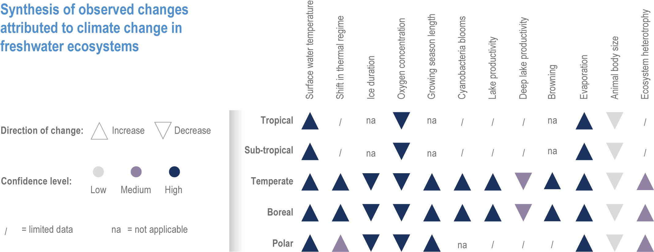
Figure 2.5 | Large-scale observed changes in freshwater ecosystems attributed to climate change over more than four decades. For description and references, see Sections 2.3.3, 2.4.2 and 2.5.3.6.2.
2.4.4.2 Observed Changes in Wildfire
2.4.4.2.1 Detection and attribution of observed changes in wildfire
Wildfire is a natural and essential component of many forest and other terrestrial ecosystems. Excessive wildfire, however, can kill people, cause respiratory disease, destroy houses, emit carbon dioxide and damage ecosystem integrity (see Sections 2.4.4.2 and 2.4.4.4). Anthropogenic climate change increases wildfire by exacerbating its three principal driving factors: heat, fuel and ignition (Moritz et al., 2012; Jolly et al., 2015). Non-climatic factors also contribute to wildfires—in tropical areas, fires are set intentionally to clear forest for agricultural fields and livestock pastures (Bowman et al., 2020). Urban areas and roads create ignition hazards. Governments in many temperate-zone countries implement policies to suppress fires, even natural ones, producing unnatural accumulations of fuel in the form of coarse woody debris and high densities of small trees (Ruffault and Mouillot, 2015; Hessburg et al., 2016; Andela et al., 2017; Balch et al., 2017; Lasslop and Kloster, 2017; Aragao et al., 2018; Kelley et al., 2019). Globally, 4.2 million km 2 of land per year burned on average from 2002 to 2016 (Giglio et al., 2018), with the highest fire frequencies in the Amazon rainforest, deciduous forests and savannas in Africa and deciduous forests in northern Australia (Earl and Simmonds, 2018; Andela et al., 2019).
Since the AR5 and the IPCC Special Report on Land, published research has detected increases in the area burned by wildfire, analysed relative contributions of climate and non-climate factors and attributed burned area increases above natural (recent historical) levels to anthropogenic climate change in one part of the world, western North America (robust evidence, high agreement) (Abatzoglou and Williams, 2016; Partain et al., 2016; Kirchmeier-Young et al., 2019; Mansuy et al., 2019; Bowman et al., 2020). Across the western USA, increases in vegetation aridity due to higher temperatures from anthropogenic climate change doubled burned area from 1984 to 2015 over what would have burned due to non-climate factors including unnatural fuel accumulation from fire suppression, with the burned area attributed to climate change accounting for 49% (32–76%, 95% confidence interval) of cumulative burned area (Abatzoglou and Williams, 2016). Anthropogenic climate change doubled the severity of a southwest North American drought from 2000 to 2020 that has reduced soil moisture to its lowest levels since the 1500s (Williams et al., 2020), driving half of the increase in burned area (Abatzoglou and Williams, 2016; Holden et al., 2018; Williams et al., 2019). In British Columbia, Canada, the increased maximum temperatures due to anthropogenic climate change increased burned area in 2017 to its highest extent in the 1950–2017 record, seven to eleven times the area that would have burned without climate change (Kirchmeier-Young et al., 2019). In Alaska, USA, the high maximum temperatures and extremely low relative humidity due to anthropogenic climate change accounted for 33–60% of the probability of wildfire in 2015, when the area burned was the second highest in the 1940–2015 record (Partain et al., 2016). In protected areas of Canada and the USA, climate factors (temperature, precipitation, relative humidity and evapotranspiration) accounted for 60% of burned area from local human and natural ignitions from 1984 to 2014, outweighing local human factors (population density, roads and built area) (Mansuy et al., 2019).
In summary, field evidence shows that anthropogenic climate change has increased the area burned by wildfire above natural levels across western North America in the period 1984–2017, at GMST increases of 0.6°C–0.9°C, increasing burned area up to 11 times in one extreme year and doubling it (over natural levels) in a 32-year period (high confidence).
2.4.4.2.2 Observed changes in wildfire globally
Regarding global terrestrial area as a whole, wildfire trends vary depending on the time period of analysis. From 1900 to 2000, global average fire frequency, based on field data, increased 0.4% but the change was not statistically significant (Gonzalez et al., 2010). Fire frequency increased on one-third of global land, mainly from burning for agricultural clearing in Africa, Asia and South America, slightly less than the area of fire frequency decrease, mainly from fire suppression across Australia, North America and Russia (Gonzalez et al., 2010). Analyses of the Global Fire Emissions Database document shows that, from 1996 to 2015, global burned area decreased at a rate of −0.7% yr -1 (Forkel et al., 2019) but the change was not statistically significant (Giglio et al., 2013). From 1998 to 2015, global burned area decreased at a rate of −1.4 ± 0.5% yr -1 (Andela et al., 2017). The area of fire increases was one-third of the area of decreases, due to reduced vegetation cover from agricultural expansion and intensification (Andela et al., 2017) and from increased precipitation (Forkel et al., 2019). Furthermore, much of the decreasing trend derives from two years: 1998 with a high burned area and 2013 with low burned area (Forkel et al., 2019). Wildfire does not show a clear long-term trend for the world as a whole because of increases and decreases in different regions (medium evidence, medium agreement ).
Where the global average burned area has decreased in the past two decades, higher correlations of rates of change in burning to human population density, cropland area and livestock density than to precipitation indicate that agricultural expansion and intensification were the main causes (Andela et al., 2017). The global decrease of fire frequency from 2000 to 2010 is correlated with increasing human population density (Knorr et al., 2014). The fire-reducing effect of reduced vegetation cover following expansion of agriculture and livestock herding can counteract the fire-increasing effect of the increased heat and drying associated with climate change (Lasslop and Kloster, 2017; Arora and Melton, 2018; Forkel et al., 2019). The reduced burning needed after the initial clearing for agricultural expansion drives much of the decline in fires in the Tropics (Andela et al., 2017; Earl and Simmonds, 2018; Forkel et al., 2019). The human influence on fire ignition can be seen through the decrease documented on holy days (Sundays and Fridays) and traditional religious days of rest (Earl et al., 2015). Overall, human land use exerts an influence on wildfire trends for global terrestrial area as a whole that can be stronger than climate change (medium confidence).
2.4.4.2.3 Observed changes in wildfire in individual regions with complex attribution
While burned area has increased in parts of Asia, Australia, Europe and South America, published research has not yet attributed the increases to anthropogenic climate change (medium evidence, high agreement ).
In the Amazon, deforestation for agricultural expansion and the degradation of forests adjacent to deforested areas cause wildfire in moist humid tropical forests not adapted to fire (robust evidence, high agreement ) (Fonseca et al., 2017; van Marle et al., 2017; da Silva et al., 2018 ; da Silva et al., 2021; dos Reis et al., 2021; Libonati et al., 2021). Roads facilitate deforestation, fragmenting the rainforest and increasing the dryness and flammability of vegetation (Alencar et al., 2015). Extreme droughts that occur during warm phases of the ENSO and the Atlantic Multi-Decadal Oscillation combine with the degradation of vegetation to cause extreme fire events (robust evidence, high agreement ) (Fonseca et al., 2017; Aragao et al., 2018; da Silva et al., 2018 ; Burton et al., 2020; dos Reis et al., 2021; Libonati et al., 2021). In the State of Roraima, Brazil, distance to roads and infrastructure that enable deforestation and ENSO were the factors most explaining fire occurrence in the extreme 2015–2016 fire season (Fonseca et al., 2017). From 1973 to 2014, burned area increased in the Amazon, coinciding with increased deforestation (van Marle et al., 2017). In the State of Acre, Brazil, burned area increased 36-fold from 1984 to 2016, with 43% burned in agricultural and livestock settlement areas (da Silva et al., 2018 ). In the extreme fire year 2019, 85% of the area burned in the Amazon occurred in areas deforested in 2018 (Cardil et al., 2020). Even though relatively higher moisture in 2019 led to burning below the 2002–2019 average across most of South America, burning in areas of recent deforestation in the Amazon were above the 2002–2019 average, indicating that deforestation, not meteorological conditions, triggered the 2019 fires (Kelley et al., 2021; Libonati et al., 2021). Furthermore, from 1981 to 2018, deforestation in the Amazon reduced moisture inputs to the lower atmosphere, increasing drought and fire in a self-reinforcing feedback (Xu et al., 2020). In the Amazon, deforestation exerts an influence on wildfire that can be stronger than climate change (robust evidence, high agreement ).
In Australia, burned area increased significantly between the periods 1950–2002 and 2003–2020 in the southeast state of Victoria, with the area burned in the 2019–2020 bushfires being the highest on record (Lindenmayer and Taylor, 2020). In addition to the deaths of dozens of people and the destruction of thousands of houses, the 2019–2020 bushfires burned almost half of the area protected for conservation in Victoria, two-thirds of the forests allocated for timber harvesting (Lindenmayer and Taylor, 2020), wildlife and extensive areas of habitat for threatened plant and animal species (Geary et al., 2021). Generally, past timber harvesting did not lead to more severe fire canopy damage (Bowman et al., 2021b). Across southeastern Australia, the fraction of vegetated area that burned increased significantly in eight of the 32 bioregions from 1975 to 2009, but decreased significantly in three bioregions (Bradstock et al., 2014). Increases in four bioregions were correlated to increasing temperature and decreasing precipitation. Decreases in burned area occurred despite increased temperature and decreased precipitation. Analyses of climate across Australia from 1950 to 2017 (Dowdy, 2018; Harris and Lucas, 2019) and during periods with extensive fires in 2017 in eastern Australia (Hope et al., 2019), in 2018 in northeastern Australia (Lewis et al., 2020), and in period 2019–2020 in southeastern Australia (Abram et al., 2021; van Oldenborgh et al., 2021) indicate that temperature and drought extremes due to the ENSO, Southern Annular Mode and other natural inter-decadal cycles drive inter-annual variability of fire weather. While the effects of inter-decadal climate cycles on fire are superimposed on long-term climate change, the relative importance of anthropogenic climate change in explaining changes in burned area in Australia remains unquantified (medium evidence, high agreement ).
In Africa, the rate of change of burned area on the continent as a whole ranged from a non-statistically significant −0.45% yr -1 in the period 2002–2016 (Zubkova et al., 2019) to a significant −1.9% yr -1 in the period 2001–2016 (Wei et al., 2020). These decreases coincided with areas of agricultural expansion or areas where drought reduced fuel loads (Zubkova et al., 2019; Wei et al., 2020). It is possible, however, that the 500-m spatial resolution of Modis remote-sensing fire data underestimates the area burned in Africa by half, by missing small fires (Ramo et al., 2021). In the Serengeti-Mara savanna of east Africa, burned area showed no significant change from 2001 to 2014, although an increase in domestic livestock would tend to reduce the grass cover that fuels savanna fires (Probert et al., 2019).
In Mediterranean Europe, the area burned in the region as a whole decreased from 1985 to 2011 (Turco et al., 2016), although the burned area for Spain did not show a significant long-term increase from 1968 to 2010 (Moreno et al., 2014) whereas that for Portugal in 2017 was the highest in the period 1980–2017 (Turco et al., 2019). Increased summer maximum temperature and decreased soil moisture explained most of the burned area observed, suggesting a contribution of climate change, but fire suppression, fire prevention, agricultural abandonment and reforestation as well as the reduction in forest area exerted even stronger influences on burned area than the climate across Mediterranean Europe (robust evidence, high agreement ) (Moreno et al., 2014; Turco et al., 2017; Viedma et al., 2018; Turco et al., 2019).
In the Arctic tundra and boreal forest, where wildfire has naturally been infrequent, burned area showed statistically significant increases of ~50% yr -1 across Siberia, Russia, from 1996 to 2015 (Ponomarev et al., 2016) and 2% yr -1 across Canada from 1959 to 2015 (Hanes et al., 2019). Wildfire burned ~6% of the area of four extensive Arctic permafrost regions in Alaska, USA, eastern Canada and Siberia from 1999 to 2014 (Nitze et al., 2018). In boreal forest in the Northwest Territories, Canada and Alaska, USA, the area burned by wildfire increased at a statistically significant rate of 6.8% yr -1 in the period 1975–2015, (Veraverbeke et al., 2017), with smouldering below-ground fires that lasted through the winter covering ~1% of burned area in the period 2002–2016 (Scholten et al., 2021). While burned area was correlated with temperature and reduced precipitation in Siberia (Ponomarev et al., 2016; Masrur et al., 2018) and correlated with lightning, temperature and precipitation in the Northwest Territories and Alaska (Veraverbeke et al., 2017), no attribution analyses have examined relative influences of climate and non-climate factors.
In Indonesia, deforestation and draining of peat swamp forests dries out the peat, providing substantial fuel for fires (Page and Hooijer, 2016). Extreme fire years in Indonesia, including 1997, 2006 and 2015, coincided with extreme heat and aridity during the warm phase of the ENSO (Field et al., 2016). Fire-resistant forest in 2019 covered only 3% of peatlands and 4.5% of non-peatlands on Sumatra and Kalimantan (Nikonovas et al., 2020).
In Chile, the area burned in the summer of 2016–2017 was 14 times the mean for the period 1985–2016 and the highest on record (Bowman et al., 2019). While this extreme fire year coincided with the highest daily mean maximum temperature in the period 1979–2017 (Bowman et al., 2019) in central Chile (the area of highest fire activity), burned area from 1976 to 2013 showed the highest correlation with the precipitation cycles of the ENSO and the temperature cycles of the Antarctic Oscillation (Urrutia-Jalabert et al., 2018).
Overall, burned area has increased in the Amazon, Arctic, Australia and parts of Africa and Asia, consistent with, but not formally attributed to anthropogenic climate change (medium evidence, high agreement ). Deforestation, peat draining, agricultural expansion or abandonment, fire suppression and inter-decadal cycles such as the ENSO exert a stronger influence than climate change on wildfire trends in numerous regions outside of North America (high confidence).
2.4.4.2.4 Observed changes in fire seasons globally
The IPCC AR6 WGI assessed fire weather (Ranasinghe et al., 2021), while this chapter assesses the impacts of changes in fire weather: burned area and fire frequency. The global increases in temperature from anthropogenic climate change have increased aridity and drought, lengthening the fire weather season (the annual period with a heat and aridity index greater than half of its annual range) on one-quarter of global vegetated area and increasing the average fire season length by one-fifth from 1979 to 2013 (Jolly et al., 2015). Climate change has contributed to increases in the fire weather season or the probability of fire weather conditions in the Amazon (Jolly et al., 2015), Australia (Dowdy, 2018; Abram et al., 2021; van Oldenborgh et al., 2021), Canada (Hanes et al., 2019), central Asia (Jolly et al., 2015), East Africa (Jolly et al., 2015) and North America (Jain et al., 2017; Williams et al., 2019; Goss et al., 2020). In forest areas, the burned area correlates with fuel aridity, a function of temperature; in non-forest areas, the burned area correlates with high precipitation in the previous year, which can produce high grass fuel loads (Abatzoglou et al., 2018). Fire use in agriculture and raising livestock or other factors have generated a second fire season on approximately one-quarter of global land where fire is present, despite sub-optimal fire weather in the second fire season (Benali et al., 2017). In summary, anthropogenic climate change, through a 0.9°C surface temperature increase since the pre-industrial period, has lengthened or increased the frequency of periods with heat and aridity that favour wildfire on up to one-quarter of vegetated area since 1979 (robust evidence, high agreement ).
2.4.4.2.5 Observed changes in post-fire vegetation
Globally, fire has contributed to biome shifts (Section 2.4.3.2) and tree mortality (Sections 2.4.4.2, 2.4.4.3) attributed to anthropogenic climate change. Research since the AR5 has also found vegetation changes from wildfire due to climate change. Through increased temperature and aridity, anthropogenic climate change has driven post-fire changes in plant regeneration and species composition in South Africa (Slingsby et al., 2017), and tree regeneration in the western USA (Davis et al., 2019b). In the fynbos vegetation of the Cape Floristic Region, South Africa, post-fire heat and drought and the legacy effects of exotic plant species reduced the regeneration of native plant species, decreasing species richness by 12% from 1966 to 2010 and shifting the average temperature tolerance of species communities upward by 0.5°C (Slingsby et al., 2017). In burned areas across the western USA, the increasing heat and aridity of anthropogenic climate change from 1979 to 2015 pushed low-elevation ponderosa pine (Pinus ponderosa) and Douglas fir (Pseudotsuga menziesii) forests across critical thresholds of heat and aridity that reduced the post-fire tree regeneration by half (Davis et al., 2019b). In the southwestern USA, where anthropogenic climate change has caused drought (Williams et al., 2019) and increased wildfire (Abatzoglou and Williams, 2016), high-severity fires have converted some forest patches to shrublands (Barton and Poulos, 2018). Field evidence shows that anthropogenic climate change and wildfire, together, altered vegetation species composition in the southwestern USA and Cape floristic region, South Africa, reducing post-fire natural regeneration and species richness of tree and other plant species, between 1966 and 2015, at GMST increases of 0.3°C–0.9°C (medium evidence, high agreement ).
2.4.4.3 Observed Changes in Tree Mortality
2.4.4.3.1 Observed tree mortality globally
Anthropogenic climate change can cause tree mortality directly via increased aridity or drought (Section 2.4.4.3.3) or indirectly through wildfire (Section 2.4.4.2.1) and insect pests (Section 2.4.4.3.3). Catastrophic failure of the plant hydraulic system, in which a lack of water causes the xylem to lose hydraulic conductance, is the principal mechanism of drought-induced tree death (Anderegg et al., 2016; Adams et al., 2017; Anderegg et al., 2018; Choat et al., 2018; Menezes-Silva et al., 2019; Brodribb et al., 2020).
Up through the AR5 (Settele et al., 2014), detection and attribution analyses had found that anthropogenic climate change, with global temperature increases of 0.3°C–0.9°C above the pre-industrial period and the increases in aridity exceeding the effects of local non-climate change factors, caused three cases of drought-induced tree mortality of up to 20% in the period 1945–2007 in western North America (van Mantgem et al., 2009), the African Sahel (Gonzalez et al., 2012) and North Africa (le Polain de Waroux and Lambin, 2012). Increased wildfire and pest infestations, driven by climate change, also contributed to North American tree mortality (van Mantgem et al., 2009). In addition, a meta-analysis of published cases found that drought consistent with, but not formally attributed to, climate change had caused tree mortality at 88 sites in boreal, temperate and tropical ecosystems (Allen et al., 2010), with 49 additional cases found by the AR5 (Settele et al., 2014).
Since the AR5 (Settele et al., 2014), global meta-analyses found at least 15 (Allen et al., 2015) and 25 (Hartmann et al., 2018) additional sites, respectively, of drought-induced tree mortality around the world. These and other global analyses found more rapid mortality than previously (Allen et al., 2015), rising background mortality (Allen et al., 2015), mortality increasing with drought severity (Greenwood et al., 2017), mortality of tropical trees increasing with temperature (Locosselli et al., 2020), mortality increasing with tree size for many species (Bennett et al., 2015), mortality predominantly at the dry edge of species ranges (Anderegg et al., 2019) and three-quarters of drought-induced mortality cases leading to a change in the dominant species (Batllori et al., 2020). Multiple non-climate factors contribute to tree mortality, including timber cutting, livestock grazing and air pollution (Martinez-Vilalta and Lloret, 2016). Globally, tropical dry forests lost, from all causes, 95,000 km 2, 8% of their total area, from 1982 to 2016, the most extensive area of mortality of any biome (Song et al., 2018).
In summary, anthropogenic climate change caused drought-induced tree mortality of up to 20% in the period 1945–2007 in western North America, the African Sahel and North Africa, via global temperature increases of 0.3°C–0.9°C above the pre-industrial period and increases in aridity, and it contributed to over 100 other cases of drought-induced tree mortality in Africa, Asia, Australia, Europe and North and South America (high confidence). Field observations document accelerating mortality rates, rising background mortality and post-mortality vegetation shifts (high confidence). Water stress, leading to plant hydraulic failure, is the principal mechanism of drought-induced tree mortality. Timber cutting, agricultural expansion, air pollution and other non-climate factors also contribute to tree death.
2.4.4.3.2 Observed tree mortality in tropical ecosystems
In the Brazilian Amazon, deforestation to clear agricultural land comprises the principal cause of tree mortality, reducing forest cover by an average of 13,900 km 2 yr -1 from 1988 to 2020 (Assis et al., 2019). In addition, in a set of 310 Amazon field plots, an annual average temperature increase of 1.2°C from 1950 to 2018 (Marengo et al., 2018) contributed to tree mortality of ~40% from 1983 to 2011 (Brienen et al., 2015). In another set of plots, mortality among newly recruited trees of mesic genera increased and drought-tolerant genera became more abundant from 1985 to 2015 (Esquivel-Muelbert et al., 2019). In other plots, tree mortality did not show a statistically significant change from 1965 to 2016, but rose abruptly in severe drought years, mainly during warm phases of the ENSO (Aleixo et al., 2019). Nearly half the area of the Amazon has experienced extremely dry conditions during ENSO warm phases; this can cause extensive wildfire (Section 2.4.4.2.3). Wildfires can increase tree mortality rates by >600% above rates in non-burned areas, with the higher mortality persisting for up to a decade after a fire (Silva et al., 2018; Berenguer et al., 2021). Climate change has contributed to tree mortality in the Amazon rainforest (medium evidence, medium agreement ).
In the African Sahel, field research has continued to detect tree mortality, ranging from 20 to 90% in the period 1965–2018 (Kusserow, 2017; Trichon et al., 2018; Dendoncker et al., 2020), and declines in tree biodiversity, with up to 80% local losses of tree species in the period 1970–2014 (Hanke et al., 2016; Kusserow, 2017; Ibrahim et al., 2018; Dendoncker et al., 2020), consistent with, but not formally attributed to, climate change. In Algeria, mortality of the Atlas cedar (Cedrus atlantica) increased from 1980 to 2006, coinciding with a ~1°C spring temperature increase, but non-climate factors were not examined (Navarro-Cerrillo et al., 2019). Across southern Africa, nine of the 13 oldest known (1100–2500 years old) baobab trees (Adansonia digitata) have died since 2005, although the causes are unknown (Patrut et al., 2018). In South Africa, savanna trees experienced an order of magnitude increase in mortality, related, but not formally attributed to, decreased rainfall (Case et al., 2019). In Tunisia, insect infestations related, but not formally attributed to, hotter temperatures led to mortality of cork oaks (Quercus suber) (Bellahirech et al., 2019).
2.4.4.3.3 Observed tree mortality in boreal and temperate ecosystems
The most extensive research into tree mortality since the AR5 has been in the western USA, where anthropogenic climate change accounted for half the magnitude of a drought in the period 2000–2020 that has been the most severe since the 1500s, (Williams et al., 2020) and for one-tenth to one-quarter of the magnitude of the 2012–2014 period of th e severe drought in California that lasted from 2012 to 2016 (Williams et al., 2015a). Across the western USA, anthropogenic climate change doubled tree mortality between 1955 and 2007 (van Mantgem et al., 2009). Lodgepole pine (Pinus contorta) mortality increased 700% from 2000 to 2013 (Anderegg et al., 2015) and piñon pine (P. edulis) experienced >50% mortality from 2002 to 2014 (Redmond et al., 2018). In montane conifer forest in California, anthropogenic climate change has increased tree mortality by one-quarter (Goulden and Bales, 2019). One-quarter of the trees died in some areas, with mortality rates of ponderosa pine (P. ponderosa) and sugar pine (P. lambertiana) increasing to up to 700% of pre-drought rates (Stephenson et al., 2019; Stovall et al., 2019). Substantial field evidence shows that anthropogenic climate change has caused extensive tree mortality in North America (robust evidence, high agreement ).
In western North America, increased infestations of bark beetles and other tree-feeding insects that benefit from higher winter temperatures (section 3.3.1.1 in (IPCC, 2021a)) and longer growing seasons (section 2.3.4.3.1 in (IPCC, 2021a)) have killed drought-stressed trees (Section 2.4.2.1) (Anderegg et al., 2015; Kolb et al., 2016; Lloret and Kitzberger, 2018; Redmond et al., 2018; Stephens et al., 2018; Fettig et al., 2019; Restaino et al., 2019; Stephenson et al., 2019). Increasing temperatures have allowed bark beetles to move further north and to higher elevations, survive through the winter at sites where they would previously have died and reproduce more often (Raffa et al., 2008; Bentz et al., 2010; Jewett et al., 2011; Macfarlane et al., 2013; Raffa et al., 2013; Hart et al., 2017; Stephenson et al., 2019; Teshome et al., 2020; Koontz et al., 2021). Under warmer conditions, some insects that were previously innocuous have become important agents of tree mortality (Stephenson et al., 2019; Trugman et al., 2021). Field observations show mixed effects of bark beetle-induced tree mortality on subsequent fire-caused tree mortality (Andrus et al., 2016; Meigs et al., 2016; Candau et al., 2018; Lucash et al., 2018; Talucci and Krawchuk, 2019; Wayman and Safford, 2021). From 1997 to 2018, ~5% of the forest area in the western USA died from bark beetle infestations (Hicke et al., 2020). Under most circumstances, trees that have been weakened by drought are more vulnerable to being killed by bark beetles (Anderegg et al., 2015; Kolb et al., 2016; Lloret and Kitzberger, 2018; Redmond et al., 2018; Stephens et al., 2018; Fettig et al., 2019; Restaino et al., 2019; Stephenson et al., 2019; Koontz et al., 2021). In summary, climate change has contributed to bark beetle infestations that have caused much of the tree mortality in North America (robust evidence, high agreement ) (see also Section 2.4.2.1).
Across Europe, rates of tree mortality in field inventories from 2000 to 2012 were highest in Spain, Bulgaria, Sweden and Finland, positively correlated to maximum winter temperature and inversely correlated to spring precipitation (Neumann et al., 2017). Tree mortality in Austria, the Czech Republic, Germany, Poland, Slovakia and Switzerland doubled from 1984 to 2016, correlated with intensified logging and increased temperatures (Senf et al., 2018). Drought-related tree mortality rates from 1987 to 2016 were highest in the Ukraine, Moldova, southern France and Spain (Senf et al., 2020). Climate contributed to tree mortality across Europe from 1958 to 2001 (Seidl et al., 2011). In addition, insect infestations related to higher temperatures (Okland et al., 2019) have caused the extensive mortality of Norway spruce (Picea abies) across nine European countries (Marini et al., 2017; Mezei et al., 2017). Across the Mediterranean Basin, a combination of drought, wildfire, pest infestations and livestock grazing (Peñuelas and Sardans, 2021) has driven tree mortality. In summary, climate change has contributed to tree mortality in Europe (high confidence) (see also Section 2.4.2.1).
2.4.4.3.4 Tree mortality and fauna
A global meta-analysis of 59 studies encompassing 631 cases of animal abundance changes in areas of tree mortality over the past 7–59 years, primarly in North America and Australia, with a few sites in other regions (e.g. Europe). Overall, in areas with documented high tree mortality, bird abundances increased (n=186 bird species), there was no significant trend for mammals (n=33 species), a slight trend towards declines in invertebrates (n=28 species), and insufficient information to categorize the responses of reptiles (n=20 species). However, within groups, significant differences appeared. Mammals that use trees as refugia showed declines with tree mortality (high confidence) , but flying mammals (e.g. bats) increased (medium confidence). Ground-nesting, ground-foraging, tree-hole nesting and bark-foraging birds increased most, but nectar-feeding and foliage-gleaning birds declined (high confidence). Within invertebrates, declines were strongest in ground-foraging predators and detritivores (medium confidence) (Fleming et al., 2021).
2.4.4.4 Observed Terrestrial Ecosystem Carbon
2.4.4.4.1 Observed terrestrial ecosystem carbon globally
Terrestrial ecosystems contain carbon stocks: 450 GtC (range 380–540 GtC) in vegetation, 1700 ± 250 GtC in soils that are not permanently frozen and 1400 ± 200 GtC in permafrost (Hugelius et al., 2014; Batjes, 2016; Jackson et al., 2017; Strauss et al., 2017; Erb et al., 2018a; Xu et al., 2021a). Ecosystem carbon stocks, totalling 3000–4000 GtC (from the lowest and highest estimates above), substantially exceed the ~900 GtC carbon in unextracted fossil fuels (see(Canadell et al., 2021)).
Deforestation, draining of peatlands and the expansion of agricultural fields, livestock pastures and human settlements and other LULCCs emitted carbon at a rate of 1.6 ± 0.7 Gt yr -1 from 2010 to 2019, (Friedlingstein et al., 2020), of which wildfires and peat burning emitted 0.4 ± 0.2 Gt yr -1 from 1997 to 2016 (van der Werf et al., 2017). Anthropogenic climate change has caused some of these emissions through increases in wildfire (Section 2.4.4.2.1) and tree mortality (Section 2.4.4.3.1), but the fraction of the total remains unquantified. LUC produced ~15% of global anthropogenic emissions, from fossil fuels and land (Friedlingstein et al., 2020). Terrestrial ecosystems removed carbon from the atmosphere through plant growth at a rate of -3.4 ± 0.9 Gt yr -1 from 2010 to 2019 (Friedlingstein et al., 2020).
Tropical deforestation and the draining and burning of peatlands produce almost all of the carbon emissions from LUC (Houghton and Nassikas, 2017; Friedlingstein et al., 2020), while forest growth accounts for two-thirds of ecosystem carbon removals from the atmosphere (Pugh et al., 2019b). Global terrestrial ecosystems comprised a net sink of -1.9 ± 1.1 Gt yr -1 from 2010 to 2019 (Friedlingstein et al., 2020), mainly due to growth in forests (Harris et al., 2021; Xu et al., 2021a), mitigating ~31% of global emissions from the burning of fossil fuels and LUC (Friedlingstein et al., 2020).
In summary, terrestrial ecosystems contain 3000–4000 GtC in vegetation, permafrost and soils, three to five times the amount of carbon in unextracted fossil fuels and 4.4 times the carbon currently in the atmosphere (robust evidence, high agreement ). Tropical deforestation, the draining and burning of peatlands and other LULCCs emit 0.9–2.3 GtC yr -1, ~15% of the global emissions from fossil fuels and ecosystems (robust evidence, high agreement ). Terrestrial ecosystems currently remove more carbon from the atmosphere (-3.4±0.9 Gt yr -1) than they emit (+1.6±0.7 Gt yr -1), a net sink of -1.9±1.1 Gt yr -1 (Friedlingstein et al., 2020) . Thus, tropical rainforests, Arctic permafrost and other ecosystems provide the global ecosystem service of naturally preventing carbon from contributing to climate change (high confidence).
2.4.4.4.2 Observed stocks in high-carbon terrestrial ecosystems
The ecosystem that attains the highest above-ground carbon density in the world is the coast redwood (Sequoia sempervirens) forest in California, USA, with 2600 ± 100 tonnes ha -1 carbon (Van Pelt et al., 2016). The ecosystem with the second highest documented carbon density in the world is the mountain ash (Eucalyptus regnans) forest in Victoria, Australia, with ~1900 tonnes ha -1 (Keith et al., 2009). In the Tropics, tropical evergreen broadleaf forests (rainforests) in the Amazon, the Congo and Indonesia attain the highest carbon densities, reaching a maximum of 230 tonnes ha -1 in the Amazon (Mitchard et al., 2014) and the Congo (Xu et al., 2017). Temperature increases reduce the tropical rainforest above-ground carbon density 9.1 tonnes ha -1 per degree Celsius, through reduced growth and increased tree mortality (Sullivan et al., 2020).
Tropical forests contain the largest vegetation carbon stocks in the world, with 180–250 GtC above and below ground (Saatchi et al., 2011; Baccini et al., 2012; Avitabile et al., 2016). The Amazon contains a stock of 45–60 GtC (Baccini et al., 2012; Mitchard et al., 2014; Englund et al., 2017).
Ecosystems with high soil carbon densities include the peat bogs in Ireland with up to 3000 tonnes ha -1 (Tomlinson, 2005), the Cuvette Centrale swamp forest peatlands in Congo with an average of ~2200 tonnes ha -1 (Dargie et al., 2017), the Arctic tundra with an average of ~900 tonnes ha -1 (Tarnocai et al., 2009) and the mangrove peatlands in Kalimantan, Indonesia, with an average of 850 ± 320 tonnes ha -1 (Murdiyarso et al., 2015). Arctic permafrost contains 1400 ± 200 GtC to a depth of 3 m, the largest soil carbon stock in the world (Hugelius et al., 2014). Globally, peatlands contain 470–620 GtC (Page et al., 2011; Hodgkins et al., 2018), of which boreal and temperate peatlands contain 415 ± 150 GtC (Hugelius et al., 2020) and tropical peatlands contain 80–350 GtC (Page et al., 2011; Dargie et al., 2017; Gumbricht et al., 2017; Ribeiro et al., 2021). Other analyses increase the upper estimates for boreal and temperate peatlands to 800–1200 GtC (Nichols and Peteet, 2019; Mishra et al., 2021b).
Tropical forests and Arctic permafrost contain the highest ecosystem carbon stocks in above-ground vegetation and soil, respectively, in the world (robust evidence, high agreement ). These ecosystems form natural sinks that prevent the emission to the atmosphere of 1400–1800 GtC that would otherwise increase the magnitude of climate change (high confidence).
2.4.4.4.3 Biodiversity and observed terrestrial ecosystem carbon
High biodiversity and ecosystem carbon generally occur together, with rainforests in the Amazon, Congo and Indonesia containing the largest above-ground vegetation carbon stocks (Saatchi et al., 2011; Baccini et al., 2012; Avitabile et al., 2016) and the highest vascular plant species richness (Kreft and Jetz, 2007) in the world. Above-ground ecosystem carbon and animal species richness show high correlation but also high spatial variability (Strassburg et al., 2010). Above-ground carbon is correlated to genus richness globally (Cavanaugh et al., 2014), but to species richness only in local areas (Poorter et al., 2015; Sullivan et al., 2017). Species richness generally increases vegetation productivity in the humid tropics while tree abundance increases productivity in drier conditions (Madrigal-Gonzalez et al., 2020). Across the Amazon, ~1% of tree species contain 50% of the above-ground carbon, due to abundance and maximum height (Fauset et al., 2015). Above-ground carbon in tropical forests shows positive correlations to vertebrate species richness (P values not reported) (Deere et al., 2018; Di Marco et al., 2018). In logged and burned tropical forest in Brazil, species richness of plants, birds and beetles increased with carbon density up to ~100 tonnes ha -1 (Ferreira et al., 2018).
National parks and other protected areas which, in June 2021, covered 15.7% of global terrestrial area (UNEP-WCMC et al., 2021) contain ~90 GtC in vegetation and ~150 GtC in soil (one-fifth and one-tenth, respectively, of global stocks) and remove carbon from the atmosphere at a rate of ~0.5 Gt yr -1 (one-sixth of global removals) (Melillo et al., 2016). The most strictly protected areas contain carbon at higher densities, but illegal deforestation and fires in some protected areas emit 38 ± 17 Mt yr -1 globally (Collins and Mitchard, 2017). In the Amazon, protected areas store more than half of the above-ground vegetation carbon stocks of the region, but account for only one-tenth of net emissions (Walker et al., 2020). Conservation of high biodiversity areas, particularly in protected areas, protects ecosystem carbon, prevents emissions to the atmosphere and reduces the magnitude of climate change (high confidence).
2.4.4.4.4 Observed emissions and removals from high-carbon terrestrial ecosystems
Most global deforestation is occurring in tropical forests (Pan et al., 2011; Liu et al., 2015; Houghton and Nassikas, 2017; Erb et al., 2018a; Li et al., 2018; Harris et al., 2021), primarily as a result of clearing for agricultural land (Hong et al., 2021), causing primary tropical forest to comprise a net source of carbon from 2001 to 2019: emissions to the atmosphere 0.6 GtC yr -1, removals from the atmosphere -0.5 GtC yr -1 and net 0.1 GtC yr -1 (Harris et al., 2021). While wildfires emitted an average of 0.4 ± 0.2 GtC yr -1 from 1997 to 2016 (van der Werf et al., 2017), individual fire seasons can emit the same magnitude, such as the 0.4 GtC from the Amazon fires of 2007 (Aragao et al., 2018), the 0.5 GtC from the Amazon fires of 2015–2016 (Berenguer et al., 2021) and the 0.2 Gt from the Australia fires of 2019–2020 (Shiraishi and Hirata, 2021). Wildfires thus account for up to one-third of annual average ecosystem carbon emissions, while major fire seasons can emit up to two-thirds of global ecosystem carbon (medium evidence, medium agreement ).
Primary boreal and temperate forests also comprised net sources in the period 2001–2019; however, when including all tree age classes, boreal, temperate and tropical forests were net sinks (boreal -1.6 ± 1.1 Gt yr -1, temperate -3.6 ± 48 Gt yr -1), as growth exceeded permanent forest cover losses (Harris et al., 2021), with boreal and temperate forests being much stronger sinks (Pan et al., 2011; Liu et al., 2015; Houghton and Nassikas, 2017). Estimates of carbon removals from remote sensing may provide more accurate estimates of boreal forest carbon balances than ESMs which overestimate regrowth after timber harvesting and other disturbance (Wang et al., 2021a). Mortality of the boreal forest in British Columbia from mountain pine beetle infestations converted 374,000 km 2 from a net carbon sink to a net carbon source (Kurz et al., 2008). Modelling suggests that a potential increase in water-use efficiency and regrowth could offset the losses in part of the forest mortality area (Giles-Hansen et al., 2021).
The Amazon as a whole was a net carbon emitter in the period 2003–2008 (Exbrayat and Williams, 2015; Yang et al., 2018b), primarily due to the expansion of agricultural and livestock areas, which caused over two-thirds of deforestation from 1990 to 2005 (De Sy et al., 2015; De Sy et al., 2019). Four sites in the Amazon also showed net carbon emissions in the period 2010–2018, from deforestation and fire (Gatti et al., 2021). In the Amazon, deforestation emitted 0.17 ± 0.05 GtC yr -1 from 2001 to 2015 (Silva Junior et al., 2020) while fires emitted 0.12 ± 0.14 GtC yr -1 from 2003 to 2015 (Aragao et al., 2018). An analysis of the Amazon carbon loss from deforestation and degradation estimated a loss of 0.5 Gt yr -1 in the period 2010 -2019, with degradation accounting for three-quarters (Qin et al., 2021). Intact old-growth Amazon rainforest has been a net carbon sink from 2000 to 2010 (-0.45 Gt yr -1, min. 0.31, max. 0.57) (Hubau et al., 2020) but may have become a net carbon source in 2010–2019 (0.67 Gt, for the entire period, uncertainty not reported) (Qin et al., 2021). These factors combined—recent impacts of climate change on undisturbed forest, coupled with deforestation and agricultural expansion, along with associated intentional burning—have caused Amazon rainforest to become an overall net carbon emitter (medium confidence).
In Indonesia and Malaysia, draining and burning of peat swamp forests for oil palm plantations emitted 60–260 MtC yr -1 from 1990 to 2015, converting peatlands in that period from a carbon sink to a carbon source (Miettinen et al., 2017; Wijedasa et al., 2018; Cooper et al., 2020). Deforestation of mangrove forests caused 10–30% of deforestation emissions in Indonesia from 1980 to 2005 (Donato et al., 2011; Murdiyarso et al., 2015), even though mangroves comprised only 3% of Indonesia primary forest area in 2000 (Margono et al., 2014; Murdiyarso et al., 2015).
In North America, wildfire emitted 0.1 ± 0.02 GtC yr -1 from in the period 1990–2012, but regrowth was slightly greater, producing a net sink (Chen et al., 2017). In California, USA, two-thirds of the 70 MtC emitted from natural ecosystems in 2001–2010 came from the 6% of the area that burned (Gonzalez et al., 2015). Anthropogenic climate change caused up to half of the burned area (Section 2.4.4.2.1).
In the Arctic, anthropogenic climate change has thawed permafrost (Guo et al., 2020), leading to emissions of 1.7 ± 0.8 GtC yr -1 in winter in the period 2003–2017 (Natali et al., 2019). Wildfires in the Arctic tundra in Alaska from ~1930 to 2010 caused up to a depth of 0.5 m of permafrost thaw (Brown et al., 2015), exposing peatland carbon (Brown et al., 2015; Gibson et al., 2018) including soil carbon deposits up to 1600 years old (Walker et al., 2019).
Tropical deforestation, the draining and burning of peatlands and the thawing of Arctic permafrost due to climate change have caused these ecosystems to emit more carbon to the atmosphere than they naturally remove through vegetation growth (high confidence).
2.4.4.5 Observed Changes in Primary Productivity
2.4.4.5.1 Observed changes in terrestrial primary productivity
The difference between photosynthesis by plants (gross primary productivity, GPP) and plant energy use through respiration is the net growth of plants (NPP), which removes CO2 from the atmosphere and mitigates emissions from deforestation and other LUCs (Section 2.4.4.4). Global terrestrial NPP has exceeded emissions due to land use since the early 2000s, making terrestrial ecosystems a net carbon sink (Friedlingstein et al., 2020).
Global terrestrial NPP increased by 6% from 1982 to 1999 through increased temperature and increased solar radiation in the Amazon from decreased cloud cover (Nemani et al., 2003), and then decreased 1% from 2000 to 2009, because of extensive droughts in the Southern Hemisphere (Zhao and Running, 2010). From 1999 to 2015, increased aridity caused extensive declines in the NDVI globally, particularly semiarid ecosystems (Huang et al., 2016), indicating widespread decreases in NPP (Yuan et al., 2019).
Global terrestrial GPP increased 2% from 1951 to 2010 and continued increasing at least until 2016, with increased atmospheric CO2 showing a greater influence than natural factors (Li et al., 2017; Fernandez-Martinez et al., 2019; Liu et al., 2019a; Cai and Prentice, 2020; Melnikova and Sasai, 2020). Global forest area increased 7% from 1982 to 2016, mainly from forest plantations and regrowth in boreal and temperate forests in Asia and Europe (Song et al., 2018); regrowth in secondary forests >20 years old, mainly in boreal, temperate and subtropical regions, generated a net removal of 7.7 Gt yr -1CO2 from the atmosphere from 2001 to 2019 (Harris et al., 2021). Vegetation growth that exceeds the modelled CO2 fertilisation, gaps in field data and incomplete knowledge of plant mortality and soil carbon responses introduce uncertainties into quantifying the magnitude of CO2 fertilisation (Walker et al., 2021). A combination of CO2 fertilisation of global vegetation and secondary forest regrowth has increased global vegetation productivity (medium evidence, medium agreement ).
The relative increase in GPP per unit of increased atmospheric CO2 declined from 1982 to 2015, indicating a weakening of any CO2 fertilisation effect (Wang et al., 2020c). Increased growth from CO2 fertilisation has begun to shorten the lifespan of trees due to a trade-off between growth rate and longevity, based on analyses of tree rings of 110 species around the world (Brienen et al., 2020). Furthermore, water availability controls the magnitude of NPP (Beer et al., 2010; Jung et al., 2017; Yu et al., 2017), including water from precipitation (Beer et al., 2010), soil moisture (Stocker et al., 2019), groundwater storage (Humphrey et al., 2018; Madani et al., 2020a) and atmospheric vapour (Novick et al., 2016; Madani et al., 2020b). Drought stress reduced NPP across tropical forests from 2000 to 2015 (Zhang et al., 2019b) and GPP in the tropics from 1982 to 2016 (Madani et al., 2020b). Drought stress has also reduced GPP in some semiarid and arid lands (Huang et al., 2016; Liu et al., 2019a). In addition, nitrogen and phosphorus constrain CO2 fertilisation (Terrer et al., 2019), although phosphorus limitation of tropical tree growth is species-specific (Alvarez-Clare et al., 2013; Thompson et al., 2019). NPP has decreased during some time periods and in some regions where drought stress has exerted a greater influence than increased atmospheric CO2 (medium evidence, high agreement ).
2.4.4.5.2 Observed changes in freshwater ecosystem productivity
Temperature affects primary productivity by moderating phytoplankton growth rates, ice cover, thermal stratification and the length of growing seasons (Rühland et al., 2015; Richardson et al., 2018). Global warming has reinforced eutrophication, especially cyanobacteria blooms (Wagner and Adrian, 2009; Kosten et al., 2012; O’Neil et al., 2012; De Senerpont Domis et al., 2013; Adrian et al., 2016; Visser et al., 2016; Huisman et al., 2018) (very high confidence). Conversely , warming can reduce cyanobacteria in hypertrophic lakes (Richardson et al., 2019). Freshwater cyanobacteria may benefit directly from elevated CO2 concentrations (Visser et al., 2016; Ji et al., 2017; Huisman et al., 2018; Richardson et al., 2019).
Macrophyte growth in freshwaters is likely to increase with rising water temperatures, atmospheric CO2 and precipitation (robust evidence, high agreement ) (Dhir, 2015; Hossain et al., 2016; Short et al., 2016; Reitsema et al., 2018). Nonetheless, primary productivity in rivers is variable and unpredictable (Bernhardt et al., 2018) because seasonal variations in temperature and light are uncorrelated, frequent high-flow events reduce biomass of autotrophs and droughts can strand and desiccate autotrophs.
In large, nutrient-poor lakes, warming-induced prolonged thermal stratification can reduce primary production (medium confidence) (Kraemer et al., 2017). Warming may reduce phytoplankton concentrations when temperature-induced increases in consumption of phytoplankton outpace increases in phytoplankton production (De Senerpont Domis et al., 2013). These decreases in productivity may be under-recognised responses to climate change.
Summary: There is robust evidence of an increase in primary production along with warming trends. However, increases or declines of algae cannot entirely be attributed to climate change; they are lake-specific and modulated through weather conditions, lake morphology, salinity, land use and restoration and biotic interactions (medium confidence) (O’Beirne et al., 2017; Velthuis et al., 2017; Rusak et al., 2018; Ho et al., 2019).
FAQ 2.3 | Is climate change increasing wildfire?
In the Amazon, Australia, North America, Siberia and other regions, wildfires are burning wider areas than in the past. Analyses show that human-caused climate change has driven the increases in burned area in the forests of western North America. Elsewhere, deforestation, fire suppression, agricultural burning and short-term cycles like El Niño can exert a stronger influence than climate change. Many forests and grasslands naturally require fire for ecosystem health but excessive wildfire can kill people, destroy homes and damage ecosystems.

Figure FAQ2.3.1 | (a) Springs Fire, May 2, 2013, Thousand Oaks, California, USA (photo by Michael Robinson Chávez, Los Angeles Times). (b) Cumulative area burned by wildfire in the western USA, with (orange) and without (yellow) the increased heat and aridity of climate change.
Wildfire is a natural and essential part of many forest, woodland and grassland ecosystems, killing pests, releasing plant seeds to sprout, thinning out small trees and serving other functions essential for ecosystem health. Excessive wildfire, however, can kill people with the smoke causing breathing illnesses, destroy homes (Figure FAQ2.3.1a) and damage ecosystems.
Human-caused climate change increases wildfire by intensifying its principal driving factor, heat. The heat of climate change dries out vegetation and accelerates burning. Non-climate factors also cause wildfires. Agricultural companies, small-scale farmers and livestock herders in many tropical areas cut down forests and intentionally set fires to clear fields and pastures. Cities, towns and roads increase the number of fires that people ignite. Governments in many countries suppress fires, even natural ones, producing unnatural accumulations of fuel in the form of coarse woody debris and dense stands of small trees. The fuel accumulations cause particularly severe fires that burn upwards into tree crowns.
Evidence shows that human-caused climate change has driven increases in the area burned by wildfire in the forests of western North America. Across this region, the higher temperatures of human-caused climate change doubled burned area from 1984 to 2015, compared with what would have burned without climate change (Figure FAQ2.3.1b). The additional area burned, 4.9 million hectares, is greater than the land area of Switzerland. Human-caused climate change drove a drought from 2000 to 2020 that has been the most severe since the 1500s, severely increasing the aridity of vegetation. In British Columbia, Canada, the higher maximum temperatures of human-caused climate change increased burned area in 2017 to its widest extent in the 1950–2017 record, seven to eleven times the area that would have burned without climate change. Moreover, in national parks and other protected areas of Canada and the USA, most of the area burned from 1984 to 2014 can be attributed to climate factors (temperature, rainfall and aridity) and these outweigh local human factors (population density, roads and urban area).
In other regions, wildfires are also burning wider areas and occurring more often. This is consistent with climate change, but analyses have not yet shown if climate change is more important than other factors. In the Amazon, deforestation by companies, farmers and herders who cut down and intentionally burn rainforests to expand agricultural fields and pastures causes wildfires even in relatively moister years. Drought exacerbates these fires. In Australia, much of the southeastern part of the continent has experienced extreme wildfire years, but analyses suggest that El Niño, a heat phenomenon that cycles up and down periodically, is more important than long-term climate change. In Indonesia, intentional burning of rainforests for oil palm plantations and El Niño seem to be more important than long-term climate change. In Mediterranean Europe, fire suppression seems to have prevented any increasing trend in burned area but the suppression and abandonment of agricultural lands have allowed fuel to build up in some areas and contribute to major fires in years of extreme heat. In Canada and Siberia, wildfires are now burning more often in permafrost areas where fire was rare, but analyses are lacking regarding the relative influence of climate change. For the world as a whole, satellite data indicate that the vast amount of land converted from forest to farmland in the period 1998–2015 actually decreased the total burned area. Nevertheless, the evidence from the forests of western North America shows that human-caused climate change has, at least on one continent, clearly driven increases in wildfire.
2.4.5 Conclusions on Observed Impacts
The consistency of patterns of biological change with expectations from regional or global warming processes, coupled with an understanding of underlying processes and the coherence of these patterns at both regional and global scales, all form multiple lines of evidence (Parmesan et al., 2013) that it is very likely that the observed range shifts and phenological changes in individual species can be attributed to regional and global climate changes (very high confidence) (Section 2.4.2, Table 2.2; Table 2.3; Table SM2.1) (Parmesan et al., 2013).
Global and regional meta-analyses of diverse systems, habitats and taxonomic groupings document that approximately half of all species with long-term records have shifted their ranges poleward and/or upward in elevation and ~2/3 have advanced their timing of spring events (phenology) (very high confidence) (Section 2.4.2, Table 2.2) (Parmesan and Hanley, 2015; Parmesan, 2019). Changes in abundance tend to match predictions from climate warming, with warm-adapted species significantly outperforming cold-adapted species in warming habitats (Feeley et al., 2020) and the composition of local communities becoming more ‘thermophilised’, that is, experiencing an ‘increase in relative abundance of heat-loving or heat-tolerant species’ (high confidence) (Section 2.4.2.3) (Cline et al., 2013; Feeley et al., 2020).
New studies since AR5, with more sophisticated analyses designed to capture complex responses, indicate that past estimates of the proportion of species impacted by recent climate change were underestimates due to unspoken assumptions that local or regional warming should lead solely to poleward/upward range shifts and advancements of spring timing (high confidence) (Duffy et al., 2019). More complex analyses have documented cases of winter warming driving delayed spring timing of northern temperate species due to chilling requirements, and increased precipitation driving species’ range shifts downslope in elevation, and eastward and westward in arid regions (high confidence). Further new studies have shown that phenological changes have, in some cases, successfully compensated for local climate change and reduced the extent of range shifts (medium confidence). The limited number of studies of this type make it difficult to estimate the generality of these effects globally (Section 2.4.2.5, Table 2.2).
Responses in freshwater species are consistent with responses in terrestrial species, including poleward and upward range shifts, earlier timing of spring plankton development, earlier spawning by fish and the extension of the growing season (high confidence). Observed changes in freshwater species are strongly related to anthropogenic climate change-driven changes in the physical environment (e.g., increased water temperature, reduced ice cover, reduced mixing in lakes, loss of oxygen and reduced river connectivity) (high confidence). While evidence is robust for an increase in primary production in nutrient rich lakes along with warming trends (high confidence), increasing or declining algal formations are lake-specific and are modulated through variability in weather conditions, lake morphology, changes in salinity, stoichiometry, land use and restoration measures and food web interactions. In boreal coniferous forest, there has been an increase in terrestrial-derived DOM transported into rivers and lakes as a consequence of climate change (which has induced increases in runoff and greening of the Northern Hemisphere) as well as from changes in forestry practices. This has caused waters to become brown, resulting in an acceleration of upper-water warming and an overall cooling of deep water (high confidence). Browning may accelerate primary production through the input of nutrients associated with DOM in nutrient-poor lakes and increases the growth of cyanobacteria, which cope better with low light intensity (medium confidence) (Sections 2.4.2.1, 2.4.2.2, 2.4.2.3, 2.4.2.4).
Field research since the AR5 has detected biome shifts at numerous sites, poleward and upslope, that are consistent with increased temperatures and altered precipitation patterns driven by climate change, and support prior studies that attributed such shifts to anthropogenic climate change (high confidence). New studies help fill previous geographic and habitat gaps, for example, documenting upward shifts in the forest/alpine tundra ecotone in the Andes, Tibet and Nepal, and northward shifts in the deciduous/boreal forest ecotones in Canada. Globally, woody encroachment into open areas (grasslands, arid regions and tundra) is likely being driven by climate change and increased CO2, in concert with changes in grazing and fire regimes (medium confidence) (Section 2.4.3).
Climate change has driven, or is contributing to, increased tree mortality directly through increased aridity and droughts and indirectly through increased wildfires and insect pests in many locations (high confidence). Analyses of causal factors have attributed increasing tree mortality at sites in Africa and North America to anthropogenic climate change, and field evidence has detected tree mortality due to drought, wildfires and insect pests in temperate and tropical forests around the world (high confidence). Water stress, leading to plant hydraulic failure, is a principal mechanism of drought-induced tree mortality, along with the indirect effects of climate change mediated by community interactions (high confidence) (Section 2.4.4.3).
Terrestrial ecosystems sequester and store globally critical stocks of carbon, but these stocks are at risk from deforestation and climate change (high confidence). Tropical deforestation and the draining and burning of peatlands produce almost all of the carbon emissions from LULCC. In the Arctic, increased temperatures have thawed permafrost at numerous sites, dried some areas and increased fires, causing net emissions of carbon from soils (high confidence) (Sections 2.4.4.4, 2.5.3.4).
Globally, increases in temperature, aridity and drought have increased the length of fire seasons and doubled the potentially burnable land area (medium confidence). Increases in the area burned have been attributed to anthropogenic climate change in North America (high confidence). In parts of Africa, Asia, Australia and South America, the area burned has also increased, consistent with anthropogenic climate change. Deforestation, peat-burning, agricultural expansion or abandonment, fire suppression and inter-decadal cycles strongly influence fire occurrence. The areas with the greatest increases in the length of the fire season include the Amazon, western North America, western Asia and East Africa (Section 2.4.4.2).
The changes in biodiversity and ecosystem health that we have observed, and project will continue, pose a risk of declines in human health and well-being (e.g., tourism, recreation, food, livelihoods and quality of life) (medium confidence). Clear attribution of these impacts is often not possible, but inferences can be made by comparison of the observed changes in biodiversity/ecosystem health and the known services from these particular ecosystems.
2.5 Projected Impacts and Risk for Species, Communities, Biomes, Key Ecosystems and Their Services
Under the risk assessment framework that was introduced in AR5 (IPCC, 2014b), risk means the probability of harmful consequences resulting from climate change. It results from the interaction of vulnerability, exposure and hazard and can be represented as the probability of occurrence of hazardous events or trends multiplied by the impacts if these events or trends occur (see Chapter 1, this report). The framework defines vulnerability as a pre-existing condition, incorporating the extent to which species or ecosystems are susceptible to, or unable to cope with, the adverse effects of climate change. Vulnerable species have limited adaptive capacity, stemming from physiological and behavioural constraints, limited dispersal abilities and restricted resource requirements or capacities for distributional and genetic changes (Foden et al., 2013; Cizauskas et al., 2017; Foden et al., 2019). Traits that render entire ecosystems vulnerable are harder to define, but it is clear that vulnerabilities are high in the coldest habitats, in those with limited geographic ranges such as low-lying islands and in specialised, restricted habitats such as serpentine outcrops in California (Anacker and Harrison, 2012) and dry meadows in Fennoscandia and Tibet (Yang et al., 2018a). Ecosystem vulnerability can depend critically on the fates of plants that function as ‘foundation species’, providing community biomass above and below the ground, structuring habitat for fauna and providing ecosystem services such as erosion control (Camac et al., 2021).
2.5.1 Projected Changes at Species and Community Levels
2.5.1.1 Assessment of Models and Sources of Uncertainties
Methods for projecting the impacts of climate change on biodiversity can be classified into three types: (1) statistical models such as SDMs (Elith and Leathwick, 2009); (2) mechanistic or process-based models (Chuine and Régnière, 2017) and (3) trait-based models (Pacifici et al., 2015). It is only recently that models have been developed looking at lower levels of warming like 1.5°C (Hoegh-Guldberg et al., 2018; Warren et al., 2018).
SDMs or niche-based models assess potential geographic areas of suitable climate for the species in current conditions and then project them into future conditions (Trisurat, 2018; Vieira et al., 2018). There are limitations in all models and it is critical that modellers understand the assumptions, proper parameterization and limitations of each model technique, including differences between climate models, emission scenarios or RCPs and baselines (Araujo et al., 2019). Several systems automate the development of SDMs, including R-packages (Beaumont et al., 2016; Hallgren et al., 2016), and other model types (Foden et al., 2019) and aid in the use of climate model data (Suggitt et al., 2017), including allowing for connectivity constraints (Peterson et al., 2013). Buisson et al. (2010) found most variation in model outputs stems from differences in design, followed by general circulation models (GCMs).
Mechanistic approaches, also known as process-based models, project the responses of species to climate changes by explicitly incorporating known biological processes, thresholds and interactions (Morin and Thuiller, 2009; Maino et al., 2016). Mechanistic models are able to accommodate a broad range of mechanisms of climate change impacts and include species-specific characteristics such as dispersal distances, longevity, fecundity, genetic evolution and phenotypic plasticity. However, sufficient knowledge is available for only a few well-studied species. Species’ traits have been used to more broadly estimate potential climate change impacts (Foden et al., 2013; Cizauskas et al., 2017).
Most models are on a large scale (20–50 km), and so cannot capture micro-climatic refugia generated by diversities of slope aspect, elevation or shade (Suggitt et al., 2015; Suggitt et al., 2018). In analysing records of 430 climate-threatened and range-declining species in England, (Suggett et al., 2015; Suggitt et al., 2018) showed that topographic diversity reduced population declines most strongly in areas experiencing the most local warming and in the species most sensitive to warming. Under these circumstances, topographic diversity reduced the risk of population extinction by 22% for plants and 9% for insects.
None of the modelling techniques are predictions of the future, they are rather projections of possible futures. To date, only a few studies have validated model performance against observations, but the studies that have been conducted do generally validate models using either SDMs or process-based models (Johnston et al., 2013; Fordham et al., 2018). SDMs should be considered as hypotheses of what a future world might look like if the climate projections came to pass. Suggestions have been made on how to start bringing more biotic interactions into SDMs (Early and Keith, 2019), but limited basic ecological understanding of interactions, along with limits on computation and funding, constrains how far and how fast these modelling techniques can advance.
Table 2.3 | Assessing uncertainty in detection and attribution of observed changes in terrestrial and freshwater species and ecosystems to climate change. The lines of evidence used to support given uncertainty statements, including confidence statements, of the attribution of key conclusions on observed biological changes to climate change and increased atmospheric CO2. Icons represent lines of evidence. This is a summary table that is fully detailed in Table SM2.1.


2.5.1.2 Risk Assessment and Non-Modelling Approaches
In order to add realism and reliability to risk assessments at the species and community levels, non-modelling approaches, based on known biological traits or processes as well as on expert opinion (Camac et al., 2021), are used to temper model outputs with ground-based validation. Trait-based assessment approaches use species’ biological characteristics as predictors of sensitivity, adaptive capacity and extinction risk due to climate change. Climate exposure can be estimated using GIS-based modelling, statistical programs or expert judgment (Chin et al., 2010). These trait-based approaches are widely applied to predict responses of biodiversity to climate change because they do not require modelling expertise or detailed distibutional data (Pacifici et al., 2015; Willis et al., 2015). Most of these methods have not been independently validated and do not allow direct comparison of vulnerability and risk across taxonomic groups.
Some studies have combined two or three approaches for the assessment of climate change risk to biodiversity, in order to capture the advantages of each and avoid their limitations. Warren et al. (2013) used combinations of SDMs and trait-based approaches to estimate the proportions of species losing their climatically suitable ranges under the various future scenarios of climate and dispersal rate. Similarly, spatial projections of exposure to climate change were combined with traits to assess the vulnerability of sub-Saharan amphibians (Garcia et al., 2014). Laurance et al. (2012) combined 31 functional groups of species and 21 potential drivers of environmental change, in order to assess both the ecological integrity and threats to protected tropical areas on a global scale. Keith et al. (2014) used a combination of three approaches (SDMs–trait–mechanistic) to determine how long before extinction a species would become eligible for listing as threatened, based on the IUCN Red List criteria.
2.5.1.3 Risk of Species’ Extinctions
2.5.1.3.1 Overview
This assessment of current findings is of studies across a range of taxa and modelling techniques. Extinction risk estimates whether or not a particular species may be at risk of extinction over the coming decades if climatic trends continue, and usually does not take into account other human-induced stressors (e.g., invasive species or pollution). It is not a prediction that a species will definitely become extinct because, even when complete loss of a species’ range is projected, the scale of the model cannot estimate persistence in very small-scale micro-climatic refugia (that can be on the order of metres in size) (Suggitt et al., 2015; Suggitt et al., 2018). Individuals and populations can survive after the conditions for successful reproduction are gone, leading to a lagged decline, called ‘extinction debt’ (see section 2.4.2.8) (Alexander et al., 2018). Therefore, range loss is an established criterion for assessing endangerment status and risk of extinction. As a species range becomes smaller and occupied habitats become more isolated, the likelihood of a single stochastic event causing extinction increases. It is this combination of projected loss of climatically suitable space and additional stressors (especially LULCC of critical habitat) that is expected to drive future extinctions.
The IUCN Red List Criteria (IUCN, 2019) classifies a species as ‘critically endangered’ if it has suffered a range loss of ≥80%, with a resulting likelihood of extinction of >50% in the near term (10–100 yrs, depending upon generation length). A species is classified as ‘endangered’ if it has suffered a range loss of ≥50%, with a resulting likelihood of extinction of >20% in the near term (10–100 years). In this assessment, a species that is projected to become classified as ‘endangered’ is deemed to be at ‘high risk’ of extinction, and becoming classified as ‘critically endangered’ is deemed at ‘very high risk’ of extinction.
2.5.1.3.2 Projections for freshwater biodiversity
Because risk to freshwater species has been limited in past reports, this section provides details of freshwater risk. Lakes, rivers and freshwater wetlands cover approximately 7.7–9.1% of global land surface area; (Lehner et al., 2008; Fluet-Chouinard et al., 2015; Allen and Pavelsky, 2018) and hold 9.5% of the Earth’s described animals (Balian et al., 2008), with climate change indicated as a threat to 50–75% of fish (Xenopoulos et al., 2005; Darwall and Freyhof, 2015). Climate change is cited as a primary factor in species’ extinction risk due to changes in water temperatures, stream flow, loss of cold water habitat, increased variability of precipitation and increased disease risk from warming temperatures (robust evidence, high agreement , high confidence) (Knouft and Ficklin, 2017; Pletterbauer et al., 2018; Jaric et al., 2019; Reid et al., 2019) adding to the stress of overexploitation and LULCC (Craig et al., 2017; IPBES, 2019).
Increased frequency of stream drying events, reducing hydrologic connectivity and limiting access of native fishes to spawning habitats is projected for RCP8.5 in Colorado, USA (medium evidence, medium agreement ) (Jaeger et al., 2014). Cold-water habitats and associated obligate species are particularly vulnerable, and losses in these habitats have been both documented and projected, for example, in salmonids (Santiago et al., 2016; Fullerton et al., 2017; Merriam et al., 2017). River networks are projected to lose connections to cold tributary refugia, that are important thermal refuges for cold water species (robust evidence, high agreement ) (Isaak et al., 2016) during low flows (Merriam et al., 2017).
Community turnovers are expected in freshwaters as cold-adapted species lose and warm-adapted species gain climatically suitable habitat (Domisch et al., 2011; Domisch et al., 2013; Shah et al., 2014). While a number of warm-adapted species may experience range expansions, the majority of species are predicted to lose climatically suitable areas by, on average, 38–44%, depending on the emission scenario (A2a and B2a) (medium evidence) (Domisch et al., 2013).
Molluscs are projected to be the most at-risk group, given their limited dispersal capability (Woodward et al., 2010). Mediterranean freshwater fish are especially susceptible to climate change due to increasing flood and drought events and the risk of surpassing critical temperature thresholds (Santiago et al., 2016; Jaric et al., 2019). In southern Europe, aquatic insects (Ephemeroptera, Plecoptera and Trichoptera) are endangered by climate change (Conti et al., 2014). European protected areas are not expected to be sufficient under warming to provide habitat for the majority of rare molluscs and fish (Markovic et al., 2014). Observed trends agree with model projections in direction, but magnitude remains uncertain (medium evidence, medium agreement , medium confidence) (see Figure 2.8 for extinction risk globally for dragonflies, amphibians and turtles).
Regional threats from climate change have been reported for 40% of amphibians in China, (Wu, 2020), 33% of European freshwater fish species (Janssen et al., 2016) and 56–69% of odonates in Australia, (Bush et al., 2014b). Assessment of site-specific extirpation for 88 aquatic insect taxa projected that climate change-induced hydrological alteration would result in a 30–40% loss of taxa in warmer, drier ecoregions and a 10–20% loss in cooler, wetter ecoregions (medium evidence, medium agreement ) (Pyne and Poff, 2017). In Africa’s Albertine Rift, 51% (n= 551) of fish are expected to be impacted by climate change, with 5.5% at a high risk due to their sensitivity and poor adaptative capability (medium evidence, high agreement ) (Carr et al., 2013).
The GLOBIO-Aquatic model (Janse et al., 2015 a) links models for demography, economy, LUCs, climate change, nutrient emissions, a global hydrological model and a global map of water bodies. It projects that changes in both water quality (eutrophication) and quantity (flow) will generate negative relations in freshwater ecosystems between the persistence of species originally present in each community and a constellation of stressors, including harmful algal blooms. Under a 4°C rise by 2050, mean abundance of species is projected to decline by 70% in running water and by 80% in standing water (medium evidence, high agreement , medium confidence) (Janse et al., 2015 a ).
2.5.1.3.3 Global projections of extinction risk
In previous reports, risk assessed from the literature was generally based on estimates of overall range contractions with climate change. In AR4, extinction risk was carefully quantified: ‘There is medium confidence that approximately 20–30% of species assessed so far are likely to be at increased risk of extinction if increases in global average warming exceed 1.5–2.5°C (relative to mean temperatures from 1980–1999). As global average temperature increase exceeds about 3.5°C, model projections suggest significant extinctions (40–70% of species assessed) around the globe.’ These estimates approximately correspond to 50–80% reductions in range size (depending upon study), that this assessment equates with a ‘high’ and ‘very high’ extinction risk, respectively (IPCC, 2007). AR5 stated: ‘a large fraction of terrestrial and freshwater species face increased extinction risk under projected climate change during and beyond the 21st century, especially as climate change interacts with other pressures (high confidence)’ (Field et al., 2014). A series of multi-species and global analyses have been published since AR5, using both statistical models and trait-based approaches.
In this chapter, risk to species, with implications for ecosystems, is assessed using three different approaches. First is an assessment of the geographic distributions of local species’ losses at different levels of GSAT warming, termed ‘local biodiversity loss’, measured as the proportion of species within a given location becoming classified as “endangered” or worse (sensu IUCN), and so at highrisk of local population losses (local population extinctions) (Figure 2.6). This measure provides the best estimates of which sites are at most risk of losing substantial numbers of species locally, leading to degradation of that ecosystem’s ability to function.
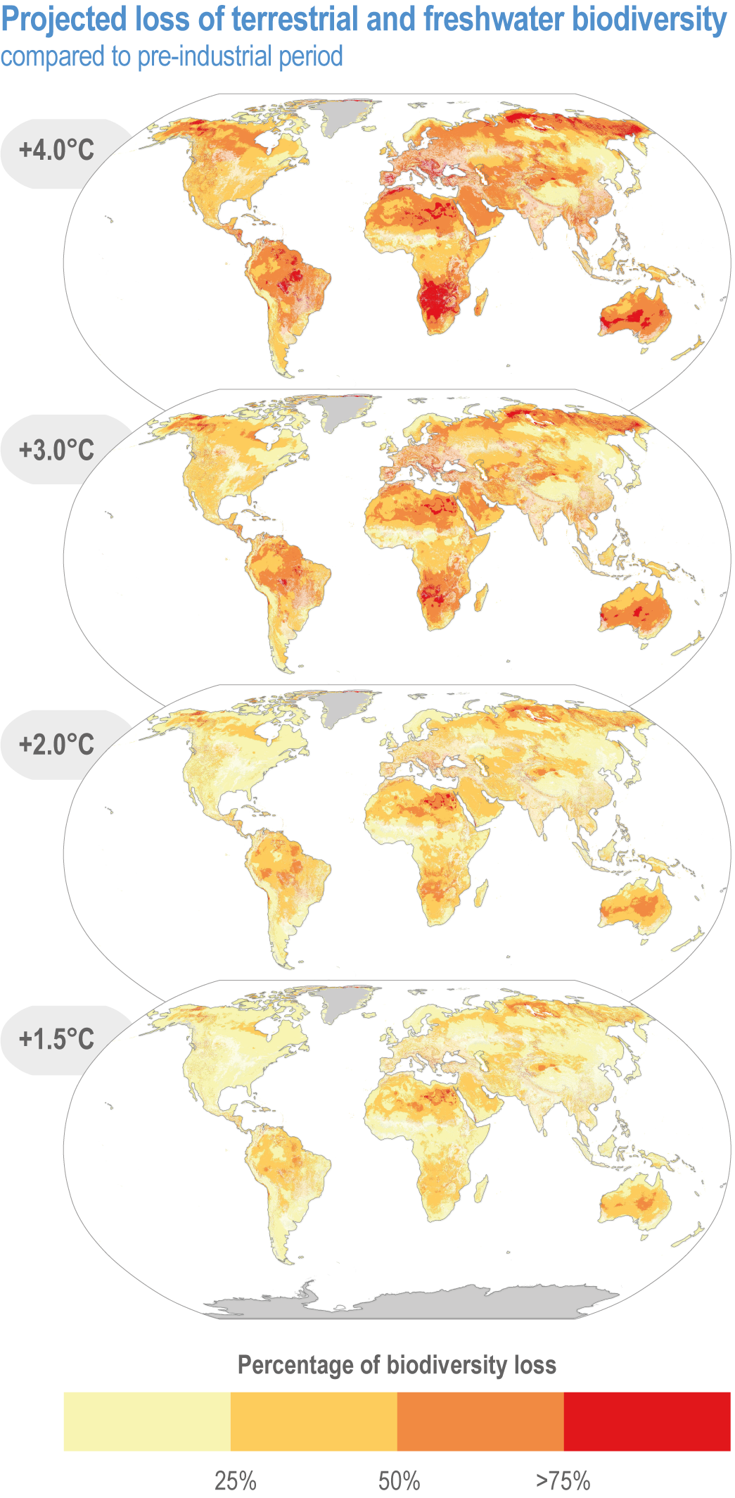
Figure 2.6 | Biodiversity loss for different areas at increasing levels of climate change. The higher the percentage of species projected to lose suitable climate in a given area, the higher the risk to ecosystem integrity, functioning and resilience to climate change. Warming levels are based on global levels (GSAT) above pre-industrial temperatures. Colour shading represents proportion of species for which the climate is projected to become sufficiently unsuitable that the species becomes locally ‘endangered’ and at high risk of local extinction within a given pixel across their current distributions at a given GSAT warming level, based on underlying data (Warren et al., 2018) (modelled n= 119,813 species globally, with no dispersal, averaged over 21 CMIP5 climate models). Areas shaded in deep orange and red represent a significant risk of biodiversity loss (areas where climates become sufficiently unsuitable that it renders >50% and >75% of species at high ris k of becoming locally extinct, respectively). The maps of species richness remaining have been overlaid with a landcover layer (2015) from the European Space Agency (ESA) Climate Change Initiative. This landcover layer leaves habitats classified by the ESA as natural as transparent. Areas with a landcover identified as agriculture are 5% transparent, such that the potential species richness remaining if the land had not been converted for agriculture shows as pale shading of the legend colours (very pale yellow to very pale red). These paler areas represent biodiversity loss due to habitat destruction, but with a potential to be restored, with yellow shading having the potential for restoration to greater species richness than orange or red shading.
Second is assessment of the proportions of species becoming endangered globally (not just locally), so at highrisk of global extinction of the species, termed ‘global biodiversity loss’ (Figure 2.8b). This metric (losing > 50% of suitable climate space across the species’ entire range) also serves to estimate a species’ becoming sufficiently rare that the species no longer fully contributes to ecosystem functioning, a state that often occurs decades before complete extinction (death of the last individual). The proportions of species becoming at highrisk of global extinction is the foundation for the burning embers diagram on global biodiversity loss in Table 2.5 and Figure 2.11.
Third is an assessment of risk of the proportions of species becoming at very highrisk of extinction globally at different levels of GSAT warming, measured using the IUCN criteria for ‘critically endangered’, and termed ‘species’ extinction risk’ (Figure 2.7 and Figure 2.8a). This measure is closest to assessing the complete loss of a species in the wild and can be used to compare to past (palaeo) extinction rates. These three approaches provide complementary information of the overall risks to individual species, to biodiversity at the community scale, and to ecosystem integrity and functioning at different levels of warming.
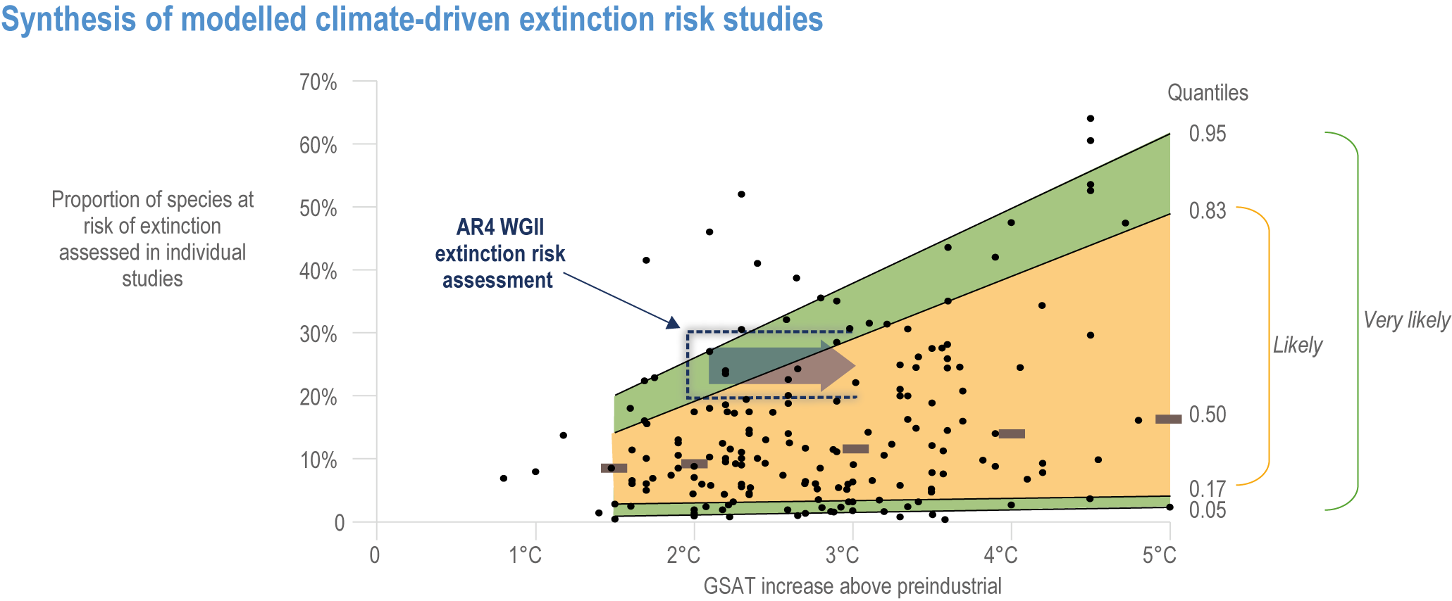
Figure 2.7 | Global assessment of species’ extinction risks under different levels of warming. Graph shows a synthesis of climate-driven models of individual species projected to become at very highrisk of extinction globally (i.e, becoming “critically endandered” sensu IUCN by losing >80% of their suitable climate space or through estimates of extinction risk from process-based models). The relationship between modelled projections of extinction (expressed as a proportion of species at a risk of extinction assessed in individual studies) and GSAT increase above the pre-industrial average. Data (global sample size n= 178 modelled estimates) were taken from a number of sources, including digitization of data points in Figure 2 in the synthetic analysis of (Urban, 2015) (note: unweighted for sample size) n= 126; Table 4.1 of AR4 WGII Chapter 2 (Fischlin et al., 2007), n= 40; (Hannah et al., 2020)n= 6; and (Warren et al., 2018) n= 6. The quantile regression (which is robust to the non-normal distribution of the response variable, and less sensitive to data outliers) was chosen as a descriptive statistic to fit quantile estimates for levels relevant to informing likely (between the 0.17 and 0.83 quantiles, shaded in orange) and very likely ranges (between the 0.05 and 0.95 quantiles, shaded in green) relating extinction risk to GSAT increase (quantile regression implemented using the Barrodale and Roberts algorithm in XLSTAT). The roughly equivalent estimate of this risk as expressed in AR4 (Fischlin et al., 2007) is indicated by the dotted block indicating the medium confidence statement ‘Approximately 20–30% of plant and animal species assessed so far (in an unbiased sample) are likely to be at increasingly high risk of extinction as global mean temperatures exceed a warming of 2–3°C above pre-industrial levels (medium confidence). ’ This box is open on the right side because AR4 estimates stipulated temperatures at or exceeding the given levels. Thick dark horizontal bars show the median values of percent of species at very high risk of extinction at 1.5°C, 2°C, 3°C, 4°C and 5°C, indicating that half of the data points lie above the bar and half below for a given level of global warming.
Risk of local biodiversity loss, estimated as the proportion of species in a given area projected to become endangered (sensu IUCN), and therefore at highrisk of extinction, is projected to affect a greater number of regions experiencing increasing warming. About one-third of land area risks more than 50% of species becoming “endangered” by 4.0° GSAT warming (Figure 2.6). That is, the deep orange and red areas in Figure 2.6 are those areas for which >50% of species currently inhabiting those ecosystems are projected to lose >50% of their climatically suitable habitat. Species’ losses are projected to be worst in northern South America, southern Africa, most of Australia and at northern high latitudes (medium confidence) (Figure 2.6).
For risk of global biodiversity loss, at 1.58°C global warming (median estimate), >10% of species are projected to become “endangered”, and so at highrisk of extinction (sensu IUCN). At 2.07°C (median) >20% of species are projected to become endangered. Ten-twenty percent losses represent high and very highrisk of biodiversity losses, respectively, substantial enough to reduce ecosystem integrity and functioning (medium confidence) (Figure 2.8b) (see Section 2.5.4; Figure 2.11; Table 2.5, Table SM2.5).
Risk of global biodiversity loss differs among taxonomic groups. The percent of species projected at high risk of extinction was 49% for all insects, 44% for all plants and 26% for all vertebrates at ~3°C global rise in temperature (Figure 2.8b) (Warren et al., 2018). These estimates dropped considerably at lower levels of warming, down to 18%, 16% and 8% at 2°C; and 6%, 8% and 4% at 1.5°C (Figure 2.8b) (Warren et al., 2018), so not entirely dissimilar to the numbers in AR4 (Figure 2.7).

Figure 2.8 | Percent of species of different groups classified as being at risk of extinction.
(a) Species groups listed projected to be at a very highrisk of extinction, corresponding to the IUCN Red List criteria for a species classified as ‘critically endangered’ (v3.1) by losing >80% of its climatically suitable range area.
(b) Species groups listed projected to be at a highrisk of extinction, corresponding to the IUCN Red List criteria for a species classified as ‘endangered’ (v3.1) by losing >50% of its climatically suitable range area. For (a) and (b), values were calculated from the underlying data in (Warren et al., 2018). Values for each temperature are the mean values across 21 CMIP5 models. The grey band represents the high end of extinction risk from the 10th percentile of the climate models to show the maximum range of values, while the low end (90th percentile, 1.5°C) is not shown as it is too small to appear on the plots. Taxa marked with * represent potential benefits from adaptation, specifically dispersal at realistic rates (Warren et al., 2018); those with no * have dispersal rates that are essentially not detected in the spatial resolution of the models (20 km). See (Warren et al., 2018) for caveats and more details. Sample size for each group is as follows: 1) fungi (16187 species); 2) all plants (72399 species), broken down into sub-groups of plants: flowering plants (52310 species), timber species (1328 species), grasses (3389 species) and pines (340 species); 3) all invertebrates (33,949 species), broken down into sub-groups of invertebrates: annelid worms (155 species), flies (4809 species), beetles (7630 species), moths (6910 species), true bugs (1728 species), spiders (2212 species), all pollinators (1755 species), butterflies (1684 species), ants/bees/wasps (5914 species), dragonflies (599 species); 4) Chordates (12642 species), broken down into major groups: 4i) all amphibians (1055 species), broken down into sub-groups of amphibians: frogs (887 species) and salamanders (163 species); 4ii) reptiles (1850 species), snakes (1741 species) and turtles (94 species); 4iii) all mammals (1769 species), broken down into sub-groups of mammals: ungulates (80 species), bats (500 species), carnivores (107 species), 4iv) all birds (7968 species), broken down into sub-groups of birds: passeriforme birds (4744 species), and non-passeriforme birds (3224 species).
‘Species’ extinction risk’, estimated as at very highrisk of extinction globally, i.e. becoming “critically endangered” (sensu IUCN) is shown in Figures 2.7 across 178 studies and in Figure 2.8a split by taxonomic group. The percentage of species at very highrisk of extinction (median estimates and maximum likely range) will be 9% (max. 14%) at 1.5°C, 10% (max. 18%) at 2°C, 12% (max. 29%) at 3.0°C, 13% (max. 39%) at 4°C and 15% (max. 48%) at 5°C (Figure 2.7). Maximum estimates of species at very highrisk of extinction reach 60% within the 95% quartiles, ie the very likely range, for 5°C GSAT warming. Among the groups containing the largest numbers of species at a very high risk of extinction for mid-levels of projected warming (3.2°C rise in GSAT) are: invertebrates (15%), specifically pollinators (12%), amphibians (11%, but 24% for salamanders) and flowering plants (10%) (Figure 2.8a). All groups fare substantially better at 2°C, with extinction projections reducing to <3% for all groups, except salamanders at 7% (medium confidence) (Figure 2.8a).
Figure 2.8 also shows the benefits of dispersal in reducing extinction risk in birds, mammals, butterflies, moths and dragonflies (depicted with an asterix). While dispersal may benefit individual species, it poses additional risks to communities and ecosystems that species are moving into, as interactions between species are changed or eliminated.
Projected species extinctions at future global warming levels are in accord with projections from AR4, assessed on much larger numbers of species with much greater geographic coverage and a broader range of climate models. (Figure 2.7; Figure 2.8a). Even the lowest estimates of species extinction (median of 9% at 1.5°C warming, Figure 2.7) are 1000 times the natural background rates (De Vos et al., 2015).
Using data from geological timescales, (Song et al., 2021) predicted that a warming of 5.2°C above pre-industrial levels would result in a mass extinction comparable to that of the five mass extinctions over the past 540 Myr, on the order of 70–85% of species becoming extinct, in the absence of non-climatic stressor. (Mathes et al., 2021) found evidence in the geological record that short-term rapid warming, on top of long-term warming trends, increases extinction risk by up to 40% over that expected from the long-term trend alone, with a biodiversity ‘memory’ of up to 60 Myr, indicating an additonal risk of multi-decadal overshoot.
Most of the large-scale studies that have been performed are for losses based on climate alone (Figures 2.6, 2.7, 2.8). However, climate is rarely the only stressor affecting species survival. Habitat loss is currently the largest driver of range loss and extinction risk for most species (IUCN, 2019). Communities in different regions are becoming more similar to each other as species tolerant of human activities prosper and spread, with many rare and endemic species already having been driven to extinction, primarily by LULCC (Pimm et al., 2006). Thus, it will likely be the interaction of climate change and habitat conversion (often driven by climate change) that will ultimately determine the risk and ability of many species to survive over the next century.
2.5.1.4 Changing Risks of Diseases
Multiple studies predict increases in disease incidence or geographic and phenological changes of pathogens, vectors and reservoir host species due to climate change with or without other non-climatic variables (González et al., 2010; Moo-Llanes et al., 2013; Roy-Dufresne et al., 2013; Liu-Helmersson et al., 2014; Laporta et al., 2015; Ryan et al., 2015; Haydock et al., 2016; Hoover and Barker, 2016; Prist et al., 2017; Blum and Hotez, 2018; Dumic and Severnini, 2018; Hundessa et al., 2018; Ryan et al., 2019; Ryan et al., 2021). However, models predicting changes in infectious disease risk are complex and sometimes produce conflicting results and lack consensus (Caminade et al., 2014; Giesen et al., 2020). For example, malaria is projected to increase in some regions of Africa, Asia and South America by the end of the 21st century if public health interventions are not sufficient, but is also forecasted to decrease in some higher-risk areas (Cross-Chapter Box Illness in this chapter) (Peterson, 2009; Caminade et al., 2014; Ryan et al., 2015; Khormi and Kumar, 2016; Leedale et al., 2016; Murdock et al., 2016; Endo and Eltahir, 2020; Mordecai et al., 2020).
While malaria risk is predicted to decrease in some lowland tropical areas as temperatures become too hot for vector or parasite development, other warm-adapted diseases, like dengue and Zika, transmitted by A. aegypti, are predicted to increase (Cross-Chapter Box Illness in this chapter, chapter 7) (Ryan et al., 2019; Ryan et al., 2021). In more temperate regions, arboviruses and other VBDs with wider thermal breadths, such as West Nile fever, Ross River fever and Lyme disease, are predicted to increase with climate warming (Ogden et al., 2008; Leighton et al., 2012; Shocket et al., 2018; Shocket et al., 2020; Couper et al., 2021). Drought can exacerbate these effects of temperature (Paull et al., 2017).
A global analysis of 7346 wildlife populations and 2021 host–parasite combinations found that organisms adapted to cool and mild climates are likely to experience increased risks of outbreaks along with climate warming, while warm-adapted organisms may experience a lower disease risk, providing further support for predictions that climate change will increase the transmission of infectious diseases at higher latitudes across a taxonomically diverse array of pathogens (robust evidence, high agreement ) (Cohen et al., 2020). A study examining the future risk of arboviruses (chikungunya, dengue, yellow fever and Zika viruses) spread by A. aegypti and A. albopictus projected increased disease risk due to interactions of multiple variables, including increased human connectivity, urbanisation and climate change (Kraemer et al., 2019), although vector species’ ranges will broaden only slightly (Campbell et al., 2015).
In sum, climate change is expected to expand and redistribute the burden of vector-borne and other environmentally transmitted diseases of wild animals, domesticated animals and humans, by shifting many regions toward the thermal optima of VBD transmission for multiple parasites, thereby increasing risk of transmission, while pushing temperatures above optimal and towards upper thermal limits for other vectors and pathogens, thus decreasing their transmission (high confidence) (see also chapter 7) (Mordecai et al., 2019; Mordecai et al., 2020). These effects are mediated by other human impacts such as LUC, mobility, socioeconomic conditions and vector and pathogen control measures (Parham et al., 2015; Tjaden et al., 2018).
2.5.2 Projected Changes at Level of Biomes and Whole Ecosystems
2.5.2.1 Global Overview, Assessment of Ecosystem-Level Models and Sources of Uncertainties
Shifts in terrestrial biome and changes in ecosystem processes in response to climate change are most frequently projected with dynamic global vegetation models (DGVMs) or land-surface models that form part of ESMs, which use gridded climate variables, atmospheric CO2 concentration and information on soil properties as input variables. Since AR5, most DGVMs have been upgraded to capture carbon–nitrogen cycle interactions (e.g., (Le Quéré et al., 2018), many also include a representation of wildfire and fire–vegetation interactions (Rabin et al., 2017) and a small number now also account for land management (e.g., wood removal from forests and crop fertilisation harvest of irrigation (Arneth et al., 2017). Other forms of disturbance, such as tree mortality, in response to, for example, episodic weather extremes or insect pest outbreaks, are relatively poorly represented or not at all, although they demonstrably impact calculated carbon cycling (Pugh et al., 2019a). Simulated biome shifts are generally in agreement in projecting broad patterns on a global scale but vary greatly regarding the simulated trends in historical and future carbon uptake or losses, both regionally and globally (Chang et al., 2017; Canadell et al., 2021).
Similar to other models, models to project large-scale changes in vegetation and ecosystem processes have to deal with structural uncertainty (associated with the choice and the representation of processes in models), input-data uncertainty (associated with variability in initial conditions and parameter values) and error propagation (associated with coupling models) (Rounsevell et al., 2019). The IPBES methodological assessment report on scenarios and models of biodiversity and ecosystem services provides a comprehensive overview over the relevant issues (Ferrier et al., 2016).
In order to assess performance, most models have been individually evaluated against a range of observations. Moreover, in the annual updates of the global carbon budgets, a model has to meet a small set of basic criteria to have its output included (Le Quéré et al., 2018). More systematic benchmarking approaches have also been proposed that utilise a range of different datasets (Kelley et al., 2013; Chang et al., 2017) to assess multiple simulated processes. These methods, in principle, facilitate assigning quality scores to models based on their overall performance (Kelley et al., 2013). So far, this scoring does not yet allow a clear quality ranking of models, since individual DGVMs tend to score well for some variables and badly for others. A recent comparison of global fire–vegetation model outputs was also able to clearly identify outliers when using a formalised benchmarking and scoring approach (Hantson et al., 2020). However, benchmarking does not address sources of uncertainty and it would be advisable to perform ‘perturbed-physics’ experiments, in which multiple model parameters are varied in parallel more frequently as a means to test parameter-value uncertainty (Wramneby et al., 2008; Booth et al., 2012; Lienert and Joos, 2018).
Species diversity impacts ecosystem functioning and hence ecosystem services (Hooper et al., 2012; Mokany et al., 2016). So far, however, integrated modelling of ecosystem processes and biodiversity across multiple trophic levels and food webs is in its infancy (Harfoot et al., 2014). Whether or not the enhanced integration of state, function and functional diversity across multiple trophic levels in models will markedly alter projections of how ecosystems respond to climate change thus remains an open research question.
Beyond dynamic simulation of biome shifts and carbon cycling, which are important aspects of climate regulation, DGVMs can also provide information on a number of variables closely linked to other ecosystem services such as water availability, air quality or food provisioning (Krause et al., 2017; Rabin et al., 2020). However, they are not intended to provide a comprehensive assessment of ecosystem services. For these, other approaches applied but, to date, these are mostly applied on regional scales and are only weakly dynamic (Ferrier et al., 2016).
2.5.2.2 Projected Changes Globally at the Biome Level
Climate change and the associated change in atmospheric CO2 levels already exacerbate other human-caused impacts on the structure and composition of land and freshwater ecosystems, such as LULCC, nitrogen deposition and pollution. The relative importance of these drivers for ecosystems over the coming decades will likely differ between biomes, but climate change and atmospheric CO2 will be pervasive unless there is a rapid lowering of fossil-fuel emissions and warming (high confidence) (Pereira et al., 2010; Warren, 2011; Ostberg et al., 2013; Davies-Barnard et al., 2015; Pecl et al., 2017; Ostberg et al., 2018). Global vegetation and ESMs agree on climate change-driven shifts of biome boundaries of potentially hundreds of kilometres over this century, combined with several substantial alterations that take place within biomes (e.g., changes in phenology, canopy structure and functional diversity, etc.). Large discrepancies exist between models and between scenarios regarding the region and the speed of change (Gonzalez et al., 2010; Pereira et al., 2010; Pecl et al., 2017), but robust understanding is emerging in that the degree of impact increases in high-emission and high-warming scenarios (high confidence) (Figure 2.9).

Figure 2.9 | Projected fraction of global terrestrial area that could experience a biome shift by 2100. Shifts due to climate change (filled symbols) or a combination of climate change and LUC (outline symbols), from publications in Supplementary Table SM2. 3 (projected vulnerabilities and risks of ecosystems to biome shifts). Filled circles (Bergengren et al., 2011), filled squares (Alo and Wang, 2008), filled diamonds (Gonzalez et al., 2010), filled triangle pointing up (Scholze et al., 2006), filled triangle pointing down (Sitch et al., 2008), filled triangle on its side (Li et al., 2018), filled cross (Warszawski et al., 2013), outlined circle (Ostberg et al., 2018)and outlined diamond (Eigenbrod et al., 2015).
Substantial changes in vegetation structure and ecosystem processes are already happening (see Section 2.4). Many of these observations have already been projected to take place as early as at least IPCC AR3 (Rosenzweig et al., 2007), and can they now be increasingly tested for their robustness with observational evidence. These multiple changes in response to warming (and changes in precipitation and increasing atmospheric CO2 levels that go hand-in-hand with warming) are further expected for already relatively small additional temperature increases. In particular, in cold (boreal and tundra) regions, as well as in dry regions (high confidence), alterations of 2–47% of the areal extent of terrestrial ecosystems in scenarios of <2°C warming above pre-industrial levels have been projected, increasing drastically with higher-warming scenarios (Warren, 2011; Wårlind et al., 2014). More recent work, applying also probabilistic methods, confirm the risk of drastic changes in vegetation cover (e.g., forest to non-forest or vice versa) at the end of the 21st century even for approximately 2°C warming scenarios, especially in tundra, and also in tropical forest and savannah regions, with more subtle changes (within a given biome type) likely to occur in all regions (Ostberg et al., 2013; Ostberg et al., 2018). Model studies have found 5–20% of terrestrial ecosystems affected by warming of around 2°C–3°C, increasing to above one-third at a warming of 4°C–5°C (Ostberg et al., 2013; Warszawski et al., 2013).
In general, vegetation types are projected to be moving into their ‘neighbouring’ climates, depending on whether temperature or precipitation is expected to be the predominant factor and how vegetation interacts with the increasing CO2 levels in the atmosphere (Wårlind et al., 2014; Scheiter et al., 2015; Schimel et al., 2015; Huntzinger et al., 2017). For instance, boreal or temperate forest vegetation is simulated to migrate polewards, closed tropical (moist) forest is expected to transition towards dry tropical forest types, while climate-driven degradation might expand arid vegetation cover (Sections 2.5.2.2–2.5.2.9). However, ‘novel ecosystems’, that is, communities with no current or historical equivalent because of the novel combinations of abiotic conditions under climate change, are expected to be increasingly common in the future (medium confidence), although the regions where these novel ecosystems might emerge are still disputed (Reu et al., 2014; Radeloff et al., 2015; Ordonez et al., 2016). The possibility of these novel ecosystems and the communities that live within them are a challenge for current modelling of ecosystem shifts, and new approaches to conservation will be required that are designed to adapt to rapid changes in species composition and the ensuing challenges.
2.5.2.3 Risk to Arid Regions
Shifts in arid system structure and functioning that have been observed to date (Section 2.4.3.3) are projected to continue (medium confidence). These include widespread woody plant encroachment, notably in savanna systems in Africa, Australia and South America, and are attributed to interactions of LULCC, climate change and CO2 fertilisation effects (Fensholt et al., 2012; Fang et al., 2017; Stevens et al., 2017). Arid Mongolian steppe grassland did not respond to experimentally elevated CO2 (Song et al., 2019). Woody encroachment is projected to continue or not reverse in North American drylands (Caracciolo et al., 2016) and southern African arid ecosystems (Moncrieff et al., 2014b). Dryland woody encroachment may increase carbon stocks, depending on emissions scenario (Martens et al., 2021), but reduce soil water and biodiversity of grassland-dependent species diversity (Archer et al., 2017). Warm season (C4) grass expansion into arid shrublands risks sudden ecosystem transformation due to introduced wildfire (Bradley et al., 2016), a risk anticipated for grass-invaded desert ecosystems of Australia and the southwestern USA (Horn and St. Clair, 2017). Novel fire regimes in grassy shrublands have enhanced grass cover locally in the southern African Nama-Karoo (du Toit et al., 2015).
Range retractions are projected for endemic plants in southern Africa (Young et al., 2016) and dry woodlands in Morocco (Alba-Sánchez et al., 2015). Increasing thermal stress is projected to increase woody plant mortality in the Sonoran Desert ecosystems (Munson et al., 2016) and facilitate perennial grass replacement by xeric shrubs in the southwestern USA (Bestelmeyer et al., 2018). Ecological effects may occur rapidly when extreme events compound long-term trends (Hoover et al., 2015), but evolve more slowly as opportunity costs accumulate due to warming (Cross-Chapter Paper 3) (Cunningham et al., 2021).
2.5.2.4 Risk to Mediterranean-Type Ecosystems (MTEs)
The regions containing MTEs all show high confidence in projected increases in the intensity and frequency of hot extremes and decreases in the intensity and frequency of cold extremes, and medium confidence in increasing ecological drought due to increased evapotranspiration (in all regions) and reduced rainfall (excluding California, USA, where model agreement is low) (see WGI Chapter 11). Projections also show a robust increase in the intensity and frequency of heavy precipitation in the event of ≥2°C warming for MTEs in South Africa, the Mediterranean Basin and California, USA, but are less clear for Australia and Chile (Seneviratne et al., 2021).
MTEs are characterised by the distinctive seasonal timing of precipitation and temperature, and the disruption of this regime is likely to be critical for their maintenance. Unfortunately, projections of changes in rainfall seasonality have received less attention and are far more uncertain than many other aspects of climate change (Pascale et al., 2016; Breinl et al., 2020), thus limiting our ability to predict the ecological consequences of climate change in MTEs. Responses to experimental manipulation of rainfall seasonality show the potential for shifts in plant functional composition and diversity loss, but results vary with soil type (van Blerk et al., 2021).
Unfortunately, global- and regional-scale dynamic vegetation models show a poor performance for large areas of MTEs, because they do not characterise shrub and Crassulacean acid metabolism (CAM)-photosynthetic plant functional types well (Moncrieff et al., 2015). Furthermore, the grain of these models is too coarse for quantifying impacts to many vegetation formations which are patchy or of limited extent (e.g., small stands of trees). There is high confidence that observations of high mortality in trees and other growth forms, reduced reproductive and recruitment success, range shifts, community shifts towards more thermophilic species and type conversions are set to continue, due to either direct climate impacts through drought and other extreme weather events or to their interaction with factors like fire and pathogens (Sections 2.4.3.5, 2.4.3.6; 2.4.3.7; 2.4.4.2; 2.4.4.3; 2.5.2.5, 2.5.2.6, 2.5.2.7, 2.5.4).
Fire is a key driver across most MTEs due to summer-dry conditions. Climate projections for the MTEs translate into high confidence that periods of low fuel moisture will become more severe and prolonged, and that episodes of extreme fire weather will become more frequent and severe (see (Douville et al., 2021; Seneviratne et al., 2021)). This will lead to the birth of novel fire regimes in MTEs, characterised by an increase in the probability of greater burned area and extreme wildfire events (e.g., megafires), with associated loss of human life and property, long-term impacts on ecosystems and acceleration of the possible loss of resilience and capacity to recover (Abatzoglou and Williams, 2016; González et al., 2018; Boer et al., 2020; Moreira et al., 2020; Nolan et al., 2020; Duane et al., 2021; Gallagher et al., 2021).
Fire is virtually certain to have additional impacts through compound events (see Section 11.8 in (Seneviratne et al., 2021)). Extreme post-fire weather is extremely likely to continue to impact diversity (Slingsby et al., 2017), retard vegetation regrowth (Slingsby et al., 2020a) and accelerate vegetation shifts (Batllori et al., 2019). Any increases in the intensity and frequency of heavy precipitation are highly likely to compromise soil stability in recently burnt areas (Morán-Ordóñez et al., 2020). The impacts of fire often depend on interactions with non-climatic factors such as habitat fragmentation (Slingsby et al., 2020b) and management (Steel et al., 2015) or the spread of flammable exotic plantation forestry and invasive species (Kraaij et al., 2018; McWethy et al., 2018). Managing these factors provides opportunities for adaptation and mitigation (Moreira et al., 2020). (See sections 2.4.4.2 and 2.5.3.2).
Human adaptation and mitigation responses to climate change may create additional threats to MTEs. MTEs have dry summers by definition, posing a challenge for the year-round supply of water to growing human populations and agriculture. With recent major droughts in all MTEs (Section 2.4.3.6), there is increasing reliance on groundwater for the bulk of the water supply (Kaiser and Macleod, 2018). The majority of groundwater systems have exceeded or are rapidly approaching their environmental flow limits (de Graaf et al., 2019), threatening human populations and ecosystems that depend on these systems for their persistence through unfavourable climatic conditions (McLaughlin et al., 2017). Similarly, much of the MTEs are open shrublands and grasslands and proposed extensive tree-planting to sequester atmospheric CO2 could result in a loss of biodiversity and threaten water security (Doblas-Miranda et al., 2017; Bond et al., 2019).
2.5.2.5 Risk to Grasslands and Savannas
Worldwide, woody cover is increasing in savannas (Buitenwerf et al., 2012; Donohue et al., 2013; Stevens et al., 2017), as a result of interactions of elevated CO2 and altered fire and herbivory impacts, some of which stems from LULCC (high confidence) (see Section 2.4.3.5; Cross-Chapter Paper 3.2) (Venter et al., 2018; Wu et al., 2021). In some regions, altered climate may also contribute (Cross-Chapter Paper 3.2). Elevated CO2 benefits plants with C3 photosynthesis (often woody plants), more than C4 species (Moncrieff et al., 2014a; Scheiter et al., 2015; Knorr et al., 2016a). Increases in woody vegetation in grassy ecosystems could provide some carbon increase (medium confidence) (Zhou et al., 2017; Mureva et al., 2018), but is expected to decrease biodiversity (Smit and Prins, 2015; Abreu et al., 2017; Andersen and Steidl, 2019) and water availability (Honda and Durigan, 2016; Stafford et al., 2017) and alter ecosystem services like grazing and wood provision (high confidence) (Anadón et al., 2014b).
The relative importance of climate, disturbance (e.g., fire/herbivory) and plant feedbacks in shaping present and future savanna distribution varies between continents (Lehmann et al., 2014), which makes projections of changing the biome extent challenging (Moncrieff et al., 2016). It has been shown that simulation studies that do not account for CO2 interactions but only consider climate change impacts do not realistically capture the future distribution of savannas (high confidence) (Higgins and Scheiter, 2012; Moncrieff et al., 2016; Scheiter et al., 2020). Due to the continued strong effect of CO2 on tree and shrub-to-grass ratios in future, models suggest a loss of savanna extent and conversion into closed canopy forest/thicket and an expansion of savanna-type vegetation into arid grasslands (Wårlind et al., 2014; Moncrieff et al., 2016). In arid savannas and their interface to grasslands, survival of woody vegetation (which may be stimulated to grow by increasing CO2) will depend on their capacity to survive potentially more severe and frequent droughts (Sankaran and Staver, 2019). Across a range of models, for RCP4.5 future climate change and CO2 concentrations, savanna expanse declines by around 50% (converting to closed canopy systems) by 2070 in Africa and South America, 25% in Asia and with small changes in Australia (Moncrieff et al., 2016; Kumar et al., 2021). Future fire-spread is expected to be reduced with increased woody dominance (Scheiter et al., 2015; Knorr et al., 2016b; Scheiter et al., 2020), feeding back to further increase tree-to-grass ratios (high confidence).
Like the tropical forest biome, savannas are at a high risk, given the projected climate changes in combination with LULCC (see Cross-Chapter Paper 3). About 50% of the Brazilian Cerrado has been converted to agricultural land and pastures (Lehman and Parr, 2016), and African savannas have been proposed to follow a similar tropical agricultural revolution pathway to enhance agronomic prosperity (Ryan et al., 2016). In fact, indirect climate change impacts arising from mitigation efforts may be particularly perilous to savannas; extensive tree-planting to restore ecosystems and remove CO2 from the atmosphere, as pledged, for example, under the African Forest Restoration Initiative, could lead to carbon losses and the loss of biodiversity as well as damage the water balance if trees are planted on what was naturally grassland or savanna (Box 2.2; FAQ 2.6) (Bond et al., 2019).
2.5.2.6 Risk to Tropical Forests
Key factors affecting the future distribution of tropical humid and dry forests are amounts and seasonalities of precipitation, increased temperatures, prolonged droughts and droughted-moderated fires (robust evidence, high agreement ) (Bonai et al., 2016; Corlett, 2016; Lyra et al., 2017; Anderson et al., 2018; da Silva et al., 2018 ; Fontes et al., 2018; O’Connell et al., 2018; Aguirre-Gutiérrez et al., 2019; Bartlett et al., 2019; Brando et al., 2019; Stan and Sanchez-Azofeifa, 2019). The probability of severe drought is projected to quadruple in natural areas in Brazil with >2°C warming (Barbosa and Lakshmi Kumar, 2016; Marengo et al., 2020). Most multi-model studies assuming rapid economic growth/business-as-usual scenarios (A2, A1B and RCP8.5) show an increase in future woody biomass and areas of woody cover towards the end of the 21st century in temperate regions (Boit et al., 2016; Nabuurs et al., 2017) and tropical forests in East Africa (Ross et al., 2021) but a decrease in the remaining tropical regions (Anadón et al., 2014a; Boit et al., 2016; Lyra et al., 2017; Nabuurs et al., 2017; Maia et al., 2020). Terrestrial species are predicted to shift to cooler temperatures and higher elevations (Pecl et al., 2017). Tropical species are more susceptible to climate warming than temperate species (Rehm and Feeley, 2016; Sentinella et al., 2020). This susceptibility will be exacerbated by road-building increasing the ease of access into forests (Brinck et al., 2017; Taubert et al., 2018; Bovendorp et al., 2019; Senior et al., 2019). Furthermore, most tropical cloud forest species are unable to invade grasslands and this will increase the risk of extinctions in tropical cloud forests (Rehm and Feeley, 2015).
SLR as the result of climate change is likely to influence mangroves in all regions, with greater impact on North and Central America, Asia, Australia and East Africa than on West Africa and South America (robust evidence, high agreement ) (Alongi, 2015; Ward et al., 2016). On a small scale, mangroves are potentially moving landward (Di Nitto et al., 2014), while on a large scale they will continue to expand poleward (Alongi, 2015).
Most simulations predict a significant geographical shift of transition areas between tropical forests and savanna in the tropical and subtropical Americas and Himalayas (Anadón et al., 2014a; Rashid et al., 2015). Forest dieback, as postulated for the Amazon region, does not occur in the majority of simulations (Malhi et al., 2009; Poulter et al., 2010; Rammig et al., 2010; Higgins and Scheiter, 2012; Huntingford et al., 2013; Davies-Barnard et al., 2015; Sakschewski et al., 2016; Wu et al., 2016a). Model projections of future biodiversity in tropical forests are rare. Arguably, species are most vulnerable to climate change effects at higher altitudes or at the dry end of tropical forest occurrence (medium evidence, medium agreement ) (Krupnick, 2013; Nobre et al., 2016; Trisurat, 2018). Tropical lowlands are expected to lose plant species as temperatures rise above species’ heat tolerance, but could also generate novel communities of heat-tolerant species (robust evidence, high agreement ) (Colwell et al., 2008; Trisurat et al., 2009; Trisurat et al., 2011; Krupnick, 2013; Zomer et al., 2014a; Zomer et al., 2014b; Sullivan et al., 2020; Pomoim et al., 2021).
Statistical models that correlate data on species abundance with information on human pressures, such as LUCs (Srichaichana et al., 2019), population density (Leclère et al., 2020) and hunting (Mockrin et al., 2011), found in tropical and subtropical forests that birds, invertebrates, mammals and reptiles show a decline in their probability of presence with declining forest cover, particularly pronounced in forest specialists or species with narrow ranges (Newbold et al., 2014). Different soil fauna groups showed different responses in abundance and diversity to climate change conditions (Coyle et al., 2017; Facey et al., 2017) but these responses can impact decomposition rates and biogeochemical cycles (medium evidence, low agreement ).
Invasive plant species are predicted to expand upward by 500–1,500 m in the western Himalayas (Thapa et al., 2018), and by 6–35% yr -1 from the current extent in South America (robust evidence, high agreement ) (Bhattarai and Cronin, 2014). Global assessment (Wang et al., 2017) also revealed that ecoregions of high-elevation tropical forests and subtropical coniferous forests have a high risk of invasive plant expansion in low-CO2- emission scenarios, with negative impacts on ecosystem functioning and local livelihoods (Shrestha et al., 2019).
The impact of unsustainable land use on tropical forests continues in all regions (see Cross-Chapter Paper 7). Projected climate changes will not only impact biodiversity but also the livelihoods of affected people (robust evidence, high agreement ). Increased drought drives crop failures that cause local communities to expand their agricultural area by further clearing native forests (Desbureaux and Damania, 2018). Climate change is projected to enlarge the area of suitability for booming tree crops such as oil palm, acacia, Eucalyptus and rubber (Koninck et al., 2011; Cramb et al., 2015; Nath, 2016; Hurni et al., 2017; Li et al., 2017; Varkkey et al., 2018). An increase of 8% in the area of rubber plantations in Yunnan Province, China, between 2002–2010 to higher altitudes due to decreased environmental limits, has potentially increased pressure on the remaining biodiversity both within and outside of protected areas (Zomer et al., 2014a). As a consequence, the suitable area for mammals is projected to be reduced by 47.7% (RCP2.6) and 67.7% (RCP8.5) by 2070, with large variability depending on the different species (Cross-Chapter Paper 7) (Brodie, 2016). To minimize these potential threats, the Yunnan provincial government has identified suitable areas for the establishment of national parks, including the Asian Elephant National Park since 2006. And the government of China developed a national park system in 2013 across the country.
2.5.2.7 Risks to Boreal and Temperate Forests
As in the Arctic, warming substantially exceeding the global average has already been observed in the northern parts of the temperate and boreal forest zone (Gauthier et al., 2015), and is projected to continue (see Cross-Chapter Paper 6 and (Lee et al., 2021)). As a consequence, boreal tree species are expected to move northwards (or in mountainous regions, upwards) into regions dominated by tundra, unless constrained by edaphic features, and temperate species are projected to grow in regions currently occupied by southern boreal forest (high confidence). In both biomes, deciduous trees are simulated to grow increasingly in regions currently dominated by conifers (Wårlind et al., 2014; Boulanger et al., 2017). These simulation results have been supported by observational examples. In eastern Siberia, fire disturbance of larch-dominated forest was followed by recovery to birch-dominated forest (Stuenzi and Schaepman-Strub, 2020). In Alberta, lodgepole pine (Pinus contorta) lost its dominant status after attacks by mountain pine beetles (Dendroctonus ponderosae) caused the canopy to switch to non-pine conifers and broadleaf trees (Axelson et al., 2018). In contrast to the examples above, some boreal forests have proven resilient to disturbances including recent unprecedented insect outbreaks (Campbell et al., 2019a; Prendin et al., 2020).
Reforestation, either natural or anthropogenic, leads to summer cooling and winter warming of the ground, while forest thinning or removal by fire has reverse effects, deepening the upper layer that is free of permafrost (Stuenzi et al., 2021a). Interactions between permafrost and vegetation are important. For example, trees in the east Siberian taiga obtained water mostly from rain in wet summers and permafrost melt water in dry summers (Sugimoto et al., 2002), suggesting that these forests will be particularly vulnerable to the combination of drought with the retraction of permafrost further underground due to climate warming.
2.5.2.8 Risk to Peatland Systems
The overall effect of climate change on the extent of northern peatlands is still debated (limited evidence, low agreement ). It is expected that climate change will drive the expansion of high-latitude peatlands poleward of their present distribution due to warming, permafrost degradation and glacier retreat, which could provide new land and conditions favourable for peat development (limited evidence, medium agreement ) (Zhang et al., 2017b), as seen during the last de-glacial warming (robust evidence, high agreement ) (MacDonald et al., 2006; Jones and Yu, 2010; Ratcliffe et al., 2018). Peatland area loss (shrinking) near the southern limit of their current distribution or in areas where the climate becomes unsuitable is also expected (medium evidence, medium agreement ) (Section 2.3.4.3.2) (Finkelstein and Cowling, 2011 Gallego-Sala and Prentice, 2013; Schneider et al., 2016; Müller and Joos, 2020) (Müller and Joos, 2021), but they could persist if moisture is maintained via their capacity to self-regulate. In western Canada, a study suggests that peatlands may persist until 2100, even though the climate will be less suitable (Schneider et al., 2016). Simulations suggest that climate change-driven increases in temperature and atmospheric CO2 could drive reductions in the northern peatland area up to 18% (SSP1–2.6), 41% (SSP2–4.5) and 61% (SSP5–8.5) by 2300 (Müller and Joos, 2020). This is in contrast with the findings of northern peatland persistence and expansion under RCP2.6 and RCP6.0 scenarios in 1861–2099 by another modelling study (Qiu et al., 2020). In the Tropics, the only available study suggests peatland area will increase until 2300, mainly due to increases in precipitation and the CO2 fertilisation effect (Müller and Joos, 2020; Müller and Joos, 2021).
The combination of changes in climate and land use represents a substantial risk to peatland carbon stocks, but full assessment is impeded because peatlands are yet to be included in ESMs (limited evidence, high agreement ) (Loisel et al., 2021). It is expected that the carbon balance of peatlands globally will switch from sink to source in the near future (2020–2100), mainly because tropical peatland emissions, together with those from climate change-driven permafrost thaw, will likely surpass the carbon gain expected from climate change-driven enhanced plant productivity in northern high latitudes (Gallego-Sala et al., 2018; Chaudhary et al., 2020; Turetsky et al., 2020; Loisel et al., 2021) which are mainly caused by groundwater drawdown (robust evidence, medium agreement ) (Hirano et al., 2014; Brouns et al., 2015; Cobb et al., 2017; Itoh et al., 2017; Evans et al., 2021). The overall northern peatland carbon sink has been simulated to persist for at least 300 years under RCP2.6, but not under RCP8.5 (Qiu et al., 2020).
Increases in the extent, severity and duration of fires are expected in all peatland regions in the future due to temperature increases (Section 4.3.1.1), changes in precipitation patterns (Section 4.3.1.2) and increases in ignition sources (e.g., lightning) (Section 5.4.3.2), with associated rapid carbon losses to the atmosphere (medium evidence, high agreement ) (Dadap et al., 2019; Chen et al., 2021a; Nelson et al., 2021). For example, drought has been linked to fires in Southeast Asian peatlands (Field et al., 2009) and there are predicted decreases in mean summer precipitation (10–30%) for high and low RCPs, particularly over the Indonesian region, by the mid and late 21st century (Section 12.4.2.2) (Tangang et al., 2020; Taufik et al., 2020). During wet years, the fire probability in Indonesian peatlands also significantly increases (by 15–40%) when temperatures in July to October surpass 0.5°C anomalies compared to the 1995–2015 baseline (Fernandes et al., 2017). Overall, current evidence suggests that peat carbon losses via fire have the potential to be equal to, or greater than, losses due to human peatland drainage and disturbance (limited evidence, high agreement ) (Turetsky et al., 2015).
Regarding permafrost peatlands, studies differ, with some projecting a net loss and others a net gain of carbon (medium evidence, low agreement ) (Estop-Aragonés et al., 2018; Hugelius et al., 2020; Loisel et al., 2021; Väliranta et al., 2021). In some permafrost peatlands, prolonged and warmer growing seasons due to climate change (Section 2.3.4.3.1), along with increases in nitrogen deposition since 1850 (Lamarque et al., 2013), are promoting plant primary productivity. Other studies indicate that increased nitrogen-mediated sequestration could be exceeded by increased decomposition due to climate change-driven warming and fire (medium evidence, low agreement ) (Natali et al., 2012; Vonk et al., 2015; Keuper et al., 2017; Burd et al., 2018; Estop-Aragonés et al., 2018; Gallego-Sala et al., 2018; Serikova et al., 2018; Wild et al., 2019; Chaudhary et al., 2020; Hugelius et al., 2020).
Any climate change- or human-driven degradation of peatlands will also entail losses in water storage (limited evidence, high agreement ) (Wooster et al., 2012; Hirano et al., 2015; Cole et al., 2019; Taufik et al., 2019) and biodiversity (Harrison, 2013; Lampela et al., 2017; Renou-Wilson et al., 2019). The environmental archive contained in peat that preserves records of vegetation, hydrology, climate change, pollution and/or human disturbances is also being lost as peatlands degrade (Kasischke and Turetsky, 2006; MacDonald et al., 2006; Turunen, 2008; Field et al., 2009; Flannigan et al., 2009; Jones and Yu, 2010; Kasischke et al., 2010; Peterson et al., 2010; Finkelstein and Cowling, 2011; Rooney et al., 2012; Gallego-Sala and Colin Prentice, 2013; Lamarque et al., 2013; Hirano et al., 2014; Brouns et al., 2015; Turetsky et al., 2015; Miettinen et al., 2016; Schneider et al., 2016; Cobb et al., 2017; Fernandes et al., 2017; Itoh et al., 2017; Gallego-Sala et al., 2018; Greiser and Joosten, 2018; Ratcliffe et al., 2018; Dadap et al., 2019; Leifeld et al., 2019; Chaudhary et al., 2020; Hoyt et al., 2020; Müller and Joos, 2020; Qiu et al., 2020; Tangang et al., 2020; Taufik et al., 2020; Turetsky et al., 2020; Chen et al., 2021a; Evans et al., 2021; Loisel et al., 2021; Nelson et al., 2021; Qiu et al., 2021).
2.5.2.9 Risks to Polar Tundra Ecosystems
For boreal–tundra systems, AR5 projected the transformation of species composition, land cover and permafrost extent, decreasing albedo and increasing GHG emissions (medium confidence). SR1.5 classified tundra and boreal forests as particularly vulnerable to degradation and encroachment by woody shrubs (high confidence). The SROCC projected climate-related changes to arctic hydrology, wildfires and abrupt thaw (high confidence) and the broad disappearance of arctic near-surface permafrost this century, with important consequences for global climate (very high confidence). Chapter 2 of AR6 has focused on new key findings about observed and projected changes in tundra vegetation and related hydrology, with implications for feedbacks to the climate system.
Due to the rapid warming at high northern latitudes, the Arctic tundra is one of the terrestrial biomes where climate change impacts are already clearly visible (Settele et al., 2014; Uboni et al., 2016). Climate models project that warming of the Arctic is likely to continue at more than double the global rate. Compared to the period 1995–2014, mean annual surface air temperatures in the Arctic tundra are projected to increase by 7.9°C–10°C by the end of the century in scenarios of high GHG emissions (RCP7.0 and RCP8.5). In scenarios of low GHG emissions (RCP1.9 and RCP2.6), the projected increase is 2.6°C–3.2°C (Lee et al., 2021). The Arctic is also projected to have amongst the largest increases in precipitation globally, but with high uncertainty. In contrast to climate change, LUC is projected to be very low in Arctic tundra systems (van Asselen and Verburg, 2013).
Models of vegetation response to climate project acceleration in the coming decades of observed increases in shrub dominance and boreal forest encroachment that have been driven by recent warming (Settele et al., 2014), leading to a shrinking of the area of tundra globally (medium confidence) (Mod and Luoto, 2016; Gang et al., 2017). Simulating changes in tundra vegetation is complicated by permafrost dynamics (e.g., the formation of thaw ponds and draining of existing ponds), changes in precipitation and low nutrient availability (which may promote the abundance of graminoids) (van der Kolk et al., 2016). Changes in vegetation, when combined with warming and increased precipitation effects on soil thawing and carbon cycling, are projected to modify GHG emissions and have biophysical feedbacks to regional and global climate. High uncertainty in modelled carbon cycle changes arises from differences between the vegetation models (Nishina et al., 2015; Ito et al., 2016). In addition, climate change is expected to strongly interact with other factors, such as fire, to further increase uncertainty in projections of tundra ecosystem function (Jiang et al., 2017).
2.5.2.10 Committed Impacts of Climate Change on Terrestrial Ecosystems and Implications of Overshoot
Projections point to potentially large changes of canopy structure and composition within and across the terrestrial biomes in response to climate change and changes in atmospheric CO2. These changes will contribute to altered ecosystem carbon uptake and losses, biophysical climate feedbacks (Sections 2.3.2; 2.4.4; 2.5.3.2; 2.5.3.3. 2.5.3.4, 2.5.3.5, Figure 2.10, Table 2.4) and multiple other ecosystem services (Sections 2.5.3, 2.5.4) as well impacts on biodiversity (Sections 2.4.2, 2.4.3, 2.4.4, 2.4.5, 2.5.1.3, 2.5.1.4, 2.5.2, Figure Box 2.1.1, Table Box 2.1.1, Table SM2.4). Until now, most studies project changes over next decades until the end of this century.
However, there is an increasing body of literature that has found continued, longer-term responses of ecosystems to climate change, so-called ‘committed changes’, that arise from lags that exist in many systems. Many processes in ecosystems take more than a few decades to quasi-equilibrate to environmental changes. Therefore, the trends of changing vegetation cover identified in simulations of transient warming continue to show up in simulations that hold climate change at low levels of warming (medium confidence) (Boulton et al., 2017; Pugh et al., 2018; Scheiter et al., 2020). Such changes, which could tip ecosystems into an alternative state, could also be triggered by a ‘warming overshoot’ if global warming were to exceed a certain threshold, even if mean temperatures afterwards decline again (Albrich et al., 2020a).
For instance, even if warming achieved by 2100 remained constant after 2100, such committed responses continue to occur. These include: (1) continued Amazon forest loss (Boulton et al., 2017), consistent with results in Pugh et al. (2018) that found continued tropical forest cover loss across a range of models and simulation setups, and (2) across Africa, an increased shift towards woody C3 vegetation was found in equilibrium state, the overall response depending on the atmospheric CO2 concentration (Scheiter et al., 2020). In Pugh et al. (2018), the opposite was found for boreal forest cover, which showed a strong committed increase. The committed changes in vegetation composition correspond to large committed changes in terrestrial carbon uptake and losses (Boulton et al., 2017; Pugh et al., 2018; Scheiter et al., 2020), and would plausibly also appear in other ecosystem functioning and services. These studies point to the importance of having not only a multi-decadal but also a multi-century perspective when exploring the impacts of political decisions on climate change mitigation taken now. Even if climate-warming targets are met, published evidence so far suggests that fundamental changes in some ecosystems are likely as these correspond to well-understood ecosystem physiological responses that trigger long-term changes in composition.
Box 2.1 | Assessing Past Projections of Ecosystem Change against Observations
To assess future climate change impacts on ecosystems, we use models to project their future distribution. Comparing the trends in the observed changes against the projections can help assess the strength of the model projections. In this box, we compare observed trends of changes in ecosystem structure to projections highlighted in previous IPCC reports, specifically AR3 (IPCC, 2001), AR4 (Fischlin et al., 2007) and AR5 (Settele et al., 2014). We use this to assess how well the projections are matching up with observed changes. The map represents studies documenting observed changes in common plant functional groups (e.g., trees, grasses and shrubs). Studies documenting changes in plant functional groups were collated from published papers in natural and semi-natural areas. Studies were included if climate change or interactions between climate change and land use showed a causal link to the observed change (Table SM2.4). Studies were excluded if the changes were only from landscape/land use transformation (e.g., deforestation). In each paper, we recorded the geographical location and type of functional change, and noted the causes. Observed changes are plotted onto a biome map derived from the WWF ecoregions database (Olson et al., 2001). Trends in changing plant functional types are good indicators of potential biome shifts and are used to assess how observations match up with projections.

Figure Box 2.1.1 | Observed changes in the distribution of plant functional types that are caused by climate change or a combination of land use and climate change. Shifts in plant functional types are indicative of shift in biome function and structure. Based upon studies listed in Table SM2.4 and section 2.4.
Table Box 2.1.1 | Comparison of projections on biome change from AR3, AR4 and AR5 (IPCC, 2001; Fischlin et al., 2007; Settele et al., 2014), with observed changes in ecosystems as assessed in this report (see Section 2.4, Figure Box 2.1.1, Table SM2.4). Observed changes marked in bold show good agreement with past projections; those in red show mismatch with observations and projections.
Biome | AR3 | AR4 | AR5 | Observed trends 1990–2021 |
MTEs | Increased disturbance by fire and warming will cause a loss of unique habitats | Loss of 65% of area due to warming. Increased fire frequencies will favour resprouting plants. An increase in grass dominance. Forest expansion within MTEs due to elevated CO2. | Range contractions of all species | Increase in water deficit and fire activity (Sections 2.4.3.6, 2.4.4.2)causing a decline in diversity; tree mortality (Fig. Box 2.1.1) with resprouting trees worst affected. Increasing dominance of grasses (often alien). Increasing dominance of deciduous over evergreen species (Fig. Box 2.1.1). |
Tundra | Tree and shrub encroachment into tundra | Increased woody plant growth due to longer and warmer growing seasons and shrub tundra replacing dwarf tundra Poleward expansion of tundra into polar desert and encroachment of coniferous trees into tundra | Continued woody expansion in tundra regions with reduced surface albedo due to less snow and more woody cover | Increase in woody shrub cover in tundra and expansion of boreal forest into tundra (Fig. Box 2.1.1, 2.4.3.4). |
Boreal forest | Reduced productivity due to weather-related disturbances (e.g., increased fire risk). Deciduous broadleaf tree encroachment into boreal forest. | Extensive boreal tree spread into tundra. Boreal forest dieback within boreal zone and contraction of boreal forest at southern ecotone with continental grasslands | Expansion into tundra and upslope treeline advance (Section 2.4.3.8 and Fig Box 2.1.1). Increased mortality due to drought, fire, beetle infestations (Sections 2.4.3.8, 2.4.42.1, 2.4.4.3.1). | |
Tropical forest | Increasing CO2 concentration would increase NPP | Increases in forest productivity and biomass through increased CO2 with localised decreases in the Amazon. Shift in forest species composition. Expansion of forest area into mesic savanna. | Shift in the climate envelope of moist tropical forests but forests are less likely to undergo major retractions or expansions than suggested in AR4 | Expansion of tropical forest into savannas in Africa, Asia, South America (Section 2.4.3.7, Fig. Box 2.1.1). Forest biomass increases (though slowing) (Section 2.4.4.4). Forest degradation from drought, warming, fire and shorter residence time of trees (Section 2.4.3.7) Shift in species composition towards species with more aridity-adapted traits (Section 2.4.3.7). |
Temperate forest | Forest decline and increased mortality | Increase in tree mortality from drought-related declines. A general increase of deciduous vegetation at the expense of evergreen vegetation is predicted at all latitudes. | Map indicates a shift towards deciduous species in western North America (Fig. Box 2.1.1). Tree death due to interactions of drought, pest outbreaks and fire (2.4.3.8, 2.4.4.2.1., 2.4.4.3.1) | |
Grasslands and savannas | Increasing CO2 concentration will increase NPP | Increased tree dominance in savannas and grasslands (from elevated CO2), with C3 plants benefitting more than C4 plants | Rising CO2 will increase the likelihood of woodier states (but the transition will vary in different environments) | Greening and encroachment across tropical and temperate savannas in Africa, Asia, Australia and America (Section 2.4.3.5). Expansion of trees into grasslands and advancement of tree lines. Signs of increased C4 grass productivity in drought conditions. Increased C3 grass productivity (Section 2.4.3.5). |
Desert/arid shrublands | An increase in desert vegetation productivity was projected in southern Africa, the Sahel, central Australia, the Arabian Peninsula and parts of central Asia due to a positive impact of rising atmospheric CO2 | Greening (increased leaf area index [LAI] and woody cover) and increased herbaceous production are occurring at desert–grassland interfaces (Cross-Chapter Paper 3) |
Assessment: There is high agreement between observations and projections of tree death in temperate and boreal forests, with current projections (AR6) indicating this trend will continue (Sections 2.4.4.3, 2.5.3.3, 2.5.4). Forest death is most widely recorded in central Europe and western North America (Fig. Box 2.1.1). There is also very high agreement between observations and projections of woody encroachment in savannas, grasslands and tundra, with projections also indicating that this trend is likely to continue (Sections 2.4.3.5, 2.4.3.9, 2.5.2.5, 2.5.2.9, 2.5.4). Observations of desert-greening show good agreement with earlier projections. Patterns of desertification are also occurring, although the geographical match between projections and observations shows moderate agreement, likely due to the strong role of land use in this process. Projections of tropical forest expansion into mesic savannas and boreal forest expansion into tundra also show agreement with the observations.
Projections of the future of Mediterranean shrublands, deserts, xeric shrublands and temperate grassy systems are limited, making assessment of this relationship less clear. It is also unclear, due to limited observations, how widespread a shift there is from deciduous forest species to evergreen forest species. Some observations suggest this is occurring, but it is not clear how widespread this change is and if the geographical pattern is as projected.
2.5.3 Risk Assessment of Ecosystems and Related Services
2.5.3.1 Risks in Protected Areas
National parks and other protected areas which, in June 2021, covered 15.7% of the global terrestrial area (UNEP-WCMC et al., 2021), conserve greater biodiversity than adjacent unprotected areas (Gray et al., 2016), and protect one-fifth of global vegetation carbon stocks and one-tenth of global soil carbon stocks (Section 2.4.4.4). This section assesses climate change specifically in protected areas. Even though it is included in a part of the chapter on projected risks, it includes both observed exposure and projected risks to gather the information on protected areas into one place.
2.5.3.1.1 Observed exposure of protected areas
In 2009, deforestation, agricultural expansion, overgrazing and urbanisation exposed one-third of the global protected area (6 million km 2) to intense human pressure, a 6% increase from 1993 (Venter et al., 2016; Jones et al., 2018). The exposure to observed climate change has not yet been quantified for protected areas globally, but research has analysed the spatial patterns and magnitudes of observed changes for the 360,000 km 2 system of US national parks (Gonzalez et al., 2018) including the first national park in the world. From 1895 to 2010, mean annual temperature of the US national park area increased at a rate of 1°C ± 0.2°C per century, double the rate of the whole USA, and precipitation decreased in 12% of the national park area, compared with 4% for the whole USA, due to a high fraction of US national park area being in the Arctic, at high elevations, and in the arid southwestern USA (Gonzalez et al., 2018). In addition, analyses of weather-station measurements in and near six South African national parks found that the maximum temperature increased at a rate of 0.024°C ± 0.003°C yr -1 from 1960 to 2010 (Van Wilgen et al., 2016). While a substantial fraction of global protected area has been exposed to observed changes in human land cover, the global exposure to observed climate change is unquantified.
2.5.3.1.2 Projected risks in protected areas
Under a climate change scenario of ~3.5°C temperature increase by 2070, current climate could disappear from individual protected areas that comprise half the global protected area, and novel climates (climate conditions that are currently not present in an individual protected area) could emerge in half the global protected area (Hoffmann et al., 2019b). A lower-emissions scenario of ~1.5°C could reduce the disappearance of current climate conditions to 40% and the exposure to novel climates to 41% (Hoffmann et al., 2019b). Models project the highest exposure to novel climates in subtropical projected areas (Hoffmann and Beierkuhnlein, 2020). Projected disappearance of current climate conditions in protected areas is most extensive in Africa, Oceania, and North and South America (Elsen et al., 2020).
Projections indicate greater exposure of tropical rainforests, shrublands and grasslands, temperate conifer forests and grasslands, and tundra to novel climates (Hoffmann et al., 2019b; Elsen et al., 2020). A climate change scenario of ~3.5°C temperature increase by 2100 could expose 32% of the protected area in humid tropical forests (1.6 million km 2 in 2000) to climate that would be novel to humid tropical-forest protected areas; by 2050, the climate currently present in humid tropical-forest protected areas could disappear from 0.6 million km 2 (12% of the current total area) (Tabor et al., 2018). High rates of deforestation and climate change combined could expose 2% of the humid tropical-forest protected area (Tabor et al., 2018). Regional analyses under RCP8.5 also project the substantial disappearance of the current climate in protected areas in Bolivia, Chile and Peru (Fuentes-Castillo et al., 2020), Canada, Mexico and the USA (Batllori et al., 2017; Holsinger et al., 2019), China (Zomer et al., 2015), Europe (Nila et al., 2019) and Indonesia (Scriven et al., 2015). Projected climate change could expose an extensive part of the global protected area to disappearing and novel climate conditions (high confidence) (Cross-Chapter Paper 1).
Continued climate change increases the risks to individual species and vegetation types in protected areas. Under a climate change scenario of 4°C temperature increase by 2100, the suitable climate for two species of baobab trees (Adansonia perrieri and A. suarezensis) in Madagascar could shift entirely out of the protected areas network (Vieilledent et al., 2013). Other species and vegetation types at risk from the partial disappearance of suitable climate in protected areas include Atlantic Forest amphibians in Brazil (Lemes et al., 2014), birds in Finland (Virkkala et al., 2013), birds and trees in Canada and Mexico (Stralberg et al., 2020), bog woodlands in Germany (Steinacker et al., 2019), butterflies and mammals in Egypt (Leach et al., 2013) and tropical dry forests in Mexico (Prieto-Torres et al., 2016). Projected disappearance of suitable climate conditions in protected areas increase risks to the survival of species and vegetation types of conservation concern in tropical, temperate and boreal ecosystems (high confidence) (Cross-Chapter Paper 1).
Protected rivers, lakes and other freshwater protected areas require inter-catchment connectivity to maintain species and population movements (Bush et al., 2014a; Hermoso et al., 2016; Thieme et al., 2016), but dams and other barriers interrupt connectivity (Grill et al., 2019). Climate change could also reduce freshwater connectivity (Section 2.3.3.3). Globally, over two-thirds of river reaches (by length) lack protected areas in their upstream catchments and nine-tenths of river reaches (by length) do not achieve full, integrated protection (Abell et al., 2017).
Terrestrial and freshwater protected areas can also serve as climate change refugia, that is, locations where suitable conditions may persist for the species into the future (e.g., Section 2.6.5.6). In Canada, Mexico and the USA, only a fraction of the protected area is located in potential climate change refugia under a 4°C temperature increase, estimated at 4% (Michalak et al., 2018) to 7% (Batllori et al., 2017). Potential refugia from biome shifts due to climate change under temperature increases of 1.8°C–3.4°C cover <1% of the area of US national parks (Gonzalez et al., 2010), a fraction that diminishes to near zero when climate change is combined with habitat fragmentation due to LUC (Eigenbrod et al., 2015). Protected areas in boreal ecosystems could serve as refugia for species shifting north in Canada (Berteaux et al., 2018) and Finland (Lehikoinen et al., 2019). Invasive species, habitat loss and other disturbances in protected areas could be lower than in unprotected areas across Europe (Gallardo et al., 2017), specifically in Spain (Regos et al., 2016), and also in Sri Lanka (Kariyawasam et al., 2020). Protected areas conserve refugia from climate change under a temperature increase of 4°C, which is important for biodiversity conservation but is limited to <10% of the current protected area (medium confidence).
2.5.3.2 Risks to Ecosystems and Services from Wildfire
2.5.3.2.1 Future projections of wildfire globally
Continued climate change under high-emission scenarios that increase global temperature ~4°C by 2100 could increase global burned area by 50% (Knorr et al., 2016b) to 70% (Kloster and Lasslop, 2017) and global mean fire frequency by ~30% (Gonzalez et al., 2010), with increases on one-third (Gonzalez et al., 2010) to two-thirds (Moritz et al., 2012) and decreases on one-fifth (Gonzalez et al., 2010; Moritz et al., 2012) of land globally. Lower emissions that would limit the global temperature increase to <2°C would reduce projected increases of global burned area to 30% (Lange et al., 2020) to 35% (Kloster and Lasslop, 2017) and projected increases of fire frequency to ~20% (Gonzalez et al., 2010; Huang et al., 2015). Continued climate change could further lengthen fire weather seasons (Ranasinghe et al., 2021). Models combining projected climate change with potential agricultural expansion project decreases in total burned area (Huang et al., 2015; Knorr et al., 2016b; Park et al., 2021). The area of projected increases in burned area and fire frequency due solely to continued climate change is higher for the world as a whole than the area of projected decreases (medium evidence, medium agreement ).
Increased wildfire due to continued climate change increases risks of tree mortality (Sections 2.5.2.6, 2.5.2.7, 2.5.3.2), biome shifts (Section 2.5.2.2) and carbon emissions (Sections 2.5.2.10, 2.5.3.4). Wildfire and biome shifts under a projected climate change of 4°C above the pre-industrial period, combined with international trade and transport, cause high risks from invasive species across one-sixth of the global area including extensive high-biodiversity regions (Early et al., 2016).
Wildfire risks to people include death and destruction of their homes, respiratory illnesses from smoke (Ford et al., 2018; Machado-Silva et al., 2020), post-fire flooding from areas exposed by vegetation loss and degraded water quality due to increased sediment flow (Dahm et al., 2015) and the chemical precursors of carcinogenic trihalomethanes when water is later chlorinated for drinking (Section 2.5.3.7) (Uzun et al., 2020). Under RCP8.5 and shared socioeconomic pathway SSP3 (high population growth, slow urbanisation), the number of people living in fire-prone areas could increase by three-quarters to 720 million in 2100, in a projected global population of 12.4 billion people (Knorr et al., 2016b). Lower emissions under RCP4.5 could reduce the number of people at risk by 70 million. In these projections, human population growth increases human exposure to wildfires more than increases in burned area (Knorr et al., 2016b). A global temperature increase <2°C could increase global population exposure to wildfire by ~30% (Lange et al., 2020). Increased wildfire under continued climate change increases the probability of human exposure to fire and risks to public health (medium evidence, high agreement ).
2.5.3.2.2 Future projections of wildfire in high-risk areas
Regions identified by multiple global analyses as being at a high risk of increased burned area, fire frequency and fire weather include: the Amazon (Gonzalez et al., 2010; Huang et al., 2015; Knorr et al., 2016b; Burton et al., 2018; Abatzoglou et al., 2019), Mediterranean Europe (Gonzalez et al., 2010; Burton et al., 2018; Abatzoglou et al., 2019), the Arctic tundra (Moritz et al., 2012; Flannigan et al., 2013), Western Australia (Gonzalez et al., 2010; Burton et al., 2018; Abatzoglou et al., 2019) and the western USA (Gonzalez et al., 2010; Moritz et al., 2012; Knorr et al., 2016b). Higher-resolution spatial projections indicate high risks of increased wildfire in the Amazon, Australia, boreal ecosystems, Mediterranean Europe and the USA with climate change (medium evidence, medium agreement ).
In the Amazon, climate change under RCP8.5, combined with high deforestation, could double the area of high fire probability (Fonseca et al., 2019), double the burned area by 2050 (Brando et al., 2020), increase the burned area by 400–2800% by 2100 (Le Page et al., 2017) and increase fire intensity by 90% (De Faria et al., 2017). Lower GHG emissions (RCP4.5) and reduced deforestation could reduce the risk of fires to a one-fifth increase in the area of high fire probability (Fonseca et al., 2019) and a 100–500% increase in burned area by 2100 (Le Page et al., 2017). Moreover, increased fire, deforestation and drought, acting via vegetation–atmosphere feedbacks, increase the risk of extensive forest dieback and potential biome shifts of up to half of the Amazon rainforest to grassland, a tipping point that could release an amount of carbon that would substantially increase global emissions (Oyama and Nobre, 2003; Sampaio et al., 2007; Lenton et al., 2008; Nepstad et al., 2008; Malhi et al., 2009; Settele et al., 2014; Lyra et al., 2016; Zemp et al., 2017a; Zemp et al., 2017b; Brando et al., 2020). Continued climate change, combined with deforestation, increases risks of wildfire and extensive forest dieback in the Amazon rainforest (robust evidence, high agreement ).
In Australia, climate change under RCP8.5 increases the risk of pyro-convective fire by 20–40 days in rangelands of Western Australia, South Australia and the Northern Territory (Dowdy et al., 2019). Pyro-convective fire conditions could reach more frequently into the more populated areas of New South Wales, particularly at the start of the austral summer (Di Virgilio et al., 2019). GCMs do not agree, however, on the areas of projected fire increase in New South Wales (Clarke and Evans, 2019). Increases in heat and potential increases in wildfire threaten the existence of temperature montane rainforest in Tasmania, Australia (Mariani et al., 2019).
In Mediterranean Europe, climate change of 3°C of warming could double or triple the burned area whereas keeping the temperature increase to 1.5°C could limit the increase in burned area to 40–50% (Turco et al., 2018). Under RCP8.5, the frequency of heat-induced fire weather could increase by 30% (Ruffault et al., 2020). Severe fire followed by drought could cause biome shifts of forest to non-forest (Batllori et al., 2019) and tree mortality >50% (Dupire et al., 2019).
In the Arctic tundra, boreal forests and northern peatlands, including permafrost areas, climate change under the scenario of a 4°C temperature increase could triple the burned area in Canada (Boulanger et al., 2014), double the number of fires in Finland (Lehtonen et al., 2016), increase the lightning-driven burned area by 30–250% (Veraverbeke et al., 2017; Chen et al., 2021a), push half of the area of tundra and boreal forest in Alaska above the burning threshold temperature and double the burned area in Alaska (Young et al., 2017a). Thawing of Arctic permafrost due to a projected temperature of 4°C and the resultant wildfires could release 11–200 GtC which could substantially exacerbate climate change (Section 2.5.2.9).
In the USA, climate change under RCP8.5 could increase the burned area by 60–80% by 2049 (Buotte et al., 2019) and the number of fires with an area >50 km 2 by 300–400% by 2070 (Barbero et al., 2015). In montane forests, climate change under RCP8.5 increases the risk of fire-facilitated conversion of ~7% of forest to non-forest by 2050 (Parks et al., 2019). In California, climate change under a scenario of a 4°C temperature increase could double fire frequency in some areas (Mann et al., 2016), but emission reductions that limit the temperature increase to ~2°C could keep this from increasing (Westerling et al., 2011). Carbon dioxide fertilisation and increased temperature under climate change could increase invasive grasses and wildfire in desert ecosystems of the southwestern USA where wildfire has historically been absent or infrequent, and increase the mortality of the sparse tree cover (Horn and St. Clair, 2017; Klinger and Brooks, 2017; Syphard et al., 2017; Moloney et al., 2019; Sweet et al., 2019).
In summary, under a high-emission scenario that increases global temperature 4°C by 2100, climate change could increase the global burned area by 50–70% and the global mean fire frequency by ~30%, with increases on one- to two-thirds and decreases on one-fifth of global land (medium confidence). Lower emissions that would limit the global temperature increase to <2°C would reduce projected increases of burned area to ~35% and projected increases of fire frequency to ~20% (medium confidence). Increased wildfire, combined with erosion due to deforestation, could degrade water supplies (high confidence). For ecosystems with an historically low fire frequency, a projected 4°C rise in global temperature increases risks of fire, contributing to potential tree mortality and conversion of over half the Amazon rainforest to grassland and thawing of the Arctic permafrost that could release 11–200 GtC that could substantially exacerbate climate change (medium confidence).
2.5.3.3 Risks to Ecosystems and Services from Tree Mortality
Under continued climate change, increased temperature, aridity, drought, wildfire (Section 2.5.3.2) and insect infestations (Section 2.4.4.3.3) will tend to increase tree mortality across many parts of the world (McDowell et al., 2020). Loss of boreal and temperate forest to fire, wind and bark beetles could cause more negative than positive effects for most ecosystem services, including carbon storage to regulate climate change (Sections 2.4.4.3, 2.5.2.6, 2.5.2.7, 2.5.3.4), water supply for people (Section 2.5.3.6.1), timber production and other forest products (Chapter 5) and protection from hazards (Thom and Seidl, 2016). In addition, deforestation in tropical and temperate forests can increase local temperatures by 0.3°C–2°C (Hesslerová et al., 2018; Lejeune et al., 2018; Zeppetello et al., 2020) and this effect can extend up to 50 km (Cohn et al., 2019).
In Amazon rainforests, the relatively lower buffering capacity for plant moisture during drought increases the risk of tree mortality and, combined with increased heat from climate change and fire from deforestation, the possibility of a tipping point of extensive forest dieback and a biome shift to grassland (Oyama and Nobre, 2003; Sampaio et al., 2007; Lenton et al., 2008; Nepstad et al., 2008; Malhi et al., 2009; Salazar and Nobre, 2010; Settele et al., 2014; Lyra et al., 2016; Zemp et al., 2017b; Brando et al., 2020). This could occur at a 4°C–5°C temperature increase above that of the pre-industrial period (Salazar and Nobre, 2010). Under RCP8.5, half the Amazon tropical evergreen forest could turn into grassland through drought-induced tree mortality and wildfire, but lower emissions (RCP4.5) could limit this loss to ~5% (Lyra et al., 2016). The decline in precipitation due to reduced evapotranspiration inputs after forest loss could cause additional Amazon forest loss of one-quarter to one-third (Zemp et al., 2017a). Similarly, in Guinean tropical deciduous forest in Africa, climate change under RCP8.5 could increase mortality 700% by 2100 or 400% under lower emissions (RCP4.5; (Claeys et al., 2019). These projections indicate risks of climate change-induced tree mortality reducing tropical forest areas in Africa and South America by up to half under a 4°C increase above the pre-industrial period, but a lower projection of a 2°C increase could limit the projected increases in tree mortality (robust evidence, high agreement ).
Temperate and boreal forests possess greater diversity of physiological traits related to plant hydraulics, so they are more buffered against drought than tropical forests (Anderegg et al., 2018). Nevertheless, in temperate forests, drought-induced tree mortality under RCP8.5 could cause the loss of half the Northern Hemisphere conifer forest area by 2100 (McDowell et al., 2016). In the western USA, under RCP8.5, one-tenth of forest area is highly vulnerable to drought-induced mortality by 2050 (Buotte et al., 2019). In California, increased evapotranspiration in Sierra Nevada conifer forests increases the potential fraction of the area at risk of tree mortality by 15–20% per degree Celsius (Goulden and Bales, 2019). In Alaska, fire-induced tree mortality from climate change under RCP8.5 could reduce the extent of spruce forest (Picea sp.) by 8–44% by 2100 (Pastick et al., 2017). Under RCP8.5, tree mortality from drought, wildfire and bark beetles could reduce the timber productivity of boreal forests in Canada by 2100 below the current levels (Boucher et al., 2018; Chaste et al., 2019; Brecka et al., 2020). In Tasmania, projected increases in wildfire (Fox-Hughes et al., 2014) increase the risk of mortality of mesic vegetation (Harris et al., 2018b) and threaten the disappearance of the long-lived endemic pencil pine (Athrotaxis cupressoides) (Holz et al., 2015; Worth et al., 2016) and temperate montane rainforest (Mariani et al., 2019). These projections indicate risks of climate change-induced tree mortality reducing some temperate forest areas by half under emissions scenarios of 2.5°C–4°C above the pre-industrial period (medium evidence, high agreement ).
2.5.3.4 Risk to Terrestrial-Ecosystem Carbon Stocks
Globally, increasing atmospheric CO2 enhances the terrestrial sink but temperature increases constrain it, reflecting the biological process understanding highlighted in previous IPCC reports (high confidence). Analyses of atmospheric inversion model output and spatial climate data indicate a sensitivity of net ecosystem productivity to CO2 fertilisation of 3.1 ± 0.1 Gt to 8.1 ± 0.3 Gt per 100 ppm CO2 (~1°C increase) and a sensitivity to temperature of -0.5 ± 0.2 Gt to -1.1 ± 0.1 Gt per degree Celsius (Fernandez-Martinez et al., 2019). The future of the global land carbon sink (Section 2.4.4.4) nevertheless remains highly uncertain because (i) of regionally complex interactions of climate change and changes in atmospheric CO2 with vegetation, soil and aquatic processes, (ii) episodic events such as heat waves or droughts (and related impacts through mortality, wildfire or insects, pests and diseases) (Section 2.5.3.2, 2.5.3.3) are so far only incompletely captured in carbon cycle models, (iii) the legacy effects from historic LUC and environmental changes are incompletely captured but likely to decline in future and (iv) lateral carbon transport processes such as the export of inland waters and erosion are incompletely understood and modelled (Pugh et al., 2019a; Friedlingstein et al., 2020; Krause et al., 2020; Canadell et al., 2021).
Enhanced carbon losses from terrestrial systems further limit the available carbon budget for global warming staying below 1.5°C (Rogelj et al., 2018). Analyses of satellite remote sensing and ground-based observations have indicated that, between 1982 and 2015, the CO2 fertilisation effect has already declined, implying a negative climate system feedback (Wang et al., 2020c). Peatlands, permafrost regions and tropical ecosystems are particularly vulnerable due to their large carbon stocks, in combination with over-proportional warming, increases in heat waves and droughts and/or a complex interplay of climate change and increasing atmospheric CO2 (Sections 2.5.2.8, 2.5.2.9, 2.5.3.2).
Model projections suggest a reduction of permafrost extent and potentially large carbon losses for all warming scenarios (Canadell et al., 2021). Already a mean temperature increase of 2°C could reduce the total permafrost area extent by about 5–20% by 2100 (Comyn-Platt et al., 2018; Yokohata et al., 2020). Associated CO2 losses in the order of 15 Gt up to nearly 70 Gt by 2100 have been projected across a number of modelling studies (Schneider von Deimling et al., 2015; Comyn-Platt et al., 2018; Yokohata et al., 2020). Limiting the global temperature increase to 1.5°C versus 2°C could reduce projected permafrost CO2 losses by 2100 by 24.2 Gt (median, calculated for a 3-m depth) (Comyn-Platt et al., 2018). Losses are possibly underestimated in the studies that consider only the upper permafrost layers. Likewise, the actual committed carbon loss may well be larger (e.g., eventually a loss of approx. 40% of today’s permafrost area extent if climate is stabilised at 2°C above pre-industrial levels) due to the long time scale of warming in deep permafrost layers (Chadburn et al., 2017). It is not known at which level of global warming an abrupt permafrost collapse (estimated to enhance CO2 emissions by 40% in 2300 in a high-emissions scenario) compared to gradual thaw (Turetsky et al., 2020) would have to be considered an important additional risk. Large uncertainties arise also from interactions with changes in surface hydrology and/or northward migrating woody vegetation as climate warms, which could dampen or even reverse projected net carbon losses in some regions (McGuire et al., 2018a; Mekonnen et al., 2018; Pugh et al., 2018). Overall, there is low confidence on how carbon–permafrost interactions will affect future carbon cycle and climate, although net carbon losses and thus positive (amplifying) feedbacks are likely (Sections 2.5.2.10, 2.5.3.5) (Shukla et al., 2019). See also WGI AR6 (Canadell et al., 2021) for a discussion on impacts of higher-emission and warming scenarios.
Peatland carbon is estimated as about 550–1000 Gt in northern latitudes (many of these peatlands would be found in permafrost regions) (Turetsky et al., 2015; Nichols and Peteet, 2019) and >100 Gt in tropical regions (Turetsky et al., 2015; Dargie et al., 2017). For both northern mid- and high-latitude and tropical peatlands, a shift from contemporary CO2 sinks to sources were simulated in high-warming scenarios (Wang et al., 2018a; Qiu et al., 2020). Due to the lack of large-scale modelling studies, there is low confidence for climate change impacts on peat carbon uptake and emissions. The largest risk to tropical peatlands is expected to arise from drainage and conversion to forestry or agriculture, which would outpace the impacts of climate change (Page and Baird, 2016; Leifeld et al., 2019; Cooper et al., 2020). The magnitude of possible carbon losses is uncertain, however, and depends strongly on socioeconomic scenarios (Sections 2.4.3.8, 2.4.4.2; 2.4.4.4.2, 2.5.2.8).
For tropical and subtropical regions, the interplay of atmospheric CO2 with precipitation and temperature becomes of particular importance for future carbon uptake, since in warm and dry environments, elevated CO2 fosters plants with C3 photosynthesis and enhances their water-use efficiency relative to C4 species (Moncrieff et al., 2014a; Midgley and Bond, 2015; Knorr et al., 2016a). As a consequence, enhanced woody cover is expected to occur in the future, especially in mesic savannas, while in xeric savannas an increase in woody cover would occur in regions with enhanced precipitation (Criado et al., 2020). Even though semiarid regions have dominated the global trend in land CO2 uptake in recent decades (Ahlström et al., 2015), so far, most studies that investigated future climate change impacts on savanna ecosystems have concentrated on changes in the extent of land area affected (2.5.2.5) rather than on carbon cycling, with medium confidence for increasing woody cover:grass ratios (Moncrieff et al., 2014a; Midgley and Bond, 2015; Moncrieff et al., 2016; Criado et al., 2020). Increases in woody vegetation in what is now grass-dominated would possibly come with a carbon benefit, for instance, it was found that a broad range of future climate and CO2 changes would enhance vegetation carbon storage on Australian savannas (Scheiter et al., 2015). Results from a number of field experiments indicate, however, that impacts on total ecosystem carbon storage may be smaller due to a loss in below-ground carbon (Coetsee et al., 2013; Wigley et al., 2020). Nunez et al. (2021) critique existing incentives to promote the invasion of non-native trees into treeless areas as a means of carbon sequestration, raising doubts about the effects on fire, albedo, biodiversity and water yield (see Box 2.2).
Substantial climate change-driven impacts on tropical tree cover and vegetation type are projected in all studies, irrespective of whether or not the degree amounts to a forest “dieback” (Sections 2.4.3.6, 2.4.4.3, 2.5.2.6, 2.5.3.3) (Davies-Barnard et al., 2015; Wu et al., 2016a; Zemp et al., 2017a; Canadell et al., 2021) . Accordingly, models also suggest a continuation of tropical forests acting as carbon sinks (Huntingford et al., 2013; Mercado et al., 2018). A recent study combining field plot data with statistical models (Hubau et al., 2020) indicates that, in the Amazonian and possibly also in the African forest, the carbon sink in above-ground biomass already declined in the three decades up to 2015. This trend is distinct in the Amazon whereas data from Africa suggests a possible decline after 2010. The authors estimate the vegetation carbon sink in 2030–2040 to decline to zero±0.205 PgC yr -1 in the Amazon and to 0.26±0.215 PgC yr -1 in Africa (a loss of 14% compared to the present). Their results suggest that, over time, CO2 fertilisation is outweighed by the impacts of higher temperatures and drought that enhance tree mortality and diminish growth. The degree of thermal resilience of tropical forests is still uncertain, however (Sullivan et al., 2020).
The lack of simulation studies that seek to quantify all important interacting factors (CO2, drought and fire) for future carbon cycling in savannas and tropical forests and the apparent disagreement between trends projected in models compared to data-driven estimates result in low confidence regarding the direction or magnitude of carbon flux and pool-size changes. Similar to tropical peatlands, given projected human population growth and socioeconomic changes, the continued conversion of forests and savannas into agricultural or pasture systems very likely poses a significant risk of rapid carbon loss which will amplify the climate change-induced risks substantially (high confidence) (2.5.2.10, 2.5.3.5) (Aragao et al., 2014; Searchinger et al., 2015; Aleman et al., 2016; Nobre et al., 2016).
The impacts of climate-induced altered animal composition and trophic cascades on land-ecosystem carbon cycling globally are as yet unquantified (Schmitz et al., 2018), even though climate change is expected to lead to shifts in consumer–resource interactions that also contribute to losses of top predators or top herbivores (Sections 2.4.2.2, 2.5.1.3, 2.5.4; (Lurgi et al., 2012; Damien and Tougeron, 2019). Cascading trophic effects triggered by top predators or the largest herbivores propagate through food webs and reverberate through to the functioning of whole ecosystems, notably altering productivity, carbon and nutrient turnover and net carbon storage (medium confidence) (Wilmers and Schmitz, 2016; Sobral et al., 2017; Stoner et al., 2018). Across different field experiments, the ecosystem consequences of the presence or absence of herbivores and carnivores have been found to be quantitatively as large as the effects of other environmental change drivers such as warming, enhanced CO2, fire and variable nitrogen deposition (medium confidence) (Hooper et al., 2012; Smith et al., 2015). Some local and regional modelling experiments have begun to explore animal impacts on vegetation dynamics and carbon and nutrient cycling (Pachzelt et al., 2015; Dangal et al., 2017; Berzaghi et al., 2019). Turnover rate is the chief factor that determines future land-ecosystem carbon dynamics and hence carbon–climate feedbacks (Friend et al., 2014). To improve projections, it is imperative to better quantify the broader role of carnivores, grazers and browsers and the way these interact in global studies of how ecosystems respond to climate change.
2.5.3.5 Feedbacks between Ecosystems and Climate
The possibility of feedbacks and interactions between climate drivers and biological systems or ecological processes was identified as a significant emerging issue in AR5, and has since also been highlighted in the SRCCL and the SR1.5. It is virtually certain that land cover changes affect regional and global climate through changes to albedo, evapotranspiration and roughness (very high confidence) (Perugini et al., 2017). There is growing evidence that biosphere-related climate processes are being affected by climate change in combination with disturbance and LULCC (high confidence) (Jia et al., 2019). It is virtually certain that land surface change caused by disturbances such as forest fires, hurricanes, phenological changes, insect outbreaks and deforestation affect carbon, water and energy exchanges, thereby influencing weather and climate (very high confidence) (Table 2.4; Figure 2.10) (Bright et al., 2013; Brovkin et al., 2013; Naudts et al., 2016; Prăvălie, 2018).

Figure 2.10 | Terrestrial ecosystem feedbacks, which affect the Earth’s climate system dynamics. Perturbations and implications for climate system dynamics (warming/cooling) are shown for the three global forest biomes (adapted from Figure 5 in (Prăvălie, 2018). The strength of the mechanism is estimated in general terms, based on the magnitude of carbon storage and evaporative cooling processes that characterise each forest biome (Bonan, 2008). Carbon storage includes forest biomass, without accounting for carbon dynamics in soil, peat and underlying permafrost deposits. Implications of bio-geochemical shifts were only estimated in relation to the intensification of the carbon cycle and increase in biomass at high latitudes, assuming nitrogen availability for the stoichiometric demands of forest vegetation.
Feedbacks can be positive or negative (i.e., amplify or dampen the original forcing), vary spatially and seasonally, and act over large geographic areas and long time periods (more than decades), making them difficult to observe and quantify directly (Schimel et al., 2015; Canadell et al., 2021). Due to the positive impacts of CO2 on vegetation growth and ecosystem carbon storage (high confidenc e) (Sections 2.4.4.4, 2.5.5.4) (Canadell et al., 2021), the associated climate feedback is negative (i.e., increased removal of atmospheric CO2 and dampened warming, compared to an absence of the feedback). By contrast, projected global losses of carbon in warmer climates (Canadell et al., 2021) imply a positive climate feedback. WGI (Canadell et al., 2021) assesses an overall increase in land carbon uptake through the 21st century. However, the overall strength of the carbon cycle–climate feedback remains very uncertain. One of the underlying reasons may be complex interactions with ecosystem water balance and nitrogen and phosphorous availability, which are poorly constrained by observational evidence and incompletely captured in ESMs (Section 2.5.2.10) (Huntzinger et al., 2017; Canadell et al., 2021).
Land ecosystems contribute substantially to global emissions of nitrous oxide and methane . As with CO2, these emissions respond both directly and indirectly to atmospheric CO2 concentration and climate change, and this gives rise to potential additional bio-geochemical feedbacks in the climate system. A large part of these emissions stem from land and water management, such as fertilizer application, rice production, aquaculture or animal husbandry (Jia et al., 2019). However, nearly 60% of total nitrous oxide emissions (in 2007–2016) has been estimated to stem from natural ecosystems, especially in the Tropics (Tian et al., 2019; Canadell et al., 2021), while freshwater wetlands and peatlands are estimated to contribute between 83% (top-down estimates) and 40% (bottom-up estimates) of total natural CH4 (and 31 and 20% of total methane emissions, respectively) for the period 2008–2017 (Canadell et al., 2021). Median CH4 emissions from northern-latitude wetlands in 2100 were estimated to be 12.1 and 13.5 PgC in emission scenarios leading to 1.5°C and 2°C warming, respectively (Comyn-Platt et al., 2018). Likewise, global warming has been attributed to soil N2O emission increases since the pre-industrial period of 0.8 (0.3–1.3) TgN yr -1 (Tian et al., 2020). Overall, climate feedbacks from future altered land ecosystem emissions of CH4 or N2O are uncertain, but are expected to be small (Canadell et al., 2021).
Changes in regional biodiversity are integral parts of ecosystem–climate feedback loops, including and beyond carbon cycle processes (Figure 2.10; Table 2.4). For instance, the impacts of climate-induced altered animal composition and trophic cascades on ecosystem carbon turnover (see Sections 2.4.4.4, 2.5.3.4) could be a substantive contribution to carbon–climate feedbacks (low confidence). Additional surface–atmosphere feedbacks that arise from changes in vegetation cover and subsequently altered albedo, evapotranspiration or roughness (often summarised as biophysical feedbacks) can be regionally relevant and could amplify or dampen vegetation cover changes (Jia et al., 2019).
Climate-induced shifts towards forests in what is currently tundra would be expected to reduce regional albedo especially in spring, but also during parts of winter when trees are snow-free (whereas tundra vegetation would be covered in snow), which amplifies warming regionally (high confidence) (Perugini et al., 2017; Jia et al., 2019). Trees would also enhance momentum absorption compared to low tundra vegetation, thus impacting surface–atmosphere mixing of latent and sensible heat fluxes (Jia et al., 2019). Boreal forests insulate and stabilize permafrost and reduce fluctuations of ground temperature: the amplitude of variation of ground surface temperatures was 28°C at a forested site, compared to 60°C in nearby grassland (Section 2.5.2.7) (Bonan, 1989; Stuenzi et al., 2021a; Stuenzi et al., 2021b). Likewise, a shift in moist tropical forests towards vegetation with drought-tolerant traits could possibly reduce evapotranspiration, increase albedo, alter heat transfer at the surface and lead to a negative feedback to precipitation (Section 2.5.2.6) (Jia et al., 2019). In savannas, restoration of woody vegetation has been shown to enhance cloud formation and precipitation in response to enhanced transpiration and turbulent mixing, leading to a positive feedback on woody cover (Syktus and McAlpine, 2016). While this has not yet been systematically explored, similar feedbacks might also emerge from a CO2-induced woody cover increase in savannas (low confidence) (Section 2.5.2.5).
Since biophysical feedbacks can contribute to both surface temperature warming or cooling, analyses so far suggest that, on a global scale, the net impact on climate change is small (Perugini et al., 2017; Jia et al., 2019), unless these feedbacks also accelerate vegetation mortality and lead to substantive carbon losses (Zemp et al., 2017a; Lemordant and Gentine, 2019). More than one-third of the Earth’s land surface has at least 50% of its evapotranspiration regulated by vegetation, and in some regions between 40 and >80% of the land’s evaporated water is returned to land as precipitation. Locally, both directly human-mediated and climate change-mediated changes in vegetation cover can therefore notably affect annual average freshwater availability to human societies, especially if negative feedbacks amplify the reduction of vegetation cover, evapotranspiration and precipitation (medium confidence) (Keys et al., 2016; Keys and Wang-Erlandsson, 2018).
Since AR5, freshwater ecosystems (lakes, reservoirs, rivers and ponds) have been increasingly recognised as important sources of GHG emissions (CO2, CH4 and N2O) into the atmosphere. Key mechanisms which contribute to rising GHG emissions from freshwater ecosystems are the temperature imbalance between photosynthesis and respiration (respiration increases more than photosynthesis with rising temperature), CO2 and CH4 emissions from exposed sediments during droughts, increased transport of matter from land to water, changes in water retention time in rivers and lakes and the effects of temperature on lake stratification and anoxia that favour CH4 emissions.
DelSontro et al. (2018) assembled the largest global data set to date on emission rates from lakes of CO2, CH4 and N2O and found that they co-vary with lake size and trophic state. They estimated that moderate global increases in eutrophication of lakes could translate to 5–40% increases in the GHG effect in the atmosphere. Moreover, they estimated that GHG emissions from lakes and impoundments in past decades accounted for 1.25–2.30 PgCO2 yr -1 (DelSontro et al., 2018), thus around 20% of global CO2 emissions from the burning of fossil fuels (9.4 PgCO2 yr -1) (Friedlingstein et al., 2020).
Global warming will strongly enhance freshwater CH4 emissions through a disproportionate increase in ebullition (gas flux) by 6–20% per 1°C increase in water temperature (Aben et al., 2017). It can be expected that ongoing eutrophication enhanced by climate change-related increases in the release of sediment nutrients and the loading of organic carbon and nutrients from catchments will enhance CH4 ebullition on a global scale (Aben et al., 2017; DelSontro et al., 2018; Bartosiewicz et al., 2019; Beaulieu et al., 2019; Sanches et al., 2019). The strongest increase in ebullition is expected in shallow waters where sediment temperatures are strongly related to atmospheric temperature (Aben et al., 2017). Given that small ponds and shallow lakes are the most abundant freshwater ecosystems globally, these may become hot spots of CH4 ebullition in the future (Aben et al., 2017). On average, CH4, CO2 and N2O account for 75, 23 and 2% of the total CO2-equivalent emissions, respectively, in lakes (DelSontro et al., 2018).
Furthermore, the exposure of lake and river sediments during droughts activates the decomposition of buried organic carbon. In dry river beds, mineralisation of buried organic matter is likely to increase with climate change as anoxic sediments are oxygenated downwards during drying, along with pulses of microbial activity following re-wetting of desiccated sediment. Conservative estimates indicate that adding emissions from exposed sediments of dry inland waters across diverse ecosystem types and climate zones to current global estimates of CO2 emissions could result in a 6% (~0.12 PgC yr −1) increase of total inland water CO2 emission rates covering streams and rivers (334 mmol m -2 day -1), lakes and reservoirs (320 mmol m -2 day -1) and small ponds (148 mmol m -2 day -1) (Marcé et al., 2019; Keller et al., 2020).
Overall, uncertainty as to the quantity of carbon fluxes within freshwater ecosystems and between terrestrial and freshwater systems, and subsequent emissions to the atmosphere remains very high (Raymond et al., 2013; Catalán et al., 2016; Stanley et al., 2016; Evans et al., 2017; Drake et al., 2018; Seekell et al., 2018; Sanches et al., 2019; Bodmer et al., 2020; Keller et al., 2020; Canadell et al., 2021) (see Table SM2.1.). Projections of carbon fluxes are, for example, challenged by the complex interaction between rising water temperatures, loss of ice, changes in hydrology, ecosystem productivity, increased extreme events and variation in terrestrial-matter transport. While we are still short of empirical data, particularly in the Tropics (DelSontro et al., 2018), improvements in sensor technology (Eugster et al., 2011; Gonzalez-Valencia et al., 2014; Maeck et al., 2014; Delwiche et al., 2015) and the use of statistically robust survey designs (Beaulieu et al., 2016; Wik et al., 2016) have improved the accuracy of measurements of GHG emissions in freshwater ecosystems. Global networks such as the Global Lakes Ecological Observatory Network (GLEON) increasingly allow a global view of carbon fluxes, thereby improving estimates of the contribution of freshwater ecosystems to global GHG emissions to the atmosphere.
In summary for freshwater systems, Drake et al. (2018) aggregated contemporary estimates of CO2 and CH4 emissions from freshwater ecosystems with global estimates made by Raymond et al. (2013), and arrived at an estimate of 3.9 PgC yr -1. Rivers and streams accounted for 85% and lakes and reservoirs for 15% of the emissions (Raymond et al., 2013). This trend will continue under scenarios of nutrient loading to inland waters over the next century where increased CH4 emission of inland water has an atmospheric impact of 1.7–2.6 PgC/CO2-eq y −1, which is equivalent to 18–33% of annual CO2 emissions from burning fossil fuels (medium evidence, medium agreement ) (Beaulieu et al., 2019). For comparison, annual uptake of CO2 in land ecosystems is estimated as 3.4 (± 0.9) PgC yr −1 (Friedlingstein et al., 2020). The freshwater numbers combine CO2 and CH4 and are thus not directly comparable. However, they are indicative of the importance of better accounting for freshwater systems in global carbon budgets.
Table 2.4 | Terrestrial and freshwater ecosystem feedbacks which affect the Earth’s climate system dynamics, according to (Prăvălie, 2018).
Perturbation | Implications for warming/feedback mechanism The Earth’s climate system dynamics |
Phenological changes (sections 2.4.2.4, 2.4.2.5) | Increased primary productivity and plant growth with CO2 fertilisation (Mao et al., 2016; Wang et al., 2018a); increasing growing season length (Peñuelas et al., 2009; Barichivich et al., 2013); reduced diurnal temperature range through evapotranspiration (mid latitudes) and albedo (high latitudes) caused by vegetation greening (Jeong et al., 2011); increased CO2 storage in biomass (cooling) (Keenan et al., 2014); reduced albedo in snow-covered regions as canopies become taller and darker (warming); increased evapotranspiration, a key component of the global water cycle and energy balance which influences global rainfall, temperature and atmospheric motion (Zeng et al., 2017) |
Insect outbreaks (sections 2.4.4.2 | Reduced carbon uptake and storage (warming); increased surface albedo (cooling) (Landry et al., 2016); increased CO2 emissions (warming); decreased LAI and gross primary productivity (Ghimire et al., 2015), leading to reduced evapotranspiration and increased land surface temperature (Bright et al., 2013) |
Range shifts (sections 2.4.2.1, 2.4.2.2, 2.4.2.3, 2.4.2.5, 2.4.3) | Reduced albedo in snow-covered regions as trees expand polewards (warming) (Chae et al., 2015); enhanced permafrost thawing; expansion of insect outbreak range, increasing forest impact (Pureswaran et al., 2018); biome-dependent changes in albedo and evapotranspiration regimes (Naudts et al., 2016); reduction in snow and ice albedo in freshwater due to loss of ice (warming) (Lang et al., 2018) |
Die-off and large-scale mortality events (sections 2.4.2.2, 2.4.4.3) | Decreased GPP; decline in carbon storage (warming); increased CO2 emissions; increased solar radiation, reduced soil moisture and higher surface runoff; albedo effects (Lewis et al., 2011; Prăvălie, 2018) |
Deforestation (sections 2.4.3.6, 2.4.3.7) | Reduced carbon storage (warming) (Pugh et al., 2019a); increase in (regional) surface air temperature due to reduced evaporation (less cooling); increased albedo in high-latitude systems (regional radiative cooling) (Loranty et al., 2014); increased air temperature and diurnal temperature variation (Alkama and Cescatti, 2016), locally and globally (Winckler et al., 2019); reduced precipitation (Perugini et al., 2017); decreased biogenic volatile organic compounds (BVOC) and aerosol emissions (warming through direct and indirect aerosol effects; cooling associated with reduction in atmospheric methane (Jia et al., 2019) |
Forest degradation (sections 2.4.3.6, 2.4.3.7) | Reduced carbon storage (warming) (de Paula et al., 2015; Bustamante et al., 2016; de Andrade et al., 2017; Mitchard, 2018) |
Fragmentation | Carbon losses because biomass is less developed at forest edges (Pütz et al., 2014; Chaplin-Kramer et al., 2015; Haddad et al., 2015) |
Air pollution | Decreased plant productivity, transpiration and carbon sequestration in forests with lower biomass due to ozone toxicity (Sitch et al., 2007; Ainsworth et al., 2012); increased (regional) productivity due to increase in diffuse solar radiation caused by terrestrial aerosols (Xie et al., 2021) |
Declining populations of megafauna | Changes to physical and chemical properties of organic matter, soils and sediments influence carbon uptake and storage (Schmitz et al., 2018); increased or decreased carbon storage biomass and carbon storage, with differences across biomes determined by floristic structure and animal size (Bello et al., 2015; Osuri et al., 2016; Peres et al., 2016; He et al., 2017; Berzaghi et al., 2018; Schmitz et al., 2018; He et al., 2019) |
Fire (sections 2.4.4.2, 2.5.3.2) | Increased carbon and aerosol emissions (van der Werf et al., 2017); surface warming (Liu et al., 2019b); albedo effect dependent on ecosystem and species-level traits (Rogers et al., 2015; Chen et al., 2018a) (initial albedo decreases post-fire; increased albedo where snow exposure is increased by canopy removal and species composition changes during recovery); black carbon deposition on snow and sea ice (short-term) (Randerson et al., 2006); indirect increases in carbon emissions due to soil erosion (Caon et al., 2014) |
Changes in forest composition (sections 2.4.3.6, 2.4.3.7, 2.5.2.6, 2.5.2.7) | Reduced carbon storage due to the decline of biomass (warming) (McIntyre et al., 2015) |
Woody encroachment in non-forested ecosystems (sections 2.4.3.3, 2.4.3.4, 2.4.3.5, 2.5.2.3, 2.5.2.4, 2.5.2.5, Box 2.1) | Reduced production, increased water use, reduced albedo and altered land–atmosphere feedbacks; increased carbon storage in woody savannas (Zhou et al., 2017; Mureva et al., 2018); uncertain feedbacks to the carbon cycle (some suggest an increase, others a decrease) |
NPP shifts (section 2.4.4.5) | Reduced albedo following high-latitude expansion of trees caused by photosynthetic enhancement of growth (cooling); increased photosynthesis and net ecosystem production (NEP) (Fernandez-Martinez et al., 2019); increased NPP in nutrient-limited ecosystems due to increased nitrogen deposition from agriculture and combustion (Du and de Vries, 2018; Schulte-Uebbing and de Vries, 2018); nutrient-limited lakes are likely to become less productive, while nutrient-rich lakes are likely to become more productive due to warming-induced prolongation of stable stratification (Adrian et al., 2016; Kraemer et al., 2017) |
Bio-geochemical shifts | Decline in carbon storage due to nitrogen limitation in nutrient-limited systems (warming) (Reich et al., 2014; Wieder et al., 2015); increased carbon storage on land (Peñuelas et al., 2013) and in lakes (Heathcote et al., 2015; Mendonça et al., 2017); increase in CO2 and CH4 emissions from freshwater ecosystems due to increased eutrophication (DelSontro et al., 2018), the imbalance between losses and gains of CO2 by photosynthesis and respiration (the metabolic theory of ecology), enhanced emissions from exposed river and lake sediments during droughts and re-wetting (Marcé et al., 2019; Keller et al., 2020), enhanced CH4 ebullition of seasonally hypoxic lakes (Aben et al., 2017; DelSontro et al., 2018; Bartosiewicz et al., 2019; Beaulieu et al., 2019; Sanches et al., 2019) and increased transfer of organic carbon from land to water (particularly in permafrost areas) (Wauthy et al., 2018) |
2.5.3.6 Risks to Freshwater Ecosystem Services: Drinking Water, Fisheries and Hydropower
AR5 named water supply and biodiversity as freshwater ecosystem services vulnerable to climate change. We discuss the risks to these and to additional services identified by model projections based both on climate-change scenarios (Schröter et al., 2005; Boithias et al., 2014; Huang et al., 2019; Jorda-Capdevila et al., 2019) and on the Common International Classification of Ecosystem Services (high confidence) (CICES, 2018). The effects of floods, droughts, permafrost and glacier-melting on global changes in water quality, particularly with respect to contamination with pollutants, are described in Section 4.2.6.
2.5.3.6.1 Risks to the quantity and quality of drinking water
Forests and other vegetated ecosystems assist the production of drinkable water by facilitating the infiltration of rainfall and snowfall into the ground, where water either moves through the saturated soil zone to supply streams and other surface waters or infiltrates further to recharge groundwater aquifers (Ellison et al., 2012; Bonnesoeur et al., 2019). Globally, 4 billion people depend on forested watersheds for drinking water (Mekonnen and Hoekstra, 2016). Chapter 4 assesses the physical science of water supply, including precipitation, runoff and hydrology as well as the social aspects of human water use. This section assesses the ecological aspects of risks to freshwater supplies for people.
Diminished vegetation cover following wildfires (Section 2.5.3.2) and tree mortality (Section 2.5.3.3) can reduce long-term water infiltration, increase soil erosion and flash floods and release sediment that degrades drinking water quality. Widlfires increase impacts of extreme precipitation events due to climate change, which contribute to increased surface runoff and hence increased risks of land erosion, landslides and flooding (Ebel et al., 2012; Robinne et al., 2020). Under current conditions, nearly half the global land area is at a moderate-to-high risk of water scarcity due to wildfires (Robinne et al., 2018; Robinne et al., 2020). From 1984 to 2014, wildfires in the western USA affected 6–11% of stream and river length (Ball et al., 2021). Under a high-emissions scenario of a 3.5°C temperature increase, post-fire erosion across the western USA could double sedimentation and degrade drinking water quality in one-third of watersheds by 2050 (Sankey et al., 2017). In Brazil, post-fire vegetation loss tends to increase runoff, reduce infiltration and reduce groundwater recharge and flow of springs (Rodrigues et al., 2019). Runoff from wildfires can contain DOC precursors for the formation of carcinogenic trihalomethanes during chlorination of water for drinking (Uzun et al., 2020) as well as chromium, mercury, selenium and other toxic trace metals (Burton et al., 2016; Burton et al., 2019).
Net effects of deforestation and afforestation on runoff and water supply depend on local factors, leading to conflicting evidence of effects of land cover change (Ellison et al., 2012; Chen et al., 2021b), but combinations of climate change and deforestation are projected to reduce water flows (Olivares et al., 2019). In southern Thailand, the combination of the conversion of forest to rubber plantations and a one-third increase in rainfall could increase erosion and sediment load by 15% (Trisurat et al., 2016). In the watershed that supplies São Paulo, Brazil, afforestation could increase water quantity and quality (Ferreira et al., 2019). In most regions with dry or Mediterranean subtropical climates, projected climate change can reduce surface water and groundwater resources (Doell et al., 2015). In northeast Spain, reduced precipitation and vegetation cover under the high-emissions scenario of a 3.5°C temperature increase could reduce drinking water supplies by half by 2100 (Bangash et al., 2013).
Changes in algal biomass development and the spread of cyanobacteria blooms, related to global warming, resemble those triggered by eutrophication with the well-known negative effects on the services lakes provide, particularly for drinking water provision and recreation (robust evidence, high agreement , high confidence) (Carvalho et al., 2013; Adrian et al., 2016; Gozlan et al., 2019).
Based on a 10% increase in precipitation, (de Wit et al., 2016) estimated an increased mobilisation of organic carbon from soils to freshwaters of at least 30%, demonstrating the importance of climate wetting for the carbon cycle. Browning negatively affects the taste of drinking water and this may be difficult to address (Kothawala et al., 2015; Kritzberg et al., 2020). It also often reduces attractiveness for recreational purposes, especially swimming (Arthington and Hadwen, 2003; Keeler et al., 2015). Based on a worst-case climate scenario until 2030, (Weyhenmeyer et al., 2016) projected an increase in the browning of lakes and rivers in boreal Sweden by a factor of 1.3. The chemical character of DOM, as modified by climate change (Kellerman et al., 2014), determines its amenability to removal by water treatment (Ritson et al., 2014). Therefore, in order to provide safe and acceptable drinking water, more advanced, more expensive and more energy/resource-intensive technical solutions may be required (Matilainen et al., 2010).
In summary, climate change increases risks to the integrity of watersheds and the provision of safe, acceptable freshwater to people (medium evidence, medium agreement ).
2.5.3.6.2 Risks to freshwater fisheries and biodiversity
Climate change will increase water temperatures and decrease dissolved oxygen levels (Section 2.3.1), impacting freshwater fisheries which form an important ecosystem service (Vári et al., 2022). People living in the vicinity of cold lakes will be affected by projected losses of ice. In a worst-case scenario (an air temperatures increase of 8°C), 230,400 lakes and 656 million people in 50 countries will be impacted (Reid et al., 2019; Sharma et al., 2019). Winter ice-fishing (Orru et al., 2014), transportation via ice roads (Prowse et al., 2011) and cultural activities (Magnuson and Lathrop, 2014) are ecosystem services at stake from the ongoing loss of lake ice.
Eutrophication of central European lakes has wiped out a significant proportion of the endemic fish fauna (Vonlanthen et al., 2012), so climate-induced further eutrophication is expected to represent an additional threat to fish fauna and commercial fisheries (Ficke et al., 2007). Given that the ecological consequences of lake warming may be especially strong in the Tropics (Section 2.3.1.1), ecosystem services may be most affected there. Tropical lakes support important fisheries (Lynch et al., 2016a; McIntyre et al., 2016) that provide a critical source of nutrition to adjacent human populations. These lakes are especially prone to the loss of deep-water oxygen due to warming, with adverse consequences for the productivity of fisheries and for biodiversity (medium evidence, medium agreement ) (Lewis Jr, 2000; Van Bocxlaer et al., 2012).
Tropical lakes tend to be hotspots of freshwater biodiversity (Vadeboncoeur et al., 2011; Brawand et al., 2014; Sterner et al., 2020); ancient tropical lakes such as Malawi, Tanganyika, Victoria, Titicaca, Towuti and Matano hold thousands of animal species found nowhere else (Vadeboncoeur et al., 2011). While biodiversity and several ecosystem services can be considered synergistic (food webs, tourism and of aesthetic and spiritual value) (Langhans et al., 2019), others can be considered antagonistic in case of a strong ecosystem service demand (such as water abstraction, water use and food security in terms of overexploitation). Here, the balance between biodiversity and ecosystem services is key (Langhans et al., 2019), where biodiversity can be integrated into water policy by means of integrated water resource management (IWRM) towards NbS (Ligtvoet et al., 2017)
2.5.3.6.3 Risks to hydropower and erosion control
River banks, riparian vegetation and macrophyte beds play important roles in erosion control through reducing current velocities, increasing sedimentation and reducing turbidity (Madsen et al., 2001). Rates of flow in rivers affect inland navigation (Vári et al., 2022). Changing seasonality in snow-dominated basins is expected to enhance hydropower production in winter but decrease it during summer (Doell et al., 2015). Glacier melt changes hydrological regimes, sediment transport and bio-geochemical and contaminant fluxes from rivers to oceans, profoundly influencing ecosystem services that glacier-fed rivers provide, particularly the provision of water for agriculture, hydropower and consumption (Milner et al., 2017). Loss of glacial mass and snowpack has already impacted flow rates, quantities and seasonality (Chapter 4, in this report) (Hock et al., 2019). Meltwater yields from glacier ice are likely to increase in many regions during the next decades but decrease thereafter, as glaciers become smaller and smaller and finally disappear (Hock et al., 2019).
2.5.4 Key Risks to Terrestrial and Freshwater Ecosystems from Climate Change
Among numerous risks to terrestrial and freshwater ecosystems from climate change, this chapter identified five phenomena as the most fundamental risks of climate change to ecosystem integrity and the ecosystem services that support human well-being that are also quantified sufficiently to estimate risk thresholds with at least medium confidence : Biodiversity loss (global losses of species from ecosystems), ecosystem structure change, increased tree mortality, increased wildfire, and ecosystem carbon losses and (Table 2.5, Table SM2.5; Figure 2.11). These key risks form part of the overall assessment of key risks in Chapter 16. The AR5 chapter on terrestrial ecosystems (Settele et al., 2014) had also identified three of these key risks—species extinctions, tree mortality and ecosystem carbon losses—and a fourth—invasion by non-native species. This chapter assesses, in multiple sections, the impacts of climate change on invasive species with respect to different processes or systems (e.g., in Section 2.4.2.3.3), and includes this aspect here in a new broader key risk of ecosystem structure change. The AR5 included wildfire as a mechanism of the key risk of ecosystem carbon loss. Based on additional research and field experience with major wildfires since then, this chapter sets wildfire apart as a specific key risk to ecosystem integrity and human well-being. These different measures of risk are interconnected, but approach the assessment of the risks to terrestrial and freshwater ecosytems from different angles, using complementary metrics.
Species are the fundamental unit of ecosystems. As species become rare, their roles in the functioning of the ecosystem diminishes and disappears altogether if they become locally extinct (high confidence) (Isbell et al., 2015; Chen et al., 2018b; van der Plas, 2019; Wang et al., 2021b). Loss of species and functional groups reduces the ability of an ecosystem to provide services, and lowers its resilience to climate change (high confidence) (Section 2.6.7) (Elmqvist et al., 2003; Cadotte et al., 2011; Harrison et al., 2014; Carlucci et al., 2020). For example, among crop systems, a key factor to succesful pollination is the phylogenetic diversity of bee species available, more than total abundances (Drossart and Gérard, 2020). Because many species have obligate interactions with, or are resources for, other species (e.g., predators and their prey, insects and their host plants, plants and their mycorrhizae symbionts), the loss of one species affects the risk to another species, and, ultimately, ecosystem functioning (Mahoney and Bishop, 2017)
Global rates of species extinction are accelerating dramatically (Barnosky et al., 2011), with approximately 10% of species having been driven extinct by humans since the late Pleistocene, principally by overexploitation and habitat destruction, a rate estimated to be 1000 times higher than pre-Anthropocene (natural) background extinction rates (De Vos et al., 2015). Therefore, this level—10%—of species becoming “endangered” (sensu IUCN),and therefore at high risk of extinction, due to the loss of suitable climate space (Figure 2.8b), is used here as a threshold, moving the risk to biodiversity from moderate to high, and twice that (20%) as the threshold from high to very high.
Key risks assessed here are interconnected. Extinction of species is an irreversible impact of climate change and has negative consequences on ecosystem integrity and functioning, and the risks increase steeply with even small rises in global temperature (Section 2.5.1.3, Figure 2.6, Figure 2.7, Figure 2.8). Continued climate change substantially increases the risk of carbon losses due to wildfires, tree mortality from drought and insect pest outbreaks, peatland drying, permafrost thaw and changes in the structure of ecosystems; these could exacerbate self-reinforcing feedbacks between emissions from high-carbon ecosystems and increasing global temperatures (medium confidence). Thawing of Arctic permafrost alone could release 11–200 GtC (medium confidence). Complex interactions of climate changes, LULCC, carbon dioxide fluxes and vegetation changes will regulate the future carbon balance of the biosphere, processes incompletely represented in ESMs. The exact timing and magnitude of climate–biosphere feedbacks and the potential tipping points of carbon loss are characterised by broad ranges of the estimates, but studies indicate that increased ecosystem carbon losses could cause extreme future temperature increases (medium confidence). (Sections 2.5.2.7, 2.5.2.8, 2.5.2.9, 2.5.3.2, 2.5.3.3, 2.5.3.4, 2.5.3.5, Figure 2.10, Figure 2.11, Table 2.4, Table 2.5, Table SM2.2, Table SM2.5)
Table 2.5 | Key risks to terrestrial and freshwater ecosystems from climate change. This IPCC chapter assesses these as the most fundamental risks of climate change to ecosystem integrity and the ecosystem services that support human well-being. Climate factors include the primary variables governing the risk. Non-climate factors include other phenomena that can dominate or contribute to the risk. Detection and attribution comprise cases of observed changes attributed predominantly, or in part, to climate change, with some cases being attributed to anthropogenic climate change (Sections 2.4.2, 2.4.3, 2.4.4, 2.4.5, Table 2.2, Table 2.3, Table SM2.1). Adaptation includes options to address the risk (Section 2.6). Risk transitions (defined in Figure 2.11) indicate an approximate GSAT increase, relative to the pre-industrial period (1850–1900), to move from one level of risk to the other as well as assessed confidence. Table SM2.5 provides details of the temperature levels for risk transitions. Both tables provides details for the key risk burning embers diagram (Figure 2.11).
Global biodiversity loss: Increasing numbers of plant and animal species at high extinction risk (species becoming endangered with projected loss of >50% of range). The transition from non-detectable risk to moderate risk was based on the observed documentation of hundreds of local population extinctions, major declines in many sub-species and two to 92 global species extinctions that are attributable to climate change (with medium confidence or higher). The transition from moderate risk to high risk of biodiversity loss is centred around 1.5°C, based on a few taxa that are known from their basic biology and habitat requirements to be at high risk of extinction (endangered) at 1.5°C, and on the increasing number of taxa that are projected to have a high extinction risk affecting >10% of the species in that taxa (1000 times the natural background rates of extinction). The transition to very high risk of biodiversity loss comes from the increasing number of taxa projected to have >20% of species at a high risk of extinction. In the worst-case scenario (10th percentile of the models), some of the taxa show >50% of the species at a high risk of extinction. These assessments are also weighted by role the species in the taxa play in performing ecosystem services (both to the ecosystems and to humans, e.g., pollinators, detritivores). There is high confidence for the moderate risk threshold because it is based on observed trends attributed to climate change. There is medium confidence for future projections since, for the purpose of developing this burning embers diagram, these risk thresholds are based on one large study (covering >119,000 species) for which there were multiple warming scenarios considered, and primarily on the loss of suitable climate. Based on Sections 2.4.2, 2.5.1, 2.6.1, 2.6.6, Table 2.3, Figure 2.6, Table SM2.1 and Table SM2.2. | ||||
Climate factors | Non-climate factors | Detection and attribution | Adaptation | Risk transitions (confidence) |
Shifts in geographic placements of climate space; loss of climate space globally; emergence of non-analogue climates, increases in extreme climate events | LUC, habitat degradation (e.g. from pollution, fertilisation, and invasive species) | Already observed: many cases of population extinctions; 2 to 92 cases of species extinctions (2.4.2.2, 2.4.2.7.1); species have tracked their climate niches raising confidence in SDM projections (2.4.2.1, 2.4.2.3, 2.4.2.5) | Habitat restoration, habitat creation, increased connectivity of habitats and protected areas, increase in protected areas, assisted colonisation | 0.8°C undetectable risk to moderate risk (high confidence) 1.58°C moderate risk to high risk (medium confidence) 2.07°C high risk to very high risk (medium confidence) |
Ecosystem structure change: increasing risk of large-scale changes in ecosystem structure. Ecosystem structural change with most information derived for tropical forests, boreal forests, savannas and tundra for both observations and future projections. The transition from non-detectable risk to moderate risk is based on detected changes attributable to climate change or to interactions between changing disturbance regime, climate and rising CO2. These changes have already been observed at 0.5°C above pre-industrial levels, with shifts initially detected in boreal forests, tundra and tropical grassy ecosystems. The transition from moderate risk to high risk is centred around 1.5°C, based on widespread global observations (at a current GSAT of 1.09°C above pre-industrial levels) that agree with projected future impacts with at least 10% area of key ecosystems being affected (Box 2.1). Overall, there is medium confidence in projections. This is based on existing observations and some projections that have a high confidence of risk for several ecosystems, but data and projections are not available for all biomes, thus lowering overall confidence to medium confidence. The transition from high risk to very high risk occurs when >50% of multiple ecosystems are projected to experience shifts in structure. (Sections 2.4.2.3, 2.4.3, 2.4.5, 2.5.2, Box 2.1, Figure Box 2.1.1, Table Box 2.1.1, Table SM2.2, Table SM2.3, Table SM2.4, Table SM2.5) | ||||
Climate factors | Non-climate factors | Detection and attribution | Adaptation | Risk transitions (confidence) |
Increases in average and extreme temperatures, changes in precipitation volume and timing, increased atmospheric CO2 | LUC, livestock grazing, deforestation, fire suppression, loss of native herbivores, food, fiber and wood production | Individual species range shifts, biome shifts | Conservation of potential refugia, habitat restoration, increasing connectivity of habitats and protected areas, increase in protected areas, changes in grazing and fire management | 0.5°C undetectable rsik to moderate risk (high confidence) 1.5°C moderate risk to high risk (medium confidence) 2.5°C high risk to very high risk (medium confidence) |
Tree mortality: tree mortality that exceeds natural levels degrades habitat for plant and animal species, increases carbon emissions and reduces water supplies for people. Anthropogenic climate change caused three cases of drought-induced tree mortality in the period 1945–2007 in western North America, the African Sahel and north Africa in temperate and tropical ecosystems. Increased pest infestations and wildfires due to climate change also caused much of the recent tree mortality in North America. These changes occurred at GMST increases of 0.3°C–0.9°C above those in the pre-industrial period. Models project increasingly extensive drought-induced tree mortality at continued temperature increases of 1°C–2°C. Models project risks of mortality of up to half the forest area in different biomes at temperature increases of 2.5°C–4.5°C. In Amazon rainforests, insufficient plant moisture reserves during drought increase the risk of tree mortality, and, combined with increased fire from climate change and deforestation, the risk of a tipping point of massive forest dieback and a biome shift to grassland. (Sections 2.4.4.3, 2.5.2.6, 2.5.3.3, 2.5.3.5) | ||||
Climate factors | Non-climate factors | Detection and attribution | Adaptation | Risk transitions (confidence) |
Increase in temperature, decrease in precipitation, increase in aridity, increase in the frequency and severity of drought | Deforestation, LUC | Tree mortality up to 20% in three regions in Africa and North America | Reduce deforestation, reduce habitat fragmentation, encourage natural regeneration, restore fragmented habitats | 0.6°C undetectable risk to moderate risk (high confidence) 1.5°C moderate risk to high risk (medium confidence) 3.5°C high risk to very high risk (medium confidence) |
Wildfire: increasing risk of wildfire that exceeds natural levels, damaging ecosystems, increasing human diseases and deaths and increasing carbon emissions. Field evidence shows that anthropogenic climate change has increased the area burned by wildfire above natural levels across western North America in the period 1984–2017, increasing burned area up to 11 times in one extreme year and doubling burned area over natural levels in a 32-year period. Burned area has increased in the Amazon, the Arctic, Australia and parts of Africa and Asia, consistent with but not formally attributed to anthropogenic climate change. These changes have occurred at GMST increases of 0.6°C–0.9°C. Empirical and dynamic global vegetation models project increases in burned area and fire frequency above natural levels on all continents under continued climate change, the emergence of an anthropogenic signal from natural variation in fire weather for a third of the global area and increases of burned area in regions where fire was previously rare or absent, particularly the Arctic tundra and Amazon rainforest, at global temperature increases of 1.5°C–2.5°C. Models project up to a doubling of burned area globally and wildfire-induced conversion of up to half the area of the Amazon rainforest to grassland at temperature increases of 3°C–4.5°C. (Sections 2.4.4.2, 2.5.3.2) | ||||
Climate factors | Non-climate factors | Detection and attribution | Adaptation | Risk transitions (confidence) |
Increase in the magnitude and duration of high temperatures, decrease in precipitation, decrease in relative humidity | Deforestation, agricultural burning, peatland burning | Increased burned area in western North America above natural levels | Reduce deforestation, reduce the use of fire in tropical forests, use prescribed burning and allow naturally ignited fires to burn in targeted areas to reduce fuel loads, encourage settlement in non-fire-prone areas | 0.75°C undetectable risk to moderate risk (high confidence) 2.0°C moderate risk to high risk (medium confidence) 4.0°C high risk to very high risk (medium confidence) |
Ecosystem carbon loss: increasing risk of ecosystem carbon losses that could substantially raise the atmospheric carbon dioxide level. Measurements have detected emissions of carbon from boreal, temperate and tropical ecosystems in places where increases in wildfire and tree mortality have been attributed to anthropogenic climate change, at GMST increases of 0.6°C–0.9°C above the pre-industrial period. Many factors govern the carbon balance of ecosystems, so changes have not been attributed to climate change. Tropical forests and Arctic permafrost contain the highest ecosystem stocks of above- and below-ground carbon, respectively. Due to deforestation and forest degradation, primary tropical forests currently emit more carbon to the atmosphere than they remove. Wildfires in the Arctic are contributing to permafrost thaw and soil carbon release. An emissions scenario of 2°C increase could thaw ~15% of permafrost area and emit 20–100 GtC by 2100. Under emissions scenarios of 4°C global temperature increase, models project possible tipping points of conversion of half the Amazon rainforest to grassland and thawing of Arctic permafrost that could release 11–200 GtC which could substantially exacerbate climate change (Sections 2.4.3, 2.4.4.3, 2.4.4.4, 2.5.2.7–10, 2.5.3.2–5, Figure 2.9, Figure 2.10, Figure 2.11, Table 2.4, Table 2.5, Table SM2.2, Table SM2.3, Table SM2.5). | ||||
Climate factors | Non-climate factors | Detection and attribution | Adaptation | Risk transitions (confidence) |
Increase in temperature, increase in aridity, increase in the frequency and severity of drought | Deforestation, road and infrastructure expansion, agricultural expansion | Losses of carbon detected in boreal, temperate and tropical ecosystems due to wildfire and tree mortality, not formally attributed to climate change | Reduce deforestation, especially in tropical forests, reduce road and infrastructure expansion, especially in the Arctic, reduce the use of fire to clear agricultural land, increase protected areas | 0.75°C undetectable risk to moderate risk (medium confidence) 2°C: moderate risk to high risk (medium confidence) 4°C high risk to very high risk (low confidence) |
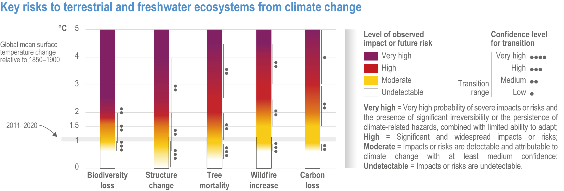
Figure 2.11 | Key risks to terrestrial and freshwater ecosystems from climate change. This IPCC chapter assesses these as fundamental risks of climate change to ecosystem integrity and the ecosystem services that support human well-being, based on observed impacts and future risks of: (far-left) “biodiversity loss” refers to losses of animal and plant species from different ecosystems globally, with resulting declines in ecosystem integrity, functioning and resilience (Section 2.4.2.1, 2.4.2.2, 2.5.1.3.3); (middle-left) “structure change” refers to major changes occurring in ecosystem structure (Sections 2.4.3, Box 2.1, 2.5.2, Figure 2.9, Figure Box 2.1.1, Table Box 2.1.1, Table SM2.5); (middle) “tree mortality” refers to tree mortality exceeding natural levels (2.4.4.3, 2.5.3.3); (middle- right) “wildfire increase” refers to wildfire exceeding natural levels (Section 2.4.4.2, 2.5.3.2); (far-right) “carbon loss” refers to ecosystem carbon losses that could occur abruptly and substantially raise atmospheric carbon dioxide (Sections 2.4.3.6–2.4.3.9, 2.4.4.4, 2.5.2.6–2.5.2.10, 2.5.3.4, 2.5.3.5). This burning embers diagram shows impacts and risks in relation to changes in GSAT, relative to the pre-industrial period (1850–1900). Risk levels reflect current levels of adaptation and do not include more interventions that could lower risk. The compound effects of climate change, combined with deforestation, agricultural expansion and urbanisation as well as air, water and soil pollution and other non-climate hazards could increase risks. Tables 2.5 and SM2.5 provide details of the key risks and temperature levels for the risk transitions.
FAQ 2.4 | How does nature benefit human health and well-being and how does climate change affect this?
Human health and well-being are highly dependent on the ‘health’ of nature. Nature provides material and economic services that are essential for human health and productive livelihoods. Studies also show that being in ‘direct contact with natural environments’ has direct positive effects on well-being, health and socio-cognitive abilities. Therefore, the loss of species and biodiversity due to climate change will reduce natural spaces and, in turn, decrease human well-being and health worldwide.
Human health and well-being are highly dependent on the ‘health’ of nature. Biodiversity—the variety of genes, species, communities and ecosystems—provides services that are essential for human health and productive livelihoods, such as breathable air, drinkable water, productive oceans and fertile soils for growing food and fuels. Natural ecosystems also help store carbon and regulate climate, floods, disease, pollution and water quality. The loss of species, leading to reduced biodiversity, has direct and measurable negative effects on all of these essential services, and therefore on humankind. A recent demonstration of this is the decline of pollinator species, with potential negative effects on crop pollination, a fundamental ecosystem function crucial for agriculture. The loss of wild relatives of the domesticated varieties that humans rely on for agriculture reduces the genetic variability that may be needed to support the adaptation of crops to future environmental and social challenges.

Figure FAQ2.4.1 | The positive relationship between human health and well-being and nature conservation. Nature provides essential services to humans including material and economic services (i.e., ecosystem services) as well as cultural, experiential and recreational services, which, in turn, enhance human psychological and physical health and well-being. People who are more connected to nature are not only happier and healthier but are also more likely to engage in pro-nature behaviours, making the enhancement of human–nature connectedness worldwide a valuable win–win solution for humans and nature to face environmental challenges.
The number of species that can be lost before negative impacts occur is not known and is likely to differ in different systems. However, in general, more diverse systems are more resilient to disturbances and able to recover from extreme events more quickly. Biodiversity loss means there are fewer connections within an ecosystem. A simpler food web with fewer interactions means less redundancy in the system, reducing the stability and ability of plants and animal communities to recover from disturbances and extreme weather events such as floods and drought.
In addition to ‘material’ and economic services such as eco-tourism, nature also provides cultural services such as recreation, spirituality and well-being. Specifically, being in ‘direct contact with natural environments’ (vs. an urban environment) has a high positive impact on human well-being (e.g., mood, happiness), psychological and physical health (energy, vitality, heart rate, depression) and socio-cognitive abilities (attention, memory, hyperactivity, altruism, cooperation). Therefore, the loss of species from climate change and urbanisation will reduce natural spaces, decrease biodiversity, and, in turn, decrease human well-being and health worldwide.
Finally, the extent to which humans consider themselves part of the natural world—known as human-nature connectedness—has been demonstrated to be closely associated with human health and well-being. Individuals who are more connected to nature are not only happier and healthier but also tend to engage more in pro-nature behaviours, making the enhancement of human–nature connectedness worldwide a valuable win–win solution for humans and nature to face environmental challenges.
2.6 Climate Change Adaptation for Terrestrial and Freshwater Ecosystems
Adaptation to reduce the vulnerability of ecosystems and their services to climate change has been addressed in previous IPCC reports, with AR4 and AR5 recognising both autonomous adaptation and human-assisted adaptation to protect natural species and ecosystems. In AR5, Ecosystem-based Adaptation (EbA), adaptation for people, based on the better protection, restoration and management of the natural environment, was identified as an area of emerging opportunity, with a dedicated Cross-Chapter Box on the topic. In the SRCCL, conservation, EbA and related concepts were integrated throughout; SR1.5 also noted the role of EbA. Since the last assessment report, the scientific literature has expanded considerably, with growing interest in the concept of Nature-based Solutions (NbS). This section assesses this new literature and its implications for the implementation of climate change adaptation.
Previous sections of this chapter have set out the vulnerability of natural and semi-natural ecosystems to climate change, and the risks this poses to both biodiversity and ecosystem services (also sometimes described as ‘Nature’s Contributions to People’). Natural systems respond to climatic and other environmental changes in a variety of ways. Individual organisms can respond through growth, movement and developmental processes. Species and populations genetically adapt to changing conditions and evolve over successive generations. Geomorphological features, such as the path of watercourses, can also change naturally in response to climate change. However, there is a limit to which these natural processes can maintain biodiversity and the benefits people derive from nature, partly due to intrinsic limits, but also because of the pressures that people exert on the natural environment.
Most of this section therefore focusses on human interventions to build the resilience of ecosystems, enable species to survive or to adjust management to climate change. Vulnerability is, in many cases, exacerbated by the degraded state of many ecosystems as a result of human exploitation and LUC, leading to the fragmentation of habitats, the loss of species and impaired ecosystem function. This interaction between climate change and environmental degradation means that protecting ecosystems in a natural or near-natural state will be an important pre-requisite for maintaining resilience and give many species the best chance of persisting in a changed climate (Belote et al., 2017; Arneth et al., 2020; Ferrier et al., 2020; França et al., 2020). Protection from degradation, deforestation and exploitation is also essential to maintain critical ecosystem services, including carbon storage and sequestration and water supply (Dinerstein et al., 2020; Pörtner et al., 2021).
It is worth briefly considering some key concepts that are relevant to adaptation in ecosystems. Adaptation for biodiversity and ecosystems can encompass both managing change and building resilience. We use the definition of ‘resilience’ set out Chapter 1: ‘the capacity of social, economic and environmental systems to cope with a hazardous event or trend or disturbance, responding or reorganising in ways that maintain their essential function, identity and structure while also maintaining the capacity for adaptation, learning and transformation’. This includes the concept of ‘resistance’, which is used in some ecological literature to distinguish systems which are resistant to change from those that recover quickly from change. We consider both interventions designed primarily to protect biodiversity and those intended to reduce the risks of climate change to people.
A variety of terms are used to describe using environmental management to reduce the impacts of climate change on people in ways that also benefit biodiversity in the scientific literature, particularly EbA and NbS (see also Section 1.4). EbA is the use of biodiversity and ecosystem services as part of an overall adaptation strategy to help people to adapt to climate change (Secretariat of the Convention on Biological Diversity, 2020). EbA aims to maintain and increase the resilience and reduce the vulnerability of ecosystems and people in the face of the adverse effects of climate change (Vignola et al., 2009). NbS is a broader term which is not restricted to climate change, and is also often used to refer to climate change mitigation; it has been defined by the IUCN as ‘Actions to protect, sustainably manage and restore natural or modified ecosystems that address societal challenges effectively and adaptively, simultaneously providing human well-being and biodiversity benefits’ (Cohen-Shacham et al., 2016). This widely accepted definition excludes actions which use the natural environment to solve human problems but do not provide benefits for biodiversity, and is closely linked to the concept of the Ecosystem Approach. NbS is not a universally accepted term, but it is being increasingly used in the scientific literature. It is a concept which recognises the importance of biodiversity in ecosystem service provision, and offers the opportunity to address climate change and loss of biodiversity together in an efficient integrated way (Chong, 2014; Seddon et al., 2020a; Ortiz et al., 2021). Given that the focus of this chapter is on adaptation, we primarily use the term EbA as it is more specific, but we do so understanding that it can be regarded as a subset of NbS. The wider concept of NbS for climate change adaptation and mitigation is covered in a cross-chapter box on the topic (see Cross-Chapter Box NATURAL in this chapter).
Whilst we distinguish between adaptation for biodiversity and EbA, it is important to recognise that the two are linked in that, if ecosystems themselves are not resilient to climate change, they will not be able to provide adaptation benefits for people. The case for resourcing biodiversity conservation and building the resilience of ecosystems is also strengthened when there are direct benefits for people in addition to the more general benefits of biodiversity.
Ecosystems are specifically included in the adaptation goals set out in the Paris Agreement and are addressed in most national adaptation plans (Seddon et al., 2020b). There are also now a large number of adaptation programmes and plans for local governments and governmental and non-governmental conservation organisations. Adaptation for and by ecosystems needs to be understood and developed in the wider contexts of conservation, climate resilient development and sustainable development. There are significant potential synergies but also conflicts between different objectives which require an integrated approach (covered further in 2.6.7).
2.6.1 Limits to Autonomous (Natural) Adaptation
Natural ecosystems often have a high degree of resilience and can, to some extent, adjust to change. Species can adjust through evolutionary adaptation, distribution change, behavioural change, developmental plasticity and ecophysiological adjustment. There are, however, limits to autonomous adaptation, because of intrinsic limitations, the rate at which the climate is changing and the degraded state of many ecosystems.
None of the evolutionary changes either documented or theorised would enable a species to survive and reproduce in climate spaces that it does not already inhabit. It is very improbable that evolutionary responses would be sufficient to prevent species extinctions in the case of that species losing its climate space entirely on a regional or global scale (section 2.4.2.8) (Parmesan and Hanley, 2015). At the highest risk are the world’s most cold-adapted species (whose habitats are restricted to polar and high mountain-top areas). Examples include the polar bear (Regehr et al., 2016), ‘sky-island’ plants in the Tropics (Kidane et al., 2019), mountain-top amphibians in Spain (Enriquez-Urzelai et al., 2019), mountain-top lichens in the Appalachians (USA) (Allen and Lendemer, 2016) and silverswords in Hawaii (Krushelnycky et al., 2013). However, there is potential for using evolutionary changes to enhance the adaptive capacity of target species, as is being done on the Great Barrier Reef by translocating symbionts and corals that have survived recent intense heat-induced bleaching events into areas that have had large die-off (Rinkevich, 2019). Multiple studies have assessed when and how evolution might be able to help wild species adapt to climate change (Ratnam et al., 2011; Sgro et al., 2011).
Some of the reasons cited in the literature as limits to autonomous adaptation are:
- Genetic changes in populations require many generations and, for many species, operate on longer timescales than those on which the climate is currently changing. In addition, experiments indicate there are strong constraints to ability to evolve beyond current climatic limits.
- Many species are moving to higher latitudes as the climate warms, but not all are keeping pace with changes in suitable climate space (Valladares et al., 2014; Mason et al., 2015). Such ‘climate debt’ (see sections 2.4.2.3.1, 2.4.2.8, 2.5.1.3.1) indicates an inability for non-genetic autonomous adaptation (e.g., evidence of limited ability for plastic responses, like those stemming from dispersal limitations, behavioural restrictions or physiological constraints).
- Some species have a low capacity for dispersal, which, combined with increased fragmentation of habitats, creates barriers to range shifts to match climate warming. Studies have shown that changes in the distribution of species and composition of communities are limited by the presence of intensively managed agricultural land fragmenting natural habitats (Oliver et al., 2017).
There are a variety of mechanisms which promote the resilience of ecosystems through persistence, recovery and reorganisation (Falk et al., 2019). Changes in the balance of different plant species within a community can maintain the persistence of the community itself, maintaining its value as a habitat for other species and providing ecosystem services. In some cases, there are negative feedback mechanisms between biological and physical processes; for example, in peatlands, lowered water tables resulting from drier conditions can lead to reduced permeability of peat, increasing rates of water loss (Page and Baird, 2016). There are limits to this resilience and the concept of tipping points beyond which ecosystems change state, and returning to the original state has been subject of much recent research (van Nes et al., 2016). There is clear evidence that the degradation of ecosystems has reduced their resilience and that restoration can help to reduce risks to biodiversity and ecosystem services, discussed below (see Section 2.6.2, 2.6.3). However, as the rate of climate change increases, the limits of this approach will start to be reached, and losses (including some with potentially catastrophic consequences) cannot be prevented; this is discussed further in Section 2.6.6.
2.6.2 Adaptation for Biodiversity Conservation
A variety of approaches have been identified as potential adaptation measures which people can take to reduce the risks of climate change to biodiversity. (Heller and Zavaleta, 2009 ), quoted in AR5, identified 113 categories of recommendation for adaptation from a survey of 112 papers and reports. Since then, the literature has expanded with thousands of relevant publications. Whilst there is increasing interest in adaptation for biodiversity conservation and a wide range of plans and strategies, there is less evidence of these plans being implemented. Since AR5, a number of studies, predominantly from Europe and North America, have investigated the extent to which adaptation has been integrated into conservation planning and is being implemented on a local and regional scale (Macgregor and van Dijk, 2014; Delach et al., 2019; Prober et al., 2019; Clifford et al., 2020; Barr et al., 2021; Duffield et al., 2021). A common pattern in these studies is that vulnerability has been assessed and potential adaptation actions identified, but implementation has been limited beyond actions to improve ecological conditions which may increase resilience on a local scale.
To date, most scientific literature on adaptation to reduce the risks to biodiversity from climate change has been based on ecological theory rather than on observations or practical experience. A recent review (Prober et al., 2019) concluded that out of 473 papers on adaptation, only 16% presented new empirical evidence and very few assessed the effectiveness of actual adaptation actions. It is also the case that relatively little research is focused on local-scale management interventions rather than on larger-scale strategies (Ledee et al., 2021), although there are some exceptions (Duffield et al., 2021).
Although direct assessments of the effectiveness of adaptation actions are rare, since AR5, there have been an increasing number of empirical analyses of how different land use and management can influence the vulnerability of species and habitats. As climate change often interacts with other factors including ecosystem degradation and fragmentation (Oliver et al., 2015a), actions to address these other interacting factors is expected to build resilience to climate change. Table 2.6 summarises evidence that supports the main categories of proposed adaptation measures. We have taken an inclusive approach and included studies that address extreme weather events such as droughts, which may be exacerbated by climate change, as well as long-term changes in climate variables. We have not distinguished between studies in which climate change adaptation was an explicit focus and those in which lessons for adaptation can be learnt, that is, when studies were conducted for other reasons but inform the assessment of the impacts of actions identified as potential adaptation measures.
Table 2.6 | Evidence to support proposed climate change adaptation measures for biodiversity. The evidence highlights that adaptation for biodiversity conservation is a broad concept, encompassing a wide range of actions. It includes targeted interventions to change the microclimate for particular species (e.g., by creating shade) to changing national conservation objectives to take account of changing distributions of species and communities. It includes targeted actions addressing both climate change and the protection and restoration of ecosystems, with multiple additional benefits including reduced vulnerability to climate change. Most of the studies are not direct tests of the impacts of adaptation actions which, as noted above, is an important gap in the evidence. There is also a major limitation in that reported studies are predominantly from Europe, North America and Australasia, with little research in other regions.
Proposed adaptation measures for biodiversity | Uncertainty Assessment | Comment | Selected references |
Protect large areas of natural and semi-natural habitat | robust evidence, high agreement | There is considerable evidence that: intact systems provide better quality and quantity of ecosystem services; larger intact areas provide better ecosystem services; the risk of species’ extinctions from disturbances including climate change, is reduced by having large, connected populations; more biodiverse systems provide higher levels of ecosystem services and are more resilient to climate change than degraded systems that have lost species | (Pimm et al., 2018; Dinerstein et al., 2019; Woodley et al., 2019; Brooks et al., 2020; Hannah et al., 2020; Luther et al., 2020; Zhao et al., 2020; Sala et al., 2021); |
Increase connectivity in terrestrial habitats: corridors, stepping stones | medium evidence, medium agreement | There is good evidence that some species move more quickly in more connected landscapes. However, not all species do and some of those that benefit are invasive/pest/disease species; to date, empirical evidence showing that connectivity has reduced climate change impacts on species is limited. | (Keeley et al., 2018; Stralberg et al., 2019; von Holle et al., 2020) |
Increase connectivity in river networks | limited evidence, high agreement | Connectivity is needed to maintain the movement of species and populations, but river reaches and catchments lack integrated protection | (Hermoso et al., 2016; Thieme et al., 2016; Abell et al., 2017; Brooks et al., 2018) |
Increase habitat patch size and expand protected areas | limited evidence, high agreement | Generally increases resilience because of functioning natural processes, large species populations and refugial areas | |
Increase replication and representation of protected areas | limited evidence, high agreement | Various benefits inferred, including a wider range of climatic and other conditions and less risk of extreme events affecting many rather than few areas. More sites available for colonisation by range-expanding species and better conditions to maintain species in situ under range contraction. | (Mawdsley et al., 2009; Thomas et al., 2012; Virkkala et al., 2014; Gillingham et al., 2015; Pavón-Jordán et al., 2020) |
Protect microclimatic refugia | medium evidence, high agreement | Locally cool areas can be identified and there is evidence that species can survive better in such areas | (Haslem et al., 2015; Suggitt et al., 2015; Isaak et al., 2016; Morelli et al., 2016; Merriam et al., 2017; Bramer et al., 2018; Suggitt et al., 2018; Massimino et al., 2020) |
Creating shade to lower temperatures for vulnerable species | limited evidence, high agreement | Creating shade (e.g., of watercourses) has been used as an adaptation strategy, but improvements in species survival under warming conditions have yet to be demonstrated | (Broadmeadow et al., 2011; Lagarde et al., 2012; Patino-Martinez et al., 2012; Thomas et al., 2016) |
Restoring hydrological processes of wetlands, rivers and catchments, including by raising water tables and restoring original channels of watercourses | medium evidence, high agreement | Wetland restoration is well established as a conservation measure in some countries. It can reduce vulnerability to drought with climate change, but evidence to demonstrate effectiveness as an adaptation measure is limited and requires the long-term monitoring of a range of sites. There is little restoration of degraded tropical peatlands to date | (Carroll et al., 2011; Hossack et al., 2013; Dokulil, 2016; Timpane-Padgham et al., 2017; Moomaw et al., 2018) |
Restoration of natural vegetation dynamics | medium evidence, medium agreement | Includes reintroduction of native herbivores and reversing woody encroachment of savannas. Benefits for biodiversity are well established in a wide range of different regions | (Coffman et al., 2014; Valkó et al., 2014; Batáry et al., 2015; Smit et al., 2016; Stevens et al., 2016; Hempson et al., 2017; Bakker and Svenning, 2018; Cromsigt et al., 2018; Fulbright et al., 2018; Olofsson and Post, 2018) |
Reduce non-climatic stressors to increase resilience of ecosystems | limited evidence, medium agreement | As a general principle, climate change is recognised as a ‘threat multiplier’ but specific details are often unclear | |
Assisted translocation and migration of species | limited evidence, medium agreement | Assisted translocation has been commonly suggested as an adaptation measure, but there have been very few examples of this being trialled. Translocations have been carried out for other reasons and lessons for climate change adaptation have been inferred. | (Willis et al., 2009; Brooker et al., 2018; Skikne et al., 2020) |
Intensive management for specific species | medium evidence, medium agreement | A variety of approaches including manipulating microclimate and competition between species to improve chances of survival under climate change | (Angerbjörn et al., 2013; Greenwood et al., 2016; Pearce-Higgins et al., 2019) |
Ex situ conservation (seedbanks/genetic stores, etc.) | Not possible to assess at present | Seed banks have been established but their long-term effectiveness can only be evaluated at a later point | |
Adjusting conservation strategies and site objectives to reflect changing species’ distributions and habitat characteristics | robust evidence, high Agreement | Conservation management will need to take account of changes that cannot be prevented (e.g., the distribution of species and composition of communities) to protect and manage biodiversity as effectively as possible in a changing climate | (Stein et al., 2013; Rannow et al., 2014; Oliver et al., 2016; Stralberg et al., 2019; Duffield et al., 2021) |
Softening the matrix of unsuitable habitats between patches to increase permeability for the movement of species in response to climate change | limited evidence | There is potential for agri-environment schemes to do this in hostile farmed landscapes |
Many climate adaptation actions for biodiversity operate on the landscape scale (von Holle et al., 2020). The total area of habitat, how fragmented it is, the size of habitat patches and the connectivity between them are inter-linked properties on this scale. A growing number of studies have investigated how these properties affect species ability to persist in situ and colonise new areas. Overall, larger areas of semi-natural habitat are associated with increased resilience to ongoing climate change and extreme events as well as the capacity to colonise new areas (Haslem et al., 2015; Oliver et al., 2017; Papanikolaou et al., 2017). Larger habitat patches can support larger populations of a given species, which are more likely to maintain themselves and recover from periods of adverse conditions. Inhabiting a large patch size has been found to increase the resilience of some populations of species to extreme events such as droughts (Oliver et al., 2015b). They are also more likely to provide a range of different resources and microclimate conditions, which may increase the chances of the persistence of species under climate change. A larger area of habitat may also enable greater connectivity between patches and increase the chances of species colonising new areas as they track climate change (Oliver et al., 2015b).
Protecting and restoring natural processes is a general principle for maintaining and building resilience to climate change for biodiversity (Timpane-Padgham et al., 2017). One element of this is ensuring naturally functioning hydrology for wetlands and river systems (Table 2.6), which is particularly important in a context of changing rainfall patterns and increased evapotranspiration. An important development in approaches to conservation over recent decades has been the concept of re-wilding (Schulte To Bühne et al., 2021); this encompasses a number of elements of restoring natural processes, including the reintroduction of top predators, larger conservation areas, and less prescriptive outcomes than many previous conservation measures. There are elements of re-wilding which may well contribute to building resilience to climate change, but it will be increasingly important to factor climate change adaptation into the planning of re-wilding schemes (Carroll and Noss, 2021).
The most consistently cited climate change adaptation measure for species is increasing connectivity to facilitate the colonisation of new areas. This reflects the fact that many species’ habitats are highly fragmented in areas with more intensive land management, which prevents them naturally changing their range to track changing climatic conditions. Advances and innovations in modelling techniques can support decision-making about connectivity (Littlefield et al., 2019). There is evidence from empirical and modelling studies that species can disperse more effectively in better-connected areas in terrestrial habitats (Keeley et al., 2018). The issues are different in more natural landscapes—species may still be threatened in intrinsically isolated habitats, such as mountain tops, but connectivity cannot be created here in the same way. Evidence suggests that increased connectivity will only benefit a subset of species, probably those which are intermediate-habitat specialists that are able to disperse (Pearce-Higgins and Green, 2014). Generalists do not require corridors or stepping stones, while many corridors or stepping stones will not be of sufficient quality to be used by most habitat specialists. There should also be a caveat to the general principle that increasing connectivity is a benefit for climate change adaptation. It can increase the spread of invasive, pest and disease-causing species into newly suitable regions. In some places, isolated refugia may better allow vulnerable species and biological communities to survive.
There are many different approaches to increasing connectivity, ranging from increasing the overall area of suitable habitat to ‘corridors’ and ‘stepping stones’, with different strategies likely to be more effective for different species and circumstances (Keeley et al., 2018). Connectivity can also be important in increasing the resilience of populations to extreme climatic events (Newson et al., 2014; Oliver et al., 2015b). Within freshwater environments, the connectivity of watercourses is essential. Fluvial corridors are necessary to ensure the survival of migrating fish populations, even without climate change; with climate change, connectivity becomes crucial for relatively cold-adapted organisms to migrate upstream to colder areas. Connectivity is also important for the larvae of benthic invertebrates to be able to drift downstream and hence to disperse (Brooks et al., 2018); for adult benthic invertebrates, riparian and terrestrial habitat features can potentially affect dispersal. Connectivity within river and wetland systems for some species can also mediated by more mobile animal species such as fish and birds (Martín-Vélez et al., 2020). Which factors are the most important in either promoting their colonisation of new sites or persisting in situ will differ between species and locations. Some general principles have been recognised and can guide conservation policy and practice (Natural England and RSPB, 2020; Stralberg et al., 2020), but this will often require additional investigation and planning based on an individual understanding of the niches of specific species.
Managed translocation, that is, moving species from areas where the climate is becoming unsuitable to places where their persistence under climate change is more likely , has been discussed as an adaptation option for many years. So far, there have been very few examples of this and it is likely to be a last resort in most cases, as it usually requires a large investment of resources, outcomes are uncertain and there may be adverse impacts on the receiving sites. Nevertheless, there are cases where it may be a be a viable option (Stralberg et al., 2019). This is discussed in more detail as a case study in Section 2.6.5.1.
The evidence that species can persist in microclimatic refugia where suitable conditions for them are maintained locally (e.g., because of variations in topography) has increased in recent years. This has opened up the potential to include refugia in conservation plans and strategies to facilitate the local survival of species (Jones et al., 2016; Morelli et al., 2016; Morelli et al., 2020), for example, targeting management actions (Sweet et al., 2019) aimed at supporting populations of species. This is likely to become an important aspect of climate change adaptation for biodiversity conservation in future. It is also possible to manipulate microclimate, for example, by creating shelters for birds’ nests; see Case Study in 2.6.5.5 of African penguins; (Patino-Martinez et al., 2012). One specific approach of this sort is the planting or retention of trees and wooded corridors to shade watercourses (Thomas et al., 2016). Riparian shading can also possibly help to reduce phytoplankton and benthic diatom growth in smaller streams and rivers (Halliday et al., 2016).
Refugia often refer to locally cool places in a landscape, such as shaded slopes or high elevations, but they can also include places where the supply of water may continue during dry periods (Morelli et al., 2016). Monitoring can reveal which streams, wetlands, springs and other aquatic resources retain suitable discharges, water quality, wetland area and ecological integrity, especially during dry years (Cartwright et al., 2020). Measures to conserve drought refugia may include protecting springs and other groundwater-fed systems from groundwater extraction, contamination, salinisation, surface-water diversion, channelisation of streams, trampling by livestock, recreation activities and invasive species and the effects of disturbances in the surrounding landscape (Cartwright et al., 2020; Krawchuk et al., 2020). Restoration of degraded aquatic ecosystems can include removing flow-diversion infrastructure, excluding livestock, reducing other human impacts, geomorphic restructuring, removing invasive species and planting native riparian vegetation.
In fire-prone areas, fire suppression and management are a key element of protecting refugia (Section 2.6.5.8 below). In ecosystems in which a natural fire regime has been suppressed, restoration practices such as prescribed fires, thinning trees and allowing some wildfire where it benefits the ecosystem can be introduced to reduce increasing risks from severe wildfires (Meigs et al., 2020).
Protected areas—areas of land set aside for species and habitat protection with legal protection from development or exploitation—have been a cornerstone of nature conservation for many years. Their effectiveness under a changing climate has been the subject of debate and investigation. There is now a large body of evidence demonstrating that colonisations by range-shifting species are more likely to occur at protected sites than at non-protected sites for a wide range of taxa (e.g., Thomas et al., 2012; Gillingham et al., 2015) including across continents (Pavón-Jordán et al., 2020). This is probably because, by protecting large areas of natural and semi-natural habitats, they provide suitable places for colonising species (Hiley et al., 2013) which may not be available in the surrounding landscape. Although the evidence for protected areas being associated with reduced extinctions is weaker, the finding by Gillingham et al. (Gillingham et al., 2015) that protected sites were associated with reduced extinction rates at low latitudes and elevations is strongly suggestive that they can help species’ persistence in the face of climate change.
It is intrinsically difficult to assess the effectiveness of climate change adaptation measures, the benefit of which will be realised in the years and decades ahead (Morecroft et al., 2019). Nevertheless, taking into account the wide range of evidence reported above, including the theory, modelling and observations of the impacts of climate change in contrasting circumstances, it is possible to make an overarching assessment that appropriate adaptation measures can reduce the vulnerability of many aspects of biodiversity to climate change (robust evidence, high agreement ). It is also clear, however, that to be most effective and avoid unintended consequences, measures need to be carefully implemented by taking into account specific local circumstances (robust evidence, high agreement) and include the management of inevitable changes (robust evidence, high agreement ). It is also clear that while there are now many plans and strategies for adapting biodiversity conservation to climate change, many have yet to be implemented fully (medium evidence, high agreement ).
2.6.3 Ecosystem-Based Adaptation
A study published in 2020 found that, out of 162 intended nationally determined contributions (covering 189 countries) submitted to the United Nations Framework Convention on Climate Change (UNFCCC), as commitments to action under the Paris Agreement, 109 indicated ‘ecosystem-orientated visions’ for adaptation, but only 23 used the term ‘ecosystem-based adaptation’ (Seddon et al., 2020b).
EbA includes a range of different approaches. Examples include restoring coastal and river systems to reduce flood risk and improve water quality, and the creation of natural areas within urban areas to reduce temperatures through shading and evaporative cooling. EbA is closely linked with a variety of other concepts such as ecosystem services, natural capital and disaster risk reduction (DRR). EbA was becoming a well-recognised concept at the time of AR5 but implementation was still at an early stage in many cases. Since then, pilot studies have been assessed and EbA projects have been initiated around the world. The evidence base continues to grow (Table 2.7), and this has led to increasing confidence in approaches which have been shown to work leading to further expansion in some countries (Table 2.7). However, this is not uniform and there is relatively little synthesis across disciplines and regions (Seddon et al., 2020a). Chausson et al. (2020) used a systematic mapping methodology to characterise 386 published studies. They found that interventions in natural or semi-natural ecosystems ameliorated adverse climate change impacts in 66% of cases, with fewer trade-offs than for more artificial systems such as plantation forest. However, the evidence base has substantial gaps. Most of the evidence has been collected in the Global North, and there is a lack of robust, site-specific investigations into the effectiveness of interventions compared to alternatives and more holistic appraisals that account for broader social and ecological outcomes.
Restoring coasts, rivers and wetlands to reduce flood risk have probably seen the largest investment in EbA and it is becoming an increasingly accepted approach in some places (e.g., case studies in Sections 2.6.5.2, 2.6.5.7), although significant social, economic and technical barriers remain (Wells et al., 2020; Bark et al., 2021; Hagedoorn et al., 2021). Natural flood management (NFM) encompasses a wide range of techniques in river systems and at the coast and has been used in varied locations around the world. In tropical and subtropical areas, the restoration of mangroves to reduce the risk of coastal flooding is a widely advocated, evidence-based approach (e.g., (Høye et al., 2013; Sierra-Correa and Kintz, 2015; Powell et al., 2019)). In temperate regions, salt marsh is a similarly important habitat (Spalding et al., 2014). Both provide buffering against SLR and storm surges. Managed realignment of the coast, by creating new habitats, can lead to a loss of terrestrial and freshwater ecosystems, but it can protect them and the services they provide by reducing the risks of catastrophic failure from hard-engineered sea defences.
Table 2.7 | Examples of key EbA measures with assessments of confidence. Note only adaptation-related services are shown; many measures also provide a range of other benefits to people. All also provide benefits for biodiversity.
EbA measures | Confidence assessment | Ecosystem services for climate change adaptation | Climate change impact addressed | Social benefits from adaptation | Relevant ecosystems and contexts | Selected references |
Natural flood risk management in river systems: restoring natural river courses (removing canalisation), restoring and protecting wetlands and riparian vegetation | medium evidence, medium agreement | Flood regulation; sediment retention; water storage; water purification | Increased rainfall intensity | Reduction of flood damage Increased water security (quality and supply) | Multiple | (Iacob et al., 2014; Meli et al., 2014; Dadson et al., 2017; Rowiński et al., 2018; Burgess-Gamble et al., 2021) |
Shade rivers and streams by restoration of riparian vegetation or trees. | medium evidence, high agreement | Provision of fish stocks | Warmer water temperatures | Food security; income benefits | Multiple | (Broadmeadow et al., 2011; Isaak et al., 2015; Williams et al., 2015b; Thomas et al., 2016) |
Managed realignment of coastlines; re-establishing and protecting coastal habitats including mangroves, saltmarshes, coral reefs and oyster reefs | robust evidence, high agreement | Coastal storm and flood protection; coastal erosion control; prevention of intrusion of salt water | SLR; increasing storm energy | Protection of life, property and livelihoods; water security | Coastal | (Høye et al., 2013; Spalding et al., 2014; Narayan et al., 2016; Morris et al., 2018; Chowdhury et al., 2019; Powell et al., 2019) |
Agro-forestry and other agro-ecological/conservation practices on agricultural land | medium evidence, medium agreement | Local climate regulation; soil conservation; soil nutrient regulation; water conservation; pest control; food provisioning | High temperature or changing temperature regimes; changing precipitation regimes | Food security; income benefits | Multiple | (Vignola et al., 2015; Torralba et al., 2016; Paul et al., 2017; Blaser et al., 2018; Nesper et al., 2019; Verburg et al., 2019; Aguilera et al., 2020; Tamburini et al., 2020) |
Restore and maintain urban and peri-urban green space: trees, parks, local nature reserves, created wetlands | robust evidence, high agreement | Local climate regulation; flood regulation; water purification; water storage; erosion control | Higher temperatures and heat waves; increased or reduced rainfall intensity | Cooler micro-climate; reduced flood damage; water security | Urban areas | (Norton et al., 2015; Liquete et al., 2016; Liu, 2016; Bowler et al., 2017; Aram et al., 2019; Stefanakis, 2019; Ziter et al., 2019) |
Ecological restoration for reducing fire risk by restoring natural vegetation and herbivory and reinstating natural fire regimes | medium evidence, high agreement | Regulation of wildfires | Mega-fires from increases in drought and heat | Reduce deaths and infrastructure damage from fires | Fire-adapted ecosystems | (Waldram et al., 2008; Stephens et al., 2010; van Mantgem et al., 2016; Boisramé et al., 2017; Johnson et al., 2018; Parisien et al., 2020a; Parisien et al., 2020b; Stephens et al., 2020) |
Invasive non-native aquatic plant control to improve water security | robust evidence, high agreement | Water provision | Increasing droughts | Water security | Water-scarce regions prone to an increase in droughts | |
Woody plant control (of encroaching biomass) in open grassy ecosystems to restore and maintain grassy vegetation (see 2.4.3.5) | medium evidence, medium agreement | Fodder biomass production | Elevated CO2 and increased rainfall promoting tree growth | Income through bush clearing, fuelwood supplies, restore grazing | Savanna and grasslands | |
Rangeland rehabilitation and management e.g. introducing livestock enclosures, appropriate grazing management, reintroducing native grassland species | medium evidence, medium agreement | Fodder biomass production; soil erosion control; soil formation; nutrient cycling; water retention | Changing precipitation and temperature regimes including prolonged dry seasons and increased drought frequency | Food security Water security, income benefits | Rangelands | (Descheemaeker et al., 2010; Wairore et al., 2016; Kimiti et al., 2017) |
Sustainable forestry of biodiverse managed forests, maintaining forest cover and protecting soils | medium evidence, medium agreement | Timber production | Increased frequency and severity of storms; higher temperatures; changing precipitation regimes (more intensive wet and dry periods); increased incidents of wildfire, pest and disease outbreaks | Livelihood and income benefits | Boreal, temperate, subtropical, tropical forests | (Gyenge et al., 2011; Barsoum et al., 2016; Jactel et al., 2017; Cabon et al., 2018) |
Watershed reforestation and conservation for hydrological services | medium evidence, medium agreement | Flood control; erosion control; water provisioning; water purification | Changing precipitation regimes | Food security; Water security; Flood Protection | Boreal, temperate, subtropical, tropical forests | |
Multi-functional forest management and conservation to provide climate-resilient sources of food and livelihoods and protect water sources | medium evidence, medium agreement | Timber and non-timber forest production; fuel wood production; water provisioning; water purification | Multiple | Food security; Water security; income benefits | Boreal, temperate, subtropical, tropical forests | (Lunga and Musarurwa, 2016; Strauch et al., 2016; Adhikari et al., 2018) |
Slope re-vegetation for landslide prevention and erosion control | robust evidence, high agreement | Soil retention; slope stabilisation | Increased rain frequency | Reduced landslide damage; prevention of loss of life | Montane and other steep-sloped regions | (Fox et al., 2011a; Krautzer et al., 2011; Osano et al., 2013; Bedelian and Ogutu, 2017; Getzner et al., 2017; de Jesús Arce-Mojica et al., 2019) |
In river systems (Iacob et al., 2014), management of both the catchments and the channel itself is important: restoring natural meanders in canalised watercourses and allowing the build-up of woody debris can slow flows rates; restoring upstream wetlands or creating them in urban and peri-urban situations can store water during flood events if they are in the right place in a catchment (Acreman and Holden, 2013; Ameli and Creed, 2019; Wu et al., 2020). There is less data on the potential for NFM in tropical compared to temperate catchments. However, (Ogden et al., 2013) showed that flooding was reduced from a secondary forested catchment area compared to those which were pasture or a mosaic of forest, pasture and subsistence agriculture. EbA approaches to reduce flooding can be applied within urban areas as well as in rural catchments, as in Durban, South Africa (Section 2.6.5.7), but effectiveness will depend on EbA being implemented at a sufficient scale and in the right locations (Hobbie and Grimm, 2020; Costa et al., 2021). This may, in turn, provide protection to downstream urban communities.
Protecting and restoring natural river systems and natural vegetation cover within catchments as well as integrating agro-ecological techniques into agricultural systems can also help to maintain and manage water supplies for human use, under climate change, including during periods of drought, by storing water in catchments and improving water quality (Taffarello et al., 2018; Agol et al., 2021; Khaniya et al., 2021). Lara et al. (2021) showed that replacing a non-native Eucalyptus plantation in Chile with native forest caused base flow to increase by 28–87% during the restoration period compared to pre-treatment, and found that it remained during periods with low summer precipitation.
EbA can operate on a range of different scales, from local to catchment to region. On the local scale, there is a variety of circumstances in which microclimates can be managed and local temperatures lowered by the presence of vegetation (Table 2.7), and these EbA techniques are now being used more widely. In both urban and agricultural situations, shade trees are a traditional technique which can be applied to contemporary climate change adaptation. As reported in Section 2.6.2 above, shading of watercourses can lower temperatures, which can allow species to survive locally; as well as supporting diversity, it can help to maintain important fisheries, including those of salmonid fish (O’Briain et al., 2020). Within cities, green spaces, including parks, local nature reserves and green roofs and walls can also provide cooling as a result of evapotranspiration (Bowler et al., 2010a; Aram et al., 2019; Hobbie and Grimm, 2020), although this may be reduced in drought conditions.
Wildfire is an increasing risk for people as well as to ecosystems in many parts of the world. As discussed in Section 2.4.4.2, this is the result not just of climate change but also past management practices, including fire suppression. Better fire management including reinstating more natural fire regimes can reduce risks.
EbA is usually a place-specific approach and a number of studies have documented how attempts to implement it without an understanding of local circumstances and the full engagement of local communities have been unsuccessful (Nalau et al., 2018). Since AR5, a number of studies have considered the factors that are important for environment adaptation programmes and projects (UNFCCC, 2015; Nalau et al., 2018; Duncan et al., 2020; EPA Network and ENCA, 2020; Townsend et al., 2020). Considering these sources, others described above and the case studies presented in Section 2.6.5, a number of requirements for effective implementation of EbA can be identified, including the following:
- Targeting of the right EbA measure in the right location
- Decision-making at the appropriate level of governance with participation from all affected communities
- Integration of IKLK and capacity into decision-making and the management of projects
- Involvement of government and non-government stakeholders
- Full integration of EbA with other policy areas including agriculture, water resources and protection of natural resources
- Protection and, if possible, improvement of incomes of local people
- Effective institutional support to manage finances and the implementation of projects and programmes
- Time—many EbA interventions take time to establish, for example, for trees to grow and wetlands to recover
- Monitoring of intended outcomes and other impacts and the communication of results
Whilst it is essential to develop place-specific EbA measures with the full engagement of local communities, it is worth noting that new opportunities may emerge that would not have been possible in the past. As the climate changes, novel ecosystems may emerge (with no present day analogue) which have the potential to provide different adaptation benefits, and societies may be more willing to adopt transformative approaches (Colloff et al., 2017; Lavorel et al., 2020).
Increasingly, it is essential to integrate adaptation and the protection of biodiversity with land-based initiatives to mitigate climate change; this is discussed in more detail in Cross-Chapter Box NATURAL in this chapter. The new IUCN standard (IUCN, 2020) offers a basis for assessing whether actions are true NbS and take into account the wider factors necessary for success.
Whilst policy interest is growing and there is an increasing deployment of EbA, there is still a long way to go in delivering its full potential (Huq and Stubbings, 2015) and significant institutional and cultural barriers remain (Huq et al., 2017; Nalau et al., 2018). Nevertheless, it is increasingly clear that EbA can offer a portfolio of effective measures to reduce the risks for people of climate change at the same time as benefitting biodiversity (robust evidence, high agreement ), providing that such measures are deployed with careful planning in a way that is appropriate for local ecological and societal contexts (robust evidence, high agreement ). This chapter has identified risks to species, communities, ecosystems and ecosystem services from climate change, all of which increase with each increment of Global Warming Level (2.5.1, 2.5.2, 2.5.3, 2.5.4). There is therefore a risk to Ecosystem-based Adaptation measures in some circumstances and this risk increases progressively above 1.5°C of warming.
2.6.4 Adaptation for Increased Risk of Disease
Low-probability events can have a very high impact (e.g., the transmission of SARS-CoV-2 from wild animals to humans, causing the Covid-19 pandemic ). A robust disease risk reduction policy would include utilising One Biosecurity (Meyerson and Reaser, 2002; Hulme, 2020; MacLeod and Spence, 2020) or One Health (Monath et al., 2010; Deem et al., 2018; Destoumieux-Garzón et al., 2018; Zinsstag et al., 2018) approaches with actions to reduce disease risk across multiple sectors and from a variety of anthropogenic drivers, including climate change, even if there is high uncertainty in projected risk (see Cross-Chapter Boxes ILLNESS in this chapter, COVID in Chapter 7 and DEEP in Chapter 17). Kraemer et al. (2019) found that vector importation was a key risk factor and that the focus should be on preventing the introduction of invasive species. Furthermore, many neglected tropical diseases (NTDs) are also VBDs, and the UN SDG of good health and well-being explicitly calls for increased control and intervention with a focus on emergency preparedness and response (Stensgaard et al., 2019a).
Online tools are being developed to warn conservation biologists when species of conservation concern are at a greater risk of disease outbreaks due to environmental changes, for example, for Hawaiian honeycreepers and avian malaria (Berio Fortini et al., 2020) and coral diseases (Caldwell et al., 2016). Forecasting models to warn of human disease outbreaks like malaria and dengue are also now available, with findings that multiple-model ensemble forecasts outperform individual models (Lowe et al., 2013; Lowe et al., 2014; Lowe et al., 2018; Zhai et al., 2018; Johansson et al., 2019; Tompkins et al., 2019; Muñoz et al., 2020; Colón-González et al., 2021; Petrova et al., 2021). Improving VBD and NTD public health responses will require multi-disciplinary teams capable of interpreting, analysing, and synthesising diverse components of complex ecosystem-based studies for effective intervention (Mills et al., 2010; Rubin et al., 2014; Valenzuela and Aksoy, 2018), broad epidemiological and entomological surveillance (Depaquit et al., 2010; Lindgren et al., 2012; Springer et al., 2016) as well as community-based disease control programmes that build local capacity (Andersson et al., 2015; Jones et al., 2020b).
Cross-Chapter Box ILLNESS | Infectious Diseases, Biodiversity and Climate: Serious Risks Posed by Vector- and Water-Borne Diseases
Authors: Marie-Fanny Racault (UK/France, Chapter 3), Stavana E. Strutz (USA, Chapter 2), Camille Parmesan (France/UK/USA, Chapter 2), Rita Adrian (Germany, Chapter 2), Guéladio Cissé (Mauritania/Switzerland/France, Chapter 7), Sarah Cooley (USA, Chapter 3), Meghnath Dhimal (Nepal), Luis E. Escobar (Guatemala/USA), Adugna Gemeda (Ethiopia, Chapter 9), Nathalie Jeanne Marie Hilmi (Monaco/France, Chapter 18), Salvador E. Lluch-Cota (Mexico, Chapter 5), Erin Mordecai (USA), Gretta Pecl (Australia, Chapter 11), A. Townsend Peterson (USA), Joacim Rocklöv (Germany/Sweden), Marina Romanello (UK/Argentina/Italy), David Schoeman (Australia, Chapter 3), Jan C. Semenza (Italy, Chapter 7), Maria Cristina Tirado (USA/Spain, Chapter 7), Gautam Hirak Talukdar (India, Chapter 2), Yongyut Trisurat (Thailand, Chapter 2)
Climate change is altering the life cycles of many pathogenic organisms and changing the risk of transmission of vector- and water-borne infectious diseases to humans ( high confidence ). The rearrangement and emergence of some diseases are already observed in temperate-zone and high-elevation areas and coastal areas ( medium confidence to high confidence, depending upon region ). Shifts in the geographic and seasonal range suitability of pathogens and vectors are related to climatic-impact drivers (warming, extreme events, precipitation and humidity) ( very high confidence ), but there are substantial non-climatic drivers (LUC, wildlife exploitation, habitat degradation, public health and socioeconomic conditions) that affect the attribution of the overall impacts on the prevalence or severity of some vector- and water-borne infectious diseases over recent decades ( high confidence ). Adaptation options that involve sustained and rapid surveillance systems as well as the preservation and restoration of natural habitats with their associated higher levels of biodiversity, both marine and terrestrial, will be key to reducing the risk of epidemics and the large-scale transmission of diseases ( medium confidence ).
Since AR5, further evidence is showing that climate-related changes in the geographic and seasonal range suitability of pathogens and vectors and the prevalence or new emergence of vector- and water-borne infectious diseases have continued across many regions worldwide and are sustained over decadal timescales (low confidence to high confidence, depending upon region)(Sections 2.4.2.5, 3.5.5.3, 7.2, 7.3, 9.10.1.2.1) (Harvell et al., 2009; Garrett et al., 2013; Burge et al., 2014; Guzman and Harris, 2015; Baker-Austin et al., 2018; Watts et al., 2019; Semenza, 2020; Watts et al., 2021). Ecosystem-mediated infectious diseases at risk of increase from climate change include water-borne diseases associated with pathogenic Vibrio spp. (e.g., those causing cholera and vibriosis) and harmful algal blooms (e.g., ciguatera fish poisoning) (Sections 3.5, 5.12, Table SM3.3) (Bindoff et al., 2019); (Baker-Austin et al., 2013; Levy, 2015; Trtanj et al., 2016; Ebi et al., 2017; Mantzouki et al., 2018; Nichols et al., 2018), and VBDs associated with arthropods (e.g., malaria, dengue, chikungunya, Zika virus, West Nile virus and Lyme disease), helminths (e.g., schistosomiasis) and zoonotic diseases associated with cattle and wildlife (e.g., leptospirosis) (low confidence to very high confidence, depending upon disease and region) (Sections 2.4.2.7, 3.5, 7.2, 7.3, 9.10.1.1.1, 13.7.1.2, 14.4.6, Cross-Chapter Box COVID in Chapter 7; Table Cross-Chapter Box ILLNESS.1) (Hoegh-Guldberg et al., 2018; Ebi et al., 2021).
The attribution of observed changes in disease incidence, partly or fully, to climatic-impact drivers remains challenging because of the difficulty of accurately capturing the contributions of multiple, interacting and often nonlinear underlying responses of host, pathogen and vector, which can be influenced further by non-climate stressors and the long history of anthropogenic disturbance. Disease emergence in new areas requires independent drivers to coincide (i.e., increasing climate suitability for pathogen or vector survival and competence/capacity, and introduction of the pathogen, that is often via the mobility of human populations). Furthermore, the extent to which changes in ecosystem-mediated diseases impact human health is highly dependent on local socioeconomic status, sanitation, medical systems and practices (Section 2.4.2.5, Figure FAQ2.3.1) (Gething et al., 2010; Lindgren et al., 2012; Mordecai et al., 2013; Liu-Helmersson et al., 2014; Bhatt et al., 2015; Morin et al., 2015; Ryan et al., 2015; Wesolowski et al., 2015; Stanaway et al., 2016; Yamana et al., 2016; Mordecai et al., 2017; Tesla et al., 2018; Ryan et al., 2019; Shah et al., 2019; Iwamura et al., 2020; Mordecai et al., 2020; Colón-González et al., 2021; Ryan et al., 2021).Thus, risk reduction is more effective when links between climate change, ecosystem change, health and adaptation are considered concurrently (Sections 2.4, 3.5.3, 7.2, 7.3, 4.3.3, 6.2.2.3, Table SM2.1).
Table Cross-Chapter Box ILLNESS.1 | Observed climate change impacts on cholera, dengue and malaria incidence. (1) Cholera: endemicity based on (Ali et al., 2015). Changes (2003–2018) in suitability for coastal Vibrio cholerae estimated from model observations driven by sea-surface temperature (SST) and chlorophyll a (CHL) concentration (Escobar et al., 2015; Watts et al., 2019); vulnerabilities based on Sigudu et al. (2015) Agtini et al. (2005) and Sack et al. (2003). (2) Dengue: endemicity based on Guzman and Harris (2015). (3) Malaria: endemicity based on Phillips et al. (2017) and the WHO Global Malaria Programme. Impacts of climate change on diseases and their vectors are most evident at the margins of current distributions. However, it is difficult to implicate climate change in areas with extensive existing transmission and vector/pathogen abundance, and it is particularly difficult to distinguish from concurrent directional trends in disease control, changes in land use, water access, socioeconomic and public health conditions. As a result, while many studies indicate increasing climate suitability of some areas for cholera, and changes in disease incidence for dengue and malaria, the degree to which these changes can be attributed to climate change remains challenging. Uncertainty statements for malaria and dengue reflect the degree to which observed trends in disease incidence can be related to observed climate change in the given region. For cholera, confidence statements reflect the degree to which observed trends in disease or pathogen incidence and coastal area suitability for outbreaks can be linked to observed climate change drivers in the given region. Acronyms: ONI (Oceanic Niño Index), Tmin (minimum temperature), SPI (Standardised Precipitation Index), LST (land surface temperature). Full references for this table can be found in Table SM2.6.
Cholera | Dengue | Malaria | |
Africa | |||
Endemicity | Endemic | Endemic in sub-Saharan Africa but not South Africa | Endemic |
Climate drivers | Disease incidence: northeast Africa, Central Africa and Madagascar: rainfall (medium confidence) Southeast Africa: rainfall, LST, SST, Plankton (medium confidence) eastern South Africa: SST, CHL (low confidence due to limited evidence) West Africa: rainfall (floods), LST, SST (medium confidence) | West Africa: temperature (medium confidence) East Africa: temperature (medium confidence) | |
Direction of Change | Area of coastline suitable for outbreak: northandwest Africa: increase (low confidence) Central and East Africa: no change (low confidence) South Africa: decrease (low confidence) | Potentially expanding (low confidence) Dengue and A. aegypti present but underdetected in climatically suitable areas | East Africa: upward shift and increase in malaria and Anopheles spp. in highland areas (medium confidence) Widespread decreases due to malaria control (medium confidence) and warming climate (low confidence) |
Vulnerabilities | Eastern South Africa: women of all ages more affected than men by outbreaks | ||
Asia | |||
Endemicity | Endemic | Endemic in South Asia, Southeast Asia and East Asia | Endemic in South Asia, Southeast Asia, partially endemic in East Asia |
Climate drivers | Disease incidence: East Asia: SST, CHL, SLR (medium confidence) South Asia: SST, CHL, LST, rainfall (floods) (high confidence) | South Asia: rainfall, temperature, Humidity (medium confidence) Southeast Asia: rainfall, temperature (medium confidence) East Asia: rainfall, temperature, Typhoons (low confidence) | South Asia: rainfall, temperature (medium confidence) Southeast Asia: rainfall, temperature (medium confidence) |
Direction of Change | Area of coastline suitable for outbreak: increase (low confidence) | Southeast Asia: increase (low confidence) South Asia: increase (medium confidence) East Asia: increase (low confidence) | South Asia: increase (medium confidence) |
Vulnerabilities | Southeast Asia: infants (<9 years) with highest incidences of cholera South Asia: older children and young adults (aged 16–20 years) more frequently reported with cholera than non-cholera diarrhoea | ||
Australasia | |||
Endemicity | Not endemic | Partially endemic in northern Australia | Not endemic |
Climate drivers | No evidence for disease incidence | Rainfall, temperature (low confidence) | |
Direction of Change | Area of coastline suitable for outbreak: no change (low confidence) | Increase in sporadic outbreaks due to climate change (low confidence) | No change |
Central America | |||
Endemicity | Not endemic | Endemic | Partially endemic |
Climate drivers | No evidence for disease incidence | ONI, SST, Tmin, temperature, rainfall, drought (low confidence) | |
Direction of Change | Areas of coastline suitable for outbreak: decrease (low confidence) | Increasing due to climate (low confidence) Upward expansion of A. aegypti (low confidence) | Overall decrease not linked to climate change. Focal increases due to human activities. |
South America | |||
Endemicity | Epidemic | Endemic in all regions except southern South America | Endemic |
Climate drivers | Abundance of coastal V. cholerae: northwestern South America: SST, Plankton (low confidence) | Temperature, precipitation, drought | Northern South America: temperature (low confidence) northern and southeastern South America: Tmax, Tmin, humidity (low confidence) |
Direction of Change | Area of coastline suitable for outbreak: no change (low confidence) | Increasing due to urbanisation and decreased vector control programmes, not strongly linked to climate | Higher elevation regions: Increase (low confidence) |
Europe | |||
Endemicity | Not endemic | Southern Europe: focal outbreaks | Not endemic |
Climate drivers | No evidence for disease incidence Abundance of coastal V. cholerae: northern Europe: SST, Plankton (medium confidence) | ||
Direction of Change | Area of coastline suitable for outbreak: increase (low confidence) | Mediterranean regions of southern Europe: outbreaks (low confidence) | No change |
North America | |||
Endemicity | Not endemic | Partially endemic in southern North America | Not endemic |
Climate drivers | No evidence for disease incidence Abundance of coastal V. cholerae: eastern North America: SST (low confidence due to limited evidence) | Winter Tmin (low confidence) | |
Direction of Change | Area of coastline suitable for outbreak: increase (low confidence) | Declining | No change |
Small Islands | |||
Endemicity | Epidemic | Endemic on many small islands in the Tropics | Endemic on many small islands in the Tropics |
Climate drivers | Disease incidence: Caribbean: SST, LST, rainfall (low to medium confidence) | Caribbean: SPI, Tmin (low confidence) | |
Direction of Change | Area of coastline suitable for outbreak: Caribbean and Pacific small islands: Decrease (low confidence) | Increasing (low confidence) | Decrease in Caribbean not linked to climate |
Observed and projected changes
In aquatic systems, at least 30 human pathogens with water infection routes (freshwater and marine) are affected by climate change (Section 3.5.3, Table SM3.G) (Nichols et al., 2018) . Warming, acidification, hypoxia, SLR and increases in extreme weather and climate events (e.g., MHWs, storm surges, flooding and drought), which are projected to intensify in the 21st century (high confidence) (IPCC, 2021b), are driving species’ geographic range shifts and global rearrangements in the location and extent of areas with suitable conditions for many harmful pathogens, including viruses, bacteria, algae, protozoa and helminths (high confidence) (Sections 2.3, 2.4.2.7, 3.5.5.3) (Trtanj et al., 2016; Ebi et al., 2017; Manning and Nobles, 2017; Pecl et al., 2017; Mantzouki et al., 2018; Nichols et al., 2018; Bindoff et al., 2019; IPCC, 2019b; Kubickova et al., 2019; Watts et al., 2019; Watts et al., 2020; Watts et al., 2021).
The incidence of cholera and Vibrio-related disease outbreaks have been shown to originate primarily in coastal regions, and then spread inland via human transportation. Our understanding of the impacts of climate-change drivers on the dynamics of Vibrio pathogens and related infections has been strengthened through improved observations from long-term monitoring programmes (Vezzulli et al., 2016) and statistical modelling supported by large-scale and high-resolution satellite observations (high confidence) ((Baker-Austin et al., 2013; Escobar et al., 2015; Jutla et al., 2015; Martinez et al., 2017; Semenza et al., 2017; Racault et al., 2019; Campbell et al., 2020).
The poleward expansion of the distribution of Vibrio spp. has increased the risk of vibriosis outbreaks from multiple species in northern latitudes. Specifically, the coastal area suitable for Vibrio infections in the past 5 years has increased by 50.6% compared with a 1980s baseline at latitudes of 40°N–70°N; in the Baltic region, the highest-risk season has been extended by 6.5 weeks over the same periods (Watts et al., 2021). Already, studies have noted greater numbers of Vibrio-related human infections and, most notably, disease outbreaks linked to extreme weather events such as heat waves in temperate regions such as Northern Europe (Baker-Austin et al., 2013; Baker-Austin et al., 2017; Baker-Austin et al., 2018) (high confidence). By the end of the 21st century, under RCP6.0, the number of months of risk of Vibrio illness is projected to increase in Chesapeake Bay by 10.4 ± 2.4%, with largest increases during May and September, which are the months of strong recreational and occupational use, compared to a 1985–2000 baseline (Jacobs et al., 2015; Davis et al., 2019a). In the Gulf of Alaska, the coastal area suitable for Vibrio spp. is projected to increase on average by 58 ± 17.2% in summer under RCP6.0 by the 2090s, compared to a 1971–2000 baseline (low to medium confidence) (Jacobs et al., 2015).
Cross-Chapter Box ILLNESS
The coastal area suitable for V. cholerae (the causative agent for cholera) has increased by 9.9% globally compared to a 2000s baseline (Escobar et al., 2015; Watts et al., 2019). However, in the case of V. cholerae and cholera disease incidence, climate change is more difficult to implicate because outbreaks require independent drivers to coincide (i.e., introduction of pathogenic strains of V. cholerae in the waters via mobility of human-infected populations) and observed trends are difficult to separate from concurrent directional trends in disease control, sanitation and water access, socioeconomic and public health conditions.
On land, increased global connectivity and mobility, unsustainable exploitation of wild areas and species and land conversion (agricultural expansion, intensification of farming, deforestation and infrastructure development), together with climate change-driven range shifts of species and human migration (Cross-Chapter Box MOVING PLATE in Chapter 5), have modified the interfaces between people and natural systems (IPBES, 2018a). Climate-driven increase in temperature, the frequency and intensity of extreme events as well as changes in precipitation and relative humidity have provided opportunities for rearrangements of disease geography and seasonality, and emergence into new areas (high confidence) (Section 2.4.2.7). In particular, malaria has expanded into higher elevations in recent decades and, although attributing this to climate change remains challenging (Hay et al., 2002; Pascual et al., 2006; Alonso et al., 2011; Campbell et al., 2019c), evidence that the elevational distribution of malaria has tracked warmer temperatures is compelling for some regions (Siraj et al., 2014). Models based on both empirical relationships between temperature and the Anopheles mosquito and Plasmodium parasite traits that drive transmission (Mordecai et al., 2013; Yamana and Eltahir, 2013; Johnson et al., 2015) and existing mosquito distributions (Peterson, 2009) predict that warming will increase the risk of malaria in highland East Africa and Southern Africa, while decreasing the risk in some lowland areas of Africa, as temperatures exceed the thermal optimum and upper thermal limit for transmission (Peterson, 2009; Yamana and Eltahir, 2013; Ryan et al., 2015; Watts et al., 2021).
In contrast to malaria, dengue has expanded globally since 1990, particularly in Latin America and the Caribbean, South Asia and sub-Saharan Africa (Stanaway et al., 2016). While urbanisation, changes in vector control and human mobility play roles in this expansion (Gubler, 2002; Åström et al., 2012; Wesolowski et al., 2015), the physiological suitability of temperatures for dengue transmission is also expected to have increased as climates have warmed (Colón-González et al., 2013; Liu-Helmersson et al., 2014; Mordecai et al., 2017; Rocklöv and Tozan, 2019). Models predict that dengue transmission risk will expand across many tropical, subtropical and seasonal temperate environments with future warming (Åström et al., 2012; Colón-González et al., 2013; Ryan et al., 2019; Iwamura et al., 2020; Watts et al., 2021)).
Adaptation options
During the 21st century, public health adaptation measures (Figure Cross-Chapter Box ILLNESS.2) have been put in place in attempts to control or eradicate a variety of infectious diseases by improving surveillance and early detection systems; constraining pathogen, vector, and/or reservoir host distributions and abundances; reducing the likelihood of transmission to humans; and improving treatment and vaccination programmes and strategies (robust evidence, high agreement ) (Chinain et al., 2014; Adrian et al., 2016; Friedman et al., 2017; Konrad et al., 2017; Semenza et al., 2017; Borbor-Córdova et al., 2018; Rocklöv and Dubrow, 2020). In addition, the effective management and treatment of domestic and waste-water effluent, through better infrastructure and preservation of aquatic systems acting as natural water purifiers, have been key to securing the integrity of the surrounding water bodies, such as groundwater, reservoirs and lakes, and agricultural watersheds as well as protecting public health (high confidence) (Okeyo et al., 2018; Guerrero-Latorre et al., 2020; Kitajima et al., 2020; Sunkari et al., 2021). The preservation and restoration of natural ecosystems, with their associated higher levels of biodiversity, have been reported as significant buffers against epidemics and large-scale pathogen transmission (medium confidence) (Johnson and Thieltges, 2010; Ostfeld and Keesing, 2017; Keesing and Ostfeld, 2021). Furthermore, the timely allocation of financial resources and sufficient political will in support of a ‘One Health’ scientific research approach, recognising the health of humans, animals and ecosystems as interconnected (Rubin et al., 2014; Whitmee et al., 2015; Zinsstag et al., 2018), holds potential for improving surveillance and prevention strategies that may help to reduce the risks of further spread and new emergence of pathogens and vectors (medium confidence) (Destoumieux-Garzón et al., 2018; Hockings et al., 2020; Volpato et al., 2020; Hopkins et al., 2021; Pörtner et al., 2021).
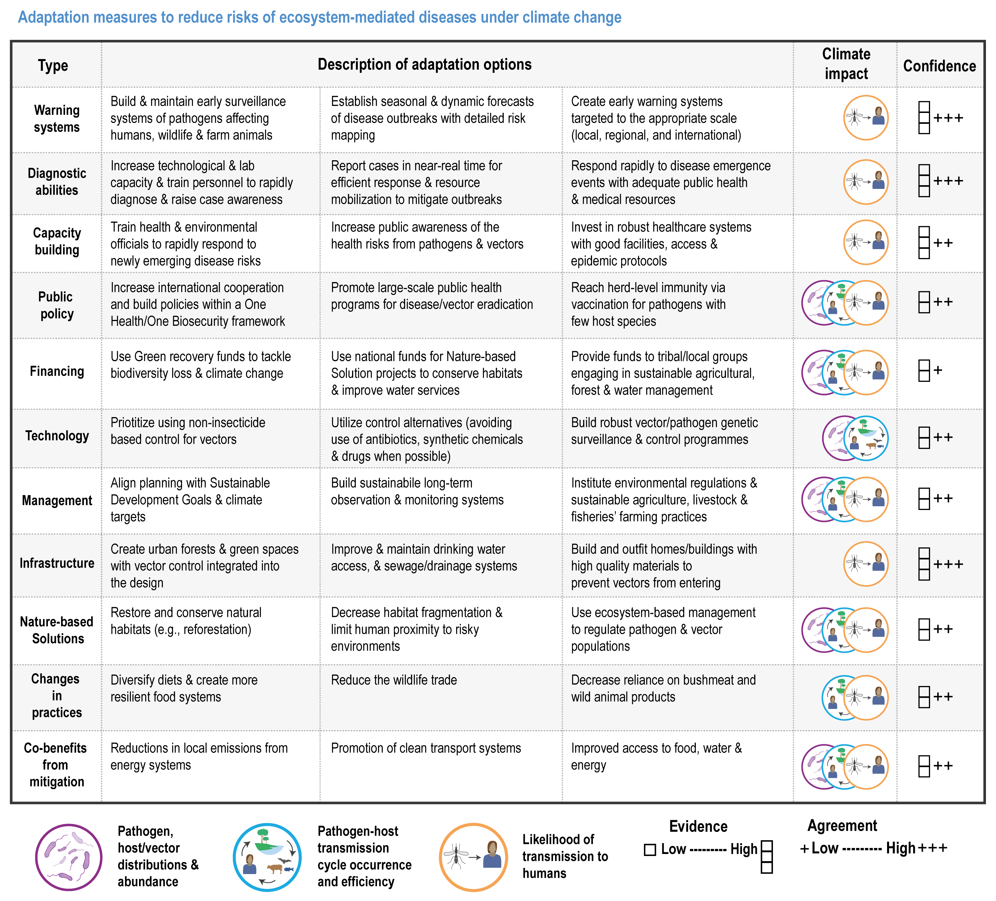
Figure Cross-Chapter Box ILLNESS.1 | Adaptation measures to reduce risks of climate change impact on water- and vector-borne diseases. Impacts are identified at three levels: (1) on pathogen, host/vector distributions and abundance; (2) on pathogen-host transmission cycle occurrence and efficiency; and (3) on the likelihood of transmission to humans. Adaptation typology is based on (Biagini et al., 2014; Pecl et al., 2019). For each type of adaptation, examples are provided with their level of evidence and agreement.
Cross-Chapter Box ILLNESS
Cross-Chapter Box ILLNESS
Cross-Chapter Box ILLNESS
2.6.5 Adaptation in Practice: Case Studies and Lessons Learned
Adaptation plans for biodiversity and EbA have been adopted in many places and on different scales, but it is difficult to get a systematic overview of adaptation in practice. We have therefore reviewed a series of contrasting case studies to illustrate some of the key issues. There is a pressing need for more thorough monitoring and evaluation of adaptation to assess effectiveness. Climate change adaptation is conceptually difficult to measure, but it is possible to test which techniques work in reducing vulnerability and to monitor their deployment (Morecroft et al., 2019).
Adaptation can take place on a range of scales, with specific projects nested within overarching national strategies. Small-scale projects can be adaptation-focused, but on the larger scale, adaptation is often integrated with wider objectives. Within an urban or peri-urban context, the benefits of natural and semi-natural areas for health and well-being help to justify support for EbA. Economic well-being is also an important factor in many cases whether, as in Durban, South Africa (Section 2.6.5.7), it provides new job opportunities or, as in the Andes (Section 2.6.5.4), it supports long-established agricultural practices. Action on the ground often depends on factors on a range of scales, for example, a local plan, a national strategy and international funding. In Durban, partnerships between local communities, local authorities and the academic community were essential, together with an international context. Nevertheless, there are examples of communities using traditional or local knowledge (LK) to adapt to changing circumstances, with little or no external input, (Section 2.6.5.4); Their scope for adaptation is, however, often limited by factors beyond their direct control.
Specific interventions to protect species from climate change, such as the case of African penguins in South Africa (Section 2.6.5.5) and threatened plant species in the Tasmanian Wilderness World Heritage Area (Section 2.6.5.8), are rare. However, in countries where nature reserves are actively managed or where ecosystem restoration projects are progressing, local practitioners may use their knowledge to adapt to weather conditions and their associated effects (e.g., fire and water shortages). This is good practice, but it may not be sufficient to address the likely future changes in climate (Duffield et al., 2021). Training and resources to support conservation practitioners are becoming available. Examples include the Climate Change Adaptation Manual in England, UK (Section 2.6.5.2), and The Alliance for Freshwater Life (https://allianceforfreshwaterlife.org) which provides expertise for the sustainable management of freshwater biodiversity (Darwall et al., 2018).
Adaptation is widely recognised as important for national conservation policies and is being considered in a variety of countries (Section 2.6.5.2, 2.6.5.3). Adaptation in this strategic context includes decisions about the selection and objectives for protected areas, for example, identifying places which can act as refugia. It can also mean recognising where protected areas remain important but will support a changing range of species and ecosystems. This is important for directing resources effectively and ensuring that the management of the sites remains appropriate. There are, however, often major uncertainties, and the extent to which there will be a need for more radical measures will depend on the success of reducing GHG emissions globally. A global rise of 1.5°C–2°C would require relatively incremental adjustments to conservation management in many parts of the world, but a 3°C–4°C rise would require radical, transformational changes to preserve many species and maintain ecosystem services (Morecroft et al., 2012).
Whilst adaptation strategies for conservation are relatively common, at least on an outline level, their implementation is slow in most places. This may partly reflect a lack of resources for conservation in many parts of the world; however, another barrier is that people often value protected sites in their present form. Actions which might jeopardise this are inevitably a last resort. Initiatives to engage wider communities in discussions are likely to be essential in gaining support for such changing approaches.
EbA and adaptation for biodiversity are intrinsically linked and the largest-scale interventions for adaptation in ecosystems have tended to bring together both elements. For example, adaptation to reduce the risk of flooding by habitat creation and using natural processes (Section 2.6.5.2, Cross-Chapter Box SLR in Chapter 3), such as re-naturalising straightened river systems or creating wetlands for water storage, offers the potential to meet multiple objectives and has increased the overall funding available for ecosystem restoration.
2.6.5.1 Case Study: Assisted Colonisation/Managed Relocation in Practice
Scale: Global
Issue: Helping species move in order to track shifting climate space
Managed relocation (assisted migration and colonisation) is the movement of species, populations or genotypes to places outside the areas of their historical distribution (Hoegh-Guldberg et al., 2008), and it may be an option where they are not able to disperse and colonise naturally. It requires careful consideration of scientific, ethical, economic and legal issues between the object of relocation and the receiving ecosystem (Hoegh-Guldberg et al., 2008; Richardson et al., 2009; Schwartz et al., 2012).
Individual cases show that assisted migration can be successful. Anich and Ward (2017) extended the geographic breeding range of a rare bird, Kirtland’s warbler, Setophaga kirtlandii, by 225 km by using song playbacks to attract migrating individuals. Wadgymar (2015) successfully transplanted an annual legume, Chamaecrista fasciculata, to sites beyond its current poleward range limit, while Liu (2012) found that all but one of 20 orchid species survived when transplanted to higher elevations than their current range limits. After introducing two British butterfly species to sites ∼65 and ∼35 km beyond their poleward range margins, Willis (2009) observed that both of these populations grew, expanded their ranges and survived for at least the 8 year span of the study.
Butterflies have been favoured subjects for assisted migration in response to regional climate warming, since they are easy to move and their range dynamics have been extensively studied. The Chequered Skipper, Carterocephalus palaemon, became locally extinct in England in the 1970s, in an area not close to either the species’ poleward or equatorial range limits. Nonetheless, Maes (2019) considers climate a crucial parameter for reintroduction, using SDMs for both choosing the source population in Belgium and introduction site.
The success of assisted migration for conservation purposes has been variable. Bellis et al. (2019) identified 56 successes and 33 failures among 107 translocations of insects undertaken explicitly for conservation purposes. They concluded that failure was most strongly associated with the low numbers of individuals being released. Another potential source of failure is local adaptation: there is good evidence that adaptive differences among potential source populations can be important. For example, the transplants of Chamaecrista fasciculata were more successful when sourced from the most poleward existing sites, while individuals from more equatorial habitats performed poorly even when artificially warmed (Wadgymar et al., 2015).
2.6.5.2 Case Study: Adaptation for Conservation and Natural Flood Management in England, UK
Scale: National
Issue: National approach to adaptation in the natural environment
Threats to biodiversity from climate change in England include range retractions of cold-adapted species and the effects of more frequent extreme weather events such as drought. These threats are exacerbated by land use and management, for example, fragmenting habitats, draining land and straightening rivers. There are also risks to people, which are exacerbated by environmental factors, including flooding and over-heating in urban areas. The National Adaptation Programme provides a broad policy framework for England and includes a chapter on the natural environment. There are also adaptation plans produced by public bodies such as Natural England and the UK Environment Agency, with a wide range of responsibilities including flood defence. The principles of adaptation to climate change are well established in the UK conservation community and resources are available. Natural England has published a Climate Change Adaptation Manual jointly with the Royal Society for the Protection of Birds (a major conservation NGO) (Natural England and RSPB, 2020) and a spatial mapping tool for vulnerability to climate change (Taylor et al., 2014).
Duffield et al. (2021) found that awareness of the need for adaptation was common amongst nature reserve managers and that they were implementing actions that might build resilience to climate change, such as restoring ecosystem processes and reducing habitat fragmentation. There was recognition that it will be necessary to change the management objectives of protected sites to adjust to changing circumstances, but little implementation of such changes. The main example of managing change was at the coast where the SLR is causing transitions from terrestrial and freshwater systems to coastal and marine ones.
A range of EbA approaches are starting to contribute to adaptation in England, but the best-developed is Natural Flood Management (NFM): restoring natural processes and natural habitats to reduce flood risk (Wingfield et al., 2019). Over the last decade, a series of NFM projects have been established in local areas. The Environment Agency collated the evidence base for NFM (Burgess-Gamble et al., 2021) and was able to draw on 65 case studies (Ngai et al., 2017) covering the management of rivers and floodplains, woodlands, runoff, and coasts and estuaries.
NFM includes a broad range of techniques, some of which deliver real benefits for biodiversity and allow natural ecological processes to become re-established. Others, such as creating ‘woody debris dams’—barriers artificially constructed from tree trunks and branches in watercourses to slow the flow of water— have fewer benefits, although they may be good for some species. Dadson et al. (2017) concluded that ‘the hazard associated with small floods in small catchments may be significantly reduced’ by NFM techniques. However, they noted that the most extreme flood events may overwhelm any risk management measures, and failed to find clear evidence of NFM reducing flood risk downstream in large catchments.
Challenges in deploying large-scale NFM remain, which partly reflects the length of time necessary to demonstrate the effectiveness of pilot studies and build confidence; building stakeholder support is important (Huq et al., 2017). There are now a number of examples of where collaborative initiatives between local communities, landowners and government agencies have been successful in establishing effective NFM schemes (Short et al., 2019).
2.6.5.3 Case Study: Protected Area Planning in Response to Climate Change in Thailand
Scale: National
Issue: Protected area network planning
Many countries in the Association of Southeast Asian Nations (ASEAN) are expanding protected area networks to meet the Aichi Target 11 of at least 17% of terrestrial area protected, and it is important to take the effects of climate change into account. Existing protected areas in Thailand cover approximately 21% of the land area and it is one of the few tropical countries that has achieved the Aichi Target 11. Most protected areas in Thailand were established on an ad hoc basis to protect remaining forest cover and, as a result, they do not represent diverse habitats and their associated species (Chutipong et al., 2014; Tantipisanuh, 2016) so they may not be resilient to the interacting impacts of future land use and climate change (Klorvuttimontara et al., 2011; Trisurat, 2018).
Recent research conducted in northern Thailand indicated that the existing protected areas (31% of the regional area) cannot secure the viability of many medium-sized and large mammals. The climate space of most species will shift substantially, bringing a risk of extinction. Results, based on a spatial distribution model and network flow, determined there was a need for expansion areas of 5,200 km 2 in size, or 3% of the region, to substantially minimise the high level of risk and increase the average coping capacity of the protection of suitable habitats from 82%—the current plan—to 90%. These results were adopted by Thailand’s Department of National Parks, Wildlife and Plant Conservation, and included in the National Wildlife Administration and Conservation Plan for 2021–2031.
2.6.5.4 Case Study: Effects of Climate Change on Tropical High Andean Social Ecological Systems
Scale: Regional
Issue: Complex ramifications of glacial retreat on vegetation, animals, herders and urban populations
Accelerated warming is shrinking tropical glaciers at rates unseen since the middle of the Little Ice Age (Rabatel et al., 2013; Zemp et al., 2015). Climate-driven upwards migration of species, associated with warming and glacier retreat, has modified species distribution and richness and community composition along the Andes altitudinal gradient (Seimon et al., 2017; Carilla et al., 2018; Zimmer et al., 2018; Moret et al., 2019). Climate-driven glacier retreat alters hydrological regimes, directly impacting Andean pastoralists (López-i-Gelats et al., 2016; Postigo, 2020; Thompson et al., 2021) and the provision of water to lowland regions (Vuille et al., 2018; Hock et al., 2019; Orlove et al., 2019; Rasul and Molden, 2019). The drying of wetlands has modified alpine plant communities, which are relevant for storing carbon, regulating water and providing food for local livestock; this has led to negative impacts on herders’ livelihoods (Dangles et al., 2017; Polk et al., 2017; Postigo, 2020) and affecting the wild vicuña and the domesticated alpaca and llama. The wool from Vicuña (Vicugna vicugna) and alpaca (V. pacos) is an important source of income for indigenous communities and the llama (Lama glama) is their main source of meat. Vicuña are adjusting their feeding behaviour and spatial distribution as vegetation migrates upwards (Reider and Schmidt, 2020), causing them to roam outside protected areas and become vulnerable to illegal poaching.
Andean herders have responded to the drying of grasslands by increasing livestock mobility, accessing new grazing areas through kinship and leases, creating and expanding wetlands through building long irrigation canals (several kilometres in length), limiting the allocation of wetlands to new households and sometimes cultivating grasses (Postigo, 2013; López-i-Gelats et al., 2015; Postigo, 2020). These adaptive responses to regional climate change are enabled by deeply embedded indigenous institutions that have traditionally governed Andean pastoralists, but they have become severely compromised by national socioeconomic pressures (Valdivia et al., 2010; Postigo, 2019; Postigo, 2020). For instance, the quality of water and local pastoralists’ access to it and control of it have declined, due to new mining concessions granted in the headwaters of Andean watersheds (Bebbington and Bury, 2009) and the diversion of water to areas of lowland coastal desert for agricultural irrigation (Mark et al., 2017).
Glacier mass and runoff in the Tropics are projected to diminish by >70% and >10%, respectively, by 2100, under mean of RCP2.6, 4.5 and 8.5 (Huss and Hock, 2018; Hock et al., 2019). In Peru, montane ice-field meltwater provides 80% of the water resources for the arid coast where half the population lives (Thompson et al., 2021). Increasing variability of precipitation has compromised rain-fed agriculture and power generation, particularly in the dry season, exacerbating pressures for new sources of water (Bradley et al., 2006; Bury et al., 2013; Buytaert et al., 2017). There is therefore a risk of increasing conflicts between adaptation to climate change to benefit human and natural communities in the high Andes and maintaining water provisioning for lowland agricultural and urban areas.
2.6.5.5 Case Study: Helping African Penguins Adapt to Climate Change
Scale: Regional/local
Issue: Adaptation for a threatened species
The African penguin, Spheniscus demersus, is the only resident penguin species on mainland Africa. It breeds in a handful of colonies in South Africa and Namibia. In 2017, the penguins of Cape Town’s Boulders Beach colony attracted almost one million visitors, providing 885 jobs and USD 18.9 M in revenue (Van Zyl and Kinghorn, 2018). Ninety-six percent of the population of this species has been lost since 1900, with a 77% decline in the last two decades (Sherley et al., 2018). By 2019, only 17,700 pairs remained (Sherley et al., 2020). The species is listed as endangered on the IUCN Red List (Birdlife International, 2018) and if this trajectory persists, the African penguin will become functionally extinct in the near future (Sherley et al., 2018).
Historically, hunting and the collection of eggs and guano were the main threats, but three aspects of climate change now predominate. Firstly, an eastward shift of several hundred kilometres in the distributions of their main prey species, anchovies and sardines, has reduced food availability (Roy et al., 2007; Crawford et al., 2011). While adult penguins typically forage up to 400 km from their colonies, they are restricted to a ~20-km radius from their colonies during breeding months (Ludynia et al., 2012; Pichegru et al., 2012). The resulting food shortage at this critical time is compounded by competition with commercial fisheries and environmental fluctuations (Crawford et al., 2011; Pichegru et al., 2012; Sherley et al., 2018). This has impacted adults’ survival and their ability to raise high-quality offspring (Crawford et al., 2006; Crawford et al., 2011; Sherley et al., 2013; Sherley et al., 2014).
The increasing frequency and intensity of heat waves recorded in recent decades presents a second threat (van Wilgen and Wannenburgh, 2016; Van Wilgen et al., 2016; Mbokodo et al., 2020). Nests were historically built in insulated guano burrows, but are now frequently sited on open ground (Kemper et al., 2007; Pichegru et al., 2012; Sherley et al., 2012). High temperatures frequently expose the birds to severe heat stress, causing adults to abandon their nests and resulting in the mortality of eggs and chicks (Frost et al., 1976; Shannon and Crawford, 1999; Pichegru et al., 2012). Intensifying storm surges and greater wave heights can cause nest flooding (Randall et al., 1986; de Villiers, 2002).
The African penguin’s survival in the wild is dependent on the success of adaptation action. Increasing access to food resources is a management priority (Birdlife International, 2018). One approach is to reduce fishing pressure immediately around breeding colonies. An experiment excluding fishing around colonies since 2008 has demonstrated positive effects (Pichegru et al., 2010; Pichegru et al., 2012; Sherley et al., 2015; Sherley et al., 2018; Campbell et al., 2019b). A second approach is to establish breeding colonies closer to their prey. An ongoing translocation initiative aims to entice birds eastwards, to recolonise an extinct breeding colony and potentially establish a new one (Schwitzer et al., 2013; Sherley et al., 2014; Birdlife International, 2018). Penguin ‘look-alikes’ or decoys, constructed from rubber and concrete, have been placed at the site of the extinct colony, and, along with call play-backs, these give the illusion of an established penguin colony (Morris and Hagen, 2018). This approach has not yet proven successful.
To promote on-site adaptation to heat extremes and flooding, initiatives are underway to provide cooler nesting sites that also provide storm protection and are sufficiently above the high-water level (Birdlife International, 2018; Saving Animals From Extinction, 2018). Artificial nest boxes of various designs and constructed from a range of materials have been explored, in combination with the use of natural vegetation. Some designs have proven successful, increasing breeding success (Kemper et al., 2007; Sherley et al., 2012), but the same designs have had less success at other locations (Pichegru, 2013; Lei et al., 2014).
Hand-rearing and releasing African penguin chicks, including from eggs, has long proven valuable because moulting parents, being shore-bound, are unable to feed late-hatching chicks. Since 2006, over 7,000 orphaned chicks have been released into the wild as part of the Chick Bolstering Project, with a success rate of 77% (Schwitzer et al., 2013; Sherley et al., 2014; Klusener et al., 2018; SANCCOB, 2018). A new project at Boulders Beach aims to use real-time weather station data, within-nest temperatures and known thresholds of penguin heat stress as triggers for implementing a Heat Wave Response Plan. Drawing on well-established chick-rearing facilities and a large body of expertise, this includes removing heat-stressed eggs and birds, hand-rearing and/or rehabilitation and release. It is hoped that such birds can be released at the proposed new colony site.
2.6.5.6 Case Study: Conserving Climate Change Refugia for the Joshua Tree in Joshua Tree National Park, CA, USA
Scale: Local
Issue: Possible extirpation of a plant species from a national park
Joshua Tree National Park conserves 3200 km 2 of the Mojave and Sonoran Desert ecosystems. The climate of the national park is arid, with an average summer temperature of 27.3°C ± 0.7°C and average annual precipitation of 170 ± 80 mm yr -1 in the period 1971–2000 (Gonzalez et al., 2018). From 1895 to 2017, the average annual temperature increased at a significant (P < 0.0001) rate of 1.5°C ± 0.1°C per century and the average annual precipitation decreased at a significant (P = 0.0174) rate of -32 ± 12% per century (Gonzalez et al., 2018). Anthropogenic climate change accounts for half the magnitude of a 2000–2020 drought in the southwestern USA, the most severe since the 1500s (Williams et al., 2020).
The national park was established to protect ecosystems and cultural features unique to the region, particularly the Joshua tree (Yucca brevifolia), a tall, tree-like yucca that provides habitat for birds and other small animals and holds cultural significance. The national park protects the southernmost populations of the Joshua tree. Palaeo-biological data from packrat (Neotoma spp.) middens and fossilised dung of the extinct Shasta ground sloth (Nothrotheriops shastensis) show that Joshua trees grew 13,000–22,000 years ago across a wider range, extending as far as 300 km south into what is now México (Holmgren et al., 2010; Cole et al., 2011). A major retraction of this range began ~11,700 years ago, coinciding with warming of approximately 4°C, caused by Milankovitch cycles, which marked the end of the Pleistocene and the beginning of the Holocene (Cole et al., 2011), suggesting a sensitivity of Joshua trees of 300 km of latitude per 4°C.
Under an emissions scenario that could increase park temperatures by >4°C by 2100, the suitable climate for the Joshua tree could shift northwards and the species become extirpated from the park (Sweet et al., 2019). Plant mortality would increase from drought stress and wildfires, which have been rare or absent in the Mojave, but which invasive grasses have fuelled and may continue to fuel (Brooks and Matchett, 2006; DeFalco et al., 2010; Abatzoglou and Kolden, 2011; Hegeman et al., 2014).
The national park had been trying to conserve the species wherever in the park it was found. The future risk of extirpation prompted adaptation of conservation efforts to focus on protecting potential refugia, where suitable conditions may persist for the species into the future (Barrows et al., 2020). The national park used spatial analyses of suitable climate to identify potential refugia under all emissions scenarios, except for the highest (Barrows and Murphy-Mariscal, 2012; Sweet et al., 2019). The park prioritises the refugia for removal of invasive grasses and fire control (Barrows et al., 2020) and works to restore refugia that have burned in fires, using native plants, including nursery-grown Joshua tree seedlings. The park and its partners are monitoring plant species composition and abundance in the refugia for early warnings of any changes (Barrows et al., 2014).
2.6.5.7 Case Study: Ecosystem Based Adaptation in Durban, South Africa
Scale: Local
Issue: EbA in a city and surrounding area
Durban was an early pioneer of EbA in a city context, establishing a Municipal Climate Protection Programme (MCPP) in 2004 (Roberts et al., 2012). The city, situated in a global biodiversity hotspot (World Bank, 2016), has a rapidly growing population (approximately 3.5 million) and is highly fragmented (Roberts et al., 2013). High levels of development, particularly in peri-urban areas, have encroached into natural habitats (World Bank, 2016). Degradation of the natural resource base in this way has direct economic and financial costs, is threatening Durban’s long-term sustainability and is exacerbated by climate change (World Bank, 2016; eThekwini Municipality, 2020). The impacts of climate change are anticipated to increase unless appropriate mitigation and adaptation interventions are prioritised (eThekwini Municipality, 2020). High rates of poverty, unemployment and health problems have pushed Durban to explore a climate change adaptation work stream within its MCPP (Roberts et al., 2013; Roberts et al., 2020b).
A single approach to adaptation is likely to be insufficient (Archer et al., 2014), and community-based adaptation should be integrated as part of a package of tools applied at the city level. Durban’s climate change adaptation work stream is composed of three separate components: municipal adaptation (adaptation activities linked to the key functions of local government), community-based adaptation (CbA, focused on improving the adaptive capacity of local communities), and a series of urban management interventions (addressing specific challenges such as the urban heat island, increased storm-water runoff, water conservation and SLR) (Roberts et al., 2013).
Lessons learnt from Durban’s experience include the importance of meaningful partnerships, long-term financial commitments (Douwes et al., 2015) and significant political and administrative will (Roberts et al., 2012; Roberts et al., 2020b). Securing these requires strong leadership (Douwes et al., 2015), including from local champions (Archer et al., 2014), even when EbA is considered cost-effective (Roberts et al., 2012). Projects for the restoration of natural habitats are seen as an ideal tool, as they combine mitigation outcomes with an increased adaptation capacity, not only reducing the vulnerability of ecosystems and communities (Douwes et al., 2016) but creating economic opportunities. These include direct job creation (Diederichs and Roberts, 2016; Douwes and Buthelezi, 2016) with various spin-offs such as better education for schoolchildren (Douwes et al., 2015). Indirect benefits, including better water quality and reduced flooding, are generated as a result of improved ecosystem service delivery (Douwes and Buthelezi, 2016). In areas that are already developed, opportunities for green-roof infrastructure can yield reductions in roof storm-water runoff (by approx.. 60 ml/m 2/min during a rainfall event), slow the release of water over time and reduce temperatures on roof surfaces (Roberts et al., 2012).
2.6.5.8 Case Study: Protecting Gondwanan Refugia against Fire in Tasmania, Australia
Scale: Local
Issue: Protection of rare endemic species
The Tasmanian Wilderness World Heritage Area (TWWHA) has a high concentration of ‘palaeo-endemic’ plant species which are restricted to living in cool, wet climates and fire-free environments, but recent wildfires have burnt substantial stands that are unlikely to recover (Harris et al., 2018b; Bowman et al., 2021a). The fires led to government inquiries and a fire-fighting review, which have suggested changes to management as climate change will make such fires more likely in the future (AFAC, 2016; Press, 2016; AFAC, 2019).
Most of the TWWHA is managed as a wilderness zone and is currently carried out in a manner that allows natural processes to predominate. The exclusion of fire from stands of fire-sensitive trees such as the pencil pine, Athrotaxis cupressoides, is part of this management strategy, possible in the past due to the moisture differential and lower flammability of these areas. However, in recent years, the threat posed by extensive and repeated wildfires and increasing awareness that fire risk is likely to increase (Fox-Hughes et al., 2014; Love et al., 2017; Love et al., 2019) have meant that more direct management intervention has been implemented. There has been a realisation that a ‘hands off’ approach to managing the threat will not be sufficient to protect the palaeo-endemics. Not only is fire-fighting difficult in this remote wilderness area, but limited resources mean that fire managers must prioritise where fires will be fought when many fires are threatening towns and lives across the state simultaneously.
After the wildfires in 2016 caused extensive damage (Bowman et al., 2021a), significant efforts and resources were spent trying to protect the remaining stands of pencil pine during the 2019 fires, using new approaches including the strategic application of long-term fire retardant and the installation of kilometres of sprinkler lines (AFAC, 2019). These approaches are thought to have been effective at halting the fire and protecting high-value vegetation in some situations. Impact reports are currently being finalised to quantify the extent of fire-sensitive vegetation communities that have been affected. However, there is concern that these interventions may have adverse effects on the values of the TWWHA if applied widely, so while research is ongoing, these will only be applied in strategic areas (e.g., fire retardant is not being applied to some areas).
The TWWHA Management Plan (2016) emphasises Aboriginal fire management as an important value of the area, along with Aboriginal knowledge of plants, animals, marine resources and minerals (ochre and rock sources), and the connection with the area as a living and dynamic landscape. Fire management planning aims to protect important sites from fire and ensure that management does not impact Aboriginal cultural values (DPIPWE, 2016). Increasingly, there is an acknowledgment that the cessation of traditional fire use has led to changes in vegetation and there are calls to incorporate Aboriginal burning knowledge into the fire management of the TWWHA.
2.6.5.9 Case Study: Bhojtal Lake, Bhopal, India
Scale: Local
Issue: Protection of water resources and biodiversity
The city of Bhopal, the capital of Madhya Pradesh state in central India, is dependent for its water supply on Bhojtal, a large man-made lake bordering the city (Everard et al., 2020). Bhojtal is also an important conservation site, with its wetlands protected under the Ramsar convention and diverse flora and fauna (WWF, 2006). It also provides a wide range of other benefits to people, including tourism, recreation, navigation and subsistence and commercial fisheries, supporting the livelihoods of many families (Verma, 2001).
Climate change in Bhopal may pose ecological and socioeconomic stresses due to changes in rainfall and weather patterns (Ministry of Environment et al., 2019), and exacerbated by a series of problems such as waste-water discharge, illegal digging of bore wells and unsustainable water extraction/exploitation (Everard et al., 2020). Ecosystem service provision at Bhojtal was assessed using the Rapid Assessment of Wetland Ecosystem Services (RAWES) approach, including an analysis of the lake’s water quality. Information on the geology, hydrology and catchment ecology of the lake was collected and a baseline biodiversity assessment was conducted.
The Lake Bhopal Conservation and Management Project (JICA, 2007) was developed with the following actions:
- Desilting and dredging; deepening and widening of spill channel; prevention of pollution (sewage scheme); management of shoreline and fringe area; improvement and management of water quality
- Soil and water conservation measures using vegetative and engineering structures, particularly at upper ridges of watersheds; construction of small check dams or percolation tanks for recharge purposes in areas marked for ‘drainage line recharge measures’
- Afforestation initiatives
Implementation of these measures with the help of local communities improved the lake’s health. NbS are more resilient adaptation measures towards climate change. Restoration not only reduced water stress but also provides multiple societal benefits in the urban area (Kabisch et al., 2016).
2.6.5.10 Case Study: Addressing the Vulnerability of Peat Swamp Forests in Southeast Asia
Scale: Regional
Issue: Protecting peatland biodiversity, carbon and ecosystem services from climate change and land degradation
Peatlands in SEA have undergone extensive logging, drainage and land use conversion that have caused habitat loss for endemic species, i.e., the orangutan (Pongo spp.) (Gregory et al., 2012; Struebig et al., 2015). Prolonged droughts associated with El Niño (Section 4.4.3.2) compound the effects of drainage, leading to large recurrent fires (Langner and Siegert, 2009; Gaveau et al., 2014; Putra et al., 2019). Under RCP8.5, it is projected that by the end of this century, the annual rainfall over SEA will decrease significantly (by 30%), and the number of consecutive dry days will increase significantly (by 60%) over Indonesia and Malaysia (Supari et al., 2020). Peat degradation and losses to fire result in high GHG emissions (Miettinen et al., 2016) as well as haze pollution which is a trans-boundary problem in the region (Heil et al., 2007).
Improving the resilience of SEA peatlands to fire and climate change through restoration is extremely difficult and presents many challenges. The Indonesian government has tasked the Badan Restorasi Gambut (Peatland Restoration Agency) to restore peatlands (Darusman et al., 2021; Giesen, 2021). Other local initiatives exist, such as fire management programmes and restoration projects (Puspitaloka et al., 2020). Since 2016, the government of Indonesia has re-wetted ~380,000 hectares of degraded peatlands, mainly by blocking canals and flooding, but less than 2000 hectares have been successfully restored to sustaining native plant species common to peat swamp forests (Giesen, 2021). Replanting native trees has had relatively little success (Lampela et al., 2017) because such trees have low tolerance to prolonged inundation and no fire adaptation strategies (Page et al., 2009; Roucoux et al., 2013; Dohong et al., 2018; Cole et al., 2019; Luom, 2020; Giesen, 2021).
The barriers to successful management are complex, and include the disparity in time frames between ecological restoration and political/socioeconomic needs (Harrison et al., 2020) and an over-focus on fire-fighting rather than fire prevention (Mishra et al., 2021a). Early protection of peat forests has been highlighted as a more effective management strategy than restoration, not only on islands in SEA but also in areas like Papua New Guinea, which may be targeted for the expansion of estate crop plantations (Neuzil et al., 1997; Dennis, 1999; Anshari et al., 2001; Anshari et al., 2004; Hooijer et al., 2006; Heil et al., 2007; Page et al., 2009; Page et al., 2011; Posa et al., 2011; Miettinen et al., 2012; Wetlands International, 2012; Biagioni et al., 2015; Miettinen et al., 2016; Rieley and Page, 2016; Adila et al., 2017; Cole et al., 2019; Vetrita and Cochrane, 2019; Harrison et al., 2020; Hoyt et al., 2020; Ruwaimana et al., 2020; Ward et al., 2020; Cole et al., 2021).
2.6.6 Limits to Adaptation Actions by People
The evidence summarised above (Sections 2.6.2–2.6.4) shows that by restoring ecosystems it is possible to increase their resilience to climate change, including the resilience of the populations of species they support and of human communities. However, changes to healthy ecosystems and biodiversity are already happening as described in this chapter (robust evidence, high agreement ) and further changes are inevitable even in scenarios of low GHG emissions (robust evidence, high agreement ). Planning to manage the consequences of inevitable changes and prioritise investments in conservation actions where they have the best chance of succeeding (e.g., Section 2.6.5.6) will be an increasingly necessary component of adaptation (robust evidence, high agreement ) (Table 2.6).
It is possible to help species survive by active interventions such as translocation, but, as described above (Section 2.6.5.1), this is not straightforward, is not suitable for all species and is resource-intensive. Modifying local microclimate or hydrological conditions can work for some species (Sections 2.6.2, 2.6.5.5), but is likely to be less effective at higher levels of climate change. It will also be less successful for larger species and more mobile ones. The microclimate of a tree is much more closely coupled with wider atmospheric conditions than that of a small plant or animal in the boundary layer, and mobile species like birds and large mammals range over large areas rather than being confined to discrete locations where conditions can be manipulated.
There is potential for using evolutionary changes to enhance the adaptive capacity for target species, as is being done on the Great Barrier Reef where symbionts and corals that have survived recent intense heat-induced bleaching events are being translocated into areas that have had large die-off. However, known limitations to genetic adaptations preclude species-level adaptations to climates beyond their ecological and evolutionary history (Sections 2.2.4.6; 2.6.1). All of these interventionist approaches are constrained by requiring significant financial resources and expertise. They also require a high level of understanding of individual species autecology, which can take years to acquire, even when resources are available. Ex situ conservation (e.g., seed banks) may be the only option to conserve some species, especially as levels of warming increase, but this will not be feasible for all species.
While the science of restoration has generated many successes, some habitats are very difficult to restore, making certain decisions effectively irreversible. For example, Acacia nilotica was introduced into Indonesia in the 1850s for gum arabic, with planting expanded for fire breaks in the 1960s. This tree became invasive and has already replaced >50% of the savanna habitat in the Baluran National Park, with complete replacement expected in the near future. This shift from savanna to acacia forest is causing large declines in native species, including the charismatic wild banteng, Bos javanicus, and the wild dog (dhole, Cuon alpinus) (Caesariantika et al., 2011; Padmanaba et al., 2017; Zahra et al., 2020). Multiple approaches to controlling the spread of this acacia have been ineffective, highlighting the difficulty of reversing the decision to plant this tree (Zahra et al., 2020). Another example is the difficulties in restoring the tropical peat forests of SEA (Section 2.6.5.10).
EbA, when implemented well, can reduce risks to people but there are limits. For example, an extreme flood event may exceed the capacity of natural catchments to hold water or slow its flow (Dadson et al., 2017), and urban shade trees and green spaces can make a few degrees difference to temperatures experienced by people but this may not be enough in the hottest conditions.
In general, adaptation measures can substantially reduce the adverse impacts of 1°C–2°C of global temperature rise, but beyond this losses will increase (IPCC, 2018b), including species extinctions and changes like major biome shifts which cannot be reversed on human time scales. Some adaptation measures will also become less effective at higher temperatures. Whilst adaptation is essential to reduce risks, it cannot be regarded as a substitute for effective climate change mitigation (robust evidence, high agreement ).
2.6.7 Climate Resilient Development
CRD is the subject of Chapter 18. This section briefly assesses some of the fundamental issues for CRD relating to ecosystems. An overview of the importance of specific ecosystem services for CRD is presented in Box 18.7 in Chapter 18. A large body of evidence has demonstrated the extent to which human life, well-being and economies are dependent on healthy ecosystems and also the range of threats that these are faced with (high confidence) (IPBES, 2019; Dasgupta, 2021; Pörtner et al., 2021). An analysis of 64 studies found a strong positive synergy among eight critical regulating services of healthy ecosystems, including climate regulation, water provisioning, pest and disease control and adjacent-crop pollination (Lee and Lautenbach, 2016). The health of ecosystems is, in turn, reliant upon the maintenance of natural levels of species’ richness and functional diversity (high confidence) (Lavorel et al., 2020) (see Section 2.5.4). A meta-analysis of 74 studies documented that the mechanism for increased ecosystem stability is increased asynchrony among species, which itself is a product of greater species diversity (Xu et al., 2021b). Responding to these threats requires the protection and restoration of natural and semi-natural ecosystems, together with sustainable management of other areas.
The CBD set the Aichi 2020 Target at 17% of each country to be protected for biodiversity. Analyses suggest that 30% or even 50% of land and sea needs to be protected or restored to confer adequate protection for species and ecosystem services (high confidence) (Dinerstein et al., 2019; Woodley et al., 2019; Brooks et al., 2020; Hannah et al., 2020; Zhao et al., 2020; Sala et al., 2021). Hannah et al. (2020) estimated that limiting warming to 2°C and protecting 30% of high-biodiversity regions (in Africa, Asia and Latin America) reduced the risk of species’ extinctions by half (medium confidence). The placement of protected areas is as important as the total area (Pimm et al., 2018), and the quality of the protection (strictness and enforcement) is as important as the official land designation (Shah et al., 2021). Pimm et al. (2018) found that many small protected areas are successful because they are in areas of very high biodiversity containing species with small range sizes, while many large regions identified as wild are often of low biodiversity value even though they may have a high mitigation value (e.g., the high Arctic tundra). A global meta-analysis of 89 restoration projects found that biodiversity increased by 44% and ecosystem services by 25% after restoration but values remained lower than in intact reference systems (Rey Benayas et al., 2009).
There is also increasing evidence, reported in this chapter, that the loss and degradation of natural and semi-natural habitats exacerbates the impacts of climate change and climatic extreme events on biodiversity and ecosystem services (high confidence) (e.g., in (Ogden et al., 2013; Eigenbrod et al., 2015; Struebig et al., 2015; Stevens et al., 2016; Oliver et al., 2017; McAlpine et al., 2018; Taffarello et al., 2018; Lehikoinen et al., 2019; Birk et al., 2020; Chapman et al., 2020; Agol et al., 2021; Khaniya et al., 2021; Lara et al., 2021; Lehikoinen et al., 2021). Considering these two sets of evidence together, it is clear that climate change adaptation and ecosystem degradation both need to be addressed if either is to be tackled successfully (robust evidence, high agreement ) as a number of recent publications concluded (Haddad et al., 2015; Hannah et al., 2020; Arneth et al., 2021; Pörtner et al., 2021). Taking this combined body of evidence, the assessment is that the protection and restoration of natural and semi-natural ecosystems are key adaptation measures (robust evidence, high agreement ) (Section 2.5.4).
Large-scale protection and restoration of ecosystems can also make a significant contribution to climate change mitigation (Dinerstein et al., 2020; Roberts et al., 2020a; Soto-Navarro et al., 2020). Globally, there is a 38% overlap between areas of high carbon storage and high intact biodiversity (mainly in the peatland tropical forests of Asia, the western Amazon and the high Arctic), but only 12% of this is protected (high confidence) (see also sections 2.4.4.4.1, 2.4.4.4.3, 2.5.3.4) (Soto-Navarro et al., 2020). Peatlands are particularly important carbon stores but are threatened by human disturbance, LULCC (Leifeld et al., 2019) and fire (sections 2.4.3.8, 2.5.2.8) (Turetsky et al., 2015). Restoration of peatlands is not only an efficient climate solution in terms of emissions of GHGs (Nugent et al., 2019), it may also increase ecosystem resilience (Glenk et al., 2021). Global restoration efforts are ongoing to target degraded temperate peatlands in the Americas and Europe (Chimner et al., 2017) in recognition of their importance for climate change mitigation (Paustian et al., 2016; Bossio et al., 2020; Humpenöder et al., 2020; Drever et al., 2021; Tanneberger et al., 2021). It has been estimated that the global GHG-saving potential of peatland restoration is similar to the most optimistic sequestration potential from all agricultural soils (Leifeld and Menichetti, 2018). However, the pressure on peatlands from human activity remains high in many parts of the world (Humpenöder et al., 2020; Tanneberger et al., 2021). Currently, the rapid destruction of tropical peatlands overshadows any current restoration efforts in temperate peatlands or any potential carbon gain from natural high-latitude peatlands (Roucoux et al., 2017; Wijedasa et al., 2017; Leifeld et al., 2019) (Sections 2.4.3.8, 2.4.4.4.2, 2.4.4.4.4, 2.5.2.8, 2.5.3.4).
Recent studies have highlighted the importance of ensuring that ecosystem protection is not implemented in a way which disadvantages those who live in or depend on the most intact ecosystems (Mehrabi et al., 2018; Schleicher et al., 2019) or risk food security. The actual area of land to be protected and the balance between sustainable use and protection will need careful planning and targeting to where it can have the most benefit (Pimm et al., 2018). It will also be important to ensure that protection measures are effective in preventing damage (Shah et al., 2021).
At a local level, EbA can often provide a wide range of additional benefits for sustainable development in both rural and urban areas (Wilbanks, 2003; Nelson et al., 2007; Cohen-Shacham et al., 2016; Hobbie and Grimm, 2020; Martín et al., 2020). A number of the case studies above, such as in Durban and at Bhojtal Lake, illustrate this (section 2.6.5). A key element of CRD is ensuring that actions taken to mitigate climate change do not compromise adaptation, biodiversity and human needs. This depends on choosing appropriate actions for different locations (Box 2.2, Cross-Chapter Box NATURAL in this chapter). A particularly notable case of this is the creation of woodland described in Box 2.2: re-afforestation of previously forested areas can provide multiple benefits (Lee et al., 2018; Lee et al., 2020) including those for climate change mitigation, adaptation and biodiversity. However, planting trees where they would not naturally grow can create multiple problems including the loss of native biodiversity and the disruption of hydrology (Box 2.2). It is also the case that protection of existing natural forest ecosystems is the highest priority for reducing GHG emissions (Moomaw et al., 2019) and restoration may not always be practical (see Section 2.6.5.10). (Sections 2.4.3.6, 2.4.3.7, 2.4.4.3, 2.4.4.4, 2.5.2.6, 2.5.2.7, 2.5.3.3, Box 2.2, Cross-Chapter Box NATURAL in this chapter)
In some cases, actions supported by international donors and presented as addressing climate change adaptation and mitigation in the natural environment can have damaging consequences for people and nature as well as failing to deliver adaptation and mitigation. One example of this was presented by Work et al. (2019), who reviewed three climate change mitigation and adaptation projects in Cambodia: an irrigation project, a protected-area forest management project and a reforestation project. In each case, they found evidence of the rights of local communities being violated, maladaptation and the destruction of biodiverse habitats. They concluded that the potential for maladaptation and adverse social and environmental impacts had been ignored by international donors and the national authorities, and that there was a need for much stricter accountability mechanisms. Moyo et al. (2021), using case studies from South Africa, documented greater success of ecosystem restoration projects when they embraced broader SDGs, particularly enhancement of people’s livelihoods. Better assessment of the impacts of adaptation and mitigation measures on people and ecosystems, before they are implemented, will be increasingly necessary to avoid unintended and damaging consequences as their deployment is scaled up (Larsen, 2014; Enríquez-de-Salamanca et al., 2017; Pour et al., 2017). This applies to ostensibly nature-based approaches as well as more engineering-based ones.
Another aspect of the benefits to people from ecosystems that needs to be taken into account in CRD is increasingly strong evidence of the benefits of natural environments for human health and well-being beyond the provision of basic necessities such as food and water (Bratman et al., 2019; Marselle et al., 2021). Meta-analyses of 162 studies involving 51,738 people documented that individuals with high levels of contact with nature throughout their lives felt significantly happier, healthier and more satisfied with their lives, and engaged in more pro-nature behaviours than those with little or no contact with nature (high confidence) (Capaldi et al., 2014; Mackay and Schmitt, 2019; Pritchard et al., 2020; Whitburn et al., 2020). Meta-analyses of manipulative human trials across 65 studies documented a significant increase in positive feelings and attitudes and a decline in negative feelings after experimental treatments involving nature (medium confidence) (Bowler et al., 2010b; McMahan and Estes, 2015; Soga et al., 2017). In the context of CRD improving the extent to which humans see themselves as part of the natural world— known as human-nature connectedness (HNC)— increasing access to natural areas, particularly within urban areas, can provide additional health, cultural and recreation benefits of NbS as well as increasing public engagement and support (robust evidence, high agreement ) (Wilbanks, 2003; Nelson et al., 2007; Bowler et al., 2010b; Capaldi et al., 2014; McMahan and Estes, 2015; Cohen-Shacham et al., 2016; Soga et al., 2017; Mackay and Schmitt, 2019; Work et al., 2019; Hobbie and Grimm, 2020; Pritchard et al., 2020; Whitburn et al., 2020).
Cross-Chapter Box NATURAL | Nature-Based Solutions for Climate Change Mitigation and Adaptation
Authors: Camille Parmesan (France/USA/UK, Chapter 2), Gusti Anshari (Indonesia, Chapter 2, CCP7), Polly Buotte (USA, Chapter 4), Donovan Campbell (Jamaica, Chapter 15), Edwin Castellanos (Guatemala, Chapter 12), Annette Cowie (Australia, WGIII Chapter 12), Marta Rivera Ferre (Spain, Chapter 8), Patrick Gonzalez (USA, Chapter 2, CCP3), Elena López Gunn (Spain, Chapter 4), Rebecca Harris (Australia, Chapter 2, CCP3), Jeff Hicke (USA, Chapter 14), Rachel Bezner Kerr (USA/Canada, Chapter 5), Rodel Lasco (Philippines, Chapter 5), Robert Lempert (USA, Chapter 1), Brendan Mackey (Australia, Chapter 11), Paulina Martinetto (Argentina, Chapter 3), Robert Matthews (UK, WGIII, Chapter 3), Timon McPhearson (USA, Chapter 6), Mike Morecroft (UK, Chapter 2, CCP5), Aditi Mukherji (India, Chapter 4), Gert-Jan Nabuurs (the Netherlands, WGIII Chapter 7), Henry Neufeldt (Denmark/Germany, Chapter 5), Roque Pedace (Argentina, WGIII Chapter 3), Julio Postigo (USA/Peru, Chapter 12), Jeff Price (UK, Chapter 2, CCP1), Juan Pulhin (Philippines, Chapter 10), Joeri Rogelj (UK/Belgium, WGI Chapter 5), Daniela Schmidt (UK/Germany, Chapter 13), Dave Schoeman (Australia, Chapter 3), Pramod Kumar Singh (India, Chapter 18), Pete Smith (UK, WGIII Chapter 12), Nicola Stevens (South Africa, Chapter 2, CCP3), Stavana E. Strutz (USA, Chapter 2), Raman Sukumar (India, Chapter 1), Gautam Hirak Talukdar (India, Chapter 2, CCP1), Maria Cristina Tirado (USA/Spain, Chapter 7), Christopher Trisos (South Africa, Chapter 9)
Nature-based solutions provide adaptation and mitigation benefits for climate change as well as contributing to other sustainable development goals (high confidence). Effective nature-based climate change mitigation stems from inclusive decision-making and adaptive management pathways that deliver climate-resilient systems serving multiple sustainable development goals. Robust decision-making adjusts management pathways as systems are impacted by ongoing climate change. Poorly conceived and poorly designed nature-based mitigation efforts have the potential for multiple negative impacts, including competing for land and water with other sectors, reducing human well-being and failing to provide mitigation that is sustainable in the long term (high confidence).
The concept of Nature-based Solutions (NbS) is broad and under debate, but has become prominent in both the scientific literature and policy since AR5, and includes earlier concepts like EbA. The key point is that these are actions benefitting both people and biodiversity (IUCN, 2020) (WGII Glossary). In the context of climate change, NbS provide adaptation and mitigation benefits in ways that support wild species and habitats, often contributing to other sustainable development goals (robust evidence, high agreement ) (Griscom et al., 2017; Keesstra et al., 2018; Hoegh-Guldberg et al., 2019; IPCC, 2019a; Lewis et al., 2019; Lavorel et al., 2020; Malhi et al., 2020; Seddon et al., 2020b) (AR6 WGIII Chapter 12; Sections 2.2, 2.5.4, 2.6.3, 2.6.5, 2.6.7). Well-designed and implemented NbS mitigation schemes can increase carbon uptake or reduce GHG emissions at the same time as protecting or restoring biodiversity and incorporating elements of food provisioning (Mehrabi et al., 2018). A variety of measures can be part of NbS, ranging from the protection of natural terrestrial, freshwater and marine ecosystems to the restoration of degraded ones (this Cross-Chapter Box; Section 13.3) and more sustainable management of naturally regenerating ecosystems used for food, fibre and energy production (Figure Cross-Chapter Box NATURAL.1, Chapter 5 in this report, Cross-Working Group Box BIOECONOMY in Chapter 5). Agro-ecological practices mitigate and adapt to climate change and can promote native biodiversity (high confidence) (Sinclair et al., 2019; Snapp et al., 2021).
The Role of Restoration in Nature-Based Solutions
Where natural ecosystems have been degraded or destroyed, re-establishing them and restoring natural processes can be a key action for adaptation and mitigation, and the science of restoration is well established (de los Santos et al., 2019; Duarte et al., 2020) (Section 13.4.1). Such restoration activities need to adapt to ongoing climate change risks for the landscape and oceans and the species composition of biological communities. Indeed, the impacts of climate change may overwhelm attempts at restoration/conservation of previous or existing ecosystems, particularly when the ecosystem is already near its tipping point, as is the case with tropical coral reefs (Bates et al., 2019; Bruno et al., 2019).
Land (e.g., forests) and oceans (e.g., fisheries) managed for products using sustainable practices (whether applied by individuals, states or Indigenous Peoples) can also be carbon- and biodiversity-rich, and thus considered effective NbS (Paneque-Gálvez et al., 2018; Soto-Navarro et al., 2020). Indigenous Peoples and private forest owners manage, use or occupy at least one-quarter of the global land area, over one-third of which overlaps with protected areas, thus combining both protection and production (Jepsen et al., 2015; Garnett et al., 2018; IPBES, 2019; Santopuoli et al., 2019).
The protection/restoration of natural systems including reducing non-climate stressors, and the sustainable management of semi-natural areas emerge as necessary actions for adaptation to minimise extinctions of species, the reaching of tipping points that cause regime shifts in natural system and the loss of whole ecosystems and their associated benefits for humans (Scheffer et al., 2001; Folke et al., 2005; Luther et al., 2020) (Chapters 2 and 3 in this report; AR6 WGIII Chapter 7). Such measures are critical for the conservation of biodiversity and the provision of ecosystem goods and services in the face of projected climate change (Duarte et al., 2020). Supporting local livelihoods and providing benefits to indigenous local communities and millions of private landowners, together with their active engagement in decision-making, are critical to ensuring support for NbS and their successful delivery (high confidence) (Chapter 5 in this report; Figure Cross-Chapter Box NATURAL.1)(Ceddia et al., 2015; Blackman et al., 2017; Nabuurs et al., 2017; Smith et al., 2019a; Smith et al., 2019b; Jones et al., 2020a; McElwee et al., 2020; Cao et al., 2021).
Cross-Chapter Box NATURAL
Forests
Intact natural forest ecosystems are major stores of carbon and support large numbers of species that cannot survive in degraded habitats (very high confidence). Extensive areas of natural forest ecosystems remain in tropical, boreal and (to a lesser extent) temperate biome regions, but in many regions they are managed (sustainably and unsustainably) or have been degraded or cleared. Deforestation and land degradation continue to be a source of global GHG emissions (very high confidence) (Friedlingstein et al., 2019). Protection of existing natural forests and sustainable management of semi-natural forests that continue to provide goods and services are highly effective NbS (Bauhus et al., 2009) (high confidence).
Natural forests and sustainably managed biodiverse forests play important roles in climate change mitigation and adaptation while providing many other ecosystem goods and services (very high confidence) (Bradshaw and Warkentin, 2015; Favero et al., 2020; Mackey et al., 2020). Contributions of natural forests to climate change mitigation are estimated at a median of 5–7 GtCO2 yr -1 (Roe et al., 2019). Forests influence the water cycle on a local, regional and global scale (Creed and van Noordwijk, 2018), reducing surface runoff, increasing infiltration to groundwater and improving water quality (Bruijnzeel, 2004; Zhou et al., 2015a; Ellison et al., 2017; Alvarez-Garreton et al., 2019). Recent evidence shows that downwind precipitation is also influenced by evapotranspiration from forests (Keys et al., 2016; Ellison et al., 2017). Protecting existing natural forests and sustainably managing production forests in a holistic manner can optimise the provision of the many functions forests fulfil for owners, conservation, mitigation and for society as a whole (Bauhus et al., 2009; Nabuurs et al., 2013).
Reforestation of previously forested land can help to protect and recover biodiversity and is one of the most practical and cost-effective ways of sequestering and storing carbon (high confidence) (Nabuurs et al., 2017; Hoegh-Guldberg et al., 2018; Paneque-Gálvez et al., 2018; Smith et al., 2018; Cook-Patton et al., 2020; Cowie et al., 2021; Drever et al., 2021). This can be achieved through planting or by allowing natural colonisation by tree and shrub species. The most effective method to deploy depends upon local circumstances (e.g., the presence of remnant forest cover) or socio-cultural and management objectives. Reforestation with climate-resilient native or geographically-near species restores biodiversity at the same time as sequestering large amounts of carbon (Lewis et al., 2019; Rozendaal et al., 2019). It can also restore hydrological processes, thereby improving water supply and quality (Ellison et al., 2017) and reducing the risk of soil erosion and floods (high confidence) (Locatelli et al., 2015).
Climate change may mean that, in any given location, different species will be able to survive and become dominant and restoring the former composition of forests may not be possible (Sections 2.4, 2.5). Severe disturbances such as insect/pathogen outbreaks, wildfires and droughts, which are an increasing risk, can cause widespread tree mortality resulting in sequestered forest carbon being returned to the atmosphere (Anderegg et al., 2020; Senf and Seidl, 2021), suggesting that we need to adapt (Sections 2.4, 2.5, 13.3 14.4.1, Box 14.1). Adaptation measures, such as increasing the diversity of forest stands through ecological restoration rather than monoculture plantations can help to reduce these risks (high confidence). When plantations are established without effective landscape planning and meaningful engagement including free prior and informed consent, they can present risks to biodiversity and the rights, well-being and livelihoods of indigenous and local communities as well as being less climate-resilient than natural forests (very high confidence) (Section 5.6) (Corbera et al., 2017; Mori et al., 2021).
Afforesting areas such as savannas and temperate peatlands, which would not naturally be forested, damages biodiversity and increases vulnerability to climate change (high confidence), so cannot be considered a nature-based solution and can even exacerbate GHG emissions (Sections 2.4.3.5, 2.5.2.5, Box 2.2 in this chapter). Remote sensing-based assessments of the suitability of land for planting trees can overestimate potential, due to their failure to adequately distinguish between degraded forest and naturally open areas (Bastin et al., 2019; Veldman et al., 2019; Bastin et al., 2020; Sullivan et al., 2020).
Cross-Chapter Box NATURAL
Peatlands
Peatlands are naturally high-carbon ecosystems, which have built up over millennia. Draining, cutting and burning peat lead to oxidation and the release of CO2 (very high confidence). Re-wetting by blocking drainage and preventing cutting and burning can reverse this process on temperate peatlands (medium confidence) but takes many years (Bonn et al., 2016). Trees are naturally found on many tropical peatlands and restoration can involve removing non-native species like the oil palm and re-establishing natural forest. However, peatland tropical forest is difficult to fully restore, and native pond-fish, vital as a local food, often do not return. Protecting intact peat forests, rather than attempting to restore cleared forest, is by far the more effective pathway, in terms of cost, CO2 mitigation and the protection of food sources (Kreft and Jetz, 2007). Naturally treeless temperate and boreal peatlands have, in some cases, been drained to enable trees to be planted, which then leads to CO2 emissions, and restoration requires the removal of trees as well as re-blocking drainage (high confidence) (Sections 2.4.3.8, 2.5.2.8, 2.6.5.10).
Blue Carbon
Blue carbon ecosystems (mangroves, saltmarshes and seagrass meadows; see Glossary Appendix II) often have high local rates of carbon accumulation and sequestration (Section 3.5.5.5) (Macreadie et al., 2019). However, quantification of their overall mitigation value is difficult due to the variable production of CH4 and N2O (Adams et al., 2012; Rosentreter et al., 2018; MacLean et al., 2019b), uncertainties regarding the provenance of the carbon accumulated (Macreadie et al., 2019) and the release of CO2 by biogenic carbonate formation in seagrass ecosystems (Saderne et al., 2019). Therefore, blue carbon strategies, referring to climate change mitigation and adaptation actions based on the conservation and restoration of blue carbon ecosystems, can be effective NbS, with evidence of the recovery of carbon stocks following restoration, although their global or regional carbon sequestration potential and net mitigation potential may be limited (medium confidence) (Sections 3.6.3.1.6, 13.4.3) (section 5.6.2.2.2 in (Canadell et al., 2021)) (Duarte et al., 2020).
They can also significantly attenuate wave energy, raise the seafloor (thereby counteracting the effects of SLR) and buffer storm surges and erosion from flooding (high confidence) (Sections 13.2.2, 13.10.2). Additionally, they provide a suite of cultural (e.g., tourism and the livelihoods and well-being of native and local communities), provision (e.g., mangrove wood, edible fish and shellfish) and regulation (e.g., nutrient cycling) services (high confidence) (Section 3.5.5.5). These services have motivated the implementation of management and conservation strategies of these ecosystems (Sections 3.6.3.1.6, 13.4.2). Blue carbon strategies are relatively new, with many of them experimental and small-scale; there is therefore only limited evidence of their long-term effectiveness. There is also limited information on the potential emission of other GHGs from restored blue carbon ecosystems, although reconnecting hydrological flow in mangroves and restoring saltmarshes are effective interventions to reduce CH4 and CO2 (limited evidence, medium agreement ) (Kroeger et al., 2017; Al-Haj and Fulweiler, 2020).
Urban Nature-Based Solutions
NbS can be a key part of urban climate adaptation efforts. Direct human adaptation benefits may stem from the cooling effects of urban forests and green spaces (parks and green roofs), from coastal wetlands and mangroves reducing storm surges and flooding and from sustainable drainage systems designed to reduce surface flooding as a result of extreme rainfall as well as the general benefits to human health and well-being (high confidence) (Sections 2.2, 2.6, Chapter 6) (Kowarik, 2011; Frantzeskaki et al., 2019; Keeler et al., 2019). Not all green schemes are considered ‘Nature-Based Solutions’ if they do not benefit biodiversity, but carefully designed urban greening can be effective NbS. Careful planning also helps limit negative equity consequences such as benefitting wealthy neighbourhoods more than poor neighbourhoods (Geneletti et al., 2016; Pasimeni et al., 2019; Grafakos et al., 2020). Effective planning should also consider what is appropriate for the climate and conditions of each city. For example, some trees emit volatiles (e.g., isoprene) which, in the presence of certain atmospheric pollutants, can increase surface ozone which can, in turn, cause human respiratory problems (Kreft and Jetz, 2007). Wetland restoration close to human settlements needs to be paired with mosquito control to prevent negative impacts on human health and well-being (Stewart-Sinclair et al., 2020), but it has been shown to provide better filtration and toxicity reduction with a lower environmental impact than other forms of waste-water treatment (Vymazal et al., 2021), including ‘green roofs’ and ‘green walls’ (Chapter 6 in this report) (Addo-Bankas et al., 2021).
Cross-Chapter Box NATURAL
Agro-Ecological Farming
AF is a holistic approach that incorporates ecological and socioeconomic principles, many of which have been shown to have a positive impact on biodiversity and on the resilience of human and natural systems to climate change (chapter 5, this report). It strives to enhance biodiversity, soil health and synergies between agro-ecosystem components, reduces reliance on synthetic inputs (e.g., pesticides), builds on IKLK and fosters social equity (e.g., supporting fair, local markets) (HLPE, 2019; Wezel et al., 2020). AF practices include inter-cropping; the mobility of livestock grazing across landscapes; organic agriculture; and the integration of livestock, fish and cropping, cover crops and agro-forestry (Sections 5.14, FAQ 12.5, FAQ 13.5).
Agro-forestry, cover crops and other practices that increase vegetation cover and enhance soil organic matter, carefully managed and varying by agro-ecosystem, mitigate climate change (high confidence) (Zomer et al., 2016; Aryal et al., 2019; Nadège et al., 2019). Global meta-analyses demonstrate agro-forestry as storing 20–33% more soil carbon than conventional agriculture (De Stefano and Jacobson, 2018; Shi et al., 2018) and reducing the spread of fire (Sections 5.6, 13.5.2, 7.4.3, Box 7.7). Minimising synthetic inputs such as nitrogen-based fertilizers reduces emissions (Gerber et al., 2016). Cover crops can reduce N2O emissions and increase soil organic carbon (Abdalla et al., 2019). Conservation farming (no-till with residue retention and crop rotation) increases soil organic carbon, particularly in arid regions (Sun et al., 2020). Silvo-pastoral systems (pastures with trees) and other practices that increase vegetation cover and enhance soil organic matter increase sequestered carbon in vegetation and soils (Zomer et al., 2016; Aryal et al., 2019; Nadège et al., 2019; Ryan, 2019). Agro-ecologically improved management of land for crops and grazing has significant mitigation potential, estimated at 2.8–4.1 GtCO2-eq yr -1 (Smith et al., 2020) (Sections 5.10, 5.14, Box 5.10, Cross Working-Group Box BIOECONOMY in Chapter 5; WGIII 7.4.3, Box 7.7).
AF enhances adaptation to climate change, including resilience to extreme events. Building organic matter improves the water-holding capacity of soils and buffers against drought; increased perenniality and high levels of ground cover reduce soil erosion during storms; agro-forestry shelters livestock and crops during heat waves; landscape complexity and agro-biodiversity increase resilience to disease and pests and stabilise livestock production; and restoration of oyster reefs provides thermal refugia and storm surge protection (Henry et al., 2018; Kremen and Merenlender, 2018; Kuyah et al., 2019; Gilby et al., 2020; Niether et al., 2020; Richard et al., 2020; Howie and Bishop, 2021; Snapp et al., 2021). Livestock mobility enables adjustment to increased climatic variability while maintaining the productivity of pastoral systems (Turner and Schlecht, 2019; Scoones, 2020). The adoption of agro-ecology principles and practices will therefore be highly beneficial to maintaining healthy, productive food systems under climate change (high confidence) (Sections 5.4.4, 13.5.2, FAQ 12.4).
AF practices such as hedgerows and poly-cultures maintain habitat and connectivity for biodiversity, thus aiding the ability of wild species to respond to climate change via range shifts, and support ecosystem functioning under climate stress compared to conventional agriculture (high confidence) (Section 5.4.4.4) (Buechley et al., 2015; Kremen and Merenlender, 2018; Albrecht et al., 2020). Increasing farm biodiversity benefits pollination, pest control, nutrient cycling, water regulation and soil fertility (Beillouin et al., 2019; Tamburini et al., 2020; Snapp et al., 2021). Biodiverse agro-forestry systems increase ecosystem services and biodiversity benefits compared to simple agro-forestry and conventional agriculture (high confidence), with up to 45% more biodiversity and 65% more ecosystem services compared to conventional production of timber and crops and profits from livestock in the Atlantic Forest in Brazil (Santos et al., 2019), including benefits for birds and local tree species (Braga et al., 2019) and meaning there are fewer invasive exotic plants species (de Almeida Campos Cordeiro et al., 2018). AF includes the conservation of semi-natural woodlands, which can conserve bird predators of insect pests (Gonthier et al., 2019). The richness and abundance of insect species, including essential pollinators, are increased by organic farming (Sections 5.10, 12.6) (Kennedy et al., 2013; Haggar et al., 2015; Lichtenberg et al., 2017).
AF significantly improves food security and nutrition by increasing access to healthy, diverse diets and raising incomes for food producers, due to the increased biodiversity of crops, animals and landscapes (high confidence) (Garibaldi et al., 2016; D’Annolfo et al., 2017; Isbell et al., 2017; Dainese et al., 2019; Kerr et al., 2021). Livestock mobility improves the site-specific matching of animals’ needs with food availability (Damonte et al., 2019; Mijiddorj et al., 2020; Postigo, 2021), and can generate a form of re-wilding that restores lost ecosystem functioning (Gordon et al., 2021). Conservation of crop wild relatives in situ supports the genetic diversity of crops for a range of future climate scenarios (Redden et al., 2015).
System-level agro-ecological transitions require policy support for experimentation and exchange of knowledge by farmers, community-based participatory methodologies and market and policy measures, for example, public procurement, local and regional market support, regulation or payments for environmental services (Mier y Terán Giménez Cacho et al., 2018; HLPE, 2019; Snapp et al., 2021). Scientific consensus about the food security and environmental implications of agro-ecological transitions on a global scale is lacking. Yields of agro-forestry and organic farming can be lower than high-input agricultural systems but, conversely, AF can boost productivity and profit, varying according to the time frame and the socioeconomic, political or ecosystem context (medium confidence) (Section 5.1 4) (Muller et al., 2017; Barbieri et al., 2019; Smith et al., 2019b; Smith et al., 2020). Such contrasting results and the limited investment in agro-ecological research to date mean it is paramount to assess the global and regional impacts of agro-ecological transitions on food production, ecosystems and economies in the context of climate change adaptation (Section 5.1 4) (DeLonge et al., 2016; Muller et al., 2017; Barbieri et al., 2019).
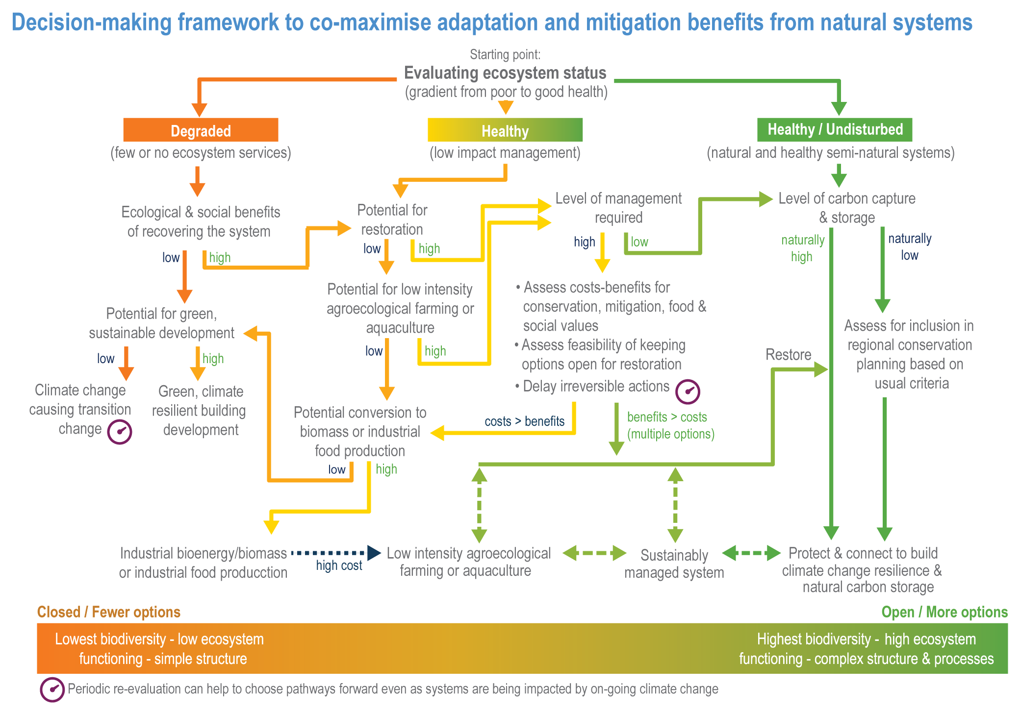
Figure Cross-Chapter Box NATURAL.1 | Decision-making framework to co-maximise adaptation and mitigation benefits from natural systems. Decision-making pathways are designed to add robustness in the face of uncertainties in future climate change and its impacts. Emphasis is on keeping open as many options as possible, for as long as possible, with periodic re-evaluation to aid in choosing pathways forward, even as systems are being impacted by ongoing climate change.
Cross-Chapter Box NATURAL
Conclusions
NbS provide adaptation and mitigation benefits for climate change as well as contributing to achieving other sustainable development goals (high confidence). NbS avoid further emissions and promote CO2 removal, by using approaches that yield long-lasting mitigation benefits and avoid negative outcomes for other sustainable development goals. Poorly conceived and poorly designed mitigation efforts have the potential for multiple negative impacts: (1) cascading negative effects on long-term mitigation by promoting short-term sequestration over existing long-term accumulated carbon stocks; (2) being detrimental for biodiversity, undermining conservation adaptation; and (3) eroding other ecosystem services important for human health and well-being (high confidence). Conversely, well-designed and implemented mitigation efforts have the potential to provide co-benefits in terms of climate change adaptation as well as providing multiple goods and services, including the conservation of biodiversity, clean and abundant water resources, flood mitigation, sustainable livelihoods, food and fibre security and human health and well-being (high confidence). A key aspect of such ‘smart’ climate mitigation is the implementation of inclusive and adaptive management pathways (Section 1.4.2). These entail acceptance of the uncertainty inherent in projections of future climate change, especially at the regional or local level, and using decision-making processes that keep open as many options as possible for as long as possible, with periodic re-evaluation to aid in choosing pathways forward, even as systems are being impacted by ongoing climate change (Figure Cross-Chapter Box NATURAL.1; Cross-Chapter Box DEEP in Chapter 17; Section 1.4.2).
Cross-Chapter Box NATURAL
Table Cross-Chapter Box NATURAL.1 | Assessment of benefits and trade-offs between mitigation and strategies for both biodiversity and human adaptation to future climate change. Best practices highlight approaches that lead to maximal positive synergy between mitigation and adaptation; worst practices are those most likely to lead to negative trade-offs for adaptation. Many best practices have additional societal benefits beyond adaptation, such as food provisioning, recreation and improved water quality. Mitigation Potential (Mit. Pot.) and Restoration Potential (Rest. Pot.) are considered.
System | Mit. Pot. | Rest. Pot. | Best practices and adaptation benefits | Worst practices and negative adaptation trade-offs | Additional societal benefits | References |
Forests | ||||||
Boreal forests | medium | medium | Maintain or restore species and structural diversity, reduce fire risk, spatially separate wood production and sustainably intensify management in some regions | Very large-scale clear cuts, aiming for one or few tree species, although boreal is characterised by few tree species and a natural fire risk | Providing goods and services, jobs and improved air quality and hydrology | |
Temperate forests | very high | high | Maintain or restore natural species and structural diversity, leading to more biodiverse and resilient systems | Planting large-scale non-native monocultures which would lead to loss of biodiversity and poor climate change resilience | Providing goods and services, jobs and improved hydrology and biodiversity | Sections 2.4.3; 2.5; Box 2.2 ; (Nabuurs et al., 2017; Roe et al., 2019; Favero et al., 2020) |
Tropical wet forests | high | moderate | Maintain or restore natural species and structural diversity, high biodiversity, more resilient to climate change | Planting non-native monocultures, loss of biodiversity, poor climate change resilience, soil erosion | Indigenous foods, medicines and other forest products, including sustainable selective logging | |
Tropical dry forests | high | moderate | Integrated landscape management | Planting non-native monocultures, loss of biodiversity, poor climate change resilience, soil erosion | ||
Tropical peatland forests | very high | low | Integrated landscape management | Cutting native rainforest and planting palm oil for biodiesel results in very high carbon emissions from exposed peat soils | Forest pond fish are a major food for local communities | Section 2.4.3; 2.5; (Smith et al., 2019b) |
Blue carbon | AR6 WGI 5.6.2.2.2 | |||||
Mangroves | moderate | high | Conservation, restoration of hydrological flows, re-vegetation with native plants, livelihood diversification, landscape planning for landward and upstream migration | Potential NH4 emissions | Improved fisheries and biodiversity, coastal protection against SLR and storm surges, recreation and cultural benefits | Sections 3.4.2.5; 3.5.5.5; 3.6.3.1; (Macreadie et al., 2019; Duarte et al., 2020; Sasmito et al., 2020) |
Saltmarshes | moderate | high | Conservation, reduction of nutrient loads, restoration of hydrological flows and sediment delivery, re-vegetation with native plants, landscape planning for landward and upstream migration | Potential NH4 emissions | Improved fisheries and biodiversity, protection against SLR and storm surges, recreational and cultural benefits | Sections 3.4.2.5; 3.5.5.5; 3.6.3.1; (Macreadie et al., 2019; Duarte et al., 2020) |
Seagrasses | moderate | high | Conservation, restoration, improve water quality and reduce local stressors (reduction of industrial sewage, anchoring and trawling regulation) | Potential NH4 emissions | Improved fisheries and biodiversity, protection from shoreline erosion, recreational benefits | Section 3.4.2.5; 3.5.5.5; 3.6.3.1; (de los Santos et al., 2019; Macreadie et al., 2019; Duarte et al., 2020) |
Urban ecosystems | ||||||
Urban forests | moderate to high* | moderate | Integrated landscape management. Species richness (including exotics) can be high. | Monoculture of an exotic tree lowers resilience and reduces biodiversity | Recreation and aesthetics, stormwater absorption benefits, heat mitigation, air quality improvements | Chapter 6, this report |
Urban wetlands | moderate* | moderate | Integrated landscape management | Recreation and aesthetics, stormwater absorption, heat mitigation, coastal flood protection | Chapter 6, this report | |
Urban grasslands | moderate* | moderate | Integrated landscape management | fertilised commercial grass monocultures often require irrigation and are less resilient to droughts than native, mixed grasses and forbs | Recreation and aesthetics, stormwater absorption, heat mitigation | Chapter 6, this report |
Open grasslands and savanna | ||||||
Boreal and temperate peatlands | high | moderate | Block drainage channels, raise water levels to their natural condition, remove planted trees, re-vegetation of bare peat, no fires, increased biodiversity resilience, reduced flood risk | Inappropriate hydrological restoration, e.g., flood surface depth greater than natural depth leading to methane emissions | Improved water quality in some conditions | Sections 2.4.3; 2.5;(Bonn et al., 2016; Nugent, 2019; Taillardat et al., 2020) |
Tropical savannas and grasslands (including rangelands) | moderate | high | Control of feral herbivores, reintroduce indigenous burning, reintroduce native herbivores and controlled grazing, strategic design of water holes, community-based natural resource management, grass reseeding, clearing of invasive and encroaching woody plants | Afforestation,over-grazing/stocking, no burning, inappropriate placement and design of watering points. All lead to loss of biodiversity and resilience, soil erosion and water insecurity. | Improved grazing potential for livestock and dairy production, sustainable wildlife harvests, increased water security, income from eco-tourism, medicinal plants, fuel wood, enhanced food security | Sections 2.4.3; 2.5; Box 2.1; (Stafford et al., 2017; Moura et al., 2019; Shackelford et al., 2021; Stringer et al., 2021; Wilsey, 2021) |
Temperate grasslands and rangelands | moderate to high | moderate to high | Integrated landscape management, sustainable grazing, community-based natural resource management, native grassland species are more resistant to drought than introduced species | Monocultures (especially of introduced species), over-fertilising with chemical or organic amendments, failure to manage human–wildlife clashes, failure to distribute income equitably, inadequate enabling policy to facilitate integrated landscape management | Sustainable harvest of wildlife, livestock and dairy production, wild fruits, medicinal plants, construction material, fuel wood, income from ecotourism | Sections 2.4.3; 2.5, Box 2.1; (Farai, 2017; Baker et al., 2018; Homewood et al., 2020; Wilsey, 2021) |
AF and aquaculture | high | high (context-specific) | Biodiverse systems on the landscape scale, participatory adaptation to context, short value chains, farmer incentives, biodiversity synergies, reduced climate risk | Poorly chosen species, practices and amendments can lead to low yields. Simplified agro-forestry systems and industrial-scale organic agriculture lack a holistic system-wide approach. Over-fertilising with organic amendments. | Food security, human health, livelihoods, socio-cultural benefits, e.g., culturally appropriate foods | Sections 5.4, 5.10, 5.12, 5.14 ; (Coulibaly et al., 2017; HLPE, 2019; Quandt et al., 2019; Sinclair et al., 2019; Smith et al., 2019b; Muchane et al., 2020; Reppin et al., 2020) |
Cross-Chapter Box NATURAL
FAQ 2.5 | How can we reduce the risks of climate change to people by protecting and managing nature better?
Damage to our natural environment can increase the risks that climate change poses to people. Protecting and restoring nature can be a way to adapt to climate change, with benefits for both humans and biodiversity. Examples include reducing flood risk by restoring catchments and coastal habitats, the cooling effects of natural vegetation and shade from trees and reducing the risk of extreme wildfires by better management of natural fires.
Protecting and restoring natural environments, such as forests and wetlands, can reduce the risks that climate change poses to people as well as supporting biodiversity, storing carbon and providing many other benefits for human health and well-being. Climate change is bringing an increasing number of threats to people, including flooding, droughts, wildfire, heat waves and rising sea levels. These threats can, however, be reduced or aggravated, depending on how land, sea and freshwater are managed or protected. There is now clear evidence that ‘Nature-based Solutions’ (NbS) can reduce the risks that climate change presents to people. ‘Ecosystem-based Adaptation’ (EbA) is a part of NbS and includes:
- Natural flood management: As warm air holds more water and, in some places, because of changing seasonal rainfall patterns, we are seeing more heavy downpours in many parts of the world. This can create serious flooding problems, with loss of life, homes and livelihoods. The risk of flooding is higher where natural vegetation has been removed, wetlands drained or channels straightened. In these circumstances, water flows quicker and the risk of flood defences being breached is increased. Restoring the natural hydrology of upstream catchments by restoring vegetation, creating wetlands and re-naturalising watercourse channels and reinstating connections with the floodplain can reduce this risk. In a natural catchment with trees or other vegetation, water flows slowly overland and much of it soaks into the soil. When the water reaches a watercourse, it moves slowly down the channel, both because of the longer distance it travels when the channel bends and because vegetation and fallen trees slow the flow. Wetlands, ponds and lakes can also hold water back and slowly release it into river systems.
- Restoring natural coastal defences: Rising sea levels as a result of climate change mean that coasts are eroding at a fast rate and storm surges are more likely to cause damaging coastal flooding. Natural coastal vegetation, such as saltmarshes and mangrove swamps can, in the right places, stabilise the shoreline and act as a buffer, absorbing the force of waves. On a natural coast, the shoreline will move inland and as the sea level rises, the coastal vegetation will gradually move inland with it. This contrasts with hard coastal defences such as sea walls and banks, which can be overwhelmed and fail. In many places, however, coastal habitats have been cleared and where there are hard sea defences behind the coastal zone, the vegetation disappears as the coast erodes rather than moving inland. This is often referred to as ‘coastal squeeze’ as the vegetation is squeezed between the sea and the sea wall. Restoring coastal habitats and removing hard sea defences, can help reduce the risks of catastrophic flooding.
- Providing local cooling: Climate change is bringing higher temperatures globally, which can result in heat waves that affect people’s health, comfort and agriculture. In cities, this can be a particular problem for health as temperatures are typically higher than in the countryside. Trees give shade, which people, in both rural and urban areas, have long used to provide cool places for themselves, for growing crops such as coffee and for livestock. Planting trees in the right place can be a valuable, low-cost natural-based solution to reduce the effects of increasing heat, including reducing water temperatures in streams and rivers which can help to maintain fisheries. Trees and other vegetation also have a cooling effect as a result of water being lost from their leaves through evaporation and transpiration (i.e., the loss of water through pores in the leaves, known as stomata). Natural areas, parks, gardens in urban areas can help reduce air temperatures by up to a few degrees.
- Restoring natural fire regimes: Some natural ecosystems are adapted to burning, such as savannas and some temperate and boreal forests. Where fire has been suppressed or non-native species of trees are planted in more open habitats, there is a risk that potential fuel accumulates, which can result in larger and hotter fires. Solutions can include restoring natural fire regimes and removing non-native species to decrease the vulnerability of people and ecosystems to the exacerbated fire risk that climate change is bringing due to higher temperatures and, in some places, changing rainfall patterns.
NbS, including protecting and restoring mangroves, forests and peatlands, also play an important part in reducing greenhouse gas emissions and taking carbon dioxide out of the atmosphere. They can also help people in a wide range of other ways, including through providing food, materials and opportunities for recreation. There is increasing evidence that spending time in natural surroundings is good for physical and mental health.
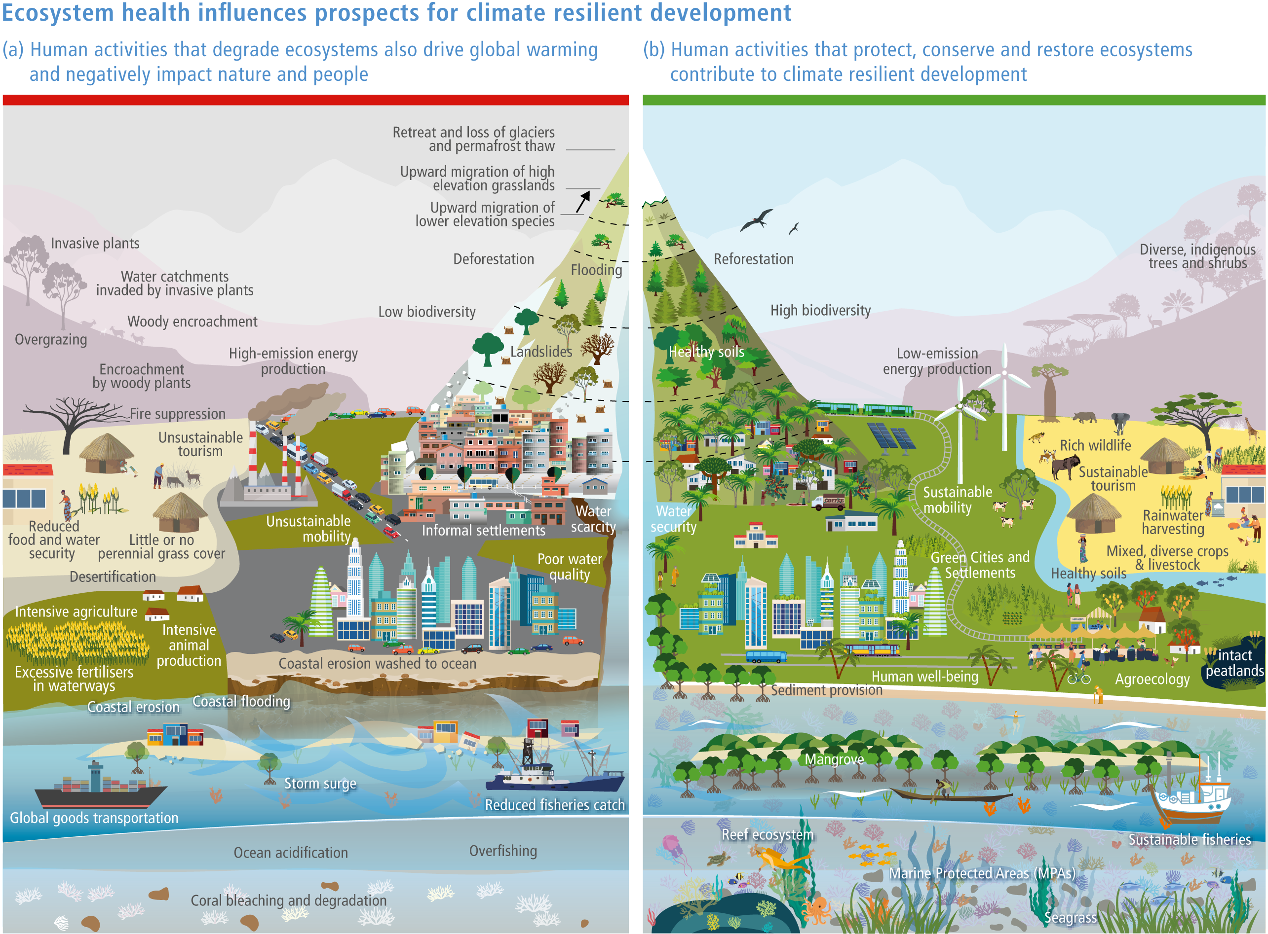
Figure FAQ2.5.1 | Different NbS strategies that contribute to climate resilient development
If NbS are to be effective, it is important that the right adaptation actions are carried out in the right place and that local communities play an active part in making decisions about their local environment. When they are not part of the process, conflicts can emerge and benefits can be lost.
While NbS help us to adapt to climate change and reduce the amount of greenhouse gases in the atmosphere, it is important to note that there are limits to what they can do. To provide a safe environment for both people and nature, it will be essential to radically reduce greenhouse gas emissions, especially those from fossil-fuel burning in the near future.
2.6.8 Feasibility of Adaptation Options
The IPCC (2018a) defined feasibility as ‘the degree to which climate goals and response options are considered possible and/or desirable’ (IPCC, 2018b) and set out an approach to assessing the feasibility of pathways to limit the global temperature rise to 1.5°C. Singh et al. (2020) developed this approach for adaptation, recognising six different dimensions of feasibility: economic, technological, institutional, socio-cultural, environmental/ecological and geophysical (Table 2.9). Feasibility is considered more fully in other chapters of this report, including Cross-Chapter Box FEASIB in Chapter 18. Adaptation for biodiversity conservation and EbA encompasses a large range of approaches and techniques (Sections 2.6.2, 2.6.3) and will vary in different contexts globally, as illustrated by the range of case studies (Section 2.6.5). It is important to take into account specific regional and local circumstances as well as the type of adaptation action envisaged before making a feasibility assessment. It is also important to note that what is a feasible adaptation response at one point in time may change with the level of warming experienced—some techniques will be become less effective at higher levels of warming. With global temperature rises of <2°C, in many cases, it will be realistic to build resilience and maintain species and ecosystems in situ, but, at higher levels of warming, this will become increasingly difficult; managing inevitable change, including the consequences of loss and damage, will be important (Prober et al., 2019). Similarly, to be effective at higher levels of warming may require the adaptation of the EbA approaches themselves (Calliari et al., 2019; Martín et al., 2021; Ossola and Lin, 2021). We have therefore not attempted a global-scale assessment of the feasibility of adaptation options, but rather present some key cross-cutting considerations in assessing feasibility for adaptation of and through ecosystems.
Many of the necessary techniques for climate change adaptation for biodiversity and EbA have been demonstrated and shown to provide a wide range of additional benefits. This does, however, depend on deploying the right techniques in the right place (Box 2.2) as well as engaging local communities (see Section 2.6.6). There is also a challenge where there is high demand for land for other purposes, especially for agriculture and urban development. Table 2.8 summarises the main feasibility considerations, drawing on previous sections. An assessment of constraints on EbA by Nalau et al. (2018) addressed similar issues.
Table 2.8 | Considerations in assessing the feasibility of ecosystem restoration for climate change adaptation, according to Singh et al. (2020)
Feasibilitycharacteristics | Feasibility indicators | Factors relevant to ecosystem restoration |
Economic | Micro-economic viability | Costs are highly variable, depending on techniques and whether land purchase is required. Costs will depend on local rates for labour and materials. Economic benefits to local communities where employment is created and where loss from extreme events are avoided (Section 2.6.4; De Groot et al., 2013). |
Macro-economic viability | ||
Socioeconomic vulnerability reduction potential | ||
Employment and productivity enhancement potential | ||
Technological | Technical resource availability | Techniques are available for restoration of most ecosystems (Sections 2.6.2; 2.6.3), although this can be very difficult to achieve in some circumstances and take a long time, e.g., the restoration of peat swamp forests (Section 2.6.5.10). Successful implementation may also require skills which are in short supply and training may be required. |
Risks mitigation potential (stranded assets, unforeseen impacts) | ||
Institutional | Political acceptability | This will vary according to local factors. It should, however, be noted that EbA and adaptation for conservation have been implemented in a wide range of different countries (see the case studies in Section 2.6.5). In many cases, the EbA can meet multiple policy objectives but falls between different decision-makers’ responsibilities. |
Legal, regulatory feasibility | ||
Institutional capacity and administrative feasibility | ||
Transparency and accountability potential | ||
Socio-cultural | Social co-benefits (health, education) | Multiple benefits to local communities are possible, but full engagement and/or leadership of the affected members of these communities has been shown to be critical. IKLK can provide important insights (Section 2.6.6). |
Socio-cultural acceptability | ||
Social and regional inclusiveness | ||
Benefits for gender equity | ||
Inter-generational equity | ||
Environmental/ecological | Ecological capacity | It is important to assess the benefits for ecosystems in relation to other potential options. In particular, for some EbA approaches, it may be possible to achieve a range of different outcomes for biodiversity. |
Adaptive capacity/potential | ||
Geophysical | Physical feasibility | Appropriate measures need to be designed to take account of local geophysical conditions, e.g., catchment characteristics, which define where some habitats can occur. This is also critical for ensuring the effectiveness of EbA in reducing natural hazards. |
LUC enhancement potential | ||
Hazard risk reduction potential |
A key element of economic feasibility is the cost of adaptation options. Costs of adaptation vary greatly depending on the actions taken, the location, the methods used, the need for ongoing maintenance and whether land purchase is necessary. At its simplest, adaptation may be a matter of taking account of actual or potential climate change impacts in the course of conservation planning and have little or no additional cost. For example, if a species of conservation concern colonises or starts to use a new area as a result of climate change, like migrant waterfowl shifting the locations where they overwinter (Pavón-Jordán et al., 2020), protection or habitat management may be redirected there. At the other extreme, large-scale restoration can incur significant costs, for example, between 1993 and 2015, the EU-LIFE nature programme invested 167.6 million Euro in 80 projects, which aim to restore over 913 km 2 of peatland habitats in Western European countries (Andersen et al., 2017). This is equivalent to <2% of the remaining peatland area, much of which has been affected to at least some extent by human pressures, and restoring the total affected area will cost considerably more.
De Groot et al. (2013) analysed 94 restoration projects globally and found costs varied by several orders of magnitude, but in terrestrial and freshwater ecosystems mostly in the range of USD 100–10,000 per hectare. They did, however, estimate that the majority of these projects provided net benefits and should be considered as high-yield investments. Some methods can be much cheaper than others, even in the same type of ecosystems in the same country; the estimated cost of restoring forest cover in Brazil varied between a mean of USD 49 using natural regeneration compared to a mean of USD 2041 per hectare using planting (Brancalion et al., 2019). When assessing costs, it is also important to take into account the benefits delivered by different options, both in economic terms and regarding other wider benefits.
The ‘technological’ dimension of feasibility in the context of ecosystems can be regarded as the range of techniques available and the capacity to implement them. As described in Sections 2.6.2 and 2.6.3 above, a wide range of techniques have been developed and are starting to be implemented. There is good evidence to support adaptation for biodiversity and EbA in general terms and, in many cases, adaptation draws on techniques for habitat creation and restoration which have been developed to meet other objectives. However, feasibility needs to be assessed alongside the likely effectiveness: a feasible but ineffective scheme is of no value and the evaluation of success for specific interventions remains poorly developed (Morecroft et al., 2019). It is therefore often important to proceed with the use of pilot studies, good monitoring and the evaluation of outcomes to build confidence before greater deployment of approaches. A linked technical area is the availability of specialist skills and knowledge to implement adaptation; this can vary considerably according to the type of adaptation measure.
Institutional dimensions are dealt with more fully in other chapters, but in the specific context of the natural environment it is notable that EbA is relevant to a wide range of organisations and policy objectives, in addition to environmental departments, NGOs and agencies which traditionally deliver conservation. Upscaling implementation is likely to be dependent on this wider range of interests. There can, however, be problems, in that appropriate geographies for decision-making about ecosystems (e.g., a catchment) may not directly map onto governance arrangements.
Socio-cultural factors are important for adaptation of the natural environment. Reviewing the constraints of EbA, Nalau et al. (2018) found that risk perceptions and cultural preferences for particular types of management approaches were frequently identified in studies.
In the IPCC feasibility assessment framework, one integral dimension is ‘environmental/ecological’. In this respect, adaptation by and for ecosystems should perform well, and this may be a reason to prefer EbA to other approaches when there is an alternative. It should, however, be noted that sometimes apparently environmentally positive approaches such as forest creation can be done in ways which are damaging (Section 2.6.7 and Box 2.2) and the impacts need to be critically assessed for local circumstances.
Geophysical dimensions are important for ecosystems as they have typically shaped which ecosystems can occur where, and feasibility will depend on implementing adaptation options in places where they are appropriate. Palaeo-ecological studies can help inform potential options (Wingard et al., 2017)
Box 2.2 | Risks of Maladaptive Mitigation
To hold global temperature rise to well below 2°C and pursue efforts to limit it to 1.5°C as required by the Paris Agreement requires major changes in land use and management. There are many opportunities for NbS, which can provide climate change mitigation and adaptation in ways that protect and restore biodiversity and provide a wide range of benefits to people (Cross-Chapter Box NATURAL in this chapter). There are also new technologies and approaches to develop the bioeconomy in ways which will provide many benefits (Cross-Working Group Box BIOECONOMY in Chapter 5). Nevertheless, renewable energy is a large and essential element of climate change mitigation and there are adverse impacts on biodiversity associated with some types of renewable energy, including wind and solar technologies (Rehbein et al., 2020). However, one of the most serious conflicts emerging is that between land-based approaches to mitigation and the protection of biodiversity, particularly as a result of afforestation strategies and potentially large areas devoted to bioenergy, including bioenergy with carbon capture and storage (BECCS). It is important to recognise the impacts of climate change mitigation at the same time as assessing the direct impacts of climate change, and ensure that adaptation and mitigation are joined up.
BECCS is an integral part of all widely accepted pathways to keeping global temperature rise to 1.5°C (IPCC, 2018b). This requires large areas of land, which can be in conflict with the need to produce food and protect biodiversity (Smith et al., 2018). One study examined the combined impacts of climate change and LULCC for bioenergy, and found that severe impacts on species were likely if bioenergy was a major component of strategies for climate change mitigation (Hof et al., 2018). A study on the potential impacts of bioenergy production and climate change on European birds found that one scenario for land conversion for bioenergy to meet a 2°C target would have less impact on species range loss than a global temperature increase of 4°C, but noted that if bioenergy were the only mitigation option it would 'very likely result in the negative effects of bioenergy outweighing the positive effects' (Meller et al., 2015). To avoid the worst impacts of BECCS, it will need to be carefully targeted according to context and local conditions, and other mitigation strategies prioritised so that its use can be minimised (IPCC, 2019a; Ohashi et al., 2019).
Reforestation of previously forested areas can bring multiple benefits, but planting trees in places where they do not naturally grow can have serious environmental impacts, including potentially exacerbating the effects of climate change. Savannas are amongst the ecosystems at risk from afforestation programmes. Savannas are grass-dominated, high-diversity ecosystems with endemic species adapted to high-light environments, herbivory and fire (Staver et al., 2011; Murphy et al., 2016). Interactions between climate change, elevated CO2 and the disruption of natural disturbance regimes have led to the widespread encroachment of woody plants (Stevens et al., 2016), causing a fundamental shift in ecosystem structure and function with loss of grass and reduced fire frequency (Archibald et al., 2009) and stream flow (Honda and Durigan, 2016) (Sections 2.4.3.5, 2.5.2.5, Box 2.1, 2.5.4, TAble 2.5, Figure 2.11). Afforestation exacerbates this degradation (Bremer and Farley, 2010; Veldman et al., 2015; Abreu et al., 2017). Global-scale analyses aimed at identifying degraded forest areas suitable for reforestation (Veldman et al., 2019) cannot reliably separate naturally grassy ecosystems with sparse tree cover from degraded forests, so local information is essential to ensure tree planting is targeted where it can benefit most and avoid harm. Figure Box 2.2.1 indicates where these issues are most likely to arise.
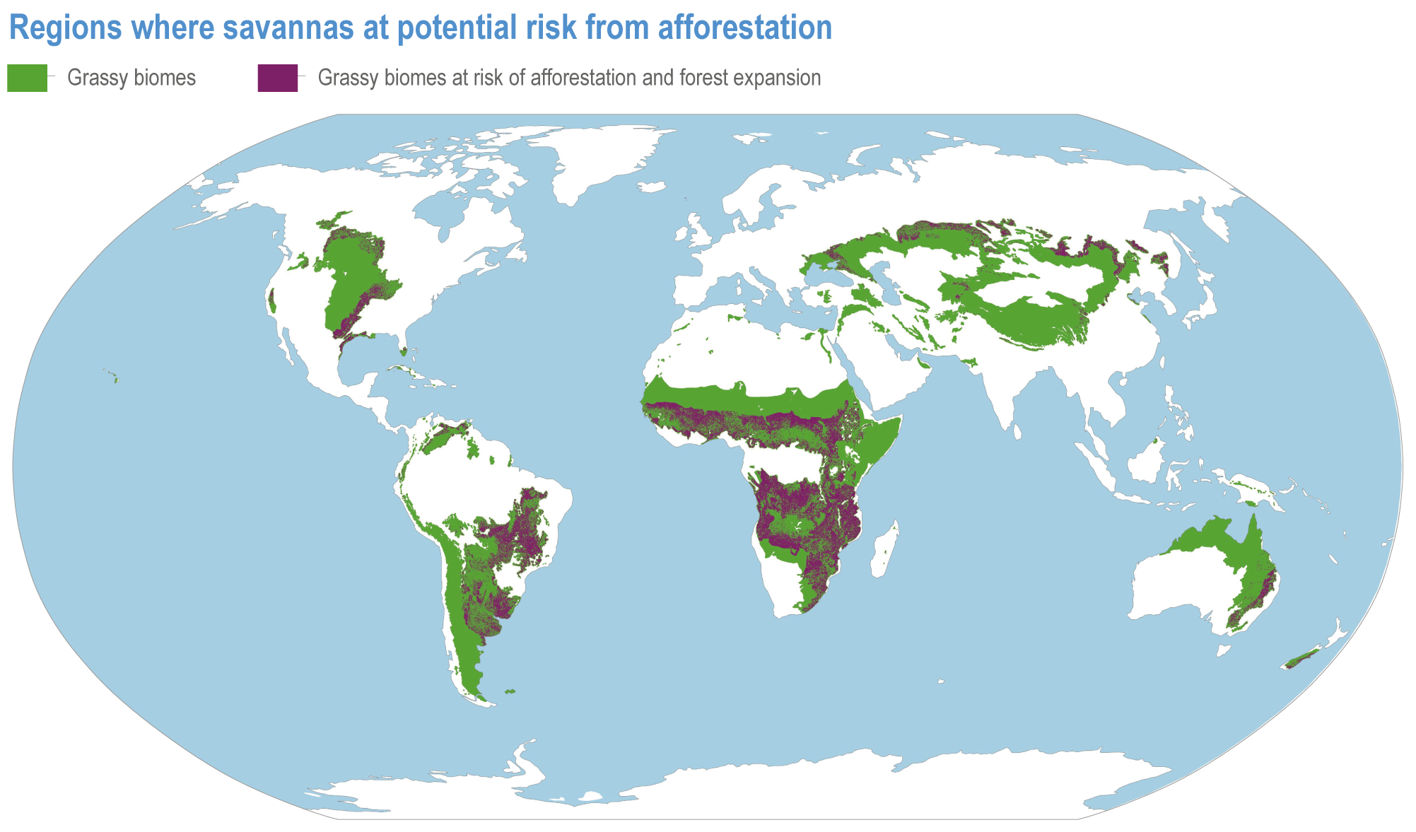
Figure Box 2.2.1 | Regions where savannas are at potential risk from afforestation. Based on (Veldman et al., 2015)
A similar issue can occur in naturally treeless peatlands which can be afforested if they are drained, but this leads to the loss of distinctive peatland species and communities as well as high GHG emissions (Wilson et al., 2014). The mitigation benefits of growing timber are reduced or become negative in these conditions due to the CO2 emissions from the oxidation of the drained peat—they can become a net carbon source rather than a carbon sink (Simola et al., 2012; Crump, 2017; Goldstein et al., 2020). (Sections 2.4.3.8, 2.5.2.8)
FAQ 2.6 | Can tree planting tackle climate change?
Restoring and preventing further loss of native forests is essential for combatting climate change. Planting trees in historically unforested areas (grasslands, shrublands, savannas and some peatlands) can reduce biodiversity and increase the risks of damage from climate change. It is therefore essential to target tree planting to the appropriate locations and use appropriate species. Restoring and protecting forests reduces human vulnerability to climate change, reduces air pollution, stores carbon and builds the resilience of natural systems.
Like all living plants, trees remove carbon dioxide from the atmosphere through the process of photosynthesis. In trees, this carbon uptake is relatively long-term, since much of it is stored in the trees’ woody stems and roots. Therefore, tree planting can be a valuable contribution to reducing climate change. Besides capturing carbon, planting trees can reduce some negative impacts of climate change by providing shade and cooling. It can also help prevent erosion and reduce flood risk by slowing water flow and improving ground water storage. Restoring forest in degraded areas supports biodiversity and can provide benefits to people, ranging from timber to food and recreation.
There are some areas where replacing lost trees is useful. These include forest that has been recently cut down and where reforestation is usually practical. However, it is very important to correctly identify areas of forest that are degraded or have definitely been deforested. Reforesting places, especially where existing native forest patches occur, brings benefits both in sucking up carbon from the atmosphere and helping us to adapt to climate change. Plantations of a non-native species, although offering some economic benefits, do not usually provide the same range of positive impacts, generally have lower biodiversity, reduced carbon uptake and storage, and are less resilient to climate change.
Reforestation options include the natural regeneration of the forest, assisted restoration, enrichment planting, native-tree plantations, commercial plantations and directed tree planting in agro-forestry systems and urban areas. Reforestation with native species usually contributes to a wide range of sustainability goals, including biodiversity recovery, improved water filtration and groundwater recharge. It can reduce the risks of soil erosion and floods. In cities, planting trees can support climate change adaptation by reducing the heat of the area, and promote a wide range of social benefits such as providing shade and benefitting outdoor recreation. Urban trees can also lower energy costs by reducing the demand for conventional sources of cooling like air-conditioning, especially during peak-demand periods. It is therefore important to recognise that there are a wide range of different planting and forest management strategies. The choice will depend on the objectives and the location.
Not everywhere is suitable for tree planting. It is particularly problematic in native non-forested ecosystems. These natural ecosystems are not deforested and degraded but are instead naturally occurring non-forested ecosystems. These areas vary from open grasslands to densely wooded savannas and shrublands. Here, restoring the natural ecosystems instead of afforesting them will better contribute to increasing carbon storage and increasing the area’s resilience to climate change and other environmental changes. It is important to remember that, just because a tree can grow somewhere, it does not mean that it should. These systems are very important in their own right, storing carbon in soils, supporting rich biodiversity and providing people with important ecosystem services such as grasslands for animal grazing. Planting trees in these areas destroys the ecosystem and threatens the biodiversity which is adapted to these environments. They can also impact on ecosystem services such as forage for livestock, on which many people rely.
Many of these open areas also occur in low-rainfall areas. Planting trees there uses a lot of water and can cause reductions in stream flow and groundwater. Many of these locations also burn regularly, and planting trees threatens the establishing trees but can also increase the intensity of the fires from that of a grass-fuelled fire to that of a wood-fuelled fire. Swapping grassy ecosystems for forests may contribute to warming, as forests absorb more incoming radiation (warmth) than grasslands. Aside from the negative impacts to adaptation, it is also questionable just how much carbon can be sequestered in these landscapes as planting trees in grassy ecosystems can reduce carbon gains. Furthermore, a high below-ground carbon store prevents carbon loss to fire in these fire-prone environments.
Another example is peatlands. Peat stores an incredible amount of carbon; maintaining and restoring peatlands is therefore important to reduce atmospheric carbon. However, the restoration actions depend on what type of peatland it is and where it is located. Many temperate and boreal peatlands are naturally treeless. Here, planting trees is often only possible following drainage, but draining and planting (especially of non-native species) destroys native biodiversity and releases GHGs. Many peatlands, especially in the Tropics, are naturally forested, and restoring them requires re-wetting and restoring the natural tree cover (see Figure FAQ2.2.1) which will increase carbon storage.
There are actions we can perform instead of planting trees in non-forested ecosystems, and these include:
- Address the causes of deforestation, forest degradation and widespread ecosystem loss
- Reduce carbon emissions from fossil fuels
- Focus on ecosystem restoration over tree planting. For example, in restoring tropical grassy ecosystems, we can look at actions that cut down trees, enhance grass regrowth and restore natural fire regimes. We then have a much better chance of both enhancing carbon capture and reducing some of the harmful effects of climate change.
In between the two extremes of where planting trees is highly suitable and areas where it is not, it is important to remember that the context matters and that decisions to (re)forest should look beyond simply the act of planting trees. We can consider what the ecological, social and economic goals are of tree planting. It is then important to verify the local context and decide what restoration action will be most effective. It is also more efficient and effective to conserve existing forests before worrying about reforesting.

Figure FAQ2.6.1 | Some places are more appropriate for tree planting than others and caution needs to be applied when planting in different biomes, with some biomes being more suitable than others. This figure highlights some basic biome-specific guidelines when planting in natural and semi-natural vegetation.
2.7 Reducing Scientific Uncertainties to Inform Policy and Management Decisions
Research since the AR5 (Settele et al., 2014) has increased the understanding of climate change impacts and vulnerability in ecosystems. Evidence gaps remain and geographic coverage of research is uneven. This section assesses gaps in ecosystem science where research is necessary for environmental policies and the management of natural resources, including under the UNFCCC and the CBD.
2.7.1 Observed Impacts
Detection and attribution efforts have increased since AR5, but there are some key impacts of high societal importance that would benefit from more detailed and sophisticated attribution studies. For example, while it is clear that diseases have altered considerably in both wild animals and humans in some areas (high confidence in detection), there are many regions that are under-studied, and few regions that provide robust assessments of the role of climate change, particularly with respect to human infectious diseases. While wildfire has been robustly linked to climate change in some regions, there are still a lack of attribution studies in some regions that have experienced large burns recently, and only one fire impact—the increase of the area burned by wildfire in western North America in the period 1984–2017 (Section 2.4.4.2.1) —has been formally attributed to anthropogenic climate change. Global changes in soil and freshwater ecosystem carbon over time remain uncertainties in global carbon stocks and changes (Section 2.4.4.4); due to the physical inability to conduct repeat-monitoring and the lack of remote sensing to scale up point measurements, no global methods can yet produce repeating spatial estimates of soil carbon stock changes.
Despite the growing understanding of the importance of ecosystem services, this assessment found limited research on the observed impacts of climate change for 14 of 18 ecosystem services (Table 2.1).
2.7.2 Projected Risks
A challenge for future projections that continues from previous IPCC reports is accurately characterising and quantifying the interactions of climate change vs. other, non-climate factors that cause ecological change, including LULCC (particularly deforestation, agricultural expansion, and urbanisation) and air and water pollution. Interactions can be particularly complex for invasive species, pests, pathogens and human infectious diseases. Modelling of risks at the species level requires comprehensive databases of the physiological, life-history, and reproduction of individual species, and modeling the impact of changes in species’ compositions requires a mechanistic understanding of functional traits relevant to ecosystem integrity, functioning and resilience to climate change. Taxa that particularly lack this basis for model projections include fungi and bacteria. For numerous plant and animal species, research into genotypic and phenotypic diversity as a source of ecosystem resilience would inform projections of risk.
Soil plays a vital role in ecosystem function, is the habitat of a large number of species and is a large carbon store which is currently a major source of GHG emissions; it is therefore a priority for climate change research (Hashimoto et al., 2015). Major uncertainties remain in our understanding of soil functions. ESMs predict that soil respiration will increase with rising temperatures (Friedlingstein et al., 2014). However, there is evidence of acclimation post-increase (Carey et al., 2016) as the opposite response of decrease in respiration with warming (Li et al., 2013; Reynolds et al., 2015). Long-term, large-scale field observations combined with a better conceptual understanding of the factors governing soil process responses to climate change are needed. A better understanding of plant–water relations is also necessary, including the response of plant transpiration to increased CO2, climate warming and changes in soil moisture and groundwater elevation.
2.7.3 Adaptation and Climate Resilient Development
There are significant evidence gaps in developing adaptation, both for biodiversity conservation and EbA. In particular, while many adaptation measures have been proposed and implementation is starting, there are very few evaluations of success in the scientific literature (Morecroft et al., 2019; Prober et al., 2019). As detailed in Section 2.6.2, there is a strong body of literature on conceptual approaches to climate change adaptation for biodiversity but very little empirical testing of which approaches actually work best. Going forward, it is important to put in place good monitoring and evaluation of adaptation strategies. For EbA, there are good examples of measuring changes in response to new adaptation measures, but these remain relatively rare globally.
Human factors which promote or hinder adaptation are important as well as the technical issues. Only a few studies incorporate climate change and ecosystem services in integrated decision-making, and even fewer aim to identify solutions robust to uncertainty (Runting et al., 2017).
Over the last decades, losses due to natural disasters including those from events related to extreme weather have strongly increased (Mechler and Bouwer, 2015). There is a need for better assessment of global adaptation costs, funding and investment (Micale et al., 2018). Potential synergies between international finance for disaster risk management (DRM) and adaptation have not yet been fully realised. Research has almost exclusively focused on normalising losses for changes in exposure, but not for vulnerability, which is a major gap, given the dynamic nature of vulnerability (Mechler and Bouwer, 2015).
References
Abatzoglou, J. T. and C. A. Kolden, 2011: Climate Change in Western US Deserts: Potential for Increased Wildfire and Invasive Annual Grasses. Rangeland Ecology & Management , 64 (5), 471–478, doi:10.2111/rem-d-09-00151.1.
Abatzoglou, J. T. and A. P. Williams, 2016: Impact of anthropogenic climate change on wildfire across western US forests. Proceedings of the National Academy of Sciences, 113 (42), 11770–11775, doi:10.1073/pnas.1607171113.
Abatzoglou, J. T., A. P. Williams and R. Barbero, 2019: Global emergence of anthropogenic climate change in fire weather indices. Geophysical Research Letters, 46 (1), 326–336, doi:10.1029/2018GL080959.
Abatzoglou, J. T. et al., 2018: Global patterns of interannual climate-fire relationships. Global Change Biology, 24 (11), 5164–5175, doi:10.1111/gcb.14405.
Abbott, B. W. et al., 2016: Biomass offsets little or none of permafrost carbon release from soils, streams, and wildfire: an expert assessment. Environmental Research Letters, 11 (3), 034014, doi:10.1088/1748-9326/11/3/034014.
Abdalla, M. et al., 2019: A critical review of the impacts of cover crops on nitrogen leaching, net greenhouse gas balance and crop productivity. Global Change Biology, 25 (8), 2530–2543, doi:10.1111/gcb.14644.
Abell, R., B. Lehner, M. Thieme and S. Linke, 2017: Looking Beyond the Fenceline: Assessing Protection Gaps for the World’s Rivers. Conservation Letters, 10 (4), 384–394, doi:10.1111/conl.12312.
Aben, R. C. H. et al., 2017: Cross continental increase in methane ebullition under climate change. Nature Communications, 8, doi:10.1038/s41467-017-01535-y.
Abrahams, C. et al., 2013: The Impact of Extreme Events on Freshwater Ecosystems[Jones, I. (ed.)]. Ecological Issues, British Ecological Society, London, England, 67 pp. Available at: https://www.britishecologicalsociety.org/wp-content/uploads/small_single-pages.pdf.
Abram, N. J. et al., 2021: Connections of climate change and variability to large and extreme forest fires in southeast Australia. Communications Earth & Environment , 2 (1), 8, doi:10.1038/s43247-020-00065-8.
Abreu, R. C. R. et al., 2017: The biodiversity cost of carbon sequestration in tropical savanna. Science advances, 3 (8), e1701284.
Acácio, V. et al., 2017: Landscape dynamics in Mediterranean oak forests under global change: understanding the role of anthropogenic and environmental drivers across forest types. Global Change Biology, 23 (3), 1199–1217, doi: 10.1111/gcb.13487.
Ackerman, D., D. Griffin, S. E. Hobbie and J. C. Finlay, 2017: Arctic shrub growth trajectories differ across soil moisture levels. Global change biology, 23 (10), 4294–4302.
Acreman, M. and J. Holden, 2013: How wetlands affect floods. Wetlands, 33 (5), 773–786, doi: 10.1007/s13157-013-0473-2.
Adams, C., J. Andrews and T. Jickells, 2012: Nitrous oxide and methane fluxes vs. carbon, nitrogen and phosphorous burial in new intertidal and saltmarsh sediments. Science of the Total Environment , 434, 240–251, doi:10.1016/j.scitotenv.2011.11.058.
Adams, H. D. et al., 2017: A multi-species synthesis of physiological mechanisms in drought-induced tree mortality. Nature Ecology & Evolution, 1 (9), 1285–1291, doi:10.1038/s41559-017-0248-x.
Addo-Bankas, O. et al., 2021: Green walls: A form of constructed wetland in green buildings. Ecological Engineering, 169, 106321, doi:10.1016/j.ecoleng.2021.106321.
Adhikari, S., H. Baral and C. Nitschke, 2018: Adaptation to climate change in Panchase Mountain ecological regions of Nepal. Environments, 5 (3), 42, doi:10.3390/environments5030042.
Adila, N. et al., 2017: Effects of peat swamp logging and agricultural expansion on species richness of native mammals in Peninsular Malaysia. Basic and Applied Ecology, 22, 1–10, doi:10.1016/j.baae.2017.04.002.
Adrian, R. et al., 2016: Environmental impacts—Lake ecosystems. In: North Sea Region Climate Change Assessment . Springer, Cham, pp. 315–340.
Adrian, R. et al., 2009: Lakes as sentinels of climate change. Limnology and Oceanography, 54 (6), 2283–2297, doi:10.4319/lo.2009.54.6_part_2.2283.
AFAC, 2016: AFAC Independent Operational Review: a review of the management of the Tasmanian fire January 2016, Limited, A. F. a. E. S. A. C., Australasian Fire and Emergency Service Authorities Council Limited,, Victoria, Australia. Available at: http://www.fire.tas.gov.au/userfiles/AFAC/AFAC_Review.pdf (accessed 20/11/2020).
AFAC, 2019: AFAC Independent Operational Review: A review of the management of the Tasmanian fires of December 2018 – March 2019, Limited, A. F. a. E. S. A. C., Australasian Fire and Emergency Service Authorities Council,, Victoria, Australia. Available at: http://www.fire.tas.gov.au/userfiles/AFAC/AFAC_Review.pdf (accessed 12/11/2020).
AghaKouchak, A., L. Y. Cheng, O. Mazdiyasni and A. Farahmand, 2014: Global warming and changes in risk of concurrent climate extremes: Insights from the 2014 California drought. Geophysical Research Letters, 41 (24), 8847–8852, doi:10.1002/2014gl062308.
Agol, D., H. Reid, F. Crick and H. Wendo, 2021: Ecosystem-based adaptation in Lake Victoria Basin; synergies and trade-offs. Royal Society Open Science, 8 (6), 201847, doi:10.1098/rsos.201847.
Agtini, M. D. et al., 2005: The burden of diarrhoea, shigellosis, and cholera in North Jakarta, Indonesia: findings from 24 months surveillance. BMC Infectious Diseases, 5 (1), 89, doi:10.1186/1471-2334-5-89.
Aguilera, E. et al., 2020: Agroecology for adaptation to climate change and resource depletion in the Mediterranean region. A review. Agricultural Systems, 181, 102809, doi:10.1016/j.agsy.2020.102809.
Aguirre-Gutiérrez, J. et al., 2019: Drier tropical forests are susceptible to functional changes in response to a long-term drought. Ecology Letters, 22 (5), 855–865, doi:10.1111/ele.13243.
Ahlström, A. et al., 2015: The dominant role of semi-arid ecosystems in the trend and variability of the land CO2 sink. Science, 348 (6237), 895–899, doi:10.1126/science.aaa1668.
Aide, T. M. et al., 2019: Woody vegetation dynamics in the tropical and subtropical Andes from 2001 to 2014: Satellite image interpretation and expert validation. Global change biology, 25 (6), 2112–2126, doi:10.1111/gcb.14618.
Ainsworth, E. A. et al., 2012: The Effects of Tropospheric Ozone on Net Primary Productivity and Implications for Climate Change. Annual Review of Plant Biology, 63, 637–661, doi:10.1146/annurev-arplant-042110-103829.
Al-Haj, A. N. and R. W. Fulweiler, 2020: A synthesis of methane emissions from shallow vegetated coastal ecosystems. Global Change Biology, 26 (5), 2988–3005, doi:10.1111/gcb.15046.
Alba-Sánchez, F., J. A. López-Sáez, D. Nieto-Lugilde and J.-C. Svenning, 2015: Long-term climate forcings to assess vulnerability in North Africa dry argan woodlands. Applied Vegetation Science, 18 (2), 283–296.
Albrecht, M. et al., 2020: The effectiveness of flower strips and hedgerows on pest control, pollination services and crop yield: a quantitative synthesis. Ecology Letters, 23 (10), 1488–1498, doi:10.1111/ele.13576.
Albrich, K., W. Rammer and R. Seidl, 2020a: Climate change causes critical transitions and irreversible alterations of mountain forests. Global Change Biology, 26 (7), 4013–4027.
Albrich, K. et al., 2020b: Simulating forest resilience: A review. Global Ecology and Biogeography, 29 (12), 2082–2096.
Albright, T. P. et al., 2017: Mapping evaporative water loss in desert passerines reveals an expanding threat of lethal dehydration. Proceedings of the National Academy of Sciences, 114 (9), 2283, doi:10.1073/pnas.1613625114.
Aleixo, I. et al., 2019: Amazonian rainforest tree mortality driven by climate and functional traits. Nature Climate Change, 9 (5), 384–388, doi:10.1038/s41558-019-0458-0.
Aleman, J. C., O. Blarquez and C. A. Staver, 2016: Land-use change outweighs projected effects of changing rainfall on tree cover in sub-Saharan Africa. Global Change Biology, 22 (9), 3013–3025, doi:10.1111/gcb.13299.
Aleman, J. C., M. A. Jarzyna and A. C. Staver, 2018: Forest extent and deforestation in tropical Africa since 1900. Nature ecology & evolution, 2 (1), 26.
Alencar, A. A., P. M. Brando, G. P. Asner and F. E. Putz, 2015: Landscape fragmentation, severe drought, and the new Amazon forest fire regime. Ecological Applications, 25 (6), 1493–1505, doi:10.1890/14-1528.1.
Alexander, J. M. et al., 2018: Lags in the response of mountain plant communities to climate change. Global Change Biology, 24 (2), 563–579.
Alfieri, L. et al., 2017: Global projections of river flood risk in a warmer world. Earths Future, 5 (2), 171–182, doi:10.1002/2016ef000485.
Ali, M., A. R. Nelson, A. L. Lopez and D. A. Sack, 2015: Updated Global Burden of Cholera in Endemic Countries. PLOS Neglected Tropical Diseases, 9 (6), e0003832, doi:10.1371/journal.pntd.0003832.
Alkama, R. and A. Cescatti, 2016: Biophysical climate impacts of recent changes in global forest cover. Science, 351 (6273), 600–604, doi:10.1126/science.aac8083.
Allen, C. D., D. D. Breshears and N. G. McDowell, 2015: On underestimation of global vulnerability to tree mortality and forest die-off from hotter drought in the Anthropocene. Ecosphere, 6 (8), 1–55, doi:10.1890/ES15-00203.1.
Allen, C. D. et al., 2010: A global overview of drought and heat-induced tree mortality reveals emerging climate change risks for forests. Forest Ecology and Management , 259 (4), 660–684, doi:10.1016/j.foreco.2009.09.001.
Allen, G. H. and T. M. Pavelsky, 2018: Global extent of rivers and streams. Science, doi:10.1126/science.aat0636.
Allen, J. L. and J. C. Lendemer, 2016: Climate change impacts on endemic, high-elevation lichens in a biodiversity hotspot. Biodiversity and Conservation, 25 (3), 555–568, doi:10.1007/s10531-016-1071-4.
Allen, T. et al., 2017: Global hotspots and correlates of emerging zoonotic diseases. Nature Communications, 8 (1), 1124, doi:10.1038/s41467-017-00923-8.
Alo, C. A. and G. Wang, 2008: Potential future changes of the terrestrial ecosystem based on climate projections by eight general circulation models. Journal of Geophysical Research: Biogeosciences, 113 (G1), doi:10.1029/2007JG000528.
Alongi, D. M., 2015: The impact of climate change on mangrove forests. Current Climate Change Reports, 1 (1), 30–39, doi:10.1007/s40641-015-0002-x.
Alonso, D., M. J. Bouma and M. Pascual, 2011: Epidemic malaria and warmer temperatures in recent decades in an East African highland. Proceedings of the Royal Society B: Biological Sciences, 278 (1712), 1661–1669, doi:10.1098/rspb.2010.2020.
Altizer, S. et al., 2013: Climate Change and Infectious Diseases: From Evidence to a Predictive Framework. Science, 341 (6145), 514–519, doi:10.1126/science.1239401.
Alvarez-Clare, S., M. C. Mack and M. Brooks, 2013: A direct test of nitrogen and phosphorus limitation to net primary productivity in a lowland tropical wet forest. Ecology, 94 (7), 1540–1551, doi:10.1890/12-2128.1.
Alvarez-Garreton, C., A. Lara, J. P. Boisier and M. Galleguillos, 2019: The Impacts of Native Forests and Forest Plantation on Water Supply in Chile. Forests, 10 (6), 473.
Amaya, D. J., A. J. Miller, S.-P. Xie and Y. Kosaka, 2020: Physical drivers of the summer 2019 North Pacific marine heatwave. Nature Communications, 11 (1), 1903, doi:10.1038/s41467-020-15820-w.
Ameli, A. A. and I. F. Creed, 2019: Does wetland location matter when managing wetlands for watershed-scale flood and drought resilience?JAWRA Journal of the American Water Resources Association, 55 (3), 529–542.
Ameztegui, A., L. Coll, L. Brotons and J. M. Ninot, 2016: Land-use legacies rather than climate change are driving the recent upward shift of the mountain tree line in the Pyrenees. Global Ecology and Biogeography, 25 (3), 263–273, doi:10.1111/geb.12407.
Anacker, B. L. and S. P. Harrison, 2012: Climate and the evolution of serpentine endemism in California. Evolutionary Ecology, 26 (4), 1011–1023, doi:10.1007/s10682-011-9532-4.
Anadón, J. D., O. E. Sala and F. T. Maestre, 2014a: Climate change will increase savannas at the expense of forests and treeless vegetation in tropical and subtropical Americas. Journal of Ecology, 102 (6), 1363–1373, doi:10.1111/1365-2745.12325.
Anadón, J. D., O. E. Sala, B. L. Turner and E. M. Bennett, 2014b: Effect of woody-plant encroachment on livestock production in North and South America. Proceedings of the National Academy of Sciences, 111 (35), 12948–12953, doi:10.1073/pnas.1320585111.
Andela, N. et al., 2017: A human-driven decline in global burned area. Science, 356 (6345), 1356–1361, doi:10.1126/science.aal4108.
Andela, N. et al., 2019: The Global Fire Atlas of individual fire size, duration, speed and direction. Earth System Science Data, 11 (2), 529–552, doi:10.5194/essd-11-529-2019.
Anderegg, W. R. et al., 2020: Climate-driven risks to the climate mitigation potential of forests. Science, 368 (6497), doi:10.1126/science.aaz7005.
Anderegg, W. R. L., L. D. L. Anderegg, K. L. Kerr and A. T. Trugman, 2019: Widespread drought-induced tree mortality at dry range edges indicates that climate stress exceeds species’ compensating mechanisms. Global Change Biology, 25 (11), 3793–3802, doi:10.1111/gcb.14771.
Anderegg, W. R. L. et al., 2015: Tree mortality from drought, insects, and their interactions in a changing climate. New Phytologist , 208 (3), 674–683, doi:10.1111/nph.13477.
Anderegg, W. R. L. et al., 2016: Meta-analysis reveals that hydraulic traits explain cross-species patterns of drought-induced tree mortality across the globe. Proceedings of the National Academy of Sciences of the United States of America, 113 (18), 5024–5029, doi:10.1073/pnas.1525678113.
Anderegg, W. R. L. et al., 2018: Hydraulic diversity of forests regulates ecosystem resilience during drought. Nature, 561 (7724), 538-+, doi:10.1038/s41586-018-0539-7.
Andersen, E. M. and R. J. Steidl, 2019: Woody plant encroachment restructures bird communities in semiarid grasslands. Biological Conservation, 240, 108276, doi:10.1016/j.biocon.2019.108276.
Andersen, R. et al., 2017: An overview of the progress and challenges of peatland restoration in Western Europe. Restoration Ecology, 25 (2), 271–282, doi:10.1111/rec.12415.
Anderson, L. O. et al., 2018: Vulnerability of Amazonian forests to repeated droughts. Philos Trans R Soc Lond B Biol Sci, 373 (1760), doi:10.1098/rstb.2017.0411.
Andersson, N. et al., 2015: Evidence based community mobilization for dengue prevention in Nicaragua and Mexico (<em>Camino Verde,</em> the Green Way): cluster randomized controlled trial. BMJ : British Medical Journal, 351, h3267, doi:10.1136/bmj.h3267.
Andresen, C. G. and V. L. Lougheed, 2015: Disappearing Arctic tundra ponds: Fine-scale analysis of surface hydrology in drained thaw lake basins over a 65 year period (1948–2013). Journal of Geophysical Research: Biogeosciences, 120 (3), 466–479.
Andrew, S. C., L. L. Hurley, M. M. Mariette and S. C. Griffith, 2017: Higher temperatures during development reduce body size in the zebra finch in the laboratory and in the wild. J. Evol. Biol. , 30 (12), 2156–2164.
Andrus, R. A., T. T. Veblen, B. J. Harvey and S. J. Hart, 2016: Fire severity unaffected by spruce beetle outbreak in spruce-fir forests in southwestern Colorado. Ecological Applications, 26 (3), 700–711, doi:10.1890/15-1121.
Angel, J. R. and K. E. Kunkel, 2010: The response of Great Lakes water levels to future climate scenarios with an emphasis on Lake Michigan-Huron. Journal of Great Lakes Research, 36, 51–58, doi:10.1016/j.jglr.2009.09.006.
Angerbjörn, A. et al., 2013: Carnivore conservation in practice: replicated management actions on a large spatial scale. Journal of Applied Ecology, 50 (1), 59–67, doi:10.1111/1365-2664.12033.
Angilletta Jr, M. J., 2009: Thermal Adaptation: A Theoretical and Empirical Synthesis. Oxford University Press, Oxford, 302 pp. ISBN 978-0-19-857087-5.
Angilletta, M. J., R. S. Wilson, C. A. Navas and R. S. James, 2003: Tradeoffs and the evolution of thermal reaction norms. Trends in Ecology & Evolution, 18 (5), 234–240, doi:10.1016/S0169-5347(03)00087-9.
Anich, N. M. and M. P. Ward, 2017: Using audio playback to expand the geographic breeding range of an endangered species. Diversity and Distributions, 23 (12), 1499–1508, doi:10.1111/ddi.12635.
Anshari, G., A. Peter Kershaw and S. van der Kaars, 2001: A Late Pleistocene and Holocene pollen and charcoal record from peat swamp forest, Lake Sentarum Wildlife Reserve, West Kalimantan, Indonesia. Palaeogeography, Palaeoclimatology, Palaeoecology, 171 (3–4), 213–228, doi:10.1016/S0031-0182(01)00246-2.
Anshari, G., A. Peter Kershaw, S. Van Der Kaars and G. Jacobsen, 2004: Environmental change and peatland forest dynamics in the Lake Sentarum area, West Kalimantan, Indonesia. Journal of Quaternary Science, 19 (7), 637–655, doi:10.1002/jqs.879.
Anshari, G. Z., E. Gusmayanti and N. Novita, 2021: The Use of Subsidence to Estimate Carbon Loss from Deforested and Drained Tropical Peatlands in Indonesia. Forests, 12 (6), 732, doi:10.3390/f12060732.
Anyamba, A., K. J. Linthicum and C. J. Tucker, 2001: Climate-disease connections: Rift Valley Fever in Kenya. Cad Saude Publica, 17 Suppl, 133–140, doi:10.1590/s0102-311x2001000700022.
Anyamba, A. et al., 2014: Recent Weather Extremes and Impacts on Agricultural Production and Vector-Borne Disease Outbreak Patterns. PLOS ONE, 9 (3), e92538, doi:10.1371/journal.pone.0092538.
Arafeh-Dalmau, N. et al., 2019: Extreme Marine Heatwaves Alter Kelp Forest Community Near Its Equatorward Distribution Limit. Frontiers in Marine Science, 6, doi:10.3389/fmars.2019.00499.
Aragao, L. E. O. C. et al., 2018: 21st Century drought-related fires counteract the decline of Amazon deforestation carbon emissions. Nature Communications, 9, doi:10.1038/s41467-017-02771-y.
Aragao, L. E. O. C. et al., 2014: Environmental change and the carbon balance of Amazonian forests. Biological Reviews, 89 (4), 913–931, doi:10.1111/brv.12088.
Aragón-Gastélum, J. L. et al., 2014: Induced climate change impairs photosynthetic performance in Echinocactus platyacanthus, an especially protected Mexican cactus species. Flora—Morphology, Distribution, Functional Ecology of Plants, 209 (9), 499–503, doi:10.1016/j.flora.2014.06.002.
Aram, F., E. Higueras García, E. Solgi and S. Mansournia, 2019: Urban green space cooling effect in cities. Heliyon, 5 (4), e01339, doi:10.1016/j.heliyon.2019.e01339.
Araujo, M. et al., 2019: Standards for distribution models in biodiversity assessments. Science Advances, 5 (1), doi:10.1126/sciadv.aat4858.
Archer, D. et al., 2014: Moving towards inclusive urban adaptation: approaches to integrating community-based adaptation to climate change at city and national scale. Climate and Development , 6 (4), 345–356, doi:10.1080/17565529.2014.918868.
Archer, S. R. et al., 2017: Woody plant encroachment: causes and consequences. In: Rangeland systems. Springer, Cham, pp. 25–84.
Archibald, S., 2016: Managing the human component of fire regimes: lessons from Africa. Philosophical Transactions of the Royal Society B: Biological Sciences, 371 (1696), 20150346, doi:10.1098/rstb.2015.0346.
Archibald, S. et al., 2019: Distribution and determinants of savannas. In: Savanna woody plants and large herbivores[Scogings, P. F. and M. Sankaran (eds.)]. John Wiley & Sons Ltd, Hoboken, NJ, USA, pp. 1–24. ISBN 9781119081128.
Archibald, S., C. E. R. Lehmann, J. L. Gómez-Dans and R. A. Bradstock, 2013: Defining pyromes and global syndromes of fire regimes. Proceedings of the National Academy of Sciences, 110 (16), 6442–6447, doi:10.1073/pnas.1211466110.
Archibald, S., D. P. Roy, B. W. van Wilgen and R. J. Scholes, 2009: What limits fire? An examination of drivers of burnt area in Southern Africa. Global Change Biology, 15 (3), 613–630, doi:10.1111/j.1365-2486.2008.01754.x.
Arneth, A. et al., 2021: Restoring Degraded Lands. Annual Review of Environment and Resources, doi:10.1146/annurev-environ-012320-054809.
Arneth, A. et al., 2020: Post-2020 biodiversity targets need to embrace climate change. Proceedings of the National Academy of Sciences, 117 (49), 30882, doi:10.1073/pnas.2009584117.
Arneth, A. et al., 2017: Historical carbon dioxide emissions caused by land-use changes are possibly larger than assumed. Nature Geoscience, 10 (2), 79–84, doi:10.1038/ngeo2882.
Arora, R., K. Tockner and M. Venohr, 2016: Changing river temperatures in northern Germany: trends and drivers of change. Hydrological Processes, 30 (17), 3084–3096, doi:10.1002/hyp.10849.
Arora, V. K. and J. R. Melton, 2018: Reduction in global area burned and wildfire emissions since 1930s enhances carbon uptake by land. Nature Communications, 9, doi:10.1038/s41467-018-03838-0.
Arthington, A. H. and W. L. Hadwen, 2003: The significance and management implications of perched dune lakes as swimming and recreation sites on Fraser Island, Australia. Journal of Tourism Studies, 14 (2), 35.
Aryal, D. R., R. R. Gómez-González, R. Hernández-Nuriasmú and D. E. Morales-Ruiz, 2019: Carbon stocks and tree diversity in scattered tree silvopastoral systems in Chiapas, Mexico. Agroforestry Systems, 93 (1), 213–227, doi:10.1007/s10457-018-0310-y.
Asner, G. P. et al., 2016a: Progressive forest canopy water loss during the 2012–2015 California drought. Proceedings of the National Academy of Sciences, 113 (2), E249–E255.
Asner, G. P., N. Vaughn, I. P. Smit and S. Levick, 2016b: Ecosystem-scale effects of megafauna in African savannas. Ecography, 39 (2), 240–252.
Assis, L. F. F. G. et al., 2019: TerraBrasilis: A Spatial Data Analytics Infrastructure for Large-Scale Thematic Mapping. ISPRS International Journal of Geo-Information, 8 (11), 1–27, doi:10.3390/ijgi8110513.
Åström, C. et al., 2012: Potential Distribution of Dengue Fever Under Scenarios of Climate Change and Economic Development. EcoHealth, 9 (4), 448–454, doi:10.1007/s10393-012-0808-0.
Avitabile, V. et al., 2016: An integrated pan-tropical biomass map using multiple reference datasets. Global Change Biology, 22 (4), 1406–1420, doi:10.1111/gcb.13139.
Axelson, J. N., B. C. Hawkes, L. van Akker and R. I. Alfaro, 2018: Stand dynamics and the mountain pine beetle-30 years of forest change in Waterton Lakes National Park, Alberta, Canada. Canadian Journal of Forest Research, 48 (10), 1159–1170, doi:10.1139/cjfr-2018-0161.
Babst, F. et al., 2019: Twentieth century redistribution in climatic drivers of global tree growth. Science Advances, 5 (1), doi:10.1126/sciadv.aat4313.
Baccini, A. et al., 2012: Estimated carbon dioxide emissions from tropical deforestation improved by carbon-density maps. Nature Climate Change, 2 (3), 182–185, doi:10.1038/nclimate1354.
Baccini, A. et al., 2017: Tropical forests are a net carbon source based on aboveground measurements of gain and loss. Science, 358 (6360), 230–234.
Bagella, S. et al., 2016: Mediterranean Temporary Ponds: new challenges from a neglected habitat. Hydrobiologia, 782 (1), 1–10, doi:10.1007/s10750-016-2962-9.
Bailey, L. and M. van de Pol, 2016: Tackling extremes: challenges for ecological and evolutionary research on extreme climatic events. Journal of Animal Ecology, 85 (1), 85–96, doi:10.1111/1365-2656.12451.
Baker-Austin, C. et al., 2018: Vibrio spp. infections. Nature Reviews Disease Primers, 4 (1), 1–19, doi:10.1038/s41572-018-0005-8.
Baker-Austin, C., J. Trinanes, N. Gonzalez-Escalona and J. Martinez-Urtaza, 2017: Non-cholera Vibrios: the microbial barometer of climate change. Trends in Microbiology, 25 (1), 76–84, doi:10.1016/j.tim.2016.09.008.
Baker-Austin, C. et al., 2013: Emerging Vibrio risk at high latitudes in response to ocean warming. Nature Climate Change, 3 (1), 73–77, doi:10.1038/nclimate1628.
Baker, D. M., G. Murray and A. K. Agyare, 2018: Governance and the making and breaking of social-ecological traps. Ecology and Society, 23 (1).
Bakker, E. S. et al., 2016: Combining paleo-data and modern exclosure experiments to assess the impact of megafauna extinctions on woody vegetation. Proceedings of the National Academy of Sciences, 113 (4), 847–855.
Bakker, E. S. and J.-C. Svenning, 2018: Trophic rewilding: impact on ecosystems under global change. Philosophical Transactions of the Royal Society B, doi:10.1098/rstb.2017.0432.
Balanya, J. et al., 2006: Global genetic change tracks global climate warming in Drosophila subobscura. Science, 313 (5794), 1773–1775, doi:10.1126/science.1131002.
Balch, J. K. et al., 2017: Human-started wildfires expand the fire niche across the United States. Proceedings of the National Academy of Sciences of the United States of America, 114 (11), 2946–2951, doi:10.1073/pnas.1617394114.
Balch, J. K. et al., 2015: The susceptibility of southeastern Amazon forests to fire: insights from a large-scale burn experiment. BioScience, 65 (9), 893–905.
Balian, E., H. Segers, C. Leveque and K. Martens, 2008: An introduction to the freshwater animal diversity assessment (FADA) project. Hydrobiologia, 595, 3–8, doi:10.1007/s10750-007-9235-6.
Ball, G. et al., 2021: Wildfires increasingly impact western US fluvial networks. Nature Communications, 12 (1), 8, doi:10.1038/s41467-021-22747-3.
Ballantyne, A. P. et al., 2012: Increase in observed net carbon dioxide uptake by land and oceans during the past 50 years. Nature, 488 (7409), 70.
Ballhorn, U., F. Siegert, M. Mason and S. Limin, 2009: Derivation of burn scar depths and estimation of carbon emissions with LIDAR in Indonesian peatlands. Proceedings of the National Academy of Sciences, 106 (50), 21213–21218, doi:10.1073/pnas.0906457106.
Bangash, R. F. et al., 2013: Ecosystem services in Mediterranean river basin: Climate change impact on water provisioning and erosion control. Science of The Total Environment , 458–460, 246–255, doi:10.1016/j.scitotenv.2013.04.025.
Barbeaux, S. J., K. Holsman and S. Zador, 2020: Marine Heatwave Stress Test of Ecosystem-Based Fisheries Management in the Gulf of Alaska Pacific Cod Fishery. Frontiers in Marine Science, 7, doi:10.3389/fmars.2020.00703.
Barbero, R. et al., 2015: Climate change presents increased potential for very large fires in the contiguous United States. International Journal of Wildland Fire, 24 (7), 892–899.
Barbieri, P., S. Pellerin, V. Seufert and T. Nesme, 2019: Changes in crop rotations would impact food production in an organically farmed world. Nature Sustainability, 2 (5), 378–385, doi:10.1038/s41893-019-0259-5.
Barbosa, H. A. and T. V. Lakshmi Kumar, 2016: Influence of rainfall variability on the vegetation dynamics over Northeastern Brazil. Journal of Arid Environments, 124, 377–387.
Barichivich, J. et al., 2013: Large-scale variations in the vegetation growing season and annual cycle of atmospheric CO2 at high northern latitudes from 1950 to 2011. Global Change Biology, 19 (10), 3167–3183, doi:10.1111/gcb.12283.
Bark, R. H., J. Martin-Ortega and K. A. Waylen, 2021: Stakeholders’ views on natural flood management: Implications for the nature-based solutions paradigm shift?Environmental Science & Policy, 115, 91–98.
Barnosky, A. D. et al., 2011: Has the Earth’s sixth mass extinction already arrived?Nature, 471 (7336), 51–57.
Barr, S. L., B. M. Larson, T. J. Beechey and D. J. Scott, 2021: Assessing climate change adaptation progress in Canada’s protected areas. The Canadian Geographer/Le Géographe canadien, 65 (2), 152–165.
Barrows, C. W. et al., 2014: Designing a sustainable monitoring framework for assessing impacts of climate change at Joshua Tree National Park, USA. Biodiversity and Conservation, 23 (13), 3263–3285, doi:10.1007/s10531-014-0779-2.
Barrows, C. W. and M. L. Murphy-Mariscal, 2012: Modeling impacts of climate change on Joshua trees at their southern boundary: How scale impacts predictions. Biological Conservation, 152, 29–36, doi:10.1016/j.biocon.2012.03.028.
Barrows, C. W. et al., 2020: Validating climate-change refugia: empirical bottom-up approaches to support management actions. Frontiers in Ecology and the Environment , 18 (5), 298–306, doi:10.1002/fee.2205.
Barsoum, N. et al., 2016: Diversity, functional structure and functional redundancy of woodland plant communities: How do mixed tree species plantations compare with monocultures?Forest Ecology and Management , 382, 244–256.
Bartlett, M. K., M. Detto and S. W. Pacala, 2019: Predicting shifts in the functional composition of tropical forests under increased drought and CO. Ecology Letters, 22 (1), 67–77, doi:10.1111/ele.13168.
Barton, A. M. and H. M. Poulos, 2018: Pine vs. oaks revisited: Conversion of Madrean pine-oak forest to oak shrubland after high-severity wildfire in the Sky Islands of Arizona. Forest Ecology and Management , 414, 28–40, doi:10.1016/j.foreco.2018.02.011.
Bartosiewicz, M. et al., 2019: Hot tops, cold bottoms: Synergistic climate warming and shielding effects increase carbon burial in lakes. Limnology and Oceanography Letters, 0 (0), doi:10.1002/lol2.10117.
Basara, J. B. and J. I. Christian, 2018: Seasonal and interannual variability of land-atmosphere coupling across the Southern Great Plains of North America using the North American regional reanalysis. International Journal of Climatology, 38 (2), 964–978, doi:10.1002/joc.5223.
Bastazini, V. A. G. et al., 2021: The impact of climate warming on species diversity across scales: Lessons from experimental meta-ecosystems. Global Ecology and Biogeography, 30 (7), 1545–1554, doi:10.1111/geb.13308
Bastin, J.-F. et al., 2019: The global tree restoration potential. Science, 365 (6448), 76–79, doi:10.1126/science.aax0848.
Bastin, J. F. et al., 2020: Erratum for the Report: “The global tree restoration potential” by J.-F. Bastin, Y. Finegold, C. Garcia, D. Mollicone, M. Rezende, D. Routh, C. M. Zohner, T. W. Crowther and for the Technical Response “Response to Comments on ‘The global tree restoration potential’” by J.-F. Bastin, Y. Finegold, C. Garcia, N. Gellie, A. Lowe, D. Mollicone, M. Rezende, D. Routh, M. Sacande, B. Sparrow, C. M. Zohner, T. W. Crowther. Science, 368 (6494), doi:10.1126/science.abc8905.
Batáry, P., L. V. Dicks, D. Kleijn and W. J. Sutherland, 2015: The role of agri-environment schemes in conservation and environmental management. Conservation Biology, 29 (4), 1006–1016.
Bates, A. E. et al., 2019: Climate resilience in marine protected areas and the ‘Protection Paradox’. Biological Conservation, 236, 305–314, doi:10.1016/j.biocon.2019.05.005.
Batjes, N. H., 2016: Harmonized soil property values for broad-scale modelling (WISE30sec) with estimates of global soil carbon stocks. Geoderma, 269, 61–68, doi:10.1016/j.geoderma.2016.01.034.
Batllori, E. et al., 2019: Compound fire-drought regimes promote ecosystem transitions in Mediterranean ecosystems. Journal of Ecology, 107 (3), 1187–1198, doi:10.1111/1365-2745.13115.
Batllori, E. et al., 2020: Forest and woodland replacement patterns following drought-related mortality. Proceedings of the National Academy of Sciences of the United States of America, 117 (47), 29720–29729, doi:10.1073/pnas.2002314117.
Batllori, E. et al., 2017: Potential relocation of climatic environments suggests high rates of climate displacement within the North American protection network. Global Change Biology, 23 (8), 3219–3230, doi:10.1111/gcb.13663.
Bauhus, J., K. Puettmann and C. Messier, 2009: Silviculture for old-growth attributes. Forest Ecology and Management , 258 (4), 525–537, doi:10.1016/j.foreco.2009.01.053.
Bay, R. A. et al., 2018: Genomic signals of selection predict climate-driven population declines in a migratory bird. Science, 359 (6371), 83–86, doi:10.1126/science.aan4380.
Beaulieu, J. J., T. DelSontro and J. A. Downing, 2019: Eutrophication will increase methane emissions from lakes and impoundments during the 21st century. Nature Communications, 10, doi:10.1038/s41467-019-09100-5.
Beaulieu, J. J., M. G. McManus and C. T. Nietch, 2016: Estimates of reservoir methane emissions based on a spatially balanced probabilistic-survey. Limnology and Oceanography, 61 (S1), S27-S40.
Beaumont, L. et al., 2016: Which species distribution models are more (or less) likely to project broad-scale, climate-induced shifts in species ranges?Ecological Modelling, 342, 135–146, doi:10.1016/j.ecolmodel.2016.10.004.
Bebbington, A. J. and J. T. Bury, 2009: Institutional challenges for mining and sustainability in Peru. Proceedings of the National Academy of Sciences, 106 (41), 17296–17301, doi:10.1073/pnas.0906057106.
Bedelian, C. and J. O. Ogutu, 2017: Trade-offs for climate-resilient pastoral livelihoods in wildlife conservancies in the Mara ecosystem, Kenya. Pastoralism, 7 (1), 10.
Beer, C. et al., 2010: Terrestrial Gross Carbon Dioxide Uptake: Global Distribution and Covariation with Climate. Science, 329 (5993), 834–838, doi:10.1126/science.1184984.
Beillouin, D., T. Ben-Ari and D. Makowski, 2019: Evidence map of crop diversification strategies at the global scale. Environmental Research Letters, 14 (12), 123001.
Bell, G. et al., 2019: Trophic structure modulates community rescue following acidification. Proceedings of the Royal Society B: Biological Sciences, 286 (1904), 9, doi:10.1098/rspb.2019.0856.
Bell, G. and A. Gonzalez, 2009: Evolutionary rescue can prevent extinction following environmental change. Ecology Letters, 12 (9), 942–948, doi:10.1111/j.1461-0248.2009.01350.x.
Bellahirech, A. et al., 2019: Site- and tree-related factors affecting colonization of cork oaks Quercus suber L. by ambrosia beetles in Tunisia. Annals of Forest Science, 76 (2), doi:10.1007/s13595-019-0815-1.
Bellis, J., D. Bourke, C. Williams and S. Dalrymple, 2019: Identifying factors associated with the success and failure of terrestrial insect translocations. Biological Conservation, 236, 29–36, doi:10.1016/j.biocon.2019.05.008.
Bello, C. et al., 2015: Defaunation affects carbon storage in tropical forests. Science Advances, 1 (11), doi:10.1126/sciadv.1501105.
Belote, R. T. et al., 2017: Wild, connected, and diverse: building a more resilient system of protected areas. Ecological Applications, 27 (4), 1050–1056.
Benali, A. et al., 2017: Bimodal fire regimes unveil a global-scale anthropogenic fingerprint. Global Ecology and Biogeography, 26 (7), 799–811, doi:10.1111/geb.12586.
Bennett, A. C., N. G. McDowell, C. D. Allen and K. J. Anderson-Teixeira, 2015: Larger trees suffer most during drought in forests worldwide. Nature Plants, 1 (10), 15139.
Bentz, B. J. et al., 2010: Climate Change and Bark Beetles of the Western United States and Canada: Direct and Indirect Effects. BioScience, 60 (8), 602–613, doi:10.1525/bio.2010.60.8.6.
Berdugo, M. et al., 2020: Global ecosystem thresholds driven by aridity. Science, 367 (6479), 787, doi:10.1126/science.aay5958.
Berenguer, E. et al., 2021: Tracking the impacts of El Niño drought and fire in human-modified Amazonian forests. Proceedings of the National Academy of Sciences, 118 (30), e2019377118, doi:10.1073/pnas.2019377118.
Bergengren, J. C., D. E. Waliser and Y. L. Yung, 2011: Ecological sensitivity: a biospheric view of climate change. Climatic Change, 107 (3–4), 433, doi:10.1007/s10584-011-0065-1.
Bergstrom, D. M. et al., 2021: Combating ecosystem collapse from the tropics to the Antarctic. Global Change Biology, 27 (9), 1692–1703.
Berio Fortini, L., L. R. Kaiser and D. A. LaPointe, 2020: Fostering real-time climate adaptation: Analyzing past, current, and forecast temperature to understand the dynamic risk to Hawaiian honeycreepers from avian malaria. Global Ecology and Conservation, 23, e01069, doi:10.1016/j.gecco.2020.e01069.
Bernhardt, E. et al., 2018: The metabolic regimes of flowing waters. Limnology and Oceanography, 63, S99-S118, doi:10.1002/lno.10726.
Bernstein, A., 2015: Climate Change and the Crystal Ball of Vector-Borne Disease Forecasts. Current Climate Change Reports, 1 (4), 217–223, doi:10.1007/s40641-015-0022-6.
Berteaux, D. et al., 2018: Northern protected areas will become important refuges for biodiversity tracking suitable climates. Scientific Reports, 8, doi:10.1038/s41598-018-23050-w.
Bertrand, R. et al., 2011: Changes in plant community composition lag behind climate warming in lowland forests. Nature, 479 (7374), 517–520.
Berzaghi, F. et al., 2019: Carbon stocks in central African forests enhanced by elephant disturbance. Nature Geoscience, 12 (9), 725-+, doi:10.1038/s41561-019-0395-6.
Berzaghi, F. et al., 2018: Assessing the role of megafauna in tropical forest ecosystems and biogeochemical cycles—the potential of vegetation models. Ecography, 41 (12), 1934–1954, doi:10.1111/ecog.03309.
Bestelmeyer, B. T. et al., 2018: The Grassland-Shrubland Regime Shift in the Southwestern United States: Misconceptions and Their Implications for Management. Bioscience, 68 (9), 678–690, doi:10.1093/biosci/biy065.
Bett, B. et al., 2017: Effects of climate change on the occurrence and distribution of livestock diseases. Preventive Veterinary Medicine, 137, 119–129, doi:10.1016/j.prevetmed.2016.11.019.
Bhatt, S. et al., 2015: The effect of malaria control on Plasmodium falciparum in Africa between 2000 and 2015. Nature, 526 (7572), 207–211, doi:10.1038/nature15535.
Bhattarai, G. P. and J. T. Cronin, 2014: Hurricane activity and the large-scale pattern of spread of an invasive plant species. PLoS One, 9 (5), e98478.
Biagini, B. et al., 2014: A typology of adaptation actions: A global look at climate adaptation actions financed through the Global Environment Facility. Global Environmental Change, 25, 97–108, doi:10.1016/j.gloenvcha.2014.01.003.
Biagioni, S. et al., 2015: 8000 years of vegetation dynamics and environmental changes of a unique inland peat ecosystem of the Jambi Province in Central Sumatra, Indonesia. Palaeogeography, Palaeoclimatology, Palaeoecology, 440, 813–829, doi:10.1016/j.palaeo.2015.09.048.
Bindoff, N. L. et al., 2019: Changing Ocean, Marine Ecosystems, and Dependent Communities. In: IPCC Special Report on the Ocean and Cryosphere in a Changing Climate[Pörtner, H. O., D. C. Roberts, V. Masson-Delmotte, P. Zhai, M. Tignor, E. Poloczanska, K. Mintenbeck, A. Alegría, M. Nicolai, A. Okem, J. Petzold, B. Rama and N. M. Weyer (eds.)], In press, pp. 447–587.
Birdlife International, 2018: Spheniscus demersus. The IUCN Red List of Threatened Species 2018: e.T22697810A132604504. IUCN Red List , 2020 (09/22/2020).
Birk, S. et al., 2020: Impacts of multiple stressors on freshwater biota across spatial scales and ecosystems. Nature Ecology & Evolution, 4 (8), 1060–1068, doi:10.1038/s41559-020-1216-4.
Bjork, S. J. and J. L. Bartholomew, 2009: The effects of water velocity on the Ceratomyxa shasta infectious cycle. Journal of Fish Diseases, 32 (2), 131–142.
Bjorkman, A. D. et al., 2019: Status and trends in Arctic vegetation: Evidence from experimental warming and long-term monitoring. Ambio, 49 (3), 1–15, doi:10.1007/s13280-019-01161-6.
Bjorkman, A. D. et al., 2018: Plant functional trait change across a warming tundra biome. Nature, 562 (7725), 57.
Blackman, A., L. Corral, E. S. Lima and G. P. Asner, 2017: Titling indigenous communities protects forests in the Peruvian Amazon. Proceedings of the National Academy of Sciences, 114 (16), 4123–4128, doi:10.1073/pnas.1603290114.
Blaser, W. J. et al., 2018: Climate-smart sustainable agriculture in low-to-intermediate shade agroforests. Nature Sustainability, 1 (5), 234.
Blum, A. J. and P. J. Hotez, 2018: Global “worming”: Climate change and its projected general impact on human helminth infections. PLoS Neglected Tropical Diseases, 12 (7), doi:10.1371/journal.pntd.0006370.
Blume-Werry, G., S. D. Wilson, J. Kreyling and A. Milbau, 2016: The hidden season: growing season is 50% longer below than above ground along an arctic elevation gradient. New Phytologist , 209 (3), 978–986.
Bodensteiner, B. L. et al., 2021: Thermal adaptation revisited: How conserved are thermal traits of reptiles and amphibians?Journal of Experimental Zoology Part A: Ecological and Integrative Physiology, 335 (1), 173–194.
Bodmer, P., J. Wilkinson and A. Lorke, 2020: Sediment Properties Drive Spatial Variability of Potential Methane Production and Oxidation in Small Streams. Journal of Geophysical Research: Biogeosciences, 125 (1), doi:10.1029/2019jg005213.
Boelman, N. T. et al., 2015: Greater shrub dominance alters breeding habitat and food resources for migratory songbirds in Alaskan arctic tundra. Global Change Biology, 21 (4), 1508–1520.
Boer, M. M., V. R. de Dios and R. A. Bradstock, 2020: Unprecedented burn area of Australian mega forest fires. Nature Climate Change, 10 (3), 171–172.
Bogan, M. T., K. S. Boersma and D. A. Lytle, 2015: Resistance and resilience of invertebrate communities to seasonal and supraseasonal drought in arid-land headwater streams. Freshwater Biology, 60 (12), 2547–2558, doi:10.1111/fwb.12522
Boisramé, G., S. Thompson, B. Collins and S. Stephens, 2017: Managed Wildfire Effects on Forest Resilience and Water in the Sierra Nevada. Ecosystems, 20 (4), 717–732, doi:10.1007/s10021-016-0048-1.
Boisvert-Marsh, L. and S. de Blois, 2021: Unravelling potential northward migration pathways for tree species under climate change. Journal of Biogeography, 48 (5), 1088–1100, doi:10.1111/jbi.14060.
Boisvert-Marsh, L., C. Perie and S. de Blois, 2019: Divergent responses to climate change and disturbance drive recruitment patterns underlying latitudinal shifts of tree species. Journal of Ecology, 107 (4), 1956–1969, doi:10.1111/1365-2745.13149.
Boit, A. et al., 2016: Large-scale impact of climate change vs. land-use change on future biome shifts in Latin America. Global Change Biology, 22 (11), 3689–3701, doi:10.1111/gcb.13355.
Boithias, L. et al., 2014: Assessment of the water supply:demand ratios in a Mediterranean basin under different global change scenarios and mitigation alternatives. Science of The Total Environment , 470–471, 567–577.
Bonai, D. et al., 2016: The response of tropical rainforests to drought-lessons from recent research and future prospects. Annals of Forest Science, 73, 27–44, doi:10.1007/s13595-015-0522-5.
Bonan, G. B., 1989: Environmental Factors and Ecological Processes in Boreal Forests. Annual review of ecology and systematics, 20 (1), 1–28, doi:0066-4162/89/1120-0001.
Bonan, G. B., 2008: Forests and Climate Change: Forcings, Feedbacks, and the Climate Benefits of Forests. Science, 320 (5882), 1444–1449, doi:10.1126/science.1155121.
Bond, W. J., N. Stevens, G. F. Midgley and C. E. R. Lehmann, 2019: The Trouble with Trees: Afforestation Plans for Africa. Trends in ecology & evolution, 34 (11), 963–965.
Bond, W. J., F. I. Woodward and G. F. Midgley, 2005: The global distribution of ecosystems in a world without fire. New phytologist , 165 (2), 525–538.
Bonn, A. et al., 2016: Peatland restoration and ecosystem services: science, policy and practice. Ecological Reviews, Cambridge University Press, Cambridge, UK. ISBN 9781107025189.
Bonn, A. et al., 2014: Investing in nature: Developing ecosystem service markets for peatland restoration. Ecosystem Services, 9, 54–65, doi:10.1016/j.ecoser.2014.06.011.
Bonnesoeur, V. et al., 2019: Impacts of forests and forestation on hydrological services in the Andes: A systematic review. Forest Ecology and Management , 433, 569–584, doi:10.1016/j.foreco.2018.11.033.
Booth, B. B. B. et al., 2012: High sensitivity of future global warming to land carbon cycle uncertainties. Environmental Research Letters, 7, doi:10.1088/1748-9326/7/2/024002.
Booth, M., 2018: Chapter Three—Climate Change and the Neglected Tropical Diseases. In: Advances in Parasitology[Rollinson, D. and J. R. Stothard (eds.)]. Academic Press, London, UK, Oxford, UK, Cambridge, MA, USA, and San Diego, CA, USA, pp. 39–126. ISBN 9780128151693.
Borbor-Córdova, M. J. et al., 2018: Risk Perception of Coastal Communities and Authorities on Harmful Algal Blooms in Ecuador. Frontiers in Marine Science, 5, doi:10.3389/fmars.2018.00365.
Borge, A. F., S. Westermann, I. Solheim and B. Etzelmüller, 2017: Strong degradation of palsas and peat plateaus in northern Norway during the last 60 years. The Cryosphere, 11 (1), 1–16, doi:10.5194/tc-11-1-2017.
Borges, A. V. et al., 2019: Response of marine methane dissolved concentrations and emissions in the Southern North Sea to the European 2018 heatwave. Continental Shelf Research, 190, 104004.
Bosco, A. et al., 2015: Outbreak of acute fasciolosis in sheep farms in a Mediterranean area arising as a possible consequence of climate change. Geospat Health, 9 (2), 319–324, doi:10.4081/gh.2015.354.
Bossio, D. A. et al., 2020: The role of soil carbon in natural climate solutions. Nature Sustainability, 3 (5), 391–398, doi:10.1038/s41893-020-0491-z.
Boucher, D. et al., 2018: Current and projected cumulative impacts of fire, drought, and insects on timber volumes across Canada. Ecological Applications, 28 (5), 1245–1259, doi:10.1002/eap.1724.
Boulanger, Y., S. Gauthier and P. J. Burton, 2014: A refinement of models projecting future Canadian fire regimes using homogeneous fire regime zones. Canadian Journal of Forest Research, 44 (4), 365–376, doi:10.1139/cjfr-2013-0372.
Boulanger, Y. et al., 2017: Climate change impacts on forest landscapes along the Canadian southern boreal forest transition zone. Landscape Ecology, 32 (7), 1415–1431, doi:10.1007/s10980-016-0421-7.
Boulton, C. A., B. B. B. Booth and P. Good, 2017: Exploring uncertainty of Amazon dieback in a perturbed parameter Earth system ensemble. Global Change Biology, 23 (12), 5032–5044, doi:10.1111/gcb.13733.
Boutin, S. and J. Lane, 2014: Climate change and mammals: evolutionary versus plastic responses. Evolutionary Applications, 7 (1), 29–41, doi:10.1111/eva.12121.
Bovendorp, R. S. et al., 2019: Defaunation and fragmentation erode small mammal diversity dimensions in tropical forests. Ecography, 42 (1), 23–35.
Bowler, D. E., L. Buyung-Ali, T. M. Knight and A. S. Pullin, 2010a: Urban greening to cool towns and cities: A systematic review of the empirical evidence. Landscape and Urban Planning, 97 (3), 147–155, doi:10.1016/j.landurbplan.2010.05.006.
Bowler, D. E., L. M. Buyung-Ali, T. M. Knight and A. S. Pullin, 2010b: A systematic review of evidence for the added benefits to health of exposure to natural environments. BMC public health, 10 (1), 456.
Bowler, D. E. et al., 2017: Cross-realm assessment of climate change impacts on species’ abundance trends. Nat Ecol Evol, 1 (3), 67, doi:10.1038/s41559-016-0067.
Bowman, D. et al., 2020: Vegetation fires in the Anthropocene. Nature Reviews Earth & Environment , 1 (10), 500–515, doi:10.1038/s43017-020-0085-3.
Bowman, D., D. Rodriguez-Cubillo and L. Prior, 2021a: The 2016 Tasmanian Wilderness fires: Fire regime shifts and climate change in a Gondwanan biogeographic refugium. In: Ecosystem Collapse and Climate Change[Jackson, R. B. and C. J. G. (eds.)]. Springer Nature, Switzerland AG. ISBN 9783030713294.
Bowman, D. et al., 2021b: The severity and extent of the Australia 2019–20 Eucalyptus forest fires are not the legacy of forest management. Nature Ecology & Evolution, 5 (7), 1003-+, doi:10.1038/s41559-021-01464-6.
Bowman, D. M. J. S. et al., 2019: Human–environmental drivers and impacts of the globally extreme 2017 Chilean fires. Ambio, 48 (4), 350–362, doi:10.1007/s13280-018-1084-1.
Boyce, R. et al., 2016: Severe Flooding and Malaria Transmission in the Western Ugandan Highlands: Implications for Disease Control in an Era of Global Climate Change. J Infect Dis, 214 (9), 1403–1410, doi:10.1093/infdis/jiw363.
Bozinovic, F., P. Calosi and J. I. Spicer, 2011: Physiological Correlates of Geographic Range in Animals. Annual Review of Ecology, Evolution, and Systematics, 42 (1), 155–179, doi:10.1146/annurev-ecolsys-102710-145055.
Bradley, B. A., C. A. Curtis and J. C. Chambers, 2016: Bromus response to climate and projected changes with climate change. In: Exotic Brome-Grasses in Arid and Semiarid Ecosystems of the Western US[Germino, M., J. Chambers and C. Brown (eds.)]. Springer, Switzerland, pp. 257–274. ISBN 9783319249285.
Bradley, M. J., S. J. Kutz, E. Jenkins and T. M. O’Hara, 2005: The potential impact of climate change on infectious diseases of Arctic fauna. International Journal of Circumpolar Health, 64 (5), 468–477, doi:10.3402/ijch.v64i5.18028.
Bradley, P. W. et al., 2019: Shifts in temperature influence how Batrachochytrium dendrobatidis infects amphibian larvae. PLoS ONE, 14 (9), 1–13, doi:10.1371/journal.pone.0222237.
Bradley, R. S., M. Vuille, H. F. Diaz and W. Vergara, 2006: Threats to water supplies in the tropical Andes. Science, 312 (5781), 1755–1756.
Bradshaw, C. J. A. and I. G. Warkentin, 2015: Global estimates of boreal forest carbon stocks and flux. Global and Planetary Change, 128, 24–30, doi:10.1016/j.gloplacha.2015.02.004.
Bradshaw, W. E. and C. M. Holzapfel, 2001: Genetic shift in photoperiodic response correlated with global warming. Proceedings of the National Academy of Sciences of the United States of America, 98 (25), 14509–14511, doi:10.1073/pnas.241391498.
Bradstock, R. et al., 2014: Divergent responses of fire to recent warming and drying across south-eastern Australia. Global Change Biology, 20 (5), 1412–1428, doi:10.1111/gcb.12449.
Braga, D. P. P., F. Domene and F. B. Gandara, 2019: Shade trees composition and diversity in cacao agroforestry systems of southern Pará, Brazilian Amazon. Agroforestry Systems, 93 (4), 1409–1421, doi:10.1007/s10457-018-0250-6.
Bragazza, L., 2008: A climatic threshold triggers the die-off of peat mosses during an extreme heat wave: SURVIVAL OF PEAT MOSSES DURING AN EXTREME DROUGHT. Global Change Biology, 14 (11), 2688–2695, doi:10.1111/j.1365-2486.2008.01699.x.
Brakefield, P. M. and P. W. de Jong, 2011: A steep cline in ladybird melanism has decayed over 25 years: a genetic response to climate change?Heredity, 107 (6), 574–578, doi:10.1038/hdy.2011.49.
Bramer, I. et al., 2018: Chapter Three—Advances in Monitoring and Modelling Climate at Ecologically Relevant Scales. In: Advances in Ecological Research[Bohan, D. A., A. J. Dumbrell, G. Woodward and M. Jackson (eds.)]. Academic Press, Oxford, UK, London, UK, Cambridge, MA, USA, and San Diego, CA, pp. 101–161. ISBN 9780128139493.
Brancalion, P. H. et al., 2019: What makes ecosystem restoration expensive? A systematic cost assessment of projects in Brazil. Biological Conservation, 240, 108274.
Brando, P. M. et al., 2014: Abrupt increases in Amazonian tree mortality due to drought–fire interactions. Proceedings of the National Academy of Sciences, 111 (17), 6347–6352.
Brando, P. M. et al., 2019: Droughts, wildfires, and forest carbon cycling: A pantropical synthesis. Annual Review of Earth and Planetary Sciences, 47, 555–581.
Brando, P. M. et al., 2020: The gathering firestorm in southern Amazonia. Science Advances, 6 (2), doi:10.1126/sciadv.aay1632.
Brandt, M. et al., 2019: Changes in rainfall distribution promote woody foliage production in the Sahel. Communications Biology, 2 (1), 133.
Bratman, G. N. et al., 2019: Nature and mental health: An ecosystem service perspective. Science Advances, 5 (7), eaax0903, doi:10.1126/sciadv.aax0903.
Brawand, D. et al., 2014: The genomic substrate for adaptive radiation in African cichlid fish. Nature, 513 (7518), 375–381.
Brecka, A. F. J. et al., 2020: Sustainability of Canada’s forestry sector may be compromised by impending climate change. Forest Ecology and Management , 474, 10, doi:10.1016/j.foreco.2020.118352.
Breinl, K. et al., 2020: Extreme dry and wet spells face changes in their duration and timing. Environmental Research Letters, 15 (7), 074040.
Bremer, L. L. and K. A. Farley, 2010: Does plantation forestry restore biodiversity or create green deserts? A synthesis of the effects of land-use transitions on plant species richness. Biodiversity and Conservation, 19 (14), 3893–3915.
Brice, M. H., K. Cazelles, P. Legendre and M. J. Fortin, 2019: Disturbances amplify tree community responses to climate change in the temperate-boreal ecotone. Global Ecology and Biogeography, 28 (11), 1668–1681, doi:10.1111/geb.12971.
Brice, M. H. et al., 2020: Moderate disturbances accelerate forest transition dynamics under climate change in the temperate-boreal ecotone of eastern North America. Global Change Biology, 26 (8), 4418–4435, doi:10.1111/gcb.15143.
Bridle, J. R., J. Buckley, E. J. Bodsworth and C. D. Thomas, 2014: Evolution on the move: specialization on widespread resources associated with rapid range expansion in response to climate change. Proceedings of the Royal Society B: Biological Sciences, 281 (1776), 7, doi:10.1098/rspb.2013.1800.
Brienen, R. J. W. et al., 2020: Forest carbon sink neutralized by pervasive growth-lifespan trade-offs. Nature Communications, 11 (1), 4241, doi:10.1038/s41467-020-17966-z.
Brienen, R. J. W. et al., 2015: Long-term decline of the Amazon carbon sink. Nature, 519 (7543), 344.
Bright, B. C., J. A. Hicke and A. J. H. Meddens, 2013: Effects of bark beetle-caused tree mortality on biogeochemical and biogeophysical MODIS products. Journal of Geophysical Research-Biogeosciences, 118 (3), 974–982, doi:10.1002/jgrg.20078.
Brinck, K. et al., 2017: High resolution analysis of tropical forest fragmentation and its impact on the global carbon cycle. Nature Communications, 8 (1), 1–6.
Brito-Morales, I. et al., 2018: Climate Velocity Can Inform Conservation in a Warming World. Trends in Ecology & Evolution, 33 (6), 441–457, doi:10.1016/j.tree.2018.03.009.
Broadmeadow, S. et al., 2011: The influence of riparian shade on lowland stream water temperatures in southern England and their viability for brown trout. River Research and Applications, 27 (2), 226–237.
Brodie, J. F., 2016: Synergistic effects of climate change and agricultural land use on mammals. Frontiers in Ecology and the Environment , 14 (1), 20–26, doi:10.1002/16-0110.1.
Brodribb, T. J., J. Powers, H. Cochard and B. Choat, 2020: Hanging by a thread? Forests and drought. Science, 368 (6488), 261-+, doi:10.1126/science.aat7631.
Brooker, R. W. et al., 2018: Tiny niches and translocations: The challenge of identifying suitable recipient sites for small and immobile species. Journal of applied ecology, 55 (2), 621–630.
Brooks, A. J., B. Wolfenden, B. J. Downes and J. Lancaster, 2018: Barriers to dispersal: The effect of a weir on stream insect drift. River research and applications, 34 (10), 1244–1253.
Brooks, C. M. et al., 2020: Progress towards a representative network of Southern Ocean protected areas. PLOS ONE, 15 (4), e0231361, doi:10.1371/journal.pone.0231361.
Brooks, M. L. and J. R. Matchett, 2006: Spatial and temporal patterns of wildfires in the Mojave Desert, 1980–2004. Journal of Arid Environments, 67, 148–164, doi:10.1016/j.jaridenv.2006.09.027.
Brookshire, E. N. J. and T. Weaver, 2015: Long-term decline in grassland productivity driven by increasing dryness. Nature communications, 6, 7148.
Brouns, K. et al., 2015: Spatial Analysis of Soil Subsidence in Peat Meadow Areas in Friesland in Relation to Land and Water Management, Climate Change, and Adaptation. Environmental Management , 55 (2), 360–372, doi:10.1007/s00267-014-0392-x.
Brovkin, V. et al., 2013: Effect of Anthropogenic Land-Use and Land-Cover Changes on Climate and Land Carbon Storage in CMIP5 Projections for the Twenty-First Century. Journal of Climate, 26 (18), 6859–6881, doi:10.1175/jcli-d-12-00623.1.
Brown, D. R. N. et al., 2015: Interactive effects of wildfire and climate on permafrost degradation in Alaskan lowland forests. Journal of Geophysical Research-Biogeosciences, 120 (8), 1619–1637, doi:10.1002/2015jg003033.
Brown, L. and V. Murray, 2013: Examining the relationship between infectious diseases and flooding in Europe. Disaster Health, 1 (2), 117–127, doi:10.4161/dish.25216.
Bruce, L. C. et al., 2018: A multi-lake comparative analysis of the General Lake Model (GLM): Stress-testing across a global observatory network. Environmental Modelling & Software, 102, 274–291, doi:10.1016/j.envsoft.2017.11.016.
Brugueras, S. et al., 2020: Environmental drivers, climate change and emergent diseases transmitted by mosquitoes and their vectors in southern Europe: A systematic review. Environmental Research, 191, 110038, doi:10.1016/j.envres.2020.110038.
Bruijnzeel, L. A., 2004: Hydrological functions of tropical forests: not seeing the soil for the trees?Agriculture, Ecosystems & Environment , 104 (1), 185–228.
Bruno, J. F., I. M. Côté and L. T. Toth, 2019: Climate change, coral loss, and the curious case of the parrotfish paradigm: Why don’t marine protected areas improve reef resilience?Annual review of marine science, 11, 307–334.
Bryson, J. M. et al., 2020: Neglected Tropical Diseases in the Context of Climate Change in East Africa: A Systematic Scoping Review. The American Journal of Tropical Medicine and Hygiene, 102 (6), 1443–1454, doi:10.4269/ajtmh.19-0380.
Büchi, L. and S. Vuilleumier, 2014: Coexistence of Specialist and Generalist Species Is Shaped by Dispersal and Environmental Factors. The American Naturalist , 183 (5), 612–624, doi:10.1086/675756.
Buechley, E. R. et al., 2015: Importance of Ethiopian shade coffee farms for forest bird conservation. Biological Conservation, 188, 50–60, doi:10.1016/j.biocon.2015.01.011.
Buisson, L. et al., 2010: Uncertainty in ensemble forecasting of species distribution. Global Change Biology, 16 (4), 1145–1157, doi:10.1111/j.1365-2486.2009.02000.x.
Buitenwerf, R., W. J. Bond, N. Stevens and W. S. W. Trollope, 2012: Increased tree densities in South African savannas: > 50 years of data suggests CO2 as a driver. Global Change Biology, 18 (2), 675–684, doi:10.1111/j.1365-2486.2011.02561.x.
Bunn, S. E. and A. H. Arthington, 2002: Basic principles and ecological consequences of altered flow regimes for aquatic biodiversity. Environ Manage, 30 (4), 492–507, doi:10.1007/s00267-002-2737-0.
Buotte, P. C. et al., 2019: Near-future forest vulnerability to drought and fire varies across the western United States. Global change biology, 25 (1), 290–303.
Burd, K. et al., 2018: Seasonal shifts in export of DOC and nutrients from burned and unburned peatland-rich catchments, Northwest Territories, Canada. Hydrology and Earth System Sciences, 22 (8), 4455–4472, doi:10.5194/hess-22-4455-2018.
Bureau of Meteorology, 2014: Special Climate Statement 47—an intense heatwave in central and eastern Australia, http://www.bom.gov.au/climate/current/statements/scs47.pdf , Government, A., Commonwealth of Australia, Melbourne, Australia (accessed 07/09/2021).
Burge, C. A. et al., 2014: Climate Change Influences on Marine Infectious Diseases: Implications for Management and Society. Annual Review of Marine Science, 6 (1), 249–277, doi:10.1146/annurev-marine-010213-135029.
Burgess-Gamble, L. et al., 2021: Working with natural processes–evidence directory. Environmental Agency, Report No. SC150005, Environment Agency, Bristol, UK. Available at: https://assets.publishing.service.gov.uk/government/uploads/system/uploads/attachment_data/file/681411/Working_with_natural_processes_evidence_directory.pdf.
Burrell, A. L., J. P. Evans and M. G. De Kauwe, 2020: Anthropogenic climate change has driven over 5 million km2 of drylands towards desertification. Nature Communications, 11 (1), 3853, doi:10.1038/s41467-020-17710-7.
Burrows, M. T. et al., 2014: Geographical limits to species-range shifts are suggested by climate velocity. Nature, 507 (7493), 492-+, doi:10.1038/nature12976.
Burton, C. et al., 2020: El Nino Driven Changes in Global Fire 2015/16. Frontiers in Earth Science, 8, 12, doi:10.3389/feart.2020.00199.
Burton, C., R. A. Betts, C. D. Jones and K. Williams, 2018: Will Fire Danger Be Reduced by Using Solar Radiation Management to Limit Global Warming to 1.5 degrees C Compared to 2.0 degrees C?Geophysical Research Letters, 45 (8), 3644–3652, doi:10.1002/2018gl077848.
Burton, C. A. et al., 2016: Trace Elements in Stormflow, Ash, and Burned Soil following the 2009 Station Fire in Southern California. Plos One, 11 (5), 26, doi:10.1371/journal.pone.0153372.
Burton, E. D., G. Choppala, N. Karimian and S. G. Johnston, 2019: A new pathway for hexavalent chromium formation in soil: Fire-induced alteration of iron oxides. Environmental Pollution, 247, 618–625, doi:10.1016/j.envpol.2019.01.094.
Bury, J. et al., 2013: New geographies of water and climate change in Peru: Coupled natural and social transformations in the Santa River watershed. Annals of the Association of American Geographers, 103 (2), 363–374.
Bush, A. et al., 2014a: Freshwater conservation planning under climate change: demonstrating proactive approaches for Australian Odonata. Journal of Applied Ecology, 51 (5), 1273–1281, doi:10.1111/1365-2664.12295.
Bush, A. A. et al., 2014b: Continental-scale assessment of risk to the Australian odonata from climate change. PLoS ONE, 9 (2), e88958, doi:10.1371/journal.pone.0088958.
Bush, M. B. et al., 2015: Anthropogenic influence on Amazonian forests in pre-history: An ecological perspective. Journal of Biogeography, 42 (12), 2277–2288, doi:10.1111/jbi.12638.
Busker, T. et al., 2019: A global lake and reservoir volume analysis using a surface water dataset and satellite altimetry. Hydrology and Earth System Sciences, 23 (2), 669–690, doi:10.5194/hess-23-669-2019.
Bustamante, M. M. C. et al., 2016: Toward an integrated monitoring framework to assess the effects of tropical forest degradation and recovery on carbon stocks and biodiversity. Global Change Biology, 22 (1), 92–109, doi:10.1111/gcb.13087.
Butcher, J. B., D. Nover, T. E. Johnson and C. M. Clark, 2015: Sensitivity of lake thermal and mixing dynamics to climate change. Climatic Change, 129 (1-2), 295–305.
Buytaert, W. et al., 2017: Glacial melt content of water use in the tropical Andes. Environmental Research Letters, 12 (11), 8, doi:10.1088/1748-9326/aa926c.
Cabon, A. et al., 2018: Thinning increases tree growth by delaying drought-induced growth cessation in a Mediterranean evergreen oak coppice. Forest Ecology and Management , 409, 333–342.
Cadotte, M. W., K. Carscadden and N. Mirotchnick, 2011: Beyond species: functional diversity and the maintenance of ecological processes and services. Journal of Applied Ecology, 48 (5), 1079–1087.
Caesariantika, E., T. Kondo and N. Nakagoshi, 2011: Impact of Acacia nilotica (L.) Willd. ex Del invasion on plant species diversity in the Bekol Savanna, Baluran National Park, East Java, Indonesia. Tropics, 20 (2), 45–53, doi:10.3759/tropics.20.45.
Cahill, A. E. et al., 2013: How does climate change cause extinction?Proceedings of the Royal Society B: Biological Sciences, 280 (1750), 20121890.
Cai, S. and Z. Yu, 2011: Response of a warm temperate peatland to Holocene climate change in northeastern Pennsylvania. Quaternary Research, 75 (3), 531–540, doi:10.1016/j.yqres.2011.01.003.
Cai, W. and I. C. Prentice, 2020: Recent trends in gross primary production and their drivers: analysis and modelling at flux-site and global scales. Environmental Research Letters, 15 (12), 124050, doi:10.1088/1748-9326/abc64e.
Caldwell, J. M., S. F. Heron, C. M. Eakin and M. J. Donahue, 2016: Satellite SST-Based Coral Disease Outbreak Predictions for the Hawaiian Archipelago. Remote Sensing, 8 (2), doi:10.3390/rs8020093.
Calliari, E., A. Staccione and J. Mysiak, 2019: An assessment framework for climate-proof nature-based solutions. Science of the Total Environment , 656, 691–700.
Camac, J. S. et al., 2021: Predicting species and community responses to global change using structured expert judgement: An Australian mountain ecosystems case study. Glob Chang Biol, 27 (18), 4420–4434, doi:10.1111/gcb.15750.
Caminade, C. et al., 2014: Impact of climate change on global malaria distribution. Proceedings of the National Academy of Sciences, 111 (9), 3286–3291, doi:10.1073/pnas.1302089111.
Caminade, C., K. M. McIntyre and A. E. Jones, 2019: Impact of recent and future climate change on vector-borne diseases. Annals of the New York Academy of Sciences, 1436 (1), 157–173, doi:10.1111/nyas.13950.
Caminade, C., J. Van Dijk, M. Baylis and D. Williams, 2015: Modelling recent and future climatic suitability for fasciolosis in Europe. Geospat Health, 9 (2), 301, doi:10.4081/gh.2015.352.
Campbell, A. M., M.-F. Racault, S. Goult and A. Laurenson, 2020: Cholera Risk: A Machine Learning Approach Applied to Essential Climate Variables. International Journal of Environmental Research and Public Health, 17 (24), doi:10.3390/ijerph17249378.
Campbell, E. M., J. A. Antos and L. vanAkker, 2019a: Resilience of southern Yukon boreal forests to spruce beetle outbreaks. Forest Ecology and Management , 433, 52–63, doi:10.1016/j.foreco.2018.10.037.
Campbell, K. J. et al., 2019b: Local forage fish abundance influences foraging effort and offspring condition in an endangered marine predator. Journal of Applied Ecology, 56 (7), 1751–1760.
Campbell, L. P. et al., 2015: Climate change influences on global distributions of dengue and chikungunya virus vectors. Philosophical Transactions of the Royal Society B: Biological Sciences, 370 (1665), 20140135, doi:10.1098/rstb.2014.0135.
Campbell, L. P., A. T. Peterson, A. M. Samy and C. Y. Arenas, 2019c: Chapter Twenty-One: Climate Change and Disease. In: Biodiversity and Climate Change[Lovejoy, T. E. and L. Hannah (eds.)]. Yale University Press, New Haven, CT, USA, pp. 278–288.
Campos, D. F., R. D. Amanajás, V. M. F. Almeida-Val and A. L. Val, 2021: Climate vulnerability of South American freshwater fish: Thermal tolerance and acclimation. Journal of Experimental Zoology, 335, 723–734, doi:10.1002/jez.2452.
Canadell, J. G. et al., 2021: Global Carbon and other Biogeochemical Cycles and Feedbacks. In: Climate Change 2021: The Physical Science Basis. Contribution of Working Group I to the Sixth Assessment Report of the Intergovernmental Panel on Climate Change[Masson-Delmotte, V., P. Zhai, A. Pirani, S. L. Connors, C. Péan, S. Berger, N. Caud, Y. Chen, L. Goldfarb, M. I. Gomis, M. Huang, K. Leitzell, E. Lonnoy, J. B. R. Matthews, T. K. Maycock, T. Waterfield, O. Yelekçi, R. Yu and B. Zhou (eds.)]. Cambridge University Press, In press.
Candau, J. N., R. A. Fleming and X. L. Wang, 2018: Ecoregional Patterns of Spruce Budworm-Wildfire Interactions in Central Canada’s Forests. Forests, 9 (3), 17, doi:10.3390/f9030137.
Cao, S., C. Xia, W. Li and J. Xian, 2021: Win–win path for ecological restoration. Land Degradation & Development , 32 (1), 430–438, doi:10.1002/ldr.3739.
Caon, L., V. R. Vallejo, C. J. Ritsema and V. Geissen, 2014: Effects of wildfire on soil nutrients in Mediterranean ecosystems. Earth-Science Reviews, 139, 47–58, doi:10.1016/j.earscirev.2014.09.001.
Capaldi, C. A., R. L. Dopko and J. M. Zelenski, 2014: The relationship between nature connectedness and happiness: a meta-analysis. Frontiers in psychology, 5, 976.
Caracciolo, D., E. Istanbulluoglu, L. V. Noto and S. L. Collins, 2016: Mechanisms of shrub encroachment into Northern Chihuahuan Desert grasslands and impacts of climate change investigated using a cellular automata model. Advances in water resources, 91, 46–62.
Cardil, A. et al., 2020: Recent deforestation drove the spike in Amazonian fires. Environmental Research Letters, 15 (12), 5, doi:10.1088/1748-9326/abcac7.
Carey, J. C. et al., 2016: Temperature response of soil respiration largely unaltered with experimental warming. Proc Natl Acad Sci U S A, 113 (48), 13797–13802, doi:10.1073/pnas.1605365113.
Carignan, A., L. Valiquette and K. B. Laupland, 2019: Impact of climate change on emerging infectious diseases: Implications for Canada. Official Journal of the Association of Medical Microbiology and Infectious Disease Canada, 4 (2), 55–59, doi:10.3138/jammi.2018-12-10.
Carilla, J. et al., 2018: Vegetation trends over eleven years on mountain summits in NW Argentina. Ecology and Evolution, 8 (23), 11554–11567.
Carlson, C. J. et al., 2020: Climate change will drive novel cross-species viral transmission. bioRxiv, 2020.2001.2024.918755, doi:10.1101/2020.01.24.918755.
Carlucci, M. B. et al., 2020: Functional traits and ecosystem services in ecological restoration. Restoration Ecology, 28 (6), 1372–1383, doi:10.1111/rec.13279.
Carr, J. A. et al., 2013: Vital but vulnerable: Climate change vulnerability and human use of wildlife in Africa’s Albertine Rift . Occasional Paper of the IUCN Species Survival Commission No. 48, IUCN, Gland, Switzerland, and Cambridge, UK, 224 pp. ISBN 9782831715919.
Carrea, L. and C. Merchant, 2019: GloboLakes: Lake Surface Water Temperature (LSWT) v4.0 (1995–2016). Centre for Environmental Data Analysis, University of Stirling, UK. Available at: https://www.geoaquawatch.org/wp-content/uploads/2018/12/Globolakes_Aug2018.pdf.
Carroll, C. and R. F. Noss, 2021: Rewilding in the face of climate change. Conservation Biology, 35 (1), 155–167, doi:10.1111/cobi.13531.
Carroll, M. J., P. Dennis, J. W. PEARCE-HIGGINS and C. D. Thomas, 2011: Maintaining northern peatland ecosystems in a changing climate: effects of soil moisture, drainage and drain blocking on craneflies. Global Change Biology, 17 (9), 2991–3001.
Carter, A. L. and F. J. Janzen, 2021: Predicting the effects of climate change on incubation in reptiles: methodological advances and new directions. Journal of Experimental Biology, 224 (Suppl_1), doi:10.1242/jeb.236018.
Cartwright, J. M. et al., 2020: Oases of the future? Springs as potential hydrologic refugia in drying climates. Frontiers in Ecology and the Environment , 18 (5), 245–253, doi:10.1002/fee.2191.
Carvalho, L. et al., 2013: Sustaining recreational quality of European lakes: minimizing the health risks from algal blooms through phosphorus control. Journal of Applied Ecology, 50 (2), 315–323.
Case, M. F. et al., 2019: Severe drought limits trees in a semi-arid savanna. Ecology, doi:10.1002/ecy.2842.
Castaneda, L. E. et al., 2019: Evolutionary potential of thermal preference and heat tolerance in Drosophila subobscura. J. Evol. Biol. , 32 (8), 818–824, doi:10.1111/jeb.13483.
Catalán, N., R. Marcé, D. N. Kothawala and L. J. Tranvik, 2016: Organic carbon decomposition rates controlled by water retention time across inland waters. Nature Geoscience, 9 (7), 501–504, doi:10.1038/ngeo2720.
Cauvy-Fraunié, S. and O. Dangles, 2019: A global synthesis of biodiversity responses to glacier retreat. Nature Ecology & Evolution, 3 (12), 1675–1685, doi:10.1038/s41559-019-1042-8.
Cavanaugh, K. C. et al., 2014: Carbon storage in tropical forests correlates with taxonomic diversity and functional dominance on a global scale. Global Ecology and Biogeography, 23 (5), 563–573, doi:10.1111/geb.12143.
Cavicchioli, R. et al., 2019: Scientists’ warning to humanity: microorganisms and climate change. Nature Reviews Microbiology, 17 (9), 569–586, doi:10.1038/s41579-019-0222-5.
Cavole, L. M. et al., 2016: Biological Impacts of the 2013–2015 Warm-Water Anomaly in the Northeast Pacific. Oceanography, 29 (2), 273–285, doi:10.5670/oceanog.2016.32.
Ceddia, M. G., U. Gunter and A. Corriveau-Bourque, 2015: Land tenure and agricultural expansion in Latin America: The role of Indigenous Peoples’ and local communities’ forest rights. Global Environmental Change, 35, 316–322, doi:10.1016/j.gloenvcha.2015.09.010.
Cernusak, L. A. et al., 2013: Tropical forest responses to increasing atmospheric CO2: current knowledge and opportunities for future research. Functional plant biology, 40 (6), 531–551.
Chacón-Moreno, E. et al., 2021: Impacts of Global Change on the Spatial Dynamics of Treeline in Venezuelan Andes. Frontiers in Ecology and Evolution, 9 (74), doi:10.3389/fevo.2021.615223.
Chadburn, S. E. et al., 2017: An observation-based constraint on permafrost loss as a function of global warming. Nature Climate Change, 7 (5), 340-+, doi:10.1038/nclimate3262.
Chae, Y. et al., 2015: Arctic greening can cause earlier seasonality of Arctic amplification. Geophysical Research Letters, 42 (2), 536–541, doi:10.1002/2014gl061841.
Chambers, J. C. et al., 2014: Resilience to stress and disturbance, and resistance to Bromus tectorum L. invasion in cold desert shrublands of western North America. Ecosystems, 17 (2), 360–375.
Chandler, J., 2014: Ghosts of the rainforest. New Scientist , 223 (2980), 42–45.
Chang, J. et al., 2017: Benchmarking carbon fluxes of the ISIMIP2a biome models. Environmental Research Letters, 12 (4), doi:045002 10.1088/1748-9326/aa63 fa.
Chaplin-Kramer, R. et al., 2015: Degradation in carbon stocks near tropical forest edges. Nature Communications, 6, doi:10.1038/ncomms10158.
Chapman, S. et al., 2020: Compounding impact of deforestation on Borneo’s climate during El Niño events. Environmental Research Letters, 15 (8), 084006, doi:10.1088/1748–9326/ab86 f5.
Chareonviriyaphap, T., P. Akratanakul, S. Nettanomsak and S. Huntamai, 2003: LARVAL HABITATS AND DISTRIBUTION PATTERNS OF AEDES AEGYPTI (LINNAEUS) AND AEDES ALBOPICTUS (SKUSE), IN THAILAND. SOUTHEAST ASIAN J TROP MED PUBLIC HEALTH, 34 (3), 7.
Charles-Dominique, T. et al., 2016: Spiny plants, mammal browsers, and the origin of African savannas. Proceedings of the National Academy of Sciences, 113 (38), E5572-E5579.
Charlier, J., 2020: Initial assessment of the economic burden of major parasitic helminth infections to the ruminant livestock industry in Europe. Preventive Veterinary Medicine, 12.
Charlier, J. et al., 2016: Climate-driven longitudinal trends in pasture-borne helminth infections of dairy cattle. International Journal for Parasitology, 46 (13), 881–888, doi:10.1016/j.ijpara.2016.09.001.
Chaste, E. et al., 2019: Increases in heat-induced tree mortality could drive reductions of biomass resources in Canada’s managed boreal forest. Landscape Ecology, 34 (2), 403–426, doi:10.1007/s10980-019-00780-4.
Chaudhary, N. et al., 2020: Modelling past and future peatland carbon dynamics across the pan-Arctic. Global Change Biology, 26 (7), 4119–4133, doi:10.1111/gcb.15099.
Chausson, A. et al., 2020: Mapping the effectiveness of nature-based solutions for climate change adaptation. Global Change Biology.
Chen, D. et al., 2018a: Strong cooling induced by stand-replacing fires through albedo in Siberian larch forests. Scientific Reports, 8, doi:10.1038/s41598-018-23253-1.
Chen, G., D. J. Hayes and A. D. McGuire, 2017: Contributions of wildland fire to terrestrial ecosystem carbon dynamics in North America from 1990 to 2012. Global Biogeochemical Cycles, 31 (5), 878–900.
Chen, I.-C. et al., 2011: Rapid Range Shifts of Species Associated with High Levels of Climate Warming. Science, 333 (6045), 1024–1026, doi:10.1126/science.1206432.
Chen, L. et al., 2015: Climate and native grassland vegetation as drivers of the community structures of shrub-encroached grasslands in Inner Mongolia, China. Landscape Ecology, 30 (9), 1627–1641.
Chen, S. et al., 2018b: Plant diversity enhances productivity and soil carbon storage. Proceedings of the National Academy of Sciences, 115 (16), 4027, doi:10.1073/pnas.1700298114.
Chen, Y. et al., 2021a: Future increases in Arctic lightning and fire risk for permafrost carbon. Nature Climate Change, 11 (5), 404-+, doi:10.1038/s41558-021-01011-y.
Chen, Z. F., W. G. Wang, R. A. Woods and Q. X. Shao, 2021b: Hydrological effects of change in vegetation components across global catchments. Journal of Hydrology, 595, 15, doi:10.1016/j.jhydrol.2020.125775.
Chessman, B. C., 2015: Relationships between lotic macroinvertebrate traits and responses to extreme drought. Freshwater Biology, 60 (1), 50–63, doi:10.1111/fwb.12466.
Cheung, W. W. L. and T. L. Frolicher, 2020: Marine heatwaves exacerbate climate change impacts for fisheries in the northeast Pacific. Scientific Reports, 10 (1), doi:10.1038/s41598-020-63650-z.
Chimner, R. A., D. J. Cooper, F. C. Wurster and L. Rochefort, 2017: An overview of peatland restoration in North America: where are we after 25 years?: Peatland restoration in North America. Restoration Ecology, 25 (2), 283–292, doi:10.1111/rec.12434.
Chin, A., P. M. Kyne, T. I. Walker and R. B. McAULEY, 2010: An integrated risk assessment for climate change: analysing the vulnerability of sharks and rays on Australia’s Great Barrier Reef. Global Change Biology, 16 (7), 1936–1953, doi:10.1111/j.1365-2486.2009.02128.x.
Chinain, M. et al., 2014: The ecology, biology and toxicology of ciguatera. Revue Francophone des Laboratoires, 2014 (460), 27–39, doi:10.1016/S1773-035X(14)72403-7.
Choat, B. et al., 2018: Triggers of tree mortality under drought. Nature, 558 (7711), 531–539, doi:10.1038/s41586-018-0240-x.
Chong, J., 2014: Ecosystem-based approaches to climate change adaptation: progress and challenges. International Environmental Agreements: Politics, Law and Economics, 14 (4), 391–405.
Chowdhury, M. S. N. et al., 2019: Oyster breakwater reefs promote adjacent mudflat stability and salt marsh growth in a monsoon dominated subtropical coast. Scientific reports, 9 (1), 8549.
Chown, S. L., K. J. Gaston and D. Robinson, 2004: Macrophysiology: large-scale patterns in physiological traits and their ecological implications. Functional Ecology, 18 (2), 159–167.
Chretien, J.-P. et al., 2007: Drought-associated chikungunya emergence along coastal East Africa. American Journal of Tropical Medicine and Hygiene, 76 (3), 405–407.
Christensen, S. A. et al., 2020: The role of drought as a determinant of hemorrhagic disease in the eastern United States. Global Change Biology, 26 (7), 3799–3808, doi:10.1111/gcb.15095.
Christmas, M. J., M. F. Breed and A. J. Lowe, 2016: Constraints to and conservation implications for climate change adaptation in plants. Conservation Genetics, 17 (2), 305–320.
Chuang, A. and C. R. Peterson, 2016: Expanding population edges: theories, traits, and trade-offs. Global Change Biology, 22 (2), 494–512, doi:10.1111/gcb.13107.
Chuine, I. and J. Régnière, 2017: Process-Based Models of Phenology for Plants and Animals. Annual Review of Ecology, Evolution, and Systematics, 48 (1), 159–182, doi:10.1146/annurev-ecolsys-110316-022706.
Chutipong, W. et al., 2014: Current distribution and conservation status of small carnivores in Thailand: a baseline review. Small Carnivore Conservation, 51, 96–136.
Ciais, P. et al., 2013: Carbon and Other Biogeochemical Cycles. In: Climate Change 2013: The Physical Science Basis. Contribution of Working Group I to the Fifth Assessment Report of the Intergovernmental Panel on Climate Change. [Stocker, T. F., D. Qin, G. K. Plattner, M. Tignor, S. K. Allen, J. Boschung, A. Nauels, Y. Xia, V. Bex and P. M. Midgley (eds.)]. Cambridge University Press, Cambridge, UK.
CICES, 2021: CICES Version 5.1. Available at: https://cices.eu/.
Civitello, D. J. et al., 2015: Biodiversity inhibits parasites: Broad evidence for the dilution effect. Proceedings of the National Academy of Sciences, 112 (28), 8667, doi:10.1073/pnas.1506279112.
Cizauskas, C. et al., 2017: Parasite vulnerability to climate change: an evidence- based functional trait approach. Royal Society Open Science, 4 (1), doi:10.1098/rsos.160535.
Claeys, F. et al., 2019: Climate change would lead to a sharp acceleration of Central African forests dynamics by the end of the century. Environmental Research Letters, 14 (4), doi:10.1088/1748-9326/aafb81.
Clarke, H. and J. P. Evans, 2019: Exploring the future change space for fire weather in southeast Australia. Theoretical and Applied Climatology, 136 (1-2), 513–527, doi:10.1007/s00704-018-2507-4.
Clavel, J., R. Julliard and V. Devictor, 2011: Worldwide decline of specialist species: toward a global functional homogenization?Frontiers in Ecology and the Environment , 9 (4), 222–228, doi:10.1890/080216
Cleaveland, S., D. T. Haydon and L. Taylor, 2007: Overviews of Pathogen Emergence: Which Pathogens Emerge, When and Why? In: Wildlife and Emerging Zoonotic Diseases: The Biology, Circumstances and Consequences of Cross-Species Transmission[Childs, J. E., J. S. Mackenzie and J. A. Richt (eds.)]. Springer, Berlin, Heidelberg, pp. 85–111. ISBN 978-3-540-70962-6.
Clifford, K. R. et al., 2020: Navigating Climate Adaptation on Public Lands: How Views on Ecosystem Change and Scale Interact with Management Approaches. Environmental Management , doi:10.1007/s00267-020-01336-y.
Cline, T., V. Bennington and J. Kitchell, 2013: Climate Change Expands the Spatial Extent and Duration of Preferred Thermal Habitat for Lake Superior Fishes. PLoS ONE, 8 (4), doi:10.1371/journal.pone.0062279.
Clusella-Trullas, S. and M. Nielsen, 2020: The evolution of insect body coloration under changing climates. Current Opinion in Insect Science, 41, 25–32.
Clusella-Trullas, S., J. H. van Wyk and J. R. Spotila, 2007: Thermal melanism in ectotherms. Journal of Thermal Biology, 32 (5), 235–245.
Coates, P. S. et al., 2016: Wildfire, climate, and invasive grass interactions negatively impact an indicator species by reshaping sagebrush ecosystems. Proceedings of the National Academy of Sciences, 113 (45), 12745, doi:10.1073/pnas.1606898113.
Coates, S. J. and S. A. Norton, 2020: The effects of climate change on infectious diseases with cutaneous manifestations. Int J Womens Dermatol, doi:10.1016/j.ijwd.2020.07.005.
Cobb, A. R. et al., 2017: How temporal patterns in rainfall determine the geomorphology and carbon fluxes of tropical peatlands. Proceedings of the National Academy of Sciences, 114 (26), E5187-E5196, doi:10.1073/pnas.1701090114.
Coetsee, C. et al., 2013: Low gains in ecosystem carbon with woody plant encroachment in a South African savanna. Journal of Tropical Ecology, 29, 49–60, doi:10.1017/s0266467412000697.
Coffman, J. M. et al., 2014: Restoration practices have positive effects on breeding bird species of concern in the Chihuahuan Desert. Restoration Ecology, 22 (3), 336–344.
Cohen-Shacham, E., G. Walters, C. Janzen and S. Maginnis, 2016: Nature-based solutions to address global societal challenges. IUCN: Gland, Switzerland, 97.
Cohen, J. M. et al., 2019a: An interaction between climate change and infectious disease drove widespread amphibian declines. Global Change Biology, 25 (3), 927–937, doi:10.1111/gcb.14489.
Cohen, J. M., M. J. Lajeunesse and J. R. Rohr, 2018: A global synthesis of animal phenological responses to climate change. Nature Climate Change, 8 (3), 224, doi:10.1038/s41558-018-0067-3.
Cohen, J. M. et al., 2019b: Impacts of thermal mismatches on chytrid fungus Batrachochytrium dendrobatidis prevalence are moderated by life stage, body size, elevation and latitude. Ecology Letters, 22 (5), 817–825, doi:10.1111/ele.13239.
Cohen, J. M. et al., 2020: Divergent impacts of warming weather on wildlife disease risk across climates. Science, 370 (6519), eabb1702, doi:10.1126/science.abb1702.
Cohn, A. S. et al., 2019: Forest loss in Brazil increases maximum temperatures within 50 km. Environmental Research Letters, 14 (8), doi:10.1088/1748-9326/ab31 fb.
Cole, K. L. et al., 2011: Past and ongoing shifts in Joshua tree distribution support future modeled range contraction. Ecological Applications, 21 (1), 137–149, doi:10.1890/09-1800.1.
Cole, L. E. S., S. A. Bhagwat and K. J. Willis, 2015: Long-term disturbance dynamics and resilience of tropical peat swamp forests. Journal of Ecology, 103 (1), 16–30, doi:10.1111/1365-2745.12329.
Cole, L. E. S., S. A. Bhagwat and K. J. Willis, 2019: Fire in the Swamp Forest: Palaeoecological Insights Into Natural and Human-Induced Burning in Intact Tropical Peatlands. Frontiers in Forests and Global Change, 2, doi:10.3389/ffgc.2019.00048.
Cole, L. E. S., K. J. Willis and S. A. Bhagwat, 2021: The future of Southeast Asia’s tropical peatlands: Local and global perspectives. Anthropocene, 34, 100292, doi:10.1016/j.ancene.2021.100292.
Collins, M. et al., 2019: Extremes, Abrupt Changes and Managing Risks. In: IPCC Special Report on the Ocean and Cryosphere in a Changing Climate[Pörtner, H. O., D. C. Roberts, V. Masson-Delmotte, P. Zhai, M. Tignor, E. Poloczanska, K. Mintenbeck, A. Alegría, M. Nicolai, A. Okem, J. Petzold, B. Rama and N. M. Weyer (eds.)], In press.
Collins, M. B. and E. T. A. Mitchard, 2017: A small subset of protected areas are a highly significant source of carbon emissions. Scientific Reports, 7, doi:10.1038/srep41902.
Colloff, M. J. et al., 2017: An integrative research framework for enabling transformative adaptation. Environmental Science & Policy, 68, 87–96.
Colón-González, F. J., C. Fezzi, I. R. Lake and P. R. Hunter, 2013: The Effects of Weather and Climate Change on Dengue. PLOS Neglected Tropical Diseases, 7 (11), e2503, doi:10.1371/journal.pntd.0002503.
Colón-González, F. J. et al., 2021: Projecting the risk of mosquito-borne diseases in a warmer and more populated world: a multi-model, multi-scenario intercomparison modelling study. The Lancet Planetary Health, 5 (7), e404-e414.
Colwell, R. K. et al., 2008: Global warming, elevational range shifts, and lowland biotic attrition in the wet tropics. Science, 322 (5899), 258–261, doi:10.1126/science.1162547.
Comte, L. and G. Grenouillet, 2013: Do stream fish track climate change? Assessing distribution shifts in recent decades. Ecography, 36 (11), 1236–1246, doi:10.1111/j.1600-0587.2013.00282.x.
Comyn-Platt, E. et al., 2018: Carbon budgets for 1.5 and 2 degrees C targets lowered by natural wetland and permafrost feedbacks. Nature Geoscience, 11 (8), 568-+, doi:10.1038/s41561-018-0174-9.
Conchedda, G. and F. N. Tubiello, 2020: Drainage of organic soils and GHG emissions: validation with country data. Earth System Science Data, 12 (4), 3113–3137, doi:10.5194/essd-12-3113-2020.
Connon, R. F., W. L. Quinton, J. R. Craig and M. Hayashi, 2014: Changing hydrologic connectivity due to permafrost thaw in the lower Liard River valley, NWT, Canada: CHANGING HYDROLOGIC CONNECTIVITY DUE TO PERMAFROST THAW. Hydrological Processes, 28 (14), 4163–4178, doi:10.1002/hyp.10206.
Conradie, S. R. et al., 2020: Avian mortality risk during heat waves will increase greatly in arid Australia during the 21st century. Conservation Physiology, 8 (1), doi:10.1093/conphys/coaa048.
Conti, L., A. Schmidt-Kloiber, G. Grenouillet and W. Graf, 2014: A trait-based approach to assess the vulnerability of European aquatic insects to climate change. Hydrobiologia, 721 (1), 297–315, doi:10.1007/s10750-013-1690-7.
Cook-Patton, S. C. et al., 2020: Mapping carbon accumulation potential from global natural forest regrowth. Nature, 585 (7826), 545–550, doi:10.1038/s41586-020-2686-x.
Cook, B. I. et al., 2012a: Sensitivity of spring phenology to warming across temporal and spatial climate gradients in two independent databases. Ecosystems, 15 (8), 1283–1294, doi:10.1007/s10021-012-9584-5.
Cook, B. I., E. M. Wolkovich and C. Parmesan, 2012b: Divergent responses to spring and winter warming drive community level flowering trends. Proceedings of the National Academy of Sciences, 109 (23), 9000–9005, doi:10.1073/pnas.1118364109.
Cooke, S. J. et al., 2021: One hundred research questions in conservation physiology for generating actionable evidence to inform conservation policy and practice. Conservation Physiology, 9 (1), doi:10.1093/conphys/coab009.
Cooper, H. V. et al., 2020: Greenhouse gas emissions resulting from conversion of peat swamp forest to oil palm plantation. Nature Communications, 11 (1), doi:10.1038/s41467-020-14298-w.
Corbera, E., C. Hunsberger and C. Vaddhanaphuti, 2017: Climate change policies, land grabbing and conflict: perspectives from Southeast Asia. Canadian Journal of Development Studies/Revue canadienne d’études du développement , 38 (3), 297–304.
Corlett, R. T., 2016: The impacts of droughts in tropical forests. Trends in plant science, 21 (7), 584–593.
Costa, S. et al., 2021: Effectiveness of nature-based solutions on pluvial flood hazard mitigation: The case study of the city of eindhoven (the netherlands). Resources, 10 (3), 24.
Coulibaly, J. Y., B. Chiputwa, T. Nakelse and G. Kundhlande, 2017: Adoption of agroforestry and the impact on household food security among farmers in Malawi. Agricultural Systems, 155, 52–69, doi:10.1016/j.agsy.2017.03.017.
Couper, L. I., A. J. MacDonald and E. A. Mordecai, 2021: Impact of prior and projected climate change on US Lyme disease incidence. Global Change Biology, 27 (4), 738–754.
Cowie, A. L. et al., 2021: Applying a science-based systems perspective to dispel misconceptions about climate effects of forest bioenergy. GCB Bioenergy, 13 (8), 1210–1231.
Coyle, D. R. et al., 2017: Soil fauna responses to natural disturbances, invasive species, and global climate change: Current state of the science and a call to action. Soil Biology and Biochemistry, 110, 116–133.
Craig, L. S. et al., 2017: Meeting the challenge of interacting threats in freshwater ecosystems: A call to scientists and managers. ELEMENTA: Science of the Anthropocene, 5 (0), 72, doi:10.1525/elementa.256.
Cramb, R. A., J. F. McCarthy and NUS Press, 2015: The oil palm complex : smallholders, agribusiness, and the state in Indonesia and Malaysia. Recherche en sciences humaines sur l’Asie du Sud-Est , 335–338, doi:10.4000/moussons.3860.
Cramer, W. et al., 2014: Detection and Attribution of Observed Impacts. In: Climate Change 2014: Impacts, Adaptation, and Vulnerability. Part A: Global and Sectoral Aspects. Contribution of Working Group II to the Fifth Assessment Report of the Intergovernmental Panel on Climate Change[Field, C. B., V. R. Barros, D. J. Dokken, K. J. Mach, M. D. Mastrandrea, T. E. Bilir, M. Chatterjee, K. L. Ebi, Y. O. Estrada, R. C. Genova, B. Girma, E. S. Kissel, A. N. Levy, S. MacCracken, P. R. Mastrandrea and L. L. White (eds.)]. Cambridge University Press, Cambridge, UK and New York, NY, USA, pp. 979–1037. ISBN 9781107058071.
Crawford, R. et al., 2011: Collapse of South Africa’s penguins in the early 21st century. African Journal of Marine Science, 33 (1), 139–156.
Crawford, R. J. et al., 2006: The influence of food availability on breeding success of African penguins Spheniscus demersus at Robben Island, South Africa. Biological Conservation, 132 (1), 119–125.
Creed, I. et al., 2018: Global change-driven effects on dissolved organic matter composition: Implications for food webs of northern lakes. Global Change Biology, 24 (8), 3692–3714, doi:10.1111/gcb.14129.
Creed, I. F. and M. van Noordwijk, 2018: Forest and Water on a Changing Planet: Vulnerability, Adaptation and Governance Opportunities: A Global Assessment Report . IUFRO World Series, 38, International Union of Forest Research Organizations (IUFRO), 190 pp. Available at: https://www.iufro.org/science/gfep/forests-and-water-panel/report/ (accessed 05/11/2020).
Criado, M. G. et al., 2020: Woody plant encroachment intensifies under climate change across tundra and savanna biomes. Global Ecology and Biogeography, doi:10.1111/geb.13072.
Cromsigt, J. P. et al., 2018: Trophic rewilding as a climate change mitigation strategy?Philosophical Transactions of the Royal Society B: Biological Sciences, 373 (1761), 20170440.
Crozier, L. G. and J. A. Hutchings, 2014: Plastic and evolutionary responses to climate change in fish. Evolutionary Applications, 7 (1), 68–87.
Crump, J. (ed.), 2017: Smoke on Water: Countering Global Threats From Peatland Loss and Degradation, UNEP Rapid Response Assessmment, UNEP, and GRID-Arendal, Arnedal, NO, and Nairobi, KE, 72 pp. ISBN 9788277011684.
Cudlin, P. et al., 2017: Drivers of treeline shift in different European mountains. Climate Research, 73 (1-2), 135–150, doi:10.3354/cr01465.
Cunningham, S. J., J. L. Gardner and R. O. Martin, 2021: Opportunity costs and the response of birds and mammals to climate warming. Frontiers in Ecology and the Environment , 19 (5), 300–307, doi:10.1002/fee.2324.
Curtis, P. G. et al., 2018: Classifying drivers of global forest loss. Science, 361 (6407), 1108–1111, doi:10.1126/science.aau3445.
D’Annolfo, R., B. Gemmill-Herren, B. Graeub and L. A. Garibaldi, 2017: A review of social and economic performance of agroecology. International Journal of Agricultural Sustainability, 15 (6), 632–644, doi:10.1080/14735903.2017.1398123.
D’Odorico, P., G. S. Okin and B. T. Bestelmeyer, 2012: A synthetic review of feedbacks and drivers of shrub encroachment in arid grasslands. Ecohydrology, 5 (5), 520–530, doi:10.1002/eco.259.
da Silva, S. S. et al., 2018: Dynamics of forest fires in the southwestern Amazon. Forest Ecology and Management , 424, 312–322, doi:10.1016/j.foreco.2018.04.041.
da Silva, S. S. et al., 2021: Burning in southwestern Brazilian Amazonia, 2016?2019. Journal of Environmental Management , 286, 10, doi:10.1016/j.jenvman.2021.112189.
Dadap, N. C. et al., 2019: Satellite soil moisture observations predict burned area in Southeast Asian peatlands. Environmental Research Letters, 14 (9), 094014, doi:10.1088/1748-9326/ab3891.
Dadson, S. J. et al., 2017: A restatement of the natural science evidence concerning catchment-based ‘natural’flood management in the UK. Proceedings of the Royal Society A: Mathematical, Physical and Engineering Sciences, 473 (2199), 20160706.
Dahal, S., 2008: Climatic determinants of malaria and kala-azar in Nepal. In: Regional Health Forum. WHO South-East Asia Region, New Delhi, India, pp. 32–37. ISBN 10204237.
Dahm, C. N. et al., 2015: Extreme water quality degradation following a catastrophic forest fire. Freshwater Biology, 60 (12), 2584–2599, doi:10.1111/fwb.12548.
Dainese, M. et al., 2019: A global synthesis reveals biodiversity-mediated benefits for crop production. Science Advances, 5 (10), eaax0121-eaax0121, doi:10.1126/sciadv.aax0121.
Damien, M. and K. Tougeron, 2019: Prey-predator phenological mismatch under climate change. Current Opinion in Insect Science, 35, 60–68, doi:10.1016/j.cois.2019.07.002.
Damonte, G. et al., 2019: Land tenure and the sustainability of pastoral production systems: a comparative analysis of the Andean Altiplano and the East African savannah. Nomadic Peoples, 23 (1), 28–54.
Dangal, S. R. S. et al., 2017: Integrating Herbivore Population Dynamics Into a Global Land Biosphere Model: Plugging Animals Into the Earth System. Journal of Advances in Modeling Earth Systems, 9 (8), 2920–2945, doi:10.1002/2016ms000904.
Dangles, O. et al., 2017: Ecosystem sentinels for climate change? Evidence of wetland cover changes over the last 30 years in the tropical Andes. PLoS ONE, 12 (5), e0175814, doi:10.1371/journal.pone.0175814.
Dargie, G. C. et al., 2019: Congo Basin peatlands: threats and conservation priorities. Mitigation and Adaptation Strategies for Global Change, 24 (4), 669–686, doi:10.1007/s11027-017-9774-8.
Dargie, G. C. et al., 2017: Age, extent and carbon storage of the central Congo Basin peatland complex. Nature, 542 (7639), 86-+, doi:10.1038/nature21048.
Darusman, T., D. P. Lestari and D. Arriyadi, 2021: Management Practice and Restoration of the Peat Swamp Forest in Katingan-Mentaya, Indonesia. In: Tropical Peatland Eco-management [Osaki, M., N. Tsuji, N. Foead and J. Rieley (eds.)]. Springer, Singapore, pp. 381–409. ISBN 978-981-334-654-3.
Darwall, W. et al., 2018: The Alliance for Freshwater Life: A global call to unite efforts for freshwater biodiversity science and conservation. Aquatic Conservation: Marine and Freshwater Ecosystems, 28 (4), 1015–1022, doi:10.1002/aqc.2958.
Darwall, W. R. T. and J. Freyhof, 2015: Lost fishes, who is counting? The extent of the threat to freshwater fish biodiversity. In: Conservation of Freshwater Fishes[Closs, G. P., J. D. Olden and M. Krkosek (eds.)]. Cambridge University Press, Cambridge, pp. 1–36. ISBN 978-1-107-04011-3.
Dasgupta, P., 2021: The Economics of Biodiversity : the Dasgupta Review. HM Treasury, London, UK. Available at: https://www.gov.uk/government/publications/final-report-the-economics-of-biodiversity-the-dasgupta-review (accessed 2021/09/01/01:17:34).
Daskalova, G. N., A. Phillimore and I. Myers-Smith, 2021: Accounting for year effects and sampling error in temporal analyses of population and biodiversity change: a comment on Seibold et al. 2019. Insect Conservation and Diversity, 14, 149–154, doi:10.1111/icad.12468.
Daskin, J. H., R. A. Alford and R. Puschendorf, 2011: Short-Term Exposure to Warm Microhabitats Could Explain Amphibian Persistence with Batrachochytrium dendrobatidis. PLoS ONE, 6 (10), doi:10.1371/journal.pone.0026215.
Daskin, J. H., M. Stalmans and R. M. Pringle, 2016: Ecological legacies of civil war: 35-year increase in savanna tree cover following wholesale large-mammal declines. Journal of Ecology, 104 (1), 79–89.
Datry, T., K. Fritz and C. Leigh, 2016: Challenges, developments and perspectives in intermittent river ecology. Freshwater Biology, 61 (8), 1171–1180, doi:10.1111/fwb.12789.
Daufresne, M., P. Bady and J. F. Fruget, 2007: Impacts of global changes and extreme hydroclimatic events on macroinvertebrate community structures in the French Rhone River. Oecologia, 151 (3), 544–559, doi:10.1007/s00442-006-0655-1.
Daufresne, M., K. Lengfellner and U. Sommer, 2009: Global warming benefits the small in aquatic ecosystems. Proceedings of the National Academy of Sciences, 106 (31), 12788–12793, doi:10.1073/pnas.0902080106.
Daufresne, M., M. C. Roger, H. Capra and N. Lamouroux, 2004: Long-term changes within the invertebrate and fish communities of the Upper Rhône River: effects of climatic factors. Global Change Biology, 10 (1), 124–140.
Davies-Barnard, T. et al., 2015: Quantifying the relative importance of land cover change from climate and land-use in the representative concentration pathways. Global Biogechemical Cycles, doi:10.1002/2014gb004949.
Davies, A. B., A. Gaylard and G. P. Asner, 2018: Megafaunal effects on vegetation structure throughout a densely wooded African landscape. Ecological applications, 28 (2), 398–408.
Davies, G. M., A. Gray, G. Rein and C. J. Legg, 2013: Peat consumption and carbon loss due to smouldering wildfire in a temperate peatland. Forest Ecology and Management , 308, 169–177, doi:10.1016/j.foreco.2013.07.051.
Davis, B. J. K. et al., 2019a: Vibrio parahaemolyticus in the Chesapeake Bay: Operational In Situ Prediction and Forecast Models Can Benefit from Inclusion of Lagged Water Quality Measurements. Applied and Environmental Microbiology, 85 (17), e01007–01019, doi:10.1128/AEM.01007-19.
Davis, E. L. et al., 2020: Regional variability in the response of alpine treelines to climate change. Climatic Change, 162 (3), 1365–1384, doi:10.1007/s10584-020-02743-0.
Davis, K. T. et al., 2019b: Wildfires and climate change push low-elevation forests across a critical climate threshold for tree regeneration. Proceedings of the National Academy of Sciences, 116 (13), 6193–6198.
de Almeida Campos Cordeiro, A., S. Deambrozi Coelho, N. Celli Ramos and J. Augusto Alves Meira-Neto, 2018: Agroforestry systems reduce invasive species richness and diversity in the surroundings of protected areas. Agroforestry systems, 92 (6), 1495–1505, doi:10.1007/s10457-017-0095-4.
de Andrade, R. B. et al., 2017: Scenarios in tropical forest degradation: carbon stock trajectories for REDD+. Carbon Balance and Management , 12 (1), 6, doi:10.1186/s13021-017-0074-0.
De Faria, B. L. et al., 2017: Current and future patterns of fire-induced forest degradation in Amazonia. Environmental Research Letters, 12 (9), 095005.
de Graaf, I. E. M. et al., 2019: Environmental flow limits to global groundwater pumping. Nature, 574 (7776), 90–94.
De Groot, R. S. et al., 2013: Benefits of investing in ecosystem restoration. Conservation Biology, 27 (6), 1286–1293.
de Jesús Arce-Mojica, T. et al., 2019: Nature-based solutions (NbS) for reducing the risk of shallow landslides: Where do we stand?International Journal of Disaster Risk Reduction, 41, 101293.
de Jong, P. W. and P. M. Brakefield, 1998: Climate and change in clines for melanism in the two–spot ladybird, Adalia bipunctata (Coleoptera: Coccinellidae). Proceedings of the Royal Society of London. Series B: Biological Sciences, 265 (1390), 39–43, doi:10.1098/rspb.1998.0261.
de los Santos, C. B. et al., 2019: Recent trend reversal for declining European seagrass meadows. Nature Communications, 10 (1), 3356, doi:10.1038/s41467-019-11340-4.
de Meira Junior, M. S. et al., 2020: The impact of long dry periods on the aboveground biomass in a tropical forests: 20 years of monitoring. Carbon Balance and Management , 15, 12, doi:10.1186/s13021-020-00147-2.
de Paula, M. D., J. Groeneveld and A. Huth, 2015: Tropical forest degradation and recovery in fragmented landscapes—Simulating changes in tree community, forest hydrology and carbon balance. Global Ecology and Conservation, 3, 664–677, doi:10.1016/j.gecco.2015.03.004.
De Senerpont Domis, L. N. E., J. J. et al., 2013: Plankton dynamics under different climatic conditions in space and time. Freshwater Biology, 58, 463–482, doi:10.1111/fwb.12053.
De Stefano, A. and M. G. Jacobson, 2018: Soil carbon sequestration in agroforestry systems: a meta-analysis. Agroforestry systems, 92 (2), 285–299.
De Sy, V. et al., 2019: Tropical deforestation drivers and associated carbon emission factors derived from remote sensing data. Environmental Research Letters, 14 (9), doi:10.1088/1748-9326/ab3dc6.
De Sy, V. et al., 2015: Land use patterns and related carbon losses following deforestation in South America. Environmental Research Letters, 10 (12), doi:10.1088/1748-9326/10/12/124004.
de Villiers, M., 2002: Effect of a storm on breeding African Penguins Spheniscus demersus at Foxy Beach, Boulders Penguin Colony, Simon’s Town. Bird Numbers, 11, 7–9.
De Vos, J. M. et al., 2015: Estimating the normal background rate of species extinction. Conservation biology, 29 (2), 452–462.
de Wit, H. A. et al., 2016: Current browning of surface waters will be further promoted by wetter climate. Environmental Science & Technology Letters, 3 (12), 430–435.
Dean, J. F. et al., 2018: Methane feedbacks to the global climate system in a warmer world. Reviews of Geophysics, 56 (1), 207–250.
Death, R. G., I. C. Fuller and M. G. Macklin, 2015: Resetting the river template: the potential for climate-related extreme floods to transform river geomorphology and ecology. Freshwater Biology, 60 (12), 2477–2496, doi:10.1111/fwb.12639.
Deb Burman, P. K. et al., 2020: The effect of Indian summer monsoon on the seasonal variation of carbon sequestration by a forest ecosystem over North-East India. SN Applied Sciences, 2 (2), 154, doi:10.1007/s42452-019-1934-x.
Deb, J., S. Phinn, N. Butt and C. McAlpine, 2018: Climate change impacts on tropical forests: identifying risks for tropical Asia. Journal of Tropical Forest Science, 30 (2), 182–194.
Deem, S. L., K. E. Lane-de Graaf and E. A. Rayhel, 2018: Introduction to One Health: an interdisciplinary approach to planetary health. John Wiley & Sons, Chichester, 296 pp. pp. ISBN 9781119382867.
Deere, N. J. et al., 2018: High Carbon Stock forests provide co-benefits for tropical biodiversity. Journal of Applied Ecology, 55 (2), 997–1008, doi:10.1111/1365-2664.13023.
Deery, S. W., J. E. Rej, D. Haro and A. R. Gunderson, 2021: Heat hardening in a pair of Anolis lizards: constraints, dynamics and ecological consequences. Journal of Experimental Biology, 224 (7), doi:10.1242/jeb.240994.
DeFalco, L. A., T. C. Esque, S. J. Scoles-Sciulla and J. Rodgers, 2010: Desert wildfire and severe drought diminish survivorship of the long-lived Joshua tree (Yucca brevifolia; Agavaceae). American Journal of Botany, 97 (2), 243–250, doi:10.3732/ajb.0900032.
Deksne, G. et al., 2020: Parasites in the changing world – Ten timely examples from the Nordic-Baltic region. Parasite Epidemiology and Control, 10, e00150.
Del Vecchio, S., I. Prisco, A. T. R. Acosta and A. Stanisci, 2015: Changes in plant species composition of coastal dune habitats over a 20-year period. AoB Plants, 7, doi:10.1093/aobpla/plv018.
Delach, A. et al., 2019: Agency plans are inadequate to conserve US endangered species under climate change. Nature Climate Change, 9 (12), 999–1004.
DeLonge, M. S., A. Miles and L. Carlisle, 2016: Investing in the transition to sustainable agriculture. Environmental Science & Policy, 55, 266–273, doi:10.1016/j.envsci.2015.09.013.
DelSontro, T., J. J. Beaulieu and J. A. Downing, 2018: Greenhouse gas emissions from lakes and impoundments: Upscaling in the face of global change. Limnology and Oceanography Letters, 3 (3), 64–75, doi:10.1002/lol2.10073.
Delwiche, K., S. Senft-Grupp and H. Hemond, 2015: A novel optical sensor designed to measure methane bubble sizes in situ. Limnology and Oceanography: Methods, 13 (12), 712–721.
Dempson, B. et al., 2017: Influence of climate and abundance on migration timing of adult Atlantic salmon (S almo salar) among rivers in N ewfoundland and L abrador. Ecology of Freshwater Fish, 26 (2), 247–259.
Dendoncker, M. et al., 2020: 50 years of woody vegetation changes in the Ferlo (Senegal) assessed by high-resolution imagery and field surveys. Regional Environmental Change, 20 (4), doi:10.1007/s10113-020-01724-4.
Dennis, R., 1999: A review of fire projects in Indonesia, 1982–1998. Center for International Forestry Research, Bogor, Indonesia, 105 pp. ISBN 978-979-8764-30-1.
Denny, M. W., L. J. H. Hunt, L. P. Miller and C. D. G. Harley, 2009: On the prediction of extreme ecological events. Ecological Monographs, 79 (3), 397–421.
Depaquit, J. et al., 2010: Arthropod-borne viruses transmitted by Phlebotomine sandflies in Europe: A review. Euro surveillance : bulletin européen sur les maladies transmissibles = European communicable disease bulletin, 15, 19507.
Desbureaux, S. and R. Damania, 2018: Rain, forests and farmers: Evidence of drought induced deforestation in Madagascar and its consequences for biodiversity conservation. Biological Conservation, 221, 357–364, doi:10.1016/j.biocon.2018.03.005.
Descheemaeker, K., E. Mapedza, T. Amede and W. Ayalneh, 2010: Effects of integrated watershed management on livestock water productivity in water scarce areas in Ethiopia. Physics and Chemistry of the Earth, Parts A/B/C, 35 (13-14), 723–729.
Destoumieux-Garzón, D. et al., 2018: The One Health Concept: 10 Years Old and a Long Road Ahead. Frontiers in Veterinary Science, 5 (14), doi:10.3389/fvets.2018.00014.
Devictor, V. et al., 2012: Differences in the climatic debts of birds and butterflies at a continental scale. Nature Climate Change, 2 (2), 121–124, doi:10.1038/nclimate1347.
Dewage, B. G. et al., 2019: Trends in canine seroprevalence to Borrelia burgdorferi and Anaplasma spp. in the eastern USA, 2010–2017. Parasites & Vectors, 12 (1), 476, doi:10.1186/s13071-019-3735-x.
Dhimal, M., B. Ahrens and U. Kuch, 2014a: Altitudinal shift of malaria vectors and malaria elimination in Nepal. Malaria Journal, 13 (1), P26, doi:10.1186/1475-2875-13-S1-P26.
Dhimal, M., B. Ahrens and U. Kuch, 2014b: Species composition, seasonal occurrence, habitat preference and altitudinal distribution of malaria and other disease vectors in eastern Nepal. Parasites & Vectors, 7 (1), 540, doi:10.1186/s13071-014-0540-4.
Dhimal, M. et al., 2015: Risk factors for the presence of chikungunya and dengue vectors (Aedes aegypti and Aedes albopictus), their altitudinal distribution and climatic determinants of their abundance in central Nepal. PLoS Neglected Tropical Diseases, 9 (3), e0003545, doi:10.1371/journal.pntd.0003545.
Dhimal, M. et al., 2021: Climate change and its association with the expansion of vectors and vector-borne diseases in the Hindu Kush Himalayan region: A systematic synthesis of the literature. Advances in Climate Change Research, 12 (3), 421–429.
Dhir, B., 2015: Status of aquatic macrophytes in changing climate: A perspective. Journal of Environmental Science and Technology, 8 (4), 139.
Di Marco, M. et al., 2018: The extent and predictability of the biodiversity-carbon correlation. Ecology Letters, 21 (3), 365–375, doi:10.1111/ele.12903.
Di Nitto, D. et al., 2014: Mangroves facing climate change: landward migration potential in response to projected scenarios of sea level rise. Biogeosciences, 11 (3), 857–871.
Di Virgilio, G. et al., 2019: Climate Change Increases the Potential for Extreme Wildfires. Geophysical Research Letters, 46 (14), 8517–8526, doi:10.1029/2019gl083699.
Díaz, S. et al., 2018: Assessing nature’s contributions to people. Science, 359 (6373), 270–272, doi:10.1126/science.aap8826.
Díaz, S. et al., 2020: Set ambitious goals for biodiversity and sustainability. Science, 370 (6515), 411–413, doi:10.1126/science.abe1530.
Diederichs, N. and D. Roberts, 2016: Climate protection in mega-event greening: the 2010 FIFA™ World Cup and COP17/CMP7 experiences in Durban, South Africa. Climate and Development , 8 (4), 376–384, doi:10.1080/17565529.2015.1085361.
Diffenbaugh, N. S., D. L. Swain and D. Touma, 2015: Anthropogenic warming has increased drought risk in California. Proceedings of the National Academy of Sciences of the United States of America, 112 (13), 3931–3936, doi:10.1073/pnas.1422385112.
Dinerstein, E. et al., 2020: A “Global Safety Net” to reverse biodiversity loss and stabilize Earth’s climate. Science Advances, 6, doi:10.1126/sciadv.abb2824.
Dinerstein, E. et al., 2019: A Global Deal For Nature: Guiding principles, milestones, and targets. Science Advances, 5 (4), eaaw2869, doi:10.1126/sciadv.aaw2869.
Doblas-Miranda, E. et al., 2017: A review of the combination among global change factors in forests, shrublands and pastures of the Mediterranean Region: Beyond drought effects. Global and Planetary Change, 148, 42–54.
Doell, P. et al., 2015: Integrating risks of climate change into water management. Hydrological Sciences Journal, 60 (1), 4–13.
Dohong, A., A. A. Aziz and P. Dargusch, 2018: A review of techniques for effective tropical peatland restoration. Wetlands, 38 (2), 275–292, doi:10.1007/s13157-018-1017-6.
Dokulil, M. T., 2016: Climate impacts on ecohydrological processes in aquatic systems. Ecohydrology & Hydrobiology, 16 (1), 66–70, doi: https://doi.org/10.1016/j.ecohyd.2015.08.001.
Domisch, S. et al., 2013: Modelling distribution in European stream macroinvertebrates under future climates. Glob Chang Biol, 19 (3), 752–762, doi:10.1111/gcb.12107.
Domisch, S., S. C. JÄHnig and P. Haase, 2011: Climate-change winners and losers: stream macroinvertebrates of a submontane region in Central Europe. Freshwater Biology, 56 (10), 2009–2020, doi:10.1111/j.1365-2427.2011.02631.x.
Dommain, R., J. Couwenberg and H. Joosten, 2011: Development and carbon sequestration of tropical peat domes in south-east Asia: links to post-glacial sea-level changes and Holocene climate variability. Quaternary Science Reviews, 30 (7), 999–1010, doi:10.1016/j.quascirev.2011.01.018.
Donald, P. F. and A. D. Evans, 2006: Habitat connectivity and matrix restoration: the wider implications of agri-environment schemes. Journal of Applied Ecology, 43 (2), 209–218, doi:10.1111/j.1365-2664.2006.01146.x.
Donato, D. C., B. J. Harvey and M. G. Turner, 2016: Regeneration of montane forests 24 years after the 1988 Yellowstone fires: A fire-catalyzed shift in lower treelines?Ecosphere, 7 (8), doi:10.1002/ecs2.1410.
Donato, D. C. et al., 2011: Mangroves among the most carbon-rich forests in the tropics. Nature Geoscience, 4 (5), 293–297, doi:10.1038/ngeo1123.
Donohue, R. J., M. L. Roderick, T. R. McVicar and G. D. Farquhar, 2013: Impact of CO2 fertilization on maximum foliage cover across the globe’s warm, arid environments. Geophysical Research Letters, 40 (12), 3031–3035, doi:10.1002/grl.50563.
Dornelas, M. et al., 2014: Assemblage Time Series Reveal Biodiversity Change but Not Systematic Loss. Science, 344 (6181), 296, doi:10.1126/science.1248484.
dos Reis, M. et al., 2021: Forest fires and deforestation in the central Amazon: Effects of landscape and climate on spatial and temporal dynamics. Journal of Environmental Management , 288, 12, doi:10.1016/j.jenvman.2021.112310.
Douville, H. et al., 2021: Water Cycle Changes. In: Climate Change 2021: The Physical Science Basis. Contribution of Working Group I to the Sixth Assessment Report of the Intergovernmental Panel on Climate Change[Masson-Delmotte, V., P. Zhai, A. Pirani, S. L. Connors, C. Péan, S. Berger, N. Caud, Y. Chen, L. Goldfarb, M. I. Gomis, M. Huang, K. Leitzell, E. Lonnoy, J. B. R. Matthews, T. K. Maycock, T. Waterfield, O. Yelekçi, R. Yu and B. Zhou (eds.)]. Cambridge University Press, In press.
Douwes, E. and N. Buthelezi, 2016: Growing Forests and Communities. Thola, 18, 58–61.
Douwes, E., N. Buthelezi, K. Mavundla and D. Roberts, 2015: EThekwini Municipality’s Community Reforestation Programme: A Model of Ecosystem-Based AdaptationPolicy Brief 4, Environmental Affairs, Republic of South Africa, South Africa (accessed 04/11/2020).
Douwes, E. et al., 2016: The Buffelsdraai Landfill Site Community Reforestation Project. Unasylva, 67, 12–19.
Dowdy, A. J., 2018: Climatological Variability of Fire Weather in Australia. Journal of Applied Meteorology and Climatology, 57 (2), 221–234, doi:10.1175/jamc-d-17-0167.1.
Dowdy, A. J. et al., 2019: Future changes in extreme weather and pyroconvection risk factors for Australian wildfires. Scientific Reports, 9, doi:10.1038/s41598-019-46362-x.
DPIPWE, 2016: Tasmanian Wilderness World Heritage Area Management Plan 2016. , ISBN 978-0-7246-6806-9, Department of Primary Industries, Parks, Water and Environment, Hobart, Australia. Available at: https://nre.tas.gov.au/Documents/TWWHA_Management_Plan_2016.pdf.
Drake, T. W., P. A. Raymond and R. G. M. Spencer, 2018: Terrestrial carbon inputs to inland waters: A current synthesis of estimates and uncertainty. Limnology and Oceanography Letters, 3 (3), 132–142, doi:10.1002/lol2.10055.
Drever, C. R. et al., 2021: Natural climate solutions for Canada. Science Advances, 7 (23), eabd6034, doi:10.1126/sciadv.abd6034.
Drexler, J. Z., S. Khanna, D. H. Schoellhamer and J. Orlando, 2018: The Fate of Blue Carbon in the Sacramento-San Joaquin Delta of California, USA. In: A Blue Carbon Primer. CRC Press, Boca Raton, FL, USA. ISBN 978-0-429-43536-2.
Drossart, M. and M. Gérard, 2020: Beyond the Decline of Wild Bees: Optimizing Conservation Measures and Bringing Together the Actors. Insects, 11 (9), doi:10.3390/insects11090649.
Du, E. and W. de Vries, 2018: Nitrogen-induced new net primary production and carbon sequestration in global forests. Environmental Pollution, 242, 1476–1487, doi:10.1016/j.envpol.2018.08.041.
Du, H. B. et al., 2018: Warming-induced upward migration of the alpine treeline in the Changbai Mountains, northeast China. Global Change Biology, 24 (3), 1256–1266, doi:10.1111/gcb.13963.
Du, J. Y. et al., 2017: Satellite microwave assessment of Northern Hemisphere lake ice phenology from 2002 to 2015. Cryosphere, 11 (1), 47–63, doi:10.5194/tc-11-47-2017.
du Plessis, K. L. et al., 2012: The costs of keeping cool in a warming world: implications of high temperatures for foraging, thermoregulation and body condition of an arid-zone bird. Global Change Biology, 18 (10), 3063–3070, doi:10.1111/j.1365-2486.2012.02778.x.
du Toit, J. C. O., T. G. O’Connor and L. Van den Berg, 2015: Photographic evidence of fire-induced shifts from dwarf-shrub-to grass-dominated vegetation in Nama-Karoo. South African Journal of Botany, 101, 148–152.
du Toit, J. C. O. and T. G. O’Connor, 2014: Changes in rainfall pattern in the eastern Karoo, South Africa, over the past 123 years. Water SA, 40 (3), 453–460, doi:10.4314/wsa.v40i3.8.
Duane, A., M. Castellnou and L. Brotons, 2021: Towards a comprehensive look at global drivers of novel extreme wildfire events. Climatic Change, 165 (3), 1–21.
Duarte, C. M. et al., 2020: Rebuilding marine life. Nature, 580 (7801), 39–51, doi:10.1038/s41586-020-2146-7.
Duffield, S. J., B. Le Bas and M. D. Morecroft, 2021: Climate change vulnerability and the state of adaptation on England’s National Nature Reserves. Biological Conservation, 254, 108938.
Duffy, P. B. et al., 2019: Strengthened scientific support for the Endangerment Finding for atmospheric greenhouse gases. Science, 363 (6427), eaat5982, doi:10.1126/science.aat5982.
Duke, N. C. et al., 2017: Large-scale dieback of mangroves in Australia’s Gulf of Carpentaria: a severe ecosystem response, coincidental with an unusually extreme weather event. Marine and Freshwater Research, 68 (10), 1816–1829, doi:10.1071/MF16322.
Dumic, I. and E. Severnini, 2018: “Ticking Bomb”: The Impact of Climate Change on the Incidence of Lyme Disease. Canadian Journal of Infectious Diseases and Medical Microbiology, 2018.
Duncan, J. M. A. et al., 2020: Managing multifunctional landscapes: Local insights from a Pacific Island Country context. Journal of Environmental Management , 260, doi:10.1016/j.jenvman.2019.109692.
Dupire, S., T. Curt, S. Bigot and T. Frejaville, 2019: Vulnerability of forest ecosystems to fire in the French Alps. European Journal of Forest Research, 138 (5), 813–830, doi:10.1007/s10342-019-01206-1.
Durance, I. and S. J. Ormerod, 2009: Trends in water quality and discharge confound long-term warming effects on river macroinvertebrates. Freshwater Biology, 54 (2), 388–405, doi:10.1111/j.1365-2427.2008.02112.x.
Durance, I. and S. J. Ormerod, 2010: Evidence for the role of climate in the local extinction of a cool-water triclad. Journal of the North American Benthological Society, 29 (4), 1367–1378, doi:10.1899/09-159.1.
Earl, N. and I. Simmonds, 2018: Spatial and Temporal Variability and Trends in 2001–2016 Global Fire Activity. Journal of Geophysical Research (Atmospheres) , 123, 2524–2536, doi:10.1002/2017JD027749.
Earl, N., I. Simmonds and N. Tapper, 2015: Weekly cycles of global fires-Associations with religion, wealth and culture, and insights into anthropogenic influences on global climate. Geophysical Research Letters, 42 (21), 9579–9589, doi:10.1002/2015gl066383.
Early, R. et al., 2016: Global threats from invasive alien species in the twenty-first century and national response capacities. Nature Communications, 7, doi:10.1038/ncomms12485.
Early, R. and S. Keith, 2019: Geographically variable biotic interactions and implications for species ranges. Global Ecology and Biogeography, 28 (1), 42–53, doi:10.1111/geb.12861.
Ebel, B. A., J. A. Moody and D. A. Martin, 2012: Hydrologic conditions controlling runoff generation immediately after wildfire. Water Resources Research, 48 (3).
Ebi, K. L. et al., 2021: Burning embers: synthesis of the health risks of climate change. Environmental Research Letters, 16 (4), 044042, doi:10.1088/1748-9326/abeadd.
Ebi, K. L., N. H. Ogden, J. C. Semenza and A. Woodward, 2017: Detecting and Attributing Health Burdens to Climate Change. Environmental Health Perspectives, 125 (8), 085004, doi:10.1289/EHP1509.
Eby, L. A., O. Helmy, L. M. Holsinger and M. K. Young, 2014: Evidence of climate-induced range contractions in bull trout Salvelinus confluentus in a Rocky Mountain watershed, USA. PLoS ONE, 9 (6), doi:10.1371/journal.pone.0098812.
Edmands, S., 2021: Sex Ratios in a Warming World: Thermal Effects on Sex-Biased Survival, Sex Determination, and Sex Reversal. Journal of Heredity, 112 (2), 155–164, doi:10.1093/jhered/esab006.
Edwards, D. P. et al., 2014: Maintaining ecosystem function and services in logged tropical forests. Trends in Ecology & Evolution, 29 (9), 511–520.
Eigenbrod, F., P. Gonzalez, J. Dash and I. Steyl, 2015: Vulnerability of ecosystems to climate change moderated by habitat intactness. Global Change Biology, 21 (1), 275–286, doi:10.1111/gcb.12669.
Ekvall, M. K. et al., 2013: Synergistic and species-specific effects of climate change and water colour on cyanobacterial toxicity and bloom formation. Freshwater Biology, 58 (11), 2414–2422.
Elberling, B. et al., 2013: Long-term CO2 production following permafrost thaw. Nature Climate Change, 3 (10), 890–894, doi:10.1038/nclimate1955.
Elith, J. and J. R. Leathwick, 2009: Species Distribution Models: Ecological Explanation and Prediction Across Space and Time. Annual Review of Ecology, Evolution, and Systematics, 40, 677–697, doi:10.1146/annurev.ecolsys.110308.120159.
Ellis, E. C. and N. Ramankutty, 2008: Putting people in the map: anthropogenic biomes of the world. Frontiers in Ecology and the Environment , 6 (8), 439–447, doi:10.1890/070062.
Ellison, D., M. N. Futter and K. Bishop, 2012: On the forest cover-water yield debate: From demand- to supply-side thinking. Global Change Biology, 18 (3), 806–820, doi:10.1111/j.1365-2486.2011.02589.x.
Ellison, D. et al., 2017: Trees, forests and water: Cool insights for a hot world. Global Environmental Change-Human and Policy Dimensions, 43, 51–61, doi:10.1016/j.gloenvcha.2017.01.002.
Elmendorf, S. C. et al., 2015: Experiment, monitoring, and gradient methods used to infer climate change effects on plant communities yield consistent patterns. Proceedings of the National Academy of Sciences, 112 (2), 448–452.
Elmqvist, T. et al., 2003: Response diversity, ecosystem change, and resilience. Frontiers in Ecology and the Environment , 1 (9), 488–494, doi:10.2307/3868116.
Elsen, P. R., W. B. Monahan, E. R. Dougherty and A. M. Merenlender, 2020: Keeping pace with climate change in global terrestrial protected areas. Science Advances, 6 (25), eaay0814, doi:10.1126/sciadv.aay0814.
Endo, N. and E. A. B. Eltahir, 2020: Increased risk of malaria transmission with warming temperature in the Ethiopian Highlands. Environmental Research Letters, 15 (5), 054006, doi:10.1088/1748–9326/ab7520.
Englund, O. et al., 2017: A new high-resolution nationwide aboveground carbon map for Brazil. Geo-Geography and Environment , 4 (2), doi:10.1002/geo2.45.
Enríquez-de-Salamanca, Á., R. Díaz-Sierra, R. M. Martín-Aranda and M. J. Santos, 2017: Environmental impacts of climate change adaptation. Environmental Impact Assessment Review, 64, 87–96.
Enriquez-Urzelai, U. et al., 2019: Are amphibians tracking their climatic niches in response to climate warming? A test with Iberian amphibians. Climatic Change, 154 (1-2), 289–301, doi:10.1007/s10584-019-02422-9.
EPA Network and ENCA, 2020: Recommendations for overcoming barriers to mainstreaming the deliver of Nature-based Solutions. Discussion paper from the Climate Change Interest Groups of the European Network of the Heads of Environment Protection Agencies (EPA Network) and Heads of European Nature Conservation Agencies (ENCA). EPA Network, Copenhagen, Denmark, 1–9 pp. Available at: https://epanet.eea.europa.eu/reports-letters/reports-and-letters/nature-based-solutions_interest-group-climate-change-and-adaptation.pdf (accessed 05/09/2021).
Erb, K. H. et al., 2018a: Unexpectedly large impact of forest management and grazing on global vegetation biomass. Nature, 553 (7686), 73-+, doi:10.1038/nature25138.
Erb, W. M. et al., 2018b: Wildfire smoke impacts activity and energetics of wild Bornean orangutans. Scientific reports, 8 (1), 7606–7606, doi:10.1038/s41598-018-25847-1.
Escobar, L. E. et al., 2015: A global map of suitability for coastal Vibrio cholerae under current and future climate conditions. Acta Tropica, 149, 202–211, doi:10.1016/j.actatropica .2015.05.028.
Espírito-Santo, M. M. et al., 2016: Understanding patterns of land-cover change in the Brazilian Cerrado from 2000 to 2015. Philosophical Transactions of the Royal Society B: Biological Sciences, 371 (1703), 20150435, doi:10.1098/rstb.2015.0435.
Esquivel-Muelbert, A. et al., 2019: Compositional response of Amazon forests to climate change. Global Change Biology, 25 (1), 39–56, doi:10.1111/gcb.14413.
Essl, F. et al., 2020: Drivers of future alien species impacts: An expert-based assessment. Global Change Biology, 26 (9), 4880–4893, doi:10.1111/gcb.15199
Estop-Aragonés, C. et al., 2018: Limited release of previously-frozen C and increased new peat formation after thaw in permafrost peatlands. Soil Biology and Biochemistry, 118, 115–129, doi:10.1016/j.soilbio.2017.12.010.
Estrada-Villegas, S., J. S. Hall, M. van Breugel and S. A. Schnitzer, 2020: Lianas reduce biomass accumulation in early successional tropical forests. Ecology, 101 (5), e02989.
eThekwini Municipality, 2020: Durban Strategic Environmental Assessment—Environmental Analysis Phase: Environmental Status Quo Summary Document , eThekwini Municipality, Durban, South Africa.
Ettinger, A. et al., 2020: Winter temperatures predominate in spring phenological responses to warming. Nature Climate Change, 10, 1137–1142.
Eugster, W., T. DelSontro and S. Sobek, 2011: Eddy covariance flux measurements confirm extreme CH (4) emissions from a Swiss hydropower reservoir and resolve their short-term variability. Biogeosciences, 8 (9), 2815–2831.
Euskirchen, E. S., E. S. Kane, C. W. Edgar and M. R. Turetsky, 2020: When the Source of Flooding Matters: Divergent Responses in Carbon Fluxes in an Alaskan Rich Fen to Two Types of Inundation. Ecosystems, 23 (6), 1138–1153, doi:10.1007/s10021-019-00460-z.
Evander, M. and C. Ahlm, 2009: Milder winters in northern Scandinavia may contribute to larger outbreaks of haemorrhagic fever virus. Global Health Action, 2 (1), 2020, doi:10.3402/gha.v2i0.2020.
Evans, C. D. et al., 2017: Variability in organic carbon reactivity across lake residence time and trophic gradients. Nature Geoscience, 10 (11), 832–835, doi:10.1038/ngeo3051.
Evans, C. D. et al., 2021: Overriding water table control on managed peatland greenhouse gas emissions. Nature, 593 (7860), 548–552, doi:10.1038/s41586-021-03523-1.
Evans, C. D. et al., 2019: Rates and spatial variability of peat subsidence in Acacia plantation and forest landscapes in Sumatra, Indonesia. Geoderma, 338, 410–421.
Everard, M. et al., 2020: Can nature-based solutions contribute to water security in Bhopal?Science of The Total Environment , 723, 138061.
Evers, C. R. et al., 2018: The ecosystem services and biodiversity of novel ecosystems: A literature review. Global Ecology and Conservation, 13, e00362.
Exbrayat, J. F. and M. Williams, 2015: Quantifying the net contribution of the historical Amazonian deforestation to climate change. Geophysical Research Letters, 42 (8), 2968–2976, doi:10.1002/2015gl063497.
Ezhova, E. et al., 2021: Climatic Factors Influencing the Anthrax Outbreak of 2016 in Siberia, Russia. EcoHealth, doi:10.1007/s10393-021-01549-5.
Facey, S. L. et al., 2017: Atmospheric change causes declines in woodland arthropods and impacts specific trophic groups. Agricultural and Forest Entomology, 19 (1), 101–112.
Fairweather, I., 2011: Reducing the future threat from (liver) fluke: realistic prospect or quixotic fantasy?Veterinary Parasitology, 180 (1), 133–143, doi:10.1016/j.vetpar.2011.05.034.
Falk, D. A., A. C. Watts and A. E. Thode, 2019: Scaling ecological resilience. Frontiers in Ecology and Evolution, 7, 275.
Fang, X. et al., 2017: Isolating and Quantifying the Effects of Climate and CO2 Changes (1980–2014) on the Net Primary Productivity in Arid and Semiarid China. Forests, 8 (3), doi:10.3390/f8030060.
Fanin, T. and G. R. van der Werf, 2017: Precipitation–fire linkages in Indonesia (1997–2015). Biogeosciences, 14 (18), 3995–4008, doi:10.5194/bg-14-3995-2017.
FAO, 2018: The state of the World’ s forests 2018—Forest pathways to sustainable development . Food and Agriculture Organization of the United Nations (FAO), FAO, Rome, 118 pp. Available at: http://www.fao.org/3/I9535EN/i9535en.pdf (accessed 10/04/2020).
Farai, M., 2017: Challenges for the sustainability of community based natural resources management programmes (CBRM) such as campfire in Zimbabwe’. International Journal of Research in Social Sciences, 7 (5), 8–16.
Farmer, T., E. Marschall, K. Dabrowski and S. Ludsin, 2015: Short winters threaten temperate fish populations. Nature Communications, 6, doi:10.1038/ncomms8724.
Fauset, S. et al., 2015: Hyperdominance in Amazonian forest carbon cycling. Nature Communications, 6, doi:10.1038/ncomms7857.
Faust, C. L. et al., 2018: Pathogen spillover during land conversion. Ecology Letters, 21 (4), 471–483, doi:10.1111/ele.12904.
Favero, A., A. Daigneault and B. Sohngen, 2020: Forests: Carbon sequestration, biomass energy, or both?Science Advances, 6 (13), eaay6792, doi:10.1126/sciadv.aay6792.
Feeley, K. et al., 2020: Climate-driven changes in the composition of New World plant communities. Nature Climate Change, 10, 965–970.
Feeley, K. J., J. T. Stroud and T. M. Perez, 2017: Most ‘global’ reviews of species’ responses to climate change are not truly global. Diversity and Distributions, 23 (3), 231–234, doi:10.1111/ddi.12517.
Fensholt, R. et al., 2012: Greenness in semi-arid areas across the globe 1981–2007 — an Earth Observing Satellite based analysis of trends and drivers. Remote Sensing of Environment , 121, 144–158, doi:10.1016/j.rse.2012.01.017.
Fernandes, K. et al., 2017: Heightened fire probability in Indonesia in non-drought conditions: the effect of increasing temperatures. Environmental Research Letters, 12 (5), 054002, doi:10.1088/1748-9326/aa6884.
Fernandez-Martinez, M. et al., 2019: Global trends in carbon sinks and their relationships with CO2 and temperature. Nature Climate Change, 9 (1), 73-+, doi:10.1038/s41558-018-0367-7.
Ferreira, J. et al., 2018: Carbon-focused conservation may fail to protect the most biodiverse tropical forests. Nature Climate Change, 8 (8), 744, doi:10.1038/s41558-018-0225-7.
Ferreira, P. et al., 2019: Can forests buffer negative impacts of land-use and climate changes on water ecosystem services? The case of a Brazilian megalopolis. Science of the Total Environment , 685, 248–258, doi:10.1016/j.scitotenv.2019.05.065.
Ferrier, S., T. D. Harwood, C. Ware and A. J. Hoskins, 2020: A globally applicable indicator of the capacity of terrestrial ecosystems to retain biological diversity under climate change: The bioclimatic ecosystem resilience index. Ecological Indicators, 117, 106554.
Ferrier, S. et al., 2016: The methodological assessment report on scenarios and models of biodiversity and ecosystem services[Rondinini, C. and B. Wintle (eds.)]. Secretariat of the Intergovernmental Science-Policy Platform on Biodiversity and Ecosystem Services, Bonn, Germany, 348 pp. Available at: https://ipbes.net/sites/default/files/downloads/pdf/2016.methodological_assessment_report_scenarios_models.pdf (accessed 12/11/2020).
Fettig, C. J., L. A. Mortenson, B. M. Bulaon and P. B. Foulk, 2019: Tree mortality following drought in the central and southern Sierra Nevada, California, US. Forest Ecology and Management , 432, 164–178, doi:10.1016/j.foreco.2018.09.006.
Feuillet, T. et al., 2020: Spatial dynamics of alpine tree lines under global warming: What explains the mismatch between tree densification and elevational upward shifts at the tree line ecotone?Journal of Biogeography, 47 (5), 1056–1068, doi:10.1111/jbi.13779.
Ficetola, G. F. and L. Maiorano, 2016: Contrasting effects of temperature and precipitation change on amphibian phenology, abundance and performance. Oecologia, 181 (3), 683–693, doi:10.1007/s00442-016-3610-9.
Ficke, A. D., C. A. Myrick and L. J. Hansen, 2007: Potential impacts of global climate change on freshwater fisheries. Reviews in Fish Biology and Fisheries, 17 (4), 581–613.
Field, C. B. et al., 2014: Summary for Policymakers. In: Climate Change 2014: Impacts, Adaptation and Vulnerability—Contributions of the Working Group II to the Fifth Assessment Report. Cambridge University Press, Cambridge and New York, pp. 1–32.
Field, R. D. et al., 2016: Indonesian fire activity and smoke pollution in 2015 show persistent nonlinear sensitivity to El Nino-induced drought. Proceedings of the National Academy of Sciences of the United States of America, 113 (33), 9204–9209, doi:10.1073/pnas.1524888113.
Field, R. D., G. R. van der Werf and S. S. P. Shen, 2009: Human amplification of drought-induced biomass burning in Indonesia since 1960. Nature Geoscience, 2 (3), 185–188, doi:10.1038/ngeo443.
Filoso, S., M. O. Bezerra, K. C. Weiss and M. A. Palmer, 2017: Impacts of forest restoration on water yield: A systematic review. PloS one, 12 (8), e0183210.
Finkelstein, S. A. and S. A. Cowling, 2011: Wetlands, temperature, and atmospheric CO2 and CH4 coupling over the past two millennia. Global Biogeochemical Cycles, 25 (1), doi:10.1029/2010GB003887.
Finstad, A. et al., 2016: From greening to browning: Catchment vegetation development and reduced S-deposition promote organic carbon load on decadal time scales in Nordic lakes. Scientific Reports, 6, doi:10.1038/srep31944.
Fischlin, A. et al., 2007: Ecosystems, their properties, goods, and services. In: Climate Change 2007: Impacts, Adaptation and Vulnerability. Contribution of Working Group II to the Fourth Assessment Report of the Intergovernmental Panel on Climate Change[Parry, M. L., O. F. Canziani, J. P. Palutifok, P. Van der Linden and C. E. Hanson (eds.)]. Cambridge University Press, Cambridge, UK, pp. 211–272.
Fisher, M. C. and T. W. J. Garner, 2020: Chytrid fungi and global amphibian declines. Nature Reviews Microbiology, 18 (6), 332–343, doi:10.1038/s41579-020-0335-x.
Flannigan, M. et al., 2013: Global wildland fire season severity in the 21st century. Forest Ecology and Management , 294, 54–61, doi:10.1016/j.foreco.2012.10.022.
Flannigan, M., B. Stocks, M. Turetsky and M. Wotton, 2009: Impacts of climate change on fire activity and fire management in the circumboreal forest. Global Change Biology, 15 (3), 549–560, doi:10.1111/j.1365-2486.2008.01660.x.
Fleming, P. A. et al., 2021: Global meta-analysis of tree decline impacts on fauna. Biological Reviews, 96 (5), 1744–1768, doi:10.1111/brv.12725.
Fluet-Chouinard, E. et al., 2015: Development of a global inundation map at high spatial resolution from topographic downscaling of coarse-scale remote sensing data. Remote Sensing of Environment , 158, 348–361.
Foden, W. B. et al., 2013: Identifying the World’s Most Climate Change Vulnerable Species: A Systematic Trait-Based Assessment of all Birds, Amphibians and Corals. PLoS ONE, 8 (6), e65427, doi:10.1371/journal.pone.0065427.
Foden, W. B. et al., 2019: Climate change vulnerability assessment of species. Wiley Interdisciplinary Reviews: Climate Change, 10 (1), e551, doi:10.1002/wcc.551.
Foli, S., M. A. F. Ros-Tonen, J. Reed and T. Sunderland, 2018: Natural Resource Management Schemes as Entry Points for Integrated Landscape Approaches: Evidence from Ghana and Burkina Faso. Environmental Management , 62 (1), 82–97, doi:10.1007/s00267-017-0866-8.
Folke, C. et al., 2005: Regime shifts, resilience, and biodiversity in ecosystem management. Annual Review of Ecology, Evolution, and Systematics, 35, 557–581.
Fonseca, M. G. et al., 2019: Effects of climate and land-use change scenarios on fire probability during the 21st century in the Brazilian Amazon. Global Change Biology, 25 (9), 2931–2946, doi:10.1111/gcb.14709.
Fonseca, M. G. et al., 2017: Climatic and anthropogenic drivers of northern Amazon fires during the 2015–2016 El Nino event. Ecological Applications, 27 (8), 2514–2527, doi:10.1002/eap.1628.
Fontes, C. G. et al., 2018: Dry and hot: the hydraulic consequences of a climate change-type drought for Amazonian trees. Philos Trans R Soc Lond B Biol Sci, 373 (1760), doi:10.1098/rstb.2018.0209.
Ford, B. et al., 2018: Future Fire Impacts on Smoke Concentrations, Visibility, and Health in the Contiguous United States. Geohealth, 2 (8), 229–247, doi:10.1029/2018gh000144.
Fordham, D. et al., 2018: How complex should models be? Comparing correlative and mechanistic range dynamics models. Global Change Biology, 24 (3), 1357–1370, doi:10.1111/gcb.13935.
Forister, M. L. et al., 2010: Compounded effects of climate change and habitat alteration shift patterns of butterfly diversity. Proceedings of the National Academy of Sciences, 107 (5), 2088, doi:10.1073/pnas.0909686107.
Forkel, M. et al., 2019: Recent global and regional trends in burned area and their compensating environmental controls. Environmental Research Communications, 1 (5), 051005, doi:10.1088/2515-7620/ab25d2.
Fox-Hughes, P. et al., 2014: Future fire danger climatology for Tasmania, Australia, using a dynamically downscaled regional climate model. International Journal of Wildland Fire, 23 (3), 309–321, doi:10.1071/wf13126.
Fox-Kemper, B. et al., 2021: Ocean, Cryosphere and Sea Level Change. In: Climate Change 2021: The Physical Science Basis. Contribution of Working Group I to the Sixth Assessment Report of the Intergovernmental Panel on Climate Change[Masson-Delmotte, V., P. Zhai, A. Pirani, S. L. Connors, C. Péan, S. Berger, N. Caud, Y. Chen, L. Goldfarb, M. I. Gomis, M. Huang, K. Leitzell, E. Lonnoy, J. B. R. Matthews, T. K. Maycock, T. Waterfield, O. Yelekçi, R. Yu and B. Zhou (eds.)]. Cambridge University Press, In press.
Fox, J., S. P. Bhattarai and Y. Gyasi-Agyei, 2011a: Evaluation of different seed mixtures for grass establishment to mitigate soil erosion on steep slopes of railway batters. Journal of irrigation and drainage engineering, 137 (9), 624–631.
Fox, N. J. et al., 2011b: Predicting Impacts of Climate Change on Fasciola hepatica Risk. PLoS ONE, 6 (1), e16126, doi:10.1371/journal.pone.0016126.
França, F. M. et al., 2020: Climatic and local stressor interactions threaten tropical forests and coral reefs. Philosophical Transactions of the Royal Society B: Biological Sciences, 375 (1794), 20190116, doi:10.1098/rstb.2019.0116.
Frank, D. C. et al., 2015: Water-use efficiency and transpiration across European forests during the Anthropocene. Nature Climate Change, 5 (6), 579.
Franks, S. J. and A. A. Hoffmann, 2012: Genetics of Climate Change Adaptation. Annual Review of Genetics, 46, 185–208, doi:10.1146/annurev-genet-110711-155511.
Frantzeskaki, N. et al., 2019: Nature-Based Solutions for Urban Climate Change Adaptation: Linking Science, Policy, and Practice Communities for Evidence-Based Decision-Making. BioScience, 69 (6), 455–466, doi:10.1093/biosci/biz042.
Freeman, B. G., J. A. Lee-Yaw, J. M. Sunday and A. L. Hargreaves, 2018: Expanding, shifting and shrinking: The impact of global warming on species’ elevational distributions. Global Ecology and Biogeography, 27 (11), 1268–1276, doi: https://doi.org/10.1111/geb.12774.
Friedlingstein, P. et al., 2019: Global Carbon Budget 2019. Earth System Science Data, 11 (4), 1783–1838, doi:10.5194/essd-11-1783-2019.
Friedlingstein, P. et al., 2014: Uncertainties in CMIP5 Climate Projections due to Carbon Cycle Feedbacks. Journal of Climate, 27 (2), 511–526, doi:10.1175/jcli-d-12-00579.1.
Friedlingstein, P. et al., 2020: Global Carbon Budget 2020. Earth System Science Data, 12 (4), 3269–3340, doi:10.5194/essd-12-3269-2020.
Friedman, A. M. et al., 2017: An updated review of ciguatera fish poisoning: clinical, epidemiological, environmental, and public health management. Marine Drugs, 15 (3), 72, doi:10.3390/md15030072.
Friend, A. D. et al., 2014: Carbon residence time dominates uncertainty in terrestrial vegetation responses to future climate and atmospheric CO2. Proceedings of the National Academy of Sciences of the United States of America, 111 (9), 3280–3285, doi:10.1073/pnas.1222477110.
Frost, P., W. Siegfried and J. Cooper, 1976: Conservation of the jackass penguin (Spheniscus demersus (L.)). Biological Conservation, 9 (2), 79–99.
Fuentes-Castillo, T., H. J. Hernandez and P. Pliscoff, 2020: Hotspots and ecoregion vulnerability driven by climate change velocity in Southern South America. Regional Environmental Change, 20 (1), 15, doi:10.1007/s10113-020-01595-9.
Fulbright, T. E., K. W. Davies and S. R. Archer, 2018: Wildlife responses to brush management: a contemporary evaluation. Rangeland Ecology & Management , 71 (1), 35–44.
Fullerton, A. H. et al., 2017: Longitudinal thermal heterogeneity in rivers and refugia for coldwater species: effects of scale and climate change. Aquatic Sciences, 80 (1), 3, doi:10.1007/s00027-017-0557-9.
Galeotti, P., D. Rubolini, R. Sacchi and M. Fasola, 2009: Global changes and animal phenotypic responses: melanin-based plumage redness of scops owls increased with temperature and rainfall during the last century. Biology Letters, 5 (4), 532–534, doi:10.1098/rsbl.2009.0207.
Gallagher, R. V. et al., 2021: High fire frequency and the impact of the 2019–2020 megafires on Australian plant diversity. Diversity and Distributions, 27 (7), 1166–1179.
Gallardo, B. et al., 2017: Protected areas offer refuge from invasive species spreading under climate change. Global Change Biology, 23 (12), 5331–5343, doi:10.1111/gcb.13798.
Gallego-Sala, A. V. et al., 2018: Latitudinal limits to the predicted increase of the peatland carbon sink with warming. Nature Climate Change, 8 (10), 907–913, doi:10.1038/s41558-018-0271-1.
Gallego-Sala, A. V. and I. Colin Prentice, 2013: Blanket peat biome endangered by climate change. Nature Climate Change, 3 (2), 152–155, doi:10.1038/nclimate1672.
Gang, C. et al., 2017: Modeling the dynamics of distribution, extent, and NPP of global terrestrial ecosystems in response to future climate change. Global and Planetary Change, 148, 153–165, doi:10.1016/j.gloplacha.2016.12.007.
Gang, C. et al., 2015: Comparative assessment of grassland NPP dynamics in response to climate change in China, North America, Europe and Australia from 1981 to 2010. Journal of Agronomy and Crop Science, 201 (1), 57–68.
Gao, Q. Z. et al., 2016: Changes in Global Grassland Productivity during 1982 to 2011 Attributable to Climatic Factors. Remote Sensing, 8 (5), doi:10.3390/rs8050384.
García-Palacios, P., N. Gross, J. Gaitán and F. T. Maestre, 2018: Climate mediates the biodiversity–ecosystem stability relationship globally. Proceedings of the National Academy of Sciences, 115 (33), 8400–8405, doi:10.1073/pnas.1800425115.
Garcia, R. et al., 2014: Matching species traits to projected threats and opportunities from climate change. Journal of Biogeography, 41 (4), 724–735, doi:10.1111/jbi.12257.
Gardner, J. L. et al., 2019: Australian songbird body size tracks climate variation: 82 species over 50 years. Proceedings of the Royal Society B: Biological Sciences, 286 (1916), 20192258, doi:10.1098/rspb.2019.2258.
Garibaldi, L. A. et al., 2016: Mutually beneficial pollinator diversity and crop yield outcomes in small and large farms. Science, 351, 388–391, doi:10.1126/science.aac7287.
Garnett, S. T. et al., 2018: A spatial overview of the global importance of Indigenous lands for conservation. Nature Sustainability, 1 (7), 369.
Garreaud, R. D. et al., 2017: The 2010–2015 megadrought in central Chile: impacts on regional hydroclimate and vegetation. Hydrology and earth system sciences, 21 (12), 6307–6327.
Garrett, K. A. et al., 2013: The effects of climate variability and the color of weather time series on agricultural diseases and pests, and on decisions for their management. Agricultural and Forest Meteorology, 170, 216–227, doi:10.1016/j.agrformet.2012.04.018.
Gatti, L. V. et al., 2021: Amazonia as a carbon source linked to deforestation and climate change. Nature, 595 (7867), 388-+, doi:10.1038/s41586-021-03629-6.
Gatti, L. V. et al., 2014: Drought sensitivity of Amazonian carbon balance revealed by atmospheric measurements. Nature, 506 (7486), 76.
Gatti, R. C. et al., 2019: Accelerating upward treeline shift in the Altai Mountains under last-century climate change. Scientific Reports, 9, doi:10.1038/s41598-019-44188-1.
Gauthier, G. et al., 2013: Long-term monitoring at multiple trophic levels suggests heterogeneity in responses to climate change in the Canadian Arctic tundra. Philosophical Transactions of the Royal Society B: Biological Sciences, 368 (1624), 20120482.
Gauthier, S. et al., 2015: Boreal Forest Health and Global Change. Science, 349, 819–822, doi:doi:10.1126/science.aaa9092.
Gaveau, D. L. A. et al., 2014: Major atmospheric emissions from peat fires in Southeast Asia during non-drought years: Evidence from the 2013 Sumatran fires. Scientific Reports, 4, doi:10.1038/srep06112.
Geary, W. L. et al., 2021: Responding to the biodiversity impacts of a megafire: A case study from south-eastern Australia’s Black Summer. Diversity and Distributions, 16, doi:10.1111/ddi.13292.
Genchi, C. et al., 2011: Changing climate and changing vector-borne disease distribution: The example of Dirofilaria in Europe. Veterinary Parasitology, 176 (4), 295–299, doi:10.1016/j.vetpar.2011.01.012.
Geneletti, D., L. Zardo and C. Cortinovis, 2016: Promoting nature-based solutions for climate adaptation in cities through impact assessment. In: Handbook on Biodiversity and Ecosystem Services in Impact Assessment [Geneletti, D. (ed.)]. Edward Elgar Publishing Limited, Cheltenham, UK. ISBN 9781783478989.
Gentemann, C. L., M. R. Fewings and M. Garcia-Reyes, 2017: Satellite sea surface temperatures along the West Coast of the United States during the 2014–2016 northeast Pacific marine heat wave. Geophysical Research Letters, 44 (1), 312–319, doi:10.1002/2016gl071039.
Gerber, J. S. et al., 2016: Spatially explicit estimates of N 2 O emissions from croplands suggest climate mitigation opportunities from improved fertilizer management. Global Change Biology, 22 (10), 3383–3394, doi:10.1111/gcb.13341.
Gething, P. W. et al., 2010: Climate change and the global malaria recession. Nature, 465 (7296), 342–345, doi:10.1038/nature09098.
Getzner, M. et al., 2017: Gravitational natural hazards: Valuing the protective function of Alpine forests. Forest Policy and Economics, 80, 150–159.
Gherlenda, A. N. et al., 2016: Boom and bust: rapid feedback responses between insect outbreak dynamics and canopy leaf area impacted by rainfall and CO2. Global Change Biology, 22 (11), 3632–3641.
Ghimire, B. et al., 2015: Large carbon release legacy from bark beetle outbreaks across Western United States. Global Change Biology, 21 (8), 3087–3101, doi:10.1111/gcb.12933.
Gibb, R. et al., 2020: Zoonotic host diversity increases in human-dominated ecosystems. Nature, 584 (7821), 398–402, doi:10.1038/s41586-020-2562-8.
Gibson-Reinemer, D. K. and F. J. Rahel, 2015: Inconsistent range shifts within species highlight idiosyncratic responses to climate warming. PloS one, 10 (7), e0132103.
Gibson, C. M. et al., 2018: Wildfire as a major driver of recent permafrost thaw in boreal peatlands. Nature Communications, 9, doi:10.1038/s41467-018-05457-1.
Gibson, D. J. and J. A. Newman, 2019: Grasslands and climate change. Ecological Reviews, Cambridge University Press, Cambridge, UK, and New York, NY, USA. ISBN 9781107195264.
Giersch, J. et al., 2015: Climate-induced range contraction of a rare alpine aquatic invertebrate. Freshwater Science, 34 (1), 53–65, doi:10.1086/679490.
Giesen, C. et al., 2020: The impact of climate change on mosquito-borne diseases in Africa. Pathogens and Global Health, 114 (6), 287–301, doi:10.1080/20477724.2020.1783865.
Giesen, W., 2021: Tropical Peatland Restoration in Indonesia by Replanting with Useful Indigenous Peat Swamp Species: Paludiculture. In: Tropical Peatland Eco-management [Osaki, M., N. Tsuji, N. Foead and J. Rieley (eds.)]. Springer, Singapore, pp. 411–441. ISBN 978-981-334-654-3.
Giglio, L. et al., 2018: The Collection 6 MODIS burned area mapping algorithm and product. Remote Sensing of Environment , 217, 72–85, doi:10.1016/j.rse.2018.08.005.
Giglio, L., J. T. Randerson and G. R. van der Werf, 2013: Analysis of daily, monthly, and annual burned area using the fourth-generation global fire emissions database (GFED4). Journal of Geophysical Research-Biogeosciences, 118 (1), 317–328, doi:10.1002/jgrg.20042.
Gilbert, L., 2021: The Impacts of Climate Change on Ticks and Tick-Borne Disease Risk. Annual Review of Entomology, 66, 373–388, doi:10.1146/annurev-ento-052720-094533.
Gilby, B. L. et al., 2020: Identifying restoration hotspots that deliver multiple ecological benefits. Restoration Ecology, 28 (1), 222–232.
Giles-Hansen, K., X. H. Wei and Y. P. Hou, 2021: Dramatic increase in water use efficiency with cumulative forest disturbance at the large forested watershed scale. Carbon Balance and Management , 16 (1), 15, doi:10.1186/s13021-021-00169-4.
Gill, A. L. et al., 2015: Changes in autumn senescence in northern hemisphere deciduous trees: a meta-analysis of autumn phenology studies. Annals of botany, 116 (6), 875–888.
Gillingham, P. K. et al., 2015: The effectiveness of protected areas in the conservation of species with changing geographical ranges. Biological Journal of the Linnean Society, 115 (3), 707–717, doi:10.1111/bij.12506.
Glenk, K. et al., 2021: The opportunity cost of delaying climate action: Peatland restoration and resilience to climate change. Global Environmental Change, 70, 102323.
Glidden, C. et al., 2021: Impacts of anthropogenic change on biodiversity affects disease spillover risk. Current Biology, 31 (19), 1342–1361.
Goldstein, A. et al., 2020: Protecting irrecoverable carbon in Earth’s ecosystems. Nature Climate Change, 10 (4), 287–295, doi:10.1038/s41558-020-0738-8.
Gonsamo, A. et al., 2021: Greening drylands despite warming consistent with carbon dioxide fertilization effect. Global Change Biology, 27 (14), 3336–3349.
Gonthier, D. J. et al., 2019: Bird services and disservices to strawberry farming in Californian agricultural landscapes. Journal of Applied Ecology, 1365–2664.13422, doi:10.1111/1365-2664.13422.
González-Roglich, M., J. J. Swenson, E. G. Jobbágy and R. B. Jackson, 2014: Shifting carbon pools along a plant cover gradient in woody encroached savannas of central Argentina. Forest Ecology and Management , 331, 71–78.
González-Tokman, D. et al., 2020: Insect responses to heat: physiological mechanisms, evolution and ecological implications in a warming world. Biological Reviews, 95 (3), 802–821.
Gonzalez-Valencia, R. et al., 2014: In situ measurement of dissolved methane and carbon dioxide in freshwater ecosystems by off-axis integrated cavity output spectroscopy. Environmental science & technology, 48 (19), 11421–11428.
González, C. et al., 2010: Climate Change and Risk of Leishmaniasis in North America: Predictions from Ecological Niche Models of Vector and Reservoir Species. PLoS Negl Trop Dis, 4 (1), e585, doi:10.1371/journal.pntd.0000585.
González, M. E. et al., 2018: The 2010–2015 Megadrought and its influence on the fire regime in central and south-central Chile. Ecosphere, 9 (8), e02300.
Gonzalez, P. et al., 2015: Aboveground live carbon stock changes of California wildland ecosystems, 2001–2010. Forest Ecology and Management , 348, 68–77, doi:10.1016/j.foreco.2015.03.040.
Gonzalez, P., R. P. Neilson, J. M. Lenihan and R. J. Drapek, 2010: Global patterns in the vulnerability of ecosystems to vegetation shifts due to climate change. Global Ecology and Biogeography, 19 (6), 755–768, doi:10.1111/j.1466-8238.2010.00558.x.
Gonzalez, P., C. Tucker and H. Sy, 2012: Tree density and species decline in the African Sahel attributable to climate. Journal of Arid Environments, 78, 55–64, doi:10.1016/j.jaridenv.2011.11.001.
Gonzalez, P. et al., 2018: Disproportionate magnitude of climate change in United States national parks. Environmental Research Letters, 13 (10), doi:10.1088/1748-9326/aade09.
Gordon, I. J., F. J. Pérez-Barbería and A. D. Manning, 2021: Rewilding Lite: Using Traditional Domestic Livestock to Achieve Rewilding Outcomes. Sustainability, 13 (6), doi:10.3390/su13063347.
Gorris, M. E., K. K. Treseder, C. S. Zender and J. T. Randerson, 2019: Expansion of Coccidioidomycosis Endemic Regions in the United States in Response to Climate Change. GeoHealth, 3 (10), 308–327, doi:10.1029/2019GH000209.
Goss, M. et al., 2020: Climate change is increasing the likelihood of extreme autumn wildfire conditions across California. Environmental Research Letters, 15 (9), 14, doi:10.1088/1748-9326/ab83a7.
Gotanda, K. M. et al., 2015: Linking macrotrends and microrates: Re-evaluating microevolutionary support for Cope’s rule. Evolution, 69 (5), 1345–1354, doi:10.1111/evo.12653.
Goulden, M. L. and R. C. Bales, 2019: California forest die-off linked to multi-year deep soil drying in 2012–2015 drought. Nature Geoscience, 12 (8), 632-+, doi:10.1038/s41561-019-0388-5.
Gozlan, R. E. et al., 2019: Status, trends, and future dynamics of freshwater ecosystems in Europe and Central Asia. Inland Waters, 9 (1), 78–94, doi:10.1080/20442041.2018.1510271.
Grafakos, S. et al., 2020: Integration of mitigation and adaptation in urban climate change action plans in Europe: A systematic assessment. Renewable and Sustainable Energy Reviews, 121, 109623, doi:10.1016/j.rser.2019.109623.
Gray, C. L. et al., 2016: Local biodiversity is higher inside than outside terrestrial protected areas worldwide. Nature Communications, 7, doi:10.1038/ncomms12306.
Greenwood, O. et al., 2016: Using in situ management to conserve biodiversity under climate change. Journal of Applied Ecology, 53 (3), 885–894, doi:10.1111/1365-2664.12602.
Greenwood, S. et al., 2017: Tree mortality across biomes is promoted by drought intensity, lower wood density and higher specific leaf area. Ecology Letters, 20 (4), 539–553, doi:10.1111/ele.12748.
Gregory, S. D. et al., 2012: Long-Term Field Data and Climate-Habitat Models Show That Orangutan Persistence Depends on Effective Forest Management and Greenhouse Gas Mitigation. PLOS ONE, 7 (9), e43846, doi:10.1371/journal.pone.0043846.
Greiser, C. and H. Joosten, 2018: Archive value: measuring the palaeo-information content of peatlands in a conservation and compensation perspective. International Journal of Biodiversity Science, Ecosystem Services & Management , 14 (1), 209–220, doi:10.1080/21513732.2018.1523229.
Grewe, Y. et al., 2013: Recent range shifts of E uropean dragonflies provide support for an inverse relationship between habitat predictability and dispersal. Global Ecology and Biogeography, 22 (4), 403–409.
Grill, G. et al., 2019: Mapping the world’s free-flowing rivers. Nature, 569 (7755), 215–221, doi:10.1038/s41586-019-1111-9.
Griscom, B. W. et al., 2017: Natural climate solutions. Proceedings of the National Academy of Sciences, 114 (44), 11645–11650, doi:10.1073/pnas.1710465114.
Gronewold, A. D. and R. B. Rood, 2019: Recent water level changes across Earth’s largest lake system and implications for future variability. Journal of Great Lakes Research, 45 (1), 1–3, doi:10.1016/j.jglr.2018.10.012.
Gruber, N., P. W. Boyd, T. L. Frölicher and M. Vogt, 2021: Biogeochemical extremes and compound events in the ocean. Nature, 600 (7889), 395–407, doi:10.1038/s41586-021-03981-7.
Gubler, D. J., 2002: Epidemic dengue/dengue hemorrhagic fever as a public health, social and economic problem in the 21st century. Trends Microbiol, 10 (2), 100–103, doi:10.1016/s0966-842x(01)02288-0.
Gudmundsson, L. et al., 2021: Globally observed trends in mean and extreme river flow attributed to climate change. Science, 371 (6534), 1159–1162.
Guerrero-Latorre, L. et al., 2020: SARS-CoV-2 in river water: Implications in low sanitation countries. The Science of the Total Environment , 743, 140832, doi:10.1016/j.scitotenv.2020.140832.
Guindon, L. et al., 2018: Missing forest cover gains in boreal forests explained. Ecosphere, 9 (1), 9, doi:10.1002/ecs2.2094.
Gulev, S. K. et al., 2021: Changing State of the Climate System. In: Climate Change 2021: The Physical Science Basis. Contribution of Working Group I to the Sixth Assessment Report of the Intergovernmental Panel on Climate Change[Masson-Delmotte, V., P. Zhai, A. Pirani, S. L. Connors, C. Péan, S. Berger, N. Caud, Y. Chen, L. Goldfarb, M. I. Gomis, M. Huang, K. Leitzell, E. Lonnoy, J. B. R. Matthews, T. K. Maycock, T. Waterfield, O. Yelekçi, R. Yu and B. Zhou (eds.)]. Cambridge University Press, In press.
Gumbricht, T. et al., 2017: An expert system model for mapping tropical wetlands and peatlands reveals South America as the largest contributor. Global Change Biology, 23 (9), 3581–3599, doi:10.1111/gcb.13689.
Gunderson, A. R. and J. H. Stillman, 2015: Plasticity in thermal tolerance has limited potential to buffer ectotherms from global warming. Proceedings of the Royal Society B: Biological Sciences, 282 (1808), 20150401, doi:10.1098/rspb.2015.0401.
Guo, D. L. et al., 2020: Attribution of historical near-surface permafrost degradation to anthropogenic greenhouse gas warming. Environmental Research Letters, 15 (8), doi:10.1088/1748-9326/ab926 f.
Guzman, M. G. and E. Harris, 2015: Dengue. The Lancet , 385 (9966), 453–465, doi:10.1016/S0140-6736(14)60572-9.
Gyenge, J., M. E. Fernández, M. Sarasola and T. Schlichter, 2011: Stand density and drought interaction on water relations of Nothofagus antarctica: contribution of forest management to climate change adaptability. Trees, 25 (6), 1111–1120.
Gynther, I., N. Waller and L. K.-P. Leung, 2016: Confirmation of the extinction of the Bramble Cay melomys Melomys rubicola on Bramble Cay, Torres Strait: results and conclusions from a comprehensive survey in August-September 2014. Queensland Government, Brisbane, AU, 59 pp.
Haddad, N. M. et al., 2015: Habitat fragmentation and its lasting impact on Earth’s ecosystems. Science advances, 1 (2), e1500052.
Hagedoorn, L. C. et al., 2021: Preferences of vulnerable social groups for ecosystem-based adaptation to flood risk in Central Vietnam. World Development , 148, 105650.
Hagedorn, F. et al., 2014: Treeline advances along the Urals mountain range–driven by improved winter conditions?Global change biology, 20 (11), 3530–3543.
Haggar, J. et al., 2015: Tree diversity on sustainably certified and conventional coffee farms in Central America. Biodiversity and Conservation, 24 (5), 1175–1194, doi:10.1007/s10531-014-0851-y.
Hall, R. J., L. M. Brown and S. Altizer, 2016: Modeling vector-borne disease risk in migratory animals under climate change. Integrative and Comparative Biology, 56 (2), 353–364, doi:10.1093/icb/icw049.
Hallett, S. L. and J. L. Bartholomew, 2008: Effects of water flow on the infection dynamics of Myxobolus cerebralis. Parasitology, 135 (3), 371–384, doi:10.1017/S0031182007003976.
Hällfors, M. H. et al., 2021: Combining range and phenology shifts offers a winning strategy for boreal Lepidoptera. Ecology Letters, 24, 1619–1632, doi:10.1111/ele.13774.
Hallgren, W. et al., 2016: The Biodiversity and Climate Change Virtual Laboratory: Where ecology meets big data. Environmental Modelling & Software, 76, 182–186, doi:10.1016/j.envsoft.2015.10.025.
Halliday, S. et al., 2016: Riparian shading controls instream spring phytoplankton and benthic algal growth. Environmental Science: Processes & Impacts, 18 (6), 677–689, doi:10.1039/C6EM00179C.
Halliday, F. W., J. R. Rohr and A.-L. Laine, 2020: Biodiversity loss underlies the dilution effect of biodiversity. Ecology Letters, 23 (11), 1611–1622, doi:10.1111/ele.13590.
Halupka, L. and K. Halupka, 2017: The effect of climate change on the duration of avian breeding seasons: a meta-analysis. Proceedings of the Royal Society B: Biological Sciences, 284 (1867), doi:10.1098/rspb.2017.1710.
Hamann, A. et al., 2015: Velocity of climate change algorithms for guiding conservation and management. Global Change Biology, 21 (2), 997–1004, doi:10.1111/gcb.12736.
Hampton, S. et al., 2017: Ecology under lake ice. Ecology Letters, 20 (1), 98–111, doi:10.1111/ele.12699.
Handmer, J., Y. et al., 2012: Changes in impacts of climate extremes: human systems and ecosystems. In: Managing the Risks of Extreme Events and Disasters to Advance Climate Change Adaptation. A Special Report of Working Groups I and II of the Intergovernmental Panel on Climate Change (IPCC) [Field, C. B., C. Barros, T. F. Stocker, D. Qin, D. J. Dokken, K. Ebi, M. D. Mastrandrea, K. J. Mach, G. K. Plattner, C. D. Allen, M. Tignor and P. M. Midgley (eds.)]. Cambridge University Press, Cambridge and New York, pp. 231–290.
Hanes, C. C. et al., 2019: Fire-regime changes in Canada over the last half century. Canadian Journal of Forest Research, 49 (3), 256–269, doi:10.1139/cjfr-2018-0293.
Hanke, H., L. Borjeson, K. Hylander and E. Enfors-Kautsky, 2016: Drought tolerant species dominate as rainfall and tree cover returns in the West African Sahel. Land Use Policy, 59, 111–120, doi:10.1016/j.landusepol.2016.08.023.
Hannah, L. et al., 2020: 30% land conservation and climate action reduces tropical extinction risk by more than 50%. Ecography, 43 (7), 943–953.
Hansen, G. J., J. S. Read, J. F. Hansen and L. A. Winslow, 2017: Projected shifts in fish species dominance in Wisconsin lakes under climate change. Global change biology, 23 (4), 1463–1476.
Hansson, A., P. Dargusch and J. Shulmeister, 2021: A review of modern treeline migration, the factors controlling it and the implications for carbon storage. Journal of Mountain Science, 18 (2), 291–306.
Hansson, L.-A. et al., 2013: Food-chain length alters community responses to global change in aquatic systems. Nature Climate Change, 3 (3), 228–233.
Hantson, S. et al., 2020: Quantitative assessment of fire and vegetation properties in historical simulations with fire-enabled vegetation models from the Fire Model Intercomparison Project . Biogeosciences. Available at: https://gmd.copernicus.org/preprints/gmd-2019-261/gmd-2019-261.pdf (accessed 2020/11/07/03:03:45).
Hao, Z., F. Hao, V. P. Singh and X. Zhang, 2018: Quantifying the relationship between compound dry and hot events and El Niño–southern Oscillation (ENSO) at the global scale. Journal of Hydrology, 567, 332–338.
Harfoot, M. B. J. et al., 2014: Emergent Global Patterns of Ecosystem Structure and Function from a Mechanistic General Ecosystem Model. PLoS Biology, 12 (4), doi:e1001841 10.1371/journal.pbio.1001841.
Hari, R. E. et al., 2006: Consequences of climatic change for water temperature and brown trout populations in Alpine rivers and streams. Global Change Biology, 12 (1), 10–26.
Harris, N. L. et al., 2021: Global maps of twenty-first century forest carbon fluxes. Nature Climate Change, 11 (3), 22, doi:10.1038/s41558-020-00976-6.
Harris, R. M. B. et al., 2018a: Biological responses to the press and pulse of climate trends and extreme events. Nature Climate Change, 8 (7), 579-587, doi:10.1038/s41558-018-0187-9.
Harris, R. M. B. et al., 2020: Biological responses to extreme weather events are detectable but difficult to formally attribute to anthropogenic climate change. Scientific Reports, 10 (1), doi:10.1038/s41598-020-70901-6.
Harris, R. M. B. et al., 2018b: Exploring the Future of Fuel Loads in Tasmania, Australia: Shifts in Vegetation in Response to Changing Fire Weather, Productivity, and Fire Frequency. Forests, 9 (4), doi:10.3390/f9040210.
Harris, S. and C. Lucas, 2019: Understanding the variability of Australian fire weather between 1973 and 2017. PLoS ONE, 14 (9), doi:10.1371/journal.pone.0222328.
Harrison, M. E., 2013: Using Conceptual Models to Understand Ecosystem Function and Impacts of Human Activities in Tropical Peat-swamp Forests. Wetlands, 33 (2), 257–267, doi:10.1007/s13157-013-0378-0.
Harrison, M. E. et al., 2020: Tropical forest and peatland conservation in Indonesia: Challenges and directions. People and Nature, 2 (1), 4–28, doi:10.1002/pan3.10060.
Harrison, P. et al., 2014: Linkages between biodiversity attributes and ecosystem services: a systematic review. Ecosyst. Serv. 9, 191–203.
Harrison, S. P., M. L. LaForgia and A. M. Latimer, 2018: Climate-driven diversity change in annual grasslands: Drought plus deluge does not equal normal. Global change biology, 24 (4), 1782–1792.
Harsch, M. A., P. E. Hulme, M. S. McGlone and R. P. Duncan, 2009: Are treelines advancing? A global meta-analysis of treeline response to climate warming. Ecology Letters, 12 (10), 1040–1049.
Hart, S. J., T. T. Veblen, D. Schneider and N. P. Molotch, 2017: Summer and winter drought drive the initiation and spread of spruce beetle outbreak. Ecology, 98 (10), 2698–2707, doi:10.1002/ecy.1963.
Hartmann, H. et al., 2018: Research frontiers for improving our understanding of drought-induced tree and forest mortality. New Phytologist , 218 (1), 15–28, doi:10.1111/nph.15048.
Harvell, C. D. et al., 2002: Climate Warming and Disease Risks for Terrestrial and Marine Biota. Science, 296 (5576), 2158–2162.
Harvell, D. et al., 2009: Climate change and wildlife diseases: When does the host matter the most?Ecology, 90 (4), 912–920, doi:10.1890/08-0616.1.
Hashimoto, S. et al., 2015: Global spatiotemporal distribution of soil respiration modeled using a global database. Biogeosciences, 12 (13), 4121–4132, doi:10.5194/bg-12-4121-2015.
Haslem, A., D. G. Nimmo, J. Q. Radford and A. F. Bennett, 2015: Landscape properties mediate the homogenization of bird assemblages during climatic extremes. Ecology, 96 (12), 3165–3174.
Haussmann, N. S., J. M. Kalwij and S. Bezuidenhout, 2016: Some ecological side-effects of chemical and physical bush clearing in a southern African rangeland ecosystem. South African Journal of Botany, 102, 234–239.
Hay, S. I. et al., 2002: Hot topic or hot air? Climate change and malaria resurgence in East African highlands. Trends in Parasitology, 18 (12), 530–534.
Hayden, B. et al., 2019: From clear lakes to murky waters—tracing the functional response of high-latitude lake communities to concurrent ‘greening’ and ‘browning’. Ecology Letters, 22 (5), 807–816, doi:10.1111/ele.13238.
Haydock, L. A. J., W. E. Pomroy, M. A. Stevenson and K. E. Lawrence, 2016: A growing degree-day model for determination of Fasciola hepatica infection risk in New Zealand with future predictions using climate change models. Veterinary Parasitology, 228, 52–59, doi:10.1016/j.vetpar.2016.05.033.
He, C., L. Zhou, W. Ma and Y. Wang, 2019: Spatial Assessment of Urban Climate Change Vulnerability during Different Urbanization Phases. Sustainability, 11 (8), 2406.
He, F. et al., 2017: Disappearing giants: a review of threats to freshwater megafauna. Wiley Interdisciplinary Reviews: Water, 4 (3), e1208.
Healy, T. M. and P. M. Schulte, 2012: Factors affecting plasticity in whole-organism thermal tolerance in common killifish (Fundulus heteroclitus). Journal of Comparative Physiology B, 182 (1), 49–62, doi:10.1007/s00360-011-0595-x.
Heathcote, A. J. et al., 2015: Large increases in carbon burial in northern lakes during the Anthropocene. Nature Communications, 6 (1), 10016, doi:10.1038/ncomms10016.
Hedrick, A. R. et al., 2021: Climate effects on nesting phenology in Nebraska turtles. Ecology and Evolution, 11 (3), 1225–1239.
Hegeman, E. E., B. G. Dickson and L. J. Zachmann, 2014: Probabilistic models of fire occurrence across National Park Service units within the Mojave Desert Network, USA. Landscape Ecology, 29 (9), 1587–1600, doi:10.1007/s10980-014-0078-z.
Heger, W. T. and T. van Andel, 2019: A social-ecological perspective on ecosystem vulnerability for the invasive creeper coralita (Antigonon leptopus) in the Caribbean: A review. Global Ecology and Conservation, 18, e00605.
Hegerl, G. C. et al., 2015: Challenges in quantifying changes in the global water cycle. Bulletin of the American Meteorological Society, 96 (7), 1097–1115.
Hegerl, G. C. et al., 2010: Good practice guidance paper on detection and attribution related to anthropogenic climate change[Stocker, T. F., C. B. Field, D. Qin, V. Barros, G. K. Plattner, M. Tignor, P. M. Midgley and K. L. Ebi (eds.)]. Meeting Report of the Intergovernmental Panel on Climate Change Expert Meeting on Detection and Attribution of Anthropogenic Climate Change, IPCC Working Group I Technical Support Unit, University of Bern, Bern, Switzerland, 9 pp.
Heil, A., B. Langmann and E. Aldrian, 2007: Indonesian peat and vegetation fire emissions: Study on factors influencing large-scale smoke haze pollution using a regional atmospheric chemistry model. Mitigation and Adaptation Strategies for Global Change, 12 (1), 113–133, doi:10.1007/s11027-006-9045-6.
Heim, K. C. et al., 2015: Seasonal cues of Arctic grayling movement in a small Arctic stream: the importance of surface water connectivity. Environmental Biology of Fishes, 99 (1), 49–65, doi:10.1007/s10641-015-0453-x.
Heinze, C. et al., 2021: The quiet crossing of ocean tipping points. Proceedings of the National Academy of Sciences, 118 (9), e2008478118, doi:10.1073/pnas.2008478118.
Helbig, M. et al., 2020: Increasing contribution of peatlands to boreal evapotranspiration in a warming climate. Nature Climate Change, 10 (6), 555–560, doi:10.1038/s41558-020-0763-7.
Heller, N. E. and E. S. Zavaleta, 2009: Biodiversity management in the face of climate change: a review of 22 years of recommendations. Biological conservation, 142 (1), 14–32.
Hempson, G. P., S. Archibald and W. J. Bond, 2017: The consequences of replacing wildlife with livestock in Africa. Scientific reports, 7 (1), 17196.
Henman, J. and B. Poulter, 2008: Inundation of freshwater peatlands by sea level rise: Uncertainty and potential carbon cycle feedbacks. Journal of Geophysical Research: Biogeosciences, 113 (G1), n/a-n/a, doi:10.1029/2006jg000395.
Henry, B., B. Murphy and A. L. Cowie, 2018: Sustainable land management for environmental benefits and food security. A Synthesis Report for the GEF. Panel, G. E. F. S. a. T. A., Washington, DC, 127 pp.
Hermoso, V., R. Abell, S. Linke and P. Boon, 2016: The role of protected areas for freshwater biodiversity conservation: challenges and opportunities in a rapidly changing world. Aquatic Conservation: Marine and Freshwater Ecosystems, 26 (S1), 3–11, doi:10.1002/aqc.2681.
Hessburg, P. F. et al., 2016: Tamm Review: Management of mixed-severity fire regime forests in Oregon, Washington, and Northern California. Forest Ecology and Management , 366, 221–250, doi:10.1016/j.foreco.2016.01.034.
Hesslerová, P., H. Huryna, J. Pokorny and J. Prochazka, 2018: The effect of forest disturbance on landscape temperature. Ecological Engineering, 120, 345–354, doi:10.1016/j.ecoleng.2018.06.011.
Hester, A. J. et al., 2019: Long-term vegetation change in Scotland’s native forests. Biological Conservation, 235, 136–146, doi:10.1016/j.biocon.2019.04.018.
Heywood, V. H., R. T. Watson and UNEP, 1995: Global Biodiversity Assessment [Heywood, V. H. (ed.)]. Cambridge University Press, Cambridge, UK, 1140 pp. ISBN 0521564816.
Hicke, J. A., B. Xu, A. J. H. Meddens and J. M. Egan, 2020: Characterizing recent bark beetle-caused tree mortality in the western United States from aerial surveys. Forest Ecology and Management , 475, 118402.
Higgins, S. I., R. Buitenwerf and G. R. Moncrieff, 2016: Defining functional biomes and monitoring their change globally. Global Change Biology, 22 (11), 3583–3593, doi:10.1111/gcb.13367.
Higgins, S. I. and S. Scheiter, 2012: Atmospheric CO2 forces abrupt vegetation shifts locally, but not globally. Nature, advance online publication, 10.1038/nature11238.
Hiley, J. R., R. B. Bradbury, M. Holling and C. D. Thomas, 2013: Protected areas act as establishment centres for species colonizing the UK. Proceedings of the Royal Society B: Biological Sciences, 280 (1760), 20122310, doi:10.1098/rspb.2012.2310.
Hill, G. M. et al., 2021: Climate change effects on animal ecology: butterflies and moths as a case study. Biological Reviews, 96, 2113–2126, doi:10.1111/brv.12746.
Hillebrand, H. et al., 2018: Decomposing multiple dimensions of stability in global change experiments. Ecology Letters, 21 (1), 21–30, doi:10.1111/ele.12867.
Hinojosa, M. B. et al., 2019: Drought and its legacy modulate the post-fire recovery of soil functionality and microbial community structure in a Mediterranean shrubland. Global Change Biology, 25 (4), 1409–1427.
Hirano, T., K. Kusin, S. Limin and M. Osaki, 2014: Carbon dioxide emissions through oxidative peat decomposition on a burnt tropical peatland. Global change biology, 20 (2), 555–565.
Hirano, T., K. Kusin, S. Limin and M. Osaki, 2015: Evapotranspiration of tropical peat swamp forests. Global change biology, 21 (5), 1914–1927.
HLPE, 2019: Agroecological and other innovative approaches for sustainable agriculture and food systems that enhance food security and nutrition. HLPE Report Series, High Level Panel of Experts on Food Security
Ho, J. C., A. M. Michalak and N. Pahlevan, 2019: Widespread global increase in intense lake phytoplankton blooms since the 1980s. Nature, 574 (7780), 667–670.
Hobbie, S. E. and N. B. Grimm, 2020: Nature-based approaches to managing climate change impacts in cities. Philosophical Transactions of the Royal Society B: Biological Sciences, 375 (1794), 20190124, doi:10.1098/rstb.2019.0124.
Hobbs, R. J. et al., 2014: Managing the whole landscape: historical, hybrid, and novel ecosystems. Frontiers in Ecology and the Environment , 12 (10), 557–564, doi:10.1890/130300.
Hock, R. et al., 2019: High Mountain Areas. In: IPCC Special Report on the Ocean and Cryosphere in a Changing Climate[Pörtner, H. O., D. C. Roberts, V. Masson-Delmotte, P. Zhai, M. Tignor, E. Poloczanska, K. Mintenbeck, A. Alegría, M. Nicolai, A. Okem, J. Petzold, B. Rama and N. M. Weyer (eds.)].
Hockings, M. et al., 2020: Editorial Essay: COVID-19 and Protected and Conserved Areas. Park, 26 (1), 18, doi:10.2305/IUCN.CH.2020.PARKS-26-1MH.en.
Hodgkins, S. B. et al., 2018: Tropical peatland carbon storage linked to global latitudinal trends in peat recalcitrance. Nature Communications, 9 (1), doi:10.1038/s41467-018-06050-2.
Hoegh-Guldberg, O. et al., 2008: Assisted colonization and rapid climate change. Science, 321 (5887), 345–346, doi:DOI: 10.1126/science.1157897.
Hoegh-Guldberg, O. et al., 2018: Impacts of 1.5°C Global Warming on Natural and Human Systems. In: Global Warming of 1.5°C. An IPCC Special Report on the impacts of global warming of 1.5°C above pre-industrial levels and related global greenhouse gas emission pathways, in the context of strengthening the global response to the threat of climate change, sustainable development, and efforts to eradicate poverty[Masson-Delmotte, V., P. Zhai, H. O. Pörtner, D. Roberts, J. Skea, P. R. Shukla, A. Pirani, W. Moufouma-Okia, C. Péan, R. Pidcock, S. Connors, J. B. R. Matthews, Y. Chen, X. Zhou, M. I. Gomis, E. Lonnoy, T. Maycock, M. Tignor and T. Waterfield (eds.)], In press.
Hoegh-Guldberg, O., E. Northrop and J. Lubchenco, 2019: The ocean is key to achieving climate and societal goals. Science, doi:10.1126/science.aaz4390.
Hof, C. et al., 2018: Bioenergy cropland expansion may offset positive effects of climate change mitigation for global vertebrate diversity. Proceedings of the National Academy of Sciences, 115 (52), 13294–13299, doi:10.1073/pnas.1807745115.
Hoffman, M. T., R. F. Rohde and L. Gillson, 2019: Rethinking catastrophe? Historical trajectories and modelled future vegetation change in southern Africa. Anthropocene, 25, 100189, doi:10.1016/j.ancene.2018.12.003.
Hoffmann, A. A. et al., 2019a: Impacts of recent climate change on terrestrial flora and fauna: Some emerging Australian examples. Austral Ecology, 44 (1), 3–27, doi:10.1111/aec.12674.
Hoffmann, A. A. and C. M. Sgro, 2011: Climate change and evolutionary adaptation. Nature, 470 (7335), 479–485, doi:10.1038/nature09670.
Hoffmann, S. and C. Beierkuhnlein, 2020: Climate change exposure and vulnerability of the global protected area estate from an international perspective. Diversity and Distributions, 26 (11), 1496–1509, doi:10.1111/ddi.13136.
Hoffmann, S., S. D. H. Irl and C. Beierkuhnlein, 2019b: Predicted climate shifts within terrestrial protected areas worldwide. Nature Communications, 10, doi:10.1038/s41467-019-12603-w.
Holden, Z. A. et al., 2018: Decreasing fire season precipitation increased recent western US forest wildfire activity. Proceedings of the National Academy of Sciences, 115 (36), E8349-E8357, doi:10.1073/pnas.1802316115.
Holmgren, C. A., J. L. Betancourt and K. A. Rylander, 2010: A long-term vegetation history of the Mojave-Colorado Desert ecotone at Joshua Tree National Park. Journal of Quaternary Science, 25 (2), 222–236, doi:10.1002/jqs.1313.
Holsinger, L. et al., 2019: Climate change likely to reshape vegetation in North America’s largest protected areas. Conservation Science and Practice, 1 (7), e50, doi:10.1111/csp2.50.
Holz, A., S. W. Wood, T. T. Veblen and D. Bowman, 2015: Effects of high-severity fire drove the population collapse of the subalpine Tasmanian endemic conifer Athrotaxis cupressoides. Global Change Biology, 21 (1), 445–458, doi:10.1111/gcb.12674.
Homewood, K., M. R. Nielsen and A. Keane, 2020: Women, wellbeing and Wildlife Management Areas in Tanzania. The Journal of Peasant Studies, 0 (0), 1–28, doi:10.1080/03066150.2020.1726323.
Honda, E. A. and G. Durigan, 2016: Woody encroachment and its consequences on hydrological processes in the savannah. Philosophical Transactions of the Royal Society B: Biological Sciences, 371 (1703), 20150313.
Hong, C. P. et al., 2021: Global and regional drivers of land-use emissions in 1961–2017. Nature, 589 (7843), 554-+, doi:10.1038/s41586-020-03138-y.
Hooijer, A., M. Silvius, H. Woesten and S. Page, 2006: PEAT-CO2 Assessment of CO2 emissions from drained peatlands in SE Asia. Delft Hydraulics, Project, W. I. s. W. a. P. R., Netherlands, 41 pp. (accessed 02/02/2022).
Hooper, D. U. et al., 2012: A global synthesis reveals biodiversity loss as a major driver of ecosystem change. Nature, 486, 105, doi:10.1038/nature11118.
Hoover, D. L., M. C. Duniway and J. Belnap, 2015: Pulse-drought atop press-drought: unexpected plant responses and implications for dryland ecosystems. Oecologia, 179 (4), 1211–1221, doi:10.1007/s00442-015-3414-3.
Hoover, D. L., A. K. Knapp and M. D. Smith, 2014: Resistance and resilience of a grassland ecosystem to climate extremes. Ecology, 95 (9), 2646–2656.
Hoover, K. C. and C. M. Barker, 2016: West Nile virus, climate change, and circumpolar vulnerability. WIREs Climate Change, 7 (2), 283–300, doi:10.1002/wcc.382.
Hope, A., G. Fouad and Y. Granovskaya, 2014: Evaluating drought response of southern Cape Indigenous Forests, South Africa, using MODIS data. International journal of remote sensing, 35 (13), 4852–4864.
Hope, P. et al., 2019: ON DETERMINING THE IMPACT OF INCREASING ATMOSPHERIC CO2 ON THE RECORD FIRE WEATHER IN EASTERN AUSTRALIA IN FEBRUARY 2017. Bulletin of the American Meteorological Society, 100 (1), S111-S117, doi:10.1175/bams-d-18-0135.1.
Hopkins, S. R. et al., 2021: How to identify win–win interventions that benefit human health and conservation. Nature Sustainability, 4 (4), 298–304, doi:10.1038/s41893-020-00640-z.
Horn, K. J. and S. B. St. Clair, 2017: Wildfire and exotic grass invasion alter plant productivity in response to climate variability in the Mojave Desert. Landscape Ecology, 32 (3), 635–646, doi:10.1007/s10980-016-0466-7.
Hossack, B. R. et al., 2013: Roles of patch characteristics, drought frequency, and restoration in long-term trends of a widespread amphibian. Conservation Biology, 27 (6), 1410–1420.
Hossain, K. et al., 2016: Vulnerabilities of macrophytes distribution due to climate change. Theoretical and Applied Climatology, 129 (3–4), 1123–1132, doi:10.1007/s00704-016-1837-3.
Hotaling, S. et al., 2017: Climate change and alpine stream biology: progress, challenges, and opportunities for the future. Biol Rev Camb Philos Soc, 92 (4), 2024–2045, doi:10.1111/brv.12319.
Hotez, P. J., 2016a: Neglected Tropical Diseases in the Anthropocene: The Cases of Zika, Ebola, and Other Infections. PLOS Neglected Tropical Diseases, 10 (4), e0004648, doi:10.1371/journal.pntd.0004648.
Hotez, P. J., 2016b: Southern Europe’s Coming Plagues: Vector-Borne Neglected Tropical Diseases. PLoS Neglected Tropical Diseases, 10 (6), doi:10.1371/journal.pntd.0004243.
Houghton, R. A. and A. A. Nassikas, 2017: Global and regional fluxes of carbon from land use and land cover change 1850–2015. Global Biogeochemical Cycles, 31 (3), 456–472, doi:10.1002/2016GB005546.
Howie, A. H. and M. J. Bishop, 2021: Contemporary oyster reef restoration: responding to a changing world. Frontiers in Ecology and Evolution, 9 (689915), 1–15, doi:10.3389/fevo.2021.689915.
Høye, T. T. et al., 2013: Shorter flowering seasons and declining abundance of flower visitors in a warmer Arctic. Nature Climate Change, 3 (8), 759.
Hoyt, A. M., E. Chaussard, S. S. Seppalainen and C. F. Harvey, 2020: Widespread subsidence and carbon emissions across Southeast Asian peatlands. Nature Geoscience, 13 (6), 435–440, doi:10.1038/s41561-020-0575-4.
Hu, Y., N. Fernandez-Anez, T. E. L. Smith and G. Rein, 2018: Review of emissions from smouldering peat fires and their contribution to regional haze episodes. International Journal of Wildland Fire, 27 (5), 293, doi:10.1071/wf17084.
Huang, L. et al., 2016: Drought dominates the interannual variability in global terrestrial net primary production by controlling semi-arid ecosystems. Scientific Reports, 6, doi:10.1038/srep24639.
Huang, L. et al., 2019: Land conservation can mitigate freshwater ecosystem services degradation due to climate change in a semiarid catchment: The case of the Portneuf River catchment, Idaho, USA. Science of The Total Environment , 651, 1796–1809, doi: https://doi.org/10.1016/j.scitotenv.2018.09.260.
Huang, L., J. Liu, Q. Shao and R. Liu, 2011: Changing inland lakes responding to climate warming in Northeastern Tibetan Plateau. Climatic Change, 109 (3-4), 479–502, doi:10.1007/s10584-011-0032-x.
Huang, P. et al., 2013: Patterns of the seasonal response of tropical rainfall to global warming. Nature Geoscience, 6 (5), 357–361.
Huang, Y. X., S. L. Wu and J. O. Kaplan, 2015: Sensitivity of global wildfire occurrences to various factors in the context of global change. Atmospheric Environment , 121, 86–92, doi:10.1016/j.atmosenv.2015.06.002.
Hubau, W. et al., 2020: Asynchronous carbon sink saturation in African and Amazonian tropical forests. Nature, 579 (7797), 80–87, doi:10.1038/s41586-020-2035-0.
Huber, I. et al., 2020: Symposium report: emerging threats for human health – impact of socioeconomic and climate change on zoonotic diseases in the Republic of Sakha (Yakutia), Russia. International Journal of Circumpolar Health, 79 (1), 1715698, doi:10.1080/22423982.2020.1715698.
Hueffer, K., D. Drown, V. Romanovsky and T. Hennessy, 2020: Factors Contributing to Anthrax Outbreaks in the Circumpolar North. EcoHealth, 17 (1), 174–180, doi:10.1007/s10393-020-01474-z.
Huey, R. B. et al., 2009: Why tropical forest lizards are vulnerable to climate warming. Proceedings of the Royal Society B: Biological Sciences, 276 (1664), 1939–1948, doi:10.1098/rspb.2008.1957.
Hufft, R. A. and T. J. Zelikova, 2016: Ecological genetics, local adaptation, and phenotypic plasticity in Bromus tectorum in the context of a changing climate. In: Exotic Brome-Grasses in Arid and Semiarid Ecosystems of the Western US[Germino, M. J., J. C. Chambers and C. S. Brown (eds.)]. Springer, Switzerland, pp. 133–154.
Hugelius, G. et al., 2020: Large stocks of peatland carbon and nitrogen are vulnerable to permafrost thaw. Proceedings of the National Academy of Sciences, 117 (34), 20438–20446, doi:10.1073/pnas.1916387117.
Hugelius, G. et al., 2014: Estimated stocks of circumpolar permafrost carbon with quantified uncertainty ranges and identified data gaps. Biogeosciences, 11 (23), 6573–6593, doi:10.5194/bg-11-6573-2014.
Hughes, T. P. et al., 2018: Global warming transforms coral reef assemblages. Nature, 556 (7702), 492-496, doi:10.1038/s41586-018-0041-2.
Huijnen, V. et al., 2016: Fire carbon emissions over maritime southeast Asia in 2015 largest since 1997. Scientific Reports, 6 (1), 26886, doi:10.1038/srep26886.
Huisman, J. et al., 2018: Cyanobacterial blooms. Nature Reviews Microbiology, 16 (8), 471–483, doi:10.1038/s41579-018-0040-1.
Hulme, P. E., 2020: One Biosecurity: a unified concept to integrate human, animal, plant, and environmental health. Emerging Topics in Life Sciences, 4 (5), 539–549, doi:10.1042/ETLS20200067.
Humpenöder, F. et al., 2020: Peatland protection and restoration are key for climate change mitigation. Environmental Research Letters, 15 (10), 104093, doi:10.1088/1748-9326/abae2a.
Humphrey, V. et al., 2018: Sensitivity of atmospheric CO2 growth rate to observed changes in terrestrial water storage. Nature, 560 (7720), 628-+, doi:10.1038/s41586-018-0424-4.
Hundessa, S. et al., 2018: Projecting potential spatial and temporal changes in the distribution of Plasmodium vivax and Plasmodium falciparum malaria in China with climate change. Science of The Total Environment , 627, 1285–1293, doi:10.1016/j.scitotenv.2018.01.300.
Huntingford, C. et al., 2013: Simulated resilience of tropical rainforests to CO2-induced climate change. Nature Geoscience, 6 (4), 268–273, doi:10.1038/ngeo1741.
Huntzinger, D. N. et al., 2017: Uncertainty in the response of terrestrial carbon sink to environmental drivers undermines carbon-climate feedback predictions. Scientific Reports, 7, doi:10.1038/s41598-017-03818-2.
Huq, N., A. Bruns, L. Ribbe and S. Huq, 2017: Mainstreaming Ecosystem Services Based Climate Change Adaptation (EbA) in Bangladesh: Status, Challenges and Opportunities. Sustainability, 9 (6), doi:10.3390/su9060926.
Huq, N. and A. Stubbings, 2015: How is the role of ecosystem services considered in local level flood management policies: case study in Cumbria, England. Journal of Environmental Assessment Policy and Management , 17 (04), 1550032.
Hurlbert, M. et al., 2019: Risk management and decision-making in relation to sustainable development. In: Climate Change and Land: an IPCC special report on climate change, desertification, land degradation, sustainable land management, food security, and greenhouse gas fluxes in terrestrial ecosystems[Shukla, P. R., J. Skea, E. Calvo Buendia, V. Masson-Delmotte, H. O. Pörtner, D. C. Roberts, P. Zhai, R. Slade, S. Connors, R. van Diemen, M. Ferrat, E. Haughey, S. Luz, S. Neogi, M. Pathak, J. Petzold, J. Portugal Pereira, P. Vyas, E. Huntley, K. Kissick, M. Belkacemi and J. Malley (eds.)], pp. In press.
Hurni, K., A. Schneider, A. Heinimann and J. M. Fox, 2017: Mapping the Expansion of Boom Crops in Mainland Southeast Asia Using Dense Time Stacks of Landsat Data. Remote Sensing, 9 (4), doi:10.3390/rs9040320.
Huss, M. and R. Hock, 2018: Global-scale hydrological response to future glacier mass loss. Nature Climate Change, 8 (2), 135–140.
Iacob, O., J. S. Rowan, I. Brown and C. Ellis, 2014: Evaluating wider benefits of natural flood management strategies: an ecosystem-based adaptation perspective. Hydrology Research, 45 (6), 774–787.
Ibrahim, Y. Z., H. Balzter and J. Kaduk, 2018: Land degradation continues despite greening in the Nigeria-Niger border region. Global Ecology and Conservation, 16, doi:10.1016/j.gecco.2018.e00505.
Innocent, G. T. et al., 2017: Combining Slaughterhouse Surveillance Data with Cattle Tracing Scheme and Environmental Data to Quantify Environmental Risk Factors for Liver Fluke in Cattle. Frontiers in Veterinary Science, 4, doi:10.3389/fvets.2017.00065.
IPBES, 2018a: The IPBES assessment report on land degradation and restoration. [Montanarella, L., R. Scholes and A. Brainich (eds.)]. Secretariat of the Intergovernmental Science-Policy Platform on Biodiversity and Ecosystem Services, Bonn, Germany, 744 pp.
IPBES, 2018b: The IPBES regional assessment report on biodiversity and ecosystem services for Africa[Archer, E. (ed.)]. Secretariat of the Intergovernmental Science-Policy Platform on Biodiversity and Ecosystem Services, Bonn, Germany, 492 pp.
IPBES, 2018c: The IPBES regional assessment report on biodiversity and ecosystem services for Asia and the Pacific[Karki, M. (ed.)]. Secretariat of the Intergovernmental Science-Policy Platform on Biodiversity and Ecosystem Services, Bonn, Germany, 612 pp.
IPBES, 2018d: The IPBES regional assessment report on biodiversity and ecosystem services for Europe and Central Asia[Rounsevell, M. (ed.)]. Secretariat of the Intergovernmental Science-Policy Platform on Biodiversity and Ecosystem Services, Bonn, Germany, 892 pp.
IPBES, 2018e: The IPBES regional assessment report on biodiversity and ecosystem services for the Americas[Rice, J. (ed.)]. Secretariat of the Intergovernmental Science-Policy Platform on Biodiversity and Ecosystem Services, Bonn, Germany, 656 pp.
IPBES, 2019: Global assessment report on biodiversity and ecosystem services of the Intergovernmental Science- Policy Platform on Biodiversity and Ecosystem Services[Brondizio, E. S., J. Settele, S. Díaz and H. T. Ngo (eds.)]. IPBES secretariat, Bonn, Germany, 1148 pp. Available at: https://doi.org/10.5281/zenodo.3831673.
IPBES, 2020: Workshop Report on Biodiversity and Pandemics of the Intergovernmental Platform on Biodiversity and Ecosystem Services (IPBES). Zenodo, Services, I. P. O. B. E. Available at: https://zenodo.org/record/4147317 (accessed 2020/11/10/02:30:50).
IPCC, 2001: Climate Change 2001: Impacts, Adaptation, and Vulnerability. Contribution of Working Group II to the Third Assessment Report of the Intergovernmental Panel on Climate Change[McCarthy, J. J., O. F. Canziani, N. A. Leary, D. J. Dokken and K. S. White (eds.)]. Cambridge University Press, Cambridge, UK and New York, NY, USA, 1032 pp. ISBN 0 521 80768 9.
IPCC, 2007: Climate Change 2007: Impacts, Adaptation and Vulnerability. Contribution of Working Group II to the Fourth Assessment Report of the Intergovernmental Panel on Climate Change. Cambridge University Press, Cambridge, UK, 976 pp.
IPCC, 2012: Managing the Risks of Extreme Events and Disasters to Advance Climate Change Adaptation. A Special Report of Working Groups I and II of the Intergovernmental Panel on Climate Change. Cambridge University Press, Cambridge, UK and New York, NY, USA, 582 pp. ISBN 9781107025066.
IPCC, 2013: Summary for Policymakers. In: Climate Change 2013: The Physical Science Basis. Contribution of Working Group I to the Fifth Assessment Report of the Intergovernmental Panel on Climate Change[Stocker, T. F., D. Qin, G. K. Plattner, M. Tignor, S. K. Allen, J. Boschung, A. Nauels, Y. Xia, V. Bex and P. M. Midgley (eds.)]. Cambridge University Press, Cambridge, UK and New York, NY, USA, pp. 1–30. ISBN 9781107057991.
IPCC, 2014a: 2013 Supplement to the 2006 IPCC Guidelines for National Greenhouse Gas Inventories: Wetlands[Hiraishi, T. (ed.)]. 354 pp. ISBN 9789291691395.
IPCC, 2014b: Climate Change 2014: Impacts, Adaptation, and Vulnerability. Part A: Global and Sectoral Aspects. Contribution of Working Group II to the Fifth Assessment Report of the Intergovernmental Panel on Climate Change[Field, C. B., V. R. Barros, D. J. Dokken, K. J. Mach, M. D. Mastrandrea, T. E. Bilir, M. Chatterjee, K. L. Ebi, Y. O. Estrada, R. C. Genova, B. Girma, E. S. Kissel, A. N. Levy, S. MacCracken, P. R. Mastrandrea and L. L. White (eds.)]. Cambridge University Press, Cambridge, UK and New York, NY, USA, 1132 pp. ISBN 9781107058071.
IPCC, 2014c: Climate Change 2014: Impacts, Adaptation, and Vulnerability. Part B: Regional Aspects. Contribution of Working Group II to the Fifth Assessment Report of the Intergovernmental Panel on Climate Change[Barros, V. R., C. B. Field, D. J. Dokken, M. D. Mastrandrea, K. J. Mach, T. E. Bilir, M. Chatterjee, K. L. Ebi, Y. O. Estrada, R. C. Genova, B. Girma, E. S. Kissel, A. N. Levy, S. MacCracken, P. R. Mastrandrea and L. L. White (eds.)]. Cambridge University Press, Cambridge, UK and New York, NY, USA, 688 pp. ISBN 9781107058163.
IPCC, 2014d: Summary for Policymakers. In: Climate Change 2014: Impacts, Adaptation, and Vulnerability. Part A: Global and Sectoral Aspects. Contribution of Working Group II to the Fifth Assessment Report of the Intergovernmental Panel on Climate Change[Field, C. B., V. R. Barros, D. J. Dokken, K. J. Mach, M. D. Mastrandrea, T. E. Bilir, M. Chatterjee, K. L. Ebi, Y. O. Estrada, R. C. Genova, B. Girma, E. S. Kissel, A. N. Levy, S. MacCracken, P. R. Mastrandrea and L. L. White (eds.)]. Cambridge University Press, Cambridge, UK and New York, NY, USA, pp. 1–32. ISBN 9781107058071.
IPCC, 2014e: Topic 3: Future Pathways for Adaption, Mitigation and Sustainable Development. In: Climate Change 2014: Synthesis Report. Contribution of Working Groups I, II and III to the Fifth Assessment Report of the Intergovernmental Panel on Climate Change[Core Writing, T., R. K. Pachauri and L. A. Meyer (eds.)]. IPCC, Geneva, Switzerland, pp. 75–112. ISBN 9789291691432.
IPCC, 2018a: Annex I: Glossary [Matthews, J.B.R. (ed.)]. In: Global Warming of 1.5°C. An IPCC Special Report on the impacts of global warming of 1.5°C above pre-industrial levels and related global greenhouse gas emission pathways, in the context of strengthening the global response to the threat of climate change, sustainable development, and efforts to eradicate poverty[Masson-Delmotte, V., P. Zhai, H. O. Pörtner, D. Roberts, J. Skea, P. R. Shukla, A. Pirani, W. Moufouma-Okia, C. Péan, R. Pidcock, S. Connors, J. B. R. Matthews, Y. Chen, X. Zhou, M. I. Gomis, E. Lonnoy, T. Maycock, M. Tignor and T. Waterfield (eds.)], In press.
IPCC, 2018b: Global Warming of 1.5° C. An IPCC Special Report on the Impacts of Global Warming of 1.5° C Above Pre-Industrial Levels and Related Global Greenhouse Gas Emission Pathways, in the Context of Strengthening the Global Response to the Threat of Climate Change, Sustainable Development, and Efforts to Eradicate Poverty. In press.
IPCC, 2019a: Climate Change and Land: an IPCC special report on climate change, desertification, land degradation, sustainable land management, food security, and greenhouse gas fluxes in terrestrial ecosystems[Skea, J., E. Calvo Buendia, V. Masson-Delmotte, H. O. Pörtner, D. C. Roberts, P. Zhai, R. Slade, S. Connors, R. van Diemen, M. Ferrat, E. Haughey, S. Luz, S. Neogi, M. Pathak, J. Petzold, J. Portugal Pereira, P. Vyas, E. Huntley, K. Kissick, M. Belkacemi and J. Malley (eds.)]. In press.
IPCC, 2019b: IPCC Special Report on the Ocean and Cryosphere in a Changing Climate[Pörtner, H.-O., D. C. Roberts, V. Masson-Delmotte, P. Zhai, M. Tignor, E. S. Poloczanska, K. Mintenbeck, M. Nicolai, A. Okem, J. Petzold, B. Rama and N. M. Weyer (eds.)]. In press.
IPCC, 2019c: Summary for Policy Makers. In: Climate Change and Land: an IPCC special report on climate change, desertification, land degradation, sustainable land management, food security, and greenhouse gas fluxes in terrestrial ecosystems[Shukla, P. R., J. Skea, E. Calvo Buendia, V. Masson-Delmotte, H. O. Pörtner, D. C. Roberts, P. Zhai, R. Slade, S. Connors, R. van Diemen, M. Ferrat, E. Haughey, S. Luz, S. Neogi, M. Pathak, J. Petzold, J. Portugal Pereira, P. Vyas, E. Huntley, K. Kissick, M. Belkacemi and J. Malley (eds.)], In press.
IPCC, 2021a: Climate Change 2021: The Physical Science Basis. Contribution of Working Group I to the Sixth Assessment Report of the Intergovernmental Panel on Climate Change. [Masson-Delmotte, V., P. Zhai, A. Pirani, S. L. Connors, C. Péan, S. Berger, N. Caud, Y. Chen, L. Goldfarb, M. I. Gomis, M. Huang, K. Leitzell, E. Lonnoy, J. B. R. Matthews, T. K. Maycock, T. Waterfield, O. Yelekçi, R. Yu and B. Zhou (eds.)]. Cambridge University Press, In press.
IPCC, 2021b: Summary for Policymakers. [Masson-Delmotte, V., P. Zhai, A. Pirani, S. L. Connors, C. Péan, S. Berger, N. Caud, Y. Chen, L. Goldfarb, M. I. Gomis, M. Huang, K. Leitzell, E. Lonnoy, J. B. R. Matthews, T. K. Maycock, T. Waterfield, O. Yelekçi, R. Yu and B. Zhou (eds.)]. Climate Change 2021: The Physical Science Basis. Contribution of Working Group I to the Sixth Assessment Report of the Intergovernmental Panel on Climate Change, Cambridge University Press, Cambridge University Press, In press.
Isaak, D. J. et al., 2010: Effects of climate change and wildfire on stream temperatures and salmonid thermal habitat in a mountain river network. Ecol Appl, 20 (5), 1350–1371, doi:10.1890/09-0822.1.
Isaak, D. J. et al., 2016: Slow climate velocities of mountain streams portend their role as refugia for cold-water biodiversity. Proceedings of the National Academy of Sciences of the United States of America, 113 (16), 4374–4379, doi:10.1073/pnas.1522429113.
Isaak, D. J. et al., 2015: The cold-water climate shield: delineating refugia for preserving salmonid fishes through the 21st century. Global Change Biology, 21 (7), 2540–2553.
Isbell, F. et al., 2017: Benefits of increasing plant diversity in sustainable agroecosystems. Journal of Ecology, 105 (4), 871–879, doi:10.1111/1365-2745.12789.
Isbell, F. et al., 2015: Biodiversity increases the resistance of ecosystem productivity to climate extremes. Nature, 526 (7574), 574–577, doi:10.1038/nature15374.
Ito, A., K. Nishina and H. M. Noda, 2016: Impacts of future climate change on the carbon budget of northern high-latitude terrestrial ecosystems: An analysis using ISI-MIP data. Polar Science, 10 (3), 346–355, doi:10.1016/j.polar.2015.11.002.
Itoh, M., Y. Okimoto, T. Hirano and K. Kusin, 2017: Factors affecting oxidative peat decomposition due to land use in tropical peat swamp forests in Indonesia. Science of the Total Environment , 609, 906–915.
IUCN, 2001: IUCN Red List Categories and Criteria: Version 3.1. IUCN Species Survival Commission, Gland, CH, and Cambridge, UK. ISBN 2-8317-0633-5.
IUCN, 2019: International Union for Conservation of Nature. 2019. The IUCN Red List of Threatened Species, version 2019-1. IUCN. www.iucnredlist.org.
IUCN, 2020: IUCN Global Standard for Nature-based Solutions: first edition, Gland, Switzerland.
Iversen, C. M. et al., 2015: The unseen iceberg: plant roots in arctic tundra. New Phytologist , 205 (1), 34–58, doi:10.1111/nph.13003.
Iwamura, T., A. Guzman-Holst and K. A. Murray, 2020: Accelerating invasion potential of disease vector Aedes aegypti under climate change. Nature Communications, 11 (1), 2130, doi:10.1038/s41467-020-16010-4.
Jackson, M. M. et al., 2016: Expansion of subalpine woody vegetation over 40 years on Vancouver Island, British Columbia, Canada. Canadian Journal of Forest Research, 46 (3), 437–443, doi:10.1139/cjfr-2015-0186.
Jackson, R. B. et al., 2017: The Ecology of Soil Carbon: Pools, Vulnerabilities, and Biotic and Abiotic Controls. Annual Review of Ecology, Evolution, and Systematics, 48, 419–445, doi:10.1146/annurev-ecolsys-112414-054234.
Jacobs, J., S. K. Moore, K. E. Kunkel and L. Sun, 2015: A framework for examining climate-driven changes to the seasonality and geographical range of coastal pathogens and harmful algae. Climate Risk Management , 8, 16–27, doi:10.1016/j.crm.2015.03.002.
Jacobsen, A. L. and R. B. Pratt, 2018: Extensive drought-associated plant mortality as an agent of type-conversion in chaparral shrublands. New Phytologist , 219 (2), 498–504.
Jactel, H. et al., 2017: Tree diversity drives forest stand resistance to natural disturbances. Current Forestry Reports, 3 (3), 223–243.
Jaeger, K. L., J. D. Olden and N. A. Pelland, 2014: Climate change poised to threaten hydrologic connectivity and endemic fishes in dryland streams. Proc Natl Acad Sci U S A, 111 (38), 13894–13899, doi:10.1073/pnas.1320890111.
Jaenson, T. G. T. et al., 2012: Changes in the geographical distribution and abundance of the tick Ixodes ricinus during the past 30 years in Sweden. Parasites & Vectors, 5 (1), 8, doi:10.1186/1756-3305-5-8.
Jaime, L. et al., 2019: Scots pine (Pinus sylvestris L.) mortality is explained by the climatic suitability of both host tree and bark beetle populations. Forest Ecology and Management , 448, 119–129.
Jain, P., X. L. Wang and M. D. Flannigan, 2017: Trend analysis of fire season length and extreme fire weather in North America between 1979 and 2015. International Journal of Wildland Fire, 26 (12), 1009–1020, doi:10.1071/wf17008.
Jane, S. F. et al., 2021: Widespread deoxygenation of temperate lakes. Nature, 594 (7861), 66–70.
Janse, J. et al., 2015: GLOBIO-Aquatic, a global model of human impact on the biodiversity of inland aquatic ecosystems. Environmental Science & Policy, 48, 99–114.
Janssen, J. A. M. et al., 2016: European Red List of Habitats. Part 2. Terrestrial and freshwater habitats. Environment, European Commission, Commission, E., Luxembourg, 39 pp. Available at: https://ec.europa.eu/environment/nature/knowledge/pdf/terrestrial_EU_red_list_report.pdf (accessed 07/10/2019).
Jaric, I. et al., 2019: Susceptibility of European freshwater fish to climate change: Species profiling based on life-history and environmental characteristics. Global Change Biology, 25 (2), 448–458, doi:10.1111/gcb.14518.
Jennings, E. et al., 2021: Ecological Consequences of Climate Extremes for Lakes. In: Encyclopedia of Inland Waters, Second Edition[Perga, M. and D. Bouffard (eds.)]. Elsevier, doi:10.1016/b978-0-12-819166-8.00027-x.
Jeong, S. J. et al., 2011: Impact of vegetation feedback on the temperature and its diurnal range over the Northern Hemisphere during summer in a 2 x CO2 climate. Climate Dynamics, 37 (3-4), 821–833, doi:10.1007/s00382-010-0827-x.
Jeppesen, E. et al., 2014: Climate change impacts on lakes: an integrated ecological perspective based on a multi-faceted approach, with special focus on shallow lakes. Journal of Limnology, 73, 84–107, doi:10.4081/jlimnol.2014.844.
Jeppesen, E. et al., 2010: Impacts of climate warming on lake fish community structure and potential effects on ecosystem function. Hydrobiologia, 646 (1), 73–90.
Jeppesen, E. et al., 2012: Impacts of climate warming on the long-term dynamics of key fish species in 24 European lakes. Hydrobiologia, 694 (1), 1–39, doi:10.1007/s10750-012-1182-1.
Jepsen, M. R. et al., 2015: Transitions in European land-management regimes between 1800 and 2010. Land Use Policy, 49, 53–64.
Jewett, J. T. et al., 2011: Spatiotemporal Relationships between Climate and Whitebark Pine Mortality in the Greater Yellowstone Ecosystem. Forest Science, 57 (4), 320–335.
Ji, X., J. M. Verspagen, M. Stomp and J. Huisman, 2017: Competition between cyanobacteria and green algae at low versus elevated CO2: who will win, and why?Journal of experimental botany, 68 (14), 3815–3828.
Jia, G. et al., 2019: Land–climate interactions. In: Climate Change and Land: an IPCC special report on climate change, desertification, land degradation, sustainable land management, food security, and greenhouse gas fluxes in terrestrial ecosystems[Shukla, P. R., J. Skea, E. Calvo Buendia, V. Masson-Delmotte, H. O. Pörtner, D. C. Roberts, P. Zhai, R. Slade, S. Connors, R. van Diemen, M. Ferrat, E. Haughey, S. Luz, S. Neogi, M. Pathak, J. Petzold, J. Portugal Pereira, P. Vyas, E. Huntley, K. Kissick, M. Belkacemi and J. Malley (eds.)], pp. In press.
Jiang, Y. et al., 2017: Modeling long-term changes in tundra carbon balance following wildfire, climate change, and potential nutrient addition. Ecological Applications, 27 (1), 105–117, doi:10.1002/eap.1413.
JICA, 2007: Lake Bhopal Conservation and Management Project . Japan International Cooperation Agency. Available at: https://www.jica.go.jp/english/our_work/evaluation/oda_loan/post/2007/pdf/project32.pdf.
Jiménez-García, D., X. Li, A. Lira-Noriega and A. T. Peterson, 2021: Upward shifts in elevational limits of forest and grassland for Mexican volcanoes over three decades. Biotropica, 53 (3), 798–807.
Johansson, M. A. et al., 2019: An open challenge to advance probabilistic forecasting for dengue epidemics. Proceedings of the National Academy of Sciences, 116 (48), 24268–24274, doi:10.1073/pnas.1909865116.
Johnson, C. N. et al., 2018: Can trophic rewilding reduce the impact of fire in a more flammable world?Philosophical Transactions of the Royal Society B: Biological Sciences, 373 (1761), 20170443.
Johnson, L. R. et al., 2015: Understanding uncertainty in temperature effects on vector-borne disease: a Bayesian approach. Ecology, 96 (1), 203–213.
Johnson, P. T. J. and D. W. Thieltges, 2010: Diversity, decoys and the dilution effect: how ecological communities affect disease risk. Journal of Experimental Biology, 213 (6), 961–970, doi:10.1242/jeb.037721.
Johnston, A. et al., 2013: Observed and predicted effects of climate change on species abundance in protected areas. Nature Climate Change, 3 (12), 1055–1061, doi:10.1038/nclimate2035.
Jolly, W. M. et al., 2015: Climate-induced variations in global wildfire danger from 1979 to 2013. Nature Communications, 6, doi:10.1038/ncomms8537.
Jones, H. P. et al., 2020a: Global hotspots for coastal ecosystem-based adaptation. PLoS ONE, 15 (5), e0233005, doi:10.1371/journal.pone.0233005.
Jones, I. J. et al., 2020b: Improving rural health care reduces illegal logging and conserves carbon in a tropical forest. Proceedings of the National Academy of Sciences, 117 (45), 28515, doi:10.1073/pnas.2009240117.
Jones, K. R. et al., 2018: One-third of global protected land is under intense human pressure. Science, 360 (6390), 788–791, doi:10.1126/science.aap9565.
Jones, K. R., J. E. M. Watson, H. P. Possingham and C. J. Klein, 2016: Incorporating climate change into spatial conservation prioritisation: A review. Biological Conservation, 194, 121–130, doi:10.1016/j.biocon.2015.12.008.
Jones, M. C., R. K. Booth, Z. Yu and P. Ferry, 2013: A 2200-Year Record of Permafrost Dynamics and Carbon Cycling in a Collapse-Scar Bog, Interior Alaska. Ecosystems, 16 (1), 1–19.
Jones, M. C. and Z. Yu, 2010: Rapid deglacial and early Holocene expansion of peatlands in Alaska. Proceedings of the National Academy of Sciences, 107 (16), 7347–7352, doi:10.1073/pnas.0911387107.
Jones, T. et al., 2019: Unusual mortality of Tufted puffins (Fratercula cirrhata) in the eastern Bering Sea. PLOS ONE, 14 (5), e0216532, doi:10.1371/journal.pone.0216532.
Joosten, H. and D. Clarke, 2002: Wise use of mires and peatlands: background and principles including a framework for decision-making. International Peat Society ; International Mire Conservation Group, Jyväskylä] : [Greifswald, 304 pp. ISBN 978-951-97744-8-0.
Jorda-Capdevila, D. et al., 2019: Impact and mitigation of global change on freshwater-related ecosystem services in Southern Europe. Science of The Total Environment , 651, 895–908.
Jovani-Sancho, A. J., T. Cummins and K. A. Byrne, 2021: Soil carbon balance of afforested peatlands in the maritime temperate climatic zone. Global Change Biology, doi:10.1111/gcb.15654.
Jung, M. et al., 2017: Compensatory water effects link yearly global land CO2 sink changes to temperature. Nature, 541 (7638), 516–520, doi:10.1038/nature20780.
Jurgelėnaitė, A. et al., 2017: Spatial distribution and temporal changes in river water temperature in the Baltic States. Hydrology Research, 49 (2), 318–331, doi:10.2166/nh.2017.289.
Jurgelėnaitė, A., J. Kriaučiūnienė and D. Šarauskienė, 2012: Spatial and temporal variation in the water temperature of Lithuanian rivers. Baltica, 25 (1), 65–76.
Jutla, A. et al., 2015: Satellite Based Assessment of Hydroclimatic Conditions Related to Cholera in Zimbabwe. PLOS ONE, 10 (9), e0137828, doi:10.1371/journal.pone.0137828.
Kabisch, N. et al., 2016: Nature-based solutions to climate change mitigation and adaptation in urban areas: perspectives on indicators, knowledge gaps, barriers, and opportunities for action. Ecology and Society, 21 (2), doi:10.5751/es-08373-210239.
Kaiser, G. and N. Macleod, 2018: Cape Town–where we’ve been and where we want to go. Civil Engineering= Siviele Ingenieurswese, 2018 (9), 8–12.
Kakouei, K., 2021: Phytoplankton and cyanobacteria abundances in mid-21st century lakes depend strongly on future land use and climate projections. Global Change Biology, 27, 6409–6422, doi:10.1111/gcb.15866.
Kakouei, K. et al., 2018: Projected effects of Climate-change-induced flow alterations on stream macroinvertebrate abundances. Ecology and Evolution, 8 (6), 3393–3409, doi:10.1002/ece3.3907.
Karell, P. et al., 2011: Climate change drives microevolution in a wild bird. Nature Communications, 2, doi:10.1038/ncomms1213.
Karesh, W. B. et al., 2012: Ecology of zoonoses: natural and unnatural histories. The Lancet , 380 (9857), 1936–1945, doi:10.1016/S0140-6736(12)61678-X.
Kariyawasam, C. S., L. Kumar and S. S. Ratnayake, 2020: Potential Risks of Plant Invasions in Protected Areas of Sri Lanka under Climate Change with Special Reference to Threatened Vertebrates. Climate, 8 (4), doi:10.3390/cli8040051.
Kasischke, E. S. and M. R. Turetsky, 2006: Recent changes in the fire regime across the North American boreal region—Spatial and temporal patterns of burning across Canada and Alaska. Geophysical Research Letters, 33 (9), doi:10.1029/2006GL025677.
Kasischke, E. S. et al., 2010: Alaska’s changing fire regime — implications for the vulnerability of its boreal forestsThis article is one of a selection of papers from The Dynamics of Change in Alaska’s Boreal Forests: Resilience and Vulnerability in Response to Climate Warming. Canadian Journal of Forest Research, 40 (7), 1313–1324, doi:10.1139/X10-098.
Kaushal, S. S., A. J. Gold, S. Bernal and J. L. Tank, 2018: Diverse water quality responses to extreme climate events: an introduction. Biogeochemistry, 141 (3), 273–279, doi:10.1007/s10533-018-0527-x.
Kaushal, S. S. et al., 2010: Rising stream and river temperatures in the United States. Frontiers in Ecology and the Environment , 8 (9), 461–466, doi:10.1890/090037.
Kearney, M. et al., 2009: Integrating biophysical models and evolutionary theory to predict climatic impacts on species’ ranges: the dengue mosquito Aedes aegypti in Australia. Functional Ecology, 23 (3), 528–538, doi: https://doi.org/10.1111/j.1365-2435.2008.01538.x.
Keeler, B. L. et al., 2019: Social-ecological and technological factors moderate the value of urban nature. Nature Sustainability, 2 (1), 29–38, doi:10.1038/s41893-018-0202-1.
Keeler, B. L. et al., 2015: Recreational demand for clean water: evidence from geotagged photographs by visitors to lakes. Frontiers in Ecology and the Environment , 13 (2), 76–81.
Keeley, A. T. et al., 2018: New concepts, models, and assessments of climate-wise connectivity. Environmental Research Letters, 13 (7), 073002.
Keeley, J. E. et al., 2011: Fire as an evolutionary pressure shaping plant traits. Trends in plant science, 16 (8), 406–411.
Keenan, R. J. et al., 2015: Dynamics of global forest area: Results from the FAO Global Forest Resources Assessment 2015. Forest Ecology and Management , 352, 9–20.
Keenan, T. F. et al., 2014: Net carbon uptake has increased through warming-induced changes in temperate forest phenology. Nature Climate Change, 4, 598, doi:10.1038/nclimate2253
Keesing, F. and R. S. Ostfeld, 2021: Impacts of biodiversity and biodiversity loss on zoonotic diseases. Proceedings of the National Academy of Sciences, 118 (17), e2023540118, doi:10.1073/pnas.2023540118.
Keesstra, S. et al., 2018: The superior effect of nature based solutions in land management for enhancing ecosystem services. Science of The Total Environment , 610–611, 997-1009.
Keith, D. A. et al., 2014: Detecting Extinction Risk from Climate Change by IUCN Red List Criteria. Conservation Biology, 28 (3), 810–819, doi:10.1111/cobi.12234.
Keith, H., B. G. Mackey and D. B. Lindenmayer, 2009: Re-evaluation of forest biomass carbon stocks and lessons from the world’s most carbon-dense forests. Proceedings of the National Academy of Sciences of the United States of America, 106 (28), 11635–11640, doi:10.1073/pnas.0901970106.
Keller, P. et al., 2020: Global CO 2 emissions from dry inland waters share common drivers across ecosystems. Nature communications, 11 (1), 1–8.
Kellerman, A. M., T. Dittmar, D. N. Kothawala and L. J. Tranvik, 2014: Chemodiversity of dissolved organic matter in lakes driven by climate and hydrology. Nature communications, 5 (1), 1–8.
Kelley, D. I. et al., 2019: How contemporary bioclimatic and human controls change global fire regimes. Nature Climate Change, 9 (9), 690–696, doi:10.1038/s41558-019-0540-7.
Kelley, D. I. et al., 2021: Technical note: Low meteorological influence found in 2019 Amazonia fires. Biogeosciences, 18 (3), 787–804, doi:10.5194/bg-18-787-2021.
Kelley, D. I. et al., 2013: A comprehensive benchmarking system for evaluating global vegetation models. Biogeosciences, 10 (5), 3313–3340, doi:10.5194/bg-10-3313-2013.
Kelly, B., A. Whiteley and D. Tallmon, 2010: The Arctic melting pot. Nature, 468 (7326), 891–891, doi:10.1038/468891a.
Kelly, M., 2019: Adaptation to climate change through genetic accommodation and assimilation of plastic phenotypes. Philosophical Transactions of the Royal Society B-Biological Sciences, 374 (1768), 10, doi:10.1098/rstb.2018.0176.
Kemper, J., L. G. Underhill and J.-P. Roux, 2007: Artificial burrows for African Penguins on Halifax Island, Namibia: do they improve breeding success. In: Final Report of the BCLME (Benguela Current Large Marine Ecosystem) Project on Top Predators as Biological Indicators of Ecosystem Change in the BCLME[Kirkman, S. (ed.)]. Avian Demography Unit, University of Cape Town, Cape Town, pp. 101–106. ISBN 978-0-620-39135-1.
Kennedy, C. M. et al., 2013: A global quantitative synthesis of local and landscape effects on wild bee pollinators in agroecosystems. Ecology Letters, 16 (5), 584–599, doi:10.1111/ele.12082.
Keogan, K. et al., 2018: Global phenological insensitivity to shifting ocean temperatures among seabirds. Nature Climate Change, 8 (4), 313–318.
Kerr, R. B. et al., 2021: Can agroecology improve food security and nutrition? A review. Global Food Security, 29, 100540.
Keuper, F. et al., 2017: Experimentally increased nutrient availability at the permafrost thaw front selectively enhances biomass production of deep-rooting subarctic peatland species. Global change biology, 23 (10), 4257–4266.
Keys, P. W., L. Wanf-Erlandsson and L. J. Gordon, 2016: Revealing invisible water: Moisture recycling as an ecosystem service. PLoS ONE, 11 (3), 1–16, doi:10.1371/journal.pone.0151993.
Keys, P. W. and L. Wang-Erlandsson, 2018: On the social dynamics of moisture recycling. Earth System Dynamics, 9 (2), 829–847, doi:10.5194/esd-9-829-2018.
Khaniya, B., M. B. Gunathilake and U. Rathnayake, 2021: Ecosystem-Based Adaptation for the Impact of Climate Change and Variation in the Water Management Sector of Sri Lanka. Mathematical Problems in Engineering, 2021, 8821329, doi:10.1155/2021/8821329.
Kharouba, H. M. et al., 2018: Global shifts in the phenological synchrony of species interactions over recent decades. Proceedings of the National Academy of Sciences of the United States of America, 115 (20), 5211–5216, doi:10.1073/pnas.1714511115.
Khatchikian, C. E. et al., 2015: Recent and rapid population growth and range expansion of the Lyme disease tick vector, Ixodes scapularis, in North America. Evolution, 69 (7), 1678–1689, doi:10.1111/evo.12690.
Khormi, H. M. and L. Kumar, 2016: Future malaria spatial pattern based on the potential global warming impact in South and Southeast Asia. Geospat Health, 11 (3), doi:10.4081/gh.2016.416.
Kidane, Y. O., M. J. Steinbauer and C. Beierkuhnlein, 2019: Dead end for endemic plant species? A biodiversity hotspot under pressure. Global Ecology and Conservation, 19, doi:10.1016/j.gecco.2019.e00670.
Kimiti, D. W., C. Riginos and J. Belnap, 2017: Low-cost grass restoration using erosion barriers in a degraded African rangeland. Restoration Ecology, 25 (3), 376–384.
Kingsolver, J. G. and L. B. Buckley, 2015: Climate variability slows evolutionary responses of Colias butterflies to recent climate change. Proceedings of the Royal Society B: Biological Sciences, 282 (1802), 20142470, doi:10.1098/rspb.2014.2470.
Kirchmeier-Young, M. C. et al., 2019: Attribution of the Influence of Human-Induced Climate Change on an Extreme Fire Season. Earth’s Future, 7 (1), 2–10, doi:10.1029/2018EF001050.
Kirillin, G., 2010: Modeling the impact of global warming on water temperature and seasonal mixing regimes in small temperate lakes. Boreal Environment Research, 15 (2), 279–293.
Kirillin, G. et al., 2012: Physics of seasonally ice-covered lakes: a review. Aquatic Sciences, 74 (4), 659–682, doi:10.1007/s00027-012-0279-y.
Kirillin, G. and T. Shatwell, 2016: Generalized scaling of seasonal thermal stratification in lakes. Earth-Science Reviews, 161, 179–190, doi:10.1016/j.earscirev.2016.08.008.
Kirwan, M. L. and S. M. Mudd, 2012: Response of salt-marsh carbon accumulation to climate change. Nature, 489 (7417), 550–553, doi:10.1038/nature11440.
Kitajima, M. et al., 2020: SARS-CoV-2 in wastewater: State of the knowledge and research needs. Science of The Total Environment , 739, 139076, doi:10.1016/j.scitotenv.2020.139076.
Kleinman, J. S., J. D. Goode, A. C. Fries and J. L. Hart, 2019: Ecological consequences of compound disturbances in forest ecosystems: a systematic review. Ecosphere, 10 (11), e02962.
Kling, M. M. et al., 2020: Multiple axes of ecological vulnerability to climate change. Global Change Biology, 26 (5), 2798–2813, doi:10.1111/gcb.15008.
Klinger, R. and M. Brooks, 2017: Alternative pathways to landscape transformation: invasive grasses, burn severity and fire frequency in arid ecosystems. Journal of Ecology, 105 (6), 1521–1533, doi:10.1111/1365-2745.12863.
Klorvuttimontara, S., C. J. McClean and J. K. Hill, 2011: Evaluating the effectiveness of Protected Areas for conserving tropical forest butterflies of Thailand. Biological Conservation, 144 (10), 2534–2540, doi:10.1016/j.biocon.2011.07.012.
Kloster, S. and G. Lasslop, 2017: Historical and future fire occurrence (1850 to 2100) simulated in CMIP5 Earth System Models. Global and Planetary Change, 150, 58–69, doi:10.1016/j.gloplacha.2016.12.017.
Klusener, R. et al., 2018: From incubation to release: Hand-rearing as a tool for the conservation of the endangered African penguin. PLoS ONE, 13 (11), e0205126.
Knelman, J. E. et al., 2019: Multiple, Compounding Disturbances in a Forest Ecosystem: Fire Increases Susceptibility of Soil Edaphic Properties, Bacterial Community Structure, and Function to Change with Extreme Precipitation Event. Soil Systems, 3 (2), doi:10.3390/soilsystems3020040.
Knorr, K., L. Jiang and A. Arneth, 2016a: Climate, CO2, and demographic impacts on global wildfire emissions. Biogeosciences, 13, 267–282, doi:doi:10.5194/bg-13-267-2016.
Knorr, W., A. Arneth and L. Jiang, 2016b: Demographic controls of future global fire risk. Nature Climate Change, 6 (8), 781-+, doi:10.1038/nclimate2999.
Knorr, W., T. Kaminski, A. Arneth and U. Weber, 2014: Impact of human population density on fire frequency at the global scale. Biogeosciences, 11 (4), 1085–1102, doi:10.5194/bg-11-1085-2014.
Knouft, J. H. and D. L. Ficklin, 2017: The Potential Impacts of Climate Change on Biodiversity in Flowing Freshwater Systems. Annual Review of Ecology, Evolution, and Systematics, 48 (1), 111–133, doi:10.1146/annurev-ecolsys-110316-022803.
Kohl, M. et al., 2015: Changes in forest production, biomass and carbon: Results from the 2015 UN FAO Global Forest Resource Assessment. Forest Ecology and Management , 352, 21–34, doi:10.1016/j.foreco.2015.05.036.
Kolb, T. E. et al., 2016: Observed and anticipated impacts of drought on forest insects and diseases in the United States. Forest Ecology and Management , 380, 321–334, doi:10.1016/j.foreco.2016.04.051.
Koninck, R. d., S. p. Bernard and J.-F. o. Bissonnette, 2011: Borneo transformed : agricultural expansion on the Southeast Asian frontier. Challenges of the agrarian transition in Southeast Asia, NUS Press, Singapore, ix, 216 p. pp. ISBN 9789971695446.
Konrad, S. et al., 2017: Remote sensing measurements of sea surface temperature as an indicator of Vibrio parahaemolyticus in oyster meat and human illnesses. Environmental Health, 16 (1), 92, doi:10.1186/s12940-017-0301-x.
Koontz, M. J. et al., 2021: Cross-scale interaction of host tree size and climatic water deficit governs bark beetle-induced tree mortality. Nature Communications, 12 (1), 13, doi:10.1038/s41467-020-20455-y.
Kosten, S. et al., 2012: Warmer climates boost cyanobacterial dominance in shallow lakes. Global Change Biology, 18 (1), 118–126.
Kothawala, D. N. et al., 2015: The relative influence of land cover, hydrology, and in-stream processing on the composition of dissolved organic matter in boreal streams. Journal of Geophysical Research: Biogeosciences, 120 (8), 1491–1505.
Kowarik, I., 2011: Novel urban ecosystems, biodiversity, and conservation. Environmental Pollution, 159 (8), 1974–1983.
Koźmińska, A. et al., 2019: Responses of succulents to drought: Comparative analysis of four Sedum (Crassulaceae) species. Scientia Horticulturae, 243, 235–242, doi:10.1016/j.scienta.2018.08.028.
Kraaij, T. et al., 2018: An assessment of climate, weather, and fuel factors influencing a large, destructive wildfire in the Knysna region, South Africa. Fire Ecology, 14 (2), 4, doi:10.1186/s42408-018-0001-0.
Kraemer, B. et al., 2015: Morphometry and average temperature affect lake stratification responses to climate change. Geophysical Research Letters, 42 (12), 4981–4988, doi:10.1002/2015gl064097.
Kraemer, B., T. Mehner and R. Adrian, 2017: Reconciling the opposing effects of warming on phytoplankton biomass in 188 large lakes. Scientific Reports, 7, doi:10.1038/s41598-017-11167-3.
Kraemer, B. M. et al., 2021: Climate change drives widespread shifts in lake thermal habitat. Nature Climate Change, 11, 521–529.
Kraemer, B. M., A. Seimon, R. Adrian and P. B. McIntyre, 2020: Worldwide lake level trends and responses to background climate variation. Hydrology and Earth System Sciences, 24 (5), 2593–2608.
Kraemer, M. U. G. et al., 2019: Past and future spread of the arbovirus vectors Aedes aegypti and Aedes albopictus. Nature Microbiology, 4 (5), 854–863, doi:10.1038/s41564-019-0376-y.
Krause, A., A. Arneth, P. Anthoni and A. Rammig, 2020: Legacy Effects from Historical Environmental Changes Dominate Future Terrestrial Carbon Uptake. Earth’s Future, 8 (10), e2020EF001674, doi:10.1029/2020EF001674.
Krause, A. et al., 2017: Global consequences of afforestation and bioenergy cultivation on ecosystem service indicators. Biogeosciences, 14 (21), 4829–4850, doi:10.5194/bg-14-4829-2017.
Krautzer, B. et al., 2011: The influence of recultivation technique and seed mixture on erosion stability after restoration in mountain environment. Natural hazards, 56 (2), 547–557.
Krawchuk, M. A. et al., 2020: Disturbance refugia within mosaics of forest fire, drought, and insect outbreaks. Frontiers in Ecology and the Environment , 18 (5), 235–244.
Kreft, H. and W. Jetz, 2007: Global patterns and determinants of vascular plant diversity. Proceedings of the National Academy of Sciences of the United States of America, 104 (14), 5925–5930, doi:10.1073/pnas.0608361104.
Kremen, C. and A. M. Merenlender, 2018: Landscapes that work for biodiversity and people. Science, 362 (6412), eaau6020-eaau6020, doi:10.1126/science.aau6020.
Kristensen, T. N. et al., 2015: Low evolutionary potential for egg-to-adult viability in Drosophila melanogaster at high temperatures. Evolution, 69 (3), 803–814, doi:10.1111/evo.12617.
Kritzberg, E. S. et al., 2020: Browning of freshwaters: Consequences to ecosystem services, underlying drivers, and potential mitigation measures. Ambio, 49 (2), 375–390, doi:10.1007/s13280-019-01227-5.
Kroeger, K. D., S. Crooks, S. Moseman-Valtierra and J. Tang, 2017: Restoring tides to reduce methane emissions in impounded wetlands: A new and potent Blue Carbon climate change intervention. Scientific reports, 7 (1), 1–12.
Krupnick, G. A., 2013: Conservation of Tropical Plant Biodiversity: What Have We Done, Where Are We Going?Biotropica, 45 (6), 693–708, doi:10.1111/btp.12064.
Krushelnycky, P. D. et al., 2013: Climate-associated population declines reverse recovery and threaten future of an iconic high-elevation plant. Global Change Biology, 19 (3), 911–922, doi:10.1111/gcb.12111.
Kubickova, B., P. Babica, K. Hilscherová and L. Šindlerová, 2019: Effects of cyanobacterial toxins on the human gastrointestinal tract and the mucosal innate immune system. Environ Sci Eur, 31 (1), 31, doi:10.1186/s12302-019-0212-2.
Kuhn, E. and J. C. Gégout, 2019: Highlighting declines of cold-demanding plant species in lowlands under climate warming. Ecography, 42 (1), 36–44.
Kumar, D. et al., 2021: Climate change and elevated CO<sub>2</sub> favor forest over savanna under different future scenarios in South Asia. Biogeosciences, 18 (9), 2957–2979, doi:10.5194/bg-18-2957-2021.
Kurpiers, L. A., B. Schulte-Herbrüggen, I. Ejotre and D. M. Reeder, 2016: Bushmeat and Emerging Infectious Diseases: Lessons from Africa. In: Problematic Wildlife: A Cross-Disciplinary Approach[Angelici, F. M. (ed.)]. Springer International Publishing, Cham, pp. 507–551. ISBN 978-3-319-22246-2.
Kurz, W. A. et al., 2008: Mountain pine beetle and forest carbon feedback to climate change. Nature, 452 (7190), 987–990, doi:10.1038/nature06777.
Kusserow, H., 2017: Desertification, resilience, and re-greening in the African Sahel—a matter of the observation period?Earth System Dynamics, 8 (4), 1141–1170, doi:10.5194/esd-8-1141-2017.
Kuyah, S. et al., 2019: Agroforestry delivers a win-win solution for ecosystem services in sub-Saharan Africa. A meta-analysis. Springer, 1–18 pp.
Kweka, E. J. et al., 2013: A first report of Anopheles funestus sibling species in western Kenya highlands. Acta Tropica, 128 (1), 158–161, doi:10.1016/j.actatropica .2013.06.006.
Laaksonen, S. et al., 2010: Climate Change Promotes the Emergence of Serious Disease Outbreaks of Filarioid Nematodes. EcoHealth, 7 (1), 7–13, doi:10.1007/s10393-010-0308-z.
Laaksonen, S. et al., 2009: Vectors and transmission dynamics for Setaria tundra (Filarioidea; Onchocercidae), a parasite of reindeer in Finland. Parasites & Vectors, 2 (1), 3, doi:10.1186/1756-3305-2-3.
Laamrani, A., O. Valeria, A. Chehbouni and Y. Bergeron, 2020: Analysis of the Effect of Climate Warming on Paludification Processes: Will Soil Conditions Limit the Adaptation of Northern Boreal Forests to Climate Change? A Synthesis. Forests, 11 (11), 1176, doi:10.3390/f11111176.
Lafleur, P. M., R. A. Hember, S. W. Admiral and N. T. Roulet, 2005: Annual and seasonal variability in evapotranspiration and water table at a shrub-covered bog in southern Ontario, Canada. Hydrological Processes, 19 (18), 3533–3550, doi:10.1002/hyp.5842.
Lagarde, F. et al., 2012: Bushes protect tortoises from lethal overheating in arid areas of Morocco. Environmental Conservation, 39 (2), 172–182.
Lal, P. N., T. Mitchell, R. Mechler and S. Hochrainer-Stigler, 2012: National systems for managing the risks from climate extremes and disasters. In: Managing the Risks of Extreme Events and Disasters to Advance Climate Change Adaptation. A Special Report of Working Groups I and II of the Intergovernmental Panel on Climate Change[Field, C. B., V. Barros, T. F. Stocker, Q. Dahe, D. J. Dokken, K. L. Ebi, M. D. Mastrandrea, K. J. Mach, G. K. Plattner, S. K. Allen, M. Tignor and P. M. Midgley (eds.)]. Cambridge University Press, Cambridge, UK and New York, NY, USA, pp. 339–392. ISBN 9781107025066.
Lamarque, J. F. et al., 2013: Multi-model mean nitrogen and sulfur deposition from the Atmospheric Chemistry and Climate Model Intercomparison Project (ACCMIP): evaluation of historical and projected future changes. Atmospheric Chemistry and Physics, 13 (16), 7997–8018, doi:10.5194/acp-13-7997-2013.
Lammers, R. B., J. W. Pundsack and A. I. Shiklomanov, 2007: Variability in river temperature, discharge, and energy flux from the Russian pan-Arctic landmass. Journal of Geophysical Research: Biogeosciences, 112 (G4), doi:10.1029/2006jg000370.
Lampela, M., J. Jauhiainen, S. Sarkkola and H. Vasander, 2017: Promising native tree species for reforestation of degraded tropical peatlands. Forest Ecology and Management , 394, 52–63, doi:10.1016/j.foreco.2016.12.004.
Lancaster, L. T., 2020: Host use diversification during range shifts shapes global variation in Lepidopteran dietary breadth. Nature Ecology & Evolution, 4 (7), 963–969, doi:10.1038/s41559-020-1199-1.
Landry, J. S. et al., 2016: Modelling long-term impacts of mountain pine beetle outbreaks on merchantable biomass, ecosystem carbon, albedo, and radiative forcing. Biogeosciences, 13 (18), 5277–5295, doi:10.5194/bg-13-5277-2016.
Lang, J. et al., 2018: An Investigation of Ice Surface Albedo and Its Influence on the High-Altitude Lakes of the Tibetan Plateau. Remote Sensing, 10 (2), 218.
Langan, S. J. et al., 2001: Variation in river water temperatures in an upland stream over a 30-year period. Science of The Total Environment , 265 (1), 195–207, doi:doi.org/10.1016/S0048-9697(00)00659-8.
Lange, S. et al., 2020: Projecting Exposure to Extreme Climate Impact Events Across Six Event Categories and Three Spatial Scales. Earths Future, 8 (12), 22, doi:10.1029/2020ef001616.
Langhans, S. D. et al., 2019: Combining eight research areas to foster the uptake of ecosystem-based management in fresh waters. Aquatic Conservation-Marine and Freshwater Ecosystems, 29, 1161–1173, doi:10.1002/aqc.3012.
Langner, A. and F. Siegert, 2009: Spatiotemporal fire occurrence in Borneo over a period of 10 years. Global Change Biology, 15 (1), 48–62, doi:10.1111/j.1365-2486.2008.01828.x.
Lapola, D. M. et al., 2018: Limiting the high impacts of Amazon forest dieback with no-regrets science and policy action. Proceedings of the National Academy of Sciences, 115 (46), 11671–11679.
Laporta, G. Z. et al., 2015: Malaria vectors in South America: current and future scenarios. Parasites & Vectors, 8 (1), 426, doi:10.1186/s13071-015-1038-4.
Lara, A., J. Jones, C. Little and N. Vergara, 2021: Streamflow response to native forest restoration in former Eucalyptus plantations in south central Chile. Hydrological Processes, 35 (8), e14270.
Larsen, M., K. Jensen and K. Mouritsen, 2011: Climate influences parasite-mediated competitive release. Parasitology, 138, 1436–1441, doi:10.1017/S0031182011001193.
Larsen, M. H. and K. N. Mouritsen, 2014: Temperature–parasitism synergy alters intertidal soft-bottom community structure. Journal of Experimental Marine Biology and Ecology, 460, 109–119.
Larsen, S., J. M. Chase, I. Durance and S. J. Ormerod, 2018: Lifting the veil: richness measurements fail to detect systematic biodiversity change over three decades. Ecology, 99 (6), 1316–1326, doi:10.1002/ecy.2213.
Larsen, S. V., 2014: Is environmental impact assessment fulfilling its potential? The case of climate change in renewable energy projects. Impact Assessment and Project Appraisal, 32 (3), 234–240, doi:10.1080/14615517.2014.898386.
Lasslop, G. and S. Kloster, 2017: Human impact on wildfires varies between regions and with vegetation productivity. Environmental Research Letters, 12 (11), doi:10.1088/1748-9326/aa8c82.
Latkovska, I. and E. Apsīte, 2016: Long-term changes in the water temperature of rivers in Latvia. Proceedings of the Latvian Academy of Sciences. Section B. Natural, Exact, and Applied Sciences. , 70 (2), 78–87.
Laurance, W. F. et al., 2012: Averting biodiversity collapse in tropical forest protected areas. Nature, 489 (7415), 290–294, doi:10.1038/nature11318.
Lavergne, S., N. Mouquet, W. Thuiller and O. Ronce, 2010: Biodiversity and Climate Change: Integrating Evolutionary and Ecological Responses of Species and Communities. Annual Review of Ecology, Evolution, and Systematics, 41, 321–350, doi:10.1146/annurev-ecolsys-102209-144628.
Lavorel, S., B. Locatelli, M. J. Colloff and E. Bruley, 2020: Co-producing ecosystem services for adapting to climate change. Philosophical Transactions of the Royal Society B: Biological Sciences, 375 (1794), 20190119, doi:10.1098/rstb.2019.0119.
Le Page, Y. et al., 2017: Synergy between land use and climate change increases future fire risk in Amazon forests. Earth System Dynamics, 8 (4), 1237–1246, doi:10.5194/esd-8-1237-2017.
le Polain de Waroux, Y. and E. F. Lambin, 2012: Monitoring degradation in arid and semi-arid forests and woodlands: The case of the argan woodlands (Morocco). Applied Geography, 32 (2), 777–786, doi:10.1016/j.apgeog.2011.08.005.
Le, P. V. V. et al., 2019: Predicting the direct and indirect impacts of climate change on malaria in coastal Kenya. PLoS ONE, 14 (2), e0211258, doi:10.1371/journal.pone.0211258.
Le Quéré, C. et al., 2018: Global Carbon Budget 2018. Earth Syst. Sci. Data, 10 (4), 2141–2194, doi:10.5194/essd-10-2141-2018.
Leach, K., S. Zalat and F. Gilbert, 2013: Egypt’s Protected Area network under future climate change. Biological Conservation, 159, 490–500, doi:10.1016/j.biocon.2012.11.025.
Leclère, D. et al., 2020: Bending the curve of terrestrial biodiversity needs an integrated strategy. Nature, 585 (7826), 551–556.
Ledee, O. E. et al., 2021: Preparing Wildlife for Climate Change: How Far Have We Come?The Journal of Wildlife Management , 85 (1), 7–16.
Ledger, M. E. and A. M. Milner, 2015: Extreme events in running waters. Freshwater Biology, 60 (12), 2455–2460, doi:10.1111/fwb.12673.
Lee, C. G., S. H. Cho and C. Y. Lee, 1995: Metacercarial production of Lymnaea viridis experimentally infected with Fasciola hepatica. Veterinary Parasitology, 58 (4), 313–318.
Lee, H. and S. Lautenbach, 2016: A quantitative review of relationships between ecosystem services. Ecological Indicators, 66, 340–351.
Lee, J. et al., 2020: Determining economically viable forest management option with consideration of ecosystem services in Korea: A strategy after successful national forestation. Ecosystem Services, 41, 101053.
Lee, J. et al., 2018: Economic viability of the national-scale forestation program: The case of success in the Republic of Korea. Ecosystem Services, 29, 40–46, doi: https://doi.org/10.1016/j.ecoser.2017.11.001.
Lee, J. Y. et al., 2021: Future Global Climate: Scenario-Based Projections and Near-Term Information. In: Climate Change 2021: The Physical Science Basis. Contribution of Working Group I to the Sixth Assessment Report of the Intergovernmental Panel on Climate Change[Masson-Delmotte, V., P. Zhai, A. Pirani, S. L. Connors, C. Péan, S. Berger, N. Caud, Y. Chen, L. Goldfarb, M. I. Gomis, M. Huang, K. Leitzell, E. Lonnoy, J. B. R. Matthews, T. K. Maycock, T. Waterfield, O. Yelekçi, R. Yu and B. Zhou (eds.)]. Cambridge University Press, In Press.
Leedale, J. et al., 2016: Projecting malaria hazard from climate change in eastern Africa using large ensembles to estimate uncertainty. Geospat Health, doi:10.4081/gh.2016.393.
Lees, K. J. et al., 2019: Changes in carbon flux and spectral reflectance of Sphagnum mosses as a result of simulated drought. Ecohydrology, 12 (6), doi:10.1002/eco.2123.
Legave, J.-M. et al., 2015: Differentiated Responses of Apple Tree Floral Phenology to Global Warming in Contrasting Climatic Regions. Frontiers in Plant Science, 6, doi:10.3389/fpls.2015.01054.
Lehikoinen, P. et al., 2019: Protected areas act as a buffer against detrimental effects of climate change-Evidence from large-scale, long-term abundance data. Global Change Biology, 25 (1), 304–313, doi:10.1111/gcb.14461.
Lehikoinen, P. et al., 2021: Increasing protected area coverage mitigates climate-driven community changes. Biological Conservation, 253, 108892.
Lehman, C. E. R. and C. L. Parr, 2016: Tropical grassy biomes: linking ecology, human use and conservation. Philosophical Transactions of the Royal Society B-Biological Sciences, 371 (1703), doi:20160329 10.1098/rstb.2016.0329.
Lehmann, C. E. R. et al., 2014: Savanna vegetation-fire-climate relationships differ among continents. Science, 343 (6170), 548–552.
Lehmann, P. et al., 2020: Complex responses of global insect pests to climate warming. Frontiers in Ecology and the Environment , 18 (3), 141–150.
Lehner, B., K. Verdin and A. Jarvis, 2008: New Global Hydrography Derived From Spaceborne Elevation Data. Eos, Transactions American Geophysical Union, 89 (10), 93–94, doi:10.1029/2008EO100001.
Lehtonen, I. et al., 2016: Risk of large-scale fires in boreal forests of Finland under changing climate. Natural Hazards and Earth System Sciences, 16 (1), 239–253, doi:10.5194/nhess-16-239-2016.
Lei, B. R., J. A. Green and L. Pichegru, 2014: Extreme microclimate conditions in artificial nests for Endangered African Penguins. Bird Conservation International, 24 (2), 201–213.
Leifeld, J. and L. Menichetti, 2018: The underappreciated potential of peatlands in global climate change mitigation strategies. Nature communications, 9 (1), 1071.
Leifeld, J., C. Wust-Galley and S. Page, 2019: Intact and managed peatland soils as a source and sink of GHGs from 1850 to 2100. Nature Climate Change, 9 (12), 945-+, doi:10.1038/s41558-019-0615-5.
Leigh, D. M., A. P. Hendry, E. Vázquez-Domínguez and V. L. Friesen, 2019: Estimated six per cent loss of genetic variation in wild populations since the industrial revolution. Evolutionary Applications, 12 (8), 1505–1512.
Leighton, P. A. et al., 2012: Predicting the speed of tick invasion: an empirical model of range expansion for the Lyme disease vector Ixodes scapularis in Canada. Journal of Applied Ecology, 49 (2), 457–464.
Lejeune, Q. et al., 2018: Historical deforestation locally increased the intensity of hot days in northern mid-latitudes. Nature Climate Change, 8 (5), 386-+, doi:10.1038/s41558-018-0131-z.
Lemes, P., A. S. Melo and R. D. Loyola, 2014: Climate change threatens protected areas of the Atlantic Forest. Biodiversity and Conservation, 23 (2), 357–368, doi:10.1007/s10531-013-0605-2.
Lemordant, L. and P. Gentine, 2019: Vegetation Response to Rising CO2 Impacts Extreme Temperatures. Geophysical Research Letters, 46 (3), 1383–1392, doi:10.1029/2018gl080238.
Lencioni, V., 2018: Glacial influence and stream macroinvertebrate biodiversity under climate change: Lessons from the Southern Alps. Science of The Total Environment , 622–623, 563–575.
Lenoir, J. et al., 2020: Species better track climate warming in the oceans than on land. Nature Ecology & Evolution, 4 (8), 1044–1059, doi:10.1038/s41559-020-1198-2.
Lenoir, J. and J. C. Svenning, 2015: Climate-related range shifts–a global multidimensional synthesis and new research directions. Ecography, 38 (1), 15–28, doi:10.1111/ecog.00967.
Lenton, T. M. et al., 2008: Tipping elements in the Earth’s climate system. Proceedings of the National Academy of Sciences of the United States of America, 105 (6), 1786–1793, doi:10.1073/pnas.0705414105.
Leonard, M. et al., 2014: A compound event framework for understanding extreme impacts. Climate Change, 5, 113–128, doi:10.1002/wcc.252.
Leroy, E. et al., 2004: Multiple Ebola Virus Transmission Events and Rapid Decline of Central African Wildlife. Science (New York, N.Y.) , 303, 387–390, doi:10.1126/science.1092528.
Levy, S., 2015: Warming Trend: How Climate Shapes Vibrio Ecology. Environmental Health Perspectives, 123 (4), A82-A89, doi:10.1289/ehp.123-A82.
Lewis Jr, W. M., 2000: Basis for the protection and management of tropical lakes. Lakes & Reservoirs: Research & Management , 5 (1), 35–48.
Lewis, S. C. et al., 2020: Deconstructing factors contributing to the 2018 fire weather in Queensland, Australia. Bulletin of the American Meteorological Society, 101 (1), S115-S121, doi:10.1175/bams-d-19-0144.1.
Lewis, S. L. et al., 2011: The 2010 Amazon Drought. Science, 331 (6017), 554–554, doi:10.1126/science.1200807.
Lewis, S. L., D. P. Edwards and D. Galbraith, 2015: Increasing human dominance of tropical forests. Science, 349 (6250), 827–832, doi:10.1126/science.aaa9932.
Lewis, S. L., C. E. Wheeler, E. T. A. Mitchard and A. Koch, 2019: Restoring natural forests is the best way to remove atmospheric carbon. Nature, 568 (25), 25–28.
Lewthwaite, J. M. M. and A. Ø. Mooers, 2022: Geographical homogenization but little net change in the local richness of Canadian butterflies. Global Ecology and Biogeography, 31 (2), 266–279.
Li, B., Y. Chen, Z. Chen and W. Li, 2012: Trends in runoff versus climate change in typical rivers in the arid region of northwest China. Quaternary International, 282, 87–95.
Li, P. et al., 2017: Quantification of the response of global terrestrial net primary production to multifactor global change. Ecological Indicators, 76, 245–255, doi:10.1016/j.ecolind.2017.01.021.
Li, W. et al., 2018: Gross and net land cover changes in the main plant functional types derived from the annual ESA CCI land cover maps (1992–2015). Earth System Science Data, 10 (1), 219–234, doi:10.5194/essd-10-219-2018.
Li, X. et al., 2013: Grazing exclusion alters soil microbial respiration, root respiration and the soil carbon balance in grasslands of the Loess Plateau, northern China. Soil Science and Plant Nutrition, 59 (6), 877–887, doi:10.1080/00380768.2013.862157.
Li, Z. et al., 2015: Potential impacts of climate change on vegetation dynamics in Central Asia. Journal of Geophysical Research: Atmospheres, 120 (24), 12345–12356, doi:10.1002/2015JD023618.
Lian, X. et al., 2020: Summer soil drying exacerbated by earlier spring greening of northern vegetation. Science advances, 6 (1), eaax0255, doi:10.1126/sciadv.aax0255.
Liang, J. J. et al., 2016: Positive biodiversity-productivity relationship predominant in global forests. Science, 354 (6309).
Libonati, R. et al., 2021: Twenty-first century droughts have not increasingly exacerbated fire season severity in the Brazilian Amazon. Scientific Reports, 11 (1), 4400, doi:10.1038/s41598-021-82158-8.
Lichtenberg, E. M. et al., 2017: A global synthesis of the effects of diversified farming systems on arthropod diversity within fields and across agricultural landscapes. Global Change Biology, 23 (11), 4946–4957, doi:10.1111/gcb.13714.
Lienert, S. and F. Joos, 2018: A Bayesian ensemble data assimilation to constrain model parameters and land-use carbon emissions. Biogeosciences, 15 (9), 2909–2930, doi:10.5194/bg-15-2909-2018.
Ligtvoet, W. et al., 2017: Overcoming water challenges through nature-based solutions. Water Policy, 19 (5), 820–836, doi:10.2166/wp.2017.105.
Liljedahl, A. K. et al., 2016: Pan-Arctic ice-wedge degradation in warming permafrost and its influence on tundra hydrology. Nature Geoscience, 9 (4), 312–318, doi:10.1038/ngeo2674.
Lindenmayer, D. B. and C. Taylor, 2020: New spatial analyses of Australian wildfires highlight the need for new fire, resource, and conservation policies. Proceedings of the National Academy of Sciences of the United States of America, 117 (22), 12481–12485, doi:10.1073/pnas.2002269117.
Lindgren, E. et al., 2012: Monitoring EU Emerging Infectious Disease Risk Due to Climate Change. Science, 336, 418–419, doi:10.1126/science.1215735.
LingZi, D., Y. Chen and J. Zhang, 2014: Leaf traits and their associations among liana species in tropical rainforest. Plant Science Journal, 32 (4), 362–370, doi:10.3724/SP.J.1142.2014.40362.
Liquete, C. et al., 2016: Integrated valuation of a nature-based solution for water pollution control. Highlighting hidden benefits. Ecosystem Services, 22, 392–401.
Littlefield, C. E., M. Krosby, J. L. Michalak and J. J. Lawler, 2019: Connectivity for species on the move: supporting climate-driven range shifts. Frontiers in Ecology and the Environment , 17 (5), 270–278.
Liu-Helmersson, J., H. Stenlund, A. Wilder-Smith and J. Rocklöv, 2014: Vectorial Capacity of Aedes aegypti: Effects of Temperature and Implications for Global Dengue Epidemic Potential. PLoS ONE, 9 (3), doi:10.1371/journal.pone.0089783.
Liu, D., 2016: Water supply: China’s sponge cities to soak up rainwater. Nature, 537 (7620), 307.
Liu, H. et al., 2012: Overcoming extreme weather challenges: Successful but variable assisted colonization of wild orchids in southwestern China. Biological Conservation, 150 (1), 68–75, doi:10.1016/j.biocon.2012.02.018.
Liu, K. et al., 2020: Climate factors and the East Asian summer monsoon may drive large outbreaks of dengue in China. Environmental Research, 183, 109190.
Liu, X., S. Feng, H. Liu and J. Ji, 2021: Patterns and determinants of woody encroachment in the eastern Eurasian steppe. Land Degradation & Development , doi:10.1002/ldr.3938.
Liu, Y. J. et al., 2017: Do invasive alien plants benefit more from global environmental change than native plants?Global Change Biology, 23 (8), 3363–3370, doi:10.1111/gcb.13579.
Liu, Y. Y. et al., 2015: Recent reversal in loss of global terrestrial biomass. Nature Climate Change, 5 (5), 470, doi:10.1038/nclimate2581.
Liu, Z. et al., 2019a: Global divergent responses of primary productivity to water, energy, and CO2. Environmental Research Letters, 14 (12), 124044, doi:10.1088/1748-9326/ab57c5.
Liu, Z. H., A. P. Ballantyne and L. A. Cooper, 2019b: Biophysical feedback of global forest fires on surface temperature. Nature Communications, 10, doi:10.1038/s41467-018-08237-z.
Lloret, F. and T. Kitzberger, 2018: Historical and event-based bioclimatic suitability predicts regional forest vulnerability to compound effects of severe drought and bark beetle infestation. Global Change Biology, 24 (5), 1952–1964, doi:10.1111/gcb.14039.
Loarie, S. R. et al., 2009: The velocity of climate change. Nature, 462 (7276), 1052–1055, doi:10.1038/nature08649.
Locatelli, B. et al., 2015: Tropical reforestation and climate change: beyond carbon. Restoration Ecology, 23 (4), 337–343, doi:10.1111/rec.12209.
Locosselli, G. M. et al., 2020: Global tree-ring analysis reveals rapid decrease in tropical tree longevity with temperature. Proceedings of the National Academy of Sciences of the United States of America, 117 (52), 33358–33364, doi:10.1073/pnas.2003873117.
Logan, J. A., J. Régnière and J. A. Powell, 2003: Assessing the impacts of global warming on forest pest dynamics. Frontiers in Ecology and the Environment , 1 (3), 130–137.
Loiseau, C. et al., 2012: First Evidence and Predictions of Plasmodium Transmission in Alaskan Bird Populations. PLoS ONE, 7 (9), e44729, doi:10.1371/journal.pone.0044729.
Loisel, J. et al., 2021: Expert assessment of future vulnerability of the global peatland carbon sink. Nature Climate Change, 11 (1), 70–77, doi:10.1038/s41558-020-00944-0.
López-i-Gelats, F. et al., 2015: Adaptation Strategies of Andean Pastoralist Households to Both Climate and Non-Climate Changes. Human Ecology, 43 (2), 267–282, doi:10.1007/s10745-015-9731-7.
López-i-Gelats, F., E. D. G. Fraser, J. F. Morton and M. G. Rivera-Ferre, 2016: What drives the vulnerability of pastoralists to global environmental change? A qualitative meta-analysis. Global Environmental Change, 39, 258–274.
Loranty, M. M. et al., 2014: Vegetation controls on northern high latitude snow-albedo feedback: observations and CMIP5 model simulations. Global Change Biology, 20 (2), 594–606, doi:10.1111/gcb.12391.
Love, P. T. et al., 2017: Impact of climate change on weather related fire risk in the Tasmanian Wilderness World Heritage Area, Technical Report, Antarctic Climate and Ecosystems Cooperative Research Centre, Hobart, Tasmania.
Love, P. T. et al., 2019: Tasmanian Wilderness World Heritage Area Climate Change and Bushfire Research Initiative, Technical Report, Antarctic Climate and Ecosystems Cooperative Research Centre, Hobart, Tasmania.
Lowe, R. et al., 2013: The development of an early warning system for climate-sensitive disease risk with a focus on dengue epidemics in Southeast Brazil. Statistics in Medicine, 32 (5), 864–883.
Lowe, R. et al., 2014: Dengue outlook for the World Cup in Brazil: an early warning model framework driven by real-time seasonal climate forecasts. The Lancet Infectious Diseases, 14 (7), 619–626, doi:10.1016/S1473-3099(14)70781-9.
Lowe, R. et al., 2018: Nonlinear and delayed impacts of climate on dengue risk in Barbados: A modelling study. PLOS Medicine, 15 (7), e1002613, doi:10.1371/journal.pmed.1002613.
Lu, X. M. et al., 2021: Mountain treelines climb slowly despite rapid climate warming. Global Ecology and Biogeography, 30 (1), 305–315, doi:10.1111/geb.13214.
Lubetkin, K., A. Westerling and L. Kueppers, 2017: Climate and landscape drive the pace and pattern of conifer encroachment into subalpine meadows. Ecological Applications, 27 (6), 1876–1887, doi:10.1002/eap.1574.
Lucash, M. S. et al., 2018: More than the sum of its parts: how disturbance interactions shape forest dynamics under climate change. Ecosphere, 9 (6), 22, doi:10.1002/ecs2.2293.
Ludynia, K., J. Kemper and J.-P. Roux, 2012: The Namibian Islands’ Marine Protected Area: using seabird tracking data to define boundaries and assess their adequacy. Biological Conservation, 156, 136–145.
Lund, M., T. R. Christensen, A. Lindroth and P. Schubert, 2012: Effects of drought conditions on the carbon dioxide dynamics in a temperate peatland. Environmental Research Letters, 7 (4), 045704, doi:10.1088/1748-9326/7/4/045704.
Lunga, W. and C. Musarurwa, 2016: Exploiting indigenous knowledge commonwealth to mitigate disasters: from the archives of vulnerable communities in Zimbabwe. Indian Journal of Traditional Knowledge, 15 (1), 22–29.
Luom, T. T., 2020: Effect of flooding on peatland in U Minh Thuong National Park, Vietnam. Journal of Soil Science and Environmental Management , 11 (2), 57–64.
Lurgi, M., B. C. Lopez and J. M. Montoya, 2012: Novel communities from climate change. Philosophical Transactions of the Royal Society B-Biological Sciences, 367 (1605), 2913–2922, doi:10.1098/rstb.2012.0238.
Luther, D. et al., 2020: Global assessment of critical forest and landscape restoration needs for threatened terrestrial vertebrate species. Global Ecology and Conservation, 24, e01359.
Lynch, A. J. et al., 2016a: The social, economic, and environmental importance of inland fish and fisheries. Environmental Reviews, doi:10.1139/er-2015-0064.
Lynch, A. J. et al., 2016b: Climate Change Effects on North American Inland Fish Populations and Assemblages. Fisheries, 41 (7), 346–361, doi:10.1080/03632415.2016.1186016.
Lyra, A. et al., 2017: Projections of climate change impacts on central America tropical rainforest. Climatic Change, 141 (1), 93–105, doi:10.1007/s10584-016-1790-2.
Lyra, A. D., S. C. Chou and G. D. Sampaio, 2016: Sensitivity of the Amazon biome to high resolution climate change projections. Acta Amazonica, 46 (2), 175–187, doi:10.1590/1809-4392201502225.
Ma, R. et al., 2010: A half-century of changes in China’s lakes: Global warming or human influence?Geophysical Research Letters, 37 (24), n/a-n/a, doi:10.1029/2010gl045514.
MacDonald, G. M. et al., 2006: Rapid Early Development of Circumarctic Peatlands and Atmospheric CH4 and CO2 Variations. Science, 314 (5797), 285–288, doi:10.1126/science.1131722.
MacFadden, D. R. et al., 2018: Antibiotic resistance increases with local temperature. Nature Climate Change, 8 (6), 510–514, doi:10.1038/s41558-018-0161-6.
Macfarlane, W. W., J. A. Logan and W. R. Kern, 2013: An innovative aerial assessment of Greater Yellowstone Ecosystem mountain pine beetle-caused whitebark pine mortality. Ecological Applications, 23 (2), 421–437, doi:10.1890/11-1982.1.
Macgregor, N. A. and N. van Dijk, 2014: Adaptation in practice: how managers of nature conservation areas in eastern England are responding to climate change. Environmental management , 54 (4), 700–719.
Machado-Silva, F. et al., 2020: Drought and fires influence the respiratory diseases hospitalizations in the Amazon. Ecological Indicators, 109, 13, doi:10.1016/j.ecolind.2019.105817.
Mack, M. C. et al., 2021: Carbon loss from boreal forest wildfires offset by increased dominance of deciduous trees. Science, 372 (6539), 280-+, doi:10.1126/science.abf3903.
Mackay, C. M. and M. T. Schmitt, 2019: Do people who feel connected to nature do more to protect it? A meta-analysis. Journal of Environmental Psychology, 65, 101323.
MacKay, M. and F. Seglenieks, 2012: On the simulation of Laurentian Great Lakes water levels under projections of global climate change. Climatic Change, 117 (1-2), 55–67, doi:10.1007/s10584-012-0560-z.
Mackey, B. et al., 2020: Understanding the importance of primary tropical forest protection as a mitigation strategy. Mitigation and Adaptation Strategies for Global Change, 25 (5), 763–787, doi:10.1007/s11027-019-09891-4.
MacLean, H. J., J. G. Kingsolver and L. B. Buckley, 2016: Historical changes in thermoregulatory traits of alpine butterflies reveal complex ecological and evolutionary responses to recent climate change. Climate Change Responses, 3 (1), 13, doi:10.1186/s40665-016-0028-x.
MacLean, H. J., M. E. Nielsen, J. G. Kingsolver and L. B. Buckley, 2019a: Using museum specimens to track morphological shifts through climate change. Philosophical Transactions of the Royal Society B: Biological Sciences, 374 (1763), 20170404, doi:10.1098/rstb.2017.0404.
MacLean, H. J. et al., 2019b: Evolution and plasticity of thermal performance: an analysis of variation in thermal tolerance and fitness in 22 Drosophila species. Philosophical Transactions of the Royal Society B-Biological Sciences, 374 (1778), 10, doi:10.1098/rstb.2018.0548.
MacLean, S. A. and S. R. Beissinger, 2017: Species’ traits as predictors of range shifts under contemporary climate change: A review and meta-analysis. Global Change Biology, 23 (10), 4094–4105.
MacLeod, A. and N. Spence, 2020: Biosecurity: tools, behaviours and concepts. Emerging Topics in Life Sciences, 4 (5), 449–452, doi:10.1042/ETLS20200343.
Macnab, V. and I. Barber, 2012: Some (worms) like it hot: fish parasites grow faster in warmer water, and alter host thermal preferences. Global Change Biology, 18 (5), 1540–1548.
Macreadie, P. I. et al., 2019: The future of Blue Carbon science. Nature Communications, 10 (1), 3998, doi:10.1038/s41467-019-11693-w.
Madani, N. et al., 2020a: Below-surface water mediates the response of African forests to reduced rainfall. Environmental Research Letters, 15 (3), doi:10.1088/1748-9326/ab724a.
Madani, N. et al., 2020b: Recent Amplified Global Gross Primary Productivity Due to Temperature Increase Is Offset by Reduced Productivity Due to Water Constraints. AGU Advances, 1 (4), e2020AV000180.
Madrigal-Gonzalez, J. et al., 2020: Climate reverses directionality in the richness-abundance relationship across the World’s main forest biomes. Nature Communications, 11 (1), 7, doi:10.1038/s41467-020-19460-y.
Madsen, J. D. et al., 2001: The interaction between water movement, sediment dynamics and submersed macrophytes. Hydrobiologia, 444 (1), 71–84, doi:10.1023/A:1017520800568.
Maeck, A., H. Hofmann and A. Lorke, 2014: Pumping methane out of aquatic sediments: Ebullition forcing mechanisms in an impounded river. Biogeosciences, 11 (11), 2925–2938.
Maes, D. et al., 2019: The potential of species distribution modelling for reintroduction projects: the case study of the Chequered Skipper in England. Journal of Insect Conservation, 23 (2), 419–431, doi:10.1007/s10841-019-00154-w.
Maestre, F. T. et al., 2021: Biogeography of global drylands. New Phytologist , 231 (2), 540–558, doi:10.1111/nph.17395.
Magnuson, J. J. and R. C. Lathrop, 2014: Lake Ice: Winter, Beauty, Value, Changes, and a Threatened Future. Lakeline,(Winter 2014), 18–27.
Magozzi, S. and P. Calosi, 2015: Integrating metabolic performance, thermal tolerance, and plasticity enables for more accurate predictions on species vulnerability to acute and chronic effects of global warming. Global Change Biology, 21 (1), 181–194.
Mahoney, P. C. and M. J. Bishop, 2017: Assessing risk of estuarine ecosystem collapse. Ocean & Coastal Management , 140, 46–58.
Maia, V. A. et al., 2020: Interactions between climate and soil shape tree community assembly and above-ground woody biomass of tropical dry forests. Forest Ecology and Management , 474, 118348.
Mainali, K. et al., 2020: Contrasting responses to climate change at Himalayan treelines revealed by population demographics of two dominant species. Ecology and Evolution, 10 (3), 1209–1222.
Maino, J. L. et al., 2016: Mechanistic models for predicting insect responses to climate change. Current Opinion in Insect Science, 17, 81–86, doi:10.1016/j.cois.2016.07.006.
Malhi, Y. et al., 2009: Exploring the likelihood and mechanism of a climate-change-induced dieback of the Amazon rainforest. Proceedings of the National Academy of Sciences, 106 (49), 20610–20615, doi:10.1073/pnas.0804619106.
Malhi, Y. et al., 2016: Megafauna and ecosystem function from the Pleistocene to the Anthropocene. Proceedings of the National Academy of Sciences, 113 (4), 838–846.
Malhi, Y. et al., 2020: Climate change and ecosystems: threats, opportunities and solutions. Philosophical Transactions of the Royal Society B: Biological Sciences, 375 (1794), 20190104, doi:10.1098/rstb.2019.0104.
Malhi, Y. et al., 2014: Tropical forests in the Anthropocene. Annual Review of Environment and Resources, 39, 125–129, doi:10.1146/annurev-environ-030713-155141.
Maljanen, M. et al., 2010: Greenhouse gas balances of managed peatlands in the Nordic countries – present knowledge and gaps. Biogeosciences, 7 (9), 2711–2738, doi:10.5194/bg-7-2711-2010.
Mallory, C. D. and M. S. Boyce, 2017: Observed and predicted effects of climate change on Arctic caribou and reindeer. Environmental Reviews, 26 (1), 13–25, doi:10.1139/er-2017-0032.
Malsy, M., T. Aus der Beek, S. Eisner and M. Flörke, 2012: Climate change impacts on Central Asian water resources. Advances in Geosciences, 32, 77–83, doi:10.5194/adgeo-32-77-2012.
Manea, A. and M. R. Leishman, 2019: The resprouting response of co-occurring temperate woody plant and grass species to elevated CO2 : An insight into woody plant encroachment of grasslands. Austral Ecology, 44 (5), 917–926, doi:10.1111/aec.12760.
Mann, M. L. et al., 2016: Incorporating Anthropogenic Influences into Fire Probability Models: Effects of Human Activity and Climate Change on Fire Activity in California. PLoS ONE, 11 (4), e0153589, doi:10.1371/journal.pone.0153589.
Manning, S. R. and D. R. Nobles, 2017: Impact of global warming on water toxicity: cyanotoxins. Current Opinion in Food Science, 18, 14–20, doi:10.1016/j.cofs.2017.09.013.
Mansuy, N. et al., 2019: Contrasting human influences and macro-environmental factors on fire activity inside and outside protected areas of North America. Environmental Research Letters, 14 (6), doi:10.1088/1748-9326/ab1bc5.
Mantzouki, E. et al., 2018: Temperature Effects Explain Continental Scale Distribution of Cyanobacterial Toxins. Toxins, 10 (4), doi:10.3390/toxins10040156.
Mao, J. F. et al., 2016: Human-induced greening of the northern extratropical land surface. Nature Climate Change, 6 (10), 959–963, doi:10.1038/nclimate3056.
Marcé, R. et al., 2019: Emissions from dry inland waters are a blind spot in the global carbon cycle. Earth-Science Reviews, 188, 240–248, doi:10.1016/j.earscirev.2018.11.012.
Marcheggiani, S. et al., 2010: Risks of water-borne disease outbreaks after extreme events. Toxicological & Environmental Chemistry, 92 (3), 593–599, doi:10.1080/02772240903252140.
Marcogliese, D. J., 2016: The Distribution and Abundance of Parasites in Aquatic Ecosystems in a Changing Climate: More than Just Temperature. Integrative and Comparative Biology, 56 (4), 611–619, doi:10.1093/icb/icw036.
Marcogliese, D. J., S. A. Locke, M. Gélinas and A. D. Gendron, 2016: Variation in Parasite Communities in Spottail Shiners (Notropis hudsonius) Linked with Precipitation. Journal of Parasitology, 102 (1), 27–36, doi:10.1645/12-31.
Marengo, J. A. et al., 2020: Assessing drought in the drylands of northeast Brazil under regional warming exceeding 4°C. Natural Hazards, 103 (2), 2589–2611, doi:10.1007/s11069-020-04097-3.
Marengo, J. A. et al., 2018: Changes in Climate and Land Use Over the Amazon Region: Current and Future Variability and Trends. Frontiers in Earth Science, 6, doi:10.3389/feart.2018.00228.
Margono, B. A. et al., 2014: Primary forest cover loss in Indonesia over 2000–2012. Nature Climate Change, 4 (8), 730–735, doi:10.1038/nclimate2277.
Mariani, M. et al., 2019: Climate change reduces resilience to fire in subalpine rainforests. Global Change Biology, 25 (6), 2030-2042, doi:10.1111/gcb.14609.
Marimon, B. S. et al., 2014: Disequilibrium and hyperdynamic tree turnover at the forest–cerrado transition zone in southern Amazonia. Plant Ecology & Diversity, 7 (1–2), 281–292.
Marini, L. et al., 2017: Climate drivers of bark beetle outbreak dynamics in Norway spruce forests. Ecography, 40 (12), 1426–1435, doi:10.1111/ecog.02769.
Mark, B. G. et al., 2017: Glacier loss and hydro-social risks in the Peruvian Andes. Global and Planetary Change, 159, 61–76, doi:10.1016/j.gloplacha.2017.10.003.
Markovic, D. et al., 2014: Europe’s freshwater biodiversity under climate change: distribution shifts and conservation needs. Diversity and Distributions, 20, 1097–1107, doi:10.1111/ddi.12232.
Markovic, D. et al., 2013: Variability and alterations of water temperatures across the Elbe and Danube River Basins. Climatic Change, 119 (2), 375–389, doi:10.1007/s10584-013-0725-4.
Marselle, M. R., M. Triguero Mas, M. J. Nieuwenhuijsen and A. Bonn, 2021: Pathways linking biodiversity to human health: A conceptual framework. Environment International, 150, doi:10.1016/j.envint.2021.106420.
Marszelewski, W. and B. Pius, 2016: Long-term changes in temperature of river waters in the transitional zone of the temperate climate: a case study of Polish rivers. Hydrological Sciences Journal, 61 (8), 1430–1442, doi:10.1080/02626667.2015.1040800.
Martens, C. et al., 2021: Large uncertainties in future biome changes in Africa call for flexible climate adaptation strategies. Global Change Biology, 27 (2), 340–358, doi:10.1111/gcb.15390.
Martin-Ortega, J., T. E. H. Allott, K. Glenk and M. Schaafsma, 2014: Valuing water quality improvements from peatland restoration: Evidence and challenges. Ecosystem Services, 9, 34–43, doi:10.1016/j.ecoser.2014.06.007.
Martín-Vélez, V. et al., 2020: Functional connectivity network between terrestrial and aquatic habitats by a generalist waterbird, and implications for biovectoring. Science of The Total Environment , 705, 135886.
Martín, E. G., M. M. Costa, S. Egerer and U. Schneider, 2021: Assessing the long-term effectiveness of Nature-Based Solutions under different climate change scenarios. Science of The Total Environment , 794, 148515.
Martín, E. G. et al., 2020: Using a system thinking approach to assess the contribution of nature based solutions to sustainable development goals. Science of the Total Environment , 738, 139693.
Martínez-Valladares, M. et al., 2013: Prevalence of gastrointestinal nematodes and Fasciola hepatica in sheep in the northwest of Spain: relation to climatic conditions and/or man-made environmental modifications. Parasites & Vectors, 6 (1), 282, doi:10.1186/1756-3305-6-282.
Martinez-Vilalta, J. and F. Lloret, 2016: Drought-induced vegetation shifts in terrestrial ecosystems: The key role of regeneration dynamics. Global and Planetary Change, 144, 94–108, doi:10.1016/j.gloplacha.2016.07.009.
Martinez, P. P. et al., 2017: Cholera forecast for Dhaka, Bangladesh, with the 2015-2016 El Niño: Lessons learned. PLOS ONE, 12 (3), e0172355, doi:10.1371/journal.pone.0172355.
Mason, S. C. et al., 2015: Geographical range margins of many taxonomic groups continue to shift polewards. Biological Journal of the Linnean Society, 115 (3), 586–597.
Masrur, A., A. N. Petrov and J. DeGroote, 2018: Circumpolar spatio-temporal patterns and contributing climatic factors of wildfire activity in the Arctic tundra from 2001–2015. Environmental Research Letters, 13 (1), doi:10.1088/1748-9326/aa9a76.
Massimino, D. et al., 2020: Can microclimate offer refuge to an upland bird species under climate change?Landscape Ecology, 35 (9), 1907–1922.
Masubelele, M. L., M. T. Hoffman and W. J. Bond, 2015a: Biome stability and long-term vegetation change in the semi-arid, south-eastern interior of South Africa: a synthesis of repeat photo-monitoring studies. South African Journal of Botany, 101, 139–147.
Masubelele, M. L., M. T. Hoffman and W. J. Bond, 2015b: A repeat photograph analysis of long-term vegetation change in semi-arid South Africa in response to land use and climate. Journal of vegetation science, 26 (5), 1013–1023.
Mathes, G. H., J. van Dijk, W. Kiessling and M. J. Steinbauer, 2021: Extinction risk controlled by interaction of long-term and short-term climate change. Nature Ecology & Evolution, 5 (3), 304–310, doi:10.1038/s41559-020-01377-w.
Matilainen, A., M. Vepsäläinen and M. Sillanpää, 2010: Natural organic matter removal by coagulation during drinking water treatment: A review. Advances in colloid and interface science, 159 (2), 189–197.
Matveev, A. et al., 2016: High methane emissions from thermokarst lakes in subarctic peatlands. Limnology and Oceanography, 61 (S1), S150-S164, doi:10.1002/lno.10311.
Matysek, M., S. Evers, M. K. Samuel and S. Sjogersten, 2018: High heterotrophic CO2 emissions from a Malaysian oil palm plantations during dry-season. Wetlands Ecology and Management , 26 (3), 415–424, doi:10.1007/s11273-017-9583-6.
Mawdsley, J. R., R. O’malley and D. S. Ojima, 2009: A review of climate-change adaptation strategies for wildlife management and biodiversity conservation. Conservation Biology, 23 (5), 1080–1089.
Mbokodo, I. et al., 2020: Heatwaves in the future warmer climate of South Africa. Atmosphere, 11 (7), 712.
McAlpine, C. A. et al., 2018: Forest loss and Borneo’s climate. Environmental Research Letters, 13 (4), 044009, doi:10.1088/1748-9326/aaa4 ff.
McDowell, N. et al., 2018: Drivers and mechanisms of tree mortality in moist tropical forests. New Phytologist , 219 (3), 851–869.
McDowell, N. G. et al., 2020: Pervasive shifts in forest dynamics in a changing world. Science, 368 (6494), doi:10.1126/science.aaz9463.
McDowell, N. G. et al., 2016: Multi-scale predictions of massive conifer mortality due to chronic temperature rise. Nature Climate Change, 6 (3), 295–300, doi:10.1038/nclimate2873.
McElwee, P. et al., 2020: The impact of interventions in the global land and agri-food sectors on Nature’s Contributions to People and the UN Sustainable Development Goals. Global Change Biology, 26 (9), 4691–4721, doi:10.1111/gcb.15219.
McGough, S. F. et al., 2020: Rates of increase of antibiotic resistance and ambient temperature in Europe: a cross-national analysis of 28 countries between 2000 and 2016. Eurosurveillance, 25 (45), 1900414, doi:10.2807/1560-7917.ES.2020.25.45.1900414.
McGuire, A. D. et al., 2018a: Assessing historical and projected carbon balance of Alaska: A synthesis of results and policy/management implications. Ecological Applications, 28 (6), 1396–1412, doi:10.1002/eap.1768.
McGuire, A. D. et al., 2018b: Dependence of the evolution of carbon dynamics in the northern permafrost region on the trajectory of climate change. Proceedings of the National Academy of Sciences, 115 (15), 3882–3887, doi:10.1073/pnas.1719903115.
McIntyre, K. M. et al., 2017: Systematic Assessment of the Climate Sensitivity of Important Human and Domestic Animals Pathogens in Europe. Scientific Reports, 7 (1), 7134, doi:10.1038/s41598-017-06948-9.
McIntyre, P. B., C. A. R. Liermann and C. Revenga, 2016: Linking freshwater fishery management to global food security and biodiversity conservation. Proceedings of the National Academy of Sciences, 113 (45), 12880–12885, doi:10.1073/pnas.1521540113.
McIntyre, P. J. et al., 2015: Twentieth-century shifts in forest structure in California: Denser forests, smaller trees, and increased dominance of oaks. Proceedings of the National Academy of Sciences, 112 (5), 1458–1463, doi:10.1073/pnas.1410186112.
McKechnie, A. E., A. R. Gerson and B. O. Wolf, 2021: Thermoregulation in desert birds: scaling and phylogenetic variation in heat tolerance and evaporative cooling. Journal of Experimental Biology, 224 (Suppl_1), doi:10.1242/jeb.229211.
McLaughlin, B. C. et al., 2017: Hydrologic refugia, plants, and climate change. Global change biology, 23 (8), 2941–2961.
McMahan, E. A. and D. Estes, 2015: The effect of contact with natural environments on positive and negative affect: A meta-analysis. The Journal of Positive Psychology, 10 (6), 507–519, doi:10.1080/17439760.2014.994224.
McMillan, K. M., D. Lesbarrères, X. A. Harrison and T. W. J. Garner, 2020: Spatiotemporal heterogeneity decouples infection parameters of amphibian chytridiomycosis. Journal of Animal Ecology, 89 (4), 1109–1121.
McNicol, I. M., C. M. Ryan and E. T. Mitchard, 2018: Carbon losses from deforestation and widespread degradation offset by extensive growth in African woodlands. Nature communications, 9 (1), 3045.
McWethy, D. B. et al., 2018: Landscape drivers of recent fire activity (2001–2017) in south-central Chile. PloS one, 13 (8), e0201195.
Meade, J. et al., 2018: Substantial reduction in thermo-suitable microhabitat for a rainforest marsupial under climate change. Biology Letters, 14 (12), 20180189, doi:10.1098/rsbl.2018.0189.
Meakem, V. et al., 2018: Role of tree size in moist tropical forest carbon cycling and water deficit responses. New Phytologist , 219 (3), 947–958.
Mechler, R. and L. M. Bouwer, 2015: Understanding trends and projections of disaster losses and climate change: is vulnerability the missing link?Climatic Change, 133 (1), 23–35.
Medlock, J. M. et al., 2013: Driving forces for changes in geographical distribution of Ixodes ricinus ticks in Europe. Parasites & Vectors, 6 (1), 1, doi:10.1186/1756-3305-6-1.
Mehmood, K. et al., 2017: A review on epidemiology, global prevalence and economical losses of fasciolosis in ruminants. Microbial Pathogenesis, 109, 253–262, doi:10.1016/j.micpath.2017.06.006.
Mehrabi, Z., E. C. Ellis and N. Ramankutty, 2018: The challenge of feeding the world while conserving half the planet. Nature Sustainability, 1 (8), 409–412, doi:10.1038/s41893-018-0119-8.
Mehran, A. et al., 2017: Compounding Impacts of Human-Induced Water Stress and Climate Change on Water Availability. Scientific Reports, 7, doi:10.1038/s41598-017-06765-0.
Meigs, G. W., C. J. Dunn, S. A. Parks and M. A. Krawchuk, 2020: Influence of topography and fuels on fire refugia probability under varying fire weather conditions in forests of the Pacific Northwest, USA. Canadian Journal of Forest Research, 50 (7), 636–647, doi:10.1139/cjfr-2019-0406.
Meigs, G. W. et al., 2016: Do insect outbreaks reduce the severity of subsequent forest fires?Environmental Research Letters, 11 (4), 10, doi:10.1088/1748-9326/11/4/045008.
Mekonnen, M. M. and A. Y. Hoekstra, 2016: Four billion people facing severe water scarcity. Science Advances, 2 (2), doi:10.1126/sciadv.1500323.
Mekonnen, Z. A., W. J. Riley and R. F. Grant, 2018: 21st century tundra shrubification could enhance net carbon uptake of North America Arctic tundra under an RCP8.5 climate trajectory. Environmental Research Letters, 13 (5), doi:10.1088/1748-9326/aabf28.
Mekonnen, Z. A., W. J. Riley, R. F. Grant and V. E. Romanovsky, 2021: Changes in precipitation and air temperature contribute comparably to permafrost degradation in a warmer climate. Environmental Research Letters, 16 (2), 024008.
Meli, P., J. M. R. Benayas, P. Balvanera and M. M. Ramos, 2014: Restoration enhances wetland biodiversity and ecosystem service supply, but results are context-dependent: a meta-analysis. PloS one, 9 (4), e93507.
Melillo, J. M. et al., 2016: Protected areas’ role in climate-change mitigation. Ambio, 45 (2), 133–145, doi:10.1007/s13280-015-0693-1.
Meller, L. et al., 2015: Balance between climate change mitigation benefits and land use impacts of bioenergy: conservation implications for European birds. GCB Bioenergy, 7 (4), 741–751, doi:10.1111/gcbb.12178.
Melnikova, I. and T. Sasai, 2020: Effects of Anthropogenic Activity on Global Terrestrial Gross Primary Production. Journal of Geophysical Research-Biogeosciences, 125 (3), doi:10.1029/2019jg005403.
Mendonça, R. et al., 2017: Organic carbon burial in global lakes and reservoirs. Nature Communications, 8 (1), 1694, doi:10.1038/s41467-017-01789-6.
Menezes-Silva, P. E. et al., 2019: Different ways to die in a changing world: Consequences of climate change for tree species performance and survival through an ecophysiological perspective. Ecology and Evolution, 9 (20), 11979-11999, doi:10.1002/ece3.5663.
Meng, F., F. Su, Y. Li and K. Tong, 2019: Changes in terrestrial water storage during 2003–2014 and possible causes in Tibetan Plateau. Journal of Geophysical Research: Atmospheres, 124 (6), 2909–2931.
Mengist, W., T. Soromessa and G. Legese, 2020: Ecosystem services research in mountainous regions: A systematic literature review on current knowledge and research gaps. Science of The Total Environment , 702, 134581.
Menzel, A. et al., 2006: European phenological response to climate change matches the warming pattern. Global change biology, 12 (10), 1969–1976.
Menzel, A. et al., 2020: Climate change fingerprints in recent European plant phenology. Global Change Biology, 26 (4), 2599–2612.
Mercado, L. M. et al., 2018: Large sensitivity in land carbon storage due to geographical and temporal variation in the thermal response of photosynthetic capacity. New Phytologist , 218 (4), 1462–1477, doi:10.1111/nph.15100.
Merriam, E. R., R. Fernandez, J. T. Petty and N. Zegre, 2017: Can brook trout survive climate change in large rivers? If it rains. Science of The Total Environment , 607–608, 1225–1236.
Meyerson, L. A. and J. K. Reaser, 2002: Biosecurity: Moving toward a Comprehensive Approach: A comprehensive approach to biosecurity is necessary to minimize the risk of harm caused by non-native organisms to agriculture, the economy, the environment, and human health. BioScience, 52 (7), 593–600.
Mezbahuddin, M., R. F. Grant and T. Hirano, 2015: How hydrology determines seasonal and interannual variations in water table depth, surface energy exchange, and water stress in a tropical peatland: Modeling versus measurements. Journal of Geophysical Research: Biogeosciences, 120 (11), 2132–2157, doi:10.1002/2015JG003005.
Mezei, P. et al., 2017: Storms, temperature maxima and the Eurasian spruce bark beetle Ips typographus-An infernal trio in Norway spruce forests of the Central European High Tatra Mountains. Agricultural and Forest Meteorology, 242, 85–95, doi:10.1016/j.agrformet.2017.04.004.
Micale, V., B. Tonkonogy and F. Mazza, 2018: Understanding and Increasing Finance for Climate Adaptation in Developing Countries. Climate Policy Initiative. Available at: https://climatepolicyinitiative.org/wp-content/uploads/2018/12/Understanding-and-Increasing-Finance-for-Climate-Adaptation-in-Developing-Countries-1.pdf (accessed 10/04/2020).
Michalak, J., J. Lawler, D. Roberts and C. Carroll, 2018: Distribution and protection of climatic refugia in North America. Conservation Biology, 32 (6), 1414–1425, doi:10.1111/cobi.13130.
Midgley, G. F. and W. J. Bond, 2015: Future of African terrestrial biodiversity and ecosystems under anthropogenic climate change. Nature Climate Change, 5 (9), 823–829, doi:10.1038/nclimate2753.
Mier y Terán Giménez Cacho, M. et al., 2018: Bringing agroecology to scale: Key drivers and emblematic cases. Agroecology and sustainable food systems, 42 (6), 637–665.
Miettinen, J. et al., 2012: Extent of industrial plantations on Southeast Asian peatlands in 2010 with analysis of historical expansion and future projections. GCB Bioenergy, 4 (6), 908–918, doi:10.1111/j.1757-1707.2012.01172.x.
Miettinen, J. et al., 2017: From carbon sink to carbon source: Extensive peat oxidation in insular Southeast Asia since 1990. Environmental Research Letters, 12 (2), doi:10.1088/1748-9326/aa5b6 f.
Miettinen, J., C. Shi and S. C. Liew, 2016: Land cover distribution in the peatlands of Peninsular Malaysia, Sumatra and Borneo in 2015 with changes since 1990. Global Ecology and Conservation, 6, 67–78, doi:10.1016/j.gecco.2016.02.004.
Mijiddorj, T. N. et al., 2020: Traditional livelihoods under a changing climate: herder perceptions of climate change and its consequences in South Gobi, Mongolia. Climatic Change, 162 (3), 1065–1079.
Millennium Ecosystem Assessment, 2005: Ecosystems and Human Well-being: Biodiversity Synthesis. World Resources Institute, Washington, DC.
Mills, J. N., K. L. Gage and A. S. Khan, 2010: Potential Influence of Climate Change on Vector-Borne and Zoonotic Diseases: A Review and Proposed Research Plan. Environmental Health Perspectives, 118 (11), 1507–1514, doi:10.1289/ehp.0901389.
Milly, P. C. D. et al., 2008: Stationarity Is Dead: Whither Water Management?Science, 319 (5863), 573–574, doi:10.1126/science.1151915.
Milner, A. M. et al., 2017: Glacier shrinkage driving global changes in downstream systems. Proc Natl Acad Sci U S A, 114 (37), 9770–9778, doi:10.1073/pnas.1619807114.
Ministry of Environment, F. a. C. C., S. A. f. D. a. Cooperation, U. N. D. Programme and G. o. M. Pradesh, 2019: Madhya Pradesh climate change vulnerabilities and response strategies. State Knowledge Management Centre on Climate Change, Madhya Pradesh. Available at: http://climatechange.mp.gov.in/sites/default/files/resources/Madhya%20Pradesh%20Climate%20Change%20Vulnerabilities%20&%20Response%20Strategies.pdf.
Miralles, D. G., P. Gentine, S. I. Seneviratne and A. J. Teuling, 2019: Land-atmospheric feedbacks during droughts and heatwaves: state of the science and current challenges. Annals of the New York Academy of Sciences, 1436 (1), 19–35, doi:10.1111/nyas.13912.
Mishra, S. et al., 2021a: Degradation of Southeast Asian tropical peatlands and integrated strategies for their better management and restoration. Journal of Applied Ecology, 58 (7), 1370–1387.
Mishra, U. et al., 2021b: Spatial heterogeneity and environmental predictors of permafrost region soil organic carbon stocks. Science Advances, 7 (9), 12, doi:10.1126/sciadv.aaz5236.
Mitchard, E. T. A., 2018: The tropical forest carbon cycle and climate change. Nature, 559 (7715), 527–534, doi:10.1038/s41586-018-0300-2.
Mitchard, E. T. A. et al., 2014: Markedly divergent estimates of Amazon forest carbon density from ground plots and satellites. Global Ecology and Biogeography, 23 (8), 935–946, doi:10.1111/geb.12168.
Mitchell, N. J. and F. J. Janzen, 2010: Temperature-Dependent Sex Determination and Contemporary Climate Change. Sexual Development , 4 (1–2), 129–140, doi:10.1159/000282494.
Mo, M. and M. Roache, 2020: A review of intervention methods used to reduce flying-fox mortalities in heat stress events. Australian Mammalogy, doi:10.1071/AM20038.
Moatar, F. and J. Gailhard, 2006: Water temperature behaviour in the River Loire since 1976 and 1881. Comptes Rendus Geoscience, 338 (5), 319–328, doi:doi.org/10.1016/j.crte.2006.02.011.
Mockrin, M. H., R. F. Rockwell, K. H. Redford and N. S. Keuler, 2011: Effects of Landscape Features on the Distribution and Sustainability of Ungulate Hunting in Northern Congo. Conservation Biology, 25 (3), 514–525.
Mod, H. K. and M. Luoto, 2016: Arctic shrubification mediates the impacts of warming climate on changes to tundra vegetation. Environmental Research Letters, 11 (12), doi:124028 10.1088/1748-9326/11/12/124028.
Moftakhari, H. R. et al., 2017: Compounding effects of sea level rise and fluvial flooding. Proceedings of the National Academy of Sciences of the United States of America, 114 (37), 9785-9790, doi:10.1073/pnas.1620325114.
Mokany, K. et al., 2016: Integrating modelling of biodiversity composition and ecosystem function. Oikos, 125 (1), 10–19, doi:10.1111/oik.02792.
Molnár, P. K., S. J. Kutz, B. M. Hoar and A. P. Dobson, 2013: Metabolic approaches to understanding climate change impacts on seasonal host-macroparasite dynamics. Ecology Letters, 16 (1), 9–21, doi:10.1111/ele.12022.
Moloney, K. A. et al., 2019: Increased fire risk in Mojave and Sonoran shrublands due to exotic species and extreme rainfall events. Ecosphere, 10 (2), doi:10.1002/ecs2.2592.
Monath, T. P., L. H. Kahn and B. Kaplan, 2010: One Health Perspective. ILAR Journal, 51 (3), 193–198, doi:10.1093/ilar.51.3.193.
Moncrieff, G. R., S. Chamaille-Jammes and W. J. Bond, 2014a: Modelling direct and indirect impacts of browser consumption on woody plant growth: moving beyond biomass. Oikos, 123 (3), 315–322, doi:10.1111/j.1600-0706.2013.00904.x.
Moncrieff, G. R., S. Scheiter, W. J. Bond and S. I. Higgins, 2014b: Increasing atmospheric CO2 overrides the historical legacy of multiple stable biome states in Africa. New Phytol, 201 (3), 908–915, doi:10.1111/nph.12551.
Moncrieff, G. R. et al., 2016: The future distribution of the savannah biome: model-based and biogeographic contingency. Philosophical Transactions of the Royal Society B-Biological Sciences, 371 (1703), doi:20150311 10.1098/rstb.2015.0311.
Moncrieff, G. R., S. Scheiter, J. A. Slingsby and S. I. Higgins, 2015: Understanding global change impacts on South African biomes using Dynamic Vegetation Models. South African Journal of Botany, 101, 16–23, doi:10.1016/j.sajb.2015.02.004.
Moo-Llanes, D. et al., 2013: Current and Future Niche of North and Central American Sand Flies (Diptera: Psychodidae) in Climate Change Scenarios. PLoS Negl Trop Dis, 7 (9), e2421, doi:10.1371/journal.pntd.0002421.
Moomaw, W. R. et al., 2018: Wetlands In a Changing Climate: Science, Policy and Management. Wetlands, 38 (2), 183–205, doi:10.1007/s13157-018-1023-8.
Moomaw, W. R., S. A. Masino and E. K. Faison, 2019: Intact Forests in the United States: Proforestation Mitigates Climate Change and Serves the Greatest Good. Frontiers in Forests and Global Change, 2 (27), doi:10.3389/ffgc.2019.00027.
Morán-Ordóñez, A. et al., 2020: Future impact of climate extremes in the Mediterranean: Soil erosion projections when fire and extreme rainfall meet. Land Degradation & Development , 31 (18), 3040–3054.
Moran, E. V. and J. M. Alexander, 2014: Evolutionary responses to global change: lessons from invasive species. Ecology Letters, 17 (5), 637–649.
Mordecai, E. A. et al., 2019: Thermal biology of mosquito-borne disease. Ecology Letters, 22 (10), 1690–1708, doi:10.1111/ele.13335.
Mordecai, E. A. et al., 2017: Detecting the impact of temperature on transmission of Zika, dengue, and chikungunya using mechanistic models. PLOS Neglected Tropical Diseases, 11 (4), e0005568, doi:10.1371/journal.pntd.0005568.
Mordecai, E. A. et al., 2013: Optimal temperature for malaria transmission is dramatically lower than previously predicted. Ecology Letters, 16 (1), 22–30.
Mordecai, E. A. et al., 2020: Climate change could shift disease burden from malaria to arboviruses in Africa. The Lancet Planetary Health, 4 (9), e416-e423, doi:10.1016/S2542-5196(20)30178-9.
Morecroft, M. D., H. Q. Crick, S. J. Duffield and N. A. Macgregor, 2012: Resilience to climate change: translating principles into practice. Journal of Applied Ecology, 49 (3), 547–551.
Morecroft, M. D. et al., 2019: Measuring the success of climate change adaptation and mitigation in terrestrial ecosystems. Science, 366 (6471), doi:10.1126/science.aaw9256.
Moreira, F. et al., 2020: Wildfire management in Mediterranean-type regions: paradigm change needed. Environmental Research Letters, 15 (1), 011001.
Morelli, T. L. et al., 2020: Climate-change refugia: biodiversity in the slow lane. Frontiers in Ecology and the Environment , 18 (5), 228–234, doi:10.1002/fee.2189.
Morelli, T. L. et al., 2016: Managing climate change refugia for climate adaptation. PLoS ONE, 11 (8), e0159909, doi:10.1371/journal.pone.0159909.
Moreno, M. V., M. Conedera, E. Chuvieco and G. B. Pezzatti, 2014: Fire regime changes and major driving forces in Spain from 1968 to 2010. Environmental Science & Policy, 37, 11–22, doi:10.1016/j.envsci.2013.08.005.
Moret, P., P. Muriel, R. Jaramillo and O. Dangles, 2019: Humboldt’s Tableau Physique revisited. Proceedings of the National Academy of Sciences, 116 (26), 12889–12894, doi:10.1073/pnas.1904585116.
Mori, A. S. et al., 2021: Biodiversity–productivity relationships are key to nature-based climate solutions. Nature Climate Change, 11 (6), 543–550, doi:10.1038/s41558-021-01062-1.
Morin, C. W. et al., 2015: Meteorologically Driven Simulations of Dengue Epidemics in San Juan, PR. PLOS Neglected Tropical Diseases, 9 (8), e0004002, doi:10.1371/journal.pntd.0004002.
Morin, X. and W. Thuiller, 2009: Comparing niche- and process-based models to reduce prediction uncertainty in species range shifts under climate change. Ecology, 90 (5), 1301–1313, doi:10.1890/08-0134.1.
Moritz, M. A. et al., 2012: Climate change and disruptions to global fire activity. Ecosphere, 3 (6), doi:10.1890/es11-00345.1.
Morris, R. L., T. M. Konlechner, M. Ghisalberti and S. E. Swearer, 2018: From grey to green: Efficacy of eco-engineering solutions for nature-based coastal defence. Global change biology, 24 (5), 1827–1842.
Morris, T. and C. Hagen, 2018: Conserving African penguins. African Birdlife, March/April 2018, 62–63.
Morueta-Holme, N. et al., 2015: Strong upslope shifts in Chimborazo’s vegetation over two centuries since Humboldt. Proceedings of the National Academy of Sciences of the United States of America, 112 (41), 12741–12745, doi:10.1073/pnas.1509938112.
Mote, P. W. et al., 2018: Dramatic declines in snowpack in the western US. npj Climate and Atmospheric Science, 1 (1), 2.
Moura, L. C. et al., 2019: The legacy of colonial fire management policies on traditional livelihoods and ecological sustainability in savannas: Impacts, consequences, new directions. Journal of Environmental Management , 232, 600–606, doi:10.1016/j.jenvman.2018.11.057.
Mouritsen, K. N., M. M. Sørensen, R. Poulin and B. L. Fredensborg, 2018: Coastal ecosystems on a tipping point: Global warming and parasitism combine to alter community structure and function. Global Change Biology, 24 (9), 4340–4356.
Moyo, H. et al., 2021: Adaptive management in restoration initiatives: Lessons learned from some of South Africa’s projects. South African Journal of Botany, 139, 352–361.
Muchane, M. N. et al., 2020: Agroforestry boosts soil health in the humid and sub-humid tropics: A meta-analysis. Agriculture, Ecosystems & Environment , 295, 106899–106899, doi:10.1016/j.agee.2020.106899.
Muhlfeld, C. et al., 2014: Invasive hybridization in a threatened species is accelerated by climate change. Nature Climate Change, 4 (7), 620–624, doi:10.1038/nclimate2252.
Muller, A. et al., 2017: Strategies for feeding the world more sustainably with organic agriculture. Nature Communications, 8 (1), 1290–1290, doi:10.1038/s41467-017-01410-w.
Müller, J. and F. Joos, 2020: Global peatland area and carbon dynamics from the Last Glacial Maximum to the present – a process-based model investigation. Biogeosciences, 17 (21), 5285–5308, doi:10.5194/bg-17-5285-2020.
Müller, J. and F. Joos, 2021: Committed and projected future changes in global peatlands – continued transient model simulations since the Last Glacial Maximum. Biogeosciences, 18 (12), 3657–3687, doi:10.5194/bg-18-3657-2021.
Muñoz, Á. G. et al., 2020: AeDES: a next-generation monitoring and forecasting system for environmental suitability of Aedes-borne disease transmission. Scientific Reports, 10 (1), 12640, doi:10.1038/s41598-020-69625-4.
Munson, S. M. et al., 2016: Decadal shifts in grass and woody plant cover are driven by prolonged drying and modified by topo-edaphic properties. Ecological Applications, 26 (8), 2480–2494.
Murdiyarso, D. et al., 2015: The potential of Indonesian mangrove forests for global climate change mitigation. Nature Climate Change, 5 (12), 1089–1092, doi:10.1038/nclimate2734.
Murdock, C. C., E. D. Sternberg and M. B. Thomas, 2016: Malaria transmission potential could be reduced with current and future climate change. Scientific Reports, 6 (1), 27771, doi:10.1038/srep27771.
Mureva, A. et al., 2018: Soil organic carbon increases in Semi-arid regions while it decreases in humid regions due to Woody-Plant encroachment of grasslands in South Africa. Scientific reports, 8 (1), 1–12.
Murphy, B. P., A. N. Andersen and C. L. Parr, 2016: The underestimated biodiversity of tropical grassy biomes. Philosophical Transactions of the Royal Society B: Biological Sciences, 371 (1703), 20150319.
Musil, C. F., P. D. R. Van Heerden, C. D. Cilliers and U. Schmiedel, 2009: Mild experimental climate warming induces metabolic impairment and massive mortalities in southern African quartz field succulents. Environmental and Experimental Botany, 66 (1), 79–87, doi:10.1016/j.envexpbot.2008.11.008.
Myers-Smith, I. H. et al., 2015: Climate sensitivity of shrub growth across the tundra biome. Nature Climate Change, 5 (9), 887.
Myers-Smith, I. H. et al., 2011: Shrub expansion in tundra ecosystems: dynamics, impacts and research priorities. Environmental Research Letters, 6 (4), 045509, doi:10.1088/1748-9326/6/4/045509.
Myers-Smith, I. H. et al., 2019: Eighteen years of ecological monitoring reveals multiple lines of evidence for tundra vegetation change. Ecological Monographs, 89 (2), e01351.
Nabuurs, G.-J. et al., 2017: By 2050 the Mitigation Effects of EU Forests Could Nearly Double through Climate Smart Forestry. Forests, 8 (12), 484.
Nabuurs, G.-J. et al., 2013: First signs of carbon sink saturation in European forest biomass. Nature Climate Change, 3 (9), 792–796, doi:10.1038/nclimate1853.
Nackley, L. L. et al., 2018: CO2 enrichment does not entirely ameliorate Vachellia karroo drought inhibition: A missing mechanism explaining savanna bush encroachment. Environmental and Experimental Botany, 155, 98–106.
Nadège, M. T. et al., 2019: Carbon storage potential of cacao agroforestry systems of different age and management intensity. Climate and Development , 11 (7), 543–554, doi:10.1080/17565529.2018.1456895.
Nalau, J., S. Becken and B. Mackey, 2018: Ecosystem-based Adaptation: A review of the constraints. Environmental science & policy, 89, 357–364.
Narayan, S. et al., 2016: The effectiveness, costs and coastal protection benefits of natural and nature-based defences. PloS one, 11 (5), e0154735.
Natali, S. M., E. A. G. Schuur and R. L. Rubin, 2012: Increased plant productivity in Alaskan tundra as a result of experimental warming of soil and permafrost. Journal of Ecology, 100 (2), 488–498, doi:10.1111/j.1365-2745.2011.01925.x.
Natali, S. M. et al., 2019: Large loss of CO2 in winter observed across the northern permafrost region. Nature Climate Change, 9 (11), 852-+, doi:10.1038/s41558-019-0592-8.
Natalini, F. et al., 2016: The role of climate change in the widespread mortality of holm oak in open woodlands of Southwestern Spain. Dendrochronologia, 38, 51–60.
Nath, T. K., 2016: Monoculture farming: global practices, ecological impact and benefits/drawbacks. Global agriculture developments, Nova Science Publishers, Hauppauge, New York, xi, 184 pages pp. ISBN 9781634851664 (hardcover).
Natural England and RSPB, 2020: Climate Change Adaptation Manual. Natural England, York.
Naudts, K. et al., 2016: Europe’s forest management did not mitigate climate warming. Science, 351 (6273), 597–600, doi:10.1126/science.aad7270.
Neely, W. J. et al., 2020: Synergistic effects of warming and disease linked to high mortality in cool-adapted terrestrial frogs. Biological Conservation, 245, 108521, doi:10.1016/j.biocon.2020.108521.
Nelson, D. R., W. N. Adger and K. Brown, 2007: Adaptation to Environmental Change: Contributions of a Resilience Framework. Annual Review of Environment and Resources, 32 (1), 395–419, doi:10.1146/annurev.energy.32.051807.090348.
Nelson, K. et al., 2021: Peatland-fire interactions: A review of wildland fire feedbacks and interactions in Canadian boreal peatlands. Science of The Total Environment , 769, 145212, doi:10.1016/j.scitotenv.2021.145212.
Nemani, R. R. et al., 2003: Climate-driven increases in global terrestrial net primary production from 1982 to 1999. Science, 300 (5625), 1560–1563, doi:10.1126/science.1082750.
Neoh, K.-B. et al., 2015: Understanding the impact of fire on termites in degraded tropical peatlands and the mechanisms for their ecological success: current knowledge and research needs. Ecological Research, 30 (5), 759–769, doi:10.1007/s11284-015-1289-8.
Nepstad, D. C., C. M. Stickler, B. Soares and F. Merry, 2008: Interactions among Amazon land use, forests and climate: prospects for a near-term forest tipping point. Philosophical Transactions of the Royal Society B-Biological Sciences, 363 (1498), 1737–1746, doi:10.1098/rstb.2007.0036.
Nesper, M. et al., 2019: Simplification of shade tree diversity reduces nutrient cycling resilience in coffee agroforestry. Journal of applied ecology, 56 (1), 119–131.
Neumann, M. et al., 2017: Climate variability drives recent tree mortality in Europe. Global Change Biology, 23 (11), 4788–4797, doi:10.1111/gcb.13724.
Neuzil, S. G., J. Rieley and S. Page, 1997: Onset and Rate of Peat and Carbon Accumulation in Four Domed Ombrogenous Peat Deposits, Indonesia, in Proceedings of the International Symposium of Biodiversity, Environmental Importance and Sustainability of Tropical Peat and Peatlands. Samara Pub., Cardigan, UK, pp. 55–72. ISBN 1-873692-10-2 978-1-873692-10-3.
Newbold, T. et al., 2014: A global model of the response of tropical and sub-tropical forest biodiversity to anthropogenic pressures. Proceedings of the Royal Society B: Biological Sciences, 281 (1792), doi:20141371 10.1098/rspb.2014.1371.
Newson, S. E. et al., 2014: Can site and landscape-scale environmental attributes buffer bird populations against weather events?Ecography, 37 (9), 872–882, doi:10.1111/ecog.00575.
Ngai, R. et al., 2017: Working with natural processes—evidence directory. Appendix 2: literature review. Environment Agency, Bristol, UK.
Nichols, G., I. Lake and C. Heaviside, 2018: Climate change and water-related infectious diseases. Atmosphere, 9 (10), 385, doi:10.3390/atmos9100385.
Nichols, J. E. and D. M. Peteet, 2019: Rapid expansion of northern peatlands and doubled estimate of carbon storage. Nature Geoscience, 12 (11), 917–921, doi:10.1038/s41561-019-0454-z.
Niether, W. et al., 2020: Cocoa agroforestry systems versus monocultures: a multi-dimensional meta-analysis. Environmental Research Letters, 15 (10), 104085.
Nikonovas, T. et al., 2020: Near-complete loss of fire-resistant primary tropical forest cover in Sumatra and Kalimantan. Communications Earth & Environment , 1 (1), 65, doi:10.1038/s43247-020-00069-4.
Nila, M. U. S. et al., 2019: Predicting the effectiveness of protected areas of Natura 2000 under climate change (vol 8, 13, 2019). Ecological Processes, 8, doi:10.1186/s13717-019-0182-8.
Nishina, K. et al., 2015: Decomposing uncertainties in the future terrestrial carbon budget associated with emission scenarios, climate projections, and ecosystem simulations using the ISI-MIP results. Earth System Dynamics, 6 (2), 435–445, doi:10.5194/esd-6-435-2015.
Nitze, I. et al., 2018: Remote sensing quantifies widespread abundance of permafrost region disturbances across the Arctic and Subarctic. Nature Communications, 9, doi:10.1038/s41467-018-07663-3.
Niwa, Y. et al., 2021: Estimation of fire-induced carbon emissions from Equatorial Asia in 2015 using in situ aircraft and ship observations. Atmospheric Chemistry and Physics, 21 (12), 9455–9473, doi:10.5194/acp-21-9455-2021.
Nobre, C. A. et al., 2016: Land-use and climate change risks in the Amazon and the need of a novel sustainable development paradigm. Proceedings of the National Academy of Sciences of the United States of America, 113 (39), 10759–10768, doi:10.1073/pnas.1605516113.
Nolan, R. H. et al., 2020: Causes and consequences of eastern Australia’s 2019–20 season of mega-fires. Global change biology, 26 (3), 1039–1041, doi:10.1111/gcb.14987.
Nolet, P. and D. Kneeshaw, 2018: Extreme events and subtle ecological effects: lessons from a long-term sugar maple–American beech comparison. Ecosphere, 9 (7), e02336.
Norby, R. J. and D. R. Zak, 2011: Ecological Lessons from Free-Air CO <sub>2</sub> Enrichment (FACE) Experiments. Annual Review of Ecology, Evolution, and Systematics, 42 (1), 181–203, doi:10.1146/annurev-ecolsys-102209-144647.
Norton, B. A. et al., 2015: Planning for cooler cities: A framework to prioritise green infrastructure to mitigate high temperatures in urban landscapes. Landscape and urban planning, 134, 127–138.
Norwegian Polar Institute, 2009: Impact of climate change on infectious diseases of animals in the Norwegian Arctic[Tryland, M., J. Godfroid and P. Arneberg (eds.)]. Kortrapport/Brief Report Series, 10, Norwegian Polar Institute, Tromsø, Norway, 1–26 pp. (accessed 11/09/2021).
Nosil, P. et al., 2018: Natural selection and the predictability of evolution in <em>Timema</em> stick insects. Science, 359 (6377), 765, doi:10.1126/science.aap9125.
Nosrat, C. et al., 2021: Impact of recent climate extremes on mosquito-borne disease transmission in Kenya. PLOS Neglected Tropical Diseases, 15 (3), e0009182, doi:10.1371/journal.pntd.0009182.
Notaro, M., V. Bennington and B. Lofgren, 2015: Dynamical downscaling–based projections of Great Lakes water levels. Journal of Climate, 28 (24), 9721–9745.
Novick, K. A. et al., 2016: The increasing importance of atmospheric demand for ecosystem water and carbon fluxes. Nature Climate Change, 6 (11), 1023–1027, doi:10.1038/nclimate3114.
Novita, N. et al., 2021: Geographic Setting and Groundwater Table Control Carbon Emission from Indonesian Peatland: A Meta-Analysis. Forests, 12 (7), 832, doi:10.3390/f12070832.
Nugent, K. A., 2019: Carbon cycling at a post-extraction restored peatland: Small-scale processes to global climate impacts. Ph. D. McGill University, Montreal, Canada, 159 pp.
Nugent, K. A. et al., 2019: Prompt active restoration of peatlands substantially reduces climate impact. Environmental Research Letters, 14 (12), 124030, doi:10.1088/1748-9326/ab56e6.
Nunez, M. A. et al., 2021: Should tree invasions be used in treeless ecosystems to mitigate climate change?Frontiers in Ecology and the Environment , 19 (6), 334–341, doi:10.1002/fee.2346.
O’Briain, R. et al., 2020: The efficacy of riparian tree cover as a climate change adaptation tool is affected by hydromorphological alterations. Hydrological Processes, 34 (11), 2433–2449, doi:10.1002/hyp.13739.
O’Connell, C. S., L. Ruan and W. L. Silver, 2018: Drought drives rapid shifts in tropical rainforest soil biogeochemistry and greenhouse gas emissions. Nat Commun, 9 (1), 1348, doi:10.1038/s41467-018-03352-3.
O’Connor, T. G., J. R. Puttick and M. T. Hoffman, 2014: Bush encroachment in southern Africa: changes and causes. African Journal of Range & Forage Science, 31 (2), 67–88.
O’Reilly, C. et al., 2015: Rapid and highly variable warming of lake surface waters around the globe. Geophysical Research Letters, 42 (24), 10773–10781, doi:10.1002/2015gl066235.
O’Beirne, M. et al., 2017: Anthropogenic climate change has altered primary productivity in Lake Superior. Nature communications, 8 (1), 1–8.
O’Donnell, J. A. et al., 2012: The Effects of Permafrost Thaw on Soil Hydrologic, Thermal, and Carbon Dynamics in an Alaskan Peatland. Ecosystems, 15 (2), 213–229, doi:10.1007/s10021-011-9504-0.
O’Gorman, E. J. et al., 2019: A simple model predicts how warming simplifies wild food webs. Nature Climate Change, 9 (8), 611–616, doi:10.1038/s41558-019-0513-x.
O’Neil, J. M., T. W. Davis, M. A. Burford and C. J. Gobler, 2012: The rise of harmful cyanobacteria blooms: The potential roles of eutrophication and climate change. Harmful Algae, 14, 313–334, doi:10.1016/j.hal.2011.10.027.
Ockendon, N. et al., 2014: Mechanisms underpinning climatic impacts on natural populations: altered species interactions are more important than direct effects. Global Change Biology, 20 (7), 2221–2229.
Ogden, F. L., T. D. Crouch, R. F. Stallard and J. S. Hall, 2013: Effect of land cover and use on dry season river runoff, runoff efficiency, and peak storm runoff in the seasonal tropics of Central Panama. Water Resources Research, 49 (12), 8443–8462.
Ogden, N. H. and L. R. Lindsay, 2016: Effects of Climate and Climate Change on Vectors and Vector-Borne Diseases: Ticks Are Different. Trends in Parasitology, 32 (8), 646–656, doi:10.1016/j.pt.2016.04.015.
Ogden, N. H. et al., 2008: Risk maps for range expansion of the Lyme disease vector, Ixodes scapularis, in Canada now and with climate change. International Journal of Health Geographics, 7 (1), 24, doi:10.1186/1476-072X-7-24.
Ohashi, H. et al., 2019: Biodiversity can benefit from climate stabilization despite adverse side effects of land-based mitigation. Nature Communications, 10, doi:10.1038/s41467-019-13241-y.
Okeyo, A. N., N. Nontongana, T. O. Fadare and A. I. Okoh, 2018: Vibrio Species in Wastewater Final Effluents and Receiving Watershed in South Africa: Implications for Public Health. International Journal of Environmental Research and Public Health, 15 (6), doi:10.3390/ijerph15061266.
Okland, B. et al., 2019: Range expansion of the small spruce bark beetle Ips amitinus: a newcomer in northern Europe. Agricultural and Forest Entomology, 21 (3), 286–298, doi:10.1111/afe.12331.
Olefeldt, D. et al., 2021: Permafrost Thaw in Northern Peatlands: Rapid Changes in Ecosystem and Landscape Functions. In: Ecosystem Collapse and Climate Change[Canadell, J. G. and R. B. Jackson (eds.)]. Springer International Publishing, Cham, pp. 27–67. ISBN 978-3-030-71330-0.
Olivares, E. A. O. et al., 2019: Climate Change, Land Use/Land Cover Change, and Population Growth as Drivers of Groundwater Depletion in the Central Valleys, Oaxaca, Mexico. Remote Sensing, 11 (11), doi:10.3390/rs11111290.
Oliver, E. C. J., S. E. Perkins-Kirkpatrick, N. J. Holbrook and N. L. Bindoff, 2018: Anthropogenic and Natural Influences on Record 2016 Marine Heat waves. Bulletin of the American Meteorological Society, 99 (1), S44-S48, doi:10.1175/bams-d-17-0093.1.
Oliver, T. H. et al., 2017: Large extents of intensive land use limit community reorganization during climate warming. Global change biology, 23 (6), 2272–2283.
Oliver, T. H. et al., 2015a: Biodiversity and resilience of ecosystem functions. Trends in ecology & evolution, 30 (11), 673–684.
Oliver, T. H. et al., 2015b: Interacting effects of climate change and habitat fragmentation on drought-sensitive butterflies. Nature Climate Change, 5 (10), 941.
Oliver, T. H., R. J. Smithers, C. M. Beale and K. Watts, 2016: Are existing biodiversity conservation strategies appropriate in a changing climate?Biological Conservation, 193, 17–26.
Ollerenshaw, C. B. and W. T. Rowlands, 1959: A method of forecasting the incidence of fascioliasis in Anglesey. Veterinary Record, 71 (29), 591–598.
Olofsson, J. and E. Post, 2018: Effects of large herbivores on tundra vegetation in a changing climate, and implications for rewilding. Philosophical Transactions of the Royal Society B: Biological Sciences, 373 (1761), 20170437.
Olson, D. M. et al., 2001: Terrestrial ecoregions of the worlds: A new map of life on Earth. BioScience, 51 (11), 933–938, doi:10.1641/0006-3568(2001)051[0933:teotwa]2.0.co;2.
Olvmo, M. et al., 2020: Sub-arctic palsa degradation and the role of climatic drivers in the largest coherent palsa mire complex in Sweden (Vissátvuopmi), 1955–2016. Scientific Reports, 10 (1), 8937, doi:10.1038/s41598-020-65719-1.
Omazic, A. et al., 2019: Identifying climate-sensitive infectious diseases in animals and humans in Northern regions. Acta Vet Scand, 61 (1), 53, doi:10.1186/s13028-019-0490-0.
Ondei, S., L. D. Prior, T. Vigilante and D. M. J. S. Bowman, 2017: Fire and cattle disturbance affects vegetation structure and rain forest expansion into savanna in the Australian monsoon tropics. Journal of biogeography, 44 (10), 2331–2342.
Ordonez, A., J. W. Williams and J. C. Svenning, 2016: Mapping climatic mechanisms likely to favour the emergence of novel communities. Nature Climate Change, 6 (12), 1104–1109, doi:10.1038/nclimate3127.
Orlove, B. et al., 2019: Framing climate change in frontline communities: anthropological insights on how mountain dwellers in the USA, Peru, and Italy adapt to glacier retreat. Regional Environmental Change, 19 (5), 1295–1309.
Orru, K. et al., 2014: Recreational ice fishing on the large Lake Peipsi: socioeconomic importance, variability of ice-cover period, and possible implications for fish stocks. Estonian Journal of Ecology, 63 (4), 282–298, doi:10.3176/eco.2014.4.06.
Ortiz, A. M. D., C. L. Outhwaite, C. Dalin and T. Newbold, 2021: A review of the interactions between biodiversity, agriculture, climate change, and international trade: research and policy priorities. One Earth, 4 (1), 88–101.
Osano, P. M. et al., 2013: Pastoralism and ecosystem-based adaptation in Kenyan Masailand. International Journal of Climate Change Strategies and Management , 5 (2), 198–214, doi:10.1108/17568691311327596.
Ossola, A. and B. B. Lin, 2021: Making nature-based solutions climate-ready for the 50° C world. Environmental Science & Policy, 123, 151–159.
Ostberg, S. et al., 2018: The Biosphere Under Potential Paris Outcomes. Earth’s Future, 6 (1), 23–39, doi:10.1002/2017EF000628.
Ostberg, S., W. Lucht, S. Schaphoff and D. Gerten, 2013: Critical impacts of global warming on land ecosystems. Earth Syst. Dynam. , 4 (2), 347–357, doi:10.5194/esd-4-347-2013.
Ostfeld, R. S. and F. Keesing, 2017: Is biodiversity bad for your health?Ecosphere, 8 (3), e01676.
Osuri, A. M. et al., 2016: Contrasting effects of defaunation on aboveground carbon storage across the global tropics. Nature Communications, 7, 11351.
Ott, C. A. and R. A. Chimner, 2016: Long-term peat accumulation in temperate forested peatlands (Thuja occidentalis swamps) in the Great Lakes region of North America. Mires and Peat ,(18), 1–9, doi:10.19189/MaP.2015.OMB.182.
Otto, F. E. L. et al., 2018: Anthropogenic influence on the drivers of the Western Cape drought 2015–2017. Environmental Research Letters, 13 (12), 124010, doi:10.1088/1748-9326/aae9 f9.
Overgaard, J., M. R. Kearney and A. A. Hoffmann, 2014: Sensitivity to thermal extremes in Australian Drosophila implies similar impacts of climate change on the distribution of widespread and tropical species. Global Change Biology, 20 (6), 1738–1750.
Overland, J. E. and M. Wang, 2021: The 2020 Siberian heat wave. International Journal of Climatology, 41 (S1), E2341-E2346.
Oyama, M. D. and C. A. Nobre, 2003: A new climate-vegetation equilibrium state for tropical South America. Geophysical Research Letters, 30 (23), doi:10.1029/2003gl018600.
Özkundakci, D. et al., 2016: Winter severity determines functional trait composition of phytoplankton in seasonally ice-covered lakes. Global change biology, 22 (1), 284–298, doi:10.1111/gcb.13085
Paaijmans, K. P., M. O. Wandago, A. K. Githeko and W. Takken, 2007: Unexpected High Losses of Anopheles gambiae Larvae Due to Rainfall. PLOS ONE, 2 (11), e1146, doi:10.1371/journal.pone.0001146.
Pachzelt, A. et al., 2015: Potential impact of large ungulate grazers on African vegetation, carbon storage and fire regimes. Global Ecology and Biogeography, 24 (9), 991–1002, doi:10.1111/geb.12313.
Pacifici, M. et al., 2015: Assessing species vulnerability to climate change. Nature Climate Change, 5 (3), 215–225, doi:10.1038/NCLIMATE2448.
Pacifici, M. et al., 2017: Species’ traits influenced their response to recent climate change. Nature Climate Change, 7 (3), 205–208, doi:10.1038/nclimate3223.
Padmanaba, M., K. W. Tomlinson, A. C. Hughes and R. T. Corlett, 2017: Alien plant invasions of protected areas in Java, Indonesia. Scientific Reports, 7, doi:10.1038/s41598-017-09768-z.
Padmanabha, H. et al., 2010: Ecological Links Between Water Storage Behaviors and Aedes aegypti Production: Implications for Dengue Vector Control in Variable Climates. EcoHealth, 7 (1), 78–90, doi:10.1007/s10393-010-0301-6.
Page, S. et al., 2009: Tropical peatland fires in Southeast Asia. In: Tropical Fire Ecology: Climate Change, Land Use, and Ecosystem Dynamics[Cochrane, M. A. (ed.)]. Springer Berlin Heidelberg, Berlin, Heidelberg, pp. 263–287. ISBN 978-3-540-77381-8.
Page, S. E. and A. J. Baird, 2016: Peatlands and Global Change: Response and Resilience. Annual Review of Environment and Resources, 41, 35–57, doi:10.1146/annurev-environ-110615-085520.
Page, S. E. and A. Hooijer, 2016: In the line of fire: the peatlands of Southeast Asia. Philos Trans R Soc Lond B Biol Sci, 371 (1696), 20150176, doi:10.1098/rstb.2015.0176.
Page, S. E., J. O. Rieley and C. J. Banks, 2011: Global and regional importance of the tropical peatland carbon pool. Global Change Biology, 17 (2), 798–818, doi:10.1111/j.1365-2486.2010.02279.x.
Page, S. E. et al., 2002: The amount of carbon released from peat and forest fires in Indonesia during 1997. Nature, 420 (6911), 61–65.
PaiMazumder, D. and J. M. Done, 2016: Potential predictability sources of the 2012 US drought in observations and a regional model ensemble. Journal of Geophysical Research-Atmospheres, 121 (21), 12581–12592, doi:10.1002/2016jd025322.
Pan, Y. et al., 2011: A large and persistent carbon sink in the world’s forests. Science, 333 (6045), 988–993.
Paneque-Gálvez, J. et al., 2018: High overlap between traditional ecological knowledge and forest conservation found in the Bolivian Amazon. Ambio, 47 (8), 908–923.
Papanikolaou, A. D., I. Kühn, M. Frenzel and O. Schweiger, 2017: Semi-natural habitats mitigate the effects of temperature rise on wild bees. Journal of Applied Ecology, 54 (2), 527–536.
Paquette, M. et al., 2015: Rapid disappearance of perennial ice on Canada’s most northern lake. Geophysical Research Letters, 42 (5), 1433–1440, doi:10.1002/2014gl062960.
Parham, P. E. et al., 2015: Climate, environmental and socio-economic change: weighing up the balance in vector-borne disease transmission. Philosophical Transactions of the Royal Society B: Biological Sciences, 370 (1665), 20130551, doi:10.1098/rstb.2013.0551.
Parisien, M.-A. et al., 2020a: Author Correction: Fire deficit increases wildfire risk for many communities in the Canadian boreal forest. Nature Communications, 11 (1), 3855, doi:10.1038/s41467-020-17650-2.
Parisien, M.-A. et al., 2020b: Fire deficit increases wildfire risk for many communities in the Canadian boreal forest. Nature Communications, 11 (1), 2121, doi:10.1038/s41467-020-15961-y.
Park, C. Y. et al., 2021: How Will Deforestation and Vegetation Degradation Affect Global Fire Activity?Earths Future, 9 (5), 20, doi:10.1029/2020ef001786.
Park, H. et al., 2016: Quantification of warming climate-induced changes in terrestrial arctic river ice thickness and phenology. Journal of Climate, 29 (5), 1733–1754.
Park, I. W., J. Hooper, J. M. Flegal and G. D. Jenerette, 2018: Impacts of climate, disturbance and topography on distribution of herbaceous cover in Southern California chaparral: Insights from a remote-sensing method. Diversity and Distributions, 24 (4), 497–508, doi:10.1111/ddi.12693.
Park, I. W. and G. D. Jenerette, 2019: Causes and feedbacks to widespread grass invasion into chaparral shrub dominated landscapes. Landscape Ecology, 34 (3), 459–471.
Parkinson, A. J. et al., 2014: Climate change and infectious diseases in the Arctic: establishment of a circumpolar working group. International Journal of Circumpolar Health, 73 (1), 25163, doi:10.3402/ijch.v73.25163.
Parks, S. A., S. Z. Dobrowski, J. D. Shaw and C. Miller, 2019: Living on the edge: trailing edge forests at risk of fire-facilitated conversion to non-forest. Ecosphere, 10 (3), doi:10.1002/ecs2.2651.
Parmesan, C., 2006: Ecological and Evolutionary Responses to Recent Climate Change. Annual Review of Ecology, Evolution, and Systematics, 37 (1), 637–669, doi:10.1146/annurev.ecolsys.37.091305.110100.
Parmesan, C., 2007: Influences of species, latitudes and methodologies on estimates of phenological response to global warming. Global Change Biology, 13 (9), 1860–1872.
Parmesan, C., 2019: Range and Abundance Changes. In: Biodiversity and Climate Change: Transforming the Biosphere[Lovejoy, T. E. and L. Hannah (eds.)]. Yale University Press, New Haven, CT, USA and London, UK, pp. 25–38. ISBN 978-0-300-20611-1.
Parmesan, C. et al., 2013: Beyond climate change attribution in conservation and ecological research. Ecology Letters, 16 (s1), 58–71, doi:10.1111/ele.12098.
Parmesan, C. and M. E. Hanley, 2015: Plants and climate change: complexities and surprises. Annals of Botany, 116 (6), 849–864, doi:10.1093/aob/mcv169.
Parmesan, C. and G. Yohe, 2003: A globally coherent fingerprint of climate change impacts across natural systems. Nature, 421 (6918), 37–42, doi:10.1038/nature01286.
Pärnänen, K. M. M. et al., 2019: Antibiotic resistance in European wastewater treatment plants mirrors the pattern of clinical antibiotic resistance prevalence. Science Advances, 5 (3), eaau9124, doi:10.1126/sciadv.aau9124.
Partain, J. L. et al., 2016: AN ASSESSMENT OF THE ROLE OF ANTHROPOGENIC CLIMATE CHANGE IN THE ALASKA FIRE SEASON OF 2015. Bulletin of the American Meteorological Society, 97 (12), S14-S18, doi:10.1175/bams-d-16-0149.1.
Pascale, S. et al., 2016: Projected changes of rainfall seasonality and dry spells in a high greenhouse gas emissions scenario. Climate Dynamics, 46 (3–4), 1331–1350.
Pascual, M. et al., 2006: Malaria resurgence in the East African highlands: Temperature trends revisited. Proceedings of the National Academy of Sciences, 103 (15), 5829, doi:10.1073/pnas.0508929103.
Pasimeni, M. R., D. Valente, G. Zurlini and I. Petrosillo, 2019: The interplay between urban mitigation and adaptation strategies to face climate change in two European countries. Environmental Science & Policy, 95, 20–27, doi:10.1016/j.envsci.2019.02.002.
Pastick, N. J. et al., 2017: Historical and projected trends in landscape drivers affecting carbon dynamics in Alaska. Ecological Applications, 27 (5), 1383–1402, doi:10.1002/eap.1538/full.
Patino-Martinez, J., A. Marco, L. Quiñones and L. Hawkes, 2012: A potential tool to mitigate the impacts of climate change to the Caribbean leatherback sea turtle. Global Change Biology, 18 (2), 401–411.
Patrut, A. et al., 2018: The demise of the largest and oldest African baobabs. Nature Plants, 4 (7), 423–426, doi:10.1038/s41477-018-0170-5.
Patterson, D. et al., 2007: Reconstructing the summer thermal history for the lower Fraser River, 1941 to 2006, and implications for adult sockeye salmon (Oncorhynchus nerka) spawning migration. Canadian Technical Report of Fisheries and Aquatic Sciences, 2724, 1–51.
Patz, J., A. et al., 2004: Unhealthy Landscapes: Policy Recommendations on Land Use Change and Infectious Disease Emergence. Environmental Health Perspectives, 112 (10), 1092–1098, doi:10.1289/ehp.6877.
Pauchard, A. et al., 2016: Non-native and native organisms moving into high elevation and high latitude ecosystems in an era of climate change: new challenges for ecology and conservation. Biological Invasions, 18 (2), 345–353, doi:10.1007/s10530-015-1025-x.
Paul, C., M. Weber and T. Knoke, 2017: Agroforestry versus farm mosaic systems–Comparing land-use efficiency, economic returns and risks under climate change effects. Science of the Total Environment , 587, 22–35.
Paull, S. H. et al., 2017: Drought and immunity determine the intensity of West Nile virus epidemics and climate change impacts. Proceedings of the Royal Society B: Biological Sciences, 284 (1848), 20162078, doi:10.1098/rspb.2016.2078.
Pauls, S. U., C. Nowak, M. Bálint and M. Pfenninger, 2013: The impact of global climate change on genetic diversity within populations and species. Molecular Ecology, 22 (4), 925–946.
Pausas, J. G., 2015: Alternative fire-driven vegetation states. Journal of Vegetation Science, 26 (1), 4–6.
Paustian, K. et al., 2016: Climate-smart soils. Nature, 532 (7597), 49–57, doi:10.1038/nature17174.
Pavón-Jordán, D. et al., 2020: Positive impacts of important bird and biodiversity areas on wintering waterbirds under changing temperatures throughout Europe and North Africa. Biological Conservation, 246, 108549.
Paz, S., 2015: Climate change impacts on West Nile virus transmission in a global context. Philosophical Transactions of the Royal Society B: Biological Sciences, 370 (1665), 20130561, doi:10.1098/rstb.2013.0561.
Pearce-Higgins, J. W. and R. E. Green, 2014: Birds and Climate Change: Impacts and Conservation Responses. Ecology, Biodiversity and Conservation, Cambridge University Press, Cambridge, UK, 481 pp. ISBN 978-0-521-11428-8.
Pearce-Higgins, J. W. et al., 2019: Site-based adaptation reduces the negative effects of weather upon a southern range margin Welsh black grouse Tetrao tetrix population that is vulnerable to climate change. Climatic Change, 153 (1–2), 253–265.
Pearce-Higgins, J. W. et al., 2015: Geographical variation in species’ population responses to changes in temperature and precipitation. Proceedings of the Royal Society B: Biological Sciences, 282 (1818), 20151561.
Pecl, G. T. et al., 2017: Biodiversity redistribution under climate change: Impacts on ecosystems and human well-being. Science, 355 (6332), doi:10.1126/science.aai9214.
Pecl, G. T. et al., 2019: Autonomous adaptation to climate-driven change in marine biodiversity in a global marine hotspot. Ambio, 1–18, doi:10.1007/s13280-019-01186-x.
Pekárová, P. et al., 2011: Long-term trend and multi-annual variability of water temperature in the pristine Bela River basin (Slovakia). Journal of Hydrology, 400 (3), 333–340, doi:doi.org/10.1016/j.jhydrol.2011.01.048.
Pekel, J., A. Cottam, N. Gorelick and A. Belward, 2016: High-resolution mapping of global surface water and its long-term changes. Nature, 540 (7633), 418-+, doi:10.1038/nature20584.
Pellegrini, A. F. A., J. B. Socolar, P. R. Elsen and X. Giam, 2016: Trade-offs between savanna woody plant diversity and carbon storage in the Brazilian Cerrado. Global change biology, 22 (10), 3373–3382.
Peñuelas, J. et al., 2013: Human-induced nitrogen–phosphorus imbalances alter natural and managed ecosystems across the globe. Nature Communications, 4, 2934, doi:10.1038/ncomms3934.
Peñuelas, J., T. Rutishauser and I. Filella, 2009: Phenology Feedbacks on Climate Change. Science, 324 (5929), 887–888, doi:10.1126/science.1173004.
Peñuelas, J. and J. Sardans, 2021: Global Change and Forest Disturbances in the Mediterranean Basin: Breakthroughs, Knowledge Gaps, and Recommendations. Forests, 12 (5), 27, doi:10.3390/f12050603.
Pereira, H. M. et al., 2010: Scenarios for Global Biodiversity in the 21st Century. Science, 330 (6010), 1496–1501, doi:10.1126/science.1196624.
Peres, C. A. et al., 2016: Dispersal limitation induces long-term biomass collapse in overhunted Amazonian forests. Proceedings of the National Academy of Sciences of the United States of America, 113 (4), 892–897, doi:10.1073/pnas.1516525113.
Perugini, L. et al., 2017: Biophysical effects on temperature and precipitation due to land cover change. Environmental Research Letters, 12 (5), doi:10.1088/1748-9326/aa6b3 f.
Peters, D. L. et al., 2016: An ecological perspective on floods in Canada. Canadian Water Resources Journal / Revue canadienne des ressources hydriques, 41 (1-2), 288–306, doi:10.1080/07011784.2015.1070694.
Peterson, A. T., 2009: Shifting suitability for malaria vectors across Africa with warming climates. BMC Infectious Diseases, 9 (1), 59, doi:10.1186/1471-2334-9-59.
Peterson, D., J. Wang, C. Ichoku and L. A. Remer, 2010: Effects of lightning and other meteorological factors on fire activity in the North American boreal forest: implications for fire weather forecasting. Atmospheric Chemistry and Physics, 10 (14), 6873–6888, doi:10.5194/acp-10-6873-2010.
Peterson, E. E. et al., 2013: Modelling dendritic ecological networks in space: an integrated network perspective. Ecology Letters, 16 (5), 707–719, doi:10.1111/ele.12084.
Petrova, D. et al., 2021: The 2018–2019 weak El Niño: Predicting the risk of a dengue outbreak in Machala, Ecuador. International Journal of Climatology, 41 (7), 3813–3823.
Phillips, B. L. and R. Puschendorf, 2013: Do pathogens become more virulent as they spread? Evidence from the amphibian declines in Central America. Proceedings of the Royal Society B-Biological Sciences, 280 (1766), doi:10.1098/rspb.2013.1290.
Phillips, M. A. et al., 2017: Malaria. Nature Reviews Disease Primers, 3 (1), 1–24, doi:10.1038/nrdp.2017.50.
Phuyal, P. et al., 2020: Spatiotemporal Distribution of Dengue and Chikungunya in the Hindu Kush Himalayan Region: A Systematic Review. International Journal of Environmental Research and Public Health, 17 (18), 6656.
Piao, S. et al., 2019: Plant phenology and global climate change: Current progresses and challenges. Global change biology, 25 (6), 1922–1940.
Piao, S. et al., 2014: Evidence for a weakening relationship between interannual temperature variability and northern vegetation activity. Nature communications, 5, 5018.
Piatt, J. F. et al., 2020: Extreme mortality and reproductive failure of common murres resulting from the northeast Pacific marine heatwave of 2014–2016. PLoS ONE, 15 (1), e0226087, doi:10.1371/journal.pone.0226087.
Pichegru, L., 2013: Increasing breeding success of an Endangered penguin: artificial nests or culling predatory gulls?Bird Conservation International, 23 (3), 296–308.
Pichegru, L., D. Grémillet, R. Crawford and P. Ryan, 2010: Marine no-take zone rapidly benefits endangered penguin. Biology letters, 6 (4), 498–501.
Pichegru, L. et al., 2012: Industrial fishing, no-take zones and endangered penguins. Biological Conservation, 156, 117–125.
Pilla, R. M. et al., 2020: Deeper waters are changing less consistently than surface waters in a global analysis of 102 lakes. Scientific reports, 10 (1), 1–15.
Pimm, S., C. Jenkins and B. Li, 2018: How to protect half of Earth to ensure it protects sufficient biodiversity. Science Advances, 4, eaat2616, doi:10.1126/sciadv.aat2616.
Pimm, S. et al., 2006: Human impacts on the rates of recent, present, and future bird extinctions. Proceedings of the National Academy of Sciences of the United States of America, 103 (29), 10941–10946, doi:10.1073/pnas.0604181103.
Pimm, S. L., 1984: The complexity and stability of ecosystems. Nature, 307 (5949), 321–326, doi:10.1038/307321a0.
Pinault, L. L. and F. F. Hunter, 2011: New highland distribution records of multiple Anopheles species in the Ecuadorian Andes. Malaria Journal, 10, 236, doi:10.1186/1475-2875-10-236.
Pletterbauer, F., A. Melcher and W. Graf, 2018: Climate Change Impacts in Riverine Ecosystems. In: Riverine Ecosystem Management. Science for Governing Towards a Sustainable Future, 8 ed. [Schmutz, S. and J. Sendzimir (eds.)]. Springer, Cham, Switzerland.
Plowright, R. K. et al., 2017: Pathways to zoonotic spillover. Nature Reviews Microbiology, 15 (8), 502–510, doi:10.1038/nrmicro.2017.45.
Poff, N. L. et al., 2018: Extreme streams: species persistence and genomic change in montane insect populations across a flooding gradient. Ecology letters, 21 (4), 525–535.
Pol, M. v. d., S. Jenouvrier, J. H. C. Cornelissen and M. E. Visser, 2017: Behavioural, ecological and evolutionary responses to extreme climatic events: challenges and directions. Philosophical Transactions of the Royal Society B: Biological Sciences, 372 (1723), 20160134, doi:doi:10.1098/rstb.2016.0134.
Polk, M. H. et al., 2017: Exploring hydrologic connections between tropical mountain wetlands and glacier recession in Peru’s Cordillera Blanca. Applied Geography, 78, 94–103.
Poloczanska, E. S. et al., 2013: Global imprint of climate change on marine life. Nature Climate Change, 3 (10), 919–925, doi:10.1038/nclimate1958.
Pomati, F. et al., 2020: Interacting Temperature, Nutrients and Zooplankton Grazing Control Phytoplankton Size-Abundance Relationships in Eight Swiss Lakes. Frontiers in Microbiology, 10 (3155), doi:10.3389/fmicb.2019.03155.
Pomoim, N., R. J. Zomer, A. C. Hughes and R. T. Corlett, 2021: The Sustainability of Thailand’s Protected-Area System under Climate Change. Sustainability, 13 (5), 2868.
Ponomarev, E. I., V. I. Kharuk and K. J. Ranson, 2016: Wildfires Dynamics in Siberian Larch Forests. Forests, 7 (6), doi:10.3390/f7060125.
Poorter, L. et al., 2015: Diversity enhances carbon storage in tropical forests. Global Ecology and Biogeography, 24 (11), 1314–1328, doi:10.1111/geb.12364.
Pörtner, H.-O., 2021: Climate impacts on organisms, ecosystems and human societies: integrating OCLTT into a wider context. Journal of Experimental Biology, 224 (Suppl_1), jeb238360.
Pörtner, H.-O. et al., 2021: Scientific outcome of the IPBES-IPCC co-sponsored workshop on biodiversity and climate change. Bonn, Germany, IPBES and IPCC, pp. 256, doi:10.5281/zenodo.4659158.
Posa, M. R. C., L. S. Wijedasa and R. T. Corlett, 2011: Biodiversity and conservation of tropical peat swamp forests. BioScience, 61 (1), 49–57, doi:10.1525/bio.2011.61.1.10.
Post, E. et al., 2009: Ecological dynamics across the Arctic associated with recent climate change. science, 325 (5946), 1355–1358.
Postigo, J. C., 2013: Adaptation of Andean Herders to Political and Climatic Changes. In: Continuity and Change in Cultural Adaptation to Mountain Environments[Lozny, L. R. (ed.)]. Springer New York, pp. 229–258. ISBN 978-1-4614-5701-5.
Postigo, J. C., 2019: Multi-temporal adatations to change in the Cetral Andes. In: Climate and Culture[Feola, G., H. Geoghegan and A. Arnall (eds.)]. Cambridge University Press, Cambridge, UK, pp. 117–140.
Postigo, J. C., 2020: The Role of Social Institutions in Indigenous Andean Pastoralists’ Adaptation to Climate-Related Water Hazards. Climate and Development , doi:10.1080/17565529.2020.1850409.
Postigo, J. C., 2021: The role of social institutions in indigenous Andean Pastoralists’ adaptation to climate-related water hazards. Climate and Development , 13 (9), 780–791.
Poulin, R., 2006: Global warming and temperature-mediated increases in cercarial emergence in trematode parasites. Parasitology, doi:10.1017/S0031182005008693.
Poulter, B. et al., 2010: Net biome production of the Amazon Basin in the 21st century. Global Change Biology, 16 (7), 2062–2075, doi:10.1111/j.1365-2486.2009.02064.x.
Pounds, J. et al., 2006: Widespread amphibian extinctions from epidemic disease driven by global warming. Nature, 439 (7073), 161–167, doi:10.1038/nature04246.
Pounds, J. A., M. P. L. Fogden and J. H. Campbell, 1999: Biological response to climate change on a tropical mountain. Nature, 398 (6728), 611–615, doi:10.1038/19297.
Pour, N., P. A. Webley and P. J. Cook, 2017: A Sustainability Framework for Bioenergy with Carbon Capture and Storage (BECCS) Technologies. Energy Procedia, 114, 6044–6056.
Powell, E. J. et al., 2019: A review of coastal management approaches to support the integration of ecological and human community planning for climate change. Journal of coastal conservation, 23 (1), 1–18.
Pöyry, J. et al., 2009: Species traits explain recent range shifts of Finnish butterflies. Global Change Biology, 15 (3), 732–743.
Prăvălie, R., 2018: Major perturbations in the Earth’s forest ecosystems. Possible implications for global warming. Earth-Science Reviews, 185, 544–571.
Prendin, A. L. et al., 2020: Immediate and carry-over effects of insect outbreaks on vegetation growth in West Greenland assessed from cells to satellite. Journal of Biogeography, 47 (1), 87–100, doi:10.1111/jbi.13644.
Press, T., 2016: Tasmanian Wilderness World Heritage Area Bushfire and Climate Change Research Project. A research project to investigate the impact of climate change on bushfire risk to Tasmania’s wilderness areas and appropriate management and firefighting responses[Press, A. (ed.)]. Department of Premier and Cabient, Tasmanian Climate Change Office, Government, T., Hobart, Tas, AUS, 1–26 pp.
Prieto-Torres, D. A., A. G. Navarro-Siguenza, D. Santiago-Alarcon and O. R. Rojas-Soto, 2016: Response of the endangered tropical dry forests to climate change and the role of Mexican Protected Areas for their conservation. Global Change Biology, 22 (1), 364–379, doi:10.1111/gcb.13090.
Prist, P. R., M. Uriarte, K. Fernandes and J. P. Metzger, 2017: Climate change and sugarcane expansion increase Hantavirus infection risk. PLOS Neglected Tropical Diseases, 11 (7), e0005705, doi:10.1371/journal.pntd.0005705.
Pritchard, A., M. Richardson, D. Sheffield and K. McEwan, 2020: The relationship between nature connectedness and eudaimonic well-being: A meta-analysis. Journal of Happiness Studies, 21 (3), 1145–1167.
Pritchard, G. C. et al., 2005: Emergence of fasciolosis in cattle in East Anglia. Veterinary Record, 157 (19), 578–582.
Prober, S. M. et al., 2019: Shifting the conservation paradigm: a synthesis of options for renovating nature under climate change. Ecological Monographs, 89 (1), e01333.
Probert, J. R. et al., 2019: Anthropogenic modifications to fire regimes in the wider Serengeti-Mara ecosystem. Global Change Biology, 25, 3406–3423, doi:10.1111/gcb.14711.
Prowse, T. et al., 2011: Effects of changes in arctic lake and river ice. Ambio, 40 (1), 63–74.
Prudhomme, C. et al., 2014: Hydrological droughts in the 21st century, hotspots and uncertainties from a global multimodel ensemble experiment. Proceedings of the National Academy of Sciences of the United States of America, 111 (9), 3262–3267, doi:10.1073/pnas.1222473110.
Pugh, T. A. M. et al., 2019a: Important role of forest disturbances in the global biomass turnover and carbon sinks. Nature Geoscience, doi:10.1038/s41561-019-0427-2.
Pugh, T. A. M. et al., 2018: A Large Committed Long-Term Sink of Carbon due to Vegetation Dynamics. Earth’s Future, 6 (10), 1413–1432, doi:doi:10.1029/2018EF000935.
Pugh, T. A. M. et al., 2019b: Role of forest regrowth in global carbon sink dynamics. Proceedings of the National Academy of Sciences of the United States of America, 116 (10), 4382–4387, doi:10.1073/pnas.1810512116.
Pureswaran, D. S., A. Roques and A. Battisti, 2018: Forest Insects and Climate Change. Current Forestry Reports, 4 (2), 35–50, doi:10.1007/s40725-018-0075-6.
Purse, B. V. et al., 2005: Climate change and the recent emergence of bluetongue in Europe. Nature Reviews Microbiology, 3 (2), 171–181, doi:10.1038/nrmicro1090.
Puschendorf, R., F. Bolanos and G. Chaves, 2006: The amphibian chytrid fungus along an altitudinal transect before the first reported declines in Costa Rica. Biological Conservation, 132 (1), 136–142, doi:10.1016/j.biocon.2006.03.010.
Puschendorf, R. et al., 2011: Environmental Refuge from Disease-Driven Amphibian Extinction. Conservation Biology, 25 (5), 956–964, doi:10.1111/j.1523-1739.2011.01728.x.
Puspitaloka, D., Y.-S. Kim, H. Purnomo and P. Z. Fulé, 2020: Defining ecological restoration of peatlands in Central Kalimantan, Indonesia. Restoration Ecology, 28 (2), 435–446.
Putra, E. I. et al., 2019: Developing better understanding on tropical peat fire occurrences and dynamics. IOP Conf. Ser.: Earth Environ. Sci. , 394, 012044, doi:10.1088/1755-1315/394/1/012044.
Puttock, A. et al., 2014: Woody plant encroachment into grasslands leads to accelerated erosion of previously stable organic carbon from dryland soils. Journal of Geophysical Research: Biogeosciences, 119 (12), 2345–2357.
Pütz, S. et al., 2014: Long-term carbon loss in fragmented Neotropical forests. Nature Communications, 5, 5037, doi:10.1038/ncomms6037
Pyne, M. I. and N. L. Poff, 2017: Vulnerability of stream community composition and function to projected thermal warming and hydrologic change across ecoregions in the western United States. Glob Chang Biol, 23 (1), 77–93, doi:10.1111/gcb.13437.
Qie, L. et al., 2017: Long-term carbon sink in Borneo’s forests halted by drought and vulnerable to edge effects. Nature communications, 8 (1), 1966.
Qin, Y. W. et al., 2021: Carbon loss from forest degradation exceeds that from deforestation in the Brazilian Amazon. Nature Climate Change, 11 (5), 442-+, doi:10.1038/s41558-021-01026-5.
Qiu, C. et al., 2021: Large historical carbon emissions from cultivated northern peatlands. Science Advances, 7 (23), eabf1332, doi:10.1126/sciadv.abf1332.
Qiu, C. J. et al., 2020: The role of northern peatlands in the global carbon cycle for the 21st century. Global Ecology and Biogeography, doi:10.1111/geb.13081.
Quandt, A., H. Neufeldt and J. T. McCabe, 2019: Building livelihood resilience: what role does agroforestry play?Climate and Development , 11 (6), 485–500, doi:10.1080/17565529.2018.1447903.
Quirk, J., C. Bellasio, D. Johnson and D. Beerling, 2019: Response of photosynthesis, growth and water relations of a savannah-adapted tree and grass grown across high to low CO2. Annals of botany, 124, 77–90, doi:10.1093/aob/mcz048.
Rabatel, A. et al., 2013: Current state of glacier in the tropical Andes: a multi-century perspective on glacier evolution and climate change. The Cryosphere, 7 (1), 81–102.
Rabin, S. S. et al., 2020: Impacts of future agricultural change on ecosystem service indicators. Earth Syst. Dynam. , 11 (2), 357–376, doi:10.5194/esd-11-357-2020.
Rabin, S. S. et al., 2017: The Fire Modeling Intercomparison Project (FireMIP), phase 1: experimental and analytical protocols with detailed model descriptions. Geoscientific Model Development , 10 (3), 1175–1197, doi:10.5194/gmd-10-1175-2017.
Racault, M.-F. et al., 2019: Environmental Reservoirs of Vibrio cholerae: Challenges and Opportunities for Ocean-Color Remote Sensing. Remote Sensing, 11 (23), doi:10.3390/rs11232763.
Radchuk, V. et al., 2019: Adaptive responses of animals to climate change are most likely insufficient. Nature communications, 10 (1), 1–14.
Radeloff, V. C. et al., 2015: The rise of novelty in ecosystems. Ecological Applications, 25 (8), 2051–2068.
Radville, L., M. L. McCormack, E. Post and D. M. Eissenstat, 2016: Root phenology in a changing climate. Journal of Experimental Botany, 67 (12), 3617–3628.
Raffa, K. F. et al., 2008: Cross-scale drivers of natural disturbances prone to anthropogenic amplification: The dynamics of bark beetle eruptions. BioScience, 58 (6), 501–517, doi:10.1641/b580607.
Raffa, K. F., E. N. Powell and P. A. Townsend, 2013: Temperature-driven range expansion of an irruptive insect heightened by weakly coevolved plant defenses. Proceedings of the National Academy of Sciences of the United States of America, 110 (6), 2193–2198, doi:10.1073/pnas.1216666110.
Raffel, T. R. et al., 2015: Temperature variability and moisture synergistically interact to exacerbate an epizootic disease. Proceedings of the Royal Society B: Biological Sciences, 282 (1801), 20142039, doi:10.1098/rspb.2014.2039.
Ralston, J., W. V. DeLuca, R. E. Feldman and D. I. King, 2017: Population trends influence species ability to track climate change. Global change biology, 23 (4), 1390–1399.
Rammig, A. et al., 2010: Estimating the risk of Amazonian forest dieback. New Phytologist , 187 (3), 694–706, doi:10.1111/j.1469-8137.2010.03318.x.
Ramo, R. et al., 2021: African burned area and fire carbon emissions are strongly impacted by small fires undetected by coarse resolution satellite data. Proceedings of the National Academy of Sciences of the United States of America, 118 (9), 7, doi:10.1073/pnas.2011160118.
Ramsar Convention on Wetlands, 2018: Global wetland outlook: state of the World’s wetlands and their services to people. Stetson University College of Law, Secretariat, R. C., Gland, Switzerland.
Ranasinghe, R. et al., 2021: Climate Change Information for Regional Impact and for Risk Assessment. In: Climate Change 2021: The Physical Science Basis. Contribution of Working Group I to the Sixth Assessment Report of the Intergovernmental Panel on Climate Change[Masson-Delmotte, V., P. Zhai, A. Pirani, S. L. Connors, C. Péan, S. Berger, N. Caud, Y. Chen, L. Goldfarb, M. I. Gomis, M. Huang, K. Leitzell, E. Lonnoy, J. B. R. Matthews, T. K. Maycock, T. Waterfield, O. Yelekçi, R. Yu and B. Zhou (eds.)]. Cambridge University Press, In press.
Randall, R., B. Randall and T. Erasmus, 1986: Rain-related breeding failures in Jackass Penguins. Le Gerfaut , 76 (4), 281–288.
Randerson, J. T. et al., 2006: The impact of boreal forest fire on climate warming. Science, 314 (5802), 1130–1132, doi:10.1126/science.1132075.
Rannow, S. et al., 2014: Managing Protected Areas Under Climate Change: Challenges and Priorities. Environmental Management , 54 (4), 732–743, doi:10.1007/s00267-014-0271-5.
Rasconi, S., A. Gall, K. Winter and M. J. Kainz, 2015: Increasing water temperature triggers dominance of small freshwater plankton. PLoS ONE, 10 (10), e0140449.
Rashid, I. et al., 2015: Projected climate change impacts on vegetation distribution over Kashmir Himalayas. Climatic Change, 132 (4), 601–613.
Rasul, G. and D. Molden, 2019: The global social and economic consequences of mountain cryospheric change. Frontiers in Environmental Science, 7 (91), doi:10.3389/fenvs.2019.00091.
Ratajczak, Z., J. B. Nippert and S. L. Collins, 2012: Woody encroachment decreases diversity across North American grasslands and savannas. Ecology, 93 (4), 697–703.
Ratajczak, Z., J. B. Nippert and T. W. Ocheltree, 2014: Abrupt transition of mesic grassland to shrubland: evidence for thresholds, alternative attractors, and regime shifts. Ecology, 95 (9), 2633–2645, doi:10.1890/13-1369.1.
Ratcliffe, J. L. et al., 2018: Holocene carbon accumulation in the peatlands of northern Scotland. Mires and Peat ,(23), 1–30, doi:10.19189/MaP.2018.OMB.347.
Ratnam, J. et al., 2011: When is a ‘forest’ a savanna, and why does it matter?Global Ecology and Biogeography, 20 (5), 653–660, doi:10.1111/j.1466-8238.2010.00634.x.
Ratnayake, H. U. et al., 2019: Forecasting wildlife die-offs from extreme heat events. Animal Conservation, 22 (4), 386–395, doi:10.1111/acv.12476.
Raymond, P. A. et al., 2013: Global carbon dioxide emissions from inland waters. Nature, 503 (7476), 355–359.
Redden, R. J. et al., 2015: Crop wild relatives and climate change. John Wiley & Sons, Ltd Chichester, UK.
Redmond, M. D., P. J. Weisberg, N. S. Cobb and M. J. Clifford, 2018: Woodland resilience to regional drought: Dominant controls on tree regeneration following overstorey mortality. Journal of Ecology, 106 (2), 625–639, doi:10.1111/1365-2745.12880.
Refsnider, J. M. and F. J. Janzen, 2016: Temperature-Dependent Sex Determination under Rapid Anthropogenic Environmental Change: Evolution at a Turtle’s Pace?Journal of Heredity, 107 (1), 61–70, doi:10.1093/jhered/esv053.
Regehr, E. V. et al., 2016: Conservation status of polar bears (Ursus maritimus) in relation to projected sea-ice declines. Biology Letters, 12 (12), doi:10.1098/rsbl.2016.0556.
Régnière, J. and V. G. Nealis, 2019: Influence of temperature on historic and future population fitness of the western spruce budworm, Choristoneura occidentalis. International Journal of Pest Management , 65 (3), 228–243, doi:10.1080/09670874.2018.1541113.
Regos, A. et al., 2016: Predicting the future effectiveness of protected areas for bird conservation in Mediterranean ecosystems under climate change and novel fire regime scenarios. Diversity and Distributions, 22 (1), 83–96, doi:10.1111/ddi.12375.
Rehbein, J. A. et al., 2020: Renewable energy development threatens many globally important biodiversity areas. Global Change Biology, 26 (5), 3040–3051.
Rehm, E. and K. J. Feeley, 2016: Many species risk mountain top extinction long before they reach the top. Frontiers of biogeography, 8 (1), doi:10.21425/F5FBG27788.
Rehm, E. M. and K. J. Feeley, 2015: The inability of tropical cloud forest species to invade grasslands above treeline during climate change: potential explanations and consequences. Ecography, 38 (12), 1167–1175.
Reich, P. B., S. E. Hobbie and T. D. Lee, 2014: Plant growth enhancement by elevated CO2 eliminated by joint water and nitrogen limitation. Nature Geoscience, 7 (12), 920–924, doi:10.1038/ngeo2284.
Reid, A. J. et al., 2019: Emerging threats and persistent conservation challenges for freshwater biodiversity. Biological Reviews, 94 (3), 849–873, doi:10.1111/brv.12480.
Reider, K. and S. Schmidt, 2020: Vicuña dung gardens at the edge of the cryosphere. Ecology, 102, doi:10.1002/ecy.3228.
Reis, S. M. et al., 2020: Causes and consequences of liana infestation in southern Amazonia. Journal of Ecology, 108 (6), 2184–2197.
Reitsema, R. E., P. Meire and J. Schoelynck, 2018: The future of freshwater macrophytes in a changing world: dissolved organic carbon quantity and quality and its interactions with macrophytes. Frontiers in plant science, 9, 629.
Renou-Wilson, F. et al., 2019: Rewetting degraded peatlands for climate and biodiversity benefits: Results from two raised bogs. Ecological Engineering, 127, 547–560, doi:10.1016/j.ecoleng.2018.02.014.
Reppin, S. et al., 2020: Contribution of agroforestry to climate change mitigation and livelihoods in Western Kenya. Agroforestry Systems, 94 (1), 203–220, doi:10.1007/s10457-019-00383-7.
Restaino, C. et al., 2019: Forest structure and climate mediate drought-induced tree mortality in forests of the Sierra Nevada, USA. Ecological Applications, 29 (4), doi:10.1002/eap.1902.
Retallick, R. W. R., H. McCallum and R. Speare, 2004: Endemic infection of the amphibian chytrid fungus in a frog community post-decline. PLoS Biology, 2 (11), 1965–1971, doi:10.1371/journal.pbio.0020351.
Reu, B. et al., 2014: Future no-analogue vegetation produced by no-analogue combinations of temperature and insolation. Global Ecology and Biogeography, 23 (2), 156–167, doi:10.1111/geb.12110.
Rey Benayas, J. M., A. C. Newton, A. Diaz and J. M. Bullock, 2009: Enhancement of Biodiversity and Ecosystem Services by Ecological Restoration: A Meta-Analysis. Science, 325 (5944), 1121–1124, doi:10.1126/science.1172460.
Reyes-Fox, M. et al., 2014: Elevated CO2 further lengthens growing season under warming conditions. Nature, 510 (7504), 259, doi:10.1038/nature13207.
Reynolds, L. L., B. R. Johnson, L. Pfeifer-Meister and S. D. Bridgham, 2015: Soil respiration response to climate change in Pacific Northwest prairies is mediated by a regional Mediterranean climate gradient. Glob Chang Biol, 21 (1), 487–500, doi:10.1111/gcb.12732.
Ribeiro, K. et al., 2021: Tropical peatlands and their contribution to the global carbon cycle and climate change. Global Change Biology, 27 (3), 489–505, doi:10.1111/gcb.15408.
Richard, R. et al., 2020: Alley cropping agroforestry mediates carabid beetle distribution at a micro-habitat scale. Agroforestry Systems, 94 (1), 309–317.
Richards-Hrdlicka, K. L., 2013: Preserved Specimens of the Extinct Golden Toad of Monteverde (Cranopsis periglenes) Tested Negative for the Amphibian Chytrid Fungus (Batrachochytrium dendrobatidis). Journal of Herpetology, 47 (3), 456–458, doi:10.1670/11-243.
Richardson, D. et al., 2017: Transparency, Geomorphology and Mixing Regime Explain Variability in Trends in Lake Temperature and Stratification across Northeastern North America (1975–2014). Water, 9 (6), doi:10.3390/w9060442.
Richardson, D. M. et al., 2009: Multidimensional evaluation of managed relocation. Proceedings of the National Academy of Sciences of the United States of America, 106 (24), 9721–9724, doi:10.1073/pnas.0902327106.
Richardson, J. et al., 2019: Response of cyanobacteria and phytoplankton abundance to warming, extreme rainfall events and nutrient enrichment. Global change biology, 25 (10), 3365–3380.
Richardson, J. et al., 2018: Effects of multiple stressors on cyanobacteria abundance vary with lake type. Global change biology, 24 (11), 5044–5055.
Rieley, J. and S. Page, 2016: Tropical Peatland of the World. In: Tropical Peatland Ecosystems[Osaki, M. and N. Tsuji (eds.)]. Springer Japan, Tokyo, pp. 3–32. ISBN 978-4-431-55681-7.
Rigling, A. et al., 2013: Driving factors of a vegetation shift from Scots pine to pubescent oak in dry Alpine forests. Global Change Biology, 19 (1), 229–240, doi:10.1111/gcb.12038.
Rinkevich, B., 2019: The Active Reef Restoration Toolbox is a Vehicle for Coral Resilience and Adaptation in a Changing World. Journal of Marine Science and Engineering, 7 (7), doi:10.3390/jmse7070201.
Ritson, J. et al., 2014: The impact of climate change on the treatability of dissolved organic matter (DOM) in upland water supplies: a UK perspective. Science of the Total Environment , 473, 714–730.
Roberts, C. M., B. C. O’Leary and J. P. Hawkins, 2020a: Climate change mitigation and nature conservation both require higher protected area targets. Philosophical Transactions of the Royal Society B: Biological Sciences, 375 (1794), 20190121, doi:10.1098/rstb.2019.0121.
Roberts, D. et al., 2012: Exploring ecosystem-based adaptation in Durban, South Africa: “learning-by-doing” at the local government coal face. Environment and Urbanization, 24 (1), 167–195, doi:10.1177/0956247811431412.
Roberts, D., J. Douwes, C. Sutherland and V. Sim, 2020b: Durban’s 100 resilient cities journey: Governing resilience from within. Environment and Urbanization, 32 (2), 547–568.
Roberts, D. A. et al., 2013: Ocean acidification increases the toxicity of contaminated sediments. Global Change Biology, 19 (2), 340–351, doi:10.1111/gcb.12048.
Roberts, J. J., K. D. Fausch, T. S. Schmidt and D. M. Walters, 2017: Thermal regimes of Rocky Mountain lakes warm with climate change. PloS one, 12 (7), e0179498.
Robinne, F. N. et al., 2018: A spatial evaluation of global wildfire-water risks to human and natural systems. Science of the Total Environment , 610, 1193–1206, doi:10.1016/j.scitotenv.2017.08.112.
Robinne, F. N., D. W. Hallema, K. D. Bladon and J. M. Buttle, 2020: Wildfire impacts on hydrologic ecosystem services in North American high-latitude forests: A scoping review. Journal of Hydrology, 581, 15, doi:10.1016/j.jhydrol.2019.124360.
Robinson, S. A. et al., 2020: The 2019/2020 summer of Antarctic heatwaves. Global Change Biology, 26 (6), 3178–3180, doi:10.1111/gcb.15083.
Rocklöv, J. and R. Dubrow, 2020: Climate change: an enduring challenge for vector-borne disease prevention and control. Nature Immunology, 21 (5), 479–483, doi:10.1038/s41590-020-0648-y.
Rocklöv, J. and Y. Tozan, 2019: Climate change and the rising infectiousness of dengue. Emerging Topics in Life Sciences, 3 (2), 133–142, doi:10.1042/ETLS20180123.
Rodell, M. et al., 2018: Emerging trends in global freshwater availability. Nature, 557 (7707), 651–659, doi:10.1038/s41586-018-0123-1
Rodrigues, E. L., C. M. Jacobi and J. E. C. Figueira, 2019: Wildfires and their impact on the water supply of a large neotropical metropolis: A simulation approach. Science of the Total Environment , 651, 1261–1271, doi:10.1016/j.scitotenv.2018.09.289.
Rodriguez-Verdugo, A. et al., 2020: Compounding Effects of Climate Warming and Antibiotic Resistance. iScience, 23 (4), UNSP-101024, doi:10.1016/j.isci.2020.101024.
Roe, S. et al., 2019: Contribution of the land sector to a 1.5°C world. Nature Climate Change, 9 (11), 817–828, doi:10.1038/s41558-019-0591-9.
Rogelj, J. et al., 2018: Mitigation pathways compatible with 1.5°C in the context of sustainable development. In: Global Warming of 1.5°C. An IPCC Special Report on the impacts of global warming of 1.5°C above pre-industrial levels and related global greenhouse gas emission pathways, in the context of strengthening the global response to the threat of climate change, sustainable development, and efforts to eradicate poverty[Masson-Delmotte, V., P. Zhai, H. O. Pörtner, D. Roberts, J. Skea, P. R. Shukla, A. Pirani, W. Moufouma-Okia, C. Péan, R. Pidcock, S. Connors, J. B. R. Matthews, Y. Chen, X. Zhou, M. I. Gomis, E. Lonnoy, T. Maycock, M. Tignor and T. Waterfield (eds.)], In press, pp. 93–174.
Rogers, B. M., A. J. Soja, M. L. Goulden and J. T. Randerson, 2015: Influence of tree species on continental differences in boreal fires and climate feedbacks. Nature Geoscience, 8, 228, doi:10.1038/ngeo2352
Rohde, R. F. et al., 2019: Vegetation and climate change in the Pro-Namib and Namib Desert based on repeat photography: Insights into climate trends. Journal of Arid Environments, 165, 119–131.
Rohr, J. R. et al., 2020: Towards common ground in the biodiversity–disease debate. Nature Ecology & Evolution, 4 (1), 24–33, doi:10.1038/s41559-019-1060-6.
Rohr, J. R. and T. R. Raffel, 2010: Linking global climate and temperature variability to widespread amphibian declines putatively caused by disease. Proceedings of the National Academy of Sciences, 107 (18), 8269, doi:10.1073/pnas.0912883107.
Román-Palacios, C. and J. J. Wiens, 2020: Recent responses to climate change reveal the drivers of species extinction and survival. Proceedings of the National Academy of Sciences, 117 (8), 4211–4217.
Rooney, R. C., S. E. Bayley and D. W. Schindler, 2012: Oil sands mining and reclamation cause massive loss of peatland and stored carbon. Proceedings of the National Academy of Sciences, 109 (13), 4933–4937, doi:10.1073/pnas.1117693108.
Root, T. L., D. P. MacMynowski, M. D. Mastrandrea and S. H. Schneider, 2005: Human-modified temperatures induce species changes: Joint attribution. Proceedings of the National Academy of Sciences of the United States of America, 102 (21), 7465–7469, doi:10.1073/pnas.0502286102.
Root, T. L. et al., 2003: Fingerprints of global warming on wild animals and plants. Nature, 421 (6918), 57, doi:10.1038/nature01333.
Rosan, T. M. et al., 2019: Extensive twenty-first century woody encroachment in South America’s savanna. Geophysical Research Letters, 6594–6603, doi:10.1029/2019GL082327.
Rosen, G. E. and K. F. Smith, 2010: Summarizing the Evidence on the International Trade in Illegal Wildlife. EcoHealth, 7 (1), 24–32, doi:10.1007/s10393-010-0317-y.
Rosentreter, J. A. et al., 2018: Methane emissions partially offset “blue carbon” burial in mangroves. Science Advances, 4 (6), eaao4985, doi:10.1126/sciadv.aao4985.
Rosenzweig, C. et al., 2007: Assessment of observed changes and responses in natural and managed systems. In: Climate Change 2007: Impacts, Adaptation and Vulnerability. Contribution of Working Group II to the Fourth Assessment Report of the Intergovernmental Panel on Climate Change[Parry, M. L., O. F. Canziani, J. P. Palutikof, P. J. van der Linden and C. E. Hanson (eds.)]. Cambridge University Press, Cambridge, UK, pp. 79–131. ISBN 9780521880107.
Rosenzweig, C. et al., 2008: Attributing physical and biological impacts to anthropogenic climate change. Nature, 453 (7193), 353–357, doi:10.1038/nature06937.
Ross, C. W. et al., 2021: Woody-biomass projections and drivers of change in sub-Saharan Africa. Nature Climate Change, 11 (5), 449–455.
Roucoux, K. H. et al., 2017: Threats to intact tropical peatlands and opportunities for their conservation. Conservation Biology, 31 (6), 1283–1292, doi:10.1111/cobi.12925.
Roucoux, K. H. et al., 2013: Vegetation development in an Amazonian peatland. Palaeogeography, Palaeoclimatology, Palaeoecology, 374, 242–255, doi:10.1016/j.palaeo.2013.01.023.
Rounsevell, M. et al., 2019: Cross-Chapter Box 1: Scenarios and other methods to characterise the future of land In: Climate Change and Land: an IPCC special report on climate change, desertification, land degradation, sustainable land management, food security, and greenhouse gas fluxes in terrestrial ecosystems[Shukla, P. R., J. Skea, E. Calvo Buendia, V. Masson-Delmotte, H. O. Pörtner, D. C. Roberts, P. Zhai, R. Slade, S. Connors, R. van Diemen, M. Ferrat, E. Haughey, S. Luz, S. Neogi, M. Pathak, J. Petzold, J. Portugal Pereira, P. Vyas, E. Huntley, K. Kissick, M. Belkacemi and J. Malley (eds.)], pp. In press.
Rowiński, P. M. et al., 2018: How vegetation can aid in coping with river management challenges: A brief review. Ecohydrology & Hydrobiology, 18 (4), 345–354.
Rowley, J. J. L. and R. A. Alford, 2013: Hot bodies protect amphibians against chytrid infection in nature. Scientific Reports, 3 (1), 1515, doi:10.1038/srep01515.
Roy-Dufresne, E. et al., 2013: Poleward Expansion of the White-Footed Mouse (Peromyscus leucopus) under Climate Change: Implications for the Spread of Lyme Disease. PLoS ONE, 8 (11), e80724, doi:10.1371/journal.pone.0080724.
Roy, C., C. D. Van der Lingen, J. C. Coetzee and J. R. E. Lutjeharms, 2007: Abrupt environmental shift associated with changes in the distribution of Cape anchovy Engraulis encrasicolus spawners in the southern Benguela. African Journal of Marine Science, 29 (3), 309–319.
Roy, J. et al., 2016: Elevated CO2 maintains grassland net carbon uptake under a future heat and drought extreme. Proceedings of the National Academy of Sciences, 113 (22), 6224–6229.
Rozendaal, D. M. A. et al., 2019: Biodiversity recovery of Neotropical secondary forests. Science Advances, 5 (3), eaau3114, doi:10.1126/sciadv.aau3114.
Rubin, C., B. Dunham and J. Sleeman, 2014: Making One Health a Reality—Crossing Bureaucratic Boundaries. Microbiology Spectrum, 2 (1), 269–283.
Ruffault, J. et al., 2020: Increased likelihood of heat-induced large wildfires in the Mediterranean Basin. Scientific Reports, 10 (1), 13790, doi:10.1038/s41598-020-70069-z.
Ruffault, J. and F. Mouillot, 2015: How a new fire-suppression policy can abruptly reshape the fire-weather relationship. Ecosphere, 6 (10), doi:10.1890/es15-00182.1.
Rühland, K. M., A. M. Paterson and J. P. Smol, 2015: Lake diatom responses to warming: reviewing the evidence. Journal of paleolimnology, 54 (1), 1–35.
Rumpf, S. B., K. Hülber, N. E. Zimmermann and S. Dullinger, 2019: Elevational rear edges shifted at least as much as leading edges over the last century. Global Ecology and Biogeography, 28 (4), 533–543.
Runting, R. K. et al., 2017: Incorporating climate change into ecosystem service assessments and decisions: a review. Global Change Biology, 23 (1), 28–41.
Rusak, J. et al., 2018: Wind and trophic status explain within and among lake variability of algal biomass. Limnology and Oceanography Letters, 3 (6), 409–418, doi:10.1002/lol2.10093.
Ruwaimana, M., G. Z. Anshari, L. C. R. Silva and D. G. Gavin, 2020: The oldest extant tropical peatland in the world: a major carbon reservoir for at least 47hspace0.167em000 years. Environmental Research Letters, 15 (11), 114027, doi:10.1088/1748-9326/abb853.
Ryan, C. M. et al., 2016: Ecosystem services from southern African woodlands and their future under global change. Philosophical Transactions of the Royal Society B: Biological Sciences, 371 (1703), 20150312.
Ryan, J., 2019: Changes in organic carbon in long-term rotation and tillage trials in northern Syria. In: Management of carbon sequestration in soil[Lal, R., J. M. Kimble, R. F. Follett and B. A. Stewart (eds.)]. CRC Press, New York, NY, USA, pp. 285–296. ISBN 1351074253.
Ryan, L. M. and A. R. Gunderson, 2021: Competing native and invasive Anolis lizards exhibit thermal preference plasticity in opposite directions. Journal of Experimental Zoology Part A: Ecological and Integrative Physiology, 335 (1), 118–125.
Ryan, S. J., C. J. Carlson, E. A. Mordecai and L. R. Johnson, 2019: Global expansion and redistribution of Aedes-borne virus transmission risk with climate change. PLOS Neglected Tropical Diseases, 13 (3), e0007213, doi:10.1371/journal.pntd.0007213.
Ryan, S. J. et al., 2021: Warming temperatures could expose more than 1.3 billion new people to Zika virus risk by 2050. Global Change Biology, 27 (1), 84–93.
Ryan, S. J. et al., 2015: Mapping Physiological Suitability Limits for Malaria in Africa Under Climate Change. Vector-Borne and Zoonotic Diseases, 15 (12), 718–725, doi:10.1089/vbz.2015.1822.
Saatchi, S. S. et al., 2011: Benchmark map of forest carbon stocks in tropical regions across three continents. Proceedings of the National Academy of Sciences of the United States of America, 108 (24), 9899–9904, doi:10.1073/pnas.1019576108.
Sack, R. B. et al., 2003: A 4-Year Study of the Epidemiology of Vibrio cholerae in Four Rural Areas of Bangladesh. J Infect Dis, 187 (1), 96–101, doi:10.1086/345865.
Sadegh, M. et al., 2018: Multihazard Scenarios for Analysis of Compound Extreme Events. Geophysical Research Letters, 45 (11), 5470–5480, doi:10.1029/2018gl077317.
Saderne, V. et al., 2019: Role of carbonate burial in Blue Carbon budgets. Nature Communications, 10, doi:10.1038/s41467-019-08842-6.
Sakschewski, B. et al., 2016: Resilience of Amazon forests emerges from plant trait diversity. Nature Climate Change, 6 (11), 1032–1036.
Sala, E. et al., 2021: Protecting the global ocean for biodiversity, food and climate. Nature, 592 (7854), 397–402, doi:10.1038/s41586-021-03371-z.
Salazar, L. F. and C. A. Nobre, 2010: Climate change and thresholds of biome shifts in Amazonia. Geophysical Research Letters, 37, doi:10.1029/2010gl043538.
Salewski, V. et al., 2014: Morphological Change to Birds over 120 Years Is Not Explained by Thermal Adaptation to Climate Change. PLOS ONE, 9 (7), e101927, doi:10.1371/journal.pone.0101927.
Salyer, S. J., R. Silver, K. Simone and C. Barton Behravesh, 2017: Prioritizing Zoonoses for Global Health Capacity Building—Themes from One Health Zoonotic Disease Workshops in 7 Countries, 2014–2016. Emerg Infect Dis. 23(Suppl 1):S55-S64. , 23.
Sampaio, G. et al., 2007: Regional climate change over eastern Amazonia caused by pasture and soybean cropland expansion. Geophysical Research Letters, 34 (17), doi:10.1029/2007gl030612.
SANCCOB, 2018: SANCCOB Annual Report . SANCCOB, Cape Town (accessed 04/11/2020).
Sanches, L. et al., 2019: Global regulation of methane emission from natural lakes. Scientific Reports, 9, doi:10.1038/s41598-018-36519-5.
Sandel, B. et al., 2011: The Influence of Late Quaternary Climate-Change Velocity on Species Endemism. Science, 334 (6056), 660–664, doi:10.1126/science.1210173.
Sankaran, M. and C. Staver, 2019: Droughts and the ecological future of tropical savanna vegetation. Journal of Ecology, 107 (4), 1531–1549, doi:10.1111/1365-2745.13195.
Sankey, J. B. et al., 2017: Climate, wildfire, and erosion ensemble foretells more sediment in western USA watersheds. Geophysical Research Letters, 44 (17), 8884–8892, doi:10.1002/2017gl073979.
Santanello, J. A., J. Roundy and P. A. Dirmeyer, 2015: Quantifying the Land-Atmosphere Coupling Behavior in Modern Reanalysis Products over the U.S. Southern Great Plains. Journal of Climate, 28 (14), 5813–5829, doi:10.1175/jcli-d-14-00680.1.
Santiago, J. M. et al., 2016: Brown trout thermal niche and climate change: expected changes in the distribution of cold-water fish in central Spain. Ecohydrology, 9 (3), 514–528, doi:10.1002/eco.1653.
Santopuoli, G. et al., 2019: Biodiversity conservation and wood production in a Natura 2000 Mediterranean forest. A trade-off evaluation focused on the occurrence of microhabitats. iForest—Biogeosciences and Forestry, 12 (1), 76–84.
Santos, P. Z. F., R. Crouzeilles and J. B. B. Sansevero, 2019: Can agroforestry systems enhance biodiversity and ecosystem service provision in agricultural landscapes? A meta-analysis for the Brazilian Atlantic Forest. Forest ecology and management , 433, 140–145.
Sapsford, S. J., M. J. Voordouw, R. A. Alford and L. Schwarzkopf, 2015: Infection dynamics in frog populations with different histories of decline caused by a deadly disease. Oecologia, 179 (4), 1099–1110, doi:10.1007/s00442-015-3422-3.
Sasmito, S. D. et al., 2020: Mangrove blue carbon stocks and dynamics are controlled by hydrogeomorphic settings and land-use change. Global Change Biology, 26 (5), 3028–3039.
Sauer, E. L. et al., 2020: A meta-analysis reveals temperature, dose, life stage, and taxonomy influence host susceptibility to a fungal parasite. Ecology, 101 (4), e02979, doi:10.1002/ecy.2979.
Sauer, E. L. et al., 2018: Variation in individual temperature preferences, not behavioural fever, affects susceptibility to chytridiomycosis in amphibians. Proceedings of the Royal Society B: Biological Sciences, 285 (1885), 20181111, doi:10.1098/rspb.2018.1111.
Saunders, D. A., P. Mawson and R. Dawson, 2011: The impact of two extreme weather events and other causes of death on Carnaby’s Black Cockatoo: a promise of things to come for a threatened species?Pacific Conservation Biology, 17 (2), 141–148.
Saving Animals From Extinction, 2018: Annual Report: Growing the Movement . SAFE, Silver Spring, MD, USA, 28 pp.
Scheele, B. C. et al., 2019: Amphibian fungal panzootic causes catastrophic and ongoing loss of biodiversity. Science, 363 (6434), 1459–1463, doi:10.1126/science.aav0379.
Scheffer, M. et al., 2001: Catastrophic shifts in ecosystems. Nature, 413 (6856), 591–596, doi:10.1038/35098000.
Scheffers, B. R. et al., 2016: The broad footprint of climate change from genes to biomes to people. Science, 354 (6313), aaf7671, doi:10.1126/science.aaf7671.
Scheiter, S., S. I. Higgins, J. Beringer and L. B. Hutley, 2015: Climate change and long-term fire management impacts on Australian savannas. New Phytologist , 205 (3), 1211–1226, doi:10.1111/nph.13130.
Scheiter, S., G. R. Moncrieff, M. Pfeiffer and S. I. Higgins, 2020: African biomes are most sensitive to changes in CO2 under recent and near-future CO2 conditions. Biogeosciences, 17 (4), 1147–1167, doi:10.5194/bg-17-1147-2020.
Schimel, D., B. B. Stephens and J. B. Fisher, 2015: Effect of increasing CO2 on the terrestrial carbon cycle. Proceedings of the National Academy of Sciences of the United States of America, 112 (2), 436–441, doi:10.1073/pnas.1407302112/-/DCSupplemental.
Schleicher, J. et al., 2019: Protecting half of the planet could directly affect over one billion people. Nature Sustainability, 2 (12), 1094–1096, doi:10.1038/s41893-019-0423-y.
Schmiedel, U., J. Dengler and S. Etzold, 2012: Vegetation dynamics of endemic-rich quartz fields in the Succulent Karoo, South Africa, in response to recent climatic trends. Journal of Vegetation Science, 23 (2), 292–303, doi:10.1111/j.1654-1103.2011.01346.x.
Schmitz, O. J. et al., 2018: Animals and the zoogeochemistry of the carbon cycle. Science, 362 (6419), doi:10.1126/science.aar3213.
Schneider, A. et al., 2017: Global-scale river network extraction based on high-resolution topography and constrained by lithology, climate, slope, and observed drainage density. Geophysical Research Letters, 44 (6), 2773–2781, doi: https://doi.org/10.1002/2016GL071844.
Schneider, P. and S. Hook, 2010: Space observations of inland water bodies show rapid surface warming since 1985. Geophysical Research Letters, 37, doi:10.1029/2010gl045059.
Schneider, R. R., K. Devito, N. Kettridge and E. Bayne, 2016: Moving beyond bioclimatic envelope models: integrating upland forest and peatland processes to predict ecosystem transitions under climate change in the western Canadian boreal plain: Western boreal ecosystem transitions under climate change. Ecohydrology, 9 (6), 899–908, doi:10.1002/eco.1707.
Schneider von Deimling, T. et al., 2015: Observation-based modelling of permafrost carbon fluxes with accounting for deep carbon deposits and thermokarst activity. Biogeosciences, 12 (11), 3469–3488, doi:10.5194/bg-12-3469-2015.
Scholten, R. C. et al., 2021: Overwintering fires in boreal forests. Nature, 593 (7859), 399-+, doi:10.1038/s41586-021-03437-y.
Scholze, M., W. Knorr, N. W. Arnell and I. C. Prentice, 2006: A climate-change risk analysis for world ecosystems. Proceedings of the National Academy of Sciences, 103 (35), 13116–13120, doi:10.1073/pnas.0601816103.
Schreiner-McGraw, A. P. et al., 2020: Woody Plant Encroachment has a Larger Impact than Climate Change on Dryland Water Budgets. Scientific Reports, 10 (1), 8112, doi:10.1038/s41598-020-65094-x.
Schröter, D. et al., 2005: Ecosystem Service Supply and Vulnerability to Global Change in Europe. Science, 310 (5752), 1333–1337, doi:10.1126/science.1115233.
Schulte-Uebbing, L. and W. de Vries, 2018: Global-scale impacts of nitrogen deposition on tree carbon sequestration in tropical, temperate, and boreal forests: A meta-analysis. Global Change Biology, 24 (2), E416-E431, doi:10.1111/gcb.13862.
Schulte To Bühne, H., N. Pettorelli and M. Hoffmann, 2021: The policy consequences of defining rewilding. Ambio, doi:10.1007/s13280-021-01560-8.
Schuur, E. A. G. et al., 2009: The effect of permafrost thaw on old carbon release and net carbon exchange from tundra. Nature, 459 (7246), 556.
Schwanz, L. E., 2016: Parental thermal environment alters offspring sex ratio and fitness in an oviparous lizard. Journal of Experimental Biology, 219 (15), 2349–2357, doi:10.1242/jeb.139972.
Schwanz, Lisa E. and Fredric J. Janzen, 2008: Climate Change and Temperature-Dependent Sex Determination: Can Individual Plasticity in Nesting Phenology Prevent Extreme Sex Ratios?Physiological and Biochemical Zoology, 81 (6), 826–834, doi:10.1086/590220.
Schwartz, M. W. et al., 2012: Managed Relocation: Integrating the Scientific, Regulatory, and Ethical Challenges. Bioscience, 62 (8), 732–743, doi:10.1525/bio.2012.62.8.6.
Schwefel, R., A. Gaudard, A. Wüest and D. Bouffard, 2016: Effects of climate change on deepwater oxygen and winter mixing in a deep lake (Lake Geneva): Comparing observational findings and modeling. Water Resources Research, 52 (11), 8811–8826, doi:10.1002/2016wr019194.
Schwitzer, C., N. Simpson, M. Roestorf and R. Sherley, 2013: The African Penguin Chick Bolstering Project: a One Plan approach to integrated species conservation. WAZA Mag, 14, 23–26.
Scoones, I., 2020: Pastoralism and development: fifty years of dynamic change. IDS Bulletin, 51A, doi:10.190881968-2020.109.
Screen, J. A. and I. Simmonds, 2010: The central role of diminishing sea ice in recent Arctic temperature amplification. Nature, 464 (7293), 1334–1337, doi:10.1038/nature09051.
Scriven, S. A., J. A. Hodgson, C. J. McClean and J. K. Hill, 2015: Protected areas in Borneo may fail to conserve tropical forest biodiversity under climate change. Biological Conservation, 184, 414–423, doi:10.1016/j.biocon.2015.02.018.
Searchinger, T. D. et al., 2015: High carbon and biodiversity costs from converting Africa’s wet savannahs to cropland. Nature Climate Change, 5 (5), 481–486, doi:10.1038/nclimate2584.
Secretariat of the Convention on Biological Diversity, 2020: Global Biodiversity Outlook 5 – Summary for
Policy Makers. Montréal. ISBN 9789292256883.
Seddon, N. et al., 2020a: Understanding the value and limits of nature-based solutions to climate change and other global challenges. Philosophical Transactions of the Royal Society B: Biological Sciences, 375 (1794), 20190120, doi:10.1098/rstb.2019.0120.
Seddon, N. et al., 2020b: Global recognition of the importance of nature-based solutions to the impacts of climate change. Global Sustainability, 3 (e15), 1–12.
Seekell, D., P. Bystrom and J. Karlsson, 2018: Lake morphometry moderates the relationship between water color and fish biomass in small boreal lakes. Limnology and Oceanography, 63 (5), 2171–2178, doi:10.1002/lno.10931.
Seidl, R., M. J. Schelhaas and M. J. Lexer, 2011: Unraveling the drivers of intensifying forest disturbance regimes in Europe. Global Change Biology, 17 (9), 2842–2852, doi:10.1111/j.1365-2486.2011.02452.x.
Seidl, R. et al., 2017: Forest disturbances under climate change. Nature Climate Change, 7 (6), 395–402, doi:10.1038/nclimate3303.
Seimon, T. A. et al., 2017: Long-term monitoring of tropical alpine habitat change, Andean anurans, and chytrid fungus in the Cordillera Vilcanota, Peru: Results from a decade of study. Ecology and Evolution, 7 (5), 1527–1540, doi:10.1002/ece3.2779.
Seltmann, C. T., B. M. Kraemer and R. Adrian, 2019: The importance of nonrandom and random trait patterns in phytoplankton communities: a case study from Lake Müggelsee, Germany. Theoretical Ecology, 12 (4), 501–512.
Semenza, J. C., 2020: Cascading risks of waterborne diseases from climate change. Nature Immunology, 21 (5), 484–487, doi:10.1038/s41590-020-0631-7.
Semenza, J. C. et al., 2017: Environmental suitability of Vibrio infections in a warming climate: an early warning system. Environmental Health Perspectives, 125 (10), 107004, doi:10.1289/EHP2198.
Seneviratne, S. I. et al., 2012: Changes in climate extremes and their impacts on the natural physical environment. In: Managing the Risks of Extreme Events and Disasters to Advance Climate Change Adaptation. A Special Report of Working Groups I and II of the Intergovernmental Panel on Climate Change (IPCC) [Field, C. B., V. Barros, T. F. Stocker, Q. Dahe, D. J. Dokken, K. L. Ebi, M. D. Mastrandrea, K. J. Mach, G. K. Plattner, S. K. Allen, M. Tignor and P. M. Midgley (eds.)]. Cambridge University Press, Cambridge, UK, and New York, NY, USA, pp. 109–230, pp. 109–230. ISBN 9781107025066.
Seneviratne, S. I. et al., 2021: Weather and Climate Extreme Events in a Changing Climate. In: Climate Change 2021: The Physical Science Basis. Contribution of Working Group I to the Sixth Assessment Report of the Intergovernmental Panel on Climate Change[Masson-Delmotte, V., P. Zhai, A. Pirani, S. L. Connors, C. Péan, S. Berger, N. Caud, Y. Chen, L. Goldfarb, M. I. Gomis, M. Huang, K. Leitzell, E. Lonnoy, J. B. R. Matthews, T. K. Maycock, T. Waterfield, O. Yelekçi, R. Yu and B. Zhou (eds.)]. Cambridge University Press.
Senf, C. et al., 2020: Excess forest mortality is consistently linked to drought across Europe. Nature Communications, 11 (1), 8, doi:10.1038/s41467-020-19924-1.
Senf, C. et al., 2018: Canopy mortality has doubled in Europe’s temperate forests over the last three decades. Nature Communications, 9, doi:10.1038/s41467-018-07539-6.
Senf, C. and R. Seidl, 2021: Mapping the forest disturbance regimes of Europe. Nature Sustainability, 4 (1), 63–70, doi:10.1038/s41893-020-00609-y.
Senior, R. A., J. K. Hill and D. P. Edwards, 2019: Global loss of climate connectivity in tropical forests. Nature Climate Change, 9 (8), 623–626.
Sentinella, A. T. et al., 2020: Tropical plants do not have narrower temperature tolerances, but are more at risk from warming because they are close to their upper thermal limits. Global Ecology and Biogeography, 29 (8), 1387–1398.
Sentis, A., J. M. Montoya and M. Lurgi, 2021: Warming indirectly increases invasion success in food webs. Proceedings of the Royal Society B: Biological Sciences, 288 (1947), 20202622, doi:10.1098/rspb.2020.2622.
Serikova, S. et al., 2018: High riverine CO2 emissions at the permafrost boundary of Western Siberia. Nature Geoscience, 11 (11), 825–829, doi:10.1038/s41561-018-0218-1.
Settele, J. et al., 2014: Terrestrial and inland water systems. In: Climate Change 2014: Impacts, Adaptation, Vulnerability. Part A: Global and Sectoral Aspects. Contribution of Working Group II to the Fifth Assessment Report of the IPCC[Field, C. B., V. R. Barros, D. J. Dokken, K. J. Mach, M. D. Mastrandrea, T. E. Bilir, M. Chatterjee, K. L. Ebi, Y. O. Estrada, R. C. Genova, B. Girma, E. S. Kissel, A. N. Levy, S. MacCracken, P. R. Mastrandrea and L. L. White (eds.)]. Cambridge University Press, Cambridge, pp. 271–359.
Sgro, C. M., A. J. Lowe and A. A. Hoffmann, 2011: Building evolutionary resilience for conserving biodiversity under climate change. Evolutionary Applications, 4 (2), 326–337, doi:10.1111/j.1752-4571.2010.00157.x.
Sgro, C. M., J. S. Terblanche and A. A. Hoffmann, 2016: What Can Plasticity Contribute to Insect Responses to Climate Change?Annual Review of Entomology, 61, 433–451, doi:10.1146/annurev-ento-010715-023859.
Shackelford, N. et al., 2021: Drivers of seedling establishment success in dryland restoration efforts. Nature Ecology & Evolution, 5 (9), 1283–1290, doi:10.1038/s41559-021-01510-3.
Shah, D. N. et al., 2014: Current and future latitudinal gradients in stream macroinvertebrate richness across North America. Freshwater Science, 33 (4), 1136–1147, doi:10.1086/678492.
Shah, M. M. et al., 2019: Malaria smear positivity among Kenyan children peaks at intermediate temperatures as predicted by ecological models. Parasites & Vectors, 12 (1), 288, doi:10.1186/s13071-019-3547-z.
Shah, P., K. Baylis, J. Busch and J. Engelmann, 2021: What determines the effectiveness of national protected area networks?Environmental Research Letters, 16 (7), 074017, doi:10.1088/1748-9326/ac05ed.
Shannon, L. and R. Crawford, 1999: Management of the African Penguin Sphenicus Demersus—Insights from Modelling. Marine Ornithology, 27, 119–128.
Sharma, S. et al., 2019: Widespread loss of lake ice around the Northern Hemisphere in a warming world. Nature Climate Change, 9 (3), 227-+, doi:10.1038/s41558-018-0393-5.
Sharpe, L., B. Cale and J. L. Gardner, 2019: Weighing the cost: the impact of serial heatwaves on body mass in a small Australian passerine. Journal of Avian Biology, 50 (11), doi: https://doi.org/10.1111/jav.02355.
Sherley, R. B. et al., 2018: Bayesian inference reveals positive but subtle effects of experimental fishery closures on marine predator demographics. Proceedings of the Royal Society B: Biological Sciences, 285 (1871), 20172443.
Sherley, R. B. et al., 2012: Artificial nests enhance the breeding productivity of African Penguins (Spheniscus demersus) on Robben Island, South Africa. Emu-Austral Ornithology, 112 (2), 97–106.
Sherley, R. B. et al., 2020: The conservation status and population decline of the African penguin deconstructed in space and time. Ecology and Evolution, 10, 8506–8516, doi:10.1002/ece3.6554.
Sherley, R. B. et al., 2013: Influence of local and regional prey availability on breeding performance of African penguins Spheniscus demersus. Marine Ecology Progress Series, 473, 291–301.
Sherley, R. B. et al., 2014: Hand-rearing, release and survival of African penguin chicks abandoned before independence by moulting parents. PLoS ONE, 9 (10), e110794.
Sherley, R. B. et al., 2015: Bottom-up effects of a no-take zone on endangered penguin demographics. Biology letters, 11 (7), 20150237.
Shi, L., W. Feng, J. Xu and Y. Kuzyakov, 2018: Agroforestry systems: Meta-analysis of soil carbon stocks, sequestration processes, and future potentials. Land degradation & development , 29 (11), 3886–3897.
Shiller, J. A., S. A. Finkelstein and S. A. Cowling, 2014: Relative importance of climatic and autogenic controls on Holocene carbon accumulation in a temperate bog in southern Ontario, Canada. The Holocene, 24 (9), 1105–1116, doi:10.1177/0959683614538070.
Shin, Y.-J. et al., 2019: Plausible futures of nature, its contributions to people and their good quality of life. In: IPBES Global Assessment on Biodiversity and Ecosystem Services[Chytrý, M. (ed.)]. IPBES, Bonn, Germany, pp. in press.
Shiraishi, T. and R. Hirata, 2021: Estimation of carbon dioxide emissions from the megafires of Australia in 2019–2020. Scientific Reports, 11 (1), 10, doi:10.1038/s41598-021-87721-x.
Shocket, M. S., S. J. Ryan and E. A. Mordecai, 2018: Temperature explains broad patterns of Ross River virus transmission. eLife, 7, e37762, doi:10.7554/eLife.37762.
Shocket, M. S. et al., 2020: Transmission of West Nile and five other temperate mosquito-borne viruses peaks at temperatures between 23°C and 26°C. eLife, 9, e58511, doi:10.7554/eLife.58511.
Short, C. et al., 2019: Capturing the multiple benefits associated with nature-based solutions: Lessons from a natural flood management project in the C otswolds, UK. Land degradation & development , 30 (3), 241–252.
Short, E. E., C. Caminade and B. N. Thomas, 2017: Climate Change Contribution to the Emergence or Re-Emergence of Parasitic Diseases. Infect Dis (Auckl) , 10, 1178633617732296, doi:10.1177/1178633617732296.
Short, F. T. et al., 2016: Impacts of climate change on submerged and emergent wetland plants. Aquatic Botany, 135, 3–17.
Shrestha, B. B. et al., 2019: Community perception and prioritization of invasive alien plants in Chitwan-Annapurna Landscape, Nepal. Journal of environmental management , 229, 38–47.
Shukla, A. K., 2019: Emerging Infectious Diseases Caused by Fungi in Animals and Their Prevention. In: Recent Developments in Fungal Diseases of Laboratory Animals[Gupta, A. and N. P. Singh (eds.)]. Springer International Publishing, Cham, pp. 1–5. ISBN 978-3-030-18586-2.
Shukla, P. R. et al., 2019: Technical Summary. In: Climate Change and Land: an IPCC special report on climate change, desertification, land degradation, sustainable land management, food security, and greenhouse gas fluxes in terrestrial ecosystems[Shukla, P. R., J. Skea, E. Calvo Buendia, V. Masson-Delmotte, H. O. Pörtner, D. C. Roberts, P. Zhai, R. Slade, S. Connors, R. van Diemen, M. Ferrat, E. Haughey, S. Luz, S. Neogi, M. Pathak, J. Petzold, J. Portugal Pereira, P. Vyas, E. Huntley, K. Kissick, M. Belkacemi and J. Malley (eds.)], pp. In press.
Shurin, J. B. et al., 2010: Environmental stability and lake zooplankton diversity–contrasting effects of chemical and thermal variability. Ecology Letters, 13 (4), 453–463.
Siebers, A. R., A. Paillex and C. T. Robinson, 2019: Flow intermittency influences the trophic base, but not the overall diversity of alpine stream food webs. Ecography, 42 (9), 1523–1535, doi:10.1111/ecog.04597.
Siepielski, A. M. et al., 2019: No evidence that warmer temperatures are associated with selection for smaller body sizes. Proceedings of the Royal Society B: Biological Sciences, 286: 20191332.
Sierra-Correa, P. C. and J. R. C. Kintz, 2015: Ecosystem-based adaptation for improving coastal planning for sea-level rise: A systematic review for mangrove coasts. Marine Policy, 51, 385–393.
Sigdel, S. R. et al., 2018: Moisture-mediated responsiveness of treeline shifts to global warming in the Himalayas. Global Change Biology, 24 (11), 5549–5559, doi:10.1111/gcb.14428.
Sigudu, T. T., K. S. Tint and B. Archer, 2015: Epidemiological description of cholera outbreak in Mpumalanga Province, South Africa, December 2008–March 2009. Southern African Journal of Infectious Diseases, 30 (4), 125–128, doi:10.1080/23120053.2015.1107263.
Sillmann, J. et al., 2017: Understanding, modeling and predicting weather and climate extremes: Challenges and opportunities. Weather and climate extremes, 18, 65–74, doi:doi: 10.1016/j.wace.2017.10.003.
Silva, C. V. J. et al., 2018: Drought-induced Amazonian wildfires instigate a decadal-scale disruption of forest carbon dynamics. Philosophical Transactions of the Royal Society B-Biological Sciences, 373 (1760), doi:10.1098/rstb.2018.0043.
Silva Junior, C. H. L. et al., 2020: Persistent collapse of biomass in Amazonian forest edges following deforestation leads to unaccounted carbon losses. Science Advances, 6 (40), eaaz8360, doi:10.1126/sciadv.aaz8360.
Silva, L. C. R. et al., 2016: Tree growth acceleration and expansion of alpine forests: The synergistic effect of atmospheric and edaphic change. Science advances, 2 (8), e1501302.
Sim, T. G. et al., 2021: Divergent responses of permafrost peatlands to recent climate change. Environmental Research Letters, 16 (3), 034001, doi:10.1088/1748-9326/abe00b.
Simola, H., A. Pitkänen and J. Turunen, 2012: Carbon loss in drained forestry peatlands in Finland, estimated by re-sampling peatlands surveyed in the 1980s. European Journal of Soil Science, 63 (6), 798–807.
Sinclair, F. et al., 2019: The Contribution of Agroecological Approaches to Realizing Climate-Resilient Agriculture. Adaptation, G. C. o., Rotterdam and Washington, DC, 1–46 pp.
Singer, M. C., 2017: Shifts in time and space interact as climate warms. Proceedings of the National Academy of Sciences of the United States of America, 114 (49), 12848–12850, doi:10.1073/pnas.1718334114.
Singh, C. et al., 2020: Assessing the feasibility of adaptation options: methodological advancements and directions for climate adaptation research and practice. Climatic Change, 162 (2), 255–277, doi:10.1007/s10584-020-02762-x.
Singh, S. P. et al., 2021: Indian Himalayan timberline ecotone in response to climate change -- initial findings. Current Science (00113891) , 120 (5), 859–871, doi:10.18520/cs/v120/i5/859-871.
Siraj, A. S. et al., 2014: Altitudinal Changes in Malaria Incidence in Highlands of Ethiopia and Colombia. Science, 343 (6175), 1154–1158, doi:10.1126/science.1244325.
Sirami, C. et al., 2017: Impacts of global change on species distributions: obstacles and solutions to integrate climate and land use. Global Ecology and Biogeography, 26 (4), 385–394.
Sitch, S., P. M. Cox, W. J. Collins and C. Huntingford, 2007: Indirect radiative forcing of climate change through ozone effects on the land-carbon sink. Nature, 448 (7155), 791-U794, doi:10.1038/nature06059.
Sitch, S. et al., 2015: Recent trends and drivers of regional sources and sinks of carbon dioxide. Biogeosciences, 12 (3), 653–679, doi:10.5194/bg-12-653-2015.
Sitch, S. et al., 2008: Evaluation of the terrestrial carbon cycle, future plant geography and climate-carbon cycle feedbacks using five Dynamic Global Vegetation Models (DGVMs). Global Change Biology, 14 (9), 2015–2039, doi:10.1111/j.1365-2486.2008.01626.x.
Sittaro, F., A. Paquette, C. Messier and C. A. Nock, 2017: Tree range expansion in eastern North America fails to keep pace with climate warming at northern range limits. Global Change Biology, 23 (8), 3292–3301, doi:10.1111/gcb.13622.
Skikne, S. A., A. L. Borker, R. S. Terrill and E. Zavaleta, 2020: Predictors of past avian translocation outcomes inform feasibility of future efforts under climate change. Biological Conservation, 247, 108597.
Skowno, A. L. et al., 2017: Woodland expansion in South African grassy biomes based on satellite observations (1990–2013): general patterns and potential drivers. Global change biology, 23 (6), 2358–2369.
Slingsby, J. et al., 2017: Intensifying postfire weather and biological invasion drive species loss in a Mediterranean-type biodiversity hotspot. Proceedings of the National Academy of Sciences of the United States of America, 114 (18), 4697–4702, doi:10.1073/pnas.1619014114.
Slingsby, J. A., G. R. Moncrieff, A. J. Rogers and E. C. February, 2020a: Altered ignition catchments threaten a hyperdiverse fire-dependent ecosystem. Global change biology, 26 (2), 616–628.
Slingsby, J. A., G. R. Moncrieff and A. M. Wilson, 2020b: Near-real time forecasting and change detection for an open ecosystem with complex natural dynamics. ISPRS Journal of Photogrammetry and Remote Sensing, 166, 15–25.
Smit, I. P. et al., 2016: An examination of the potential efficacy of high-intensity fires for reversing woody encroachment in savannas. Journal of applied ecology, 53 (5), 1623–1633.
Smit, I. P. J. and H. H. T. Prins, 2015: Predicting the effects of woody encroachment on mammal communities, grazing biomass and fire frequency in African savannas. PloS one, 10 (9), e0137857.
Smith, K. R. et al., 2014: Human Health: Impacts, Adaptation, and Co-Benefits. In: Climate Change 2014: Impacts, Adaptation, and Vulnerability. Part A: Global and Sectoral Aspects. Contribution of Working Group II to the Fifth Assessment Report of the Intergovernmental Panel on Climate Change[Field, C. B., V. R. Barros, D. J. Dokken, K. J. Mach, M. D. Mastrandrea, T. E. Bilir, M. Chatterjee, K. L. Ebi, Y. O. Estrada, R. C. Genova, B. Girma, E. S. Kissel, A. N. Levy, S. MacCracken, P. R. Mastrandrea and L. L. White (eds.)]. Cambridge University Press, Cambridge, UK and New York, NY, USA, pp. 709–754. ISBN 9781107058071.
Smith, L. C., Y. Sheng, G. M. MacDonald and L. D. Hinzman, 2005: Disappearing Arctic lakes. Science, 308 (5727), 1429, doi:10.1126/science.1108142.
Smith, P. et al., 2019a: Impacts of land-based greenhouse gas removal options on ecosystem services and the United Nations sustainable development goals. Annual Review of Environment and Resources, 44 (4), 1–32.
Smith, P. et al., 2020: Which practices co-deliver food security, climate change mitigation and adaptation, and combat land degradation and desertification?Global Change Biology, 26 (3), 1532–1575, doi:10.1111/gcb.14878.
Smith, P. et al., 2019b: Interlinkages Between Desertification, Land Degradation, Food Security and Greenhouse Gas Fluxes: Synergies, Trade-offs and Integrated Response Options. In: Climate Change and Land: an IPCC special report on climate change, desertification, land degradation, sustainable land management, food security, and greenhouse gas fluxes in terrestrial ecosystems[Abdulla, A., I. Noble and T. Zatari (eds.)]. Cambridge University Press, pp. 551–672.
Smith, P. et al., 2018: Impacts on terrestrial biodiversity of moving from a 2°C to a 1.5°C target. Philosophical Transactions of the Royal Society A, 376, doi:10.1098/rsta.2016.0456.
Smith, S. W. et al., 2015: Combination of herbivore removal and nitrogen deposition increases upland carbon storage. Global Change Biology, 21 (8), 3036–3048, doi:10.1111/gcb.12902.
Smithers, B. V., M. P. North, C. I. Millar and A. M. Latimer, 2018: Leap frog in slow motion: Divergent responses of tree species and life stages to climatic warming in Great Basin subalpine forests. Global Change Biology, 24 (2), E442-E457, doi:10.1111/gcb.13881.
Snapp, S. et al., 2021: Agroecology and climate change rapid evidence review: Performance of agroecological approaches in low- and middle- income countries. CGIAR Research Program on Climate Change, Agriculture and Food Security. Available at: https://cgspace.cgiar.org/handle/10568/113487 (accessed 2021/09/08/03:49:15).
Snyder, K. A. et al., 2019: Effects of changing climate on the hydrological cycle in cold desert ecosystems of the Great Basin and Columbia Plateau. Rangeland Ecology & Management , 72 (1), 1–12.
Sobral, M. et al., 2017: Mammal diversity influences the carbon cycle through trophic interactions in the Amazon. Nature Ecology & Evolution, doi:10.1038/s41559-017-0334-0.
Socolar, J. B., P. N. Epanchin, S. R. Beissinger and M. W. Tingley, 2017: Phenological shifts conserve thermal niches in North American birds and reshape expectations for climate-driven range shifts. Proceedings of the National Academy of Sciences of the United States of America, 114 (49), 12976–12981, doi:10.1073/pnas.1705897114.
Soga, M., K. J. Gaston and Y. Yamaura, 2017: Gardening is beneficial for health: A meta-analysis. Preventive Medicine Reports, 5, 92–99, doi:10.1016/j.pmedr.2016.11.007.
Solomon, C. T. et al., 2015: Ecosystem consequences of changing inputs of terrestrial dissolved organic matter to lakes: current knowledge and future challenges. Ecosystems, 18 (3), 376–389.
Song, H. et al., 2021: Thresholds of temperature change for mass extinctions. Nature Communications, 12 (1), 4694, doi:10.1038/s41467-021-25019-2.
Song, J. et al., 2019: Elevated CO2 does not stimulate carbon sink in a semi-arid grassland. Ecology Letters, 22 (3), 458–468, doi:10.1111/ele.13202.
Song, X.-P. et al., 2018: Global land change from 1982 to 2016. Nature, 560 (7720), 639.
Soroye, P., T. Newbold and J. Kerr, 2020: Climate change contributes to widespread declines among bumble bees across continents. Science, 367 (6478), 685–688.
Sousa, P. M. et al., 2018: The ‘Day Zero’Cape Town drought and the poleward migration of moisture corridors. Environmental Research Letters, 13 (12), 124025.
Spalding, M. D. et al., 2014: The role of ecosystems in coastal protection: Adapting to climate change and coastal hazards. Ocean & Coastal Management , 90, 50–57, doi:10.1016/j.ocecoaman.2013.09.007.
Springer, Y. P. et al., 2016: Tick-, mosquito-, and rodent-borne parasite sampling designs for the National Ecological Observatory Network. Ecosphere, 7 (5), e01271.
Srichaichana, J., Y. Trisurat and S. Ongsomwang, 2019: Land Use and Land Cover Scenarios for Optimum Water Yield and Sediment Retention Ecosystem Services in Klong U-Tapao Watershed, Songkhla, Thailand. Sustainability, 11 (10), doi:10.3390/su11102895.
Stafford, W. et al., 2017: The economics of landscape restoration: Benefits of controlling bush encroachment and invasive plant species in South Africa and Namibia. Ecosystem Services, 27, 193–202, doi:10.1016/j.ecoser.2016.11.021.
Stålhandske, S., K. Gotthard and O. Leimar, 2017: Winter chilling speeds spring development of temperate butterflies. Journal of Animal Ecology, 86 (4), 718–729, doi:10.1111/1365-2656.12673.
Stammler, F. M. and A. Ivanova, 2020: From spirits to conspiracy? Nomadic perceptions of climate change, pandemics and disease. Anthropology Today, 36 (4), 8–12, doi:10.1111/1467-8322.12589.
Stan, K. and A. Sanchez-Azofeifa, 2019: Tropical dry forest diversity, climatic response, and resilience in a changing climate. Forests, 10 (5), 1–19, doi:10.3390/f10050443.
Stanaway, J. D. et al., 2016: The global burden of dengue: an analysis from the Global Burden of Disease Study 2013. The Lancet Infectious Diseases, 16 (6), 712–723.
Stanley, E. H. et al., 2016: The ecology of methane in streams and rivers: patterns, controls, and global significance. Ecological Monographs, 86 (2), 146–171.
Staver, A. C., 2018: Prediction and scale in savanna ecosystems. New Phytologist , 219 (1), 52–57.
Staver, A. C., S. Archibald and S. A. Levin, 2011: The global extent and determinants of savanna and forest as alternative biome states. Science, 334 (6053), 230–232.
Steel, Z. L., H. D. Safford and J. H. Viers, 2015: The fire frequency-severity relationship and the legacy of fire suppression in California forests. Ecosphere, 6 (1), 1–23.
Stefanakis, A., 2019: The Role of Constructed Wetlands as Green Infrastructure for Sustainable Urban Water Management. Sustainability, 11, 6981, doi:10.3390/su11246981.
Stegehuis, A. I. et al., 2015: An observation-constrained multi-physics WRF ensemble for simulating European mega heat waves. Geoscientific Model Development , 8 (7), 2285–2298, doi:10.5194/gmd-8-2285-2015.
Stein, B. A. et al., 2013: Preparing for and managing change: climate adaptation for biodiversity and ecosystems. Frontiers in Ecology and the Environment , 11 (9), 502–510.
Steinacker, C., C. Beierkuhnlein and A. Jaeschke, 2019: Assessing the exposure of forest habitat types to projected climate change-Implications for Bavarian protected areas. Ecology and Evolution, 9 (24), 14417–14429, doi:10.1002/ece3.5877.
Steinbauer, M. J. et al., 2018: Accelerated increase in plant species richness on mountain summits is linked to warming. Nature, 556 (7700), 231–234.
Stensgaard, A.-S., L. Rinaldi and R. Bergquist, 2019a: The future is now: New United Nations’ Sustainable Development Goals report provides a perspective on vector-borne diseases. Geospat Health, 14 (2), doi:10.4081/gh.2019.828.
Stensgaard, A.-S., P. Vounatsou, M. E. Sengupta and J. Utzinger, 2019b: Schistosomes, snails and climate change: Current trends and future expectations. Acta Tropica, 190, 257–268, doi:10.1016/j.actatropica .2018.09.013.
Stephens, S. L. et al., 2018: Drought, Tree Mortality, and Wildfire in Forests Adapted to Frequent Fire. BioScience, 68 (2), 77–88, doi:10.1093/biosci/bix146.
Stephens, S. L., C. I. Millar and B. M. Collins, 2010: Operational approaches to managing forests of the future in Mediterranean regions within a context of changing climates. Environmental Research Letters, 5 (2), 024003, doi:10.1088/1748-9326/5/2/024003.
Stephens, S. L. et al., 2020: Fire and climate change: conserving seasonally dry forests is still possible. Frontiers in Ecology and the Environment , 18 (6), 354–360.
Stephenson, N. L. et al., 2019: Which trees die during drought? The key role of insect host-tree selection. Journal of Ecology, 107 (5), 2383–2401, doi:10.1111/1365-2745.13176.
Sterner, R. W. et al., 2020: Ecosystem services of Earth’s largest freshwater lakes. Ecosystem Services, 41, 101046.
Stevens, N., B. Erasmus, S. Archibald and W. Bond, 2016: Woody encroachment over 70 years in South African savannahs: overgrazing, global change or extinction aftershock?Philosophical Transactions of the Royal Society B: Biological Sciences, 371 (1703), 20150437.
Stevens, N., C. E. Lehmann, B. P. Murphy and G. Durigan, 2017: Savanna woody encroachment is widespread across three continents. Global change biology, 23 (1), 235–244.
Stewart-Sinclair, P. J. et al., 2020: Blue Restoration – Building Confidence and Overcoming Barriers. Frontiers in Marine Science, 7, doi:10.3389/fmars.2020.541700.
Stillman, J. H., 2003: Acclimation Capacity Underlies Susceptibility to Climate Change. Science, 301 (5629), 65, doi:10.1126/science.1083073.
Stocker, B. D. et al., 2019: Drought impacts on terrestrial primary production underestimated by satellite monitoring. Nature Geoscience, 12 (4), 264–270, doi:10.1038/s41561-019-0318-6.
Stockwell, J. D. et al., 2020: Storm impacts on phytoplankton community dynamics in lakes. Global Change Biology, 26 (5), 2756–2784, doi:10.1111/gcb.15033.
Stoks, R., A. N. Geerts and L. De Meester, 2014: Evolutionary and plastic responses of freshwater invertebrates to climate change: realized patterns and future potential. Evolutionary applications, 7 (1), 42–55.
Stoner, D. C. et al., 2018: Climatically driven changes in primary production propagate through trophic levels. Global Change Biology, 24 (10), 4453–4463, doi:10.1111/gcb.14364.
Stouffer, P. C., E. I. Johnson, R. O. J. Bierregaard and T. E. Lovejoy, 2011: Understory Bird Communities in Amazonian Rainforest Fragments: Species Turnover through 25 Years Post-Isolation in Recovering Landscapes. PLoS ONE, 6 (6), e20543, doi:10.1371/journal.pone.0020543.
Stovall, A. E. L., H. Shugart and X. Yang, 2019: Tree height explains mortality risk during an intense drought. Nature Communications, 10, doi:10.1038/s41467-019-12380-6.
Straile, D. et al., 2010: Effects of a half a millennium winter on a deep lake—a shape of things to come?Global Change Biology, 16 (10), 2844–2856, doi:10.1111/j.1365-2486.2009.02158.x.
Stralberg, D. et al., 2019: Conservation planning for boreal birds in a changing climate: a framework for action. Avian Conservation and Ecology, 14 (1), doi:10.5751/ACE-01363-140113.
Stralberg, D., C. Carroll and S. E. Nielsen, 2020: Toward a climate-informed North American protected areas network: Incorporating climate-change refugia and corridors in conservation planning. Conservation Letters, 13 (4), 10, doi:10.1111/conl.12712.
Strassburg, B. B. N. et al., 2010: Global congruence of carbon storage and biodiversity in terrestrial ecosystems. Conservation Letters, 3 (2), 98–105, doi:10.1111/j.1755-263X.2009.00092.x.
Strauch, A. M., M. T. Rurai and A. M. Almedom, 2016: Influence of forest management systems on natural resource use and provision of ecosystem services in Tanzania. Journal of environmental management , 180, 35–44.
Strauss, J. et al., 2017: Deep Yedoma permafrost: A synthesis of depositional characteristics and carbon vulnerability. Earth-Science Reviews, 172, 75–86, doi:10.1016/j.earscirev.2017.07.007.
Stringer, L. C. et al., 2021: Climate change impacts on water security in global drylands. One Earth, 4 (6), 851–864.
Strömberg, C. A. E., 2011: Evolution of grasses and grassland ecosystems. Annual Review of Earth and Planetary Sciences, 39, 517–544.
Struebig, M. J. et al., 2015: Anticipated climate and land-cover changes reveal refuge areas for Borneo’s orang-utans. Global Change Biology, 21 (8), 2891–2904.
Strutz, S. E., 2017: Cutaneous Leishmaniasis Emergence in Texas: Changing Patterns of Disease and Hosts. Ph. D. University of Texas at Austin, Austin, Texas, USA, 99 pp.
Stuart-Fox, D., E. Newton and S. Clusella-Trullas, 2017: Thermal consequences of colour and near-infrared reflectance. Philosophical Transactions of the Royal Society B: Biological Sciences, 372 (1724), 20160345, doi:10.1098/rstb.2016.0345.
Stuecker, M. F. et al., 2018: Polar amplification dominated by local forcing and feedbacks. Nature Climate Change, 8 (12), 1076–1081, doi:10.1038/s41558-018-0339-y.
Stuenzi, S. M. et al., 2021a: Variability of the surface energy balance in permafrost-underlain boreal forest. Biogeosciences, 18 (2), 343–365, doi:10.5194/bg-18-343-2021.
Stuenzi, S. M. et al., 2021b: Sensitivity of ecosystem-protected permafrost under changing boreal forest structures. Environmental Research Letters, 16 (8), 084045, doi:10.1088/1748-9326/ac153d.
Stuenzi, S. M. and G. Schaepman-Strub, 2020: Vegetation Trajectories and Shortwave Radiative Forcing Following Boreal Forest Disturbance in Eastern Siberia. Journal of Geophysical Research-Biogeosciences, 125 (6), 13, doi:10.1029/2019jg005395.
Suggitt, A. et al., 2017: Conducting robust ecological analyses with climate data. Oikos, 126 (11), 1533–1541, doi:10.1111/oik.04203.
Suggitt, A. et al., 2015: Microclimate affects landscape level persistence in the British Lepidoptera. Journal of Insect Conservation, 19 (2), 237–253, doi:10.1007/s10841-014-9749-y.
Suggitt, A. J. et al., 2018: Extinction risk from climate change is reduced by microclimatic buffering. Nature Climate Change, 8 (8), 713–717, doi:10.1038/s41558-018-0231-9.
Sugimoto, A. et al., 2002: Importance of permafrost as a source of water for plants in east Siberian taiga. Ecological Research, 17 (4), 493–503, doi:10.1046/j.1440-1703.2002.00506.x.
Sullivan, M. J. P. et al., 2020: Long-term thermal sensitivity of Earth’s tropical forests. Science, 368 (6493), 869-+, doi:10.1126/science.aaw7578.
Sullivan, M. J. P. et al., 2017: Diversity and carbon storage across the tropical forest biome. Scientific Reports, 7, doi:10.1038/srep39102.
Sun, B. et al., 2021: Latitudinal embryonic thermal tolerance and plasticity shape the vulnerability of oviparous species to climate change. Ecological Monographs, 91 (3), e01468.
Sun, W. et al., 2020: Climate drives global soil carbon sequestration and crop yield changes under conservation agriculture. Global Change Biology, 26 (6), 3325–3335, doi:10.1111/gcb.15001.
Sunkari, E. D., H. M. Korboe, M. Abu and T. Kizildeniz, 2021: Sources and routes of SARS-CoV-2 transmission in water systems in Africa: Are there any sustainable remedies?Science of The Total Environment , 753, 142298, doi:10.1016/j.scitotenv.2020.142298.
Supari et al., 2020: Multi-model projections of precipitation extremes in Southeast Asia based on CORDEX-Southeast Asia simulations. Environmental Research, 184, 109350, doi:10.1016/j.envres.2020.109350.
Swails, E. et al., 2018: Will CO2 Emissions from Drained Tropical Peatlands Decline Over Time? Links Between Soil Organic Matter Quality, Nutrients, and C Mineralization Rates. Ecosystems, 21 (5), 868–885, doi:10.1007/s10021-017-0190-4.
Sweet, L. C. et al., 2019: Congruence between future distribution models and empirical data for an iconic species at Joshua Tree National Park. Ecosphere, 10 (6), doi:10.1002/ecs2.2763.
Swindles, G. et al., 2019: Widespread drying of European peatlands in recent centuries. Nature Geoscience, 12 (11), 922–928, doi:10.1038/s41561-019-0462-z.
Swindles, G. T. et al., 2016: The long-term fate of permafrost peatlands under rapid climate warming. Scientific Reports, 5 (1), 17951, doi:10.1038/srep17951.
Syktus, J. I. and C. A. McAlpine, 2016: More than carbon sequestration: Biophysical climate benefits of restored savanna woodlands. Scientific Reports, 6, doi:10.1038/srep29194.
Syphard, A. D., T. J. Brennan and J. E. Keeley, 2019a: Drivers of chaparral type conversion to herbaceous vegetation in coastal Southern California. Diversity and Distributions, 25 (1), 90–101.
Syphard, A. D., T. J. Brennan and J. E. Keeley, 2019b: Extent and drivers of vegetation type conversion in Southern California chaparral. Ecosphere, 10 (7), doi:10.1002/ecs2.2796.
Syphard, A. D., J. E. Keeley and J. T. Abatzoglou, 2017: Trends and drivers of fire activity vary across California aridland ecosystems. Journal of Arid Environments, 144, 110–122, doi:10.1016/j.jaridenv.2017.03.017.
Tabachnick, W. J., 2010: Challenges in predicting climate and environmental effects on vector-borne disease episystems in a changing world. J Exp Biol, 213 (6), 946–954, doi:10.1242/jeb.037564.
Tabor, K. et al., 2018: Tropical Protected Areas Under Increasing Threats from Climate Change and Deforestation. Land, 7 (3), doi:10.3390/land7030090.
Taffarello, D. et al., 2018: Modeling freshwater quality scenarios with ecosystem-based adaptation in the headwaters of the Cantareira system, Brazil. Hydrol. Earth Syst. Sci. , 22 (9), 4699–4723, doi:10.5194/hess-22-4699-2018.
Taillardat, P. et al., 2020: Climate change mitigation potential of wetlands and the cost-effectiveness of their restoration. Interface Focus. , 10 (5), 20190129, doi:10.1098/rsfs.2019.0129.
Talbot, C. J. et al., 2018: The impact of flooding on aquatic ecosystem services. Biogeochemistry, 141 (3), 439–461, doi:10.1007/s10533-018-0449-7.
Talucci, A. C. and M. A. Krawchuk, 2019: Dead forests burning: the influence of beetle outbreaks on fire severity and legacy structure in sub-boreal forests. Ecosphere, 10 (5), 17, doi:10.1002/ecs2.2744.
Tamburini, G. et al., 2020: Agricultural diversification promotes multiple ecosystem services without compromising yield. Science Advances, 6, eaba1715, doi:10.1126/sciadv.aba1715.
Tangang, F. et al., 2020: Projected future changes in rainfall in Southeast Asia based on CORDEX–SEA multi-model simulations. Climate Dynamics, 55 (5–6), 1247–1267, doi:10.1007/s00382-020-05322-2.
Tanneberger, F. et al., 2021: The Power of Nature-Based Solutions: How Peatlands Can Help Us to Achieve Key EU Sustainability Objectives. Adv. Sustainable Syst. , 5 (1), 2000146, doi:10.1002/adsu.202000146.
Tantipisanuh, N., 2016: Locality and Hotspot Areas of Globally Threatened Vertebrates in Thailand. 旭硝子財団助成研究成果報告Reports of research assisted by the Asahi Glass Foundation, 1–11.
Tape, K. D., K. Christie, G. Carroll and J. A. O’Donnell, 2016a: Novel wildlife in the Arctic: the influence of changing riparian ecosystems and shrub habitat expansion on snowshoe hares. Global Change Biology, 22 (1), 208–219.
Tape, K. D. et al., 2016b: Range expansion of moose in Arctic Alaska linked to warming and increased shrub habitat. PLoS ONE, 11 (4), e0152636.
Tape, K. D. et al., 2018: Tundra be dammed: Beaver colonization of the Arctic. Global change biology, 24 (10), 4478–4488.
Tarnocai, C. et al., 2009: Soil organic carbon pools in the northern circumpolar permafrost region. Global Biogeochemical Cycles, 23, doi:10.1029/2008gb003327.
Taubert, F. et al., 2018: Global patterns of tropical forest fragmentation. Nature, 554 (7693), 519–522.
Taufik, M. et al., 2020: Human-induced changes in Indonesian peatlands increase drought severity. Environmental Research Letters, 15 (8), 084013, doi:10.1088/1748-9326/ab96d4.
Taufik, M. et al., 2017: Amplification of wildfire area burnt by hydrological drought in the humid tropics. Nature Climate Change, 7 (6), 428–431, doi:10.1038/nclimate3280.
Taufik, M., A. A. Veldhuizen, J. H. M. Wösten and H. A. J. van Lanen, 2019: Exploration of the importance of physical properties of Indonesian peatlands to assess critical groundwater table depths, associated drought and fire hazard. Geoderma, 347, 160–169, doi:10.1016/j.geoderma.2019.04.001.
Taylor, S., M. Knight and A. Harfoot, 2014: National biodiversity climate change vulnerability model. Natural England Research Report NERR054. Natural England, York, UK.
Taylor, S. and L. Kumar, 2016: Will climate change impact the potential distribution of a native vine (Merremia peltata) which is behaving invasively in the Pacific region?Ecology and Evolution, 6 (3), 742–754.
Teixeira, C. P. and C. O. Fernandes, 2020: Novel ecosystems: a review of the concept in non-urban and urban contexts. Landscape Ecology, 35 (1), 23–39, doi:10.1007/s10980-019-00934-4.
Telemeco, R. S., M. J. Elphick and R. Shine, 2009: Nesting lizards (Bassiana duperreyi) compensate partly, but not completely, for climate change. Ecology, 90 (1), 17–22.
Telemeco, R. S. et al., 2017: Lizards fail to plastically adjust nesting behavior or thermal tolerance as needed to buffer populations from climate warming. Global Change Biology, 23 (3), 1075–1084.
Teplitsky, C. and V. Millien, 2014: Climate warming and Bergmann’s rule through time: is there any evidence?Evolutionary applications, 7 (1), 156–168, doi:10.1111/eva.12129.
Terrer, C. et al., 2019: Nitrogen and phosphorus constrain the CO2 fertilization of global plant biomass. Nature Climate Change, 9 (9), 684-+, doi:10.1038/s41558-019-0545-2.
Tersago, K. et al., 2009: Hantavirus disease (nephropathia epidemica) in Belgium: effects of tree seed production and climate. Epidemiol. Infect. , 137 (2), 250–256, doi:10.1017/S0950268808000940.
Terskaia, A., R. J. Dial and P. F. Sullivan, 2020: Pathways of tundra encroachment by trees and tall shrubs in the western Brooks Range of Alaska. Ecography, 43 (5), 769–778, doi:10.1111/ecog.05015.
Terzi, S. et al., 2019: Multi-risk assessment in mountain regions: A review of modelling approaches for climate change adaptation. Journal of Environmental Management , 232, 759–771.
Teshome, D. T., G. E. Zharare and S. Naidoo, 2020: The Threat of the Combined Effect of Biotic and Abiotic Stress Factors in Forestry Under a Changing Climate. Frontiers in Plant Science, 11, 19, doi:10.3389/fpls.2020.601009.
Tesla, B. et al., 2018: Temperature drives Zika virus transmission: evidence from empirical and mathematical models. Proceedings of the Royal Society B: Biological Sciences, 285 (1884), 20180795, doi:10.1098/rspb.2018.0795.
Thackeray, S. et al., 2010: Trophic level asynchrony in rates of phenological change for marine, freshwater and terrestrial environments. Global Change Biology, 16 (12), 3304–3313, doi:10.1111/j.1365-2486.2010.02165.x.
Thackeray, S. J. et al., 2016: Phenological sensitivity to climate across taxa and trophic levels. Nature, 535 (7611), 241–245, doi:10.1038/nature18608
Thapa, S. et al., 2018: Understanding the dynamics in distribution of invasive alien plant species under predicted climate change in Western Himalaya. PLoS ONE, 13 (4), e0195752.
Thayne, M. W. et al., 2021: Antecedent lake conditions shape resistance and resilience of a shallow lake ecosystem following extreme wind storms. Limnology and Oceanography, 1–20, doi:10.1002/lno.11859.
Thieme, M. L. et al., 2016: Freshwater conservation potential of protected areas in the Tennessee and Cumberland River Basins, USA. Aquatic Conservation: Marine and Freshwater Ecosystems, 26 (S1), 60–77, doi:10.1002/aqc.2644.
Thom, D. and R. Seidl, 2016: Natural disturbance impacts on ecosystem services and biodiversity in temperate and boreal forests. Biological Reviews, 91 (3), 760–781, doi:10.1111/brv.12193.
Thomas, C. D. et al., 2001: Ecological and evolutionary processes at expanding range margins. Nature, 411 (6837), 577–581, doi:10.1038/35079066.
Thomas, C. D. et al., 2012: Protected areas facilitate species’ range expansions. Proceedings of the National Academy of Sciences, 109 (35), 14063, doi:10.1073/pnas.1210251109.
Thomas, S. M., S. W. Griffiths and S. J. Ormerod, 2016: Beyond cool: adapting upland streams for climate change using riparian woodlands. Global change biology, 22 (1), 310–324.
Thompson, J. B. et al., 2019: Species-specific effects of phosphorus addition on tropical tree seedling response to elevated CO2. Functional Ecology, 33 (10), 1871–1881, doi:10.1111/1365-2435.13421.
Thompson, L. C. et al., 2012: Water management adaptations to prevent loss of spring-run Chinook salmon in California under climate change. Journal of Water Resources Planning and Management , 138 (5), 465–478.
Thompson, L. G. et al., 2021: The impacts of warming on rapidly retreating high-altitude, low-latitude glaciers and ice core-derived climate records. Global and Planetary Change, 203, 103538.
Thomson, J. R. et al., 2012: The influences of climatic variation and vegetation on stream biota: lessons from the Big Dry in southeastern Australia. Global Change Biology, 18 (5), 1582–1596.
Thornton, S. et al., 2018: Peatland fish of Sebangau, Borneo: Diversity, monitoring and conservation. Mires and Peat , 22, 1–25, doi:10.19189/MaP.2017.OMB.313.
Thorp, J. H. et al., 2010: Linking Ecosystem Services, Rehabilitation, and River Hydrogeomorphology. BioScience, 60 (1), 67–74, doi:10.1525/bio.2010.60.1.11.
Tian, H. et al., 2020: A comprehensive quantification of global nitrous oxide sources and sinks. Nature, 586 (7828), 248–256, doi:10.1038/s41586-020-2780-0.
Tian, H. et al., 2019: Global soil nitrous oxide emissions since the preindustrial era estimated by an ensemble of terrestrial biosphere models: Magnitude, attribution, and uncertainty. Global Change Biology, 25 (2), 640–659, doi:10.1111/gcb.14514.
Tickner, D. et al., 2020: Bending the Curve of Global Freshwater Biodiversity Loss: An Emergency Recovery Plan. BioScience, doi:10.1093/biosci/biaa002.
Tiemeyer, B. et al., 2016: High emissions of greenhouse gases from grasslands on peat and other organic soils. Global Change Biology, 22 (12), 4134–4149, doi:10.1111/gcb.13303.
Tiemeyer, B. et al., 2017: Moor protection in Germany—Optimization of moor management with regard to the protection of biodiversity of ecosystem services: evaluation tools and survey of indicators. Federal Agency for Nature Conservation, 462, doi:10.19217/skr462.
Till, A., A. L. Rypel, A. Bray and S. B. Fey, 2019: Fish die-offs are concurrent with thermal extremes in north temperate lakes. Nature Climate Change, 9 (8), 637–641.
Timpane-Padgham, B. L., T. Beechie and T. Klinger, 2017: A systematic review of ecological attributes that confer resilience to climate change in environmental restoration. PLoS ONE, 12 (3), e0173812.
Tingley, M. W. et al., 2012: The push and pull of climate change causes heterogeneous shifts in avian elevational ranges. Global Change Biology, 18 (11), 3279–3290, doi:10.1111/j.1365-2486.2012.02784.x.
Tingley, M. W., W. B. Monahan, S. R. Beissinger and C. Moritz, 2009: Birds track their Grinnellian niche through a century of climate change. Proceedings of the National Academy of Sciences, 106 (Supplement 2), 19637, doi:10.1073/pnas.0901562106.
Tjaden, N. B., C. Caminade, C. Beierkuhnlein and S. M. Thomas, 2018: Mosquito-Borne Diseases: Advances in Modelling Climate-Change Impacts. Trends in Parasitology, 34 (3), 227–245, doi:10.1016/j.pt.2017.11.006.
Tomlinson, R. W., 2005: Soil carbon stocks and changes in the Republic of Ireland. Journal of Environmental Management , 76 (1), 77–93, doi:10.1016/j.jenvman.2005.02.001.
Tompkins, A. M., F. J. Colón-González, F. D. Giuseppe and D. B. Namanya, 2019: Dynamical Malaria Forecasts Are Skillful at Regional and Local Scales in Uganda up to 4 Months Ahead. GeoHealth, 3 (3), 58–66, doi:10.1029/2018GH000157.
Torralba, M. et al., 2016: Do European agroforestry systems enhance biodiversity and ecosystem services? A meta-analysis. Agriculture, ecosystems & environment , 230, 150–161.
Townsend, J., F. Moola and M.-K. Craig, 2020: Indigenous Peoples are critical to the success of nature-based solutions to climate change. FACETS, doi:10.1139/facets-2019–0058.
Trewin, B. J., B. H. Kay, J. M. Darbro and T. P. Hurst, 2013: Increased container-breeding mosquito risk owing to drought-induced changes in water harvesting and storage in Brisbane, Australia. International Health, 5 (4), 251–258, doi:10.1093/inthealth/iht023.
Trichon, V., P. Hiernaux, R. Walcker and E. Mougin, 2018: The persistent decline of patterned woody vegetation: The tiger bush in the context of the regional Sahel greening trend. Global Change Biology, 24 (6), 2633–2648, doi:10.1111/gcb.14059.
Trisurat, Y., 2018: Planning Thailand’s Protected Areas in Response to Future Land Use and Climate Change. International Journal of Conservation Science, 9 (4), 805–820.
Trisurat, Y., J. Alkemade and E. Arets, 2009: Projecting forest tree distributions and adaptation to climate change in northern Thailand. Journal of ecology and the natural environment , 1 (3), 55–63.
Trisurat, Y., P. Eawpanich and R. Kalliola, 2016: Integrating land use and climate change scenarios and models into assessment of forested watershed services in Southern Thailand. Environmental research, 147, 611–620.
Trisurat, Y., R. P. Shrestha and R. Kjelgren, 2011: Plant species vulnerability to climate change in Peninsular Thailand. Applied Geography, 31 (3), 1106–1114.
Trtanj, J. et al., 2016: Climate Impacts on Water-Related Illness. The Impacts of Climate Change on Human Health in the United States: A Scientific Asssessment, U.S. Global Change Research Program, Washington, D.C., 157–188 pp.
Trugman, A. T. et al., 2021: Why is Tree Drought Mortality so Hard to Predict?Trends in Ecology & Evolution, 36 (6), 520–532, doi:10.1016/j.tree.2021.02.001.
Turco, M. et al., 2016: Decreasing Fires in Mediterranean Europe. PLoS ONE, 11 (3), doi:10.1371/journal.pone.0150663.
Turco, M. et al., 2019: Climate drivers of the 2017 devastating fires in Portugal. Scientific Reports, 9, doi:10.1038/s41598-019-50281-2.
Turco, M. et al., 2018: Exacerbated fires in Mediterranean Europe due to anthropogenic warming projected with non-stationary climate-fire models. Nature Communications, 9 (1), 3821, doi:10.1038/s41467-018-06358-z.
Turco, M. et al., 2017: On the key role of droughts in the dynamics of summer fires in Mediterranean Europe. Scientific Reports, 7, doi:10.1038/s41598-017-00116-9.
Turetsky, M. R. et al., 2020: Carbon release through abrupt permafrost thaw. Nature Geoscience, 13 (2), 138–143, doi:10.1038/s41561-019-0526-0.
Turetsky, M. R. et al., 2015: Global vulnerability of peatlands to fire and carbon loss. Nature Geoscience, 8 (1), 11–14, doi:10.1038/ngeo2325.
Turner, A., S. Wassens, G. Heard and A. Peters, 2021: Temperature As A Driver of the Pathogenicity and Virulence of Amphibian Chytrid Fungus Batrachochytrium dendrobatidis: A Systematic Review. Journal of Wildlife Diseases, 57 (3), 477–494, doi:10.7589/jwd-d-20-00105.
Turner, J. M., 2020: Facultative hyperthermia during a heatwave delays injurious dehydration of an arboreal marsupial. Journal of Experimental Biology, 223 (5), doi:10.1242/jeb.219378.
Turner, M. and G. N. Batianoff, 2007: Vulnerability of island flora and fauna in the Great Barrier Reef to climate change. In: Climate change and the Great Barrier Reef: a vulnerability assessment [Johnson, J. E. and P. A. Marshall (eds.)]. The Great Barrier Reef Marine Park Authority
Turner, M. D. and E. Schlecht, 2019: Livestock mobility in sub-Saharan Africa: A critical review. Pastoralism, 9 (1), 1–15.
Turunen, J., 2008: Development of Finnish peatland area and carbon storage 1950–2000. Boreal Environment Research, 13, 319–334.
Uboni, A. et al., 2016: Long-Term Trends and Role of Climate in the Population Dynamics of Eurasian Reindeer. PLoS ONE, 11 (6), doi:e0158359 10.1371/journal.pone.0158359.
Ummenhofer, C. C. and G. A. Meehl, 2017: Extreme weather and climate events with ecological relevance: a review. Philosophical Transactions of the Royal Society B: Biological Sciences, 372 (1723), doi:10.1098/rstb.2016.0135.
UNEP-WCMC, UNEP and IUCN, 2021: Protected Planet Report 2020[Bingham, H. C., E. Lewis, J. Tayleur, C. Cunningham, N. Kingston, N. D. Burgess, N. Ash, T. Sandwith and K. MacKinnon (eds.)]. UNEP-WCMC, UNEP and IUCN, Cambridge, UK.
UNEP, 2019: Global Environment Outlook 6. United Nations Environment Programme, Nairobi, Kenya. Available at: https://www.unenvironment.org/resources/global-environment-outlook-6 (accessed 10/04/2020).
UNFCCC, 2015: Good practices and lessons learned in adaptation planning processes addressing ecosystems, human settlements, water resources and health, and in processes and structures for linking national and local adaptation planning: a synthesis of case studies. FCCC/SBSTA/2015/4. , Advice, S. B. f. S. a. T., United Nations, 1–95 pp. Available at: https://unfccc.int/sites/default/files/resource/docs/2015/sbsta/eng/04.pdf (accessed 19/10/2020).
Urban, M., 2015: Accelerating extinction risk from climate change. Science, 348 (6234), 571–573, doi:10.1126/science.aaa4984.
Urban, M. C. et al., 2016: Improving the forecast for biodiversity under climate change. Science, 353 (6304).
Urrutia-Cordero, P., M. K. Ekvall and L.-A. Hansson, 2016: Local food web management increases resilience and buffers against global change effects on freshwaters. Scientific reports, 6, 29542.
Urrutia-Cordero, P. et al., 2017: Phytoplankton diversity loss along a gradient of future warming and brownification in freshwater mesocosms. Freshwater Biology, 62 (11), 1869–1878, doi:10.1111/fwb.13027.
Urrutia-Jalabert, R. et al., 2018: Climate variability and forest fires in central and south-central Chile. Ecosphere, 9 (4), 17, doi:10.1002/ecs2.2171.
USGCRP, 2017: Climate science special report [Wuebbles, D. J., D. W. Fahey, K. A. Hibbard, D. J. Dokken, B. C. Stewart and T. K. Maycock (eds.)]. Fourth National Climate Assessment, 1, U.S. Global Change Research Program, Washington, DC, USA.
Uzun, H. et al., 2020: Two years of post-wildfire impacts on dissolved organic matter, nitrogen, and precursors of disinfection by-products in California stream waters. Water Research, 181, 115891.
Vadeboncoeur, Y., P. B. McIntyre and M. J. Vander Zanden, 2011: Borders of biodiversity: life at the edge of the world’s large lakes. BioScience, 61 (7), 526–537.
Vadrevu, K. P. et al., 2019: Trends in Vegetation fires in South and Southeast Asian Countries. Scientific Reports, 9 (1), 7422, doi:10.1038/s41598-019-43940-x.
Valdivia, C. et al., 2010: Adapting to Climate Change in Andean Ecosystems: Landscapes, Capitals, and Perceptions Shaping Rural Livelihood Strategies and Linking Knowledge Systems. Annals of the Association of American Geographers, 100 (4), 818–834.
Valenzuela, J. G. and S. Aksoy, 2018: Impact of vector biology research on old and emerging neglected tropical diseases. PLOS Neglected Tropical Diseases, 12 (5), e0006365, doi:10.1371/journal.pntd.0006365.
Väliranta, M. et al., 2021: Warming climate forcing impact from a sub-arctic peatland as a result of late Holocene permafrost aggradation and initiation of bare peat surfaces. Quaternary Science Reviews, 264, 107022, doi:10.1016/j.quascirev.2021.107022.
Valkó, O., P. Török, B. Deák and B. Tóthmérész, 2014: Prospects and limitations of prescribed burning as a management tool in European grasslands. Basic and Applied Ecology, 15 (1), 26–33.
Valladares, F. et al., 2014: The effects of phenotypic plasticity and local adaptation on forecasts of species range shifts under climate change. Ecology letters, 17 (11), 1351–1364.
van Asselen, S. and P. H. Verburg, 2013: Land cover change or land use intensification: simulating land system change with a global-scale land change model. Global Change Biology, n/a-n/a, doi:10.1111/gcb.12331.
van Blerk, J. J., A. G. West, R. Altwegg and M. T. Hoffman, 2021: Does a trade-off between growth plasticity and resource conservatism mediate post-fire shrubland responses to rainfall seasonality?New Phytologist , 230 (4), 1407–1420.
Van Bocxlaer, B., R. SCHULTHEIß, P. D. PLISNIER and C. Albrecht, 2012: Does the decline of gastropods in deep water herald ecosystem change in Lakes Malawi and Tanganyika?Freshwater Biology, 57 (8), 1733–1744.
van de Ven, T. M. F. N., A. E. McKechnie and S. J. Cunningham, 2019: The costs of keeping cool: behavioural trade-offs between foraging and thermoregulation are associated with significant mass losses in an arid-zone bird. Oecologia, 191 (1), 205–215, doi:10.1007/s00442-019-04486-x.
van de Ven, T. M. F. N., A. E. McKechnie, S. Er and S. J. Cunningham, 2020: High temperatures are associated with substantial reductions in breeding success and offspring quality in an arid-zone bird. Oecologia, 193 (1), 225–235, doi:10.1007/s00442-020-04644-6.
van der Heijden, G. M., S. A. Schnitzer, J. S. Powers and O. L. Phillips, 2013: Liana Impacts on Carbon Cycling, Storage and Sequestration in Tropical Forests. Biotropica, 45 (6), 682–692.
van der Kolk, H.-J. et al., 2016: Potential Arctic tundra vegetation shifts in response to changing temperature, precipitation and permafrost thaw. Biogeosciences, 13 (22), 6229–6245, doi:10.5194/bg-13-6229-2016.
van der Plas, F., 2019: Biodiversity and ecosystem functioning in naturally assembled communities. Biological Reviews, 94 (4), 1220–1245.
Van Der Sleen, P. et al., 2015: No growth stimulation of tropical trees by 150 years of CO2 fertilization but water-use efficiency increased. Nature geoscience, 8 (1), 24.
van der Werf, G. R. et al., 2017: Global fire emissions estimates during 1997–2016. Earth System Science Data, 9 (2), 697–720, doi:10.5194/essd-9-697-2017.
van Dijk, J., G. P. David, G. Baird and E. R. Morgan, 2008: Back to the future: Developing hypotheses on the effects of climate change on ovine parasitic gastroenteritis from historical data. Veterinary Parasitology, 158 (1), 73–84, doi:10.1016/j.vetpar.2008.08.006.
van Dijk, J., N. D. Sargison, F. Kenyon and P. J. Skuce, 2010: Climate change and infectious disease: helminthological challenges to farmed ruminants in temperate regions. Animal: an International Journal of Animal Bioscience; Cambridge, 4 (3), 377–392, doi:10.1017/S1751731109990991.
van Mantgem, P. et al., 2009: Widespread Increase of Tree Mortality Rates in the Western United States. Science, 323 (5913), 521–524, doi:10.1126/science.1165000.
van Mantgem, P. J., A. C. Caprio, N. L. Stephenson and A. J. Das, 2016: Does Prescribed Fire Promote Resistance to Drought in Low Elevation Forests of the Sierra Nevada, California, USA?Fire Ecology, 12 (1), 13–25, doi:10.4996/fireecology.1201013.
van Marle, M. J. E. et al., 2017: Fire and deforestation dynamics in Amazonia (1973–2014): Fire Dynamics in Amazonia (1973–2014). Global Biogeochemical Cycles, 31 (1), 24–38, doi:10.1002/2016GB005445.
van Nes, E. H. et al., 2016: What do you mean,‘tipping point’?Trends in ecology & evolution, 31 (12), 902–904.
van Oldenborgh, G. J. et al., 2021: Attribution of the Australian bushfire risk to anthropogenic climate change. Natural Hazards and Earth System Sciences, 21 (3), 941–960, doi:10.5194/nhess-21-941-2021.
Van Pelt, R. et al., 2016: Emergent crowns and light-use complementarity lead to global maximum biomass and leaf area in Sequoia sempervirens forests. Forest Ecology and Management , 375, 279–308, doi:10.1016/j.foreco.2016.05.018.
van Wilgen, B. W. and A. Wannenburgh, 2016: Co-facilitating invasive species control, water conservation and poverty relief: achievements and challenges in South Africa’s Working for Water programme. Current Opinion in Environmental Sustainability, 19, 7–17.
Van Wilgen, N. J. et al., 2016: Rising temperatures and changing rainfall patterns in South Africa’s national parks. International Journal of Climatology, 36 (2), 706–721.
Van Zyl, H. and J. Kinghorn, 2018: The Economic Value and Contributrion of the Simon’s Town Penguin Colony. 10, Independent Economic Researchers, Cape Town, South Africa. Available at: https://www.capebirdclub.org.za/wp-content/uploads/2020/04/cbc-simons-town-penguin-colony-economic-assessment-report.pdf (accessed 05/11/2020).
Vári, Á. et al., 2022: Freshwater systems and ecosystem services: Challenges and chances for cross-fertilization of disciplines. Ambio, 51 (1), 135–151, doi:10.1007/s13280-021-01556-4.
Varkkey, H., A. Tyson, S. Al and B. Choiruzzad, 2018: Palm oil intensification and expansion in Indonesia and Malaysia : Environmental and socio-political factors influencing policy. Forest Policy and Economics, 92, 148–159, doi:10.1016/j.forpol.2018.05.002.
Vázquez, D. P., E. Gianoli, W. F. Morris and F. Bozinovic, 2017: Ecological and evolutionary impacts of changing climatic variability. Biological Reviews, 92 (1), 22–42.
Veldman, J. W. et al., 2019: Comment on “The global tree restoration potential”. Science, 366 (6463), eaay7976.
Veldman, J. W. et al., 2015: Where tree planting and forest expansion are bad for biodiversity and ecosystem services. BioScience, 65 (10), 1011–1018.
Velthuis, M. et al., 2017: Warming advances top-down control and reduces producer biomass in a freshwater plankton community. Ecosphere, 8 (1), e01651.
Venter, O. et al., 2016: Sixteen years of change in the global terrestrial human footprint and implications for biodiversity conservation. Nature Communications, 7, doi:10.1038/ncomms12558.
Venter, Z. S., M. D. Cramer and H.-J. Hawkins, 2018: Drivers of woody plant encroachment over Africa. Nature communications, 9 (1), 2272.
Veraverbeke, S. et al., 2021: Direct and longer-term carbon emissions from arctic-boreal fires: A short review of recent advances. Current Opinion in Environmental Science & Health, 23, 100277, doi:10.1016/j.coesh.2021.100277.
Veraverbeke, S. et al., 2017: Lightning as a major driver of recent large fire years in North American boreal forests. Nature Climate Change, 7 (7), 529-+, doi:10.1038/nclimate3329.
Verburg, R. et al., 2019: An innovation perspective to climate change adaptation in coffee systems. Environmental science & policy, 97, 16–24.
Verma, M., 2001: Economic Valuation of Bhoj Wetlands for Sustainable UseEERC Working Paper, Indian Institute of Forest Management, Bhopal, India, 1–227 pp. Available at: https://irade.org/eerc/pdf/WB_FR_MadhuVerma.pdf.
Vetrita, Y. and M. A. Cochrane, 2019: Fire Frequency and Related Land-Use and Land-Cover Changes in Indonesia’s Peatlands. Remote Sensing, 12 (1), 5, doi:10.3390/rs12010005.
Vezzulli, L. et al., 2016: Climate influence on Vibrio and associated human diseases during the past half-century in the coastal North Atlantic. Proceedings of the National Academy of Sciences of the United States of America, 113 (34), E5062-E5071, doi:10.1073/pnas.1609157113.
Vicente-Serrano, S. M. et al., 2020: A review of environmental droughts: Increased risk under global warming?Earth-Science Reviews, 201, 102953.
Viedma, O., I. R. Urbieta and J. M. Moreno, 2018: Wildfires and the role of their drivers are changing over time in a large rural area of west-central Spain. Scientific Reports, 8 (1), 17797, doi:10.1038/s41598–018-36134-4.
Vieilledent, G. et al., 2013: Vulnerability of baobab species to climate change and effectiveness of the protected area network in Madagascar: Towards new conservation priorities. Biological Conservation, 166, 11–22, doi:10.1016/j.biocon.2013.06.007.
Vieira, K. S., P. F. G. Montenegro, G. G. Santana and W. L. d. S. Vieira, 2018: Effect of climate change on distribution of species of common horned frogs in South America. PLoS ONE, 13 (9), e0202813, doi:10.1371/journal.pone.0202813.
Vignola, R. et al., 2015: Ecosystem-based adaptation for smallholder farmers: Definitions, opportunities and constraints. Agriculture, Ecosystems & Environment , 211, 126–132.
Vignola, R., B. Locatelli, C. Martinez and P. Imbach, 2009: Ecosystem-based adaptation to climate change: what role for policy-makers, society and scientists?Mitigation and Adaptation Strategies for Global Change, 14 (8), 691, doi:10.1007/s11027-009-9193-6.
Virkkala, R. et al., 2013: Does the protected area network preserve bird species of conservation concern in a rapidly changing climate?Biodiversity and Conservation, 22 (2), 459–482, doi:10.1007/s10531-012-0423-y.
Virkkala, R. et al., 2014: Protected areas alleviate climate change effects on northern bird species of conservation concern. Ecology and Evolution, 4 (15), 2991–3003.
Visser, P. M. et al., 2016: How rising CO2 and global warming may stimulate harmful cyanobacterial blooms. Harmful Algae, 54, 145–159.
Vitali, A. et al., 2017: Deconstructing human-shaped treelines: Microsite topography and distance to seed source control Pinus nigra colonization of treeless areas in the Italian Apennines. Forest Ecology and Management , 406, 37–45, doi:10.1016/j.foreco.2017.10.004.
Vitasse, Y., C. Signarbieux and Y. H. Fu, 2018: Global warming leads to more uniform spring phenology across elevations. Proceedings of the National Academy of Sciences, 115 (5), 1004–1008.
Vogel, M. M. et al., 2017: Regional amplification of projected changes in extreme temperatures strongly controlled by soil moisture-temperature feedbacks. Geophysical Research Letters, 44 (3), 1511–1519, doi:10.1002/2016gl071235.
Voigt, C. et al., 2020: Nitrous oxide emissions from permafrost-affected soils. Nature Reviews Earth & Environment , 1 (8), 420–434, doi:10.1038/s43017-020-0063-9.
Voigt, C. et al., 2017: Increased nitrous oxide emissions from Arctic peatlands after permafrost thaw. Proceedings of the National Academy of Sciences, 114 (24), 6238, doi:10.1073/pnas.1702902114.
Volpato, G. et al., 2020: Baby pangolins on my plate: possible lessons to learn from the COVID-19 pandemic. Journal of Ethnobiology and Ethnomedicine, 16 (1), 16–19.
von Holle, B., S. Yelenik and E. S. Gornish, 2020: Restoration at the landscape scale as a means of mitigation and adaptation to climate change. Current Landscape Ecology Reports, 5 (3), 85–97, doi:10.1007/s40823-020-00056-7.
Vonk, J. E. et al., 2015: Reviews and syntheses: Effects of permafrost thaw on Arctic aquatic ecosystems. Biogeosciences, 12 (23), 7129–7167, doi:10.5194/bg-12-7129-2015.
Vonlanthen, P. et al., 2012: Eutrophication causes speciation reversal in whitefish adaptive radiations. Nature, 482 (7385), 357-U1500, doi:10.1038/nature10824.
Voyles, J. et al., 2018: Shifts in disease dynamics in a tropical amphibian assemblage are not due to pathogen attenuation. Science, 359, 1517–1519, doi:10.1126/science.aao4806.
Vuille, M. et al., 2018: Rapid decline of snow and ice in the tropical Andes – Impacts, uncertainties and challenges ahead. Earth-Science Reviews, 176, 195–213.
Vymazal, J., Y. Zhao and Ü. Mander, 2021: Recent research challenges in constructed wetlands for wastewater treatment: A review. Ecological Engineering, 169, 106318.
Wadgymar, S. M., M. N. Cumming and A. E. Weis, 2015: The success of assisted colonization and assisted gene flow depends on phenology. Global Change Biology, 21 (10), 3786–3799, doi:10.1111/gcb.12988.
Wagner, C. and R. Adrian, 2009: Cyanobacteria dominance: quantifying the effects of climate change. Limnology and Oceanography, 54 (6part2), 2460–2468.
Wairore, J. N., S. M. Mureithi, O. V. Wasonga and G. Nyberg, 2016: Benefits Derived from Rehabilitating a Degraded Semi-Arid Rangeland in Private Enclosures in West Pokot County, Kenya. Land Degradation & Development , 27 (3), 532–541.
Waits, A. et al., 2018: Human infectious diseases and the changing climate in the Arctic. Environment International, 121, 703–713.
Waldram, M. S., W. J. Bond and W. D. Stock, 2008: Ecological engineering by a mega-grazer: white rhino impacts on a South African savanna. Ecosystems, 11 (1), 101–112.
Walker, A. P. et al., 2021: Integrating the evidence for a terrestrial carbon sink caused by increasing atmospheric CO2. New Phytologist , 229 (5), 2413–2445, doi:10.1111/nph.16866.
Walker, W. S. et al., 2020: The role of forest conversion, degradation, and disturbance in the carbon dynamics of Amazon indigenous territories and protected areas. Proceedings of the National Academy of Sciences of the United States of America, 117 (6), 3015–3025, doi:10.1073/pnas.1913321117.
Walsh, J. E. et al., 2018: The High Latitude Marine Heat Wave of 2016 and Its Impacts on Alaska. Bulletin of the American Meteorological Society, 99 (1), S39-S43, doi:10.1175/bams-d-17-0105.1.
Walsh, R. E. et al., 2016: Morphological and dietary responses of chipmunks to a century of climate change. Global Change Biology, 22 (9), 3233–3252.
Wan, W. H. et al., 2017: Hydrological Drought in the Anthropocene: Impacts of Local Water Extraction and Reservoir Regulation in the US. Journal of Geophysical Research-Atmospheres, 122 (21), 11313–11328, doi:10.1002/2017jd026899.
Wan, Z. et al., 2018: Ecological responses of Stipa steppe in Inner Mongolia to experimentally increased temperature and precipitation. 2: Plant species diversity and sward characteristics. The Rangeland Journal, 40 (2), 147–152.
Wang, C.-J., J.-Z. Wan and Z.-X. Zhang, 2017: Expansion potential of invasive tree plants in ecoregions under climate change scenarios: an assessment of 54 species at a global scale. Scandinavian Journal of Forest Research, 32 (8), 663–670.
Wang, J., X. Chen, Q. Hu and J. Liu, 2020a: Responses of terrestrial water storage to climate variation in the Tibetan Plateau. Journal of Hydrology, 584, 124652.
Wang, J. A. et al., 2021a: Disturbance suppresses the aboveground carbon sink in North American boreal forests. Nature Climate Change, 11 (5), 435–441, doi:10.1038/s41558-021-01027-4.
Wang, J. A. et al., 2020b: Extensive land cover change across Arctic–Boreal Northwestern North America from disturbance and climate forcing. Global Change Biology, 26 (2), 807–822, doi:10.1111/gcb.14804.
Wang, S. et al., 2021b: Biotic homogenization destabilizes ecosystem functioning by decreasing spatial asynchrony. Ecology, 102 (6), e03332.
Wang, S. H. et al., 2020c: Recent global decline of CO2 fertilization effects on vegetation photosynthesis. Science, 370 (6522), 1295–1300, doi:10.1126/science.abb7772.
Wang, S. R. et al., 2018a: Potential shift from a carbon sink to a source in Amazonian peatlands under a changing climate. Proceedings of the National Academy of Sciences of the United States of America, 115 (49), 12407–12412, doi:10.1073/pnas.1801317115.
Wang, W. et al., 2018b: Global lake evaporation accelerated by changes in surface energy allocation in a warmer climate. Nature Geoscience, 11 (6), 410–414, doi:10.1038/s41561-018-0114-8.
Wang, X. et al., 2019: No trends in spring and autumn phenology during the global warming hiatus. Nature communications, 10 (1), 1–10.
Ward, C. et al., 2020: Wading through the swamp: what does tropical peatland restoration mean to national-level stakeholders in Indonesia?Restoration Ecology, 28 (4), 817–827, doi:10.1111/rec.13133.
Ward, D., M. T. Hoffman and S. J. Collocott, 2014: A century of woody plant encroachment in the dry Kimberley savanna of South Africa. African Journal of Range & Forage Science, 31 (2), 107–121.
Ward, R. D., D. A. Friess, R. H. Day and R. A. MacKenzie, 2016: Impacts of climate change on mangrove ecosystems: a region by region overview. Ecosystem Health and Sustainability, 2 (4), e01211.
Wårlind, D., B. Smith, T. Hickler and A. Arneth, 2014: Nitrogen feedbacks increase future terrestrial ecosystem carbon uptake in an individual-based dynamic vegetation model. Biogeosciences, 11 (21), 6131–6146, doi:10.5194/bg-11-6131-2014.
Warren, R., 2011: The role of interactions in a world implementing adaptation and mitigation solutions to climate change. Philos. Trans. R. Soc. A-Math. Phys. Eng. Sci. , 369 (1934), 217–241, doi:10.1098/rsta.2010.0271.
Warren, R. et al., 2018: The projected effect on insects, vertebrates, and plants of limiting global warming to 1.5 degrees C rather than 2 degrees C. Science, 360 (6390), 791-+, doi:10.1126/science.aar3646.
Warren, R. et al., 2013: Quantifying the benefit of early climate change mitigation in avoiding biodiversity loss. Nature Climate Change, 3 (7), 678–682, doi:10.1038/nclimate1887.
Warszawski, L. et al., 2013: A multi-model analysis of risk of ecosystem shifts under climate change. Environmental Research Letters, 8 (4), doi:10.1088/1748-9326/8/4/044018.
Watras, C. J. et al., 2014: Decadal oscillation of lakes and aquifers in the upper Great Lakes region of North America: Hydroclimatic implications. Geophysical Research Letters, 41 (2), 456–462, doi:10.1002/2013gl058679.
Watson, J., 2016: Bring climate change back from the future. Nature, 534 (7608), 437–437, doi:10.1038/534437a.
Watts, M. J. et al., 2020: Influence of socio-economic, demographic and climate factors on the regional distribution of dengue in the United States and Mexico. International Journal of Health Geographics, 19 (1), 1–15, doi:10.1186/s12942-020-00241-1.
Watts, N. et al., 2021: The 2020 report of The Lancet Countdown on health and climate change: responding to converging crises. The Lancet , 397 (10269), 129–170.
Watts, N. et al., 2019: The 2019 report of The Lancet Countdown on health and climate change: ensuring that the health of a child born today is not defined by a changing climate. The Lancet , 394 (10211), 1836–1878, doi:10.1016/S0140-6736(19)32596-6.
Wauthy, M. et al., 2018: Increasing dominance of terrigenous organic matter in circumpolar freshwaters due to permafrost thaw. Limnology and Oceanography Letters, 3 (3), 186–198.
Wayman, R. B. and H. D. Safford, 2021: Recent bark beetle outbreaks influence wildfire severity in mixed-conifer forests of the Sierra Nevada, California, USA. Ecological Applications, 31 (3), 19, doi:10.1002/eap.2287.
Webb, B. W. and F. Nobilis, 2007: Long-term changes in river temperature and the influence of climatic and hydrological factors. Hydrological Sciences Journal, 52 (1), 74–85, doi:doi.org/10.1623/hysj.52.1.74.
Webb, B. W. and D. E. Walling, 1992: Long term water temperature behaviour and trends in a Devon, UK, river system. Hydrological Sciences Journal, 37 (6), 567–580, doi:10.1080/02626669209492624.
Weber, E. T. et al., 2021: Managing a World Heritage Site in the Face of Climate Change: A Case Study of the Wet Tropics in Northern Queensland. Earth, 2 (2), doi:10.3390/earth2020015.
Weed, A. S., M. P. Ayres and J. A. Hicke, 2013: Consequences of climate change for biotic disturbances in North American forests. Ecological Monographs, 83 (4), 441–470.
Weeks, B. C. et al., 2020: Shared morphological consequences of global warming in North American migratory birds. Ecology Letters, 23 (2), 316–325.
Wei, F. L. et al., 2020: Nonlinear dynamics of fires in Africa over recent decades controlled by precipitation. Global Change Biology, 26 (8), 4495–4505, doi:10.1111/gcb.15190.
Welbergen, J. A., S. M. Klose, N. Markus and P. Eby, 2008: Climate change and the effects of temperature extremes on Australian flying-foxes. Proceedings of the Royal Society B: Biological Sciences, 275 (1633), 419–425, doi:10.1098/rspb.2007.1385.
Wells, J., J. C. Labadz, A. Smith and M. M. Islam, 2020: Barriers to the uptake and implementation of natural flood management: A social-ecological analysis. Journal of flood risk management , 13, e12561.
Wesolowski, A. et al., 2015: Impact of human mobility on the emergence of dengue epidemics in Pakistan. Proceedings of the National Academy of Sciences, 112 (38), 11887, doi:10.1073/pnas.1504964112.
Westerling, A. L. et al., 2011: Climate change and growth scenarios for California wildfire. Climatic Change, 109, 445–463, doi:10.1007/s10584-011-0329-9.
Wetlands International, 2012: Peatlands: guidance for climate change mitigation through conservation, rehabilitation and sustainable use[Tapio-Biström, M.-L., H. Joosten and S. Tol (eds.)]. Mitigation of climate change in agriculture series, Food and Agriculture Organization of the United Nations : Wetlands International, 2nd ed ed., Mitigation of Climate Change in Agriculture, P. and I. Wetlands, Rome, 12 pp.
Weyhenmeyer, G. A., R. A. Müller, M. Norman and L. J. Tranvik, 2016: Sensitivity of freshwaters to browning in response to future climate change. Climatic Change, 134 (1–2), 225–239.
Wezel, A. et al., 2020: Agroecological principles and elements and their implications for transitioning to sustainable food systems. A review. Agronomy for Sustainable Development , 40, 1–13, doi:10.1007/s13593-020-00646-z.
While, G. M. and T. Uller, 2014: Quo vadis amphibia? Global warming and breeding phenology in frogs, toads and salamanders. Ecography, 37 (10), 921–929.
Whitburn, J., W. Linklater and W. Abrahamse, 2020: Meta-analysis of human connection to nature and proenvironmental behavior. Conservation Biology, 34 (1), 180–193.
White, J. D. M. et al., 2016: Collapse of an iconic conifer: long-term changes in the demography of Widdringtonia cedarbergensis using repeat photography. BMC ecology, 16 (1), 1–11.
Whitmee, S. et al., 2015: Safeguarding human health in the Anthropocene epoch: Report of the Rockefeller Foundation-Lancet Commission on planetary health. The Lancet , 386 (10007), 1973–2028, doi:10.1016/S0140-6736(15)60901-1.
Whittaker, R. H., 1975: Community and Ecosystems. McMillan Company, New York, NY.
Wieder, W. R., C. C. Cleveland, W. K. Smith and K. Todd-Brown, 2015: Future productivity and carbon storage limited by terrestrial nutrient availability. Nature Geoscience, 8, 441, doi:10.1038/ngeo2413
Wiedner, C., J. Rücker, R. Brüggemann and B. Nixdorf, 2007: Climate change affects timing and size of populations of an invasive cyanobacterium in temperate regions. Oecologia, 152 (3), 473–484, doi:10.1007/s00442-007-0683-5.
Wiens, J., 2016: Climate-Related Local Extinctions Are Already Widespread among Plant and Animal Species. PLoS Biology, 14 (12), doi:10.1371/journal.pbio.2001104.
Wigley, B. J. et al., 2020: Grasses continue to trump trees at soil carbon sequestration following herbivore exclusion in a semiarid African savanna. Ecology, doi:10.1002/ecy.3008.
Wijedasa, L. S. et al., 2018: Carbon emissions from South-East Asian peatlands will increase despite emission-reduction schemes. Glob Chang Biol, 24 (10), 4598–4613, doi:10.1111/gcb.14340.
Wijedasa, L. S. L. S. et al., 2017: Denial of long-term issues with agriculture on tropical peatlands will have devastating consequences. Global Change Biology, 23 (3), 977–982, doi:10.1111/gcb.13516.
Wik, M. et al., 2016: Biased sampling of methane release from northern lakes: A problem for extrapolation. Geophysical Research Letters, 43 (3), 1256–1262.
Wilbanks, T. J., 2003: Integrating climate change and sustainable development in a place-based context. Climate Policy, 3 (sup1), S147-S154, doi:10.1016/j.clipol.2003.10.013.
Wilcox, B. A., P. Echaubard, M. d. Garine-Wichatitsky and B. Ramirez, 2019: Vector-borne disease and climate change adaptation in African dryland social-ecological systems. Infectious Diseases of Poverty, 8 (1), 1–12, doi:10.1186/s40249-019-0539-3.
Wilcox, B. P., A. Birt, S. D. Fuhlendorf and S. R. Archer, 2018: Emerging frameworks for understanding and mitigating woody plant encroachment in grassy biomes. Current Opinion in Environmental Sustainability, 32, 46–52, doi:10.1016/j.cosust.2018.04.005.
Wilcox, K. R. et al., 2017: Asymmetric responses of primary productivity to precipitation extremes: a synthesis of grassland precipitation manipulation experiments. Global change biology, 23 (10), 4376–4385.
Wild, B. et al., 2019: Rivers across the Siberian Arctic unearth the patterns of carbon release from thawing permafrost. Proceedings of the National Academy of Sciences, 116 (21), 10280–10285, doi:10.1073/pnas.1811797116.
Wiley, E. M. and A. R. Ridley, 2016: The effects of temperature on offspring provisioning in a cooperative breeder. Animal Behaviour, 117, 187–195.
Williams, A. P. et al., 2019: Observed Impacts of Anthropogenic Climate Change on Wildfire in California. Earth’s Future, 7 (8), 892–910, doi:10.1029/2019ef001210.
Williams, A. P. et al., 2020: Large contribution from anthropogenic warming to an emerging North American megadrought. Science, 368 (6488), 314-+, doi:10.1126/science.aaz9600.
Williams, A. P. et al., 2015a: Contribution of anthropogenic warming to California drought during 2012–2014. Geophysical Research Letters, 42 (16), 6819–6828, doi:10.1002/2015gl064924.
Williams, J. E. et al., 2015b: Climate change adaptation and restoration of western trout streams: opportunities and strategies. Fisheries, 40 (7), 304–317.
Williams, J. W. and S. T. Jackson, 2007: Novel climates, no-analog communities, and ecological surprises. Frontiers in Ecology and the Environment , 5 (9), 475–482.
Williamson, C. et al., 2015: Ecological consequences of long-term browning in lakes. Scientific Reports, 5, doi:10.1038/srep18666.
Willis, C. G. et al., 2010: Favorable Climate Change Response Explains Non-Native Species’ Success in Thoreau’s Woods. PLoS ONE, 5(1), e8878.
Willis, S. G. et al., 2015: Integrating climate change vulnerability assessments from species distribution models and trait-based approaches. Biological Conservation, 190, 167–178, doi:10.1016/j.biocon.2015.05.001.
Willis, S. G. et al., 2009: Assisted colonization in a changing climate: a test-study using two UK butterflies. Conservation Letters, 2 (1), 46–52.
Wilmers, C. C. and O. J. Schmitz, 2016: Effects of gray wolf-induced trophic cascades on ecosystem carbon cycling. Ecosphere, 7 (10), e01501, doi:doi:10.1002/ecs2.1501.
Wilsey, B., 2021: Restoration in the face of changing climate: importance of persistence, priority effects, and species diversity. Restoration Ecology, 29 (S1), e13132.
Wilson, A. M. et al., 2010: A hierarchical Bayesian model of wildfire in a Mediterranean biodiversity hotspot: implications of weather variability and global circulation. Ecological Modelling, 221 (1), 106–112.
Wilson, J. D. et al., 2014: Modelling edge effects of mature forest plantations on peatland waders informs landscape-scale conservation. Journal of Applied Ecology, 51 (1), 204–213.
Wilson, R. J., S. J. Brooks and P. B. Fenberg, 2019: The influence of ecological and life history factors on ectothermic temperature–size responses: Analysis of three Lycaenidae butterflies (Lepidoptera). Ecology and Evolution, 9 (18), 10305–10316.
Winckler, J., Q. Lejeune, C. H. Reick and J. Pongratz, 2019: Nonlocal Effects Dominate the Global Mean Surface Temperature Response to the Biogeophysical Effects of Deforestation. Geophysical Research Letters, 46 (2), 745–755, doi:10.1029/2018gl080211.
Winder, M., J. Reuter and S. Schladow, 2009: Lake warming favours small-sized planktonic diatom species. Proceedings of the Royal Society B: Biological Sciences, 276 (1656), 427–435, doi:10.1098/rspb.2008.1200.
Wingard, G. L., C. E. Bernhardt and A. H. Wachnicka, 2017: The Role of Paleoecology in Restoration and Resource Management—The Past As a Guide to Future Decision-Making: Review and Example from the Greater Everglades Ecosystem, U.S.A. Frontiers in Ecology and Evolution, 5 (11), doi:10.3389/fevo.2017.00011.
Wingfield, T. et al., 2019: Natural flood management: Beyond the evidence debate. Area, 51 (4), 743–751.
Winslow, L., J. Read, G. Hansen and P. Hanson, 2015: Small lakes show muted climate change signal in deepwater temperatures. Geophysical Research Letters, 42 (2), 355–361, doi:10.1002/2014gl062325.
Woinarski, J., A. Burbidge and P. Harrison, 2014: The action plan for Australian mammals 2012. Commonwealth Scientific and Industrial Research Organization Publishing (CSIRO Publishing), Collingwood, Australia. ISBN 978-0-643-10873-8.
Woinarski, J. C. Z., 2016: A very preventable mammal extinction. Nature, 535 (7613), 493–493, doi:10.1038/535493e.
Woinarski, J. C. Z., S. T. Garnett, S. M. Legge and D. B. Lindenmayer, 2017: The contribution of policy, law, management, research, and advocacy failings to the recent extinctions of three Australian vertebrate species. Conservation Biology, 31 (1), 13–23.
Wolfe, N. D. et al., 2004: Naturally acquired simian retrovirus infections in central African hunters. The Lancet , 363 (9413), 932–937, doi:10.1016/S0140-6736(04)15787-5.
Woodley, S. et al., 2019: A review of evidence for area-based conservation targets for the post-2020 global biodiversity framework. Parks, 25, 31–46, doi:10.2305/IUCN.CH.2019.PARKAS-25-2SW2.en.
Woodward, F. I., M. R. Lomas and C. K. Kelly, 2004: Global climate and the distribution of plant biomes. Philosophical Transactions of the Royal Society of London Series B-Biological Sciences, 359 (1450), 1465–1476, doi:10.1098/rstb.2004.1525.
Woodward, G. et al., 2016: The effects of climatic fluctuations and extreme events on running water ecosystems. Philosophical Transactions of the Royal Society B-Biological Sciences, 371 (1694), doi:ARTN 20150274 10.1098/rstb.2015.0274.
Woodward, G., D. M. Perkins and L. E. Brown, 2010: Climate change and freshwater ecosystems: impacts across multiple levels of organization. Philosophical Transactions of the Royal Society B-Biological Sciences, 365 (1549), 2093–2106, doi:DOI 10.1098/rstb.2010.0055.
Woolhouse, M. E. J. et al., 2001: Risk factors for human disease emergence. Philosophical Transactions of the Royal Society of London. Series B: Biological Sciences, 356 (1411), 983–989, doi:10.1098/rstb.2001.0888.
Woolhouse, M. E. J. and S. Gowtage-Sequeria, 2005: Host Range and Emerging and Reemerging Pathogens—Volume 11, Number 12—December 2005—Emerging Infectious Diseases journal—CDC. doi:10.3201/eid1112.050997.
Woolway, R. I., E. Jennings and L. Carrea, 2020a: Impact of the 2018 European heatwave on lake surface water temperature. Inland Waters, 10 (3), 322–332, doi:10.1080/20442041.2020.1712180.
Woolway, R. I. et al., 2021: Lake heatwaves under climate change. Nature, 589 (7842), 402–407.
Woolway, R. I. et al., 2020b: Global lake responses to climate change. Nature Reviews Earth & Environment , 1 (8), 388–403, doi:10.1038/s43017-020-0067-5.
Woolway, R. I. and S. C. Maberly, 2020: Climate velocity in inland standing waters. Nature Climate Change, doi:10.1038/s41558-020-0889-7.
Woolway, R. I. et al., 2017: Atmospheric stilling leads to prolonged thermal stratification in a large shallow polymictic lake. Climatic Change, 141 (4), 759–773, doi:10.1007/s10584-017-1909-0.
Woolway, R. I. and C. J. Merchant, 2017: Amplified surface temperature response of cold, deep lakes to inter-annual air temperature variability. Scientific reports, 7 (1), 4130, doi:10.1038/s41598-017-04058-0.
Woolway, R. I. and C. J. Merchant, 2019: Worldwide alteration of lake mixing regimes in response to climate change. Nature Geoscience, 12 (4), 271–276.
Wooster, M. J., G. L. W. Perry and A. Zoumas, 2012: Fire, drought and El Niño relationships on Borneo (Southeast Asia) in the pre-MODIS era (1980–2000). Biogeosciences, 9 (1), 317–340, doi:10.5194/bg-9-317-2012.
Work, C., V. Rong, D. Song and A. Scheidel, 2019: Maladaptation and development as usual? Investigating climate change mitigation and adaptation projects in Cambodia. Climate Policy, 19 (sup1), S47-S62.
World Bank, G., 2021: Urbanization, Climate Change Threaten eThekwini Municipality’s Long-Term Sustainability, World Bank. Available at: https://www.worldbank.org/en/country/southafrica/publication/urbanization-climate-change-threaten-ethekwini-municipalitys-long-term-sustainability.
Worth, J. R. P. et al., 2016: Gondwanan conifer clones imperilled by bushfire. Scientific Reports, 6, doi:10.1038/srep33930.
Wösten, J. H. M., A. B. Ismail and A. L. M. van Wijk, 1997: Peat subsidence and its practical implications: a case study in Malaysia. Geoderma, 78 (1), 25–36, doi:10.1016/S0016-7061(97)00013-X.
Wramneby, A., B. Smith, S. Zaehle and M. T. Sykes, 2008: Parameter uncertainties in the modelling of vegetation dynamics—effects on tree community structure and ecosystem functioning in European forest biomes. Ecological Modelling, 216, 277–290.
Wu, C. et al., 2021: Historical and future global burned area with changing climate and human demography. One Earth, 4 (4), 517–530.
Wu, J., 2020: The hazard and unsureness of reducing habitat ranges in response to climate warming for 91 amphibian species in China. Acta Oecologica, 108, doi:10.1016/j.actao.2020.103640.
Wu, M. et al., 2016a: Vegetation-climate feedbacks modulate rainfall patterns in Africa under future climate change. Earth System Dynamics, 7 (3), 627–647, doi:10.5194/esd-7-627-2016.
Wu, X.-H. et al., 2008: Effect of floods on the transmission of schistosomiasis in the Yangtze River valley, People’s Republic of China. Parasitology International, 57 (3), 271–276, doi:10.1016/j.parint.2008.04.004.
Wu, X. et al., 2016b: Impact of climate change on human infectious diseases: Empirical evidence and human adaptation. Environment International, 86, 14–23, doi:10.1016/j.envint.2015.09.007.
Wu, Y. et al., 2020: On how wetlands can provide flood resilience in a large river basin: A case study in Nenjiang river Basin, China. Journal of Hydrology, 587, 125012.
WWF, 2006: Living Planet Report 2006[Loh, J. and S. Goldfinger (eds.)]. WWF International, Nature, W. W. F. F., Gland, Switzerland.
Xenopoulos, M. A. et al., 2005: Scenarios of freshwater fish extinctions from climate change and water withdrawal. Global Change Biology, 11 (10), 1557–1564, doi:10.1111/j.1365-2486.2005.001008.x.
Xie, H., J. Zhao, K. Wang and H. Peng, 2021: Long-term variations in solar radiation, diffuse radiation, and diffuse radiation fraction caused by aerosols in China during 1961–2016. PLOS ONE, 16 (5), e0250376, doi:10.1371/journal.pone.0250376.
Xu, J., P. J. Morris, J. Liu and J. Holden, 2018a: PEATMAP: Refining estimates of global peatland distribution based on a meta-analysis. CATENA, 160, 134–140, doi:10.1016/j.catena.2017.09.010.
Xu, L. et al., 2017: Spatial Distribution of Carbon Stored in Forests of the Democratic Republic of Congo. Scientific Reports, 7, doi:10.1038/s41598-017-15050-z.
Xu, L. et al., 2021a: Changes in global terrestrial live biomass over the 21st century. Science Advances, 7 (27), 18, doi:10.1126/sciadv.abe9829.
Xu, Q. et al., 2021b: Consistently positive effect of species diversity on ecosystem, but not population, temporal stability. Ecology Letters.
Xu, X. et al., 2018b: Tree cover shows strong sensitivity to precipitation variability across the global tropics. Global ecology and biogeography, 27 (4), 450–460.
Xu, X. Y. et al., 2020: Climate regime shift and forest loss amplify fire in Amazonian forests. Global Change Biology, 26 (10), 5874–5885, doi:10.1111/gcb.15279.
Xue, Q., M. Z. Majeed, W. Zhang and C. S. Ma, 2019: Adaptation of Drosophila species to climate change—A literature review since 2003. J. Integr. Agric. , 18 (4), 805–814, doi:10.1016/s2095-3119(18)62042-8.
Yamana, T. K., A. Bomblies and E. A. B. Eltahir, 2016: Climate change unlikely to increase malaria burden in West Africa. Nature Climate Change, 6 (11), 1009–1013, doi:10.1038/nclimate3085.
Yamana, T. K. and E. A. B. Eltahir, 2013: Projected Impacts of Climate Change on Environmental Suitability for Malaria Transmission in West Africa. Environmental Health Perspectives, 121 (10), 1179–1186, doi:10.1289/ehp.1206174.
Yang, X., T. M. Pavelsky and G. H. Allen, 2020: The past and future of global river ice. Nature, 577 (7788), 69–73.
Yang, Y. et al., 2016: Long-term CO2 fertilization increases vegetation productivity and has little effect on hydrological partitioning in tropical rainforests. Journal of Geophysical Research: Biogeosciences, 121 (8), 2125–2140.
Yang, Y. et al., 2018a: Permafrost and drought regulate vulnerability of Tibetan Plateau grasslands to warming. Ecosphere, 9 (5), e02233.
Yang, Y. et al., 2018b: Post-drought decline of the Amazon carbon sink. Nature Communications, 9, doi:10.1038/s41467-018-05668-6.
Yankova, Y., S. Neuenschwander, O. Köster and T. Posch, 2017: Abrupt stop of deep water turnover with lake warming: drastic consequences for algal primary producers. Scientific reports, 7 (1), 1–9.
Yokohata, T. et al., 2020: Model improvement and future projection of permafrost processes in a global land surface model. Progress in Earth and Planetary Science, 7 (1), 69, doi:10.1186/s40645-020-00380-w.
Yokohata, T. et al., 2019: Visualizing the Interconnections Among Climate Risks. Earths Future, 7 (2), 85–100, doi:10.1029/2018ef000945.
Yom-Tov, Y. and S. Yom-Tov, 2004: Climatic Change and Body Size in Two Species of Japanese Rodents. Biological Journal of the Linnean Society, 82 (2), 263–267.
Young, A. J., D. Guo, P. G. Desmet and G. F. Midgley, 2016: Biodiversity and climate change: Risks to dwarf succulents in Southern Africa. Journal of Arid Environments, 129, 16–24.
Young, A. M., P. E. Higuera, P. A. Duffy and F. S. Hu, 2017a: Climatic thresholds shape northern high-latitude fire regimes and imply vulnerability to future climate change. Ecography, 40 (5), 606–617, doi:10.1111/ecog.02205.
Young, H. S. et al., 2017b: Introduced Species, Disease Ecology, and Biodiversity–Disease Relationships. Trends in Ecology & Evolution, 32 (1), 41–54.
Yu, Z. et al., 2010: Global peatland dynamics since the Last Glacial Maximum. Geophysical Research Letters, 37 (13), doi:10.1029/2010GL043584.
Yu, Z. et al., 2017: Global gross primary productivity and water use efficiency changes under drought stress. Environmental Research Letters, 12 (1), 014016, doi:10.1088/1748-9326/aa5258.
Yuan, W. P. et al., 2019: Increased atmospheric vapor pressure deficit reduces global vegetation growth. Science Advances, 5 (8), doi:10.1126/sciadv.aax1396.
Zahra, S., R. W. Hofstetter, K. M. Waring and C. Gehring, 2020: The invasion of Acacia nilotica in Baluran National Park, Indonesia, and potential future control strategies. Biodiversitas Journal of Biological Diversity, 21 (1), 104–116.
Zemp, D. C. et al., 2017a: Self-amplified Amazon forest loss due to vegetation-atmosphere feedbacks. Nature Communications, 8, doi:10.1038/ncomms14681.
Zemp, D. C., C. F. Schleussner, H. M. J. Barbosa and A. Rammig, 2017b: Deforestation effects on Amazon forest resilience. Geophysical Research Letters, 44 (12), 6182–6190.
Zemp, M. et al., 2015: Historically unprecedented global glacier decline in the early 21st century. Journal of glaciology, 61 (228), 745–762.
Zeng, Z. et al., 2017: Climate mitigation from vegetation biophysical feedbacks during the past three decades. Nature Climate Change, 7, 432, doi:10.1038/nclimate3299
Zeppetello, L. R. V. et al., 2020: Large scale tropical deforestation drives extreme warming. Environmental Research Letters, 15 (8), 7, doi:10.1088/1748-9326/ab96d2.
Zettlemoyer, M. A., E. H. Schultheis and J. A. Lau, 2019: Phenology in a warming world: differences between native and non-native plant species. Ecology Letters, 22 (8), 1253–1263.
Zeuss, D. et al., 2014: Global warming favours light-coloured insects in Europe. Nature Communications, 5 (1), 3874, doi:10.1038/ncomms4874.
Zhai, J. X. et al., 2018: Development of an empirical model to predict malaria outbreaks based on monthly case reports and climate variables in Hefei, China, 1990–2011. Acta Tropica, 178, 148–154, doi:10.1016/j.actatropica .2017.11.001.
Zhang, H. et al., 2020: Decreased carbon accumulation feedback driven by climate-induced drying of two southern boreal bogs over recent centuries. Global Change Biology, 26 (4), 2435–2448, doi:10.1111/gcb.15005.
Zhang, W. et al., 2019a: Ecosystem structural changes controlled by altered rainfall climatology in tropical savannas. Nature communications, 10 (1), 671.
Zhang, Y. et al., 2017a: Global loss of aquatic vegetation in lakes. Earth-Science Reviews, 173, 259–265.
Zhang, Y. et al., 2015: Dissolved oxygen stratification and response to thermal structure and long-term climate change in a large and deep subtropical reservoir (Lake Qiandaohu, China). Water Research, 75, 249–258.
Zhang, Y. L., C. H. Song, L. E. Band and G. Sun, 2019b: No Proportional Increase of Terrestrial Gross Carbon Sequestration From the Greening Earth. Journal of Geophysical Research-Biogeosciences, 124 (8), 2540–2553, doi:10.1029/2018jg004917.
Zhang, Z. et al., 2017b: Emerging role of wetland methane emissions in driving 21st century climate change. Proceedings of the National Academy of Sciences, 114 (36), 9647–9652.
Zhao, M. S. and S. W. Running, 2010: Drought-Induced Reduction in Global Terrestrial Net Primary Production from 2000 Through 2009. Science, 329 (5994), 940–943, doi:10.1126/science.1192666.
Zhao, Q. et al., 2020: Where Marine Protected Areas would best represent 30% of ocean biodiversity. Biological Conservation, 244, 108536.
Zhou, G. et al., 2015a: Global pattern for the effect of climate and land cover on water yield. Nature Communications, 6, 5918, doi:10.1038/ncomms6918.
Zhou, L. et al., 2014: Widespread decline of Congo rainforest greenness in the past decade. Nature, 509 (7498), 86.
Zhou, X.-N. et al., 2005: The public health significance and control of schistosomiasis in China—then and now. Acta Tropica, 96 (2-3), 97–105, doi:10.1016/j.actatropica .2005.07.005.
Zhou, Y., T. W. Boutton and X. B. Wu, 2017: Soil carbon response to woody plant encroachment: importance of spatial heterogeneity and deep soil storage. Journal of Ecology, 105 (6), 1738–1749.
Zhou, Z. et al., 2015b: Responses of alpine grassland to climate warming and permafrost thawing in two basins with different precipitation regimes on the Qinghai-Tibetan Plateaus. Arctic Antarctic and Alpine Research, 47 (1), 125–131.
Zimmer, A. et al., 2018: Time lag between glacial retreat and upward migration alters tropical alpine communities. Perspectives in Plant Ecology, Evolution and Systematics, 30, 89–102.
Zimova, M., D. E. Willard, B. M. Winger and B. C. Weeks, 2021: Widespread shifts in bird migration phenology are decoupled from parallel shifts in morphology. Journal of Animal Ecology, n/a (n/a).
Zinsstag, J. et al., 2018: Climate change and One Health. FEMS Microbiology Letters, 365 (11), doi:10.1093/femsle/fny085.
Ziter, C. D., E. J. Pedersen, C. J. Kucharik and M. G. Turner, 2019: Scale-dependent interactions between tree canopy cover and impervious surfaces reduce daytime urban heat during summer. Proceedings of the National Academy of Sciences, 116 (15), 7575–7580.
Zomer, R. J. et al., 2016: Global Tree Cover and Biomass Carbon on Agricultural Land: The contribution of agroforestry to global and national carbon budgets. Scientific Reports, 6 (1), 29987–29987, doi:10.1038/srep29987.
Zomer, R. J. et al., 2014a: Projected climate change impacts on spatial distribution of bioclimatic zones and ecoregions within the Kailash Sacred Landscape of China, India, Nepal. Climatic Change, 125 (3–4), 445–460.
Zomer, R. J. et al., 2014b: Environmental stratification to model climate change impacts on biodiversity and rubber production in Xishuangbanna, Yunnan, China. Biological Conservation, 170, 264–273, doi:10.1016/j.biocon.2013.11.028.
Zomer, R. J. et al., 2015: Projected impact of climate change on the effectiveness of the existing protected area network for biodiversity conservation within Yunnan Province, China. Biological Conservation, 184, 335–345, doi:10.1016/j.biocon.2015.01.031.
Zscheischler, J. and S. I. Seneviratne, 2017: Dependence of drivers affects risks associated with compound events. Science Advances, 3 (6), doi:10.1126/sciadv.1700263.
Zscheischler, J. et al., 2018: Future climate risk from compound events. Nature Climate Change, 8 (6), 469–477, doi:10.1038/s41558-018-0156-3.
Zubkova, M., L. Boschetti, J. T. Abatzoglou and L. Giglio, 2019: Changes in Fire Activity in Africa from 2002 to 2016 and Their Potential Drivers. Geophysical Research Letters, 46 (13), 7643–7653, doi:10.1029/2019gl083469.
Zumbado-Ulate, H., F. Bolanos, G. Gutierrez-Espeleta and R. Puschendorf, 2014: Extremely Low Prevalence of Batrachochytrium dendrobatidis in Frog Populations from Neotropical Dry Forest of Costa Rica Supports the Existence of a Climatic Refuge from Disease. EcoHealth, 11 (4), 593–602, doi:10.1007/s10393-014-0967-2.
Zvereva, E. L. et al., 2019: Climate warming leads to decline in frequencies of melanic individuals in subarctic leaf beetle populations. Science of The Total Environment , 673, 237–244.
Zwart, J. A. et al., 2016: Metabolic and physiochemical responses to a whole-lake experimental increase in dissolved organic carbon in a north-temperate lake. Limnology and Oceanography, 61 (2), 723–734.
1 Previous IPCC assessments include the AR5 (IPCC, 2013; IPCC, 2014b; IPCC, 2014c), the SR1.5 (IPCC, 2014a), the Special Report on Ocean and Cryosphere in a Changing Climate (SROCC) (IPCC, 2019b) and the IPCC Sixth Assessment Report Working Group I (IPCC, 2021a).
2 In this report, the following terms have been used to indicate the assessed likelihood of an outcome or a result: virtually certain 99–100% probability, very likely 90–100%, likely 66–100%, about as likely as not 33–66%, unlikely 0–33%, very unlikely 0–10% and exceptionally unlikely 0–1%. Additional terms (extremely likely 95–100%, more likely than not >50–100% and extremely unlikely 0–5%) may also be used when appropriate. Assessed likelihood is typeset in italics, e.g., very likely ). This report also uses the term ‘likely range’ to indicate that the assessed likelihood of an outcome lies within the 17–83% probability range.
3 In this report, the following summary terms are used to describe the available evidence: limited, medium or robust; and for the degree of agreement: low, medium or high. A level of confidence is expressed using five qualifiers: very low, low, medium, high and very high, and is typeset in italics, e.g., medium confidence. For a given evidence and agreement statement, different confidence levels can be assigned, but increasing levels of evidence and degrees of agreement are correlated with increasing confidence.


