Chapter 10


This chapter should be cited as:
Doblas-Reyes, F.J., A.A. Sörensson, M. Almazroui, A. Dosio, W.J. Gutowski, R. Haarsma, R. Hamdi, B. Hewitson, W.-T. Kwon, B.L. Lamptey, D. Maraun, T.S. Stephenson, I. Takayabu, L. Terray, A. Turner, and Z. Zuo, 2021: Linking Global to Regional Climate Change. In Climate Change 2021: The Physical Science Basis. Contribution of Working Group I to the Sixth Assessment Report of the Intergovernmental Panel on Climate Change [Masson-Delmotte, V., P. Zhai, A. Pirani, S.L. Connors, C. Péan, S. Berger, N. Caud, Y. Chen, L. Goldfarb, M.I. Gomis, M. Huang, K. Leitzell, E. Lonnoy, J.B.R. Matthews, T.K. Maycock, T. Waterfield, O. Yelekçi, R. Yu, and B. Zhou (eds.)]. Cambridge University Press, Cambridge, United Kingdom and New York, NY, USA, pp. 1363–1512, doi: 10.1017/9781009157896.012.
Executive Summary
Although climate change is a global phenomenon, its manifestations and consequences are different in different regions, and therefore climate information on spatial scales ranging from sub-continental to local is used for impact and risk assessments. Chapter 10 assesses the foundations of how regional climate information is distilled from multiple, sometimes contrasting, lines of evidence. Starting from the assessment of global-scale observations in Chapter 2, Chapter 10 assesses the challenges and requirements associated with observations relevant at the regional scale. Chapter 10 also assesses the fitness of modelling tools available for attributing and projecting anthropogenic climate change in a regional context starting from the methodologies assessed in Chapters 3 and 4. Regional climate change is the result of the interplay between regional responses to both natural forcings and human influence (considered in Chapters 2, 5, 6 and 7), responses to large-scale climate phenomena characterizing internal variability (considered in Chapters 1–9), and processes and feedbacks of a regional nature.
(Chapter 10 is the first of four chapters that assess regional-scale information in this Report. The region-by-region assessment of past and future changes in extremes (Chapter 11), climatic impact-drivers (Chapter 12) and mean climate (Atlas) relies on the sources and methodologies used for constructing regional climate change information assessed in Chapter 10. Building on the assessment of observations and modelling tools of Chapter 10, Chapter 11 assesses the observation and modelling of extremes. Chapter 10 assesses methodologies to attribute multi-decadal regional trends to the interplay between external forcing and internal variability, while (Chapter 11 assesses the attribution of extreme events. The assessment of climate services in Chapter 12 builds on the assessment of distillation of regional climate information from multiple lines of evidence in Chapter 10.
Distilling regional climate information from multiple lines of evidence and taking the user context into account will increase the fitness, usefulness and relevance for decision-making and enhances the trust users will have in applying it (high confidence). This distillation process can draw upon multiple observational datasets, ensembles of different model types, process understanding, expert judgement and indigenous knowledge. Important elements of distillation include attribution studies, the characterization of possible outcomes associated with internal variability and a comprehensive assessment of observational, model and forcing uncertainties and possible contradictions using different analysis methods. Taking the values of the relevant actors into account when co-producing climate information, and translating this information into the broader user context, improves the usefulness and uptake of this information (high confidence). {10.5}
Observations and Models as Sources of Regional Information
The use of multiple sources of observations and tailored diagnostics to evaluate climate model performance increases trust in future projections of regional climate (high confidence). The availability of multiple observational records, including reanalyses, that are fit for evaluating the phenomena of interest and account for observational uncertainty, are fundamental for both understanding past regional climate change and assessing climate model performance at regional scales (high confidence). Employing tailored, process-oriented and potentially multivariate diagnostics to evaluate whether a climate model realistically simulates relevant aspects of present-day regional climate increases trust in future projections of these aspects (high confidence). {10.2.2, 10.3.3}
Currently, scarcity and reduced availability of adequate observations increase the uncertainty of long-term temperature and precipitation estimates (virtually certain). Precipitation measurements in mountainous areas, especially of solid precipitation, are strongly affected by gauge location and setup (very high confidence). Over data-scarce regions or over complex orography, gridded temperature and precipitation products are strongly affected by interpolation methods. Lack of access to the raw station data used to create gridded products compromises the trustworthiness of these products since the influence of the gridding process on the product cannot be assessed. The use of statistical homogenization methods reduces uncertainties related to long-term warming estimates at regional scales (virtually certain). {10.2.2, 10.6.2, 10.6.3, 10.6.4, Box 10.3}
Regional reanalyses provide surrogates of observed climate variables that are highly relevant in areas with scarce surface observations. Regional reanalyses represent the distributions of precipitation, surface air temperature, and surface wind, including the frequency of extremes, better than global reanalyses (high confidence). However, their usefulness is limited by their short length, the typical regional model errors, and the relatively simple data assimilation algorithms. {Section 10.2.1}
Global and regional climate models are important sources of climate information at the regional scale. Global models by themselves provide a useful line of evidence for the construction of regional climate information through the attribution or projection of forced changes or the quantification of the role of the internal variability (high confidence). Dynamical downscaling using regional climate models adds value in representing many regional weather and climate phenomena, especially over regions of complex orography or with heterogeneous surface characteristics (very high confidence). Increasing climate model resolution improves some aspects of model performance (high confidence). Some local-scale phenomena such as land–sea breezes and mountain wind systems can only be realistically represented by simulations at a resolution of the order of 10 km or finer (high confidence). Simulations at kilometre-scale resolution add value in particular to the representation of convection, sub-daily precipitation extremes (high confidence) and soil-moisture–precipitation feedbacks (medium confidence). Sensitivity experiments aid the understanding of regional processes and can provide additional user-relevant information. {10.3.3, 10.4, 10.5, 10.6}
The performance of global and regional climate models and their fitness for future projections depend on their representation of relevant processes, forcings and drivers and on the specific context. Improving global model performance for regional scales is fundamental for increasing their usefulness as regional information sources. It is also key for improving the boundary conditions for dynamical downscaling and the input for statistical approaches, in particular when regional climate change is strongly influenced by large-scale circulation changes. Increasing resolution per se does not solve all performance limitations. Including the relevant forcings (e.g., aerosols, land-use change and stratospheric ozone concentrations) and representing the relevant feedbacks (e.g., snow–albedo, soil-moisture–temperature, soil-moisture–precipitation) in global and regional models is a prerequisite for reproducing historical regional trends and ensuring fitness for future projections (high confidence). The sign of projected regional changes of variables such as precipitation and wind speed is in some cases only simulated in a trustworthy manner if relevant regional processes are represented (medium confidence). {10.3.3, 10.4.1, 10.4.2, 10.6.2, Cross-Chapter Box 10.2}
Statistical downscaling, bias adjustment and weather generators are useful approaches for improving the representation of regional climate from dynamical climate models. Statistical downscaling methods with carefully chosen predictors and an appropriate model structure for a given application realistically represent many statistical aspects of present-day daily temperature and precipitation (high confidence). Bias adjustment has proven beneficial as an interface between climate model projections and impact modelling in many different contexts (high confidence). Weather generators realistically simulate many statistical characteristics of present-day daily temperature and precipitation, such as extreme temperatures and wet- and dry-day transition probabilities (high confidence). {10.3.3}
The performance of statistical downscaling, bias adjustment and weather generators in climate change applications depends on the specific model and on the dynamical climate model driving it. Knowledge is still limited about suitable predictors for statistical downscaling of regional climate change, particularly for precipitation. Bias adjustment cannot overcome all consequences of unresolved or strongly misrepresented physical processes, such as large-scale circulation biases or local feedbacks, and may instead introduce other biases and implausible climate change signals (medium confidence). Using bias adjustment as a method for statistical downscaling, particularly for coarse-resolution global models, may lead to substantial misrepresentations of regional climate and climate change (medium confidence). Instead, dynamical downscaling may resolve relevant local processes prior to bias adjustment, thereby improving the representation of regional changes. The performance of statistical approaches and their fitness for future projections depends on predictors and change factors taken from the driving dynamical models (high confidence). {10.3.3, Cross-Chapter Box 10.2}
Different types of climate model ensembles allow for the assessment of regional climate projection uncertainties, although ensemble spread is not a full measure of the uncertainty (very high confidence). Multi-model ensembles enable the assessment of regional climate response uncertainty (very high confidence). Discarding models that fundamentally misrepresent processes relevant for a given purpose improves the fitness of multi-model ensembles for generating regional climate information (high confidence). At the regional scale, multi-model mean and ensemble spread are not sufficient to characterize low-likelihood, high-impact changes or situations where different models simulate substantially different or even opposing changes (high confidence). In such cases, storylines aid the interpretation of projection uncertainties. Since AR5, the availability of multiple single-model initial-condition large ensembles (SMILEs) allows for a more robust separation of model uncertainty and internal variability in regional-scale projections and provides a more comprehensive spectrum of possible changes associated with internal variability (high confidence). {10.3.4}
Interplay Between Human Influence and Internal Variability at Regional Scales
Human influence has been a major driver of regional mean temperature change since 1950 in many sub-continental regions of the world (virtually certain). Regional-scale detection and attribution studies as well as observed emergence analysis provide robust evidence supporting the dominant contribution of human influence to regional temperature changes over multi-decadal periods. {10.4.1, 10.4.3}
While human influence has contributed to multi-decadal mean precipitation changes in several regions, internal variability can delay emergence of the anthropogenic signal in long-term precipitation changes in many land regions (high confidence). Multiple attribution approaches, including optimal fingerprinting, grid-point detection, pattern recognition and dynamical adjustment methods, as well as multi-model, single-forcing large ensembles and multi-centennial paleoclimate records, support the contribution of human influence to several regional multi-decadal mean precipitation changes (high confidence). At regional scale, internal variability is stronger and uncertainties in observations, models and human influence are all larger than at the global scale, precluding a robust assessment of the relative contributions of greenhouse gases, stratospheric ozone, different aerosol species and land-use/land-cover changes. Multiple lines of evidence, combining multi-model ensemble global projections with those coming from SMILEs, show that internal variability is largely contributing to the delayed or absent emergence of the anthropogenic signal in long-term regional mean precipitation changes (high confidence). {10.4.1, 10.4.2, 10.4.3, 10.6.3, 10.6.4}
Various mechanisms operating at different time scales can modify the amplitude of the regional-scale response of temperature, and both the amplitude and sign of the response of precipitation, to human influence (high confidence). These mechanisms include non-linear temperature, precipitation and soil moisture feedbacks, slow and fast responses of sea surface temperature patterns and atmospheric circulation changes to increasing greenhouse gases. {10.4.3}
Urban Climate
Many types of urban parametrizations simulate radiation and energy exchanges in a realistic way (very high confidence). For urban climate studies focusing on the interplay between the urban heat island and regional climate change, a simple single-layer parametrization is fit for purpose (medium confidence). New networks of monitoring stations in urban areas provide key information to enhance the understanding of urban microclimates and improve urban parametrizations. {Box 10.3}
The difference in observed warming trends between cities and their surroundings can partly be attributed to urbanization (very high confidence). Annual mean daily minimum temperature is more affected by urbanization than annual mean daily maximum temperature (very high confidence). The global annual mean surface air temperature response to urbanization is, however, negligible (very high confidence). {Box 10.3}
Future urbanization will amplify the projected air temperature change in cities regardless of the characteristics of the background climate, resulting in a warming signal on minimum temperatures that could be as large as the global warming signal (very high confidence). A large effect is expected from the combination of future urban development and more frequent occurrence of extreme climatic events, such as heatwaves (very high confidence). {Box 10.3}
Distillation of Regional Climate Information
The process of distilling regional climate information from multiple lines of evidence can vary substantially from one case to another. Although methodologies for distillation have been established, in practice the process is conditioned by the sources available, the actors involved and the context, which depend heavily on the regions considered, and is framed by the question being addressed. To make the most appropriate decisions and responses to changing climate, it is necessary to consider all physically plausible outcomes from multiple lines of evidence, especially in the case when they are contrasting. {10.5, 10.6, Cross-Chapter Box 10.1, Cross-Chapter Box 10.3}
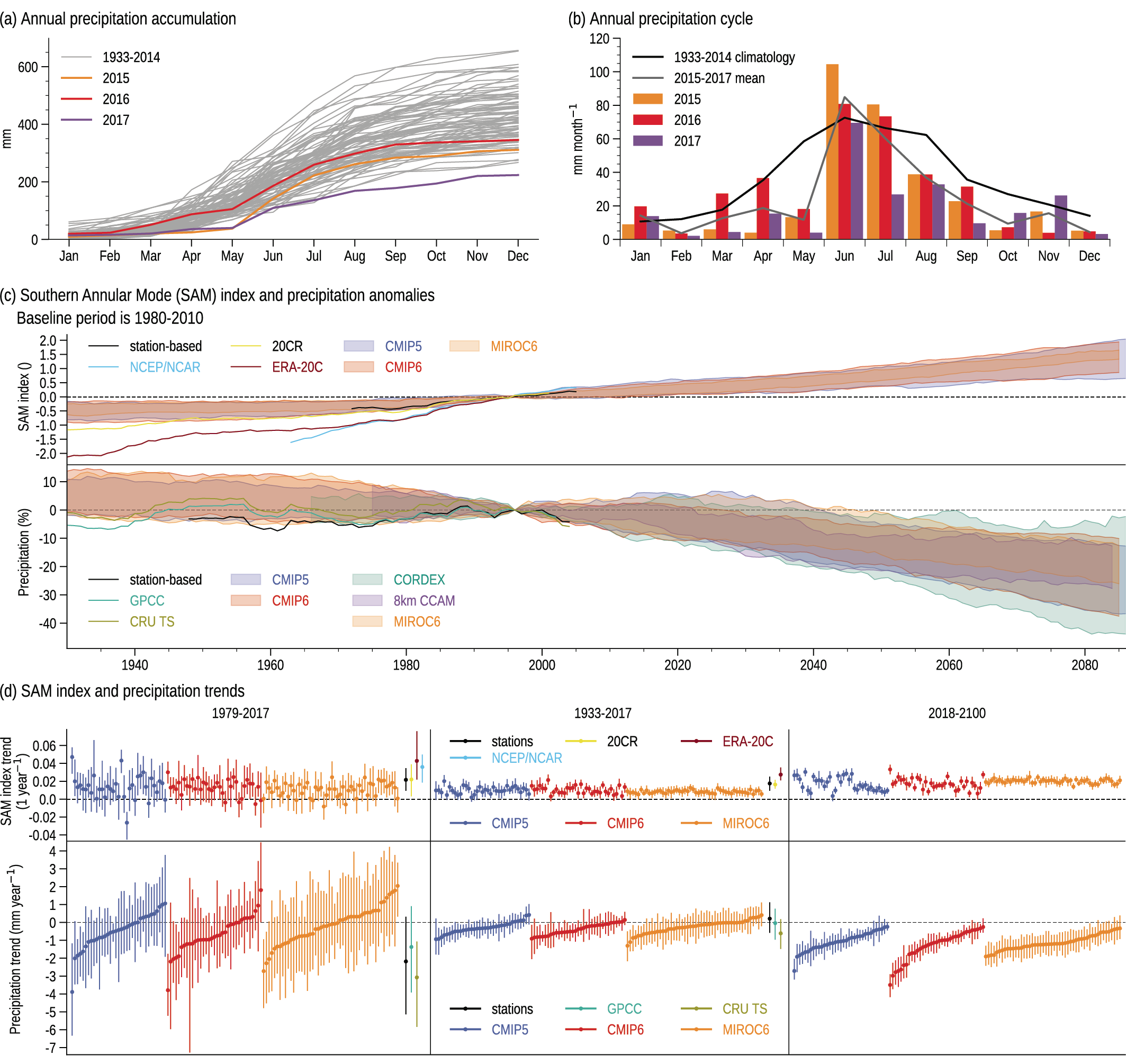
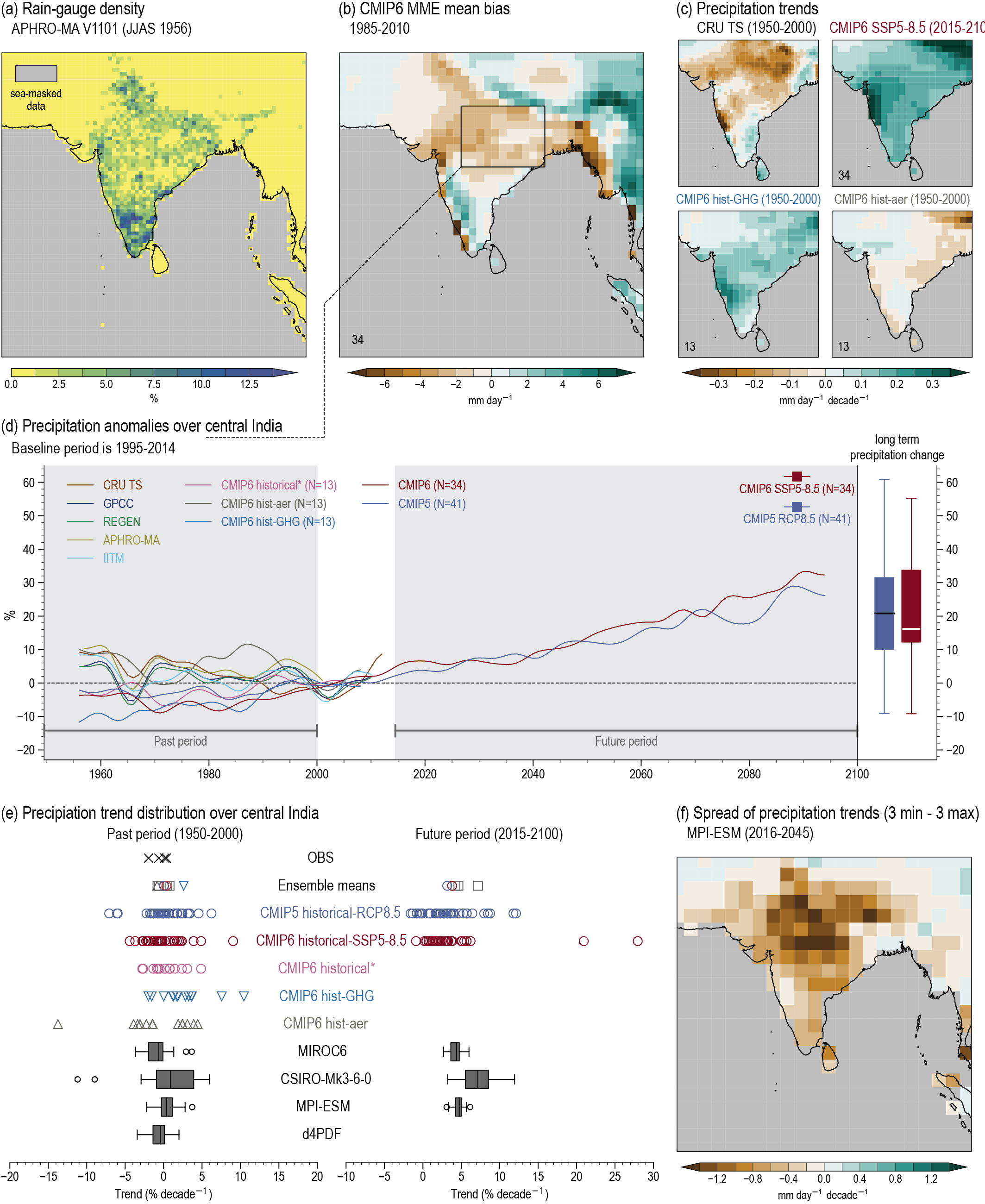
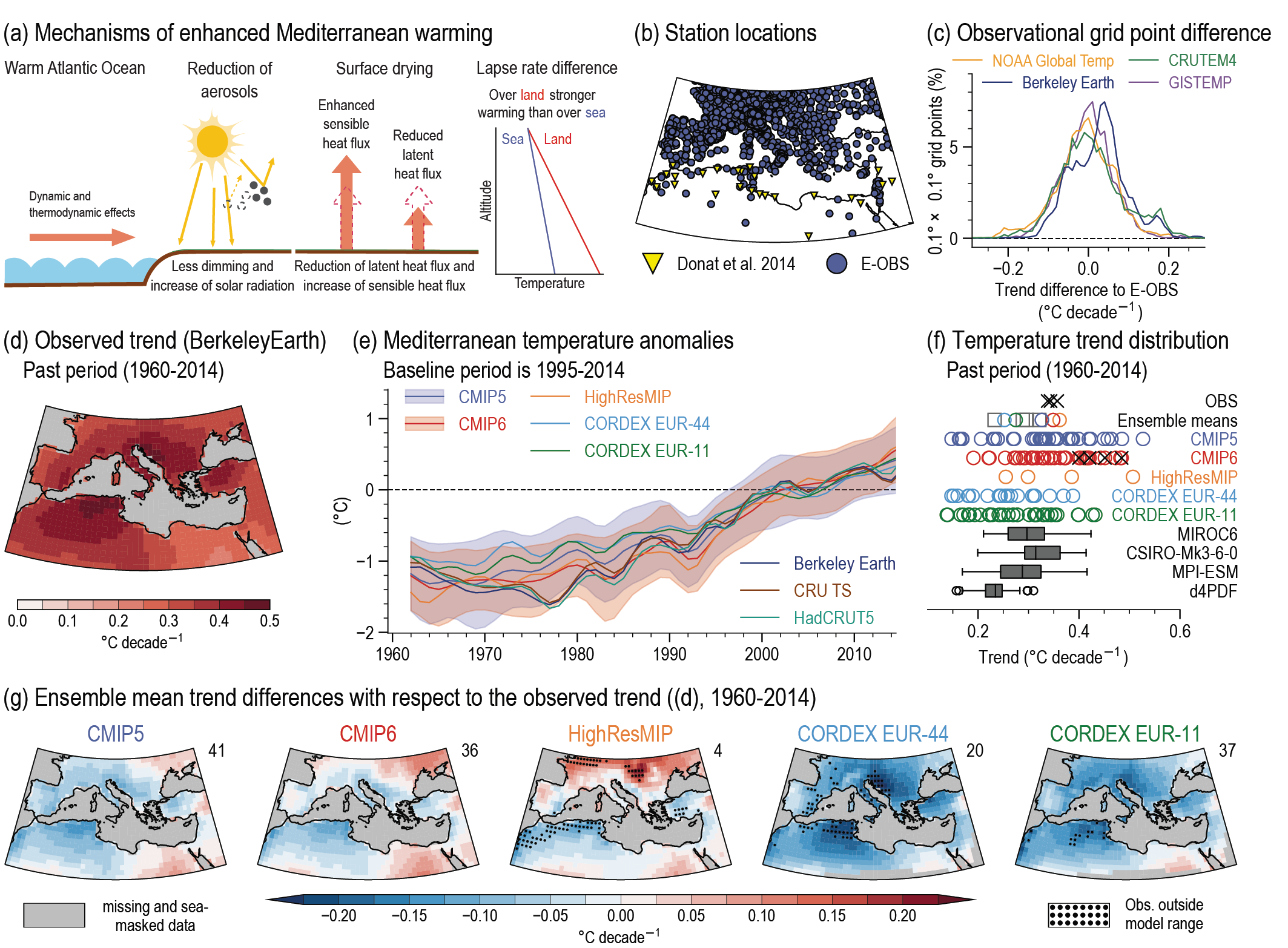
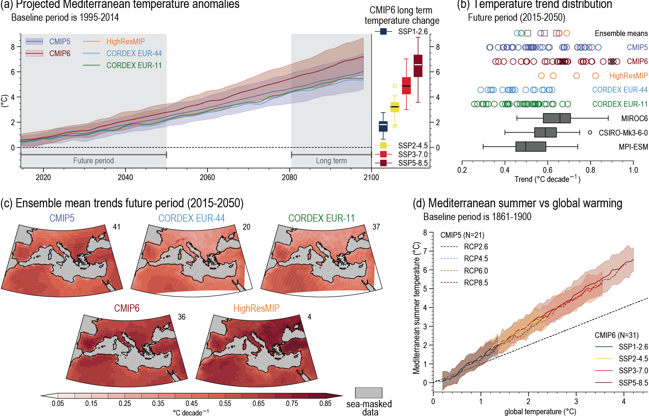
confidence in the distilled regional climate information is enhanced when there is agreement across multiple lines of evidence. For example, the apparent contradiction between the observed decrease in Indian monsoon rainfall over the second half of the 20th century and the projected long-term increase is explained by attribution of the trends to different forcings, with aerosols dominating recently and greenhouse gases in the future (high confidence). For the Mediterranean region, the agreement between different lines of evidence, such as observations, projections by regional and global models, and understanding of the underlying mechanisms, provides high confidence in summer warming that exceeds the global average. {10.5.3, 10.6, 10.6.3, 10.6.4, Cross-Chapter Box 10.3}
The outcome of distilling regional climate information can be limited by inconsistent or contradictory information. Initial observational analyses of the Cape Town drying showed a strong, post-1979 association between increasing greenhouse gases, changes in a key mode of variability (the Southern Annular Mode) and drought in the Cape Town region. However, not all global models show this association, and subsequent analysis extending farther back in time, when human influence was weaker, showed no strong association in observations between the Southern Annular Mode and Cape Town drought. Thus, despite the consistency among global-model future projections, there is medium confidence in a projected future drier climate for Cape Town. Likewise, the distillation process results in low confidence in the influence of Arctic warming on mid-latitude climate because of contrasting lines of evidence. {10.5.3, 10.6.2, Cross-Chapter Box 10.1, Cross-Chapter Box 10.3}
10.1 Foundations for Regional Climate Change Information
10.1.1 Introduction
This chapter assesses the foundations for the distillation of regional climate change information from multiple lines of evidence. The AR5, SR1.5 and SRCCL reports underlined the relevance of assessing regional climate information that is useful and relevant to the decision scale (Box 10.1). To respond to this need, the AR6 WGI Report includes four regional chapters of which this is the first. Chapter 10 assesses the sources and methodologies used by the Chapters 11, 12 and Atlas to construct regional information. Chapter 10 builds on the assessment of methodologies considered to construct global climate change information in Chapters 2 to 4 and on the processes assessed in Chapters 5 to 9. Additionally, this chapter assesses the methodologies for the co-production of regional climate information, the role of the different actors involved in the process and the relevance of the user context and values.
Regional climate change refers to a change in climate in a given region (Section 10.1.2.1) identified by changes in the mean or higher moments of the probability distribution of a climate variable and persisting for a few decades or longer. It can also refer to a change in temporal properties such as persistence and frequency of occurrence of weather and climate extreme events. Regional climate change may be caused by natural internal processes such as atmospheric internal variability and local climate response to low-frequency modes of climate variability (Technical Annex IV), as well as by changes in external forcings such as modulations of the solar cycle, orbital forcing, volcanic eruptions, and persistent anthropogenic changes in the composition of the atmosphere or in land use and land cover (Cross-Chapter Box 3.2; IPCC, 2018a), in addition to the interactions and feedbacks between them. Process interaction in space is pervasive, which means that small spatial scales often have an influence on the larger scales (Palmer, 2013; Sandu et al., 2016). Depending on the context, a region may refer to a large area such as a monsoon region, but may also be confined to smaller areas such as coastlines, mountain ranges or human settlements like cities. Users (understood as anyone incorporating climate information into their activity) often request climate information for these range of scales since their operating and adaptation decision scales range from the local to the sub-continental level.
Given the many types of regional climates, the broad range of spatial and temporal scales (Section 10.1.2), and the diversity of user needs, a variety of methodologies and approaches have been developed to construct regional climate change information. The sources include global and regional climate model simulations, statistical downscaling and bias adjustment methods. A commonly used source is long-term (end-of-century) model projections of regional climate change, as well as near-term (next 10 years) climate predictions (Kushnir et al., 2019; Rössler et al., 2019a). Regional observations, with their associated challenges, are a key source for the regional climate information construction process (Q. Li et al., 2020). High-quality observations that enable monitoring of the regional aspects of climate are used to adjust inherent model biases and are the basis for assessing model performance. Process understanding and attribution of observed changes to large- and regional-scale anthropogenic and natural drivers and forcings are also important sources.
All these sources are used, when available, to distil regional climate information from multiple lines of evidence (Figure 10.1). The resulting climate information can then be integrated, following a co-production process involving both the user and the producer, into a user context that often is already taken into account when constructing the regional climate information. In fact, the distillation process leading to the climate information can consider the specific context of the question at stake, the values of both the user and the producer, and the challenge of communicating across different communities (Section 10.5).
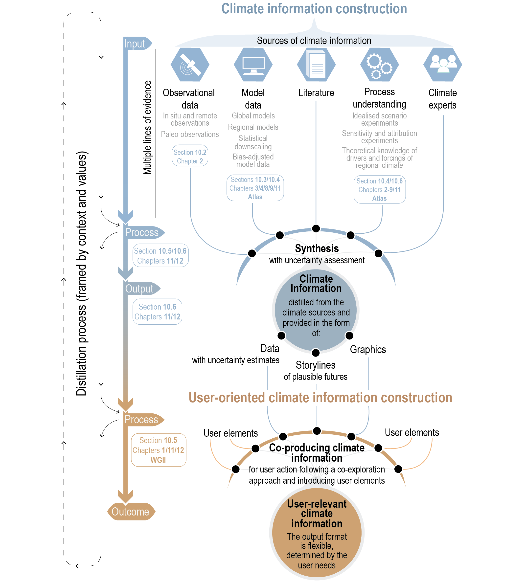 Figure 10.1 | Diagram of the processes leading to the construction of regional climate information (blue) and user-relevant regional climate information (brown). The chapter sections and the other chapters of the Report involved in each step are indicated in rectangles. WGII stands for Working Group II. Literature refers to scientific and technical literature, and climate experts refers to climate scientists, practitioners and local communities, as defined in Section 10.5.
 The chapter (Figure 10.2) starts with an introduction of the concepts used in the distillation of regional climate information (Section 10.1). Section 10.2 addresses the aspects associated with the access to and use of observations, while different modelling approaches are introduced and assessed in Section 10.3. Section 10.3 also addresses the performance of models in simulating relevant climate characteristics as needed to estimate the credibility of future projections. Section 10.4 assesses the interplay between anthropogenic causes and internal variability at regional scales, and its relevance for the attribution of regional climate changes and the emergence of regional climate change signals. Section 10.5 tackles the issue of how regional climate information is distilled from different sources taking into account the context and the values of both the producer and the user. Section 10.6 illustrates the distillation approach using three comprehensive examples. Finally, Section 10.7 lists some limitations to the assessment of regional climate information.
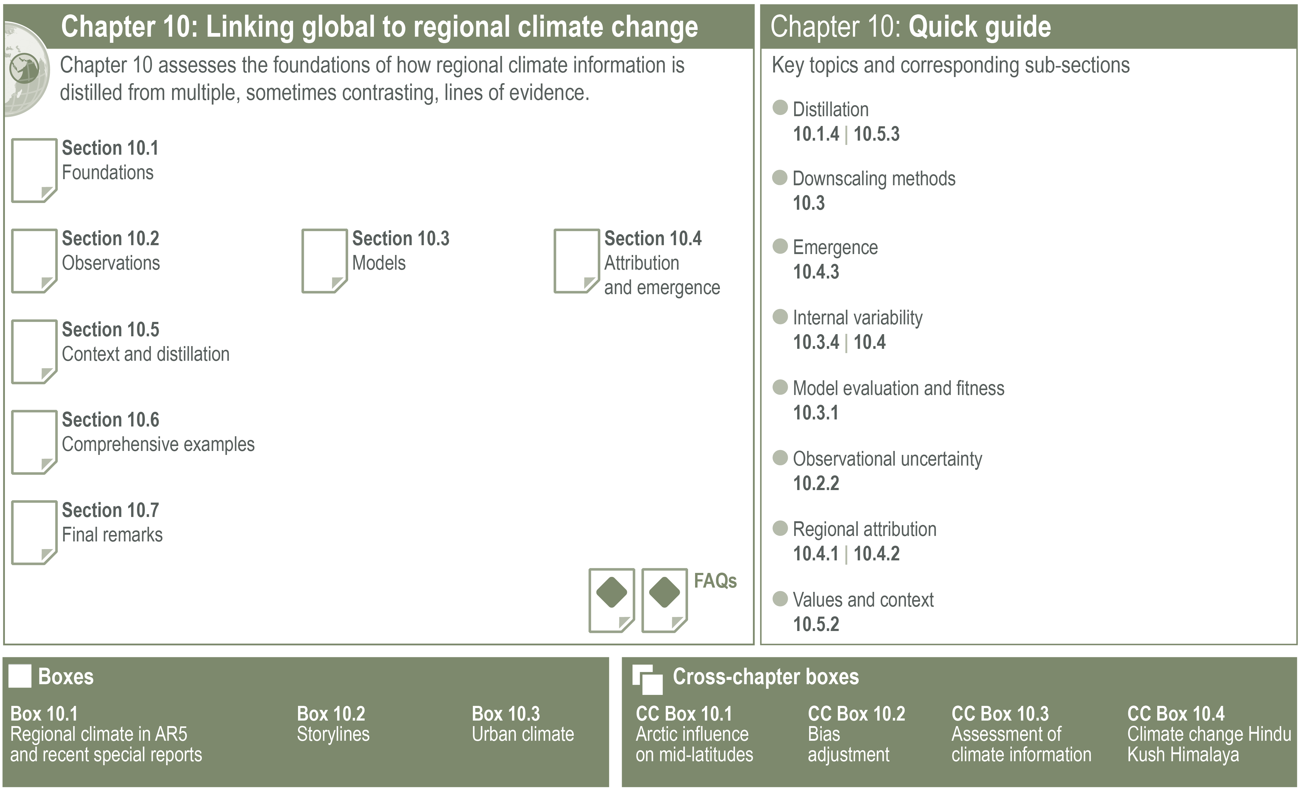
 Figure 10.2 | Visual guide to Chapter 10.
 10.1.2 Regional Climate Change and the Relevant Spatial and Temporal Scales
The global coupled atmosphere–ocean–land–cryosphere system, including its feedbacks, shows variability over a wide spectrum of spatial and temporal scales (Hurrell et al., 2009). This section discusses concepts and definitions of what can be considered a region, the relevant temporal scales and region-specific aspects of the baselines used.
10.1.2.1 Spatial Scales and Definition of Regions
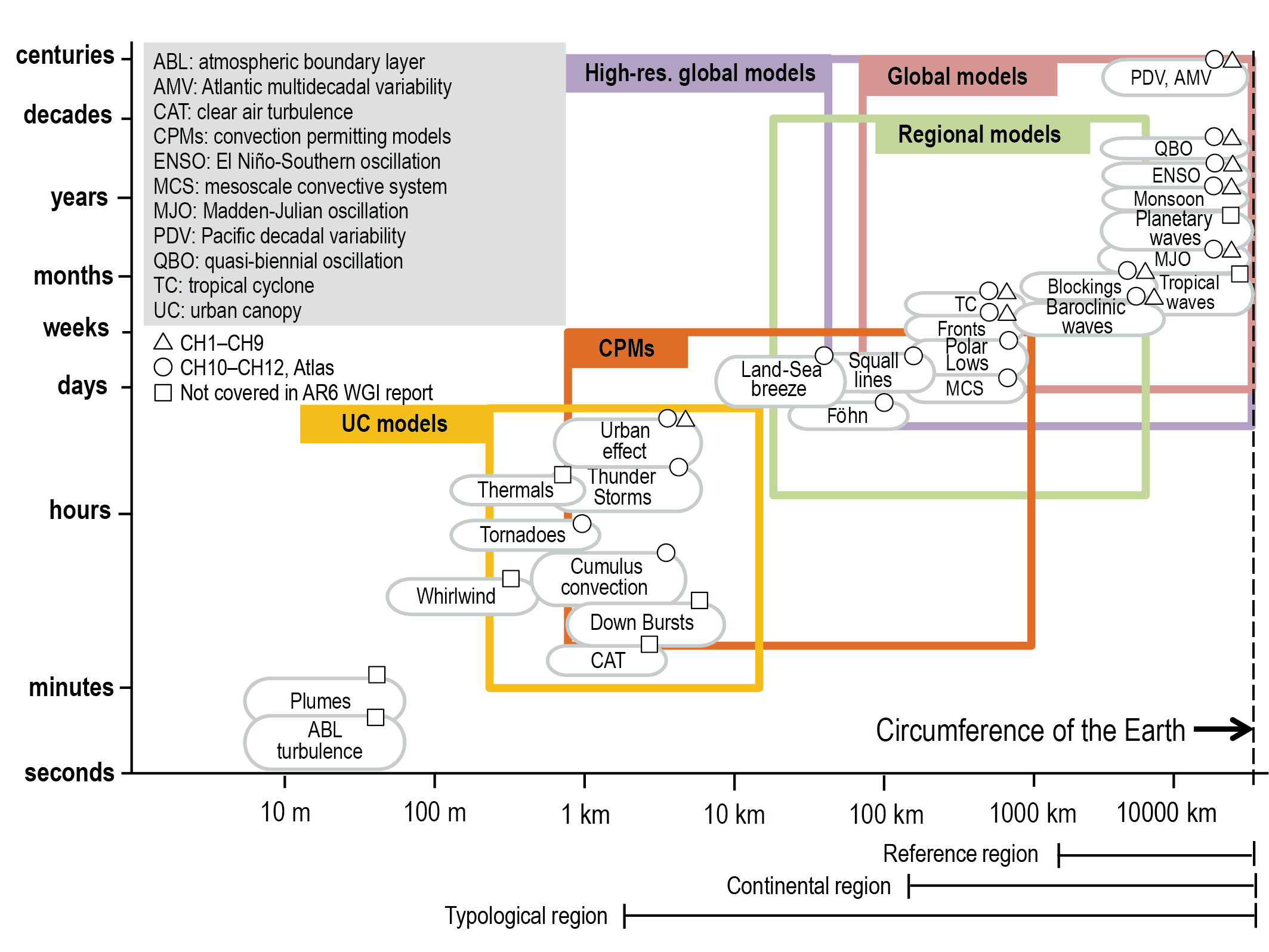
Large-scale climate and the associated phenomena have been defined in Chapter 2 (e.g., Cross-Chapter Box 2.2) as ranging from global and hemispheric, to ocean basin and continental scales. The definition of the regional scale is case specific in the AR6 WGI Report. Section 1.4.5provides definitions of the different regional types adopted by the different chapters. In this chapter, regional scales are defined as ranging from the size of sub-continental areas (e.g., the Mediterranean basin) to local scales (e.g., coastlines, mountain ranges and cities) without prescribing any formal regional boundaries. These spatial length scales range from a few thousand down to a few kilometres and the relevant driving modes and processes at regional scales are summarized in Figure 10.3. In contrast to Chapters 11, 12 and Atlas, which make a region-by-region assessment of climate change, this chapter does not necessarily restrict itself to the use of the AR6 WGI Reference Regions (Section 1.4.5 and Atlas.1.3). Different regional definitions have been used in sections 10.4 and 10.6, selected for their adequacy to illustrate methodological aspects (e.g., for the attribution of long-term regional trends, regions that display such trends have been selected). Typological regions (Section 1.4.5 and Atlas.1.3) are used in Box 10.3 and Cross-Chapter Box 10.4.

Figure 10.3 | Schematic diagramto display interacting spatial and temporal scales relevant to regional climate change information. Figure adapted from Orlanski (1975). The processes included in the different models and model components considered in Chapter 10 are indicated as a function of these scales. The various types of models (including global and regional climate models) for constructing regional climate information are assessed in Section 10.3.1 and Box 10.3.
10.1.2.2 Temporal Scales, Baselines and Dimensions of Integration
The concept of a unified and seamless framework for weather and climate prediction (A. Brown et al., 2012; Hoskins, 2013) provides the context for understanding and simulating regional climate across multiple spatial and temporal scales. This concept is embodied in the subseasonal-to-seasonal (Vitart et al., 2017) and the seasonal-to-multi-annual (Smith et al., 2020) prediction activities that generate regional climate information across temporal scales. The seamless framework benefits from the convergence of methods traditionally used in weather forecasting and climate projections, in particular the role of the initialization in climate models and the strategies for the evaluation of physical processes relevant at different temporal scales.
The relatively short observational record (Section 10.2) is a primary challenge to estimate the forced signal and to isolate low-frequency, multi-decadal and longer-term internal variability (Frankcombe et al., 2015; Overland et al., 2016; Bathiany et al., 2018). Because only one realization of the actual climate exists, it is non-trivial to extract estimates of internal and forced variability from the available data (Frankcombe et al., 2015). As an alternative, approaches that use large observational ensembles can be applied (Section 10.4; McKinnon and Deser, 2018).
There is a close relationship between spatial and temporal scales (Figure 10.3). For example, an individual convective storm may exhibit scales of variability ranging from metres and seconds to kilometres and hours, while for El Niño–Southern Oscillation (ENSO) the scales of variability are regional to hemispheric in extent and multi-year in length. These scales interact and the interactions are represented in climate models, although the ability of current models to simulate regional phenomena and even large-scale climate drivers still leaves room for improvement (Section 10.3) and limits their capability to represent the interactions across spatial and temporal scales.
It is important to note that in this chapter and subsequent regional chapters, including the Interactive Atlas, the baselines and reference periods used for climate change estimates from regional models may vary from those used in Chapters 1 to 9. In these chapters three main time baselines are defined for the past, for example, pre-industrial (before 1750), early industrial (1850–1900) and recent (1995–2014), while the future reference periods are 2021–2040 (near term), 2041–2060 (mid-term) and 2081–2100 (long term) (Section 1.4.1 and Cross-Chapter Box 1.2). Regional climate simulations used in the recent literature have been performed with different baselines. The differences are often due to the availability of the boundary conditions from global simulations, leading to periods chosen for those simulations like 1950–2005, in line with the CMIP5 historical simulations followed by projections from 2005 onwards (Vaittinada Ayar et al., 2016; Zhang et al., 2017; L. Cai et al., 2018). For simulations that use CMIP3 boundary conditions other periods have been used. As a consequence, these regional simulations mix for the recent period historical simulations with projections. The mismatch needs to be considered when assessing results obtained from both global and regional models in the context of the climate information distillation process, or when linking the regional chapters to the assessments performed in previous chapters. The choice of baseline provides a source of uncertainty for the assessment of climate impacts (e.g., for the response of bird species in Africa; Baker et al., 2016). Besides, a range of different baselines may need to be considered to satisfy a variety of users, since this choice affects the perceived result (Dobor and Hlásny, 2019). The influence of the different baseline periods can be explored using the Interactive Atlas where different baselines are available, for example, 1986–2005 (according to AR5), 1995–2014 (this Report), and both 1961–1990 and 1981–2010 (WMO).
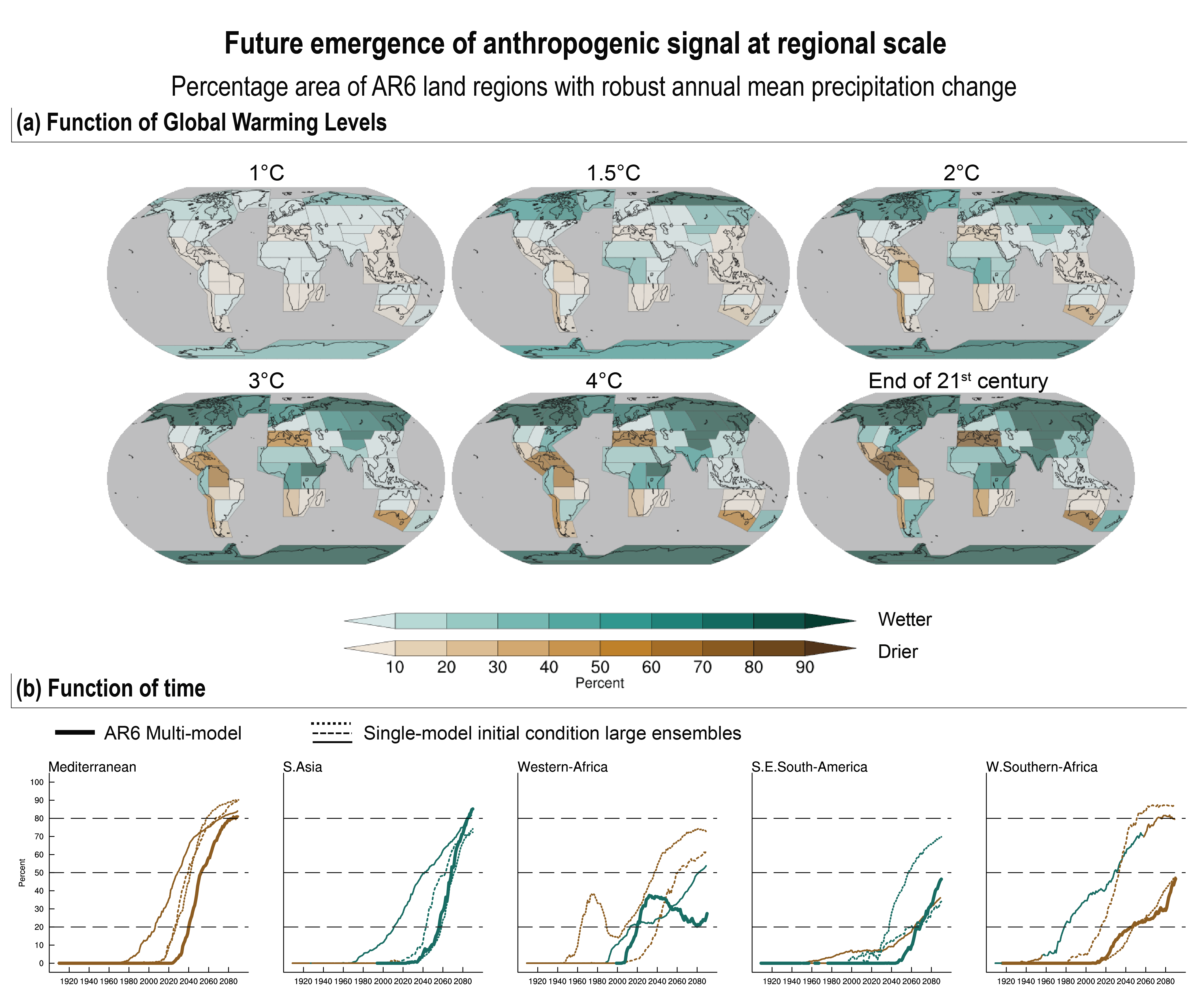
One way of overcoming the baseline uncertainty is to define the results for a given model based on specific global mean temperature changes from the pre-industrial period (e.g., Sylla et al., 2018 for West Africa; Kjellström et al., 2018 for Europe; Taylor et al., 2018 for the Caribbean; Montroull et al., 2018 for South America). The specific global mean temperature is known as global warming level (GWL; Sections 1.6.2 and 10.6.4, and Cross-Chapter Box 11.1). The GWL is a useful dimension of integration because important changes in regional climate, including many types of extremes, scale quasi-linearly with the GWLs, often independently of the underlying emissions scenarios (e.g., Hoegh-Guldberg et al., 2018; Beusch et al., 2020; Seneviratne and Hauser, 2020), always taking into account caveats described in Cross-Chapter Box 11.1. In addition, GWLs allow a separated analysis of the global and regional climate responses associated with a warming level (Section 10.6.4; Seneviratne and Hauser, 2020). The choice of global temperature goal in the context of the 2015 Paris Agreement means that there is an increasing desire for the regional climate information to be expressed as a function of GWLs.
10.1.3 Sources of Regional Climate Variability and Change
Variability in regional climate arises from natural and anthropogenic forcings, internal variability including the local expression of large-scale remote drivers (also known as teleconnections), and the feedbacks between them. Due to the many possible drivers of variability and change (Figure 10.3), quantifying the interplay between internal modes of decadal variability and any externally forced component is crucial in attempts to attribute causes of regional climate changes (e.g., Hoell et al., 2017; Nath et al., 2018). A regional climate signal could arise purely due to some anthropogenic influence or conversely, entirely due to internal variability, but it is most likely the result of a combination of both (Section 10.4). This section briefly introduces these sources of regional variability and should be read along with corresponding sections in Chapters 3, 6 and 7. Section 10.3 assesses their representation in climate models, Section 10.4 discusses their relevance for the attribution of multi-decadal trends and Section 10.6 refers to them as sources in specific examples where regional climate information is built. Section 8.2 offers a companion discussion focussing on changes in the water cycle. An example of how changes in one region could act as a source for changes in a neighbouring one is assessed in the Cross-Chapter Box 10.1 for the linkages between polar and mid-latitude regions, an interaction that has led to substantial recent research. This section also introduces the sources of uncertainty in model-derived regional climate information and how the quantification of the uncertainties influences the confidence of the regional climate information.
10.1.3.1 Forcings Controlling Regional Climate
There are important differences in the processes affected by greenhouse gases (GHGs) over land and ocean. Notably, this leads to preferential warming of the land regions, which are themselves skewed towards the Northern Hemisphere (NH).
Variations in solar forcing (Section 2.2.1) could influence regional climate through its modulation of circulation patterns, although this research field is still hampered by large observational and modelling uncertainties. The 11-year solar cycle has been suggested to affect the leading atmospheric circulation modes of the North Atlantic region in model-based studies (Gray et al., 2013; Thiéblemont et al., 2015; Sjolte et al., 2018). In particular the solar cycle has been suggested as an important source of near-term predictability of the North Atlantic Oscillation (NAO; Kushnir et al., 2019), while other studies have not found evidence for links between the solar cycle and NAO in observational records (Ortega et al., 2015; Sjolte et al., 2018; Chiodo et al., 2019). On centennial time scales, solar fluctuations were found to be correlated with the Eastern Atlantic Pattern (Sjolte et al., 2018). Possible influences on winter circulation and temperature over Eurasia (Chen et al., 2015) and North America (Liu et al., 2014; Li and Xiao, 2018) have also been identified.
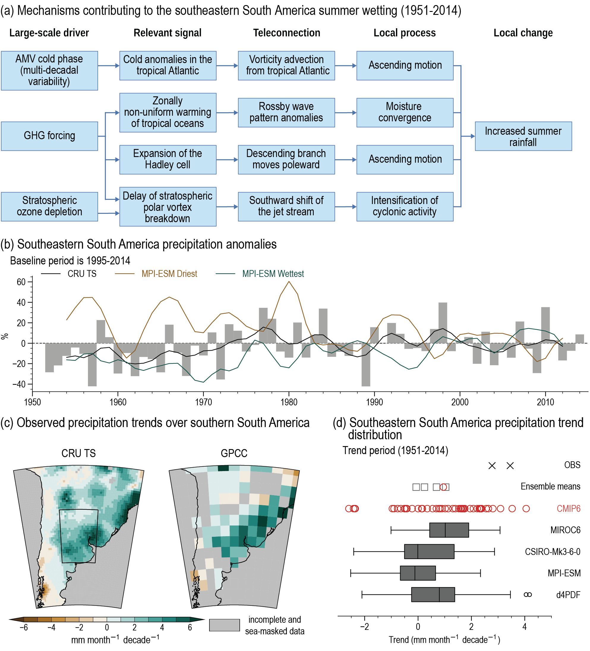
An updated assessment of past changes in stratospheric ozone can be found in Section 2.2.5.2. The AR6 assesses that both GHG and stratospheric ozone depletion have contributed to the expansion of the zonal mean Hadley cell in the Southern Hemisphere (SH) for the period 1981–2000 with medium confidenceSection 3.3.3; Garfinkel et al., 2015; Waugh et al., 2015; Grise et al., 2019). There is medium confidence that stratospheric ozone depletion contributed to the strengthening trend of the summer Southern Annular Mode (SAM) for the period 1970–1990, but this influence has been weaker since 2000 (Section 3.7.2). The poleward shift of the SH westerlies has also been explained by stratospheric ozone depletion (Solman and Orlanski, 2016). Section 10.4 assesses its role in the multi-decadal increase of rainfall in south-eastern South America and Section 10.6.2 does so for the occurrence of the Cape Town drought.
Both natural and anthropogenic aerosols are often emitted at a regional scale, have a short atmospheric lifetime (from a few hours to several days; Section 6.1), are dispersed regionally and affect climate at a regional scale through radiative cooling/heating and cloud microphysical effects (Chapter 8; Rotstayn et al., 2015; Sherwood et al., 2015). The majority of aerosols scatter solar radiation, but with strong regional variations (Shindell and Faluvegi, 2009) that lead to regional radiative effects of up to two orders of magnitude larger than the global average (B. Li et al., 2016; K. Li et al., 2016; Mallet et al., 2016). Black carbon, instead, is known to absorb solar radiation, leading to regional atmospheric warming patterns due to its inhomogeneous spatial distribution (Gustafsson and Ramanathan, 2016). Patterns of forcing generally follow those of aerosol burden. However, temperature and precipitation responses are both local and remote (Z. Li et al., 2016; Kasoar et al., 2018; L. Liu et al., 2018; Samset et al., 2018; Thornhill et al., 2018; Westervelt et al., 2018). For instance, changes in aerosol concentrations in the NH have been reported to modulate monsoon precipitation in West Africa and the Sahel (Undorf et al., 2018; Section 10.4.2.1) and in Asia (H. Zhang et al., 2018; Section 10.6.3).
Natural aerosols include mineral dust, volcanic aerosol and sea salt. The feedback processes between climate and mineral dust as well as sea salt are assessed in Section 6.4, while the volcanic aerosol is dealt with in Cross-Chapter Box 4.1. Mineral dust created by wind erosion of arid and semi-arid surfaces dominates the aerosol load over some areas. The major sources of contemporary dust are located in the arid topographic basins of northern Africa, Middle East, Central and south-west Asia, the Indian subcontinent, and East Asia (Prospero et al., 2002; Ginoux et al., 2012) and emissions are controlled by changes in surface winds, precipitation, and vegetation (Ridley et al., 2014; W. Wang et al., 2015; DeFlorio et al., 2016; Evan et al., 2016; Pu and Ginoux, 2018). Dust both scatters and absorbs radiation and serves as a nuclei of warm and cold clouds (Chapter 6). The surface direct radiative effect is likely negative over land and ocean, especially when the assumed solar absorption by dust is large (Miller et al., 2014; Strong et al., 2015). Surface temperature and precipitation adjust to the direct radiative effect with both sign and magnitude depending on the dust absorptive properties. Dust often cools the surface, but in regions such as the Sahara surface air temperature increases as the shortwave absorption by dust is increased, leading to increases of surface temperature over the major reflective dust sources (Miller et al., 2014; Solmon et al., 2015; Strong et al., 2015; Jin et al., 2016; Sharma and Miller, 2017).
Volcanic eruptions load the atmosphere with large amounts of sulphur, which is transformed through chemical reactions and micro-physics processes into sulphate aerosols (Cross-Chapter Box 4.1; Stoffel et al., 2015; LeGrande et al., 2016). If the plume reaches the stratosphere, sulphate aerosols can remain there for months or years (about two to three for large eruptions) and can then be transported to other areas by the Brewer-Dobson circulation. If the eruption occurs in the tropics, its plume is dispersed across the Earth in a few years, while if the eruption occurs in the high latitudes, aerosols mainly remain in the same hemisphere (Pausata et al., 2015). The global temperature response observed after the last five major eruptions of the last two centuries is estimated to be around –0.2°C (Swingedouw et al., 2017), in association with a general decrease of precipitation (Iles and Hegerl, 2017). Nevertheless, the statistical significance of the regional response remains difficult to evaluate over the historical era (Bittner et al., 2016; Swingedouw et al., 2017) due to the small sampling of large volcanic eruptions over this period and the fact that the signal is superimposed upon relatively large internal variability (Gao and Gao, 2018; Dogar and Sato, 2019). Evidence from paleoclimate observations is therefore crucial to obtain a sufficient signal-to-noise ratio (Sigl et al., 2015). Reconstructed modes of climate variability based on proxy records allow evaluation of the influence on those modes (Zanchettin et al., 2013; Ortega et al., 2015; Sjolte et al., 2018; Michel et al., 2020).
Anthropogenic aerosols play a key role in climate change (Chapter 6). Although the global mean optical depth caused by anthropogenic aerosols did not change from 1975 to 2005 (Chapter 6), the regional pattern changed dramatically between Europe and eastern Asia (Fiedler et al., 2017, 2019; Stevens et al., 2017). Large regional differences in present-day aerosol forcing exist with consequences for regional temperature, hydrological cycle and modes of variability (Chapter 8, Section 10.6). Examples of regions with a notable role for anthropogenic aerosol forcing are the Indian monsoon region (Section 10.6.3) and the Mediterranean basin Section 10.6.4). Anthropogenic aerosols are also very relevant in many urban areas (Box 10.3; Gao et al., 2016; Kajino et al., 2017).
The SRCCL assessed that nearly three-quarters of the land surface is under some form of land use, particularly in agriculture and forest management (Jia et al., 2019). The effects of land management on climate are much less studied than land cover effects although net cropland has changed little over the past 50 years, while land management has continuously changed (Jia et al., 2019). Section 7.3.4.1 assesses the global influence of both land use and irrigation on the effective radiative forcings. Land cover changes and land management can influence climate locally, such as the urban heat island and non-locally as in the case of increased rainfall downwind of a city (Jia et al., 2019; Box 10.3) or the monsoon circulation affected by irrigation (Section 10.6.3). The influence of land cover changes and land management on regional climate extremes is assessed in Section 11.1.6.
It is very likely that the global land surface air temperature response to urbanization is negligible (Section 2.3.1.1.3). However, there is evidence that urbanization may regionally amplify the air temperature response to climate change in different climatic zones (Mahmood et al., 2014), either under present (Doan et al., 2016; Kaplan et al., 2017; X. Li et al., 2018) or future climate conditions (Argüeso et al., 2014; Kim et al., 2016; Kusaka et al., 2016; Grossman-Clarke et al., 2017; Krayenhoff et al., 2018). For instance, in northern Belgium, Berckmans et al. (2019) found that including urbanization scenarios for the near future (up to 2035) have a comparable influence on minimum temperature (increasing it by 0.6°C) to that of the GHG-induced warming under RCP8.5.
10.1.3.2 Internal Drivers of Regional Climate Variability
Internal climate variability on seasonal to multi-decadal temporal scales is substantial at regional scales. This variability arises from internal modes of atmospheric and oceanic variability, intrinsically coupled climate modes, and may additionally be driven by processes other than those originating the modes. It also interacts with the response of the climate system to external forcing. The teleconnections associated with the modes are useful to understand the relationship between large and regional scales (Annex IV: Modes of Variability). A description of various large-scale modes of variability can be found in Chapters 2, 3 and 8, and in Annex IV, while their future projections are assessed in Chapter 4. The specificities of their regional influence are briefly discussed here. More details of their typical temporal scales and regional influences can be found in Annex IV.
Atmospheric modes of variability may have seasonally-dependent regional effects like the North Atlantic Oscillation (NAO) in European winter (Tsanis and Tapoglou, 2019) and summer (Bladé et al., 2012; Dong et al., 2013). Even though these modes are internal to the climate system, their variability can be affected by anthropogenic forcings. For instance, the SAM (Hendon et al., 2014) is both internally driven (Smith and Polvani, 2017), but also affected by recent stratospheric ozone changes (Bandoro et al., 2014). The teleconnections between these modes of variability and surface weather often exhibit considerable non-stationarity (Hertig et al., 2015).
Due to the large ocean heat capacity and their long temporal scales, multi-annual to multi-decadal modes of ocean variability such as the Pacific Decadal Variability (PDV; Newman et al., 2016) and the Atlantic Multi-decadal Variability (AMV; Buckley and Marshall, 2016) are key drivers of regional climate change. In the case of the AMV both natural (volcanic) and anthropogenic (aerosol) external forcings are thought to be involved in its timing and intensity (Section 3.7.7). These modes not only affect nearby regions but also remote parts of the globe through atmospheric teleconnections (Meehl et al., 2013; Dong and Dai, 2015) and can act to modulate the influence of natural and anthropogenic forcings (Davini et al., 2015; Ghosh et al., 2017; Ménégoz et al., 2018b). The dynamics of the ocean modes is simultaneously affected by other modes of variability spanning the full range of spatial and temporal scales due to non-linear interactions (Figure 10.3; Kucharski et al., 2010; Dong et al., 2018). This mutual interdependence can result in changing characteristics of the connection over time (Gallant et al., 2013; Brands, 2017; Dong and McPhaden, 2017), and of their regional climate impact (Martín-Gómez and Barreiro, 2016, 2017). As with atmospheric modes of variability, the regional influence of ocean modes of variability on regional climates can be seasonally dependent (Haarsma et al., 2015).
10.1.3.3 Uncertainty and Confidence
Uncertainty and confidence are treated in the same way in regional climate change information as in larger-scale (continental and global) climate problems (Chapter 1 and Section 10.3.4). The degree of confidence in climate simulations and in the resulting climate information typically depends on the identification of the role of the uncertainties (Section 10.3.4). Since the direct verification of simulations of future climate changes is not possible, model performance and reliable (i.e., trustworthy) uncertainty estimates need to be assessed indirectly through process understanding and a systematic comparison with observations of past and current climate (Section 10.3.3; Knutti et al., 2010; Eyring et al., 2019). The observational uncertainty, which is particularly large at regional scales, also has to be taken into account (Section 10.2). These uncertainty estimates are then propagated in the distillation process to generate climate information.
Uncertainties in model-based future regional climate information arise from different sources and are introduced at various stages in the process (Lehner et al., 2020): (i) forcing uncertainties associated with the future scenario or pathway that is assumed; (ii) internal variability; and (iii) uncertainties related to imperfections in climate models, also referred to as structural or model uncertainty. However, the relative role of each of these sources of uncertainty differs between the global and the regional scales as well as between variables and also between different regions (Lehner et al., 2020). One way to address the internal variability and model uncertainties is to consider results from both multiple models and multiple realizations of the same model (Eyring et al., 2016a; Lehner et al., 2020; Díaz et al., 2021). These models are at times also combined with different weights that are a function of their performance and independence to increase the confidence of the multi-model ensemble (Abramowitz et al., 2019; Brunner et al., 2019).
Other elements that play a role are the inconsistency between the global and regional models in dynamical downscaling or the observational and methodological uncertainty in bias-adjustment methods (Sørland et al., 2018). These elements, in addition to those typical of the uncertainty in global and large-scale phenomena (Chapters 1–9), affect the overall confidence of regional climate information. This complex scene with different sources of uncertainty makes the collection of results available from multi-model, multi-member simulations most useful when synthesized through a distillation process (Section 10.5.3).
10.1.4 Distillation of Regional Climate Information
Regional climate information is synthesized from different lines of evidence from a number of sources (Sections 10.2–10.4) taking into account the context of a user vulnerable to climate variability and change at regional scales (Baztan et al., 2017) and the values of all relevant actors (Corner et al., 2014; Bessette et al., 2017) in a process called distillation (Section 10.5). Distillation, understood as the process of synthesizing information about climate change from different lines of evidence obtained from a variety of sources and taking into account the user context and the values of all relevant actors, allows the connection of global climate change to the local and regional scales, where adaptation responses and policy decisions take place. Climate information is translated into the user context in a co-production process that introduces further user-relevant elements leading to user-relevant climate information (Figure 10.1; Pettenger, 2016; Verrax, 2017) for a specific demand like, for instance, guiding climate-resilient development (Kruk et al., 2017; Parker and Lusk, 2019).
The approaches adopted in the distillation of regional climate information are diverse and range from the simple delivery of data as information to co-production with the user using as many lines of evidence as possible (Lourenço et al., 2016). The availability and selection of the sources and the approach followed has implications for the usefulness of the information. For instance, it is well-established that it is invalid to take a time series from a gridcell of a model simulation as equivalent to an observational estimate of a point within the cell, due to the lack of representativeness (Section 10.3), and consequently the information building solely on this type of data source is of limited use. Relevant decisions are made during the distillation process, such as what method is most suitable to a specific user context and the question being addressed. The information may be provided in the form of summarized raw data, a set of user-oriented indicators, a set of figures and maps with either a brief description, in the form of a storyline, or formulated as rich and complex climate adaptation plans. The information typically includes a description of the sources and assumptions, estimates of the associated uncertainty and its sources, and guidance to prevent possible misunderstandings in its communication.
The choices made for the distillation have typically been part of a linear supply chain, starting from the access to climate data that are transformed into maps or derived climate data products, and finally formulating statements that are communicated and delivered to a broad range of users (Hewitt et al., 2012; Hewitson et al., 2017). This methodology has proven to be valuable in many cases, but it is equally fraught with dangers of not communicating important assumptions, not estimating the impact of relevant uncertainties, and possibly causing misunderstandings in the handover to the user community. This has led to the emergence of new pathways to generate user-oriented climate information, many in the context of emerging climate services (Buontempo et al., 2018; Hewitt et al., 2020), which are assessed in Section 10.5 and in Chapter 12.
10.1.5 Regional Climate Information in the AR6 WGI Report
This chapter is part of a cluster devoted to regional climate (Chapters 10, 11, 12 and Atlas). It introduces many of the aspects relevant to the generation of regional climate information that are dealt with in detail elsewhere. Figure 10.4 summarizes how these chapters relate to one another and to the rest of the report.
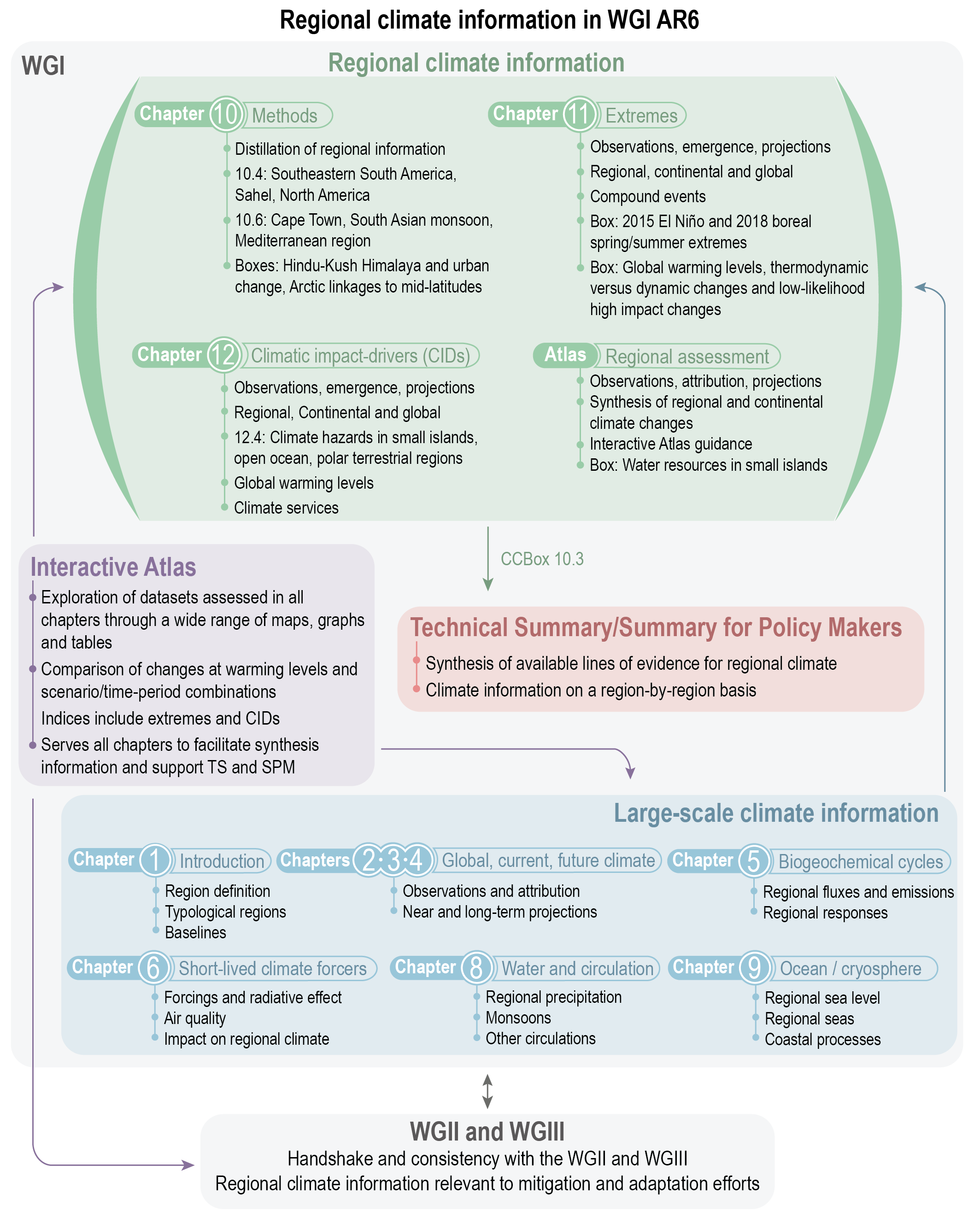
 Figure 10.4 | Schematic diagram that illustrates the treatment of regional climate change in the different parts of the WGI Report and how the chapters relate to each other.
 (Chapter 11 assesses observed, attributed and projected changes in weather and climate extremes, provides a mechanistic understanding on how changes in extremes are related to human-induced climate change and provides regional, continental and global-scale assessments on changes in extremes, including compound events. Chapter 12 identifies elements of the climate system relevant for sectoral impacts referred to as climatic impact-drivers (CIDs), assesses past and future evolutions of sector-relevant CIDs for each AR6 region, synthesizes such evolutions for different time periods and by GWL, and assesses how CIDs are used in climate services. The (Atlas assesses observed, attributed and projected changes in mean climate, performs a comparison of CMIP5, CMIP6 and CORDEX simulations, evaluates downscaling performance and assesses approaches to communicate climate information. The Interactive Atlas facilitates the exploration of datasets assessed in all chapters through a wide range of maps, graphs and tables generated in an interactive manner. This allows for the comparison of changes at warming levels and scenario/time-period combinations, display of indices for extremes and CIDs, and serves all chapters in the report to facilitate synthesis information and support the Technical Summary and the Summary for Policymakers.
Other chapters also include a strong regional component and provide context for the assessment of regional climate. Chapter 1 introduces the different types of climatic regions used in the AR6 WGI Report and the main types of climatic models. Chapter 2 describes the recent and current state of the climate from observations, most of which are key for the production of regional information. Chapter 3 assesses human influence on the climate system and Chapter 4 assesses climate change projections, with a global focus. These three chapters include phenomena that are important for shaping regional climate such as general circulation, jets, storm tracks, blocking and modes of variability. At the same time, the visualization of information in global maps in these chapters provides valuable information for the sub-continental scale. Chapter 5 assesses the knowledge about the carbon and biogoechemical cycles, whose fluxes and responses show variability that is strongly regional in nature. Chapter 6 assesses the regional evolution of short-lived climate forcers as well as their influence on regional climate and air quality. Chapter 8 assesses observed and projected changes in the variability of the regional water cycle, including monsoons, while changes of the regional oceans, changes in cryosphere and regional sea level change are assessed in Chapter 9.
Box 10.1 | Regional Climate in AR5 and the Special Reports SRCCL, SROCC and SR1.5
This box summarizes the information on linking global and regional climate change information in the Fifth Assessment Report (AR5) and the three Special Reports of the IPCC Sixth Assessment Cycle. This information frames the treatment of the production of regional climate information in previous reports and identifies some of the gaps that the AR6 WGI Report needs to address.
Fifth Assessment Report, AR5
In WGI Chapter 9 (Flato et al., 2014), regional downscaling methods were addressed as tools to provide climate information at the scales needed for many climate impact studies. The assessment found high confidence that downscaling adds value both in regions with highly variable topography and for various small-scale phenomena. Regional models necessarily inherit biases from the global models used to provide boundary conditions. Furthermore, the ability of AR5 to systematically evaluate regional climate models (RCMs), and statistical downscaling schemes, were hampered because coordinated intercomparison studies were still emerging. However, several studies demonstrated that added value arises from higher resolution in regions where stationary small-scale features like topography and complex coastlines are present, and from improved representation of small-scale processes like convective precipitation.
WGI Chapter 14 (Christensen et al., 2013) stressed that credibility in regional climate change projections increases when key drivers of the change are known to be well-simulated and well-projected by climate models.
Working Group II (WGII) Chapter 21 (Hewitson et al., 2014b) addressed the regional climate change context from the perspective of impacts, vulnerability and adaptation. This chapter emphasized that a good understanding of decision-making contexts is essential to define the type and scale of information required from physical climate. Further, the chapter identified that the regional climate information was limited by the paucity of comprehensive observations and their analysis along with the different levels of confidence in projections (high confidence). Notably, at the time of AR5, many studies still relied on global datasets, models, and assessment methods to inform regional decisions, which were not considered as effective as tailored regional approaches. The regional scale was not defined but instead it was emphasized that climate change responses play out on a range of scales, and the relevance and limitations of information differ strongly from global to local scales, and from one region to another.
Chapter 21 noted that the production of downscaled datasets (by both dynamical and statistical methods) remains weakly coordinated, and that results indicate that high-resolution downscaled reconstructions of the current climate can have significant errors. Key in this was that the increase in downscaled datasets has not narrowed the uncertainty range, and that integrating these data with historical change and process-based understanding remains an important challenge.
The chapter identified the common perception that higher resolution (i.e., more spatial detail) equates to more usable and robust information, which is not necessarily true. Instead, it is through the integration of multiple sources of information that robust understanding of change is developed.
WGII Chapter 21 highlighted that the different contexts of an impact study are defining features for how climate risk is perceived. Perspectives were characterized as top-down (physical vulnerability) and bottom-up perspectives (social vulnerability). The top-down perspective uses climate change impacts as the starting point of how people and/or ecosystems are vulnerable to climate change, and commonly applies global-scale scenario information or refines this to the region of interest through downscaling procedures. Conversely, in the ‘bottom-up’ approach the development context is the starting point, focusing on local scales, and layers climate change on top of this. An impact focus tends to look to the future to see how to adjust to expected changes, whereas a vulnerability-focused approach is centred on addressing the drivers of current vulnerability.
Box 10.1
Special Report on Climate Change and Land (SRCCL; IPCC, 2019a)
The SRCCL (Jia et al., 2019) assessed that there is robust evidence and high agreement that land cover and land use or management exert significant influence on atmospheric states (e.g., temperature, rainfall, wind intensity) and phenomena (e.g., monsoons), at various spatial and temporal scales, through their biophysical influences on climate. There is robust evidence that dry soil moisture anomalies favour summer heatwaves. Part of the projected increase in heatwaves and droughts can be attributed to soil moisture feedbacks in regions where evapotranspiration is limited by moisture availability (medium confidence). Vegetation changes can also amplify or dampen extreme events through changes in albedo and evapotranspiration, which will influence future trends in extreme events (medium confidence).
The influence of different changes in land use (e.g., afforestation, urbanization), on the local climate depends on the background climate (robust evidence, high agreement). There is high confidence that regional climate change can be dampened or enhanced by changes in local land cover and land use, with sign and magnitude depending on region and season.
Water management and irrigation were generally not accounted for by CMIP5 global models available at the time of SRCCL. Additional water can modify regional energy and moisture balance particularly in areas with highly productive agricultural crops with high rate of evapotranspiration. Urbanization increases the risks associated with extreme events (high confidence). Urbanization suppresses evaporative cooling and amplifies heatwave intensity (high confidence) with a strong influence on minimum temperatures (high confidence).
Special Report on the Ocean and Cryosphere in a Changing Climate (SROCC; IPCC, 2019b)
The SROCC (IPCC, 2019b) stated that observations and models for assessing changes in the ocean and the cryosphere have been developed considerably during the past century but observations in some key regions remain under-sampled and were very short relative to the time scales of natural variability and anthropogenic changes. Retreat of mountain glaciers and thawing of mountain permafrost continues and will continue due to significant warming in those regions, where it is likely to exceed global temperature increase.
The SROCC assessed that it is virtually certain that Antarctica and Greenland have lost mass over the past decade and observed glacier mass loss over the last decades is attributable to anthropogenic climate change (high confidence). It is virtually certain that projected warming will result in continued loss in Arctic sea ice in summer, but there is low confidence in climate model projections of Antarctic sea ice change because of model biases and disagreement with observed trends. Knowledge and observations of the polar regions were sparse compared to many other regions, due to remoteness and challenges of operating in them.
The sensitivity of small islands and coastal areas to increased sea levels differs between emissions scenarios and regionally, and a consideration of local processes is critical for projections of sea level influences at local scales.
Special Report on Global Warming of 1.5°C (SR1.5; IPCC, 2018b)
The SR1.5 (Hoegh-Guldberg et al., 2018) assessed that most land regions were experiencing greater warming than the global average, with annual average warming already exceeding 1.5°C in many regions. Over one quarter of the global population live in regions that have already experienced more than 1.5°C of warming in at least one season. Land regions will warm more than ocean regions over the coming decades (transient climate conditions).
Transient climate projections reveal observable differences between 1.5°C and 2°C global warming in terms of mean temperature and extremes, both at a global scale and for most land regions. Such studies also reveal detectable differences between 1.5°C and 2°C precipitation extremes in many land regions. For mean precipitation and various drought measures there is substantially lower risk for human systems and ecosystems in the Mediterranean region at 1.5°C compared to 2°C.
The different pathways to a 1.5°C warmer world may involve a transition through 1.5°C, with both short- and long-term stabilization (without overshoot), or a temporary rise and fall over decades and centuries (overshoot). The influence of these pathways is small for some climate variables at the regional scale (e.g., regional temperature and precipitation extremes) but can be very large for others (e.g., sea level).
Cross-Chapter Box 10.1 | Influence of the Arctic on Mid-latitude Climate
Coordinator: Rein Haarsma (The Netherlands)
Contributors: Francisco J. Doblas-Reyes (Spain), Hervé Douville (France), Nathan P. Gillett (Canada), Gerhard Krinner (France/Germany, France), Dirk Notz (Germany), Krishnan Raghavan (India), Alex C. Ruane (United States of America), Sonia I. Seneviratne (Switzerland), Laurent Terray (France), Cunde Xiao (China)
The Arctic has very likely warmed more than twice the global rate over the past 50 years with the greatest increase during the cold season (Atlas.11.2). Several mechanisms are responsible for the enhanced lower troposphere warming of the Arctic, including ice albedo, lapse rate, Planck and cloud feedbacks (Section 7.4.4.1). The rapid Arctic warming strongly affects the ocean, atmosphere, and cryosphere in that region (Section 2.3.2.1 and Atlas.11.2). Averaged over the decade 2010–2019, monthly average sea ice area in August, September and October has been about 25% smaller than during 1979–1988 (high confidence) (Section 9.3.1.1). It is very likely that anthropogenic forcings mainly due to greenhouse gas increases have contributed substantially to Arctic sea ice loss since 1979, explaining at least half of the observed long-term decrease in summer sea ice extent (Section 3.4.1.1).
Cross-Chapter Box 10.1
In this box, the possible influences of the Arctic warming on the lower latitudes are assessed. This linkage was also the topic of Box 3.2 of the Special Report on the Ocean and Cryosphere in a Changing Climate (SROCC; IPCC, 2019b). It is a topic that has been strongly debated (Ogawa et al., 2018; K. Wang et al., 2018). Separate hypotheses have emerged for winter and summer that describe possible mechanisms of how the Arctic can influence the weather and climate at lower latitudes. They involve changes in the polar vortex, storm tracks, jet stream, planetary waves, stratosphere-troposphere coupling, and eddy-mean flow interactions, thereby affecting the mid-latitude atmospheric circulation, and the frequency, intensity, duration, seasonality and spatial extent of extremes and climatic impact-drivers like cold spells, heatwaves, and floods (Cross-Chapter Box 10.1, Figure 1). However, we note that a decrease in the intensity of cold extremes has been observed in the Northern Hemisphere mid-latitudes in winter since 1950 (Section 11.3.2; van Oldenborgh et al., 2019). Since SROCC, new literature has appeared, and the mechanisms and their criticisms are assessed here as an update and extension to the SROCC box.
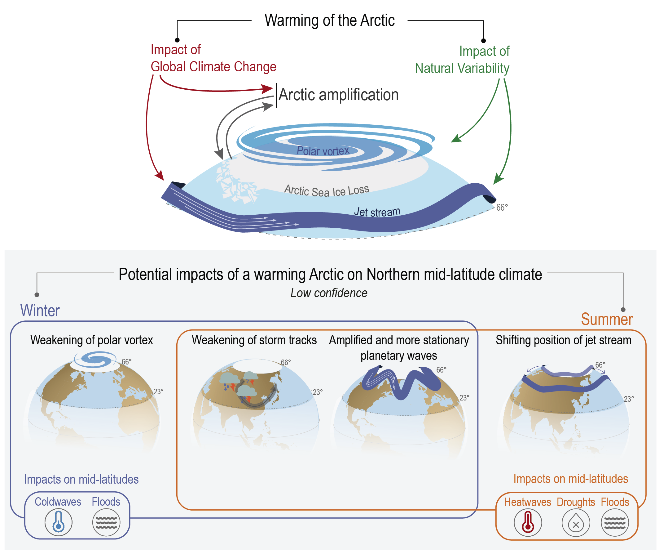
Cross-Chapter Box 10.1, Figure 1 | Mechanisms of potential influences of recent and future Arctic warming on mid-latitude climate and variability. Mechanisms are different for winter and summer with different associated influences on mid-latitudes. The mechanisms involve changes in the polar vortex, storm tracks, planetary waves and jet stream.
Mechanisms for a potential influence in winter
It has been proposed that Arctic amplification, by reducing the equator–pole temperature contrast, could result in a weaker and more meandering jet with Rossby waves of larger amplitude (Francis et al., 2017; Zhang and Luo, 2020). This may cause weather systems to travel eastward more slowly and thus, all other things being equal, Arctic amplification could lead to more persistent weather patterns over the mid-latitudes (Francis and Vavrus, 2012). The persistent large meandering flow may increase the likelihood of connected patterns of temperature and precipitation climatic impact-drivers because they frequently occur when atmospheric circulation patterns are persistent, which tends to occur with a strong meridional wind component. Another possible consequence of Arctic warming is on the NAO/AO that shows a negative trend over the 1990s and early 2000s (Robson et al., 2016; Iles and Hegerl, 2017), and has been linked to the reduction of sea ice in the Barents and Kara seas, and the increase in Eurasian snow cover (Cohen et al., 2012; Nakamura et al., 2015; Yang et al., 2016). During negative NAO/AO the storm tracks shift equatorward and winters are predominantly more severe across northern Eurasia and the eastern United States, but relatively mild in the Arctic. This temperature pattern is sometimes referred to as the ‘warm Arctic–cold continents (WACC)’ pattern (Chen et al., 2018). However, L. Sun et al. (2016) noticed that the WACC is a manifestation of natural variability. Enhanced sea ice loss in the Barents-Kara Sea has also been related to a weakening of the stratospheric polar vortex (Kretschmer et al., 2020) and its increased variability (Kretschmer et al., 2016) that would induce a negative NAO/AO (Kim et al., 2014), the WACC pattern (Kim et al., 2014), and an increase in cold air outbreaks (CAO) in mid-latitudes (Kretschmer et al., 2018). Arctic warming might also increase Eurasian snow cover in autumn caused by the moister air that is advected into Eurasia from the Arctic with reduced sea ice cover (Cohen et al., 2014; Jaiser et al., 2016), although Peings (2019) suggests a possible influence of Ural blockings on both the autumn snow cover and the early winter polar stratosphere. The circulation changes over the Ural-Siberian region are also suggested to provide a link between Barents-Kara sea ice and the NAO (Santolaria-Otín et al., 2021).
Mechanisms for a potential influence in summer
As in winter, Arctic summer warming may result in a weakening of the westerly jet and mid-latitude storm tracks, as suggested for the recent period of Arctic warming (Coumou et al., 2015; Petrie et al., 2015; Chang et al., 2016). Additional proposed consequences are a southward shift of the jet (Butler et al., 2010) and a double jet structure associated with an increase of the land–ocean thermal gradient at the coastal boundary (Coumou et al., 2018). It is hypothesized that weaker jets, diminished meridional temperature contrast, and reduced baroclinicity might induce a larger amplitude in stationary wave response to stationary forcings (Zappa et al., 2011; Petoukhov et al., 2013; Hoskins and Woollings, 2015; Coumou et al., 2018; Mann et al., 2018; R. Zhang et al., 2020), and also that a double jet structure would favour wave resonance (Kornhuber et al., 2017; Mann et al., 2017). Some studies suggest that this is corroborated by an observed increase of quasi-stationary waves (Di Capua and Coumou, 2016; Vavrus et al., 2017; Coumou et al., 2018).
Assessment
The above proposed hypotheses are based on concepts of geophysical fluid dynamics and surface coupling and can, in principle, help explain the existence of a link between the Arctic changes and the mid-latitudes with the potential to affect many impact sectors (Barnes and Screen, 2015). However, the validity of some dynamical underlying mechanisms, such as a reduced meridional temperature contrast inducing enhanced wave amplitude, has been questioned (Hassanzadeh et al., 2014; Hoskins and Woollings, 2015). On the contrary, the reduced meridional temperature contrast has been related to reduced meridional temperature advection and thereby reduced winter temperature variability (Collow et al., 2019).
Studies that support the Arctic influence are mostly based on observational relationships between the Arctic temperature or sea ice extent and mid-latitude anomalies or extremes (Cohen et al., 2012; Francis and Vavrus, 2012, 2015; Budikova et al., 2017). They are often criticized for the lack of statistical significance and the inability to disentangle cause and effect (Barnes, 2013; Barnes and Polvani, 2013; Screen and Simmonds, 2013; Barnes et al., 2014; Hassanzadeh et al., 2014; Barnes and Screen, 2015; Sorokina et al., 2016; Douville et al., 2017; Gastineau et al., 2017; Blackport and Screen, 2020a; Oudar et al., 2020; Riboldi et al., 2020). The role of the Barents-Kara sea ice loss is challenged by Blackport et al. (2019) who find a minimal influence of reduced sea ice on severe mid-latitude winters, and by Warner et al. (2020) who suggest thatthe apparent winter NAO response to the Barents-Kara sea ice variability is mainly an artefact of the Aleutian Low internal variability and of the co-variability between sea ice and the Aleutian Low originating from tropical-extratropical teleconnections. Also Gong et al. (2020) do not find a link between Rossby wave propagation into the mid-latitudes and Arctic sea ice loss. Mori et al. (2019) argue that models underestimate the influence of the Barents-Kara Sea ice loss on the atmosphere, which is disputed by Screen and Blackport (2019). Other studies have stressed the importance of atmospheric variability as a driver of Arctic variability (Lee, 2014; Woods and Caballero, 2016; Praetorius et al., 2018; Olonscheck et al., 2019). Analysing observed key variables of mid-latitude climate for 1980–2020, Blackport and Screen (2020b) and Riboldi et al. (2020) argue that the Arctic influence on mid-latitudes is small compared to other aspects of climate variability, and that observed periods of strong correlation are an artefact of internal variability or intermittency (Kolstad and Screen, 2019; Siew et al., 2020; Warner et al., 2020).
An additional argument in the criticism is the inability of climate models to simulate a significant response to Arctic sea ice loss, larger than the natural variability (Screen et al., 2014; Walsh, 2014; H.W. Chen et al., 2016; Peings et al., 2017; Dai and Song, 2020), or that a very large multi-model ensemble is needed (Liang et al., 2020), although some studies find a significant response in summer, because then the internal variability is weaker (Petrie et al., 2015).
Finally, a warmer Arctic climate can, without any additional changes in atmospheric dynamics, reduce cold extremes in winter due to advection of increasingly warmer air from the Arctic into the mid-latitudes (Screen, 2014; Ayarzagüena and Screen, 2016; Ayarzagüena et al., 2018).
Summarizing, different hypotheses have been developed about the influence of recent Arctic warming on the mid-latitudes in both winter and summer. Although some of the proposed mechanisms seem to be supported by various studies, the underlying mechanisms and relative strength compared to internal climate variability have been questioned. A recent review (Cohen et al., 2020) states that divergent conclusions between model and observational studies, and also between different model studies, continue to obfuscate a clear understanding of how Arctic warming is influencing mid-latitude weather. In this context, Shepherd (2016b) stresses the need for collaboration between scientists with different viewpoints for further understanding that could be achieved by carefully designed, multi-investigator, coordinated, multi-model simulations, data analyses and diagnostics (Overland et al., 2016). In agreement with Box 3.2 of SROCC, there is low to medium confidence in the exact role and quantitative effect of historical Arctic warming and sea ice loss on mid-latitude atmospheric variability.
Regarding future climate, it is important to note that mid-latitude variability is also affected by many drivers other than the Arctic changes and that those drivers as well as the linkages to mid-latitude variability might change in a warmer world. The AMV, PDV, ENSO (see Annex IV), upper tropospheric tropical heating, polar stratospheric vortex, and land surface processes associated with soil moisture (Miralles et al., 2014; Hauser et al., 2016) and snow cover (Nakamura et al., 2019; Sato and Nakamura, 2019) are a few examples. A considerable body of literature has shown that changes to the NAO/AO on seasonal and climate change time scales can be driven by variations in the wavelength and amplitude of Rossby waves, mainly of tropical origin (Fletcher and Kushner, 2011; Cattiaux and Cassou, 2013; Ding et al., 2014; Goss et al., 2016). The influence of future Arctic warming on mid-latitude circulation is difficult to disentangle from the effect of such a plethora of drivers (Blackport and Kushner, 2017; F. Li et al., 2018). One of the consequences of climate change is a poleward shift of the jet induced by the tropical warming (Barnes and Polvani, 2013), which is less obvious in winter especially over the North Atlantic (Peings et al., 2018; Oudar et al., 2020), and the increase of the meridional temperaturegradient in the upper troposphere, which increases storm track activity (Barnes and Screen, 2015; Parding et al., 2019). Although climate models indicate that future Arctic warming and the associated equator–pole temperature gradient decrease could affect mid-latitude climate and variability (Haarsma et al., 2013a; McCusker et al., 2017; Zappa et al., 2018), and even the tropics and subtropics (Deser et al., 2015; Cvijanovic et al., 2017; K. Wang et al., 2018; England et al., 2020; Kennel and Yulaeva, 2020), they do not reveal a strong influence on extreme weather (Woollings et al., 2014).
In conclusion, there is low confidence in the relative contribution of Arctic warming to mid-latitude atmospheric changes compared to other drivers. Future climate change could affect mid-latitude variability in a number of ways that are still to be clarified, and which may also include the influence of Arctic warming. The linkages between the Arctic warming and the mid-latitude circulation are an example of contrasting lines of evidence that cannot yet be reconciled (Section 10.5).
10.2 Using Observations for Constructing Regional Climate Information
Considerable challenges (and opportunities) remain in using observations for climate monitoring, for evaluating and improving climate models (Section 10.3.1), for constructing reanalyses and post-processing model outputs, and therefore, ultimately, for increasing our confidence in the attribution of past climate changes and in future climate projections at the regional scale. While an assessment of large-scale observations can be found in Chapter 2 (Cross-Chapter Box 2.2 and Section 2.3), this section discusses the specific aspects of the observations at regional scale and over the typological regions considered in the regional chapters (Section 10.1.5). This section focuses on land regions and does not consider the specific requirements of ocean observations (see Chapter 9 and SROCC (IPCC, 2019b) for more information on this aspect).
10.2.1 Observation Types and Their Use at Regional Scale
10.2.1.1 In Situ and Remote-sensing Data
Surface or in situ observations can come from a variety of networks: climate reference networks, mesoscale weather and supersite observation networks, citizen science networks, among others, all with their strengths and weaknesses (McPherson, 2013; Thorne et al., 2018). Supersite observatories are surface and atmospheric boundary layer observing networks that measure a large number of atmospheric and soil variables at least hourly over a decade or more, ideally located in rural areas (Ackerman and Stokes, 2003; Haeffelin et al., 2005; Xie et al., 2010; Chiriaco et al., 2018). Adequate calibration of instruments, quality control and homogenization are essential in these sites. They produce valuable data needed to diagnose processes and changes in regional and local climate. Many climate datasets have been developed from in situ station observations, at different spatial scales and temporal frequencies (Annex I: Observational Products). These include sub-daily (Dumitrescu et al., 2016; Blenkinsop et al., 2017), daily (Chen et al., 2008; Camera et al., 2014; Journée et al., 2015; Funk et al., 2015; Aalto et al., 2016; Beck et al., 2017a, b; Schneider et al., 2017) or monthly time scales (Cuervo-Robayo et al., 2014; Aryee et al., 2018). Sub-daily data is useful for estimating storm surge (Mori et al., 2014) or river discharge (Shrestha et al., 2015), daily data for carbon-stock dynamics (Haga et al., 2020) or tourism (Watanabe et al., 2018), and monthly data for beach morphology (Bennett et al., 2019).
Satellite products provide a valuable complement to in situ measurements, particularly over regions where in situ measurements are unavailable. They have been discussed in earlier chapters (e.g., Chapters 2 and 8) for large-scale assessment. Currently 54 essential climate variables (ECVs; Bojinski et al., 2014) are defined by the Global Climate Observing System (GCOS) program, and passed on, for example, to NASA programmes through the Decadal Survey, to the Copernicus Climate Change Service of the European Union, to the ESA Climate Change Initiative ESA-CCI, as well as to the international collaborations with geostationary Earth orbit (GEO) satellites. Their observations are valuable (high confidence) for regional applications since they provide multi-channel images at very high spatiotemporal resolutions, typically 16 channels, 1–2 km, every 10 to 15 minutes. The advanced geostationary satellites are: Himawari-8 and 9 (Kurihara et al., 2016), GOES-East and GOES-17 (Goodman et al., 2018), Meteosat-10 and 11 (Schmetz et al., 2002) and FY-4 (Cao et al., 2014). Geostationary satellite networks or constellations form an essential component of the Global Observation System (https://www.wmo.int/pages/prog/www/OSY/GOS.html), providing measurements not only for various cloud properties and moisture but also for air quality, land and ocean surface conditions, and lightning.
Low Earth orbit (LEO) satellites, with orbits typically at 400–700 km, provide advanced measurements of the Earth’s surface. Sun-synchronous polar orbiters can also cover the polar regions, which cannot be observed with GEO satellites. Examples of LEO observations for land surface monitoring are NASA’s Landsat (Wulder et al., 2016), ESA’s Soil Moisture Ocean Salinity Earth Explorer (SMOS) mission (Kerr et al., 2012), the Sentinel missions of the Copernicus programme, and JAXA’s ALOS-2 (Ohki et al., 2019), providing high spatial resolution land surface images. Many kinds of data are accumulated for land use and land cover studies, targeting aspects like urban footprint (Florczyk et al., 2019), land-cover data (Global Land 30; CCI-LC: ESA, 2021; Chen and Chen, 2018), land surfacetemperature data (Landsat, Parastatidis et al., 2017), and surface albedo (Chrysoulakis et al., 2019).
Availability of active sensors on LEO satellites enables measurement of microphysical properties of aerosol, cloud and precipitation, which can advance regional climate studies and process evaluation studies to improve regional climate models (high confidence). An example is the polar-orbiting ‘afternoon-train’ satellite constellation (known as the A-train), incorporating Aqua, CALIPSO, Cloudsat, PARASOL, Glory and Aura satellites. Vertical profiling observations from Cloudsat (with a W-band cloud radar) and CALIPSO (with a cloud lidar) led to considerable advances in measurements of cloud microphysics (Stephens et al., 2018). Precipitation and its extremes are essential concerns of regional climate studies. The GPM (65°N–65°S, 2014–present) and the preceding TRMM (36.5°N–36.5°S, 1997–2015) with Ku-/Ka-band precipitation radars have provided three-dimensional measurements of precipitation with about 5 km resolution and sub-daily sampling (Skofronick-Jackson et al., 2017). Their non-sun-synchronous observation works to cross-calibrate the constellation satellites to produce global high-resolution mapped products of precipitation, such as Integrated Multi-satellitE Retrievals for GPM (IMERG; Huffman et al., 2007) and the Global Satellite Mapping of Precipitation (GSMaP; Kubota et al., 2007), with hourly sampling at about 11 km resolution. The CPC MORPHing technique (CMORPH) has provided 30 min interval global precipitation with about 8 km coverage since 2002 (Joyce et al., 2004). Precipitation estimations from Remotely Sensed Information using Artificial Neural Networks (PERSIANN) is a sub-daily to daily rainfall product that covers 50°S to 50°N globally with 25 km resolution from 2000 to the present (Nguyen et al., 2019), and is used for semi-global-scale precipitation coverage (Benestad, 2018). TRMM/GPM observations have enabled estimates to be obtained for global four-dimensional convective heating (Shige et al., 2009; Tao et al., 2016; Takayabu and Tao, 2020).
The use of these data has enhanced our understanding of precipitation processes at regional scale (high confidence), such as diurnal cycles in a large river valley (H. Chen et al., 2012), and in coastal (Hassim et al., 2016; Yokoi et al., 2017) and mountainous regions (Hirose et al., 2017). Three-dimensional observations revealed the contrasts in regional characteristics of rainfall extremes in monsoon regions and continental dry regions (Sohn et al., 2013; Hamada and Takayabu, 2018). Satellite measurements are also used to evaluate climate model performance, as well as to develop new parametrizations. As a demonstration of the utility of these products in studying model bias, a subtropical cumulus congestus regime has been identified that may be implicated in the unrealistic double Inter-tropical Convergence Zone (ITCZ) found in some climate models (Takayabu et al., 2010; Hirota et al., 2011, 2014). Another example is a parametrization of a land surface model that was developed specifically for a certain soil type. By assimilating satellite brightness temperature observations with their LDAS-UT scheme, Yang et al. (2007) successfully optimized a land surface model for the Tibetan Plateau.
For application at a regional scale, it is important to consider variations in the spatiotemporal resolution of the satellite products. A simple concatenation of data in time can show artificial jumps that are artefacts of changes in calibration and processing algorithms, or related to satellite orbital stability or changing performance of the instruments (Wielicki et al., 2013; Barrett et al., 2014). Recalibration and cross-calibration are then prerequisites for obtaining homogeneous time series of measurements across different or successive satellites that can then be used to produce long series that are valid as climate data records (Kanemaru et al., 2017; Merchant et al., 2017). Scale representativeness is also an issue in utilizing soil observations (Taylor et al., 2012, 2013). Although a variety of technologies to measure soil moisture at the point scale exist (Dobriyal et al., 2012), its spatial representativeness is less than 1 m2 (Ochsner et al., 2013; L. Liu et al., 2016). Therefore, to be able to use in situ soil moisture for validating coarser-scale data from satellites or models, networks of point-scale measurements are used (Crow et al., 2015; Polcher et al., 2016). Smaller networks are typically of the size of a single climate model gridcell or a satellite pixel and are suitable for monitoring watersheds, while small numbers of those representing larger areas (>100 km2) are emerging (Ochsner et al., 2013).
10.2.1.2 Derived Products
Derived observational products are created from raw datasets collected from surface stations, remote-sensing instruments, or research vessels, which are converted into meaningful physical quantities by applying a suitable measurement theory, using either statistical interpolation techniques (Section 10.2.2.4) or numerical atmospheric and land surface models (Bosilovich et al., 2015).
Most global observational datasets are available at coarse temporal and spatial resolution, and do not include all available station data from a particular region, due to data availability problems. Therefore, efforts have been made to develop regional or country-scale datasets (Annex I). Radar and satellite remote sensing are resources that can provide a valuable complement to direct measurements at regional scale. Examples for precipitation have been described already, some of which have been released to the community (Dinku et al., 2014; Oyler et al., 2015; Manz et al., 2016; Dietzsch et al., 2017; Yang et al., 2017; Bližňák et al., 2018; Krähenmann et al., 2018; Panziera et al., 2018; Shen et al., 2018). However, some of these datasets are limited by their short record, varying between one (Shen et al., 2018) and 64 years (Oyler et al., 2015).
Reanalysis products are numerical climate simulations that use data assimilation to incorporate as many irregular observations as possible. These products encompass many physical and dynamical processes. They generate a coherent estimate of the state of the climate system on uniform grids either at global (Chaudhuri et al., 2013; Balsamo et al., 2015), regional (Chaney et al., 2014; Maidment et al., 2014; Dahlgren et al., 2016; Langodan et al., 2017; Attada et al., 2018; Mahmood et al., 2018) or country scales (Rostkier-Edelstein et al., 2014; Krähenmannet al., 2018; Mahmood et al., 2018).
Reanalyses incorporate an increasing volume of observations from a growing number of sources over time, which sometimes presents a difficulty for trend analysis. However, regional reanalyses are valuable for regional climate assessments, since they can employ high-resolution model simulations due to their limited spatial domain. Their accuracy is also better than global reanalyses since they are often developed over regions with a high density of observational data (sometimes not freely available for all regions) to be assimilated into the model (e.g., Yamada et al., 2012). Regional reanalyses can assimilate locally dense and high-frequency observations, such as from local observation networks (Mahmood et al., 2018; Su et al., 2019) and radar precipitation (Wahl et al., 2017) in addition to the observations assimilated by global reanalyses. In some regional reanalyses, satellite-derived high-resolution sea ice (Bromwich et al., 2016, 2018) and sea surface temperature (Su et al., 2019) are also applied as lower boundary conditions. The periods of regional reanalyses are limited by the availability of the observations for assimilation and by the global reanalyses needed as lateral boundary conditions. Most regional reanalyses cover the past 10 to 30 years. There are also regional reanalysis activities that use conventional observations only, which produce consistent datasets over 60 years to capture precipitation trends, extremes and changes (Fukui et al., 2018). Existing regional reanalyses cover North America (Mesinger et al., 2006), Europe (Dahlgren et al., 2016; Jermey and Renshaw, 2016; Kaspar et al., 2020), the Arctic (Bromwich et al., 2016, 2018), South Asia (Mahmood et al., 2018), and Australia (Su et al., 2019). A project for regional reanalysis covering Japan has also started (Fukui et al., 2018), where grid spacing is between 5 and 32 km, although cumulus parametrizations are still needed to compute sub-grid scale cumulus convection. Recently, reanalyses using convection-permitting regional models have been published (e.g., Wahl et al., 2017, for central Europe).
The data assimilation schemes used in regional reanalyses are often relatively simple methods, specifically nudging (Kaspar et al., 2020) and 3DVAR (Mesinger et al., 2006; Bromwich et al., 2016; Dahlgren et al., 2016), rather than the more complex schemes implemented in state-of-the-art global reanalysis systems. This is partly due to limitations of computational resources. Recently, a number of regional reanalyses using more sophisticated methods, such as 4DVAR and Ensemble Kalman filter, have been published (Jermey and Renshaw, 2016; Fukui et al., 2018; Mahmood et al., 2018; Su et al., 2019). The regional reanalyses also incorporate uncertainties due to deficiencies of the models, data assimilation schemes and observations. To estimate uncertainties, some regional reanalyses apply data assimilation using ensemble forecasts (Bach et al., 2016). Another approach compares multiple regional reanalyses produced with different systems covering the same domain, which represents the uncertainties better than single reanalysis systems with ensemble data assimilation schemes (Kaiser-Weiss et al., 2019).
The regional reanalyses represent the frequencies of extremes and the distributions of precipitation, surface air temperature, and surface wind better than global reanalyses (high confidence). This is due to the use of high-resolution regional climate models (RCMs), as indicated by different regional climate modelling studies (Mesinger et al., 2006; Bollmeyer et al., 2015; Bromwich et al., 2016, 2018; Dahlgren et al., 2016; Jermey and Renshaw, 2016; Fukui et al., 2018; Su et al., 2019). Regional reanalyses, however, retain uncertainties due to deficiencies in the physical parametrization used in RCMs and by the use of relatively simple data assimilation algorithms (Bromwich et al., 2016; Jermey and Renshaw, 2016; Su et al., 2019). Regional reanalyses can provide estimates that are more consistent with observations than dynamical downscaling approaches, due to the assimilation of additional local observations (high confidence) (Bollmeyer et al., 2015; Fukui et al., 2018).
10.2.2 Challenges for Regional Climate Change Assessment
10.2.2.1 Quality Control
The usefulness of any observational dataset is conditioned by the availability and outcome of a quality control (QC) process. The objective of the QC is to verify that data are representative of the measured variable and to what degree the value could be contaminated by unrelated or conflicting factors (WMO, 2017a). Data quality assessment is key for ensuring that the data are credible and to establish trusted relationships between the data provider and the users (Nightingale et al., 2019). QC is performed for all relevant global climate datasets (e.g., Menne et al., 2018). For instance, QC informs users that old reanalysis datasets can be inconsistent in the long term because they assimilated inhomogeneous observations over the reanalyses period (Kobayashi et al., 2015). As a consequence, the evaluation against independent observations suggests that reanalyses should not be automatically regarded as climate-quality products for monitoring long-term trends at the regional level (Manzanas et al., 2014; Torralba et al., 2017). QC needs to be systematically carried out by the institutions responsible for handling the data (e.g., Cao et al., 2016b).
The QC procedure depends strongly on the specific nature of the dataset. It focuses on aspects such as the correct identification of sensor, time and location, detection of unfeasible or inconsistent data, error estimation, assessment of the adequacy of the uncertainty information and the adequacy of the documentation (e.g., Heaney et al., 2016). QC principles also apply to model data (Tapiador et al., 2017). An important piece of information provided is the representativeness error (Section 10.2.1.1; Gervais et al., 2014). When problems in the data representativeness are identified, observational datasets are provided with a quality mask (Contractor et al., 2020), or the problematic dataare either removed or corrected (Ashcroft et al., 2018). These are factors often taken into account in constructing regional climate information (Kotlarski et al., 2019).
Quality-controlled data are now produced widely at the regional level, as in the case of sub-daily precipitation records in the United Kingdom (Blenkinsop et al., 2017) and the USA (Nelson et al., 2016). However, many more datasets and variables lack the same level of scrutiny (Alexander, 2016). Quality-controlled, high-resolution observational datasets are especially needed at regional and local scales to assess models as their resolution increases (Di Luca et al., 2016; Zittis and Hadjinicolaou, 2017), although the awareness and appropriate use of the QC information is challenging (Tapiador et al., 2017) when generating regional climate information (high confidence).
10.2.2.2 Homogenization
Homogenization aims to make data spatially and temporally ‘homogeneous’. Changes in a homogeneous time series are solely due to large-scale climatic changes (whether forced or due to internal variability). Station data are influenced by factors that act at regional scales, from the mesoscale and local scale down to the microscale (WMO, 2019). Station time series contain inhomogeneities such as artificial jumps or trends, which hamper assessments of regional long-term trends. Typical reasons for this are the urbanization of a station’s surroundings, which can lead to warming (Hamdi, 2010; Hansen et al., 2010; Adachi et al., 2012; Jones, 2016; Y. Sun et al., 2016), or relocations outside of the urban area, which could lead to cooling (Tuomenvirta, 2001; Yan et al., 2010; Xu et al., 2013; Dienst et al., 2017, 2019). Another potential source of inhomogeneity is a change in measurement methods that affect most instruments of an observational network over a limited time span, such as the transition to Stevenson screens (Parker, 1994; Böhm et al., 2010; Brunet et al., 2011; Auchmann and Brönnimann, 2012) or to automatic weather stations (WMO, 2017b).
The above examples have been selected as they are present in many stations and without going through homogenization they could potentially have influenced global land warming estimates (Section 1.5.1). Single-break inhomogeneities tend to have a magnitude comparable to global climate change (Tuomenvirta, 2001; Venema et al., 2012) and are thus important for analyses of small regions. Also station records in national networks often have similar changes, making them important for national climate change estimates, but many of these influences are averaged out at the global scale (Jones, 2016).
The main approach to reduce the influence of inhomogeneities in station observations is statistical homogenization by comparing the data from a candidate station with those of neighbouring reference stations in conjunction with the use of metadata (Trewin, 2010). This is a challenging task because both reference and candidate records normally have multiple inhomogeneities. Three challenges should be considered. First, most of our understanding of statistical homogenization stems from the homogenization of temperature observations from dense networks. Recent studies suggest that our ability to remove biases quickly diminishes for sparse networks (Gubler et al., 2017; Lindau and Venema, 2018a). This affects early instrumental data and observations that are not strongly correlated between stations, such as wind and humidity (Chimani et al., 2018).
Second, in addition to systematic errors, homogenized data also suffer from random errors, introduced by the homogenization process. These errors are largest at the station level but are also present in network-averaged signals (Lindau and Venema, 2018b). These errors are determined by the break time series, as well as the noise series and the performance of the homogenization method, are spatially correlated, and have an impact on activities such as interpolation and statistical post-processing of climate simulations (Section 10.2.3.1). Third, the above discussion pertains to the homogenization of monthly and annual means. Homogenization of daily variability around the mean is more difficult. For daily data, specific correction methods are used (Della-Marta and Wanner, 2006; Mestre et al., 2011; Trewin, 2013; C. Zhou et al., 2021) that are able to improve the homogeneity of test cases, although recent independent validation efforts were not able to show much improvement (Chimani et al., 2018). The difference with homogenization methods of monthly and annual means may stem from assumptions on the nature of inhomogeneities for daily data, which are not yet well understood (Chimani et al., 2018).
It is virtually certain that statistical homogenization methods reduce the uncertainties of long-term estimates. Considering a decomposition of the long-term warming error into a bias and a noise uncertainty around the bias, the (trend) bias especially will be reduced, but also most of the noise uncertainty. This conclusion is based on our understanding of the causes of inhomogeneities and their statistical nature combined with the design principles of statistical homogenization methods, as well as on analytical (Lindau and Venema, 2018b), numerical (Venema et al., 2012; Williams et al., 2012) and empirical validation studies (Hausfather et al., 2016; Gubler et al., 2017; Killick et al., 2020).
The above section is about the homogenization of land stations. Satellite data has its own issues and methods for homogenization (Brinckmann et al., 2013; Huang et al., 2015; Brogniez et al., 2016). The homogenization of radiosonde data and land station data use similar methods (Haimberger et al., 2012; Jovanovic et al., 2017).
10.2.2.3 Data Scarcity
Data scarcity arises largely due to the lack of maintenance of observing stations, inaccessibility of the data held in national networks, and uneven spatial distribution of stations that lead to a low density in many regions. This is particularly problematic when trying to assess regional climate change, for which a high density of observational data is desirable. Although in several regions numerous stations provide (monthly) data covering more than 100 years for both temperature and precipitation (GCOS, 2015), large areas of the world remain sparsely covered. The post-1990 decline in the total number of stations contributing to the Global Precipitation Climatology Centre (GPCC) monthly product may be related to delays in data acquisition and not paucity of data (GCOS, 2015). This is because GPCC is the result of a single time scale, single Essential Climate Variable (ECV) and single data collection centre. There is no similar drop-off of the rainfall reports in the Global Historical Climatology Network Daily database (GHCNd, Menne et al., 2012) or the Integrated Surface Database (ISD) at the sub-daily time scale.
Kidd et al. (2017) made some assumptions about GPCC-available gauges and indicated that only 1.6% of Earth’s surface lies within 10 km of a rain gauge, and many areas of the world are beyond 100 km from the nearest rain gauge. Data scarcity is especially critical over Africa (Nikulin et al., 2012; Dike et al., 2018) but the apparent data scarcity could be due to reasons other than actual paucity of data, as stated earlier. For instance, over South Africa, the number of weather stations collecting daily temperature used in the fourth version of the Climatic Research Unit Temperature dataset (CRUTEM4, Osborn and Jones, 2014) has significantly declined since 1980 (Archer et al., 2018). Although CRUTEM4 has now been replaced by CRUTEM5 (Osborn et al., 2021) it has yet to take advantage of the significant international efforts to curate and make available improved global holdings (Rennie et al., 2014) which increased the global available station count for monthly mean temperatures. This includes additional stations from many African countries. The apparent decline in stations since the 1980s could also be due to countries not contributing their data to the SYNOP/CLIMAT networks for reasons other than having non-operational stations.
Even in Europe, precipitation station density in the widely used E-OBS gridded dataset varies largely in space and time across regions (Prein and Gobiet, 2017). This variability is partly due to the reluctance of some data owners to share their data with an international effort. Regardless of the reason, low station density is a major source of uncertainty (Isotta et al., 2015). Kirchengast et al. (2014) and O and Foelsche (2019) found that at least 2 to 5 (12) stations are required for capturing the area-averaged precipitation amount of heavy summer precipitation events on a daily (hourly) basis with a normalized root-mean-square error of less than 20%. Like the E-OBS dataset, gridded daily temperature and precipitation datasets are being developed for other regions of the world. Examples include south-east Asia (SA-OBS, Van den Besselaar et al., 2017), and Latin America and West Africa (ICA&D, Van den Besselaar et al., 2015). Despite the uneven distribution of stations in space and time, the value in these initiatives is illustrated by the large number of studies in which the data product is used. This is the case, for instance, in the work of Condom et al. (2020) over the Andes, a region with prominent data scarcity, and the African Monsoon Multidisciplinary Analyses project over West Africa (AMMA; e.g., Lebel and Ali, 2009). There have been efforts to reduce data scarcity through initiatives such as the International Surface Temperature Initiative (ISTI, Thorne et al., 2011), GHCND, and the Expanding Met Office Hadley Centre ISD with quality-controlled, sub-daily station data from 1931 (HadISD, Dunn et al., 2016).
Data scarcity arising from changing coverage in observation station networks results in substantial problems for climate monitoring (e.g., trend analysis of extreme events requires high temporal and spatial resolutions) or model evaluation (Section 10.3.3.1). It is virtually certain that the scarcity and decline of observational availability in some regions (but not necessarily globally), increase the uncertainty of the long-term global temperature and precipitation estimates. As an example, Lin and Huybers (2019) found that changes in the number of rain gauges after 1975 resulted in spurious trends in extremes of Indian rainfall in a 0.25° gridded dataset spanning the 20th century. In fact, the number of stations used to construct the gridded dataset dropped by half after 1990, leading to inhomogeneity and spurious trends (Section 10.6.3). Over the southern part of the Mediterranean, which is an area sparsely covered by meteorological stations, data scarcity can lead to large uncertainties in the different gridded datasets and strongly affect model evaluation (Section 10.6.4). Satellite observations can compensate the ground-based precipitation radar data sparsity to prevent an oversight of significant climate change signals (Yokoyama et al., 2019).
There are techniques for estimating and reconstructing missing data. The methods depend on the variable of interest, the temporal resolution (e.g., daily or monthly), and the type of climate (wet or dry), among others. There has been very little evaluation of the performance of classical and data mining methods (e.g., Sattari et al., 2017). The classical methods include the arithmetic mean, inverse distance weighting method, multiple regression analysis, multiple imputation, and single best estimator, while the data-mining methods include multilayer perceptron artificial neural network, support vector machine, adaptive neuro-fuzzy inference system, gene expression programming method, and K-nearest neighbour. Crowd-sourced data (individuals contribute their own data points to create a dataset for others to use) could play a role in minimizing data scarcity (Section 10.2.4).
10.2.2.4 Gridding
Derived gridded datasets require merging data from different sources of observations and/or reanalysis data on a regular grid (Section 10.2.1.2; e.g., Xie and Arkin, 1997). However, in situ observations are distributed irregularly, especially over sparsely populated areas. This leads to an interpolation challenge. Gridded products of climate variables, including temperature and precipitation, are strongly affected (high confidence) by the interpolation method over complex orography and data scarce regions (Hofstra et al., 2008; Herrera et al., 2016).
There are two main approaches to produce gridded datasets: (i) based on in situ observations only, and (ii) combining in situ observations with remote-sensing data and/or reanalysis data. The first approach has been widely employed in regions with high station density using interpolation techniques, such as inverse-distance weighting, optimal interpolation, and kriging (Chen et al., 2008; Haylock et al., 2008; Frei, 2014; Isotta et al., 2014; Masson and Frei, 2014; Hiebl and Frei, 2016; Nguyen-Xuan et al., 2016). The second approach has been mainly applied in data-sparse regions with low station density, using simple bias adjustment, quantile mapping, and kriging techniques with in situ observations, remote-sensing and reanalysis data (Cheema and Bastiaanssen, 2012; Erdin et al., 2012; Dinku et al., 2014; Abera et al., 2016; Krähenmann et al., 2018).
Gridding of station data is affected by uncertainties stemming from measurement errors, inhomogeneities, the distribution of the underlying stations and the interpolation error, with station density being the dominant factor (Herrera et al., 2019). Uncertainty due to interpolation is typically small for temperature but substantial for precipitation and its derivatives, such as drought indices (Chubb et al., 2015; Hellwig et al., 2018). The largest uncertainties typically occur in sparsely sampled mountain areas (Section 10.2.2.5). Interpolation generally give rise to smoothing effects, such as low variability of the derived dataset with respect to the in situ observations (Chen et al., 2019). As a result, the effective resolution of gridded data is typically much lower than its nominal resolution. For instance, a 5 km gridded precipitation dataset for the European Alps has an effective resolution of about 10 to 25 km (Isotta et al., 2014). In an example for precipitation in Spain, the effective resolution converged to the nominal resolution only when at least 6 to 7 stations were inside the gridcell (Herrera et al., 2019). To account for the smoothing errors, new stochastic ensemble observation datasets have been introduced (Von Clarmann, 2014).
10.2.2.5 Observations in Mountain Areas
Spatiotemporal variability of meteorological parameters observed over mountainous areas is often large, indicating strong control exerted by local topography on meteorological parameters (Gultepe et al., 2014). Difficult access, harsh climatic conditions as well as instrumental issues make meteorological measurements extremely challenging at higher elevations (Azam et al., 2018; Beniston et al., 2018). Measurements of wind speed, temperature, relative humidity and radiative fluxes are critical for climate model evaluation, but difficult to handle due to their point-scale representativeness and small-scale spatiotemporal variability over mountainous terrain, and often need adjustment (Gultepe, 2015). High-altitude (>3000 metres) permanent meteorological stations are limited and current knowledge is mainly based on valley-bottom or low-elevation meteorological stations (Qin et al., 2009; Lawrimore et al., 2011; Gultepe, 2015; Condom et al., 2020), which, generally do not represent the higher elevation climate (Immerzeel et al., 2015; Shea et al., 2015).
Measuring precipitation amounts, especially of solid precipitation, in mountainous areas is particularly challenging due to the presence of orographic barriers, strong vertical and horizontal precipitation rate variability, and the difficulty in finding representative sites for precipitation measurements (Barry, 2012). However, the precipitation amounts can be indirectly estimated by the observed point mass balances at glacier accumulation areas representing net snow accumulation (Haimberger et al., 2012; Immerzeel et al., 2015; Sakai et al., 2015; Azam et al., 2018). There is very high confidence that precipitation measurements, especially solid precipitation, in mountainous areas are strongly affected by the gauge location and setup. Precipitation measurements are also affected by the type of measurement method, presence/absence of shielding, presence/absence of a heating system and operating meteorological conditions (Nitu et al., 2018). Solid precipitation measurements may have errors ranging from 20% to 50%, largely due to under-catch in windy, icing and riming conditions (Rasmussen et al., 2012), and therefore require corrections by applying transfer functions developed mainly from collected wind speed and temperature data (Kochendorfer et al., 2017). The latest Solid Precipitation Intercomparison Experiment (SPICE) report recommends measurements of wind speed, wind direction and temperature as the minimum standard ancillary data for solid precipitation monitoring (Nitu et al., 2018).
Recent advances in remote-sensing methods provide an alternative, but they also have limitations over mountainous areas. Different versions of the Tropical Rainfall Measuring Mission (TRMM) products were found to perform differently over mountainous areas (Zulkafli et al., 2014). Orographic heavy rainfall associated with Typhoon Morakot in 2009 was severely underestimated in all microwave products including TRMM 3B42 (Shige et al., 2013). The underestimation has been mitigated in the Global Satellite Mapping of Precipitation (GSMaP) product by considering the orographic effects (Shige et al., 2013). Studies have suggested a high accuracy of passive optical satellite (e.g., MODIS, Landsat) snow products under clear skies when compared with the field observations. However, cloud masking and sub-pixel cloud heterogeneity in these snow-cover products considerably restrict their applications (Kahn et al., 2011; Brun et al., 2015; Tang et al., 2017; Stillinger et al., 2019). Gridded datasets (e.g., CRU, GPCC Full Data Product, GPCC Monitoring Product, ERA-Interim, ERA5, ERA5-land, MERRA-2, MERRA-2 bias adjusted, PERSIANN-CDR) are of paramount importance, yet they often lack enough in situ observations to improve the temporal and spatial distribution of meteorological parameters over complex mountain terrain (Zandler et al., 2019).
10.2.2.6 Structural Uncertainty
Beyond climate monitoring, the quality and availability of multiple observational reference datasets play a central role in model evaluation. In fact, when using observations for model evaluation, there are multiple examples where inter-observational uncertainty is as large as the inter-model variability. This has been shown for various aspects of the Indian monsoon (Section 10.6.3; Collins et al., 2013a) and for precipitation uncertainties over Africa (Section 10.6.4; Nikulin et al., 2012; Sylla et al., 2013; Dosio et al., 2015; Bador et al., 2020) and Europe (Prein and Gobiet, 2017). Kotlarski et al. (2019) compared three high-resolution observational temperature and precipitation datasets (E-OBS, a compilation of national/regional high-resolution gridded datasets, and the EURO4M-MESAN 0.22° reanalysis based on a high-resolution limited-area model) with five EURO-CORDEX RCMs driven by ERA-Interim. Generally, the differences between RCMs are larger than those between observation datasets, but for individual regions and performance metrics, observational uncertainty can dominate. They also showed that the choice of reference dataset can have an influence on the RCM performance score. Over the high mountain Asia region and East Asia, differences among gridded precipitation datasets can generate significant uncertainties in deriving precipitation characteristics (J. Kim et al., 2015; Kim and Park, 2016; Guo et al., 2017). Over western North America, observational uncertainty induces differences in multi-decadal precipitation trends (Lehner et al., 2018). Taking a very different perspective, the agreement between model simulations may be used to estimate the uncertainty and quality of observations (Massonnet et al., 2016). There is high confidence that an ensemble of multiple observational references at a regional scale is fundamental for model performance assessment. The uncertainties vary according to region, season, and statistical properties (Cross-Chapter Box 10.2).
10.2.3 Other Uses of Observations at Regional Scale
10.2.3.1 Observations for Calibrating Statistical Methods
Statistical downscaling, bias adjustment and weather generators are post-processing methods used to derive climate information from climate simulations. They all require observational data for calibration as well as evaluation (Section 10.3.3.1). Typically, the so-called perfect prognosis methods use quasi-observations for the predictors (i.e., reanalyses) and actual observations for the predictands (the surface variables of interest). By contrast, bias adjustment methods use observations only for the predictands. Weather generators typically require only observed predictands, although some are conditioned on observed predictors as well. Very often these methods are based on daily data, because of user needs, but also because of the limited availability of sub-daily observations and the limited ability of climate models to realistically simulate sub-daily weather (Iizumi et al., 2012). Some methods are calibrated on the monthly scale, but some of the generated time series are then further disaggregated to the daily scale (e.g., Thober et al., 2014). A few methods, mainly weather generators, represent sub-daily weather (Mezghani and Hingray, 2009; Kaczmarska et al., 2014). Many methods simulate temperature and precipitation only, although some also represent wind, radiation and other variables. The limited availability of high quality and long observational records typically restricts these applications to a few cases (Verfaillie et al., 2017; Pryor and Hahmann, 2019). Overall, there is high confidence that limited availability of station observations, including variables beyond temperature and precipitation as well as sub-daily data, limit the use of statistical modelling of regional climate.
All the limitations and challenges of observational data discussed in Section 10.2.2 also apply to its use for post-processing of climate model data. High quality and long observational data series are particularly relevant to quantify uncertainties. Different reanalyses present significant discrepancies when used as key predictor variables at the daily scale and may even affect the downscaled climate change signal (Brands et al., 2012; Dayon et al., 2015; Manzanas et al., 2015; Horton and Brönnimann, 2019). There is high confidence that reanalysis uncertainties limit the quality of statistical downscaling in some regions, although no assessment has been made for the most recent reanalysis products.
An important issue for bias adjustment is the correct representation of the required spatial scale. Ideally, bias adjustment is calibrated against area-averaged data of the same spatial scale as the climate model output. Hence, high-quality observed gridded datasets with an effective resolution close to the nominal model resolution are required. Driven by the need to also generate regional-scale information in station-sparse regions, researchers have considered derived datasets that blend in situ and remote-sensing data to produce high-resolution observations to be used as predictands (Sections 10.2.1.2 and 10.2.2.4; Haiden et al., 2011; Wilby and Yu, 2013).
10.2.3.2 Observation for Paleoclimate Data Assimilation
Following some early concept studies, the first practical applications of paleoclimate data assimilation over past centuries used only selected data to reconstruct past climate changes for analysis of a specific process or case (Widmann et al., 2010). Recently, assimilation of multiple series from various data sources, including tree rings, ice cores, lake cores, corals, and bivalves, has allowed production of reconstructions that can be widely shared and applied to multiple purposes, as with modern reanalyses (Hakim et al., 2016; Franke et al., 2017; Steiger et al., 2018; Tardif et al., 2019). Most of these paleo-reanalyses are global but there are products using regional models or targeted at specific regions such as Europe, East Africa and the Indian Ocean (Fallah et al., 2018; Klein and Goosse, 2018).
Paleo-reanalyses are enabling a new range of applications and have already provided useful information on seasonal-to-multi-decadal climate variability over past millennia. They are useful tools to study the co-variance between variables at interannual-to-centennial time scales and at regional to global spatial scales. In particular, they have highlighted the processes that can be responsible for changes in continental hydrology at multi-decadal time scales (Franke et al., 2017; Klein and Goosse, 2018; Steiger et al., 2018). Paleo-reanalyses have confirmed a large contribution of internal variability in past changes at regional scale during the pre-industrial period, superimposed on a weak common signal due to forcing changes (Goosse et al., 2012) and the absence of a globallycoherent warm period in the common era before the recent warming (Neukom et al., 2019). Reconstructions of the atmospheric state obtained in the reanalysis also provide robust evidence of a local enhancement of warming or cooling conditions due to changes in atmospheric circulation, such as for the warm conditions in some European regions around 950–1250 CE, the cooling observed in 1809/1810, or the cold and rainy 1816 summer in Europe (Cross-Chapter Box 4.1; Goosse et al., 2012; Hakim et al., 2016; Franke et al., 2017; Schurer et al., 2019).
10.2.4 Outlook for Improving Observational Data for Regional Climates
An encouraging development for understanding climate variations over the past 250 years or so at the global and regional scale lies in the field of data rescue, in which hitherto hidden archives of meteorological data are brought to the forefront (Sections 1.5.1.1 and 2.5). Surface observations from data rescue projects may then be assimilated to derive long-term high-resolution gridded surface regional reanalysis (Devers et al., 2020). Global extended reanalyses such as 20CR (Compo et al., 2011), ERA-20C (Poli et al., 2016a, b) or CERA-20C (Laloyaux et al., 2018) may be further downscaled to quantify the variability of past climate at the regional scale (Caillouet et al., 2016, 2019).
One of the main scientific challenges related to high-resolution regional climate modelling is dealing with the representation of fine-scale processes (e.g., Yano et al., 2018) in observational datasets. Additionally, reliable observation networks following WMO standards have a very sparse geographical representation. Hence, regional climate models have started to use high-resolution data combined with crowdsourced observations (Zheng et al., 2018). Recent efforts have led to the production of homogeneously processed long-term datasets for regional climate model evaluation (Goudenhoofdt and Delobbe, 2016; Humphrey et al., 2017; Yang and Ng, 2019). While they are far less reliable and accurate than professional observations, crowdsourced data are abundantly available and can give spatial representations at very high resolution. This technological trend could prove very useful (high confidence), and the regional climate community is making efforts to understand the extent to which these data sources can be exploited, at least as a complement to traditional datasets (Overeem et al., 2013; Meier et al., 2017; Uijlenhoet et al., 2018; de Vos et al., 2019; Langendijk et al., 2019b).
10.3 Using Models for Constructing Regional Climate Information
Much of the information available on future regional climate arises from studies based on climate model simulations (Chapters 3, 4 and 8). In this section, different types of models (Section 10.3.1) and model experiments (Section 10.3.2) for generating regional climate information are discussed, followed by an assessment of the performance, added value, and fitness-for-purpose of different model types (Section 10.3.3). The focus is on the representation of large- to local-scale phenomena and processes relevant for regional climate. Finally, uncertainties of regional climate projections and methodologies to manage these are assessed (Section 10.3.4).
10.3.1 Model Types
Regional climate change information may be derived from a hierarchy of different model types covering a wide range of spatial scales and processes (Figure 10.5). The application of any model relies on assumptions, depending on the specific model as well as the application. Table 10.1 gives an overview of the generic assumptions of the different model types discussed here for generating regional climate information. The violation of these assumptions will affect the model performance, which is discussed in Section 10.3.3.
Model Type | Scale at Which the Assumption Applies | Assumptions to Realistically Simulate Present Regional Climate | Additional Assumptions to Be Fit for Simulating Future Regional Climate |
Global model i.e., atmosphere-only general circulation model, global climate model, Earth system model (AGCM, GCM or ESM; not bias adjusted) (Section 10.3.1.1) | Large (>1000 km) | Global model includes all relevant large-scale forcings and realistically simulates relevant large-scale circulation (Sections 3.3.3, 8.5.1 and 10.3.3.3). | Global model realistically simulates processes controlling large-scale changes. Parametrizations are valid in future climate (Chapter 3, and Sections 4.2, 4.5, 8.5.1 and 10.3.3.9). |
Regional (<1000 km) | Global model includes all relevant regional forcings and realistically simulates all relevant regional-scale processes and feedbacks and their dependence on large-scale climate (Sections 8.5.1, 10.3.3.4–10.3.3.6 and 10.3.3.8). | Global model realistically simulates processes controlling regional changes. Parametrizations are valid in future climate (Sections 8.5.1 and 10.3.3.9). | |
Dynamical downscaling of global model with regional climate model (RCM; not bias adjusted) (Section 10.3.1.2) | Large | Driving global model includes all relevant large-scale forcings and realistically simulates relevant large-scale circulation, RCM does not deteriorate global simulations. Feedbacks from regional into large-scale processes are negligible (Sections 3.3.3, 8.5.1 and 10.3.3.3). | Driving global model realistically simulates processes controlling large-scale changes, RCM does not deteriorate global model changes. Parametrizations are valid in future climate (Chapter 3 and Sections 4.2, 4.5. 8.5.1 and 10.3.3.9). |
Regional | RCM includes all relevant regional forcings and realistically simulates all relevant regional-scale processes and feedbacks and their dependence on large-scale climate (Sections 10.3.3.4–10.3.3.6 and 10.3.3.8). | RCM realistically simulates processes controlling regional changes. Parametrizations are valid in future climate (Section 10.3.3.9). | |
Perfect prognosis statistical downscaling of GCM (Section 10.3.1.3) | Large | Global model realistically simulates all relevant large-scale predictors. The predictors are bias free and represent the regional variability at all desired time scales (Sections 3.3.3, 8.5.1 and 10.3.3.3). | Global model realistically simulates processes controlling changes in the predictors. The predictors represent the response to external forcing (Chapter 3 and Sections 4.2, 4.5. 8.5.1 and 10.3.3.9). |
Regional | The statistical model structure is adequate to represent the predictor influence on regional-scale variability. There is no relevant feedback involving the predictands (Section 10.3.3.7). | The statistical model structure is adequate under the required extrapolation (Section 10.3.3.9). | |
Bias adjustment of dynamical model (GCM or RCM) (Section 10.3.1.3) | Large | As per driving model. | As per driving model. |
Regional | As per driving model, apart from adjustable biases. The gap between driving model resolution and target resolution is minor (Sections 10.3.3.4–10.3.3.6 and 10.3.3.8, and Cross-Chapter Box 10.2). | As per driving model, apart from adjustable biases. The chosen bias adjustment is applicable in a future climate (Section 10.3.3.9 and Cross-Chapter Box 10.2). | |
Delta change approach applied to dynamical model (Section 10.3.1.3) | Large | Not applicable | As per driving model. There are no changes altering the non-changed statistics (e.g., no circulation changes that alter temporal structure) (Chapter 3 and Sections 4.2, 4.5, 8.5.1 and 10.3.3.9). |
Regional | Not applicable | As per driving model. There are no changes altering the non-changed statistics. The gap between driving model resolution and target resolution is minor (Section 10.3.3.9). | |
Change factor weather generator applied to dynamical model (Section 10.3.1.3) | Large | Not applicable | As per driving model. |
Regional | The weather generator structure is adequate (Section 10.3.3.7). | As per driving model. The weather generator structure is adequate in a future climate. Change factors are adequately incorporated for all changing weather aspects. The gap between driving model resolution and target resolution is minor (Section 10.3.3.9). |
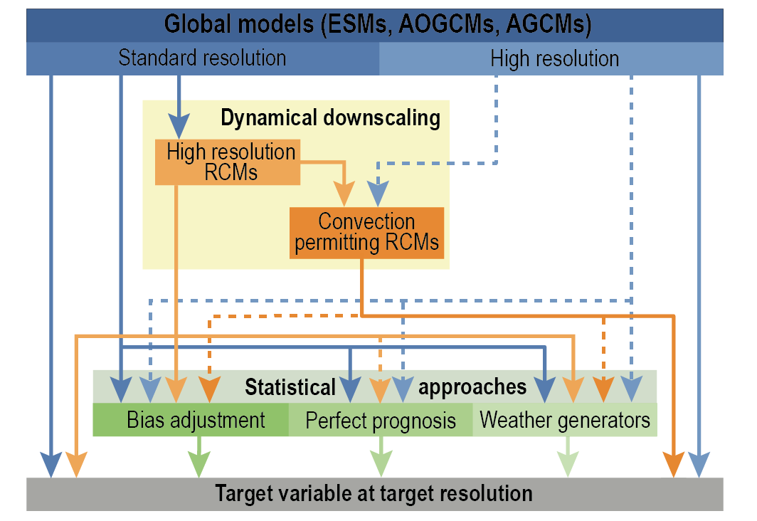 Figure 10.5 | Typical model types and chains used in modelling regional climate. The dashed lines indicate model chains that might prove useful but have not or only rarely been used. Hybrid approaches combining the model types shown have been developed.
 10.3.1.1 Global Models, Including High-resolution and Variable Resolution Models
Model-based regional climate projections are all based upon some type of global model, including state-of-the-art Earth system models (ESMs), coupled atmosphere–ocean general circulation models (GCMs) or atmosphere-only general circulation models (AGCMs) (see Section 1.5.3.1). They are collectively referred to as global models.
State-of-the-art global models are generally used to derive climate information at continental to global scales both for past and future climates (e.g., Chapters 3 and 4). The nominal horizontal resolution in CMIP5 global models is typically 100–200 km. The effective resolution, for which the shape of the kinetic energy spectrum is simulated correctly, is about three to five times larger (Klaver et al., 2020), and a similar relationship also applies to RCMs (Skamarock, 2004). This strongly limits their ability to resolve local details. Since AR5 the progress in reducing biases and providing more credible regional projections by global models has been moderate in spite of the more realistic representation of a number of processes and the increase in resolution of some models. For AR6, several of the new CMIP6 (Eyring et al., 2016a) model intercomparison projects (MIPs) address some of these limitations. The list of MIPs is provided in Chapter 1 (Table 1.3). High-Resolution MIP (HighResMIP; Haarsma et al., 2016) and Global Monsoons MIP (GMMIP; Zhou et al., 2016) specifically address the regional climate challenge using global models. HighResMIP focuses on producing global climate projections at a horizontal resolution of around 50 km grid spacing or finer while GMMIP aims at better understanding and predicting the monsoons.
An alternative to increasing resolution everywhere is offered by variable resolution global models, that is, with regionally finer resolution. They have been developed since the 1970s (Li, 1999), resulting in a first coordinated effort (SGMIP) by Fox-Rabinovitz et al. (2006, 2008). They are expected to offer the finest resolution possible in the region of interest, while still resolving the climate processes at the global scale (although at lower resolution). An overview of recent developments is in McGregor (2015). This is a rapidly developing field (Krinner et al., 2014; Ferguson et al., 2016; Huang et al., 2016) that will possibly contribute to improved future regional projections.
10.3.1.2 Regional Climate Models
Regional climate models (RCMs) are dynamical models similar to global models that are applied over a limited area, but with a horizontal resolution higher than that of standard global models. They are the basis for dynamical downscaling to produce sub-continental climate information (e.g., Chapters 11, 12 and Atlas) but are also often used for process understanding. At lateral and, if applicable, lower boundaries, RCMs take their values from a driving dataset, which could be a global model or a reanalysis. RCMs are typically one-way nested: they do not feed back into the driving model, although two-way nested global model-RCM simulations have been performed that examine regional influence on large-scale climate, potentially improving it (Lorenz and Jacob, 2005; Harris and Lin, 2013; Junquas et al., 2016). Spectral nudging (Kida et al., 1991; Waldron et al., 1996; von Storch et al., 2000; Kanamaru and Kanamitsu, 2007) can increase consistency with the driving model, whereby selected variables, such as the wind field, are forced to closely follow a prescribed large-scale field over a specified range of spatial scales. RCMs can inherit biases from the driving global model in addition to producing biases themselves (Hall, 2014; Hong and Kanamitsu, 2014; Dosio et al., 2015; Takayabu et al., 2016). The consistency between the circulation features simulated by the RCM and those inherited through the boundary conditions depends on (i) the relative importance of the large-scale forcing compared to local-scale phenomena, and (ii) the size of the RCM domain (e.g., Diaconescu and Laprise, 2013). Large domains also allow the RCM to generate much of its own internally generated unforced variability (Nikiema et al., 2017, and references therein; Sanchez-Gomez and Somot, 2018).
The Coordinated Regional Climate Downscaling Experiment (CORDEX) initiative (Giorgi et al., 2009; Giorgi and Gutowski, 2015; Gutowski Jr. et al., 2016) provides ensembles of high-resolution historical (starting as early as 1950) and future climate projections for various regions. RCMs in CORDEX typically have a horizontal resolution between 10 and 50 km. But much finer spatial resolution is required to fully resolve deep convection, an important cause of precipitation in much of the world. Therefore, an emerging strand in dynamical downscaling employs simulations at convection permitting scales, at horizontal resolutions of a few kilometres, where deep-convection parametrizations can be switched off, approximately simulating deep convection (Prein et al., 2015; Stratton et al., 2018; Coppola et al., 2020). A recent study indicates that switching off the deep-convection parametrization may be beneficial also in simulations performed at coarser resolutions (Vergara-Temprado et al., 2020). Alternatively, some RCMs make use of scale-aware parametrizations that are able to adapt to increasing resolution without switching off the convection scheme (Hamdi et al., 2012; De Troch et al., 2013; Plant and Yano, 2015; Giot et al., 2016; Termonia et al., 2018; Yano et al., 2018).
RCMs have often consisted of atmospheric and land components that do not include all possible Earth system processes and therefore neglect important processes such as air-sea coupling (in standard RCMs sea surface temperatures, SSTs, are prescribed from global model simulations or reanalyses) or the chemistry of aerosol–cloud interaction (aerosols prescribed with a climatology), which may influence regional climate projections. Therefore, some RCMs have been extended by coupling to additional components like interactive oceans, sometimes with sea ice (Kjellström et al., 2005; Somot et al., 2008; Van Pham et al., 2014; Sein et al., 2015; Ruti et al., 2016; Zou and Zhou, 2016a; Zou et al., 2017; Samanta et al., 2018), rivers (Sevault et al., 2014; Lee et al., 2015; Di Sante et al., 2019), glaciers (Kotlarski et al., 2010), and aerosols (Zakey et al., 2006; Zubler et al., 2011; Nabat et al., 2015). The coupling of these components allows for the investigation of additional climate processes such as regional sea level change (Adloff et al., 2018), ocean–land interactions (Lima et al., 2019; Soares et al., 2019a), or the impact of high-frequency ocean–atmosphere coupling on the climatology of Mediterranean cyclones (Flaounas et al., 2018).
10.3.1.3 Statistical Approaches to Generate Regional Climate Projections
An alternative or addition to dynamical downscaling is the use of statistical approaches to generate regional projections. In AR5 these methods were collectively referred to as statistical downscaling, but their performance assessment has received little attention. A major conclusion was that a wide range of different methods exist and a general assessment of their performance is difficult (Flato et al., 2014). Since AR5, several initiatives have been launched to improve the understanding of statistical approaches such as VALUE (Validating and Integrating Downscaling Methods for Climate Change Research, now merged into the EURO-CORDEX activities; Maraun et al., 2015), STaRMIP (Statistical Regionalization Models Intercomparisons and Hydrological Impacts Project; Vaittinada Ayar et al., 2016) and BADJAM (Bias ADJustment of climate scenarios for Agricultural Model applications; Galmarini et al., 2019). The performance of different implementations of these approaches will be assessed in Section 10.3.3.7.
10.3.1.3.1 Perfect prognosis
Perfect-prognosis models are statistical models calibrated between observation-based large-scale predictors (e.g., from reanalysis) and observed local-scale predictands (Maraun and Widmann, 2018b). Regional climate projections are then generated by replacing the quasi-observed predictors by those from climate model (typically global model) projections. Predictor patterns that are common to observations and climate model data can be defined by common empirical orthogonal functions (Benestad, 2011). The perfect prognosis approach can either be used to generate daily (or even sub-daily) time series, or local weather statistics (e.g., Benestad et al., 2018).
Regression-like models (Maraun and Widmann, 2018b) rely on a transfer function linking an observed local statistic (such as the temperature at a given day) to some set of large-scale predictors. Recent developments include stochastic regression models to explicitly simulate local variability (San-Martín et al., 2017; those explicitly modelling temporal dependence are assessed in Section 10.3.1.3.4). The use of machine learning techniques has been reinvigorated, including genetic programming to construct a data-driven model structure (Zerenner et al., 2016) and deep and convolutional neural networks (Reichstein et al., 2019; Baño-Medina et al., 2020).
Analogue methods (Martin et al., 1996; Maraun and Widmann, 2018b) compare a simulated large-scale atmospheric field with an archive of observations and select, using some distance metric, the closest observed field in the archive. The downscaled atmospheric field is then chosen as the local atmospheric field observed on the instant the analogue occurred. New analogue methods have been developed to simulate unobserved values including a rescaling of the analogue (Pierce et al., 2014) or by combining analogues and regression models (Chardon et al., 2018).
10.3.1.3.2 Bias adjustment
Bias adjustment is a statistical post-processing technique used to pragmatically reduce the mismatch between the statistics of climate model output and observations. The approach estimates the bias or relative error between a chosen simulated statistical property (such as the long-term mean or specific quantiles of the climatological distribution) and that observed over a calibration period; the simulated statistic is then adjusted taking into account the simulated deviation. Bias adjustment methods are regularly applied on a spatial scale similar to that of the simulation being adjusted, but they are often used as a simple statistical downscaling method by calibrating them between coarse resolution (e.g., global) model output and finer observations (Maraun and Widmann, 2018b).
Typical implementations of bias adjustment are (i) additive adjustments, where the model data is adjusted by adding a constant, (ii) rescaling, where the model data is adjusted by a factor, and (iii) more flexible quantile mapping approaches that adjust different ranges of a distribution individually. Hempel et al. (2013), Pierce et al. (2015), Switanek et al. (2017), and Lange (2019) developed variants of quantile mapping that preserve trends in the mean or even further distributional statistics. Multivariate bias adjustment extends univariate methods, which adjust statistics of individual variables separately, to joint adjustment of multiple variables simultaneously. Implementations remove biases in (i) specific measures of multivariate dependence, like correlation structure, via linear transformations (Bárdossy and Pegram, 2012; Cannon, 2016), or, more flexibly, (ii) the full multivariate distribution via non-linear transformations (Vrac and Friederichs, 2015; Dekens et al., 2017; Cannon, 2018; Vrac, 2018; Robin et al., 2019). Other research strands focus on the explicit separation of bias adjustment and downscaling (Section 10.3.1.3.5), or the integration of process understanding (Maraun et al., 2017), such as by conditioning the adjustment on the occurrence of relevant phenomena (Addor et al., 2016; Verfaillie et al., 2017; Manzanas and Gutiérrez, 2019). Some authors suggest to mitigate the influence of large-scale temperature or circulation biases by performing a bias adjustment of the driving fields prior to dynamical downscaling (Colette et al., 2012; Hernández-Díaz et al., 2013, 2019). Issues that may arise when using bias adjustment are discussed in Cross-Chapter Box 10.2.
10.3.1.3.3 Delta-change approaches
In the delta change approach, selected observations are modified according to corresponding changes derived from dynamical model simulations. Traditionally, only long-term means have been adjusted, but recently approaches to modify temporal dependence (Webber et al., 2018) have been developed, as well as quantile mapping approaches that individually adjust quantiles of the observed distribution (Willems and Vrac, 2011). By construction, the approach cannot modify the spatial and temporal dependence structure of the input observations (Maraun, 2016).
10.3.1.3.4 Weather generators
Weather generators are statistical models that simulate weather time series of arbitrary length. They are calibrated to represent observed weather statistics, in particular daily or even sub-daily variability. One variant of these models are advanced stochastic perfect-prognosis methods, conditioned on large-scale atmospheric predictors on a daily basis, for instance multisite generalized linear models (Chandler, 2020). Another widely used variant is change-factor weather generators: the weather generator parameters are calibrated against present and future climate model simulations, and the climate change signals are then applied to the parameters calibrated to observations. Recent research has mainly focussed on multi-site Richardson type (Markov-chain) weather generators (Keller et al., 2015; Dubrovsky et al., 2019), some explicitly modelling extremes and their spatial dependence (Evin et al., 2018).
10.3.1.3.5 Hybrid approaches and emulators
A wide variety of approaches has been proposed to combine the advantages of different statistical approaches. For instance, to overcome the scale mismatch between climate model output and observations, bias adjustment has been combined with stochastic downscaling (Volosciuk et al., 2017; Lange, 2019) or rescaled analogues (Pierce et al., 2014). Other approaches known as emulators have been developed to emulate an RCM using a statistical model and also applied to a range of driving global models (Déqué et al., 2012; Haas and Pinto, 2012; Walton et al., 2015, 2017; Beusch et al., 2020; Erlandsen et al., 2020).
10.3.2 Types of Model Experiments
The most commonly used model experiments to generate regional climate information are transient simulations. Alternative experiment types serve specific purposes. The role of these experiment types for generating regional climate information is assessed in this subsection.
10.3.2.1 Transient Simulations and Time-slice Experiments
Transient simulations intend to represent the evolving climate state of the Earth system (Chapter 4). They are typically based on coupled global model simulations, such as those in the Diagnostic, Evaluation and Characterization of Klima (DECK) and ScenarioMIP part of CMIP6 covering the period 1850–2100 (Eyring et al., 2016a), and HighResMIP (1950–2050; Haarsma et al., 2016). Global transient climate simulations may be further downscaled by either dynamical or statistical downscaling. Currently available CORDEX RCM simulations (1950–2100) are based on CMIP5 (Gutowski Jr. et al., 2016).
In contrast, time-slice experiments are designed to represent only a specific period of time (typically 30 years). They are often run using global and regional models in atmosphere-only mode, forced by SSTs derived either from observations, as AMIP experiments, or from historical simulations and future projections of coupled global models. Compared to transient simulations, they offer advantages in being computationally cheaper (due to the lack of coupled ocean and short duration), which allows for the number of ensemble members(T. Zhang et al., 2016), and/or the resolution (Haarsma et al., 2013b; Davini et al., 2017) to be increased. Convection-permitting simulations, both covering the globe or particular regions, are currently conducted for short time slices only (Kendon et al., 2017; Hewitt and Lowe, 2018; Coppola et al., 2020; Pichelli et al., 2021). Another high-resolution time-slice data base is d4PDF (Mizuta et al., 2017; Ishii and Mori, 2020). Experiments covering a limited integration period have been carried out for coupled ocean–atmosphere RCMs (Sein et al., 2015; Zou and Zhou, 2016b, 2017). However, long spin-up periods are required to reach a stable stationary state in the deep ocean that otherwise might lead to invalid projections (Planton et al., 2012; Soto-Navarro et al., 2020).
10.3.2.2 Pseudo-global Warming Experiments
Results from downscaling experiments often suffer from large-scale circulation biases in the driving global models such as misplaced storm tracks (Section 10.3.3.4), while changes in atmospheric circulation are often uncertain owing to both climate response uncertainty (Section 10.3.4.2) and internal variability (Section 10.3.4.3). In a given application, if one can assume that changes in the regional climate are dominated by thermodynamic rather than by circulation changes, so-called pseudo-global warming (PGW) experiments (Schär et al., 1996) may be helpful in mitigating the effects of circulation biases, and to fix the large-scale circulation to present climate. In classical PGW experiments, boundary conditions for the downscaling are taken from reanalysis data, but modified according to the thermodynamic signals of climate change. The boundary conditions thus represent the sequence of observed weather, but with adjusted temperatures, humidity and atmospheric stability. Recent applications of PGW experiments include assessments of climate change in Japan (Adachi et al., 2012; Kawase et al., 2012, 2013), the Los Angeles area (Walton et al., 2015), Hawaii (C. Zhang et al., 2016), and the Alps (Keller et al., 2018). Recently, PGW studies have been generalized to modify global model simulations with the objective of separating the drivers of regional climate change, such as the Mediterranean amplification (e.g., Brogli et al., 2019b; Section 10.3.2.3).
Equivalent simulations can be conducted for individual events, thereby allowing for very high resolution. With counterfactual past climate conditions, such simulations can be used for conditional event attribution (Trenberth et al., 2015; Chapter 11), using hypothetical future conditions to generate physical climate storylines of how specific events may manifest in a warmer climate. The approach has been employed to study extreme events that require very high resolution simulations such as tropical cyclones (Lackmann, 2015; Takayabu et al., 2015; Lau et al., 2016; Kanada et al., 2017a; Gutmann et al., 2018; Patricola and Wehner, 2018; J. Chen et al., 2020) or convective precipitation events (Pall et al., 2017; Hibino et al., 2018). The range of possible events is broader and has included Korean heatwaves (Kim et al., 2018) and monsoon onset in West Africa (Lawal et al., 2016). However, if only individual events are simulated, no immediate conclusions can be derived for changes to the occurrence probability of these events (F.E.L. Otto et al., 2016; Shepherd, 2016a).
10.3.2.3 Sensitivity Studies With Selected Drivers
Sensitivity studies are used to identify the impact of a specific forcing, driver or process on regional climate phenomena and changes and improve the process understanding. The influence of a single external forcing can be assessed with transient historical simulations within two different frameworks (Bindoff et al., 2013; Gillett et al., 2016). The first entails simulations taking prescribed (often observed) changes only in the external forcing of interest, the others being fixed at a constant value (often pre-industrial). The second framework is based on simulations in which all external forcings are applied other than the one of interest. Both approaches may not give the same results since the climate response to a range of forcings is not necessarily equal to the sum of climate responses to individual forcings (Ming and Ramaswamy, 2011; Jones et al., 2013; Schaller et al., 2013; Shiogama et al., 2013; Marvel et al., 2015; Deng et al., 2020).
To study the influence of internal variability, new approaches such as partial coupling simulations are now routinely used since AR5. These are coupled ocean–atmosphere simulations in which the interaction between atmosphere and ocean is only one-way over a specified ocean basin or sub-basin and two-way everywhere else. Different implementations have been used such as SST anomaly Newtonian relaxation at the air–sea interface or prescription of wind-stress anomalies from reanalysis (Kosaka and Xie, 2013, 2016; England et al., 2014; McGregor et al., 2014; Douville et al., 2015; Deser et al., 2017a). Such simulations have been applied to identify the regional impacts of the Pacific Decadal Variability (PDV) and Atlantic Multi-decadal Variability (AMV) (Kosaka and Xie, 2013; Watanabe et al., 2014; Delworth et al., 2015; Boer et al., 2016; Ruprich-Robert et al., 2017, 2018).
Nudging experiments have been used to identify the relative roles of dynamic and thermodynamic processes in climate model biases and specific extreme events (Wehrli et al., 2018, 2019). Another related framework is used to evaluate the impact land conditions have on a climate phenomenon in a pair of experiments with one simulation serving as control run, and a perturbed simulation with prescribed land conditions (i.e., soil moisture, leaf area index, or surface albedo) characterizing a specific state of the land surface (i.e., afforestation or deforestation). The difference between the perturbed and control simulations enables a robust assessment of the possible impact of land conditions on events like droughts and heatwaves (Seneviratne et al., 2013; Stegehuis et al., 2015; Hauser et al., 2016, 2017; van den Hurk et al., 2016; Vogel et al., 2017; Rasmijn et al., 2018; Strandberg and Kjellström, 2019).
RCM sensitivity simulations have been used in a similar way to assess the contribution of external forcings and large-scale drivers to projected regional climate change (Nabat et al., 2014; Brogli et al., 2019a, b) and the influence of selected drivers on observed extreme events (Meredith et al., 2015b; J. Wang et al., 2017; Ardilouze et al., 2019).
In summary, there is robust evidence that sensitivity experiments are key to assessing the influence of different forcings and drivers on regional climate change.
10.3.2.4 Control Simulations
In recent years, the role of internal variability in the interpretation of climate projections has become clearer, particularly at the regional scale (Section 10.3.4.3). A considerable fraction of CMIP5 and CMIP6 resources has been invested in generating an ensemble of centennial or multi-centennial control simulations with constant external forcings (Pedro et al., 2016; Rackow et al., 2018). As part ofthe CMIP6 DECK (Eyring et al., 2016a) pre-industrial control (piControl) simulations have been conducted (Menary et al., 2018). Similarly, control simulations with present-day conditions (pdControl) have been performed to represent internal variability under more recent forcing conditions (Pedro et al., 2016; Williams et al., 2018). Control simulations have been used to study the role of internal variability, teleconnections and many other fundamental aspects of climate models (Z. Wang et al., 2015; Krishnamurthy and Krishnamurthy, 2016). Control simulations are also used along with large ensembles of historical or scenario simulations to assess the characteristics of the regional internal climate variability (Olonscheck and Notz, 2017).
10.3.2.5 Simulations for Evaluating Downscaling Methods
Experiments driven by quasi-perfect boundary conditions or predictors (observations or reanalysis) can be useful to evaluate downscaling performance (Frei et al., 2003; Laprise et al., 2013), including the simulation of observed past trends (Lorenz and Jacob, 2010; Zubler et al., 2011; Nabat et al., 2014; Gutiérrez et al., 2018; Drugé et al., 2019; Bozkurt et al., 2020) and the added value of downscaling compared to the reanalysis fields (Section 10.3.3.2). Although the reanalysis model itself can introduce biases especially for non-assimilated variables (such as precipitation) it is assumed that in such a setting, discrepancies between the modelled and observed climate arise mostly from errors in the downscaling method (Laprise et al., 2013) or internal climate variability generated by the downscaling method (Böhnisch et al., 2020; Ehmele et al., 2020). Since AR5, reanalysis-driven RCMs have been extensively evaluated for many regions, especially in the CORDEX framework (see region specific examples in the Atlas).
Over Europe, the VALUE initiative assessed statistical downscaling for marginal, temporal, and spatial aspects of temperature and precipitation including extremes, and performed a process-based evaluation of specific climatic phenomena (Gutiérrezet al., 2019; Maraun et al., 2019a). Alternatively, statistical downscaling can be evaluated in so-called perfect model or pseudo-reality simulations (Charles et al., 1999), where a high-resolution climate model simulation is used as a proxy for a hypothetical present and future realities. A statistical downscaling model is first calibrated with this pseudo present-day climate and, subsequently, assessed whether it correctly reproduces the pseudo-future conditions (Dixon et al., 2016).
10.3.3 Model Performance and Added Value in Simulating and Projecting Regional Climate
Assessing model performance is a prerequisite for building confidence in regional climate projections. This subsection assesses the performance of different model types at simulating regional climate and climate change. The subsection builds on the assessment of global model performance in Chapter 3, and complements the model assessment in Chapter 8, which focuses on the water cycle, and the Atlas.
While the ability of global models to simulate large-scale indicators of climate change has improved since AR5 (Chapter 3), the simulation of regional climate and climate change poses an additional challenge. Users demand regional climate projections for decision-making and have high expectations regarding accuracy and resolution (Rössler et al., 2019a), but some scientists consider such projections still a matter of basic research (Hewitson et al., 2014a). For instance, large-scale circulation biases or the misrepresentation of regional topography as well as regional phenomena and feedbacks are very relevant (Hall, 2014; Maraun and Widmann, 2018b). New global model ensembles such as CMIP6 (Eyring et al., 2016a), HighResMIP (Haarsma et al., 2016) or, at the regional scale, the convection permitting simulations from the CORDEX Flagship Pilot Study (FPS) on convective phenomena (Coppola et al., 2020) have the potential to substantially improve the basis for generating regional climate information, yet uncertainties and (often unresolved) contradictions between model projections at the regional scale can be substantial (Fernández et al., 2019).
Figure 10.6 shows the mean summer temperature and precipitation biases of several state-of-the-art climate model ensembles for the western Mediterranean. It additionally illustrates the role of observational uncertainty for model evaluation (Section 10.2), where observations display differences that can be substantial. Model performance varies strongly from model to model, but also between ensembles. These biases are an expression of model error that leads to misrepresented phenomena and processes, and thus limit the confidence in future projections of regional climate. The focus of this subsection is therefore to evaluate the representation of relevant regional-scale phenomena for representing regional climate.
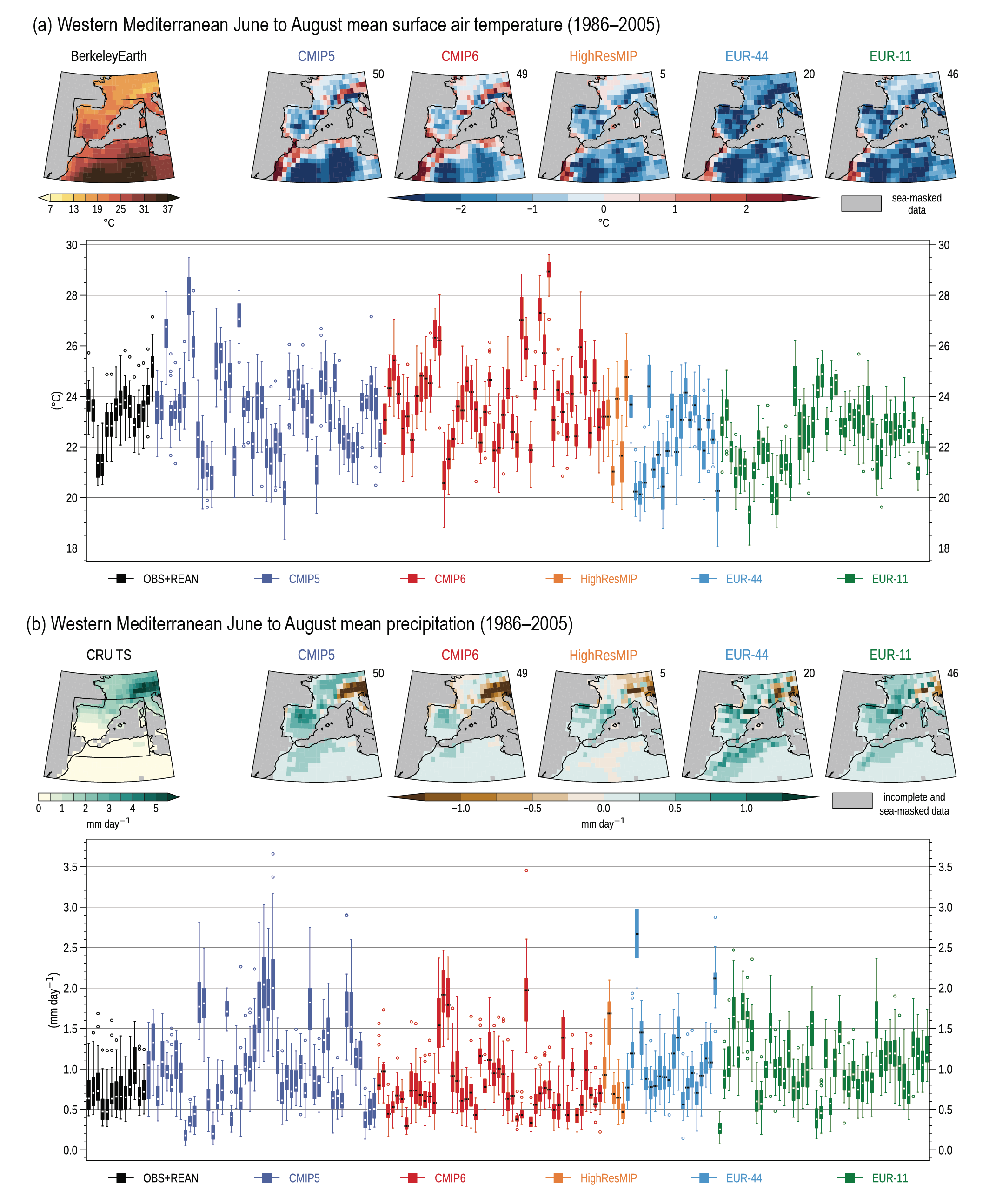 Figure 10.6 | Illustration of some model biases in simulations performed with dynamical models. (a) Top row: Mean summer (June to August) near-surface air temperature (in °C) over the Mediterranean area in Berkeley Earth and respective mean bias for five multi-model historical experiments with global models (CMIP5, CMIP6 and HighResMIP) and regional climate models (CORDEX EUR-44 and EUR-11) averaged between 1986–2005. Bottom row: Box-and-whisker plot shows spread of the 20 annual mean summer surface air temperature averaged over land areas in the western Mediterranean region (33°N–45°N, 10°W–10°E, black quadrilateral in the first panel of the top row) for a set of references and single model runs of the five multi-model experiments (one simulation per model) between 1986–2005. Additional observation and reanalysis data included in the bottom row are CRU TS, HadCRUT4, HadCRUT5, E-OBS, WFDE5, ERA5, ERA-Interim, CERA-20C, JRA-25, JRA-55, CFSR, MERRA2, MERRA. Berkeley Earth is shown in the first box to the left. (b) As (a) but for precipitation rate (mm day–1) and showing CRU TS in the first panel of the top row. Biases of the five multi-model experiments are shown with respect to CRU TS. Additional observation and reanalysis data included in the bottom row are GPCC, REGEN, E-OBS, GHCN, WFDE5, CFSR, ERA-Interim, ERA5, JRA-55, MERRA2, MERRA. CRU TS is shown in the first box to the left. All box-and-whisker plots show the median (line), and the interquartile range (IQR = Q3–Q1, box), with top whiskers extending to the last data less than Q3 + 1.5 × IQR and analogously for bottom whiskers. Data outside the whiskers range appear as flyers (circles). Further details on data sources and processing are available in the chapter data table (Table 10.SM.11).
10.3.3.1 Evaluation Diagnostics
Since AR5, model evaluation has made use of a broad combination of diagnostics (Colette et al., 2012; Kotlarski et al., 2014; Eyring et al., 2016b; Gleckler et al., 2016; Ivanov et al., 2017, 2018; Vautard et al., 2021), ranging from long-term means to indices of extreme events (Zhang et al., 2011; Sillmann et al., 2013) or a combination of these (Dittus et al., 2016). This evaluation has shown that global models have pervasive biases in some aspects of their large-scale behaviour (Section 1.5.3.1, Chapter 3). More complex diagnostics are used to characterize specific meteorological phenomena (Sprenger et al., 2017), such as feedbacks in the El Niño–Southern Oscillation (ENSO; Bellenger et al., 2014), Madden-Julian Oscillation (MJO) characteristics (Benedict et al., 2014; Jiang et al., 2015; D. Kim et al., 2015; Ahn et al., 2017), extratropical modes of variability (Lee et al., 2019), cyclone tracking (Neu et al., 2013; Flaounas et al., 2018), front detection (Hope et al., 2014; Schemm et al., 2015), thunderstorm environment parameters (Bukovsky et al., 2017), African easterly waves (McCrary et al., 2014; Martin and Thorncroft, 2015), land–atmosphere coupling (Spennemann and Saulo, 2015; Santanello et al., 2018), and sea–atmosphere coupling (Bellenger et al., 2014; Mayer et al., 2017).
New diagnostics for multivariate dependencies are needed to characterize compound events (Section 11.8; Hobaek Haff et al., 2015; Wahl et al., 2015; Sippel et al., 2016, 2017; Tencer et al., 2016; Bevacqua et al., 2017; Careto et al., 2018; Zscheischler et al., 2018). However, their success depends on the availability of adequate observational data (Section 10.2.2). Multivariate dependencies discovered in compound events can also be used for designing and evaluating multivariate bias adjustment and statistical downscaling. Process-based diagnostics are useful for identifying the cause of model errors, although it is not always possible to associate a systematic error with a specific cause (Eyring et al., 2019). AR5 discussed two approaches of process-based evaluation: (i) the isolation of physical components or parametrizations by dedicated experiments (Section 10.3.2.4) and (ii) diagnostics conditioned on relevant regimes, usually synoptic-scale weather patterns. The regime-based approach has been used with both global models (e.g., Barton et al., 2012; Catto et al., 2015; Taylor et al., 2019) and RCMs (Endris et al., 2016; Bukovsky et al., 2017; Whan and Zwiers, 2017; Pinto et al., 2018), but also with perfect prognosis and bias adjustment methods (Marteau et al., 2015; Addor et al., 2016; Beranová and Kyselý, 2016; Soares and Cardoso, 2018; Soares et al., 2019b).
Recent studies highlight the importance of user-defined or user-relevant diagnostics for model evaluation (Maraun et al., 2015; Rhoades et al., 2018; Rössler et al., 2019b; Nissan et al., 2020). Diagnostics have been used to assess the performance of climate models to produce useful input data for impact models as in the comparison between RCMs and convection-permitting models to capture flood-generating precipitation events in the Alps (Reszler et al., 2018). Alternatively, the observed impact can be compared to that simulated by an impact model that uses input from both observations and climate models. This approach has been used to evaluate the influence of statistical downscaling and bias adjustment on hydrological (Rojas et al., 2011; H. Chen et al., 2012; Gutiérrez et al., 2019; Rössler et al., 2019b), agricultural (Ruiz-Ramos et al., 2016; Galmarini et al., 2019), forest and wildfire (Abatzoglou and Brown, 2012; Migliavacca et al., 2013) (Bedia et al., 2013), snow depth (Verfaillie et al., 2017), and regional ocean modelling (e.g., Macias et al., 2018).
There is high confidence that to assess whether a climate model realistically simulates required aspects of present-day regional climate, and to increase confidence of future projections of these aspects, evaluation needs to be based on diagnostics taking into account multiple variables and process understanding.
10.3.3.2 Model Improvement and Added Value
Obtaining regional information from global simulations may involve a range of different methods (Section 10.3.1). An approach with higher complexity or resolution is useful if it adds further, useful information to that of a reference model. Section 10.5 discusses the set of considerations that determine if the information is useful. This further useful information is often referred to as added value and is a function of variables, processes, and the temporal and spatial scales targeted taking into account the needs of specific users (Di Luca et al., 2012; Ekström et al., 2015; Giorgi and Gutowski, 2015; Torma et al., 2015; Rummukainen, 2016; Falco et al., 2019). There is no common definition of added value, but here it is considered a characteristic that arises when one methodology gives further value to what another methodology yields.
Downscaling is expected to improve the representation of a region’s climate compared to the driving global model (Di Luca et al., 2015). Arguably, there should be a clear physical reason for the improvement, which is applicable to the evaluation of added value in downscaled projections (Giorgi et al., 2016). The added value depends on the region, season, and governing physical processes (Lenz et al., 2017; Schaaf and Feser, 2018). Thus, added value of downscaling global model simulations is most likely where regional- and local-scale processes play an important role in a region’s climate, for example in complex or heterogeneous terrain such as mountains (Lee and Hong, 2014; Prein et al., 2016b), urban areas (Argüeso et al., 2014), along coastlines (Feser et al., 2011; Herrmann et al., 2011; Bozkurt et al., 2019), or where convective processes are important (Prein et al., 2015). Examples of model improvements and added value are given in the following subsections and the Atlas.
A first step in determining added value in downscaling is to analyse whether the downscaling procedure gives detail on spatial or temporal scales not well-resolved by a global model, thus potentially representing climatic features missing in the GCM. This added detail, referred to as potential added value (PAV; Di Luca et al., 2012), is insufficient for demonstrating added value in downscaling (Takayabu et al., 2016), but lack of PAV indicates that the downscaling method lacks usefulness. Added value is not guaranteed simply by producing model output at finer resolution. It depends on several factors, such as the simulation setup and the specific climatic variables analysed (Di Luca et al., 2012; Hong and Kanamitsu, 2014; Xue et al., 2014). A variety of performance measures are needed to assess added value (Section 10.3.3.1; Di Luca et al., 2016; Wilks, 2016; Ivanov et al., 2017, 2018; Soares and Cardoso, 2018).
A further challenge, especially at increasingly higher resolutions, is that adequate observational data may not be available to assess added value (Section 10.2, e.g., Di Luca et al., 2016; Zittis et al., 2017; Bozkurt et al., 2019). This implies a need for additional efforts to obtain, catalogue and quality-control higher resolution observational (or observation-based) datasets (Thorne et al., 2017; Section 10.2). Univariate demonstration of added value is necessary, but may be insufficient, as better agreement with observations in the downscaled variable may be a consequence of compensating errors that are not guaranteed to compensate similarly as climate changes. Multivariate analysis of added value is better able to demonstrate physical consistency between observed and simulated behaviour (Prein et al., 2013a; Meredith et al., 2015a; Reboita et al., 2018).
10.3.3.3 Performance at Simulating Large-scale Phenomena and Teleconnections Relevant for Regional Climate
Regional climate is often controlled by large-scale weather phenomena, modes of variability and teleconnections (e.g., Sections 2.3 and 2.4, Annex IV). In particular, extreme events are often caused by specific, in some cases persistent, circulation patterns (Sections 11.3–11.7). It is therefore important for climate models to reasonably represent not only continental, but also regional climate and its variability for such extremes. As explained in Section 3.3.3, standard resolution global models can suffer biases in the location, occurrence frequency or intensity of large-scale phenomena, such that statements about a specific regional climate and its change can be highly uncertain (Hall, 2014). RCMs have difficulties improving especially large-scale circulation biases, although some successful examples exist. But due to their enhanced representation of complex topography and coastlines, RCMs may add value to simulating the regional expression of teleconnections. Bias adjustment cannot mitigate fundamental misrepresentations of the large-scale atmospheric circulation (Maraun et al., 2017, Cross-Chapter Box 10.2). This subsection illustrates the relevance of large-scale circulation biases for regional climate assessments with selected examples from the mid- to high latitudes and tropics.
10.3.3.3.1 Mid- to high-latitude atmospheric variability phenomena: Blocking and extratropical cyclones
Major large-scale meteorological phenomena for mid- to high latitude mean and extreme climate include atmospheric blocking and extratropical cyclones (Section 2.3.1.4). Atmospheric blocking is characterized by a quasi-stationary, long-lasting, high-pressure system that blocks and diverts the movement of synoptic cyclones (Woollings et al., 2018). In regions where blocking occurs, it is known to lead to cold conditions in winter and warmth and drought during summer, defining the seasonal regional climate in certain years (Sousa et al., 2017, 2018b). Extratropical cyclones are storm systems that propagate preferentially in confined storm-track regions, characterized by large eddy kinetic energy, heat and momentum transports that shape regional weather at mid- to high latitudes (Shaw et al., 2016). Given their importance in shaping mean and extreme regional climate (Sections 3.3.3.3, 11.3 and 11.4), an accurate representation of blocking and extratropical cyclones in global and regional climate models is needed to better understand regional climate variability and extremes as well as to project future changes (Section 11.7.2; Grotjahn et al., 2016; Mitchell et al., 2017; Rohrer et al., 2018; Huguenin et al., 2020). An overview of CMIP5 and CMIP6 model performance in simulating blocking and extratropical cyclones is given in Section 3.3.3.3. CMIP6 models still suffer from long-standing blocking biases identified in previous generations of models. However, blocking location has improved compared to CMIP5, while comparable performance is seen for blocking frequency and persistence (Figure 10.7). Increasing horizontal model resolution to about 20 km in the HighResMIP experiments improves the representation of blocking frequency and its spatial pattern in most models, but no clear effect could be shown for blocking persistence. Biases associated with these two phenomena are highly region- and season-dependent and their amplitudes vary among CMIP models (Drouard and Woollings, 2018; Schaller et al., 2018; Woollings et al., 2018; Harvey et al., 2020; Schiemann et al., 2020).
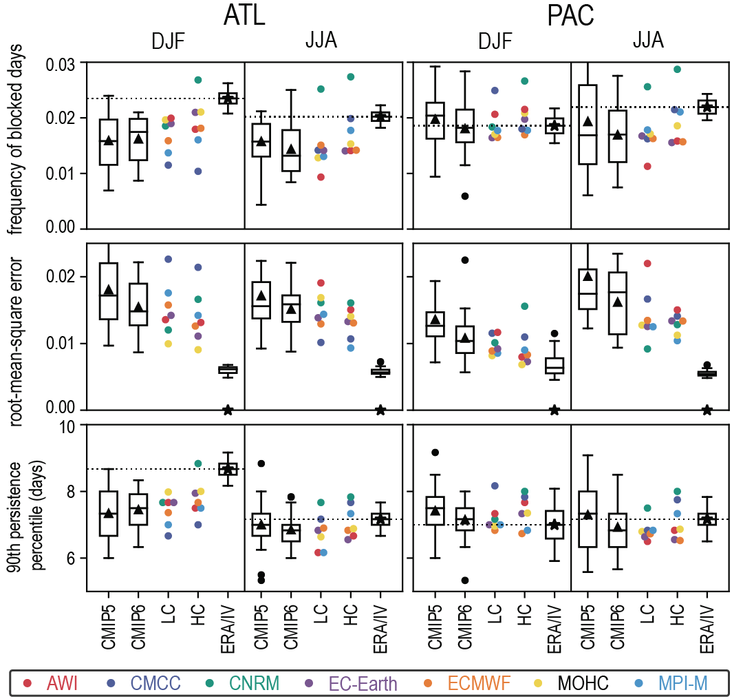 Figure 10.7 | Northern Hemisphere blocking performance in historical coupled simulations for different multi-model ensembles. Coupled Model Intercomparison Project Phases 5 and 6 (CMIP5/6): CMIP5 and CMIP6 Diagnostic, Evaluation and Characterization of Klima (DECK) historical simulations, 1950–2005, LC/HC: Low- (LC)/high- (HC) resolution coupled simulations from the PRIMAVERA project, 1950–2014 following the hist-1950 experiment of the CMIP6 HighResMIP Protocol (Haarsma et al., 2016). (Top) blocking frequency, for example, fraction of blocked days; (middle) root-mean-squared error in blocking frequency; (bottom) 90th percentile of blocking persistence, aggregated over an Atlantic domain (left, ATL: 90°W–90°E, 50°–75°N) and a Pacific domain (right, PAC: 90°E–270°E, 50°–75°N). Results are for boreal winter (December–January–February, DJF) and summer (June–July–August, JJA). Box-and-whisker plots for CMIP5/6 follow the methodology used in Figure 10.6 and show median (line), mean (triangle), and interquartile range (box) across 29 models for each ensemble. The reference estimate (ERA, asterisk) is from a 50-year reanalysis dataset that merged ERA-40 (1962–1978) and ERA-Interim (1979–2011) reanalyses. An estimate of internal variability for each metric (IV) is shown as a box-and-whisker plot over the asterisk and is obtained from a single-model ensemble (ECMWF-IFS high-resolution hist-1950 experiment, 6 × 65 years). For details on the methodology see (Schiemann et al., 2020). Further details on data sources and processing are available in the chapter data table (Table 10.SM.11).
 RCMs have a very limited ability to reduce large-scale circulation errors of the driving GCM (Hall, 2014). In a study of five ERA-Interim-driven RCMs, Jury et al. (2018) showed that RCMs typically simulate fewer blocking events over Europe than are present in the driving data, irrespective of the RCM horizontal resolution. Based on a simple blocking bias-decomposition method, they suggest that blocking frequency biases can contribute to the RCM mean surface biases. Over some large domains, reanalysis-driven RCMs can significantly improve the representation of storm characteristics compared to the driving reanalysis near regions with complex orography and/or large water masses (Poan et al., 2018). However, this is not necessarily true if the domain is large enough because the RCM and its biases will then control the circulation leading to a biased performance with regard to storm characteristics (Pontoppidan et al., 2019). An ensemble of 12 RCMs with and without air-sea coupling reasonably reproduced the climatology of Mediterranean cyclones, and air-sea coupling had a rather weak impact (Flaounas et al., 2018). Over the Gulf Stream, however, air-sea coupling played an important role in representing cyclone development (Vries et al., 2019). Sanchez-Gomez and Somot (2018) showed that the effect of RCM internal variability on density of cyclone tracks is very significant and larger than for other variables such as precipitation. It is larger in summer than in winter, in particular over the Iberian Peninsula, northern Africa and the eastern Mediterranean, which are regions of enhanced cyclogenesis during the warm season.
Biases in the representation of large-scale atmospheric circulation can result in biased representation of regional climate. While, in principle, the connection between large-scale and regional biases is obvious, given the strong control of regional climate by large-scale phenomena, research on this connection is still limited. Munday and Washington (2018) relate CMIP5 model rainfall biases over South Africa to anomalous low-level moisture transport across high topography due to upstream wind biases and inaccurate representation of unresolved orographic drag effects. Addor et al. (2016) show that the overestimated frequency of westerly synoptic situations was a significant contributor to the wet bias in several RCMs in winter over Switzerland. Pepler et al. (2014, 2016) suggest that better capturing westerly-driven synoptic systems such as cold fronts and cut-off lows in climate models could be key in simulating the observed pattern correlation between rainfall and zonal wind in southern south-east Australia. Cannon (2020) shows global improvement in performance going from CMIP5 to CMIP6 for both frequency and persistence of circulation types.
The robust quantification of the influence of atmospheric circulation errors on regional climate remains a challenge as many parametrized processes such as cloud radiative effects and soil moisture or snow feedbacks can also contribute and interact with the circulation errors. Atmospheric nudging experiments where the simulated circulation is constrained to be close to that observed have been used to separate the circulation effect from other contributions to regional climate biases (Wehrli et al., 2018). The nudging approach requires detailed and careful implementation in order to limit detrimental effects due to the added tendency term in the model equations (Zhang et al., 2014; Lin et al., 2016). Based on single-model experiments, Wehrli et al. (2018) show that the circulation induced biases are often not the main contributors to mean and extreme temperature and precipitation biases for many regions and seasons.
There is high confidence that atmospheric circulation biases can deteriorate the model representation of regional land surface climate. Assessing the relative contributions of atmospheric circulation and other sources of bias remains a challenge due to the strong coupling between the atmosphere and other components of the climate system, including the land surface.
10.3.3.3.2 Tropical phenomena: ENSO teleconnections
Model performance in simulating ENSO characteristics, including ENSO spatial pattern, frequency, asymmetry between warm and cold events, and diversity, is assessed in Chapter 3 (Section 3.7.3). The ability of the recent generation of GCMs and RCMs to adequately simulate ENSO-related teleconnections is reviewed here along with relevant methodological issues (see also Annex IV2.3.2, Figure 3.38 and Section 3.7.3).
Langenbrunner and Neelin (2013) show that there is little improvement in CMIP5 relative to CMIP3 in amplitude and spatial patterns of the ENSO influence on boreal winter precipitation (spatial pattern correlations against observations are typically less than 0.5). However, the CMIP5 ensemble accurately represents the amplitude of the precipitation response in regions where observed teleconnections are strong. Garcia-Villada et al. (2020) found a decline in performance of the representation of simulated ENSO teleconnection patterns for model experiments with fewer observational constraints. They also show that ENSO warm phase (El Niño) teleconnections are better represented than those for the cold phase (La Niña). Individual CMIP5 and CMIP6 models show a good ability to represent the observed teleconnections at aggregated spatial scales (Power and Delage, 2018; Section 3.7.3 and Figure 3.38). The evaluation of the atmospheric dynamical linkages is also an important part of the assessment. Hurwitz et al. (2014) showed that CMIP5 models broadly simulate the expected (as seen in the MERRA reanalysis) upper-tropospheric responses to central equatorial Pacific or eastern equatorial Pacific ENSO events in boreal autumn and winter. CMIP5 models also simulate the correct sign of the Arctic stratospheric response, consisting of polar vortex weakening during eastern and central Pacific Niño events and vortex strengthening during both types of La Niña events. In contrast, most CMIP5 models do not capture the observed weakening of the Southern Hemisphere polar vortex in response to central Pacific ENSO events (Brown et al., 2013).
In RCMs, the effects of tropical large-scale modes and teleconnections are inherited through the boundary conditions and influenced by the size of the numerical domain. Done et al. (2015) and Erfanian and Wang (2018) claim that large domains that include source oceanic regions are required to capture the remote influence of teleconnections, although, without spectral nudging, this can lead to biased synoptic-scale patterns (Prein et al., 2019). RCMs generally reproduce the regional precipitation responses to ENSO, and can sometimes even improve the representation of these teleconnections compared to the driving reanalysis (Endris et al., 2013; Fita et al., 2017), but the overall performance may depend both on the driving reanalysis or GCM (Endris et al., 2016; Chandrasa and Montenegro, 2020) and on the chosen RCMs (Whan and Zwiers, 2017).
New studies since AR5 have shown that model performance assessment regarding ENSO teleconnections remains a difficult challenge due to the different types of ENSO and model errors in ENSO spatial patterns, as well as the strong influence of atmospheric internal variability at mid- to high latitudes (Coats et al., 2013; Polade et al., 2013; Capotondi et al., 2015; Deser et al., 2017c; Tedeschi and Collins, 2017; Garcia-Villada et al., 2020). Another difficulty comes from the non-stationary aspects of teleconnections in both observations and models, raising methodological questions on how best to compare a given model with another model or observations (Herein et al., 2017; Perry et al., 2017; O’Reilly, 2018; O’Reilly et al., 2019; Abram et al., 2020).
There is robust evidence that an accurate representation of both atmospheric circulation and sea surface temperature (SST) variability are key factors for the realistic representation of ENSO teleconnections in climate models. A robust and thorough evaluation of model performance regarding ENSO teleconnections is a challenging task with many methodological issues related to asymmetry between the warm and cold phases, non-stationarity and time-varying interaction between the Pacific and other ocean basins, signal-to-noise issues in the mid-latitudes and observational uncertainties, particularly for precipitation (Section 10.2.2.3).
10.3.3.4 Performance at Simulating Regional Phenomena and Processes
Regional climate is shaped by a wide range of weather phenomena occurring at scales from about 2000 km to 2 km (Figure 10.3). These modulate the influence of large-scale atmospheric phenomena and create the characteristic and potentially severe weather conditions. The climate in different regions will be affected by different mesoscale phenomena, of which several may be relevant. A skilful representation of these phenomena is a necessary condition for providing credible and relevant climate information for a given region and application. Therefore, it is important to understand the strengths and weaknesses of different model types in simulating these phenomena. The performance of different dynamical climate model types to simulate a selection of relevant mesoscale weather phenomena is assessed here.
10.3.3.4.1 Convection including tropical cyclones
Convection is the process of vertical mixing due to atmospheric instability. Deep moist convection is associated with thunderstorms and severe weather such as heavy precipitation and strong wind gusts. Convection may occur in single locations, in spatially extended severe events such as supercells, and organized into larger mesoscale convective systems such as squall lines or tropical cyclones, and embedded in fronts (see below). Shallow and deep convection are not explicitly simulated but parametrized in standard global and regional models. In consequence, these models suffer from several biases. AR5 has stated that many CMIP3 and CMIP5 models simulate the peak in the diurnal cycle of precipitation too early, but increasing resolution and better parametrizations help to mitigate this problem (Flato et al., 2014). Similar issues arise for RCMs with parametrized deep convection (Prein et al., 2015), which also tend to overestimate high cloud cover (Langhans et al., 2013; Keller et al., 2016).
Non-hydrostatic RCMs at convection-permitting resolution (4 km and finer) improve features such as the initiation and diurnal cycle of convection (Zhu et al., 2012; Prein et al., 2013a, b; Fosser et al., 2015; Stratton et al., 2018; Sugimoto et al., 2018; Finney et al., 2019; Berthou et al., 2020; Ban et al., 2021; Pichelli et al., 2021), the triggering of convection by orographic lifting (Langhans et al., 2013; Fosser et al., 2015), and maximum vertical wind speeds in convective cells (Meredith et al., 2015a). Also spatial patterns of precipitation (Prein et al., 2013a, b; Stratton et al., 2018), precipitation intensities (Prein et al., 2015; Fumière et al., 2020; Ban et al., 2021; Pichelli et al., 2021), the scaling of precipitation with temperature (Ban et al., 2014), cloud cover (Böhme et al., 2011; Langhans et al., 2013) and its resultant radiative effects (Stratton et al., 2018), as well as the annual cycle of tropical convection (Hart et al., 2018) are improved. Phenomena such as supercells, mesoscale convective systems, or the local weather associated with squall lines are not captured by global models and standard RCMs. Convection-permitting RCM simulations, however, have been shown to realistically simulate supercells (Trapp et al., 2011), mesoscale convective systems, their life cycle and motion (Prein et al., 2017; Crook et al., 2019), and heavy precipitation associated with a squall line (Kendon et al., 2014). There is high confidence that simulations at convection-permitting resolution add value to the representation of deep convection and related phenomena.
Convection is the key ingredient of tropical cyclones. An intercomparison of high-resolution AGCM simulations (Shaevitz et al., 2014) showed that tropical cyclone intensities appeared to be better represented with increasing model resolution. Takayabu et al. (2015) have compared simulations of typhoon Haiyan at different resolutions ranging from 20 km to 1 km (Figure 10.8). While the eyewall structure in the precipitation pattern was strongly smoothed in the coarse resolution simulations, it was well-resolved at the highest resolution. Gentry and Lackmann (2010) found similar improvements in simulating hurricane Ivan for horizontal resolutions between 8 km and 1 km. High-resolution coupled ocean–atmosphere simulations improve the representation of the radial structure of core convection and thereby the rapid intensification of the cyclone (Kanada et al., 2017b). There is high confidence that convection-permitting resolution is required to realistically simulate the three-dimensional structure of tropical cyclones.
 Figure 10.8 | Hourly accumulated precipitation profiles (mm hour–1) around the eye of Typhoon Haiyan. Represented by (a) Global Satellite Mapping of Precipitation (GSMaP) data (multi-satellite observation), (b) Guiuan radar (PAGASA), (c) Weekly Ensemble Prediction System (WEPS) data (JMA; 60 km), (d) NHRCM (20 km), (e) NHRCM (5 km), and (f) WRF (1 km) models. Panels (b), (d–f) are adapted from Takayabu et al. (2015), CCBY3.0 https://creativecommons.org/licenses/by/3.0. Further details on data sources and processing are available in the chapter data table (Table 10.SM.11).
 Initial studies with convection-permitting global models suggests that improvements in representing convection, as described for RCMs above, have a positive impact on the tropical and extratropical atmospheric circulation and, thus, regional climate (Satoh et al., 2019; Stevens et al., 2019; see also Section 8.5.1.2 and Chapter 7). Computational constraints currently limit these simulations to a length of few months only, such that they cannot yet be used for routine climate change studies.
10.3.3.4.2 Mountain wind systems
Mountain slope and valley winds are localized thermally generated diurnal circulations that have a strong influence on temperature and precipitation patterns in mountain regions. During the day, heating of mountain slopes induces upslope winds; during the night this circulation reverses. This phenomenon is not realistically represented by global models and coarse-resolution RCMs. RCM simulations at 4 km resolution showed good skill in simulating the diurnal cycle of temperature and wind on days of weak synoptic forcing in the Rocky Mountains (Letcher and Minder, 2017) as well as in simulating the mountain-plain wind circulation over the Tianshan mountains in central Asia (Cai et al., 2019), while in the Alps, a 1 km resolution has been required (Zängl, 2004).
Föhn winds are synoptically-driven winds across a mountain range that are warm and dry due to adiabatic warming in the downwind side. In an RCM study for the Japanese Alps, Ishizaki and Takayabu (2009) found that at least 10 km resolution was required to realistically simulate the basic characteristics of Föhn events.
Synoptically-forced winds may be channelled and accelerated in long valleys. For instance, the Tramontana, Mistral and Bora are northerly winds blowing down-valley from central France and the Balkans into the Mediterranean (Flaounas et al., 2013). In winter, these winds may cause severe cold air outbreaks along the coast. Flaounas et al. (2013) have shown that a GCM with a horizontal resolution of roughly 3.75° longitude/1.875° latitude (roughly 400 km × 200 km depending on latitude) is unable to reproduce these winds because of the coarse representation of orography. Fifty-kilometre RCM simulations did not realistically represent the Mistral (Obermann et al., 2018) and Bora winds (Belušić et al., 2018), but simulations at 12 km added substantial value. Similarly, Cholette et al. (2015) found that a 30 km RCM resolution was not sufficient to adequately simulate the channelling of winds in the St Lawrence River Valley in eastern Canada, whereas a 10 km resolution was.
There is high confidence that climate models with resolutions of around 10 km or finer are necessary for realistically simulating mountain wind systems such as slope and valley winds and the channelling of winds in valleys.
10.3.3.4.3 Coastal winds and lake effects
Simulating coastal climates and the influence of big lakes are a modelling challenge, due to the complex coastlines, the different heat capacities of land and water, the resulting wind system, and differential evaporation. The AR5 concluded that RCMs can add value to the simulation of coastal climates.
Summer coastal low-level jets off the mid-latitude western continental coasts are forced by the semi-permanent subtropical anticyclones, inland thermal lows, strong across-shore temperature contrasts in upwelling regions, and high coastal topography. They are important factors in shaping regional climate by, for instance, preventing onshore advection of humidity and thereby causing aridity in the Iberian Peninsula (Soares et al., 2014), or by transporting moisture towards precipitating regions as in the North American monsoon (Bukovsky et al., 2013).
Reanalyses and most global models do not well resolve the details of coastal low-level jets (Bukovsky et al., 2013; Soares et al., 2014), but they are still able to represent annual and diurnal cycles and interannual variability (Cardoso et al., 2016; Lima et al., 2019). Bukovsky et al. (2013) found RCM simulations at a 50 km resolution to improve the representation of the coastal low-level jet in the Gulf of California and the associated precipitation pattern compared to the driving global models. Lucas-Picher et al. (2017) find indirect evidence via precipitation patterns that 12 km simulations further improve the representation. Soares et al. (2014) demonstrated that an 8 km resolution RCM simulated a realistic three-dimensional structure of the Iberian coastal low-level jet, and the surface winds compare well with observations. Lucas-Picher et al. (2017) showed that a 0.44° resolution RCM underestimated winds along the Canadian east coast, whereas a 0.11° resolution version simulated more realistic 10 metre wind speed. Also, the Etesian winds in the Aegean Sea were realistically simulated by 12 km resolution RCMs (Dafka et al., 2018).
A particularly relevant coastal phenomenon is the sea breeze, which is caused by the differential heating of water and land during the diurnal cycle and typically reaches several tens of kilometres inland. Reanalyses and global models have too coarse a resolution to realistically represent this phenomenon, such that they typically underestimate precipitation over islands and misrepresent its diurnal cycle (Lucas-Picher et al., 2017). RCMs improve the representation of sea breezes and thereby precipitation in coastal areas and islands. Over Cuba and Florida only a 12 km-resolution RCM is able to realistically simulate the inland propagation of precipitation during the course of the day (Lucas-Picher et al., 2017). RCM simulations at 20 km horizontal resolution realistically represented the sea breeze circulation in the Mediterranean Gulf of Lions including the intensity, direction and inward propagation (Drobinski et al., 2018). Even though a coupled ocean–atmosphere simulation improved the representation of diurnal SST variations, the sea breeze representation itself was not improved.
Big lakes modify the downwind climate. In particular during winter they are relatively warm compared to the surrounding land, provide moisture, destabilize the passing air column and produce convective systems. The increase in friction when moving air reaches land causes convergence and uplift, and may trigger precipitation. Gula and Peltier (2012) found that a state-of-the-art GCM does not realistically simulate these effects over the North American Great Lakes, but a 10 km RCM better represents them and thereby simulates realistic downwind precipitation patterns, in particular enhanced snowfall during the winter season. Similar results were found by Wright et al. (2013), Notaro et al. (2015)and Lucas-Picher et al. (2017). In a convection permitting simulation of the Lake Victoria region, a too strong nocturnal land breeze resulted in unrealistically high precipitation (Finney et al., 2019).
There is high confidence that climate models with sufficiently high resolution are necessary for realistically simulating lake and coastal weather including coastal low-level jets, lake and sea breezes, as well as lake effects on rainfall and snow.
In regions like Fenno-Scandinavia or central-eastern Canada, very large fractions of land are covered by small and medium sized lakes. Other regions have fewer but larger lakes, such as central-eastern Africa, the eastern border between the USA and Canada, and central Asia. In these regions it has been considered essential to include a lake model in an RCM to realistically represent regional temperatures (Samuelsson et al., 2010; Deng et al., 2013; Mallard et al., 2014; Thiery et al., 2015; Pietikäinen et al., 2018), as well as remote effects (Spero et al., 2016). The most common approach in RCMs is the two-layer lake model, including a lake-ice model, with parametrized vertical temperature profiles (Mironov et al., 2010; Golosov et al., 2018). For the Caspian Sea, it is found that a three-dimensional ocean model simulated the SST fields better than a one-dimensional lake model when coupled to the same RCM (Turuncoglu et al., 2013).
There is medium evidence and high agreement that it is important to include interactive lake models in RCMs to improve the simulation of regional temperature, in particular in seasonally ice-covered areas with large fractions of lakes. There is medium evidence of the local influence of lakes on snow and rainfall as well as the importance of including lakes in regional climate simulations.
10.3.3.4.4 Fronts
Weather fronts are two-dimensional surfaces separating air masses of different characteristics and are a key element of mid-latitude cyclones. In particular cold fronts are regions of relatively strong uplift and hence often associated with severe weather (e.g., Schemm et al., 2016). Stationary or slowly moving fronts may cause extended heavy precipitation. The evaluation of how climate models represent fronts, however, remains limited. Catto et al. (2014) found in both ERA-Interim and CMIP5 models that frontal frequency and strength were realistically simulated, albeit with some biases in the location. Follow-up investigations, for boreal and austral winter (Catto et al., 2015) found frontal precipitation frequency to be too high and the intensity too low, but these compensating biases resulted in only a small total precipitation bias. Blázquez and Solman (2018) found similar results for Southern Hemisphere (SH) winter, and also showed that CMIP5 models typically overestimate the fraction of frontal precipitation compared to total precipitation. As for the reference, the ERA-Interim reanalysis misrepresents conditional symmetric instability associated with fronts, and the corresponding precipitation (Glinton et al., 2017). Only a few studies evaluating fronts in RCMs have been conducted. Kawazoe and Gutowski (2013) diagnosed strong temperature gradients associated with extreme winter precipitation in the North American Regional Climate Change Assessment Program (NARCCAP) RCM ensemble (Mearns et al., 2012) and found the models agreed well with gradients in a reanalysis. De Jesus et al. (2016) diagnosed the representations of cold fronts over southern Brazil in two RCMs, finding that they were only underestimated by about 5% across the year, but in one RCM, summer cold fronts were underestimated by 17%. An RCM-based reanalysis suggests that high-resolution RCM simulations improve the representation of orographic influences on fronts (Jenkner et al., 2009).
10.3.3.5 Performance at Simulating Regional Feedbacks
Both SRCCL (Jia et al., 2019) and SROCC (Hock et al., 2019) highlight the weaknesses of climate models at simulating atmosphere–surface feedbacks. The performance at simulating some of these feedbacks is assessed below (climate feedbacks in urban areas are discussed in Box 10.3).
The snow-albedo feedback contributes to enhanced warming at high elevations (Section 8.5; Pepin et al., 2015). Global models often do not simulate it realistically due to their misrepresentation of orography in complex terrain (Hall, 2014; Walton et al., 2015). The elevation dependence of historical warming, which is partly caused by the snow-albedo effect, is realistically represented across Europe by the ENSEMBLES RCMs (Kotlarski et al., 2015). Some EURO-CORDEX RCMs simulate a spring snow–albedo feedback close to that observed, whereas others considerably overestimate it (Winter et al., 2017). In a multi-physics ensemble RCM experiment, the cold bias in north-eastern Europe is amplified by the albedo feedback (García-Díez et al., 2015). For the Rocky Mountains, RCM simulations generally reproduce the observed spatial and seasonal variability in snow cover, but strongly overestimate the snow albedo (Minder et al., 2016). There is high confidence (medium evidence and high agreement) that RCMs considerably improve the representation of the snow-albedo effect in complex terrain.
Soil-moisture feedbacks influence changes in both temperature and precipitation. More than 30% of CMIP5 models overestimate the influence of preceding precipitation (a proxy for soil moisture) on temperature extremes in Europe and the USA (Donat et al., 2018), and many CMIP5 models simulate an unrealistic influence of evaporation on temperature extremes for wet regions in Europe and the US (Ukkola et al., 2018). RCMs were found to realistically simulate the correlation between latent and sensible heat fluxes and temperature (coupling strength) over Africa (Knist et al., 2017; Careto et al., 2018) and in northern and southern Europe, but to overestimate it in central Europe (Knist et al., 2017). Land surface models driven by global reanalysis agreed relatively well with observations. However, the coupling strength varied strongly across models at the regional scale, and a realistic partitioning of the incoming radiation into latent and sensible heat fluxes did not necessarily result in a realistic soil moisture-temperature coupling (Gevaert et al., 2018; Boé et al., 2020a).
Evaluating the representation of soil-moisture–precipitation feedbacks in climate models is challenging as different processes may induce feedbacks including moisture recycling, boundary-layer dynamics and mesoscale circulation. Moreover, the effects of soil moisture on precipitation may be region and scale dependent and may even change sign depending on the strength of the background flow (Taylor et al., 2013; Froidevaux et al., 2014; Guillod et al., 2015; Larsen et al., 2016; Tuttle and Salvucci, 2016). On seasonal-to-interannual time scales, CMIP5 models showed a stronger soil-moisture–precipitation feedback than estimated by satellite data (Levine et al., 2016). Taylor et al. (2013) found that convection-permitting RCMs perform well at simulating surface-induced mesoscale circulations in daytime convection and the observed negative soil moisture feedback, whereas an RCM with parametrized convection, even when run at the same resolution, simulated an unrealistic positive feedback. There is medium evidence and high agreement that simulations at convection-permitting resolution are required to realistically represent soil-moisture–precipitation feedbacks.
Ocean–atmosphere RCMs have successfully been used to understand and simulate phenomena involving strong regional feedbacks like tropical cyclones in the Indian Ocean (Samson et al., 2014), Indian summer monsoon (Samanta et al., 2018), East Asian summer monsoon (Zou et al., 2016), near coastline intense precipitation in the Mediterranean (Berthou et al., 2015, 2018), air-sea fluxes influencing heat and humidity advection over land (Sevault et al., 2014; Lebeaupin Brossier et al., 2015; Akhtar et al., 2018) or snow bands in the Baltic region (Pham et al., 2017). The positive impact of ocean-coupling on the simulation of strongly convective phenomena such as Medicanes, a class of severe cyclones in the Mediterranean, can only be diagnosed when using relatively fine atmospheric resolution of about 10 km (Akhtar et al., 2014; Flaounas et al., 2018; Gaertner et al., 2018). A positive impact of ocean coupling has been quantified in marginal sea regions with reduced large-scale influence (e.g., in the Baltic Sea area during weak phases of the NAO and thus weak influence of Atlantic westerlies (Kjellström et al., 2005; Pham et al., 2018). There is some evidence that coupled ocean components also positively impact RCM simulations of inland climates such as precipitation extremes in central Europe (Ho-Hagemann et al., 2017; Akhtar et al., 2019). There is high confidence that coupled ocean–atmosphere RCMs improve the representation of ocean–atmosphere feedbacks and related phenomena.
The influence of ice-sheet mass balance on regional climate, explored with global and regional models by (Noël et al., 2018; Fettweis et al., 2020), is discussed in Section 9.4.
10.3.3.6 Performance at Simulating Regional Drivers of Climate and Climate Change
Dust, with its regional character in both emissions and climatic influences, has traditionally been specified in climate simulations with a climatological estimate. In CMIP5 models, the influence of vegetation changes on mineral dust is largely underestimated while the influence of surface wind and precipitation are overestimated, resulting in a low bias of dust load (Pu and Ginoux, 2018). Interactive dust emission modules that simulate the dust optical depth in most of the key emission regions have only been recently introduced (Pu and Ginoux, 2018). However, coarse dust is underestimated in global models (Adebiyi and Kok, 2020). Simulations of future changes in dust are hindered by the uncertainties in future regional wind and precipitation as the climate warms (Evan et al., 2016), in the effect of CO2 fertilization on source extent (Huang et al., 2017), in the dust feedbacks (Evans et al., 2019), and in the effect of human activities that change land use and disturb the soil, including cropping and livestock grazing, recreation and urbanization, and water diversion for irrigation (Ginoux et al., 2012).
Volcanoes also provide forcings with a marked regional impact (Cross-Chapter Box 4.1). This implies that models are expected to capture these effects (Bethke et al., 2017). Both proxy analyses and simulations have demonstrated reduced Asian monsoon precipitation after tropical and Northern Hemisphere (NH) volcanic eruptions due to reduced humidity and divergent circulation (Man and Zhou, 2014; Zhuo et al., 2014; F. Liu et al., 2016; Stevenson et al., 2016). Global model experiments (Zanchettin et al., 2013; Ortega et al., 2015; Sjolte et al., 2018; Michel et al., 2020) have suggested that tropical volcanic eruptions (larger than the one from Mount Pinatubo in 1991) may lead to a positive phase of the winter NAO in the following few years (with an uncertainty on the exact years affected), but this influence is not well-reproduced in climate models and requires very large ensembles (Driscoll et al., 2012; Toohey et al., 2014; Swingedouw et al., 2017; Ménégoz et al., 2018b). The ability to simulate the effect of volcanic aerosol in global models is evaluated in VolMIP (Zanchettin et al., 2016). Given the relevance of volcanic aerosol, a good knowledge of the initial conditions is important because the response has proven to be sensitive to them (Ménégoz et al., 2018a; Zanchettin et al., 2019). A few decadal prediction systems have illustrated that current systems can predict some aspects of regional climate a few years in advance (Swingedouw et al., 2017; Illing et al., 2018; Ménégoz et al., 2018a; Hermanson et al., 2020). However, a better performance requires information about volcanic location (Haywood et al., 2013; Pausata et al., 2015; Stevenson et al., 2016; F. Liu et al., 2018a), strength (Emile-Geay et al., 2008; H.-G. Lim et al., 2016; F. Liu et al., 2018b), and seasonality (Stevenson et al., 2017; Sun et al., 2019a, b).
Some recent regional climate changes can only be simulated by climate models if anthropogenic aerosols are correctly included (Sections 10.4.2.1, 10.6.3 and 10.6.4; Chapters 6 and 8). Examples of the importance of correctly representing anthropogenic aerosols are the recent enhanced warming over Europe (Nabat et al., 2014; Dong et al., 2017), the cooling over the East Asian monsoon region, leading to a weakening of the monsoon (Section 8.3.2.4; Song et al., 2014; Q. Wang et al., 2017), as well as changes in the monsoons of West Africa (Sections 8.3.2.4 and 10.4.2.1) and South Asia (Sections 8.3.2.4 and 10.6.3; Undorf et al., 2018). The relevance of appropriately representing anthropogenic aerosols has been widely studied in regional models (Boé et al., 2020a; Gutiérrez et al., 2020), with an advantage for models with interactive aerosol schemes (Drugé et al., 2019; Nabat et al., 2020). Without a fully coupled chemistry module, radiative forcing can be simulated by including simple models of sulphate chemistry or specifying the optical properties from observations and prescribing the effect of aerosols on the cloud-droplet number (Fiedler et al., 2017, 2019; Stevens et al., 2017). In all cases, the specification of the aerosol load limits the trustworthiness of the simulations at the regional scale when enough detail is not provided (Samset et al., 2019; Shonk et al., 2020; Z. Wang et al., 2021).
The inclusion of irrigation in global and regional models over the South Asian monsoon region (Section 10.6.3) has been found to be important to represent the monsoon circulation and rainfall correctly (Lucas-Picher et al., 2011; Guimberteau et al., 2012; Shukla et al., 2014; Tuinenburg et al., 2014; Cook et al., 2015a; Devanand et al., 2019). Similarly, the inclusion of irrigation over northern India and western Pakistan could be important for the correct simulation of precipitation over the Upper Indus Basin in northern Pakistan (Saeed et al., 2013). Irrigation in the East African Sahel inhibits rainfall over the irrigated region and instead enhances rainfall to the east, coherent with both observations and theoretical understanding of the local circulation anomalies induced by the lower surface air temperatures over the irrigated region (Alter et al., 2015). Although several studies show how modelled irrigation reduces daytime temperature extremes, few compare modelled results with observations. Global model studies have found improvements in simulated surface temperature when including irrigation (Thiery et al., 2017), in particular in areas where the model used has a strong land-atmosphere coupling (Chen and Dirmeyer, 2019). An RCM study over the North China Plain showed that the inclusion of irrigation led to a better representation of the observed nighttime warming (Chen and Jeong, 2018).
There is medium confidence that representing irrigation is important for a realistic simulation of South Asian monsoon precipitation. There is limited evidence that including irrigation in climate models improves the simulation of maximum and minimum daily temperatures as well as precipitation for other regions.
Regional land-radiation management, including modifying the albedo through, for instance, no-tillage practices, has been suggested as a measure to decrease regional maximum daily temperatures (see review in Seneviratne et al., 2018), but although modelled results and theoretical understanding are coherent, few studies have verified the results with observations. Hirsch et al. (2018) is an exception, showing that implementing minimal tillage, crop residue management and crop rotation in a global model over regions where it is practiced, improves the simulation of surface heat fluxes.
10.3.3.7 Statistical Downscaling, Bias Adjustment and Weather Generators
The performance of statistical downscaling models, bias adjustment and weather generators is determined by the chosen model structure (e.g., to represent variability and extremes or spatial dependence) and, if applicable, the predictors selected (Maraun et al., 2019a). The VALUE initiative has assessed a range of such methods in a perfect-predictor experiment where the predictors are taken from reanalysis data (Maraun et al., 2015, 2019a; Gutiérrez et al., 2019). Table 10.2 shows an overview comprising performance results from VALUE and other studies. These results isolate the performance of the statistical method in the present climate. The overall performance in a climate change application also depends on the performance of the driving climate model (Sections 10.3.3.3–10.3.3.6) and the fitness of both the driving model and the statistical method for projecting the climatic aspects of interest (Section 10.3.3.9).
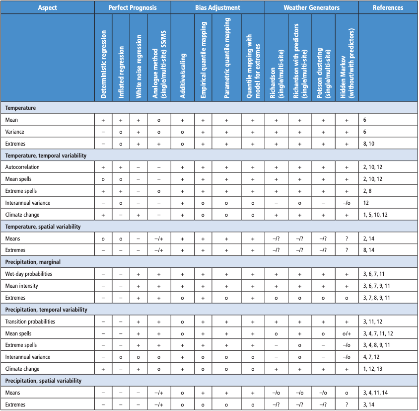
10.3.3.7.1 Performance of perfect prognosis methods
Perfect prognosis methods can perform well when the synoptic forcing (i.e., the explanatory power of large-scale predictors) is strong (Schoof, 2013). Using this approach, downscaling of precipitation is particularly skilful in the presence of strong orographic forcing. The representation of daily variability and extremes requires analogue methods or stochastic regression models, although the former typically do not extrapolate to unobserved values (Gutiérrez et al., 2019; Hertig et al., 2019). Temporal precipitation variability is well-represented by analogue methods and stochastic regression, but analogue methods typically underestimate temporal dependence of temperature (Maraun et al., 2019b). Spatial dependence of both temperature and precipitation is only well-represented by analogue methods, for which analogues are defined jointly across locations, and by stochastic regression methods explicitly representing spatial dependence (Widmann et al., 2019). Overall, there is high confidence that analogue methods and stochastic regression are able to represent many aspects of daily temperature and variability, but the analogue method is inherently limited in representing climate change (Gutiérrez et al., 2013).
10.3.3.7.2 Performance of bias adjustment methods
This subsection assesses the performance of bias adjustment in a perfect predictor context. In practice, climate model imperfections may cause substantial additional issues in the application of bias adjustment. These are assessed separately in Cross-Chapter Box 10.2.
Bias adjustment methods, if driven by reanalysis predictors, in principle adjust well all the aspects that they intend to address (Maraun and Widmann, 2018b). For temperature, all univariate methods are good for adjusting means, variance, and high quantiles (Gutiérrez et al., 2019; Hertig et al., 2019). For precipitation, means, intensities, wet-day frequencies, and wet–dry and dry–wet transitions are well-adjusted (Gutiérrez et al., 2019; Maraun et al., 2019b). The representation of high quantiles depends on the chosen method, although flexible quantile mapping performs best (Hertig et al., 2019). Empirical (non-parametric) methods perform better than parametric methods over the observed range, but it is unclear how this translates into extrapolation to unobserved values (IPCC, 2015; Hertig et al., 2019). Many quantile mapping methods overestimate interannual variability (Maraun et al., 2019b). Temporal and spatial dependence are usually not adjusted and thus inherited from the driving model (Maraun et al., 2019b; Widmann et al., 2019). Spatial fields are thus typically too smooth in space, even after bias adjustment (Widmann et al., 2019).
Several studies show improved simulations of present-day impacts, when the impact model is fed with bias-adjusted climate model output, including the assessment of river discharge (Rojas et al., 2011; Muerth et al., 2013; Montroull et al., 2018), forest fires (Migliavacca et al., 2013), crop production (Ruiz-Ramos et al., 2016), and regional ocean modelling (Macias et al., 2018).
There is high confidence that bias adjustment can improve the marginal distribution of simulated climate variables, if applied to a climate model that adequately represents the processes relevant for a given application (Cross-Chapter Box 10.2).
10.3.3.7.3 Performance of weather generators
Weather generators represent well most aspects that are explicitly calibrated. This typically includes mean, variance, high quantiles (for precipitation, if explicitly modelled), and short-term temporal variability for both temperature and precipitation, whereas interannual variability is strongly underestimated (Frost et al., 2011; Hu et al., 2013a; Keller et al., 2015; Dubrovsky et al., 2019; Gutiérrez et al., 2019; Hertig et al., 2019; Maraun et al., 2019b; Widmann et al., 2019). There is growing evidence that some spatial weather generators fairly realistically capture the spatial dependence of temperature and precipitation (Frost et al., 2011; Hu et al., 2013a; Keller et al., 2015; Evin et al., 2018; Dubrovsky et al., 2019). There is high confidence that weather generators can realistically simulate a wide range of local weather characteristics at single locations, but there is limited evidence and low agreement of the ability of weather generators to realistically simulate the spatial dependence of atmospheric variables across multiple sites.
10.3.3.8 Performance at Simulating Historical Regional Climate Changes
This section assesses how well climate models perform at realistically simulating historical regional climatic trends. Current global model ensembles reproduce global to continental-scale surface temperature trends at multi-decadal to centennial time scales (CMIP5, CMIP6), but underestimate precipitation trends (CMIP5) (Sections 3.3.1 and 3.3.2). For regional trends, AR5 concluded that the CMIP5 ensemble cannot be taken as a reliable representation of reality and that the true uncertainty can be larger than the simulated model spread (Kirtman et al., 2014). Case studies of regional trend simulations by global models can be found in Sections 10.4.1 and 10.6, and region-by-region assessments in the Atlas. A key limitation for assessing the representation of regional observed trends by single transient simulations of global models (or downscaled versions thereof) is the strong amplitude of internal variability compared to the forced signal at the regional scale (Section 10.3.4.3). Even on multi-decadal time scales, an agreement between observed and individual simulated trends would be expected to occur only by chance (Laprise, 2014).
In the context of downscaling, the ability of downscaling methods to reproduce observed trends when driven with boundary conditions or predictors taken from reanalysis data (which reproduce the observed internal variability on long time scales) can be assessed. For temperature in the continental USA, reanalysis-driven RCMs skilfully simulated recent spring and winter trends, but did not reproduce summer and autumn trends, (Bukovsky, 2012). Over Central America, observed warming trends were reproduced (Cavazos et al., 2020). In contrast, a reanalysis-driven coupled atmosphere–ocean RCM covering the Mediterranean could not reproduce the observed SST trend (Sevault et al., 2014).
Similar studies have been carried out for statistical downscaling and bias adjustment using predictors from reanalyses (or in case of bias adjustment, dynamically downscaled reanalyses). For a range of different perfect prognosis methods, Huth et al. (2015) found that simulated temperature trends were too strong for winter and too weak for summer. The performance was similar for the different methods, indicating the importance of choosing informative predictors. Similarly, Maraun et al. (2019b) found that the performance of perfect prognosis methods depends mostly on the predictor and domain choice (for instance, temperature trends were only captured by those methods including surface temperature as predictor). Bias adjustment methods reproduced the trends of the driving reanalysis, apart from quantile mapping methods, which deteriorated these trends.
RCM experiments are often set up such that changes in forcing agents are included only via the boundary conditions, but not explicitly included inside the domain. Jerez et al. (2018) demonstrated that not including time-varying GHG concentrations within the RCM domain may misrepresent temperature trends by 1–2°C per century. Including the past trend in anthropogenic sulphate aerosols in reanalysis-driven RCM simulations substantially improved the representation of recent brightening and warming trends in Europe (Nabat et al., 2014; see Sections 10.3.3.6 and 10.6.4, and Atlas.8.4). Similarly, Bukovsky (2012) argued that RCMs may not capture observed summer temperature trends in the USA because changes in land cover are not taken into account. Barlage et al. (2015) have revealed that including the behaviour of groundwater in land schemes increases the performance of an RCM model to represent climate variability in the central USA. Hamdi et al. (2014) found that an RCM that did not incorporate the historical urbanization in the land-use, land-cover scheme is not able to reproduce the warming trend observed in urban stations, with a larger bias for the minimum temperature trend.
Overall, there is high confidence that including all relevant forcings is a prerequisite for reproducing historical trends.
10.3.3.9 Fitness of Climate Models for Projecting Regional Climate
AR5 stated that confidence in climate model projections is based on the physical understanding of the climate system and its representation in climate models. A climate model’s credibility for future projections may be increased if the model is able to simulate past variations in climate (Sections 10.3.3.8, 10.4.1 and 10.6; Flato et al., 2014). In particular, the credibility of downscaled information depends on the quality of both the downscaling method and of the global model providing the large-scale boundary conditions (Flato et al., 2014). Credibility is closely linked to the concept of adequacy or fitness-for-purpose (Section 1.5.4.1; Parker, 2009). From a regional perspective, one may ask about the fitness of a climate model for simulating future changes of specific aspects of a specific regional climate. The required level of model fitness may depend on the user context (Section 10.5). A key challenge is to link performance at representing present and past climate (Sections 10.3.3.3–10.3.3.8) to the confidence in future projections (Section 1.3.5; Baumberger et al., 2017) and it is addressed in this subsection.
A general idea of model fitness for a given application may be obtained by checking whether relevant large- (Section 10.3.3.4) and regional-scale (Sections 10.3.3.5 and 10.3.3.6) processes are explicitly resolved (Figure 10.3). The basis for confidence in climate projection is a solid process understanding (Flato et al., 2014; Baumberger et al., 2017). Thus, the key to assessing the fitness-for-purpose of a model is the evaluation of how relevant processes controlling regional climate are represented (Collins et al., 2018). A process-based evaluation may be more appropriate than an evaluation of the variables of interest (e.g., temperature, precipitation), because biases in the latter may in principle be reduced if the underlying processes are realistically simulated (Cross-Chapter Box 10.2), while individual variables may appear as well-represented because of compensating errors (Flato et al., 2014; Baumberger et al., 2017). Combining a process-based evaluation with a mechanistic explanation of projected changes further increases confidence in projections (Bukovsky et al., 2017). Fitness-for-purpose can also be assessed by comparing the simulated response of a model with simulations of higher resolution models that better represent relevant processes (Baumberger et al., 2017). For instance, Giorgi et al. (2016) have corroborated their findings on precipitation changes comparing standard RCM simulations with convection-permitting simulations.
The evaluation of model performance at historical variability and long-term changes provides further relevant information (Flato et al., 2014). Trend evaluation may provide very useful insight, but has limitations, in particular at the regional scale, mainly due to multi-decadal internal climate variability (Section 10.3.3.8), observational uncertainty (in both driving reanalysis and local trends; Section 10.2), and the fact that often not all regional forcings are known, and that past trends may be driven by forcings other than those driving future trends (Sections 10.4.1 and 10.6.3).
Increasing resolution (Haarsma et al., 2016) or performing downscaling may be particularly important when it modifies the climate change signal of a lower resolution model in a physically plausible way (Hall, 2014). Improvements may result from a better representation of regional processes, upscale effects, as well as the possibility of a region-specific model tuning (Sørland et al., 2018). For instance, Gula and Peltier (2012) showed that a higher resolution allows for a more realistic simulation of lake-induced precipitation, resulting in a more credible projection of changes in the snow belts of the North American Great Lakes. Similarly, Giorgi et al. (2016) demonstrated that an ensemble of RCMs better represents high-elevation surface heating and in turn increased convective instability. As a result, the summer convective precipitation response was opposite to that simulated by the driving global models (Figure 10.9). Similarly, Walton et al. (2015) showed that a kilometre-scale RCM enables a more realistic representation of the snow-albedo feedback in mountainous terrain compared to standard resolution global models, leading to a more plausible simulation of elevation-dependent warming. Bukovsky et al. (2017) argue that strong seasonal changes in warm-season precipitation in the Southern Great Plains of the USA, projected by RCMs, are more credible than the weaker global model changes because precipitation is better simulated in the RCMs.
 Figure 10. 9 | Projected changes in summer (June to August) precipitation (in percent with respect to the mean precipitation) over the Alps between the periods 2070–2099 and 1975–2004. (a) Mean of four global climate models (GCMs) regridded to a common 1.32° × 1.32° grid resolution; (b) mean of six regional climate models (RCMs) driven with these GCMs. The grey isolines show elevation at 200 m intervals of the underlying model data. Further details on data sources and processing are available in the chapter data table (Table 10.SM.11). Figure adapted from Giorgi et al. (2016).
 Including additional components, feedbacks and drivers can substantially modify the simulated future climate. For example, Kjellström et al. (2005) and Somot et al. (2008) have shown that a regional ESM can significantly modify the SST response to climate change of its driving global model with implications for the climate change signal over both the sea and land. In particular, coupled ocean–atmosphere RCMs may increase the credibility of projections in regions of strong air-sea coupling such as the East Asia–western North Pacific domain (Zou and Zhou, 2016b, 2017). Recent studies demonstrate the importance of including regional patterns of evolving aerosols in RCMs for simulating regional climate change (Boé et al., 2020a; Gutiérrez et al., 2020). RCMs not including the plant physiological response to increasing CO2 concentrations have been shown to substantially underestimate projected increases in extreme temperatures across Europe compared to global models that explicitly model this effect (Schwingshackl et al., 2019).
A difference between the climate changes simulated by two models does not automatically imply the more complex or higher resolution model is superior (e.g., Dosio et al., 2019). Studies comparing convection-permitting RCM simulations to simulations of climate models with parametrized convection find, depending on the considered models, regions and seasons, either similar or qualitatively different projected changes in short duration extreme precipitation (Chan et al., 2014a, b, 2020; Ban et al., 2015; Tabari et al., 2016; Fosser et al., 2017; Kendon et al., 2017, 2019; Vanden Broucke et al., 2018). Process studies provide evidence that convection-permitting simulations better represent crucial local and mesoscale features of convective storms and thus simulate more plausible changes (Meredith et al., 2015a; Prein et al., 2017; Fitzpatrick et al., 2020), but further research is required to confirm and reconcile the different findings.
Studies assessing the fitness of statistical approaches for regional climate projections are still very limited in number. For statistical downscaling, a key issue is to include predictors that control long-term changes in regional climate. Models differing only in the choice of predictors may perform similarly in the present climate, but may project opposite precipitation changes (Fu et al., 2018; Manzanas et al., 2020). In addition to trend-evaluation studies (Section 10.3.3.8), perfect-model experiments (Section 10.3.2.5) have been used to assess whether a given model structure with a chosen set of predictors is capable of reproducing the simulated future climates (Gutiérrez et al., 2013; Räty et al., 2014; Dayon et al., 2015; Dixon et al., 2016; San-Martín et al., 2017). Importantly, it is found that standard analogue methods inherently underestimate future warming trends because of missing analogues for a warmer climate (Gutiérrez et al., 2013).
Bias adjustment assumes that model biases are time invariant (or more precisely, independent of the climate state), such that the adjustment made to present climate simulations is still applicable to future climate simulations. Many findings challenge the validity of this assumption, as already assessed in AR5 (Flato et al., 2014). Further research has addressed this issue by means of perfect model experiments (Section 10.3.2.5) and process understanding. Perfect-model studies with GCMs found that circulation, energy, and water-cycle biases are roughly state-independent (Krinner and Flanner, 2018), whereas temperature biases depend linearly on temperature (Kerkhoff et al., 2014). Others show that regional temperature biases may depend on soil moisture and albedo, and may thus be state-dependent (Maraun, 2012; Bellprat et al., 2013; Maraun et al., 2017; see Cross-Chapter Box 10.2 for further limitations of bias adjustment). The fitness of weather generators for future projections depends on whether they account for all relevant changes in their parameters, either by predictors or change factors (Maraun and Widmann, 2018b).
In any case, the fitness of regional climate projections based on dynamical downscaling or statistical approaches depends on the fitness of the driving models in projecting boundary conditions, predictors and change factors (Hall, 2014; Maraun and Widmann, 2018b).
Overall, there is high confidence that an assessment of model fitness for projections applying process-based evaluation, process-based plausibility checks of projections and a comparison of different model types, increases the confidence in climate projections. There is high confidence that increasing model resolution, dynamical downscaling, statistical downscaling with well-simulated predictors controlling regional climate change, and adding relevant model components can increase the fitness for projecting some aspects of regional climate when accompanied by a process-understanding analysis.
10.3.3.10 Synthesis of Model Performance at Simulating Regional Climate and Climate Change
Global models reproduce many of the features of observed climate and its variability at regional scales. However, global models can show a variety of biases in, for instance, precipitation and temperature at scales ranging from continental (Prasanna, 2016) to sub-continental scales (Lovino et al., 2018), both in the mean and in higher order moments of the climatological distribution of the variable (Figure 10.6; Ren et al., 2019; Xin et al., 2020). Regional biases could occur even if all the relevant large-scale processes are correctly represented, but not their interaction with regional features such as orography or land–sea contrasts (Section 10.3.3.4). These biases have been considered an important limiting factor in model usability, especially at the regional scale (Palmer, 2016). In spite of this, global model simulations have been extensively used to create regional estimates of climate change (Chapters 11, 12 and Atlas), taking into account the result of a performance assessment (Chapter 11, Sections 10.3.3.3–10.3.3.8, and Atlas; Jiang et al., 2020). However, their application is limited in part by the effective resolution of these models (Klaver et al., 2020).
Global model performance at the regional scale is assessed in terms of the time or spatial averages of key variables (see Atlas; Brunner et al., 2019), the ability to reproduce their seasonal cycle (Hasson et al., 2013) or a set of extreme climate indicators (Chapter 11; Luo et al., 2020) and the representation of regional processes and phenomena, feedbacks, drivers and forcing impacts (Sections 10.3.3.4–10.3.3.6). In many cases, the performance estimates have been used to select models for either an application or a more in-depth study (Lovino et al., 2018), to select the models that provide boundary conditions to perform RCM simulations (McSweeney et al., 2015) or to weight the results of the global model simulations (Sanderson et al., 2015; Brunner et al., 2020). While some large-scale metrics are improved between the CMIP5 and CMIP6 experiments (Chapter 3; Cannon, 2020), there is not yet concluding evidence of a systematic improvement for surface variables at the regional scale.
The special class of high-resolution global models (Sections 1.5.3.1 and 10.3.3.1, Chapter 3; Haarsma et al., 2016; Prodhomme et al., 2016) is expected to improve some of the regional processes that are not appropriately represented in standard global models (Roberts et al., 2018). There is general consensus that increasing global model resolution improves some long-standing biases (Chapter 3, Section 10.3.3.3, and Figures 10.6 and 10.7; Demory et al., 2014, 2020; Schiemann et al., 2014; Dawson and Palmer, 2015; van Haren et al., 2015; Feng et al., 2017; Fabiano et al., 2020), although the resolution increase is not a guarantee of overall improvement (Section 8.5.1; Fabiano et al., 2020; Hertwig et al., 2021). For instance, increasing resolution in global models has been shown to improve Asian monsoon rainfall anchored to orography and the monsoon circulation (Johnson et al., 2016), but fails to solve the major dry bias. It is also difficult to disentangle the role of resolution increase and model tuning on the performance of the GCM (Anand et al., 2018). Some efforts have been undertaken to complement the performance improvements of resolution by using stochastic parametrizations (Palmer, 2019), which explicitly acknowledge the multi-scale nature of the climate system, in standard resolution global models with some success (Dawson and Palmer, 2015; MacLeod et al., 2016; Zanna et al., 2017, 2019). The expectation is to achieve a similar performance to the increase in resolution at a reduced computational cost.
Despite their known errors that affect model performance, there is high confidence that global models provide useful information for the production of regional climate information. There is robust evidence and high agreement that the increase of global model resolution helps in reducing the biases limiting performance at the regional scale, although resolution per se does not automatically solve all performance limitations shown by global models. There is robust evidence that stochastic parametrizations can help to improve some aspects of the global model performance that are relevant to regional climate information.
Global models tend to have difficulties in simulating climate over regions where unresolved local scale processes, feedbacks and non-linear scale interactions result in a degradation of the model performance compared to models with higher resolution. In this case, RCMs and variable resolution global models can resolve part of these processes in the regions of interest at an acceptable computational cost (Rummukainen, 2016; Giorgi, 2019; Gutowski Jr. et al., 2020).
The assessment of RCM performance needs to focus not only on mean climatology (Atlas), but also trends (Section 10.3.3.8) and extremes (Chapter 11), and the RCM’s ability at correctly reproducing relevant processes, forcings and feedbacks including aerosols, plant responses to increasing CO2, and so on, (Schwingshackl et al., 2019; Boé et al., 2020a; Sections 11.2. and 10.3.3.3 to 10.3.3.8) to be fit for future projections (Section 10.3.3.9).
When RCMs are driven by global models, part of the uncertainty in the RCM simulation is introduced by the global model biases (Kjellström et al., 2018; Sørland et al., 2018; Christensen and Kjellström, 2020). As RCMs are typically not able to mitigate global model biases in large-scale dynamical processes, if such biases are substantial, and if the corresponding large-scale processes are important drivers of regional climate, downscaling is questionable (Section 10.3.3.3). However, when global models have weak circulation biases and regional climate change is controlled mainly by regional-scale processes and feedbacks, dynamical downscaling has the potential to add substantial value to global model simulations (Section 10.3.3.4 and Atlas; Hall, 2014; Rummukainen, 2016; Giorgi, 2019; Schwingshackl et al., 2019; Boé et al., 2020a; Lloyd et al., 2021).
There is very high confidence (robust evidence and high agreement) that RCMs add value to global simulations in representing many regional weather and climate phenomena, especially over regions of complex orography or with heterogeneous surface characteristics and for local-scale phenomena. Realistically representing local-scale phenomena such as land–sea breezes requires simulations at a resolution of the order of 10 km (high confidence). Simulations at kilometre-scale resolution add value in particular to the representation of convection, sub-daily summer precipitation extremes (high confidence) and soil-moisture–precipitation feedbacks (medium confidence). Resolving regional processes may be required to correctly represent the sign of regional climate change (medium confidence). However, the performance of RCMs and their fitness for future projections depend on their representation of relevant processes, forcings and drivers in the specific context (Sections 10.3.3.4–10.3.3.8).
Statistical downscaling, bias adjustment and weather generators outperform uncorrected output of global and regional models for a range of statistical aspects at single locations due to their calibration (Casanueva et al., 2016), but RCMs are superior when spatial fields are relevant (Mehrotra et al., 2014; Vaittinada Ayar et al., 2016; Maraun et al., 2019a). Similarly, there is some evidence that bias adjustment is comparable in performance when applied to global models and dynamically downscaled global models only for single locations, but dynamical downscaling prior to bias adjustment clearly adds value once spatial dependence is relevant (Maraun et al., 2019a). These results may explain why dynamical downscaling does not add value to global model simulations for (single-site) agricultural modelling, when both global and regional models are bias adjusted (Glotter et al., 2014), but dynamical downscaling adds value compared to bias-adjusted global model output for spatially distributed hydrological models (Qiao et al., 2014).
Overall, statistical downscaling methods with carefully chosen predictors and an appropriate model structure for a given application realistically represent many statistical aspects of present-day daily temperature and precipitation (high confidence, Section 10.3.3.7). Bias adjustment has proven beneficial as an interface between climate model projections and impact modelling in many different contexts (high confidence) (Section 10.3.3.7). Weather generators realistically simulate many statistical aspects of present-day daily temperature and precipitation (high confidence) (Section 10.3.3.7). The performance of these approaches and their fitness for future projections also depends on predictors and change factors taken from the driving dynamical models (high confidence) (Section 10.3.3.9).
10.3.4 Managing Uncertainties in Regional Climate Projections
Regional climate projections are affected by three main sources of uncertainty (Sections 10.2.2, 1.4.3 and 4.2.5): unknown future external forcings, imperfect knowledge and implementation of the response of the climate system to external forcings, and internal variability (Lehner et al., 2020). In a regional downscaling context, uncertainties arise in every step of the modelling chain. Here the propagation of uncertainties (Section 10.3.4.1), the management of uncertainties (Section 10.3.4.2), the role of the internal variability for regional projections (Section 10.3.4.3), and the design and use of ensembles to account for uncertainties (Section 10.3.4.4) will be assessed. Observational uncertainty, in particular for the calibration of statistical downscaling methods (Section 10.2.3.1), also contributes to projection uncertainty.
10.3.4.1 Propagation of Uncertainties
Modelling chains for generating regional climate information range from the definition of forcing scenarios to the global modelling, and potentially to dynamical or statistical downscaling and bias adjustment (Section 10.3.1). The propagation and potential accumulation of uncertainties along the chain has been termed the cascade of uncertainty (Wilby and Dessai, 2010). Even within one model, like a global model, uncertainty propagates across scales. From a process point of view, these uncertainties are related to forcings and global climate sensitivity, and errors in the representation of the large-scale circulation (Section 10.3.3.3; McNeall et al., 2016) and regional processes (Section 10.3.3.4), feedbacks (Section 10.3.3.5) and drivers (Section 10.3.3.6). From a modelling point of view, these uncertainties are related to the choice of dynamical and statistical models (Section 10.3.1) and experimental design (Section 10.3.2). The overall uncertainty can be statistically decomposed into the individual sources (Evin et al., 2019; Christensen and Kjellström, 2020), although there might be non-linear dependencies between them.
Uncertainty propagation often increases the spread in regional climate projections when comparing global model and downscaled results, which has been used as an argument against top-down approaches to climate information (Prudhomme et al., 2010). Increased spread in the modelling chain may also arise from a more comprehensive representation of previously unknown or underrepresented uncertainties (Maraun and Widmann, 2018b). The increased spread in this case goes together with a better representation of processes and thus an increased model fitness-for-purpose (Section 10.3.3.9).
10.3.4.2 Representing and Reducing Uncertainties
Climate response uncertainties (Chapter 1) can be represented by multi-model ensembles, although the sampled uncertainty typically underestimates the full range of uncertainty (Collins et al., 2013b; Shepherd et al., 2018; Almazroui et al., 2021). Traditionally, climate response uncertainty has been characterized by the ensemble spread around the multi-model mean change. The change has then further been qualified in terms of the agreement across models and compared to estimates of internal climate variability (Collins et al., 2013b). Since AR5, several limitations of this approach have been identified (Madsen et al., 2017) such as the failure to address physically plausible, but low-likelihood, high-impact scenarios (Chapters 1, 4, 8 and 9; Sutton, 2018) or that qualitatively different or even opposite changes may be equally plausible at the regional scale (Shepherd, 2014). In a multi-model mean these different responses would be lumped together, strongly dampened, and qualified as non-robust, whereas in fact high impacts might occur. Further, the multi-model mean itself is often implausible because it is a statistical construct (Zappa and Shepherd, 2017). Overall, there is high confidence that some regional future climate changes are not well-characterized by multi-model mean and spread.
Since AR5, physical climate storyline approaches (see also Chapter 1, Section 10.5.3, Box 10.2, and Atlas.2.5.2) have been developed to better characterize and communicate uncertainties in regional climate projections (Shepherd, 2019). A special class of such storylines attempts to attribute regional uncertainties to uncertainties in remote drivers. For instance, the Dutch Meteorological Service has presented climate projections for the Netherlands for different plausible changes of the mid-latitude atmospheric circulation and different levels of European warming (van den Hurk et al., 2014). Manzini et al. (2014) have quantified the impact of uncertainties in tropical upper troposphere warming, polar amplification, and stratospheric wind change on Northern Hemisphere winter climate change. Based on these results, Zappa and Shepherd (2017) separated the multi-model ensemble into physically consistent sub-groups or storylines of qualitatively different projections in relevant remote drivers of the atmospheric circulation. In a similar vein, (Ose et al., 2020) trace uncertainties in projections of the East Asian summer monsoon and Mindlin et al. (2020) conditioned the response of Southern Hemisphere mid-latitude circulation and precipitation to greenhouse gas forcing on large-scale climate indicators (Section 8.4.2.9.2).
These physical climate storylines help to physically explain contradicting regional projections and thus make the conveyed information a better representation of the true uncertainty (Hewitson et al., 2014a). Additionally, the attribution of regional uncertainties to drivers may in principle help reduce uncertainty in the case where some storylines can be ruled out because the projected changes in the driving processes appear to be physically implausible (Zappa and Shepherd, 2017). There is thus high confidence that storylines attributing uncertainties in regional projections to uncertainties in changes of remote drivers aid the interpretation of uncertainties in climate projections.
Another approach that has continued to develop for characterising and reducing projection uncertainties is the use of emergent constraints (Chapters 1, 4, 5 and 7; Hall et al., 2019). The idea is to link the spread in climate model projections via regression to the spread in present climate model biases for relevant driving processes. Models with lower biases are assigned higher weight in the projections, which in turn reduces the spread of the projections in a physical way and may additionally reduce projection uncertainty. For instance, Simpson et al. (2016) have reduced the spread in projections of North American winter hydroclimate by linking this spread to model biases in the representation of relevant stationary wave patterns. Other examples of using emergent constraints in a regional context are Brown et al. (2016), G. Li et al. (2017), Giannini and Kaplan (2019), Ose (2019) and Zhou et al. (2019).
10.3.4.3 Role of Internal Variability
A regional climate projection based on a single simulation from a single global model or driving a single RCM alone will inevitably be affected by not considering the internal variability (Figure 10.10). This is mainly due to the dominant influence of the chaotic atmospheric circulation on regional climate variability, in particular at mid- to high latitudes. Internal variability is an irreducible source of uncertainty for mid- to long-term projections with an amplitude that typically decreases with increasing spatial scale and lead time (Sections 1.4.3 and 4.2.1). However, regional-scale studies show that both large- and local-scale internal variability together can still represent a substantial fraction of the total uncertainty related to hydrological cycle variables, even at the end of the 21st century (Lafaysse et al., 2014; Vidal et al., 2016; Aalbers et al., 2018; Gu et al., 2018).
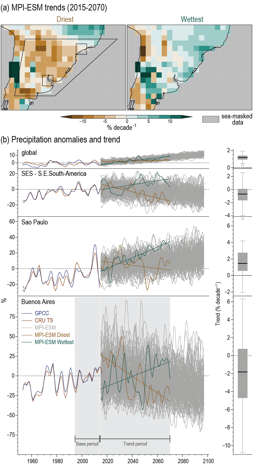 Figure 10.10 | Observed and projected changes in austral summer (December to February) mean precipitation in Global Precipitation Climatoloy Centre (GPCC), Climatic Research Unit Time Series (CRU TS) and 100 members of the Max Planck Institute for Meteorology Earth System Model (MPI-ESM. (a) 55-year trends (2015–2070) from the ensemble members with the lowest (left) and highest (right) trend (% per decade, baseline 1995–2014). (b) Time series (%, baseline 1995–2014) for different spatial scales (from top to bottom: global averages; South-Eastern South America; grid boxes close to São Paulo and Buenos Aires) with a five-point weighted running mean applied (a variant on the binomial filter with weights [1-3-4-3-1]). The brown (green) lines correspond to the ensemble member with weakest (strongest) 55-year trend and the grey lines to all remaining ensemble members. Box-and-whisker plots show the distribution of 55-year linear trends across all ensemble members, and follow the methodology used in Figure 10.6. Trends are estimated using ordinary least squares. Further details on data sources and processing are available in the chapter data table (Table 10.SM.11).
 Analysis of multi-model archives such as CMIP or CORDEX simulation results cannot easily disentangle model uncertainty and uncertainty related to internal variability. Since AR5, the development of single-model (global model and/or RCM) initial-condition large ensembles (SMILEs) has emerged as a promising way to robustly assess the regional-scale forced response to external forcings and the respective contribution of internal variability and model uncertainty to future regional climate changes (Section 4.2.5; Deser et al., 2014, 2020; Kay et al., 2015; Sigmond and Fyfe, 2016; Aalbers et al., 2018; Bengtsson and Hodges, 2019; Dai and Bloecker, 2019; Leduc et al., 2019; Maher et al., 2019; von Trentini et al., 2019; Lehner et al., 2020). The recent development of a multi-model archive of SMILE simulations facilitates the quantification and comparison of the influence of internal variability on global model-based regional climate projections between different models (Deser et al., 2020; Lehner et al., 2020). Another related development is the more frequent use of observation-based statistical models to assess the influence of internal variability on regional-scale global and regional model projections (Thompson et al., 2015; Salazar et al., 2016). However, these methods often implicitly assume that regional-scale internal variability does not change under anthropogenic forcing, which is a strong assumption that does not seem to hold at regional and local scales (LaJoie and DelSole, 2016; Pendergrass et al., 2017; W. Cai et al., 2018; Dai and Bloecker, 2019; Mankin et al., 2020; Milinski et al., 2020).
The appropriate ensemble size for a robust use of SMILEs depends on the model and physical variable being investigated, the spatial and time aggregation being performed, the magnitude of the acceptable error and the type of questions one seeks to answer (Deser et al., 2012, 2017b; Kang et al., 2013; Wettstein and Deser, 2014; Dai and Bloecker, 2019; Maher et al., 2019). It is noteworthy that the recent development of ensembles with a very large ensemble size (greater than 100) have led to new insights and methodologies to robustly assess the required ensemble size for questions such as the estimation of the forced response to external forcing or a forced change in modes of internal variability, such as ENSO, and its associated teleconnections (Herein et al., 2017; Maher et al., 2018; Haszpra et al., 2020; Milinski et al., 2020).
The use of SMILEs assumes that they have a realistic representation of internal variability and its evolution under anthropogenic climate change (Eade et al., 2014; McKinnon et al., 2017; McKinnon and Deser, 2018; Chen and Brissette, 2019). Assessing the realism of simulated internal variability for past and current climates remains an active research field with a number of issues such as the shortness and uncertainties of the observed record, in particular in data-scarce regions (Section 10.2.2.3), the signal-to-noise paradox (Section 4.4.3.1; Scaife and Smith, 2018), uncertainty in past observed external forcing estimates (Chapters 2, 6 and 7) and the limitations of assumptions underlying the statistical methods used to derive observational large ensembles (McKinnon et al., 2017; McKinnon and Deser, 2018; Castruccio et al., 2019). Calibration methods inspired by weather and seasonal forecasts can be used to improve the reliability of regional-scale climate projections from large ensembles (Brunner et al., 2019; O’Reilly et al., 2020). Interestingly, reliability is improved when the calibration is performed separately for the dynamical and residual components of the ensemble resulting from dynamical adjustment (Section 10.4.1; O’Reilly et al., 2020).
Importantly, accurately partitioning uncertainty in regional climate projections can provide an incentive for immediate action, accepting a large range of possible outcomes due to internal variability, while confounding model uncertainty with internal variability may be understood as a lack of knowledge and lead to delayed action in adaptation decision-making (Section 10.5.3; Maraun, 2013b; Mankin et al., 2020).
There is high confidence that the availability of SMILEs allows a robust assessment of the relative contributions of model uncertainty and internal variability in regional-scale projection uncertainty. There is high confidence that the use of SMILEs with appropriate ensemble size leads to an improved estimate of regional-scale forced response to an external forcing as well as of the full spectrum of possible changes associated with internal variability. There is high confidence that these improved estimates are beneficial for characterizing the full distribution of outcomes that is a key ingredient of climate information for robust decision-making and risk-analysis frameworks.
10.3.4.4 Designing and Using Ensembles for Regional Climate Change Assessments to Take Uncertainty Into Account
Ensembles of climate simulations play an important role in quantifying uncertainties in the simulation output (Sections 10.3.4.2 and 10.3.4.3). In addition to providing information on internal variability, ensembles of simulations can estimate scenario uncertainty and model (structural) uncertainty. Chapter 4, especially Box 4.1, discusses issues involved with evaluating ensembles of global model simulations and their uncertainties. In a downscaling context, further considerations are necessary, such as the selection of global model–RCM combinations when performing dynamical downscaling. This is a relevant issue when resources are limited. The structural uncertainty of both the global model and the downscaling method can be important (e.g., Mearnset al., 2012; Dosio, 2017), as well as further potential uncertainty created by inconsistencies between the global model and the downscaling method (e.g., Dosio et al., 2019), which could include, for example, differences in topography or the way to model precipitation processes (Mearns et al., 2013).
An important consideration is which set of global models should be used for global model–RCM combinations. If adequate resources exist, then large numbers of global model–RCM combinations are possible (Déqué et al., 2012; Coppola et al., 2021; Vautard et al., 2021). However, coordinated downscaling programmes can be limited by the human and computational resources available, for producing ensembles of downscaled output, which limits the number of feasible global model–RCM combinations. With this limitation in mind, a small set of GCMs may be chosen that span the range of equilibrium climate sensitivity in available global models (e.g., Mearns et al., 2012, 2013; Inatsu et al., 2015), though this range may be inconsistent with the likely range (Chapter 4), or some other relevant measure of sensitivity, such as the projected range of tropical SSTs (Suzuki-Parker et al., 2018). A further choice is to emphasize models that do not have the same origins or that do not use similar parametrizations and thus might be viewed as independent, a criterion that could be applied to both global models (Chapter 4) and RCMs (Evans et al., 2014). Global models and RCMs could also be discarded that unrealistically represent processes controlling the regional climate of interest (McSweeney et al., 2015; Maraun et al., 2017; Bukovsky et al., 2019; Eyring et al., 2019). Box 4.1 offers a more detailed discussion of the issues surrounding these approaches. Finally, global models may be selected to represent different physically self-consistent changes in regional climate (Zappa and Shepherd, 2017). Statistical methods can provide estimates of outcomes from missing global model–RCM combinations in a large matrix (Déqué et al., 2012; Heinrich et al., 2014; Evin et al., 2019).
However, even using a relatively small set of global models can still involve substantial computation that strains available resources, both for performing the simulations and for using all simulations in the ensemble for further impacts assessment. The NARCCAP programme (Mearns et al., 2012) used only a subset of its possible global model–RCM combinations that balanced comprehensiveness of sampling the matrix with economy of computation demand, while still allowing discrimination, via ANOVA methods, of global model and RCM influences on regional climate change (Mearns et al., 2013). An advantage of the sparse, but balanced matrix for those using the downscaling output for further studies, is that they have a smaller, yet comprehensive set of global model–RCM combinations to work with. Alternatively, data-clustering methods can clump together downscaling simulations featuring similar climate-change characteristics, so that only one representative simulation from each cluster may be needed for further impacts analysis, again systematically reducing the necessary number of simulations to work with (Mendlik andGobiet, 2016; Wilcke and Bärring, 2016).
Independently of the resources, participation of multiple models in a simulation programme such as CORDEX for RCMs or CMIP for global models creates ensembles of opportunity, which are ensembles populated by models that participants chose to use without there necessarily being an overarching guiding principle for an optimum choice. As discussed in Chapter 4, these ensembles are likely suboptimal for assessing sources of uncertainty. An important contributor to the suboptimal character of such an ensemble is that the models are not independent. Some may also have larger biases than others. Yet often, the output from models in these ensembles has received equal weight when viewed collectively, as was the case in much of the AR5 assessment (e.g., Collins et al., 2013b; Knutti et al., 2013; Flato et al., 2014; Kirtman et al., 2014). A number of emerging methodologies aim at optimizing the ensembles available by weighting the simulation results according to a number of criteria relevant at the regional scale that aim at obtaining more realistic estimates of the uncertainty (Sanderson et al., 2015; Brunner et al., 2020).
There is high confidence that ensembles for regional climate projections should be selected such that models unrealistically simulating processes relevant for a given application are discarded, but at the same time, the chosen ensemble spans an appropriate range of projection uncertainties.
Cross-Chapter Box 10.2 | Relevance and Limitations of Bias Adjustment
Coordinators: Alessandro Dosio (Italy), Douglas Maraun (Austria/Germany)
Contributors: Ana Casanueva (Spain), José Manuel Gutiérrez (Spain), Stefan Lange (Germany), Jana Sillmann (Norway/Germany)
Bias adjustment is an approach to post-process climate model output and has become widely used in climate hazard and impact studies (Gangopadhyay et al., 2011; Hagemann et al., 2013; Warszawski et al., 2014) and national assessment reports (Cayan et al., 2013; Georgakakos et al., 2014). Despite its wide use, bias adjustment was not assessed in AR5 (Flato et al., 2014). Several problems have been identified that may arise from an uncritical use of bias adjustment, and that may result in misleading impact assessments. The rationale of this Cross-Chapter Box is to provide an overview of the use of bias adjustment in this Report, and to assess key limitations of the approach.
Bias-adjusted climate model output is used extensively throughout this Report. Several results from Chapter 8, and many of the climatic impact-drivers in Chapter 12 (Section 12.2) are based on bias adjustment. The (Atlas presents many results both as raw and bias-adjusted data (Atlas.1.4.5). The application of bias adjustment in the WGI report was informed by the assessment in Chapter 10 and this Cross-Chapter Box. Finally, bias adjustment is crucial for many studies assessed in the WGII report. An overview of bias adjustment can be found in Section 10.3.1.3, a general performance assessment of individual method classes in Section 10.3.3.7. The fitness of bias adjustment for climate change applications is assessed in Section 10.3.3.9.
Relevance of bias adjustment
An argument made for the use of bias adjustment is the fact that impact models are commonly very sensitive, often non-linearly, to the input climatic variables and their biases, in particular when threshold-based climate indices are required (Dosio, 2016). There are, however, cases where bias adjustment may not be necessary or useful, such as: when only qualitative statements are required; when only changes in mean climate are considered (instead of absolute values); when percentile-based indices are used.
Modification of the climate change signal
Bias adjustment methods like quantile mapping can modify simulated climate trends, with impacts on changes to climate indices, in particular, extremes (Haerter et al., 2011; Dosio et al., 2012; Ahmed et al., 2013; Hempel et al., 2013; Maurer and Pierce, 2014; Cannon et al., 2015; Dosio, 2016; Casanueva et al., 2020). Some argue that these trend modifications are implicit corrections of state-dependent biases (Boberg and Christensen, 2012; Gobiet et al., 2015). However, others argue that the modification is generally invalid because the modification is linked to the representation of day-to-day rather than long-term variability (Pierce et al., 2015; Maraun et al., 2017); a given temperature value does not necessarily belong to the same weather state in present and future climate (Maraun et al., 2017); the modification affects the models climate sensitivity (Hempel et al., 2013); and is affected by random internal climate variability (Switanek et al., 2017). Thus, trend preserving quantile mapping methods have been developed (Section 10.3.1.3.2), although some authors found no clear advantage of these methods (Maurer and Pierce, 2014). Further research is required to fully understand the validity of trend modifications by quantile-mapping.
Bias adjustment in the presence of large-scale circulation errors
The large-scale circulation has a strong impact on regional climate, thus circulation errors will cause regional climate biases (Section 10.3.3.3). As bias adjustment in general does not account for circulation errors, it is therefore important to understand the impact of these errors on the outcome of the bias adjustment (Addor et al., 2016; Photiadou et al., 2016; Maraun et al., 2017). If the frequency of precipitation-relevant weather types is biased, a standard bias adjustment (not accounting for this frequency bias) would remove the overall climatological bias, but the precipitation falling in a given weather type could still be substantially biased (Addor et al., 2016). Adjusting the number of wet days can artificially deteriorate the spell-length distribution (Maraun et al., 2017). In the presence of location biases of circulation patterns, bias adjustment may introduce physically implausible solutions (Maraun et al., 2017). Bias adjusting the location of circulation features (Levy et al., 2013) may introduce inconsistencies with the model orography, land–sea contrasts, and SSTs (Maraun et al., 2017).
There is medium confidence that the selection of climate models with low biases in the frequency, persistence and location of large-scale atmospheric circulation can reduce negative impacts of bias adjustment.
Using bias adjustment for statistical downscaling
Bias adjustment is often used to downscale climate model results from grid box data to finer resolution or point scale. It is sometimes even directly applied to coarse-resolution global model output to avoid an intermediate dynamical downscaling step (Johnson and Sharma, 2012; Stoner et al., 2013). But bias adjustment does not add any information about the processes acting on unresolved scales and is therefore by construction not capable of bridging substantial scale gaps (Maraun, 2013a; Maraun et al., 2017). Using bias adjustment for downscaling has been shown to artificially modify long-term trends, misrepresent the spatial characteristics of extreme events, and misrepresent local weather phenomena such as temperature inversions (Maraun, 2013a; Gutmann et al., 2014; Maraun et al., 2017). Crucially, sub-grid influences on the local climate change signal are not represented. For instance, if a mountain chain is not resolved in the driving model, the snow–albedo feedback is not represented by the bias adjustment such that local temperature trends in high altitudes are under-represented (Cross-Chapter Box 10.2, Figure 1; Maraun et al., 2017). It has therefore been suggested to account for local random variability by combining bias adjustment with stochastic downscaling (Volosciuk et al., 2017; Lange, 2019), although this approach still does not account for local modifications of the climate change signal. Two approaches have been proposed to represent these local changes: dynamical downscaling with high-resolution RCMs (Maraun et al., 2017) or statistical emulators of such (Walton et al., 2015). Sections 10.3.3.4–10.3.3.6 and 10.3.3.9 discuss other examples where RCMs improve the representation of regional phenomena and regional climate change.

Cross-ChapterBox 10.2, Figure 1 | Boreal spring (March to May) daily mean surface air temperature in the Sierra Nevada region in California. (a) Present climate (1981–2000 average, in °C) in the GFDL-CM3 GCM, interpolated to 8 km (left), GCM bias adjusted (using quantile mapping) to observations at 8 km resolution (middle) and WRF RCM at 3 km horizontal resolution (right). (b) Climate change signal (2081–2100 average minus 1981–2000 average according to RCP8.5, in °C) in the GCM (left), the bias adjusted GCM (middle) and the RCM (right). Further details on data sources and processing are available in the chapter data table (Table 10.SM.11). Figure adapted from Maraun et al. (2017).
Overall, there is high confidence that the use of bias adjustment for statistical downscaling, in particular to downscale coarse resolution global models, has severe limitations.
Bias adjustment of multiple variables
Impact models, as well as indices of climatic impact-drivers, often require input of several meteorological variables (Chapter 12). In several situations, for example, if the dependence between the variables is not well-simulated, univariate bias adjustment of the individual variables may increase biases in the resulting indicator (Zscheischler et al., 2019). A simple alternative would be a bias adjustment of the indicator, but such a procedure may substantially alter the climate change signal, in particular for extreme events (Casanueva et al., 2018). In principle, multivariate bias adjustment methods are good to adjust all statistical aspects of the multivariate distribution that they intend to adjust. Depending on the method, this includes the correlation structure or even broader aspects of the dependence (Cannon, 2016, 2018; Vrac, 2018; François et al., 2020). If multivariate adjustment includes a spatial dimension, then spatial dependence is adjusted well (Vrac, 2018), but care is needed when applied across large areas (François et al., 2020). Adjustment of multivariate dependence necessarily modifies the temporal sequencing of the driving model (Cannon, 2016; Maraun, 2016). The extent of the modification depends on the chosen method and the number of variables to adjust (Vrac and Friederichs, 2015; Cannon, 2016; Vrac, 2018; François et al., 2020).
Bias adjustment in the presence of observational uncertainty and internal variability
Observational uncertainties and internal variability introduce uncertainty in the estimation of biases and thus in the calibration of bias-adjustment methods. Dobor and Hlásny (2019) found a considerable influence of the choice of the observational dataset and calibration period on the adjustment for some regions. RCM biases are typically larger than observational uncertainties, but in some regions, and in particular for wet-day frequencies, spatial patterns and the intensity distribution of daily precipitation, the situation may reverse (Kotlarski et al., 2019). Switanek et al. (2017) found a strong influence of internal variability and thus of the choice of calibration period on the calibration of quantile mapping and on the modification of the climate change signal.
Bias adjustment is typically evaluated using cross-validation, that is, by calibrating the adjustment function to one period of the observational record, and by evaluating it on a different one. Maraun et al. (2017) and Maraun and Widmann (2018a) demonstrated that, in the presence of multi-decadal internal variability, cross-validation may lead to a rejection of a valid bias adjustment or even lead to a positive evaluation of an invalid adjustment. The authors therefore argued that, in the presence of substantial internal variability, the evaluation of bias adjustment requires to consider aspects that have not been adjusted, such as temporal, spatial, or multivariable dependence.
There is high confidence that observational uncertainty and internal variability adversely affect bias adjustment and introduce uncertainties in bias-adjusted future projections.
Overall assessment and new avenues
In the light of these issues, several authors dismiss the use of bias adjustment for climate change studies (Vannitsem, 2011; Ehret et al., 2012). Ehret et al. (2012) and IPCC (2015) propose to at least provide the raw model output alongside the adjusted data. Maraun et al. (2017) argue that the target resolution should be similar to the model resolution to avoid downscaling issues. IPCC (2015) and Maraun et al. (2017) highlighted the relevance of understanding model biases and the misrepresentations of the underlying physical processes prior to any adjustment. Together with Galmarini et al. (2019), they point out the need for collaboration between bias adjustment users, experts in climate modelling and experts in the considered regional climate. As new research avenues, development of process-oriented bias adjustment methods (Addor et al., 2016; Verfaillie et al., 2017; Manzanas and Gutiérrez, 2019) or run-time bias adjustment integrated into the climate simulation, for example, to reduce circulation errors (Guldberg et al., 2005; Kharin et al., 2012; Krinner et al., 2019, 2020) are proposed.
10.4 Interplay Between Anthropogenic Change and Internal Variability at Regional Scales
This section focuses on the assessment of the methodologies used to identify the physical causes of past and future regional climate change in the context of the ongoing anthropogenic influence on the global climate. The main foci are the attribution of past regional-scale changes (Sections 10.4.1–2) and the robustness and future emergence of the regional-scale response to anthropogenic forcing (Section 10.4.3).
In this chapter, regional-scale attribution is defined as the process of evaluating the relative contributions of multiple causal factors (or drivers) to regional climate change (Cross-Working Group Box: Attribution in Chapter 1; Rosenzweig and Neofotis, 2013; Shepherd, 2019). Attribution at regional scale builds upon the usual definition of attribution used in the AR5 (Cross-Working Group Box: Attribution in Chapter 1; Hegerl et al., 2010). However, in contrast with global-scale attribution methods where internal variability might be considered as a noise problem (Section 3.2), the preliminary detection step is not always required to perform regional-scale attribution since causal factors of regional climate change may also include internal modes of variability in addition to external natural and anthropogenic forcing. Importantly, regional-scale (or process-based) attribution also seeks to determine the physical processes and uncertainties involved in the causal factor’s influence (Cross-Working Group Box: Attribution in Chapter 1).
(Section 10.4.1 describes regional-scale attribution methodologies and assesses their application to regional changes of temperature and precipitation. Section 10.4.2 presents three illustrative attribution examples that illustrate a number of specific regional-scale challenges and methodological aspects. Section 10.4.3 focuses on methodologies used to assess the robustness and emergence of the regional climate response to anthropogenic forcing. A basic description of future regional climate change for all regions considered in the report (as defined in Section 1.4.5) appears in the Atlas.
10.4.1 Methodologies for Regional Climate Change Attribution
Attribution at sub-continental and regional scales is usually more complicated than at the global scale due to various factors: a larger contribution from internal variability, an increased similarity among the responses to different external forcings leading to a more difficult discrimination of their effects, the importance at regional scale of some omitted forcings in global model simulations, and model biases related to the representation of small-scale phenomena (Zhai et al., 2018). Since AR5 and in addition to standard optimal fingerprint regression-based approaches (Section 3.2.1 and Zhai et al. 2018), several emerging methodologies have been increasingly used for regional-scale climate change attribution. These include several statistical approaches that differ in their use or omission of spatiotemporal co-variance information. Dynamical adjustment and pattern recognition techniques fall into the category of spatiotemporal methods while univariate detection and attribution methods rely on single grid-point analysis. Finally, the development, evaluation and use of all these methodologies rely upon the availability of multiple and high-quality observational datasets (Section 10.2) as well as multi-model simulations of the historical period constrained by different external forcing combinations, including single-forcing experiments and single-model initial-condition large ensembles (SMILEs).
10.4.1.1 Optimal Fingerprinting Methods
Optimal fingerprint regression-based methods have been applied to detection and attribution of mean temperature anthropogenic signal in several regions of the world such as Canada, India, central Asia, northern and western China, Australia, and North Africa (Xu et al., 2015; C. Li et al., 2017; Dileepkumar et al., 2018; Y. Wang et al., 2018; Peng et al., 2019; Wan et al., 2019). The influence of anthropogenic forcing, and in particular that of greenhouse gases (GHGs), is robustly detected in annual and seasonal mean temperatures for all considered regions. Most of the observed regional temperature changes since the mid-twentieth century can only be explained by external forcings, with anthropogenic influence being the dominant factor. GHG increase is found to be the primary factor of the anthropogenic-induced warming while the aerosol forcing leads to a cooling offsetting a fraction of the GHG change (C. Li et al., 2016, 2017). While the influence of external natural forcing can often be detected as well, its contribution to observed changes is usually much smaller (C. Li et al., 2017; Wan et al., 2019). Temperature detection results are found to be robust to the use of different observational datasets and detection methodologies (Dileepkumar et al., 2018).
Detection of mean precipitation changes caused by human influence is much more difficult, due to a larger role of internal variability at regional to local scales, as well as substantial modelling and observational uncertainty (Wan et al., 2015; Sarojini et al., 2016; C. Li et al., 2017). However, multi-decadal precipitation changes due to anthropogenic forcing have been detected for several regions. Ma et al. (2017b) show that anthropogenic forcing has strongly contributed to the observed shift of China daily precipitation towards heavy precipitation. The observed weakening of the East Asia summer monsoon, also known as the southern flooding and northern drought pattern has been partially linked to anthropogenic forcing (Section 8.3.2.4.2; Song et al., 2014; Zhou et al., 2017; Tian et al., 2018). Changes in GHGs lead to increasing precipitation over southern China, while changes in anthropogenic aerosols over East Asia are the dominant factors determining drought conditions over northern China (Song et al., 2014; Tian et al., 2018). Based on all-forcing and single-forcing simulation ensembles with a high-resolution model, Delworth and Zeng (2014) found that the observed long-term regional austral autumn and winter rainfall decline over southern and particularly south-west Australia is partially reproduced in response to anthropogenic changes in GHGs and ozone in the atmosphere, whereas anthropogenic aerosols do not contribute to the simulated precipitation decline. In contrast, the observed increase of north-west Australian summer rainfall since 1950 has been partially attributed to anthropogenic aerosol based on CMIP5 detection and attribution single-forcing simulations (Section 8.3.2.4.6; Dey et al., 2019a, b).
It is noteworthy that these methods require a very significant reduction of spatial and temporal dimensions in order to reliably estimate the co-variance matrix of internal variability (an entire region is thus often considered as being only one or a few spatial points that represent the spatial average of the whole region or a few sub-regions; time samples are often 5- or 10-year averages). Finally, model bias is rarely considered in statistical models used in detection and attribution regional studies, while it has been shown to have a strong impact on the stability of detection results and their associated confidence intervals when increasing the spatial dimension (Ribes and Terray, 2013). New statistical methods are emerging to provide some alternative to standard optimal fingerprinting but they have not yet been evaluated and applied at regional scales (Section 3.2.2).
10.4.1.2 Other Spatiotemporal Statistical Methods for Isolating Regional Climate Responses to External Forcing
The primary objective of any attribution method is to optimally separate the influences of external forcing and internal variability on a global or regional climate record. In a multi-model ensemble context, the estimation of the externally-forced climate response has been typically performed by ensemble averaging of linear trends or regional domain spatial average, thus not taking into account the available and complete space and time co-variance information. Since AR5, methods using spatiotemporal information have been further developed and used to improve the separation between external and internal drivers in multiple or single historical climate realizations performed by a given global model.
The typical ensemble size of CMIP historical climate simulations for a given model traditionally range between one and ten members, with three often being the default choice. At the regional scale, a simple ensemble average with such sample sizes does not provide robust estimates of the response patterns to external forcing (Maher et al., 2019; Deser et al., 2020). Since AR5, pattern filtering methods such as signal-to-noise maximizing empirical orthogonal functions (Ting et al., 2009) have been shown to improve the identification of forced response patterns when few model members are available (Wills et al., 2020). Using SMILEs as a test bed, it has been shown that pattern filtering strongly reduces the number of ensemble members needed to estimate the forced response pattern compared to simple ensemble averaging. Pattern filtering allows the identification of low signal-to-noise signals such as the El Niño-like response to volcanic eruptions (Khodri et al., 2017; Wills et al., 2020).
Methods to extract the response to external forcing in an observed or simulated single realization include dynamical adjustment (Smoliak et al., 2015; Deser et al., 2016; Sippel et al., 2019) and time scale separation methods (DelSole et al., 2011; Wills et al., 2018, 2020). Dynamical adjustment seeks to isolate changes in surface air temperature or precipitation that are due purely to atmospheric circulation changes. The residual can then be analysed and attributed to internal changes in both land or ocean surface conditions and the thermodynamical response to external forcing. Smoliak et al. (2015) performed their dynamical adjustment using partial least squares regression of temperature to remove variations arising from sea level pressure changes. Deser et al. (2016) used constructed atmospheric circulation analogues and resampling to estimate the dynamical contribution to changes in temperature. Sippel et al. (2019) used machine learning techniques known as regularized linear regression to provide estimates of circulation-induced components of precipitation and temperature variability from global to local scales. It is noteworthy that the dynamical adjustment method by itself cannot account for the component of the forced response associated with circulation changes that project onto atmospheric internal variability. However, this component can be estimated within a model framework by averaging the dynamical contribution across multiple members of a SMILE (Deser et al., 2016).
Dynamical adjustment methods have been used by, for instance, Deser et al. (2016), Saffioti et al. (2016), O’Reilly et al. (2017), Gong et al. (2019), and R. Guo et al. (2019). Deser et al. (2016) focused on the causes of observed and simulated multi-decadal trends in North American temperature. They demonstrated that the main advantage of this technique is to narrow the spread of temperature trends found by the model ensemble and to bring the dynamically-adjusted observational trend much closer to the forced response estimated by the model ensemble mean. Similar results were obtained by Saffioti et al. (2016) regarding recent observed winter temperature and precipitation trends over Europe. Similarly, O’Reilly et al. (2017) applied dynamical adjustment techniques to more carefully determine the influence of the Atlantic Multi-decadal Variability (AMV; Annex IV.2.7) on continental climates. Over Europe, summer temperature anomalies induced thermodynamically by the warm phase of the AMV are further reinforced by circulation anomalies; meanwhile, precipitation signals are largely controlled by dynamical responses to the AMV. Based on a partial least-squares approach, Gong et al. (2019) showed that recent winter temperature 30-year trends over northern East Asia are strongly influenced by internal variability linked to decadal changes of the Arctic Oscillation. Using dynamical adjustment purely on precipitation observations, R. Guo et al. (2019) showed that human influence has led to increased winter precipitation across north-eastern North America, as well as a small region of north-western North America, and to an increase in precipitation across much of north-western and north central Eurasia. The latter results confirm previous findings obtained by standard optimal fingerprinting methods (Wan et al., 2015).
Time scale separation methods such as the low-frequency component analysis and ensemble empirical mode decomposition methods take advantage of the longer time scale associated with anthropogenic external forcing compared to that of most internal modes of variability. The low-frequency component analysis method tries to find low-frequency variability patterns by searching for linear combinations of a moderate number of empirical orthogonal functions that maximize the ratio of low-frequency to total variance. It has first been used to separate internal modes of interannual and decadal variability from slowly varying and externally-forced variability in the Pacific and Atlantic oceans (Wills et al., 2018, 2019). The methodology has also been applied to patterns of observed surface air temperature to isolate the slow components of observed changes that are consistent with the expected response to anthropogenic greenhouse gas and aerosol forcing (Wills et al., 2020).
The ensemble empirical mode decomposition method (Wu and Huang, 2009; Wilcox et al., 2013; Ji et al., 2014; Qian and Zhou, 2014) decomposes data, such as time series of historical temperature and precipitation, into independent oscillatory modes of decreasing frequency. The last step of the method leaves behind a smooth and low-frequency residual time series. Typically, the non-linear anthropogenic trend (e.g., of 20th-century temperature) can be reconstructed by summing the long-term mean, the residual, and eventually the lowest-frequency mode to account for a multi-decadal forced signal, for instance associated with anthropogenic aerosol forcing. The ensemble empirical mode decomposition method is an example of a data-driven, non-parametric approach that can be used to directly provide an estimate of the forced response without the need for model data (Qian, 2016).
10.4.1.3 Other Regional-scale Attribution Approaches
The univariate detection method does not use spatial pattern information, but compares observed trends in gridded datasets with distributions of trends from ensembles of simulations during the historical period (Knutson et al., 2013; Knutson and Zeng, 2018). The trends arising from simulations constrained by natural forcing-only and all-forcing are compared with distributions of trends purely due to internal variability and derived from long simulations with constant pre-industrial external forcing. Consistency between observed and simulated historical trends is also assessed with statistical tests that can be applied independently over a large number of grid points. The fraction of area over a given region where the change is classified as detectable, attributable, or consistent/inconsistent, is then finally estimated. The method can be viewed as a simple consistency test for both amplitude and pattern of observed versus simulated trends. Its application to CMIP3 and CMIP5 models suggests that 80% of the Earth’s surface has a detectable anthropogenic warming signal (Knutson et al., 2013). Regarding regional land precipitation changes over the 1901–2010 and 1951–2010 periods, application of the univariate detection method based on CMIP5 models suggests attributable anthropogenic changes at several locations such as increases over regions of the north-central USA, southern Canada, Europe, and southern South America and decreases over parts of the Mediterranean region, northern tropical Africa and south-western Australia (Delworth and Zeng, 2014; Knutson and Zeng, 2018).
Another regional attribution technique is based on the similarity of past changes between observations and one or several simulations of a large ensemble that share the same time evolution for a suggested driver of these changes. Huang et al. (2020b) used a perturbed physics ensemble to attribute the drying trend of the Indian monsoon over the latter half of the 20th century to decadal forcing from the Pacific Decadal Variability (PDV; Annex IV.2.6). The ensemble members predicted different trends in PDV behaviour across the 20th century and the negative precipitation trend was only replicated in those members with a strong negative-to-positive PDV transition across the 1970s, consistent with the observed PDV behaviour (see also the detailed case study in Section 10.6.3). In a similar manner, Cvijanovic et al. (2017) addressed the possible influence of Arctic sea ice loss on the North Pacific pressure ridge and, consequently, on south-western USA precipitation. They sampled the uncertainties in selected sea ice physics parameters to achieve a ‘low Arctic sea ice’ state in their perturbed simulations. They then compared the latter with control simulations representative of sea ice conditions at the end of the 20th century to assess changes purely due to sea ice loss.
New methods aiming to remove underlying model biases before performing detection and attribution, for instance related to precipitation changes, are emerging based on image transformation techniques such as warping (Levy et al., 2014a). By correcting location and seasonal precipitation biases in CMIP5 models, Levy et al. (2014b) showed that the agreement between observed and fingerprint patterns can be improved, further enhancing the ability to attribute observed precipitation changes to external forcings. The improvement mainly relies on the assumption that precipitation changes are tied to the underlying climatology, which has been shown to be a reasonable assumption in regions of the world where intensification of the hydrological cycle is expected (Held and Soden, 2006).
Importantly, evidence that the models employed in regional-scale attribution are fit for purpose is essential in order to estimate the degree of confidence in the attribution results (Section 10.3.3). For example, models need to be evaluated and assessed in their ability to simulate internal variability modes that are known to be important drivers of regional climate change (Sections 3.7 and 10.3.3.3 and Annexes IV.2 and IV.3). Models are likely to have different performance in different regions and therefore their evaluation needs to be performed in terms of key physical processes and mechanisms relevant to the climate of the region under consideration (Section 10.3.3).
To conclude, there is very high confidence (robust evidence and high agreement) that the use of diverse and independent attribution methods, multiple model ensemble types and observed datasets strengthens the robustness of results of regional-scale attribution studies. Since AR5, multiple SMILEs have provided an adequate testbed for new attribution methodologies aimed at separating forced signals from internal variability in observational records as well as small-size single-model ensembles.
10.4.2 Regional Climate Change Attribution Examples
This section focuses on three illustrative examples that span different regions, time scales, and attribution methods, without aiming at being comprehensive. These examples illustrate attribution statements that are based upon multiple lines of evidence, combining multiple observational datasets, different generations and types of models, process understanding and assessment of various sources of uncertainty. Detection and attribution assessments for all AR6 regions and specific variables can be found in the Atlas.
10.4.2.1 The Sahel and West African Monsoon Drought and Recovery
The Sahel, fed by the West African monsoon, has experienced severe decadal rainfall variations (Figure 10.11a). Abundant rainfall in the 1950s–1960s was followed by a large negative trend (Figure 10.11b) until at least the 1980s, over which annual rainfall fell by 20–30% (Hulme, 2001). The subsequent partial recovery (B. Wang et al., 2021) is more uncertain: rain-gauge studies suggest a return to long-term positive anomalies in the western Sahel in the early 2000s (Panthou et al., 2018), while CHIRPS merged satellite/gauge data show a wetter western Sahel since 1981 (Bichet and Diedhiou, 2018a, b). The recovery has been more significant over the central rather than the western Sahel (Lebel and Ali, 2009; Maidment et al., 2015; Sanogo et al., 2015) and a multiple-gauge record supports a greater recovery to the eastern side (Nicholson et al., 2018). In this attribution example, drivers of the long-term drought and subsequent partial recovery are discussed, including anthropogenic GHG and aerosol emissions, and sea surface temperature (SST) variations that, in part, relate to internal variability. The reader is also referred to assessment in Section 8.3.2.4. We define the Sahel within 10°N–20°N across to 30°E, consistent with the eastern boundary used in Chapter 8, and the rainy season as spanning June to September.
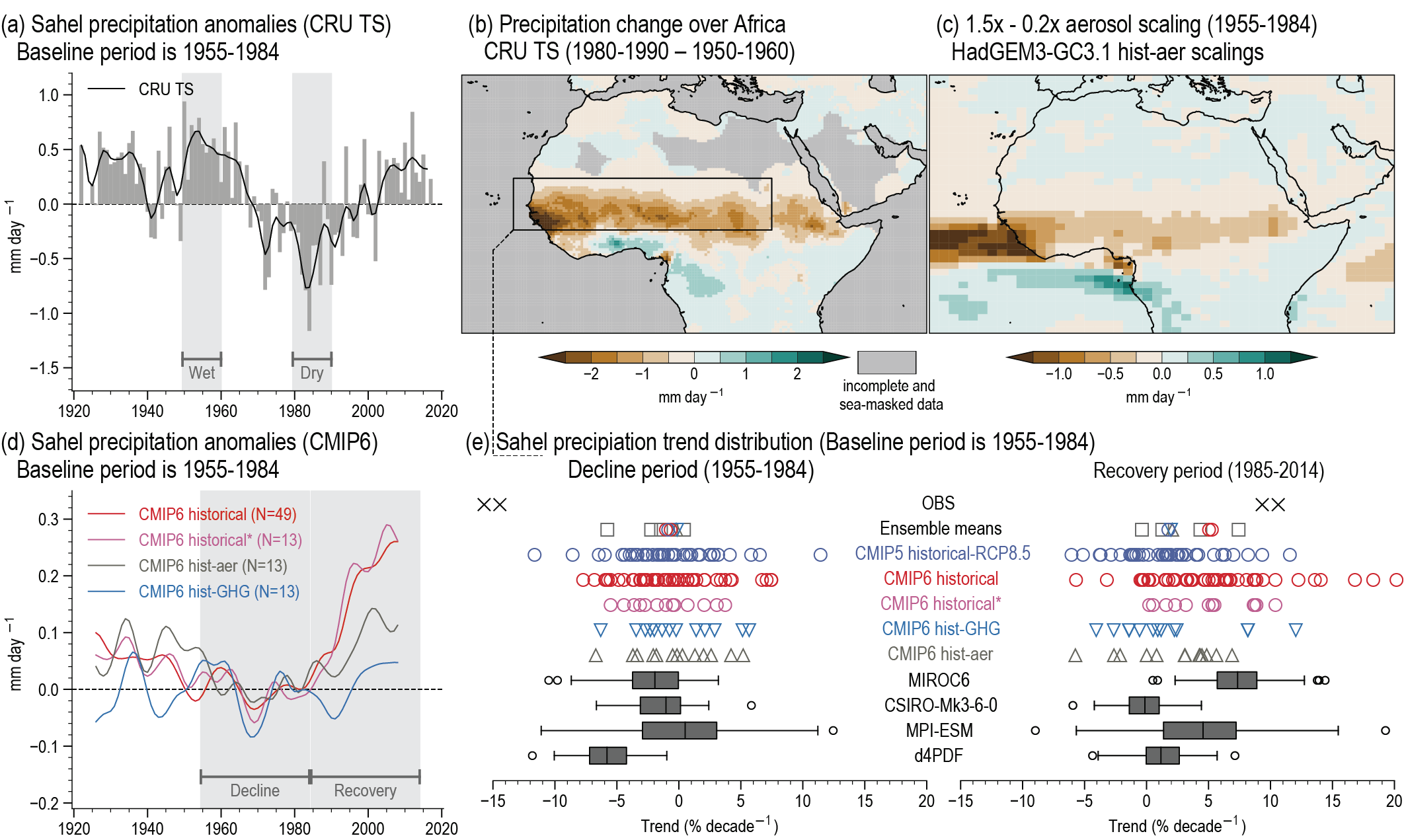 Figure 10.11 | Attribution of historic precipitation change in the Sahelian West African monsoon during June to September. (a) Time series of CRU TS precipitation anomalies (mm day–1, baseline 1955–1984) in the Sahel box (10°N–20°N, 20°W–30°E) indicated in panel (b) applying the same low-pass filter as that used in Figure 10.10. The two periods used for difference diagnostics are shown in grey columns. (b) Precipitation change (mm day–1) in CRU TS data for 1980–1990 minus 1950–1960 periods. (c) Precipitation difference (mm day–1) between 1.5× and 0.2× historical aerosol emissions scaling factors averaged over 1955–1984 and five ensemble members of HadGEM3 experiments after Shonk et al. (2020). (d) Sahel precipitation anomaly time series (mm day–1, baseline 1955–1984) in Coupled Model Intercomparison Project Phase 6 (CMIP6) for 49 historical simulations with all forcings (red), and thirteen for each of greenhouse gas-only forcing (light blue) and aerosol-only forcing (grey), with a thirteen-point weighted running mean applied (a variant on the binomial filter with weights [1-6-19-42-71-96-106-96-71-42-19-6-1]). The CMIP6 subsample of all forcings matching the individual forcing simulations is also shown (pink). (e) Precipitation linear trend (% per decade) for (left) decline (1955–1984) and (right) recovery periods (1985–2014) for ensemble means and individual CMIP6 historical experiments (including single-forcing) as in panel (d) plus 34 CMIP5 models (dark blue). Box-and-whisker plots show the trend distribution of the three coupled and the d4PDF atmosphere-only single-model initial-condition large ensembles (SMILEs) used throughout (Chapter 10 and follow the methodology used in Figure 10.6. The two black crosses represent observational estimates from GPCC and CRU TS. Trends are estimated using ordinary least-squares regression. Further details on data sources and processing are available in the chapter data table (Table 10.SM.11).
 The role of SST forcing in the rainfall decline is assessed first. Competing mechanisms from equatorial Atlantic SSTs and inter-hemispheric SST gradients regulate decadal variability in the Sahel (Nicholson, 2013), alternatively explained by tropical warming leading to Sahel drought, while North Atlantic warming promotes increased rainfall (Rodríguez-Fonseca et al., 2015). The SST influence has been formalized in an AMV framework (Giannini et al., 2013; Martin and Thorncroft, 2014; Martin et al., 2014; Park et al., 2015), suggesting that relative North Atlantic SST warming increases the Northern Hemisphere differential warming, enhancing Sahel rainfall. The AMV influence is supported by CMIP5 initialized decadal hindcasts (Gaetani and Mohino, 2013; Mohino et al., 2016; Sheen et al., 2017), which outperform empirical predictions based on persistence. Some caution is needed since the full magnitude of internal variability is not captured in most CMIP5 models, as poor resolution prevents reproduction of AMV teleconnection responses (Vellinga et al., 2016), and the magnitude of AMV-related SST variation may be underestimated in CMIP5 (Section 3.7.7, which also assesses that the AMV may be partially forced). The influence of PDV has been studied to a lesser extent, with the PDV positive phase having a negative impact on Sahel rainfall in combined observational/CMIP5 analysis (Villamayor and Mohino, 2015). The closer match between the observed rainfall declining trend and those in an atmosphere-only SMILE, in which SSTs are matched to observations, compared to three coupled SMILEs in which they are not, suggests that the underlying ocean surface might be essential in driving the decline (Figure 10.11e).
In terms of anthropogenic emissions, regional aerosol emissions from Europe, and to a lesser extent from Asia, have been shown in a global model to weaken Sahel precipitation either through a weakened Saharan heat low or via the Walker circulation (Dong et al., 2014). Greenhouse gases (GHGs) and anthropogenic aerosol can be considered together to control ITCZ position based on temperature asymmetry at the hemispheric scale. GHGs increase Sahel precipitation, while aerosol reduces it (in coupled slab-ocean model experiments by Ackerley et al. (2011) following Biasutti and Giannini (2006)). This effect is stronger when models account for aerosol–cloud interactions (Allen et al., 2015). Perturbed physics GCM ensembles suggests that aerosol emissions were the main driver of observed drying over 1950–1980 (Ackerley et al., 2011), supported by CMIP5 single-forcing experiments (Polson et al., 2014). A coherent drying signal in CMIP5 over the extended 1901–2010 period has also been found, although smaller than the observed trend (Knutson and Zeng, 2018). By applying aerosol scaling factors to the historical period in order to sample the uncertainty in CMIP5 aerosol radiative forcing, Shonk et al. (2020) found differences of 0.5 mm day–1 for Gulf of Guinea rainfall between strong and weak aerosol experiments as illustrated in Figure 10.11c, although the drying appears further south than observed due to model bias.
For the partial recovery in West African monsoon and Sahel rainfall since the late 1980s, a detection study using three reanalyses (Cook and Vizy, 2015) shows a connection to increasing Saharan temperatures at a rate two to four times greater than the tropical mean, also confirmed by multiple observational and satellite-based data (Zhou and Wang, 2016; Vizy and Cook, 2017) and the review of Cook and Vizy (2019). Reanalyses are also noted to significantly underestimate the Saharan warming (Zhou and Wang, 2016). Saharan warming causes a stronger thermal low and more intense monsoon flow, providing more moisture to the central and eastern Sahel, supported by CMIP5 models (Lavaysse et al., 2016), although not all models capture the observed rainfall–heat–low relationship. Sahel rainfall is also incorrectly located in prototype versions of a few CMIP6 models, related to tropospheric temperature biases (Martin et al., 2017). Amplified Saharan warming has increased the wind shear, leading to a tripling of extreme storms since 1982, which may partially explain the recovery (Taylor et al., 2017). Instead, observations, multiple models and SST-sensitivity experiments with AGCMs have suggested that stronger Mediterranean Sea evaporation enhances low-level moisture convergence to the Sahel, increasing rainfall (Park et al., 2016). Meanwhile, an AGCM study suggested that GHGs alone (in the absence of SST warming) could cause Sahel rainfall recovery, with an additional role for anthropogenic aerosol (Dong and Sutton, 2015); recent changes in North Atlantic SSTs, although substantial, did not exert a significant impact on the recovery. Large spread in the recovery in a five-member AGCM ensemble suggests that atmospheric internal variability cannot be discounted (Roehrig et al., 2013).
Consistent timing of the southward ITCZ shift during the decline period in CMIP3 and CMIP5 historical simulations supports the role of external forcing, chiefly anthropogenic aerosol (Hwang et al., 2013). The evolution of the observed decline and recovery is largely followed by the CMIP5 multi-model mean, further supporting the role of external drivers (Giannini and Kaplan, 2019). Updated results from CMIP6 for historical simulations with all and single forcings are represented in Figure 10.11d,e showing smaller trends than those observed. Giannini and Kaplan (2019) attempted to unify the driving mechanisms for decline and recovery based on singular-value decomposition of observed and modelled SSTs. Since the 1950s, tropical warming arising from GHGs and North Atlantic cooling from aerosol led to regional stabilization, suppressing Sahel rainfall. The subsequent reduction in aerosol emissions then led to North Atlantic warming and recovery of Sahel rainfall. Such mechanisms continue into the near-term future in idealized and modified RCP experiments, with scenarios featuring more aggressive reductions in aerosol emissions, or including aerosol–cloud interactions, favouring a greater northward shift of rainfall (Allen, 2015; Westervelt et al., 2017, 2018; Scannell et al., 2019). There is paleoclimate evidence of changes to Sahel rainfall in the past, in particular with enhancement of the West African monsoon during the mid-Holocene. However, the mechanisms governing such a change have been shown to be largely dynamical in nature (D’Agostino et al., 2019), suggesting that the mid-Holocene cannot be used to inform the credibility of changes due to greenhouse warming.
There is very high confidence (robust evidence and high agreement) that patterns of 20th-century ocean and land surface temperature variability have caused the Sahel drought and subsequent recovery by adjusting meridional gradients. There is high confidence (robust evidence and medium agreement) that the changing temperature gradients that perturb the West African monsoon and Sahel rainfall are themselves driven by anthropogenic emissions: warming by GHG emissions was initially restricted to the tropics but suppressed in the North Atlantic due to nearby emissions of sulphate aerosols, leading to a reduction in rainfall. The North Atlantic subsequently warmed following the reduction of aerosol emissions, leading to rainfall recovery.
10.4.2.2 The South-Eastern South America Summer Wetting
A positive trend in summer (December to February) precipitation has been detected in multiple observational sources in south-eastern South America since the beginning of the 20th century (Gonzalez et al., 2013; Vera and Díaz, 2015; Wu et al., 2016; H. Zhang et al., 2016; Díaz and Vera, 2017; Saurral et al., 2017). Sedimentary records from the Mar Chiquita lake indicate that the last quarter of the 20th century was wetter than any period during the last 200 years (Piovano et al., 2004). In this attribution example the drivers contributing to the positive trend for the period 1951–2014 are discussed (Figure 10.12a). Precipitation anomalies of Climatic Research Unit Time Series (CRU TS) as well as for the two members of a SMILE with the most negative and positive trends for 1951–2014 are displayed in Figure 10.12b. The trend for 1951–2014 using CRU TS and GPCC is illustrated in Figure 10.12c, and for the region defined by the black quadrilateral, it amounts to 2.8 (CRU TS) – 3.5 (GPCC) mm per month and decade (see black crosses in Figure 10.12d) while the mean summer monthly precipitation for the same period is 104 (CRU TS) –109 (GPCC) mm. The trend is also detectable in daily and monthly extremes (Re and Barros, 2009; Marengo et al., 2010; Penalba and Robledo, 2010; Doyle et al., 2012; Donat et al., 2013; Lorenz et al., 2016).
 Figure 10.12 | South-Eastern South America positive mean precipitation trend and its drivers during 1951–2014. (a) Mechanisms that have been suggested to contribute to South-Eastern South America summer wetting. (b) Time series of austral summer (December to February) precipitation anomalies (%, baseline 1995–2014) over the South-Eastern South American region (26.25°S–38.75°S, 56.25°W–66.25°W), black quadrilateral in the first map of panel (c). Black, brown and green lines show low-pass filtered time series for CRU TS), and the members with driest and wettest trends of the MPI-ESM single-model initial-condition large ensemble (SMILE; between 1951–2014), respectively. The filter is the same as the one used in Figure 10.10. (c) Mean austral summer precipitation spatial linear 1951–2014 trends (mm per month and decade) from CRU TS and GPCC. Trends are estimated using ordinary least squares regression. (d) Distribution of precipitation 1951–2014 trends over South-Eastern South America from GPCC and CRU TS (black crosses), CMIP6 all-forcing historical (red circles) and MIROC6, CSIRO-Mk3-6-0, MPI-ESM and d4PDF SMILEs (grey box-and-whisker plots). Grey squares refer to ensemble mean trends of their respective SMILE and the red circle refers to the CMIP6 multi-model mean. Box-and-whisker plots follow the methodology used in Figure 10.6. Further details on data sources and processing are available in the chapter data table (Table 10.SM.11).
 The influence of SST anomalies on south-eastern South America precipitation have been studied extensively on interannual to multi-decadal time scales (Paegle and Mo, 2002). The positive phase of El Niño–Southern Oscillation (ENSO; Annex IV.2.3) is related to stronger mean and extreme rainfall over south-eastern South America (Ropelewski and Halpert, 1987; Grimm and Tedeschi, 2009; Robledo et al., 2016). The ENSO influence may be modulated by the PDV (Kayano and Andreoli, 2007; Fernandes and Rodrigues, 2018) and the AMV (Kayano and Capistrano, 2014). PDV and AMV also influence the south-eastern South American climate independently of ENSO (Barreiro et al., 2014; Grimm and Saboia, 2015; Robledo et al., 2020). While Pacific SSTs dominate the overall influence of oceanic variability in the region, the Atlantic variability seems to dominate on multi-decadal time scales and has been proposed as a driver for the long-term positive trend (Seager et al., 2010; Barreiro et al., 2014). Based on experiments designed to test how south-eastern South America precipitation is modulated by tropical Atlantic SSTs, Seager et al. (2010) showed that cold anomalies in the tropical Atlantic favour wetter conditions by inducing an upper-tropospheric flow towards the equator, which, via advection of vorticity, leads to ascending motion over south-eastern South America (Figure 10.12a). Monerie et al. (2019) supported this argument showing a negative relationship between south-eastern South America precipitation and the AMV index (Huang et al., 2015) using an AGCM coupled to an ocean mixed-layer model with nudged SSTs.
The positive trend of precipitation has also been attributed to anthropogenic GHGemissions and stratospheric ozone depletion. CMIP5 models only show a positive trend when including anthropogenic forcings (Vera and Díaz, 2015). These results were supported by Knutson and Zeng (2018) based on univariate detection/attribution analysis of annual mean trends for the 1901–2010 and 1951–2010 periods. However, the main features of summer mean precipitation and variability of South America are still not well-represented in all CMIP5 and CMIP6 models (Gulizia and Camilloni, 2015; Díaz and Vera, 2017; Díaz et al., 2021). This motivates the construction of ensembles that exclude the worst performing models (Section 10.3.3.4). The construction of ensembles of CMIP5 historical simulations with realistic representation of precipitation anomalies with opposite sign over south-eastern South America and eastern Brazil showed that the trend since the 1950s could be related to changes in precipitation characteristics only when simulations included anthropogenic forcings (Díaz and Vera, 2017). GHG emissions have been related to increased precipitation in south-eastern South America through three different mechanisms (Figure 10.12a). First, GHG warming induces a non-zonally uniform pattern of SST warming that includes a warming pattern over the Indian and Pacific oceans that excites wave responses over South America (Junquas et al., 2013). Zonally uniform SST patterns of warming alone lead to precipitation signals opposite to those observed in an AGCM (Junquas et al., 2013). Second, GHG radiative forcing drives an expansion of the Hadley cell so that its descending branch moves poleward from the region, generating anomalous ascending motion and precipitation (H. Zhang et al., 2016; Saurral et al., 2019). The third mechanism by which increased GHG can contribute to increased precipitation in the region is through a delay of the stratospheric polar vortex breakdown. As depicted in Figure 10.12a, both stratospheric ozone depletion and increased GHGs have contributed to the later breakdown of the polar vortex in recent decades (McLandress et al., 2010; Wu and Polvani, 2017; Ceppi and Shepherd, 2019). Mindlin et al. (2020) developed future atmospheric circulation storylines (Section 10.3.4.2, Box 10.2) for Southern Hemisphere mid-latitudes with the CMIP5 models and found that for south-eastern South America summer precipitation, increases are related to the late-spring breakdown of the stratospheric polar vortex. The connecting mechanism is through a lagged southward shift of the jet stream (Saggioro and Shepherd, 2019), which enhances cyclonic activity over the region (Wu and Polvani, 2017).
A common feature among the above discussed studies is that even if global models simulate positive trends when forced with GHG and/or stratospheric ozone, these trends are in general smaller than those observed (e.g., CMIP6 trends in red open circles in Figure 10.12d). Díaz et al. (2021) showed that to capture the observed trend a multi-model ensemble of SMILEs is needed. Out of the 12 large ensembles examined (with ensemble size varying in the 16–100 range), only seven simulated the observed trend within their range. This could partly be explained by model biases in mean precipitation and its interannual variability. In the sub-ensemble of six models that reproduce reasonably well the observed spatial patterns of mean precipitation and interannual variability, the ensemble mean spread is lower, and the forced response, taken as the multi-model ensemble mean, is slightly more positive than that of the six poorly performing models. The signal-to-noise ratio, estimated as the ratio of the forced response to the spread due to internal variability, is also slightly higher for the best-performing models, suggesting that selecting the best-performing models may have an influence on both attribution of the observed trend and emergence of the forced response in future (Section 10.4.3).
There is high confidence that South-Eastern South America summer precipitation has increased since the beginning of the 20th century. Since AR5, science has advanced in the identification of the drivers of the precipitation increase in South-Eastern South America since 1950, including GHG through various mechanisms, stratospheric ozone depletion and Pacific and Atlantic variability. There is high confidence that anthropogenic forcing has contributed to the South-Eastern South America summer precipitation increase since 1950, butvery low confidence on the relative contribution of each driver to the precipitation increase.
10.4.2.3 The South-western North America Drought
Persistent hydroclimatic drought in south-western North America remains a much-studied event. Drought is a regular feature of the south-western North America’s climate regime, as can be seen in both the modern record, and through paleoclimate reconstructions (Cook et al., 2010; Woodhouse et al., 2010; Williams et al., 2020), as well as in future climate model projections (Cook et al., 2015a). Since the early 1980s, which were relatively wet in terms of precipitation and streamflow, the region has experienced major multi-year droughts such as the turn-of-the-century drought that lasted from 1999 to 2005, and the most recent and extreme 2012–2014 drought that in certain locations is perhaps unprecedented in the last millennium (Section 8.3.1.6; Griffin and Anchukaitis, 2014; Robeson, 2015). Shorter dry spells also happened between these multi-year droughts making 1980 to present a period with an exceptionally steep trend from wet to dry (Figure 10.13a), leading to strong declines in Rio Grande and Colorado river flows (Lehner et al., 2017b; Udall and Overpeck, 2017). While robust attribution of this trend is complicated by the large natural variability in this region, the 20th century warming has been suggested to increase the chances for hydrological drought periods by lowering runoff efficiency (Woodhouse et al., 2016; Lehner et al., 2017b; Woodhouse and Pederson, 2018) and affecting evapotranspiration (Williams et al., 2020). There is some evidence suggesting that the Last Glacial Maximum, a period of low atmospheric CO2, about 21 ka ago, has a thermodynamically-driven zonal mean precipitation response similar to that of the current state with relatively high CO2 levels when compared with the pre-industrial period. Pluvial conditions at that time and a reduction in precipitation from the Last Glacial Maximum to the pre-industrial period are consistent with drying trends for the region in models with GHG concentrations exceeding pre-industrial levels. However, the dominant large-scale drivers responsible for the precipitation changes observed during these two transitions are markedly different: mainly ice-sheet retreat and increasing insolation on one hand, increasing GHGs on the other hand. This suggests that the Last Glacial Maximum correspondence is fortuitous which strongly limits its use to capture future hydrological cycle changes (Section 8.3.2.4.4; Morrill et al., 2018; Lowry and Morrill, 2019). Furthermore, the conclusion of the Last Glacial Maximum drying versus wetting seems to strongly depend on the physical property of interest, hydrologic or vegetation indicators (Scheff et al., 2017). Droughts are characterized by deficits in total soil moisture content that can be caused by a combination of decreasing precipitation and warming temperature, which promotes greater evapotranspiration. Regional-scale attribution of the prevalence of south-western North America drought since 1980 then mostly focuses on the attribution of change in these two variables.
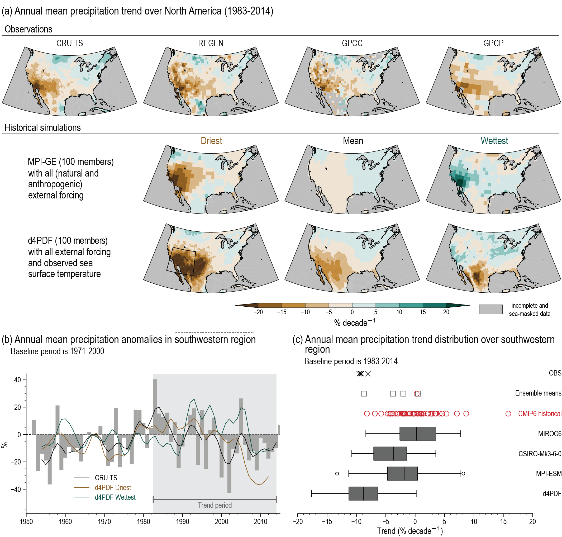 Figure 10.13 | Attribution of the south-western North America precipitation decline during the 1983–2014 period. (a) Water year (October to September) precipitation spatial linear trend (in percent per decade) over North America from 1983 to 2014. Trends are estimated using ordinary least squares. Top row: observed trends from CRU TS, REGEN, GPCC, and the Global Precipitation Climatology Project (GPCP). Middle row: driest, mean and wettest trends (relative to the region enclosed in the black quadrilateral, bottom row) from the 100 members of the MPI-ESM coupled SMILE. Bottom row: driest, mean and wettest trends relative to the above region from the 100 members of the d4PDF atmosphere-only SMILE. (b) Time series of water year precipitation anomalies (%, baseline 1971–2000) over the above south-western North America region for CRU TS (grey bar charts). Black, brown and green lines show low-pass filtered time series for CRU TS, driest and wettest members of the d4PDF SMILE, respectively. The filter is the same as the one used in Figure 10.10. (c) Distribution of south-western region-averaged water-year precipitation 1983–2014 trends (in percent per decade) for observations (CRU TS, REGEN, GPCC and GPCP, black crosses), CMIP6 all-forcing historical simulations (red circles), the MIROC6, CSIRO-Mk3-6-0, MPI-ESM and d4PDF SMILEs (grey box-and-whisker plots). Grey squares refer to ensemble mean trends of their respective SMILE and the red circle refers to the CMIP6 multi-model mean. Box-and-whisker plots follow the methodology used in Figure 10.6. Further details on data sources and processing are available in the chapter data table (Table 10.SM.11).
 The observed south-western North America drying fits the narrative of what might happen in response to increasing GHG concentrations due to a poleward expansion of the subtropics, that is conducive to drying trends over subtropical to mid-latitude regions (Hu et al., 2013b; Birner et al., 2014; Lucas et al., 2014). However, several studies based on modern reanalyses and CMIP5 models have recently shown that the current contribution of GHGs to Northern Hemisphere tropical expansion is much smaller than in the Southern Hemisphere and will remain difficult to detect due to large internal variability, even by the end of the 21st century (Section 3.3.3.1; Garfinkel et al., 2015; Allen and Kovilakam, 2017; Grise et al., 2018, 2019). In addition, the widening of the Northern Hemisphere tropical belt exhibits strong seasonality and zonal asymmetry, particularly in autumn and the North Atlantic (Amaya et al., 2018; Grise et al., 2018). Therefore, it seems that the recent Northern Hemisphere tropical expansion results from the interplay of internal and forced modes of tropical width variations and that the forced response has not robustly emerged from internal variability (Sections 3.3.3.1 and 10.4.3).
A second possible causal factor is the role for ocean-forced or internal atmospheric circulation change. Analysis of observed and CMIP5-simulated precipitation indicates that the drought prevalence since 1980 is linked to natural, internal variability in the climate system (Knutson and Zeng, 2018). Based on observations and ensembles of SST-driven atmospheric simulations, Seager and Hoerling (2014) suggested that robust tropical Pacific and tropical North Atlantic forcing drove an important fraction of annual mean precipitation and soil moisture changes and that early 21st century multi-year droughts could be attributed to natural decadal swings in tropical Pacific and North Atlantic SSTs. A cold state of the tropical Pacific would lead by well-established atmospheric teleconnections to anomalous high pressure across the North Pacific and southern North America, favouring a weaker jet stream and a diversion of the Pacific storm track away from the south-west (Delworth et al., 2015; Seager and Ting, 2017). The multi-year drought of 2012–2016 has been linked to the multi-year persistence of anomalously high atmospheric pressure over the north-eastern Pacific Ocean, which deflected the Pacific storm track northward and suppressed regional precipitation during California’s rainy season (Swain et al., 2017). Going into more detail, Prein et al. (2016a) used an assessment of changing occurrence of weather regimes to judge that changes in the frequency of certain regimes during 1979–2014 have led to a decline in precipitation by about 25%, chiefly related to the prevalence of anticyclonic circulation patterns in the north-east Pacific. Finally, the moderate model performance in representing Pacific SST decadal variability and its remote influence (Section 3.7.6) as well as its change under warming may affect attribution results of observed and future precipitation changes (Seager et al., 2019).
It has also been suggested that the ocean-controlled influence is limited and internal atmospheric variability has to be invoked to fully explain the observed history of drought on decadal time scales (Seager and Hoerling, 2014; Seager and Ting, 2017). From roughly 1980 to the present, the regional climate signals show an interesting mix between forced and internal variability. Lehner et al. (2018) used a dynamical adjustment method and large ensembles of coupled and SST-forced atmospheric experiments to suggest that the observed south-western North America rainfall decline mainly results from the effects of atmospheric internal variability, which is in part driven by a PDV-related phase shift in Pacific SST around 2000 (Figure 10.13b,c). Based upon four SMILEs (three using a GCM and another one an AGCM constrained by observed SSTs) and a CMIP6 multi-model suite constrained by observed external forcings, Figure 10.13 shows, in agreement with Lehner et al. (2018), that observed SSTs with their associated atmospheric response are the main drivers of the south-western North America precipitation decrease during the 1983–2014 period. Once aspects of the internal variability are removed by dynamical adjustment, the observed precipitation change signal and simulated anthropogenically-forced components look more similar (Lehner et al., 2018).
Importantly, as the AR6 assessment views the PDV as being mostly driven by internal variability (Section 3.7.6), the lines of evidence cited above suggest that the contribution of natural and anthropogenic forcings to the precipitation decline has a small amplitude. Unlike the precipitation deficit, the accompanying south-western North America warming is driven primarily by anthropogenic forcing from GHGs rather than atmospheric circulation variability and may help to enhance the drought through increased evapotranspiration (Knutson et al., 2013; Diffenbaugh et al., 2015; Williams et al., 2015, Williams et al., 2020; Lehner et al., 2018, 2020).
To conclude, there is high confidence (robust evidence and medium agreement) that most (>50%) of the anomalous atmospheric circulation that caused the south-western North America negative precipitation trend can be attributed to teleconnections arising from tropical Pacific SST variations related to PDV. There is high confidence (robust evidence and medium agreement) that anthropogenic forcing has made a substantial contribution (about 50%) to the south-western North America warming since 1980.
10.4.2.4 Assessment Summary
The robustness of regional-scale attribution differs strongly between temperature and precipitation changes. While the influence of anthropogenic forcing on regional temperature long-term change has been detected and attributed in almost all land regions, a robust detection and attribution of human influence on regional precipitation change has not yet fully occurred for many land regions (Section 10.4.3). Although the contribution of anthropogenic forcing to long-term regional precipitation change has been detected in some regions, a robust quantification of the contributions of different drivers remains elusive. The delayed emergence of the anthropogenic precipitation fingerprint with respect to temperature is likely due to the opposing sign of the fast and slow land precipitation forced responses and time-dependent SST change patterns (Sections 8.2.1 and Section 10.4.3), stronger internal variability (Section 10.3.4.3) as well as larger observational uncertainty (Section 10.2) and impact of model biases. The contribution of internal variability to the observed changes can also be very sensitive to the period length and level of spatial aggregation for the region under scrutiny (Section 4.4.1 and Cross-Chapter Box 3.1; Kumar et al., 2016). Finally, even in the case of temperature changes at multi-decadal time scale, internal variability can still be a substantial driver of regional changes due to cancellation between different external forcings (Nath et al., 2018).
To conclude, it is virtually certain (robust evidence and high agreement) that anthropogenic forcing has been a major driver of temperature change since 1950 in many sub-continental regions of the world. There is high confidence (robust evidence and medium agreement) that anthropogenic forcing has contributed to multi-decadal mean precipitation changes in several regions, for example western Africa, south-east South America, south-western Australia, northern central Eurasia, and South and East Asia. However, at regional scale, the role of internal variability is stronger while uncertainties in observations, models and external forcing are all larger than at the global scale, precluding a robust assessment of the magnitude of the relative contributions of greenhouse gases, including stratospheric ozone, and different aerosol species.
10.4.3 Future Regional Changes: Robustness and Emergence of the Anthropogenic Signal
Regional climate projections are one key element of the multiple lines of evidence that are used for climate risk assessments as well as for adaptation and policy decisions at regional scales (Sections 10.3.3.9 and 10.5). Regional climate projections can be separated into two components: the regional-scale forced response or regional-scale climate sensitivity when normalized by the global mean temperature change (Seneviratne and Hauser, 2020) and the climate internal variability characterizing the future period or global warming level under scrutiny. This section assesses a few methodological aspects related to robustness and emergence properties of the regional-scale forced response as well as the possible influence of internal variability on the emergence of the anthropogenic signal.
10.4.3.1 Robustness of the Anthropogenic Signal at Regional Scale
Standard methodologies to derive the regional forced response include pattern-scaling and the time-shift or epoch approach (Section 4.2.4; Tebaldi and Arblaster, 2014; Vautard et al., 2014; Herger et al., 2015; Tebaldi and Knutti, 2018; Christensen et al., 2019). Pattern-scaling assumes that the spatial patterns of regional change, often based on a time-averaged 20- or 30-year period at the end of the 21st century, are roughly constant in time, and simply scale linearly with global mean warming. The time-shift approach defines a target in terms of global warming level (GWL) and locates the time segment, usually 20 or 30 years, in historical or scenario simulations in which global mean warming matches the required GWL (Section 10.1.2 and Cross-Chapter Box 11.1). Physical consistency between multiple variables and space-time co-variance are fully preserved in the time-shift approach, which is not the case for pattern-scaling (Herger et al., 2015). Importantly, pattern scaling cannot account for the non-linearity arising from either interacting quasi-linear processes (Chadwick and Good, 2013) and purely non-linear mechanisms, which have been shown to be present in CMIP5 models for high GWL (4°C) and affect precipitation more than temperature at the regional-scale (Section 8.5.3.1; Good et al., 2015, 2016). The time-shift approach can also be used to test whether regional climate change patterns depend on the rate of global mean warming and external forcing pathways, in addition to global warming magnitude. A global evaluation of both approaches in projecting the forced temperature and precipitation response for a highly mitigated scenario based on a moderately mitigated one has been performed using a perfect-model framework (Tebaldi and Knutti, 2018). The amplitude of errors for both approaches appears to be substantially smaller than model uncertainty approximated by the CMIP5 multi-model spread.
Based on large and coordinated modelling exercises such as CMIP5 and CORDEX, the time-shift approach has been largely used to assess differences in regional climate impacts for different GWLs, with a strong focus on 1.5°C versus 2°C (Karmalkar and Bradley, 2017; Dosio and Fischer, 2018; Karnauskas et al., 2018; W. Liu et al., 2018; Taylor et al., 2018; Weber et al., 2018; Chapter 3, SR1.5, Hoegh-Guldberg et al., 2018). Comparisons between pattern-scaling and time-shift approaches allow assessment of the scalability of the regional climate change signal and the extent to which pattern-scaling assumptions still hold at regional scale for a wide range of GWL. This was the approach followed by Matte et al. (2019) in their assessment of the scalability of European regional climate projections. Based on EURO-CORDEX projections, they performed a detailed comparison between the pattern scaling and the GWL spatial patterns (GWL range: 1°C, 2°C and 3°C) for different seasons, regional model resolutions, and both temperature and precipitation. High pattern correlation values (greater than 0.9) are found between the scaled pattern and all GWL patterns for temperature. In the case of precipitation, the correspondence is slightly lower, especially in summer, for high GWLs (2°C and 3°C) and much lower for 1°C.
Figure 10.14 illustrates a similar comparison based on the CMIP6 multi-model ensemble forced with the scenario SSP5-8.5 and applied to two large-scale continental areas. The forced response to anthropogenic forcing is simply taken as the CMIP6 multi-model mean of future regional climate change relative to the 1850–1900 reference period. Robustness of the forced response is based on both significance of the change and model agreement about the sign (direction) of change (Cross-Chapter Box Atlas.1; Figure 10.14). Caution has to be exercised against a too literal interpretation of lack of robust change given that significance and sign agreement can be sensitive to spatial and temporal aggregation (Cross-Chapter Box Atlas.1, Figure 2) and lack of a robust change does not necessarily translate to lack of regional-scale climate change impacts (McSweeney and Jones, 2013; Hibino and Takayabu, 2016).
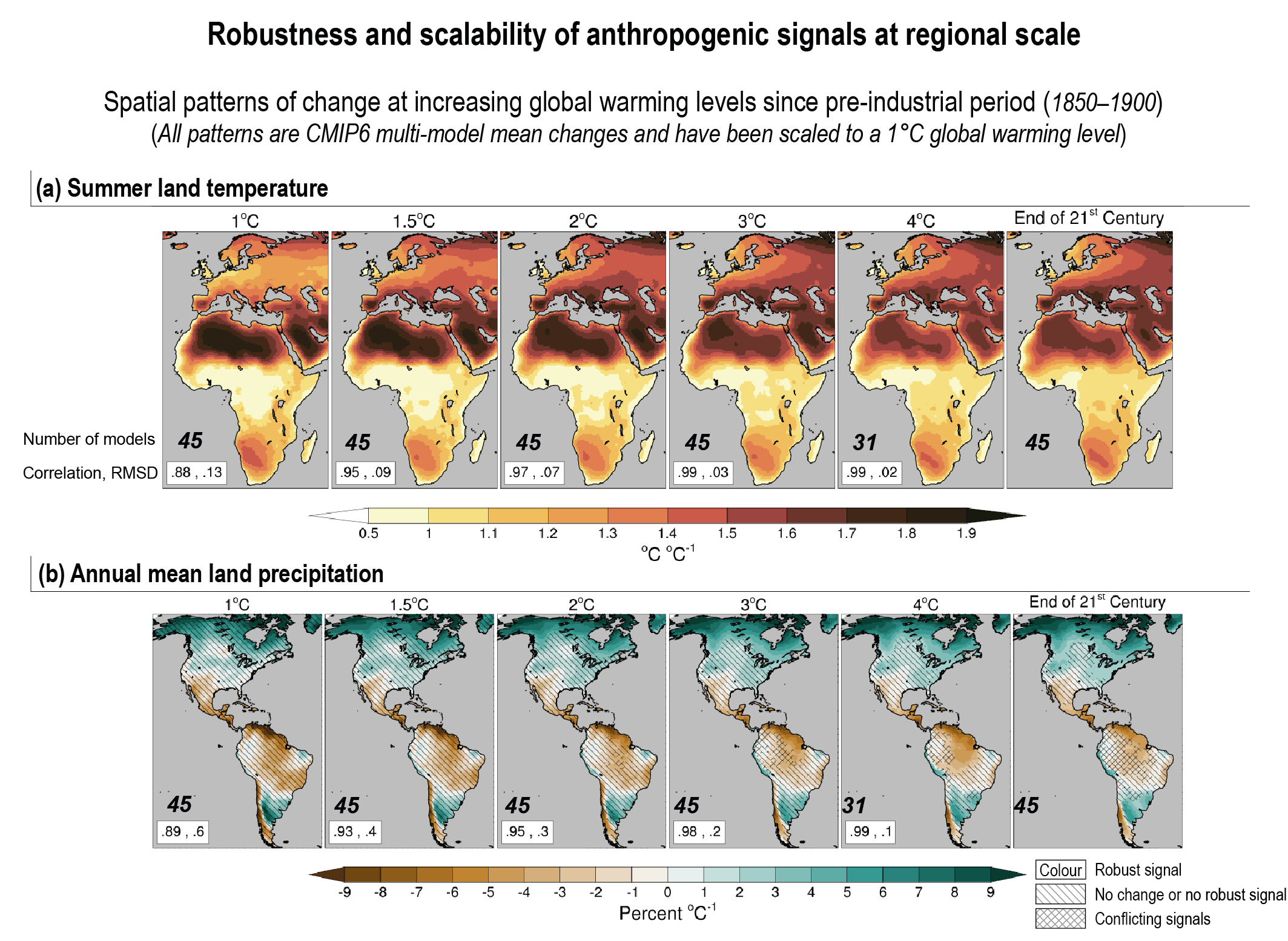 Figure 10.14 | Robustness and scalability of anthropogenic signals at regional scale. (a) Spatial patterns of European and African summer (June to August) surface air temperature change (in °C °C–1) from the Coupled Model Intercomparison Project Phase 6 (CMIP6) multi-model mean (45 models, one member per model, historical simulations and scenario SSP5-8.5) at different global warming levels (GWLs) and the end-21st century scaling pattern estimated from the multi-model mean difference between 2081–2100 and the pre-industrial period (1850–1900) divided by the corresponding global mean warming. The scale of all GWL patterns has been adjusted to a global mean warming of 1°C (for example, the resulting 3°C spatial pattern has been divided by three). The scales of the GWL patterns have to be multiplied by their threshold values to obtain the actual simulated warming. The metrics shown in the bottom left corner of the GWL pattern plots indicate the spatial pattern correlation and the root-mean-square difference between the GWL patterns and the scaling pattern. The number in bold just above the metrics gives the number of used CMIP6 models (out of 45) that have reached the GWL threshold. Areas with robust change (at least 66% of the models have a signal-to-noise ratio greater than one and 80% or more of the models agree on the sign of the change) are coloured with no pattern overlaid (Cross-Chapter Box Atlas.1). Areas with a significant change (at least 66% of the models have a signal-to-noise ratio greater than one) and lack of model agreement (meaning that less than 80% of the models agree on the sign of the change) are marked by cross-hatching. Areas with no change or no robust change (less than 66% of the models have a signal-to-noise ratio greater than one) are marked by negatively sloped hatching. (b) Same as (a) but for North, Central and South America annual mean precipitation relative change (percent °C–1). The baseline for precipitation climatology is 1850–1900. Further details on data sources and processing are available in the chapter data table (Table 10.SM.11).
 If projected regional mean temperature (Figure 10.14a) and precipitation (Figure 10.14b) changes were to scale linearly with global mean warming, the adjusted spatial patterns would be congruent with each other at different GWLs. While pattern scaling seems to be a reasonable first-order approximation for both temperature and precipitation changes in tropical and high latitude regions (high pattern correlation values), there are a number of regions exhibiting substantial amplitude differences at different GWLs (northern Africa and Middle East, southern and eastern Europe for temperature; south-western North America, Chile and north-eastern Brazil for precipitation). These differences hint at the possible influence of non-linear mechanisms (Good et al., 2015), including soil-moisture feedbacks (Seneviratne et al., 2010; Vogel et al., 2017), a time-dependent balance between the different contributions of fast and slow response to greenhouse gas forcing as well as changing SST response patterns (Long et al., 2014; Good et al., 2016; Ceppi et al., 2018; Zappa et al., 2020). Decreasing spatial pattern amplitude with increasing GWL suggests that the initial transient regional response overshoots the long-term change in regions such as northern Africa for summer temperature and south-western South America for precipitation (Zappa et al., 2020). In the latter region, long simulations with stabilized GHG concentrations even suggest a change of sign when near-equilibrium is reached (Sniderman et al., 2019). The reverse behaviour, increasing pattern amplitude with increasing GWL, is seen for summer temperature in southern and eastern Europe and for precipitation in south-western North America (Sniderman et al., 2019; Zappa et al., 2020), suggesting that, in these regions, the initial transient response is lagging global mean warming and final regional climate change will be reached once GHG concentrations are stabilized.
There is high confidence that the time-evolving contribution of different mechanisms operating at different time scales can modify the amplitude of the regional-scale response of temperature, and both the amplitude and sign of the regional-scale response of precipitation, to anthropogenic forcing. These mechanisms include non-linear temperature, precipitation and soil-moisture feedbacks, and slow and fast response of SST patterns and atmospheric circulation changes to increasing GHGs.
10.4.3.2 Emergence of the Anthropogenic Signal at Regional Scale
This section provides an assessment of the different approaches used in emergence studies as well as sensitivities to methodological choices. The section then focuses on the possible influence of internal variability on future emergence of the simulated mean precipitation anthropogenic signal at regional scales with some illustrative examples.
In climate science, emergence or distinguishability of a signal refers to the appearance of a persistent change in the probability distribution and/or temporal properties of a climate variable compared with that of a reference period (Section 1.4.2; Giorgi and Bi, 2009; Mahlstein et al., 2011, 2012; Hawkins and Sutton, 2012). Similar to anthropogenic climate change detection (Cross-Working Group Box: Attribution in Chapter 1), signal emergence can be detected, at least initially, without identifying the physical causes of the emergence (Section 1.4.2). In the context of human influence on climate, the objective of emergence studies is the search for the appearance of a signal characterizing an anthropogenically-forced change relatively to the climate variability of a reference period, defined as the noise.
Precise definitions of signal and noise as well as a metric to measure the relative importance of the signal are key ingredients of the emergence framework and depend on the framing question. In particular, emergence study results can depend on the specific definitions of signal and noise such as the level of spatial and temporal aggregation (McSweeney and Jones, 2013). For instance, grid-point scale emergence will likely be delayed compared with region-average emergence (Section 11.2.4 and Cross-Chapter Box Atlas.1, Figure 2; Fischer et al., 2013; Maraun, 2013b; Lehner et al., 2017a). The signal is often estimated by a running mean multi-decadal average or probability distribution function of the physical variable under scrutiny in order to avoid false emergence due to manifestation of multi-decadal internal variability (King et al., 2015). In the case of extremes such as climate records, a notion of multi-year persistence or recurrence can also be used to fully characterize the anthropogenic signal and its emergence (Christiansen, 2013; Bador et al., 2016).
Emergence is also sensitive to the noise characteristics: assuming a common signal definition, larger signal-to-noise values and earlier emergence will arise if the noise is based on decadal mean variability rather than interannual variability (Kusunoki et al., 2020). Depending on the framing question, the noise can include or omit external natural forcing such as volcanic and solar forcing (Zhang and Delworth, 2018; Silvy et al., 2020). Furthermore, emergence results are very sensitive to the choice and length of the reference period (Section 1.4.1). The reference period can be the pre-industrial, the very recent past or even a time-evolving baseline, depending on both the framing and assumption that adaptation to the current climate has already occurred (King et al., 2015; Zhang and Delworth, 2018; Brouillet and Joussaume, 2020). These choices will then determine the type of simulations and periods that will be used to construct the noise distribution. Finally, the permanence of future emergence cannot be taken for granted when emergence occurs in the late-21st century based on simulations ending in 2100 (Hawkins et al., 2014; King et al., 2015; Lehner et al., 2017a).
Robust assessments and comparisons of past emergence between observations and models are strengthened by the use of consistent definitions of signal and noise (Lehner et al., 2017a; Hawkins et al., 2020). In the case of future emergence under increasing greenhouse gas emissions, two main approaches have been followed to assess emergence. The first is based on estimating the signal and noise (and sometimes the signal-to-noise ratio as well) in individual models before using the resulting distribution median or mean to construct the final emergence metric (Hawkins and Sutton, 2012; Maraun, 2013b; Sui et al., 2014; Barrow and Sauchyn, 2019). The second method first estimates the signal as a multi-model mean change and the noise variance as a combination of internal variability and model structural differences (Giorgi and Bi, 2009; Mariotti et al., 2015; Nguyen et al., 2018). The first approach allows the definition of emergence of the signal relative to internal variability only and treats model error as source of uncertainty (Maraun, 2013b; Lehner et al., 2017a). The second assumes that the multi-model mean is the optimal estimate of the signal and confounds internal variability and model structural differences in the noise estimate. It is noteworthy that most emergence studies implicitly assume model independence (Annan and Hargreaves, 2017; Boé, 2018; Box 4.1) and therefore sensitivity of emergence results to model selection or weighting is rarely performed (Akhter et al., 2018).
Metrics can vary from a simple signal-to-noise ratio to statistical distributional tests (King et al., 2015; Gaetani et al., 2020) and give median estimates and uncertainty bounds for the date (or time of emergence) corresponding to the exceedance of specific thresholds by the emergence metric. Reconciling future emergence results among different studies is challenging due to their many methodological differences including the choice of the reference period, the selected climate models and scenario, the precise definition of signal and noise and the choice of different signal-to-noise thresholds to characterize robust emergence. Contrasting with binary yes/no statements, emergence can also be viewed as a continuous process characterized by an amplitude or level, for example the value of the signal-to-noise ratio, that is a function of time or global warming level.
Since AR5, the development and production of SMILEs (Sections 4.2.5 and 10.3.4.3) has allowed the assessment of the influence of internal variability on anthropogenic signal emergence. The influence of internal variability, and specifically of the unforced atmospheric circulation, on temperature signal emergence can delay or advance the time of emergence by a decade or two in mid- to high-latitude regions (Lehner et al., 2017a; Koenigk et al., 2020). Internal variability can also result in small or decreasing decadal to multi-decadal heatwave frequency trends under the historical anthropogenic forcing over most regions, thereby delaying emergence of unprecedented heatwave frequency trends relative to the pre-industrial trend distribution (Sections 11.2–11.3; Perkins-Kirkpatrick et al., 2017).
Regional precipitation future changes are much more impacted by internal variability than their temperature counterpart (Monerie et al., 2017b; Dai and Bloecker, 2019; Singh and AchutaRao, 2019; von Trentini et al., 2019; Koenigk et al., 2020). Relative to mean temperature changes, this larger influence of internal variability on mean precipitation changes contributes, among other factors (Sarojini et al., 2016), to a much delayed emergence of the forced precipitation response in observations (Hawkins et al., 2020). Based on the CMIP6 multi-model ensemble forced with the scenario SSP5-8.5, we assess the future emergence of mean precipitation forced change as a function of GWLs for all AR6 land regions (Figure 10.15a). The methodology is a straightforward adaptation of the standard approach (Hawkins and Sutton, 2012). While the standard method is only based on the signal-to-noise ratio exceedance of a specified threshold (taken as one), the approach used here assumes that grid-point emergence occurs when the forced change is considered robust following the AR6 WGI definition of robustness for projected changes (Cross-Chapter Box Atlas.1). At a GWL of 1°C, emergence only occurs in high-latitude regions (Wan et al., 2015; R. Guo et al., 2019), albeit with only small (less than 30%) area fraction with robust change. Robust changes in tropical and subtropical regions only appear from GWLs of 1.5°C, for example in south-western South America (Boisier et al., 2016), western Africa (Hawkins et al., 2020; Section 10.4.2.1) and southern Australia (Delworth and Zeng, 2014). Substantial (taken here simply as area fraction greater than 50%) emergence only occurs in some tropical, subtropical and mid-latitude regions when high GWLs (3°C–4°C) are reached. Importantly, even at these high GWL values, there are still a large number of these regions with robust changes covering less than 50% of their area. In contrast, most high-latitude regions have an area fraction with robust changes greater than 80% at GWLs of 3°C and above.
 Figure 10.15 | Future emergence of anthropogenic signal at regional scale. (a) Percentage area of land regions with robust annual mean precipitation change as a function of increasing global warming levels (GWLs). Robustness of the precipitation change is first estimated at each grid-point followed by the estimation of the AR6 region area with robust changes. For each Coupled Model Intercomparison Project Phase 6 (CMIP6) model considered (45 models, one member per model, historical simulations and scenario SSP5-8.5), the annual mean precipitation change is based on the difference between a 20-year average centred on the GWL crossing year and the mean precipitation during the pre-industrial period (1850–1900) taken as a reference. The change is considered to be robust when at least 66% of the models (30 out of 45) have a signal-to-noise ratio greater than one and at least 80% of them (36 out of 45) agree on the sign of change. The signal-to-noise ratio is estimated for each model from the ratio between the change and the standard deviation of non-overlapping 20-year means of the corresponding pre-industrial simulation (scaled by square root of 2 times 1.645). (b) Time evolution of the percentage area of land region with robust annual mean precipitation change for five AR6 land regions. Thick solid lines represent precipitation changes based on the same CMIP6 ensemble as in (a). Thin solid, dotted and dashed lines represent changes based on the three coupled single-model initial-condition large ensembles (SMILEs) used in Chapter 10, illustrating the influence of internal variability on the emergence of robust change. The change is estimated from the difference between all consecutive 20-year periods from 1900–1919 up to 2081–2100 and the pre-industrial period. The line colour indicates the sign of the robust change given by the multi-model mean (CMIP6) or ensemble mean (SMILE) change: brown (decreasing precipitation) and dark green (increasing precipitation). Further details on data sources and processing are available in the chapter data table (Table 10.SM.11).
 We now illustrate the potential influence of internal variability on late or lack of emergence for a few AR6 land regions (Figure 10.15b). For each of these AR6 regions, the time evolution of the percentage area with robust annual mean precipitation change is estimated for both the CMIP6 multi-model ensemble and the three coupled SMILEs used throughout Chapter 10. Similarity in percentage area time evolution between CMIP6 and the three coupled SMILEs suggests that internal variability can substantially influence the timing of emergence. For example, internal variability could explain the mid-21st century emergence (percentage area greater than 50%) of the drying and wetting signal over the Mediterranean and South Asia (see also Section 10.6.3) regions, respectively. Internal variability can also contribute to the late and moderate emergence over South-Eastern South America (see also Section 10.4.2) and West South Africa (see also Section 10.6.2). In contrast, it cannot explain the lack of robust changes (percentage area less than 30%) over Western Africa at the end of the 21st century, suggesting that model differences are also contributing to the lack of emergence (Monerie et al., 2017a, b). In addition to different forced signals, the differences of time evolution between the three SMILEs, in particular for African regions, point to the issue of global model performance in accurately representing internal variability and its future changes. While overestimation and underestimation of internal variability in current models have been reported (Eade et al., 2014; Laepple and Huybers, 2014), methodological challenges to assess the magnitude and spatial pattern of model biases in simulating internal variability, still remain Section 10.3.4.3). Therefore, the existence of model biases and the limited knowledge of their characteristics lead to limitations about a precise quantification of internal variability influence on delayed regional-scale emergence.
There is high confidence that consistency in definitions of signal and noise, choice of the reference period and signal-to-noise threshold, is important to robustly assess the future emergence of anthropogenic signals across different types or generations of models, as well as comparing past emergence results between observations and models. There is high confidence that internal variability can delay the emergence of the regional-scale mean precipitation anthropogenic signal in many regions, mainly located in the tropics, subtropics and mid-latitudes. An accurate estimation of the delay in regional-scale emergence caused by internal variability remains challenging due to global model biases in their representation of internal variability as well as methodological difficulties to precisely estimate these biases (high confidence).
10.5 Combining Approaches to Constructing Regional Climate Information
This section assesses approaches and challenges for producing climate information for climate risk assessments as well as for adaptation and policy decisions at regional scales (Section 10.1.2.1). An overview of the different sources used for developing regional climate information is given in Section 10.5.1. The role of the user context in the construction of climate information is assessed in Section 10.5.2. The distillation to combine multiple lines of evidence is assessed in Section 10.5.3. Finally, climate services in the context of regional climate information are assessed in Section 10.5.4. The role of storylines in constructing climate information is assessed in Box 10.2. The assessment of how regional climate information is distilled in the report is treated in Cross-Chapter Box 10.3, whereas the assessment of information on regional, physical climate processes that impact society or ecosystems, termed climatic impact-drivers (Section 10.1), appears in Chapter 12, as well as more information on climate services in Cross-Chapter Box 12.2.
The rise in demand for relevant regional climate information (Hewitt et al., 2012, 2020; Lourenço et al., 2016) has resulted in diverse approaches to produce it. Historically, the construction of climate information has been embedded in a linear supply chain: extracting the source data, processing into maps or derived data products, preparing the material for communication, and delivering to users (Section 10.1.4). Typical products are open-access, web-portal delivery services of data (Hewitson et al., 2017), which may also be implemented as commercialized climate services (Webber and Donner, 2017). Such a chain, although it is intended to meet a demand for regional climate information, contains many assumptions that are not obvious to the recipients and that may introduce possible misunderstandings in the handover from one community to the next (Meinke et al., 2006; Lemos et al., 2012). In recognition that data is not necessarily relevant information, a new pathway towards a tailored distillation of climate information has emerged. The construction of information assessed in this section draws on multiple sources (Figure 10.16), whereby the context framing for an application is addressed through co-design with users. The constructed information is then translated into the context of the user taking into account the values of all actors involved (Sections 10.5.2 and 10.5.3, and Figure 10.1).
 Figure 10.16 | Illustration of how using different sources can result in different and potentially conflicting information. Change in daily precipitation (2071–2100 RCP8.5 relative to 1981–2010) over Western Africa as simulated by an ensemble of regional climate models (RCMs) driven by global climate models (GCMs). (a) Change in daily precipitation (mm) for April to September, as mean of 17 CORDEX models (Dosio et al., 2020) (b–e) Time-latitude diagram of daily precipitation change for four selected RCM-GCM combinations. For each month and latitude, model results are zonally averaged between 10°W–10°E (blue box in a). Different GCM–RCM combinations can produce substantially different and contrasting results, when the same RCM is used to downscale different GCMs (b, d), or the same GCM is downscaled by different RCMs (d, e). GCM1=IPSL-IPSL-CM5A, GCM2=ICHEC-EC-EARTH, RCM1=RCA4, RCM2=REMO2009. Adapted from Dosio et al. (2020), CCBY4.0 https://creativecommons.org/licenses/by/4.0/. Further details on data sources and processing are available in the chapter data table (Table 10.SM.11).
 10.5.1 Sources of Regional Climate Information
Regional climate information may be constructed from a diverse range of sources, each depending on different assumptions and affected by different methodological limitations (Sections 10.2, 10.3 and 10.4). The construction of information may lead to products for direct adoption by users, or intermediate products for further analysis by users and climate services agencies in collaboration with climate scientists. Widely used sources include:
- Extrapolation of observed historical trends into the future (e.g., Livezey et al., 2007; Laaha et al., 2016). Given that internal variability can affect regional trends significantly on decadal to multi-decadal time scales (Section 10.4), this approach could be potentially misleading without other supporting evidence (Westra et al., 2010), or finding congruence with other changes (e.g., Langodan et al., 2020).
- The output from global models (Section 10.3.1), including high-resolution GCMs and ESMs, for which performance has been assessed and documented (Section 10.3.3). Model data can be used in its raw form or may be bias adjusted (Section 10.3.1 and Cross-Chapter Box 10.2) or weighted (Section 10.3.4 and Box 4.1).
- The output from dynamically (Section 10.3.1.2) or statistically (Section 10.3.1.3) downscaled global model simulations for which performance has been assessed and documented as trustworthy (Section 10.3.3). Model data can be used in its raw form or may be bias adjusted, in the case of regional climate models (RCMs, Section 10.3.1).
- Process understanding about climate and the drivers of regional climate variability and change, grounded in theory about dynamics, thermodynamics and other physics of the climate system as a basis for process-based evaluation. For instance, teleconnections are useful to understand the links between large and regional scales at both near and long-term depending on the application. (Sections 10.1.3, 10.3.3, 10.4.1, 10.4.3 and Annex IV).
- Idealized scenarios of possible future climates as narratives to explore the implications and consequences of such scenarios in the presence of uncertainty (Jack et al., 2021). This approach has been used to explore the response to geoengineering (Cao et al., 2016a), as well as alternative scenarios where model projections are highly uncertain (Brown et al., 2016; Jack et al., 2021).
- Information directly from research reported in the peer-reviewed scientific literature (e.g., Sanderson et al., 2017) or related research reports such as communications to the UN Framework Convention on Climate Change (UNFCCC) about national adaptation.
- Engaging with climate scientists and local communities who may provide indigenous information (Rosenzweig and Neofotis, 2013; Makondo and Thomas, 2018).
- Relevant information may also be drawn from paleoclimate studies (e.g., McGregor, 2018; Armstrong et al., 2020; Kiem et al., 2020) to support and contextualize other sources about more recent and projected changes.
Different sources of information may be more appropriate for some purposes than others, as they may provide information better aligned to the spatial and temporal scales of interest, in different formats, and tailored to different types of application. In some cases, a purpose may be best served using several types of information together. For example, when model data is the primary source, it can be advantageous to employ data from multiple models or even from a range of different experiment types (Section 10.3.2) supported by assessing how the models reflect changes in driving processes. In this manner a purpose may be best served by seeking the congruence of several types of information together, though one needs to recognize how well the attributes of each source align with the specific need for information. Depending on resources, one may even design model experiments specifically for a given use, such as constructing physical climate storylines of individual events (Section 10.3.2 and Box 10.2). Such analyses may be complemented by event attribution studies (Section 11.1.4).
Users of climate information may face the so-called practitioner’s dilemma: a plethora of different and potentially contrasting sources (Figure 10.16) may be available without a comprehensive and user-relevant evaluation, and these datasets may also lack a transparent and easily understandable explanation of underlying assumptions, strengths and limitations (Barsugli et al., 2013; Hewitson et al., 2017). Often, the choice of information source is therefore not determined by what is most relevant and informative for the question at hand, but rather by practical constraints such as accessibility and ease of use and may be limited to the availability of just one source in extreme cases (Rössler et al., 2019a).
10.5.2 Framing Elements for Constructing User-Relevant Information
10.5.2.1 Consideration of Different Contexts
Without considering the specific context, the distillation of climate information relevant to users may poorly serve the goal of informing adaptation and policy (Cash et al., 2003; Lemos et al., 2012; Baztan et al., 2017). Section 10.1.4 identifies three implicit framing issues of constructing and delivering user-relevant climate information: practical issues arising from the climate information sources, issues with including the context in constructing the information, and difficulties presented by complex networks of practitioners. The social context strongly influences decisions about constructing information and requires a nuanced and holistic approach to recognize the complexity of a coupled social and physical system (Daron et al., 2014). For example, urban water managers must recognize the dependency of the city on different water resources and the interplay of both local and national government legislation that can involve a range of different constituencies and decision makers (Scott et al., 2018; Savelli et al., 2021).
Context plays a role in determining the risks that may affect human systems and ecosystems and consequently the climate information needs. The context may also limit access to such information. Hence, the context imposes inherent constraints on how climate information can be constructed and optimally aligned with its intended application. Although contexts are unlimited in variety, some key contextual elements include:
- Whether the problem formulation needs to be constructed through consultative activities that, for instance, help identify thresholds of vulnerability in complex urban or rural systems (Baztan et al., 2017; Willyard et al., 2018) or is more a matter of addressing a generic vulnerability already identified, such as the frequency of flood events or recurrence intervals of multi-year droughts (Hallegatte et al., 2013).
- Societal capacity, such as cultural or institutional flexibility and willingness to respond to different scientific information (e.g., Hart and Nisbet, 2012; Kahan, 2012, 2013).
- The technical capability and expertise of the different actors, including users, producers, and communicators (e.g., Sarewitz, 2004; Gorddard et al., 2016).
- Potential contrasts in value systems such as the different views of the Global North compared to those of economies in transition or under development (Henrich et al., 2010a, b; Sapiains et al., 2021).
- The relative importance of climate change in relation to non-climate stressors on the temporal and spatial scales of interest to the user, which at times are not the ones initially assumed by the producers (Otto et al., 2015).
- Availability, timing and accessibility of the required climate information, including the availability of sources such as observations, model simulations, literature and experts of the relevant regional climate (Mulwa et al., 2017). In developing countries, the availability of all or some of these sources may be limited (Dinku et al., 2014).
These and other contextual elements can frame subsequent decisions about the construction of regional climate information for applications. For example, an engineer typically seeks quantitative information, while the policy community may be more responsive to storylines and how information is positioned within a causal network describing regional climate risk (Section 1.4.4 and Box 10.2). Multiple contexts can coexist and potentially result in competing approaches (for example, when urban governance contends with regional water-resource management in the same area).
10.5.2.2 Developing Climate Information Conditioned by Values of Different Actors and Communities
Developing climate information relevant to user needs can be influenced by the explicit and implicit values of all parties: those constructing the information, those communicating the information, those receiving the information, and, critically, those who construct the problem statement being addressed. A discussion of how values in the scientific community shape climate research appears in Section 1.2.3.2. The influence of values need not be a source of bias or distortion; it is sometimes appropriate and beneficial: critical scrutiny from a diverse range of value-governing perspectives may uncover and challenge biases and omissions in the information that might otherwise go unrecognized (Longino, 2004). Dialogue among all parties in a culturally, socially, and economically heterogeneous society is therefore important for recognizing and reconciling value differences to best yield information that is salient, relevant and avoids ambiguity, most notably when informing the complexity of risks and resilience for human systems and ecosystems in developing nations (e.g., Baztan et al., 2017).
Thus, a challenge with constructing climate information for users, especially about impactful change, is that producing the information may need to involve people with a variety of backgrounds, who have different sets of experiences, capabilities, and values. The information thus would need to accommodate and be relevant to a range of different ways of viewing the problem (Sarewitz, 2004; Rosenzweig and Neofotis, 2013; Gorddard et al., 2016). Failure to recognize the variety of people using the climate information can make it ineffective, even if the source data on which it is based is of the highest quality, and may create a danger of maladaptation.
A substantial body of evidence shows that the receptivity of individuals to climate information is strongly conditioned by motivated reasoning (Hart and Nisbet, 2012; Kahan, 2012, 2013), wherein a person’s reception of climate information is influenced by the values of the community with which the person identifies. Adherence to a community’s values forms part of an individual’s social identity (Hart and Nisbet, 2012). Individuals thus frame their analysis and understanding of climate information in the context of cultural values espoused by their community (Hart and Nisbet, 2012; Kahan, 2012, 2013; Campbell and Kay, 2014; Bessette et al., 2017; Tschakert et al., 2017; Vezér et al., 2018). Successful framing of climate information products thus seeks to identify common ground with users, taking account of their values and interests.
Given the relevance of both context and values, the effectiveness of climate information can increase if developed in partnership with the target communities (Figure 10.17; Tschakert et al., 2016). Such an approach can inspire trust among all parties and at the same time promote a co-production process (Cash et al., 2003). Recipients of information have the greatest trust when the communicator is perceived as understanding their context and sharing their values and identity (Corner et al., 2014). As a consequence, developing mental models informed by user values can help with understanding complex climate models and their outcomes (Bessette et al., 2017).
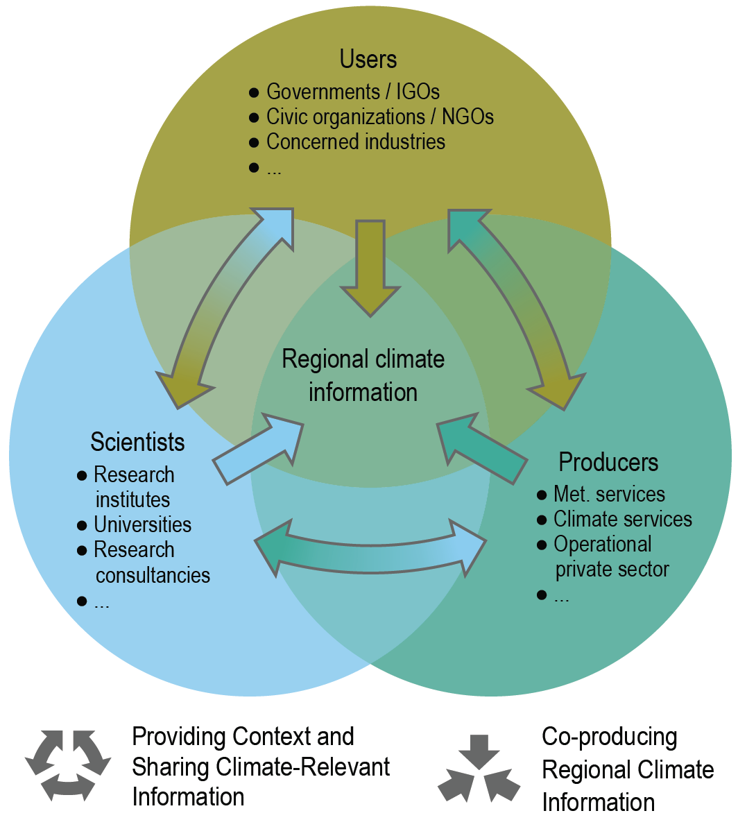 Figure 10.17 | Effective regional climate information requires shared development of actionable information that engages all parties involved and the values that guide their engagement. Participants in the development of climate information come from varying perspectives, based in part on their professions and communities. Each of the three broad categories shown in the Venn diagram (Users, Producers, Scientists) is not a homogenous group, and often has a diversity of perspectives, values and interests among its members. The subheadings in each category are illustrative and not all-inclusive. The arrows connecting those categories represent the distillation process of providing context and sharing climate relevant information. The arrows that point toward the centre represent the distillation of climate information that involves all three categories.
 The importance of a co-production process does not preclude the climate-research community from taking steps to develop and convey relevant information on its own. Indeed, communicating expert consensus about contested scientific issues is beneficial (Goldberg et al., 2019). Climate services (Section 10.5.4), in particular, can become an effective means for using sources from the climate community and crafting these to be consistent with the needs, interests and values of stakeholder communities. However, simply presenting more information without recognizing user values and the contextual elements listed in Section 10.5.2.1 may be ineffective (Kahan, 2013). An aversion to climate information discordant with one’s pre-existing beliefs can actually become stronger for people who are more scientifically literate: they feel more confident sifting through all sources of information to find support for their positions (Kahan, 2012). A challenge is that if climate information is not framed carefully, recognizing context and user values, it may make the sceptical person less receptive to further information about climate change (Corner et al., 2012; Hart and Nisbet, 2012; Shalev, 2015). A further complication is that audiences may view climate change as a problem distant in time and space (Spence et al., 2012), too threatening to acknowledge (Brügger et al., 2015; McDonald et al., 2015), or too economically challenging to accept (Bessette et al., 2017). Identifying positive outcomes that align with user values, instead of adaptation and mitigation efforts, appears to promote the interest in and the success of climate information (Bain et al., 2012).
10.5.2.3 The Roles of Spatial and Temporal Resolution in Relation to Decision Scale
Climate processes occur on a range of spatial and temporal scales, from global to local, from centuries and longer to days or less (Section 10.1.2 and Figure 10.3). Similarly, decisions by stakeholders cover a range of spatial and temporal scales that can vary with the size of their region of interest and scope of activity. However, the link between decision scales and the spatial and temporal resolution of climate and related non-climatic, natural-system information is not straightforward, and failure to recognize mismatches between the two can undermine the effectiveness and relevance of the information (Cumming et al., 2006; Sayles, 2018).
Nevertheless, the scale of regional climate information does not have to be the same as the decision scale. Physical-climate storylines (Box 10.2) valid at large scales can be used to develop understanding that is relevant to local decisions. For example, global climate change affecting Antarctic ice-mass loss is relevant to formulating Dutch responses to sea level rise (Haasnoot et al., 2020). On the other hand, extreme precipitation processes can occur on scales of tens of kilometres and smaller and thus require high resolution climate information when projecting future changes (e.g., Xie et al., 2015). An important factor for developing effective climate information using the distillation process is aligning the vulnerabilities of the social and economic systems under consideration ranging from, for example, those important to a farmer to those important to a national agricultural ministry (Andreassen et al., 2018; O’Higgins et al., 2019). Thus, more sophisticated matching of spatial and temporal resolution of climate information with decision scales requires engagement across a hierarchy of governance structures at national, regional and local level (e.g., Lagabrielle et al., 2018).
10.5.3 Distillation of Climate Information
The preceding sections laid out the diversity of sources of climate information (Section 10.5.1) and important elements for its use in a decision context (Section 10.5.2). Here, it is assessed how context-relevant climate information can be distilled from these sources of information. Although the term distillation lacks a clear definition in the literature, it has, in principle, two aspects: the construction of (potentially user-targeted) information that is defensible and evidence-based (Giorgi, 2020), and the translation of this information into a specific context, targeting a specific purpose and set of values. The former typically involves data from multiple sources, including expert knowledge, and comprehensively considers relevant uncertainties to give physically plausible climate information. The latter translates the information explicitly into the user context, such as by linking it to experience, by formulating a narrative, by highlighting the relevance for the user context, or by putting the climate information into the context of the relevant non-climatic stressors.
Distilling climate information for a specific purpose benefits from a co-production process that includes non-climate-scientists in the research design, analysis and the exploration and interpretation of the results to best place it in context of the intended application (Collins and Ison, 2009; Berkhout et al., 2013; Wildschut, 2017; Bhave et al., 2018; Dessai et al., 2018). Consideration of the specific contexts of information requirements by the provider as well as including the user values in connecting the science with users is increasingly recognized as paramount to construct information relevant for decisions at the regional scale (Section 10.5.2; Kruk et al., 2017; Vizy and Cook, 2017; Djenontin and Meadow, 2018; Parker and Lusk, 2019; Norström et al., 2020; Turnhout et al., 2020). As a response, regional climate change information is increasingly being developed through participatory and context-specific dialogues that bring together producers and users across disciplines and define climate impacts as one of the many stressors shaping user decisions (Brown and Wilby, 2012; Lemos et al., 2012). Although there are multiple practical issues involving communication (Rössler et al., 2019a), such as providing data in a format that users can interpret, being mindful of the contextual issues raised in Section 10.5.2 allows non-scientists to be involved in decisions about approaches and assumptions for the distillation and thus to take ownership of the resultant information and to make informed decisions based on the distilled information (Pettenger, 2016; Verrax, 2017). Importantly, the application of transdisciplinary engagement processes that emphasize the role of non-scientists in the learning and knowledge production process builds relationships and trust between information users and producers, which is arguably as important for the uptake of climate science into decision-making as the nature of the climate information itself (Section 10.5.2).
10.5.3.1 Information Construction
Data, either from observations or models, is in general not inherently information, but may contain relevant information if interpreted appropriately (Hewitson et al., 2017). The same applies to other sources of climate information. Relevance is controlled by the given user context (Section 10.5.2.1) and relates to the required temporal and spatial scales (Section 10.5.2.3), the characteristics of required variables (often referred to as indicators), and the meteorological and climatic phenomena driving these variables (Section 10.1.3). For example, if climate information for driving impact models is sought (e.g., McSweeney et al., 2015), the impact modelling analysis in the target region is the specific user context.
Climate risk assessment considers all plausible outcomes (Weaver et al., 2017; Marchau et al., 2019; Sutton, 2019). Thus, a key element of information construction is the exploration and reconciliation of different sources of information (Barsugli et al., 2013; Hewitson et al., 2014b; Maraun and Widmann, 2018b) and involves mainly two issues: first, assessing the fitness of different sources in the given context and thereby potentially omitting (or down-weighting) selected sources (Sections 10.3.3), and, second, integrating different sources into a broader picture within a context (Sections 10.3.4).
A non-comprehensive selection of approaches that may contribute to the construction of information includes:
- Overall assessment and intercomparison of different sources of information, including hierarchies of models and identification of potentially conflicting results (Figure 10.16), where observational availability plays a critical role (Section 10.2.3).
- Assessing the emergence of forced trends from internal variability (Section 10.4.3), and testing whether differences in simulations can be explained by internal variability, ideally using initial-condition large ensembles (Sections 10.3.4.3 and 10.4.3).
- Assessing the interdependence of chosen models to identify the amount of independent information (Section 10.3.4.4).
- Process-based evaluation with focus on those processes that are relevant for the specific application (Sections 10.3.3.4–10.3.3.10).
- Weighting or sub-selecting ensembles based on a priori knowledge or the outcome of a process-based evaluation, while sampling as much uncertainty as possible (Section 10.3.4.4).
- Tracing back differences in projections to the representation of fundamental processes, for example, by using physical climate storylines (Sections 10.3.4.2 and Box 10.2) or sensitivity simulations (Section 10.3.2.3).
- Producing physical-climate storylines (Box 10.2) to explore uncertainties not sampled by available model ensembles (Shepherd et al., 2018), for example in pseudo-global warming experiments (Section 10.3.2.2), or to simulate events that have never happened before but are nevertheless plausible (Lin and Emanuel, 2016).
- Attributing observed changes to different external forcings and internal drivers (Section 10.4.1).
- Comparing observed trends with past simulated trends in order to constrain projections with, for instance, the Allen–Stott–Kettleborough method (Allen et al., 2000; Stott and Kettleborough, 2002; Stott et al., 2013) to explain drivers of past observed trends (Section 10.4.2) for understanding future trends.
- Integrating present-day performance via emergent constraints to reduce projection uncertainty (Section 10.3.2).
- Complementing the observational and model-based sources with expert judgement (e.g., integrating knowledge from theory or experience that is available from experts or the literature; Section 10.5.1).
These approaches often can be used in combination to increase confidence in conclusions drawn (Hewitson et al., 2017).
10.5.3.2 Translating Climate Information Into the User Context
Awareness and understanding of the users’ decision-making context is a central and key aspect of developing tailored, context-appropriate information (Briley et al., 2015), as clearly evidenced by the climate services’ experiences (e.g., Vincent et al., 2018). Understanding the context, however, is not trivial and requires understanding of both the user and provider (Guido et al., 2020) if the information is to be robust, reliable and relevant (Giorgi, 2020). Translating the information into context requires consideration of terminology and expectations (Briley et al., 2015), issues of user interpretation (Daron et al., 2015), and hence necessitating engagement in co-production with all attendant challenges (Vincent et al., 2021). The actual provision of climate information may be conducted at different levels of sophistication, ranging from generic data provision via web portals (Hewitson et al., 2017), potentially including impact-relevant climate indicators, region-specific factsheets and stakeholder reports, social media (Pearce et al., 2019), to a close engagement with specific stakeholders in co-exploring the research (Steynor et al., 2016).
Climate information products may often lack explanations of their potential use and misuse (Street, 2016; Lamb, 2017; Chimani et al., 2020). This is particularly important if the information is provided as a generic, publicly accessible product without a specific context (Hewitson et al., 2017). Context-specific collaboration, especially if organized in workshop, enables a close transdisciplinary co-exploration of the results as in the form of climate risk narratives (Jack et al., 2020, Box 10.2). Such approaches explicitly account for the user context, values and non-climatic stressors (Steynor and Pasquini, 2019).
10.5.3.3 Transdisciplinary Approaches to Stakeholder Interaction
The transdisciplinary interaction with stakeholders has been categorized into top-down, bottom-up and interactive approaches (Berkhout et al., 2013). Traditional top-down approaches frame the research from the perspective of global climate change as a driver of regional climate risk. Bottom-up approaches, also referred to as scenario-neutral impact studies (Prudhomme et al., 2010; A. Brown et al., 2012; C. Brown et al., 2012; Culley et al., 2016) begin with the user’s articulation of vulnerability in the context of climatic and non-climatic stressors, follow with the definition of key system thresholds of climatic variables, and only incorporate climate data to assess the likelihood of threshold exceedances. Bottom-up approaches are special cases of robust decision-making (Lempert et al., 2006; Lempert and Collins, 2007; Walker et al., 2013; Weaver et al., 2013), which are designed to account for uncertainties not represented by climate models as well as non-climatic stressors. Interactive approaches combine aspects of top-down and bottom-up approaches. The choice of approach depends on the context. While bottom-up approaches might be optimal in a local context, where case-specific risks are addressed, top-down approaches provide generic information that may serve a range of different purposes, for example, at the national scale (Berkhout et al., 2013). All these approaches benefit from the integration of fully distilled climate information (Berkhout et al., 2013; Maraun and Widmann, 2018b).
10.5.3.4 Barriers to the Distillation of Climate Information
As implied by (Section 10.5.2, meeting the needs of users can be a substantial challenge for climate scientists if they misunderstand or have limited understanding of user needs and context (Porter and Dessai, 2017). Several barriers in user communities can trigger and sustain this challenge. This can include an institutional aversion to incorporating new tools into decision-making (Callahan et al., 1999). Coincident with this factor, there may be limited staff capacity, lack of management support and lack of a mandate to plan for climate change (Lee and Whitely Binder, 2010).
Following from those challenges, constructing and communicating regional climate information often occurs under the overarching assumption that uncertainty is a problem and reducing uncertainty is the priority (Eisenack et al., 2014; J. Otto et al., 2016). This is both a psychological (Morton et al., 2011) as well as a pragmatic barrier in cases where uncertainty appears to limit the ability to make decisions (Mukheibir and Ziervogel, 2007). However, where in-depth engagements with decision contexts are undertaken, these initial barriers are often dismantled to reveal a more complex, nuanced and potentially more productive intersection with climate information producers that can efficiently handle uncertainty (e.g., Rice et al., 2009; Lemos et al., 2012; Moss, 2016). Specifically, disclosure of all uncertainties in the climate information, transparency about the sources of these uncertainties, and tailoring the uncertainty information to specific decision frameworks have the potential for reducing problems of distilling and communicating uncertain climate information (J. Otto et al., 2016).
10.5.3.5 Synthesis Assessment of Climate Information Distillation
There is high confidence that distilling climate information for a specific purpose benefits from a co-production process that involves users of the information, considers the specific user context and the values of relevant actors such as users and scientists, and translates the resultant information into the broader user context. This process allows users to take ownership of the information, builds relationships and trust between information users and producers and helps to overcome barriers in the information construction. This process enhances trust in the information as well its usefulness, relevance, and uptake, especially when the communication involves complex, contextual details (high confidence). The optimal approach for the transdisciplinary collaboration with users depends on the specific context conditioned by the sources available and the actors involved, which together are dependent on the regions considered and the framing by the question being addressed.
Drawing upon multiple lines of evidence in the construction of climate information increases the fitness of this information and creates a stronger foundation (high confidence). The lines of evidence can include multiple observational datasets, ensembles of different model types, process understanding, expert judgement, and indigenous knowledge, among others. Attribution studies, the characterization of possible outcomes associated with internal variability and a comprehensive assessment of observational, model and forcing uncertainties and possible contradictions using different analysis methods are important elements of distillation. To make the most appropriate decisions and responses to changing climate it is necessary to consider all physically plausible outcomes from multiple lines of evidence, especially in the case when they are contrasting such as in the examples of Cross-Chapter Box 10.1 and Section 10.6.2.
10.5.4 Climate Services and the Construction of Regional Climate Information
Climate services have been defined as the provision of climate information to assist decision-making (Sections 1.2.3, and 12.6, and Cross-Chapter Box 12.2). Services are expected to be based on scientifically credible information and expertise, have appropriate engagement from users and providers, have an effective access mechanism and aim at meeting the users’ needs (Hewitt et al., 2020). To achieve this, climate services synthesize context-relevant climate information addressing questions for a wide range of climate time scales. From this point of view, climate services are instruments for the production, translation and transfer of climate information and knowledge for their use in climate-informed decision-making and climate-smart policy and planning (Hewitt et al., 2012). The appropriate provision of climate services considers the diagnosis of climate information needs, the service itself and a number of good practices still under development (Vaughan et al., 2018).
The preceding subsections assess research on the distillation of climate information, which is directly relevant for the development of climate services. Distillation, when implemented appropriately and interpreted with all due caveats, leads to credible climate information with a broader foundation of evidence to be used in climate services practice according to the recommendations of the Global Framework for Climate Services (Hewitt et al., 2012). As stated in Chapter 12, climate services set new scientific challenges to research. Examples of some of the challenges have been given in Chapters 1 and 12, which are complemented by the barriers to the distillation assessed in Section 10.5.3.3.
Box 10.2 | Storylines for Constructing and Communicating Regional Climate Information
Communicating the full extent of available information on future climate for a region, including an uncertainty quantification, can act as a barrier to the uptake and use of such information (Lemos et al., 2012; Daron et al., 2018). To address the need to simplify and increase the relevance of information for specific contexts, recent studies have adopted storyline and narrative approaches (Section 1.4.4.2; Hazeleger et al., 2015; Shepherd et al., 2018). As such, these approaches are an important tool for the climate information distillation (Section 10.5.3). Here we assess these in a regional climate information context, namely for exploring uncertainties, embedding climate information into a given user context, and communicating climate change information.
Physical climate storylines are self-consistent and plausible unfolding of a physical trajectory of the climate system, or a weather or climate event, on time scales from hours to multiple decades (Section 1.4.4.2). Storylines that condition climatic features and processes on a set of plausible but distinct large-scale climatic changes enables the exploration of uncertainties in regional climate projections (Box 10.2, Figure 1 and Section 10.3.4.2). For instance, Zappa and Shepherd (2017) condition projected changes in European surface wind speeds on different plausible projections of tropical upper tropospheric warming and the polar vortex strength in the CMIP5 multi-model ensemble. Storylines of specific events are generated to explore the unfolding and impacts of comparable events in counterfactual climates (Lackmann, 2015; Meredith et al., 2015b; Takayabu et al., 2015; Hegdahl et al., 2020; Sillmann et al., 2021). Those event storylines can be based on pseudo-global warming studies (Lackmann, 2015; Meredith et al., 2015b; Takayabu et al., 2015; see Section 10.3.2.2), selected and possibly downscaled events from long-term climate projections (Hegdahl et al., 2020; Huang et al., 2020a), or based on expert judgment of plausible changes to observed events (Pisaric et al., 2011; Dessai et al., 2018). They can be used for attributing events to different causal factors (Lackmann, 2015; Meredith et al., 2015b; Takayabu et al., 2015; Trenberth et al., 2015; Shepherd, 2016a; Section 11.2.4) as well as for exploring the unfolding of events in future climates.
Physical climate storylines are complementary to probabilistic or unconditional risk-based approaches, and are particularly suitable to explore low-likelihood changes or events, which are often associated with the highest impacts (Shepherd et al., 2018; Sillmann et al., 2020; Section 4.8). They also facilitate providing local context to large-scale trends and changes, by conditioning the projections on locally relevant circumstances (Hazeleger et al., 2015). Storylines are also developed based on expert elicitation and include plausible changes beyond those simulated by existing model projections in order to explore deep uncertainties (Dessai et al., 2018).
Storylines can be combined with impact modelling (Strasser et al., 2019; Hegdahl et al., 2020) and can be embedded in a user’s risk landscape (Shepherd, 2019; Box 10.2, Figure 1). In particular, this holds for event storylines, where confounding factors such as regional characteristics like land-use changes and non-climatic drivers of the event are an element of the storyline (Pisaric et al., 2011; Dessai et al., 2018; Lloyd and Shepherd, 2020; Sillmann et al., 2021). In a co-production process, multidisciplinary expert knowledge as well as the values and interests of the intended audiences and stakeholders can be explicitly considered (Kok et al., 2014; Bhave et al., 2018; Dessai et al., 2018; Scott et al., 2018; Hegdahl et al., 2020).
Storylines can also be used to communicate climate information by narrative elements describing the main climatological features and the relevant consequences in the user context (Fløttum and Gjerstad, 2017; Moezzi et al., 2017; Dessai et al., 2018; Scott et al., 2018; Jack et al., 2020). Co-produced narratives have been demonstrated to enhance knowledge integration in decision-making contexts (e.g., de Bruijn et al., 2016). Narrative elements have also been employed to convey information from climate models (Corballis, 2019). Jack et al. (2020) introduced the concept of climate risk narratives and developed a set of principles, such as using present tense in their presentation to avoid the effects of future discounting and writing individual narratives without uncertainty language to assume an imagined observer perspective. From this point of view, event storylines are particularly useful for communication purposes as they link to the experience and episodic memory of stakeholders (Schacter et al., 2007; Steynor et al., 2016; Shepherd et al., 2018).
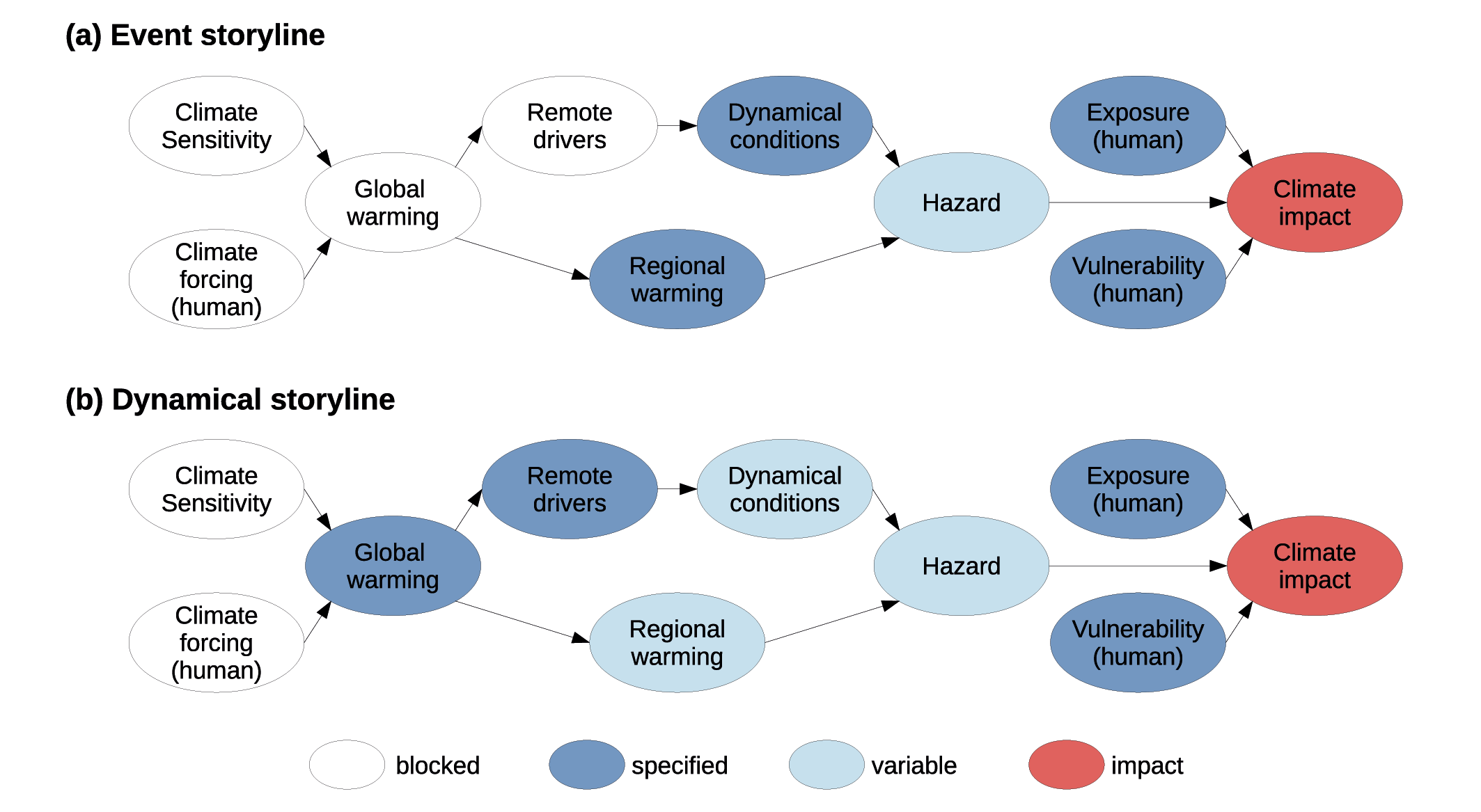
Box 10.2, Figure 1 | Schematic of two types of physical climate storylines with a particular climate impact of concern (red). The storylines are defined by specified elements (dark blue). Variable elements (light blue) are simulated conditional on the specified elements. The white elements are ‘blocked’ since their state does not need to be known to determine the light blue elements. Other types of storylines could be defined by specifying other elements (e.g., storylines of different climate sensitivities or different representative concentration pathways). (a) Event storyline, where the particular dynamical conditions during the event as well as the regional warming are specified and control the hazard arising from the event. (b) Dynamical storyline, where the global warming level and remote drivers are specified and control the long-term changes in atmospheric dynamics and regional warming. In both storylines, the impact is also conditioned on specified exposure and vulnerability. Figure adapted from Shepherd (2019).
Cross-Chapter Box 10.3 | Assessment of Climate Change Information at the Regional Scale
Coordinators: Erika Coppola (Italy), Alessandro Dosio (Italy), Friederike Otto (United Kingdom/Germany)
Contributors: Claudine Dereczynski (Brazil), Melissa I. Gomis (France/Switzerland), Richard G. Jones (United Kingdom), Roshanka Ranasinghe (The Netherlands/Sri Lanka, Australia), Alex C. Ruane (The United States of America), Sonia I. Seneviratne (Switzerland), Anna A. Sörensson (Argentina), Bart van den Hurk (The Netherlands), Robert Vautard (France), Sergio M. Vicente-Serrano (Spain)
This Cross-Chapter Box illustrates how assessments of past, present and future regional climate changes (e.g., change in an extreme event index or climatic impact-driver, CID) are derived in the WGI report. Robust assessments can be derived when changes are supported by multiple lines of evidence.
Multiple, sometimes contrasting, lines of evidence are derived from the various data sources, methodologies and approaches that can be used to construct climate information (Section 10.5 and Figure 10.1). Such data sources and methodologies include theoretical understanding of relevant processes, drivers and feedbacks of climate at regional scale, observed data from multiple datasets (e.g., ground station networks, satellite products, reanalysis, etc.), simulations from different model types (including general circulation models (GCMs), regional climate models (RCMs), statistical downscaling methods, etc.) and experiments (e.g., Coupled Model Intercomparison Project Phases 5 and 6 (CMIP5 and 6), Coordinated Regional Climate Downscaling Experiment (CORDEX), and single-model initial-condition large ensembles), methodologies to attribute observed changes or events to large- and regional-scale anthropogenic and natural drivers and forcings as well as other relevant local knowledge (e.g., indigenous knowledge).

Cross-Chapter Box 10.3, Figure 1 | Schematic illustration of the process to derive the assessment of regional climate change information based on a distillation process of multiple lines of evidence taken from observed trends, attribution of trends or events, climate model projections, and physical understanding.
The assessment is derived following the IPCC uncertainty guidance through a distillation process of multiple lines of evidence on observed trends, attribution of trends or events, climate model projections and physical understanding, covered in several chapters of the WGI Report.
In particular, this Cross-Chapter Box explains the methodology used to derive the regional assessments summarized in the Technical Summary (TS) table that are, in turn, used as a basis for the synthesis assessment in the Summary for Policymakers (SPM).
The process consists of three discrete steps, listed below and schematically illustrated in Cross-Chapter Box 10.3, Figure 1:
1. Collection and assessment of the fitness-for-purpose of available information
Any specific climate change that is regionally relevant is assessed looking at lines of evidence, potentially across multiple indices. For example, several definitions of ‘drought’ exist that refer to a variety of the underlying processes, temporal and spatial scales, as well as sectoral applications and associated impacts (Sections 11.6 and 12.3). Such diverse definitions need to be gathered from the relevant literature, compared, and individually assessed if appropriate.
Once the indices of change are properly defined, the relevant climate information is collated from the available sources.
The information is then evaluated against its fitness-for-purpose, for example, whether it is adequate to provide robust evidence to derive an assessment. In the case of observed data, issues to be considered include (but are not limited to): spatial and temporal resolution, accuracy, gaps in the recorded data, homogeneity in the station network, uncertainty treatment, etc. (Sections 10.2, 11.2, 11.9, 12.4; Atlas.1.4). In the case of modelled data, an assessment of the fitness-for-purpose typically includes an evaluation of numerical or statistical methods adopted, adequate representation of the physical processes, forcings and feedbacks relevant for the region and the change under consideration, the availability of adequate ensembles to assess the interplay between forced response and internal variability and the uncertainty in future projections (Sections 10.3, 10.4, 11.2, 11.9, 12.4 and Chapter Atlas). Attribution assessments are usually based on models and observations for which the fitness-for-purpose is assessed with similar criteria as those described above (Cross-Working Group Box: Attribution in Chapter 1). The assessment is made either directly or indirectly by scrutinizing the data and methods of the relevant literature against the criteria listed above.
2. Assessment of confidence of the multiple lines of evidence
Once the relevant information has been collated for a given regional change, an assessment of the confidence is first made for each line of evidence separately. The assessment of confidence is the result of expert judgment drawing around a set of questions such as:
- Do we have a physical explanation of the processes responsible for past and future changes in the region?
- Do observed trends agree amongst different observational products/datasets? Are they statistically significant? Do the observations cover the same temporal period and/or spatial area? Are the observations homogeneous in time?
- Can past trends be attributed to human activities (greenhouse gases, short-lived climate forcers or land-use/management changes)? Are attributed trends and events consistent? What is the interplay between internal variability and forced response?
- Do model projections agree on the magnitude and sign of the projected signal? Are we able to understand the reasons underlying any discrepancies? Can we quantify the uncertainty in the projected signal? Are the projections based on similar SSP-RCP/time horizon or global warming level (GWL; Cross-Chapter Box 11.1)? If not, are they comparable?
- Has the signal already emerged? Are there studies indicating the time of emergence of the signal?
The assessment is then tested for overall coherence across the available lines of evidence, for example:
- Are observed historical changes consistent with future projections?
- Are attributed events similar to the types of changes projected for the future?
- Is there a physical explanation for changes that are projected but have not yet been clearly observed or attributed?
- Are assessments of confidence and likelihood performed in a similar way across regions?
3. Distillation of regional information and synthesis of the independent assessments
To ensure transparency, a traceback matrix is constructed (refer to 10.SM) that, for each region and index, identifies where in the chapters the relevant information can be found, together with a summary of the relevant information in the Technical Summary.
Cross-Chapter Box 10.3
Based on assessments mainly in Chapters 8, 9 11, 12 and Atlas, the table in Technical Summary (TS.4.3.1) collates, by means of colours and symbols, the assessment of the confidence in past trend, attribution and direction of future change. This distillation process is illustrated below with two examples: (i) a relatively simple case for the assessment of extreme heat over South-Eastern South America, where most of the lines of evidence agree, and (ii) ecological, agricultural and hydrological drought in the Mediterranean, which is more complex due to the different definitions of ‘drought’ and the sometimes conflicting information arising from different lines of evidence and the example shown here is preceded by the decision to focus on these types of drought rather than, for example, meteorological drought.
(a) Extreme heat in South-Eastern South America (SES)
Observed past trends
Mean temperature and extreme maximum and minimum temperatures have shown an increasing trend (high confidence). An increase in the intensity and in the frequency of heatwave events between 1961 and 2014 is also observed. However, there is medium confidence that warm extremes have decreased in the last decades over the central region of SES during austral summer (Section 11.9 and Atlas.7.2.2).
There is evidence of increasing heat stress during summer in much of SES for the period 1973–2012 (Section 12.4.4.1).
Attribution
Based on trend detection and attribution studies of maximum and minimum temperatures and event attribution of heatwaves in the region, there is high confidence in a human contribution to the observed increase in the intensity and frequency of hot extremes (Section 11.9).
The increasing heat stress over summer in much of SES has been attributed to human influence on the climate system (Section 12.4.4.1).
Projections
There is high confidence that by the end of century most regions in South America will undergo extreme heat stress conditions much more often than in the recent past, with about 50–100 more days per year under SSP1-2.6 and more than 200 additional days per year under SSP5-8.5 (high confidence) (Section 12.4.4.1).
Based on different lines of evidence (GCMs, RCMs) an increase in the intensity and frequency of hot extremes is extremely likely for SES at all assessed warming levels (compared with pre-industrial) (Section 11.9).
Synthesized assessment in the Technical Summary from multiple lines of evidence
There is high confidence that extreme temperatures have increased over SES over the last decades and that human influence likely contributed to the observed changes in extreme temperatures. An increase in the frequency and intensity of heatwave events has been observed. Most land regions will frequently undergo extreme heat stress conditions by the end of the 21st century, with an increase in the frequency of heatwaves and heat stress conditions (Technical Summary TS.4.3.2).
(b) Mediterranean ecological, agricultural and hydrological droughts
Observed past trends
Hydrological modelling suggests that the recent decline in soil moisture in the Mediterranean is unprecedented in the last 250 years. Paleoclimate evidence extends this view, additionally indicating that dryness in the Mediterranean is approaching an extreme condition compared to the last millennium (Section 8.3.1.6).
There is an increase in probability and intensity of agricultural and ecological droughts (medium confidence) and there is an increase in frequency and severity of hydrological droughts (high confidence) (Section 11.9).
Attribution
Global warming has contributed to drying in dry summer climates including the Mediterranean (high confidence). Records of soil moisture indicate that higher temperatures and increased atmospheric demand have played a strong role in driving Mediterranean aridity. Multiple lines of evidence suggest that anthropogenic forcings are causing increased aridity and drought severity in the Mediterranean region (high confidence) (Section 8.3.1.6).
Cross-Chapter Box 10.3
An increasing trend towards agricultural and ecological droughts has been attributed to human-induced climate change in the Mediterranean (medium confidence). Model-based assessment shows with medium confidence a human fingerprint on increased hydrological drought, related to rising temperature and atmospheric demand, and frequency and intensity of recent drought events. There is medium confidence that change in land-use and terrestrial water management contribute to trends in hydrological drought (Section 11.9).
Projections
There is high confidence that drought severity and intensity will increase in the Mediterranean. Increased evapotranspiration due to growing atmospheric water demand will decrease soil moisture (high confidence). The seasonality of runoff and streamflow (the annual difference between the wettest and driest months of the year) is expected to increase with global warming (high confidence). Annual runoff is very likely to decrease. Under middle or high-emissions scenarios, the likelihood of extreme droughts increases by 200–300% in the Mediterranean. The paleoclimate record provides context for these future expected changes: climate change will shift soil moisture outside the range of observed and reconstructed values spanning the last millennium (high confidence) (Sections 8.4.1.5 and 8.4.1.6).
There is medium confidence in the increase of agricultural and ecological drought at +1.5°C, high confidence at +2°C and very likely at +4°C, with large decreases in soil water availability during drought events and increase in drought magnitude. There is medium confidence in the increase in hydrological drought at +1.5°C, high confidence at +2°C and very likely at +4°C with very strong decrease (40–60%) of total runoff in the spring-summer half-year and a 50–60% increase in frequency of days under low flow (Section 11.9).
There is high confidence that agricultural, ecological and hydrological droughts will increase in the Mediterranean region by mid- and end-of-century under all RCPs (except RCP2.6/SSP1-2.6), or for GWLs equal to or higher than 2°C (Section 12.4.5.2).
Synthesized assessment in the Technical Summary from multiple lines of evidence
There is high confidence that hydrological droughts have increased in the Mediterranean since the 1960s related to rising temperature and atmospheric demand, and medium confidence of a human fingerprint on this increase. There is medium confidence in the increase of ecological and agricultural droughts and in their attribution to human-induced climate change. There is high confidence of an increase in ecological, agricultural and hydrological droughts for warming levels exceeding 2°C, and medium confidence of an increase for lower warming levels (Technical Summary TS4.3.2).
10.6 Comprehensive Examples of Steps Toward Constructing Regional Climate Information
10.6.1 Introduction
This section presents three comprehensive examples of steps for distilling regional climate information from the multiple sources of regional climate information presented in this chapter. These examples build on the general framework presented in Section 10.5, examining in particular the strengths and challenges in linking the different sources, while also exposing the assumptions behind and consequences of decisions made in the process. The examples are framed taking into account societal perspectives that provide context for their regional climate statements. Although the nature of an IPCC Working Group I assessment precludes engaging with users of climate information (Section 10.5), we do cite relevant national and regional reports that give user perspectives to set a foundation from which one could distil climate information for users. We have chosen the recent Cape Town drought, Indian summer-monsoon trends and the Mediterranean summer warming because they provide a geographically diverse set of locations and relevant processes and because most of the components for constructing regional climate information outlined in Chapter 10 are directly relevant to each case.
The three comprehensive examples follow a similar structure:
- Motivation and regional context.
- The region’s climate.
- Observational issues.
- Relevant anthropogenic and natural drivers.
- Model simulation and attribution over the historical period.
- Future climate information from global simulations.
- Future climate information from regional downscaling.
- Storylines.
- Climate information distilled from multiple lines of evidence.
Following this structure, construction of the regional climate information presented in these examples depends on an assessment of observational uncertainty relative to the magnitude of a climate change signal (Section 10.2), the evaluations of model performance to judge the fitness-for-purpose of a given model (Section 10.3), and expert judgement. These factors contribute to attribution of historical climate change signals (Section 10.4), recognizing that attribution must account for the interplay between externally forced signals and unforced internal variability. This interplay is explored using multiple model ensembles, including, when appropriate and feasible, single-model initial-condition large ensembles (SMILEs). The multiple lines of evidence for the climate information may conflict, thus requiring distillation of the evidence (Section 10.5) to arrive at climate-change statements. When moving from global climate information to climate information at the regional scale, following the structure above provides a basis for arriving at relevant and credible climate information. The comprehensive examples of distilling climate information thus show the value of working with multiple lines of evidence to develop robust climate change information for a region.
In addition to the three comprehensive examples, this section contains two additional examples analysing multiple sources of regional climate information. Box 10.3 on urban climate assesses information that provides a foundation for understanding climatic behaviour in urban areas and its projected change. Cross-Chapter Box 10.4 on climate change over the Hindu Kush Himalaya assembles information rooted in several chapters and previous assessment reports to assess understanding of several climate elements (temperature, precipitation, snow and glaciers, and extreme events) for the region and their projected changes.
As these examples will show, the distillation process of regional climate information from multiple lines of evidence can vary substantially from one case to another. Confidence in the distilled regional climate information is enhanced when there is agreement across multiple lines of evidence, but the outcome of distilling regional climate information can be limited by inconsistent or contradictory sources.
10.6.2 Cape Town Drought
10.6.2.1 Motivation and Regional Context
Cape Town’s ‘Day Zero’ water crisis in 2018 threatened a shut-down of water supply to 3.4 million inhabitants of the city and resulted in domestic water use restriction of 50 litres per person per day lasting for nine months (pre-drought unconstrained water use was about 170 litres per person per day, DWA, 2013), punitive water tariffs, and temporary closure of irrigation systems. Problems with water supply in many large cities in developing countries are endemic and rarely reported internationally. The water crisis in Cape Town attracted considerable international attention to a city with functional government structures, well-developed services (compared to other urban centres in Africa), a centre of international tourism, and an economic hub with GDP of 22 billion USD (about 7,500 USD per capita, Gallie et al., 2018). Economic and social impacts of the crisis were significant. Loss of revenue for companies of all sizes resulted not only from the scaling down of water-dependent activities, but also from the need to invest in water-efficient technologies and processes. Tourism was affected through reduced arrivals and bookings, although only temporarily (CTT, 2018). In the agricultural sector, 30,000 people were laid-off and production dropped by 20% (Piennaar and Boonzaaier, 2018). The crisis initially polarized society, with conflict emerging between various water users and erosion of trust in the government, but eventually social cohesion and an acute awareness of limited water resources emerged (Robins, 2019).
Cape Town’s crisis resulted from a combination of a strong, rare multi-year meteorological drought (Figure 10.18), estimated at 1 in 300 years (Wolski, 2018), and factors related to the nature of the water supply system, operational water management and water resource policies. Cape Town was very successful in implementing water-saving actions after the previous drought of 2000–2003, reducing water losses from over 22% to 15% (Frame and Killick, 2007; DWA, 2013), breaking the previous coupling of growth in water demand with growth in population. As a consequence, Cape Town won a Water Smart City award from the C40 Cities program only three years prior to the crisis. However, the water-saving actions, together with changing priorities in water resource provision from infrastructure-oriented towards resource and demand management, may well have led to delays in implementation of the expansion of water supply infrastructure (Muller, 2018). The expansion plan, formulated a decade prior to the crisis, included an expectation of long-term climate-change drying in the region (DWAF, 2007). The crisis also exposed structural deficiencies of water management and inadequacy of a policy process in which decisions about local water resources are taken at a national level, particularly in a situation of political tension (Visser, 2018). The crisis was widely seen as a harbinger of future problems to be faced by the city, and a highlight of vulnerability of many cities in the world resulting from the interplay of three factors: (i) the fast urban-population growth, (ii) the economic, policy, infrastructural and water resource paradigms and constraints, and (iii) anthropogenic climate change.
 Figure 10.18 | Historical and projected rainfall and Southern Annular Mode (SAM) over the Cape Town region. (a) Yearly accumulation of rainfall (in mm) obtained by summing monthly totals between January and December, with the drought years 2015 (orange), 2016 (red), and 2017 (purple) highlighted in colour. (b) Monthly rainfall for the drought years (in colour) compared with the 1981–2014 climatology (grey line). Rainfall in (a) and (b) is the average of 20 quality controlled and gap-filled series from stations within the Cape Town region (31°S–35°S, 18°W–20.5°W). (c) Time series of the SAM index and of historical and projected rainfall anomalies (%, baseline 1980–2010) over the Cape Town region. Observed data presented as 30-year running means of relative total annual rainfall over the Cape Town region for station-based data (black line, average of 20 stations as in (a) and (b), and gridded data (average of all gridcells falling within 31°S–35°S, 18°W–20.5°W), GPCC (green line) and CRU TS (olive line). Model ensemble results presented as the 90th-percentile range of relative 30-year running means of rainfall and the SAM index from 35 CMIP5 (blue shading) and 35 CMIP6 (red shading) simulations, 6 CORDEX simulations driven by 1 to 10 GCMs (cyan shading), 6 CCAM (purple shading) simulations from individual ensemble members, and 50 members from the MIROC6 SMILE simulations (orange shading). The light blue, dark red and yellow lines correspond to NCEP/NCAR, ERA20C and 20CR, respectively. The SAM index is calculated from sea level pressure reanalysis and GCM data as per Gong and Wang (1999) and averaged over the aforementioned bounding box. CMIP5, CORDEX and CCAM projections use RCP8.5, and CMIP6 and MIROC6 SMILE projections use SSP5-8.5. (d) Historical and projected trends in rainfall over the Cape Town region and in the SAM index. Observations and gridded data processed as in (c). Trends calculated as Theil-Sen trend with block-bootstrap confidence interval estimate. Markers show median trend, bars 95% confidence interval. Global models in each CMIP group were ordered according to the magnitude of trend in rainfall, and the same order is maintained in panels showing trends in the SAM. Further details on data sources and processing are available in the chapter data table (Table 10.SM.11).
 10.6.2.2 The Region’s Climate
An evaluation of the relative role of rainfall and temperature signal in the 2015–2017 hydrological drought gives a strong indication that lack of rainfall was the primary driver (Otto et al., 2018) leading to the 2018 water crisis. Thus, the remainder of this section focuses on rainfall. Section 11.6 offers a discussion of African drought over broader areas, including mechanisms relevant to them.
Cape Town is located at the south-western tip of Africa, within an approximately 100 km × 300 km region that receives 80% of its rainfall during the austral winter (March to October), with the largest portion in June to August. In the vicinity of Cape Town, rainfall is strongly heterogeneous, ranging from about 300 mm/year on coastal plains to >2,000 mm/year in mountain ranges. The Cape Town water supply relies on surface water reservoirs located in a few small mountain catchments (about 800 km2 in total). The Cape Town region receives 85% of its rainfall from a series of cold fronts forming within mid-latitude cyclones. The remainder is brought in by infrequent cut-off lows that occur throughout the year (Favre et al., 2013). This creates a very strong water resource dependency on a single rainfall delivery mechanism that may be strongly affected by anthropogenic climate change (Chapter 4 and Section 10.6.2.6).
The 2015–2017 drought had strong low-rainfall anomalies in shoulder seasons (March to May and September to November, though weaker in the latter), and average rainfall in June and July (Sousa et al., 2018a; Mahlalela et al., 2019). The anomaly resulted from fewer rainfall events and lower average intensity of events. The anomaly was strongest in the mountainous region where the water supply system’s catchments are located (Wolski et al., 2021).
Although the 2015–2017 drought was unprecedented in the historical record, the Cape Town region has experienced other droughts of substantial magnitude, notably in the 1930s, 1970s and more recently in 2000–2003. Long-term (>90 years) rainfall trends are mixed in sign, location-dependent, and weak (Kruger and Nxumalo, 2017; Wolski et al., 2021); mid-term (about 50 years) trends are similarly mixed in sign (MacKellar et al., 2014). In the south-western part of the region, rainfall is mostly decreasing in the post 1981 period, particularly in December–January–February and March–April–May, although there is no trend or a weak wetting in June–July–August (Sousa et al., 2018a; Wolski et al., 2021). Rainfall trends of similar magnitude and duration to the post-1981 trend accompanied previous strong droughts in the region (Wolski et al., 2021).
10.6.2.3 Observational Issues
South Africa and the Cape Town region have good instrumental weather data. Records start in the late 1800s, with in excess of 10 gauges reporting since the 1920s, expanding to about 80 gauges in the 1980s, but the number of stations has declined since. The mountains have only a few stations, which receive more than 1000 mm per year. In view of the strong heterogeneity of rainfall, changes in the number of stations contributing to datasets such as Climatic Research Unit (CRU) and Global Precipitation Climatology Project results in a lack of consistency between them, which limits their reliability in the region (Section 10.2; Wolski et al., 2021).
10.6.2.4 Relevant Anthropogenic and Natural Drivers
Because the primary rainfall mechanism is frontal rain, the most relevant large-scale drivers are those that affect cyclogenesis, frontogenesis and the mid-latitude westerlies’ latitudinal position and moisture supply. These drivers and, thus, the region’s rainfall are linked to the Antarctic Oscillation (AAO; Reason and Rouault, 2005) or Southern Annular Mode (SAM), the dominant monthly and interannual mode of Southern Hemisphere atmospheric variability, and a measure of the pressure gradient between mid- and high latitudes. (See Sections 3.3, 3.7, 4.3 and Annex IV.2.2 for more general discussion of the SAM.) While in the post-1930 period, the SAM displays a long-term positive trend, the Cape Town region’s rainfall does not, and only the post-1979 trends of rainfall and SAM are conceptually consistent. For example, a positive trend in the SAM is associated with a negative trend in rainfall (Section 10.6.2.5 and Figure 10.18). There is also good agreement between the seasonality of the SAM and rainfall trends in the post-1979 period: a drying trend appears strongly in December to February and March to May, but not in June to August and September to November (Wolski et al., 2021), and trends in the SAM have similar seasonal dependence (E.-P. Lim et al., 2016; Section 3.7.2). Additionally, there is a similar seasonal pattern in the post-1979 trends in indices capturing the southern edge of the Hadley circulation (Grise et al., 2018).
In the longer-term, Cape Town regional rainfall is characterized by a multi-decadal scale quasi-periodicity (Figure 10.18; Dieppois et al., 2019; Wolski et al., 2021), with the 2015–2017 drought and previous strong droughts (1930s and 1970s) occurring during the rainfall’s periodic low phases. However, the studies linking the Cape Town 2015–2017 drought to the hemispheric processes expressed by the SAM (Sousa et al., 2018a; Burls et al., 2019; Mahlalela et al., 2019) focused almost exclusively on the post-1979 period, when global reanalyses are available. Detailed understanding of the drivers of previous (1930s and 1970s) Cape Town region droughts and the role of hemispheric processes expressed by the SAM in the pre-1979 period is missing.
The Cape Town regional rainfall is also potentially linked to other hemispheric phenomena, such as the expansion of the tropics and, specifically, the South Atlantic high-pressure system and the position of the subtropical jet, which share some variability with the SAM. The relationships between these phenomena and Cape Town rainfall have not been thoroughly investigated outside of the context of the 2015–2017 drought, but the drought itself was associated with poleward expansion of the subtropical anticyclones in the South Atlantic and South Indian oceans and (a resulting) poleward displacement of the moisture corridor across the South Atlantic (Sousa et al., 2018a), as well as a weaker subtropical jet (Mahlalela et al., 2019). Burls et al. (2019) also link the decline in the number of rainy days to the increase in sea level pressure along the poleward flank of the South Atlantic high-pressure system and the intensity of the post-frontal ridging high. Additionally, there is a possible linkage between Cape Town rainfall and near-shore cold sea surface temperature (SST) anomalies arising from Ekman upwelling due to reduced westerly and increased south-easterly winds. These might lead to suppression of convection and reduction of rainfall over land (Rouault et al., 2010). All these phenomena are conceptually consistent with the poleward migration of the westerlies and expansion of the tropics.
Rainfall in the Cape Town region also responds to SST anomalies in the south-east Atlantic, including the Agulhas Current retroflection region, which may drive intensification of low-pressure systems, leading to the trailing front strengthening as it makes landfall over the Cape Town region (Reason and Jagadheesha, 2005). There are also linkages at the seasonal time scale between the Cape Town regional rainfall and Antarctic sea ice (Blamey and Reason, 2007).
In addition to mid-latitude controls, subtropical processes also play a role in the Cape Town region’s rainfall variability. The 10°S–30°S region of the subtropical Atlantic, parts of the South American continent and even parts of the African continent north of Cape Town are sources of moisture for atmospheric river events contributing to frontal rainfall (Blamey et al., 2018; Ramos et al., 2019), with implications for the 2015–2017 drought (Sousa et al., 2018a). Also, the second major rainfall contributing system, cut-off-lows, is conditional on moisture supply from the subtropics (Abba Omar and Abiodun, 2020).
Although El Niño–Southern Oscillation (ENSO) influences climate in southern Africa, any relationship between ENSO and Cape Town’s rainfall is weak and inconsistent, showing the strongest impact in May to June (Philippon et al., 2012). ENSO, however, does influence large-scale processes and phenomena relevant to the drought, though the relationship between ENSO and the SAM is complex, with each ENSO event influencing the SAM differently in different seasons (Ding et al., 2012). Similarly, ENSO affects meridional circulation and thus the subtropical anticyclone as well as the polar and subtropical jets (Seager et al., 2019), but only modifying, not controlling, their role in Cape Town’s rainfall.
Paleoclimate studies reveal that long-term variability in the winter rainfall region of South Africa (including Cape Town) is consistent with a general framework of warming/cooling-induced latitudinal migration of the westerlies and transformation of the subtropical high-pressure belt and associated hemispherical processes (see section 10.2.3.2 for assessment of paleoclimate analysis). The synchronicity of winter rainfall with Antarctic ice-core-derived polar temperature anomalies is consistently revealed in studies using different paleoclimate proxies and time scales of 1400 years (Stager et al., 2012), about 3000 years (Hahn et al., 2016) and 12,000 years (Weldeab et al., 2013). Changes in rainfall regimes at shorter (decadal) time scales appear to reflect influence of local processes such as the Agulhas current’s interaction with the Atlantic, resulting in changes in SST and coastal upwelling, as well as modification of the wind tracks by topography (Stager et al., 2012).
10.6.2.5 Model Simulation and Attribution Over the Historical Period
Due to the small scale of the Cape Town region, robust comparison of CMIP simulations to observations is difficult. However, in general, CMIP5 models capture the seasonality well, such as the dominance of austral winter rains, although they overestimate the peak and underestimate the shoulder season rainfall (Mahlalela et al., 2019). Trends in rainfall are particularly difficult to assess as they are generally weak and depend strongly on the time period and dataset adopted for the analyses (Section 10.6.2.3). A multi-method attribution study (Otto et al., 2018) estimates the probability of the 2015–2017 drought to have increased by a factor of three since pre-industrial times (with a wide 95% confidence interval of 1.5 to 6). However, throughout the 20th century, a substantial portion of the global models (about 36% of CMIP5 and 44% of CMIP6 models, as well as many of the MIROC SMILE members) simulate a statistically significant (95% level) decline in total annual rainfall, while there is no robust long-term trend in observations (Figure 10.18). Section 10.4 offers a more detailed assessment of attribution challenges.
Global models capture the overall behaviour of the observed main hemispherical processes, such as the expansion of the tropics, a positive trend in SAM and the poleward shift of the westerly jet. However, they fail to capture details of their observed climatology and variability (Simpson and Polvani, 2016), and the magnitudes of simulated trends vary, though the models typically underestimate observed trends in these processes (Purich et al., 2013; Staten et al., 2018). In general, CMIP5 models do capture the SAM-regional rainfall association, although not consistently across all seasons (Purich et al., 2013; E.-P. Lim et al., 2016).
10.6.2.6 Future Climate Information from Global Simulations
Global models show strong consistency in a drying signal for the Cape Town region, with the reduction in total annual rainfall of up to 20% by the end of the 21st century in CMIP5 RCP8.5 and CMIP6 SSP5-8.5 simulations (Figure 10.18; Almazroui et al., 2020c). The consistency across the models is a robust signal compared to the rest of southern Africa, where the climate change signal varies spatially: stronger drying in the west and moderate drying or weak wetting in the east (DEA, 2013, 2018; see Atlas.4.4 for further discussion of southern Africa precipitation projections). Rainfall changes projected for the Cape Town region are consistent with projected changes in hemispheric-scale processes and regional-scale dynamics that point toward reduced frequency of frontal systems affecting that region. These changes include robust signals in CMIP5 models for the Southern Hemisphere for a poleward expansion of the tropics (Hu et al., 2013b), poleward displacement of mid-latitude storm tracks (Chang et al., 2012), increased strength and poleward shift of the westerly winds (Bracegirdle et al., 2018) and subtropical jet-streams (Chenoli et al., 2017), and a shift toward a more positive phase of the SAM (E.-P. Lim et al., 2016). However, despite the consistency in circulation changes, the emergence of anthropogenic rainfall change above unforced variability in West Southern Africa remains uncertain for annual rainfall throughout most of the 21st century, even under SSP5-8.5 (Figure 10.15).
There is also a substantial increase in the frequency of conditions supporting atmospheric rivers and water vapour transport towards the south-west coast of southern Africa in the projected climate (Espinoza et al., 2018). This behaviour has strong implications for the region, as most topographically high locations receive rainfall from persistent atmospheric rivers (Blamey et al., 2018). A thorough understanding of the role of atmospheric rivers in the Cape Town region under a changing climate is missing.
10.6.2.7 Future Climate Information from Regional Downscaling
Dynamical downscaling studies implemented with a stretched-grid model (Engelbrecht et al., 2009) revealed a signal compatible with the driving CMIP5 ensemble, that is, consistent drying throughout the region, amplifying in time, irrespective of the considered emissions scenario and the generation of global models (DEA, 2013, 2018). A multi-model CORDEX ensemble indicates a robust signal of reduction of total annual rainfall in the future, although there is less agreement on how changes in rainfall occurrence may evolve in the region, such as through fewer consecutive rain days or longer dry spells (Abiodun et al., 2017; Maúre et al., 2018). For the end of the century under RCP8.5, Dosio et al. (2019) also found drying. Moreover, in their analysis, the drying is associated with an increase in the number of consecutive dry days and a reduction in number of rainy days. Their results are consistent with the driving global models for all the precipitation indices, and they are robust independent of the choice of the regional climate model (RCM) or global model. However, collectively, these analyses indicate that uncertainty remains in the characteristics of the precipitation decrease.
10.6.2.8 Storyline Approaches
There is a consistency in rainfall projections with the projections of rainfall drivers and with the general understanding of the influence of global warming on the circulation dynamics and rainfall patterns in the region. Thus, the expansion of the South Atlantic high-pressure system, related to widespread warming of the tropics and poleward shift of the subsiding limb of the Hadley cell, is associated with the southward displacement of the subtropical jet, and southward migration of mid-latitude westerlies and storm tracks, in addition to changes in the SAM (Section 10.6.2.4). These effects are also relatively consistent with recent (post-1980s) declines in rainfall in the Cape Town region. The storyline of an extended drought is thus a set of events that can yield reduced rainfall in the Cape Town region: a poleward shift of the downward branch of the Hadley cell that produces a sustained southward shift in mid-latitude westerlies and storm tracks. The behaviour is potentially reinforced by changes in the SAM.
10.6.2.9 Climate Information Distilled From Multiple Lines of Evidence
There is high agreement among observational data and reanalyses that the recent (post-1979) downward trend in the Cape Town region’s rainfall leading to the 2015–2017 drought is related to the hemispheric processes of poleward shift in the westerlies and expansion of the Hadley circulation. However, there is less support for the precipitation–circulation relationship in historical CMIP5 and CMIP6 simulations. As a consequence, there is only medium confidence that these process changes produced the 2015–2017 drought leading to the 2018 water crisis.
For the water-resource planner who has to deal with potential drought like the 2015–2017 event, several lines of evidence indicate future drying: the projected precipitation by global models and RCMs of different spatial resolutions, and the observed and projected changes of circulation patterns consistent with drier conditions, the paleoclimatic evidence confirming a millennial-scale circulation–rainfall link. However, the distillation is limited by a lack of information about whether or not a relationship between Cape Town precipitation and large-scale circulation processes adequately explains droughts in the twentieth century prior to 1979.
Thus, although a clear association appears in observations from 1979 onward between increasing GHG concentrations, drying in the Cape Town region and behaviour of a key circulation process, the SAM, further analysis suggests caution. Not all global models show the historical post-1979 association among these factors, and when the observational record is extended back further to times when the anthropogenic greenhouse forcing was weaker, there is no strong association between the SAM and Cape Town drought. Thus, there is only medium confidence in the expectation of a future drier climate for Cape Town.
10.6.3 Indian Summer Monsoon
10.6.3.1 Motivation and Regional Context
The Indian summer monsoon provides 80% of the country’s annual rainfall from June to September, supplying the majority of water for agriculture, industry, drinking and sanitation to over a billion people. Any variations in the monsoon on time scales from days to decades can have large impacts (Challinor et al., 2006; Gadgil and Gadgil, 2006). Evidence from paleoclimate records (Sections 8.3.2.4.1) shows high confidence in a weakened Indian monsoon during cold epochs of the past such as the Younger Dryas (12,800–11,600 years ago) as measured by speleothem oxygen isotopes (Kathayat et al., 2016). There is a pressing need to understand if the monsoon will change in the future under anthropogenic forcing and to quantify such changes. Multiple datasets have shown robust negative trends since the 1950s until the turn of the century (Bollasina et al., 2011) followed by a recovery (Jin and Wang, 2017), yet repeated assessments project the monsoon to increase in strength under enhanced GHG forcing (Christensen et al., 2007, 2013; Sections 8.3.2.4.1 and 8.4.2.4.1). The apparent contradiction between future projections and observed historical trends makes the region an ideal choice for an in-depth assessment. The reader is also referred to the South Asia (SAS) regional assessment of precipitation extremes (Section 11.9), which is not discussed here for brevity.
10.6.3.2 The Regional Climate of India
Local geography gives rise to distinct differences in societal experience of the summer monsoon. The south-westerly monsoon winds are incident upon the Western Ghats mountains on the west coast, leading to orographic enhancement and heavy rains (Shige et al., 2017), which supply rivers with water for much of the southern peninsula, often the subject of inter-regional water disputes. The northern plains contain the Ganges river and also India’s most intensive agriculture, both rainfed and irrigated. Synoptic systems known as monsoon depressions cross the northern east coast, supplying much of the rain in central India (Hunt and Fletcher, 2019). Further north, the eastern Himalayas are dominated by the summer monsoon, while the western Himalayas receive most rainfall from western disturbances during winter (Palazzi et al., 2013). Meanwhile, south-eastern India sits under a rain shadow (the only region to receive more rainfall during the winter monsoon).
10.6.3.3 Observational Issues for India
India has one of the oldest rain-gauge networks in the world, leading to the production of numerous observational products (reviewed in Khouider et al., 2020). Gridded gauge-based products dating back to the 19th century reveal pronounced decadal variability (Sontakke et al., 2008). Trends for India over the whole 20th century are inconclusive (Knutson and Zeng, 2018), although declining over central and northern areas (Roxy et al., 2015). Assessment of multiple observational datasets covering the Indian summer monsoon reveals significant declining rainfall over the second half of the 20th century (Section 8.3.2.4.1 and Figure 10.19c,d). A subsequent recovery has been noted since the early 2000s (Jin and Wang, 2017).
 Figure 10. 19 | Changes in the Indian summer monsoon in the historical and future periods. Observational uncertainty demonstrated by a snapshot of rain-gauge density (% of 0.05° subgrid boxes containing at least one gauge) in the APHRO-MA 0.5° daily precipitation dataset for June to September 1956. (b) Multi-model ensemble (MME) mean bias of 34 CMIP6 models for June to September precipitation (mm day–1) compared to CRU TS observations for the 1985–2010 period. (c) Maps of rainfall trends (mm day–1 per decade) in CRU TS observations (1950–2000), the CMIP6 MME-mean of SSP5-8.5 future projections for 2015–2100 (34 models), the CMIP6 hist-GHG and hist-aer runs, both measured over 1950 to 2000. (d) Low-pass filtered time series of June to September precipitation anomalies (%, relative to 1995–2014 baseline) averaged over the central India box shown in panel (b). The averaging region (20°N–28°N, 76°E–87°E) follows other works (Bollasina et al., 2011; Jin and Wang, 2017; Huang et al., 2020b). Time series are shown for CRU TS (brown), GPCC (dark blue), REGEN (green), APHRO-MA (light brown) observational estimates and the IITM all-India rainfall product (light blue) in comparison with the CMIP6 mean of 13 models for the all-forcings historical (pink) the aerosol-only (hist-aer, grey) and greenhouse gas-only (hist-GHG, blue). Dark red and blue lines show low-pass filtered MME-mean change in the CMIP6 historical/SSP5-8.5 (34 models) and CMIP5 historical/RCP8.5 (41 models) experiments for future projections to 2100. The filter is the same as that used in Figure 10.11 (d). To the right, box-and-whisker plots show the 2081–2100 change averaged over the CMIP5 (blue) and CMIP6 (dark red) ensembles. Note that some models exceed the plotting range (CMIP5: GISS-E2-R-CC, GISS-E2-R, IPSL-CM5B-LRl and CMIP6: CanESM5-CanOE, CanESM5 and GISS-E2-1-G). (e) Precipitation linear trend (% per decade) over Central India for historical 1950–2000 (left) and future 2015–2100 (right) periods in Indian Monsoon rainfall in observed estimates (black crosses), the CMIP5 historical-RCP8.5 simulations (blue), the CMIP6 ensemble (dark red) for historical all-forcings experiment and SSP5-8.5 future projection, the CMIP6 hist-GHG (light blue triangles), hist-aer (grey triangles) and historical all-forcings (same sample as for hist-aer and hist-GHG, pink circles). Ensemble means are also shown. Box-and-whisker plots show the trend distribution of the three coupled and the d4PDF atmosphere-only (for past period only) SMILEs used throughout (Chapter 10 and follow the methodology used in Figure 10.6. (f) Example spread of trends (mm day–1 per decade) for the period 2016–2045 in RCP8.5 SMILE experiments of the MPI-ESM model, showing the difference between the three driest and three wettest trends among ensemble members over central India. All trends are estimated using ordinary least-squares regression. Further details on data sources and processing are available in the chapter data table (Table 10.SM.11).
Observational products containing critical inhomogeneities in gauge distribution and reporting over time are acknowledged as suitable for mesoscale analysis (Rajeevan and Bhate, 2009), while use for climate trends requires consistent reporting over time from quality-controlled gauges (e.g., about 2000 gauges since the 1950s in Rajeevan et al., 2006). A newer 0.25°-gridded product covering 1901 onwards (Pai et al., 2014, 2015), based on Shepard’s interpolation method for irregularly-spaced stations (Shepard, 1968), shows increased intensity of daily rainfall and extremes over some regions, especially in the late-20th century. However, changes to the inputted gauges may have introduced an artificial jump in extreme rainfall since 1975 over central India (Section 10.2.2.3; Lin and Huybers, 2019). They suggest that this method may have masked declines in mean rainfall and highlight the need for availability of raw gauge data to allow transparent assessments. Khouider et al. (2020) have successfully tested a probabilistic interpolation method for India to overcome problems inherent in algorithms based on inverse-distance weighting when applied to data-sparse regions. An example snapshot of the uneven distribution of rain gauges in a common observational product is shown in Figure 10.19a.
The uncertainty among local and international observational products for India can pose challenges when evaluating climate models (as in Section 10.2.2.6; Prakash et al., 2015). For the seasonal mean summer monsoon rainfall, Collins et al. (2013a) found large biases separating many CMIP5 models from the available observational products. However, for seasonal mean variability, the spread across observational products was larger than across the CMIP5 ensemble.
10.6.3.4 Relevant Anthropogenic and Natural Drivers for Long-term Change
The relevant drivers for long-term change in the mean Indian summer monsoon are summarized briefly:
- Increased greenhouse gas (GHG) concentrations (chiefly CO2) are a strong contributor to changes in the monsoon, with repercussions for the meridional temperature contrast driving the monsoon circulation (Ueda et al., 2006; Roxy et al., 2015), for the monsoon winds in the lower troposphere (Cherchi et al., 2011; Krishnan et al., 2013), or for the availability of moisture from the Indian Ocean (May, 2011).
- Industrial emissions of sulphate aerosol predominantly in the Northern Hemisphere could change inter-hemispheric energy transports and weaken the monsoon (Polson et al., 2014; Undorf et al., 2018). The effect of local anthropogenic emissions of black carbon (chiefly from cooking fires) is uncertain (Lau and Kim, 2006; Nigam and Bollasina, 2010).
- India’s green revolution over the late-20th century led to considerable land-use change, with massive expansion of agriculture at the expense of forest and shrublands. As a result, India’s northern plains feature widespread irrigation, suggested to be a cause of drying (Mathur and AchutaRao, 2020).
- Decadal modes of variability such as the Pacific Decadal Variability (PDV, Annex IV) and Atlantic Multi-decadal Variability (AMV, Annex IV), which may be partly forced (Section 3.7.7), are known to cause decadal modulation of the monsoon (Krishnamurthy and Krishnamurthy, 2014; Naidu et al., 2020).
The interplay of these external and internal drivers is key to understanding past and future monsoon change.
10.6.3.5 Model Simulation and Attribution of Drying Over the Historical Period
The robust decline of Indian summer monsoon rainfall averaged over India in the second half of the 20th century (Section 10.6.3.3) is not in line with expectations arising from thermodynamic constraints on the water cycle in a warming world (Section 8.2.2) and has been regarded as a puzzle (Goswami et al., 2006). Assessing the attribution of 20th-century changes to Indian rainfall is the subject of coordinated modelling under the Global Monsoon MIP (GMMIP; Zhou et al., 2016), but is complicated by long-standing dry biases in coupled CMIP3, CMIP5 (Sperber et al., 2013) and CMIP6 (Figure 10.19b) global models. These dry biases are connected to a lower tropospheric circulation that is too weak (Sperber et al., 2013) and wet biases in the equatorial Indian Ocean (Bollasina and Ming, 2013). Section 8.3.2.4.1 finds high confidence that anthropogenic aerosol emissions have dominated the observed declining trends of countrywide Indian summer monsoon rainfall, consistent with findings at the global-monsoon scale (Section 3.3.3.2).
Stronger Northern Hemisphere aerosol emissions cool it relative to the Southern Hemisphere, increasing northward energy transport at the expense of moisture transport towards India (Bollasina et al., 2011). The attribution to anthropogenic aerosols is supported in CMIP5 single-forcing experiments, including some testing the sensitivity to local and remote emissions (Guo et al., 2015, 2016; Shawki et al., 2018), comparing CMIP5 GCMs forced by both aerosol and GHG to GHG only (Salzmann et al., 2014) and reducing emissions to pre-industrial levels (Takahashi et al., 2018). The large spread between individual model realisations of comparable magnitude to the aerosol-induced signal suggested to Salzmann et al. (2014) that internal variability may also play a role over regions such as northern-central India. Further uncertainty surrounds the level of radiative forcing. Dittus et al. (2020) forced a GCM with historical aerosol emissions scaled between 0.2 and 1.5 times their observed values, representing the spread in CMIP5 effective radiative forcing. The strongest forcing led to around 0.5 mm day–1less late-20th century Indian monsoon rainfall than the weakest (Shonk et al., 2020). Meanwhile, the uncertainty surrounding aerosol–cloud interactions could change the sign of long-term precipitation trends (Takahashi et al., 2018).
There is some evidence that declining Indian monsoon rainfall is due to regional SST warming patterns, themselves arising due to radiative forcing from GHG (e.g., in the Indian Ocean, Guemas et al., 2013). Roxy et al. (2015) artificially raised SST in a GCM in the equatorial Indian Ocean (the region of strongest observed SST warming), leading to a weakened monsoon. Annamalai et al. (2013) used a GCM to suggest instead that preferential warming of the western North Pacific may force a Rossby-wave response to its west that weakens the monsoon through dry advection and subsidence. These hypotheses are not borne out in GHG-forced future projections (Section 10.6.3.6).
A small anthropogenic contribution may be expected from local land-use/land-cover changes and land management. India is the world’s most irrigated region with around 0.5 mm/day in places, although peaking higher in summer (Cook et al., 2015b; McDermid et al., 2017). Including irrigation in GCMs and RCMs slows the monsoon circulation and diminishes rainfall (Lucas-Picher et al., 2011; Guimberteau et al., 2012; Shukla et al., 2014; Tuinenburg et al., 2014; Cook et al., 2015b) due to reduced surface temperature (Thiery et al., 2017), reducing the monsoon wind and moisture fluxes towards India (Mathur and AchutaRao, 2020). However, implementation methodologies for irrigation in climate models are simplified and often do not account for spatial heterogeneity while overestimating demand and supply (Section 10.3.3.6; Nazemi and Wheater, 2015; Pokhrel et al., 2016). Changing forest cover to agricultural land in an RCM (Paul et al., 2016) finds weakened summer monsoon rainfall especially in central and eastern India, due to decreased local evapotranspiration. Decreased evapotranspiration from a warmer surface since the 1950s in the CMIP5 ensemble may also feedback on the supply of moisture (Ramarao et al., 2015). Based on an AGCM study and literature review, Krishnan et al. (2016) support the role of land-use/land-cover change in adding to the effects of aerosol in weakening the monsoon, in addition to dynamic effects on the circulation caused by rapid warming of the Indian Ocean.
In addition to anthropogenic forcing, there is evidence that internal variability in the Pacific is a significant driver. Huang et al. (2020b) compared a large perturbed-physics ensemble (HadCM3C) with a SMILE for the historical period. Ensemble members replicating the negative Indian rainfall trend were accompanied by a strong phase change in the PDV from negative to positive, consistent with SST observations. Jin and Wang (2017) have demonstrated increasing Indian monsoon rainfall since 2002 in a variety of observed datasets, suggesting the increase is due either to a change in dominance of a particular forcing (for example from aerosol to GHG) or to a change in phase of internal variability such as the PDV. Huang et al. (2020b) partially attribute the rainfall recovery to a phase change in the PDV, supported by a SMILE study combined with reanalyses (Ha et al., 2020).
The drying trend of Indian summer monsoon rainfall since the mid-20th century can be attributed with high confidence to aerosol as the dominant anthropogenic forcing with a further contribution from internal variability, supported by the review of B. Wang et al. (2021) including CMIP6 results. Understanding the interplay between anthropogenic and internal drivers will be important for understanding future change.
10.6.3.6 Future Climate Projections from Global Simulations
The AR5 (Christensen et al., 2013) concluded that Indian summer monsoon rainfall will strengthen under all RCP future climate scenarios, while the circulation will weaken (medium confidence). SR1.5 (Hoegh-Guldberg et al., 2018) found onlylow confidence in projections of monsoon change at 1.5°C and 2°C, or any difference between them. The AR6 assessment of (Chapter 8 (Section 8.4.2.4.1) finds more precipitation in future projections (also depicted in Figure 10.19c,d,e), supported by reviews of CMIP3, CMIP5 and CMIP6 models (Turner and Annamalai, 2012; Kitoh, 2017; Z. Chen et al., 2020; B. Wang et al., 2021).
Given the assessment for a future wetter monsoon dominated by GHG emissions and attribution of the late-20th century decline to aerosol (Sections 8.3.2.4.1 and 10.6.3.5), the change between dominant forcings will lead, at some point, to a positive trend. For example, RCP4.5 experiments in an AGCM forced by coupled model-derived future SSTs showed continuation of 20th-century drying, before a rainfall recovery (Krishnan et al., 2016). By holding aerosol emissions at 2005 levels, lower monsoon rainfall is found throughout the 21st century than in a standard RCP8.5 scenario (Zhao et al., 2019), suggesting that the timing of the recovery will be partially controlled by the rate at which aerosol emissions decline. The spread in spatial distribution of aerosol emissions in SSPs may also play a role in near-term projections (Samset et al., 2019). Under divergent air-quality policies, SSP3 features a dipole of declining sulphate emissions for China but increases over India, leading to suppression of GHG-related precipitation increases there (Wilcox et al., 2020). For the near-term future around the mid-21st century, the interplay between internal variability and external forcing must be considered (Singh and AchutaRao, 2019). Huang et al. (2020a) used two SMILEs to show that internal variability related to PDV could potentially overcome the GHG-forced upward trend in Indian monsoon rainfall, consistent with assessments of the global monsoon for the near term (Section 4.4.1.4). Emergence of the anthropogenic signal for South Asian precipitation is shown from the 2050s onwards in CMIP6 (Figure 10.15b).
In long-term projections, robust signals consist of a weakened upper-tropospheric meridional temperature gradient, either due to upper-level heating over the tropical Pacific (Sooraj et al., 2015) or Indian oceans (Sabeerali and Ajayamohan, 2018) in CMIP5, and increased seasonal mean rainfall, including in CMIP6 (Almazroui et al., 2020b; B. Wang et al., 2021). The weakened temperature gradient combines with increased atmospheric stability to weaken the monsoon overturning circulation, with some findings showing northward movement of the lower-tropospheric monsoon winds in response to a stronger land–sea temperature contrast in CMIP3 and CMIP5 (Sandeep and Ajayamohan, 2015; Endo et al., 2018). The northward shift was also found in the genesis of synoptic systems (monsoon depressions) in a single high-resolution AGCM forced by an ensemble of SSTs derived from four GCMs under the RCP8.5 scenario (Sandeep et al., 2018).
Projections can also be expressed in terms of global-mean warming levels (GWLs) rather than time horizons (Cross-Chapter Box 11.1). Advancing on SR1.5, amplification of mean and extreme monsoon rainfall at 2.0°C compared to 1.5°C has been found both by an AGCM forced by future SST patterns (Chevuturi et al., 2018) and by using time slices in CMIP5 GCMs (Yaduvanshi et al., 2019; J. Zhang et al., 2020). These findings are consistent with the general scaling of Indian monsoon precipitation per degree of warming in CMIP5 (Zhang et al., 2019) and CMIP6 (B. Wang et al., 2021). Increasing GWLs also lead to emergence of the anthropogenic signal over larger proportions of the South Asian region (Figure 10.15a).
Decomposition of the increased rainfall signal showed that while the dynamic component led to a drying tendency, this was overcome by the thermodynamic contribution (Sooraj et al., 2015; Z. Chen et al., 2020). Alternative decomposition experiments using AGCMs and their coupled counterparts found increases in the lower-tropospheric temperature gradient and monsoon rainfall to be dominated by the fast radiative response to GHG increase rather than SST changes (Li and Ting, 2017; Endo et al., 2018). The response to SST forcing featured a large model spread, particularly arising from the dynamic component (Li and Ting, 2017). Chen and Zhou (2015) found that the Indo-Pacific SST warming pattern dominated the uncertainty in Indian monsoon rainfall change. Finally, in assessing the relative impact of CO2 radiative forcing and plant physiological changes in quadrupled CO2 experiments in four Earth system models, Cui et al. (2020) showed little impact of plant physiology on annual rainfall for the Indian region.
While several of the above studies selected model subsets to constrain future projections based on standard performance metrics of the historical period, such as pattern correlation and root-mean-square error, Latif et al. (2018) included a performance measure based on agreement with historical rainfall trends. This is an unproven constraint for regional projections (Section 10.3.3.9), since the 20th-century rainfall trend over India is assessed to have been driven chiefly by aerosol and other factors such as PDV (Sections 8.3.2.4.1 and 10.6.3.5), while the dominant late-21st century forcing is GHG emissions. Modern emergent-constraint techniques (Section 10.3.4.2) are being applied to the Indian monsoon such as G. Li et al. (2017), who found that models with excessive tropical western Pacific rainfall tend to project a greater Indian monsoon rainfall change in future, due to an exaggerated cloud-radiation feedback. Correcting for this bias reduces the future change.
In summary, long-term future scenarios dominated by GHG increases (such as the RCPs) suggest increases in Indian summer monsoon rainfall (high confidence), dominated by thermodynamic mechanisms leading to increases in the available moisture. In the near-term, there is high confidence (medium agreement, robust evidence) that increased rainfall trends due to GHGs could be overcome by aerosol forcing or internal variability.
10.6.3.7 Future Climate Projections from Regional Downscaling
Coordinated monsoon-relevant dynamical downscaling efforts such as CORDEX South Asia (Gutowski Jr. et al., 2016; Choudhary et al., 2018) are relevant to the Indian summer monsoon, first with assessment of their added value (Section 10.3.3.2 and Atlas.5.3.3). Singh et al. (2017) compared nine CORDEX-South Asia RCMs against their driving CMIP5 GCMs, for present-day rainfall patterns and processes related to intra-seasonal variability. They found no consistent improvement other than for spatial patterns (e.g., rainfall close to better-resolved orography); some characteristics were made worse. Both the rainfall pattern and its bias were worsened in CORDEX compared to CMIP5 in Mishra et al. (2018). In contrast, Varikoden et al. (2018) found improved representation of historical rainfall patterns, such as over the Western Ghats mountains (consistent with Singh et al., 2017), reducing the dry bias; improvements were not found over the northern plains, which are dominated by synoptic variability known as monsoon depressions. Similarly, Sabin et al. (2013) compared a uniform 1° resolution model ensemble with another zoomed to about 35 km over South Asia. Local zooming improved simulation of orographic precipitation and the monsoon trough. For the future, a surrogate approach (like pseudo-global warming, see Section 10.3.2.2) was used in an RCM to test the impacts of warming or moistening on monsoon depressions (Sørland and Sorteberg, 2016; Sørland et al., 2016). The depressions are found to give more rainfall in future, dominated by strengthened synoptic circulation from the warming perturbation. By forcing an RCM with a perturbed parameter ensemble of a GCM, Bal et al. (2016) made projections under SRES A1B for the 2020s, 2050s and 2080s. They noted increases in rainfall of 15–24% for India. Finally, evidence from a single CORDEX South Asia RCM showed a mixed signal for changes in peak season rainfall under RCP2.6 and RCP8.5 (Ashfaq et al., 2021).
Statistical downscaling and other post-processing require calibration in historical conditions (e.g., Akhter et al., 2019) and assessment of fitness-for-purpose (Section 10.3.3.9) before use for future projections. Given the noted biases in GCM monsoon simulation (Section 10.6.3.5), Vigaud et al. (2013) used a variant of quantile mapping to bias adjust (Section 10.3.1.3.2 and Cross-Chapter Box 10.2) GCM outputs. For the historical period, the pattern, mean and seasonal cycle of rainfall versus the input GCMs were improved. Increased future monsoon rain, albeit in older SRES A2 projections, was found for southern India. Salvi et al. (2013) used regression-based perfect prognosis (Section 10.3.1.3.1) for the whole country at 0.5° resolution based on five ensemble members of a GCM in SRES scenarios. They noted increases over rainy regions of west coast and north-east India, but decreases in the north, west and south-east. Madhusoodhanan et al. (2018) statistically downscaled 20 CMIP5 models to 0.05° resolution. While the global models projected increased rainfall, the downscaled ensemble depicted both increasing and decreasing trends, indicating uncertainty. However, key physical processes operating at below-GCM scale cannot be resolved nor calibrated for, such as aspects of the flow around topography. This is notably an issue given the resolution disparity between the driving global models and output, and the regional challenges in observational data used for calibration (Section 10.6.3.3).
There are mixed messages as to whether downscaling adds value to climate projections of the Indian summer monsoon; however, there is high confidence in projections of precipitation changes in orographic regions given the consistent improved representation in these regions among several dynamical downscaling studies.
10.6.3.8 Storyline Approaches for India
Formal storyline approaches (see Box 10.2) have been used infrequently for the Indian summer monsoon, representing a knowledge gap. In an expert-elicitation approach (Dessai et al., 2018), physically plausible futures substantiated by climate processes were constructed, focusing on a river basin in southern India. Possible outcomes were framed based on changes in two drivers: availability of moisture from the Arabian Sea and strength of the low-level flow. The narratives identified were able to explain 70% of the variance in monsoon rainfall over 1979–2013, the implication being that climate uncertainties could be easily communicated to stakeholders in the context of present-day variability.
The storylines terminology could be used to loosely describe the interplay between internal variability and forced change (see Section 10.6.3.6), such as considering the difference between groups of wettest and driest ensemble members of a SMILE for the near-term future in Figure 10.19f. However, given the interest in low-likelihood high-impact scenarios (Sutton, 2018), we can also consider possible storylines for the Indian monsoon constructed from evidence in paleoclimate records and modelling. For example, a future AMOC collapse could cause reduced monsoon rainfall (Section 8.6.1; Liu et al., 2017), offsetting increases expected due to GHG. Large tropical volcanic eruptions are also known to weaken the Asian summer monsoon, in observations and model simulations over the last millennium (Section 8.5.2.3; Zambri et al., 2017), although a hemispheric dependence is found, with Southern Hemisphere eruptions even strengthening the monsoon around India (Zuo et al., 2019). Typically, future climate projections do not consider plausible eruption scenarios and their mitigating effects on greenhouse warming (see also Cross-Chapter Box 4.1). A single-model ensemble (Bethke et al., 2017) demonstrates a future drier Indian monsoon relative to conditions in which volcanic eruptions are not considered, although the effects of GHG warming dominate beyond the mid-term.
The few studies on low-likelihood high-impact scenarios, often in single models, together with findings in SR1.5 (Hoegh-Guldberg et al., 2018), noting the small radiative forcing in 1.5°C or 2°C scenarios, or the absence of large aerosol emissions at the end of the 21st century in RCPs, give us low confidence in abrupt changes to the monsoon on this time scale.
10.6.3.9 Regional Climate Information Distilled from Multiple Lines of Evidence
Above, we presented assessments from observational and model attribution studies of the historical period, followed by future climate projections in global and regional models, and storylines approaches including low-likelihood high impact events. Miscellaneous lines of evidence are considered here.
Our assessment could also be informed by attempting to constrain future projections of the Indian summer monsoon using paleoclimate evidence. In modelling work of the mid-Holocene (D’Agostino et al., 2019), the increased obliquity (axial tilt) and altered orbital precession lead to an enhanced monsoon with a stronger dynamic component (strengthening the mean monsoon overturning) controlling the increase in monsoon rainfall. In future climates however, the dynamic contribution decreases (Section 10.6.3.6), yet the increased thermodynamic component (greater moisture availability) overcomes this to cause a wetter monsoon. Monsoon changes under different epochs may not be governed by the same mechanisms (D’Agostino et al., 2019; Hill, 2019), making the mid-Holocene, in particular, unsuitable as a period to compare with.
Finally, the recent national climate-change assessment for India (Krishnan et al., 2020) has distilled multiple lines of evidence to show declining summer monsoon rainfall over the second half of the 20th century, attributable to emissions of anthropogenic aerosols, while future projections informed by CMIP5 modelling and dominated by GHG forcing show increased mean rainfall by the end of the 21st century.
There is very high confidence (robust evidence, high agreement) of a negative trend of summer monsoon rainfall over the second half of the 20th century averaged over all of India. There is medium agreement over trends at the regional level owing to uncertainty among observational products, which hinders model evaluation, downscaling and assessment of changes to extremes. There is high confidence (robust evidence, medium agreement) that anthropogenic aerosol emissions over the Northern Hemisphere and internal variability have contributed to the negative trend, while there is high confidence (robust evidence, medium agreement) that Indian summer monsoon rainfall will increase at the end of the 21st century in response to increased GHG forcing, due to the dominance of thermodynamic mechanisms. No contradictory evidence is found from downscaling methods. The contrast between declining rainfall in the observational record and long-term future increases can be explained using multiple lines of evidence. They are not contradictory since they are attributable to different mechanisms (primarily aerosols and greenhouse gases, respectively). The long-term future changes are generally consistent across global (including at high resolution) and regional climate models, and supported by theoretical arguments. Furthermore, while there are subtle differences found in past periods with a climate similar to the future climate (the mid-Holocene), different physical mechanisms at play suggest that paleoclimate evidence does not reduce confidence in the future projections. In the near term, there is high confidence that internal variability will dominate.
10.6.4 Mediterranean Summer Warming
10.6.4.1 Motivation and Regional Context
The Mediterranean region is loosely denoted as the region that surrounds the Mediterranean Sea, and it is characterized by complex orography and strong land–sea contrasts. The region contains a dense and growing human population, with large regional differences: whereas the population of the European Mediterranean countries has been relatively stable or even declining during the past decades, the population of countries in Mediterranean areas of the Middle East and North Africa has quadrupled between 1960 and 2015, and the degree of urbanization has risen from 35 to 64% during the same period (Cramer et al., 2018) and during the more recent period 2000–2020 the urban expansion rate has exceeded 5% (Kuang et al., 2021).
The Mediterranean region has experienced significant climate variability over recent decades and has been affected in particular by severe heatwaves and droughts (Sections 8.3, 11.3, 11.6 and 12.4; Hoegh-Guldberg et al., 2018). Increasing summer temperatures will enhance the frequency and intensity of such extreme events and will cause additional environmental and socio-economic pressure on the region.
10.6.4.2 The Region’s Climate
The Mediterranean has a heterogeneous climate that is partly semi-arid, especially along the southern coast of the Mediterranean Sea (Lionello et al., 2012). It is characterized by mild humid winters and dry warm or hot summers, which are associated with large scale subsidence that is partly related to the downward branch of the Hadley circulation. Other factors affecting the Mediterranean circulation include the monsoon heating over Asia (Rodwell and Hoskins, 1996; Cherchi et al., 2014; Ossó et al., 2019) and circulation anomalies induced by topography (Simpson et al., 2015). Seasonal and interannual variability is strongly linked to natural modes of variability (Section 10.6.4.4). The Mediterranean Sea acts as an evaporation source that dominates the regional hydrological cycle, which is characterized by local cyclogenesis and a separate branch of the mid-latitude storm track (Lionello et al., 2016). It also affects remote locations such as the Sahel (Park et al., 2016; Section 10.4.2.1). Strong storms can develop over the Mediterranean. Among these, Medicanes are particularly destructive and exhibit several similarities with tropical cyclones (Cavicchia et al., 2014; Kouroutzoglou et al., 2015; Gaertner et al., 2018). The Mediterranean region is also characterized by strong land-atmosphere coupling and feedbacks (Seneviratne et al., 2006) generating prolonged droughts and intense heatwaves, which can also affect continental Europe (Zampieri et al., 2009). Other aspects of Mediterranean climate include regional winds, which can be very strong due to the channelling effect (Obermann et al., 2018) and extreme rainfall during autumn (Ducrocq et al., 2014; Ribes et al., 2019).
10.6.4.3 Observational Issues
The Mediterranean region spans a wide variety of countries and economies. This has led to large differences in the existence and availability of observational records, with the southern part of the area being sparsely covered by meteorological stations (Figure 10.20b). Consequently, basin-wide, homogeneous, quality controlled observational datasets are lacking, especially before the advent of substantial satellite observations in the 1970s. Observational uncertainties exist also for those regions that are covered by high quality networks such as European Climate Assessment & Dataset (ECA&D; Flaounas et al., 2012).
Large differences of up to 7°C between the CRU and UDEL datasets have been found especially over mountainous areas, such as the Atlas in Morocco (Zittis and Hadjinicolaou, 2017; Strobach and Bel, 2019). Bucchignani et al. (2016a, b) compared three different datasets (CRU, UDEL, and MERRA) with the available ground observations and found that although the geographical distribution of the bias is qualitatively similar for the three datasets, differences exist, with the absolute bias being generally lower in Modern-Era Retrospective Analysis for Research and Applications (MERRA) especially over North Africa during the summer and winter season. There is high confidence that the sparse monitoring network in parts of the Mediterranean region strongly increases the uncertainty across different gridded datasets (Section 10.2.2.3, Figure 10.20b,c).
10.6.4.4 Relevant Anthropogenic and Natural Drivers
The Mediterranean summer climate is affected by large-scale modes of natural variability, the most dominant being the NAO (Annex IV) in winter and the summer NAO in summer (Folland et al., 2009; Bladé et al., 2012), although regional differences exist. The influence of those modes of variability over the eastern Mediterranean is recognized by some studies (Chronis et al., 2011; Kahya, 2011; Black, 2012; Bladé et al., 2012), but disputed by others (Ben-Gai et al., 2001; Ziv et al., 2006; Donat et al., 2014; Turki et al., 2016; Zamrane et al., 2016; Han et al., 2019). During positive summer NAO phase, associated with an upper-level trough over the Balkans, the Mediterranean is anomalously wet (Bladé et al., 2012). Drivers of Mediterranean climate variability include modes of variability such as the AMV (Sutton and Dong, 2012) and the Asian monsoon (Rodwell and Hoskins, 1996; Logothetis et al., 2020). In addition, the increase of GHGs (e.g., Zittis et al., 2019), the decrease of anthropogenic aerosols over Europe and the Mediterranean since the 1980s resulting from air pollution policies (Turnock et al., 2016), and anthropogenic land-use change (Millán, 2014; MedECC 2020) have been shown to be linked to the regional warming. The role of the zonal averaged circulation as a driver for the Mediterranean climate has been stressed by (Garfinkel et al., 2020).
The attribution of observed Mediterranean summer warming to above drivers and implications for future projections will be discussed in Sections 10.6.4.5 and 10.6.4.6.
10.6.4.5 Model Simulation and Attribution Over the Historical Period
Observational datasets show large agreement on the historical (1960–2014) temperature evolution at basin-wide scale (Figure 10.20e), with an enhanced warming since the 1990s, and the early decades of the 21st century being on average approximately more than 1°C warmer than late 19th century levels (van der Schrier et al., 2013; Cramer et al., 2018; Lionello and Scarascia, 2018; Figure 10.20e). Over recent decades, the surface air temperature of the Mediterranean including the Mediterranean Sea has warmed by around 0.4°C per decade (Macias et al., 2013). Observed trends over land show large geographical heterogeneity (Figure 10.20d) and notable differences exist amongst different datasets at grid point scale (Figure 10.20c; Qasmi et al., 2021).
Several mechanisms have been proposed for the enhanced Mediterranean warming, although their relative importance and the possible interplay between them are not fully understood. Circulation changes might have contributed to this enhanced warming (Figure 10.20a). Sutton and Dong (2012) argued that the AMV induced a shift around the 1990s towards warmer southern European summers. This mechanism is associated with a linear baroclinic atmospheric response to the AMV-related surface heat flux. Also O’Reilly et al. (2017) related warm summer decades to the AMV, but the connection was shown to be mainly thermodynamic. Qasmi et al. (2021) estimate an increase in Mediterranean summer temperature of 0.2°C–0.8°C during a positive AMV.
Increased warming over land compared to the sea is expected due to the lapse-rate changes associated with tropospheric moisture contrasts (Kröner et al., 2017; Byrne and O’Gorman, 2018; Brogli et al., 2019b; Figure 10.20a). Enhanced land–sea temperature contrast leads to relative humidity and soil moisture feedbacks (Rowell and Jones, 2006), the latter also depending on weather regimes (Quesada et al., 2012). The globally enhanced land–sea contrast in near surface temperature is also a robust result in CMIP5 and CMIP6 models (Section 4.5.1.1).
Due to its semi-arid climate, strong atmosphere–land coupling has contributed to the larger increase of mean summer temperature compared to the increase of annual mean temperature (Seneviratne et al., 2006). In particular, during drought spells, limits to evaporation due to low soil moisture provide a positive feedback and enhances the intensity of heatwaves (Lorenz et al., 2016; Box 11.1). By comparing reanalysis-driven RCM simulations with observations, Knist et al. (2017) found that RCMs are able to reproduce soil moisture interannual variability, spatial patterns, and annual cycles of surface fluxes over the period 1990–2008, revealing a strong land–atmosphere coupling especially in southern Europe in summer. In addition cloud feedbacks can modulate the Mediterranean summer temperature (Mariotti and Dell’Aquila, 2012).
The observed trends over 1901–2010 are outside the range of internal variability shown in CMIP5 pre-industrial control experiments and consistent with, or greater than those simulated by experiments including both anthropogenic and natural forcings (Knutson et al., 2013) and therefore partly attributable to anthropogenic forcing. The decrease of anthropogenic aerosols over Europe including the Mediterranean resulting from European de-industrialisation and air pollution policies (Turnock et al., 2016) has been highlighted as an important contributor to the observed warming (Ruckstuhl et al., 2008; Philipona et al., 2009; de Laat and Crok, 2013; Nabat et al., 2014; Besselaar et al., 2015; Dong et al., 2017; Boé et al., 2020a). Pfeifroth et al. (2018) argue that this brightening is mainly due to cloud changes caused by the indirect aerosol effect with a minor role for the direct aerosol effect, in contrast to Nabat et al. (2014) and Boers et al. (2017) who attribute it to the direct aerosol effect. Using model sensitivity experiments, Nabat et al. (2014) also associated the increase in Mediterranean SST since 1980–2012 with the decrease in aerosol concentrations (Atlas.8.2, Atlas.8.3 and Atlas.8.5).
Over the period 1960–2014, observed trends over land are consistent with those of most of the multi-model or SMILEs ensembles (Figure 10.20f), although large differences exist for individual models and ensemble members. The modelled ensemble-mean trends show large geographical variations. Generally, both global and regional models often underestimate the observed trend especially over parts of North Africa, Italy, the Balkans and Turkey. The cold bias in global models is related to simulated SLP trends that are anti-correlated to the observed trend, which is probably due to systematic model errors (Boé et al., 2020b). Biases in the simulation of soil-moisture and cloud-cover might also have contributed to the underestimation of the warming trend in GCMs (van Oldenborgh et al., 2009). The CORDEX results (at both 0.44° and 0.11° resolution) show consistently smaller values than those in global models and the available datasets (Figure 10.20g; Vautard et al., 2021). This is partly due to the overestimation in the temperature evolution before 1990 (Figure 10.20e), possibly because of differences in the aerosol forcing (Boé et al., 2020a), although the driving global models also have a cold bias (Vautard et al., 2021). Cold biases for recent decades are also found in Med-CORDEX simulations (Dell’Aquila et al., 2018) and by RCM simulations over the southern part of the Mediterranean, Middle East and North Africa region (Almazroui, 2016; Almazroui et al., 2016a, b; Zittis and Hadjinicolaou, 2017; Ozturk et al., 2018), although higher resolution, new bare soil albedo and modified aerosol parametrization significantly improve the results (Bucchignani et al., 2016a, b, 2018). Despite large differences in the multi-model mean trend (Figure 10.20g), in most of the land points the observed trend lies within the model range in all ensembles. For the SST bias exhibited by coupled RCMs the choice of driving global model has the largest impact (Darmaraki et al., 2019; Soto-Navarro et al., 2020).
10.6.4.6 Future Climate Information From Global Simulations
The Mediterranean is expected to be one of the most prominent and vulnerable climate change hotspots (Diffenbaugh and Giorgi, 2012). CMIP5, CMIP6, HighResMIP and CORDEX (Section 10.6.4.7) simulations all project a future warming for the 21st century that ranges between 3.5°C and 8.75°C for RCP8.5 at the end of this century for those ending at 2100 (Figure 10.21a, b). CMIP6 results project more pronounced warming than CMIP5 for a given emissions scenario and time period (Figure 10.21c; Coppola et al., 2020). However, when analysing the Mediterranean warming in terms of mean global warming levels, the two ensembles largely agree, showing that summer warming is projected to reach values up to 40–50% larger than the global annual warming, largely independent of models and emissions scenarios (Figure 10.21d). Large regional differences exist, with enhanced warming projected over Turkey, the Balkans, the Iberian Peninsula and North African regions (Figures 10.14a, 10.21c; Almazroui et al., 2020a) and reaching, locally, values of up to double the global mean (Lionello and Scarascia, 2018). The enhanced summer warming also increases the amplitude of the seasonal cycle (Yettella and England, 2018).
 Figure 10.20 | Aspects of Mediterranean summer warming. (a) Mechanisms and feedbacks involved in enhanced Mediterranean summer warming. (b) Locations of observing stations in E-OBS and Donat et al. (2014). (c) Differences in temperature observational datasets (NOAA Global Temp, Berkeley Earth, CRUTEM4 and GISTEMP) with respect to E-OBS for the land points between the Mediterranean Sea and 46°N and west of 30°E. (d) Observed summer (June to August) surface air temperature linear trends (°C decade–1) over the 1960–2014 period from Berkeley Earth. (e) Time series of area averaged Mediterranean (25°N–50°N, 10°W–40°E) land point summer temperature anomalies (°C, baseline 1995–2014). Dark blue, brown and turquoise lines show low-pass filtered temperature of Berkeley Earth, CRU TS and HadCRUT5, respectively. Orange, light blue and green lines show low-pass filtered ensemble means of HighResMIP (4 members), CORDEX EUR-44 (20 members) and CORDEX EUR-11 (37 members). Blue and red lines and shadings show low-pass filtered ensemble means and standard deviations of CMIP5 (41 members) and CMIP6 (36 members). The filter is the same as the one used in Figure 10.10. (f) Distribution of 1960–2014 Mediterranean summer temperature linear trends (°C decade–1) for observations (black crosses), CORDEX EUR-11 (green circles), CORDEX EUR-44 (light blue circles), HighResMIP (orange circles), CMIP6 (red circles), CMIP5 (blue circles) and selected SMILEs (grey box-and-whisker plots, MIROC6, CSIRO-Mk3-6-0, MPI-ESM and d4PDF). Ensemble means are also shown. CMIP6 models showing a very high ECS (Box. 4.1) have been marked with a black cross. All trends are estimated using ordinary least-squares and box-and-whisker plots follow the methodology used in Figure 10.6. (g) Ensemble mean differences with respect to the Berkeley Earth linear trend for 1960–2014 (°C decade–1) of CMIP5, CMIP6, HighResMIP, CORDEX EUR-44 and CORDEX EUR-11. Further details on data sources and processing are available in the chapter data table (Table 10.SM.11).
  Figure 10. 21 | Projected Mediterranean summer warming. (a) Time series of area averaged Mediterranean (25°N–50°N, 10°W–40°E) land point summer surface air temperature anomalies (°C, baseline period is 1995–2014). Orange, light blue and green lines show low-pass filtered ensemble means of HighResMIP (highres-future, four members), CORDEX EUR-44 (RCP8.5, 20 members) and CORDEX EUR-11 (RCP8.5, 37 members). Blue and dark red lines and shadings show low-pass filtered ensemble means and standard deviations of CMIP5 (RCP8.5, 41 members) and CMIP6 (SSP5-8.5, 36 members). The filter is the same as the one used in Figure 10.10. The box-and-whisker plots show long-term (until 2081–2100) temperature changes of different CMIP6 scenarios with respect to the baseline period (SSP1-2.6 in dark blue, SSP2-4.5 in yellow, SSP3-7.0 in red, SSP5-8.5 in dark red). (b) Distribution of 2015–2050 Mediterranean summer temperature linear trends (°C per decade) for CORDEX EUR-11 (RCP8.5, green circles), CORDEX EUR-44 (RCP8.5, light blue circles), HighResMIP (highres-future, orange circles), CMIP6 (SSP5-8.5, dark red circles), CMIP5 (RCP8.5, blue circles) and selected SMILEs (grey box-and-whisker plots, MIROC6, CSIRO-Mk3-6-0 and MPI-ESM). Ensemble means are also shown. CMIP6 models showing a very high ECS (Box 4.1) have been marked with a black cross. All trends are estimated using ordinary least-squares and box-and-whisker plots follow the methodology used in Figure 10.6. (c) Projections of ensemble mean 2015–2050 linear trends (°C per decade) of CMIP5 (RCP8.5), CORDEX EUR-44 (RCP8.5), CORDEX EUR-11 (RCP8.5), CMIP6 (SSP5-8.5) and HighResMIP (highres-future). All trends are estimated using ordinary least-squares. (d) Projected Mediterranean summer warming in comparison to global annual mean warming of CMIP5 (dashed lines, RCP2.6 in dark blue, RCP4.5 in light blue, RCP6.0 in orange and RCP8.5 in red) and CMIP6 (solid lines, SSP1-2.6 in dark blue, SSP2-4.5 in yellow, SSP3-7.0 in red and SSP5-8.5 in dark red) ensemble means. Further details on data sources and processing are available in the chapter data table (Table 10.SM.11).
 As noted in Section 10.6.4.4, the Mediterranean summer climate is affected by large-scale circulation patterns, of which the summer NAO is the most important (Folland et al., 2009; Bladé et al., 2012). Barcikowska et al. (2020) highlight the importance of correctly simulating the summer NAO impact on the Mediterranean climate, as it partly offsets the anthropogenic warming signal in the western and central Mediterranean.
Climate models project a reduction in precipitation in all seasons, and a northward and eastward expansion of the Mediterranean climate, with the affected areas becoming more arid with an increased summer drying (Atlas.8.5; Alessandri et al., 2015; Mariotti et al., 2015; Rajczak and Schär, 2017; Waha et al., 2017; Barredo et al., 2018; Lionello and Scarascia, 2018; Spinoni et al., 2018, 2020). The drying can contribute to the enhanced warming by land surface feedbacks (Whan et al., 2015; Lorenz et al., 2016; Russo et al., 2019). A negative feedback to this dryness-induced warming might be provided by an enhanced moisture transport into the dry area associated with the dynamical response of the atmosphere (Zhou et al., 2021). Due to the arid climate, no positive soil moisture-temperature feedback is found over the North African regions of the Mediterranean, where the surface energy budget is mostly governed by radiative cooling (Lelieveld et al., 2016), implying that soil moisture feedbacks are not contributing to enhanced warming over those regions.
Over the Mediterranean region, daily maximum temperature is projected to increase more than the daily minimum. Consequently, the difference between daytime maxima and nighttime minima is expected to increase, particularly in summer (Lionello and Scarascia, 2018). Temperature extremes will be affected as well, with a dramatic increase in the number of warm days and reduction of cold nights (Section 11.9; Lionello and Scarascia, 2020). The Mediterranean summer warming will also increase the frequency and intensity of heatwaves (Section 11.9).
10.6.4.7 Future Climate Information From Regional Downscaling
To unravel the complex interactions and feedbacks over the region on a range of spatial and temporal scales, regional downscaling projects are being developed to provide more comprehensive and detailed information on the future of the Mediterranean. The importance of regional downscaling for investigating the subregional details caused by the complex morphology of the Mediterranean region is a well-known issue in the literature (Planton et al., 2012), which has been addressed in many studies since AR5. Recent examples of dynamical downscaling are EURO-CORDEX (Jacob et al., 2014) and Med-CORDEX (Ruti et al., 2016; Somot et al., 2018), but earlier activities have included ENSEMBLES (Déqué et al., 2012; Fernández et al., 2019), PRUDENCE (Christensen et al., 2002), CIRCE (Gualdi et al., 2013) and ESCENA (Jiménez-Guerrero et al., 2013).
From an analysis of CORDEX results, studies showed that southern Europe is projected to face a robust non-linear increase in temperature larger than the global mean (Zittis et al., 2019), EURO-CORDEX projections, that are driven by CMIP5 global models, project a less pronounced warming than that of CMIP6 (Coppola et al., 2021; see Figure 10.21c). The non-linear increase is especially evident for both hot and cold extremes (Section 11.9; Maule et al., 2017; Jacob et al., 2018; Kjellström et al., 2018). In particular, Dosio and Fischer (2018) showed that in many places in southern Europe and the Mediterranean, the increase in the number of nights with temperature above 20°C is more than 60% larger under 2°C warming compared to 1.5°C. Over the region, the projected temperature increase, including a higher probability of severe heatwaves (Russo et al., 2015), is accompanied by a reduction in precipitation (Jacob et al., 2014; Dosio, 2016; Rajczak and Schär, 2017), resulting in projected increases of drought frequency and severity (Spinoni et al., 2018, 2020; Raymond et al., 2019). Also, the frequency and severity of marine heatwaves of the Mediterranean Sea are projected to increase (Darmaraki et al., 2019; see Section 12.4 and Atlas.8.4).
Only a limited number of RCM simulations for the MENA domain are currently available. For the southern and eastern Mediterranean, they project a mean warming ranging from 3°C for RCP4.5 to 9°C for RCP8.5 at the end of this century compared to its beginning (Bucchignani et al., 2018; Ozturk et al., 2018). The frequency and duration of heatwaves and annual number of extremely hot days (i.e., those with maximum temperature >50°C) in the southern Mediterranean will increase substantially. For 2070–2099 with respect to 1971–2000 the latter might even reach 70 days for RCP8.5 (Lelieveld et al., 2016; Almazroui, 2019; Driouech et al., 2020; Varela et al., 2020).
Despite the large efforts of these regional downscaling projects, the global model–RCM matrix is still sparse and lacking a systematic design to explore the uncertainty sources (e.g., global model, RCM, scenario, resolution) (Section 10.3). Focusing on the Iberian peninsula, Fernández et al. (2019) argued that the driving global model is the main contributor to uncertainty in the ensemble. Physically consistent but implausible temperature changes in RCMs can occur. An example is a strong temperature increase over the Pyrenees due to excessive snow cover in the present climate (Fernández et al., 2019). Based on an older set of RCM simulations (ENSEMBLES), Déqué et al. (2012) also argued that the largest source of uncertainty in the temperature response over southern Europe is the choice of the driving global model (whereas for summer precipitation the choice of the RCM dominates the uncertainty). Finally, Boé et al. (2020a) found that over a large area of Europe, including parts of the Mediterranean, RCMs project a summer warming 1.5°C–2°C colder than in their driving global models for the end of the 21st century. This is caused by differences in solar radiation related to the absence of time-varying anthropogenic aerosols in RCMs (Boé et al., 2020a; Gutiérrez et al., 2020), which also affects the noted differences in cloud cover between global models and RCMs (Bartók et al., 2017).
Statistical downscaling studies for the Mediterranean confirm the results from global model and RCM studies, with large agreement among future projections showing lower rates of warming in winter and spring, and, in most cases, higher ones in summer and autumn (Jacobeit et al., 2014).
10.6.4.8 Storyline Approaches
The atmospheric circulation is influenced by large-scale, often slowly varying components of the climate system, such as ocean, sea ice and soil moisture. Historical and future changes of the atmospheric circulation depend, among other factors, on how these drivers have changed and will change. Zappa and Shepherd (2017) have analysed this for the Mediterranean region and developed a set of storylines based on different plausible evolutions of those drivers and their impact on the Mediterranean winter climate. Important identified drivers during winter are tropical and polar amplification of global warming and the polar stratospheric vortex (Manzini et al., 2014; Simpson et al., 2018), with implications for precipitation. Zappa (2019) discusses the relative amplitude of tropical and Arctic warming, response of the AMOC, patterns of Pacific SST change, and changes in stratospheric vortex strength as possible drivers of the Mediterranean summer climate and stresses that given the present state of knowledge, alternative storylines based on these drivers should be considered as equally plausible future manifestations of regional climate change. Brogli et al. (2019a, b) and Kröner et al. (2017) have revealed thermodynamic processes, lapse rate, and circulation as important drivers for Mediterranean summer climate.
Low-likelihood high-impact events might affect future Mediterranean climate. An example of such an event is the collapse of the AMOC (Weijer et al., 2019), that would bring widespread cooling over the Northern Hemisphere. For the Mediterranean this is estimated to be a few degrees Celsius during summer in the case of a total collapse (Jackson et al., 2015).
10.6.4.9 Climate Information Distilled From Multiple Lines of Evidence
There is very high confidence (high agreement, robust evidence) that the Mediterranean region has experienced a summer temperature increase in recent decades that is faster than the increase for the Northern Hemisphere summer mean. There is also very high confidence (high agreement, robust evidence) that the projected Mediterranean summer temperature increase will be larger than the global warming level, with an increase in the frequency and intensity of heatwaves.
Traditionally, the distillation process to produce contextualized, policy relevant information has taken place at regional or national level. For example, the potential effects of climate change on public health are discussed in several national climate change and adaptation reports (Bruci et al., 2016; MoARE, 2016; MoE, 2016; MoEP, 2018; MoEU, 2018). Although these reports are extremely helpful and widely used for the development of national adaptation policies, they are often based on non-comprehensive and heterogeneous sources of climate information (e.g., MEEN, 2018; MoE/UNDP/GEF, 2019). For instance, future climate change projections are based on a limitednumber of socio-economic scenarios and climate model simulations, which are also often not evaluated comprehensively (e.g., Bruci et al., 2016; MoARE, 2016; MoEU, 2018). In addition, these reports are often not peer-reviewed, not availablein English, and mainly limited to the country level, thus making it difficult to compare the details of the climate information across them.
Box 10.3 | Urban Climate: Processes and Trends
Urban areas have special interactions with the climate system that produce heat islands. This box presents information about these processes, how they are parametrized in climate modules, and on the role of urban monitoring networks. A discussion on the observed climate trends and climate change projections for urban areas follows.
Urban heat island
During nighttime, urban centres are often several degrees warmer than the surrounding rural area, a phenomenon known as the nighttime canopy urban heat island effect (Bader et al., 2018; Kuang, 2019; Li et al., 2019; Y. Li et al., 2020a). While green and blue infrastructures can mitigate the urban heat island effect, three main factors contribute to its development (Hamdi et al., 2020; Masson et al., 2020): (i) three-dimensional urban geometry including building density and plan area, street aspect ratio and building height; (ii) thermal characteristics of impervious surfaces; and (iii) anthropogenic heat release, either from building energy consumption, especially waste heat from air conditioning systems, or as direct emissions from industry, traffic, or human metabolism (Ichinose et al., 1999; Sailor, 2011; de Munck et al., 2013; Bohnenstengel et al., 2014; Chow et al., 2014; Salamanca et al., 2014; Dou and Miao, 2017; Ma et al., 2017a; Chrysoulakis et al., 2018; Takane et al., 2019). Urban heat island magnitude is also affected by aerosols due to air pollution in urban areas (Cheng et al., 2020; Han et al., 2020) and by local background climate (Zhao et al., 2014; Ward et al., 2016).
Monitoring network
Long-term climate datasets (a year or more) at the small spatial scales required to resolve processes of interest for cities (<1 km) are scarce (Bader et al., 2018; Caluwaerts et al., 2020). Moreover, urban observation sites often represent only parts of the urban environment and are suboptimal for detecting urban effects (e.g., sites in city parks). Recently, city-scale climate monitoring networks as well as satellite and ground-based remote sensing are being used (though still missing in Global South cities; Technical Annex I), enhancing our understanding of the urban microclimate and its interaction with climate change, and providing key information for users (F. Chen et al., 2012; Barlow et al., 2017; Bader et al., 2018). It has been found that harmonization of collection practices, instrumentation, station locations, and quality control methodologies across urban environments needs improvement to facilitate collaborative research (Muller et al., 2013; Barlow et al., 2017). Real time crowdsourcing data is becoming available (Section 10.2.4). The urban climate community is making efforts to understand how these methods can complement traditional datasets (Meier et al., 2017; Zheng et al., 2018; Langendijk et al., 2019b; Venter et al., 2020).
Urban modules in climate models
Exchanges of heat, water and momentum between the urban surface and its overlying atmosphere are calculated using specific surface-atmosphere exchange schemes. Three different schemes, here in order of increasing complexity, can be distinguished (Masson, 2006; Grimmond et al., 2010, 2011; Chen et al., 2011; Best and Grimmond, 2015): (i) in the slab or bulk approach, the three-dimensional city structure is not resolved but cities are represented by modifying soil and vegetation parameters within land surface models, increasing roughness length and displacement height (e.g., Seaman et al., 1989; Dandou et al., 2005; Best et al., 2006; Liu et al., 2006). The energy balance is often modifiedto account for the radiation trapped by the urban canopy, heat storage, evaporation and anthropogenic heat fluxes. (ii) Single-layer urban canopy modules use a simplified geometry (urban canyon, with three surface types: roof, road and wall) that approximately capture the three-dimensional dynamical and thermal physical processes influencing radiative and energy fluxes (Masson, 2000; Kusaka et al., 2001). (iii) Multi-layer urban canopy modules compute urban effects vertically, allowing a direct interaction with the planetary boundary layer (Brown, 2000; Martilli et al., 2002; Hagishima et al., 2005; Dupont and Mestayer, 2006; Hamdi and Masson, 2008; Schubert et al., 2012). Building-energy models that estimate anthropogenic heat from a building for given atmospheric conditions can be incorporated. Recent model development has focused on improving the representation of urban vegetation (Lee et al., 2016; Redon et al., 2017; Mussetti et al., 2020).
Global (McCarthy et al., 2010; Oleson et al., 2011; Zhang et al., 2013; H. Chen et al., 2016; Katzfey et al., 2020; Sharma et al., 2020; Hertwig et al., 2021) and regional modelling groups (Oleson et al., 2011; Kusaka et al., 2012a; McCarthy et al., 2012; Hamdi et al., 2014; Trusilova et al., 2016; Daniel et al., 2019; Halenka et al., 2019; Langendijk et al., 2019a) are beginning to implement these urban parametrizations within the land surface component of their models. There is very high confidence (robust evidence and high agreement) that while all types of urban parametrizations generally simulate radiation exchanges in a realistic way, they have strong biases when simulating latent heat fluxes, though recent research incorporating in-canyon vegetation processes improved their performance. There is medium confidence (medium evidence, high agreement) (Kusaka et al., 2012b; McCarthy et al., 2012; Hamdi et al., 2014; Trusilova et al., 2016; Jänicke et al., 2017; Daniel et al., 2019) that a simple single-layer parametrization, is sufficient for the correct simulation of the urban heat island magnitude and its interplay with regional climate change.
Box 10.3
Observed trends
There is medium evidence but high agreement (Parker, 2010; Zhang et al., 2013; H. Chen et al., 2016) that the global annual mean surface air temperature response to urbanization is negligible. There is very high confidence that the different observed warming trend in cities as compared to their surroundings can partly be attributed to urbanization (Box 10.3, Figure 1; Park et al., 2017).
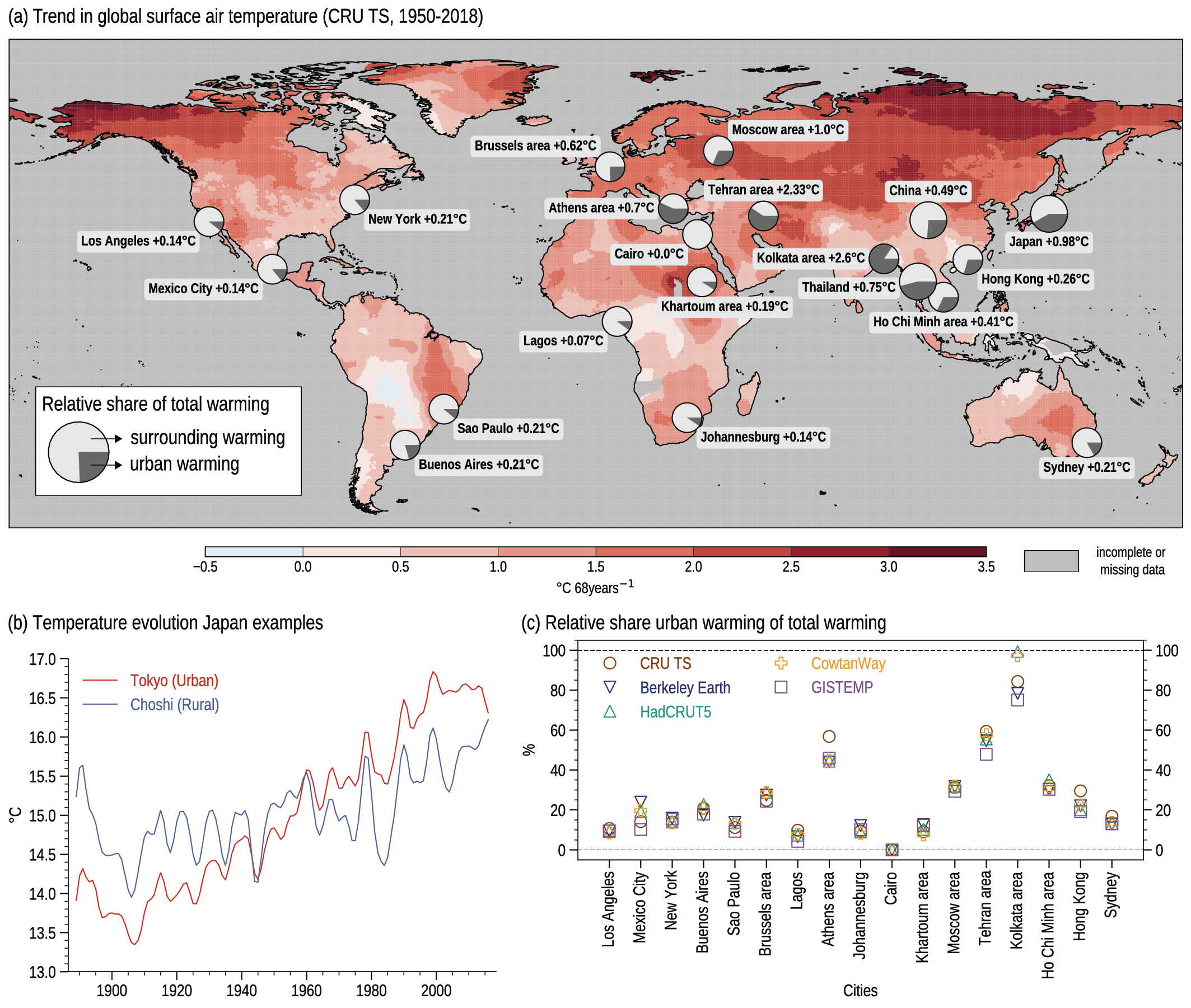
Box 10.3, Figure 1 | Urban warming compared to global GHG-induced warming. (a) Change in the annual mean surface air temperature over the period 1950–2018 based on the local linear trend retrieved from CRU TS (°C per 68 years). This background warming is compared to the local warming that has been reported during 1950–2018 in the literature from historical urbanization. The relative share of the total warming as percentage between the urban warming and the surrounding warming is plotted in a circle for each city. This map has been compiled from a review study (Hamdi et al., 2020). (b) Low-pass filtered time series of the annual mean temperature (°C) observed in the urban station of Tokyo (red line) and the rural reference station in Choshi (blue line) in Japan. The filter is the same as the one used in Figure 10.10. (c) Uncertainties in the relative share of urban warming with respect to the total warming (%) related to the use of different global observational datasets: CRU TS (brown circles), Berkeley Earth (dark blue downward triangle), HadCRUT5 (cyan upward triangle), Cowtan Way (orange plus) and GISTEMP (purple squares). Further details on data sources and processing are available in the chapter data table (Table 10.SM.11).
There is very high confidence (robust evidence and high agreement) that the annual mean minimum temperature is more affected by urbanization than the maximum temperature (Ezber et al., 2007; Fujibe, 2009; Hamdi, 2010; Elagib, 2011; Camilloni and Barrucand, 2012; Hausfather et al., 2013; Robaa, 2013; Argüeso et al., 2014; Alghamdi and Moore, 2015; Alizadeh-Choobari et al., 2016; Sachindra et al., 2016; Liao et al., 2017; Lokoshchenko, 2017; J. Wang et al., 2017; Arsiso et al., 2018). Beside temperature, urbanization can induce an urban dryness island, which refers to lower relative humidity in cities than in nearby rural locations (Lokoshchenko, 2017; Bian et al., 2020) and the urban wind island, where slower wind speeds are observed in cities (Wu et al., 2017; Bader et al., 2018; Peng et al., 2018). There is medium confidence (medium evidence and medium agreement) (Schlünzen et al., 2010; Ganeshan et al., 2013;
Ganeshan and Murtugudde, 2015; Haberlie et al., 2015; Daniels et al., 2016; Liang and Ding, 2017; McLeod et al., 2017; Li et al., 2020b) that cities induce increases in mean and extreme precipitation over and downwind of the city especially in the afternoon and early evening.
Climate projections
Estimates of the urban heat island under further climate change are very uncertain because studies using different methods report contrasting results. However, there is very high confidence (robust evidence and high agreement) that the projected change of the urban heat island under climate change conditions is one order of magnitude less than the projected warming in both urban and rural areas under simulation constraints of no urban growth (McCarthy et al., 2010, 2012; Oleson et al., 2011; Früh et al., 2011; Adachi et al., 2012; Kusaka et al., 2012a; Oleson, 2012; Hamdi et al., 2014; Sachindra et al., 2016; Hatchett et al., 2016; Arsiso et al., 2018; Hoffmann et al., 2018).
Combining climate change conditions together with urban growth scenarios, there is very high confidence (robust evidence and high agreement) that future urbanization will amplify the projected air temperature warming irrespective of the background climate (Georgescu et al., 2013; Argüeso et al., 2014; Mahmood et al., 2014; Doan et al., 2016; Kim et al., 2016; Kusaka et al., 2016; Grossman-Clarke et al., 2017; Kaplan et al., 2017; Li et al., 2018). Urbanization will have a strong influence on minimum temperatures that could be locally comparable in magnitude to the global GHG-induced warming (Berckmans et al., 2019). There is very high confidence (robust evidence and high agreement) for the combination of future urban development and more frequent occurrence of extreme climatic events, such as heatwaves (Hamdi et al., 2016; Bader et al., 2018; He et al., 2021).
The choice of urban planning scenarios and RCM projections shows a large sensitivity during nighttime, up to 0.6°C (Kusaka et al., 2016). The sensitivity is significantly less than the uncertainties arising from global emissions scenarios or global model projections. However, there is a large difference between RCM simulations with and without urban land use, indicating that this impact is comparable to the uncertainties related to the use of different global model projections (Hamdi et al., 2014; Kusaka et al., 2016; Daniel et al., 2019). Therefore, impact assessments and adaptation plans for urban areas require high spatial resolution climate projections along with models that represent urban processes, ensemble dynamical and statistical downscaling, and local-impact models (Masson et al., 2014; Baklanov et al., 2018, 2020; Duchêne et al., 2020; Schoetter et al., 2020; Le Roy et al., 2021; Zhao et al., 2021).
Cross-Chapter Box 10.4 | Climate Change over the Hindu Kush Himalaya
Coordinators: Izuru Takayabu (Japan), Andrew Turner (United Kingdom), Zhiyan Zuo (China)
Contributors: Bhupesh Adhikary (Nepal), Muhammad Adnan (Pakistan), Muhammad Amjad (Pakistan), Subimal Ghosh (India), Rafiq Hamdi (Belgium),Akm Saiful Islam (Bangladesh), Richard G. Jones (United Kingdom), Martin Jury (Austria), Asif Khan (Pakistan), Akio Kitoh (Japan), Krishnan Raghavan (India), Lucas Ruiz (Argentina), Laurent Terray (France)
The Hindu Kush Himalaya (HKH) constitutes the largest glacierized region outside the poles and provides the headwaters for several major rivers (Sharma et al., 2019). Since the 1960s, the HKH has experienced significant trends in the mean and extremes of temperature and precipitation, accompanied by glacier mass loss and retreat, snowmelt and permafrost degradation (Yao et al., 2012a, b; Azam et al., 2018; Bolch et al., 2019; Krishnan et al., 2019a, b; Chug et al., 2020; Sabin et al., 2020). Observational uncertainty and lack of consistent, high-quality datasets hamper reliable assessments of climate change and model evaluation over several mountain areas, including the HKH (Section 10.2.2). This box assesses observed and projected climate change in the extended HKH (outline in Cross-Chapter Box 10.4, Figure 1a), in which we include the Tibetan Plateau (TP) and Pamir mountains.
Temperature trends
Little evidence was presented in the AR5 (IPCC, 2014) other than increased minimum and maximum temperature trends in the western Himalaya (Hartmann et al., 2013). The SROCC assessed that HKH (named High Mountain Asia) surface-air temperature has warmed more rapidly than the global mean over recent decades (high confidence). Annual mean HKH surface air temperature increased significantly (about 0.1°C per decade) over 1901–2014 (Ren et al., 2017), although Cross-Chapter Box 10.4, Figure 1d shows an observational range of 0.20°C–0.25°C per decade over 1961–2014. There is a rising trend of extreme warm events and fewer extreme cold events over 1961–2015 (Krishnan et al., 2019b; Wester et al., 2019). However, summer cooling over the Karakoram (western HKH) was reported for 1960–2010 (Forsythe et al., 2017). A key relevant process is elevation-dependent warming (EDW; reviewed inPepin et al., 2015), leading to warming of 2°C–2.5°C at 5000 m over 1961–2006, but only 0.5°C at sea level (Xu et al., 2016). However, EDW behaviour appears to depend on region, time period and elevation (D. Guo et al., 2019; b. Li et al., 2020) and understanding is limited by the sparse observational network (You et al., 2020). Observational and model analyses have attributed EDW to GHG and black carbon emissions, accelerating warming by snow-albedo feedback (Ming et al., 2012; Gautam et al., 2013; Xu et al., 2016; Yan et al., 2016; Lau and Kim, 2018; Y. Zhang et al., 2018), or the more pronounced cooling effect of scattering aerosols at low elevations and stratospheric ozone depletion (Guo and Wang, 2012; Zeng et al., 2015). There is high confidence that the eastern and central HKH has exhibited rising temperatures (Cross-Chapter Box 10.4, Figure 1), with warming dependent on season and elevation. There is high confidence that much of the warming can be attributed to GHGs, but the effect of albedo has only medium confidence. There is high confidence in more frequent extreme warm events and fewer extreme cold events over the eastern Himalayas in the last five decades.
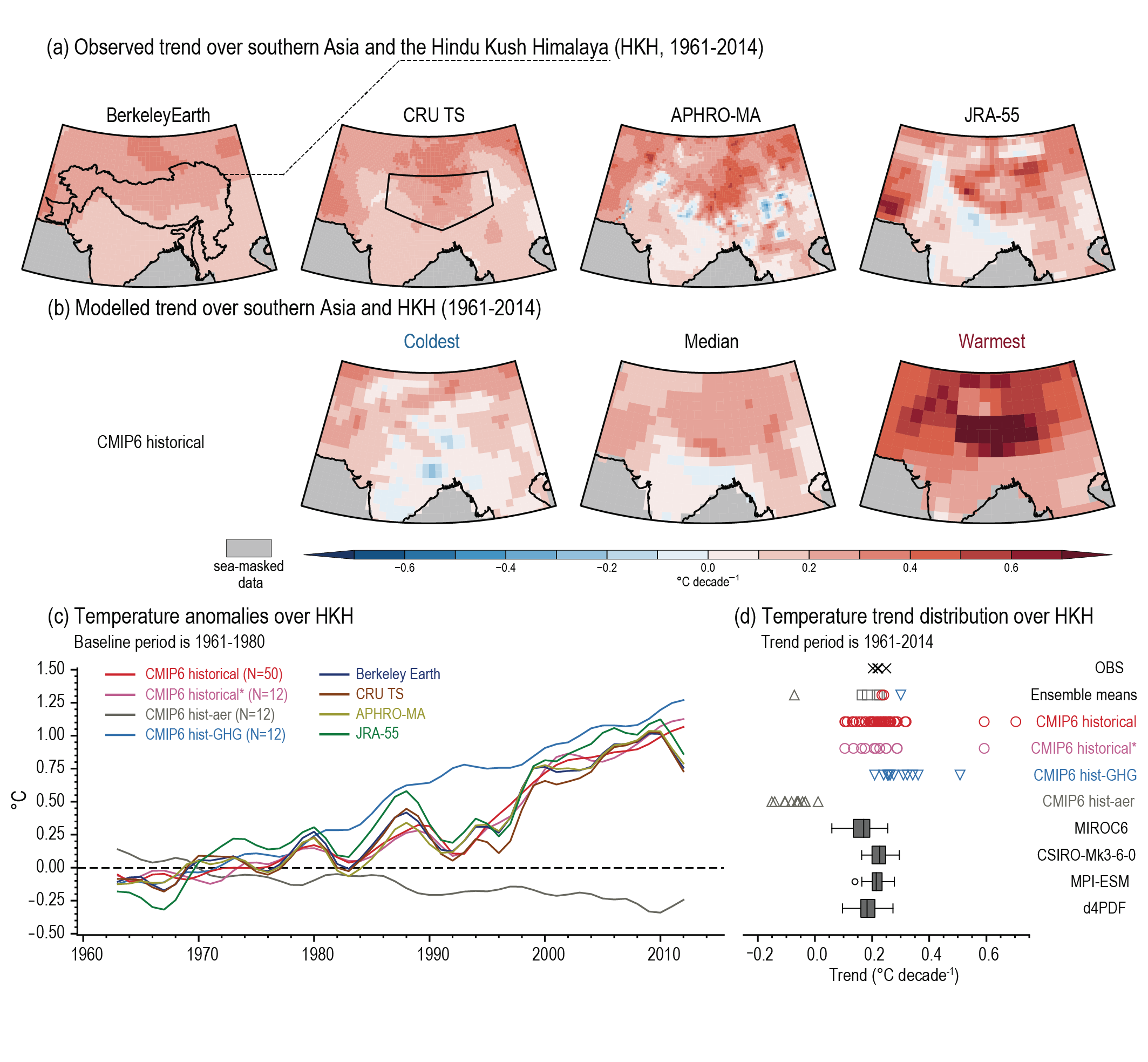
Cross-chapter Box 10.4, Figure 1 | Historical annual-mean surface air temperature linear trend (°C per decade) and its attribution over the Hindu Kush Himalaya (HKH) region. (a) Observed trends from Berkeley Earth (also showing the HKH outline), CRU TS (also showing the AR6 Tibetan Plateau (TIB) outline, for ease of comparison to the Interactive Atlas), APHRO-MA and JRA-55 datasets over 1961–2014. (b) Models showing the coldest, median and warmest HKH temperature linear trends among the CMIP6 historical ensemble over 1961–2014. (c) Low-pass-filtered time series of annual-mean surface air temperature anomalies (°C, baseline 1961–1980) over the HKH region as outlined in panel (a), showing means of CMIP6 hist all-forcings (red), and the CMIP6 hist all-forcings sample corresponding to DAMIP experiments (pink), for hist-aer (grey) and hist-GHG (pale blue). Observed datasets are Berkeley Earth (dark blue), CRU (brown), APHRO-MA (light green) and JRA-55 (dark green). The filter is the same as that used in Figure 10.10. (d) Distribution of annual mean surface air temperature trends (°C per decade) over the HKH region from 1961 to 2014 for ensemble means, the aforementioned observed and reanalysis data (black crosses), individual members of CMIP6 hist all-forcings (red circles), CMIP6 hist-GHG (blue triangles), CMIP6 hist-aer (grey triangles), and box-and-whisker plots for the SMILEs used throughout (Chapter 10 (grey shading). Ensemble means are also shown. All trends are estimated using ordinary least-squares regression and box-and-whisker plots follow the methodology used in Figure 10.6. Further details on data sources and processing are available in the chapter data table (Table 10.SM.11).
Cross-Chapter Box 10.4
Precipitation trends
Annual and summer precipitation over the central-eastern HKH show decreasing trends over 1979–2010 in multiple observed datasets, attributable to a weakening South Asian monsoon (Yao et al., 2012a; Palazzi et al., 2013; Roxy et al., 2015). There are contradictory trends in the western HKH (Azmat et al., 2017; Yadav et al., 2017; H. Li et al., 2018; Meher et al., 2018), where most precipitation is associated with western disturbances on the subtropical westerly jet, but trends in western disturbance activity are unclear (Kumar et al., 2015; Hunt et al., 2019; Krishnan et al., 2019a). There has been an increased frequency and intensity of extreme precipitation over the central-western HKH but contrasting evidence in the east (Sheikh et al., 2015; Talchabhadel et al., 2018). The number of consecutive wet days has increased over 1961–2012, but with no uniform trend in consecutive dry days (Zhan et al., 2017). There is medium confidence that the eastern-central HKH has experienced decreased summer precipitation (Section 10.6.3). There is medium confidence in the increase of summer extreme precipitation over the western HKH.
Glacier trends
The SROCC assessed that snow cover has declined in duration, depth and accumulated mass at lower elevations in mountain regions, including the HKH (high confidence). Glaciers are losing mass (very high confidence) and permafrost is warming (high confidence) over high mountains in recent decades, and it is very likely that atmospheric warming is the main driver. A significant reduction in HKH glacier area has been observed since the 1970s, with smaller glaciers generally shrinking faster (e.g., Bolch et al., 2019). HKH glacier mass loss took place at the lowest rate among high mountain areas in the last 20 years, although with one of the largest total losses (Section 9.5.1.1 and Figure 9.20; Shean et al., 2020). The highest mass-loss rates occurred in the eastern and northern HKH, while gains occurred in the west (e.g., Shean et al., 2020). Glacier mass gain has been coined as the ‘Karakoram anomaly’ (Sections 8.3.1.7.1 and 9.5.1), explained by a combination of low temperature sensitivity of debris-covered glaciers, a decrease in summer air temperatures, and increased snowfall possibly linked to evapotranspiration from irrigated agriculture (You et al., 2017; Bolch et al., 2019; de Kok et al., 2020a; Farinotti et al., 2020). Meanwhile, increased air temperature and decreased snowfall explain the glacier mass decrease elsewhere (Bonekamp et al., 2019; de Kok et al., 2020b; Farinotti et al., 2020; Shean et al., 2020). There is high confidence that glaciers in most HKH regions have thinned, retreated and lost mass since the 1970s.
Projections
In AR5, the HKH was projected to continue warming over the 21st century, faster than the likely ranges for the global mean and South Asia. New CMIP5 results show temperature increases across mountainous HKH by about 1°C–2°C (in some places in summer 4°C–5°C) during 2021–2050 compared to 1961–1990 (Shrestha et al., 2015). Projected warming differs by up to 1°C between east and west, with higher values in winter (Sanjay et al., 2017; see Interactive Atlas). Statistically significant mean warming (0.30°C–0.90°C per decade until the end of the 21st century) across all RCPs has been projected by CORDEX South Asia (Dimri et al., 2018). CMIP6 models report that north-western South Asia, including the western Himalayas, is projected to experience temperature increases exceeding 6°C by the end of the 21st century under SSP5-8.5 relative to 1995–2014 (Almazroui et al., 2020b). Results from CMIP5, CMIP6 and CORDEX ensembles for different warming levels are shown in the Interactive Atlas and summarized in Figure Atlas.20. The HKH will likely continue warming in the coming decades.
The SR1.5 (IPCC, 2018b) stated that heavy precipitation risk in high-elevation regions is projected to be higher at 2°C compared to 1.5°C of global warming (medium confidence). CMIP5 models project increased annual or summer monsoon precipitation over the HKH in the 21st century (Palazzi et al., 2015; Kitoh and Arakawa, 2016), intensifying by about 22% in the hilly south-eastern Himalaya and TP for the long term in RCP8.5, but with no trends in the western HKH (Rajbhandari et al., 2015; Krishnan et al., 2019a). CMIP6 projects an increase of winter precipitation over the western Himalayas, with a corresponding decrease in the east (Almazroui et al., 2020b). HKH projections are subject to large uncertainties in CMIP5 and CORDEX (Hasson et al., 2013, 2017; Mishra, 2015; Sanjay et al., 2017). CORDEX, in particular, has inherent limitations at reproducing the characteristics of summer monsoon rainfall variability (Singh et al., 2017). There is medium confidence that HKH precipitation will increase in the coming decades.
The SROCC assessed that glaciers will lose substantial mass (high confidence) and permafrost will undergo increasing thaw and degradation (very high confidence) over high mountain regions (including the HKH), with stronger changes for higher emissions scenarios. Regional differences in warming and precipitation projections and glacier properties cause considerable differences in glacier response within High Mountain Asia (Kraaijenbrink et al., 2017). Glacier mass loss will accelerate through the 21st century, increasing with RCP after 2030 (Section 9.5.1.3; Marzeion et al., 2014). Loss of between 40 ± 25% to 69 ± 21 % of 2015 glacier volume is expected by 2100 in RCP 2.6 and RCP 8.5, respectively (Section 9.5.1.3 and Figure 9.21). Glacier mass loss is expected due to decreased snowfall, increased snowline elevations and longer melt seasons. However, due to projection uncertainties, simplicity of the models, and limited observations, there is medium confidence in the magnitude and timing of glacier mass changes (Section 9.5.1.3). Glacier mass in HKH will decline through the 21st century (high confidence), more so under high-emissions scenarios.
10.7 Final remarks
The assessments in this chapter are based on a rapidly growing body of evidence from the peer-reviewed literature, most of which was not previously considered by IPCC reports. Several challenges in the construction of regional climate change information have been identified:
- Limited climate monitoring in some regions impedes the full understanding of the relevant climate processes, an appropriate validation of model simulations, and the formulation of trustworthy regional climate information. Beyond temperature and precipitation, there is a shortage of observed variables needed for regional process understanding, attribution, and model development and validation, among others. Examples include surface evapotranspiration, soil moisture, radiation, wind and relative humidity, among many others identified by sectors sensitive to climate (Sections 10.2, 10.3 and 10.6).
- Compared to the increasing number of large-scale evaluations, there is a shortage of process-based model evaluations at regional scales to assess the fitness of the chosen models for specific purposes (Sections 10.3 and 10.4).
- There is a general lack of studies of the simulation of large-scale, downscaling-relevant processes in global models to support the design of global/regional model matrices that both span a sufficiently large range of projection uncertainty and realistically represent the regional climate of interest. The fitness of statistical methods for regional climate change studies has received limited attention by the scientific community, while as in the case of global models, process-based evaluation has proven useful (Soares et al., 2019b). Studies of past changes and pseudo-reality studies to assess the predictors and model structures required for downscaling in a future climate are promising avenues (Section 10.3).
- Internal variability is a large contributor to climate uncertainty at regional scales, especially for extreme events. Further study of the processes governing regional internal variability, such as the modes of variability and the teleconnections that connect them to the regional variability, but also of the local processes and drivers involved, will help improve its understanding. The same applies to the validation of the simulated internal variability that underpins the trustworthiness of model-based climate information (Sections 10.3, 10.4 and 10.6, and Cross-Chapter Box 10.1).
- Methodologies on how to propagate climate uncertainties from global and regional scales down to the human settlement scale are still under development. In some cases, bias-adjustment methods are used with substantial neglect of the physical processes involved (Section 10.3 and Cross-Chapter Box 10.2).
- The production of regional climate information relies mainly on global and regional models that often do not incorporate human-controlled surface processes (urban parametrizations is one example) in their land surface components. This limits the representation of uncertainties for climate information at the urban scale (Section 10.3, Box 10.2, and Cross-Chapter Box 10.2).
- Literature plays a central role as a source for constructing regional climate change information. The amount of climate change literature available is unevenly distributed across the world, and large bodies of literature (e.g., local and regional reports) are often overlooked in the construction of climate information. Furthermore, research tends to focus on regions that attract the attention of the Global North so that climate aspects relevant to other regions may not receive sufficient attention for generating appropriate regional climate information (Sections 10.2, 10.3, 10.5 and 10.6).
- Governmental institutions producing regional and local climate information often use diverging approaches that are not necessarily coherent with each other. Coherency could be improved by implementing a quality control system and a traceability solution for the sources of the information. Collective work with the social sciences and humanities will improve the communication, perception and response to regional climate information and help translate user requirements (Sections 10.5 and 10.6).
- There is a shortage of regional climate change studies distilling multiple lines of evidence. Most studies rely on either global models or downscaled global models, with an increasing number of studies focusing on the use of emulators and the selection and combination of models. However, there are limited studies distilling this information with a wider range of lines of evidence that includes observations, process understanding, attribution, and hierarchies of models (Sections 10.3, 10.5 and 10.6).
Addressing these challenges could facilitate the assessment of both sources and methodologies that lead to an increased fitness and usefulness of regional climate information for a wide range of purposes.
Acknowledgements
We acknowledge the E-OBS dataset and the data providers in the ECA&D project (https://www.ecad.eu) for their help and the Japan Aerospace Exploration Agency (JAXA) for delivering the GSMaP (Global Satellite Mapping of Precipitation) data to us. The invaluable contributions from Lisa van Aardenne (South Africa), Peng Cai (China), Joseph Ching (China), Huili He (China), Kenshi Hibino (Japan), Yukiko Imada (Japan), Nazrul Islam (Saudi Arabia), Isadora Christel Jiménez (Spain) and Misako Kachi (Japan) are also greatly acknowledged. We acknowledge the World Climate Research Programme for coordinating the modelling intercomparison projects CMIP and CORDEX and thank the climate modelling groups for producing and making available their model output.
Frequently Asked Questions
FAQ 10.1 | How Can We Provide Useful Climate Information for Regional Stakeholders?
The world is physically and culturally diverse, and the challenges posed by climate change vary by region and location. Because climate change affects so many aspects of people’s daily work and living, climate change information can help with decision-making, but only when the information is relevant for the people involved in making those decisions. Users of climate information may be highly diverse, ranging from professionals in areas such as human health, agriculture or water management to a broader community that experiences the impacts of changing climate. Providing information that supports response actions thus requires engaging all relevant stakeholders, their knowledge and their experiences, formulating appropriate information, and developing a mutual understanding of the usefulness and limitations of the information.
The development, delivery, and use of climate change information requires engaging all parties involved: those producing the climate data and related knowledge, those communicating it, and those who combine that information with their knowledge of the community, region or activity that climate change may impact. To be successful, these parties need to work together to explore the climate data and thus co-develop the climate information needed to make decisions or solve problems, distilling output from the various sources of climate knowledge into relevant climate information. Effective partnerships recognize and respond to the diversity of all parties involved (including their values, beliefs and interests), especially when they involve culturally diverse communities and their indigenous and local knowledge of weather, climate and their society. This is particularly true for climate change – a global issue posing challenges that vary by region. By recognizing this diversity, climate information can be relevant and credible, most notably when conveying the complexity of risks for human systems and ecosystems and for building resilience.
Constructing useful climate information requires considering all available sources in order to capture the fullest possible representation of projected changes and distilling the information in a way that meets the needs of the stakeholders and communities impacted by the changes. For example, climate scientists can provide information on future changes by using simulations of global and/or regional climate and inferring changes in the weather behaviour influencing a region. An effective distillation process (FAQ 10.1, Figure 1) engages with the intended recipients of the information, especially stakeholders whose work involves non-climatic factors, such as human health, agriculture or water resources. The distillation evaluates the accuracy of all information sources (observations, simulations, expert judgement), weighs the credibility of possible conflicting information, and arrives at climate information that includes estimating the confidence a user should have in it. Producers of climate data should further recognize that the geographic regions and time periods governing stakeholders’ interest (for example, the growing season of an agricultural zone) may not align well with the time and space resolution of available climate data; thus additional model development or data processing may be required to extract useful climate information.
One way to distil complex information for stakeholder applications is to connect this information to experiences stakeholders have already had through storylines as plausible unfoldings of weather and climate events related to stakeholders’ experiences. Dialogue between stakeholders and climate scientists can determine the most relevant experiences to evaluate for possible future behaviour. The development of storylines uses the experience and expertise of stakeholders, such as water-resource managers and health professionals, who seek to develop appropriate response measures. Storylines are thus a pathway through the distillation process that can make climate information more accessible and physically comprehensible. For example, a storyline may take a common experience like an extended drought, with depleted water availability and damaged crops, and show how droughts may change in the future, perhaps with even greater precipitation deficits or longer duration. With appropriate choices, storylines can engage nuances of the climate information in a meaningful way by building on common experiences, thus enhancing the information’s usefulness.
Forging partnerships among all involved with producing, exploring and distilling climate data into climate information is at the centre of creating stakeholder-relevant information. These partnerships can occur through direct interaction between climate scientists and stakeholders as well as through organizations that have emerged to facilitate this process, such as climate services, national and regional climate forums, and consulting firms providing specialized climate information. These so-called ‘boundary organizations’ can serve the varied needs of all who would fold climate information into their decision processes. All of these partnerships are vital
for arriving at climate information that responds to physical and cultural diversity and to challenges posed by climate change that can vary region-by-region around the world.

FAQ 10.1, Figure 1 | Climate information for decision makers is more useful if the physical and cultural diversity across the world is considered. The figure illustrates schematically the broad range of knowledge that must be blended with the diversity of users to distil information that will have relevance and credibility. This blending or distillation should engage the values and knowledge of both the stakeholders and the scientists. The bottom row contains examples of stakeholders’ interests and is not all-inclusive. As part of the distillation, the outcomes can advance the United Nations’ Sustainable Development Goals, covered in part by these examples.
FAQ 10.2 | Why Are Cities Hotspots of Global Warming?
Urban areas experience air temperatures that can be several degrees Celsius warmer than surrounding areas, especially during the night. This ‘urban heat island’ effect results from several factors, including reduced ventilation and heat trapping due to the close proximity of tall buildings, heat generated directly from human activities, the heat-absorbing properties of concrete and other urban building materials, and the limited amount of vegetation. Continuing urbanization and increasingly severe heatwaves under climate change will further amplify this effect in the future.
Today, cities are home to 55% of the world’s population. This number is increasing, and every year cities welcome 67 million new residents, 90% of whom are moving to cities in developing countries. By 2030, almost 60% of the world’s population is expected to live in urban areas. Cities and their inhabitants are highly vulnerable to weather and climate extremes, particularly heatwaves, because urban areas already are local hotspots. Cities are generally warmer – up to several degrees Celsius at night – than their surroundings. This warming effect, called the urban heat island, occurs because cities both receive and retain more heat than the surrounding countryside areas and because natural cooling processes are weakened in cities compared to rural areas.
Three main factors contribute to amplify the warming of urban areas (orange bars in FAQ 10.2, Figure 1). The strongest contribution comes from urban geometry, which depends on the number of buildings, their size and their proximity. Tall buildings close to each other absorb and store heat and also reduce natural ventilation. Human activities, which are very concentrated in cities, also directly warm the atmosphere locally, due to heat released from domestic and industrial heating or cooling systems, running engines, and other sources. Finally, urban warming also results directly from the heat-retaining properties of the materials that make up cities, including concrete buildings, asphalt roadways, and dark rooftops. These materials are very good at absorbing and retaining heat, and then re-emitting that heat at night.
The urban heat island effect is further amplified in cities that lack vegetation and water bodies, both of which can strongly contribute to local cooling (green bars in FAQ 10.2, Figure 1). This means that when enough vegetation and water are included in the urban fabric, they can counterbalance the urban heat island effect, to the point of even cancelling out the urban heat island effect in some neighbourhoods.
The urban heat island phenomenon is well-known and understood. For instance, temperature measurements from thermometers located in cities are corrected for this effect when global warming trends are calculated. Nevertheless, observations, including long-term measurements of the urban heat island effect are currently too limited to allow a full understanding of how the urban heat island varies across the world and across different types of cities and climatic zones, or how this effect will evolve in the future.
As a result, it is hard to assess how climate change will affect the urban heat island effect, and various studies disagree. Two things are, however, very clear. First, future urbanization will expand the urban heat island areas, thereby amplifying future warming in many places all over the world. In some places, the nighttime warming from the urban heat island effect could even be on the same order of magnitude as the warming expected from human-induced climate change. Second, more intense, longer and more frequent heatwaves caused by climate change will more strongly impact cities and their inhabitants, because the extra warming from the urban heat island effect will exacerbate the impacts of climate change.
In summary, cities are currently local hotspots because their structure, material and activities trap and release heat and reduce natural cooling processes. In the future, climate change will, on average, have a limited effect on the magnitude of the urban heat island itself, but ongoing urbanization together with more frequent, longer and warmer heatwaves will make cities more exposed to global warming.
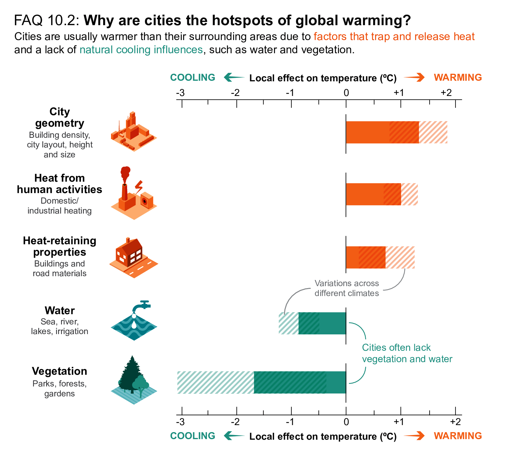
FAQ 10.2, Figure 1 | Efficiency of the various factors at warming up or cooling down neighbourhoods of urban areas. Overall, cities tend to be warmer than their surroundings. This is called the ‘urban heat island’ effect. The hatched areas on the bars show how the strength of the warming or cooling effects of each factor varies depending on the local climate. For example, vegetation has a stronger cooling effect in temperate and warm climates. Further details on data sources are available in the chapter data table (Table 10.SM.11).
References
Aalbers, E.E., G. Lenderink, E. van Meijgaard, and B.J.J.M. van den Hurk, 2018: Local-scale changes in mean and heavy precipitation in Western Europe, climate change or internal variability?Climate Dynamics, 50(11–12), 4745–4766, doi: 10.1007/s00382-017-3901-9.
Aalto, J., P. Pirinen, and K. Jylhä, 2016: New gridded daily climatology of Finland: Permutation-based uncertainty estimates and temporal trends in climate. Journal of Geophysical Research: Atmospheres, 121(8), 3807–3823, doi: 10.1002/2015jd024651.
Abatzoglou, J.T. and T.J. Brown, 2012: A comparison of statistical downscaling methods suited for wildfire applications. International Journal of Climatology, 32(5), 772–780, doi: 10.1002/joc.2312.
Abba Omar, S. and B.J. Abiodun, 2020: Characteristics of cut-off lows during the 2015–2017 drought in the Western Cape, South Africa. Atmospheric Research, 235, 104772, doi: 10.1016/j.atmosres.2019.104772.
Abera, W., L. Brocca, and R. Rigon, 2016: Comparative evaluation of different satellite rainfall estimation products and bias correction in the Upper Blue Nile (UBN) basin. Atmospheric Research, 178–179, 471–483, doi: 10.1016/j.atmosres.2016.04.017.
Abiodun, B.J. et al., 2017: Potential impacts of climate change on extreme precipitation over four African coastal cities. Climatic Change, 143(3–4), 399–413, doi: 10.1007/s10584-017-2001-5.
Abram, N.J. et al., 2020: Coupling of Indo-Pacific climate variability over the last millennium. Nature, 579(7799), 385–392, doi: 10.1038/s41586-020-2084-4.
Abramowitz, G. et al., 2019: ESD Reviews: Model dependence in multi-model climate ensembles: weighting, sub-selection and out-of-sample testing. Earth System Dynamics, 10(1), 91–105, doi: 10.5194/esd-10-91-2019.
Ackerley, D. et al., 2011: Sensitivity of Twentieth-Century Sahel Rainfall to Sulfate Aerosol and CO2 Forcing. Journal of Climate, 24(19), 4999–5014, doi: 10.1175/jcli-d-11-00019.1.
Ackerman, T.P. and G.M. Stokes, 2003: The Atmospheric Radiation Measurement Program. Physics Today, 56(1), 38–44, doi: 10.1063/1.1554135.
Adachi, S.A., F. Kimura, H. Kusaka, T. Inoue, and H. Ueda, 2012: Comparison of the Impact of Global Climate Changes and Urbanization on Summertime Future Climate in the Tokyo Metropolitan Area. Journal of Applied Meteorology and Climatology, 51(8), 1441–1454, doi: 10.1175/jamc-d-11-0137.1.
Addor, N., M. Rohrer, R. Furrer, and J. Seibert, 2016: Propagation of biases in climate models from the synoptic to the regional scale: Implications for bias adjustment. Journal of Geophysical Research: Atmospheres, 121(5), 2075–2089, doi: 10.1002/2015jd024040.
Adebiyi, A.A. and J.F. Kok, 2020: Climate models miss most of the coarse dust in the atmosphere. Science Advances, 6(15), eaaz9507, doi: 10.1126/sciadv.aaz9507.
Adloff, F. et al., 2018: Improving sea level simulation in Mediterranean regional climate models. Climate Dynamics, 51(3), 1167–1178, doi: 10.1007/s00382-017-3842-3.
Ahmed, K.F. et al., 2013: Statistical downscaling and bias correction of climate model outputs for climate change impact assessment in the U.S. northeast. Global and Planetary Change, 100, 320–332, doi: 10.1016/j.gloplacha.2012.11.003.
Ahn, M.-S. et al., 2017: MJO simulation in CMIP5 climate models: MJO skill metrics and process-oriented diagnosis. Climate Dynamics, 49(11–12), 4023–4045, doi: 10.1007/s00382-017-3558-4.
Akhtar, N., J. Brauch, and B. Ahrens, 2018: Climate modeling over the Mediterranean Sea: impact of resolution and ocean coupling. Climate Dynamics, 51(3), 933–948, doi: 10.1007/s00382-017-3570-8.
Akhtar, N., J. Brauch, A. Dobler, K. Béranger, and B. Ahrens, 2014: Medicanes in an ocean–atmosphere coupled regional climate model. Natural Hazards and Earth System Sciences, 14(8), 2189–2201, doi: 10.5194/nhess-14-2189-2014.
Akhtar, N. et al., 2019: European marginal seas in a regional atmosphere–ocean coupled model and their impact on Vb-cyclones and associated precipitation. Climate Dynamics, 53(9–10), 5967–5984, doi: 10.1007/s00382-019-04906-x.
Akhter, J., L. Das, J.K. Meher, and A. Deb, 2018: Uncertainties and time of emergence of multi-model precipitation projection over homogeneous rainfall zones of India. Climate Dynamics, 50(9–10), 3813–3831, doi: 10.1007/s00382-017-3847-y.
Akhter, J., L. Das, J.K. Meher, and A. Deb, 2019: Evaluation of different large-scale predictor-based statistical downscaling models in simulating zone-wise monsoon precipitation over India. International Journal of Climatology, 39(1), 465–482, doi: 10.1002/joc.5822.
Alessandri, A. et al., 2015: Robust assessment of the expansion and retreat of Mediterranean climate in the 21st century. Scientific Reports, 4(1), 7211, doi: 10.1038/srep07211.
Alexander, L., 2016: Global observed long-term changes in temperature and precipitation extremes: A review of progress and limitations in IPCC assessments and beyond. Weather and Climate Extremes, 11, 4–16, doi: 10.1016/j.wace.2015.10.007.
Alghamdi, A.S. and T.W. Moore, 2015: Detecting Temporal Changes in Riyadh’s Urban Heat Island. Papers in Applied Geography, 1(4), 312–325, doi: 10.1080/23754931.2015.1084525.
Alizadeh-Choobari, O., P. Ghafarian, and P. Adibi, 2016: Inter-annual variations and trends of the urban warming in Tehran. Atmospheric Research, 170, 176–185, doi: 10.1016/j.atmosres.2015.12.001.
Allen, M.R., P.A. Stott, J.F.B. Mitchell, R. Schnur, and T.L. Delworth, 2000: Quantifying the uncertainty in forecasts of anthropogenic climate change. Nature, 407(6804), 617–620, doi: 10.1038/35036559.
Allen, R.J., 2015: A 21st century northward tropical precipitation shift caused by future anthropogenic aerosol reductions. Journal of Geophysical Research: Atmospheres, 120(18), 9087–9102, doi: 10.1002/2015jd023623.
Allen, R.J. and M. Kovilakam, 2017: The Role of Natural Climate Variability in Recent Tropical Expansion. Journal of Climate, 30(16), 6329–6350, doi: 10.1175/jcli-d-16-0735.1.
Allen, R.J., A.T. Evan, and B.B.B. Booth, 2015: Interhemispheric Aerosol Radiative Forcing and Tropical Precipitation Shifts during the Late Twentieth Century. Journal of Climate, 28(20), 8219–8246, doi: 10.1175/jcli-d-15-0148.1.
Almazroui, M., 2016: RegCM4 in climate simulation over CORDEX-MENA/Arab domain: selection of suitable domain, convection and land-surface schemes. International Journal of Climatology, 36(1), 236–251, doi: 10.1002/joc.4340.
Almazroui, M., 2019: Temperature Changes over the CORDEX-MENA Domain in the 21st Century Using CMIP5 Data Downscaled with RegCM4: A Focus on the Arabian Peninsula. Advances in Meteorology, 2019, 5395676, doi: 10.1155/2019/5395676.
Almazroui, M., M.N. Islam, A.K. Al-Khalaf, and F. Saeed, 2016a: Best convective parameterization scheme within RegCM4 to downscale CMIP5 multi-model data for the CORDEX-MENA/Arab domain. Theoretical and Applied Climatology, 124(3–4), 807–823, doi: 10.1007/s00704-015-1463-5.
Almazroui, M., M.N. Islam, S. Saeed, F. Saeed, and M. Ismail, 2020a: Future Changes in Climate over the Arabian Peninsula based on CMIP6 Multimodel Simulations. Earth Systems and Environment, 4(4), 611–630, doi: 10.1007/s41748-020-00183-5.
Almazroui, M., S. Saeed, F. Saeed, M.N. Islam, and M. Ismail, 2020b: Projections of Precipitation and Temperature over the South Asian Countries in CMIP6. Earth Systems and Environment, 4(2), 297–320, doi: 10.1007/s41748-020-00157-7.
Almazroui, M. et al., 2016b: Simulation of temperature and precipitation climatology for the CORDEX-MENA/Arab domain using RegCM4. Arabian Journal of Geosciences, 9(1), 13, doi: 10.1007/s12517-015-2045-7.
Almazroui, M. et al., 2020c: Projected Change in Temperature and Precipitation Over Africa from CMIP6. Earth Systems and Environment, 4(3), 455–475, doi: 10.1007/s41748-020-00161-x.
Almazroui, M. et al., 2021: Projected Changes in Temperature and Precipitation Over the United States, Central America, and the Caribbean in CMIP6 GCMs. Earth Systems and Environment, 5(1), 1–24, doi: 10.1007/s41748-021-00199-5.
Alter, R.E., E.-S. Im, and E.A.B. Eltahir, 2015: Rainfall consistently enhanced around the Gezira Scheme in East Africa due to irrigation. Nature Geoscience, 8(10), 763–767, doi: 10.1038/ngeo2514.
Amaya, D.J., N. Siler, S.-P. Xie, and A.J. Miller, 2018: The interplay of internal and forced modes of Hadley Cell expansion: lessons from the global warming hiatus. Climate Dynamics, 51(1–2), 305–319, doi: 10.1007/s00382-017-3921-5.
Anand, A. et al., 2018: Indian Summer Monsoon Simulations: Usefulness of Increasing Horizontal Resolution, Manual Tuning, and Semi-Automatic Tuning in Reducing Present-Day Model Biases. Scientific Reports, 8(1), 3522, doi: 10.1038/s41598-018-21865-1.
Andreassen, H.P., K.E. Gangaas, and B.P. Kaltenborn, 2018: Matching social-ecological systems by understanding the spatial scale of environmental attitudes. Nature Conservation, 30, 69–81, doi: 10.3897/natureconservation.30.28289.
Annamalai, H., J. Hafner, K.P. Sooraj, and P. Pillai, 2013: Global warming shifts the monsoon circulation, drying South Asia. Journal of Climate, 26(9), 2701–2718, doi: 10.1175/jcli-d-12-00208.1.
Annan, J.D. and J.C. Hargreaves, 2017: On the meaning of independence in climate science. Earth System Dynamics, 8(1), 211–224, doi: 10.5194/esd-8-211-2017.
Archer, E. et al., 2018: Seasonal prediction and regional climate projections for southern Africa. Biodiversity & Ecology, 6, 14–21, doi: 10.7809/b-e.00296.
Ardilouze, C., L. Batté, M. Déqué, E. van Meijgaard, and B. van den Hurk, 2019: Investigating the impact of soil moisture on European summer climate in ensemble numerical experiments. Climate Dynamics, 52(7–8), 4011–4026, doi: 10.1007/s00382-018-4358-1.
Argüeso, D., J.P. Evans, L. Fita, and K.J. Bormann, 2014: Temperature response to future urbanization and climate change. Climate Dynamics, 42(7–8), 2183–2199, doi: 10.1007/s00382-013-1789-6.
Armstrong, M.S., A.S. Kiem, and T.R. Vance, 2020: Comparing instrumental, palaeoclimate, and projected rainfall data: Implications for water resources management and hydrological modelling. Journal of Hydrology: Regional Studies, 31, 100728, doi: 10.1016/j.ejrh.2020.100728.
Arsiso, B.K., G. Mengistu Tsidu, G.H. Stoffberg, and T. Tadesse, 2018: Influence of urbanization-driven land use/cover change on climate: The case of Addis Ababa, Ethiopia. Physics and Chemistry of the Earth, Parts A/B/C, 105, 212–223, doi: 10.1016/j.pce.2018.02.009.
Aryee, J.N.A. et al., 2018: Development of high spatial resolution rainfall data for Ghana. International Journal of Climatology, 38(3), 1201–1215, doi: 10.1002/joc.5238.
Ashcroft, L. et al., 2018: A rescued dataset of sub-daily meteorological observations for Europe and the southern Mediterranean region, 1877–2012. Earth System Science Data, 10(3), 1613–1635, doi: 10.5194/essd-10-1613-2018.
Ashfaq, M. et al., 2021: Robust late twenty-first century shift in the regional monsoons in RegCM-CORDEX simulations. Climate Dynamics, 57(5–6), 1463–1488, doi: 10.1007/s00382-020-05306-2.
Attada, R., A. Parekh, J.S. Chowdary, and C. Gnanaseelan, 2018: Reanalysis of the Indian summer monsoon: four dimensional data assimilation of AIRS retrievals in a regional data assimilation and modeling framework. Climate Dynamics, 50(7–8), 2905–2923, doi: 10.1007/s00382-017-3781-z.
Auchmann, R. and S. Brönnimann, 2012: A physics-based correction model for homogenizing sub-daily temperature series. Journal of Geophysical Research: Atmospheres, 117(D17), D17119, doi: 10.1029/2012jd018067.
Ayarzagüena, B. and J.A. Screen, 2016: Future Arctic sea ice loss reduces severity of cold air outbreaks in midlatitudes. Geophysical Research Letters, 43(6), 2801–2809, doi: 10.1002/2016gl068092.
Ayarzagüena, B. et al., 2018: No robust evidence of future changes in major stratospheric sudden warmings: a multi-model assessment from CCMI. Atmospheric Chemistry and Physics, 18(15), 11277–11287, doi: 10.5194/acp-18-11277-2018.
Azam, M.F. et al., 2018: Review of the status and mass changes of Himalayan-Karakoram glaciers. Journal of Glaciology, 64(243), 61–74, doi: 10.1017/jog.2017.86.
Azmat, M., U.W. Liaqat, M.U. Qamar, and U.K. Awan, 2017: Impacts of changing climate and snow cover on the flow regime of Jhelum River, Western Himalayas. Regional Environmental Change, 17(3), 813–825, doi: 10.1007/s10113-016-1072-6.
Bach, L., C. Schraff, J.D. Keller, and A. Hense, 2016: Towards a probabilistic regional reanalysis system for Europe: evaluation of precipitation from experiments. Tellus A: Dynamic Meteorology and Oceanography, 68(1), 32209, doi: 10.3402/tellusa.v68.32209.
Bader, D.A. et al., 2018: Urban Climate Science. In: Climate Change and Cities: Second Assessment Report of the Urban Climate Change Research Network[Rosenzweig, C., P. Romero-Lankao, S. Mehrotra, S. Dhakal, S. Ali Ibrahim, and W.D. Solecki (eds.)]. Cambridge University Press, Cambridge, United Kingdom, pp. 27–60, doi: 10.1017/9781316563878.009.
Bador, M., L. Terray, and J. Boé, 2016: Emergence of human influence on summer record-breaking temperatures over Europe. Geophysical Research Letters, 43(1), 404–412, doi: 10.1002/2015gl066560.
Bador, M. et al., 2020: Impact of Higher Spatial Atmospheric Resolution on Precipitation Extremes Over Land in Global Climate Models. Journal of Geophysical Research: Atmospheres, 125(13), e2019JD032184, doi: 10.1029/2019jd032184.
Bain, P.G., M.J. Hornsey, R. Bongiorno, and C. Jeffries, 2012: Promoting pro-environmental action in climate change deniers. Nature Climate Change, 2(8), 600–603, doi: 10.1038/nclimate1532.
Baker, D.J., A.J. Hartley, S.H.M. Butchart, and S.G. Willis, 2016: Choice of baseline climate data impacts projected species’ responses to climate change. Global Change Biology, 22(7), 2392–2404, doi: 10.1111/gcb.13273.
Baklanov, A. et al., 2018: From urban meteorology, climate and environment research to integrated city services. Urban Climate, 23, 330–341, doi: 10.1016/j.uclim.2017.05.004.
Baklanov, A. et al., 2020: Integrated urban services: Experience from four cities on different continents. Urban Climate, 32, 100610, doi: 10.1016/j.uclim.2020.100610.
Bal, P.K. et al., 2016: Climate change projections over India by a downscaling approach using PRECIS. Asia-Pacific Journal of Atmospheric Sciences, 52(4), 353–369, doi: 10.1007/s13143-016-0004-1.
Balsamo, G. et al., 2015: ERA-Interim/Land: a global land surface reanalysis data set. Hydrology and Earth System Sciences, 19(1), 389–407, doi: 10.5194/hess-19-389-2015.
Ban, N., J. Schmidli, and C. Schär, 2014: Evaluation of the convection-resolving regional climate modeling approach in decade-long simulations. Journal of Geophysical Research: Atmospheres, 119(13), 7889–7907, doi: 10.1002/2014jd021478.
Ban, N., J. Schmidli, and C. Schär, 2015: Heavy precipitation in a changing climate: Does short-term summer precipitation increase faster?Geophysical Research Letters, 42(4), 1165–1172, doi: 10.1002/2014gl062588.
Ban, N. et al., 2021: The first multi-model ensemble of regional climate simulations at kilometer-scale resolution, part I: evaluation of precipitation. Climate Dynamics, 57(1–2), 275–302, doi: 10.1007/s00382-021-05708-w.
Bandoro, J., S. Solomon, A. Donohoe, D.W.J. Thompson, and B.D. Santer, 2014: Influences of the Antarctic Ozone Hole on Southern Hemispheric Summer Climate Change. Journal of Climate, 27(16), 6245–6264, doi: 10.1175/jcli-d-13-00698.1.
Baño-Medina, J., R. Manzanas, and J.M. Gutiérrez, 2020: Configuration and intercomparison of deep learning neural models for statistical downscaling. Geoscientific Model Development, 13(4), 2109–2124, doi: 10.5194/gmd-13-2109-2020.
Barcikowska, M.J. et al., 2020: Changes in the future summer Mediterranean climate: contribution of teleconnections and local factors. Earth System Dynamics, 11(1), 161–181, doi: 10.5194/esd-11-161-2020.
Bárdossy, A. and G. Pegram, 2012: Multiscale spatial recorrelation of RCM precipitation to produce unbiased climate change scenarios over large areas and small. Water Resources Research, 48(9), 2011WR011524, doi: 10.1029/2011wr011524.
Barlage, M. et al., 2015: The effect of groundwater interaction in North American regional climate simulations with WRF/Noah-MP. Climatic Change, 129(3–4), 485–498, doi: 10.1007/s10584-014-1308-8.
Barlow, J. et al., 2017: Developing a Research Strategy to Better Understand, Observe, and Simulate Urban Atmospheric Processes at Kilometer to Subkilometer Scales. Bulletin of the American Meteorological Society, 98(10), ES261–ES264, doi: 10.1175/bams-d-17-0106.1.
Barnes, E.A., 2013: Revisiting the evidence linking Arctic amplification to extreme weather in midlatitudes. Geophysical Research Letters, 40(17), 4734–4739, doi: 10.1002/grl.50880.
Barnes, E.A. and L. Polvani, 2013: Response of the Midlatitude Jets, and of Their Variability, to Increased Greenhouse Gases in the CMIP5 Models. Journal of Climate, 26(18), 7117–7135, doi: 10.1175/jcli-d-12-00536.1.
Barnes, E.A. and J.A. Screen, 2015: The impact of Arctic warming on the midlatitude jet-stream: Can it? Has it? Will it?WIREs Climate Change, 6(3), 277–286, doi: 10.1002/wcc.337.
Barnes, E.A., E. Dunn-Sigouin, G. Masato, and T. Woollings, 2014: Exploring recent trends in Northern Hemisphere blocking. Geophysical Research Letters, 41(2), 638–644, doi: 10.1002/2013gl058745.
Barredo, J.I., A. Mauri, G. Caudullo, and A. Dosio, 2018: Assessing Shifts of Mediterranean and Arid Climates Under RCP4.5 and RCP8.5 Climate Projections in Europe. Pure and Applied Geophysics, 175(11), 3955–3971, doi: 10.1007/s00024-018-1853-6.
Barreiro, M., N. Díaz, and M. Renom, 2014: Role of the global oceans and land–atmosphere interaction on summertime interdecadal variability over northern Argentina. Climate Dynamics, 42(7–8), 1733–1753, doi: 10.1007/s00382-014-2088-6.
Barrett, B., I. Nitze, S. Green, and F. Cawkwell, 2014: Assessment of multi-temporal, multi-sensor radar and ancillary spatial data for grasslands monitoring in Ireland using machine learning approaches. Remote Sensing of Environment, 152, 109–124, doi: 10.1016/j.rse.2014.05.018.
Barrow, E.M. and D.J. Sauchyn, 2019: Uncertainty in climate projections and time of emergence of climate signals in the western Canadian Prairies. International Journal of Climatology, 39(11), 4358–4371, doi: 10.1002/joc.6079.
Barry, R.G., 2012: Recent advances in mountain climate research. Theoretical and Applied Climatology, 110(4), 549–553, doi: 10.1007/s00704-012-0695-x.
Barsugli, J.J. et al., 2013: The Practitioner’s Dilemma: How to Assess the Credibility of Downscaled Climate Projections. Eos, Transactions American Geophysical Union, 94(46), 424–425, doi: 10.1002/2013eo460005.
Bartók, B. et al., 2017: Projected changes in surface solar radiation in CMIP5 global climate models and in EURO-CORDEX regional climate models for Europe. Climate Dynamics, 49(7–8), 2665–2683, doi: 10.1007/s00382-016-3471-2.
Barton, N.P., S.A. Klein, J.S. Boyle, and Y.Y. Zhang, 2012: Arctic synoptic regimes: Comparing domain-wide Arctic cloud observations with CAM4 and CAM5 during similar dynamics. Journal of Geophysical Research: Atmospheres, 117(D15), D15205, doi: 10.1029/2012jd017589.
Bathiany, S., V. Dakos, M. Scheffer, and T.M. Lenton, 2018: Climate models predict increasing temperature variability in poor countries. Science Advances, 4(5), eaar5809, doi: 10.1126/sciadv.aar5809.
Baumberger, C., R. Knutti, and G. Hirsch Hadorn, 2017: Building confidence in climate model projections: an analysis of inferences from fit. WIREs Climate Change, 8(3), e454, doi: 10.1002/wcc.454.
Baztan, J., M. Cordier, J.-M. Huctin, Z. Zhu, and J.-P. Vanderlinden, 2017: Life on thin ice: Insights from Uummannaq, Greenland for connecting climate science with Arctic communities. Polar Science, 13, 100–108, doi: 10.1016/j.polar.2017.05.002.
Beck, H.E. et al., 2017a: Global evaluation of runoff from 10 state-of-the-art hydrological models. Hydrology and Earth System Sciences, 21(6), 2881–2903, doi: 10.5194/hess-21-2881-2017.
Beck, H.E. et al., 2017b: MSWEP: 3-hourly 0.25° global gridded precipitation (1979–2015) by merging gauge, satellite, and reanalysis data. Hydrology and Earth System Sciences, 21(1), 589–615, doi: 10.5194/hess-21-589-2017.
Bedia, J., S. Herrera, D.S. Martín, N. Koutsias, and J.M. Gutiérrez, 2013: Robust projections of Fire Weather Index in the Mediterranean using statistical downscaling. Climatic Change, 120(1–2), 229–247, doi: 10.1007/s10584-013-0787-3.
Bellenger, H., E. Guilyardi, J. Leloup, M. Lengaigne, and J. Vialard, 2014: ENSO representation in climate models: from CMIP3 to CMIP5. Climate Dynamics, 42(7–8), 1999–2018, doi: 10.1007/s00382-013-1783-z.
Bellprat, O., S. Kotlarski, D. Lüthi, and C. Schär, 2013: Physical constraints for temperature biases in climate models. Geophysical Research Letters, 40(15), 4042–4047, doi: 10.1002/grl.50737.
Belušić, A. et al., 2018: Near-surface wind variability over the broader Adriatic region: insights from an ensemble of regional climate models. Climate Dynamics, 50(11–12), 4455–4480, doi: 10.1007/s00382-017-3885-5.
Benedict, J.J., E.D. Maloney, A.H. Sobel, and D.M.W. Frierson, 2014: Gross Moist Stability and MJO Simulation Skill in Three Full-Physics GCMs. Journal of the Atmospheric Sciences, 71(9), 3327–3349, doi: 10.1175/jas-d-13-0240.1.
Benestad, R.E., 2011: A New Global Set of Downscaled Temperature Scenarios. Journal of Climate, 24(8), 2080–2098, doi: 10.1175/2010jcli3687.1.
Benestad, R.E., 2018: Implications of a decrease in the precipitation area for the past and the future. Environmental Research Letters, 13(4), 044022, doi: 10.1088/1748-9326/aab375.
Benestad, R.E. et al., 2018: Downscaling probability of long heatwaves based on seasonal mean daily maximum temperatures. Advances in Statistical Climatology, Meteorology and Oceanography, 4(1/2), 37–52, doi: 10.5194/ascmo-4-37-2018.
Ben-Gai, T., A. Bitan, A. Manes, P. Alpert, and Y. Kushnir, 2001: Temperature and surface pressure anomalies in Israel and the North Atlantic Oscillation. Theoretical and Applied Climatology, 69(3–4), 171–177, doi: 10.1007/s007040170023.
Bengtsson, L. and K.I. Hodges, 2019: Can an ensemble climate simulation be used to separate climate change signals from internal unforced variability?Climate Dynamics, 52(5–6), 3553–3573, doi: 10.1007/s00382-018-4343-8.
Beniston, M. et al., 2018: The European mountain cryosphere: a review of its current state, trends, and future challenges. The Cryosphere, 12(2), 759–794, doi: 10.5194/tc-12-759-2018.
Bennett, W.G., H. Karunarathna, D.E. Reeve, and N. Mori, 2019: Computational modelling of morphodynamic response of a macro-tidal beach to future climate variabilities. Marine Geology, 415, 105960, doi: 10.1016/j.margeo.2019.105960.
Beranová, R. and J. Kyselý, 2016: Links between circulation indices and precipitation in the Mediterranean in an ensemble of regional climate models. Theoretical and Applied Climatology, 123(3–4), 693–701, doi: 10.1007/s00704-015-1381-6.
Berckmans, J., R. Hamdi, and N. Dendoncker, 2019: Bridging the Gap Between Policy-Driven Land Use Changes and Regional Climate Projections. Journal of Geophysical Research: Atmospheres, 124(12), 5934–5950, doi: 10.1029/2018jd029207.
Berkhout, F. et al., 2013: Framing climate uncertainty: socio-economic and climate scenarios in vulnerability and adaptation assessments. Regional Environmental Change, 14, 879–893, doi: 10.1007/s10113-013-0519-2.
Berthou, S. et al., 2015: Sensitivity of an intense rain event between atmosphere-only and atmosphere–ocean regional coupled models: 19 September 1996. Quarterly Journal of the Royal Meteorological Society, 141(686), 258–271, doi: 10.1002/qj.2355.
Berthou, S. et al., 2018: Lagged effects of the Mistral wind on heavy precipitation through ocean–atmosphere coupling in the region of Valencia (Spain). Climate Dynamics, 51(3), 969–983, doi: 10.1007/s00382-016-3153-0.
Berthou, S. et al., 2020: Pan-European climate at convection-permitting scale: a model intercomparison study. Climate Dynamics, 55(1–2), 35–59, doi: 10.1007/s00382-018-4114-6.
Besselaar, E.J.M., A. Sanchez-Lorenzo, M. Wild, A.M.G. Klein Tank, and A.T.J. Laat, 2015: Relationship between sunshine duration and temperature trends across Europe since the second half of the twentieth century. Journal of Geophysical Research: Atmospheres, 120(20), 10810–10836, doi: 10.1002/2015jd023640.
Bessette, D.L. et al., 2017: Building a Values-Informed Mental Model for New Orleans Climate Risk Management. Risk Analysis, 37(10), 1993–2004, doi: 10.1111/risa.12743.
Best, M.J. and C.S.B. Grimmond, 2015: Key Conclusions of the First International Urban Land Surface Model Comparison Project. Bulletin of the American Meteorological Society, 96(5), 805–819, doi: 10.1175/bams-d-14-00122.1.
Best, M.J., C.S.B. Grimmond, and M.G. Villani, 2006: Evaluation of the urban tile in MOSES using surface energy balance observations. Boundary-Layer Meteorology, 118, 503–525, doi: 10.1007/s10546-005-9025-5.
Bethke, I. et al., 2017: Potential volcanic impacts on future climate variability. Nature Climate Change, 7(11), 799–805, doi: 10.1038/nclimate3394.
Beusch, L., L. Gudmundsson, and S.I. Seneviratne, 2020: Emulating Earth system model temperatures with MESMER: from global mean temperature trajectories to grid-point-level realizations on land. Earth System Dynamics, 11(1), 139–159, doi: 10.5194/esd-11-139-2020.
Bevacqua, E., D. Maraun, I. Hobæk Haff, M. Widmann, and M. Vrac, 2017: Multivariate statistical modelling of compound events via pair-copula constructions: analysis of floods in Ravenna (Italy). Hydrology and Earth System Sciences, 21(6), 2701–2723, doi: 10.5194/hess-21-2701-2017.
Bhave, A.G., D. Conway, S. Dessai, and D.A. Stainforth, 2018: Water Resource Planning Under Future Climate and Socioeconomic Uncertainty in the Cauvery River Basin in Karnataka, India. Water Resources Research, 54(2), 708–728, doi: 10.1002/2017wr020970.
Bian, T. et al., 2020: Half-century urban drying in Shijiazhuang City. Environmental Research Communications, 2(7), 75006, doi: 10.1088/2515-7620/aba10f .
Biasutti, M. and A. Giannini, 2006: Robust Sahel drying in response to late 20th century forcings. Geophysical Research Letters, 33(11), L11706, doi: 10.1029/2006gl026067.
Bichet, A. and A. Diedhiou, 2018a: Less frequent and more intense rainfall along the coast of the Gulf of Guinea in West and Central Africa (1981–2014). Climate Research, 76(3), 191–201, doi: 10.3354/cr01537.
Bichet, A. and A. Diedhiou, 2018b: West African Sahel has become wetter during the last 30 years, but dry spells are shorter and more frequent. Climate Research, 75(2), 155–162, doi: 10.3354/cr01515.
Bindoff, N.L. et al., 2013: Detection and Attribution of Climate Change: from Global to Regional. In: Climate Change 2013: The Physical Science Basis. Contribution of Working Group I to the Fifth Assessment Report of the Intergovernmental Panel on Climate Change[Stocker, T.F., D. Qin, G.-K. Plattner, M. Tignor, S.K. Allen, J. Boschung, A. Nauels, Y. Xia, V. Bex, and P.M. Midgley (eds.)]. Cambridge University Press, Cambridge, United Kingdom and New York, NY, USA, pp. 867–952, doi: 10.1017/cbo9781107415324.022.
Birner, T., S.M. Davis, and D.J. Seidel, 2014: The changing width of Earth’s tropical belt. Physics Today, 67(12), 38–44, doi: 10.1063/pt.3.2620.
Bittner, M., H. Schmidt, C. Timmreck, and F. Sienz, 2016: Using a large ensemble of simulations to assess the Northern Hemisphere stratospheric dynamical response to tropical volcanic eruptions and its uncertainty. Geophysical Research Letters, 43(17), 9324–9332, doi: 10.1002/2016gl070587.
Black, E., 2012: The influence of the North Atlantic Oscillation and European circulation regimes on the daily to interannual variability of winter precipitation in Israel. International Journal of Climatology, 32(11), 1654–1664, doi: 10.1002/joc.2383.
Blackport, R. and P.J. Kushner, 2017: Isolating the Atmospheric Circulation Response to Arctic Sea Ice Loss in the Coupled Climate System. Journal of Climate, 30(6), 2163–2185, doi: 10.1175/jcli-d-16-0257.1.
Blackport, R. and J.A. Screen, 2020a: Insignificant effect of Arctic amplification on the amplitude of midlatitude atmospheric waves. Science Advances, 6(8), eaay2880, doi: 10.1126/sciadv.aay2880.
Blackport, R. and J.A. Screen, 2020b: Weakened evidence for mid-latitude impacts of Arctic warming. Nature Climate Change, 10(12), 1065–1066, doi: 10.1038/s41558-020-00954-y.
Blackport, R., J.A. Screen, K. van der Wiel, and R. Bintanja, 2019: Minimal influence of reduced Arctic sea ice on coincident cold winters in mid-latitudes. Nature Climate Change, 9(9), 697–704, doi: 10.1038/s41558-019-0551-4.
Bladé, I., B. Liebmann, D. Fortuny, and G.J. van Oldenborgh, 2012: Observed and simulated impacts of the summer NAO in Europe: implications for projected drying in the Mediterranean region. Climate Dynamics, 39(3–4), 709–727, doi: 10.1007/s00382-011-1195-x.
Blamey, R.C. and C.J.C. Reason, 2007: Relationships between Antarctic sea-ice and South African winter rainfall. Climate Research, 33, 183–193, doi: 10.3354/cr033183.
Blamey, R.C., S.R. Kolusu, P. Mahlalela, M.C. Todd, and C.J.C. Reason, 2018: The role of regional circulation features in regulating El Niño climate impacts over southern Africa: A comparison of the 2015/2016 drought with previous events. International Journal of Climatology, 38(11), 4276–4295, doi: 10.1002/joc.5668.
Blázquez, J. and S.A. Solman, 2018: Fronts and precipitation in CMIP5 models for the austral winter of the Southern Hemisphere. Climate Dynamics, 50(7–8), 2705–2717, doi: 10.1007/s00382-017-3765-z.
Blenkinsop, S., E. Lewis, S.C. Chan, and H.J. Fowler, 2017: Quality-control of an hourly rainfall dataset and climatology of extremes for the UK. International Journal of Climatology, 37(2), 722–740, doi: 10.1002/joc.4735.
Bližňák, V., M. Kašpar, and M. Müller, 2018: Radar-based summer precipitation climatology of the Czech Republic. International Journal of Climatology, 38(2), 677–691, doi: 10.1002/joc.5202.
Boberg, F. and J.H. Christensen, 2012: Overestimation of Mediterranean summer temperature projections due to model deficiencies. Nature Climate Change, 2(6), 1–4, doi: 10.1038/nclimate1454.
Boé, J., 2018: Interdependency in Multimodel Climate Projections: Component Replication and Result Similarity. Geophysical Research Letters, 45(6), 2771–2779, doi: 10.1002/2017gl076829.
Boé, J., S. Somot, L. Corre, and P. Nabat, 2020a: Large discrepancies in summer climate change over Europe as projected by global and regional climate models: causes and consequences. Climate Dynamics, 54(5–6), 2981–3002, doi: 10.1007/s00382-020-05153-1.
Boé, J. et al., 2020b: Past long-term summer warming over western Europe in new generation climate models: role of large-scale atmospheric circulation. Environmental Research Letters, 15(8), 084038, doi: 10.1088/1748-9326/ab8a89.
Boer, G.J. et al., 2016: The Decadal Climate Prediction Project (DCPP) contribution to CMIP6. Geoscientific Model Development, 9(10), 3751–3777, doi: 10.5194/gmd-9-3751-2016.
Boers, R., T. Brandsma, and A.P. Siebesma, 2017: Impact of aerosols and clouds on decadal trends in all-sky solar radiation over the Netherlands (1966–2015). Atmospheric Chemistry and Physics, 17(13), 8081–8100, doi: 10.5194/acp-17-8081-2017.
Böhm, R. et al., 2010: The early instrumental warm-bias: a solution for long central European temperature series 1760–2007. Climatic Change, 101(1–2), 41–67, doi: 10.1007/s10584-009-9649-4.
Böhme, T. et al., 2011: Long-term evaluation of COSMO forecasting using combined observational data of the GOP period. Meteorologische Zeitschrift, 20(2), 119–132, doi: 10.1127/0941-2948/2011/0225.
Bohnenstengel, S.I., I. Hamilton, M. Davies, and S.E. Belcher, 2014: Impact of anthropogenic heat emissions on London’s temperatures. Quarterly Journal of the Royal Meteorological Society, 140(679), 687–698, doi: 10.1002/qj.2144.
Böhnisch, A., R. Ludwig, and M. Leduc, 2020: Using a nested single-model large ensemble to assess the internal variability of the North Atlantic Oscillation and its climatic implications for central Europe. Earth System Dynamics, 11(3), 617–640, doi: 10.5194/esd-11-617-2020.
Boisier, J.P., R. Rondanelli, R.D. Garreaud, and F. Muñoz, 2016: Anthropogenic and natural contributions to the Southeast Pacific precipitation decline and recent megadrought in central Chile. Geophysical Research Letters, 43(1), 413–421, doi: 10.1002/2015gl067265.
Bojinski, S. et al., 2014: The Concept of Essential Climate Variables in Support of Climate Research, Applications, and Policy. Bulletin of the American Meteorological Society, 95(9), 1431–1443, doi: 10.1175/bams-d-13-00047.1.
Bolch, T. et al., 2019: Status and Change of the Cryosphere in the Extended Hindu Kush Himalaya Region. In: The Hindu Kush Himalaya Assessment: Mountains, Climate Change, Sustainability and People[Wester, P., A. Mishra, A. Mukherji, and A.B. Shrestha (eds.)]. Springer, Cham, Switzerland, pp. 209–255, doi: 10.1007/978-3-319-92288-1_7.
Bollasina, M.A. and Y. Ming, 2013: The general circulation model precipitation bias over the southwestern equatorial Indian Ocean and its implications for simulating the South Asian monsoon. Climate Dynamics, 40(3–4), 823–838, doi: 10.1007/s00382-012-1347-7.
Bollasina, M.A., Y. Ming, and V. Ramaswamy, 2011: Anthropogenic Aerosols and the Weakening of the South Asian Summer Monsoon. Science, 334(6055), 502–505, doi: 10.1126/science.1204994.
Bollmeyer, C. et al., 2015: Towards a high-resolution regional reanalysis for the European CORDEX domain. Quarterly Journal of the Royal Meteorological Society, 141(686), 1–15, doi: 10.1002/qj.2486.
Bonekamp, P.N.J., R.J. de Kok, E. Collier, and W.W. Immerzeel, 2019: Contrasting Meteorological Drivers of the Glacier Mass Balance Between the Karakoram and Central Himalaya. Frontiers in Earth Science, 7, 107, doi: 10.3389/feart.2019.00107.
Bosilovich, M.G., J.-D. Chern, D. Mocko, F.R. Robertson, and A.M. da Silva, 2015: Evaluating Observation Influence on Regional Water Budgets in Reanalyses. Journal of Climate, 28(9), 3631–3649, doi: 10.1175/jcli-d-14-00623.1.
Bozkurt, D. et al., 2019: Dynamical downscaling over the complex terrain of southwest South America: present climate conditions and added value analysis. Climate Dynamics, 53(11), 6745–6767, doi: 10.1007/s00382-019-04959-y.
Bozkurt, D. et al., 2020: Recent Near-surface Temperature Trends in the Antarctic Peninsula from Observed, Reanalysis and Regional Climate Model Data. Advances in Atmospheric Sciences, 37(5), 477–493, doi: 10.1007/s00376-020-9183-x.
Bracegirdle, T.J., P. Hyder, and C.R. Holmes, 2018: CMIP5 Diversity in Southern Westerly Jet Projections Related to Historical Sea Ice Area: Strong Link to Strengthening and Weak Link to Shift. Journal of Climate, 31(1), 195–211, doi: 10.1175/jcli-d-17-0320.1.
Brands, S., 2017: Which ENSO teleconnections are robust to internal atmospheric variability?Geophysical Research Letters, 44(3), 1483–1493, doi: 10.1002/2016gl071529.
Brands, S., J.M. Gutiérrez, S. Herrera, and A.S. Cofiño, 2012: On the Use of Reanalysis Data for Downscaling. Journal of Climate, 25(7), 2517–2526, doi: 10.1175/jcli-d-11-00251.1.
Briley, L., D. Brown, and S.E. Kalafatis, 2015: Overcoming barriers during the co-production of climate information for decision-making. Climate Risk Management, 9, 41–49, doi: 10.1016/j.crm.2015.04.004.
Brinckmann, S., J. Trentmann, and B. Ahrens, 2013: Homogeneity Analysis of the CM SAF Surface Solar Irradiance Dataset Derived from Geostationary Satellite Observations. Remote Sensing, 6(1), 352–378, doi: 10.3390/rs6010352.
Brogli, R., S.L. Sørland, N. Kröner, and C. Schär, 2019a: Causes of future Mediterranean precipitation decline depend on the season. Environmental Research Letters, 14(11), 114017, doi: 10.1088/1748-9326/ab4438.
Brogli, R., N. Kröner, S.L. Sørland, D. Lüthi, and C. Schär, 2019b: The Role of Hadley Circulation and Lapse-Rate Changes for the Future European Summer Climate. Journal of Climate, 32(2), 385–404, doi: 10.1175/jcli-d-18-0431.1.
Brogniez, H. et al., 2016: A review of sources of systematic errors and uncertainties in observations and simulations at 183 GHz. Atmospheric Measurement Techniques, 9(5), 2207–2221, doi: 10.5194/amt-9-2207-2016.
Bromwich, D.H., A.B. Wilson, L.-S. Bai, G.W.K. Moore, and P. Bauer, 2016: A comparison of the regional Arctic System Reanalysis and the global ERA-Interim Reanalysis for the Arctic. Quarterly Journal of the Royal Meteorological Society, 142(695), 644–658, doi: 10.1002/qj.2527.
Bromwich, D.H. et al., 2018: The Arctic System Reanalysis, Version 2. Bulletin of the American Meteorological Society, 99(4), 805–828, doi: 10.1175/bams-d-16-0215.1.
Brouillet, A. and S. Joussaume, 2020: More perceived but not faster evolution of heat stress than temperature extremes in the future. Climatic Change, 162(2), 527–544, doi: 10.1007/s10584-020-02752-z.
Brown, A. et al., 2012: Unified Modeling and Prediction of Weather and Climate: A 25-Year Journey. Bulletin of the American Meteorological Society, 93(12), 1865–1877, doi: 10.1175/bams-d-12-00018.1.
Brown, C. and R.L. Wilby, 2012: An alternate approach to assessing climate risks. Eos, Transactions American Geophysical Union, 93(41), 401–402, doi: 10.1029/2012eo410001.
Brown, C., Y. Ghile, M. Laverty, and K. Li, 2012: Decision scaling: Linking bottom-up vulnerability analysis with climate projections in the water sector. Water Resources Research, 48(9), 1–12, doi: 10.1029/2011wr011212.
Brown, J.R., A.F. Moise, and R.A. Colman, 2013: The South Pacific Convergence Zone in CMIP5 simulations of historical and future climate. Climate Dynamics, 41(7–8), 2179–2197, doi: 10.1007/s00382-012-1591-x.
Brown, J.R., A.F. Moise, R. Colman, and H. Zhang, 2016: Will a Warmer World Mean a Wetter or Drier Australian Monsoon?Journal of Climate, 29(12), 4577–4596, doi: 10.1175/jcli-d-15-0695.1.
Brown, M.J., 2000: Urban parameterizations for mesoscale meteorological models. In: Mesoscale Atmospheric Dispersion[Boybeyi, Z. (ed.)]. Wit Press, Southampton, UK, pp. 193–255.
Bruci, E.D., B. Islami, and M. Kamberi, 2016: Third National Communication of the Republic of Albania under the United Nations Framework Convention on Climate Change. Ministry of Environment of the Republic of Albania, Tirana, Albania, 294 pp., https://unfccc.int/sites/default/files/resource/Albania NC3_13 October 2016_0.pdf .
Brügger, A., S. Dessai, P. Devine-Wright, T.A. Morton, and N.F. Pidgeon, 2015: Psychological responses to the proximity of climate change. Nature Climate Change, 5(12), 1031–1037, doi: 10.1038/nclimate2760.
Brun, F. et al., 2015: Seasonal changes in surface albedo of Himalayan glaciers from MODIS data and links with the annual mass balance. The Cryosphere, 9(1), 341–355, doi: 10.5194/tc-9-341-2015.
Brunet, M. et al., 2011: The minimization of the screen bias from ancient Western Mediterranean air temperature records: an exploratory statistical analysis. International Journal of Climatology, 31(12), 1879–1895, doi: 10.1002/joc.2192.
Brunner, L., R. Lorenz, M. Zumwald, and R. Knutti, 2019: Quantifying uncertainty in European climate projections using combined performance-independence weighting. Environmental Research Letters, 14(12), 124010, doi: 10.1088/1748-9326/ab492f .
Brunner, L. et al., 2020: Comparing Methods to Constrain Future European Climate Projections Using a Consistent Framework. Journal of Climate, 33(20), 8671–8692, doi: 10.1175/jcli-d-19-0953.1.
Bucchignani, E., L. Cattaneo, H.-J. Panitz, and P. Mercogliano, 2016a: Sensitivity analysis with the regional climate model COSMO-CLM over the CORDEX-MENA domain. Meteorology and Atmospheric Physics, 128(1), 73–95, doi: 10.1007/s00703-015-0403-3.
Bucchignani, E., P. Mercogliano, G. Rianna, and H.J. Panitz, 2016b: Analysis of ERA-Interim-driven COSMO-CLM simulations over Middle East – North Africa domain at different spatial resolutions. International Journal of Climatology, 36(9), 3346–3369, doi: 10.1002/joc.4559.
Bucchignani, E., P. Mercogliano, H.-J. Panitz, and M. Montesarchio, 2018: Climate change projections for the Middle East–North Africa domain with COSMO-CLM at different spatial resolutions. Advances in Climate Change Research, 9(1), 66–80, doi: 10.1016/j.accre.2018.01.004.
Buckley, M.W. and J. Marshall, 2016: Observations, inferences, and mechanisms of the Atlantic Meridional Overturning Circulation: A review. Reviews of Geophysics, 54(1), 5–63, doi: 10.1002/2015rg000493.
Budikova, D., T.W. Ford, and T.J. Ballinger, 2017: Connections between north-central United States summer hydroclimatology and Arctic sea ice variability. International Journal of Climatology, 37(12), 4434–4450, doi: 10.1002/joc.5097.
Bukovsky, M.S., 2012: Temperature Trends in the NARCCAP Regional Climate Models. Journal of Climate, 25(11), 3985–3991, doi: 10.1175/jcli-d-11-00588.1.
Bukovsky, M.S., D.J. Gochis, and L.O. Mearns, 2013: Towards Assessing NARCCAP Regional Climate Model Credibility for the North American Monsoon: Current Climate Simulations. Journal of Climate, 26(22), 8802–8826, doi: 10.1175/jcli-d-12-00538.1.
Bukovsky, M.S., J.A. Thompson, and L.O. Mearns, 2019: Weighting a regional climate model ensemble: Does it make a difference? Can it make a difference?Climate Research, 77(1), 23–43, doi: 10.3354/cr01541.
Bukovsky, M.S., R.R. McCrary, A. Seth, and L.O. Mearns, 2017: A Mechanistically Credible, Poleward Shift in Warm-Season Precipitation Projected for the U.S. Southern Great Plains?Journal of Climate, 30(20), 8275–8298, doi: 10.1175/jcli-d-16-0316.1.
Buontempo, C. et al., 2018: What have we learnt from EUPORIAS climate service prototypes?Climate Services, 9, 21–32, doi: 10.1016/j.cliser.2017.06.003.
Burls, N.J. et al., 2019: The Cape Town “Day Zero” drought and Hadley cell expansion. npj Climate and Atmospheric Science, 2(1), 27, doi: 10.1038/s41612-019-0084-6.
Butler, A.H., D.W.J. Thompson, and R. Heikes, 2010: The Steady-State Atmospheric Circulation Response to Climate Change–like Thermal Forcings in a Simple General Circulation Model. Journal of Climate, 23(13), 3474–3496, doi: 10.1175/2010jcli3228.1.
Byrne, M.P. and P.A. O’Gorman, 2018: Trends in continental temperature and humidity directly linked to ocean warming. Proceedings of the National Academy of Sciences, 115(19), 4863–4868, doi: 10.1073/pnas.1722312115.
Cai, L. et al., 2018: The Polar WRF Downscaled Historical and Projected Twenty-First Century Climate for the Coast and Foothills of Arctic Alaska. Frontiers in Earth Science, 5, 1–15, doi: 10.3389/feart.2017.00111.
Cai, P. et al., 2019: Agriculture intensification increases summer precipitation in Tianshan Mountains, China. Atmospheric Research, 227, 140–146, doi: 10.1016/j.atmosres.2019.05.005.
Cai, W. et al., 2018: Increased variability of eastern Pacific El Niño under greenhouse warming. Nature, 564(7735), 201–206, doi: 10.1038/s41586-018-0776-9.
Caillouet, L., J.-P. Vidal, E. Sauquet, and B. Graff, 2016: Probabilistic precipitation and temperature downscaling of the Twentieth Century Reanalysis over France. Climate of the Past, 12(3), 635–662, doi: 10.5194/cp-12-635-2016.
Caillouet, L., J.-P. Vidal, E. Sauquet, B. Graff, and J.-M. Soubeyroux, 2019: SCOPE Climate: a 142-year daily high-resolution ensemble meteorological reconstruction dataset over France. Earth System Science Data, 11(1), 241–260, doi: 10.5194/essd-11-241-2019.
Callahan, B., E. Miles, and D. Fluharty, 1999: Policy implications of climate forecasts for water resources management in the Pacific Northwest. Policy Sciences, 32(3), 269–293, doi: 10.1023/1004604805647.
Caluwaerts, S. et al., 2020: The urban climate of Ghent, Belgium: A case study combining a high-accuracy monitoring network with numerical simulations. Urban Climate, 31, 100565, doi: 10.1016/j.uclim.2019.100565.
Camera, C., A. Bruggeman, P. Hadjinicolaou, S. Pashiardis, and M.A. Lange, 2014: Evaluation of interpolation techniques for the creation of gridded daily precipitation (1 × 1 km²); Cyprus, 1980–2010. Journal of Geophysical Research: Atmospheres, 119(2), 693–712, doi: 10.1002/2013jd020611.
Camilloni, I. and M. Barrucand, 2012: Temporal variability of the Buenos Aires, Argentina, urban heat island. Theoretical and Applied Climatology, 107(1–2), 47–58, doi: 10.1007/s00704-011-0459-z.
Campbell, T.H. and A.C. Kay, 2014: Solution aversion: On the relation between ideology and motivated disbelief. Journal of Personality and Social Psychology, 107(5), 809–824, doi: 10.1037/a0037963.
Cannon, A.J., 2016: Multivariate Bias Correction of Climate Model Output: Matching Marginal Distributions and Intervariable Dependence Structure. Journal of Climate, 29(19), 7045–7064, doi: 10.1175/jcli-d-15-0679.1.
Cannon, A.J., 2018: Multivariate quantile mapping bias correction: an N-dimensional probability density function transform for climate model simulations of multiple variables. Climate Dynamics, 50(1–2), 31–49, doi: 10.1007/s00382-017-3580-6.
Cannon, A.J., 2020: Reductions in daily continental-scale atmospheric circulation biases between generations of global climate models: CMIP5 to CMIP6. Environmental Research Letters, 15(6), 064006, doi: 10.1088/1748-9326/ab7e4f .
Cannon, A.J., S.R. Sobie, and T.Q. Murdock, 2015: Bias Correction of GCM Precipitation by Quantile Mapping: How Well Do Methods Preserve Changes in Quantiles and Extremes?Journal of Climate, 28(17), 6938–6959, doi: 10.1175/jcli-d-14-00754.1.
Cao, D., F. Huang, and X. Qie, 2014: Development and Evaluation of detection algorithm for FY-4 Geostationary Lightning Imager (GLI) measurement. In: Proceedings of XV International Conference on Atmospheric Electricity, Norman, OK, USA. pp. 1–6.
Cao, L., L. Duan, G. Bala, and K. Caldeira, 2016a: Simulated long-term climate response to idealized solar geoengineering. Geophysical Research Letters, 43(5), 2209–2217, doi: 10.1002/2016gl068079.
Cao, L., Y. Zhu, G. Tang, F. Yuan, and Z. Yan, 2016b: Climatic warming in China according to a homogenized data set from 2419 stations. International Journal of Climatology, 36(13), 4384–4392, doi: 10.1002/joc.4639.
Capotondi, A. et al., 2015: Understanding ENSO Diversity. Bulletin of the American Meteorological Society, 96(6), 921–938, doi: 10.1175/bams-d-13-00117.1.
Cardoso, R.M., P.M.M. Soares, D.C.A. Lima, and A. Semedo, 2016: The impact of climate change on the Iberian low-level wind jet: EURO-CORDEX regional climate simulation. Tellus A: Dynamic Meteorology and Oceanography, 68(1), 29005, doi: 10.3402/tellusa.v68.29005.
Careto, J.A.M., R.M. Cardoso, P.M.M. Soares, and R.M. Trigo, 2018: Land–Atmosphere Coupling in CORDEX-Africa: Hindcast Regional Climate Simulations. Journal of Geophysical Research: Atmospheres, 123(19), 11048–11067, doi: 10.1029/2018jd028378.
Casanueva, A., S. Herrera, J. Fernández, and J.M. Gutiérrez, 2016: Towards a fair comparison of statistical and dynamical downscaling in the framework of the EURO-CORDEX initiative. Climatic Change, 137(3–4), 411–426, doi: 10.1007/s10584-016-1683-4.
Casanueva, A., J. Bedia, S. Herrera, J. Fernández, and J.M. Gutiérrez, 2018: Direct and component-wise bias correction of multi-variate climate indices: the percentile adjustment function diagnostic tool. Climatic Change, 147(3–4), 411–425, doi: 10.1007/s10584-018-2167-5.
Casanueva, A. et al., 2020: Testing bias adjustment methods for regional climate change applications under observational uncertainty and resolution mismatch. Atmospheric Science Letters, 21(7), e978, doi: 10.1002/asl.978.
Cash, D.W. et al., 2003: Knowledge Systems for Sustainable Development. Proceedings of theNationalAcademy ofSciences, 100(14), 8086–8091, doi: 10.1073/pnas.1231332100.
Castruccio, S., Z. Hu, B. Sanderson, A. Karspeck, and D. Hammerling, 2019: Reproducing Internal Variability with Few Ensemble Runs. Journal of Climate, 32(24), 8511–8522, doi: 10.1175/jcli-d-19-0280.1.
Cattiaux, J. and C. Cassou, 2013: Opposite CMIP3/CMIP5 trends in the wintertime Northern Annular Mode explained by combined local sea ice and remote tropical influences. Geophysical Research Letters, 40(14), 3682–3687, doi: 10.1002/grl.50643.
Catto, J.L., C. Jakob, and N. Nicholls, 2015: Can the CMIP5 models represent winter frontal precipitation?Geophysical Research Letters, 42(20), 8596–8604, doi: 10.1002/2015gl066015.
Catto, J.L., N. Nicholls, C. Jakob, and K.L. Shelton, 2014: Atmospheric fronts in current and future climates. Geophysical Research Letters, 41(21), 7642–7650, doi: 10.1002/2014gl061943.
Cavazos, T. et al., 2020: Climatic trends and regional climate models intercomparison over the CORDEX-CAM (Central America, Caribbean, and Mexico) domain. International Journal of Climatology, 40(3), 1396–1420, doi: 10.1002/joc.6276.
Cavicchia, L., H. von Storch, and S. Gualdi, 2014: A long-term climatology of medicanes. Climate Dynamics, 43(5–6), 1183–1195, doi: 10.1007/s00382-013-1893-7.
Cayan, D. et al., 2013: Future climate: Projected average. In: Assessment of Climate Change in the Southwest United States: A Report Prepared for the National Climate Assessment[Garfin, G., A. Jardine, R. Merideth, M. Black, and S. LeRoy (eds.)]. A report by the Southwest Climate Alliance. Island Press, Washington, DC, USA, pp. 101–125, doi: 10.5822/978-1-61091-484-0_6.
Ceppi, P. and T.G. Shepherd, 2019: The Role of the Stratospheric Polar Vortex for the Austral Jet Response to Greenhouse Gas Forcing. Geophysical Research Letters, 46(12), 6972–6979, doi: 10.1029/2019gl082883.
Ceppi, P., G. Zappa, T.G. Shepherd, and J.M. Gregory, 2018: Fast and Slow Components of the Extratropical Atmospheric Circulation Response to CO2 Forcing. Journal of Climate, 31(3), 1091–1105, doi: 10.1175/jcli-d-17-0323.1.
Chadwick, R. and P. Good, 2013: Understanding nonlinear tropical precipitation responses to CO2 forcing. Geophysical Research Letters, 40(18), 4911–4915, doi: 10.1002/grl.50932.
Challinor, A., J. Slingo, A. Turner, and T. Wheeler, 2006: Indian Monsoon: Contribution to the Stern Review. University of Reading, Reading, UK, 3 pp.
Chan, S.C., E.J. Kendon, H.J. Fowler, S. Blenkinsop, and N.M. Roberts, 2014a: Projected increases in summer and winter UK sub-daily precipitation extremes from high-resolution regional climate models. Environmental Research Letters, 9(8), 084019, doi: 10.1088/1748-9326/9/8/084019.
Chan, S.C. et al., 2014b: The value of high-resolution Met Office regional climate models in the simulation of multihourly precipitation extremes. Journal of Climate, 27(16), 6155–6174, doi: 10.1175/jcli-d-13-00723.1.
Chan, S.C. et al., 2020: Europe-wide precipitation projections at convection permitting scale with the Unified Model. Climate Dynamics, 55(3–4), 409–428, doi: 10.1007/s00382-020-05192-8.
Chandler, R.E., 2020: Multisite, multivariate weather generation based on generalised linear models. Environmental Modelling & Software, 134, 104867, doi: 10.1016/j.envsoft.2020.104867.
Chandrasa, G.T. and A. Montenegro, 2020: Evaluation of regional climate model simulated rainfall over Indonesia and its application for downscaling future climate projections. International Journal of Climatology, 40(4), 2026–2047, doi: 10.1002/joc.6316.
Chaney, N.W., J. Sheffield, G. Villarini, and E.F. Wood, 2014: Development of a High-Resolution Gridded Daily Meteorological Dataset over Sub-Saharan Africa: Spatial Analysis of Trends in Climate Extremes. Journal of Climate, 27(15), 5815–5835, doi: 10.1175/jcli-d-13-00423.1.
Chang, E.K.M., Y. Guo, and X. Xia, 2012: CMIP5 multimodel ensemble projection of storm track change under global warming. Journal of Geophysical Research: Atmospheres, 117(D23), D23118, doi: 10.1029/2012jd018578.
Chang, E.K.M., C.-G. Ma, C. Zheng, and A.M.W. Yau, 2016: Observed and projected decrease in Northern Hemisphere extratropical cyclone activity in summer and its impacts on maximum temperature. Geophysical Research Letters, 43(5), 2200–2208, doi: 10.1002/2016gl068172.
Chardon, J., B. Hingray, and A.-C. Favre, 2018: An adaptive two-stage analog/regression model for probabilistic prediction of small-scale precipitation in France. Hydrology and Earth System Sciences, 22(1), 265–286, doi: 10.5194/hess-22-265-2018.
Charles, S.P., B.C. Bates, P.H. Whetton, and J.P. Hughes, 1999: Validation of downscaling models for changed climate conditions: case study of southwestern Australia. Climate Research, 12, 1–14, doi: 10.3354/cr012001.
Chaudhuri, A.H., R.M. Ponte, G. Forget, and P. Heimbach, 2013: A Comparison of Atmospheric Reanalysis Surface Products over the Ocean and Implications for Uncertainties in Air–Sea Boundary Forcing. Journal of Climate, 26(1), 153–170, doi: 10.1175/jcli-d-12-00090.1.
Cheema, M.J.M. and W.G.M. Bastiaanssen, 2012: Local calibration of remotely sensed rainfall from the TRMM satellite for different periods and spatial scales in the Indus Basin. International Journal of Remote Sensing, 33(8), 2603–2627, doi: 10.1080/01431161.2011.617397.
Chen, F. et al., 2011: The integrated WRF/urban modelling system: development, evaluation, and applications to urban environmental problems. International Journal of Climatology, 31(2), 273–288, doi: 10.1002/joc.2158.
Chen, F. et al., 2012: Research Priorities in Observing and Modeling Urban Weather and Climate. Bulletin of the American Meteorological Society, 93(11), 1725–1728, doi: 10.1175/bams-d-11-00217.1.
Chen, H., C.-Y. Xu, and S. Guo, 2012: Comparison and evaluation of multiple GCMs, statistical downscaling and hydrological models in the study of climate change impacts on runoff. Journal of Hydrology, 434–435, 36–45, doi: 10.1016/j.jhydrol.2012.02.040.
Chen, H., H. Ma, X. Li, and S. Sun, 2015: Solar influences on spatial patterns of Eurasian winter temperature and atmospheric general circulation anomalies. Journal of Geophysical Research: Atmospheres, 120(17), 8642–8657, doi: 10.1002/2015jd023415.
Chen, H., Y. Zhang, M. Yu, W. Hua, S. Sun, X. Li and C. Gao, 2016b: Large-scale urbanization effects on eastern Asian summer monsoon circulation and climate. Climate Dynamics, 47(1–2), 117–136, doi: 10.1007/s00382-015-2827-3.
Chen, H.W., F. Zhang, and R.B. Alley, 2016: The Robustness of Midlatitude Weather Pattern Changes due to Arctic Sea Ice Loss. Journal of Climate, 29(21), 7831–7849, doi: 10.1175/jcli-d-16-0167.1.
Chen, J. and J. Chen, 2018: GlobeLand30: Operational global land cover mapping and big-data analysis. Science China Earth Sciences, 61(10), 1533–1534, doi: 10.1007/s11430-018-9255-3.
Chen, J. and F.P. Brissette, 2019: Reliability of climate model multi-member ensembles in estimating internal precipitation and temperature variability at the multi-decadal scale. International Journal of Climatology, 39(2), 843–856, doi: 10.1002/joc.5846.
Chen, J. et al., 2020: Impacts of climate change on tropical cyclones and induced storm surges in the Pearl River Delta region using pseudo-global-warming method. Scientific Reports, 10(1), 1965, doi: 10.1038/s41598-020-58824-8.
Chen, L. and P.A. Dirmeyer, 2019: Global observed and modelled impacts of irrigation on surface temperature. International Journal of Climatology, 39(5), 2587–2600, doi: 10.1002/joc.5973.
Chen, L., J. Francis, and E. Hanna, 2018: The “Warm-Arctic/Cold-continents” pattern during 1901–2010. International Journal of Climatology, 38(14), 5245–5254, doi: 10.1002/joc.5725.
Chen, M. et al., 2008: Assessing objective techniques for gauge-based analyses of global daily precipitation. Journal of Geophysical Research: Atmospheres, 113(D4), D04110, doi: 10.1029/2007jd009132.
Chen, S. et al., 2019: Added Value of a Dynamical Downscaling Approach for Simulating Precipitation and Temperature Over Tianshan Mountains Area, Central Asia. Journal of Geophysical Research: Atmospheres, 124(21), 11051–11069, doi: 10.1029/2019jd031016.
Chen, X. and T. Zhou, 2015: Distinct effects of global mean warming and regional sea surface warming pattern on projected uncertainty in the South Asian summer monsoon. Geophysical Research Letters, 42(21), 9433–9439, doi: 10.1002/2015gl066384.
Chen, X. and S.-J. Jeong, 2018: Irrigation enhances local warming with greater nocturnal warming effects than daytime cooling effects. Environmental Research Letters, 13(2), 024005, doi: 10.1088/1748-9326/aa9dea.
Chen, Z. et al., 2020: Global Land Monsoon Precipitation Changes in CMIP6 Projections. Geophysical Research Letters, 47(14), e2019GL086902, doi: 10.1029/2019gl086902.
Cheng, X. et al., 2020: Reducing air pollution increases the local diurnal temperature range: A case study of Lanzhou, China. Meteorological Applications, 27(4), e1939, doi: 10.1002/met.1939.
Chenoli, S.N., M.Y. Ahmad Mazuki, J. Turner, and A.A. Samah, 2017: Historical and projected changes in the Southern Hemisphere Sub-tropical Jet during winter from the CMIP5 models. Climate Dynamics, 48(1–2), 661–681, doi: 10.1007/s00382-016-3102-y.
Cherchi, A., A. Alessandri, S. Masina, and A. Navarra, 2011: Effects of increased CO2 levels on monsoons. Climate Dynamics, 37(1–2), 83–101, doi: 10.1007/s00382-010-0801-7.
Cherchi, A., H. Annamalai, S. Masina, and A. Navarra, 2014: South Asian Summer Monsoon and the Eastern Mediterranean Climate: The Monsoon–Desert Mechanism in CMIP5 Simulations. Journal of Climate, 27(18), 6877–6903, doi: 10.1175/jcli-d-13-00530.1.
Chevuturi, A., N.P. Klingaman, A.G. Turner, and S. Hannah, 2018: Projected Changes in the Asian-Australian Monsoon Region in 1.5°C and 2.0°C Global-Warming Scenarios. Earth’s Future, 6(3), 339–358, doi: 10.1002/2017ef000734.
Chimani, B. et al., 2018: Inter-comparison of methods to homogenize daily relative humidity. International Journal of Climatology, 38(7), 3106–3122, doi: 10.1002/joc.5488.
Chimani, B. et al., 2020: Compilation of a guideline providing comprehensive information on freely available climate change data and facilitating their efficient retrieval. Climate Services, 19, 100179, doi: 10.1016/j.cliser.2020.100179.
Chiodo, G., J. Oehrlein, L.M. Polvani, J.C. Fyfe, and A.K. Smith, 2019: Insignificant influence of the 11-year solar cycle on the North Atlantic Oscillation. Nature Geoscience, 12(2), 94–99, doi: 10.1038/s41561-018-0293-3.
Chiriaco, M. et al., 2018: ReOBS: a new approach to synthesize long-term multi-variable dataset and application to the SIRTA supersite. Earth System Science Data, 10(2), 919–940, doi: 10.5194/essd-10-919-2018.
Cholette, M., R. Laprise, and J. Thériault, 2015: Perspectives for Very High-Resolution Climate Simulations with Nested Models: Illustration of Potential in Simulating St. Lawrence River Valley Channelling Winds with the Fifth-Generation Canadian Regional Climate Model. Climate, 3(2), 283–307, doi: 10.3390/cli3020283.
Choudhary, A., A.P. Dimri, and P. Maharana, 2018: Assessment of CORDEX-SA experiments in representing precipitation climatology of summer monsoon over India. Theoretical and Applied Climatology, 134(1–2), 283–307, doi: 10.1007/s00704-017-2274-7.
Chow, W.T.L. et al., 2014: A multi-method and multi-scale approach for estimating city-wide anthropogenic heat fluxes. Atmospheric Environment, 99, 64–76, doi: 10.1016/j.atmosenv.2014.09.053.
Christensen, J.H., T.R. Carter, and F. Giorgi, 2002: PRUDENCE employs new methods to assess European climate change. Eos, Transactions American Geophysical Union, 83(13), 147, doi: 10.1029/2002eo000094.
Christensen, J.H., M.A.D. Larsen, O.B. Christensen, M. Drews, and M. Stendel, 2019: Robustness of European climate projections from dynamical downscaling. Climate Dynamics, 53(7–8), 4857–4869, doi: 10.1007/s00382-019-04831-z.
Christensen, J.H. et al., 2007: Regional Climate Projections. In: Climate Change 2007: The Physical Science Basis. Contribution of Working Group I to the Fourth Assessment Report of the Intergovernmental Panel on Climate Change[Solomon, S., D. Qin, M. Manning, Z. Chen, M. Marquis, K.B. Averyt, M. Tignor, and H.L. Miller (eds.)]. Cambridge University Press, Cambridge, United Kingdom and New York, NY, USA, pp. 847–940, w ww.ipcc.ch/report/ar4/wg1.
Christensen, J.H. et al., 2013: Climate Phenomena and their Relevance for Future Regional Climate Change. In: Climate Change 2013: The Physical Science Basis. Contribution of Working Group I to the Fifth Assessment Report of the Intergovernmental Panel on Climate Change[Stocker, T.F., D. Qin, G.-K. Plattner, M. Tignor, S.K. Allen, J. Boschung, A. Nauels, Y. Xia, V. Bex, and P.M. Midgley (eds.)]. Cambridge University Press, Cambridge, United Kingdom and New York, NY, USA, pp. 1217–1308, doi: 10.1017/cbo9781107415324.028.
Christensen, O.B. and E. Kjellström, 2020: Partitioning uncertainty components of mean climate and climate change in a large ensemble of European regional climate model projections. Climate Dynamics, 54(9–10), 4293–4308, doi: 10.1007/s00382-020-05229-y.
Christiansen, B., 2013: Changes in Temperature Records and Extremes: Are They Statistically Significant?Journal of Climate, 26(20), 7863–7875, doi: 10.1175/jcli-d-12-00814.1.
Chronis, T., D.E. Raitsos, D. Kassis, and A. Sarantopoulos, 2011: The Summer North Atlantic Oscillation Influence on the Eastern Mediterranean. Journal of Climate, 24(21), 5584–5596, doi: 10.1175/2011jcli3839.1.
Chrysoulakis, N., Z. Mitraka, and N. Gorelick, 2019: Exploiting satellite observations for global surface albedo trends monitoring. Theoretical and Applied Climatology, 137(1–2), 1171–1179, doi: 10.1007/s00704-018-2663-6.
Chrysoulakis, N. et al., 2018: Urban energy exchanges monitoring from space. Scientific Reports, 8(1), 11498, doi: 10.1038/s41598-018-29873-x.
Chubb, T., M.J. Manton, A.D. Peace, and S.P. Bilish, 2015: Estimation of Wind-Induced Losses from a Precipitation Gauge Network in the Australian Snowy Mountains. Journal of Hydrometeorology, 16(6), 2619–2638, doi: 10.1175/jhm-d-14-0216.1.
Chug, D. et al., 2020: Observed Evidence for Steep Rise in the Extreme Flow of Western Himalayan Rivers. Geophysical Research Letters, 47(15), e2020GL087815, doi: 10.1029/2020gl087815.
Coats, S., J.E. Smerdon, B.I. Cook, and R. Seager, 2013: Stationarity of the tropical pacific teleconnection to North America in CMIP5/PMIP3 model simulations. Geophysical Research Letters, 40(18), 4927–4932, doi: 10.1002/grl.50938.
Cohen, J.L., J.C. Furtado, M.A. Barlow, V.A. Alexeev, and J.E. Cherry, 2012: Arctic warming, increasing snow cover and widespread boreal winter cooling. Environmental Research Letters, 7(1), 014007, doi: 10.1088/1748-9326/7/1/014007.
Cohen, J.L. et al., 2014: Recent Arctic amplification and extreme mid-latitude weather. Nature Geoscience, 7(9), 627–637, doi: 10.1038/ngeo2234.
Cohen, J.L. et al., 2020: Divergent consensuses on Arctic amplification influence on midlatitude severe winter weather. Nature Climate Change, 10(1), 20–29, doi: 10.1038/s41558-019-0662-y.
Colette, A., R. Vautard, and M. Vrac, 2012: Regional climate downscaling with prior statistical correction of the global climate forcing. Geophysical Research Letters, 39(13), L13707, doi: 10.1029/2012gl052258.
Collins, K. and R. Ison, 2009: Jumping off Arnstein’s ladder: social learning as a new policy paradigm for climate change adaptation. Environmental Policy and Governance, 19(6), 358–373, doi: 10.1002/eet.523.
Collins, M. et al., 2013a: Observational challenges in evaluating climate models. Nature Climate Change, 3(11), 940–941, doi: 10.1038/nclimate2012.
Collins, M. et al., 2013b: Long-term Climate Change: Projections, Commitments and Irreversibility. In: Climate Change 2013: The Physical Science Basis. Contribution of Working Group I to the Fifth Assessment Report of the Intergovernmental Panel on Climate Change[Stocker, T.F., D. Qin, G.-K. Plattner, M. Tignor, S.K. Allen, J. Boschung, A. Nauels, Y. Xia, V. Bex, and M. Midgley (eds.)]. Cambridge University Press, Cambridge, United Kingdom and New York, NY, USA, pp. 1029–1136, doi: 10.1017/cbo9781107415324.024.
Collins, M. et al., 2018: Challenges and opportunities for improved understanding of regional climate dynamics. Nature Climate Change, 8(2), 101–108, doi: 10.1038/s41558-017-0059-8.
Collow, T.W., W. Wang, and A. Kumar, 2019: Reduction in Northern Midlatitude 2-m Temperature Variability due to Arctic Sea Ice Loss. Journal of Climate, 32(16), 5021–5035, doi: 10.1175/jcli-d-18-0692.1.
Compo, G.P. et al., 2011: The Twentieth Century Reanalysis Project. Quarterly Journal of the Royal Meteorological Society, 137(654), 1–28, doi: 10.1002/qj.776.
Condom, T. et al., 2020: Climatological and Hydrological Observations for the South American Andes: In situ Stations, Satellite, and Reanalysis Data Sets. Frontiers in Earth Science, 8, doi: 10.3389/feart.2020.00092.
Contractor, S. et al., 2020: Rainfall Estimates on a Gridded Network (REGEN) – a global land-based gridded dataset of daily precipitation from 1950 to 2016. Hydrology and Earth System Sciences, 24(2), 919–943, doi: 10.5194/hess-24-919-2020.
Cook, B.I., T.R. Ault, and J.E. Smerdon, 2015a: Unprecedented 21st century drought risk in the American Southwest and Central Plains. Science Advances, 1(1), e1400082, doi: 10.1126/sciadv.1400082.
Cook, B.I., S.P. Shukla, M.J. Puma, and L.S. Nazarenko, 2015b: Irrigation as an historical climate forcing. Climate Dynamics, 44(5–6), 1715–1730, doi: 10.1007/s00382-014-2204-7.
Cook, E.R. et al., 2010: Megadroughts in North America: placing IPCC projections of hydroclimatic change in a long-term palaeoclimate context. Journal of Quaternary Science, 25(1), 48–61, doi: 10.1002/jqs.1303.
Cook, K.H. and E.K. Vizy, 2015: Detection and Analysis of an Amplified Warming of the Sahara Desert. Journal of Climate, 28(16), 6560–6580, doi: 10.1175/jcli-d-14-00230.1.
Cook, K.H. and E.K. Vizy, 2019: Contemporary Climate Change of the African Monsoon Systems. Current Climate Change Reports, 5(3), 145–159, doi: 10.1007/s40641-019-00130-1.
Coppola, E. et al., 2020: A first-of-its-kind multi-model convection permitting ensemble for investigating convective phenomena over Europe and the Mediterranean. Climate Dynamics, 55(1–2), 3–34, doi: 10.1007/s00382-018-4521-8.
Coppola, E. et al., 2021: Assessment of the European Climate Projections as Simulated by the Large EURO-CORDEX Regional and Global Climate Model Ensemble. Journal of Geophysical Research: Atmospheres, 126(4), e2019JD032344, doi: 10.1029/2019jd032356.
Corballis, T., 2019: Populating the Climate: Narrative In and With Climate Models. Environmental Philosophy, 16(2), 275–289, doi: 10.5840/envirophil201981284.
Corner, A., L. Whitmarsh, and D. Xenias, 2012: Uncertainty, scepticism and attitudes towards climate change: biased assimilation and attitude polarisation. Climatic Change, 114(3–4), 463–478, doi: 10.1007/s10584-012-0424-6.
Corner, A., E. Markowitz, and N. Pidgeon, 2014: Public engagement with climate change: the role of human values. WIREs Climate Change, 5(3), 411–422, doi: 10.1002/wcc.269.
Coumou, D., J. Lehmann, and J. Beckmann, 2015: The weakening summer circulation in the Northern Hemisphere mid-latitudes. Science, 348(6232), 324–327, doi: 10.1126/science.1261768.
Coumou, D., G. Di Capua, S. Vavrus, L. Wang, and S. Wang, 2018: The influence of Arctic amplification on mid-latitude summer circulation. Nature Communications, 9(1), 2959, doi: 10.1038/s41467-018-05256-8.
Cramer, W. et al., 2018: Climate change and interconnected risks to sustainable development in the Mediterranean. Nature Climate Change, 8(11), 972–980, doi: 10.1038/s41558-018-0299-2.
Crook, J. et al., 2019: Assessment of the Representation of West African Storm Lifecycles in Convection-Permitting Simulations. Earth and Space Science, 6(5), 818–835, doi: 10.1029/2018ea000491.
Crow, W.T. et al., 2015: Robust estimates of soil moisture and latent heat flux coupling strength obtained from triple collocation. Geophysical Research Letters, 42(20), 8415–8423, doi: 10.1002/2015gl065929.
CTT, 2018: Future Forward: Cape Town Tourism Annual Report 2017/2018. Cape Town Tourism (CTT), Cape Town, South Africa, 11 pp., www.capetown.travel/wp-content/uploads/2018/10/Annual-Report-20172018.pdf .
Cuervo-Robayo, A.P. et al., 2014: An update of high-resolution monthly climate surfaces for Mexico. International Journal of Climatology, 34(7), 2427–2437, doi: 10.1002/joc.3848.
Cui, J. et al., 2020: Vegetation forcing modulates global land monsoon and water resources in a CO2 -enriched climate. Nature Communications, 11(1), 5184, doi: 10.1038/s41467-020-18992-7.
Culley, S. et al., 2016: A bottom-up approach to identifying the maximum operational adaptive capacity of water resource systems to a changing climate. Water Resources Research, 52(9), 6751–6768, doi: 10.1002/2015wr018253.
Cumming, G.S., D.H.M. Cumming, and C.L. Redman, 2006: Scale Mismatches in Social-Ecological Systems: Causes, Consequences, and Solutions. Ecology and Society, 11(1), 14, www.ecologyandsociety.org/vol11/iss1/art14/.
Cvijanovic, I. et al., 2017: Future loss of Arctic sea-ice cover could drive a substantial decrease in California’s rainfall. Nature Communications, 8(1), 1947, doi: 10.1038/s41467-017-01907-4.
D’Agostino, R., J. Bader, S. Bordoni, D. Ferreira, and J. Jungclaus, 2019: Northern Hemisphere Monsoon Response to Mid-Holocene Orbital Forcing and Greenhouse Gas–Induced Global Warming. Geophysical Research Letters, 46(3), 1591–1601, doi: 10.1029/2018gl081589.
Dafka, S. et al., 2018: On the ability of RCMs to capture the circulation pattern of Etesians. Climate Dynamics, 51(5–6), 1687–1706, doi: 10.1007/s00382-017-3977-2.
Dahlgren, P., T. Landelius, P. Kållberg, and S. Gollvik, 2016: A high-resolution regional reanalysis for Europe. Part 1: Three-dimensional reanalysis with the regional HIgh-Resolution Limited-Area Model (HIRLAM). Quarterly Journal of the Royal Meteorological Society, 142(698), 2119–2131, doi: 10.1002/qj.2807.
Dai, A. and C.E. Bloecker, 2019: Impacts of internal variability on temperature and precipitation trends in large ensemble simulations by two climate models. Climate Dynamics, 52(1–2), 289–306, doi: 10.1007/s00382-018-4132-4.
Dai, A. and M. Song, 2020: Little influence of Arctic amplification on mid-latitude climate. Nature Climate Change, 10(3), 231–237, doi: 10.1038/s41558-020-0694-3.
Dandou, A., M. Tombrou, E. Akylas, N. Soulakellis, and E. Bossioli, 2005: Development and evaluation of an urban parameterization scheme in the Penn State/NCAR Mesoscale Model (MM5). Journal of Geophysical Research: Atmospheres, 110(D10), D10102, doi: 10.1029/2004jd005192.
Daniel, M. et al., 2019: Benefits of explicit urban parameterization in regional climate modeling to study climate and city interactions. Climate Dynamics, 52(5–6), 2745–2764, doi: 10.1007/s00382-018-4289-x.
Daniels, E.E., G. Lenderink, R.W.A. Hutjes, and A.A.M. Holtslag, 2016: Observed urban effects on precipitation along the Dutch West coast. International Journal of Climatology, 36(4), 2111–2119, doi: 10.1002/joc.4458.
Darmaraki, S. et al., 2019: Future evolution of Marine Heatwaves in the Mediterranean Sea. Climate Dynamics, 53(3–4), 1371–1392, doi: 10.1007/s00382-019-04661-z.
Daron, J.D., K. Sutherland, C. Jack, and B.C. Hewitson, 2014: The role of regional climate projections in managing complex socio-ecological systems. Regional Environmental Change, 15(1), 1–12, doi: 10.1007/s10113-014-0631-y.
Daron, J.D., S. Lorenz, P. Wolski, R.C. Blamey, and C. Jack, 2015: Interpreting climate data visualisations to inform adaptation decisions. Climate Risk Management, 10, 17–26, doi: 10.1016/j.crm.2015.06.007.
Daron, J.D. et al., 2018: Providing future climate projections using multiple models and methods: insights from the Philippines. Climatic Change, 148(1–2), 187–203, doi: 10.1007/s10584-018-2183-5.
Davini, P., J. Hardenberg, and S. Corti, 2015: Tropical origin for the impacts of the Atlantic Multidecadal Variability on the Euro-Atlantic climate. Environmental Research Letters, 10(9), 094010, doi: 10.1088/1748-9326/10/9/094010.
Davini, P. et al., 2017: Climate SPHINX: evaluating the impact of resolution and stochastic physics parameterisations in the EC-Earth global climate model. Geoscientific Model Development, 10(3), 1383–1402, doi: 10.5194/gmd-10-1383-2017.
Dawson, A. and T.N. Palmer, 2015: Simulating weather regimes: impact of model resolution and stochastic parameterization. Climate Dynamics, 44(7), 2177–2193, doi: 10.1007/s00382-014-2238-x.
Dayon, G., J. Boé, and E. Martin, 2015: Transferability in the future climate of a statistical downscaling method for precipitation in France. Journal of Geophysical Research: Atmospheres, 120(3), 1023–1043, doi: 10.1002/2014jd022236.
de Bruijn, K.M., L. Cumiskey, R. Ní Dhubhda, M. Hounjet, and W. Hynes, 2016: Flood vulnerability of critical infrastructure in Cork, Ireland. E3S Web of Conferences, 7, 07005, doi: 10.1051/e3sconf/20160707005.
de Jesus, E.M. et al., 2016: Contribution of cold fronts to seasonal rainfall in simulations over the southern La Plata Basin. Climate Research, 68(2–3), 243–255, doi: 10.3354/cr01358.
de Kok, R.J., P.D.A. Kraaijenbrink, O.A. Tuinenburg, P.N.J. Bonekamp, and W.W. Immerzeel, 2020b: Towards understanding the pattern of glacier mass balances in High Mountain Asia using regional climatic modelling. The Cryosphere, 14(9), 3215–3234, doi: 10.5194/tc-14-3215-2020.
de Laat, A.T.J. and M. Crok, 2013: A Late 20th Century European Climate Shift: Fingerprint of Regional Brightening?Atmospheric and Climate Sciences, 3(3), 291–300, doi: 10.4236/acs.2013.33031.
de Munck, C. et al., 2013: How much can air conditioning increase air temperatures for a city like Paris, France?International Journal of Climatology, 33(1), 210–227, doi: 10.1002/joc.3415.
De Troch, R., R. Hamdi, H. Van de Vyver, J.-F. Geleyn, and P. Termonia, 2013: Multiscale Performance of the ALARO-0 Model for Simulating Extreme Summer Precipitation Climatology in Belgium. Journal of Climate, 26(22), 8895–8915, doi: 10.1175/jcli-d-12-00844.1.
de Vos, L.W., H. Leijnse, A. Overeem, and R. Uijlenhoet, 2019: Quality Control for Crowdsourced Personal Weather Stations to Enable Operational Rainfall Monitoring. Geophysical Research Letters, 46(15), 8820–8829, doi: 10.1029/2019gl083731.
DEA, 2013: Long-Term Adaptation Scenarios Flagship Research Programme (LTAS) for South Africa. Climate Trends and Scenarios for South Africa. Department of Environmental Affairs (DEA), Pretoria, South Africa, 132 pp., www.dffe.gov.za/sites/default/files/docs/climate_trends_bookV3.pdf .
DEA, 2018: South Africa’s Third National Communication under the United Nations Framework Convention on Climate Change. Department of Environmental Affairs (DEA), Pretoria, South Africa, 351 pp., https://unfccc.int/sites/default/files/resource/South%20African%20TNC%20Report%20%20to%20the%20UNFCCC_31%20Aug.pdf .
DeFlorio, M.J. et al., 2016: Interannual modulation of subtropical Atlantic boreal summer dust variability by ENSO. Climate Dynamics, 46(1), 585–599, doi: 10.1007/s00382-015-2600-7.
Dekens, L., S. Parey, M. Grandjacques, and D. Dacunha-Castelle, 2017: Multivariate distribution correction of climate model outputs: A generalization of quantile mapping approaches. Environmetrics, 28(6), e2454, doi: 10.1002/env.2454.
Dell’Aquila, A. et al., 2018: Evaluation of simulated decadal variations over the Euro-Mediterranean region from ENSEMBLES to Med-CORDEX. Climate Dynamics, 51(3), 857–876, doi: 10.1007/s00382-016-3143-2.
Della-Marta, P.M. and H. Wanner, 2006: A Method of Homogenizing the Extremes and Mean of Daily Temperature Measurements. Journal of Climate, 19(17), 4179–4197, doi: 10.1175/jcli3855.1.
DelSole, T., M.K. Tippett, and J. Shukla, 2011: A Significant Component of Unforced Multidecadal Variability in the Recent Acceleration of Global Warming. Journal of Climate, 24(3), 909–926, doi: 10.1175/2010jcli3659.1.
Delworth, T.L. and F. Zeng, 2014: Regional rainfall decline in Australia attributed to anthropogenic greenhouse gases and ozone levels. Nature Geoscience, 7(8), 583–587, doi: 10.1038/ngeo2201.
Delworth, T.L., F. Zeng, A. Rosati, G.A. Vecchi, and A.T. Wittenberg, 2015: A Link between the Hiatus in Global Warming and North American Drought. Journal of Climate, 28(9), 3834–3845, doi: 10.1175/jcli-d-14-00616.1.
Demory, M.-E. et al., 2014: The role of horizontal resolution in simulating drivers of the global hydrological cycle. Climate Dynamics, 42(7), 2201–2225, doi: 10.1007/s00382-013-1924-4.
Demory, M.-E. et al., 2020: European daily precipitation according to EURO-CORDEX regional climate models (RCMs) and high-resolution global climate models (GCMs) from the High-Resolution Model Intercomparison Project (HighResMIP). Geoscientific Model Development, 13(11), 5485–5506, doi: 10.5194/gmd-13-5485-2020.
Deng, B. et al., 2013: Evaluation of the CLM4 Lake Model at a Large and Shallow Freshwater Lake. Journal of Hydrometeorology, 14(2), 636–649, doi: 10.1175/jhm-d-12-067.1.
Deng, J., A. Dai, and H. Xu, 2020: Nonlinear Climate Responses to Increasing CO2 and Anthropogenic Aerosols Simulated by CESM1. Journal of Climate, 33(1), 281–301, doi: 10.1175/jcli-d-19-0195.1.
Déqué, M. et al., 2012: The spread amongst ENSEMBLES regional scenarios: regional climate models, driving general circulation models and interannual variability. Climate Dynamics, 38(5–6), 951–964, doi: 10.1007/s00382-011-1053-x.
Deser, C., R.A. Tomas, and L. Sun, 2015: The Role of Ocean–Atmosphere Coupling in the Zonal-Mean Atmospheric Response to Arctic Sea Ice Loss. Journal of Climate, 28(6), 2168–2186, doi: 10.1175/jcli-d-14-00325.1.
Deser, C., L. Terray, and A.S. Phillips, 2016: Forced and Internal Components of Winter Air Temperature Trends over North America during the past 50 Years: Mechanisms and Implications. Journal of Climate, 29(6), 2237–2258, doi: 10.1175/jcli-d-15-0304.1.
Deser, C., R. Guo, and F. Lehner, 2017a: The relative contributions of tropical Pacific sea surface temperatures and atmospheric internal variability to the recent global warming hiatus. Geophysical Research Letters, 44(15), 7945–7954, doi: 10.1002/2017gl074273.
Deser, C., J.W. Hurrell, and A.S. Phillips, 2017b: The role of the North Atlantic Oscillation in European climate projections. Climate Dynamics, 49(9–10), 3141–3157, doi: 10.1007/s00382-016-3502-z.
Deser, C., A. Phillips, V. Bourdette, and H. Teng, 2012: Uncertainty in climate change projections: the role of internal variability. Climate Dynamics, 38(3–4), 527–546, doi: 10.1007/s00382-010-0977-x.
Deser, C., A.S. Phillips, M.A. Alexander, and B. Smoliak, 2014: Projecting North American Climate over the Next 50 Years: Uncertainty due to Internal Variability. Journal of Climate, 27(6), 2271–2296, doi: 10.1175/jcli-d-13-00451.1.
Deser, C., I.R. Simpson, K.A. McKinnon, and A.S. Phillips, 2017c: The Northern Hemisphere Extratropical Atmospheric Circulation Response to ENSO: How Well Do We Know It and How Do We Evaluate Models Accordingly?Journal of Climate, 30(13), 5059–5082, doi: 10.1175/jcli-d-16-0844.1.
Deser, C. et al., 2020: Insights from Earth system model initial-condition large ensembles and future prospects. Nature Climate Change, 10(4), 277–286, doi: 10.1038/s41558-020-0731-2.
Dessai, S. et al., 2018: Building narratives to characterise uncertainty in regional climate change through expert elicitation. Environmental Research Letters, 13(7), 074005, doi: 10.1088/1748-9326/aabcdd.
Devanand, A., M. Huang, M. Ashfaq, B. Barik, and S. Ghosh, 2019: Choice of Irrigation Water Management Practice Affects Indian Summer Monsoon Rainfall and Its Extremes. Geophysical Research Letters, 46(15), 9126–9135, doi: 10.1029/2019gl083875.
Devers, A., J.-P. Vidal, C. Lauvernet, B. Graff, and O. Vannier, 2020: A framework for high-resolution meteorological surface reanalysis through offline data assimilation in an ensemble of downscaled reconstructions. Quarterly Journal of the Royal Meteorological Society, 146(726), 153–173, doi: 10.1002/qj.3663.
Dey, R., S.C. Lewis, and N.J. Abram, 2019a: Investigating observed northwest Australian rainfall trends in Coupled Model Intercomparison Project phase 5 detection and attribution experiments. International Journal of Climatology, 39(1), 112–127, doi: 10.1002/joc.5788.
Dey, R., S.C. Lewis, J.M. Arblaster, and N.J. Abram, 2019b: A review of past and projected changes in Australia’s rainfall. WIREs Climate Change, 10(3), e00577, doi: 10.1002/wcc.577.
Di Capua, G. and D. Coumou, 2016: Changes in meandering of the Northern Hemisphere circulation. Environmental Research Letters, 11(9), 094028, doi: 10.1088/1748-9326/11/9/094028.
Di Luca, A., R. de Elía, and R. Laprise, 2012: Potential for added value in precipitation simulated by high-resolution nested Regional Climate Models and observations. Climate Dynamics, 38(5–6), 1229–1247, doi: 10.1007/s00382-011-1068-3.
Di Luca, A., R. de Elía, and R. Laprise, 2015: Challenges in the Quest for Added Value of Regional Climate Dynamical Downscaling. Current Climate Change Reports, 1(1), 10–21, doi: 10.1007/s40641-015-0003-9.
Di Luca, A., D. Argüeso, J.P. Evans, R. de Elía, and R. Laprise, 2016: Quantifying the overall added value of dynamical downscaling and the contribution from different spatial scales. Journal of Geophysical Research: Atmospheres, 121(4), 1575–1590, doi: 10.1002/2015jd024009.
Di Sante, F., E. Coppola, R. Farneti, and F. Giorgi, 2019: Indian Summer Monsoon as simulated by the regional earth system model RegCM-ES: the role of local air–sea interaction. Climate Dynamics, 53(1–2), 759–778, doi: 10.1007/s00382-019-04612-8.
Diaconescu, E.P. and R. Laprise, 2013: Can added value be expected in RCM-simulated large scales?Climate Dynamics, 41(7–8), 1769–1800, doi: 10.1007/s00382-012-1649-9.
Díaz, L.B. and C.S. Vera, 2017: Austral summer precipitation interannual variability and trends over Southeastern South America in CMIP5 models. International Journal of Climatology, 37(S1), 681–695, doi: 10.1002/joc.5031.
Díaz, L.B., R.I. Saurral, and C.S. Vera, 2021: Assessment of South America summer rainfall climatology and trends in a set of global climate models large ensembles. International Journal of Climatology, 41(S1), joc.6643, doi: 10.1002/joc.6643.
Dienst, M., J. Lindén, E. Engström, and J. Esper, 2017: Removing the relocation bias from the 155-year Haparanda temperature record in Northern Europe. International Journal of Climatology, 37(11), 4015–4026, doi: 10.1002/joc.4981.
Dienst, M., J. Lindén, Saladié, and J. Esper, 2019: Detection and elimination of UHI effects in long temperature records from villages – A case study from Tivissa, Spain. Urban Climate, 27, 372–383, doi: 10.1016/j.uclim.2018.12.012.
Dieppois, B. et al., 2019: Southern African summer-rainfall variability, and its teleconnections, on interannual to interdecadal timescales in CMIP5 models. Climate Dynamics, 53(5–6), 3505–3527, doi: 10.1007/s00382-019-04720-5.
Dietzsch, F. et al., 2017: A Global ETCCDI-Based Precipitation Climatology from Satellite and Rain Gauge Measurements. Climate, 5, 9, doi: 10.3390/cli5010009.
Diffenbaugh, N.S. and F. Giorgi, 2012: Climate change hotspots in the CMIP5 global climate model ensemble. Climatic Change, 114(3–4), 813–822, doi: 10.1007/s10584-012-0570-x.
Diffenbaugh, N.S., D.L. Swain, and D. Touma, 2015: Anthropogenic warming has increased drought risk in California. Proceedings of the National Academy of Sciences, 112(13), 3931–3936, doi: 10.1073/pnas.1422385112.
Dike, V.N. et al., 2018: Obstacles facing Africa’s young climate scientists. Nature Climate Change, 8(6), 447–449, doi: 10.1038/s41558-018-0178-x.
Dileepkumar, R., K. AchutaRao, and T. Arulalan, 2018: Human influence on sub-regional surface air temperature change over India. Scientific Reports, 8(1), 8967, doi: 10.1038/s41598-018-27185-8.
Dimri, A.P., D. Kumar, A. Choudhary, and P. Maharana, 2018: Future changes over the Himalayas: Mean temperature. Global and Planetary Change, 162, 235–251, doi: 10.1016/j.gloplacha.2018.01.014.
Ding, Q., E.J. Steig, D.S. Battisti, and J.M. Wallace, 2012: Influence of the Tropics on the Southern Annular Mode. Journal of Climate, 25(18), 6330–6348, doi: 10.1175/jcli-d-11-00523.1.
Ding, Q. et al., 2014: Tropical forcing of the recent rapid Arctic warming in northeastern Canada and Greenland. Nature, 509(7499), 209–212, doi: 10.1038/nature13260.
Dinku, T., K. Hailemariam, R. Maidment, E. Tarnavsky, and S. Connor, 2014: Combined use of satellite estimates and rain gauge observations to generate high-quality historical rainfall time series over Ethiopia. International Journal of Climatology, 34(7), 2489–2504, doi: 10.1002/joc.3855.
Dittus, A.J., D.J. Karoly, S.C. Lewis, L. Alexander, and M.G. Donat, 2016: A Multiregion Model Evaluation and Attribution Study of Historical Changes in the Area Affected by Temperature and Precipitation Extremes. Journal of Climate, 29(23), 8285–8299, doi: 10.1175/jcli-d-16-0164.1.
Dittus, A.J. et al., 2020: Sensitivity of Historical Climate Simulations to Uncertain Aerosol Forcing. Geophysical Research Letters, 47(13), e2019GL085806, doi: 10.1029/2019gl085806.
Dixon, K.W. et al., 2016: Evaluating the stationarity assumption in statistically downscaled climate projections: is past performance an indicator of future results?Climatic Change, 135(3–4), 395–408, doi: 10.1007/s10584-016-1598-0.
Djenontin, I.N.S. and A.M. Meadow, 2018: The art of co-production of knowledge in environmental sciences and management: lessons from international practice. Environmental Management, 61(6), 885–903, doi: 10.1007/s00267-018-1028-3.
Doan, Q., H. Kusaka, and Q.B. Ho, 2016: Impact of future urbanization on temperature and thermal comfort index in a developing tropical city: Ho Chi Minh City. Urban Climate, 17, 20–31, doi: 10.1016/j.uclim.2016.04.003.
Dobor, L. and T. Hlásny, 2019: Choice of reference climate conditions matters in impact studies: Case of bias-corrected CORDEX data set. International Journal of Climatology, 39(4), 2022–2040, doi: 10.1002/joc.5930.
Dobriyal, P., A. Qureshi, R. Badola, and S.A. Hussain, 2012: A review of the methods available for estimating soil moisture and its implications for water resource management. Journal of Hydrology, 458–459, 110–117, doi: 10.1016/j.jhydrol.2012.06.021.
Dogar, M.M. and T. Sato, 2019: Regional Climate Response of Middle Eastern, African, and South Asian Monsoon Regions to Explosive Volcanism and ENSO Forcing. Journal of Geophysical Research: Atmospheres, 124(14), 7580–7598, doi: 10.1029/2019jd030358.
Donat, M.G., A.J. Pitman, and O. Angélil, 2018: Understanding and Reducing Future Uncertainty in Midlatitude Daily Heat Extremes Via Land Surface Feedback Constraints. Geophysical Research Letters, 45(19), 10627–10636, doi: 10.1029/2018gl079128.Donat, M.G. et al., 2013: Updated analyses of temperature and precipitation extreme indices since the beginning of the twentieth century: The HadEX2 dataset. Journal of Geophysical Research: Atmospheres, 118(5), 2098–2118, doi: 10.1002/jgrd.50150.
Donat, M.G. et al., 2014: Changes in extreme temperature and precipitation in the Arab region: long-term trends and variability related to ENSO and NAO. International Journal of Climatology, 34(3), 581–592, doi: 10.1002/joc.3707.
Done, J.M., G.J. Holland, C.L. Bruyère, L.R. Leung, and A. Suzuki-Parker, 2015: Modeling high-impact weather and climate: lessons from a tropical cyclone perspective. Climatic Change, 129(3–4), 381–395, doi: 10.1007/s10584-013-0954-6.
Dong, B. and A. Dai, 2015: The influence of the Interdecadal Pacific Oscillation on Temperature and Precipitation over the Globe. Climate Dynamics, 45(9), 2667–2681, doi: 10.1007/s00382-015-2500-x.
Dong, B. and R. Sutton, 2015: Dominant role of greenhouse-gas forcing in the recovery of Sahel rainfall. Nature Climate Change, 5, 757–760, doi: 10.1038/nclimate2664.
Dong, B., R.T. Sutton, and L. Shaffrey, 2017: Understanding the rapid summer warming and changes in temperature extremes since the mid-1990s over Western Europe. Climate Dynamics, 48(5), 1537–1554, doi: 10.1007/s00382-016-3158-8.
Dong, B., R.T. Sutton, T. Woollings, and K. Hodges, 2013: Variability of the North Atlantic summer storm track: mechanisms and impacts on European climate. Environmental Research Letters, 8(3), 034037, doi: 10.1088/1748-9326/8/3/034037.
Dong, B., R.T. Sutton, E. Highwood, and L. Wilcox, 2014: The impacts of European and Asian anthropogenic sulfur dioxide emissions on Sahel rainfall. Journal of Climate, 27, 7000–7017, doi: 10.1175/jcli-d-13-00769.1.
Dong, B., A. Dai, M. Vuille, and O.E. Timm, 2018: Asymmetric Modulation of ENSO Teleconnections by the Interdecadal Pacific Oscillation. Journal of Climate, 31(18), 7337–7361, doi: 10.1175/jcli-d-17-0663.1.
Dong, L. and M.J. McPhaden, 2017: Why Has the Relationship between Indian and Pacific Ocean Decadal Variability Changed in Recent Decades?Journal of Climate, 30(6), 1971–1983, doi: 10.1175/jcli-d-16-0313.1.
Dosio, A., 2016: Projections of climate change indices of temperature and precipitation from an ensemble of bias-adjusted high-resolution EURO-CORDEX regional climate models. Journal of Geophysical Research: Atmospheres, 121(10), 5488–5511, doi: 10.1002/2015jd024411.
Dosio, A., 2017: Projection of temperature and heat waves for Africa with an ensemble of CORDEX Regional Climate Models. Climate Dynamics, 49(1–2), 493–519, doi: 10.1007/s00382-016-3355-5.
Dosio, A. and E.M. Fischer, 2018: Will Half a Degree Make a Difference? Robust Projections of Indices of Mean and Extreme Climate in Europe Under 1.5°C, 2°C, and 3°C Global Warming. Geophysical Research Letters, 45(2), 935–944, doi: 10.1002/2017gl076222.
Dosio, A., P. Paruolo, and R. Rojas, 2012: Bias correction of the ENSEMBLES high resolution climate change projections for use by impact models: Analysis of the climate change signal. Journal of Geophysical Research: Atmospheres, 117(D17), D17110, doi: 10.1029/2012jd017968.
Dosio, A., H.-J. Panitz, M. Schubert-Frisius, and D. Lüthi, 2015: Dynamical downscaling of CMIP5 global circulation models over CORDEX-Africa with COSMO-CLM: evaluation over the present climate and analysis of the added value. Climate Dynamics, 44(9–10), 2637–2661, doi: 10.1007/s00382-014-2262-x.
Dosio, A. et al., 2019: What can we know about future precipitation in Africa? Robustness, significance and added value of projections from a large ensemble of regional climate models. Climate Dynamics, 53(9–10), 5833–5858, doi: 10.1007/s00382-019-04900-3.
Dosio, A. et al., 2020: A tale of two futures: contrasting scenarios of future precipitation for West Africa from an ensemble of regional climate models. Environmental Research Letters, 15(6), 064007, doi: 10.1088/1748-9326/ab7fde.
Dou, J. and S. Miao, 2017: Impact of mass human migration during Chinese New Year on Beijing urban heat island. International Journal of Climatology, 37(11), 4199–4210, doi: 10.1002/joc.5061.
Douville, H., A. Voldoire, and O. Geoffroy, 2015: The recent global warming hiatus: What is the role of Pacific variability?Geophysical Research Letters, 42(3), 880–888, doi: 10.1002/2014gl062775.
Douville, H., Y. Peings, and D. Saint-Martin, 2017: Snow-(N)AO relationship revisited over the whole twentieth century. Geophysical Research Letters, 44(1), 569–577, doi: 10.1002/2016gl071584.
Doyle, M.E., R.I. Saurral, and V.R. Barros, 2012: Trends in the distributions of aggregated monthly precipitation over the La Plata Basin. International Journal of Climatology, 32(14), 2149–2162, doi: 10.1002/joc.2429.
Driouech, F., K. ElRhaz, W. Moufouma-Okia, K. Arjdal, and S. Balhane, 2020: Assessing Future Changes of Climate Extreme Events in the CORDEX-MENA Region Using Regional Climate Model ALADIN-Climate. Earth Systems and Environment, 4(3), 477–492, doi: 10.1007/s41748-020-00169-3.
Driscoll, S., A. Bozzo, L.J. Gray, A. Robock, and G. Stenchikov, 2012: Coupled Model Intercomparison Project 5 (CMIP5) simulations of climate following volcanic eruptions. Journal of Geophysical Research: Atmospheres, 117(D17), D17105, doi: 10.1029/2012jd017607.
Drobinski, P. et al., 2018: North-western Mediterranean sea-breeze circulation in a regional climate system model. Climate Dynamics, 51(3), 1077–1093, doi: 10.1007/s00382-017-3595-z.
Drouard, M. and T. Woollings, 2018: Contrasting Mechanisms of Summer Blocking Over Western Eurasia. Geophysical Research Letters, 45(21), 12040–12048, doi: 10.1029/2018gl079894.
Drugé, T., P. Nabat, M. Mallet, and S. Somot, 2019: Model simulation of ammonium and nitrate aerosols distribution in the Euro-Mediterranean region and their radiative and climatic effects over 1979–2016. Atmospheric Chemistry and Physics, 19(6), 3707–3731, doi: 10.5194/acp-19-3707-2019.
Dubrovsky, M., R. Huth, H. Dabhi, and M.W. Rotach, 2019: Parametric gridded weather generator for use in present and future climates: focus on spatial temperature characteristics. Theoretical and Applied Climatology, 139(3), 1041-1044, doi: 10.1007/s00704-019-03027-z.
DuchÊne, F. et al., 2020: A Statistical–Dynamical Methodology to Downscale Regional Climate Projections to Urban Scale. Journal of Applied Meteorology and Climatology, 59(6), 1109–1123, doi: 10.1175/jamc-d-19-0104.1.
Ducrocq, V. et al., 2014: HyMeX-SOP1: The Field Campaign Dedicated to Heavy Precipitation and Flash Flooding in the Northwestern Mediterranean. Bulletin of the American Meteorological Society, 95(7), 1083–1100, doi: 10.1175/bams-d-12-00244.1.
Dumitrescu, A., M.-V. Birsan, and A. Manea, 2016: Spatio-temporal interpolation of sub-daily (6 h) precipitation over Romania for the period 1975–2010. International Journal of Climatology, 36(3), 1331–1343, doi: 10.1002/joc.4427.
Dunn, R.J.H., K.M. Willett, D.E. Parker, and L. Mitchell, 2016: Expanding HadISD: quality-controlled, sub-daily station data from 1931. Geoscientific Instrumentation, Methods and Data Systems, 5(2), 473–491, doi: 10.5194/gi-5-473-2016.
Dupont, S. and P.G. Mestayer, 2006: Parameterization of the Urban Energy Budget with the Submesoscale Soil Model. Journal of Applied Meteorology and Climatology, 45(12), 1744–1765, doi: 10.1175/jam2417.1.
DWA, 2013: Metropolitan Municipality Non-Revenue/Water Loss Assessment. Department of Water Affairs (DWA), Republic of South Africa, 82 pp., http://ws. dwa.gov.za/wsks/UserControls/DownloadImportFiles.aspx?FileID=211.
DWAF, 2007: Western Cape Water Supply System: Reconciliation Strategy. P WMA 19/000/00/0507, Department of Water Affairs and Forestry (DWAF), South Africa, 160 pp., www.dwa.gov.za/Projects/RS_WC_WSS/Docs/Reconciliation Strategy.pdf .
Eade, R. et al., 2014: Do seasonal-to-decadal climate predictions underestimate the predictability of the real world?Geophysical Research Letters, 41(15), 5620–5628, doi: 10.1002/2014gl061146.
Ehmele, F., L.-A. Kautz, H. Feldmann, and J.G. Pinto, 2020: Long-term variance of heavy precipitation across central Europe using a large ensemble of regional climate model simulations. Earth System Dynamics, 11(2), 469–490, doi: 10.5194/esd-11-469-2020.
Ehret, U., E. Zehe, V. Wulfmeyer, K. Warrach-Sagi, and J. Liebert, 2012: HESS Opinions “Should we apply bias correction to global and regional climate model data?”. Hydrology and Earth System Sciences, 16(9), 3391–3404, doi: 10.5194/hess-16-3391-2012.
Eisenack, K. et al., 2014: Explaining and overcoming barriers to climate change adaptation. Nature Climate Change, 4(10), 867–872, doi: 10.1038/nclimate2350.
Ekström, M., M.R. Grose, and P.H. Whetton, 2015: An appraisal of downscaling methods used in climate change research. WIREs Climate Change, 6(3), 301–319, doi: 10.1002/wcc.339.
Elagib, N.A., 2011: Evolution of urban heat island in Khartoum. International Journal of Climatology, 31(9), 1377–1388, doi: 10.1002/joc.2159.
Emile-Geay, J., R. Seager, M.A. Cane, E.R. Cook, and G.H. Haug, 2008: Volcanoes and ENSO over the Past Millennium. Journal of Climate, 21(13), 3134–3148, doi: 10.1175/2007jcli1884.1.
Endo, H., A. Kitoh, and H. Ueda, 2018: A Unique Feature of the Asian Summer Monsoon Response to Global Warming: The Role of Different Land–Sea Thermal Contrast Change between the Lower and Upper Troposphere. SOLA, 14, 57–63, doi: 10.2151/sola.2018-010.
Endris, H.S. et al., 2013: Assessment of the Performance of CORDEX Regional Climate Models in Simulating East African Rainfall. Journal of Climate, 26(21), 8453–8475, doi: 10.1175/jcli-d-12-00708.1.
Endris, H.S. et al., 2016: Teleconnection responses in multi-GCM driven CORDEX RCMs over Eastern Africa. Climate Dynamics, 46(9–10), 2821–2846, doi: 10.1007/s00382-015-2734-7.
Engelbrecht, F.A., J.L. McGregor, and C.J. Engelbrecht, 2009: Dynamics of the Conformal-Cubic Atmospheric Model projected climate-change signal over southern Africa. International Journal of Climatology, 29(7), 1013–1033, doi: 10.1002/joc.1742.
England, M.H. et al., 2014: Recent intensification of wind-driven circulation in the Pacific and the ongoing warming hiatus. Nature Climate Change, 4(3), 222–227, doi: 10.1038/nclimate2106.
England, M.R., L.M. Polvani, L. Sun, and C. Deser, 2020: Tropical climate responses to projected Arctic and Antarctic sea-ice loss. Nature Geoscience, 13(4), 275–281, doi: 10.1038/s41561-020-0546-9.
Erdin, R., C. Frei, and H.R. Künsch, 2012: Data Transformation and Uncertainty in Geostatistical Combination of Radar and Rain Gauges. Journal of Hydrometeorology, 13(4), 1332–1346, doi: 10.1175/jhm-d-11-096.1.
Erfanian, A. and G. Wang, 2018: Explicitly Accounting for the Role of Remote Oceans in Regional Climate Modeling of South America. Journal of Advances in Modeling Earth Systems, 10(10), 2408–2426, doi: 10.1029/2018ms001444.
Erlandsen, H.B., K.M. Parding, R. Benestad, A. Mezghani, and M. Pontoppidan, 2020: A Hybrid Downscaling Approach for Future Temperature and Precipitation Change. Journal of Applied Meteorology and Climatology, 59(11), 1793–1807, doi: 10.1175/jamc-d-20-0013.1.
ESA, 2021: ESA Land Cover CCI. European Space Agency (ESA). Retrieved from: www.esa-landcover-cci.org.
Espinoza, V., D.E. Waliser, B. Guan, D.A. Lavers, and F.M. Ralph, 2018: Global Analysis of Climate Change Projection Effects on Atmospheric Rivers. Geophysical Research Letters, 45(9), 4299–4308, doi: 10.1029/2017gl076968.
Evan, A.T., C. Flamant, M. Gaetani, and F. Guichard, 2016: The past, present and future of African dust. Nature, 531(7595), 493–495, doi: 10.1038/nature17149.
Evans, J.P. et al., 2014: Design of a regional climate modelling projection ensemble experiment – NARCliM. Geoscientific Model Development, 7(2), 621–629, doi: 10.5194/gmd-7-621-2014.
Evans, S., S. Malyshev, P. Ginoux, and E. Shevliakova, 2019: The Impacts of the Dust Radiative Effect on Vegetation Growth in the Sahel. Global Biogeochemical Cycles, 33(12), 1582–1593, doi: 10.1029/2018gb006128.
Evin, G., A.-C. Favre, and B. Hingray, 2018: Stochastic generation of multi-site daily precipitation focusing on extreme events. Hydrology and Earth System Sciences, 22(1), 655–672, doi: 10.5194/hess-22-655-2018.
Evin, G. et al., 2019: Partitioning Uncertainty Components of an Incomplete Ensemble of Climate Projections Using Data Augmentation. Journal of Climate, 32(8), 2423–2440, doi: 10.1175/jcli-d-18-0606.1.
Eyring, V. et al., 2016a: Overview of the Coupled Model Intercomparison Project Phase 6 (CMIP6) experimental design and organization. Geoscientific Model Development, 9(5), 1937–1958, doi: 10.5194/gmd-9-1937-2016.
Eyring, V. et al., 2016b: ESMValTool (v1.0) – a community diagnostic and performance metrics tool for routine evaluation of Earth system models in CMIP. Geoscientific Model Development, 9(5), 1747–1802, doi: 10.5194/gmd-9-1747-2016.
Eyring, V. et al., 2019: Taking climate model evaluation to the next level. Nature Climate Change, 9(2), 102–110, doi: 10.1038/s41558-018-0355-y.
Ezber, Y., O. Lutfi Sen, T. Kindap, and M. Karaca, 2007: Climatic effects of urbanization in istanbul: a statistical and modeling analysis. International Journal of Climatology, 27(5), 667–679, doi: 10.1002/joc.1420.
Fabiano, F. et al., 2020: Euro-Atlantic weather Regimes in the PRIMAVERA coupled climate simulations: impact of resolution and mean state biases on model performance. Climate Dynamics, 54(11), 5031–5048, doi: 10.1007/s00382-020-05271-w.
Falco, M., A.F. Carril, C.G. Menéndez, P.G. Zaninelli, and L.Z.X. Li, 2019: Assessment of CORDEX simulations over South America: added value on seasonal climatology and resolution considerations. Climate Dynamics, 52(7–8), 4771–4786, doi: 10.1007/s00382-018-4412-z.
Fallah, B. et al., 2018: Towards high-resolution climate reconstruction using an off-line data assimilation and COSMO-CLM 5.00 model. Climate of the Past, 14(9), 1345–1360, doi: 10.5194/cp-14-1345-2018.
Farinotti, D., W.W. Immerzeel, R.J. de Kok, D.J. Quincey, and A. Dehecq, 2020: Manifestations and mechanisms of the Karakoram glacier Anomaly. Nature Geoscience, 13(1), 8–16, doi: 10.1038/s41561-019-0513-5.
Favre, A., B. Hewitson, C. Lennard, R. Cerezo-Mota, and M. Tadross, 2013: Cut-off Lows in the South Africa region and their contribution to precipitation. Climate Dynamics, 41(9–10), 2331–2351, doi: 10.1007/s00382-012-1579-6.
Feng, X., B. Huang, B.P. Kirtman, J.L. Kinter, and L.S. Chiu, 2017: A multi-model analysis of the resolution influence on precipitation climatology in the Gulf Stream region. Climate Dynamics, 48(5–6), 1685–1704, doi: 10.1007/s00382-016-3167-7.
Ferguson, J.O. et al., 2016: Analyzing the Adaptive Mesh Refinement (AMR) Characteristics of a High-Order 2D Cubed-Sphere Shallow-Water Model. Monthly Weather Review, 144(12), 4641–4666, doi: 10.1175/mwr-d-16-0197.1.
Fernandes, L.G. and R.R. Rodrigues, 2018: Changes in the patterns of extreme rainfall events in southern Brazil. International Journal of Climatology, 38(3), 1337–1352, doi: 10.1002/joc.5248.
Fernández, J. et al., 2019: Consistency of climate change projections from multiple global and regional model intercomparison projects. Climate Dynamics, 52, 1139–1156, doi: 10.1007/s00382-018-4181-8.
Feser, F., B. Rockel, H. von Storch, J. Winterfeldt, and M. Zahn, 2011: Regional Climate Models Add Value to Global Model Data: A Review and Selected Examples. Bulletin of the American Meteorological Society, 92(9), 1181–1192, doi: 10.1175/2011bams3061.1.
Fettweis, X. et al., 2020: GrSMBMIP: intercomparison of the modelled 1980–2012 surface mass balance over the Greenland Ice Sheet. The Cryosphere, 14(11), 3935–3958, doi: 10.5194/tc-14-3935-2020.
Fiedler, S., B. Stevens, and T. Mauritsen, 2017: On the sensitivity of anthropogenic aerosol forcing to model-internal variability and parameterizing a Twomey effect. Journal of Advances in Modeling Earth Systems, 9(2), 1325–1341, doi: 10.1002/2017ms000932.
Fiedler, S. et al., 2019: Anthropogenic aerosol forcing – insights from multiple estimates from aerosol–climate models with reduced complexity. Atmospheric Chemistry and Physics, 19(10), 6821–6841, doi: 10.5194/acp-19-6821-2019.
Finney, D.L. et al., 2019: Implications of Improved Representation of Convection for the East Africa Water Budget Using a Convection-Permitting Model. Journal of Climate, 32(7), 2109–2129, doi: 10.1175/jcli-d-18-0387.1.
Fischer, E.M., U. Beyerle, and R. Knutti, 2013: Robust spatially aggregated projections of climate extremes. Nature Climate Change, 3(12), 1033–1038, doi: 10.1038/nclimate2051.
Fita, L., J.P. Evans, D. Argüeso, A. King, and Y. Liu, 2017: Evaluation of the regional climate response in Australia to large-scale climate modes in the historical NARCliM simulations. Climate Dynamics, 49(7–8), 2815–2829, doi: 10.1007/s00382-016-3484-x.
Fitzpatrick, R.G.J. et al., 2020: What Drives the Intensification of Mesoscale Convective Systems over the West African Sahel under Climate Change?Journal of Climate, 33(8), 3151–3172, doi: 10.1175/jcli-d-19-0380.1.
Flaounas, E., P. Drobinski, and S. Bastin, 2013: Dynamical downscaling of IPSL-CM5 CMIP5 historical simulations over the Mediterranean: benefits on the representation of regional surface winds and cyclogenesis. Climate Dynamics, 40(9–10), 2497–2513, doi: 10.1007/s00382-012-1606-7.
Flaounas, E. et al., 2012: Assessment of gridded observations used for climate model validation in the Mediterranean region: the HyMeX and MED-CORDEX framework. Environmental Research Letters, 7(2), 024017, doi: 10.1088/1748-9326/7/2/024017.
Flaounas, E. et al., 2018: Assessment of an ensemble of ocean–atmosphere coupled and uncoupled regional climate models to reproduce the climatology of Mediterranean cyclones. Climate Dynamics, 51(3), 1023–1040, doi: 10.1007/s00382-016-3398-7.
Flato, G. et al., 2014: Evaluation of Climate Models. In: Climate Change 2013: The Physical Science Basis. Contribution of Working Group I to the Fifth Assessment Report of the Intergovernmental Panel on Climate Change[Stocker, T.F., D. Qin, G.-K. Plattner, M. Tignor, S.K. Allen, J. Boschung, A. Nauels, Y. Xia, V. Bex, and P.M. Midgley (eds.)]. Cambridge University Press, Cambridge, United Kingdom and New York, NY, USA, pp. 741–866, doi: 10.1017/cbo9781107415324.020.
Fletcher, C.G. and P.J. Kushner, 2011: The Role of Linear Interference in the Annular Mode Response to Tropical SST Forcing. Journal of Climate, 24(3), 778–794, doi: 10.1175/2010jcli3735.1.
Florczyk, A.J. et al., 2019: GHSL Data Package 2019. EUR 29788 EN, Publications Office of the European Union, Luxembourg, 32 pp., doi: 10.2760/290498.
Fløttum, K. and Gjerstad, 2017: Narratives in climate change discourse. WIREs Climate Change, 8(1), e429, doi: 10.1002/wcc.429.
Folland, C.K. et al., 2009: The Summer North Atlantic Oscillation: Past, Present, and Future. Journal of Climate, 22(5), 1082–1103, doi: 10.1175/2008jcli2459.1.
Forsythe, N., H.J. Fowler, X.F. Li, S. Blenkinsop, and D. Pritchard, 2017: Karakoram temperature and glacial melt driven by regional atmospheric circulation variability. Nature Climate Change, 7(9), 664–670, doi: 10.1038/nclimate3361.
Fosser, G., S. Khodayar, and P. Berg, 2015: Benefit of convection permitting climate model simulations in the representation of convective precipitation. Climate Dynamics, 44(1–2), 45–60, doi: 10.1007/s00382-014-2242-1.
Fosser, G., S. Khodayar, and P. Berg, 2017: Climate change in the next 30 years: What can a convection-permitting model tell us that we did not already know?Climate Dynamics, 48(5–6), 1987–2003, doi: 10.1007/s00382-016-3186-4.
Fox-Rabinovitz, M., J. Côté, B. Dugas, M. Déqué, and J.L. McGregor, 2006: Variable resolution general circulation models: Stretched-grid model intercomparison project (SGMIP). Journal of Geophysical Research: Atmospheres, 111(D16), D16104, doi: 10.1029/2005jd006520.
Fox-Rabinovitz, M. et al., 2008: Stretched-grid Model Intercomparison Project: decadal regional climate simulations with enhanced variable and uniform-resolution GCMs. Meteorology and Atmospheric Physics, 100(1–4), 159–178, doi: 10.1007/s00703-008-0301-z.
Frame, J. and M. Killick, 2007: Integrated water resource planning in the city of Cape Town. Water SA, 30(5), doi: 10.4314/wsa.v30i5.5188.
Francis, J.A. and S.J. Vavrus, 2012: Evidence linking Arctic amplification to extreme weather in mid-latitudes. Geophysical Research Letters, 39(6), L06801, doi: 10.1029/2012gl051000.
Francis, J.A. and S.J. Vavrus, 2015: Evidence for a wavier jet stream in response to rapid Arctic warming. Environmental Research Letters, 10(1), 014005, doi: 10.1088/1748-9326/10/1/014005.
Francis, J.A., S.J. Vavrus, and J. Cohen, 2017: Amplified Arctic warming and mid-latitude weather: new perspectives on emerging connections. WIREs Climate Change, 8(5), e474, doi: 10.1002/wcc.474.
François, B., M. Vrac, A.J. Cannon, Y. Robin, and D. Allard, 2020: Multivariate bias corrections of climate simulations: which benefits for which losses?Earth System Dynamics, 11(2), 537–562, doi: 10.5194/esd-11-537-2020.
Frankcombe, L.M., M.H. England, M.E. Mann, and B.A. Steinman, 2015: Separating internal variability from the externally forced climate response. Journal of Climate, 28(20), 8184–8202, doi: 10.1175/jcli-d-15-0069.1.
Franke, J., S. Brönnimann, J. Bhend, and Y. Brugnara, 2017: A monthly global paleo-reanalysis of the atmosphere from 1600 to 2005 for studying past climatic variations. Scientific data, 4, 170076, doi: 10.1038/sdata.2017.76.
Frei, C., 2014: Interpolation of temperature in a mountainous region using nonlinear profiles and non-Euclidean distances. International Journal of Climatology, 1605, 1585–1605, doi: 10.1002/joc.3786.
Frei, C. et al., 2003: Daily precipitation statistics in regional climate models: Evaluation and intercomparison for the European Alps. Journal of Geophysical Research: Atmospheres, 108(D3), 4124, doi: 10.1029/2002jd002287.
Froidevaux, P., L. Schlemmer, J. Schmidli, W. Langhans, and C. Schär, 2014: Influence of the Background Wind on the Local Soil Moisture–Precipitation Feedback. Journal of the Atmospheric Sciences, 71(2), 782–799, doi: 10.1175/jas-d-13-0180.1.
Frost, A.J. et al., 2011: A comparison of multi-site daily rainfall downscaling techniques under Australian conditions. Journal of Hydrology, 408(1–2), 1–18, doi: 10.1016/j.jhydrol.2011.06.021.
Früh, B. et al., 2011: Estimation of Climate-Change Impacts on the Urban Heat Load Using an Urban Climate Model and Regional Climate Projections. Journal of Applied Meteorology and Climatology, 50(1), 167–184, doi: 10.1175/2010jamc2377.1.
Fu, G., S.P. Charles, F.H.S. Chiew, M. Ekström, and N.J. Potter, 2018: Uncertainties of statistical downscaling from predictor selection: Equifinality and transferability. Atmospheric Research, 203, 130–140, doi: 10.1016/j.atmosres.2017.12.008.
Fujibe, F., 2009: Detection of urban warming in recent temperature trends in Japan. International Journal of Climatology, 29(12), 1811–1822, doi: 10.1002/joc.1822.
Fukui, S., T. Iwasaki, K. Saito, H. Seko, and M. Kunii, 2018: A Feasibility Study on the High-Resolution Regional Reanalysis over Japan Assimilating Only Conventional Observations as an Alternative to the Dynamical Downscaling. Journal of the Meteorological Society of Japan. Series II, 96(6), 565–585, doi: 10.2151/jmsj.2018-056.
Fumière, Q. et al., 2020: Extreme rainfall in Mediterranean France during the fall: added value of the CNRM-AROME Convection-Permitting Regional Climate Model. Climate Dynamics, 55(1–2), 77–91, doi: 10.1007/s00382-019-04898-8.
Funk, C. et al., 2015: The climate hazards infrared precipitation with stations – a new environmental record for monitoring extremes. Scientific Data, 2, 150066, doi: 10.1038/sdata.2015.66.
Gadgil, S. and S. Gadgil, 2006: The Indian Monsoon, GDP and Agriculture. Economic & Political Weekly, 41(47), 4887–4889, www.jstor.org/stable/4418949.
Gaertner, M. et al., 2018: Simulation of medicanes over the Mediterranean Sea in a regional climate model ensemble: impact of ocean–atmosphere coupling and increased resolution. Climate Dynamics, 51(3), 1041–1057, doi: 10.1007/s00382-016-3456-1.
Gaetani, M. and E. Mohino, 2013: Decadal Prediction of the Sahelian Precipitation in CMIP5 Simulations. Journal of Climate, 26, 7708–7719, doi: 10.1175/jcli-d-12-00635.1.
Gaetani, M., S. Janicot, M. Vrac, A.M. Famien, and B. Sultan, 2020: Robust assessment of the time of emergence of precipitation change in West Africa. Scientific Reports, 10(1), 7670, doi: 10.1038/s41598-020-63782-2.
Gallant, A.J.E., S.J. Phipps, D.J. Karoly, A.B. Mullan, and A.M. Lorrey, 2013: Nonstationary Australasian Teleconnections and Implications for Paleoclimate Reconstructions. Journal of Climate, 26(22), 8827–8849, doi: 10.1175/jcli-d-12-00338.1.
Gallie, D., M. Petersen, L. Booley, and Y. Tiwe, 2018: EPIC: Economic Performance Indicators for Cape Town – 2018: Quarter 4. Organisational Policy and Planning Department of the City of Cape Town, Cape Town, South Africa, 20 pp., https://resource.capetown.gov.za/documentcentre/Documents/City research reports and review/EPIC 2018 Q4 FINAL.pdf .
Galmarini, S. et al., 2019: Adjusting climate model bias for agricultural impact assessment: How to cut the mustard. Climate Services, 13, 65–69, doi: 10.1016/j.cliser.2019.01.004.
Ganeshan, M. and R. Murtugudde, 2015: Nocturnal propagating thunderstorms may favor urban “hot-spots”: A model-based study over Minneapolis. Urban Climate, 14, 606–621, doi: 10.1016/j.uclim.2015.10.005.
Ganeshan, M., R. Murtugudde, and M.L. Imhoff, 2013: A multi-city analysis of the UHI-influence on warm season rainfall. Urban Climate, 6, 1–23, doi: 10.1016/j.uclim.2013.09.004.
Gangopadhyay, S., T. Pruitt, L. Brekke, and D. Raff, 2011: Hydrologic projections for the western United States. Eos, Transactions American Geophysical Union, 92(48), 441–442, doi: 10.1029/2011eo480001.
Gao, C.C. and Y.J. Gao, 2018: Revisited Asian Monsoon Hydroclimate Response to Volcanic Eruptions. Journal of Geophysical Research: Atmospheres, 123(15), 7883–7896, doi: 10.1029/2017jd027907.
Gao, M. et al., 2016: Modeling study of the 2010 regional haze event in the North China Plain. Atmospheric Chemistry and Physics, 16(3), 1673–1691, doi: 10.5194/acp-16-1673-2016.
García-Díez, M., J. Fernández, and R. Vautard, 2015: An RCM multi-physics ensemble over Europe: multi-variable evaluation to avoid error compensation. Climate Dynamics, 45(11–12), 3141–3156, doi: 10.1007/s00382-015-2529-x.
Garcia-Villada, L.P., M.G. Donat, O. Angélil, and A.S. Taschetto, 2020: Temperature and precipitation responses to El Niño-Southern Oscillation in a hierarchy of datasets with different levels of observational constraints. Climate Dynamics, 55(9–10), 2351–2376, doi: 10.1007/s00382-020-05389-x.
Garfinkel, C.I., D.W. Waugh, and L.M. Polvani, 2015: Recent Hadley cell expansion: The role of internal atmospheric variability in reconciling modeled and observed trends. Geophysical Research Letters, 42(24), 10824–10831, doi: 10.1002/2015gl066942.
Garfinkel, C.I. et al., 2020: The Role of Zonally Averaged Climate Change in Contributing to Intermodel Spread in CMIP5 Predicted Local Precipitation Changes. Journal of Climate, 33(3), 1141–1154, doi: 10.1175/jcli-d-19-0232.1.
Gastineau, G., J. García-Serrano, and C. Frankignoul, 2017: The Influence of Autumnal Eurasian Snow Cover on Climate and Its Link with Arctic Sea Ice Cover. Journal of Climate, 30(19), 7599–7619, doi: 10.1175/jcli-d-16-0623.1.
Gautam, R., N.C. Hsu, W.K.-M. Lau, and T.J. Yasunari, 2013: Satellite observations of desert dust-induced Himalayan snow darkening. Geophysical Research Letters, 40(5), 988–993, doi: 10.1002/grl.50226.
GCOS, 2015: Status of the Global Observing System for Climate. GCOS-195, Global Climate Observing System (GCOS) Secretariat, c/o World Meteorological Organization (WMO), Geneva, Switzerland, 353 pp., ht tps://library.wmo.int/index.php?lvl=notice_display&id=18962#.YavjjdDMKUk.
Gentry, M.S. and G.M. Lackmann, 2010: Sensitivity of Simulated Tropical Cyclone Structure and Intensity to Horizontal Resolution. Monthly Weather Review, 138(3), 688–704, doi: 10.1175/2009mwr2976.1.
Georgakakos, A. et al., 2014: Ch. 3: Water Resources. In: Climate Change Impacts in the United States: The Third National Climate Assessment[Melillo, J.M., T.C. Richmond, and G. Yohe (eds.)]. U.S. Global Change Research Program, pp. 69–112, doi: 10.7930/j0g44n6t .
Georgescu, M., M. Moustaoui, A. Mahalov, and J. Dudhia, 2013: Summer-time climate impacts of projected megapolitan expansion in Arizona. Nature Climate Change, 3(1), 37–41, doi: 10.1038/nclimate1656.
Gervais, M., L.B. Tremblay, J.R. Gyakum, and E. Atallah, 2014: Representing Extremes in a Daily Gridded Precipitation Analysis over the United States: Impacts of Station Density, Resolution, and Gridding Methods. Journal of Climate, 27(14), 5201–5218, doi: 10.1175/jcli-d-13-00319.1.
Gevaert, A.I., D.G. Miralles, R.A.M. Jeu, J. Schellekens, and A.J. Dolman, 2018: Soil Moisture–Temperature Coupling in a Set of Land Surface Models. Journal of Geophysical Research: Atmospheres, 123(3), 1481–1498, doi: 10.1002/2017jd027346.
Ghosh, R., W.A. Müller, J. Baehr, and J. Bader, 2017: Impact of observed North Atlantic multidecadal variations to European summer climate: a linear baroclinic response to surface heating. Climate Dynamics, 48(11–12), 3547–3563, doi: 10.1007/s00382-016-3283-4.
Giannini, A. and A. Kaplan, 2019: The role of aerosols and greenhouse gases in Sahel drought and recovery. Climatic Change, 152(3–4), 449–466, doi: 10.1007/s10584-018-2341-9.
Giannini, A. et al., 2013: A unifying view of climate change in the Sahel linking intra-seasonal, interannual and longer time scales. Environmental Research Letters, 8(2), 024010, doi: 10.1088/1748-9326/8/2/024010.
Gillett, N.P. et al., 2016: The Detection and Attribution Model Intercomparison Project (DAMIP v1.0) contribution to CMIP6. Geoscientific Model Development, 9(10), 3685–3697, doi: 10.5194/gmd-9-3685-2016.
Ginoux, P., J. Prospero, T. Gill, N. Hsu, and M. Zhao, 2012: Global-scale attribution of anthropogenic and natural dust sources and their emission rates based on MODIS Deep Blue aerosol products. Reviews of Geophysics, 50, 3005, doi: 10.1029/2012rg000388.
Giorgi, F., 2019: Thirty Years of Regional Climate Modeling: Where Are We and Where Are We Going next?Journal of Geophysical Research: Atmospheres, 124(11), 5696–5723, doi: 10.1029/2018jd030094.
Giorgi, F., 2020: Producing actionable climate change information for regions: the distillation paradigm and the 3R framework. The European Physical Journal Plus, 135(5), 435, doi: 10.1140/epjp/s13360-020-00453-1.
Giorgi, F. and X. Bi, 2009: Time of emergence (TOE) of GHG-forced precipitation change hot-spots. Geophysical Research Letters, 36(6), L06709, doi: 10.1029/2009gl037593.
Giorgi, F. and W.J. Gutowski, 2015: Regional Dynamical Downscaling and the CORDEX Initiative. Annual Review of Environment and Resources, 40(1), 467–490, doi: 10.1146/annurev-environ-102014-021217.
Giorgi, F., C. Jones, and G.R. Asrar, 2009: Addressing climate information needs at the regional level: the CORDEX framework. WMO Bulletin, 58(3), 175–183, https://public.wmo.int/en/bulletin/addressing-climate-information-needs-regional-level-cordex-framework.
Giorgi, F. et al., 2016: Enhanced summer convective rainfall at Alpine high elevations in response to climate warming. Nature Geoscience, 9(8), 584–589, doi: 10.1038/ngeo2761.
Giot, O. et al., 2016: Validation of the ALARO-0 model within the EURO-CORDEX framework. Geoscientific Model Development, 9(3), 1143–1152, doi: 10.5194/gmd-9-1143-2016.
Gleckler, P. et al., 2016: A More Powerful Reality Test for Climate Models. Eos, Transactions American Geophysical Union, 97, doi: 10.1029/2016eo051663.
Glinton, M.R., S.L. Gray, J.M. Chagnon, and C.J. Morcrette, 2017: Modulation of precipitation by conditional symmetric instability release. Atmospheric Research, 185, 186–201, doi: 10.1016/j.atmosres.2016.10.013.
Glotter, M. et al., 2014: Evaluating the utility of dynamical downscaling in agricultural impacts projections. Proceedings of the National Academy of Sciences, 111(24), 8776–8781, doi: 10.1073/pnas.1314787111.
Gobiet, A., M. Suklitsch, and G. Heinrich, 2015: The effect of empirical-statistical correction of intensity-dependent model errors on the temperature climate change signal. Hydrology and Earth System Sciences, 19(10), 4055–4066, doi: 10.5194/hess-19-4055-2015.
Goldberg, M.H., S. Linden, M.T. Ballew, S.A. Rosenthal, and A. Leiserowitz, 2019: The role of anchoring in judgments about expert consensus. Journal of Applied Social Psychology, 49(3), 192–200, doi: 10.1111/jasp.12576.
Golosov, S., I. Zverev, E. Shipunova, and A. Terzhevik, 2018: Modified parameterization of the vertical water temperature profile in the FLake model. Tellus A: Dynamic Meteorology and Oceanography, 70(1), 1–7, doi: 10. 1080/16000870.2018.1441247.
Gong, D. and S. Wang, 1999: Definition of Antarctic Oscillation index. Geophysical Research Letters, 26(4), 459–462, doi: 10.1029/1999gl900003.
Gong, H., L. Wang, W. Chen, and R. Wu, 2019: Attribution of the East Asian Winter Temperature Trends During 1979–2018: Role of External Forcing and Internal Variability. Geophysical Research Letters, 46(19), 10874–10881, doi: 10.1029/2019gl084154.
Gong, T., S.B. Feldstein, and S. Lee, 2020: Rossby Wave Propagation from the Arctic into the Midlatitudes: Does It Arise from In Situ Latent Heating or a Trans-Arctic Wave Train?Journal of Climate, 33(9), 3619–3633, doi: 10.1175/jcli-d-18-0780.1.
Gonzalez, P.L.M., L. Goddard, and A.M. Greene, 2013: Twentieth-century summer precipitation in South Eastern South America: comparison of gridded and station data. International Journal of Climatology, 33(13), 2923–2928, doi: 10.1002/joc.3633.
Good, P. et al., 2015: Nonlinear regional warming with increasing CO2 concentrations. Nature Climate Change, 5(2), 138–142, doi: 10.1038/nclimate2498.
Good, P. et al., 2016: Large differences in regional precipitation change between a first and second 2 K of global warming. Nature Communications, 7(1), 13667, doi: 10.1038/ncomms13667.
Goodman, S.J., T.J. Schmit, J. Daniels, W. Denig, and K. Metcalf, 2018: GOES: Past, Present, and Future. In: Comprehensive Remote Sensing Vol. 1[Liang, S. (ed.)]. Elsevier, Oxford, UK, pp. 119–149, doi: 10.1016/b978-0-12-409548-9.10315-x.
Goosse, H. et al., 2012: The role of forcing and internal dynamics in explaining the “Medieval Climate Anomaly”. Climate Dynamics, 39(12), 2847–2866, doi: 10.1007/s00382-012-1297-0.
Gorddard, R., M.J. Colloff, R.M. Wise, D. Ware, and M. Dunlop, 2016: Values, rules and knowledge: Adaptation as change in the decision context. Environmental Science & Policy, 57, 60–69, doi: 10.1016/j.envsci.2015.12.004.
Goss, M., S.B. Feldstein, and S. Lee, 2016: Stationary Wave Interference and Its Relation to Tropical Convection and Arctic Warming. Journal of Climate, 29(4), 1369–1389, doi: 10.1175/jcli-d-15-0267.1.
Goswami, B.N., V. Venugopal, D. Sangupta, M.S. Madhusoodanan, and P.K. Xavier, 2006: Increasing trend of extreme rain events over India in a warming environment. Science, 314(5804), 1442–1445, doi: 10.1126/science.1132027.
Goudenhoofdt, E. and L. Delobbe, 2016: Generation and Verification of Rainfall Estimates from 10-Yr Volumetric Weather Radar Measurements. Journal of Hydrometeorology, 17(4), 1223–1242, doi: 10.1175/jhm-d-15-0166.1.
Gray, L.J. et al., 2013: A lagged response to the 11 year solar cycle in observed winter Atlantic/European weather patterns. Journal of Geophysical Research: Atmospheres, 118(24), 13405–13420, doi: 10.1002/2013jd020062.
Griffin, D. and K.J. Anchukaitis, 2014: How unusual is the 2012–2014 California drought?Geophysical Research Letters, 41(24), 9017–9023, doi: 10.1002/2014gl062433.
Grimm, A.M. and R.G. Tedeschi, 2009: ENSO and Extreme Rainfall Events in South America. Journal of Climate, 22(7), 1589–1609, doi: 10.1175/2008jcli2429.1.
Grimm, A.M. and J.P.J. Saboia, 2015: Interdecadal Variability of the South American Precipitation in the Monsoon Season. Journal of Climate, 28(2), 755–775, doi: 10.1175/jcli-d-14-00046.1.
Grimmond, C.S.B. et al., 2010: The International Urban Energy Balance Models Comparison Project: First Results from Phase 1. Journal of Applied Meteorology and Climatology, 49(6), 1268–1292, doi: 10.1175/2010jamc2354.1.
Grimmond, C.S.B. et al., 2011: Initial results from Phase 2 of the international urban energy balance model comparison. International Journal of Climatology, 31(2), 244–272, doi: 10.1002/joc.2227.
Grise, K.M., S.M. Davis, P.W. Staten, and O. Adam, 2018: Regional and Seasonal Characteristics of the Recent Expansion of the Tropics. Journal of Climate, 31(17), 6839–6856, doi: 10.1175/jcli-d-18-0060.1.
Grise, K.M. et al., 2019: Recent Tropical Expansion: Natural Variability or Forced Response?Journal of Climate, 32(5), 1551–1571, doi: 10.1175/jcli-d-18-0444.1.
Grossman-Clarke, S., S. Schubert, and D. Fenner, 2017: Urban effects on summertime air temperature in Germany under climate change. International Journal of Climatology, 37(2), 905–917, doi: 10.1002/joc.4748.
Grotjahn, R. et al., 2016: North American extreme temperature events and related large scale meteorological patterns: a review of statistical methods, dynamics, modeling, and trends. Climate Dynamics, 46(3–4), 1151–1184, doi: 10.1007/s00382-015-2638-6.
Gu, H. et al., 2018: High-resolution ensemble projections and uncertainty assessment of regional climate change over China in CORDEX East Asia. Hydrology and Earth System Sciences, 22(5), 3087–3103, doi: 10.5194/hess-22-3087-2018.
Gualdi, S. et al., 2013: The CIRCE Simulations: Regional Climate Change Projections with Realistic Representation of the Mediterranean Sea. Bulletin of the American Meteorological Society, 94(1), 65–81, doi: 10.1175/bams-d-11-00136.1.
Gubler, S. et al., 2017: The influence of station density on climate data homogenization. International Journal of Climatology, 37(13), 4670–4683, doi: 10.1002/joc.5114.
Guemas, V. et al., 2013: The Indian Ocean: The Region of Highest Skill Worldwide in Decadal Climate Prediction. Journal of Climate, 26(3), 726–739, doi: 10.1175/jcli-d-12-00049.1.
Guido, Z., C. Knudson, D. Campbell, and J. Tomlinson, 2020: Climate information services for adaptation: what does it mean to know the context?Climate and Development, 12(5), 395–407, doi: 10.1080/17565529.2019.1630352.
Guillod, B.P., B. Orlowsky, D.G. Miralles, A.J. Teuling, and S.I. Seneviratne, 2015: Reconciling spatial and temporal soil moisture effects on afternoon rainfall. Nature Communications, 6(1), 6443, doi: 10.1038/ncomms7443.
Guimberteau, M., K. Laval, A. Perrier, and J. Polcher, 2012: Global effect of irrigation and its impact on the onset of the Indian summer monsoon. Climate Dynamics, 39(6), 1329–1348, doi: 10.1007/s00382-011-1252-5.
Gula, J. and W.R. Peltier, 2012: Dynamical Downscaling over the Great Lakes Basin of North America Using the WRF Regional Climate Model: The Impact of the Great Lakes System on Regional Greenhouse Warming. Journal of Climate, 25(21), 7723–7742, doi: 10.1175/jcli-d-11-00388.1.
Guldberg, A., E. Kaas, M. Deque, S. Yang, and S. Thorsen, 2005: Reduction of systematic errors by empirical model correction: impact on seasonal prediction skill. Tellus A: Dynamic Meteorology and Oceanography, 57(4), 575–588, doi: 10.1111/j.1600-0870.2005.00120.x.
Gulizia, C. and I. Camilloni, 2015: Comparative analysis of the ability of a set of CMIP3 and CMIP5 global climate models to represent precipitation in South America. International Journal of Climatology, 35(4), 583–595, doi: 10.1002/joc.4005.
Gultepe, I., 2015: Chapter Three – Mountain Weather: Observation and Modeling. In: Advances in Geophysics[Dmowska, R. (ed.)]. Elsevier, pp. 229–312, doi: 10.1016/bs.agph.2015.01.001.
Gultepe, I. et al., 2014: Roundhouse (RND) Mountain Top Research Site: Measurements and Uncertainties for Winter Alpine Weather Conditions. Pure and Applied Geophysics, 171(1), 59–85, doi: 10.1007/s00024-012-0582-5.
Guo, D. and H. Wang, 2012: The significant climate warming in the northern Tibetan Plateau and its possible causes. International Journal of Climatology, 32(12), 1775–1781, doi: 10.1002/joc.2388.
Guo, D., J. Sun, K. Yang, N. Pepin, and Y. Xu, 2019: Revisiting Recent Elevation-Dependent Warming on the Tibetan Plateau Using Satellite-Based Data Sets. Journal of Geophysical Research: Atmospheres, 124(15), 8511–8521, doi: 10.1029/2019jd030666.
Guo, H. et al., 2017: Systematical Evaluation of Satellite Precipitation Estimates Over Central Asia Using an Improved Error-Component Procedure. Journal of Geophysical Research: Atmospheres, 122(20), 10906–10927, doi: 10.1002/2017jd026877.
Guo, L., A.G. Turner, and E.J. Highwood, 2015: Impacts of 20th century aerosol emissions on the South Asian monsoon in the CMIP5 models. Atmospheric Chemistry and Physics, 15(11), 6367–6378, doi: 10.5194/acp-15-6367-2015.
Guo, L., A.G. Turner, and E.J. Highwood, 2016: Local and Remote Impacts of Aerosol Species on Indian Summer Monsoon Rainfall in a GCM. Journal of Climate, 29(19), 6937–6955, doi: 10.1175/jcli-d-15-0728.1.
Guo, R., C. Deser, L. Terray, and F. Lehner, 2019: Human Influence on Winter Precipitation Trends (1921–2015) over North America and Eurasia Revealed by Dynamical Adjustment. Geophysical Research Letters, 46(6), 3426–3434, doi: 10.1029/2018gl081316.
Gustafsson, Ö. and V. Ramanathan, 2016: Convergence on climate warming by black carbon aerosols. Proceedings of the National Academy of Sciences, 113(16), 4243–4245, doi: 10.1073/pnas.1603570113.
Gutiérrez, C. et al., 2018: Impact of aerosols on the spatiotemporal variability of photovoltaic energy production in the Euro-Mediterranean area. Solar Energy, 174, 1142–1152, doi: 10.1016/j.solener.2018.09.085.
Gutiérrez, C. et al., 2020: Future evolution of surface solar radiation and photovoltaic potential in Europe: investigating the role of aerosols. Environmental Research Letters, 15(3), 034035, doi: 10.1088/1748-9326/ab6666.
Gutiérrez, J.M., D. San-Martín, S. Brands, R. Manzanas, and S. Herrera, 2013: Reassessing Statistical Downscaling Techniques for Their Robust Application under Climate Change Conditions. Journal of Climate, 26(1), 171–188, doi: 10.1175/jcli-d-11-00687.1.
Gutiérrez, J.M. et al., 2019: An intercomparison of a large ensemble of statistical downscaling methods over Europe: Results from the VALUE perfect predictor cross-validation experiment. International Journal of Climatology, 39(9), 3750–3785, doi: 10.1002/joc.5462.
Gutmann, E.D. et al., 2014: An intercomparison of statistical downscaling methods used for water resource assessments in the United States. Water Resources Research, 50(9), 7167–7186, doi: 10.1002/2014wr015559.
Gutmann, E.D. et al., 2018: Changes in Hurricanes from a 13-Yr Convection-Permitting Pseudo–Global Warming Simulation. Journal of Climate, 31(9), 3643–3657, doi: 10.1175/jcli-d-17-0391.1.
Gutowski Jr., W.J. et al., 2016: WCRP COordinated Regional Downscaling EXperiment (CORDEX): a diagnostic MIP for CMIP6. Geoscientific Model Development, 9(11), 4087–4095, doi: 10.5194/gmd-9-4087-2016.
Gutowski Jr., W.J. et al., 2020: The Ongoing Need for High-Resolution Regional Climate Models: Process Understanding and Stakeholder Information. Bulletin of the American Meteorological Society, 101(5), E664–E683, doi: 10.1175/bams-d-19-0113.1.
Ha, K.-J., B.-H. Kim, E.-S. Chung, J.C.L. Chan, and C.-P. Chang, 2020: Major factors of global and regional monsoon rainfall changes: natural versus anthropogenic forcing. Environmental Research Letters, 15(3), 034055, doi: 10.1088/1748-9326/ab7767.
Haarsma, R.J., F. Selten, and G.J. van Oldenborgh, 2013a: Anthropogenic changes of the thermal and zonal flow structure over Western Europe and Eastern North Atlantic in CMIP3 and CMIP5 models. Climate Dynamics, 41(9–10), 2577–2588, doi: 10.1007/s00382-013-1734-8.
Haarsma, R.J., F.M. Selten, and S.S. Drijfhout, 2015: Decelerating Atlantic meridional overturning circulation main cause of future west European summer atmospheric circulation changes. Environmental Research Letters, 10(9), 094007, doi: 10.1088/1748-9326/10/9/094007.
Haarsma, R.J. et al., 2013b: More hurricanes to hit western Europe due to global warming. Geophysical Research Letters, 40(9), 1783–1788, doi: 10.1002/grl.50360.
Haarsma, R.J. et al., 2016: High Resolution Model Intercomparison Project (HighResMIP v1.0) for CMIP6. Geoscientific Model Development, 9(11), 4185–4208, doi: 10.5194/gmd-9-4185-2016.
Haas, R. and J.G. Pinto, 2012: A combined statistical and dynamical approach for downscaling large-scale footprints of European windstorms. Geophysical Research Letters, 39(23), L23804, doi: 10.1029/2012gl054014.
Haasnoot, M. et al., 2020: Adaptation to uncertain sea-level rise; how uncertainty in Antarctic mass-loss impacts the coastal adaptation strategy of the Netherlands. Environmental Research Letters, 15(3), 034007, doi: 10.1088/1748-9326/ab666c.
Haberlie, A.M., W.S. Ashley, and T.J. Pingel, 2015: The effect of urbanisation on the climatology of thunderstorm initiation. Quarterly Journal of the Royal Meteorological Society, 141(688), 663–675, doi: 10.1002/qj.2499.
Haeffelin, M. et al., 2005: SIRTA, a ground-based atmospheric observatory for cloud and aerosol research. Annales Geophysicae, 23(2), 253–275, doi: 10.5194/angeo-23-253-2005.
Haerter, J.O., S. Hagemann, C. Moseley, and C. Piani, 2011: Climate model bias correction and the role of timescales. Hydrology and Earth System Sciences, 15(3), 1065–1079, doi: 10.5194/hess-15-1065-2011.
Haga, C. et al., 2020: Scenario Analysis of Renewable Energy–Biodiversity Nexuses Using a Forest Landscape Model. Frontiers in Ecology and Evolution, 8, 1–15, doi: 10.3389/fevo.2020.00155.
Hagemann, S. et al., 2013: Climate change impact on available water resources obtained using multiple global climate and hydrology models. Earth System Dynamics, 4(1), 129–144, doi: 10.5194/esd-4-129-2013.
Hagishima, A., J. Tanimoto, and K.I. Narita, 2005: Intercomparisons of experimental convective heat transfer coefficients and mass transfer coefficients of urban surfaces. Boundary-Layer Meteorology, 117, 551–576, doi: 10.1007/s10546-005-2078-7.
Hahn, A. et al., 2016: Holocene paleo-climatic record from the South African Namaqualand mudbelt: A source to sink approach. Quaternary International, 404, 121–135, doi: 10.1016/j.quaint.2015.10.017.
Haiden, T. et al., 2011: The Integrated Nowcasting through Comprehensive Analysis (INCA) System and Its Validation over the Eastern Alpine Region. Weather and Forecasting, 26(2), 166–183, doi: 10.1175/2010waf2222451.1.
Haimberger, L., C. Tavolato, and S. Sperka, 2012: Homogenization of the Global Radiosonde Temperature Dataset through Combined Comparison with Reanalysis Background Series and Neighboring Stations. Journal of Climate, 25(23), 8108–8131, doi: 10.1175/jcli-d-11-00668.1.
Hakim, G.J. et al., 2016: The last millennium climate reanalysis project: Framework and first results. Journal of Geophysical Research: Atmospheres, 121(12), 6745–6764, doi: 10.1002/2016jd024751.
Halenka, T. et al., 2019: On the comparison of urban canopy effects parameterisation. International Journal of Environment and Pollution, 65(1–3), 177–194, doi: 10.1504/ijep.2019.101840.
Hall, A., 2014: Projecting regional change. Science, 346(6216), 1461–1462, doi: 10.1126/science.aaa0629.
Hall, A., P. Cox, C. Huntingford, and S. Klein, 2019: Progressing emergent constraints on future climate change. Nature Climate Change, 9(4), 269–278, doi: 10.1038/s41558-019-0436-6.
Hallegatte, S., C. Green, R.J. Nicholls, and J. Corfee-Morlot, 2013: Future flood losses in major coastal cities. Nature Climate Change, 3(9), 802–806, doi: 10.1038/nclimate1979.
Hamada, A. and Y.N. Takayabu, 2018: Large-Scale Environmental Conditions Related to Midsummer Extreme Rainfall Events around Japan in the TRMM Region. Journal of Climate, 31(17), 6933–6945, doi: 10.1175/jcli-d-17-0632.1.
Hamdi, R., 2010: Estimating Urban Heat Island Effects on the Temperature Series of Uccle (Brussels, Belgium) Using Remote Sensing Data and a Land Surface Scheme. Remote Sensing, 2(12), 2773–2784, doi: 10.3390/rs2122773.
Hamdi, R. and V. Masson, 2008: Inclusion of a Drag Approach in the Town Energy Balance (TEB) Scheme: Offline 1D Evaluation in a Street Canyon. Journal of Applied Meteorology and Climatology, 47(10), 2627–2644, doi: 10.1175/2008jamc1865.1.
Hamdi, R., H. Van de Vyver, and P. Termonia, 2012: New cloud and microphysics parameterisation for use in high-resolution dynamical downscaling: application for summer extreme temperature over Belgium. International Journal of Climatology, 32(13), 2051–2065, doi: 10.1002/joc.2409.
Hamdi, R., H. Van de Vyver, R. De Troch, and P. Termonia, 2014: Assessment of three dynamical urban climate downscaling methods: Brussels’s future urban heat island under an A1B emission scenario. International Journal of Climatology, 34(4), 978–999, doi: 10.1002/joc.3734.
Hamdi, R. et al., 2016: Evolution of urban heat wave intensity for the Brussels Capital Region in the ARPEGE-Climat A1B scenario. Urban Climate, 17, 176–195, doi: 10.1016/j.uclim.2016.08.001.
Hamdi, R. et al., 2020: The State-of-the-Art of Urban Climate Change Modeling and Observations. Earth Systems and Environment, 4(4), 631–646, doi: 10.1007/s41748-020-00193-3.
Han, F., K.H. Cook, and E.K. Vizy, 2019: Changes in intense rainfall events and dry periods across Africa in the twenty-first century. Climate Dynamics, 53(5–6), 2757–2777, doi: 10.1007/s00382-019-04653-z.
Han, W. et al., 2020: The mechanisms and seasonal differences of the impact of aerosols on daytime surface urban heat island effect. Atmospheric Chemistry and Physics, 20(11), 6479–6493, doi: 10.5194/acp-20-6479-2020.
Hansen, J., R. Ruedy, M. Sato, and K. Lo, 2010: Global Surface Temperature Change. Reviews of Geophysics, 48(4), RG4004, doi: 10.1029/2010rg000345.
Harris, L.M. and S.-J. Lin, 2013: A Two-Way Nested Global-Regional Dynamical Core on the Cubed-Sphere Grid. Monthly Weather Review, 141(1), 283–306, doi: 10.1175/mwr-d-11-00201.1.
Hart, N.C.G., R. Washington, and R.A. Stratton, 2018: Stronger Local Overturning in Convective-Permitting Regional Climate Model Improves Simulation of the Subtropical Annual Cycle. Geophysical Research Letters, 45(20), 11334–11342, doi: 10.1029/2018gl079563.
Hart, P.S. and E.C. Nisbet, 2012: Boomerang Effects in Science Communication: How Motivated Reasoning and Identity Cues Amplify Opinion Polarization About Climate Mitigation Policies. Communication Research, 39(6), 701–723, doi: 10.1177/0093650211416646.
Hartmann, D.L. et al., 2013: Observations: Atmosphere and surface. In: Climate Change 2013: The Physical Science Basis. Contribution of Working Group I to the Fifth Assessment Report of the Intergovernmental Panel on Climate Change[Stocker, T.F., D. Qin, G.-K. Plattner, M. Tignor, S.K. Allen, J. Boschung, A. Nauels, Y. Xia, V. Bex, and P.M. Midgley (eds.)]. Cambridge University Press, Cambridge, United Kingdom and New York, NY, USA, pp. 159–254, doi: 10.1017/cbo9781107415324.008.
Harvey, B.J., P. Cook, L.C. Shaffrey, and R. Schiemann, 2020: The Response of the Northern Hemisphere Storm Tracks and Jet Streams to Climate Change in the CMIP3, CMIP5, and CMIP6 Climate Models. Journal of Geophysical Research: Atmospheres, 125(23), e2020JD032701, doi: 10.1029/2020jd032701.
Hassanzadeh, P., Z. Kuang, and B.F. Farrell, 2014: Responses of midlatitude blocks and wave amplitude to changes in the meridional temperature gradient in an idealized dry GCM. Geophysical Research Letters, 41(14), 5223–5232, doi: 10.1002/2014gl060764.
Hassim, M.E.E., T.P. Lane, and W.W. Grabowski, 2016: The diurnal cycle of rainfall over New Guinea in convection-permitting WRF simulations. Atmospheric Chemistry and Physics, 16(1), 161–175, doi: 10.5194/acp-16-161-2016.
Hasson, S., V. Lucarini, and S. Pascale, 2013: Hydrological cycle over South and Southeast Asian river basins as simulated by PCMDI/CMIP3 experiments. Earth System Dynamics, 4(2), 199–217, doi: 10.5194/esd-4-199-2013.
Hasson, S., J. Böhner, and V. Lucarini, 2017: Prevailing climatic trends and runoff response from Hindukush–Karakoram–Himalaya, upper Indus Basin. Earth System Dynamics, 8(2), 337–355, doi: 10.5194/esd-8-337-2017.
Haszpra, T., M. Herein, and T. Bódai, 2020: Investigating ENSO and its teleconnections under climate change in an ensemble view – a new perspective. Earth System Dynamics, 11(1), 267–280, doi: 10.5194/esd-11-267-2020.
Hatchett, B.J., D. Koračin, J.F. Mejía, and D.P. Boyle, 2016: Assimilating urban heat island effects into climate projections. Journal of Arid Environments, 128, 59–64, doi: 10.1016/j.jaridenv.2016.01.007.
Hauser, M., R. Orth, and S.I. Seneviratne, 2016: Role of soil moisture versus recent climate change for the 2010 heat wave in western Russia. Geophysical Research Letters, 43(6), 2819–2826, doi: 10.1002/2016gl068036.
Hauser, M., R. Orth, and S.I. Seneviratne, 2017: Investigating soil moisture–climate interactions with prescribed soil moisture experiments: an assessment with the Community Earth System Model (version 1.2). Geoscientific Model Development, 10(4), 1665–1677, doi: 10.5194/gmd-10-1665-2017.
Hausfather, Z., K. Cowtan, M.J. Menne, and C.N. Williams Jr., 2016: Evaluating the impact of U.S. Historical Climatology Network homogenization using the U.S. Climate Reference Network. Geophysical Research Letters, 43(4), 1695–1701, doi: 10.1002/2015gl067640.
Hausfather, Z. et al., 2013: Quantifying the effect of urbanization on U.S. Historical Climatology Network temperature records. Journal of Geophysical Research: Atmospheres, 118(2), 481–494, doi: 10.1029/2012jd018509.
Hawkins, E. and R. Sutton, 2012: Time of emergence of climate signals. Geophysical Research Letters, 39(1), L01702, doi: 10.1029/2011gl050087.
Hawkins, E. et al., 2014: Uncertainties in the timing of unprecedented climates. Nature, 511(7507), E3–E5, doi: 10.1038/nature13523.
Hawkins, E. et al., 2020: Observed Emergence of the Climate Change Signal: From the Familiar to the Unknown. Geophysical Research Letters, 47(6), e2019GL086259, doi: 10.1029/2019gl086259.
Haylock, M.R. et al., 2008: A European daily high-resolution gridded data set of surface temperature and precipitation for 1950–2006. Journal ofGeophysical Research: Atmospheres, 113(D20), D20119, doi: 10.1029/2008jd010201.
Haywood, J.M., A. Jones, N. Bellouin, and D. Stephenson, 2013: Asymmetric forcing from stratospheric aerosols impacts Sahelian rainfall. Nature Climate Change, 3(7), 660–665, doi: 10.1038/nclimate1857.
Hazeleger, W. et al., 2015: Tales of future weather. Nature Climate Change, 5(2), 107–113, doi: 10.1038/nclimate2450.
He, B.-J., J. Wang, H. Liu, and G. Ulpiani, 2021: Localized synergies between heat waves and urban heat islands: Implications on human thermal comfort and urban heat management. Environmental Research, 193, 110584, doi: 10.1016/j.envres.2020.110584.
Heaney, A., E. Little, S. Ng, and J. Shaman, 2016: Meteorological variability and infectious disease in Central Africa: a review of meteorological data quality. Annals of the New York Academy of Sciences, 1382(1), 31–43, doi: 10.1111/nyas.13090.
Hegdahl, T.J., K. Engeland, M. Müller, and J. Sillmann, 2020: An Event-Based Approach to Explore Selected Present and Future Atmospheric River–Induced Floods in Western Norway. Journal of Hydrometeorology, 21(9), 2003–2021, doi: 10.1175/jhm-d-19-0071.1.
Hegerl, G. et al., 2010: Good Practice Guidance Paper on Detection and Attribution Related to Anthropogenic Climate Change. In: Meeting Report of the Intergovernmental Panel on Climate Change Expert Meeting on Detection and Attribution of Anthropogenic Climate Change[Stocker, T.F., C.B. Field, D. Qin, V. Barros, G.-K. Plattner, M. Tignor, P.M. Midgley, and K.L. Ebi (eds.)]. Working Group I Technical Support Unit, University of Bern, Bern, Switzerland, pp. 1–8, www.ipcc.ch/publication/ipcc-expert-meeting-on-detection-and-attribution-related-to-anthropogenic-climate-change/.
Heinrich, G., A. Gobiet, and T. Mendlik, 2014: Extended regional climate model projections for Europe until the mid-twentyfirst century: combining ENSEMBLES and CMIP3. Climate Dynamics, 42(1–2), 521–535, doi: 10.1007/s00382-013-1840-7.
Held, I.M. and B.J. Soden, 2006: Robust Responses of the Hydrological Cycle to Global Warming. Journal of Climate, 19(21), 5686–5699, doi: 10.1175/jcli3990.1.
Hellwig, J., K. Stahl, M. Ziese, and A. Becker, 2018: The impact of the resolution of meteorological data sets on catchment-scale precipitation and drought studies. International Journal of Climatology, 38(7), 3069–3081, doi: 10.1002/joc.5483.
Hempel, S., K. Frieler, L. Warszawski, J. Schewe, and F. Piontek, 2013: A trend-preserving bias correction – the ISI-MIP approach. Earth System Dynamics, 4(2), 219–236, doi: 10.5194/esd-4-219-2013.
Hendon, H.H., E.-P. Lim, and H. Nguyen, 2014: Seasonal Variations of Subtropical Precipitation Associated with the Southern Annular Mode. Journal of Climate, 27(9), 3446–3460, doi: 10.1175/jcli-d-13-00550.1.
Henrich, J., S. Heine, and A. Norenzayan, 2010a: Beyond WEIRD: Towards a broad-based behavioral science. Behavioral and Brain Sciences, 33(2–3), 111–135, doi: 10.1017/s0140525x10000725.
Henrich, J., S.J. Heine, and A. Norenzayan, 2010b: The weirdest people in the world?Behavioral and Brain Sciences, 33(2–3), 61–83, doi: 10.1017/s0140525x0999152x.
Herein, M., G. Drótos, T. Haszpra, J. Márfy, and T. Tél, 2017: The theory of parallel climate realizations as a new framework for teleconnection analysis. Scientific Reports, 7(1), 44529, doi: 10.1038/srep44529.
Herger, N., B.M. Sanderson, and R. Knutti, 2015: Improved pattern scaling approaches for the use in climate impact studies. Geophysical Research Letters, 42(9), 3486–3494, doi: 10.1002/2015gl063569.
Hermanson, L. et al., 2020: Robust Multiyear Climate Impacts of Volcanic Eruptions in Decadal Prediction Systems. Journal of Geophysical Research: Atmospheres, 125(9), e2019JD031739, doi: 10.1029/2019jd031739.
Hernández-Díaz, L., O. Nikiéma, R. Laprise, K. Winger, and S. Dandoy, 2019: Effect of empirical correction of sea-surface temperature biases on the CRCM5-simulated climate and projected climate changes over North America. Climate Dynamics, 53(1–2), 453–476, doi: 10.1007/s00382-018-4596-2.
Hernández-Díaz, L. et al., 2013: Climate simulation over CORDEX Africa domain using the fifth-generation Canadian Regional Climate Model (CRCM5). Climate Dynamics, 40(5–6), 1415–1433, doi: 10.1007/s00382-012-1387-z.
Herrera, S., J. Fernández, and J.M. Gutiérrez, 2016: Update of the Spain02 gridded observational dataset for EURO-CORDEX evaluation: assessing the effect of the interpolation methodology. International Journal of Climatology, 36(2), 900–908, doi: 10.1002/joc.4391.
Herrera, S. et al., 2019: Uncertainty in gridded precipitation products: Influence of station density, interpolation method and grid resolution. International Journal of Climatology, 39(9), 3717–3729, doi: 10.1002/joc.5878.
Herrmann, M., S. Somot, S. Calmanti, C. Dubois, and F. Sevault, 2011: Representation of spatial and temporal variability of daily wind speed and of intense wind events over the Mediterranean Sea using dynamical downscaling: impact of the regional climate model configuration. Natural Hazards and Earth System Sciences, 11(7), 1983–2001, doi: 10.5194/nhess-11-1983-2011.
Hertig, E., C. Beck, H. Wanner, and J. Jacobeit, 2015: A review of non-stationarities in climate variability of the last century with focus on the North Atlantic–European sector. Earth-Science Reviews, 147, 1–17, doi: 10.1016/j.earscirev.2015.04.009.
Hertig, E. et al., 2019: Comparison of statistical downscaling methods with respect to extreme events over Europe: Validation results from the perfect predictor experiment of the COST Action VALUE. International Journal of Climatology, 39(9), 3846–3867, doi: 10.1002/joc.5469.
Hertwig, D., M. Ng, S. Grimmond, P.L. Vidale, and P.C. McGuire, 2021: High-resolution global climate simulations: Representation of cities. International Journal of Climatology, 41(5), 3266–3285, doi: 10.1002/joc.7018.
Hewitson, B.C., J. Daron, R.G. Crane, M.F. Zermoglio, and C. Jack, 2014a: Interrogating empirical–statistical downscaling. Climatic Change, 122(4), 539–554, doi: 10.1007/s10584-013-1021-z.
Hewitson, B.C., K. Waagsaether, J. Wohland, K. Kloppers, and T. Kara, 2017: Climate information websites: an evolving landscape. WIREs Climate Change, 8(5), e470, doi: 10.1002/wcc.470.
Hewitson, B.C. et al., 2014b: Regional context. In: Climate Change 2014: Impacts, Adaptation, and Vulnerability. Part B: Regional Aspects. Contribution of Working Group II to the Fifth Assessment Report of the Intergovernmental Panel on Climate Change[Barros, V.R., C.B. Field, D.J. Dokken, M.D. Mastrandrea, K.J. Mach, T.E. Bilir, M. Chatterjee, K.L. Ebi, Y.O. Estrada, R.C. Genova, B. Girma, E.S. Kissel, A.N. Levy, S. MacCracken, P.R. Mastrandrea, and L.L.White (eds.)]. Cambridge University Press, Cambridge, United Kingdom and New York, NY, USA, pp. 1133–1197, doi: 10.1017/cbo9781107415386.001.
Hewitt, C.D. and J.A. Lowe, 2018: Toward a European Climate Prediction System. Bulletin of the American Meteorological Society, 99(10), 1997–2001, doi: 10.1175/bams-d-18-0022.1.
Hewitt, C.D., S. Mason, and D. Walland, 2012: The Global Framework for Climate Services. Nature Climate Change, 2(12), 831–832, doi: 10.1038/nclimate1745.
Hewitt, C.D. et al., 2020: Making Society Climate Resilient: International Progress under the Global Framework for Climate Services. Bulletin of the American Meteorological Society, 101(2), E237–E252, doi: 10.1175/bams-d-18-0211.1.
Hibino, K. and I. Takayabu, 2016: A Trade-Off Relation between Temporal and Spatial Averaging Scales on Future Precipitation Assessment. Journal of the Meteorological Society of Japan. Series II, 94A, 121–134, doi: 10.2151/jmsj.2015-056.
Hibino, K., I. Takayabu, Y. Wakazuki, and T. Ogata, 2018: Physical Responses of Convective Heavy Rainfall to Future Warming Condition: Case Study of the Hiroshima Event. Frontiers in Earth Science, 6, 35, doi: 10.3389/feart.2018.00035.
Hiebl, J. and C. Frei, 2016: Daily temperature grids for Austria since 1961 – concept, creation and applicability. Theoretical and Applied Climatology, 124(1–2), 161–178, doi: 10.1007/s00704-015-1411-4.
Hill, S.A., 2019: Theories for Past and Future Monsoon Rainfall Changes. Current Climate Change Reports, 5(3), 160–171, doi: 10.1007/s40641-019-00137-8.
Hirose, M., Y.N. Takayabu, A. Hamada, S. Shige, and M.K. Yamamoto, 2017: Spatial contrast of geographically induced rainfall observed by TRMM PR. Journal of Climate, 30(11), 4165–4184, doi: 10.1175/jcli-d-16-0442.1.
Hirota, N., Y.N. Takayabu, M. Watanabe, and M. Kimoto, 2011: Precipitation reproducibility over tropical oceans and its relationship to the double ITCZ problem in CMIP3 and MIROC5 climate models. Journal of Climate, 24(18), 4859–4873, doi: 10.1175/2011jcli4156.1.
Hirota, N., Y.N. Takayabu, M. Watanabe, M. Kimoto, and M. Chikira, 2014: Role of convective entrainment in spatial distributions of and temporal variations in precipitation over tropical oceans. Journal of Climate, 27(23), 8707–8723, doi: 10.1175/jcli-d-13-00701.1.
Hirsch, A.L. et al., 2018: Modelled biophysical impacts of conservation agriculture on local climates. Global Change Biology, 24(10), 4758–4774, doi: 10.1111/gcb.14362.
Hobaek Haff, I., A. Frigessi, and D. Maraun, 2015: How well do regional climate models simulate the spatial dependence of precipitation? An application of pair-copula constructions. Journal of Geophysical Research: Atmospheres, 120(7), 2624–2646, doi: 10.1002/2014jd022748.
Hock, R. et al., 2019: High Mountain Areas. In: IPCC Special Report on the Ocean and Cryosphere in a Changing Climate[Pörtner, H.-O., D.C. Roberts, V. Masson-Delmotte, P. Zhai, M. Tignor, E. Poloczanska, K. Mintenbeck, A. Alegria, M. Nicolai, A. Okem, J. Petzold, B. Rama, and N.M. Weyer (eds.)]. In Press, pp. 131–202, www.ipcc.ch/srocc/chapter/chapter-2.
Hoegh-Guldberg, O. et al., 2018: Impacts of 1.5°C of Global Warming on Natural and Human Systems. In: Global Warming of 1.5°C. An IPCC Special Report on the impacts of global warming of 1.5°C above pre-industrial levels and related global greenhouse gas emission pathways, in the context of strengthening the global response to the threat of climate change, sustainable development, and efforts to eradicate poverty[Masson-Delmotte, V., P. Zhai, H.-O. Pörtner, D. Roberts, J. Skea, P.R. Shukla, A. Pirani, W. Moufouma-Okia, C. Péan, R. Pidcock, S. Connors, J.B.R. Matthews, Y. Chen, X. Zhou, M.I. Gomis, E. Lonnoy, T. Maycock, M. Tignor, and T. Waterfield (eds.)]. In Press, pp. 175–311, www.ipcc.ch/sr15/chapter/chapter-3.
Hoell, A., M. Hoerling, J. Eischeid, X.-W. Quan, and B. Liebmann, 2017: Reconciling Theories for Human and Natural Attribution of Recent East Africa Drying. Journal of Climate, 30(6), 1939–1957, doi: 10.1175/jcli-d-16-0558.1.
Hoffmann, P., R. Schoetter, and K.H. Schlünzen, 2018: Statistical–dynamical downscaling of the urban heat island in Hamburg, Germany. Meteorologische Zeitschrift, 27(2), 89–109, doi: 10.1127/metz/2016/0773.
Hofstra, N., M. Haylock, M. New, P. Jones, and C. Frei, 2008: Comparison of six methods for the interpolation of daily, European climate data. Journal of Geophysical Research: Atmospheres, 113(D21), D21110, doi: 10.1029/2008jd010100.
Ho-Hagemann, H.T.M. et al., 2017: Effects of air-sea coupling over the North Sea and the Baltic Sea on simulated summer precipitation over Central Europe. Climate Dynamics, 49(11–12), 3851–3876, doi: 10.1007/s00382-017-3546-8.
Hong, S.-Y. and M. Kanamitsu, 2014: Dynamical downscaling: Fundamental issues from an NWP point of view and recommendations. Asia-Pacific Journal of Atmospheric Sciences, 50(1), 83–104, doi: 10.1007/s13143-014-0029-2.
Hope, P. et al., 2014: A Comparison of Automated Methods of Front Recognition for Climate Studies: A Case Study in Southwest Western Australia. Monthly Weather Review, 142(1), 343–363, doi: 10.1175/mwr-d-12-00252.1.
Horton, P. and S. Brönnimann, 2019: Impact of global atmospheric reanalyses on statistical precipitation downscaling. Climate Dynamics, 52(9–10), 5189–5211, doi: 10.1007/s00382-018-4442-6.
Hoskins, B., 2013: The potential for skill across the range of the seamless weather-climate prediction problem: A stimulus for our science. Quarterly Journal of the Royal Meteorological Society, 139(672), 573–584, doi: 10.1002/qj.1991.
Hoskins, B. and T. Woollings, 2015: Persistent Extratropical Regimes and Climate Extremes. Current Climate Change Reports, 1(3), 115–124, doi: 10.1007/s40641-015-0020-8.
Hu, Y., S. Maskey, and S. Uhlenbrook, 2013a: Downscaling daily precipitation over the Yellow River source region in China: a comparison of three statistical downscaling methods. Theoretical and Applied Climatology, 112(3–4), 447–460, doi: 10.1007/s00704-012-0745-4.
Hu, Y., L. Tao, and J. Liu, 2013b: Poleward expansion of the Hadley circulation in CMIP5 simulations. Advances in Atmospheric Sciences, 30(3), 790–795, doi: 10.1007/s00376-012-2187-4.
Huang, B. et al., 2015: Extended Reconstructed Sea Surface Temperature Version 4 (ERSST.v4). Part I: Upgrades and Intercomparisons. Journal of Climate, 28(3), 911–930, doi: 10.1175/jcli-d-14-00006.1.
Huang, J. et al., 2017: Dryland climate change: Recent progress and challenges. Reviews of Geophysics, 55(3), 719–778, doi: 10.1002/2016rg000550.
Huang, X., A.M. Rhoades, P.A. Ullrich, and C.M. Zarzycki, 2016: An evaluation of the variable-resolution CESM for modeling California’s climate. Journal of Advances in Modeling Earth Systems, 8(1), 345–369, doi: 10.1002/2015ms000559.
Huang, X. et al., 2020a: South Asian summer monsoon projections constrained by the interdecadal Pacific oscillation. Science Advances, 6(11), 1–10, doi: 10.1126/sciadv.aay6546.
Huang, X. et al., 2020b: The Recent Decline and Recovery of Indian Summer Monsoon Rainfall: Relative Roles of External Forcing and Internal Variability. Journal of Climate, 33(12), 5035–5060, doi: 10.1175/jcli-d-19-0833.1.
Huffman, G.J. et al., 2007: The TRMM Multisatellite Precipitation Analysis (TMPA): Quasi-Global, Multiyear, Combined-Sensor Precipitation Estimates at Fine Scales. Journal of Hydrometeorology, 8(1), 38–55, doi: 10.1175/jhm560.1.
Huguenin, M.F. et al., 2020: Lack of Change in the Projected Frequency and Persistence of Atmospheric Circulation Types Over Central Europe. Geophysical Research Letters, 47(9), e2019GL086132, doi: 10.1029/2019gl086132.
Hulme, M., 2001: Climatic perspectives on Sahelian desiccation: 1973–1998. Global Environmental Change, 11(1), 19–29, doi: 10.1016/s0959-3780(00)00042-x.
Humphrey, V., L. Gudmundsson, and S.I. Seneviratne, 2017: A global reconstruction of climate-driven subdecadal water storage variability. Geophysical Research Letters, 44(5), 2300–2309, doi: 10.1002/2017gl072564.
Hunt, K.M.R. and J.K. Fletcher, 2019: The relationship between Indian monsoon rainfall and low-pressure systems. Climate Dynamics, 53(3–4), 1859–1871, doi: 10.1007/s00382-019-04744-x.
Hunt, K.M.R., A.G. Turner, and L.C. Shaffrey, 2019: Falling Trend of Western Disturbances in Future Climate Simulations. Journal of Climate, 32(16), 5037–5051, doi: 10.1175/jcli-d-18-0601.1.
Hurrell, J. et al., 2009: A Unified Modeling Approach to Climate System Prediction. Bulletin of the American Meteorological Society, 90(12), 1819–1832, doi: 10.1175/2009bams2752.1.
Hurwitz, M.M. et al., 2014: Extra-tropical atmospheric response to ENSO in the CMIP5 models. Climate Dynamics, 43(12), 3367–3376, doi: 10.1007/s00382-014-2110-z.
Huth, R. et al., 2015: Comparative validation of statistical and dynamical downscaling models on a dense grid in central Europe: temperature. Theoretical and Applied Climatology, 120(3–4), 533–553, doi: 10.1007/s00704-014-1190-3.
Hwang, Y.-T., D.M.W. Frierson, and S.M. Kang, 2013: Anthropogenic sulfate aerosol and the southward shift of tropical precipitation in the late 20th century. Geophysical Research Letters, 40(11), 2845–2850, doi: 10.1002/grl.50502.
Ichinose, T., K. Shimodozono, and K. Hanaki, 1999: Impact of anthropogenic heat on urban climate in Tokyo. Atmospheric Environment, 33(24–25), 3897–3909, doi: 10.1016/s1352-2310(99)00132-6.
Iizumi, T., M.A. Semenov, M. Nishimori, Y. Ishigooka, and T. Kuwagata, 2012: ELPIS-JP: a dataset of local-scale daily climate change scenarios for Japan. Philosophical Transactions of the Royal Society A: Mathematical, Physical and Engineering Sciences, 370(1962), 1121–1139, doi: 10.1098/rsta.2011.0305.
Iles, C. and G. Hegerl, 2017: Role of the North Atlantic Oscillation in decadal temperature trends. Environmental Research Letters, 12(11), 114010, doi: 10.1088/1748-9326/aa9152.
Illing, S., C. Kadow, H. Pohlmann, and C. Timmreck, 2018: Assessing the impact of a future volcanic eruption on decadal predictions. Earth System Dynamics, 9(2), 701–715, doi: 10.5194/esd-9-701-2018.
Immerzeel, W.W., N. Wanders, A.F. Lutz, J.M. Shea, and M.F.P. Bierkens, 2015: Reconciling high-altitude precipitation in the upper Indus basin with glacier mass balances and runoff. Hydrology and Earth System Sciences, 19(11), 4673–4687, doi: 10.5194/hess-19-4673-2015.
Inatsu, M. et al., 2015: Multi-GCM by multi-RAM experiments for dynamical downscaling on summertime climate change in Hokkaido. Atmospheric Science Letters, 16(3), 297–304, doi: 10.1002/asl2.557.
IPCC, 2014: Climate Change 2014: Synthesis Report. Contribution of Working Groups I, II and III to the Fifth Assessment Report of the Intergovernmental Panel on Climate Change [Core Writing Team, R.K. Pachauri, and L.A. Meyer (eds.)]. IPCC, Geneva, Switzerland, 151 pp., www.ipcc.ch/report/ar5/syr.
IPCC, 2015: Workshop Report of the Intergovernmental Panel on Climate Change Workshop on Regional Climate Projections and their Use in Impacts and Risk Analysis Studies [Stocker, T.F., Q. Dahe, G.-K. Plattner, and M. Tignor (eds.)]. IPCC Working Group I Technical Support Unit, University of Bern, Bern, Switzerland, 171 pp., www.ipcc.ch/publication/ipcc-workshop-on-regional-climate-projections-and-their-use-in-impacts-and-risk-analysis-studies.
IPCC, 2018a: Annex I: Glossary [Matthews, J.B.R. (ed.)]. In: Global Warming of 1.5°C. An IPCC Special Report on the impacts of global warming of 1.5°C above pre-industrial levels and related global greenhouse gas emission pathways, in the context of strengthening the global response to the threat of climate change, sustainable development, and efforts to eradicate poverty[Masson-Delmotte, V., P. Zhai, H.-O. Pörtner, D. Roberts, J. Skea, P.R. Shukla, A. Pirani, W. Moufouma-Okia, C. Péan, R. Pidcock, S. Connors, J.B.R. Matthews, Y. Chen, X. Zhou, M.I. Gomis, E. Lonnoy, T. Maycock, M. Tignor, and T. Waterfield (eds.)]. In Press, pp. 541–562, www.ipcc.ch/sr15/chapter/glossary.
IPCC, 2018b: Global Warming of 1.5°C. An IPCC Special Report on the impacts of global warming of 1.5°C above pre-industrial levels and related global greenhouse gas emission pathways, in the context of strengthening the global response to the threat of climate change, sustainable development, and efforts to eradicate poverty [Masson-Delmotte, V., P. Zhai, H.-O. Pörtner, D. Roberts, J. Skea, P.R. Shukla, A. Pirani, W. Moufouma-Okia, C. Péan, R. Pidcock, S. Connors, J.B.R. Matthews, Y. Chen, X. Zhou, M.I. Gomis, E. Lonnoy, T. Maycock, M. Tignor, and T. Waterfield (eds.)]. In Press, 616 pp., www.ipcc.ch/sr15.
IPCC, 2019a: Climate Change and Land: an IPCC special report on climate change, desertification, land degradation, sustainable land management, food security, and greenhouse gas fluxes in terrestrial ecosystems [Shukla, P.R., J. Skea, E.C. Buendia, V. Masson-Delmotte, H.-O. Pörtner, D.C. Roberts, P. Zhai, R. Slade, S. Connors, R. Diemen, M. Ferrat, E. Haughey, S. Luz, S. Neogi, M. Pathak, J. Petzold, J.P. Pereira, P. Vyas, E. Huntley, K. Kissick, M. Belkacemi, and J. Malley (eds.)]. In Press, 896 pp., www.ipcc.ch/srccl.
IPCC, 2019b: IPCC Special Report on the Ocean and Cryosphere in a Changing Climate [Pörtner, H.-O., D.C. Roberts, V. Masson-Delmotte, P. Zhai, M. Tignor, E. Poloczanska, K. Mintenbeck, A. Alegría, M. Nicolai, A. Okem, J. Petzold, B. Rama, and N.M. Weyer (eds.)]. In Press, 755 pp., www.ipcc.ch/srocc.
Ishii, M. and N. Mori, 2020: d4PDF: large-ensemble and high-resolution climate simulations for global warming risk assessment. Progress in Earth and Planetary Science, 7(1), 58, doi: 10.1186/s40645-020-00367-7.
Ishizaki, N. and I. Takayabu, 2009: On the Warming Events over Toyama Plain by Using NHRCM. SOLA, 5, 129–132, doi: 10.2151/sola.2009-033.
Isotta, F.A., R. Vogel, and C. Frei, 2015: Evaluation of European regional reanalyses and downscalings for precipitation in the Alpine region. Meteorologische Zeitschrift, 24(1), 15–37, doi: 10.1127/metz/2014/0584.
Isotta, F.A. et al., 2014: The climate of daily precipitation in the Alps: development and analysis of a high-resolution grid dataset from pan-Alpine rain-gauge data. International Journal of Climatology, 1675, 1657–1675, doi: 10.1002/joc.3794.
Ivanov, M., K. Warrach-Sagi, and V. Wulfmeyer, 2017: Field significance of performance measures in the context of regional climate model evaluation. Part 1: temperature. Theoretical and Applied Climatology, 1–19, doi: 10.1007/s00704-017-2100-2.
Ivanov, M., K. Warrach-Sagi, and V. Wulfmeyer, 2018: Field significance of performance measures in the context of regional climate model evaluation. Part 2: precipitation. Theoretical and Applied Climatology, 132(1–2), 239–261, doi: 10.1007/s00704-017-2077-x.
Jack, C.D., R. Jones, L. Burgin, and J. Daron, 2020: Climate risk narratives: An iterative reflective process for co-producing and integrating climate knowledge. Climate Risk Management, 29, 100239, doi: 10.1016/j.crm.2020.100239.
Jack, C.D., J. Marsham, D.P. Rowell, and R.G. Jones, 2021: Climate Information: Towards Transparent Distillation. In: Climate Risk in Africa: Adaptation and Resilience[Conway, D. and K. Vincent (eds.)]. Palgrave Macmillan, Cham, Switzerland, pp. 17–35, doi: 10.1007/978-3-030-61160-6_2.
Jackson, L.C. et al., 2015: Global and European climate impacts of a slowdown of the AMOC in a high resolution GCM. Climate Dynamics, 45(11–12), 3299–3316, doi: 10.1007/s00382-015-2540-2.
Jacob, D. et al., 2014: EURO-CORDEX: new high-resolution climate change projections for European impact research. Regional Environmental Change, 14(2), 563–578, doi: 10.1007/s10113-013-0499-2.
Jacob, D. et al., 2018: Climate Impacts in Europe Under +1.5°C Global Warming. Earth’s Future, 6(2), 264–285, doi: 10.1002/2017ef000710.
Jacobeit, J., E. Hertig, S. Seubert, and K. Lutz, 2014: Statistical downscaling for climate change projections in the Mediterranean region: methods and results. Regional Environmental Change, 14(5), 1891–1906, doi: 10.1007/s10113-014-0605-0.
Jaiser, R. et al., 2016: Atmospheric winter response to Arctic sea ice changes in reanalysis data and model simulations. Journal of Geophysical Research: Atmospheres, 121(13), 7564–7577, doi: 10.1002/2015jd024679.
Jänicke, B. et al., 2017: Urban–rural differences in near-surface air temperature as resolved by the Central Europe Refined analysis (CER): sensitivity to planetary boundary layer schemes and urban canopy models. International Journal of Climatology, 37(4), 2063–2079, doi: 10.1002/joc.4835.
Jenkner, J. et al., 2009: Detection and climatology of fronts in a high-resolution model reanalysis over the Alps. Meteorological Applications, 17(1), 1–18, doi: 10.1002/met.142.
Jerez, S. et al., 2018: Impact of evolving greenhouse gas forcing on the warming signal in regional climate model experiments. Nature Communications, 9(1), 1304, doi: 10.1038/s41467-018-03527-y.
Jermey, P.M. and R.J. Renshaw, 2016: Precipitation representation over a two-year period in regional reanalysis. Quarterly Journal of the Royal Meteorological Society, 142(696), 1300–1310, doi: 10.1002/qj.2733.
Ji, F., Z. Wu, J. Huang, and E.P. Chassignet, 2014: Evolution of land surface air temperature trend. Nature Climate Change, 4(6), 462–466, doi: 10.1038/nclimate2223.
Jia, G. et al., 2019: Land–climate interactions. In: Climate Change and Land: an IPCC special report on climate change, desertification, land degradation, sustainable land management, food security, and greenhouse gas fluxes in terrestrial ecosystems[Shukla, P.R., J. Skea, E. Calvo Buendia, V. Masson-Delmotte, H.-O. Pörtner, D.C. Roberts, P. Zhai, R. Slade, S. Connors, R. van Diemen, M. Ferrat, E. Haughey, S. Luz, S. Neogi, M. Pathak, J. Petzold, J. Portugal Pereira, P. Vyas, E. Huntley, K. Kissick, M. Belkacemi, and J. Malley (eds.)]. In Press, pp. 131–248, www.ipcc.ch/srccl/chapter/chapter-2.
Jiang, J., T. Zhou, X. Chen, and L. Zhang, 2020: Future changes in precipitation over Central Asia based on CMIP6 projections. Environmental Research Letters, 15(5), 54009, doi: 10.1088/1748-9326/ab7d03.
Jiang, X. et al., 2015: Vertical structure and physical processes of the Madden–Julian oscillation: Exploring key model physics in climate simulations. Journal of Geophysical Research: Atmospheres, 120(10), 4718–4748, doi: 10.1002/2014jd022375.
Jiménez-Guerrero, P. et al., 2013: Mean fields and interannual variability in RCM simulations over Spain: the ESCENA project. Climate Research, 57(3), 201–220, doi: 10.3354/cr01165.
Jin, Q. and C. Wang, 2017: A revival of Indian summer monsoon rainfall since 2002. Nature Climate Change, 7(8), 587–594, doi: 10.1038/nclimate3348.
Jin, Q., Z.-L. Yang, and J. Wei, 2016: High sensitivity of Indian summer monsoon to Middle East dust absorptive properties. Scientific Reports, 6(1), 30690, doi: 10.1038/srep30690.
Johnson, F. and A. Sharma, 2012: A nesting model for bias correction of variability at multiple time scales in general circulation model precipitation simulations. Water Resources Research, 48(1), W01504, doi: 10.1029/2011wr010464.
Johnson, S.J. et al., 2016: The resolution sensitivity of the South Asian monsoon and Indo-Pacific in a global 0.35° AGCM. Climate Dynamics, 46(3–4), 807–831, doi: 10.1007/s00382-015-2614-1.
Jones, A.D., W.D. Collins, and M.S. Torn, 2013: On the additivity of radiative forcing between land use change and greenhouse gases. Geophysical Research Letters, 40(15), 4036–4041, doi: 10.1002/grl.50754.
Jones, P., 2016: The reliability of global and hemispheric surface temperature records. Advances in Atmospheric Sciences, 33(3), 269–282, doi: 10.1007/s00376-015-5194-4.
Journée, M., C. Delvaux, and C. Bertrand, 2015: Precipitation climate maps of Belgium. Advances in Science and Research, 12(1), 73–78, doi: 10.5194/asr-12-73-2015.
Jovanovic, B., R. Smalley, B. Timbal, and S. Siems, 2017: Homogenized monthly upper-air temperature data set for Australia. International Journal of Climatology, 37(7), 3209–3222, doi: 10.1002/joc.4909.
Joyce, R.J., J.E. Janowiak, P.A. Arkin, and P. Xie, 2004: CMORPH: A Method that Produces Global Precipitation Estimates from Passive Microwave and Infrared Data at High Spatial and Temporal Resolution. Journal of Hydrometeorology, 5(3), 487–503, doi: 10.1175/1525-7541(2004)005<0487:camtpg>2.0.co;2.
Junquas, C., C.S. Vera, L. Li, and H. Le Treut, 2013: Impact of projected SST changes on summer rainfall in southeastern South America. Climate Dynamics, 40(7–8), 1569–1589, doi: 10.1007/s00382-013-1695-y.
Junquas, C., L. Li, C.S. Vera, H. Le Treut, and K. Takahashi, 2016: Influence of South America orography on summertime precipitation in Southeastern South America. Climate Dynamics, 46(11–12), 3941–3963, doi: 10.1007/s00382-015-2814-8.
Jury, M.W., S. Herrera, J.M. Gutiérrez, and D. Barriopedro, 2018: Blocking representation in the ERA-Interim driven EURO-CORDEX RCMs. Climate Dynamics, 52, 3291–3306, doi: 10.1007/s00382-018-4335-8.
Kaczmarska, J., V. Isham, and C. Onof, 2014: Point process models for fine-resolution rainfall. Hydrological Sciences Journal, 59(11), 1972–1991, doi: 10.1080/02626667.2014.925558.
Kahan, D.M., 2012: Ideology, Motivated Reasoning, and Cognitive Reflection: An Experimental Study. SSRN Electronic Journal, 8(4), 407–424, doi: 10.2139/ssrn.2182588.
Kahan, D.M., 2013: Making Climate-Science Communication Evidence-Based – All the Way Down. In: Culture, Politics and Climate Change[Boykoff, M. and D. Crow (eds.)]. Routledge Press, pp. 1–19, doi: 10.2139/ssrn.2216469.
Kahn, B.H., S.L. Nasiri, M.M. Schreier, and B.A. Baum, 2011: Impacts of subpixel cloud heterogeneity on infrared thermodynamic phase assessment. Journal of Geophysical Research: Atmospheres, 116(D20), D20201, doi: 10.1029/2011jd015774.
Kahya, E., 2011: The Impacts of NAO on the Hydrology of the Eastern Mediterranean. In: Hydrological, Socioeconomic and Ecological Impacts of the North Atlantic Oscillation in the Mediterranean Region[Vicente-Serrano, S.M. and R.M. Trigo (eds.)]. Springer, Dordrecht, The Netherlands, pp. 57–71, doi: 10.1007/978-94-007-1372-7_5.
Kaiser-Weiss, A.K. et al., 2019: Added value of regional reanalyses for climatological applications. Environmental Research Communications, 1(7), 071004, doi: 10.1088/2515-7620/ab2ec3.
Kajino, M. et al., 2017: Synergy between air pollution and urban meteorological changes through aerosol–radiation–diffusion feedback – A case study of Beijing in January 2013. Atmospheric Environment, 171, 98–110, doi: 10.1016/j.atmosenv.2017.10.018.
Kanada, S., K. Tsuboki, H. Aiki, S. Tsujino, and I. Takayabu, 2017a: Future Enhancement of Heavy Rainfall Events Associated with a Typhoon in the Midlatitude Regions. SOLA, 13, 246–251, doi: 10.2151/sola.2017-045.
Kanada, S. et al., 2017b: Impacts of SST Patterns on Rapid Intensification of Typhoon Megi (2010). Journal of Geophysical Research: Atmospheres, 122(24), 13245–13262, doi: 10.1002/2017jd027252.
Kanamaru, H. and M. Kanamitsu, 2007: Scale-Selective Bias Correction in a Downscaling of Global Analysis Using a Regional Model. Monthly Weather Review, 135(2), 334–350, doi: 10.1175/mwr3294.1.
Kanemaru, K., T. Kubota, T. Iguchi, Y.N. Takayabu, and R. Oki, 2017: Development of a precipitation climate record from spaceborne precipitation radar data. Part I: Mitigation of the effects of switching to redundancy electronics in the TRMM precipitation radar. Journal of Atmospheric and Oceanic Technology, 34(9), 2043–2057, doi: 10.1175/jtech-d-17-0026.1.
Kang, S.M., C. Deser, and L.M. Polvani, 2013: Uncertainty in Climate Change Projections of the Hadley Circulation: The Role of Internal Variability. Journal of Climate, 26(19), 7541–7554, doi: 10.1175/jcli-d-12-00788.1.
Kaplan, S., M. Georgescu, N. Alfasi, and I. Kloog, 2017: Impact of future urbanization on a hot summer: a case study of Israel. Theoretical and Applied Climatology, 128(1–2), 325–341, doi: 10.1007/s00704-015-1708-3.
Karmalkar, A. and R.S. Bradley, 2017: Consequences of Global Warming of 1.5°C and 2°C for Regional Temperature and Precipitation Changes in the Contiguous United States. PLOS ONE, 12(1), e0168697, doi: 10.1371/journal.pone.0168697.
Karnauskas, K.B., C.-F. Schleussner, J.P. Donnelly, and K.J. Anchukaitis, 2018: Freshwater stress on small island developing states: population projections and aridity changes at 1.5 and 2°C. Regional Environmental Change, 18(8), 2273–2282, doi: 10.1007/s10113-018-1331-9.
Kasoar, M., D. Shawki, and A. Voulgarakis, 2018: Similar spatial patterns of global climate response to aerosols from different regions. npj Climate and Atmospheric Science, 1(1), 12, doi: 10.1038/s41612-018-0022-z.
Kaspar, F. et al., 2020: Regional atmospheric reanalysis activities at Deutscher Wetterdienst: review of evaluation results and application examples with a focus on renewable energy. Advances in Science and Research, 17, 115–128, doi: 10.5194/asr-17-115-2020.
Kathayat, G. et al., 2016: Indian monsoon variability on millennial-orbital timescales. Scientific Reports, 6(1), 24374, doi: 10.1038/srep24374.
Katzfey, J., H. Schlünzen, P. Hoffmann, and M. Thatcher, 2020: How an urban parameterization affects a high-resolution global climate simulation. Quarterly Journal of the Royal Meteorological Society, 146(733), 3808–3829, doi: 10.1002/qj.3874.
Kawase, H. et al., 2012: Downscaling of Snow Cover Changes in the Late 20th Century Using a Past Climate Simulation Method over Central Japan. SOLA, 8, 61–64, doi: 10.2151/sola.2012-016.
Kawase, H. et al., 2013: Altitude dependency of future snow cover changes over Central Japan evaluated by a regional climate model. Journal of Geophysical Research: Atmospheres, 118(22), 12444–12457, doi: 10.1002/2013jd020429.
Kawazoe, S. and W.J. Gutowski, 2013: Regional, Very Heavy Daily Precipitation in NARCCAP Simulations. Journal of Hydrometeorology, 14(4), 1212–1227, doi: 10.1175/jhm-d-12-068.1.
Kay, J.E. et al., 2015: The Community Earth System Model (CESM) Large Ensemble Project: A Community Resource for Studying Climate Change in the Presence of Internal Climate Variability. Bulletin of the American Meteorological Society, 96(8), 1333–1349, doi: 10.1175/bams-d-13-00255.1.
Kayano, M.T. and R. Andreoli, 2007: Relations of South American summer rainfall interannual variations with the Pacific Decadal Oscillation. International Journal of Climatology, 27(4), 531–540, doi: 10.1002/joc.1417.
Kayano, M.T. and V.B. Capistrano, 2014: How the Atlantic multidecadal oscillation (AMO) modifies the ENSO influence on the South American rainfall. International Journal of Climatology, 34(1), 162–178, doi: 10.1002/joc.3674.
Keller, D.E. et al., 2015: Implementation and validation of a Wilks-type multi-site daily precipitation generator over a typical Alpine river catchment. Hydrology and Earth System Sciences, 19(5), 2163–2177, doi: 10.5194/hess-19-2163-2015.
Keller, M. et al., 2016: Evaluation of convection-resolving models using satellite data: The diurnal cycle of summer convection over the Alps. Meteorologische Zeitschrift, 25(2), 165–179, doi: 10.1127/metz/2015/0715.
Keller, M. et al., 2018: The sensitivity of Alpine summer convection to surrogate climate change: an intercomparison between convection-parameterizing and convection-resolving models. Atmospheric Chemistry and Physics, 18(8), 5253–5264, doi: 10.5194/acp-18-5253-2018.
Kendon, E.J. et al., 2014: Heavier summer downpours with climate change revealed by weather forecast resolution model. Nature Climate Change, 4, 570, doi: 10.1038/nclimate2258.
Kendon, E.J. et al., 2017: Do Convection-Permitting Regional Climate Models Improve Projections of Future Precipitation Change?Bulletin of theAmerican Meteorological Society, 98(1), 79–93, doi: 10.1175/bams-d-15-0004.1.
Kendon, E.J. et al., 2019: Enhanced future changes in wet and dry extremes over Africa at convection-permitting scale. Nature Communications, 10(1), 1794, doi: 10.1038/s41467-019-09776-9.
Kennel, C.F. and E. Yulaeva, 2020: Influence of Arctic sea-ice variability on Pacific trade winds. Proceedings of the National Academy of Sciences, 117(6), 2824–2834, doi: 10.1073/pnas.1717707117.
Kerkhoff, C., H.R. Künsch, and C. Schär, 2014: Assessment of Bias Assumptions for Climate Models. Journal of Climate, 27(17), 6799–6818, doi: 10.1175/jcli-d-13-00716.1.
Kerr, Y.H. et al., 2012: The SMOS Soil Moisture Retrieval Algorithm. IEEE Transactions on Geoscience and Remote Sensing, 50(5), 1384–1403, doi: 10.1109/tgrs.2012.2184548.
Kharin, V., G.J. Boer, W.J. Merryfield, J.F. Scinocca, and W.-S. Lee, 2012: Statistical adjustment of decadal predictions in a changing climate. Geophysical Research Letters, 39(19), L19705, doi: 10.1029/2012gl052647.
Khodri, M. et al., 2017: Tropical explosive volcanic eruptions can trigger El Niño by cooling tropical Africa. Nature Communications, 8(1), 778, doi: 10.1038/s41467-017-00755-6.
Khouider, B. et al., 2020: A Novel Method for Interpolating Daily Station Rainfall Data Using a Stochastic Lattice Model. Journal of Hydrometeorology, 21(5), 909–933, doi: 10.1175/jhm-d-19-0143.1.
Kida, H., T. Koide, H. Sasaki, and M. Chiba, 1991: A New Approach for Coupling a Limited Area Model to a GCM for Regional Climate Simulations. Journal of the Meteorological Society of Japan. Series II, 69(6), 723–728, doi: 10.2151/jmsj1965.69.6_723.
Kidd, C. et al., 2017: So, How Much of the Earth’s Surface Is Covered by Rain Gauges?Bulletin of the American Meteorological Society, 98(1), 69–78, doi: 10.1175/bams-d-14-00283.1.
Kiem, A.S. et al., 2020: Learning from the past – Using palaeoclimate data to better understand and manage drought in South East Queensland (SEQ), Australia. Journal of Hydrology: Regional Studies, 29, 100686, doi: 10.1016/j.ejrh.2020.100686.
Killick, R., M.I. Knight, G.P. Nason, and I.A. Eckley, 2020: The local partial autocorrelation function and some applications. Electronic Journal of Statistics, 14(2), 3268–3314, doi: 10.1214/20-ejs1748.
Kim, B.-M. et al., 2014: Weakening of the stratospheric polar vortex by Arctic sea-ice loss. Nature Communications, 5(1), 4646, doi: 10.1038/ncomms5646.
Kim, D., M.-S. Ahn, I.-S. Kang, and A.D. Del Genio, 2015: Role of Longwave Cloud–Radiation Feedback in the Simulation of the Madden–Julian Oscillation. Journal of Climate, 28(17), 6979–6994, doi: 10.1175/jcli-d-14-00767.1.
Kim, H., Y.K. Kim, S.K. Song, and H.W. Lee, 2016: Impact of future urban growth on regional climate changes in the Seoul Metropolitan Area, Korea. Science of the Total Environment, 571, 355–363, doi: 10.1016/j.scitotenv.2016.05.046.
Kim, J. and S.K. Park, 2016: Uncertainties in calculating precipitation climatology in East Asia. Hydrology and Earth System Sciences, 20(2), 651–658, doi: 10.5194/hess-20-651-2016.
Kim, J. et al., 2015: Uncertainties in estimating spatial and interannual variations in precipitation climatology in the India–Tibet region from multiple gridded precipitation datasets. International Journal of Climatology, 35(15), 4557–4573, doi: 10.1002/joc.4306.
Kim, Y.H., S.K. Min, D.A. Stone, H. Shiogama, and P. Wolski, 2018: Multi-model event attribution of the summer 2013 heat wave in Korea. Weather and Climate Extremes, 20, 33–44, doi: 10.1016/j.wace.2018.03.004.
King, A.D. et al., 2015: The timing of anthropogenic emergence in simulated climate extremes. Environmental Research Letters, 10(9), 094015, doi: 10.1088/1748-9326/10/9/094015.
Kirchengast, G., T. Kabas, A. Leuprecht, C. Bichler, and H. Truhetz, 2014: WegenerNet: A Pioneering High-Resolution Network for Monitoring Weather and Climate. Bulletin of the American Meteorological Society, 95(2), 227–242, doi: 10.1175/bams-d-11-00161.1.
Kirtman, B.P. et al., 2014: Near-term Climate Change: Projections and Predictability. In: Climate Change 2013: The Physical Science Basis. Contribution of Working Group I to the Fifth Assessment Report of the Intergovernmental Panel on Climate Change[Stocker, T.F., D. Qin, G.-K. Plattner, M. Tignor, S.K. Allen, J. Boschung, A. Nauels, Y. Xia, V. Bex, and P.M. Midgley (eds.)]. Cambridge University Press, Cambridge, United Kingdom and NewYork, NY, USA, pp. 953–1028, doi: 10.1017/cbo9781107415324.023.
Kitoh, A., 2017: The Asian Monsoon and its Future Change in Climate Models: A Review. Journal of the Meteorological Society of Japan. Series II, 95(1), 7–33, doi: 10.2151/jmsj.2017-002.
Kitoh, A. and O. Arakawa, 2016: Reduction in the east–west contrast in water budget over the Tibetan Plateau under a future climate. Hydrological Research Letters, 10(4), 113–118, doi: 10.3178/hrl.10.113.
Kjellström, E., R. Döscher, and H.E.M. Meier, 2005: Atmospheric response to different sea surface temperatures in the Baltic Sea: coupled versus uncoupled regional climate model experiments. Hydrology Research, 36(4–5), 397–409, doi: 10.2166/nh.2005.0030.
Kjellström, E. et al., 2018: European climate change at global mean temperature increases of 1.5 and 2°C above pre-industrial conditions as simulated by the EURO-CORDEX regional climate models. Earth System Dynamics, 9(2), 459–478, doi: 10.5194/esd-9-459-2018.
Klaver, R., R. Haarsma, P.L. Vidale, and W. Hazeleger, 2020: Effective resolution in high resolution global atmospheric models for climate studies. Atmospheric Science Letters, 21(4), e952, doi: 10.1002/asl.952.
Klein, F. and H. Goosse, 2018: Reconstructing East African rainfall and Indian Ocean sea surface temperatures over the last centuries using data assimilation. Climate Dynamics, 50(11), 3909–3929, doi: 10.1007/s00382-017-3853-0.
Knist, S. et al., 2017: Land–atmosphere coupling in EURO-CORDEX evaluation experiments. Journal of Geophysical Research: Atmospheres, 122(1), 79–103, doi: 10.1002/2016jd025476.
Knutson, T.R. and F. Zeng, 2018: Model Assessment of Observed Precipitation Trends over Land Regions: Detectable Human Influences and Possible Low Bias in Model Trends. Journal of Climate, 31(12), 4617–4637, doi: 10.1175/jcli-d-17-0672.1.
Knutson, T.R., F. Zeng, and A.T. Wittenberg, 2013: Multimodel Assessment of Regional Surface Temperature Trends: CMIP3 and CMIP5 Twentieth-Century Simulations. Journal of Climate, 26(22), 8709–8743, doi: 10.1175/jcli-d-12-00567.1.
Knutti, R., D. Masson, and A. Gettelman, 2013: Climate model genealogy: Generation CMIP5 and how we got there. Geophysical Research Letters, 40(6), 1194–1199, doi: 10.1002/grl.50256.
Knutti, R., R. Furrer, C. Tebaldi, J. Cermak, and G.A. Meehl, 2010: Challenges in combining projections from multiple climate models. Journal of Climate, 23(10), 2739–2758, doi: 10.1175/2009jcli3361.1.
Kobayashi, S. et al., 2015: The JRA-55 Reanalysis: General Specifications and Basic Characteristics. Journal of the Meteorological Society of Japan. Series II, 93(1), 5–48, doi: 10.2151/jmsj.2015-001.
Kochendorfer, J. et al., 2017: The quantification and correction of wind-induced precipitation measurement errors. Hydrology and Earth System Sciences, 21(4), 1973–1989, doi: 10.5194/hess-21-1973-2017.
Koenigk, T. et al., 2020: On the contribution of internal climate variability to European future climate trends. Tellus A: Dynamic Meteorology and Oceanography, 72(1), 1–17, doi: 10.1080/16000870.2020.1788901.
Kok, K. et al., 2014: European participatory scenario development: strengthening the link between stories and models. Climatic Change, 128(3–4), 187–200, doi: 10.1007/s10584-014-1143-y.
Kolstad, E.W. and J.A. Screen, 2019: Nonstationary Relationship Between Autumn Arctic Sea Ice and the Winter North Atlantic Oscillation. Geophysical Research Letters, 46(13), 7583–7591, doi: 10.1029/2019gl083059.
Kornhuber, K., V. Petoukhov, S. Petri, S. Rahmstorf, and D. Coumou, 2017: Evidence for wave resonance as a key mechanism for generating high-amplitude quasi-stationary waves in boreal summer. Climate Dynamics, 49(5–6), 1961–1979, doi: 10.1007/s00382-016-3399-6.
Kosaka, Y. and S.-P. Xie, 2013: Recent global-warming hiatus tied to equatorial Pacific surface cooling. Nature, 501(7467), 403–407, doi: 10.1038/nature12534.
Kosaka, Y. and S.-P. Xie, 2016: The tropical Pacific as a key pacemaker of the variable rates of global warming. Nature Geoscience, 9(9), 669–673, doi: 10.1038/ngeo2770.
Kotlarski, S., D. Lüthi, and C. Schär, 2015: The elevation dependency of 21st century European climate change: an RCM ensemble perspective. International Journal of Climatology, 35(13), 3902–3920, doi: 10.1002/joc.4254.
Kotlarski, S., D. Jacob, R. Podzun, and F. Paul, 2010: Representing glaciers in a regional climate model. Climate Dynamics, 34(1), 27–46, doi: 10.1007/s00382-009-0685-6.
Kotlarski, S. et al., 2014: Regional climate modeling on European scales: a joint standard evaluation of the EURO-CORDEX RCM ensemble. Geoscientific Model Development, 7(4), 1297–1333, doi: 10.5194/gmd-7-1297-2014.
Kotlarski, S. et al., 2019: Observational uncertainty and regional climate model evaluation: A pan-European perspective. International Journal of Climatology, 39(9), 3730–3749, doi: 10.1002/joc.5249.
Kouroutzoglou, J. et al., 2015: On the dynamics of a case study of explosive cyclogenesis in the Mediterranean. Meteorology and Atmospheric Physics, 127(1), 49–73, doi: 10.1007/s00703-014-0357-x.
Kraaijenbrink, P.D.A., M.F.P. Bierkens, A.F. Lutz, and W.W. Immerzeel, 2017: Impact of a global temperature rise of 1.5 degrees Celsius on Asia’s glaciers. Nature, 549(7671), 257–260, doi: 10.1038/nature23878.
Krähenmann, S., A. Walter, S. Brienen, F. Imbery, and A. Matzarakis, 2018: High-resolution grids of hourly meteorological variables for Germany. Theoretical and Applied Climatology, 131(3–4), 899–926, doi: 10.1007/s00704-016-2003-7.
Krayenhoff, E.S., M. Moustaoui, A.M. Broadbent, V. Gupta, and M. Georgescu, 2018: Diurnal interaction between urban expansion, climate change and adaptation in US cities. Nature Climate Change, 8(12), 1097–1103, doi: 10.1038/s41558-018-0320-9.
Kretschmer, M., G. Zappa, and T.G. Shepherd, 2020: The role of Barents–Kara sea ice loss in projected polar vortex changes. Weather and Climate Dynamics, 1(2), 715–730, doi: 10.5194/wcd-1-715-2020.
Kretschmer, M., D. Coumou, J.F. Donges, and J. Runge, 2016: Using Causal Effect Networks to Analyze Different Arctic Drivers of Midlatitude Winter Circulation. Journal of Climate, 29(11), 4069–4081, doi: 10.1175/jcli-d-15-0654.1.
Kretschmer, M. et al., 2018: More-Persistent Weak Stratospheric Polar Vortex States Linked to Cold Extremes. Bulletin of the American Meteorological Society, 99(1), 49–60, doi: 10.1175/bams-d-16-0259.1.
Krinner, G. and M.G. Flanner, 2018: Striking stationarity of large-scale climate model bias patterns under strong climate change. Proceedings of the National Academy of Sciences, 115(38), 9462–9466, doi: 10.1073/pnas.1807912115.
Krinner, G., C. Largeron, M. Ménégoz, C. Agosta, and C. Brutel-Vuilmet, 2014: Oceanic Forcing of Antarctic Climate Change: A Study Using a Stretched-Grid Atmospheric General Circulation Model. Journal of Climate, 27(15), 5786–5800, doi: 10.1175/jcli-d-13-00367.1.
Krinner, G., J. Beaumet, V. Favier, M. Déqué, and C. Brutel-Vuilmet, 2019: Empirical Run-Time Bias Correction for Antarctic Regional Climate Projections With a Stretched-Grid AGCM. Journal of Advances in Modeling Earth Systems, 11(1), 64–82, doi: 10.1029/2018ms001438.
Krinner, G., V. Kharin, R. Roehrig, J. Scinocca, and F. Codron, 2020: Historically-based run-time bias corrections substantially improve model projections of 100 years of future climate change. Communications Earth & Environment, 1(1), 29, doi: 10.1038/s43247-020-00035-0.
Krishnamurthy, L. and V. Krishnamurthy, 2014: Influence of PDO on South Asian summer monsoon and monsoon–ENSO relation. Climate Dynamics, 42(9–10), 2397–2410, doi: 10.1007/s00382-013-1856-z.
Krishnamurthy, L. and V. Krishnamurthy, 2016: Teleconnections of Indian monsoon rainfall with AMO and Atlantic tripole. Climate Dynamics, 46(7), 2269–2285, doi: 10.1007/s00382-015-2701-3.
Krishnan, R. et al., 2013: Will the South Asian monsoon overturning circulation stabilize any further?Climate Dynamics, 40(1–2), 187–211, doi: 10.1007/s00382-012-1317-0.
Krishnan, R. et al., 2016: Deciphering the desiccation trend of the South Asian monsoon hydroclimate in a warming world. Climate Dynamics, 47(3–4), 1007–1027, doi: 10.1007/s00382-015-2886-5.
Krishnan, R. et al., 2019a: Non-monsoonal precipitation response over the Western Himalayas to climate change. Climate Dynamics, 52(7–8), 4091–4109, doi: 10.1007/s00382-018-4357-2.
Krishnan, R. et al., 2019b: Unravelling Climate Change in the Hindu Kush Himalaya: Rapid Warming in the Mountains and Increasing Extremes. In: The Hindu Kush Himalaya Assessment: Mountains, Climate Change, Sustainability and People[Wester, P., A. Mishra, A. Mukherji, and A.B. Shrestha (eds.)]. Springer, Cham, Switzerland, pp. 57–97, doi: 10.1007/978-3-319-92288-1_3.
Krishnan, R., J. Sanjay, C. Gnanaseelan, M. Mujumdar, A. Kulkarni, and S. Chakraborty (eds.), 2020: Assessment of Climate Change over the Indian Region: A Report of the Ministry of Earth Sciences (MoES), Government of India. Springer, Singapore, 226 pp., doi: 10.1007/978-981-15-4327-2.
Kröner, N. et al., 2017: Separating climate change signals into thermodynamic, lapse-rate and circulation effects: theory and application to the European summer climate. Climate Dynamics, 48(9–10), 3425–3440, doi: 10.1007/s00382-016-3276-3.
Kruger, A.C. and M.P. Nxumalo, 2017: Historical rainfall trends in South Africa: 1921–2015. Water SA, 43(2), 285, doi: 10.4314/wsa.v43i2.12.
Kruk, M.C. et al., 2017: Engaging with Users of Climate Information and the Coproduction of Knowledge. Weather, Climate, and Society, 9(4), 839–849, doi: 10.1175/wcas-d-16-0127.1.
Kuang, W., 2019: New Evidences on Anomalous Phenomenon of Buildings in Regulating Urban Climate From Observations in Beijing, China. Earth and Space Science, 6(5), 861–872, doi: 10.1029/2018ea000542.
Kuang, W. et al., 2021: Global observation of urban expansion and land-cover dynamics using satellite big-data. Science Bulletin, 66(4), 297–300, doi: 10.1016/j.scib.2020.10.022.
Kubota, T. et al., 2007: Global Precipitation Map Using Satellite-Borne Microwave Radiometers by the GSMaP Project: Production and Validation. IEEE Transactions on Geoscience and Remote Sensing, 45(7), 2259–2275, doi: 10.1109/tgrs.2007.895337.
Kucharski, F., I.-S. Kang, D. Straus, and M.P. King, 2010: Teleconnections in the Atmosphere and Oceans. Bulletin of the American Meteorological Society, 91(3), 381–383, doi: 10.1175/2009bams2834.1.
Kumar, N., B.P. Yadav, S. Gahlot, and M. Singh, 2015: Winter frequency of western disturbances and precipitation indices over Himachal Pradesh, India: 1977–2007. Atmósfera, 28(1), 63–70, doi: 10.20937/atm.2015.28.01.06.
Kumar, S., J.L. Kinter, Z. Pan, and J. Sheffield, 2016: Twentieth century temperature trends in CMIP3, CMIP5, and CESM-LE climate simulations: Spatial-temporal uncertainties, differences, and their potential sources. Journal of Geophysical Research: Atmospheres, 121(16), 9561–9575, doi: 10.1002/2015jd024382.
Kurihara, Y., H. Murakami, and M. Kachi, 2016: Sea surface temperature from the new Japanese geostationary meteorological Himawari-8 satellite. Geophysical Research Letters, 43(3), 1234–1240, doi: 10.1002/2015gl067159.
Kusaka, H., M. Hara, and Y. Takane, 2012a: Urban Climate Projection by the WRF Model at 3-km Horizontal Grid Increment: Dynamical Downscaling and Predicting Heat Stress in the 2070’s August for Tokyo, Osaka, and Nagoya Metropolises. Journal of the Meteorological Society of Japan. Series II, 90B, 47–63, doi: 10.2151/jmsj.2012-b04.
Kusaka, H., H. Kondo, Y. Kikegawa, and F. Kimura, 2001: A simple single-layer urban canopy model for atmospheric models: Comparison with multi-layer and slab models. Boundary-Layer Meteorology, 101, 329–358, doi: 10.1023/a:1019207923078.
Kusaka, H., A. Suzuki-Parker, T. Aoyagi, S.A. Adachi, and Y. Yamagata, 2016: Assessment of RCM and urban scenarios uncertainties in the climate projections for August in the 2050s in Tokyo. Climatic Change, 137(3–4), 427–438, doi: 10.1007/s10584-016-1693-2.
Kusaka, H. et al., 2012b: Numerical Simulation of Urban Heat Island Effect by the WRF Model with 4-km Grid Increment: An Inter-Comparison Study between the Urban Canopy Model and Slab Model. Journal of the Meteorological Society of Japan. Series II, 90B, 33–45, doi: 10.2151/jmsj.2012-b03.
Kushnir, Y. et al., 2019: Towards operational predictions of the near-term climate. Nature Climate Change, 9(2), 94–101, doi: 10.1038/s41558-018-0359-7.
Kusunoki, S., T. Ose, and M. Hosaka, 2020: Emergence of unprecedented climate change in projected future precipitation. Scientific Reports, 10(1), 4802, doi: 10.1038/s41598-020-61792-8.
Laaha, G. et al., 2016: A three-pillar approach to assessing climate impacts on low flows. Hydrology and Earth System Sciences, 20(9), 3967–3985, doi: 10.5194/hess-20-3967-2016.
Lackmann, G.M., 2015: Hurricane Sandy before 1900 and after 2100. Bulletin of the American Meteorological Society, 96(4), 547–560, doi: 10.1175/bams-d-14-00123.1.
Laepple, T. and P. Huybers, 2014: Ocean surface temperature variability: Large model–data differences at decadal and longer periods. Proceedings of the National Academy of Sciences, 111(47), 16682–16687, doi: 10.1073/pnas.1412077111.
Lafaysse, M., B. Hingray, A. Mezghani, J. Gailhard, and L. Terray, 2014: Internal variability and model uncertainty components in future hydrometeorological projections: The Alpine Durance basin. Water Resources Research, 50(4), 3317–3341, doi: 10.1002/2013wr014897.
Lagabrielle, E., A.T. Lombard, J.M. Harris, and T.C. Livingstone, 2018: Multi-scale multi-level marine spatial planning: A novel methodological approach applied in South Africa. PLOS ONE, 13(7), 1–29, doi: 10.1371/journal.pone.0192582.
LaJoie, E. and T. DelSole, 2016: Changes in Internal Variability due to Anthropogenic Forcing: A New Field Significance Test. Journal of Climate, 29(15), 5547–5560, doi: 10.1175/jcli-d-15-0718.1.
Laloyaux, P. et al., 2018: CERA-20C: A Coupled Reanalysis of the Twentieth Century. Journal of Advances in Modeling Earth Systems, 10(5), 1172–1195, doi: 10.1029/2018ms001273.
Lamb, M., 2017: Ethics for Climate Change Communicators. In: Oxford Research Encyclopedia of Climate Science. Oxford University Press, Oxford, UK, doi: 10.1093/acrefore/9780190228620.013.564.
Lange, S., 2019: Trend-preserving bias adjustment and statistical downscaling with ISIMIP3BASD (v1.0). Geoscientific Model Development, 12(7), 3055–3070, doi: 10.5194/gmd-12-3055-2019.
Langenbrunner, B. and J.D. Neelin, 2013: Analyzing ENSO Teleconnections in CMIP Models as a Measure of Model Fidelity in Simulating Precipitation. Journal of Climate, 26(13), 4431–4446, doi: 10.1175/jcli-d-12-00542.1.
Langendijk, G.S., D. Rechid, and D. Jacob, 2019a: Urban Areas and Urban–Rural Contrasts under Climate Change: What Does the EURO-CORDEX Ensemble Tell Us? – Investigating near Surface Humidity in Berlin and Its Surroundings. Atmosphere, 10(12), 730, doi: 10.3390/atmos10120730.
Langendijk, G.S. et al., 2019b: Three Ways Forward to Improve Regional Information for Extreme Events: An Early Career Perspective. Frontiers in Environmental Science, 7, 6, doi: 10.3389/fenvs.2019.00006.
Langhans, W., J. Schmidli, O. Fuhrer, S. Bieri, and C. Schär, 2013: Long-Term Simulations of Thermally Driven Flows and Orographic Convection at Convection-Parameterizing and Cloud-Resolving Resolutions. Journal of Applied Meteorology and Climatology, 52(6), 1490–1510, doi: 10.1175/jamc-d-12-0167.1.
Langodan, S., L. Cavaleri, J. Portilla, Y. Abualnaja, and I. Hoteit, 2020: Can we extrapolate climate in an inner basin? The case of the Red Sea. Global and Planetary Change, 188, 103151, doi: 10.1016/j.gloplacha.2020.103151.
Langodan, S. et al., 2017: The climatology of the Red Sea – part 1: the wind. International Journal of Climatology, 37(13), 4509–4517, doi: 10.1002/joc.5103.
Laprise, R., 2014: Comment on “The added value to global model projections of climate change by dynamical downscaling: A case study over the continental U.S. using the GISS-ModelE2 and WRF models” by Racherla et al. Journal of Geophysical Research: Atmospheres, 119(7), 3877–3881, doi: 10.1002/2013jd019945.
Laprise, R. et al., 2013: Climate projections over CORDEX Africa domain using the fifth-generation Canadian Regional Climate Model (CRCM5). Climate Dynamics, 41(11–12), 3219–3246, doi: 10.1007/s00382-012-1651-2.
Larsen, M.A.D., J.H. Christensen, M. Drews, M.B. Butts, and J.C. Refsgaard, 2016: Local control on precipitation in a fully coupled climate-hydrology model. Scientific Reports, 6(1), 22927, doi: 10.1038/srep22927.
Latif, M., A. Hannachi, and F.S. Syed, 2018: Analysis of rainfall trends over Indo-Pakistan summer monsoon and related dynamics based on CMIP5 climate model simulations. International Journal of Climatology, 38, e577–e595, doi: 10.1002/joc.5391.
Lau, K.-M. and K.-M. Kim, 2006: Observational relationships between aerosol and Asian monsoon rainfall, and circulation. Geophysical Research Letters, 33(21), L21810, doi: 10.1029/2006gl027546.
Lau, W.K.M. and K.-M. Kim, 2018: Impact of Snow Darkening by Deposition of Light-Absorbing Aerosols on Snow Cover in the Himalayas–Tibetan Plateau and Influence on the Asian Summer Monsoon: A Possible Mechanism for the Blanford Hypothesis. Atmosphere, 9(11), 438, doi: 10.3390/atmos9110438.
Lau, W.K.M., J.J. Shi, W.K. Tao, and K.M. Kim, 2016: What would happen to Superstorm Sandy under the influence of a substantially warmer Atlantic Ocean?Geophysical Research Letters, 43(2), 802–811, doi: 10.1002/2015gl067050.
Lavaysse, C., C. Flamant, A. Evan, S. Janicot, and M. Gaetani, 2016: Recent climatological trend of the Saharan heat low and its impact on the West African climate. Climate Dynamics, 47(11), 3479–3498, doi: 10.1007/s00382-015-2847-z.
Lawal, K.A. et al., 2016: 13. The late onset of the 2015 wet season in Nigeria. Bulletin of the American Meteorological Society, 97(12), S63–S69, doi: 10.1175/bams-d-16-0131.1.
Lawrimore, J.H. et al., 2011: An overview of the Global Historical Climatology Network monthly mean temperature data set, version 3. Journal of Geophysical Research: Atmospheres, 116(D19), D19121, doi: 10.1029/2011jd016187.
Le Roy, B., A. Lemonsu, and R. Schoetter, 2021: A statistical–dynamical downscaling methodology for the urban heat island applied to the EURO-CORDEX ensemble. Climate Dynamics, 56(7–8), 2487–2508, doi: 10.1007/s00382-020-05600-z.
Lebeaupin Brossier, C., S. Bastin, K. Béranger, and P. Drobinski, 2015: Regional mesoscale air–sea coupling impacts and extreme meteorological events role on the Mediterranean Sea water budget. Climate Dynamics, 44(3–4), 1029–1051, doi: 10.1007/s00382-014-2252-z.
Lebel, T. and A. Ali, 2009: Recent trends in the Central and Western Sahel rainfall regime (1990–2007). Journal of Hydrology, 375(1–2), 52–64, doi: 10.1016/j.jhydrol.2008.11.030.
Leduc, M. et al., 2019: The ClimEx Project: A 50-Member Ensemble of Climate Change Projections at 12-km Resolution over Europe and Northeastern North America with the Canadian Regional Climate Model (CRCM5). Journal of Applied Meteorology and Climatology, 58(4), 663–693, doi: 10.1175/jamc-d-18-0021.1.
Lee, C. and L. Whitely Binder, 2010: Assessing Pacific Northwest Water Resources Stakeholder Data Needs. In: Final Report for the Columbia Basin Climate Change Scenarios Project. Climate Impacts Group, Center for Science in the Earth System, Joint Institute for the Study of the Atmosphere and Ocean, University of Washington, Seattle, Washington, USA, pp. 12, https://cig. uw.edu/publications/assessing-pacific-northwest-water-resources-stakeholder-data-needs/.
Lee, J.-W. and S.-Y. Hong, 2014: Potential for added value to downscaled climate extremes over Korea by increased resolution of a regional climate model. Theoretical and Applied Climatology, 117(3–4), 667–677, doi: 10.1007/s00704-013-1034-6.
Lee, J.-W., K.R. Sperber, P.J. Gleckler, C.J.W. Bonfils, and K.E. Taylor, 2019: Quantifying the agreement between observed and simulated extratropical modes of interannual variability. Climate Dynamics, 52(7–8), 4057–4089, doi: 10.1007/s00382-018-4355-4.
Lee, J.-W. et al., 2015: Development and implementation of river-routing process module in a regional climate model and its evaluation in Korean river basins. Journal of Geophysical Research: Atmospheres, 120(10), 4613–4629, doi: 10.1002/2014jd022698.
Lee, S., 2014: A theory for polar amplification from a general circulation perspective. Asia-Pacific Journal of Atmospheric Sciences, 50(1), 31–43, doi: 10.1007/s13143-014-0024-7.
Lee, S.-H. et al., 2016: Impacts of in-canyon vegetation and canyon aspect ratio on the thermal environment of street canyons: numerical investigation using a coupled WRF-VUCM model. Quarterly Journal of the Royal Meteorological Society, 142(699), 2562–2578, doi: 10.1002/qj.2847.
LeGrande, A.N., K. Tsigaridis, and S.E. Bauer, 2016: Role of atmospheric chemistry in the climate impacts of stratospheric volcanic injections. Nature Geoscience, 9(9), 652–655, doi: 10.1038/ngeo2771.
Lehner, F., C. Deser, and L. Terray, 2017a: Toward a New Estimate of “Time of Emergence” of Anthropogenic Warming: Insights from Dynamical Adjustment and a Large Initial-Condition Model Ensemble. Journal of Climate, 30(19), 7739–7756, doi: 10.1175/jcli-d-16-0792.1.
Lehner, F., C. Deser, I.R. Simpson, and L. Terray, 2018: Attributing the U.S. Southwest’s Recent Shift Into Drier Conditions. Geophysical Research Letters, 45(12), 6251–6261, doi: 10.1029/2018gl078312.
Lehner, F., E.R. Wahl, A.W. Wood, D.B. Blatchford, and D. Llewellyn, 2017b: Assessing recent declines in Upper Rio Grande runoff efficiency from a paleoclimate perspective. Geophysical Research Letters, 44(9), 4124–4133, doi: 10.1002/2017gl073253.
Lehner, F. et al., 2020: Partitioning climate projection uncertainty with multiple large ensembles and CMIP5/6. Earth System Dynamics, 11(2), 491–508, doi: 10.5194/esd-11-491-2020.
Lelieveld, J. et al., 2016: Strongly increasing heat extremes in the Middle East and North Africa (MENA) in the 21st century. Climatic Change, 137, 245–260, doi: 10.1007/s10584-016-1665-6.
Lemos, M.C., C.J. Kirchhoff, and V. Ramprasad, 2012: Narrowing the climate information usability gap. Nature Climate Change, 2(11), 789–794, doi: 10.1038/nclimate1614.
Lempert, R.J. and M.T. Collins, 2007: Managing the Risk of Uncertain Threshold Responses: Comparison of Robust, Optimum, and Precautionary Approaches. Risk Analysis, 27(4), 1009–1026, doi: 10.1111/j.1539-6924.2007.00940.x.
Lempert, R.J., D.G. Groves, S.W. Popper, and S.C. Bankes, 2006: A General, Analytic Method for Generating Robust Strategies and Narrative Scenarios. Management Science, 52(4), 514–528, doi: 10.1287/mnsc.1050.0472.
Lenz, C.J., B. Früh, and F.D. Adalatpanah, 2017: Is there potential added value in COSMO-CLM forced by ERA reanalysis data?Climate Dynamics, 49(11–12), 4061–4074, doi: 10.1007/s00382-017-3562-8.
Letcher, T.W. and J.R. Minder, 2017: The Simulated Response of Diurnal Mountain Winds to Regionally Enhanced Warming Caused by the Snow Albedo Feedback. Journal of the Atmospheric Sciences, 74(1), 49–67, doi: 10.1175/jas-d-16-0158.1.
Levine, P.A., J.T. Randerson, S.C. Swenson, and D.M. Lawrence, 2016: Evaluating the strength of the land–atmosphere moisture feedback in Earth system models using satellite observations. Hydrology and Earth System Sciences, 20(12), 4837–4856, doi: 10.5194/hess-20-4837-2016.
Levy, A.A.L., M. Jenkinson, W. Ingram, and M. Allen, 2014a: Correcting precipitation feature location in general circulation models. Journal of Geophysical Research: Atmospheres, 119(23), 13350–13369, doi: 10.1002/2014jd022357.
Levy, A.A.L. et al., 2013: Can correcting feature location in simulated mean climate improve agreement on projected changes?Geophysical Research Letters, 40(2), 354–358, doi: 10.1002/2012gl053964.
Levy, A.A.L. et al., 2014b: Increasing the detectability of external influence on precipitation by correcting feature location in GCMs. Journal of Geophysical Research: Atmospheres, 119(22), 12466–12478, doi: 10.1002/2014jd022358.
Li, B., Y. Chen, and X. Shi, 2020: Does elevation dependent warming exist in high mountain Asia?Environmental Research Letters, 15(2), 024012, doi: 10.1088/1748-9326/ab6d7f .
Li, B. et al., 2016: The contribution of China’s emissions to global climate forcing. Nature, 531(7594), 357–361, doi: 10.1038/nature17165.
Li, C., T. Zhao, and K. Ying, 2016: Effects of anthropogenic aerosols on temperature changes in China during the twentieth century based on CMIP5 models. Theoretical and Applied Climatology, doi: 10.1007/s00704-015-1527-6.
Li, C., T. Zhao, and K. Ying, 2017: Quantifying the contributions of anthropogenic and natural forcings to climate changes over arid-semiarid areas during 1946–2005. Climatic Change, 144(3), 505–517, doi: 10.1007/s10584-017-2028-7.
Li, D. and Z. Xiao, 2018: Can solar cycle modulate the ENSO effect on the Pacific/North American pattern?Journal of Atmospheric and Solar-Terrestrial Physics, 167, 30–38, doi: 10.1016/j.jastp.2017.10.007.
Li, D. et al., 2019: Urban heat island: Aerodynamics or imperviousness?Science Advances, 5(4), eaau4299, doi: 10.1126/sciadv.aau4299.
Li, F., Y.J. Orsolini, H. Wang, Y. Gao, and S. He, 2018: Atlantic Multidecadal Oscillation Modulates the Impacts of Arctic Sea Ice Decline. Geophysical Research Letters, 45(5), 2497–2506, doi: 10.1002/2017gl076210.
Li, G., S.-P. Xie, C. He, and Z. Chen, 2017: Western Pacific emergent constraint lowers projected increase in Indian summer monsoon rainfall. Nature Climate Change, 7(10), 708–712, doi: 10.1038/nclimate3387.
Li, H., J.E. Haugen, and C.Y. Xu, 2018: Precipitation pattern in the Western Himalayas revealed by four datasets. Hydrology and Earth System Sciences, 22(10), 5097–5110, doi: 10.5194/hess-22-5097-2018.
Li, K., H. Liao, Y. Mao, and D.A. Ridley, 2016: Source sector and region contributions to concentration and direct radiative forcing of black carbon in China. Atmospheric Environment, 124, 351–366, doi: 10.1016/j.atmosenv.2015.06.014.
Li, Q., W. Dong, and P. Jones, 2020: Continental scale surface air temperature variations: Experience derived from the Chinese region. Earth-Science Reviews, 200, 102998, doi: 10.1016/j.earscirev.2019.102998.
Li, X. and M. Ting, 2017: Understanding the Asian summer monsoon response to greenhouse warming: the relative roles of direct radiative forcing and sea surface temperature change. Climate Dynamics, 49(7–8), 2863–2880, doi: 10.1007/s00382-016-3470-3.
Li, X., C. Mitra, L. Dong, and Q. Yang, 2018: Understanding land use change impacts on microclimate using Weather Research and Forecasting (WRF) model. Physics and Chemistry of the Earth, Parts A/B/C, 103, 115–126, doi: 10.1016/j.pce.2017.01.017.
Li, Y., S. Schubert, J.P. Kropp, and D. Rybski, 2020a: On the influence of density and morphology on the Urban Heat Island intensity. Nature Communications, 11(1), 2647, doi: 10.1038/s41467-020-16461-9.
Li, Y. et al., 2020b: Strong Intensification of Hourly Rainfall Extremes by Urbanization. Geophysical Research Letters, 47(14), e2020GL088758, doi: 10.1029/2020gl088758.
Li, Z. et al., 2016: Aerosol and monsoon climate interactions over Asia. Reviews of Geophysics, 54(4), 866–929, doi: 10.1002/2015rg000500.
Li, Z.-X., 1999: Ensemble Atmospheric GCM Simulation of Climate Interannual Variability from 1979 to 1994. Journal of Climate, 12(4), 986–1001, doi: 10.1175/1520-0442(1999)012<0986:eagsoc>2.0.co;2.
Liang, P. and Y. Ding, 2017: The long-term variation of extreme heavy precipitation and its link to urbanization effects in Shanghai during 1916–2014. Advances in Atmospheric Sciences, 34(3), 321–334, doi: 10.1007/s00376-016-6120-0.
Liang, Y.-C. et al., 2020: Quantification of the Arctic Sea Ice-Driven Atmospheric Circulation Variability in Coordinated Large Ensemble Simulations. Geophysical Research Letters, 47(1), e2019GL085397, doi: 10.1029/2019gl085397.
Liao, W., D. Wang, X. Liu, G. Wang, and J. Zhang, 2017: Estimated influence of urbanization on surface warming in Eastern China using time-varying land use data. International Journal of Climatology, 37(7), 3197–3208, doi: 10.1002/joc.4908.
Lim, E.-P. et al., 2016: The impact of the Southern Annular Mode on future changes in Southern Hemisphere rainfall. Geophysical Research Letters, 43(13), 7160–7167, doi: 10.1002/2016gl069453.
Lim, H.-G. et al., 2016: Threshold of the volcanic forcing that leads the El Niño-like warming in the last millennium: results from the ERIK simulation. Climate Dynamics, 46(11), 3725–3736, doi: 10.1007/s00382-015-2799-3.
Lima, D.C.A. et al., 2019: How Will a Warming Climate Affect the Benguela Coastal Low-Level Wind Jet?Journal of Geophysical Research: Atmospheres, 124(9), 5010–5028, doi: 10.1029/2018jd029574.
Lin, G., H. Wan, K. Zhang, Y. Qian, and S.J. Ghan, 2016: Can nudging be used to quantify model sensitivities in precipitation and cloud forcing?Journal of Advances in Modeling Earth Systems, 8(3), 1073–1091, doi: 10.1002/2016ms000659.
Lin, M. and P. Huybers, 2019: If Rain Falls in India and No One Reports It, Are Historical Trends in Monsoon Extremes Biased?Geophysical Research Letters, 46(3), 1681–1689, doi: 10.1029/2018gl079709.
Lin, N. and K. Emanuel, 2016: Grey swan tropical cyclones. Nature Climate Change, 6(1), 106–111, doi: 10.1038/nclimate2777.
Lindau, R. and V. Venema, 2018a: On the reduction of trend errors by the ANOVA joint correction scheme used in homogenization of climate station records. International Journal of Climatology, 38(14), 5255–5271, doi: 10.1002/joc.5728.
Lindau, R. and V.K.C. Venema, 2018b: The joint influence of break and noise variance on the break detection capability in time series homogenization. Advances in Statistical Climatology, Meteorology and Oceanography, 4(1/2), 1–18, doi: 10.5194/ascmo-4-1-2018.
Lionello, P. and L. Scarascia, 2018: The relation between climate change in the Mediterranean region and global warming. Regional Environmental Change, 18(5), 1481–1493, doi: 10.1007/s10113-018-1290-1.
Lionello, P. and L. Scarascia, 2020: The relation of climate extremes with global warming in the Mediterranean region and its north versus south contrast. Regional Environmental Change, 20(1), 31, doi: 10.1007/s10113-020-01610-z.
Lionello, P. et al., 2012: Introduction: Mediterranean Climate – Background Information. In: The Climate of the Mediterranean Region[Lionello, P. (ed.)]. Elsevier, Oxford, UK, pp. xxxv–xc, doi: 10.1016/b978-0-12-416042-2.00012-4.
Lionello, P. et al., 2016: Objective climatology of cyclones in the Mediterranean region: a consensus view among methods with different system identification and tracking criteria. Tellus A: Dynamic Meteorology and Oceanography, 68(1), 29391, doi: 10.3402/tellusa.v68.29391.
Liu, F. et al., 2016: Global monsoon precipitation responses to large volcanic eruptions. Scientific Reports, 6(1), 24331, doi: 10.1038/srep24331.
Liu, F. et al., 2018a: Divergent El Niño responses to volcanic eruptions at different latitudes over the past millennium. Climate Dynamics, 50(9–10), 3799–3812, doi: 10.1007/s00382-017-3846-z.
Liu, F. et al., 2018b: How Do Tropical, Northern Hemispheric, and Southern Hemispheric Volcanic Eruptions Affect ENSO Under Different Initial Ocean Conditions?Geophysical Research Letters, 45(23), 2018GL080315, doi: 10.1029/2018gl080315.
Liu, L., R. Zhang, and Z. Zuo, 2016: The Relationship between Soil Moisture and LAI in Different Types of Soil in Central Eastern China. Journal of Hydrometeorology, 17(11), 2733–2742, doi: 10.1175/jhm-d-15-0240.1.
Liu, L. et al., 2018: A PDRMIP Multimodel Study on the Impacts of Regional Aerosol Forcings on Global and Regional Precipitation. Journal of Climate, 31(11), 4429–4447, doi: 10.1175/jcli-d-17-0439.1.
Liu, W., S.-P. Xie, Z. Liu, and J. Zhu, 2017: Overlooked possibility of a collapsed Atlantic Meridional Overturning Circulation in warming climate. Science Advances, 3(1), e1601666, doi: 10.1126/sciadv.1601666.
Liu, W. et al., 2018: Global drought and severe drought-affected populations in 1.5 and 2°C warmer worlds. Earth System Dynamics, 9(1), 267–283, doi: 10.5194/esd-9-267-2018.
Liu, Y., F. Chen, T. Warner, and J. Basara, 2006: Verification of a Mesoscale Data-Assimilation and Forecasting System for the Oklahoma City Area during the Joint Urban 2003 Field Project. Journal of Applied Meteorology and Climatology, 45(7), 912–929, doi: 10.1175/jam2383.1.
Liu, Z., K. Yoshimura, N.H. Buenning, and X. He, 2014: Solar cycle modulation of the Pacific–North American teleconnection influence on North American winter climate. Environmental Research Letters, 9(2), 24004, doi: 10.1088/1748-9326/9/2/024004.
Livezey, R.E., K.Y. Vinnikov, M.M. Timofeyeva, R. Tinker, and H.M. van den Dool, 2007: Estimation and Extrapolation of Climate Normals and Climatic Trends. Journal of Applied Meteorology and Climatology, 46(11), 1759–1776, doi: 10.1175/2007jamc1666.1.
Lloyd, E.A. and T.G. Shepherd, 2020: Environmental catastrophes, climate change, and attribution. Annals of the New York Academy of Sciences, 1469(1), 105–124, doi: 10.1111/nyas.14308.
Lloyd, E.A., M. Bukovsky, and L.O. Mearns, 2021: An analysis of the disagreement about added value by regional climate models. Synthese, 198(12), 11645–11672, doi: 10.1007/s11229-020-02821-x.
Logothetis, I., K. Tourpali, S. Misios, and P. Zanis, 2020: Etesians and the summer circulation over East Mediterranean in Coupled Model Intercomparison Project Phase 5 simulations: Connections to the Indian summer monsoon. International Journal of Climatology, 40(2), 1118–1131, doi: 10.1002/joc.6259.
Lokoshchenko, M.A., 2017: Urban Heat Island and Urban Dry Island in Moscow and Their Centennial Changes. Journal of Applied Meteorology and Climatology, 56(10), 2729–2745, doi: 10.1175/jamc-d-16-0383.1.
Long, S.-M., S.-P. Xie, X.-T. Zheng, and Q. Liu, 2014: Fast and Slow Responses to Global Warming: Sea Surface Temperature and Precipitation Patterns. Journal of Climate, 27(1), 285–299, doi: 10.1175/jcli-d-13-00297.1.
Longino, H.E., 2004: How Values Can Be Good for Science. In: Science, Values, and Objectivity[Machamer, P. and G. Wolters (eds.)]. Pittsburgh University Press, Pittsburgh, PA, USA, pp. 127–142, doi: 10.2307/j.ctt5vkg7t.11.
Lorenz, P. and D. Jacob, 2005: Influence of regional scale information on the global circulation: A two-way nesting climate simulation. Geophysical Research Letters, 32(18), L18706, doi: 10.1029/2005gl023351.
Lorenz, P. and D. Jacob, 2010: Validation of temperature trends in the ENSEMBLES regional climate model runs driven by ERA40. Climate Research, 44(2–3), 167–177, doi: 10.3354/cr00973.
Lorenz, R. et al., 2016: Influence of land–atmosphere feedbacks on temperature and precipitation extremes in the GLACE-CMIP5 ensemble. Journal of Geophysical Research: Atmospheres, 121(2), 607–623, doi: 10.1002/2015jd024053.
Lourenço, T.C., R. Swart, H. Goosen, and R. Street, 2016: The rise of demand-driven climate services. Nature Climate Change, 6(1), 13–14, doi: 10.1038/nclimate2836.
Lovino, M.A., O. Müller, E.H. Berbery, and G. Müller, 2018: Evaluation of CMIP5 retrospective simulations of temperature and precipitation in northeastern Argentina. International Journal of Climatology, 38(S1), e1158–e1175, doi: 10.1002/joc.5441.
Lowry, D.P. and C. Morrill, 2019: Is the Last Glacial Maximum a reverse analog for future hydroclimate changes in the Americas?Climate Dynamics, 52(7–8), 4407–4427, doi: 10.1007/s00382-018-4385-y.
Lucas, C., B. Timbal, and H. Nguyen, 2014: The expanding tropics: a critical assessment of the observational and modeling studies. WIREs Climate Change, 5(1), 89–112, doi: 10.1002/wcc.251.
Lucas-Picher, P., R. Laprise, and K. Winger, 2017: Evidence of added value in North American regional climate model hindcast simulations using ever-increasing horizontal resolutions. Climate Dynamics, 48(7–8), 2611–2633, doi: 10.1007/s00382-016-3227-z.
Lucas-Picher, P. et al., 2011: Can Regional Climate Models Represent the Indian Monsoon?Journal of Hydrometeorology, 12(5), 849–868, doi: 10.1175/2011jhm1327.1.
Luo, N., Y. Guo, Z. Gao, K. Chen, and J. Chou, 2020: Assessment of CMIP6 and CMIP5 model performance for extreme temperature in China. Atmospheric and Oceanic Science Letters, 13(6), 589–597, doi: 10.1080/16742834.2020.1808430.
Ma, S. et al., 2017a: The impact of an urban canopy and anthropogenic heat fluxes on Sydney’s climate. International Journal of Climatology, 37, 255–270, doi: 10.1002/joc.5001.
Ma, S. et al., 2017b: Detectable Anthropogenic Shift toward Heavy Precipitation over Eastern China. Journal of Climate, 30(4), 1381–1396, doi: 10.1175/jcli-d-16-0311.1.
Macias, D., E. Garcia-Gorriz, and A. Stips, 2013: Understanding the Causes of Recent Warming of Mediterranean Waters. How Much Could Be Attributed to Climate Change?PLOS ONE, 8(11), e81591, doi: 10.1371/journal.pone.0081591.
Macias, D., E. Garcia-Gorriz, A. Dosio, A. Stips, and K. Keuler, 2018: Obtaining the correct sea surface temperature: bias correction of regional climate model data for the Mediterranean Sea. Climate Dynamics, 51(3), 1095–1117, doi: 10.1007/s00382-016-3049-z.
MacKellar, N., M. New, and C. Jack, 2014: Observed and modelled trends in rainfall and temperature for South Africa: 1960–2010. South African Journal of Science, 110(7/8), 1–13, doi: 10.1590/sajs.2014/20130353.
MacLeod, D.A., H.L. Cloke, F. Pappenberger, and A. Weisheimer, 2016: Improved seasonal prediction of the hot summer of 2003 over Europe through better representation of uncertainty in the land surface. Quarterly Journal of the Royal Meteorological Society, 142(694), 79–90, doi: 10.1002/qj.2631.
Madhusoodhanan, C.G., K. Shashikanth, T.I. Eldho, and S. Ghosh, 2018: Can statistical downscaling improve consensus among CMIP5 models for Indian summer monsoon rainfall projections?International Journal of Climatology, 38(5), 2449–2461, doi: 10.1002/joc.5352.
Madsen, M.S., P.L. Langen, F. Boberg, and J.H. Christensen, 2017: Inflated Uncertainty in Multimodel-Based Regional Climate Projections. Geophysical Research Letters, 44(22), 11,606–11,613, doi: 10.1002/2017gl075627.
Maher, N., D. Matei, S. Milinski, and J. Marotzke, 2018: ENSO Change in Climate Projections: Forced Response or Internal Variability?Geophysical Research Letters, 45(20), 11390–11398, doi: 10.1029/2018gl079764.
Maher, N. et al., 2019: The Max Planck Institute Grand Ensemble: Enabling the Exploration of Climate System Variability. Journal of Advances in Modeling Earth Systems, 11(7), 2050–2069, doi: 10.1029/2019ms001639.
Mahlalela, P.T., R.C. Blamey, and C.J.C. Reason, 2019: Mechanisms behind early winter rainfall variability in the southwestern Cape, South Africa. Climate Dynamics, 53, 21–39, doi: 10.1007/s00382-018-4571-y.
Mahlstein, I., G. Hegerl, and S. Solomon, 2012: Emerging local warming signals in observational data. Geophysical Research Letters, 39(21), L21711, doi: 10.1029/2012gl053952.
Mahlstein, I., R. Knutti, S. Solomon, and R.W. Portmann, 2011: Early onset of significant local warming in low latitude countries. Environmental Research Letters, 6(3), 034009, doi: 10.1088/1748-9326/6/3/034009.
Mahmood, R. et al., 2014: Land cover changes and their biogeophysical effects on climate. International Journal of Climatology, 34(4), 929–953, doi: 10.1002/joc.3736.
Mahmood, S. et al., 2018: Indian monsoon data assimilation and analysis regional reanalysis: Configuration and performance. Atmospheric Science Letters, 19(3), e808, doi: 10.1002/asl.808.
Maidment, R.I., R.P. Allan, and E. Black, 2015: Recent observed and simulated changes in precipitation over Africa. Geophysical Research Letters, 42(19), 8155–8164, doi: 10.1002/2015gl065765.
Maidment, R.I. et al., 2014: The 30 year TAMSAT African Rainfall Climatology And Time series (TARCAT) data set. Journal of Geophysical Research: Atmospheres, 119(18), 10619–10644, doi: 10.1002/2014jd021927.
Makondo, C.C. and D.S.G. Thomas, 2018: Climate change adaptation: Linking indigenous knowledge with western science for effective adaptation. Environmental Science & Policy, 88, 83–91, doi: 10.1016/j.envsci.2018.06.014.
Mallard, M.S., C.G. Nolte, O.R. Bullock, T.L. Spero, and J. Gula, 2014: Using a coupled lake model with WRF for dynamical downscaling. Journal of Geophysical Research: Atmospheres, 119(12), 7193–7208, doi: 10.1002/2014jd021785.
Mallet, M. et al., 2016: Overview of the Chemistry–Aerosol Mediterranean Experiment/Aerosol Direct Radiative Forcing on the Mediterranean Climate (ChArMEx/ADRIMED) summer 2013 campaign. Atmospheric Chemistry and Physics, 16(2), 455–504, doi: 10.5194/acp-16-455-2016.
Man, W. and T. Zhou, 2014: Response of the East Asian summer monsoon to large volcanic eruptions during the last millennium. Chinese Science Bulletin, 59(31), 4123–4129, doi: 10.1007/s11434-014-0404-5.
Mankin, J.S., F. Lehner, S. Coats, and K.A. McKinnon, 2020: The Value of Initial Condition Large Ensembles to Robust Adaptation Decision-Making. Earth’s Future, 8(10), e2012EF001610, doi: 10.1029/2020ef001610.
Mann, M.E. et al., 2017: Influence of Anthropogenic Climate Change on Planetary Wave Resonance and Extreme Weather Events. Scientific Reports, 7(1), 45242, doi: 10.1038/srep45242.
Mann, M.E. et al., 2018: Projected changes in persistent extreme summer weather events: The role of quasi-resonant amplification. Science Advances, 4(10), eaat3272, doi: 10.1126/sciadv.aat3272.
Manz, B. et al., 2016: High-resolution satellite-gauge merged precipitation climatologies of the Tropical Andes. Journal of Geophysical Research: Atmospheres, 121(3), 1190–1207, doi: 10.1002/2015jd023788.
Manzanas, R. and J.M. Gutiérrez, 2019: Process-conditioned bias correction for seasonal forecasting: a case-study with ENSO in Peru. Climate Dynamics, 52(3–4), 1673–1683, doi: 10.1007/s00382-018-4226-z.
Manzanas, R., L.K. Amekudzi, K. Preko, S. Herrera, and J.M. Gutiérrez, 2014: Precipitation variability and trends in Ghana: An intercomparison of observational and reanalysis products. Climatic Change, 124(4), 805–819, doi: 10.1007/s10584-014-1100-9.
Manzanas, R., L. Fiwa, C. Vanya, H. Kanamaru, and J.M. Gutiérrez, 2020: Statistical downscaling or bias adjustment? A case study involving implausible climate change projections of precipitation in Malawi. Climatic Change, 162(3), 1437–1453, doi: 10.1007/s10584-020-02867-3.
Manzanas, R. et al., 2015: Statistical Downscaling in the Tropics Can Be Sensitive to Reanalysis Choice: A Case Study for Precipitation in the Philippines. Journal of Climate, 28(10), 4171–4184, doi: 10.1175/jcli-d-14-00331.1.
Manzini, E. et al., 2014: Northern winter climate change: Assessment of uncertainty in CMIP5 projections related to stratosphere–troposphere coupling. Journal of Geophysical Research: Atmospheres, 119(13), 7979–7998, doi: 10.1002/2013jd021403.
Maraun, D., 2012: Nonstationarities of regional climate model biases in European seasonal mean temperature and precipitation sums. Geophysical Research Letters, 39(6), L06706, doi: 10.1029/2012gl051210.
Maraun, D., 2013a: Bias Correction, Quantile Mapping, and Downscaling: Revisiting the Inflation Issue. Journal of Climate, 26(6), 2137–2143, doi: 10.1175/jcli-d-12-00821.1.
Maraun, D., 2013b: When will trends in European mean and heavy daily precipitation emerge?Environmental Research Letters, 8(1), 014004, doi: 10.1088/1748-9326/8/1/014004.
Maraun, D., 2016: Bias Correcting Climate Change Simulations – a Critical Review. Current Climate Change Reports, 2(4), 211–220, doi: 10.1007/s40641-016-0050-x.
Maraun, D. and M. Widmann, 2018a: Cross-validation of bias-corrected climate simulations is misleading. Hydrology and Earth System Sciences, 22(9), 4867–4873, doi: 10.5194/hess-22-4867-2018.
Maraun, D. and M. Widmann, 2018b: Statistical Downscaling and Bias Correction for Climate Research. Cambridge University Press, Cambridge, United Kingdom and NewYork, NY, USA, 360 pp., doi: 10.1017/9781107588783.
Maraun, D., M. Widmann, and J.M. Gutiérrez, 2019a: Statistical downscaling skill under present climate conditions: A synthesis of the VALUE perfect predictor experiment. International Journal of Climatology, 39(9), 3692–3703, doi: 10.1002/joc.5877.
Maraun, D. et al., 2015: VALUE: A framework to validate downscaling approaches for climate change studies. Earth’s Future, 3(1), 1–14, doi: 10.1002/2014ef000259.
Maraun, D. et al., 2017: Towards process-informed bias correction of climate change simulations. Nature Climate Change, 7(11), 664–773, doi: 10.1038/nclimate3418.
Maraun, D. et al., 2019b: The VALUE perfect predictor experiment: Evaluation of temporal variability. International Journal of Climatology, 39(9), 3786–3818, doi: 10.1002/joc.5222.
Marchau, V.A.W.J., W.E. Walker, P.J.T.M. Bloemen, and S.W. Popper (eds.), 2019: Decision Making under Deep Uncertainty: From Theory to Practice. Springer, Cham, Switzerland, 405 pp., doi: 10.1007/978-3-030-05252-2.
Marengo, J.A., M. Rusticucci, O. Penalba, and M. Renom, 2010: An intercomparison of observed and simulated extreme rainfall and temperature events during the last half of the twentieth century: part 2: historical trends. Climatic Change, 98(3–4), 509–529, doi: 10.1007/s10584-009-9743-7.
Mariotti, A. and A. Dell’Aquila, 2012: Decadal climate variability in the Mediterranean region: roles of large-scale forcings and regional processes. Climate Dynamics, 38(5–6), 1129–1145, doi: 10.1007/s00382-011-1056-7.
Mariotti, A., Y. Pan, N. Zeng, and A. Alessandri, 2015: Long-term climate change in the Mediterranean region in the midst of decadal variability. Climate Dynamics, 44(5–6), 1437–1456, doi: 10.1007/s00382-015-2487-3.
Marteau, R., Y. Richard, B. Pohl, C.C. Smith, and T. Castel, 2015: High-resolution rainfall variability simulated by the WRF RCM: application to eastern France. Climate Dynamics, 44(3–4), 1093–1107, doi: 10.1007/s00382-014-2125-5.
Martilli, A., A. Clappier, and M.W. Rotach, 2002: An urban surface exchange parameterisation for mesoscale models. Boundary-Layer Meteorology, 104(2), 261–304, doi: 10.1023/a:1016099921195.
Martin, E., B. Timbal, and E. Brun, 1996: Downscaling of general circulation model outputs: simulation of the snow climatology of the French Alps and sensitivity to climate change. Climate Dynamics, 13(1), 45–56, doi: 10.1007/s003820050152.
Martin, E.R. and C.D. Thorncroft, 2014: The impact of the AMO on the West African monsoon annual cycle. Quarterly Journal of the Royal Meteorological Society, 140, 31–46, doi: 10.1002/qj.2107.
Martin, E.R. and C. Thorncroft, 2015: Representation of African Easterly Waves in CMIP5 Models. Journal of Climate, 28(19), 7702–7715, doi: 10.1175/jcli-d-15-0145.1.
Martin, E.R., C. Thorncroft, and B.B.B. Booth, 2014: The Multidecadal Atlantic SST–Sahel Rainfall Teleconnection in CMIP5 Simulations. Journal of Climate, 27(2), 784–806, doi: 10.1175/jcli-d-13-00242.1.
Martin, G.M. et al., 2017: Understanding the West African Monsoon from the analysis of diabatic heating distributions as simulated by climate models. Journal of Advances in Modeling Earth Systems, 9(1), 239–270, doi: 10.1002/2016ms000697.
Martín-Gómez, V. and M. Barreiro, 2016: Analysis of oceans’ influence on spring time rainfall variability over Southeastern South America during the 20th century. International Journal of Climatology, 36(3), 1344–1358, doi: 10.1002/joc.4428.
Martín-Gómez, V. and M. Barreiro, 2017: Effect of future climate change on the coupling between the tropical oceans and precipitation over Southeastern South America. Climatic Change, 141(2), 315–329, doi: 10.1007/s10584-016-1888-6.
Marvel, K. et al., 2015: Do responses to different anthropogenic forcings add linearly in climate models?Environmental Research Letters, 10(10), 104010, doi: 10.1088/1748-9326/10/10/104010.
Marzeion, B., J.G. Cogley, K. Richter, and D. Parkes, 2014: Attribution of global glacier mass loss to anthropogenic and natural causes. Science, 345(6199), 919–921, doi: 10.1126/science.1254702.
Masson, D. and C. Frei, 2014: Spatial analysis of precipitation in a high-mountain region: exploring methods with multi-scale topographic predictors and circulation types. Hydrology and Earth System Sciences, 18(11), 4543–4563, doi: 10.5194/hess-18-4543-2014.
Masson, V., 2000: A physically-based scheme for the urban energy budget in atmospheric models. Boundary-Layer Meteorology, 94(3), 357–397, doi: 10.1023/a:1002463829265.
Masson, V., 2006: Urban surface modeling and the meso-scale impact of cities. Theoretical and Applied Climatology, 84, 35–45, doi: 10.1007/s00704-005-0142-3.
Masson, V., A. Lemonsu, J. Hidalgo, and J. Voogt, 2020: Urban Climates and Climate Change. Annual Review of Environment and Resources, 45(1), 411–444, doi: 10.1146/annurev-environ-012320-083623.
Masson, V. et al., 2014: Adapting cities to climate change: A systemic modelling approach. Urban Climate, 10(P2), 407–429, doi: 10.1016/j.uclim.2014.03.004.
Massonnet, F., O. Bellprat, V. Guemas, and F.J. Doblas-Reyes, 2016: Using climate models to estimate the quality of global observational data sets. Science, 354(6311), 452–455, doi: 10.1126/science.aaf6369.
Mathur, R. and K. AchutaRao, 2020: A modelling exploration of the sensitivity of the India’s climate to irrigation. Climate Dynamics, 54(3–4), 1851–1872, doi: 10.1007/s00382-019-05090-8.
Matte, D., M.A.D. Larsen, O.B. Christensen, and J.H. Christensen, 2019: Robustness and Scalability of Regional Climate Projections Over Europe. Frontiers in Environmental Science, 6, 163, doi: 10.3389/fenvs.2018.00163.
Maule, C.F., T. Mendlik, and O.B. Christensen, 2017: The effect of the pathway to a two degrees warmer world on the regional temperature change of Europe. Climate Services, 7, 3–11, doi: 10.1016/j.cliser.2016.07.002.
Maúre, G. et al., 2018: The southern African climate under 1.5°C and 2°C of global warming as simulated by CORDEX regional climate models. Environmental Research Letters, 13(6), 065002, doi: 10.1088/1748-9326/aab190.
Maurer, E.P. and D.W. Pierce, 2014: Bias correction can modify climate model simulated precipitation changes without adverse effect on the ensemble mean. Hydrology and Earth System Sciences, 18(3), 915–925, doi: 10.5194/hess-18-915-2014.
May, W., 2011: The sensitivity of the Indian summer monsoon to a global warming of 2°C with respect to pre-industrial times. Climate Dynamics, 37(9–10), 1843–1868, doi: 10.1007/s00382-010-0942-8.
Mayer, M., L. Haimberger, J.M. Edwards, and P. Hyder, 2017: Toward Consistent Diagnostics of the Coupled Atmosphere and Ocean Energy Budgets. Journal of Climate, 30(22), 9225–9246, doi: 10.1175/jcli-d-17-0137.1.
McCarthy, M.P., M.J. Best, and R.A. Betts, 2010: Climate change in cities due to global warming and urban effects. Geophysical Research Letters, 37(9), L09705, doi: 10.1029/2010gl042845.
McCarthy, M.P., C. Harpham, C.M. Goodess, and P.D. Jones, 2012: Simulating climate change in UK cities using a regional climate model, HadRM3. International Journal of Climatology, 32(12), 1875–1888, doi: 10.1002/joc.2402.
McCrary, R.R., D.A. Randall, and C. Stan, 2014: Simulations of the West African Monsoon with a Superparameterized Climate Model. Part II: African Easterly Waves. Journal of Climate, 27(22), 8323–8341, doi: 10.1175/jcli-d-13-00677.1.
McCusker, K.E. et al., 2017: Remarkable separability of circulation response to Arctic sea ice loss and greenhouse gas forcing. Geophysical Research Letters, 44(15), 7955–7964, doi: 10.1002/2017gl074327.
McDermid, S.S., L.O. Mearns, and A.C. Ruane, 2017: Representing agriculture in Earth System Models: Approaches and priorities for development. Journal of Advances in Modeling Earth Systems, 9(5), 2230–2265, doi: 10.1002/2016ms000749.
McDonald, R.I., H.Y. Chai, and B.R. Newell, 2015: Personal experience and the ‘psychological distance’ of climate change: An integrative review. Journal of Environmental Psychology, 44, 109–118, doi: 10.1016/j.jenvp.2015.10.003.
McGregor, H., 2018: Regional climate goes global. Nature Geoscience, 11(1), 18–19, doi: 10.1038/s41561-017-0046-8.
McGregor, J.L., 2015: Recent developments in variable-resolution global climate modelling. Climatic Change, 129(3–4), 369–380, doi: 10.1007/s10584-013-0866-5.
McGregor, S. et al., 2014: Recent Walker circulation strengthening and Pacific cooling amplified by Atlantic warming. Nature Climate Change, 4(10), 888–892, doi: 10.1038/nclimate2330.
McKinnon, K.A. and C. Deser, 2018: Internal Variability and Regional Climate Trends in an Observational Large Ensemble. Journal of Climate, 31(17), 6783–6802, doi: 10.1175/jcli-d-17-0901.1.
McKinnon, K.A., A. Poppick, E. Dunn-Sigouin, and C. Deser, 2017: An “Observational Large Ensemble” to Compare Observed and Modeled Temperature Trend Uncertainty due to Internal Variability. Journal of Climate, 30(19), 7585–7598, doi: 10.1175/jcli-d-16-0905.1.
McLandress, C. et al., 2010: Separating the Dynamical Effects of Climate Change and Ozone Depletion. Part I: Southern Hemisphere Stratosphere. Journal of Climate, 23(18), 5002–5020, doi: 10.1175/2010jcli3586.1.
McLeod, J., M. Shepherd, and C.E. Konrad, 2017: Spatio-temporal rainfall patterns around Atlanta, Georgia and possible relationships to urban land cover. Urban Climate, 21, 27–42, doi: 10.1016/j.uclim.2017.03.004.
McNeall, D. et al., 2016: The impact of structural error on parameter constraint in a climate model. Earth System Dynamics, 7(4), 917–935, doi: 10.5194/esd-7-917-2016.
McPherson, R.A., 2013: High-Resolution Surface Observations for Climate Monitoring. In: Climate Variability – Regional and Thematic Patterns[Tarhule, A. (ed.)]. InTechOpen, London, UK, doi: 10.5772/56044.
McSweeney, C.F. and R.G. Jones, 2013: No consensus on consensus: the challenge of finding a universal approach to measuring and mapping ensemble consistency in GCM projections. Climatic Change, 119(3–4), 617–629, doi: 10.1007/s10584-013-0781-9.
McSweeney, C.F., R.G. Jones, R.W. Lee, and D.P. Rowell, 2015: Selecting CMIP5 GCMs for downscaling over multiple regions. Climate Dynamics, 44(11–12), 3237–3260, doi: 10.1007/s00382-014-2418-8.
Mearns, L.O. et al., 2012: The North American Regional Climate Change Assessment Program. Bulletin of the American Meteorological Society, 93(9), 1337–1362, doi: 10.1175/bams-d-11-00223.1.
Mearns, L.O. et al., 2013: Climate change projections of the North American Regional Climate Change Assessment Program (NARCCAP). Climatic Change, 120(4), 965–975, doi: 10.1007/s10584-013-0831-3.
MedECC, 2020: MedECC 2020 Summary for Policymakers. In: Climate and Environmental Change in the Mediterranean Basin – Current Situation and Risks for the Future. First Mediterranean Assessment Report[Cramer, W., J. Guiot, and K. Marini (eds.)]. Union for the Mediterranean, Plan Bleu, UNEP/MAP, Marseille, France, pp.11–40, www.medecc.org/first-mediterranean-assessment-report-mar1/.
Meehl, G.A., A. Hu, J.M. Arblaster, J. Fasullo, and K.E. Trenberth, 2013: Externally Forced and Internally Generated Decadal Climate Variability Associated with the Interdecadal Pacific Oscillation. Journal of Climate, 26(18), 7298–7310, doi: 10.1175/jcli-d-12-00548.1.
MEEN, 2018: 7th National Communication and 3rd Biennial Report under the United Nations Framework Convention on Climate Change. Ministry of Environment and Energy (MEEN), Greece, 461 pp., https://unfccc.int/sites/default/files/resource/48032915_Greece-NC7-BR3-1-NC7_Greece.pdf .
Meher, J.K., L. Das, R.E. Benestad, and A. Mezghani, 2018: Analysis of winter rainfall change statistics over the Western Himalaya: the influence of internal variability and topography. International Journal of Climatology, 38, e475–e496, doi: 10.1002/joc.5385.
Mehrotra, R., J.P. Evans, A. Sharma, and B. Sivakumar, 2014: Evaluation of downscaled daily rainfall hindcasts over Sydney, Australia using statistical and dynamical downscaling approaches. Hydrology Research, 45(2), 226–249, doi: 10.2166/nh.2013.094.
Meier, F., D. Fenner, T. Grassmann, M. Otto, and D. Scherer, 2017: Crowdsourcing air temperature from citizen weather stations for urban climate research. Urban Climate, 19, 170–191, doi: 10.1016/j.uclim.2017.01.006.
Meinke, H., R. Nelson, P. Kokic, R. Stone, and R. Selvaraju, 2006: Actionable climate knowledge: from analysis to synthesis. Climate Research, 33(1), 101–110, doi: 10.3354/cr033101.
Menary, M.B. et al., 2018: Preindustrial Control Simulations With HadGEM3-GC3.1 for CMIP6. Journal of Advances in Modeling Earth Systems, 10(12), 3049–3075, doi: 10.1029/2018ms001495.
Mendlik, T. and A. Gobiet, 2016: Selecting climate simulations for impact studies based on multivariate patterns of climate change. Climatic Change, 135(3–4), 381–393, doi: 10.1007/s10584-015-1582-0.
Ménégoz, M., R. Bilbao, O. Bellprat, V. Guemas, and F.J. Doblas-Reyes, 2018a: Forecasting the climate response to volcanic eruptions: prediction skill related to stratospheric aerosol forcing. Environmental Research Letters, 13(6), 64022, doi: 10.1088/1748-9326/aac4db.
Ménégoz, M. et al., 2018b: Role of the Atlantic Multidecadal Variability in modulating the climate response to a Pinatubo-like volcanic eruption. Climate Dynamics, 51(5), 1863–1883, doi: 10.1007/s00382-017-3986-1.
Menne, M.J., I. Durre, R.S. Vose, B.E. Gleason, and T.G. Houston, 2012: An Overview of the Global Historical Climatology Network-Daily Database. Journal of Atmospheric and Oceanic Technology, 29(7), 897–910, doi: 10.1175/jtech-d-11-00103.1.
Menne, M.J., C.N. Williams, B.E. Gleason, J.J. Rennie, and J.H. Lawrimore, 2018: The Global Historical Climatology Network Monthly Temperature Dataset, Version 4. Journal of Climate, 31(24), 9835–9854, doi: 10.1175/jcli-d-18-0094.1.
Merchant, C.J. et al., 2017: Uncertainty information in climate data records from Earth observation. Earth System Science Data, 9(2), 511–527, doi: 10.5194/essd-9-511-2017.
Meredith, E.P., D. Maraun, V.A. Semenov, and W. Park, 2015a: Evidence for added value of convection-permitting models for studying changes in extreme precipitation. Journal of Geophysical Research: Atmospheres, 120(24), 12500–12513, doi: 10.1002/2015jd024238.
Meredith, E.P., V.A. Semenov, D. Maraun, W. Park, and A. Chernokulsky, 2015b: Crucial role of Black Sea warming in amplifying the 2012 Krymsk precipitation extreme. Nature Geoscience, 8(8), 615–619, doi: 10.1038/ngeo2483.
Mesinger, F. et al., 2006: North American Regional Reanalysis. Bulletin of the American Meteorological Society, 87(3), 343–360, doi: 10.1175/bams-87-3-343.
Mestre, O., C. Gruber, C. Prieur, H. Caussinus, and S. Jourdain, 2011: SPLIDHOM: A Method for Homogenization of Daily Temperature Observations. Journal of Applied Meteorology and Climatology, 50(11), 2343–2358, doi: 10.1175/2011jamc2641.1.
Mezghani, A. and B. Hingray, 2009: A combined downscaling-disaggregation weather generator for stochastic generation of multisite hourly weather variables over complex terrain: Development and multi-scale validation for the Upper Rhone River basin. Journal of Hydrology, 377(3–4), 245–260, doi: 10.1016/j.jhydrol.2009.08.033.
Michel, S. et al., 2020: Reconstructing climatic modes of variability from proxy records using ClimIndRec version 1.0. Geoscientific Model Development, 13(2), 841–858, doi: 10.5194/gmd-13-841-2020.
Migliavacca, M. et al., 2013: Modeling biomass burning and related carbon emissions during the 21st century in Europe. Journal of Geophysical Research: Biogeosciences, 118(4), 1732–1747, doi: 10.1002/2013jg002444.
Milinski, S., N. Maher, and D. Olonscheck, 2020: How large does a large ensemble need to be?Earth System Dynamics, 11(4), 885–901, doi: 10.5194/esd-11-885-2020.
Millán, M.M., 2014: Extreme hydrometeorological events and climate change predictions in Europe. Journal of Hydrology, 518, 206–224, doi: 10.1016/j.jhydrol.2013.12.041.
Miller, R.L., P. Knippertz, C. Pérez García-Pando, J.P. Perlwitz, and I. Tegen, 2014: Impact of Dust Radiative Forcing upon Climate. In: Mineral Dust[Knippertz, P. and J.-B.W. Stuut (eds.)]. Springer, Dordrecht, The Netherlands, pp. 327–357, doi: 10.1007/978-94-017-8978-3_13.
Minder, J.R., T.W. Letcher, and S.M.K. Skiles, 2016: An evaluation of high-resolution regional climate model simulations of snow cover and albedo over the Rocky Mountains, with implications for the simulated snow-albedo feedback. Journal of Geophysical Research: Atmospheres, 121(15), 9069–9088, doi: 10.1002/2016jd024995.
Mindlin, J. et al., 2020: Storyline description of Southern Hemisphere midlatitude circulation and precipitation response to greenhouse gas forcing. Climate Dynamics, 54(9–10), 4399–4421, doi: 10.1007/s00382-020-05234-1.
Ming, J., Z. Du, C. Xiao, X. Xu, and D. Zhang, 2012: Darkening of the mid-Himalaya glaciers since 2000 and the potential causes. Environmental Research Letters, 7(1), 014021, doi: 10.1088/1748-9326/7/1/014021.
Ming, Y. and V. Ramaswamy, 2011: A Model Investigation of Aerosol-Induced Changes in Tropical Circulation. Journal of Climate, 24(19), 5125–5133, doi: 10.1175/2011jcli4108.1.
Miralles, D.G., A.J. Teuling, C.C. van Heerwaarden, and J. Vilà-Guerau de Arellano, 2014: Mega-heatwave temperatures due to combined soil desiccation and atmospheric heat accumulation. Nature Geoscience, 7, 345, doi: 10.1038/ngeo2141.
Mironov, D. et al., 2010: Implementation of the lake parameterisation scheme FLake into numerical weather prediction model COSMO. Boreal Environment Research, 15, 218–230, www.borenv.net/BER/archive/pdfs/ber15/ber15-218.pdf .
Mishra, S.K., S. Sahany, and P. Salunke, 2018: CMIP5 vs. CORDEX over the Indian region: how much do we benefit from dynamical downscaling?Theoretical and Applied Climatology, 133(3–4), 1133–1141, doi: 10.1007/s00704-017-2237-z.
Mishra, V., 2015: Climatic uncertainty in Himalayan water towers. Journal of Geophysical Research: Atmospheres, 120(7), 2689–2705, doi: 10.1002/2014jd022650.
Mitchell, D. et al., 2017: Assessing mid-latitude dynamics in extreme event attribution systems. Climate Dynamics, 48(11–12), 3889–3901, doi: 10.1007/s00382-016-3308-z.
Mizuta, R. et al., 2017: Over 5,000 Years of Ensemble Future Climate Simulations by 60-km Global and 20-km Regional Atmospheric Models. Bulletin of the American Meteorological Society, 98(7), 1383–1398, doi: 10.1175/bams-d-16-0099.1.
MoARE, 2016: The Cyprus Climate Change Risk Assessment: Evidence Report. Department of Environment, Cyprus Government, Cyprus, 165 pp., www.moa.gov.cy/moa/environment/environmentnew.nsf/276491E82F8428E1C22580C30034ABF2/$file/Evidence-Report-v1_final.pdf .
MoE, 2016: Troisième Communication Nationale du Maroc à la Convention Cadre des Nations Unies sur les Changements Climatiques. Ministère de l’Energie, des Mines, de l’Eau et de l’Environnement, Rabat, Morocco, 295 pp., https://unfccc.int/resource/docs/natc/marnc3.pdf .
MoE/UNDP/GEF, 2019: Lebanon’s Third Biennial Update Report (BUR) to the UNFCCC. Ministry of Environment (Lebanon), Beirut, Lebanon, 231 pp., https://unfccc.int/sites/default/files/resource/LEBANON-%20Third%20Biennial%20Update%20Report%202019.pdf .
MoEP, 2018: Israel’s third National Communication on Climate Change. Ministry of Environmental Protection (MoEP), Israel, 59 pp., https://unfccc.int/sites/default/files/resource/UNFCCC%20National%20Communication%202018.pdf .
MoEU, 2018: Seventh National Communication of Turkey under the United Nations Framework Convention on Climate Change. Ministry of Environment and Urbanization (MoEU), Republic of Turkey, 265 pp., https://unfccc.int/sites/default/files/resource/496715_Turkey-NC7-1-7th National Communication of Turkey.pdf .
Moezzi, M., K.B. Janda, and S. Rotmann, 2017: Using stories, narratives, and storytelling in energy and climate change research. Energy Research & Social Science, 31, 1–10, doi: 10.1016/j.erss.2017.06.034.
Mohino, E., N. Keenlyside, and H. Pohlmann, 2016: Decadal prediction of Sahel rainfall: where does the skill (or lack thereof) come from?Climate Dynamics, 47(11), 3593–3612, doi: 10.1007/s00382-016-3416-9.
Monerie, P.-A., E. Sanchez-Gomez, and J. Boé, 2017a: On the range of future Sahel precipitation projections and the selection of a sub-sample of CMIP5 models for impact studies. Climate Dynamics, 48(7–8), 2751–2770, doi: 10.1007/s00382-016-3236-y.
Monerie, P.-A., E. Sanchez-Gomez, B. Pohl, J. Robson, and B. Dong, 2017b: Impact of internal variability on projections of Sahel precipitation change. Environmental Research Letters, 12(11), 114003, doi: 10.1088/1748-9326/aa8cda.
Monerie, P.-A., J. Robson, B. Dong, D.L.R. Hodson, and N.P. Klingaman, 2019: Effect of the Atlantic Multidecadal Variability on the Global Monsoon. Geophysical Research Letters, 46, 1765–1775, doi: 10.1029/2018gl080903.
Montroull, N.B., R.I. Saurral, and I.A. Camilloni, 2018: Hydrological impacts in La Plata basin under 1.5, 2 and 3°C global warming above the pre-industrial level. International Journal of Climatology, 38(8), 3355–3368, doi: 10.1002/joc.5505.
Mori, M., Y. Kosaka, M. Watanabe, H. Nakamura, and M. Kimoto, 2019: A reconciled estimate of the influence of Arctic sea-ice loss on recent Eurasian cooling. Nature Climate Change, 9(2), 123–129, doi: 10.1038/s41558-018-0379-3.
Mori, N. et al., 2014: Local amplification of storm surge by Super Typhoon Haiyan in Leyte Gulf. Geophysical Research Letters, 41(14), 5106–5113, doi: 10.1002/2014gl060689.
Morrill, C., D.P. Lowry, and A. Hoell, 2018: Thermodynamic and Dynamic Causes of Pluvial Conditions During the Last Glacial Maximum in Western North America. Geophysical Research Letters, 45(1), 335–345, doi: 10.1002/2017gl075807.
Morton, T.A., A. Rabinovich, D. Marshall, and P. Bretschneider, 2011: The future that may (or may not) come: How framing changes responses to uncertainty in climate change communications. Global Environmental Change, 21(1), 103–109, doi: 10.1016/j.gloenvcha.2010.09.013.
Moss, R.H., 2016: Assessing decision support systems and levels of confidence to narrow the climate information “usability gap”. Climatic Change, 135(1), 143–155, doi: 10.1007/s10584-015-1549-1.
Muerth, M.J. et al., 2013: On the need for bias correction in regional climate scenarios to assess climate change impacts on river runoff. Hydrology and Earth System Sciences, 17(3), 1189–1204, doi: 10.5194/hess-17-1189-2013.
Mukheibir, P. and G. Ziervogel, 2007: Developing a Municipal Adaptation Plan (MAP) for climate change: the city of Cape Town. Environment and Urbanization, 19(1), 143–158, doi: 10.1177/0956247807076912.
Muller, C.L., L. Chapman, C.S.B. Grimmond, D.T. Young, and X. Cai, 2013: Sensors and the city: a review of urban meteorological networks. International Journal of Climatology, 33(7), 1585–1600, doi: 10.1002/joc.3678.
Muller, M., 2018: Cape Town’s drought: don’t blame climate change. Nature, 559(7713), 174–176, doi: 10.1038/d41586-018-05649-1.
Mulwa, C., P. Marenya, D.B. Rahut, and M. Kassie, 2017: Response to climate risks among smallholder farmers in Malawi: A multivariate probit assessment of the role of information, household demographics, and farm characteristics. Climate Risk Management, 16, 208–221, doi: 10.1016/j.crm.2017.01.002.
Munday, C. and R. Washington, 2018: Systematic Climate Model Rainfall Biases over Southern Africa: Links to Moisture Circulation and Topography. Journal of Climate, 31(18), 7533–7548, doi: 10.1175/jcli-d-18-0008.1.
Mussetti, G. et al., 2020: COSMO-BEP-Tree v1.0: a coupled urban climate model with explicit representation of street trees. Geoscientific Model Development, 13(3), 1685–1710, doi: 10.5194/gmd-13-1685-2020.
Nabat, P., S. Somot, M. Mallet, A. Sanchez-Lorenzo, and M. Wild, 2014: Contribution of anthropogenic sulfate aerosols to the changing Euro-Mediterranean climate since 1980. Geophysical Research Letters, 41(15), 5605–5611, doi: 10.1002/2014gl060798.
Nabat, P. et al., 2015: Dust aerosol radiative effects during summer 2012 simulated with a coupled regional aerosol–atmosphere–ocean model over the Mediterranean. Atmospheric Chemistry and Physics, 15(6), 3303–3326, doi: 10.5194/acp-15-3303-2015.
Nabat, P. et al., 2020: Modulation of radiative aerosols effects by atmospheric circulation over the Euro-Mediterranean region. Atmospheric Chemistry and Physics, 20(14), 8315–8349, doi: 10.5194/acp-20-8315-2020.
Naidu, P.D. et al., 2020: Coherent response of the Indian Monsoon Rainfall to Atlantic Multi-decadal Variability over the last 2000 years. Scientific Reports, 10(1), 1302, doi: 10.1038/s41598-020-58265-3.
Nakamura, T., K. Yamazaki, T. Sato, and J. Ukita, 2019: Memory effects of Eurasian land processes cause enhanced cooling in response to sea ice loss. Nature Communications, 10(1), 5111, doi: 10.1038/s41467-019-13124-2.
Nakamura, T. et al., 2015: A negative phase shift of the winter AO/NAO due to the recent Arctic sea-ice reduction in late autumn. Journal of Geophysical Research: Atmospheres, 120(8), 3209–3227, doi: 10.1002/2014jd022848.
Nath, R., Y. Luo, W. Chen, and X. Cui, 2018: On the contribution of internal variability and external forcing factors to the Cooling trend over the Humid Subtropical Indo-Gangetic Plain in India. Scientific Reports, 8(1), 18047, doi: 10.1038/s41598-018-36311-5.
Nazemi, A. and H.S. Wheater, 2015: On inclusion of water resource management in Earth system models – Part 1: Problem definition and representation of water demand. Hydrology and Earth System Sciences, 19(1), 33–61, doi: 10.5194/hess-19-33-2015.
Nelson, B.R., O.P. Prat, D.-J. Seo, and E. Habib, 2016: Assessment and Implications of NCEP Stage IV Quantitative Precipitation Estimates for Product Intercomparisons. Weather and Forecasting, 31(2), 371–394, doi: 10.1175/waf-d-14-00112.1.
Neu, U. et al., 2013: IMILAST: A Community Effort to Intercompare Extratropical Cyclone Detection and Tracking Algorithms. Bulletin of the American Meteorological Society, 94(4), 529–547, doi: 10.1175/bams-d-11-00154.1.
Neukom, R., N. Steiger, J.J. Gómez-Navarro, J. Wang, and J.P. Werner, 2019: No evidence for globally coherent warm and cold periods over the preindustrial Common Era. Nature, 571(7766), 550–554, doi: 10.1038/s41586-019-1401-2.
Newman, M. et al., 2016: The Pacific Decadal Oscillation, Revisited. Journal of Climate, 29(12), 4399–4427, doi: 10.1175/jcli-d-15-0508.1.
Nguyen, P. et al., 2019: The CHRS Data Portal, an easily accessible public repository for PERSIANN global satellite precipitation data. Scientific Data, 6(1), 180296, doi: 10.1038/sdata.2018.296.
Nguyen, T.-H., S.-K. Min, S. Paik, and D. Lee, 2018: Time of emergence in regional precipitation changes: an updated assessment using the CMIP5 multi-model ensemble. Climate Dynamics, 51(9–10), 3179–3193, doi: 10.1007/s00382-018-4073-y.
Nguyen-Xuan, T. et al., 2016: The Vietnam Gridded Precipitation (VnGP) Dataset: Construction and Validation. SOLA, 12, 291–296, doi: 10.2151/sola.2016-057.
Nicholson, S.E., 2013: The West African Sahel: A Review of Recent Studies on the Rainfall Regime and Its Interannual Variability. ISRN Meteorology, 2013, 1–32, doi: 10.1155/2013/453521.
Nicholson, S.E., A.H. Fink, and C. Funk, 2018: Assessing recovery and change in West Africa’s rainfall regime from a 161-year record. International Journal of Climatology, 38(10), 3770–3786, doi: 10.1002/joc.5530.
Nigam, S. and M. Bollasina, 2010: “Elevated heat pump” hypothesis for the aerosol-monsoon hydroclimate link: “Grounded” in observations?Journal of Geophysical Research: Atmospheres, 115(D16), D16201, doi: 10.1029/2009jd013800.
Nightingale, J. et al., 2019: Ten Priority Science Gaps in Assessing Climate Data Record Quality. Remote Sensing, 11(8), 986, doi: 10.3390/rs11080986.
Nikiema, P.M. et al., 2017: Multi-model CMIP5 and CORDEX simulations of historical summer temperature and precipitation variabilities over West Africa. International Journal of Climatology, 37(5), 2438–2450, doi: 10.1002/joc.4856.
Nikulin, G. et al., 2012: Precipitation Climatology in an Ensemble of CORDEX-Africa Regional Climate Simulations. Journal of Climate, 25(18), 6057–6078, doi: 10.1175/jcli-d-11-00375.1.
Nissan, H., G. Muñoz, and S.J. Mason, 2020: Targeted model evaluations for climate services: A case study on heat waves in Bangladesh. Climate Risk Management, 28, 100213, doi: 10.1016/j.crm.2020.100213.
Nitu, R. et al., 2018: WMO Solid Precipitation Intercomparison Experiment (SPICE) (2012–2015). Instruments and Observing Methods Report No. 131, World Meteorological Organization (WMO), Geneva, Switzerland, 1445 pp., https://library.wmo.int/index.php?lvl=notice_display&id=20742#.YGs-ZNV1DIV.
Noël, B. et al., 2018: Modelling the climate and surface mass balance of polar ice sheets using RACMO2 – Part 1: Greenland (1958–2016). The Cryosphere, 12(3), 811–831, doi: 10.5194/tc-12-811-2018.
Norström, A. et al., 2020: Principles for knowledge co-production in sustainability research. Nature Sustainability, 3(3), 182–190, doi: 10.1038/s41893-019-0448-2.
Notaro, M., V. Bennington, and S. Vavrus, 2015: Dynamically Downscaled Projections of Lake-Effect Snow in the Great Lakes Basin. Journal of Climate, 28(4), 1661–1684, doi: 10.1175/jcli-d-14-00467.1.
O, S. and U. Foelsche, 2019: Assessment of spatial uncertainty of heavy rainfall at catchment scale using a dense gauge network. Hydrology and Earth System Sciences, 23(7), 2863–2875, doi: 10.5194/hess-23-2863-2019.
O’Higgins, T., A.A. Nogueira, and A.I. Lillebø, 2019: A simple spatial typology for assessment of complex coastal ecosystem services across multiple scales. Science of the Total Environment, 649, 1452–1466, doi: 10.1016/j.scitotenv.2018.08.420.
O’Reilly, C.H., 2018: Interdecadal variability of the ENSO teleconnection to the wintertime North Pacific. Climate Dynamics, 51(9–10), 3333–3350, doi: 10.1007/s00382-018-4081-y.
O’Reilly, C.H., T. Woollings, and L. Zanna, 2017: The Dynamical Influence of the Atlantic Multidecadal Oscillation on Continental Climate. Journal of Climate, 30(18), 7213–7230, doi: 10.1175/jcli-d-16-0345.1.
O’Reilly, C.H., D.J. Befort, and A. Weisheimer, 2020: Calibrating large-ensemble European climate projections using observational data. Earth System Dynamics, 11(4), 1033–1049, doi: 10.5194/esd-11-1033-2020.
O’Reilly, C.H., T. Woollings, L. Zanna, and A. Weisheimer, 2019: An Interdecadal Shift of the Extratropical Teleconnection From the Tropical Pacific During Boreal Summer. Geophysical Research Letters, 46(22), 13379–13388, doi: 10.1029/2019gl084079.
Obermann, A. et al., 2018: Mistral and Tramontane wind speed and wind direction patterns in regional climate simulations. Climate Dynamics, 51(3), 1059–1076, doi: 10.1007/s00382-016-3053-3.
Ochsner, T.E. et al., 2013: State of the Art in Large-Scale Soil Moisture Monitoring. Soil Science Society of America Journal, 77(6), 1888, doi: 10.2136/sssaj2013.03.0093.
Ogawa, F. et al., 2018: Evaluating Impacts of Recent Arctic Sea Ice Loss on the Northern Hemisphere Winter Climate Change. Geophysical Research Letters, 45(7), 3255–3263, doi: 10.1002/2017gl076502.
Ohki, M. et al., 2019: Flood Area Detection Using ALOS-2 PALSAR-2 Data for the 2015 Heavy Rainfall Disaster in the Kanto and Tohoku Area, Japan. Journal of The Remote Sensing Society of Japan, 39, 43–55, doi: 10.11440/rssj.36.348.
Oleson, K., 2012: Contrasts between Urban and rural climate in CCSM4 CMIP5 climate change scenarios. Journal of Climate, 25(5), 1390–1412, doi: 10.1175/jcli-d-11-00098.1.
Oleson, K.W., G.B. Bonan, J. Feddema, and T. Jackson, 2011: An examination of urban heat island characteristics in a global climate model. International Journal of Climatology, 31(12), 1848–1865, doi: 10.1002/joc.2201.
Olonscheck, D. and D. Notz, 2017: Consistently Estimating Internal Climate Variability from Climate Model Simulations. Journal of Climate, 30(23), 9555–9573, doi: 10.1175/jcli-d-16-0428.1.
Olonscheck, D., T. Mauritsen, and D. Notz, 2019: Arctic sea-ice variability is primarily driven by atmospheric temperature fluctuations. Nature Geoscience, 12(6), 430–434, doi: 10.1038/s41561-019-0363-1.
Orlanski, I., 1975: A Rational Subdivision of Scales for Atmospheric Processes. Bulletin of the American Meteorological Society, 56(5), 527–530, www.jstor.org/stable/26216020.
Ortega, P. et al., 2015: A model-tested North Atlantic Oscillation reconstruction for the past millennium. Nature, 523(7558), 71–74, doi: 10.1038/nature14518.
Osborn, T.J. and P.D. Jones, 2014: The CRUTEM4 land-surface air temperature data set: construction, previous versions and dissemination via Google Earth. Earth System Science Data, 6(1), 61–68, doi: 10.5194/essd-6-61-2014.
Osborn, T.J. et al., 2021: Land Surface Air Temperature Variations Across the Globe Updated to 2019: The CRUTEM5 Data Set. Journal of Geophysical Research: Atmospheres, 126(2), e2019JD032352, doi: 10.1029/2019jd032352.
Ose, T., 2019: Future Changes in Summertime East Asian Monthly Precipitation in CMIP5 and Their Dependence on Present-Day Model Climatology. Journal of the Meteorological Society of Japan. Series II, 97(5), 1041–1053, doi: 10.2151/jmsj.2019-055.
Ose, T., Y. Takaya, S. Maeda, and T. Nakaegawa, 2020: Resolution of Summertime East Asian Pressure Pattern and Southerly Monsoon Wind in CMIP5 Multi-model Future Projections. Journal of the Meteorological Society of Japan. Series II, 98(5), 927–944, doi: 10.2151/jmsj.2020-047.
Ossó, A., L. Shaffrey, B. Dong, and R. Sutton, 2019: Impact of air–sea coupling on Northern Hemisphere summer climate and the monsoon–desert teleconnection. Climate Dynamics, 53(7–8), 5063–5078, doi: 10.1007/s00382-019-04846-6.
Otto, F.E.L. et al., 2015: Factors Other Than Climate Change, Main Drivers of 2014/15 Water Shortage in Southeast Brazil. Bulletin of the American Meteorological Society, 96(12), S35–S40, doi: 10.1175/bams-d-15-00120.1.
Otto, F.E.L. et al., 2016: The attribution question. Nature Climate Change, 6(9), 813–816, doi: 10.1038/nclimate3089.
Otto, F.E.L. et al., 2018: Anthropogenic influence on the drivers of the Western Cape drought 2015–2017. Environmental Research Letters, 13(12), 124010, doi: 10.1088/1748-9326/aae9f9.
Otto, J. et al., 2016: Uncertainty: Lessons Learned for Climate Services. Bulletin of the American Meteorological Society, 97(12), ES265–ES269, doi: 10.1175/bams-d-16-0173.1.
Oudar, T., J. Cattiaux, and H. Douville, 2020: Drivers of the Northern Extratropical Eddy-Driven Jet Change in CMIP5 and CMIP6 Models. Geophysical Research Letters, 47(8), e2019GL086695, doi: 10.1029/2019gl086695.
Overeem, A. et al., 2013: Crowdsourcing urban air temperatures from smartphone battery temperatures. Geophysical Research Letters, 40(15), 4081–4085, doi: 10.1002/grl.50786.
Overland, J.E. et al., 2016: Nonlinear response of mid-latitude weather to the changing Arctic. Nature Climate Change, 6(11), 992–999, doi: 10.1038/nclimate3121.
Oyler, J.W., A. Ballantyne, K. Jencso, M. Sweet, and S.W. Running, 2015: Creating a topoclimatic daily air temperature dataset for the conterminous United States using homogenized station data and remotely sensed land skin temperature. International Journal of Climatology, 35(9), 2258–2279, doi: 10.1002/joc.4127.
Ozturk, T., M.T. Turp, M. Türkeş, and M.L. Kurnaz, 2018: Future projections of temperature and precipitation climatology for CORDEX-MENA domain using RegCM4.4. Atmospheric Research, 206, 87–107, doi: 10.1016/j.atmosres.2018.02.009.
Paegle, J.N. and K.C. Mo, 2002: Linkages between Summer Rainfall Variability over South America and Sea Surface Temperature Anomalies. Journal of Climate, 15(12), 1389–1407, doi: 10.1175/1520-0442(2002)015<1389:lbsrvo>2.0.co;2.
Pai, D.S., L. Sridhar, M.R. Badwaik, and M. Rajeevan, 2015: Analysis of the daily rainfall events over India using a new long period (1901–2010) high resolution (0.25° × 0.25°) gridded rainfall data set. Climate Dynamics, 45(3–4), 755–776, doi: 10.1007/s00382-014-2307-1.
Pai, D.S. et al., 2014: Development of a new high spatial resolution (0.25° × 0.25°) long period (1901–2010) daily gridded rainfall data set over India and its comparison with existing data sets over the region. Mausam, 65(1), 1–18, doi: 10.54302/mausam.v65i1.851.
Palazzi, E., J. von Hardenberg, and A. Provenzale, 2013: Precipitation in the Hindu-Kush Karakoram Himalaya: Observations and future scenarios. Journal of Geophysical Research: Atmospheres, 118(1), 85–100, doi: 10.1029/2012jd018697.
Palazzi, E., J. von Hardenberg, S. Terzago, and A. Provenzale, 2015: Precipitation in the Karakoram-Himalaya: a CMIP5 view. Climate Dynamics, 45(1–2), 21–45, doi: 10.1007/s00382-014-2341-z.
Pall, P. et al., 2017: Diagnosing conditional anthropogenic contributions to heavy Colorado rainfall in September 2013. Weather and Climate Extremes, 17, 1–6, doi: 10.1016/j.wace.2017.03.004.
Palmer, T.N., 2013: Climate extremes and the role of dynamics. Proceedings of the National Academy of Sciences, 110(14), 5281–5282, doi: 10.1073/pnas.1303295110.
Palmer, T.N., 2016: A personal perspective on modelling the climate system. Proceedings of the Royal Society A: Mathematical, Physical and Engineering Sciences, 472(2188), 20150772, doi: 10.1098/rspa.2015.0772.
Palmer, T.N., 2019: Stochastic weather and climate models. Nature Reviews Physics, 1(7), 463–471, doi: 10.1038/s42254-019-0062-2.
Panthou, G. et al., 2018: Rainfall intensification in tropical semi-arid regions: the Sahelian case. Environmental Research Letters, 13(6), 064013, doi: 10.1088/1748-9326/aac334.
Panziera, L., M. Gabella, U. Germann, and O. Martius, 2018: A 12-year radar-based climatology of daily and sub-daily extreme precipitation over the Swiss Alps. International Journal of Climatology, 38(10), 3749–3769, doi: 10.1002/joc.5528.
Parastatidis, D., Z. Mitraka, N. Chrysoulakis, and M. Abrams, 2017: Online Global Land Surface Temperature Estimation from Landsat. Remote Sensing, 9(12), 1208, doi: 10.3390/rs9121208.
Parding, K.M., R. Benestad, A. Mezghani, and H.B. Erlandsen, 2019: Statistical Projection of the North Atlantic Storm Tracks. Journal of Applied Meteorology and Climatology, 58(7), 1509–1522, doi: 10.1175/jamc-d-17-0348.1.
Park, B.-J. et al., 2017: Long-Term Warming Trends in Korea and Contribution of Urbanization: An Updated Assessment. Journal of Geophysical Research: Atmospheres, 122(20), 10610–10654, doi: 10.1002/2017jd027167.
Park, J.-Y., J. Bader, and D. Matei, 2015: Northern-hemispheric differential warming is the key to understanding the discrepancies in the projected Sahel rainfall. Nature Communications, 6(1), 5985, doi: 10.1038/ncomms6985.
Park, J.-Y., J. Bader, and D. Matei, 2016: Anthropogenic Mediterranean warming essential driver for present and future Sahel rainfall. Nature Climate Change, 6(10), 941–945, doi: 10.1038/nclimate3065.
Parker, D.E., 1994: Effects of changing exposure of thermometers at land stations. International Journal of Climatology, 14(1), 1–31, doi: 10.1002/joc.3370140102.
Parker, D.E., 2010: Urban heat island effects on estimates of observed climate change. WIREs Climate Change, 1(1), 123–133, doi: 10.1002/wcc.21.
Parker, W.S., 2009: Confirmation and Adequacy-for-Purpose in Climate Modelling. Aristotelian Society Supplementary Volume, 83(1), 233–249, doi: 10.1111/j.1467-8349.2009.00180.x.
Parker, W.S. and G. Lusk, 2019: Incorporating User Values into Climate Services. Bulletin of the American Meteorological Society, 100(9), 1643–1650, doi: 10.1175/bams-d-17-0325.1.
Patricola, C.M. and M.F. Wehner, 2018: Anthropogenic influences on major tropical cyclone events. Nature, 563(7731), 339–346, doi: 10.1038/s41586-018-0673-2.
Paul, S. et al., 2016: Weakening of Indian Summer Monsoon Rainfall due to Changes in Land Use Land Cover. Scientific Reports, 6(1), 32177, doi: 10.1038/srep32177.
Pausata, F.S.R., L. Chafik, R. Caballero, and D.S. Battisti, 2015: Impacts of high-latitude volcanic eruptions on ENSO and AMOC. Proceedings of the National Academy of Sciences, 112(45), 13784–13788, doi: 10.1073/pnas.1509153112.
Pearce, W., S. Niederer, S.M. Özkula, and N. Sánchez Querubín, 2019: The social media life of climate change: Platforms, publics, and future imaginaries. WIREs Climate Change, 10(2), e569, doi: 10.1002/wcc.569.
Pedro, J.B. et al., 2016: Southern Ocean deep convection as a driver of Antarctic warming events. Geophysical Research Letters, 43(5), 2192–2199, doi: 10.1002/2016gl067861.
Peings, Y., 2019: Ural Blocking as a Driver of Early-Winter Stratospheric Warmings. Geophysical Research Letters, 46(10), 5460–5468, doi: 10.1029/2019gl082097.
Peings, Y., J. Cattiaux, S.J. Vavrus, and G. Magnusdottir, 2018: Projected squeezing of the wintertime North-Atlantic jet. Environmental Research Letters, 13(7), 074016, doi: 10.1088/1748-9326/aacc79.
Peings, Y., H. Douville, J. Colin, D. Martin, and G. Magnusdottir, 2017: Snow–(N)AO Teleconnection and Its Modulation by the Quasi-Biennial Oscillation. Journal of Climate, 30(24), 10211–10235, doi: 10.1175/jcli-d-17-0041.1.
Penalba, O.C. and F.A. Robledo, 2010: Spatial and temporal variability of the frequency of extreme daily rainfall regime in the La Plata Basin during the 20th century. Climatic Change, 98(3), 531–550, doi: 10.1007/s10584-009-9744-6.
Pendergrass, A.G., R. Knutti, F. Lehner, C. Deser, and B.M. Sanderson, 2017: Precipitation variability increases in a warmer climate. Scientific Reports, 7(1), 17966, doi: 10.1038/s41598-017-17966-y.
Peng, D., T. Zhou, L. Zhang, and L. Zou, 2019: Detecting human influence on the temperature changes in Central Asia. Climate Dynamics, 53(7–8), 4553–4568, doi: 10.1007/s00382-019-04804-2.
Peng, L. et al., 2018: Wind weakening in a dense high-rise city due to over nearly five decades of urbanization. Building and Environment, 138, 207–220, doi: 10.1016/j.buildenv.2018.04.037.
Pepin, N. et al., 2015: Elevation-dependent warming in mountain regions of the world. Nature Climate Change, 5(5), 424–430, doi: 10.1038/nclimate2563.
Pepler, A., A. Coutts-Smith, and B. Timbal, 2014: The role of East Coast Lows on rainfall patterns and inter-annual variability across the East Coast of Australia. International Journal of Climatology, 34(4), 1011–1021, doi: 10.1002/joc.3741.
Pepler, A.S., L. Alexander, J.P. Evans, and S.C. Sherwood, 2016: Zonal winds and southeast Australian rainfall in global and regional climate models. Climate Dynamics, 46(1–2), 123–133, doi: 10.1007/s00382-015-2573-6.
Perkins-Kirkpatrick, S.E., E.M. Fischer, O. Angélil, and P.B. Gibson, 2017: The influence of internal climate variability on heatwave frequency trends. Environmental Research Letters, 12(4), 044005, doi: 10.1088/1748-9326/aa63fe.
Perry, S.J., S. McGregor, A. Gupta, and M.H. England, 2017: Future Changes to El Niño-Southern Oscillation Temperature and Precipitation Teleconnections. Geophysical Research Letters, 44(20), 10608–10616, doi: 10.1002/2017gl074509.
Petoukhov, V., S. Rahmstorf, S. Petri, and H.J. Schellnhuber, 2013: Quasiresonant amplification of planetary waves and recent Northern Hemisphere weather extremes. Proceedings of the National Academy of Sciences, 110(14), 5336–5341, doi: 10.1073/pnas.1222000110.
Petrie, R.E., L.C. Shaffrey, and R.T. Sutton, 2015: Atmospheric Impact of Arctic Sea Ice Loss in a Coupled Ocean–Atmosphere Simulation. Journal of Climate, 28(24), 9606–9622, doi: 10.1175/jcli-d-15-0316.1.
Pettenger, M.E. (ed.), 2016: The Social Construction of Climate Change. Routledge, London, UK, 280 pp., doi: 10.4324/9781315552842.
Pfeifroth, U. et al., 2018: Satellite-based trends of solar radiation and cloud parameters in Europe. Advances in Science and Research, 15, 31–37, doi: 10.5194/asr-15-31-2018.
Pham, T., J. Brauch, B. Früh, and B. Ahrens, 2017: Simulation of snowbands in the Baltic Sea area with the coupled atmosphere–ocean–ice model COSMO-CLM/NEMO. Meteorologische Zeitschrift, 26(1), 71–82, doi: 10.1127/metz/2016/0775.
Pham, T., J. Brauch, B. Früh, and B. Ahrens, 2018: Added decadal prediction skill with the coupled regional climate model COSMO-CLM/NEMO. Meteorologische Zeitschrift, 27(5), 391–399, doi: 10.1127/metz/2018/0872.
Philipona, R., K. Behrens, and C. Ruckstuhl, 2009: How declining aerosols and rising greenhouse gases forced rapid warming in Europe since the 1980s. Geophysical Research Letters, 36(2), L02806, doi: 10.1029/2008gl036350.
Philippon, N., M. Rouault, Y. Richard, and A. Favre, 2012: The influence of ENSO on winter rainfall in South Africa. International Journal of Climatology, 32(15), 2333–2347, doi: 10.1002/joc.3403.
Photiadou, C., B. van den Hurk, A. van Delden, and A. Weerts, 2016: Incorporating circulation statistics in bias correction of GCM ensembles: hydrological application for the Rhine basin. Climate Dynamics, 46(1–2), 187–203, doi: 10.1007/s00382-015-2578-1.
Pichelli, E. et al., 2021: The first multi-model ensemble of regional climate simulations at kilometer-scale resolution part 2: historical and future simulations of precipitation. Climate Dynamics, 56(11–12), 3581–3602, doi: 10.1007/s00382-021-05657-4.
Piennaar, L. and J. Boonzaaier, 2018: Drought Policy Brief: Western Cape Agriculture. Bureau for Food and Agriculture Policy, Die Wilgers, South Africa, 17 pp., www.bfap.co.za/wp-content/uploads/2018/08/DroughtPolicyBrief_2018.pdf .
Pierce, D.W., D.R. Cayan, and B.L. Thrasher, 2014: Statistical Downscaling Using Localized Constructed Analogs (LOCA). Journal of Hydrometeorology, 15(6), 2558–2585, doi: 10.1175/jhm-d-14-0082.1.
Pierce, D.W., D.R. Cayan, E.P. Maurer, J.T. Abatzoglou, and K.C. Hegewisch, 2015: Improved Bias Correction Techniques for Hydrological Simulations of Climate Change. Journal of Hydrometeorology, 16(6), 2421–2442, doi: 10.1175/jhm-d-14-0236.1.
Pietikäinen, J.-P. et al., 2018: The regional climate model REMO (v2015) coupled with the 1-D freshwater lake model FLake (v1): Fenno-Scandinavian climate and lakes. Geoscientific Model Development, 11(4), 1321–1342, doi: 10.5194/gmd-11-1321-2018.
Pinto, I., C. Jack, and B. Hewitson, 2018: Process-based model evaluation and projections over southern Africa from Coordinated Regional Climate Downscaling Experiment and Coupled Model Intercomparison Project Phase 5 models. International Journal of Climatology, 38(11), 4251–4261, doi: 10.1002/joc.5666.
Piovano, E.L., D. Ariztegui, S.M. Bernasconi, and J.A. McKenzie, 2004: Stable isotopic record of hydrological changes in subtropical Laguna Mar Chiquita (Argentina) over the last 230 years. The Holocene, 14(4), 525–535, doi: 10.1191/0959683604hl729rp.
Pisaric, M.F.J. et al., 2011: Impacts of a recent storm surge on an Arctic delta ecosystem examined in the context of the last millennium. Proceedings of the National Academy of Sciences, 108(22), 8960–8965, doi: 10.1073/pnas.1018527108.
Plant, R.S. and J.-I. Yano (eds.), 2015: Parameterization of Atmospheric Convection. World Scientific, 1132 pp., doi: 10.1142/p1005.
Planton, S. et al., 2012: The Climate of the Mediterranean Region in Future Climate Projections. In: The Climate of the Mediterranean Region[Lionello, P. (ed.)]. Elsevier, Oxford, UK, pp. 449–502, doi: 10.1016/b978-0-12-416042-2.00008-2.
Poan, E.D., P. Gachon, R. Laprise, R. Aider, and G. Dueymes, 2018: Investigating added value of regional climate modeling in North American winter storm track simulations. Climate Dynamics, 50(5–6), 1799–1818, doi: 10.1007/s00382-017-3723-9.
Pokhrel, Y.N., N. Hanasaki, Y. Wada, and H. Kim, 2016: Recent progresses in incorporating human land-water management into global land surface models toward their integration into Earth system models. WIREs Water, 3(4), 548–574, doi: 10.1002/wat2.1150.
Polade, S.D., A. Gershunov, D.R. Cayan, M.D. Dettinger, and D.W. Pierce, 2013: Natural climate variability and teleconnections to precipitation over the Pacific-North American region in CMIP3 and CMIP5 models. Geophysical Research Letters, 40(10), 2296–2301, doi: 10.1002/grl.50491.
Polcher, J., M. Piles, E. Gelati, A. Barella-Ortiz, and M. Tello, 2016: Comparing surface-soil moisture from the SMOS mission and the ORCHIDEE land-surface model over the Iberian Peninsula. Remote Sensing of Environment, 174, 69–81, doi: 10.1016/j.rse.2015.12.004.
Poli, P. et al., 2016a: Recent Advances in Satellite Data Rescue. Bulletin of the American Meteorological Society, 98(7), 1471–1484, doi: 10.1175/bams-d-15-00194.1.
Poli, P. et al., 2016b: ERA-20C: An Atmospheric Reanalysis of the Twentieth Century. Journal of Climate, 29(11), 4083–4097, doi: 10.1175/jcli-d-15-0556.1.
Polson, D., M. Bollasina, G.C. Hegerl, and L.J. Wilcox, 2014: Decreased monsoon precipitation in the Northern Hemisphere due to anthropogenic aerosols. Geophysical Research Letters, 41(16), 6023–6029, doi: 10.1002/2014gl060811.
Pontoppidan, M. et al., 2019: Large-scale regional model biases in the extratropical North Atlantic storm track and impacts on downstream precipitation. Quarterly Journal of the Royal Meteorological Society, 145(723), 2718–2732, doi: 10.1002/qj.3588.
Porter, J.J. and S. Dessai, 2017: Mini-me: Why do climate scientists’ misunderstand users and their needs?Environmental Science & Policy, 77, 9–14, doi: 10.1016/j.envsci.2017.07.004.
Power, S.B. and F.P.D. Delage, 2018: El Niño-Southern Oscillation and Associated Climatic Conditions around the World during the Latter Half of the Twenty-First Century. Journal of Climate, 31(15), 6189–6207, doi: 10.1175/jcli-d-18-0138.1.
Praetorius, S., M. Rugenstein, G. Persad, and K. Caldeira, 2018: Global and Arctic climate sensitivity enhanced by changes in North Pacific heat flux. Nature Communications, 9(1), 3124, doi: 10.1038/s41467-018-05337-8.
Prakash, S. et al., 2015: Seasonal intercomparison of observational rainfall datasets over India during the southwest monsoon season. International Journal of Climatology, 35(9), 2326–2338, doi: 10.1002/joc.4129.
Prasanna, V., 2016: Assessment of South Asian Summer Monsoon Simulation in CMIP5-Coupled Climate Models During the Historical Period (1850–2005). Pure and Applied Geophysics, 173(4), 1379–1402, doi: 10.1007/s00024-015-1126-6.
Prein, A.F. and A. Gobiet, 2017: Impacts of uncertainties in European gridded precipitation observations on regional climate analysis. International Journal of Climatology, 37(1), 305–327, doi: 10.1002/joc.4706.
Prein, A.F., G.J. Holland, R.M. Rasmussen, M.P. Clark, and M.R. Tye, 2016a: Running dry: The U.S. Southwest’s drift into a drier climate state. Geophysical Research Letters, 43(3), 1272–1279, doi: 10.1002/2015gl066727.
Prein, A.F., M.S. Bukovsky, L.O. Mearns, C.L. Bruyère, and J.M. Done, 2019: Simulating North American Weather Types With Regional Climate Models. Frontiers in Environmental Science, 7, 36, doi: 10.3389/fenvs.2019.00036.
Prein, A.F. et al., 2013a: Added value of convection permitting seasonal simulations. Climate Dynamics, 41(9–10), 2655–2677, doi: 10.1007/s00382-013-1744-6.
Prein, A.F. et al., 2013b: Importance of Regional Climate Model Grid Spacing for the Simulation of Heavy Precipitation in the Colorado Headwaters. Journal of Climate, 26(13), 4848–4857, doi: 10.1175/jcli-d-12-00727.1.
Prein, A.F. et al., 2015: A review on regional convection-permitting climate modeling: Demonstrations, prospects, and challenges. Reviews of Geophysics, 53(2), 323–361, doi: 10.1002/2014rg000475.
Prein, A.F. et al., 2016b: Precipitation in the EURO-CORDEX 0.11° and 0.44° simulations: high resolution, high benefits?Climate Dynamics, 46(1–2), 383–412, doi: 10.1007/s00382-015-2589-y.
Prein, A.F. et al., 2017: Increased rainfall volume from future convective storms in the US. Nature Climate Change, 7(12), 880–884, doi: 10.1038/s41558-017-0007-7.
Prodhomme, C. et al., 2016: Benefits of Increasing the Model Resolution for the Seasonal Forecast Quality in EC-Earth. Journal of Climate, 29(24), 9141–9162, doi: 10.1175/jcli-d-16-0117.1.
Prospero, J.M., P. Ginoux, O. Torres, S.E. Nicholson, and T.E. Gill, 2002: Environmental characterization of global sources of atmospheric soil dust identified with the Nimbus 7 Total Ozone Mapping Spectrometer (TOMS) absorbing aerosol product. Reviews of Geophysics, 40(1), 2–31, doi: 10.1029/2000rg000095.
Prudhomme, C., R.L. Wilby, S. Crooks, A.L. Kay, and N.S. Reynard, 2010: Scenario-neutral approach to climate change impact studies: Application to flood risk. Journal of Hydrology, 390(3–4), 198–209, doi: 10.1016/j.jhydrol.2010.06.043.
Pryor, S.C. and A.N. Hahmann, 2019: Downscaling Wind. In: Oxford Research Encyclopedia of Climate Science. Oxford University Press, Oxford, UK, doi: 10.1093/acrefore/9780190228620.013.730.
Pu, B. and P. Ginoux, 2018: How reliable are CMIP5 models in simulating dust optical depth?Atmospheric Chemistry and Physics, 18(16), 12491–12510, doi: 10.5194/acp-18-12491-2018.
Purich, A., T. Cowan, S.-K. Min, and W. Cai, 2013: Autumn Precipitation Trends over Southern Hemisphere Midlatitudes as Simulated by CMIP5 Models. Journal of Climate, 26(21), 8341–8356, doi: 10.1175/jcli-d-13-00007.1.
Qasmi, S., E. Sanchez-Gomez, Y. Ruprich-Robert, J. Boé, and C. Cassou, 2021: Modulation of the Occurrence of Heatwaves over the Euro-Mediterranean Region by the Intensity of the Atlantic Multidecadal Variability. Journal of Climate, 34(3), 1099–1114, doi: 10.1175/jcli-d-19-0982.1.
Qian, C., 2016: Disentangling the urbanization effect, multi-decadal variability, and secular trend in temperature in eastern China during 1909–2010. Atmospheric Science Letters, 17(2), 177–182, doi: 10.1002/asl.640.
Qian, C. and T. Zhou, 2014: Multidecadal variability of North China aridity and its relationship to PDO during 1900–2010. Journal of Climate, 27(3), 1210–1222, doi: 10.1175/jcli-d-13-00235.1.
Qiao, L. et al., 2014: Climate Change and Hydrological Response in the Trans-State Oologah Lake Watershed – Evaluating Dynamically Downscaled NARCCAP and Statistically Downscaled CMIP3 Simulations with VIC Model. Water Resources Management, 28(10), 3291–3305, doi: 10.1007/s11269-014-0678-z.
Qin, J., K. Yang, S. Liang, and X. Guo, 2009: The altitudinal dependence of recent rapid warming over the Tibetan Plateau. Climatic Change, 97(1), 321, doi: 10.1007/s10584-009-9733-9.
Quesada, B., R. Vautard, P. Yiou, M. Hirschi, and S.I. Seneviratne, 2012: Asymmetric European summer heat predictability from wet and dry southern winters and springs. Nature Climate Change, 2(10), 736–741, doi: 10.1038/nclimate1536.
Rackow, T. et al., 2018: Towards multi-resolution global climate modeling with ECHAM6-FESOM. Part II: climate variability. Climate Dynamics, 50(7), 2369–2394, doi: 10.1007/s00382-016-3192-6.
Rajbhandari, R., A.B. Shrestha, A. Kulkarni, S.K. Patwardhan, and S.R. Bajracharya, 2015: Projected changes in climate over the Indus river basin using a high resolution regional climate model (PRECIS). Climate Dynamics, 44(1–2), 339–357, doi: 10.1007/s00382-014-2183-8.
Rajczak, J. and C. Schär, 2017: Projections of Future Precipitation Extremes Over Europe: A Multimodel Assessment of Climate Simulations. Journal of Geophysical Research: Atmospheres, 122(20), 10773–10800, doi: 10.1002/2017jd027176.
Rajeevan, M. and J. Bhate, 2009: A High Resolution Daily Gridded rainfall dataset (1971–2005) for Mesoscale Meteorological Studies. Current Science, 96(4), 558–562, www.jstor.org/stable/24105470.
Rajeevan, M., J. Bhate, J.D. Kale, and B. Lal, 2006: High resolution daily gridded rainfall data for the Indian region: Analysis of break and active monsoon spells. Current Science, 91(3), 296–306, www.jstor.org/stable/24094135.
Ramarao, M.V.S., R. Krishnan, J. Sanjay, and T.P. Sabin, 2015: Understanding land surface response to changing South Asian monsoon in a warming climate. Earth System Dynamics, 6(2), 569–582, doi: 10.5194/esd-6-569-2015.
Ramos, A.M. et al., 2019: From Amazonia to southern Africa: atmospheric moisture transport through low-level jets and atmospheric rivers. Annals of the New York Academy of Sciences, 1436(1), 217–230, doi: 10.1111/nyas.13960.
Rasmijn, L.M. et al., 2018: Future equivalent of 2010 Russian heatwave intensified by weakening soil moisture constraints. Nature Climate Change, 8(5), 381–385, doi: 10.1038/s41558-018-0114-0.
Rasmussen, R. et al., 2012: How Well Are We Measuring Snow: The NOAA/FAA/NCAR Winter Precipitation Test Bed. Bulletin of the American Meteorological Society, 93(6), 811–829, doi: 10.1175/bams-d-11-00052.1.
Räty, O., J. Räisänen, and J.S. Ylhäisi, 2014: Evaluation of delta change and bias correction methods for future daily precipitation: intermodel cross-validation using ENSEMBLES simulations. Climate Dynamics, 42(9–10), 2287–2303, doi: 10.1007/s00382-014-2130-8.
Raymond, F., A. Ullmann, Y. Tramblay, P. Drobinski, and P. Camberlin, 2019: Evolution of Mediterranean extreme dry spells during the wet season under climate change. Regional Environmental Change, 19(8), 2339–2351, doi: 10.1007/s10113-019-01526-3.
Re, M. and V.R. Barros, 2009: Extreme rainfalls in SE South America. Climatic Change, 96(1–2), 119–136, doi: 10.1007/s10584-009-9619-x.
Reason, C.J.C. and D. Jagadheesha, 2005: Relationships between South Atlantic SST Variability and Atmospheric Circulation over the South African Region during Austral Winter. Journal of Climate, 18(16), 3339–3355, doi: 10.1175/jcli3474.1.
Reason, C.J.C. and M. Rouault, 2005: Links between the Antarctic Oscillation and winter rainfall over western South Africa. Geophysical Research Letters, 32(7), L07705, doi: 10.1029/2005gl022419.
Reboita, M.S., R.P. da Rocha, M.R. de Souza, and M. Llopart, 2018: Extratropical cyclones over the southwestern South Atlantic Ocean: HadGEM2-ES and RegCM4 projections. International Journal of Climatology, 38(6), 2866–2879, doi: 10.1002/joc.5468.
Redon, E.C., A. Lemonsu, V. Masson, B. Morille, and M. Musy, 2017: Implementation of street trees within the solar radiative exchange parameterization of TEB in SURFEX v8.0. Geoscientific Model Development, 10(1), 385–411, doi: 10.5194/gmd-10-385-2017.
Reichstein, M. et al., 2019: Deep learning and process understanding for data-driven Earth system science. Nature, 566(7743), 195–204, doi: 10.1038/s41586-019-0912-1.
Ren, Y., L. Song, Y. Xiao, and L. Du, 2019: Underestimated interannual variability of East Asian summer rainfall under climate change. Theoretical and Applied Climatology, 135, 911–920, doi: 10.1007/s00704-018-2398-4.
Ren, Y.-Y. et al., 2017: Observed changes in surface air temperature and precipitation in the Hindu Kush Himalayan region over the last 100-plus years. Advances in Climate Change Research, 8(3), 148–156, doi: 10.1016/j.accre.2017.08.001.
Rennie, J.J. et al., 2014: The international surface temperature initiative global land surface databank: monthly temperature data release description and methods. Geoscience Data Journal, 1(2), 75–102, doi: 10.1002/gdj3.8.
Reszler, C., M.B. Switanek, and H. Truhetz, 2018: Convection-permitting regional climate simulations for representing floods in small- and medium-sized catchments in the Eastern Alps. Natural Hazards and Earth System Sciences, 18(10), 2653–2674, doi: 10.5194/nhess-18-2653-2018.
Rhoades, A.M., A.D. Jones, and P.A. Ullrich, 2018: Assessing Mountains as Natural Reservoirs With a Multimetric Framework. Earth’s Future, 6(9), 1221–1241, doi: 10.1002/2017ef000789.
Ribes, A. and L. Terray, 2013: Application of regularised optimal fingerprinting to attribution. Part II: application to global near-surface temperature. Climate Dynamics, 41(11–12), 2837–2853, doi: 10.1007/s00382-013-1736-6.
Ribes, A. et al., 2019: Observed increase in extreme daily rainfall in the French Mediterranean. Climate Dynamics, 52(1–2), 1095–1114, doi: 10.1007/s00382-018-4179-2.
Riboldi, J., F. Lott, F. D’Andrea, and G. Rivière, 2020: On the Linkage Between Rossby Wave Phase Speed, Atmospheric Blocking, and Arctic Amplification. Geophysical Research Letters, 47(19), e2020GL087796, doi: 10.1029/2020gl087796.
Rice, J.L., C.A. Woodhouse, and J.J. Lukas, 2009: Science and Decision Making: Water Management and Tree-Ring Data in the Western United States. JAWRA Journal of the American Water Resources Association, 45(5), 1248–1259, doi: 10.1111/j.1752-1688.2009.00358.x.
Ridley, D.A., C.L. Heald, and J.M. Prospero, 2014: What controls the recent changes in African mineral dust aerosol across the Atlantic?Atmospheric Chemistry and Physics, 14(11), 5735–5747, doi: 10.5194/acp-14-5735-2014.
Robaa, S.M., 2013: Some aspects of the urban climates of Greater Cairo Region, Egypt. International Journal of Climatology, 33(15), 3206–3216, doi: 10.1002/joc.3661.
Roberts, M.J. et al., 2018: The Benefits of Global High Resolution for Climate Simulation: Process Understanding and the Enabling of Stakeholder Decisions at the Regional Scale. Bulletin of the American Meteorological Society, 99(11), 2341–2359, doi: 10.1175/bams-d-15-00320.1.
Robeson, S.M., 2015: Revisiting the recent California drought as an extreme value. Geophysical Research Letters, 42(16), 6771–6779, doi: 10.1002/2015gl064593.
Robin, Y., M. Vrac, P. Naveau, and P. Yiou, 2019: Multivariate stochastic bias corrections with optimal transport. Hydrology and Earth System Sciences, 23(2), 773–786, doi: 10.5194/hess-23-773-2019.
Robins, S., 2019: ‘Day Zero’, Hydraulic Citizenship and the Defence of the Commons in Cape Town: A Case Study of the Politics of Water and its Infrastructures (2017–2018). Journal of Southern African Studies, 45(1), 5–29, doi: 10.1080/03057070.2019.1552424.
Robledo, F.A., C. Vera, and O.C. Penalba, 2016: Influence of the large-scale climate variability on daily rainfall extremes over Argentina. International Journal of Climatology, 36(1), 412–423, doi: 10.1002/joc.4359.
Robledo, F.A., C. Vera, and O. Penalba, 2020: Multi-scale features of the co-variability between global sea surface temperature anomalies and daily extreme rainfall in Argentina. International Journal of Climatology, 40(9), 4289–4299, doi: 10.1002/joc.6462.
Robson, J., P. Ortega, and R. Sutton, 2016: A reversal of climatic trends in the North Atlantic since 2005. Nature Geoscience, 9(7), 513–517, doi: 10.1038/ngeo2727.
Rodríguez-Fonseca, B. et al., 2015: Variability and Predictability of West African Droughts: A Review on the Role of Sea Surface Temperature Anomalies. Journal of Climate, 28(10), 4034–4060, doi: 10.1175/jcli-d-14-00130.1.
Rodwell, M.J. and B.J. Hoskins, 1996: Monsoons and the dynamics of deserts. Quarterly Journal of the Royal Meteorological Society, 122(534), 1385–1404, doi: 10.1002/qj.49712253408.
Roehrig, R., D. Bouniol, F. Guichard, F. Hourdin, and J.-L. Redelsperger, 2013: The Present and Future of the West African Monsoon: A Process-Oriented Assessment of CMIP5 Simulations along the AMMA Transect. Journal of Climate, 26(17), 6471–6505, doi: 10.1175/jcli-d-12-00505.1.
Rohrer, M. et al., 2018: Representation of Extratropical Cyclones, Blocking Anticyclones, and Alpine Circulation Types in Multiple Reanalyses and Model Simulations. Journal of Climate, 31(8), 3009–3031, doi: 10.1175/jcli-d-17-0350.1.
Rojas, R., L. Feyen, A. Dosio, and D. Bavera, 2011: Improving pan-European hydrological simulation of extreme events through statistical bias correction of RCM-driven climate simulations. Hydrology and Earth System Sciences, 15(8), 2599–2620, doi: 10.5194/hess-15-2599-2011.
Ropelewski, C.F. and M.S. Halpert, 1987: Global and Regional Scale Precipitation Patterns Associated with the El Niño/Southern Oscillation. Monthly Weather Review, 115(8), 1606–1626, doi: 10.1175/1520-0493(1987)115<1606:garspp>2.0.co;2.
Rosenzweig, C. and P. Neofotis, 2013: Detection and attribution of anthropogenic climate change impacts. WIREs Climate Change, 4(2), 121–150, doi: 10.1002/wcc.209.
Rössler, O. et al., 2019a: Challenges to link climate change data provision and user needs: Perspective from the COST-action VALUE. International Journal of Climatology, 39(9), 3704–3716, doi: 10.1002/joc.5060.
Rössler, O. et al., 2019b: Evaluating the added value of the new Swiss climate scenarios for hydrology: An example from the Thur catchment. Climate Services, 13, 1–13, doi: 10.1016/j.cliser.2019.01.001.
Rostkier-Edelstein, D. et al., 2014: Towards a high-resolution climatography of seasonal precipitation over Israel. International Journal of Climatology, 34(6), 1964–1979, doi: 10.1002/joc.3814.
Rotstayn, L.D., M.A. Collier, D.T. Shindell, and O. Boucher, 2015: Why Does Aerosol Forcing Control Historical Global-Mean Surface Temperature Change in CMIP5 Models?Journal of Climate, 28(17), 6608–6625, doi: 10.1175/jcli-d-14-00712.1.
Rouault, M., B. Pohl, and P. Penven, 2010: Coastal oceanic climate change and variability from 1982 to 2009 around South Africa. African Journal of Marine Science, 32(2), 237–246, doi: 10.2989/1814232x.2010.501563.
Rowell, D.P. and R.G. Jones, 2006: Causes and uncertainty of future summer drying over Europe. Climate Dynamics, 27(2–3), 281–299, doi: 10.1007/s00382-006-0125-9.
Roxy, M.K. et al., 2015: Drying of Indian subcontinent by rapid Indian Ocean warming and a weakening land–sea thermal gradient. Nature Communications, 6(1), 7423, doi: 10.1038/ncomms8423.
Ruckstuhl, C. et al., 2008: Aerosol and cloud effects on solar brightening and the recent rapid warming. Geophysical Research Letters, 35(12), L12708, doi: 10.1029/2008gl034228.
Ruiz-Ramos, M. et al., 2016: Comparing correction methods of RCM outputs for improving crop impact projections in the Iberian Peninsula for 21st century. Climatic Change, 134(1–2), 283–297, doi: 10.1007/s10584-015-1518-8.
Rummukainen, M., 2016: Added value in regional climate modeling. WIREs Climate Change, 7(1), 145–159, doi: 10.1002/wcc.378.
Ruprich-Robert, Y. et al., 2017: Assessing the Climate Impacts of the Observed Atlantic Multidecadal Variability Using the GFDL CM2.1 and NCAR CESM1 Global Coupled Models. Journal of Climate, 30(8), 2785–2810, doi: 10.1175/jcli-d-16-0127.1.
Ruprich-Robert, Y. et al., 2018: Impacts of the Atlantic Multidecadal Variability on North American Summer Climate and Heat Waves. Journal of Climate, 31(9), 3679–3700, doi: 10.1175/jcli-d-17-0270.1.
Russo, A., C.M. Gouveia, E. Dutra, P.M.M. Soares, and R.M. Trigo, 2019: The synergy between drought and extremely hot summers in the Mediterranean. Environmental Research Letters, 14(1), 014011, doi: 10.1088/1748-9326/aaf09e.
Russo, S., J. Sillmann, and E.M. Fischer, 2015: Top ten European heatwaves since 1950 and their occurrence in the coming decades. Environmental Research Letters, 10(12), 124003, doi: 10.1088/1748-9326/10/12/124003.
Ruti, P.M. et al., 2016: Med-CORDEX Initiative for Mediterranean Climate Studies. Bulletin of the American Meteorological Society, 97(7), 1187–1208, doi: 10.1175/bams-d-14-00176.1.
Sabeerali, C.T. and R.S. Ajayamohan, 2018: On the shortening of Indian summer monsoon season in a warming scenario. Climate Dynamics, 50(5–6), 1609–1624, doi: 10.1007/s00382-017-3709-7.
Sabin, T.P. et al., 2013: High resolution simulation of the South Asian monsoon using a variable resolution global climate model. Climate Dynamics, 41(1), 173–194, doi: 10.1007/s00382-012-1658-8.
Sabin, T.P. et al., 2020: Climate Change Over the Himalayas. In: Assessment of Climate Change over the Indian Region[Krishnan, R., J. Sanjay, C. Gnanaseelan, M. Mujumdar, A. Kulkarni, and S. Chakraborty (eds.)]. Springer, Singapore, pp. 207–222, doi: 10.1007/978-981-15-4327-2_11.
Sachindra, D.A., A.W.M. Ng, S. Muthukumaran, and B.J.C. Perera, 2016: Impact of climate change on urban heat island effect and extreme temperatures: a case-study. Quarterly Journal of the Royal Meteorological Society, 142(694), 172–186, doi: 10.1002/qj.2642.
Saeed, F., S. Hagemann, S. Saeed, and D. Jacob, 2013: Influence of mid-latitude circulation on upper Indus basin precipitation: the explicit role of irrigation. Climate Dynamics, 40(1–2), 21–38, doi: 10.1007/s00382-012-1480-3.
Saffioti, C., E.M. Fischer, S.C. Scherrer, and R. Knutti, 2016: Reconciling observed and modeled temperature and precipitation trends over Europe by adjusting for circulation variability. Geophysical Research Letters, 43(15), 8189–8198, doi: 10.1002/2016gl069802.
Saggioro, E. and T.G. Shepherd, 2019: Quantifying the Timescale and Strength of Southern Hemisphere Intraseasonal Stratosphere-troposphere Coupling. Geophysical Research Letters, 46(22), 13479–13487, doi: 10.1029/2019gl084763.
Sailor, D.J., 2011: A review of methods for estimating anthropogenic heat and moisture emissions in the urban environment. International Journal of Climatology, 31(2), 189–199, doi: 10.1002/joc.2106.
Sakai, A. et al., 2015: Climate regime of Asian glaciers revealed by GAMDAM glacier inventory. The Cryosphere, 9(3), 865–880, doi: 10.5194/tc-9-865-2015.
Salamanca, F., M. Georgescu, A. Mahalov, M. Moustaoui, and M. Wang, 2014: Anthropogenic heating of the urban environment due to air conditioning. Journal of Geophysical Research: Atmospheres, 119(10), 5949–5965, doi: 10.1002/2013jd021225.
Salazar, E. et al., 2016: Observation-based blended projections from ensembles of regional climate models. Climatic Change, 138(1–2), 55–69, doi: 10.1007/s10584-016-1722-1.
Salvi, K., K. S., and S. Ghosh, 2013: High-resolution multisite daily rainfall projections in India with statistical downscaling for climate change impacts assessment. Journal of Geophysical Research: Atmospheres, 118(9), 3557–3578, doi: 10.1002/jgrd.50280.
Salzmann, M., H. Weser, and R. Cherian, 2014: Robust response of Asian summer monsoon to anthropogenic aerosols in CMIP5 models. Journal of Geophysical Research: Atmospheres, 119(19), 11321–11337, doi: 10.1002/2014jd021783.
Samanta, D. et al., 2018: Impact of a Narrow Coastal Bay of Bengal Sea Surface Temperature Front on an Indian Summer Monsoon Simulation. Scientific Reports, 8(1), 17694, doi: 10.1038/s41598-018-35735-3.
Samset, B.H., M.T. Lund, M. Bollasina, G. Myhre, and L. Wilcox, 2019: Emerging Asian aerosol patterns. Nature Geoscience, 12(8), 582–584, doi: 10.1038/s41561-019-0424-5.
Samset, B.H. et al., 2018: Climate Impacts From a Removal of Anthropogenic Aerosol Emissions. Geophysical Research Letters, 45(2), 1020–1029, doi: 10.1002/2017gl076079.
Samson, G. et al., 2014: The NOW regional coupled model: Application to the tropical Indian Ocean climate and tropical cyclone activity. Journal of Advances in Modeling Earth Systems, 6(3), 700–722, doi: 10.1002/2014ms000324.
Samuelsson, P., E. Kourzeneva, and D. Mironov, 2010: The impact of lakes on the European climate as simulated by a regional climate model. Boreal Environment Research, 15, 113–129, www.borenv.net/BER/archive/pdfs/ber15/ber15-113.pdf .
Sanchez-Gomez, E. and S. Somot, 2018: Impact of the internal variability on the cyclone tracks simulated by a regional climate model over the Med-CORDEX domain. Climate Dynamics, 51(3), 1005–1021, doi: 10.1007/s00382-016-3394-y.
Sandeep, S. and R.S. Ajayamohan, 2015: Poleward shift in Indian summer monsoon low level jetstream under global warming. Climate Dynamics, 45(1–2), 337–351, doi: 10.1007/s00382-014-2261-y.
Sandeep, S., R.S. Ajayamohan, W.R. Boos, T.P. Sabin, and V. Praveen, 2018: Decline and poleward shift in Indian summer monsoon synoptic activity in a warming climate. Proceedings of the National Academy of Sciences, 115(11), 2681–2686, doi: 10.1073/pnas.1709031115.
Sanderson, B.M., R. Knutti, and P. Caldwell, 2015: Addressing Interdependency in a Multimodel Ensemble by Interpolation of Model Properties. Journal of Climate, 28(13), 5150–5170, doi: 10.1175/jcli-d-14-00361.1.
Sanderson, M., K. Arbuthnott, S. Kovats, S. Hajat, and P. Falloon, 2017: The use of climate information to estimate future mortality from high ambient temperature: A systematic literature review. PLOS ONE, 12(7), e0180369, doi: 10.1371/journal.pone.0180369.
Sandu, I. et al., 2016: Impacts of parameterized orographic drag on the Northern Hemisphere winter circulation. Journal of Advances in Modeling Earth Systems, 8(1), 196–211, doi: 10.1002/2015ms000564.
Sanjay, J., R. Krishnan, A.B. Shrestha, R. Rajbhandari, and G.-Y. Ren, 2017: Downscaled climate change projections for the Hindu Kush Himalayan region using CORDEX South Asia regional climate models. Advances in Climate Change Research, 8(3), 185–198, doi: 10.1016/j.accre.2017.08.003.
San-Martín, D., R. Manzanas, S. Brands, S. Herrera, and J.M. Gutiérrez, 2017: Reassessing Model Uncertainty for Regional Projections of Precipitation with an Ensemble of Statistical Downscaling Methods. Journal of Climate, 30(1), 203–223, doi: 10.1175/jcli-d-16-0366.1.
Sanogo, S. et al., 2015: Spatio-temporal characteristics of the recent rainfall recovery in West Africa. International Journal of Climatology, 35(15), 4589–4605, doi: 10.1002/joc.4309.
Santanello, J.A. et al., 2018: Land–Atmosphere Interactions: The LoCo Perspective. Bulletin of the American Meteorological Society, 99(6), 1253–1272, doi: 10.1175/bams-d-17-0001.1.
Santolaria-Otín, M., J. García-Serrano, M. Ménégoz, and J. Bech, 2021: On the observed connection between Arctic sea ice and Eurasian snow in relation to the winter North Atlantic Oscillation. Environmental Research Letters, 15(12), 124010, doi: 10.1088/1748-9326/abad57.
Sapiains, R. et al., 2021: Exploring the contours of climate governance: An interdisciplinary systematic literature review from a southern perspective. Environmental Policy and Governance, 31(1), 46–59, doi: 10.1002/eet.1912.
Sarewitz, D., 2004: How science makes environmental controversies worse. Environmental Science & Policy, 7(5), 385–403, doi: 10.1016/j.envsci.2004.06.001.
Sarojini, B.B., P.A. Stott, and E. Black, 2016: Detection and attribution of human influence on regional precipitation. Nature Climate Change, 6(7), 669–675, doi: 10.1038/nclimate2976.
Sato, T. and T. Nakamura, 2019: Intensification of hot Eurasian summers by climate change and land–atmosphere interactions. Scientific Reports, 9(1), 10866, doi: 10.1038/s41598-019-47291-5.
Satoh, M. et al., 2019: Global Cloud-Resolving Models. Current Climate Change Reports, 5(3), 172–184, doi: 10.1007/s40641-019-00131-0.
Sattari, M.T., A. Rezazadeh-Joudi, and A. Kusiak, 2017: Assessment of different methods for estimation of missing data in precipitation studies. Hydrology Research, 48(4), 1032–1044, doi: 10.2166/nh.2016.364.
Saurral, R.I., I.A. Camilloni, and V.R. Barros, 2017: Low-frequency variability and trends in centennial precipitation stations in southern South America. International Journal of Climatology, 37(4), 1774–1793, doi: 10.1002/joc.4810.
Saurral, R.I., F. Kucharski, and G.A. Raggio, 2019: Variations in ozone and greenhouse gases as drivers of Southern Hemisphere climate in a medium-complexity global climate model. Climate Dynamics, 53(11), 6645–6663, doi: 10.1007/s00382-019-04950-7.
Savelli, E., M. Rusca, H. Cloke, and G. Di Baldassarre, 2021: Don’t blame the rain: Social power and the 2015–2017 drought in Cape Town. Journal of Hydrology, 594, 125953, doi: 10.1016/j.jhydrol.2020.125953.
Sayles, J.S., 2018: Effects of social-ecological scale mismatches on estuary restoration at the project and landscape level in Puget Sound, USA. Ecological Restoration, 36(1), 62–75, doi: 10.3368/er.36.1.62c.
Scaife, A.A. and D. Smith, 2018: A signal-to-noise paradox in climate science. npj Climate and Atmospheric Science, 1(1), 28, doi: 10.1038/s41612-018-0038-4.
Scannell, C. et al., 2019: The Influence of Remote Aerosol Forcing from Industrialized Economies on the Future Evolution of East and West African Rainfall. Journal of Climate, 32(23), 8335–8354, doi: 10.1175/jcli-d-18-0716.1.
Schaaf, B. and F. Feser, 2018: Is there added value of convection-permitting regional climate model simulations for storms over the German Bight and Northern Germany?Meteorology Hydrology and Water Management, 6(2), 21–37, doi: 10.26491/mhwm/85507.
Schacter, D.L., D.R. Addis, and R.L. Buckner, 2007: Remembering the past to imagine the future: the prospective brain. Nature Reviews Neuroscience, 8(9), 657–661, doi: 10.1038/nrn2213.
Schaller, N., J. Cermak, M. Wild, and R. Knutti, 2013: The sensitivity of the modeled energy budget and hydrological cycle to CO2 and solar forcing. Earth System Dynamics, 4(2), 253–266, doi: 10.5194/esd-4-253-2013.
Schaller, N. et al., 2018: Influence of blocking on Northern European and Western Russian heatwaves in large climate model ensembles. Environmental Research Letters, 13(5), 054015, doi: 10.1088/1748-9326/aaba55.
Schär, C., C. Frei, D. Lüthi, and H.C. Davies, 1996: Surrogate climate-change scenarios for regional climate models. Geophysical Research Letters, 23(6), 669–672, doi: 10.1029/96gl00265.
Scheff, J., R. Seager, H. Liu, and S. Coats, 2017: Are Glacials Dry? Consequences for Paleoclimatology and for Greenhouse Warming. Journal of Climate, 30(17), 6593–6609, doi: 10.1175/jcli-d-16-0854.1.
Schemm, S., I. Rudeva, and I. Simmonds, 2015: Extratropical fronts in the lower troposphere – global perspectives obtained from two automated methods. Quarterly Journal of the Royal Meteorological Society, 141(690), 1686–1698, doi: 10.1002/qj.2471.
Schemm, S., L. Nisi, A. Martinov, D. Leuenberger, and O. Martius, 2016: On the link between cold fronts and hail in Switzerland. Atmospheric Science Letters, 17(5), 315–325, doi: 10.1002/asl.660.
Schiemann, R. et al., 2014: The sensitivity of the tropical circulation and Maritime Continent precipitation to climate model resolution. Climate Dynamics, 42(9), 2455–2468, doi: 10.1007/s00382-013-1997-0.
Schiemann, R. et al., 2020: Northern Hemisphere blocking simulation in current climate models: evaluating progress from the Climate Model Intercomparison Project Phase 5 to 6 and sensitivity to resolution. Weather and Climate Dynamics, 1(1), 277–292, doi: 10.5194/wcd-1-277-2020.
Schlünzen, K.H., P. Hoffmann, G. Rosenhagen, and W. Riecke, 2010: Long-term changes and regional differences in temperature and precipitation in the metropolitan area of Hamburg. International Journal of Climatology, 30(8), 1121–1136, doi: 10.1002/joc.1968.
Schmetz, J. et al., 2002: An Introduction to Meteosat Second Generation (MSG). Bulletin of the American Meteorological Society, 83(7), 977–992, doi: 10.1175/1520-0477(2002)083<0977:aitmsg>2.3.co;2.
Schneider, U. et al., 2017: Evaluating the Hydrological Cycle over Land Using the Newly-Corrected Precipitation Climatology from the Global Precipitation Climatology Centre (GPCC). Atmosphere, 8(12), 52, doi: 10.3390/atmos8030052.
Schoetter, R. et al., 2020: A Statistical–Dynamical Downscaling for the Urban Heat Island and Building Energy Consumption – Analysis of Its Uncertainties. Journal of Applied Meteorology and Climatology, 59(5), 859–883, doi: 10.1175/jamc-d-19-0182.1.
Schoof, J.T., 2013: Statistical Downscaling in Climatology. Geography Compass, 7(4), 249–265, doi: 10.1111/gec3.12036.
Schubert, S., S. Grossman-Clarke, and A. Martilli, 2012: A Double-Canyon Radiation Scheme for Multi-Layer Urban Canopy Models. Boundary-Layer Meteorology, 145(3), 439–468, doi: 10.1007/s10546-012-9728-3.
Schurer, A.P. et al., 2019: Disentangling the causes of the 1816 European year without a summer. Environmental Research Letters, 14(9), 94019, doi: 10.1088/1748-9326/ab3a10.
Schwingshackl, C. et al., 2019: Regional climate model projections underestimate future warming due to missing plant physiological CO2 response. Environmental Research Letters, 14(11), 114019, doi: 10.1088/1748-9326/ab4949.
Scott, D. et al., 2018: The Story of Water in Windhoek: A Narrative Approach to Interpreting a Transdisciplinary Process. Water, 10(10), 1366, doi: 10.3390/w10101366.
Screen, J.A., 2014: Arctic amplification decreases temperature variance in northern mid- to high-latitudes. Nature Climate Change, 4(7), 577–582, doi: 10.1038/nclimate2268.
Screen, J.A. and I. Simmonds, 2013: Exploring links between Arctic amplification and mid-latitude weather. Geophysical Research Letters, 40(5), 959–964, doi: 10.1002/grl.50174.
Screen, J.A. and R. Blackport, 2019: Is sea-ice-driven Eurasian cooling too weak in models?Nature Climate Change, 9(12), 934–936, doi: 10.1038/s41558-019-0635-1.
Screen, J.A., C. Deser, I. Simmonds, and R. Tomas, 2014: Atmospheric impacts of Arctic sea-ice loss, 1979–2009: separating forced change from atmospheric internal variability. Climate Dynamics, 43(1–2), 333–344, doi: 10.1007/s00382-013-1830-9.
Seager, R. and M. Hoerling, 2014: Atmosphere and Ocean Origins of North American Droughts. Journal of Climate, 27(12), 4581–4606, doi: 10.1175/jcli-d-13-00329.1.
Seager, R. and M. Ting, 2017: Decadal Drought Variability Over North America: Mechanisms and Predictability. Current Climate Change Reports, 3(2), 141–149, doi: 10.1007/s40641-017-0062-1.
Seager, R. et al., 2010: Tropical Oceanic Causes of Interannual to Multidecadal Precipitation Variability in Southeast South America over the Past Century. Journal of Climate, 23(20), 5517–5539, doi: 10.1175/2010jcli3578.1.
Seager, R. et al., 2019: Climate Variability and Change of Mediterranean-Type Climates. Journal of Climate, 32(10), 2887–2915, doi: 10.1175/jcli-d-18-0472.1.
Seaman, N.L., F.L. Ludwig, E.G. Donall, T.T. Warner, and C.M. Bhumralkar, 1989: Numerical Studies of Urban Planetary Boundary-Layer Structure under Realistic Synoptic Conditions. Journal of Applied Meteorology, 28(8), 760–781, doi: 10.1175/1520-0450(1989)028<0760:nsoupb>2.0.co;2.
Sein, D. et al., 2015: Regionally coupled atmosphere-ocean-sea ice-marine biogeochemistry model ROM: 1. Description and validation. Journal of Advances in Modeling Earth Systems, 7(1), 268–304, doi: 10.1002/2014ms000357.
Seneviratne, S.I. and M. Hauser, 2020: Regional Climate Sensitivity of Climate Extremes in CMIP6 Versus CMIP5 Multimodel Ensembles. Earth’s Future, 8(9), e2019EF001474, doi: 10.1029/2019ef001474.
Seneviratne, S.I., D. Lüthi, M. Litschi, and C. Schär, 2006: Land–atmosphere coupling and climate change in Europe. Nature, 443(7108), 205–209, doi: 10.1038/nature05095.
Seneviratne, S.I. et al., 2010: Investigating soil moisture–climate interactions in a changing climate: A review. Earth-Science Reviews, 99(3–4), 125–161, doi: 10.1016/j.earscirev.2010.02.004.
Seneviratne, S.I. et al., 2013: Impact of soil moisture–climate feedbacks on CMIP5 projections: First results from the GLACE-CMIP5 experiment. Geophysical Research Letters, 40(19), 5212–5217, doi: 10.1002/grl.50956.
Seneviratne, S.I. et al., 2018: Land radiative management as contributor to regional-scale climate adaptation and mitigation. Nature Geoscience, 11(2), 88–96, doi: 10.1038/s41561-017-0057-5.
Sevault, F. et al., 2014: A fully coupled Mediterranean regional climate system model: design and evaluation of the ocean component for the 1980–2012 period. Tellus A: Dynamic Meteorology and Oceanography, 66(1), 23967, doi: 10.3402/tellusa.v66.23967.
Shaevitz, D.A. et al., 2014: Characteristics of tropical cyclones in high-resolution models in the present climate. Journal of Advances in Modeling Earth Systems, 6(4), 1154–1172, doi: 10.1002/2014ms000372.
Shalev, I., 2015: The climate change problem: promoting motivation for change when the map is not the territory. Frontiers in Psychology, 6, 131, doi: 10.3389/fpsyg.2015.00131.
Sharma, A. et al., 2020: Urban-Scale Processes in High-Spatial-Resolution Earth System Models. Bulletin of the American Meteorological Society, 101(9), E1555–E1561, doi: 10.1175/bams-d-20-0114.1.
Sharma, D. and R.L. Miller, 2017: Revisiting the observed correlation between weekly averaged Indian monsoon precipitation and Arabian Sea aerosol optical depth. Geophysical Research Letters, 44(19), 10006–10016, doi: 10.1002/2017gl074373.
Sharma, E. et al., 2019: Introduction to the Hindu Kush Himalaya Assessment. In: The Hindu Kush Himalaya Assessment: Mountains, Climate Change, Sustainability and People[Wester, P., A. Mishra, A. Mukherji, and A.B. Shrestha (eds.)]. Springer, Cham, Switzerland, pp. 1–16, doi: 10.1007/978-3-319-92288-1_1.
Shaw, T.A. et al., 2016: Storm track processes and the opposing influences of climate change. Nature Geoscience, 9, 656, doi: 10.1038/ngeo2783.
Shawki, D., A. Voulgarakis, A. Chakraborty, M. Kasoar, and J. Srinivasan, 2018: The South Asian Monsoon Response to Remote Aerosols: Global and Regional Mechanisms. Journal of Geophysical Research: Atmospheres, 123(20), 11585–11601, doi: 10.1029/2018jd028623.
Shea, J.M. et al., 2015: A comparative high-altitude meteorological analysis from three catchments in the Nepalese Himalaya. International Journal of Water Resources Development, 31(2), 174–200, doi: 10.1080/07900627.2015.1020417.
Shean, D.E. et al., 2020: A Systematic, Regional Assessment of High Mountain Asia Glacier Mass Balance. Frontiers in Earth Science, 7, 363, doi: 10.3389/feart.2019.00363.
Sheen, K.L. et al., 2017: Skilful prediction of Sahel summer rainfall on inter-annual and multi-year timescales. Nature Communications, 8, 14966, doi: 10.1038/ncomms14966.
Sheikh, M.M. et al., 2015: Trends in extreme daily rainfall and temperature indices over South Asia. International Journal of Climatology, 35, 1625–1637, doi: 10.1002/joc.4081.
Shen, Y., Z. Hong, Y. Pan, J. Yu, and L. Maguire, 2018: China’s 1 km Merged Gauge, Radar and Satellite Experimental Precipitation Dataset. Remote Sensing, 10(2), 264, doi: 10.3390/rs10020264.
Shepard, D., 1968: A two-dimensional interpolation function for irregularly-spaced data. In: Proceedings of the 1968 23rd ACM National Conference. pp. 517–524, doi: 10.1145/800186.810616.
Shepherd, T.G., 2014: Atmospheric circulation as a source of uncertainty in climate change projections. Nature Geoscience, 7(10), 703–708, doi: 10.1038/ngeo2253.
Shepherd, T.G., 2016a: A Common Framework for Approaches to Extreme Event Attribution. Current Climate Change Reports, 2(1), 28–38, doi: 10.1007/s40641-016-0033-y.
Shepherd, T.G., 2016b: Effects of a warming Arctic. Science, 353(6303), 989–990, doi: 10.1126/science.aag2349.
Shepherd, T.G., 2019: Storyline approach to the construction of regional climate change information. Proceedings of the Royal Society A: Mathematical, Physical and Engineering Sciences, 475(2225), 20190013, doi: 10.1098/rspa.2019.0013.
Shepherd, T.G. et al., 2018: Storylines: an alternative approach to representing uncertainty in physical aspects of climate change. Climatic Change, 151(3–4), 555–571, doi: 10.1007/s10584-018-2317-9.
Sherwood, S.C. et al., 2015: Adjustments in the Forcing-Feedback Framework for Understanding Climate Change. Bulletin of the American Meteorological Society, 96(2), 217–228, doi: 10.1175/bams-d-13-00167.1.
Shige, S., Y. Nakano, and M.K. Yamamoto, 2017: Role of Orography, Diurnal Cycle, and Intraseasonal Oscillation in Summer Monsoon Rainfall over the Western Ghats and Myanmar Coast. Journal of Climate, 30(23), 9365–9381, doi: 10.1175/jcli-d-16-0858.1.
Shige, S., S. Kida, H. Ashiwake, T. Kubota, and K. Aonashi, 2013: Improvement of TMI Rain Retrievals in Mountainous Areas. Journal of Applied Meteorology and Climatology, 52(1), 242–254, doi: 10.1175/jamc-d-12-074.1.
Shige, S. et al., 2009: Spectral retrieval of latent heating profiles from TRMM PR data. Part IV: comparisons of lookup tables from two-and three-dimensional cloud-resolving model simulations. Journal of Climate, 22, 5577–5594, doi: 10.1175/2009jcli2919.1.
Shindell, D. and G. Faluvegi, 2009: Climate response to regional radiative forcing during the twentieth century. Nature Geoscience, 2(4), 294–300, doi: 10.1038/ngeo473.
Shiogama, H., D.A. Stone, T. Nagashima, T. Nozawa, and S. Emori, 2013: On the linear additivity of climate forcing–response relationships at global and continental scales. International Journal of Climatology, 33(11), 2542–2550, doi: 10.1002/joc.3607.
Shonk, J.K.P. et al., 2020: Uncertainty in aerosol radiative forcing impacts the simulated global monsoon in the 20th century. Atmospheric Chemistry and Physics, 20(23), 14903–14915, doi: 10.5194/acp-20-14903-2020.
Shrestha, A.B., N.K. Agrawal, B. Alfthan, S.R. Bajracharya, J. Maréchal, and B. van Oort (eds.), 2015: The Himalayan Climate and Water Atlas: Impact of climate change on water resources in five of Asia’s major river basins. ICIMOD, GRID-Arendal and CICERO, 1000 pp., www.grida.no/publications/69.
Shukla, S.P., M.J. Puma, and B.I. Cook, 2014: The response of the South Asian Summer Monsoon circulation to intensified irrigation in global climate model simulations. Climate Dynamics, 42(1–2), 21–36, doi: 10.1007/s00382-013-1786-9.
Siew, P.Y.F., C. Li, S.P. Sobolowski, and M.P. King, 2020: Intermittency of Arctic–mid-latitude teleconnections: stratospheric pathway between autumn sea ice and the winter North Atlantic Oscillation. Weather and Climate Dynamics, 1(1), 261–275, doi: 10.5194/wcd-1-261-2020.
Sigl, M. et al., 2015: Timing and climate forcing of volcanic eruptions for the past 2,500 years. Nature, 523(7562), 543–549, doi: 10.1038/nature14565.
Sigmond, M. and J.C. Fyfe, 2016: Tropical Pacific impacts on cooling North American winters. Nature Climate Change, 6(10), 970–974, doi: 10.1038/nclimate3069.
Sillmann, J., V. Kharin, X. Zhang, F.W. Zwiers, and D. Bronaugh, 2013: Climate extremes indices in the CMIP5 multimodel ensemble: Part 1. Model evaluation in the present climate. Journal of Geophysical Research: Atmospheres, 118(4), 1716–1733, doi: 10.1002/jgrd.50203.
Sillmann, J. et al., 2021: Event-Based Storylines to Address Climate Risk. Earth’s Future, 9(2), e2020EF001783, doi: 10.1029/2020ef001783.
Silvy, Y., E. Guilyardi, J.-B. Sallée, and P.J. Durack, 2020: Human-induced changes to the global ocean water masses and their time of emergence. Nature Climate Change, 10(11), 1030–1036, doi: 10.1038/s41558-020-0878-x.
Simpson, I.R. and L.M. Polvani, 2016: Revisiting the relationship between jet position, forced response, and annular mode variability in the southern midlatitudes. Geophysical Research Letters, 43(6), 2896–2903, doi: 10.1002/2016gl067989.
Simpson, I.R., R. Seager, T.A. Shaw, and M. Ting, 2015: Mediterranean Summer Climate and the Importance of Middle East Topography. Journal of Climate, 28(5), 1977–1996, doi: 10.1175/jcli-d-14-00298.1.
Simpson, I.R., R. Seager, M. Ting, and T.A. Shaw, 2016: Causes of change in Northern Hemisphere winter meridional winds and regional hydroclimate. Nature Climate Change, 6(1), 65–70, doi: 10.1038/nclimate2783.
Simpson, I.R., P. Hitchcock, R. Seager, Y. Wu, and P. Callaghan, 2018: The Downward Influence of Uncertainty in the Northern Hemisphere Stratospheric Polar Vortex Response to Climate Change. Journal of Climate, 31(16), 6371–6391, doi: 10.1175/jcli-d-18-0041.1.
Singh, R. and K. AchutaRao, 2019: Quantifying uncertainty in twenty-first century climate change over India. Climate Dynamics, 52(7–8), 3905–3928, doi: 10.1007/s00382-018-4361-6.
Singh, S., S. Ghosh, A.S. Sahana, H. Vittal, and S. Karmakar, 2017: Do dynamic regional models add value to the global model projections of Indian monsoon?Climate Dynamics, 48(3–4), 1375–1397, doi: 10.1007/s00382-016-3147-y.
Sippel, S., F.E.L. Otto, M. Flach, and G.J. van Oldenborgh, 2016: The Role of Anthropogenic Warming in 2015 Central European Heat Waves. Bulletin of the American Meteorological Society, 97(12), S51–S56, doi: 10.1175/bams-d-16-0150.1.
Sippel, S. et al., 2017: Refining multi-model projections of temperature extremes by evaluation against land–atmosphere coupling diagnostics. Earth System Dynamics, 8(2), 387–403, doi: 10.5194/esd-8-387-2017.
Sippel, S. et al., 2019: Uncovering the Forced Climate Response from a Single Ensemble Member Using Statistical Learning. Journal of Climate, 32(17), 5677–5699, doi: 10.1175/jcli-d-18-0882.1.
Sjolte, J. et al., 2018: Solar and volcanic forcing of North Atlantic climate inferred from a process-based reconstruction. Climate of the Past, 14(8), 1179–1194, doi: 10.5194/cp-14-1179-2018.
Skamarock, W.C., 2004: Evaluating Mesoscale NWP Models Using Kinetic Energy Spectra. Monthly Weather Review, 132(12), 3019–3032, doi: 10.1175/mwr2830.1.
Skofronick-Jackson, G. et al., 2017: The Global Precipitation Measurement (GPM) Mission for Science and Society. Bulletin of the American Meteorological Society, 98(8), 1679–1695, doi: 10.1175/bams-d-15-00306.1.
Smith, D.M. et al., 2020: North Atlantic climate far more predictable than models imply. Nature, 583(7818), 796–800, doi: 10.1038/s41586-020-2525-0.
Smith, K.L. and L.M. Polvani, 2017: Spatial patterns of recent Antarctic surface temperature trends and the importance of natural variability: lessons from multiple reconstructions and the CMIP5 models. Climate Dynamics, 48(7–8), 2653–2670, doi: 10.1007/s00382-016-3230-4.
Smoliak, B., J.M. Wallace, P. Lin, and Q. Fu, 2015: Dynamical Adjustment of the Northern Hemisphere Surface Air Temperature Field: Methodology and Application to Observations. Journal of Climate, 28(4), 1613–1629, doi: 10.1175/jcli-d-14-00111.1.
Sniderman, J.M.K. et al., 2019: Southern Hemisphere subtropical drying as a transient response to warming. Nature Climate Change, 9(3), 232–236, doi: 10.1038/s41558-019-0397-9.
Soares, P.M.M. and R.M. Cardoso, 2018: A simple method to assess the added value using high-resolution climate distributions: application to the EURO-CORDEX daily precipitation. International Journal of Climatology, 38(3), 1484–1498, doi: 10.1002/joc.5261.
Soares, P.M.M., R.M. Cardoso, L. Semedo, M.J. Chinita, and R. Ranjha, 2014: Climatology of the Iberia coastal low-level wind jet: weather research forecasting model high-resolution results. Tellus A: Dynamic Meteorology and Oceanography, 66(1), 22377, doi: 10.3402/tellusa.v66.22377.
Soares, P.M.M. et al., 2019a: Assessing the climate change impact on the North African offshore surface wind and coastal low-level jet using coupled and uncoupled regional climate simulations. Climate Dynamics, 52(11), 7111–7132, doi: 10.1007/s00382-018-4565-9.
Soares, P.M.M. et al., 2019b: Process-based evaluation of the VALUE perfect predictor experiment of statistical downscaling methods. International Journal of Climatology, 39(9), 3868–3893, doi: 10.1002/joc.5911.
Sohn, B.J. et al., 2013: Characteristic Features of Warm-Type Rain Producing Heavy Rainfall over the Korean Peninsula Inferred from TRMM Measurements. Monthly Weather Review, 141(11), 3873–3888, doi: 10.1175/mwr-d-13-00075.1.
Solman, S.A. and I. Orlanski, 2016: Climate Change over the Extratropical Southern Hemisphere: The Tale from an Ensemble of Reanalysis Datasets. Journal of Climate, 29(5), 1673–1687, doi: 10.1175/jcli-d-15-0588.1.
Solmon, F., V.S. Nair, and M. Mallet, 2015: Increasing Arabian dust activity and the Indian summer monsoon. Atmospheric Chemistry and Physics, 15(14), 8051–8064, doi: 10.5194/acp-15-8051-2015.
Somot, S., F. Sevault, M. Déqué, and M. Crépon, 2008: 21st century climate change scenario for the Mediterranean using a coupled atmosphere–ocean regional climate model. Global and Planetary Change, 63(2–3), 112–126, doi: 10.1016/j.gloplacha.2007.10.003.
Somot, S. et al., 2018: Editorial for the Med-CORDEX special issue. Climate Dynamics, 51(3), 771–777, doi: 10.1007/s00382-018-4325-x.
Song, F., T. Zhou, and Y. Qian, 2014: Responses of East Asian summer monsoon to natural and anthropogenic forcings in the 17 latest CMIP5 models. Geophysical Research Letters, 41(2), 596–603, doi: 10.1002/2013gl058705.
Sontakke, N.A., N. Singh, and H.N. Singh, 2008: Instrumental period rainfall series of the Indian region (AD 1813–2005): revised reconstruction, update and analysis. The Holocene, 18(7), 1055–1066, doi: 10.1177/0959683608095576.
Sooraj, K.P., P. Terray, and M. Mujumdar, 2015: Global warming and the weakening of the Asian summer monsoon circulation: assessments from the CMIP5 models. Climate Dynamics, 45(1–2), 233–252, doi: 10.1007/s00382-014-2257-7.
Sørland, S.L. and A. Sorteberg, 2016: Low-pressure systems and extreme precipitation in central India: sensitivity to temperature changes. Climate Dynamics, 47(1–2), 465–480, doi: 10.1007/s00382-015-2850-4.
Sørland, S.L., A. Sorteberg, C. Liu, and R. Rasmussen, 2016: Precipitation response of monsoon low-pressure systems to an idealized uniform temperature increase. Journal of Geophysical Research: Atmospheres, 121(11), 6258–6272, doi: 10.1002/2015jd024658.
Sørland, S.L., C. Schär, D. Lüthi, and E. Kjellström, 2018: Bias patterns and climate change signals in GCM-RCM model chains. Environmental Research Letters, 13(7), 074017, doi: 10.1088/1748-9326/aacc77.
Sorokina, S.A., C. Li, J.J. Wettstein, and N.G. Kvamstø, 2016: Observed Atmospheric Coupling between Barents Sea Ice and the Warm-Arctic Cold-Siberian Anomaly Pattern. Journal of Climate, 29(2), 495–511, doi: 10.1175/jcli-d-15-0046.1.
Sousa, P.M., R.C. Blamey, C.J.C. Reason, A.M. Ramos, and R.M. Trigo, 2018a: The ‘Day Zero’ Cape Town drought and the poleward migration of moisture corridors. Environmental Research Letters, 13(12), 124025, doi: 10.1088/1748-9326/aaebc7.
Sousa, P.M., R.M. Trigo, D. Barriopedro, P.M.M. Soares, and J.A. Santos, 2018b: European temperature responses to blocking and ridge regional patterns. Climate Dynamics, 50(1–2), 457–477, doi: 10.1007/s00382-017-3620-2.
Sousa, P.M. et al., 2017: Responses of European precipitation distributions and regimes to different blocking locations. Climate Dynamics, 48(3–4), 1141–1160, doi: 10.1007/s00382-016-3132-5.
Spence, A., W. Poortinga, and N. Pidgeon, 2012: The Psychological Distance of Climate Change. Risk Analysis, 32(6), 957–972, doi: 10.1111/j.1539-6924.2011.01695.x.
Spennemann, P.C. and A.C. Saulo, 2015: An estimation of the land-atmosphere coupling strength in South America using the Global Land Data Assimilation System. International Journal of Climatology, 35(14), 4151–4166, doi: 10.1002/joc.4274.
Sperber, K.R. et al., 2013: The Asian summer monsoon: an intercomparison of CMIP5 vs. CMIP3 simulations of the late 20th century. Climate Dynamics, 41(9–10), 2711–2744, doi: 10.1007/s00382-012-1607-6.
Spero, T.L., C.G. Nolte, J.H. Bowden, M.S. Mallard, and J.A. Herwehe, 2016: The Impact of Incongruous Lake Temperatures on Regional Climate Extremes Downscaled from the CMIP5 Archive Using the WRF Model. Journal of Climate, 29(2), 839–853, doi: 10.1175/jcli-d-15-0233.1.
Spinoni, J., J. Vogt, G. Naumann, P. Barbosa, and A. Dosio, 2018: Will drought events become more frequent and severe in Europe?International Journal of Climatology, 38(4), 1718–1736, doi: 10.1002/joc.5291.
Spinoni, J. et al., 2020: Future Global Meteorological Drought Hot Spots: A Study Based on CORDEX Data. Journal of Climate, 33(9), 3635–3661, doi: 10.1175/jcli-d-19-0084.1.
Sprenger, M. et al., 2017: Global Climatologies of Eulerian and Lagrangian Flow Features based on ERA-Interim. Bulletin of the American Meteorological Society, 98(8), 1739–1748, doi: 10.1175/bams-d-15-00299.1.
Stager, J.C. et al., 2012: Precipitation variability in the winter rainfall zone of South Africa during the last 1400 yr linked to the austral westerlies. Climate of the Past, 8(3), 877–887, doi: 10.5194/cp-8-877-2012.
Staten, P.W., J. Lu, K.M. Grise, S.M. Davis, and T. Birner, 2018: Re-examining tropical expansion. Nature Climate Change, 8(9), 768–775, doi: 10.1038/s41558-018-0246-2.
Stegehuis, A.I. et al., 2015: An observation-constrained multi-physics WRF ensemble for simulating European mega heat waves. Geoscientific Model Development, 8(7), 2285–2298, doi: 10.5194/gmd-8-2285-2015.
Steiger, N.J., J.E. Smerdon, E.R. Cook, and B.I. Cook, 2018: A reconstruction of global hydroclimate and dynamical variables over the Common Era. Scientific Data, 5, 180086, doi: 10.1038/sdata.2018.86.
Stephens, G. et al., 2018: CloudSat and CALIPSO within the A-Train: Ten Years of Actively Observing the Earth System. Bulletin of the American Meteorological Society, 99(3), 569–581, doi: 10.1175/bams-d-16-0324.1.
Stevens, B. et al., 2017: MACv2-SP: a parameterization of anthropogenic aerosol optical properties and an associated Twomey effect for use in CMIP6. Geoscientific Model Development, 10(1), 433–452, doi: 10.5194/gmd-10-433-2017.
Stevens, B. et al., 2019: DYAMOND: the DYnamics of the Atmospheric general circulation Modeled On Non-hydrostatic Domains. Progress in Earth and Planetary Science, 6(1), 61, doi: 10.1186/s40645-019-0304-z.
Stevenson, S., B. Otto-Bliesner, J. Fasullo, and E. Brady, 2016: “El Niño Like” Hydroclimate Responses to Last Millennium Volcanic Eruptions. Journal of Climate, 29(8), 2907–2921, doi: 10.1175/jcli-d-15-0239.1.
Stevenson, S., J.T. Fasullo, B.L. Otto-Bliesner, R.A. Tomas, and C. Gao, 2017: Role of eruption season in reconciling model and proxy responses to tropical volcanism. Proceedings of the National Academy of Sciences, 114(8), 1822–1826, doi: 10.1073/pnas.1612505114.
Steynor, A. and L. Pasquini, 2019: Informing climate services in Africa through climate change risk perceptions. Climate Services, 15, 100112, doi: 10.1016/j.cliser.2019.100112.
Steynor, A., J. Padgham, C. Jack, B. Hewitson, and C. Lennard, 2016: Co-exploratory climate risk workshops: Experiences from urban Africa. Climate Risk Management, 13, 95–102, doi: 10.1016/j.crm.2016.03.001.
Stillinger, T., D.A. Roberts, N.M. Collar, and J. Dozier, 2019: Cloud Masking for Landsat 8 and MODIS Terra Over Snow-Covered Terrain: Error Analysis and Spectral Similarity Between Snow and Cloud. Water Resources Research, 55(7), 6169–6184, doi: 10.1029/2019wr024932.
Stoffel, M. et al., 2015: Estimates of volcanic-induced cooling in the Northern Hemisphere over the past 1,500 years. Nature Geoscience, 8(10), 784–788, doi: 10.1038/ngeo2526.
Stoner, A.M.K., K. Hayhoe, X. Yang, and D.J. Wuebbles, 2013: An asynchronous regional regression model for statistical downscaling of daily climate variables. International Journal of Climatology, 33(11), 2473–2494, doi: 10.1002/joc.3603.
Stott, P.A. and J.A. Kettleborough, 2002: Origins and estimates of uncertainty in predictions of twenty-first century temperature rise. Nature, 416(6882), 723–726, doi: 10.1038/416723a.
Stott, P.A., P. Good, G. Jones, N. Gillett, and E. Hawkins, 2013: The upper end of climate model temperature projections is inconsistent with past warming. Environmental Research Letters, 8(1), 014024, doi: 10.1088/1748-9326/8/1/014024.
Strandberg, G. and E. Kjellström, 2019: Climate Impacts from Afforestation and Deforestation in Europe. Earth Interactions, 23(1), 1–27, doi: 10.1175/ei-d-17-0033.1.
Strasser, U. et al., 2019: Storylines of combined future land use and climate scenarios and their hydrological impacts in an Alpine catchment (Brixental/Austria). Science of The Total Environment, 657, 746–763, doi: 10.1016/j.scitotenv.2018.12.077.
Stratton, R.A. et al., 2018: A Pan-African Convection-Permitting Regional Climate Simulation with the Met Office Unified Model: CP4-Africa. Journal of Climate, 31(9), 3485–3508, doi: 10.1175/jcli-d-17-0503.1.
Street, R.B., 2016: Towards a leading role on climate services in Europe: A research and innovation roadmap. Climate Services, 1, 2–5, doi: 10.1016/j.cliser.2015.12.001.
Strobach, E. and G. Bel, 2019: Regional decadal climate predictions using an ensemble of WRF parameterizations driven by the MIROC5 GCM. Journal of Applied Meteorology and Climatology, 58(3), 527–549, doi: 10.1175/jamc-d-18-0051.1.
Strong, J.D.O., G.A. Vecchi, and P. Ginoux, 2015: The Response of the Tropical Atlantic and West African Climate to Saharan Dust in a Fully Coupled GCM. Journal of Climate, 28(18), 7071–7092, doi: 10.1175/jcli-d-14-00797.1.
Su, C.-H. et al., 2019: BARRA v1.0: the Bureau of Meteorology Atmospheric high-resolution Regional Reanalysis for Australia. Geoscientific Model Development, 12(5), 2049–2068, doi: 10.5194/gmd-12-2049-2019.
Sugimoto, S. et al., 2018: Impact of Spatial Resolution on Simulated Consecutive Dry Days and Near-Surface Temperature over the Central Mountains in Japan. SOLA, 14, 46–51, doi: 10.2151/sola.2018-008.
Sui, Y., X. Lang, and D. Jiang, 2014: Time of emergence of climate signals over China under the RCP4.5 scenario. Climatic Change, 125(2), 265–276, doi: 10.1007/s10584-014-1151-y.
Sun, L., J. Perlwitz, and M. Hoerling, 2016: What caused the recent “Warm Arctic, Cold Continents” trend pattern in winter temperatures?Geophysical Research Letters, 43(10), 5345–5352, doi: 10.1002/2016gl069024.
Sun, W. et al., 2019a: A “La Niña-like” state occurring in the second year after large tropical volcanic eruptions during the past 1500 years. Climate Dynamics, 52(12), 7495–7509, doi: 10.1007/s00382-018-4163-x.
Sun, W. et al., 2019b: How Northern High-Latitude Volcanic Eruptions in Different Seasons Affect ENSO. Journal of Climate, 32(11), 3245–3262, doi: 10.1175/jcli-d-18-0290.1.
Sun, Y., X. Zhang, G. Ren, F.W. Zwiers, and T. Hu, 2016: Contribution of urbanization to warming in China. Nature Climate Change, 6(7), 706–709, doi: 10.1038/nclimate2956.
Sutton, R.T., 2018: ESD Ideas: a simple proposal to improve the contribution of IPCC WGI to the assessment and communication of climate change risks. Earth System Dynamics, 9(4), 1155–1158, doi: 10.5194/esd-9-1155-2018.
Sutton, R.T., 2019: Climate Science Needs to Take Risk Assessment Much More Seriously. Bulletin of the American Meteorological Society, 100(9), 1637–1642, doi: 10.1175/bams-d-18-0280.1.
Sutton, R.T. and B. Dong, 2012: Atlantic Ocean influence on a shift in European climate in the 1990s. Nature Geoscience, 5, 788, doi: 10.1038/ngeo1595.
Suzuki-Parker, A. et al., 2018: Contributions of GCM/RCM Uncertainty in Ensemble Dynamical Downscaling for Precipitation in East Asian Summer Monsoon Season. SOLA, 14, 97–104, doi: 10.2151/sola.2018-017.
Swain, D.L. et al., 2017: Remote Linkages to Anomalous Winter Atmospheric Ridging Over the Northeastern Pacific. Journal of Geophysical Research: Atmospheres, 122(22), 12194–12209, doi: 10.1002/2017jd026575.
Swingedouw, D. et al., 2017: Impact of explosive volcanic eruptions on the main climate variability modes. Global and Planetary Change, 150, 24–45, doi: 10.1016/j.gloplacha.2017.01.006.
Switanek, M.B. et al., 2017: Scaled distribution mapping: a bias correction method that preserves raw climate model projected changes. Hydrology and Earth System Sciences, 21(6), 2649–2666, doi: 10.5194/hess-21-2649-2017.
Sylla, M.B., F. Giorgi, E. Coppola, and L. Mariotti, 2013: Uncertainties in daily rainfall over Africa: assessment of gridded observation products and evaluation of a regional climate model simulation. International Journal of Climatology, 33(7), 1805–1817, doi: 10.1002/joc.3551.
Sylla, M.B., A. Faye, F. Giorgi, A. Diedhiou, and H. Kunstmann, 2018: Projected Heat Stress Under 1.5°C and 2°C Global Warming Scenarios Creates Unprecedented Discomfort for Humans in West Africa. Earth’s Future, 6(7), 1029–1044, doi: 10.1029/2018ef000873.
Tabari, H. et al., 2016: Local impact analysis of climate change on precipitation extremes: are high-resolution climate models needed for realistic simulations?Hydrology and Earth System Sciences, 20(9), 3843–3857, doi: 10.5194/hess-20-3843-2016.
Takahashi, H.G., S. Watanabe, M. Nakata, and T. Takemura, 2018: Response of the atmospheric hydrological cycle over the tropical Asian monsoon regions to anthropogenic aerosols and its seasonality. Progress in Earth and Planetary Science, 5(1), 44, doi: 10.1186/s40645-018-0197-2.
Takane, Y., Y. Kikegawa, M. Hara, and C.S.B. Grimmond, 2019: Urban warming and future air-conditioning use in an Asian megacity: importance of positive feedback. npj Climate and Atmospheric Science, 2(1), 39, doi: 10.1038/s41612-019-0096-2.
Takayabu, I. et al., 2015: Climate change effects on the worst-case storm surge: a case study of Typhoon Haiyan. Environmental Research Letters, 10(6), 064011, doi: 10.1088/1748-9326/10/6/064011.
Takayabu, I. et al., 2016: Reconsidering the Quality and Utility of Downscaling. Journal of the Meteorological Society of Japan. Series II, 94A, 31–45, doi: 10.2151/jmsj.2015-042.
Takayabu, Y.N. and W.-K. Tao, 2020: Latent heating retrievals from satellite observations. In: Satellite Precipitation Measurement Volume 2[Levizzani, V., C. Kidd, D. Kirschbaum, C. Kummerow, K. Nakamura, and F.J. Turk (eds.)]. Springer, Cham, Switzerland, pp. 897–915, doi: 10.1007/978-3-030-35798-6_22.
Takayabu, Y.N., S. Shige, W.K. Tao, and N. Hirota, 2010: Shallow and Deep Latent Heating Modes Over Tropical Oceans Observed with TRMM PR Spectral Latent Heating Data. Journal of Climate, 23, 2030–2046, doi: 10.1175/2009jcli3110.1.
Talchabhadel, R., R. Karki, B.R. Thapa, M. Maharjan, and B. Parajuli, 2018: Spatio-temporal variability of extreme precipitation in Nepal. International Journal of Climatology, 38(11), 4296–4313, doi: 10.1002/joc.5669.
Tang, Z. et al., 2017: Spatiotemporal Variation of Snow Cover in Tianshan Mountains, Central Asia, Based on Cloud-Free MODIS Fractional Snow Cover Product, 2001–2015. Remote Sensing, 9(10), 1045, doi: 10.3390/rs9101045.
Tao, W.-K. et al., 2016: TRMM Latent Heating Retrieval: Applications and Comparisons with Field Campaigns and Large-Scale Analyses. Meteorological Monographs, 56, 2.1–2.34, doi: 10.1175/amsmonographs-d-15-0013.1.
Tapiador, F.J. et al., 2017: Global precipitation measurements for validating climate models. Atmospheric Research, 197, 1–20, doi: 10.1016/j.atmosres.2017.06.021.
Tardif, R. et al., 2019: Last Millennium Reanalysis with an expanded proxy database and seasonal proxy modeling. Climate of the Past, 15(4), 1251–1273, doi: 10.5194/cp-15-1251-2019.
Taylor, C.M., R.A.M. de Jeu, F. Guichard, P.P. Harris, and W.A. Dorigo, 2012: Afternoon rain more likely over drier soils. Nature, 489(7416), 423–426, doi: 10.1038/nature11377.
Taylor, C.M. et al., 2013: Modeling soil moisture–precipitation feedback in the Sahel: Importance of spatial scale versus convective parameterization. Geophysical Research Letters, 40(23), 6213–6218, doi: 10.1002/2013gl058511.
Taylor, C.M. et al., 2017: Frequency of extreme Sahelian storms tripled since 1982 in satellite observations. Nature, 544(7651), 475–478, doi: 10.1038/nature22069.
Taylor, M.A. et al., 2018: Future Caribbean Climates in a World of Rising Temperatures: The 1.5 vs 2.0 Dilemma. Journal of Climate, 31(7), 2907–2926, doi: 10.1175/jcli-d-17-0074.1.
Taylor, P.C., R.C. Boeke, Y. Li, and D.W.J. Thompson, 2019: Arctic cloud annual cycle biases in climate models. Atmospheric Chemistry and Physics, 19(13), 8759–8782, doi: 10.5194/acp-19-8759-2019.
Tebaldi, C. and J.M. Arblaster, 2014: Pattern scaling: Its strengths and limitations, and an update on the latest model simulations. Climatic Change, 122(3), 459–471, doi: 10.1007/s10584-013-1032-9.
Tebaldi, C. and R. Knutti, 2018: Evaluating the accuracy of climate change pattern emulation for low warming targets. Environmental Research Letters, 13(5), 055006, doi: 10.1088/1748-9326/aabef2.
Tedeschi, R.G. and M. Collins, 2017: The influence of ENSO on South American precipitation: simulation and projection in CMIP5 models. International Journal of Climatology, 37(8), 3319–3339, doi: 10.1002/joc.4919.
Tencer, B., M.L. Bettolli, and M. Rusticucci, 2016: Compound temperature and precipitation extreme events in southern South America: associated atmospheric circulation, and simulations by a multi-RCM ensemble. Climate Research, 68(2–3), 183–199, doi: 10.3354/cr01396.
Termonia, P. et al., 2018: The ALADIN System and its canonical model configurations AROME CY41T1 and ALARO CY40T1. Geoscientific Model Development, 11(1), 257–281, doi: 10.5194/gmd-11-257-2018.
Thiéblemont, R., K. Matthes, N.-E. Omrani, K. Kodera, and F. Hansen, 2015: Solar forcing synchronizes decadal North Atlantic climate variability. Nature Communications, 6(1), 8268, doi: 10.1038/ncomms9268.
Thiery, W. et al., 2015: The Impact of the African Great Lakes on the Regional Climate. Journal of Climate, 28(10), 4061–4085, doi: 10.1175/jcli-d-14-00565.1.
Thiery, W. et al., 2017: Present-day irrigation mitigates heat extremes. Journal of Geophysical Research: Atmospheres, 122(3), 1403–1422, doi: 10.1002/2016jd025740.
Thober, S., J. Mai, M. Zink, and L. Samaniego, 2014: Stochastic temporal disaggregation of monthly precipitation for regional gridded data sets. Water Resources Research, 50(11), 8714–8735, doi: 10.1002/2014wr015930.
Thompson, D.W.J., E.A. Barnes, C. Deser, W.E. Foust, and A.S. Phillips, 2015: Quantifying the Role of Internal Climate Variability in Future Climate Trends. Journal of Climate, 28(16), 6443–6456, doi: 10.1175/jcli-d-14-00830.1.
Thorne, P.W. et al., 2011: Guiding the Creation of A Comprehensive Surface Temperature Resource for Twenty-First-Century Climate Science. Bulletin of the American Meteorological Society, 92(11), ES40–ES47, doi: 10.1175/2011bams3124.1.
Thorne, P.W. et al., 2017: Toward an Integrated Set of Surface Meteorological Observations for Climate Science and Applications. Bulletin of the American Meteorological Society, 98(12), 2689–2702, doi: 10.1175/bams-d-16-0165.1.
Thorne, P.W. et al., 2018: Towards a global land surface climate fiducial reference measurements network. International Journal of Climatology, 38(6), 2760–2774, doi: 10.1002/joc.5458.
Thornhill, G.D., C.L. Ryder, E.J. Highwood, L.C. Shaffrey, and B.T. Johnson, 2018: The effect of South American biomass burning aerosol emissions on the regional climate. Atmospheric Chemistry and Physics, 18(8), 5321–5342, doi: 10.5194/acp-18-5321-2018.
Tian, F., B. Dong, J. Robson, and R. Sutton, 2018: Forced decadal changes in the East Asian summer monsoon: the roles of greenhouse gases and anthropogenic aerosols. Climate Dynamics, 51(9–10), 3699–3715, doi: 10.1007/s00382-018-4105-7.
Ting, M., Y. Kushnir, R. Seager, and C. Li, 2009: Forced and Internal Twentieth-Century SST Trends in the North Atlantic. Journal of Climate, 22(6), 1469–1481, doi: 10.1175/2008jcli2561.1.
Toohey, M., K. Krüger, M. Bittner, C. Timmreck, and H. Schmidt, 2014: The impact of volcanic aerosol on the Northern Hemisphere stratospheric polar vortex: mechanisms and sensitivity to forcing structure. Atmospheric Chemistry and Physics, 14(23), 13063–13079, doi: 10.5194/acp-14-13063-2014.
Torma, C., F. Giorgi, and E. Coppola, 2015: Added value of regional climate modeling over areas characterized by complex terrain – Precipitation over the Alps. Journal of Geophysical Research: Atmospheres, 120(9), 3957–3972, doi: 10.1002/2014jd022781.
Torralba, V., F.J. Doblas-Reyes, and N. Gonzalez-Reviriego, 2017: Uncertainty in recent near-surface wind speed trends: A global reanalysis intercomparison. Environmental Research Letters, 12, 114019, doi: 10.1088/1748-9326/aa8a58.
Trapp, R.J., E.D. Robinson, M.E. Baldwin, N.S. Diffenbaugh, and B.R.J. Schwedler, 2011: Regional climate of hazardous convective weather through high-resolution dynamical downscaling. Climate Dynamics, 37(3–4), 677–688, doi: 10.1007/s00382-010-0826-y.
Trenberth, K.E., J.T. Fasullo, and T.G. Shepherd, 2015: Attribution of climate extreme events. Nature Climate Change, 5(8), 725–730, doi: 10.1038/nclimate2657.
Trewin, B., 2010: Exposure, instrumentation, and observing practice effects on land temperature measurements. WIREs Climate Change, 1(4), 490–506, doi: 10.1002/wcc.46.
Trewin, B., 2013: A daily homogenized temperature data set for Australia. International Journal of Climatology, 33(6), 1510–1529, doi: 10.1002/joc.3530.
Trusilova, K. et al., 2016: The urban land use in the COSMO-CLM model: a comparison of three parameterizations for Berlin. Meteorologische Zeitschrift, 25(2), 231–244, doi: 10.1127/metz/2015/0587.
Tsanis, I. and E. Tapoglou, 2019: Winter North Atlantic Oscillation impact on European precipitation and drought under climate change. Theoretical and Applied Climatology, 135(1), 323–330, doi: 10.1007/s00704-018-2379-7.
Tschakert, P., N. Tuana, H. Westskog, B. Koelle, and A. Afrika, 2016: TCHANGE: The role of values and visioning in transformation science. Current Opinion in Environmental Sustainability, 20, 21–25, doi: 10.1016/j.cosust.2016.04.003.
Tschakert, P. et al., 2017: Climate change and loss, as if people mattered: values, places, and experiences. WIREs Climate Change, 8(5), 1–19, doi: 10.1002/wcc.476.
Tuinenburg, O.A., R.W.A. Hutjes, T. Stacke, A. Wiltshire, and P. Lucas-Picher, 2014: Effects of Irrigation in India on the Atmospheric Water Budget. Journal of Hydrometeorology, 15(3), 1028–1050, doi: 10.1175/jhm-d-13-078.1.
Tuomenvirta, H., 2001: Homogeneity adjustments of temperature and precipitation series – Finnish and Nordic data. International Journal of Climatology, 21(4), 495–506, doi: 10.1002/joc.616.
Turki, I. et al., 2016: Hydrological variability of the Soummam watershed (Northeastern Algeria) and the possible links to climate fluctuations. Arabian Journal of Geosciences, 9(6), 477, doi: 10.1007/s12517-016-2448-0.
Turner, A.G. and H. Annamalai, 2012: Climate change and the South Asian summer monsoon. Nature Climate Change, 2(8), 587–595, doi: 10.1038/nclimate1495.
Turnhout, E., T. Metze, C. Wyborn, N. Klenk, and E. Louder, 2020: The politics of co-production: participation, power, and transformation. Current Opinion in Environmental Sustainability, 42, 15–21, doi: 10.1016/j.cosust.2019.11.009.
Turnock, S.T. et al., 2016: The impact of European legislative and technology measures to reduce air pollutants on air quality, human health and climate. Environmental Research Letters, 11(2), 24010, doi: 10.1088/1748-9326/11/2/024010.
Turuncoglu, U.U., G. Giuliani, N. Elguindi, and F. Giorgi, 2013: Modelling the Caspian Sea and its catchment area using a coupled regional atmosphere–ocean model (RegCM4-ROMS): model design and preliminary results. Geoscientific Model Development, 6(2), 283–299, doi: 10.5194/gmd-6-283-2013.
Tuttle, S. and G. Salvucci, 2016: Empirical evidence of contrasting soil moisture–precipitation feedbacks across the United States. Science, 352(6287), 825–828, doi: 10.1126/science.aaa7185.
Udall, B. and J. Overpeck, 2017: The twenty-first century Colorado River hot drought and implications for the future. Water Resources Research, 53(3), 2404–2418, doi: 10.1002/2016wr019638.
Ueda, H., A. Iwai, K. Kuwako, and M.E. Hori, 2006: Impact of anthropogenic forcing on the Asian summer monsoon as simulated by eight GCMs. Geophysical Research Letters, 33, L06703, doi: 10.1029/2005gl025336.
Uijlenhoet, R., A. Overeem, and H. Leijnse, 2018: Opportunistic remote sensing of rainfall using microwave links from cellular communication networks. WIREs Water, 5(4), e1289, doi: 10.1002/wat2.1289.
Ukkola, A.M., A.J. Pitman, M.G. Donat, M.G. De Kauwe, and O. Angélil, 2018: Evaluating the Contribution of Land–Atmosphere Coupling to Heat Extremes in CMIP5 Models. Geophysical Research Letters, 45(17), 9003–9012, doi: 10.1029/2018gl079102.
Undorf, S. et al., 2018: Detectable Impact of Local and Remote Anthropogenic Aerosols on the 20th Century Changes of West African and South Asian Monsoon Precipitation. Journal of Geophysical Research: Atmospheres, 123(10), 4871–4889, doi: 10.1029/2017jd027711.
Vaittinada Ayar, P. et al., 2016: Intercomparison of statistical and dynamical downscaling models under the EURO- and MED-CORDEX initiative framework: present climate evaluations. Climate Dynamics, 46(3–4), 1301–1329, doi: 10.1007/s00382-015-2647-5.
Van den Besselaar, E.J.M., G. van der Schrier, R.C. Cornes, A.S. Iqbal, and A.M.G. Klein Tank, 2017: SA-OBS: A Daily Gridded Surface Temperature and Precipitation Dataset for Southeast Asia. Journal of Climate, 30(14), 5151–5165, doi: 10.1175/jcli-d-16-0575.1.
Van den Besselaar, E.J.M. et al., 2015: International Climate Assessment & Dataset: Climate Services across Borders. Bulletin of the American Meteorological Society, 96(1), 16–21, doi: 10.1175/bams-d-13-00249.1.
van den Hurk, B. et al., 2014: Drivers of mean climate change around the Netherlands derived from CMIP5. Climate Dynamics, 42(5–6), 1683–1697, doi: 10.1007/s00382-013-1707-y.
van den Hurk, B. et al., 2016: LS3MIP (v1.0) contribution to CMIP6: the Land Surface, Snow and Soil moisture Model Intercomparison Project – aims, setup and expected outcome. Geoscientific Model Development, 9(8), 2809–2832, doi: 10.5194/gmd-9-2809-2016.
van der Schrier, G., E.J.M. van den Besselaar, A.M.G. Klein Tank, and G. Verver, 2013: Monitoring European average temperature based on the E-OBS gridded data set. Journal of Geophysical Research: Atmospheres, 118(11), 5120–5135, doi: 10.1002/jgrd.50444.
van Haren, R., R.J. Haarsma, H. de Vries, G.J. van Oldenborgh, and W. Hazeleger, 2015: Resolution dependence of circulation forced future central European summer drying. Environmental Research Letters, 10(5), 55002, doi: 10.1088/1748-9326/10/5/055002.
van Oldenborgh, G.J. et al., 2009: Western Europe is warming much faster than expected. Climate of the Past, 5(1), 1–12, doi: 10.5194/cp-5-1-2009.
van Oldenborgh, G.J. et al., 2019: Cold waves are getting milder in the northern midlatitudes. Environmental Research Letters, 14(11), 114004, doi: 10.1088/1748-9326/ab4867.
Van Pham, T., J. Brauch, C. Dieterich, B. Frueh, and B. Ahrens, 2014: New coupled atmosphere–ocean–ice system COSMO-CLM/NEMO: assessing air temperature sensitivity over the North and Baltic Seas. Oceanologia, 56(2), 167–189, doi: 10.5697/oc.56-2.167.
Vanden Broucke, S., H. Wouters, M. Demuzere, and N.P.M. van Lipzig, 2018: The influence of convection-permitting regional climate modeling on future projections of extreme precipitation: dependency on topography and timescale. Climate Dynamics, 52, 1–22, doi: 10.1007/s00382-018-4454-2.
Vannitsem, S., 2011: Bias correction and post-processing under climate change. Nonlinear Processes in Geophysics, 18(6), 911–924, doi: 10.5194/npg-18-911-2011.
Varela, R., L. Rodríguez-Díaz, and M. DeCastro, 2020: Persistent heat waves projected for Middle East and North Africa by the end of the 21st century. PLOS ONE, 15(11), e0242477, doi: 10.1371/journal.pone.0242477.
Varikoden, H. et al., 2018: Assessment of regional downscaling simulations for long term mean, excess and deficit Indian Summer Monsoons. Global and Planetary Change, 162, 28–38, doi: 10.1016/j.gloplacha.2017.12.002.
Vaughan, C., S. Dessai, and C. Hewitt, 2018: Surveying Climate Services: What Can We Learn from a Bird’s-Eye View?Weather, Climate, and Society, 10(2), 373–395, doi: 10.1175/wcas-d-17-0030.1.
Vautard, R. et al., 2014: The European climate under a 2°C global warming. Environmental Research Letters, 9(3), 034006, doi: 10.1088/1748-9326/9/3/034006.
Vautard, R. et al., 2021: Evaluation of the Large EURO-CORDEX Regional Climate Model Ensemble. Journal of Geophysical Research: Atmospheres, 126(17), e2019JD032344, doi: 10.1029/2019jd032344.
Vavrus, S.J. et al., 2017: Changes in North American Atmospheric Circulation and Extreme Weather: Influence of Arctic Amplification and Northern Hemisphere Snow Cover. Journal of Climate, 30(11), 4317–4333, doi: 10.1175/jcli-d-16-0762.1.
Vellinga, M. et al., 2016: Sahel decadal rainfall variability and the role of model horizontal resolution. Geophysical Research Letters, 43(1), 326–333, doi: 10.1002/2015gl066690.
Venema, V.K.C. et al., 2012: Benchmarking homogenization algorithms for monthly data. Climate of the Past, 8(1), 89–115, doi: 10.5194/cp-8-89-2012.
Venter, Z.S., O. Brousse, I. Esau, and F. Meier, 2020: Hyperlocal mapping of urban air temperature using remote sensing and crowdsourced weather data. Remote Sensing of Environment, 242, 111791, doi: 10.1016/j.rse.2020.111791.
Vera, C.S. and L. Díaz, 2015: Anthropogenic influence on summer precipitation trends over South America in CMIP5 models. International Journal of Climatology, 35(10), 3172–3177, doi: 10.1002/joc.4153.
Verfaillie, D., M. Déqué, S. Morin, and M. Lafaysse, 2017: The method ADAMONT v1.0 for statistical adjustment of climate projections applicable to energy balance land surface models. Geoscientific Model Development, 10(11), 4257–4283, doi: 10.5194/gmd-10-4257-2017.
Vergara-Temprado, J., N. Ban, D. Panosetti, L. Schlemmer, and C. Schär, 2020: Climate Models Permit Convection at Much Coarser Resolutions Than Previously Considered. Journal of Climate, 33(5), 1915–1933, doi: 10.1175/jcli-d-19-0286.1.
Verrax, F., 2017: Engineering ethics and post-normal science: A French perspective. Futures, 91, 76–79, doi: 10.1016/j.futures.2017.01.009.
Vezér, M., A. Bakker, K. Keller, and N. Tuana, 2018: Epistemic and ethical trade-offs in decision analytical modelling: A case study of flood risk management in New Orleans. Climatic Change, 147(1–2), 1–10, doi: 10.1007/s10584-017-2123-9.
Vidal, J.-P., B. Hingray, C. Magand, E. Sauquet, and A. Ducharne, 2016: Hierarchy of climate and hydrological uncertainties in transient low-flow projections. Hydrology and Earth System Sciences, 20(9), 3651–3672, doi: 10.5194/hess-20-3651-2016.
Vigaud, N., M. Vrac, and Y. Caballero, 2013: Probabilistic downscaling of GCM scenarios over southern India. International Journal of Climatology, 33(5), 1248–1263, doi: 10.1002/joc.3509.
Villamayor, J. and E. Mohino, 2015: Robust Sahel drought due to the Interdecadal Pacific Oscillation in CMIP5 simulations. Geophysical Research Letters, 42(4), 1214–1222, doi: 10.1002/2014gl062473.
Vincent, K., M. Daly, C. Scannell, and B. Leathes, 2018: What can climate services learn from theory and practice of co-production?Climate Services, 12, 48–58, doi: 10.1016/j.cliser.2018.11.001.
Vincent, K. et al., 2021: Co-production: Learning from Contexts. In: Climate Risk in Africa: Adaptation and Resilience[Conway, D. and K. Vincent (eds.)]. Palgrave Macmillan, Cham, Switzerland, pp. 37–56, doi: 10.1007/978-3-030-61160-6_3.
Visser, W.P., 2018: A perfect storm: The ramifications of Cape Town’s drought crisis. The Journal for Transdisciplinary Research in Southern Africa, 14(1), 1–10, doi: 10.4102/td.v14i1.567.
Vitart, F. et al., 2017: The Subseasonal to Seasonal (S2S) Prediction Project Database. Bulletin of the American Meteorological Society, 98(1), 163–173, doi: 10.1175/bams-d-16-0017.1.
Vizy, E.K. and K.H. Cook, 2017: Seasonality of the Observed Amplified Sahara Warming Trend and Implications for Sahel Rainfall. Journal of Climate, 30(9), 3073–3094, doi: 10.1175/jcli-d-16-0687.1.
Vogel, M.M. et al., 2017: Regional amplification of projected changes in extreme temperatures strongly controlled by soil moisture–temperature feedbacks. Geophysical Research Letters, 44(3), 1511–1519, doi: 10.1002/2016gl071235.
Volosciuk, C., D. Maraun, M. Vrac, and M. Widmann, 2017: A combined statistical bias correction and stochastic downscaling method for precipitation. Hydrology and Earth System Sciences, 21(3), 1693–1719, doi: 10.5194/hess-21-1693-2017.
Von Clarmann, T., 2014: Smoothing error pitfalls. Atmospheric Measurement Techniques, 7(9), 3023–3034, doi: 10.5194/amt-7-3023-2014.
von Storch, H., H. Langenberg, and F. Feser, 2000: A Spectral Nudging Technique for Dynamical Downscaling Purposes. Monthly Weather Review, 128(10), 3664–3673, doi: 10.1175/1520-0493(2000)128<3664:asntfd>2.0.co;2.
von Trentini, F., M. Leduc, and R. Ludwig, 2019: Assessing natural variability in RCM signals: comparison of a multi model EURO-CORDEX ensemble with a 50-member single model large ensemble. Climate Dynamics, 53(3–4), 1963–1979, doi: 10.1007/s00382-019-04755-8.
Vrac, M., 2018: Multivariate bias adjustment of high-dimensional climate simulations: the Rank Resampling for Distributions and Dependences (R²D²) bias correction. Hydrology and Earth System Sciences, 22(6), 3175–3196, doi: 10.5194/hess-22-3175-2018.
Vrac, M. and P. Friederichs, 2015: Multivariate-Intervariable, Spatial, and Temporal-Bias Correction. Journal of Climate, 28(1), 218–237, doi: 10.1175/jcli-d-14-00059.1.
Vries, H., S. Scher, R. Haarsma, S. Drijfhout, and A. Delden, 2019: How Gulf-Stream SST-fronts influence Atlantic winter storms. Climate Dynamics, 52(9–10), 5899–5909, doi: 10.1007/s00382-018-4486-7.
Waha, K. et al., 2017: Climate change impacts in the Middle East and Northern Africa (MENA) region and their implications for vulnerable population groups. Regional Environmental Change, 17(6), 1623–1638, doi: 10.1007/s10113-017-1144-2.
Wahl, S. et al., 2017: A novel convective-scale regional reanalysis COSMO-REA2: Improving the representation of precipitation. Meteorologische Zeitschrift, 26(4), 345–361, doi: 10.1127/metz/2017/0824.
Wahl, T., S. Jain, J. Bender, S.D. Meyers, and M.E. Luther, 2015: Increasing risk of compound flooding from storm surge and rainfall for major US cities. Nature Climate Change, 5(12), 1093–1097, doi: 10.1038/nclimate2736.
Waldron, K.M., J. Paegle, and J.D. Horel, 1996: Sensitivity of a Spectrally Filtered and Nudged Limited-Area Model to Outer Model Options. Monthly Weather Review, 124(3), 529–547, doi: 10.1175/1520-0493(1996)124<0529:soasfa>2.0.co;2.
Walker, W., M. Haasnoot, and J. Kwakkel, 2013: Adapt or Perish: A Review of Planning Approaches for Adaptation under Deep Uncertainty. Sustainability, 5(3), 955–979, doi: 10.3390/su5030955.
Walsh, J.E., 2014: Intensified warming of the Arctic: Causes and impacts on middle latitudes. Global and Planetary Change, 117, 52–63, doi: 10.1016/j.gloplacha.2014.03.003.
Walton, D.B., F. Sun, A. Hall, and S. Capps, 2015: A Hybrid Dynamical–Statistical Downscaling Technique. Part I: Development and Validation of the Technique. Journal of Climate, 28(12), 4597–4617, doi: 10.1175/jcli-d-14-00196.1.
Walton, D.B., A. Hall, N. Berg, M. Schwartz, and F. Sun, 2017: Incorporating Snow Albedo Feedback into Downscaled Temperature and Snow Cover Projections for California’s Sierra Nevada. Journal of Climate, 30(4), 1417–1438, doi: 10.1175/jcli-d-16-0168.1.
Wan, H., X. Zhang, and F. Zwiers, 2019: Human influence on Canadian temperatures. Climate Dynamics, 52(1–2), 479–494, doi: 10.1007/s00382-018-4145-z.
Wan, H., X. Zhang, F. Zwiers, and S.-K. Min, 2015: Attributing northern high-latitude precipitation change over the period 1966–2005 to human influence. Climate Dynamics, 45(7–8), 1713–1726, doi: 10.1007/s00382-014-2423-y.
Wang, B. et al., 2021: Monsoons Climate Change Assessment. Bulletin of the American Meteorological Society, 102(1), E1–E19, doi: 10.1175/bams-d-19-0335.1.
Wang, J., Z. Yan, X.W. Quan, and J. Feng, 2017: Urban warming in the 2013 summer heat wave in eastern China. Climate Dynamics, 48(9–10), 3015–3033, doi: 10.1007/s00382-016-3248-7.
Wang, K., C. Deser, L. Sun, and R.A. Tomas, 2018: Fast Response of the Tropics to an Abrupt Loss of Arctic Sea Ice via Ocean Dynamics. Geophysical Research Letters, 45(9), 4264–4272, doi: 10.1029/2018gl077325.
Wang, Q., Z. Wang, and H. Zhang, 2017: Impact of anthropogenic aerosols from global, East Asian, and non-East Asian sources on East Asian summer monsoon system. Atmospheric Research, 183, 224–236, doi: 10.1016/j.atmosres.2016.08.023.
Wang, W., A.T. Evan, C. Flamant, and C. Lavaysse, 2015: On the decadal scale correlation between African dust and Sahel rainfall: The role of Saharan heat low–forced winds. Science Advances, 1(9), e1500646, doi: 10.1126/sciadv.1500646.
Wang, Y., Y. Sun, T. Hu, D. Qin, and L. Song, 2018: Attribution of temperature changes in Western China. International Journal of Climatology, 38(2), 742–750, doi: 10.1002/joc.5206.
Wang, Z., Y. Li, B. Liu, and J. Liu, 2015: Global climate internal variability in a 2000-year control simulation with Community Earth System Model (CESM). Chinese Geographical Science, 25(3), 263–273, doi: 10.1007/s11769-015-0754-1.
Wang, Z. et al., 2021: Incorrect Asian aerosols affecting the attribution and projection of regional climate change in CMIP6 models. npj Climate and Atmospheric Science, 4(1), 2, doi: 10.1038/s41612-020-00159-2.
Ward, K., S. Lauf, B. Kleinschmit, and W. Endlicher, 2016: Heat waves and urban heat islands in Europe: A review of relevant drivers. Science of the Total Environment, 569–570, 527–539, doi: 10.1016/j.scitotenv.2016.06.119.
Warner, J.L., J.A. Screen, and A.A. Scaife, 2020: Links Between Barents-Kara Sea Ice and the Extratropical Atmospheric Circulation Explained by Internal Variability and Tropical Forcing. Geophysical Research Letters, 47(1), e2019GL085679, doi: 10.1029/2019gl085679.
Warszawski, L. et al., 2014: The Inter-Sectoral Impact Model Intercomparison Project (ISI–MIP): Project framework. Proceedings of the National Academy of Sciences, 111(9), 3228–3232, doi: 10.1073/pnas.1312330110.
Watanabe, M. et al., 2014: Contribution of natural decadal variability to global warming acceleration and hiatus. Nature Climate Change, 4(10), 893–897, doi: 10.1038/nclimate2355.
Watanabe, S., N. Utsumi, and H. Kim, 2018: Projection of the Changes in Weather Potentially Affecting Tourism in the Yaeyama Islands Under Global Warming. Journal of Japan Society of Civil Engineers, Series G (Environmental Research) , 74(5), I_19–I_24, doi: 10.2208/jscejer.74.i_19.
Waugh, D.W., C.I. Garfinkel, and L.M. Polvani, 2015: Drivers of the Recent Tropical Expansion in the Southern Hemisphere: Changing SSTs or Ozone Depletion?Journal of Climate, 28(16), 6581–6586, doi: 10.1175/jcli-d-15-0138.1.
Weaver, C.P. et al., 2013: Improving the contribution of climate model information to decision making: the value and demands of robust decision frameworks. WIREs Climate Change, 4(1), 39–60, doi: 10.1002/wcc.202.
Weaver, C.P. et al., 2017: Reframing climate change assessments around risk: recommendations for the US National Climate Assessment. Environmental Research Letters, 12(8), 080201, doi: 10.1088/1748-9326/aa7494.
Webber, H. et al., 2018: Diverging importance of drought stress for maize and winter wheat in Europe. Nature Communications, 9(1), 4249, doi: 10.1038/s41467-018-06525-2.
Webber, S. and S.D. Donner, 2017: Climate service warnings: cautions about commercializing climate science for adaptation in the developing world. WIREs Climate Change, 8(1), e424, doi: 10.1002/wcc.424.
Weber, T. et al., 2018: Analyzing Regional Climate Change in Africa in a 1.5, 2, and 3°C Global Warming World. Earth’s Future, 6(4), 643–655, doi: 10.1002/2017ef000714.
Wehrli, K., B.P. Guillod, M. Hauser, M. Leclair, and S.I. Seneviratne, 2018: Assessing the Dynamic Versus Thermodynamic Origin of Climate Model Biases. Geophysical Research Letters, 45(16), 8471–8479, doi: 10.1029/2018gl079220.
Wehrli, K., B.P. Guillod, M. Hauser, M. Leclair, and S.I. Seneviratne, 2019: Identifying Key Driving Processes of Major Recent Heat Waves. Journal of Geophysical Research: Atmospheres, 124(22), 11746–11765, doi: 10.1029/2019jd030635.
Weijer, W. et al., 2019: Stability of the Atlantic Meridional Overturning Circulation: A Review and Synthesis. Journal of Geophysical Research: Oceans, 124(8), 5336–5375, doi: 10.1029/2019jc015083.
Weldeab, S., J.-B.W. Stuut, R.R. Schneider, and W. Siebel, 2013: Holocene climate variability in the winter rainfall zone of South Africa. Climate of the Past, 9(5), 2347–2364, doi: 10.5194/cp-9-2347-2013.
Wester, P., A. Mishra, A. Mukherji, and A.B. Shrestha (eds.), 2019: The Hindu Kush Himalaya Assessment: Mountains, Climate Change, Sustainability and People. Springer, Cham, Switzerland, 627 pp., doi: 10.1007/978-3-319-92288-1.
Westervelt, D.M. et al., 2017: Multimodel precipitation responses to removal of U.S. sulfur dioxide emissions. Journal of Geophysical Research: Atmospheres, 122(9), 5024–5038, doi: 10.1002/2017jd026756.
Westervelt, D.M. et al., 2018: Connecting regional aerosol emissions reductions to local and remote precipitation responses. Atmospheric Chemistry and Physics, 18(16), 12461–12475, doi: 10.5194/acp-18-12461-2018.
Westra, S. et al., 2010: Addressing Climatic Non-Stationarity in the Assessment of Flood Risk. Australasian Journal of Water Resources, 14(1), 1–16, doi: 10.1080/13241583.2010.11465370.
Wettstein, J.J. and C. Deser, 2014: Internal Variability in Projections of Twenty-First-Century Arctic Sea Ice Loss: Role of the Large-Scale Atmospheric Circulation. Journal of Climate, 27(2), 527–550, doi: 10.1175/jcli-d-12-00839.1.
Whan, K. and F. Zwiers, 2017: The impact of ENSO and the NAO on extreme winter precipitation in North America in observations and regional climate models. Climate Dynamics, 48(5–6), 1401–1411, doi: 10.1007/s00382-016-3148-x.
Whan, K. et al., 2015: Impact of soil moisture on extreme maximum temperatures in Europe. Weather and Climate Extremes, 9, 57–67, doi: 10.1016/j.wace.2015.05.001.
Widmann, M., H. Goosse, G. van der Schrier, R. Schnur, and J. Barkmeijer, 2010: Using data assimilation to study extratropical Northern Hemisphere climate over the last millennium. Climate of the Past, 6(5), 627–644, doi: 10.5194/cp-6-627-2010.
Widmann, M. et al., 2019: Validation of spatial variability in downscaling results from the VALUE perfect predictor experiment. International Journal of Climatology, 39(9), 3819–3845, doi: 10.1002/joc.6024.
Wielicki, B.A. et al., 2013: Achieving climate change absolute accuracy in orbit. Bulletin of the American Meteorological Society, 94(10), 1519–1539, doi: 10.1175/bams-d-12-00149.1.
Wilby, R.L. and S. Dessai, 2010: Robust adaptation to climate change. Weather, 65(7), 180–185, doi: 10.1002/wea.543.
Wilby, R.L. and D. Yu, 2013: Rainfall and temperature estimation for a data sparse region. Hydrology and Earth System Sciences, 17(10), 3937–3955, doi: 10.5194/hess-17-3937-2013.
Wilcke, R.A.I. and L. Bärring, 2016: Selecting regional climate scenarios for impact modelling studies. Environmental Modelling & Software, 78, 191–201, doi: 10.1016/j.envsoft.2016.01.002.
Wilcox, L.J., E.J. Highwood, and N.J. Dunstone, 2013: The influence of anthropogenic aerosol on multi-decadal variations of historical global climate. Environmental Research Letters, 8, 024033, doi: 10.1088/1748-9326/8/2/024033.
Wilcox, L.J. et al., 2020: Accelerated increases in global and Asian summer monsoon precipitation from future aerosol reductions. Atmospheric Chemistry and Physics, 20(20), 11955–11977, doi: 10.5194/acp-20-11955-2020.
Wildschut, D., 2017: The need for citizen science in the transition to a sustainable peer-to-peer-society. Futures, 91, 46–52, doi: 10.1016/j.futures.2016.11.010.
Wilks, D.S., 2016: “The Stippling Shows Statistically Significant Grid Points”: How Research Results are Routinely Overstated and Overinterpreted, and What to Do about It. Bulletin of the American Meteorological Society, 97(12), 2263–2273, doi: 10.1175/bams-d-15-00267.1.
Willems, P. and M. Vrac, 2011: Statistical precipitation downscaling for small-scale hydrological impact investigations of climate change. Journal of Hydrology, 402(3–4), 193–205, doi: 10.1016/j.jhydrol.2011.02.030.
Williams, A.P. et al., 2015: Contribution of anthropogenic warming to California drought during 2012–2014. Geophysical Research Letters, 42(16), 6819–6828, doi: 10.1002/2015gl064924.
Williams, A.P. et al., 2020: Large contribution from anthropogenic warming to an emerging North American megadrought. Science, 368(6488), 314–318, doi: 10.1126/science.aaz9600.
Williams, C.N., M.J. Menne, and P.W. Thorne, 2012: Benchmarking the performance of pairwise homogenization of surface temperatures in the United States. Journal of Geophysical Research: Atmospheres, 117, D05116, doi: 10.1029/2011jd016761.
Williams, K.D. et al., 2018: The Met Office Global Coupled Model 3.0 and 3.1 (GC3.0 and GC3.1) Configurations. Journal of Advances in Modeling Earth Systems, 10(2), 357–380, doi: 10.1002/2017ms001115.
Wills, R.C., T. Schneider, J.M. Wallace, D.S. Battisti, and D.L. Hartmann, 2018: Disentangling Global Warming, Multidecadal Variability, and El Niño in Pacific Temperatures. Geophysical Research Letters, 45(5), 2487–2496, doi: 10.1002/2017gl076327.
Wills, R.C.J., K.C. Armour, D.S. Battisti, and D.L. Hartmann, 2019: Ocean–Atmosphere Dynamical Coupling Fundamental to the Atlantic Multidecadal Oscillation. Journal of Climate, 32(1), 251–272, doi: 10.1175/jcli-d-18-0269.1.
Wills, R.C.J., D.S. Battisti, K.C. Armour, T. Schneider, and C. Deser, 2020: Pattern Recognition Methods to Separate Forced Responses from Internal Variability in Climate Model Ensembles and Observations. Journal of Climate, 33(20), 8693–8719, doi: 10.1175/jcli-d-19-0855.1.
Willyard, C., M. Scudellari, and L. Nordling, 2018: How three research groups are tearing down the ivory tower. Nature, 562(7725), 24–28, doi: 10.1038/d41586-018-06858-4.
Winter, K.J.-P.M., S. Kotlarski, S.C. Scherrer, and C. Schär, 2017: The Alpine snow-albedo feedback in regional climate models. Climate Dynamics, 48(3–4), 1109–1124, doi: 10.1007/s00382-016-3130-7.
WMO, 2017a: Challenges in the Transition from Conventional to Automatic Meteorological Observing Networks for Long-term Climate Records. WMO-No. 1202, World Meteorological Organization (WMO), Geneva, Switzerland, 20 pp., https://library.wmo.int/?lvl=notice_display&id=20154#.YDRAqHmCFZU.
WMO, 2017b: WMO Guidelines on Generating a Defined Set of National Climate Monitoring Products 2017. WMO-No. 1204, World Meteorological Organization (WMO), Geneva, Switzerland, 21 pp., https://library.wmo.int/?lvl=notice_display&id=20166#.Yay42dDMKUk.
WMO, 2019: Guide to the WMO Integrated Global Observing System 2019. WMO-No. 1165, World Meteorological Organization (WMO), Geneva, Switzerland, 81 pp., https://library.wmo.int/?lvl=notice_display&id=20026#.Yay5FdDMKUk.
Wolski, P., 2018: How severe is Cape Town’s “Day Zero” drought?Significance, 15(2), 24–27, doi: 10.1111/j.1740-9713.2018.01127.x.
Wolski, P., S. Conradie, C. Jack, and M. Tadross, 2021: Spatio-temporal patterns of rainfall trends and the 2015–2017 drought over the winter rainfall region of South Africa. International Journal of Climatology, 41(S1), E1303–E1319, doi: 10.1002/joc.6768.
Woodhouse, C.A. and G.T. Pederson, 2018: Investigating Runoff Efficiency in Upper Colorado River Streamflow Over Past Centuries. Water Resources Research, 54(1), 286–300, doi: 10.1002/2017wr021663.
Woodhouse, C.A., D.M. Meko, G.M. MacDonald, D.W. Stahle, and E.R. Cook, 2010: A 1,200-year perspective of 21st century drought in southwestern North America. Proceedings of the National Academy of Sciences, 107(50), 21283–21288, doi: 10.1073/pnas.0911197107.
Woodhouse, C.A., G.T. Pederson, K. Morino, S.A. McAfee, and G.J. McCabe, 2016: Increasing influence of air temperature on upper Colorado River streamflow. Geophysical Research Letters, 43(5), 2174–2181, doi: 10.1002/2015gl067613.
Woods, C. and R. Caballero, 2016: The Role of Moist Intrusions in Winter Arctic Warming and Sea Ice Decline. Journal of Climate, 29(12), 4473–4485, doi: 10.1175/jcli-d-15-0773.1.
Woollings, T., B. Harvey, and G. Masato, 2014: Arctic warming, atmospheric blocking and cold European winters in CMIP5 models. Environmental Research Letters, 9(1), 014002, doi: 10.1088/1748-9326/9/1/014002.
Woollings, T. et al., 2018: Blocking and its Response to Climate Change. Current Climate Change Reports, 4(3), 287–300, doi: 10.1007/s40641-018-0108-z.
Wright, D.M., D.J. Posselt, and A.L. Steiner, 2013: Sensitivity of Lake-Effect Snowfall to Lake Ice Cover and Temperature in the Great Lakes Region. Monthly Weather Review, 141(2), 670–689, doi: 10.1175/mwr-d-12-00038.1.
Wu, G.X. et al., 2016: Advances in studying interactions between aerosols and monsoon in China. Science China Earth Sciences, 59(1), 1–16, doi: 10.1007/s11430-015-5198-z.
Wu, J., J. Zha, and D. Zhao, 2017: Evaluating the effects of land use and cover change on the decrease of surface wind speed over China in recent 30 years using a statistical downscaling method. Climate Dynamics, 48(1–2), 131–149, doi: 10.1007/s00382-016-3065-z.
Wu, Y. and L.M. Polvani, 2017: Recent Trends in Extreme Precipitation and Temperature over Southeastern South America: The Dominant Role of Stratospheric Ozone Depletion in the CESM Large Ensemble. Journal of Climate, 30(16), 6433–6441, doi: 10.1175/jcli-d-17-0124.1.
Wu, Z. and N.E. Huang, 2009: Ensemble empirical mode decomposition: a noise-assisted data analysis method. Advances in Adaptive Data Analysis, 1(1), 1–41, doi: 10.1142/s1793536909000047.
Wulder, M.A. et al., 2016: The global Landsat archive: Status, consolidation, and direction. Remote Sensing of Environment, 185, 271–283, doi: 10.1016/j.rse.2015.11.032.
Xie, P. and P.A. Arkin, 1997: Global Precipitation: A 17-Year Monthly Analysis Based on Gauge Observations, Satellite Estimates, and Numerical Model Outputs. Bulletin of the American Meteorological Society, 78(11), 2539–2558, doi: 10.1175/1520-0477(1997)078<2539:gpayma>2.0.co;2.
Xie, S. et al., 2010: CLOUDS AND MORE: ARM Climate Modeling Best Estimate Data. Bulletin of the American Meteorological Society, 91(1), 13–20, doi: 10.1175/2009bams2891.1.
Xie, S.-P. et al., 2015: Towards predictive understanding of regional climate change. Nature Climate Change, 5, 921, doi: 10.1038/nclimate2689.
Xin, X., T. Wu, J. Zhang, J. Yao, and Y. Fang, 2020: Comparison of CMIP6 and CMIP5 simulations of precipitation in China and the East Asian summer monsoon. International Journal of Climatology, 40(15), 6423–6440, doi: 10.1002/joc.6590.
Xu, W. et al., 2013: Homogenization of Chinese daily surface air temperatures and analysis of trends in the extreme temperature indices. Journal of Geophysical Research: Atmospheres, 118(17), 9708–9720, doi: 10.1002/jgrd.50791.
Xu, Y., V. Ramanathan, and W.M. Washington, 2016: Observed high-altitude warming and snow cover retreat over Tibet and the Himalayas enhanced by black carbon aerosols. Atmospheric Chemistry and Physics, 16(3), 1303–1315, doi: 10.5194/acp-16-1303-2016.
Xu, Y., X. Gao, Y. Shi, and Z. Botao, 2015: Detection and attribution analysis of annual mean temperature changes in China. Climate Research, 63(1), 61–71, doi: 10.3354/cr01283.
Xue, Y., Z. Janjic, J. Dudhia, R. Vasic, and F. De Sales, 2014: A review on regional dynamical downscaling in intraseasonal to seasonal simulation/prediction and major factors that affect downscaling ability. Atmospheric Research, 147–148, 68–85, doi: 10.1016/j.atmosres.2014.05.001.
Yadav, R.R. et al., 2017: Recent Wetting and Glacier Expansion in the Northwest Himalaya and Karakoram. Scientific Reports, 7(1), 6139, doi: 10.1038/s41598-017-06388-5.
Yaduvanshi, A., M. Zaroug, R. Bendapudi, and M. New, 2019: Impacts of 1.5°C and 2°C global warming on regional rainfall and temperature change across India. Environmental Research Communications, 1(12), 125002, doi: 10.1088/2515-7620/ab4ee2.
Yamada, T.J., M.-I. Lee, M. Kanamitsu, and H. Kanamaru, 2012: Diurnal Characteristics of Rainfall over the Contiguous United States and Northern Mexico in the Dynamically Downscaled Reanalysis Dataset (US10). Journal of Hydrometeorology, 13(3), 1142–1148, doi: 10.1175/jhm-d-11-0121.1.
Yan, L., Z. Liu, G. Chen, J.E. Kutzbach, and X. Liu, 2016: Mechanisms of elevation-dependent warming over the Tibetan plateau in quadrupled CO2 experiments. Climatic Change, 135(3–4), 509–519, doi: 10.1007/s10584-016-1599-z.
Yan, Z., Z. Li, Q. li, and P. Jones, 2010: Effects of site change and urbanisation in the Beijing temperature series 1977–2006. International Journal of Climatology, 30(8), 1226–1234, doi: 10.1002/joc.1971.
Yang, K. et al., 2007: Auto-calibration System Developed to Assimilate AMSR-E Data into a Land Surface Model for Estimating Soil Moisture and the Surface Energy Budget. Journal of the Meteorological Society of Japan. Series II, 85A, 229–242, doi: 10.2151/jmsj.85a.229.
Yang, P. and T.L. Ng, 2019: Fast Bayesian Regression Kriging Method for Real-Time Merging of Radar, Rain Gauge, and Crowdsourced Rainfall Data. Water Resources Research, 55(4), 3194–3214, doi: 10.1029/2018wr023857.
Yang, X.-Y., X. Yuan, and M. Ting, 2016: Dynamical Link between the Barents–Kara Sea Ice and the Arctic Oscillation. Journal of Climate, 29(14), 5103–5122, doi: 10.1175/jcli-d-15-0669.1.
Yang, Z. et al., 2017: Merging high-resolution satellite-based precipitation fields and point-scale rain gauge measurements – A case study in Chile. Journal of Geophysical Research: Atmospheres, 122(10), 5267–5284, doi: 10.1002/2016jd026177.
Yano, J.-I. et al., 2018: Scientific Challenges of Convective-Scale Numerical Weather Prediction. Bulletin of the American Meteorological Society, 99(4), 699–710, doi: 10.1175/bams-d-17-0125.1.
Yao, T. et al., 2012a: Different glacier status with atmospheric circulations in Tibetan Plateau and surroundings. Nature Climate Change, 2(9), 663–667, doi: 10.1038/nclimate1580.
Yao, T. et al., 2012b: Third Pole Environment (TPE). Environmental Development, 3, 52–64, doi: 10.1016/j.envdev.2012.04.002.
Yettella, V. and M.R. England, 2018: The Role of Internal Variability in Twenty-First-Century Projections of the Seasonal Cycle of Northern Hemisphere Surface Temperature. Journal of Geophysical Research: Atmospheres, 123(23), 13149–13167, doi: 10.1029/2018jd029066.
Yokoi, S. et al., 2017: Diurnal cycle of precipitation observed in the western coastal area of Sumatra Island: Offshore preconditioning by gravity waves. Monthly Weather Review, 145(9), 3745–3761, doi: 10.1175/mwr-d-16-0468.1.
Yokoyama, C., Y.N. Takayabu, O. Arakawa, and T. Ose, 2019: A Study on Future Projections of Precipitation Characteristics around Japan in Early Summer Combining GPM DPR Observation and CMIP5 Large-Scale Environments. Journal of Climate, 32(16), 5251–5274, doi: 10.1175/jcli-d-18-0656.1.
You, Q. et al., 2020: Elevation dependent warming over the Tibetan Plateau: Patterns, mechanisms and perspectives. Earth-Science Reviews, 210(2005), 103349, doi: 10.1016/j.earscirev.2020.103349.
You, Q.-L. et al., 2017: An overview of studies of observed climate change in the Hindu Kush Himalayan (HKH) region. Advances in Climate Change Research, 8(3), 141–147, doi: 10.1016/j.accre.2017.04.001.
Zakey, A.S., F. Solmon, and F. Giorgi, 2006: Implementation and testing of a desert dust module in a regional climate model. Atmospheric Chemistry and Physics, 6(12), 4687–4704, doi: 10.5194/acp-6-4687-2006.
Zambri, B., A.N. LeGrande, A. Robock, and J. Slawinska, 2017: Northern Hemisphere winter warming and summer monsoon reduction after volcanic eruptions over the last millennium. Journal of Geophysical Research: Atmospheres, 122(15), 7971–7989, doi: 10.1002/2017jd026728.
Zampieri, M. et al., 2009: Hot European Summers and the Role of Soil Moisture in the Propagation of Mediterranean Drought. Journal of Climate, 22(18), 4747–4758, doi: 10.1175/2009jcli2568.1.
Zamrane, Z., I. Turki, B. Laignel, G. Mahé, and N.-E. Laftouhi, 2016: Characterization of the Interannual Variability of Precipitation and Streamflow in Tensift and Ksob Basins (Morocco) and Links with the NAO. Atmosphere, 7(6), 84, doi: 10.3390/atmos7060084.
Zanchettin, D. et al., 2013: Delayed winter warming: A robust decadal response to strong tropical volcanic eruptions?Geophysical Research Letters, 40(1), 204–209, doi: 10.1029/2012gl054403.
Zanchettin, D. et al., 2016: The Model Intercomparison Project on the climatic response to Volcanic forcing (VolMIP): experimental design and forcing input data for CMIP6. Geoscientific Model Development, 9(8), 2701–2719, doi: 10.5194/gmd-9-2701-2016.
Zanchettin, D. et al., 2019: Clarifying the Relative Role of Forcing Uncertainties and Initial-Condition Unknowns in Spreading the Climate Response to Volcanic Eruptions. Geophysical Research Letters, 46(3), 1602–1611, doi: 10.1029/2018gl081018.
Zandler, H., I. Haag, and C. Samimi, 2019: Evaluation needs and temporal performance differences of gridded precipitation products in peripheral mountain regions. Scientific Reports, 9(1), 15118, doi: 10.1038/s41598-019-51666-z.
Zängl, G., 2004: A reexamination of the valley wind system in the Alpine Inn Valley with numerical simulations. Meteorology and Atmospheric Physics, 87(4), 241–256, doi: 10.1007/s00703-003-0056-5.
Zanna, L., P.G.L. Porta Mana, J. Anstey, T. David, and T. Bolton, 2017: Scale-aware deterministic and stochastic parametrizations of eddy–mean flow interaction. Ocean Modelling, 111, 66–80, doi: 10.1016/j.ocemod.2017.01.004.
Zanna, L. et al., 2019: Uncertainty and scale interactions in ocean ensembles: From seasonal forecasts to multidecadal climate predictions. Quarterly Journal of the Royal Meteorological Society, 145(S1), 160–175, doi: 10.1002/qj.3397.
Zappa, G., 2019: Regional Climate Impacts of Future Changes in the Mid-Latitude Atmospheric Circulation: a Storyline View. Current Climate Change Reports, 5(4), 358–371, doi: 10.1007/s40641-019-00146-7.
Zappa, G. and T.G. Shepherd, 2017: Storylines of Atmospheric Circulation Change for European Regional Climate Impact Assessment. Journal of Climate, 30(16), 6561–6577, doi: 10.1175/jcli-d-16-0807.1.
Zappa, G., V. Lucarini, and A. Navarra, 2011: Baroclinic Stationary Waves in Aquaplanet Models. Journal of the Atmospheric Sciences, 68(5), 1023–1040, doi: 10.1175/2011jas3573.1.
Zappa, G., F. Pithan, and T.G. Shepherd, 2018: Multimodel Evidence for an Atmospheric Circulation Response to Arctic Sea Ice Loss in the CMIP5 Future Projections. Geophysical Research Letters, 45(2), 1011–1019, doi: 10.1002/2017gl076096.
Zappa, G., P. Ceppi, and T.G. Shepherd, 2020: Time-evolving sea-surface warming patterns modulate the climate change response of subtropical precipitation over land. Proceedings of the National Academy of Sciences, 117(9), 4539–4545, doi: 10.1073/pnas.1911015117.
Zeng, Z. et al., 2015: Regional air pollution brightening reverses the greenhouse gases induced warming-elevation relationship. Geophysical Research Letters, 42(11), 4563–4572, doi: 10.1002/2015gl064410.
Zerenner, T., V. Venema, P. Friederichs, and C. Simmer, 2016: Downscaling near-surface atmospheric fields with multi-objective Genetic Programming. Environmental Modelling & Software, 84, 85–98, doi: 10.1016/j.envsoft.2016.06.009.
Zhai, P., B. Zhou, and Y. Chen, 2018: A Review of Climate Change Attribution Studies. Journal of Meteorological Research, 32(5), 671–692, doi: 10.1007/s13351-018-8041-6.
Zhan, Y.-J. et al., 2017: Changes in extreme precipitation events over the Hindu Kush Himalayan region during 1961–2012. Advances in Climate Change Research, 8(3), 166–175, doi: 10.1016/j.accre.2017.08.002.
Zhang, C., Y. Wang, K. Hamilton, and A. Lauer, 2016: Dynamical downscaling of the climate for the Hawaiian islands. Part II: Projection for the late twenty-first century. Journal of Climate, 29, 8333–8354, doi: 10.1175/jcli-d-16-0038.1.
Zhang, D.-F., Z.-Y. Han, and Y. Shi, 2017: Comparison of climate projections between driving CSIRO-Mk3.6.0 and downscaling simulation of RegCM4.4 over China. Advances in Climate Change Research, 8(4), 245–255, doi: 10.1016/j.accre.2017.10.001.
Zhang, G.J., M. Cai, and A. Hu, 2013: Energy consumption and the unexplained winter warming over northern Asia and North America. Nature Climate Change, 3(5), 466–470, doi: 10.1038/nclimate1803.
Zhang, H. and T.L. Delworth, 2018: Robustness of anthropogenically forced decadal precipitation changes projected for the 21st century. Nature Communications, 9(1), 1150, doi: 10.1038/s41467-018-03611-3.
Zhang, H., B. Xie, and Z. Wang, 2018: Effective Radiative Forcing and Climate Response to Short-Lived Climate Pollutants Under Different Scenarios. Earth’s Future, 6(6), 857–866, doi: 10.1029/2018ef000832.
Zhang, H. et al., 2016: Detection, Attribution, and Projection of Regional Rainfall Changes on (Multi-) Decadal Time Scales: A Focus on Southeastern South America. Journal of Climate, 29(23), 8515–8534, doi: 10.1175/jcli-d-16-0287.1.
Zhang, J., F. Wang, K.B. Tokarska, and Z. Yang, 2020: Multiple possibilities for future precipitation changes in Asia under the Paris Agreement. International Journal of Climatology, 40(11), 4888–4902, doi: 10.1002/joc.6495.
Zhang, K. et al., 2014: Technical Note: On the use of nudging for aerosol–climate model intercomparison studies. Atmospheric Chemistry and Physics, 14(16), 8631–8645, doi: 10.5194/acp-14-8631-2014.
Zhang, R., C. Sun, J. Zhu, R. Zhang, and W. Li, 2020: Increased European heat waves in recent decades in response to shrinking Arctic sea ice and Eurasian snow cover. npj Climate and Atmospheric Science, 3(1), 7, doi: 10.1038/s41612-020-0110-8.
Zhang, T., M.P. Hoerling, J. Perlwitz, and T. Xu, 2016: Forced Atmospheric Teleconnections during 1979–2014. Journal of Climate, 29(7), 2333–2357, doi: 10.1175/jcli-d-15-0226.1.
Zhang, W. and D. Luo, 2020: A Nonlinear Theory of Atmospheric Blocking: An Application to Greenland Blocking Changes Linked to Winter Arctic Sea Ice Loss. Journal of the Atmospheric Sciences, 77(2), 723–751, doi: 10.1175/jas-d-19-0198.1.
Zhang, W., T. Zhou, L. Zhang, and L. Zou, 2019: Future Intensification of the Water Cycle with an Enhanced Annual Cycle over Global Land Monsoon Regions. Journal of Climate, 32(17), 5437–5452, doi: 10.1175/jcli-d-18-0628.1.
Zhang, X. et al., 2011: Indices for monitoring changes in extremes based on daily temperature and precipitation data. WIREs Climate Change, 2(6), 851–870, doi: 10.1002/wcc.147.
Zhang, Y. et al., 2018: Black carbon and mineral dust in snow cover on the Tibetan Plateau. The Cryosphere, 12(2), 413–431, doi: 10.5194/tc-12-413-2018.
Zhao, A.D., D.S. Stevenson, and M.A. Bollasina, 2019: The role of anthropogenic aerosols in future precipitation extremes over the Asian Monsoon Region. Climate Dynamics, 52(9–10), 6257–6278, doi: 10.1007/s00382-018-4514-7.
Zhao, L., X. Lee, R.B. Smith, and K. Oleson, 2014: Strong contributions of local background climate to urban heat islands. Nature, 511(7508), 216–219, doi: 10.1038/nature13462.
Zhao, L. et al., 2021: Global multi-model projections of local urban climates. Nature Climate Change, 11(2), 152–157, doi: 10.1038/s41558-020-00958-8.
Zheng, F. et al., 2018: Crowdsourcing Methods for Data Collection in Geophysics: State of the Art, Issues, and Future Directions. Reviews of Geophysics, 56(4), 698–740, doi: 10.1029/2018rg000616.
Zhou, C. and K. Wang, 2016: Land surface temperature over global deserts: Means, variability, and trends. Journal of Geophysical Research: Atmospheres, 121(24), 14344–14357, doi: 10.1002/2016jd025410.
Zhou, C., J. Wang, A. Dai, and P.W. Thorne, 2021: A New Approach to Homogenize Global Subdaily Radiosonde Temperature Data from 1958 to 2018. Journal of Climate, 34(3), 1163–1183, doi: 10.1175/jcli-d-20-0352.1.
Zhou, S., P. Huang, G. Huang, and K. Hu, 2019: Leading source and constraint on the systematic spread of the changes in East Asian and western North Pacific summer monsoon. Environmental Research Letters, 14(12), 124059, doi: 10.1088/1748-9326/ab547c.
Zhou, S. et al., 2021: Soil moisture–atmosphere feedbacks mitigate declining water availability in drylands. Nature Climate Change, 11(1), 38–44, doi: 10.1038/s41558-020-00945-z.
Zhou, T., F. Song, K.J. Ha, and X. Chen, 2017: Decadal changes of East Asian summer monsoon: Contributions of internal variability and external forcing. In: The Global Monsoon System: Research and Forecasting (3rd Edition)[Chang, C.-P., H.-C. Kuo, N.-C. Lau, R.H. Johnson, B. Wang, and M.C. Wheeler (eds.)]. World Scientific, pp. 327–336, doi: 10.1142/9789813200913_0026.
Zhou, T. et al., 2016: GMMIP (v1.0) contribution to CMIP6: Global Monsoons Model Inter-comparison Project. Geoscientific Model Development, 9(10), 3589–3604, doi: 10.5194/gmd-9-3589-2016.
Zhu, P. et al., 2012: A limited area model (LAM) intercomparison study of a TWP-ICE active monsoon mesoscale convective event. Journal of Geophysical Research: Atmospheres, 117(D11), D11208, doi: 10.1029/2011jd016447.
Zhuo, Z., C. Gao, and Y. Pan, 2014: Proxy evidence for China’s monsoon precipitation response to volcanic aerosols over the past seven centuries. Journal of Geophysical Research: Atmospheres, 119(11), 6638–6652, doi: 10.1002/2013jd021061.
Zittis, G. and P. Hadjinicolaou, 2017: The effect of radiation parameterization schemes on surface temperature in regional climate simulations over the MENA-CORDEX domain. International Journal of Climatology, 37(10), 3847–3862, doi: 10.1002/joc.4959.
Zittis, G., A. Bruggeman, C. Camera, P. Hadjinicolaou, and J. Lelieveld, 2017: The added value of convection permitting simulations of extreme precipitation events over the eastern Mediterranean. Atmospheric Research, 191, 20–33, doi: 10.1016/j.atmosres.2017.03.002.
Zittis, G., P. Hadjinicolaou, M. Klangidou, Y. Proestos, and J. Lelieveld, 2019: A multi-model, multi-scenario, and multi-domain analysis of regional climate projections for the Mediterranean. Regional Environmental Change, 19(8), 2621–2635, doi: 10.1007/s10113-019-01565-w.
Ziv, B., U. Dayan, Y. Kushnir, C. Roth, and Y. Enzel, 2006: Regional and global atmospheric patterns governing rainfall in the southern Levant. International Journal of Climatology, 26(1), 55–73, doi: 10.1002/joc.1238.
Zou, L. and T. Zhou, 2016a: A regional ocean–atmosphere coupled model developed for CORDEX East Asia: assessment of Asian summer monsoon simulation. Climate Dynamics, 47(12), 3627–3640, doi: 10.1007/s00382-016-3032-8.
Zou, L. and T. Zhou, 2016b: Future summer precipitation changes over CORDEX-East Asia domain downscaled by a regional ocean–atmosphere coupled model: A comparison to the stand-alone RCM. Journal of Geophysical Research: Atmospheres, 121(6), 2691–2704, doi: 10.1002/2015jd024519.
Zou, L. and T. Zhou, 2017: Dynamical downscaling of East Asian winter monsoon changes with a regional ocean–atmosphere coupled model. Quarterly Journal of the Royal Meteorological Society, 143(706), 2245–2259, doi: 10.1002/qj.3082.
Zou, L., T. Zhou, and D. Peng, 2016: Dynamical downscaling of historical climate over CORDEX East Asia domain: A comparison of regional ocean–atmosphere coupled model to stand-alone RCM simulations. Journal of Geophysical Research: Atmospheres, 121(4), 1442–1458, doi: 10.1002/2015jd023912.
Zou, L., T. Zhou, F. Qiao, and W. Zhao, 2017: Development of a regional ocean–atmosphere-wave coupled model and its preliminary evaluation over the CORDEX East Asia domain. International Journal of Climatology, 37(12), 4478–4485, doi: 10.1002/joc.5067.
Zscheischler, J., E.M. Fischer, and S. Lange, 2019: The effect of univariate bias adjustment on multivariate hazard estimates. Earth System Dynamics, 10(1), 31–43, doi: 10.5194/esd-10-31-2019.
Zscheischler, J. et al., 2018: Future climate risk from compound events. Nature Climate Change, 8(6), 469–477, doi: 10.1038/s41558-018-0156-3.
Zubler, E.M. et al., 2011: Simulation of dimming and brightening in Europe from 1958 to 2001 using a regional climate model. Journal of Geophysical Research: Atmospheres, 116(D18), D18205, doi: 10.1029/2010jd015396.
Zulkafli, Z. et al., 2014: A Comparative Performance Analysis of TRMM 3B42 (TMPA) Versions 6 and 7 for Hydrological Applications over Andean–Amazon River Basins. Journal of Hydrometeorology, 15(2), 581–592, doi: 10.1175/jhm-d-13-094.1.
Zuo, M., T. Zhou, and W. Man, 2019: Hydroclimate Responses over Global Monsoon Regions Following Volcanic Eruptions at Different Latitudes. Journal of Climate, 32(14), 4367–4385, doi: 10.1175/jcli-d-18-0707.1.


