Special Report: Special Report on Climate Change and Land
Ch 02

Land–Climate interactions

Coordinating Lead Aurhors

  • Gensuo Jia (China)
  • Elena Shevliakova (United States)

Lead Authors

  • Paulo Artaxo (Brazil)
  • Nathalie De Noblet-Ducoudré (France)
  • Richard Houghton (United States)
  • Joanna House (United Kingdom)
  • Kaoru Kitajima (Japan)
  • Christopher Lennard (South Africa)
  • Alexander Popp (Germany)
  • Andrey Sirin (Russia)
  • Raman Sukumar (India)
  • Louis Verchot (Colombia, United States)

Contributing Authors

  • William Anderegg (United States)
  • Edward Armstrong (United Kingdom)
  • Ana Bastos (Portugal, Germany)
  • Terje Koren Bernsten (Norway)
  • Peng Cai (China)
  • Katherine Calvin (United States)
  • Francesco Cherubini (Norway, Italy)
  • Sarah Connors (France, United Kingdom)
  • Annette Cowie (Australia)
  • Edouard Davin (Switzerland, France)
  • Cecile De Klein (New Zealand)
  • Giacomo Grassi (Italy)
  • Rafiq Hamdi (Belgium)
  • Florian Humpenöder (Germany)
  • David Kanter (United States)
  • Gerhard Krinner (France)
  • Sonali McDermid (India, United States)
  • Devaraju Narayanappa (India, France)
  • Josep Peñuelas (Spain)
  • Prajal Pradhan (Germany, Nepal)
  • Benjamin Quesada (Colombia)
  • Stephanie Roe (Philippines, United States)
  • Robert A. Rohde (United States)
  • Martijn Slot (Panama)
  • Rolf Sommer (Germany)
  • Moa Sporre (Norway)
  • Benjamin Sulman (United States)
  • Alasdair Sykes (United Kingdom)
  • Phil Williamson (United Kingdom)
  • Yuyu Zhou (China)

Review Editors

  • Pierre Bernier (Canada)
  • Jhan Carlo Espinoza (Peru)
  • Sergey Semenov (Russia)

Chapter Scientist

  • Xiyan Xu (China)

FAQ 2.1 | How does climate change affect land use and land cover?

Contemporary land cover and land use is adapted to current climate variability within particular temperature and/or rainfall ranges (referred to as climate envelopes). Anthropogenic GHG emissions impact land through changes in the weather and climate and also through modifications in atmospheric composition through increased GHGs, especially CO2. A warming climate alters the current regional climate variability and results in a shift of regional climate envelopes poleward and to higher elevations. The shift of warmer climate envelopes into high latitude areas has potential benefits for agriculture here through extended growing seasons, warmer seasonal temperatures and increased atmospheric CO2 concentrations which enhance photosynthetic activity. However, this warming will also lead to enhanced snowmelt and reduced albedo, permafrost melting and the further release of CH4 and CO2 into the atmosphere as the permafrost begins to decompose. Concurrent with these climate envelope shifts will be the emergence of new, hot climates in the tropics and increases in the frequency, intensity and duration of extreme events (e.g., heatwaves, very heavy rainfall, drought). These emergent hot climates will negatively affect land use (through changes in crop productivity, irrigation needs and management practices) and land cover through loss of vegetation productivity in many parts of the world, and would overwhelm any benefits to land use and land cover derived from increased atmospheric CO2 concentrations.

FAQ 2.2 | How do the land and land use contribute to climate change?

Any changes to the land and how it is used can effect exchanges of water, energy, GHGs (e.g., CO2, CH4, N2O), non-GHGs (e.g., BVOCs) and aerosols (mineral, e.g., dust, or carbonaceous, e.g., BC) between the land and the atmosphere. Land and land use change therefore alter the state (e.g., chemical composition and air quality, temperature and humidity) and the dynamics (e.g., strength of horizontal and vertical winds) of the atmosphere, which, in turn, can dampen or amplify local climate change. Land-induced changes in energy, moisture and wind can affect neighbouring, and sometimes more distant, areas. For example, deforestation in Brazil warms the surface, in addition to global warming, and enhances convection which increases the relative temperature difference between the land and the ocean, boosting moisture advection from the ocean and thus rainfall further inland. Vegetation absorbs CO2 to use for growth and maintenance. Forests contain more carbon in their biomass and soils than croplands and so a conversion of forest to cropland, for example, results in emissions of CO2 to the atmosphere, thereby enhancing the GHG-induced global warming. Terrestrial ecosystems are both sources and sinks of chemical compounds such as nitrogen and ozone. BVOCs contribute to forming tropospheric ozone and secondary aerosols, which respectively effect surface warming and cloud formation. Semi-arid and arid regions release dust, as do cropland areas after harvest. Increasing the amount of aerosols in the atmosphere impacts temperature in both positive and negative ways depending on the particle size, altitude and nature (carbonaceous or mineral, for example). Although global warming will impact the functioning and state of the land (FAQ 2.1), this is not a one-way interaction as changes in land and land use can also affect climate and thus modulate climate change. Understanding this two-way interaction can help improve adaptation and mitigation strategies, as well as manage landscapes.

FAQ 2.3 | How does climate change affect water resources?

Renewable freshwater resources are essential for the survival of terrestrial and aquatic ecosystems and for human use in agriculture, industry and in domestic contexts. As increased water vapour concentrations are expected in a warmer atmosphere, climate change will alter the hydrological cycle and therefore regional freshwater resources. In general, wet regions are projected to get wetter and dry regions drier, although there are regional exceptions to this. The consequent impacts vary regionally; where rainfall is projected to be lower in the future (many arid subtropical regions and those with a Mediterranean climate), a reduction of water resources is expected. Here increased temperatures and decreased rainfall will reduce surface and groundwater resources, increase plant evapotranspiration and increase evaporation rates from open water (rivers, lakes, wetlands) and water supply infrastructure (canals, reservoirs). In regions where rainfall is projected to be higher in the future (many high latitude regions and the wet tropics), an increase in water resources can be expected to benefit terrestrial and freshwater ecosystems, agriculture and domestic use, however, these benefits may be limited due to increased temperatures. An increase in extreme rainfall events is also expected which will lead to increases in surface runoff, regional flooding and nutrient removal as well as a reduction in soil water and groundwater recharge in many places. Anthropogenic land use change may amplify or moderate the climate change effect on water resources, therefore informed land management strategies need to be developed. A warming climate will exacerbate the existing pressures on renewable freshwater resources in water-stressed regions of the Earth and result in increased competition for water between human and natural systems.

Box-2.1-Figure-1
View details
Figure 2.1
View details
Figure 2.2
View details
Figure 2.3
View details
Cross-Chapter Box 3, Figure 1
View details
Figure 2.4
View details
Figure 2.4
View details
Figure 2.5
View details
Figure 2.6
View details
Figure 2.7
View details
Figure 2.8
View details
Figure 2.9
View details
Figure 2.10
View details
Figure 2.11
View details
Figure 2.12
View details
Figure 2.13
View details
Figure 2.14
View details
Figure 2.15
View details
Figure 2.16
View details
Figure 2.17
View details
Figure 2.18
View details
Figure 2.19
View details
Figure 2.20
View details
Figure 2.21
View details
Figure 2.22
View details
Figure 2.23
View details
Cross Chapter Box 4 Figure 1
View details
Figure 2.24
View details
Figure 2.25
View details
Figure 2.26
View details
Figure 2.27
View details
Figure 2.28
View details
ES

Executive Summary

Land and climate interact in complex ways through changes in forcing and multiple biophysical and biogeochemical feedbacks across different spatial and temporal scales. This chapter assesses climate impacts on land and land impacts on climate, the human contributions to these changes, as well as land-based adaptation and mitigation response options to combat projected climate changes.

Implications of climate change, variability and extremes for land systems

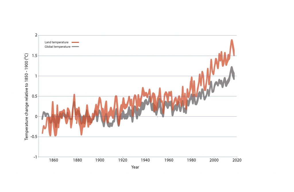
It is certain that globally averaged land surface air temperature (LSAT) has risen faster than the global mean surface temperature (i.e., combined LSAT and sea surface temperature) from the preindustrial period (1850–1900) to the present day (1999–2018). According to the single longest and most extensive dataset, from 1850–1900 to 2006–2015 mean land surface air temperature has increased by 1.53°C (very likely range from 1.38°C to 1.68°C) while global mean surface temperature has increased by 0.87°C (likely range from 0.75°C to 0.99°C). For the 1880–2018 period, when four independently produced datasets exist, the LSAT increase was 1.41°C (1.31–1.51°C), where the range represents the spread in the datasets’ median estimates. Analyses of paleo records, historical observations, model simulations and underlying physical principles are all in agreement that LSATs are increasing at a higher rate than SST as a result of differences in evaporation, land–climate feedbacks and changes in the aerosol forcing over land (very high confidence). For the 2000–2016 period, the land-to-ocean warming ratio (about 1.6) is in close agreement between different observational records and the CMIP5 climate model simulations (the likely range of 1.54–1.81). {2.2.1}

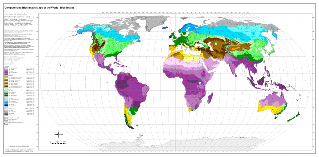
Anthropogenic warming has resulted in shifts of climate zones, primarily as an increase in dry climates and decrease of polar climates (high confidence). Ongoing warming is projected to result in new, hot climates in tropical regions and to shift climate zones poleward in the mid- to high latitudes and upward in regions of higher elevation (high confidence). Ecosystems in these regions will become increasingly exposed to temperature and rainfall extremes beyonwd the climate regimes they are currently adapted to (high confidence), which can alter their structure, composition and functioning. Additionally, high-latitude warming is projected to accelerate permafrost thawing and increase disturbance in boreal forests through abiotic (e.g., drought, fire) and biotic (e.g., pests, disease) agents (high confidence). {2.2.1, 2.2.2, 2.5.3}

Globally, greening trends (trends of increased photosynthetic activity in vegetation) have increased over the last 2–3 decades by 22–33%, particularly over China, India, many parts of Europe, central North America, southeast Brazil and southeast Australia (high confidence). This results from a combination of direct (i.e., land use and management, forest conservation and expansion) and indirect factors (i.e., CO2 fertilisation, extended growing season, global warming, nitrogen deposition, increase of diffuse radiation) linked to human activities (high confidence). Browning trends (trends of decreasing photosynthetic activity) are projected in many regions where increases in drought and heatwaves are projected in a warmer climate. There is low confidence in the projections of global greening and browning trends. {2.2.4, Cross- Chapter Box 4 in this chapter}

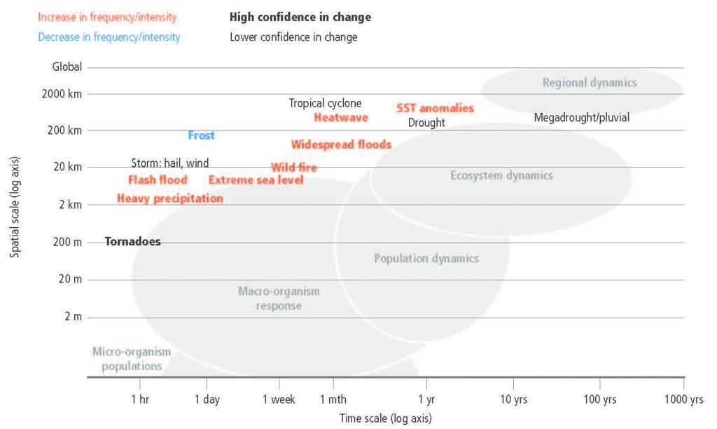
The frequency and intensity of some extreme weather and climate events have increased as a consequence of global warming and will continue to increase under medium and high emission scenarios (high confidence). Recent heat-related events, for example, heatwaves, have been made more frequent or intense due to anthropogenic greenhouse gas (GHG) emissions in most land regions and the frequency and intensity of drought has increased in Amazonia, north-eastern Brazil, the Mediterranean, Patagonia, most of Africa and north-eastern China (medium confidence). Heatwaves are projected to increase in frequency, intensity and duration in most parts of the world (high confidence) and drought frequency and intensity is projected to increase in some regions that are already drought prone, predominantly in the Mediterranean, central Europe, the southern Amazon and southern Africa (medium confidence). These changes will impact ecosystems, food security and land processes including GHG fluxes (high confidence). {2.2.5}

Climate change is playing an increasing role in determining wildfire regimes alongside human activity (medium confidence), with future climate variability expected to enhance the risk and severity of wildfires in many biomes such as tropical rainforests (high confidence). Fire weather seasons have lengthened globally between 1979 and 2013 (low confidence). Global land area burned has declined in recent decades, mainly due to less burning in grasslands and savannahs (high confidence). While drought remains the dominant driver of fire emissions, there has recently been increased fire activity in some tropical and temperate regions during normal to wetter than average years due to warmer temperatures that increase vegetation flammability (medium confidence). The boreal zone is also experiencing larger and more frequent fires, and this may increase under a warmer climate (medium confidence). {Cross-Chapter Box 4 in this chapter}

Terrestrial greenhouse gas fluxes on unmanaged and managed lands

Agriculture, forestry and other land use (AFOLU) is a significant net source of GHG emissions (high confidence), contributing to about 23% of anthropogenic emissions of carbon dioxide (CO2), methane (CH4) and nitrous oxide (N2O) combined as CO2 equivalents in 2007–2016 (medium confidence). AFOLU results in both emissions and removals of CO2, CH4 and N2O to and from the atmosphere (high confidence). These fluxes are affected simultaneously by natural and human drivers, making it difficult to separate natural from anthropogenic fluxes (very high confidence). {2.3}

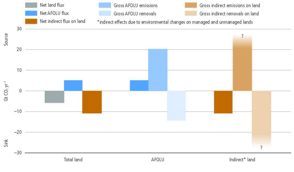
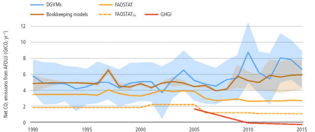
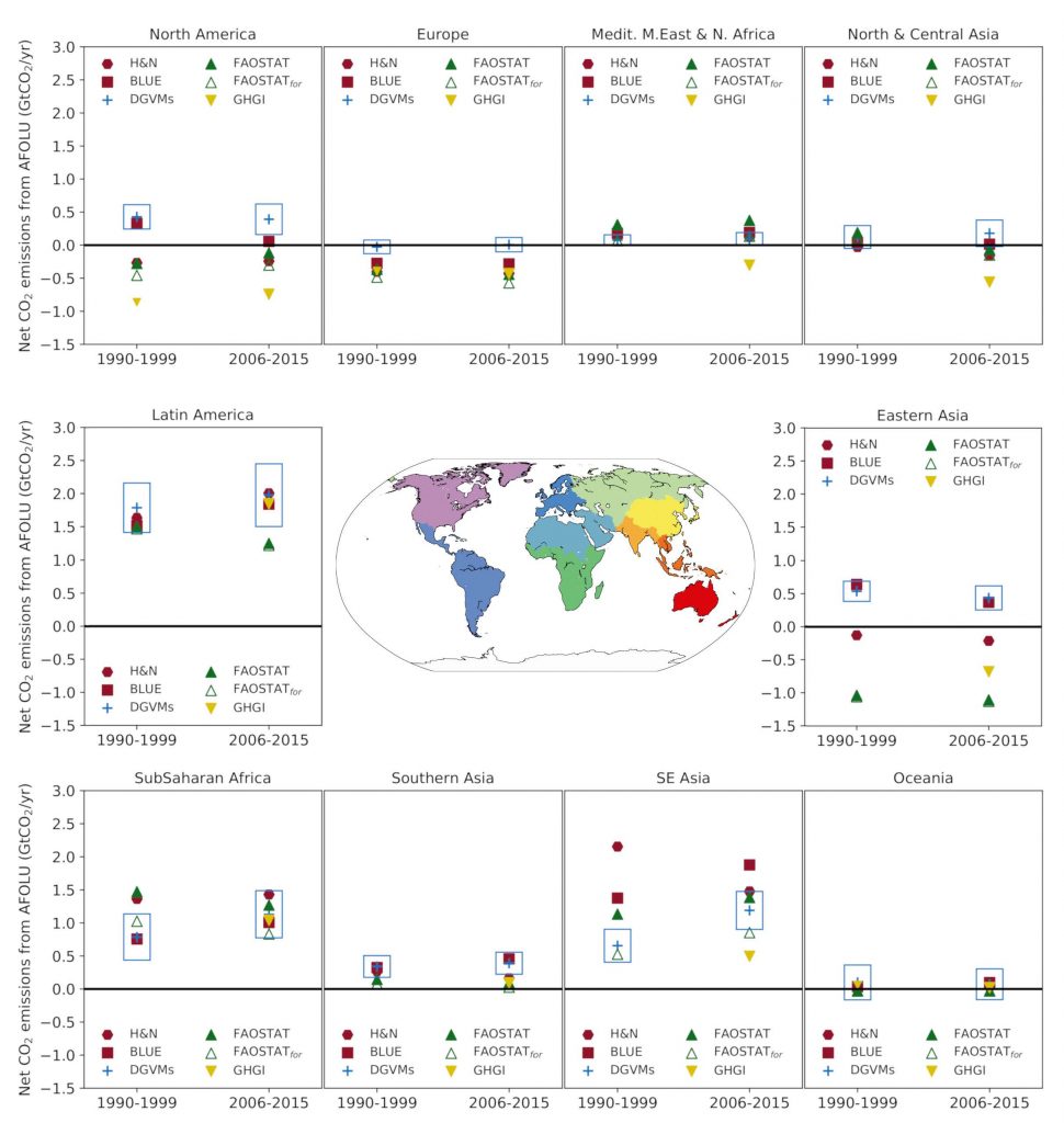
The total net land-atmosphere flux of CO2 on both managed and unmanaged lands very likely provided a global net removal from 2007 to 2016 according to models (-6.0 ± 3.7 CO2 yr–1,  likely range). This net removal is comprised of two major components: (i) modelled net anthropogenic emissions from AFOLU are 5.2 ± 2.6 GtCO2 yr–1 (likely range) driven by land cover change, including deforestation and afforestation/reforestation, and wood harvesting (accounting for about 13% of total net anthropogenic emissions of CO2) (medium confidence), and (ii) modelled net removals due to non-anthropogenic processes are 11.2 ± 2.6 GtCO2 yr–1 (likely range) on managed and unmanaged lands, driven by environmental changes such as increasing CO2, nitrogen deposition and changes in climate (accounting for a removal of 29% of the CO2 emitted from all anthropogenic activities (fossil fuel, industry and AFOLU) (medium confidence). {2.3.1}

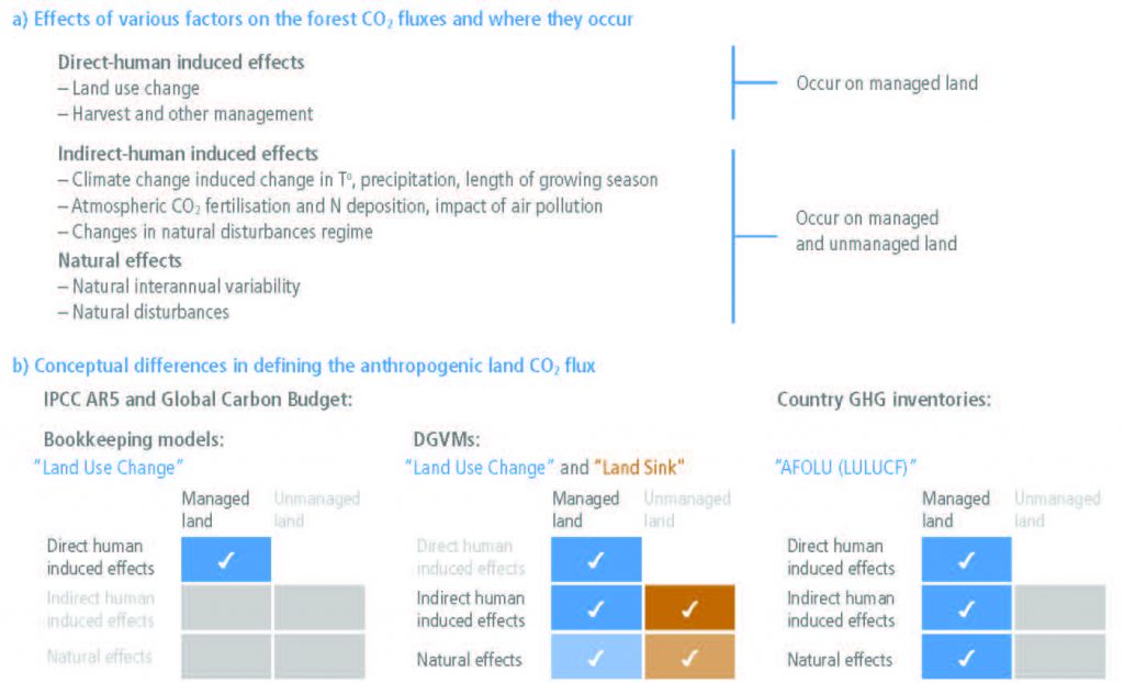
Global models and national GHG inventories use different methods to estimate anthropogenic CO2 emissions and removals for the land sector. Consideration of differences in methods can enhance understanding of land sector net emission such as under the Paris Agreement’s global stocktake (medium confidence). Both models and inventories produce estimates that are in close agreement for land-use change involving forest (e.g., deforestation, afforestation), and differ for managed forest. Global models consider as managed forest those lands that were subject to harvest whereas, consistent with IPCC guidelines, national GHG inventories define managed forest more broadly. On this larger area, inventories can also consider the natural response of land to human-induced environmental changes as anthropogenic, while the global model approach {Table SPM.1} treats this response as part of the non-anthropogenic sink. For illustration, from 2005 to 2014, the sum of the national GHG inventories net emission estimates is 0.1 ± 1.0 GtCO2 yr–1, while the mean of two global bookkeeping models is 5.1 ± 2.6 GtCO2 yr–1 (likely range).

The gross emissions from AFOLU (one-third of total global emissions) are more indicative of mitigation potential of reduced deforestation than the global net emissions (13% of total global emissions), which include compensating deforestation and afforestation fluxes (high confidence). The net flux of CO2 from AFOLU is composed of two opposing gross fluxes: (i) gross emissions (20 GtCO2 yr–1) from deforestation, cultivation of soils and oxidation of wood products, and (ii) gross removals (–14 GtCO2 yr–1), largely from forest growth following wood harvest and agricultural abandonment (medium confidence). {2.3.1}

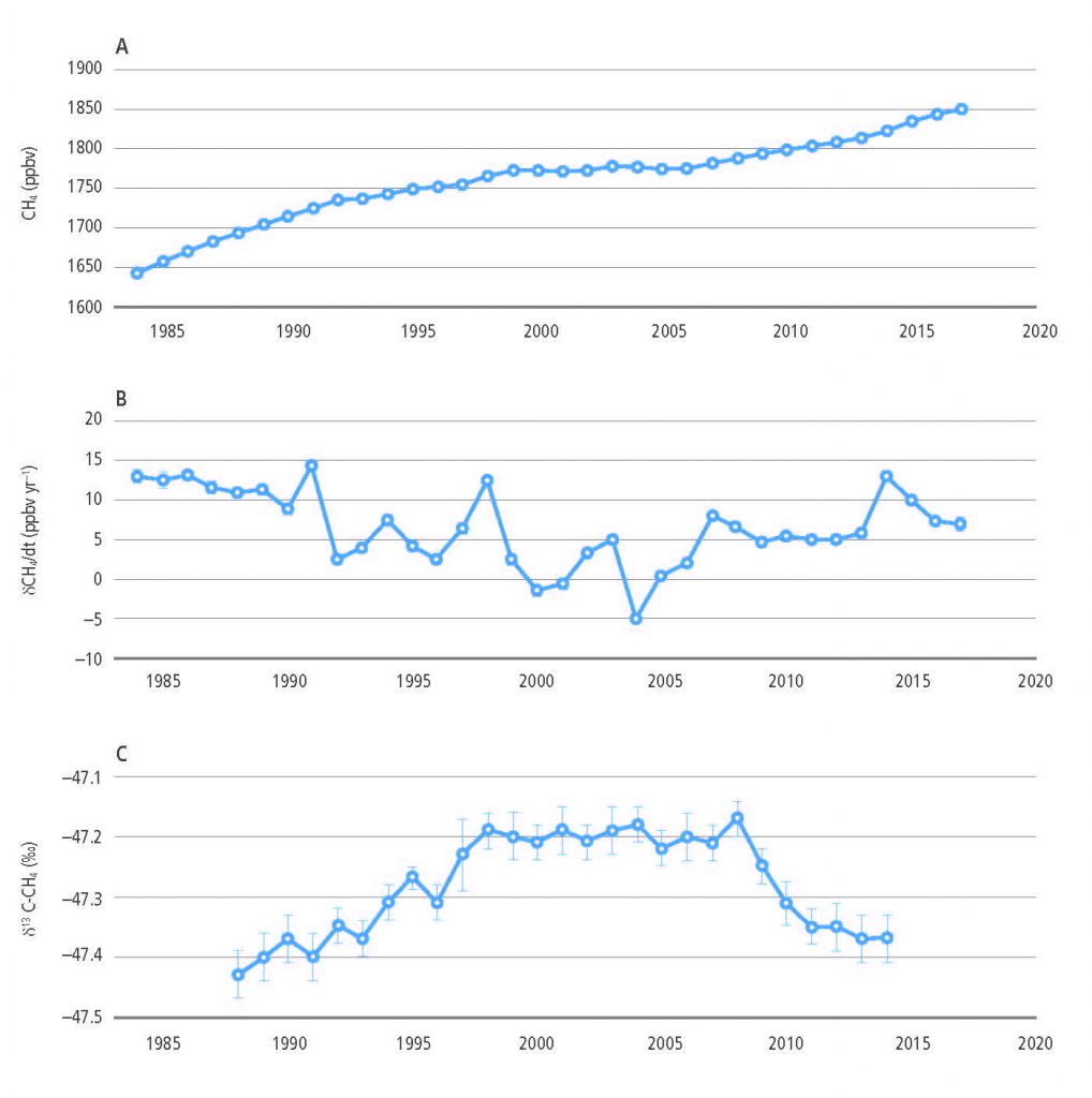
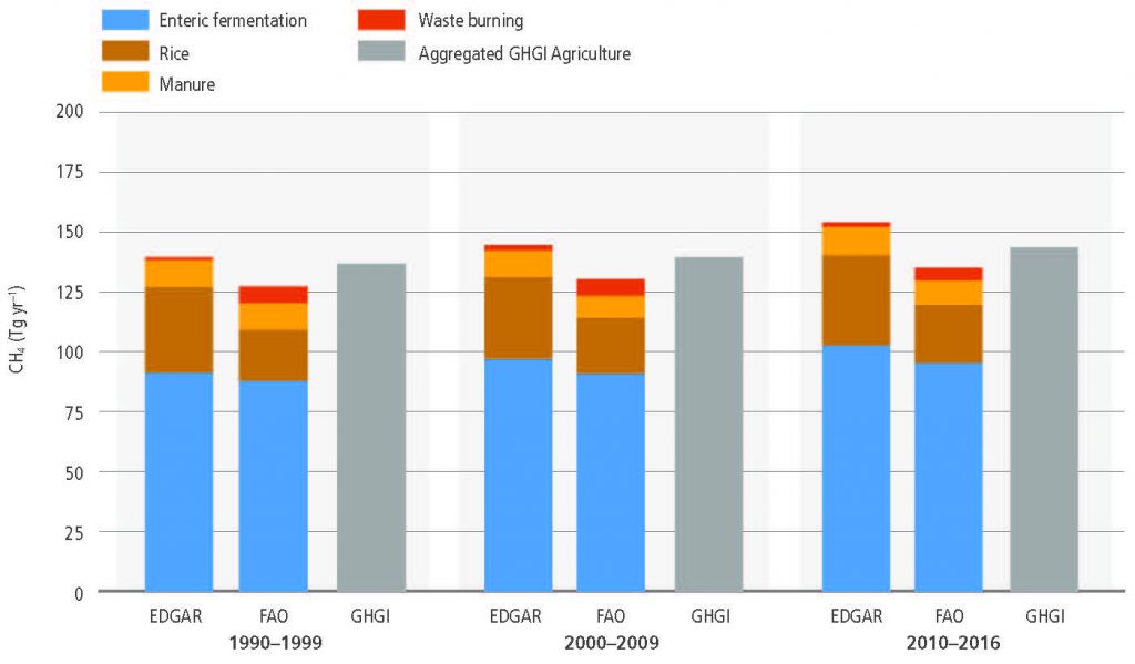
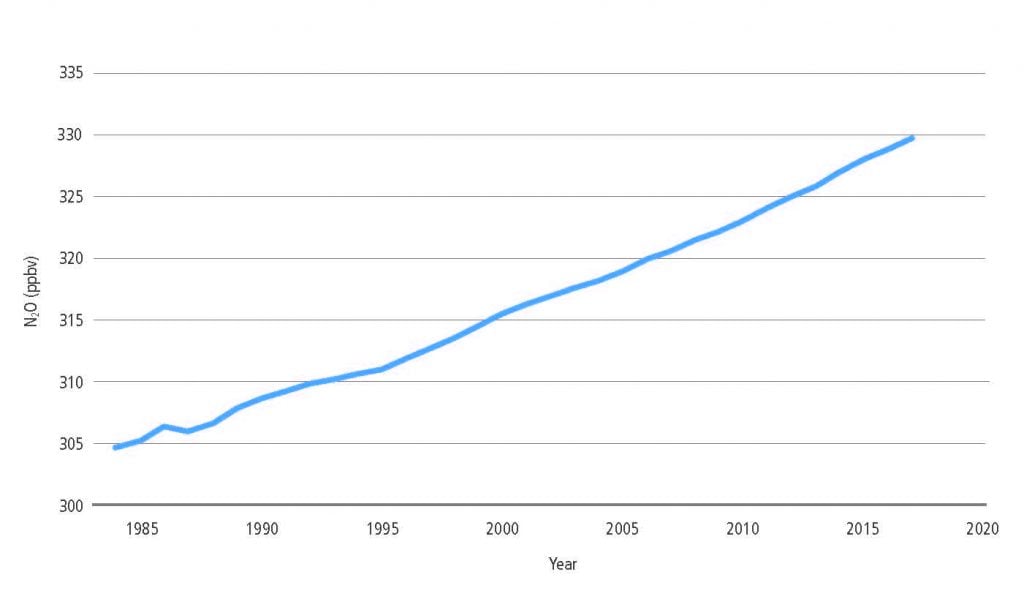
Land is a net source of CH4, accounting for 44% of anthropogenic CH4 emissions for the 2006–2017 period (medium confidence). The pause in the rise of atmospheric CH4 concentrations between 2000 and 2006 and the subsequent renewed increase appear to be partially associated with land use and land use change. The recent depletion trend of the 13C isotope in the atmosphere indicates that higher biogenic sources explain part of the current CH4 increase and that biogenic sources make up a larger proportion of the source mix than they did before 2000 (high confidence). In agreement with the findings of AR5, tropical wetlands and peatlands continue to be important drivers of inter- annual variability and current CH4 concentration increases (medium evidence, high agreement). Ruminants and the expansion of rice cultivation are also important contributors to the current trend (medium evidence, high agreement). There is significant and ongoing accumulation of CH4 in the atmosphere (very high confidence). {2.3.2}

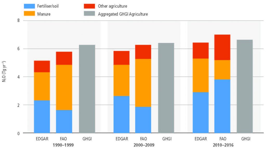
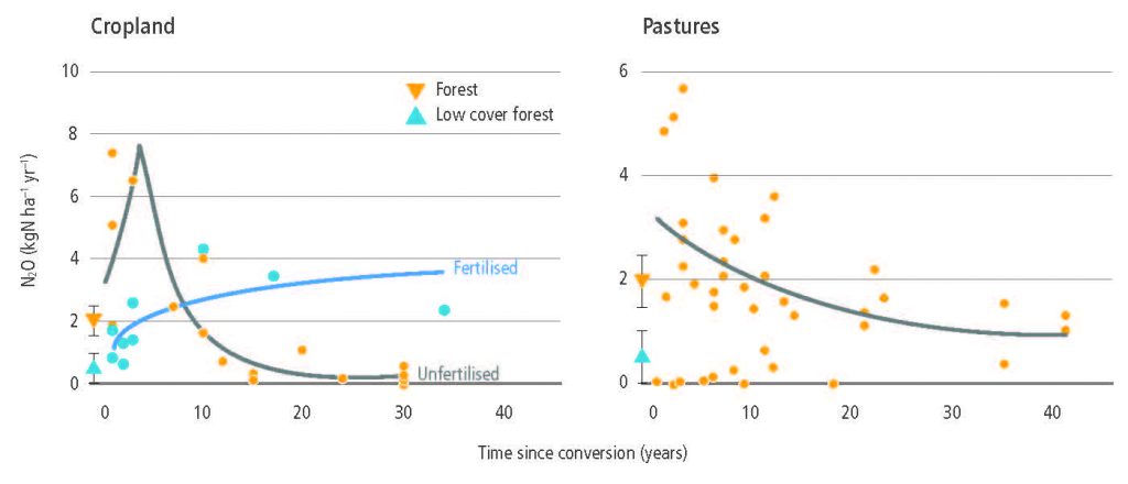
AFOLU is the main anthropogenic source of N2O primarily due to nitrogen application to soils (high confidence). In croplands, the main driver of N2O emissions is a lack of synchronisation between crop nitrogen demand and soil nitrogen supply, with approximately 50% of the nitrogen applied to agricultural land not taken up by the crop. Cropland soils emit over 3 MtN2O-N yr–1 (medium confidence). Because the response of N2O emissions to fertiliser application rates is non-linear, in regions of the world where low nitrogen application rates dominate, such as sub-Saharan Africa and parts of Eastern Europe, increases in nitrogen fertiliser use would generate relatively small increases in agricultural N2O emissions. Decreases in application rates in regions where application rates are high and exceed crop demand for parts of the growing season will have very large effects on emissions reductions (medium evidence, high agreement). {2.3.3}

While managed pastures make up only one-quarter of grazing lands, they contributed more than three-quarters of N2O emissions from grazing lands between 1961 and 2014 with rapid recent increases of nitrogen inputs resulting in disproportionate growth in emissions from these lands (medium confidence). Grazing lands (pastures and rangelands) are responsible for more than one-third of total anthropogenic N2O emissions or more than one-half of agricultural emissions (high confidence). Emissions are largely from North America, Europe, East Asia, and South Asia, but hotspots are shifting from Europe to southern Asia (medium confidence). {2.3.3}

Increased emissions from vegetation and soils due to climate change in the future are expected to counteract potential sinks due to CO2 fertilisation (low confidence). Responses of vegetation and soil organic carbon (SOC) to rising atmospheric CO2 concentration and climate change are not well constrained by observations (medium confidence). Nutrient (e.g., nitrogen, phosphorus) availability can limit future plant growth and carbon storage under rising CO2 (high confidence). However, new evidence suggests that ecosystem adaptation through plant-microbe symbioses could alleviate some nitrogen limitation (medium evidence, high agreement). Warming of soils and increased litter inputs will accelerate carbon losses through microbial respiration (high confidence). Thawing of high latitude/altitude permafrost will increase rates of SOC loss and change the balance between CO2 and CH4 emissions(medium confidence).Thebalancebetweenincreased respiration in warmer climates and carbon uptake from enhanced plant growth is a key uncertainty for the size of the future land carbon sink (medium confidence). {2.3.1, 2.7.2, Box 2.3}

Biophysical and biogeochemical land forcing and feedbacks to the climate system

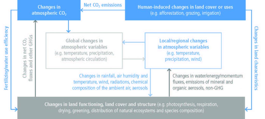
Changes in land conditions from human use or climate change in turn affect regional and global climate (high confidence). On the global scale, this is driven by changes in emissions or removals of CO2, CH4 and N2O by land (biogeochemical effects) and by changes in the surface albedo (very high confidence). Any local land changes that redistribute energy and water vapour between the land and the atmosphere influence regional climate (biophysical effects; high confidence). However, there is no confidence in whether such biophysical effects influence global climate. {2.1, 2.3, 2.5.1, 2.5.2}

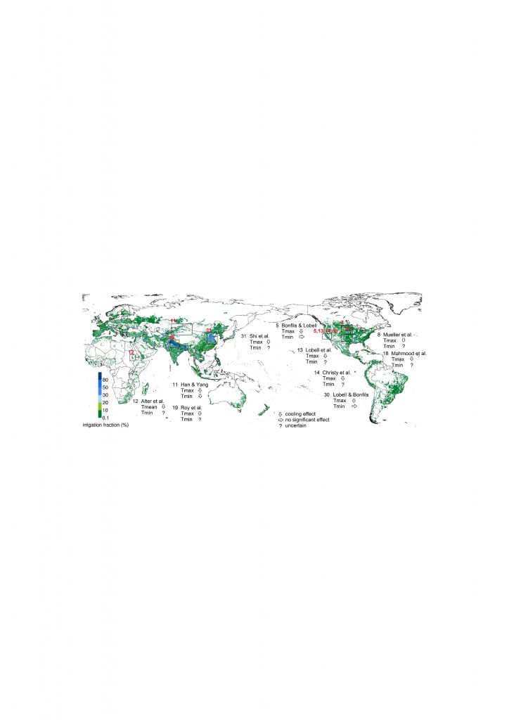
Changes in land conditions modulate the likelihood, intensity and duration of many extreme events including heatwaves (high confidence) and heavy precipitation events (medium confidence). Dry soil conditions favour or strengthen summer heatwave conditions through reduced evapotranspiration and increased sensible heat. By contrast wet soil conditions, for example from irrigation or crop management practices that maintain a cover crop all year round, can dampen extreme warm events through increased evapotranspiration and reduced sensible heat. Droughts can be intensified by poor land management. Urbanisation increases extreme rainfall events over or downwind of cities (medium confidence). {2.5.1, 2.5.2, 2.5.3}

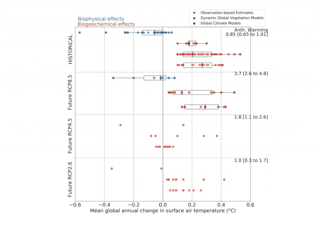
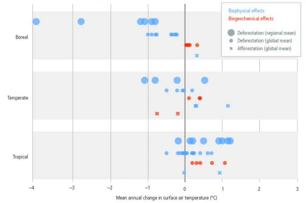
Historical changes in anthropogenic land cover have resulted in a mean annual global warming of surface air from biogeochemical effects (very high confidence), dampened by a cooling from biophysical effects (medium confidence). Biogeochemical warming results from increased emissions of GHGs by land, with model-based estimates of +0.20 ± 0.05°C (global climate models) and +0.24 ± 0.12°C – dynamic global vegetation models (DGVMs) as well as an observation-based estimate of +0.25 ± 0.10°C. A net biophysical cooling of –0.10 ± 0.14°C has been derived from global climate models in response to the increased surface albedo and decreased turbulent heat fluxes, but it is smaller than the warming effect from land-based emissions. However, when both biogeochemical and biophysical effects are accounted for within the same global climate model, the models do not agree on the sign of the net change in mean annual surface air temperature. {2.3, 2.5.1, Box 2.1}

The future projected changes in anthropogenic land cover that have been examined for AR5 would result in a biogeochemical warming and a biophysical cooling whose magnitudes depend on the scenario (high confidence). Biogeochemical warming has been projected for RCP8.5 by both global climate models (+0.20 ± 0.15°C) and DGVMs (+0.28 ± 0.11°C) (high confidence). A global biophysical cooling of 0.10 ± 0.14°C is estimated from global climate models and is projected to dampen the land-based warming (low confidence). For RCP4.5, the biogeochemical warming estimated from global climate models (+0.12 ± 0.17°C) is stronger than the warming estimated by DGVMs (+0.01 ± 0.04°C) but based on limited evidence, as is the biophysical cooling (–0.10 ± 0.21°C). {2.5.2}

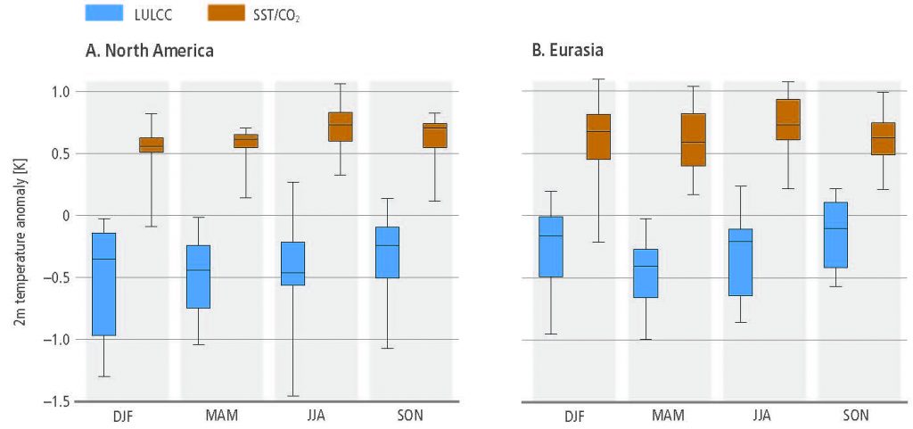
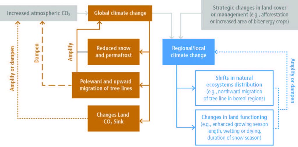
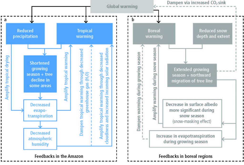
Regional climate change can be dampened or enhanced by changes in local land cover and land use (high confidence) but this depends on the location and the season (high confidence). In boreal regions, for example, where projected climate change will migrate the treeline northward, increase the growing season length and thaw permafrost, regional winter warming will be enhanced by decreased surface albedo and snow, whereas warming will be dampened during the growing season due to larger evapotranspiration (high confidence). In the tropics, wherever climate change will increase rainfall, vegetation growth and associated increase in evapotranspiration will result in a dampening effect on regional warming (medium confidence). {2.5.2, 2.5.3}

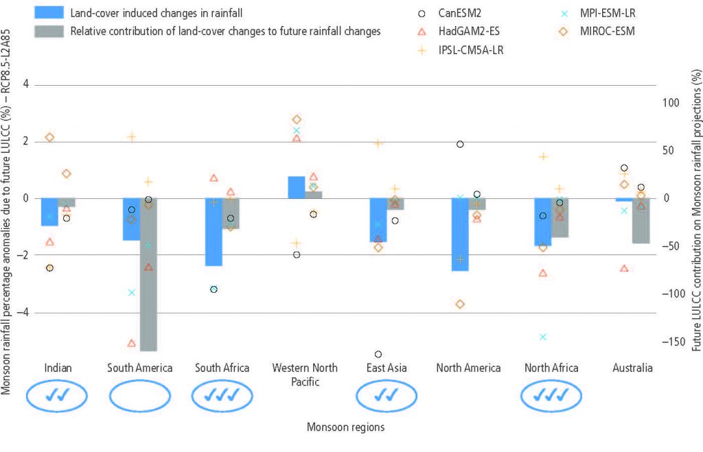
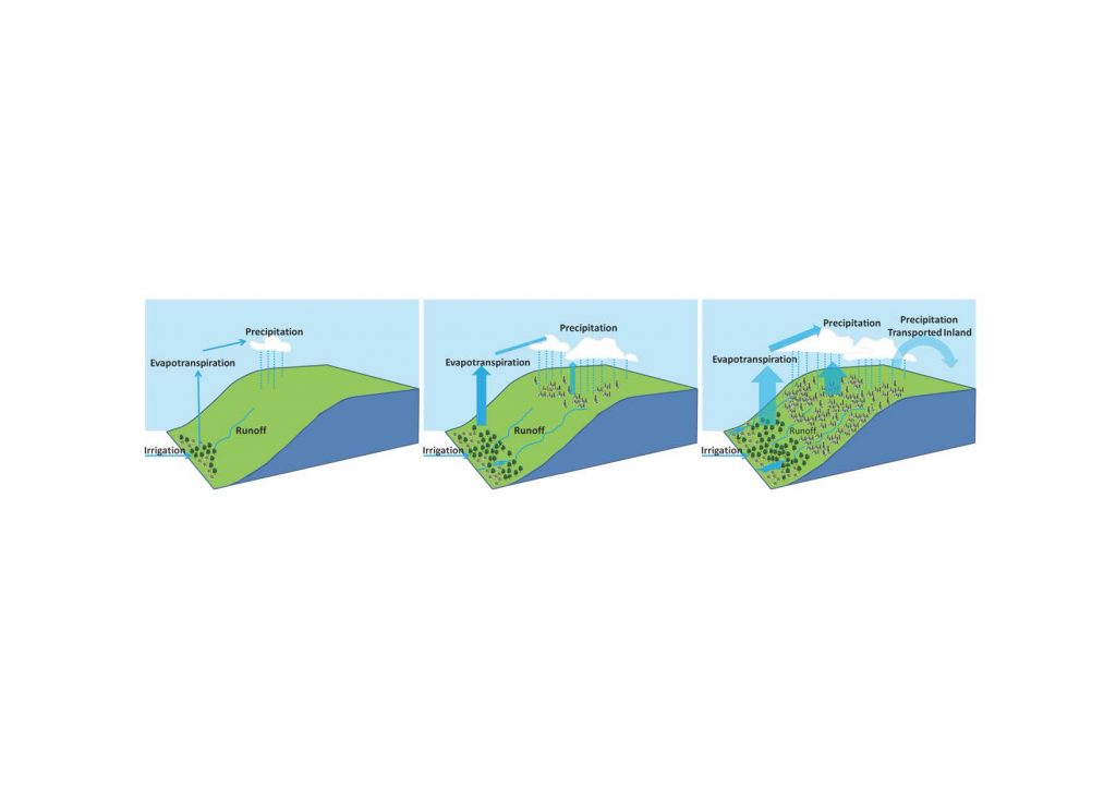
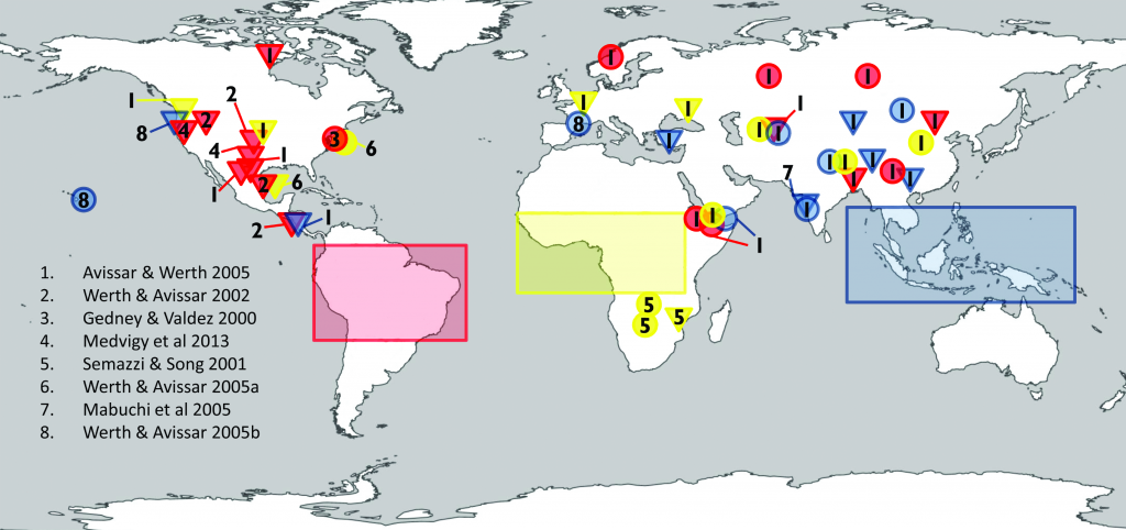
According to model-based studies, changes in local land cover or available water from irrigation will affect climate in regions as far as few hundreds of kilometres downwind (high confidence). The local redistribution of water and energy following the changes on land affect the horizontal and vertical gradients of temperature, pressure and moisture, thus altering regional winds and consequently moisture and temperature advection and convection and subsequently, precipitation. {2.5.2, 2.5.4, Cross-Chapter Box 4}

Future increases in both climate change and urbanisation will enhance warming in cities and their surroundings (urban heat island), especially during heatwaves (high confidence). Urban and peri-urban agriculture, and more generally urban greening, can contribute to mitigation (medium confidence) as well as to adaptation (high confidence), with co-benefits for food security and reduced soil-water-air pollution. {Cross-Chapter Box 4}

Regional climate is strongly affected by natural land aerosols (medium confidence) (e.g., mineral dust, black, brown and organic carbon), but there is low confidence in historical trends, inter-annual and decadal variability and future changes. Forest cover affects climate through emissions of biogenic volatile organic compounds (BVOC) and aerosols (low confidence). The decrease in the emissions of BVOC resulting from the historical conversion of forests to cropland has resulted in a positive radiative forcing through direct and indirect aerosol effects, a negative radiative forcing through the reduction in the atmospheric lifetime of methane and it has contributed to increased ozone concentrations in different regions (low confidence). {2.4, 2.5}

Consequences for the climate system of land-based adaptation and mitigation options, including carbon dioxide removal (negative emissions)

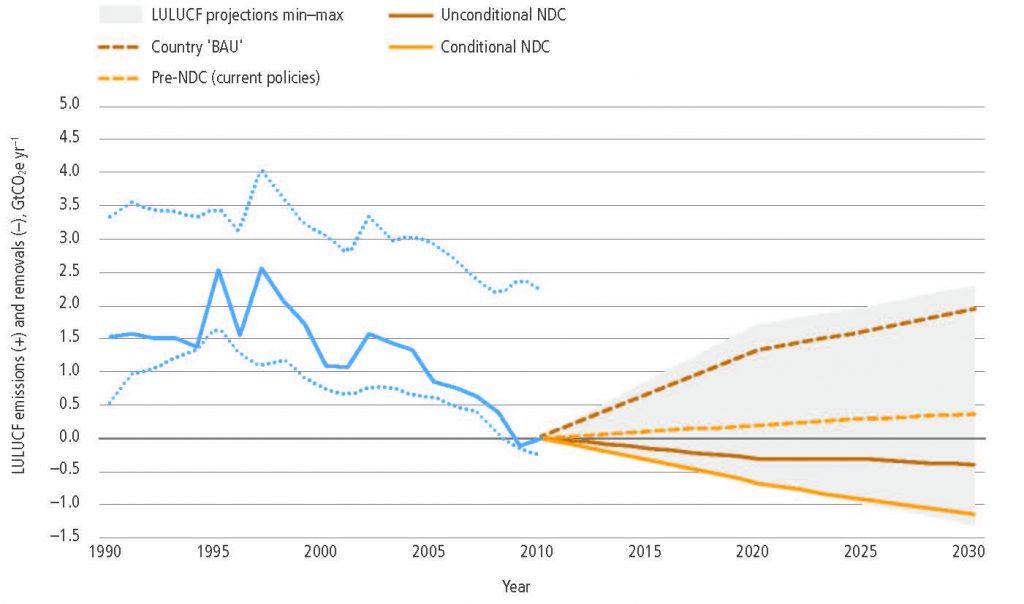
About one-quarter of the 2030 mitigation pledged by countries in their initial nationally determined contributions (NDCs) under the Paris Agreement is expected to come from land- based mitigation options (medium confidence). Most of the NDCs submitted by countries include land-based mitigation, although many lack details. Several refer explicitly to reduced deforestation and forest sinks, while a few include soil carbon sequestration, agricultural management and bioenergy. Full implementation of NDCs (submitted by February 2016) is expected to result in net removals of 0.4–1.3 GtCO2 yr–1 in 2030 compared to the net flux in 2010, where the range represents low to high mitigation ambition in pledges, not uncertainty in estimates (medium confidence). {2.6.3}

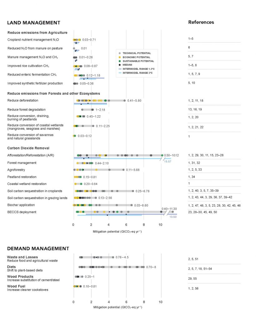
Several mitigation response options have technical potential for >3 GtCO2-eq yr–1 by 2050 through reduced emissions and Carbon Dioxide Removal (CDR) (high confidence), some of which compete for land and other resources, while others may reduce the demand for land (high confidence). Estimates of the technical potential of individual response options are not necessarily additive. The largest potential for reducing AFOLU emissions are through reduced deforestation and forest degradation (0.4–5.8 GtCO2-eq yr–1) (high confidence), a shift towards plant- based diets (0.7–8.0 GtCO2-eq yr–1) (high confidence) and reduced food and agricultural waste (0.8–4.5 GtCO2-eq yr–1) (high confidence). Agriculture measures combined could mitigate 0.3–3.4 GtCO2-eq yr–1 (medium confidence). The options with largest potential for CDR are afforestation/reforestation (0.5–10.1 GtCO2-eq yr–1) (medium confidence), soil carbon sequestration in croplands and grasslands (0.4–8.6 GtCO2-eq yr–1) (high confidence) and Bioenergy with Carbon Capture and Storage (BECCS) (0.4–11.3 GtCO2-eq yr–1) (medium confidence). While some estimates include sustainability and cost considerations, most do not include socio-economic barriers, the impacts of future climate change or non-GHG climate forcings. {2.6.1}

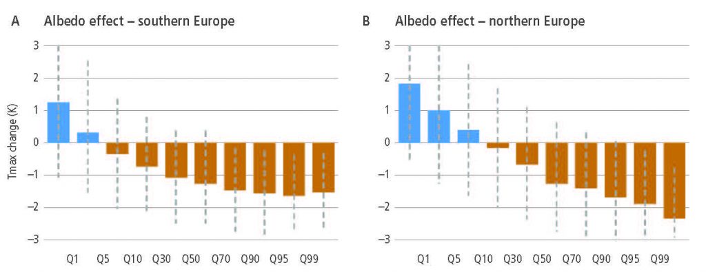
Response options intended to mitigate global warming will also affect the climate locally and regionally through biophysical effects (high confidence). Expansion of forest area, for example, typically removes CO2 from the atmosphere and thus dampens global warming (biogeochemical effect, high confidence), but the biophysical effects can dampen or enhance regional warming depending on location, season and time of day. During the growing season, afforestation generally brings cooler days from increased evapotranspiration, and warmer nights (high confidence). During the dormant season, forests are warmer than any other land cover, especially in snow-covered areas where forest cover reduces albedo (high confidence). At the global level, the temperature effects of boreal afforestation/reforestation run counter to GHG effects, while in the tropics they enhance GHG effects. In addition, trees locally dampen the amplitude of heat extremes (medium confidence). {2.5.2, 2.5.4, 2.7, Cross-Chapter Box 4}

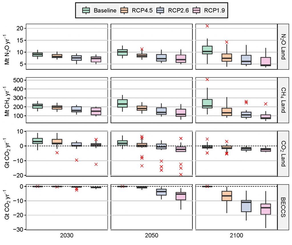
Mitigation response options related to land use are a key element of most modelled scenarios that provide strong mitigation, alongside emissions reduction in other sectors (high confidence). More stringent climate targets rely more heavily on land-based mitigation options, in particular, CDR (high confidence). Across a range of scenarios in 2100, CDR is delivered by both afforestation (median values of –1.3, –1.7 and –2.4 GtCO2 yr–1 for scenarios RCP4.5, RCP2.6 and RCP1.9 respectively) and bioenergy with carbon capture and storage (BECCS) (–6.5, –11 and –14.9 GtCO2 yr–1 respectively). Emissions of CH4 and N2O are reduced through improved agricultural and livestock management as well as dietary shifts away from emission-intensive livestock products by 133.2, 108.4 and 73.5 MtCH4 yr–1; and 7.4, 6.1 and 4.5 MtN2O yr–1 for the same set of scenarios in 2100 (high confidence). High levels of bioenergy crop production can result in increased N2O emissions due to fertiliser use. The Integrated Assessment Models that produce these scenarios mostly neglect the biophysical effects of land-use on global and regional warming. {2.5, 2.6.2}

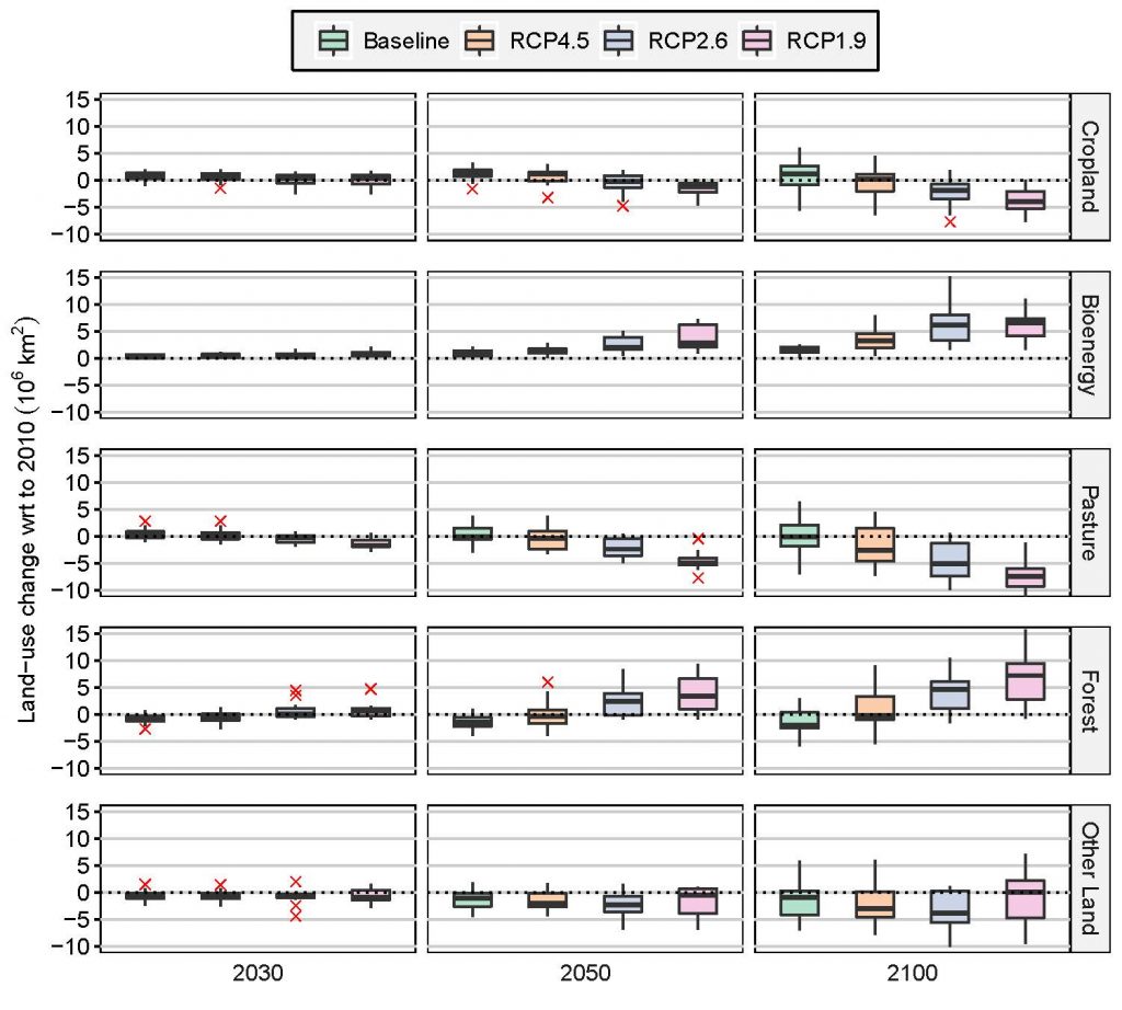
Large-scale implementation of mitigation response options that limit warming to 1.5°C or 2°C would require conversion of large areas of land for afforestation/reforestation and bioenergy crops, which could lead to short-term carbon losses (high confidence). The change of global forest area in mitigation pathways ranges from about –0.2 to +7.2 Mkm2 between 2010 and 2100 (median values across a range of models and scenarios: RCP4.5, RCP2.6, RCP1.9), and the land demand for bioenergy crops ranges from about 3.2 to 6.6 Mkm2 in 2100 (high confidence). Large- scale land-based CDR is associated with multiple feasibility and sustainability constraints (Chapters 6 and 7). In high carbon lands such as forests and peatlands, the carbon benefits of land protection are greater in the short-term than converting land to bioenergy crops for BECCS, which can take several harvest cycles to ‘pay-back’ the carbon emitted during conversion (carbon-debt), from decades to over a century (medium confidence). {2.6.2, Chapters 6, 7}

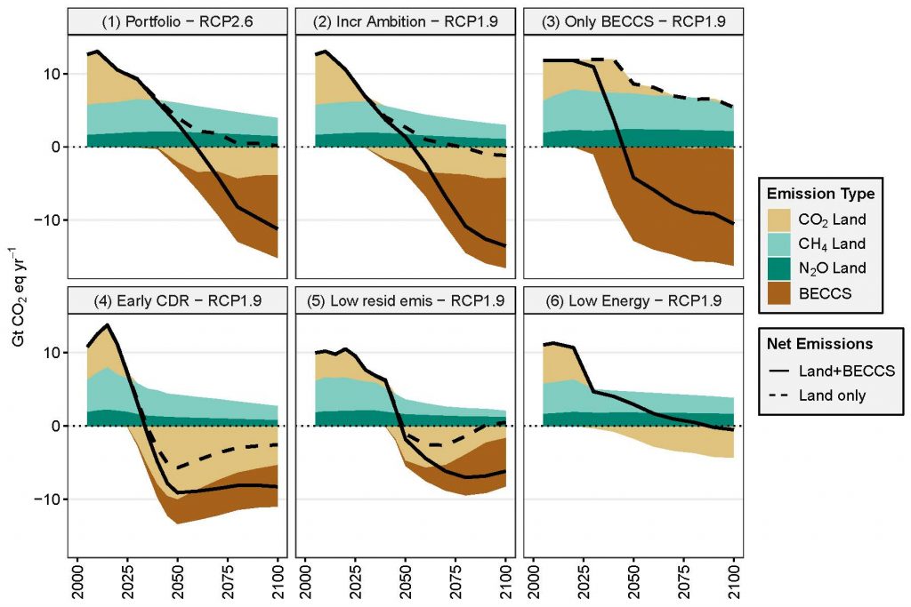
It is possible to achieve climate change targets with low need for land-demanding CDR such as BECCS, but such scenarios rely more on rapidly reduced emissions or CDR from forests, agriculture and other sectors. Terrestrial CDR has the technical potential to balance emissions that are difficult to eliminate with current technologies (including food production). Scenarios that achieve climate change targets with less need for terrestrial CDR rely on agricultural demand-side changes (diet change, waste reduction), and changes in agricultural production such as agricultural intensification. Such pathways that minimise land use for bioenergy and BECCS are characterised by rapid and early reduction of GHG emissions in all sectors, as well as earlier CDR in through afforestation. In contrast, delayed mitigation action would increase reliance on land-based CDR (high confidence). {2.6.2}

2.1

Introduction: Land–climate interactions

This chapter assesses the literature on two-way interactions between climate and land, with focus on scientific findings published since AR5 and some aspects of the land–climate interactions that were not assessed in previous IPCC reports. Previous IPCC assessments recognised that climate affects land cover and land surface processes, which in turn affect climate. However, previous assessments mostly focused on the contribution of land to global climate change via its role in emitting and absorbing greenhouse gases (GHGs) and short-lived climate forcers (SLCFs), or via implications of changes in surface reflective properties (i.e., albedo) for solar radiation absorbed by the surface. This chapter examines scientific advances in understanding the interactive changes of climate and land, including impacts of climate change, variability and extremes on managed and unmanaged lands. It assesses climate forcing of land changes from direct (e.g., land use change and land management) and indirect (e.g., increasing atmospheric CO2 concentration and nitrogen deposition) effects at local, regional and global scales.

2.1.1

Recap of previous IPCC and other relevant reports as baselines

The evidence that land cover matters for the climate system have long been known, especially from early paleoclimate modelling studies and impacts of human-induced deforestation at the margin of deserts (de Noblet et al. 19961; Kageyama et al. 20042). The understanding of how land use activities impact climate has been put forward by the pioneering work of Charney (1975)3 who examined the role of overgrazing-induced desertification on the Sahelian climate.

Since then there have been many modelling studies that reported impacts of idealised or simplified land cover changes on weather patterns (e.g., Pielke et al. 20114). The number of studies dealing with such issues has increased significantly over the past 10 years, with more studies that address realistic past or projected land changes. However, very few studies have addressed the impacts of land cover changes on climate as very few land surface models embedded within climate models (whether global or regional), include a representation of land management. Observation-based evidence of land-induced climate impacts emerged even more recently (e.g., Alkama and Cescatti 20165; Bright et al. 20176; Lee et al. 20117; Li et al. 20158; Duveiller et al. 20189; Forzieri et al. 201710) and the literature is therefore limited.

In previous IPCC reports, the interactions between climate change and land were covered separately by three working groups. AR5 WGI assessed the role of land use change in radiative forcing, land-based GHGs source and sink, and water cycle changes that focused on changes of evapotranspiration, snow and ice, runoff and humidity. AR5 WGII examined impacts of climate change on land, including terrestrial and freshwater ecosystems, managed ecosystems, and cities and settlements. AR5 WGIII assessed land-based climate change mitigation goals and pathways related to the agriculture, forestry and other land use (AFOLU). Here, this chapter assesses land–climate interactions from all three working groups. It also builds on previous special reports such as the Special Report on Global Warming of 1.5°C (SR15). It links to the IPCC Guidelines on National Greenhouse Gas Inventories in the land sector. Importantly, this chapter assesses knowledge that has never been reported in any of those previous reports. Finally, the chapter also tries to reconcile the possible inconsistencies across the various IPCC reports.

Land-based water cycle changes

AR5 reported an increase in global evapotranspiration from the early 1980s to 2000s, but a constraint on further increases from low soil moisture availability. Rising CO2 concentration limits stomatal opening and thus also reduces transpiration, a component of evapotranspiration. Increasing aerosol levels, declining surface wind speeds and declining levels of solar radiation reaching the ground are additional regional causes of the decrease in evapotranspiration.

Land area precipitation change

Averaged over the mid-latitude land areas of the northern hemisphere, precipitation has increased since 1901 (medium confidence before 1951 and high confidence thereafter). For other latitudes, area-averaged long-term positive or negative trends have low confidence. There are likely more land regions where the number of heavy precipitation events has increased than where it has decreased. Extreme precipitation events over most of the mid- latitude land masses and over wet tropical regions will very likely become more intense and more frequent (IPCC 2013a11).

Land-based GHGs

AR5 reported that annual net CO2 emissions from anthropogenic land use change were 0.9 [0.1–1.7] GtC yr–1 on average during 2002–2011 (medium confidence). From 1750–2011, CO2 emissions from fossil fuel combustion have released an estimated 375 [345–405] GtC to the atmosphere, while deforestation and other land use change have released an estimated 180 [100–260] GtC. Of these cumulative anthropogenic CO2 emissions, 240 [230–250] GtC have accumulated in the atmosphere, 155 [125–185] GtC have been taken up by the ocean and 160 [70–250] GtC have accumulated in terrestrial ecosystems (i.e., the cumulative residual land sink) (Ciais et al. 2013a12). Updated assessment and knowledge gaps are covered in Section 2.3.

Future terrestrial carbon source/sink

AR5 projected with high confidence that tropical ecosystems will uptake less carbon and with medium confidence that at high latitudes, land carbon sink will increase in a warmer climate. Thawing permafrost in the high latitudes is potentially a large carbon source in warmer climate conditions, however the magnitude of CO2 and CH4 emissions due to permafrost thawing is still uncertain. The SR15 further indicates that constraining warming to 1.5°C would prevent the melting of an estimated permafrost area of 2 million km2 over the next centuries compared to 2°C. Updates to these assessments are found in Section 2.3.

Land use change altered albedo

AR5 stated with high confidence that anthropogenic land use change has increased the land surface albedo, which has led to a RF of –0.15 ± 0.10 W m–2. However, it also underlined that the sources of the large spread across independent estimates were caused by differences in assumptions for the albedo of natural and managed surfaces and for the fraction of land use change before 1750. Generally, our understanding of albedo changes from land use change has been enhanced from AR4 to AR5, with a narrower range of estimates and a higher confidence level. The radiative forcing from changes in albedo induced by land use changes was estimated in AR5 at–0.15 W m–2 (–0.25 to about –0.05), with medium confidence in AR5 (Myhre et al. 201313). This was an improvement over AR4 in which it was estimated at –0.2 W m–2 (–0.4 to about 0), with low to medium confidence (Forster et al. 200714). Section 2.5 shows that albedo is not the only source of biophysical land-based climate forcing to be considered.

Hydrological feedback to climate

Land use changes also affect surface temperatures through non- radiative processes, and particularly through the hydrological cycle. These processes are less well known and are difficult to quantify but tend to offset the impact of albedo changes. As a consequence, there is low agreement on the sign of the net change in global mean temperature as a result of land use change (Hartmann et al. 2013a15). An updated assessment on these points is covered in Sections 2.5 and 2.2.

Climate-related extremes on land

AR5 reported that impacts from recent climate-related extremes reveal significant vulnerability and exposure of some ecosystems to current climate variability. Impacts of such climate-related extremes include alteration of ecosystems, disruption of food production and water supply, damage to infrastructure and settlements, morbidity and mortality, and consequences for mental health and human well- being (Burkett et al. 201416). The SR15 further indicates that limiting global warming to 1.5°C limits the risks of increases in heavy precipitation events in several regions (high confidence). In urban areas, climate change is projected to increase risks for people, assets, economies and ecosystems (very high confidence). These risks are amplified for those lacking essential infrastructure and services or living in exposed areas. An updated assessment and a knowledge gap for this chapter are covered in Section 2.2 and Cross-Chapter Box 4.

Land-based climate change adaptation and mitigation

AR5 reported that adaptation and mitigation choices in the near- term will affect the risks related to climate change throughout the 21st century (Burkett et al. 201417). AFOLU are responsible for about 10–12 GtCO2eq yr–1 anthropogenic greenhouse gas emissions, mainly from deforestation and agricultural production. Global CO2 emissions from forestry and other land use have declined since AR4, largely due to increased afforestation. The SR15 further indicates that afforestation and bioenergy with carbon capture and storage (BECCS) are important land-based carbon dioxide removal (CDR) options. It also states that land use and land-use change emerge as a critical feature of virtually all mitigation pathways that seek to limit global warming to 1.5oC. The Climate Change 2014 Synthesis Report concluded that co-benefits and adverse side effects of mitigation could affect achievement of other objectives, such as those related to human health, food security, biodiversity, local environmental quality, energy access, livelihoods and equitable sustainable development. Updated assessment and knowledge gaps are covered in Section 2.6 and Chapter 7.

Overall, sustainable land management is largely constrained by climate change and extremes, but also puts bounds on the capacity of land to effectively adapt to climate change and mitigate its impacts. Scientific knowledge has advanced on how to optimise our adaptation and mitigation efforts while coordinating sustainable land management across sectors and stakeholders. Details are assessed in subsequent sections.

2.1.2

Introduction to the chapter structure

This chapter assesses the consequences of changes in land cover and functioning, resulting from both land use and climate change, to global and regional climates. The chapter starts with an assessment of the historical and projected responses of land processes to climate change and extremes (Section 2.2). Subsequently, the chapter assesses historical and future changes in terrestrial GHG fluxes (Section 2.3) as well as non-GHG fluxes and precursors of SLCFs (Section 2.4). Section 2.5 focuses on how historical and future changes in land use and land cover influence climate change/variability through biophysical and biogeochemical forcing and feedbacks, how specific land management affects climate, and how, in turn, climate- induced land changes feed back to climate. Section 2.6 assesses the consequences of land-based adaptation and mitigation options for the climate system in GHG and non-GHG exchanges. Sections 2.3 and 2.6 address implications of the Paris Agreement for land– climate interactions, and the scientific evidence base for ongoing negotiations around the Paris rulebook, the global stocktake and credibility in measuring, reporting and verifying the climate impacts of anthropogenic activities on land. This chapter also examines how land use and management practices may affect climate change through biophysical feedbacks and radiative forcing (Section 2.5), and assesses policy-relevant projected land use changes and sustainable land management for mitigation and adaptation (Section 2.6). Finally, the chapter concludes with a brief assessment of advances in the understanding of the ecological and biogeochemical processes underlying land–climate interactions (Section 2.7).

The chapter includes three chapter boxes providing general overview of (i) processes underlying land–climate interactions (Box 2.1), (ii) methodological approaches for estimating anthropogenic land carbon fluxes from national to global scales (Box 2.2), and (iii) CO2 fertilisation and enhanced terrestrial uptake of carbon (Box 2.3). In addition, this chapter includes two cross-chapter boxes on climate change and fire (Cross-Chapter Box 3), and on urbanisation and climate change (Cross-Chapter Box 4).

In summary, the chapter assesses scientific understanding related to (i) how a changing climate affects terrestrial ecosystems, including those on managed lands, (ii) how land affects climate through biophysical and biogeochemical feedbacks, and (iii) how land use or cover change and land management play an important and complex role in the climate system. This chapter also pays special attention to advances in understanding cross-scale interactions, emerging issues, heterogeneity and teleconnections.

2.2

The effect of climate variability and change on land

2.2.1

Overview of climate impacts on land

2.2.1.1

Climate drivers of land form and function

Energy is redistributed from the warm equator to the colder poles through large-scale atmospheric and oceanic processes driving the Earth’s weather and climate (Oort and Peixóto 198326; Carissimo et al. 198527; Yang et al. 2015a28). Subsequently, a number of global climate zones have been classified ranging from large-scale primary climate zones (tropical, sub-tropical, temperate, sub-polar, polar) to much higher-resolution, regional climate zones (e.g., the Köppen-Geiger classification, Kottek et al. 200629). Biomes are adapted to regional climates (Figure 2.1) and may shift as climate, land surface characteristics (e.g., geomorphology, hydrology), CO2 fertilisation and fire interact. These biomes and the processes therein are subject to modes of natural variability in the ocean-atmosphere system that result in regionally wetter/dryer or hotter/cooler periods having temporal scales from weeks to months (e.g., Southern Annular Mode), months to seasons (e.g., Madden-Julian Oscillation), years (e.g., El Niño Southern Oscillation) and decades (e.g., Pacific Decadal Oscillation). Furthermore, climate and weather extremes (such as drought, heatwaves, very heavy rainfall, strong winds), whose frequency, intensity and duration are often a function of large-scale modes of variability, impact ecosystems at various space and timescales.

It is very likely that changes to natural climate variability as a result of global warming has and will continue to impact terrestrial ecosystems with subsequent impacts on land processes (Hulme et al. 199930; Parmesan and Yohe 200331; Di Lorenzo et al. 200832; Kløve et al. 201433; Berg et al. 201534; Lemordant et al. 201635; Pecl et al. 201736). This chapter assesses climate variability and change, particularly extreme weather and climate, in the context of desertification, land degradation, food security and terrestrial ecosystems more generally. This section does specifically assess the impacts of climate variability and climate change on desertification, land degradation and food security as these impacts are assessed respectively in Chapters 3, 4 and 5. This chapter begins with an assessment of observed warming on land.

Figure 2.1

Worldwide Bioclimatic Classification System, 1996–2018.Source: Rivas-Martinez et al. (2011). Online at www.globalbioclimatics.org

Worldwide Bioclimatic Classification System, 1996–2018.Source: Rivas-Martinez et al. (2011). Online at www.globalbioclimatics.org

2.2.1.2

Changes in global land surface air temperature

Based on analysis of several global and regional land surface air temperature (LSAT) datasets, AR5 concluded that the global LSAT had increased over the instrumental period of record, with the warming rate approximately double that reported over the oceans since 1979 and that ‘it is certain that globally averaged LSAT has risen since the late 19th century and that this warming has been particularly marked since the 1970s’. Warming found in the global land datasets is also in a broad agreement with station observations (Hartmann et al. 2013a37).

Since AR5, LSAT datasets have been improved and extended. The National Center for Environmental Information, which is a part of the US National Oceanic and Atmospheric Administration (NOAA), developed a new, fourth version of the Global Historical Climatology Network monthly dataset (GHCNm, v4). The dataset provides an expanded set of station temperature records with more than 25,000 total monthly temperature stations compared to 7200 in versions v2 and v3 (Menne et al. 201838). Goddard Institute for Space Studies, which is a part of the US National Aeronautics and Space Administration, (NASA/ GISS), provides estimate of land and ocean temperature anomalies (GISTEMP). The GISTEMP land temperature anomalies are based upon primarily NOAA/GHCN version 3 dataset (Lawrimore et al. 201139) and account for urban effects through nightlight adjustments (Hansen et al. 201040). The Climatic Research Unit (CRU) of the University of East Anglia, UK (CRUTEM) dataset, now version CRUTEM4.6,

incorporates additional stations (Jones et al. 201241). Finally, the Berkeley Earth Surface Temperature (BEST) dataset provides LSAT from 1750 to present based on almost 46,000 time series and has the longest temporal coverage of the four datasets (Rohde et al. 201342). This dataset was derived with methods distinct from those used for development of the NOAA GHCNm, NASA/GISS GISTEMP and the University of East Anglia CRUTEM datasets.

Table 2.1

Increases in land surface air temperature (LSAT) from preindustrial period and the late 19th century to present day.

Dataset of LSAT increase (°C)

Time period

BEST

CRUTEM4.6

GHCNm, v4

GISTEMP

From 1850–1900 to 2006–2015

1.53
1.38–1.68
(95% confidence)

1.32*

From 1850–1900 to 1999–2018

1.52
1.39–1.66
(95% confidence)

1.31

NA

NA

From 1881–1900 to 1999–2018

1.51
1.40–1.63
(95% confidence)

1.31

1.37

1.45

According to the available observations in the four datasets, the globally averaged LSAT increased by 1.44°C from the preindustrial period (1850–1900) to the present day (1999–2018).The warming from the late 19th century (1881–1900) to the present day (1999–2018) was 1.41°C (1.31°C–1.51°C) (Table 2.1). The 1.31°C–1.51°C range represents the spread in median estimates from the four available land datasets and does not reflect uncertainty in data coverage or methods used. Based on the BEST dataset (the longest dataset with the most extensive land coverage) the total observed increase in LSAT between the average of the 1850–1900 period and the 2006– 2015 period was 1.53°C, (1.38–1.68°C; 95% confidence), while the GMST increase for the same period was 0.87°C (0.75–0.99°C; 90% confidence) (IPCC, 2018: Summary for policymakers, Allen et al. 201843).

The extended and improved land datasets reaffirmed the AR5 conclusion that it is certain that globally averaged LSAT has risen since the preindustrial period and that this warming has been particularly marked since the 1970s (Figure 2.2).

Recent analyses of LSAT and sea surface temperature (SST) observations, as well as analyses of climate model simulations, have refined our understanding of underlying mechanisms responsible for a faster rate of warming over land than over oceans. Analyses of paleo records, historical observations, model simulations and underlying physical principles are all in agreement that the land is warming faster than the oceans as a result of differences in evaporation, land–climate feedbacks (Section 2.5) and changes in the aerosol forcing over land (very high confidence) (Braconnot et al. 201244; Joshi et al. 201345; Sejas et al. 201446; Byrne and O’Gorman 201347, 201548; Wallace and Joshi 201849; Allen et al. 201950). There is also high confidence that difference in land and ocean heat capacity is not the primary reason for faster land than ocean warming. For the recent period, the land-to-ocean warming ratio is in close agreement between different observational records (about 1.6) and the CMIP5 climate model simulations (the likely range of 1.54°C to 1.81°C). Earlier studies analysing slab ocean models (models in which it is assumed that the deep ocean has equilibrated) produced a higher land temperature increases than sea surface temperature (Manabe et al. 199151; Sutton et al. 200752).

It is certain that globally averaged LSAT has risen faster than GMST from the preindustrial period (1850–1900) to the present day (1999–2018). This is because the warming rate of the land compared to the ocean is substantially higher over the historical period (by approximately 60%) and because the Earth’s surface is approximately one-third land and two-thirds ocean. This enhanced land warming impacts land processes with implications for desertification (Section 2.2.2 and Chapter 3), food security (Section 2.2.3 and Chapter 5), terrestrial ecosystems (Section 2.2.4), and GHG and non-GHG fluxes between the land and climate (Sections 2.3 and 2.4). Future changes in land characteristics through adaptation and mitigation processes and associated land–climate feedbacks can dampen warming in some regions and enhance warming in others (Section 2.5).

Figure 2.2

Evolution of land surface air temperature (LSAT) and global mean surface temperature (GMST) over the period of instrumental observations. The brown line shows annual mean LSAT in the BEST, CRUTEM4.6, GHCNmv4 and GISTEMP datasets, expressed as departures from global average LSAT in 1850–1900, with the brown line thickness indicating inter-dataset range. The blue line shows […]

Evolution of land surface air temperature (LSAT) and global mean surface temperature (GMST) over the period of instrumental observations. The brown line shows annual mean LSAT in the BEST, CRUTEM4.6, GHCNmv4 and GISTEMP datasets, expressed as departures from global average LSAT in 1850–1900, with the brown line thickness indicating inter-dataset range. The blue line shows annual mean GMST in the HadCRUT4, NOAAGlobal Temp, GISTEMP and Cowtan&Way datasets (monthly values of which were reported in the Special Report on Global Warming of 1.5ºC; Allen et al. 201853).

2.2.2

Climate-driven changes in aridity

Desertification is defined and discussed at length in Chapter 3 and is a function of both human activity and climate variability and change. There are uncertainties in distinguishing between historical climate- caused aridification and desertification and future projections of aridity as different measurement methods of aridity do not agree on historical or projected changes (Sections 3.1.1 and 3.2.1). However, warming trends over drylands are twice the global average (Lickley and Solomon 201854) and some temperate drylands are projected to convert to subtropical drylands as a result of an increased drought frequency causing reduced soil moisture availability in the growing season (Engelbrecht et al. 201555; Schlaepfer et al. 201756). We therefore assess with medium confidence that a warming climate will result in regional increases in the spatial extent of drylands under mid- and high emission scenarios and that these regions will warm faster than the global average warming rate.

2.2.3

The influence of climate change on food security

Food security and the various components thereof are addressed in depth in Chapter 5. Climate variables relevant to food security and food systems are predominantly temperature and precipitation-related, but also include integrated metrics that combine these and other variables (e.g., solar radiation, wind, humidity) and extreme weather and climate events including storm surge (Section 5.2.1). The impact of climate change through changes in these variables is projected to negatively impact all aspects of food security (food availability, access, utilisation and stability), leading to complex impacts on global food security (high confidence) (Chapter 5, Table 5.1).

Climate change will have regionally distributed impacts, even under aggressive mitigation scenarios (Howden et al. 200757; Rosenzweig et al. 201358; Challinor et al. 201459; Parry et al. 200560; Lobell and Tebaldi 201461; Wheeler and Von Braun 201362). For example, in the northern hemisphere the northward expansion of warmer temperatures in the middle and higher latitudes will lengthen the growing season (Gregory and Marshall 201263; Yang et al. 2015b64) which may benefit crop productivity (Parry et al. 200465; Rosenzweig et al., 201466; Deryng et al. 201667). However, continued rising temperatures are expected to impact global wheat yields by about 4–6% reductions for every degree of temperature rise (Liu et al. 2016a68; Asseng et al. 201569) and across both mid- and low latitude regions, rising temperatures are also expected to be a constraining factor for maize productivity by the end of the century (Bassu et al. 201470; Zhao et al. 201771). Although there has been a general reduction in frost occurrence during winter and spring, and a lengthening of the frost free season in response to growing concentrations of GHGs (Fischer and Knutti 201472; Wypych et al. 201773), there are regions where the frost season length has increased, for example, in southern Australia (Crimp et al. 201674). Despite the general reduced frost season length, late spring frosts may increase risk of damage to warming induced precocious vegetation growth and flowering (Meier et al. 201875). Observed and projected warmer minimum temperatures have, and will continue to, reduce the number of winter chill units required by temperate fruit and nut trees (Luedeling 201276). Crop yields are impacted negatively by increases of seasonal rainfall variability in the tropics, sub-tropics, water-limited and high elevation environments, while drought severity and growing season temperatures also have a negative impact on crop yield (Nelson et al. 200977; Schlenker and Lobell 201078; Müller et al. 201779; Parry et al. 200480; Wheeler and Von Braun 201381; Challinor et al. 201482).

Changes in extreme weather and climate (Section 2.2.5) have negative impacts on food security through regional reductions of crop yields. A recent study shows that 18–43% of the explained yield variance of four crops (maize, soybeans, rice and spring wheat) is attributable to extremes of temperature and rainfall, depending on the crop type (Vogel et al. 201983). Climate shocks, particularly severe drought impact low-income small-holder producers disproportionately (Vermeulen et al. 201284; Rivera Ferre 201485). Extremes also compromise critical food supply chain infrastructure, making transport of and access to harvested food more difficult (Brown et al. 201586; Fanzo et al. 201887). There is high confidence that the impacts of enhanced climate extremes, together with non-climate factors such as nutrient limitation, soil health and competitive plant species, generally outweighs the regionally positive impacts of warming (Lobell et al. 201188; Leakey et al. 201289; Porter et al. 201490; Gray et al. 201691; Pugh et al. 201692; Wheeler and Von Braun 201393; Beer 201894).

2.2.4

Climate-driven changes in terrestrial ecosystems

Previously, the IPCC AR5 reported high confidence that the Earth’s biota composition and ecosystem processes have been strongly affected by past changes in global climate and that the magnitudes of projected changes for the 21st century under high warming scenarios (for example, RCP8.5) are higher than those under historic climate change (Settele et al. 201495). There is high confidence that as a

result of climate changes over recent decades many plant and animal species have experienced range size and location changes, altered abundances and shifts in seasonal activities (Urban 201596; Ernakovich et al. 201497; Elsen and Tingley 201598; Hatfield and Prueger 201599; Savage and Vellend 2015100; Yin et al. 2016101; Pecl et al. 2017102; Gonsamo et al. 2017103; Fadrique et al. 2018104; Laurance et al. 2018105). There is high confidence that climate zones have already shifted in many parts of the world, primarily as an increase of dry, arid climates accompanied by a decrease of polar climates (Chan and Wu 2015106; Chen and Chen 2013107; Spinoni et al. 2015b108). Regional climate zones shifts have been observed over the Asian monsoon region (Son and Bae 2015109), Europe (Jylhä et al. 2010110), China (Yin et al. 2019111), Pakistan (Adnan et al. 2017112), the Alps (Rubel et al. 2017113) and north-eastern Brazil, southern Argentina, the Sahel, Zambia and Zimbabwe, the Mediterranean area, Alaska, Canada and north-eastern Russia (Spinoni et al. 2015b114).

There is high confidence that bioclimates zones will further shift as the climate warms (Williams et al. 2007115; Rubel and Kottek 2010116; Garcia et al. 2016117; Mahony et al. 2017118; Law et al. 2018120). There is also high confidence that novel, unprecedented climates (climate conditions with no analogue in the observational record) will emerge, particularly in the tropics (Williams and Jackson 2007121; Colwell et al. 2008a122; Mora et al. 2013123, 2014124; Hawkins et al. 2014126; Mahony et al. 2017127; Maule et al. 2017128). It is very likely that terrestrial ecosystems and land processes will be exposed to disturbances beyond the range of current natural variability as a result of global warming, even under low- to medium-range warming scenarios, and that these disturbances will alter the structure, composition and functioning of the system (Settele et al. 2014129; Gauthier et al. 2015; Seddon et al. 2016130).

In a warming climate, many species will be unable to track their climate niche as it moves, especially those in extensive flat landscapes with low dispersal capacity and in the tropics whose thermal optimum is already near current temperature (Diffenbaugh and Field 2013131; Warszawski et al. 2013132). Range expansion in higher latitudes and elevations as a result of warming often, but not exclusively, occurs in abandoned lands (Harsch et al. 2009133; Landhäusser et al. 2010134; Gottfried et al. 2012135; Boisvert-Marsh et al. 2014136; Bryn and Potthoff 2018137; Rumpf et al. 2018138; Buitenwerf et al. 2018139; Steinbauer et al. 2018140). This expansion typically favours thermophilic species at the expense of cold adapted species as the climate becomes suitable for lower latitude/altitude species (Rumpf et al. 2018141). In temperate drylands, however, range expansion can be countered by intense and frequent drought conditions which result in accelerated rates of taxonomic change and spatial heterogeneity in an ecotone (Tietjen et al. 2017142).

Since the advent of satellite observation platforms, a global increase in vegetation photosynthetic activity (i.e., greening) as evidenced through remotely sensed indices such as leaf area index (LAI) and normalised difference vegetation index (NDVI). Three satellite-based leaf area index records (GIMMS3g, GLASS and GLOMAP) imply increased growing season LAI (greening) over 25–50% and browning over less than 4% of the global vegetated area, resulting in greening trend of 0.068 ± 0.045 m2 m−2 yr−1 over 1982–2009 (Zhu et al. 2016143). Greening has been observed in southern Amazonia, southern Australia, the Sahel and central Africa, India, eastern China and the northern extratropical latitudes (Myneni et al. 1997144; de Jong et al. 2012145; Los 2013146; Piao et al. 2015147; Mao et al. 2016148; Zhu et al. 2016149; Carlson et al. 2017150; Forzieri et al. 2017151; Pan et al. 2018152; Chen et al. 2019153). Greening has been attributed to direct factors, namely human land use management and indirect factors such as CO2 fertilisation, climate change, and nitrogen deposition (Donohue et al. 2013154; Keenan et al. 2016155; Zhu et al. 2016156). Indirect factors have been used to explain most greening trends primarily through CO2 fertilisation in the tropics and through an extended growing season and increased growing season temperatures as a result of climate change in the high latitudes (Fensholt et al. 2012157; Zhu et al. 2016158). The extension of the growing season in high latitudes has occurred together with an earlier spring greenup (the time at which plants begin to produce leaves in northern mid- and high-latitude ecosystems) (Goetz et al. 2015159; Xu et al. 2016a160, 2018161) with subsequent earlier spring carbon uptake (2.3 days per decade) and gross primary productivity (GPP) (Pulliainen et al. 2017162). The role of direct factors of greening are being increasingly investigated and a recent study has attributed over a third of observed global greening between 2000 and 2017 to direct factors, namely afforestation and croplands, in China and India (Chen et al. 2019163).

It should be noted that measured greening is a product of satellite- derived radiance data and, as such, does not provide information on ecosystem health indicators such as species composition and richness, homeostasis, absence of disease, vigour, system resilience and the different components of ecosystems (Jørgensen et al. 2016164). For example, a regional greening attributable to croplands expansion or intensification might occur at the expense of ecosystem biodiversity.

Within the global greening trend are also detected regional decreases in vegetation photosynthetic activity (i.e., browning) in northern Eurasia, the southwestern USA, boreal forests in North America, inner Asia and the Congo Basin, largely as a result of intensified drought stress. Since the late 1990s rates and extents of browning have exceeded those of greening in some regions, the collective result of which has been a slowdown of the global greening rate (de Jong et al. 2012165; Pan et al. 2018166). Within these long-term trends, inter-annual variability of regional greening and browning is attributable to regional climate variability, responses to extremes such as drought, disease and insect infestation and large- scale tele-connective controls such as ENSO and the Atlantic Multi- decadal Organization (Verbyla 2008167; Revadekar et al. 2012168; Epstein et al. 2018169; Zhao et al. 2018170).

Projected increases in drought conditions in many regions suggest long-term global vegetation greening trends are at risk of reversal to browning in a warmer climate (de Jong et al. 2012171; Pan et al. 2018172; Pausas and Millán 2018173). On the other hand, in higher latitudes vegetation productivity is projected to increase as a result of higher atmospheric CO2 concentrations and longer growing periods as a result of warming (Ito et al. 2016) (Section 2.3 and Box 2.3). Additionally, climate-driven transitions of ecosystems, particularly range changes, can take years to decades for the equilibrium state to be realised and the rates of these ‘committed ecosystem changes’ (Jones et al. 2009174) vary between low and high latitudes (Jones et al. 2010175). Furthermore, as direct factors are poorly integrated into Earth systems models (ESMs) uncertainties in projected trends of greening and browning are further compounded (Buitenwerf et al. 2018176; Chen et al. 2019177). Therefore, there is low confidence in the projection of global greening and browning trends.

Increased atmospheric CO2 concentrations have both direct and indirect effects on terrestrial ecosystems (Sections 2.2.2 and 2.2.3, and Box 2.3). The direct effect is primarily through increased vegetation photosynthetic activity as described above. Indirect effects include decreased evapotranspiration that may offset the projected impact of drought in some water-stressed plants through improved water use efficiency in temperate regions, suggesting that some rain-fed cropping systems and grasslands will benefit from elevated atmospheric CO2 concentrations (Roy et al. 2016178; Milly and Dunne 2016179; Swann et al. 2016180; Chang et al. 2017181; Zhu et al. 2017182). In tropical regions, increased flowering activity is associated primarily with increasing atmospheric CO2, suggesting that a long- term increase in flowering activity may persist in some vegetation, particularly mid-story trees and tropical shrubs, and may enhance reproduction levels until limited by nutrient availability or climate factors such as drought frequency, rising temperatures, and reduced insolation (Pau et al. 2018183).

2.2.5

Climate extremes and their impact on land functioning

Extreme weather events are generally defined as the upper or lower statistical tails of the observed range of values of climate variables or climate indicators (e.g., temperature/rainfall or drought/aridity indices respectively). Previous IPCC reports have reported with high confidence on the increase of many types of observed extreme temperature events (Seneviratne et al. 2012183; Hartmann et al. 2013b184; Hoegh-Guldberg et al. 2018185). However, as a result of observational constraints, increases in precipitation extremes are less confident, except in observations-rich regions with dense, long-lived station networks, such as Europe and North America, where there have been likely increases in the frequency or intensity of heavy rainfall.

Extreme events occur across a wide range of time and space scales (Figure 2.3) and may include individual, relatively short-lived weather events (e.g., extreme thunderstorms storms) or a combination or accumulation of non-extreme events (Colwell et al. 2008b186; Handmer et al. 2012187), for example, moderate rainfall in a saturated catchment having the flood peak at mean high tide (Leonard et al. 2014188). Combinatory processes leading to a significant impact are referred to as a compound event and are a function of the nature and number of physical climate and land variables, biological agents such as pests and disease, the range of spatial and temporal scales, the strength of dependence between processes and the perspective of the stakeholder who defines the impact (Leonard et al. 2014189; Millar and Stephenson 2015190). Currently, there is low confidence in the impact of compound events on land as the multi-disciplinary approaches needed to address the problem are few (Zscheischler et al. 2018191) and the rarity of compound extreme climatic events renders the analysis of impacts difficult.

Figure 2.3

Spatial and temporal scales of typical extreme weather and climate events and the biological systems they impact (shaded grey).Individuals, populations and ecosystems within these space-time ranges respond to relevant climate stressors. Orange (blue) labels indicate an increase (decrease) in the frequency or intensity of the event, with bold font reflecting confidence in the change. Non-bold […]

Spatial and temporal scales of typical extreme weather and climate events and the biological systems they impact (shaded grey).Individuals, populations and ecosystems within these space-time ranges respond to relevant climate stressors. Orange (blue) labels indicate an increase (decrease) in the frequency or intensity of the event, with bold font reflecting confidence in the change. Non-bold black labels indicate low confidence in observed changes in frequency or intensity of these events. Each event type indicated in the figure is likely to affect biological systems at all temporal and spatial scales located to the left and below the specific event position in the figure. From Ummenhofer and Meehl (2017192).

2.2.5.1

Changes in extreme temperatures, heatwaves and drought

It is very likely that most land areas have experienced a decrease in the number of cold days and nights, and an increase in the number of warm days and unusually hot nights (Orlowsky and Seneviratne 2012193; Seneviratne et al. 2012194; Mishra et al. 2015195; Ye et al. 2018196). Although there is no consensus definition of heatwaves, as some heatwave indices have relative thresholds and others absolute thresholds, trends between indices of the same type show that recent heat-related events have been made more frequent or more intense due to anthropogenic GHG emissions in most land regions (Lewis and Karoly 2013197; Smith et al. 2013b198; Scherer and Diffenbaugh 2014199; Fischer and Knutti 2015200; Ceccherini et al. 2016201; King et al. 2016202; Bador et al. 2016203; Stott et al. 2016204; King 2017205; Hoegh-Guldberg et al. 2018206). Globally, 50–80% of the land fraction is projected to experience significantly more intense hot extremes than historically recorded (Fischer and Knutti 2014207; Diffenbaugh et al. 2015208; Seneviratne et al. 2016209). There is high confidence that heatwaves will increase in frequency, intensity and duration into the 21st century (Russo et al. 2016210; Ceccherini et al. 2017211; Herrera-Estrada and Sheffield 2017212) and under high emission scenarios, heatwaves by the end of the century may become extremely long (more than 60 consecutive days) and frequent (once every two years) in Europe, North America, South America, Africa, Indonesia, the Middle East, South and Southeast Asia and Australia (Rusticucci 2012213; Cowan et al. 2014214; Russo et al. 2014215; Scherer and Diffenbaugh 2014216; Pal and Eltahir 2016217; Rusticucci et al. 2016218; Schär 2016219; Teng et al. 2016220; Dosio 2017221; Mora et al. 2017222; Dosio et al. 2018223; Lehner et al. 2018224; Lhotka et al. 2018225; Lopez et al. 2018226; Tabari and Willems 2018227). Furthermore, unusual heatwave conditions today will occur regularly by 2040 under the RCP 8.5 scenario (Russo et al. 2016228). The intensity of heat events may be modulated by land cover and soil characteristics (Miralles et al. 2014229; Lemordant et al. 2016230; Ramarao et al. 2016231). Where temperature increase results in decreased soil moisture, latent heat flux is reduced while sensible heat fluxes are increased, allowing surface air temperature to rise further. However, this feedback may be diminished if the land surface is irrigated through enhanced evapotranspiration (Mueller et al. 2015232; Siebert et al. 2017233) (Section 2.5.2.2).

Drought (IPCC 2013c234), including megadroughts of the last century, for example, the Dustbowl drought (Hegerl et al. 2018235) (Chapter 5), is a normal component of climate variability (Hoerling et al. 2010; Dai 2011236) and may be seasonal, multi-year (Van Dijk et al. 2013237) or multi-decadal (Hulme 2001238) with increasing degrees of impact on regional activities. This inter-annual variability is controlled particularity through remote sea surface temperature (SST) forcings, such as the Inter-decadal Pacific Oscillation (IPO) and the Atlantic Multi-decadal Oscillation (AMO), El Niño/Southern Oscillation (ENSO) and Indian Ocean Dipole (IOD), that cause drought as a result of reduced rainfall (Kelley et al. 2015239; Dai 2011240; Hoell et al. 2017241; Espinoza et al. 2018242). In some cases however, large scale SST modes do not fully explain the severity of drought some recent event attribution studies have identified a climate change fingerprint in several regional droughts, for example, the western Amazon (Erfanian et al. 2017243), southern Africa (Funk et al. 2018244; Yuan et al. 2018245), southern Europe and the Mediterranean including North Africa (Kelley et al. 2015246; Wilcox et al. 2018247), parts of North America (Williams et al. 2015248; Mote et al. 2016249), Russia (Otto et al. 2012250), India (Ramarao et al. 2015251) and Australia (Lewis and Karoly 2013252).

Long-term global trends in drought are difficult to determine because of this natural variability, potential deficiencies in drought indices (especially in how evapotranspiration is treated) and the quality and availability of precipitation data (Sheffield et al. 2012253; Dai 2013254; Trenberth et al. 2014255; Nicholls and Seneviratne 2015256; Mukherjee et al. 2018257). However, regional trends in frequency and intensity of drought are evident in several parts of the world, particularly in low latitude land areas, such as the Mediterranean, North Africa and the Middle East (Vicente-Serrano et al. 2014258; Spinoni et al. 2015a259; Dai and Zhao 2017260; Páscoa et al. 2017261), many regions of sub-Saharan Africa (Masih et al. 2014262; Dai and Zhao 2017263), central China (Wang et al. 2017e264), the southern Amazon (Fu et al. 2013265; Espinoza et al. 2018266), India (Ramarao et al. 2016267), east and south Asia, parts of North America and eastern Australia (Dai and Zhao 2017268). A recent analysis of 4500 meteorological droughts globally found increased drought frequency over the East Coast of the USA, Amazonia and north-eastern Brazil, Patagonia, the Mediterranean region, most of Africa and north-eastern China with decreased drought frequency over northern Argentina, Uruguay and northern Europe (Spinoni et al. 2019269). The study also found drought intensity has become more severe over north-western USA, parts of Patagonia and southern Chile, the Sahel, the Congo River basin, southern Europe, north-eastern China, and south-eastern Australia, whereas the eastern USA, south-eastern Brazil, northern Europe, and central- northern Australia experienced less severe droughts. In addition to the IPCC SR15 assessment of medium confidence in increased drying over the Mediterranean region (Hoegh-Guldberg et al. 2018270), it is further assessed with medium confidence that frequency and intensity of droughts in Amazonia, north-eastern Brazil, Patagonia, most of Africa, and north-eastern China has increased.

There is low confidence in how large-scale modes of variability will respond to a warming climate (Deser et al. 2012271; Liu 2012272; Christensen et al. 2013273; Hegerl et al. 2015274; Newman et al. 2016275). Although, there is evidence for an increased frequency of extreme ENSO events, such as the 1997/98 El Niño and 1988/89 La Niña (Cai et al. 2014a276, 2015277) and extreme positive phases of the IOD (Christensen et al. 2013278; Cai et al. 2014b279). However, the assessment by the SR15 was retained on an increased regional drought risk (medium confidence), specifically over the Mediterranean and South Africa at both 1.5°C and 2°C warming levels compared to present day, with drought risk at 2°C being significantly higher than at 1.5°C (Hoegh-Guldberg et al. 2018280).

2.2.5.2

Impacts of heat extremes and drought on land

There is high confidence that heat extremes such as unusually hot nights, extremely high daytime temperatures, heatwaves and drought are damaging to crop production (Chapter 5). Extreme heat events impact a wide variety of tree functions including reduced photosynthesis, increased photooxidative stress, leaves abscise, a decreased growth rate of remaining leaves and decreased growth of the whole tree (Teskey et al. 2015281). Although trees are more resilient to heat stress than grasslands (Teuling et al. 2010282), it has been observed that different types of forest (e.g., needleleaf vs broadleaf) respond differently to drought and heatwaves (Babst et al. 2012283). For example, in the Turkish Anatolian forests net primary productivity (NPP) generally decreased during drought and heatwave events between 2000 and 2010 but in a few other regions, NPP of needle leaf forests increased (Erşahin et al. 2016284). However, forests may become less resilient to heat stress in future due to the long recovery period required to replace lost biomass and the projected increased frequency of heat and drought events (Frank et al. 2015a285; McDowell and Allen 2015286; Johnstone et al. 2016287; Stevens-Rumann et al. 2018288). Additionally, widespread regional tree mortality may be triggered directly by drought and heat stress (including warm winters) and exacerbated by insect outbreak and fire (Neuvonen et al. 1999289; Breshears et al. 2005290; Berg et al. 2006291; Soja et al. 2007292; Kurz et al. 2008293; Allen et al. 2010294).

Gross primary production (GPP) and soil respiration form the first and second largest carbon fluxes from terrestrial ecosystems to the atmosphere in the global carbon cycle (Beer et al. 2010295; Bond- Lamberty and Thomson 2010296). Heat extremes impact the carbon cycle through altering these and change ecosystem-atmosphere CO2 fluxes and the ecosystem carbon balance. Compound heat and drought events result in a stronger carbon sink reduction compared to single-factor extremes as GPP is strongly reduced and ecosystem respiration less so (Reichstein et al. 2013297; Von Buttlar et al. 2018298). In forest biomes, however, GPP may increase temporarily as a result of increased insolation and photosynthetic activity as was seen during the 2015–2016 ENSO related drought over Amazonia (Zhu et al. 2018299). Longer extreme events (heatwave or drought or both) result in a greater reduction in carbon sequestration and may also reverse long-term carbon sinks (Ciais et al. 2005300; Phillips et al. 2009301; Wolf et al. 2016b302; Ummenhofer and Meehl 2017303; Von Buttlar et al. 2018304; Reichstein et al. 2013305). Furthermore, extreme heat events may impact the carbon cycle beyond the lifetime of the event. These lagged effects can slow down or accelerate the carbon cycle: it will slow down if reduced vegetation productivity and/or widespread mortality after an extreme drought are not compensated by regeneration, or speed up if productive tree and shrub seedlings cause rapid regrowth after windthrow or fire (Frank et al. 2015a306). Although some ecosystems may demonstrate resilience to a single heat climate stressor like drought (e.g., forests), compound effects of, for example, deforestation, fire and drought, potentially can result in changes to regional precipitation patterns and river discharge, losses of carbon storage and a transition to a disturbance-dominated regime (Davidson et al. 2012307). Additionally, adaptation to seasonal drought may be overwhelmed by multi-year drought and their legacy effects (Brando et al. 2008308; da Costa et al. 2010309).

Under medium- and high-emission scenarios, global warming will exacerbate heat stress, thereby amplifying deficits in soil moisture and runoff despite uncertain precipitation changes (Ficklin and Novick 2017310; Berg and Sheffield 2018311; Cook et al. 2018312; Dai et al. 2018313; Engelbrecht et al. 2015314; Ramarao et al. 2015315; Grillakis 2019316). This will  increase the rate of drying causing drought to set in quicker, become more intense and widespread, last longer and could result in an increased global aridity (Dai 2011317; Prudhomme et al. 2014318).

The projected changes in the frequency and intensity of extreme temperatures and drought is expected to result in decreased carbon sequestration by ecosystems and degradation of ecosystems health and loss of resilience (Trumbore et al. 2015319). Also affected are many aspects of land functioning and type including agricultural productivity (Lesk et al. 2016320), hydrology (Mosley 2015321; Van Loon and Laaha 2015322), vegetation productivity and distribution (Xu et al. 2011323; Zhou et al. 2014324), carbon fluxes and stocks, and other biogeochemical cycles (Frank et al. 2015b325; Doughty et al. 2015326; Schlesinger et al. 2016327). Carbon stocks are particularly vulnerable to extreme events due to their large carbon pools and fluxes, potentially large lagged impacts and long recovery times to regain lost stocks (Frank et al. 2015a328) (Section 2.2).

2.2.5.3

Changes in heavy precipitation

A large number of extreme rainfall events have been documented over the past decades (Coumou and Rahmstorf 2012329; Seneviratne et al. 2012330; Trenberth 2012331; Westra et al. 2013332; Espinoza et al. 2014333; Guhathakurta et al. 2017334; Taylor et al. 2017335; Thompson et al. 2017336; Zilli et al. 2017337). The observed shift in the trend distribution of precipitation extremes is more distinct than for annual mean precipitation and the global land fraction experiencing more intense precipitation events is larger than expected from internal variability (Fischer and Knutti 2014338; Espinoza et al. 2018339; Fischer et al. 2013340). As a result of global warming, the number of record-breaking rainfall events globally has increased significantly by 12% during the period 1981–2010 compared to those expected due to natural multi-decadal climate variability (Lehmann et al. 2015341). The IPCC SR15 reports robust increases in observed precipitation extremes for annual maximum 1-day precipitation (RX1day) and consecutive 5-day precipitation (RX5day) (Hoegh-Guldberg et al. 2018342; Schleussner et al. 2017343). A number of extreme rainfall events have been attributed to human influence (Min et al. 2011344; Pall et al. 2011345; Sippel and Otto 2014346; Trenberth et al. 2015347; Krishnan et al. 2016348) and the largest fraction of anthropogenic influence is evident in the most rare and extreme events (Fischer and Knutti 2014349).

A warming climate is expected to intensify the hydrological cycle as a warmer climate facilitates more water vapour in the atmosphere, as approximated by the Clausius-Clapeyron (C-C) relationship, with subsequent effects on regional extreme precipitation events (Christensen and Christensen 2003350; Pall et al. 2007351; Berg et al. 2013352; Wu et al. 2013353; Guhathakurta et al. 2017354; Thompson et al. 2017355; Taylor et al. 2017356; Zilli et al. 2017357; Manola et al. 2018358). Furthermore, changes to the dynamics of the atmosphere amplify or weaken future precipitation extremes at the regional scale (O’Gorman 2015359; Pfahl et al. 2017360). Continued anthropogenic warming is very likely to increase the frequency and intensity of extreme rainfall in many regions of the globe (Seneviratne et al. 2012361; Mohan and Rajeevan 2017362; Prein et al. 2017363; Stott et al. 2016364) although many general circulation models (GCMs) underestimate observed increased trends in heavy precipitation suggesting a substantially stronger intensification of future heavy rainfall than the multi-model mean (Borodina et al. 2017365; Min et al. 2011366). Furthermore, the response of extreme convective precipitation to warming remains uncertain because GCMs and regional climate models (RCMs) are unable to explicitly simulate sub-grid scale processes such as convection, the hydrological cycle and surface fluxes and have to rely on parameterisation schemes for this (Crétat et al. 2012367; Rossow et al. 2013368; Wehner 2013369; Kooperman et al. 2014370; O’Gorman 2015371; Larsen et al. 2016372; Chawla et al. 2018373; Kooperman et al. 2018374; Maher et al. 2018375; Rowell and Chadwick 2018376). High-resolution RCMs that explicitly resolve convection have a better representation of extreme precipitation but are dependent on the GCM to capture the large scale environment in which the extreme event may occur (Ban et al. 2015377; Prein et al. 2015378; Kendon et al. 2017379). Inter- annual variability of precipitation extremes in the convective tropics are not well captured by global models (Allan and Liu 2018380).

There is low confidence in the detection of long-term observed and projected seasonal and daily trends of extreme snowfall. The narrow rain–snow transition temperature range at which extreme snowfall can occur is relatively insensitive to climate warming and subsequent large interdecadal variability (Kunkel et al. 2013381; O’Gorman 2014382, 2015383).

2.2.5.4

Impacts of precipitation extremes on different land cover types

More intense rainfall leads to water redistribution between surface and ground water in catchments as water storage in the soil decreases (green water) and runoff and reservoir inflow increases (blue water) (Liu and Yang 2010384; Eekhout et al. 2018385). This results in increased surface flooding and soil erosion, increased plant water stress and reduced water security, which in terms of agriculture means an increased dependency on irrigation and reservoir storage (Nainggolan et al. 2012386; Favis-Mortlock and Mullen 2011387; García- Ruiz et al. 2011388; Li and Fang 2016389; Chagas and Chaffe 2018390). As there is high confidence of a positive correlation between global warming and future flood risk, land cover and processes are likely to be negatively impacted, particularly near rivers and in floodplains (Kundzewicz et al. 2014391; Alfieri et al. 2016392; Winsemius et al. 2016393; Arnell and Gosling 2016394; Alfieri et al. 2017395; Wobus et al. 2017396).

In agricultural systems, heavy precipitation and inundation can delay planting, increase soil compaction and cause crop losses through anoxia and root diseases (Posthumus et al. 2009397). In tropical regions, flooding associated with tropical cyclones can lead to crop failure from both rainfall and storm surge. In some cases, flooding can affect yield more than drought, particularly in tropical regions (e.g., India) and in some mid/high latitude regions such as China and central and northern Europe (Zampieri et al. 2017398). Waterlogging of croplands and soil erosion also negatively affect farm operations and block important transport routes (Vogel and Meyer 2018399; Kundzewicz and Germany 2012400). Flooding can be beneficial in drylands if the floodwaters infiltrate and recharge alluvial aquifers along ephemeral river pathways, extending water availability into dry seasons and drought years, and supporting riparian systems and human communities (Kundzewicz and Germany 2012; Guan et al. 2015401). Globally, the impact of rainfall extremes on agriculture is less than that of temperature extremes and drought, although in some regions and for some crops, extreme precipitation explains a greater component of yield variability, for example, of maize in the Midwestern USA and southern Africa (Ray et al. 2015402; Lesk et al. 2016403; Vogel et al. 2019404).

Although many soils on floodplains regularly suffer from inundation, the increases in the magnitude of flood events mean that new areas with no recent history of flooding are now becoming severely affected (Yellen et al. 2014405). Surface flooding and associated soil saturation often results in decreased soil quality through nutrient loss, reduced plant productivity, stimulated microbial growth and microbial community composition, negatively impacted soil redox and increased GHG emissions (Bossio and Scow 1998406; Niu et al. 2014407; Barnes et al. 2018408; Sánchez-Rodríguez et al. 2019409). The impact of flooding on soil quality is influenced by management systems that may mitigate or exacerbate the impact. Although soils tend to recover quickly after floodwater removal, the impact of repeated extreme flood events over longer timescales on soil quality and function is unclear (Sánchez-Rodríguez et al. 2017410).

Flooding in ecosystems may be detrimental through erosion or permanent habitat loss, or beneficial, as a flood pulse brings nutrients to downstream regions (Kundzewicz et al. 2014411). Riparian forests can be damaged through flooding; however, increased flooding may also be of benefit to forests where upstream water demand has lowered stream flow, but this is difficult to assess and the effect of flooding on forests is not well studied (Kramer et al. 2008412; Pawson et al. 2013413). Forests may mitigate flooding, however flood mitigation potential is limited by soil saturation and rainfall intensity (Pilaš et al. 2011414; Ellison et al. 2017415). Some grassland species under heavy rainfall and soil saturated conditions responded negatively with decreased reproductive biomass and germination rates (Gellesch et al. 2017416), however overall productivity in grasslands remains constant in response to heavy rainfall (Grant et al. 2014417).

Extreme rainfall alters responses of soil CO2 fluxes and CO2 uptake by plants within ecosystems, and therefore result in changes in ecosystem carbon cycling (Fay et al. 2008418; Frank et al. 2015a419). Extreme rainfall and flooding limits oxygen in soil which may suppress the activities of soil microbes and plant roots and lower soil respiration, therefore lowering carbon cycling (Knapp et al. 2008420; Rich and Watt 2013421; Philben et al. 2015422). However, the impact of extreme rainfall on carbon fluxes in different biomes differs. For example, extreme rainfall in mesic biomes reduces soil CO2 flux to the atmosphere and GPP whereas in xeric biomes the opposite is true, largely as a result of increased soil water availability (Knapp and Smith 2001423; Heisler and Knapp 2008424; Heisler-White et al. 2009425; Zeppel et al. 2014426; Xu and Wang 2016427; Liu et al. 2017b428; Connor and Hawkes 2018429).

As shown above GHG fluxes between the land and atmosphere are affected by climate. The next section assesses these fluxes in greater detail and the potential for land as a carbon sink.

2.3

Greenhouse gas fluxes between land and atmosphere

Land is simultaneously a source and sink for several GHGs. Moreover, both natural and anthropogenic processes determine fluxes of GHGs, making it difficult to separate ‘anthropogenic’ and ‘non-anthropogenic’ emissions and removals. A meeting report by the IPCC (2010495) divided the processes responsible for fluxes from land into three categories: (i) the direct effects of anthropogenic activity due to changing land cover and land management, (ii) the indirect effects of anthropogenic environmental change, such as climate change, carbon dioxide (CO2) fertilisation, nitrogen deposition, and (iii) natural climate variability and natural disturbances (e.g., wildfires, windrow, disease). The meeting report (IPCC 2010) noted that it was impossible with any direct observation to separate direct anthropogenic effects from non-anthropogenic (indirect and natural) effects in the land sector.

As a result, different approaches and methods for estimating the anthropogenic fluxes have been developed by different communities to suit their individual purposes, tools and data availability.

The major GHGs exchanged between land and the atmosphere discussed in this chapter are CO2 (Section 2.3.1), methane (CH4) (Section 2.3.2) and nitrous oxide (N2O) (Section 2.3.3). We estimate the total emissions from AFOLU to be responsible for approximately 23% of global anthropogenic GHG emissions over the period 2007–2016 (Smith et al. 2013a496; Ciais et al. 2013a497) (Table 2.2). The estimate is similar to that reported in AR5 (high confidence), with slightly more than half these emissions coming as non-CO2 GHGs from agriculture. Emissions from AFOLU have remained relatively constant since AR4, although their relative contribution to anthropogenic emissions has decreased due to increases in emissions from the energy sector.

Table 2.2

Net anthropogenic emissions due to Agriculture, Forestry, and other Land Use (AFOLU) and non-AFOLU (average for 2007–2016)

Positive value represents emissions; negative value represents removals.


Figure 2.4

Net and gross fluxes of CO2 from land (annual averages for 2008–2017).Left: The total net flux of CO2 between land and atmosphere (grey) is shown with its two component fluxes, (i) net AFOLU emissions (blue), and (ii) the net land sink (brown), due to indirect environmental effects and natural effects on managed and unmanaged lands. […]

Net and gross fluxes of CO2 from land (annual averages for 2008–2017).Left: The total net flux of CO2 between land and atmosphere (grey) is shown with its two component fluxes, (i) net AFOLU emissions (blue), and (ii) the net land sink (brown), due to indirect environmental effects and natural effects on managed and unmanaged lands. Middle: The gross emissions and removals contributing to the net AFOLU flux. Right: The gross emissions and removals contributing to the land sink.

2.3.1

Carbon dioxide

This section is divided into four sub-sections (Figure 2.4): (i) the total net flux of CO2 between land and atmosphere, (ii) the contributions of AFOLU fluxes and the non-AFOLU land sink to that total net CO2 flux, (iii) the gross emissions and removals comprising the net AFOLU flux, and (iv) the gross emissions and removals comprising the land sink. Emissions to the atmosphere are positive; removals from the atmosphere are negative.

Figure 2.4

Net and gross fluxes of CO2 from land (annual averages for 2008–2017).Left: The total net flux of CO2 between land and atmosphere (grey) is shown with its two component fluxes, (i) net AFOLU emissions (blue), and (ii) the net land sink (brown), due to indirect environmental effects and natural effects on managed and unmanaged lands. […]

Net and gross fluxes of CO2 from land (annual averages for 2008–2017).Left: The total net flux of CO2 between land and atmosphere (grey) is shown with its two component fluxes, (i) net AFOLU emissions (blue), and (ii) the net land sink (brown), due to indirect environmental effects and natural effects on managed and unmanaged lands. Middle: The gross emissions and removals contributing to the net AFOLU flux. Right: The gross emissions and removals contributing to the land sink.

2.3.1.1

The total net flux of CO2 between land and atmosphere

The net effects of all anthropogenic and non-anthropogenic processes on managed and unmanaged land result in a net removal of CO2 from the atmosphere (high confidence). This total net land-atmosphere removal (defined here as the total net land flux) is estimated to have averaged 6.0 ± 2.0 GtCO2 yr–1 (likely range) from 2007–2016 (Table 2.3). The estimate is determined from summing the AFOLU and non-AFOLU fluxes due to transient climate change, CO2 fertilisation and nitrogen deposition calculated by models in the global carbon budget (Le Quéré et al. 2018498), and is consistent with inverse modelling techniques based on atmospheric CO2 concentrations and air transport (range: 5.1–8.8 GtCO2 yr–1) (Peylin et al. 2013499; Van Der Laan-Luijkx et al. 2017500; Saeki and Patra 2017501; Le Quéré et al. 2018502) (see Box 2.2 for methods). A recent inverse analysis, considering carbon transport in rivers and oceans, found a net flux of CO2 for land within this range, but a lower source from southern lands and a lower sink in northern lands (Resplandy et al. 2018503).

The net removal of CO2 by land has generally increased over the last 60 years in proportion to total emissions of CO2 (high confidence). Although land has been a net sink for CO2 since around the middle of last century, it was a net source to the atmosphere before that time, primarily as a result of emissions from AFOLU (Le Quéré et al. 2018504).

2.3.1.2

Separation of the total net land flux into AFOLU fluxes and the land sink

The total net flux of carbon between land and the atmosphere can be divided into fluxes due to direct human activities (i.e., AFOLU) and fluxes due to indirect anthropogenic and natural effects (i.e., the land sink) (Table 2.3). These two components are less certain than their sums, the total net flux of CO2 between atmosphere and land. The land sink, estimated with DGVMs, is least certain (Figure 2.5).

Fluxes attributed to AFOLU

The modelled AFOLU flux was a net emission of 5.2 ± 2.6 GtCO2 yr–1 (likely range) for 2007–2016, approximately 13% of total anthropogenic CO2 emissions (Le Quéré et al. 2018505) (Table 2.3). This net flux was due to direct anthropogenic activities, predominately tropical deforestation, but also afforestation/reforestation, and fluxes due to forest management (e.g., wood harvest) and other types of land management, as well as peatland drainage and burning. The AFOLU flux is the mean of two estimates from bookkeeping models (Hansis et al. 2015506; Houghton and Nassikas 2017507), and this estimated mean is consistent with the mean obtained from an assemblage of DGVMs (Le Quéré et al. 2018508) (Box 2.2 and Figure 2.5), although not all individual DGMVs include the same types of land use. Net CO2 emissions from AFOLU have been relatively constant since 1900. AFOLU emissions were the dominant anthropogenic emissions until around the middle of the last century when fossil fuel emissions became dominant (Le Quéré et al. 2018509). AFOLU activities have resulted in emissions of CO2 over recent decades (robust evidence, high agreement) although there is a wide range of estimates from different methods and approaches (Smith et al. 2014510; Houghton et al. 2012511; Gasser and Ciais 2013512; Pongratz et al. 2014513; Tubiello et al. 2015514; Grassi et al. 2018515) (Box 2.2, Figure 2.5 and Figure 2.7).

DGVMs and one bookkeeping model (Hansis et al. 2015516) used spatially explicit, harmonised land-use change data (LUH2) (Hurtt et al. 2017517) based on HYDE 3.2. The HYDE data, in turn, are based on changes in the areas of croplands and pastures. In contrast, the Houghton bookkeeping approach (Houghton and Nassikas 2017518) used primarily changes in forest area from the FAO Forest Resource Assessment (FAO 2015519) and FAOSTAT to determine changes in land use. To the extent that forests are cleared for land uses other than crops and pastures, estimates from Houghton and Nassikas (2017520, 2018521) are higher than estimates from DGMVs. In addition, both bookkeeping models (Hansis et al. 2015522; Houghton and Nassikas 2017523) included estimates of carbon emissions in Southeast Asia from peat burning from GFED4s (Randerson et al. 2015524) and from peat drainage (Hooijer et al. 2010525).

Satellite-based estimates of CO2 emissions from losses of tropical forests during 2000–2010 corroborate the modelled emissions but are quite variable; 4.8 GtCO2 yr–1 (Tyukavina et al. 2015526), 3.0 GtCO2 yr–1 (Harris et al. 2015527), 3.2 GtCO2 yr–1 (Achard et al. 2014528) and 1.6 GtCO2 yr–1 (Baccini et al. 2017529). Differences in estimates can be explained to a large extent by the different approaches used. For example, the analysis by Tyukavina et al. (2015530) led to a higher estimate because they used a finer spatial resolution. Three of the estimates considered losses in forest area and ignored degradation and regrowth of forests. Baccini et al. (2017531) in contrast, included both losses and gains in forest area and losses and gains of carbon within forests (i.e., forest degradation and growth). The four remote sensing studies cited above also reported committed emissions; in essence, all of the carbon lost from deforestation was assumed to be released to the atmosphere in the year of deforestation. In reality, only some of the carbon in trees is released immediately to the atmosphere at the time of deforestation. The unburned portion is transferred to woody debris and wood products. Both bookkeeping models and DGVMs account for the delayed emissions in growth and decomposition. Finally, the satellite-based estimates do not include changes in soil carbon.

In addition to differences in land-cover data sets between models and satellites, there are many other methodological reasons for differences (Houghton et al. 2012532; Gasser and Ciais 2013533; Pongratz et al. 2014534; Tubiello et al. 2015535) (Box 2.2). There are different definitions of land-cover type, including forest (e.g., FAO uses a tree cover threshold for forests of 10%, Tyukavina et al. (2017536) used 25%), different estimates of biomass and soil carbon density (MgC ha–1), different approaches to tracking emissions through time (legacy effects) and different types of activity included (e.g., forest harvest, peatland drainage and fires). Most DGVMS only recently (since AR5) included forest management processes, such as tree harvesting and land clearing for shifting cultivation, leading to larger estimates of CO2 emissions than when these processes are not considered (Arneth et al. 2017537; Erb et al. 2018538). Grazing management has likewise been found to have large effects (Sanderman et al. 2017539), and is not included in most DGVMs (Pugh et al. 2015540; Pongratz et al., 2018541).

Nationally reported greenhouse gas inventories versus global model estimates

There are large differences globally between estimates of net anthropogenic land-atmosphere fluxes of CO2 from national GHGIs and from global models, and the same is true in many regions (Figure 2.5). Fluxes reported to the UNFCCC through country GHGIs were noted as about 4.3 GtCO2 yr–1 lower (Grassi et al. 2018542) than estimates from the bookkeeping model (Houghton et al. 2012) used in the carbon budget for AR5 (Ciais et al. 2013a543). The anthropogenic emissions of CO2 from AFOLU reported in countries’ GHG inventories were 0.1 ± 1.0 GtCO2 yr–1 globally during 2005–2014 (Grassi et al. 2018544) much lower than emission estimates from the two global bookkeeping models of 5.1 ± 2.6 GtCO2 yr–1 (likely range) over the same time period (Le Quéré et al. 2018545). Transparency and comparability in estimates can support measuring, reporting and verifying GHG fluxes under the UNFCCC, and also the global stocktake, which will assess globally the progress towards achieving the long-term goals of the Paris Agreement. These differences can be reconciled largely by taking account of the different approaches to defining ‘anthropogenic’ in terms of different areas of land and treatment of indirect environmental change (Grassi et al. 2018546).

To date there has been one study that quantitatively reconciles the global model estimates with GHGIs (Grassi et al. 2018547). The separation of anthropogenic from non-anthropogenic effects is impossible with direct observation (IPCC 2010548). The different approaches of models and GHGIs to estimating anthropogenic emissions and removals are shown in (Figure 2.6). The difficulty is that indirect effects of environmental changes (e.g., climate change and rising atmospheric CO2) affect both manged and unmanaged lands, and some approaches treat these as anthropogenic while others do not. Bookkeeping models (e.g., Houghton and Nassikas 2017549) attempt to estimate the fluxes of CO2 driven by direct anthropogenic effects alone. DGVMs model the indirect environmental effects of climate and CO2. If the indirect effects happen on land experiencing anthropogenic land cover change or management (harvest and regrowth), DGVMs treat this as anthropogenic. Country GHGIs separately report fluxes due to land conversion (e.g., forests to croplands) and fluxes due to land management (e.g., forest land remaining forest land). The ‘managed land proxy’ is used as a pragmatic approach to estimate anthropogenic fluxes on managed lands, whereby countries define the areas they consider managed and include all of the emissions and removals that occur on those lands. Emissions and removals are caused simultaneously by direct, indirect and natural drivers and are captured in the reporting, which often relies on inventories.

Grassi et al. (2018550) demonstrated that estimates of CO2 emissions from global models and from nationally reported GHGIs were similar for deforestation and afforestation, but different for managed forests. Countries generally reported larger areas of managed forests than the models and the carbon removals by these managed forests were also larger. The flux due to indirect effects on managed lands was quantified using post-processing of results from DGVMs, looking at the indirect effects of CO2 and climate change on secondary forest areas. The derived DGVM indirect managed forest flux was found to account for most of the difference between the bookkeeping models and the inventories.

Regional differences

Figure 2.7 shows regional differences in emissions due to AFOLU. Recent increases in deforestation rates in some tropical countries have been partially balanced by increases in forest area in India, China, the USA and Europe (FAO-FRA 2015551). The trend in emissions from AFOLU since the 1990s is uncertain because some data suggest a declining rate of deforestation (FAO-FRA 2015552), while data from satellites suggest an increasing rate (Kim 2014553; Hansen et al. 2012554). The disagreement results in part from differences in the definition of forest and approaches to estimating deforestation. The FAO defines deforestation as the conversion of forest to another land use (FAO-FRA 2015555), while the measurement of forest loss by satellite may include wood harvests (forests remaining forests) and natural disturbances that are not directly caused by anthropogenic activity (e.g., forest mortality from droughts and fires). Trends in anthropogenic and natural disturbances may be in opposite directions. For example, recent drought-induced fires in the Amazon have increased the emissions from wildfires at the same time that emissions from anthropogenic deforestation have declined (Aragão et al. 2018556). Furthermore, there have been advances since AR5 in estimating the GHG effects of different types of forest management (e.g., Valade et al. 2017557). Overall, there is robust evidence and high agreement for a net loss of forest area and tree cover in the tropics and a net gain, mainly of secondary forests and sustainably managed forests, in the temperate and boreal zones (Chapter 1).

Processes responsible for the land sink

Just over half of total net anthropogenic CO2 emissions (AFOLU and fossil fuels) were taken up by oceanic and land sinks (robust evidence, high agreement) (Table 2.3). The land sink was referred to in AR5 as the ‘residual terrestrial flux’, as it was not estimated directly, but calculated by difference from the other directly estimated fluxes in the budget (Table 2.3). In the 2018 budget (Le Quéré et al. 2018558), the land sink term was instead estimated directly by DGVMs, leaving a budget imbalance of 2.2 GtCO2 yr–1 (sources overestimated or sinks underestimated). The budget imbalance may result from variations in oceanic uptake or from uncertainties in fossil fuel or AFOLU emissions, as well as from land processes not included in DGVMs.

The land sink is thought to be driven largely by the indirect effects of environmental change (e.g., climate change, increased atmospheric CO2 concentration, nitrogen deposition) on unmanaged and managed lands (robust evidence, high agreement). The land sink has generally increased since 1900 and was a net sink of 11.7 ± 3.7 GtCO2 yr–1 during the period 2008–2017 (Table 2.3), absorbing 29% of global anthropogenic emissions of CO2. The land sink has slowed the rise in global land-surface air temperature by 0.09 ± 0.02°C since 1982 (medium confidence) (Zeng et al. 2017559).

The rate of CO2 removal by land accelerated from –0.026 ± 0.24 GtCO2 yr–1 during the warming period (1982–1998) to –0.436 ± 0.260 GtCO2 yr–1 during the warming hiatus (1998–2012). One explanation is that respiration rates were lower during the warming hiatus (Ballantyne et al. 2017560). However, the lower rate of growth in atmospheric CO2 during the warming hiatus may have resulted, not from lower rates of respiration, but from declining emissions from AFOLU (lower rates of tropical deforestation and increased forest growth in northern mid-latitudes) (Piao et al. 2018561). Changes in the growth rate of atmospheric CO2, by themselves, do not identify the processes responsible and the cause of the variation is uncertain.

While year-to-year variability in the indirect land sink is high in response to climate variability, DGVM fluxes are influenced far more on decadal timescales by CO2 fertilisation. A DGVM intercomparison (Sitch et al. 2015562) for 1990–2009 found that CO2 fertilisation alone contributed a mean global removal of –10.54 ± 3.68 GtCO2 yr–1 (trend –0.444 ± 0.202 GtCO2 yr–1). Data from forest inventories around the world corroborate the modelled land sink (Pan et al. 2011). The geographic distribution of the non-AFOLU land sink is less certain. While it seems to be distributed globally, its distribution between the tropics and non-tropics is estimated to be between 1:1 (Pan et al. 2011563) and 1:2 (Houghton et al. 2018564).

As described in Box 2.3, rising CO2 concentrations have a fertilising effect on land, while climate has mixed effects; for example, rising temperature increases respiration rates and may enhance or reduce photosynthesis depending on location and season, while longer growing seasons might allow for higher carbon uptake. However, these processes are not included in DGVMs, which may account for at least some of the land sink. For example, a decline in the global area burned by fires each year (Andela et al. 2017565) accounts for an estimated net sink (and/or reduced emissions) of 0.5 GtCO2 yr–1 (limited evidence, medium agreement) (Arora and Melton 2018566).

Boreal forests represent an exception to this decline (Kelly et al. 2013567). The reduction in burning not only reduces emissions, but also allows more growth of recovering forests. There is also an estimated net carbon sink of about the same magnitude (0.5 GtCO2 yr–1) as a result of soil erosion from agricultural lands and redeposition in anaerobic environments where respiration is reduced (limited evidence, low agreement) (Wang et al. 2017d568). A recent study attributes an increase in land carbon to a longer-term (1860–2005) aerosol-induced cooling (Zhang et al. 2019569). Recent evidence also suggests that DGVMs and ESMs underestimate the effects of drought on CO2 emissions (Humphrey et al. 2018570; Green et al. 2019571; Kolus et al. 2019572).

Table 2.3

Perturbation of the global carbon cycle caused by anthropogenic activities (GtCO2 yr–1)

Source: Le Quéré et al. (2018573).

CO2 flux (GtCO2 y–1), 10-year mean

1960–1969

1970–1979

1980–1989

1990–1999

2000–2009

2008–2017

Emissions

Fossil CO2 emissions

11.4 ± 0.7

17.2 ± 0.7

19.8 ± 1.1

23.1 ± 1.1

28.6 ± 1.5

34. ± 1.8

AFOLU net emissions

5.5 ± 2.6

4.4 ± 2.6

4.4 ± 2.6

5.1 ± 2.6

4.8 ± 2.6

5.5 ± 2.6

Partitioning

Growth in atmosphere

6.2 ± 0.3

10.3 ± 0.3

12.5 ± 0.07

11.4 ± 0.07

14.7 ± 0.07

17.2 ± 0.07

Ocean sink

3.7 ± 1.8

4.8 ± 1.8

6.2 ± 1.8

7.3 ± 1.8

7.7 ± 1.8

8.8 ± 1.8

Land sink (non-AFOLU)

4.4 ± 1.8

7.7 ± 1.5

6.6 ± 2.2

8.8 ± 1.8

9.9 ± 2.6

11.7 ± 2.6

Budget imbalance

2.2

–1.1

–1.1

0.7

0.7

1.8

Total net land flux (AFOLU – land sink)

+1.1 ± 3.2

–3.3 ± 3.0

–2.2 ± 3.4

–3.7 ± 2.2

–5.1 ± 3.2

–6.2 ± 3.7

Figure 2.5

Global net CO2 emissions due to AFOLU from different approaches (in GtCO2 yr–1).Brown line: the mean and individual estimates (brown shading) from two bookkeeping models (Houghton and Nassikas 2017; Hansis et al. 2015). Blue line: the mean from DGVMs run with the same driving data with the pale blue shading showing the ±1 standard deviation […]

Global net CO2 emissions due to AFOLU from different approaches (in GtCO2 yr–1).Brown line: the mean and individual estimates (brown shading) from two bookkeeping models (Houghton and Nassikas 2017574; Hansis et al. 2015575). Blue line: the mean from DGVMs run with the same driving data with the pale blue shading showing the ±1 standard deviation range. Yellow line: data downloaded from FAOSTAT website (Tubiello et al. 2013576); the dashed line is primarily forest-related emissions, while the solid yellow line also includes emissions from peat fires and peat draining. Orange line: Greenhouse Gas Inventories (GHGI) based on country reports to UNFCCC (Grassi et al. 2018577), data are shown only from 2005 because reporting in many developing countries became more consistent/reliable after this date. For more details on methods see Box 2.2.

Figure 2.6

Summary of the main conceptual differences between GHG Inventories and global models in considering what is the ‘anthropogenic land CO2 flux’. Adapted from Grassi et al. (2018), effects of key processes on the land flux as defined by IPCC (2010) including where these effects occur (in managed and/or unmanaged lands) and how these effects are […]

Summary of the main conceptual differences between GHG Inventories and global models in considering what is the ‘anthropogenic land CO2 flux’. Adapted from Grassi et al. (2018)578, effects of key processes on the land flux as defined by IPCC (2010)579 including where these effects occur (in managed and/or unmanaged lands) and how these effects are captured in (a) bookkeeping models that do not explicitly model the effects of environmental change (although some is implicitly captured in data on carbon densities and growth and decay rates), (b) DGVMs that include the effects of environmental change on all lands, and run the models with and without land use change to diagnose ‘land use change’. The ‘land sink’ is then conceptually assumed to be a natural response of land to the anthropogenic perturbation of environmental change, DGVMs include the effects of inter-annual climate variability, and some include fires but no other natural disturbances, and (c) GHG Inventories reported by countries to the UNFCCC that report all fluxes in areas the countries define as ‘managed land’ but do not report unmanaged land. This is the CO2flux due to Land Use Land Use Change and Forestry (LULUCF) which is a part of the overall AFOLU flux. The area of land considered as managed in the inventories is greater than that considered as subject to direct management activities (harvest and regrowth) in the models.

Figure 2.7

Regional trends in net anthropogenic land-atmosphere CO2 flux from a range of different approaches (in GtCO2 yr–1).Red symbols: bookkeeping models (hexagon: Houghton and Nassikas 2017; square: Hansis et al. 2015). Blue cross: the mean from DGMVs with the box showing the 1 standard deviation range. Green triangles: downloaded from FAOSTAT website; the open triangle is […]

Regional trends in net anthropogenic land-atmosphere CO2 flux from a range of different approaches (in GtCO2 yr–1).Red symbols: bookkeeping models (hexagon: Houghton and Nassikas 2017580; square: Hansis et al. 2015581). Blue cross: the mean from DGMVs with the box showing the 1 standard deviation range. Green triangles: downloaded from FAOSTAT website; the open triangle is primarily forest-related emissions, while the closed triangle includes emission from peat fires and peat drainage. Yellow inverted triangle: GHGI LULUCF flux based on country reports to UNFCCC (Grassi et al. 2018582). Data for developing countries are only shown for 2006–2015 because reporting in many developing countries became more consistent/reliable after 2005. For more details on methods see Box 2.2.

2.3.1.3

Gross emissions and removals contributing to AFOLU emissions

The modelled AFOLU flux of 5.5 ± 3.7 GtCO2 yr–1 over the period 2008–2017 represents a net value. It consists of both gross emissions of CO2 from deforestation, forest degradation and the oxidation of wood products, as well as gross removals of CO2 in forests and soils recovering from harvests and agricultural abandonment (Figure 2.4). The uncertainty of these gross fluxes is high because few studies report gross fluxes from AFOLU. Houghton and Nassikas (2017583) estimated gross emissions to be as high as 20.2 GtCO2 yr–1 (limited evidence, low agreement) (Figure 2.4), and even this may be an underestimate because the land-use change data used from FAOSTAT (Tubiello et al. 2013584) is itself a net of all changes within a country.

Gross emissions and removals of CO2 result from rotational uses of land, such as wood harvest and shifting cultivation, including regrowth. These gross fluxes are more informative for assessing the timing and potential for mitigation than estimates of net fluxes, because the gross fluxes include a more complete accounting of individual activities. Gross emissions from rotational land use in the tropics are approximately 37% of total CO2 emissions, rather than 14%, as suggested by net AFOLU emissions (Houghton and Nassikas 2018585). Further, if the forest is replanted or allowed to regrow, gross removals of nearly the same magnitude would be expected to continue for decades.

2.3.1.4

Gross emissions and removals contributing to the non-anthropogenic land sink

The net land sink averaged 11.2 ± 2.6 GtCO2 yr–1 (likely range) over 2007–2016 (Table 2.3.2), but its gross components have not been estimated at the global level. There are many studies that suggest increasing emissions of carbon are due to indirect environmental effects and natural disturbance, for example, temperature-induced increases in respiration rates (Bond-Lamberty et al. 2018586), increased tree mortality (Brienen et al. 2015587; Berdanier and Clark 2016588; McDowell et al. 2018589) and thawing permafrost (Schuur et al. 2015590). The global carbon budget indicates that land and ocean sinks have increased over the last six decades in proportion to total CO2 emissions (Le Quéré et al. 2018591) (robust evidence, high agreement). That means that any emissions must have been balanced by even larger removals (likely driven by CO2 fertilisation, climate change, nitrogen deposition, erosion and redeposition of soil carbon, a reduction in areas burned, aerosol-induced cooling and changes in natural disturbances) (Box 2.3).

Climate change is expected to impact terrestrial biogeochemical cycles via an array of complex feedback mechanisms that will act to either enhance or decrease future CO2 emissions from land. Because the gross emissions and removals from environmental changes are not constrained at present, the balance of future positive and negative feedbacks remains uncertain. Estimates from climate models in Coupled Model Intercomparison Project 5 (CMIP5) exhibit large differences for different carbon and nitrogen cycle feedbacks and how they change in a warming climate (Anav et al. 2013592; Friedlingstein et al. 2006593; Friedlingstein, et al. 2014594). The differences are in large part due to the uncertainty regarding how primary productivity and soil respiration will respond to environmental changes, with many of the models not even agreeing on the sign of change. Furthermore, many models do not include a nitrogen cycle, which may limit the CO2 fertilisation effect in the future (Box 2.3). There is an increasing amount of observational data available and methods to constrain models (e.g., Cox et al. 2013595; Prentice, et al., 2015596) which can reduce uncertainty.

2.3.1.5

Potential impact of mitigation on atmospheric CO2 concentrations

If CO2 concentrations decline in the future as a result of low 2 emissions and large negative emissions, the global land and
ocean sinks are expected to weaken (or even reverse). The oceans
are expected to release CO2 back to the atmosphere when the concentration declines (Ciais et al. 2013a597; Jones et al. 2016598).

This means that to maintain atmospheric CO2 and temperature at low levels, both the excess CO2 from the atmosphere and the CO2 progressively outgassed from the ocean and land sinks will need to be removed. This outgassing from the land and ocean sinks is called the ‘rebound effect’ of the global carbon cycle (Ciais et al. 2013a599). It will reduce the effectiveness of negative emissions and increase the deployment level needed to achieve a climate stabilisation target (Jackson et al. 2017600; Jones et al. 2016601) (limited evidence, high agreement).

2.3.2

Methane

2.3.2.2

Land use effects

Agricultural emissions are predominantly from enteric fermentation and rice, with manure management and waste burning contributing
small amounts (Figure 2.9). Since 2000, livestock production has been responsible for 33% of total global emissions and 66% of agricultural emissions (EDGAR 4.3.2 database, May 2018; USEPA 2012628; Tubiello et al. 2014629; Janssens-Maenhout et al. 2017b630). Asia has the largest livestock emissions (37%) and emissions in the region have been growing by around 2% per year over the same period.

North America is responsible for 26% and emissions are stable; Europe is responsible for around 8% of emissions, and these are decreasing slightly (<1% per year). Africa is responsible for 14%, but emissions are growing fastest in this region at around 2.5% y–1. In Latin America and the Caribbean, livestock emissions are decreasing at around 1.6% per year and the region makes up 16% of emissions.

Rice emissions are responsible for about 24% of agricultural emissions and 89% of these are from Asia. Rice emissions are increasing by 0.9% per year in that region. These trends are predicted to continue through 2030 (USEPA 2013631).

Upland soils are a net sink of atmospheric CH4, but soils both produce and consume the gas. On the global scale, climatic zone, soil texture and land cover have an important effect on CH4 uptake in upland soils (Tate 2015632; Yu et al. 2017633; Dutaur and Verchot 2007634). Boreal soils take up less than temperate or tropical soils, coarse textured soils take up more CH4 than medium and fine textured soils, and forests take up more than other ecosystems. Low levels of nitrogen fertilisation or atmospheric deposition can affect the soil microbial community and stimulate soil CH4 uptake in nitrogen-limited soils, while higher fertilisation rates decrease uptake (Edwards et al. 2005635; Zhuang et al., 2013636). Globally, nitrogen fertilisation on agricultural lands may have suppressed CH4 oxidation by as much as 26 Tg between 1998 and 2004 (low confidence, low agreement) (Zhuang et al., 2013637). The effect of nitrogen additions is cumulative and repeated fertilisation events have progressively greater suppression effects (robust evidence, high agreement) (Tate 2015638). Other factors such as higher temperatures, increased atmospheric concentrations and changes in rainfall patterns stimulate soil CH4 consumption in unfertilised ecosystems. Several studies (Yu et al. 2017639; Xu et al. 2016640; Curry 2009641) have shown that globally, uptake has been increasing during the second half of the 20th century and is expected to continue to increase by as much as 1 Tg in the 21st century, particularly in forests and grasslands (medium evidence, high agreement).

Northern peatlands (40–70°N) are a significant source of atmospheric CH4, emitting about 48 TgCH4, or about 10% of the total emissions to the atmosphere (Zhuang et al. 2006642; Wuebbles and Hayhoe 2002643). CH4 emissions from natural northern peatlands are highly variable, with the highest rate from fens (medium evidence, high agreement). Peatland management and restoration alters the exchange of CH4 with the atmosphere (medium evidence, high agreement). Management of peat soils typically converts them from CH4 sources to sinks (Augustin et al. 2011644; Strack and Waddington 2008645; Abdalla et al. 2016646) (robust evidence, high agreement). While restoration decreases CO2 emissions (Section 4.9.4), CH4 emissions often increase relative to the drained conditions (robust evidence, high agreement) (Osterloh et al. 2018647; Christen et al. 2016648; Koskinen et al. 2016649; Tuittila et al. 2000650; Vanselow-Algan et al. 2015651; Abdalla et al. 2016652). Drained peatlands are usually considered to be negligible methane sources, but they emit CH4 under wet weather conditions and from drainage ditches (Drösler et al. 2013653; Sirin et al. 2012654). While ditches cover only a small percentage of the drained area, emissions can be sufficiently high that drained peatlands emit comparable CH4 as undrained ones (medium evidence, medium agreement) (Sirin et al. 2012655; Wilson et al. 2016656).

Because of the large uncertainty in the tropical peatland area, estimates of the global flux are highly uncertain. A meta-analysis of the effect of conversion of primary forest to rice production showed that emissions increased by a factor of four (limited evidence, high agreement) (Hergoualc’h and Verchot, 2012657). For land uses that required drainage, emissions decreased by a factor of three (limited evidence, high agreement).There are no representative measurements of emissions from drainage ditches in tropical peatlands.

Figure 2.9

Average agricultural CH4 emissions estimates from 1990. Sub-sectorial agricultural emissions are based on the Emissions Database for Global Atmospheric Research (EDGAR v4.3.2; Janssens-Maenhout et al. 2017a); FAOSTAT (Tubiello et al. 2013); and National GHGI data (Grassi et al. 2018). GHGI data are aggregate values for the sector. Note that EDGAR data are complete only through […]

Average agricultural CH4 emissions estimates from 1990. Sub-sectorial agricultural emissions are based on the Emissions Database for Global Atmospheric Research (EDGAR v4.3.2; Janssens-Maenhout et al. 2017a658); FAOSTAT (Tubiello et al. 2013659); and National GHGI data (Grassi et al. 2018660). GHGI data are aggregate values for the sector. Note that EDGAR data are complete only through 2012; the data in the right-hand panel represent the three years 2010–2012 and are presented for comparison.

2.3.3

Nitrous oxide

2.3.3.2

Land use effects

Agriculture is responsible for approximately two-thirds of N2O emissions (robust evidence, high agreement) (Janssens-Maenhout et al. 2017b678). Total emissions from this sector are the sum of direct and indirect emissions. Direct emissions from soils are the result of mineral fertiliser and manure application, manure management, deposition of crop residues, cultivation of organic soils and inorganic nitrogen inputs through biological nitrogen fixation. Indirect emissions come from increased warming, enrichment of downstream water bodies from runoff, and downwind nitrogen deposition on soils. The main driver of N2O emissions in croplands is a lack of synchronisation between crop nitrogen demand and soil nitrogen supply, with approximately 50% of nitrogen applied to agricultural land not taken up by the crop (Zhang et al. 2017679). Cropland soils emit over 3 TgN2O-N yr–1 (medium evidence, high agreement) (Janssens-Maenhout et al. 2017b680; Saikawa et al. 2014681). Regional inverse modelling studies show larger tropical emissions than the inventory approaches and they show increases in N2O emissions from the agricultural sector in South Asia, Central America, and South America (Saikawa et al. 2014682; Wells et al. 2018683).

Emissions of N2O from pasturelands and rangelands have increased by as much as 80% since 1960 due to increased manure production and deposition (robust evidence, high agreement) (de Klein et al. 2014684; Tian et al. 2018685; Chadwick et al. 2018686; Dangal et al. 2019687; Cardenas et al. 2019689). Studies consistently report that pasturelands and rangelands are responsible for around half of the total agricultural N2O emissions (Davidson 2009690; Oenema et al. 2014691; Dangal et al. 2019692). An analysis by Dangal et al. (2019) shows that, while managed pastures make up around one-quarter of the global grazing lands, they contribute 86% of the net global N2O emissions from grasslands and that more than half of these emissions are related to direct deposition of livestock excreta on soils.

Many studies calculate N2O emissions from a linear relationship between nitrogen application rates and N2O emissions. New studies are increasingly finding nonlinear relationships, which means that N2O emissions per hectare are lower than the Tier 1 EFs (IPCC 2003693) at low nitrogen application rates, and higher at high nitrogen application rates (robust evidence, high agreement) (Shcherbak et al. 2014694; van Lent et al. 2015695; Satria 2017696). This not only has implications for how agricultural N2O emissions are estimated in national and regional inventories, which now often use a linear relationship between nitrogen applied and N2O emissions, it also means that in regions of the world where low nitrogen application rates dominate, increases in nitrogen fertiliser use would generate relatively small increases in agricultural N2O emissions. Decreases in application rates in regions where application rates are high and exceed crop demand for parts of the growing season are likely to have very large effects on emissions reductions (medium evidence, high agreement).

Deforestation and other forms of land-use change alter soil N2O emissions. Typically, N2O emissions increase following conversion of native forests and grasslands to pastures or croplands (McDaniel et al. 2019697; van Lent et al. 2015698). This increase lasts from a few years to a decade or more, but there is a trend toward decreased N2O emissions with time following land use change and, ultimately, lower N2O emissions than had been occurring under native vegetation, in the absence of fertilisation (medium evidence, high agreement) (Meurer et al. 20162132; van Lent et al. 2015699) (Figure 2.12). Conversion of native vegetation to fertilised systems typically leads to increased N2O emissions over time, with the rate of emission often being a function of nitrogen fertilisation rates, however, this response can be moderated by soil characteristics and water availability (medium evidence, high agreement) (van Lent et al. 2015700; Meurer et al. 2016701). Restoration of agroecosystems to natural vegetation, over the period of one to two decades does not lead to recovery of N2O emissions to the levels of the original vegetation (McDaniel et al. 2019702). To conclude, findings since AR5 increasingly highlight the limits of linear N2O emission factors, particularly from field to regional scales, with emissions rising nonlinearly at high nitrogen application rates (high confidence). Emissions from unfertilised systems often increase and then decline over time with typically lower emissions than was the case under native vegetation (high confidence).

While soil emissions are the predominant source of N2O in agriculture, other sources are important (or their importance is only just emerging). Biomass burning is responsible for approximately 0.7 TgN2O-N yr–1 (0.5–1.7 TgN2O-N yr–1) or 11% of total gross anthropogenic emissions due to the release of N2O from the oxidation of organic nitrogen in biomass (UNEP 2013703). This source includes crop residue burning, forest fires, household cook stoves and prescribed savannah, pasture and cropland burning. Aquaculture is currently not accounted for in most assessments or compilations. While it is currently responsible for less than 0.1 TgN2O-N yr–1, it is one of the fastest growing sources of anthropogenic N2O emissions (Williams and Crutzen 2010704; Bouwman et al. 2013705) (limited evidence, high agreement). Finally, increased nitrogen deposition from terrestrial sources is leading to greater indirect N2O emissions, particularly since 1980 (moderate evidence, high agreement) (Tian et al. 2018706, 20162133). In marine systems, deposition is estimated to have increased the oceanic N2O source by 0.2 TgN2O-N yr–1 or 3% of total gross anthropogenic emissions (Suntharalingam et al. 2012707).

Figure 2.12

Effect of time since conversion on N2O fluxes in unfertilised (orange circles) and fertilised (blue circles) tropical croplands (left frame) and in unfertilised tropical pastures (right frame). Average N2O flux and 95% confidence intervals are given for upland forests (orange inverted triangle) and low canopy forests (blue inverted triangle), for comparison. The solid lines represent […]

Effect of time since conversion on N2O fluxes in unfertilised (orange circles) and fertilised (blue circles) tropical croplands (left frame) and in unfertilised tropical pastures (right frame). Average N2O flux and 95% confidence intervals are given for upland forests (orange inverted triangle) and low canopy forests (blue inverted triangle), for comparison. The solid lines represent the trends for unfertilised and fertilised cases. Data source: van Lent et al. (2015)708.

2.4

Emissions and impacts of short-lived climate forcers (SLCF) from land

While the rising atmospheric concentration of GHGs is the largest driver of anthropogenic changes in climate, the levels of short-lived climate forcers (SLCF) can significantly modulate regional climate by altering radiation exchanges and hydrological cycle and impact ecosystems (high confidence) (Boucher et al. 2013793; Rogelj et al. 2014794; Kok et al. 2018795). This section assesses the current state of knowledge with respect to past and future emissions of the three major SLCFs and their precursors: mineral dust, carbonaceous aerosols (black carbon (BC) and organic carbon (OC)) and BVOCs. This section also reports on implications of changes in their emissions for climate. Aerosols particles with diameters between about 0.010 μm to about 20 μm are recognised as SLCFs, a term that refers to their short atmospheric lifetime (a few days). BVOCs are important precursors of ozone and OC, both important climate forcing agents with short atmospheric lifetimes.

While the AR5 did not assess land aerosols emissions in depth, their findings stated that although progress in quantifying regional emissions of anthropogenic and natural land aerosols has been made, considerable uncertainty still remains about their historical trends, their inter-annual and decadal variability and about any changes in the future (Calvo et al. 2013796; Klimont et al. 2017797). Some new and improved understanding of processes controlling emissions and atmospheric processing has been developed since AR5, for example, a better understanding of the climatic role of BC as well as the understanding of the role of BVOCs in formation of secondary organic aerosols (SOA).

Depending on the chemical composition and size, aerosols can absorb or scatter sunlight and thus directly affect the amount of absorbed and scattered radiation (Fuzzi et al. 2015798; Nousiainen 2011799; de Sá et al. 2019800) Aerosols affect cloud formation and development, and thus can also influence precipitation patterns and amounts (Suni et al. 2015801). In addition, deposition of aerosols – especially BC – on snow and ice surfaces can reduce albedo and increase warming as a self-reinforcing feedback. Aerosols deposition also changes biogeochemical cycling in critical terrestrial ecosystems, with deposition of nutrients such as nitrogen and phosphorus (Andreae et al. 2002802). Primary land aerosols are emitted directly into the atmosphere due to natural or anthropogenic processes and include mineral aerosols (or dust), volcanic dust, soot from combustion, organic aerosols from industry, vehicles or biomass burning, bioaerosols from forested regions and others. SOAs are particulates that are formed in the atmosphere by the gas-to-particles conversion processes from gaseous precursors, such as BVOCs, and account for a large fraction of fine mode (particles less than 2.5μm) aerosol mass (Hodzic et al. 2016803; Manish et al. 2017804). Land use change can affect the climate through changed emissions of SLCFs such as aerosols, ozone precursors and methane.

Aerosols from air pollution will decline in the coming years as a means for improving urban and regional air, but their removal will lead to additional warming (Boucher et al. 2013805), with important regional variability, and partially offsetting projected mitigation effects for two to three decades in 1.5°C consistent pathways (high confidence) (IPCC 2018806). It is important to emphasise that changes in emissions can either be due to external forcing or through a feedback in the climate system (Box 2.1). For instance, enhanced dust emissions due to reduced vegetation could be a forcing if overgrazing is the cause of larger dust emission, or a feedback if dryer climate is the cause. This distinction is important in terms of mitigation measures to be implemented.

2.4.1

Mineral dust

One of the most abundant atmospheric aerosols emitted into the atmosphere is mineral dust, a ‘natural’ aerosol that is produced by wind strong enough to initiate the emissions process of sandblasting. Mineral dust is preferentially emitted from dry and unvegetated soils in topographic depressions where deep layers of alluvium have been accumulated (Prospero et al. 2002807). Dust is also emitted from disturbed soils by human activities, with a 25% contribution to global emissions based on a satellite-based estimate (Ginoux et al. 2012808).

Dust is then transported over long distances across continents and oceans. The dust cycle, which consists of mineral dust emission, transport, deposition and stabilisation, has multiple interactions with many climate processes and biogeochemical cycles.

2.4.1.1

Mineral dust as a short-lived climate forcer from land

Depending on the dust mineralogy, mixing state and size, dust particles can absorb or scatter shortwave and longwave radiation. Dust particles serve as cloud condensation nuclei and ice nuclei. They can influence the microphysical properties of clouds, their lifetime and precipitation rate (Kok et al. 2018809). New and improved understanding of processes controlling emissions and transport of dust, its regional patterns and variability, as well as its chemical composition, has been developed since AR5.

While satellites remain the primary source of information to locate dust sources and atmospheric burden, in-situ data remains critical to constrain optical and mineralogical properties of the dust (DiBiagio et al. 2017810; Rocha-Lima et al. 2018811). Dust particles are composed of minerals, including iron oxides which strongly absorb shortwave radiation and provide nutrients for marine ecosystems. Another mineral such as feldspar is an efficient ice nuclei (Harrison et al. 2016812). Dust mineralogy varies depending on the native soils, so global databases were developed to characterise the mineralogical composition of soils for use in weather and climate models (Journet et al. 2014813; Perlwitz et al. 2015814). New field campaigns, as well as new analyses of observations from prior campaigns, have produced insights into the role of dust in western Africa in climate system, such as long-ranged transport of dust across the Atlantic (Groß et al. 2015815) and the characterisation of aerosol particles and their ability to act as ice and cloud condensation nuclei (Price et al. 2018816). Size distribution at emission is another key parameter controlling dust interactions with radiation. Most models now use the parametrisation of Kok (2011)817 based on the theory of brittle material. It was shown that most models underestimate the size of the global dust cycle (Kok 2011818).

Characterisation of spatial and temporal distribution of dust emissions is essential for weather prediction and climate projections (high confidence). Although there is a growing confidence in characterising the seasonality and peak of dust emissions (i.e., spring–summer (Wang et al. 2015819)) and how the meteorological and soil conditions control dust sources, an understanding of long-term future dust dynamics, inter-annual dust variability and how they will affect future climate still requires substantial work. Dust is also important at high latitude, where it has an impact on snow-covered surface albedo and weather (Bullard et al. 2016820).

2.4.1.2

Effects of past climate change on dust emissions and feedbacks

A limited number of model-based studies found that dust emissions have increased significantly since the late 19th century: by 25% from the preindustrial period to the present day (e.g., from 729 Tg yr–1 to 912 Tg yr–1) with about 50% of the increase driven by climate change and about 40% driven by land use cover change, such as conversion of natural land to agriculture (low confidence) (Stanelle et al. 2014821). These changes resulted in a clear sky radiative forcing at the top of the atmosphere of –0.14 W m–2 (Stanelle et al. 2014822). The authors found that, in North Africa, most dust is of natural origin, with a recent 15% increase in dust emissions attributed to climate change. In North America two-thirds of dust emissions take place on agricultural lands and both climate change and land-use change jointly drive the increase; between the pre-industrial period and the present day, the overall effect of changes in dust was –0.14 W m–2 cooling of clear sky net radiative forcing on top of the atmosphere, with –0.05 W m–2 from land use and –0.083 W m–2 from changes in climate.

The comparison of observations for vertically integrated mass of atmospheric dust per unit area (i.e., dust mass path (DMP)) obtained from the remotely sensed data and the DMP from CMIP5 models reveal that the model-simulate range of DMP was much lower than the estimates (Evan et al. 2014823). ESMs typically do not reproduce inter- annual and longer timescales variability seen in observations (Evan et al. 2016824). Analyses of the CMIP5 models (Evan 2018825; Evan et al. 2014826) reveal that all climate models systematically underestimate dust emissions, the amount of dust in the atmosphere and its inter- annual variability (medium confidence).

One commonly suggested reason for the lack of dust variability in climate models is the models’ inability to simulate the effects of land surface changes on dust emission (Stanelle et al. 2014827). Models that account for changes in land surface show more agreement with the satellite observations both in terms of aerosol optical depth and DMP (Kok et al. 2014828). New prognostic dust emissions models are now able to account for both changes in surface winds and vegetation characteristics (e.g., leaf area index and stem area index) and soil water, ice and snow cover (Evans et al. 2016829). As a result, new modelling studies (e.g., Evans et al. 2016830) indicate that, in regions where soil and vegetation respond strongly to ENSO events, such as in Australia, inclusion of dynamic vegetation characteristics into dust emission parameterisations improves comparisons between the modelled and observed relationship with long-term climate variability (e.g., ENSO) and dust levels (Evans et al. 2016831). Thus, there has been progress in incorporating the effects of vegetation, soil moisture, surface wind and vegetation on dust emission source functions, but the number of studies demonstrating such improvement remains small (limited evidence, medium agreement).

2.4.1.3

Future changes of dust emissions

There is no agreement about the direction of future changes in dust emissions. Atmospheric dust loading is projected to increase over the southern edge of the Sahara in association with surface wind and precipitation changes (Pu and Ginoux, 2018832), while Evan et al. (2016)833 project a decline in African dust emissions. Dust optical depth (DOD) is also projected to increase over the central Arabian peninsula in all seasons, and to decrease over northern China from March-April-May to September-October-November (Pu and Ginoux 2018834). Climate models project rising drought risks over the south-western and central US in the 21st century. The projected drier regions largely overlay the major dust sources in the US. However, whether dust activity in the US will increase in the future is not clear, due to the large uncertainty in dust modelling (Pu and Ginoux 2017835). Future trends of dust emissions will depend on changes in precipitation patterns and atmospheric circulation (limited evidence, high agreement). However, implication of changes in human activities, including mitigation (e.g., bioenergy production) and adaption (e.g., irrigation) are not characterised in the current literature.

2.4.2

Carbonaceous aerosols

Carbonaceous aerosols are one of the most abundant components of aerosol particles in continental areas of the atmosphere and a key land–atmosphere component (Contini et al. 2018836). They can make up to 60–80% of PM2.5 (particulate matter with size less than 2.5 μm) in urban and remote atmospheres (Tsigaridis et al. 2014837; Kulmala et al. 2011838). It comprises an organic fraction (OC) and a refractory light-absorbing component, generally referred to as elemental carbon (EC), from which BC is the optically active absorption component of EC (Gilardoni et al. 2011839; Bond et al. 2013840).

2.4.2.1

Carbonaceous aerosol precursors of short-lived climate forcers from land

OC is a major component of aerosol mass concentration, and it originates from different anthropogenic (combustion processes) and natural (natural biogenic emissions) sources (Robinson et al. 2007841). A large fraction of OC in the atmosphere has a secondary origin, as it can be formed in the atmosphere through condensation to the aerosol phase of low vapour pressure gaseous compounds emitted as primary pollutants or formed in the atmosphere. This component is SOA (Hodzic et al. 2016842). A third component of the optically active aerosols is the so-called brown carbon (BrC), an organic material that shows enhanced solar radiation absorption at short wavelengths (Wang et al. 2016b843; Laskin et al. 2015844; Liu et al. 2016a845; Bond et al. 2013846; Saturno et al. 2018847).

OC and EC have distinctly different optical properties, with OC being important for the scattering properties of aerosols and EC central for the absorption component (Rizzo et al. 2013848; Tsigaridis et al. 2014849; Fuzzi et al. 2015850). While OC is reflective and scatters solar radiation, it has a cooling effect on climate. On the other side, BC and BrC absorb solar radiation and they have a warming effect in the climate system (Bond et al. 2013851).

OC is also characterised by a high solubility with a high fraction of water-soluble organic compounds (WSOC) and it is one of the main drivers of the oxidative potential of atmospheric particles. This makes particles loaded with oxidised OC an efficient cloud condensation nuclei (CCN) in most of the conditions (Pöhlker et al. 2016852; Thalman et al. 2017853; Schmale et al. 2018854).

Biomass burning is a major global source of carbonaceous aerosols (Bowman et al. 2011855; Harrison et al. 2010856; Reddington et al. 2016857; Artaxo et al. 2013858). As knowledge of past fire dynamics improved through new satellite observations, new fire proxies’ datasets (Marlon et al. 2013859; van Marle et al. 2017a860), process-based models (Hantson et al. 2016861) and a new historic biomass burning emissions dataset starting in 1750 have been developed (van Marle et al. 2017b862) (Cross-Chapter Box 3 in this chapter). Revised versions of OC biomass burning emissions (van Marle et al. 2017b863) show, in general, reduced trends compared to the emissions derived by Lamarque et al. (2010)864 for CMIP5. CMIP6 global emissions pathways (Gidden et al. 2018865; Hoesly et al. 2018866) estimate global BC emissions in 2015 at 9.8 MtBC yr–1, while global OC emissions are 35 MtOC yr–1.

Land use change is critically important for carbonaceous aerosols, since biomass-burning emissions consist mostly of organic aerosol, and the undisturbed forest is also a large source of organic aerosols (Artaxo et al. 2013867). Additionally, urban aerosols are also mostly carbonaceous because of the source composition (traffic, combustion, industry, etc.) (Fuzzi et al. 2015868). Burning of fossil fuels, biomass- burning emissions and SOA from natural BVOC emissions are the main global sources of carbonaceous aerosols. Any change in each of these components directly influence the radiative forcing (Contini et al. 2018869; Boucher et al. 2013870; Bond et al. 2013871).

One important component of carbonaceous aerosols is the primary biological aerosol particles (PBAP), also called bioaerosols, that correspond to a significant fraction of aerosols in forested areas (Fröhlich-Nowoisky et al. 2016872; Pöschl and Shiraiwa 2015873). They are emitted directly by the vegetation as part of the biological processes (Huffman et al. 2012874). Airborne bacteria, fungal spores, pollen, archaea, algae and other bioparticles are essential for the reproduction and spread of organisms across various terrestrial ecosystems. They can serve as nuclei for cloud droplets, ice crystals and precipitation, thus influencing the hydrological cycle and climate (Whitehead et al. 2016875; Scott et al. 2015876; Pöschl et al. 2010877).

2.4.2.2

Effects of past climate change on carbonaceous aerosols emissions and feedbacks

Annual global emission estimates of BC range from 7.2–7.5 Tg yr–1 (using bottom-up inventories) (Bond et al. 2013878; Klimont et al. 2017879) up to 17.8 ± 5.6 Tg yr–1 (using a fully coupled climate-aerosol-urban model constrained by aerosol measurements) (Cohen and Wang 2014880), with considerably higher BC emissions for Eastern Europe, southern East Asia, and Southeast Asia, mostly due to higher anthropogenic BC emissions estimates. A significant source of BC, the net trend in global burned area from 2000–2012 was a modest decrease of 4.3 Mha yr–1 (–1.2% yr–1).

Carbonaceous aerosols are important in urban areas as well as pristine continental regions, since they can be responsible for 50–85% of PM2.5 (Contini et al. 2018881; Klimont et al. 2017882). In boreal and tropical forests, carbonaceous aerosols originate from BVOC oxidation (Section 2.4.3). The largest global source of BC aerosols is open burning of forests, savannah and agricultural lands with emissions of about 2700 Gg yr–1 in the year 2000 (Bond et al. 2013883).

ESMs most likely underestimate globally averaged EC emissions (Bond et al. 2013884; Cohen and Wang 2014885), although recent emission inventories have included an upwards adjustment in these numbers (Hoesly et al. 2018886). Vertical EC profiles have also been shown to be poorly constrained (Samset et al. 2014887), with a general tendency of too much EC at high altitudes. Models differ strongly in the magnitude and importance of the coating-enhancement of ambient EC absorption (Boucher et al. 2016888; Gustafsson and Ramanathan 2016889) in their estimated lifetime of these particles, as well as in dry and wet removal efficiency (limited evidence, medium agreement) (Mahmood et al. 2016890).

The equilibrium in emissions and concentrations between the scattering properties of organic aerosol versus the absorption component of BC is a key ingredient in the future climatic projections of aerosol effects (limited evidence, high agreement). The uncertainties in net climate forcing from BC-rich sources are substantial, largely due to lack of knowledge about cloud interactions with both BC and co-emitted OC. A strong positive forcing of about 1.1 wm–2 was calculated by Bond et al. (2013), but this forcing is balanced by a negative forcing of –1.45 wm–2, and shows clearly a need to work on the co-emission issue for carbonaceous aerosols. The forcing will also depend on the aerosol-cloud interactions, where carbonaceous aerosol can be coated and change their CCN capability. It is difficult to estimate the changes in any of these components in a future climate, but this will strongly influence the radiative forcing (high confidence) (Contini et al. 2018891; Boucher et al. 2013892; Bond et al. 2013893).

De Coninck et al. (2018)894 reported studies estimating a lower global temperature effect from BC mitigation (e.g., Samset et al. 2014895; Boucher et al. 2016896), although commonly used models do not capture properly observed effects of BC and co-emissions on climate (e.g., Bond et al. 2013897). Regionally, the warming effects can be substantially larger, for example, in the Arctic (Sand et al. 2015898) and high mountain regions near industrialised areas or areas with heavy biomass-burning impacts (high confidence) (Ming et al. 2013899).

2.4.2.3

Future changes of carbonaceous aerosol emissions

Due to the short atmospheric lifetime of carbonaceous aerosols in the atmosphere, of the order of a few days, most studies dealing with the future concentration levels have a regional character (Cholakian et al. 2018900; Fiore et al. 2012901). The studies agree that the uncertainties in changes in emissions of aerosols and their precursors are generally higher than those connected to climate change itself. Confidence in future changes in carbonaceous aerosol concentration projections is limited by the reliability of natural and anthropogenic emissions (including wildfires, largely caused by human activity) of primary aerosol as well as that of the precursors. The Aerosol Chemistry Model Intercomparison Project (AerChemMIP) is endorsed by the Coupled-Model Intercomparison Project 6 (CMIP6) and is designed to quantify the climate impacts of aerosols and chemically reactive gases (Lamarque et al. 2013902). These simulations calculated future responses to SLCF emissions for the RCP scenarios in terms of concentration changes and radiative forcing. Carbonaceous aerosol emissions are expected to increase in the near future due to possible increases in open biomass-burning emissions (from forest, savannah and agricultural fires), and increase in SOA from oxidation of BVOCs (medium confidence) (Tsigaridis et al. 2014903; van Marle et al. 2017b904; Giglio et al. 2013905).

More robust knowledge has been produced since the conclusions reported in AR5 (Boucher et al. 2013906) and all lines of evidence now agree on a small effect on carbonaceous aerosol global burden due to climate change (medium confidence). The regional effects, however, are predicted to be much higher (Westervelt et al. 2015907). With respect to possible changes in the chemical composition of PM as a result of future climate change, only a few sparse data are available in the literature and the results are, as yet, inconclusive. The co-benefits of reducing aerosol emissions due to air quality issues will play an important role in future carbonaceous aerosol emissions (high confidence) (Gonçalves et al. 2018908; Shindell et al. 2017909).

2.4.3

Biogenic volatile organic compounds

BVOCs are emitted in large amounts by forests (Guenther et al. 2012910). They include isoprene, terpenes, alkanes, alkenes, alcohols, esters, carbonyls and acids (Peñuelas and Staudt 2010911; Guenther et al. 1995912, 2012913). Their emissions represent a carbon loss to the ecosystem, which can be up to 10% of the carbon fixed by photosynthesis under stressful conditions (Bracho-Nunez et al. 2011914). The global average emission for vegetated surfaces is 0.7g C m–2 yr–1 but can exceed 100 g C m–2 yr–1 in some tropical ecosystems (Peñuelas and Llusià 2003915).

2.4.3.1

BVOC precursors of short-lived climate forcers from land

BVOCs are rapidly oxidised in the atmosphere to form less volatile compounds that can condense and form SOA. In boreal and tropical forests, carbonaceous aerosols originate from BVOC oxidation, of which isoprene and terpenes are the most important precursors (Claeys et al. 2004916; Hu et al. 2015917; De Sá et al. 2017918; de Sá et al. 2018919; Liu et al. 2016b920). See the following sub-section for more detail.

BVOCs are the most important precursors of SOA. The transformation process of BVOCs affects the aerosol size distribution both by contributing to new particle formation and to the growth of larger pre-existing particles. SOA affects the scattering of radiation by the particles themselves (direct aerosol effect), but also changes the amount of CCN and the lifetime and optical properties of clouds (indirect aerosol effect).

High amounts of SOA are observed over forest areas, in particular in boreal and tropical regions where they have been found to mostly originate from BVOC emissions (Manish et al. 2017921). In particular, isoprene epoxydiol-derived SOA (IEPOX-SOA) is being identified in recent studies in North America and Amazonian forest as a major component in the oxidation of isoprene (Allan et al. 2014922; Schulz et al. 2018923; De Sá et al. 2017924). In tropical regions, BVOCs can be convected up to the upper atmosphere, where their volatility is reduced and where they become SOA. In some cases those particles are transported back to the lower atmosphere (Schulz et al. 2018925; Wang et al. 2016a926; Andreae et al. 2018927). In the upper troposphere in the Amazon, SOA are important CCN and are responsible for the vigorous hydrological cycle (Pöhlker et al. 2018928). This strong link between BVOC emissions by plants and the hydrological cycle has been discussed in a number of studies (Fuentes et al. 2000929; Schmale et al. 2018930; Pöhlker et al. 2018931, 2016932).

Changing BVOC emissions also affect the oxidant concentrations in the atmosphere. Their impact on the concentration of ozone depends on the NOx concentrations. In polluted regions, high BVOC emissions lead to increased production of ozone, followed by the formation of more OH and a reduction in the methane lifetime. In more pristine regions (NOx-limited), increasing BVOC emissions instead lead to decreasing OH and ozone concentrations, resulting in a longer methane lifetime. The net effect of BVOCs then can change over time if NOx emissions are changing.

BVOCs’ possible climate effects have received little attention because it was thought that their short lifetime would preclude them from having any significant direct influence on climate (Unger 2014a933; Sporre et al. 2019934). Higher temperatures and increased CO2 concentrations are (separately) expected to increase the emissions of BVOCs (Jardine et al. 2011935, 2015936; Fuentes et al. 2016937). This has been proposed to initiate negative climate feedback mechanisms through increased formation of SOA (Arneth et al. 2010938; Kulmala 2004939; Unger et al. 2017940). More SOA can make clouds more reflective, which can provide a cooling effect. Furthermore, the increase in SOA formation has also been proposed to lead to increased aerosol scattering, resulting in an increase in diffuse radiation. This could boost GPP and further increase BVOC emissions (Kulmala et al. 2014941; Cirino et al. 2014942; Sena et al. 2016943; Schafer et al. 2002944; Ometto et al. 2005945; Oliveira et al. 2007946). This important feedback is starting to emerge (Sporre et al. 2019947; Kulmala 2004948; Arneth et al. 2017949). However, there is evidence that this influence might be significant at different spatial scales, from local to global, through aerosol formation and through direct and indirect greenhouse effects (limited evidence, medium agreement). Most tropical forest BVOCs are primarily emitted from tree foliage, but soil microbes can also be a major source of some compounds including sesquiterpenes (Bourtsoukidis et al. 2018950).

2.4.3.2

Historical changes of BVOCs and contribution to climate change

Climate warming over the past 30 years, together with the longer growing season experienced in boreal and temperate environments, have increased BVOC global emissions since the preindustrial times (limited evidence, medium agreement) (Peñuelas 2009951; Sanderson et al. 2003952; Pacifico et al. 2012953). This was opposed by lower BVOC emissions caused by the historical conversion of natural vegetation and forests to cropland (limited evidence, medium agreement) (Unger 2013954, 2014a955; Fu and Liao 2014956). The consequences of historical anthropogenic land cover change were a decrease in the global formation of SOA (–13%) (Scott et al. 2017957) and tropospheric burden (–13%) (Heald and Geddes 2016958). This has resulted in a positive radiative forcing (and thus warming) from 1850–2000 of 0.017 W m–2 (Heald and Geddes 2016959), 0.025 W m–2 (Scott et al. 2017960) and 0.09 W m–2 (Unger 2014b961) through the direct aerosol effect. In present-day conditions, global SOA production from all sources spans between 13 and 121 Tg yr–1 (Tsigaridis et al. 2014962). The indirect aerosol effect (change in cloud condensation nuclei), resulting from land use induced changes in BVOC emissions, adds an additional positive radiative forcing of 0.008 W m–2 (Scott et al. 2017963). More studies with different model setups are needed to fully assess this indirect aerosol effect associated with land use change from the preindustrial to present. CMIP6 global emissions pathways (Hoesly et al. 2018964; Gidden et al. 2018965) estimates global VOCs emissions in 2015 at 230 MtVOC yr–1. They also estimated that, from 2000–2015, emissions were up from 200–230 MtVOC yr–1.

There is (limited evidence, medium agreement) that historical changes in BVOC emissions have also impacted on tropospheric ozone. At most surface locations where land use has changed, the NOx concentrations are sufficiently high for the decrease in BVOC emissions to lead to decreasing ozone concentrations (Scott et al. 2017966). However, in more pristine regions (with low NOx concentrations), the imposed conversion to agriculture has increased ozone through decreased BVOC emissions and their subsequent decrease in OH (Scott et al. 2017967; Heald and Geddes 2016968). In parallel, the enhanced soil NOx emissions from agricultural land can increase the ozone concentrations in NOx limited regions (Heald and Geddes 2016969).

Another impact of the historical decrease in BVOC emissions is the reduction in the atmospheric lifetime of methane (limited evidence, medium agreement), which results in a negative radiative forcing that ranges from –0.007 W m–2 (Scott et al. 2017970) to –0.07 W m–2 (Unger 2014b971). However, knowledge of the degree that BVOC emissions impact on oxidant concentrations, in particular OH (and thus methane concentrations), is still limited and therefore these numbers are very uncertain (Heald and Spracklen 2015972; Scott et al. 2017973). The effect of land use change on BVOC emissions are highly heterogeneous (Rosenkranz et al. 2015974) and though the global values of forcing described above are small, the local or regional values can be higher, and even of opposite sign, than the global values.

2.4.3.3

Future changes of BVOCs

Studies suggest that increasing temperature will change BVOC emissions through change in species composition and rate of BVOC production. A further 2°C–3°C rise in the mean global temperature could increase BVOC global emissions by an additional 30–45% (Peñuelas and Llusià 2003975). In two modelling studies, the impact on climate from rising BVOC emissions was found to become even larger with decreasing anthropogenic aerosol emissions (Kulmala et al. 2013976; Sporre et al. 2019977). A negative feedback on temperature, arising from the BVOC-induced increase in the first indirect aerosol effect, has been estimated by two studies to be in the order of –0.01 W m–2 K (Scott et al. 2018b978; Paasonen et al. 2013979). Enhanced aerosol scattering from increasing BVOC emissions has been estimated to contribute to a global gain in BVOC emissions of 7% (Rap et al. 2018980). In a warming planet, BVOC emissions are expected to increase but magnitude of this increase is unknown and will depend on future land use change, in addition to climate (limited evidence, medium agreement).

There is a very limited number of studies investigating the climate impacts of BVOCs using future land use scenarios (Ashworth et al. 2012981; Pacifico et al. 2012982). Scott et al. (2018a)983 found that a future deforestation according to the land use scenario in RCP8.5 leads to a 4% decrease in BVOC emissions at the end of the century. This resulted in a direct aerosol forcing of +0.006 W m–2 (decreased reflection by particles in the atmosphere) and a first indirect aerosol forcing of –0.001 W m–2 (change in the amount of CCN). Studies not including future land use scenarios but investigating the climate feedbacks leading to increasing future BVOC emissions, have found a direct aerosol effect of –0.06 W m–2 (Sporre et al. 2019984) and an indirect aerosol effect of –0.45 W m–2 (Makkonen et al. 2012985; Sporre et al. 20192134). The stronger aerosol effects from the feedback compared to the land use are, at least partly, explained by a much larger change in the BVOC emissions.

A positive climate feedback could happen in a future scenario with increasing BVOC emissions, where higher ozone and methane concentrations could lead to an enhanced warming which could further increase BVOC emissions (Arneth et al. 2010986). This possible feedback is mediated by NOx levels. One recent study including dynamic vegetation, land use change, CO2 and climate change found no increase and even a slight decrease in global BVOC emissions at the end of the century (Hantson et al. 2017987). There is a lack of understanding concerning the processes governing the BVOC emissions, the oxidation processes in the atmosphere, the role of the BVOC oxidation products in new particle formation and particle growth, as well as general uncertainties in aerosol–cloud interactions. There is a need for continued research into these processes, but the current knowledge indicates that changing BVOC emissions need to be taken into consideration when assessing the future climate and how land use will affect it. In summary, the magnitude and sign of net effect of BVOC emissions on the radiation budget and surface temperature is highly uncertain.

2.5

Land impacts on climate and weather through biophysical and GHG effects

The focus of this section is summarised in Figure 2.13. We report on what we know regarding the influence land has on climate via biophysical and biogeochemical exchanges. Biogeochemical effects herein only refer to changes in net emissions of CO2 from land. The influence of land on atmospheric composition is discussed in Section 2.3.

All sections discuss impacts of land on global and regional climate, and climate extremes, whenever the information is available. Section 2.5.1 presents effects of historical and future land use scenarios, Section 2.5.2 is devoted to impacts of specific anthropogenic land uses such as forestation, deforestation, irrigation, crop and forest management, Section 2.5.3 focuses on how climate-driven land changes feedback on climate, and Section 2.5.4 puts forward the theory that land use changes in one region can affect another region.

Figure 2.13

Global, local and regional climate changes are the focus of this section. They are examined through changes in climate states (e.g., changes in air temperature and humidity, rainfall, radiation) as well as through changes in atmospheric dynamics (e.g., circulation patterns). Changes in land that influence climate are either climate- or human-driven. Dark-blue arrows and boxes […]

Global, local and regional climate changes are the focus of this section. They are examined through changes in climate states (e.g., changes in air temperature and humidity, rainfall, radiation) as well as through changes in atmospheric dynamics (e.g., circulation patterns). Changes in land that influence climate are either climate- or human-driven. Dark-blue arrows and boxes refer to what we consider imposed changes (forcings). Dark-grey arrows and boxes refer to responses of land to forcings (blue boxes and blue-outline box) and feedbacks on those initial forcings. Pale-grey and pale-blue arrows and boxes refer respectively to global and local/regional climate changes and their subsequent changes on land.

2.5.1

Impacts of historical and future anthropogenic land cover changes

The studies reported below focus essentially on modelling experiments, as there is no direct observation of how historical land use changes have affected the atmospheric dynamics and physics at the global and regional scales. Moreover, the climate modelling experiments only assess the impacts of anthropogenic land cover changes (e.g., deforestation, urbanisation) and neglect the effects of changes in land management (e.g., irrigation, use of fertilisers, choice of species varieties among managed forests or crops). Because of this restricted accounting for land use changes, we will use the term ‘land cover changes’ in Sections 2.5.1.1 and 2.5.1.2.

Each section starts by describing changes at the global scale and regional scale, and ends with what we know about the impacts of those scenarios on extreme weather events, whenever the information is available.

2.5.1.1

Impacts of global historical land cover changes on climate

At the global level

The contribution of anthropogenic land cover changes to the net global warming throughout the 20th century has been derived from few model-based estimates that account simultaneously for biogeochemical and biophysical effects of land on climate (Table 2.4). The simulated net change in mean global annual surface air temperature, averaged over all the simulations, is a small warming of 0.078 ± 0.093°C, ranging from small cooling simulated by two models (–0.05°C and –0.02°C respectively in Brovkin et al. (2004)988 and Simmons and Matthews (2016)989, to larger warming simulated by three models (>+0.14°C; Shevliakova et al. 2013990; Pongratz et al. 2010991; Matthews et al. 2004992). When starting from the Holocene period, He et al. (2014)993 estimated an even larger net warming effect of anthropogenic land cover changes (+0.72°C).

This net small warming signal results from the competing effects of biophysical cooling (medium confidence) and biogeochemical warming (very high confidence) (Figure 2.14 1). The global biophysical cooling alone has been estimated by a larger range of climate models and is –0.10 ± 0.14°C; it ranges from –0.57°C to +0.06°C (e.g., Zhang et al. 2013a994; Hua and Chen 2013995; Jones et al. 2013b996; Simmons and Matthews 2016997) (Table A2.1). This cooling is essentially dominated by increases in surface albedo: historical land cover changes have generally led to a dominant brightening of land as discussed in AR5 (Myhre et al. 2013998). Reduced incoming longwave radiation at the surface from reduced evapotranspiration and thus less water vapour in the atmosphere has also been reported as a potential contributor to this cooling (Claussen et al. 2001999). The cooling is, however, dampened by decreases in turbulent fluxes, leading to decreased loss of heat and water vapour from the land through convective processes. Those non-radiative processes are well-known to often oppose the albedo- induced surface temperature changes (e.g., Davin and de Noblet- Ducoudre (2010)1000, Boisier et al. (2012)1001).

Historical land cover changes have contributed to the increase in atmospheric CO2 content (Section 2.3) and thus to global warming (biogeochemical effect, very high confidence). The global mean biogeochemical warming has been calculated from observation- based estimates (+0.25 ± 0.10°C) (e.g., Li et al. (2017a)1002, Avitabile et al. (2016)1003, Carvalhais et al. (2014)1004, Le Quéré et al. (2015)1005), or estimated from DGVMs (+0.24 ± 0.12°C) (Peng et al. 20171006; Arneth et al. 20171007; Pugh et al. 20151008; Hansis et al. 20151009) and global climate models (+0.20 ± 0.05°C) (Pongratz et al. 20101010; Brovkin et al. 20041011; Matthews et al. 20041012; Simmons and Matthews 20161013).

The magnitude of these simulated biogeochemical effects may, however, be underestimated as they do not account for a number of processes such as land management, nitrogen/phosphorus cycles, changes in the emissions of CH4, N2O and non-GHG emissions from land (Ward et al. 20141014; Arneth et al. 20171015; Cleveland et al. 20151016; Pongratz et al. 20181017). Two studies have accounted for those compounds and found a global net positive radiative forcing in response to historical anthropogenic land cover changes, indicating a net surface warming (Mahowald et al. 20171018; Ward et al. 20141019). However, first the estimated biophysical radiative forcing in those studies only accounts for changes in albedo and not for changes in turbulent fluxes. Secondly, the combined estimates also depend on other several key modelling estimates such as climate sensitivity, CO2 fertilisation caused by land use emissions, possible synergistic effects, validity of radiative forcing concept for land forcing. The comparison with the other above-mentioned modelling studies is thus difficult.

In addition, most of those estimates do not account for the evolution of natural vegetation in unmanaged areas, while observations and numerical studies have reported a greening of the land in boreal regions resulting from both extended growing season and poleward migration of tree lines (Lloyd et al. 20031020; Lucht et al. 19951021; Section 2.2). This greening enhances global warming via a reduction of surface albedo (winter darkening of the land through the snow- albedo feedbacks; e.g., Forzieri et al. 20171022). At the same time, cooling occurs due to increased evapotranspiration during the growing season, along with enhanced photosynthesis, in essence, increased CO2 sink (Qian et al. 20101023). When feedbacks from the poleward migration of treeline are accounted for, together with the biophysical effects of historical anthropogenic land cover change, the biophysical annual cooling (about –0.20°C to –0.22°C on land, –0.06°C globally) is significantly dampened by the warming (about +0.13°C) resulting from the movements of natural vegetation (Strengers et al. 20101024). Accounting simultaneously for both anthropogenic and natural land cover changes reduces the cooling impacts of historical land cover change in this specific study.

At the regional level

The global and annual estimates reported above mask out very contrasted regional and seasonal differences. Biogeochemical effects of anthropogenic land cover change on temperature follow the spatial patterns of GHG-driven climate change with stronger warming over land than ocean, and stronger warming in northern high latitudes than in the tropics and equatorial regions (Arctic amplification). Biophysical effects on the contrary are much stronger where land cover has been modified than in their surroundings (see Section 2.5.4 for a discussion on non-local effects). Very contrasted regional temperature changes can thus result, depending on whether biophysical processes dampen or exacerbate biogeochemical impacts.

Figure 2.15 compares, for seven climate models, the biophysical effects of historical anthropogenic land cover change in North America and Eurasia (essentially cooling) to the regional warming resulting from the increased atmospheric CO2 content since pre- industrial times (De Noblet-Ducoudré et al. 20121025; comparing 1973–2002 to 1871–1900). It shows a dominant biophysical cooling effect of changes in land cover, at all seasons, as large as the regional footprint of anthropogenic global warming. Averaged over all agricultural areas of the world (Pongratz et al. 20101026) reported a 20th century biophysical cooling of –0.10°C, and Strengers et al. (2010)1027 reported a land induced cooling as large as –1.5°C in western Russia and eastern China between 1871 and 2007. There is thus medium confidence that anthropogenic land cover change has dampened warming in many regions of the world over the historical period.

Very few studies have explored the effects of historical land cover changes on seasonal climate. There is, however, evidence that the seasonal magnitude and sign of those effects at the regional level are strongly related to soil-moisture/evapotranspiration and snow regimes, particularly in temperate and boreal latitudes (Teuling et al. 20101028; Pitman and de Noblet-Ducoudré 20121029; Alkama and Cescatti 20161030). Quesada et al. (2017a)1031 showed that atmospheric circulation changes can be significantly strengthened in winter for tropical and temperate regions. However, the lack of studies underlines the need for a more systematic assessment of seasonal, regional and other- than-mean-temperature metrics in the future.

Effects on extremes

The effect of historical deforestation on extreme temperature trends is intertwined with the effect of other climate forcings, thus making it difficult to quantify based on observations. Based on results from four climate models, the impact of historical anthropogenic land cover change on temperature and precipitation extremes was found to be locally as important as changes arising from increases in atmospheric CO2 and sea-surface temperatures, but with a lack of model agreement on the sign of changes (Pitman et al. 20121032). In some regions, the impact of land cover change masks or amplifies the effect of increased CO2 on extremes (Avila et al. 20121033; Christidis et al. 20131034). Using an observational constraint for the local biophysical effect of land cover change applied to a set of CMIP5 climate models, Lejeune et al. (2018)1035 found that historical deforestation increased extreme hot temperatures in northern mid-latitudes. The results also indicate a stronger impact on the warmest temperatures compared to mean temperatures. Findell et al. (2017)1036 reached similar conclusions, although using only a single climate model. Importantly, the climate models involved in these three studies did not consider the effect of management changes, which have been shown to be important, as discussed in Section 2.5.2.

Based on the studies discussed above, there is limited evidence but high agreement that land cover change affects local temperature extremes more than mean values. Observational studies assessing the role of land cover on temperature extremes are still very limited (Zaitchik et al. 20061037; Renaud and Rebetez 20081038), but suggest that trees dampen seasonal and diurnal temperature variations at all latitudes, and even more so in temperate regions compared to short vegetation (Chen et al. 20181039; Duveiller et al. 20181040; Li et al. 2015a1041; Lee et al. 20111042). Furthermore, trees also locally dampen the amplitude of heat extremes (Renaud and Rebetez 20081043; Zaitchik et al. 20061044) although this result depends on the forest type, coniferous trees providing less cooling effect than broadleaf trees (Renaud et al. 20111045; Renaud and Rebetez 20081046).

Table 2.4

Change in mean global annual surface air temperature resulting from anthropogenic land cover change over the historical period.

This historical period varies from one simulation to another (middle column).

Reference of the study

Time period

Mean global annual change in surface air temperature (°C)

Simmons and Matthews (2016)

1750–2000

–0.02

Shevliakova et al. (2013)

1861–2005

+0.17

Pongratz et al. (2010)

1900–2000

+0.14

Matthews et al. (2004)

1700–2000

+0.15

Brovkin et al. (2004)

1850–2000

–0.05

Mean ± standard deviation

0.078 ± 0.093

Figure 2.14

Changes in mean global annual surface air temperature (ºC) in response to historical and future anthropogenic land cover changes as estimated from a range of studies. See Table A2.1 in the Appendix for detailed information. Temperature changes resulting from biophysical processes (e.g., changes in physical land surface characteristics such as albedo, evapotranspiration and roughness length) […]

Changes in mean global annual surface air temperature (ºC) in response to historical and future anthropogenic land cover changes as estimated from a range of studies. See Table A2.1 in the Appendix for detailed information. Temperature changes resulting from biophysical processes (e.g., changes in physical land surface characteristics such as albedo, evapotranspiration and roughness length) are illustrated using blue symbols and temperature changes resulting from biogeochemical processes (e.g., changes in atmospheric CO2 composition) use red symbols. Future changes are shown for three distinct scenarios: RCP8.5, RCP4.5 and RCP2.6. The markers ‘filled circle’, ‘filled cross’ and ‘filled triangle down’ represent estimates from global climate models, DGVMs and observations respectively. When the number of estimates is sufficiently large, box plots are overlaid; they show the ensemble minimum, first quartile (25th percentile), median, third quartile (75th percentile), and the ensemble maximum. Scatter points beyond the box plot are the outliers. Details about how temperature change is estimated from DGVMs and observations is provided in the Appendix. Numbers on the right-hand side give the mean and the range of simulated mean global annual warming from various climate models

Figure 2.15

Simulated changes in mean surface air temperature (ºC) between the pre-industrial period (1870–1900) and the present-day (1972–2002) for all seasons and for (A) North America and (B) Eurasia.Source: De Noblet-Ducoudré et al. (2012). Brown boxes are the changes simulated in response to increased atmospheric GHG content between both time periods and subsequent changes in sea-surface […]

Simulated changes in mean surface air temperature (ºC) between the pre-industrial period (1870–1900) and the present-day (1972–2002) for all seasons and for (A) North America and (B) Eurasia.Source: De Noblet-Ducoudré et al. (2012)1047. Brown boxes are the changes simulated in response to increased atmospheric GHG content between both time periods and subsequent changes in sea-surface temperature and sea-ice extent (SST/CO2). The CO2 changes accounted for include emissions from all sources, including land use. Blue boxes are the changes simulated in response to the biophysical effects of historical land cover changes. The box-and-whisker plots have been drawn using results from seven climate models and ensembles of 10 simulations per model and time period. The bottom and top of each grey box are the 25th and 75th percentiles, and the horizontal line within each box is the 50th percentile (the median). The whiskers (straight lines) indicate the ensemble maximum and minimum values. Seasons are respectively December-January-February (DJF), March-April-May (MAM), June-July-August (JJA) and September-October-November (SON). North America and Eurasia are extended regions where land-use changes are the largest between the two time periods considered (their contours can be found in Figure 1 of De Noblet-Ducoudré et al. (2012).

2.5.1.2

Impacts of future global land cover changes on climate

At the global level

The most extreme CMIP5 emissions scenario, RCP8.5, has received the most attention in the literature with respect to how projected future anthropogenic land use land cover changes (Hurtt et al. 20111048) will affect the highest levels of global warming.

Seven model-based studies have examined both the biophysical and biogeochemical effects of anthropogenic changes in land cover, as projected in RCP8.5, on future climate change (Simmons and Matthews 20161049; Davies-Barnard et al. 20141050; Boysen et al. 20141051) (Table 2.5). They all agree on a biogeochemical warming, ranging from +0.04°C to +0.35°C, in response to land cover change. Two models predict an additional biophysical warming, while the others agree on a biophysical cooling that dampens (or overrules) the biogeochemical warming. Using a wider range of global

climate models, the biogeochemical warming (high confidence) is +0.20 ± 0.15°C whereas it is +0.28 ± 0.11°C when estimated from DGVMs (Pugh et al. 20151052; Stocker et al. 20141053). This biogeochemical warming is compensated for by a biophysical cooling (medium confidence) of –0.10 ± 0.14°C (Quesada et al. 2017a1054; Davies-Barnard et al. 20151055; Boysen et al. 20141056). The estimates of temperature changes resulting from anthropogenic land cover changes alone remain very small compared to the projected mean warming of +3.7°C by the end of the 21st century (ranging from 2.6°C–4.8°C depending on the model and compared to 1986–2005; Figure 2.14).

Two other projected land cover change scenarios have been examined (RCP4.5 and RCP2.6; Table 2.5; Figure 2.14) but only one climate modelling experiment has been carried out for each, to estimate the biophysical impacts on climate of those changes (Davies-Barnard et al. 20151057). For RCP2.6, ESMs and DGVMs agree on a systematic biogeochemical warming resulting from the imposed land cover changes, ranging from +0.03 to +0.28°C (Brovkin et al. 20131058), which is significant compared to the projected mean climate warming of +1°C by the end of the 21st century (ranging from 0.3°C–1.7°C depending on the models, compared to 1986–2005). A very small amount of biophysical cooling is expected from the one estimate. For RCP4.5, biophysical warming is expected from only one estimate, and results from a projected large forestation in the temperate and high latitudes. There is no agreement on the sign of the biogeochemical effect: there are as many studies predicting cooling as warming, whichever the method to compute those effects (ESMs or DGVMs).

Previous scenarios – Special Report on Emission Scenarios (SRES) results of climate studies using those scenarios were reported in AR4 – displayed larger land use changes than the more recent ones (RCP,AR5). There is low confidence from some of those previous scenarios (SRES A2 and B1) of a small warming effect (+0.2 to +0.3°C) of anthropogenic land cover change on mean global climate, this being dominated by the release of CO2 in the atmosphere from land conversions (Sitch et al. 20051059). This additional warming remains quite small when compared to the one resulting from the combined anthropogenic influences (+1.7°C for SRES B1 and +2.7°C for SRES A2). A global biophysical cooling of –0.14°C is estimated in response to the extreme land cover change projected in SRES A2, a value that far exceeds the impacts of historical land use changes (–0.05°C) calculated using the same climate model (Davin et al. 20071060). The authors derived a biophysical climatic sensitivity to land use change of about –0.3°C W.m–2 for their model, whereas a warming of about 1°C W.m–2 is obtained in response to changes in atmospheric CO2 concentration.

Those studies generally do not report on changes in atmospheric variables other than surface air temperature, thereby limiting our ability to assess the effects of anthropogenic land cover changes on regional climate (Sitch et al. 20051061). However, small reductions reported in rainfall via changes in biophysical properties of the land, following the massive tropical deforestation in SRES A2 (+0.5 and +0.25 mm day–1 respectively in the Amazon and Central Africa). They also report opposite changes – that is, increased rainfall of about 0.25 mm day–1 across the entire tropics and subtropics, triggered by biogeochemical effects of this same deforestation.

At the regional level

In regions that will undergo land cover changes, dampening of the future anthropogenic warming can be as large as –26% while enhancement is always smaller than 9% within RCP8.5 by the end of the 21st century (Boysen et al. 20141062). Voldoire (2006)1063 shows that, by 2050, and following the SRES B2 scenario, the contribution of land cover changes to the total temperature change can be as large as 15% in many boreal regions, and as large as 40% in south-western tropical Africa. Feddema et al. (2005)1064 simulate large decreases in the diurnal temperature range in the future (2050 and 2100 in SRES B1 and A2) following tropical deforestation in both scenarios. In the Amazon, for example, the diurnal temperature range is lowered by 2.5°C due to increases in minimum temperature, while little change is obtained for the maximum value.

There is thus medium evidence that future anthropogenic land cover change will have a significant effect on regional temperature via biophysical effects in many regions of the world. There is, however, no agreement on whether warming will be dampened or enhanced, and there is no agreement on the sign of the contribution across regions.

There are very few studies that go beyond analysing the changes in mean surface air temperature. Some studies attempted to look at global changes in rainfall and found no significant influence of future land cover changes (Brovkin et al. 20131065; Sitch et al. 20051066; Feddema et al. 20051067). Quesada et al. (2017a1068, b1069) however carried out a systematic multi-model analysis of the response of a number of atmospheric, radiative and hydrological variables (e.g., rainfall, sea level pressure, geopotential height, wind speed, soil-moisture, turbulent heat fluxes, shortwave and longwave radiation, cloudiness) to RCP8.5 land cover scenario. In particular, they found a significant reduction of rainfall in six out of eight monsoon regions studied (Figure 2.16) of about 1.9–3% (which means more than –0.5 mm day–1 in some areas) in response to future anthropogenic land cover changes. Including those changes in global climate models reduces the projected increase in rainfall by about 9–41% in those same regions, when all anthropogenic forcings are accounted for (30% in the global monsoon region as defined by Wang and Ding (20081070)). In addition, they found a shortening of the monsoon season of one to four days. They conclude that the projected future increase in monsoon rains may be overestimated by those models that do not yet include biophysical effects of land cover changes. Overall, the regional hydrological cycle was found to be substantially reduced and wind speed significantly strengthened in response to regional deforestation within the tropics, with magnitude comparable to projected changes with all forcings (Quesada et al. 2017b1071).

Effects on extremes

Results from a set of climate models have shown that the impact of future anthropogenic land cover change on extreme temperatures can be of similar magnitude as the changes arising from half a degree global mean annual surface temperature change (Hirsch et al. 20181072). However, this study also found a lack of agreement between models with respect to the magnitude and sign of changes, thus making land cover change a factor of uncertainty in future climate projections.

Table 2.5

Change in mean global annual surface air temperature resulting from anthropogenic land cover changes projected for the future, according to three different scenarios: RCP8.5, RCP4.5 and RCP2.6.

Temperature changes resulting from biophysical and biogeochemical effects of land cover change are examined.

Figure 2.16

Changes in monsoon rainfall in RCP8.5 scenario resulting from projected changes in anthropogenic land cover, in eight monsoon regions (%, blue bars). Differences are calculated between the end of the 21st century (2071–2100) and the end of the 20th century (1976–2005), and the percent change is calculated with reference to 1976–2005. Grey bars refer to […]

Changes in monsoon rainfall in RCP8.5 scenario resulting from projected changes in anthropogenic land cover, in eight monsoon regions (%, blue bars). Differences are calculated between the end of the 21st century (2071–2100) and the end of the 20th century (1976–2005), and the percent change is calculated with reference to 1976–2005. Grey bars refer to the relative contribution of land-cover changes (in %) to future rainfall projections: it is the ratio between the change in rainfall responding to land cover changes and the one responding to all anthropogenic changes (Quesada et al. 2017b1073). Negative values mean that changes in land cover have an opposite effect (dampening) on rainfall compared to the effects of all anthropogenic changes. Monsoon regions have been defined following Yim et al. (2014)1074. The changes have been simulated by five climate models (Brovkin et al. 2013)1075. Results are shown for December-January-February for southern hemisphere regions, and for June-July-August for northern hemisphere regions. Statistical significance is given by green tick marks and circles: one, two and three blue tick marks are displayed for the regions where at least 80% of the climate models have regional changes significant at the 66th, 75th and 80th confidence level, respectively; green circles are added when the regional values are also significant at 90th confidence level. Note that future land cover change impacts on South American monsoon are neither significant nor robust among models, along with very small future projected changes in South American monsoon rainfall.

2.5.2

Impacts of specific land use changes

2.5.2.1

Impacts of deforestation and forestation

Deforestation or forestation2, wherever it occurs, triggers simultaneously warming and cooling of the surface and of the atmosphere via changes in its various characteristics (Pitman 20031076; Strengers et al. 20101077; Bonan 20081078). Following deforestation, warming results from (i) the release of  CO2 and other GHGs in the atmosphere (biogeochemical impact) and subsequent increase in incoming infrared radiation at surface (greenhouse effect), (ii) a decrease in the total loss of energy through turbulent fluxes (latent and sensible heat fluxes) resulting from reduced surface roughness, (iii) an increased incoming solar radiation following reduced cloudiness that often (but not always) accompanies the decreased total evapotranspiration. Cooling occurs in response to (iv) increased surface albedo that reduces the amount of absorbed solar radiation, (v) reduced incoming infrared radiation triggered by the decreased evapotranspiration and subsequent decrease in atmospheric water vapour. Points ii–v are referred to as biophysical effects. Deforestation and forestation also alter rainfall and winds (horizontal as well as vertical, as will be further discussed below).

The literature that discusses the effects of forestation on climate is more limited than for deforestation, but they reveal a similar climatic response with opposite sign, as further discussed below. For each latitudinal band (tropical, temperate and boreal) we look at how very large-scale deforestation or forestation impacts on the global mean climate, followed by an examination of the large-scale changes in the specific latitudinal band, and finally more regionally focused analysis. Large-scale idealised deforestation or forestation experiments are often carried out with global or regional climate models as they allow us to understand and measure how sensitive climate is to very large changes

in land cover (similar to the instant doubling of CO2 in climate models to calculate the climatic sensitivity to GHGs). Details of the model-based studies discussed below can be found in Table A2.2 in the Appendix.

Global and regional impacts of deforestation/forestation in tropical regions

A pan-tropical deforestation would lead to the net release of CO2 from land, and thus to mean global annual warming, with model-based estimates of biogeochemical effects ranging from +0.19 to +1.06°C, with a mean value of +0.53 ± 0.32°C (Ganopolski et al. 20011079; Snyder et al. 20041080; Devaraju et al. 2015a1081; Longobardi et al. 20161082; Perugini et al. 20171083). There is, however, no agreement between models on the magnitude and sign of the biophysical effect of such changes at the global scale (the range spans from –0.5°C to +0.7°C with a mean value of +0.1 ± 0.27°C) (e.g., Devaraju et al. (2015b)1084, Snyder (2010)1085, Longobardi et al. (2016a)1086) (Figure 2.17). This is the result of many compensation effects in action: increased surface albedo following deforestation, decreased atmospheric water vapour content due to less tropical evapotranspiration, and decreased loss of energy from tropical land in the form of latent and sensible heat fluxes.

There is, however, high confidence that such large land cover change would lead to a mean biophysical warming when averaged over the deforested land. A mean warming of +0.61 ± 0.48°C is found over the entire tropics. On the other hand, biophysical regional cooling and global warming is expected from forestation (Wang et al. 2014b1087; Bathiany et al. 20101088).

Large-scale deforestation (whether pan-tropical or imposed at the sub-continent level, e.g., the Amazon) results in significant mean rainfall decrease (Lawrence and Vandecar 20151089; Lejeune et al. 20151090; Perugini et al. 20171091). In their review, Perugini et al. (2017)1092 reported an average simulated decrease of –288 ± 75 mm yr–1 (95% confidence interval). Inversely large-scale forestation increases tropical rainfall by 41 ± 21 mm yr–1. The magnitude of the change in precipitation strongly depends on the type of land cover conversion. For instance, conversion of tropical forest to bare soil causes larger reductions in regional precipitation than conversion to pasture (respectively –470 ± 60 mm yr–1 and –220 ± 100 mm yr–1). Biogeochemical effects in response to pan-tropical deforestation, particularly CO2 release, are generally not taken into account in those studies, but could intensify the hydrological cycle and thus precipitation (Kendra Gotangco Castillo and Gurney 20131093).

Specific model-based deforestation studies have been carried out for Africa (Hagos et al. 20141094; Boone et al. 20161095; Xue et al. 20161096; Nogherotto et al. 20131097; Hartley et al. 20161098; Klein et al. 20171099; Abiodun et al. 20121100), southern America (Butt et al. 20111101; Wu et al. 20171102; Spracklen and Garcia-Carreras 20151103; Lejeune et al. 2015) and Southeast Asia (Ma et al. 2013b1104; Werth and Avissar 20051105; Mabuchi et al. 20051106; Tölle et al. 20171107). All found decreases in evapotranspiration following deforestation (high agreement), resulting in surface warming, despite the competing effect from increased surface albedo (high agreement). Changes in thermal gradients between deforested and adjacent regions, between land and ocean, affect horizontal surface winds (high agreement) and thus modify the areas where rain falls, as discussed in Section 2.5.4. An increase in the land-sea thermal contrast has been found in many studies as surface friction is reduced by deforestation, thus increasing the monsoon flow in Africa and South America (Wu et al. 20171108).

Observation-based estimates all agree that deforestation increases local land-surface and ambient air temperatures in the tropics, while forestation has the reverse effect (very high confidence) (Prevedello et al. 20191109; Schultz et al. 20171110; Li et al. 2015b1111; Alkama and Cescatti 20161112). There is very high confidence that forests are cooler than any shorter vegetation (crops, grasses, bare soil) during daytime due to larger transpiration rates, and there is high confidence that the amplitude of the diurnal cycle is smaller in the presence of forests.

Large-scale forestation scenarios of West Africa (Abiodun et al. 20121113), eastern China (Ma et al. 2013a1114) or the Saharan and Australian deserts (Ornstein et al. 20091115; Kemena et al. 20171116) all concluded that regional surface cooling is simulated wherever trees are grown (–2.5°C in the Sahel, –1°C in the savanna area of West Africa, up to –8°C in the western Sahara and –1.21°C over land in eastern China) while cooling of the ambient air is smaller (–0.16°C). In the case of savanna forestation, this decrease entirely compensates the GHG-induced future warming (+1°C following the SRESA1B scenario).WestAfrican countries thus have the potential to reduce, or even totally cancel in some places, the GHG-induced warming in the deforested regions (Abiodun et al. 20121117). However, this is compensated by enhanced warming in adjacent countries (non-local effect).

Global and regional impacts of deforestation/forestation in temperate regions.

As for the tropics, model-based experiments show that large- scale temperate deforestation would induce a small mean global annual warming through the net release of CO2 into the atmosphere (ranging from +0.10 to +0.40°C with a mean value of +0.20 ± 0.13°C) (Figure 2.17), whereas there is less agreement on the sign of the mean global annual temperature change resulting from biophysical processes: estimates range from –0.5°C to +0.18°C with a mean value of –0.13 ± 0.22°C. There is also very low agreement on the mean annual temperature change in the temperate zone (–0.4 ± 0.62°C; Phillips et al. 20071118; Snyder et al. 20041119; Longobardi et al. 2016a1120; Devaraju et al. 2015a1121, 20181122). There is medium agreement on a global and latitudinal biophysical warming in response to forestation (Laguë and Swann 20161123; Swann et al. 20121124; Gibbard et al. 20051125; Wang et al. 2014b1126) (Figure 2.17), but this is based on a smaller number of studies.

Figure 2.17

Changes in mean annual surface air temperature (ºC) in response to idealised large-scale deforestation (circles) or forestation (crosses).Estimated from a range of studies (see Table A2.2 in the Appendix for detailed information and references to the studies). Temperature changes resulting from biophysical processes (e.g., changes in physical land surface characteristics such as albedo, evapotranspiration, and […]

Changes in mean annual surface air temperature (ºC) in response to idealised large-scale deforestation (circles) or forestation (crosses).Estimated from a range of studies (see Table A2.2 in the Appendix for detailed information and references to the studies). Temperature changes resulting from biophysical processes (e.g., changes in physical land surface characteristics such as albedo, evapotranspiration, and roughness length) are illustrated using blue symbols and temperature changes resulting from biogeochemical processes (e.g., changes in atmospheric CO2 composition) use orange symbols. Small blue and orange circles and crosses are model-based estimates of changes in temperature averaged globally. Large circles are estimates averaged only over the latitudinal band where deforestation is imposed.

The lack of agreement at the annual scale among the climate models is, however, masking rising agreement regarding seasonal impacts of deforestation at those latitudes. There is high agreement that temperate deforestation leads to summer warming and winter cooling (Bright et al. 20171127; Zhao and Jackson 20141128; Gálos et al. 20111129, 20131130; Wickham etal.20131131;Ahlswede and Thomas 20171132; Anderson-Teixeira et al. 20121133; Anderson et al. 20111134; Chen et al. 20121135; Strandberg and Kjellström 20181136). The winter cooling is driven by the increased surface albedo, amplified by the snow-albedo feedback. In some models, and when deforestation is simulated for very large areas, the cooling is further amplified by high latitude changes in sea-ice and snow extent (polar amplification). Summer warming occurs because the latent and sensible heat fluxes that take energy out of the surface diminish with the smaller roughness length and lower evapotranspiration efficiency of low vegetation, as compared to tree canopies (Davin and de Noblet-Ducoudre 20101137; Anav et al. 20101138). Conversely, there is high agreement that forestation in North America or in Europe cools surface climate during summer time, especially in regions where water availability can support large evapotranspiration rates. In temperate regions with water deficits, the simulated change in evapotranspiration following forestation will be insignificant, while the decreased surface albedo will favour surface warming.

Observation-based estimates confirm the existence of a seasonal pattern of response to deforestation, with colder winters any time there is snow on the ground and in any place where soils are brighter than the trees, and warmer summers (Schultz et al. 20171139; Wickham et al. 20141140; Juang et al. 20071141; Tang et al. 20181142; Peng et al. 20141143; Zhang et al. 2014b1144; Prevedello et al. 20191145; Li et al. 2015b1146; Alkama and Cescatti 20161147). In contrast, forestation induces cooler summers wherever trees have access to sufficient soil moisture to transpire. The magnitude of the cooling depends on the wetness of the area of concern (Wickham et al. 2013) as well as on the original and targeted species and varieties implicated in the vegetation conversion (Peng et al. 20141148; Juang et al. 20071149).

There is also high confidence from observation-based estimates that mean annual daytime temperatures are warmer following deforestation, while night-time temperatures are cooler (Schultz et al. 20171150; Wickham et al. 20141151; Juang et al. 20071152; Tang et al. 20181153; Prevedello et al. 20191154; Peng et al. 20141155; Zhang et al. 2014b1156; Li et al. 2015b1157; Alkama and Cescatti 20161158). Deforestation then increases the amplitude of diurnal temperature variations while forestation reduces it (high confidence). Two main reasons have been put forward to explain why nights are warmer in forested areas: their larger capacity to store heat and the existence of a nocturnal temperature inversion bringing warmer air from the higher atmospheric levels down to the surface.

In addition to those seasonal and diurnal fluctuations, Lejeune et al. (2018)1159 found systematic warming of the hottest summer days following historical deforestation in the northern mid-latitudes, and this echoes Strandberg and Kjellström (2018)1160 who argue that the August 2003 and July 2010 heatwaves could have been largely mitigated if Europe had been largely forested.

In a combined modelling of large-scale forestation of western Europe and climate change scenario (SRES A2), Gálos et al. (2013)1161 found relatively small dampening potential of additional forest on ambient air temperature at the end of the 21st century when compared to the beginning (the cooling resulting from land cover changes is –0.5°C whereas the GHG-induced warming exceeds 2.5°C). Influence on rainfall was, however, much larger and significant. Projected annual rainfall decreases following warming were cancelled in Germany and significantly reduced in both France and Ukraine through forestation. In addition, forestation decreased the number of warming-induced dry days but increased the number of extreme precipitation events.

The net impact of forestation, combining both biophysical and biogeochemical effects, has been tested in the warmer world predicted by RCP 8.5 scenario (Sonntag et al. 20161162, 20181163). The cooling effect from the addition of 8 Mkm2 of forests following the land use RCP 4.5 scenario was too small (–0.27°C annually) to dampen the RCP 8.5 warming. However, it reached about –1°C in some temperate regions and –2.5°C in boreal ones. This is accompanied by a reduction in the number of extremely warm days.

Global and regional impacts of deforestation/forestation in boreal regions

Consistent with what we have previously discussed for temperate and tropical regions, large-scale boreal deforestation induces a biogeochemical warming of +0.11 ± 0.09°C (Figure 2.17). But contrary to those other latitudinal bands, the biophysical effect is a consistent cooling across all models (–0.55 ± 0.29°C when averaged globally). It is also significantly larger than the biogeochemical warming (e.g., Dass et al. (2013)1164, Longobardi et al. (2016a)1165, Devaraju et al. (2015a)1166, Bathiany et al. (2010)1167, Devaraju et al. (2018)1168) and is driven by the increased albedo, enhanced by the snow-albedo feedback as well as by an increase in sea-ice extent in the Arctic. Over boreal lands, the cooling is as large as –1.8 ± 1.2°C. However, this means that annual cooling masks a seasonal contrast, as discussed in Strandberg and Kjellström (2018)1169 and Gao et al. (2014)1170: during summer time, following the removal of forest, the decreased evapotranspiration results in a significant summer warming that outweighs the effect of an increased albedo effect.

The same observation-based estimates (as discussed in the previous subsection) show similar patterns for the temperate latitudes: seasonal and daily contrasts. Schultz et al. (2017)1171, however, found that mean annual night-time changes are as large as daytime ones in those regions (mean annual nocturnal cooling of –1.4 ± 0.10°C, balanced by mean annual daytime warming of 1.4 ± 0.04°C). This contrasts with both temperate and tropical regions where daytime changes are always larger than the night-time ones.

Arora and Montenegro (2011)1172 combined large-scale forestation and climate change scenario (SRES A2): forestation of either 50% or 100% of the total agricultural area was gradually prescribed between years 2011 and 2060 everywhere. In addition, boreal, temperate and tropical forestation have been tested separately. Both biophysical and biogeochemical effects were accounted for. The net simulated impact of forestation was a cooling varying from –0.04°C to –0.45°C, depending on the location and magnitude of the additional forest cover. It was, however, quite marginal compared to the large global warming resulting from anthropogenic GHG emissions (+3°C at the end of the 21st century). In their experiment, forestation in boreal regions led to biophysical warming and biogeochemical cooling that compensated each other, whereas forestation in the tropics led to both biophysical and biogeochemical cooling. The authors concluded that tropical forestation is three times more effective at cooling down climate than boreal or temperate forestation.

Conclusion

In conclusion, planting trees will always result in capturing more atmospheric CO2, and thus will mean annual cooling of the globe (very high confidence). At the regional level, however, the magnitude and sign of the local temperature change depends on (i) where forestation occurs, (ii) its magnitude, (iii) the level of warming under which the land cover change is applied, and (iv) the land conversion type. This is because the background climatic conditions (e.g., precipitation and snow regimes, mean annual temperature) within which the land cover changes occur vary across regions (Pitman et al. 20111173; Montenegro et al. 20091174; Juang et al. 20071175; Wickham et al. 20141176; Hagos et al. 20141177; Voldoire 20061178; Feddema et al. 20051179; Strandberg and Kjellström 20181180). In addition, there is high confidence that estimates of the influence of any land cover or land use change on surface temperature from the sole consideration of the albedo and the CO2 effects is incorrect as changes in turbulent fluxes (i.e., latent and sensible heat fluxes) are large contributors to local temperature change (Bright et al. 20171181).

There is high confidence that, in boreal and temperate latitudes, the presence of forest cools temperature in warmer locations and seasons (provided that the soil is not dry), whereas it warms temperature in colder locations and seasons (provided the soil is brighter than the trees or covered with snow). In the humid tropics, forestation increases evapotranspiration year-round and thus decreases temperature (high confidence). In tropical areas with a strong seasonality of rainfall, forestation will also increase evapotranspiration year-round, unless the soil becomes too dry. In all regions there is medium confidence that the diurnal temperature range decreases with increasing forest cover, with potentially reduced extreme values of temperature.

Although there is not enough literature yet that rigorously compares both biophysical and biogeochemical effects of realistic scenarios of forestation, there is high confidence that, at the local scale (that is where the forest change occurs), biophysical effects on surface temperature are far more important than the effects resulting from the changes in emitted CO2.

What is lacking in the literature today is an estimate of the impacts that natural disturbances in forests will have on local climates and on the build-up of atmospheric CO2 (O’Halloran et al. 20121182), illustrated with many examples that changes in albedo following disturbances can result in radiative forcing changes opposite to, and as large as, the ones resulting from the associated changes in the net release of CO2 by land. The resulting climate effects depend on the duration of the perturbation and of the following recovery of vegetation.

2.5.2.2

Impacts of changes in land management

There have been little changes in net cropland area over the past 50 years (at the global scale) compared to continuous changes in land management (Erb et al. 20171183). Similarly, in Europe, change in forest management has resulted in a very significant anthropogenic land change. Management affects water, energy and GHG fluxes exchanged between the land and the atmosphere, and thus affects temperature and rainfall, sometimes to the same extent as changes in land cover do (as discussed in Luyssaert et al. (2014)1184).

The effects of irrigation, which is a practice that has been substantially studied, including one attempt to manage solar radiation via increases in cropland albedo (geoengineering the land) are assessed, along with a discussion of recent findings on the effects of forest management on local climate, although there is not enough literature yet on this topic to carry out a thorough assessment. The effects of urbanisation on climate are assessed in a specific cross-chapter box within this chapter (Cross-Chapter Box 4 in this chapter).

There are a number of other practices that exist whose importance for climate mitigation has been examined (some are reported in Section 2.6 and Chapter 6). There is, however, not enough literature available for assessing their biophysical effect on climate. Few papers are generally found per agricultural practice, for example, Jeong et al. (2014b)1185 for double cropping, Bagley et al. (2017)1186 for the timing of the growing season and Erb et al. (2017)1187 for a review of 10 management practices.

Similarly, there are very few studies that have examined how choosing species varieties and harvesting strategies in forest management impacts on climate through biophysical effects, and how those effects compare to the consequences of the chosen strategies on the net CO2 sink of the managed forest. The modelling studies highlight the existence of competing effects, for example, between the capacity of certain species to store more carbon than others (thus inducing cooling) while at the same time reducing the total evapotranspiration loss and absorbing more solar radiation via lower albedo (thus inducing warming) (Naudts et al. 2016a1188; Luyssaert et al. 20181189).

Irrigation

There is substantial literature on the effects of irrigation on local, regional and global climate as this is a major land management issue. There is very high confidence that irrigation increases total evapotranspiration, increases the total amount of water vapour in the atmosphere and decreases mean surface daytime temperature within the irrigated area and during the time of irrigation (Bonfils and Lobell 20071190; Alter et al. 20151191; Chen and Jeong 20181192; Christy et al. 20061193; Im and Eltahir 20141194; Im et al. 20141195; Mueller et al. 20151196). Decreases in maximum daytime temperature can locally be as large as –3°C to –8°C (Cook et al. 20151197; Han and Yang 20131198; Huber et al. 20141199; Alter et al. 20151200; Im et al. 20141201). Estimates of the contribution of irrigation to past historical trends in ambient air temperature vary between –0.07°C and –0.014°C/decade in northern China (Han and Yang 20131202; Chen and Jeong 20181203) while being quite larger in California, USA (–0.14°C to –0.25°C/decade) (Bonfils and Lobell 20071204). Surface cooling results from increased energy being taken up from the land via larger evapotranspiration rates. In addition, there is growing evidence from modelling studies that such cooling can locally mitigate the effect of heatwaves (Thiery et al. 20171205; Mueller et al. 20151206).

There is no agreement on changes in night-time temperatures, as discussed in Chen and Jeong (2018)1207 who summarised the findings from observations in many regions of the world (India, China, North America and eastern Africa) (Figure 2.18). Where night-time warming is found (Chen and Jeong 20181208; Christy et al. 20061209), two explanations are put forward, (i) an increase in incoming longwave radiation in response to increased atmospheric water vapour content (greenhouse effect), and (ii) an increased storage of heat in the soil during daytime. Because of the larger heat capacity of moister soil, heat is then released to the atmosphere at night.

Figure 2.18

Global map of areas equipped for irrigation (colours), expressed as a percentage of total area, or irrigation fraction. Source: Siebert et al. (2013). Numbered boxes show regions where irrigation causes cooling (down arrow) of surface mean (Tmean), maximum (Tmax) or minimum (Tmin) temperature, or else no significant effect (right arrow) or where the effect is […]

Global map of areas equipped for irrigation (colours), expressed as a percentage of total area, or irrigation fraction. Source: Siebert et al. (2013)1210. Numbered boxes show regions where irrigation causes cooling (down arrow) of surface mean (Tmean), maximum (Tmax) or minimum (Tmin) temperature, or else no significant effect (right arrow) or where the effect is uncertain (question mark), based on observational studies as reviewed in Chen and Jeong (2018)1211. Tmax refers to the warmest daily temperature while Tmin to the coldest one, which generally occurs at night (Alter et al. 20151212; Han and Yang 20131213; Roy et al. 20071214; Shi et al. 20131215; Bonfils and Lobell 20071216; Lobell et al. 20081217; Lobell and Bonfils 20081218; Christy et al. 20061219; Mahmood et al. 20061220; Mueller et al. 20151221).

There is robust evidence from modelling studies that implementing irrigation enhances rainfall, although there is very low confidence on where this increase occurs. When irrigation occurs in Sahelian Africa during the monsoon period, rainfall is decreased over irrigated areas (high agreement), increased in the southwest if the crops are located in western Africa (Alter et al. 20151222) and increased in the east/northeast when crops are located further east in Sudan (Im and Eltahir 20141223; Im et al. 20141224) The cooler irrigated surfaces in the Sahel, because of their greater evapotranspiration, inhibit convection and create an anomalous descending motion over crops that suppresses rainfall but influences the circulation of monsoon winds. Irrigation in India occurs prior to the start of the monsoon season and the resulting land cooling decreases the land-sea temperature contrast. This can delay the onset of the Indian monsoon and decrease its intensity (Niyogi et al. 20101225; Guimberteau et al. 20121226). Results from a modelling study by De Vrese et al. (2016)1227 suggest that part of the excess rainfall triggered by Indian irrigation falls westward, in the horn of Africa. The theory behind those local and downwind changes in rainfall support the findings from the models, but we do not yet have sufficient literature to robustly assess the magnitude and exact location of the expected changes driven by irrigation.

Cropland albedo

Various methods have been proposed to increase surface albedo in cropland and thus reduce local surface temperature (high confidence): choose ‘brighter’ crop varieties (Ridgwell et al. 20091228; Crook et al. 20151229; Hirsch et al. 20171230; Singarayer et al. 20091231; Singarayer and Davies-Barnard 20121232), abandon tillage (Lobell et al. 20061233; Davin et al. 20141234), include cover crops into rotation in areas where soils are darker than vegetation (Carrer et al. 20181235; Kaye and Quemada 20171236) or use greenhouses (as in Campra et al. (2008)1237). See Seneviratne et al. (2018)1238 for a review.

Whatever the solution chosen, the induced reduction in absorbed solar radiation cools the land – more specifically during the hottest summer days (low confidence) (Davin et al. 20141239; Wilhelm et al. 20151240; Figure 2.19). Changes in temperature are essentially local and seasonal (limited to crop growth season) or sub-seasonal (when resulting from inclusion of cover crop or tillage suppression). Such management action on incoming solar radiation thus holds the potential to counteract warming in cultivated areas during crop growing season.

Figure 2.19

Change in summer (July–August) daily maximum temperature (ºC) resulting from increased surface albedo in unploughed versus ploughed land, in (A) southern, and (B) northern Europe, during the period 1986–2009. Changes are simulated for different quantiles of the daily maximum temperature distribution, where Q1 represents the coolest 1% and Q99 the warmest 1% of summer days. […]

Change in summer (July–August) daily maximum temperature (ºC) resulting from increased surface albedo in unploughed versus ploughed land, in (A) southern, and (B) northern Europe, during the period 1986–2009. Changes are simulated for different quantiles of the daily maximum temperature distribution, where Q1 represents the coolest 1% and Q99 the warmest 1% of summer days. Only grid cells with more than 60% of their area in cropland are included. The dashed bars represent the standard deviation calculated across all days and grid points. SE refers to southern Europe (below 45ºN) and NE to northern Europe (above 45ºN). (Davin et al., 2014)

Introducing cover crops into a rotation can also have a warming effect in areas where vegetation has a darker albedo than soil, or in winter during snow periods if the cover crops or their residues are tall enough to overtop the snow cover (Kaye and Quemada 20171241; Lombardozzi et al. 20181242). In addition, evapotranspiration greater than that of bare soil during this transitional period reduces soil temperature (Ceschia et al. 20171243). Such management strategy can have another substantial mitigation effect as it allows carbon to be stored in the soil and to reduce both direct and indirect N2O emissions (Basche et al. 20141244; Kaye and Quemada 20171245), in particular if fertilisation of the subsequent crop is reduced (Constantin et al. 20101246, 20111247). The use of cover crops thus substantially improves the GHG budget of croplands (Kaye and Quemada 20171248; Tribouillois et al. 20181249). More discussion on the role of management practices for mitigation can be found in Section 2.6 and Chapter 6.

Only a handful of modelling studies have looked at effects other than changes in atmospheric temperature in response to increased cropland albedo. Seneviratne et al. (2018)1250 have found significant changes in rainfall following an idealised increase in cropland albedo, especially within the Asian monsoon regions. The benefits of cooler temperature on production, resulting from increased albedo, is cancelled out by decreases in rainfall that are harmful for crop productivity. The rarity of a concomitant evaluation of albedo management impact on crop productivity prevents us from providing a robust assessment of this practice in terms of both climate mitigation and food security.

2.5.3

Amplifying/dampening climate changes via land responses

Section 2.1 and Box 2.1 illustrate the various ways through which land can affect the atmosphere and thereby climate and weather. Section 2.2 illustrates the many impacts that climate changes have on the functioning of land ecosystems. Section 2.3 discusses the effects that future climatic conditions have on the capacity of the land to absorb anthropogenic CO2, which then controls the sign of the feedback to the initial global warming. Sections 2.5.1 and 2.5.2 show the effects of changes in anthropogenic land cover or land management on climate variables or processes. Therefore, land has the potential to dampen or amplify the GHG-induced global climate warming, or can be used as a tool to mitigate regional climatic consequences of global warming such as extreme weather events, in addition to increasing the capacity of land to absorb CO2 (Figure 2.20).

Land-to-climate feedbacks are difficult to assess with global or regional climate models, as both types of models generally omit a large number of processes. Among these are (i) the response of vegetation to climate change in terms of growth, productivity, and geographical distribution, (ii) the dynamics of major disturbances such as fires, (iii) the nutrients dynamics, and (iv) the dynamics and effects of short-lived chemical tracers such as biogenic volatile organic compounds (Section 2.4). Therefore, only those processes that are fully accounted for in climate models are considered here.

Figure 2.20

Schematics of the various ways land has been shown in the literature to either amplify or dampen the initial GHG-induced climatic change. Brown arrows and boxes represent the global scale and blue arrows and boxes represent the regional/local level. Grey arrows and boxes refer to what we consider herein as imposed changes – that is, […]

Schematics of the various ways land has been shown in the literature to either amplify or dampen the initial GHG-induced climatic change. Brown arrows and boxes represent the global scale and blue arrows and boxes represent the regional/local level. Grey arrows and boxes refer to what we consider herein as imposed changes – that is, the initial atmospheric GHG content as well as anthropogenic land cover change and land management. Dampening feedbacks are represented with dashed lines, amplifying ones with solid lines and feedbacks where the direction may be variable are represented using dotted lines. The feedbacks initiated by changes in snow and permafrost areas in boreal regions are discussed in Section 2.5.3.2, the ones initiated by changes in ecosystem distribution are discussed in Sections 2.5.3.1, 2.5.1 and 2.5.2, and the feedbacks related to changes in the land functioning are discussed in Sections 2.5.3.3 and 2.5.1, as well as in Sections 2.3and 2.5 (for changes in net CO2 fluxes). References supporting this figure can be found in each of those sections.

2.5.3.1

Effects of changes in land cover and productivity resulting from global warming

In boreal regions, the combined northward migration of the treeline and increased growing season length in response to increased temperatures in those regions (Section 2.2) will have positive feedbacks both on global and regional annual warming (high confidence) (Garnaud and Sushama 20151251; Jeong et al. 2014a1252; O’ishi and Abe-Ouchi 20091253; Port et al. 20121254; Strengers et al. 20101255). The warming resulting from the decreased surface albedo remains the dominant signal in all modelling studies at the annual timescale and during the snow season, while cooling is obtained during the growing season (Section 2.5.2.1 and Figure 2.21, right panel).

In the tropics, climate change will cause both greening and browning (Section 2.2). Where global warming provokes a decrease in rainfall, the induced decrease in biomass production leads to increased local warming (high confidence) (Port et al. 20121256; Wu et al. 20161257; Yu et al. 20161258). The reverse is true where warming generates increases in rainfall and thus greening. As an example, Port e tal. (2012)1259 simulated decreases in tree cover and shortened growing season in the Amazon, despite the CO2 fertilisation effects, in response to both future tropical warming and reduced precipitation (Figure 2.21, left panel). This browning of the land decreases both evapotranspiration and atmospheric humidity. The warming driven by the drop in evapotranspiration is enhanced via a decrease in cloudiness, increasing solar radiation, and is dampened by reduced water vapour greenhouse radiation.

There is very low confidence on how feedbacks affect rainfall in the tropics where vegetation changes may occur, as the sign of the change in precipitation depends on where the greening occurs and on the season (as discussed in Section 2.5.2). There is, however, high confidence that increased vegetation growth in the southern Sahel increases African monsoon rains (Yu et al. 20161260; Port et al. 20121261; Wu et al. 20161263). Confidence on the direction of such feedbacks is also based on a significant number of paleoclimate studies that analysed how vegetation dynamics helped maintain a northward position of the African monsoon during the Holocene time period (9–6 kyr BP) (de Noblet-Ducoudré et al. 20001264; Rachmayani et al. 20151265).

Figure 2.21

Schematic illustration of the processes through which the effects of global warming in (a) the Amazon (blue arrows and boxes), and (b) boreal regions (grey arrows and boxes) feedback on the regional climate change. In boreal regions, the sign of the feedbacks depends on the season, although annually global warming is further enhanced in those […]

Schematic illustration of the processes through which the effects of global warming in (a) the Amazon (blue arrows and boxes), and (b) boreal regions (grey arrows and boxes) feedback on the regional climate change. In boreal regions, the sign of the feedbacks depends on the season, although annually global warming is further enhanced in those regions. Dashed lines illustrate negative feedbacks, while solid lines indicate positive feedbacks. References supporting this figure can be found in the text.

2.5.3.2

Feedbacks to climate from high-latitude land-surface changes

In high latitudes, snow albedo and permafrost carbon feedbacks are the most well-known and most important surface-related climate feedbacks because of their large-scale impacts.

In response to ongoing and projected decrease in seasonal snow cover (Derksen and Brown 20121266; Brutel-Vuilmet et al. 20131267) warming is, and will continue to be, enhanced in boreal regions (high confidence) (Brutel-Vuilmet et al. 20131268; Perket et al. 20141269; Thackeray and Fletcher 20151270; Mudryk et al. 20171271). One reason for this is the large reflectivity (albedo) the snow exerts on shortwave radiative forcing: the all- sky global land snow shortwave radiative effect is evaluated to be around –2.5 ± 0.5 W m–2 (Flanner et al. 20111272; Singh et al. 20151273). In the southern hemisphere, perennial snow on the Antarctic is the dominant contribution, while in the northern hemisphere, this is essentially attributable to seasonal snow, with a smaller contribution  from snow on glaciated areas. Another reason is the sensitivity of snow cover to temperature: Mudryk et al. (2017)1274 recently showed that, in the high latitudes, climate models tend to correctly represent this sensitivity, while in mid-latitude and alpine regions, the simulated snow cover sensitivity to temperature variations tends to be biased low. In total, the global snow albedo feedback is about 0.1 W m–2 K–1, which amounts to about 7% of the strength of the globally dominant water vapour feedback (e.g., Thackeray and Fletcher (2015)1275. While climate models do represent this feedback, a persistent spread in the modelled feedback strength has been noticed (Qu and Hall 20141276) and, on average, the simulated snow albedo feedback strength tends to be somewhat weaker than in reality (medium confidence) (Flanner et al. 20111277; Thackeray and Fletcher 20151278). Various reasons for the spread and biases of the simulated snow albedo feedback have been identified, notably inadequate representations of vegetation masking snow in forested areas (Loranty et al. 20141279; Wang et al. 2016c1280; Thackeray and Fletcher 20151281).

The second most important potential feedback from land to climate relates to permafrost decay. There is high confidence that, following permafrost decay from a warming climate, the resulting emissions of CO2 and/or CH4 (caused by the decomposition of organic matter in previously frozen soil) will produce additional GHG- induced warming. There is, however, substantial uncertainty on the magnitude of this feedback, although recent years have seen large progress in its quantification. Lack of agreement results from several critical factors that carry large uncertainties. The most important are (i) the size of the permafrost carbon pool, (ii) its decomposability, (iii) the magnitude, timing and pathway of future high-latitude climate change, and (iv) the correct identification and model representation of the processes at play (Schuur et al. 20151282). The most recent comprehensive estimates establish a total soil organic carbon storage in permafrost of about 1500 ± 200 PgC (Hugelius et al. 20141283, 20131284; Olefeldt et al. 20161285), which is about 300 Pg C lower than previous estimates (low confidence). Important progress has been made in recent years at incorporating permafrost-related processes in complex ESMs (e.g., McGuire et al. (2018)1286), but representations of some critical processes such as thermokarst formation are still in their infancy (Schuur et al. 2015)1287. Recent model-based estimates of future permafrost carbon release (Koven et al. 20151288; McGuire et al. 20181289) have converged on an important insight. Their results suggest that substantial net carbon release of the coupled vegetation-permafrost system will probably not occur before about 2100 because carbon uptake by increased vegetation growth will initially compensate for GHG releases from permafrost (limited evidence, high agreement).

2.5.4

Non-local and downwind effects resulting from changes in land cover

Changes in land cover or land management do not just have local consequences but also affect adjacent or more remote areas. Those non-local impacts may occur in three different ways.

  1. Any action on land that affects photosynthesis and respiration has an impact on the atmospheric CO2 content as this GHG is well mixed in the atmosphere. In turn, this change affects the downwelling longwave radiation everywhere on the planet and contributes to global climate change. This is more thoroughly discussed in Section 2.6 where various land-based mitigation solutions are examined. Local land use changes thus have the potential to affect the global climate via changes in atmospheric CO2.
  2. Any change in land cover or land management may impact on local surface air temperature and moisture, and thus sea-level pressure. Thermal, moisture and surface pressure gradients between the area of change and neighbouring areas are then modified and affect the amount of heat, water vapour and pollutants flowing out (downwind) of the area (e.g., Ma et al. (2013b)1317, McLeod et al. (2017)1318, Abiodun et al. (2012)1319, Keys (2012)1320). Forests, for example, provide water vapour to the atmosphere which supports terrestrial precipitation downwind (Ellison et al. 20171321; Layton and Ellison 20161322; Spracklen et al. 20121323, 20181324). Within a few days, water vapour can travel several hundred kilometres before being condensed into rain and potentially being transpired again (Makarieva et al. 20091325). This cascading moisture recycling (succession of evapotranspiration, water vapour transport and condensation-rainfall) has been observed in South America (Spracklen et al. 20181326; Zemp et al. 20141327; Staal et al. 20181328; Spracklen et al. 20121329). Deforestation can thus potentially decrease rainfall downwind, while combining ‘small- scale’ forestation and irrigation, which in the semi-arid region is susceptible to boost the precipitation-recycling mechanism with better vegetation growth downwind (Ellison et al. 20171330; Layton and Ellison, 20161331) (Figure 2.22).
  3. Many studies using global climate models have reported that the climatic changes resulting from changes in land are not limited to the lower part of the atmosphere, but can reach the upper levels via changes in large-scale ascent (convection) or descent (subsidence) of air. This coupling to the upper atmosphere triggers perturbations in large-scale atmospheric transport (of heat, energy and water) and subsequent changes in temperature and rainfall in regions located quite far away from the original perturbation (Laguë and Swann 20161332; Feddema et al. 20051333, Badger and Dirmeyer 20161334; Garcia 20161335; Stark 20151336; Devaraju 20181337; Quesada et al. 2017a1338) (Figure 2.23).

De Vrese et al. (2016)1339 for example, using a global climate model, found that irrigation in India could affect regions as remote as eastern

Africa through changes in the atmospheric transport of water vapour. At the onset of boreal spring (February to March) evapotranspiration is already large over irrigated crops and the resulting excess moisture in the atmosphere is transported southwestward by low-level winds. This results in increases in precipitation as large as 1mm d–1 in the Horn of Africa. Such a finding implies that, if irrigation is to decrease in India, rainfall can decrease in eastern Africa where the consequences of drought are already disastrous.

Changes in sea-surface temperature have also been simulated in response to large-scale vegetation changes (Cowling et al. 20091340; Davin and de Noblet-Ducoudre 20101341; Wang et al. 2014b1342, Notaro Liu 20071343). Most of those modelling studies have been carried out with land cover changes that are extremely large and often exaggerated with respect to reality. The existence of such teleconnections can thus be biased, as discussed in Lorenz et al. (2016)1344.

In conclusion, there is high confidence that any action on land (for example, to dampen global warming effects), wherever they occur, will not only have effects on local climate but also generate atmospheric changes in neighbouring regions, and potentially as far as hundreds of kilometres downwind. More remote teleconnections, thousands of kilometres away from the initial perturbation, are impossible to observe and have only been reported by modelling studies using extreme land cover changes. There is very low confidence that detectable changes due to such long-range processes can occur.

Figure 2.22

Schematic illustration of how combined forestation and irrigation can influence downwind precipitation on mountainous areas, favour vegetation growth and feed back to the forested area via increased runoff. Showing Los Angeles, California (Layton and Ellison 2016). Areas of forest plantations and irrigation are located on the left panel, whereas consequent downwind effects and feedbacks are […]

Schematic illustration of how combined forestation and irrigation can influence downwind precipitation on mountainous areas, favour vegetation growth and feed back to the forested area via increased runoff. Showing Los Angeles, California (Layton and Ellison 20161345). Areas of forest plantations and irrigation are located on the left panel, whereas consequent downwind effects and feedbacks are illustrated in the middle and right panels.

Figure 2.23

Extra-tropical effects on precipitation due to deforestation in each of the three major tropical regions. Increasing (circles) and decreasing (triangles) precipitation result from complete deforestation of either Amazonia (red), Africa (yellow) or Southeast Asia (blue) as reviewed by Lawrence and Vandecar (2015). Boxes indicate the area where tropical forest was removed in each region. Numbers […]

Extra-tropical effects on precipitation due to deforestation in each of the three major tropical regions. Increasing (circles) and decreasing (triangles) precipitation result from complete deforestation of either Amazonia (red), Africa (yellow) or Southeast Asia (blue) as reviewed by Lawrence and Vandecar (2015)1346. Boxes indicate the area where tropical forest was removed in each region. Numbers refer to the study the data were derived from (Avissar and Werth 20051347; Gedney and Valdes 20001348; Semazzi and Song 20011349; Werth 2002; Mabuchi et al. 20051350; Werth 20051351)

2.6

Climate consequences of response options

Response options can affect climate mitigation and adaptation simultaneously, therefore this Special Report on Climate Change and Land (SRCCL) discusses land-based response options in an integrated way (Chapter 1). In this chapter, we assess response options that that have an effect on climate. A description of the full set of response options across the SRCCL can be found in Chapter 6, including the interplay between mitigation, adaptation, desertification, land degradation, food security and other co- benefits and trade-offs. Response options specific to desertification, degradation and food security are described in more detail in Chapters 3, 4 and 5.

Some response options lead to land use change and can compete with other land uses, including other response options, while others may free-up land that can be used for further mitigation/adaptation by reducing demand for land or products (e.g., agricultural intensification, diet shifts and reduction of waste) (high confidence).

Some response options result in a net removal of GHGs from the atmosphere and storage in living or dead organic material, or in geological stores (IPCC SR151488). Such options are frequently referred to in the literature as CO2 removal (CDR), greenhouse gas removal (GGR) or negative emissions technologies (NETs). CDR options are assessed alongside emissions reduction options. Although they have a land footprint, solar and wind farms are not are not assessed here as they affect GHG flux in the energy industrial sectors with minimal effect in the land sector, but the impact of solar farms on agricultural land competition is dealt with in Chapter 7.

A number of different types of scenario approach exist for estimating climate contribution of land-based response options (Cross-Chapter Box 1 and Chapter 1). Mitigation potentials have been estimated for single and sometimes multiple response options using stylised ‘bottom-up’ scenarios. Response options are not mutually exclusive (e.g., management of soil carbon and cropland management). Different options interact with each other; they may have additive effects or compete with each other for land or other resources and thus these potentials cannot necessarily be added up. The interplay between different land-based mitigation options, as well as with mitigation options in other sectors (such as energy or transport), in contributing to specific mitigation pathways has been assessed using IAMs (Section 2.7.2). These include interactions with wider socioeconomic conditions (Cross-Chapter Box 1 and Chapter 1) and other sustainability goals (Chapter 6).

2.6.1

Climate impacts of individual response options

Since AR5, there have been many new estimates of the climate impacts of single or multiple response options, summarised in Figure 2.24 and discussed in sub-sections below. Recently published syntheses of mitigation potential of land-based response options (e.g., Hawken (2017a)1489, Smith et al. (2016b)1490, Griscom et al. (2017)1491, Minx et al. (2018)1492, Fuss et al. (2018b)1493, Nemet et al. (2018)1494) are also included in Figure 2.24. The wide range in mitigation estimates reflects differences in methodologies that may not be directly comparable, and estimates cannot be necessarily be added if they were calculated independently as they may be competing for land and other resources.

Some studies assess a ‘technical mitigation potential’ – the amount possible with current technologies. Some include resource constraints (e.g., limits to yields, limits to natural forest conversion) to assess a ‘sustainable potential’. Some assess an ‘economic potential’ mitigation at different carbon prices. Few include social and political constraints (e.g., behaviour change, enabling conditions) (Chapter 7), the biophysical climate effects (Section 2.5) or the impacts of future climate change (Section 2.3). Carbon stored in biomass and soils may be at risk of future climate change (Section 2.2), natural disturbances such as wildfire (Cross-Chapter Box 3 in this chapter) and future changes in land use or management changes that result in a net loss of carbon (Gren and Aklilu 20161495).

2.6.1.1

Land management in agriculture

Reducing non-CO2 emissions from agriculture through cropland nutrient management, enteric fermentation, manure management, rice cultivation and fertiliser production has a total mitigation potential of 0.30–3.38 GtCO2-eq yr–1 (medium confidence) (combined sub-category measures in Figure 2.24, details below) with a further 0.25–6.78 GtCO2-eq yr–1 from soil carbon management (Section 2.6.1.3). Other literature that looks at broader categories finds mitigation potential of 1.4–2.3 GtCO2-eq yr–1 from improved cropland management (Smith et al. 20081496, 20141497; Pradhan et al., 20131498); 1.4–1.8 GtCO2-eq yr–1 from improved grazing land management (Conant et al. 20171499; Herrero et al. 20161500; Smith et al. 20081501, 20141502) and 0.2–2.4 GtCO2-eq yr–1 from improved livestock management (Smith et al. 20081503, 20141504; Herrero et al. 20161505, FAO 20071506). Detailed discussions of the mitigation potential of agricultural response options and their co-benefits are provided in Chapter 5 and Sections 5.5 and 5.6.

The three main measures to reduce enteric fermentation include improved animal diets (higher quality, more digestible livestock feed), supplements and additives (reduce methane by changing the microbiology of the rumen), and animal management and breeding (improve husbandry practices and genetics). Applying these measures can mitigate 0.12–1.18 GtCO2-eq yr–1 (medium confidence) (Hristov et al. 20131507; Dickie et al. 20141508; Herrero et al. 20161509; Griscom et al. 20171510). However, these measures may have limitations such as need of crop-based feed (Pradhan et al. 20131511) and associated ecological costs, toxicity and animal welfare issues related to food additives (Llonch et al. 20171512). Measures to manage manure include anaerobic digestion for energy use, composting as a nutrient source, reducing storage time and changing livestock diets, and have a potential of 0.01–0.26 GtCO2-eq yr–1 (Herrero et al. 20161513; Dickie et al. 20141514).

On croplands, there is a mitigation potential of 0.03–0.71 GtCO2-eq yr–1 for cropland nutrient management (fertiliser application) (medium confidence) (Griscom et al. 20171515; Hawken 20171516; Paustian et al. 20161517; Dickie et al. 20141518; Beach et al. 20151519). Reducing emissions from rice production through improved water management (periodic draining of flooded fields to reduce methane emissions from anaerobic decomposition) and straw residue management (applying in dry conditions instead of on flooded fields and avoiding burning to reduce methane and N2O emissions) has the potential to mitigate up to 60% of emissions (Hussain et al. 20151520), or 0.08–0.87 GtCO2-eq yr–1 (medium confidence) (Griscom et al. 20171521; Hawken 20171522; Paustian et al. 20161523; Hussain et al. 20151524; Dickie et al. 20141525; Beach et al. 20151526). Furthermore, sustainable intensification through the integration of crop and livestock systems can increase productivity, decrease emission intensity and act as a climate adaptation option (Section 5.5.1.4).

Agroforestry is a land management system that combines woody biomass (e.g., trees or shrubs) with crops and/or livestock). The mitigation potential from agroforestry ranges between 0.08–5.7 GtCO2 yr–1, (medium confidence) (Griscom et al. 20171527; Dickie et al. 20141528; Zomer et al. 20161529; Hawken 20171530). The high estimate is from an optimum scenario combing four agroforestry solutions (silvopasture, tree intercropping, multistrata agroforestry and tropical staple trees) of Hawken (2017a)1531. Zomer et al. (2016)1532 reported that the trees in agroforestry landscapes had increased carbon stock by 7.33 GtCO2 between 2000 and 2010, or 0.7 GtCO2 yr–1 (Section 5.5.1.3).

Figure 2.24

Mitigation potential of response options in 2020–2050, measured in GtCO2-eq yr–1, adapted from Roe et al. (2017).Mitigation potentials reflect the full range of low to high estimates from studies published after 2010, differentiated according to technical (possible with current technologies), economic (possible given economic constraints) and sustainable potential (technical or economic potential constrained by sustainability […]

Mitigation potential of response options in 2020–2050, measured in GtCO2-eq yr–1, adapted from Roe et al. (2017).Mitigation potentials reflect the full range of low to high estimates from studies published after 2010, differentiated according to technical (possible with current technologies), economic (possible given economic constraints) and sustainable potential (technical or economic potential constrained by sustainability considerations). Medians are calculated across all potentials in categories with more than four data points. We only include references that explicitly provide mitigation potential estimates in CO2-eq yr–1(or a similar derivative) by 2050. Not all options for land management potentials are additive, as some may compete for land. Estimates reflect a range of methodologies (including definitions, global warming potentials and time horizons) that may not be directly comparable or additive. Results from IAMs are shown to compare with single option ‘bottom-up’ estimates, in available categories from the 2ºC and 1.5ºC scenarios in the SSP Database (version 2.0). The models reflect land management changes, yet in some instances, can also reflect demand-side effects from carbon prices, so may not be defined exclusively as ‘supply-side’. References: 1) Griscom et al. (2017)2136, 2) Hawken (2017)2137, 3) Paustian et al. (2016)2138, 4) Beach et al. (2016)2139, 5) Dickie et al. (2014)2140, 6) Herrero et al. (2013)2141, 7) Herrero et al. (2016)2142, 8) Hussain et al. (2015)2143, 9) Hristov, et al. (2013)2144, 10) Zhang et al. (2013)2145, 11) Houghton and Nassikas (2018)2146, 12) Busch and Engelmann (2017)2147, 13) Baccini et al. (2017)2148, 14) Zarin et al. (2016)2149, 15) Houghton, et al. (2015)2150, 16) Federici et al. (2015)2151, 17) Carter et al. (2015)2152, 18) Smith et al. (2013)2153, 19) Pearson et al. (2017)2154, 20) Hooijer et al. (2010)2155, 21) Howard (2017)2156, 22) Pendleton et al. (2012)2157, 23) Fuss et al. (2018)2158, 24) Dooley and Kartha (2018)2159, 25) Kreidenweis et al. (2016)2160, 26) Yan et al. (2017)2161, 27) Sonntag et al. (2016)2162, 28) Lenton (2014)2163, 29) McLaren (2012)2164, 30) Lenton (2010)2165, 31) Sasaki et al. (2016)2166, 32) Sasaki et al. (2012)2167, 33) Zomer et al. (2016)2168, 34) Couwenberg et al. (2010)2169, 35) Conant et al. (2017)2170, 36) Sanderman et al. (2017)2171, 37) Frank et al. (2017)2172, 38) Henderson et al. (2015)2173, 39) Sommer and Bossio (2014)2174, 40. Lal (2010)2175, 41. Zomer et al. (2017)2176, 42. Smith et al. (2016)2177, 43) Poeplau and Don (2015)2178, 44. Powlson et al. (2014)2179, 45. Powell and Lenton (2012)2180, 46) Woolf et al. (2010)2181, 47) Roberts et al. (2010)2182, 48. Pratt and Moran (2010)2183, 49. Turner et al. (2018)2184, 50) Koornneef et al. (2012)2185, 51) Bajželj et al. (2014)2192, 52) Springmann et al. (2016)2187, 53) Tilman and Clark (2014)2188, 54) Hedenus et al. (2014)2189, 55) Miner (2010)2190, 56) Bailis et al. (2015)2191.

2.6.1.2

Land management in forests

The mitigation potential for reducing and/or halting deforestation and degradation ranges from 0.4–5.8 GtCO2 yr–1 (high confidence) (Griscom et al. 20171533; Hawken 20171534; Busch and Engelmann 20171535; Baccini et al. 20171536; Zarin et al. 20161537; Federici et al. 20151538; Carter et al. 20151539; Houghton et al. 20151540; Smith et al. 2013a1541; Houghton and Nassikas 20181542). The higher figure represents a complete halting of land use conversion in forests and peatlands (i.e., assuming recent rates of carbon loss are saved each year). Separate estimates of degradation only range from 1.0–2.18 GtCO2 yr–1. Reduced deforestation and forest degradation include conservation of existing carbon pools in vegetation and soil through protection in reserves, controlling disturbances such as fire and pest outbreaks, and changing management practices. Differences in estimates stem from varying land cover definitions, the time periods assessed and the carbon pools included (most higher estimates include belowground, dead wood, litter, soil and peat carbon). When deforestation and degradation are halted, it may take many decades to fully recover the biomass initially present in native ecosystems (Meli et al. 20171543) (Section 4.8.3).

Afforestation/reforestation (A/R) and forest restoration can increase carbon sequestration in both vegetation and soils by 0.5–10.1 GtCO2 yr–1 (medium confidence) (Fuss et al. 20181544; Griscom et al. 20171545; Hawken 20171546; Kreidenweis et al. 20161547; Li et al. 20161548; Huang et al. 20171549; Sonntag et al. 20161550; Lenton 20141551; McLaren 20121552; Lenton 20101553; Erb et al. 20181554; Dooley and Kartha 20181555; Yan et al. 20171556; Houghton et al. 20151557; Houghton and Nassikas 20181558). Afforestation is the conversion to forest of land that historically has not contained forests. Reforestation is the conversion to forest of land that has previously contained forests but that has been converted to some other use. Forest restoration refers to practices aimed at regaining ecological integrity in a deforested or degraded forest landscape. The lower estimate represents the lowest range from an ESM (Yan et al. 20171559) and of sustainable global negative emissions potential (Fuss et al. 20181560), and the higher estimate reforests all areas where forests are the native cover type, constrained by food security and biodiversity considerations (Griscom et al. 20171561). It takes time for full carbon removal to be achieved as the forest grows. Removal occurs at faster rates in young- to medium-aged forests and declines thereafter such that older forest stands have smaller carbon removals but larger stocks, with net uptake of carbon slowing as forests reach maturity (Yao et al. 20181562; Poorter et al. 20161563; Tang et al. 20141564). The land intensity of afforestation and reforestation has been estimated at 0.0029 km2 tC–1 yr–1 (Smith et al. 2016a1565). Boysen et al. (2017)1566 estimated that to sequester about 100 GtC by 2100 would require 13 Mkm2 of abandoned cropland and pastures (Section 4.8.3).

Forest management has the potential to mitigate 0.4–2.1 GtCO2-eq yr–1 (medium confidence) (Sasaki et al. 20161567; Griscom et al. 20171568; Sasaki et al. 20121569). Forest management can alter productivity, turnover rates, harvest rates carbon in soil and carbon in wood products (Erb et al. 20171570; Campioli et al. 20151571; Birdsey and Pan 20151572; Erb et al. 20161573; Noormets et al. 20151574; Wäldchen et al. 20131575; Malhi et al. 20151576; Quesada et al. 20181577; Nabuurs et al. 20171578; Bosello et al. 20091579) (Section 4.8.4). Fertilisation may enhance productivity but would increase N2O emissions. Preserving and enhancing carbon stocks in forests has immediate climate benefits but the sink can saturate and is vulnerable to future climate change (Seidl et al. 20171580). Wood can be harvested and used for bioenergy substituting for fossil fuels (with or without carbon capture and storage) (Section 2.6.1.5), for long- lived products such as timber (see below), to be buried as biochar (Section 2.6.1.1) or for use in the wider bioeconomy, enabling areas of land to be used continuously for mitigation. This leads to initial carbon loss and lower carbon stocks but with each harvest cycle, the carbon loss (debt) can be paid back and after a parity time, result in net savings (Laganière et al. 20171581; Bernier and Paré 20131582; Mitchell et al. 20121583; Haberl et al. 20121584; Haberl 20131585; Ter-Mikaelian et al. 20151586; Macintosh et al. 20151587). The trade-off between maximising forest carbon stocks and maximising substitution is highly dependent on the counterfactual assumption (no-use vs extrapolation of current management), initial forest conditions and site-specific contexts (such as regrowth rates and the displacement factors and efficiency of substitution), and relative differences in emissions released during extraction, transport and processing of the biomass- or fossil- based resources, as well as assumptions about emission associated with the product or energy source that is substituted (Grassi et al. 2018b1588; Nabuurs et al. 20171589; Pingoud et al. 20181590; Smyth et al. 2017a1591; Luyssaert et al. 20181592; Valade et al. 20171593; York 20121594; Ter-Mikaelian et al. 20141595; Naudts et al. 2016b1596; Mitchell et al. 20121597; Haberl et al. 20121598; Macintosh et al. 20151599; Laganière et al. 20171600; Haberl 20131601). This leads to uncertainty about optimum mitigation strategies in managed forests, while high carbon ecosystems such as primary forests would have large initial carbon losses and long pay-back times, and thus protection of stocks would be more optimal (Lemprière et al. 20131602; Kurz et al. 20161603; Keith et al. 20141604) (Section 4.8.4).

Global mitigation potential from increasing the demand of wood products to replace construction materials range from 0.25–1 GtCO2-eq yr–1 (medium confidence) (McLaren 20121605; Miner 20101606), the uncertainty is determined in part by consideration of the factors described above, and is sensitive to the displacement factor, or the substitution benefit in CO2, when wood is used instead of another material, which may vary in the future as other sectors reduce emissions (and may also vary due to market factors) (Sathre and O’Connor 20101607; Nabuurs et al. 20181608; Iordan et al. 20181609; Braun et al. 20161610; Gustavsson et al. 20171611; Peñaloza et al. 20181612; Soimakallio et al. 20161613; Grassi et al. 2018b1614). Using harvested carbon in long-lived products (e.g., for construction) can represent a store that can sometimes be from decades to over a century, while the wood can also substitute for intensive building materials, avoiding emissions from the production of concrete and steel (Sathre and O’Connor 20101615; Smyth et al. 2017b1616; Nabuurs et al. 20071617; Lemprière et al. 20131618). The harvest of carbon and storage in products affects the net carbon balance of the forest sector, with the aim of sustainable forest management strategies being to optimise carbon stocks and use harvested products to generate sustained mitigation benefits (Nabuurs et al. 20071619).

Biophysical effects of forest response options are variable depending on the location and scale of activity (Section 2.6). Reduced deforestation or afforestation in the tropics contributes to climate mitigation through both biogeochemical and biophysical effects. It also maintains rainfall recycling to some extent. In contrast, in higher latitude boreal areas, observational and modelling studies show that afforestation and reforestation lead to local and global warming effects, particularly in snow covered regions in the winter as the albedo is lower for forests than bare snow (Bathiany et al. 20101620; Dass et al. 20131621; Devaraju et al. 20181622; Ganopolski et al. 20011623; Snyder et al. 20041624; West et al. 20111625; Arora and Montenegro 20111626) (Section 2.6). Management, for example, thinning practices in forestry, could increase the albedo in regions where albedo decreases with age. The length of rotation cycles in forestry affects tree height and thus roughness, and through the removal of leaf mass harvest reduces evapotranspiration (Erb et al. 20171627), which could lead to increased fire susceptibility in the tropics. In temperate and boreal sites, biophysical forest management effects on surface temperature were shown to be of similar magnitude than changes in land cover (Luyssaert et al. 20141628). These biophysical effects could be of a magnitude to overcompensate biogeochemical effects, for example, the sink strength of regrowing forests after past depletions (Luyssaert et al. 20181629; Naudts et al. 2016b1630), but many parameters and assumptions on counterfactual influence the account (Anderson et al. 20111631; Li et al. 2015b1632; Bright et al. 20151633).

Forest cover also affects climate through reactive gases and aerosols, with limited evidence and medium agreement that the decrease in the emissions of BVOC resulting from the historical conversion of forests to cropland has resulted in a positive radiative forcing through direct and indirect aerosol effects. A negative radiative forcing through reduction in the atmospheric lifetime of CH4 has increased and decreased ozone concentrations in different regions (Section 2.4).

2.6.1.3

Land management of soils

The global mitigation potential for increasing soil organic matter stocks in mineral soils is estimated to be in the range of 0.4–8.64 GtCO2 yr–1 (high confidence), though the full literature range is wider with high uncertainty related to some practices (Fuss et al. 20181634; Sommer and Bossio 20141635; Lal 20101636; Lal et al. 20041637; Conant et al. 20171638; Dickie et al. 20141639; Frank et al. 2017a1640; Griscom et al. 20171641; Herrero et al. 20151642, 20161643; McLaren 20121644; Paustian et al. 20161645; Poeplau and Don 20151646; Powlson et al. 20141647; Smith et al. 2016c1648; Zomer et al. 20171649). Some studies have separate potentials for soil carbon sequestration in croplands (0.25–6.78 GtCO2 yr–1) (Griscom et al. 20171650; Hawken 20171651; Frank et al. 2017a1652; Paustian et al. 20161653; Herrero et al. 20161654; Henderson et al. 20151655; Dickie et al. 20141656; Conant et al. 20171657; Lal 20101658) and soil carbon sequestration in grazing lands (0.13–2.56 GtCO2 yr–1) (Griscom et al. 20171659; Hawken 20171660; Frank et al. 2017a1661; Paustian et al. 20161662; Powlson et al. 20141663; McLaren 20121664; Zomer et al. 20171665; Smith et al. 20151666; Sommer and Bossio 20141667; Lal 20101668). The potential for soil carbon sequestration and storage varies considerably depending on prior and current land management approaches, soil type, resource availability, environmental conditions, microbial composition and nutrient availability among other factors (Hassink and Whitmore 19971669; Smith and Dukes 20131670; Palm et al. 20141671; Lal 20131672; Six et al. 20021673; Feng et al. 20131674). Soils are a finite carbon sink and sequestration rates may decline to negligible levels over as little as a couple of decades as soils reach carbon saturation (West et al. 20041675; Smith and Dukes 20131676). The sink is at risk of reversibility, in particular due to increased soil respiration under higher temperatures (Section 2.3).

Land management practices to increase carbon interact with agricultural and fire management practices (Cross-chapter Box 3 and Chapter 5) and include improved rotations with deeper rooting cultivars, addition of organic materials and agroforestry (Lal 20111677; Smith et al. 20081678; Lorenz and Pitman 20141679; Lal 20131680; Vermeulen et al. 20121681; de Rouw et al. 20101682). Adoption of green manure cover crops, while increasing cropping frequency or diversity, helps sequester SOC (Poeplau and Don 20151683; Mazzoncini et al. 20111684; Luo et al. 20101685). Studies of the long-term SOC sequestration potential of conservation agriculture (i.e., the simultaneous adoption of minimum tillage, (cover) crop residue retention and associated soil surface coverage, and crop rotations) include results that are both positive (Powlson et al. 20161686; Zhang et al. 20141687) and inconclusive (Cheesman et al. 20161688; Palm et al. 20141689; Govaerts et al. 20091690).

The efficacy of reduced and zero-till practices is highly context-specific; many studies demonstrate increased carbon storage (e.g., Paustian et al. (2000)1691, Six et al. (2004)1692, van Kessel et al. (2013)1693), while others show the opposite effect (Sisti et al. 20041694; Álvaro-Fuentes et al. 20081695; Christopher et al. 20091696). On the other hand, deep ploughing can contribute to SOC sequestration by burying soil organic matter in the subsoil where it decomposes slowly (Alcántara et al. 20161697). Meta- analyses (Haddaway et al. 20171698; Luo et al. 20101699; Meurer et al. 20181700) also show a mix of positive and negative responses, and the lack of robust comparisons of soils on an equivalent mass basis continues to be a problem for credible estimates (Wendt and Hauser 20131701; Powlson et al. 20111702; Powlson et al. 20141703).

Soil carbon management interacts with N2O (Paustian et al. 20161704). For example, Li et al. (2005)1705 estimate that the management strategies required to increase carbon sequestration (reduced tillage, crop residue and manure recycling) would increase N2O emissions significantly, offsetting 75–310% of the carbon sequestered in terms of CO2 equivalence, while other practices such as cover crops can reduce N2O emissions (Kaye and Quemada 20171706).

The management of soil erosion could avoid a net emissions of 1.36–3.67 GtCO2 yr–1 and create a sink of 0.44–3.67 GtCO2 yr–1 (low confidence) (Jacinthe and Lal 20011707; Lal et al. 20041708; Stallard 19981709; Smith et al. 20011710; Van Oost et al. 20071711). The overall impact of erosion control on mitigation is context-specific and uncertain at the global level and the final fate of eroded material is still debated (Hoffmann et al., 20131712).

Biochar is produced by thermal decomposition of biomass in the absence of oxygen (pyrolysis) into a stable, long-lived product like charcoal that is relatively resistant to decomposition (Lehmann et al. 20151713) and which can stabilise organic matter when added to soil (Weng et al. 20171714). Although charcoal has been used traditionally by many cultures as a soil amendment, ‘modern biochar’, produced in facilities that control emissions, is not widely used. The range of global potential of biochar is 0.03–6.6 GtCO2-eq yr–1 by 2050, including energy substitution, with 0.03–4.9 GtCO2 yr–1 for CDR only (medium confidence) (Griscom et al. 20171715; Hawken 20171716; Paustian et al. 20161717; Fuss et al. 20181718; Lenton 20141719, 20101720; Powell and Lenton 20121721; Woolf et al. 20101722; Pratt and Moran 20101723; Smith 20161724; Roberts et al. 20101725). An analysis in which biomass supply constraints were applied to protect against food insecurity, loss of habitat and land degradation, estimated technical potential abatement of 3.7–6.6 GtCO2-eq yr–1 (including 2.6–4.6 GtCO2 yr–1 carbon stabilisation) (Woolf et al. 20101726). Fuss et al. (2018)1727 propose a range of 0.5–2 GtCO2-eq yr–1 as the sustainable potential for negative emissions through biochar. Griscom et al. (2017)1728 suggest a potential of 1.0 GtCO2 yr–1 based on available residues. Biochar can provide additional climate change mitigation benefits by decreasing N2O emissions from soil and reducing nitrogen fertiliser requirements in agricultural soils (Borchard et al. 20191729). Application of biochar to cultivated soils can darken the surface and reduce its mitigation potential via decreases in surface albedo, but the magnitude of this effect depends on soil moisture content, biochar application method and type of land use (low confidence) (Verheijen et al. 20131730; Bozzi et al. 20151731) (Section 4.9.5).

2.6.1.4

Land management in other ecosystems

Protection and restoration of wetlands, peatlands and coastal habitats reduces net carbon loss (primarily from sediment/soils) and provides continued or enhanced natural CO2 removal (Section 4.9.4). Reducing annual emissions from peatland conversion, draining and burning could mitigate 0.45–1.22 GtCO2-eq yr–1 up to 2050 (medium confidence) (Hooijer et al. 20101732; Griscom et al. 20171733; Hawken 20171734) and peatland restoration 0.15–0.81 (low confidence) (Couwenberg et al. 20101735; Griscom et al. 20171736). The upper end from Griscom et al. (2017)1737 represents a maximum sustainable potential (accounting for biodiversity and food security safeguards) for rewetting and biomass enhancement. Wetland drainage and rewetting was included as a flux category under the second commitment period of the Kyoto Protocol, with significant management knowledge gained over the last decade (IPCC 2013b). However, there are high uncertainties as to carbon storage and flux rates, in particular the balance between CH4 sources and CO2 sinks (Spencer et al. 20161738). Peatlands are sensitive to climate change which may increase carbon uptake by vegetation and carbon emissions due to respiration, with the balance being regionally dependent (high confidence). There is low confidence about the future peatland sink globally. Some peatlands have been found to be resilient to climate change (Minayeva and Sirin 20121739), but the combination of land use change and climate change may make them vulnerable to fire (Sirin et al. 20111740). While models show mixed results for the future sink (Spahni et al. 20131741; Chaudhary et al. 20171742; Ise et al. 20081743), a study that used extensive historical data sets to project change under future warming scenarios found that the current global peatland sink could increase slightly until 2100 and decline thereafter (Gallego-Sala et al. 20181744).

Reducing the conversion of coastal wetlands (mangroves, seagrass and marshes) could reduce emissions by 0.11–2.25 GtCO2-eq yr–1 by 2050 (medium confidence) (Pendleton et al. 20121745; Griscom et al. 20171746; Howard et al. 20171747; Hawken 20171748). Mangrove restoration can mitigate the release of 0.07 GtCO2 yr–1 through rewetting (Crooks et al. 20111749) and take up 0.02–0.84 GtCO2 yr–1 from biomass and soil enhancement (medium confidence) (Griscom et al. 20171750). The ongoing benefits provided by mangroves as a natural carbon sink can be nationally-important for small island developing states (SIDS) and other countries with extensive coastlines, based on estimates of high carbon sequestration rates per unit area (McLeod et al. 20111751; Duarte et al. 20131752; Duarte 20171753; Taillardat et al. 20181754). There is only medium confidence in the effectiveness of enhanced carbon uptake using mangroves, due to the many uncertainties regarding the response of mangroves to future climate change (Jennerjahn et al. 20171755), dynamic changes in distributions (Kelleway et al. 20171756) and other local-scale factors affecting long-term sequestration and climatic benefits (e.g., methane release) (Dutta et al. 20171757). The climate mitigation potential of coastal vegetated habitats (mangrove forests, tidal marshes and seagrasses) is considered in Chapter 5 of the IPCC Special Report on the Ocean, Cryosphere and Climate Change (SROCC), in a wider ‘blue carbon’ context.

2.6.1.5

Bioenergy and bioenergy with carbon capture and storage

An introduction and overview of bioenergy and bioenergy with carbon capture and storage (BECCS) can be found in Cross-Chapter Boxes 7 and 12, and Chapters 6 and 7. CCS technologies are discussed in SR15. The discussion below refers to modern bioenergy only (e.g., liquid biofuels for transport and the use of solid biofuels in combined heat and power plants).

The mitigation potential of bioenergy coupled with CCS (i.e., BECCS), is estimated to be between 0.4 and 11.3 GtCO2 yr–1 (medium confidence) based on studies that directly estimate mitigation for BECCS (not bioenergy) in units of CO2 (not EJ) (McLaren 20121758; Lenton 20141759; Fuss et al. 20181760; Turner et al. 2018b1761; Lenton 20101762; Koornneef et al. 20121763; Powell and Lenton 20121764). SR15 reported a potential of 1–85 GtCO2 yr–1 which they noted could be narrowed to a range of 0.5–5 GtCO2 yr–1 when taking account of sustainability aims (Fuss et al. 20181765). The upper end of the SR15 range is considered as a theoretical potential. Previously, the IPCC Special Report on Renewable Energy Sources concluded the technical potential of biomass supply for energy (without BECCS) could reach 100–300 EJ yr–1 by 2050, which would be 2–15 GtCO2 yr–1 (using conversion factors 1 EJ = 0.02–0.05 GtCO2 yr–1 emission reduction, SR15). A range of recent studies including sustainability or economic constraints estimate that 50–244 EJ (1–12 GtCO2 yr–1 using the conversion factors above) of bioenergy could be produced on 0.1–13 Mkm2 of land (Fuss et al. 20181766; Chan and Wu 20151767; Schueler et al. 20161767; Wu et al. 20131768; Searle and Malins 20151769; Wu et al. 20191770; Heck et al. 20181771; Fritz et al. 20131772).

There is high confidence that the most important factors determining future biomass supply for energy are land availability and land productivity (Berndes et al. 20131773; Creutzig et al. 2015a1774; Woods et al. 20151775; Daioglou et al. 20191776). Estimates of marginal/degraded lands currently considered available for bioenergy range from 3.2–14.0 Mkm2, depending on the adopted sustainability criteria, land class definitions, soil conditions, land mapping method and environmental and economic considerations (Campbell et al. 20081778; Cai et al. 20111779; Lewis and Kelly 20141780).

Bioenergy production systems can lead to net emissions in the short term that can be ‘paid-back’ over time, with multiple harvest cycles and fossil fuel substitution, unlike fossil carbon emissions (Campbell et al. 20081781; Cai et al. 20111782; Lewis and Kelly 20141783; De Oliveira Bordonal et al. 20151784). Stabilising bioenergy crops in previous high carbon forestland or peatland results in high emissions of carbon that may take from decades to more than a century to be re-paid in terms of net CO2 emission savings from replacing fossil fuels, depending on previous forest carbon stock, bioenergy yields and displacement efficiency (Elshout et al. 20151785; Harper et al. 20181786; Daioglou et al. 20171787). In the case of bioenergy from managed forests, the magnitude and timing of the net mitigation benefits is controversial as it varies with differences due to local climate conditions, forest management practice, fossil fuel displacement efficiency and methodological approaches (Hudiburg et al. 20111788; Berndes et al. 20131789; Guest et al. 20131790; Lamers and Junginger 20131791; Cherubini et al. 20161792; Cintas et al. 20171793; Laurance et al. 20181794; Valade et al. 20181795; Baker et al. 20191796). Suitable bioenergy crops can be integrated in agricultural landscapes to reverse ecosystem carbon depletion (Creutzig et al. 2015a1797; Robertson et al. 20171798; Vaughan et al. 20181799; Daioglou et al. 20171800). Cultivation of short rotation woody crops and perennial grasses on degraded land or cropland previously used for annual crops typically accumulate carbon in soils due to their deep root systems (Don et al. 20121801; Robertson et al. 20171802). The use of residues and organic waste as bioenergy feedstock can mitigate land use change pressures associated with bioenergy deployment, but residues are limited and the removal of residues that would otherwise be left on the soil could lead soil degradation (Chum et al. 20111803; Liska et al. 20141804; Monforti et al. 20151805; Zhao et al. 20151806; Daioglou et al. 20161807).

The steps required to cultivate, harvest, transport, process and use biomass for energy generate emissions of GHGs and other climate pollutants (Chum et al. 20111808; Creutzig et al. 2015b1809; Staples et al. 20171810; Daioglou et al. 20191811). Life-cycle GHG emissions of modern bioenergy alternatives are usually lower than those for fossil fuels (robust evidence, medium agreement) (Chum et al. 20111812; Creutzig et al. 2015b1813). The magnitude of these emissions largely depends on location (e.g., soil quality, climate), prior land use, feedstock used (e.g., residues, dedicated crops, algae), land use practice (e.g., soil management, fertiliser use), biomass transport (e.g., distances and transport modes) and the bioenergy conversion pathway and product (e.g., wood pellets, ethanol). Use of conventional food and feed crops as a feedstock generally provides the highest bioenergy yields per hectare, but also causes more GHG emissions per unit energy compared to agriculture residues, biomass from managed forests and lignocellulosic crops such as short-rotation coppice and perennial grasses (Chum et al. 20111814; Gerbrandt et al. 20161815) due to the application of fertilisers and other inputs (Oates et al. 20161816; Rowe et al. 20161817; Lai et al. 20171818; Robertson et al. 20171819).

Bioenergy from dedicated crops are in some cases held responsible for GHG emissions resulting from indirect land use change (iLUC), that is the bioenergy activity may lead to displacement of agricultural or forest activities into other locations, driven by market-mediated effects. Other mitigation options may also cause iLUC. At a global level of analysis, indirect effects are not relevant because all land-use emissions are direct. iLUC emissions are potentially more significant for crop-based feedstocks such as corn, wheat and soybean, than for advanced biofuels from lignocellulosic materials (Chum et al. 20111820; Wicke et al. 20121821; Valin et al. 20151822; Ahlgren and Di Lucia 20141823). Estimates of emissions from iLUC are inherently uncertain, widely debated in the scientific community and are highly dependent on modelling assumptions, such as supply/demand elasticities, productivity estimates, incorporation or exclusion of emission credits for coproducts and scale of biofuel deployment (Rajagopal and Plevin 20131824; Finkbeiner 20141825; Kim et al. 20141826; Zilberman 20171827). In some cases, iLUC effects are estimated to result in emission reductions. For example, market-mediated effects of bioenergy in North America showed potential for increased carbon stocks by inducing conversion of pasture or marginal land to forestland (Cintas et al. 20171828; Duden et al. 20171829; Dale et al. 20171830; Baker et al. 20191831). There is a wide range of variability in iLUC values for different types of biofuels, from –75–55 gCO2MJ–1 (Ahlgren and Di Lucia 20141832; Valin et al. 20151833; Plevin et al. 20151834; Taheripour and Tyner 20131835; Bento and Klotz 20141836). There is low confidence in attribution of emissions from iLUC to bioenergy.

Bioenergy deployment can have large biophysical effects on regional climate, with the direction and magnitude of the impact depending on the type of bioenergy crop, previous land use and seasonality (limited evidence, medium agreement). A study of two alternative future bioenergy scenarios using 15 Mkm2 of intensively used managed land or conversion of natural areas showed a nearly neutral effect on surface temperature at global levels (considering biophysical effects and CO2 and N2O fluxes from land but not substitution effects), although there were significant seasonal and regional differences (Kicklighter et al. 20131837). Modelling studies on biofuels in the US found the switch from annual crops to perennial bioenergy plantations like Miscanthus could lead to regional cooling due to increases in evapotranspiration and albedo (Georgescu et al. 20111838; Harding et al. 20161839), with perennial bioenergy crop expansion over suitable abandoned and degraded farmlands causing near-surface cooling up to 5°C during the growing season (Wang et al. 2017b1840). Similarly, growing sugarcane on existing cropland in Brazil cools down the local surface during daytime conditions up to –1°C, but warmer conditions occur if sugar cane is deployed at the expense of natural vegetation (Brazilian Cerrado (Loarie et al. 20111841). In general, bioenergy crops (as for all crops) induce a cooling of ambient air during the growing season, but after harvest the decrease in evapotranspiration can induce warming (Harding et al. 20161842; Georgescu et al. 20131843; Wang et al. 2017b1844). Bioenergy crops were found to cause increased isoprene emissions in a scenario where 0.69 Mkm2 of oil palm for biodiesel in the tropics and 0.92 Mkm2 of short rotation coppice (SRC) in the mid-latitudes were planted, but effects on global climate were negligible (Ashworth et al. 20121845).

2.6.1.6

Enhanced weathering

Weathering is the natural process of rock decomposition via chemical and physical processes in which CO2 is removed from the atmosphere and converted to bicarbonates and/or carbonates (IPCC 20051846). Formation of calcium carbonates in the soil provides a permanent sink for mineralised organic carbon (Manning 20081847; Beerling et al. 20181848). Mineral weathering can be enhanced through grinding up rock material to increase the surface area, and distributing it over land to provide carbon removals of 0.5–4.0 GtCO2 yr–1 (medium confidence) (Beerling et al. 20181849; Lenton 20101850; Smith et al. 2016a1851; Taylor et al. 20161852). While the geochemical potential is quite large, agreement on the technical potential is low due to a variety of unknown parameters and limits, such as rates of mineral extraction, grinding, delivery and challenges with scaling and deployment.

2.6.1.7

Demand management in the food sector (diet change, waste reduction)

Demand-side management has the potential for climate change mitigation via reducing emissions from production, switching to consumption of less emission intensive commodities and making land available for CO2 removal (Section 5.5.2). Reducing food losses and waste increases the overall efficiency of food value chains (with less land and inputs needed) along the entire supply chain and has the potential to mitigate 0.8–4.5 GtCO2-eq yr–1 (high confidence) (Bajželj et al. 20141853; Dickie et al 20141854; Hawken 20171855; Hiç et al. 20161856) (Section 5.5.2.5).

Shifting to diets that are lower in emissions-intensive foods like beef delivers a mitigation potential of 0.7–8.0 GtCO2-eq yr–1 (high confidence) (Bajželj et al. 20141857; Dickie et al. 20141858; Herrero et al. 20161859; Hawken 20171860; Springmann et al. 20161861; Tilman and Clark 20141862; Hedenus et al. 20141863; Stehfest et al. 20091864) with most of the higher end estimates (>6 GtCO2-eq yr–1) based on veganism, vegetarianism or very low ruminant meat consumption (Section 5.5.2). In addition to direct mitigation gains, decreasing meat consumption, primarily of ruminants, and reducing wastes further reduces water use, soil degradation, pressure on forests and land used for feed potentially freeing up land for mitigation (Tilman and Clark 20141865) (Chapters 5 and 6). Additionally, consumption of locally produced food, shortening the supply chain, can in some cases minimise food loss, contribute to food security and reduce GHG emissions associated with energy consumption and food loss (Section 5.5.2.6).

2.6.2

Integrated pathways for climate change mitigation

Land-based response options have the potential to interact, resulting in additive effects (e.g., climate co-benefits) or negating each other (e.g., through competition for land). They also interact with mitigation options in other sectors (such as energy or transport) and thus they need to be assessed collectively under different climate mitigation targets and in combination with other sustainability goals (Popp et al. 20171866; Obersteiner et al. 20161867; Humpenöder et al. 20181868). IAMs with distinctive land-use modules are the basis for the assessment of mitigation pathways as they combine insights from various disciplines in a single framework and cover the largest sources of anthropogenic GHG emissions from different sectors (see also SR15 Chapter 2 and Technical Annex for more details). IAMs consider a limited, but expanding, portfolio of land- based mitigation options. Furthermore, the inclusion and detail of a specific mitigation measure differs across IAMs and studies (see also SR15 and Chapter 6). For example, the IAM scenarios based on the shared socio-economic pathways (SSPs) (Riahi et al. 20171869) (Cross-Chapter Box 1 and Chapter 1) include possible trends in agriculture and land use for five different socioeconomic futures, but cover a limited set of land-based mitigation options: dietary changes, higher efficiency in food processing (especially in livestock production systems), reduction of food waste, increasing agricultural productivity, methane reductions in rice paddies, livestock and grazing management for reduced methane emissions from enteric fermentation, manure management, improvement of N-efficiency, 1st generation biofuels, reduced deforestation, afforestation, 2nd generation bioenergy crops and BECCS (Popp et al. 20171870). However, many ‘natural climate solutions’ (Griscom et al. 20171871), such as forest management, rangeland management, soil carbon management or wetland management, are not included in most of these scenarios. In addition, most IAMs neglect the biophysical effects of land-use such as changes in albedo or evapotranspiration with few exceptions (Kreidenweis et al. 20161872).

Mitigation pathways, based on IAMs, are typically designed to find the least cost pathway to achieve a pre-defined climate target (Riahi et al. 20171873). Such cost-optimal mitigation pathways, especially in RCP2.6 (broadly a 2°C target) and 1.9 scenarios (broadly a 1.5°C target), project GHG emissions to peak early in the 21st century, 2 strict GHG emission reduction afterwards and, depending on the climate target, net CDR from the atmosphere in the second half of the century (Chapter 2 of SR15; Tavoni et al. 20151874; Riahi et al. 20171875). In most of these pathways, land use is of great importance because of its mitigation potential as discussed in Section 2.7.1: these pathways are based on the assumptions that (i) large-scale afforestation and reforestation removes substantial amounts of CO2 from the atmosphere, (ii) biomass grown on cropland or from forestry residues can be used for energy generation or BECCS substituting fossil fuel emissions and generating CDR, and (iii) non-CO2 emissions from agricultural production can be reduced, even under improved agricultural management (Popp et al. 20171876; Rogelj et al. 2018a1877; Van Vuuren et al. 20181878, Frank et al. 20181879).

From the IAM scenarios available to this assessment, a set of feasible mitigation pathways has been identified which is illustrative of the range of possible consequences on land use and GHG emissions (presented in this chapter) and sustainable development (Chapter 6). Thus, the IAM scenarios selected here vary due to underlying socio- economic and policy assumptions, the mitigation options considered, long-term climate goals, the level of inclusion of other sustainability goals (such as land and water restrictions for biodiversity conservation or food production) and the models by which they are generated.

In the baseline case without climate change mitigation, global CO2 emissions from land-use change decrease over time in most scenarios due to agricultural intensification and decreases in demand for agricultural commodities – some even turning negative by the end of the century due to abandonment of agricultural land and associated carbon uptake through vegetation regrowth. Median global CO2 emissions from land-use change across 5 SSPs and 5 IAMs decrease throughout the 21st century: 3, 1.9 and –0.7 GtCO2 yr–1 in 2030, 2050 and 2100 respectively (Figure 2.25). In contrast, CH4 and N2O emissions from agricultural production remain rather constant throughout the 21st century (CH4: 214, 231.7 and 209.1 MtCH4 yr–1 in 2030, 2050 and 2100 respectively; N2O: 9.1, 10.1 and 10.3 MtN2O yr–1 in 2030, 2050 and 2100 respectively).

Figure 2.25

Land-based global GHG emissions and removals in 2030, 2050 and 2100 for baseline, RCP4.5, RCP2.6 and RCP1.9 based on the SSP. Source: Popp et al. (2017), Rogelj et al. (2018), Riahi et al. (2017). Data is from an update of the IAMC Scenario Explorer developed for the SR15 (Huppmann et al. 2018; Rogelj et al. […]

Land-based global GHG emissions and removals in 2030, 2050 and 2100 for baseline, RCP4.5, RCP2.6 and RCP1.9 based on the SSP. Source: Popp et al. (2017)2193, Rogelj et al. (2018)2194, Riahi et al. (2017)2195. Data is from an update of the IAMC Scenario Explorer developed for the SR15 (Huppmann et al. 20182196; Rogelj et al. 20182197). Boxplots (Tukey style) show median (horizontal line), interquartile range (IQR box) and the range of values within 1.5 × IQR at either end of the box (vertical lines) across 5 SSPs and across 5 IAMs. Outliers (red crosses) are values greater than 1.5 × IQR at either end of the box. The categories CO2 Land, CH4 Land and N2O Land include GHG emissions from land-use change and agricultural land use (including emissions related to bioenergy production). In addition, the category CO2 Land includes negative emissions due to afforestation. BECCS reflects the CO2 emissions captured from bioenergy use and stored in geological deposits.

In the mitigation cases (RCP4.5, RCP2.6 and RCP1.9), most of the scenarios indicate strong reductions in CO2 emissions due to (i) reduced deforestation and (ii) carbon uptake due to afforestation. However, CO2 emissions from land use can occur in some mitigation scenarios as a result of weak land-use change regulation (Fujimori et al. 20171880; Calvin et al. 20171881) or displacement effects into pasture land caused by high bioenergy production combined with forest protection only (Popp et al. 20141882). The level of CO2 removal globally (median value across SSPs and IAMs) increases with the stringency of the climate target (RCP4.5, RCP2.6 and RCP1.9) for both afforestation (–1.3, –1.7 and –2.4 GtCO2 yr–1 in 2100) and BECCS (–6.5, –11 and –14.9 GtCO2 yr–1 in 2100) (Cross-Chapter Box 7 and Chapter 6). In the mitigation cases (RCP4.5, RCP2.6 and RCP1.9), CH4 and N2O emissions are remarkably lower compared to the baseline case (CH4: 133.2, 108.4 and 73.5 MtCH4 yr–1 in 2100; N2O: 7.4, 6.1 and 4.5 MtN2O yr–1 in 2100; see previous paragraph for CH4 and N2O emissions in the baseline case). The reductions in the mitigation cases are mainly due to improved agricultural management such as improved nitrogen fertiliser management, improved water management in rice production, improved manure management (by, for example, covering of storages or adoption of biogas plants), better herd management and better quality of livestock through breeding and improved feeding practices. In addition, dietary shifts away from emission-intensive livestock products also lead to decreased CH4 and N2O emissions especially in RCP2.6 and RCP1.9 scenarios. However, high levels of bioenergy production can result in increased N2O emissions due to nitrogen fertilisation of dedicated bioenergy crops.

Such high levels of CO2 removal through mitigation options that require land conversion (BECCS and afforestation) shape the land system dramatically (Figure 2.26). Across the different RCPs, SSPs and IAMs, median change of global forest area throughout the 21st century ranges from about –0.2 to +7.2 Mkm2 between 2010 and 2100, and agricultural land used for 2nd generation bioenergy crop production ranges from about 3.2–6.6 Mkm2 in 2100 (Popp et al. 20171883; Rogelj et al. 20181884). Land requirements for bioenergy and afforestation for a RCP1.9 scenario are higher than for a RCP2.6 scenario and especially a RCP4.5 mitigation scenario. As a consequence of the expansion of mainly land-demanding mitigation options, global pasture land is reduced in most mitigation scenarios much more strongly than compared to baseline scenarios (median reduction of 0, 2.6, 5.1 and 7.5 Mkm2 between 2010 and 2100 in baseline, RCP4.5, RCP2.6 and RCP1.9 respectively). In addition, cropland for food and feed production decreases with the stringency of the climate target (+1.2, +0.2, –1.8 and –4 Mkm2 in 2100 compared to 2010 in baseline, RCP4.5, RCP2.6 and RCP1.9 respectively). These reductions in agricultural land for food and feed production are facilitated by agricultural intensification on agricultural land and in livestock production systems (Popp et al. 20171885), but also by changes in consumption patterns (Fujimori et al. 20171886; Frank et al. 2017b1887).

The pace of projected land-use change over the coming decades in ambitious mitigation scenarios goes well beyond historical changes in some instances (Turner et al. (2018b)2207, see also SR15). This raises issues for societal acceptance, and distinct policy and governance for avoiding negative consequences for other sustainability goals will be required (Humpenöder et al. 20181888; Obersteiner et al. 20161889; Calvin et al. 20141890) (Chapters 6 and 7).

Different mitigation strategies can achieve the net emissions reductions that would be required to follow a pathway that limits global warming to 2°C or 1.5°C, with very different consequences on the land system.

Figure 2.27 shows six alternative pathways (archetypes) for achieving ambitious climate targets (RCP2.6 and RCP1.9), highlighting land- based strategies and GHG emissions. All pathways are assessed by different models but are all based on the SSP2 (Riahi et al. 20171891), with all based on an RCP 1.9 mitigation pathway expect for Pathway 1, which is RCP2.6. All scenarios show land-based negative emissions, but the amount varies across pathways, as do the relative contributions of different land-based CDR options, such as afforestation/reforestation and BECCS.

Pathway 1 RCP2.6 ‘Portfolio’ (Fricko et al. 20171892) shows a strong near-term decrease of CO2 emissions from land-use change, mainly due to reduced deforestation, as well as slightly decreasing N2O and CH4 emissions after 2050 from agricultural production due to improved agricultural management and dietary shifts away from emissions-intensive livestock products. However, in contrast to CO2 emissions, which turn net-negative around 2050 due to afforestation/ reforestation, CH4 and N2O emissions persist throughout the century due to difficulties of eliminating these residual emissions based on existing agricultural management methods (Stevanović et al. 20171893; Frank et al. 2017b1894). In addition to abating land related GHG emissions as well as increasing the terrestrial sink, this example also shows the importance of the land sector in providing biomass for BECCS and hence CDR in the energy sector. In this scenario, annual BECCS-based CDR is about three times higher than afforestation-based CDR in 2100 (–11.4 and –3.8 GtCO2 yr–1 respectively). Cumulative CDR throughout the century amounts to –395 GtCO2 for BECCS and –73 GtCO2 for afforestation. Based on these GHG dynamics, the land sector turns GHG emission neutral in 2100. However, accounting also for BECCS- based CDR taking place in the energy sector, but with biomass provided by the land sector, turns the land sector GHG emission neutral already in 2060, and significantly net-negative by the end of the century.

Pathway 2 RCP1.9 ‘Increased Ambition’ (Rogelj et al. 20181895) has dynamics of land-based GHG emissions and removals that are very similar to those in Pathway 1 (RCP2.6) but all GHG emission reductions as well as afforestation/reforestation and BECCS-based CDR start earlier in time at a higher rate of deployment. Cumulative CDR throughout the century amounts to –466 GtCO2 for BECCS and –117 GtCO2 for afforestation.

Pathway 3 RCP 1.9 ‘Only BECCS’, in contrast to Pathway 2, includes only BECCS-based CDR (Kriegler et al. 20171896). As a consequence, CO2 emissions are persistent much longer, predominantly from indirect land-use change due to large-scale bioenergy cropland expansion into non-protected natural areas (Popp et al. 20171897; Calvin et al. 20141898). While annual BECCS CDR rates in 2100 are similar to Pathways 1 and 2 (–15.9 GtCO2 yr–1), cumulative BECCS-based CDR throughout the century is much larger (–944 GtCO2).

Pathway 4 RCP1.9 ‘Early CDR’ (Bertram et al. 20181899) indicates that a significant reduction in the later century in the BECCS-related CDR as well as CDR in general can be achieved with earlier and mainly terrestrial CDR, starting in 2030. In this scenario, terrestrial CDR is based on afforestation but could also be supported by soil organic carbon sequestration (Paustian et al. 20161900) or other natural climate solutions, such as rangeland or forest management (Griscom et al. 20171901). This scenario highlights the importance of the timing for CDR- based mitigation pathways (Obersteiner et al. 20161902). As a result of near-term and mainly terrestrial CDR deployment, cumulative BECCS- based CDR throughout the century is limited to –300 GtCO2, while cumulative afforestation-based CDR amounts to –428 GtCO2.

In Pathway 5 RCP1.9 ‘Low residual emissions’ (van Vuuren et al. 20181903), land-based mitigation is driven by stringent enforcement of measures and technologies to reduce end-of-pipe non-CO2 emissions and by introduction of in-vitro (cultured) meat, reducing residual N2O and CH4 emissions from agricultural production. In consequence, much lower amounts of CDR from afforestation and BECCS are needed with much later entry points to compensate for residual emissions. Cumulative CDR throughout the century amounts to –252 GtCO2 for BECCS and –128 GtCO2 for afforestation. Therefore, total cumulative land-based CDR in Pathway 5 is substantially lower compared to Pathways 2–4 (380 GtCO2).

Finally, Pathway 6 RCP1.9 ‘Low Energy’ (Grubler et al. 20181904), equivalent to Pathway LED in SR15, indicates the importance of other sectoral GHG emission reductions for the land sector. In this example, rapid and early reductions in energy demand and associated drops in energy- related CO2 emissions limit overshoot and decrease the requirements for negative emissions technologies, especially for land-demanding CDR, such as biomass production for BECCS and afforestation. While BECCS is not used at all in Pathway 6, cumulative CDR throughout the century for afforestation amounts to –124 GtCO2.

Besides their consequences on mitigation pathways and land consequences, those archetypes can also affect multiple other sustainable development goals that provide both challenges and opportunities for climate action (Chapter 6).

Figure 2.26

Global change of major land cover types by 2030, 2050 and 2100 relative to 2010 for baseline, RCP4.5, RCP2.6 and RCP1.9 based on the SSP. Source: Popp et al. (2017), Rogelj et al. (2018), Riahi et al. (2017). Data is from an update of the IAMC Scenario Explorer developed for the SR15 (Huppmann et al. […]

Global change of major land cover types by 2030, 2050 and 2100 relative to 2010 for baseline, RCP4.5, RCP2.6 and RCP1.9 based on the SSP. Source: Popp et al. (2017)2208, Rogelj et al. (2018)2209, Riahi et al. (2017)2210. Data is from an update of the IAMC Scenario Explorer developed for the SR15 (Huppmann et al. 20182211; Rogelj et al. 20182212). Boxplots (Tukey style) show median (horizontal line), interquartile range IQR (box) and the range of values within 1.5 × IQR at either end of the box (vertical lines) across 5 SSPs and across 5 IAMs. Outliers (red crosses) are values greater than 1.5 × IQR at either end of the box. In 2010, total land cover at global scale was estimated 15–16 Mkm2 for cropland, 0–0.14 Mkm2 for bioenergy, 30–35 Mkm2 for pasture and 37–42 Mkm2 for forest, across the IAMs that reported SSP pathways (Popp et al. 20172198).

Figure 2.27

Evolution and breakdown of global land-based GHG emissions and removals under six alternative mitigation pathways.This figure illustrates the differences in timing and magnitude of land-based mitigation approaches including afforestation and BECCS. All pathways are based on different IAM realisations of SSP2. Pathway 1 is based on RCP 2.6, while all other pathways are based on […]

Evolution and breakdown of global land-based GHG emissions and removals under six alternative mitigation pathways.This figure illustrates the differences in timing and magnitude of land-based mitigation approaches including afforestation and BECCS. All pathways are based on different IAM realisations of SSP2. Pathway 1 is based on RCP 2.6, while all other pathways are based on RCP 1.9. Pathway 1: MESSAGE-GLOBIOM (Fricko et al. 20172199); Pathway 2: MESSAGE-GLOBIOM (Rogelj et al. 20182200); Pathway 3: REMIND-MAgPIE (Kriegler et al. 20172201); Pathway 4: REMIND-MAgPIE (Bertram et al. 20182202); Pathway 5: IMAGE (van Vuuren et al. 20182203); Pathway 6: MESSAGE-GLOBIOM (Grubler et al. 20182204). Data is from an update of the IAMC Scenario Explorer developed for the SR15 (Rogelj et al. 20182205). The categories CO2 Land, CH4 Land and N2O Land include GHG emissions from land-use change and agricultural land use (including emissions related to bioenergy production). In addition, the category CO2 Land includes negative emissions due to afforestation. BECCS reflects the CO2 emissions captured from bioenergy use and stored in geological deposits. Solid lines show the net effect of all land based GHG emissions and removals (CO2 Land, CH4 Land, N2O Land and BECCS), while dashed lines show the net effect excluding BECCS. CH4 and N2O emissions are converted to CO2-eq using GWP factors of 28 and 265 respectively.

2.6.3

The contribution of response options to the Paris Agreement

The previous sections indicated how land-based response options have the potential to contribute to the Paris Agreement, not only though reducing anthropogenic emissions but also for providing anthropogenic sinks that can contribute to “…a balance between anthropogenic emissions by sources and removals by sinks of greenhouse gases in the second half of this century…” (Paris Agreement, Article 4). The balance applies globally, and relates only to GHGs, not aerosols (Section 2.4) or biophysical effects (Section 2.5).

The Paris Agreement includes an enhanced transparency framework to track countries’ progress towards achieving their individual targets (i.e., nationally determined contributions (NDCs)), and a global stocktake (every five years starting in 2023), to assess the countries’ collective progress towards the long-term goals of the Paris Agreement. The importance of robust and transparent definitions and methods (including the approach to separating anthropogenic from natural fluxes) (Fuglestvedt et al. 20181910), and the needs for reconciling country GHG inventories and models (Grassi et al. 2018a1911), was highlighted in Section 2.3 in relation to estimating emissions. Issues around estimating mitigation is also key to transparency and credibility and is part of the Paris Rulebook.

The land sector is expected to deliver up to 25% of GHG mitigation pledged by countries by 2025–2030 in their NDCs, based on early assessments of ‘Intended’ NDCs submitted ahead of the Paris Agreement and updates immediately after (low confidence) (Grassi et al. 20171912; Forsell et al. 20161913). While most NDCs submitted to date include commitments related to the land sector, they vary with how much information is given and the type of target, with more ambitious targets for developing countries often being ‘conditional’ on support and climate finance. Some do not specify the role of AFOLU but include it implicitly as part of economy-wide pledges (e.g., reducing total emission or emission intensity), a few mention multi-sectoral mitigation targets which include AFOLU in a fairly unspecified manner. Many NDCs include specific AFOLU response options, with most focused on the role of forests. A few included soil carbon sequestration or agricultural mitigation and a few explicitly mentioned bioenergy (e.g., Cambodia, Indonesia and Malaysia), but this could be implicitly included with reduced emissions in energy sectors through fuel substitution (see Cross-Chapter Box 7 and Chapter 6 for discussion on cross sector flux reporting). The countries indicating AFOLU mitigation most prominently were Brazil and Indonesia, followed by other countries focusing either on avoiding carbon emissions (e.g., Ethiopia, Gabon, Mexico, DRC, Guyana and Madagascar) or on promoting the sink through large afforestation programmes (e.g., China, India) (Grassi et al. 20171914).

Figure 2.28

Global LULUCF net GHG flux for the historical period and future scenarios based on analyses of countries’ NDCs.The LULUCF historical data (blue solid line) reflect the following countries’ documents (in order of priority): (i) data submitted to UNFCCC (NDCs, 2015 GHG Inventories and recent National Communications ), (ii) other official countries’ documents, (iii) FAO-based datasets […]

Global LULUCF net GHG flux for the historical period and future scenarios based on analyses of countries’ NDCs.The LULUCF historical data (blue solid line) reflect the following countries’ documents (in order of priority): (i) data submitted to UNFCCC (NDCs4, 2015 GHG Inventories5 and recent National Communications6 7), (ii) other official countries’ documents, (iii) FAO-based datasets (i.e., FAO-FRA for forest (Tian et al. 2015)) as elaborated by (Federici et al. 2015), and (iv) FAOSTAT for non-forest land use emissions (FAO 2015). The four future scenarios reflect official countries’ information, mostly intended NDCs or updated NDCs available at the time of the analysis (Feb 2016), complemented by Biennial Update Reports8 and National Communications, and show (i) the BAU scenario as defined by the country, (ii) the trend based on pre-NDC levels of activity (current policies in place in countries), and (iii) the unconditional NDC and conditional NDC scenarios. The shaded area indicates the full range of countries’ available projections (min-max), expressing the available countries’ information on uncertainties beyond the specific scenarios shown. The range of historical country datasets (dotted lines) reflects differences between alternative selections of country sources, in essence, GHG inventories for developed countries complemented by FAO-based datasets (upper range) or by data in National Communications (lower range) for developing countries.

Figure 2.28 shows the CO2 mitigation potential of NDCs compared to historical fluxes from LULUCF.3 It shows future fluxes based on current policies in place and on country-stated Business As Usual (BAU) activities (these are different from current policies as many countries are already implementing polices that they do not include as part of their historical business-as-usual baseline) (Grassi et al. 2017). Under implementation of unconditional pledges, the net LULUCF flux in 2030 has been estimated to be a sink of –0.41 ± 0.68 GtCO2 yr–1, which increases to –1.14 ± 0.48 GtCO2 yr–1 in 2030 with conditional activities. This compares to net LULUCF in 2010 calculated from the GHG Inventories of 0.01 ± 0.86 GtCO2 yr–1 (Grassi et al. 20171915). Forsell et al. (2016)1916 similarly find a reduction in 2030 compared to 2010 of 0.5 GtCO2 yr–1 (range: 0.2–0.8) by 2020 and 0.9 GtCO2 yr–1 (range: 0.5–1.3) by 2030 for unconditional and conditional cases.

The approach of countries to calculating the LULUCF contribution towards the NDC varies, with implications for comparability and transparency. For example, by following the different approaches used to include LULUCF in country NDCs, Grassi et al. (2017)1917 found a three-fold difference in estimated mitigation: 1.2–1.9 GtCO2-eq yr–1 when 2030 expected emissions are compared to 2005 emissions, 0.7–1.4 GtCO2-eq yr–1 when 2030 emissions are compared to reference scenarios based on current policies or 2.3–3.0 GtCO2-eq yr–1 when compared to BAU, and 3.0–3.8 GtCO2-eq yr–1 when based on using each countries’ approach to calculation stated in the NDC (i.e., when based on a mix of country approaches, using either past years or BAU projections as reference).

In exploring the effectiveness of the NDCs, SR15 concluded “[e]stimates of global average temperature increase are 2.9°–3.4°C above preindustrial levels with a greater than 66% probability by 2100” (Roberts et al. 20061918; Rogelj et al. 20161919), under a full implementation of unconditional NDCs and a continuation of climate action similar to that of the NDCs. In order to achieve either the 1.5°C or 2°C pathways, this shortfall would imply the need for submission (and achievement) of more ambitious NDCs, and plan for a more rapid transformation of their national energy, industry, transport and land use sectors (Peters and Geden 20171920; Millar et al. 20171921; Rogelj et al. 20161922).

Response options relying on the use of land could provide around a third of the additional mitigation needed in the near term (2030) to close the gap between current policy trajectories based on NDCs and what is required to achieve a 2°C (>66% chance) or 1.5°C (50–66% chance) pathway according to the UNEP Emissions Gap Report (Roberts et al. 20061923). The report estimates annual reduction potentials in 2030 from agriculture at 3.0 (2.3–3.7) GtCO2-eq yr–1, a combination of ‘uncertain measures’ (biochar, peat-related emission reductions and demand-side management) at 3.7 (2.6–4.8) GtCO2-eq yr–1; forests at 5.3 (4.1–6.5) GtCO2-eq yr–1, bioenergy at 0.9 GtCO2-eq yr–1 and BECCS at 0.3 (0.2–0.4) GtCO2-eq yr–1 (UNEP 20171924) (Table 4.1). These response options account for 35% of potential reduction (or 32% without bioenergy and BECCS) out of a total (all sector) potential of 38 (35–41) GtCO2-eq yr–1. The potentials estimated in the UNEP Emissions Gap Report are based on the technical potential of individual response options from literature including that presented in Section 2.1. CDR related to land use, while not a substitute for strong action in the energy sector, has the technical potential to balance unavoidable emissions that are difficult to eliminate with current technologies (high confidence), with early action avoiding deeper and more rapid action later (very high confidence) (Strefler et al. 20181925; Elmar et al. 20181926; SR15).

2.7

Plant and soil processes underlying land–climate interactions

Projecting future complex interactions between land and climate require ESMs. A growing number of studies suggested that many processes important for interactions between land and climate were missing in the CMIP5-class ESMs and that the DGVMs used tended to elevate CO2 emission and removals (high confidence) (Busch and Sage 20171927; Rogers et al. 20171928; Anderegg et al. 20161929; Tjoelker 20181930; Sulman et al. 20141931; Wieder et al. 20181932; Davidson et al. 2006a1933).

Ecosystem complexity stemming from the diversity of plants, animals and microbes, as well as their biological responses to gradual climate changes (e.g., adaptive migration) and disturbance events (e.g., extreme weather events, fire, pest outbreaks) (Section 2.2), are of potential importance. Of these processes, this section focuses on plant and soil processes as recent empirical work, including those explained in the following subsections, offers potential for improved model projections under warmer and CO2-rich futures.

The magnitude of future uptake and release of CO2 and other GHGs by vegetation are among the greatest uncertainties (Ciais et al. 2013b1934). One reason for this uncertainty stems from the lack of understanding of the mechanisms responsible for plant responses to increasing temperatures. The short- and long-term projections of gross photosynthesis responses to changes in temperature, CO2 and nutrient availability vary greatly among the models (Busch and Sage 20171935; Rogers et al. 20171936). Net CO2 exchange requires estimation of autotrophic respiration, which is another source of uncertainty in ESM projections (Malhi et al. 20111937). The importance of plant acclimation of photosynthesis and respiration in understanding vegetation response to climate change is now widely recognised (high confidence) (Rogers et al., 20171938; Tan et al., 20172206; Tjoelker, 20181939; Vanderwel et al., 20151940) (Section 2.7.1). Acclimation is broadly defined as the biochemical, physiological, morphological or developmental adjustments within the lifetime of organisms that result in improved performance under the new condition. Acclimation often operates over a time span of days to weeks, and can mitigate the negative effects of climate change on organismal growth and ecosystem functions (Tjoelker 20181941).

Soil carbon and microbial processes, which interact with plant responses to climate, represent another large source of uncertainty in model projections (medium confidence) (Sections 2.7.2, 2.7.3 and 2.7.4). Given the wide range of uncertainty associated with SOC size estimates, CMIP5 models use a wide range of starting SOC stocks from 510–3040 GtC (Todd-Brown et al. 20131942). Soil microbial respiration is estimated to release 40–70 GtC annually from the soil to the atmosphere globally (Hawkes et al. 20171943). Projections of changes in global SOC stocks during the 21st century by CMIP5 models also ranged widely, from a loss of 37 Gt to a gain of 146 Gt, with differences largely explained by initial SOC stocks, differing carbon input rates and different decomposition rates and temperature sensitivities (Todd-Brown et al. 20131944). With respect to land–climate interactions, the key processes affecting SOC stocks are warming (which is expected to accelerate SOC losses through microbial respiration) and acceleration of plant growth (which increases inputs of carbon to soils). However, complex mechanisms underlying SOC responses to moisture regimes, carbon addition, and warming drive considerable uncertainty in projections of future changes in SOC stocks (Sulman et al. 20141945; Singh et al. 20101946; Wieder et al. 20181947).

2.7.1

Temperature responses of plant and ecosystem production

Climate-change responses of net ecosystem production cannot be modelled by simple instantaneous response functions because of thermal acclimation responses of plants and soil microbes, as well as delayed responses arising from interactions between plants and the soil (high confidence) (Slot et al. 20141948; Rogers et al. 20171949; Tan et al. 20171950; Tjoelker 20181951). Photosynthesis and respiration of component plant species exhibit different functional shapes among species (Slot et al. 20141952), and carbon balance at the stand level is influenced by respiration of ecosystem biomass other than plants. Large uncertainty remains for thermal responses of bacteria and other soil organisms (Section 2.7.5). Bayesian statistical estimates of global photosynthesis and total ecosystem respirations suggest that they exhibit different responses to thermal anomalies during the last 35 years (Li et al. 2018b1953).

Thermal responses of plant respiration, which consumes approximately one half of GPP, have not been appropriately incorporated in most ESMs (Davidson et al., 20061954; Tjoelker, 20181955). Assumptions associated with respiration have been a major source of uncertainty for ESMs at the time of AR5. In most existing models, a simple assumption that respiration doubles with each 10°C increase of temperature (i.e., Q10 = 2) is adopted, ignoring acclimation. Even a small error stemming from this assumption can strongly influence estimated net carbon balance at large spatial scales of ecosystems and biomes over the time period of multiple decades (Smith and Dukes 20131956; Smith et al. 2016b1957). In order to estimate more appropriate thermal response curves of respiration, a global database including data from 899 plant species has been compiled (Atkin et al. 20151958), and respiration data from 231 plants species across seven biomes have been analysed (Heskel et al. 20161959). These empirical data on thermal responses of respiration demonstrate a globally convergent pattern (Huntingford et al. 20171960). According to a sensitivity analysis of a relatively small number of ESMs, a newly derived function of instantaneous responses of plant respiration to temperature (instead of a traditional exponential function of Q10 = 2) makes a significant difference in estimated autotrophic respiration especially in cold biomes (Heskel et al. 20161961).

Acclimation results in reduced sensitivity of plant respiration with rising temperature, in essence, down regulation of warming-related increase in respiratory carbon emission (high confidence) (Atkin et al. 20151962; Slot and Kitajima 20151963; Tjoelker 20181964). For example, experimental data from a tropical forest canopy show that temperature acclimation ameliorates the negative effects of rising temperature to leaf and plant carbon balance (Slot et al. 20141965). Analysis of CO2 flux data to quantify optimal temperature of net primary production of tropical forests also suggest acclimation potential for many tropical forests (Tan et al. 20171966). Comparisons of models with and without thermal acclimation of respiration show that acclimation can halve the increase of plant respiration with projected temperature increase by the end of 21st century (Vanderwel et al. 20151967).

It is typical that acclimation response to warming results in increases of the optimum temperature for photosynthesis and growth (Slot and Winter 20171968; Yamori et al. 20141969; Rogers et al. 20171970). Although such shift is a result of a complex interactions of biochemical, respiratory and stomatal regulation (Lloyd and Farquhar 20081971), it can be approximated by a simple algorithm to address acclimation (Kattge et al. 20071972). Mercado et al. (2018)1973, using this approach, found that inclusion of biogeographical variation in photosynthetic temperature response was critically important for estimating future land surface carbon uptake. In the tropics, CO2 fertilisation effect (Box 2.3) is suggested to be more important for observed increases in carbon sink strength than increased leaf area index or a longer growing season (Zhu et al. 20161974). Acclimation responses of photosynthesis and growth to simultaneous changes of temperature and CO2, as well as stress responses above the optimal temperature for photosynthesis, remain a major knowledge gap in modelling responses of plant productivity under future climate change (Rogers et al. 20171975).

2.7.2

Water transport through soil-plant-atmosphere continuum and drought mortality

How climate change, especially changes of precipitation patterns, influence water transport through the soil-plant-atmosphere continuum, is a key element in projecting the future of water vapour flux from land and cooling via latent heat flux (high confidence) (Sellers et al. 19961976; Bonan 20081977; Brodribb 20091978; Choat et al. 20121979; Sperry and Love 20151980; Novick et al. 20161981; Sulman et al. 20161982). Even without changes in leaf area per unit area of land, when plants close stomata in response to water shortage, dry atmosphere or soil moisture deficit, the stand-level fluxes of water (and associated latent heat flux) decrease (Seneviratne et al. 20181983). Closing stomata enhances drought survival at the cost of reduced photosynthetic production, while not closing stomata avoids loss of photosynthetic production at the cost of increased drought mortality (Sperry and Love 20151984). Hence, species-specific responses to drought, in terms of whether they close stomata or not, have short- and long-term consequences (Anderegg et al. 2018a1985; Buotte et al. 20191986). Increased drought-induced mortality of forest trees, often exacerbated by insect outbreak and fire (e.g., Breshears et al. (2005)1987, Kurz et al. (2008)1988, Allen et al. (2010)1989) (Section 2.2.4), have long-term impact on hydrological interactions between land and atmosphere (Anderegg et al. 2018b1990).

New models linking plant water transport with canopy gas exchange and energy fluxes are expected to improve projections of climate change impacts on forests and land-atmosphere interactions (medium confidence) (Bohrer et al., 20051991; Anderegg et al., 20161992; Sperry and Love, 20151993; Wolf et al., 20161994). Yet, there is much uncertainty in the ability of current vegetation and land surface models to adequately capture tree mortality and the response of forests to climate extremes like drought (Rogers et al. 20171995; Hartmann et al. 20181996). Most vegetation models use climate stress envelopes or vegetation carbon balance estimations to project climate-driven mortality and loss of forests (McDowell et al. 20111997); these may not adequately project biome shifts and impacts of disturbance in future climates. For example, a suite of vegetation models was compared to a field drought experiment in the Amazon on mature rainforest trees and all models performed poorly in projecting the timing and magnitude of biomass loss due to drought (Powell et al. 20131998). More recently, the loss of water transport due to embolism (disruption of xylem water continuity) (Sperry and Love 20151999), rather than carbon starvation (Rowland et al. 20152000), is receiving attention as a key physiological process relevant for drought-induced tree mortality (Hartmann et al. 20182001). A key challenge to modelling efforts is to consider differences among plant species and vegetation types in their drought responses. One approach is to classify plant species to ‘functional types’ that exhibit similar responses to environmental variations (Anderegg et al. 20162002). Certain traits of species, such as tree height, is shown to be predictive of growth decline and mortality in response to drought (Xu et al. 2016a2003). Similarly, tree rooting depth is positively related to mortality, contrary to expectation, during prolonged droughts in tropical dry forest (Chitra-Tarak et al. 20172004).

2.7.3

Soil microbial effects on soil nutrient dynamics and plant responses to elevated CO2

Soil microbial processes influencing nutrient and carbon dynamics represent a large source of uncertainty in projecting land–climate interactions. For example, ESMs incorporating nitrogen and phosphorus limitations (but without considering the effects of mycorrhizae and rhizosphere priming) indicate that the simulated future carbon-uptake on land is reduced significantly when both nitrogen and phosphorus are limited as compared to only carbon- stimulation, by 63% (of 197 Pg C) under RCP2.6 and by 67% (of 425 Pg C) under RCP8.5 (Zhang et al. 2013c2005). Mineral nutrient limitation progressively reduces the CO2 fertilisation effects on plant growth and productivity over time (robust evidence, medium agreement) (Norby et al. 20102006; Sardans et al. 20122007; Reich and Hobbie 20132008; Feng et al. 20152009; Terrer et al. 20172010). The rates at which nutrient limitation develops differ among studies and sites. A recent meta- analysis shows that experimental CO2 enrichment generally results in lower nitrogen and phosphorus concentrations in plant tissues (Du et al. 20192011), and isotopic analysis also suggest a global trend of decreases in leaf nutrient concentration (Craine et al. 20182012; Jonard et al. 20152013). However, reduced responses to elevated CO2 (eCO2) may not be a simple function of nitrogen dilution per se, as they result from complex interactions of ecosystem factors that influence nitrogen acquisition by plants (Liang et al. 20162014; Rutting 20172015; Du et al. 20192016).

Increasing numbers of case studies suggest that soil microbial processes, such as nitrogen mineralisation rates and symbiosis with plants, influence nutrient limitation on eCO2 effects on plant growth (medium confidence) (Drake et al. 20112017; Zak et al. 20112018; Hungate et al. 20132019; Talhelm et al. 20142020; Du et al. 20192021). Rhizosphere priming effects (i.e., release of organic matters by roots to stimulate microbial activities) and mycorrhizal associations are proposed to explain why some sites are becoming nitrogen limited after a few years and others are sustaining growth through accelerated nitrogen uptake (limited evidence, medium agreement) (Phillips et al. 20112022; Terrer et al. 20172023).

Model assessments that including rhizosphere priming effects and ectomycorrhizal symbiosis suggest that soil organic matter (SOM) cycling is accelerated through microbial symbiosis (medium confidence) (Elbert et al. 20122024; Sulman et al. 20172025; Orwin et al. 20112026; Baskaran et al. 20172027). Uncertainty exists in differences among ectomycorrhizal fungal species in their ability to decompose SOM (Pellitier and Zak 20182028) and the capacity of ecosystems to sustain long-term growth with these positive symbiotic feedbacks is still under debate (Terrer et al. 20172029). ESMs include only biological nitrogen cycles, even though a recent study suggests that bedrock weathering can be a significant source of nitrogen to plants (Houlton et al. 20182030). In contrast, rock weathering is widely considered to be key for phosphorus availability, and tropical forests with highly weathered soils are considered to be limited by phosphorus availability rather than nitrogen availability (Reed et al. 20152031). Yet evidence from phosphorus fertilisation experiments is lacking (Schulte-Uebbing and de Vries 20182032) and phosphorus limitation of tropical tree growth may be strongly species-specific (Ellsworth et al. 20172033; Turner et al. 2018a2034). Limitation by availability of soil nutrients other than nitrogen and phosphorus has not been studied in the context of land–climate interactions, except potassium as a potentially limiting factor for terrestrial plant productivity in interaction with nitrogen, phosphorus and hydrology (Sardans and Peñuelas 20152035; Zhao et al. 20172036; Wright et al. 20182037).

Anthropogenic alteration of global and regional nitrogen and phosphorus cycles, largely through use of chemical fertilisers and pollution, has major implications for future ecosystem attributes, including carbon storage, in natural and managed ecosystems (high confidence) (Peñuelas et al. 20132038, 20172039; Wang et al. 2017c2040; Schulte- Uebbing and de Vries 20182041; Yuan et al. 20182042). During 1997–2013, the contribution of nitrogen deposition to the global carbon sink has been estimated at 0.27 ± 0.13 GtC yr–1, and the contribution of phosphorus deposition as 0.054 ± 0.10 GtC yr–1; these constitute about 9% and 2% of the total land carbon sink, respectively (Wang et al. 2017c2043). Anthropogenic deposition of nitrogen enhances carbon sequestration by vegetation (Schulte-Uebbing and de Vries 20182044), but this effect of nitrogen deposition on carbon sequestration may be offset by increased emission of GHGs such as N2O and CH4 (Liu and Greaver 20092045). Furthermore, nitrogen deposition may lead to imbalance of nitrogen vs phosphorus availability (Peñuelas et al. 20132046), soil microbial activity and SOM decomposition (Janssens et al. 20102047) and reduced ecosystem stability (Chen et al. 2016b2048).

2.7.4

Vertical distribution of soil organic carbon

It has long been recognised that dynamics of soil organic carbon (SOC) represent a large source of uncertainties on biogeochemical interactions of land with atmosphere and climate as detailed below. Since AR5, there have been new understandings on SOC size, as well as on the microbial processes that influence SOM dynamics under climate change and LULCC. Three existing databases (SoilGrids, the Harmonized World Soil Data Base and Northern Circumpolar Soil Database) substantially differ in the estimated size of global SOC stock down to 1 m depth, varying between 2500 Pg to 3400 Pg with differences among databases largely attributable to carbon stored in permafrost (Joosten 20152049; Köchy et al. 20152050; Tifafi et al. 20182051). These values are four to eight times larger than the carbon stock associated with the terrestrial vegetation (Bond-Lamberty et al. 20182052). New estimates since AR5 show that much larger areas in the Amazon and Congo basins are peatlands (Gumbricht et al. 20172053; Dargie et al. 20192054).

Deep soil layers can contain much more carbon than previously assumed (limited evidence, medium agreement) (e.g., González- Jaramillo et al. (2016)2055). Based on radiocarbon measurements, deep SOC can be very old, with residence times up to several thousand years (Rumpel and Kögel-Knabner 20112056) or even several tens of thousands of years (Okuno and Nakamura 20032057). Dynamics associated with such deeply buried carbon remain poorly studied and ignored by the models, and are not addressed in most of the studies assessed in this subsection. Deep soil carbon is thought to be stabilised by mineral interactions, but recent experiments suggest that CO2 release from deep soils can also be increased by warming, with a 4 ̊C warming enhancing annual soil respiration by 34–37% (Hicks Pries et al. 20172058), or with the addition of fresh carbon (Fontaine et al. 20072059). While erosion is not typically modelled as a carbon flux in ESMs, erosion and burial of carbon-containing sediments is likely a significant carbon transfer from land to ocean (medium confidence) (Berhe et al. 20072060; Asefaw et al. 20082061; Wang et al. 2017e2062).

2.7.5

Soil carbon responses to warming and changes in soil moisture

Annually, 119 GtC is estimated to be emitted from the terrestrial ecosystem to the atmosphere, of which about 50% is attributed to soil microbial respiration (Auffret et al. 20162063; Shao et al. 20132064). It is yet not possible to make mechanistic and quantitative projections about how multiple environmental factors influence soil microbial respiration (Davidson et al. 2006a2065; Dungait et al. 20122066). Soil warming experiments show significant variability in temperature and moisture responses across biomes and climates; Crowther et al. (2016)2067 found that warming-induced SOC loss is greater in regions with high initial carbon stocks, while an analysis of an expanded version of the same dataset did not support this conclusion (Gestel et al. 20182068). Studies of SOC responses to warming over time have also shown complex responses. In a multi-decadal warming experiment, Melillo et al. (2017)2069 found that soil respiration response to warming went through multiple phases of increasing and decreasing strength, which were related to changes in microbial communities and available substrates over time. Conant et al. (2011)2070 and Knorr et al. (2005)2071 suggested that transient decomposition responses to warming could be explained by depletion of labile substrates, but that long-term SOC losses could be amplified by high temperature sensitivity of slowly decomposing SOC components. Overall, long-term SOC responses to warming remain uncertain (Davidson et al. 2006a2072; Dungait et al. 20122073; Nishina et al. 20142074; Tian et al. 20152075).

It is widely known that soil moisture plays an important role in SOM decomposition by influencing microbial processes (e.g., Monard et al. (2012)2076, Moyano et al. (2013)2077, Yan et al. (2018)2078), as confirmed by a recent global meta-analysis (high confidence) (Hawkes et al. 20172079). A likely mechanism is that increased soil moisture lowers carbon mineralisation rates under anaerobic conditions, resulting in enhanced carbon stocks, but experimental analyses have shown that this effect may last for only 3–4 weeks after which iron reduction can actually accelerate the loss of previously protected OC by facilitating microbial access (Huang and Hall 20172080).

Experimental studies of responses of microbial respiration to warming have found variable results (Luo et al. 20012081; Bradford et al. 20082082; Zhou et al. 20112083; Carey et al. 20162084; Teramoto et al. 20162085). No acclimation was observed in carbon-rich calcareous temperate forest soils (Schindlbacher et al. 20152086) and arctic soils (Hartley et al. 20082087), and a variety of ecosystems from the Arctic to the Amazon indicated that microbes appear to enhance the temperature sensitivity of soil respiration in Arctic and boreal soils, thereby releasing even more carbon than currently projected (Karhu et al. 20142088). In tropical forests, phosphorus limitation of microbial processes is a key factor influencing soil respiration (Camenzind et al. 20182089). Temperature responses of symbiotic mycorrhizae differ widely among host plant species, without a clear pattern that may allow generalisation across plant species and vegetation types (Fahey et al. 20162090).

Some new insights have been obtained since AR5 from investigations of improved mechanistic understanding of factors that regulate temperature responses of soil microbial respiration. Carbon use efficiency and soil nitrogen dynamics have large influence on SOC responses to warming (high confidence) (Allison et al. 20102091; Frey et al. 20132092; Wieder, William R., Bonan, Gordon B., Allison 20132093; García-Palacios et al. 20152094). More complex community interactions including competitive and trophic interactions could drive unexpected responses to SOC cycling to changes in temperature, moisture and carbon inputs (Crowther et al. 20152095; Buchkowski et al. 20172096).

Competition for nitrogen among bacteria and fungi could also suppress decomposition (Averill et al. 20142097). Overall, the roles of soil microbial community and trophic dynamics in global SOC cycling remain very uncertain.

2.7.6

Soil carbon responses to changes in organic matter inputs by plants

While current ESM structures mean that increasing carbon inputs to soils drive corresponding increases in SOC stocks, long-term carbon addition experiments have found contradictory SOC responses. Some litter addition experiments have observed increased SOC accumulation (Lajtha et al. 2014b2098; Liu et al. 20092099), while others suggest insignificant SOC responses (Lajtha et al. 2014a2100; van Groenigen et al. 20142101). Microbial dynamics are believed to have an important role in driving complex responses to carbon additions. The addition of fresh organic material can accelerate microbial growth and SOM decomposition via priming effects (Kuzyakov et al. 20142102; Cheng et al. 20172103). SOM cycling is dominated by ‘hot spots’ including the rhizosphere as well as areas surrounding fresh detritus (medium evidence, high agreement) (Finzi et al. 20152104; Kuzyakov and Blagodatskaya 20152105). This complicates projections of SOC responses to increasing plant productivity as increasing carbon inputs could promote higher SOC storage, but these fresh carbon inputs could also deplete SOC stocks by promoting faster decomposition (Hopkins et al. 20142106; Guenet et al. 20182107; Sulman et al. 20142108). A meta-analysis by van Groenigen et al. (2014)2109 suggested that elevated CO2 accelerated SOC turnover rates across several biomes. These effects could be especially important in high-latitude regions where soils have high organic matter content and plant productivity is increasing (Hartley et al. 20122110), but have also been observed in the tropics (Sayer et al. 20112111).

Along with biological decomposition, another source of uncertainty in projecting responses of SOC to climate change is stabilisation via interactions with mineral particles (high confidence) (Kögel- Knabner et al. 20082112; Kleber et al. 20112113; Marschner et al. 20082114; Schmidt 20112115). Historically, conceptual models of SOC cycling have centred on the role of chemical recalcitrance: the hypothesis that long-lived components of SOC are formed from organic compounds that are inherently resistant to decomposition. Under the emerging new paradigm, stable SOC is primarily formed by the bonding of microbially-processed organic material to mineral particles, which limits the accessibility of organic material to microbial decomposers (Lützow et al. 20062116; Keiluweit et al. 20152117; Kallenbach et al. 20162118; Kleber et al. 20112119; Hopkins et al. 20142120). SOC in soil aggregates can be protected from microbial decomposition by being trapped in soil pores too small for microbes to access (Blanco-Canqui and Lal 20042121; Six et al. 20042122) or by oxygen limitation (Keiluweit et al. 20162123). Some new models are integrating these mineral protection processes into SOC cycling projections (Wang et al. 2017a2124; Sulman et al. 20142125; Riley et al. 20142126; Wieder et al. 20152127), although the sensitivity of mineral-associated organic matter to changes in temperature, moisture, fire (Box 2.1) and carbon inputs is highly uncertain. Improved quantitative understanding of soil ecosystem processes will be critically important for projection of future land–climate feedback interactions.

Footnotes

  1. Estimates are only given until 2016 as this is the latest date when data are available for all gases.
  2. Net anthropogenic flux of CO2 due to land cover change such as deforestation and afforestation, and land management including wood harvest and regrowth, as well as peatland burning, based on two bookkeeping models as used in the Global Carbon Budget and for AR5. Agricultural soil carbon stock change under the same land use is not considered in these models.
  3. Estimates show the mean and assessed uncertainty of two databases, FAOSTAT and USEPA 2012
  4. Total non-AFOLU emissions were calculated as the sum of total CO2-eq emissions values for energy, industrial sources, waste and other emissions with data from the Global Carbon Project for CO2, including international aviation and shipping and from the PRIMAP database for CH4 and N2O averaged over 2007–2014 only as that was the period for which data were available.
  5. The natural response of land to human-induced environmental changes is the response of vegetation and soils to environmental changes such as increasing atmospheric CO2 concentration, nitrogen deposition, and climate change. The estimate shown represents the average from Dynamic Global Vegetation Models.
  6. All values expressed in units of CO2-eq are based on AR5 100-year Global Warming Potential (GWP) values without climate-carbon feedbacks (N2O = 265; CH4 = 28). Note that the GWP has been used across fossil fuel and biogenic sources of methane. If a higher GWP for fossil fuel CH4 (30 per AR5), then total anthropogenic CH4 emissions expressed in CO2-eq would be 2% greater.
  7. The detailed list of all values used to construct this figure is provided in Table A2.1 in the Appendix at the end of the chapter.
  8. The term “forestation” is used herein as this chapter does not distinguish between afforestation and reforestation. In model-based studies, simulations with and without trees are compared; in observation-based estimates, sites with and without trees are compared.
  9. CO2 fluxes due to land use, land-use change and forestry, in essence, not including the part of AFOLU fluxes that are from agriculture.
  10. UNFCCC. INDCs as communicated by Parties, www4.unfccc.int/submissions/indc/Submission%20Pages/submissions.aspx (UNFCCC, 2015).
  11. UNFCCC. Greenhouse Gas Inventories, unfccc.int/national_reports/annex_i_ghg_inventories/national_inventories_submissions/items/8812.php (UNFCCC, 2015).
  12. UNFCCC. National Communications Non-Annex 1, unfccc.int/nationalreports/non-annexinatcom/submittednatcom/items/653.php (UNFCCC, 2015).
  13. UNFCCC. National Communications Annex 1, unfccc.int/nationalreports/annexinatcom/submittednatcom/items/7742.php (UNFCCC, 2015).
  14. UNFCCC. Biennial Update Reports, unfccc.int/national_reports/non-annex_i_natcom/reporting_on_climate_change/items/8722.php (UNFCCC, 2015).

References

  1. de Noblet, N.I. et al., 1996: Possible role of atmosphere-biosphere interactions in triggering the last glaciation. Geophys. Res. Lett., 23, 3191–3194, doi:10.1029/96GL03004.
  2. Kageyama, M., S. Charbit, C. Ritz, M. Khodri, and G. Ramstein, 2004: Quantifying ice-sheet feedbacks during the last glacial inception. Geophys. Res. Lett., 31, 1–4, doi:10.1029/2004GL021339.
  3. Charney, J.G., 1975: Dynamics of deserts and drought in the Sahel. Q.J.R. Meteorol. Soc., 101, 193–202, doi:10.1002/qj.49710142802.
  4. Pielke, R.A. et al., 2011: Land use/land cover changes and climate: Modeling analysis and observational evidence. Wiley Interdiscip. Rev. Clim. Chang., 2, 828–850, doi:10.1002/wcc.144.
  5. Alkama, R., and A. Cescatti, 2016: Biophysical climate impacts of recent changes in global forest cover. Science, 351, 600–604, doi:10.1126/science.aac8083.
  6. Bright, R. et al., 2017: Local temperature response to land cover and management change driven by non-radiative processes. Nat. Clim. Chang., 7, 296–302, doi:10.1038/nclimate3250.
  7. Lee, X. et al., 2011: Observed increase in local cooling effect of deforestation at higher latitudes. Nature, 479, 384–387, doi:10.1038/nature10588.
  8. Li, D. et al., 2015a: Contrasting responses of urban and rural surface energy budgets to heat waves explain synergies between urban heat islands and heat waves. Environ. Res. Lett., 10, 54009, doi:10.1088/1748-9326/10/5/054009.
  9. Duveiller, G., J. Hooker, and A. Cescatti, 2018: The mark of vegetation change on Earth’s surface energy balance. Nat. Commun., 9, 679, doi:10.1038/s41467-017-02810-8.
  10. Forzieri, G., R. Alkama, D.G. Miralles, and A. Cescatti, 2017: Satellites reveal contrasting responses of regional climate to the widespread greening of Earth. Science, 356, 1180–1184, doi:10.1126/science.aal1727.
  11. IPCC, 2013a: Summary for Policymakers. In: Climate Change 2013: The Physical Science Basis. Contribution of Working Group I to the Fifth Assessment Report of the Intergovernmental Panel on Climate Change [Stocker, T.F., D. Qin, G.-K. Plattner, M. Tignor, S.K. Allen, J. Boschung, A. Nauels, Y. Xia, V. Bex and P.M. Midgley (eds.)], Cambridge University Press, Cambridge, United Kingdom and New York, NY, USA, pp. 1–29.
  12. Ciais, P. Ciais, P., C. Sabine, G. Bala, L. Bopp, V. Brovkin, J. Canadell, A. Chhabra, R. DeFries, J. Galloway, M. Heimann, C. Jones, C. Le Quéré, R.B. Myneni, S. Piao, and P. Thornton, 2013a: Carbon and other biogeochemical cycles. In: Climate Change 2013: The Physical Science Basis. Contribution of Working Group I to the Fifth Assessment Report of the Intergovernmental Panel on Climate Change [Stocker, T.F., D. Qin, G.-K. Plattner, M. Tignor, S.K. Allen, J. Boschung, A. Nauels, Y. Xia, V. Bex and P.M. Midgley (eds.)]. Cambridge University Press, Cambridge, United Kingdom and New York, NY, USA, pp. 465–570.
  13. Myhre, G., D. Shindell, F.-M. Bréon, W. Collins, J. Fuglestvedt, J. Huang, D. Koch, J.-F. Lamarque, D. Lee, B. Mendoza, T. Nakajima, A. Robock, G. Stephens, T. Takemura and H. Zhang, 2013: Anthropogenic and Natural Radiative Forcing. Climate Change 2013: The Physical Science Basis. Contribution of Working Group I to the Fifth Assessment Report of the Intergovernmental Panel on Climate Change [Stocker, T.F., D. Qin, G.-K. Plattner, M. Tignor, S.K. Allen, J. Boschung, A. Nauels, Y. Xia, V. Bex and P.M. Midgley (eds.)]. Cambridge University Press, Cambridge, United Kingdom and New York, NY, USA, pp. 659–740.
  14. Hartmann, D.L. Hartmann, D.L., A.M.G. Klein Tank, M. Rusticucci, L.V. Alexander, S. Brönnimann, Y. Charabi, F.J. Dentener, E.J. Dlugokencky, D.R. Easterling, A. Kaplan, B.J. Soden, P.W. Thorne, M. Wild and P.M. Zhai, 2013a: Observations: Atmosphere and Surface. In: Climate Change 2013: The Physical Science Basis. Contribution of Working Group I to the Fifth Assessment Report of the Intergovernmental Panel on Climate Change [Stocker, T.F., D. Qin, G.-K. Plattner, M. Tignor, S.K. Allen, J. Boschung, A. Nauels, Y. Xia, V. Bex and P.M. Midgley (eds.)]. Cambridge University Press, Cambridge, United Kingdom and New York, NY, USA, pp. 159–254.
  15. Burkett, V.R., A.G. Suarez, M. Bindi, C. Conde, R. Mukerji, M.J. Prather, A.L. St. Clair, and G.W. Yohe, 2014: Point of departure. Impacts, Adaptation and Vulnerability. Part A: Global and Sectoral Aspects. Contribution of Working Group II to the Fifth Assessment Report of the Intergovernmental Panel on Climate Change [Field, C.B., V.R. Barros, D.J. Dokken, K.J. Mach, M.D. Mastrandrea, T.E. Bilir, M. Chatterjee, K.L. Ebi, Y.O. Estrada, R.C. Genova, B. Girma, E.S. Kissel, A.N. Levy, S. MacCracken, P.R. Mastrandrea, and L.L.White (eds.)]. Cambridge University Press, Cambridge, United Kingdom and New York, NY, USA, pp. 169–194.
  16. Burkett, V.R., A.G. Suarez, M. Bindi, C. Conde, R. Mukerji, M.J. Prather, A.L. St. Clair, and G.W. Yohe, 2014: Point of departure. Impacts, Adaptation and Vulnerability. Part A: Global and Sectoral Aspects. Contribution of Working Group II to the Fifth Assessment Report of the Intergovernmental Panel on Climate Change [Field, C.B., V.R. Barros, D.J. Dokken, K.J. Mach, M.D. Mastrandrea, T.E. Bilir, M. Chatterjee, K.L. Ebi, Y.O. Estrada, R.C. Genova, B. Girma, E.S. Kissel, A.N. Levy, S. MacCracken, P.R. Mastrandrea, and L.L.White (eds.)]. Cambridge University Press, Cambridge, United Kingdom and New York, NY, USA, pp. 169–194.
  17. Anderson, R.G. et al., 2011: Biophysical considerations in forestry for climate protection. Front. Ecol. Environ., 9, 174–182, doi:10.1890/090179.
  18. Bonan, G.B., 2008: Forests and climate change: Forcings, feedbacks, and the climate benefits of forests. Science, 320, 1444–1449, doi:10.1126/science.1155121.
  19. Burakowski, E. et al., 2018: The role of surface roughness, albedo, and Bowen ratio on ecosystem energy balance in the Eastern United States. Agric. For. Meteorol., 249, 367–376, doi:10.1016/j.agrformet.2017.11.030.
  20. Ellison, D. et al., 2017: Trees, forests and water: Cool insights for a hot world. Glob. Environ. Chang., 43, 51–61, doi:10.1016/j.gloenvcha.2017.01.002.
  21. Hollinger, D.Y. et al., 2010: Albedo estimates for land surface models and support for a new paradigm based on foliage nitrogen concentration. Glob. Chang. Biol., 16, 696–710, doi:10.1111/j.1365-2486.2009.02028.x.
  22. Moore, K.E. et al., 1996: Seasonal variation in radiative and turbulent exchange at a deciduous forest in Central Massachusetts. J. Appl. Meterology, 35, 122–134, doi:10.1175/1520-0450(1996)035<0122:SVIRAT>2.0.CO;2.
  23. Richardson, A. et al., 2013: Climate change, phenology, and phenological controlof vegetatif feedbacks to the climate system. Agric. For, Meteorol, 169, 156–157, doi:10.1016/j.agrformet.2012.09.012.
  24. Hoffman, F.M. et al., 2014: Causes and implications of persistent atmospheric carbon dioxide biases in Earth System Models. J. Geophys. Res. Biogeosciences, 119, 141–162, doi:10.1002/2013JG002381.
  25. Oort, A.H., and J.P. Peixóto, 1983: Global angular momentum and energy balance requirements from observations. Adv. Geophys., 25, 355–490, doi:10.1016/S0065-2687(08)60177-6.
  26. Carissimo, B.C., A.H. Oort, and T.H. Vonder Haar, 1985: Estimating the meridional energy transports in the atmosphere and ocean. J. Phys. Oceanogr., 15, 82–91, doi:10.1175/1520-0485(1985)015<0082:ETMETI>2.0.CO;2.
  27. Yang, H., Q. Li, K. Wang, Y. Sun, and D. Sun, 2015a: Decomposing the meridional heat transport in the climate system. Clim. Dyn., 44, 2751–2768, doi:10.1007/s00382-014-2380-5.
  28. Kottek, M., J. Grieser, C. Beck, B. Rudolf, and F. Rubel, 2006: World map of the Köppen-Geiger climate classification updated. Meteorol. Zeitschrift, 15, 259–263, doi:10.1127/0941-2948/2006/0130.
  29. Hulme, M. et al., 1999: Relative impacts of human-induced climate change and natural climate variability. Nature, 397, 688–691, doi:10.1038/17789.
  30. Parmesan, C. and G. Yohe, 2003: A globally coherent fingerprint of climate change impacts across natural systems. Nature, 421, 37–42, doi:10.1038/nature01286.
  31. Di Lorenzo, E. et al., 2008: North Pacific Gyre Oscillation links ocean climate and ecosystem change. Geophys. Res. Lett., 35, L08607, doi:10.1029/2007GL032838.
  32. Kløve, B. et al., 2014: Climate change impacts on groundwater and dependent ecosystems. J. Hydrol., 518, 250–266, doi:10.1016/j.jhydrol.2013.06.037.
  33. Berg, A. et al., 2015: Interannual coupling between summertime surface temperature and precipitation over land: Processes and implications for climate change. J. Clim., 28, 1308–1328, doi:10.1175/JCLI-D-14-00324.1.
  34. Lemordant, L., P. Gentine, M. Stefanon, P. Drobinski, and S. Fatichi, 2016: Modification of land-atmosphere interactions by CO2 effects: Implications for summer dryness and heat wave amplitude. Geophys. Res. Lett., 43, 10,240-10,248, doi:10.1002/2016GL069896.
  35. Pecl, G.T. et al., 2017: Biodiversity redistribution under climate change: Impacts on ecosystems and human well-being. Science, 355, eaai9214, doi:10.1126/science.aai9214.
  36. Hartmann, D.L. Hartmann, D.L., A.M.G. Klein Tank, M. Rusticucci, L.V. Alexander, S. Brönnimann, Y. Charabi, F.J. Dentener, E.J. Dlugokencky, D.R. Easterling, A. Kaplan, B.J. Soden, P.W. Thorne, M. Wild and P.M. Zhai, 2013a: Observations: Atmosphere and Surface. In: Climate Change 2013: The Physical Science Basis. Contribution of Working Group I to the Fifth Assessment Report of the Intergovernmental Panel on Climate Change [Stocker, T.F., D. Qin, G.-K. Plattner, M. Tignor, S.K. Allen, J. Boschung, A. Nauels, Y. Xia, V. Bex and P.M. Midgley (eds.)]. Cambridge University Press, Cambridge, United Kingdom and New York, NY, USA, pp. 159–254.
  37. Menne, M.J., C.N. Williams, B.E. Gleason, J.J. Rennie, and J.H. Lawrimore, 2018: The global historical climatology network monthly temperature dataset, Version 4. J. Clim., 31, 9835–9854, doi:10.1175/JCLI-D-18-0094.1.
  38. Lawrimore, J.H. et al. 2011: An overview of the Global Historical Climatology Network monthly mean temperature data set, version 3. J. Geophys. Res. Atmos., 116, doi:10.1029/2011JD016187.
  39. Hansen, J., R. Ruedy, M. Sato, and K. Lo, 2010: Global surface temperature change. Rev. Geophys., 48, RG4004, doi:10.1029/2010RG000345.
  40. Jones, P.D. et al., 2012: Hemispheric and large-scale land-surface air temperature variations: An extensive revision and an update to 2010. J. Geophys. Res. Atmos., 117, doi:10.1029/2011JD017139.
  41. Rohde, R. et al., 2013: Berkeley earth temperature averaging process. Geoinformatics Geostatistics An Overv., 1, 1–13, doi:10.4172/2327-4581.1000103.
  42. Allen, M., O.P. Dube, W. Solecki, F. Aragón–Durand, W. Cramer, S. Humphreys, M. Kainuma, J. Kala, N. Mahowald, Y. Mulugetta, R. Perez, M. Wairiu, and K. Zickfeld, 2018: Framing and Context. In: Global Warming of 1.5°C. An IPCC Special Report on the impacts of global warming of 1.5°C above pre- industrial levels and related global greenhouse gas emission pathways, in the context of strengthening the global response to the threat of climate change, sustainable development, and efforts to eradicate poverty [Masson-Delmotte, V., P. Zhai, H.-O. Pörtner, D. Roberts, J. Skea, P.R. Shukla, A. Pirani, W. Moufouma-Okia, C. Péan, R. Pidcock, S. Connors, J.B.R. Matthews, Y. Chen, X. Zhou, M.I. Gomis, E. Lonnoy, T. Maycock, M. Tignor, and T. Waterfield (eds.)]. In press.
  43. Braconnot, P. et al., 2012: Evaluation of climate models using palaeoclimatic data. Nat. Clim. Chang., 2, 417–424, doi:10.1038/nclimate1456.
  44. Joshi, M.M., F.H. Lambert, and M.J. Webb, 2013: An explanation for the difference between twentieth and twenty-first century land-sea warming ratio in climate models. Clim. Dyn., 41, 1853–1869, doi:10.1007/s00382-013-1664-5.
  45. Sejas, S.A., O.S. Albert, M. Cai, and Y. Deng, 2014: Feedback attribution of the land-sea warming contrast in a global warming simulation of the NCAR CCSM4. Environ. Res. Lett., 9, 124005, doi:10.1088/1748-9326/9/12/124005.
  46. Byrne, M.P. and P.A. O’Gorman, 2013: Land-ocean warming contrast over a wide range of climates: Convective quasi-equilibrium theory and idealized simulations. J. Clim., 26, 4000–4016, doi:10.1175/JCLI-D-12-00262.1.
  47. Byrne, M.P., and P.A. O’Gorman, 2015: The response of precipitation minus evapotranspiration to climate warming: Why the “wet-get-wetter, dry- get-drier” scaling does not hold over land. J. Clim., 28, 8078–8092, doi:10.1175/JCLI-D-15-0369.1.
  48. Wallace, C.J. and M. Joshi, 2018: Comparison of land-ocean warming ratios in updated observed records and CMIP5 climate models. Environ. Res. Lett., 13, doi:10.1088/1748-9326/aae46f.
  49. Allen, R.J., T. Hassan, C.A. Randles, and H. Su, 2019: Enhanced land–sea warming contrast elevates aerosol pollution in a warmer world. Nat. Clim. Chang., 9, 300-305, doi:10.1038/s41558-019-0401-4.
  50. Manabe, S., R.J. Stouffer, M.J. Spelman, and K. Bryan, 1991: Transient responses of a coupled ocean–atmosphere model to gradual changes of atmospheric CO2. Part I: Annual mean response. J. Clim., 4, 785–818, doi:10.1175/1520-0442(1991)004<0785:TROACO>2.0.CO;2.
  51. Sutton, R.T., B. Dong, and J.M. Gregory, 2007: Land/sea warming ratio in response to climate change: IPCC AR4 model results and comparison with observations. Geophys. Res. Lett., 34, doi:10.1029/2006GL028164.
  52. Allen, M., O.P. Dube, W. Solecki, F. Aragón–Durand, W. Cramer, S. Humphreys, M. Kainuma, J. Kala, N. Mahowald, Y. Mulugetta, R. Perez, M. Wairiu, and K. Zickfeld, 2018: Framing and Context. In: Global Warming of 1.5°C. An IPCC Special Report on the impacts of global warming of 1.5°C above pre- industrial levels and related global greenhouse gas emission pathways, in the context of strengthening the global response to the threat of climate change, sustainable development, and efforts to eradicate poverty [Masson-Delmotte, V., P. Zhai, H.-O. Pörtner, D. Roberts, J. Skea, P.R. Shukla, A. Pirani, W. Moufouma-Okia, C. Péan, R. Pidcock, S. Connors, J.B.R. Matthews, Y. Chen, X. Zhou, M.I. Gomis, E. Lonnoy, T. Maycock, M. Tignor, and T. Waterfield (eds.)]. In press.
  53. Lickley, M., and S. Solomon, 2018: Drivers, timing and some impacts of global aridity change. Environ. Res. Lett., 13, 104010, doi:10.1088/1748-9326/aae013.
  54. Engelbrecht, F. et al., 2015: Projections of rapidly rising surface temperatures over Africa under low mitigation. Environ. Res. Lett., 10, 85004, doi:10.1088/1748-9326/10/8/085004.
  55. Schlaepfer, D.R. et al., 2017: Climate change reduces extent of temperate drylands and intensifies drought in deep soils. Nat. Commun., 8, 14196, doi:10.1038/ncomms14196.
  56. Howden, S.M. et al., 2007: Adapting agriculture to climate change. Proc. Natl. Acad. Sci., 104, 19691–19696, doi:10.1073/pnas.0701890104.
  57. Rosenzweig, C. et al., 2013: The Agricultural Model Intercomparison and Improvement Project (AgMIP): Protocols and pilot studies. Agric. For. Meteorol., 170, 166–182, doi:10.1016/j.agrformet.2012.09.011.
  58. Challinor, A.J. et al., 2014: A meta-analysis of crop yield under climate change and adaptation. Nat. Clim. Chang., 4, 287–291, doi:10.1038/nclimate2153.
  59. Parry, M., C. Rosenzweig, and M. Livermore, 2005: Climate change, global food supply and risk of hunger. Philos. Trans. R. Soc. B Biol. Sci., 360, 2125–2138, doi:10.1098/rstb.2005.1751.
  60. Lobell, D.B., and C. Tebaldi, 2014: Getting caught with our plants down: The risks of a global crop yield slowdown from climate trends in the next two decades.Environ.Res.Lett.,9,74003,doi:10.1088/1748-9326/9/7/074003.
  61. Wheeler, T. and J. Von Braun, 2013: Climate change impacts on global food security. Science, 341, 508–513, doi:10.1126/science.1239402.
  62. Gregory, P.J., and B. Marshall, 2012: Attribution of climate change: A methodology to estimate the potential contribution to increases in potato yield in Scotland since 1960. Glob. Chang. Biol., 18, 1372–1388, doi:10.1111/j.1365-2486.2011.02601.x.
  63. Yang, X. et al., 2015b: Potential benefits of climate change for crop productivity in China. Agric. For. Meteorol., 208, 76–84, doi:10.1016/j.agrformet.2015.04.024.
  64. Parry, M.L., C. Rosenzweig, A. Iglesias, M. Livermore, and G. Fischer, 2004: Effects of climate change on global food production under SRES emissions and socio-economic scenarios. Glob. Environ. Chang., 14, 53–67, doi:10.1016/j.gloenvcha.2003.10.008.
  65. Rosenzweig, C. et al., 2013: The Agricultural Model Intercomparison and Improvement Project (AgMIP): Protocols and pilot studies. Agric. For. Meteorol., 170, 166–182, doi:10.1016/j.agrformet.2012.09.011.
  66. Deryng, D. et al., 2016b: Regional disparities in the beneficial effects of rising CO2 concentrations on crop water productivity. Nat. Clim. Chang., 6, 786–790, doi:10.1038/nclimate2995.
  67. Liu, B. et al., 2016a: Similar estimates of temperature impacts on global wheat yield by three independent methods. Nat. Clim. Chang., 6, 1130–1136, doi:10.1038/nclimate3115.
  68. Asseng, S. et al., 2015: Rising temperatures reduce global wheat production. Nat. Clim. Chang., 5, 143–147, doi:10.1038/nclimate2470.
  69. Bassu, S. et al., 2014: How do various maize crop models vary in their responses to climate change factors? Glob. Chang. Biol., 20, 2301–2320, doi:10.1111/gcb.12520.
  70. Zhao, C. et al., 2017: Temperature increase reduces global yields of major crops in four independent estimates. Proc. Natl. Acad. Sci., 114(35), 9326–9331, doi:10.1073/pnas.1701762114.
  71. Fischer, E.M. and R. Knutti, 2014: Detection of spatially aggregated changes in temperature and precipitation extremes. Geophys. Res. Lett., 41, 547–554, doi:10.1002/2013GL058499.
  72. Wypych, A., Z. Ustrnul, A. Sulikowska, F.M. Chmielewski, and B. Bochenek, 2017: Spatial and temporal variability of the frost-free season in Central Europe and its circulation background. Int. J. Climatol., 37, 3340–3352, doi:10.1002/joc.4920.
  73. Crimp, S.J. et al., 2016: Recent seasonal and long-term changes in southern Australian frost occurrence. Clim. Change, 139, 115–128, doi:10.1007/s10584-016-1763-5.
  74. Meier, M., J. Fuhrer, and A. Holzkämper, 2018: Changing risk of spring frost damage in grapevines due to climate change? A case study in the Swiss Rhone Valley. Int. J. Biometeorol., 62, 991–1002, doi:10.1007/s00484-018-1501-y.
  75. Luedeling, E., 2012: Climate change impacts on winter chill for temperate fruit and nut production: A review. Sci. Hortic. (Amsterdam)., 144, 218–229, doi:10.1016/j.scienta.2012.07.011.
  76. Nelson, G.C., et al., 2009: Climate Change: Impact on Agriculture and Costs of Adaptation. Food Policy Report. International Food Policy Research Institute (IFPRI), Washington, DC, USA, doi:10.2499/0896295354.
  77. Schlenker, W., and D.B. Lobell, 2010: Robust negative impacts of climate change on African agriculture. Environ. Res. Lett., 5, 14010, doi:10.1088/1748-9326/5/1/014010.
  78. Müller, C. et al., 2017: An AgMIP framework for improved agricultural representation in integrated assessment models. Environ. Res. Lett., 12, 125003, doi:10.1088/1748-9326/aa8da6.
  79. Parry, M.L., C. Rosenzweig, A. Iglesias, M. Livermore, and G. Fischer, 2004: Effects of climate change on global food production under SRES emissions and socio-economic scenarios. Glob. Environ. Chang., 14, 53–67, doi:10.1016/j.gloenvcha.2003.10.008.
  80. Wheeler, T. and J. Von Braun, 2013: Climate change impacts on global food security. Science, 341, 508–513, doi:10.1126/science.1239402.
  81. Challinor, A.J. et al., 2014: A meta-analysis of crop yield under climate change and adaptation. Nat. Clim. Chang., 4, 287–291, doi:10.1038/nclimate2153.
  82. Vogel, E. et al., 2019: The effects of climate extremes on global agricultural yields. Environ. Res. Lett., doi:10.1088/1748-9326/ab154b.
  83. Vermeulen, S.J., B.M. Campbell, and J.S.I. Ingram, 2012a: Climate change and food systems. Annu. Rev. Environ. Resour., 37, 195–222, doi:10.1146/annurev-environ-020411-130608.
  84. Rivera Ferre, M.G., 2014: Impacts of climate change on food availability: Distribution and exchange of food. In: Global Environmental Change [Freedman, B. (ed.)]. Springer Dordrecht, Netherlands, pp. 701–707.
  85. Brown, M.E. et al., 2015: Climate Change, Global Food Security, and the U.S. Food System. US Global Change Research Program, Washington DC, USA, 146 pp.
  86. Fanzo, J., C. Davis, R. McLaren, and J. Choufani, 2018: The effect of climate change across food systems: Implications for nutrition outcomes. Glob. Food Sec., 18, 12–19, doi:10.1016/j.gfs.2018.06.001.
  87. Lobell, D.B., W. Schlenker, and J. Costa-Roberts, 2011: Climate trends and global crop production since 1980. Science, 333, 616–620, doi:10.1126/ 2 science.1204531.
  88. Leakey, A.D.B., K.A. Bishop, and E.A. Ainsworth, 2012: A multi-biome gap in understanding of crop and ecosystem responses to elevated CO2. Curr. Opin. Plant Biol., 15, 228–236, doi:10.1016/j.pbi.2012.01.009.
  89. Porter, J.R., L. Xie, A.J. Challinor, K. Cochrane, S.M. Howden, M.M. Iqbal, D.B. Lobell, and M.I. Travasso, 2014: Food Security and Food Production Systems. Climate Change 2014: Impacts, Adaptation and Vulnerability. Part A: Global and Sectoral Aspects. Contribution of Working Group II to the Fifth Assessment Report of the Intergovernmental Panel on Climate Change [Field, C.B., V.R. Barros, D.J. Dokken, K.J. Mach, M.D. Mastrandrea, T.E. Bilir, M. Chatterjee, K.L. Ebi, Y.O. Estrada, R.C. Genova, B. Girma, E.S. Kissel, A.N. Levy, S. MacCracken, P.R. Mastrandrea, and L.L. White (eds.)]. Cambridge University Press, Cambridge, United Kingdom and New York, NY, USA, pp. 485–533.
  90. Gray, S.B. et al., 2016: Intensifying drought eliminates the expected benefits of elevated carbon dioxide for soybean. Nat. Plants, 2, 16132, doi:10.1038/nplants.2016.132.
  91. Pugh, T.A.M. et al., 2016: Climate analogues suggest limited potential for intensification of production on current croplands under climate change. Nat. Commun., 7, 1–8, doi:10.1038/ncomms12608.
  92. Wheeler, T. and J. Von Braun, 2013: Climate change impacts on global food security. Science, 341, 508–513, doi:10.1126/science.1239402.
  93. Beer, T., 2018: The impact of extreme weather events on food security. In: Climate Change, Extreme Events and Disaster Risk Reduction [S. Mal, R. Singh, and C. Huggel (eds.)]. Sustainable Development Goals Series. Springer, Cham, Switzerland, pp. 121–133.
  94. Settele, J., R. Scholes, R. Betts, S. Bunn, P. Leadley, D. Nepstad, J.T. Overpeck, and M.A. Taboada 2014: Terrestrial and Inland Water Systems. In: Climate Change 2014: Impacts, Adaptation and Vulnerability. Part A: Global and Sectoral Aspects. Contribution of Working Group II to the Fifth Assessment Report of the Intergovernmental Panel on Climate Change [Field, C.B., V.R. Barros, D.J. Dokken, K.J. Mach, M.D. Mastrandrea, T.E. Bilir, M. Chatterjee, K.L. Ebi, Y.O. Estrada, R.C. Genova, B. Girma, E.S. Kissel, A.N. Levy, S. MacCracken, P.R. Mastrandrea, and L.L.White (eds.)]. Cambridge University Press, Cambridge, United Kingdom and New York, NY, USA, pp. 271–360.
  95. Urban, M.C., 2015: Accelerating extinction risk from climate change. Science, 348, 571–573, doi:10.1126/science.aaa4984.
  96. Ernakovich, J.G. et al., 2014: Predicted responses of arctic and alpine ecosystems to altered seasonality under climate change. Glob. Chang. Biol., 20, 3256–3269, doi:10.1111/gcb.12568.
  97. Elsen, P.R., and M.W. Tingley, 2015: Global mountain topography and the fate of montane species under climate change. Nat. Clim. Chang., 5, 772–776, doi:10.1038/nclimate2656.
  98. Hatfield, J.L. and J.H. Prueger, 2015: Temperature extremes: Effect on plant growth and development. Weather Clim. Extrem., 10, 4–10, doi:10.1016/J.WACE.2015.08.001.
  99. Savage, J. and M. Vellend, 2015: Elevational shifts, biotic homogenization and time lags in vegetation change during 40 years of climate warming. Ecography (Cop.)., 38, 546–555, doi:10.1111/ecog.01131.
  100. Yin, Y., Q. Tang, L. Wang, and X. Liu, 2016: Risk and contributing factors of ecosystem shifts over naturally vegetated land under climate change in China. Sci. Rep., 6, 1–11, doi:10.1038/srep20905.
  101. Pecl, G.T. et al., 2017: Biodiversity redistribution under climate change: Impacts on ecosystems and human well-being. Science, 355, eaai9214, doi:10.1126/science.aai9214.
  102. Gonsamo, A., J.M. Chen, Y.W. Ooi, C.J.M., and O.Y.W., 2017: Peak season plant activity shift towards spring is reflected by increasing carbon uptake by extratropical ecosystems. Glob. Chang. Biol., 24, 2117–2128, doi:10.1111/gcb.14001.
  103. Fadrique, B. et al., 2018: Widespread but heterogeneous responses of Andean forests to climate change. Nature, 564, 207–212, doi:10.1038/s41586-018-0715-9.
  104. Laurance, S. et al., 2018: Compositional response of Amazon forests to climate change. Glob. Chang. Biol., 25, 39–56, doi:10.1111/gcb.14413.
  105. Chan, D. and Q. Wu, 2015: Significant anthropogenic-induced changes of climate classes since 1950. Sci. Rep., 5, 13487, doi:10.1038/srep13487.
  106. Chen, D. and H.W. Chen, 2013: Using the Köppen classification to quantify climate variation and change: An example for 1901–2010. Environ. Dev., 6, 69–79, doi:10.1016/j.envdev.2013.03.007.
  107. Spinoni, J., J. Vogt, G. Naumann, H. Carrao, and P. Barbosa, 2015b: Towards identifying areas at climatological risk of desertification using the Köppen-Geiger classification and FAO aridity index. Int. J. Climatol., 35, 2210–2222, doi:10.1002/joc.4124.
  108. Son, K.H. and D.H. Bae, 2015: Drought analysis according to shifting of climate zones to arid climate zone over Asia monsoon region. J. Hydrol., 529, 1021–1029, doi:10.1016/j.jhydrol.2015.09.010.
  109. Jylhä, K. et al., 2010: Observed and projected future shifts of climatic zones in Europe and their use to visualize climate change information. Weather. Clim. Soc., 2, 148–167, doi:10.1175/2010wcas1010.1.
  110. Yin, Y., D. Ma, and S. Wu, 2019: Enlargement of the semi-arid region in China from 1961 to 2010. Clim. Dyn., 52, 509–521, doi:10.1007/s00382-018-4139-x.
  111. Adnan, S., K. Ullah, S. Gao, A.H. Khosa, and Z. Wang, 2017: Shifting of agro-climatic zones, their drought vulnerability, and precipitation and temperature trends in Pakistan. Int. J. Climatol., 37, 529–543, doi:10.1002/joc.5019.
  112. Rubel, F., K. Brugger, K. Haslinger, and I. Auer, 2017: The climate of the European Alps: Shift of very high resolution Köppen-Geiger climate zones 1800–2100. Meteorol. Zeitschrift, 26, 115–125, doi:10.1127/metz/2016/0816.
  113. Spinoni, J., J. Vogt, G. Naumann, H. Carrao, and P. Barbosa, 2015b: Towards identifying areas at climatological risk of desertification using the Köppen-Geiger classification and FAO aridity index. Int. J. Climatol., 35, 2210–2222, doi:10.1002/joc.4124.
  114. Williams, J.W., S.T. Jackson, and J.E. Kutzbach, 2007: Projected distributions of novel and disappearing climates by 2100 AD. Proc. Natl. Acad. Sci., 104, 5738–5742, doi:10.1073/pnas.0606292104.
  115. Rubel, F. and M. Kottek, 2010: Observed and projected climate shifts 1901–2100 depicted by world maps of the Köppen-Geiger climate classification. Meteorol. Zeitschrift, 19, 135–141, doi:10.1127/0941-2948/2010/0430.
  116. Garcia, R.A., M. Cabeza, R. Altwegg, and M.B. Araújo, 2016: Do projections from bioclimatic envelope models and climate change metrics match? Glob. Ecol. Biogeogr., 25, 65–74, doi:10.1111/geb.12386.
  117. Mahony, C.R., A.J. Cannon, T. Wang, and S.N. Aitken, 2017: A closer look at novel climates: new methods and insights at continental to landscape scales. Glob. Chang. Biol., 23, 3934–3955, doi:10.1111/gcb.13645.
  118. Law, D.J. et al., 2018: Bioclimatic envelopes for individual demographic events driven by extremes: Plant mortality from drought and warming. Int. J. Plant Sci., 180, 53–62, doi:10.1086/700702.
  119. Williams, J.W. and S.T. Jackson, 2007: Novel climates, no-analog communities, and ecological surprises. Front. Ecol. Environ., 5, 475–482, doi:10.1890/070037.
  120. Colwell, R.K., G. Brehm, C.L. Cardelús, A.C. Gilman, and J.T. Longino, 2008a: Global warming, elevational range shifts, and lowland biotic attrition in the wet tropics. Science, 322, 258–261, doi:10.1126/science.1162547.
  121. Mora, C. et al., 2013: The projected timing of climate departure from recent variability. Nature, 502, 183–187, doi:10.1038/nature12540.
  122. Mora, C. et al., 2014: Mora et al. reply. Nature, 511, E5–E6, doi:10.1038/nature13524.
  123. Hawkins, E. et al., 2014: Uncertainties in the timing of unprecedented climates. Nature, 511, E3–E5, doi:10.1038/nature13523.
  124. Mahony, C.R., A.J. Cannon, T. Wang, and S.N. Aitken, 2017: A closer look at novel climates: new methods and insights at continental to landscape scales. Glob. Chang. Biol., 23, 3934–3955, doi:10.1111/gcb.13645.
  125. Maule, C.F., T. Mendlik, and O.B. Christensen, 2017: The effect of the pathway to a two degrees warmer world on the regional temperature change of Europe. Clim. Serv., 7, 3–11, doi:10.1016/j.cliser.2016.07.002.
  126. Settele, J., R. Scholes, R. Betts, S. Bunn, P. Leadley, D. Nepstad, J.T. Overpeck, and M.A. Taboada 2014: Terrestrial and Inland Water Systems. In: Climate Change 2014: Impacts, Adaptation and Vulnerability. Part A: Global and Sectoral Aspects. Contribution of Working Group II to the Fifth Assessment Report of the Intergovernmental Panel on Climate Change [Field, C.B., V.R. Barros, D.J. Dokken, K.J. Mach, M.D. Mastrandrea, T.E. Bilir, M. Chatterjee, K.L. Ebi, Y.O. Estrada, R.C. Genova, B. Girma, E.S. Kissel, A.N. Levy, S. MacCracken, P.R. Mastrandrea, and L.L.White (eds.)]. Cambridge University Press, Cambridge, United Kingdom and New York, NY, USA, pp. 271–360.
  127. Seddon, A.W.R., M. Macias-Fauria, P.R. Long, D. Benz, and K.J. Willis, 2016: Sensitivity of global terrestrial ecosystems to climate variability. Nature, 531, 229–232, doi:10.1038/nature16986.
  128. Diffenbaugh, N.S., and C.B. Field, 2013: Changes in ecologically critical terrestrial climate conditions. Science, 341, 486–492, doi:10.1126/science.1237123.
  129. Warszawski, L. et al., 2013: A multi-model analysis of risk of ecosystem shifts under climate change. Environ. Res. Lett., 8, 44018, doi:10.1088/1748-9326/8/4/044018.
  130. Harsch, M.A., P.E. Hulme, M.S. McGlone, and R.P. Duncan, 2009: Are treelines advancing? A global meta-analysis of treeline response to climate warming. Ecol. Lett., 12, 1040–1049, doi:10.1111/j.1461-0248.2009.01355.x.
  131. Landhäusser, S.M., D. Deshaies, and V.J. Lieffers, 2010: Disturbance facilitates rapid range expansion of aspen into higher elevations of the Rocky Mountains under a warming climate. J. Biogeogr., 37, 68–76, doi:10.1111/j.1365-2699.2009.02182.x.
  132. Gottfried, M. et al., 2012: Continent-wide response of mountain vegetation to climate change. Nat. Clim. Chang., 2, 111–115, doi:10.1038/nclimate1329.
  133. Boisvert-Marsh, L., C. Périé, and S. de Blois, 2014: Shifting with climate? Evidence for recent changes in tree species distribution at high latitudes. Ecosphere, 5 (7), 1–33, doi:10.1890/ES14-00111.1.
  134. Bryn, A. and K. Potthoff, 2018: Elevational treeline and forest line dynamics in Norwegian mountain areas – a review. Landsc. Ecol., 33, 1225–1245, doi:10.1007/s10980-018-0670-8.
  135. Rumpf, S.B. et al., 2018: Range dynamics of mountain plants decrease with elevation. Proc. Natl. Acad. Sci., 115, 1848–1853, doi:10.1073/pnas.1713936115.
  136. Buitenwerf, R., B. Sandel, S. Normand, A. Mimet, and J.-C. Svenning, 2018: Land surface greening suggests vigorous woody regrowth throughout European semi-natural vegetation. Glob. Chang. Biol., 24, 5789–5801, doi:10.1111/gcb.14451.
  137. Steinbauer, M.J. et al., 2018: Accelerated increase in plant species richness on mountain summits is linked to warming. Nature, 556, 231–234, doi:10.1038/s41586-018-0005-6.
  138. Rumpf, S.B. et al., 2018: Range dynamics of mountain plants decrease with elevation. Proc. Natl. Acad. Sci., 115, 1848–1853, doi:10.1073/pnas.1713936115.
  139. Tietjen, B. et al., 2017: Climate change-induced vegetation shifts lead to more ecological droughts despite projected rainfall increases in many global temperate drylands. Glob. Chang. Biol., 23, 2743–2754, doi:10.1111/gcb.13598.
  140. Zhu, Z. et al., 2016: Greening of the Earth and its drivers. Nat. Clim. Chang., 6, 791–795, doi:10.1038/nclimate3004.
  141. Myneni, R.B., C.D. Keeling, C.J. Tucker, G. Asrar, and R.R. Nemani, 1997: Increased plant growth in the northern high latitudes from 1981 to 1991. Nature, 386, 698–702, doi:10.1038/386698a0.
  142. de Jong, R., J. Verbesselt, M.E. Schaepman, and S. de Bruin, 2012: Trend changes in global greening and browning: Contribution of short-term trends to longer-term change. Glob. Chang. Biol., 18, 642–655, doi:10.1111/j.1365-2486.2011.02578.x.
  143. Los, S.O., 2013: Analysis of trends in fused AVHRR and MODIS NDVI data for 1982-2006: Indication for a CO2 fertilization effect in global vegetation. Global Biogeochem. Cycles, 27, 318–330, doi:10.1002/gbc.20027.
  144. Piao, S. et al., 2015: Detection and attribution of vegetation greening trend in China over the last 30 years. Glob. Chang. Biol., 21, 1601–1609, doi:10.1111/gcb.12795.
  145. Mao, J. et al., 2016: Human-induced greening of the northern extratropical land surface. Nat. Clim. Chang., 6, 959–963, doi:10.1038/nclimate3056.
  146. Zhu, Z. et al., 2016: Greening of the Earth and its drivers. Nat. Clim. Chang., 6, 791–795, doi:10.1038/nclimate3004.
  147. Carlson, B.Z. et al., 2017: Observed long-term greening of alpine vegetation – A case study in the French Alps. Environ. Res. Lett., 12, 114006, doi:10.1088/1748-9326/aa84bd.
  148. Forzieri, G., R. Alkama, D.G. Miralles, and A. Cescatti, 2017: Satellites reveal contrasting responses of regional climate to the widespread greening of Earth. Science, 356, 1180–1184, doi:10.1126/science.aal1727.
  149. Pan, N., X. Feng, B. Fu, S. Wang, F. Ji, and S. Pan, 2018: Increasing global vegetation browning hidden in overall vegetation greening: Insights from time-varying trends. Remote Sens. Environ., 214, 59–72, doi:10.1016/j.rse.2018.05.018.
  150. Chen, C. et al., 2019: China and India lead in greening of the world through land-use management. Nat. Sustain., 2, 122–129, doi:10.1038/s41893-019-0220-7.
  151. Donohue, R.J., M.L. Roderick, T.R. McVicar, and G.D. Farquhar, 2013: Impact of CO2 fertilization on maximum foliage cover across the globe’s warm, arid environments. Geophys. Res. Lett., 40, 3031–3035, doi:10.1002/grl.50563.
  152. Keenan, T.F. et al., 2016: Recent pause in the growth rate of atmospheric CO2 due to enhanced terrestrial carbon uptake. Nat. Commun., 7, doi:10.1038/ncomms13428.
  153. Zhu, Z. et al., 2016: Greening of the Earth and its drivers. Nat. Clim. Chang., 6, 791–795, doi:10.1038/nclimate3004.
  154. Fensholt, R. et al., 2012: Greenness in semi-arid areas across the globe 1981–2007 – an Earth Observing Satellite based analysis of trends and drivers. Remote Sens. Environ., 121, 144–158, doi:10.1016/j.rse.2012.01.017.
  155. Zhu, Z. et al., 2016: Greening of the Earth and its drivers. Nat. Clim. Chang., 6, 791–795, doi:10.1038/nclimate3004.
  156. Goetz, S.J. et al., 2015: Measurement and monitoring needs, capabilities and potential for addressing reduced emissions from deforestation and forest degradation under measurement and monitoring needs, capabilities and potential for addressing reduced emissions from deforestation. Environ. Res. Lett., 10, 123001, doi:10.1088/1748-9326/10/12/123001.
  157. Xu, C., H. Liu, A.P. Williams, Y. Yin, and X. Wu, 2016a: Trends toward an earlier peak of the growing season in Northern Hemisphere mid-latitudes. Glob. Chang. Biol., 22, 2852–2860, doi:10.1111/gcb.13224.
  158. Xu, X., W.J. Riley, C.D. Koven, and G. Jia, 2018: Observed and simulated sensitivities of spring greenup to preseason climate in northern temperate and boreal regions. J. Geophys. Res. Biogeosciences, 123, 60–78, doi:10.1002/2017JG004117.
  159. Pulliainen, J. et al., 2017: Early snowmelt significantly enhances boreal springtime carbon uptake. Proc. Natl. Acad. Sci., 114, 201707889, doi:10.1073/pnas.1707889114.
  160. Chen, C. et al., 2019: China and India lead in greening of the world through land-use management. Nat. Sustain., 2, 122–129, doi:10.1038/s41893-019-0220-7.
  161. Jørgensen, S.E., L. Xu, J. Marques, and F. Salas, 2016: Application of indicators for the assessment of ecosystem health. In: Handbook of Ecological Indicators for Assessment of Ecosystem Health [Jørgensen, S.E., L. Xu, and R. Costanza (eds.)]. CRC Press, Boca Raton, Florida Taylor & Francis Group, pp. 22–89.
  162. de Jong, R., J. Verbesselt, M.E. Schaepman, and S. de Bruin, 2012: Trend changes in global greening and browning: Contribution of short-term trends to longer-term change. Glob. Chang. Biol., 18, 642–655, doi:10.1111/j.1365-2486.2011.02578.x.
  163. Pan, N., X. Feng, B. Fu, S. Wang, F. Ji, and S. Pan, 2018: Increasing global vegetation browning hidden in overall vegetation greening: Insights from time-varying trends. Remote Sens. Environ., 214, 59–72, doi:10.1016/j.rse.2018.05.018.
  164. Verbyla, D., 2008: The greening and browning of Alaska based on 1982–2003 satellite data. Glob. Ecol. Biogeogr., 17, 547–555, doi:10.1111/j.1466-8238.2008.00396.x.
  165. Revadekar, J.V., Y.K. Tiwari, and K.R. Kumar, 2012: Impact of climate variability on NDVI over the Indian region during 1981–2010. Int. J. Remote Sens., 33, 7132–7150, doi:10.1080/01431161.2012.697642.
  166. Epstein, H. et al., 2018: Tundra Greeness. In: NOAA Arctic Report Card 2018, 46–52 pp https://www.arctic.noaa.gov/Report-Card.
  167. Zhao, L., A. Dai, and B. Dong, 2018: Changes in global vegetation activity and its driving factors during 1982–2013. Agric. For. Meteorol., 249, 198–209, doi:10.1016/j.agrformet.2017.11.013.
  168. de Jong, R., J. Verbesselt, M.E. Schaepman, and S. de Bruin, 2012: Trend changes in global greening and browning: Contribution of short-term trends to longer-term change. Glob. Chang. Biol., 18, 642–655, doi:10.1111/j.1365-2486.2011.02578.x.
  169. Pan, N., X. Feng, B. Fu, S. Wang, F. Ji, and S. Pan, 2018: Increasing global vegetation browning hidden in overall vegetation greening: Insights from time-varying trends. Remote Sens. Environ., 214, 59–72, doi:10.1016/j.rse.2018.05.018.
  170. Pausas, J.G., and M.M. Millán, 2018: greening and browning in a climate change hotspot: The Mediterranean Basin. Bioscience, 69, 143–151, doi:10.1093/biosci/biy157.
  171. Jones, C., J. Lowe, S. Liddicoat, and R. Betts, 2009: Committed terrestrial ecosystem changes due to climate change. Nat. Geosci., 2, 484–487, doi:10.1038/ngeo555.
  172. Buitenwerf, R., B. Sandel, S. Normand, A. Mimet, and J.-C. Svenning, 2018: Land surface greening suggests vigorous woody regrowth throughout European semi-natural vegetation. Glob. Chang. Biol., 24, 5789–5801, doi:10.1111/gcb.14451.
  173. Chen, C. et al., 2019: China and India lead in greening of the world through land-use management. Nat. Sustain., 2, 122–129, doi:10.1038/s41893-019-0220-7.
  174. Milly, P.C.D., and K.A. Dunne, 2016: Potential evapotranspiration and continental drying. Nat. Clim. Chang., 6, 946–949, doi:10.1038/nclimate3046.
  175. Roy, J. et al., 2016: Elevated CO2 maintains grassland net carbon uptake under a future heat and drought extreme. Proc. Natl. Acad. Sci., 113, 6224–6229, doi:10.1073/pnas.1524527113.
  176. Milly, P.C.D., and K.A. Dunne, 2016: Potential evapotranspiration and continental drying. Nat. Clim. Chang., 6, 946–949, doi:10.1038/nclimate3046.
  177. Swann, A.L.S., F.M. Hoffman, C.D. Koven, and J.T. Randerson, 2016: Plant responses to increasing CO2 reduce estimates of climate impacts on drought severity. Proc. Natl. Acad. Sci., 113, 10019–10024, doi:10.1073/pnas.1604581113.
  178. Chang, J. et al., 2017: Future productivity and phenology changes in European grasslands for different warming levels: Implications for grassland management and carbon balance. Carbon Balance Manag., 12, 11, doi:10.1186/s13021-017-0079-8.
  179. Zhu, P. et al., 2017: Elevated atmospheric CO2 negatively impacts photosynthesis through radiative forcing and physiology-mediated climate feedback. Geophys. Res. Lett., 44, 1956–1963, doi:10.1002/2016GL071733.
  180. Pau, S., D.K. Okamoto, O. Calderón, and S.J. Wright, 2018: Long-term increases in tropical flowering activity across growth forms in response to rising CO2 and climate change. Glob. Chang. Biol., 24, 2105–2116, doi:10.1111/gcb.14004.
  181. Seneviratne, S.I., N. Nicholls, D. Easterling, C.M. Goodess, S. Kanae, J. Kossin, Y. Luo, J. Marengo, K. McInnes, M. Rahimi, M. Reichstein, A. Sorteberg, C. Vera, and X. Zhang, 2012: Changes in Climate Extremes and Their Impacts on the Natural Physical Environment. In: Managing the Risks of Extreme Events and Disasters to Advance Climate Change Adaptation. A Special Report of Working Groups I and II of the Intergovernmental Panel on Climate Change (IPCC) [Field, C.B., V. Barros, T.F. Stocker, D. Qin, D.J. Dokken, K.L. Ebi, M.D. Mastrandrea, K.J. Mach, G.-K. Plattner, S.K. Allen, M. Tignor, and P.M. Midgley (eds.)]. Cambridge University Press, Cambridge, UK, and New York, NY, USA, pp. 109–230.
  182. Hoegh-Guldberg, O., D. Jacob, M. Taylor, M. Bindi, S. Brown, I. Camilloni, A. Diedhiou, R. Djalante, K.L. Ebi, F. Engelbrecht, J.Guiot, Y. Hijioka, S. Mehrotra, A. Payne, S.I. Seneviratne, A. Thomas, R. Warren, and G. Zhou, 2018: Impacts of 1.5°C of Global Warming on Natural and Human Systems. In: Global Warming of 1.5°C. An IPCC Special Report on the impacts of global warming of 1.5°C above pre-industrial levels and related global greenhouse gas emission pathways, in the context of strengthening the global response to the threat of climate change, sustainable development, and efforts to eradicate poverty [Masson-Delmotte, V., P. Zhai, H.-O. Pörtner, D. Roberts, J. Skea, P.R. Shukla, A. Pirani, W. Moufouma-Okia, C. Péan, R. Pidcock, S. Connors, J.B.R. Matthews, Y. Chen, X. Zhou, M.I.Gomis, E. Lonnoy, T.Maycock, M.Tignor, and T. Waterfield (eds.)]. In press, pp. 175–311.
  183. Colwell, R.K., G. Brehm, C.L. Cardelús, A.C. Gilman, and J.T. Longino, 2008b: Global warming, elevational range shifts, and lowland biotic attrition in the wet tropics. Science, 322, 258–261, doi:10.1126/science.1162547.
  184. Handmer, J., Y. Honda, Z.W. Kundzewicz, N. Arnell, G. Benito, J. Hatfield, I.F. Mohamed, P. Peduzzi, S. Wu, B. Sherstyukov, K. Takahashi, and Z. Yan, 2012: Changes in Impacts of Climate Extremes: Human Systems and Ecosystems. In: Managing the Risks of Extreme Events and Disasters to Advance Climate Change Adaptation. A Special Report of Working Groups I and II of the Intergovernmental Panel on Climate Change (IPCC) [Field, C.B., V. Barros, T.F. Stocker, D. Qin, D.J. Dokken, K.L. Ebi, M.D. Mastrandrea, K.J. Mach, G.-K. Plattner, S.K. Allen, M. Tignor, and P.M. Midgley (eds.)]. Cambridge University Press, Cambridge, UK, and New York, NY, USA, pp. 231–290.
  185. Leonard, M. et al., 2014: A compound event framework for understanding extreme impacts. Wiley Interdiscip. Rev. Clim. Chang., 5, 113–128, doi:10.1002/wcc.252.
  186. Leonard, M. et al., 2014: A compound event framework for understanding extreme impacts. Wiley Interdiscip. Rev. Clim. Chang., 5, 113–128, doi:10.1002/wcc.252.
  187. Millar, C.I., and N.L. Stephenson, 2015: Temperate forest health in an era of emerging megadisturbance. Science, 349, 823–826, doi:10.1126/science.aaa9933.
  188. Ummenhofer, C.C. and G.A. Meehl, 2017: Extreme weather and climate events with ecological relevance: A review. Philos. Trans. R. Soc. B Biol. Sci., 372, 20160135, doi:10.1098/rstb.2016.0135.
  189. Orlowsky, B., and S.I. Seneviratne, 2012: Global changes in extreme events: Regional and seasonal dimension. Clim. Change, 110, 669–696, doi:10.1007/s10584-011-0122-9.
  190. Seneviratne, S.I., N. Nicholls, D. Easterling, C.M. Goodess, S. Kanae, J. Kossin, Y. Luo, J. Marengo, K. McInnes, M. Rahimi, M. Reichstein, A. Sorteberg, C. Vera, and X. Zhang, 2012: Changes in Climate Extremes and Their Impacts on the Natural Physical Environment. In: Managing the Risks of Extreme Events and Disasters to Advance Climate Change Adaptation. A Special Report of Working Groups I and II of the Intergovernmental Panel on Climate Change (IPCC) [Field, C.B., V. Barros, T.F. Stocker, D. Qin, D.J. Dokken, K.L. Ebi, M.D. Mastrandrea, K.J. Mach, G.-K. Plattner, S.K. Allen, M. Tignor, and P.M. Midgley (eds.)]. Cambridge University Press, Cambridge, UK, and New York, NY, USA, pp. 109–230.
  191. Mishra, V., A.R. Ganguly, B. Nijssen, and D.P. Lettenmaier, 2015: Changes in observed climate extremes in global urban areas. Environ. Res. Lett., 10, 24005, doi:10.1088/1748-9326/10/2/024005.
  192. Ye, J.S. et al., 2018: Which temperature and precipitation extremes best explain the variation of warm versus cold years and wet versus dry years? J. Clim., 31, 45–59, doi:10.1175/JCLI-D-17-0377.1.
  193. Lewis, S.C., and D.J. Karoly, 2013: Anthropogenic contributions to Australia’s record summer temperatures of 2013. Geophys. Res. Lett., 40, 3708–3709, doi:10.1002/grl.50673.
  194. Smith, T.T., B.F. Zaitchik, and J.M. Gohlke, 2013b: Heat waves in the United States: Definitions, patterns and trends. Clim. Change, 118, 811–825, doi:10.1007/s10584-012-0659-2.
  195. Scherer, M. and N.S. Diffenbaugh, 2014: Transient twenty-first century changes in daily-scale temperature extremes in the United States. Clim. Dyn., 42, 1383–1404, doi:10.1007/s00382-013-1829-2.
  196. Fischer, E.M. and R. Knutti, 2015: Anthropogenic contribution to global occurrence of heavy-precipitation and high-temperature extremes. Nat. Clim. Chang., 5, 560–564, doi:10.1038/nclimate2617.
  197. Ceccherini, G., S. Russo, I. Ameztoy, C. Patricia Romero, and C. Carmona-Moreno, 2016: Magnitude and frequency of heat and cold waves in recent decades: The case of South America. Nat. Hazards Earth Syst. Sci., 16, 821–831, doi:10.5194/nhess-16-821-2016.
  198. King, A.D. et al., 2016: Emergence of heat extremes attributable to anthropogenic influences. Geophys. Res. Lett., 43, 3438–3443, doi:10.1002/2015GL067448.
  199. Bador, M., L. Terray, and J. Boé, 2016: Emergence of human influence on summer record-breaking temperatures over Europe. Geophys. Res. Lett., 43, 404–412, doi:10.1002/2015GL066560. http://doi.wiley.com/10.1002/2015GL066560 (Accessed October 28, 2018).
  200. Stott, P.A. et al., 2016: Attribution of extreme weather and climate-related events. Wiley Interdiscip. Rev. Clim. Chang., 7, 23–41, doi:10.1002/wcc.380.
  201. King, A.D., 2017: Attributing changing rates of temperature record breaking to anthropogenic influences. Earth’s Futur., 5, 1156–1168, doi:10.1002/2017EF000611.
  202. Hoegh-Guldberg, O., D. Jacob, M. Taylor, M. Bindi, S. Brown, I. Camilloni, A. Diedhiou, R. Djalante, K.L. Ebi, F. Engelbrecht, J.Guiot, Y. Hijioka, S. Mehrotra, A. Payne, S.I. Seneviratne, A. Thomas, R. Warren, and G. Zhou, 2018: Impacts of 1.5°C of Global Warming on Natural and Human Systems. In: Global Warming of 1.5°C. An IPCC Special Report on the impacts of global warming of 1.5°C above pre-industrial levels and related global greenhouse gas emission pathways, in the context of strengthening the global response to the threat of climate change, sustainable development, and efforts to eradicate poverty [Masson-Delmotte, V., P. Zhai, H.-O. Pörtner, D. Roberts, J. Skea, P.R. Shukla, A. Pirani, W. Moufouma-Okia, C. Péan, R. Pidcock, S. Connors, J.B.R. Matthews, Y. Chen, X. Zhou, M.I.Gomis, E. Lonnoy, T.Maycock, M.Tignor, and T. Waterfield (eds.)]. In press, pp. 175–311.
  203. Fischer, E.M. and R. Knutti, 2014: Detection of spatially aggregated changes in temperature and precipitation extremes. Geophys. Res. Lett., 41, 547–554, doi:10.1002/2013GL058499.
  204. Diffenbaugh, N.S., D.L. Swain, and D. Touma, 2015: Anthropogenic warming has increased drought risk in California. Proc. Natl. Acad. Sci., 112, 3931–3936, doi:10.1073/pnas.1422385112.
  205. Seneviratne, S.I., M.G. Donat, A.J. Pitman, R. Knutti, and R.L. Wilby, 2016: Allowable CO2 emissions based on regional and impact-related climate targets. Nature, 529, 477–483, doi:10.1038/nature16542.
  206. Russo, S., A.F. Marchese, J. Sillmann, and G. Imme, 2016: When will unusual heat waves become normal in a warming Africa? Environ. Res. Lett., 11, 54016, doi:10.1088/1748-9326/11/5/054016.
  207. Ceccherini, G., S. Russo, I. Ameztoy, A. Francesco Marchese, and C. Carmona-Moreno, 2017: Heat waves in Africa 1981-2015, observations and reanalysis. Nat. Hazards Earth Syst. Sci., 17, 115–125, doi:10.5194/nhess-17-115-2017.
  208. Herrera-Estrada, J.E., and J. Sheffield, 2017: Uncertainties in future projections of summer droughts and heat waves over the contiguous United States. J. Clim., 30, 6225–6246, doi:10.1175/JCLI-D-16-0491.1.
  209. Rusticucci, M., 2012: Observed and simulated variability of extreme temperature events over South America. Atmos. Res., 106, 1–17, doi:10.1016/j.atmosres.2011.11.001.
  210. Cowan, T. et al., 2014: More frequent, longer, and hotter heat waves for Australia in the twenty-first century. J. Clim., 27, 5851–5871, doi:10.1175/JCLI-D-14-00092.1.
  211. Russo, S. et al., 2014: Magnitude of extreme heat waves in present climate and their projection in a warming world. J. Geophys. Res. Atmos., 119, 12500–12512, doi:10.1002/2014JD022098.
  212. Scherer, M. and N.S. Diffenbaugh, 2014: Transient twenty-first century changes in daily-scale temperature extremes in the United States. Clim. Dyn., 42, 1383–1404, doi:10.1007/s00382-013-1829-2.
  213. Pal, J.S. and E.A.B. Eltahir, 2016: Future temperature in southwest Asia projected to exceed a threshold for human adaptability. Nat. Clim. Chang., 6, 197–200, doi:10.1038/nclimate2833.
  214. Rusticucci, M., J. Kyselý, G. Almeira, and O. Lhotka, 2016: Long-term variability of heat waves in Argentina and recurrence probability of the severe 2008 heat wave in Buenos Aires. Theor. Appl. Climatol., 124, 679–689, doi:10.1007/s00704-015-1445-7.
  215. Schär, C., 2016: Climate extremes: The worst heat waves to come. Nat. Clim. Chang., 6, 128–129, doi:10.1038/nclimate2864.
  216. Teng, H., G. Branstator, G.A. Meehl, and W.M. Washington, 2016: Projected intensification of subseasonal temperature variability and heat waves in the Great Plains. Geophys. Res. Lett., 43, 2165–2173, doi:10.1002/2015GL067574.
  217. Dosio, A., 2017: Projection of temperature and heat waves for Africa with an ensemble of CORDEX Regional Climate Models. Clim. Dyn., 49, 493–519, doi:10.1007/s00382-016-3355-5.
  218. Mora, C. et al., 2017: Global risk of deadly heat. Nat. Clim. Chang., 7, 501–506, doi:10.1038/nclimate3322.
  219. Dosio, A., L. Mentaschi, E.M. Fischer, and K. Wyser, 2018: Extreme heat waves under 1.5°C and 2°C global warming. Environ. Res. Lett., 13, 54006, doi:10.1088/1748-9326/aab827.
  220. Lehner, F., C. Deser, and B.M. Sanderson, 2018: Future risk of record-breaking summer temperatures and its mitigation. Clim. Change, 146, 363–375, doi:10.1007/s10584-016-1616-2.
  221. Lhotka, O., J. Kyselý, and A. Farda, 2018: Climate change scenarios of heat waves in Central Europe and their uncertainties. Theor. Appl. Climatol., 131, 1043–1054, doi:10.1007/s00704-016-2031-3.
  222. Lopez, H. et al., 2018: Early emergence of anthropogenically forced heat waves in the western United States and Great Lakes. Nat. Clim. Chang., 8, 414–420, doi:10.1038/s41558-018-0116-y.
  223. Tabari, H. and P. Willems, 2018: More prolonged droughts by the end of the century in the Middle East. Environ. Res. Lett., 13, 104005, doi:10.1088/1748-9326/aae09c.
  224. Russo, S., A.F. Marchese, J. Sillmann, and G. Imme, 2016: When will unusual heat waves become normal in a warming Africa? Environ. Res. Lett., 11, 54016, doi:10.1088/1748-9326/11/5/054016.
  225. Miralles, D.G., A.J. Teuling, C.C. Van Heerwaarden, and J.V.G. De Arellano, 2014: Mega-heatwave temperatures due to combined soil desiccation and atmospheric heat accumulation. Nat. Geosci., 7, 345–349, doi:10.1038/ngeo2141.
  226. Lemordant, L., P. Gentine, M. Stefanon, P. Drobinski, and S. Fatichi, 2016: Modification of land-atmosphere interactions by CO2 effects: Implications for summer dryness and heat wave amplitude. Geophys. Res. Lett., 43, 10,240-10,248, doi:10.1002/2016GL069896.
  227. Ramarao, M.V.S., J. Sanjay, and R. Krishnan, 2016: Modulation of summer monsoon sub-seasonal surface air temperature over India by soil moisture-temperature coupling. Mausam, 67, 53–66.
  228. Mueller, N.D., 2015: Cooling of US Midwest summer temperature extremes from cropland intensification. Nat. Clim. Chang., 6, 317–322, doi:10.1038/nclimate2825.
  229. Siebert, S., H. Webber, G. Zhao, and F. Ewert, 2017: Heat stress is overestimated in climate impact studies for irrigated agriculture. Environ. Res. Lett., 12, 54023, doi:10.1088/1748-9326/aa702f.
  230. IPCC, 2013c: Annex III: Glossary [Planton, S. (ed.)]. In: Climate Change 2013: The Physical Science Basis. Contribution of Working Group I to the Fifth Assessment Report of the Intergovernmental Panel on Climate Change [Stocker, T.F., D. Qin, G.-K. Plattner, M. Tignor, S.K. Allen, J. Boschung, A. Nauels, Y. Xia, V. Bex and P.M. Midgley (eds.)]. Cambridge University Press, Cambridge, United Kingdom and New York, NY, USA, pp. 1447–1466.
  231. Hegerl, G.C., S. Brönnimann, A. Schurer, and T. Cowan, 2018: The early 20th century warming: Anomalies, causes, and consequences. Wiley Interdiscip. Rev. Clim. Chang., 9, e522, doi:10.1002/wcc.522.
  232. Hoerling, M., J. Eischeid, and J. Perlwitz, 2010: Regional precipitation trends: Distinguishing natural variability from anthropogenic forcing. J. Clim., 23, 2131–2145, doi:10.1175/2009JCLI3420.1.
  233. Van Dijk, A.I.J.M. et al., 2013: The Millennium Drought in southeast Australia (2001–2009): Natural and human causes and implications for water resources, ecosystems, economy, and society. Water Resour. Res., 49, 1040–1057, doi:10.1002/wrcr.20123.
  234. Hulme, M., 2001: Climatic perspectives on Sahelian desiccation: 1973–1998. Glob. Environ. Chang., 11, 19–29, doi:10.1016/S0959-3780(00)00042-X.
  235. Kelley, C.P., S. Mohtadi, M.A. Cane, R. Seager, and Y. Kushnir, 2015: Climate change in the Fertile Crescent and implications of the recent Syrian drought. Proc. Natl. Acad. Sci., 112, 3241–3246, doi:10.1073/pnas.1421533112.
  236. Dai, A., 2011: Drought under global warming: A review. Wiley Interdiscip. Rev. Clim. Chang., 2, 45–65, doi:10.1002/wcc.81.
  237. Hoell, A., M. Hoerling, J. Eischeid, X.W. Quan, and B. Liebmann, 2017: Reconciling theories for human and natural attribution of recent East Africa drying. J. Clim., 30, 1939–1957, doi:10.1175/JCLI-D-16-0558.1.
  238. Espinoza, J.C., J. Ronchail, J.A. Marengo, and H. Segura, 2018: Contrasting North–South changes in Amazon wet-day and dry-day frequency and related atmospheric features (1981–2017). Climate Dynamics, 52, 5413–5430, doi:10.1007/s00382-018-4462-2.
  239. Erfanian, A., G. Wang, and L. Fomenko, 2017: Unprecedented drought over tropical South America in 2016: Significantly under-predicted by tropical SST. Sci. Rep., 7, 5811, doi:10.1038/s41598-017-05373-2.
  240. Funk, C. et al., 2018: Anthropogenic enhancement of moderate-to-strong El Niño events likely contributed to drought and poor harvests in southern Africa during 2016. Bull. Am. Meteorol. Soc., 99, S91–S96, doi:10.1175/BAMS-D-17-0112.1.
  241. Yuan, X., L. Wang, and E. Wood, 2018: Anthropogenic intensification of southern African flash droughts as exemplified by the 2015/16 season. Bull. Am. Meteorol. Soc., 99, S86–S90, doi:10.1175/BAMS-D-17-0077.1.
  242. Kelley, C.P., S. Mohtadi, M.A. Cane, R. Seager, and Y. Kushnir, 2015: Climate change in the Fertile Crescent and implications of the recent Syrian drought. Proc. Natl. Acad. Sci., 112, 3241–3246, doi:10.1073/pnas.1421533112.
  243. Wilcox, L.J. et al., 2018: Multiple perspectives on the attribution of the extreme European summer of 2012 to climate change. Clim. Dyn., 50, 3537–3555, doi:10.1007/s00382-017-3822-7.
  244. Williams, A.P. et al., 2015: Contribution of anthropogenic warming to California drought during 2012-2014. Geophys. Res. Lett., 42, 6819–6828, doi:10.1002/2015GL064924.
  245. Mote, P.W. et al., 2016: Perspectives on the causes of exceptionally low 2015 snowpack in the western United States. Geophys. Res. Lett., 43, 10,980-10,988, doi:10.1002/2016GL069965.
  246. Otto, F.E.L., N. Massey, G.J. Van Oldenborgh, R.G. Jones, and M.R. Allen, 2012: Reconciling two approaches to attribution of the 2010 Russian heat wave. Geophys. Res. Lett., 39, n/a-n/a, doi:10.1029/2011GL050422.
  247. Ramarao, M.V.S., R. Krishnan, J. Sanjay, and T.P. Sabin, 2015: Understanding land surface response to changing South Asian monsoon in a warming climate. Earth Syst. Dyn., 6, 569–582, doi:10.5194/esd-6-569-2015.
  248. Lewis, S.C., and D.J. Karoly, 2013: Anthropogenic contributions to Australia’s record summer temperatures of 2013. Geophys. Res. Lett., 40, 3708–3709, doi:10.1002/grl.50673.
  249. Sheffield, J., E.F. Wood, and M.L. Roderick, 2012: Little change in global drought over the past 60 years. Nature, 491, 435–438, doi:10.1038/nature11575.
  250. Dai, A., 2013: Increasing drought under global warming in observations and models. Nat. Clim. Chang., 3, 52–58, doi:10.1038/nclimate1633.
  251. Trenberth, K.E. et al., 2014: Global warming and changes in drought. Nat. Clim. Chang., 4, 17–22, doi:10.1038/nclimate2067.
  252. Nicholls, N., and S.I. Seneviratne, 2015: Comparing IPCC assessments: How do the AR4 and SREX assessments of changes in extremes differ? Clim. Change, 133, 7–21, doi:10.1007/s10584-013-0818-0.
  253. Mukherjee, S., A. Mishra, and K.E. Trenberth, 2018: Climate change and drought: A perspective on drought indices. Curr. Clim. Chang. Reports, 4, 145–163, doi:10.1007/s40641-018-0098-x.
  254. Vicente-Serrano, S.M. et al., 2014: Evidence of increasing drought severity caused by temperature rise in southern Europe. Environ. Res. Lett., 9, 44001, doi:10.1088/1748-9326/9/4/044001.
  255. Spinoni, J., G. Naumann, J. Vogt, and P. Barbosa, 2015a: European drought climatologies and trends based on a multi-indicator approach. Glob. Planet. Change, 127, 50–57, doi:10.1016/J.GLOPLACHA.2015.01.012.
  256. Dai, A., and T. Zhao, 2017: Uncertainties in historical changes and future projections of drought. Part I: Estimates of historical drought changes. Clim. Change, 144, 519–533, doi:10.1007/s10584-016-1705-2.
  257. Páscoa, P., C.M. Gouveia, A. Russo, and R.M. Trigo, 2017: Drought trends in the Iberian Peninsula over the last 112 years. Adv. Meteorol., 2017, 1–13, doi:10.1155/2017/4653126.
  258. Masih, I., S. Maskey, F.E.F. Mussá, and P. Trambauer, 2014: A review of droughts on the African continent: a geospatial and long-term perspective. Hydrol. Earth Syst. Sci., 18, 3635–3649, doi:10.5194/hess-18-3635-2014.
  259. Dai, A., and T. Zhao, 2017: Uncertainties in historical changes and future projections of drought. Part I: Estimates of historical drought changes. Clim. Change, 144, 519–533, doi:10.1007/s10584-016-1705-2.
  260. Wang, Z. et al., 2017e: Does drought in China show a significant decreasing trend from 1961 to 2009? Sci. Total Environ., 579, 314–324, doi:10.1016/j.scitotenv.2016.11.098.
  261. Fu, R. et al., 2013: Increased dry-season length over southern Amazonia in recent decades and its implication for future climate projection. Proc. Natl. Acad. Sci., 110, 18110–18115, doi:10.1073/pnas.1302584110.
  262. Espinoza, J.C., J. Ronchail, J.A. Marengo, and H. Segura, 2018: Contrasting North–South changes in Amazon wet-day and dry-day frequency and related atmospheric features (1981–2017). Climate Dynamics, 52, 5413–5430, doi:10.1007/s00382-018-4462-2.
  263. Ramarao, M.V.S., J. Sanjay, and R. Krishnan, 2016: Modulation of summer monsoon sub-seasonal surface air temperature over India by soil moisture-temperature coupling. Mausam, 67, 53–66.
  264. Dai, A., and T. Zhao, 2017: Uncertainties in historical changes and future projections of drought. Part I: Estimates of historical drought changes. Clim. Change, 144, 519–533, doi:10.1007/s10584-016-1705-2.
  265. Spinoni, J. et al., 2019: A new global database of meteorological drought events from 1951 to 2016. J. Hydrol. Reg. Stud., 22, 100593, doi:10.1016/j.ejrh.2019.100593.
  266. Hoegh-Guldberg, O., D. Jacob, M. Taylor, M. Bindi, S. Brown, I. Camilloni, A. Diedhiou, R. Djalante, K.L. Ebi, F. Engelbrecht, J.Guiot, Y. Hijioka, S. Mehrotra, A. Payne, S.I. Seneviratne, A. Thomas, R. Warren, and G. Zhou, 2018: Impacts of 1.5°C of Global Warming on Natural and Human Systems. In: Global Warming of 1.5°C. An IPCC Special Report on the impacts of global warming of 1.5°C above pre-industrial levels and related global greenhouse gas emission pathways, in the context of strengthening the global response to the threat of climate change, sustainable development, and efforts to eradicate poverty [Masson-Delmotte, V., P. Zhai, H.-O. Pörtner, D. Roberts, J. Skea, P.R. Shukla, A. Pirani, W. Moufouma-Okia, C. Péan, R. Pidcock, S. Connors, J.B.R. Matthews, Y. Chen, X. Zhou, M.I.Gomis, E. Lonnoy, T.Maycock, M.Tignor, and T. Waterfield (eds.)]. In press, pp. 175–311.
  267. Deser, C., A. Phillips, V. Bourdette, and H. Teng, 2012: 1. Uncertainty in climate change projections: The role of internal variability. Clim. Dyn., 38, 527–546, doi:10.1007/s00382-010-0977-x.
  268. Liu, Z., 2012: Dynamics of interdecadal climate variability: A historical perspective. J. Clim., 25, 1963–1995, doi:10.1175/2011JCLI3980.1.
  269. Christensen, J.H. et al., 2013: Climate phenomena and their relevance for future regional climate change. Climate Change 2013: The Physical Science Basis. Contribution of Working Group I to the Fifth Assessment Report of the Intergovernmental Panel on Climate Change [Stocker, T.F., D. Qin, G.-K. Plattner, M. Tignor, S.K. Allen, J. Boschung, A. Nauels, Y. Xia, V. Bex and P.M. Midgley (eds.)], Cambridge University Press, Cambridge, United Kingdom and New York, NY, USA, pp. 1217–1308.
  270. Hegerl, G.C. et al., 2015: Challenges in quantifying changes in the global water cycle. Bull. Am. Meteorol. Soc., 96, 1097–1115, doi:10.1175/BAMS-D-13-00212.1.
  271. Newman, M. et al., 2016: The Pacific Decadal Oscillation, revisited. J. Clim., 29, 4399–4427, doi:10.1175/JCLI-D-15-0508.1.
  272. Cai, W. et al., 2014a: Increasing frequency of extreme El Niño events due to greenhouse warming. Nat. Clim. Chang., 4, 111–116, doi:10.1038/nclimate2100.
  273. Cai, W. et al., 2015: Increased frequency of extreme La Niña events under greenhouse warming. Nat. Clim. Chang., 5, 132–137, doi:10.1038/nclimate2492.
  274. Christensen, J.H. et al., 2013: Climate phenomena and their relevance for future regional climate change. Climate Change 2013: The Physical Science Basis. Contribution of Working Group I to the Fifth Assessment Report of the Intergovernmental Panel on Climate Change [Stocker, T.F., D. Qin, G.-K. Plattner, M. Tignor, S.K. Allen, J. Boschung, A. Nauels, Y. Xia, V. Bex and P.M. Midgley (eds.)], Cambridge University Press, Cambridge, United Kingdom and New York, NY, USA, pp. 1217–1308.
  275. Cai, W. et al., 2014b: Increased frequency of extreme Indian ocean dipole events due to greenhouse warming. Nature, 510, 254–258, doi:10.1038/nature13327.
  276. Hoegh-Guldberg, O., D. Jacob, M. Taylor, M. Bindi, S. Brown, I. Camilloni, A. Diedhiou, R. Djalante, K.L. Ebi, F. Engelbrecht, J.Guiot, Y. Hijioka, S. Mehrotra, A. Payne, S.I. Seneviratne, A. Thomas, R. Warren, and G. Zhou, 2018: Impacts of 1.5°C of Global Warming on Natural and Human Systems. In: Global Warming of 1.5°C. An IPCC Special Report on the impacts of global warming of 1.5°C above pre-industrial levels and related global greenhouse gas emission pathways, in the context of strengthening the global response to the threat of climate change, sustainable development, and efforts to eradicate poverty [Masson-Delmotte, V., P. Zhai, H.-O. Pörtner, D. Roberts, J. Skea, P.R. Shukla, A. Pirani, W. Moufouma-Okia, C. Péan, R. Pidcock, S. Connors, J.B.R. Matthews, Y. Chen, X. Zhou, M.I.Gomis, E. Lonnoy, T.Maycock, M.Tignor, and T. Waterfield (eds.)]. In press, pp. 175–311.
  277. Teskey, R. et al., 2015: Responses of tree species to heat waves and extreme heat events. Plant Cell Environ., 38, 1699–1712, doi:10.1111/pce.12417.
  278. Teuling, A.J. et al., 2010: Contrasting response of European forest and grassland energy exchange to heatwaves. Nat. Geosci., 3, 722–727, doi:10.1038/ngeo950.
  279. Babst, F. et al., 2012: 500 years of regional forest growth variability and links to climatic extreme events in Europe. Environ. Res. Lett., 7, 45705, doi:10.1088/1748-9326/7/4/045705.
  280. Erşahin, S., B.C. Bilgili, Ü. Dikmen, and I. Ercanli, 2016: Net primary productivity of Anatolian forests in relation to climate, 2000–2010. For. Sci., 62, 698–709, doi:10.5849/forsci.15-171.
  281. Frank, D. et al., 2015a: Effects of climate extremes on the terrestrial carbon cycle: Concepts, processes and potential future impacts. Glob. Chang. Biol., 21, 2861–2880, doi:10.1111/gcb.12916.
  282. McDowell, N.G., and C.D. Allen, 2015: Darcy’s law predicts widespread forest mortality under climate warming. Nat. Clim. Chang., 5, 669–672, doi:10.1038/nclimate2641.
  283. Johnstone, J.F. et al., 2016: Changing disturbance regimes, ecological memory, and forest resilience. Front. Ecol. Environ., 14, 369–378, doi:10.1002/fee.1311.
  284. Stevens-Rumann, C.S. et al., 2018: Evidence for declining forest resilience to wildfires under climate change. Ecol. Lett., 21, 243–252, doi:10.1111/ele.12889.
  285. Neuvonen, S., P. Niemela, and T. Virtanen, 1999: Climatic change and insect outbreaks in boreal forests: The role of winter temperatures. Ecological Bulletins., 47, 63–67, http://www.jstor.org/stable/20113228.
  286. Breshears, D.D. et al., 2005: Regional vegetation die-off in response to global-change-type drought. Proc. Natl. Acad. Sci., 102, 15144–15148, doi:10.1073/pnas.0505734102.
  287. Berg, E.E., J. David Henry, C.L. Fastie, A.D. De Volder, and S.M. Matsuoka, 2006: Spruce beetle outbreaks on the Kenai Peninsula, Alaska, and Kluane National Park and Reserve, Yukon Territory: Relationship to summer temperatures and regional differences in disturbance regimes. For. Ecol. Manage., 227, 219–232, doi:10.1016/j.foreco.2006.02.038.
  288. Soja, A.J. et al., 2007: Climate-induced boreal forest change: Predictions versus current observations. Glob. Planet. Change, 56, 274–296, doi:10.1016/j.gloplacha.2006.07.028.
  289. Kurz, W.A. et al., 2008: Mountain pine beetle and forest carbon feedback to climate change. Nature, 452, 987–990, doi:10.1038/nature06777.
  290. Allen, C.D. et al., 2010: A global overview of drought and heat-induced tree mortality reveals emerging climate change risks for forests. For. Ecol. Manage., 259, 660–684, doi:10.1016/j.foreco.2009.09.001.
  291. Beer, C. et al., 2010: Terrestrial gross carbon dioxide uptake: global distribution and covariation with climate. Science, 329, 834–838, doi:10.1126/science.1184984.
  292. Bond-Lamberty, B. and A. Thomson, 2010: Temperature-associated increases in the global soil respiration record. Nature, 464, 579–582, doi:10.1038/nature08930.
  293. Reichstein, M. et al., 2013: Climate extremes and the carbon cycle. Nature, 500, 287–295, doi:10.1038/nature12350.
  294. Von Buttlar, J. et al., 2018: Impacts of droughts and extreme-temperature events on gross primary production and ecosystem respiration: A systematic assessment across ecosystems and climate zones. Biogeosciences, 15, 1293–1318, doi:10.5194/bg-15-1293-2018.
  295. Zhu, J., M. Zhang, Y. Zhang, X. Zeng, and X. Xiao, 2018: Response of tropical terrestrial gross primary production to the super El Niño event in 2015. J. Geophys. Res. Biogeosciences, 123, 3193–3203, doi:10.1029/2018JG004571.
  296. Ciais, P. et al., 2005: Europe-wide reduction in primary productivity caused by the heat and drought in 2003. Nature, 437, 529–533, doi:10.1038/nature03972.
  297. Phillips, O.L. et al., 2009: Drought sensitivity of the Amazon Rainforest. Science, 323, 1344–1347, doi:10.1126/science.1164033.
  298. Wolf, S. et al., 2016b: Warm spring reduced carbon cycle impact of the 2012 US summer drought. Proc. Natl. Acad. Sci., 113, 5880–5885, doi:10.1073/pnas.1519620113.
  299. Ummenhofer, C.C. and G.A. Meehl, 2017: Extreme weather and climate events with ecological relevance: A review. Philos. Trans. R. Soc. B Biol. Sci., 372, 20160135, doi:10.1098/rstb.2016.0135.
  300. Von Buttlar, J. et al., 2018: Impacts of droughts and extreme-temperature events on gross primary production and ecosystem respiration: A systematic assessment across ecosystems and climate zones. Biogeosciences, 15, 1293–1318, doi:10.5194/bg-15-1293-2018.
  301. Reichstein, M. et al., 2013: Climate extremes and the carbon cycle. Nature, 500, 287–295, doi:10.1038/nature12350.
  302. Frank, D. et al., 2015a: Effects of climate extremes on the terrestrial carbon cycle: Concepts, processes and potential future impacts. Glob. Chang. Biol., 21, 2861–2880, doi:10.1111/gcb.12916.
  303. Davidson, E.A. et al., 2012: The Amazon basin in transition. Nature, 481, 321–328, doi:10.1038/nature10717.
  304. Brando, P.M. et al., 2008: Drought effects on litterfall, wood production and belowground carbon cycling in an Amazon forest: results of a throughfall reduction experiment. Philos. Trans. R. Soc. B Biol. Sci., 363, 1839–1848, doi:10.1098/rstb.2007.0031.
  305. da Costa, A.C.L. et al., 2010: Effect of 7 yr of experimental drought on vegetation dynamics and biomass storage of an eastern Amazonian rainforest. New Phytol., 187, 579–591, doi:10.1111/j.1469-8137.2010.03309.x.
  306. Ficklin, D.L., and K.A. Novick, 2017: Historic and projected changes in vapor pressure deficit suggest a continental-scale drying of the United States atmosphere. J. Geophys. Res., 122, 2061–2079, doi:10.1002/2016JD025855.
  307. Berg, A. and J. Sheffield, 2018: Climate change and drought: The soil moisture perspective. Curr. Clim. Chang. Reports, 4, 180–191, doi:10.1007/s40641-018-0095-0.
  308. Cook, B.I., J.S. Mankin, and K.J. Anchukaitis, 2018: Climate change and drought: From past to future. Curr. Clim. Chang. Reports, 4, 164–179, doi:10.1007/s40641-018-0093-2.
  309. Dai, A., T. Zhao, and J. Chen, 2018: Climate change and drought: A precipitation and evaporation perspective. Curr. Clim. Chang. Reports, 4, 301–312, doi:10.1007/s40641-018-0101-6.
  310. Engelbrecht, F. et al., 2015: Projections of rapidly rising surface temperatures over Africa under low mitigation. Environ. Res. Lett., 10, 85004, doi:10.1088/1748-9326/10/8/085004.
  311. Ramarao, M.V.S., R. Krishnan, J. Sanjay, and T.P. Sabin, 2015: Understanding land surface response to changing South Asian monsoon in a warming climate. Earth Syst. Dyn., 6, 569–582, doi:10.5194/esd-6-569-2015.
  312. Grillakis, M.G., 2019: Increase in severe and extreme soil moisture droughts for Europe under climate change. Sci. Total Environ., 660, 1245–1255, doi:10.1016/j.scitotenv.2019.01.001.
  313. Dai, A., 2011: Drought under global warming: A review. Wiley Interdiscip. Rev. Clim. Chang., 2, 45–65, doi:10.1002/wcc.81.
  314. Prudhomme, C. et al., 2014: Hydrological droughts in the 21st century, hotspots and uncertainties from a global multimodel ensemble experiment. Proc. Natl. Acad. Sci., 111, 3262–3267, doi:10.1073/pnas.1222473110.
  315. Trumbore, S., P. Brando, and H. Hartmann, 2015: Forest health and global change. Science, 349, 814–818, doi:10.1126/science.aac6759.
  316. Lesk, C., P. Rowhani, and N. Ramankutty, 2016: Influence of extreme weather disasters on global crop production. Nature, 529, 84. doi:10.1038/nature16467.
  317. Mosley, L.M., 2015: Drought impacts on the water quality of freshwater systems; review and integration. Earth-Science Rev., 140, 203–214, doi:10.1016/j.earscirev.2014.11.010.
  318. Van Loon, A.F., and G. Laaha, 2015: Hydrological drought severity explained by climate and catchment characteristics. J. Hydrol., 526, 3–14, doi:10.1016/j.jhydrol.2014.10.059.
  319. Xu, L. et al., 2011: Widespread decline in greenness of Amazonian vegetation due to the 2010 drought. Geophys. Res. Lett., 38, L07402, doi:10.1029/2011GL046824.
  320. Zhou, L. et al., 2014: Widespread decline of Congo rainforest greenness in the past decade. Nature, 508, 86–90, doi:10.1038/nature13265.
  321. Frank, D. et al., 2015b: Effects of climate extremes on the terrestrial carbon cycle: Concepts, processes and potential future impacts. Glob. Chang. Biol., 21, 2861–2880, doi:10.1111/gcb.12916.
  322. Doughty, C.E. et al., 2015: Drought impact on forest carbon dynamics and fluxes in Amazonia. Nature, 519, 78–82, doi:10.1038/nature14213.
  323. Schlesinger, W.H. et al., 2016: Forest biogeochemistry in response to drought. Glob. Chang. Biol., 22, 2318–2328, doi:10.1111/gcb.13105.
  324. Frank, D. et al., 2015a: Effects of climate extremes on the terrestrial carbon cycle: Concepts, processes and potential future impacts. Glob. Chang. Biol., 21, 2861–2880, doi:10.1111/gcb.12916.
  325. Coumou, D. and S. Rahmstorf, 2012: A decade of weather extremes. Nat. Clim. Chang., 2, 491–496, doi:10.1038/nclimate1452.
  326. Seneviratne, S.I., N. Nicholls, D. Easterling, C.M. Goodess, S. Kanae, J. Kossin, Y. Luo, J. Marengo, K. McInnes, M. Rahimi, M. Reichstein, A. Sorteberg, C. Vera, and X. Zhang, 2012: Changes in Climate Extremes and Their Impacts on the Natural Physical Environment. In: Managing the Risks of Extreme Events and Disasters to Advance Climate Change Adaptation. A Special Report of Working Groups I and II of the Intergovernmental Panel on Climate Change (IPCC) [Field, C.B., V. Barros, T.F. Stocker, D. Qin, D.J. Dokken, K.L. Ebi, M.D. Mastrandrea, K.J. Mach, G.-K. Plattner, S.K. Allen, M. Tignor, and P.M. Midgley (eds.)]. Cambridge University Press, Cambridge, UK, and New York, NY, USA, pp. 109–230.
  327. Trenberth, K.E., 2012: Framing the way to relate climate extremes to climate change. Clim. Change, 115, 283–290, doi:10.1007/s10584-012-0441-5.
  328. Westra, S., L.V. Alexander, and F.W. Zwiers, 2013: Global increasing trends in annual maximum daily precipitation. J. Clim., 26, 3904–3918, doi:10.1175/JCLI-D-12-00502.1.
  329. Espinoza, J.C. et al., 2014: The extreme 2014 flood in south-western Amazon basin: The role of tropical-subtropical South Atlantic SST gradient. Environ. Res. Lett., 9, 124007, doi:10.1088/1748-9326/9/12/124007.
  330. Guhathakurta, P., D.S. Pai, and M.N. Rajeevan, 2017: Variability and trends of extreme rainfall and rainstorms. In: Observed Climate Variability and Change over the Indian Region [Rajeevan, M. and S. Nayak (eds.)]. Springer, Singapore, pp. 37–49.
  331. Taylor, C.M. et al., 2017: Frequency of extreme Sahelian storms tripled since 1982 in satellite observations. Nature, 544, 475–478, doi:10.1038/nature22069.
  332. Thompson, V. et al., 2017: High risk of unprecedented UK rainfall in the current climate. Nat. Commun., 8, 107, doi:10.1038/s41467-017-00275-3.
  333. Zilli, M.T., L.M.V. Carvalho, B. Liebmann, and M.A. Silva Dias, 2017: A comprehensive analysis of trends in extreme precipitation over southeastern coast of Brazil. Int. J. Climatol., 37, 2269–2279, doi:10.1002/joc.4840.
  334. Fischer, E.M. and R. Knutti, 2014: Detection of spatially aggregated changes in temperature and precipitation extremes. Geophys. Res. Lett., 41, 547–554, doi:10.1002/2013GL058499.
  335. Espinoza, J.C., J. Ronchail, J.A. Marengo, and H. Segura, 2018: Contrasting North–South changes in Amazon wet-day and dry-day frequency and related atmospheric features (1981–2017). Climate Dynamics, 52, 5413–5430, doi:10.1007/s00382-018-4462-2.
  336. Fischer, E.M., U. Beyerle, and R. Knutti, 2013: Robust spatially aggregated projections of climate extremes. Nat. Clim. Chang., 3, 1033–1038, doi:10.1038/nclimate2051.
  337. Lehmann, J., D. Coumou, and K. Frieler, 2015: Increased record-breaking precipitation events under global warming. Clim. Change, 132, 501–515, doi:10.1007/s10584-015-1434-y.
  338. Hoegh-Guldberg, O., D. Jacob, M. Taylor, M. Bindi, S. Brown, I. Camilloni, A. Diedhiou, R. Djalante, K.L. Ebi, F. Engelbrecht, J.Guiot, Y. Hijioka, S. Mehrotra, A. Payne, S.I. Seneviratne, A. Thomas, R. Warren, and G. Zhou, 2018: Impacts of 1.5°C of Global Warming on Natural and Human Systems. In: Global Warming of 1.5°C. An IPCC Special Report on the impacts of global warming of 1.5°C above pre-industrial levels and related global greenhouse gas emission pathways, in the context of strengthening the global response to the threat of climate change, sustainable development, and efforts to eradicate poverty [Masson-Delmotte, V., P. Zhai, H.-O. Pörtner, D. Roberts, J. Skea, P.R. Shukla, A. Pirani, W. Moufouma-Okia, C. Péan, R. Pidcock, S. Connors, J.B.R. Matthews, Y. Chen, X. Zhou, M.I.Gomis, E. Lonnoy, T.Maycock, M.Tignor, and T. Waterfield (eds.)]. In press, pp. 175–311.
  339. Schleussner, C.-F., P. Pfleiderer, and E.M. Fischer, 2017: In the observational record half a degree matters. Nat. Clim. Chang., 7, 460–462, doi:10.1038/nclimate3320.
  340. Min, S.K., X. Zhang, F.W. Zwiers, and G.C. Hegerl, 2011: Human contribution to more-intense precipitation extremes. Nature, 470, 378–381, doi:10.1038/ nature09763.
  341. Pall, P. et al., 2011: Anthropogenic greenhouse gas contribution to flood risk in England and Wales in autumn 2000. Nature, 470, 382–385, doi:10.1038/nature09762.
  342. Sippel, S. and F.E.L. Otto, 2014: Beyond climatological extremes – Assessing how the odds of hydrometeorological extreme events in South-East Europe change in a warming climate. Clim. Change, 125, 381–398, doi:10.1007/s10584-014-1153-9.
  343. Trenberth, K.E., J.T. Fasullo, and T.G. Shepherd, 2015: Attribution of climate extreme events. Nat. Clim. Chang., 5, 725–730, doi:10.1038/nclimate2657.
  344. Krishnan, R. et al., 2016: Deciphering the desiccation trend of the South Asian monsoon hydroclimate in a warming world. Clim. Dyn., 47, 1007–1027, doi:10.1007/s00382-015-2886-5.
  345. Fischer, E.M. and R. Knutti, 2014: Detection of spatially aggregated changes in temperature and precipitation extremes. Geophys. Res. Lett., 41, 547–554, doi:10.1002/2013GL058499.
  346. Christensen, J.H., and O.B. Christensen, 2003: Severe summertime flooding in Europe. Nature, 421, 805–806, doi:10.1038/421805a.
  347. Pall, P., M.R. Allen, and D.A. Stone, 2007: Testing the Clausius-Clapeyron constraint on changes in extreme precipitation under CO2 warming. Clim. Dyn., 28, 351–363, doi:10.1007/s00382-006-0180-2.
  348. Berg, P., C. Moseley, and J.O. Haerter, 2013: Strong increase in convective precipitation in response to higher temperatures. Nat. Geosci., 6, 181–185, doi:10.1038/ngeo1731.
  349. Wu, P., N. Christidis, and P. Stott, 2013: Anthropogenic impact on Earth’s hydrological cycle. Nat. Clim. Chang., 3, 807–810, doi:10.1038/nclimate1932.
  350. Guhathakurta, P., D.S. Pai, and M.N. Rajeevan, 2017: Variability and trends of extreme rainfall and rainstorms. In: Observed Climate Variability and Change over the Indian Region [Rajeevan, M. and S. Nayak (eds.)]. Springer, Singapore, pp. 37–49.
  351. Thompson, V. et al., 2017: High risk of unprecedented UK rainfall in the current climate. Nat. Commun., 8, 107, doi:10.1038/s41467-017-00275-3.
  352. Taylor, C.M. et al., 2017: Frequency of extreme Sahelian storms tripled since 1982 in satellite observations. Nature, 544, 475–478, doi:10.1038/nature22069.
  353. Zilli, M.T., L.M.V. Carvalho, B. Liebmann, and M.A. Silva Dias, 2017: A comprehensive analysis of trends in extreme precipitation over southeastern coast of Brazil. Int. J. Climatol., 37, 2269–2279, doi:10.1002/joc.4840.
  354. Manola, I., B. Van Den Hurk, H. De Moel, and J.C.J.H. Aerts, 2018: Future extreme precipitation intensities based on a historic event. Hydrol. Earth Syst. Sci., 22, 3777–3788, doi:10.5194/hess-22-3777-2018.
  355. O’Gorman, P.A., 2015: Precipitation extremes under climate change. Curr. Clim. Chang. Reports, 1, 49–59, doi:10.1007/s40641-015-0009-3.
  356. Pfahl, S., P.A. O’Gorman, and E.M. Fischer, 2017: Understanding the regional pattern of projected future changes in extreme precipitation. Nat. Clim. Chang., 7, 423–427, doi:10.1038/nclimate3287.
  357. Seneviratne, S.I., N. Nicholls, D. Easterling, C.M. Goodess, S. Kanae, J. Kossin, Y. Luo, J. Marengo, K. McInnes, M. Rahimi, M. Reichstein, A. Sorteberg, C. Vera, and X. Zhang, 2012: Changes in Climate Extremes and Their Impacts on the Natural Physical Environment. In: Managing the Risks of Extreme Events and Disasters to Advance Climate Change Adaptation. A Special Report of Working Groups I and II of the Intergovernmental Panel on Climate Change (IPCC) [Field, C.B., V. Barros, T.F. Stocker, D. Qin, D.J. Dokken, K.L. Ebi, M.D. Mastrandrea, K.J. Mach, G.-K. Plattner, S.K. Allen, M. Tignor, and P.M. Midgley (eds.)]. Cambridge University Press, Cambridge, UK, and New York, NY, USA, pp. 109–230.
  358. Mohan, T.S., and M. Rajeevan, 2017: Past and future trends of hydroclimatic intensity over the Indian monsoon region. J. Geophys. Res. Atmos., 122, 896–909, doi:10.1002/2016JD025301.
  359. Prein, A.F. et al., 2017: The future intensification of hourly precipitation extremes. Nat. Clim. Chang., 7, 48–52, doi:10.1038/nclimate3168.
  360. Stott, P.A. et al., 2016: Attribution of extreme weather and climate-related events. Wiley Interdiscip. Rev. Clim. Chang., 7, 23–41, doi:10.1002/wcc.380.
  361. Borodina, A., E.M. Fischer, and R. Knutti, 2017: Models are likely to underestimate increase in heavy rainfall in the extratropical regions with high rainfall intensity. Geophys. Res. Lett., 44, 7401–7409, doi:10.1002/2017GL074530.
  362. Min, S.K., X. Zhang, F.W. Zwiers, and G.C. Hegerl, 2011: Human contribution to more-intense precipitation extremes. Nature, 470, 378–381, doi:10.1038/nature09763.
  363. Crétat, J., B. Pohl, Y. Richard, and P. Drobinski, 2012: Uncertainties in simulating regional climate of Southern Africa: Sensitivity to physical parameterizations using WRF. Clim. Dyn., 38, 613–634, doi:10.1007/s00382-011-1055-8.
  364. Rossow, W.B., A. Mekonnen, C. Pearl, and W. Goncalves, 2013: Tropical precipitation extremes. J. Clim., 26, 1457–1466, doi:10.1175/JCLI-D-
11-00725.1. http://journals.ametsoc.org/doi/abs/10.1175/JCLI-D-11-00725.1
 (Accessed October 30, 2018).
  365. Wehner, M.F., 2013: Very extreme seasonal precipitation in the NARCCAP ensemble: Model performance and projections. Clim. Dyn., 40, 59–80, doi:10.1007/s00382-012-1393-1.
  366. Kooperman, G.J., M.S. Pritchard, and R.C.J. Somerville, 2014: The response of US summer rainfall to quadrupled CO2 climate change in conventional and superparameterized versions of the NCAR community atmosphere model. J. Adv. Model. Earth Syst., 6, 859–882, doi:10.1002/2014MS000306.
  367. O’Gorman, P.A., 2015: Precipitation extremes under climate change. Curr. Clim. Chang. Reports, 1, 49–59, doi:10.1007/s40641-015-0009-3.
  368. Larsen, M.A.D., J.H. Christensen, M. Drews, M.B. Butts, and J.C. Refsgaard, 2016: Local control on precipitation in a fully coupled climate-hydrology model. Sci. Rep., 6, 22927, doi:10.1038/srep22927.
  369. Chawla, I., K.K. Osuri, P.P. Mujumdar, and D. Niyogi, 2018: Assessment of the Weather Research and Forecasting (WRF) model for simulation of extreme rainfall events in the upper Ganga Basin. Hydrol. Earth Syst. Sci., 22, 1095–1117, doi:10.5194/hess-22-1095-2018.
  370. Kooperman, G.J., M.S. Pritchard, T.A. O’Brien, and B.W. Timmermans, 2018: Rainfall from resolved rather than parameterized processes better represents the present-day and climate change response of moderate rates in the Community Atmosphere Model. J. Adv. Model. Earth Syst., 10, 971–988, doi:10.1002/2017MS001188.
  371. Maher, P., G.K. Vallis, S.C. Sherwood, M.J. Webb, and P.G. Sansom, 2018: The impact of parameterized convection on climatological precipitation in atmospheric global climate models. Geophys. Res. Lett., 45, 3728–3736, doi:10.1002/2017GL076826.
  372. Rowell, D.P. and R. Chadwick, 2018: Causes of the uncertainty in projections of tropical terrestrial rainfall change: East Africa. J. Clim., 31, 5977–5995, doi:10.1175/JCLI-D-17-0830.1.
  373. Ban, N., J. Schmidli, and C. Schär, 2015: Heavy precipitation in a changing climate: Does short-term summer precipitation increase faster? Geophys. Res. Lett., 42, 1165–1172, doi:10.1002/2014GL062588.
  374. Prein, A.F. et al., 2015: A review on regional convection-permitting climate modeling: Demonstrations, prospects, and challenges. Rev. Geophys., 53, 323–361, doi:10.1002/2014RG000475.
  375. Kendon, E.J. et al., 2017: Do convection-permitting regional climate models improve projections of future precipitation change? Bull. Am. Meteorol. Soc., 98, 79–93, doi:10.1175/BAMS-D-15-0004.1.
  376. Allan, R.P., and C. Liu, 2018: Evaluating large-scale variability and change in tropical rainfall and its extremes. In: Tropical Extremes: Natural Variability and Trends, [Venugopal, V., J. Sukhatme, R. Murtugudde, and R. Roca, (eds.)]. Elsevier, pp. 139–163.
  377. Kunkel, K.E. et al., 2013: Monitoring and understanding trends in extreme storms: State of knowledge. Bull. Am. Meteorol. Soc., 94, 499–514, doi:10.1175/BAMS-D-11-00262.1.
  378. O’Gorman, P.A., 2014: Contrasting responses of mean and extreme snowfall to climate change. Nature, 512, 416–418, doi:10.1038/nature13625.
  379. O’Gorman, P.A., 2015: Precipitation extremes under climate change. Curr. Clim. Chang. Reports, 1, 49–59, doi:10.1007/s40641-015-0009-3.
  380. Liu, J., and H. Yang, 2010: Spatially explicit assessment of global consumptive water uses in cropland: Green and blue water. J. Hydrol., 384, 187–197, doi:10.1016/j.jhydrol.2009.11.024.
  381. Eekhout, J.P.C., J.E. Hunink, W. Terink, and J. de Vente, 2018: Why increased extreme precipitation under climate change negatively affects water security. Hydrol. Earth Syst. Sci. Discuss., 1–16, doi:10.5194/hess-2018-161.
  382. Nainggolan, D. et al., 2012: Afforestation, agricultural abandonment and intensification: Competing trajectories in semi-arid Mediterranean agro-ecosystems. Agric. Ecosyst. Environ., 159, 90–104, doi:10.1016/j.agee.2012.06.023.
  383. Favis-Mortlock, D., and D. Mullen, 2011: Soil erosion by water under future climate change. In: Soil Hydrology, Land Use and Agriculture: Measurement and Modelling [Shukla, M.K. (ed.)]. CABI, Wallingford, UK, 384–414 pp.
  384. García-Ruiz, J.M., I.I. López-Moreno, S.M. Vicente-Serrano, T. Lasanta-Martínez, and S. Beguería, 2011: Mediterranean water resources in a global change scenario. Earth-Science Rev., 105, 121–139, doi:10.1016/j.earscirev.2011.01.006.
  385. Li, Z. and H. Fang, 2016: Impacts of climate change on water erosion: A review. Earth-Science Rev., 163, 94–117, doi:10.1016/j.earscirev.2016.10.004.
  386. Chagas, V.B.P. and P.L.B. Chaffe, 2018: The role of land cover in the propagation of rainfall into streamflow trends. Water Resour. Res., 54, 5986–6004, doi:10.1029/2018WR022947.
  387. Kundzewicz, Z.W. et al., 2014: Flood risk and climate change: Global and regional perspectives. Hydrol. Sci. J., 59, 1–28, doi:10.1080/02626667.2013.857411.
  388. Alfieri, L., L. Feyen, and G. Di Baldassarre, 2016: Increasing flood risk under climate change: A pan-European assessment of the benefits of four adaptation strategies. Clim. Change, 136, 507–521, doi:10.1007/s10584-016-1641-1.
  389. Winsemius, H.C. et al., 2016: Global drivers of future river flood risk. Nat. Clim. Chang., 6, 381–385, doi:10.1038/nclimate2893.
  390. Arnell, N.W., and S.N. Gosling, 2016: The impacts of climate change on river flood risk at the global scale. Clim. Change, 134, 387–401, doi:10.1007/s10584-014-1084-5.
  391. Alfieri, L. et al., 2017: Global projections of river flood risk in a warmer world. Earth’s Futur., 5, 171–182, doi:10.1002/2016EF000485.
  392. Wobus, C. et al., 2017: Climate change impacts on flood risk and asset damages within mapped 100-year floodplains of the contiguous United States. Nat. Hazards Earth Syst. Sci., 17, 2199–2211, doi:10.5194/nhess-17-2199-2017.
  393. Posthumus, H. et al., 2009: Impacts of the summer 2007 floods on agriculture in England. J. Flood Risk Manag., 2, 182–189, doi:10.1111/j.1753-318X.2009.01031.x.
  394. Zampieri, M., A. Ceglar, F. Dentener, and A. Toreti, 2017: Wheat yield loss attributable to heat waves, drought and water excess at the global, national and subnational scales. Environ. Res. Lett., 12, 64008, doi:10.1088/1748-9326/aa723b.
  395. Vogel, E. and R. Meyer, 2018: Climate change, climate extremes, and global food production—adaptation in the agricultural sector. Resilience, 31–49, doi:10.1016/B978-0-12-811891-7.00003-7.
  396. Guan, K., B. Sultan, M. Biasutti, C. Baron, and D.B. Lobell, 2015: What aspects of future rainfall changes matter for crop yields in West Africa? Geophys. Res. Lett., 42, 8001–8010, doi:10.1002/2015GL063877.
  397. Ray, D.K., J.S. Gerber, G.K. Macdonald, and P.C. West, 2015: Climate variation explains a third of global crop yield variability. Nat. Commun., 6, 5989, doi:10.1038/ncomms6989.
  398. Lesk, C., P. Rowhani, and N. Ramankutty, 2016: Influence of extreme weather disasters on global crop production. Nature, 529, 84. doi:10.1038/nature16467.
  399. Vogel, E. et al., 2019: The effects of climate extremes on global agricultural yields. Environ. Res. Lett., doi:10.1088/1748-9326/ab154b.
  400. Yellen, B. et al., 2014: Source, conveyance and fate of suspended sediments following Hurricane Irene. New England, USA. Geomorphology, 226, 124–134, doi:10.1016/j.geomorph.2014.07.028.
  401. Bossio, D.A. and K.M. Scow, 1998: Impacts of carbon and flooding on soil microbial communities: Phospholipid fatty acid profiles and substrate utilization patterns. Microb. Ecol., 35, 265–278, doi:10.1007/s002489900082.
  402. Niu, S. et al., 2014: Plant growth and mortality under climatic extremes: An overview. Environ. Exp. Bot., 98, 13–19, doi:10.1016/j.envexpbot.2013.10.004.
  403. Barnes, C.J., C.J. van der Gast, N.P. Mcnamara, R. Rowe, and G.D. Bending, 2018: Extreme rainfall affects assembly of the root-associated fungal community. New Phytol., doi:10.1111/nph.14990.
  404. Sánchez-Rodríguez, A.R., C. Nie, P.W. Hill, D.R. Chadwick, and D.L. Jones, 2019: Extreme flood events at higher temperatures exacerbate the loss of soil functionality and trace gas emissions in grassland. Soil Biol. Biochem., 130, 227–236, doi:10.1016/j.soilbio.2018.12.021.
  405. Sánchez-Rodríguez, A.R., P.W. Hill, D.R. Chadwick, and D.L. Jones, 2017: Crop residues exacerbate the negative effects of extreme flooding on soil quality. Biol. Fertil. Soils, 53, 751–765, doi:10.1007/s00374-017-1214-0.
  406. Kundzewicz, Z.W. et al., 2014: Flood risk and climate change: Global and regional perspectives. Hydrol. Sci. J., 59, 1–28, doi:10.1080/02626667.2013.857411.
  407. Kramer, K., S.J. Vreugdenhil, and D.C. van der Werf, 2008: Effects of flooding on the recruitment, damage and mortality of riparian tree species: A field and simulation study on the Rhine floodplain. For. Ecol. Manage., 255, 3893–3903, doi:10.1016/j.foreco.2008.03.044.
  408. Pawson, S.M. et al., 2013: Plantation forests, climate change and biodiversity. Biodivers. Conserv., 22, 1203–1227, doi:10.1007/s10531-013-0458-8.
  409. Pilaš, I., K.-H. Feger, U. Vilhar, and A. Wahren, 2011: Multidimensionality of scales and approaches for forest–water interactions. In: Forest Management and the Water Cycle [Bredemeier, M., S. Cohen, D.L. Goldbold, E. Lode, V. Pichler, and P. Schleppi (eds.)]. Springer, Heidelberg, Germany, pp. 351–380.
  410. Ellison, D. et al., 2017: Trees, forests and water: Cool insights for a hot world. Glob. Environ. Chang., 43, 51–61, doi:10.1016/j.gloenvcha.2017.01.002.
  411. Gellesch, E., M.A.S. Arfin Khan, J. Kreyling, A. Jentsch, and C. Beierkuhnlein, 2017: Grassland experiments under climatic extremes: Reproductive fitness versus biomass. Environ. Exp. Bot., 144, 68–75, doi:10.1016/j.envexpbot.2017.10.007.
  412. Grant, K., J. Kreyling, H. Heilmeier, C. Beierkuhnlein, and A. Jentsch, 2014: Extreme weather events and plant–plant interactions: Shifts between competition and facilitation among grassland species in the face of drought and heavy rainfall. Ecol. Res., 29, 991–1001, doi:10.1007/s11284-014-1187-5.
  413. Fay, P.A., D.M. Kaufman, J.B. Nippert, J.D. Carlisle, and C.W. Harper, 2008: Changes in grassland ecosystem function due to extreme rainfall events: Implications for responses to climate change. Glob. Chang. Biol., 14, 1600–1608, doi:10.1111/j.1365-2486.2008.01605.x.
  414. Frank, D. et al., 2015a: Effects of climate extremes on the terrestrial carbon cycle: Concepts, processes and potential future impacts. Glob. Chang. Biol., 21, 2861–2880, doi:10.1111/gcb.12916.
  415. Knapp, A.K. et al., 2008: Consequences of more extreme precipitation regimes for terrestrial ecosystems. Bioscience, 58, 811–821, doi:10.1641/B580908.
  416. Rich, S.M. and M. Watt, 2013: Soil conditions and cereal root system architecture: Review and considerations for linking Darwin and Weaver. J. Exp. Bot., 64, 1193–1208, doi:10.1093/jxb/ert043.
  417. Philben, M. et al., 2015: Temperature, oxygen, and vegetation controls on decomposition in a James Bay peatland. Global Biogeochem. Cycles, 29, 729–743, doi:10.1002/2014GB004989.
  418. Knapp, A.K., and M.D. Smith, 2001: Variation among biomes in temporal dynamics of aboveground primary production. Science, 291, 481–484, doi:10.1126/science.291.5503.481.
  419. Heisler, J.L., and A.K. Knapp, 2008: Temporal coherence of aboveground net primary productivity in mesic grasslands. Ecography (Cop.)., 31, 408–416, doi:10.1111/j.0906-7590.2008.05351.x.
  420. Heisler-White, J.L., J.M. Blair, E.F. Kelly, K. Harmoney, and A.K. Knapp, 2009: Contingent productivity responses to more extreme rainfall regimes across a grassland biome. Glob. Chang. Biol., 15, 2894–2904, doi:10.1111/j.1365-2486.2009.01961.x.
  421. Zeppel, M.J.B., J.V. Wilks, and J.D. Lewis, 2014: Impacts of extreme precipitation and seasonal changes in precipitation on plants. Biogeosciences, 11, 3083–3093, doi:10.5194/bg-11-3083-2014.
  422. Xu, H.-jie, and X.-P. Wang, 2016: Effects of altered precipitation regimes on plant productivity in the arid region of northern China. Ecol. Inform., 31, 137–146, doi:10.1016/j.ecoinf.2015.12.003.
  423. Liu, W.J. et al., 2017b: Repackaging precipitation into fewer, larger storms reduces ecosystem exchanges of CO2 and H2O in a semiarid steppe. Agric. For. Meteorol., 247, 356–364, doi:10.1016/j.agrformet.2017.08.029.
  424. Connor, E.W. and C.V. Hawkes, 2018: Effects of extreme changes in precipitation on the physiology of C4 grasses. Oecologia, 188, 355–365, doi:10.1007/s00442-018-4212-5.
  425. Scott, A., 2000: The Pre-Quaternary history of fire. Palaeogeogr. Palaeoclimatol. Palaeoecol., 164, 281–329, doi:10.1016/S0031-0182(00)00192-9.
  426. Stanne, T.M., L.L.E. Sjögren, S. Koussevitzky, and A.K. Clarke, 2009: Identification of new protein substrates for the chloroplast ATP-dependent Clp protease supports its constitutive role in Arabidopsis. Biochem. J., 417, 257–269, doi:10.1042/BJ20081146.
  427. Archibald, S., C.E.R. Lehmann, J.L. Gómez-Dans, and R.A. Bradstock, 2013: Defining pyromes and global syndromes of fire regimes. Proc. Natl. Acad. Sci., 110, 6442–6447, doi:10.1073/pnas.1211466110.
  428. Krawchuk, M.A., and M.A. Moritz, 2011: Constraints on global fire activity vary across a resource gradient. Ecology, 92, 121–132, doi:10.1890/09-1843.1.
  429. Pausas, J.G., and S. Paula, 2012: Fuel shapes the fire-climate relationship: Evidence from Mediterranean ecosystems. Glob. Ecol. Biogeogr., 21, 1074–1082, doi:10.1111/j.1466-8238.2012.00769.x.
  430. Mondal, N., and R. Sukumar, 2016: Fires in seasonally dry tropical forest: Testing the varying constraints hypothesis across a regional rainfall gradient. PLoS One, 11, e0159691.
  431. Bowman, D.M.J.S. et al., 2017: Human exposure and sensitivity to globally extreme wildfire events. Nat. Ecol. Evol., 1, 0058, doi: 10.1038/s41559-016-0058.
  432. Harris, R.M.B., T.A. Remenyi, G.J. Williamson, N.L. Bindoff, and D.M.J.S. Bowman, 2016: Climate–vegetation–fire interactions and feedbacks: Trivial detail or major barrier to projecting the future of the Earth system? Wiley Interdiscip. Rev. Clim. Chang., 7, 910–931, doi:10.1002/wcc.428.
  433. Veraverbeke, S. et al., 2017: Lightning as a major driver of recent large fire years in North American boreal forests. Nat. Clim. Chang., 7, 529, doi:10.1038/nclimate3329.
  434. Doerr, S.H., and C. Santín, 2016: Global trends in wildfire and its impacts: Perceptions versus realities in a changing world. Philos. Trans. R. Soc. B Biol. Sci., 371, 20150345, doi:10.1098/rstb.2015.0345.
  435. Marlon, J.R. et al., 2016: Reconstructions of biomass burning from sediment-charcoal records to improve data–model comparisons. Biogeosciences, 13, 3225–3244, doi:10.5194/bg-13-3225-2016.
  436. Giglio, L., J.T. Randerson, and G.R. Van Der Werf, 2013: Analysis of daily, monthly, and annual burned area using the fourth-generation global fire emissions database (GFED4). J. Geophys. Res. Biogeosciences, 118, 317–328, doi:10.1002/jgrg.20042.
  437. Andela, N. et al., 2017: A human-driven decline in global burned area. Science, 356, 1356–1362, doi:10.1126/science.aal4108.
  438. Andela, N. et al., 2017: A human-driven decline in global burned area. Science, 356, 1356–1362, doi:10.1126/science.aal4108.
  439. Abatzoglou, J.T. and A.P. Williams, 2016: Impact of anthropogenic climate change on wildfire across western US forests. Proc. Natl. Acad. Sci., 113, 11770–11775, doi:10.1073/pnas.1607171113.
  440. Ansmann, A. et al., 2018: Extreme levels of Canadian wildfire smoke in the stratosphere over central Europe on 21–22 August 2017. Atmos. Chem. Phys., 18, 11831–11845, doi:10.5194/acp-18-11831-2018.
  441. Ponomarev, I.E., I.V. Kharuk, and J.K. Ranson, 2016: Wildfires dynamics in Siberian larch forests. For., 7, 125, doi:10.3390/f7060125.
  442. Hanes, C.C. et al., 2018: Fire-regime changes in Canada over the last half century. Can. J. For. Res., 49, 256–269, doi:10.1139/cjfr-2018-0293.
  443. Ansmann, A. et al., 2018: Extreme levels of Canadian wildfire smoke in the stratosphere over central Europe on 21–22 August 2017. Atmos. Chem. Phys., 18, 11831–11845, doi:10.5194/acp-18-11831-2018.
  444. Huijnen, V. et al., 2016: Fire carbon emissions over maritime southeast Asia in 2015 largest since 1997. Sci. Rep., 6, 26886, doi:10.1038/srep26886.
  445. Chen, Y. et al., 2017: A pan-tropical cascade of fire driven by El Niño/Southern Oscillation. Nat. Clim. Chang., 7, 906–911, doi:10.1038/s41558-017-0014-8.
  446. Davidson, E.A. et al., 2012: The Amazon basin in transition. Nature, 481, 321–328, doi:10.1038/nature10717.
  447. Brando, P.M. et al., 2014: Abrupt increases in Amazonian tree mortality due to drought-fire interactions. Proc. Natl. Acad. Sci., 111, 6347–6352, doi:10.1073/pnas.1305499111.
  448. Aragão, L.E.O.C. et al., 2018: 21st Century drought-related fires counteract the decline of Amazon deforestation carbon emissions. Nat. Commun., 9, 536, doi:10.1038/s41467-017-02771-y.
  449. Akagi, S.K. et al., 2011: Emission factors for open and domestic biomass burning for use in atmospheric models. Atmos. Chem. Phys., 11, 4039–4072, doi:10.5194/acp-11-4039-2011.
  450. Van Der Werf, G.R. et al., 2010: Global fire emissions and the contribution of deforestation, savanna, forest, agricultural, and peat fires (1997–2009). Atmos. Chem. Phys., 10, 11707–11735, doi:10.5194/acp-10-11707-2010.
  451. Akagi, S.K. et al., 2011: Emission factors for open and domestic biomass burning for use in atmospheric models. Atmos. Chem. Phys., 11, 4039–4072, doi:10.5194/acp-11-4039-2011.
  452. Urbanski, S.P., 2014: Wildland fire emissions, carbon, and climate: Emission factors. For. Ecol. Manage., 317, 51–60, doi:10.1016/j.foreco.2013.05.045.
  453. van der Werf, G.R. et al., 2017: Global fire emissions estimates during 1997–2015. Earth Syst. Sci. Data Discuss., 1–43, doi:10.5194/essd-2016-62.
  454. van der Werf, G.R. et al., 2017: Global fire emissions estimates during 1997–2015. Earth Syst. Sci. Data Discuss., 1–43, doi:10.5194/essd-2016-62.
  455. Doerr, S.H., and C. Santín, 2016: Global trends in wildfire and its impacts: Perceptions versus realities in a changing world. Philos. Trans. R. Soc. B Biol. Sci., 371, 20150345, doi:10.1098/rstb.2015.0345.
  456. Loehman, R.A., E. Reinhardt, and K.L. Riley, 2014: Wildland fire emissions, carbon, and climate: Seeing the forest and the trees – A cross-scale assessment of wildfire and carbon dynamics in fire-prone, forested ecosystems. For. Ecol. Manage., 317, 9–19, doi:10.1016/j.foreco.2013.04.014.
  457. Landry, J.S., and H.D. Matthews, 2016: Non-deforestation fire vs. fossil fuel combustion: The source of CO2 emissions affects the global carbon cycle and climate responses. Biogeosciences, 13, 2137–2149, doi:10.5194/bg-13-2137-2016.
  458. Turetsky, M.R. et al., 2014: Global vulnerability of peatlands to fire and carbon loss. Nat. Geosci., 8, 11. doi:10.1038/ngeo2325.
  459. van der Werf, G.R. et al., 2017: Global fire emissions estimates during 1997–2015. Earth Syst. Sci. Data Discuss., 1–43, doi:10.5194/essd-2016-62.
  460. Turetsky, M.R. et al., 2014: Global vulnerability of peatlands to fire and carbon loss. Nat. Geosci., 8, 11. doi:10.1038/ngeo2325.
  461. Bond, W.J., F.I. Woodward, G.F. Midgley, 2004: The global distribution of ecosystems in a world without fire. New Phytol., 165, 525–538, doi:10.1111/j.1469-8137.2004.01252.x.
  462. Bremer, D.J., and J.M. Ham, 1999: Effect of spring burning on the surface energy balance in a tallgrass prairie. Agric. For. Meteorol., 97, 43–54, doi:10.1016/S0168-1923(99)00034-9.
  463. MacDermott, H.J., R.J. Fensham, Q. Hua, and D.M.J.S. Bowman, 2016: Vegetation, fire and soil feedbacks of dynamic boundaries between rainforest, savanna and grassland. Austral Ecol., 42, 154–164, doi:10.1111/aec.12415.
  464. Tepley, A.J. et al., 2018: Influences of fire–vegetation feedbacks and post-fire recovery rates on forest landscape vulnerability to altered fire regimes. J. Ecol., 106, 1925–1940, doi:10.1111/1365-2745.12950.
  465. Moody, J.A., R.A. Shakesby, P.R. Robichaud, S.H. Cannon, and D.A. Martin, 2013: Current research issues related to post-wildfire runoff and erosion processes. Earth-Science Rev., 122, 10–37, doi:10.1016/j.earscirev.2013.03.004.
  466. Veraverbeke, S. et al., 2012: Assessing post-fire vegetation recovery using red-near infrared vegetation indices: Accounting for background and vegetation variability. ISPRS J. Photogramm. Remote Sens., 68, 28–39, doi:10.1016/j.isprsjprs.2011.12.007.
  467. Fletcher, M.-S., S.W. Wood, and S.G. Haberle, 2014: A fire-driven shift from forest to non-forest: evidence for alternative stable states? Ecology, 95, 2504–2513, doi:10.1890/12-1766.1.
  468. Moritz, E.B. and D.D.A. and M.A., 2015: A minimal model of fire-vegetation feedbacks and disturbance stochasticity generates alternative stable states in grassland–shrubland–woodland systems. Environ. Res. Lett., 10, 034018, doi:10.1088/1748-9326/10/3/034018.
  469. Moody, J.A., R.A. Shakesby, P.R. Robichaud, S.H. Cannon, and D.A. Martin, 2013: Current research issues related to post-wildfire runoff and erosion processes. Earth-Science Rev., 122, 10–37, doi:10.1016/j.earscirev.2013.03.004.
  470. Yue, X. and N. Unger, 2018: Fire air pollution reduces global terrestrial productivity. Nat. Commun., 9, 5413, doi:10.1038/s41467-018-07921-4. https://doi.org/10.1038/s41467-018-07921-4.
  471. Pechony, O. and D.T. Shindell, 2010: Driving forces of global wildfires over the past millennium and the forthcoming century. Proc. Natl. Acad. Sci., 107, 19167–19170, doi:10.1073/pnas.1003669107.
  472. Aldersley, A., S.J. Murray, and S.E. Cornell, 2011: Global and regional analysis of climate and human drivers of wildfire. Sci. Total Environ., 409, 3472–3481, doi:10.1016/j.scitotenv.2011.05.032.
  473. Abatzoglou, J.T. and A.P. Williams, 2016: Impact of anthropogenic climate change on wildfire across western US forests. Proc. Natl. Acad. Sci., 113, 11770–11775, doi:10.1073/pnas.1607171113.
  474. Fernandes, K. et al., 2017: Heightened fire probability in Indonesia in non-drought conditions: The effect of increasing temperatures. Environ. Res. Lett., 12, doi:10.1088/1748-9326/aa6884.
  475. Liu, J., and H. Yang, 2010: Spatially explicit assessment of global consumptive water uses in cropland: Green and blue water. J. Hydrol., 384, 187–197, doi:10.1016/j.jhydrol.2009.11.024.
  476. Jolly, W.M. et al., 2015: Climate-induced variations in global wildfire danger from 1979 to 2013. Nat. Commun., 6, 7537, doi:10.1038/ncomms8537.
  477. Jolly, W.M. et al., 2015: Climate-induced variations in global wildfire danger from 1979 to 2013. Nat. Commun., 6, 7537, doi:10.1038/ncomms8537.
  478. Huang, Y., S. Wu, and J.O. Kaplan, 2014: Sensitivity of global wildfire occurrences to various factors in thecontext of global change. Atmos. Environ., 121, 86–92, doi:10.1016/j.atmosenv.2015.06.002.
  479. Bowman, D.M.J.S. et al., 2011: The human dimension of fire regimes on Earth. J. Biogeogr., 38, 2223–2236, doi:10.1111/j.1365-2699.2011.02595.x.
  480. Knorr, W., A. Arneth, and L. Jiang, 2016a: Demographic controls of future global fire risk. Nat. Clim. Chang., 6, 781–785, doi:10.1038/nclimate2999.
  481. Knorr, W., L. Jiang, and A. Arneth, 2016b: Climate, CO2 and human population impacts on global wildfire emissions. Biogeosciences, 13, 267–282, doi:10.5194/bg-13-267-2016.
  482. Knorr, W., A. Arneth, and L. Jiang, 2016a: Demographic controls of future global fire risk. Nat. Clim. Chang., 6, 781–785, doi:10.1038/nclimate2999.
  483. Knorr, W., L. Jiang, and A. Arneth, 2016b: Climate, CO2 and human population impacts on global wildfire emissions. Biogeosciences, 13, 267–282, doi:10.5194/bg-13-267-2016.
  484. Hantson, S. et al., 2016: The status and challenge of global fire modelling. Biogeosciences, 13, 3359–3375, doi:10.5194/bg-13-3359-2016.
  485. Harris, R.M.B., T.A. Remenyi, G.J. Williamson, N.L. Bindoff, and D.M.J.S. Bowman, 2016: Climate–vegetation–fire interactions and feedbacks: Trivial detail or major barrier to projecting the future of the Earth system? Wiley Interdiscip. Rev. Clim. Chang., 7, 910–931, doi:10.1002/wcc.428.
  486. Moritz, M.A. et al., 2014: Learning to coexist with wildfire. Nature, 515, 58. doi:10.1038/nature13946.
  487. Gharun, M., M. Possell, T.L. Bell, and M.A. Adams, 2017: Optimisation of fuel reduction burning regimes for carbon, water and vegetation outcomes. J. Environ. Manage., 203, 157–170, doi:10.1016/j.jenvman.2017.07.056.
  488. Knorr, W., A. Arneth, and L. Jiang, 2016a: Demographic controls of future global fire risk. Nat. Clim. Chang., 6, 781–785, doi:10.1038/nclimate2999.
  489. IPCC, 2010a: Revisiting the Use of Managed Land as a Proxy for Estimating National Anthropogenic Emissions and Removals [Eggleston H.S., N. Srivastava N., K. Tanabe, and J. Baasansuren (eds.)]. Meeting Report, 5–7 May, 2009, INPE, São José dos Campos, Brazil. IGES, Japan 2010, 56 pp.
  490. Smith, P. et al., 2013a: How much land-based greenhouse gas mitigation can be achieved without compromising food security and environmental goals? Glob. Chang. Biol., 19, 2285–2302, doi:10.1111/gcb.12160.
  491. Ciais, P. Ciais, P., C. Sabine, G. Bala, L. Bopp, V. Brovkin, J. Canadell, A. Chhabra, R. DeFries, J. Galloway, M. Heimann, C. Jones, C. Le Quéré, R.B. Myneni, S. Piao, and P. Thornton, 2013a: Carbon and other biogeochemical cycles. In: Climate Change 2013: The Physical Science Basis. Contribution of Working Group I to the Fifth Assessment Report of the Intergovernmental Panel on Climate Change [Stocker, T.F., D. Qin, G.-K. Plattner, M. Tignor, S.K. Allen, J. Boschung, A. Nauels, Y. Xia, V. Bex and P.M. Midgley (eds.)]. Cambridge University Press, Cambridge, United Kingdom and New York, NY, USA, pp. 465–570.
  492. Le Quéré, C. et al., 2018: Global Carbon Budget 2018. Earth Syst. Sci. Data, 10, 2141–2194, doi:10.5194/essd-10-2141-2018.
  493. Peylin, P. et al., 2013: Global atmospheric carbon budget: results from an ensemble of atmospheric CO2 inversions. Biogeosciences, 10, 6699–6720, doi:10.5194/bg-10-6699-2013.
  494. van der Laan-Luijkx, I.T. et al., 2017: The CarbonTracker Data Assimilation Shell (CTDAS) v1.0: Implementation and global carbon balance 2001–2015. Geosci. Model Dev., 10, 2785–2800, doi:10.5194/gmd-10-2785-2017.
  495. Saeki, T., and P.K. Patra, 2017: Implications of overestimated anthropogenic CO2 emissions on East Asian and global land CO2 flux inversion. Geosci. Lett., 4, 9, doi:10.1186/s40562-017-0074-7.
  496. Le Quéré, C. et al., 2018: Global Carbon Budget 2018. Earth Syst. Sci. Data, 10, 2141–2194, doi:10.5194/essd-10-2141-2018.
  497. Resplandy, L. et al., 2018: Revision of global carbon fluxes based on a reassessment of oceanic and riverine carbon transport. Nat. Geosci., 11, 504–509, doi:10.1038/s41561-018-0151-3.
  498. Le Quéré, C. et al., 2018: Global Carbon Budget 2018. Earth Syst. Sci. Data, 10, 2141–2194, doi:10.5194/essd-10-2141-2018.
  499. Le Quéré, C. et al., 2018: Global Carbon Budget 2018. Earth Syst. Sci. Data, 10, 2141–2194, doi:10.5194/essd-10-2141-2018.
  500. Hansis, E., S.J. Davis, and J. Pongratz, 2015: Relevance of methodological choices for accounting of land use change carbon fluxes. Global Biogeochem. Cycles, 29, 1230–1246, doi:10.1002/2014GB004997.
  501. Houghton, R.A. and A.A. Nassikas, 2017: Global and regional fluxes of carbon from land use and land cover change 1850–2015. Global Biogeochem. Cycles, 31, 456–472, doi:10.1002/2016GB005546.
  502. Le Quéré, C. et al., 2018: Global Carbon Budget 2018. Earth Syst. Sci. Data, 10, 2141–2194, doi:10.5194/essd-10-2141-2018.
  503. Le Quéré, C. et al., 2018: Global Carbon Budget 2018. Earth Syst. Sci. Data, 10, 2141–2194, doi:10.5194/essd-10-2141-2018.
  504. Smith, N.G., and J.S. Dukes, 2013: Plant respiration and photosynthesis in global-scale models: Incorporating acclimation to temperature and CO2. Glob. Chang. Biol., 19, 45–63, doi:10.1111/j.1365-2486.2012.02797.x.
  505. Houghton, R.A. et al., 2012: Carbon emissions from land use and land-cover change. Biogeosciences, 9, 5125–5142, doi:10.5194/bg-9-5125-2012.
  506. Gasser, T., and P. Ciais, 2013: A theoretical framework for the net land-to-atmosphere CO2 flux and its implications in the definition of “emissions from land-use change.” Earth Syst. Dyn., 4, 171–186, doi:10.5194/esd-4-171-2013.
  507. Pongratz, J., C.H. Reick, R.A. Houghton, and J.I. House, 2014: Terminology as a key uncertainty in net land use and land cover change carbon flux estimates. Earth Syst. Dyn., 5, 177–195, doi:10.5194/esd-5-177-2014.
  508. Tubiello, F.N. et al., 2015: The contribution of agriculture, forestry and other land use activities to global warming, 1990–2012. Glob. Chang. Biol., 21, 2655–2660, doi:10.1111/gcb.12865.
  509. Grassi, G. et al., 2018a: Reconciling global model estimates and country reporting of anthropogenic forest CO2 sinks. Nat. Clim. Chang., 1–35.
  510. Hansis, E., S.J. Davis, and J. Pongratz, 2015: Relevance of methodological choices for accounting of land use change carbon fluxes. Global Biogeochem. Cycles, 29, 1230–1246, doi:10.1002/2014GB004997.
  511. Hurtt, G.C. et al., 2011: Harmonization of land-use scenarios for the period 1500–2100: 600 years of global gridded annual land-use transitions, wood harvest, and resulting secondary lands. Clim. Change, 109, 117–161, doi:10.1007/s10584-011-0153-2.
  512. Houghton, R.A. and A.A. Nassikas, 2017: Global and regional fluxes of carbon from land use and land cover change 1850–2015. Global Biogeochem. Cycles, 31, 456–472, doi:10.1002/2016GB005546.
  513. FAO, 2015: FAOSTAT. Land use emissions database. http://faostat.fao.org/site/705/default.aspx.
  514. Houghton, R.A. and A.A. Nassikas, 2017: Global and regional fluxes of carbon from land use and land cover change 1850–2015. Global Biogeochem. Cycles, 31, 456–472, doi:10.1002/2016GB005546.
  515. Houghton, R.A. and A.A. Nassikas, 2018: Negative emissions from stopping deforestation and forest degradation, globally. Glob. Chang. Biol., 24, 350–359, doi:10.1111/gcb.13876.
  516. Hansis, E., S.J. Davis, and J. Pongratz, 2015: Relevance of methodological choices for accounting of land use change carbon fluxes. Global Biogeochem. Cycles, 29, 1230–1246, doi:10.1002/2014GB004997.
  517. Houghton, R.A. and A.A. Nassikas, 2017: Global and regional fluxes of carbon from land use and land cover change 1850–2015. Global Biogeochem. Cycles, 31, 456–472, doi:10.1002/2016GB005546.
  518. Randerson, J., G.R. van der Werf, L. Giglio, G.J. Collagtz, and P.S. Kasibhatla, 2015: Global Fire Emissions Data Base, Version 4. Oak Ridge, Tennessee, USA. Retrieved from: http://www.globalfiredata.org/index.html.
  519. Hooijer, A. et al., 2010: Current and future CO2 emissions from drained peatlands in Southeast Asia. Biogeosciences, 7, 1505–1514, doi:10.5194/bg-7-1505-2010.
  520. Tyukavina, A. et al., 2015: Aboveground carbon loss in natural and managed tropical forests from 2000 to 2012. Environ. Res. Lett., 10, 74002–74002, doi:10.1088/1748-9326/10/7/074002.
  521. Harris, Z.M., R. Spake, and G. Taylor, 2015: Land use change to bioenergy: A meta-analysis of soil carbon and GHG emissions. Biomass and Bioenergy, 82, 27–39, doi:10.1016/j.biombioe.2015.05.008.
  522. Achard, F. et al., 2014: Determination of tropical deforestation rates and related carbon losses from 1990 to 2010. Glob. Chang. Biol., 20, 2540–2554, doi:10.1111/gcb.12605.
  523. Baccini, A. et al., 2017: Tropical forests are a net carbon source based on aboveground measurements of gain and loss. Science, 358, 230–234, doi:10.1126/science.aam5962.
  524. Tyukavina, A. et al., 2015: Aboveground carbon loss in natural and managed tropical forests from 2000 to 2012. Environ. Res. Lett., 10, 74002–74002, doi:10.1088/1748-9326/10/7/074002.
  525. Baccini, A. et al., 2017: Tropical forests are a net carbon source based on aboveground measurements of gain and loss. Science, 358, 230–234, doi:10.1126/science.aam5962.
  526. Houghton, R.A. et al., 2012: Carbon emissions from land use and land-cover change. Biogeosciences, 9, 5125–5142, doi:10.5194/bg-9-5125-2012.
  527. Gasser, T., and P. Ciais, 2013: A theoretical framework for the net land-to-atmosphere CO2 flux and its implications in the definition of “emissions from land-use change.” Earth Syst. Dyn., 4, 171–186, doi:10.5194/esd-4-171-2013.
  528. Pongratz, J., C.H. Reick, R.A. Houghton, and J.I. House, 2014: Terminology as a key uncertainty in net land use and land cover change carbon flux estimates. Earth Syst. Dyn., 5, 177–195, doi:10.5194/esd-5-177-2014.
  529. Tubiello, F.N. et al., 2015: The contribution of agriculture, forestry and other land use activities to global warming, 1990–2012. Glob. Chang. Biol., 21, 2655–2660, doi:10.1111/gcb.12865.
  530. Tyukavina, A. et al., 2017: Types and rates of forest disturbance in Brazilian Legal Amazon, 2000–2013. Sci. Adv., 3, e1601047, doi:10.1126/sciadv.1601047.
  531. Arneth, A. et al., 2017: Historical carbon dioxide emissions caused by land-use changes are possibly larger than assumed. Nat. Geosci., 10, 79–84. doi:10.1038/ngeo2882.
  532. Erb, K.-H. et al., 2018: Unexpectedly large impact of forest management and grazing on global vegetation biomass. Nature, 553, 73–76, doi:10.1038/nature25138.
  533. Sanderman, J., T. Hengl, and G.J. Fiske, 2017: Soil carbon debt of 12,000 years of human land use. Proc. Natl. Acad. Sci., 114, 9575–9580, doi:10.1073/pnas.1706103114.
  534. Pugh, T.A.M. et al., 2015: Simulated carbon emissions from land-use change are substantially enhanced by accounting for agricultural management. Environ. Res. Lett., 10, 124008, doi:10.1088/1748-9326/10/12/124008.
  535. Pongratz, J. et al., 2018: Models Meet Data: Challenges and Opportunities in Implementing Land Management in Earth System Models. 24, 1470–11487, doi: 10.1111/gcb.13988.
  536. Grassi, G. et al., 2018a: Reconciling global model estimates and country reporting of anthropogenic forest CO2 sinks. Nat. Clim. Chang., 1–35.
  537. Ciais, P. Ciais, P., C. Sabine, G. Bala, L. Bopp, V. Brovkin, J. Canadell, A. Chhabra, R. DeFries, J. Galloway, M. Heimann, C. Jones, C. Le Quéré, R.B. Myneni, S. Piao, and P. Thornton, 2013a: Carbon and other biogeochemical cycles. In: Climate Change 2013: The Physical Science Basis. Contribution of Working Group I to the Fifth Assessment Report of the Intergovernmental Panel on Climate Change [Stocker, T.F., D. Qin, G.-K. Plattner, M. Tignor, S.K. Allen, J. Boschung, A. Nauels, Y. Xia, V. Bex and P.M. Midgley (eds.)]. Cambridge University Press, Cambridge, United Kingdom and New York, NY, USA, pp. 465–570.
  538. Grassi, G. et al., 2018a: Reconciling global model estimates and country reporting of anthropogenic forest CO2 sinks. Nat. Clim. Chang., 1–35.
  539. Le Quéré, C. et al., 2018: Global Carbon Budget 2018. Earth Syst. Sci. Data, 10, 2141–2194, doi:10.5194/essd-10-2141-2018.
  540. Grassi, G. et al., 2018a: Reconciling global model estimates and country reporting of anthropogenic forest CO2 sinks. Nat. Clim. Chang., 1–35.
  541. Grassi, G. et al., 2018a: Reconciling global model estimates and country reporting of anthropogenic forest CO2 sinks. Nat. Clim. Chang., 1–35.
  542. IPCC, 2010a: Revisiting the Use of Managed Land as a Proxy for Estimating National Anthropogenic Emissions and Removals [Eggleston H.S., N. Srivastava N., K. Tanabe, and J. Baasansuren (eds.)]. Meeting Report, 5–7 May, 2009, INPE, São José dos Campos, Brazil. IGES, Japan 2010, 56 pp.
  543. Houghton, R.A. and A.A. Nassikas, 2017: Global and regional fluxes of carbon from land use and land cover change 1850–2015. Global Biogeochem. Cycles, 31, 456–472, doi:10.1002/2016GB005546.
  544. Grassi, G. et al., 2018a: Reconciling global model estimates and country reporting of anthropogenic forest CO2 sinks. Nat. Clim. Chang., 1–35.
  545. FAO-FRA, 2015: The Global Forest Resources Assessment 2015. Food and Agriculture Organization of the United Nations, Rome, Italy, 244 pp.
  546. FAO-FRA, 2015: The Global Forest Resources Assessment 2015. Food and Agriculture Organization of the United Nations, Rome, Italy, 244 pp.
  547. Kim, D., 2014: The effect of land-use change on the net exchange rates of greenhouse gases: A meta-analytical approach. doi:10.5194/bgd-11-1053-2014.
  548. Hansen, M.C. et al., 2012: Carbon emissions from land use and land-cover change. Biogeosciences, 9, 5125–5142, doi:10.5194/bg-9-5125-2012.
  549. FAO-FRA, 2015: The Global Forest Resources Assessment 2015. Food and Agriculture Organization of the United Nations, Rome, Italy, 244 pp.
  550. Aragão, L.E.O.C. et al., 2018: 21st Century drought-related fires counteract the decline of Amazon deforestation carbon emissions. Nat. Commun., 9, 536, doi:10.1038/s41467-017-02771-y.
  551. Valade, A., C. Magand, S. Luyssaert, and V. Bellassen, 2017: Sustaining the sequestration efficiency of the European forest sector. For. Ecol. Manage., 405, 44–55, doi:10.1016/j.foreco.2017.09.009.
  552. Le Quéré, C. et al., 2018: Global Carbon Budget 2018. Earth Syst. Sci. Data, 10, 2141–2194, doi:10.5194/essd-10-2141-2018.
  553. Zeng, Z. et al., 2017: Climate mitigation from vegetation biophysical feedbacks during the past three decades. Nat. Clim. Chang., 7, 432–436, doi:10.1038/nclimate3299.
  554. Ballantyne, A. et al., 2017: Accelerating net terrestrial carbon uptake during the warming hiatus due to reduced respiration. Nat. Clim. Chang., 7, 148–152, doi:10.1038/nclimate3204.
  555. Piao, S. et al., 2018: Lower land-use emissions responsible for increased net land carbon sink during the slow warming period. Nat. Geosci., 11, 739–743, doi:10.1038/s41561-018-0204-7.
  556. Sitch, S. et al., 2015: Recent trends and drivers of regional sources and sinks of carbon dioxide. Biogeosciences, 12, 653–679, doi:10.5194/bg-12-653-2015.
  557. Pan, Y. et al., 2011: A large and persistent carbon sink in the world’s forests. Science, 333, 988–993, doi:10.1126/science.1201609.
  558. Houghton, R.A. and A.A. Nassikas, 2018: Negative emissions from stopping deforestation and forest degradation, globally. Glob. Chang. Biol., 24, 350–359, doi:10.1111/gcb.13876.
  559. Andela, N. et al., 2017: A human-driven decline in global burned area. Science, 356, 1356–1362, doi:10.1126/science.aal4108.
  560. Arora, V.K., and J.R. Melton, 2018: Reduction in global area burned and wildfire emissions since 1930s enhances carbon uptake by land. Nat. Commun., doi:10.1038/s41467-018-03838-0.
  561. Kelly, R. et al., 2013: Recent burning of boreal forests exceeds fire regime limits of the past 10,000 years. Proc. Natl. Acad. Sci., 110, 13055–13060, doi:10.1073/pnas.1305069110.
  562. Wang, Z. et al., 2017d: Human-induced erosion has offset one-third of carbon emissions from land cover change. Nat. Clim. Chang., 7, 345–349, doi:10.1038/nclimate3263.
  563. Zhang, Y. et al., 2019: increased global land carbon sink due to aerosol-induced cooling. Global Biogeochem. Cycles, 33, 439–457, doi:10.1029/2018GB006051.
  564. Humphrey, V. et al., 2018: Sensitivity of atmospheric CO2 growth rate to observed changes in terrestrial water storage. Nature, 560, 628–631, doi:10.1038/s41586-018-0424-4. http://www.nature.com/articles/s41586-018-0424-4.
  565. Green, J.K. et al., 2019: Large influence of soil moisture on long-term terrestrial carbon uptake. Nature, 565, 476–479, doi:10.1038/s41586-018-0848-x.
  566. Kolus, H.R. et al., 2019: Land carbon models underestimate the severity and duration of drought’s impact on plant productivity. Sci. Rep., 9, 2758, doi:10.1038/s41598-019-39373-1.
  567. Le Quéré, C. et al., 2018: Global Carbon Budget 2018. Earth Syst. Sci. Data, 10, 2141–2194, doi:10.5194/essd-10-2141-2018.
  568. Houghton, R.A. and A.A. Nassikas, 2018: Negative emissions from stopping deforestation and forest degradation, globally. Glob. Chang. Biol., 24, 350–359, doi:10.1111/gcb.13876.
  569. Hansis, E., S.J. Davis, and J. Pongratz, 2015: Relevance of methodological choices for accounting of land use change carbon fluxes. Global Biogeochem. Cycles, 29, 1230–1246, doi:10.1002/2014GB004997.
  570. Tubiello, F.N. et al., 2013: The FAOSTAT database of greenhouse gas emissions from agriculture. Environ. Res. Lett., 8, 15009, doi:10.1088/1748-9326/8/1/015009.
  571. Grassi, G. et al., 2018a: Reconciling global model estimates and country reporting of anthropogenic forest CO2 sinks. Nat. Clim. Chang., 1–35.
  572. Grassi, G. et al., 2018a: Reconciling global model estimates and country reporting of anthropogenic forest CO2 sinks. Nat. Clim. Chang., 1–35.
  573. IPCC, 2010a: Revisiting the Use of Managed Land as a Proxy for Estimating National Anthropogenic Emissions and Removals [Eggleston H.S., N. Srivastava N., K. Tanabe, and J. Baasansuren (eds.)]. Meeting Report, 5–7 May, 2009, INPE, São José dos Campos, Brazil. IGES, Japan 2010, 56 pp.
  574. Houghton, R.A. and A.A. Nassikas, 2018: Negative emissions from stopping deforestation and forest degradation, globally. Glob. Chang. Biol., 24, 350–359, doi:10.1111/gcb.13876.
  575. Hansis, E., S.J. Davis, and J. Pongratz, 2015: Relevance of methodological choices for accounting of land use change carbon fluxes. Global Biogeochem. Cycles, 29, 1230–1246, doi:10.1002/2014GB004997.
  576. Grassi, G. et al., 2018a: Reconciling global model estimates and country reporting of anthropogenic forest CO2 sinks. Nat. Clim. Chang., 1–35.
  577. Houghton, R.A. and A.A. Nassikas, 2018: Negative emissions from stopping deforestation and forest degradation, globally. Glob. Chang. Biol., 24, 350–359, doi:10.1111/gcb.13876.
  578. Tubiello, F.N. et al., 2013: The FAOSTAT database of greenhouse gas emissions from agriculture. Environ. Res. Lett., 8, 15009, doi:10.1088/1748-9326/8/1/015009.
  579. Houghton, R.A. and A.A. Nassikas, 2018: Negative emissions from stopping deforestation and forest degradation, globally. Glob. Chang. Biol., 24, 350–359, doi:10.1111/gcb.13876.
  580. Bond-Lamberty, B., V.L. Bailey, M. Chen, C.M. Gough, and R. Vargas, 2018: Globally rising soil heterotrophic respiration over recent decades. Nature, 560, 80–83, doi:10.1038/s41586-018-0358-x.
  581. Brienen, R.J.W. et al., 2015: Long-term decline of the Amazon carbon sink. Nature, 519, 344–348, doi:10.1038/nature14283.
  582. Berdanier, A.B. and J.S. Clark, 2016: Multiyear drought-induced morbidity preceding tree death in southeastern U.S. forests. Ecol. Appl., 26, 17–23, doi:10.1890/15-0274.
  583. McDowell, N. et al., 2018: Drivers and mechanisms of tree mortality in moist tropical forests. New Phytol., 219, 851–869, doi:10.1111/nph.15027.
  584. Schuur, E.A.G. et al., 2015: Climate change and the permafrost carbon feedback. Nature, 520, 171–179, doi:10.1038/nature14338.
  585. Le Quéré, C. et al., 2018: Global Carbon Budget 2018. Earth Syst. Sci. Data, 10, 2141–2194, doi:10.5194/essd-10-2141-2018.
  586. Anav, A. et al., 2013: Evaluating the land and ocean components of the Global Carbon Cycle in the CMIP5 Earth System Models. J. Clim., 26, 6801–6843, doi:10.1175/JCLI-D-12-00417.1.
  587. Friedlingstein, P. et al., 2006: Climate-carbon cycle feedback analysis: results from the C4MIP model intercomparison. J. Clim., 19, 3337–3353, doi:10.1175/JCLI3800.1.
  588. Friedlingstein, P. et al., 2014: Uncertainties in CMIP5 climate projections due to carbon cycle feedbacks. J. Clim., doi:10.1175/JCLI-D-12-00579.1.
  589. Cox, P.M. et al., 2013: Sensitivity of tropical carbon to climate change constrained by carbon dioxide variability. Nature, 494, 341–344, doi:10.
1038/nature11882.
  590. Prentice, I.C., Liang, X., Medlyn, B.E. and Wang, Y.P., 2015: Reliable, robust and realistic: The three R’s of next-generation land-surface modelling. Atmos. Chem. Phys., 15, 5987–6005, doi:10.5194/acp-15-5987-2015.
  591. Ciais, P. Ciais, P., C. Sabine, G. Bala, L. Bopp, V. Brovkin, J. Canadell, A. Chhabra, R. DeFries, J. Galloway, M. Heimann, C. Jones, C. Le Quéré, R.B. Myneni, S. Piao, and P. Thornton, 2013a: Carbon and other biogeochemical cycles. In: Climate Change 2013: The Physical Science Basis. Contribution of Working Group I to the Fifth Assessment Report of the Intergovernmental Panel on Climate Change [Stocker, T.F., D. Qin, G.-K. Plattner, M. Tignor, S.K. Allen, J. Boschung, A. Nauels, Y. Xia, V. Bex and P.M. Midgley (eds.)]. Cambridge University Press, Cambridge, United Kingdom and New York, NY, USA, pp. 465–570.
  592. Jones, C.D. et al., 2016: Simulating the Earth system response to negative emissions. Environ. Res. Lett., 11, 95012, doi:10.1088/1748-9326/11/9/095012.
  593. Ciais, P. Ciais, P., C. Sabine, G. Bala, L. Bopp, V. Brovkin, J. Canadell, A. Chhabra, R. DeFries, J. Galloway, M. Heimann, C. Jones, C. Le Quéré, R.B. Myneni, S. Piao, and P. Thornton, 2013a: Carbon and other biogeochemical cycles. In: Climate Change 2013: The Physical Science Basis. Contribution of Working Group I to the Fifth Assessment Report of the Intergovernmental Panel on Climate Change [Stocker, T.F., D. Qin, G.-K. Plattner, M. Tignor, S.K. Allen, J. Boschung, A. Nauels, Y. Xia, V. Bex and P.M. Midgley (eds.)]. Cambridge University Press, Cambridge, United Kingdom and New York, NY, USA, pp. 465–570.
  594. Jackson, R.B. et al., 2017: The ecology of soil carbon: Pools, vulnerabilities, and biotic and abiotic controls. Annu. Rev. Ecol. Evol. Syst., 48, 419–445, doi:10.1146/annurev-ecolsys-112414-054234.
  595. Jones, C.D. et al., 2016: Simulating the Earth system response to negative emissions. Environ. Res. Lett., 11, 95012, doi:10.1088/1748-9326/11/9/095012.
  596. Nisbet, E.G. et al., 2019: Very strong atmospheric methane growth in the four years 2014–2017: Implications for the Paris Agreement. Global Biogeochem. Cycles, 33, 318–342, doi:10.1029/2018GB006009.
  597. Rice, A.L. et al., 2016: Atmospheric methane isotopic record favors fossil sources flat in 1980s and 1990s with recent increase. Proc. Natl. Acad. Sci., 113, 10791–10796, doi:10.1073/pnas.1522923113.
  598. Bousquet, P. et al., 2006: Contribution of anthropogenic and natural sources to atmospheric methane variability. Nature, 443, 439–443, doi:10.1038/nature05132.
  599. Bousquet, P. et al., 2011: Source attribution of the changes in atmospheric methane for 2006–2008. Atmos. Chem. Phys., 11, 3689–3700, doi:10.5194/acp-11-3689-2011.
  600. Pison, I., B. Ringeval, P. Bousquet, C. Prigent, and F. Papa, 2013: Stable atmospheric methane in the 2000s: Key-role of emissions from natural wetlands. Atmos. Chem. Phys., 13, 11609–11623, doi:10.5194/acp-13-11609-2013.
  601. Poulter, B. et al., 2017: Global wetland contribution to 2000–2012 atmospheric methane growth rate dynamics. Environ. Res. Lett., 12, doi:10.1088/1748-9326/aa8391.
  602. Taraborrelli, D. et al., 2012: Hydroxyl radical buffered by isoprene oxidation over tropical forests. Nat. Geosci., 5, 190–193, doi:10.1038/ngeo1405.
  603. Prather, M.J. et al., 2017: Global atmospheric chemistry – Which air matters. Atmos. Chem. Phys., 17, 9081–9102, doi:10.5194/acp-17-9081-2017.
  604. Turner, A.J., C. Frankenberg, P.O. Wennberg, and D.J. Jacob, 2017: Ambiguity in the causes for decadal trends in atmospheric methane and hydroxyl. Proc. Natl. Acad. Sci., 114, 5367–5372, doi:10.1073/pnas.1616020114.
  605. Rigby, M. et al., 2013: Re-evaluation of the lifetimes of the major CFCs and Biogeosciences CH3CCl3 using atmospheric trends. Atmos. Chem. Phys., 13, 2691–2702, doi:10.5194/acp-13-2691-2013.
  606. McNorton, J. et al., 2016: Role of OH variability in the stalling of the global atmospheric CH4 growth rate from 1999 to 2006. Atmos. Chem. Phys., 16, 7943–7956, doi:10.5194/acp-16-7943-2016.
  607. Nisbet, E.G. et al., 2019: Very strong atmospheric methane growth in the four years 2014–2017: Implications for the Paris Agreement. Global Biogeochem. Cycles, 33, 318–342, doi:10.1029/2018GB006009.
  608. Nicely, J.M. et al., 2018: Changes in global tropospheric OH expected as a result of climate change over the last several decades. J. Geophys. Res. Atmos., 123, 10,774–10,795, doi:10.1029/2018JD028388.
  609. Worden, J.R., et al., 2017: Reduced biomass burning emissions reconcile conflicting estimates of the post-2006 atmospheric methane budget. Nat. Commun., 8, 1–12, doi:10.1038/s41467-017-02246-0.
  610. Schaefer, H. et al., 2016: A 21st-century shift from fossil-fuel to biogenic methane emissions indicated by 13CH4. Science, 352, 80–84, doi:10.1126/science.aad2705.
  611. Bergamaschi, P. et al., 2013: Atmospheric CH4 in the first decade of the 21st century: Inverse modeling analysis using SCIAMACHY satellite retrievals and NOAA surface measurements. J. Geophys. Res. Atmos., 118, 7350–7369, doi:10.1002/jgrd.50480.
  612. Melton, J.R. et al., 2013: Present state of global wetland extent and wetland methane modelling: conclusions from a model inter-comparison project (WETCHIMP). Biogeosciences, 10, 753–788, doi:10.5194/bg-10-753-2013.
  613. Houweling, S. et al., 2014: A multi-year methane inversion using SCIAMACHY, accounting for systematic errors using TCCON measurements. Atmos. Chem. Phys., 14, 3991–4012, doi:10.5194/acp-14-3991-2014.
  614. Pangala, S.R. et al., 2017: Large emissions from floodplain trees close the Amazon methane budget. Nature, 552, 230–234, doi:10.1038/nature24639.
  615. Wolf, J., G.R. Asrar, and T.O. West, 2017: Revised methane emissions factors and spatially distributed annual carbon fluxes for global livestock. Carbon Balance Manag., 12, 16, doi:10.1186/s13021-017-0084-y.
  616. Patra, P.K. et al., 2016: Regional methane emission estimation based on observed atmospheric concentrations (2002–2012). J. Meteorol. Soc. Japan. Ser. II, 94, 91–113, doi:10.2151/jmsj.2016-006.
  617. Schaefer, H. et al., 2016: A 21st-century shift from fossil-fuel to biogenic methane emissions indicated by 13CH4. Science, 352, 80–84, doi:10.1126/science.aad2705.
  618. Rice, A.L. et al., 2016: Atmospheric methane isotopic record favors fossil sources flat in 1980s and 1990s with recent increase. Proc. Natl. Acad. Sci., 113, 10791–10796, doi:10.1073/pnas.1522923113.
  619. Hausmann, P., R. Sussmann, and D. Smale, 2015: Contribution of oil and natural gas production to renewed increase of atmospheric methane (2007–2014): Top-down estimate from ethane and methane column observations. Atmos. Chem. Phys. Discuss., 15, 35991–36028, doi:10.5194/acpd-15-35991-2015.
  620. Dlugokencky, E.J., L.P. Steele, P.M. Lang, and K.A. Masarie, 1994: The growth rate and distribution of atmospheric methane. J. Geophys. Res., 99, 17021, doi:10.1029/94JD01245.
  621. Schaefer, H. et al., 2016: A 21st-century shift from fossil-fuel to biogenic methane emissions indicated by 13CH4. Science, 352, 80–84, doi:10.1126/science.aad2705.
  622. USEPA, 2012: Global Anthropogenic Non-CO2 Greenhouse Gas Emissions: 1990–2030. Office of Atmospheric Programs, Climate Change Division, U.S. Environmental Protection Agency, Washington, DC, USA, 176 pp.
  623. Tubiello, F.N. et al., 2014: Agriculture, Forestry and Other Land Use Emissions by Sources and Removals by Sinks: 1990-2011 Analysis. FAO Statistics Division Working Paper Series, ESS/14-02, 4–89 pp.
  624. Janssens-Maenhout, G. et al., 2017b: Fossil CO2 & GHG Emissions of All World Countries. JRC Science for Policy Report, EUR 28766 EN. Publications Office of the European Union, Luxembourg, doi:10.2760/709792, 239 pp.
  625. USEPA, 2013: Global Mitigation of Non-CO2 Greenhouse Gases: 2010–2030. EPA-430-R-13-011, United States Environmental Protection Agency Office of Atmospheric Programs (6207J), Washington, DC, USA, 410 pp.
  626. Tate, K.R., 2015: Soil methane oxidation and land-use change – From process to mitigation. Soil Biol. Biochem., 80, 260–272, doi:10.1016/j.soilbio.2014.10.010.
  627. Yu, L., Y. Huang, W. Zhang, T. Li, and W. Sun, 2017: Methane uptake in global forest and grassland soils from 1981 to 2010. Sci. Total Environ., 607–608, 1163–1172, doi:10.1016/j.scitotenv.2017.07.082.
  628. Dutaur, L. and L.V. Verchot, 2007: A global inventory of the soil CH4 sink. Global Biogeochem. Cycles, 21, 1–9, doi:10.1029/2006GB002734.
  629. Edwards, M.E., L.B. Brubaker, A. V Lozhkin, and M. Patricia, 2005: Structurally novel biomes: A response to past warming in Beringia. Ecology, 86, 1696–1703, doi:10.1890/03-0787.
  630. Zhuang, Q et al., 2013: Response of global soil consumption of atmospheric methane to changes in atmospheric climate and nitrogen deposition. Global Biogeochem. Cycles, 27, 650–663, doi:10.1002/gbc.20057.
  631. Zhuang, Q et al., 2013: Response of global soil consumption of atmospheric methane to changes in atmospheric climate and nitrogen deposition. Global Biogeochem. Cycles, 27, 650–663, doi:10.1002/gbc.20057.
  632. Tate, K.R., 2015: Soil methane oxidation and land-use change – From process to mitigation. Soil Biol. Biochem., 80, 260–272, doi:10.1016/j.soilbio.2014.10.010.
  633. Yu, L., Y. Huang, W. Zhang, T. Li, and W. Sun, 2017: Methane uptake in global forest and grassland soils from 1981 to 2010. Sci. Total Environ., 607–608, 1163–1172, doi:10.1016/j.scitotenv.2017.07.082.
  634. Xu, C., H. Liu, A.P. Williams, Y. Yin, and X. Wu, 2016a: Trends toward an earlier peak of the growing season in Northern Hemisphere mid-latitudes. Glob. Chang. Biol., 22, 2852–2860, doi:10.1111/gcb.13224.
  635. Curry, C.L., 2009: The consumption of atmospheric methane by soil in a simulated future climate. Biogeosciences, 6, 2355–2367, doi:10.5194/bgd-6-6077-2009.
  636. Zhuang, Q. et al., 2006: CO2 and CH4 exchanges between land ecosystems and the atmosphere in northern high latitudes over the 21st century. Geophys. Res. Lett., 33, 2–6, doi:10.1029/2006GL026972.
  637. Wuebbles, D. and K. Hayhoe, 2002: Atmospheric methane and global change. Earth-Science Rev., 57, 177–210, doi:10.1016/S0012-8252(01)00062-9.
  638. Augustin, J., J. Couwenberg, and M. Minke, 2011: Peatlands and greenhouse gases (Sec. 3.1). In: Carbon Credits From Peatland Rewetting: Climate – Biodiversity – Land Use [Parish, T.F., A.Sirin, D.Charman, H. Joosten, Minayeva and L. Silvius, M. and Stringer, (eds.)]. Global Environment Centre and Wetlands International, Kuala Lumpur, Malaysia and Wageningen, Netherlands, pp. 13–19.
  639. Strack, M., and J.M. Waddington, 2008: Spatiotemporal variability in peatland subsurface methane dynamics. J. Geophys. Res. Biogeosciences, 113, doi:10.1029/2007JG000472.
  640. Abdalla, M. et al., 2016: Emissions of methane from northern peatlands: A review of management impacts and implications for future management options. Ecol. Evol., 6, 7080–7102, doi:10.1002/ece3.2469.
  641. Osterloh, K., N. Tauchnitz, O. Spott, J. Hepp, S. Bernsdorf, and R. Meissner, 2018: Changes of methane and nitrous oxide emissions in a transition bog in central Germany (German National Park Harz Mountains) after rewetting. Wetl. Ecol. Manag., 26, 87–102, doi:10.1007/s11273-017-9555-x.
  642. Christen, A. et al., 2016: Summertime greenhouse gas fluxes from an urban bog undergoing restoration through rewetting. Mires Peat, 17, 1–24, doi:10.19189/MaP.2015.OMB.207.
  643. Koskinen, M., L. Maanavilja, M. Nieminen, K. Minkkinen, and E.-S. Tuittila, 2016: High methane emissions from restored Norway spruce swamps in southern Finland over one growing season. Mires Peat, 17, 1–13, doi:10.19189/MaP.2015.OMB.202.
  644. Tuittila, E.-S. et al., 2000: Methane dynamics of a restored cut-away peatland. Glob. Chang. Biol., 6, 569–581, doi:10.1046/j.1365-2486.2000.00341.x.
  645. Vanselow-Algan, M. et al., 2015: High methane emissions dominated annual greenhouse gas balances 30 years after bog rewetting. Biogeosciences, 12, 4361–4371, doi:10.5194/bg-12-4361-2015.
  646. Abdalla, M. et al., 2016: Emissions of methane from northern peatlands: A review of management impacts and implications for future management options. Ecol. Evol., 6, 7080–7102, doi:10.1002/ece3.2469.
  647. Drösler, M., L.V. Verchot, A. Freibauer, G. Pan, A. Freibauer, C.D. Evans, R.A. Bourboniere, J.P. Alm, S. Page, F. Agus, S. Sabiham, C. Wang, N. Srivastava, L. Borheau-Chavez, J. Couwenberg, K. Hergoualc’h, A. Hooijer, J. Jauhiainen, K. Minkkinen, N. French, T. Strand, A. Sirin, R. Mickler, K. Tansey, N. Larkin, 2014. Drained Inland Organic Soils, 2013. In: Task Force on National Greenhouse Gas Inventories of the IPCC, [Hiraishi T., T. Krug, K. Tanabe, N. Srivastava, B. Jamsranjav, M. Fukuda, and T. Troxler (eds.)]. Supplement to the 2006 IPCC Guidelines: Wetlands. Hayama, Japan: Institute for Global Environmental Strategies (IGES) on behalf of the Intergovernmental Panel on Climate Change (IPCC).
  648. Sirin, A.A., G. Suvorov, M. Chistotin, and M. Glagolev, 2012: Values of methane emission from drainage channels. Doosigik, 2, 1–10.
  649. Sirin, A.A., G. Suvorov, M. Chistotin, and M. Glagolev, 2012: Values of methane emission from drainage channels. Doosigik, 2, 1–10.
  650. Wilson, D. et al., 2016: Multiyear greenhouse gas balances at a rewetted temperate peatland. Glob. Chang. Biol., 22, 4080–4095, doi:10.1111/gcb.13325.
  651. Hergoualc’h, K.A., and L.V. Verchot, 2012: Changes in soil CH4 fluxes from the conversion of tropical peat swamp forests: a meta-analysis. J. Integr. Environ. Sci., 9, 93–101, doi:10.1080/1943815X.2012.679282.
  652. Janssens-Maenhout, G. et al., 2017a: EDGAR v4.3.2 global atlas of the three major greenhouse gas emissions for the period 1970–2012. Earth Syst. Sci. Data Discuss., 2017, 1–55, doi:10.5194/essd-2017-79.
  653. Tubiello, F.N. et al., 2013: The FAOSTAT database of greenhouse gas emissions from agriculture. Environ. Res. Lett., 8, 15009, doi:10.1088/1748-9326/8/1/015009.
  654. Grassi, G. et al., 2018a: Reconciling global model estimates and country reporting of anthropogenic forest CO2 sinks. Nat. Clim. Chang., 1–35.
  655. Wells, K.C. et al., 2018: Top-down constraints on global N2O emissions at optimal resolution: Application of a new dimension reduction technique. Atmos. Chem. Phys., 18, 735–756, doi:10.5194/acp-18-735-2018.
  656. Prokopiou, M. et al., 2018: Changes in the isotopic signature of atmospheric nitrous oxide and its global average source during the last three millennia. J. Geophys. Res. Atmos., 123, 10,757–10,773, doi:10.1029/2018JD029008.
  657. Snider, D.M., J.J. Venkiteswaran, S.L. Schiff, and J. Spoelstra, 2015: From the ground up: Global nitrous oxide sources are constrained by stable isotope values. PLoS One, 10, e0118954, doi:10.1371/journal.pone.0118954.
  658. Fowler, D. et al., 2015: Effects of global change during the 21st century on the nitrogen cycle. Atmos. Chem. Phys., 15, 13849–13893, doi:10.5194/acp-15-13849-2015.
  659. Park, S. et al., 2012: Trends and seasonal cycles in the isotopic composition of nitrous oxide since 1940. Nat. Geosci., 5, 261–265, doi:10.1038/ngeo1421.
  660. Toyoda, S. et al., 2013: Decadal time series of tropospheric abundance of N2O isotopomers and isotopologues in the Northern Hemisphere obtained by the long-term observation at Hateruma Island, Japan. J. Geophys. Res. Atmos., 118, 3369–3381, doi:10.1002/jgrd.50221.
  661. Snider, D.M., J.J. Venkiteswaran, S.L. Schiff, and J. Spoelstra, 2015: From the ground up: Global nitrous oxide sources are constrained by stable isotope values. PLoS One, 10, e0118954, doi:10.1371/journal.pone.0118954.
  662. Prokopiou, M. et al., 2018: Changes in the isotopic signature of atmospheric nitrous oxide and its global average source during the last three millennia. J. Geophys. Res. Atmos., 123, 10,757–10,773, doi:10.1029/2018JD029008.
  663. USEPA, 2013: Global Mitigation of Non-CO2 Greenhouse Gases: 2010–2030. EPA-430-R-13-011, United States Environmental Protection Agency Office of Atmospheric Programs (6207J), Washington, DC, USA, 410 pp.
  664. Tubiello, F.N. et al., 2015: The contribution of agriculture, forestry and other land use activities to global warming, 1990–2012. Glob. Chang. Biol., 21, 2655–2660, doi:10.1111/gcb.12865.
  665. Janssens-Maenhout, G. et al., 2017a: EDGAR v4.3.2 global atlas of the three major greenhouse gas emissions for the period 1970–2012. Earth Syst. Sci. Data Discuss., 2017, 1–55, doi:10.5194/essd-2017-79.
  666. Thompson, R.L. et al., 2014: TransCom N2O model inter-comparison – Part 2: Atmospheric inversion estimates of N2O emissions. Atmos. Chem. Phys., 14, 6177–6194, doi:10.5194/acp-14-6177-2014.
  667. Saikawa, E. et al., 2014: Global and regional emissions estimates for N2O. Atmos. Chem. Phys., 14, 4617–4641, doi:10.5194/acp-14-4617-2014.
  668. Tian, H. et al., 2016: The terrestrial biosphere as a net source of greenhouse gases to the atmosphere. Nature, 531, 225–228, doi:10.1038/nature16946.
  669. Ciais, P. Ciais, P., C. Sabine, G. Bala, L. Bopp, V. Brovkin, J. Canadell, A. Chhabra, R. DeFries, J. Galloway, M. Heimann, C. Jones, C. Le Quéré, R.B. Myneni, S. Piao, and P. Thornton, 2013a: Carbon and other biogeochemical cycles. In: Climate Change 2013: The Physical Science Basis. Contribution of Working Group I to the Fifth Assessment Report of the Intergovernmental Panel on Climate Change [Stocker, T.F., D. Qin, G.-K. Plattner, M. Tignor, S.K. Allen, J. Boschung, A. Nauels, Y. Xia, V. Bex and P.M. Midgley (eds.)]. Cambridge University Press, Cambridge, United Kingdom and New York, NY, USA, pp. 465–570.
  670. Buitenhuis, E.T., P. Suntharalingam, and C. Le Quéré, 2018: Constraints on global oceanic emissions of N2O from observations and models. Biogeosciences, 15, 2161–2175, doi:10.5194/bg-15-2161-2018.
  671. Saikawa, E. et al., 2014: Global and regional emissions estimates for N2O. Atmos. Chem. Phys., 14, 4617–4641, doi:10.5194/acp-14-4617-2014.
  672. Janssens-Maenhout, G. et al., 2017b: Fossil CO2 & GHG Emissions of All World Countries. JRC Science for Policy Report, EUR 28766 EN. Publications Office of the European Union, Luxembourg, doi:10.2760/709792, 239 pp.
  673. Zhang, G. et al., 2017: Extensive and drastically different alpine lake changes on Asia’s high plateaus during the past four decades. Geophys. Res. Lett., 44, 252–260, doi:10.1002/2016GL072033.
  674. Janssens-Maenhout, G. et al., 2017b: Fossil CO2 & GHG Emissions of All World Countries. JRC Science for Policy Report, EUR 28766 EN. Publications Office of the European Union, Luxembourg, doi:10.2760/709792, 239 pp.
  675. Saikawa, E. et al., 2014: Global and regional emissions estimates for N2O. Atmos. Chem. Phys., 14, 4617–4641, doi:10.5194/acp-14-4617-2014.
  676. Saikawa, E. et al., 2014: Global and regional emissions estimates for N2O. Atmos. Chem. Phys., 14, 4617–4641, doi:10.5194/acp-14-4617-2014.
  677. Wells, K.C. et al., 2018: Top-down constraints on global N2O emissions at optimal resolution: Application of a new dimension reduction technique. Atmos. Chem. Phys., 18, 735–756, doi:10.5194/acp-18-735-2018.
  678. de Klein, C.A.M., M.A. Shepherd, and T.J. van der Weerden, 2014: Nitrous oxide emissions from grazed grasslands: Interactions between the N cycle and climate change – A New Zealand case study. Curr. Opin. Environ. Sustain., 9–10, 131–139, doi:10.1016/j.cosust.2014.09.016.
  679. Tian, H. et al., 2018: The Global N2O Model Intercomparison Project. Bull. Am. Meteorol. Soc., 99, 1231–1251, doi:10.1175/BAMS-D-17-0212.1.
  680. Chadwick, D.R. et al., 2018: The contribution of cattle urine and dung to nitrous oxide emissions: Quantification of country specific emission factors and implications for national inventories. Sci. Total Environ., 635, 607–617, doi:10.1016/j.scitotenv.2018.04.152.
  681. Dangal, S.R.S. et al., 2019: Global nitrous oxide emissions from pasturelands and rangelands: Magnitude, spatiotemporal patterns, and attribution. Global Biogeochem. Cycles, 33, 200–222, doi:10.1029/2018GB006091.
  682. Cardenas, L.M. et al., 2019: Nitrogen use efficiency and nitrous oxide emissions from five UK fertilised grasslands. Sci. Total Environ., 661, 696–710, doi:10.1016/j.scitotenv.2019.01.082.
  683. Cardenas, L.M. et al., 2019: Nitrogen use efficiency and nitrous oxide emissions from five UK fertilised grasslands. Sci. Total Environ., 661, 696–710, doi:10.1016/j.scitotenv.2019.01.082.
  684. Davidson, E.A., 2009: The contribution of manure and fertilizer nitrogen to atmospheric nitrous oxide since 1860. Nat. Geosci., 2, 659–662, doi:10.1038/ngeo608.
  685. Oenema, O. et al., 2014: Reducing nitrous oxide emissions from the global food system. Curr. Opin. Environ. Sustain., 9–10, 55–64, doi:10.1016/j.cosust.2014.08.003.
  686. Dangal, S.R.S. et al., 2019: Global nitrous oxide emissions from pasturelands and rangelands: Magnitude, spatiotemporal patterns, and attribution. Global Biogeochem. Cycles, 33, 200–222, doi:10.1029/2018GB006091.
  687. IPCC, 2003: Good Practice Guidance for Land Use, Land-Use Change and Forestry. [Penman, J., M. Gytarsky, T. Hiraishi, T. Krug, D. Kruger, R. Pipatti, L. Buendia, K. Miwa, T. Ngara, K. Tanabe and F. Wagner (eds.)]. Institute for Global Environmental Strategies (IGES) for the IPCC, Hayama, Kanagawa, Japan, 590 pp.
  688. Shcherbak, I., N. Millar, and G.P. Robertson, 2014: Global metaanalysis of the nonlinear response of soil nitrous oxide (N2O) emissions to fertilizer nitrogen. Proc. Natl. Acad. Sci., 111, 9199–9204, doi:10.1073/pnas.1322434111.
  689. van Lent, J., K. Hergoualc’h, and L.V. Verchot, 2015: Reviews and syntheses: Soil N2O and NO emissions from land use and land-use change in the tropics and subtropics: A meta-analysis. Biogeosciences, 12, 7299–7313, doi:10.5194/bg-12-7299-2015.
  690. Satria, 2017: Substantial N2O emissions from peat decomposition and N fertilization in an oil palm plantation exacerbated by hotspots. Environ. Res. Lett, 12, doi:10.1088/1748-9326/aa80f1.
  691. McDaniel, M.D., D. Saha, M.G. Dumont, M. Hernández, and M.A. Adams, 2019: The effect of land-use change on soil CH4 and N2O Fluxes: A global meta-analysis. Ecosystems, doi:10.1007/s10021-019-00347-z.
  692. van Lent, J., K. Hergoualc’h, and L.V. Verchot, 2015: Reviews and syntheses: Soil N2O and NO emissions from land use and land-use change in the tropics and subtropics: A meta-analysis. Biogeosciences, 12, 7299–7313, doi:10.5194/bg-12-7299-2015.
  693. van Lent, J., K. Hergoualc’h, and L.V. Verchot, 2015: Reviews and syntheses: Soil N2O and NO emissions from land use and land-use change in the tropics and subtropics: A meta-analysis. Biogeosciences, 12, 7299–7313, doi:10.5194/bg-12-7299-2015.
  694. van Lent, J., K. Hergoualc’h, and L.V. Verchot, 2015: Reviews and syntheses: Soil N2O and NO emissions from land use and land-use change in the tropics and subtropics: A meta-analysis. Biogeosciences, 12, 7299–7313, doi:10.5194/bg-12-7299-2015.
  695. Meurer, K.H.E. et al., 2016: Direct nitrous oxide (N2O) fluxes from soils under different land use in Brazil—a critical review. Environ. Res. Lett., 11, 23001, doi:10.1088/1748-9326/11/2/023001.
  696. McDaniel, M.D., D. Saha, M.G. Dumont, M. Hernández, and M.A. Adams, 2019: The effect of land-use change on soil CH4 and N2O Fluxes: A global meta-analysis. Ecosystems, doi:10.1007/s10021-019-00347-z.
  697. UNEP, 2013: Drawing Down N2O to Protect Climate and the Ozone Layer: A UNEP Synthesis Report.. United Nations Environment Programme (UNEP), Nairobi, Kenya, 76 pp, http://www.unep.org/publications/ebooks/UNEPN2Oreport/.
  698. Williams, J. and P.J. Crutzen, 2010: Nitrous oxide from aquaculture. Nat. Geosci., 3, 143, doi:10.1038/ngeo804.
  699. Bouwman, A.F. et al., 2013: Global trends and uncertainties in terrestrial denitrification and N2O emissions. Philos. Trans. R. Soc. B Biol. Sci., 368, 20130112–20130112, doi:10.1098/rstb.2013.0112.
  700. Tian, H. et al., 2018: The Global N2O Model Intercomparison Project. Bull. Am. Meteorol. Soc., 99, 1231–1251, doi:10.1175/BAMS-D-17-0212.1.
  701. Suntharalingam, P. et al., 2012: Quantifying the impact of anthropogenic nitrogen deposition on oceanic nitrous oxide. Geophys. Res. Lett., 39, 1–7, doi:10.1029/2011GL050778.
  702. van Lent, J., K. Hergoualc’h, and L.V. Verchot, 2015: Reviews and syntheses: Soil N2O and NO emissions from land use and land-use change in the tropics and subtropics: A meta-analysis. Biogeosciences, 12, 7299–7313, doi:10.5194/bg-12-7299-2015.
  703. Houghton, R.A. et al., 2012: Carbon emissions from land use and land-cover change. Biogeosciences, 9, 5125–5142, doi:10.5194/bg-9-5125-2012.
  704. Hansis, E., S.J. Davis, and J. Pongratz, 2015: Relevance of methodological choices for accounting of land use change carbon fluxes. Global Biogeochem. Cycles, 29, 1230–1246, doi:10.1002/2014GB004997.
  705. Houghton, R.A. and A.A. Nassikas, 2017: Global and regional fluxes of carbon from land use and land cover change 1850–2015. Global Biogeochem. Cycles, 31, 456–472, doi:10.1002/2016GB005546.
  706. Randerson, J., G.R. van der Werf, L. Giglio, G.J. Collagtz, and P.S. Kasibhatla, 2015: Global Fire Emissions Data Base, Version 4. Oak Ridge, Tennessee, USA. Retrieved from: http://www.globalfiredata.org/index.html.
  707. Sitch, S. et al. 2005: Impacts of future land cover changes on atmospheric CO2 and climate. Global Biogeochem. Cycles, 19, 1–15, doi:10.1029/2004GB002311.
  708. Le Quéré, C. et al., 2018: Global Carbon Budget 2018. Earth Syst. Sci. Data, 10, 2141–2194, doi:10.5194/essd-10-2141-2018.
  709. Pongratz, J., C.H. Reick, T. Raddatz, and M. Claussen, 2010: Biogeophysical versus biogeochemical climate response to historical anthropogenic land cover change. Geophys. Res. Lett., 37, 1–5, doi:10.1029/2010GL043010.
  710. Friedlingstein, P. et al., 2014: Uncertainties in CMIP5 climate projections due to carbon cycle feedbacks. J. Clim., doi:10.1175/JCLI-D-12-00579.1.
  711. Lawrence, D.M. et al., 2016: The Land Use Model Intercomparison Project (LUMIP) contribution to CMIP6: Rationale and experimental design. Geosci. Model Dev., 9, 2973–2998, doi:10.5194/gmd-9-2973-2016.
  712. Zarin, D.J. et al., 2016: Can carbon emissions from tropical deforestation drop by 50% in 5 years? Glob. Chang. Biol., 22, 1336–1347, doi:10.1111/gcb.13153.
  713. Baccini, A. et al., 2012: Estimated carbon dioxide emissions from tropical deforestation improved by carbon-density maps. Nat. Clim. Chang., 2, 182–185, doi:10.1038/nclimate1354.
  714. Saatchi, S.S. et al., 2011: Benchmark map of forest carbon stocks in tropical regions across three continents. Proc. Natl. Acad. Sci., 108, 9899–9904, doi:10.1073/pnas.1019576108.
  715. Tyukavina, A. et al., 2015: Aboveground carbon loss in natural and managed tropical forests from 2000 to 2012. Environ. Res. Lett., 10, 74002–74002, doi:10.1088/1748-9326/10/7/074002.
  716. Harris, Z.M., R. Spake, and G. Taylor, 2015: Land use change to bioenergy: A meta-analysis of soil carbon and GHG emissions. Biomass and Bioenergy, 82, 27–39, doi:10.1016/j.biombioe.2015.05.008.
  717. Baccini, A. et al., 2012: Estimated carbon dioxide emissions from tropical deforestation improved by carbon-density maps. Nat. Clim. Chang., 2, 182–185, doi:10.1038/nclimate1354.
  718. Baccini, A. et al., 2017: Tropical forests are a net carbon source based on aboveground measurements of gain and loss. Science, 358, 230–234, doi:10.1126/science.aam5962.
  719. Mitchard, E.T.A. et al., 2013: Uncertainty in the spatial distribution of tropical forest biomass: A comparison of pan-tropical maps. Carbon Balance Manag., 8, 10, doi:10.1186/1750-0680-8-10.
  720. Saatchi, S. et al., 2015: Seeing the forest beyond the trees. Glob. Ecol. Biogeogr., 24, 606–610, doi:10.1111/geb.12256.
  721. Avitabile, V., M. Herold, G.B.M. Heuvelink, A.G. P, de B. Jong, and V.G. Laurin, 2016: An integrated pan-tropical biomass map using multiple reference datasets. Glob. Chang. Biol., 22, 1406–1420.
  722. Gatti, L.V. et al., 2014: Drought sensitivity of Amazonian carbon balance revealed by atmospheric measurements. Nature, 506, 76–80, doi:10.1038/nature12957.
  723. Liu, J. et al., 2017a: Contrasting carbon cycle responses of the tropical continents to the 2015–2016 El Niño. Science, 358, eaam5690, doi:10.1126/science.aam5690.
  724. van der Laan-Luijkx, I.T. et al., 2017: The CarbonTracker Data Assimilation Shell (CTDAS) v1.0: Implementation and global carbon balance 2001–2015. Geosci. Model Dev., 10, 2785–2800, doi:10.5194/gmd-10-2785-2017.
  725. Tubiello, F.N. et al., 2013: The FAOSTAT database of greenhouse gas emissions from agriculture. Environ. Res. Lett., 8, 15009, doi:10.1088/1748-9326/8/1/015009.
  726. FAO, 2015: FAOSTAT. Land use emissions database. http://faostat.fao.org/site/705/default.aspx.
  727. Rossi, S., F.N. Tubiello, P. Prosperi, M. Salvatore, H. Jacobs, R. Biancalani, J.I. House, and L. Boschetti, 2016: FAOSTAT estimates of greenhouse gas emissions from biomass and peat fires. Clim. Change, 135, 699–711, doi:10.1007/s10584-015-1584-y.
  728. Federici, S., F.N. Tubiello, M. Salvatore, H. Jacobs, and J. Schmidhuber, 2015: New estimates of CO2 forest emissions and removals: 1990–2015. For. Ecol. Manage., 352, 89–98, doi:10.1016/j.foreco.2015.04.022.
  729. IPCC, 2003: Good Practice Guidance for Land Use, Land-Use Change and Forestry. [Penman, J., M. Gytarsky, T. Hiraishi, T. Krug, D. Kruger, R. Pipatti, L. Buendia, K. Miwa, T. Ngara, K. Tanabe and F. Wagner (eds.)]. Institute for Global Environmental Strategies (IGES) for the IPCC, Hayama, Kanagawa, Japan, 590 pp.
  730. IPCC, 2006: 2006 IPCC Guidelines for National Greenhouse Gas Inventories – A Primer. [Eggleston H.S., K. Miwa, N. Srivastava, and K. Tanabe (eds.)]. Institute for Global Environmental Strategies (IGES) for the Intergovernmental Panel on Climate Change. IGES, Japan, 20 pp.
  731. Cowie, A.L., M.U.F. Kirschbaum, and M. Ward, 2007: Options for including all lands in a future greenhouse gas accounting framework. Env. Sci Policy, 10, 306–321.
  732. Lee, D. and Sanz, M.J., 2017: UNFCCC Accounting for Forests: What’s In and What’s Out of NDCs and REDD+. Climate and Land Use Alliance, 16 pp.
  733. Canadell, J.G. et al., 2007: Contributions to accelerating atmospheric CO2 growth from economic activity, carbon intensity, and efficiency of natural sinks. Proc. Natl. Acad. Sci., 104, 18866–18870, doi:10.1073/pnas.0702737104.
  734. Grassi, G. et al., 2018a: Reconciling global model estimates and country reporting of anthropogenic forest CO2 sinks. Nat. Clim. Chang., 1–35.
  735. Le Quéré, C. et al., 2017: Global Carbon Budget 2017. Earth Syst. Sci. Data Discuss., 10, 1–79, doi:10.5194/essd-2017-123.
  736. Hoffman, F.M. et al., 2014: Causes and implications of persistent atmospheric carbon dioxide biases in Earth System Models. J. Geophys. Res. Biogeosciences, 119, 141–162, doi:10.1002/2013JG002381.
  737. Swann, A.L.S., F.M. Hoffman, C.D. Koven, and J.T. Randerson, 2016: Plant responses to increasing CO2 reduce estimates of climate impacts on drought severity. Proc. Natl. Acad. Sci., 113, 10019–10024, doi:10.1073/pnas.1604581113.
  738. Field, C.B., R.B. Jackson, and H.A. Mooney, 1995: Stomatal responses to increased CO2: implications from the plant to the global scale. Plant. Cell Environ., 18, 1214–1225, doi:10.1111/j.1365-3040.1995.tb00630.x.
  739. Donohue, R.J., M.L. Roderick, T.R. McVicar, and G.D. Farquhar, 2013: Impact of CO2 fertilization on maximum foliage cover across the globe’s warm, arid environments. Geophys. Res. Lett., 40, 3031–3035, doi:10.1002/grl.50563.
  740. Körner, C., 2006: Plant CO2 responses: An issue of definition, time and resource supply. New Phytol., 172, 393–411, doi:10.1111/j.1469-8137.2006.01886.x.
  741. Peñuelas, J. et al., 2017: Shifting from a fertilization-dominated to a warming-dominated period. Nat. Ecol. Evol., 1, 1438–1445, doi:10.1038/s41559-017-0274-8.
  742. Friend, A.D. et al., 2014a: Carbon residence time dominates uncertainty in terrestrial vegetation responses to future climate and atmospheric CO2. Proc. Natl. Acad. Sci. U.S.A., 111, 3280–3285, doi:10.1073/pnas.1222477110.
  743. Terrer, C. et al., 2017: Ecosystem responses to elevated CO2 governed by plant-soil interactions and the cost of nitrogen acquisition. New Phytol., 2, 507–522, doi:10.1111/nph.14872.
  744. De Kauwe, M.G., T.F. Keenan, B.E. Medlyn, I.C. Prentice, and C. Terrer, 2016: Satellite based estimates underestimate the effect of CO2 fertilization on net primary productivity. Nat. Clim. Chang., 6, 892–893, doi:10.1038/nclimate3105.
  745. Farrior, C.E., I. Rodriguez-Iturbe, R. Dybzinski, S.A. Levin, and S.W. Pacala, 2015: Decreased water limitation under elevated CO2 amplifies potential for forest carbon sinks. Proc. Natl. Acad. Sci., 112, 7213–7218, doi:10.1073/pnas.1506262112.
  746. Keenan, T.F. et al., 2017: Corrigendum: Recent pause in the growth rate of atmospheric CO2 due to enhanced terrestrial carbon uptake. Nat. Commun., 8, 16137, doi:10.1038/ncomms16137.
  747. Sulman, B.N. et al., 2019: Diverse mycorrhizal associations enhance terrestrial C storage in a global model. Global Biogeochem. Cycles, 33, 501–523, doi:10.1029/2018GB005973.
  748. Norby, R.J., J.M. Warren, C.M. Iversen, B.E. Medlyn, and R.E. McMurtrie, 2010: CO2 enhancement of forest productivity constrained by limited nitrogen availability. Proc. Natl. Acad. Sci., 107, 19368–19373, doi:10.1073/pnas.1006463107.
  749. Körner, C., 2015: Paradigm shift in plant growth control. Curr. Opin. Plant Biol., 25, 107–114, doi:10.1016/j.pbi.2015.05.003.
  750. Feng, Z.Z. et al., 2015: Constraints to nitrogen acquisition of terrestrial plants under elevated CO2. Glob. Chang. Biol., 21, 3152–3168, doi:10.1111/gcb.12938.
  751. Paschalis, A., G.G. Katul, S. Fatichi, S. Palmroth, and D. Way, 2017: On the variability of the ecosystem response to elevated atmospheric CO2 across spatial and temporal scales at the Duke Forest FACE experiment. Agric. For. Meteorol., 232, 367–383, doi:10.1016/j.agrformet.2016.09.003.
  752. Terrer, C. et al., 2017: Ecosystem responses to elevated CO2 governed by plant-soil interactions and the cost of nitrogen acquisition. New Phytol., 2, 507–522, doi:10.1111/nph.14872.
  753. Paschalis, A., G.G. Katul, S. Fatichi, S. Palmroth, and D. Way, 2017: On the variability of the ecosystem response to elevated atmospheric CO2 across spatial and temporal scales at the Duke Forest FACE experiment. Agric. For. Meteorol., 232, 367–383, doi:10.1016/j.agrformet.2016.09.003.
  754. Berry, J.A., D.J. Beerling, and P.J. Franks, 2010: Stomata: Key players in the earth system, past and present. Curr. Opin. Plant Biol., 13, 233–240, doi:10.1016/j.pbi.2010.04.013.
  755. Ainsworth, E.A., and A. Rogers, 2007: The response of photosynthesis and stomatal conductance to rising [CO2]: Mechanisms and environmental interactions. Plant, Cell Environ., 30, 258–270, doi:10.1111/j.1365-3040.2007.01641.x.
  756. Keenan, T.F. et al., 2013: Increase in forest water-use efficiency as atmospheric carbon dioxide concentrations rise. Nature, 499, 324–327, doi:10.1038/nature12291.
  757. Laguë, M.M. and A.L.S. Swann, 2016: Progressive midlatitude afforestation: Impacts on clouds, global energy transport, and precipitation. J. Clim., 29, 5561–5573, doi:10.1175/jcli-d-15-0748.1.
  758. Wolf, A., W.R.L. Anderegg, and S.W. Pacala, 2016a: Optimal stomatal behavior with competition for water and risk of hydraulic impairment. Proc. Natl. Acad. Sci., 113, E7222–E7230, doi:10.1073/pnas.1615144113.
  759. Anderegg, W.R.L. et al., 2018a: Woody plants optimise stomatal behaviour relative to hydraulic risk. Ecol. Lett., 0, doi:10.1111/ele.12962.
  760. Battipaglia, G. et al., 2013: Elevated CO2 increases tree-level intrinsic water use efficiency: Insights from carbon and oxygen isotope analyses in tree rings across three forest FACE sites. New Phytol., 197, 544–554, doi:10.1111/nph.12044.
  761. Silva, L.C.R. and M. Anand, 2013: Probing for the influence of atmospheric CO2 and climate change on forest ecosystems across biomes. Glob. Ecol. Biogeogr., 22, 83–92, doi:10.1111/j.1466-8238.2012.00783.x.
  762. van der Sleen, P. et al., 2014: No growth stimulation of tropical trees by 150 years of CO2 fertilization but water-use efficiency increased. Nat. Geosci., 8, 24–28, doi:10.1038/ngeo2313.
  763. van der Sleen, P. et al., 2014: No growth stimulation of tropical trees by 150 years of CO2 fertilization but water-use efficiency increased. Nat. Geosci., 8, 24–28, doi:10.1038/ngeo2313.
  764. Gedalof, Z. and A.A. Berg, 2010: Tree ring evidence for limited direct CO2 fertilization of forests over the 20th century. Global Biogeochem. Cycles, 24, n/a-n/a, doi:10.1029/2009GB003699.
  765. Roy, J. et al., 2016: Elevated CO2 maintains grassland net carbon uptake under a future heat and drought extreme. Proc. Natl. Acad. Sci., 113, 6224–6229, doi:10.1073/pnas.1524527113.
  766. Donohue, R.J., M.L. Roderick, T.R. McVicar, and G.D. Farquhar, 2013: Impact of CO2 fertilization on maximum foliage cover across the globe’s warm, arid environments. Geophys. Res. Lett., 40, 3031–3035, doi:10.1002/grl.50563.
  767. Morgan, J.A. et al., 2011: C4 grasses prosper as carbon dioxide eliminates desiccation in warmed semi-arid grassland. Nature, 476, 202–205, doi:10.1038/nature10274.
  768. Derner, J.D. et al., 2003: Above- and below-ground responses of C3-C4species mixtures to elevated CO2 and soil water availability. Glob. Chang. Biol., 9, 452–460, doi:10.1046/j.1365-2486.2003.00579.x.
  769. Reich, P.B., S.E. Hobbie, and T.D. Lee, 2014: Plant growth enhancement by elevated CO2 eliminated by joint water and nitrogen limitation. Nat. Geosci., 7, 920–924, doi:10.1038/ngeo2284.
  770. Reich, P.B., S.E. Hobbie, T.D. Lee, and M.A. Pastore, 2018: Unexpected reversal of C3 versus C4 grass response to elevated CO2 during a 20-year field experiment. Science, 360, 317–320, doi:10.1126/science.aas9313.
  771. Deryng, D. et al., 2016b: Regional disparities in the beneficial effects of rising CO2 concentrations on crop water productivity. Nat. Clim. Chang., 6, 786–790, doi:10.1038/nclimate2995.
  772. Nazemi, A. and H.S. Wheater, 2015: On inclusion of water resource management in Earth system models – Part 1: Problem definition and representation of water demand. Hydrol. Earth Syst. Sci., 19, 33–61, doi:10.5194/hess-19-33-2015.
  773. Elliott, J. et al., 2014: Constraints and potentials of future irrigation water availability on agricultural production under climate change. Proc. Natl. Acad. Sci., 111, 3239–3244, doi:10.1073/pnas.1222474110.
  774. Deryng, D. et al., 2016b: Regional disparities in the beneficial effects of rising CO2 concentrations on crop water productivity. Nat. Clim. Chang., 6, 786–790, doi:10.1038/nclimate2995.
  775. Los, S.O., 2013: Analysis of trends in fused AVHRR and MODIS NDVI data for 1982-2006: Indication for a CO2 fertilization effect in global vegetation. Global Biogeochem. Cycles, 27, 318–330, doi:10.1002/gbc.20027.
  776. Sitch, S. et al., 2015: Recent trends and drivers of regional sources and sinks of carbon dioxide. Biogeosciences, 12, 653–679, doi:10.5194/bg-12-653-2015.
  777. Campbell, J.E. et al., 2017: Large historical growth in global terrestrial gross primary production. Nature, 544, 84–87, doi:10.1038/nature22030.
  778. Keenan, T.F., and W.J. Riley, 2018: Greening of the land surface in the world’s cold regions consistent with recent warming. Nat. Clim. Chang., 8, 825–828, doi:10.1038/s41558-018-0258-y.
  779. Schimel, D., B.B. Stephens, and J.B. Fisher, 2015: Effect of increasing CO2 on the terrestrial carbon cycle. Proc. Natl. Acad. Sci., 112, 436–441, doi:10.1073/pnas.1407302112.
  780. Los, S.O., 2013: Analysis of trends in fused AVHRR and MODIS NDVI data for 1982-2006: Indication for a CO2 fertilization effect in global vegetation. Global Biogeochem. Cycles, 27, 318–330, doi:10.1002/gbc.20027.
  781. Shevliakova, E. et al. 2013: Historical warming reduced due to enhanced land carbon uptake. Proc. Natl. Acad. Sci., 110, 16730–16735, doi:10.1073/pnas.1314047110.
  782. Chen, C. et al., 2019: China and India lead in greening of the world through land-use management. Nat. Sustain., 2, 122–129, doi:10.1038/s41893-019-0220-7.
  783. Zhu, Z. et al., 2016: Greening of the Earth and its drivers. Nat. Clim. Chang., 6, 791–795, doi:10.1038/nclimate3004.
  784. Friend, A.D. et al., 2014a: Carbon residence time dominates uncertainty in terrestrial vegetation responses to future climate and atmospheric CO2. Proc. Natl. Acad. Sci. U.S.A., 111, 3280–3285, doi:10.1073/pnas.1222477110.
  785. Körner, C., 2006: Plant CO2 responses: An issue of definition, time and resource supply. New Phytol., 172, 393–411, doi:10.1111/j.1469-8137.2006.01886.x.
  786. Peñuelas, J. et al., 2017: Shifting from a fertilization-dominated to a warming-dominated period. Nat. Ecol. Evol., 1, 1438–1445, doi:10.1038/s41559-017-0274-8.
  787. Boucher, O., D. Randall, P. Artaxo, C. Bretherton, G. Feingold, P. Forster, V.-M. Kerminen, Y. Kondo, H. Liao, U. Lohmann, P. Rasch, S.K. Satheesh, S. Sherwood, B. Stevens and X.Y. Zhang, 2013: Clouds and aerosols. In: Climate Change 2013: The Physical Science Basis. Contribution of Working Group I to the Fifth Assessment Report of the Intergovernmental Panel on Climate Change [Stocker, T.F., D. Qin, G.-K. Plattner, M. Tignor, S.K. Allen, J. Boschung, A. Nauels, Y. Xia, V. Bex and P.M. Midgley (eds.)]. Cambridge University Press, Cambridge, United Kingdom and New York, NY, USA, pp. 571–658.
  788. Rogelj, J. et al., 2014: Disentangling the effects of CO2 and short-lived climate forcer mitigation. Proc. Natl. Acad. Sci., 111, 16325–16330, doi:10.1073/pnas.1415631111.
  789. Kok, J.F., D.S. Ward, N.M. Mahowald, and A.T. Evan, 2018: Global and regional importance of the direct dust-climate feedback. Nat. Commun., 9, 241, doi:10.1038/s41467-017-02620-y.
  790. Calvo, A.I. et al., 2013: Research on aerosol sources and chemical composition: Past, current and emerging issues. Atmos. Res., 120–121, 1–28, doi:10.1016/j.atmosres.2012.09.021.
  791. Klimont, Z. et al., 2017: Global anthropogenic emissions of particulate matter including black carbon. Atmos. Chem. Phys., 17, 8681–8723, doi:10.5194/acp-17-8681-2017.
  792. Fuzzi, S. et al., 2015a: Particulate matter, air quality and climate: Lessons learned and future needs. Atmos. Chem. Phys., 15, 8217–8299, doi:10.5194/acp-15-8217-2015.
  793. Nousiainen, T., 2011: Optical modeling of mineral dust particles: A review. J. Quant. Spectrosc. Radiat. Transf., 110, 14–16, doi:10.1016/j.jqsrt.2009.02.002.
  794. de Sá, S.S. et al., 2019: Contributions of biomass-burning, urban, and biogenic emissions to the concentrations and light-absorbing properties of particulate matter in central Amazonia during the dry season. Atmos. Chem. Phys. Discuss., 1–77, doi:10.5194/acp-2018-1309.
  795. Suni, T. et al., 2015: The significance of land-atmosphere interactions in the Earth system – ILEAPS achievements and perspectives. Anthropocene, 12, 69–84, doi:10.1016/j.ancene.2015.12.001.
  796. Andreae et al., 2002: Biogeochemical cycling of carbon, water, energy, trace gases, and aerosols in Amazonia: The LBA-EUSTACH experiments. J. Geophys. Res. D Atmos., 107, 1998–2000, doi:10.1029/2001JD000524.
  797. Hodzic, A., P.S. Kasibhatla, D.S. Jo, C.D. Cappa, J.L. Jimenez, S. Madronich, and R.J. Park, 2016: Rethinking the global secondary organic aerosol (SOA) budget: Stronger production, faster removal, shorter lifetime. Atmos. Chem. Phys., 16, 7917–7941, doi:10.5194/acp-16-7917-2016.
  798. Manish, S. et al., 2017: Recent advances in understanding secondary organic aerosol: Implications for global climate forcing. Rev. Geophys., 55, 509–559, doi:10.1002/2016RG000540.
  799. Boucher, O., D. Randall, P. Artaxo, C. Bretherton, G. Feingold, P. Forster, V.-M. Kerminen, Y. Kondo, H. Liao, U. Lohmann, P. Rasch, S.K. Satheesh, S. Sherwood, B. Stevens and X.Y. Zhang, 2013: Clouds and aerosols. In: Climate Change 2013: The Physical Science Basis. Contribution of Working Group I to the Fifth Assessment Report of the Intergovernmental Panel on Climate Change [Stocker, T.F., D. Qin, G.-K. Plattner, M. Tignor, S.K. Allen, J. Boschung, A. Nauels, Y. Xia, V. Bex and P.M. Midgley (eds.)]. Cambridge University Press, Cambridge, United Kingdom and New York, NY, USA, pp. 571–658.
  800. IPCC, 2018: Global Warming of 1.5°C: An IPCC special report on the impacts of global warming of 1.5°C above pre-industrial levels and related global greenhouse gas emission pathways, in the context of strengthening the global response to the threat of climate change [V. Masson-Delmotte, P. Zhai, H.-O. Pörtner, D. Roberts, J. Skea, P.R. Shukla, A. Pirani, W. Moufouma-Okia, C. Péan, R. Pidcock, S. Connors, J.B.R. Matthews, Y. Chen, X. Zhou, M.I. Gomis, E. Lonnoy, T. Maycock, M. Tignor, and T. Waterfield (eds.)]. In press, 1552 pp.
  801. Prospero, J.M., P. Ginoux, O. Torres, S.E. Nicholson, and T.E. Gill, 2002: Environmental characterization of global sources of atmospheric soil dust identified with the Nimbus 7 Total Ozone Mapping Spectrometer (TOMS) absorbing aerosol product. Rev. Geophys., 40, 2–31, doi:10.1029/2000RG000095.
  802. Ginoux, P., J.M. Prospero, T.E. Gill, N.C. Hsu, and M. Zhao, 2012: Global-scale attribution of anthropogenic and natural dust sources and their emission rates based on MODIS Deep Blue aerosol products. Rev. Geophys., 50, doi:10.1029/2012RG000388.
  803. Kok, J.F., D.S. Ward, N.M. Mahowald, and A.T. Evan, 2018: Global and regional importance of the direct dust-climate feedback. Nat. Commun., 9, 241, doi:10.1038/s41467-017-02620-y.
  804. Di Biagio, C. et al., 2017: Global scale variability of the mineral dust long-wave refractive index: A new dataset of in situ measurements for climate modeling and remote sensing. Atmos. Chem. Phys., 17, 1901–1929, doi:10.5194/acp-17-1901-2017.
  805. Rocha-Lima, A. et al., 2018: A detailed characterization of the Saharan dust collected during the Fennec campaign in 2011: In situ ground-based and laboratory measurements. Atmos. Chem. Phys., 18, 1023–1043, doi:10.5194/acp-18-1023-2018.
  806. Harrison, A.D. et al., 2016: Not all feldspars are equal: a survey of ice nucleating properties across the feldspar group of minerals. Atmos. Chem. Phys., 16, 10927–10940, doi:10.5194/acp-16-10927-2016.
  807. Journet, E., Y. Balkanski, and S.P. Harrison, 2014: A new data set of soil mineralogy for dust-cycle modeling. Atmos. Chem. Phys., 14, 3801–3816, doi:10.5194/acp-14-3801-2014.
  808. Perlwitz, J.P., C. Pérez García-Pando, and R.L. Miller, 2015: Predicting the mineral composition of dust aerosols – Part 2: Model evaluation and identification of key processes with observations. Atmos. Chem. Phys., 15, 11629–11652, doi:10.5194/acp-15-11629-2015.
  809. Groß, S. et al., 2015: Optical properties of long-range transported Saharan dust over Barbados as measured by dual-wavelength depolarization Raman lidar measurements. Atmos. Chem. Phys., 15, 11067–11080, doi:10.5194/acp-15-11067-2015.
  810. Price, H.C. et al., 2018: Atmospheric ice-nucleating particles in the dusty tropical Atlantic. J. Geophys. Res. Atmos., 123, 2175–2193, doi:10.1002/2017JD027560.
  811. Kok, J.F., 2011: A scaling theory for the size distribution of emitted dust aerosols suggests climate models underestimate the size of the global dust cycle. Proc. Natl. Acad. Sci., 108, 1016–1021, doi:10.1073/pnas.1014798108.
  812. Kok, J.F., 2011: A scaling theory for the size distribution of emitted dust aerosols suggests climate models underestimate the size of the global dust cycle. Proc. Natl. Acad. Sci., 108, 1016–1021, doi:10.1073/pnas.1014798108.
  813. Wang, W., A.T. Evan, C. Flamant, and C. Lavaysse, 2015: On the decadal scale correlation between African dust and Sahel rainfall: The role of Saharan heat low-forced winds. Sci. Adv., 1, p.e1500646, doi:10.1126/sciadv.1500646.
  814. Bullard, J.E. et al., 2016: High latitude dust in the Earth system. Rev. Geophys., 54, 447–485, doi:10.1002/2016RG000518.
  815. Stanelle, T., I. Bey, T. Raddatz, C. Reick, and I. Tegen, 2014: Anthropogenically induced changes in twentieth century mineral dust burden and the associated impact on radiative forcing. J. Geophys. Res., 119, 13526–13546, doi:10.1002/2014JD022062.
  816. Stanelle, T., I. Bey, T. Raddatz, C. Reick, and I. Tegen, 2014: Anthropogenically induced changes in twentieth century mineral dust burden and the associated impact on radiative forcing. J. Geophys. Res., 119, 13526–13546, doi:10.1002/2014JD022062.
  817. Evan, A.T., C. Flamant, S. Fiedler, and O. Doherty, 2014: An analysis of aeolian dust in climate models. Geophys. Res. Lett., 41, 5996–6001, doi:10.1002/2014GL060545.
  818. Evan, A.T., C. Flamant, M. Gaetani, and F. Guichard, 2016: The past, present and future of African dust. Nature, 531, 493–495, doi:10.1038/nature17149.
  819. Evan, A.T., 2018: Surface winds and dust biases in climate models. Geophys. Res. Lett., 45, 1079–1085, doi:10.1002/2017GL076353.
  820. Evan, A.T., C. Flamant, S. Fiedler, and O. Doherty, 2014: An analysis of aeolian dust in climate models. Geophys. Res. Lett., 41, 5996–6001, doi:10.1002/2014GL060545.
  821. Stanelle, T., I. Bey, T. Raddatz, C. Reick, and I. Tegen, 2014: Anthropogenically induced changes in twentieth century mineral dust burden and the associated impact on radiative forcing. J. Geophys. Res., 119, 13526–13546, doi:10.1002/2014JD022062.
  822. Kok, J.F., S. Albani, N.M. Mahowald, and D.S. Ward, 2014: An improved dust emission model – Part 2: Evaluation in the Community Earth System Model, with implications for the use of dust source functions. Atmos. Chem. Phys., 14, 13043–13061, doi:10.5194/acp-14-13043-2014.
  823. Evans, S., P. Ginoux, S. Malyshev, and E. Shevliakova, 2016: Climate-vegetation interaction and amplification of Australian dust variability. Geophys. Res. Lett., 43, 11,823-11,830, doi:10.1002/2016GL071016.
  824. Evans, S., P. Ginoux, S. Malyshev, and E. Shevliakova, 2016: Climate-vegetation interaction and amplification of Australian dust variability. Geophys. Res. Lett., 43, 11,823-11,830, doi:10.1002/2016GL071016.
  825. Evans, S., P. Ginoux, S. Malyshev, and E. Shevliakova, 2016: Climate-vegetation interaction and amplification of Australian dust variability. Geophys. Res. Lett., 43, 11,823-11,830, doi:10.1002/2016GL071016.
  826. Pu, B. and P. Ginoux, 2018: How reliable are CMIP5 models in simulating dust optical depth? Atmos. Chem. Phys., 18, 12491–12510, doi:10.5194/acp-18-12491-2018.
  827. Evan, A.T., C. Flamant, M. Gaetani, and F. Guichard, 2016: The past, present and future of African dust. Nature, 531, 493–495, doi:10.1038/nature17149.
  828. Pu, B. and P. Ginoux, 2018: How reliable are CMIP5 models in simulating dust optical depth? Atmos. Chem. Phys., 18, 12491–12510, doi:10.5194/acp-18-12491-2018.
  829. Pu, B. and P. Ginoux, 2017: Projection of American dustiness in the late 21st century due to climate change. Sci. Rep., 7, 5553, doi:10.1038/s41598-017-05431-9.
  830. Contini, D., R. Vecchi, and M. Viana, 2018: Carbonaceous aerosols in the atmosphere. Atmosphere, 9, 181, doi:10.3390/atmos9050181.
  831. Tsigaridis, K. et al., 2014: The AeroCom evaluation and intercomparison of organic aerosol in global models. Atmos. Chem. Phys., 14, 10845–10895, doi:10.5194/acp-14-10845-2014.
  832. Kulmala, M. et al., 2011: General overview: European Integrated project on Aerosol Cloud Climate and Air Quality interactions (EUCAARI) – Integrating aerosol research from nano to global scales. Atmos. Chem. Phys., 11, 13061–130143, doi:10.5194/acp-11-13061-2011.
  833. Bond, T.C. et al., 2013: Bounding the role of black carbon in the climate system: A scientific assessment. J. Geophys. Res. Atmos., 118, 5380–5552, doi:10.1002/jgrd.50171.
  834. Robinson, A.L. et al., 2007: Rethinking organic aerosols: Semivolatile emissions and photochemical aging. Science, 315, 1259–1262, doi:10.1126/science.1133061.
  835. Hodzic, A., P.S. Kasibhatla, D.S. Jo, C.D. Cappa, J.L. Jimenez, S. Madronich, and R.J. Park, 2016: Rethinking the global secondary organic aerosol (SOA) budget: Stronger production, faster removal, shorter lifetime. Atmos. Chem. Phys., 16, 7917–7941, doi:10.5194/acp-16-7917-2016.
  836. Wang, J., B. Huang, D. Fu, P.M. Atkinson, and X. Zhang, 2016b: Response of urban heat island to future urban expansion over the Beijing–Tianjin–Hebei metropolitan area. Appl. Geogr., 70, 26–36, doi:10.1016/j.apgeog.2016.02.010.
  837. Laskin, A., J. Laskin, and S.A. Nizkorodov, 2015: Chemistry of atmospheric brown carbon. Chem. Rev., 115, 4335–4382, doi:10.1021/cr5006167.
  838. Liu, B. et al., 2016a: Similar estimates of temperature impacts on global wheat yield by three independent methods. Nat. Clim. Chang., 6, 1130–1136, doi:10.1038/nclimate3115.
  839. Bond, T.C. et al., 2013: Bounding the role of black carbon in the climate system: A scientific assessment. J. Geophys. Res. Atmos., 118, 5380–5552, doi:10.1002/jgrd.50171.
  840. Saturno, J. et al., 2018: Black and brown carbon over central Amazonia: Long-term aerosol measurements at the ATTO site. Atmos. Chem. Phys., 18, 12817–12843, doi:10.5194/acp-18-12817-2018.
  841. Rizzo, L.V. et al., 2013: Long term measurements of aerosol optical properties at a primary forest site in Amazonia. Atmos. Chem. Phys., 13, 2391–2413, doi:10.5194/acp-13-2391-2013.
  842. Tsigaridis, K. et al., 2014: The AeroCom evaluation and intercomparison of organic aerosol in global models. Atmos. Chem. Phys., 14, 10845–10895, doi:10.5194/acp-14-10845-2014.
  843. Fuzzi, S. et al., 2015a: Particulate matter, air quality and climate: Lessons learned and future needs. Atmos. Chem. Phys., 15, 8217–8299, doi:10.5194/acp-15-8217-2015.
  844. Bond, T.C. et al., 2013: Bounding the role of black carbon in the climate system: A scientific assessment. J. Geophys. Res. Atmos., 118, 5380–5552, doi:10.1002/jgrd.50171.
  845. Pöhlker, M.L. et al., 2016: Long-term observations of cloud condensation nuclei in the Amazon rain forest – Part 1: Aerosol size distribution, hygroscopicity, and new model parametrizations for CCN prediction. Atmos. Chem. Phys., 16, 15709–15740, doi:10.5194/acp-16-15709-2016.
  846. Thalman, R. et al., 2017: CCN activity and organic hygroscopicity of aerosols downwind of an urban region in central Amazonia: Seasonal and diel variations and impact of anthropogenic emissions. Atmos. Chem. Phys., 17, 11779–11801, doi:10.5194/acp-17-11779-2017.
  847. Schmale, J. et al., 2018: Long-term cloud condensation nuclei number concentration, particle number size distribution and chemical composition measurements at regionally representative observatories. Atmos. Chem. Phys., 185194, 2853–2881, doi:10.5194/acp-18-2853-2018.
  848. Bowman, D.M.J.S. et al., 2011: The human dimension of fire regimes on Earth. J. Biogeogr., 38, 2223–2236, doi:10.1111/j.1365-2699.2011.02595.x.
  849. Harrison, S.P., J.R. Marlon, and P.J. Bartlein, 2010: Fire in the Earth system. Chang. Clim. Earth Syst. Soc., 324, 21–48, doi:10.1007/978-90-481-8716-4_3.
  850. Reddington, C.L. et al., 2016: Analysis of particulate emissions from tropical biomass burning using a global aerosol model and long-term surface observations. Atmos. Chem. Phys., 16, 11083–11106, doi:10.5194/acp-16-11083-2016.
  851. Artaxo, P. et al., 2013: Atmospheric aerosols in Amazonia and land use change: From natural biogenic to biomass burning conditions. Faraday Discuss., 165, 203–235, doi:10.1039/c3fd00052d.
  852. Marlon, J.R. et al., 2013: Global biomass burning: A synthesis and review of Holocene paleofire records and their controls. Quat. Sci. Rev., 65, 5–25, doi:10.1016/j.quascirev.2012.11.029.
  853. van Marle, M.J.E. et al., 2017a: Fire and deforestation dynamics in Amazonia (1973–2014). Global Biogeochem. Cycles, 31, 24–38, doi:10.1002/2016GB005445.
  854. Hantson, S. et al., 2016: The status and challenge of global fire modelling. Biogeosciences, 13, 3359–3375, doi:10.5194/bg-13-3359-2016.
  855. van Marle, M.J.E. et al., 2017b: Historic global biomass burning emissions for CMIP6 (BB4CMIP) based on merging satellite observations with proxies and fire models (1750–2015). Geosci. Model Dev., 10, 3329–3357, doi:10.5194/gmd-10-3329-2017.
  856. van Marle, M.J.E. et al., 2017b: Historic global biomass burning emissions for CMIP6 (BB4CMIP) based on merging satellite observations with proxies and fire models (1750–2015). Geosci. Model Dev., 10, 3329–3357, doi:10.5194/gmd-10-3329-2017.
  857. Lamarque, J.-F. et al., 2010: Historical (1850–2000) gridded anthropogenic and biomass burning emissions of reactive gases and aerosols: methodology and application. Atmos. Chem. Phys., 10, 7017–7039, doi:10.5194/acp-10-7017-2010.
  858. Gidden, M.J. et al., 2018: Global emissions pathways under different socioeconomic scenarios for use in CMIP6: a dataset of harmonized emissions trajectories through the end of the century. Geosci. Model Dev. Discuss., 1–42, doi:10.5194/gmd-2018-266.
  859. Hoesly, R.M. et al., 2018: Historical (1750–2014) anthropogenic emissions of reactive gases and aerosols from the Community Emissions Data System (CEDS). Geosci. Model Dev., 11, 369–408, doi:10.5194/gmd-11-369-2018.
  860. Artaxo, P. et al., 2013: Atmospheric aerosols in Amazonia and land use change: From natural biogenic to biomass burning conditions. Faraday Discuss., 165, 203–235, doi:10.1039/c3fd00052d.
  861. Fuzzi, S. et al., 2015a: Particulate matter, air quality and climate: Lessons learned and future needs. Atmos. Chem. Phys., 15, 8217–8299, doi:10.5194/acp-15-8217-2015.
  862. Contini, D., R. Vecchi, and M. Viana, 2018: Carbonaceous aerosols in the atmosphere. Atmosphere, 9, 181, doi:10.3390/atmos9050181.
  863. Boucher, O., D. Randall, P. Artaxo, C. Bretherton, G. Feingold, P. Forster, V.-M. Kerminen, Y. Kondo, H. Liao, U. Lohmann, P. Rasch, S.K. Satheesh, S. Sherwood, B. Stevens and X.Y. Zhang, 2013: Clouds and aerosols. In: Climate Change 2013: The Physical Science Basis. Contribution of Working Group I to the Fifth Assessment Report of the Intergovernmental Panel on Climate Change [Stocker, T.F., D. Qin, G.-K. Plattner, M. Tignor, S.K. Allen, J. Boschung, A. Nauels, Y. Xia, V. Bex and P.M. Midgley (eds.)]. Cambridge University Press, Cambridge, United Kingdom and New York, NY, USA, pp. 571–658.
  864. Bond, T.C. et al., 2013: Bounding the role of black carbon in the climate system: A scientific assessment. J. Geophys. Res. Atmos., 118, 5380–5552, doi:10.1002/jgrd.50171.
  865. Fröhlich-Nowoisky, J. et al., 2016: Bioaerosols in the Earth system: Climate, health, and ecosystem interactions. Atmos. Res., 182, 346–376, doi:10.1016/j.atmosres.2016.07.018.
  866. Pöschl, U., and M. Shiraiwa, 2015: Multiphase chemistry at the atmosphere–biosphere interface influencing climate and public health in the Anthropocene. Chem. Rev., 115, 4440–4475, doi:10.1021/cr500487s.
  867. Huffman, J.A. et al., 2012: Size distributions and temporal variations of biological aerosol particles in the Amazon rainforest characterized by microscopy and real-time UV-APS fluorescence techniques during AMAZE-08. Atmos. Chem. Phys., 12, 11997–12019, doi:10.5194/acp-12-11997-2012.
  868. Whitehead, J.D. et al., 2016: Biogenic cloud nuclei in the central Amazon during the transition from wet to dry season. Atmos. Chem. Phys., 16, 9727–9743, doi:10.5194/acp-16-9727-2016.
  869. Scott, C.E. et al., 2015: Impact of gas-to-particle partitioning approaches on the simulated radiative effects of biogenic secondary organic aerosol. Atmos. Chem. Phys., 15, 12989–13001, doi:10.5194/acp-15-12989-2015.
  870. Pöschl, U. et al., 2010: Rainforest aerosols as biogenic nuclei of clouds and precipitation in the Amazon. Science, 329, 1513–1516, doi:10.1126/science.1191056.
  871. Bond, T.C. et al., 2013: Bounding the role of black carbon in the climate system: A scientific assessment. J. Geophys. Res. Atmos., 118, 5380–5552, doi:10.1002/jgrd.50171.
  872. Klimont, Z. et al., 2017: Global anthropogenic emissions of particulate matter including black carbon. Atmos. Chem. Phys., 17, 8681–8723, doi:10.5194/acp-17-8681-2017.
  873. Cohen, J.B. and C. Wang, 2014: Estimating global black carbon emissions using a top-down Kalman Filter approach. J. Geophys. Res. Atmos., 119, 307–323, doi:10.1002/2013JD019912.
  874. Contini, D., R. Vecchi, and M. Viana, 2018: Carbonaceous aerosols in the atmosphere. Atmosphere, 9, 181, doi:10.3390/atmos9050181.
  875. Klimont, Z. et al., 2017: Global anthropogenic emissions of particulate matter including black carbon. Atmos. Chem. Phys., 17, 8681–8723, doi:10.5194/acp-17-8681-2017.
  876. Bond, T.C. et al., 2013: Bounding the role of black carbon in the climate system: A scientific assessment. J. Geophys. Res. Atmos., 118, 5380–5552, doi:10.1002/jgrd.50171.
  877. Bond, T.C. et al., 2013: Bounding the role of black carbon in the climate system: A scientific assessment. J. Geophys. Res. Atmos., 118, 5380–5552, doi:10.1002/jgrd.50171.
  878. Cohen, J.B. and C. Wang, 2014: Estimating global black carbon emissions using a top-down Kalman Filter approach. J. Geophys. Res. Atmos., 119, 307–323, doi:10.1002/2013JD019912.
  879. Hoesly, R.M. et al., 2018: Historical (1750–2014) anthropogenic emissions of reactive gases and aerosols from the Community Emissions Data System (CEDS). Geosci. Model Dev., 11, 369–408, doi:10.5194/gmd-11-369-2018.
  880. Samset, B.H. et al., 2014: Modelled black carbon radiative forcing and atmospheric lifetime in AeroCom Phase II constrained by aircraft observations. Atmos. Chem. Phys., 14, 12465–12477, doi:10.5194/acp-14-12465-2014.
  881. Boucher, O. et al., 2016: Jury is still out on the radiative forcing by black carbon. Proc. Natl. Acad. Sci., 113, E5092–E5093, doi:10.1073/pnas.1607005113.
  882. Gustafsson, Ö., and V. Ramanathan, 2016: Convergence on climate warming by black carbon aerosols. Proc. Natl. Acad. Sci., 113, 4243–4245, doi:10.1073/pnas.1603570113.
  883. Mahmood, R. et al., 2016: Seasonality of global and Arctic black carbon processes in the Arctic Monitoring and Assessment Programme models. J. Geophys. Res. Atmos., 121, 7100–7116, doi:10.1002/2016JD024849.
  884. Contini, D., R. Vecchi, and M. Viana, 2018: Carbonaceous aerosols in the atmosphere. Atmosphere, 9, 181, doi:10.3390/atmos9050181.
  885. Boucher, O., D. Randall, P. Artaxo, C. Bretherton, G. Feingold, P. Forster, V.-M. Kerminen, Y. Kondo, H. Liao, U. Lohmann, P. Rasch, S.K. Satheesh, S. Sherwood, B. Stevens and X.Y. Zhang, 2013: Clouds and aerosols. In: Climate Change 2013: The Physical Science Basis. Contribution of Working Group I to the Fifth Assessment Report of the Intergovernmental Panel on Climate Change [Stocker, T.F., D. Qin, G.-K. Plattner, M. Tignor, S.K. Allen, J. Boschung, A. Nauels, Y. Xia, V. Bex and P.M. Midgley (eds.)]. Cambridge University Press, Cambridge, United Kingdom and New York, NY, USA, pp. 571–658.
  886. Bond, T.C. et al., 2013: Bounding the role of black carbon in the climate system: A scientific assessment. J. Geophys. Res. Atmos., 118, 5380–5552, doi:10.1002/jgrd.50171.
  887. de Coninck, H., A. Revi, M. Babiker, P. Bertoldi, M. Buckeridge, A. Cartwright, W. Dong, J. Ford, S. Fuss, J.-C. Hourcade, D. Ley, R. Mechler, P. Newman, A. Revokatova, S. Schultz, L. Steg, and T. Sugiyama, 2018, 2018: Strengthening and implementing the global response. In: Global Warming of 1.5°C: An IPCC special report on the impacts of global warming of 1.5°C above pre-industrial levels and related global greenhouse gas emission pathways, in the context of strengthening the global response to the threat of climate change [V. Masson-Delmotte, P. Zhai, H.-O. Pörtner, D. Roberts, J. Skea, P.R. Shukla, A. Pirani, W. Moufouma-Okia, C. Péan, R. Pidcock, S. Connors, J.B.R. Matthews, Y. Chen, X. Zhou, M.I. Gomis, E. Lonnoy, T. Maycock, M. Tignor, and T. Waterfield (eds.)]. In press.
  888. Samset, B.H. et al., 2014: Modelled black carbon radiative forcing and atmospheric lifetime in AeroCom Phase II constrained by aircraft observations. Atmos. Chem. Phys., 14, 12465–12477, doi:10.5194/acp-14-12465-2014.
  889. Boucher, O. et al., 2016: Jury is still out on the radiative forcing by black carbon. Proc. Natl. Acad. Sci., 113, E5092–E5093, doi:10.1073/pnas.1607005113.
  890. Bond, T.C. et al., 2013: Bounding the role of black carbon in the climate system: A scientific assessment. J. Geophys. Res. Atmos., 118, 5380–5552, doi:10.1002/jgrd.50171.
  891. Sand, M. et al., 2015: Response of Arctic temperature to changes in emissions of short-lived climate forcers. Nat. Clim. Chang., 6, 286. doi:10.1038/nclimate2880.
  892. Ming, J., C. Xiao, Z. Du, and X. Yang, 2013: An overview of black carbon deposition in High Asia glaciers and its impacts on radiation balance. Adv. Water Resour., 55, 80–87, doi:10.1016/j.advwatres.2012.05.015.
  893. Cholakian, A., A. Colette, G. Ciarelli, I. Coll, and M. Beekmann, 2018: Future climatic drivers and their effect on PM10 components in Europe and the Mediterranean Sea. Atmos. Chem. Phys. Discuss., 1–35, doi:10.5194/acp-2018-868.
  894. Fiore, A.M. et al., 2012: Global air quality and climate. Chem. Soc. Rev., 41, 6663, doi:10.1039/c2cs35095e.
  895. Lamarque, J.F. et al., 2013: The Atmospheric Chemistry and Climate Model Intercomparison Project (ACCMIP): Overview and description of models, simulations and climate diagnostics. Geosci. Model Dev., 6, 179–206, doi:10.5194/gmd-6-179-2013.
  896. Tsigaridis, K. et al., 2014: The AeroCom evaluation and intercomparison of organic aerosol in global models. Atmos. Chem. Phys., 14, 10845–10895, doi:10.5194/acp-14-10845-2014.
  897. van Marle, M.J.E. et al., 2017b: Historic global biomass burning emissions for CMIP6 (BB4CMIP) based on merging satellite observations with proxies and fire models (1750–2015). Geosci. Model Dev., 10, 3329–3357, doi:10.5194/gmd-10-3329-2017.
  898. Giglio, L., J.T. Randerson, and G.R. Van Der Werf, 2013: Analysis of daily, monthly, and annual burned area using the fourth-generation global fire emissions database (GFED4). J. Geophys. Res. Biogeosciences, 118, 317–328, doi:10.1002/jgrg.20042.
  899. Boucher, O., D. Randall, P. Artaxo, C. Bretherton, G. Feingold, P. Forster, V.-M. Kerminen, Y. Kondo, H. Liao, U. Lohmann, P. Rasch, S.K. Satheesh, S. Sherwood, B. Stevens and X.Y. Zhang, 2013: Clouds and aerosols. In: Climate Change 2013: The Physical Science Basis. Contribution of Working Group I to the Fifth Assessment Report of the Intergovernmental Panel on Climate Change [Stocker, T.F., D. Qin, G.-K. Plattner, M. Tignor, S.K. Allen, J. Boschung, A. Nauels, Y. Xia, V. Bex and P.M. Midgley (eds.)]. Cambridge University Press, Cambridge, United Kingdom and New York, NY, USA, pp. 571–658.
  900. Westervelt, D.M., L.W. Horowitz, V. Naik, J.C. Golaz, and D.L. Mauzerall, 2015: Radiative forcing and climate response to projected 21st century aerosol decreases. Atmos. Chem. Phys., 15, 12681–12703, doi:10.5194/acp-15-12681-2015.
  901. Gonçalves, K. dos S. et al., 2018: Development of non-linear models predicting daily fine particle concentrations using aerosol optical depth retrievals and ground-based measurements at a municipality in the Brazilian Amazon region. Atmos. Environ., 184, 156–165, doi:10.1016/j.atmosenv.2018.03.057.
  902. Shindell, D. et al., 2017: A climate policy pathway for near- and long-term benefits. Science, 356, 493–494, doi:10.1126/science.aak9521.
  903. Guenther, A.B. et al., 2012: The model of emissions of gases and aerosols from nature version 2.1 (MEGAN2.1): An extended and updated framework for modeling biogenic emissions. Geosci. Model Dev., 5, 1471–1492, doi:10.5194/gmd-5-1471-2012.
  904. Peñuelas, J. and M. Staudt, 2010: BVOCs and global change. Trends Plant Sci., 15, 133–144, doi:10.1016/j.tplants.2009.12.005.
  905. Guenther, A. et al., 1995: A global model of natural volatile organic compound emissions. J. Geophys. Res., 100, 8873–8892, doi:10.1029/94JD02950.
  906. Guenther, A.B. et al., 2012: The model of emissions of gases and aerosols from nature version 2.1 (MEGAN2.1): An extended and updated framework for modeling biogenic emissions. Geosci. Model Dev., 5, 1471–1492, doi:10.5194/gmd-5-1471-2012.
  907. Bracho-Nunez, A., S. Welter, M. Staudt, and J. Kesselmeier, 2011: Plant-specific volatile organic compound emission rates from young and mature leaves of Mediterranean vegetation. J. Geophys. Res. Atmos., 116, 1–13, doi:10.1029/2010JD015521.
  908. Peñuelas, J. and J. Llusià, 2003: BVOCs: Plant defense against climate warming? Trends Plant Sci., 8, 105–109, doi:10.1016/S1360-1385(03)00008-6.
  909. Claeys, M. et al., 2004: Formation of secondary organic aerosols from isoprene and its gas-phase oxidation products through reaction with hydrogen peroxide. Atmos. Environ., 38, 4093–4098, doi:10.1016/j.atmosenv.2004.06.001.
  910. Hu, W.W. et al., 2015: Characterization of a real-time tracer for isoprene epoxydiols-derived secondary organic aerosol (IEPOX-SOA) from aerosol mass spectrometer measurements. Atmos. Chem. Phys., 15, 11807–11833, doi:10.5194/acp-15-11807-2015.
  911. de Sá, S.S. et al., 2018: Urban influence on the concentration and composition of submicron particulate matter in central Amazonia. Atmos. Chem. Phys. Discuss., doi:10.5194/acp-2018-172.
  912. de Sá, S.S. et al., 2019: Contributions of biomass-burning, urban, and biogenic emissions to the concentrations and light-absorbing properties of particulate matter in central Amazonia during the dry season. Atmos. Chem. Phys. Discuss., 1–77, doi:10.5194/acp-2018-1309.
  913. Liu, C., C.E. Chung, F. Zhang, and Y. Yin, 2016b: The colors of biomass burning aerosols in the atmosphere. Sci. Rep., 6, doi:10.1038/srep28267.
  914. Manish, S. et al., 2017: Recent advances in understanding secondary organic aerosol: Implications for global climate forcing. Rev. Geophys., 55, 509–559, doi:10.1002/2016RG000540.
  915. Allan, J.D. et al., 2014: Airborne observations of IEPOX-derived isoprene SOA in the Amazon during SAMBBA. Atmos. Chem. Phys., 14, 11393–11407, doi:10.5194/acp-14-11393-2014.
  916. Schulz, C. et al., 2018: Aircraft-based observations of isoprene epoxydiol-derived secondary organic aerosol (IEPOX-SOA) in the tropical upper troposphere over the Amazon region. Atmos. Chem. Phys. Discuss., 3, 1–32, doi:10.5194/acp-2018-232.
  917. de Sá, S.S. et al., 2017: Influence of urban pollution on the production of organic particulate matter from isoprene epoxydiols in central Amazonia. Atmos. Chem. Phys., 17, 6611–6629, doi:10.5194/acp-17-6611-2017.
  918. Schulz, C. et al., 2018: Aircraft-based observations of isoprene epoxydiol-derived secondary organic aerosol (IEPOX-SOA) in the tropical upper troposphere over the Amazon region. Atmos. Chem. Phys. Discuss., 3, 1–32, doi:10.5194/acp-2018-232.
  919. Wang, J. et al., 2016a: Amazon boundary layer aerosol concentration sustained by vertical transport during rainfall. Nature, 539, 416–419, doi:10.1038/nature19819.
  920. Andreae, M.O. et al., 2018: Aerosol characteristics and particle production in the upper troposphere over the Amazon Basin. Atmos. Chem. Phys., 18, 921–961, doi:10.5194/acp-18-921-2018.
  921. Pöhlker, M.L. et al., 2018: Long-term observations of cloud condensation nuclei over the Amazon rain forest – Part 2: Variability and characteristics of biomass burning, long-range transport, and pristine rain forest aerosols. Atmos. Chem. Phys., 18, 10289–10331, doi:10.5194/acp-18-10289-2018.
  922. Fuentes, J.D. et al., 2000: Biogenic hydrocarbons in the atmospheric boundary layer: A review. Bull. Am. Meteorol. Soc., 81, 1537–1575, doi:10.1175/1520-0477(2000)081<1537:BHITAB>2.3.CO;2.
  923. Schmale, J. et al., 2018: Long-term cloud condensation nuclei number concentration, particle number size distribution and chemical composition measurements at regionally representative observatories. Atmos. Chem. Phys., 185194, 2853–2881, doi:10.5194/acp-18-2853-2018.
  924. Pöhlker, M.L. et al., 2018: Long-term observations of cloud condensation nuclei over the Amazon rain forest – Part 2: Variability and characteristics of biomass burning, long-range transport, and pristine rain forest aerosols. Atmos. Chem. Phys., 18, 10289–10331, doi:10.5194/acp-18-10289-2018.
  925. Pöhlker, M.L. et al., 2016: Long-term observations of cloud condensation nuclei in the Amazon rain forest – Part 1: Aerosol size distribution, hygroscopicity, and new model parametrizations for CCN prediction. Atmos. Chem. Phys., 16, 15709–15740, doi:10.5194/acp-16-15709-2016.
  926. Unger, N., 2014a: On the role of plant volatiles in anthropogenic global climate change. Geophys. Res. Lett., 41, 8563–8569, doi:10.1002/2014GL061616.
  927. Sporre, M.K., S.M. Blichner, I.H.H. Karset, R. Makkonen, and T.K. Berntsen, 2019: BVOC-aerosol-climate feedbacks investigated using NorESM. Atmos. Chem. Phys., 19, 4763–4782, doi:10.5194/acp-19-4763-2019.
  928. Jardine, K. et al., 2011: Within-canopy sesquiterpene ozonolysis in Amazonia. J. Geophys. Res. Atmos., 116, 1–10, doi:10.1029/2011JD016243.
  929. Jardine, K. et al., 2015: Green leaf volatile emissions during high temperature and drought stress in a Central Amazon rainforest. Plants, 4, 678–690, doi:10.3390/plants4030678.
  930. Fuentes, J.D. et al., 2016: Linking meteorology, turbulence, and air chemistry in the amazon rain forest. Bull. Am. Meteorol. Soc., 97, 2329–2342, doi:10.1175/BAMS-D-15-00152.1.
  931. Arneth, A. et al., 2010: Terrestrial biogeochemical feedbacks in the climate system. Nat. Geosci., 3, 525–532, doi:10.1038/ngeo905.
  932. Kulmala, M., 2004: A new feedback mechanism linking forests, aerosols, and climate. Atmos. Chem. Phys., 4, 557–562, doi:10.5194/acp-4-557-2004.
  933. Unger, N., X. Yue, and K.L. Harper, 2017: Aerosol climate change effects on land ecosystem services. Faraday Discuss., 200, 121–142, doi:10.1039/c7fd00033b.
  934. Kulmala, M. et al., 2014: CO2-induced terrestrial climate feedback mechanism: From carbon sink to aerosol source and back. Boreal Environ. Res., 19, 122–131.Kundzewicz, Z.W. et al., 2014: Flood risk and climate change: Global and regional perspectives. Hydrol. Sci. J., 59, 1–28, doi:10.1080/02626667.2013.857411.
  935. Cirino, G.G., R.A.F. Souza, D.K. Adams, and P. Artaxo, 2014: The effect of atmospheric aerosol particles and clouds on net ecosystem exchange in the Amazon. Atmos. Chem. Phys., 14, 6523–6543, doi:10.5194/acp-14-6523-2014.
  936. Sena, E.T., A. McComiskey, and G. Feingold, 2016: A long-term study of aerosol-cloud interactions and their radiative effect at the Southern Great Plains using ground-based measurements. Atmos. Chem. Phys., 16, 11301–11318, doi:10.5194/acp-16-11301-2016.
  937. Schafer, J.S. et al., 2002: Observed reductions of total solar irradiance by biomass-burning aerosols in the Brazilian Amazon and Zambian Savanna. Geophys. Res. Lett., 29, 4-1-4–4, doi:10.1029/2001GL014309.
  938. Ometto, J.P.H.B., A.D. Nobre, H.R. Rocha, P. Artaxo, and L.A. Martinelli, 2005: Amazonia and the modern carbon cycle: Lessons learned. Oecologia, 143, 483–500, doi:10.1007/s00442-005-0034-3.
  939. Oliveira, P.H.F. et al., 2007: The effects of biomass burning aerosols and clouds on the CO2 flux in Amazonia. Tellus, Ser. B Chem. Phys. Meteorol., 59, 338–349, doi:10.1111/j.1600-0889.2007.00270.x.
  940. Sporre, M.K., S.M. Blichner, I.H.H. Karset, R. Makkonen, and T.K. Berntsen, 2019: BVOC-aerosol-climate feedbacks investigated using NorESM. Atmos. Chem. Phys., 19, 4763–4782, doi:10.5194/acp-19-4763-2019.
  941. Kulmala, M., 2004: A new feedback mechanism linking forests, aerosols, and climate. Atmos. Chem. Phys., 4, 557–562, doi:10.5194/acp-4-557-2004.
  942. Arneth, A. et al., 2017: Historical carbon dioxide emissions caused by land-use changes are possibly larger than assumed. Nat. Geosci., 10, 79–84. doi:10.1038/ngeo2882.
  943. Bourtsoukidis, E. et al., 2018: Strong sesquiterpene emissions from Amazonian soils. Nat. Commun., 9, doi:10.1038/s41467-018-04658-y.
  944. Peñuelas, J., 2009: Phenology feedbacks on climate change. Science, 324, 887–888, doi:10.1126/science.1173004.
  945. Sanderson, M.G., C.D. Jones, W.J. Collins, C.E. Johnson, and R.G. Derwent, 2003: Effect of climate change on isoprene emissions and surface ozone levels. Geophys. Res. Lett., 30, doi:10.1029/2003GL017642.
  946. Pacifico, F., G.A. Folberth, C.D. Jones, S.P. Harrison, and W.J. Collins, 2012: Sensitivity of biogenic isoprene emissions to past, present, and future environmental conditions and implications for atmospheric chemistry. J. Geophys. Res. Atmos., 117, D22302, doi:10.1029/2012JD018276.
  947. Unger, N., 2013: Isoprene emission variability through the twentieth century. J. Geophys. Res. Atmos., 118, 13, 606–613, doi:10.1002/2013JD020978.
  948. Unger, N., 2014a: On the role of plant volatiles in anthropogenic global climate change. Geophys. Res. Lett., 41, 8563–8569, doi:10.1002/2014GL061616.
  949. Fu, Y., and H. Liao, 2014: Impacts of land use and land cover changes on biogenic emissions of volatile organic compounds in China from the late 1980s to the mid-2000s: implications for tropospheric ozone and secondary organic aerosol. Tellus B Chem. Phys. Meteorol., 66, 24987, doi:10.3402/tellusb.v66.24987.
  950. Scott, C.E. et al., 2017: Impact on short-lived climate forcers (SLCFs) from a realistic land-use change scenario via changes in biogenic emissions. Faraday Discuss., 200, 101–120, doi:10.1039/c7fd00028f.
  951. Heald, C.L. and J.A. Geddes, 2016: The impact of historical land use change from 1850 to 2000 on secondary particulate matter and ozone. Atmos. Chem. Phys., 16, 14997–15010, doi:10.5194/acp-16-14997-2016.
  952. Heald, C.L. and J.A. Geddes, 2016: The impact of historical land use change from 1850 to 2000 on secondary particulate matter and ozone. Atmos. Chem. Phys., 16, 14997–15010, doi:10.5194/acp-16-14997-2016.
  953. Scott, C.E. et al., 2017: Impact on short-lived climate forcers (SLCFs) from a realistic land-use change scenario via changes in biogenic emissions. Faraday Discuss., 200, 101–120, doi:10.1039/c7fd00028f.
  954. Unger, N., 2014b: Human land-use-driven reduction of forest volatiles cools global climate. Nat. Clim. Chang., 4, 907–910, doi:10.1038/nclimate2347.
  955. Tsigaridis, K. et al., 2014: The AeroCom evaluation and intercomparison of organic aerosol in global models. Atmos. Chem. Phys., 14, 10845–10895, doi:10.5194/acp-14-10845-2014.
  956. Scott, C.E. et al., 2017: Impact on short-lived climate forcers (SLCFs) from a realistic land-use change scenario via changes in biogenic emissions. Faraday Discuss., 200, 101–120, doi:10.1039/c7fd00028f.
  957. Hoesly, R.M. et al., 2018: Historical (1750–2014) anthropogenic emissions of reactive gases and aerosols from the Community Emissions Data System (CEDS). Geosci. Model Dev., 11, 369–408, doi:10.5194/gmd-11-369-2018.
  958. Gidden, M.J. et al., 2018: Global emissions pathways under different socioeconomic scenarios for use in CMIP6: a dataset of harmonized emissions trajectories through the end of the century. Geosci. Model Dev. Discuss., 1–42, doi:10.5194/gmd-2018-266.
  959. Scott, C.E. et al., 2017: Impact on short-lived climate forcers (SLCFs) from a realistic land-use change scenario via changes in biogenic emissions. Faraday Discuss., 200, 101–120, doi:10.1039/c7fd00028f.
  960. Scott, C.E. et al., 2017: Impact on short-lived climate forcers (SLCFs) from a realistic land-use change scenario via changes in biogenic emissions. Faraday Discuss., 200, 101–120, doi:10.1039/c7fd00028f.
  961. Heald, C.L. and J.A. Geddes, 2016: The impact of historical land use change from 1850 to 2000 on secondary particulate matter and ozone. Atmos. Chem. Phys., 16, 14997–15010, doi:10.5194/acp-16-14997-2016.
  962. Heald, C.L. and J.A. Geddes, 2016: The impact of historical land use change from 1850 to 2000 on secondary particulate matter and ozone. Atmos. Chem. Phys., 16, 14997–15010, doi:10.5194/acp-16-14997-2016.
  963. Scott, C.E. et al., 2017: Impact on short-lived climate forcers (SLCFs) from a realistic land-use change scenario via changes in biogenic emissions. Faraday Discuss., 200, 101–120, doi:10.1039/c7fd00028f.
  964. Unger, N., 2014b: Human land-use-driven reduction of forest volatiles cools global climate. Nat. Clim. Chang., 4, 907–910, doi:10.1038/nclimate2347.
  965. Heald, C.L., and D.V. Spracklen, 2015: Land use change impacts on air quality and climate. Chem. Rev., 115, 4476–4496, doi:10.1021/cr500446g.
  966. Scott, C.E. et al., 2017: Impact on short-lived climate forcers (SLCFs) from a realistic land-use change scenario via changes in biogenic emissions. Faraday Discuss., 200, 101–120, doi:10.1039/c7fd00028f.
  967. Rosenkranz, M., T.A.M. Pugh, J.-P. Sghnitzler, and A. Arneth, 2015: Effect of land-use change and management on biogenic volatile organic compound emissions – selecting climate-smart cultivars. Plant. Cell Environ., 38, 1896–1912, doi:10.1111/pce.12453.
  968. Peñuelas, J. and J. Llusià, 2003: BVOCs: Plant defense against climate warming? Trends Plant Sci., 8, 105–109, doi:10.1016/S1360-1385(03)00008-6.
  969. Kulmala, M. et al., 2013: Climate feedbacks linking the increasing atmospheric CO2 concentration, BVOC emissions, aerosols and clouds in forest ecosystems. In: Biology, Controls and Models of Tree Volatile Organic Compound Emissions [Niinemets, Ü. and R. Monson (eds.)]. Springer, Dordrecht, Netherlands, pp. 489–508.
  970. Sporre, M.K., S.M. Blichner, I.H.H. Karset, R. Makkonen, and T.K. Berntsen, 2019: BVOC-aerosol-climate feedbacks investigated using NorESM. Atmos. Chem. Phys., 19, 4763–4782, doi:10.5194/acp-19-4763-2019.
  971. Scott, C.E. et al., 2018b: Substantial large-scale feedbacks between natural aerosols and climate. Nat. Geosci., 11, 44–48, doi:10.1038/s41561-017-0020-5.
  972. Paasonen, P. et al., 2013: Warming-induced increase in aerosol number concentration likely to moderate climate change. Nat. Geosci., 6, 438–442, doi:10.1038/ngeo1800.
  973. Rap, A. et al., 2018: Enhanced global primary production by biogenic aerosol via diffuse radiation fertilization. Nat. Geosci., 11, 640–644, doi:10.1038/s41561-018-0208-3.
  974. Ashworth, K., G. Folberth, C.N. Hewitt, and O. Wild, 2012: Impacts of near-future cultivation of biofuel feedstocks on atmospheric composition and local air quality. Atmos. Chem. Phys., 12, 919–939, doi:10.5194/acp-12-919-2012.
  975. Pacifico, F., G.A. Folberth, C.D. Jones, S.P. Harrison, and W.J. Collins, 2012: Sensitivity of biogenic isoprene emissions to past, present, and future environmental conditions and implications for atmospheric chemistry. J. Geophys. Res. Atmos., 117, D22302, doi:10.1029/2012JD018276.
  976. Scott, C.E. et al., 2018a: Impact on short-lived climate forcers increases projected warming due to deforestation. Nat. Commun., 9, 157, doi:10.1038/s41467-017-02412-4.
  977. Sporre, M.K., S.M. Blichner, I.H.H. Karset, R. Makkonen, and T.K. Berntsen, 2019: BVOC-aerosol-climate feedbacks investigated using NorESM. Atmos. Chem. Phys., 19, 4763–4782, doi:10.5194/acp-19-4763-2019.
  978. Makkonen, R. et al., 2012: Air pollution control and decreasing new particle formation lead to strong climate warming. Atmos. Chem. Phys., 12, 1515–1524, doi:10.5194/acp-12-1515-2012.
  979. Arneth, A. et al., 2010: Terrestrial biogeochemical feedbacks in the climate system. Nat. Geosci., 3, 525–532, doi:10.1038/ngeo905.
  980. Hantson, S et al., 2017: Global isoprene and monoterpene emissions under changing climate, vegetation, CO2 and land use. Atmos. Environ., 155, 35–45, doi:10.1016/j.atmosenv.2017.02.010.
  981. Brovkin, V. et al., 2004: Role of land cover changes for atmospheric CO2 increase and climate change during the last 150 years. Glob. Chang. Biol., 10, 1253–1266, doi:10.1111/j.1365-2486.2004.00812.x.
  982. Simmons, C.T. and H.D. Matthews, 2016: Assessing the implications of human land-use change for the transient climate response to cumulative carbon emissions. Environ. Res. Lett., 11, doi:10.1088/1748-9326/11/3/035001.
  983. Shevliakova, E. et al. 2013: Historical warming reduced due to enhanced land carbon uptake. Proc. Natl. Acad. Sci., 110, 16730–16735, doi:10.1073/pnas.1314047110.
  984. Pongratz, J., C.H. Reick, T. Raddatz, and M. Claussen, 2010: Biogeophysical versus biogeochemical climate response to historical anthropogenic land cover change. Geophys. Res. Lett., 37, 1–5, doi:10.1029/2010GL043010.
  985. Matthews, H.D.D., A.J.J. Weaver, K.J.J. Meissner, N.P.P. Gillett, and M. Eby, 2004: Natural and anthropogenic climate change: incorporating historical land cover change, vegetation dynamics and the global carbon cycle. Clim. Dyn., 22, 461–479, doi:10.1007/s00382-004-0392-2.
  986. He, F. et al., 2014: Simulating global and local surface temperature changes due to Holocene anthropogenic land cover change. Geophys. Res. Lett., 41, 623–631, doi:10.1002/2013GL058085.
  987. Zhang, Q., A.J. Pitman, Y.P. Wang, Y.J. Dai, and P.J. Lawrence, 2013a: The impact of nitrogen and phosphorous limitation on the estimated terrestrial carbon balance and warming of land use change over the last 156 yr. Earth Syst. Dyn., 4, 333–345, doi:10.5194/esd-4-333-2013.
  988. Hua, W.J. and H.S. Chen, 2013: Recognition of climatic effects of land use/land cover change under global warming. Chinese Sci. Bull., doi:10.1007/s11434-013-5902-3.
  989. Jones, A., W.D. Collins, and M.S. Torn, 2013b: On the additivity of radiative forcing between land use change and greenhouse gases. Geophys. Res. Lett., doi:10.1002/grl.50754.
  990. Simmons, C.T. and H.D. Matthews, 2016: Assessing the implications of human land-use change for the transient climate response to cumulative carbon emissions. Environ. Res. Lett., 11, doi:10.1088/1748-9326/11/3/035001.
  991. Myhre, G., D. Shindell, F.-M. Bréon, W. Collins, J. Fuglestvedt, J. Huang, D. Koch, J.-F. Lamarque, D. Lee, B. Mendoza, T. Nakajima, A. Robock, G. Stephens, T. Takemura and H. Zhang, 2013: Anthropogenic and Natural Radiative Forcing. Climate Change 2013: The Physical Science Basis. Contribution of Working Group I to the Fifth Assessment Report of the Intergovernmental Panel on Climate Change [Stocker, T.F., D. Qin, G.-K. Plattner, M. Tignor, S.K. Allen, J. Boschung, A. Nauels, Y. Xia, V. Bex and P.M. Midgley (eds.)]. Cambridge University Press, Cambridge, United Kingdom and New York, NY, USA, pp. 659–740.
  992. Claussen, M. et al., 2001: Biophysical versus biogeochemical feedbacks of large-scale land cover change. Geophys. Res. Lett., 28, 1011–1014, doi:10.1029/2000GL012471.
  993. Davin, E.L., and N. de Noblet-Ducoudre, 2010: Climatic impact of global-scale deforestation: Radiative versus nonradiative processes. J. Clim., 23, 97–112, doi:10.1175/2009JCLI3102.1.
  994. Boisier, J.P. et al., 2012: Attributing the impacts of land-cover changes in temperate regions on surface temperature and heat fluxes to specific causes: Results from the first LUCID set of simulations. J. Geophys. Res. Atmos., 117, 1–16, doi:10.1029/2011JD017106.
  995. Li, W. et al., 2017a: Land-use and land-cover change carbon emissions between 1901 and 2012 constrained by biomass observations. Biogeosciences, 14, 5053–5067, doi:10.5194/bg-14-5053-2017.
  996. Avitabile, V., M. Herold, G.B.M. Heuvelink, A.G. P, de B. Jong, and V.G. Laurin, 2016: An integrated pan-tropical biomass map using multiple reference datasets. Glob. Chang. Biol., 22, 1406–1420.
  997. Carvalhais, N. et al., 2014: Global covariation of carbon turnover times with climate in terrestrial ecosystems. Nature, 514, 213–217, doi:10.1038/nature13731.
  998. Le Quéré, C. et al., 2015: Global Carbon Budget 2015. Earth Syst. Sci. Data, 7, 349–396, doi:10.5194/essd-7-349-2015.
  999. Peng, S. et al., 2017: Sensitivity of land use change emission estimates to historical land use and land cover mapping. Global Biogeochem. Cycles, 31, 626–643, doi:10.1002/2015GB005360.
  1000. Arneth, A. et al., 2017: Historical carbon dioxide emissions caused by land-use changes are possibly larger than assumed. Nat. Geosci., 10, 79–84. doi:10.1038/ngeo2882.
  1001. Pugh, T.A.M. et al., 2015: Simulated carbon emissions from land-use change are substantially enhanced by accounting for agricultural management. Environ. Res. Lett., 10, 124008, doi:10.1088/1748-9326/10/12/124008.
  1002. Hansis, E., S.J. Davis, and J. Pongratz, 2015: Relevance of methodological choices for accounting of land use change carbon fluxes. Global Biogeochem. Cycles, 29, 1230–1246, doi:10.1002/2014GB004997.
  1003. Pongratz, J., C.H. Reick, T. Raddatz, and M. Claussen, 2010: Biogeophysical versus biogeochemical climate response to historical anthropogenic land cover change. Geophys. Res. Lett., 37, 1–5, doi:10.1029/2010GL043010.
  1004. Brovkin, V. et al., 2004: Role of land cover changes for atmospheric CO2 increase and climate change during the last 150 years. Glob. Chang. Biol., 10, 1253–1266, doi:10.1111/j.1365-2486.2004.00812.x.
  1005. Matthews, H.D.D., A.J.J. Weaver, K.J.J. Meissner, N.P.P. Gillett, and M. Eby, 2004: Natural and anthropogenic climate change: incorporating historical land cover change, vegetation dynamics and the global carbon cycle. Clim. Dyn., 22, 461–479, doi:10.1007/s00382-004-0392-2.
  1006. Simmons, C.T. and H.D. Matthews, 2016: Assessing the implications of human land-use change for the transient climate response to cumulative carbon emissions. Environ. Res. Lett., 11, doi:10.1088/1748-9326/11/3/035001.
  1007. Ward, D.S., N.M. Mahowald, and S. Kloster, 2014: Potential climate forcing of land use and land cover change. Atmos. Chem. Phys., 14, 12701–12724, doi:10.5194/acp-14-12701-2014.
  1008. Arneth, A. et al., 2017: Historical carbon dioxide emissions caused by land-use changes are possibly larger than assumed. Nat. Geosci., 10, 79–84. doi:10.1038/ngeo2882.
  1009. Cleveland, C. et al., 2015: Future productivity and carbon storage limited by terrestrial nutrient availability Future productivity and carbon storage limited by terrestrial nutrient availability. Nat. Geosci., 8, 441, doi:10.1038/NGEO2413.
  1010. Pongratz, J. et al., 2018: Models Meet Data: Challenges and Opportunities in Implementing Land Management in Earth System Models. 24, 1470–11487, doi: 10.1111/gcb.13988.
  1011. Mahowald, N.M., D.S. Ward, S.C. Doney, P.G. Hess, and J.T. Randerson, 2017: Are the impacts of land use on warming underestimated in climate policy? Environ. Res. Lett., 12, 94016, doi:10.1088/1748-9326/aa836d.
  1012. Ward, D.S., N.M. Mahowald, and S. Kloster, 2014: Potential climate forcing of land use and land cover change. Atmos. Chem. Phys., 14, 12701–12724, doi:10.5194/acp-14-12701-2014.
  1013. Lloyd, A.H., T.S. Rupp, C.L. Fastie, and A.M. Starfield, 2003: Patterns and dynamics of treeline advance on the Seward Peninsula, Alaska. 108, D2, 8161, doi:10.1029/2001JD000852.
  1014. Lucht, W. et al., 1995: Climatic control of the high-latitude vegetation greening trend and Pinatubo effect. Science, 296, 1687–1689, doi:10.1126/science.1071828.
  1015. Forzieri, G., R. Alkama, D.G. Miralles, and A. Cescatti, 2017: Satellites reveal contrasting responses of regional climate to the widespread greening of Earth. Science, 356, 1180–1184, doi:10.1126/science.aal1727.
  1016. Qian, H., R. Joseph, and N. Zeng, 2010: Enhanced terrestrial carbon uptake in the northern high latitudes in the 21st century from the Coupled Carbon Cycle Climate Model Intercomparison Project model projections. Glob. Chang. Biol., 16, 641–656, doi:10.1111/j.1365-2486.2009.01989.x.
  1017. Strengers, B.J. et al., 2010: Assessing 20th century climate-vegetation feedbacks of land-use change and natural vegetation dynamics in a fully coupled vegetation-climate model. Int. J. Climatol., 30, 2055–2065, doi:10.1002/joc.2132.
  1018. De Noblet-Ducoudré, N. et al., 2012: Determining robust impacts of land-use-induced land cover changes on surface climate over North America and Eurasia: Results from the first set of LUCID experiments. J. Clim., 25, 3261–3281, doi:10.1175/JCLI-D-11-00338.1.
  1019. Pongratz, J., C.H. Reick, T. Raddatz, and M. Claussen, 2010: Biogeophysical versus biogeochemical climate response to historical anthropogenic land cover change. Geophys. Res. Lett., 37, 1–5, doi:10.1029/2010GL043010.
  1020. Pongratz, J., C.H. Reick, T. Raddatz, and M. Claussen, 2010: Biogeophysical versus biogeochemical climate response to historical anthropogenic land cover change. Geophys. Res. Lett., 37, 1–5, doi:10.1029/2010GL043010.
  1021. Teuling, A.J. et al., 2010: Contrasting response of European forest and grassland energy exchange to heatwaves. Nat. Geosci., 3, 722–727, doi:10.1038/ngeo950.
  1022. Pitman, A., and N. de Noblet-Ducoudré, 2012: Human effects on climate through land-use-induced land-cover change. Futur. World’s Clim., 77–95, doi:10.1016/B978-0-12-386917-3.00004-X.
  1023. Alkama, R., and A. Cescatti, 2016: Biophysical climate impacts of recent changes in global forest cover. Science, 351, 600–604, doi:10.1126/science.aac8083.
  1024. Quesada, B., A. Arneth, and N. de Noblet-Ducoudré, 2017a: Atmospheric, radiative, and hydrologic effects of future land use and land cover changes: A global and multimodel climate picture. J. Geophys. Res., 122, 5113–5131, doi:10.1002/2016JD025448.
  1025. Pitman, A., and N. de Noblet-Ducoudré, 2012: Human effects on climate through land-use-induced land-cover change. Futur. World’s Clim., 77–95, doi:10.1016/B978-0-12-386917-3.00004-X.
  1026. Avila, F.B., A.J. Pitman, M.G. Donat, L.V. Alexander, and G. Abramowitz, 2012: Climate model simulated changes in temperature extremes due to land cover change. J. Geophys. Res. Atmos., 117, 1–19, doi:10.1029/2011JD016382.
  1027. Christidis, N., P.A. Stott, G.C. Hegerl, and R.A. Betts, 2013: The role of land use change in the recent warming of daily extreme temperatures. Geophys. Res. Lett., 40, 589–594, doi:10.1002/grl.50159.
  1028. Lejeune, Q., E.L. Davin, L. Gudmundsson, and S.I. Seneviratne, 2018: Historical deforestation increased the risk of heat extremes in northern mid-latitudes 2. Nat. Clim. Chang., 8, 1–16, doi:10.1038/s41558-018-0131-z.
  1029. Findell, K.L. et al., 2017: The impact of anthropogenic land use and land cover change on regional climate extremes. Nat. Commun., 8, 989, doi:10.1038/s41467-017-01038-w.
  1030. Zaitchik, B.F., A.K. Macalady, L.R. Bonneau, and R.B. Smith, 2006: Europe’s 2003 heat wave: A satellite view of impacts and land–atmosphere feedbacks. Int. J. Climatol., 26, 743–769, doi:10.1002/joc.1280.
  1031. Renaud, V., and M. Rebetez, 2008: Comparison between open site and below canopy climatic conditions in Switzerland during the exceptionally hot summer of 2003. Agric. For. Meteorol., 149, 873–880, doi:10.1016/j.agrformet.2008.11.006.
  1032. Chen, L., P.A. Dirmeyer, Z. Guo, and N.M. Schultz, 2018: Pairing FLUXNET sites to validate model representations of land-use/land-cover change. Hydrol. Earth Syst. Sci., 22, 111–125, doi:10.5194/hess-22-111-2018.
  1033. Duveiller, G., J. Hooker, and A. Cescatti, 2018: The mark of vegetation change on Earth’s surface energy balance. Nat. Commun., 9, 679, doi:10.1038/s41467-017-02810-8.
  1034. Li, D. et al., 2015a: Contrasting responses of urban and rural surface energy budgets to heat waves explain synergies between urban heat islands and heat waves. Environ. Res. Lett., 10, 54009, doi:10.1088/1748-9326/10/5/054009.
  1035. Lee, X. et al., 2011: Observed increase in local cooling effect of deforestation at higher latitudes. Nature, 479, 384–387, doi:10.1038/nature10588.
  1036. Renaud, V., and M. Rebetez, 2008: Comparison between open site and below canopy climatic conditions in Switzerland during the exceptionally hot summer of 2003. Agric. For. Meteorol., 149, 873–880, doi:10.1016/j.agrformet.2008.11.006.
  1037. Zaitchik, B.F., A.K. Macalady, L.R. Bonneau, and R.B. Smith, 2006: Europe’s 2003 heat wave: A satellite view of impacts and land–atmosphere feedbacks. Int. J. Climatol., 26, 743–769, doi:10.1002/joc.1280.
  1038. Renaud, V., J.L. Innes, M. Dobbertin, and M. Rebetez, 2011: Comparison between open-site and below-canopy climatic conditions in Switzerland for different types of forests over 10 years (1998–2007). Theor. Appl. Climatol., 105, 119–127, doi:10.1007/s00704-010-0361-0.
  1039. Renaud, V., and M. Rebetez, 2008: Comparison between open site and below canopy climatic conditions in Switzerland during the exceptionally hot summer of 2003. Agric. For. Meteorol., 149, 873–880, doi:10.1016/j.agrformet.2008.11.006.
  1040. De Noblet-Ducoudré, N. et al., 2012: Determining robust impacts of land-use-induced land cover changes on surface climate over North America and Eurasia: Results from the first set of LUCID experiments. J. Clim., 25, 3261–3281, doi:10.1175/JCLI-D-11-00338.1.
  1041. Hurtt, G.C. et al., 2011: Harmonization of land-use scenarios for the period 1500–2100: 600 years of global gridded annual land-use transitions, wood harvest, and resulting secondary lands. Clim. Change, 109, 117–161, doi:10.1007/s10584-011-0153-2.
  1042. Simmons, C.T. and H.D. Matthews, 2016: Assessing the implications of human land-use change for the transient climate response to cumulative carbon emissions. Environ. Res. Lett., 11, doi:10.1088/1748-9326/11/3/035001.
  1043. Davies-Barnard, T., P.J. Valdes, J.S. Singarayer, F.M. Pacifico, and C.D. Jones, 2014: Full effects of land use change in the representative concentration pathways. Environ. Res. Lett., 9, doi:10.1088/1748-9326/9/11/114014.
  1044. Boysen, L.R. et al., 2014: Global and regional effects of land-use change on climate in 21st century simulations with interactive carbon cycle. Earth Syst. Dyn. Discuss., 5, 443–472, doi:10.5194/esdd-5-443-2014.
  1045. Pugh, T.A.M. et al., 2015: Simulated carbon emissions from land-use change are substantially enhanced by accounting for agricultural management. Environ. Res. Lett., 10, 124008, doi:10.1088/1748-9326/10/12/124008.
  1046. Stocker, B.D., F. Feissli, K.M. Strassmann, R. Spahni, and F. Joos, 2014: Past and future carbon fluxes from land use change, shifting cultivation and wood harvest. Tellus, Ser. B Chem. Phys. Meteorol., 66, 23188, doi:10.3402/tellusb.v66.23188.
  1047. Quesada, B., A. Arneth, and N. de Noblet-Ducoudré, 2017a: Atmospheric, radiative, and hydrologic effects of future land use and land cover changes: A global and multimodel climate picture. J. Geophys. Res., 122, 5113–5131, doi:10.1002/2016JD025448.
  1048. Davies-Barnard, T., P.J. Valdes, J.S. Singarayer, A.J. Wiltshire, and C.D. Jones, 2015: Quantifying the relative importance of land cover change from climate and land use in the representative concentration pathways. Global Biogeochem. Cycles, 29, 842–853, doi:10.1002/2014GB004949.
  1049. Boysen, L.R. et al., 2014: Global and regional effects of land-use change on climate in 21st century simulations with interactive carbon cycle. Earth Syst. Dyn. Discuss., 5, 443–472, doi:10.5194/esdd-5-443-2014.
  1050. Davies-Barnard, T., P.J. Valdes, J.S. Singarayer, A.J. Wiltshire, and C.D. Jones, 2015: Quantifying the relative importance of land cover change from climate and land use in the representative concentration pathways. Global Biogeochem. Cycles, 29, 842–853, doi:10.1002/2014GB004949.
  1051. Brovkin, V. et al., 2013: Effect of anthropogenic land-use and land-cover changes on climate and land carbon storage in CMIP5 projections for the twenty-first century. J. Clim., 26, 6859–6881, doi:10.1175/JCLI-D-12-00623.1.
  1052. Sitch, S. et al. 2005: Impacts of future land cover changes on atmospheric CO2 and climate. Global Biogeochem. Cycles, 19, 1–15, doi:10.1029/2004GB002311.
  1053. Davin, E.L., N. de Noblet-Ducoudré, and P. Friedlingstein, 2007: Impact of land cover change on surface climate: Relevance of the radiative forcing concept. Geophys. Res. Lett., 34, n/a-n/a, doi:10.1029/2007GL029678.
  1054. Sitch, S. et al. 2005: Impacts of future land cover changes on atmospheric CO2 and climate. Global Biogeochem. Cycles, 19, 1–15, doi:10.1029/2004GB002311.
  1055. Boysen, L.R. et al., 2014: Global and regional effects of land-use change on climate in 21st century simulations with interactive carbon cycle. Earth Syst. Dyn. Discuss., 5, 443–472, doi:10.5194/esdd-5-443-2014.
  1056. Voldoire, A., 2006: Quantifying the impact of future land-use changes against increases in GHG concentrations. Geophys. Res. Lett., 33, 2–5, doi:10.1029/2005GL024354.
  1057. Feddema, J.J. et al., 2005: The importance of land-cover change in simulating future climates. Science, 310, 1674–1678, doi:10.1126/science.1118160.
  1058. Brovkin, V. et al., 2013: Effect of anthropogenic land-use and land-cover changes on climate and land carbon storage in CMIP5 projections for the twenty-first century. J. Clim., 26, 6859–6881, doi:10.1175/JCLI-D-12-00623.1.
  1059. Sitch, S. et al. 2005: Impacts of future land cover changes on atmospheric CO2 and climate. Global Biogeochem. Cycles, 19, 1–15, doi:10.1029/2004GB002311.
  1060. Feddema, J.J. et al., 2005: The importance of land-cover change in simulating future climates. Science, 310, 1674–1678, doi:10.1126/science.1118160.
  1061. Quesada, B., A. Arneth, and N. de Noblet-Ducoudré, 2017a: Atmospheric, radiative, and hydrologic effects of future land use and land cover changes: A global and multimodel climate picture. J. Geophys. Res., 122, 5113–5131, doi:10.1002/2016JD025448.
  1062. Quesada, B., N. Devaraju, N. de Noblet-Ducoudré, and A. Arneth, 2017b: Reduction of monsoon rainfall in response to past and future land use and land cover changes. Geophys. Res. Lett., 44, 1041–1050, doi:10.1002/2016GL070663.
  1063. Wang, B., and Q. Ding, 2008: Global monsoon: Dominant mode of annual variation in the tropics. Dyn. Atmos. Ocean., 44, 165–183, doi:10.1016/j.dynatmoce.2007.05.002.
  1064. Quesada, B., N. Devaraju, N. de Noblet-Ducoudré, and A. Arneth, 2017b: Reduction of monsoon rainfall in response to past and future land use and land cover changes. Geophys. Res. Lett., 44, 1041–1050, doi:10.1002/2016GL070663.
  1065. Hirsch, A.L. et al., 2018: Biogeophysical impacts of land-use change on climate extremes in low-emission scenarios: Results from HAPPI-Land. Earth’s Futur., 6, 396–409, doi:10.1002/2017EF000744.
  1066. Quesada, B., N. Devaraju, N. de Noblet-Ducoudré, and A. Arneth, 2017b: Reduction of monsoon rainfall in response to past and future land use and land cover changes. Geophys. Res. Lett., 44, 1041–1050, doi:10.1002/2016GL070663.
  1067. Yim, S.Y., B. Wang, J. Liu, and Z. Wu, 2014: A comparison of regional monsoon variability using monsoon indices. Clim. Dyn., 43, 1423–1437, doi:10.1007/s00382-013-1956-9.
  1068. Brovkin, V. et al., 2013: Effect of anthropogenic land-use and land-cover changes on climate and land carbon storage in CMIP5 projections for the twenty-first century. J. Clim., 26, 6859–6881, doi:10.1175/JCLI-D-12-00623.1.
  1069. Pitman, A.J., 2003: The evolution of, and revolution in, land surface schemes designed for climate models. Int. J. Climatol., 23, 479–510, doi:10.1002/joc.893.
  1070. Strengers, B.J. et al., 2010: Assessing 20th century climate-vegetation feedbacks of land-use change and natural vegetation dynamics in a fully coupled vegetation-climate model. Int. J. Climatol., 30, 2055–2065, doi:10.1002/joc.2132.
  1071. Bonan, G.B., 2008: Forests and climate change: Forcings, feedbacks, and the climate benefits of forests. Science, 320, 1444–1449, doi:10.1126/science.1155121.
  1072. Ganopolski, A. et al., 2001: Climber-2: A climate system model of intermediate complexity. Part II: Model sensitivity. Clim. Dyn., 17, 735–751, doi:10.1007/s003820000144.
  1073. Snyder, P.K., C. Delire, and J.A. Foley, 2004: Evaluating the influence of different vegetation biomes on the global climate. Clim. Dyn., 23, 279–302, doi:10.1007/s00382-004-0430-0.
  1074. Devaraju, N., G. Bala, and A. Modak, 2015a: Effects of large-scale deforestation on precipitation in the monsoon regions: Remote versus local effects. Proc. Natl. Acad. Sci., 112, 3257–3262, doi:10.1073/pnas.1423439112.
  1075. Longobardi, P., A. Montenegro, H. Beltrami, and M. Eby, 2016b: Deforestation induced climate change: Effects of spatial scale. PLoS One, 11, doi:10.1371/journal.pone.0153357.
  1076. Perugini, L. et al., 2017: Biophysical effects on temperature and precipitation due to land cover change. Environ. Res. Lett., 12, 053002, doi:10.1088/1748-9326/aa6b3f.
  1077. Devaraju, N., G. Bala, and R. Nemani, 2015b: Modelling the influence of land-use changes on biophysical and biochemical interactions at regional and global scales. Plant, Cell Environ., 38, 1931–1946, doi:10.1111/pce.12488.
  1078. Snyder, P.K., 2010: The influence of tropical deforestation on the Northern Hemisphere climate by atmospheric teleconnections. Earth Interact., doi:10.1175/2010EI280.1.
  1079. Longobardi, P., A. Montenegro, H. Beltrami, and M. Eby, 2016a: Deforestation induced climate change: Effects of spatial scale. PLoS One, doi:10.1371/journal.pone.0153357.
  1080. Wang, Y., X. Yan, and Z. Wang, 2014b: The biogeophysical effects of extreme afforestation in modeling future climate. Theor. Appl. Climatol., 118, 511–521, doi:10.1007/s00704-013-1085-8.
  1081. Bathiany, S., M. Claussen, V. Brovkin, T. Raddatz, and V. Gayler, 2010a: Combined biogeophysical and biogeochemical effects of large-scale forest cover changes in the MPI earth system model. Biogeosciences, 7, 1383–1399, doi:10.5194/bg-7-1383-2010.
  1082. Lawrence, D. and K. Vandecar, 2015: Effects of tropical deforestation on climate and agriculture. Nat. Clim. Chang., 5, 27–36, doi:10.1038/nclimate2430.
  1083. Lejeune, Q., E.L. Davin, B.P. Guillod, and S.I. Seneviratne, 2015: Influence of Amazonian deforestation on the future evolution of regional surface fluxes, circulation, surface temperature and precipitation. Clim. Dyn., 44, 2769–2786, doi:10.1007/s00382-014-2203-8.
  1084. Perugini, L. et al., 2017: Biophysical effects on temperature and precipitation due to land cover change. Environ. Res. Lett., 12, 053002, doi:10.1088/1748-9326/aa6b3f.
  1085. Perugini, L. et al., 2017: Biophysical effects on temperature and precipitation due to land cover change. Environ. Res. Lett., 12, 053002, doi:10.1088/1748-9326/aa6b3f.
  1086. Kendra Gotangco Castillo, C., and K.R. Gurney, 2013: A sensitivity analysis of surface biophysical, carbon, and climate impacts of tropical deforestation rates in CCSM4-CNDV.J. Clim., 26, 805–821, doi:10.1175/JCLI-D-11-00382.1.
  1087. Hagos, S. et al., 2014: Assessment of uncertainties in the response of the African monsoon precipitation to land use change simulated by a regional model. Clim. Dyn., 43, 2765–2775, doi:10.1007/s00382-014-2092-x.
  1088. Boone, A.A. et al., 2016: The regional impact of Land-Use Land-cover Change (LULCC) over West Africa from an ensemble of global climate models under the auspices of the WAMME2 project. Clim. Dyn., 47, 3547–3573, doi:10.1007/s00382-016-3252-y.
  1089. Xue, Y. et al., 2016: West African monsoon decadal variability and surface-related forcings: Second West African Monsoon Modeling and Evaluation Project Experiment (WAMME II). Clim. Dyn., 47, 3517–3545, doi:10.1007/s00382-016-3224-2.
  1090. Nogherotto, R., E. Coppola, F. Giorgi, and L. Mariotti, 2013: Impact of Congo Basin deforestation on the African monsoon. Atmos. Sci. Lett., 14, 45–51, doi:10.1002/asl2.416.
  1091. Hartley, A.J., D.J. Parker, L. Garcia-Carreras, and S. Webster, 2016: Simulation of vegetation feedbacks on local and regional scale precipitation in West Africa. Agric. For. Meteorol., 222, 59–70, doi:10.1016/j.agrformet.2016.03.001.
  1092. Klein, C. et al., 2017: Feedback of observed interannual vegetation change: A regional climate model analysis for the West African monsoon. Clim. Dyn., 48, 2837–2858, doi:10.1007/s00382-016-3237-x.
  1093. Abiodun, B.J., Z.D. Adeyewa, P.G. Oguntunde, A.T. Salami, and V.O. Ajayi, 2012: Modeling the impacts of reforestation on future climate in West Africa. Theor. Appl. Climatol., 110, 77–96, doi:10.1007/s00704-012-0614-1.
  1094. Butt, N., P.A. De Oliveira, and M.H. Costa, 2011: Evidence that deforestation affects the onset of the rainy season in Rondonia, Brazil. J. Geophys. Res. Atmos., 116, 2–9, doi:10.1029/2010JD015174.
  1095. Wu, M. et al., 2017: Impacts of land use on climate and ecosystem productivity over the Amazon and the South American continent. Environ. Res. Lett., 12, 054016, doi:10.1088/1748-9326/aa6fd6.
  1096. Spracklen, D.V., and L. Garcia-Carreras, 2015: The impact of Amazonian deforestation on Amazon Basin rainfall. Geophys. Res. Lett., 42, 9546–9552, doi:10.1002/2015GL066063.
  1097. Ma, E., A. Liu, X. Li, F. Wu, and J. Zhan, 2013b: Impacts of vegetation change on the regional surface climate: A scenario-based analysis of afforestation in Jiangxi Province, China. Adv. Meteorol., 2013, doi:10.1155/2013/796163.
  1098. Werth, D., 2005: The local and global effects of African deforestation. Geophys. Res. Lett., 32, 1–4, doi:10.1029/2005GL022969.
  1099. Mabuchi, K., Y. Sato, and H. Kida, 2005: Climatic impact of vegetation change in the Asian tropical region. Part I: Case of the Northern Hemisphere summer. J. Clim., 18, 410–428, doi:10.1175/JCLI-3273.1.
  1100. Tölle, M.H., S. Engler, and H.J. Panitz, 2017: Impact of abrupt land cover changes by tropical deforestation on Southeast Asian climate and agriculture. J. Clim., 30, 2587–2600, doi:10.1175/JCLI-D-16-0131.1.
  1101. Wu, M. et al., 2017: Impacts of land use on climate and ecosystem productivity over the Amazon and the South American continent. Environ. Res. Lett., 12, 054016, doi:10.1088/1748-9326/aa6fd6.
  1102. Prevedello, J.A., G.R. Winck, M.M. Weber, E. Nichols, and B. Sinervo, 2019: Impacts of forestation and deforestation on local temperature across the globe. PLoS One, 14, 1–18, doi:10.1371/journal.pone.0213368.
  1103. Schultz, N.M., P.J. Lawrence, and X. Lee, 2017: Global satellite data highlights the diurnal asymmetry of the surface temperature response to deforestation. J. Geophys. Res. Biogeosciences, 122, 903–917, doi:10.1002/2016JG003653.
  1104. Li, Y., M. Zhao, S. Motesharrei, Q. Mu, E. Kalnay, and S. Li, 2015b: Local cooling and warming effects of forests based on satellite observations. Nat. Commun., 6, 1–8, doi:10.1038/ncomms7603.
  1105. Alkama, R., and A. Cescatti, 2016: Biophysical climate impacts of recent changes in global forest cover. Science, 351, 600–604, doi:10.1126/science.aac8083.
  1106. Abiodun, B.J., Z.D. Adeyewa, P.G. Oguntunde, A.T. Salami, and V.O. Ajayi, 2012: Modeling the impacts of reforestation on future climate in West Africa. Theor. Appl. Climatol., 110, 77–96, doi:10.1007/s00704-012-0614-1.
  1107. Ma, D., M. Notaro, Z. Liu, G. Chen, and Y. Liu, 2013a: Simulated impacts of afforestation in East China monsoon region as modulated by ocean variability. Clim. Dyn., 41, 2439–2450, doi:10.1007/s00382-012-1592-9.
  1108. Ornstein, L., I. Aleinov, and D. Rind, 2009: Irrigated afforestation of the Sahara and Australian Outback to end global warming. Clim. Change, 97, 409–437, doi:10.1007/s10584-009-9626-y.
  1109. Kemena, T.P., K. Matthes, T. Martin, S. Wahl, and A. Oschlies, 2017: Atmospheric feedbacks in North Africa from an irrigated, afforested Sahara. Clim. Dyn., 0, 1–21, doi:10.1007/s00382-017-3890-8.
  1110. Abiodun, B.J., Z.D. Adeyewa, P.G. Oguntunde, A.T. Salami, and V.O. Ajayi, 2012: Modeling the impacts of reforestation on future climate in West Africa. Theor. Appl. Climatol., 110, 77–96, doi:10.1007/s00704-012-0614-1.
  1111. Phillips, T.J. et al., 2007: Combined climate and carbon-cycle effects of large-scale deforestation. Proc. Natl. Acad. Sci., 104, 6550–6555, doi:10.1073/pnas.0608998104.
  1112. Snyder, P.K., C. Delire, and J.A. Foley, 2004: Evaluating the influence of different vegetation biomes on the global climate. Clim. Dyn., 23, 279–302, doi:10.1007/s00382-004-0430-0.
  1113. Longobardi, P., A. Montenegro, H. Beltrami, and M. Eby, 2016a: Deforestation induced climate change: Effects of spatial scale. PLoS One, doi:10.1371/journal.pone.0153357.
  1114. Devaraju, N., G. Bala, and A. Modak, 2015a: Effects of large-scale deforestation on precipitation in the monsoon regions: Remote versus local effects. Proc. Natl. Acad. Sci., 112, 3257–3262, doi:10.1073/pnas.1423439112.
  1115. Devaraju, N., N. de Noblet-Ducoudré, B. Quesada, and G. Bala, 2018: Quantifying the relative importance of direct and indirect biophysical effects of deforestation on surface temperature and teleconnections. J. Clim., 31, 3811–3829, doi:10.1175/JCLI-D-17-0563.1.
  1116. Laguë, M.M. and A.L.S. Swann, 2016: Progressive midlatitude afforestation: Impacts on clouds, global energy transport, and precipitation. J. Clim., 29, 5561–5573, doi:10.1175/jcli-d-15-0748.1.
  1117. Swann, A.L.S., I.Y. Fung, and J.C.H. Chiang, 2012: Mid-latitude afforestation shifts general circulation and tropical precipitation. Proc. Natl. Acad. Sci., 109, 712–716, doi:10.1073/pnas.1116706108.
  1118. Gibbard, S., K. Caldeira, G. Bala, T.J. Phillips, and M. Wickett, 2005: Climate effects of global land cover change. Geophys. Res. Lett., 32, 1–4, doi:10.1029/2005GL024550.
  1119. Wang, Y., X. Yan, and Z. Wang, 2014b: The biogeophysical effects of extreme afforestation in modeling future climate. Theor. Appl. Climatol., 118, 511–521, doi:10.1007/s00704-013-1085-8.
  1120. Bright, R. et al., 2017: Local temperature response to land cover and management change driven by non-radiative processes. Nat. Clim. Chang., 7, 296–302, doi:10.1038/nclimate3250.
  1121. Zhao, K. and R.B. Jackson, 2014: Biophysical forcings of land-use changes from potential forestry activities in North America. Ecol. Monogr., 84, 329–353, doi:10.1890/12-1705.1.
  1122. Gálos, B., C. Mátyás, and D. Jacob, 2011: Regional characteristics of climate change altering effects of afforestation. Environ. Res. Lett., 6, 44010, doi:10.1088/1748-9326/6/4/044010.
  1123. Gálos, B. et al., 2013: Case study for the assessment of the biogeophysical effects of a potential afforestation in Europe. Carbon Balance Manag., 8, 3, doi:10.1186/1750-0680-8-3.
  1124. Wickham, J.D., T.G. Wade, and K.H. Riitters, 2013: Empirical analysis of the influence of forest extent on annual and seasonal surface temperatures for the continental United States. Glob. Ecol. Biogeogr., 22, 620–629, doi:10.1111/geb.12013.
  1125. Ahlswede, B.J. and R.Q. Thomas, 2017: Community earth system model simulations reveal the relative importance of afforestation and forest management to surface temperature in eastern North America. Forests, 8, 1–10, doi:10.3390/f8120499.
  1126. Anderson-Teixeira, K.J. et al., 2012: Climate-regulation services of natural and agricultural ecoregions of the Americas. Nat. Clim. Chang., 2, 177–181, doi:10.1038/nclimate1346.
  1127. Anderson, R.G. et al., 2011: Biophysical considerations in forestry for climate protection. Front. Ecol. Environ., 9, 174–182, doi:10.1890/090179.
  1128. Chen, G.S., M. Notaro, Z. Liu, and Y. Liu, 2012: Simulated local and remote biophysical effects of afforestation over the Southeast United States in boreal summer. J. Clim., 25, 4511–4522, doi:10.1175/JCLI-D-11-00317.1.
  1129. Strandberg, G., and E. Kjellström, 2018: Climate impacts from afforestation and deforestation in Europe. Earth Interact., 23, 1–27, doi:10.1175/ei-d-17-0033.1.
  1130. Davin, E.L., and N. de Noblet-Ducoudre, 2010: Climatic impact of global-scale deforestation: Radiative versus nonradiative processes. J. Clim., 23, 97–112, doi:10.1175/2009JCLI3102.1.
  1131. Anav, A., P.M. Ruti, V. Artale, and R. Valentini, 2010: Modelling the effects of land-cover changes on surface climate in the Mediterranean region. Clim. Res., 41, 91–104, doi:10.3354/cr00841.
  1132. Schultz, N.M., P.J. Lawrence, and X. Lee, 2017: Global satellite data highlights the diurnal asymmetry of the surface temperature response to deforestation. J. Geophys. Res. Biogeosciences, 122, 903–917, doi:10.1002/2016JG003653.
  1133. Wickham, J., T.G. Wade, and K.H. Riitters, 2014: An isoline separating relatively warm from relatively cool wintertime forest surface temperatures for the southeastern United States. Glob. Planet. Change, 120, 46–53, doi:10.1016/j.gloplacha.2014.05.012.
  1134. Juang, J.Y., G. Katul, M. Siqueira, P. Stoy, and K. Novick, 2007: Separating the effects of albedo from eco-physiological changes on surface temperature along a successional chronosequence in the southeastern United States. Geophys. Res. Lett., 34, 1–5, doi:10.1029/2007GL031296.
  1135. Tang, B., X. Zhao, and W. Zhao, 2018: Local effects of forests on temperatures across Europe. Remote Sens., 10, 1–24, doi:10.3390/rs10040529.
  1136. Peng, S.-S. et al., 2014: Afforestation in China cools local land surface temperature. Proc. Natl. Acad. Sci., 111, 2915–2919, doi:10.1073/pnas.1315126111.
  1137. Zhang, M. et al., 2014b: Response of surface air temperature to small-scale land clearing across latitudes. Environ. Res. Lett., 9, 034002, doi:10.1088/1748-9326/9/3/034002.
  1138. Prevedello, J.A., G.R. Winck, M.M. Weber, E. Nichols, and B. Sinervo, 2019: Impacts of forestation and deforestation on local temperature across the globe. PLoS One, 14, 1–18, doi:10.1371/journal.pone.0213368.
  1139. Li, Y., M. Zhao, S. Motesharrei, Q. Mu, E. Kalnay, and S. Li, 2015b: Local cooling and warming effects of forests based on satellite observations. Nat. Commun., 6, 1–8, doi:10.1038/ncomms7603.
  1140. Alkama, R., and A. Cescatti, 2016: Biophysical climate impacts of recent changes in global forest cover. Science, 351, 600–604, doi:10.1126/science.aac8083.
  1141. Peng, S.-S. et al., 2014: Afforestation in China cools local land surface temperature. Proc. Natl. Acad. Sci., 111, 2915–2919, doi:10.1073/pnas.1315126111.
  1142. Juang, J.Y., G. Katul, M. Siqueira, P. Stoy, and K. Novick, 2007: Separating the effects of albedo from eco-physiological changes on surface temperature along a successional chronosequence in the southeastern United States. Geophys. Res. Lett., 34, 1–5, doi:10.1029/2007GL031296.
  1143. Schultz, N.M., P.J. Lawrence, and X. Lee, 2017: Global satellite data highlights the diurnal asymmetry of the surface temperature response to deforestation. J. Geophys. Res. Biogeosciences, 122, 903–917, doi:10.1002/2016JG003653.
  1144. Wickham, J., T.G. Wade, and K.H. Riitters, 2014: An isoline separating relatively warm from relatively cool wintertime forest surface temperatures for the southeastern United States. Glob. Planet. Change, 120, 46–53, doi:10.1016/j.gloplacha.2014.05.012.
  1145. Juang, J.Y., G. Katul, M. Siqueira, P. Stoy, and K. Novick, 2007: Separating the effects of albedo from eco-physiological changes on surface temperature along a successional chronosequence in the southeastern United States. Geophys. Res. Lett., 34, 1–5, doi:10.1029/2007GL031296.
  1146. Tang, B., X. Zhao, and W. Zhao, 2018: Local effects of forests on temperatures across Europe. Remote Sens., 10, 1–24, doi:10.3390/rs10040529.
  1147. Prevedello, J.A., G.R. Winck, M.M. Weber, E. Nichols, and B. Sinervo, 2019: Impacts of forestation and deforestation on local temperature across the globe. PLoS One, 14, 1–18, doi:10.1371/journal.pone.0213368.
  1148. Peng, S.-S. et al., 2014: Afforestation in China cools local land surface temperature. Proc. Natl. Acad. Sci., 111, 2915–2919, doi:10.1073/pnas.1315126111.
  1149. Zhang, M. et al., 2014b: Response of surface air temperature to small-scale land clearing across latitudes. Environ. Res. Lett., 9, 034002, doi:10.1088/1748-9326/9/3/034002.
  1150. Li, D. et al., 2015a: Contrasting responses of urban and rural surface energy budgets to heat waves explain synergies between urban heat islands and heat waves. Environ. Res. Lett., 10, 54009, doi:10.1088/1748-9326/10/5/054009.
  1151. Alkama, R., and A. Cescatti, 2016: Biophysical climate impacts of recent changes in global forest cover. Science, 351, 600–604, doi:10.1126/science.aac8083.
  1152. Lejeune, Q., E.L. Davin, L. Gudmundsson, and S.I. Seneviratne, 2018: Historical deforestation increased the risk of heat extremes in northern mid-latitudes 2. Nat. Clim. Chang., 8, 1–16, doi:10.1038/s41558-018-0131-z.
  1153. Strandberg, G., and E. Kjellström, 2018: Climate impacts from afforestation and deforestation in Europe. Earth Interact., 23, 1–27, doi:10.1175/ei-d-17-0033.1.
  1154. Gálos, B. et al., 2013: Case study for the assessment of the biogeophysical effects of a potential afforestation in Europe. Carbon Balance Manag., 8, 3, doi:10.1186/1750-0680-8-3.
  1155. Sonntag, S., J. Pongratz, C.H. Reick, and H. Schmidt, 2016: Reforestation in a high-CO2 world—Higher mitigation potential than expected, lower adaptation potential than hoped for. Geophys. Res. Lett., 43, 6546–6553, doi:10.1002/2016GL068824.
  1156. Sonntag, S. et al., 2018: Quantifying and comparing effects of climate engineering methods on the Earth system. Earth’s Futur., doi:10.1002/eft2.285.
  1157. Dass, P., C. Müller, V. Brovkin, and W. Cramer, 2013: Can bioenergy cropping compensate high carbon emissions from large-scale deforestation of high latitudes? Earth Syst. Dyn., 4, 409–424, doi:10.5194/esd-4-409-2013.
  1158. Longobardi, P., A. Montenegro, H. Beltrami, and M. Eby, 2016a: Deforestation induced climate change: Effects of spatial scale. PLoS One, doi:10.1371/journal.pone.0153357.
  1159. Devaraju, N., G. Bala, and A. Modak, 2015a: Effects of large-scale deforestation on precipitation in the monsoon regions: Remote versus local effects. Proc. Natl. Acad. Sci., 112, 3257–3262, doi:10.1073/pnas.1423439112.
  1160. Bathiany, S., M. Claussen, V. Brovkin, T. Raddatz, and V. Gayler, 2010a: Combined biogeophysical and biogeochemical effects of large-scale forest cover changes in the MPI earth system model. Biogeosciences, 7, 1383–1399, doi:10.5194/bg-7-1383-2010.
  1161. Devaraju, N., N. de Noblet-Ducoudré, B. Quesada, and G. Bala, 2018: Quantifying the relative importance of direct and indirect biophysical effects of deforestation on surface temperature and teleconnections. J. Clim., 31, 3811–3829, doi:10.1175/JCLI-D-17-0563.1.
  1162. Strandberg, G., and E. Kjellström, 2018: Climate impacts from afforestation and deforestation in Europe. Earth Interact., 23, 1–27, doi:10.1175/ei-d-17-0033.1.
  1163. Gao, Y. et al., 2014: Biogeophysical impacts of peatland forestation on regional climate changes in Finland. Biogeosciences, 11, 7251–7267, doi:10.5194/bg-11-7251-2014.
  1164. Schultz, N.M., P.J. Lawrence, and X. Lee, 2017: Global satellite data highlights the diurnal asymmetry of the surface temperature response to deforestation. J. Geophys. Res. Biogeosciences, 122, 903–917, doi:10.1002/2016JG003653.
  1165. Arora, V.K. and A. Montenegro, 2011: Small temperature benefits provided by realistic afforestation efforts. Nat. Geosci., 4, 514–518, doi:10.1038/ngeo1182.
  1166. Pitman, A.J. et al., 2011: Importance of background climate in determining impact of land-cover change on regional climate. Nat. Clim. Chang., 1, 472–475, doi:10.1038/nclimate1294.
  1167. Montenegro, A. et al., 2009: The net carbon drawdown of small scale afforestation from satellite observations. Glob. Planet. Change, 69, 195–204, doi:10.1016/j.gloplacha.2009.08.005.
  1168. Juang, J.Y., G. Katul, M. Siqueira, P. Stoy, and K. Novick, 2007: Separating the effects of albedo from eco-physiological changes on surface temperature along a successional chronosequence in the southeastern United States. Geophys. Res. Lett., 34, 1–5, doi:10.1029/2007GL031296.
  1169. Wickham, J., T.G. Wade, and K.H. Riitters, 2014: An isoline separating relatively warm from relatively cool wintertime forest surface temperatures for the southeastern United States. Glob. Planet. Change, 120, 46–53, doi:10.1016/j.gloplacha.2014.05.012.
  1170. Hagos, S. et al., 2014: Assessment of uncertainties in the response of the African monsoon precipitation to land use change simulated by a regional model. Clim. Dyn., 43, 2765–2775, doi:10.1007/s00382-014-2092-x.
  1171. Voldoire, A., 2006: Quantifying the impact of future land-use changes against increases in GHG concentrations. Geophys. Res. Lett., 33, 2–5, doi:10.1029/2005GL024354.
  1172. Feddema, J.J. et al., 2005: The importance of land-cover change in simulating future climates. Science, 310, 1674–1678, doi:10.1126/science.1118160.
  1173. Strandberg, G., and E. Kjellström, 2018: Climate impacts from afforestation and deforestation in Europe. Earth Interact., 23, 1–27, doi:10.1175/ei-d-17-0033.1.
  1174. Bright, R. et al., 2017: Local temperature response to land cover and management change driven by non-radiative processes. Nat. Clim. Chang., 7, 296–302, doi:10.1038/nclimate3250.
  1175. O’Halloran, T.L. et al., 2012: Radiative forcing of natural forest disturbances. Glob. Chang. Biol., 18, 555–565, doi:10.1111/j.1365-2486.2011.02577.x.
  1176. Erb, K.-H. et al., 2017: Land management: data availability and process understanding for global change studies. Glob. Chang. Biol., 23, 512–533, doi:10.1111/gcb.13443.
  1177. Luyssaert, S. et al., 2018: Trade-offs in using European forests to meet climate objectives. Nature, 562, 259–262, doi:10.1038/s41586-018-0577-1.
  1178. Jeong, J.H. et al., 2014a: Intensified Arctic warming under greenhouse warming by vegetation-atmosphere-sea ice interaction. Environ. Res. Lett., 9, doi:10.1088/1748-9326/9/9/094007.
  1179. Bagley, J.E. et al., 2017: The influence of land cover on surface energy partitioning and evaporative fraction regimes in the U.S. Southern Great Plains. J. Geophys. Res. Atmos., 122, 5793–5807, doi:10.1002/2017JD026740.
  1180. Erb, K.-H. et al., 2017: Land management: data availability and process understanding for global change studies. Glob. Chang. Biol., 23, 512–533, doi:10.1111/gcb.13443.
  1181. Naudts, K. et al., 2016a: Mitigate climate warming. Science, 351, 597–601, doi:10.1126/science.aac9976.
  1182. Luyssaert, S. et al., 2018: Trade-offs in using European forests to meet climate objectives. Nature, 562, 259–262, doi:10.1038/s41586-018-0577-1.
  1183. Bonfils, C. and D. Lobell, 2007: Empirical evidence for a recent slowdown in irrigation-induced cooling. Proc. Natl. Acad. Sci., 104, 13582–13587, doi:10.1073/pnas.0700144104.
  1184. Alter, R.E., E.S. Im, and E.A.B. Eltahir, 2015: Rainfall consistently enhanced around the Gezira Scheme in East Africa due to irrigation. Nat. Geosci., 8, 763–767, doi:10.1038/ngeo2514.
  1185. Chen, X. and S.J. Jeong, 2018: Irrigation enhances local warming with greater nocturnal warming effects than daytime cooling effects. Environ. Res. Lett., 13, 24005, doi:10.1088/1748-9326/aa9dea.
  1186. Christy, J.R., W.B. Norris, K. Redmond, and K.P. Gallo, 2006: Methodology and results of calculating central California surface temperature trends: Evidence of human-induced climate change? J. Clim., 19, 548–563, doi:10.1175/JCLI3627.1.
  1187. Im, E.S. and E.A.B. Eltahir, 2014: Enhancement of rainfall and runoff upstream from irrigation location in a climate model of West Africa. Water Resour. Res., 50, 8651–8674, doi:10.1002/2014WR015592.
  1188. Im, E.S, M.P. Marcella, and E.A.B. Eltahir, 2014: Impact of potential large-scale irrigation on the West African monsoon and its dependence on location of irrigated area. J. Clim., 27, 994–1009, doi:10.1175/JCLI-D-13-00290.1.
  1189. Mueller, N.D., 2015: Cooling of US Midwest summer temperature extremes from cropland intensification. Nat. Clim. Chang., 6, 317–322, doi:10.1038/nclimate2825.
  1190. Cook, B.I., T.R. Ault, and J.E. Smerdon, 2015: Unprecedented 21st century drought risk in the American Southwest and Central Plains. Sci. Adv., 1, e1400082–e1400082, doi:10.1126/sciadv.1400082.
  1191. Han, S., and Z. Yang, 2013: Cooling effect of agricultural irrigation over Xinjiang, Northwest China from 1959 to 2006. Environ. Res. Lett., 8, doi:10.1088/1748-9326/8/2/024039.
  1192. Huber, D., D. Mechem, and N. Brunsell, 2014: The effects of Great Plains irrigation on the surface energy balance, regional circulation, and precipitation. Climate, 2, 103–128, doi:10.3390/cli2020103.
  1193. Alter, R.E., E.S. Im, and E.A.B. Eltahir, 2015: Rainfall consistently enhanced around the Gezira Scheme in East Africa due to irrigation. Nat. Geosci., 8, 763–767, doi:10.1038/ngeo2514.
  1194. Im, E.S, M.P. Marcella, and E.A.B. Eltahir, 2014: Impact of potential large-scale irrigation on the West African monsoon and its dependence on location of irrigated area. J. Clim., 27, 994–1009, doi:10.1175/JCLI-D-13-00290.1.
  1195. Han, S., and Z. Yang, 2013: Cooling effect of agricultural irrigation over Xinjiang, Northwest China from 1959 to 2006. Environ. Res. Lett., 8, doi:10.1088/1748-9326/8/2/024039.
  1196. Chen, X. and S.J. Jeong, 2018: Irrigation enhances local warming with greater nocturnal warming effects than daytime cooling effects. Environ. Res. Lett., 13, 24005, doi:10.1088/1748-9326/aa9dea.
  1197. Bonfils, C. and D. Lobell, 2007: Empirical evidence for a recent slowdown in irrigation-induced cooling. Proc. Natl. Acad. Sci., 104, 13582–13587, doi:10.1073/pnas.0700144104.
  1198. Thiery, W. et al., 2017: Present-day irrigation mitigates heat extremes. J. Geophys. Res., 122, 1403–1422, doi:10.1002/2016JD025740.
  1199. Mueller, N.D., 2015: Cooling of US Midwest summer temperature extremes from cropland intensification. Nat. Clim. Chang., 6, 317–322, doi:10.1038/nclimate2825.
  1200. Chen, X. and S.J. Jeong, 2018: Irrigation enhances local warming with greater nocturnal warming effects than daytime cooling effects. Environ. Res. Lett., 13, 24005, doi:10.1088/1748-9326/aa9dea.
  1201. Chen, X. and S.J. Jeong, 2018: Irrigation enhances local warming with greater nocturnal warming effects than daytime cooling effects. Environ. Res. Lett., 13, 24005, doi:10.1088/1748-9326/aa9dea.
  1202. Christy, J.R., W.B. Norris, K. Redmond, and K.P. Gallo, 2006: Methodology and results of calculating central California surface temperature trends: Evidence of human-induced climate change? J. Clim., 19, 548–563, doi:10.1175/JCLI3627.1.
  1203. Siebert, S., V. Henrich, K. Frenken, and J. Burke, 2013: Global map of irrigation areas Version 5. Food and Agriculture Organization of the United Nations, Rome, Italy. http://www.fao.org/nr/water/aquastat/irrigationmap/index10.stm.
  1204. Chen, X. and S.J. Jeong, 2018: Irrigation enhances local warming with greater nocturnal warming effects than daytime cooling effects. Environ. Res. Lett., 13, 24005, doi:10.1088/1748-9326/aa9dea.
  1205. Alter, R.E., E.S. Im, and E.A.B. Eltahir, 2015: Rainfall consistently enhanced around the Gezira Scheme in East Africa due to irrigation. Nat. Geosci., 8, 763–767, doi:10.1038/ngeo2514.
  1206. Han, S., and Z. Yang, 2013: Cooling effect of agricultural irrigation over Xinjiang, Northwest China from 1959 to 2006. Environ. Res. Lett., 8, doi:10.1088/1748-9326/8/2/024039.
  1207. Roy, S. et al., 2007: Impacts of the agricultural Green Revolution-induced land use changes on air temperatures in India. J. Geophys. Res. Atmos., 112, 1–13, doi:10.1029/2007JD008834.
  1208. Shi, W., F. Tao, and J. Liu, 2013: Regional temperature change over the Huang-Huai-Hai Plain of China: The roles of irrigation versus urbanization. Int. J. Climatol., 34, 1181–1195, doi:10.1002/joc.3755.
  1209. Bonfils, C. and D. Lobell, 2007: Empirical evidence for a recent slowdown in irrigation-induced cooling. Proc. Natl. Acad. Sci., 104, 13582–13587, doi:10.1073/pnas.0700144104.
  1210. Lobell, D.B., C.J. Bonfils, L.M. Kueppers, and M.A. Snyder, 2008: Irrigation cooling effect on temperature and heat index extremes. Geophys. Res. Lett., 35, 1–5, doi:10.1029/2008GL034145.
  1211. Lobell, D.B., and C. Bonfils, 2008: The effect of irrigation on regional temperatures: A spatial and temporal analysis of trends in California, 1934–2002. J. Clim., 21, 2063–2071, doi:10.1175/2007JCLI1755.1.
  1212. Christy, J.R., W.B. Norris, K. Redmond, and K.P. Gallo, 2006: Methodology and results of calculating central California surface temperature trends: Evidence of human-induced climate change? J. Clim., 19, 548–563, doi:10.1175/JCLI3627.1.
  1213. Mahmood, R. et al., 2006: Impacts of irrigation on 20th century temperature in the northern Great Plains. Glob. Planet. Change, 54, 1–18, doi:10.1016/j.gloplacha.2005.10.004.
  1214. Mueller, N.D., 2015: Cooling of US Midwest summer temperature extremes from cropland intensification. Nat. Clim. Chang., 6, 317–322, doi:10.1038/nclimate2825.
  1215. Alter, R.E., E.S. Im, and E.A.B. Eltahir, 2015: Rainfall consistently enhanced around the Gezira Scheme in East Africa due to irrigation. Nat. Geosci., 8, 763–767, doi:10.1038/ngeo2514.
  1216. Im, E.S. and E.A.B. Eltahir, 2014: Enhancement of rainfall and runoff upstream from irrigation location in a climate model of West Africa. Water Resour. Res., 50, 8651–8674, doi:10.1002/2014WR015592.
  1217. Im, E.S, M.P. Marcella, and E.A.B. Eltahir, 2014: Impact of potential large-scale irrigation on the West African monsoon and its dependence on location of irrigated area. J. Clim., 27, 994–1009, doi:10.1175/JCLI-D-13-00290.1.
  1218. Niyogi, D., C. Kishtawal, S. Tripathi, and R.S. Govindaraju, 2010: Observational evidence that agricultural intensification and land use change may be reducing the Indian summer monsoon rainfall. Water Resour. Res., 46, 1–17, doi:10.1029/2008WR007082.
  1219. Guimberteau, M., K. Laval, A. Perrier, and J. Polcher, 2012: Global effect of irrigation and its impact on the onset of the Indian summer monsoon. Clim. Dyn., 39, 1329–1348, doi:10.1007/s00382-011-1252-5.
  1220. De Vrese, P., S. Hagemann, and M. Claussen, 2016: Asian irrigation, African rain: Remote impacts of irrigation. Geophys. Res. Lett., 43, 3737–3745, doi:10.1002/2016GL068146.
  1221. Ridgwell, A., J.S. Singarayer, A.M. Hetherington, and P.J. Valdes, 2009: Tackling regional climate change by leaf albedo bio-geoengineering. Curr. Biol., 19, 146–150, doi:10.1016/j.cub.2008.12.025.
  1222. Crook, J.A., L.S. Jackson, S.M. Osprey, and P.M. Forster, 2015: A comparison of temperature and precipitation responses to different earth radiation management geoengineering schemes. J. Geophys. Res., 120, 9352–9373, doi:10.1002/2015JD023269.
  1223. Hirsch, A.L., M. Wilhelm, E.L. Davin, W. Thiery, and S.I. Seneviratne, 2017: Can climate-effective land management reduce regional warming? J. Geophys. Res., 122, 2269–2288, doi:10.1002/2016JD026125.
  1224. Singarayer, J.S., A. Ridgwell, and P. Irvine, 2009: Assessing the benefits of crop albedo bio-geoengineering. Environ. Res. Lett., 4, doi:10.1088/1748-9326/4/4/045110.
  1225. Singarayer, J.S. and T. Davies-Barnard, 2012: Regional climate change mitigation with crops: Context and assessment. Philos. Trans. R. Soc. A Math. Phys. Eng. Sci., 370, 4301–4316, doi:10.1098/rsta.2012.0010.
  1226. Lobell, D.B., G. Bala, and P.B. Duffy, 2006: Biogeophysical impacts of cropland management changes on climate. Geophys. Res. Lett., 33, 4–7, doi:10.1029/2005GL025492.
  1227. Davin, E.L., S.I. Seneviratne, P. Ciais, A. Olioso, and T. Wang, 2014: Preferential cooling of hot extremes from cropland albedo management. Proc. Natl. Acad. Sci., 111, 9757–9761, doi:10.1073/pnas.1317323111.
  1228. Carrer, D., G. Pique, M. Ferlicoq, X. Ceamanos, and E. Ceschia, 2018: What is the potential of cropland albedo management in the fight against global warming? A case study based on the use of cover crops. Environ. Res. Lett., 13, 44030, doi:10.1088/1748-9326/aab650.
  1229. Kaye, J.P., and M. Quemada, 2017: Using cover crops to mitigate and adapt to climate change. A review. Agron. Sustain. Dev., 37, 4, doi:10.1007/s13593-016-0410-x.
  1230. Campra, P., M. Garcia, Y. Canton, and A. Palacios-Orueta, 2008: Surface temperature cooling trends and negative radiative forcing due to land use change toward greenhouse farming in southeastern Spain. J. Geophys. Res. Atmos., 113, 1–10, doi:10.1029/2008JD009912.
  1231. Seneviratne, S.I. et al., 2018: Land radiative management as contributor to regional-scale climate adaptation and mitigation. Nat. Geosci., 11, 88–96, doi:10.1038/s41561-017-0057-5.
  1232. Davin, E.L., S.I. Seneviratne, P. Ciais, A. Olioso, and T. Wang, 2014: Preferential cooling of hot extremes from cropland albedo management. Proc. Natl. Acad. Sci., 111, 9757–9761, doi:10.1073/pnas.1317323111.
  1233. Wilhelm, M., E.L. Davin, and S.I. Seneviratne, 2015: Climate engineering of vegetated land for hot extremes mitigation: An Earth system model sensitivity study. J. Geophy. Res. Atmos., 120, 2612–2623, doi:10.1002/2014JD022293.
  1234. Kaye, J.P., and M. Quemada, 2017: Using cover crops to mitigate and adapt to climate change. A review. Agron. Sustain. Dev., 37, 4, doi:10.1007/s13593-016-0410-x.
  1235. Lombardozzi, D.L. et al., 2018: Cover Crops May Cause Winter Warming in Snow-Covered Regions. Geophys. Res. Lett., 45, 9889–9897, doi:10.1029/2018GL079000.
  1236. Ceschia, E. et al., 2017: Potentiel d’atténuation des changements climatiques par les couverts intermédiaires. Innov. Agron., 62, 43–58, doi:10.15454/1.517402718167511E12.
  1237. Basche, A.D., F.E. Miguez, T.C. Kaspar, and M.J. Castellano, 2014: Do cover crops increase or decrease nitrous oxide emissions? A meta-analysis. J. Soil Water Conserv., 69, 471–482, doi:10.2489/jswc.69.6.471.
  1238. Kaye, J.P., and M. Quemada, 2017: Using cover crops to mitigate and adapt to climate change. A review. Agron. Sustain. Dev., 37, 4, doi:10.1007/s13593-016-0410-x.
  1239. Constantin, J. et al., 2010: Effects of catch crops, no till and reduced nitrogen fertilization on nitrogen leaching and balance in three long-term experiments. Agric. Ecosyst. Environ., 135, 268–278, doi:10.1016/j.agee.2009.10.005.
  1240. Constantin, J. et al., 2011: Cumulative effects of catch crops on nitrogen uptake, leaching and net mineralization. Plant Soil, 341, 137–154, doi:10.1007/s11104-010-0630-9.
  1241. Kaye, J.P., and M. Quemada, 2017: Using cover crops to mitigate and adapt to climate change. A review. Agron. Sustain. Dev., 37, 4, doi:10.1007/s13593-016-0410-x.
  1242. Tribouillois, H., J. Constantin, and E. Justes, 2018: Cover crops mitigate direct greenhouse gases balance but reduce drainage under climate change scenarios in temperate climate with dry summers. Glob. Chang. Biol., 24, 2513–2529, doi:10.1111/gcb.14091.
  1243. Seneviratne, S.I. et al., 2018: Land radiative management as contributor to regional-scale climate adaptation and mitigation. Nat. Geosci., 11, 88–96, doi:10.1038/s41561-017-0057-5.
  1244. Garnaud, C. and L. Sushama, 2015: Biosphere-climate interactions in a changing climate over North America. J. Geophys. Res. Atmos., 120, 1091–1108, doi:10.1002/2014JD022055.
  1245. Jeong, J.H. et al., 2014a: Intensified Arctic warming under greenhouse warming by vegetation-atmosphere-sea ice interaction. Environ. Res. Lett., 9, doi:10.1088/1748-9326/9/9/094007.
  1246. O’ishi, R., and A. Abe-Ouchi, 2009: Influence of dynamic vegetation on climate change arising from increasing CO2. Clim. Dyn., 33, 645–663, doi:10.1007/s00382-009-0611-y.
  1247. Port, U., V. Brovkin, and M. Claussen, 2012: The influence of vegetation dynamics on anthropogenic climate change. Earth Syst. Dyn., 3, 233–243, doi:10.5194/esd-3-233-2012.
  1248. Strengers, B.J. et al., 2010: Assessing 20th century climate-vegetation feedbacks of land-use change and natural vegetation dynamics in a fully coupled vegetation-climate model. Int. J. Climatol., 30, 2055–2065, doi:10.1002/joc.2132.
  1249. Port, U., V. Brovkin, and M. Claussen, 2012: The influence of vegetation dynamics on anthropogenic climate change. Earth Syst. Dyn., 3, 233–243, doi:10.5194/esd-3-233-2012.
  1250. Wu, M. et al., 2016: Vegetation-climate feedbacks modulate rainfall patterns in Africa under future climate change. Earth Syst. Dyn., 7, 627–647, doi:10.5194/esd-7-627-2016.
  1251. Yu, M., G. Wang, and H. Chen, 2016: Quantifying the impacts of land surface schemes and dynamic vegetation on the model dependency of projected changes in surface energy and water budgets. J. Adv. Model. Earth Syst., 8, 370–386, doi:10.1002/2015MS000492.
  1252. Port, U., V. Brovkin, and M. Claussen, 2012: The influence of vegetation dynamics on anthropogenic climate change. Earth Syst. Dyn., 3, 233–243, doi:10.5194/esd-3-233-2012.
  1253. Yu, M., G. Wang, and H. Chen, 2016: Quantifying the impacts of land surface schemes and dynamic vegetation on the model dependency of projected changes in surface energy and water budgets. J. Adv. Model. Earth Syst., 8, 370–386, doi:10.1002/2015MS000492.
  1254. Port, U., V. Brovkin, and M. Claussen, 2012: The influence of vegetation dynamics on anthropogenic climate change. Earth Syst. Dyn., 3, 233–243, doi:10.5194/esd-3-233-2012.
  1255. Wu, M. et al., 2016: Vegetation-climate feedbacks modulate rainfall patterns in Africa under future climate change. Earth Syst. Dyn., 7, 627–647, doi:10.5194/esd-7-627-2016.
  1256. Wu, M. et al., 2016: Vegetation-climate feedbacks modulate rainfall patterns in Africa under future climate change. Earth Syst. Dyn., 7, 627–647, doi:10.5194/esd-7-627-2016.
  1257. de Noblet-Ducoudré, N., M. Claussen, and C. Prentice, 2000: Mid-Holocene greening of the Sahara: First results of the GAIM 6000 year BP experiment with two asynchronously coupled atmosphere/biome models. Clim. Dyn., 16, 643–659, doi:10.1007/s003820000074.
  1258. Rachmayani, R., M. Prange, and M. Schulz, 2015: North African vegetation-precipitation feedback in early and mid-Holocene climate simulations with CCSM3-DGVM. Clim. Past, 11, 175–185, doi:10.5194/cp-11-175-2015.
  1259. Derksen, C., and R. Brown, 2012: Spring snow cover extent reductions in the 2008-2012 period exceeding climate model projections. Geophys. Res. Lett., 39, doi:10.1029/2012GL053387. doi:10.1029/2012GL053387.
  1260. Brutel-Vuilmet, C., M. Ménégoz, and G. Krinner, 2013: An analysis of present and future seasonal Northern Hemisphere land snow cover simulated by CMIP5 coupled climate models. Cryosphere, 7, 67–80, doi:10.5194/tc-7-67-2013.
  1261. Brutel-Vuilmet, C., M. Ménégoz, and G. Krinner, 2013: An analysis of present and future seasonal Northern Hemisphere land snow cover simulated by CMIP5 coupled climate models. Cryosphere, 7, 67–80, doi:10.5194/tc-7-67-2013.
  1262. Perket, J., M.G. Flanner, and J.E. Kay, 2014: Diagnosing shortwave cryosphere radiative effect and its 21st century evolution in CESM.J. Geophys. Res., 119, 1356–1362, doi:10.1002/2013JD021139.
  1263. Thackeray, C.W. and C.G. Fletcher, 2015: Snow albedo feedback: Current knowledge, importance, outstanding issues and future directions. Prog. Phys. Geogr., 40, 392–408, doi:10.1177/0309133315620999.
  1264. Mudryk, L.R., P.J. Kushner, C. Derksen, and C. Thackeray, 2017: Snow cover response to temperature in observational and climate model ensembles. Geophys. Res. Lett., 44, 919–926, doi:10.1002/2016GL071789.
  1265. Flanner, M.G., K.M. Shell, M. Barlage, D.K. Perovich, and M.A. Tschudi, 2011: Radiative forcing and albedo feedback from the Northern Hemisphere cryosphere between 1979 and 2008. Nat. Geosci., 4, 151–155, doi:10.1038/ngeo1062.
  1266. Singh, D., M.G. Flanner, and J. Perket, 2015: The global land shortwave cryosphere radiative effect during the MODIS era. Cryosphere, 9, 2057–2070, doi:10.5194/tc-9-2057-2015.
  1267. Mudryk, L.R., P.J. Kushner, C. Derksen, and C. Thackeray, 2017: Snow cover response to temperature in observational and climate model ensembles. Geophys. Res. Lett., 44, 919–926, doi:10.1002/2016GL071789.
  1268. Thackeray, C.W. and C.G. Fletcher, 2015: Snow albedo feedback: Current knowledge, importance, outstanding issues and future directions. Prog. Phys. Geogr., 40, 392–408, doi:10.1177/0309133315620999.
  1269. Qu, X. and A. Hall, 2014: On the persistent spread in snow-albedo feedback. Clim. Dyn., 42, 69–81, doi:10.1007/s00382-013-1774-0.
  1270. Flanner, M.G., K.M. Shell, M. Barlage, D.K. Perovich, and M.A. Tschudi, 2011: Radiative forcing and albedo feedback from the Northern Hemisphere cryosphere between 1979 and 2008. Nat. Geosci., 4, 151–155, doi:10.1038/ngeo1062.
  1271. Thackeray, C.W. and C.G. Fletcher, 2015: Snow albedo feedback: Current knowledge, importance, outstanding issues and future directions. Prog. Phys. Geogr., 40, 392–408, doi:10.1177/0309133315620999.
  1272. Loranty, M.M., L.T. Berner, S.J. Goetz, Y. Jin, and J.T. Randerson, 2014: Vegetation controls on northern high latitude snow-albedo feedback: Observations and CMIP5 model simulations. Glob. Chang. Biol., 20, 594–606, doi:10.1111/gcb.12391.
  1273. Wang, W. et al., 2016c: Evaluation of air-soil temperature relationships simulated by land surface models during winter across the permafrost region. Cryosphere, 10, 1721–1737, doi:10.5194/tc-10-1721-2016.
  1274. Thackeray, C.W. and C.G. Fletcher, 2015: Snow albedo feedback: Current knowledge, importance, outstanding issues and future directions. Prog. Phys. Geogr., 40, 392–408, doi:10.1177/0309133315620999.
  1275. Schuur, E.A.G. et al., 2015: Climate change and the permafrost carbon feedback. Nature, 520, 171–179, doi:10.1038/nature14338.
  1276. Hugelius, G. et al., 2014: Estimated stocks of circumpolar permafrost carbon with quantified uncertainty ranges and identified data gaps. Biogeosciences, 11, 6573–6593, doi:10.5194/bg-11-6573-2014.
  1277. Hugelius, G. et al., 2013: The northern circumpolar soil carbon database: Spatially distributed datasets of soil coverage and soil carbon storage in the northern permafrost regions. Earth Syst. Sci. Data, 5, 3–13, doi:10.5194/essd-5-3-2013.
  1278. Olefeldt, D. et al., 2016: Circumpolar distribution and carbon storage of thermokarst landscapes. Nat. Commun., 7, 1–11, doi:10.1038/ncomms13043.
  1279. McGuire, A.D. et al., 2018: Dependence of the evolution of carbon dynamics in the northern permafrost region on the trajectory of climate change. Proc. Natl. Acad. Sci., 115, 201719903, doi:10.1073/pnas.1719903115.
  1280. Schuur, E.A.G. et al., 2015: Climate change and the permafrost carbon feedback. Nature, 520, 171–179, doi:10.1038/nature14338.
  1281. Koven, C.D. et al., 2015: A simplified, data-constrained approach to estimate the permafrost carbon–climate feedback. Philos. Trans. R. Soc. A Math. Phys. Eng. Sci., 373, 20140423, doi:10.1098/rsta.2014.0423.
  1282. McGuire, A.D. et al., 2018: Dependence of the evolution of carbon dynamics in the northern permafrost region on the trajectory of climate change. Proc. Natl. Acad. Sci., 115, 201719903, doi:10.1073/pnas.1719903115.
  1283. Mueller, B., and S.I. Seneviratne, 2012: Hot days induced by precipitation deficits at the global scale. Proc. Natl. Acad. Sci., 109, 12398–12403, doi:10.1073/pnas.1204330109.
  1284. Quesada, B., R. Vautard, P. Yiou, M. Hirschi, and S.I. Seneviratne, 2012: Asymmetric European summer heat predictability from wet and dry southern winters and springs. Nat. Clim. Chang., 2, 736–741, doi:10.1038/nclimate1536.
  1285. Miralles, D.G., P. Gentine, S.I. Seneviratne, and A.J. Teuling, 2018: Land-atmospheric feedbacks during droughts and heatwaves: state of the science and current challenges. Ann. N.Y. Acad. Sci., 1436, 19–35, doi:10.1111/nyas.13912.
  1286. Geirinhas, J.L., R.M. Trigo, R. Libonati, C.A.S. Coelho, and A.C. Palmeira, 2018: Climatic and synoptic characterization of heat waves in Brazil. Int. J. Climatol., 38, 1760–1776, doi:10.1002/joc.5294.
  1287. Miralles, D.G., A.J. Teuling, C.C. Van Heerwaarden, and J.V.G. De Arellano, 2014: Mega-heatwave temperatures due to combined soil desiccation and atmospheric heat accumulation. Nat. Geosci., 7, 345–349, doi:10.1038/ngeo2141.
  1288. Chiang, F., O. Mazdiyasni, and A. AghaKouchak, 2018: Amplified warming of droughts in southern United States in observations and model simulations. Sci. Adv., 4, eaat2380, doi:10.1126/sciadv.aat2380.
  1289. Dong, J., and W.T. Crow, 2019: L-band remote-sensing increases sampled levels of global soil moisture-air temperature coupling strength. Remote Sens. Environ., 220, 51–58, doi:10.1016/j.rse.2018.10.024.
  1290. Hirschi, M., B. Mueller, W. Dorigo, and S.I. Seneviratne, 2014: Using remotely sensed soil moisture for land-atmosphere coupling diagnostics: The role of surface vs. root-zone soil moisture variability. Remote Sens. Environ., 154, 246–252, doi:10.1016/j.rse.2014.08.030.
  1291. Seneviratne, S.I. et al., 2013: Impact of soil moisture-climate feedbacks on CMIP5 projections: First results from the GLACE-CMIP5 experiment. Geophys. Res. Lett., 40, 5212–5217, doi:10.1002/grl.50956.
  1292. Vogel, M.M. et al., 2017: Regional amplification of projected changes in extreme temperatures strongly controlled by soil moisture-temperature feedbacks. Geophys. Res. Lett., 44, 1511–1519, doi:10.1002/2016GL071235.
  1293. Donat, M.G., A.J. Pitman, and O. Angélil, 2018: Understanding and reducing future uncertainty in midlatitude daily heat extremes via land surface feedback constraints. Geophys. Res. Lett., 45, 10,627-10,636, doi:10.1029/2018GL079128.
  1294. Miralles, D.G., P. Gentine, S.I. Seneviratne, and A.J. Teuling, 2018: Land-atmospheric feedbacks during droughts and heatwaves: state of the science and current challenges. Ann. N.Y. Acad. Sci., 1436, 19–35, doi:10.1111/nyas.13912.
  1295. Seneviratne, S.I., D. Lüthi, M. Litschi, and C. Schär, 2006: Land-atmosphere coupling and climate change in Europe. Nature, 443, 205–209, doi:10.1038/nature05095.
  1296. Fischer, E.M., J. Rajczak, and C. Schär, 2012: Changes in European summer temperature variability revisited. Geophys. Res. Lett., 39, doi:10.1029/2012GL052730.
  1297. IPCC, 2013a: Summary for Policymakers. In: Climate Change 2013: The Physical Science Basis. Contribution of Working Group I to the Fifth Assessment Report of the Intergovernmental Panel on Climate Change [Stocker, T.F., D. Qin, G.-K. Plattner, M. Tignor, S.K. Allen, J. Boschung, A. Nauels, Y. Xia, V. Bex and P.M. Midgley (eds.)], Cambridge University Press, Cambridge, United Kingdom and New York, NY, USA, pp. 1–29.
  1298. Sippel, S. et al., 2017: Refining multi-model projections of temperature extremes by evaluation against land–atmosphere coupling diagnostics. Earth Syst. Dyn., 8, 387–403, doi:10.5194/esd-8-387-2017.
  1299. Ukkola, A.M., A.J. Pitman, M.G. Donat, M.G. De Kauwe, and O. Angélil, 2018: Evaluating the contribution of land-atmosphere coupling to heat extremes in CMIP5 Models. Geophys. Res. Lett., 45, 9003–9012, doi:10.1029/2018GL079102.
  1300. Donat, M.G., A.J. Pitman, and O. Angélil, 2018: Understanding and reducing future uncertainty in midlatitude daily heat extremes via land surface feedback constraints. Geophys. Res. Lett., 45, 10,627-10,636, doi:10.1029/2018GL079128.
  1301. Miralles, D.G., P. Gentine, S.I. Seneviratne, and A.J. Teuling, 2018: Land-atmospheric feedbacks during droughts and heatwaves: state of the science and current challenges. Ann. N.Y. Acad. Sci., 1436, 19–35, doi:10.1111/nyas.13912.
  1302. Hauser, M., R. Orth, and S.I. Seneviratne, 2017: Investigating soil moisture–climate interactions with prescribed soil moisture experiments: an assessment with the Community Earth System Model (version 1.2). Geosci. Model Dev., 10, 1665–1677, doi:10.5194/gmd-10-1665-2017.
  1303. Berg, A. et al., 2016: Land-atmosphere feedbacks amplify aridity increase over land under global warming. Nat. Clim. Chang., 6, 869–874, doi:10.1038/nclimate3029.
  1304. Dirmeyer, P.A., Z. Wang, M.J. Mbuh, and H.E.Norton, 2014: Intensified land surface control on boundary layer growth in a changing climate. Geophys. Res. Lett., 45, 1290–1294, doi:10.1002/2013GL058826.Received.
  1305. Guo, Z. et al., 2006: GLACE: The global land–atmosphere coupling experiment. Part II: Analysis. J. Hydrometeorol., 7, 611–625, doi:10.1175/JHM511.1.
  1306. Tuttle, S. and G. Salvucci, 2016: Atmospheric science: Empirical evidence of contrasting soil moisture-precipitation feedbacks across the United States. Science, 352, 825–828, doi:10.1126/science.aaa7185.
  1307. Yang, L., G. Sun, L. Zhi, and J. Zhao, 2018: Negative soil moisture-precipitation feedback in dry and wet regions. Sci. Rep., 8, 4026, doi:10.1038/s41598-018-22394-7.
  1308. Froidevaux, P. et al., 2014: Influence of the background wind on the local soil moisture–precipitation feedback. J. Atmos. Sci., 71, 782–799, doi:10.1175/JAS-D-13-0180.1.
  1309. Guillod, B.P., B. Orlowsky, D.G. Miralles, A.J. Teuling, and S.I. Seneviratne, 2015: Reconciling spatial and temporal soil moisture effects on afternoon rainfall. Nat. Commun., 6, 6443, doi:10.1038/ncomms7443.
  1310. Ma, E., A. Liu, X. Li, F. Wu, and J. Zhan, 2013b: Impacts of vegetation change on the regional surface climate: A scenario-based analysis of afforestation in Jiangxi Province, China. Adv. Meteorol., 2013, doi:10.1155/2013/796163.
  1311. McLeod, J., M. Shepherd, and C.E. Konrad, 2017: Spatio-temporal rainfall patterns around Atlanta, Georgia and possible relationships to urban land cover. Urban Clim., 21, 27–42, doi:10.1016/j.uclim.2017.03.004.
  1312. Abiodun, B.J., Z.D. Adeyewa, P.G. Oguntunde, A.T. Salami, and V.O. Ajayi, 2012: Modeling the impacts of reforestation on future climate in West Africa. Theor. Appl. Climatol., 110, 77–96, doi:10.1007/s00704-012-0614-1.
  1313. Ellison, D. et al., 2017: Trees, forests and water: Cool insights for a hot world. Glob. Environ. Chang., 43, 51–61, doi:10.1016/j.gloenvcha.2017.01.002.
  1314. Layton, K. and D. Ellison, 2016: Induced precipitation recycling (IPR): A proposed concept for increasing precipitation through natural vegetation feedback mechanisms. Ecol. Eng., 91, 553–565, doi:10.1016/j.ecoleng.2016.02.031.
  1315. Spracklen, D.V., S.R. Arnold, and C.M. Taylor, 2012: Observations of increased tropical rainfall preceded by air passage over forests. Nature, 489, 282–285, doi:10.1038/nature11390.
  1316. Spracklen, D. V, J.C.A. Baker, L. Garcia-Carreras, and J.H. Marsham, 2018: The effects of tropical vegetation on rainfall. Annu. Rev. Environ. Resour., 43, 193–218, doi:10.1146/annurev-environ-102017-030136.
  1317. Makarieva, A.M., V.G. Gorshkov, and B.L. Li, 2009: Precipitation on land versus distance from the ocean: Evidence for a forest pump of atmospheric moisture. Ecol. Complex., 6, 302–307, doi:10.1016/j.ecocom.2008.11.004.
  1318. Spracklen, D. V, J.C.A. Baker, L. Garcia-Carreras, and J.H. Marsham, 2018: The effects of tropical vegetation on rainfall. Annu. Rev. Environ. Resour., 43, 193–218, doi:10.1146/annurev-environ-102017-030136.
  1319. Zemp, D.C. et al., 2014: On the importance of cascading moisture recycling in South America. 13337–13359, doi:10.5194/acp-14-13337-2014.
  1320. Staal, A. et al., 2018: Forest-rainfall cascades buffer against drought across the Amazon. Nat. Clim. Chang., 8, 539-543, doi:10.1038/s41558-018-0177-y.
  1321. Spracklen, D.V., S.R. Arnold, and C.M. Taylor, 2012: Observations of increased tropical rainfall preceded by air passage over forests. Nature, 489, 282–285, doi:10.1038/nature11390.
  1322. Ellison, D. et al., 2017: Trees, forests and water: Cool insights for a hot world. Glob. Environ. Chang., 43, 51–61, doi:10.1016/j.gloenvcha.2017.01.002.
  1323. Layton, K. and D. Ellison, 2016: Induced precipitation recycling (IPR): A proposed concept for increasing precipitation through natural vegetation feedback mechanisms. Ecol. Eng., 91, 553–565, doi:10.1016/j.ecoleng.2016.02.031.
  1324. Laguë, M.M. and A.L.S. Swann, 2016: Progressive midlatitude afforestation: Impacts on clouds, global energy transport, and precipitation. J. Clim., 29, 5561–5573, doi:10.1175/jcli-d-15-0748.1.
  1325. Feddema, J.J. et al., 2005: The importance of land-cover change in simulating future climates. Science, 310, 1674–1678, doi:10.1126/science.1118160.
  1326. Garcia, R.A., M. Cabeza, R. Altwegg, and M.B. Araújo, 2016: Do projections from bioclimatic envelope models and climate change metrics match? Glob. Ecol. Biogeogr., 25, 65–74, doi:10.1111/geb.12386.
  1327. Devaraju, N., N. de Noblet-Ducoudré, B. Quesada, and G. Bala, 2018: Quantifying the relative importance of direct and indirect biophysical effects of deforestation on surface temperature and teleconnections. J. Clim., 31, 3811–3829, doi:10.1175/JCLI-D-17-0563.1.
  1328. Quesada, B., A. Arneth, and N. de Noblet-Ducoudré, 2017a: Atmospheric, radiative, and hydrologic effects of future land use and land cover changes: A global and multimodel climate picture. J. Geophys. Res., 122, 5113–5131, doi:10.1002/2016JD025448.
  1329. De Vrese, P., S. Hagemann, and M. Claussen, 2016: Asian irrigation, African rain: Remote impacts of irrigation. Geophys. Res. Lett., 43, 3737–3745, doi:10.1002/2016GL068146.
  1330. Cowling, S.A., C.D. Jones, and P.M. Cox, 2009: Greening the terrestrial biosphere: Simulated feedbacks on atmospheric heat and energy circulation. Clim. Dyn., 32, 287–299, doi:10.1007/s00382-008-0481-8.
  1331. Davin, E.L., and N. de Noblet-Ducoudre, 2010: Climatic impact of global-scale deforestation: Radiative versus nonradiative processes. J. Clim., 23, 97–112, doi:10.1175/2009JCLI3102.1.
  1332. Wang, Y., X. Yan, and Z. Wang, 2014b: The biogeophysical effects of extreme afforestation in modeling future climate. Theor. Appl. Climatol., 118, 511–521, doi:10.1007/s00704-013-1085-8.
  1333. Lorenz, R. et al., 2016: Influence of land-atmosphere feedbacks on temperature and precipitation extremes in the GLACE-CMIP5 ensemble. J. Geophys. Res., 121, 607–623, doi:10.1002/2015JD024053.
  1334. Layton, K. and D. Ellison, 2016: Induced precipitation recycling (IPR): A proposed concept for increasing precipitation through natural vegetation feedback mechanisms. Ecol. Eng., 91, 553–565, doi:10.1016/j.ecoleng.2016.02.031.
  1335. Lawrence, D. and K. Vandecar, 2015: Effects of tropical deforestation on climate and agriculture. Nat. Clim. Chang., 5, 27–36, doi:10.1038/nclimate2430.
  1336. Avissar, R. and D. Werth, 2005: Global hydroclimatological teleconnections resulting from tropical deforestation. J. Hydrometeorol., 6, 134–145, doi:10.1175/JHM406.1.
  1337. Gedney, N. and P.J. Valdes, 2000: The effect of Amazonian deforestation on the northern hemisphere circulation and climate. Geophys. Res. Lett., 27, 3053, doi:10.1029/2000GL011794.
  1338. Semazzi, F.H.M. and Y. Song, 2001: A GCM study of climate change induced by deforestation in Africa. Clim. Res., 17, 169–182, doi:10.3354/cr017169.
  1339. Mabuchi, K., Y. Sato, and H. Kida, 2005: Climatic impact of vegetation change in the Asian tropical region. Part I: Case of the Northern Hemisphere summer. J. Clim., 18, 410–428, doi:10.1175/JCLI-3273.1.
  1340. Werth, D., 2005: The local and global effects of African deforestation. Geophys. Res. Lett., 32, 1–4, doi:10.1029/2005GL022969.
  1341. Esch, T. et al., 2017: Breaking new ground in mapping human settlements from space – The Global Urban Footprint. ISPRS J. Photogramm. Remote Sens., 134, 30–42, doi:10.1016/j.isprsjprs.2017.10.012.
  1342. Zhou, Y. et al., 2015: A global map of urban extent from nightlights. Environ. Res. Lett., 10, 2000–2010, doi:10.1088/1748-9326/10/5/054011.
  1343. United Nations, Department of Economic and Social Affairs, Population Division, 2017: World Population Prospects: The 2017 Revision, Key Findings and Advance Tables. Working paper ESA/P/WP/248, 53 pp.
  1344. Creutzig, F., G. Baiocchi, R. Bierkandt, P.-P. Pichler, and K.C. Seto, 2015b: Global typology of urban energy use and potentials for an urbanization mitigation wedge. Proc. Natl. Acad. Sci., 112, 6283–6288, doi:10.1073/pnas.1315545112.
  1345. Seto K.C., S. Dhakal, A. Bigio, H. Blanco, G.C. Delgado, D. Dewar, L. Huang, A. Inaba, A. Kansal, S. Lwasa, J.E. McMahon, D.B. Müller, J. Murakami, H. Nagendra, and A. Ramaswami, 2014: Human Settlements, Infrastructure and Spatial Planning. In: Climate Change 2014: Mitigation of Climate Change. Contribution of Working Group III to the Fifth Assessment Report of the Intergovernmental Panel on Climate Change [Edenhofer, O., R. Pichs-Madruga, Y. Sokona, E. Farahani, S. Kadner, K. Seyboth, A. Adler, I. Baum, S. Brunner, P. Eickemeier, B. Kriemann, J. Savolainen, S. Schlömer, C. von Stechow, T. Zwickel and J.C. Minx (eds.)]. Cambridge University Press, Cambridge, United Kingdom and New York, NY, USA, pp. 923–1000.
  1346. Goldstein, B., M. Birkved, J. Fernández, and M. Hauschild, 2017: Surveying the environmental footprint of urban food consumption. J. Ind. Ecol., 21, 151–165, doi:10.1111/jiec.12384.
  1347. Gudipudi, R. et al., 2019: The efficient, the intensive, and the productive: Insights from urban Kaya scaling. Appl. Energy, 236, 155–162, doi:10.1016/j.apenergy.2018.11.054.
  1348. Santamouris, M., C. Cartalis, A. Synnefa, and D. Kolokotsa, 2015: On the impact of urban heat island and global warming on the power demand and electricity consumption of buildings – A review. Energy Build., 98, 119–124, doi:10.1016/j.enbuild.2014.09.052.
  1349. Wenz, L., A. Levermann and M. Auffhammer, 2017: North–south polarization of European electricity consumption under future warming. Proc. Natl. Acad. Sci., 114, E7910–E7918, doi:10.1073/pnas.1704339114.
  1350. Du, X., and Z. Huang, 2017: Ecological and environmental effects of land use change in rapid urbanization: The case of Hangzhou, China. Ecol. Indic., 81, 243–251, doi:10.1016/j.ecolind.2017.05.040.
  1351. Nizeyimana, E.L. et al., 2001: Assessing the impact of land conversion to urban use on soils with different productivity levels in the USA. Soil Sci. Soc. Am. J., 65, 391–402, doi:10.2136/sssaj2001.652391x.
  1352. Pandey, B., Q. Zhang, and K.C. Seto, 2018: Time series analysis of satellite data to characterize multiple land use transitions: A case study of urban growth and agricultural land loss in India. J. Land Use Sci., 13, 221–237, doi:10.1080/1747423X.2018.1533042.
  1353. Chen, J., 2007: Rapid urbanization in China: A real challenge to soil protection and food security. CATENA, 69, 1–15, doi:https://doi.org/10.1016/j.catena.2006.04.019.
  1354. United Nations, Department of Economic and Social Affairs, Population Division, 2017: World Population Prospects: The 2017 Revision, Key Findings and Advance Tables. Working paper ESA/P/WP/248, 53 pp.
  1355. Angel, S., J. Parent, D.L. Civco, A. Blei, and D. Potere, 2011: The dimensions of global urban expansion: Estimates and projections for all countries, 2000–2050. Prog. Plann., 75, 53–107, doi.org/10.1016/j.progress.2011.04.001.
  1356. Dahiya, B., 2012: Cities in Asia, 2012: Demographics, economics, poverty, environment and governance. Cities, 29, S44–S61, doi:10.1016/j.cities.2012.06.013. doi:10.1016/j.cities.2012.06.013.
  1357. Pradhan, P., M.K.B. Lüdeke, D.E. Reusser, and J.P. Kropp, 2014: Food self-sufficiency across scales: How local can we go? Environ. Sci. Technol., 48, 9463–9470, doi:10.1021/es5005939.
  1358. Bren d’Amour, C. et al., 2016: Future urban land expansion and implications for global croplands. Proc. Natl. Acad. Sci., 114, 8939–8944, doi:10.1073/pnas.1606036114.
  1359. Adger, W.N. et al., 2015: Focus on environmental risks and migration: Causes and consequences. Environ. Res. Lett., 10, doi:10.1088/1748-9326/10/6/060201.
  1360. Seto, K.C., M. Fragkias, B. Güneralp, and M.K. Reilly, 2011: A meta-analysis of global urban land expansion. PLoS One, 6, e23777, doi:10.1371/journal.pone.0023777.
  1361. Geddes, A., W.N. Adger, N.W. Arnell, R. Black, and D.S.G. Thomas, 2012: Migration, environmental change, and the “challenges of governance.” Environ. Plan. C Gov. Policy, 30, 951–967, doi:10.1068/c3006ed.
  1362. Barbero-Sierra, C., M.J. Marques, and M. Ruíz-Pérez, 2013: The case of urban sprawl in Spain as an active and irreversible driving force for desertification. J. Arid Environ., 90, 95–102, doi:10.1016/j.jaridenv.2012.10.014.
  1363. Boettle, M., D. Rybski, and J.P. Kropp, 2016: Quantifying the effect of sea level rise and flood defence – A point process perspective on coastal flood damage. Nat. Hazards Earth Syst. Sci., 16, 559–576, doi:10.5194/nhess-16-559-2016.
  1364. Revi, A., D.E. Satterthwaite, F. Aragón-Durand, J. Corfee-Morlot, R.B.R. Kiunsi, M. Pelling, D.C. Roberts, and W. Solecki, 2014: Urban Areas. Climate Change 2014: Impacts, Adaptation and Vulnerability. Part A: Global and Sectoral Aspects. Contribution of Working Group II to the Fifth Assessment Report of the Intergovernmental Panel on Climate Change [Field, C.B., V.R. Barros, D.J. Dokken, K.J. Mach, M.D. Mastrandrea, T.E. Bilir, M. Chatterjee, K.L. Ebi, Y.O. Estrada, R.C. Genova, B. Girma, E.S. Kissel, A.N. Levy, S. MacCracken, P.R. Mastrandrea, and L.L.White (eds.)]. Cambridge University Press, Cambridge, United Kingdom and New York, NY, USA, pp. 535–612.
  1365. Adger, W.N. et al., 2015: Focus on environmental risks and migration: Causes and consequences. Environ. Res. Lett., 10, doi:10.1088/1748-9326/10/6/060201.
  1366. Geddes, A., W.N. Adger, N.W. Arnell, R. Black, and D.S.G. Thomas, 2012: Migration, environmental change, and the “challenges of governance.” Environ. Plan. C Gov. Policy, 30, 951–967, doi:10.1068/c3006ed.
  1367. Revi, A., D.E. Satterthwaite, F. Aragón-Durand, J. Corfee-Morlot, R.B.R. Kiunsi, M. Pelling, D.C. Roberts, and W. Solecki, 2014: Urban Areas. Climate Change 2014: Impacts, Adaptation and Vulnerability. Part A: Global and Sectoral Aspects. Contribution of Working Group II to the Fifth Assessment Report of the Intergovernmental Panel on Climate Change [Field, C.B., V.R. Barros, D.J. Dokken, K.J. Mach, M.D. Mastrandrea, T.E. Bilir, M. Chatterjee, K.L. Ebi, Y.O. Estrada, R.C. Genova, B. Girma, E.S. Kissel, A.N. Levy, S. MacCracken, P.R. Mastrandrea, and L.L.White (eds.)]. Cambridge University Press, Cambridge, United Kingdom and New York, NY, USA, pp. 535–612.
  1368. Kuang, W. et al., 2017: An EcoCity model for regulating urban land cover structure and thermal environment: Taking Beijing as an example. Sci. China Earth Sci., 60, 1098–1109, doi:10.1007/s11430-016-9032-9.
  1369. Wang, J., B. Huang, D. Fu, P.M. Atkinson, and X. Zhang, 2016b: Response of urban heat island to future urban expansion over the Beijing–Tianjin–Hebei metropolitan area. Appl. Geogr., 70, 26–36, doi:10.1016/j.apgeog.2016.02.010.
  1370. Zhong, S. et al., 2017: Urbanization-induced urban heat island and aerosol effects on climate extremes in the Yangtze River Delta region of China. Atmos. Chem. Phys., 17, 5439–5457, doi:10.5194/acp-17-5439-2017.
  1371. Torres-Valcárcel, Á.R., J. Harbor, A.L. Torres-Valcárcel, and C.J. González-Avilés, 2015: Historical differences in temperature between urban and non-urban areas in Puerto Rico. Int. J. Climatol., 35, 1648–1661, doi:10.1002/joc.4083.
  1372. Li, H. et al., 2018a: A new method to quantify surface urban heat island intensity. Sci. Total Environ., 624, 262–272, doi:10.1016/j.scitotenv.2017.11.360.
  1373. Doan, Q. Van, H. Kusaka, and Q.B. Ho, 2016: Impact of future urbanization on temperature and thermal comfort index in a developing tropical city: Ho Chi Minh City. Urban Clim., 17, 20–31, doi:10.1016/j.uclim.2016.04.003.
  1374. Oke, T.R., G. Mills, A. Christen, and J.A. Voogt, 2017: Urban Climates. Cambridge University Press, Cambridge, 526 pp.
  1375. Bader, D.A. et al., 2018: Urban climate science. In: Climate Change and Cities: Second Assessment Report of the Urban Climate Change Research Network [Rosenweigh, C. et al. (eds.)]. Urban Climate Change Research Network, Cambridge University Press, Cambridge, UK, pp. 27–60.
  1376. Wienert, U., and W. Kuttler, 2005: The dependence of the urban heat island intensity on latitude – A statistical approach. Meteorol. Zeitschrift, 14, 677–686, doi:10.1127/0941-2948/2005/0069.
  1377. Zhao, L., X. Lee, R.B. Smith, and K. Oleson, 2014: Strong contributions of local background climate to urban heat islands. Nature, 511, 216–219, doi:10.1038/nature13462.
  1378. Ward, K., S. Lauf, B. Kleinschmit, and W. Endlicher, 2016: Heat waves and urban heat islands in Europe: A review of relevant drivers. Sci. Total Environ., 569–570, 527–539, doi:10.1016/j.scitotenv.2016.06.119.
  1379. Argüeso, D., J.P. Evans, L. Fita, and K.J. Bormann, 2014: Temperature response to future urbanization and climate change. Clim. Dyn., 42, 2183–2199, doi:10.1007/s00382-013-1789-6.
  1380. Alghamdi, A.S., and T.W. Moore, 2015: Detecting temporal changes in Riyadh’s urban heat island. Pap. Appl. Geogr., 1, 312–325, doi:10.1080/23754931.2015.1084525.
  1381. Alizadeh-Choobari, O., P. Ghafarian, and P. Adibi, 2016: Inter-annual variations and trends of the urban warming in Tehran. Atmos. Res., 170, 176–185, doi:10.1016/j.atmosres.2015.12.001.
  1382. Fujibe, F., 2009: Detection of urban warming in recent temperature trends in Japan. Int. J. Climatol., 29, 1811–1822, doi:10.1002/joc.1822.
  1383. Hausfather, Z. et al., 2013: Quantifying the effect of urbanization on U.S. historical climatology network temperature records. J. Geophys. Res. Atmos., 118, 481–494, doi:10.1029/2012JD018509.
  1384. Liao, W., D. Wang, X. Liu, G. Wang, and J. Zhang, 2017: Estimated influence of urbanization on surface warming in Eastern China using time-varying land use data. Int. J. Climatol., 37, 3197–3208, doi:10.1002/joc.4908.
  1385. Sachindra, D.A., A.W.M.M. Ng, S. Muthukumaran, and B.J.C.C. Perera, 2016: Impact of climate change on urban heat island effect and extreme temperatures: A case-study. Q.J.R. Meteorol. Soc., 142, 172–186, doi:10.1002/qj.2642.
  1386. Camilloni, I., and M. Barrucand, 2012: Temporal variability of the Buenos Aires, Argentina, urban heat island. Theor. Appl. Climatol., 107, 47–58, doi:10.1007/s00704-011-0459-z.
  1387. Wang, J., Z. Yan, X.W. Quan, and J. Feng, 2017a: Urban warming in the 2013 summer heat wave in eastern China. Clim. Dyn., 48, 3015–3033, doi:10.1007/s00382-016-3248-7.
  1388. Hamdi, R., 2010: Estimating urban heat island effects on the temperature series of Uccle (Brussels, Belgium) using remote sensing data and a land surface scheme. Remote Sens., 2, 2773–2784, doi:10.3390/rs2122773.
  1389. Arsiso, B.K., G. Mengistu Tsidu, G.H. Stoffberg, and T. Tadesse, 2018: Influence of urbanization-driven land use/cover change on climate: The case of Addis Ababa, Ethiopia. Phys. Chem. Earth, doi:10.1016/j.pce.2018.02.009.
  1390. Elagib, N.A., 2011: Evolution of urban heat island in Khartoum. Int. J. Climatol., 31, 1377–1388, doi:10.1002/joc.2159.
  1391. Lokoshchenko, M.A., 2017: Urban heat island and urban dry island in Moscow and their centennial changes. J. Appl. Meteorol. Climatol., 56, 2729–2745, doi:10.1175/JAMC-D-16-0383.1.
  1392. Robaa, S.M., 2013: Some aspects of the urban climates of Greater Cairo Region, Egypt. Int. J. Climatol., 33, 3206–3216, doi:10.1002/joc.3661.
  1393. Li, D., and E. Bou-Zeid, 2013: Synergistic interactions between urban heat islands and heat waves: The impact in cities is larger than the sum of its parts. J. Appl. Meteorol. Climatol., 52, 2051–2064, doi:10.1175/JAMC-D-13-02.1.
  1394. Li, X., Y. Zhou, G.R. Asrar, M. Imhoff, and X. Li, 2017b: The surface urban heat island response to urban expansion: A panel analysis for the conterminous United States. Sci. Total Environ., 605–606, 426–435, doi:10.1016/j.scitotenv.2017.06.229.
  1395. Hamdi, R. et al., 2016: Evolution of urban heat wave intensity for the Brussels Capital Region in the ARPEGE-Climat A1B scenario. Urban Clim., 17, 176–195, doi:10.1016/j.uclim.2016.08.001.
  1396. Founda, D., and M. Santamouris, 2017: Synergies between Urban Heat Island and Heat Waves in Athens (Greece), during an extremely hot summer (2012). Sci. Rep., 7, 1–11, doi:10.1038/s41598-017-11407-6.
  1397. Wang, J., Z. Yan, X.W. Quan, and J. Feng, 2017a: Urban warming in the 2013 summer heat wave in eastern China. Clim. Dyn., 48, 3015–3033, doi:10.1007/s00382-016-3248-7.
  1398. Watts, N., W.N. Adger, and P. Agnolucci, 2015: Health and climate change: Policy responses to protect public health. Environnement, Risques et Sante, 14, 466–468, doi:10.1016/S0140-6736(15)60854-6.
  1399. Costa, H., G. Floater, H. Hooyberghs, S. Verbeke, K. De Ridder, 2016: Climate change , heat stress and labour productivity: A cost methodology for city economies. Working Paper No. 278, Centre for Climate Change Economics and Policy. and Working Paper No. 248, Grantham Research Institute on Climate Change and the Environment, London, UK, 15 pp.
  1400. Kim, S. et al., 2014: Indirect land use change and biofuels: Mathematical analysis reveals a fundamental flaw in the regulatory approach. Biomass and Bioenergy, 71, 408–412, doi:10.1016/j.biombioe.2014.09.015.
  1401. Sun, Y., X. Zhang, G. Ren, F.W. Zwiers, and T. Hu, 2016: Contribution of urbanization to warming in China. Nat. Clim. Chang., 6, 706–709, doi:10.1038/nclimate2956.
  1402. Chen, B. et al., 2016a: Exploring the possible effect of anthropogenic heat release due to global energy consumption upon global climate: a climate model study. Int. J. Climatol., 36, 4790–4796, doi:10.1002/joc.4669.
  1403. Founda, D., F. Pierros, M. Petrakis, and C. Zerefos, 2015: Interdecadal variations and trends of the Urban Heat Island in Athens (Greece) and its response to heat waves. Atmos. Res., 161–162, 1–13, doi:10.1016/j.atmosres.2015.03.016.
  1404. Rafael, S. et al., 2017: Quantification and mapping of urban fluxes under climate change: Application of WRF-SUEWS model to Greater Porto area (Portugal). Environ. Res., 155, 321–334, doi:10.1016/j.envres.2017.02.033.
  1405. Hinkel, K.M., and F.E. Nelson, 2007: Anthropogenic heat island at Barrow, Alaska, during winter: 2001–2005. J. Geophys. Res. Atmos., 112, 2001–2005, doi:10.1029/2006JD007837.
  1406. Chrysanthou, A., G. Van Der Schrier, E.J.M. Van Den Besselaar, A.M.G. Klein Tank, and T. Brandsma, 2014: The effects of urbanization on the rise of the European temperature since 1960. Geophys. Res. Lett., 41, 7716–7722, doi:10.1002/2014GL061154.
  1407. Dou, J., Y. Wang, R. Bornstein, and S. Miao, 2014: Observed spatial characteristics of Beijing urban climate impacts on summer thunderstorms. J. Appl. Meteorol. Climatol., 54, 94–105, doi:10.1175/JAMC-D-13-0355.1.
  1408. Zhou, D. et al., 2016: Spatiotemporal trends of urban heat island effect along the urban development intensity gradient in China. Sci. Total Environ., 544, 617–626, doi:10.1016/j.scitotenv.2015.11.168.
  1409. Zhou, B., D. Rybski, and J.P. Kropp, 2017: The role of city size and urban form in the surface urban heat island. Sci. Rep., 7, 4791, doi:10.1038/s41598-017-04242-2.
  1410. Polydoros, A., T. Mavrakou, and C. Cartalis, 2018: Quantifying the trends in land surface temperature and surface urban heat island intensity in Mediterranean cities in view of smart urbanization. Urban Sci., 2, 16, doi:10.3390/urbansci2010016.
  1411. Li, H. et al., 2018a: A new method to quantify surface urban heat island intensity. Sci. Total Environ., 624, 262–272, doi:10.1016/j.scitotenv.2017.11.360.
  1412. Bader, D.A. et al., 2018: Urban climate science. In: Climate Change and Cities: Second Assessment Report of the Urban Climate Change Research Network [Rosenweigh, C. et al. (eds.)]. Urban Climate Change Research Network, Cambridge University Press, Cambridge, UK, pp. 27–60.
  1413. Alizadeh-Choobari, O., P. Ghafarian, and P. Adibi, 2016: Inter-annual variations and trends of the urban warming in Tehran. Atmos. Res., 170, 176–185, doi:10.1016/j.atmosres.2015.12.001.
  1414. Fujibe, F., 2009: Detection of urban warming in recent temperature trends in Japan. Int. J. Climatol., 29, 1811–1822, doi:10.1002/joc.1822.
  1415. Lokoshchenko, M.A., 2017: Urban heat island and urban dry island in Moscow and their centennial changes. J. Appl. Meteorol. Climatol., 56, 2729–2745, doi:10.1175/JAMC-D-16-0383.1.
  1416. Torres-Valcárcel, Á.R., J. Harbor, A.L. Torres-Valcárcel, and C.J. González-Avilés, 2015: Historical differences in temperature between urban and non-urban areas in Puerto Rico. Int. J. Climatol., 35, 1648–1661, doi:10.1002/joc.4083.
  1417. Doan, Q. Van, H. Kusaka, and Q.B. Ho, 2016: Impact of future urbanization on temperature and thermal comfort index in a developing tropical city: Ho Chi Minh City. Urban Clim., 17, 20–31, doi:10.1016/j.uclim.2016.04.003.
  1418. Elagib, N.A., 2011: Evolution of urban heat island in Khartoum. Int. J. Climatol., 31, 1377–1388, doi:10.1002/joc.2159.
  1419. Liao, W., D. Wang, X. Liu, G. Wang, and J. Zhang, 2017: Estimated influence of urbanization on surface warming in Eastern China using time-varying land use data. Int. J. Climatol., 37, 3197–3208, doi:10.1002/joc.4908.
  1420. Haberlie, A.M., W.S. Ashley, T.J. Pingel, 2014: The effect of urbanisation on the climatology of thunderstorm initiation. Q.J.R. Meteorol. Soc., 141, 663–675, doi:10.1002/qj.2499.
  1421. McLeod, J., M. Shepherd, and C.E. Konrad, 2017: Spatio-temporal rainfall patterns around Atlanta, Georgia and possible relationships to urban land cover. Urban Clim., 21, 27–42, doi:10.1016/j.uclim.2017.03.004.
  1422. Ganeshan, M. and R. Murtugudde, 2015: Nocturnal propagating thunderstorms may favor urban “hot-spots”: A model-based study over Minneapolis. Urban Clim., 14, 606–621, doi:10.1016/j.uclim.2015.10.005.
  1423. Daniels, E.E., G. Lenderink, R.W.A. Hutjes, and A.A.M. Holtslag, 2016: Observed urban effects on precipitation along the Dutch west coast. Int. J. Climatol., 36, 2111–2119, doi:10.1002/joc.4458.
  1424. Schlünzen, K.H., P. Hoffmann, G. Rosenhagen, and W. Riecke, 2010: Long-term changes and regional differences in temperature and precipitation in the metropolitan area of Hamburg. Int. J. Climatol., 30, 1121–1136, doi:10.1002/joc.1968.
  1425. Liang, P. and Y. Ding, 2017: The long-term variation of extreme heavy precipitation and its link to urbanization effects in Shanghai during 1916–2014. Adv. Atmos. Sci., 34, 321–334, doi:10.1007/s00376-016-6120-0.
  1426. Dou, J., Y. Wang, R. Bornstein, and S. Miao, 2014: Observed spatial characteristics of Beijing urban climate impacts on summer thunderstorms. J. Appl. Meteorol. Climatol., 54, 94–105, doi:10.1175/JAMC-D-13-0355.1.
  1427. Lorenz, R. et al., 2016: Influence of land-atmosphere feedbacks on temperature and precipitation extremes in the GLACE-CMIP5 ensemble. J. Geophys. Res., 121, 607–623, doi:10.1002/2015JD024053.
  1428. Daniels, E.E., G. Lenderink, R.W.A. Hutjes, and A.A.M. Holtslag, 2016: Observed urban effects on precipitation along the Dutch west coast. Int. J. Climatol., 36, 2111–2119, doi:10.1002/joc.4458.
  1429. Zhong, S. et al., 2017: Urbanization-induced urban heat island and aerosol effects on climate extremes in the Yangtze River Delta region of China. Atmos. Chem. Phys., 17, 5439–5457, doi:10.5194/acp-17-5439-2017.
  1430. Zipper, S.C., J. Schatz, C.J. Kucharik, and S.P. Loheide, 2017: Urban heat island-induced increases in evapotranspirative demand. Geophys. Res. Lett., 44, 873–881, doi:10.1002/2016GL072190.
  1431. Hamdi, R., P. Termonia, and P. Baguis, 2011: Effects of urbanization and climate change on surface runoff of the Brussels Capital Region: A case study using an urban soil-vegetation-atmosphere-transfer model. Int. J. Climatol., 31, 1959–1974, doi:10.1002/joc.2207.
  1432. Pataki, D.E. et al., 2011: Socio-ecohydrology and the urban water challenge. Ecohydrology, 4, 341–347, doi:10.1002/eco.209.
  1433. IPCC, 2013a: Summary for Policymakers. In: Climate Change 2013: The Physical Science Basis. Contribution of Working Group I to the Fifth Assessment Report of the Intergovernmental Panel on Climate Change [Stocker, T.F., D. Qin, G.-K. Plattner, M. Tignor, S.K. Allen, J. Boschung, A. Nauels, Y. Xia, V. Bex and P.M. Midgley (eds.)], Cambridge University Press, Cambridge, United Kingdom and New York, NY, USA, pp. 1–29.
  1434. Shade, C. and P. Kremer, 2019: Predicting land use changes in philadelphia following green infrastructure policies. Land, 8, 28, doi:10.3390/land8020028.
  1435. Wang, G.Q. et al., 2013: Simulating the impact of climate change on runoff in a typical river catchment of the Loess Plateau, China. J. Hydrometeorol., 14, 1553–1561, doi:10.1175/JHM-D-12-081.1.
  1436. EPA, 2015: Stormwater Management in Response to Climate Change Impacts: Lessons from the Chesapeake Bay and Great Lakes Regions (Final Report). EPA/600/R-15/087F, 2015. U.S. Environmental Protection Agency, Washington, DC, USA, 80 pp.
  1437. Xu, Q., R. Yang, Y.-X.X. Dong, Y.-X.X. Liu, and L.-R.R. Qiu, 2016b: The influence of rapid urbanization and land use changes on terrestrial carbon sources/sinks in Guangzhou, China. Ecol. Indic., 70, 304–316, doi:10.1016/j.ecolind.2016.05.052.
  1438. Tao, Y. et al., 2015: Variation in ecosystem services across an urbanization gradient: A study of terrestrial carbon stocks from Changzhou, China. Ecol. Modell., 318, 210–216, doi:10.1016/j.ecolmodel.2015.04.027.
  1439. Zhang, D. et al., 2015: Effects of forest type and urbanization on carbon storage of urban forests in Changchun, Northeast China. Chinese Geogr. Sci., 25, 147–158, doi:10.1007/s11769-015-0743-4.
  1440. Bae, J., and Y. Ryu, 2015: Land use and land cover changes explain spatial and temporal variations of the soil organic carbon stocks in a constructed urban park. Landsc. Urban Plan., 136, 57–67, doi:10.1016/j.landurbplan.2014.11.015.
  1441. Zhang, D. et al., 2015: Effects of forest type and urbanization on carbon storage of urban forests in Changchun, Northeast China. Chinese Geogr. Sci., 25, 147–158, doi:10.1007/s11769-015-0743-4.
  1442. Sharma, S.B., S. Jain, P. Khirwadkar, and S. Kulkarni, 2013: The effects of air pollution on the environment and human health. Indian Journal of Research in Pharmacy and Biotechnoly, 1(3), 2320–3471.
  1443. D’Amato, G., L. Cecchi, M. D’Amato, and G. Liccardi, 2010: Urban air pollution and climate change as environmental risk factors of respiratory allergy: An update. J. Investig. Allergol. Clin. Immunol., 20, 95–102.
  1444. Harlan, S.L., and D.M. Ruddell, 2011: Climate change and health in cities: impacts of heat and air pollution and potential co-benefits from mitigation and adaptation. Curr. Opin. Environ. Sustain., 3, 126–134, doi:10.1016/j.cosust.2011.01.001.
  1445. Shindell, D., G. Faluvegi, K. Seltzer, and C. Shindell, 2018: Quantified, localized health benefits of accelerated carbon dioxide emissions reductions. Nat. Clim. Chang., 8, 291–295, doi:10.1038/s41558-018-0108-y.
  1446. de Coninck, H., A. Revi, M. Babiker, P. Bertoldi, M. Buckeridge, A. Cartwright, W. Dong, J. Ford, S. Fuss, J.-C. Hourcade, D. Ley, R. Mechler, P. Newman, A. Revokatova, S. Schultz, L. Steg, and T. Sugiyama, 2018, 2018: Strengthening and implementing the global response. In: Global Warming of 1.5°C: An IPCC special report on the impacts of global warming of 1.5°C above pre-industrial levels and related global greenhouse gas emission pathways, in the context of strengthening the global response to the threat of climate change [V. Masson-Delmotte, P. Zhai, H.-O. Pörtner, D. Roberts, J. Skea, P.R. Shukla, A. Pirani, W. Moufouma-Okia, C. Péan, R. Pidcock, S. Connors, J.B.R. Matthews, Y. Chen, X. Zhou, M.I. Gomis, E. Lonnoy, T. Maycock, M. Tignor, and T. Waterfield (eds.)]. In press.
  1447. Davies, Z.G., J.L. Edmondson, A. Heinemeyer, J.R. Leake, and K.J. Gaston, 2011: Mapping an urban ecosystem service: Quantifying above-ground carbon storage at a city-wide scale. J. Appl. Ecol., 48, 1125–1134, doi:10.1111/j.1365-2664.2011.02021.x.
  1448. Edmondson, J.L., Z.G. Davies, K.J. Gaston, and J.R. Leake, 2014: Urban cultivation in allotments maintains soil qualities adversely affected by conventional agriculture. J. Appl. Ecol., 51, 880–889, doi:10.1111/1365-2664.12254.
  1449. Demuzere, M. et al., 2014: Mitigating and adapting to climate change: Multi-functional and multi-scale assessment of green urban infrastructure. J. Environ. Manage., 146, 107–115, doi:10.1016/j.jenvman.2014.07.025.
  1450. Sussams, L.W., W.R. Sheate, and R.P. Eales, 2015: Green infrastructure as a climate change adaptation policy intervention: Muddying the waters or clearing a path to a more secure future? J. Environ. Manage., 147, 184–193, doi:10.1016/j.jenvman.2014.09.003.
  1451. Elmqvist, T. et al., 2016: Ecosystem Services Provided by Urban Green Infrastructure, In Routledge Handbook of Ecosystem Services [Potschin, M., R. Haines-Young, R. Fish, and R.K. Turner (eds.)]. 1st ed. Routledge, Oxford, UK, 630 pp.
  1452. Gill, S.E., J.F. Handley, A.R. Ennos, and S. Pauleit, 2007: Adapting cities for climate change: The role of the green infrastructure. Built Environ., 33, 115–133, doi:10.2148/benv.33.1.115.
  1453. Revi, A., D.E. Satterthwaite, F. Aragón-Durand, J. Corfee-Morlot, R.B.R. Kiunsi, M. Pelling, D.C. Roberts, and W. Solecki, 2014: Urban Areas. Climate Change 2014: Impacts, Adaptation and Vulnerability. Part A: Global and Sectoral Aspects. Contribution of Working Group II to the Fifth Assessment Report of the Intergovernmental Panel on Climate Change [Field, C.B., V.R. Barros, D.J. Dokken, K.J. Mach, M.D. Mastrandrea, T.E. Bilir, M. Chatterjee, K.L. Ebi, Y.O. Estrada, R.C. Genova, B. Girma, E.S. Kissel, A.N. Levy, S. MacCracken, P.R. Mastrandrea, and L.L.White (eds.)]. Cambridge University Press, Cambridge, United Kingdom and New York, NY, USA, pp. 535–612.
  1454. Cavan, G. et al., 2014: Urban morphological determinants of temperature regulating ecosystem services in two African cities. Ecol. Indic., 42, 43–57, doi:10.1016/j.ecolind.2014.01.025.
  1455. Di Leo, N., F.J. Escobedo, and M. Dubbeling, 2016: The role of urban green infrastructure in mitigating land surface temperature in Bobo-Dioulasso, Burkina Faso. Environ. Dev. Sustain., 18, 373–392, doi:10.1007/s10668-015-9653-y.
  1456. Di Leo, N., F.J. Escobedo, and M. Dubbeling, 2016: The role of urban green infrastructure in mitigating land surface temperature in Bobo-Dioulasso, Burkina Faso. Environ. Dev. Sustain., 18, 373–392, doi:10.1007/s10668-015-9653-y.
  1457. Feyisa, G.L., K. Dons, and H. Meilby, 2014: Efficiency of parks in mitigating urban heat island effect: An example from Addis Ababa. Landsc. Urban Plan., 123, 87–95, doi:10.1016/j.landurbplan.2013.12.008.
  1458. Zölch, T., J. Maderspacher, C. Wamsler, and S. Pauleit, 2016: Using green infrastructure for urban climate-proofing: An evaluation of heat mitigation measures at the micro-scale. Urban For. Urban Green., 20, 305–316, doi:10.1016/j.ufug.2016.09.011.
  1459. Li, D. et al., 2019: Urban heat island: Aerodynamics or imperviousness? Sci. Adv., 5, doi:10.1126/sciadv.aau4299.
  1460. Brown, S., and R.J. Nicholls, 2015: Subsidence and human influences in mega deltas: The case of the Ganges–Brahmaputra–Meghna. Sci. Total Environ., 527–528, 362–374, doi:https://doi.org/10.1016/j.scitotenv.2015.04.124.
  1461. Klemm, W., B.G. Heusinkveld, S. Lenzholzer, M.H. Jacobs, and B. Van Hove, 2015: Psychological and physical impact of urban green spaces on outdoor thermal comfort during summertime in The Netherlands. Build. Environ., 83, 120–128, doi:10.1016/j.buildenv.2014.05.013.
  1462. Coma, J. et al., 2017: Vertical greenery systems for energy savings in buildings: A comparative study between green walls and green facades. Build. Environ., 111, 228–237, doi:10.1016/j.buildenv.2016.11.014.
  1463. Zeleňáková, M., D.C. Diaconu, and K. Haarstad, 2017: Urban water retention measures. Procedia Eng., 190, 419–426, doi:10.1016/j.proeng.2017.05.358.
  1464. Murata, T. and N. Kawai, 2018: Degradation of the urban ecosystem function due to soil sealing: Involvement in the heat island phenomenon and hydrologic cycle in the Tokyo Metropolitan Area. Soil Sci. Plant Nutr., 64, 145–155, doi:10.1080/00380768.2018.1439342.
  1465. Scalenghe, R., and F.A. Marsan, 2009: The anthropogenic sealing of soils in urban areas. Landsc. Urban Plan., 90, 1–10, doi:10.1016/j.landurbplan.2008.10.011.
  1466. Wilhelm, J.A. and R.G. Smith, 2018: Ecosystem services and land sparing potential of urban and peri-urban agriculture: A review. Renew. Agric. Food Syst., 33, 481–494, doi:10.1017/S1742170517000205.
  1467. Gerster-Bentaya, M., 2013: Nutrition-sensitive urban agriculture. Food Secur., 5, 723–737, doi:10.1007/s12571-013-0295-3.
  1468. Brodt, S., K.J. Kramer, A. Kendall, and G. Feenstra, 2013: Comparing environmental impacts of regional and national-scale food supply chains: A case study of processed tomatoes. Food Policy, 42, 106–114, doi:10.1016/j.foodpol.2013.07.004.
  1469. Michalský, M., and P.S. Hooda, 2015: Greenhouse gas emissions of imported and locally produced fruit and vegetable commodities: A quantitative assessment. Environ. Sci. Policy, 48, 32–43, doi:10.1016/j.envsci.2014.12.018.
  1470. Tobarra, M.A., L.A. López, M.A. Cadarso, N. Gómez, and I. Cazcarro, 2018: Is seasonal households’ consumption good for the nexus carbon/water footprint? The Spanish fruits and vegetables case. Environ. Sci. Technol., 52, 12066–12077, doi:10.1021/acs.est.8b00221.
  1471. Goldstein, B., M. Birkved, J. Fernández, and M. Hauschild, 2017: Surveying the environmental footprint of urban food consumption. J. Ind. Ecol., 21, 151–165, doi:10.1111/jiec.12384.
  1472. Moragues-Faus, A., and A. Marceau, 2018: Measuring progress in sustainable food cities: An indicators toolbox for action. Sustain., 11, 1–17, doi:10.3390/su11010045.
  1473. Magarini, A. and A. Calori, 2015: Food and the Cities. Food Policies for Sustainable Cities. 1st ed. Edizioni Ambiente, Milán.
  1474. Newman, L., C. Ling, and K. Peters, 2012: Between field and table: environmental impl ications of local food distribution. Int. J. Sustain. Soc., 5, 11, doi:10.1504/ijssoc.2013.050532.
  1475. Hamilton, A.J. et al., 2014: Give peas a chance? Urban agriculture in developing countries. A review. Agron. Sustain. Dev., 34, 45–73, doi:10.1007/s13593-013-0155-8.
  1476. Ercilla-Montserrat, M., P. Muñoz, J.I. Montero, X. Gabarrell, and J. Rieradevall, 2018: A study on air quality and heavy metals content of urban food produced in a Mediterranean city (Barcelona). J. Clean. Prod., 195, 385–395, doi:https://doi.org/10.1016/j.jclepro.2018.05.183.
  1477. IPCC, 2018: Global Warming of 1.5°C: An IPCC special report on the impacts of global warming of 1.5°C above pre-industrial levels and related global greenhouse gas emission pathways, in the context of strengthening the global response to the threat of climate change [V. Masson-Delmotte, P. Zhai, H.-O. Pörtner, D. Roberts, J. Skea, P.R. Shukla, A. Pirani, W. Moufouma-Okia, C. Péan, R. Pidcock, S. Connors, J.B.R. Matthews, Y. Chen, X. Zhou, M.I. Gomis, E. Lonnoy, T. Maycock, M. Tignor, and T. Waterfield (eds.)]. In press, 1552 pp.
  1478. Hawkes, C.V., B.G. Waring, J.D. Rocca, and S.N. Kivlin, 2017: Historical climate controls soil respiration responses to current soil moisture. Proc. Natl. Acad. Sci., 114, 6322–6327, doi:10.1073/pnas.1620811114.
  1479. Smith, M.C., J.S. Singarayer, P.J. Valdes, J.O. Kaplan, and N.P. Branch, 2016a: The biogeophysical climatic impacts of anthropogenic land use change during the Holocene. Clim. Past, 12, 923–941, doi:10.5194/cp-12-923-2016.
  1480. Griscom, B.W. et al., 2017a: Natural climate solutions. Proc. Natl. Acad. Sci., 114, 11645–11650, doi:10.1073/pnas.1710465114.
  1481. Minx, J.C. et al., 2018: Negative emissions – Part 1: Research landscape and synthesis. Environ. Res. Lett., doi:10.1088/1748-9326/aabf9b.
  1482. Fuss, S. et al., 2018: Negative emissions – Part 2: Costs, potentials and side effects. Environ. Res. Lett., submitted, 2–4, doi:10.1088/1748-9326/aabf9f.
  1483. Nemet, G.F. et al., 2018: Negative emissions – Part 3: Innovation and upscaling. Environ. Res. Lett., doi:10.1088/1748-9326/aabff4.
  1484. Gren, I.-M., and A.Z. Aklilu, 2016: Policy design for forest carbon sequestration: A review of the literature. For. Policy Econ., 70, 128–136, doi:10.1016/j.forpol.2016.06.008.
  1485. Smith, P. et al., 2008: Greenhouse gas mitigation in agriculture. Philos. Trans. R. Soc. B Biol. Sci., 363, 789–813, doi:10.1098/rstb.2007.2184.
  1486. Pradhan, P., D.E. Reusser, and J.P. Kropp, 2013: Embodied greenhouse gas emissions in diets. PLoS One, 8, e62228, doi:10.1371/journal.pone.0062228.
  1487. Conant, R.T., C.E.P. Cerri, B.B. Osborne, and K. Paustian, 2017: Grassland management impacts on soil carbon stocks: A new synthesis. Ecol. Appl., doi:10.1002/eap.1473.
  1488. Herrero, M. et al., 2016: Greenhouse gas mitigation potentials in the livestock sector. Nat. Clim. Chang., 6, 452–461, doi:10.1038/nclimate2925.
  1489. Smith, P. et al., 2008: Greenhouse gas mitigation in agriculture. Philos. Trans. R. Soc. B Biol. Sci., 363, 789–813, doi:10.1098/rstb.2007.2184.
  1490. Smith, P. et al., 2008: Greenhouse gas mitigation in agriculture. Philos. Trans. R. Soc. B Biol. Sci., 363, 789–813, doi:10.1098/rstb.2007.2184.
  1491. Herrero, M. et al., 2016: Greenhouse gas mitigation potentials in the livestock sector. Nat. Clim. Chang., 6, 452–461, doi:10.1038/nclimate2925.
  1492. FAO, 2015: FAOSTAT. Land use emissions database. http://faostat.fao.org/site/705/default.aspx.
  1493. Hristov, A.N. et al., 2013: Mitigation of Greenhouse Gas Emissions in Livestock Production: A Review of Technical Options for Non-CO2 Emissions [Gerber, P.J., B. Henderson, and H.P.S. Makkar (eds.)]. FAO Animal Production and Health Paper No. 177. Food and Agriculture Organization of the United Nations, Rome, Italy, 226 pp.
  1494. Dickie, A., C. Streck, S. Roe, M. Zurek, F. Haupt, and A. Dolginow, 2014: Strategies for Mitigating Climate Change in Agriculture:Recommentations for Philanthropy-Executive Summary. Climate Focus and California Environmental Associates, and the Climate and Land Use Alliance. 87 pp.
  1495. Herrero, M. et al., 2016: Greenhouse gas mitigation potentials in the livestock sector. Nat. Clim. Chang., 6, 452–461, doi:10.1038/nclimate2925.
  1496. Griscom, B.W. et al., 2017a: Natural climate solutions. Proc. Natl. Acad. Sci., 114, 11645–11650, doi:10.1073/pnas.1710465114.
  1497. Pradhan, P., D.E. Reusser, and J.P. Kropp, 2013: Embodied greenhouse gas emissions in diets. PLoS One, 8, e62228, doi:10.1371/journal.pone.0062228.
  1498. Llonch, P., M.J. Haskell, R.J. Dewhurst, and S.P. Turner, 2017: Current available strategies to mitigate greenhouse gas emissions in livestock systems: An animal welfare perspective. Animal, doi:10.1017/S1751731116001440.
  1499. Herrero, M. et al., 2016: Greenhouse gas mitigation potentials in the livestock sector. Nat. Clim. Chang., 6, 452–461, doi:10.1038/nclimate2925.
  1500. Dickie, A., C. Streck, S. Roe, M. Zurek, F. Haupt, and A. Dolginow, 2014: Strategies for Mitigating Climate Change in Agriculture:Recommentations for Philanthropy-Executive Summary. Climate Focus and California Environmental Associates, and the Climate and Land Use Alliance. 87 pp.
  1501. Griscom, B.W. et al., 2017a: Natural climate solutions. Proc. Natl. Acad. Sci., 114, 11645–11650, doi:10.1073/pnas.1710465114.
  1502. Hawken, P. (ed.), 2017: Drawdown: The Most Comprehensive Plan Ever Proposed to Reverse Global Warming. Penguin Books, 240 pp.
  1503. Paustian, K. et al., 2016: Climate-smart soils. Nature, 532, 49–57, doi:10.1038/nature17174.
  1504. Dickie, A., C. Streck, S. Roe, M. Zurek, F. Haupt, and A. Dolginow, 2014: Strategies for Mitigating Climate Change in Agriculture:Recommentations for Philanthropy-Executive Summary. Climate Focus and California Environmental Associates, and the Climate and Land Use Alliance. 87 pp.
  1505. Beach, R.H. et al., 2015: Global mitigation potential and costs of reducing agricultural non-CO2 greenhouse gas emissions through 2030. J. Integr. Environ. Sci., 12, 87–105, doi:10.1080/1943815X.2015.1110183.
  1506. Hussain, S. et al., 2015: Rice management interventions to mitigate greenhouse gas emissions: A review. Environ. Sci. Pollut. Res., 22, 3342–3360, doi:10.1007/s11356-014-3760-4.
  1507. Griscom, B.W. et al., 2017a: Natural climate solutions. Proc. Natl. Acad. Sci., 114, 11645–11650, doi:10.1073/pnas.1710465114.
  1508. Hawken, P. (ed.), 2017: Drawdown: The Most Comprehensive Plan Ever Proposed to Reverse Global Warming. Penguin Books, 240 pp.
  1509. Paustian, K. et al., 2016: Climate-smart soils. Nature, 532, 49–57, doi:10.1038/nature17174.
  1510. Hussain, S. et al., 2015: Rice management interventions to mitigate greenhouse gas emissions: A review. Environ. Sci. Pollut. Res., 22, 3342–3360, doi:10.1007/s11356-014-3760-4.
  1511. Dickie, A., C. Streck, S. Roe, M. Zurek, F. Haupt, and A. Dolginow, 2014: Strategies for Mitigating Climate Change in Agriculture:Recommentations for Philanthropy-Executive Summary. Climate Focus and California Environmental Associates, and the Climate and Land Use Alliance. 87 pp.
  1512. Beach, R.H. et al., 2015: Global mitigation potential and costs of reducing agricultural non-CO2 greenhouse gas emissions through 2030. J. Integr. Environ. Sci., 12, 87–105, doi:10.1080/1943815X.2015.1110183.
  1513. Griscom, B.W. et al., 2017a: Natural climate solutions. Proc. Natl. Acad. Sci., 114, 11645–11650, doi:10.1073/pnas.1710465114.
  1514. Dickie, A., C. Streck, S. Roe, M. Zurek, F. Haupt, and A. Dolginow, 2014: Strategies for Mitigating Climate Change in Agriculture:Recommentations for Philanthropy-Executive Summary. Climate Focus and California Environmental Associates, and the Climate and Land Use Alliance. 87 pp.
  1515. Zomer, R.J. et al., 2016: Global tree cover and biomass carbon on agricultural land: The contribution of agroforestry to global and national carbon budgets. Sci. Rep., 6, 29987. doi:10.1038/srep29987.
  1516. Hawken, P. (ed.), 2017: Drawdown: The Most Comprehensive Plan Ever Proposed to Reverse Global Warming. Penguin Books, 240 pp.
  1517. Hawken, P. (ed.), 2017: Drawdown: The Most Comprehensive Plan Ever Proposed to Reverse Global Warming. Penguin Books, 240 pp.
  1518. Zomer, R.J. et al., 2016: Global tree cover and biomass carbon on agricultural land: The contribution of agroforestry to global and national carbon budgets. Sci. Rep., 6, 29987. doi:10.1038/srep29987.
  1519. Griscom, B.W. et al., 2017a: Natural climate solutions. Proc. Natl. Acad. Sci., 114, 11645–11650, doi:10.1073/pnas.1710465114.
  1520. Hawken, P. (ed.), 2017: Drawdown: The Most Comprehensive Plan Ever Proposed to Reverse Global Warming. Penguin Books, 240 pp.
  1521. Busch, J., and J. Engelmann, 2017: Cost-effectiveness of reducing emissions from tropical deforestation, 2016–2050. Environ. Res. Lett., 13, 15001, doi:10.1088/1748-9326/aa907c.
  1522. Baccini, A. et al., 2017: Tropical forests are a net carbon source based on aboveground measurements of gain and loss. Science, 358, 230–234, doi:10.1126/science.aam5962.
  1523. Zarin, D.J. et al., 2016: Can carbon emissions from tropical deforestation drop by 50% in 5 years? Glob. Chang. Biol., 22, 1336–1347, doi:10.1111/gcb.13153.
  1524. Federici, S., F.N. Tubiello, M. Salvatore, H. Jacobs, and J. Schmidhuber, 2015: New estimates of CO2 forest emissions and removals: 1990–2015. For. Ecol. Manage., 352, 89–98, doi:10.1016/j.foreco.2015.04.022.
  1525. Carter, S., M. et al., 2015: Mitigation of agricultural emissions in the tropics: Comparing forest land-sparing options at the national level. Biogeosciences, 12, 4809–4825, doi:10.5194/bg-12-4809-2015.
  1526. Houghton, R.A., B. Byers, and A.A. Nassikas, 2015: A role for tropical forests in stabilizing atmospheric CO2. Nat. Clim. Chang., doi:10.1038/nclimate2869.
  1527. Smith, P. et al., 2013a: How much land-based greenhouse gas mitigation can be achieved without compromising food security and environmental goals? Glob. Chang. Biol., 19, 2285–2302, doi:10.1111/gcb.12160.
  1528. Houghton, R.A. and A.A. Nassikas, 2018: Negative emissions from stopping deforestation and forest degradation, globally. Glob. Chang. Biol., 24, 350–359, doi:10.1111/gcb.13876.
  1529. Meli, P. et al., 2017: A global review of past land use, climate, and active vs. passive restoration effects on forest recovery. PLoS One, doi:10.1371/journal.pone.0171368.
  1530. Fuss, S. et al., 2018: Negative emissions – Part 2: Costs, potentials and side effects. Environ. Res. Lett., submitted, 2–4, doi:10.1088/1748-9326/aabf9f.
  1531. Griscom, B.W. et al., 2017a: Natural climate solutions. Proc. Natl. Acad. Sci., 114, 11645–11650, doi:10.1073/pnas.1710465114.
  1532. Hawken, P. (ed.), 2017: Drawdown: The Most Comprehensive Plan Ever Proposed to Reverse Global Warming. Penguin Books, 240 pp.
  1533. Kreidenweis, U. et al., 2016: Afforestation to mitigate climate change: impacts on food prices under consideration of albedo effects. Environ. Res. Lett., 11, 85001, doi:10.1088/1748-9326/11/8/085001.
  1534. Li, Y. et al., 2016: The role of spatial scale and background climate in the latitudinal temperature response to deforestation. Earth Syst. Dyn., 7, 167–181, doi:10.5194/esd-7-167-2016.
  1535. Huang, J. et al., 2017: Dryland climate change: Recent progress and challenges. Rev. Geophys., 55, 719–778, doi:10.1002/2016RG000550.
  1536. Sonntag, S., J. Pongratz, C.H. Reick, and H. Schmidt, 2016: Reforestation in a high-CO2 world—Higher mitigation potential than expected, lower adaptation potential than hoped for. Geophys. Res. Lett., 43, 6546–6553, doi:10.1002/2016GL068824.
  1537. Lenton, T.M., 2014: The Global Potential for Carbon Dioxide Removal. Geoengineering of the Climate System [Harrison, R.M. and R.E. Hester (eds.)]. Royal Society of Chemistry, Cambridge, U.K., 52–79 pp. doi:10.1039/9781782621225-00052.
  1538. McLaren, D., 2012: A comparative global assessment of potential negative emissions technologies. Process Saf. Environ. Prot., 90, 489–500, doi:10.1016/j.psep.2012.10.005.
  1539. Lenton, T.M., 2010: The potential for land-based biological CO2 removal to lower future atmospheric CO2 concentration. Carbon Manag., doi:10.4155/cmt.10.12.
  1540. Erb, K.-H. et al., 2018: Unexpectedly large impact of forest management and grazing on global vegetation biomass. Nature, 553, 73–76, doi:10.1038/nature25138.
  1541. Dooley, K., and S. Kartha, 2018: Land-based negative emissions: Risks for climate mitigation and impacts on sustainable development. Int. Environ. Agreements Polit. Law Econ., doi:10.1007/s10784-017-9382-9.
  1542. Yan, M., J. Liu, and Z. Wang, 2017: Global climate responses to land use and land cover changes over the past two millennia. Atmosphere, 8, 64, doi:10.3390/atmos8040064.
  1543. Houghton, R.A., B. Byers, and A.A. Nassikas, 2015: A role for tropical forests in stabilizing atmospheric CO2. Nat. Clim. Chang., doi:10.1038/nclimate2869.
  1544. Houghton, R.A. and A.A. Nassikas, 2018: Negative emissions from stopping deforestation and forest degradation, globally. Glob. Chang. Biol., 24, 350–359, doi:10.1111/gcb.13876.
  1545. Yan, M., J. Liu, and Z. Wang, 2017: Global climate responses to land use and land cover changes over the past two millennia. Atmosphere, 8, 64, doi:10.3390/atmos8040064.
  1546. Fuss, S. et al., 2018: Negative emissions – Part 2: Costs, potentials and side effects. Environ. Res. Lett., submitted, 2–4, doi:10.1088/1748-9326/aabf9f.
  1547. Griscom, B.W. et al., 2017a: Natural climate solutions. Proc. Natl. Acad. Sci., 114, 11645–11650, doi:10.1073/pnas.1710465114.
  1548. Yao, Y., S. Piao, and T. Wang, 2018: Future biomass carbon sequestration capacity of Chinese forests. Sci. Bull., 63, 1108–1117, doi:10.1016/j.scib.2018.07.015.
  1549. Poorter, L. et al., 2016: Biomass resilience of neotropical secondary forests. Nature, 530, 211–214, doi:10.1038/nature16512.
  1550. Tang, J., S. Luyssaert, A.D. Richardson, W. Kutsch, and I.A. Janssens, 2014: Steeper declines in forest photosynthesis than respiration explain age-driven decreases in forest growth. Proc. Natl. Acad. Sci., 111, 8856–8860, doi:10.1073/pnas.1320761111.
  1551. Smith, M.C., J.S. Singarayer, P.J. Valdes, J.O. Kaplan, and N.P. Branch, 2016a: The biogeophysical climatic impacts of anthropogenic land use change during the Holocene. Clim. Past, 12, 923–941, doi:10.5194/cp-12-923-2016.
  1552. Boysen, L.R., W. Lucht, and D. Gerten, 2017: Trade-offs for food production, nature conservation and climate limit the terrestrial carbon dioxide removal potential. Glob. Chang. Biol., 23, 4303–4317, doi:10.1111/gcb.13745.
  1553. Sasaki, N. et al., 2016: Sustainable management of tropical forests can reduce carbon emissions and stabilize timber production. Front. Environ. Sci., 4, 50, doi:10.3389/fenvs.2016.00050.
  1554. Griscom, B.W. et al., 2017a: Natural climate solutions. Proc. Natl. Acad. Sci., 114, 11645–11650, doi:10.1073/pnas.1710465114.
  1555. Erb, K.-H. et al., 2017: Land management: data availability and process understanding for global change studies. Glob. Chang. Biol., 23, 512–533, doi:10.1111/gcb.13443.
  1556. Campioli, M. et al., 2015: Biomass production effciency controlled by management in temperate and boreal ecosystems.Nat. Geosci., 8, 843–846, doi: 10.1038/ngeo2553.
  1557. Birdsey, R. and Y. Pan, 2015: Trends in management of the world’s forests and impacts on carbon stocks. For. Ecol. Manag., 355, 83–89, doi:10.1016/j.foreco.2015.04.031.
  1558. Erb, K.-H. et al., 2016: Biomass turnover time in terrestrial ecosystems halved by land use.Nat. Geosci., 9, 674–678, doi:10.1038/NGE02782.
  1559. Noormets, A. et al., 2015: Effects of forest management on productivity and carbon sequestration: A review and hypothesis. For. Ecol. Manage., 355, 124–140, doi:10.1016/j.foreco.2015.05.019.
  1560. Wäldchen, J., E.-D. Schulze, I. Schöning, M. Schrumpf, and C. Sierra, 2013: The influence of changes in forest management over the past 200 years on present soil organic carbon stocks. For. Ecol. Manage., 289, 243–254, doi:10.1016/j.foreco.2012.10.014.
  1561. Malhi, Y. et al., 2015: The linkages between photosynthesis, productivity, growth and biomass in lowland Amazonian forests. Glob. Chang. Biol., 21, 2283–2295, doi:10.1111/gcb.12859.
  1562. Quesada, B., A. Arneth, E. Robertson, and N. de Noblet-Ducoudré, 2018: Potential strong contribution of future anthropogenic land-use and land-cover change to the terrestrial carbon cycle. Environ. Res. Lett., 13, 64023, doi:10.1088/1748-9326/aac4c3.
  1563. Nabuurs, G.J., E.J.M.M. Arets, and M.J. Schelhaas, 2017: European forests show no carbon debt, only a long parity effect. For. Policy Econ., 75, 120–125, doi:10.1016/j.forpol.2016.10.009.
  1564. Bosello, F., C. Carraro, and E. De Cian, 2009: An Analysis of Adaptation as a Response to Climate Change. Copenhagen Consensus Center, Frederiksberg, Denmark, 29 pp.
  1565. Seidl, R. et al., 2017: Forest disturbances under climate change. Nat. Clim. Chang., 7, 395–402, doi:10.1038/nclimate3303.
  1566. Laganière, J., D. Paré, E. Thiffault, and P.Y. Bernier, 2017: Range and uncertainties in estimating delays in greenhouse gas mitigation potential of forest bioenergy sourced from Canadian forests. GCB Bioenergy, 9, 358–369, doi:10.1111/gcbb.12327.
  1567. Bernier, P. and D. Paré, 2013: Using ecosystem CO2 measurements to estimate the timing and magnitude of greenhouse gas mitigation potential of forest bioenergy. GCB Bioenergy, 5, 67–72, doi:10.1111/j.1757-1707.2012.01197.x.
  1568. Mitchell, S.R., M.E. Harmon, and K.E.B. O’Connell, 2012: Carbon debt and carbon sequestration parity in forest bioenergy production. Glob. Chang. Biol. Bioenergy, 4, 818–827, doi:10.1111/j.1757-1707.2012.01173.x.
  1569. Haberl, H. et al., 2012: Correcting a fundamental error in greenhouse gas accounting related to bioenergy. Energy Policy, 45, 18–23, doi:10.1016/j.enpol.2012.02.051.
  1570. Haberl, H., 2013: Net land-atmosphere flows of biogenic carbon related to bioenergy: Towards an understanding of systemic feedbacks. GCB Bioenergy, 5, 351–357, doi:10.1111/gcbb.12071.
  1571. Ter-Mikaelian, M.T. et al., 2015: Carbon debt repayment or carbon sequestration parity? Lessons from a forest bioenergy case study in Ontario, Canada. GCB Bioenergy, 7, 704–716, doi:10.1111/gcbb.12198.
  1572. Macintosh, A., H. Keith, and D. Lindenmayer, 2015: Rethinking forest carbon assessments to account for policy institutions. Nat. Clim. Chang., 5, 946.
  1573. Grassi, G., R. Pilli, J. House, S. Federici, and W.A. Kurz, 2018b: Science-based approach for credible accounting of mitigation in managed forests. Carbon Balance Manag., doi:10.1186/s13021-018-0096-2.
  1574. Nabuurs, G.J., E.J.M.M. Arets, and M.J. Schelhaas, 2017: European forests show no carbon debt, only a long parity effect. For. Policy Econ., 75, 120–125, doi:10.1016/j.forpol.2016.10.009.
  1575. Pingoud, K., T. Ekholm, R. Sievänen, S. Huuskonen, and J. Hynynen, 2018: Trade-offs between forest carbon stocks and harvests in a steady state – A multi-criteria analysis. J. Environ. Manage., doi:10.1016/j.jenvman.2017.12.076.
  1576. Smyth, C., W.A. Kurz, G. Rampley, T.C. Lemprière, and O. Schwab, 2017a: Climate change mitigation potential of local use of harvest residues for bioenergy in Canada. GCB Bioenergy, 9, 817–832, doi:10.1111/gcbb.12387.
  1577. Luyssaert, S. et al., 2018: Trade-offs in using European forests to meet climate objectives. Nature, 562, 259–262, doi:10.1038/s41586-018-0577-1.
  1578. Valade, A., C. Magand, S. Luyssaert, and V. Bellassen, 2017: Sustaining the sequestration efficiency of the European forest sector. For. Ecol. Manage., 405, 44–55, doi:10.1016/j.foreco.2017.09.009.
  1579. York, R., 2012: Do alternative energy sources displace fossil fuels? Nat. Clim. Chang., doi:10.1038/nclimate1451.
  1580. Ter-Mikaelian, M.T., S.J. Colombo, and J. Chen, 2014: The burning question: Does forest bioenergy reduce carbon emissions? A review of common misconceptions about forest carbon accounting. J. For., 113, 57–68, doi:10.5849/jof.14-016.
  1581. Naudts, K. et al., 2016b: Europe’s forest management did not mitigate climate warming. Science, 351, 597 LP-600, doi:10.1126/science.aad7270.
  1582. Mitchell, S.R., M.E. Harmon, and K.E.B. O’Connell, 2012: Carbon debt and carbon sequestration parity in forest bioenergy production. Glob. Chang. Biol. Bioenergy, 4, 818–827, doi:10.1111/j.1757-1707.2012.01173.x.
  1583. Haberl, H. et al., 2012: Correcting a fundamental error in greenhouse gas accounting related to bioenergy. Energy Policy, 45, 18–23, doi:10.1016/j.enpol.2012.02.051.
  1584. Macintosh, A., H. Keith, and D. Lindenmayer, 2015: Rethinking forest carbon assessments to account for policy institutions. Nat. Clim. Chang., 5, 946.
  1585. Laganière, J., D. Paré, E. Thiffault, and P.Y. Bernier, 2017: Range and uncertainties in estimating delays in greenhouse gas mitigation potential of forest bioenergy sourced from Canadian forests. GCB Bioenergy, 9, 358–369, doi:10.1111/gcbb.12327.
  1586. Haberl, H., 2013: Net land-atmosphere flows of biogenic carbon related to bioenergy: Towards an understanding of systemic feedbacks. GCB Bioenergy, 5, 351–357, doi:10.1111/gcbb.12071.
  1587. Lemprière, T.C. et al., 2013: Canadian boreal forests and climate change mitigation. Environ. Rev., 21, 293–321, doi:10.1139/er-2013-0039.
  1588. Kurz, W.A., C. Smyth, and T. Lemprière, 2016: Climate change mitigation through forest sector activities: principles, potential and priorities. Unasylva, 67, 61–67.
  1589. Keith, H. et al., 2014: Managing temperate forests for carbon storage: impacts of logging versus forest protection on carbon stocks. Ecosphere, 5, art75, doi:10.1890/ES14-00051.1.
  1590. McLaren, D., 2012: A comparative global assessment of potential negative emissions technologies. Process Saf. Environ. Prot., 90, 489–500, doi:10.1016/j.psep.2012.10.005.
  1591. Miner, R., 2010: Impact of the Global Forest Industry on Atmospheric Greenhouse Gases. Food and Agriculture Organization of the United Nations, Rome, Italy, 71 pp.
  1592. Sathre, R. and J. O’Connor, 2010: Meta-analysis of greenhouse gas displacement factors of wood product substitution. Environ. Sci. Policy, 13, 104–114, doi:10.1016/j.envsci.2009.12.005.
  1593. Nabuurs, G.-J., E.J.M.M. Arets, and M.-J. Schelhaas, 2018: Understanding the implications of the EU-LULUCF regulation for the wood supply from EU forests to the EU. Carbon Balance Manag., 13, 18, doi:10.1186/s13021-018-0107-3.
  1594. Iordan, C.M., X. Hu, A. Arvesen, P. Kauppi, and F. Cherubini, 2018: Contribution of forest wood products to negative emissions: Historical comparative analysis from 1960 to 2015 in Norway, Sweden and Finland. Carbon Balance Manag., 13, 12, doi:10.1186/s13021-018-0101-9.
  1595. Braun, M. et al., 2016: A holistic assessment of greenhouse gas dynamics from forests to the effects of wood products use in Austria. Carbon Manag., 7, 271–283, doi:10.1080/17583004.2016.1230990.
  1596. Gustavsson, L. et al., 2017: Climate change effects of forestry and substitution of carbon-intensive materials and fossil fuels. Renew. Sustain. Energy Rev., doi:10.1016/j.rser.2016.09.056.
  1597. Peñaloza, D., M. Erlandsson, J. Berlin, M. Wålinder, and A. Falk, 2018: Future scenarios for climate mitigation of new construction in Sweden: Effects of different technological pathways. J. Clean. Prod., 187, 1025–1035, doi:10.1016/j.jclepro.2018.03.285.
  1598. Soimakallio, S., L. Saikku, L. Valsta, and K. Pingoud, 2016: Climate change mitigation challenge for wood utilization – The case of Finland. Environ. Sci. Technol., 50, 5127–5134, doi:10.1021/acs.est.6b00122.
  1599. Grassi, G., R. Pilli, J. House, S. Federici, and W.A. Kurz, 2018b: Science-based approach for credible accounting of mitigation in managed forests. Carbon Balance Manag., doi:10.1186/s13021-018-0096-2.
  1600. Sathre, R. and J. O’Connor, 2010: Meta-analysis of greenhouse gas displacement factors of wood product substitution. Environ. Sci. Policy, 13, 104–114, doi:10.1016/j.envsci.2009.12.005.
  1601. Smyth, C., G. Rampley, T.C. Lemprière, O. Schwab, and W.A. Kurz, 2017b: Estimating product and energy substitution benefits in national-scale mitigation analyses for Canada. GCB Bioenergy, 9, 1071–1084, doi:10.1111/gcbb.12389.
  1602. Nabuurs, G.J., O. Masera, K. Andrasko, P. Benitez-Ponce, R. Boer, M. Dutschke, E. Elsiddig, J. Ford-Robertson, P. Frumhoff, T. Karjalainen, O. Krankina, W.A. Kurz, M. Matsumoto, W. Oyhantcabal, N.H. Ravindranath, M.J. Sanz Sanchez, X. Zhang, 2007: In Climate Change 2007: Mitigation. Contribution of Working Group III to the Fourth Assessment Report of the Intergovernmental Panel on Climate Change [Metz, B., O.R. Davidson, P.R. Bosch, R. Dave, L.A. Meyer (eds)]. Cambridge University Press, Cambridge, United Kingdom and New York, NY, USA, pp. 541–584.
  1603. Lemprière, T.C. et al., 2013: Canadian boreal forests and climate change mitigation. Environ. Rev., 21, 293–321, doi:10.1139/er-2013-0039.
  1604. Nabuurs, G.J., O. Masera, K. Andrasko, P. Benitez-Ponce, R. Boer, M. Dutschke, E. Elsiddig, J. Ford-Robertson, P. Frumhoff, T. Karjalainen, O. Krankina, W.A. Kurz, M. Matsumoto, W. Oyhantcabal, N.H. Ravindranath, M.J. Sanz Sanchez, X. Zhang, 2007: In Climate Change 2007: Mitigation. Contribution of Working Group III to the Fourth Assessment Report of the Intergovernmental Panel on Climate Change [Metz, B., O.R. Davidson, P.R. Bosch, R. Dave, L.A. Meyer (eds)]. Cambridge University Press, Cambridge, United Kingdom and New York, NY, USA, pp. 541–584.
  1605. Bathiany, S., M. Claussen, V. Brovkin, T. Raddatz, and V. Gayler, 2010a: Combined biogeophysical and biogeochemical effects of large-scale forest cover changes in the MPI earth system model. Biogeosciences, 7, 1383–1399, doi:10.5194/bg-7-1383-2010.
  1606. Dass, P., C. Müller, V. Brovkin, and W. Cramer, 2013: Can bioenergy cropping compensate high carbon emissions from large-scale deforestation of high latitudes? Earth Syst. Dyn., 4, 409–424, doi:10.5194/esd-4-409-2013.
  1607. Devaraju, N., N. de Noblet-Ducoudré, B. Quesada, and G. Bala, 2018: Quantifying the relative importance of direct and indirect biophysical effects of deforestation on surface temperature and teleconnections. J. Clim., 31, 3811–3829, doi:10.1175/JCLI-D-17-0563.1.
  1608. Ganopolski, A. et al., 2001: Climber-2: A climate system model of intermediate complexity. Part II: Model sensitivity. Clim. Dyn., 17, 735–751, doi:10.1007/s003820000144.
  1609. Snyder, P.K., C. Delire, and J.A. Foley, 2004: Evaluating the influence of different vegetation biomes on the global climate. Clim. Dyn., 23, 279–302, doi:10.1007/s00382-004-0430-0.
  1610. West, P.C., G.T. Narisma, C.C. Barford, C.J. Kucharik, and J.A. Foley, 2011: An alternative approach for quantifying climate regulation by ecosystems. Front. Ecol. Environ., 9, 126–133, doi:10.1890/090015.
  1611. Arora, V.K. and A. Montenegro, 2011: Small temperature benefits provided by realistic afforestation efforts. Nat. Geosci., 4, 514–518, doi:10.1038/ngeo1182.
  1612. Erb, K.-H. et al., 2017: Land management: data availability and process understanding for global change studies. Glob. Chang. Biol., 23, 512–533, doi:10.1111/gcb.13443.
  1613. Luyssaert, S. et al., 2014: Land management and land-cover change have impacts of similar magnitude on surface temperature. Nat. Clim. Chang., 4, 389–393, doi:10.1038/nclimate2196.
  1614. Luyssaert, S. et al., 2018: Trade-offs in using European forests to meet climate objectives. Nature, 562, 259–262, doi:10.1038/s41586-018-0577-1.
  1615. Naudts, K. et al., 2016b: Europe’s forest management did not mitigate climate warming. Science, 351, 597 LP-600, doi:10.1126/science.aad7270.
  1616. Anderson, R.G. et al., 2011: Biophysical considerations in forestry for climate protection. Front. Ecol. Environ., 9, 174–182, doi:10.1890/090179.
  1617. Li, Y., M. Zhao, S. Motesharrei, Q. Mu, E. Kalnay, and S. Li, 2015b: Local cooling and warming effects of forests based on satellite observations. Nat. Commun., 6, 1–8, doi:10.1038/ncomms7603.
  1618. Bright, R.M., K. Zhao, R.B. Jackson, and F. Cherubini, 2015: Quantifying surface albedo and other direct biogeophysical climate forcings of forestry activities. Glob. Chang. Biol., 21, 3246–3266, doi:10.1111/gcb.12951.
  1619. Fuss, S. et al., 2018: Negative emissions – Part 2: Costs, potentials and side effects. Environ. Res. Lett., submitted, 2–4, doi:10.1088/1748-9326/aabf9f.
  1620. Sommer, R., and D. Bossio, 2014: Dynamics and climate change mitigation potential of soil organic carbon sequestration. J. Environ. Manage., 144, 83–87, doi:10.1016/j.jenvman.2014.05.017.
  1621. Lal, R., 2010: Managing soils and ecosystems for mitigating anthropogenic carbon emissions and advancing global food security. Bioscience, doi:10.1525/bio.2010.60.9.8.
  1622. Lal, R., M. Griffin, J. Apt, L. Lave, and M.G. Morgan, 2004: Managing soil carbon. Science, 304, 393, doi: 10.1126/science.1093079.
  1623. Conant, R.T., C.E.P. Cerri, B.B. Osborne, and K. Paustian, 2017: Grassland management impacts on soil carbon stocks: A new synthesis. Ecol. Appl., doi:10.1002/eap.1473.
  1624. Dickie, A., C. Streck, S. Roe, M. Zurek, F. Haupt, and A. Dolginow, 2014: Strategies for Mitigating Climate Change in Agriculture:Recommentations for Philanthropy-Executive Summary. Climate Focus and California Environmental Associates, and the Climate and Land Use Alliance. 87 pp.
  1625. Frank, S. et al., 2017a: Reducing greenhouse gas emissions in agriculture without compromising food security? Environ. Res. Lett., 12, 105004, doi:10.1088/1748-9326/aa8c83.
  1626. Griscom, B.W. et al., 2017a: Natural climate solutions. Proc. Natl. Acad. Sci., 114, 11645–11650, doi:10.1073/pnas.1710465114.
  1627. Herrero, M. et al., 2015: Livestock and the environment: What have we learned in the past decade? Annu. Rev. Environ. Resour., 40, 177–202, doi:10.1146/annurev-environ-031113-093503.
  1628. Herrero, M. et al., 2016: Greenhouse gas mitigation potentials in the livestock sector. Nat. Clim. Chang., 6, 452–461, doi:10.1038/nclimate2925.
  1629. McLaren, D., 2012: A comparative global assessment of potential negative emissions technologies. Process Saf. Environ. Prot., 90, 489–500, doi:10.1016/j.psep.2012.10.005.
  1630. Paustian, K. et al., 2016: Climate-smart soils. Nature, 532, 49–57, doi:10.1038/nature17174.
  1631. Poeplau, C. and A. Don, 2015: Carbon sequestration in agricultural soils via cultivation of cover crops – A meta-analysis. Agric. Ecosyst. Environ., 200, 33–41, doi:10.1016/j.agee.2014.10.024.
  1632. Powlson, D.S. et al., 2014: Limited potential of no-till agriculture for climate change mitigation. Nat. Clim. Chang., 4, 678–683, doi:10.1038/nclimate2292.
  1633. Smith, P. et al., 2016c: Biophysical and economic limits to negative CO2 emissions. Nat. Clim. Chang., 6, 42–50, doi:10.1038/nclimate2870.
  1634. Zomer, R.J., D.A. Bossio, R. Sommer, and L.V. Verchot, 2017: Global sequestration potential of increased organic carbon in cropland soils. Sci. Rep., doi:10.1038/s41598-017-15794-8.
  1635. Griscom, B.W. et al., 2017a: Natural climate solutions. Proc. Natl. Acad. Sci., 114, 11645–11650, doi:10.1073/pnas.1710465114.
  1636. Hawken, P. (ed.), 2017: Drawdown: The Most Comprehensive Plan Ever Proposed to Reverse Global Warming. Penguin Books, 240 pp.
  1637. Frank, S. et al., 2017a: Reducing greenhouse gas emissions in agriculture without compromising food security? Environ. Res. Lett., 12, 105004, doi:10.1088/1748-9326/aa8c83.
  1638. Paustian, K. et al., 2016: Climate-smart soils. Nature, 532, 49–57, doi:10.1038/nature17174.
  1639. Herrero, M. et al., 2016: Greenhouse gas mitigation potentials in the livestock sector. Nat. Clim. Chang., 6, 452–461, doi:10.1038/nclimate2925.
  1640. Henderson, B.B. et al., 2015: Greenhouse gas mitigation potential of the world’s grazing lands: Modeling soil carbon and nitrogen fluxes of mitigation practices. Agric. Ecosyst. Environ., 207, 91–100, doi:10.1016/j.agee.2015.03.029.
  1641. Dickie, A., C. Streck, S. Roe, M. Zurek, F. Haupt, and A. Dolginow, 2014: Strategies for Mitigating Climate Change in Agriculture:Recommentations for Philanthropy-Executive Summary. Climate Focus and California Environmental Associates, and the Climate and Land Use Alliance. 87 pp.
  1642. Conant, R.T., C.E.P. Cerri, B.B. Osborne, and K. Paustian, 2017: Grassland management impacts on soil carbon stocks: A new synthesis. Ecol. Appl., doi:10.1002/eap.1473.
  1643. Lal, R., 2010: Managing soils and ecosystems for mitigating anthropogenic carbon emissions and advancing global food security. Bioscience, doi:10.1525/bio.2010.60.9.8.
  1644. Griscom, B.W. et al., 2017a: Natural climate solutions. Proc. Natl. Acad. Sci., 114, 11645–11650, doi:10.1073/pnas.1710465114.
  1645. Hawken, P. (ed.), 2017: Drawdown: The Most Comprehensive Plan Ever Proposed to Reverse Global Warming. Penguin Books, 240 pp.
  1646. Frank, S. et al., 2017a: Reducing greenhouse gas emissions in agriculture without compromising food security? Environ. Res. Lett., 12, 105004, doi:10.1088/1748-9326/aa8c83.
  1647. Paustian, K. et al., 2016: Climate-smart soils. Nature, 532, 49–57, doi:10.1038/nature17174.
  1648. Powlson, D.S. et al., 2014: Limited potential of no-till agriculture for climate change mitigation. Nat. Clim. Chang., 4, 678–683, doi:10.1038/nclimate2292.
  1649. McLaren, D., 2012: A comparative global assessment of potential negative emissions technologies. Process Saf. Environ. Prot., 90, 489–500, doi:10.1016/j.psep.2012.10.005.
  1650. Zomer, R.J., D.A. Bossio, R. Sommer, and L.V. Verchot, 2017: Global sequestration potential of increased organic carbon in cropland soils. Sci. Rep., doi:10.1038/s41598-017-15794-8.
  1651. Smith, P. et al., 2015: Global change pressures on soils from land use and management. Glob. Chang. Biol., 22, 1008–1028, doi:10.1111/gcb.13068.
  1652. Sommer, R., and D. Bossio, 2014: Dynamics and climate change mitigation potential of soil organic carbon sequestration. J. Environ. Manage., 144, 83–87, doi:10.1016/j.jenvman.2014.05.017.
  1653. Lal, R., 2010: Managing soils and ecosystems for mitigating anthropogenic carbon emissions and advancing global food security. Bioscience, doi:10.1525/bio.2010.60.9.8.
  1654. Hassink, J. and A.P. Whitmore, 1997: A model of the physical protection of organic matter in soils. Soil Sci. Soc. Am. J., 61, 131, doi:10.2136/sssaj1997.03615995006100010020x.
  1655. Smith, N.G., and J.S. Dukes, 2013: Plant respiration and photosynthesis in global-scale models: Incorporating acclimation to temperature and CO2. Glob. Chang. Biol., 19, 45–63, doi:10.1111/j.1365-2486.2012.02797.x.
  1656. Palm, C., H. Blanco-Canqui, F. DeClerck, L. Gatere, and P. Grace, 2014: Conservation agriculture and ecosystem services: An overview. Agric. Ecosyst. Environ., 187, 87–105, doi:10.1016/j.agee.2013.10.010.
  1657. Lal, R., 2013: Soil carbon management and climate change. Carbon Manag., 4, 439–462, doi:10.4155/cmt.13.31.
  1658. Six, J., R.T. Conant, E.A. Paul, and K. Paustian, 2002: Stabilization mechanisms of soil organic matter: Implications for C-saturation of soils. Plant Soil, 241, 155–176, doi:10.1023/A:1016125726789.
  1659. Feng, W., A.F. Plante, and J. Six, 2013: Improving estimates of maximal organic carbon stabilization by fine soil particles. Biogeochemistry, 112, 81–93, doi:10.1007/s10533-011-9679-7.
  1660. West, T.O. et al., 2004: Carbon management response curves: Estimates of temporal soil carbon dynamics. Environ. Manage., 33, 507–518, doi:10.1007/s00267-003-9108-3.
  1661. Smith, N.G., and J.S. Dukes, 2013: Plant respiration and photosynthesis in global-scale models: Incorporating acclimation to temperature and CO2. Glob. Chang. Biol., 19, 45–63, doi:10.1111/j.1365-2486.2012.02797.x.
  1662. Lal, R., 2011: Sequestering carbon in soils of agro-ecosystems. Food Policy, 36, S33–S39, doi:10.1016/j.foodpol.2010.12.001.
  1663. Smith, P. et al., 2008: Greenhouse gas mitigation in agriculture. Philos. Trans. R. Soc. B Biol. Sci., 363, 789–813, doi:10.1098/rstb.2007.2184.
  1664. Lorenz, R., and A.J. Pitman, 2014: Effect of land-atmosphere coupling strength on impacts from Amazonian deforestation. Geophys. Res. Lett., 41, 5987–5995, doi:10.1002/2014GL061017.
  1665. Lal, R., 2013: Soil carbon management and climate change. Carbon Manag., 4, 439–462, doi:10.4155/cmt.13.31.
  1666. Vermeulen, S.J., B.M. Campbell, and J.S.I. Ingram, 2012a: Climate change and food systems. Annu. Rev. Environ. Resour., 37, 195–222, doi:10.1146/annurev-environ-020411-130608.
  1667. de Rouw, A. et al., 2010: Possibilities of carbon and nitrogen sequestration under conventional tillage and no-till cover crop farming (Mekong valley, Laos). Agric. Ecosyst. Environ., doi:10.1016/j.agee.2009.12.013.
  1668. Poeplau, C. and A. Don, 2015: Carbon sequestration in agricultural soils via cultivation of cover crops – A meta-analysis. Agric. Ecosyst. Environ., 200, 33–41, doi:10.1016/j.agee.2014.10.024.
  1669. Mazzoncini, M., T.B. Sapkota, P. Bàrberi, D. Antichi, and R. Risaliti, 2011: Long-term effect of tillage, nitrogen fertilization and cover crops on soil organic carbon and total nitrogen content. Soil Tillage Res., 114, 165–174, doi:10.1016/j.still.2011.05.001.
  1670. Luo, Z., E. Wang, and O.J. Sun, 2010: Can no-tillage stimulate carbon sequestration in agricultural soils? A meta-analysis of paired experiments. Agric. Ecosyst. Environ., 139, 224–231, doi:10.1016/j.agee.2010.08.006.
  1671. Powlson, D.S., C.M. Stirling, C. Thierfelder, R.P. White, and M.L. Jat, 2016: Does conservation agriculture deliver climate change mitigation through soil carbon sequestration in tropical agro-ecosystems? Agric. Ecosyst. Environ., 220, 164–174, doi:10.1016/j.agee.2016.01.005.
  1672. Zhang, H.L., R. Lal, X. Zhao, J.F. Xue, and F. Chen, 2014a: Opportunities and challenges of soil carbon sequestration by conservation agriculture in China. Advances in Agronomy, 124, 1–36, doi:10.1016/B978-0-12-800138-7.00001-2.
  1673. Cheesman, S., C. Thierfelder, N.S. Eash, G.T. Kassie, and E. Frossard, 2016: Soil carbon stocks in conservation agriculture systems of Southern Africa. Soil Tillage Res., 156, 99–109, doi:10.1016/j.still.2015.09.018.
  1674. Palm, C., H. Blanco-Canqui, F. DeClerck, L. Gatere, and P. Grace, 2014: Conservation agriculture and ecosystem services: An overview. Agric. Ecosyst. Environ., 187, 87–105, doi:10.1016/j.agee.2013.10.010.
  1675. Govaerts, B. et al., 2009: Conservation agriculture and soil carbon sequestration: Between myth and farmer reality. CRC. Crit. Rev. Plant Sci., 28, 97–122, doi:10.1080/07352680902776358.
  1676. Paustian, K., J. Six, E.T. Elliott, and H.W. Hunt, 2000: Management options for reducing CO2 emissions from agricultural soils. Biogeochemistry, 48, 147–163, doi:10.1023/A:1006271331703.
  1677. Six, J. et al., 2004: The potential to mitigate global warming with no-tillage management is only realised when practised in the long term. Glob. Chang. Biol., 10, 155–160, doi:10.1111/j.1529-8817.2003.00730.x.
  1678. van Kessel, C. et al., 2013: Climate, duration, and N placement determine N2O emissions in reduced tillage systems: A meta-analysis. Glob. Chang. Biol., 19, 33–44, doi:10.1111/j.1365-2486.2012.02779.x.
  1679. Sisti, C.P.J. et al., 2004: Change in carbon and nitrogen stocks in soil under 13 years of conventional or zero tillage in southern Brazil. Soil Tillage Res., 76, 39–58, doi:10.1016/j.still.2003.08.007.
  1680. Álvaro-Fuentes, J., M. V López Sánchez, C. Cantero-Martínez, and J.L. Arrúe Ugarte, 2008: Tillage effects on soil organic carbon fractions in Mediterranean dryland agroecosystems. Soil Sci. Soc. Am. J., 72, 541–547, doi:10.2136/sssaj2007.0164.
  1681. Christopher, S.F., R. Lal, and U. Mishra, 2009: Regional study of no-till effects on carbon sequestration in the Midwestern United States. Soil Sci. Soc. Am. J., 73, 207–216, doi:10.2136/sssaj2007.0336.
  1682. Alcántara, V., A. Don, R. Well, and R. Nieder, 2016: Deep ploughing increases agricultural soil organic matter stocks. Glob. Chang. Biol., doi:10.1111/gcb.13289.
  1683. Haddaway, N.R. et al., 2017: How does tillage intensity affect soil organic carbon? A systematic review. Environ. Evid., 6, 30, doi:10.1186/s13750-017-0108-9.
  1684. Luo, Z., E. Wang, and O.J. Sun, 2010: Can no-tillage stimulate carbon sequestration in agricultural soils? A meta-analysis of paired experiments. Agric. Ecosyst. Environ., 139, 224–231, doi:10.1016/j.agee.2010.08.006.
  1685. Meurer, K.H.E., N.R. Haddaway, M.A. Bolinder, and T. Kätterer, 2018: Tillage intensity affects total SOC stocks in boreo-temperate regions only in the topsoil—A systematic review using an ESM approach. Earth-Science Rev., 177, 613–622, doi:10.1016/j.earscirev.2017.12.015.
  1686. Wendt, J.W. and S. Hauser, 2013: An equivalent soil mass procedure for monitoring soil organic carbon in multiple soil layers. Eur. J. Soil Sci., 64, 58–65, doi:10.1111/ejss.12002.
  1687. Powlson, D.S., A.P. Whitmore, and K.W.T. Goulding, 2011: Soil carbon sequestration to mitigate climate change: A critical re-examination to identify the true and the false. Eur. J. Soil Sci., 62, 42–55, doi:10.1111/j.1365-2389.2010.01342.x.
  1688. Powlson, D.S. et al., 2014: Limited potential of no-till agriculture for climate change mitigation. Nat. Clim. Chang., 4, 678–683, doi:10.1038/nclimate2292.
  1689. Paustian, K. et al., 2016: Climate-smart soils. Nature, 532, 49–57, doi:10.1038/nature17174.
  1690. Li, C., S. Frolking, and K. Butterbach-Bahl, 2005: Carbon sequestration in arable soils is likely to increase nitrous oxide emissions, offsetting reductions in climate radiative forcing. Clim. Change, 72, 321–338, doi:10.1007/s10584-005-6791-5.
  1691. Kaye, J.P., and M. Quemada, 2017: Using cover crops to mitigate and adapt to climate change. A review. Agron. Sustain. Dev., 37, 4, doi:10.1007/s13593-016-0410-x.
  1692. Jacinthe, P.A. and R. Lal, 2001: A mass balance approach to assess carbon dioxide evolution during erosional events. L. Degrad. Dev., 12, 329–339, doi:10.1002/ldr.454.
  1693. Lal, R., M. Griffin, J. Apt, L. Lave, and M.G. Morgan, 2004: Managing soil carbon. Science, 304, 393, doi: 10.1126/science.1093079.
  1694. Stallard, R.F., 1998: Terrestrial sedimentation and the carbon cycle: Coupling weathering and erosion to carbon burial. Global Biogeochem. Cycles, 12, 231–257, doi:10.1029/98GB00741.
  1695. Smith, S. V, W.H. Renwick, R.W. Buddemeier, and C.J. Crossland, 2001: Budgets of soil erosion and deposition for sediments and sedimentary organic carbon across the conterminous United States. Global Biogeochem. Cycles, 15, 697–707, doi:10.1029/2000GB001341.
  1696. Van Oost, K. et al., 2007: The impact of agricultural soil erosion on the global carbon cycle. Science, 318, 626–629, doi:10.1126/science.1145724.
  1697. Hoffman, F.M. et al., 2014: Causes and implications of persistent atmospheric carbon dioxide biases in Earth System Models. J. Geophys. Res. Biogeosciences, 119, 141–162, doi:10.1002/2013JG002381.
  1698. Lehmann, J., D. Coumou, and K. Frieler, 2015: Increased record-breaking precipitation events under global warming. Clim. Change, 132, 501–515, doi:10.1007/s10584-015-1434-y.
  1699. Weng, Z. et al., 2017: Biochar built soil carbon over a decade by stabilizing rhizodeposits. Nat. Clim. Chang., 7, 371–376, doi:10.1038/nclimate3276.
  1700. Griscom, B.W. et al., 2017a: Natural climate solutions. Proc. Natl. Acad. Sci., 114, 11645–11650, doi:10.1073/pnas.1710465114.
  1701. Hawken, P. (ed.), 2017: Drawdown: The Most Comprehensive Plan Ever Proposed to Reverse Global Warming. Penguin Books, 240 pp.
  1702. Paustian, K. et al., 2016: Climate-smart soils. Nature, 532, 49–57, doi:10.1038/nature17174.
  1703. Fuss, S. et al., 2018: Negative emissions – Part 2: Costs, potentials and side effects. Environ. Res. Lett., submitted, 2–4, doi:10.1088/1748-9326/aabf9f.
  1704. Lenton, T.M., 2014: The Global Potential for Carbon Dioxide Removal. Geoengineering of the Climate System [Harrison, R.M. and R.E. Hester (eds.)]. Royal Society of Chemistry, Cambridge, U.K., 52–79 pp. doi:10.1039/9781782621225-00052.
  1705. Lenton, T.M., 2010: The potential for land-based biological CO2 removal to lower future atmospheric CO2 concentration. Carbon Manag., doi:10.4155/cmt.10.12.
  1706. Powell, T.W.R. and T.M. Lenton, 2012: Future carbon dioxide removal via biomass energy constrained by agricultural efficiency and dietary trends. Energy Environ. Sci., 5, 8116-8133, doi:10.1039/c2ee21592f.
  1707. Woolf, D., J.E. Amonette, F.A. Street-Perrott, J. Lehmann, and S. Joseph, 2010: Sustainable biochar to mitigate global climate change. Nat. Commun., 1, doi:10.1038/ncomms1053.
  1708. Pratt, K., and D. Moran, 2010: Evaluating the cost-effectiveness of global biochar mitigation potential. Biomass and Bioenergy, 34, 1149–1158, doi:10.1016/j.biombioe.2010.03.004.
  1709. Smith, P., 2016: Soil carbon sequestration and biochar as negative emission technologies. Glob. Chang. Biol., 22, 1315–1324, doi:10.1111/gcb.13178.
  1710. Roberts, K.G., B.A. Gloy, S. Joseph, N.R. Scott, and J. Lehmann, 2010: Life cycle assessment of biochar systems: Estimating the energetic, economic, and climate change potential. Environ. Sci. Technol., 44, 827–833, doi:10.1021/es902266r.
  1711. Woolf, D., J.E. Amonette, F.A. Street-Perrott, J. Lehmann, and S. Joseph, 2010: Sustainable biochar to mitigate global climate change. Nat. Commun., 1, doi:10.1038/ncomms1053.
  1712. Fuss, S. et al., 2018: Negative emissions – Part 2: Costs, potentials and side effects. Environ. Res. Lett., submitted, 2–4, doi:10.1088/1748-9326/aabf9f.
  1713. Griscom, B.W. et al., 2017a: Natural climate solutions. Proc. Natl. Acad. Sci., 114, 11645–11650, doi:10.1073/pnas.1710465114.
  1714. Borchard, N. et al., 2019: Biochar, soil and land-use interactions that reduce nitrate leaching and N2O emissions: A meta-analysis. Sci. Total Environ., doi:10.1016/j.scitotenv.2018.10.060.
  1715. Verheijen, F.G.A. et al., 2013: Reductions in soil surface albedo as a function of biochar application rate: Implications for global radiative forcing. Environ. Res. Lett., 8, 044008, doi:10.1088/1748-9326/8/4/044008.
  1716. Bozzi, E., L. Genesio, P. Toscano, M. Pieri, and F. Miglietta, 2015: Mimicking biochar-albedo feedback in complex Mediterranean agricultural landscapes. Environ. Res. Lett., 10, doi:10.1088/1748-9326/10/8/084014.
  1717. Hooijer, A. et al., 2010: Current and future CO2 emissions from drained peatlands in Southeast Asia. Biogeosciences, 7, 1505–1514, doi:10.5194/bg-7-1505-2010.
  1718. Griscom, B.W. et al., 2017a: Natural climate solutions. Proc. Natl. Acad. Sci., 114, 11645–11650, doi:10.1073/pnas.1710465114.
  1719. Hawken, P. (ed.), 2017: Drawdown: The Most Comprehensive Plan Ever Proposed to Reverse Global Warming. Penguin Books, 240 pp.
  1720. Couwenberg, J., R. Dommain, and H. Joosten, 2010: Greenhouse gas fluxes from tropical peatlands in south-east Asia. Glob. Chang. Biol., 16, 1715–1732, doi:10.1111/j.1365-2486.2009.02016.x.
  1721. Griscom, B.W. et al., 2017a: Natural climate solutions. Proc. Natl. Acad. Sci., 114, 11645–11650, doi:10.1073/pnas.1710465114.
  1722. Griscom, B.W. et al., 2017a: Natural climate solutions. Proc. Natl. Acad. Sci., 114, 11645–11650, doi:10.1073/pnas.1710465114.
  1723. Spencer, T. et al., 2016: Global coastal wetland change under sea-level rise and related stresses: The DIVA Wetland Change Model. Glob. Planet. Change, 139, 15–30, doi:10.1016/j.gloplacha.2015.12.018.
  1724. Minayeva, T.Y. and A.A. Sirin, 2012: Peatland biodiversity and climate change. Biol. Bull. Rev., 2, 164–175, doi:10.1134/s207908641202003x.
  1725. Sirin, A., T. Minayeva, A. Vozbrannaya, and S. Bartalev, 2011: How to avoid peat fires? Sci. Russ., N2, 13-21.
  1726. Spahni, R., F. Joos, B.D. Stocker, M. Steinacher, and Z.C. Yu, 2013: Transient simulations of the carbon and nitrogen dynamics in northern peatlands: From the Last Glacial Maximum to the 21st century. Clim. Past, 9, 1287–1308, doi:10.5194/cp-9-1287-2013.
  1727. Chaudhary, N., P.A. Miller, and B. Smith, 2017: Modelling Holocene peatland dynamics with an individual-based dynamic vegetation model. Biogeosciences, doi:10.5194/bg-14-2571-2017.
  1728. Ise, T., A.L. Dunn, S.C. Wofsy, and P.R. Moorcroft, 2008: High sensitivity of peat decomposition to climate change through water-table feedback. Nat. Geosci., 1, 763–766, doi:10.1038/ngeo331.
  1729. Gallego-Sala, A. V et al., 2018: Latitudinal limits to the predicted increase of the peatland carbon sink with warming. Nat. Clim. Chang., 8, 907–913, doi:10.1038/s41558-018-0271-1.
  1730. Pendleton, L. et al., 2012: Estimating global “blue carbon” emissions from conversion and degradation of vegetated coastal ecosystems. PLoS One, 7, e43542, doi:10.1371/journal.pone.0043542.
  1731. Griscom, B.W. et al., 2017a: Natural climate solutions. Proc. Natl. Acad. Sci., 114, 11645–11650, doi:10.1073/pnas.1710465114.
  1732. Howard, J. et al., 2017: Clarifying the role of coastal and marine systems in climate mitigation. Front. Ecol. Environ., 15, 42–50, doi:10.1002/fee.1451.
  1733. Hawken, P. (ed.), 2017: Drawdown: The Most Comprehensive Plan Ever Proposed to Reverse Global Warming. Penguin Books, 240 pp.
  1734. Crooks, S., D. Herr, J. Tamelander, D. Laffoley, and J. Vandever, 2011: Mitigating Climate Change through Restoration and Management of Coastal Wetlands and Near-shore Marine Ecosystems: Challenges and Opportunities. Environment department papers, no.121. Marine Ecosystem Series. World Bank, Washington, DC, USA. 69 pp.
  1735. Griscom, B.W. et al., 2017a: Natural climate solutions. Proc. Natl. Acad. Sci., 114, 11645–11650, doi:10.1073/pnas.1710465114.
  1736. McLeod, E. et al., 2011: A blueprint for blue carbon: Toward an improved understanding of the role of vegetated coastal habitats in sequestering CO2. Front. Ecol. Environ., 9, 552–560, doi:10.1890/110004.
  1737. Duarte, C.M., I.J. Losada, I.E. Hendriks, I. Mazarrasa, and N. Marba, 2013: The role of coastal plant communities for climate change mitigation and adaptation. Nat. Clim. Chang., 3, 961–968, doi:10.1038/nclimate1970.
  1738. Duarte, C.M., 2017: Reviews and syntheses: Hidden forests, the role of vegetated coastal habitats in the ocean carbon budget. Biogeosciences, 14, 301–310, doi:10.5194/bg-14-301-2017.
  1739. Taillardat, P., D.A. Friess, and M. Lupascu, 2018: Mangrove blue carbon strategies for climate change mitigation are most effective at the national scale. Biol. Lett., 14, 20180251, doi:10.1098/rsbl.2018.0251.
  1740. Jennerjahn, T.C. et al., 2017: Mangrove ecosystems under climate change. In: Mangrove Ecosystems: A Global Biogeographic Perspective [Rivera-Monroy, V.H., S.Y. Lee, E. Kristensen, and R.R. Twilley (eds.)]. Springer International Publishing, Cham, Switzerland, pp. 211–244.
  1741. Kelleway, J.J. et al., 2017: Review of the ecosystem service implications of mangrove encroachment into salt marshes. Glob. Chang. Biol., 23, 3967–3983, doi:10.1111/gcb.13727.
  1742. Dutta, M.K., T.S. Bianchi, and S.K. Mukhopadhyay, 2017: Mangrove Methane Biogeochemistry in the Indian Sundarbans: A Proposed Budget. Front. Mar. Sci., 4, 187, doi:10.3389/fmars.2017.00187.
  1743. McLaren, D., 2012: A comparative global assessment of potential negative emissions technologies. Process Saf. Environ. Prot., 90, 489–500, doi:10.1016/j.psep.2012.10.005.
  1744. Lenton, T.M., 2014: The Global Potential for Carbon Dioxide Removal. Geoengineering of the Climate System [Harrison, R.M. and R.E. Hester (eds.)]. Royal Society of Chemistry, Cambridge, U.K., 52–79 pp. doi:10.1039/9781782621225-00052.
  1745. Fuss, S. et al., 2018: Negative emissions – Part 2: Costs, potentials and side effects. Environ. Res. Lett., submitted, 2–4, doi:10.1088/1748-9326/aabf9f.
  1746. Turner, P.A., C.B. Field, D.B. Lobell, D.L. Sanchez, and K.J. Mach, 2018b: Unprecedented rates of land-use transformation in modelled climate change mitigation pathways. Nat. Sustain., 1, 240–245, doi:10.1038/s41893-018-0063-7.
  1747. Lenton, T.M., 2010: The potential for land-based biological CO2 removal to lower future atmospheric CO2 concentration. Carbon Manag., doi:10.4155/cmt.10.12.
  1748. Koornneef, J. et al., 2012: Global potential for biomass and carbon dioxide capture, transport and storage up to 2050. Int. J. Greenh. Gas Control, doi:10.1016/j.ijggc.2012.07.027.
  1749. Powell, T.W.R. and T.M. Lenton, 2012: Future carbon dioxide removal via biomass energy constrained by agricultural efficiency and dietary trends. Energy Environ. Sci., 5, 8116-8133, doi:10.1039/c2ee21592f.
  1750. Fuss, S. et al., 2018: Negative emissions – Part 2: Costs, potentials and side effects. Environ. Res. Lett., submitted, 2–4, doi:10.1088/1748-9326/aabf9f.
  1751. Chan, D. and Q. Wu, 2015: Significant anthropogenic-induced changes of climate classes since 1950. Sci. Rep., 5, 13487, doi:10.1038/srep13487.
  1752. Schueler, V., S. Fuss, J.C. Steckel, U. Weddige, and T. Beringer, 2016: Productivity ranges of sustainable biomass potentials from non-agricultural land. Environ. Res. Lett., 11, 074026, doi:10.1088/1748-9326/11/7/074026.
  1753. Wu, P., N. Christidis, and P. Stott, 2013: Anthropogenic impact on Earth’s hydrological cycle. Nat. Clim. Chang., 3, 807–810, doi:10.1038/nclimate1932.
  1754. Searle, S. and C. Malins, 2015: A reassessment of global bioenergy potential in 2050. GCB Bioenergy, 7, 328–336, doi:10.1111/gcbb.12141.
  1755. Wu, W. et al., 2019: Global advanced bioenergy potential under environmental protection policies and societal transformation measures. GCB Bioenergy, doi:10.1111/gcbb.12614.
  1756. Heck, V., D. Gerten, W. Lucht, and A. Popp, 2018: Biomass-based negative emissions difficult to reconcile with planetary boundaries. Nat. Clim. Chang., doi:10.1038/s41558-017-0064-y.
  1757. Fritz, S. et al., 2013: Downgrading recent estimates of land available for biofuel production. Environ. Sci. Technol., doi:10.1021/es303141h.
  1758. Berndes, G., S. Ahlgren, P. Börjesson, and A.L. Cowie, 2013: Bioenergy and land use change—state of the art. Wiley Interdiscip. Rev. Energy Environ., 2, 282–303, doi:10.1002/wene.41.
  1759. Creutzig, F. et al., 2015a: Bioenergy and climate change mitigation: An assessment. GCB Bioenergy, 7, 916–944, doi:10.1111/gcbb.12205.
  1760. Woods, J., L. M, B. M, K.L. Kline, and A. Faaij, 2015: Land and bioenergy. In: Bioenergy & Sustainability: Bridging the Gaps, [Souza, G.M., R.L. Victoria, C.A. Joly, L.M. Verdade(eds.)], 258–295pp, São Paulo.
  1761. Daioglou, V., J.C. Doelman, B. Wicke, A. Faaij, and D.P. van Vuuren, 2019: Integrated assessment of biomass supply and demand in climate change mitigation scenarios. Glob. Environ. Chang., doi:10.1016/j.gloenvcha.2018.11.012.
  1762. Campbell, J.E., D.B. Lobell, R.C. Genova, and C.B. Field, 2008: The global potential of bioenergy on abandoned agriculture lands. Environ. Sci. Technol., 42, 5791–5794, doi:10.1021/es800052w.
  1763. Campbell, J.E., D.B. Lobell, R.C. Genova, and C.B. Field, 2008: The global potential of bioenergy on abandoned agriculture lands. Environ. Sci. Technol., 42, 5791–5794, doi:10.1021/es800052w.
  1764. Cai, X., X. Zhang, and D. Wang, 2011: Land availability for biofuel production. Environ. Sci. Technol., 45, 334–339, doi:10.1021/es103338e.
  1765. Lewis, S.M., and M. Kelly, 2014: Mapping the potential for biofuel production on marginal lands: Differences in definitions, data and models across scales. Isprs Int. J. Geo-Information, 3, 430–459, doi:10.3390/ijgi3020430.
  1766. Campbell, J.E., D.B. Lobell, R.C. Genova, and C.B. Field, 2008: The global potential of bioenergy on abandoned agriculture lands. Environ. Sci. Technol., 42, 5791–5794, doi:10.1021/es800052w.
  1767. Cai, X., X. Zhang, and D. Wang, 2011: Land availability for biofuel production. Environ. Sci. Technol., 45, 334–339, doi:10.1021/es103338e.
  1768. Lewis, S.M., and M. Kelly, 2014: Mapping the potential for biofuel production on marginal lands: Differences in definitions, data and models across scales. Isprs Int. J. Geo-Information, 3, 430–459, doi:10.3390/ijgi3020430.
  1769. De Oliveira Bordonal, R. et al., 2015: Greenhouse gas balance from cultivation and direct land use change of recently established sugarcane (Saccharum officinarum) plantation in south-central Brazil. Renew. Sustain. Energy Rev., 52, 547–556, doi:10.1016/j.rser.2015.07.137.
  1770. Elshout, P.M.F. et al., 2015: Greenhouse-gas payback times for crop-based biofuels. Nat. Clim. Chang., 5, 604–610, doi:10.1038/nclimate2642.
  1771. Harper, A.B. et al., 2018: Land-use emissions play a critical role in land-based mitigation for Paris climate targets. Nature Communications doi:10.1038/s41467-018-05340-z.
  1772. Daioglou, V. et al., 2017: Greenhouse gas emission curves for advanced biofuel supply chains. Nat. Clim. Chang., doi:10.1038/s41558-017-0006-8.
  1773. Hudiburg, T.W., B.E. Law, C. Wirth, and S. Luyssaert, 2011: Regional carbon dioxide implications of forest bioenergy production. Nat. Clim. Chang., 1, 419–423, doi:10.1038/nclimate1264.
  1774. Berndes, G., S. Ahlgren, P. Börjesson, and A.L. Cowie, 2013: Bioenergy and land use change—state of the art. Wiley Interdiscip. Rev. Energy Environ., 2, 282–303, doi:10.1002/wene.41.
  1775. Guest, G., F. Cherubini, and A.H. Strømman, 2013: The role of forest residues in the accounting for the global warming potential of bioenergy. GCB Bioenergy, 5, 459–466, doi:10.1111/gcbb.12014.
  1776. Lamers, P., and M. Junginger, 2013: The “debt” is in the detail: A synthesis of recent temporal forest carbon analyses on woody biomass for nergy. Biofuels, Bioprod. Biorefining, 7, 373–385, doi:10.1002/bbb.1407.
  1777. Cherubini, F. et al., 2016: Global spatially explicit CO2 emission metrics for forest bioenergy. Sci. Rep., 6, 20186, doi:10.1038/srep20186 http://dx.doi.org/10.1038/srep20186.
  1778. Cintas, O. et al., 2017: Carbon balances of bioenergy systems using biomass from forests managed with long rotations: Bridging the gap between stand and landscape assessments. GCB Bioenergy, 9, 1238–1251, doi:10.1111/gcbb.12425.
  1779. Laurance, S. et al., 2018: Compositional response of Amazon forests to climate change. Glob. Chang. Biol., 25, 39–56, doi:10.1111/gcb.14413.
  1780. Valade, A. et al., 2018: Carbon costs and benefits of France’s biomass energy production targets. Carbon Balance Manag., 13, 26, doi:10.1186/s13021-018-0113-5.
  1781. Baker, J.S., C.M. Wade, B.L. Sohngen, S. Ohrel, and A.A. Fawcett, 2019: Potential complementarity between forest carbon sequestration incentives and biomass energy expansion. Energy Policy, doi:10.1016/j.enpol.2018.10.009.
  1782. Creutzig, F. et al., 2015a: Bioenergy and climate change mitigation: An assessment. GCB Bioenergy, 7, 916–944, doi:10.1111/gcbb.12205.
  1783. Robertson, G.P. et al., 2017: Cellulosic biofuel contributions to a sustainable energy future: Choices and outcomes. Science, 356, eaal2324, doi:10.1126/science.aal2324.
  1784. Vaughan, N.E. et al., 2018: Evaluating the use of biomass energy with carbon capture and storage in low emission scenarios. Environ. Res. Lett., 13, 44014, doi:10.1088/1748-9326/aaaa02.
  1785. Daioglou, V. et al., 2017: Greenhouse gas emission curves for advanced biofuel supply chains. Nat. Clim. Chang., doi:10.1038/s41558-017-0006-8.
  1786. Don, A. et al., 2012: Land-use change to bioenergy production in Europe: implications for the greenhouse gas balance and soil carbon. GCB Bioenergy, 4, 372–391, doi:10.1111/j.1757-1707.2011.01116.x.
  1787. Robertson, G.P. et al., 2017: Cellulosic biofuel contributions to a sustainable energy future: Choices and outcomes. Science, 356, eaal2324, doi:10.1126/science.aal2324.
  1788. Chum, H., A. Faaij, J. Moreira, G. Berndes, P. Dhamija, H. Dong, B. Gabrielle, A. Goss Eng, W. Lucht, M. Mapako, O. Masera Cerutti, T. McIntyre, T. Minowa, and K. Pingoud, 2011: Bioenergy. In: IPCC Special Report on Renewable Energy Sources and Climate Change Mitigation, (Edenhofer, O., R. Pichs-Madruga, Y. Sokona, K. Seyboth, P. Matschoss, S. Kadner, T. Zwickel, P. Eickemeier, G. Hansen, S. Schlömer, C. von Stechow (eds.)]. Cambridge University Press, Cambridge, United Kingdom and New York, NY, USA, United Kingdom and New York, NY, USA, pp. 209–332.
  1789. Liska, A.J. et al., 2014: Biofuels from crop residue can reduce soil carbon and increase CO2 emissions. Nat. Clim. Chang., 4, 398–401, doi:10.1038/nclimate2187.
  1790. Monforti, F. et al., 2015: Optimal energy use of agricultural crop residues preserving soil organic carbon stocks in Europe. Renew. Sustain. Energy Rev., 44, 519–529, doi:10.1016/j.rser.2014.12.033.
  1791. Zhao, G. et al., 2015: Sustainable limits to crop residue harvest for bioenergy: Maintaining soil carbon in Australia’s agricultural lands. GCB Bioenergy, 7, 479–487, doi:10.1111/gcbb.12145.
  1792. Daioglou, V., E. Stehfest, B. Wicke, A. Faaij, and D.P. van Vuuren, 2016: Projections of the availability and cost of residues from agriculture and forestry. GCB Bioenergy, doi:10.1111/gcbb.12285.
  1793. Chum, H., A. Faaij, J. Moreira, G. Berndes, P. Dhamija, H. Dong, B. Gabrielle, A. Goss Eng, W. Lucht, M. Mapako, O. Masera Cerutti, T. McIntyre, T. Minowa, and K. Pingoud, 2011: Bioenergy. In: IPCC Special Report on Renewable Energy Sources and Climate Change Mitigation, (Edenhofer, O., R. Pichs-Madruga, Y. Sokona, K. Seyboth, P. Matschoss, S. Kadner, T. Zwickel, P. Eickemeier, G. Hansen, S. Schlömer, C. von Stechow (eds.)]. Cambridge University Press, Cambridge, United Kingdom and New York, NY, USA, United Kingdom and New York, NY, USA, pp. 209–332.
  1794. Creutzig, F., G. Baiocchi, R. Bierkandt, P.-P. Pichler, and K.C. Seto, 2015b: Global typology of urban energy use and potentials for an urbanization mitigation wedge. Proc. Natl. Acad. Sci., 112, 6283–6288, doi:10.1073/pnas.1315545112.
  1795. Staples, M.D., R. Malina, and S.R.H. Barrett, 2017: The limits of bioenergy for mitigating global life-cycle greenhouse gas emissions from fossil fuels. Nat. Energy, 2, 16202, doi:10.1038/nenergy.2016.202.
  1796. Daioglou, V., J.C. Doelman, B. Wicke, A. Faaij, and D.P. van Vuuren, 2019: Integrated assessment of biomass supply and demand in climate change mitigation scenarios. Glob. Environ. Chang., doi:10.1016/j.gloenvcha.2018.11.012.
  1797. Chum, H., A. Faaij, J. Moreira, G. Berndes, P. Dhamija, H. Dong, B. Gabrielle, A. Goss Eng, W. Lucht, M. Mapako, O. Masera Cerutti, T. McIntyre, T. Minowa, and K. Pingoud, 2011: Bioenergy. In: IPCC Special Report on Renewable Energy Sources and Climate Change Mitigation, (Edenhofer, O., R. Pichs-Madruga, Y. Sokona, K. Seyboth, P. Matschoss, S. Kadner, T. Zwickel, P. Eickemeier, G. Hansen, S. Schlömer, C. von Stechow (eds.)]. Cambridge University Press, Cambridge, United Kingdom and New York, NY, USA, United Kingdom and New York, NY, USA, pp. 209–332.
  1798. Creutzig, F., G. Baiocchi, R. Bierkandt, P.-P. Pichler, and K.C. Seto, 2015b: Global typology of urban energy use and potentials for an urbanization mitigation wedge. Proc. Natl. Acad. Sci., 112, 6283–6288, doi:10.1073/pnas.1315545112.
  1799. Chum, H., A. Faaij, J. Moreira, G. Berndes, P. Dhamija, H. Dong, B. Gabrielle, A. Goss Eng, W. Lucht, M. Mapako, O. Masera Cerutti, T. McIntyre, T. Minowa, and K. Pingoud, 2011: Bioenergy. In: IPCC Special Report on Renewable Energy Sources and Climate Change Mitigation, (Edenhofer, O., R. Pichs-Madruga, Y. Sokona, K. Seyboth, P. Matschoss, S. Kadner, T. Zwickel, P. Eickemeier, G. Hansen, S. Schlömer, C. von Stechow (eds.)]. Cambridge University Press, Cambridge, United Kingdom and New York, NY, USA, United Kingdom and New York, NY, USA, pp. 209–332.
  1800. Gerbrandt, K. et al., 2016: Life cycle assessment of lignocellulosic ethanol: a review of key factors and methods affecting calculated GHG emissions and energy use. Curr. Opin. Biotechnol., 38, 63–70, doi:10.1016/j.copbio.2015.12.021.
  1801. Oates, L.G. et al., 2016: Nitrous oxide emissions during establishment of eight alternative cellulosic bioenergy cropping systems in the North Central United States. GCB Bioenergy, 8, 539–549, doi:10.1111/gcbb.12268.
  1802. Rowe, R.L. et al., 2016: Initial soil C and land-use history determine soil C sequestration under perennial bioenergy crops. GCB Bioenergy, 8, 1046–1060, doi:10.1111/gcbb.12311.
  1803. Lai, L. et al., 2017: Soil nitrogen dynamics in switchgrass seeded to a marginal cropland in South Dakota. GCB Bioenergy, n/a-n/a, doi:10.1111/gcbb.12475.
  1804. Robertson, G.P. et al., 2017: Cellulosic biofuel contributions to a sustainable energy future: Choices and outcomes. Science, 356, eaal2324, doi:10.1126/science.aal2324.
  1805. Chum, H., A. Faaij, J. Moreira, G. Berndes, P. Dhamija, H. Dong, B. Gabrielle, A. Goss Eng, W. Lucht, M. Mapako, O. Masera Cerutti, T. McIntyre, T. Minowa, and K. Pingoud, 2011: Bioenergy. In: IPCC Special Report on Renewable Energy Sources and Climate Change Mitigation, (Edenhofer, O., R. Pichs-Madruga, Y. Sokona, K. Seyboth, P. Matschoss, S. Kadner, T. Zwickel, P. Eickemeier, G. Hansen, S. Schlömer, C. von Stechow (eds.)]. Cambridge University Press, Cambridge, United Kingdom and New York, NY, USA, United Kingdom and New York, NY, USA, pp. 209–332.
  1806. Wicke, B., P. Verweij, H. van Meijl, D.P. van Vuuren, and A.P.C. Faaij, 2012: Indirect land use change: Review of existing models and strategies for mitigation. Biofuels, 3, 87–100, doi:10.4155/bfs.11.154.
  1807. Valin, H., et al., 2015: The Land Use Change Impact of Biofuels Consumed in the EU: Quantification of Area and Greenhouse Gas Impacts. ECOFYS Netherlands B.V., Utrecht, Netherlands, 261 pp.
  1808. Ahlgren, S. and L. Di Lucia, 2014: Indirect land use changes of biofuel production – A review of modelling efforts and policy developments in the European Union. Biotechnol. Biofuels, doi:10.1186/1754-6834-7-35.
  1809. Rajagopal, D. and R.J. Plevin, 2013: Implications of market-mediated emissions and uncertainty for biofuel policies. Energy Policy, 56, 75–82, doi:10.1016/j.enpol.2012.09.076.
  1810. Finkbeiner, M., 2014: Indirect land use change – Help beyond the hype? Biomass and Bioenergy, 62, 218–221, doi:10.1016/j.biombioe.2014.01.024.
  1811. Kim, S. et al., 2014: Indirect land use change and biofuels: Mathematical analysis reveals a fundamental flaw in the regulatory approach. Biomass and Bioenergy, 71, 408–412, doi:10.1016/j.biombioe.2014.09.015.
  1812. Zilberman, D., 2017: Indirect land use change: much ado about (almost) nothing. GCB Bioenergy, 9, 485–488, doi:10.1111/gcbb.12368.
  1813. Cintas, O. et al., 2017: Carbon balances of bioenergy systems using biomass from forests managed with long rotations: Bridging the gap between stand and landscape assessments. GCB Bioenergy, 9, 1238–1251, doi:10.1111/gcbb.12425.
  1814. Duden, A.S. et al., 2017: Modeling the impacts of wood pellet demand on forest dynamics in southeastern United States. Biofuels, Bioprod. Biorefining, doi:10.1002/bbb.1803.
  1815. Dale, V.H., E. Parish, K.L. Kline, and E. Tobin, 2017: How is wood-based pellet production affecting forest conditions in the southeastern United States? For. Ecol. Manage., doi:10.1016/j.foreco.2017.03.022.
  1816. Baker, J.S., C.M. Wade, B.L. Sohngen, S. Ohrel, and A.A. Fawcett, 2019: Potential complementarity between forest carbon sequestration incentives and biomass energy expansion. Energy Policy, doi:10.1016/j.enpol.2018.10.009.
  1817. Ahlgren, S. and L. Di Lucia, 2014: Indirect land use changes of biofuel production – A review of modelling efforts and policy developments in the European Union. Biotechnol. Biofuels, doi:10.1186/1754-6834-7-35.
  1818. Valin, H., et al., 2015: The Land Use Change Impact of Biofuels Consumed in the EU: Quantification of Area and Greenhouse Gas Impacts. ECOFYS Netherlands B.V., Utrecht, Netherlands, 261 pp.
  1819. Plevin, R.J., J. Beckman, A.A. Golub, J. Witcover, and M. O’Hare, 2015: Carbon accounting and economic model uncertainty of emissions from biofuels-induced land use change. Environ. Sci. Technol., doi:10.1021/es505481d.
  1820. Taheripour, F., and W.E. Tyner, 2013: Induced land use emissions due to first and second generation biofuels and uncertainty in land use emission factors. Econ. Res. Int., 2013, 315787, doi:10.1155/2013/315787.
  1821. Bento, A.M. and R. Klotz, 2014: Climate policy decisions require policy-based lifecycle analysis. Environ. Sci. Technol., 48, 5379–5387, doi:10.1021/es405164g.
  1822. Kicklighter, D. et al., 2013: Climate impacts of a large-scale biofuels expansion. Geophys. Res. Lett., 40, 1624–1630, doi:10.1002/grl.50352.
  1823. Georgescu, M., D.B. Lobell, and C.B. Field, 2011: Direct climate effects of perennial bioenergy crops in the United States. Proc. Natl. Acad. Sci., 108, 4307–4312, doi:10.1073/pnas.1008779108.
  1824. Harding, K.J., T.E. Twine, A. VanLoocke, J.E. Bagley, and J. Hill, 2016: Impacts of second-generation biofuel feedstock production in the central U.S. on the hydrologic cycle and global warming mitigation potential. Geophys. Res. Lett., 43, 10,773–10,781, doi:10.1002/2016gl069981.
  1825. Wang, M. et al., 2017b: On the long-term hydroclimatic sustainability of perennial bioenergy crop expansion over the United States. J. Clim., 30, 2535–2557, doi:10.1175/jcli-d-16-0610.1.
  1826. Loarie, S.R., D.B. Lobell, G.P. Asner, Q. Mu, and C.B. Field, 2011: Direct impacts on local climate of sugar-cane expansion in Brazil. Nat. Clim. Chang., 1, 105–109, doi:10.1038/nclimate1067.
  1827. Harding, K.J., T.E. Twine, A. VanLoocke, J.E. Bagley, and J. Hill, 2016: Impacts of second-generation biofuel feedstock production in the central U.S. on the hydrologic cycle and global warming mitigation potential. Geophys. Res. Lett., 43, 10,773–10,781, doi:10.1002/2016gl069981.
  1828. Georgescu, M., D.B. Lobell, C.B. Field, and A. Mahalov, 2013: Simulated hydroclimatic impacts of projected Brazilian sugarcane expansion. Geophys. Res. Lett., 40, 972–977, doi:10.1002/grl.50206.
  1829. Wang, M. et al., 2017b: On the long-term hydroclimatic sustainability of perennial bioenergy crop expansion over the United States. J. Clim., 30, 2535–2557, doi:10.1175/jcli-d-16-0610.1.
  1830. Ashworth, K., G. Folberth, C.N. Hewitt, and O. Wild, 2012: Impacts of near-future cultivation of biofuel feedstocks on atmospheric composition and local air quality. Atmos. Chem. Phys., 12, 919–939, doi:10.5194/acp-12-919-2012.
  1831. IPCC, 2005: Special Report on Carbon Dioxide Capture and Storage. Prepared by Working Group III of the Intergovernmental Panel on Climate Change. [Metz, B., O. Davidson, H.C. de Coninck, M. Loos, and L.A. Meyer, (eds.)]. Cambridge University Press, Cambridge, United Kingdom and New York, NY, USA, 443 pp.
  1832. Manning, D.A.C., 2008: Biological enhancement of soil carbonate precipitation: Passive removal of atmospheric CO2, Mineral. Mag., 72, 639–649, doi:10.1180/minmag.2008.072.2.639.
  1833. Beerling, D.J. et al., 2018: Farming with crops and rocks to address global climate, food and soil security. Nat. Plants, 4, 138–147, doi:10.1038/s41477-018-0108-y.
  1834. Beerling, D.J. et al., 2018: Farming with crops and rocks to address global climate, food and soil security. Nat. Plants, 4, 138–147, doi:10.1038/s41477-018-0108-y.
  1835. Lenton, T.M., 2010: The potential for land-based biological CO2 removal to lower future atmospheric CO2 concentration. Carbon Manag., doi:10.4155/cmt.10.12.
  1836. Smith, M.C., J.S. Singarayer, P.J. Valdes, J.O. Kaplan, and N.P. Branch, 2016a: The biogeophysical climatic impacts of anthropogenic land use change during the Holocene. Clim. Past, 12, 923–941, doi:10.5194/cp-12-923-2016.
  1837. Taylor, L.L. et al., 2016: Enhanced weathering strategies for stabilizing climate and averting ocean acidification. Nat. Clim. Chang., 6, 402–406, doi:10.1038/nclimate2882.
  1838. Bajželj, B. and K. Richards, 2014: The positive feedback loop between the impacts of climate change and agricultural expansion and relocation. Land, 3, 898–916, doi:10.3390/land3030898. http://www.mdpi.com/2073-445X/3/3/898/.
  1839. Dickie, A., C. Streck, S. Roe, M. Zurek, F. Haupt, and A. Dolginow, 2014: Strategies for Mitigating Climate Change in Agriculture:Recommentations for Philanthropy-Executive Summary. Climate Focus and California Environmental Associates, and the Climate and Land Use Alliance. 87 pp.
  1840. Hawken, P. (ed.), 2017: Drawdown: The Most Comprehensive Plan Ever Proposed to Reverse Global Warming. Penguin Books, 240 pp.
  1841. Hiç, C., P. Pradhan, D. Rybski, and J.P. Kropp, 2016: Food surplus and its climate burdens. Environ. Sci. Technol., doi:10.1021/acs.est.5b05088.
  1842. Bajželj, B. and K. Richards, 2014: The positive feedback loop between the impacts of climate change and agricultural expansion and relocation. Land, 3, 898–916, doi:10.3390/land3030898. http://www.mdpi.com/2073-445X/3/3/898/.
  1843. Dickie, A., C. Streck, S. Roe, M. Zurek, F. Haupt, and A. Dolginow, 2014: Strategies for Mitigating Climate Change in Agriculture:Recommentations for Philanthropy-Executive Summary. Climate Focus and California Environmental Associates, and the Climate and Land Use Alliance. 87 pp.
  1844. Herrero, M. et al., 2016: Greenhouse gas mitigation potentials in the livestock sector. Nat. Clim. Chang., 6, 452–461, doi:10.1038/nclimate2925.
  1845. Hawken, P. (ed.), 2017: Drawdown: The Most Comprehensive Plan Ever Proposed to Reverse Global Warming. Penguin Books, 240 pp.
  1846. Springmann, M., H.C.J. Godfray, M. Rayner, and P. Scarborough, 2016: Analysis and valuation of the health and climate change cobenefits of dietary change. Proc. Natl. Acad. Sci., 113, 4146–4151, doi:10.1073/pnas.1523119113.
  1847. Tilman, D., and M. Clark, 2014: Global diets link environmental sustainability and human health. Nature, 515, 518–522, doi:10.1038/nature13958.
  1848. Hedenus, F., S. Wirsenius, and D.J.A. Johansson, 2014: The importance of reduced meat and dairy consumption for meeting stringent climate change targets. Clim. Change, 124, 79–91, doi:10.1007/s10584-014-1104-5.
  1849. Tilman, D., and M. Clark, 2014: Global diets link environmental sustainability and human health. Nature, 515, 518–522, doi:10.1038/nature13958.
  1850. Popp, A. et al., 2017: Land-use futures in the shared socio-economic pathways. Glob. Environ. Chang., 42, 331–345, doi:10.1016/J.GLOENVCHA.2016.10.002.
  1851. Obersteiner, M. et al., 2016: Assessing the land resource–food price nexus of the Sustainable Development Goals. Sci. Adv., 2, e1501499–e1501499, doi:10.1126/sciadv.1501499.
  1852. Humpenöder, F. et al., 2018: Large-scale bioenergy production: How to resolve sustainability trade-offs? Environ. Res. Lett., 13, 24011, doi:10.1088/1748-9326/aa9e3b.
  1853. Riahi, K. et al., 2017: The Shared Socioeconomic Pathways and their energy, land use, and greenhouse gas emissions implications: An overview. Glob. Environ. Chang., 42, 153–168, doi:10.1016/j.gloenvcha.2016.05.009.
  1854. Popp, A. et al., 2017: Land-use futures in the shared socio-economic pathways. Glob. Environ. Chang., 42, 331–345, doi:10.1016/J.GLOENVCHA.2016.10.002.
  1855. Griscom, B.W. et al., 2017a: Natural climate solutions. Proc. Natl. Acad. Sci., 114, 11645–11650, doi:10.1073/pnas.1710465114.
  1856. Kreidenweis, U. et al., 2016: Afforestation to mitigate climate change: impacts on food prices under consideration of albedo effects. Environ. Res. Lett., 11, 85001, doi:10.1088/1748-9326/11/8/085001.
  1857. Riahi, K. et al., 2017: The Shared Socioeconomic Pathways and their energy, land use, and greenhouse gas emissions implications: An overview. Glob. Environ. Chang., 42, 153–168, doi:10.1016/j.gloenvcha.2016.05.009.
  1858. Tavoni, M. et al., 2015: Post-2020 climate agreements in the major economies assessed in the light of global models. Nat. Clim. Chang., 5, 119–126, doi:10.1038/nclimate2475.
  1859. Riahi, K. et al., 2017: The Shared Socioeconomic Pathways and their energy, land use, and greenhouse gas emissions implications: An overview. Glob. Environ. Chang., 42, 153–168, doi:10.1016/j.gloenvcha.2016.05.009.
  1860. Popp, A. et al., 2017: Land-use futures in the shared socio-economic pathways. Glob. Environ. Chang., 42, 331–345, doi:10.1016/J.GLOENVCHA.2016.10.002.
  1861. Rogelj, J. et al., 2018: Scenarios towards limiting global mean temperature increase below 1.5°c. Nat. Clim. Chang., 8, 325–332, doi:10.1038/s41558-018-0091-3.
  1862. van Vuuren, D.P. et al., 2018: Alternative pathways to the 1.5°C target reduce the need for negative emission technologies. Nat. Clim. Chang., 8, 1–7, doi:10.1038/s41558-018-0119-8.
  1863. Frank, S. et al., 2017a: Reducing greenhouse gas emissions in agriculture without compromising food security? Environ. Res. Lett., 12, 105004, doi:10.1088/1748-9326/aa8c83.
  1864. Fujimori, S. et al., 2017: SSP3: AIM implementation of Shared Socioeconomic Pathways. Glob. Environ. Chang., 42, 268–283, doi:10.1016/J.GLOENVCHA.2016.06.009.
  1865. Calvin, K. et al., 2017: The SSP4: A world of deepening inequality. Glob. Environ. Chang., 42, 284–296, doi:10.1016/J.GLOENVCHA.2016.06.010.
  1866. Popp, A. et al., 2014: Land-use transition for bioenergy and climate stabilization: Model comparison of drivers, impacts and interactions with other land use based mitigation options. Clim. Change, 123, 495–509, doi:10.1007/s10584-013-0926-x.
  1867. Popp, A. et al., 2017: Land-use futures in the shared socio-economic pathways. Glob. Environ. Chang., 42, 331–345, doi:10.1016/J.GLOENVCHA.2016.10.002.
  1868. Rogelj, J. et al., 2018: Scenarios towards limiting global mean temperature increase below 1.5°c. Nat. Clim. Chang., 8, 325–332, doi:10.1038/s41558-018-0091-3.
  1869. Popp, A. et al., 2017: Land-use futures in the shared socio-economic pathways. Glob. Environ. Chang., 42, 331–345, doi:10.1016/J.GLOENVCHA.2016.10.002.
  1870. Fujimori, S. et al., 2017: SSP3: AIM implementation of Shared Socioeconomic Pathways. Glob. Environ. Chang., 42, 268–283, doi:10.1016/J.GLOENVCHA.2016.06.009.
  1871. Frank, S. et al., 2017b: Reducing greenhouse gas emissions in agriculture without compromising food security? Environ. Res. Lett., 12, 105004, doi:10.1088/1748-9326/aa8c83.
  1872. Humpenöder, F. et al., 2018: Large-scale bioenergy production: How to resolve sustainability trade-offs? Environ. Res. Lett., 13, 24011, doi:10.1088/1748-9326/aa9e3b.
  1873. Obersteiner, M. et al., 2016: Assessing the land resource–food price nexus of the Sustainable Development Goals. Sci. Adv., 2, e1501499–e1501499, doi:10.1126/sciadv.1501499.
  1874. Calvin, K. et al., 2014: Trade-offs of different land and bioenergy policies on the path to achieving climate targets. Clim. Change, 123, 691–704, doi:10.1007/s10584-013-0897-y.
  1875. Riahi, K. et al., 2017: The Shared Socioeconomic Pathways and their energy, land use, and greenhouse gas emissions implications: An overview. Glob. Environ. Chang., 42, 153–168, doi:10.1016/j.gloenvcha.2016.05.009.
  1876. Fricko, O. et al., 2017: The marker quantification of the Shared Socioeconomic Pathway 2: A middle-of-the-road scenario for the 21st century. Glob. Environ. Chang., 42, 251–267, doi:10.1016/J.GLOENVCHA.2016.06.004.
  1877. Stevanović, M. et al., 2017: Mitigation strategies for greenhouse gas emissions from agriculture and land-use change: Consequences for food prices. Environ. Sci. Technol., 51, 365–374, doi:10.1021/acs.est.6b04291.
  1878. Frank, S. et al., 2017b: Reducing greenhouse gas emissions in agriculture without compromising food security? Environ. Res. Lett., 12, 105004, doi:10.1088/1748-9326/aa8c83.
  1879. Rogelj, J. et al., 2018: Scenarios towards limiting global mean temperature increase below 1.5°c. Nat. Clim. Chang., 8, 325–332, doi:10.1038/s41558-018-0091-3.
  1880. Kriegler, E. et al., 2017: Fossil-fueled development (SSP5): An energy and resource intensive scenario for the 21st century. Glob. Environ. Chang., 42, 297–315, doi:10.1016/J.GLOENVCHA.2016.05.015.
  1881. Popp, A. et al., 2017: Land-use futures in the shared socio-economic pathways. Glob. Environ. Chang., 42, 331–345, doi:10.1016/J.GLOENVCHA.2016.10.002.
  1882. Calvin, K. et al., 2014: Trade-offs of different land and bioenergy policies on the path to achieving climate targets. Clim. Change, 123, 691–704, doi:10.1007/s10584-013-0897-y.
  1883. Bertram, C. et al., 2018: Targeted policies can compensate most of the increased sustainability risks in 1.5°C mitigation scenarios. Environ. Res. Lett., 13, 64038, doi:10.1088/1748-9326/aac3ec.
  1884. Paustian, K. et al., 2016: Climate-smart soils. Nature, 532, 49–57, doi:10.1038/nature17174.
  1885. Griscom, B.W. et al., 2017a: Natural climate solutions. Proc. Natl. Acad. Sci., 114, 11645–11650, doi:10.1073/pnas.1710465114.
  1886. Obersteiner, M. et al., 2016: Assessing the land resource–food price nexus of the Sustainable Development Goals. Sci. Adv., 2, e1501499–e1501499, doi:10.1126/sciadv.1501499.
  1887. van Vuuren, D.P. et al., 2018: Alternative pathways to the 1.5°C target reduce the need for negative emission technologies. Nat. Clim. Chang., 8, 1–7, doi:10.1038/s41558-018-0119-8.
  1888. Grubler, A. et al., 2018: A low energy demand scenario for meeting the 1.5 C target and sustainable development goals without negative emission technologies. Nat. Energy, 3, 515–527, doi:10.1038/s41560-018-0172-6.
  1889. Popp, A. et al., 2017: Land-use futures in the shared socio-economic pathways. Glob. Environ. Chang., 42, 331–345, doi:10.1016/J.GLOENVCHA.2016.10.002.
  1890. Rogelj, J. et al., 2018: Scenarios towards limiting global mean temperature increase below 1.5°c. Nat. Clim. Chang., 8, 325–332, doi:10.1038/s41558-018-0091-3.
  1891. Riahi, K. et al., 2017: The Shared Socioeconomic Pathways and their energy, land use, and greenhouse gas emissions implications: An overview. Glob. Environ. Chang., 42, 153–168, doi:10.1016/j.gloenvcha.2016.05.009.
  1892. Huppmann, D., J. Rogelj, E. Kriegler, V. Krey, and K. Riahi, 2018: A new scenario resource for integrated 1.5°C research. Nat. Clim. Chang., 8, 1027–1030, doi:10.1038/s41558-018-0317-4.
  1893. Rogelj, J. et al., 2018: Scenarios towards limiting global mean temperature increase below 1.5°c. Nat. Clim. Chang., 8, 325–332, doi:10.1038/s41558-018-0091-3.
  1894. Fuglestvedt, J. et al., 2018: Implications of possible interpretations of “greenhouse gas balance” in the Paris Agreement. Philos. Trans. R. Soc. A Math. Phys. Eng. Sci., 376, 20160445, doi:10.1098/rsta.2016.0445.
  1895. Grassi, G. et al., 2018a: Reconciling global model estimates and country reporting of anthropogenic forest CO2 sinks. Nat. Clim. Chang., 1–35.
  1896. Grassi, G. et al., 2017: The key role of forests in meeting climate targets requires science for credible mitigation. Nat. Clim. Chang., 7, 220–226, doi:10.1038/nclimate3227.
  1897. Forsell, N. et al., 2016: Assessing the INDCs’ land use, land use change, and forest emission projections. Carbon Balance Manag., 11, 26, doi:10.1186/s13021-016-0068-3.
  1898. Grassi, G. et al., 2017: The key role of forests in meeting climate targets requires science for credible mitigation. Nat. Clim. Chang., 7, 220–226, doi:10.1038/nclimate3227.
  1899. Grassi, G. et al., 2017: The key role of forests in meeting climate targets requires science for credible mitigation. Nat. Clim. Chang., 7, 220–226, doi:10.1038/nclimate3227.
  1900. Forsell, N. et al., 2016: Assessing the INDCs’ land use, land use change, and forest emission projections. Carbon Balance Manag., 11, 26, doi:10.1186/s13021-016-0068-3.
  1901. Grassi, G. et al., 2017: The key role of forests in meeting climate targets requires science for credible mitigation. Nat. Clim. Chang., 7, 220–226, doi:10.1038/nclimate3227.
  1902. Roberts, P.D., G.B. Stewart, and A.S. Pullin, 2006: Are review articles a reliable source of evidence to support conservation and environmental management? A comparison with medicine. Biol. Conserv., 132, 409–423, doi:10.1016/j.biocon.2006.04.034.
  1903. Rogelj, J. et al., 2016: Paris Agreement climate proposals need a boost to keep warming well below 2°C. Nature, 534, 631. doi:10.1038/nature18307.
  1904. Peters, G.P. and O. Geden, 2017: Catalysing a political shift from low to negative carbon. Nat. Clim. Chang., 7, 619–621, doi:10.1038/nclimate3369.
  1905. Millar, R.J. et al., 2017: Emission budgets and pathways consistent with limiting warming to 1.5°c. Nat. Geosci., 10, 741–747, doi:10.1038/NGEO3031.
  1906. Rogelj, J. et al., 2016: Paris Agreement climate proposals need a boost to keep warming well below 2°C. Nature, 534, 631. doi:10.1038/nature18307.
  1907. Roberts, P.D., G.B. Stewart, and A.S. Pullin, 2006: Are review articles a reliable source of evidence to support conservation and environmental management? A comparison with medicine. Biol. Conserv., 132, 409–423, doi:10.1016/j.biocon.2006.04.034.
  1908. UNEP, 2017: The Emissions Gap Report 2017: A UN Environment Synthesis Report. United Nations Environment Programme (UNEP), Nairobi, Kenya, 116 pp.
  1909. Strefler, J. et al., 2018: Between Scylla and Charybdis: Delayed mitigation narrows the passage between large-scale CDR and high costs. Environ. Res. Lett., 13, 44015, doi:10.1088/1748-9326/aab2ba.
  1910. Elmar, K. et al., 2018: Pathways limiting warming to 1.5°C: A tale of turning around in no time? Philos. Trans. R. Soc. A Math. Phys. Eng. Sci., 376, 20160457, doi:10.1098/rsta.2016.0457.
  1911. Busch, F.A., and R.F. Sage, 2017: The sensitivity of photosynthesis to O2 and CO2 concentration identifies strong Rubisco control above the thermal optimum. New Phytol., 213, 1036–1051, doi:10.1111/nph.14258.
  1912. Rogers, A. et al., 2017: A roadmap for improving the representation of photosynthesis in Earth system models. New Phytol., 213, 22–42, doi:10.1111/nph.14283.
  1913. Anderegg, W.R.L. et al., 2016: Meta-analysis reveals that hydraulic traits explain cross-species patterns of drought-induced tree mortality across the globe. Proc. Natl. Acad. Sci., 113, 5024–5029, doi:10.1073/pnas.1525678113.
  1914. Tjoelker, M.G., 2018: The role of thermal acclimation of plant respiration under climate warming: Putting the brakes on a runaway train? Plant Cell Environ., 41, 501–503, doi:10.1111/pce.13126.
  1915. Sulman, B.N., R.P. Phillips, A.C. Oishi, E. Shevliakova, and S.W. Pacala, 2014: Microbe-driven turnover offsets mineral-mediated storage of soil carbon under elevated CO2. Nat. Clim. Chang., 4, 1099–1102, doi:10.1038/nclimate2436.
  1916. Wieder, W.R. et al., 2018: Carbon cycle confidence and uncertainty: Exploring variation among soil biogeochemical models. Glob. Chang. Biol., 24, 1563–1579, doi:10.1111/gcb.13979.
  1917. Davidson, E.A., I.A. Janssens, E.A. Davidson, and I.A. Janssens, 2006a: Temperature sensitivity of soil carbon decomposition and feedbacks to climate change. Nature, 440, 165–173, doi:10.1038/nature04514.
  1918. Ciais, P. Ciais, P., C. Sabine, G. Bala, L. Bopp, V. Brovkin, J. Canadell, A. Chhabra, R. DeFries, J. Galloway, M. Heimann, C. Jones, C. Le Quéré, R.B. Myneni, S. Piao, and P. Thornton, 2013a: Carbon and other biogeochemical cycles. In: Climate Change 2013: The Physical Science Basis. Contribution of Working Group I to the Fifth Assessment Report of the Intergovernmental Panel on Climate Change [Stocker, T.F., D. Qin, G.-K. Plattner, M. Tignor, S.K. Allen, J. Boschung, A. Nauels, Y. Xia, V. Bex and P.M. Midgley (eds.)]. Cambridge University Press, Cambridge, United Kingdom and New York, NY, USA, pp. 465–570.
  1919. Busch, F.A., and R.F. Sage, 2017: The sensitivity of photosynthesis to O2 and CO2 concentration identifies strong Rubisco control above the thermal optimum. New Phytol., 213, 1036–1051, doi:10.1111/nph.14258.
  1920. Rogers, A. et al., 2017: A roadmap for improving the representation of photosynthesis in Earth system models. New Phytol., 213, 22–42, doi:10.1111/nph.14283.
  1921. Malhi, Y., C. Doughty, and D. Galbraith, 2011: The allocation of ecosystem net primary productivity in tropical forests. Philos. Trans. R. Soc. B Biol. Sci., 366, 3225–3245, doi:10.1098/rstb.2011.0062.
  1922. Rogers, A. et al., 2017: A roadmap for improving the representation of photosynthesis in Earth system models. New Phytol., 213, 22–42, doi:10.1111/nph.14283.
  1923. Tjoelker, M.G., 2018: The role of thermal acclimation of plant respiration under climate warming: Putting the brakes on a runaway train? Plant Cell Environ., 41, 501–503, doi:10.1111/pce.13126.
  1924. Vanderwel, M.C. et al., 2015: Global convergence in leaf respiration from estimates of thermal acclimation across time and space. New Phytol., 207, 1026–1037, doi:10.1111/nph.13417.
  1925. Tjoelker, M.G., 2018: The role of thermal acclimation of plant respiration under climate warming: Putting the brakes on a runaway train? Plant Cell Environ., 41, 501–503, doi:10.1111/pce.13126.
  1926. Todd-Brown, K.E.O. et al., 2013: Causes of variation in soil carbon simulations from CMIP5 Earth system models and comparison with observations. Biogeosciences, 10, 1717–1736, doi:10.5194/bg-10-1717-2013.
  1927. Hawkes, C.V., B.G. Waring, J.D. Rocca, and S.N. Kivlin, 2017: Historical climate controls soil respiration responses to current soil moisture. Proc. Natl. Acad. Sci., 114, 6322–6327, doi:10.1073/pnas.1620811114.
  1928. Todd-Brown, K.E.O. et al., 2013: Causes of variation in soil carbon simulations from CMIP5 Earth system models and comparison with observations. Biogeosciences, 10, 1717–1736, doi:10.5194/bg-10-1717-2013.
  1929. Sulman, B.N., R.P. Phillips, A.C. Oishi, E. Shevliakova, and S.W. Pacala, 2014: Microbe-driven turnover offsets mineral-mediated storage of soil carbon under elevated CO2. Nat. Clim. Chang., 4, 1099–1102, doi:10.1038/nclimate2436.
  1930. Singh, B.K., R.D. Bardgett, P. Smith, and D.S. Reay, 2010: Microorganisms and climate change: Terrestrial feedbacks and mitigation options. Nat. Rev. Microbiol., 8, 779–790, doi:10.1038/nrmicro2439.
  1931. Wieder, W.R. et al., 2018: Carbon cycle confidence and uncertainty: Exploring variation among soil biogeochemical models. Glob. Chang. Biol., 24, 1563–1579, doi:10.1111/gcb.13979.
  1932. Slot, M. et al, 2014: Thermal acclimation of leaf respiration of tropical trees and lianas: Response to experimental canopy warming, and consequences for tropical forest carbon balance. Glob. Chang. Biol., 20, 2915–2926, doi:10.1111/gcb.12563.
  1933. Rogers, A. et al., 2017: A roadmap for improving the representation of photosynthesis in Earth system models. New Phytol., 213, 22–42, doi:10.1111/nph.14283.
  1934. Tan, Z.H. et al., 2017: Optimum air temperature for tropical forest photosynthesis: Mechanisms involved and implications for climate warming. Environ. Res. Lett., 12, doi:10.1088/1748-9326/aa6f97.
  1935. Tjoelker, M.G., 2018: The role of thermal acclimation of plant respiration under climate warming: Putting the brakes on a runaway train? Plant Cell Environ., 41, 501–503, doi:10.1111/pce.13126.
  1936. Slot, M. et al, 2014: Thermal acclimation of leaf respiration of tropical trees and lianas: Response to experimental canopy warming, and consequences for tropical forest carbon balance. Glob. Chang. Biol., 20, 2915–2926, doi:10.1111/gcb.12563.
  1937. Li, W. et al., 2018b: Recent changes in global photosynthesis and terrestrial ecosystem respiration constrained from multiple observations. Geophys. Res. Lett., 45, 1058–1068, doi:10.1002/2017GL076622.
  1938. Davidson, E.A., I.A. Janssens, E.A. Davidson, and I.A. Janssens, 2006a: Temperature sensitivity of soil carbon decomposition and feedbacks to climate change. Nature, 440, 165–173, doi:10.1038/nature04514.
  1939. Tjoelker, M.G., 2018: The role of thermal acclimation of plant respiration under climate warming: Putting the brakes on a runaway train? Plant Cell Environ., 41, 501–503, doi:10.1111/pce.13126.
  1940. Smith, N.G., and J.S. Dukes, 2013: Plant respiration and photosynthesis in global-scale models: Incorporating acclimation to temperature and CO2. Glob. Chang. Biol., 19, 45–63, doi:10.1111/j.1365-2486.2012.02797.x.
  1941. Smith, N.G., S.L. Malyshev, E. Shevliakova, J. Kattge, and J.S. Dukes, 2016b: Foliar temperature acclimation reduces simulated carbon sensitivity to climate. Nat. Clim. Chang., 6, 407–411, doi:10.1038/nclimate2878.
  1942. Atkin, O.K. et al., 2015: Global variability in leaf respiration in relation to climate, plant functional types and leaf traits. New Phytol., 206, 614–636, doi:10.1111/nph.13253.
  1943. Heskel, M.A. et al., 2016: Convergence in the temperature response of leaf respiration across biomes and plant functional types. Proc. Natl. Acad. Sci., 113, 3832–3837, doi:10.1073/pnas.1520282113.
  1944. Huntingford, C. et al., 2017: Implications of improved representations of plant respiration in a changing climate. Nat. Commun., 8, 1602, doi:10.1038/s41467-017-01774-z.
  1945. Heskel, M.A. et al., 2016: Convergence in the temperature response of leaf respiration across biomes and plant functional types. Proc. Natl. Acad. Sci., 113, 3832–3837, doi:10.1073/pnas.1520282113.
  1946. Atkin, O.K. et al., 2015: Global variability in leaf respiration in relation to climate, plant functional types and leaf traits. New Phytol., 206, 614–636, doi:10.1111/nph.13253.
  1947. Slot, M., and K. Kitajima, 2015: General patterns of acclimation of leaf respiration to elevated temperatures across biomes and plant types. Oecologia, 177, 885–900, doi:10.1007/s00442-014-3159-4.
  1948. Tjoelker, M.G., 2018: The role of thermal acclimation of plant respiration under climate warming: Putting the brakes on a runaway train? Plant Cell Environ., 41, 501–503, doi:10.1111/pce.13126.
  1949. Slot, M. et al, 2014: Thermal acclimation of leaf respiration of tropical trees and lianas: Response to experimental canopy warming, and consequences for tropical forest carbon balance. Glob. Chang. Biol., 20, 2915–2926, doi:10.1111/gcb.12563.
  1950. Tan, Z.H. et al., 2017: Optimum air temperature for tropical forest photosynthesis: Mechanisms involved and implications for climate warming. Environ. Res. Lett., 12, doi:10.1088/1748-9326/aa6f97.
  1951. Vanderwel, M.C. et al., 2015: Global convergence in leaf respiration from estimates of thermal acclimation across time and space. New Phytol., 207, 1026–1037, doi:10.1111/nph.13417.
  1952. Slot, M., and K. Winter, 2017: Photosynthetic acclimation to warming in tropical forest tree Seedlings. J. Exp. Bot., 68, 2275–2284, doi:10.1093/jxb/erx071.
  1953. Yamori, W., K. Hikosaka, and D.A. Way, 2014: Temperature response of photosynthesis in C3, C4, and CAM plants: Temperature acclimation and temperature adaptation. Photosynth. Res., 119, 101–117, doi:10.1007/s11120-013-9874-6.
  1954. Rogers, A. et al., 2017: A roadmap for improving the representation of photosynthesis in Earth system models. New Phytol., 213, 22–42, doi:10.1111/nph.14283.
  1955. Lloyd, J., and G.D. Farquhar, 2008: Effects of rising temperatures and [CO2] on the physiology of tropical forest trees. Philos. Trans. R. Soc. B Biol. Sci., 363, 1811–1817, doi:10.1098/rstb.2007.0032.
  1956. Kattge, J. et al., 2007: Temperature acclimation in a biochemical model of photosynthesis: A reanalysis of data from 36 species. Plant, Cell Environ., 30, 1176–1190, doi:10.1111/j.1365-3040.2007.01690.x.
  1957. Mercado, L.M. et al., 2018: Large sensitivity in land carbon storage due to geographical and temporal variation in the thermal response of photosynthetic capacity. New Phytol., 218, 1462–1477, doi:10.1111/nph.15100.
  1958. Zhu, Z. et al., 2016: Greening of the Earth and its drivers. Nat. Clim. Chang., 6, 791–795, doi:10.1038/nclimate3004.
  1959. Rogers, A. et al., 2017: A roadmap for improving the representation of photosynthesis in Earth system models. New Phytol., 213, 22–42, doi:10.1111/nph.14283.
  1960. Sellers, P.J. et al., 1996: A revised land surface parameterization (SiB2) for atmospheric GCMs. Part I: Model formulation. J. Clim., 9, 676–705, doi:10.1175/1520-0442(1996)009<0676:ARLSPF>2.0.CO;2.
  1961. Bonan, G.B., 2008: Forests and climate change: Forcings, feedbacks, and the climate benefits of forests. Science, 320, 1444–1449, doi:10.1126/science.1155121.
  1962. Brodribb, T.J., 2009: Xylem hydraulic physiology: The functional backbone of terrestrial plant productivity. Plant Sci., 177, 245–251, doi:10.1016/j.plantsci.2009.06.001.
  1963. Choat, B. et al., 2012: Global convergence in the vulnerability of forests to drought. Nature, 491, 752–755, doi:10.1038/nature11688.
  1964. Sperry, J.S., and D.M. Love, 2015: What plant hydraulics can tell us about responses to climate-change droughts. New Phytol., 207, 14–27, doi:10.1111/nph.13354.
  1965. Novick, K.A. et al., 2016: The increasing importance of atmospheric demand for ecosystem water and carbon fluxes. Nat. Clim. Chang., 6, 1023–1027, doi:10.1038/nclimate3114.
  1966. Sulman, B.N., D.T. Roman, K. Yi, L.X. Wang, R.P. Phillips, and K.A. Novick, 2016: High atmospheric demand for water can limit forest carbon uptake and transpiration as severely as dry soil. Geophys. Res. Lett., 43, 9686–9695, doi:10.1002/2016gl069416.
  1967. Seneviratne, S.I. et al., 2018: Land radiative management as contributor to regional-scale climate adaptation and mitigation. Nat. Geosci., 11, 88–96, doi:10.1038/s41561-017-0057-5.
  1968. Sperry, J.S., and D.M. Love, 2015: What plant hydraulics can tell us about responses to climate-change droughts. New Phytol., 207, 14–27, doi:10.1111/nph.13354.
  1969. Anderegg, W.R.L. et al., 2018a: Woody plants optimise stomatal behaviour relative to hydraulic risk. Ecol. Lett., 0, doi:10.1111/ele.12962.
  1970. Buotte, P.C. et al., 2019: Near-future forest vulnerability to drought and fire varies across the western United States. Glob. Chang. Biol., 25, 290–303, doi:10.1111/gcb.14490.
  1971. Breshears, D.D. et al., 2005: Regional vegetation die-off in response to global-change-type drought. Proc. Natl. Acad. Sci., 102, 15144–15148, doi:10.1073/pnas.0505734102.
  1972. Kurz, W.A. et al., 2008: Mountain pine beetle and forest carbon feedback to climate change. Nature, 452, 987–990, doi:10.1038/nature06777.
  1973. Allen, C.D. et al., 2010: A global overview of drought and heat-induced tree mortality reveals emerging climate change risks for forests. For. Ecol. Manage., 259, 660–684, doi:10.1016/j.foreco.2009.09.001.
  1974. Anderegg, W.R.L. et al., 2018b: Hydraulic diversity of forests regulates ecosystem resilience during drought. Nature, 561, 538–541, doi:10.1038/s41586-018-0539-7.
  1975. Bohrer, G. et al., 2005: Finite element tree crown hydrodynamics model (FETCH) using porous media flow within branching elements: A new representation of tree hydrodynamics. Water Resour. Res., 41, doi:10.1029/2005wr004181.
  1976. Anderegg, W.R.L. et al., 2016: Meta-analysis reveals that hydraulic traits explain cross-species patterns of drought-induced tree mortality across the globe. Proc. Natl. Acad. Sci., 113, 5024–5029, doi:10.1073/pnas.1525678113.
  1977. Sperry, J.S., and D.M. Love, 2015: What plant hydraulics can tell us about responses to climate-change droughts. New Phytol., 207, 14–27, doi:10.1111/nph.13354.
  1978. Wolf, A., W.R.L. Anderegg, and S.W. Pacala, 2016a: Optimal stomatal behavior with competition for water and risk of hydraulic impairment. Proc. Natl. Acad. Sci., 113, E7222–E7230, doi:10.1073/pnas.1615144113.
  1979. Rogers, A. et al., 2017: A roadmap for improving the representation of photosynthesis in Earth system models. New Phytol., 213, 22–42, doi:10.1111/nph.14283.
  1980. Hartmann, H. et al., 2018: Research frontiers for improving our understanding of drought-induced tree and forest mortality. New Phytol., 218, 15–28, doi:10.1111/nph.15048.
  1981. McDowell, N.G. et al., 2011: The interdependence of mechanisms underlying climate-driven vegetation mortality. Trends Ecol. Evol., 26, 523–532, doi:10.1016/j.tree.2011.06.003.
  1982. Powell, T.L. et al., 2013: Confronting model predictions of carbon fluxes with measurements of Amazon forests subjected to experimental drought. New Phytol., 200, 350–365, doi:10.1111/nph.12390.
  1983. Sperry, J.S., and D.M. Love, 2015: What plant hydraulics can tell us about responses to climate-change droughts. New Phytol., 207, 14–27, doi:10.1111/nph.13354.
  1984. Rowland, L. et al., 2015: Death from drought in tropical forests is triggered by hydraulics not carbon starvation. Nature, 528, 119.doi:10.1038/nature15539.
  1985. Hartmann, H. et al., 2018: Research frontiers for improving our understanding of drought-induced tree and forest mortality. New Phytol., 218, 15–28, doi:10.1111/nph.15048.
  1986. Anderegg, W.R.L. et al., 2016: Meta-analysis reveals that hydraulic traits explain cross-species patterns of drought-induced tree mortality across the globe. Proc. Natl. Acad. Sci., 113, 5024–5029, doi:10.1073/pnas.1525678113.
  1987. Xu, C., H. Liu, A.P. Williams, Y. Yin, and X. Wu, 2016a: Trends toward an earlier peak of the growing season in Northern Hemisphere mid-latitudes. Glob. Chang. Biol., 22, 2852–2860, doi:10.1111/gcb.13224.
  1988. Chitra-Tarak, R. et al., 2017: The roots of the drought: Hydrology and water uptake strategies mediate forest-wide demographic response to precipitation. J. Ecol., 106, 1495–1507, doi:10.1111/1365-2745.12925.
  1989. Zhang, W.-f. et al., 2013c: New technologies reduce greenhouse gas emissions from nitrogenous fertilizer in China. Proc. Natl. Acad. Sci., 110, 8375–8380, doi:10.1073/pnas.1210447110.
  1990. Norby, R.J., J.M. Warren, C.M. Iversen, B.E. Medlyn, and R.E. McMurtrie, 2010: CO2 enhancement of forest productivity constrained by limited nitrogen availability. Proc. Natl. Acad. Sci., 107, 19368–19373, doi:10.1073/pnas.1006463107.
  1991. Sardans, J., A. Rivas-Ubach, and J. Peñuelas, 2012: The C:N:P stoichiometry of organisms and ecosystems in a changing world: A review and perspectives. Perspect. Plant Ecol. Evol. Syst., 14, 33–47, doi:10.1016/j.ppees.2011.08.002.
  1992. Reich, P.B. and S.E. Hobbie, 2013: Decade-long soil nitrogen constraint on the CO2 fertilization of plant biomass. Nat. Clim. Chang., 3, 278–282, doi:10.1038/nclimate1694.
  1993. Feng, Z.Z. et al., 2015: Constraints to nitrogen acquisition of terrestrial plants under elevated CO2. Glob. Chang. Biol., 21, 3152–3168, doi:10.1111/gcb.12938.
  1994. Terrer, C. et al., 2017: Ecosystem responses to elevated CO2 governed by plant-soil interactions and the cost of nitrogen acquisition. New Phytol., 2, 507–522, doi:10.1111/nph.14872.
  1995. Du, C.J., X.D. Wang, M.Y. Zhang, J. Jing, and Y.H. Gao, 2019: Effects of elevated CO2 on plant C-N-P stoichiometry in terrestrial ecosystems: A meta-analysis. Sci. Total Environ., 650, 697–708, doi:10.1016/j.scitotenv.2018.09.051.
  1996. Craine, J.M. et al., 2018: Isotopic evidence for oligotrophication of terrestrial ecosystems. Nat. Ecol. Evol., 2, 1735–1744, doi:10.1038/s41559-018-0694-0.
  1997. Jonard, M. et al., 2015: Tree mineral nutrition is deteriorating in Europe. Glob. Chang. Biol., 21, 418–430, doi:10.1111/gcb.12657.
  1998. Liang, J., X. Qi, L. Souza, and Y. Luo, 2016: Processes regulating progressive nitrogen limitation under elevated carbon dioxide: A meta-analysis. Biogeosciences, 13, 2689–2699, doi:10.5194/bg-13-2689-2016.
  1999. Rutting, T., 2017: Nitrogen mineralization, not N-2 fixation, alleviates progressive nitrogen limitation – Comment on “Processes regulating progressive nitrogen limitation under elevated carbon dioxide: a meta-analysis” by Liang et al. (2016). Biogeosciences, 14, 751–754, doi:10.5194/bg-14-751-2017.
  2000. Du, C.J., X.D. Wang, M.Y. Zhang, J. Jing, and Y.H. Gao, 2019: Effects of elevated CO2 on plant C-N-P stoichiometry in terrestrial ecosystems: A meta-analysis. Sci. Total Environ., 650, 697–708, doi:10.1016/j.scitotenv.2018.09.051.
  2001. Drake, J.E. et al., 2011: Increases in the flux of carbon belowground stimulate nitrogen uptake and sustain the long-term enhancement of forest productivity under elevated CO2. Ecol. Lett., 14, 349–357, doi:10.1111/j.1461-0248.2011.01593.x.
  2002. Zak, D.R., K.S. Pregitzer, M.E. Kubiske, and A.J. Burton, 2011: Forest productivity under elevated CO2 and O3: Positive feedbacks to soil N cycling sustain decade-long net primary productivity enhancement by CO2. Ecol. Lett., 14, 1220–1226, doi:10.1111/j.1461-0248.2011.01692.x.
  2003. Hungate, B.A. et al., 2013: Cumulative response of ecosystem carbon and nitrogen stocks to chronic CO2 exposure in a subtropical oak woodland. New Phytol., 200, 753–766, doi:10.1111/nph.12333.
  2004. Talhelm, A.F. et al., 2014: Elevated carbon dioxide and ozone alter productivity and ecosystem carbon content in northern temperate forests. Glob. Chang. Biol., 20, 2492–2504, doi:10.1111/gcb.12564.
  2005. Du, C.J., X.D. Wang, M.Y. Zhang, J. Jing, and Y.H. Gao, 2019: Effects of elevated CO2 on plant C-N-P stoichiometry in terrestrial ecosystems: A meta-analysis. Sci. Total Environ., 650, 697–708, doi:10.1016/j.scitotenv.2018.09.051.
  2006. Phillips, R.P. et al., 2011: Enhanced root exudation induces microbial feedbacks to N cycling in a pine forest under long-term CO2 fumigation. Ecol. Lett., 14, 187–194, doi:10.1111/j.1461-0248.2010.01570.x.
  2007. Terrer, C. et al., 2017: Ecosystem responses to elevated CO2 governed by plant-soil interactions and the cost of nitrogen acquisition. New Phytol., 2, 507–522, doi:10.1111/nph.14872.
  2008. Elbert, W. et al., 2012: Contribution of cryptogamic covers to the global cycles of carbon and nitrogen. Nat. Geosci., 5, 459–462, doi:10.1038/ngeo1486.
  2009. Sulman, B.N. et al., 2017: Feedbacks between plant N demand and rhizosphere priming depend on type of mycorrhizal association. Ecol. Lett., 20, 1043–1053, doi:10.1111/ele.12802.
  2010. Orwin, K.H., M.U.F. Kirschbaum, M.G. St John, and I.A. Dickie, 2011: Organic nutrient uptake by mycorrhizal fungi enhances ecosystem carbon storage: A model-based assessment. Ecol. Lett., 14, 493–502, doi:10.1111/j.1461-0248.2011.01611.x.
  2011. Baskaran, P., R. et al., 2017: Modelling the influence of ectomycorrhizal decomposition on plant nutrition and soil carbon sequestration in boreal forest ecosystems. New Phytol., 213, 1452–1465, doi:10.1111/nph.14213.
  2012. Pellitier, P.T. and D.R. Zak, 2018: Ectomycorrhizal fungi and the enzymatic liberation of nitrogen from soil organic matter: Why evolutionary history matters. New Phytol., 217, 68–73, doi:10.1111/nph.14598.
  2013. Terrer, C. et al., 2017: Ecosystem responses to elevated CO2 governed by plant-soil interactions and the cost of nitrogen acquisition. New Phytol., 2, 507–522, doi:10.1111/nph.14872.
  2014. Houlton, B.Z., S.L. Morford, and R.A. Dahlgren, 2018: Convergent evidence for widespread rock nitrogen sources in Earth’s surface environment. Science, 360, 58–62, doi:10.1126/science.aan4399.
  2015. Reed, S.C., X. Yang, and P.E. Thornton, 2015: Incorporating phosphorus cycling into global modeling efforts: A worthwhile, tractable endeavor. New Phytol., 208, 324–329, doi:10.1111/nph.13521.
  2016. Schulte-Uebbing, L. and W. de Vries, 2018: Global-scale impacts of nitrogen deposition on tree carbon sequestration in tropical, temperate, and boreal forests: A meta-analysis. Glob. Chang. Biol., 24, e416–e431, doi:10.1111/gcb.13862.
  2017. Ellsworth, D.S. et al., 2017: Elevated CO2 does not increase eucalypt forest productivity on a low-phosphorus soil. Nat. Clim. Chang., 7, 279–282, doi:10.1038/nclimate3235.
  2018. Turner, B.L., T. Brenes-Arguedas, and R. Condit, 2018a: Pervasive phosphorus limitation of tree species but not communities in tropical forests. Nature, 555, 367–370, doi:10.1038/nature25789.
  2019. Sardans, J. and J. Peñuelas, 2015: Potassium: A neglected nutrient in global change. Glob. Ecol. Biogeogr., 24, 261–275, doi:10.1111/geb.12259.
  2020. Zhao, C. et al., 2017: Temperature increase reduces global yields of major crops in four independent estimates. Proc. Natl. Acad. Sci., 114(35), 9326–9331, doi:10.1073/pnas.1701762114.
  2021. Wright, S.J. et al., 2018: Plant responses to fertilization experiments in lowland, species-rich, tropical forests. Ecology, 99, 1129–1138, doi:10.1002/ecy.2193.
  2022. Peñuelas, J. et al., 2013: Human-induced nitrogen-phosphorus imbalances alter natural and managed ecosystems across the globe. Nat. Commun., 4, doi:10.1038/ncomms3934.
  2023. Peñuelas, J. et al., 2017: Shifting from a fertilization-dominated to a warming-dominated period. Nat. Ecol. Evol., 1, 1438–1445, doi:10.1038/s41559-017-0274-8.
  2024. Wang, R. et al., 2017c: Global forest carbon uptake due to nitrogen and phosphorus deposition from 1850 to 2100. Glob. Chang. Biol., 23, 4854–4872, doi:10.1111/gcb.13766.
  2025. Schulte-Uebbing, L. and W. de Vries, 2018: Global-scale impacts of nitrogen deposition on tree carbon sequestration in tropical, temperate, and boreal forests: A meta-analysis. Glob. Chang. Biol., 24, e416–e431, doi:10.1111/gcb.13862.
  2026. Yuan, X., L. Wang, and E. Wood, 2018: Anthropogenic intensification of southern African flash droughts as exemplified by the 2015/16 season. Bull. Am. Meteorol. Soc., 99, S86–S90, doi:10.1175/BAMS-D-17-0077.1.
  2027. Wang, R. et al., 2017c: Global forest carbon uptake due to nitrogen and phosphorus deposition from 1850 to 2100. Glob. Chang. Biol., 23, 4854–4872, doi:10.1111/gcb.13766.
  2028. Schulte-Uebbing, L. and W. de Vries, 2018: Global-scale impacts of nitrogen deposition on tree carbon sequestration in tropical, temperate, and boreal forests: A meta-analysis. Glob. Chang. Biol., 24, e416–e431, doi:10.1111/gcb.13862.
  2029. Liu, L. and T.L. Greaver, 2009: A review of nitrogen enrichment effects on three biogenic GHGs: The CO2 sink may be largely offset by stimulated N2O and CH4 emission. Ecol. Lett., 12, 1103–1117, doi:10.1111/j.1461-0248.2009.01351.x.
  2030. Peñuelas, J. et al., 2013: Human-induced nitrogen-phosphorus imbalances alter natural and managed ecosystems across the globe. Nat. Commun., 4, doi:10.1038/ncomms3934.
  2031. Janssens, I.A. et al., 2010: Reduction of forest soil respiration in response to nitrogen deposition. Nat. Geosci., 3, 315–322, doi:10.1038/ngeo844.
  2032. Chen, W., Y. Zhang, X. Mai, and Y. Shen, 2016b: Multiple mechanisms contributed to the reduced stability of Inner Mongolia grassland ecosystem following nitrogen enrichment. Plant Soil, 409, 283–296, doi:10.1007/s11104-016-2967-1.
  2033. Joosten, H., 2015: Current soil carbon loss and land degradation globally-where are the hotspots and why there? In: Soil Carbon: Science, Management and Policy for Multiple Benefits [Banwart, S.A., E. Noellemeyer, and E. Milne (eds.)]. Wallingford, UK, pp. 224–234.
  2034. Köchy, M., R. Hiederer, and A. Freibauer, 2015: Global distribution of soil organic carbon – Part 1: Masses and frequency distributions of SOC stocks for the tropics, permafrost regions, wetlands, and the world. SOIL, 1, 351–365, doi:10.5194/soil-1-351-2015.
  2035. Tifafi, M., B. Guenet, and C. Hatté, 2018: Large differences in global and regional total soil carbon stock estimates based on SoilGrids, HWSD, and NCSCD: Intercomparison and evaluation based on field data from USA, England, Wales, and France. Global Biogeochem. Cycles, 32, 42–56, doi:10.1002/2017GB005678.
  2036. Bond-Lamberty, B., V.L. Bailey, M. Chen, C.M. Gough, and R. Vargas, 2018: Globally rising soil heterotrophic respiration over recent decades. Nature, 560, 80–83, doi:10.1038/s41586-018-0358-x.
  2037. Gumbricht, T. et al., 2017: An expert system model for mapping tropical wetlands and peatlands reveals South America as the largest contributor. Glob. Chang. Biol., 23, 3581–3599, doi:10.1111/gcb.13689.
  2038. Dargie, G.C. et al., 2019: Congo Basin peatlands: Threats and conservation priorities. Mitig. Adapt. Strateg. Glob. Chang., 24, 669–686, doi:10.1007/s11027-017-9774-8.
  2039. González-Jaramillo, V. et al., 2016: Assessment of deforestation during the last decades in Ecuador using NOAA-AVHRR satellite data. Erdkunde, 70, 217–235, doi:10.3112/erdkunde.2016.03.02.
  2040. Rumpel, C., and I. Kögel-Knabner, 2011: Deep soil organic matter – A key but poorly understood component of terrestrial C cycle. Plant Soil, 338, 143–158, doi:10.1007/s11104-010-0391-5.
  2041. Okuno, M., and T. Nakamura, 2003: Radiocarbon dating of tephra layers: recent progress in Japan. Quat. Int., 105, 49–56, doi:10.1016/S1040-6182(02)00150-7.
  2042. Hicks Pries, C.E., C. Castanha, R.C. Porras, and M.S. Torn, 2017: The whole-soil carbon flux in response to warming. Science, 355, 1420 LP-1423.
  2043. Fontaine, S., P. Barre, N. Bdioui, B. Mary, and C. Rumpel, 2007: Stability of organic carbon in deep soil layers. Nature, 450, 277–281. doi:10.1038/nature06275.
  2044. Berhe, A.A., J. Harte, J.W. Harden, and M.S. Torn, 2007: The significance of the erosion-induced terrestrial carbon sink. Bioscience, 57, 337–346, doi:10.1641/B570408.
  2045. Asefaw, B.A., J.W. Harden, M.S. Torn, and J. Harte, 2008: Linking soil organic matter dynamics and erosion-induced terrestrial carbon sequestration at different landform positions. J. Geophys. Res. Biogeosciences, 113, 1–12, doi:10.1029/2008JG000751. https://doi.org/10.1029/2008JG000751.
  2046. Wang, Z. et al., 2017e: Does drought in China show a significant decreasing trend from 1961 to 2009? Sci. Total Environ., 579, 314–324, doi:10.1016/j.scitotenv.2016.11.098.
  2047. Auffret, M.D. et al., 2016: The role of microbial community composition in controlling soil respiration responses to temperature. PLoS One, 11, e0165448, doi:10.1371/journal.pone.0165448.
  2048. Shao, P. et al., 2013: Soil microbial respiration from observations and Earth System Models. Environ. Res. Lett., 8, 034034, doi:10.1088/1748-9326/8/3/034034.
  2049. Davidson, E.A., I.A. Janssens, E.A. Davidson, and I.A. Janssens, 2006a: Temperature sensitivity of soil carbon decomposition and feedbacks to climate change. Nature, 440, 165–173, doi:10.1038/nature04514.
  2050. Dungait, J.A.J., D.W. Hopkins, A.S. Gregory, and A.P. Whitmore, 2012: Soil organic matter turnover is governed by accessibility not recalcitrance. Glob. Chang. Biol., 18, 1781–1796, doi:10.1111/j.1365-2486.2012.02665.x.
  2051. Crowther, T.W. et al., 2016: Quantifying global soil carbon losses in response to warming. Nature, 540, 104–108, doi:10.1038/nature20150.
  2052. Gestel, N. Van et al., 2018: Brief communications arising predicting soil carbon loss with warming. Nat. Publ. Gr., 554, E4–E5, doi:10.1038/nature25745.
  2053. Melillo, J.M. et al., 2017: Long-term pattern and magnitude of soil carbon feedback to the climate system in a warming world. Science, 358, 101–105, doi:10.1126/science.aan2874.
  2054. Conant, R.T. et al., 2011: Temperature and soil organic matter decomposition rates – synthesis of current knowledge and a way forward. Glob. Chang. Biol., 17, 3392–3404, doi:10.1111/j.1365-2486.2011.02496.x.
  2055. Knorr, W., I.C. Prentice, J.I. House, and E.A. Holland, 2005: Long-term sensitivity of soil carbon turnover to warming. Nature, 433, 298–301, doi:10.1038/nature03226.
  2056. Davidson, E.A., I.A. Janssens, E.A. Davidson, and I.A. Janssens, 2006a: Temperature sensitivity of soil carbon decomposition and feedbacks to climate change. Nature, 440, 165–173, doi:10.1038/nature04514.
  2057. Dungait, J.A.J., D.W. Hopkins, A.S. Gregory, and A.P. Whitmore, 2012: Soil organic matter turnover is governed by accessibility not recalcitrance. Glob. Chang. Biol., 18, 1781–1796, doi:10.1111/j.1365-2486.2012.02665.x.
  2058. Nishina, K. et al., 2014: Quantifying uncertainties in soil carbon responses to changes in global mean temperature and precipitation. Earth Syst. Dyn., 5, 197–209, doi:10.5194/esd-5-197-2014.
  2059. Tian, H. et al., 2015: Global patterns and controls of soil organic carbon dynamics as simulated by multiple terrestrial biosphere models: Current status and future directions. Global Biogeochem. Cycles, 29, 775–792, doi:10.1002/2014GB005021.
  2060. Monard, C., C. Mchergui, N. Nunan, F. Martin-Laurent, and L. Vieublé-Gonod, 2012: Impact of soil matric potential on the fine-scale spatial distribution and activity of specific microbial degrader communities. FEMS Microbiol. Ecol., 81, 673–683, doi:10.1111/j.1574-6941.2012.01398.x.
  2061. Moyano, F.E., S. Manzoni, and C. Chenu, 2013: Responses of soil heterotrophic respiration to moisture availability: An exploration of processes and models. Soil Biol. Biochem., 59, 72–85, doi:10.1016/j.soilbio.2013.01.002.
  2062. Yan, Z. et al., 2018: A moisture function of soil heterotrophic respiration that incorporates microscale processes. Nat. Commun., 9, 2562, doi:10.1038/s41467-018-04971-6.
  2063. Hawkes, C.V., B.G. Waring, J.D. Rocca, and S.N. Kivlin, 2017: Historical climate controls soil respiration responses to current soil moisture. Proc. Natl. Acad. Sci., 114, 6322–6327, doi:10.1073/pnas.1620811114.
  2064. Huang, W., and S.J. Hall, 2017: Elevated moisture stimulates carbon loss from mineral soils by releasing protected organic matter. Nat. Commun., 8, 1774, doi:10.1038/s41467-017-01998-z.
  2065. Luo, Y., S. Wan, D. Hui, and L.L. Wallace, 2001: Acclimatization of soil respiration to warming in a tall grass prairie. Nature, 413, 622–625, doi:10.1038/35098065.
  2066. Bradford, M.A. et al., 2008: Thermal adaptation of soil microbial respiration to elevated temperature. Ecol. Lett., 11, 1316–1327, doi:10.1111/j.1461-0248.2008.01251.x.
  2067. Zhou, J. et al., 2011: Microbial mediation of carbon-cycling feedbacks to climate warming. Nat. clinate Chang., 2, 106–110. doi:10.1038/nclimate1331.
  2068. Carey, J.C. et al., 2016: Temperature response of soil respiration largely unaltered with experimental warming. Proc. Natl. Acad. Sci., 113, 13797–13802, doi:10.1073/pnas.1605365113.
  2069. Teramoto, M., N. Liang, M. Takagi, J. Zeng, and J. Grace, 2016: Sustained acceleration of soil carbon decomposition observed in a 6-year warming experiment in a warm-temperate forest in southern Japan. Sci. Rep., 6, 35563. doi:10.1038/srep35563.
  2070. Schindlbacher, A., J. Schnecker, M. Takriti, W. Borken, and W. Wanek, 2015: Microbial physiology and soil CO2 efflux after 9 years of soil warming in a temperate forest – no indications for thermal adaptations. Glob. Chang. Biol., 21, 4265–4277, doi:10.1111/gcb.12996.
  2071. Hartley, I.P., D.W. Hopkins, M.H. Garnett, M. Sommerkorn, and P.A. Wookey, 2008: Soil microbial respiration in arctic soil does not acclimate to temperature. Ecol. Lett., 11, 1092–1100, doi:10.1111/j.1461-0248.2008.01223.x.
  2072. Karhu, K. et al., 2014: Temperature sensitivity of soil respiration rates enhanced by microbial community response. Nature, 513, 81–84, doi:10.1038/nature13604.
  2073. Camenzind, T., S. Hättenschwiler, K.K. Treseder, A. Lehmann, and M.C. Rillig, 2018: Nutrient limitation of soil microbial processes in tropical forests. Ecol. Monogr., 88, 4–21, doi:10.1002/ecm.1279.
  2074. Fahey, C., K. Winter, M. Slot, and K. Kitajima, 2016: Influence of arbuscular mycorrhizal colonization on whole-plant respiration and thermal acclimation of tropical tree seedlings. Ecol. Evol., 6, 859–870, doi:10.1002/ece3.1952.
  2075. Allison, S.D., M.D. Wallenstein, and M.A. Bradford, 2010: Soil-carbon response to warming dependent on microbial physiology. Nat. Geosci., 3, 336–340, doi:10.1038/ngeo846.
  2076. Frey, S.D., J. Lee, J.M. Melillo, and J. Six, 2013: The temperature response of soil microbial efficiency and its feedback to climate. Nat. Clim. Chang., 3, 395, doi:10.1038/nclimate1796.
  2077. Wieder, W.R., G.B. Bonan, and S.D. Allison, 2013: Global Soil Carbon Projections are Improved by Modeling Microbial Processes. Nat. Clim. Chang., 3, 909. doi:/10.1038/nclimate1951.
  2078. García-Palacios, P. et al., 2015: Are there links between responses of soil microbes and ecosystem functioning to elevated CO2, N deposition and warming? A global perspective. Glob. Chang. Biol., 21, 1590–1600, doi:10.1111/gcb.12788.
  2079. Crowther, T.W. et al., 2015: Biotic interactions mediate soil microbial feedbacks to climate change. Proc. Natl. Acad. Sci., 112, 7033–7038, doi:10.1073/pnas.1502956112.
  2080. Buchkowski, R.W., M.A. Bradford, A.S. Grandy, O.J. Schmitz, and W.R. Wieder, 2017: Applying population and community ecology theory to advance understanding of belowground biogeochemistry. Ecol. Lett., 20, 231–245, doi:10.1111/ele.12712.
  2081. Averill, C., B.L. Turner, and A.C. Finzi, 2014: Mycorrhiza-mediated competition between plants and decomposers drives soil carbon storage. Nature, 505, 543–545, doi:10.1038/nature12901.
  2082. Lajtha, K. et al., 2014b: Changes to particulate versus mineral-associated soil carbon after 50 years of litter manipulation in forest and prairie experimental ecosystems. Biogeochemistry, 119, 341–360, doi:10.1007/s10533-014-9970-5.
  2083. Liu, L. et al.., 2009: Enhanced litter input rather than changes in litter chemistry drive soil carbon and nitrogen cycles under elevated CO2: A microcosm study. Glob. Chang. Biol., 15, 441–453, doi:10.1111/j.1365-2486.2008.01747.x. https://doi.org/10.1111/j.1365-2486.2008.01747.x.
  2084. Lajtha, K., R.D. Bowden, and K. Nadelhoffer, 2014a: Litter and root manipulations provide insights into soil organic matter dynamics and stability. Soil Sci. Soc. Am. J., 78, S261, doi:10.2136/sssaj2013.08.0370nafsc.
  2085. van Groenigen, K.J., X. Qi, C.W. Osenberg, Y. Luo, and B.A. Hungate, 2014: Faster decomposition under increased atmospheric CO2 limits soil carbon storage. Science, 344, 508–509, doi:10.1126/science.1249534.
  2086. Kuzyakov, Y., I. Bogomolova, and B. Glaser, 2014: Biochar stability in soil: Decomposition during eight years and transformation as assessed by compound-specific14C analysis. Soil Biol. Biochem., 70, 229–236, doi:10.1016/j.soilbio.2013.12.021.
  2087. Cheng, L. et al., 2017: Warming enhances old organic carbon decomposition through altering functional microbial communities. Isme J., 11, 1825. https://doi.org/10.1038/ismej.2017.48.
  2088. Finzi, A.C. et al., 2015: Rhizosphere processes are quantitatively important components of terrestrial carbon and nutrient cycles. Glob. Chang. Biol., 21, 2082–2094, doi:10.1111/gcb.12816.
  2089. Kuzyakov, Y., and E. Blagodatskaya, 2015: Microbial hotspots and hot moments in soil: Concept & review. Soil Biol. Biochem., 83, 184–199, doi:10.1016/j.soilbio.2015.01.025.
  2090. Hopkins, F.M. et al., 2014: Increased belowground carbon inputs and warming promote loss ofsoil organic carbon through complementary microbial responses. Soil Biol. Biochem., 76, 57–69, doi:10.1016/j.soilbio.2014.04.028.
  2091. Guenet, B., et al., 2018: Impact of priming on global soil carbon stocks. Glob. Chang. Biol., 24, 1873–1883, doi:10.1111/gcb.14069.
  2092. Sulman, B.N., R.P. Phillips, A.C. Oishi, E. Shevliakova, and S.W. Pacala, 2014: Microbe-driven turnover offsets mineral-mediated storage of soil carbon under elevated CO2. Nat. Clim. Chang., 4, 1099–1102, doi:10.1038/nclimate2436.
  2093. van Groenigen, K.J., X. Qi, C.W. Osenberg, Y. Luo, and B.A. Hungate, 2014: Faster decomposition under increased atmospheric CO2 limits soil carbon storage. Science, 344, 508–509, doi:10.1126/science.1249534.
  2094. Hartley, I.P. et al., 2012: A potential loss of carbon associated with greater plant growth in the European Arctic. Nat. Clim. Chang., 2, 875–879, doi:10.1038/nclimate1575.
  2095. Sayer, E.J., M.S. Heard, H.K. Grant, T.R. Marthews, and E.V.J. Tanner, 2011: Soil carbon release enhanced by increased tropical forest litterfall. Nat. Clim. Chang., 1, 304–307, doi:10.1038/nclimate1190.
  2096. Kögel-Knabner, I. et al., 2008: Organo-mineral associations in temperate soils: Integrating biology, mineralogy, and organic matter chemistry. J. Plant Nutr. Soil Sci., 171, 61–82, doi:10.1002/jpln.200700048.
  2097. Kleber, M. et al., 2011: Old and stable soil organic matter is not necessarily chemically recalcitrant: Implications for modeling concepts and temperature sensitivity. Glob. Chang. Biol., 17, 1097–1107, doi:10.1111/j.1365-2486.2010.02278.x.
  2098. Marschner, B. et al., 2008: How relevant is recalcitrance for the stabilization of organic matter in soils? J. Plant Nutr. Soil Sci., 171, 91–110, doi:10.1002/jpln.200700049. doi:10.1002/jpln.200700049.
  2099. Schmidt, M. et al., 2011: Persistance of soil organic matter as an ecosystem property. Nature, 478, 49–56, doi:10.1038/nature10386.
  2100. Lützow, M.V. et al., 2006: Stabilization of organic matter in temperate soils: Mechanisms and their relevance under different soil conditions – A review. Eur. J. Soil Sci., 57, 426–445, doi:10.1111/j.1365-2389.2006.00809.x.
  2101. Keiluweit, M. et al., 2015: Mineral protection of soil carbon counteracted by root exudates. Nat. Clim. Chang., 5, 588–595, doi:10.1038/nclimate2580.
  2102. Kallenbach, C.M., S.D. Frey, and A.S. Grandy, 2016: Direct evidence for microbial-derived soil organic matter formation and its ecophysiological controls. Nat. Commun., 7, 13630, doi:10.1038/ncomms13630.
  2103. Kleber, M. et al., 2011: Old and stable soil organic matter is not necessarily chemically recalcitrant: Implications for modeling concepts and temperature sensitivity. Glob. Chang. Biol., 17, 1097–1107, doi:10.1111/j.1365-2486.2010.02278.x.
  2104. Hopkins, F.M. et al., 2014: Increased belowground carbon inputs and warming promote loss ofsoil organic carbon through complementary microbial responses. Soil Biol. Biochem., 76, 57–69, doi:10.1016/j.soilbio.2014.04.028.
  2105. Blanco-Canqui, H. and R. Lal, 2004: Mechanisms of carbon sequestration 
in soil aggregates. Crit. Rev. Plant Sci., 23, 481–504, doi:10.1080/
07352680490886842.
  2106. Six, J. et al., 2004: The potential to mitigate global warming with no-tillage management is only realised when practised in the long term. Glob. Chang. Biol., 10, 155–160, doi:10.1111/j.1529-8817.2003.00730.x.
  2107. Keiluweit, M., P.S. Nico, M. Kleber, and S. Fendorf, 2016: Are oxygen limitations under recognized regulators of organic carbon turnover in upland soils? Biogeochemistry, 127, 157–171, doi:10.1007/s10533-015-0180-6.
  2108. Wang, J., Z. Yan, X.W. Quan, and J. Feng, 2017a: Urban warming in the 2013 summer heat wave in eastern China. Clim. Dyn., 48, 3015–3033, doi:10.1007/s00382-016-3248-7.
  2109. Sulman, B.N., R.P. Phillips, A.C. Oishi, E. Shevliakova, and S.W. Pacala, 2014: Microbe-driven turnover offsets mineral-mediated storage of soil carbon under elevated CO2. Nat. Clim. Chang., 4, 1099–1102, doi:10.1038/nclimate2436.
  2110. Riley, W., J. Tang, and W.J. Riley, 2014: Weaker soil carbon – Climate feedbacks resulting from microbial and abiotic interactions. Nat. Clim. Chang., 5, 56, doi:10.1038/nclimate2438.
  2111. Wieder, W.R., C.C. Cleveland, W.K. Smith, and K. Todd-Brown, 2015: Future productivity and carbon storage limited by terrestrial nutrient availability. Nat. Geosci., 8, 441–444, doi:10.1038/NGEO2413.
  2112. EDGAR v4.3.2 global atlas of the three major greenhouse gas emissions for the period 1970–2012. Earth Syst. Sci. Data Discuss., 2017, 1–55, doi:10.5194/essd-2017-79
  2113. Janssens-Maenhout, G. et al., 2017b: Fossil CO2 & GHG Emissions of All World Countries. JRC Science for Policy Report, EUR 28766 EN. Publications Office of the European Union, Luxembourg, doi:10.2760/709792, 239 pp.
  2114. Tubiello, F.N. et al., 2013: The FAOSTAT database of greenhouse gas emissions from agriculture. Environ. Res. Lett., 8, 15009, doi:10.1088/1748-9326/8/1/015009.
  2115. Grassi, G. et al., 2018a: Reconciling global model estimates and country reporting of anthropogenic forest CO2 sinks. Nat. Clim. Chang., 1–35.
  2116. Meurer, K.H.E. et al., 2016: Direct nitrous oxide (N2O) fluxes from soils under different land use in Brazil—a critical review. Environ. Res. Lett., 11, 23001, doi:10.1088/1748-9326/11/2/023001.
  2117. Tian, H. et al., 2016: The terrestrial biosphere as a net source of greenhouse gases to the atmosphere. Nature, 531, 225–228, doi:10.1038/nature16946.
  2118. Sporre, M.K., S.M. Blichner, I.H.H. Karset, R. Makkonen, and T.K. Berntsen, 2019: BVOC-aerosol-climate feedbacks investigated using NorESM. Atmos. Chem. Phys., 19, 4763–4782, doi:10.5194/acp-19-4763-2019.
  2119. Arneth, A. et al., 2010: Terrestrial biogeochemical feedbacks in the climate system. Nat. Geosci., 3, 525–532, doi:10.1038/ngeo905.
  2120. Griscom, B.W. et al., 2017a: Natural climate solutions. Proc. Natl. Acad. Sci., 114, 11645–11650, doi:10.1073/pnas.1710465114.
  2121. Hawken, P. (ed.), 2017: Drawdown: The Most Comprehensive Plan Ever Proposed to Reverse Global Warming. Penguin Books, 240 pp.
  2122. Paustian, K. et al., 2016: Climate-smart soils. Nature, 532, 49–57, doi:10.1038/nature17174.
  2123. Beach, R.H. et al., 2015: Global mitigation potential and costs of reducing agricultural non-CO2 greenhouse gas emissions through 2030. J. Integr. Environ. Sci., 12, 87–105, doi:10.1080/1943815X.2015.1110183.
  2124. Dickie, A., C. Streck, S. Roe, M. Zurek, F. Haupt, and A. Dolginow, 2014: Strategies for Mitigating Climate Change in Agriculture:Recommentations for Philanthropy-Executive Summary. Climate Focus and California Environmental Associates, and the Climate and Land Use Alliance. 87 pp.
  2125. Herrero, M. et al., 2015: Livestock and the environment: What have we learned in the past decade? Annu. Rev. Environ. Resour., 40, 177–202, doi:10.1146/annurev-environ-031113-093503.
  2126. Herrero, M. et al., 2016: Greenhouse gas mitigation potentials in the livestock sector. Nat. Clim. Chang., 6, 452–461, doi:10.1038/nclimate2925.
  2127. Hussain, S. et al., 2015: Rice management interventions to mitigate greenhouse gas emissions: A review. Environ. Sci. Pollut. Res., 22, 3342–3360, doi:10.1007/s11356-014-3760-4.
  2128. Hristov, A.N. et al., 2013: Mitigation of Greenhouse Gas Emissions in Livestock Production: A Review of Technical Options for Non-CO2 Emissions [Gerber, P.J., B. Henderson, and H.P.S. Makkar (eds.)]. FAO Animal Production and Health Paper No. 177. Food and Agriculture Organization of the United Nations, Rome, Italy, 226 pp.
  2129. Zhang, W.-f. et al., 2013c: New technologies reduce greenhouse gas emissions from nitrogenous fertilizer in China. Proc. Natl. Acad. Sci., 110, 8375–8380, doi:10.1073/pnas.1210447110.
  2130. Houghton, R.A. and A.A. Nassikas, 2017: Global and regional fluxes of carbon from land use and land cover change 1850–2015. Global Biogeochem. Cycles, 31, 456–472, doi:10.1002/2016GB005546.
  2131. Busch, J., and J. Engelmann, 2017: Cost-effectiveness of reducing emissions from tropical deforestation, 2016–2050. Environ. Res. Lett., 13, 15001, doi:10.1088/1748-9326/aa907c.
  2132. Baccini, A. et al., 2017: Tropical forests are a net carbon source based on aboveground measurements of gain and loss. Science, 358, 230–234, doi:10.1126/science.aam5962.
  2133. Zarin, D.J. et al., 2016: Can carbon emissions from tropical deforestation drop by 50% in 5 years? Glob. Chang. Biol., 22, 1336–1347, doi:10.1111/gcb.13153.
  2134. Houghton, R.A., B. Byers, and A.A. Nassikas, 2015: A role for tropical forests in stabilizing atmospheric CO2. Nat. Clim. Chang., doi:10.1038/nclimate2869.
  2135. Federici, S., F.N. Tubiello, M. Salvatore, H. Jacobs, and J. Schmidhuber, 2015: New estimates of CO2 forest emissions and removals: 1990–2015. For. Ecol. Manage., 352, 89–98, doi:10.1016/j.foreco.2015.04.022.
  2136. Carter, S., M. et al., 2015: Mitigation of agricultural emissions in the tropics: Comparing forest land-sparing options at the national level. Biogeosciences, 12, 4809–4825, doi:10.5194/bg-12-4809-2015.
  2137. Smith, N.G., and J.S. Dukes, 2013: Plant respiration and photosynthesis in global-scale models: Incorporating acclimation to temperature and CO2. Glob. Chang. Biol., 19, 45–63, doi:10.1111/j.1365-2486.2012.02797.x.
  2138. Pearson et al. (2017)
  2139. Hooijer, A. et al., 2010: Current and future CO2 emissions from drained peatlands in Southeast Asia. Biogeosciences, 7, 1505–1514, doi:10.5194/bg-7-1505-2010.
  2140. Howard, J. et al., 2017: Clarifying the role of coastal and marine systems in climate mitigation. Front. Ecol. Environ., 15, 42–50, doi:10.1002/fee.1451.
  2141. Pendleton, L. et al., 2012: Estimating global “blue carbon” emissions from conversion and degradation of vegetated coastal ecosystems. PLoS One, 7, e43542, doi:10.1371/journal.pone.0043542.
  2142. Fuss, S. et al., 2018: Negative emissions – Part 2: Costs, potentials and side effects. Environ. Res. Lett., submitted, 2–4, doi:10.1088/1748-9326/aabf9f.
  2143. Dooley, K., and S. Kartha, 2018: Land-based negative emissions: Risks for climate mitigation and impacts on sustainable development. Int. Environ. Agreements Polit. Law Econ., doi:10.1007/s10784-017-9382-9.
  2144. Kreidenweis, U. et al., 2016: Afforestation to mitigate climate change: impacts on food prices under consideration of albedo effects. Environ. Res. Lett., 11, 85001, doi:10.1088/1748-9326/11/8/085001.
  2145. Yan, M., J. Liu, and Z. Wang, 2017: Global climate responses to land use and land cover changes over the past two millennia. Atmosphere, 8, 64, doi:10.3390/atmos8040064.
  2146. Sonntag, S., J. Pongratz, C.H. Reick, and H. Schmidt, 2016: Reforestation in a high-CO2 world—Higher mitigation potential than expected, lower adaptation potential than hoped for. Geophys. Res. Lett., 43, 6546–6553, doi:10.1002/2016GL068824.
  2147. Lenton, T.M., 2014: The Global Potential for Carbon Dioxide Removal. Geoengineering of the Climate System [Harrison, R.M. and R.E. Hester (eds.)]. Royal Society of Chemistry, Cambridge, U.K., 52–79 pp. doi:10.1039/9781782621225-00052.
  2148. McLaren, D., 2012: A comparative global assessment of potential negative emissions technologies. Process Saf. Environ. Prot., 90, 489–500, doi:10.1016/j.psep.2012.10.005.
  2149. Lenton, T.M., 2010: The potential for land-based biological CO2 removal to lower future atmospheric CO2 concentration. Carbon Manag., doi:10.4155/cmt.10.12.
  2150. Sasaki, N. et al., 2016: Sustainable management of tropical forests can reduce carbon emissions and stabilize timber production. Front. Environ. Sci., 4, 50, doi:10.3389/fenvs.2016.00050.
  2151. Sasaki, N. et al., 2016: Sustainable management of tropical forests can reduce carbon emissions and stabilize timber production. Front. Environ. Sci., 4, 50, doi:10.3389/fenvs.2016.00050.
  2152. Zomer, R.J., D.A. Bossio, R. Sommer, and L.V. Verchot, 2017: Global sequestration potential of increased organic carbon in cropland soils. Sci. Rep., doi:10.1038/s41598-017-15794-8.
  2153. Couwenberg, J., R. Dommain, and H. Joosten, 2010: Greenhouse gas fluxes from tropical peatlands in south-east Asia. Glob. Chang. Biol., 16, 1715–1732, doi:10.1111/j.1365-2486.2009.02016.x.
  2154. Conant, R.T., C.E.P. Cerri, B.B. Osborne, and K. Paustian, 2017: Grassland management impacts on soil carbon stocks: A new synthesis. Ecol. Appl., doi:10.1002/eap.1473.
  2155. Sanderman, J., T. Hengl, and G.J. Fiske, 2017: Soil carbon debt of 12,000 years of human land use. Proc. Natl. Acad. Sci., 114, 9575–9580, doi:10.1073/pnas.1706103114.
  2156. Frank, S. et al., 2017a: Reducing greenhouse gas emissions in agriculture without compromising food security? Environ. Res. Lett., 12, 105004, doi:10.1088/1748-9326/aa8c83.
  2157. Henderson, B.B. et al., 2015: Greenhouse gas mitigation potential of the world’s grazing lands: Modeling soil carbon and nitrogen fluxes of mitigation practices. Agric. Ecosyst. Environ., 207, 91–100, doi:10.1016/j.agee.2015.03.029.
  2158. Sommer, R., and D. Bossio, 2014: Dynamics and climate change mitigation potential of soil organic carbon sequestration. J. Environ. Manage., 144, 83–87, doi:10.1016/j.jenvman.2014.05.017.
  2159. Lal, R., 2010: Managing soils and ecosystems for mitigating anthropogenic carbon emissions and advancing global food security. Bioscience, doi:10.1525/bio.2010.60.9.8.
  2160. Zomer, R.J., D.A. Bossio, R. Sommer, and L.V. Verchot, 2017: Global sequestration potential of increased organic carbon in cropland soils. Sci. Rep., doi:10.1038/s41598-017-15794-8.
  2161. Smith, M.C., J.S. Singarayer, P.J. Valdes, J.O. Kaplan, and N.P. Branch, 2016a: The biogeophysical climatic impacts of anthropogenic land use change during the Holocene. Clim. Past, 12, 923–941, doi:10.5194/cp-12-923-2016.
  2162. Poeplau, C. and A. Don, 2015: Carbon sequestration in agricultural soils via cultivation of cover crops – A meta-analysis. Agric. Ecosyst. Environ., 200, 33–41, doi:10.1016/j.agee.2014.10.024.
  2163. Powlson, D.S. et al., 2014: Limited potential of no-till agriculture for climate change mitigation. Nat. Clim. Chang., 4, 678–683, doi:10.1038/nclimate2292.
  2164. Powell, T.W.R. and T.M. Lenton, 2012: Future carbon dioxide removal via biomass energy constrained by agricultural efficiency and dietary trends. Energy Environ. Sci., 5, 8116-8133, doi:10.1039/c2ee21592f.
  2165. Woolf, D., J.E. Amonette, F.A. Street-Perrott, J. Lehmann, and S. Joseph, 2010: Sustainable biochar to mitigate global climate change. Nat. Commun., 1, doi:10.1038/ncomms1053.
  2166. Roberts, K.G., B.A. Gloy, S. Joseph, N.R. Scott, and J. Lehmann, 2010: Life cycle assessment of biochar systems: Estimating the energetic, economic, and climate change potential. Environ. Sci. Technol., 44, 827–833, doi:10.1021/es902266r.
  2167. Pratt, K., and D. Moran, 2010: Evaluating the cost-effectiveness of global biochar mitigation potential. Biomass and Bioenergy, 34, 1149–1158, doi:10.1016/j.biombioe.2010.03.004.
  2168. Turner, B.L., T. Brenes-Arguedas, and R. Condit, 2018a: Pervasive phosphorus limitation of tree species but not communities in tropical forests. Nature, 555, 367–370, doi:10.1038/nature25789.
  2169. Koornneef, J. et al., 2012: Global potential for biomass and carbon dioxide capture, transport and storage up to 2050. Int. J. Greenh. Gas Control, doi:10.1016/j.ijggc.2012.07.027.
  2170. Bajželj, B. and K. Richards, 2014: The positive feedback loop between the impacts of climate change and agricultural expansion and relocation. Land, 3, 898–916, doi:10.3390/land3030898. http://www.mdpi.com/2073-445X/3/3/898/.
  2171. Springmann, M., H.C.J. Godfray, M. Rayner, and P. Scarborough, 2016: Analysis and valuation of the health and climate change cobenefits of dietary change. Proc. Natl. Acad. Sci., 113, 4146–4151, doi:10.1073/pnas.1523119113.
  2172. Tilman, D., and M. Clark, 2014: Global diets link environmental sustainability and human health. Nature, 515, 518–522, doi:10.1038/nature13958.
  2173. Hedenus, F., S. Wirsenius, and D.J.A. Johansson, 2014: The importance of reduced meat and dairy consumption for meeting stringent climate change targets. Clim. Change, 124, 79–91, doi:10.1007/s10584-014-1104-5.
  2174. Miner, R., 2010: Impact of the Global Forest Industry on Atmospheric Greenhouse Gases. Food and Agriculture Organization of the United Nations, Rome, Italy, 71 pp.
  2175. Bailis et al. (2015)
  2176. Bajželj, B. and K. Richards, 2014: The positive feedback loop between the impacts of climate change and agricultural expansion and relocation. Land, 3, 898–916, doi:10.3390/land3030898. http://www.mdpi.com/2073-445X/3/3/898/.
  2177. Popp, A. et al., 2017: Land-use futures in the shared socio-economic pathways. Glob. Environ. Chang., 42, 331–345, doi:10.1016/J.GLOENVCHA.2016.10.002.
  2178. Rogelj, J. et al., 2018: Scenarios towards limiting global mean temperature increase below 1.5°c. Nat. Clim. Chang., 8, 325–332, doi:10.1038/s41558-018-0091-3.
  2179. Riahi, K. et al., 2017: The Shared Socioeconomic Pathways and their energy, land use, and greenhouse gas emissions implications: An overview. Glob. Environ. Chang., 42, 153–168, doi:10.1016/j.gloenvcha.2016.05.009.
  2180. Huppmann, D., J. Rogelj, E. Kriegler, V. Krey, and K. Riahi, 2018: A new scenario resource for integrated 1.5°C research. Nat. Clim. Chang., 8, 1027–1030, doi:10.1038/s41558-018-0317-4.
  2181. Rogelj, J. et al., 2018: Scenarios towards limiting global mean temperature increase below 1.5°c. Nat. Clim. Chang., 8, 325–332, doi:10.1038/s41558-018-0091-3.
  2182. Popp, A. et al., 2017: Land-use futures in the shared socio-economic pathways. Glob. Environ. Chang., 42, 331–345, doi:10.1016/J.GLOENVCHA.2016.10.002.
  2183. Fricko, O. et al., 2017: The marker quantification of the Shared Socioeconomic Pathway 2: A middle-of-the-road scenario for the 21st century. Glob. Environ. Chang., 42, 251–267, doi:10.1016/J.GLOENVCHA.2016.06.004.
  2184. Rogelj, J. et al., 2018: Scenarios towards limiting global mean temperature increase below 1.5°c. Nat. Clim. Chang., 8, 325–332, doi:10.1038/s41558-018-0091-3.
  2185. Kriegler, E. et al., 2017: Fossil-fueled development (SSP5): An energy and resource intensive scenario for the 21st century. Glob. Environ. Chang., 42, 297–315, doi:10.1016/J.GLOENVCHA.2016.05.015.
  2186. Bertram, C. et al., 2018: Targeted policies can compensate most of the increased sustainability risks in 1.5°C mitigation scenarios. Environ. Res. Lett., 13, 64038, doi:10.1088/1748-9326/aac3ec.
  2187. van Vuuren, D.P. et al., 2018: Alternative pathways to the 1.5°C target reduce the need for negative emission technologies. Nat. Clim. Chang., 8, 1–7, doi:10.1038/s41558-018-0119-8.
  2188. Grubler, A. et al., 2018: A low energy demand scenario for meeting the 1.5 C target and sustainable development goals without negative emission technologies. Nat. Energy, 3, 515–527, doi:10.1038/s41560-018-0172-6.
  2189. Rogelj, J. et al., 2018: Scenarios towards limiting global mean temperature increase below 1.5°c. Nat. Clim. Chang., 8, 325–332, doi:10.1038/s41558-018-0091-3.
  2190. Tan, Z.H. et al., 2017: Optimum air temperature for tropical forest photosynthesis: Mechanisms involved and implications for climate warming. Environ. Res. Lett., 12, doi:10.1088/1748-9326/aa6f97.
  2191. Turner, P.A., C.B. Field, D.B. Lobell, D.L. Sanchez, and K.J. Mach, 2018b: Unprecedented rates of land-use transformation in modelled climate change mitigation pathways. Nat. Sustain., 1, 240–245, doi:10.1038/s41893-018-0063-7.
  2192. Popp, A. et al., 2017: Land-use futures in the shared socio-economic pathways. Glob. Environ. Chang., 42, 331–345, doi:10.1016/J.GLOENVCHA.2016.10.002.
  2193. Rogelj, J. et al., 2018: Scenarios towards limiting global mean temperature increase below 1.5°c. Nat. Clim. Chang., 8, 325–332, doi:10.1038/s41558-018-0091-3.
  2194. Riahi, K. et al., 2017: The Shared Socioeconomic Pathways and their energy, land use, and greenhouse gas emissions implications: An overview. Glob. Environ. Chang., 42, 153–168, doi:10.1016/j.gloenvcha.2016.05.009.
  2195. Huppmann, D., J. Rogelj, E. Kriegler, V. Krey, and K. Riahi, 2018: A new scenario resource for integrated 1.5°C research. Nat. Clim. Chang., 8, 1027–1030, doi:10.1038/s41558-018-0317-4.
  2196. Rogelj, J. et al., 2018: Scenarios towards limiting global mean temperature increase below 1.5°c. Nat. Clim. Chang., 8, 325–332, doi:10.1038/s41558-018-0091-3.

Desertification