Technical Summary


This Technical Summary should be cited as:
Arias, P.A., N. Bellouin, E. Coppola, R.G. Jones, G. Krinner, J. Marotzke, V. Naik, M.D. Palmer, G.-K. Plattner, J. Rogelj, M. Rojas, J. Sillmann, T. Storelvmo, P.W. Thorne, B. Trewin, K. Achuta Rao, B. Adhikary, R.P. Allan, K. Armour, G. Bala, R. Barimalala, S. Berger, J.G. Canadell, C. Cassou, A. Cherchi, W. Collins, W.D. Collins, S.L. Connors, S. Corti, F. Cruz, F.J. Dentener, C. Dereczynski, A. Di Luca, A. Diongue Niang, F.J. Doblas-Reyes, A. Dosio, H. Douville, F. Engelbrecht, V. Eyring, E. Fischer, P. Forster, B. Fox-Kemper, J.S. Fuglestvedt, J.C. Fyfe, N.P. Gillett, L. Goldfarb, I. Gorodetskaya, J.M. Gutierrez, R. Hamdi, E. Hawkins, H.T. Hewitt, P. Hope, A.S. Islam, C. Jones, D.S. Kaufman, R.E. Kopp, Y. Kosaka, J. Kossin, S. Krakovska, J.-Y. Lee, J. Li, T. Mauritsen, T.K. Maycock, M. Meinshausen, S.-K. Min, P.M.S. Monteiro, T. Ngo-Duc, F. Otto, I. Pinto, A. Pirani, K. Raghavan, R. Ranasinghe, A.C. Ruane, L. Ruiz, J.-B. Sallée, B.H. Samset, S. Sathyendranath, S.I. Seneviratne, A.A. Sörensson, S. Szopa, I. Takayabu, A.-M. Tréguier, B. van den Hurk, R. Vautard, K. von Schuckmann, S. Zaehle, X. Zhang, and K. Zickfeld, 2021: Technical Summary. In Climate Change 2021: The Physical Science Basis. Contribution of Working Group I to the Sixth Assessment Report of the Intergovernmental Panel on Climate Change [Masson-Delmotte, V., P. Zhai, A. Pirani, S.L. Connors, C. Péan, S. Berger, N. Caud, Y. Chen, L. Goldfarb, M.I. Gomis, M. Huang, K. Leitzell, E. Lonnoy, J.B.R. Matthews, T.K. Maycock, T. Waterfield, O. Yelekçi, R. Yu, and B. Zhou (eds.)]. Cambridge University Press, Cambridge, United Kingdom and New York, NY, USA, pp. 33−144. doi: 10.1017/9781009157896.002.
Introduction
The Working Group I (WGI) contribution to the Intergovernmental Panel on Climate Change (IPCC) Sixth Assessment Report (AR6) assesses the physical science basis of climate change. As part of that contribution, this Technical Summary (TS) is designed to bridge between the comprehensive assessment of the WGI Chapters and its Summary for Policymakers (SPM). It is primarily built from the Executive Summaries of the individual chapters and Atlas and provides a synthesis of key findings based on multiple lines of evidence (e.g., analyses of observations, models, paleoclimate information and understanding of physical, chemical and biological processes and components of the climate system). All the findings and figures here are supported by and traceable to the underlying chapters, with relevant chapter sections indicated in curly brackets.
Throughout this Technical Summary, key assessment findings are reported using the IPCC calibrated uncertainty language (Chapter 1, Box 1.1). Two calibrated approaches are used to communicate the degree of certainty in key findings, which are based on author teams’ evaluations of underlying scientific understanding:
- Confidence1is a qualitative measure of the validity of a finding, based on the type, amount, quality and consistency of evidence (e.g., data, mechanistic understanding, theory, models, expert judgment) and the degree of agreement.
- Likelihood2provides a quantified measure of confidence in a finding expressed probabilistically (e.g., based on statistical analysis of observations or model results, or both, and expert judgement by the author team or from a formal quantitative survey of expert views, or both).
Where there is sufficient scientific confidence, findings can also be formulated as statements of fact without uncertainty qualifiers. Throughout IPCC reports, the calibrated language is clearly identified by being typeset in italics.
The context and progress in climate science (Section TS.1) is followed by a Cross-Section Box TS.1 on global surface temperature change. Section TS.2 provides information about past and future large-scale changes in all components of the climate system. Section TS.3 summarizes knowledge and understanding of climate forcings, feedbacks and responses. Infographic TS.1 uses a storyline approach to integrate findings on possible climate futures. Finally, Section TS.4 provides a synthesis of climate information at regional scales. 3 The list of acronyms used in the WGI Report is in Annex VIII.
The AR6 WGI Report promotes best practices in traceability and reproducibility, including through adoption of the Findable, Accessible, Interoperable, and Reusable (FAIR) principles for scientific data. Each chapter has a data table (in its Supplementary Material) documenting the input data and code used to generate its figures and tables. In addition, a collection of data and code from the report has been made freely-available online via long-term archives. 4
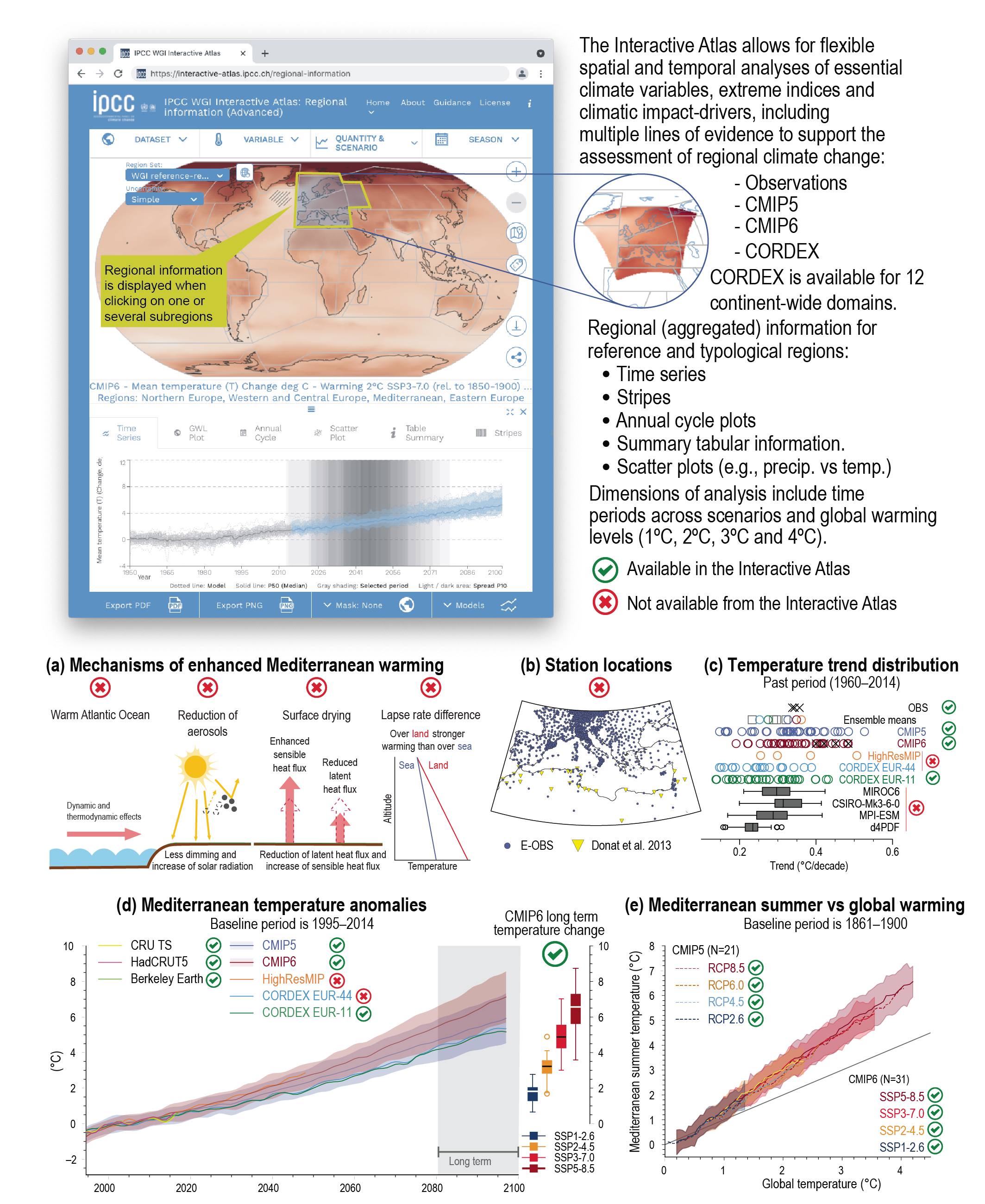
These FAIR principles are central to the WGI Interactive Atlas5, an online tool that complements the WGI Report by providing flexible spatial and temporal analyses of past, observed and projected climate change information. It comprises a regional information component that supports many of the chapters of the Report and a regional synthesis component that supports the Technical Summary and Summary for Policymakers.
Regarding the representation of robustness and uncertainty in maps, the method chosen for the AR66differs from the method used in the Fifth Assessment Report (AR5). This choice is based on new research on the visualization of uncertainty and on user surveys.
Box TS.1 | Core Concepts Central to This Report
This box provides short descriptions of key concepts that are relevant to the AR6 WGI assessment, with a focus on their use in the Technical Summary and the Summary for Policymakers. The Glossary (Annex VII) includes more information on these concepts along with definitions of many other important terms and concepts used in this Report.
Characteristics of Climate Change Assessment
Global warming: Global warming refers to the change of global surface temperature relative to a baseline depending upon the application. Specific global warming levels, such as 1.5°C, 2°C, 3°C or 4°C, are defined as changes in global surface temperature relative to the years 1850–1900 as the baseline (the earliest period of reliable observations with sufficient geographic coverage). They are used to assess and communicate information about global and regional changes, linking to scenarios and used as a common basis for Working Group II (WGII) and Working Group III (WGIII) assessments. (Section TS.1.3, Cross-Section Box TS.1) Links to chapters1.4.1, 1.6.2, 4.6.1, Cross-Chapter Boxes 1.5, 2.3, 11.1, and 12.1, Atlas Sections 3–11, Glossary
Emergence: Emergence refers to the experience or appearance of novel conditions of a particular climate variable in a given region. This concept is often expressed as the ratio of the change in a climate variable relative to the amplitude of natural variations of that variable (often termed a ‘signal-to-noise’ ratio, with emergence occurring at a defined threshold of this ratio). Emergence can be expressed in terms of a time or a global warming level at which the novel conditions appear and can be estimated using observations or model simulations. (Sections TS.1.2.3 and TS.4.2) Links to chapters1.4.2, FAQ 1.2, 7.5.5, 10.3, 10.4, 12.5.2, Cross-Chapter Box Atlas.1, Glossary
Cumulative carbon dioxide (CO2) emissions: The total net amount of CO2 emitted into the atmosphere as a result of human activities. Given the nearly linear relationship between cumulative CO2 emissions and increases in global surface temperature, cumulative CO2 emissions are relevant for understanding how past and future CO2 emissions affect global surface temperature. A related term – remaining carbon budget – is used to describe the total net amount of CO2 that could be released in the future by human activities while keeping global warming to a specific global warming level, such as 1.5°C, taking into account the warming contribution from non-CO2 forcers as well. The remaining carbon budget is expressed from a recent specified date, while the total carbon budget is expressed starting from the pre-industrial period. (Sections TS.1.3 and TS.3.3) Links to chapters1.6.3, 5.5, Glossary
Net zero CO2 emissions: A condition that occurs when the amount of CO2 emitted into the atmosphere by human activities equals the amount of CO2 removed from the atmosphere by human activities over a specified period of time. Net negative CO2 emissions occur when anthropogenic removals exceed anthropogenic emissions. (Section TS.3.3) Links to chaptersBox 1.4, Glossary
Human Influence on the Climate System
Earth’s energy imbalance: In a stable climate, the amount of energy that Earth receives from the Sun is approximately in balance with the amount of energy that is lost to space in the form of reflected sunlight and thermal radiation. ‘Climate drivers’, such as an increase in greenhouse gases or aerosols, interfere with this balance, causing the system to either gain or lose energy. The strength of a climate driver is quantified by its effective radiative forcing (ERF), measured in W m–2. Positive ERF leads to warming, and negative ERF leads to cooling. That warming or cooling in turn can change the energy imbalance through many positive (amplifying) or negative (dampening) climate feedbacks. (Sections TS.2.2, TS.3.1 and TS.3.2) Links to chapters2.2.8, 7.2, 7.3, 7.4, Box 7.1, Box 7.2, Glossary
Attribution: Attribution is the process of evaluating the relative contributions of multiple causal factors to an observed change in climate variables (e.g., global surface temperature, global mean sea level), or to the occurrence of extreme weather or climate-related events. Attributed causal factors include human activities (such as increases in greenhouse gas concentration and aerosols, or land-use change) or natural external drivers (solar and volcanic influences), and in some cases internal variability. (Sections TS.1.2.4 and TS.2, Box TS.10) Links to chaptersCross-Working Group Box: Attribution in Chapter 1; 3.5; 3.8; 10.4; 11.2.4; Glossary
Committed change, long-term commitment: Changes in the climate system, resulting from past, present and future human activities, which will continue long into the future (centuries to millennia) even with strong reductions in greenhouse gas emissions. Some aspects of the climate system, including the terrestrial biosphere, the deep ocean and the cryosphere, respond much more slowly than surface temperatures to changes in greenhouse gas concentrations. As a result, there are already substantial committed changes associated with past greenhouse gas emissions. For example, global mean sea level will continue to rise for thousands of years, even if future CO2 emissions are reduced to net zero and global warming halted, as excess energy due to past emissions continues to propagate into the deep ocean and as glaciers and ice sheets continue to melt. (Section TS.2.1, Box TS.4, Box TS.9) Links to chapters1.2.1, 1.3, Box 1.2, Cross-Chapter Box 5.3
Climate Information for Regional Climate Change and Risk Assessment
Distillation: The process of synthesizing information about climate change from multiple lines of evidence obtained from a variety of sources, taking into account user context and values. It leads to an increase in the usability, usefulness and relevance of climate information, enhances stakeholder trust, and expands the foundation of evidence used in climate services. It is particularly relevant in the context of co-producing regional-scale climate information to support decision-making. (Section TS.4.1, Box TS.11) Links to chapters10.1, 10.5, 12.6
(Climate change) risk: The concept of risk is a key aspect of how the IPCC assesses and communicates to decision-makers about the potential for adverse consequences for human or ecological systems, recognizing the diversity of values and objectives associated with such systems. In the context of climate change, risks can arise from potential impacts of climate change as well as human responses to climate change. WGI contributes to the common IPCC risk framing through the assessment of relevant climate information, including climatic impact-drivers and low-likelihood, high-impact outcomes. (Sections TS.1.4 and TS.4.1, Box TS.4) Links to chaptersCross-Chapter Boxes 1.3 and 12.1, Glossary
Climatic impact-drivers: Physical climate system conditions (e.g., means, events, extremes) that can be directly connected with having impacts on human or ecological systems are described as ‘climatic impact-drivers’ (CIDs) without anticipating whether their impacts are detrimental (i.e., as for hazards in the context of climate change risks) or provide potential opportunities. A range of indices may capture the sector- or application-relevant characteristics of a climatic impact-driver and can reflect exceedances of identified tolerance thresholds. (Sections TS.1.4 and TS.4.3) Links to chapters12.1–12.3, FAQ 12.1, Glossary
Storylines: The term storyline is used both in connection to scenarios (related to a future trajectory of emissions or socio-economic developments) or to describe plausible trajectories of weather and climate conditions or events, especially those related to high levels of risk. Physical climate storylines are introduced in AR6 to explore uncertainties in climate change and natural climate variability, to develop and communicate integrated and context-relevant regional climate information, and to address issues with deep uncertainty7, including low-likelihood, high-impact outcomes . (Section TS.1.4, Box TS.3, Infographic TS.1) Links to chapters1.4.4, Box 10.2, Glossary
Low-likelihood, high impact outcomes: Outcomes/events whose probability of occurrence is low or not well known (as in the context of deep uncertainty) but whose potential impacts on society and ecosystems could be high. To better inform risk assessment and decision-making, such low-likelihood outcomes are considered if they are associated with very large consequences and may therefore constitute material risks, even though those consequences do not necessarily represent the most likely outcome. (Section TS.1.4, Box TS.3, Figure TS.6) Links to chapters1.4.4, 4.8, Cross Chapter Box 1.3, Glossary
As part of the AR6 cycle, the IPCC produced three Special Reports in 2018 and 2019: the Special Report on Global Warming of 1.5°C (SR1.5), the Special Report on the Ocean and Cryosphere in a Changing Climate (SROCC), and the Special Report on Climate Change and Land (SRCCL).
The AR6 WGI Report provides a full and comprehensive assessment of the physical science basis of climate change that builds on the previous assessments and these Special Reports and considers new information and knowledge from the recent scientific literature8, including longer observational datasets and new scenarios and model results.
The structure of the AR6 WGI Report is designed to enhance the visibility of knowledge developments and to facilitate the integration of multiple lines of evidence, thereby improving confidence in findings. The Report has been peer-reviewed by the scientific community and governments (Annex X provides the Expert Reviewer list). The substantive introduction provided by (Chapter 1 is followed by a first set of chapters dedicated to large-scale climate knowledge (Chapters 2–4), which encompasses observations and paleoclimate evidence, causes of observed changes, and projections; these are complemented by (Chapter 11 for large-scale changes in extremes. The second set of chapters (Chapters 5–9) is orientated around the understanding of key climate system components and processes, including the global cycles of carbon, energy and water; short-lived climate forcers and their link to air quality; and the ocean, cryosphere and sea level change. The last set of chapters (Chapters 10–12 and the Atlas) is dedicated to the assessment and distillation of regional climate information from multiple lines of evidence at sub-continental to local scales (including urban climate), with a focus on recent and projected regional changes in mean climate, extremes, and climatic impact-drivers. The new online Interactive Atlas allows users to interact in a flexible manner through maps, time series and summary statistics with climate information for a set of updated WGI reference regions. The Report also includes 34 Frequently Asked Questions and answers for the general public (https://www.ipcc.ch/report/ar6/wg1/faqs).
Together, this Technical Summary and the underlying chapters aim at providing a comprehensive picture of knowledge progress since the WGI contribution to AR5. Multiple lines of scientific evidence confirm that the climate is changing due to human influence. Important advances in the ability to understand past, present and possible future changes should result in better-informed decision-making.
Some of the new results and main updates to key findings in this Report compared to AR5, SR1.5, SRCCL, and SROCC are summarized below. Relevant Technical Summary sections with further details are shown in parentheses after each bullet point.
Selected Updates and/or New Results since AR5
- Human influence9on the climate system is now an established fact: The Fourth Assessment Report (AR4) stated in 2007 that ‘warming of the climate system is unequivocal’, and AR5 stated in 2013 that ‘human influence on the climate system is clear’. Combined evidence from across the climate system strengthens this finding. It is unequivocal that the increase of CO2, methane (CH4) and nitrous oxide (N2O) in the atmosphere over the industrial era is the result of human activities and that human influence is the main driver10 of many changes observed across the atmosphere, ocean, cryosphere and biosphere. (Sections TS.1.2, TS.2.1 and TS.3.1)
- Observed global warming to date: A combination of improved observational records and a series of very warm years since AR5 have resulted in a substantial increase in the estimated level of global warming to date. The contribution of changes in observational understanding alone between AR5 and AR6 leads to an increase of about 0.1°C in the estimated warming since 1850–1900. For the decade 2011–2020, the increase in global surface temperature since 1850–1900 is assessed to be 1.09 [0.95 to 1.20] °C. 11Estimates of crossing times of global warming levels and estimates of remaining carbon budgets are updated accordingly. (Section TS.1.2, Cross-Section Box TS.1)
- Paleoclimate evidence: The AR5 assessed that many of the changes observed since the 1950s are unprecedented over decades to millennia. Updated paleoclimate evidence strengthens this assessment; over the past several decades, key indicators of the climate system are increasingly at levels unseen in centuries to millennia and are changing at rates unprecedented in at least the last 2000 years. (Box TS.2, Section TS.2)
- Updated assessment of recent warming: The AR5 reported a smaller rate of increase in global mean surface temperature over the period 1998–2012 than the rate calculated since 1951. Based on updated observational datasets showing a larger trend over 1998–2012 than earlier estimates, there is now high confidence that the observed 1998–2012 global surface temperature trend is consistent with ensembles of climate model simulations, and there is nowvery high confidence that the slower rate of global surface temperature increase observed over this period was a temporary event induced by internal and naturally forced variability that partly offset the anthropogenic surface warming trend over this period, while heat uptake continued to increase in the ocean. Since 2012, strong warming has been observed, with the past five years (2016–2020) being the hottest five-year period in the instrumental record since at least 1850 (high confidence). (Section TS.1.2, Cross-Section Box TS.1)
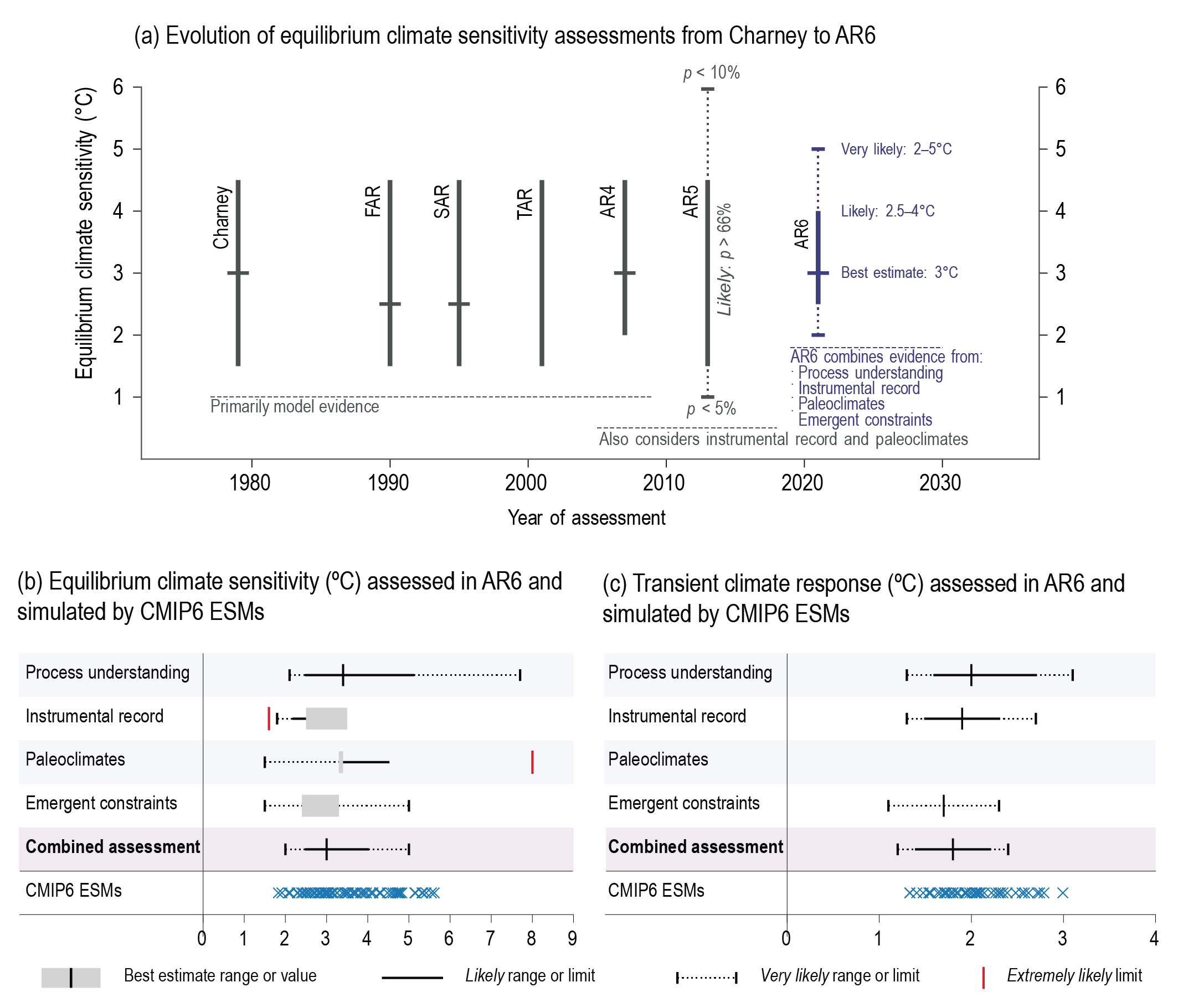
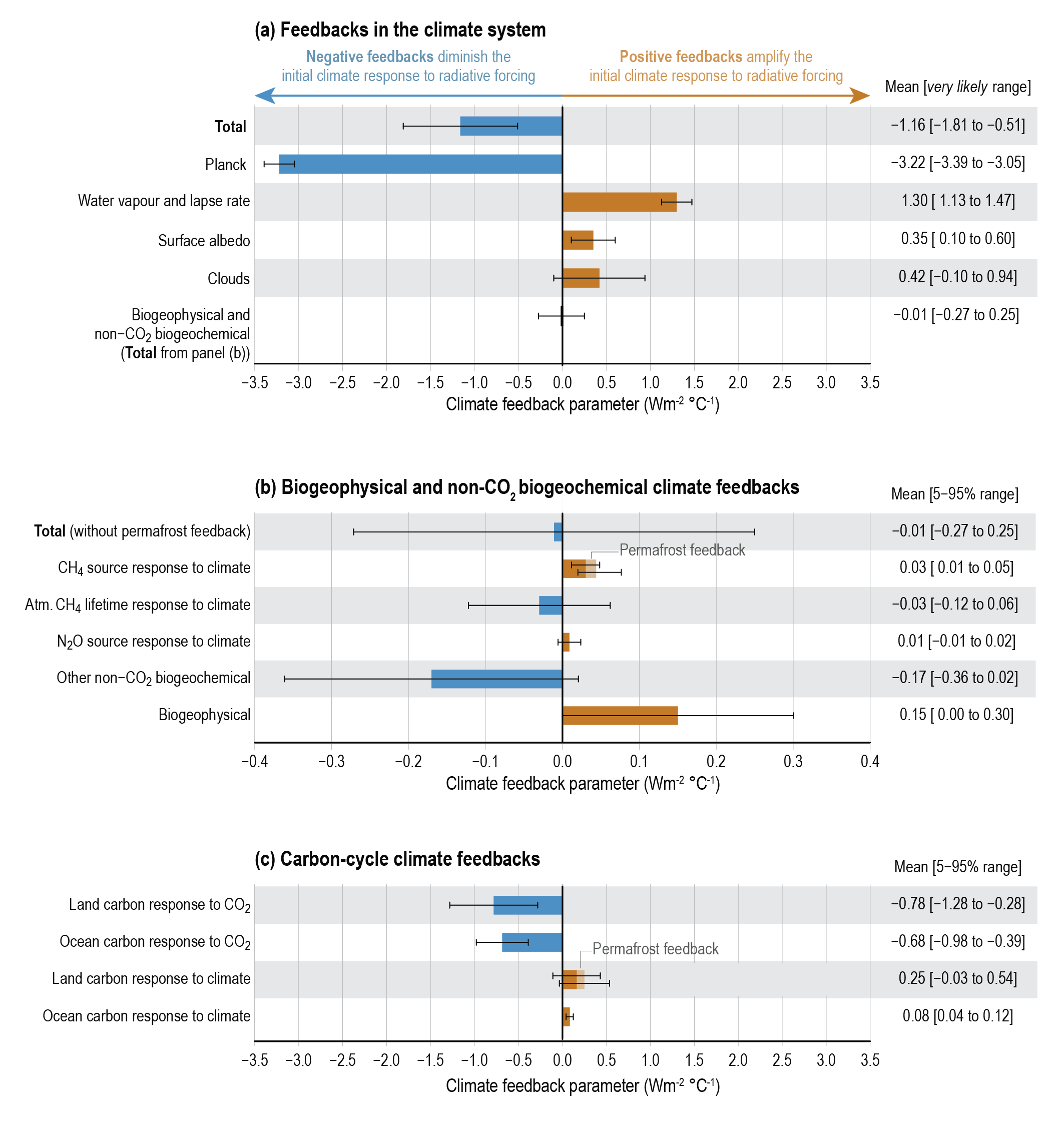
- Magnitude of climate system response: In this Report, it has been possible to reduce the long-standing uncertainty ranges for metrics that quantify the response of the climate system to radiative forcing, such as the equilibrium climate sensitivity (ECS) and the transient climate response (TCR), due to substantial advances (e.g., a 50% reduction in the uncertainty range of cloud feedbacks) and improved integration of multiple lines of evidence, including paleoclimate information. Improved quantification of ERF, the climate system radiative response, and the observed energy increase in the Earth system over the past five decades demonstrate improved consistency between independent estimates of climate drivers, the combined climate feedbacks, and the observed energy increase relative to AR5. (Section TS.3.2)
- Improved constraints on projections of future climate change: For the first time in an IPCC report, the assessed future change in global surface temperature is consistently constructed by combining scenario-based projections (which AR5 focused on) with observational constraints based on past simulations of warming as well as the updated assessment of ECS and TCR. In addition, initialized forecasts have been used for the period 2019–2028. The inclusion of these lines of evidence reduces the assessed uncertainty for each scenario. (Section TS.1.3, Cross-Section Box TS.1)
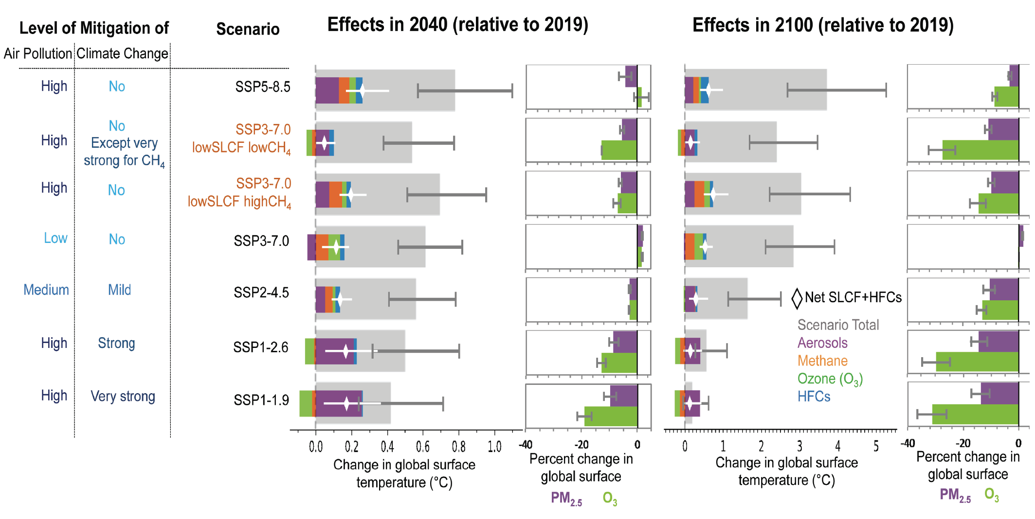
- Air quality: The AR5 assessed that projections of air quality are driven primarily by precursor emissions, including CH4. New scenarios explore a diversity of future options in air pollution management. The AR6 reports rapid recent shifts in the geographical distribution of some of these precursor emissions, confirms the AR5 finding, and shows higher warming effects of short-lived climate forcers in scenarios with the highest air pollution. (Sections TS.1.3 and TS.2.2, Box TS.7)
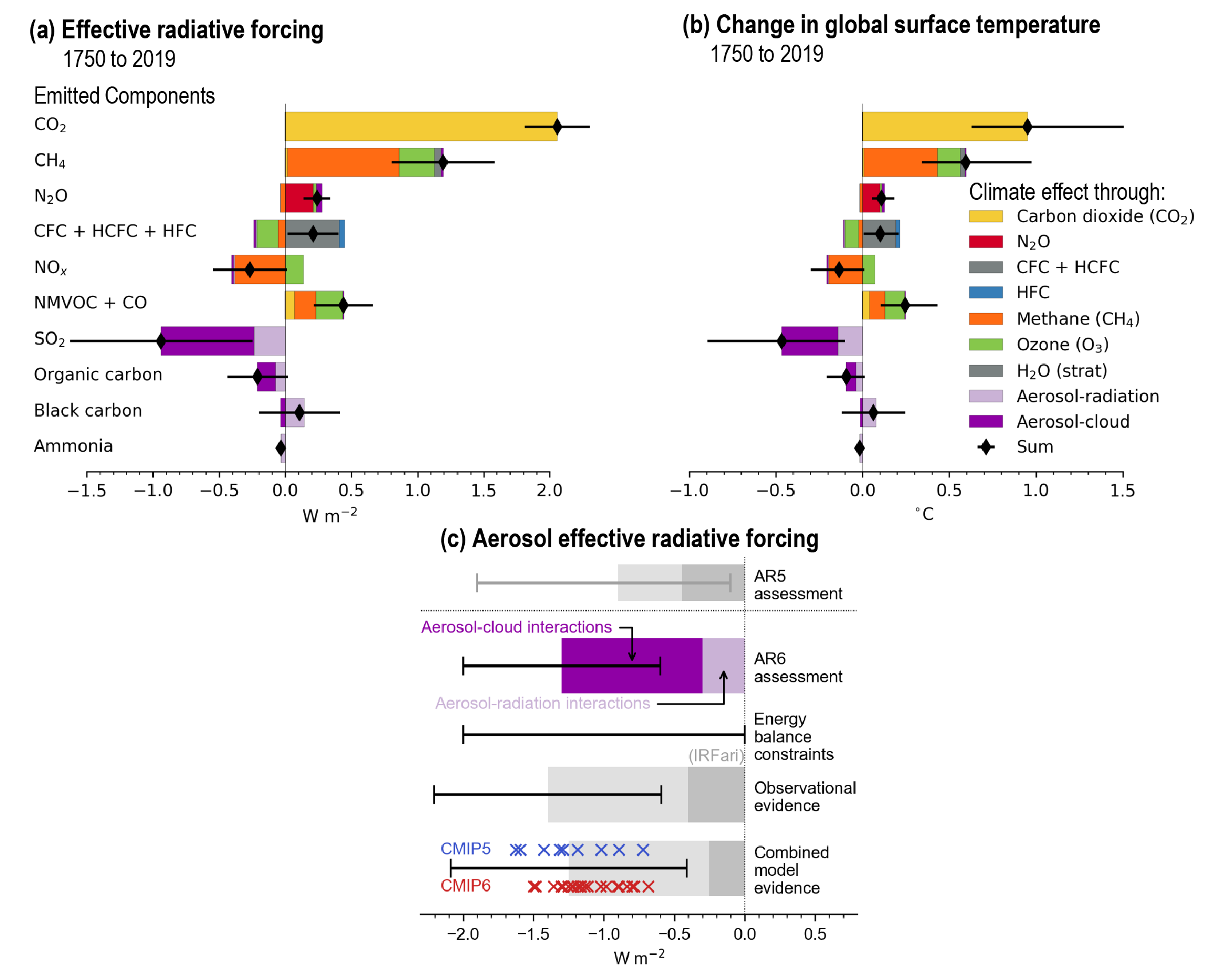
- Effects of short-lived climate forcers on global warming: The AR5 assessed the radiative forcing for emitted compounds. The AR6 has extended this by assessing the emissions-based ERFs also accounting for aerosol–cloud interactions. The best estimates of ERF attributed to sulphur dioxide (SO2) and CH4 emissions are substantially greater than in AR5, while that of black carbon is substantially reduced. The magnitude of uncertainty in the ERF due to black carbon emissions has also been reduced relative to AR5. (Section TS.3.1)
- Global water cycle: The AR5 assessed that anthropogenic influences have likely affected the global water cycle since 1960. The dedicated chapter in AR6 (Chapter 8) concludes with high confidence that human-caused climate change has driven detectable changes in the global water cycle since the mid-20th century, with a better understanding of the response to aerosol and greenhouse gas changes. The AR6 further projects with high confidence an increase in the variability of the water cycle in most regions of the world and under all emissions scenarios. (Box TS.6)
- Extreme events: The AR5 assessed that human influence had been detected in changes in some climate extremes. A dedicated chapter in AR6 (Chapter 11) concludes that it is now an established fact that human-induced greenhouse gas emissions have led to an increased frequency and/or intensity of some weather and climate extremes since 1850, in particular for temperature extremes. Evidence of observed changes and attribution to human influence has strengthened for several types of extremes since AR5, in particular for extreme precipitation, droughts, tropical cyclones and compound extremes (including fire weather). (Sections TS.1.2 and TS.2.1, Box TS.10)
Selected Updates and/or New Results Since AR5 and SR1.5
- Timing of crossing 1.5°C global warming: Slightly different approaches are used in SR1.5 and in this Report. SR1.5 assessed a likely range of 2030 to 2052 for reaching a global warming level of 1.5°C (for a 30-year period), assuming a continued, constant rate of warming. In AR6, combining the larger estimate of global warming to date and the assessed climate response to all considered scenarios, the central estimate of crossing 1.5°C of global warming (for a 20-year period) occurs in the early 2030s, in the early part of the likely range assessed in SR1.5, assuming no major volcanic eruption. (Section TS.1.3, Cross-Section Box TS.1)
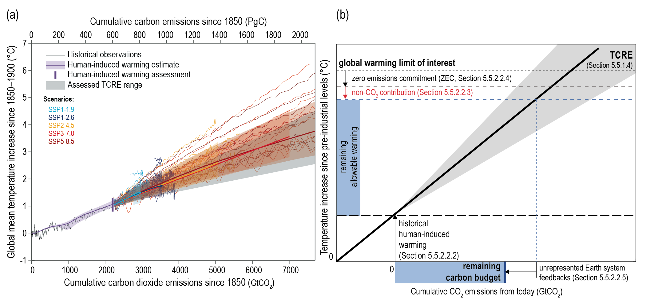
- Remaining carbon budgets: The AR5 had assessed the transient climate response to cumulative emissions of CO2 to be likely in the range of 0.8°C to 2.5°C per 1000 GtC (1 Gigatonne of carbon, GtC, = 1 Petagram of carbon, PgC, = 3.664 Gigatonnes of carbon dioxide, GtCO2), and this was also used in SR1.5. The assessment in AR6, based on multiple lines of evidence, leads to a narrowerlikely range of 1.0°C–2.3°C per 1000 GtC. This has been incorporated in updated estimates of remaining carbon budgets (see Section TS.3.3.1), together with methodological improvements and recent observations. (Sections TS.1.3 and TS.3.3)
- Effect of short-lived climate forcers on global warming in coming decades: The SR1.5 stated that reductions in emissions of cooling aerosols partially offset greenhouse gas mitigation effects for two to three decades in pathways limiting global warming to 1.5°C. The AR6 assessment updates the AR5 assessment of the net cooling effect of aerosols and confirms that changes in short-lived climate forcers will very likely cause further warming in the next two decades across all scenarios. (Section TS.1.3, Box TS.7)
- COVID-19: Temporary emissions reductions in 2020 associated with COVID-19 containment led to small and positive net radiative effect (warming influence). However, global and regional climate responses to this forcing are undetectable above internal climate variability due to the temporary nature of emissions reductions. (Section TS.3.3)
Selected Updates and/or New Results Since AR5, SRCCL and SROCC
- Atmospheric concentration of methane: The SRCCL reported a resumption of atmospheric CH4 concentration growth since 2007. The AR6 reports a faster growth over 2014–2019 and assesses growth since 2007 to be largely driven by emissions from the fossil fuels and agriculture (dominated by livestock) sectors. (Section TS.2.2)
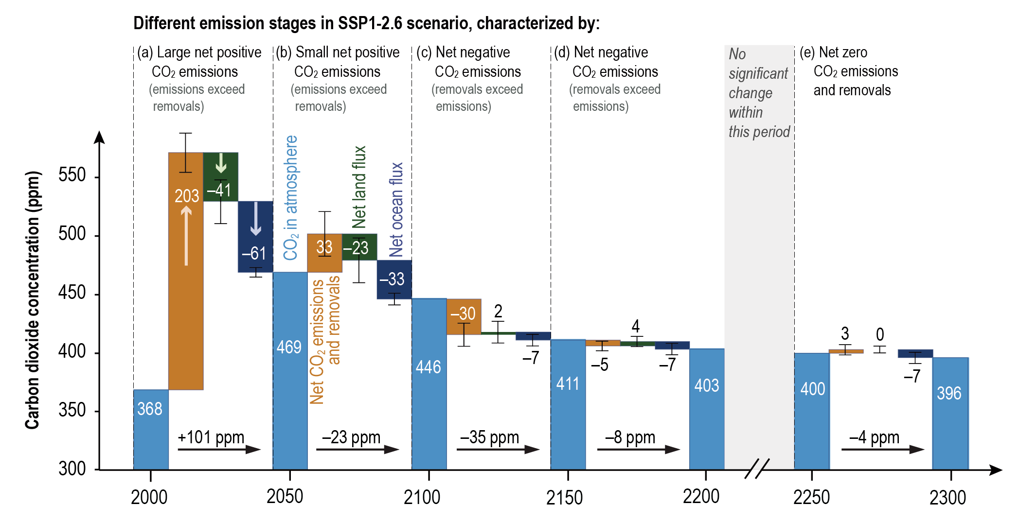
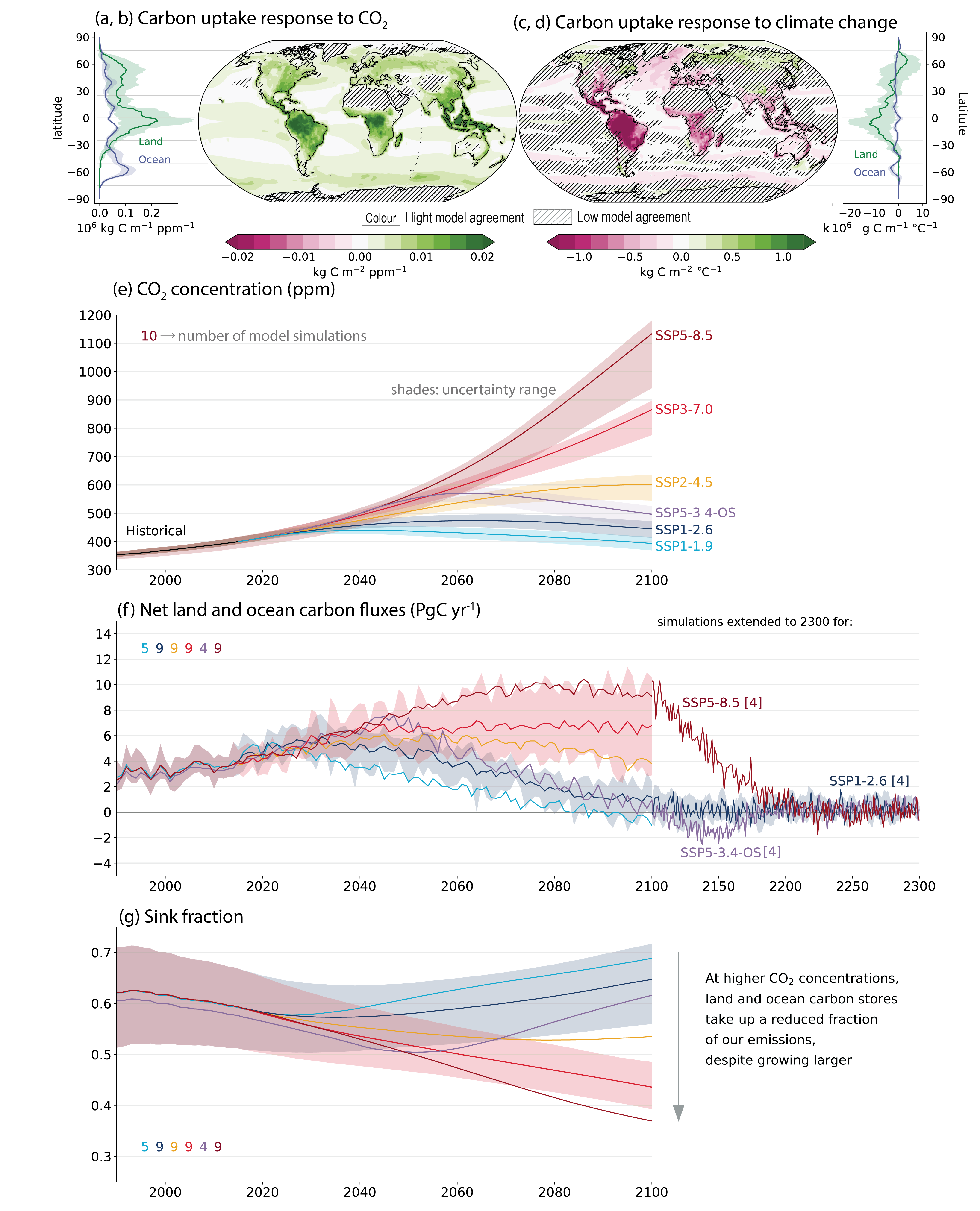
- Land and ocean carbon sinks: The SRCCL assessed that the persistence of the land carbon sink is uncertain due to climate change. The AR6 finds that land and ocean carbon sinks are projected to continue to grow until 2100 with increasing atmospheric concentrations of CO2, but the fraction of emissions taken up by land and ocean is expected to decline as the CO2 concentration increases, with a much larger uncertainty range for the land sink. The AR5, SR1.5 and SRCCL assessed carbon dioxide removal options and scenarios. The AR6 finds that the carbon cycle response is asymmetric for pulse emissions or removals, which means that CO2 emissions would be more effective at raising atmospheric CO2 than CO2 removals are at lowering atmospheric CO2. (Section TS.3.3, Box TS.5)
- Ocean stratification increase12: Refined analyses of available observations in the AR6 lead to a reassessment of the rate of increase of the global stratification in the upper 200 m to be double that estimated in SROCC from 1970 to 2018. (Section TS.2.4)
- Projected ocean oxygen loss: Future subsurface oxygen decline in new projections assessed in WGI AR6 is substantially greater in 2080–2099 than assessed in SROCC. (Section TS.2.4)
- Ice loss from glaciers and ice sheets: Since SROCC, globally resolved glacier changes have improved estimates of glacier mass loss over the past 20 years, and estimates of the Greenland and Antarctic Ice Sheet loss have been extended to 2020. (Section TS.2.5)
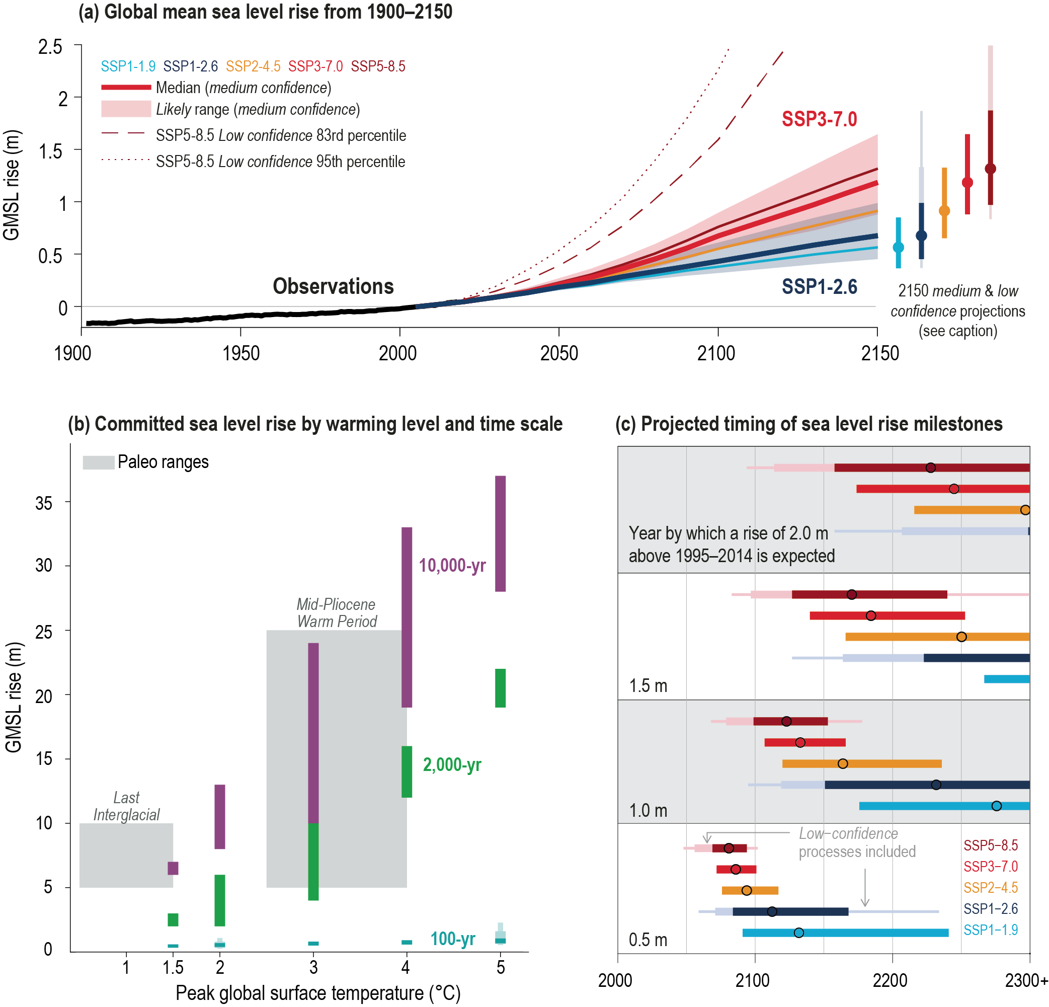
- Observed global mean sea level change: new observation-based estimates published since SROCC lead to an assessed sea level rise estimate from 1901 to 2018 that is now consistent with the sum of individual components and consistent with closure of the global energy budget. (Box TS.4)
- Projected global mean sea level change: The AR6 projections of global mean sea level are based on projections from ocean thermal expansion and land ice contribution estimates, which are consistent with the assessed ECS and assessed changes in global surface temperature. They are underpinned by new land ice model intercomparisons and consideration of processes associated with low confidence to characterize the deep uncertainty in future ice loss from Antarctica. The AR6 projections based on new models and methods are broadly consistent with SROCC findings. (Box TS.4)
TS.1 A Changing Climate
This section introduces the assessment of the physical science basis of climate change in the AR6 and presents the climate context in which this assessment takes place, recent progress in climate science and the relevance of global and regional climate information for impact and risk assessments. The future emissions scenarios and global warming levels, used to integrate assessments across this Report, are introduced and their applications for future climate projections are briefly addressed. Paleoclimate science provides a long-term context for observed climate change of the past 150 years and the projected changes in the 21st century and beyond (Box TS.2). The assessment of past, current and future global surface temperature changes relative to the standard baselines and reference periods13used throughout this Report is summarized in Cross-Section Box TS.1.
TS1.1 Context of a Changing Climate
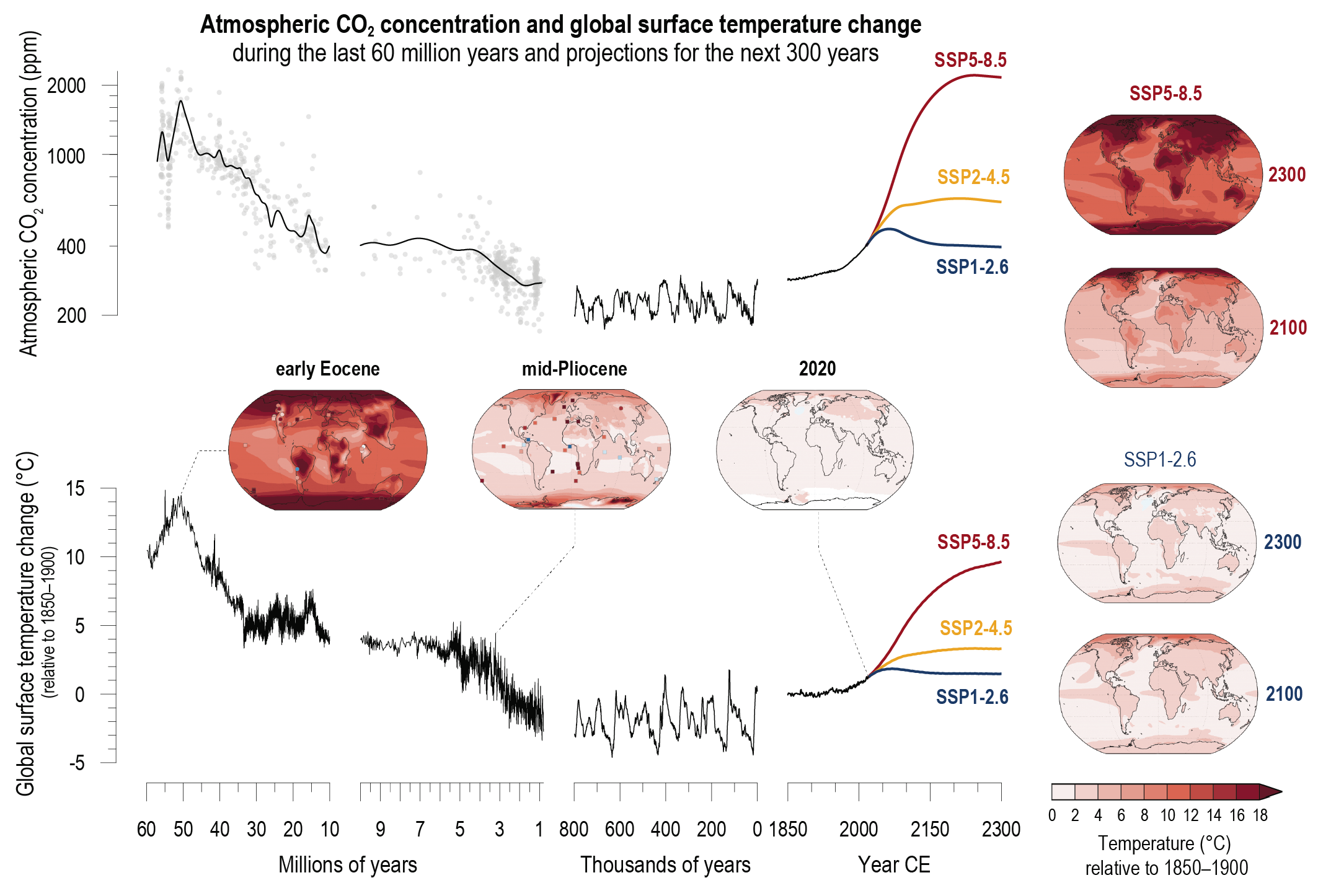
Earth’s climate system has evolved over many millions of years, and evidence from natural archives provides a long-term perspective on observed changes and projected changes over the coming centuries. These reconstructions of past climate also show that atmospheric CO2 concentrations and global surface temperature are strongly coupled (Figure TS.1), based on evidence from a variety of proxy records over multiple time scales (Box TS.2, Section TS.2). Levels of global warming (see Core Concepts Box) that have not been seen in millions of years could be reached by 2300, depending on the emissions pathway that is followed (Section TS.1.3). For example, there is medium confidence that, by 2300, an intermediate scenario14used in this Report leads to global surface temperatures of [2.3°C to 4.6°C] higher than 1850–1900, similar to the mid-Pliocene Warm Period [2.5°C to 4°C], about 3.2 million years ago, whereas the high CO2 emissions scenario SSP5-8.5 leads to temperatures of [6.6°C to 14.1°C] by 2300, which overlaps with the Early Eocene Climate Optimum [10°C to 18°C], about 50 million years ago. Links to chaptersCross-Chapter Boxes 2.1 and 2.4, 2.3.1, 4.3.1.1, 4.7.1.2, 7.4.4.1
Understanding of the climate system’s fundamental elements is robust and well established. Scientists in the 19th century identified the major natural factors influencing the climate system. They also hypothesized the potential for anthropogenic climate change due to CO2 emitted by combustion of fossil fuels (petroleum, coal, natural gas). The principal natural drivers of climate change, including changes in incoming solar radiation, volcanic activity, orbital cycles and changes in global biogeochemical cycles, have been studied systematically since the early 20th century. Other major anthropogenic drivers, such as atmospheric aerosols (fine solid particles or liquid droplets), land-use change and non-CO2 greenhouse gases, were identified by the 1970s. Since systematic scientific assessments began in the 1970s, the influence of human activities on the warming of the climate system has evolved from theory to established fact (see also Section TS.2). The evidence for human influence on recent climate change strengthened from the IPCC First Assessment Report in 1990 to the IPCC Fifth Assessment Report in 2013/14, and is now even stronger in this assessment (Sections TS.1.2.4 and TS.2). Changes across a greater number of climate system components, including changes in regional climate and extremes can now be attributed to human influence (see Sections TS.2 and TS.4). Links to chapters1.3.1–1.3.5, 3.1, 11.2, 11.9
Box TS.2 | Paleoclimate
Paleoclimate reference periods. Over the long evolution of Earth’s climate, several periods have received extensive research attention as examples of distinct climate states and rapid climate transitions (Box TS.2, Figure 1). These paleoclimate reference periods represent the present geological era (Cenozoic; past 65 million years) and are used across chapters to help structure the assessment of climate changes prior to industrialization. Cross-Chapter Box 2.1 describes the reference periods, along with a brief account of their climate forcings, and lists where each is discussed in other chapters. Cross-Chapter Box 2.4 summarizes information on one of the reference periods, the mid-Pliocene Warm Period. The Interactive Atlas includes model output from the World Climate Research Programme Coupled Model Intercomparison Project Phase 6 (CMIP6) for four of the paleoclimate reference periods.
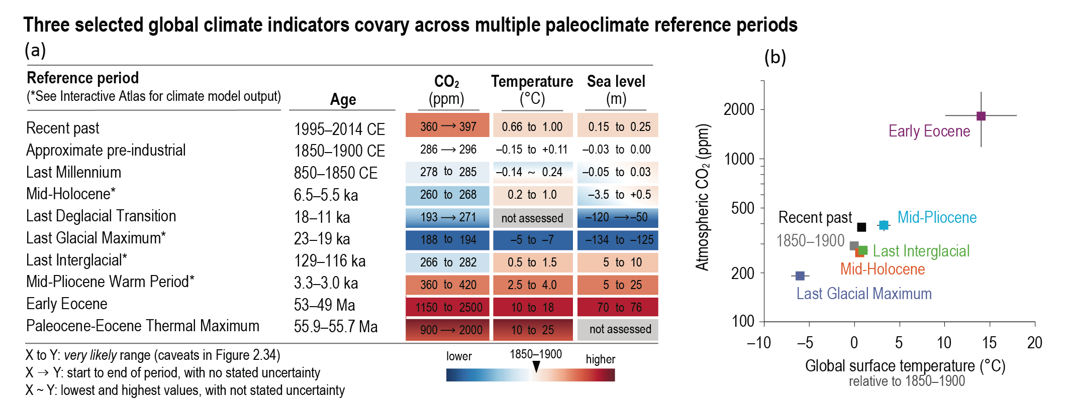
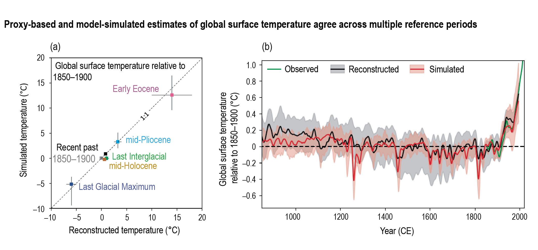
Box TS.2, Figure 1 | Paleoclimate and recent reference periods, with selected key indicators. The intent of this figure is to list the paleoclimate reference periods used in this Report, to summarize three key global climate indicators, and compare CO2 with global temperature over multiple periods. (a) Three large-scale climate indicators (atmospheric CO2, global surface temperature relative to 1850–1900, and global mean sea level relative to 1900), based on assessments in Chapter 2, with confidence levels ranging fromlow tovery high. (b) Comparison between global surface temperature (relative to 1850–1900) and atmospheric CO2 concentration (shown on a log scale) for multiple reference periods (mid-points with 5–95% ranges). Links to chapters2.2.3, 2.3.1.1, 2.3.3.3, Figure 2.34
Paleoclimate models and reconstructions. Climate models that target paleoclimate reference periods have been featured by the IPCC since the First Assessment Report. Under the framework of CMIP6-PMIP4 (Paleoclimate Modelling Intercomparison Project), new protocols for model intercomparisons have been developed for multiple paleoclimate reference periods. These modelling efforts have led to improved understanding of the climate response to different external forcings, including changes in Earth’s orbital and plate movements, solar irradiance, volcanism, ice-sheet size and atmospheric greenhouse gases. Likewise, quantitative reconstructions of climate variables from proxy records that are compared with paleoclimate simulations have improved as the number of study sites and variety of proxy types have expanded, and as records have been compiled into new regional and global datasets. Links to chapters1.3.2, 1.5.1, Cross-Chapter Boxes 2.1 and 2.4
Global surface temperature. Since AR5, updated climate forcings, improved models, new understanding of the strengths and weaknesses of a growing array of proxy records, better chronologies and more robust proxy data products have led to better agreement between models and reconstructions. For global surface temperature, the mid-point of the AR6-assessed range and the median of the model-simulated temperatures differ by an average of 0.5°C across five reference periods; they overlap within their 90% ranges in four of five cases, which together span from about 6 [5 to 7]°C colder during the Last Glacial Maximum to about 14 [10 to 18] °C warmer during the Early Eocene, relative to 1850–1900 (Box TS.2, Figure 2a). Changes in temperature by latitude in response to multiple forcings show that polar amplification (stronger warming at high latitudes than the global average) is a prominent feature of the climate system across multiple climate states, and the ability of models to simulate this polar amplification in past warm climates has improved since AR5 (high confidence). Over the past millennium, and especially since about 1300 CE, simulated global surface temperature anomalies are well within the uncertainty of reconstructions (medium confidence), except for some short periods immediately following large volcanic eruptions, for which different forcing datasets disagree (Box TS.2, Figure 2b). Links to chapters2.3.1.1, 3.3.3.1, 3.8.2.1, 7.4.4.1.2

Box TS.2, Figure 2 | Global surface temperature as estimated from proxy records (reconstructed) and climate models (simulated). The intent of this figure is to show the agreement between observations and models of global temperatures during paleo reference periods. (a) For individual paleoclimate reference periods. (b) For the last millennium, with instrumental temperature (AR6 assessed mean, 10-year smoothed). Model uncertainties in (a) and (b) are 5–95% ranges of multi-model ensemble means; reconstructed uncertainties are 5–95% ranges (medium confidence) of (a) midpoints and (b) multi-method ensemble median. Links to chapters2.3.1.1, Figure 2.34, Figure 3.2c, Figure 3.44
Equilibrium climate sensitivity. Paleoclimate data provide evidence to estimate equilibrium climate sensitivity (ECS15) (Section TS.3.2.1). In AR6, refinements in paleo data for paleoclimate reference periods indicate that ECS is very likely greater than 1.5°C and likely less than 4.5°C, which is largely consistent with other lines of evidence and helps narrow the uncertainty range of the overall assessment of ECS. Some of the CMIP6 climate models that have either high (>5°C) or low (<2°C) ECS also simulate past global surface temperature changes outside the range of proxy-based reconstructions for the coldest and warmest reference periods. Since AR5, independent lines of evidence, including proxy records from past warm periods and glacial–interglacial cycles, indicate that sensitivity to forcing increases as temperature increases (Section TS.3.2.2). Links to chapters7.4.3.2, 7.5.3, 7.5.6, Table 7.11
Water cycle. New hydroclimate reconstructions and model-data comparisons have improved the understanding of the causes and effects of long-term changes in atmospheric and ocean circulation, including monsoon variability and modes of variability (Box TS.13, Section TS.4.2). Climate models are able to reproduce decadal drought variability on large regional scales, including the severity, persistence and spatial extent of past megadroughts known from proxy records (medium confidence). Some long-standing discrepancies remain, however, such as the magnitude of African monsoon precipitation during the early Holocene (the past 11,700 years), suggesting continuing knowledge gaps. Paleoclimate evidence shows that, in relatively high CO2 climates such as the Pliocene, Walker circulation over the equatorial Pacific Ocean weakens, supporting the high confidence model projections of weakened Walker cells by the end of the 21st century. Links to chapters3.3.2, 8.3.1.6, 8.4.1.6, 8.5.2.1, 9.2
Sea level and ice sheets. Although past and future global warming differ in their forcings, evidence from paleoclimate records and modelling show that ice-sheet mass and global mean sea level (GMSL) responded dynamically over multiple millennia (high confidence). This evidence helps to constrain estimates of the committed GMSL response to global warming (Box TS.4). For example, under a past global warming levels of around [2.5°C to 4°C] relative to 1850–1900, like during the mid-Pliocene Warm Period, sea level was [5 to 25 m] higher than 1900 (medium confidence); under past global warming levels of [10°C to 18°C], like during the Early Eocene, the planet was essentially ice free (high confidence). Constraints from these past warm periods, combined with physical understanding, glaciology and modelling, indicate a committed long-term GMSL rise over 10,000 years, reaching about 8 to 13 m for sustained peak global warming of 2°C and up to 28 to 37 m for 5°C, which exceeds the AR5 estimate. Links to chapters2.3.3.3, 9.4.1.4, 9.4.2.6, 9.6.2, 9.6.3.5
Ocean. Since AR5, better integration of paleo-oceanographic data with modelling along with higher-resolution analyses of transient changes have improved understanding of long-term ocean processes. Low-latitude sea surface temperatures at the Last Glacial Maximum cooled more than previously inferred, resolving some inconsistencies noted in AR5. This paleo context supports the assessment that ongoing increase in ocean heat content (OHC) represents a long-term commitment (see Core Concepts Box), essentially irreversible on human time scales (high confidence). Estimates of past global OHC variations generally track those of sea surface temperatures around Antarctica, underscoring the importance of Southern Ocean processes in regulating deep-ocean temperatures. Paleoclimate data, along with other evidence of glacial–interglacial changes, show that Antarctic Circumpolar flow strengthened and that ventilation of Antarctic Bottom Water accelerated during warming intervals, facilitating release of CO2 stored in the deep ocean to the atmosphere. Paleo evidence suggests significant reduction of deep-ocean ventilation associated with meltwater input during times of peak warmth. Links to chapters2.3.1.1, 2.3.3.1, 9.2.2, 9.2.3.2
Carbon cycle. Past climate states were associated with substantial differences in the inventories of the various carbon reservoirs, including the atmosphere (Section TS.2.2). Since AR5, the quantification of carbon stocks has improved due to the development of novel sedimentary proxies and stable-isotope analyses of air trapped in polar ice. Terrestrial carbon storage decreased markedly during the Last Glacial Maximum by 300–600 PgC, possibly by 850 PgC when accounting for interactions with the lithosphere and ocean sediments, a larger reduction than previously estimated, owing to a colder and drier climate. At the same time, the storage of remineralized carbon in the ocean interior increased by as much as 750–950 PgC, sufficient to balance the removal of carbon from the atmosphere (200 PgC) and terrestrial biosphere reservoirs combined (high confidence). Links to chapters5.1.2.2
TS.1.2 Progress in Climate Science
TS.1.2.1 Observation-based Products and their Assessments
Earth system observations are an essential driver of progress in our understanding of climate change. Overall, capabilities to observe the physical climate system have continued to improve and expand. Improvements are particularly evident in ocean observing networks and remote-sensing systems. Records from several recently instigated satellite measurement techniques are now long enough to be relevant for climate assessments. For example, globally distributed, high-vertical-resolution profiles of temperature and humidity in the upper troposphere and stratosphere can be obtained from the early 2000s using global navigation satellite systems, leading to updated estimates of recent atmospheric warming. Improved measurements of ocean heat content, warming of the land surface, ice-sheet mass loss and sea level changes allow a better closure of the global energy and sea level budgets relative to AR5. For surface and balloon-based networks, apparent regional data reductions result from a combination of data policy issues, data curation/provision challenges, and real cessation of observations, and are to an extent counter-balanced by improvements elsewhere. Limited observational records of extreme events and spatial data gaps currently limit the assessment of some observed regional climate change. Links to chapters1.5.1, 2.3.2, 7.2.2, Box 7.2, Cross-Chapter Box 9.1, 9.6.1, 10.2.2, 10.6, 11.2, 12.4
New paleoclimate reconstructions from natural archives have enabled more robust reconstructions of the spatial and temporal patterns of past climate changes over multiple time scales (Box TS.2). However, paleoclimate archives, such as tropical glaciers and modern natural archives used for calibration (e.g., corals and trees), are rapidly disappearing owing to a host of pressures, including increasing temperatures (high confidence). Substantial quantities of past instrumental observations of weather and other climate variables, over both land and ocean, which could fill gaps in existing datasets, remain un-digitized or inaccessible. These include measurements of temperature (air and sea surface), rainfall, surface pressure, wind strength and direction, sunshine amount and many other variables dating back into the 19th century. Links to chapters1.5.1
Reanalyses combine observations and models (e.g., a numerical weather prediction model) using data assimilation techniques to provide a spatially complete, dynamically consistent estimate of multiple variables describing the evolving climate state. Since AR5, new reanalyses have been developed for the atmosphere and the ocean with various combinations of increased resolution, extended records, more consistent data assimilation and larger availability of uncertainty estimates. Limitations remain, for example, in how reanalyses represent global-scale changes to the water cycle. Regional reanalyses use high-resolution, limited-area models constrained by regional observations and with boundary conditions from global reanalyses. There is high confidence that regional reanalyses better represent the frequencies of extremes and variability in precipitation, surface air temperature and surface wind than global reanalyses and provide estimates that are more consistent with independent observations than dynamical downscaling approaches. Links to chapters1.5.2, 10.2.1.2, Annex I
TS.1.2.2 Climate Model Performance
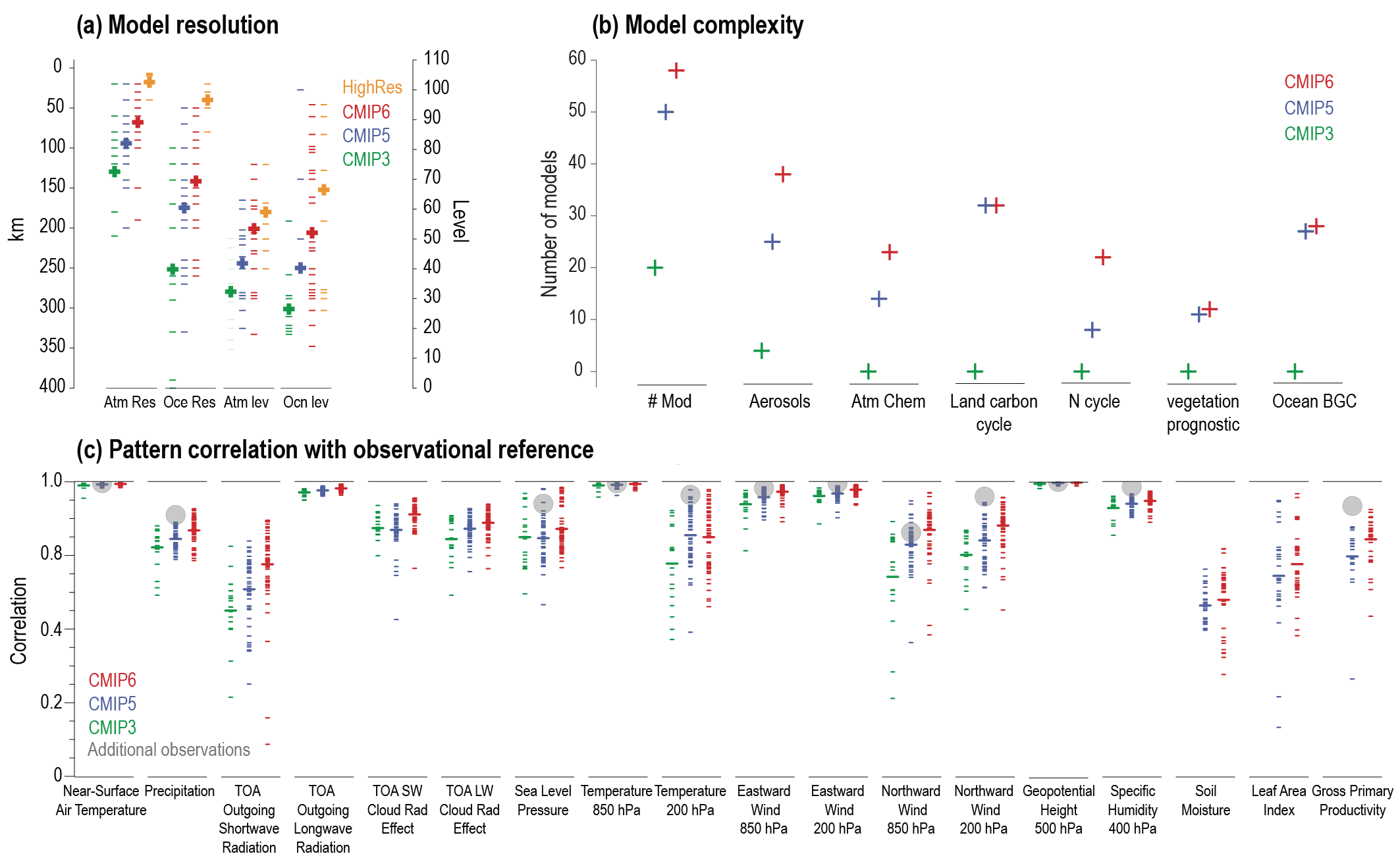
Climate model simulations coordinated and collected as part of the World Climate Research Programme’s Coupled Model Intercomparison Project Phase 6 (CMIP6), complemented by a range of results from the previous phase (CMIP5), constitute a key line of evidence supporting this Report. The latest generation of CMIP6 models have an improved representation of physical processes relative to previous generations, and a wider range of Earth system models now represent biogeochemical cycles. Higher-resolution models that better capture smaller-scale processes are also increasingly becoming available for climate change research (Figure TS.2, Panels a and b). Results from coordinated regional climate modelling initiatives, such as the Coordinated Regional Climate Downscaling Experiment (CORDEX) complement and add value to the CMIP global models, particularly in complex topography zones, coastal areas and small islands, as well as for extremes. Links to chapters1.5.3, 1.5.4, 2.8.2, FAQ 3.3, 6.2.2, 6.4, 6.4.5, 8.5.1, 10.3.3, Atlas.1.4
Projections of the increase in global surface temperature and the pattern of warming from previous IPCC Assessment Reports and other studies are broadly consistent with subsequent observations (limited evidence, high agreement), especially when accounting for the difference in radiative forcing scenarios used for making projections and the radiative forcings that actually occurred (Figure TS.3). The AR5 and SROCC projections of GMSL for the 2007–2018 period have been shown to be consistent with observed trends in GMSL and regional weighted mean tide gauges. Links to chapters1.3.6, 9.6.3.1
For most large-scale indicators of climate change, the simulated recent mean climate from CMIP6 models underpinning this assessment have improved compared to the CMIP5 models used in AR5 (high confidence). This is evident from the performance of 18 simulated atmospheric and land large-scale indicators of climate change between the three generations of models (CMIP3, CMIP5, and CMIP6) when benchmarked against reanalysis and observational data (Figure TS.2, Panel c). Earth system models, characterized by additional biogeochemical feedbacks, often perform at least as well as related, more constrained, lower-complexity models lacking these feedbacks (medium confidence). Links to chapters3.8.2, 10.3.3.3
The CMIP6 multi-model mean global surface temperature change from 1850–1900 to 2010–2019 is close to the best estimate of the observed warming. However, some CMIP6 models simulate a warming that is below or above the assessed very likely range. The CMIP6 models also reproduce surface temperature variations over the past millennium, including the cooling that follows periods of intense volcanism (medium confidence). For upper air temperature, an overestimation of the upper tropical troposphere warming by about 0.1°C per decade between 1979 and 2014 persists in most CMIP5 and CMIP6 models (medium confidence), whereas the differences between simulated and improved satellite-derived estimates of change in global mean temperature through the depth of the stratosphere have decreased. Links to chapters3.3.1
Some CMIP6 models demonstrate an improvement in how clouds are represented. CMIP5 models commonly displayed a negative shortwave cloud radiative effect that was too weak in the present climate. These errors have been reduced, especially over the Southern Ocean, due to a more realistic simulation of supercooled liquid droplets with sufficient numbers and an associated increase in the cloud optical depth. Because a negative cloud optical depth feedback in response to surface warming results from ‘brightening’ of clouds via active phase change from ice to liquid cloud particles (increasing their shortwave cloud radiative effect), the extratropical cloud shortwave feedback in CMIP6 models tends to be less negative, leading to a better agreement with observational estimates (medium confidence). CMIP6 models generally represent more processes that drive aerosol–cloud interactions than the previous generation of climate models, but there is only medium confidence that those enhancements improve their fitness-for-purpose of simulating radiative forcing of aerosol–cloud interactions. Links to chapters6.4, 7.4.2, FAQ 7.2
CMIP6 models still have deficiencies in simulating precipitation patterns, particularly in the tropical ocean. Increasing horizontal resolution in global climate models improves the representation of small-scale features and the statistics of daily precipitation (high confidence). There is high confidence that high-resolution global, regional and hydrological models provide a better representation of land surfaces, including topography, vegetation and land-use change, which can improve the accuracy of simulations of regional changes in the terrestrial water cycle. Links to chapters3.3.2, 8.5.1, 10.3.3, 11.2.3
There is high confidence that climate models can reproduce the recent observed mean state and overall warming of temperature extremes globally and in most regions, although the magnitude of the trends may differ. There is high confidence in the ability of models to capture the large-scale spatial distribution of precipitation extremes over land. The overall performance of CMIP6 models in simulating the intensity and frequency of extreme precipitation is similar to that of CMIP5 models (high confidence). Links to chaptersCross-Chapter Box 3.2, 11.3.3, 11.4.3
The structure and magnitude of multi-model mean ocean temperature biases have not changed substantially between CMIP5 and CMIP6 (medium confidence). Since AR5, there is improved consistency between recent observed estimates and model simulations of changes in upper (<700 m) ocean heat content. The mean zonal and overturning circulations of the Southern Ocean and the mean overturning circulation of the North Atlantic (AMOC) are broadly reproduced by CMIP5 and CMIP6 models. Links to chapters3.5.1, 3.5.4, 9.2.3, 9.3.2, 9.4.2
CMIP6 models better simulate the sensitivity of Arctic sea ice area to anthropogenic CO2 emissions, and thus better capture the time evolution of the satellite-observed Arctic sea ice loss (high confidence). The ability to model ice-sheet processes has improved substantially since AR5. As a consequence, there is medium confidence in the representation of key processes related to surface-mass balance and retreat of the grounding-line (the junction between a grounded ice sheet and an ice shelf, where the ice starts to float) in the absence of instabilities. However, there remains low confidence in simulations of ice-sheet instabilities, ice-shelf disintegration and basal melting owing to their high sensitivity to both uncertain oceanic forcing and uncertain boundary conditions and parameters. Links to chapters1.5.3, 2.3.2, 3.4.1, 3.4.2, 3.8.2, 9.3.1, 9.3.2, 9.4.1, 9.4.2
CMIP6 models are able to reproduce most aspects of the spatial structure and variance of the El Niño–Southern Oscillation (ENSO) and Indian Ocean Basin and Dipole modes of variability (medium confidence). However, despite a slight improvement in CMIP6, some underlying processes are still poorly represented. Models reproduce observed spatial features and variance of the Southern Annular Mode (SAM) and Northern Annular Mode (NAM) very well (high confidence). The summertime SAM trend is well captured, with CMIP6 models outperforming CMIP5 models (medium confidence). By contrast, the cause of the NAM trend towards its positive phase is not well understood. In the Tropical Atlantic basin, which contains the Atlantic Zonal and Meridional modes, major biases in modelled mean state and variability remain. Model performance is limited in reproducing sea surface temperature anomalies for decadal modes of variability, despite improvements from CMIP5 to CMIP6 (medium confidence) (see also Section TS.1.4.2.2, Table TS.4). Links to chapters3.7.3–3.7.7
Earth system models (ESMs) simulate globally averaged land carbon sinks within the range of observation-based estimates (high confidence), but global-scale agreement masks large regional disagreements. There is also high confidence that the ESMs simulate the weakening of the global net flux of CO2 into the ocean during the 1990s, as well as the strengthening of the flux from 2000. Links to chapters3.6
Two important quantities used to estimate how the climate system responds to changes in greenhouse gas (GHG) concentrations are the equilibrium climate sensitivity (ECS) and transient climate response (TCR16). The CMIP6 ensemble has broader ranges of ECS and TCR values than CMIP5 (see Section TS.3.2 for the assessed range). These higher sensitivity values can, in some models, be traced to changes in extratropical cloud feedbacks (medium confidence). To combine evidence from CMIP6 models and independent assessments of ECS and TCR, various emulators are used throughout the report. Emulators are a broad class of simple climate models or statistical methods that reproduce the behaviour of complex ESMs to represent key characteristics of the climate system, such as global surface temperature and sea level projections. The main application of emulators in AR6 is to extrapolate insights from ESMs and observational constraints to produce projections from a larger set of emissions scenarios, which is achieved due to their computational efficiency. These emulated projections are also used for scenario classification in WGIII. Links to chaptersBox 4.1, 4.3.4, 7.4.2, 7.5.6, Cross-Chapter Box 7.1, FAQ 7.2

TS.1.2.3 Understanding Climate Variability and Emerging Changes
Observational datasets have been extended and improved since AR5, providing stronger evidence that the climate is changing and allowing better estimates of natural climate variability on decadal time scales. There is very high confidence that the slower rate of global surface temperature change observed over 1998–2012 compared to 1951–2012 was temporary, and was, with high confidence, induced by internal variability (particularly Pacific Decadal Variability) and variations in solar irradiance and volcanic forcing that partly offset the anthropogenic warming over this period. Global ocean heat content continued to increase throughout this period, indicating continuous warming of the entire climate system (very high confidence). Hot extremes also continued to increase during this period over land (high confidence). Even in a continually warming climate, periods of reduced and increased trends in global surface temperature at decadal time scales will continue to occur in the 21st century (very high confidence). Links to chaptersCross-Chapter Box 3.1, 3.3.1, 3.5.1, 4.6.2, 11.3.2
Since AR5, the increased use of ‘large ensembles’, or multiple simulations with the same climate model but using different initial conditions, supports improved understanding of the relative roles of internal variability and forced change in the climate system. Simulations and understanding of modes of climate variability, including teleconnections, have improved since AR5 (medium confidence), and larger ensembles allow a better quantification of uncertainty in projections due to internal climate variability. Links to chapters1.4.2, 1.5.3, 1.5.4, 4.2, 4.4.1, Box 4.1, 8.5.2, 10.3.4, 10.4
Changes in regional climate can be detected even though natural climate variations can temporarily increase or obscure anthropogenic climate change on decadal time scales. While anthropogenic forcing has contributed to multi-decadal mean precipitation changes in several regions, internal variability can delay emergence of the anthropogenic signal in long-term precipitation changes in many land regions (high confidence). Links to chapters10.4
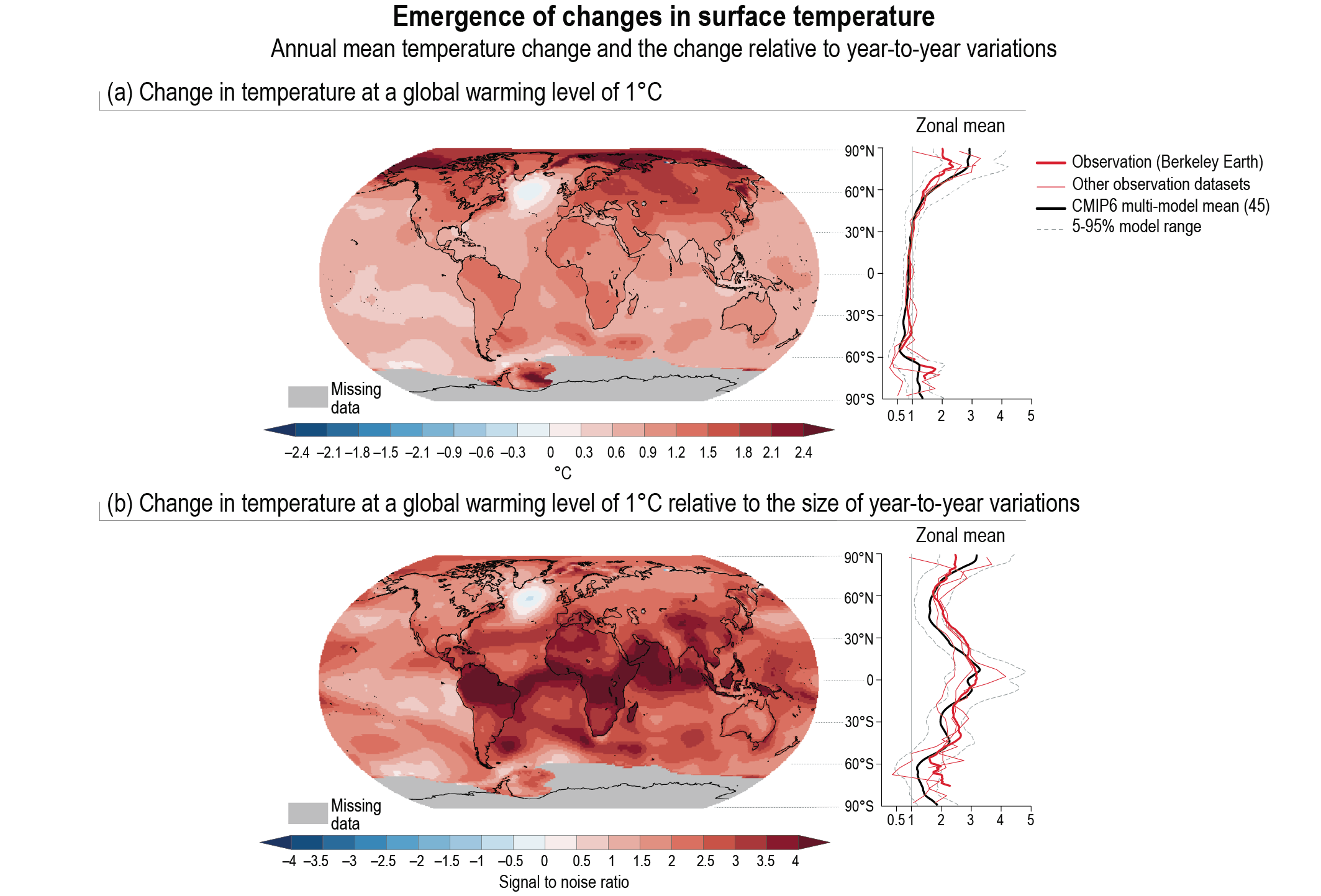
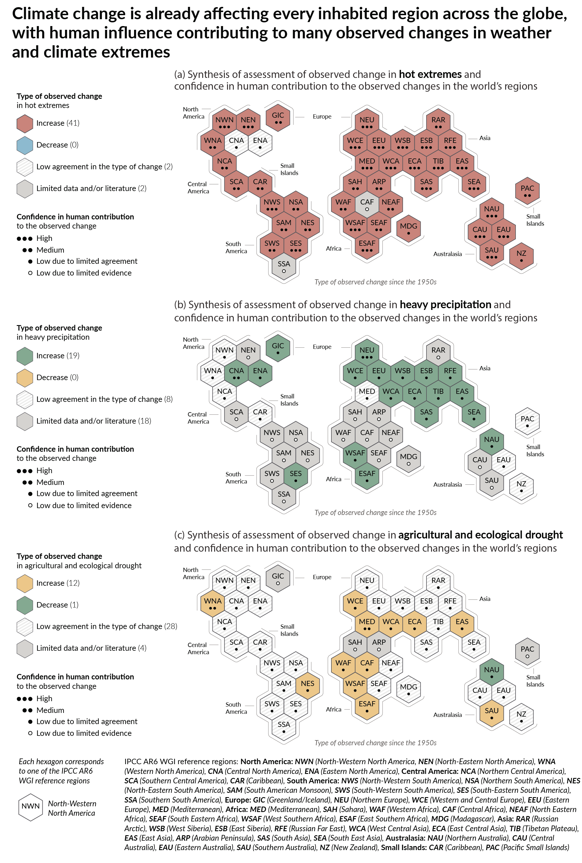
Mean temperatures and heat extremes have emerged above natural variability in almost all land regions with high confidence. Changes in temperature-related variables, such as regional temperatures, growing season length, extreme heat and frost, have already occurred, and there is medium confidence that many of these changes are attributable to human activities. Several impact-relevant changes have not yet emerged from natural variability but will emerge sooner or later in this century depending on the emissions scenario (high confidence). Ocean acidification and deoxygenation have already emerged over most of the global open ocean, as has a reduction in Arctic sea ice (high confidence). Links to chapters9.3.1, 9.6.4, 11.2, 11.3, 12.4, 12.5, Atlas.3–Atlas.11
TS.1.2.4 Understanding of Human Influence
Combining the evidence from across the climate system increases the level of confidence in the attribution of observed climate change to human influence and reduces the uncertainties associated with assessments based on single variables. Links to chaptersCross-Chapter Box 10.3
Since AR5, the accumulation of energy in the Earth system has become established as a robust measure of the rate of global climate change on interannual-to-decadal time scales. The rate of accumulation of energy is equivalent to Earth’s energy imbalance and can be quantified by changes in the global energy inventory for all components of the climate system, including global ocean heat uptake, warming of the atmosphere, warming of the land and melting of ice. Compared to changes in global surface temperature, Earth’s energy imbalance (see Core Concepts Box) exhibits less variability, enabling more accurate identification and estimation of trends. Links to chaptersBox 7.2 and Section 7.2
Identifying the human-induced components contributing to the energy budget provides an implicit estimate of the human influence on global climate change (Sections TS.2 and TS.3.1). Links to chaptersCross-Working Group Box: Attribution in Chapter 1, 3.8, 7.2.2, Box 7.2, Cross-Chapter Box 9.1
Regional climate changes can be moderated or amplified by regional forcing from land-use and land-cover changes or from aerosol concentrations and other short-lived climate forcers (SLCFs). For example, the difference in observed warming trends between cities and their surroundings can partly be attributed to urbanization (very high confidence). While established attribution techniques provide confidence in our assessment of human influence on large-scale climate changes (as described in Section TS.2), new techniques developed since AR5, including attribution of individual events, have provided greater confidence in attributing changes in climate extremes to climate change (Box TS.10). Multiple attribution approaches support the contribution of human influence to several regional multi-decadal mean precipitation changes (high confidence). Understanding about past and future changes in weather and climate extremes has increased due to better observation-based datasets, physical understanding of processes, an increasing proportion of scientific literature combining different lines of evidence, and improved accessibility to different types of climate models (high confidence) (see Sections TS.2 and TS.4). Links to chaptersCross-Working Group Box: Attribution in Chapter 1, 1.5, 3.2, 3.5, 5.2, 6.4.3, 8.3, 9.6, 10.1, 10.2, 10.3.3, 10.4.1, 10.4.2, 10.4.3, 10.5, 10.6, Cross-Chapter Box 10.3, Box 10.3, 11.1.6, 11.2–11.9, 12.4
TS.1.3 Assessing Future Climate Change
Various frameworks can be used to assess future climatic changes and to synthesize knowledge across climate change assessment in WGI, WGII and WGIII. These frameworks include: (i) scenarios, (ii) global warming levels and (iii) cumulative CO2 emissions (see Core Concepts Box). The latter two offer scenario- and path-independent approaches to assess future projections. Additional choices, for instance with regard to common reference periods and time windows for which changes are assessed, can further help to facilitate integration across the WGI report and across the whole AR6 (see Section TS.1.1). Links to chapters1.4.1, 1.6, Cross-Chapter Box 1.4, 4.2.2, 4.2.4, Cross-Chapter Box 11.1
TS.1.3.1 Climate Change Scenarios
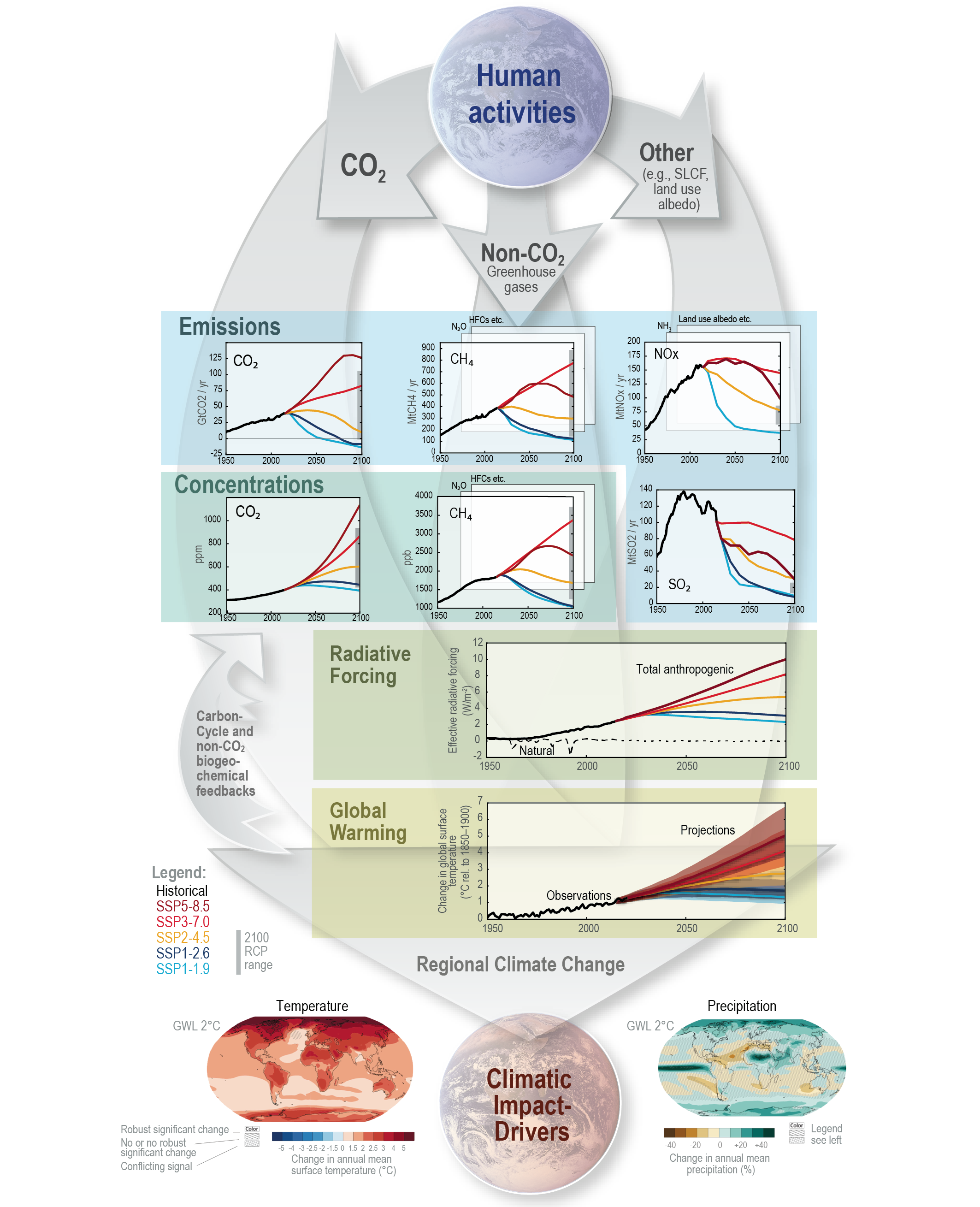
Climate change projections with climate models require information about future emissions or concentrations of greenhouse gases, aerosols, ozone-depleting substances, and land use over time (Figure TS.4). This information can be provided by scenarios, which are internally consistent projections of these quantities based on assumptions of how socio-economic systems could evolve over the 21st century. Emissions from natural sources, such as the ocean and the land biosphere, are usually assumed to be constant, or to evolve in response to changes in anthropogenic forcings or to projected climate change. Natural forcings, such as past changes in solar irradiance and historical volcanic eruptions, are represented in model simulations covering the historical era. Future simulations assessed in this Report account for projected changes in solar irradiance and for the long-term mean background forcing from volcanoes, but not for individual volcanic eruptions. Scenarios have a long history in IPCC as a method for systematically examining possible futures and following the cause–effect chain: from anthropogenic emissions, to changes in atmospheric concentrations, to changes in Earth’s energy balance (‘forcing’), to changes in global climate and ultimately regional climate and climatic impact-drivers (Figure TS.4, Section TS.2, Infographic TS.1). Links to chapters1.5.4, 1.6.1, 4.2.2, 4.4.4, Cross-Chapter Box 4.1, 11.1
The uncertainty in climate change projections that results from assessing alternative socio-economic futures, the so-called scenario uncertainty, is explored through the use of scenario sets. Designed to span a wide range of possible future conditions, these scenarios do not intend to match how events actually unfold in the future, and they do not account for impacts of climate change on the socio-economic pathways. Besides scenario uncertainty, climate change projections are also subject to climate response uncertainty (i.e., the uncertainty related to our understanding of the key physical processes and structural uncertainties in climate models) and irreducible and intrinsic uncertainties related to internal variability. Depending on the spatial and temporal scales of the projection, and on the variable of interest, the relative importance of these different uncertainties may vary substantially. Links to chapters1.4.3, 1.6, 4.2.5, Box 4.1, 8.5.1
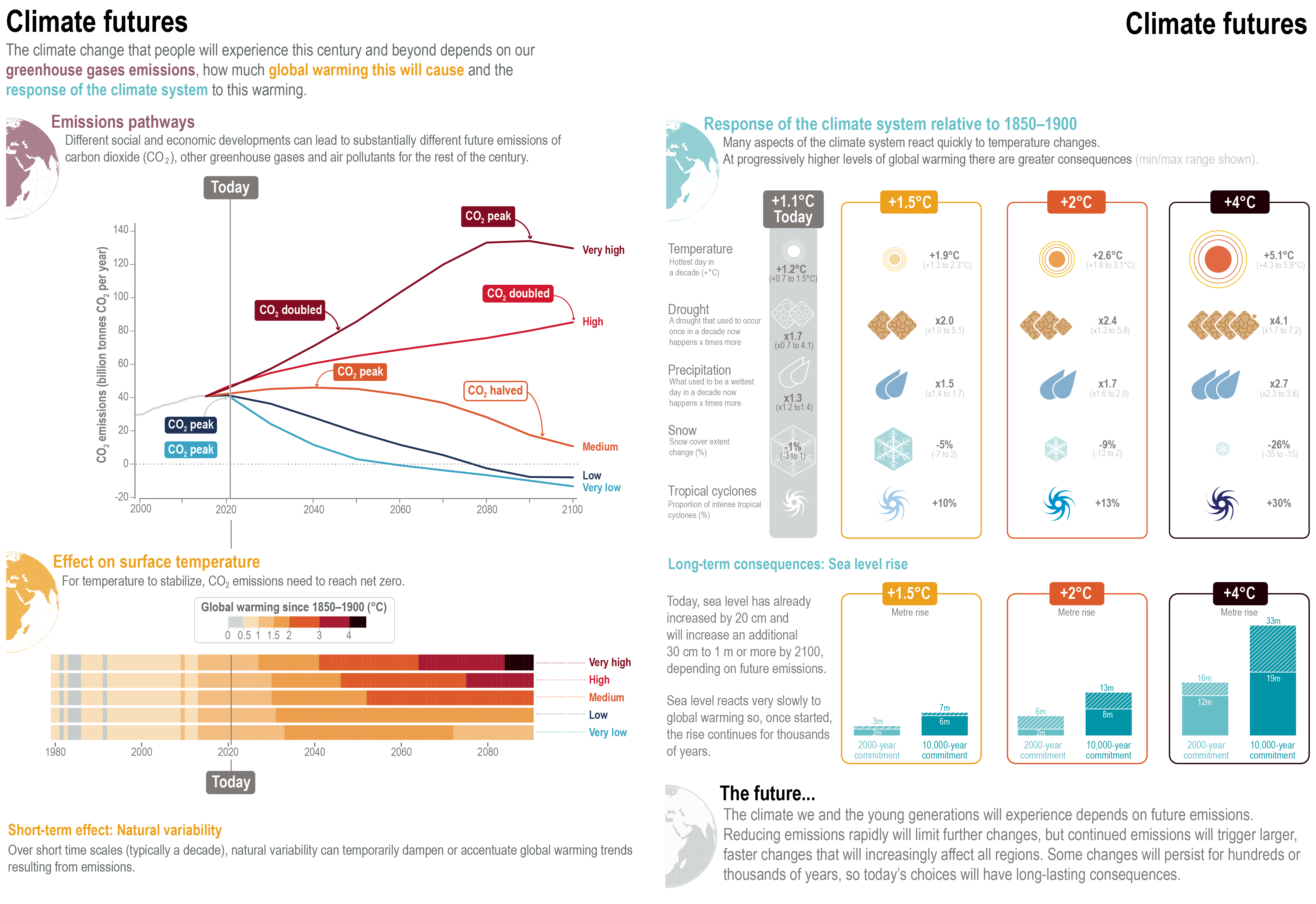
Scenarios in AR6 cover a broader range of emissions futures than considered in AR5, including high CO2 emissions scenarios without climate change mitigation as well as a low CO2 emissions scenario reaching net zero CO2 emissions (see Core Concepts Box) around mid-century. In this Report, a core set of five illustrative scenarios is used to explore climate change over the 21st century and beyond (Section TS.2). They are labelled SSP1-1.9, SSP1-2.6, SSP2-4.5, SSP3-7.0, and SSP5-8.517 and span a wide range of radiative forcing levels in 2100. They start in 2015 and include scenarios with high and very high GHG emissions and CO2 emissions that roughly double from current levels by 2100 and 2050, respectively (SSP3-7.0 and SSP5-8.5); scenarios with intermediate GHG emissions and CO2 emissions remaining around current levels until the middle of the century (SSP2-4.5); and scenarios with very low and low GHG emissions and CO2 emissions declining to net zero around or after 2050, followed by varying levels of net negative CO2 emissions (SSP1-1.9 and SSP1-2.6). These SSP scenarios offer unprecedented detail of input data for ESM simulations and allow for a more comprehensive assessment of climate drivers and responses, in particular because some aspects, such as the temporal evolution of pollutants, emissions or changes in land use and land cover, span a broader range in the SSP scenarios than in the RCPs used in AR5. Modelling studies utilizing the RCPs complement the assessment based on SSP scenarios, for example, at the regional scale (Section TS.4). Scenario extensions are based on assumptions about the post-2100 evolution of emissions or of radiative forcing that are independent from the modelling of socio-economic dynamics, which does not extend beyond 2100. To explore specific dimensions, such as air pollution or temporary overshoot of a given warming level, scenario variants are used in addition to the core set. Links to chapters1.6.1, Cross-Chapter Box 1.4, 4.2.2, 4.2.6, 4.7.1, Cross-Chapter Box 7.1
SSP1-1.9 represents the low end of future emissions pathways, leading to warming below 1.5°C in 2100 and limited temperature overshoot of 1.5°C over the course of the 21st century (see Figure TS.6). At the opposite end of the range, SSP5-8.5 represents the very high warming end of future emissions pathways from the literature. SSP3-7.0 has overall lower GHG emissions than SSP5-8.5 but, for example, CO2 emissions still almost double by 2100 compared to today’s levels. SSP2-4.5 and SSP1-2.6 represent scenarios with stronger climate change mitigation and thus lower GHG emissions. SSP1-2.6 was designed to limit warming to below 2°C. Infographic TS.1 presents a narrative depiction of SSP-related climate futures. No likelihood is attached to the scenarios assessed in this Report, and the feasibility of specific scenarios in relation to current trends is best informed by the WGIII contribution to AR6. In the scenario literature, the plausibility of some scenarios with high CO2 emissions, such as RCP8.5 or SSP5-8.5, has been debated in light of recent developments in the energy sector. However, climate projections from these scenarios can still be valuable because the concentration levels reached in RCP8.5 or SSP5-8.5 and corresponding simulated climate futures cannot be ruled out. That is because of uncertainty in carbon-cycle feedbacks which, in nominally lower emissions trajectories, can result in projected concentrations that are higher than the central concentration levels typically used to drive model projections. Links to chapters1.6.1; Cross-Chapter Box 1.4; 4.2.2, 5.4; SROCC; Chapter 3 in WGIII
The socio-economic narratives underlying SSP-based scenarios differ in their assumed level of air pollution control. Together with variations in climate change mitigation stringency, this difference strongly affects anthropogenic emissions trajectories of SLCFs, some of which are also air pollutants. SSP1 and SSP5 assume strong pollution control, projecting a decline of global emissions of ozone precursors (except methane; CH4) and of aerosols and most of their precursors in the mid- to long term. The reductions due to air pollution controls are further strengthened in scenarios that assume a marked decarbonization, such as SSP1-1.9 or SSP1-2.6. SSP2-4.5 is a medium pollution-control scenario with air pollutant emissions following current trends, and SSP3-7.0 is a weak pollution-control scenario with strong increases in emissions of air pollutants over the 21st century. Methane emissions in SSP-based scenarios vary with the overall climate change mitigation stringency, declining rapidly in SSP1-1.9 and SSP1-2.6 but declining only after 2070 in SSP5-8.5. SSP trajectories span a wider range of air pollutant emissions than considered in the RCP scenarios (see Figure TS.4), reflecting the potential for large regional differences in their assumed pollution policies. Their effects on climate and air pollution are assessed in Box TS.7. Links to chapters4.4.4, 6.6.1, Figure 6.4, 6.7.1, Figure 6.19
Since the RCPs are also labelled by the level of radiative forcing they reach in 2100, they can in principle be related to the core set of AR6 scenarios (Figure TS.4). However, the RCPs and SSP-based scenarios are not directly comparable. First, the gas-to-gas compositions differ; for example, the SSP5-8.5 scenario has higher CO2 but lower CH4 concentrations compared to RCP8.5. Second, the projected 21st-century trajectories may differ, even if they result in the same radiative forcing by 2100. Third, the overall effective radiative forcing (see Core Concepts Box) may differ, and tends to be higher for the SSPs compared to RCPs that share the same nominal stratospheric-temperature-adjusted radiative forcing label. Comparing the differences between CMIP5 and CMIP6 projections (Cross-Section Box TS.1) that were driven by RCPs and SSP-based scenarios, respectively, indicates that about half of the difference in simulated warming arises because of higher climate sensitivity being more prevalent in CMIP6 model versions; the remainder arises from higher ERF in nominally corresponding scenarios (e.g., RCP8.5 and SSP5-8.5; medium confidence) (see Section TS.1.2.2). In SSP1-2.6 and SSP2-4.5, changes in ERF also explain about half of the changes in the range of warming (medium confidence). For SSP5-8.5, higher climate sensitivity is the primary reason behind the upper end of the CMIP6-projected warming being higher than for RCP8.5 in CMIP5 (medium confidence). Note that AR6 uses multiple lines of evidence beyond CMIP6 results to assess global surface temperature under various scenarios (see Cross-Section Box TS.1 for the detailed assessment). Links to chapters1.6, 4.2.2, 4.6.2.2, Cross-Chapter Box 7.1
Earth system models can be driven by anthropogenic CO2 emissions (‘emissions-driven’ runs), in which case atmospheric CO2 concentration is a projected variable; or by prescribed time-varying atmospheric concentrations (‘concentration-driven’ runs). In emissions-driven runs, changes in climate feed back on the carbon cycle and interactively modify the projected CO2 concentration in each ESM, thus adding the uncertainty in the carbon cycle response to climate change to the projections. Concentration-driven simulations are based on a central estimate of carbon cycle feedbacks, while emissions-driven simulations help quantify the role of feedback uncertainty. The differences in the few ESMs for which both emissions and concentration-driven runs were available for the same scenario are small and do not affect the assessment of global surface temperature projections discussed in Cross-Section Box TS.1 and Section TS.2 (high confidence). By the end of the 21st century, emissions-driven simulations are on average around 0.1°C cooler than concentration-driven runs, reflecting the generally lower CO2 concentrations simulated by the emissions-driven ESMs, and have a spread about 0.1°C greater, reflecting the range of simulated CO2 concentrations. However, these carbon cycle–climate feedbacks do affect the transient climate response to cumulative CO2 emissions (TCRE18), and their quantification is crucial for the assessment of remaining carbon budgets consistent with global warming levels simulated by ESMs (see Section TS.3). Links to chapters1.6.1, Cross-Chapter Box 1.4, 4.2, 4.3.1, 5.4.5, Cross-Chapter Box 7.1
TS.1.3.2 Global Warming Levels and Cumulative CO2 Emissions
For many indicators of climate change, such as seasonal and annual mean and extreme surface air temperatures and precipitation, the geographical patterns of changes are well estimated by the level of global surface warming, independently of the details of the emissions pathways that caused the warming, or the time at which the level of warming is attained. GWLs, defined as a global surface temperature increase of, for example, 1.5°C or 2°C relative to the mean of 1850–1900, are therefore a useful way to integrate climate information independently of specific scenarios or time periods. Links to chapters1.6.2, 4.2.4, 4.6.1, 11.2.4, Cross-Chapter Box 11.1
The use of GWLs allows disentangling the contribution of changes in global warming from regional aspects of the climate response, as scenario differences in response patterns at a given GWL are often smaller than model uncertainty and internal variability. The relationship between the GWL and response patterns is often linear, but integration of information can also be done for non-linear changes, like the frequency of heat extremes. The requirement is that the relationship to the GWL is broadly independent of the scenario and relative contribution of radiative forcing agents. Links to chapters1.6, 11.2.4, Cross-Chapter Box 11.1
The GWL approach to integration of climate information also has some limitations. Variables that are quick to respond to warming, like temperature and precipitation, including extremes, sea ice area, permafrost and snow cover, show little scenario dependence for a given GWL, whereas slow-responding variables such as glacier and ice-sheet mass, warming of the deep ocean and their contributions to sea level rise, have substantial dependency on the trajectory of warming taken to reach the GWL. A given GWL can also be reached for different balances between anthropogenic forcing agents, such as long-lived greenhouse gas and SLCF emissions, and the response patterns may depend on this balance. Finally, there is a difference in the response even for temperature-related variables if a GWL is reached in a rapidly warming transient state or in an equilibrium state when the land–sea warming contrast is less pronounced. In this Report, the climate responses at different GWLs are calculated based on climate model projections for the 21st century (see Figure TS.5), which are mostly not in equilibrium. The SSP1-1.9 scenario allows assessing the response to a GWL of about 1.5°C after a (relatively) short-term stabilization by the end of the 21st century. Links to chapters4.6.2, 9.3.1.1, 9.5.2.3, 9.5.3.3, 11.2.4, Cross-Chapter Box 11.1, Cross-Chapter Box 12.1
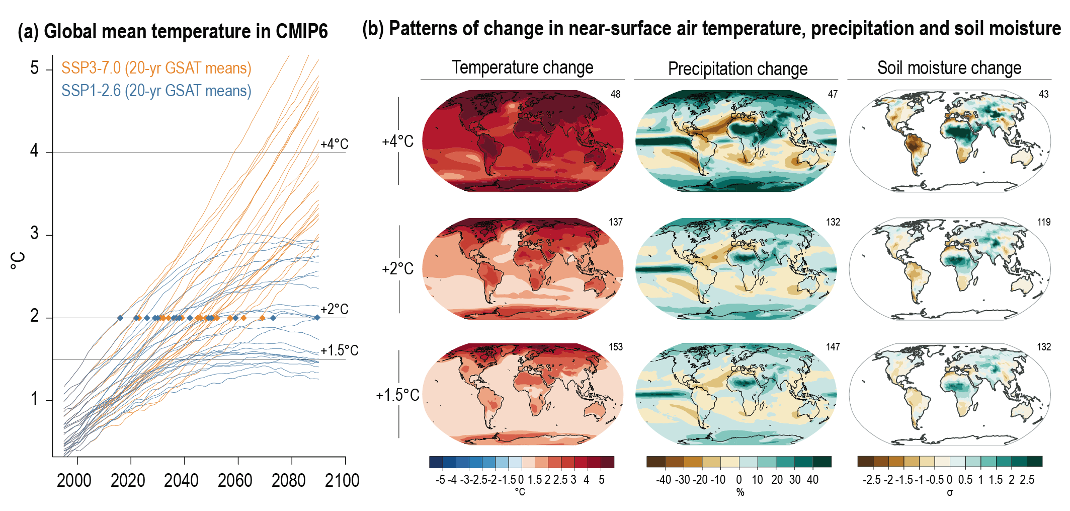 Figure TS.5 | Scenarios, global warming levels, and patterns of change. The intent of this figure is to show how scenarios are linked to global warming levels (GWLs) and to provide examples of the evolution of patterns of change with global warming levels. (a) Illustrative example of GWLs defined as global surface temperature response to anthropogenic emissions in unconstrained Coupled Model Intercomparison Project Phase 6 (CMIP6) simulations, for two illustrative scenarios (SSP1-2.6 and SSP3-7.0). The time when a given simulation reaches a GWL, for example, +2°C, relative to 1850–1900 is taken as the time when the central year of a 20-year running mean first reaches that level of warming. See the dots for +2°C, and how not all simulations reach all levels of warming. The assessment of the timing when a GWL is reached takes into account additional lines of evidence and is discussed in Cross-Section Box TS.1. (b) Multi-model, multi-simulation average response patterns of change in near-surface air temperature, precipitation (expressed as percentage change) and soil moisture (expressed in standard deviations of interannual variability) for three GWLs. The number to the top right of the panels shows the number of model simulations averaged across including all models that reach the corresponding GWL in any of the five Shared Socio-economic Pathways (SSPs). See Section TS.2 for discussion. Links to chaptersCross-Chapter Box 11.1
 Global warming levels are highly relevant as a dimension of integration across scientific disciplines and socio-economic actors and are motivated by the long-term goal in the Paris Agreement of ‘holding the increase in the global average temperature to well below 2°C above pre-industrial levels and to pursue efforts to limit the temperature increase to 1.5°C above pre-industrial levels’. The evolution of aggregated impacts with temperature levels has also been widely used and embedded in the WGII assessment. This includes the ‘Reasons for Concern’ (RFC) and other ‘burning ember’ diagrams in IPCC WGII. The RFC framework has been further expanded in SR1.5, SROCC and SRCCL by explicitly looking at the differential impacts between half-degree GWLs and the evolution of risk for different socio-economic assumptions. Links to chapters1.4.4, 1.6.2, 11.2.4, 12.5.2, Cross-Chapter Box 11.1, Cross-Chapter Box 12.1
SR1.5 concluded that ‘climate models project robust differences in regional climate characteristics between present-day and global warming of 1.5°C, and between 1.5°C and 2°C’. This Report adopts a set of common GWLs across which climate projections, impacts, adaptation challenges and climate change mitigation challenges can be integrated, within and across the three Working Groups, relative to 1850–1900. The core set of GWLs in this Report are 1.0°C (close to present day conditions), 1.5°C, 2.0°C, 3.0°C and 4.0°C. Links to chapters1.4, 1.6.2, Cross-Chapter Box 1.2, Table 1.5, Cross-Chapter Box 11.1
Connecting Scenarios and Global Warming Levels
In this Report, scenario-based climate projections are translated into GWLs by aggregating the ESM model response at specific GWLs across scenarios (see Figure TS.5 and Figure TS.6). The climate response pattern for the 20-year period around when individual simulations reach a given GWL are averaged across all models and scenarios that reach that GWL. The best estimate and likely range of the timing of when a certain GWL is reached under a particular scenario (or ‘GWL-crossing time’), however, is based not only on CMIP6 output, but on a combined assessment taking into account the observed warming to date, CMIP6 output and additional lines of evidence (see Cross-Section Box TS.1). Links to chapters4.3.4, Cross-Chapter Box 11.1, Atlas.2, Interactive Atlas
Global warming levels are closely related to cumulative CO2 (and in some cases CO2-equivalent) emissions. This Report confirms the assessment of the WGI contribution to AR5 and SR1.5 that a near-linear relationship exists between cumulative CO2 emissions and the resulting increase in global surface temperature (Section TS.3.2). This implies that continued CO2 emissions will cause further warming and associated changes in all components of the climate system. For declining cumulative CO2 emissions (i.e., if negative net emissions are achieved), the relationship is less strong for some components, such as the hydrological cycle. The WGI report uses cumulative CO2 emissions to compare climate response across scenarios and provides a link to the emissions pathways assessment in WGIII. The advantage of using cumulative CO2 emissions is that it is an inherent emissions scenario characteristic rather than an outcome of the scenario-based projections, where uncertainties in the cause–effect chain from emissions to temperature change are important (Figure TS.4), for example, the uncertainty in ERF and TCR. Cumulative CO2 emissions can also provide a link to the assessments of mitigation options. Cumulative CO2 emissions do not carry information about non-CO2 emissions, although these can be included with specific emissions metrics to estimate CO2-equivalent emissions. (Section TS.3.3) Links to chapters1.3.2, 1.6, 4.6.2, 5.5, 7.6
TS.1.4 From Global to Regional Climate Information for Impact and Risk Assessment
Climate change is a global phenomenon, but manifests differently in different regions. The impacts of climate change are generally experienced at local, national and regional scales, and these are also the scales at which decisions are typically made. Robust climate change information is increasingly available at regional scales for impact and risk assessments. Depending on the climate information context, geographical regions in AR6 may refer to larger areas, such as sub-continents and oceanic regions, or to typological regions, such as monsoon regions, coastlines, mountain ranges or cities, as used in Section TS.4. A new set of standard AR6 WGI reference regions has also been included in this Report (Figure TS.6, bottom panels). Links to chapters1.4.5, 10.1, 11.9, 12.1–12.4, Atlas.1.3.3–1.3.4
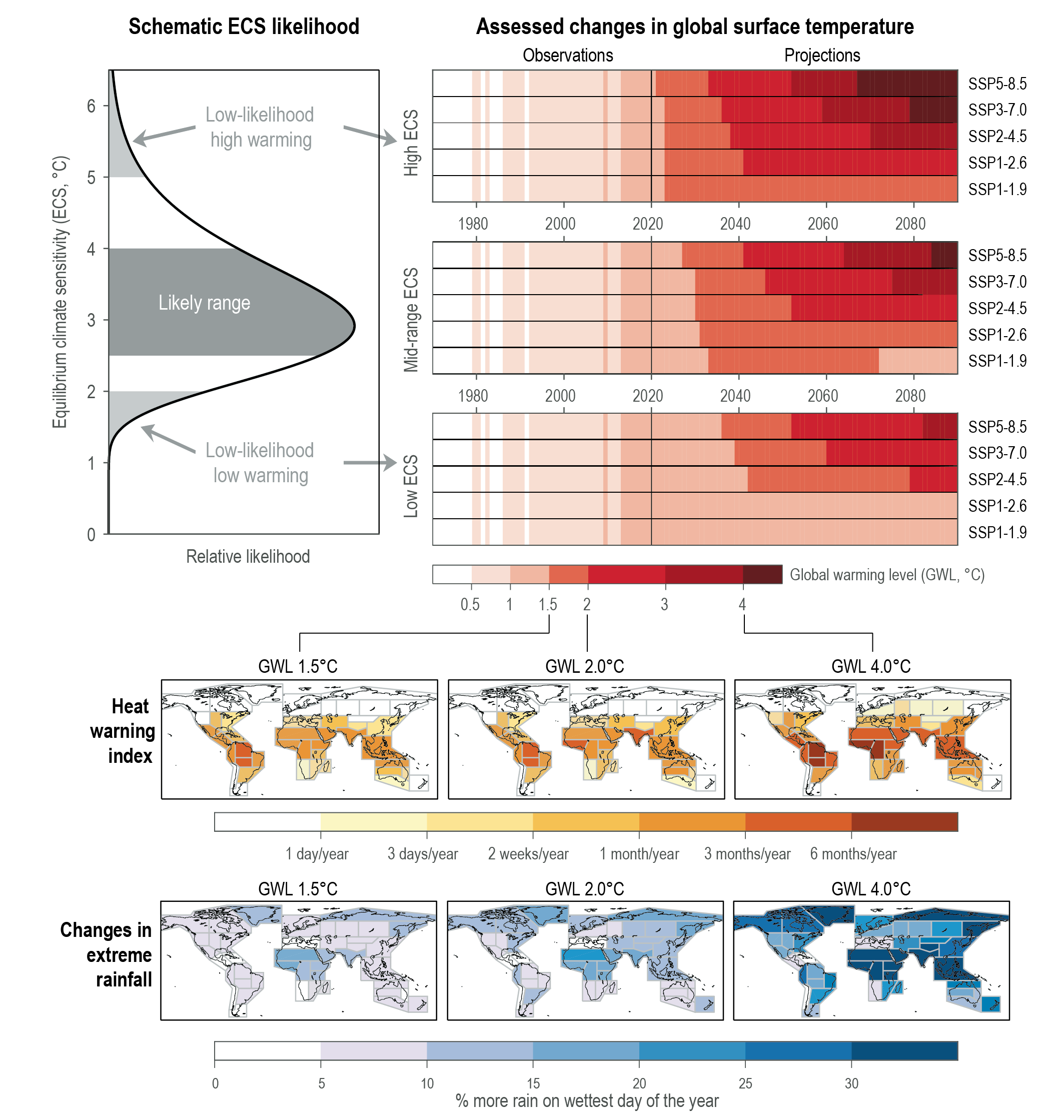
Global and regional climate models are important sources of climate information at the regional scale. Since AR5, a more comprehensive assessment of past and future evolution of a range of climate variables on a regional scale has been enabled by the increased availability of coordinated ensemble regional climate model projections and improvements in the level of sophistication and resolution of global and regional climate models. This has been complemented by observational, attribution and sectoral-vulnerability studies informing, for instance, about impact-relevant tolerance thresholds. Links to chapters10.3.3, 11.9, 12.1, 12.3, 12.6, Atlas.3–Atlas.11
Multiple lines of evidence derived from observations, model simulations and other approaches can be used to construct climate information on a regional scale as described in detail in Sections TS.4.1.1 and TS.4.1.2. Depending on the phenomena and specific context, these sources and methodologies include theoretical understanding of the relevant processes, drivers and feedbacks of climate at regional scale; trends in observed data from multiple datasets; and the attribution of these trends to specific drivers. Furthermore, simulations from different model types (including global and regional climate models, emulators, statistical downscaling methods, etc.) and experiments (e.g., CMIP, CORDEX, and large ensembles of single-model simulations with different initial conditions), attribution methodologies and other relevant local knowledge (e.g., indigenous knowledge) are utilized (see Box TS.11). Links to chapters1.5.3, 1.5.4, Cross-Chapter Box 7.1, 10.2–10.6, 11.2, Atlas.1.4, Cross-Chapter Box 10.3
From the multiple lines of evidence, climate information can be distilled in a co-production process that involves users, related stakeholders and producers of climate information, considering the specific context of the question at stake, the underlying values and the challenge of communicating across different communities. The co-production process is an essential part of climate services, which are discussed in Section TS.4.1.2. Links to chapters10.5, 12.6, Cross-Chapter Box 12.2
With the aim of informing decision-making at local or regional scales, a common risk framework has been implemented in AR6. Methodologies have been developed to construct more impact- and risk-relevant climate change information tailored to regions and stakeholders. Physical storyline approaches are used in order to build climate information based on multiple lines of evidence, and which can explicitly address physically plausible, but low-likelihood, high-impact outcomes and uncertainties related to climate variability for consideration in risk assessments (Figure TS.6). Links to chaptersCross-Chapter Box 1.3, 4.8, Box 9.4, 10.5, Box 10.2, Box 11.2, 12.1–12.3, 12.6, Glossary
The climatic impact-driver framework developed in AR6 supports an assessment of changing climate conditions that are relevant for sectoral impacts and risk assessment. Climatic impact-drivers (CIDs) are physical climate system conditions (e.g., means, extremes, events) that affect an element of society or ecosystems and are thus a potential priority for providing climate information. For instance, the heat index used by the U.S. National Oceanic and Atmospheric Administration (NOAA HI) for issuing heat warnings is a CID index that can be associated with adverse human health impacts due to heat stress (see Figure TS.6). Depending on system tolerance, CIDs and their changes can be detrimental (i.e., hazards in the risk framing), beneficial, neutral, or a mixture of each across interacting system elements, regions and sectors (aligning with WGII Sectoral Chapters 2–8). Each sector is affected by multiple CIDs, and each CID affects multiple sectors. Climate change has already altered CID profiles and resulted in shifting magnitude, frequency, duration, seasonality and spatial extent of associated indices (high confidence) (see regional details in Section TS.4.3). Links to chapters12.1–12.4, Table 12.1, Table 12.2, Annex VI
Many global- and regional-scale CIDs, including extremes, have a direct relation to global warming levels (GWLs) and can thus inform the hazard component of ‘Representative Key Risks’ and ‘Reasons for Concern’ assessed by AR6 WGII. These include heat, cold, wet and dry hazards, both mean and extremes; cryospheric hazards (snow cover, ice extent, permafrost) and oceanic hazards (marine heatwaves) (high confidence) (Figure TS.6). Establishing links between specific GWLs with tipping points and irreversible behaviour is challenging due to model uncertainties and lack of observations, but their occurrence cannot be excluded, and their likelihood of occurrence generally increases at greater warming levels (Box TS.1, Section TS.9). Links to chapters11.2.4, Box 11.2, Cross-Chapter Boxes 11.1 and 12.1
Cross-Section Box TS.1: Global Surface Temperature Change
This box synthesizes the outcomes of the assessment of past, current and future global surface temperature. Global mean surface temperature (GMST) and global surface air temperature (GSAT) are the two primary metrics of global surface temperature used to estimate global warming in IPCC reports. GMST merges sea surface temperature (SST) over the ocean and 2 m air temperature over land and sea ice areas and is used in most paleo, historical and present-day observational estimates. The GSAT metric is 2 m air temperature over all surfaces and is the diagnostic generally used from climate models. Changes in GMST and GSAT over time differ by at most 10% in either direction (high confidence), but conflicting lines of evidence from models and direct observations, combined with limitations in theoretical understanding, lead to low confidence in the sign of any difference in long-term trend. Therefore, long-term changes in GMST/GSAT are presently assessed to be identical, with expanded uncertainty in GSAT estimates. Hence the term global surface temperature is used in reference to both quantities in the text of the TS and SPM. Links to chaptersCross-Chapter Box 2.3
Surface Temperature History
Dataset innovations, particularly more comprehensive representation of polar regions, and the availability of new datasets have led to an assessment of increased global surface temperature change relative to the directly equivalent estimates reported in AR5. The contribution of changes in observational understanding alone between AR5 and AR6 in assessing temperature changes from 1850–1900 to 1986–2005 is estimated at 0.08 [–0.01 to 0.12] °C. Global surface temperature increased from 1850–1900 to 1995–2014 by 0.85 [0.69 to 0.95] °C, between 1850–1900 and the first two decades of the 21st century (2001–2020) by 0.99 [0.84 to 1.20] °C, and to the most recent decade (2011–2020) by 1.09 [0.95 to 1.20] °C. Each of the last four decades has in turn been warmer than any decade that preceded it since 1850. Temperatures have increased faster over land than over the ocean since 1850–1900, with warming to 2011–2020 of 1.59 [1.34 to 1.83] °C over land and 0.88 [0.68 to 1.01] °C over the ocean. Links to chapters2.3.1, Cross-Chapter Box 2.3
Global surface temperature during the period 1850–1900 is used as an approximation for pre-industrial conditions for consistency with AR5 and AR6 Special Reports, whilst recognizing that radiative forcings have a baseline of 1750 for the start of anthropogenic influences. It is likely that there was a net anthropogenic forcing of 0.0–0.3 Wm–2 in 1850–1900 relative to 1750 (medium confidence), and from the period around 1750 to 1850–1900, there was a change in global surface temperature of around 0.1°C (likely range –0.1 to +0.3°C, medium confidence), with an anthropogenic component of 0.0°C to 0.2°C (likely range , medium confidence). Links to chaptersCross-Chapter Box 1.2, 7.3.5
Global surface temperature has evolved over geological time (Figure TS.1, Box TS.2). Beginning approximately 6500 years ago, global surface temperature generally decreased, culminating in the coldest multi-century interval of the post-glacial period (since roughly 7000 years ago), which occurred between around 1450 and 1850 (high confidence). Over the last 50 years, global surface temperature has increased at an observed rate unprecedented in at least the last two thousand years (high confidence). Temperatures as high as during the most recent decade (2011–2020) exceed the warmest centennial-scale range reconstructed for the present interglacial, around 6500 years ago [0.2°C to 1°C] (medium confidence). The next most recent warm period was about 125,000 years ago during the Last Interglacial when the multi-centennial temperature range [0.5°C to 1.5°C] encompasses the 2011–2020 values (medium confidence) (Cross-Section Box TS.1, Figure 1). During the mid-Pliocene Warm Period, around 3.3–3.0 million years ago, global surface temperature was 2.5°C to 4°C warmer (medium confidence). Links to chapters2.3.1, Cross-Chapter Box 2.1 and 2.4
Current Warming
There is very high confidence that the CMIP6 model ensemble reproduces observed global surface temperature trends and variability since 1850 with errors small enough to allow for detection and attribution of human-induced warming. The CMIP6 multi-model mean global surface warming between 1850–1900 and 2010–2019 is close to the best estimate of observed warming, though some CMIP6 models simulate a warming that is outside the assessed very likely observed range. Links to chapters3.3.1
The likely range of human-induced change in global surface temperature in 2010–2019 relative to 1850–1900 is 0.8°C to 1.3°C, with a central estimate of 1.07°C (Figure Cross-Section Box TS.1, Figure 1), encompassing the best estimate of observed warming for that period, which is 1.06°C with avery likely range of [0.88°C to 1.21°C], while the likely range of the change attributable to natural forcing is only –0.1°C to +0.1°C. This assessment is consistent with an estimate of the human-induced global surface temperature rise based on assessed ranges of perturbations to the top of the atmosphere (effective radiative forcing) and with metrics of feedbacks of the climate response (equilibrium climate sensitivity and the transient climate response). Over the same period, well-mixed greenhouse gas forcing likely warmed global surface temperature by 1.0°C to 2.0°C, while aerosols and other anthropogenic forcings likely cooled global surface temperature by 0.0°C to 0.8°C. Links to chapters2.3.1, 3.3.1, 7.3.5, Cross-Chapter Box 7.1
The observed slower increase in global surface temperature (relative to preceding and following periods) in the 1998–2012 period, sometimes referred to as ‘the hiatus’, was temporary (very high confidence). The increase in global surface temperature during the 1998–2012 period is also greater in the data sets used in the AR6 assessment than in those available at the time of AR5. Using these updated observational data sets and a like-for-like consistent comparison of simulated and observed global surface temperature, all observed estimates of the 1998–2012 trend lie within the very likely range of CMIP6 trends. Furthermore, the heating of the climate system continued during this period, as reflected in the continued warming of the global ocean (very high confidence) and in the continued rise of hot extremes over land (medium confidence). Since 2012, global surface temperature has risen strongly, with the past five years (2016–2020) being the hottest five-year period between 1850 and 2020 (high confidence). Links to chapters2.3.1, 3.3.1, 3.5.1, Cross-Chapter Box 3.1
Future Changes in Global Surface Temperature
The AR6 assessment of future change in global surface temperature is, for the first time in an IPCC report, explicitly constructed by combining new projections for the SSP scenarios with observational constraints based on past simulated warming as well as the AR6-updated assessment of equilibrium climate sensitivity and transient climate response. In addition, climate forecasts initialized from the observed climate state have been used for the period 2019–2028. The inclusion of additional lines of evidence has reduced the assessed uncertainty ranges for each scenario (Cross-Section Box TS.1, Figure 1). Links to chapters4.3.1, 4.3.4, Box 4.1, 7.5
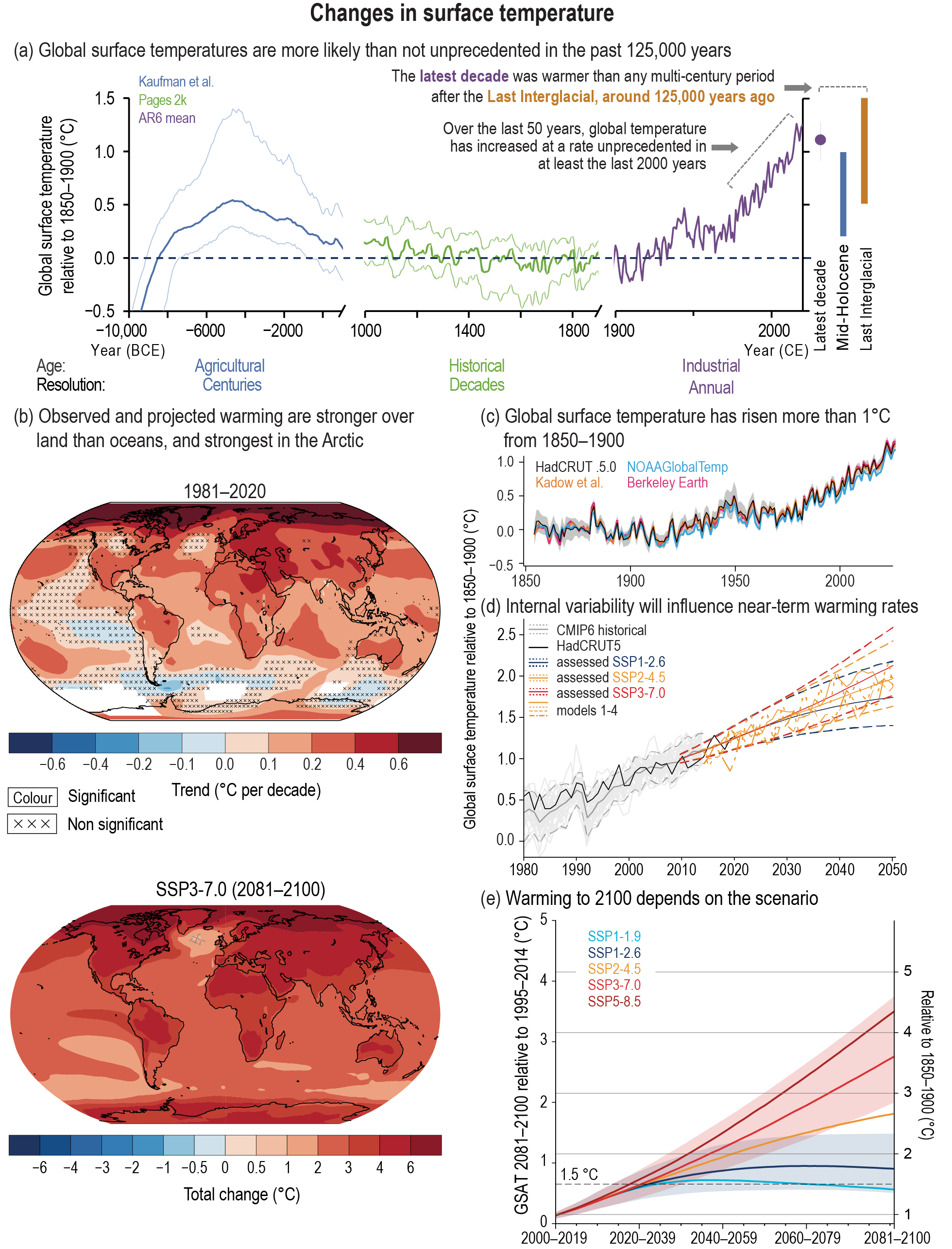
Cross-Section Box TS.1, Figure 1 | Earth’s surface temperature history and future with key findings annotated within each panel. The intent of this figure is to show global surface temperature observed changes from the Holocene to now, and projected changes. (a) Global surface temperature over the Holocene divided into three time scales: (i) 12,000 to 1000 years ago (10,000 BCE to 1000 CE) in 100-year time steps, (ii) 1000 to 1900 CE, 10-year smooth, and (iii) 1900 to 2020 CE (mean of four datasets in panel c). Bold lines show the median of the multi-method reconstruction, with 5% and 95% percentiles of the ensemble members (thin lines). Vertical bars are 5–95th percentile ranges of estimated global surface temperature for the Last Interglacial and mid-Holocene (medium confidence) (Section 2.3.1.1). All temperatures are relative to 1850–1900. (b) Spatially resolved trends (°C per decade) for (upper map) HadCRUTv5 over 1981–2020, and (lower map, total change) multi-model mean projected changes from 1995–2014 to 2081–2100 in the SST3-7.0 scenario. Observed trends have been calculated where data are present in both the first and last decade and for at least 70% of all years within the period using ordinary least squares. Significance is assessed with autoregressive AR(1) model correction and denoted by stippling. Hatched areas in the lower map show areas of conflicting model evidence on significance of changes. (c) Temperature from instrumental data for 1850–2020, including annually resolved averages for the four global surface temperature datasets assessed in Section 2.3.1.1.3 (see text for references). The grey shading shows the uncertainty associated with the HadCRUTv5 estimate. All temperatures are relative to the 1850–1900 reference period. (d) Recent past and 2015–2050 evolution of annual mean global surface temperature change relative to 1850–1900, from HadCRUTv5 (black), Coupled Model Intercomparison Project Phase 6 (CMIP6) historical simulations (up to 2014, in grey, ensemble mean solid, 5% and 95% percentiles dashed, individual models thin), and CMIP6 projections under scenario SSP2-4.5, from four models that have an equilibrium climate sensitivity near the assessed central value (thick yellow). Solid thin coloured lines show the assessed central estimate of 20-year change in global surface temperature for 2015–2050 under three scenarios, and dashed thin coloured lines the corresponding 5% and 95% quantiles. (e) Assessed projected change in 20-year running mean global surface temperature for five scenarios (central estimate solid, very likely range shaded for SSP1-2.6 and SSP3-7.0), relative to 1995–2014 (left y-axis) and 1850–1900 (right y-axis). The y-axis on the right-hand side is shifted upward by 0.85°C, the central estimate of the observed warming for 1995–2014, relative to 1850–1900. The right y-axis in (e) is the same as the y-axis in (d). Links to chapters2.3, 4.3, 4.4
During the near term (2021–2040), a 1.5°C increase in global surface temperature, relative to 1850–1900, is very likely to occur in scenario SSP5-8.5, likely to occur in scenarios SSP2-4.5 and SSP3-7.0, and more likely than not to occur in scenarios SSP1-1.9 and SSP1-2.6. The time of crossing a warming level is defined here as the midpoint of the first 20-year period during which the average global surface temperature exceeds the level. In all scenarios assessed here except SSP5-8.5, the central estimate of crossing the 1.5°C level lies in the early 2030s. This is in the early part of the likely range (2030–2052) assessed in SR1.5, which assumed continuation of the then-current warming rate; this rate has been confirmed in the AR6. Roughly half of this difference arises from a larger historical warming diagnosed in AR6. The other half arises because for central estimates of climate sensitivity, most scenarios show stronger warming over the near term than was estimated as ‘current’ in SR1.5 (medium confidence). When considering scenarios similar to SSP1-1.9 instead of linear extrapolation, the SR1.5 estimate of when 1.5°C global warming is crossed is close to the central estimate reported here. (Cross-Section Box TS.1, Table 1) Links to chapters2.3.1, Cross-Chapter Box 2.3, 3.3.1, 4.3.4, Box 4.1
It is more likely than not that under SSP1-1.9, global surface temperature relative to 1850–1900 will remain below 1.6°C throughout the 21st century, implying a potential temporary overshoot of 1.5°C global warming of no more than 0.1°C. If climate sensitivity lies near the lower end of the assessed very likely range, crossing the 1.5°C warming level is avoided in scenarios SSP1-1.9 and SSP1-2.6 (medium confidence). Global surface temperature in any individual year, in contrast to the 20-year average, could by 2030 exceed 1.5°C relative to 1850–1900 with a likelihood between 40% and 60%, across the scenarios considered here (medium confidence). (Cross-Section Box TS.1, Table 1) Links to chapters4.3.4, 4.4.1, Box 4.1, 7.5
During the 21st century, a 2°C increase in global surface temperature relative to 1850–1900 will be crossed under SSP5-8.5 and SSP3-7.0, is extremely likely to be crossed under SSP2-4.5, but is unlikely to be crossed under SSP1-2.6 and extremely unlikely to be crossed under SSP1-1.9. For the mid-term period 2041–2060, this 2°C global warming level is very likely to be crossed under SSP5-8.5, likely to be crossed under SSP3-7.0, and more likely than not to be crossed under SSP2-4.5. (Cross-Section Box TS.1, Table 1) Links to chapters4.3.4
Events of reduced and increased global surface temperature trends at decadal time scales will continue to occur in the 21st century but will not affect the centennial-scale warming (very high confidence). If strong mitigation is applied from 2020 onward as reflected in SSP1-1.9, its effect on 20-year trends in global surface temperature would likely emerge during the near term (2021–2040), measured against an assumed non-mitigation scenario such as SSP3-7.0 or SSP5-8.5. All statements about crossing the 1.5°C level assume that no major volcanic eruption occurs during the near term (Cross-Section Box TS.1, Table 1). Links to chapters2.3.1, Cross-Chapter Box 2.3, 4.3.4, 4.4.1, 4.6.3, Box 4.1
Compared to 1850–1900, average global surface temperature over the period 2081–2100 is very likely to be higher by [1.0°C to 1.8°C] in the low CO2 emissions scenario SSP1-1.9 and by [3.3°C to 5.7°C] in the high CO2 emissions scenario SSP5-8.5. For the scenarios SSP1-2.6, SSP2-4.5, and SSP3-7.0, the correspondingvery likely ranges are [1.3°C to 2.4°C], [2.1°C to 3.5°C], and [2.8°C to 4.6°C], respectively. The uncertainty ranges for the period 2081–2100 continue to be dominated by the uncertainty in equilibrium climate sensitivity and transient climate response (very high confidence) (Cross-Section Box TS.1, Table 1). Links to chapters4.3.1, 4.3.4, 4.4.1, 7.5
The CMIP6 models project a wider range of global surface temperature change than the assessed range (high confidence); furthermore, the CMIP6 global surface temperature increase tends to be larger than that in CMIP5 (very high confidence). Links to chapters4.3.1, 4.3.4, 4.6.2, 7.5.6
Cross-Section Box TS.1, Table 1 | Assessment results for 20-year averaged change in global surface temperature based on multiple lines of evidence. The change is displayed in °C relative to the 1850–1900 reference period for selected time periods (first three rows), and as the first 20-year period during which the average global surface temperature change exceeds the specified level relative to the period 1850–1900 (last four rows). The entries give both the central estimate and, in parentheses, the very likely (5–95%) range. An entry n.c. means that the global warming level is not crossed during the period 2021–2100.
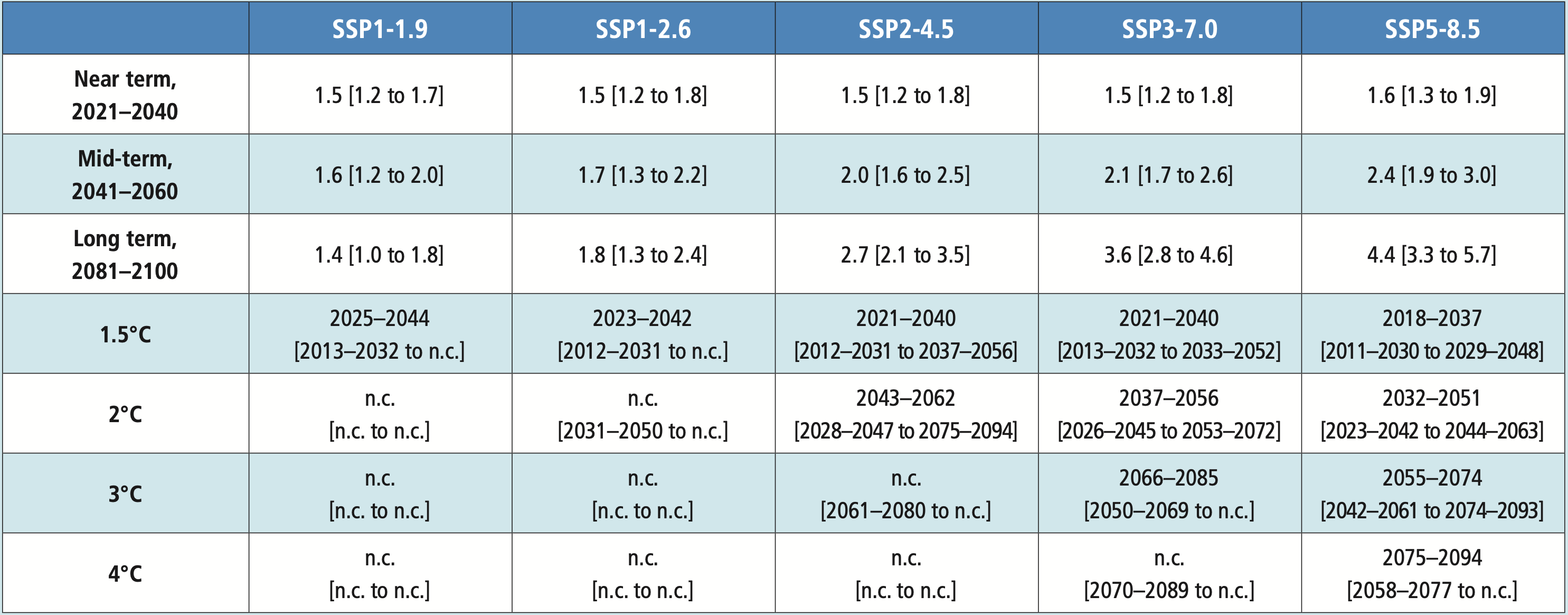
TS.2 Large-scale Climate Change: Mean Climate, Variability and Extremes
This section summarizes knowledge about observed and projected large-scale climate change (including variability and extremes), drivers and attribution of observed changes to human activities. It describes observed and projected large-scale changes associated with major components of the climate system: atmosphere, ocean (including sea level change), land, biosphere and cryosphere, and the carbon, energy and water cycles. In each subsection, reconstructed past changes, observed and attributed recent changes, and projected near- and long-term changes to mean climate, variability and extremes are presented, where possible, in an integrated way. See Section TS.1.3.1 for information on the scenarios used for projections.
TS.2.1 Changes Across the Global Climate System
Earth system model simulations of the historical period since 1850 are only able to reproduce the observed changes in key climate indicators when anthropogenic forcings are included (Figure TS.7). Taken together with numerous formal attribution studies across an even broader range of indicators and theoretical understanding, this underpins the unequivocal attribution of observed warming of the atmosphere, ocean, and land to human influence (Table TS.1). Links to chapters2.3, 3.8

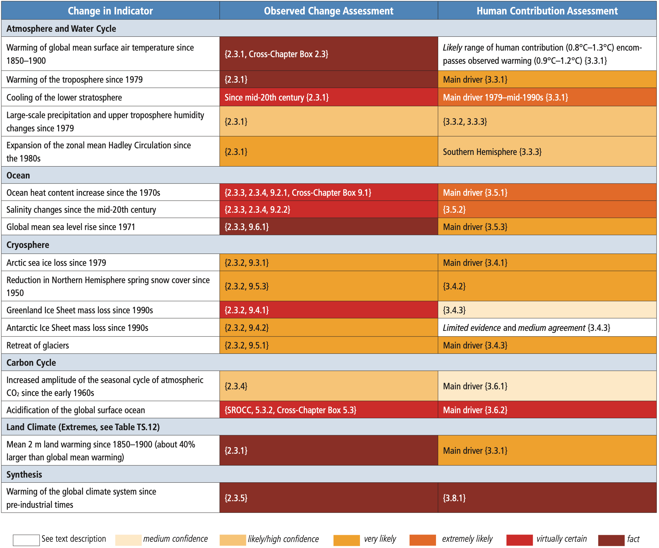
Future climate change across a range of atmospheric, cryospheric, oceanic and biospheric indicators depends upon future emissions pathways. Outcomes for a broad range of indicators increasingly diverge through the 21st century across the different SSPs (Section TS.1.3.1, Figure TS.8). Due to the slow response of the deep ocean and ice sheets, this divergence continues long after 2100, and 21st century emissions choices will have implications for GMSL rise for centuries to millennia. Furthermore, it is likely that at least one large volcanic eruption will occur during the 21st century. Such an eruption would reduce global surface temperature for several years, decrease land precipitation, alter monsoon circulation and modify extreme precipitation, at both global and regional scales. Links to chapters4.3, 4.7, 9.4, 9.6, Cross-Chapter Box 4.1
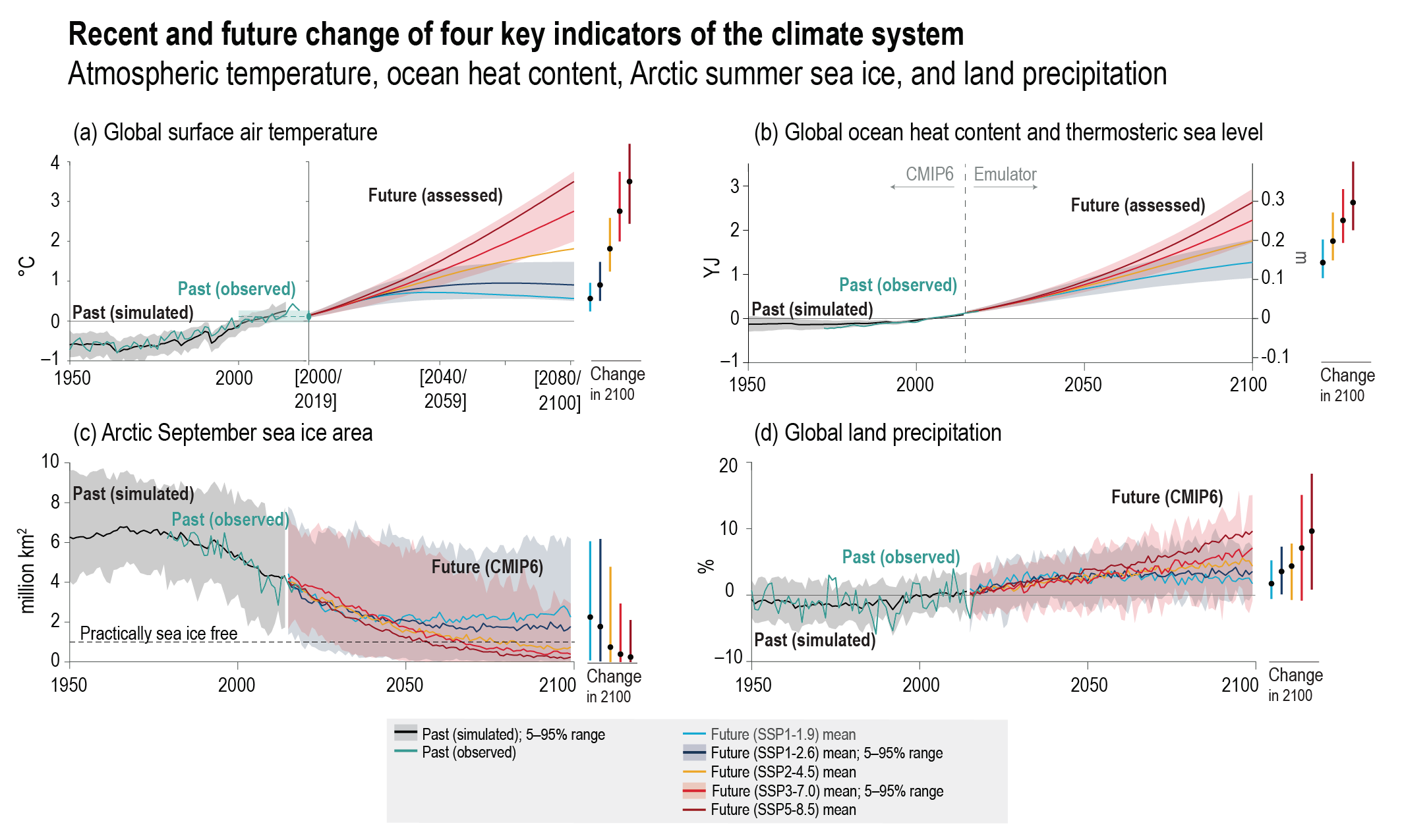
Observational records show changes in a wide range of climate extremes that have been linked to human influence on the climate system (Table TS.2). In many cases, the frequency and intensity of future changes in extremes can be directly linked to the magnitude of future projected warming. Changes in extremes have been widespread over land since the 1950s, including avirtually certainglobal increase in extreme air temperatures and a likely intensification in global-scale extreme precipitation. It is extremely likely that human influence is the main contributor to the observed increase (decrease) in the likelihood and severity of hot (cold) extremes (Table TS.2). The frequency of extreme temperature and precipitation events in the current climate will change with warming, with warm extremes becoming more frequent (virtually certain), cold extremes becoming less frequent (extremely likely) and precipitation extremes becoming more frequent in most locations (very likely) . Links to chapters9.6.4, 11.2, 11.3, 11.4, 11.6, 11.7, 11.8, 11.9, Box 9.2
Table TS.2 | Summary table on observed changes in extremes, their attribution since 1950 (except where stated otherwise), and projected changes at +1.5°C, +2°C and +4°C of global warming, on global and continental scales. An increase in warm/hot extremes refers to warmer and/or more frequent hot days and nights and warm spells/heatwaves, over most land areas. A decrease in cold extremes refers to warmer and/or fewer cold days and nights and cold spells/cold waves, over most land areas. Drought events are relative to a predominant fraction of land area. For tropical cyclones, observed changes and attribution refer to Categories 3–5, while projected changes refer to Categories 4–5. Tables 11.1 and 11.2 are more detailed versions of this table, containing, in particular, information on regional scales. In general, higher warming levels also imply stronger projected changes for indicators where the confidence level does not depend on the warming level and the table does not explicitly quantify the global sensitivity. See also Box TS.10. Links to chapters9.6, Box 9.2, 11.3, 11.7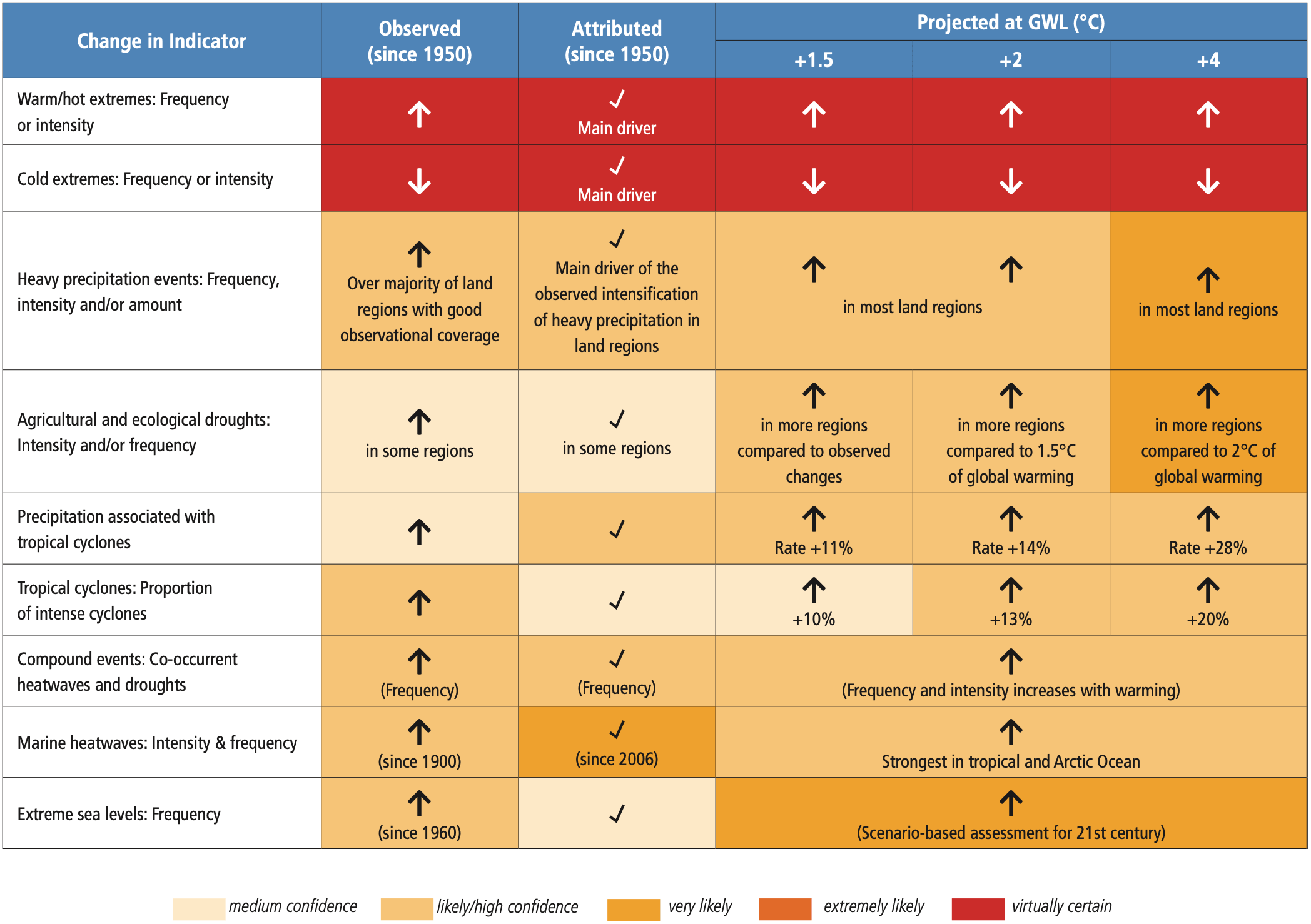
TS.2.2 Changes in the Drivers of the Climate System
Solar activity since 1900 was high but not exceptional compared to the past 9000 years (high confidence). The average magnitude and variability of volcanic aerosols since 1900 has not been unusual compared to at least the past 2500 years (medium confidence). However, sporadic strong volcanic eruptions can lead to temporary drops in global surface temperature lasting 2–5 years. Links to chapters2.2.1, 2.2.2, 2.2.8, Cross-Chapter Box 4.1
Atmospheric CO2 concentrations have changed substantially over millions of years (Figure TS.1). Current levels of atmospheric CO2 have not been experienced for at least 2 million years (high confidence, Figure TS.9a). Over 1750–2019, CO2 increased by 131.6 ± 2.9 ppm (47.3%). The centennial rate of change of CO2 since 1850 has no precedent in at least the past 800,000 years (Figure TS.9), and the fastest rates of change over the last 56 million years were at least a factor of four lower (low confidence) than over 1900–2019. Several networks of high-accuracy surface observations show that concentrations of CO2 have exceeded 400 ppm, reaching 409.9 (± 0.3) ppm in 2019 (Figure TS.9c). The ERF from CO2 in 2019 (relative to 1750) was 2.16 Wm–2. Links to chapters2.2.3, 5.1.2, 5.2.1, 7.3
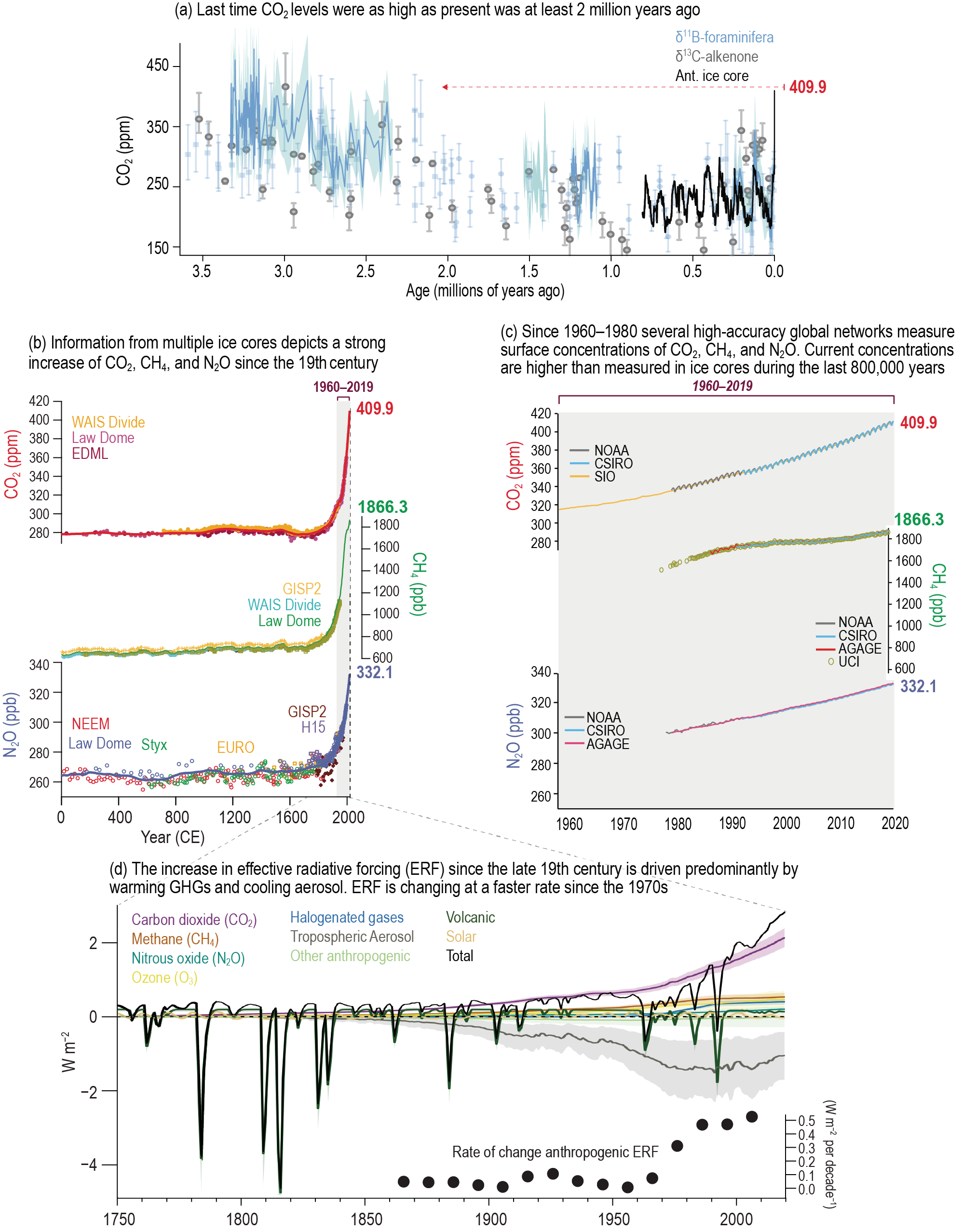
By 2019, concentrations of CH4 reached 1866.3 (± 3.3) ppb (Figure TS.9c). The increase since 1750 of 1137 ± 10 ppb (157.8%) far exceeds the range over multiple glacial–interglacial transitions of the past 800,000 years (high confidence). In the 1990s, CH4 concentrations plateaued, but started to increase again around 2007 at an average rate of 7.6 ± 2.7 ppb yr–1 (2010–2019; high confidence). There is high confidence that this recent growth is largely driven by emissions from fossil fuel exploitation, livestock, and waste, with ENSO driving multi-annual variability of wetland and biomass burning emissions. In 2019, ERF from CH4 was 0.54 Wm–2. Links to chapters2.2.3, 5.2.2, 7.3
Since 1750, N2O increased by 62.0 ± 6.0 ppb, reaching a level of 332.1 (± 0.4) ppb in 2019. The increase since 1750 is of comparable magnitude to glacial–interglacial fluctuations of the past 800,000 years (Figure TS.9c). N2O concentration trends since 1980 are largely driven by a 30% increase in emissions from the expansion and intensification of global agriculture (high confidence). By 2019 its ERF was 0.21 W m–2. Links to chapters2.2.3, 5.2.3
Halogenated gases consist of chlorofluorocarbons (CFCs), hydrochlorofluorocarbons (HCFCs), hydrofluorocarbons (HFCs) and other gases, many of which can deplete stratospheric ozone and warm the atmosphere. In response to controls on production and consumption mandated by the Montreal Protocol on Substances that Deplete the Ozone Layer and its amendments, the atmospheric abundances of most CFCs have continued to decline since AR5. Abundances of HFCs, which are replacements for CFCs and HCFCs, are increasing (high confidence), though increases of the major HCFCs have slowed in recent years. The ERF from halogenated components in 2019 was 0.41 Wm–2. Links to chapters2.2.4, 6.3.4, 7.3.2
Tropospheric aerosols mainly act to cool the climate system, directly by reflecting solar radiation, and indirectly by enhancing cloud reflectance. Ice cores show increases in aerosols across the Northern Hemisphere mid-latitudes since 1700 and reductions since the late 20th century (high confidence). Aerosol optical depth (AOD), derived from satellite- and ground-based radiometers, has decreased since 2000 over the mid-latitude continents of both hemispheres, but increased over South Asia and East Africa (high confidence). Trends in AOD are more pronounced from sub-micrometre aerosols for which the anthropogenic contribution is particularly large. Global carbonaceous aerosol budgets and trends remain poorly characterized due to limited observations, but black carbon (BC), a warming aerosol component, is declining in several regions of the Northern Hemisphere (low confidence). Total aerosol ERF in 2019, relative to 1750, is −1.1 [−1.7 to −0.4] W m−2 (medium confidence) and more likely than not became less negative since the late 20th century, with low confidence in the magnitude of post-2014 changes due to conflicting evidence (Section TS.3.1). Links to chapters2.2.6, 6.2.1, 6.3.5, 6.4.1, 7.3.3
There is high confidence that tropospheric ozone has been increasing from 1750 in response to anthropogenic changes in ozone precursor emissions (nitrogen oxides, carbon monoxide, non-methane volatile organic compounds, and methane), but with medium confidence in the magnitude of this change, due to limited observational evidence and knowledge gaps. Since the mid-20th century, tropospheric ozone surface concentrations have increased by 30–70% across the Northern Hemisphere (medium confidence); since the mid-1990s, free tropospheric ozone has increased by 2–7% per decade in most northern mid-latitude regions and 2–12% per decade in sampled tropical regions. Future changes in surface ozone concentrations will be primarily driven by changes in precursor emissions rather than climate change (high confidence). Stratospheric ozone has declined between 60°S–60°N by 2.2% from 1964–1980 to 2014–2017 (high confidence), with the largest declines during 1980–1995. The strongest loss of stratospheric ozone continues to occur in austral spring over Antarctica (ozone hole), with emergent signs of recovery after 2000. The 1750–2019 ERF for total (stratospheric and tropospheric) ozone is 0.47 [0.24 to 0.71] W m−2, which is dominated by tropospheric ozone changes. Links to chapters2.2.5, 6.3.2, 7.3.2, 7.3.5
The global mean abundance of hydroxyl (OH) radical, or ‘oxidizing capacity’, chemically regulates the lifetimes of many SLCFs, and therefore the radiative forcing of CH4, ozone, secondary aerosols and many halogenated species. Model estimates suggest no significant change in oxidizing capacity from 1850 to 1980 (low confidence). Increases of about 9% over 1980–2014 computed by ESMs and carbon cycle models are not confirmed by observationally constrained inverse models, rendering an overall medium confidence in stable OH or positive trends since the 1980s, and implying that OH is not the primary driver of recent observed growth in CH4. Links to chapters6.3.6, Cross-Chapter Box 5.2
Land use and land-cover change exert biophysical and biogeochemical effects. There is medium confidence that the biophysical effects of land-use change since 1750, most notably the increase in global albedo, have had an overall cooling on climate, whereas biogeochemical effects (i.e., changes in GHG and volatile organic compound emissions or sinks) led to net warming. Overall land-use and land-cover ERF is estimated at –0.2 [–0.3 to –0.1] W m−2. Links to chapters2.2.7, 7.3.4, SRCCLSection 2.5
The total anthropogenic ERF in 2019 relative to 1750 was 2.72 [1.96 to 3.48] W m−2 (Figure TS.9), dominated by GHGs (positive ERF) and partially offset by aerosols (negative ERF). The rate of change of ERFlikely has increased since the 1970s, mainly due to growing CO2 concentrations and less negative aerosol ERF (Section TS.3.1). Links to chapters2.2.8, 7.3
TS.2.3 Upper Air Temperatures and Atmospheric Circulation
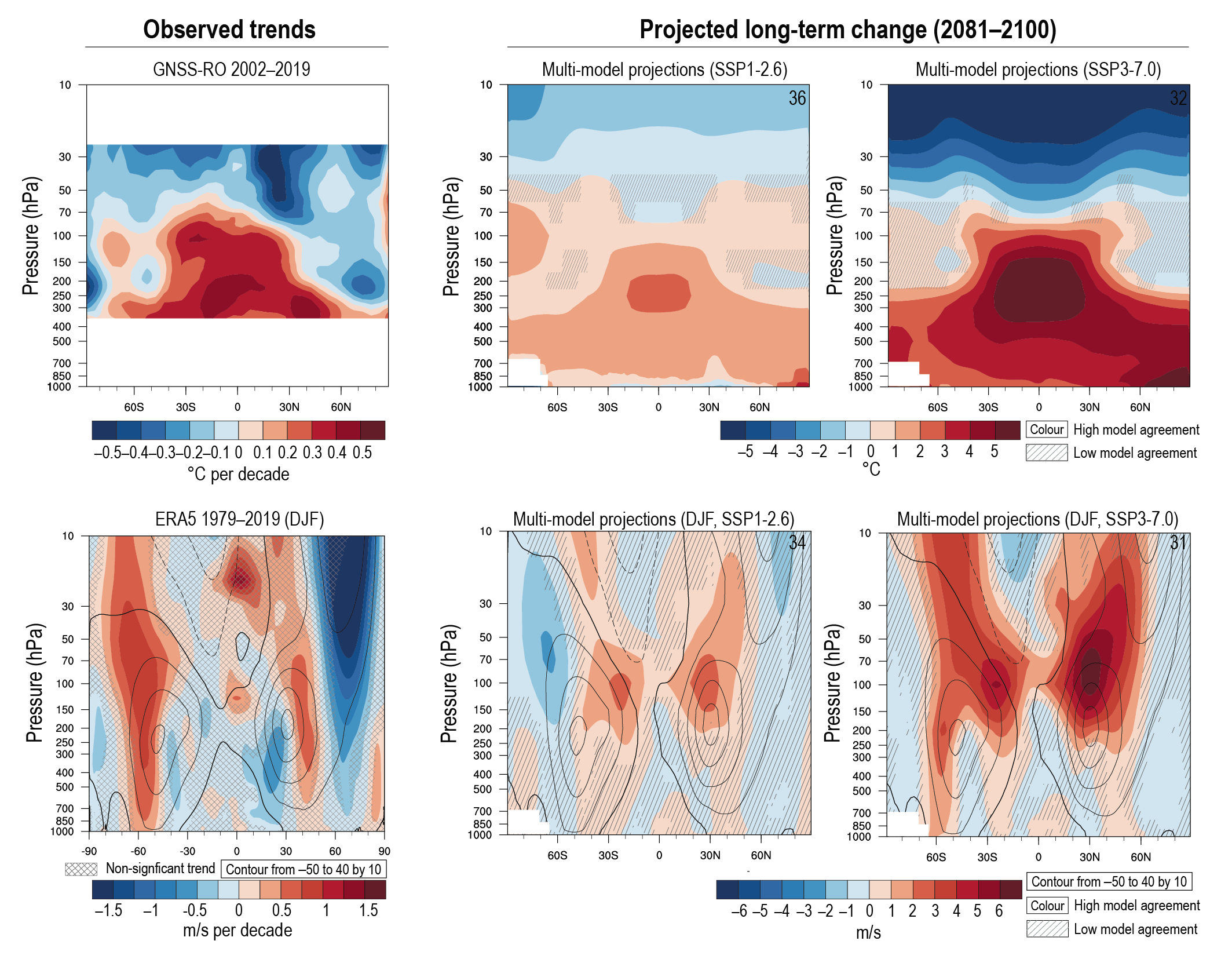
The troposphere has warmed since at least the 1950s, and it is virtually certain that the stratosphere has cooled. It is very likely that human-induced increases in GHGs were the main driver of tropospheric warming since 1979. It is extremely likely that anthropogenic forcing, both from increases in GHG concentrations and depletion of stratospheric ozone due to ozone-depleting substances, was the main driver of upper stratospheric cooling since 1979. It is very likely that global mean stratospheric cooling will be larger for scenarios with higher atmospheric CO2 concentrations. In the tropics, since at least 2001 (when new techniques permit more robust quantification), the upper troposphere has warmed faster than the near-surface (medium confidence) (Figure TS.10). There is medium confidence that most CMIP5 and CMIP6 models overestimate the observed warming in the upper tropical troposphere over the period 1979–2014, in part because they overestimate tropical SST warming. It is likely that future tropical upper tropospheric warming will be larger than at the tropical surface. Links to chapters2.3.1, 3.3.1, 4.5.1
The Hadley Circulation has likely widened since at least the 1980s, predominantly in the Northern Hemisphere, although there is only medium confidence in the extent of the changes. This has been accompanied by a strengthening of the Hadley Circulation in the Northern Hemisphere (medium confidence). It is likely that human influence has contributed to the poleward expansion of the zonal mean Hadley cell in the Southern Hemisphere since the 1980s, which is projected to further expand with global warming (high confidence). There is medium confidence that the observed poleward expansion in the Northern Hemisphere is within the range of internal variability. Links to chapters2.3.1, 3.3.3, 8.4.3
Since the 1970s, near-surface average winds have likely weakened over land. Over the ocean, near-surface average winds likely strengthened over 1980–2000, but divergent estimates lead to low confidence thereafter. Extratropical storm tracks have likely shifted poleward since the 1980s. There is low confidence in projected poleward shifts of the Northern Hemisphere mid-latitude jet and storm tracks due to large internal variability and structural uncertainty in model simulations. There is medium confidence in a projected decrease in the frequency of atmospheric blocking over Greenland and the North Pacific in boreal winter in 2081–2100 under the SSP3-7.0 and SSP5-8.5 scenarios. There is high confidence that Southern Hemisphere storm tracks and associated precipitation have migrated polewards over recent decades, especially in the austral summer and autumn, associated with a trend towards more positive phases of the Southern Annular Mode (SAM) (Section TS.4.2.2) and the strengthening and southward shift of the Southern Hemisphere extratropical jet in austral summer. In the long term (2081–2100), the Southern Hemisphere mid-latitude jet is likely to shift poleward and strengthen under the SSP5-8.5 scenario relative to 1995–2014, accompanied by an increase in the SAM (Section TS.4.2.2). It is likely that wind speeds associated with extratropical cyclones will strengthen in the Southern Hemisphere storm track for SSP5-8.5. There is low confidence in the potential role of Arctic warming and sea ice loss on historical or projected mid-latitude atmospheric variability. Links to chapters2.3.1, 3.3.3, 3.7.2, 4.3.3, 4.4.3, 4.5.1, 4.5.3, 8.2.2, 8.3.2, Cross-Chapter Box 10.1
It is likely that the proportionof major (Category 3–5) tropical cyclones (TCs) and the frequency of rapid TC intensification events have increased over the past four decades. The average location of peak TC wind-intensity has very likely migrated poleward in the western North Pacific Ocean since the 1940s, and TC forward translation speed has likely slowed over the contiguous USA since 1900. It is likely that the poleward migration of TCs in the western North Pacific and the global increase in TC intensity rates cannot be explained entirely by natural variability. There is high confidence that average peak TC wind speeds and the proportion of Category 4–5 TCs will increase with warming and that peak winds of the most intense TCs will increase. There is medium confidence that the average location where TCs reach their maximum wind-intensity will migrate poleward in the western North Pacific Ocean, while the total global frequency of TC formation will decrease or remain unchanged with increasing global warming. Links to chapters11.7.1
There is low confidence in observed recent changes in the total number of extratropical cyclones over both hemispheres. There is also low confidence in past-century trends in the number and intensity of the strongest extratropical cyclones over the Northern Hemisphere due to the large interannual-to-decadal variability and temporal and spatial heterogeneities in the volume and type of assimilated data in atmospheric reanalyses, particularly before the satellite era. Over the Southern Hemisphere, it is likely that the number of extratropical cyclones with low central pressures (<980 hPa) has increased since 1979. The frequency of intense extratropical cyclones is projected to decrease (medium confidence). Projected changes in the intensity depend on the resolution of climate models (medium confidence). There is medium confidence that wind speeds associated with extratropical cyclones will change following changes in the storm tracks. Links to chapters2.3.1, 3.3.3, 4.5.1, 4.5.3, 8.3.2, 8.4.2, 11.7.2
Box TS.3 | Low-likelihood, High-warming Storylines
Previous IPCC reports largely focused their assessment on the projected very likely range of future surface warming and associated climate change. However, a comprehensive risk assessment also requires considering the potentially larger changes in the physical climate system that are unlikely orvery unlikely but possible and potentially associated with the highest risks for society and ecosystems (Figure TS.6). Since AR5, the development of physical climate storylines of high warming has emerged as a useful approach for exploring the future risk space that lies outside of the IPCCvery likely range projections. Links to chapters4.8
Uncertainty in the true values of equilibrium climate sensitivity (ECS) and transient climate response (TCR) dominate uncertainty in projections of future warming under moderate to strong emissions scenarios (Section TS.3.2). A real-world ECS higher than the assessed very likely range (2°C–5°C) would require a strong historical aerosol cooling and/or a trend towards stronger warming from positive feedbacks linked to changes in SST patterns (pattern effects), combined with a strong positive cloud feedback and substantial biases in paleoclimate reconstructions – each of which is assessed as eitherunlikely orvery unlikely , but not ruled out. Since CMIP6 contains several ESMs that exceed the upper bound of the assessed very likely range in future surface warming, these models can be used to develop low-likelihood, high warming storylines to explore risks and vulnerabilities, even in the absence of a quantitative assessment of likelihood. Links to chapters4.3.4, 4.8, 7.3.2, 7.4.4, 7.5.2, 7.5.5, 7.5.7
CMIP6 models with surface warming outside, or close to, the upper bound of the very likely range exhibit patterns of large widespread temperature and precipitation changes that differ substantially from the multi-model mean in all scenarios. For SSP5-8.5, the high-warming models exhibit widespread warming of more than 6°C over most extratropical land regions and parts of the Amazon. In the Arctic, annual mean temperatures increase by more than 10°C relative to present-day, corresponding to about 30% more than the best estimate of warming. Even for SSP1-2.6, high-warming models show on average 2°C–3°C warming relative to present-day conditions over much of Eurasia and North America (about 40% more than the best estimate of warming) and more than 4°C warming relative to the present over the Arctic in 2081–2100 (Box TS.3, Figure 1). Such a high global warming storyline would imply that the remaining carbon budget consistent with a 2°C warming is smaller than the assessed very likely range. Put another way, even if a carbon budget that likely limits warming to 2°C is met, a low-likelihood, high-warming storyline would result in warming of 2.5°C or more. Links to chapters4.8
CMIP6 models with global warming close to the upper bound of the assessed very likely warming range tend to exhibit greater changes in the intensity of regional drying and wetting than the multi-model mean. Furthermore, these model projections show a larger area of drying and tend to show a larger fraction of strong precipitation increases than the multi-model mean. However, regional precipitation changes arise from both thermodynamic and dynamic processes so that the most pronounced global warming levels are not necessarily associated with the strongest precipitation response. Abrupt human-caused changes to the water cycle cannot be ruled out. Positive land surface feedbacks, involving vegetation and dust, can contribute to abrupt changes in aridity, but there is onlylow confidence that such changes will occur during the 21st century. Continued Amazon deforestation, combined with a warming climate, raises the probability that this ecosystem will cross a tipping point into a dry state during the 21st century (low confidence). (See also Box TS.9). Links to chapters4.8, 8.6.2
While there is medium confidence that the projected decline in the AMOC (Section TS.2.4) will not involve an abrupt collapse before 2100, such a collapse might be triggered by an unexpected meltwater influx from the Greenland Ice Sheet. If an AMOC collapse were to occur, it would very likely cause abrupt shifts in the regional weather patterns and water cycle, such as a southward shift in the tropical rain belt, and could result in weakening of the African and Asian monsoons, strengthening of Southern Hemisphere monsoons, and drying in Europe. (See also Boxes TS.9 and TS.13). Links to chapters4.7.2, 8.6.1, 9.2.3
Very rare extremes and compound or concurrent events, such as the 2018 concurrent heatwaves across the Northern Hemisphere, are often associated with large impacts. The changing climate state is already altering the likelihood of extreme events, such as decadal droughts and extreme sea levels, and will continue to do so under future warming. Compound events and concurrent extremes contribute to increasing probability of low-likelihood, high-impact outcomes and will become more frequent with increasing global warming (high confidence). Higher warming levels increase the likelihood of events unprecedented in the observational record. Links to chapters9.6.4, Box 11.2
Finally, low likelihood storylines need not necessarily relate solely to the human-induced changes in climate. A low-likelihood, high-impact outcome, consistent with historical precedent in the past 2500 years, would be to see several large volcanic eruptions that could greatly alter the 21st century climate trajectory compared to SSP-based Earth system model projections. Links to chaptersCross-Chapter Box 4.1

Box TS.3, Figure 1 | High-warming storylines. The intent of this figure is to illustrate high warming storylines compared to the CMIP6 multi-model-mean. (a) Coupled Model Intercomparison Project Phase 6 (CMIP6) multi-model mean linearly scaled to the assessed best global surface temperature estimate for SSP1-2.6 in 2081–2100 relative to 1995–2014, (b) mean across five high-warming models with global surface temperature changes nearest to the upper bound of the assessed very likely range, and (c) mean across five very high-warming models with global surface temperature changes higher than the assessed very likely . (d–f) Same as (a–c) but for SSP5-8.5. Note the different colour bars in (a–c) and (d–f). Links to chapters4.7, Figure 4.41
TS.2.4 The Ocean
 Figure TS.11 | Past and future ocean and ice-sheet changes. The intent of this figure is to show that observed and projected time series of many ocean and cryosphere indicators are consistent. Observed and simulated historical changes and projected future changes under varying greenhouse gas emissions scenarios. Simulated and projected ocean changes are shown as Coupled Model Intercomparison Project Phase 6 (CMIP6) ensemble mean, and 5–95% range (shading) is provided for scenarios SSP1-2.6 and SSP3-7.0 (except in panel a where the range is provided for scenario SSP1-2.6 and SSP5-8.5). Mean and 5–95%range in 2100 are shown as vertical bars on the right-hand side of each panel. (a) Change in multiplication factor in surface ocean marine heatwave days relative to 1995–2014 (defined as days exceeding the 99th percentile in sea surface temperature (SST) from 1995–2014 distribution). Assessed observational change span 1982–2019 from AVHRR satellite SST. (b) Atlantic Meridional Overturning Circulation (AMOC) transport relative to 1995–2014 (defined as maximum transport at 26°N). Assessed observational change spans 2004–2018 from the RAPID array smoothed with a 12-month running mean (shading around the mean shows the 12-month running standard deviation around the mean). (c) Global mean percent change in ocean oxygen (100–600 m depth), relative to 1995–2014. Assessed observational trends and very likely range are from the SROCC assessment, and span 1970–2010 centred on 2005. (d) Global mean surface pH. Assessed observational change spans 1985–2019, from the CMEMS SOCAT-based reconstruction (shading around the global mean shows the 90% confidence interval). (e), (f): Ice sheet mass changes. Projected ice-sheet changes are shown as median, 5–95% range (light shading), and 17–83% range (dark shading) of cumulative mass loss and sea level equivalent from ISMIP6 emulation under SSP1-2.6 and SSP5-8.5 (shading and bold line), with individual emulated projections as thin lines. Median (dot), 17–83% range (thick vertical bar), and 5–95% range (thin vertical bar) in 2100 are shown as vertical bars on the right-hand side of each panel, from ISMIP6, ISMIP6 emulation, and LARMIP-2. Observation-based estimates: For Greenland (e), for 1972–2018 (Mouginot), for 1992–2016 (Bamber), for 1992–2020 (IMBIE) and total estimated mass loss range for 1840–1972 (Box). For Antarctica (f), estimates based on satellite data combined with simulated surface mass balance and glacial isostatic adjustment for 1992–2020 (IMBIE), 1992–2016 (Bamber), and 1979–2017 (Rignot). Left inset maps: mean Greenland elevation changes 2010–2017 derived from CryoSat-2 radar altimetry (e) and mean Antarctica elevation changes 1978–2017 derived from restored analogue radar records (f). Right inset maps: ISMIP6 model mean (2093–2100) projected changes under the MIROC5 climate model for the RCP8.5 scenario. Links to chapters2.3.3; 2.3.4; 3.5.4; 4.3.2; 5.3.2; 5.3.3; 5.6.3; 9.2.3; 9.4.1; 9.4.2; Box 9.2; Box 9.2, Figure 1; Figures 9.10, 9.17 and 9.18
 It is virtually certain that the global ocean has warmed since at least 1971, representing about 90% of the increase in the global energy inventory (Section TS.3.1). The ocean is currently warming faster than at any other time since at least the last deglacial transition (medium confidence), with warming extending to depths well below 2000 m (very high confidence). It is extremely likely that human influence was the main driver of this recent ocean warming. Ocean warming will continue over the 21st century (virtually certain), and will likely continue until at least to 2300 even for low CO2 emissions scenarios. Ocean warming is irreversible over centuries to millennia (medium confidence), but the magnitude of warming is scenario-dependent from about the mid-21st century (medium confidence). The warming will not be globally uniform, with heat primarily stored in Southern Ocean water-masses and weaker warming in the subpolar North Atlantic (high confidence). Limitations in the understanding of feedback mechanisms limit our confidence in future ocean warming close to Antarctica and how this will affect sea ice and ice shelves. Links to chapters2.3.3, 3.5.1, 4.7.2, 7.2.2, 9.2.2, 9.2.3, 9.2.4, 9.3.2, 9.6.1, Cross-Chapter Box 9.1
Global mean SST has increased since the beginning of the 20th century by 0.88 [0.68 to 1.01] °C, and it is virtually certain it will continue to increase throughout the 21st century, with increasing hazards to marine ecosystems (medium confidence). Marine heatwaves have become more frequent over the 20th century (high confidence), approximately doubling in frequency (high confidence) and becoming more intense and longer since the 1980s (medium confidence). Most of the marine heatwaves over 2006–2015 have been attributed to anthropogenic warming (very likely) . Marine heatwaves will continue to increase in frequency, with a likely global increase of 2–9 times in 2081–2100 compared to 1995–2014 under SSP1-2.6, and 3–15 times under SSP5-8.5 (Figure TS.11a), with the largest changes in the tropical and Arctic ocean. Links to chapters2.3.1, Cross-Chapter Box 2.3, 9.2.1, Box 9.2, 12.4.8
Observed upper-ocean stratification (0–200 m) has increased globally since at least 1970(virtually certain). Based on recent refined analyses of the available observations, there is high confidence that it increased by 4.9 ± 1.5% from 1970–2018, which is about twice as much as assessed in SROCC, and will continue to increase throughout the 21st century at a rate depending on the emissions scenario (virtually certain). Links to chapters2.3.3, 9.2.1
It is virtually certain that since 1950 near-surface high-salinity regions have become more saline, while low-salinity regions have become fresher, with medium confidence that this is linked to an intensification of the hydrological cycle (Box TS.6). It is extremely likely that human influence has contributed to this salinity change and that the large-scale pattern will grow in amplitude over the 21st century (medium confidence). Links to chapters2.3.3, 3.5.2, 9.2.2, 12.4.8
The AMOC was relatively stable during the past 8000 years (medium confidence). There is low confidence in the quantification of AMOC changes in the 20th century because of low agreement in quantitative reconstructed and simulated trends, missing key processes in both models and measurements used for formulating proxies, and new model evaluations. Direct observational records since the mid-2000s are too short to determine the relative contributions of internal variability, natural forcing and anthropogenic forcing to AMOC change (high confidence). An AMOC decline over the 21st century is very likely for all SSP scenarios (Figure TS.11b); a possible abrupt decline is assessed further in Box TS.3. Links to chapters2.3.3, 3.5.4, 4.3.2, 8.6.1, 9.2.3, Cross-Chapter Box 12.3
There is high confidence that many ocean currents will change in the 21st century in response to changes in wind stress. There is low confidence in 21st century change of Southern Ocean circulation, despite high confidence that it is sensitive to changes in wind patterns and increased ice-shelf melt. Western boundary currents and subtropical gyres have shifted poleward since 1993 (medium confidence). Subtropical gyres, the East Australian Current Extension, the Agulhas Current, and the Brazil Current are projected to intensify in the 21st century in response to changes in wind stress, while the Gulf Stream and the Indonesian Throughflow are projected to weaken (medium confidence). All of the four main eastern boundary upwelling systems are projected to weaken at low latitudes and intensify at high latitudes in the 21st century (high confidence). Links to chapters2.3.3, 9.2.3
It is virtually certain that surface pH has declined globally over the last 40 years and that the main driver is uptake of anthropogenic CO2. Ocean acidification and associated reductions in the saturation state of calcium carbonate – a constituent of skeletons or shells of a variety of marine organisms – is expected to increase in the 21st century under all emissions scenarios (high confidence). A long-term increase in surface open ocean pH occurred over the past 50 million years (high confidence), and surface ocean pH as low as recent times is uncommon in the last 2 million years (medium confidence). There is very high confidence that present-day surface pH values are unprecedented for at least 26,000 years and current rates of pH change are unprecedented since at least that time. Over the past 2–3 decades, a pH decline in the ocean interior has been observed in all ocean basins (high confidence) (Figure TS.11d). Links to chapters2.3.3, 2.3.4, 3.6.2, 4.3.2, 5.3.2, 5.3.3, 5.6.3, 12.4.8
Open-ocean deoxygenation and expansion of oxygen minimum zones have been observed in many areas of the global ocean since the mid 20th century (high confidence), in part due to human influence (medium confidence). Deoxygenation is projected to continue to increase with ocean warming (high confidence) (Figure TS.11c). Higher climate sensitivity and reduced ocean ventilation in CMIP6 compared to CMIP5 results in substantially greaterprojections ofsubsurface (100–600 m) oxygen decline than reported in SROCC for the period 2080–2099. Links to chapters2.3.3, 2.3.4, Cross-Chapter Box 2.4, 3.6.2, 5.3.3, 12.4.8
Over at least the last two decades, the geographic range of many marine organisms has shifted towards the poles and towards greater depths (high confidence), indicative of shifts towards cooler waters. The range of a smaller subset of organisms has shifted equatorward and to shallower depths (high confidence). Phenological metrics associated with the life cycles of many organisms have also changed over the last two decades or longer (high confidence). Since the changes in the geographical range of organisms and their phenological metrics have been observed to differ with species and location, there is the possibility of disruption to major marine ecosystems. Links to chapters2.3.4
TS.2.5 The Cryosphere
Current Arctic sea ice coverage levels (both annual and late summer) are at their lowest since at least 1850 (high confidence), and for late summer for the past 1000 years (medium confidence). Since the late 1970s, Arctic sea ice area and thickness have decreased in both summer and winter, with sea ice becoming younger, thinner and more dynamic (very high confidence). It is very likely that anthropogenic forcing, mainly due to greenhouse gas increases, was the main driver of this loss, although new evidence suggests that anthropogenic aerosol forcing has offset part of the greenhouse gas-induced losses since the 1950s (medium confidence). The annual Arctic sea ice area minimum will likely fall below 1 million km2 at least once before 2050 under all assessed SSP scenarios. This practically sea ice-free state will become the norm for late summer by the end of the 21st century in high CO2 emissions scenarios (high confidence). Arctic summer sea ice varies approximately linearly with global surface temperature, implying that there is no tipping point and observed/projected losses are potentially reversible (high confidence). Links to chapters2.3.2, 3.4.1, 4.3.2, 9.3.1, 12.4.9
For Antarctic sea ice, there is no significant trend in satellite-observed sea ice area from 1979 to 2020 in both winter and summer, due to regionally opposing trends and large internal variability. Due to mismatches between model simulations and observations, combined with a lack of understanding of reasons for substantial inter-model spread, there is low confidence in model projections of future Antarctic sea ice changes, particularly at the regional level. Links to chapters2.3.2, 3.4.1, 9.3.2
In permafrost regions, increases in ground temperatures in the upper 30 m over the past three to four decades have been widespread (high confidence). For each additional 1°C of warming (up to 4°C above the 1850–1900 level), the global volume of perennially frozen ground to 3 m below the surface is projected to decrease by about 25% relative to the present volume (medium confidence). However, these decreases may be underestimated due to an incomplete representation of relevant physical processes in ESMs (low confidence). Seasonal snow cover is treated in Section TS.2.6. Links to chapters2.3.2, 9.5.2, 12.4.9
There is very high confidence that, with few exceptions, glaciers have retreated since the second half of the 19th century; this behaviour is unprecedented in at least the last 2000 years (medium confidence). Mountain glaciers very likely contributed 67.2 [41.8 to 92.6] mm to the observed GMSL change between 1901 and 2018. This retreat has occurred at increased rates since the 1990s, with human influence very likely being the main driver. Under RCP2.6 and RCP8.5, respectively, glaciers are projected to lose 18% ± 13% and 36% ± 20% of their current mass over the 21st century (medium confidence). Links to chapters2.3.2, 3.4.3, 9.5.1, 9.6.1
The Greenland Ice Sheet was smaller than at present during the Last Interglacial period (roughly 125,000 years ago) and the mid-Holocene (roughly 6,000 years ago) (high confidence). After reaching a recent maximum ice mass at some point between 1450 and 1850, the ice sheet retreated overall, with some decades likely close to equilibrium (i.e., mass loss approximately equalling mass gained). It is virtually certain that the Greenland Ice Sheet has lost mass since the 1990s, with human influence a contributing factor (medium confidence). There is high confidence that annual mass changes have been consistently negative since the early 2000s. Over the period 1992–2020, Greenland likely lost 4890 ± 460 Gt of ice, contributing 13.5 ± 1.3 mm to GMSL rise. There is high confidence that Greenland ice mass losses are increasingly dominated by surface melting and runoff, with large interannual variability arising from changes in surface mass balance. Projections of future Greenland ice-mass loss (Box TS.4, Table 1; Figure TS.11e) are dominated by increased surface melt under all emissions scenarios (high confidence). Potential irreversible long-term loss of the Greenland Ice Sheet, and of parts of the Antarctic Ice Sheet, is assessed in Box TS.9. Links to chapters2.3.2, 3.4.3, 9.4.1, 9.4.2, 9.6.3, Atlas.11.2
It is likely that the Antarctic Ice Sheet has lost 2670 ± 530 Gt, contributing 7.4 ± 1.5 mm to GMSL rise over 1992–2020. The total Antarctic ice mass losses were dominated by the West Antarctic Ice Sheet, with combined West Antarctic and Peninsula annual loss rates increasing since about 2000 (very high confidence). Furthermore, it is very likely that parts of the East Antarctic Ice Sheet have lost mass since 1979. Since the 1970s, snowfall has likely increased over the western Antarctic Peninsula and eastern West Antarctica, with large spatial and interannual variability over the rest of Antarctica. Mass losses from West Antarctic outlet glaciers, mainly induced by ice shelf basal melt (high confidence), outpace mass gain from increased snow accumulation on the continent (very high confidence). However, there is onlylimited evidence, with medium agreement, of anthropogenic forcing of the observed Antarctic mass loss since 1992 (with low confidence in process attribution). Increasing mass loss from ice shelves and inland discharge will likely continue to outpace increasing snowfall over the 21st century (Figure TS.11f). Deep uncertainty persists with respect to the possible evolution of the Antarctic Ice Sheet along high-end mass-loss storylines within the 21st century and beyond, primarily related to the abrupt and widespread onset of marine ice sheet instability and marine ice cliff instability. (See also Boxes TS.3 and TS.4). Links to chapters2.3.2, 3.4.3, 9.4.2, 9.6.3, Box 9.4, Atlas.11.1
Box TS.4 | Sea Level
GMSL change is driven by warming or cooling of the ocean (and the associated expansion/contraction) and changes in the amount of ice and water stored on land. Paleo-evidence shows that GMSL has been about 70 m higher and 130 m lower than present within the past 55 million years and was likely 5 to 10 m higher during the Last Interglacial (Box TS.2, Figure 1). Sea level observations show that GMSL rose by 0.20 [0.15 to 0.25] m over the period 1901–2018 at an average rate of 1.7 [1.3 to 2.2] mm yr–1. New analyses and paleo-evidence since AR5 show this rate is very likely faster than during any century over at least the last three millennia (high confidence). Since AR5, there is strengthened evidence for an increase in the rate of GMSL rise since the mid-20th century, with an average rate of 2.3 [1.6–3.1] mm yr–1 over the period 1971–2018 increasing to 3.7 [3.2–4.2] mm yr–1 for the period 2006–2018 (high confidence). Links to chapters2.3.3, 9.6.1, 9.6.2

Box TS.4, Figure 1 | Global mean sea level (GMSL) change on different time scales and under different scenarios. The intent of this figure is to (i) show the century-scale GMSL projections in the context of the 20th century observations, (ii) illustrate ‘deep uncertainty’ in projections by considering the timing of GMSL rise milestones, and (iii) show the long-term commitment associated with different warming levels, including the paleo evidence to support this. (a) GMSL change from 1900 to 2150, observed (1900–2018) and projected under the SSP scenarios (2000–2150), relative to a 1995–2014 baseline. Solid lines show median projections. Shaded regions showlikely ranges for SSP1-2.6 and SSP3-7.0. Dotted and dashed lines show respectively the 83rd and 95th percentilelow confidence projections for SSP5-8.5. Bars at right showlikely ranges for SSP1-1.9, SSP1-2.6, SSP2-4.5, SSP3-7.0 and SSP5-8.5 in 2150. Lightly shaded thick/thin bars show 17th–83rd/5th–95th percentile low-confidence ranges in 2150 for SSP1-2.6 and SSP5-8.5, based upon projection methods incorporating structured expert judgement and marine ice cliff instability. Low confidence range for SSP5-8.5 in 2150 extends to 4.8/5.4 m at the 83rd/95th percentile. (b) GMSL change on 100- (blue), 2000- (green) and 10,000-year (magenta) time scales as a function of global surface temperature, relative to 1850–1900. For 100-year projections, GMSL is projected for the year 2100, relative to a 1995–2014 baseline, and temperature anomalies are average values over 2081–2100. For longer-term commitments, warming is indexed by peak warming above 1850–1900 reached after cessation of emissions. Shaded regions show paleo-constraints on global surface temperature and GMSL for the Last Interglacial and mid-Pliocene Warm Period. Lightly shaded thick/thin blue bars show 17th–83rd/5th–95th percentile low confidence ranges for SSP1-2.6 and SSP5-8.5 in 2100, plotted at 2°C and 5°C. (c) Timing of exceedance of GMSL thresholds of 0.5, 1.0, 1.5 and 2.0 m, under different SSPs. Lightly shaded thick/thin bars show 17th–83rd/5th–95th percentile low-confidence ranges for SSP1-2.6 and SSP5-8.5. Links to chapters4.3.2, 9.6.1, 9.6.2, 9.6.3, Box 9.4
GMSL will continue to rise throughout the 21st century (Box TS.4, Figure 1a). Considering only those processes in whose projections we have at least medium confidence, relative to the period 1995–2014, GMSL is projected to rise between 0.18 m (0.15–0.23 m, likely range; SSP1-1.9) and 0.23 m (0.20–0.30 m, likely range; SSP5-8.5) by 2050. By 2100, the projected rise is between 0.38 m (0.28–0.55 m, likely range; SSP1-1.9) and 0.77 m (0.63–1.01 m, likely range; SSP5-8.5) Links to chaptersTable 9.9 . The methods, models and scenarios used for sea level projections in the AR6 are updated from those employed by SROCC, with contributions informed by the latest model projections described in the ocean and cryosphere Sections (Sections TS.2.4 and TS.2.5). Despite these differences, the sea level projections are broadly consistent with those of SROCC. Links to chapters4.3.2, 9.6.3
Importantly, likely range projections do not include those ice-sheet-related processes whose quantification is highly uncertain or that are characterized by deep uncertainty. Higher amounts of GMSL rise before 2100 could be caused by earlier-than-projected disintegration of marine ice shelves, the abrupt, widespread onset of marine ice sheet instability (MISI) and marine ice cliff instability (MICI) around Antarctica, and faster-than-projected changes in the surface mass balance and dynamical ice loss from Greenland (Box TS.4, Figure 1). In a low-likelihood, high-impact storyline and a high CO2 emissions scenario, such processes could in combination contribute more than one additional meter of sea level rise by 2100 (Box TS.3). Links to chapters4.3.2, 9.6.3, Box 9.4
Beyond 2100, GMSL will continue to rise for centuries to millennia due to continuing deep ocean heat uptake and mass loss from ice sheets, and will remain elevated for thousands of years (high confidence). By 2150, considering only those processes in whose projections we have at least medium confidence and assuming no acceleration in ice-mass flux after 2100, GMSL is projected to rise between 0.6 m (0.4–0.9 m, likely range, SSP1-1.9) and 1.3 m (1.0–1.9 m, likely range) (SSP5-8.5), relative to the period 1995–2014 based on the SSP scenario extensions. Under high CO2 emissions, processes in which there is low confidence, such as MICI, could drive GMSL rise up to about 5 m by 2150 (Box TS.4, Figure 1a). By 2300, GMSL will rise 0.3–3.1 m under low CO2 emissions (SSP1-2.6) (low confidence). Under high CO2 emissions (SSP5-8.5), projected GMSL rise is between 1.7 and 6.8 m by 2300 in the absence of MICI and by up to 16 m considering MICI (low confidence). Over 2000 years, there is medium agreemen t and limited evidence that committed GMSL rise is projected to be about 2–3 m with 1.5°C peak warming, 2–6 m with 2°C of peak warming, 4–10 m with 3°C of peak warming, 12–16 m with 4°C of peak warming, and 19–22 m with 5°C of peak warming. Links to chapters9.6.3
Looking at uncertainty in time provides an alternative perspective on uncertainty in future sea level rise (Box TS.4, Figure 1c). For example, considering only medium confidence processes, GMSL rise is likely to exceed 0.5 m between about 2080 and 2170 under SSP1-2.6 and between about 2070 and 2090 under SSP5-8.5. Given the long-term commitment, uncertainty in the timing of reaching different levels of GMSL rise is an important consideration for adaptation planning. Links to chapters9.6.3
At regional scales, additional processes come into play that modify the local sea level change relative to GMSL, including vertical land motion, ocean circulation and density changes, and gravitational, rotational, and deformational effects arising from the redistribution of water and ice mass between land and the ocean. These processes give rise to a spatial pattern that tends to increase sea level rise at the low latitudes and reduce sea level rise at high latitudes. However, over the 21st century, the majority of coastal locations have a median projected regional sea level rise within ±20% of the projected GMSL change (medium confidence). Further details on regional sea level change and extremes are provided in Section TS.4. Links to chapters9.6.3
Box TS.5 | The Carbon Cycle
Carbon sinks for anthropogenic CO2 are associated with mainly physical ocean and biospheric land processes that drive the exchange of carbon between multiple land, ocean and atmospheric reservoirs. These exchanges are driven by increasing atmospheric CO2, but are modulated by changes in climate (Box TS.5, Figure 1c,d). The Northern and Southern Hemispheres dominate the land and ocean sinks, respectively (Box TS.5, Figure 1). Ocean circulation and thermodynamic processes also play a critical role in coupling the global carbon and energy (heat) cycles. There is high confidence that this ocean carbon–heat nexus is an important basis for one of the most important carbon–climate metrics, the transient climate response to cumulative CO2 emissions (TCRE; Section TS.3.2.1) used to determine the remaining carbon budget. Links to chapters5.1, 5.2, 5.5, 9.2, Cross-Chapter Box 5.3
Based on multiple lines of evidence using interhemispheric gradients of CO2 concentrations, isotopes, and inventory data, it is unequivocal that the growth in CO2 in the atmosphere since 1750 (see Section TS.2.2) is due to the direct emissions from human activities. The combustion of fossil fuels and land-use change for the period 1750–2019 resulted in the release of 700 ± 75 PgC (likely range, 1 PgC = 1015g of carbon) to the atmosphere, of which about 41% ± 11% remains in the atmosphere today (high confidence). Of the total anthropogenic CO2 emissions, the combustion of fossil fuels was responsible for about 64% ± 15%, growing to an 86% ± 14% contribution over the past 10 years. The remainder resulted from land-use change. During the last decade (2010–2019), average annual anthropogenic CO2 emissions reached the highest levels in human history at 10.9 ± 0.9 PgC yr–1 (high confidence). Of these emissions, 46% accumulated in the atmosphere (5.1 ± 0.02 PgC yr–1), 23% (2.5 ± 0.6 PgC yr–1) was taken up by the ocean and 31% (3.4 ± 0.9 PgC yr–1) was removed by terrestrial ecosystems (high confidence). Links to chapters5.2.1, 5.2.2, 5.2.3
The ocean (high confidence) and land (medium confidence) sinks of CO2 have increased with anthropogenic emissions over the past six decades (Box TS.5, Figure 1). This coherence between emissions and the growth in ocean and land sinks has resulted in the airborne fraction of anthropogenic CO2 remaining at 44 ± 10% over the past 60 years (high confidence). Interannual and decadal variability of the ocean and land sinks indicate that they are sensitive to changes in the growth rate of emissions as well as climate variability and are therefore also sensitive to climate change (high confidence). Links to chapters5.2.1
The land CO2 sink is driven by carbon uptake by vegetation, with large interannual variability, for example, linked to the El Niño–Southern Oscillation (ENSO). Since the 1980s, carbon fertilization from rising atmospheric CO2 has increased the strength of the net land CO2 sink (medium confidence). During the historical period, the growth of the ocean sink has been primarily determined by the growth rate of atmospheric CO2. However, there is medium confidence that changes to physical and chemical processes in the ocean and in the land biosphere, which govern carbon feedbacks, are already modifying the characteristics of variability, particularly the seasonal cycle of CO2, in both the ocean and land. However, changes to the multi-decadal trends in the sinks have not yet been observed. Links to chapters2.3.4, 3.6.1, 5.2.1
In AR6, ESM projections are assessedwith CO2 concentrations by 2100 from about 400 ppm (SSP1-1.9) to above 1100 ppm (SSP5-8.5). Most simulations are performed with prescribed atmospheric CO2 concentrations, which already account for a central estimate of climate–carbon feedback effects. Carbon dioxide emissions-driven simulations account for uncertainty in these feedbacks, but do not significantly change the projected global surface temperature changes (high confidence). Although land and ocean sinks absorb more CO2 under high emissions than low emissions scenarios, the fraction of emissions removed from the atmosphere decreases (high confidence). This means that the more CO2 that is emitted, the less efficient the ocean and land sinks become (high confidence), an effect which compensates for the logarithmic relationship between CO2 and its radiative forcing, which means that for each unit increase in additional atmospheric CO2 the effect on global temperature decreases. (Box TS.5, Figure 1f,g). Links to chapters4.3.1, 5.4.5, 5.5.1.2
Ocean and land sinks show similar responses for a given scenario, but the land sink has a much higher interannual variability and wider model spread. Under SSP3-7.0 and SSP5-8.5, the initial growth of both sinks in response to increasing atmospheric concentrations of CO2 is subsequently limited by emerging carbon–climate feedbacks (high confidence) (Box TS.5, Figure 1f). Projections show that the ocean and land sinks will stop growing from the second part of the 21st century under all emissions scenarios, but with different drivers for different emissions scenarios. Under SSP3-7.0 and SSP5-8.5, the weakening growth rate of the ocean CO2 sink in the second half of the century is primarily linked to the strengthening positive feedback from reduced carbonate buffering capacity, ocean warming and altered ocean circulation (e.g., AMOC changes). In contrast, for SSP1-1.9, SSP1-2.6 and SSP2-4.5, the weakening growth rate of the ocean carbon sink is a response to the stabilizing or declining atmospheric CO2 concentrations. Under SSP1-1.9, models project that combined land and ocean sinks will turn into a weak source by 2100 (medium confidence). Under high CO2 emissions scenarios, it is very likely that the land carbon sink will grow more slowly due to warming and drying from the mid-21st century, but it is very unlikely that it will switch from being a sink to a source before 2100.

Box TS.5, Figure 1 | Carbon cycle processes and projections. The intent of this figure is to show the response of the carbon cycle to carbon dioxide (CO2) emissions and climate and its role in determining future CO2levels through projected changes to sinks and sink fractions. The figure shows changes in carbon storage in response to elevated CO2 (a, b) and the response to climate warming (c, d). Maps show spatial patterns of changes in carbon uptake during simulations with 1% per year increase in CO2 (Section 5.4.5.5), and zonal mean plots show distribution of carbon changes is dominated by the land (green lines) in the tropics and Northern Hemisphere and ocean (blue lines) in the Southern Hemisphere. Hatching indicates regions where fewer than 80% of models agree on the sign of response. (e) Future CO2 projections: projected CO2 concentrations in the Shared Socio-economic Pathway (SSP) scenarios in response to anthropogenic emissions, results from coupled Earth system models for SSP5-8.5 and from the MAGICC7 emulator for other scenarios (Section 4.3.1). (f) Future carbon fluxes: projected combined land and ocean fluxes (positive downward) up to 2100 for the SSP scenarios, and extended to 2300 for available scenarios, 5–95% uncertainty plumes shown for SSP1-2.6 and SSP3-7.0 (Sections 4.3.2.4, 5.4.5.4 and 5.4.10). The numbers near the top show the number of model simulations used. (g) Sink fraction: the fraction of cumulative emissions of CO2 removed by land and ocean sinks. The sink fraction is smaller under conditions of higher emissions. Links to chaptersFigure 4.3; 5.4.5; Figures 5.25, 5.27 and 5.30
Climate change alone is expected to increase land carbon accumulation in the high latitudes (not including permafrost, which is assessed in Sections TS.2.5 and TS.3.2.2), but also to lead to a counteracting loss of land carbon in the tropics (medium confidence). Earth system model projections show that the overall uncertainty of atmospheric CO2 by 2100 is still dominated by the emissions pathway, but carbon–climate feedbacks (see Section TS.3.3.2) are important, with increasing uncertainties in high emissions pathways (Box TS.5, Figure 1e). Links to chapters4.3.2, 5.4.1, 5.4.2, 5.4.4, 5.4.5, 11.6, 11.9, Cross-Chapter Box 5.1, Cross-Chapter Box 5.3
Under three SSP scenarios with long-term extensions until 2300 (SSP5-8.5, SSP5-3.4-OS, SSP1-2.6), ESMs project a change of the land from a sink to a source (medium confidence). The scenarios make simplified assumptions about emissions reductions, with SSP1-2.6 and SSP5-3.4-OS reaching about 400 ppm by 2300, while SSP5-8.5 exceeds 2000 ppm. Under high emissions, the transition is warming-driven, whereas it is linked to the decline in atmospheric CO2 under net negative CO2 emissions. The ocean remains a sink throughout the period to 2300 except under very large net negative emissions. The response of the natural aspects of the carbon cycle to carbon dioxide removal is further developed in Section TS.3.3.2. Links to chapters5.4.9
TS.2.6 Land Climate, Including Biosphere and Extremes
Observed temperatures over land have increased by 1.59 [1.34–1.83] °C between the period 1850–1900 and 2011–2020. Warming of the land is about 45% larger than for global surface temperature and about 80% larger than warming of the ocean surface. Warming of the land surface during the period 1971–2018 contributed about 5% of the increase in the global energy inventory (Section TS.3.1), nearly twice the estimate in AR5 (high confidence). It is virtually certain that the average surface warming over land will continue to be higher than over the ocean throughout the 21st century. The warming pattern will likely vary seasonally, with northern high latitudes warming more during winter than summer (medium confidence). Links to chapters2.3.1, 4.3.1, 4.5.1, 7.2.2, Box 7.2, Cross-Chapter Box 9.1, 11.3, Atlas 11.2
The frequency and intensity of hot extremes (warm days and nights) and the intensity and duration of heatwaves have increased globally and in most regions since 1950, while the frequency and intensity of cold extremes have decreased (virtually certain). There is high confidence that the increases in frequency and severity of hot extremes are due to human-induced climate change. Some recent extreme events would have been extremely unlikely to occur without human influence on the climate system. It is virtually certain that further changes in hot and cold extremes will occur throughout the 21st century in nearly all inhabited regions, even if global warming is stabilized at 1.5°C (Table TS.2, Figure TS.12a). Links to chapters1.3, Cross-Chapter Box 3.2, 11.1.4, 11.3.2, 11.3.4, 11.3.5, 11.9, 12.4
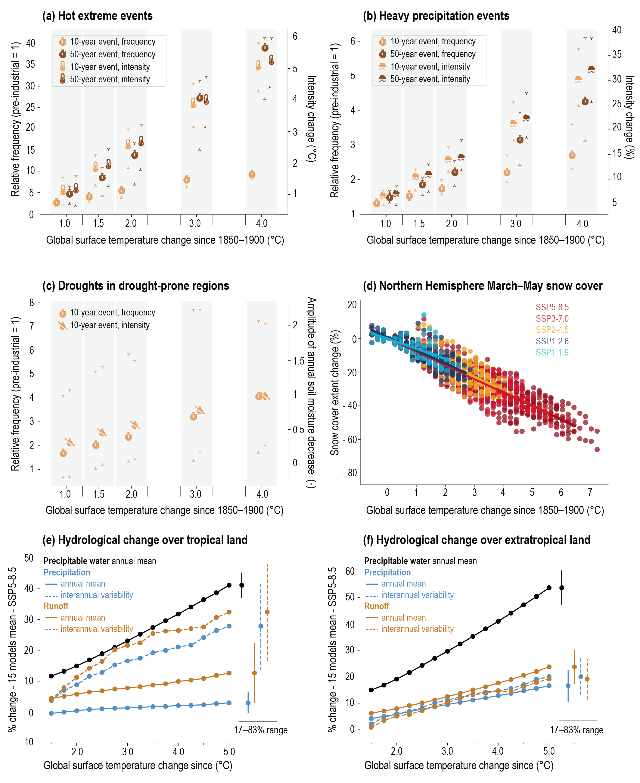 Figure TS.12 | Land-related changes relative to the 1850-1900 as a function of global warming levels. The intent of this figure is to show that extremes and mean land variables change consistently with warming levels and to show the changes with global warming levels of water cycle indicators (i.e., precipitation and runoff) over tropical and extratropical land in terms of mean and interannual variability (interannual variability increases at a faster rate than the mean). (a) Changes in the frequency (left scale) and intensity (in °C, right scale) of daily hot extremes occurring every 10 and 50 years. (b) as (a), but for daily heavy precipitation extremes, with intensity change in %. (c) Changes in 10-year droughts aggregated over drought-prone regions (WNA, CNA, NCA, SCA, NSA, NES, SAM, SWS, SSA, WCE, MED, WSAF, ESAF, MDG, SAU, and EAU; for definitions of these regions, see Figure Atlas.2), with drought intensity (right scale) represented by the change of annual mean soil moisture, normalized with respect to interannual variability. Limits of the 5%−95% confidence interval are shown in panels (a–c). (d) Changes in Northern Hemisphere spring (March–April–May) snow cover extent relative to 1850–1900; (e,f) Relative change (%) in annual mean of total precipitable water (grey line), precipitation (red solid lines), runoff (blue solid lines) and in standard deviation (i.e., variability) of precipitation (red dashed lines) and runoff (blue dashed lines) averaged over (e) tropical and (f) extratropical land as function of global warming levels. Coupled Model Intercomparison Project Phase 6 (CMIP6) models that reached a 5°C warming level above the 1850–1900 average in the 21st century in SSP5-8.5 have been used. Precipitation and runoff variability are estimated by respective standard deviation after removing linear trends. Error bars show the 17–83% confidence interval for the warmest +5°C global warming level. Links to chaptersFigures 8.16, 9.24, 11.6, 11.7, 11.12, 11.15, 11.18 and Atlas.2
 Greater warming over land alters key water cycle characteristics (Box TS.6). The rates of change in mean precipitation and runoff, and their variability, increase with global warming (Figure TS.12e,f). Human-induced climate change has contributed to increases in agricultural and ecological droughts in some regions due to increases in evapotranspiration (medium confidence). More regions are affected by increases in agricultural and ecological droughts with increasing global warming (high confidence; see also Figure TS.12c).
There is low confidence that the increase of plant water-use efficiency due to higher atmospheric CO2 concentration alleviates extreme agricultural and ecological droughts in conditions characterized by limited soil moisture and increased atmospheric evaporative demand. Links to chapters2.3.1, Cross-Chapter Box 5.1, 8.2.3, 8.4.1, 11.2.4, 11.4, 11.6, Box 11.1
Northern Hemisphere spring snow cover has decreased since at least 1978 (very high confidence), and there is high confidence that trends in snow cover loss extend back to 1950. It is very likely that human influence contributed to these reductions. Earlier onset of snowmelt has contributed to seasonally dependent changes in streamflow (high confidence). A further decrease of Northern Hemisphere seasonal snow cover extent is virtually certainunder further global warming (Figure TS.12d). Links to chapters2.3.2, 3.4.2, 8.3.2. 9.5.3, 12.4, 9.2, 11.2, Atlas 8.2
The frequency and intensity of heavy precipitation events have increased over a majority of land regions with good observational coverage since 1950 (high confidence, Box TS.6, Table TS.2). Human influence is likely the main driver of this change (Table TS.2). It is extremely likely that on most land regions heavy precipitation will become more frequent and more intense with additional global warming (Table TS.2, Figure TS.12b). The projected increase in heavy precipitation extremes translates to an increase in the frequency and magnitude of pluvial floods (high confidence) (Table TS.2). Links to chaptersCross-Chapter Box 3.2, 8.4.1, 11.4.2, 11.4.4, 11.5.5, 12.4
Theprobability of compound extreme events has likely increased due to human-induced climate change. Concurrent heatwaves and droughts have become more frequent over the last century, and this trend will continue with higher global warming (high confidence). The probability of compound flooding (storm surge, extreme rainfall and/or river flow) has increased in some locations and will continue to increase due to both sea level rise and increases in heavy precipitation, including changes in precipitation intensity associated with tropical cyclones (high confidence). Links to chapters11.8.1, 11.8.2, 11.8.3
Changes in key aspects of the terrestrial biosphere, such as an increase of the growing season length in much of the Northern Hemisphere extratropics since the mid-20th century (high confidence), are consistent with large-scale warming. At the same time an increase in the amplitude of the seasonal cycle of atmospheric CO2 poleward of 45°N since the early 1960s (high confidence) and a global-scale increase in vegetation greenness of the terrestrial surface since the early 1980s (high confidence) have been observed. Increasing atmospheric CO2, warming at high latitudes, and land management interventions have contributed to the observed greening trend, but there is low confidence in their relative roles. There is medium confidence that increased plant growth associated with CO2 fertilization is the main driver of the observed increase in amplitude of the seasonal cycle of atmospheric CO2 in the Northern Hemisphere. Reactive nitrogen, ozone and aerosols affect terrestrial vegetation and carbon cycle through deposition and effects on large-scale radiation (high confidence), but the magnitude of these effects on the land carbon sink, ecosystem productivity and indirect CO2 forcing remains uncertain. Links to chapters2.3.4, 3.6.1, 5.2.1, 6.4.5, 12.3.7, 12.4
Over the last century, there has been a poleward and upslope shift in the distribution of many land species (very high confidence) as well as increases in species turnover within many ecosystems (high confidence). There is high confidence that the geographical distribution of climate zones has shifted in many parts of the world in the last half century. The SRCCL concluded that continued warming will exacerbate desertification processes (medium confidence) and that ecosystems will become increasingly exposed to climates beyond those that they are currently adapted to (high confidence). There is medium confidence that climate change will increase disturbance by, for example, fire and tree mortality, across several ecosystems. Increases are projected in drought, aridity and fire weather in some regions (Section TS.4.3; high confidence). There is low confidence in the magnitude of these changes, but the probability of crossing uncertain regional thresholds (e.g., fires, forest dieback) increases with further warming (high confidence). The response of biogeochemical cycles to the anthropogenic perturbation can be abrupt at regional scales, and irreversible on decadal to century time scales (high confidence). Links to chapters2.3.4, 5.4.3, 5.4.9, 11.6, 11.8, 12.5, SRCCL 2.2, SRCCL 2.5, SR1.5 3.4
Box TS.6 | Water Cycle
There is high confidence that the global water cycle has intensified since at least 1980 expressed by, for example, increased atmospheric moisture fluxes and amplified precipitation minus evaporation patterns. Global land precipitation has likely increased since 1950, with a faster increase since the 1980s (medium confidence), and a likely human contribution to patterns of change, particularly for increases in high-latitude precipitation over the Northern Hemisphere. Increases in global mean precipitation are determined by a robust response to global surface temperature (very likely 2–3% per °C) that is partly offset by fast atmospheric adjustments to atmospheric heating by greenhouse gases (GHGs) and aerosols (Section TS.3.2.2). The overall effect of anthropogenic aerosols is to reduce global precipitation through surface radiative cooling effects (high confidence). Over much of the 20th century, opposing effects of GHGs and aerosols on precipitation have been observed for some regional monsoons (high confidence) (Box TS.13). Global annual precipitation over land is projected to increase on average by 2.4% (–0.2% to +4.7%likely range) under SSP1-1.9, 4.6% (1.5% to 8.3%likely range) under SSP2-4.5, and 8.3% (0.9% to 12.9%likely range) under SSP5-8.5 by 2081–2100 relative to 1995–2014 (Box TS.6, Figure 1). Inter-model differences and internal variability contribute to a substantial range in projections of large-scale and regional water cycle changes (high confidence). The occurrence of volcanic eruptions can alter the water cycle for several years (high confidence). Projected patterns of precipitation change exhibit substantial regional differences and seasonal contrast as global surface temperature increases over the 21st century (Box TS.6, Figure 1). Links to chapters2.3.1, 3.3.2, 3.3.3, 3.5.2, 4.3.1, 4.4.1, 4.5.1, 4.6.1, Cross-Chapter Box 4.1, 8.2.1, 8.2.2, 8.2.3, Box 8.1, 8.3.2.4, 8.4.1, 8.5.2, 10.4.2
Global total column water vapour content has very likely increased since the 1980s, and it is likely that human influence has contributed to tropical upper tropospheric moistening. Near-surface specific humidity has increased over the ocean (likely) and land (very likely) since at least the 1970s, with a detectable human influence (medium confidence). Human influence has been detected in amplified surface salinity and precipitation minus evaporation (P–E) patterns over the ocean (high confidence). It is virtually certain that evaporation will increase over the ocean and very likely that evapotranspiration will increase over land, with regional variations under future surface warming (Box TS.6, Figure 1). There is high confidence that projected increases in precipitation amount and intensity will be associated with increased runoff in northern high latitudes (Box TS.6, Figure 1). In response to cryosphere changes (Section TS.2.5), there have been changes in streamflow seasonality, including an earlier occurrence of peak streamflow in high-latitude and mountain catchments (high confidence). Projected runoff (Box TS.6, Figure 1c) is typically decreased by contributions from small glaciers because of glacier mass loss, while runoff from larger glaciers will generally increase with increasing global warming levels until their mass becomes depleted (high confidence). Links to chapters2.3.1, 3.3.2, 3.3.3, 3.5.2, 8.2.3, 8.4.1, 11.5
Warming over land drives an increase in atmospheric evaporative demand and in the severity of drought events (high confidence). Greater warming over land than over the ocean alters atmospheric circulation patterns and reduces continental near-surface relative humidity, which contributes to regional drying (high confidence). Avery likely decrease in relative humidity has occurred over much of the global land area since 2000. Projected increases in evapotranspiration due to growing atmospheric water demand will decrease soil moisture over the Mediterranean region, south-western North America, South Africa, South-Western South America and south-western Australia (high confidence) (Box TS.6, Figure 1). Some tropical regions are also projected to experience enhanced aridity, including the Amazon basin and Central America (high confidence). The total land area subject to increasing drought frequency and severity will expand (high confidence), and in the Mediterranean, South-Western South America, and Western North America, future aridification will far exceed the magnitude of change seen in the last millennium (high confidence). Links to chapters4.5.1, 8.2.2, 8.2.3, 8.4.1, Box 8.2, 11.6, 11.9
Land-use change and water extraction for irrigation have influenced local and regional responses in the water cycle (high confidence). Large-scale deforestation likely decreases evapotranspiration and precipitation and increases runoff over the deforested regions relative to the regional effects of climate change (medium confidence). Urbanization increases local precipitation (medium confidence) and runoff intensity (high confidence) (Box TS.14). Increased precipitation intensities have enhanced groundwater recharge, most notably in tropical regions (medium confidence). There is high confidence that groundwater depletion has occurred since at least the start of the 21st century, as a consequence of groundwater withdrawals for irrigation in agricultural areas in drylands. Links to chapters8.2.3, 8.3.1, 11.1.6, 11.4, 11.6, FAQ 8.1
Water cycle variability and related extremes are projected to increase faster than mean changes in most regions of the world and under all emissions scenarios (high confidence). A warmer climate increases moisture transport into weather systems, which intensifies wet seasons and events (high confidence). The magnitudes of projected precipitation increases and related extreme events depend on model resolution and the representation of convective processes (high confidence). Increases in near-surface atmospheric moisture capacity of about 7% per 1ºC of warming lead to a similar response in the intensification of heavy precipitation from sub-daily up to seasonal time scales, increasing the severity of flood hazards (high confidence). The average and maximum rain-rates associated with tropical and extratropical cyclones, atmospheric rivers and severe convective storms will therefore also increase with future warming (high confidence). For some regions, there is medium confidence that peak tropical cyclone rain-rates will increase by more than 7% per 1°C of warming due to increased low-level moisture convergence caused by increases in wind intensity. In the tropics year-round and in the summer season elsewhere, interannual variability of precipitation and runoff over land is projected to increase at a faster rate than changes in seasonal mean precipitation (Figure TS.12e,f) (medium confidence). Sub-seasonal precipitation variability is also projected to increase, with fewer rainy days but increased daily mean precipitation intensity over many land regions (high confidence). Links to chapters4.5.3, 8.2.3, 8.4.1, 8.4.2, 8.5.1, 8.5.2, 11.4, 11.5, 11.7, 11.9
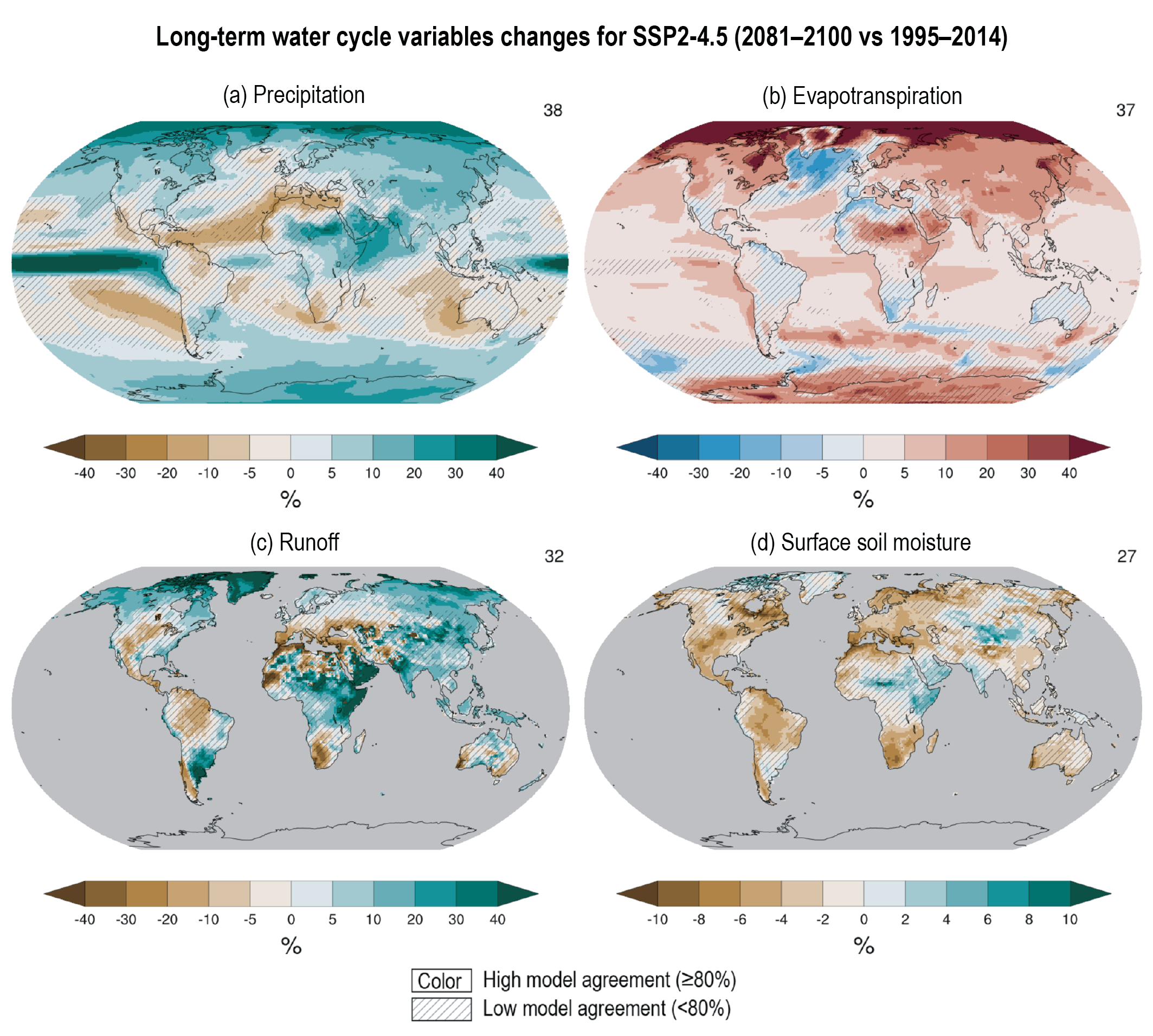
Box TS.6, Figure 1 | Projected water cycle changes. The intent of this figure is to give a geographical overview of changes in multiple components of the global water cycle using an intermediate emissions scenario. Important key message: without drastic reductions in greenhouse gas emissions, human-induced global warming will be associated with widespread changes in all components of the water cycle. Long-term (2081–2100) projected annual mean changes (%) relative to present-day (1995–2014) in the SSP2-4.5 emissions scenario for (a) precipitation, (b) surface evapotranspiration, (c) total runoff and (d) surface soil moisture. Numbers in top right of each panel indicate indicate the number of Coupled Model Intercomparison Project Phase 6 (CMIP6) models used for estimating the ensemble mean. For other scenarios, please refer to relevant figures in Chapter 8. Uncertainty is represented using the simple approach: No overlay indicates regions with high model agreement, where ≥80% of models agree on sign of change; diagonal lines indicate regions with low model agreement, where <80% of models agree on sign of change. For more information on the simple approach, please refer to the Cross-Chapter Box Atlas.1. Links to chapters8.4.1; Figures 8.14, 8.17, 8.18, and 8.19
Infographic TS.1 | Climate Futures

(top left) Annual emissions of CO2 for the five core Shared Socio-economic Pathway (SSP) scenarios (very low: SSP1-1.9, low: SSP1-2.6, intermediate: SSP2-4.5, high: SSP3-7.0, very high: SSP5-8.5). (bottom left) Projected warming for each of these emissions scenarios. (top right) Response of some selected climate variables to four levels of global warming (°C). Changes in the ‘Today’ column are based on a global warming level of 1°C. (bottom right) The long-term effect of each global warming level on sea level. See Section TS.1.3.1 for more detail on the SSP climate change scenarios. This infographic builds from several figures in the Technical Summary: Figure TS.4 (for top left panel), Figure TS.6 (bottom left), Figure TS.12 (top right) and Box TS.4, Figure 1b (bottom right).
TS.3 Understanding the Climate System Response and Implications for Limiting Global Warming
This section summarizes advances in our knowledge of Earth’s energy budget, including the time evolution of forcings and climate feedbacks that lead to the climate system responses summarized in Section TS.2. It assesses advances since AR5 and SR1.5 in the estimation of remaining carbon budgets, the Earth system response to carbon dioxide removal, and the quantification of metrics that allow comparisons of the relative effects of different forcing agents. The section also highlights: future climate and air pollution responses due to projected changes in short-lived climate forcers (SLCFs); the state of understanding of the climate response to potential interventions related to solar radiation modification (SRM); and irreversibility, tipping points and abrupt changes in the climate system.
TS.3.1 Radiative Forcing and Energy Budget

The global energy inventory change for the period 1971–2006 corresponds to an Earth energy imbalance (Box TS.1) of 0.50 [0.32 to 0.69] W m–2, increasing to 0.79 [0.52 to 1.06] W m–2 for the period 2006–2018. Ocean heat uptake is by far the largest contribution and accounts for 91% of the total energy change. Land warming, melting of ice and warming of the atmosphere account for about 5%, 3% and 1% of the total change, respectively. More comprehensive analysis of inventory components, cross-validation of satellite and in situ-based estimates of the global energy imbalance, and closure of the global sea level budget have led to a strengthened assessment relative to AR5. (high confidence) Links to chapters7.2.2, 7.5.2.3, Box 7.2, Table 7.1, 9.6.1, Cross-Chapter Box 9.1, Table 9.5
As in AR5, the perturbations to Earth’s top-of-atmosphere energy budget are quantified using ERFs (see also Section TS.2.2). These include any consequent adjustments to the climate system(e.g., from changes in atmospheric temperatures, clouds and water vapour as shown in Figure TS.14), but exclude any surface temperature response. Since AR5, ERFs have been estimated for a larger number of forcing agents and shown to be more closely related to the temperature response than the stratospheric-temperature-adjusted radiative forcing. (high confidence) Links to chapters7.3.1
Improved quantifications of ERF, the climate system radiative response, and the observed energy increase in the Earth system for the period 1971–2018 demonstrate improved closure of the global energy budget relative to AR5 (Figure TS.13). Combining the likely range of ERF over this period with the central estimate of radiative response gives an expected energy gain of 340 [47 to 662] ZJ. Both estimates are consistent with an independent observation-based assessment of the global energy increase of 284 [96 to 471] ZJ (very likely range), expressed relative to the estimated 1850–1900 Earth energy imbalance. (high confidence) Links to chapters7.2.2, 7.3.5, Box 7.2
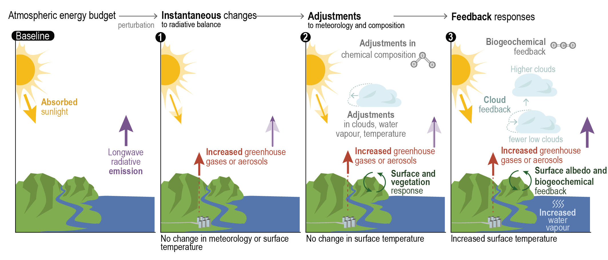
The assessed greenhouse gas ERF over the 1750–2019 period (Section TS.2.2) has increased by +0.59 W m−2 over AR5 estimates for 1750–2011. This increase includes +0.34 W m–2 from increases in atmospheric concentrations of well-mixed greenhouse gases (including halogenated species) since 2011, +0.15 W m–2 from upwards revisions of their radiative efficiencies and +0.10 W m–2 from re-evaluation of the ozone and stratospheric water vapour ERF. Links to chapters7.3.2, 7.3.4, 7.3.5
For CO2, CH4, N2O, and chlorofluorocarbons, there is now evidence to quantify the effect on ERF of tropospheric adjustments. The assessed ERF for a doubling of CO2 compared to 1750 levels (3.9 ± 0.5 Wm–2) is larger than in AR5. For CO2, the adjustments include the physiological effects on vegetation. The reactive well-mixed greenhouse gases (CH4, N2O, and halocarbons) cause additional chemical adjustments to the atmosphere through changes in ozone and aerosols (Figure TS.15a). The ERF due to CH4 emissions is 1.19 [0.81 to 1.58] W m–2, of which 0.35 [0.16 to 0.54] W m–2 is attributed to chemical adjustments mainly via ozone. These chemical adjustments also affect the emissions metrics (Section TS.3.3.3). Changes in sulphur dioxide (SO2) emissions make the dominant contribution to the ERF from aerosol–cloud interactions (high confidence). Over the 1750–2019 period, the contributions from the emitted compounds to global surface temperature changes broadly match their contributions to the ERF (high confidence) (Figure TS.15b). Since a peak in emissions-induced SO2 eRF has already occurred recently (Section TS.2.2) and since there is a delay in the full global surface temperature response owing to the thermal inertia in the climate system, changes in SO2 emissions have a slightly larger contribution to global surface temperature change compared with changes in CO2 emissions, relative to their respective contributions to ERF. Links to chapters6.4.2, 7.3.2

Aerosols contributed an ERF of –1.3 [–2.0 to –0.6] W m–2 over the period 1750 to 2014 (medium confidence). The ERF due to aerosol–cloud interactions (ERFaci) contributes most to the magnitude of the total aerosol ERF (high confidence) and is assessed to be –1.0 [–1.7 to –0.3] W m–2 (medium confidence), with the remainder due to aerosol–radiation interactions (ERFari), assessed to be –0.3 [–0.6 to 0.0] W m–2 (medium confidence). There has been an increase in the estimated magnitude – but a reduction in the uncertainty – of the total aerosol ERF relative to AR5, supported by a combination of increased process-understanding and progress in modelling and observational analyses (Figure TS.15c). Effective radiative forcing estimates from these separate lines of evidence are now consistent with each other, in contrast to AR5, and support the assessment that it is virtually certain that the total aerosol ERF is negative. Compared to AR5, the assessed magnitude of ERFaci has increased, while that of ERFari has decreased . Links to chapters7.3.3, 7.3.5
TS.3.2 Climate Sensitivity and Earth System Feedbacks
TS.3.2.1 Equilibrium Climate Sensitivity, Transient Climate Response, and Transient Climate Response to Cumulative Carbon-dioxide Emissions
Constraints on equilibrium climate sensitivity (ECS) and transient climate response (TCR) (see Glossary) are based on four main lines of evidence: feedback process understanding, climate change and variability seen within the instrumental record, paleoclimate evidence, and so-called ‘emergent constraints’, whereby a relationship between an observable quantity and either ECS or TCR established within an ensemble of models is combined with observations to derive a constraint on ECS or TCR. In reports up to and including the IPCC Third Assessment Report, ECS and TCR derived directly from ESMs were the primary line of evidence. However, since AR4, historical warming and paleoclimates provided useful additional evidence (Figure TS.16a). This Report differs from previous reports in not directly using climate model estimates of ECS and TCR in the assessed ranges of climate sensitivity. Links to chapters1.5, 7.5

It is now clear that when estimating ECS and TCR, the dependence of feedbacks on time scales and the climate state must be accounted for. Feedback processes are expected to become more positive overall (more amplifying of global surface temperature changes) on multi-decadal time scales as the spatial pattern of surface warming evolves and global surface temperature increases, leading to an ECS that is higher than was inferred in AR5 based on warming over the instrumental record (high confidence). Historical surface temperature change since 1870 has shown relatively little warming in several key regions of positive feedbacks, including the eastern equatorial Pacific Ocean and the Southern Ocean, while showing greater warming in key regions of negative feedbacks, including the western Pacific warm pool. Based on process understanding, climate modelling, and paleoclimate reconstructions of past warm periods, it is expected that future warming will become enhanced over the eastern Pacific Ocean (medium confidence) and Southern Ocean (high confidence) on centennial time scales. This new understanding, along with updated estimates of historical temperature change, ERF, and energy imbalance, reconciles previously disparate ECS estimates. Links to chapters7.4.4, 7.5.2, 7.5.3
The AR6 best estimate of ECS is 3°C, the likely range is 2.5°C to 4°C and the very likely range is 2°C to 5°C. There is a high level of agreement among the four main lines of evidence listed above (Figure TS.16b), and altogether it is virtually certain that ECS is larger than 1.5°C, but currently it is not possible to rule out ECS values above 5°C. Therefore, the 5°C upper end of the very likely range is assessed with medium confidence and the other bounds with high confidence. Links to chapters7.5.5
Based on process understanding, warming over the instrumental record, and emergent constraints, the best estimate of TCR is 1.8°C, the likely range is 1.4°C to 2.2°C and the very likely range is 1.2°C to 2.4°C. There is a high level of agreement among the different lines of evidence (Figure TS.16c) (high confidence). Links to chapters7.5.5
On average, CMIP6 models have higher mean ECS and TCR values than the CMIP5 generation of models and also have higher mean values and wider spreads than the assessed best estimates and very likely ranges within this Report. These higher mean ECS and TCR values can be traced to a positive net cloud feedback that is larger in CMIP6 by about 20%. The broader ECS and TCR ranges from CMIP6 also lead the models to project a range of future warming that is wider than the assessed future warming range, which is based on multiple lines of evidence (Cross-Section Box TS.1). However, some of the high-sensitivity CMIP6 models (Section TS.1.2.2) are less consistent with observed recent changes in global warming and with paleoclimate proxy records than models with ECS within the very likely range. Similarly, some of the low-sensitivity models are less consistent with the paleoclimate data. The CMIP6 models with the highest ECS and TCRs values provide insights into low-likelihood, high-impact futures, which cannot be excluded based on currently available evidence (Cross-Section Box TS.1). Links to chapters4.3.1, 4.3.4, 7.4.2, 7.5.6
Uncertainties regarding the true value ofECS and TCR are the dominant source of uncertainty in global temperature projections over the 21st century under moderate to high GHG concentrations scenarios. For scenarios that reach net zero CO2 emissions (Section TS.3.3), the uncertainty in the ERF values ofaerosol and other SLCFs contribute substantial uncertainty in projected temperature. Global ocean heat uptake is a smaller source of uncertainty in centennial warming. Links to chapters7.5.7
The transient climate response to cumulative CO2 emissions (TCRE) is the ratio between globally averaged surface temperature increase and cumulative CO2 emissions (see Glossary). This Report reaffirms with high confidence the finding of AR5 that there is a near-linear relationship between cumulative CO2 emissions and the increase in global average temperature caused by CO2 over the course of this century for global warming levels up to at least 2°C relative to 1850–1900. The TCRE falls likely in the 1.0°C–2.3°C per 1000 PgC range, with a best estimate of 1.65°C per 1000 PgC. This is equivalent to a 0.27°C–0.63°C range with a best estimate of 0.45°C when expressed in units per 1000 GtCO2. This range is about 15% narrower than the 0.8°–2.5°C per 1000 PgC assessment of AR5 because of a better integration of evidence across chapters, in particular the assessment of TCR. Beyond this century, there is low confidence that the TCRE alone remains an accurate predictor of temperature changes in scenarios of very low or net negative CO2 emissions because of uncertain Earth system feedbacks that can result in further changes in temperature or a path dependency of warming as a function of cumulative CO2 emissions. Links to chapters4.6.2, 5.4, 5.5.1
TS.3.2.2 Earth System Feedbacks
The combined effect of all climate feedback processes is to amplify the climate response to forcing (virtually certain). While major advances in the understanding of cloud processes have increased the level of confidence and decreased the uncertainty range for the cloud feedback by about 50% compared to AR5, clouds remain the largest contribution to overall uncertainty in climate feedbacks (high confidence). Uncertainties in the ECS and other climate sensitivity metrics, such as the TCR and TCRE, are the dominant source of uncertainty in global temperature projections over the 21st century under moderate to high GHG emissions scenarios. CMIP6 models have higher mean values and wider spreads in ECS and TCR than the assessed best estimates and very likely ranges within this Report, leading the models to project a range of future warming that is wider than the assessed future warming range (Section TS.2.2). Links to chapters7.1, 7.4.2, 7.5
Earth system feedbacks can be categorized into three broad groups: physical feedbacks, biogeophysical and biogeochemical feedbacks, and feedbacks associated with ice sheets. In previous assessments, the ECS has been associated with a distinct set of physical feedbacks (Planck response, water vapour, lapse rate, surface albedo, and cloud feedbacks). In this assessment, a more general definition of ECS is adopted whereby all biogeophysical and biogeochemical feedbacks that do not affect the atmospheric concentration of CO2 are included. These include changes in natural CH4 emissions, natural aerosol emissions, N2O, ozone, and vegetation, which all act on time scales of years to decades and are therefore relevant for temperature change over the 21st century. Because the total biogeophysical and non-CO2 biogeochemical feedback is assessed to have a central value that is near zero (low confidence), including it does not affect the assessed ECS but does contribute to the net feedback uncertainty. The biogeochemical feedbacks that affect the atmospheric concentration of CO2 are not included because ECS is defined as the response to a sustained doubling of CO2. Moreover, the long-term feedbacks associated with ice sheets are not included in the ECS owing to their long time scales of adjustment. Links to chapters5.4, 6.4, 7.4, 7.5, Box 7.1
The net effect of changes in clouds in response to global warming is to amplify human-induced warming, that is, the net cloud feedback is positive (high confidence). Compared to AR5, major advances in the understanding of cloud processes have increased the level of confidence and decreased the uncertainty range in the cloud feedback by about 50% (Figure TS.17a). An assessment of the low-altitude cloud feedback over the subtropical ocean, which was previously the major source of uncertainty in the net cloud feedback, is improved owing to a combined use of climate model simulations, satellite observations, and explicit simulations of clouds, altogether leading to strong evidence that this type of cloud amplifies global warming. The net cloud feedback is assessed to be +0.42 [–0.10 to 0.94] W m–2°C–1. A net negative cloud feedback is very unlikely . The CMIP5 and CMIP6 ranges of cloud feedback are similar to this assessed range, with CMIP6 having a slightly more positive median cloud feedback (high confidence). The surface albedo feedback and combined water vapour-lapse rate feedback are positive (Figure TS.17a), with high confidence in the estimated value of each based on multiple lines of evidence, including observations, models and theory (Box TS.6). Links to chapters7.4.2, Figure 7.14, Table 7.10

Natural sources and sinks of non-CO2 greenhouse gases such as methane (CH4) and nitrous oxide (N2O) respond both directly and indirectly to atmospheric CO2 concentration and climate change, and thereby give rise to additional biogeochemical feedbacks in the climate system. Many of these feedbacks are only partially understood and are not yet fully included in ESMs. There is medium confidence that the net response of natural ocean and land CH4 and N2O sources to future warming will be increased emissions, but the magnitude and timing of the responses of each individual process is known with low confidence. Links to chapters5.4.7
Non-CO2 biogeochemical feedbacks induced from changes in emissions, abundances or lifetimes of SLCFs mediated by natural processes or atmospheric chemistry are assessed to decrease ECS (Figure TS.17b). These non-CO2 biogeochemical feedbacks are estimated from ESMs, which since AR5 have advanced to include a consistent representation of biogeochemical cycles and atmospheric chemistry. However, process-level understanding of many biogeochemical feedbacks involving SLCFs, particularly natural emissions, is still emerging, resulting in low confidence in the magnitude and sign of the feedbacks. The central estimate of the total biogeophysical and non-CO2 biogeochemical feedback is assessed to be −0.01 [–0.27 to +0.25] W m–2°C–1 (Figure TS.17a). Links to chapters5.4.7, 5.4.8, 6.2.2, 6.4.5, 7.4, Table 7.10
The combined effect of all known radiative feedbacks (physical, biogeophysical, and non-CO2 biogeochemical) is to amplify the base climate response (in the absence of feedbacks), also known as the Planck temperature response20 (virtually certain). Combining these feedbacks with the Planck response, the net climate feedback parameter is assessed to be –1.16 [–1.81 to –0.51] W m–2°C–1, which is slightly less negative than that inferred from the overall ECS assessment. The combined water vapour and lapse rate feedback makes the largest single contribution to global warming, whereas the cloud feedback remains the largest contribution to overall uncertainty. Due to the state-dependence of feedbacks, as evidenced from paleoclimate observations and from models, the net feedback parameter will increase (become less negative) as global temperature increases. Furthermore, on long time scales the ice-sheet feedback parameter is very likely positive, promoting additional warming on millennial time scales as ice sheets come into equilibrium with the forcing. (high confidence) Links to chapters7.4.2, 7.4.3, Figure 7.14, Table 7.10
The carbon cycle provides for additional feedbacks on climate owing to the sensitivity of land–atmosphere and ocean–atmosphere carbon fluxes and storage to changes in climate and in atmospheric CO2 (Figure TS.17c). Because of the time scales associated with land and ocean carbon uptake, these feedbacks are known to be scenario dependent. Feedback estimates deviate from linearity in scenarios of stabilizing or reducing concentrations. With high confidence, increased atmospheric CO2 will lead to increased land and ocean carbon uptake, acting as a negative feedback on climate change. It is likely that a warmer climate will lead to reduced land and ocean carbon uptake, acting as a positive feedback (Box TS.5). Links to chapters4.3.2, 5.4.1–5
Thawing terrestrial permafrost will lead to carbon release (high confidence), but there is low confidence in the timing, magnitude and the relative roles of CO2 versus CH4 as feedback processes. An ensemble of models projects CO2 release from permafrost to be 3–41 PgC per 1ºC of global warming by 2100, leading to warming strong enough that it must be included in estimates of the remaining carbon budget but weaker than the warming from fossil fuel burning. However, the incomplete representation of important processes, such as abrupt thaw, combined with weak observational constraints, only allowlow confidence in both the magnitude of these estimates and in how linearly proportional this feedback is to the amount of global warming. There is emerging evidence that permafrost thaw and thermokarst give rise to increased CH4 and N2O emissions, which leads to the combined radiative forcing from permafrost thaw being larger than from CO2 emissions only. However, the quantitative understanding of these additional feedbacks is low, particularly for N2O. These feedbacks, as well as potential additional carbon losses due to climate-induced fire feedback are not routinely included in Earth system models. Links to chaptersBox 5.1, 5.4.3, 5.4.7, 5.4.8
TS.3.3 Temperature Stabilization, Net Zero Emissions and Mitigation
TS.3.3.1 Remaining Carbon Budgets and Temperature Stabilization
Limiting further climate change would require substantial and sustained reductions of GHG emissions. Without net zero CO2 emissions, and a decrease in the net non-CO2 forcing (or sufficient net negative CO2 emissions to offset any further warming from net non-CO2 forcing), the climate system will continue to warm. There is high confidence that mitigation requirements for limiting warming to specific levels over this century can be estimated using a carbon budget that relates cumulative CO2 emissions to global mean temperature increase (Figure TS.18, Table TS.3). For the period 1850–2019, a total of 2390 ± 240 GtCO2 of anthropogenic CO2 has been emitted. Remaining carbon budgets (starting from 1 January 2020) for limiting warming to 1.5°C, 1.7°C and 2.0°C are estimated at 500 GtCO2, 850 GtCO2 and 1350 GtCO2, respectively, based on the 50th percentile of TCRE. For the 67th percentile, the respective values are 400 GtCO2, 700 GtCO2 and 1150 GtCO2. The remaining carbon budget estimates for different temperature limits assume that non-CO2 emissions are mitigated consistent with the median reductions found in scenarios in the literature as assessed in SR1.5, but they may vary by an estimated ±220 GtCO2 depending on how deeply future non-CO2 emissions are assumed to be reduced (Table TS.3). Links to chapters5.5.2, 5.6, Box 5.2, 7.6

There is high confidence that several factors, including estimates of historical warming, future emissions from thawing permafrost, and variations in projected non-CO2 warming, affect the value of carbon budgets but do not change the conclusion that global CO2 emissions would need to decline to net zero to halt global warming. Estimates may vary by ±220 GtCO2 depending on the level of non-CO2 emissions at the time global anthropogenic CO2 emissions reach net zero levels. This variation is referred to as non-CO2 scenario uncertainty and will be further assessed in the AR6 Working Group III Contribution. Geophysical uncertainties surrounding the climate response to these non-CO2 emissions result in an additional uncertainty of at least ±220 GtCO2, and uncertainties in the level of historical warming result in a ±550 GtCO2 uncertainty. Links to chapters5.4, 5.5.2

aHuman-induced global surface temperature increase between 1850–1900 and 2010–2019 is assessed at 0.8–1.3°C (likely range; Cross-Section Box TS.1) with a best estimate of 1.07°C. Combined with a central estimate of TCRE (1.65°C per 1000 PgC) this uncertainty in isolation results in a potential variation of remaining carbon budgets of ±550 GtCO2, which, however, is not independent of the assessed uncertainty of TCRE and thus not fully additional.
bTCRE: transient climate response to cumulative emissions of carbon dioxide, assessed to fall likely between 1.0–2.3°C per 1000 PgC with a normal distribution, from which the percentiles are taken. Additional Earth system feedbacks are included in the remaining carbon budget estimates as discussed in Section 5.5.2.2.5.
cEstimates assume that non-CO2 emissions are mitigated consistent with the median reductions found in scenarios in the literature as assessed in SR1.5. Non-CO2 scenario variations indicate how much remaining carbon budget estimates vary due to different scenario assumptions related to the future evolution of non-CO2 emissions in mitigation scenarios from SR1.5 that reach net zero CO2 emissions. This variation is additional to the uncertainty in TCRE. The Working Group III Contribution to AR6 will reassess the potential for non-CO2 mitigation based on literature since SR1.5.
dGeophysical uncertainties reported in these columns and TCRE uncertainty are not statistically independent, as uncertainty in TCRE depends on uncertainty in the assessment of historical temperature, non-CO2 versus CO2 forcing, and uncertainty in emissions estimates. These estimates cannot be formally combined, and these uncertainty variations are not directly additional to the spread of remaining carbon budgets due to TCRE uncertainty reported in columns three to seven.
eRecent emissions uncertainty reflects the ±10% uncertainty in the historical CO2 emissions estimate since 1 January 2015.
Methodological improvements and new evidence result in updated remaining carbon budget estimates. The assessment in AR6 applies the same methodological improvements as in SR1.5, which uses a recent observed baseline for historic temperature change and cumulative emissions. Changes compared to SR1.5 are therefore small: the assessment of new evidence results in updated median remaining carbon budget estimates for limiting warming to 1.5°C and 2°C being the same and about 60 GtCO2 smaller, respectively, after accounting for emissions since SR1.5. Meanwhile, remaining carbon budgets for limiting warming to 1.5°C would be about 300–350 GtCO2 larger if evidence and methods available at the time of AR5 would be used. If a specific remaining carbon budget is exceeded, this results in a lower probability of keeping warming below a specified temperature level and higher irreversible global warming over decades to centuries, or alternatively a need for net negative CO2 emissions or further reductions in non-CO2 greenhouse gases after net zero CO2 is achieved to return warming to lower levels in the long term. Links to chapters5.5.2, 5.6, Box 5.2
Based on idealized model simulations that explore the climate response once CO2 emissions have been brought to zero, the magnitude of the zero CO2 emissions commitment (ZEC, see Glossary) is assessed to be likely smaller than 0.3°C for time scales of about half a century and cumulative CO2 emissions broadly consistent with global warming of 2°C. However, there is low confidence about its sign on time scales of about half a century. For lower cumulative CO2 emissions, the range would be smaller yet with equal uncertainty about the sign. If the ZEC is positive on decadal time scales, additional warming leads to a reduction in the estimates of remaining carbon budgets, and vice versa if it is negative. Links to chapters4.7.1, 5.5.2
Permafrost thaw is included in estimates together with other feedbacks that are often not captured by models. Limitations in modelling studies combined with weak observational constraints only allowlow confidence in the magnitude of these estimates (Section TS.3.2.2). Despite the large uncertainties surrounding the quantification of the effect of additional Earth system feedback processes, such as emissions from wetlands and permafrost thaw, these feedbacks represent identified additional risk factors that scale with additional warming and mostly increase the challenge of limiting warming to specific temperature levels. These uncertainties do not change the basic conclusion that global CO2 emissions would need to decline to net zero to halt global warming. Links to chapters5.4.8, 5.5.2, Box 5.1
TS.3.3.2 Carbon Dioxide Removal
Carbon dioxide removal (CDR) refers to anthropogenic activities that deliberately remove CO2 from the atmosphere and durably store it in geological, terrestrial or ocean reservoirs, or in products. Carbon dioxide is removed from the atmosphere by enhancing biological or geochemical carbon sinks or by direct capture of CO2 from air. Emissions pathways that limit global warming to 1.5°C or 2°C typically assume the use of CDR approaches in combination with GHG emissions reductions. CDR approaches could be used to compensate for residual emissions from sectors that are difficult or costly to decarbonize. CDR could also be implemented at a large scale to generate global net negative CO2 emissions (i.e., anthropogenic CO2 removals exceeding anthropogenic emissions), which could compensate for earlier emissions as a way to meet long-term climate stabilization goals after a temperature overshoot. This Report assesses the effects of CDR on the carbon cycle and climate. Co-benefits and trade-offs for biodiversity, water and food production are briefly discussed for completeness, but a comprehensive assessment of the ecological and socio-economic dimensions of CDR options is left to the WGII and WGIII reports. Links to chapters4.6.3, 5.6
CDR methods have the potential to sequester CO2 from the atmosphere (high confidence). In the same way part of current anthropogenic net CO2 emissions are taken up by land and ocean carbon stores, net CO2 removal will be partially counteracted by CO2 release from these stores, such that the amount of CO2 sequestered by CDR will not result in an equivalent drop in atmospheric CO2 (very high confidence). The fraction of CO2 removed from the atmosphere that is not replaced by CO2 released from carbon stores – a measure of CDR effectiveness – decreases slightly with increasing amounts of removal (medium confidence) and decreases strongly if CDR is applied at lower atmospheric CO2 concentrations (medium confidence). The reduction in global surface temperature is approximately linearly related to cumulative CO2 removal (high confidence). Because of this near-linear relationship, the amount of cooling per unit CO2 removed is approximately independent of the rate and amount of removal (medium confidence). Links to chapters4.6.3, 5.6.2.1, Figure 5.32, Figure 5.34
Due to non-linearities in the climate system, the century-scale climate–carbon cycle response to a CO2 removal from the atmosphere is not always equal and opposite to its response to a simultaneous CO2 emission (mediumconfidence). For CO2 emissions of 100 PgC released from a state in equilibrium with pre-industrial atmospheric CO2 levels, CMIP6 models simulate that 27± 6% (mean ± 1 standard deviation) of emissions remain in the atmosphere 80–100 years after the emissions, whereas for removals of 100 PgC only 23 ± 6% of removals remain out of the atmosphere. This asymmetry implies that an extra amount of CDR is required to compensate for a positive emission of a given magnitude to attain the same change in atmospheric CO2. Due to low agreement between models, there is low confidence in the sign of the asymmetry of the temperature response to CO2 emissions and removals. Links to chapters4.6.3, 5.6.2.1, Figure 5.35
Simulations with ESMs indicate that under scenarios where CO2 emissions gradually decline, reach net zero and become net negative during the 21st century (e.g., SSP1-2.6), land and ocean carbon sinks begin to weaken in response to declining atmospheric CO2 concentrations, and the land sink eventually turns into a source (Figure TS.19). This sink-to-source transition occurs decades to a few centuries after CO2 emissions become net negative. The ocean remains a sink of CO2 for centuries after emissions become net negative. Under scenarios with large net negative CO2 emissions (e.g., SSP5-3.4-OS) and rapidly declining CO2 concentrations, the land source is larger than for SSP1-2.6 and the ocean also switches to a source. While the general response is robust across models, there is low confidence in the timing of the sink-to-source transition and the magnitude of the CO2 source in scenarios with net negative CO2 emissions. Carbon dioxide removal could reverse some aspects climate change if CO2 emissions become net negative, but some changes would continue in their current direction for decades to millennia. For instance, sea level rise due to ocean thermal expansion would not reverse for several centuries to millennia (high confidence) (Box TS.4). Links to chapters4.6.3, 5.4.10, 5.6.2.1, Figure 5.30, Figure 5.33

Carbon dioxide removal methods have a range of side effects that can either weaken or strengthen the carbon sequestration and cooling potential of these methods and affect the achievement of sustainable development goals (high confidence). Biophysical and biogeochemical side-effects of CDR methods are associated with changes in surface albedo, the water cycle, emissions of CH4 and N2O, ocean acidification and marine ecosystem productivity (high confidence). These side-effects and associated Earth system feedbacks can decrease carbon uptake and/or change local and regional climate and in turn limit the CO2 sequestration and cooling potential of specific CDR methods (medium confidence). Deployment of CDR, particularly on land, can also affect water quality and quantity, food production and biodiversity (high confidence). These effects are often highly dependent on local context, management regime, prior land use, and scale (high confidence). The largest co-benefits are obtained with methods that seek to restore natural ecosystems or improve soil carbon sequestration (medium confidence). The climate and biogeochemical effects of terminating CDR are expected to be small for most CDR methods (medium confidence). Links to chapters4.6.3, 5.6.2.2, Figure 5.36, 8.4.3, 8.6.3
TS.3.3.3 Relating Different Forcing Agents
The relative climate effects of different forcing agents are typically quantified using emissions metrics that compare the effects of an idealised pulse of 1 kg of some climate forcing agent against a reference climate forcing agent, almost always CO2. The two most prominent pulse emissions metrics are the global warming potential (GWP) and global temperature change potential (GTP) (see Glossary). The climate responses to CO2 emissions by convention include the effects of warming on the carbon cycle, so for consistency these also need to be determined for non-CO2 emissions. The methodology for doing this has been placed on a more robust scientific footing compared to AR5 (high confidence). Methane from fossil fuel sources has slightly higher emissions metric values than those from biogenic sources since it leads to additional fossil CO2 in the atmosphere (high confidence). Updates to the chemical adjustments for CH4 and N2O emissions (Section TS.3.1) and revisions in their lifetimes result in emissions metrics for GWP and GTP that are slightly lower than in AR5 (medium confidence). Emissions metrics for the entire suite of GHGs assessed in the AR6 have been calculated for various time horizons. Links to chapters7.6.1, Table 7.15, Table 7.SM.7
New emissions metric approaches, such as GWP* and Combined-GTP (CGTP), relate changes in the emissions rate of short-lived greenhouse gases to equivalent cumulative emissions of CO2 (CO2 -e). Global surface temperature response from aggregated emissions of short-lived greenhouse gases over time is determined by multiplying these cumulative CO2 -e by TCRE (see Section TS.3.2.1). When GHGs are aggregated using standard metrics such as GWP or GTP, cumulative CO2 -e emissions are not necessarily proportional to future global surface temperature outcomes (high confidence) Links to chapters7.6.1, Box 7.3
Emissions metrics are needed to aggregate baskets of gases to determine net zero GHG emissions. Generally, achieving net zero CO2 emissions and declining non-CO2 radiative forcing would halt human-induced warming. Reaching net zero GHG emissions quantified by GWP-100 typically leads to declining temperatures after net zero GHGs emissions are achieved if the basket includes short-lived gases, such as CH4. Net zero GHG emissions defined by CGTP or GWP* imply net zero CO2 and other long-lived GHG emissions and constant (CGTP) or gradually declining (GWP*) emissions of short-lived gases. The warming evolution resulting from net zero GHG emissions defined in this way corresponds approximately to reaching net zero CO2 emissions, and would thus not lead to declining temperatures after net zero GHG emissions are achieved but to an approximate temperature stabilization (high confidence). The choice of emissions metric hence affects the quantification of net zero GHG emissions, and therefore the resulting temperature outcome of reaching and sustaining net zero GHG emissions levels (high confidence). Links to chapters7.6.1.4, 7.6.2, 7.6.3
As pointed out in AR5, ultimately, it is a matter for policymakers to decide which emissions metric is most applicable to their needs. This Report does not recommend the use of any specific emissions metric, as the most appropriate metric depends on the policy goal and context (see Chapter 7, Section 7.6). A detailed assessment of GHG metrics to support climate change mitigation and associated policy contexts is provided in the WGIII contribution to the AR6.
The global surface temperature response following a climate change mitigation measure that affects emissions of both short- and long-lived climate forcers depends on their lifetimes, their ERFs, how fast and for how long the emissions are reduced, and the thermal inertia in the climate system. Mitigation, relying on emissions reductions and implemented through new legislation or technology standards, implies that emissions reductions occur year after year. Global temperature response to a year’s worth of current emissions from different sectors informs about the mitigation potential (Figure TS.20). Over 10- to 20-year time scales, the influence of SLCFs is at least as large as that of CO2, with sectors producing the largest warming being fossil fuel production and distribution, agriculture, and waste management. Because the effects of the SLCFs decay rapidly over the first few decades after emission, the net long-term temperature effect from a single year’s worth of current emissions is predominantly determined by CO2. Fossil fuel combustion for energy, industry and land transportation are the largest contributing sectors on a 100-year time scale (high confidence). Current emissions of CO2, N2O and SLCFs from East Asia and North America are the largest regional contributors to additional net future warming on both short (medium confidence) and long time scales (10 and 100 years, respectively) (high confidence). Links to chapters6.6.1, 6.6.2, Figure 6.16

COVID-19 restrictions led to detectable reductions in global anthropogenic emissions of nitrogen oxides (NOx) (about 35% in April 2020) and fossil CO2 (7%, with estimates ranging from 5.8% to 13.0%), driven largely by reduced emissions from the transportation sector (medium confidence). There is high confidence that, with the exception of surface ozone, reductions in pollutant precursors contributed to temporarily improved air quality in most regions of the world. However, these reductions were lower than what would be expected from sustained implementation of policies addressing air quality and climate change (medium confidence). Overall, the net global ERF from COVID-19 containment was likely small and positive for 2020 (with a temporary peak value less than 0.2 W m–2), thus temporarily adding to the total anthropogenic climate influence, with positive forcing (warming influence) from aerosol changes dominating over negative forcings (cooling influence) from CO2, NOx and contrail cirrus changes. Consistent with this small net radiative forcing, and against a large component of internal variability, Earth system models show no detectable effect on global or regional surface temperature or precipitation (high confidence). Links to chaptersCross Chapter Box 6.1
Box TS.7 | Climate and Air Quality Responses to Short-lived Climate Forcers in SharedSocio-economicPathways
The net effect of SLCF emissions changes on temperature will depend on how emissions of warming and cooling SLCFs will evolve in the future. The magnitude of the cooling effect of aerosols remains the largest uncertainty in the effect of SLCFs in future climate projections. Since the SLCFs have undergone large changes over the past two decades, the temperature and air pollution responses are estimated relative to the year 2019 instead of 1995–2014.
Temperature Response
In the next two decades, it is very likely that SLCF emissions changes will cause a warming relative to 2019, across the WGI core set of SSPs (see Section TS.1.3.1), in addition to the warmingfrom long-lived GHGs. The net effect of SLCF and HFC changes in global surface temperature across the SSPs is a likely warming of 0.06°C–0.35°C in 2040 relative to 2019. This near-term global mean warming linked to SLCFs is quite similar in magnitude across the SSPs due to competing effects of warming (CH4, ozone) and cooling (aerosols) forcers (Box TS.7, Figure 1). There is greater diversity in the end-of-century response among the scenarios. SLCF changes in scenarios with no climate change mitigation (SSP3-7.0 and SSP5-8.5) will cause a warming in the likely range of 0.4°C–0.9°C in 2100 relative to 2019 due to increases in CH4, tropospheric ozone and HFC levels. For the stringent climate change and pollution mitigation scenarios (SSP1-1.9 and SSP1-2.6), the cooling from reductions in CH4, ozone and HFCs partially balances the warming from reduced aerosols, primarily sulphate, and the overall SLCF effect is a likely increase in global surface temperature of 0.0°C–0.3°C in 2100, relative to 2019. With intermediate climate change and air pollution mitigations, SLCFs in SSP2-4.5 add a likely warming of 0.2°C–0.5°C to global surface temperature change in 2100, with the largest warming resulting from reductions in aerosols. Links to chapters4.4.4, 6.7.3
Assuming implementation and efficient enforcement of both the Kigali Amendment to the Montreal Protocol on Substances that Deplete the Ozone Layer and current national plans result in limiting emissions (as in SSP1-2.6), the effects of HFCs on global surface temperature, relative to 2019, would remain below +0. 02°C from 2050 onwards versus about +0.04°C–0.08°C in 2050 and +0.1°C–0.3°C in 2100 considering only national HFC regulations decided prior to the Kigali Amendment (as in SSP5-8.5) (medium confidence). Links to chapters6.6.3, 6.7.3
Air Quality Responses
Air pollution projections range from strong reductions in global surface ozone and PM (e.g., SSP1-2.6, with stringent mitigation of both air pollution and climate change) to no improvement and even degradation (e.g., SSP3-7.0 without climate change mitigation and with only weak air pollution control) (high confidence). Under the SSP3-7.0 scenario, PM levels are projected to increase until 2050 over large parts of Asia, and surface ozone pollution is projected to worsen over all continental areas through 2100 (high confidence). In SSP5-8.5, a scenario without climate change mitigation but with stringent air pollution control, PM levels decline through 2100, but high CH4 levels hamper the decline in global surface ozone at least until 2080 (high confidence). Links to chapters6.7.1

Box TS.7, Figure 1 | Effects of short-lived climate forcers (SLCFs) on global surface temperature and air pollution across the WGI core set of Shared Socio-economic Pathways (SSPs). The intent of this figure is to show the climate and air quality (surface ozone and particulate matter smaller than 2.5 microns in diameter, or PM2.5) response to SLCFs in the SSP scenarios for the near and long-term. Effects of net aerosols, tropospheric ozone, hydrofluorocarbons (HFCs; with lifetimes less than 50 years), and methane (CH4) are compared with those of total anthropogenic forcing for 2040 and 2100 relative to year 2019. The global surface temperature changes are based on historical and future evolution of effective radiative forcing (ERF) as assessed in Chapter 7 of this Report. The temperature responses to the ERFs are calculated with a common impulse response function (RT) for the climate response, consistent with the metric calculations in Chapter 7 (Box 7.1). The RT has an equilibrium climate sensitivity of 3.0°C for a doubling of atmospheric CO2 concentration (feedback parameter of –1.31 W m–2°C–1). The scenario total (grey bar) includes all anthropogenic forcings (long- and short-lived climate forcers, and land-use changes). Uncertainties are 5–95% ranges. The global changes in air pollutant concentrations (ozone and PM2.5) are based on multimodel Coupled Model Intercomparison Project Phase 6 (CMIP6) simulations and represent changes in five-year mean surface continental concentrations for 2040 and 2098 relative to 2019. Uncertainty bars represent inter-model ±1 standard deviation. Links to chapters6.7.2, 6.7.3, Figure 6.24
Box TS.8 | Earth System Response to Solar Radiation Modification
Solar radiation modification (SRM) refers to deliberate, large-scale climate intervention options that are studied as potential supplements to deep mitigation, for example, in scenarios that overshoot climate stabilization goals. SRM options aim to offset some of the warming effects of GHG emissions by modification of Earth’s shortwave radiation budget. Following SR1.5, the SRM assessed in this Report also includes some options, such as cirrus cloud thinning, that alter the longwave radiation budget.
SRM contrasts with climate change mitigation activities, such as emissions reductions and CDR, as it introduces a ‘mask’ to the climate change problem by altering Earth’s radiation budget, rather than attempting to address the root cause of the problem, which is the increase in GHGs in the atmosphere. By masking only the climate effects of GHG emissions, SRM does not address other issues related to atmospheric CO2 increase, such as ocean acidification. This Report assesses physical understanding of the Earth system response to proposed SRM, and the assessment is based primarily on idealized climate model simulations. There are other important considerations, such as risk to human and natural systems, perceptions, ethics, cost, governance, and trans-boundary issues and their relationship to the United Nations Sustainable Development Goals – issues that the WGII (Chapter 16) and WGIII (Chapter 14) Reports address. Links to chapters4.6.3
SRM options include those that increase surface albedo, brighten marine clouds by increasing the amount of cloud condensation nuclei, or reduce the optical depth of cirrus clouds by seeding them with ice nucleating particles. However, the most commonly studied approaches attempt to mimic the cooling effects of major volcanic eruptions by injecting reflective aerosols (e.g., sulphate aerosols) or their precursors (e.g., sulphur dioxide) into the stratosphere. Links to chapters4.6.3, 5.6.3, 6.4.6
SRM could offset some effects of greenhouse gas-induced warming on global and regional climate, but there would be substantial residual and overcompensating climate change at the regional scale and seasonal time scales (high confidence). Since AR5, more modelling work has been conducted with more sophisticated treatment of aerosol-based SRM approaches, but the uncertainties in cloud–aerosol–radiation interactions are still large (high confidence). Modelling studies suggest that it is possible to stabilize multiple large-scale temperature indicators simultaneously by tailoring the deployment strategy of SRM options (medium confidence) but with large residual or overcompensating regional and seasonal climate changes. Links to chapters4.6.3
SRM approaches targeting shortwave radiation are likely to reduce global mean precipitation, relative to future CO2 emissions scenarios, if all global mean warming is offset. In contrast, cirrus cloud thinning, targeting longwave radiation, is expected to cause an increase in global mean precipitation (medium confidence). If shortwave approaches are used to offset global mean warming, the magnitude of reduction in regional precipitation minus evapotranspiration (P–E) (Box TS.5), which is more relevant to freshwater availability, is smaller than precipitation decrease because of simultaneous reductions in both precipitation and evapotranspiration (medium confidence). Links to chapters4.6.3, 8.2.1, 8.6.3 .
If SRM is used to cool the planet, it would cause a reduction in plant and soil respiration and slow the reduction of ocean carbon uptake due to warming (medium confidence). The result would be an enhancement of the global land and ocean CO2 sinks (medium confidence) and a slight reduction in atmospheric CO2 concentration relative to unmitigated climate change. However, SRM would not stop CO2 from increasing in the atmosphere or affect the resulting ocean acidification under continued anthropogenic emissions (high confidence). Links to chapters5.6.3
The effect of stratospheric aerosol injection on global temperature and precipitation is projected by models to be detectable after one to two decades, which is similar to the time scale for the emergence of the benefits of emissions reductions. A sudden and sustained termination of SRM in a high GHG emissions scenario would cause rapid climate change and a reversal of the SRM effects on the carbon sinks (high confidence). It is also likely that a termination of strong SRM would drive abrupt changes in the water cycle globally and regionally, especially in the tropical regions by shifting the Inter-tropical Convergence Zone and Hadley cells. At the regional scale, non-linear responses cannot be excluded, due to changes in evapotranspiration. However, a gradual phase-out of SRM combined with emissions reductions and CDR would avoid larger rates of changes (medium confidence). Links to chapters4.6.3, 5.6.3, 8.6.3 .
Box TS.9 | Irreversibility, Tipping Points and Abrupt Changes
Understanding of multi-decadal reversibility (i.e., the system returns to the previous climate state within multiple decades after the radiative forcing is removed) has improved since AR5 for many atmospheric, land surface and sea ice climate metrics following sea surface temperature recovery. Some processes suspected of having tipping points, such as the Atlantic Meridional Overturning Circulation (AMOC), have been found to often undergo recovery after temperature stabilization with a time delay (low confidence). However, substantial irreversibility is further substantiated for some cryosphere changes, ocean warming, sea level rise, and ocean acidification. Links to chapters4.7.2, 5.3.3, 5.4.9, 9.2.2, 9.2.4, 9.4.1, 9.4.2, 9.6.3
Some climate system components are slow to respond, such as the deep ocean overturning circulation and the ice sheets. It is likely that under stabilization of global warming at 1.5°C, 2.0°C or 3.0°C relative to 1850–1900, the AMOC will continue to weaken for several decades by about 15%, 20% and 30% of its strength and then recover to pre-decline values over several centuries (medium confidence). At sustained warming levels between 2°C and 3°C, there is limited evidence that the Greenland and West Antarctic ice sheets will be lost almost completely and irreversibly over multiple millennia; both the probability of their complete loss and the rate of mass loss increases with higher surface temperatures (high confidence). At sustained warming levels between 3°C and 5°C, near-complete loss of the Greenland Ice Sheet and complete loss of the West Antarctic Ice Sheet is projected to occur irreversibly over multiple millennia (medium confidence); with substantial parts or all of Wilkes Subglacial Basin in East Antarctica lost over multiple millennia (low confidence). Early-warning signals of accelerated sea level rise from Antarctica could possibly be observed within the next few decades. For other hazards (e.g., ice-sheet behaviour, glacier mass loss and global mean sea level change, coastal floods, coastal erosion, air pollution, and ocean acidification) the time and/or scenario dimensions remain critical, and a simple and robust relationship with global warming level cannot be established (high confidence). Links to chapters4.3.2, 4.7.2, 5.4.3, 5.4.5, 5.4.8, 8.6, 9.2, 9.4, Box 9.3, Cross-Chapter Box 12.1
For global climate indicators, evidence for abrupt change is limited. For global warming up to 2°C above 1850–1900 levels, paleoclimate records do not indicate abrupt changes in the carbon cycle (low confidence). Despite the wide range of model responses, uncertainty in atmospheric CO2 by 2100 is dominated by future anthropogenic emissions rather than uncertainties related to carbon–climate feedbacks (high confidence). There is no evidence of abrupt change in climate projections of global temperature for the next century: there is a near-linear relationship between cumulative CO2 emissions and maximum global mean surface air temperature increase caused by CO2 over the course of this century for global warming levels up to at least 2°C relative to 1850–1900. The increase in global ocean heat content (Section TS.2.4) will likely continue until at least 2300 even for low emissions scenarios, and global mean sea level will continue to rise for centuries to millennia following cessation of emissions (Box TS.4) due to continuing deep ocean heat uptake and mass loss of the Greenland and Antarctic ice sheets (high confidence). Links to chapters2.2.3; Cross-Chapter Box 2.1; 5.1.1; 5.4; Cross-Chapter Box 5.1; Figures 5.3, 5.4, 5.25, and 5.26; 9.2.2; 9.2.4
The response of biogeochemical cycles to anthropogenic perturbations can be abrupt at regional scales and irreversible on decadal to century time scales (high confidence). The probability of crossing uncertain regional thresholds increases with climate change (highBox TS.9
confidence). It is very unlikely that gas clathrates (mostly methane) in deeper terrestrial permafrost and subsea clathrates will lead to a detectable departure from the emissions trajectory during this century. Possible abrupt changes and tipping points in biogeochemical cycles lead to additional uncertainty in 21st century atmospheric GHG concentrations, but future anthropogenic emissions remain the dominant uncertainty (high confidence). There is potential for abrupt water cycle changes in some high emissions scenarios, but there is no overall consistency regarding the magnitude and timing of such changes. Positive land surface feedbacks, including vegetation, dust, and snow, can contribute to abrupt changes in aridity, but there is onlylow confidence that such changes will occur during the 21st century. Continued Amazon deforestation, combined with a warming climate, raises the probability that this ecosystem will cross a tipping point into a dry state during the 21st century (low confidence). (Section TS.3.2.2) Links to chapters5.4.3, 5.4.5, 5.4.8, 5.4.9, 8.6.2, 8.6.3, Cross-Chapter Box 12.1
TS.4 Regional Climate Change
This section focuses on how to generate regional climate change information and its relevance for climate services; the drivers of regional climate variability and change and how they are being affected by anthropogenic factors; and observed, attributed and projected changes in climate, including extreme events and climatic impact-drivers (CIDs), across all regions of the world. There is a small set of CID changes common to all land or ocean regions and a specific set of changes from a broader range of CIDs seen in each region. This regional diversity results from regional climate being determined by a complex interplay between the seasonal-to-multi-decadal variation of large-scale modes of climate variability, external natural and anthropogenic forcings, local climate processes and related feedbacks.
TS.4.1 Generation and Communication of Regional Climate Change Information
TS.4.1.1 Sources and Methodologies for Generating Regional Climate Information
Climate change information at regional scale is generated using a range of data sources and methodologies (Section TS.1.4). Understanding of observed regional climate change and variability is based on the availability and analysis of multiple observational datasets that are suitable for evaluating the phenomena of interest (e.g., extreme events), including accounting for observational uncertainty (Section TS.1.2.1). These datasets are combined with climate model simulations of observed changes and events to attribute causes of those changes and events to large- and regional-scale anthropogenic and natural drivers and to assess the performance of the models. Future simulations with many climate models (multi-model ensembles) are then used to generate and quantify ranges of projected regional climate responses (Section TS.4.2). Discarding models that fundamentally misrepresent relevant processes improves the credibility of regional climate information generated from these ensembles (high confidence). However, multi-model mean and ensemble spread are not a full measure of the range of projection uncertainty and are not sufficient to characterize low-likelihood, high-impact changes (Box TS.3) or situations where different models simulate substantially different or even opposite changes (high confidence). Large single-model ensembles are now available and provide a more comprehensive spectrum of possible changes associated with internal variability (high confidence) (Section TS.1.2.3). Links to chapters1.5.1, 1.5.4, 10.2, 10.3.3, 10.3.4, 10.4.1, 10.6.2, 11.2, Box 11.2, Cross-Chapter Box 11.1, 12.4, Atlas.1.4.1
Depending on the region of interest, representing regionally important forcings (e.g., aerosols, land-use change and ozone concentrations) and feedbacks (e.g., between snow and albedo, soil moisture and temperature, or soil moisture and precipitation) in climate models is a prerequisite for them to reproduce past regional trends to underpin the reliability of future projections (medium confidence) (Section TS.1.2.2). In some cases, even the sign of a projected change in regional climate cannot be trusted if relevant regional processes are not represented, for example, for variables such as precipitation and wind speed (medium confidence). In some regions, either geographical (e.g., Central Africa, Antarctica) or typological (e.g., mountainous areas, Small Islands and cities), and for certain phenomena, fewer observational records are available or accessible, which limits the assessment of regional climate change in these cases. Links to chapters1.5.1, 1.5.3, 1.5.4, 8.5.1, 10.2, 10.3.3, 10.4.1, 11.1.6, 11.2, 12.4, Atlas.8.3, Atlas.11.1.5, Cross-Chapter Box Atlas.2
Methodologies such as statistical downscaling, bias adjustment and weather generators are beneficial as an interface between climate model projections and impact modelling and for deriving user-relevant indicators (high confidence). However, the performance of these techniques depends on that of the driving climate model: in particular, bias adjustment cannot overcome all consequences of unresolved or strongly misrepresented physical processes, such as large-scale circulation biases or local feedbacks (medium confidence). Links to chapters10.3.3, Cross-Chapter Box 10.2, 12.2, Atlas.2.2
Box TS.10 | Event Attribution
Since AR5, the attribution of extreme weather events has emerged as a growing field of climate research with an increasing body of literature. It provides evidence that greenhouse gases and other external forcings have affected individual extreme weather events by disentangling anthropogenic drivers from natural variability. Event attribution is now an important line of evidence for assessing changes in extremes on regional scales. (Section TS.1) Links to chaptersCross-Working Group Box: Attribution, 11.1.4
The regional extremes and events that have been studied are geographically uneven (Section TS.4.1). A few events, for example, extreme rainfall events in the United Kingdom, heatwaves in Australia, or Hurricane Harvey that hit Texas in 2017, have been heavily studied. Many highly impactful extreme weather events have not been studied in the event attribution framework, particularly in the developing world where studies are generally lacking. This is due to various reasons, including lack of observational data, lack of reliable climate models, and lack of scientific capacity. While the events that have been studied are not representative of all extreme events that have occurred, and results from these studies may also be subject to selection bias, the large number of event attribution studies provide evidence that changes in the properties of these local and individual events are in line with expected consequences of human influence on the climate and can be attributed to external drivers. Links to chaptersCross-Working Group Box: Attribution, 11.1.4, 11.2.2
It is very likely that human influence is the main contributor to the observed increase in the intensity and frequency of hot extremes and the observed decrease in the intensity and frequency of cold extremes on continental scales. Some specific recent hot extreme events would have been extremely unlikely to occur without human influence on the climate system. Changes in aerosol concentrations have likely slowed the increase in hot extremes in some regions, in particular from 1950–1980. No-till farming, irrigation and crop expansion have similarly attenuated increases in summer hot extremes in some regions, such as central North America (medium confidence). Links to chapters11.3.4
Human influence has contributed to the intensification of heavy precipitation in three continents where observational data are most abundant: North America, Europe and Asia (high confidence). On regional scales, evidence of human influence on extreme precipitation is limited, but new evidence from attributing individual heavy precipitation events found that human influence was a significant driver of the events. Links to chapters11.4.4
There is low confidence that human influence has affected trends in meteorological droughts in most regions, butmedium confidence that they have contributed to the severity of some specific events. There is medium confidence that human-induced climate change has contributed to increasing trends in the probability or intensity of recent agricultural and ecological droughts, leading to an increase of the affected land area. Links to chapters11.6.4
Event attribution studies of specific strong tropical cyclones providelimited evidence for anthropogenic effects on tropical cyclone intensifications so far, but high confidence for increases in precipitation. There is high confidence that anthropogenic climate change contributed to extreme rainfall amounts during Hurricane Harvey (in 2017) and other intense tropical cyclones. Links to chapters11.7.3
The number of evident attribution studies on compound events is limited. There is medium confidence that weather conditions that promote wildfires have become more probable in southern Europe, northern Eurasia, the USA, and Australia over the last century. In Australia a number of event attribution studies show that there is medium confidence of increase in fire weather conditions due to human influence. Links to chapters11.8.3, 12.4.3.2

Box TS.10, Figure 1 | Synthesis of assessed observed and attributable regional changes. The IPCC AR6 WGI inhabited regions are displayed as hexagons of identical sizes in their approximate geographical location (see legend for regional acronyms). All assessments are made for each region as a whole and for the 1950s to the present. Assessments made on different time scales or more local spatial scales might differ from what is shown in the figure. The colours in each panel represent the four outcomes of the assessment on observed changes. Striped hexagons (white and light-grey) are used where there is low agreement in the type of change for the region as a whole, and grey hexagons are used when there is limited data and/or literature that prevents an assessment of the region as a whole. Other colours indicate at least medium confidence in the observed change. The confidence level for the human influence on these observed changes is based on assessing trend detection and attribution and event attribution literature, and it is indicated by the number of dots: three dots for high confidence, two dots formedium confidence and one dot for low confidence (single, filled dot: limited agreement; single, empty dot: limited evidence).
Panel (a) For hot extremes, the evidence is mostly drawn from changes in metrics based on daily maximum temperatures; regional studies using other indices (heatwave duration, frequency and intensity) are used in addition. Red hexagons indicate regions where there is at least medium confidence in an observed increase in hot extremes.
Panel (b) For heavy precipitation, the evidence is mostly drawn from changes in indices based on one-day or five-day precipitation amounts using global and regional studies. Green hexagons indicate regions where there is at least medium confidence in an observed increase in heavy precipitation.
Panel (c) Agricultural and ecological droughts are assessed based on observed and simulated changes in total column soil moisture, complemented by evidence on changes in surface soil moisture, water balance (precipitation minus evapotranspiration) and indices driven by precipitation and atmospheric evaporative demand. Yellow hexagons indicate regions where there is at least medium confidence in an observed increase in this type of drought and green hexagons indicate regions where there is at least medium confidence in an observed decrease in agricultural and ecological drought.
For all regions, Table TS.5 shows a broader range of observed changes besides the ones shown in this figure. Note that Southern South America (SSA) is the only region that does not display observed changes in the metrics shown in this figure, but is affected by observed increases in mean temperature, decreases in frost and increases in marine heatwaves. (Table TS.5) Links to chapters11.9, Atlas, 1.3.3, Figure Atlas.2
TS.4.1.2 Regional Climate Information Distillation and Climate Services
The construction of regional climate information involves people with a variety of backgrounds, from various disciplines, who have different sets of experiences, capabilities and values. The process of synthesizing climate information from different lines of evidence from a number of sources, taking into account the context of a user vulnerable to climate variability and change and the values of all relevant actors, is called distillation. Distillation is conditioned by the sources available, the actors involved, and the context, which all depend heavily on the regions considered, and is framed by the question being addressed. Distilling regional climate information from multiple lines of evidence and taking the user context into account increases fitness, usefulness, relevance and trust in that information for use in climate services (Box TS.11) and decision-making (high confidence). Links to chapters1.2.3, 10.1.4, 10.5, Cross-Chapter Box 10.3, 12.6
The distillation process can vary substantially, as it needs to consider multiple lines of evidence on all physically plausible outcomes (especially when they are contrasting) relevant to a specific decision required in response to a changing climate. Confidence in the distilled regional climate information is enhanced when there is agreement across multiple lines of evidence, so the outcome can be limited if these are inconsistent or contradictory. For example, in the Mediterranean region the agreement between different lines of evidence, such as observations, projections by regional and global models, and understanding of the underlying mechanisms, provides high confidence in summer warming that exceeds the global average (see Box TS.12). In a less clear-cut case for Cape Town, South Africa, despite consistency among global model future projections, there is medium confidence in a projected future drier climate due to the lack of consistency in links between increasing greenhouse gases, changes in a key mode of variability (the Southern Annular Mode) and drought in Cape Town among different observation periods and in model simulations. Links to chapters10.5.3, 10.6, 10.6.2, 10.6.4, Cross-Chapter Box 10.3, 12.4
Since AR5, physical climate storyline approaches have emerged as a complementary instrument to provide a different perspective, or additional climate information, to facilitate communication of the information or provide a more flexible consideration of risk. Storylines that condition climatic events and processes on a set of plausible but distinct large-scale climatic changes enable the exploration of uncertainties in regional climate projections. For example, they can explicitly address low-likelihood, high-impact outcomes, which would be less emphasized in a probabilistic approach, and can be embedded in a user’s risk landscape, taking account of socio-economic factors as well as physical climate changes. Storylines can also be used to communicate climate information by narrative elements describing and contextualizing the main climatological features and the relevant consequences in the user context and, as such, can be used as part of a climate information distillation process. Links to chapters1.4.4., Box 10.2, 11.2, Box 11.2, Cross-Chapter Box 12.2
Box TS.11 | Climate Services
Climate services include engagement from users and providers and an effective access mechanism; they are responsive to user needs and based on integrating scientifically credible information and relevant expertise. Climate services are being developed across regions, sectors, time scales and user-groups and include a range of knowledge brokerage and integration activities. These involve identifying knowledge needs; compiling, translating and disseminating knowledge; coordinating networks and building capacity through informed decision-making; analysis, evaluation and development of policy; and personal consultation.
Since AR5, climate change information produced in climate service contexts has increased significantly due to scientific and technological advancements and growing user awareness, requirements and demand (very high confidence). Climate services are growing rapidly and are highly diverse in their practices and products. The decision-making context, level of user engagement and co-production between scientists, practitioners and intended users are important determinants of the type of climate service developed and their utility for supporting adaptation, mitigation and risk management decisions. They require different types of user–producer engagement depending on what the service aims to deliver (high confidence), and these fall into three broad categories: website-based services, interactive group activities and focused relationships .
Realization of the full potential of climate services is often hindered by limited resources for the co-design and co-production process, including sustained engagement between scientists, service providers and users (high confidence). Further challenges relate to the development and provision of climate services, generation of climate service products, communication with users, and evaluation of their quality and socio-economic benefit. (Section TS.4.1) Links to chapters1.2.3, 10.5.4, 12.6, Cross-Chapter Box 12.2, Glossary
Box TS.12 | Multiple Lines of Evidence for Assessing Regional Climate Change and the InteractiveAtlas
A significant innovation in the AR6 WGI Report is the Atlas. Part of its remit is to provide region-by-region assessment on changes in mean climate and to link with other WGI chapters to generate climate change information for the regions. An important component is the new online interactive tool, the Interactive Atlas, with flexible spatial and temporal analyses of much of the observed, simulated past and projected future climate change data underpinning the WGI assessment. This includes the ability to generate global maps and a number of regionally aggregated products (time series, scatter plots, tables, etc.) for a range of observations and ensemble climate change projections of variables (such as changes in the climatic impact-drivers summarized in Table TS.5) from the Coupled Model Intercomparison Project Phases 5 and 6 (CMIP5, CMIP6) and the Coordinated Regional Climate Downscaling Experiment (CORDEX). The data can be displayed and summarized under a range of SSP-RCP scenarios and future time slices and also for different global warming levels, relative to several different baseline periods. The maps and various statistics can be generated for annual mean trends and changes or for any user-specified season. A new set of WGI reference regions is used for the regional summary statistics and applied widely throughout the report (with the regions, along with aggregated datasets and the code to generate these, available at the ATLAS GitHub: https://github.com/IPCC-WG1/Atlas).
Box TS.12, Figure 1 shows how the Interactive Atlas products, together with other lines of evidence, can be used to generate climate information for an illustrative example of the Mediterranean summer warming. The lines of evidence include the understanding of relevant mechanisms, dynamic and thermodynamic processes and the effect of aerosols in this case (Box TS.12, Figure 1a); trends in observational datasets (which can have different spatial and temporal coverage; Box TS.12, Figure 1b, c); and attribution of these trends and temperature projections from global and regional climate models at different resolutions, including single-model initial-condition large ensembles (SMILEs; Box TS.12, Figure 1d, e). Taken together, this evidence shows there is high confidence that the projected Mediterranean summer temperature increase will be larger than the global mean, with consistent results from CMIP5 and CMIP6 (Box TS.12, Figure 1e). However, CMIP6 results project both more pronounced warming than CMIP5 for a given emissions scenario and time period and a greater range of changes (Box TS.12, Figure 1d). Links to chapters10.6.4, Atlas.2, Atlas.8.4

Box TS.12, Figure 1 | Example of generating regional climate information from multiple lines of evidence for the case of Mediterranean summer warming. Box TS.12 The intent of this figure is to provide an example of using different lines of evidence to assess the confidence in or likelihood of a projected change in regional climate and which of these lines of evidence are available to view and explore in the Interactive Atlas. (a) Mechanisms and feedbacks involved in enhanced Mediterranean summer warming. (b) Locations of observing stations from different datasets. (c) Distribution of 1960–2014 summer temperature trends (°C per decade) for observations (black crosses), CMIP5 (blue circles), CMIP6 (red circles), HighResMIP (orange circles), CORDEX EUR-44 (light blue circles), CORDEX EUR-11 (green circles), and selected single model initial-condition large ensembles (SMILEs; grey boxplots, MIROC6, CSIRO-Mk3-6-0, MPI-ESM and d4PDF). (d) Time series of area averaged (25°N–50°N, 10°W–40°E) land point summer temperature anomalies (°C, baseline period is 1995–2014): the boxplot shows long term (2081–2100) temperature changes of different CMIP6 scenarios in respect to the baseline period. (e) Projected Mediterranean summer warming in comparison to global annual mean warming of CMIP5 (RCP2.6, RCP4.5, RCP6.0 and RCP8.5) and CMIP6 (SSP1-2.6, SSP2-4.5, SSP3-7.0 and SSP5-8.5) ensemble means (lines) and spread (shading). Links to chaptersFigure 10.20, Figure 10.21, Figure Atlas.8
TS.4.2 Drivers of Regional Climate Variability and Change
TS.4.2.1 Regional Fingerprints of Anthropogenic and Natural Forcing
While anthropogenic forcing has contributed to multi-decadal mean precipitation changes in several regions, internal variability can delay emergence of the anthropogenic signal in long-term precipitation changes in many land regions (high confidence). At the regional scale, the effect of human-induced GHG forcing on extreme temperature is moderated or amplified by soil moisture feedback, snow/ice-albedo feedback, regional forcing from land-use/land-cover changes, forcing from aerosol concentrations, or decadal/multi-decadal natural variability. Changes in local and remote aerosol forcings lead to south–north gradients of the effective radiative forcing (hemispherical asymmetry). Along latitudes, it is more uniform, with strong amplification of the temperature response towards the Arctic (medium confidence). The decrease of SO2 emissions since the 1980s reduces the damping effect of aerosols, leading to a faster increase in surface air temperature that is most pronounced at mid- and high latitudes of the Northern Hemisphere, where the largest emissions reductions have taken place (medium confidence). Links to chapters1.3, 3.4.1, 6.3.4, 6.4.1, 6.4.3, 8.3.1, 8.3.2, Box 8.1, 10.4.2, 10.6, 11.1.6, 11.3
Multi-decadal dimming and brightening trends in incoming solar radiation at Earth’s surface occurred at widespread locations (high confidence). Multi-decadal variation in anthropogenic aerosol emissions are thought to be a major contributor (medium confidence), but multi-decadal variability in cloudiness may also have played a role. Volcanic eruptions affect regional climate through their spatially heterogeneous effect on the radiative budget as well as through triggering dynamical responses by favouring a given phase from some MoVs, for instance. Links to chapters1.4.1, Cross-Chapter Box 1.2, 2.2.1, 2.2.2, 3.7.1, 3.7.3, 4.3.1, 4.4.1, 4.4.4, Cross-Chapter Box 4.1, 7.2.2, 8.5.2, 10.1.4, 11.1.6, 11.3.1
Historical urbanization affects the observed warming trends in cities and their surroundings (very high confidence). Future urbanization will amplify the projected air temperature under different background climates, with a strong effect on minimum temperatures that could be as large as the global warming signal (very high confidence) (Box TS.14). Irrigation and crop expansion have attenuated increases in summer hot extremes in some regions, such as central North America (medium confidence) (Box TS.6). Links to chaptersBox 10.3, 11.1.6, 11.3
TS.4.2.2 Modes of Variability and Regional Teleconnections
Modes of variability (Annex IV, Table TS.4) have existed for millennia or longer (high confidence), but there is low confidence in detailed reconstructions of most of them prior to direct instrumental records. MoVs are treated as a main source of uncertainties associated with internal dynamics, as they can either accentuate or dampen, even mask, the anthropogenically forced responses. Links to chapters2.4, 8.5.2, 10.4, 10.6, 11.1.5, Atlas.3.1
Since the late 19th century, major MoVs (Table TS.4) show no sustained trends, exhibiting fluctuations in frequency and magnitude at multi-decadal time scales, except for the Southern Annular Mode (SAM), which has become systematically more positive (high confidence) (Table TS.4). It is very likely that human influence has contributed to this trend from the 1970s to the 1990s, and to the associated strengthening and southward shift of the Southern Hemispheric extratropical jet in austral summer. The influence of stratospheric ozone forcing on the SAM trend has been reduced since the early 2000s compared to earlier decades, contributing to the weakening of its positive trend observed over 2000–2019 (medium confidence). By contrast, the cause of the Northern Annular Mode (NAM) trend toward its positive phase since the 1960s and associated northward shifts of Northern Hemispheric extratropical jet and storm track in boreal winter is not well understood. The evaluation of model performance on simulating MoVs is assessed in Section TS.1.2.2. Links to chapters2.3.3, 2.4, 3.3.3, 3.7.1, 3.7.2
In the near term, the forced change in SAM in austral summer is likely to be weaker than observed during the late 20th century under all five SSPs assessed. This is because of the opposing influence in the near to mid-term from stratospheric ozone recovery and increases in other greenhouse gases on the Southern Hemisphere summertime mid-latitude circulation (high confidence). In the near term, forced changes in the SAM in austral summer are therefore likely to be smaller than changes due to natural internal variability. In the long term (2081–2100) under the SSP5-8.5 scenario, the SAM index is likely to increase in all seasons relative to 1995–2014. The CMIP6 multi-model ensemble projects a long-term (2081–2100) increase in the boreal wintertime NAM index under SSP3-7.0 and SSP5-8.5, but regional associated changes may deviate from a simple shift in the mid-latitude circulation due to a modified teleconnection resulting from interaction with a modified mean background state. Links to chapters4.3.3, 4.4.3, 4.5.1, 4.5.3, 8.4.2
Human influence has not affected the principal tropical modes of interannual climate variability (Table TS.4) and their associated regional teleconnections beyond the range of internal variability (high confidence). It is virtually certain that the El Niño–Southern Oscillation (ENSO) will remain the dominant mode of interannual variability in a warmer world. There is no consensus from models for a systematic change in amplitude of ENSO sea surface temperature (SST) variability over the 21st century in any of the SSP scenarios assessed (medium confidence). However, it is very likely that rainfall variability related to ENSO will be enhanced significantly by the latter half of the 21st century in the SSP2-4.5, SSP3-7.0 and SSP5-8.5 scenarios, regardless of the amplitude changes in SST variability related to the mode. It is very likely that rainfall variability related to changes in the strength and spatial extent of ENSO teleconnections will lead to significant changes at regional scale. Links to chapters3.7.3, 3.7.4, 3.7.5, 4.3.3, 4.5.3, 8.4.2, 10.3.3
Modes of decadal and multi-decadal variability over the Pacific and Atlantic Ocean exhibit no significant changes in variance over the period of observational records (high confidence). There is medium confidence that anthropogenic and volcanic aerosols contributed to observed temporal evolution in the Atlantic Multi-decadal Variability (AMV) and associated regional teleconnections, especially since the 1960s, but there is low confidence in the magnitude of this influence and the relative contributions of natural and anthropogenic forcings. Internal variability is the main driver of Pacific Decadal Variability (PDV) observed since the start of the instrumental records (high confidence), despite some modelling evidence for potential external influence. There is medium confidence that the AMV will undergo a shift towards a negative phase in the near term. Links to chapters2.4, 3.7.6, 3.7.7, 8.5.2, 4.4.3
Table TS.4 | Summary of the assessments on modes of variability (MoVs) and associated teleconnections. (a) Assessments on observed changes since the start of instrumental records, Coupled Model Intercomparison Project Phases 5 and 6 (CMIP5 and CMIP6) model performance, human influence on the observed changes, and near-term (2021–2040) and mid- to long-term (2041–2100) changes. Curves schematically illustrate the assessed overall changes, with the horizontal axis indicating time, and are not intended to precisely represent the time evolution. (b) Fraction of surface air temperature (SAT) and precipitation (pr) variance explained at interannual time scale by each MoV for each AR6 region (numbers in each cell; in percent). Values correspond to the average of significant explained variance fractions based on HadCRUT, GISTEMP, BerkeleyEarth and CRU-TS (for SAT) and GPCC and CRU-TS (for precipitation). Significance is tested based on F-statistics at the 95% level confidence, and a slash indicates that the value is not significant in more than half of the available data sets. The colour scale corresponds to the sign and values of the explained variance as shown at the bottom. The corresponding anomaly maps are shown in Annex IV. DJF: December–January–February. MAM: March–April–May. JJA: June–July–August. SON: September–October–November. In (b), Northern Annular Mode (NAM) and El Niño–Southern Oscillation (ENSO) teleconnections are evaluated for 1959–2019, Southern Annular Mode (SAM) for 1979–2019, Indian Ocean Basin (IOB), Indian Ocean Dipole (IOD), Atlantic Zonal Mode (AZM) and Atlantic Meridional Mode (AMM) for 1958–2019, and Pacific Decadal Variability (PDV) and Atlantic Multi-decadal Variability (AMV) for 1900–2019. All data are linearly detrended prior to computation. (Section TS.1.2.2) Links to chapters2.4, 3.7, 4.3.3, 4.4.3, 4.5.3, Table Atlas.1, Annex IV (a) Assessments on MoV.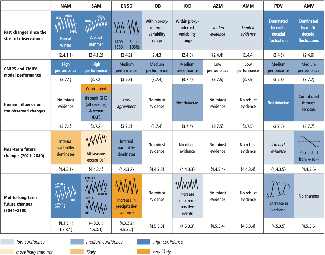 Table TS.4 (continued): (b) Regional climate anomalies associated with MoV.
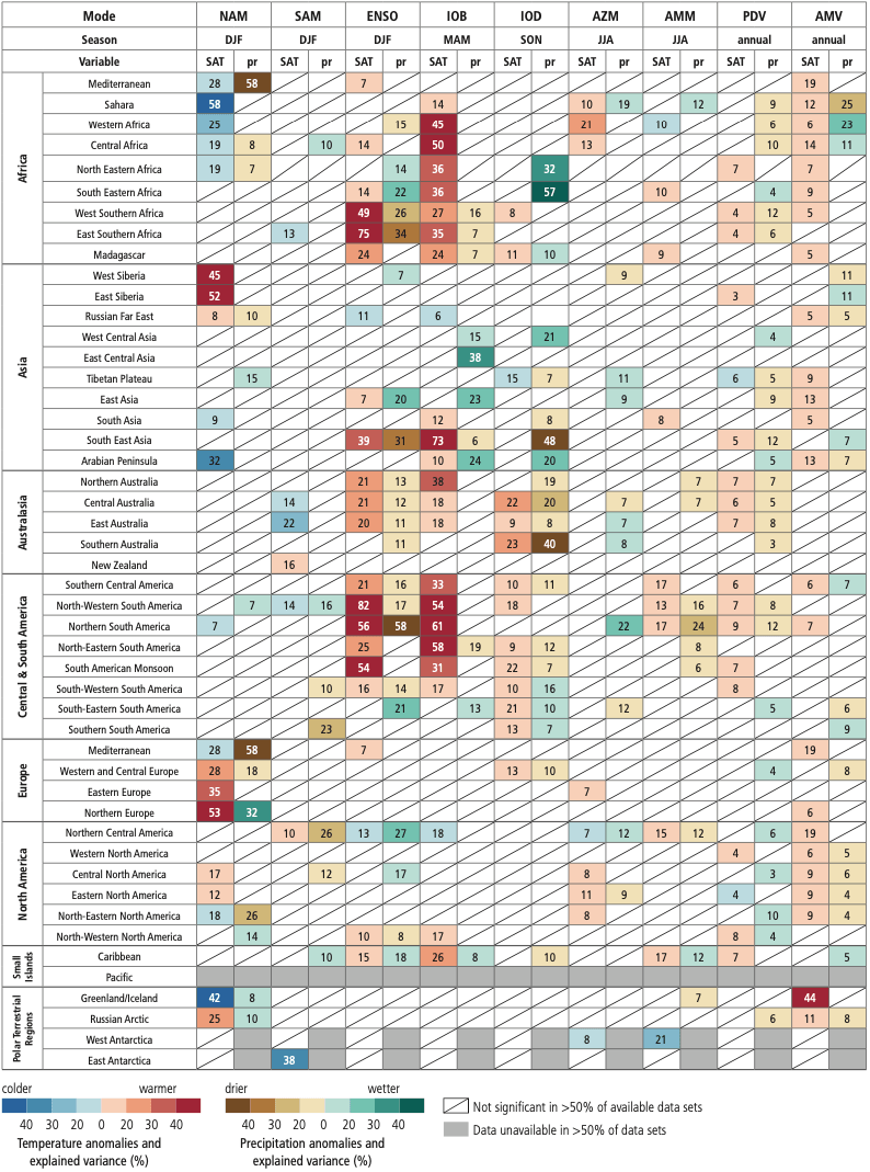
TS.4.2.3 Interplay Between Drivers of Climate Variability and Change at Regional Scales
Anthropogenic forcing has been a major driver of regional mean temperature change since 1950 in many sub-continental regions of the world (virtually certain). At regional scales, internal variability is stronger, and uncertainties in observations, models and external forcing are all larger than at the global scale, hindering a robust assessment of the relative contributions of greenhouse gases, stratospheric ozone, and different aerosol species in most of the cases. Multiple lines of evidence, combining multi-model ensemble global projections with those coming from single-model initial-condition large ensembles, show that internal variability is largely contributing to the delayed or absent emergence of the anthropogenic signal in long-term regional mean precipitation changes (high confidence). Internal variability in ocean dynamics dominates regional patterns on annual to decadal time scales (high confidence). The anthropogenic signal in regional sea level change will emerge in most regions by 2100 (medium confidence). Links to chapters9.2.4, 9.6.1, 10.4.1, 10.4.2, 10.4.3
Regional climate change is subject to the complex interplay between multiple external forcings and internal variability. Time evolution of mechanisms operating at different time scales can modify the amplitude of the regional-scale response of temperature, and both the amplitude and sign of the response of precipitation, to anthropogenic forcing (high confidence). These mechanisms include non-linear temperature, precipitation and soil moisture feedbacks; slow and fast responses of SST patterns; and atmospheric circulation changes to increasing GHGs. Land-use and aerosol forcings and land–atmosphere feedback play important roles in modulating regional changes, for instance in weather and climate extremes (high confidence). These can also lead to a higher warming of extreme temperatures compared to mean temperature (high confidence), and possibly cooling in some regions (medium confidence). The soil moisture–temperature feedback was shown to be relevant for past and present-day heatwaves based on observations and model simulations. Links to chapters10.4.3, 11.1.6, 11.3.1
South-Eastern South America (SES) is one of the AR6 WGI reference regions (outlined with black thick contour in Figure TS.21a), and it is used here as an illustrative example of the interplay between drivers of climate variability and change at regional scale. Austral summer (DJF) precipitation positive trends have been observed over the region during 1950–2014. Drivers of this change include MoVs, such as AMV, ENSO, and PDV, as well as external forcing, like GHG increases and ozone depletion together with aerosols (as illustrated in Figure TS.21a). Modes of variability and external forcing collectively affect climate phenomena, such as the Hadley cell width and strength, Rossby waves activity emerging from the large-scale tropical SST anomalies, and the Southern Hemisphere polar vortex, which are relevant for the region. In fact, local changes over SES in terms of moisture convergence, ascending motion and storm-track locations depend on these climate phenomena, and they are overall responsible for the observed precipitation trends. Projections suggest continuing positive trends in rainfall over SES in the near-term in response to GHG emissions scenarios. Multi-model mean and ensemble spread are not sufficient to characterize situations where different models simulate substantially different or even opposite changes (high confidence). In such cases, physical climate storylines addressing possible outcomes for climate phenomena shown to play a role in the variability of the region of interest can aid the interpretation of projection uncertainties. In addition, single-model initial-condition large ensembles of many realizations of internal variability are required to separate internal variability from forced changes (high confidence) and to partition the different sources of uncertainties as a function of future assessed periods. Links to chapters10.3.4, 10.4.2, Figure 10.12a

Box TS.13 | Monsoons
Global Monsoon
Paleoclimate records indicate that during warm climates, like the mid-Pliocene Warm Period, monsoon systems were stronger (medium confidence). In the instrumental records, global summer monsoon precipitation intensity has likely increased since the 1980s, dominated by Northern Hemisphere summer trends and large multi-decadal variability. Contrary to the expected increase of precipitation under global warming, the Northern Hemisphere monsoon regions experienced declining precipitation from the 1950s to 1980s, which is partly attributable to the influence of anthropogenic aerosols (medium confidence) (Box TS.13, Figure 1). Links to chapters2.3.1, Cross-Chapter Box 2.4, 3.3.2, 3.3.3

Box TS.13, Figure 1 | Global and regional monsoons: past trends and projected changes. The intent of this figure is to show changes in precipitation over regional monsoon domains in terms of observed past trends, how greenhouse gases and aerosols relate to these changes, and in terms of future projections in one intermediate emissions scenario in the near, medium and long term. (a) Global (black contour) and regional monsoons (colour shaded) domains. The global monsoon (GM) is defined as the area with local summer-minus-winter precipitation rate exceeding 2.5 mm day–1 (see Annex V). The regional monsoon domains are defined based on published literature and expert judgement (see Annex V) and accounting for the fact that the climatological summer monsoon rainy season varies across the individual regions. Assessed regional monsoons are South and South East Asia (SAsiaM, Jun–July–August–September), East Asia (EAsiaM, June–July–August), West Africa (WAfriM, June–July–August–September), North America (NAmerM, July–August–-September), South America (SAmerM, December–January–February), Australia and Maritime Continent Monsoon (AusMCM, December–January–February). Equatorial South America (EqSAmer) and South Africa (SAfri)regions are also shown, as they receive unimodal summer seasonal rainfall although their qualification as monsoons is subject to discussion. (b) Global and regional monsoons precipitation trends based on DAMIP CMIP6 simulations with both natural and anthropogenic (ALL), greenhouse gas only (GHG), aerosols only (AER) and natural only (NAT) radiative forcing. Weighted ensemble means are based on nine Coupled model Intercomparison Project Phase 6 (CMIP6) models contributing to the MIP (with at least three members). Observed trends computed from CRU, GPCP and APHRO (only forSAsiaM and EAsiaM) datasets are shown as well. (c) Percentage change in projected seasonal mean precipitation over global and regional monsoons domain in the near term (2021–2040), mid-term (2041–2060), and long term (2081–2100) under SSP2-4.5 based on 24 CMIP6 models. Links to chaptersFigures 8.11 and 8.22
With continued global warming, it is likely that global land monsoon precipitation will increase during this century (Box TS.13, Figure 1), particularly in the Northern Hemisphere, although the monsoon circulation is projected to weaken. A slowdown of the tropical circulation with global warming can partly offset the warming-induced strengthening of precipitation in monsoon regions (high confidence). In the near term, global monsoon changes are likely to be dominated by the effects of internal variability and model uncertainties (medium confidence). In the long term, global monsoon rainfall change will feature a robust north–south asymmetry characterized by a greater increase in the Northern Hemisphere than in the Southern Hemisphere and an east–west asymmetry characterized by enhanced Asian–African monsoons and a weakened North American monsoon (medium confidence). Links to chapters4.4.1, 4.5.1, 8.4.1
Regional Monsoons
Paleoclimate reconstructions indicate stronger monsoons in the Northern Hemisphere but weaker ones in the Southern Hemisphere during warm periods, particularly for the South and South East Asian, East Asian, and North and South American monsoons, with the opposite occurring during cold periods (medium confidence). It is very likely that Northern Hemispheric anthropogenic aerosols weakened the regional monsoon circulations in South Asia, East Asia and West Africa during the second half of the 20th century, thereby offsetting the expected strengthening of monsoon precipitation in response to GHG-induced warming (Box TS.13, Figure 1). Multiple lines of evidence explain this contrast over South Asia, with the observed trends dominated by the effects of aerosols, while future projections are mostly driven by GHG increases. The recent partial recovery and enhanced intensity of monsoon precipitation over West Africa is related to the growing influence of GHGs with an additional contribution due to the reduced cooling effect of anthropogenic aerosols, emitted largely from North America and Europe (medium confidence). For other regional monsoons, that is, North and South America and Australia, there is low confidence in the attribution of recent changes in precipitation (Box TS.13, Figure 1) and winds. Links to chapters2.3.1, 8.3.1, 8.3.2, Box 8.1, 10.6.3
Projections of regional monsoons during the 21st century indicate contrasting (region-dependent) and uncertain precipitation and circulation changes. The annual contrast between the wettest and driest month of the year is likely to increase by 3–5% per degree Celsius in most monsoon regions in terms of precipitation, precipitation minus evaporation, and runoff (medium confidence). For the North American monsoon, projections indicate a decrease in precipitation, whereas increased monsoon rainfall is projected over South and South East Asia and over East Asia (medium confidence) (Box TS.13, Figure 1). West African monsoon precipitation is projected to increase over the central Sahel and decrease over the far western Sahel (medium confidence). There is low confidence in projected precipitation changes in the South American and Australian-Maritime Continent regional monsoons (for both magnitude and sign) (Box TS.13, Figure 1). There is medium confidence that the monsoon season will be delayed in the Sahel and high confidence that it will be delayed in North and South America. Links to chapters8.2.2, 8.4.2.4, Box 8.2
Building the Assessment from Multiple Lines of Evidence
Large natural variability of monsoon precipitation across different time scales, found in both paleoclimate reconstructions and instrumental measurements, poses an inherent challenge for robust quantification of future changes in precipitation at regional and smaller spatial scales. At both global and regional scales, there is medium confidence that internal variability contributes the largest uncertainty related to projected changes, at least in the near term (2021–2040). A collapse of the Atlantic Meridional Overturning Circulation could weaken the African and Asian monsoons but strengthen the Southern Hemisphere monsoons (high confidence). Links to chapters4.4.4, 4.5.1, Cross-Chapter Box 4.1, 8.5.2, 8.6.1, 9.2.3, 10.6.3
Overall, long-term (2081–2100) future changes in regional monsoons like the South and South East Asian monsoon are generally consistent across global (including high-resolution) and regional climate models and are supported by theoretical arguments. Uncertainties in simulating the observed characteristics of regional monsoon precipitation are related to varying complexities of regional monsoon processes and their responses to external forcing, internal variability, and deficiencies in representing monsoon warm rain processes, organized tropical convection, heavy orographic rainfall and cloud–aerosol interactions. Links to chapters8.3.2, 8.5.1, 10.3.3, 10.6.3
TS.4.3 Regional Climate Change and Implications for Climate Extremes and Climatic Impact-Drivers
An overview of changes in regional CIDs (introduced in Section TS.1) is given in Table TS.5, which summarizes multiple lines of evidence on regional climate change derived from observed trends, attribution of these trends and future projections. The level of confidence and the amplitude in the projected direction of change in CIDs at a given time horizon depends on climate change mitigation efforts over the 21st century. It is evident from Table TS.5 that many heat, cold, snow and ice, coastal, and oceanic CID changes are projected with high confidence in most regions starting from a global warming level (GWL) of 2°C, indicating worldwide challenges. Changes in many other regional CIDs have higher confidence later in the 21st century or at higher GWLs (high confidence), and another small subset are projected with high confidence for the 1.5°C GWL. This section focuses on the 2°C GWL and mid-century time period because the signal emerges from natural variability for a wider range of CIDs at this higher warming level. Figure TS.22 shows the geographical location of regions belonging to one of five groups characterized by a specific combination of changing CIDs. The Regional Synthesis component of the Interactive Atlas provides comprehensive synthesis information about changes in all of the individual CIDs across all of the AR6 WGI reference regions. Links to chapters10.5, Cross-Chapter Box 10.3, 11.1, 11.9, Box 11.1, 12.1, 12.2, 12.4, 12.5
Table TS.5 | Summary of confidence for climatic impact-driver changes in each AR6 WGI reference region (illustrated in Figure TS.25) across multiple lines of evidence for observed, attributed and projected directional changes. The colours represent their projected aggregate characteristic changes for the mid-21st century, considering scenarios RCP4.5, SSP2-4.5, SRES A1B, or above (RCP6.0, RCP8.5, SSP3-7.0, SSP5-8.5, SRES A2), which approximately encompasses global warming levels of 2.0°C to 2.4°C. Arrows indicate medium to high confidence trends derived from observations, and asterisks indicate medium and high confidence in attribution of observed changes. (North Africa is not an AR6 WGI reference region, but assessment here is based upon the African portion of the Mediterranean reference region). Links to chaptersTables 12.3–12.11 and Tables 11.4–11.21
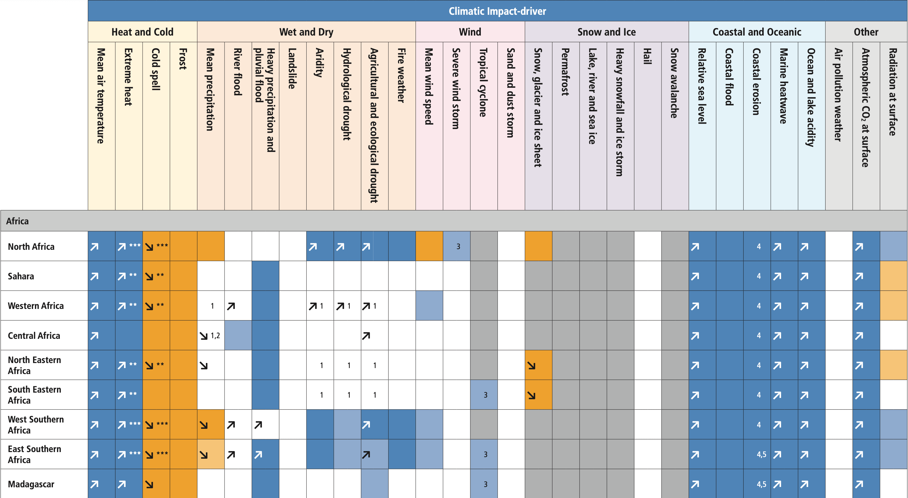
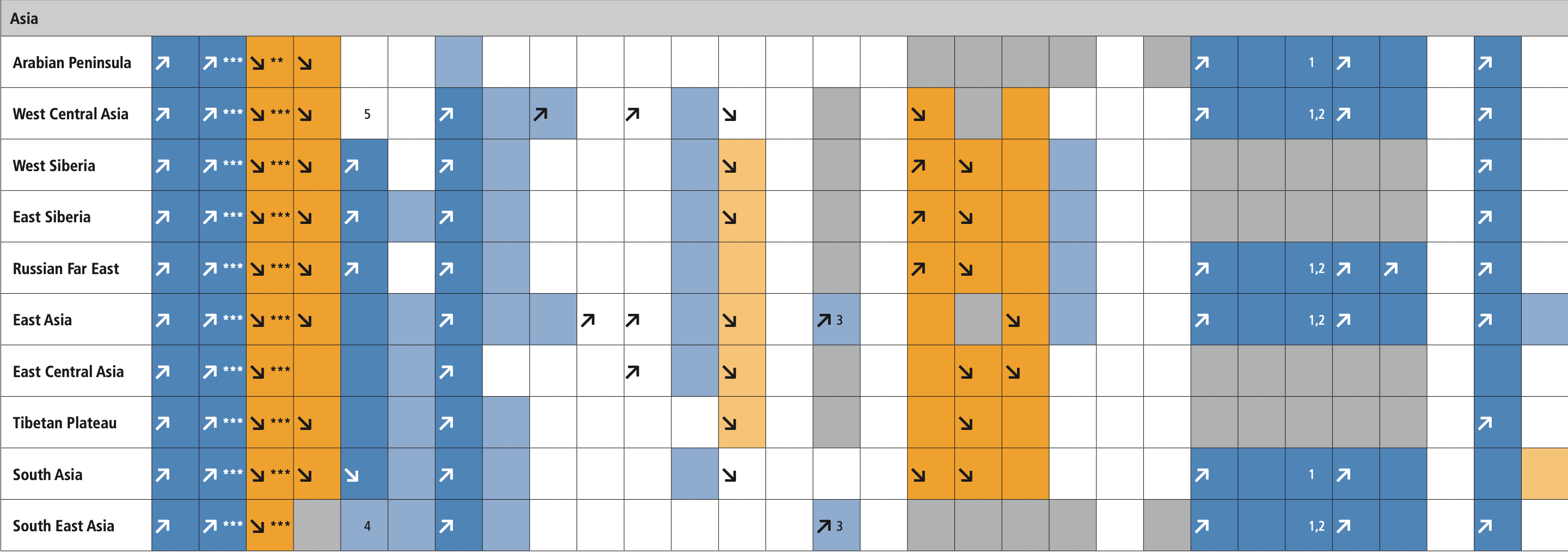


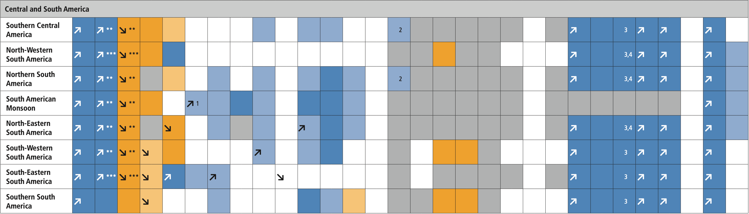
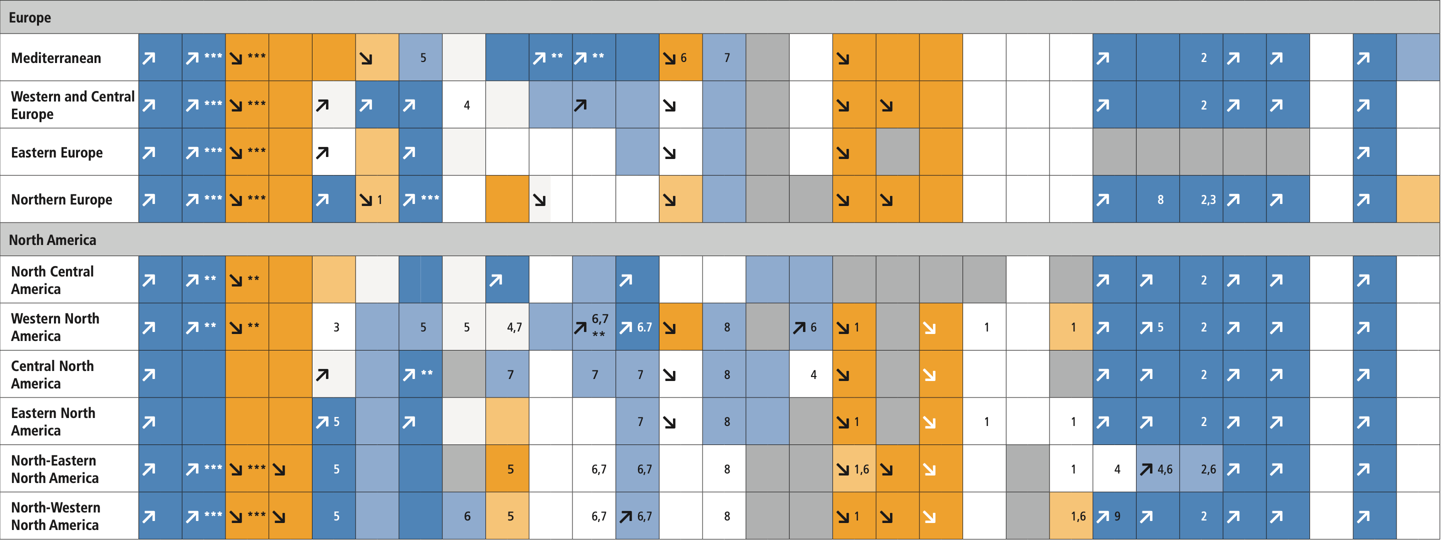
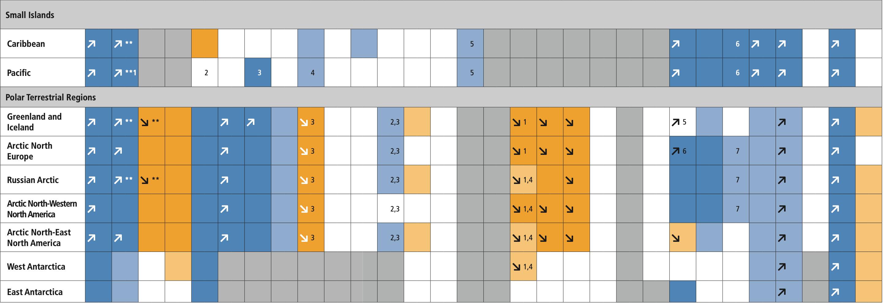

Notes:
Africa (projections)
1. Contrasted regional signal: drying in western portions and wetting in eastern portions
2. Likely increase over the Ethiopian Highlands
3. Medium confidence of decrease in frequency and increase in intensity
4. Along sandy coasts and in the absence of sufficient sediment supply from terrestrial or offshore sources
5. Substantial parts of the East Southern Africa and Madagascar coast are projected to prograde if present-day ambient shoreline change rates continue
Asia (projections)
1. Along sandy coasts and in the absence of additional sediment sinks/sources or any physical barriers to shoreline retreat.
2. Substantial parts of the coasts in these regions are projected to prograde if present-day ambient shoreline change rates continue
3. Tropical cyclones decrease in number but increase in intensity
4. High confidence of decrease in Indonesia (Atlas.5.4.5)
5. Medium confidence of decreasing in summer and increasing in winter
Australasia (projections)
1. High confidence of decrease in the south-west of the state of Western Australia
2. Medium confidence of decrease in north and east and increase in south and west
3. High confidence of increase in the south-west of the state of Western Australia
4. Medium confidence of increase in the north and east and decrease in south and west
5. Low confidence of increasing intensity, and high confidence of decreasing occurrence
6. High confidence of decrease in glacier volume, medium confidence of decrease in snow
7. Along sandy coasts and in the absence of additional sediment sinks/sources or any physical barriers to shoreline retreat
Central and South America (projections)
1. Increase in extreme flow in the Amazon basin
2. Tropical cyclones decrease in number but increase in intensity
3. Along sandy coasts and in the absence of additional sediment sinks/sources or any physical barriers to shoreline retreat.
4. Substantial parts of the North-Western South America, Northern South America and North-Eastern South America coasts are projected to prograde if present-day ambient shoreline change rates continue
Europe (projections)
1. Excluding southern United Kingdom
2. Along sandy coasts and in the absence of additional sediment sinks/sources or any physical barriers to shoreline retreat
3. The Baltic Sea shoreline is projected prograde if present-day ambient shoreline change rates continue.
4. For the Alps, conditions conducive to landslides are expected to increase
5. Low confidence of decrease in the southernmost part of the region
6. General decrease except in Aegean Sea
7. Medium confidence of decrease in frequency and increase in intensities
8. Except in the Northern Baltic Sea region
North America (projections)
1. Snow may increase in some high elevations and during the cold season and decrease in other seasons and at lower elevations
2. Along sandy coasts and in the absence of additional sediment sinks/sources or any physical barriers to shoreline retreat.
3. Increasing in northern regions and decreasing toward the south
4. Decreasing in northern regions and increasing toward the south
5. Higher confidence in northern regions and lower toward the south
6. Higher confidence in southern regions and lower toward the north
7. Higher confidence in increase for some climatic impact-driver indices during summertime
8. Increase in convective conditions but decrease in winter extratropical cyclones
9. Relative sea level rise reduced given land uplift in Southern Alaska
Small Islands (projections)
1. Very high confidence in the direction of change, butlow tomedium confidence in the magnitude of change due to model uncertainty
2. Decrease in eastern Pacific and southern Pacific subtropics, but increase in parts of western and equatorial Pacific; with seasonal variation in future changes
3. High confidence in increase in extreme rain frequency and intensity in western tropical Pacific; low confidence in magnitude of change due to model bias
4. Increase in southern Pacific
5. Increase in intensity; decrease in frequency except over central North Pacific.
6. Along sandy coasts and in the absence of additional sediment sinks/sources or any physical barriers to shoreline retreat.
Polar Terrestrial Regions (projections)
1. Snow may increase in some high elevations and during the cold season and decrease in other seasons and at lower elevations
2. Higher confidence in southern regions and lower toward the north
3. Higher confidence in increase for some climatic impact-driver indices during summertime
4. Glaciers decline even as some regional snow climatic impact-driver indices increase
5. Decreasing in west and increasing in east
6. Except for Northern Baltic Sea coasts where relative sea levels fall
7. Along sandy coasts and in the absence of additional sediment sinks/sources or any physical barriers to shoreline retreat

Panel (a) shows the geographical location of regions belonging to one of five groups characterized by a specific combination of changing climatic impact-drivers (CIDs). The five groups are represented by the five different colours, and the CID combinations associated with each group are represented in the corresponding ‘fingerprint’ and text below the map. Each fingerprint comprises a set of CIDs projected to change with high confidence in every region in the group and a second set of CIDs, one or more of which are projected to change in each region with highormedium confidence. The CID combinations follow a progression from those becoming hotter and drier (group 1) to those becoming hotter and wetter (group 5). In between (groups 2–4), the CIDs that change include some becoming drier and some wetter and always include a set of CIDs which are getting hotter. Tropical cyclones and severe wind CID changes are represented on the map with black dots in the regions affected. Regions affected by coastal CID changes are described by text on the map. The five groups are chosen to provide a reasonable level of detail for each region while not overwhelming the map with a full summary of all aspects of the assessment, which is available in Table TS.5 and can be visualized in the Regional Synthesis component of the Interactive Atlas. The CID changes summarized in the figure represent high and medium confidence changes for the mid-21st century, considering scenarios SSP2-4.5, RCP4.5, SRES A1B, or above (SSP3-7.0, SSP5-8.5, RCP6.0, RCP8.5, SRES A2), which approximately encompasses global warming levels of 2.0°C to 2.4°C.
The bar chart in panel (b) shows the numbers of regions where each CID is increasing or decreasing with mediumor high confidence for all land regions and ocean regions listed in Table TS.5. The colours represent the direction of change and the level of confidence in the change: purple indicates an increase while brown indicates a decrease; darker and lighter shades refer to high and medium confidence, respectively. Lighter background colours represent the maximum number of regions for which each CID is broadly relevant. Sub-panel (i) shows the 30 CIDs relevant to the land and coastal regions while sub-panel (ii) shows the 5 CIDs relevant to the open ocean regions. Marine heatwaves and ocean acidity are assessed for coastal ocean regions in panel (i) and for open ocean regions in panel (ii). Changes refer to a 20- to 30-year period centred around 2050 and/or consistent with 2°C global warming compared to a similar period within 1960–2014, except for hydrological drought and agricultural and ecological drought, which is compared to 1850–1900. Definitions of the regions are provided in Atlas.1, the Interactive Atlas (https://interactive-atlas.ipcc.ch/) and Chapter 12. (Table TS.5, Figure TS.24) Links to chapters11.9, 12.2, 12.4, Atlas.1
TS.4.3.1 Common Regional Changes in Climatic Impact-Drivers
Heat and cold: Changes in temperature-related CIDs such as mean temperatures, growing season length, and extreme heat and frost have already occurred (high confidence), and many of these changes have been attributed to human activities (medium confidence). Over all land regions with sufficient data (i.e., all except Antarctica), observed changes in temperature have already clearly emerged outside the range of internal variability, relative to 1850–1900 (Figure TS.23). In tropical regions, recent past temperature distributions have already shifted to a range different to that of the early 20th century (high confidence) (Section TS.1.2.4). Most land areas have very likely warmed by at least 0.1°C per decade since 1960, and faster in recent decades. On regional-to-continental scales, trends of increased frequency of hot extremes and decreased frequency of cold extremes are generally consistent with the global-scale trends in mean temperature (high confidence). In a few regions, trends are difficult to assess due to limited data availability. Links to chapters2.3.1.1, 11.3, 11.9, 12.4, Atlas.3.1
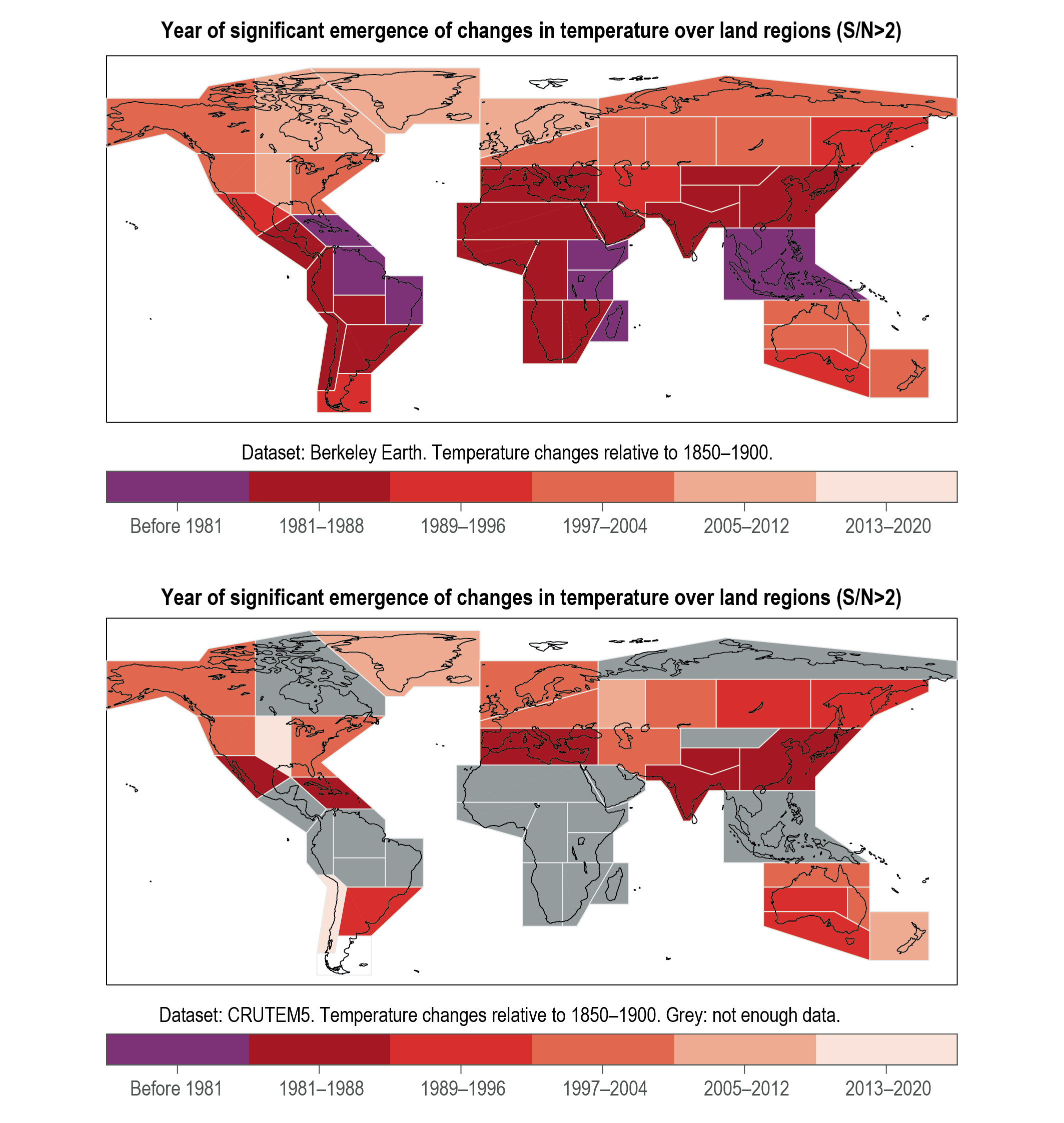
Warming trends observed in recent decades are projected to continue over the 21st century and over most land regions at a rate higher than the global average (high confidence). For given global warming levels, model projections from CMIP6 show future regional warming changes that are similar to those projected by CMIP5. However, projected regional warming in CMIP6 for given time periods and emissions scenarios has a wider range with a higher upper limit compared to CMIP5 because of the higher climate sensitivity in some CMIP6 models and differences in the forcings. Links to chaptersAtlas.3–Atlas.11
Under RCP8.5/SSP5-8.5, it is likely that most land areas will experience further warming of at least 4°C compared to a 1995–2014 baseline by the end of the 21st century, and in some areas significantly more. At increasing warming levels, extreme heat will exceed critical thresholds for health, agriculture and other sectors more frequently (high confidence), and it is likely that cold spells will become less frequent towards the end of the century. For example, by the end of the 21st century, dangerous humid heat thresholds, such as the National Oceanic and Atmospheric Administration (NOAA) heat index (HI) threshold of 41°C, will be exceeded much more frequently under the SSP5-8.5 scenario than under SSP1-2.6 and will affect many regions (high confidence). In many tropical regions, the number of days per year where a heat index of 41°C is exceeded would increase by more than 100 days relative to the recent past under SSP5-8.5, while this increase will be limited to less than 50 days under SSP1-2.6 (high confidence) (Figure TS.6). The number of days per year where temperature exceeds 35°C would increase by more than 150 days in many tropical areas, such as the Amazon basin and South East Asia, by the end of century for the SSP5-8.5 scenario, while it is expected to increase by less than 60 days in these areas under SSP1-2.6 (except for the Amazon Basin) (high confidence) (Figure TS.24). Links to chapters4.6.1, 11.3, 11.9, 12.4, 12.5.2, Atlas

Wet and dry: Compared to the global scale, precipitation internal variability is stronger at the regional scale while uncertainties in observations, models and external forcing are all larger. However, GHG forcing has driven increased contrasts in precipitation amounts between wet and dry seasons and weather regimes over tropical land areas (medium confidence), with a detectable precipitation increase in the northern high latitudes (high confidence) (Box TS.6). The frequency and intensity of heavy precipitation events have increased over a majority of land regions with good observational coverage (high confidence). A majority of land areas have experienced decreases in available water in dry seasons due to human-induced climate change associated with changes in evapotranspiration (medium confidence). Global hydrological models project a larger fraction of land areas to be affected by an increase rather than by a decrease in river floods (medium confidence). Extreme precipitation and pluvial flooding will increase in many regions around the world on almost all continents(high confidence), but regional changes in river floods are more uncertain than changes in pluvial floods because complex hydrological processes, including land cover and human water management, are involved. Links to chapters8.2.2.1, 8.3.1, Box 8.2, 10.4.1, 11.5, 11.6, 11.9, 12.4, 12.5.1, Atlas.3.1
Wind: Mean wind speed has decreased over most land areas with good observational coverage (medium confidence). It is likely that the global proportion of major tropical cyclone (TC) intensities (Categories 3–5) over the past four decades has increased. The proportion of intense TCs, average peak TC wind speeds, and peak wind speeds of the most intense TCs will increase on the global scale with increasing global warming (high confidence). Links to chapters11.7.1
Snow and ice: Many aspects of the cryosphere either have seen significant changes in the recent past or will see them during the 21st century (high confidence). Glaciers will continue to shrink and permafrost to thaw in all regions where they are present (high confidence). Also, it is virtually certain that snow cover will experience a decline over most land regions during the 21st century, in terms of water equivalent, extent and annual duration. There is high confidence that the global warming-induced earlier onset of spring snowmelt and increased melting of glaciers have already contributed to seasonal changes in streamflow in high-latitude and low-elevation mountain catchments. Nevertheless, it is very likely that some high-latitude regions will experience an increase in winter snow water equivalent due to the effect of increased snowfall prevailing over warming-induced increased snowmelt. (Section TS.2.5) Links to chapters8.2.2.1, 8.3.1, Box 8.2, 9.4, 9.5.1, 9.5.2, 12.4, Atlas.4–Atlas.9, Atlas.11
Coastal and oceanic: There is high confidence that SST will increase in all oceanic regions except the North Atlantic. Regional sea level change has been the main driver of changes in extreme sea levels across the quasi-global tide gauge network over the 20th century (high confidence). With the exception of a few regions with substantial land uplift, relative sea level rise is very likely to virtually certain (depending on the region) to continue during the 21st century, contributing to increased coastal flooding in low-lying areas (high confidence) and coastal erosion along most sandy coasts (high confidence) over the 21st century. In the open ocean, acidification, changes in sea ice, and deoxygenation have already emerged in many areas (high confidence). Marine heatwaves are also expected to increase around the globe over the 21st century (high confidence). (Section TS.2.4) Links to chaptersBox 9.2, 9.2.1.1, 9.6, 9.6.4, 9.6.4.2, 12.4
Other variables and concurrent CID changes: It is virtually certain that atmospheric CO2 and oceanic pH will increase in all climate scenarios, until net zero CO2 emissions are achieved (Section TS.2.2). In nearly all regions, there is low confidence in changes in hail, ice storms, severe storms, dust storms, heavy snowfall, and avalanches, although this does not indicate that these CIDs will not be affected by climate change. For such CIDs, observations are often short-term or lack homogeneity, and models often do not have sufficient resolution or accurate parametrizations to adequately simulate them over climate change time scales. The probability of compound events has increased in the past due to human-induced climate change and will likely continue to increase with further global warming, including for concurrent heatwaves and droughts, compound flooding, and the possibility of connected sectors experiencing multiple regional extreme events at the same time (for example, in multiple breadbaskets) (high confidence). Links to chapters5.3.4.2, 11.8, Box 11.3, Box 11.4, 12.4
TS.4.3.2 Region-by-Region Changes in Climatic Impact-Drivers
This section provides a continental synthesis of changes in CIDs, some examples of which are presented in Figure TS.25.
TS.4.3.2.1 Africa
In addition to the main changes summarized above and in Section TS.4.3.1, additional details per CID are given below.
Heat and cold: Observed and projected increases in mean temperature and a shift toward heat extreme characteristics are broadly similar to the generic pattern described in Section TS.4.3.1. Links to chapters2.3.1.1.2, 11.3, 11.9, 12.4.1.1, Atlas.4.2, Atlas.4.4
 Figure TS.25 | Distribution of projected changes in selected climatic impact-driver (CID) indices for selected regions for Coupled Model Intercomparison Project Phases 5 and 6 (CMIP6, CMIP5) and Coordinated Regional Downscaling Experiment (CORDEX) model ensembles. The intent of this figure is to show that many CID projections for multiple global warming levels and scenarios time slices are available for all the AR6 WGI reference regions and are based on both global (CMIP5, CMIP6) and regional (CORDEX) model ensembles. Different indices are shown for different region: for Eastern Europe and North Asia, the mean number of days per year with maximum temperature exceeding 35°C; for Central America, the Caribbean, South West Asia, South Asia and South East Asia, the mean number of days per year with the National Oceanic and Atmospheric Administration (NOAA) Heat Index exceeding 41°C; for Australasia, East Asia and Russian Far East, the average shoreline position change; for South America, Europe and Africa, the mean change in 1-in-100-year river discharge per unit catchment area (m3s–1km–2); and for North America, the median change in the number of days with snow water equivalent (SWE) over 100 mm. For each box plot, the changes or the climatological values are reported with respect to, or compared to, the recent past (1995–2014) period for 1.5°C, 2°C and 4°C global warming levels and for mid-century (2041–2060) or end-century (2081–2100) periods for the CMIP5 and CORDEX RCP8.5 and RCP2.6 and CMIP6 SSP5-8.5 and SSP1-2.6 scenarios ensembles. Links to chaptersFigures 12.5, 12.6, 12.9, 12.SM.1, 12.SM.2, and 12.SM.6
 Wet and dry: Mean precipitation changes have been observed over Africa, but the historical trends are not spatially coherent (high confidence). North Eastern Africa, East Southern Africa and Central Africa have experienced a decline in rainfall since about 1980 and parts of West Africa an increase (high confidence). Increases in the frequency and/or the intensity of heavy rainfall have been observed in East and West Southern Africa, and the eastern Mediterranean region (medium confidence). Increasing trends in river flood occurrence can be identified beyond 1980 in East and West Southern Africa (medium confidence) and Western Africa (high confidence). However, Northern Africa and West Southern Africa are likely to have a reduction in precipitation. Over West Africa, rainfall is projected to decrease in the western Sahel subregion and increase along the Guinea Coast subregion (medium confidence). Rainfall is projected to increase over Eastern Africa (medium confidence). Links to chapters8.3.1.6, 11.4, 11.9, 12.4.1.2, Atlas.4.2, Atlas.4.4, Atlas.4.5
Precipitation declines and aridity trends in Western Africa, Central Africa, Southern Africa and the Mediterranean co-occur with trends towards increased agricultural and ecological droughts in the same regions (medium confidence). Trends towards increased hydrological droughts have been observed in the Mediterranean (high confidence) and Western Africa (medium confidence). These trends correspond with projected regional increases in aridity and fire weather conditions (high confidence). Links to chapters8.3.1.6, 8.4.1.6, 11.6, 11.9, 12.4.1.2
Wind: Mean wind, extreme winds and the wind energy potential in North Africa and the Mediterranean are projected to decrease across all scenarios (high confidence). Over Western Africa and Southern Africa, a future significant increase in wind speed and wind energy potential is projected (medium confidence). There is a projected decrease in the frequency of tropical cyclones making landfall over Madagascar, East Southern Africa and East Africa (medium confidence). Links to chapters12.4.1.3
Snow and ice: There is high confidence that African glaciers and snow have very significantly decreased in the last decades and that this trend will continue in the 21st century. Links to chapters12.4.1.4
Coastal and oceanic: Relative sea level has increased at a higher rate than GMSL around Africa over the last 3 decades. The present day 1-in-100-year extreme total water level (ETWL) is between 0.1 m and 1.2 m around Africa, with values around 1 m or above along the East and West Southern and Central Eastern Africa coasts. Satellite-derived shoreline retreat rates up to 1 m yr–1have been observed around the continent from 1984 to 2015, except in South Eastern Africa, which has experienced a shoreline progradation (growth) rate of 0.1 m yr–1 over the same period. Links to chapters12.4.1.5
TS.4.3.2.2 Asia
Due to the high climatological and geographical heterogeneity of Asia, some assessment findings below are summarized over five sub-continental areas comprising one or more of the AR6 WGI reference regions (Box TS.12): East Asia (EAS+ECA), North Asia (WSB+ESB+RFE), South Asia (SAS), South East Asia (SEA) and South West Asia (ARP+WCA).
In addition to the main changes summarized above and in Section TS.4.3.1, further details are given below.
Heat and cold: Over all regions of Asia, observed and projected increases in mean temperature and a shift toward heat extreme characteristics are broadly similar to the generic pattern described in Section TS.4.3.1. Over South East Asia, annual mean surface temperature will likely increase by a slightly smaller amount than the global average. Links to chaptersAtlas.5.4.4
Wet and dry: Over East Asia, historical trends of annual precipitation show considerable regional differences but with increases over north-west China and South Korea (high confidence). Daily precipitation extremes have increased over part of the region (high confidence). Extreme hydrological drought frequency has increased in a region extending from south-west to north-east China, with projected increases of agricultural and ecological drought for 4°C GWL and fire weather for 2°C and above (medium confidence). Links to chapters8.3.2, 8.4.2, 11.4.4, 11.4.5, 11.9, 12.4.2.2, Atlas.5.1.2
Over North Asia, annual mean precipitation totals have very likely increased, causing more intense flooding events, and there is medium confidence that the number of dry days has decreased. Concurrently, total soil moisture is projected to decline extensively (medium confidence). Links to chapters8.3.1.3, 8.4.1.6, 11.4.5, 11.5.2, 11.5.5, 12.4.2.2, Atlas.5.2.2
Over South Asia, the summer monsoon precipitation decreased over several areas since the mid-20th century (high confidence), while it increased in parts of the western HKH and decreased over eastern-central HKH (medium confidence). The frequency of heavy precipitation and flood events has increased over several areas during the last few decades (medium confidence). Links to chapters8.3.1.3, 8.3.2.4.1, 8.4.1.5, 8.4.2.4.1, 10.6.3.3, 10.6.3.5, 10.6.3.6, 10.6.3.8, Cross-Chapter Box 10.4, 11.4.1, 11.4.2, 11.4.5, 11.5.5, 12.4.2.2, Box 10.4, Atlas 5.3.2
Over South East Asia, mean precipitation trends are not spatially coherent or consistent across datasets and seasons (high confidence). Most of the region has experienced an increase in rainfall intensity but with a reduced number of wet days (medium confidence). Rainfall is projected to increase in the northern parts of South East Asia and decrease in areas in the Maritime Continent (medium confidence). Links to chapters8.4.1, 11.4.2, 11.5.5, 11.9, 12.4.2.2, Atlas.3.1, Atlas.5.4.2, Atlas.5.4.4
Over South West Asia, an observed annual precipitation decline over the Arabian Peninsula since the 1980s of 6.3 mm per decade is contrasted with observed increases between 1.3 mm and 4.8 mm per decade during 1960–2013 over the elevated part of eastern West Central Asia (very high confidence), along with an increase of the frequency and intensity of extreme precipitation. Links to chaptersFigure 8.19, Figure 8.20, 8.3.1.6, 8.4.1.6, 11.9, Table 11.2A, 12.4.2.2, Atlas.5.5
Wind: Over East Asia, the terrestrial near-surface wind speed has decreased and is projected to decrease further in the future (medium confidence). Since the mid 1980’s, there has been an increase in the number and intensification rate of intense TCs (medium confidence), with a significant north-westward shift in tracks and a northward shift in their average latitude, increasing exposure over East China, the Korean Peninsula and the Japanese Archipelago (medium confidence). Links to chapters11.7.1, 12.4.2.3
Over North Asia, there is medium confidence for a decreasing trend in wind speed during 1979–2018 and for projected continuing decreases of terrestrial near-surface wind speed. Links to chapters2.3.1.4.4, 12.4.2.3
Over South East Asia, although there is no significant long-term trend in the number of TCs, fewer but more extreme TCs have affected the Philippines during 1951–2013. Links to chapters11.7.4, 12.4.2.3
Snow and ice: Over East Asia, decreases have been observed in the frequency, and increases in the mean intensity, of snowfall in north-western, north-eastern and south-eastern China and the eastern Tibetan Plateau since the 1960s. Heavy snowfall is projected to occur more frequently in some parts of Japan (medium confidence). Links to chapters12.4.2.4, Atlas.5.1.2
Over North Asia, seasonal snow duration and extent have decreased in recent decades (high confidence), and maximum snow depth likely has increased since the mid-1970s, particularly over the south of the Russian Far East. Links to chapters2.3.2.5, 8.3.1.7.2, 9.5, 12.4.2.4, Atlas.5.2, Atlas.5.4
Over South Asia, snow cover has reduced over most of the HKH since the early 21st century, and glaciers have thinned, retreated, and lost mass since the 1970s (high confidence), although the Karakoram glaciers have either slightly gained mass or are in an approximately balanced state (medium confidence). Links to chapters8.3.1.7.1, Cross-Chapter Box 10.4
Over South West Asia, mountain permafrost degradation at high altitudes has increased the instability of mountain slopes in the past decade (medium confidence). More than 60% of glacier mass in the Caucasus is projected to disappear under RCP8.5 emissions by the end of the 21st century (medium confidence). Links to chapters9.5.1, 9.5.3, 12.4.2.4
Coastal and oceanic: Over the last three decades, relative sea level has increased at a rate higher than GMSL around Asia (high confidence). Gross coastal area loss and shoreline retreat has been observed over 1984–2015, but with localized shoreline progradation in the Russian Far East, East and South East Asia. Links to chapters12.4.2.5
Projections show that regional mean sea level continues to rise (high confidence), ranging from 0.4–0.5 m under SSP1-2.6 to 0.8–1.0 m under SSP5-8.5 for 2081–2100 relative to 1995–2014 (median values). This will contribute to more frequent coastal flooding and higher ETWL in low-lying areas and coastal erosion along sandy beaches (high confidence). There is high confidence that compound effects of climate change, land subsidence, and human factors will lead to higher flood levels and prolonged inundation in the Mekong Delta and other Asian coasts. Links to chapters9.6.1, 9.6.3, 12.4.2.5
TS.4.3.2.3 Australasia
In addition to the main changes summarized above and in Section TS.4.3.1, further details are given below.
Heat and cold: Observed and projected increases in mean temperature and a shift toward heat extreme characteristics are broadly similar to the generic pattern described in Section TS.4.3.1. Links to chapters11.9, 12.4.3.1, Atlas.6
Wet and dry: There is medium confidence that heavy precipitation has increased in Northern Australia since 1950. Annual mean precipitation is projected to increase in the south and west of New Zealand (medium confidence) and is projected to decrease in south-west Southern Australia (high confidence), Eastern Australia (medium confidence), and in the north and east of New Zealand (medium confidence) for a GWL of 2°C. There is medium confidence that river flooding will increase in New Zealand and Australia, with higher increases in NorthernAustralia. Aridity is projected to increase with medium confidence in Southern Australia (high confidence in south-west Southern Australia), Eastern Australia (medium confidence) and in the north and east of New Zealand (medium confidence) for GWLs around 2°C. Links to chapters11.4, 11.9, Table 11.6, 12.4.3.2, Atlas.6.2
Wind: Mean wind speeds are projected to increase in parts of north-eastern Australia (medium confidence) by the end of the 21st century under high CO2 emissions scenarios. TCs in north-eastern and north Australia are projected to decrease in number (high confidence) but increase in intensity except for ‘east coast lows’ (low confidence). Links to chapters12.4.3.3
Snow and ice: Observations in Australia show that the snow season length has decreased by 5% in the last five decades. Furthermore, the date of peak snowfall in Australia has advanced by 11 days over the last 5 decades. Glacier ice volume in New Zealand has decreased by 33% from 1977 to 2018. Links to chapters12.4.3.4, Atlas.6.2
Coastal and oceanic: Observed changes in marine heatwaves (MHWs) over the 20th century in the region show an increase in their occurrence frequency, except along the south-east coast of New Zealand, an increase in duration per event, and the total number of MHW days per decade, with the change being stronger in the Tasman Sea than elsewhere. The present day 1-in-100-year ETWL is between 0.5–2.5 m around most of Australia, except the north-western coast where 1-in-100-year ETWL can be as high as 6–7 m. Links to chaptersBox 9.1, 12.3.1.5, 12.4.3.5
TS.4.3.2.4 Central and South America
In addition to the main changes summarized above and in Section TS.4.3.1, further details are given below.
Heat and cold: Observed and projected increases in mean temperature and a shift toward heat extreme characteristics are broadly similar to the generic pattern described in Section TS.4.3.1. Links to chapters11.3.2, 11.3.5, Table 11.13, 12.4.4.1, Atlas.7.1.2, Atlas.7.2.2, Atlas.7.2.4
Wet and dry: Mean precipitation is projected to change in a dipole pattern with increases in North-Western and South-Eastern South America and decreases in North-Eastern and South-Western South America (high confidence) and with further decreases in Northern South America and Southern Central America (medium confidence). In Northern South America and Southern Central America, aridity and agricultural and ecological droughts are increasing with medium confidence. Fire weather is projected to increase over Southern Central America and Southern South America with medium confidence. Links to chapters8.3.1.3, 8.4.2.4.5, 11.4.2, 11.9, Table 11.14, Table 11.15, 12.4.4.2, Atlas.7.2.2, Atlas.7.2.4
Wind: Climate projections indicate an increase in mean wind speed and in wind power potential over the Amazonian region (Northern South America, South American Monsoon, North-Eastern South America) (medium confidence). Links to chapters12.4.4.3
Snow and ice: Glacier volume loss and permafrost thawing will likely continue in the Andes Cordillera under all climate scenarios, causing important reductions in river flow and potentially high-magnitude glacial lake outburst floods. Links to chapters9.5.1.1, 12.4.4.4
Coastal and oceanic: Around Central and South America, relative sea level has increased at a higher rate than GMSL in the South Atlantic and the subtropical North Atlantic, and at a rate lower than GMSL in the East Pacific over the last 3 decades. The present day 1-in-100-year ETWL is highest in Southern and South-Western South America subregions, where it can be as large as 5 to 6 m. Satellite observations for 1984–2015 show shoreline retreat rates along the sandy coasts of Southern Central America, South-Eastern South America and Southern South America, while shoreline progradation rates have been observed in North-Western South America and Northern South America. Over the period 1982–2016, the coastlines experienced at least one MHW per year, and more along the Pacific coast of North Central America and the Atlantic coast of South-Eastern South America. Links to chapters12.4.4.5
TS.4.3.2.5 Europe
In addition to the main changes summarized above and in Section TS.4.3.1, further details are given below.
Heat and cold: Observed and projected increases in mean temperature and a shift toward heat extreme characteristics are broadly similar to the generic pattern described in Section TS.4.3.1. Links to chapters11.3, 11.9, 12.4.5.1, 12.5.2, Atlas.8.2, Atlas.8.4
Wet and dry: There is medium confidence that annual mean precipitation has increased in Northern Europe, West and Central Europe, and Eastern Europe since the early 20th century and high confidence for increases in extreme precipitation. In the European Mediterranean, the magnitude and sign of observed land precipitation trends depend on time period and exact study region (medium confidence). There is medium confidence that river floods will decrease in Northern, Eastern and southern Europe for high warming levels. Links to chapters8.3.1.3, 11.3, 11.9, 12.4.5.2, Atlas.8.2, Atlas.8.4
Wind: Mean wind speed over land has decreased (medium confidence), but the role of human-induced climate change has not been established. There is high confidence that mean wind speeds will decrease in Mediterranean areas and medium confidence for such decreases in Northern Europe for GWLs exceeding 2°C. The frequency of Medicanes (tropical-like cyclones in the Mediterranean) is projected to decrease (medium confidence). Links to chapters11.9, 12.4.5.3
Snow and ice: In the Alps, snow cover will decrease below elevations of 1500–2000 m throughout the 21st century (high confidence). A reduction of glacier ice volume is projected in the European Alps and Scandinavia with high confidence and with medium confidence for the timing and mass change rates. Links to chapters9.5.2, 12.4.5.4
Coastal and oceanic: Over the last three decades, relative sea level has increased at a lower rate than GMSL in the sub-polar North Atlantic coasts of Europe. The present-day 1-in-100-year ETWL is between 0.5–1.5 m in the Mediterranean basin and 2.5–5.0 m in the western Atlantic European coasts, around the United Kingdom and along the North Sea coast, and lower at 1.5–2.5 m along the Baltic Sea coast. Satellite-derived shoreline change estimates over 1984–2015 indicate shoreline retreat rates of around 0.5 m yr–1along the sandy coasts of Central Europe and the Mediterranean and more or less stable shorelines in Northern Europe. Over the period 1982–2016, the coastlines of Europe experienced on average more than 2.0 MHW per year, with the eastern Mediterranean and Scandinavia experiencing 2.5–3 MHWs per year. Links to chapters12.4.5.5
TS.4.3.2.6 North America
In addition to the main changes summarized above and in Section TS.4.3.1, further details are given below.
Heat and cold: Observed and projected increases in mean temperature and a shift toward heat extreme characteristics are broadly similar to the generic pattern described in Section TS.4.3.1. Links to chapters11.3, 11.9, 12.4.6.1, Atlas.9.2, Atlas.9.4
Wet and dry: Annual precipitation increased over parts of Eastern and Central North America during 1960–2015 (high confidence) and has decreased in parts of south-western United States and north-western Mexico (medium confidence). River floods are projected to increase for all North American regions other than Northern Central America (med ium confidence). Links to chapters8.4.2.4, 11.4, 11.5, 11.9, 12.4.6.2, Atlas.9.2, Atlas.9.4
Agricultural and ecological drought increases have been observed in Western North America (medium confidence), and aridity is projected to increase in the south-western United States and Northern Central America, with lower summer soil moisture across much of the continental interior (medium confidence). Links to chapters8.4.1, 11.6.2, 12.4.6.2
Wind: Projections indicate a greater number of the most intense TCs, with slower translation speeds and higher rainfall potential for Mexico’s Pacific Coast, the Gulf Coast and the United States East Coast (medium confidence). Mean wind speed and wind power potential are projected to decrease in Western North America (high confidence), with differences between global and regional models lending low confidence elsewhere. Links to chapters11.4, 11.7, 12.4.6.3
Snow and ice: It is likely that some high-latitude regions will experience an increase in winter snow water equivalent due to the snowfall increase prevailing over the warming trend. At sustained GWLs between 3°C and 5°C, nearly all glacial mass in Western Canada and Western North America will disappear (medium confidence). Links to chapters9.5.1, 9.5.3, 12.4.6.4, Atlas.9.4
Coastal and oceanic: Around North America, relative sea level has increased over the last three decades at a rate lower than GMSL in the subpolar North Atlantic and in the East Pacific, while it has increased at a rate higher than GMSL in the subtropical North Atlantic. Observations indicate that episodic coastal flooding is increasing along many coastlines in North America. Shoreline retreat rates of around 1 m yr–1have been observed during 1984–2015 along the sandy coasts of North-Western North America and Northern Central America, while portions of the United States Gulf Coast have seen a retreat rate approaching 2.5 m yr–1. Sandy shorelines along Eastern North America and Western North America have remained more or less stable during 1984–2014, but a shoreline progradation rate of around 0.5 m yr–1has been observed in North-Eastern North America. Links to chapters12.4.6.5
TS.4.3.2.7 Small Islands
In addition to the main changes summarized above and in Section TS.4.3.1, further details are given below.
Heat and cold: It is very likely that most Small Islands have warmed over the period of instrumental records, and continued temperature increases in the 21st century will further increase heat stress in these regions. Links to chapters11.3.2, 11.9, 12.4.7.1, Atlas.10.2, Atlas.10.4, Cross-Chapter Box Atlas.2
Wet and dry: Observed and projected rainfall trends vary spatially across the Small Islands. Higher evapotranspiration under a warming climate can partially offset future increases or amplify future reductions in rainfall, resulting in increased aridity as well as more severe agricultural and ecological drought in the Caribbean (medium confidence). Links to chapters11.4.2, 11.9, 12.4.7.2, Atlas.10.2, Atlas.10.4, Cross-Chapter Box Atlas.2
Wind: Global changes indicate that Small Islands will face fewer but more intense TCs, with spatial inconsistency in projections given poleward shifts in TC tracks (medium confidence). Links to chapters11.7.1.2, 11.7.1.5, 12.4.7.3
Coastal and oceanic: Continued relative sea level rise is very likely in the ocean around Small Islands and, along with storm surges and waves, will exacerbate coastal inundation with the potential to increase saltwater intrusion into aquifers in small islands. Shoreline retreat is projected along sandy coasts of most small islands (high confidence). Links to chapters9.6.3.3, 12.4.7.4, Cross-Chapter Box Atlas.2
TS.4.3.2.8 Polar
In addition to the main changes summarized above and in Section TS.4.3.1, further details are given below.
Heat and cold: Changes in Antarctica showed larger spatial variability, with very likely warming in the Antarctic Peninsula since the 1950s and no overall trend in East Antarctica. Less warming and weaker polar amplification are projected as very likely over the Antarctic than in the Arctic, with a weak polar amplification projected as very likely by the end of the 21st century. Links to chapters4.3.1, 4.5.1, 7.4.4, 12.4.9.1, Atlas.11.1, Atlas.11.2
Wet and dry: Recent decades have seen a general decrease in Arctic aridity (high confidence), with increased moisture transport leading to higher precipitation, humidity and streamflow and a corresponding decrease in dry days. Antarctic precipitation showed a positive trend during the 20th century. The water cycle is projected to intensify in both polar regions, leading to higher precipitation totals (and a shift to more heavy precipitation) and higher fraction of precipitation falling as rain. In the Arctic, this will result in higher river flood potential and earlier meltwater flooding, altering seasonal characteristics of flooding (high confidence). A lengthening of the fire season (medium confidence) and encroachment of fire regimes into tundra regions (high confidence) are projected. Links to chapters8.2.3, 8.4.1, Box 8.2, 9.4.1, 9.4.2, 12.4.9.2, Atlas.11.1, Atlas.11.2
Wind: There is medium confidence in mean wind decrease over the Russian Arctic and Arctic North-East North America, but low confidence of changes in other Arctic regions and Antarctica. Links to chapters12.4.9.3
Snow and ice: Reductions in spring snow cover extent have occurred across the Northern Hemisphere since at least 1978 (very high confidence). Permafrost warming and thawing have been widespread in the Arctic since the 1980s (high confidence), causing strong heterogeneity in surface conditions. There is high confidence in future glacier- and ice-sheet loss, permafrost warming, decreasing permafrost extent and decreasing seasonal duration and extent of snow cover in the Arctic. Decline in seasonal sea ice coverage along the majority of the Arctic coastline in recent decades is projected to continue, contributing to an increase in coastal hazards (including open water storm surge, coastal erosion and flooding). Links to chapters2.3.2, 3.4.2, 3.4.3, 9.4.1, 9.4.2, 9.5, 12.4.6, 12.4.9, Atlas.11.2
Coastal and oceanic: Higher sea levels contribute to high confidence for projected increases of Arctic coastal flooding and higher coastal erosion (aided by sea ice loss) (medium confidence), with lower confidence for those regions with substantial land uplift (Arctic North-East North America and Greenland). Links to chapters12.4.9.5
TS.4.3.2.9 Ocean
In addition to the main changes summarized above and in Section TS.4.3.1, further details are given below.
Ocean surface temperature: The Southern Ocean, the eastern equatorial Pacific, and the North Atlantic Ocean have warmed more slowly than the global average or slightly cooled. Global warming of 2°C above 1850–1900 levels would result in the exceedance of numerous hazard thresholds for pathogens, seagrasses, mangroves, kelp forests, rocky shores, coral reefs and other marine ecosystems (medium confidence). Links to chapters9.2.13, 12.4.8
Marine heatwaves: Moderate increases in MHW frequency are projected for mid-latitudes, and only small increases are projected for the Southern Ocean (medium confidence). Under the SSP5-8.5 scenario, permanent MHWs (more than 360 days per year) are projected to occur in the 21st century in parts of the tropical ocean, the Arctic Ocean, and around 45°S; however, the occurrence of such permanent MHWs can be largely avoided under the SSP1-2.6 scenario. Links to chaptersBox 9.2, 12.4.8
Ocean acidity: With the rising CO2 concentration, the ocean surface pH has declined globally over the past four decades (virtually certain). Links to chapters2.3.3.5, 5.3.3.2, 12.4.8
Ocean salinity: At the basin scale, it is very likely that the Pacific and the Southern Ocean have freshened while the Atlantic has become more saline. Links to chapters2.3.3.2, 9.2.2.2, 12.4.8
Dissolved oxygen: In recent decades, low oxygen zones in ocean ecosystems have expanded. Links to chapters2.3.4.2, 5.3.3.2, 12.4.8
Sea ice: Arctic perennial sea ice is being replaced by thin, seasonal ice, with earlier spring melt and delayed fall freeze up. There is no clear trend in the Antarctic sea ice area over the past few decades and low confidence in its future change. Links to chapters2.3.2.1.1, 9.3.1.1, 12.4.8, 12.4.9
TS.4.3.2.10 Other Typological Domains
Biodiversity hotspots located around the world will each face unique challenges in CID changes. Heat, drought and length of dry season, wildfire weather, sea surface temperature and deoxygenation are relevant drivers to terrestrial and freshwater ecosystems and have marked increasing trends. Links to chapters12.3, 12.4.10.1
Desert and semi-arid areas are strongly affected by CIDs such as extreme heat, drought and dust storms, with large-scale aridity trends contributing to expanding drylands in some regions (high confidence). Links to chapters12.3, 12.4.10.3
Average warming in mountain areas varies with elevation, but the pattern is not globally uniform (medium confidence). Extreme precipitation is projected to increase in major mountainous regions (medium to high confidence depending on location), with potential cascading consequences of floods, landslides and lake outbursts in all scenarios (medium confidence). Links to chapters8.4.1.5, Box 8.2, 9.5.1.3, 9.5.3.3, 9.5.2.3, Cross-Chapter Box 10.4, 11.5.5, 12.3, 12.4.1–12.4.6, 12.4.10.4
Most tropical forests are challenged by a mix of emerging warming trends that are particularly large in comparison to historical variability (medium confidence). Water cycle changes bring prolonged drought, longer dry seasons and increased fire weather to many tropical forests (medium confidence). Links to chapters10.5, 12.3, 12.4
Box TS.14 | Urban Areas
Urban areas have special interactions with the climate system, for instance in terms of heat islands and altering the water cycle, and thereby will be more affected by extreme climate events such as extreme heat (high confidence). With global warming, increasing relative sea level compounded by increasing tropical cyclone storm surge and rainfall intensity will increase the probability of coastal city flooding (high confidence). Arctic coastal settlements are particularly exposed to climate change due to sea ice retreat (high confidence). Improvements in urban climate modelling and climate monitoring networks have contributed to understanding the mutual interaction between regional and urban climate (high confidence). Links to chaptersBox 10.3, 11.3, 11.5, 12.3, 12.4
Despite having a negligible effect on global surface temperature (high confidence), urbanization has exacerbated the effects of global warming through its contribution to the observed warming trend in and near cities, particularly in annual mean minimum temperature (very high confidence) and increases in mean and extreme precipitation over and downwind of the city, especially in the afternoon and early evening (medium confidence). Links to chapters2.3, Box 10.3, 11.3, 11.4, 12.3, 12.4
Combining climate change projections with urban growth scenarios, future urbanization will amplify (very high confidence) the projected local air temperature increase, particularly by strong influence on minimum temperatures, which is approximately comparable in magnitude to global warming (high confidence). Compared to present day, large implications are expected from the combination of future urban development and more frequent occurrence of extreme climate events, such as heatwaves, with more hot days and warm nights adding to heat stress in cities (very high confidence). Links to chaptersBox 10.2, 11.3, 12.4
Both sea levels and air temperatures are projected to rise in most coastal settlements (high confidence). There is high confidence in an increase in pluvial flood potential in urban areas where extreme precipitation is projected to increase, especially at high global warming levels. Links to chapters11.4, 11.5, 12.4
1In this Technical Summary, the following summary terms are used to describe the available evidence: limited, medium, or robust; and for the degree of agreement: low, medium, or high. A level of confidence is expressed using five qualifiers: very low, low, medium, high, and very high, and typeset in italics, e.g., medium confidence. For a given evidence and agreement statement, different confidence levels can be assigned, but increasing levels of evidence and degrees of agreement are correlated with increasing confidence (see Chapter 1, Box 1.1 for more details).
2In this Technical Summary, the following terms are used to indicate the assessed likelihood of an outcome or a result: virtually certain 99–100% probability, very likely 90–100%, likely 66–100%, about as likely as not 33–66%, unlikely 0–33%, very unlikely 0–10%, exceptionally unlikely 0–1%. Additional terms (extremely likely : 95–100%, more likely than not >50–100%, and extremely unlikely 0–5%) may also be used when appropriate. Assessed likelihood is typeset in italics, e.g., very likely (see Chapter 1, Box 1.1 for more details). Throughout the WGI report and unless stated otherwise, uncertainty is quantified using 90% uncertainty intervals. The 90% uncertainty interval, reported in square brackets [x to y], is estimated to have a 90% likelihood of covering the value that is being estimated. The range encompasses the median value, and there is an estimated 10% combined likelihood of the value being below the lower end of the range (x) and above its upper end (y). Often, the distribution will be considered symmetric about the corresponding best estimate, but this is not always the case. In this Report, an assessed 90% uncertainty interval is referred to as a ‘very likely range’. Similarly, an assessed 66% uncertainty interval is referred to as a ‘likely range’.
3The regional traceback matrices that provide the location of the assessment findings synthesized in Section TS.4 are in the Supplementary Material (SM) of Chapter 10.
4Data archive is available at https://catalogue.ceda.ac.uk/uuid/3234e9111d4f4354af00c3aaecd879b7.
6The AR6 figures use one of the following approaches. For observations, the absence of ‘x’ symbols shows areas with statistical significance, while the presence of ‘x’ indicates non-significance. For model projections, the method offers two approaches with varying complexity. In the simple approach, high agreement (≥80%) is indicated with no overlay, and diagonal lines (///) showlow agreement (<80%); In the advanced approach, areas with no overlay display robust signal (≥66% of models show change greater than the variability threshold and ≥80% of all models agree on the sign of change), reverse diagonal lines () show no robust signal, and crossed lines show conflicting signals (i.e., significant change butlow agreement ). Cross-Chapter Box Atlas.1 provides more information on the AR6 method for visualizing robustness and uncertainty on maps.
7Although not a core concept of the WGI Report, deep uncertainty is used in the Technical Summary in the following sense: ‘A situation of deep uncertainty exists when experts or stakeholders do not know or cannot agree on: (1) appropriate conceptual models that describe relationships among key driving forces in a system; (2) the probability distributions used to represent uncertainty about key variables and parameters; and/or (3) how to weigh and value desirable alternative outcomes’ (Lempert et al., 2003). Lempert, R. J., Popper, S. W., and Bankes, S. C. (2003). Shaping the next one hundred years: New methods for quantitative long-term strategy analysis (MR-1626-RPC). Santa Monica, CA: The RAND Pardee Center.
8The assessment covers scientific literature accepted for publication by 31 January 2021.
9Human influence on the climate system refers to human-driven activities that lead to changes in the climate system due to perturbations of Earth’s energy budget (also called anthropogenic forcing). Human influence results from emissions of greenhouse gases, aerosols and tropospheric ozone precursors, ozone-depleting substances, and land-use change.
10Throughout this Technical Summary, ‘main driver’ means responsible for more than 50% of the change.
11Throughout the WGI report and unless stated otherwise, uncertainty is quantified using 90% uncertainty intervals. The 90% uncertainty interval, reported in square brackets [x to y], is estimated to have a 90% likelihood of covering the value that is being estimated. The range encompasses the median value and there is an estimated 10% combined likelihood of the value being below the lower end of the range (x) and above its upper end (y). Often the distribution will be considered symmetric about the corresponding best estimate, but this is not always the case. In this Report, an assessed 90% uncertainty interval is referred to as a ‘very likely range’. Similarly, an assessed 66% uncertainty interval is referred to as a ‘likely range’.
12Increased stratification reduces the vertical exchange of heat, salinity, oxygen, carbon and nutrients. Stratification is an important indicator for ocean circulation.
13Several baselines or reference periods are used consistently throughout this Report. Baseline refers to a period against which anomalies (i.e., differences from the average value for the baseline period) are calculated. Examples include the 1750 baseline (used for anthropogenic radiative forcings), the 1850–1900 baseline (an approximation for pre-industrial global surface temperature from which global warming levels are calculated) and the 1995–2014 baseline (used for many climate model projections). A reference period indicates a time period over which various statistics are calculated (e.g., the near-term reference period, 2021–2040). Paleo reference periods are listed in Box TS.2. Links to chapters1.4.1, Cross-Chapter Boxes 1.2 and 2.1
14Please refer to Section TS.1.3.1 for an overview of the climate change scenarios used in this Report.
15In this Report, equilibrium climate sensitivity is defined as the equilibrium (steady state) change in the surface temperature following a doubling of the atmospheric carbon dioxide (CO2) concentration from pre-industrial conditions.
16In this Report, transient climate response is defined as the surface temperature response for the hypothetical scenario in which atmospheric carbon dioxide (CO2) increases at 1% yr–1 from pre-industrial to the time of a doubling of atmospheric CO2 concentration.
17Throughout this Report, scenarios are referred to as SSPx-y, where “SSPx” refers to the Shared Socio-economic Pathway or “SSP” describing the socio-economic trends underlying the scenario, and “y” refers to the approximate target level of radiative forcing (in W m–-2) resulting from the scenario in the year 2100.
18The transient surface temperature change per unit of cumulative CO2emissions, usually 1000 GtC.
19Throughout this Technical Summary, ‘main driver’ means responsible for more than 50% of the change.
20For reference, the Planck temperature response for a doubling of atmospheric CO2 is approximately 1.2°C at equilibrium.
21Although cirrus cloud thinning aims to cool the planet by increasing longwave emissions to space, it is included in the portfolio of SRM options for consistency with AR5 and SR1.5. Links to chapters4.6.3.3


