Chapter 5: Global Carbon and other Biogeochemical Cycles and Feedbacks


This chapter should be cited as:
Canadell, J.G., P.M.S. Monteiro, M.H. Costa, L. Cotrim da Cunha, P.M. Cox, A.V. Eliseev, S. Henson, M. Ishii, S. Jaccard, C. Koven, A. Lohila, P.K. Patra, S. Piao, J. Rogelj, S. Syampungani, S. Zaehle, and K. Zickfeld, 2021: Global Carbon and other Biogeochemical Cycles and Feedbacks. In Climate Change 2021: The Physical Science Basis. Contribution of Working Group I to the Sixth Assessment Report of the Intergovernmental Panel on Climate Change [Masson-Delmotte, V., P. Zhai, A. Pirani, S.L. Connors, C. Péan, S. Berger, N. Caud, Y. Chen, L. Goldfarb, M.I. Gomis, M. Huang, K. Leitzell, E. Lonnoy, J.B.R. Matthews, T.K. Maycock, T. Waterfield, O. Yelekçi, R. Yu, and B. Zhou (eds.)]. Cambridge University Press, Cambridge, United Kingdom and New York, NY, USA, pp. 673–816, doi: 10.1017/9781009157896.007.
Executive Summary
It is unequivocal that the increases in atmospheric carbon dioxide (CO2), methane (CH4) and nitrous oxide (N2O) since the pre-industrial period are caused by human activities. The accumulation of GHGs in the atmosphere is determined by the balance between anthropogenic emissions, anthropogenic removals, and physical-biogeochemical source and sink dynamics on land and in the ocean. This chapter assesses how physical and biogeochemical processes of the carbon and nitrogen cycles affect the variability and trends of GHGs in the atmosphere as well as ocean acidification and deoxygenation. It identifies physical and biogeochemical feedbacks that have affected (or could affect) future rates of GHG accumulation in the atmosphere, and therefore, influence climate change and its impacts. This chapter also assesses the remaining carbon budget to limit global warming within various goals, as well as the large-scale consequences of carbon dioxide removal (CDR) and solar radiation modification (SRM) on biogeochemical cycles. {Figures 5.1, 5.2}.
The Human Perturbation of the Carbon and Biogeochemical Cycles
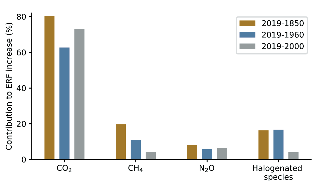
Global mean concentrations for well-mixed GHGs (CO2 , CH4 and N2 O) in 2019 correspond to increases of about 47%, 156%, and 23%, respectively, above the levels in 1750 (representative of the pre-industrial era) (high confidence). Current atmospheric concentrations of the three GHGs are higher than at any point in the last 800,000 years, and in 2019 reached 409.9 parts per million (ppm) of CO2, 1866.3 parts per billion (ppb) of CH4, and 332.1 ppb of N2O (very high confidence). Current CO2 concentrations in the atmosphere are also unprecedented in the last 2 million years (high confidence). In the past 60 million years, there have been periods in Earth’s history when CO2 concentrations were significantly higher than at present, but multiple lines of evidence show that the rate at which CO2 has increased in the atmosphere during 1900–2019 is at least 10 times faster than at any other time during the last 800,000 years (high confidence), and 4–5 times faster than during the last 56 million years (low confidence). {5.1.1, 2.2.3; Figures 5.3, 5.4; Cross-Chapter Box 2.1}
Contemporary Trends of Greenhouse Gases
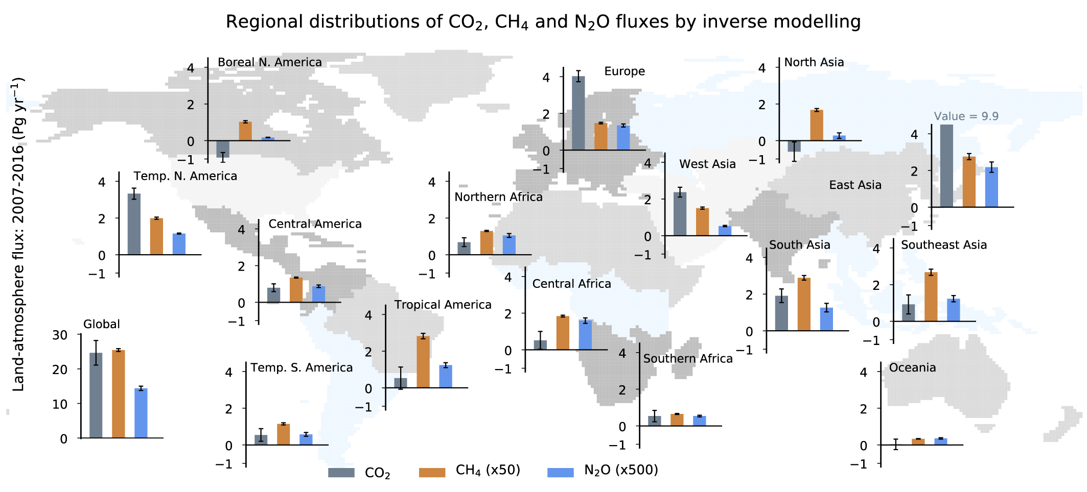
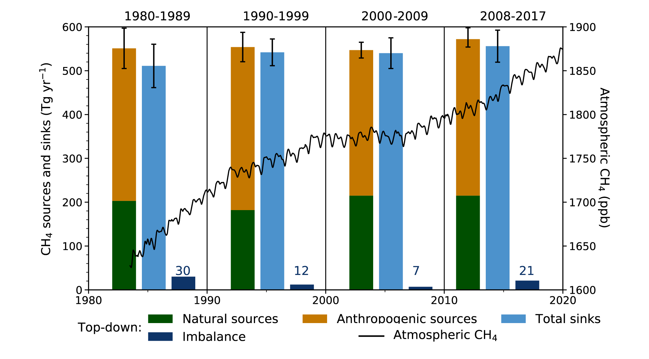
It is unequivocal that the increase of CO2 , CH4 , and N2 O in the atmosphere over the industrial era is the result of human activities (very high confidence). This assessment is based on multiple lines of evidence including atmospheric gradients, isotopes, and inventory data. During the last measured decade, global average annual anthropogenic emissions of CO2, CH4, and N2O, reached the highest levels in human history at 10.9 ± 0.9 petagrams of carbon per year (PgC yr–1, 2010–2019), 335–383 teragrams of methane per year (TgCH4yr–1, 2008–2017), and 4.2–11.4 teragrams of nitrogen per year (TgN yr–1, 2007–2016), respectively (high confidence). {5.2.1, 5.2.2, 5.2.3, 5.2.4; Figures 5.6, 5.13, 5.15}.
The CO2 emitted from human activities during the decade of 2010–2019 (decadal average 10.9 ± 0.9PgC yr–1) was distributed between three Earth system components: 46% accumulated in the atmosphere (5.1 ± 0.02PgC yr–1), 23% was taken up by the ocean (2.5 ± 0.6PgC yr–1) and 31% was stored by vegetation in terrestrial ecosystems (3.4 ± 0.9PgC yr–1) (high confidence). Of the total anthropogenic CO2 emissions, the combustion of fossil fuels was responsible for 81–91%, with the remainder being the net CO2 flux from land-use change and land management (e.g., deforestation, degradation, regrowth after agricultural abandonment, and peat drainage). {5.2.1.2, 5.2.1.5; Table 5.1; Figures 5.5, 5.7, 5.12}
Over the past six decades, the average fraction of anthropogenic CO2 emissions that has accumulated in the atmosphere (referred to as the airborne fraction) has remained nearly constant at approximately 44%. The ocean and land sinks of CO2 have continued to grow over the past six decades in response to increasing anthropogenic CO2 emissions (high confidence). Interannual and decadal variability of the regional and global ocean and land sinks indicate that these sinks are sensitive to climate conditions and therefore to climate change (high confidence). {5.2.1.1, 5.2.1.2, 5.2.1.3, 5.2.1.4; Figures 5.7, 5.8, 5.10}
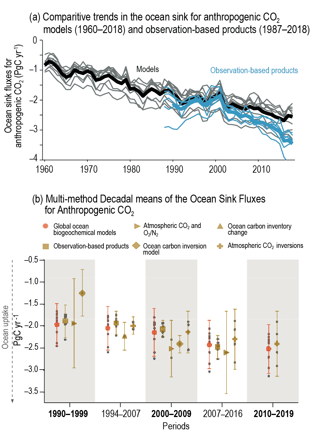
Recent observations show that ocean carbon processes are starting to change in response to the growing ocean sink, and these changes are expected to contribute significantly to future weakening of the ocean sink under medium- to high-emissions scenarios. However, the effects of these changes are not yet reflected in a weakening trend of the contemporary (1960–2019) ocean sink (high confidence). {5.1.2, 5.2.1.3, 5.3.2.1; Figures 5.8, 5.20; Cross-Chapter Box 5.3}
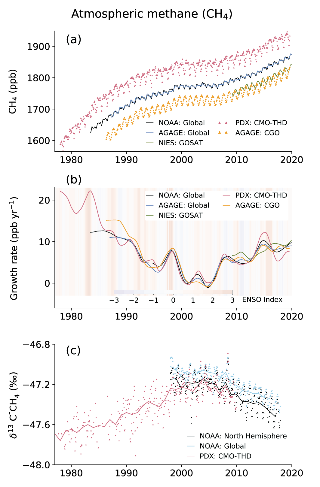
Atmospheric concentration of CH4 grew at an average rate of 7.6 ± 2.7 ppb yr–1 for the last decade (2010–2019), with a faster growth of 9.3 ± 2.4 ppb yr–1 over the last six years (2014–2019) (high confidence). The multi-decadal growth trend in atmospheric CH4 is dominated by anthropogenic activities (high confidence), and the growth since 2007 is largely driven by emissions from both fossil fuels and agriculture (dominated by livestock) (medium confidence). The interannual variability is dominated by El Niño–Southern Oscillation cycles, during which biomass burning and wetland emissions, as well as loss by reaction with tropospheric hydroxyl radical (OH) play an important role. {5.2.2; Figures 5.13, 5.14; Table 5.2; Cross-Chapter Box 5.2}
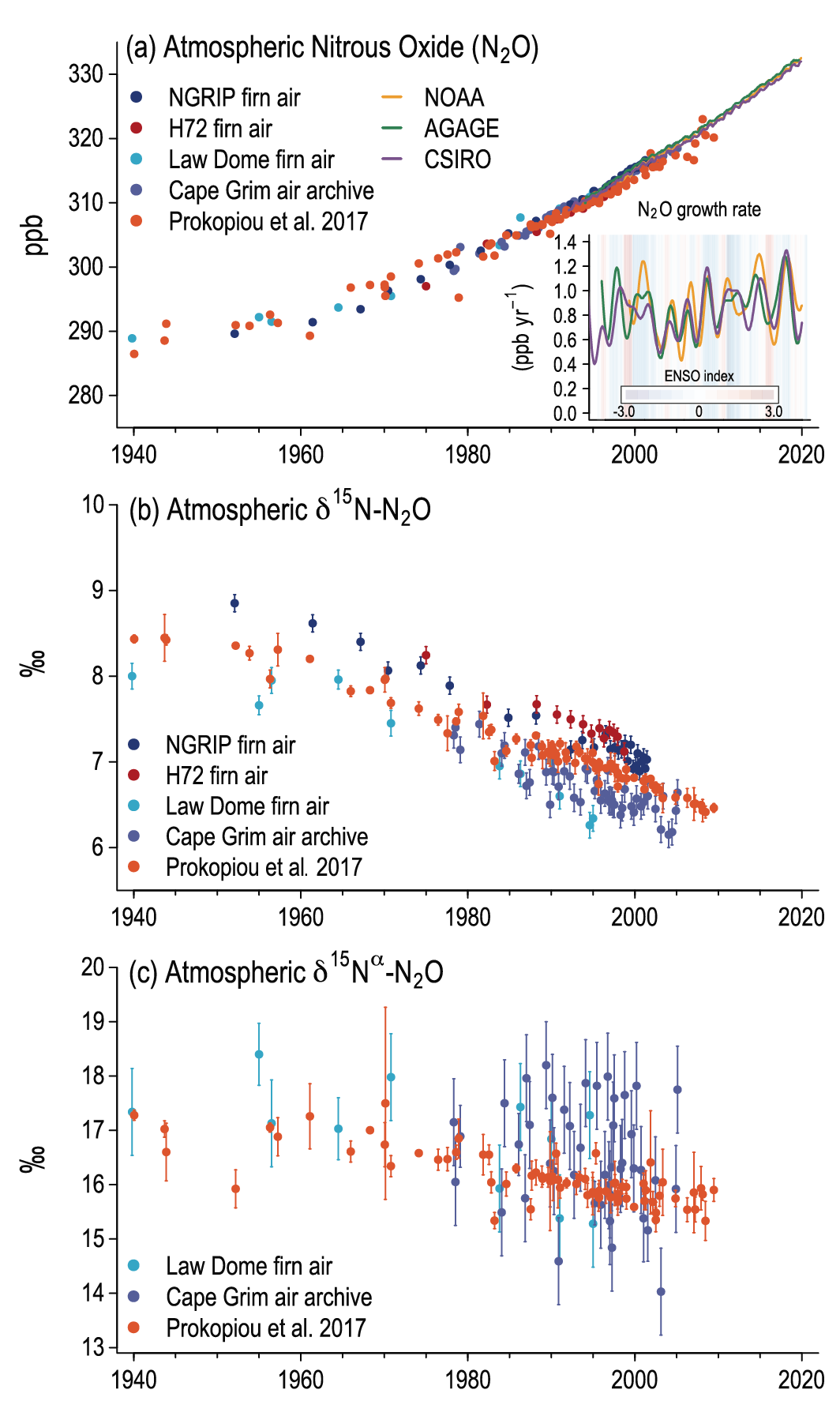
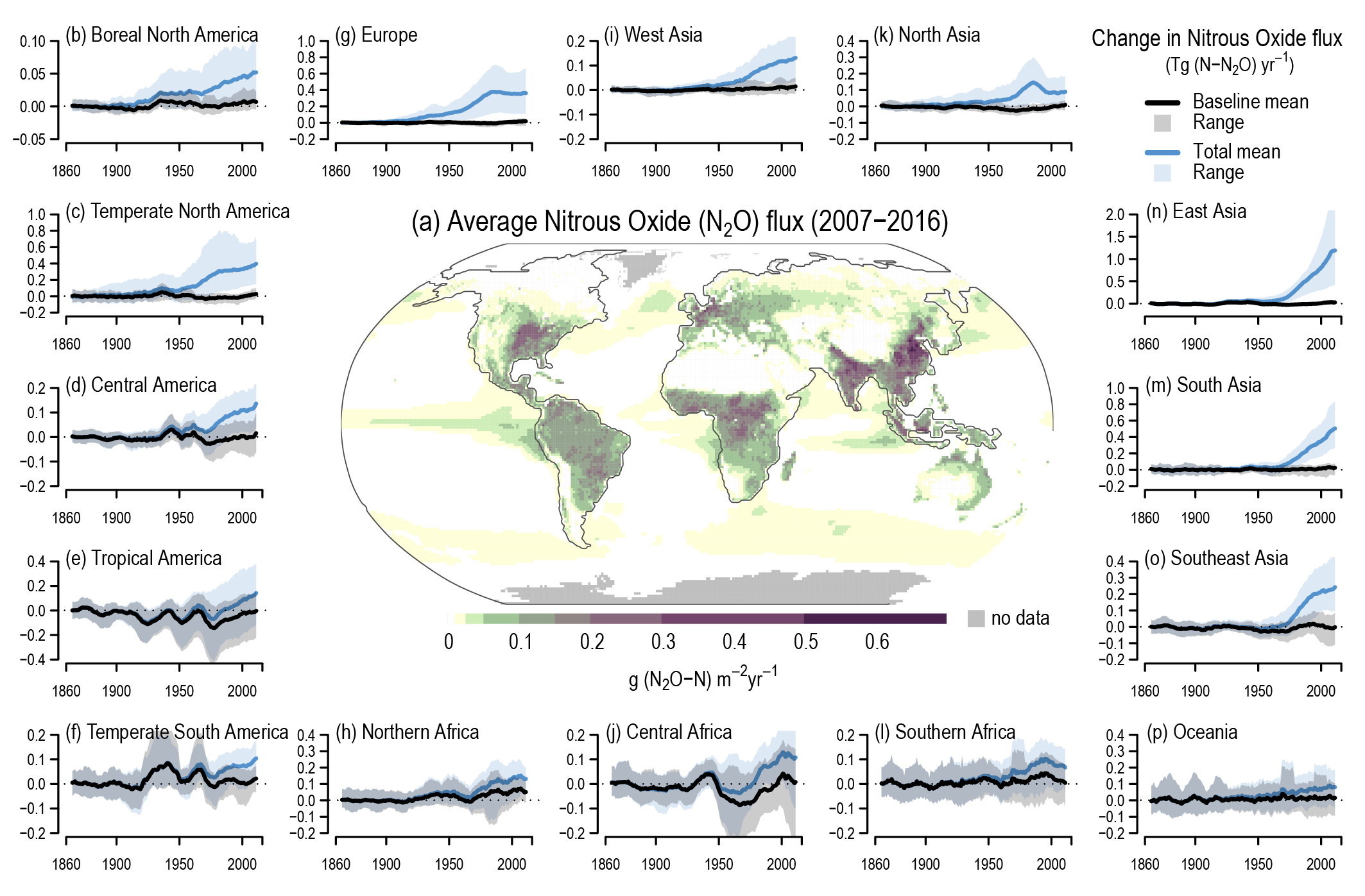
Atmospheric concentration of N2 O grew at an average rate of 0.85 ± 0.03 ppb yr–1 between 1995 and 2019, with a further increase to 0.95 ± 0.04 ppb yr–1 in the most recent decade (2010–2019). This increase is dominated by anthropogenic emissions, which have increased by 30% between the 1980s and the most recent observational decade (2007–2016) (high confidence). Increased use of nitrogen fertilizer and manure contributed to about two-thirds of the increase during the 1980–2016 period, with the fossil fuels/industry, biomass burning, and wastewater accounting for much of the rest (high confidence). {5.2.3; Figures 5.15, 5.16, 5.17}
Ocean Acidification and Ocean Deoxygenation
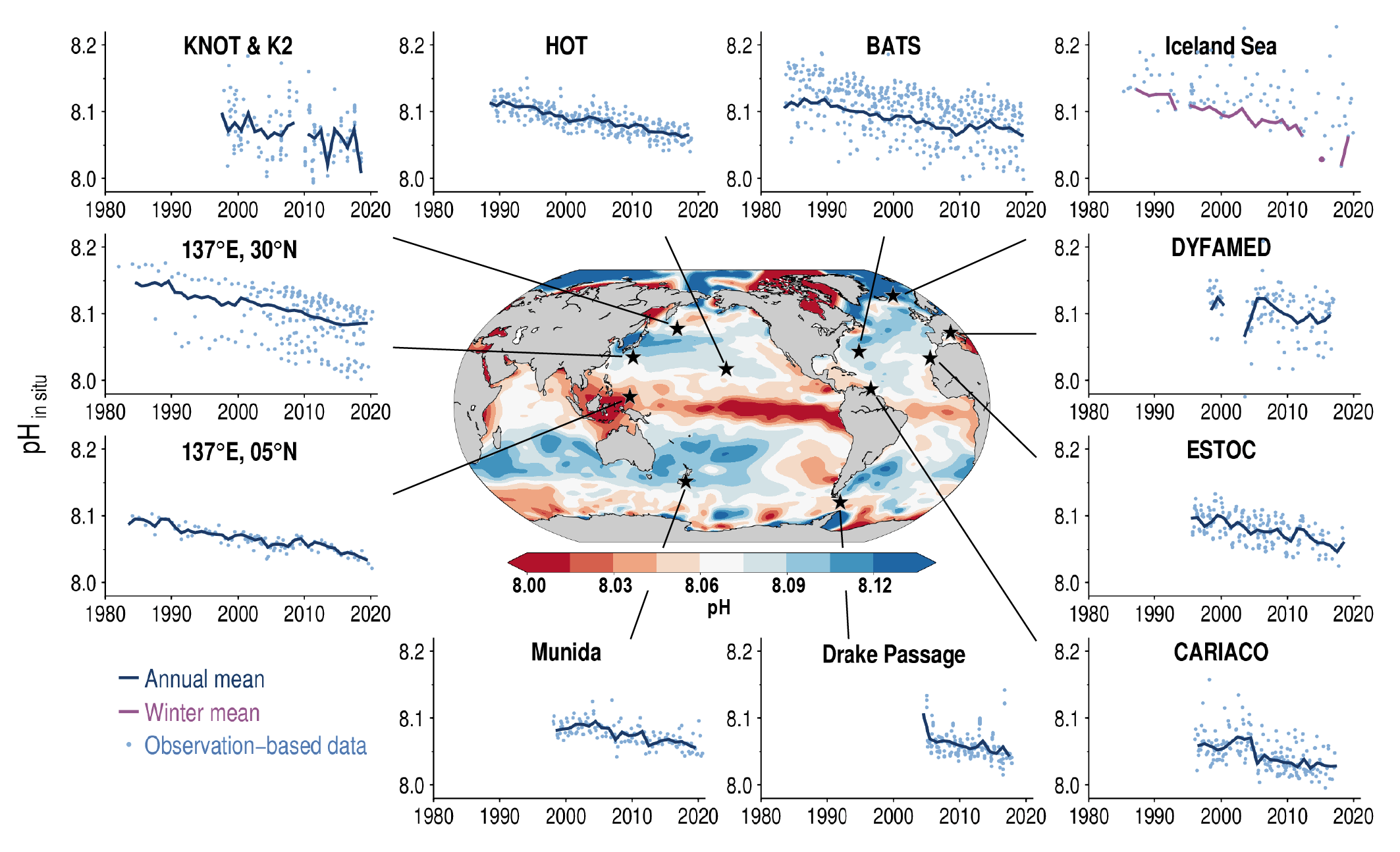
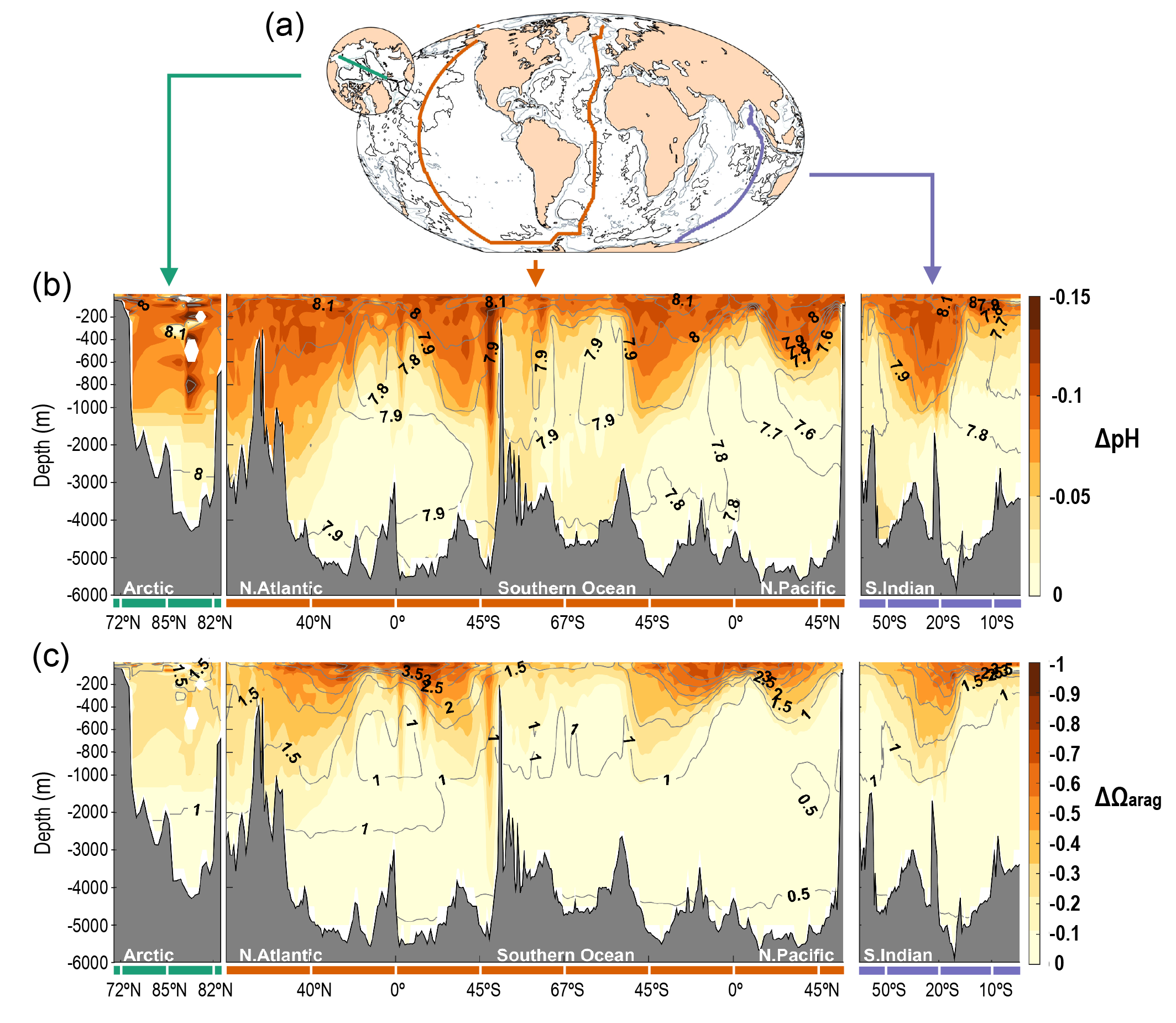
Ocean acidification is strengthening as a result of the ocean continuing to take up CO2 from human-caused emissions (very high confidence). This CO2 uptake is driving changes in seawater chemistry that result in the decrease of pH and associated reductions in the saturation state of calcium carbonate, which is a constituent of skeletons or shells of a variety of marine organisms. These trends of ocean acidification are becoming clearer globally, with avery likely rate of decrease in pH in the ocean surface layer of 0.016 to 0.020 per decade in the subtropics and 0.002 to 0.026 per decade in subpolar and polar zones since the 1980s. Ocean acidification has spread deeper in the ocean, surpassing 2000 m depth in the northern North Atlantic and in the Southern Ocean. The greater projected pH declines in Coupled Model Intercomparison Project Phase 6 (CMIP6) models are primarily a consequence of higher atmospheric CO2 concentrations in the Shared Socio-economic Pathways (SSPs) scenarios than their Coupled Model Intercomparison Project Phase 5 (CMIP5) Representative Concentration Pathway (RCP) analogues. {5.3.2.2, 5.3.3.1; 5.3.4.1; Figures 5.20, 5.21}
Ocean deoxygenation is projected to continue to increase with ocean warming (high confidence). Earth system models (ESMs) project a 32–71% greater subsurface (100–600 m) oxygen decline, depending on the scenario, than reported in the Special Report on the Ocean and Cryosphere (SROCC) for the period 2080–2099. This is attributed to the effect of larger surface warming in CMIP6 models, which increases ocean stratification and reduces ventilation (medium confidence). There is low confidence in the projected reduction of oceanic N2O emissions under high-emissions scenarios because of greater oxygen losses simulated in ESMs in CMIP6, uncertainties in the process of oceanic N2O emissions, and a limited number of modelling studies available. {5.3.3.2; 7.5}
Future Projections of Carbon Feedbacks on Climate Change
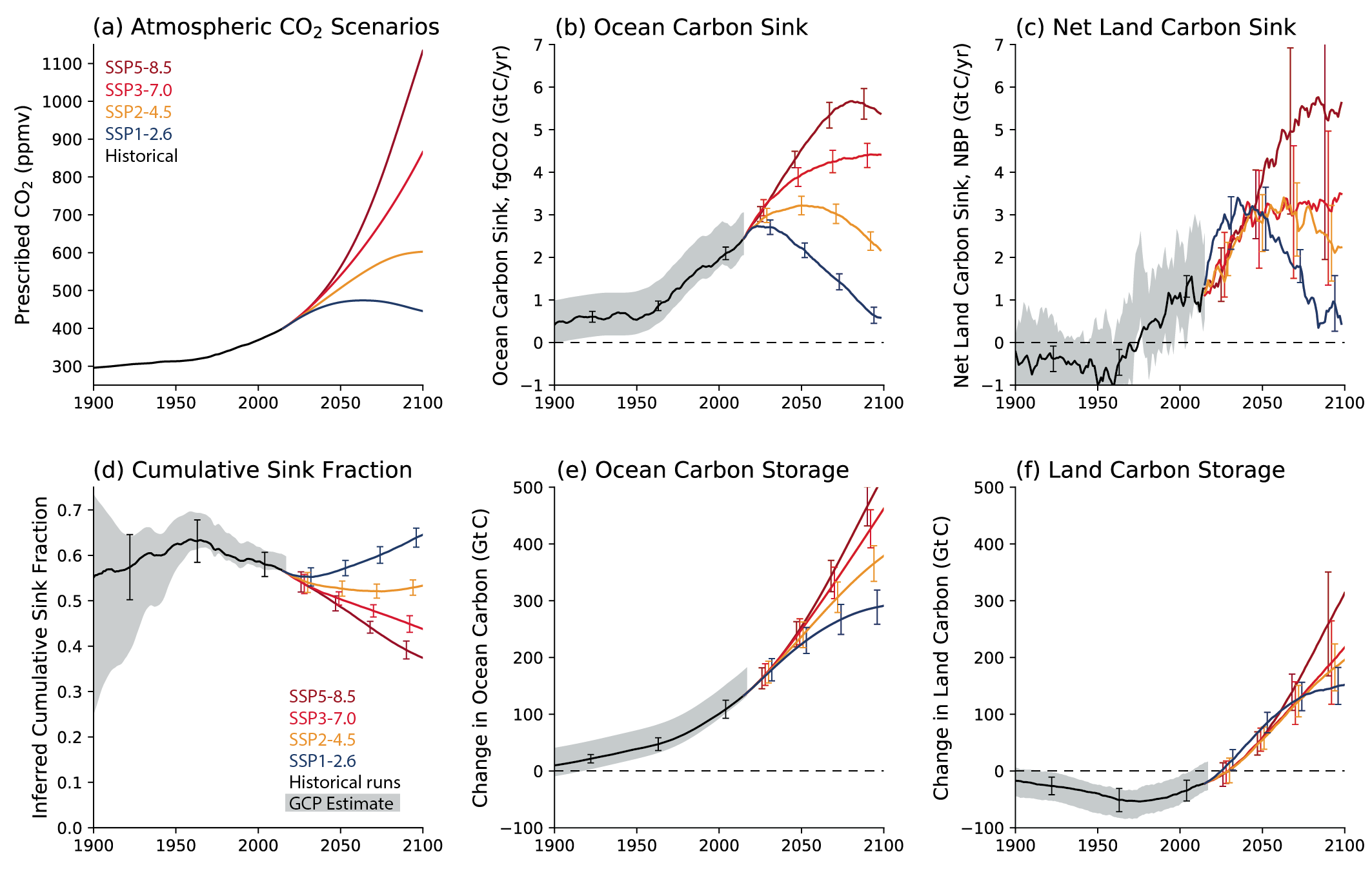
Oceanic and terrestrial carbon sinks are projected to continue to grow with increasing atmospheric concentrations of CO2 , but the fraction of emissions taken up by land and ocean is expected to decline as the CO2 concentration increases (high confidence). ESMs suggest approximately equal global land and ocean carbon uptake for each of the SSP scenarios. However, the range of model projections is much larger for the land carbon sink. Despite the wide range of model responses, uncertainty in atmospheric CO2 by 2100 is dominated by future anthropogenic emissions rather than uncertainties related to carbon–climate feedbacks (high confidence). {5.4.5; Figure 5.25, 5.26}
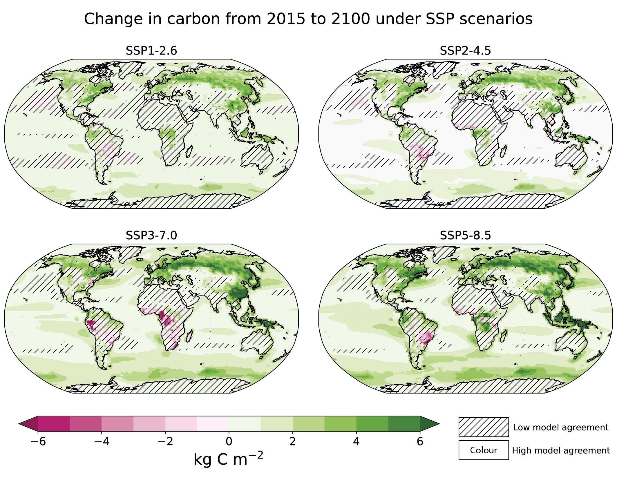
Increases in atmospheric CO2 lead to increases in land carbon storage through CO2 fertilization of photosynthesis and increased water use efficiency (high confidence). However, the overall change in land carbon also depends on land-use change and on the response of vegetation and soil to continued warming and changes in the water cycle, including increased droughts in some regions that will diminish the sink capacity. Climate change alone is expected to increase land carbon accumulation in the high latitudes (not including permafrost) and also to lead to a counteracting loss of land carbon in the tropics (medium confidence, Figure 5.25). More than half of the latest CMIP6 ESMs include nutrient limitations on the carbon cycle, but these models still project increasing tropical land carbon (medium confidence) and increasing global land carbon (high confidence) through the 21st century. {5.4.1, 5.4.3, 5.4.5; Figure 5.27; Cross-Chapter Box 5.1}
Future trajectories of the ocean CO2 sink are strongly emissions-scenario dependent (high confidence). Emissions scenarios SSP4-6.0 and SSP5-8.5 lead to warming of the surface ocean and large reductions of the buffering capacity, which will slow the growth of the ocean sink after 2050. Scenario SSP1-2.6 limits further reductions in buffering capacity and warming, and the ocean sink weakens in response to the declining rate of increasing atmospheric CO2. There is low confidence in how changes in the biological pump will influence the magnitude and direction of the ocean carbon feedback. {5.4.2, 5.4.4, Cross-Chapter Box 5.3}
Beyond 2100, land and ocean may transition from being a carbon sink to a source under either very high emissions or net negative emissions scenarios, but for different reasons. Under very high emissions scenarios such as SSP5-8.5, ecosystem carbon losses due to warming lead the land to transition from a carbon sink to a source (medium confidence), while the ocean is expected to remain a sink (high confidence). For scenarios in which CO2 concentration stabilizes, land and ocean carbon sinks gradually take up less carbon as the increase in atmospheric CO2 slows down. In scenarios with moderate net negative CO2 emissions, and CO2 concentrations declining during the 21st century (e.g., SSP1-2.6), the land sink transitions to a net source in decades to a few centuries after CO2 emissions become net negative, while the ocean remains a sink (low confidence). Under scenarios with large net negative CO2 emissions and rapidly declining CO2 concentrations (e.g., SSP5-3.4-OS (overshoot)), both land and ocean switch from a sink to a transient source during the overshoot period (medium confidence). {5.4.10, 5.6.2.1.2; Figures 5.30, 5.33}
Thawing terrestrial permafrost will lead to carbon release (high confidence), but there is low confidence in the timing, magnitude and the relative roles of CO2 versus CH4 as feedback processes. CO2 release from permafrost is projected to be 3–41 PgC per 1°C of global warming by 2100, based on an ensemble of models. However, the incomplete representation of important processes such as abrupt thaw, combined with weak observational constraints, only allowlow confidence in both the magnitude of these estimates and in how linearly proportional this feedback is to the amount of global warming. It is very unlikely that gas clathrates in terrestrial and subsea permafrost will lead to a detectable departure from the emissions trajectory during this century. {5.4.9; Box 5.1}
The net response of natural CH4 and N2 O sources to future warming will be increased emissions (medium confidence). Key processes include increased CH4 emissions from wetlands and permafrost thaw, as well as increased soil N2O emissions in a warmer climate, while ocean N2O emissions are projected to decline at centennial time scale. The magnitude of the responses of each individual process and how linearly proportional these feedbacks are to the amount of global warming is known with low confidence due to incomplete representation of important processes in models combined with weak observational constraints. Models project that, over the 21st century, the combined feedback of 0.02–0.09 W m–2°C–1is comparable to the effect of a CO2 release of 5–18 petagrams of carbon equivalent per °C (PgCeq °C–1) (low confidence). {5.4.7, 5.4.8; Figure 5.29}
The response of biogeochemical cycles to the anthropogenic perturbation can be abrupt at regional scales, and irreversible on decadal to century time scales (high confidence). The probability of crossing uncertain regional thresholds (e.g., high severity fires, forest dieback) increases with climate change (high confidence). Possible abrupt changes and tipping points in biogeochemical cycles lead to additional uncertainty in 21st century GHG concentrations, but these are very likely to be smaller than the uncertainty associated with future anthropogenic emissions (high confidence). {5.4.9}
Remaining Carbon Budgets to Climate Stabilization
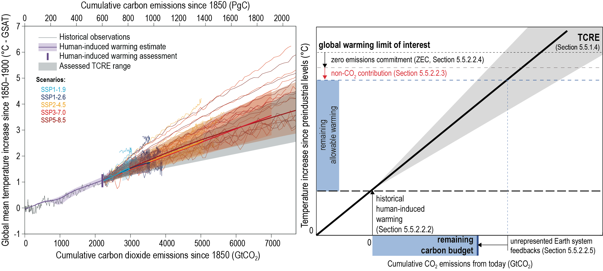
There is a near-linear relationship between cumulative CO2 emissions and the increase in global mean surface air temperature (GSAT) caused by CO2 over the course of this century for global warming levels up to at least 2°C relative to pre-industrial (high confidence). Halting global warming would thus require global net anthropogenic CO2 emissions to become zero. The ratio between cumulative CO2 emissions and the consequent GSAT increase, which is called the transient climate response to cumulative emissions of CO2 (TCRE), likely falls in the 1.0°C–2.3°C per 1000 PgC range. The narrower range compared to the IPCC Fifth Assessment Report (AR5) is due to a better integration of evidence across the science in this assessment. Beyond this century, there is low confidence that the TCRE remains an accurate predictor of temperature changes in scenarios of very low or net negative CO2 emissions because of uncertain Earth system feedbacks that can result in further warming or a path-dependency of warming as a function of cumulative CO2 emissions. {5.4, 5.5.1}
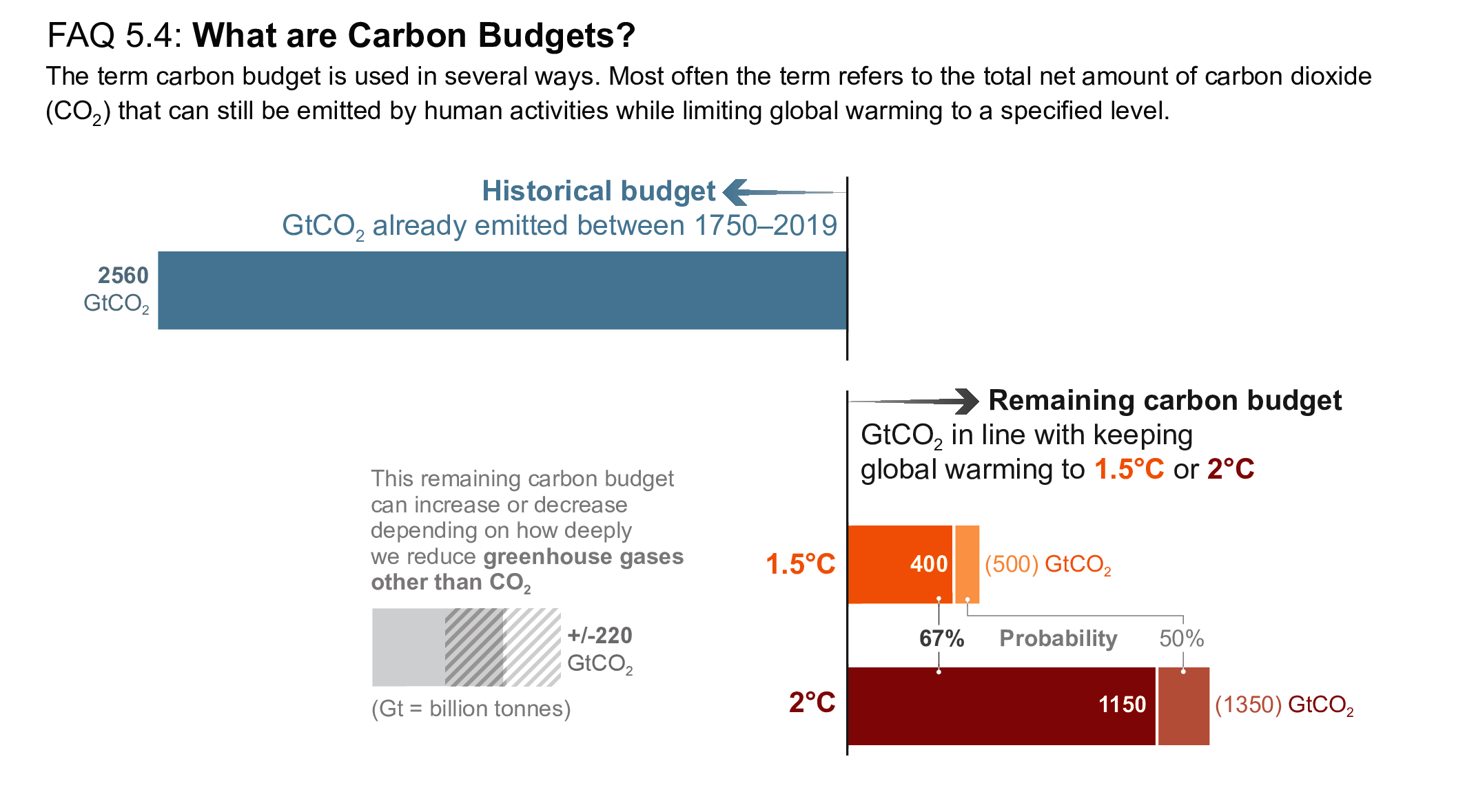
Mitigation requirements over this century for limiting maximum warming to specific levels can be quantified using a carbon budget that relates cumulative CO2 emissions to global mean temperature increase (high confidence). For the period 1850–2019, a total of 655 ± 65 PgC (2390 ± 240 GtCO2, likely range) of anthropogenic CO2 has been emitted. Remaining carbon budgets (starting from 1 January 2020) for limiting warming to 1.5°C, 1.7°C, and 2.0°C are 140 PgC (500 GtCO2), 230 PgC (850 GtCO2) and 370 PgC (1350 GtCO2), respectively, based on the 50th percentile of TCRE. For the 67th percentile, the respective values are 110 PgC (400 GtCO2), 190 PgC (700 GtCO2) and 310 PgC (1150 GtCO2). These remaining carbon budgets may vary by an estimated ± 60 PgC (220 GtCO2) depending on how successfully future non-CO2 emissions can be reduced. Since AR5 and the Special Report on Global Warming of 1.5°C (SR1.5), estimates have undergone methodological improvements, resulting in larger, yet consistent estimates. {5.5.2, 5.6; Figure 5.31; Table 5.8}
Several factors affect the precise value of remaining carbon budgets, including estimates of historical warming, future emissions from thawing permafrost, and variations in projected non-CO2 warming. Remaining carbon budget estimates can increase or decrease by 150 PgC (likely range; 150 PgC equals 550 GtCO2) due to uncertainties in the level of historical warming, and by an additional ± 60 PgC (±220 GtCO, likely range) due to geophysical uncertainties surrounding the climate response to non-CO2 emissions such as CH4, N2O, and aerosols. Permafrost thaw is included in the estimates, together with other feedbacks that are often not captured by models. Despite the large uncertainties surrounding the quantification of the effects of additional Earth system feedback processes, such as emissions from wetlands and permafrost thaw, these feedbacks represent identified additional amplifying risk factors that scale with additional warming and mostly increase the challenge of limiting warming to specific temperature thresholds. These uncertainties do not change the basic conclusion that global CO2 emissions would need to decline to at least net zero to halt global warming. {5.4, 5.5.2}
Biogeochemical Implications of Carbon Dioxide Removal and Solar Radiation Modification
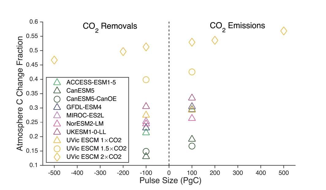
Land- and ocean-based carbon dioxide removal (CDR) methods have the potential to sequester CO2 from the atmosphere, but the benefits of this removal would be partially offset by CO2 release from land and ocean carbon stores (very high confidence). The fraction of CO2 removed that remains out of the atmosphere, a measure of CDR effectiveness, decreases slightly with increasing amount of removal (medium confidence) and decreases strongly if CDR is applied at lower CO2 concentrations (medium confidence). {5.6.2.1; Figures 5.32, 5.33, 5.34}
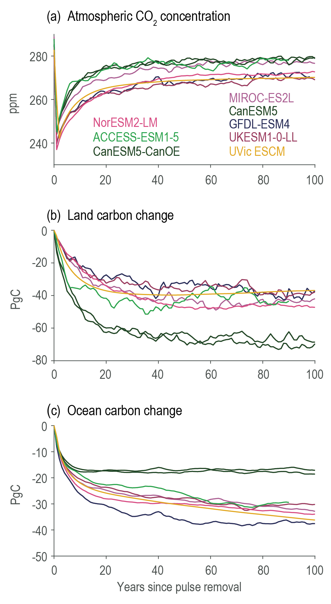
The century-scale climate–carbon cycle response to a CO2 removal from the atmosphere is not always equal and opposite to the response to a CO2 emission (medium confidence). For simultaneously cumulative CO2 emissions and removals of greater than or equal to 100 PgC, CO2 emissions are 4 ± 3% more effective at raising atmospheric CO2 than CO2 removals are at lowering atmospheric CO2. The asymmetry originates from state-dependencies and non-linearities in carbon cycle processes and implies that an extra amount of CDR is required to compensate for a positive emission of a given magnitude to attain the same change in atmospheric CO2. The net effect of this asymmetry on the global surface temperature is poorly constrained due to low agreement between models (low confidence). {5.6.2.1; Figure 5.35}
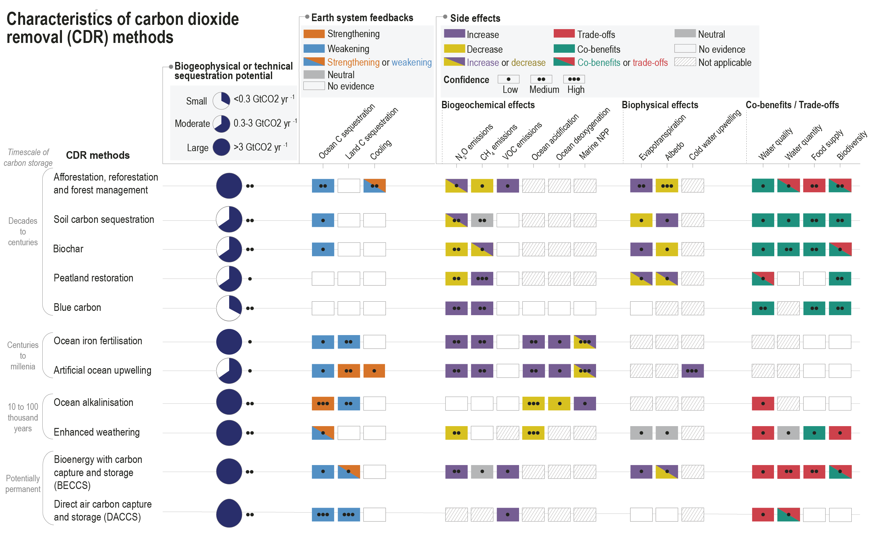
Wide-ranging side effects of CDR methods have been identified that can either weaken or strengthen the carbon sequestration and cooling potential of these methods and affect the achievement of sustainable development goals (high confidence). Biophysical and biogeochemical side effects of CDR methods are associated with changes in surface albedo, the water cycle, emissions of CH4 and N2O, ocean acidification and marine ecosystem productivity (high confidence). These side effects and associated Earth system feedbacks can decrease carbon uptake and/or change local and regional climate, and in turn limit the CO2 sequestration and cooling potential of specific CDR methods (medium confidence). Deployment of CDR, particularly on land, can also affect water quality and quantity, food production and biodiversity, with consequences for the achievement of related sustainable development goals (high confidence). These effects are often highly dependent on local context, management regime, prior land use, and scale of deployment (high confidence). A wide range of co-benefits are obtained with methods that seek to restore natural ecosystems or improve soil carbon (high confidence). The biogeochemical effects of terminating CDR are expected to be small for most CDR methods (medium confidence). {5.6.2.2; Figure 5.36; Cross-Chapter Box 5.1}
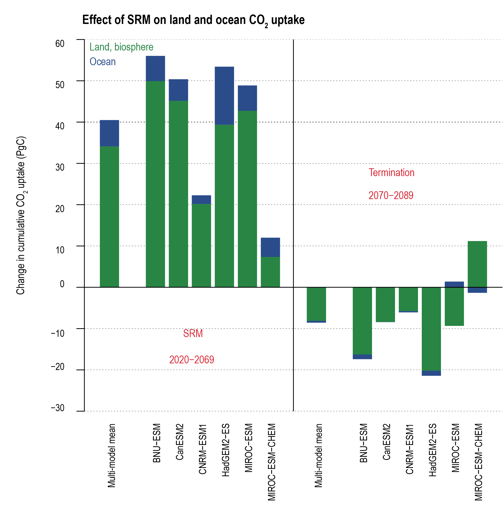
Solar radiation modification (SRM) would increase the global land and ocean CO2 sinks (medium confidence) but would not stop CO2 from increasing in the atmosphere, thus exacerbating ocean acidification under continued anthropogenic emissions (high confidence). SRM acts to cool the planet relative to unmitigated climate change, which would increase the land sink by reducing plant and soil respiration and slow the reduction of ocean carbon uptake due to warming (medium confidence). SRM would not counteract or stop ocean acidification (high confidence). The sudden and sustained termination of SRM would rapidly increase global warming, with the return of positive and negative effects on the carbon sinks (very high confidence). {4.6.3; 5.6.3}
5.1 Introduction
The physical and biogeochemical controls of greenhouse gases (GHGs) is a central motivation for this chapter, which identifies biogeochemical feedbacks that have led or could lead to a future acceleration, slowdown or abrupt transitions in the rate of GHG accumulation in the atmosphere, and therefore of climate change. A characterization of the trends and feedbacks lead to improved quantification for the remaining carbon budgets for climate stabilization, and the responses of the carbon cycle to atmospheric carbon dioxide removal (CDR), which is embedded in many of the mitigation scenarios, to achieve the goals of the Paris Agreement.
Changes in the abundance of well-mixed GHGs – carbon dioxide (CO2), methane (CH4) and nitrous oxide (N2O) – in the atmosphere play a large role in determining the Earth’s radiative properties and its climate in the past, the present and the future (Chapters 2, 4, 6 and 7). Since 1950, the increase in atmospheric GHGs has been the dominant cause of the human-induced climate change (Section 3.3). While the main driver of changes in atmospheric GHGs over the past 200 years relates to the direct emissions from human activities, the net accumulation of GHGs in the atmosphere is controlled by biogeochemical source-sink dynamics of carbon that exchange between multiple reservoirs on land, oceans and atmosphere. The combustion of fossil fuels and land-use change for the period 1750–2019 released an estimated 700 ± 75 PgC (1 PgC = 1015g of carbon) into the atmosphere, of which less than half remains in the atmosphere today (Sections 5.2.1.2; 5.2.1.5) (Friedlingstein et al., 2020). This emphasizes the central role of terrestrial and ocean CO2 sinks in regulating its atmospheric concentration (Ballantyne et al., 2012; W. Li et al., 2016; Le Quéré et al., 2018a; Ciais et al., 2019; Gruber et al., 2019b; Friedlingstein et al., 2020).
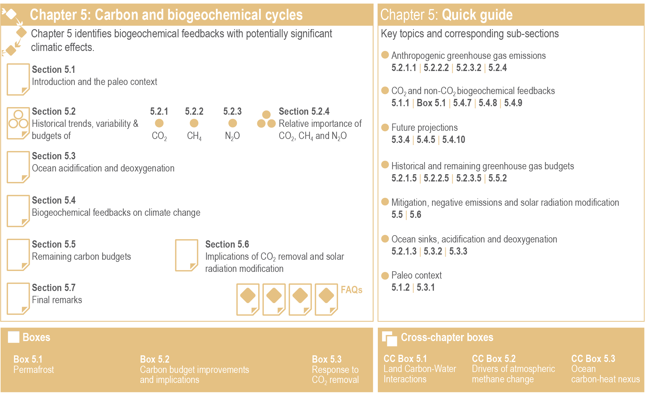
The chapter covers three dominant GHGs in the human perturbation of the Earth’s radiation budget for which high-quality records exist: CO2, CH4 and N2O (Figure 5.1).
 Figure 5.1 | Visual guide to Chapter 5.
 (Section 5.1 (this section) provides the time context on how unique current and future scenarios of GHGs atmospheric concentrations and growth rates are in the Earth’s history. It also introduces the main processes involved in carbon–climate feedbacks, followed by an assessment of what can be learned from the paleo record towards a better understanding of contemporary and future GHGs–climate dynamics and their response to different mitigation trajectories.
(Section 5.2 covers the state of the carbon cycle and other biogeochemical cycles, and global budgets of CO2, CH4 and N2O for the industrial era (since 1750). The section emphasizes the last 60-year period for which high-resolution observations are available and the most recent decade for comprehensive GHG budgets. Significant advances have taken place since the IPCC Fifth Assessment Report (AR5), particularly in constraining the annual-to-decadal variability of the ocean and land carbon sources and sinks, and in revealing the sensitivity of carbon pools to current and future climate changes. There has been an important increase in modelling capability of the three GHGs, for land and oceans, atmospheric and ocean observations, and remote sensing products that have enabled researchers to constrain the causes of the observed trends and variability.
(Section 5.3 builds on the Special Report on the Ocean and Cryosphere (SROCC) covering the change in ocean acidification due to oceanic CO2 uptake across the paleo, historical periods and future projections using Coupled Model Intercomparison Project Phase 6 (CMIP6), with consequences for marine life (assessed in the Sixth Assessment Report Working Group II, AR6 WGII) and biogeochemical cycles. The section also assesses changes in deoxygenation of the oceans due to warming, increased stratification of the surface ocean, and slowing of the meridional overturning circulation.
(Section 5.4 covers the future projections of biogeochemical cycles and their feedbacks to the climate system fully utilizing the database of the concentration-driven CMIP6. Since AR5, Earth system models (ESMs) have made progress towards including more complex carbon cycle and associated biogeochemical processes that enable exploring a range of possible future carbon–climate feedbacks and their influences on the climate system. The section addresses uncertainties and limits of our models to predict future dynamics for GHG emissions trajectories, as well as new understanding on processes involved in carbon–climate feedbacks and the possibility for rapid and abrupt changes brought by non-linear dynamics.
(Section 5.5 covers the development of the total and remaining carbon budgets to climate stabilization targets and the associated transient climate response to cumulative CO2 emissions. The section shows the progress made since AR5 (IPCC, 2013a) and the Special Report on Global Warming of 1.5°C (IPCC, 2018), particularly on key components required to estimate the remaining carbon budget, including the transient response to cumulative emissions of CO2, the zero emissions commitment, the projected non-CO2 warming, and the unrepresented Earth system feedbacks.
(Section 5.6 assesses the impacts of CDR and solar radiation modification for the purpose of climate change mitigation on the global carbon cycle, building from the assessment in the IPCC Special Report on Climate Change and Land (SRCCL). It includes an overview of the major CDR options and potential collateral biogeochemical effects beyond the intended climate change mitigation strategies. The potential capacity to deliver atmospheric reductions and the socio-economic feasibility of such options are assessed in detail in AR6 working group III (WGIII).
Finally, Section 5.7 highlights the knowledge gaps as limits to the assessment. The assessment would have been strengthened had those gaps not existed.
5.1.1 The Physical and Biogeochemical Processes in Carbon–Climate Feedbacks
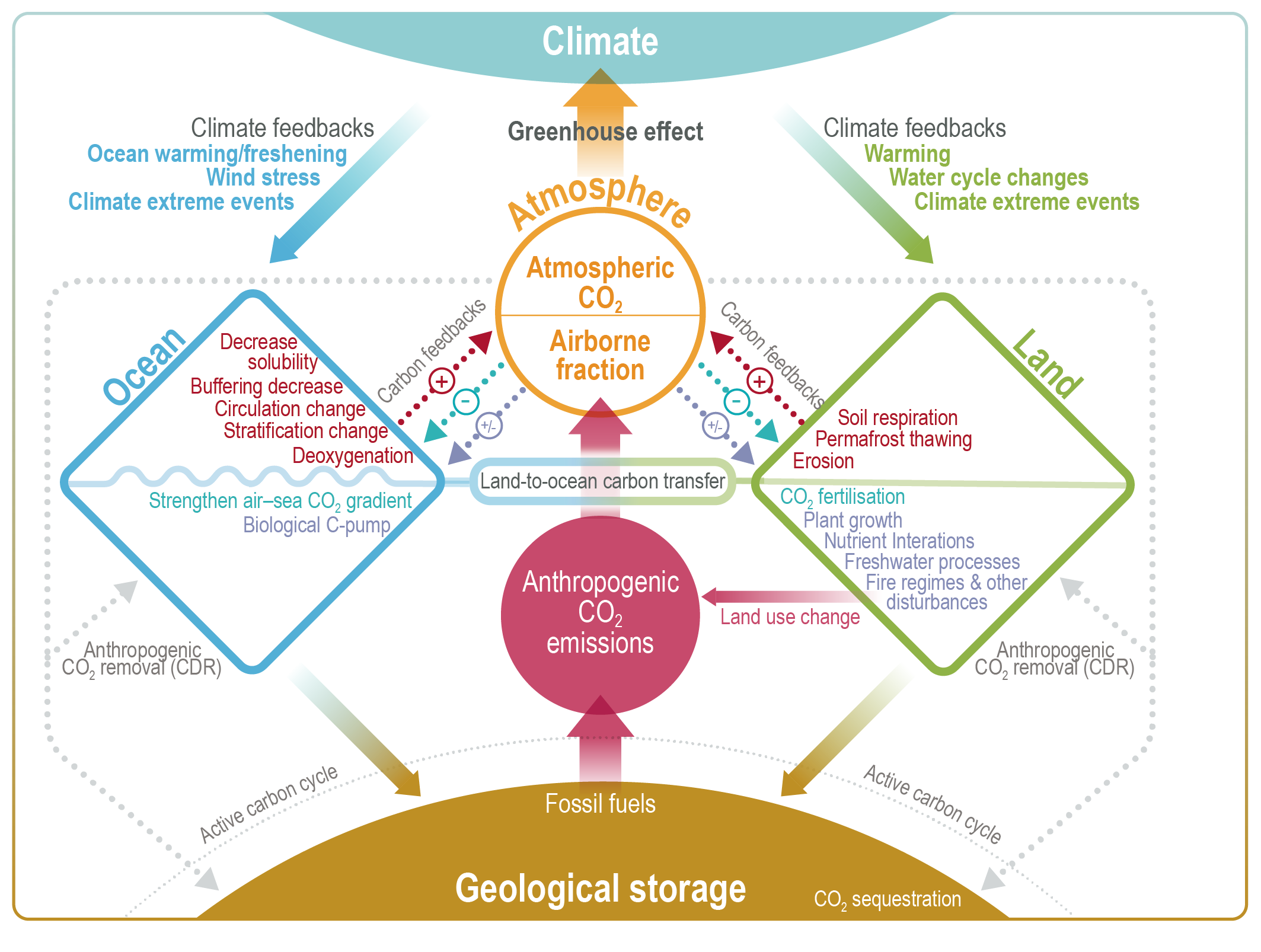
The influence of anthropogenic CO2 emissions and emissions scenarios on the carbon–climate system is the primary driver of ocean and terrestrial sinks as the major negative feedbacks that determine the atmospheric CO2 levels, which then drive climate feedbacks through radiative forcing (Figure 5.2) (Friedlingstein et al., 2006; Jones et al., 2013; Jones and Friedlingstein, 2020). Biogeochemical feedbacks follow as an outcome of both carbon and climate forcing on the physics and the biogeochemical processes of the ocean and terrestrial carbon cycles (Figure 5.2) (Katavouta et al., 2018; Williams et al., 2019; Jones and Friedlingstein, 2020). Together, these carbon–climate feedbacks can amplify or suppress climate change by altering the rate at which CO2 builds up in the atmosphere through changes in the land and ocean sources and sinks (Figure 5.2; C.D. Jones et al., 2013; Raupach et al., 2014; Williams et al., 2019). These changes depend on the, often non-linear, interaction of the drivers (CO2 and climate) and processes in the ocean and land as well as the emissions scenarios (Figure 5.2; Sections 5.4 and 5.6) (Raupach et al., 2014; Schwinger et al., 2014; Williams et al., 2019). There is high confidence that carbon–climate feedbacks and their century scale evolution play a critical role in two linked climate metrics that have significant climate and policy implications: (i) the fraction of anthropogenic CO2 emissions that remains in the atmosphere, the so-called airborne fraction of CO2 (AF; Section 5.2.1.2, Figures 5.2 and 5.7, and FAQ 5.1); and (ii) the quasi-linear trend characteristic of the transient temperature response to cumulative CO2 emissions (TCRE; Section 5.5; MacDougall, 2016; Williams et al., 2016; Jones and Friedlingstein, 2020) and other GHGs (CH4 and N2O). This chapter assesses the implications of these issues from the perspective of carbon cycle processes (Figure 5.2) in Section 5.2 (historical and contemporary), Section 5.3 (changing carbonate chemistry), Section 5.4 (future projections), Section 5.5 (remaining carbon budget) and Section 5.6 (response to carbon dioxide removal and solar radiation modification).
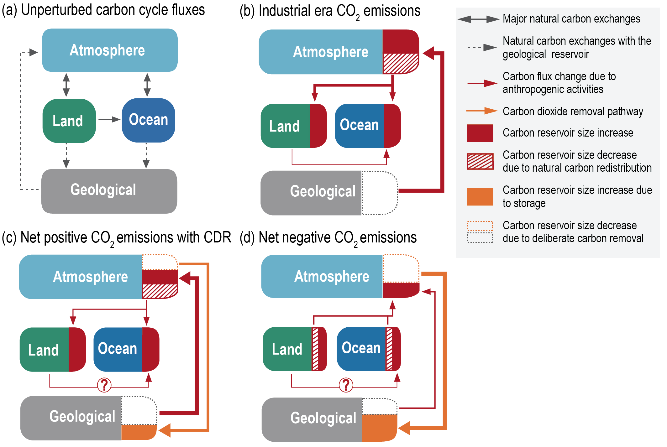
 Figure 5.2 | Key compartments, processes and pathways that govern historical and future CO2 concentrations and carbon–climate feedbacks through the coupled Earth system. The anthropogenic CO2 emissions, including land-use change, are partitioned via negative feedbacks (turquoise dotted arrows) between the ocean (23%), the land (31%) and the airborne fraction (46%) of anthropogenic CO2 that sets the changing CO2 concentration in the atmosphere (2010–2019; Table 5.1). This regulates most of the radiative forcing that creates the heat imbalance that drives the climate feedbacks to the ocean (blue) and land (green). Positive feedbacks (red arrows) result from processes in the ocean and on land (red text). Positive feedbacks are influenced by both carbon-concentration and carbon–climate feedbacks simultaneously. Additional biosphere processes have been included, but these have an as-yet-uncertain feedback impact (blue-dotted arrows). CO2 removal from the atmosphere into the ocean, land and geological reservoirs, necessary for negative emissions, has been included (grey arrows). Although this schematic is built around CO2 (the dominant greenhouse gas), some of the same processes also influence the fluxes of CH4 and N2O and the strength of the positive feedbacks from the terrestrial and ocean systems.
 The airborne fraction is an important constraint for adjustments in carbon–climate feedbacks and reflects the partitioning of CO2 emissions between reservoirs by the negative feedbacks, which were 31% on land and 23% in the ocean for the decade 2010–2019 and also dominated the historical period (Figure 5.2; Table 5.1) (Friedlingstein et al., 2020). During the period 1959–2019, the airborne fraction has largely followed the growth in anthropogenic CO2 emissions with a mean of 44% and a large interannual variability (Ballantyne et al., 2012; Ciais et al., 2019; Friedlingstein et al., 2020, Section 5.2.1.2; Table 5.1). The negative feedback to CO2 concentrations is associated with its impact on the air–sea and air–land CO2 exchange through strengthening of partial pressure of CO2 (pCO2) gradients as well as the internal processes that enhance uptake. Two of these key processes are the buffering capacity of the ocean and the CO2 fertilization effect on gross primary production (Sections 5.4.1–5.4.4).
Positive and negative climate and carbon feedbacks involve: (i) fast processes on land and oceans at time scales from minutes to years, such as photosynthesis, soil respiration, net primary production, shallow ocean physics and air–sea fluxes; and (ii) slower processes taking from decades to millennia, such as changing ocean buffering capacity, ocean ventilation, vegetation dynamics, permafrost changes, peat formation and decomposition (Figure 5.2; Ciais et al., 2013; Forzieri et al., 2017; Williams et al., 2019). Depending on the particular combination of driver process and response dynamics, they behave as positive or negative feedbacks that amplify or dampen the magnitude and rates of climate change, respectively (Cox et al., 2000; Friedlingstein et al., 2003, 2006; Hauck and Völker, 2015; Williams et al., 2019); red and turquoise arrows in Figure 5.2 and Table 5.1).
Carbon cycle feedbacks co-exist with climate (heat and moisture) feedbacks (Cross-Chapter Boxes 5.1 and 5.3), which together drive contemporary (Section 5.2) and future (Section 5.4) carbon–climate feedbacks (Williams et al., 2019). The excess heat generated by radiative forcing from increasing concentration of atmospheric CO2 and other GHGs is mostly taken up by the ocean (>90%) and the residual balance partitioned between atmospheric, terrestrial and ice melting (Cross-Chapter Box 9.2; Frölicher et al., 2015). The combined effect of these two large-scale negative feedbacks of CO2 and heat are reflected in the TCRE (Section 5.5 and Cross-Chapter Box 5.3), which points to a quasi-linear and quasi-emission-path independent relationship between cumulative emissions of CO2 and global warming, which is used as the basis to estimate the remaining carbon budget (Section 5.5; MacDougall and Friedlingstein, 2015; MacDougall, 2017; Bronselaer and Zanna, 2020; Jones and Friedlingstein, 2020). There is still low confidence on the relative roles and importance of the ocean and terrestrial carbon processes on TCRE variability and uncertainty on centennial time scales (MacDougall, 2016; MacDougall et al., 2017; Williams et al., 2017; Katavouta et al., 2018, 2019; Jones and Friedlingstein, 2020) (Sections 5.5.1.1, 5.5.1.2).
The combined effects of climate and CO2 concentration feedbacks on the global carbon cycle are projected by ESMs to modify both the processes and natural reservoirs of carbon on a regional and global scale that may result in positive feedbacks (red arrows in Figure 5.2), which could weaken the major terrestrial and ocean sinks and disrupt the airborne fraction and TCRE under medium- to high-emissions scenarios (Section 5.4.5 and Figure 5.25).
5.1.2 Paleo Trends and Feedbacks
Paleoclimatic proxy records extend beyond the variability of recent decadal climate oscillations and thus provide an independent perspective on feedbacks between climate and carbon cycle dynamics. According to reconstructions, these past changes were slower than the current anthropogenic ones, so they cannot provide an unequivocal comparison. Nonetheless, they can help appraise sensitivities and point towards potentially dominant mechanisms of change (Tierney et al., 2020) on (sub)centennial to (multi)millennial time scales.
The AR5 (WGI, Chapter 5) concluded with medium confidence that atmospheric CO2 concentrations reached 350–450 ppm during the mid-Pliocene (3.3–3.0 million years ago (Ma)), and possibly 1000 ppm during the Early Eocene (52–48 Ma). The AR5 (WGI, Chapter 5) also concluded with very high confidence that the current rates of increases in CO2, CH4 and N2O atmospheric concentrations were unprecedented with respect to the ice core record covering the last deglacial transition (LDT, 18–11 ka) and with medium confidence that the rate of change of the reconstructed GHG rise was also unprecedented compared to the lower resolution of the records of the past 800 kyr.
5.1.2.1 Cenozoic Proxy CO2 Record
Quantifying past changes in the rate of CO2 accumulation in the atmosphere based on reconstructions using marine sediment proxies is complex as age model uncertainties, assumptions and shortcomings underlying proxy applications and sedimentary processes conspire to alter and confound rate estimates (Ajayi et al., 2020). Differential sediment mixing and bioturbation contribute to smooth and attenuate proxy records (Hupp and Kelly, 2020), thereby tending to underestimate maximum rates of change (Kemp et al., 2015). Considering the extent to which uncertainties can affect sediment-based rate estimates, and notwithstanding recent effort in minimizing their inherent contribution, there is generallylow to medium confidence in quantifying rates of change on a time scale less than a decade back thousands of years, and less than a millennium back millions of years in the past based on marine sediments.
In the past, atmospheric CO2 concentrations reached much higher levels than present day (Cross-Chapter Box 2.1 and Figure 5.3). In particular, the Paleocene–Eocene thermal maximum (PETM), 55.9–55.7 Ma (Figure 5.3), provides some level of comparison with the current and projected anthropogenic increase in CO2 emissions (Chapter 2). Atmospheric CO2 concentrations increased from about 900 to around 2000 ppm in 3–20 kyr as a result of geological carbon release to the ocean–atmosphere system (Zeebe et al., 2016; Gutjahr et al., 2017; Cui and Schubert, 2018; Kirtland Turner, 2018). There is low to medium confidence in evaluations of the total amount of carbon released during the PETM, as proxy data constrained estimates vary from around 3000 to more than 7000 PgC, with methane hydrates, volcanic emissions, terrestrial and/or marine organic carbon, or some combination thereof, as the probable sources of carbon (Zeebe et al., 2009; Cui et al., 2011; Gutjahr et al., 2017; Elling et al., 2019; Jones et al., 2019; Haynes and Hönisch, 2020). Methane emissions related to hydrate/permafrost thawing and fossil carbon oxidation may have acted as positive feedbacks (Lunt et al., 2011; Armstrong McKay and Lenton, 2018; Lyons et al., 2019), as the inferred increase in atmospheric CO2 can only account for approximately half of the reported warming (Zeebe et al., 2009). The estimated, time-integrated carbon input is broadly similar to the RCP8.5 extension scenario, although CO2 emissions rates (0.3–1.5 Pg yr–1) and by inference the rate of CO2 accumulation in the atmosphere (4–42 ppm per century) during the PETM were at least 4–5 lower than during the modern era (from 1995 to 2014; Table 2.1; Zeebe et al., 2016; Gingerich, 2019).
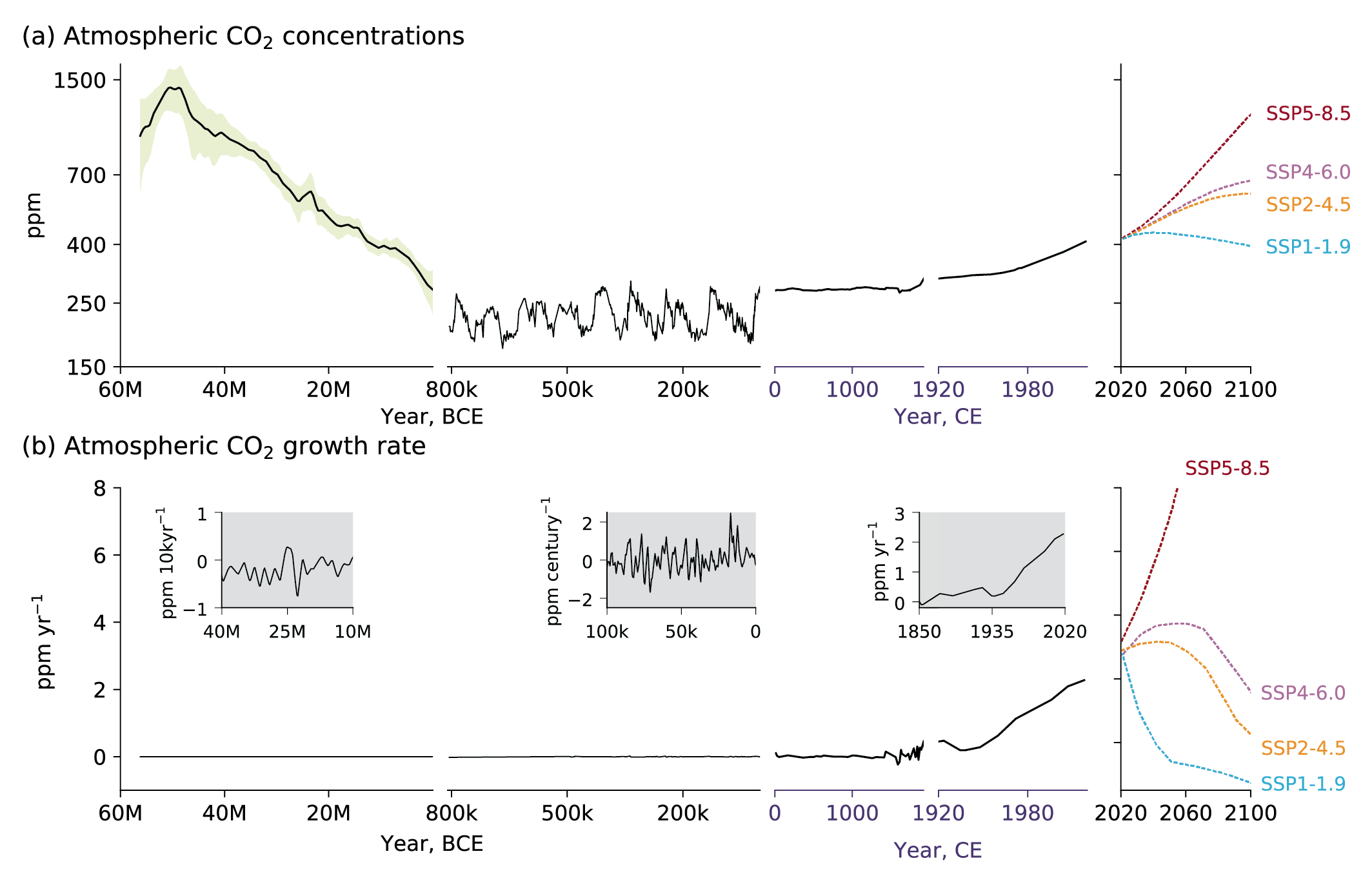 Figure 5.3 | Atmospheric CO2 concentrations and growth rates for the past 60 million years (Myr) and projections to 2100. (a) CO2 concentrations data for the period 60 Myr to the time prior to 800 kyr (left column) are shown as the LOESS Fit and 68% range (data from Chapter 2) (Foster et al., 2017). Concentrations from 1750 and projections through 2100 are taken from Shared Socio-economic Pathways of IPCC AR6 (Meinshausen et al., 2017). (b) Growth rates are shown as the time derivative of the concentration time series. Inserts in (b) show growth rates at the scale of the sampling resolution. Further details on data sources and processing are available in the chapter data table (Table 5.SM.6).
 The last 50 Myr (50 million years) have been characterized by a gradual decline in atmospheric CO2 levels at a rate of about 16 ppm Myr–1 (Figure 5.3; Foster et al., 2017; Gutjahr et al., 2017). The exact cause of this long-term change in CO2 remains uncertain, but may be related to an imbalance between long-term sources of CO2 (volcanic outgassing) and long-term sinks (organic carbon burial and silicate weathering).
The most recent time interval when atmospheric CO2 concentration was as high as 1000 ppm (i.e., similar to the end of 21st century projection for the high-end emissions scenario RCP8.5) was around 33.5 Ma, prior to the Eocene-Oligocene transition (Zhang et al., 2013; Anagnostou et al., 2016). Atmospheric CO2 levels then reached a critical threshold (1000–750 ppm; DeConto et al., 2008) to allow for the development of permanent regional ice sheets on Antarctica, associated with changes in Southern Ocean hydrography, which would have increased deep ocean CO2 storage (Leutert et al., 2020).
The most recent interval characterized by atmospheric CO2 levels similar to modern (i.e., 360–420 ppm) was the mid-Pliocene Warm Period (MPWP, 3.3–3.0 Ma; Martínez-Botí et al., 2015; de la Vega et al., 2020) (Chapter 2). The relatively high atmospheric CO2 concentration during the MPWP are related to vigorous ocean circulation and a rather inefficient marine biological carbon pump (Burls et al., 2017), which would have reduced deep ocean carbon storage. After the MPWP, atmospheric CO2 concentrations declined gradually at a rate of 30 ppm Myr–1 (Figure 5.3; de la Vega et al., 2020), as an increase in ocean stratification led to enhanced ocean carbon storage, allowing for major, sustained advances in Northern Hemisphere ice sheets, 2.7 Ma (Sigman et al., 2004; DeConto et al., 2008).
5.1.2.2 Glacial–Interglacial Greenhouse Gas Records
The Antarctic ice core record covering the past 800 kyr provides an important archive to explore the carbon–climate feedbacks prior to anthropogenic perturbations (Brovkin et al., 2016). Polar ice cores represent the only climatic archive from which past GHG concentrations can be directly measured. Major GHGs, CH4, N2O and CO2 generally co-vary on orbital time scales (Loulergue et al., 2008; Lüthi et al., 2008; Schilt et al., 2010b; Chapter 2), with consistently higher atmospheric concentrations during warm intervals of the past, pointing to a strong sensitivity to climate (Figure 5.4). Modelling work suggests that the carbon cycle contributed to globalise and amplify changes in orbital forcing, which are pacing glacial–interglacial climate oscillations (Ganopolski and Brovkin, 2017), with ocean biogeochemistry and physics, terrestrial vegetation, peatland, permafrost and exchanges with the lithosphere including chemical weathering, volcanic activity, sediment burial and marine calcium carbonate compensation all playing a role in modulating the concentration of atmospheric GHGs.
 Figure 5.4 | Atmospheric concentrations of CO2 , CH4 and N2 O in air bubbles and clathrate crystals in ice cores (800,000 BCE to 1990 CE). Note the variable x-axis range and tick mark intervals for the three columns. Ice core data is over-plotted by atmospheric observations from 1958 to present for CO2, from 1984 for CH4 and from 1994 for N2O. The time-integrated, millennial-scale linear growth rates for different time periods (800,000–0 BCE, 0–1900 CE and 1900–2017 CE) are given in each panel. For the BCE period, mean rise and fall rates are calculated for the individual slopes between the peaks (interglacials) and troughs (glacial periods), which are given in the panels in left column. The data for BCE period are used from the Vostok, EPICA, Dome C and WAIS ice cores (Petit et al., 1999; Monnin, 2001; Pépin et al., 2001; Raynaud et al., 2005; Siegenthaler et al., 2005; Loulergue et al., 2008; Lüthi et al., 2008; Schilt et al., 2010a). The data after 0–yr CE are taken mainly from Law Dome ice core analysis (MacFarling Meure et al., 2006). The surface observations for all species are taken from NOAA cooperative research network (Dlugokencky and Tans, 2019), where ALT, MLO and SPO stand for Alert (Canada), Mauna Loa Observatory, and South Pole Observatory, respectively. BCE = before current era, CE = current era. Further details on data sources and processing are available in the chapter data table (Table 5.SM.6).
 Since AR5, the number of ice core records and the temporal resolution of their data for the last 800 kyr have improved, in particular for the last 60 kyr. Additionally, the advent of isotopic measurements on GHGs extracted from air trapped in ice, allows for more robust source apportionments and inventory assessments. Therefore, the ensuing discussion focuses on these two specific aspects.
Major pre-industrial sources of CH4 comprise wetlands (including subglacial environments) and biomass burning (Bock et al., 2010, 2017; Lamarche-Gagnon et al., 2019; Kleinen et al., 2020). Pre-industrial atmospheric N2O concentrations were regulated by microbial production in marine and terrestrial environments and by photochemical removal in the stratosphere (Schilt et al., 2014; Battaglia and Joos, 2018b; H. Fischer et al., 2019). Pre-industrial atmospheric CO2 concentrations were largely regulated by exchange with exogenic terrestrial and ocean carbon reservoirs. The imbalance between geological sources and sinks in the ocean–atmosphere–land biosphere system additionally plays an important role in modulating the air–sea partitioning of the active carbon inventory on multi-millennial time scales (Cartapanis et al., 2018).
Model-based estimates indicate that wetland CH4 emissions were reduced by 24–40% during the Last Glacial Maximum (LGM) when compared to pre-industrial, while CH4 emissions related to biomass burning (wildfires) decreased by 35–75% (Valdes et al., 2005; Hopcroft et al., 2017; Kleinen et al., 2020). N2O emissions decreased by about 30% during the LGM based on data-constrained model estimates (Schilt et al., 2014; H. Fischer et al., 2019) owing to a combination of a weaker hydrological cycle and a generally better ventilated intermediate depth ocean relative to present, reducing (de)nitrification processes (Galbraith et al., 2013; Fischer et al., 2019).
During past ice ages, generally colder and drier climate conditions contributed to a substantial decline of the land biosphere carbon inventory, in particular in boreal peatlands (–300 PgC; Treat et al., 2019). Estimates assessing the glacial decrease in the global terrestrial biosphere carbon stock vary between –300 and –600 PgC (Ciais et al., 2012; Peterson et al., 2014; Menviel et al., 2017; Kleinen et al., 2020), possibly –850 PgC when accounting for ocean-sediment interactions and burial (Jeltsch-Thömmes et al., 2019), a considerable contraction when compared to the modern land biosphere stock. The large range of estimates reflects a yet limited understanding of how carbon cycle dynamics were altered by glacially perturbed nutrient fluxes and soil dynamics, as well as largely exposed shelf areas in the tropics as a result of lowered sea level. Recent estimates suggest deep-sea CO2 storage during the last ice age exceeded modern values by as much as 750 – 950 PgC (Skinner et al., 2015, 2017; Buchanan et al., 2016; Anderson et al., 2019; Gottschalk et al., 2020b). A combination of increased CO2 solubility associated with 2–3°C lower mean oceanic temperatures (Bereiter et al., 2018), increased the oceanic residence time of CO2 (Skinner et al., 2017), altered oceanic alkalinity (Yu et al., 2010; Cartapanis et al., 2018). A generally more efficient marine biological carbon pump (BCP; Galbraith and Jaccard, 2015; Yu et al., 2019; Galbraith and Skinner, 2020) enhanced the partition CO2 into the ocean interior, (although the relative contribution of each mechanism remains a matter of debate). Recent observationally constrained ESM results highlight that air–sea disequilibrium amplifies the effect of cooling and iron fertilization on glacial carbon storage (Khatiwala et al., 2019).
Ice core observations combined with model-based estimates thus reveal with high confidence that both terrestrial and marine CH4 and N2O emissions were reduced under glacial climate conditions. Multiple lines of evidence indicate with high confidence that enhanced storage of remineralized CO2 in the ocean interior, owing to a combination of synergistic mechanisms, was sufficient to balance the removal of carbon from the atmosphere and the terrestrial biosphere reservoirs combined during the last ice age.
Vegetation regrowth and increased precipitation in wetland regions associated with the mid-deglacial Northern Hemisphere warming (referred to as the Bølling/Allerød (B/A) warm interval, 14.7–12.7 ka), in particular in the (sub)tropics, accounts for large increases in both CH4 and N2O emissions to the atmosphere (Baumgartner et al., 2014; Schilt et al., 2014; Bock et al., 2017; H. Fischer et al., 2019). Specifically, changes in CH4 sources were steered by variations in vegetation productivity, source size area, temperatures and precipitation as modulated by insolation, local sea level changes and monsoon intensity (Bock et al., 2017; Kleinen et al., 2020). Changes in the CH4 atmospheric sink term probably only played a secondary role in modulating atmospheric CH4 inventories across the LDT (Hopcroft et al., 2017; Kleinen et al., 2020) Geological emissions, related to the destabilization of fossil (radiocarbon-dead) CH4 sources buried in continental margins as a result of sudden warming, appear small (Bock et al., 2017; Petrenko et al., 2017; Dyonisius et al., 2020). Stable isotope analysis on N2O extracted from Antarctic and Greenland ice reveal that marine and terrestrial emissions increased by 0.7 ± 0.3 and 1.7 ± 0.3 TgN, respectively, across the LDT (Fischer et al., 2019). During abrupt Northern Hemisphere warmings, terrestrial emissions responded rapidly to the northward displacement of the Intertropical Convergence Zone (ITCZ) associated with the resumption of the Atlantic meridional overturning circulation (AMOC; H. Fischer et al., 2019). About 90% of these step increases occurred rapidly, possibly in less than 200 years (Fischer et al., 2019). In contrast, marine emissions increased more gradually, modulated by global ocean circulation reorganization.
The gradual increase in atmospheric CO2 across the LDT was punctuated by three centennial 10–13 ppm increments, coeval with 100–200 ppb increases in CH4 (Marcott et al., 2014), reminiscent of similar oscillations reported for the last ice age associated with transient warming events (Dansgaard/Oeschger (DO) events; Ahn and Brook, 2014; Rhodes et al., 2017; Bauska et al., 2018) as well as previous deglacial transitions (Nehrbass-Ahles et al., 2020). The rate of change in atmospheric CO2 accumulation during these transient events exceeds the averaged deglacial growth rates by at least 50% (Table 2.1, Figure 5.4). The early deglacial release of remineralized carbon from the ocean abyss coincided with the resumption of Southern Ocean overturning circulation (Skinner et al.,2010; Schmitt et al., 2012; Ferrari et al., 2014; Gottschalk et al., 2016, 2020a; Jaccard et al., 2016; Rae et al., 2018; Moy et al., 2019) and the concomitant reduction in the global efficiency of the marine BCP, associated, in part, with dwindling iron fertilization (Hain et al., 2010; Martínez-García et al., 2014; Jaccard et al., 2016) The two subsequent pulses, centred 14.8 and 12.9 ka, are associated with enhanced air–sea gas exchange in the Southern Ocean (T. Li et al., 2020), iron fertilization in the South Atlantic and North Pacific (Lambert et al., 2021) and rapid increase in soil respiration owing to the resumption of AMOC and associated southward migration of the ITCZ (Marcottet al., 2014; Bauska et al., 2018). Rapid warming of high northern latitudes contributed to thaw permafrost, possibly liberating labile organic carbon to the atmosphere (Köhler et al.,2014; Crichton et al., 2016; Winterfeld et al., 2018; Meyer et al., 2019). Ocean surface pH reconstructions indicate that the ocean was oversaturated with respect to the atmosphere during the early, mid-LDT (Martínez-Botí et al., 2015b; Shao et al., 2019; Shuttleworth et al., 2021), suggesting that ocean sources at that time may have been larger than terrestrial sources. Over the course of the LDT, the decrease in Northern Hemisphere permafrost carbon stocks has been more than compensated by an increase in the carbon stocks of mineral soils, peatland and vegetation (Lindgren et al., 2018; Jeltsch-Thömmes et al., 2019). The land biosphere was, on average, a net sink for atmospheric carbon and accumulated several hundred Gt of carbon over the LDT. Detailed investigations reveal that Antarctic air temperatures, and more generally Southern Hemisphere (30°S–60°S) proxy temperature reconstructions, led the rise inpCO2 at the onset of the LDT, 18 ka ago, by several hundred years (Shakun et al., 2012; Chowdhry Beeman et al., 2019). Atmospheric CO2 led reconstructed global average temperature by several centuries (Shakun et al., 2012), corroborating the importance of CO2 as an amplifier of orbitally driven warming. During the LDT, the phasing between Antarctic air temperature and atmospheric GHG concentration changes was nearly synchronous, yet variable, owing to the complex nature of the mechanisms modulating the global carbon cycle (Chowdhry Beeman et al., 2019). Mean ocean temperature reconstructions, based on noble gas extracted from Antarctic ice are closely correlated with Antarctic air temperature and pCO2 records, emphasizing the role the Southern Ocean is playing in modulating global climate variability (Bereiter et al., 2018; Baggenstos et al., 2019).
Enhanced mid-ocean ridge magmatism and/or hydrothermal activity modulated by sea level rise has recently been hypothesized to have contributed to the deglacial CO2 rise (Crowley et al., 2015; Lund et al., 2016; Huybers and Langmuir, 2017; Stott et al., 2019b). While geological carbon release may have affected the ocean’s radiocarbon budget (Ronge et al., 2016; Rafter et al., 2019; Stott et al., 2019a), model results suggest that the potential contribution of geological carbon sources to the atmosphere remained small (Roth and Joos, 2012; Hasenclever et al., 2017).
Simulations of Earth models of intermediate complexity (EMIC) with coupled glacial–interglacial climate and the carbon cycle were able to reproduce first-order changes in the atmospheric CO2 content for the first time in recent years (Ganopolski and Brovkin, 2017; Khatiwala et al., 2019). The most important processes accounting for the full deglacial CO2 amplitude in the models include solubility changes, changes in oceanic circulation and marine carbonate chemistry. The effect of the terrestrial carbon cycle, variable volcanic outgassing and the temperature dependence on the oceanic remineralization length scale contribute less than 15 ppm CO2 between the glacial and interglacial intervals of the cycles. However, details in the simulated response of the marine carbon cycle and atmospheric CO2 concentrations to changes in ocean circulation depend to a large degree on model parametrization (Gottschalk et al., 2019).
Independent paleoclimatic evidence suggests with high confidence that marine and terrestrial CH4 and N2O emissions are highly sensitive to climate on (sub)centennial time scales. Limited, yet internally consistent ice core measurements indicate with medium confidence that pulsed geologic CH4 release from continental margins associated with warming remained negligible across the LDT. Multiple lines of evidence suggest with high confidence that CO2 was released from the ocean interior on centennial time scales during the LDT in response to, or associated with warming, contributing to the transition out of the last glacial stage to the current interglacial period.
Multiple lines of evidence inferred from marine sediment proxies indicate with low to medium confidence that the millennial rates of CO2 concentration change in the atmosphere during the last 56 Myr were at least four to five times lower than during the last century (Figure 5.3). In spite of uncertainties in ice core reconstructions related to delayed enclosure of air bubbles, which tend to smooth the records, there is high confidence that the rates of atmospheric CO2 and CH4 change during the last century were at least 10 and 5 times faster, respectively, than the maximum centennial growth rate averages of those gases during the last 800 kyr (Fig. 5.4).
5.1.2.3 Holocene Changes
Atmospheric GHG concentrations were much less variable during the pre-industrial Holocene (from 11.7 ka to 1750 CE). Atmospheric CH4 concentrations decreased at the beginning of the Holocene, consistent with a general weakening of boreal sources (Yang et al., 2017; Beck et al., 2018) and further decline during the mid-Holocene owing to a reduction in Southern Hemisphere emissions concomitant with a southward shift of the ITCZ (Singarayer et al., 2011; Beck et al., 2018). Atmospheric CH4 concentrations increased about 5 ka, which prompted the hypothesis of an early anthropogenic influence related to land-use changes in South East Asia (Ruddiman et al., 2016). However, stable isotope compositions on CH4 extracted from Greenland and Antarctic ice (Beck et al., 2018) reveal that natural emissions located in the southern tropics were responsible for the rise in atmospheric CH4 concentrations, in line with model simulations (Singarayer et al., 2011) thus disputing the early anthropogenic influence on the global CH4 budget. Atmospheric N2O concentrations increased slightly (20 ppb) across the Holocene, associated with a gradual decline in its nitrogen stable isotope composition (H. Fischer et al., 2019). The combined signal is consistent with a small increase in terrestrial emissions, offset by a reduction in marine emissions (Schilt et al., 2010b; Fischer et al., 2019).
The early Holocene decrease in CO2 concentration by about 5 ppm (Schmitt et al., 2012) has been attributed to post-glacial regrowth in terrestrial biomass and a gradual increase in peat reservoirs over the Holocene, resulting in the sequestration of several hundred PgC (Yu et al., 2010; Nichols and Peteet, 2019). Peat accumulation rates in boreal and temperate regions were higher under warmer summer conditions in the early to mid-Holocene (Loisel et al., 2014; Stocker et al., 2017). The 20 ppm gradual increase of atmospheric CO2 starting 7 ka has been attributed to a decrease in natural terrestrial biomass due to climate change, carbonate compensation and enhanced shallow water carbonate deposition (Menviel and Joos, 2012; Brovkin et al., 2016), consistent with stable carbon isotope measurements on CO2 extracted from Antarctic ice (Elsig et al., 2009; Schmitt et al., 2012). These isotopic measurements do not support an early anthropogenic influence on atmospheric CO2 due to land-use change and forest clearing (Ruddiman et al., 2016). Recent paleoceanographic evidence suggests that remineralized carbon outgassing associated with increased Southern Ocean circulation and upwelling (Studer et al., 2018), possibly promoted by stronger Southern Hemisphere westerly winds (Saunders et al., 2018), could have additionally contributed to the late Holocene increase in atmospheric CO2 concentrations. However, the role of these mechanisms remained insignificant in transient Holocene ESM simulations (Brovkin et al., 2019). Overall, as in AR5 (WGI, Chapter 5), there is medium confidence in the key drivers of the CO2 increase between the early Holocene and the beginning of the industrial era, yet there is low confidence in the relative contributions of these drivers due to insufficient quantitative constraints on particular processes.
5.2 Historical Trends, Variability and Budgets of CO2, CH4 and N2O
This section assesses the trends and variability in atmospheric accumulation of the three main greenhouse gases (GHGs) – CO2, CH4 and N2O – their ocean and terrestrial sources and sinks as well as their budgets during the Industrial Era (1750–2019). Emphasis is placed on the more recent contemporary period (1959–2019) where understanding is increasingly better constrained by atmospheric, ocean and land observations. The section also assesses our increased understanding of the anthropogenic forcing and processes driving the trends, as well as how variability at the seasonal to decadal scales provide insights on the mechanism governing long-term trends and emerging biogeochemical–climate feedbacks with their regional characteristics.
5.2.1 CO2: Trends, Variability and Budget
5.2.1.1 Anthropogenic CO2 emissions
There are two anthropogenic sources of carbon dioxide (CO2): fossil emissions and net emissions (including removals) resulting from land-use change and land management (also shown in this chapter as LULUCF: land use, land-use change, and forestry; in previous IPCC reports it has been termed forestry and other land use, FOLU). Fossil CO2 emissions include the combustion of the fossil fuels coal, oil and gas, covering all sectors of the economy (electricity, transport, industrial, and buildings), fossil carbonates such as in cement manufacturing, and other industrial processes such as the production of chemicals and fertilizers (Figure 5.5a). Fossil CO2 emissions are estimated by combining economic activity data and emissions factors, with different levels of methodological complexity (tiers) or approaches (e.g., IPCC Guidelines for National Greenhouse Gas Inventories). Several organizations or groups provide estimates of fossil CO2 emissions, with each dataset having slightly different system boundaries, methods, activity data, and emissions factors (Andrew, 2020). Datasets cover different time periods, which can dictate the datasets and methods that are used for a particular application. The data reported here is from an annually updated data source that combines multiple sources to maximise temporal coverage (Friedlingstein et al., 2020). The uncertainty in global fossil CO2 emissions is estimated to be ±5% (1 standard deviation).
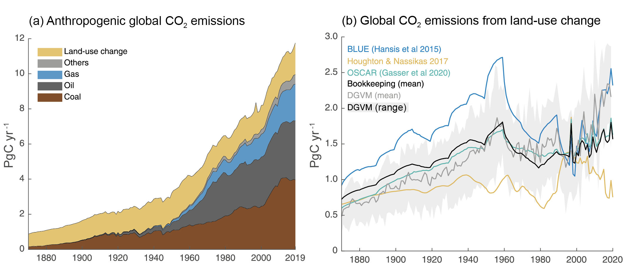 Figure 5.5 | Global anthropogenic CO2 emissions. (a) Historical trends of anthropogenic CO2 emissions (fossil fuels and net land-use change, including land management, called LULUCF flux in the main text) for the period 1870 to 2019, with ‘others’ representing flaring, emissions from carbonates during cement manufacture. Data sources: (Boden et al., 2017; IEA, 2017; Andrew, 2018; BP, 2018; Le Quéré et al., 2018a; Friedlingstein et al., 2020). (b) The net land-use change CO2 flux (PgC yr–1) as estimated by three bookkeeping models and 16 Dynamic Global Vegetation Models (DGVMs) for the global annual carbon budget 2019 (Friedlingstein et al., 2020). The three bookkeeping models are from Hansis et al., 2015; Houghton and Nassikas, 2017; Gasser et al., 2020 and are all updated to 2019. Their average is used to determine the net land-use change flux in the annual global carbon budget (black line). The DGVM estimates are the result of differencing a simulation with and without land-use changes run under observed historical climate and CO2, following the Trendy v9 protocol (https://sites.exeter.ac.uk/trendy/protocol/); they are used to provide an uncertainty range to the bookkeeping estimates (Friedlingstein et al., 2020). All estimates are unsmoothed annual data. Estimates differ in process comprehensiveness of the models and in definition of flux components included in the net land use change flux. Further details on data sources and processing are available in the chapter data table (Table 5.SM.6).
 Fossil CO2 emissions have grown continuously since the beginning of the industrial era (Figure 5.5) with short intermissions due to global economic crises or social instability (Peters et al., 2012; Friedlingstein et al., 2020). In the most recent decade (2010–2019), fossil CO2 emissions reached an average 9.6 ± 0.5 PgC yr–1 and were responsible for 86% of all anthropogenic CO2 emissions. In 2019, fossil CO2 emissions were estimated to be 9.9 ±0.5 PgC yr–1excluding carbonation (Friedlingstein et al., 2020), the highest on record. These estimates exclude the cement carbonation sink of around 0.2 PgC yr–1. Fossil CO2 emissions grew at 0.9% yr–1 in the 1990s, increasing to 3.0% yr–1 in the 2000s, and reduced to 1.2% from 2010 to 2019. The slower growth in fossil CO2 emissions in the last decade is due to a slowdown in growth from coal use. CO2 emissions from coal use grew at 4.8% yr–1 in the 2000s, but slowed to 0.4% yr–1 in the 2010s. CO2 emissions from oil use grew steadily at 1.1% yr–1 in both the 2000s and 2010s. CO2 emissions from gas use grew at 2.5% yr–1 in the 2000s and 2.4% yr–1 in 2010s, but has shown signs of accelerated growth of 3% yr–1 since 2015 (Peters et al., 2020). Direct CO2 emissions from carbonates in cement production are around 4% of total fossil CO2 emissions, and grew at 5.8% yr–1 in the 2000s but a slower 2.4% yr–1 in the 2010s. The uptake of CO2 in cement infrastructure (carbonation) offsets about one half of the carbonate emissions from current cement production (Friedlingstein et al., 2020). These results are robust across the different fossil CO2 emissions datasets, despite minor differences in levels and rates, as expected given the reported uncertainties (Andrew, 2020). During 2020, the COVID-19 pandemic led to a rapid, temporary decline in fossil CO2 emissions, estimated to be around 7% based on a synthesis of four estimates. (Cross-Chapter Box 6.1; Forster et al., 2020; Friedlingstein et al., 2020; Le Quéré et al., 2020; Liu et al., 2020).
The global net flux from land-use change and land management is composed of carbon fluxes from land-use conversions, land management and changes therein (Pongratz et al., 2018) and is equivalent to the LULUCF fluxes from the agriculture, forestry and other land use (AFOLU) sector (Jia et al., 2019). It consists of gross emissions (loss of biomass and soil carbon in clearing or logging, harvested product decay, emissions from peat drainage and burning, degradation) and gross removals (CO2 uptake in natural vegetation regrowing after harvesting or agricultural abandonment, afforestation). The LULUCF flux relates to direct human interference with terrestrial vegetation, as opposed to the natural carbon fluxes occurring due to interannual variability or trends in environmental conditions (in particular, climate, CO2, and nutrient deposition) (Houghton, 2013).
Progress since AR5 and SRCCL (IPCC, 2019a) allows more accurate estimates of gross and net fluxes due to the availability of more models, model advancement in terms of inclusiveness of land-use practices, and advanced land-use forcings (Ciais et al., 2013; Klein Goldewijk et al., 2017; Hurtt et al., 2020). In addition, important terminological discrepancies were resolved. First, synergistic effects of land-use change and environmental changes have been identified as a key reason for the large discrepancies between model estimates of the LULUCF flux, explaining up to 50% of differences (Pongratz et al., 2014; Stocker and Joos, 2015; Gasser et al., 2020). Another reason for discrepancies relates to natural fluxes being considered as part of the LULUCF flux when occurring on managed land in the United Nations Framework Convention on Climate Change (UNFCCC) national GHG inventories; these fluxes are considered part of the natural terrestrial sink in global vegetation models and excluded in bookkeeping models (Grassi et al., 2018). LULUCF fluxes following national GHG inventories or Food and Agriculture Organization of the United Nations (FAO) datasets, including recent estimates (Tubiello et al., 2021), are thus excluded from our global assessment, but their comparison against the academic approach is available elsewhere – at the global scale (Jia et al., 2019) and European level (Petrescu et al., 2020).
Land-use-related component fluxes can be verified by the growing databases of global satellite-based biomass observations in combination with information on remotely sensed land cover change. However, they differ from bookkeeping and modelling with Dynamic Global Vegetation Models (DGVMs) in excluding legacy emissions from pre-satellite-era land-use change and land management, and neglecting soil carbon changes, often focusing on gross deforestation, not regrowth (Jia et al., 2019).
For the decade 2010–2019, average emissions were estimated at 1.6 ± 0.7 PgC yr–1 (mean ± standard deviation, 1 sigma; Friedlingstein et al., 2020). Alikely general upward trend since 1850 is reversed during the second part of the 20th century (Figure 5.5b). Trends since the 1980s have low confidence because they differ between estimates, which is related, among other things, to Houghton and Nassikas (2017) using a different land-use forcing than Hansis et al. (2015) and the DGVMs. Higher emissions estimates are expected from DGVMs run under transient environmental conditions compared to bookkeeping estimates, because the DGVM estimate includes the loss of additional sink capacity. Because the transient setup requires a reference simulation without land-use change to separate anthropogenic fluxes from natural land fluxes, LULUCF estimates by DGVMs include the sink forests that would have developed in response to environmental changes on areas that in reality have been cleared (Pongratz et al., 2014). The agricultural areas that replaced these forests have a reduced residence time of carbon, lacking woody material, and thus provide a substantially smaller additional sink over time (Gitz and Ciais, 2003). The loss of additional sink capacity is growing in particular with atmospheric CO2 and increases DGVM-based LULUCF flux estimates relative to bookkeeping estimates over time (Figure 5.5).
Gross emissions are on average two to three times larger than the net flux from LULUCF, increasing from an average of 3.5 ± 1.2 PgC yr–1 for the decade of the 1960s to an average of 4.4 ± 1.6 PgC yr–1 during 2010–2019 (Friedlingstein et al., 2020). Gross removals partly balance these gross emissions to yield the net flux from LULUCF and increase from –2.0 ± 0.7 PgC yr–1 for the 1960s to –2.9 ± 1.2 PgC yr–1 during 2010–2019. These large gross fluxes show the relevance of land management, such as harvesting or rotational agriculture, and the large potential to reduce emissions by halting deforestation and degradation.
More evidence on the pre-industrial LULUCF flux has emerged since AR5 in the form of new estimates of cumulative carbon losses until today, and of a better understanding of natural carbon cycle processes over the Holocene (Ciais et al., 2013). Cumulative carbon losses by land-use activities since the start of agriculture and forestry (pre-industrial and industrial era) have been estimated at 116 PgC based on global compilations of carbon stocks for soils (Sanderman et al., 2017) with about 70 PgC of this occurring prior to 1750, and for vegetation as 447 PgC (inner quartiles of 42 calculations: 375–525 PgC) (Erb et al., 2018). Emissions prior to 1750 can be estimated by subtracting the post-1750 LULUCF flux from Table 5.1 from the combined soil and vegetation losses until today; they would then amount to 328 (161–501) PgC assuming error ranges are independent. A share of 353 (310–395) PgC from prior to 1800 has indirectly been suggested as the difference between net biosphere flux and terrestrial sink estimates, which is compatible with ice-core records due to a low airborne fraction of anthropogenic emissions in pre-industrial times (Erb et al., 2018; see also Section 5.1.2.3). Low confidence is assigned to pre-industrial emissions estimates.
Since AR5, evidence emerged that the LULUCF flux might have been underestimated as DGVMs include anthropogenic land cover change, but often ignore land management practices not associated with a change in land cover; land management is more widely captured by bookkeeping models through use of observation-based carbon densities (Ciais et al., 2013; Pongratz et al., 2018). Sensitivity studies show that practices such as wood and crop harvesting increase global net LULUCF emissions (Arneth et al., 2017) and explain about half of the cumulative loss in biomass (Erb et al., 2018).
5.2.1.2 Atmosphere
Atmospheric CO2 concentration measurements in remote locations began in 1957 at the South Pole Observatory (SPO) and in 1958 at Mauna Loa Observatory (MLO), Hawaii, USA (Keeling, 1960) (Figure 5.6a). Since then, measurements have been extended to multiple locations around the world (Bacastow et al., 1980; Conway et al., 1994; Nakazawa et al., 1997). In addition, high-density global observations of total column CO2 measurements by dedicated GHG-observing satellites began in 2009 (Yoshida et al., 2013; O’Dell et al., 2018). Annual mean CO2 growth rates are observed to be 1.56 ± 0.18 ppm yr–1 (average and range from 1 standard deviation of annual values) over the 61 years of atmospheric measurements (1959–2019), with the rate of CO2 accumulation almost tripling from an average of 0.82 ± 0.29 ppm yr–1 during the decade of 1960–1969 to 2.39 ± 0.37 ppm yr–1 during the decade of 2010–2019 (Chapter 2). The latter agrees well with that derived for total column (XCO2) measurements by the Greenhouse Gases Observing Satellite (GOSAT; Figure 5.6b). The interannual oscillations in monthly mean CO2 growth rates (Figure 5.6b) show a close relationship with the El Niño–Southern Oscillation (ENSO) cycle (Figure 5.6b) due to the ENSO-driven changes in terrestrial and ocean CO2 sources and sinks on the Earth’s surface (Section 5.2.1.4).
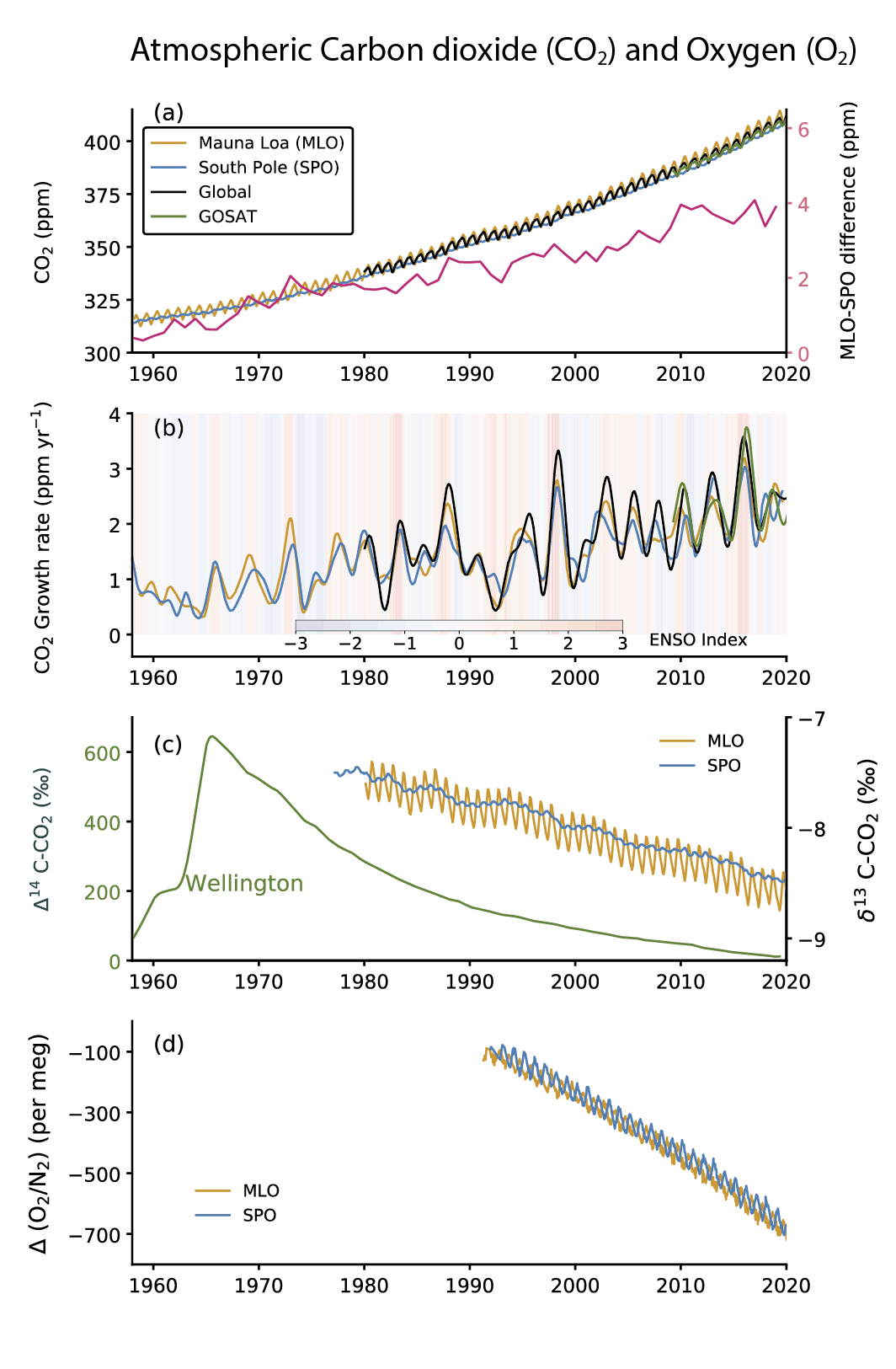
Multiple lines of evidence unequivocally establish the dominant role of human activities in the growth of atmospheric CO2. First, the systematic increase in the difference between the MLO and SPO records (Figure 5.6a) is caused primarily by the increase in emissions from fossil fuel combustion in industrialized regions that are situated predominantly in the Northern Hemisphere (Ciais et al., 2019). Second, measurements of the stable carbon isotope in the atmosphere (d13C–CO2) are more negative over time because CO2 from fossil fuels extracted from geological storage is depleted in13C (Figure 5.6c; Rubino et al., 2013; Keeling et al., 2017). Third, measurements of the d(O2/N2) ratio show a declining trend because for every molecule of carbon burned, 1.17 to 1.98 molecules of oxygen (O2) is consumed (Figure 5.6d; Ishidoya et al., 2012; Keeling and Manning, 2014). These three lines of evidence confirm unambiguously that the atmospheric increase of CO2 is due to an oxidative process (i.e., combustion). Fourth, measurements of radiocarbon (14C–CO2) at sites around the world (Levin et al., 2010; Graven et al., 2017; Turnbull et al., 2017) show a continued long-term decrease in the14C/12C ratio. Fossil fuels are devoid of14C and therefore fossil fuel-derived CO2 additions decrease the atmospheric14C/12C ratio (Suess, 1955).
Over the past six decades, the fraction of anthropogenic CO2 emissions that has accumulated in the atmosphere (referred to as airborne fraction) has remained near constant at approximately 44% (Figure 5.7) (Ballantyne et al., 2012; Ciais et al., 2019; Gruber et al., 2019b; Friedlingstein et al., 2020). This suggests that the land and ocean CO2 sinks have continued to grow at a rate consistent with the growth rate of anthropogenic CO2 emissions, albeit with large interannual and sub-decadal variability dominated by the land sinks (Figure 5.7).
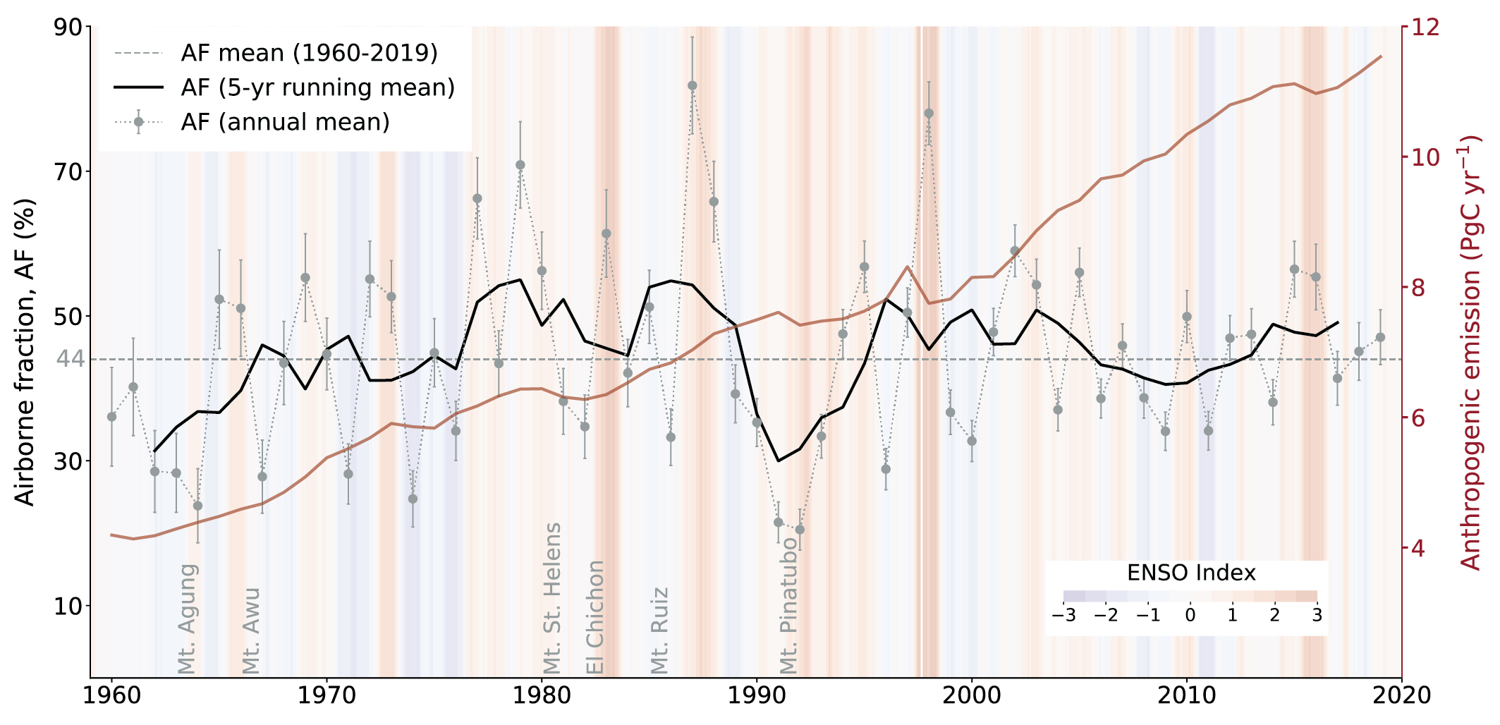 Figure 5.7 | Airborne fraction and anthropogenic (fossil fuel and land-use change) CO2 emissions. Data as in Section 5.2.1.1. The multivariate El Niño–Southern Oscillation (ENSO) index (shaded) and the major volcanic eruptions are marked along the x-axis. Further details on data sources and processing are available in the chapter data table (Table 5.SM.6).
 Since AR5, an alternative observable diagnostic to the airborne fraction has been proposed to understand the trends in land and ocean sinks in response to its driving atmospheric CO2 concentrations (Raupach et al., 2014; Bennedsen et al., 2019). It is the sink rate that is defined as the combined ocean and land sink flux per unit of atmospheric excess of CO2 above pre-industrial levels (Raupach et al., 2014). The sink rate has declined over the past six decades, which indicates that the combined ocean and land sinks are not growing as fast as the growth in atmospheric CO2 (Raupach et al., 2014; Bennedsen et al., 2019). Possible explanations for the sink rate decline are that the land and/or ocean CO2 sinks are no longer responding linearly with CO2 concentrations or that anthropogenic emissions are slower than exponential (Figure 5.7 and Sections 5.2.1.3 and 5.2.1.4; Gloor et al., 2010; Raupach et al., 2014; Bennedsen et al., 2019). In addition, both diagnostics are influenced by major climate modes (e.g., ENSO) and volcanic eruptions that contribute to high interannual variability (Gloor et al., 2010; Frölicher et al., 2013; Raupach et al., 2014), suggesting high sensitivity to future climate change. Uncertain land-use change fluxes (Section 5.2.1.2) influence the robustness of the trends. Based on the airborne fraction (AF), it is concluded with medium confidence that both ocean and land CO2 sinks have grown consistent with the rising of anthropogenic emissions. Further research is needed to understand the drivers of changes in the CO2 sink rate.
5.2.1.3 Ocean Carbon Fluxes and Storage
Since AR5 and SROCC, major advances in globally coordinated ocean CO2 observations (Surface Ocean CO2 Atlas, SOCAT; and Global Ocean Data Analysis Project, GLODAP), the harmonization of ocean and coastal-observation-based products, atmospheric and oceanic inversion models and forced global ocean biogeochemical models (GOBMs) have increased the level of confidence in the assessment of trends and variability of air–sea fluxes and storage of CO2 in the ocean during the historical period (1960–2018; see also Supplementary Materials 5.SM.1; Ciais et al., 2013; Bakker et al., 2016; Landschützer et al., 2016, 2020; Bindoff et al., 2019; DeVries et al., 2019; Gregor et al., 2019; Gruber et al., 2019a, b; Tohjima et al., 2019; Friedlingstein et al., 2020; Hauck et al., 2020; Olsen et al., 2020). A major advance since SROCC is that, for the first time, all six published observational product fluxes used in this assessment, are made more comparable using a common ocean and sea ice cover area, integration of climatological coastal fluxes scaled to increasing atmospheric CO2 and an ensemble mean of ocean fluxes calculated from three re-analysis wind products (Supplementary Materials 5.SM.2; Landschützer et al., 2014, 2020; Rödenbeck et al., 2014; Zeng et al., 2014; Denvil-Sommer et al., 2019; Gregor et al., 2019; Iida et al., 2021). From a process point of view, the ocean uptake of anthropogenic carbon is a two-step set of abiotic processes that involves the exchange of CO2, first across the air–sea boundary into the surface mixed layer, followed by its transport into the ocean interior where it is stored for decades to millennia, depending on the depth of storage (Gruber et al., 2019b). Two definitions of air–sea fluxes of CO2 are used in this assessment for both observational products and models: Socean is the global mean ocean CO2 sink and Fnet denotes the net spatially varying CO2 fluxes (Hauck et al., 2020). Adjustment of the mean global Fnet for the pre-industrial sea-to-air CO2 flux associated with land-to-ocean carbon flux term makes Fnet comparable to Socean (Jacobson et al., 2007; Resplandy et al., 2018; Hauck et al., 2020).
There are multiple lines of observational and modelling evidence that support with high confidence the finding that, in the historical period (1960–2018), air–sea fluxes and storage of anthropogenic CO2 are largely influenced by atmospheric CO2 concentrations, physical ocean processes and physicochemical carbonate chemistry, which determines the unique properties of CO2 in seawater (Chapter 9 and Cross-Chapter Box 5.3; Wanninkhof, 2014; DeVries et al., 2017; McKinley et al., 2017, 2020, Gruber et al., 2019a, b; Hauck et al., 2020). Here we assess three different approaches (Figures 5.8a,b and 5.9) that together provide high confidence that, during the historical period (1960–2018), the ocean carbon sink (Socean) and its associated ocean carbon storage have grown in response to global anthropogenic CO2 emissions (Gruber et al., 2019a; Hauck et al., 2020; McKinley et al., 2020).
5.2.1.3.1 Ocean carbon fluxes and storage: Global multi-decadal trends
In the first assessment approach, the mean global multi-decadal (1960–2019) trends in the ocean sink (Socean) for CO2 show a high degree of coherence across the nine GOBMs and sixpCO2 -based observational product reconstructions (1987–2018) which, despite a temporary slowdown (or ‘hiatus’) in the 1990s, is also quasi-linear over that period (Figure 5.8a; Gregor et al., 2019; Hauck et al., 2020). This coherence between the GOBMs and observations-based reconstructions (1987–2018; r2=0.85) provides high confidence that the ocean sink (Socean in Section 5.2.1.5) evaluated from GOBMs (1960–2019) grew quasi-linearly from 1.0 ± 0.3 PgC yr–1 to 2.5 ± 0.6 PgC yr–1 between the decades 1960–1969 and 2010–2019 in response to global CO2 emissions (Figure 5.8a; Table 5.1; Friedlingstein et al., 2020; Hauck et al., 2020). The cumulative ocean CO2 uptake (105 ± 20 PgC) is 23% of total anthropogenic CO2 emissions (450 ± 50 PgC) for the same period (Friedlingstein et al., 2020). Notwithstanding the high confidence in the magnitude of the annual to decadal trends for Socean, this assessment is moderated to mediumconfidence by the low confidence in the currently inadequately constrained uncertainties in the pre-industrial land-to-ocean carbon flux, the uncertain magnitude of winter outgassing from the Southern Ocean, and the uncertain effect of the ocean surface cool-skin, the effect of data sparsity, differences between wind products and the uncertain contribution from the changing land–ocean continuum on global and regional fluxes (Jacobson et al., 2007; Resplandy et al., 2018; Roobaert et al., 2018; Bushinsky et al., 2019; Hauck et al., 2020; Watson et al., 2020; Gloege et al., 2021). However, both GOBMs and pCO2 -based observational products independently reveal a slowdown or ‘hiatus’ of the ocean sink in the 1990s, which provides a valuable constraint for model verification and leads to greater confidence in the model outputs (Figure 5.8a; Landschützer et al., 2016; Gregor et al., 2018; DeVries et al., 2019; Hauck et al., 2020). A number of studies point to the role of the Southern Ocean in the global ‘1990s hiatus’ in air–sea CO2 fluxes, but provide different process-based explanations linking ocean temperature, mixing and meridional overturning circulation (MOC) responses to variability in large-scale climate systems, wind stress and volcanic activity, as well as the sensitivity of the air–sea CO2 flux to small changes in the atmospheric forcing from anthropogenic CO2 (Landschützer et al., 2016; DeVries et al., 2017; Bronselaer et al., 2018; Gregor et al., 2018; Gruber et al., 2019a; Keppler and Landschützer, 2019; McKinley et al., 2020; Nevison et al., 2020). Data sparsity in the Southern Ocean could also be a factor amplifying the global decadal perturbation of the 1990s (Gloege et al., 2021). Therefore, while there is high confidence in the 1990s hiatus of the global ocean sink for anthropogenic CO2, and that the Southern Ocean makes an observable contribution to it, there is still low confidence in the attribution for the processes behind the 1990s hiatus (Section 5.2.1.3.2). Observed increases in the amplitude of the seasonal cycle of oceanpCO2 and reductions in the mean global buffering capacity provide high confidence that the growing CO2 sink is also beginning to drive observable large-scale changes in ocean carbonate chemistry (Jiang et al., 2019). However, there is medium confidence that these changes which, depending on the emissions scenario, could drive future ocean feedbacks, are still too small to emerge from the historical multi-decadal observed growth rate of Socean (Sections 5.1.2; 5.3.2 and 5.4.2, and Figure 5.8a; SROCC (Section 5.2.2.3.2; Bates et al., 2014; Sutton et al., 2016; Fassbender et al., 2017; Landschützer et al., 2018; Jiang et al., 2019). A recent model-based study suggests that re-emergence of previously stored anthropogenic CO2 is changing the buffering capacity of the mixed layer and reducing the ocean sink for anthropogenic CO2 during the historical period (Rodgers et al., 2020). This trend is not reflected in observations-based products (Figure 5.8a), so we attribute a low confidence.
 Figure 5.8 | Multi-decadal trends for the ocean sink of CO2 . (a) The multi-decadal (1960–2019) trends in the annual ocean sink (Socean) reconstructed from nine Global Ocean Biogeochemical Models (GOBM) forced with atmospheric re-analysis products (Hauck et al., 2020), six observationally based gap-filling products that reconstructed spatial and temporal variability in the ocean CO2 flux from sparse observations of surface oceanpCO2 (Supplementary Materials 5.SM.2). The trends in Socean were calculated from the mean annual GOBM outputs, and the observational products were used to provide confidence in the GOBM assessments (r2=0.85). Thick lines represent the multi-model mean. Observationally based products have been corrected for pre-industrial river carbon fluxes (0.62 PgC yr–1) based on the average of estimates from Jacobson et al. (2007) and Resplandy et al. (2018). (b) Mean decadal constraints and their confidence intervals for global ocean sink (Socean) of anthropogenic CO2 using multiple independent or quasi-independent lines of evidence or methods for the period 1990–2019 (see Supplementary Materials Tables 5.SM.1 and 5.SM.2 for magnitudes, uncertainties and published sources). Further details on data sources and processing are available in the chapter data table (Table 5.SM.6).
 The second assessment approach makes use of six independent methods to constrain the mean decadal ocean sink over the period 1990–2019 (Figure 5.8b). This provides a multi-decadal advance on the 1990–1999 decadal constraint from (Denman et al., 2007) that has been widely used as a model constraint for GOBMs used for the global carbon budget (Hauck et al., 2020). The medium confidence attributed by this assessment of the global multi-decadal trend (Figure 5.8a) is further supported by the broad agreement in magnitude and trend of the decadal mean ocean CO2 uptake with assessments that also include additional observations-based, independent methods such as ocean CO2 inversion and atmospheric CO2 and O2/N2 measurements (Figure 5.8b; Supplementary Materials Tables 5.SM.1 and 5.SM.2).
Here we provide a third comparative assessment approach depicting the spatial coherence of ocean air–sea fluxes and storage rates of CO2 as well as a quantitative assessment of both fluxes for the same period (1994–2007; Figure 5.9). Observation-based pCO2 flux products show that emissions of natural CO2 occur mostly in the tropics and high-latitude Southern Ocean, and that the uptake and storage of anthropogenic CO2 occurs predominantly in the mid-latitudes (Chapter 9, Figure 5.9 and Cross-Chapter Box 5.3). Strong ocean CO2 sink regions are those in the mid-latitudes associated with the cooling of poleward flowing subtropical surface waters as well as equatorward flowing sub-polar surface waters, both of which contribute to the formation of Mode, Intermediate and Deep water masses that transport anthropogenic CO2 into the ocean interior on time scales of decades to centuries in both hemispheres (Section 9.2.2.3 and Figure 5.9; DeVries, 2014; Gruber et al., 2019b; Wu et al., 2019). The mean decadal scale magnitude and uncertainties of Socean from net air sea fluxes (Fnet ) were calculated from an ensemble of six observational-based product reconstructions (Figure 5.9a) and the storage rates in the ocean interior derived from multiple ocean interior CO2 datasets (Gruber et al., 2019b; Figure 5.9b). The cumulative CO2 stored in the ocean interior from 1800 to 2007 has been estimated at 140 ±18 PgC (Gruber et al., 2019b). As reported in SROCC (Section 5.2.2.3.1; IPCC, 2019b), the net ocean CO2 storage between 1994–2007 was 29 ± 4 PgC, which corresponds to a mean storage of 26 ± 5% of anthropogenic CO2 emissions for that period (Gruber et al., 2019b). The resulting net annual storage rate of anthropogenic CO2, equivalent to Socean for the period mid-1994 to mid-2007 is 2.2 ± 0.3 PgC yr–1, which is in very close agreement with the top-down air–sea flux estimate of Socean of 2.1 ± 0.5 PgC yr–1 from GOBMs and 1.9 ± 0.3PgC yr–1 frompCO2 -based observational products with the steady river carbon flux correction of 0.62 PgC yr–1 for the same time period (Gruber et al., 2019b; Hauck et al., 2020). This close agreement between these independent ocean CO2 sink estimates derived from air–sea fluxes and storage rates in the ocean interior support the medium confidence assessment that the ocean anthropogenic carbon storage rates continue to be determined by the ocean sink (Socean) in response to growing CO2 emissions (Figure 5.9; McKinley et al., 2020).
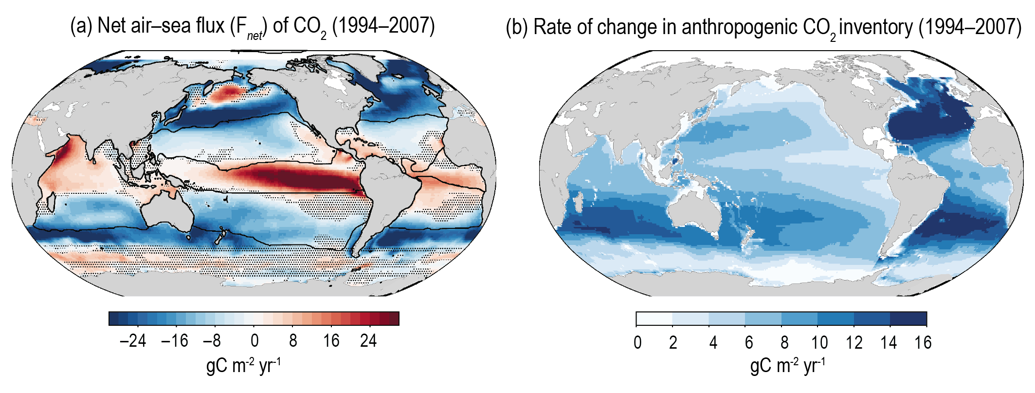 Figure 5.9 | Comparative regional characteristics of the mean decadal (1994–2007) sea-air CO2 flux (Fnet) and ocean storage of anthropogenic CO2 . (a) Regional source–sink characteristics for contemporary ocean air–sea CO2 fluxes (Fnet ) derived from the ensemble of six observation-based products using Surface Ocean CO2 (Atlas (SOCAT)v6 observational dataset (Landschützer et al., 2014; Rödenbeck et al., 2014; Zeng et al., 2014; Bakker et al., 2016; Denvil-Sommer et al., 2019; Gregor et al., 2019; Iida et al., 2021). Warm colours depict outgassing fluxes and black contours characterize the super-biomes defined from Fay and McKinley (2014) and adjusted by Gregor et al. (2019) also used to calculate the variability in regional flux anomalies (Supplementary Materials Figure 5.SM.1); (b) The regional characteristics of the storage fluxes of CO2 in the ocean interior for the same period (Gruber et al., 2019b). The dots reflect ocean areas where the 1-sigma standard deviation of Fnet from the six observational-based product reconstructions is larger than the magnitude of the mean. This reflects source–sink transition areas where the mean Fnet is small and more strongly influenced by spatial and temporal variability across the products. Further details on data sources and processing are available in the chapter data table (Table 5.SM.6).
 5.2.1.3.2 Ocean carbon fluxes and storage: Regional and global variability
The intent of this assessment is to show how global variability can be regionally forced (Gregor et al., 2019; Landschützer et al., 2019; Hauck et al., 2020). Since AR5 and SROCC, advances in global ocean CO2 flux products, GOBMs and atmospheric inversion models have strengthened confidence in the assessment of how ocean regions influence mean global variability and trends of ocean CO2 air–sea fluxes (Fnet ; see Supplementary Materials Figure 5.SM.1; Ciais et al., 2013; Landschützer et al., 2014, 2015; Rödenbeck et al., 2014; McKinley et al., 2017; Bindoff et al., 2019; Gregor et al., 2019; Friedlingstein et al., 2020; Hauck et al., 2020). The coherence in the regional variability of the anomalies in Fnet from three independent lines of evidence support with high confidence that the non-steady state global interannual-decadal variability of Fnet has clear regional influences (Gregor et al., 2019; Landschützer et al., 2019). The tropical oceans contribute the most to the global mean interannual variability (Supplementary Materials Figure 5.SM.1d). The high latitude oceans, particularly the Southern Ocean, contribute the most to the global-scale decadal variability (Supplementary Materials Figure 5.SM5.1b,c; (Landschützer et al., 2016, 2019; Gregor et al., 2019; Gruber et al., 2019a; Hauck et al., 2020). The influence of the Southern Ocean on the global mean decadal variability and the 1990s hiatus is supported by the highest regional–global correlation coefficients (Supplementary Materials Figures 5.SM.1a,c). In contrast, the equatorial oceans’ influence on global mean Fnet has a low correlation because, notwithstanding the coherence in interannual variability, it does not show the same global mean trend of strengthening sink in response to growing global emissions (Supplementary Materials Figure 5.SM.1d; Gregor et al., 2019). All regions, except the equatorial ocean, contribute to varying extents to the multi-decadal trend of growth in the global ocean sink (Supplementary Materials Figure 5.SM.1). Data sparseness in the high latitudes and the relatively short length of the observational records leads to low confidence in the attribution of the processes that link regional–global variability to climate (Landschützer et al., 2019; Gloege et al., 2021).
Regional decadal-scale anomalies in the variability of ocean CO2 storage have also emerged, probably associated with changes in the MOC, which may influence the global variability in Fnet (Chapter 9; DeVries et al., 2017). In the interior of the Indian and Pacific sectors of the Southern Ocean, and the North Atlantic, the increase in the CO2 inventory from 1994 to 2007 was about 20% smaller than expected from the atmospheric CO2 increase during the same period and the anthropogenic CO2 inventory in 1994 (Sabine eta al., 2004; Gruber et al., 2019a). There is medium confidence that the ocean CO2 inventory strengthened again in the decade 2005–2015 (DeVries et al., 2017). In the North Atlantic, a low rate of anthropogenic CO2 storage at 1.9 ± 0.4 PgC per decade during the time period of 1989–2003 increased to 4.4 ± 0.9 PgC per decade during 2003–2014. This is associated with changing ventilation patterns driven by the North Atlantic Oscillation (Woosley et al., 2016). In the Pacific sector of the Southern Ocean, the rate of anthropogenic CO2 storage also increased from 8.8 ± 1.1 (1σ) PgC per decade during 1995–2005 to 11.7 ± 1.1 PgC per decade during 2005–2015 (Carter et al., 2019). However, in the Subantarctic Mode Water of the Atlantic sector of the Southern Ocean, the storage rate of the anthropogenic CO2 was rather lower after 2005 than before (Section 9.2.3.2; Tanhua et al., 2017; Bindoff et al., 2019). These changes have been predominantly ascribed to the impact of changes in the MOC on the transport of anthropogenic CO2 into the ocean interior due to regional climate variability, in addition to the increase in the atmospheric CO2 concentration (Section 9.2.3.1; Wanninkhof et al., 2010; Pérez et al., 2013; DeVries et al., 2017, 2019; Gruber et al., 2019b; McKinley et al., 2020). However,the low frequency of carbon observations in the interior of the vast ocean leads to medium confidence in the assessment of temporal variability in the rate of regional ocean CO2 storage and its controlling mechanisms.
In summary, multiple lines of observational and modelling evidence provide high confidence in the finding that the ocean sink for anthropogenic CO2 has increased quasi-linearly over the past 60 years in response to growing global emissions of anthropogenic CO2, with a mean fraction of 23% of total emissions. The high confidence assessment is moderated to medium confidence due to a number of ocean CO2 flux terms yet to be adequately constrained. Observed changes in the variability of oceanpCO2 and observed reductions in the mean global buffering capacity provide high confidence that the growing CO2 sink is also beginning to drive observable large-scale changes in ocean carbonate chemistry. However, there is medium confidence that these changes which, depending on the emissions scenario, could drive future ocean feedbacks, are still too small to emerge from the historical multi-decadal observed growth rate of Socean.
5.2.1.4 Land CO2 Fluxes: Historical and Contemporary Variability and Trends
5.2.1.4.1 Trend in land–atmosphere CO2 exchange
The global net land CO2 sink is assessed to have grown over the past six decades (Sarmiento et al., 2010; Ballantyne et al., 2017; Le Quéré et al., 2018b; Ciais et al., 2019; Friedlingstein et al., 2020) (high confidence). Estimated as residual from the mass balance budget of fossil fuel CO2 emissions minus atmospheric CO2 growth and the ocean CO2 sink, the global net land CO2 sink (including both land CO2 sink and net land-use change emissions) increased from 0.3 ± 0.6 PgC yr–1 during the 1960s to 1.8 ± 0.8 PgC yr–1 during the 2010s (Friedlingstein et al., 2020). An increasing global net land CO2 sink since the 1980s (Figure 5.10) was consistently suggested both by atmospheric inversions (e.g., Peylin et al., 2013) and by DGVMs (e.g., Sitch et al., 2015; Friedlingstein et al., 2019). The Northern Hemisphere contributes more to the net increase in the land CO2 sink compared to the Southern Hemisphere (Ciais et al., 2019), and boreal and temperate forests probably contribute the most (Tagesson et al., 2020). Attributing an increased net land CO2 sink to finer regional scales remains challenging, but inversions of satellite-based column CO2 products that have emerged since AR5 are a promising tool to further constrain regional land-atmosphere CO2 exchange (Ciais et al., 2013; Houweling et al., 2015; Reuter et al., 2017; O’Dell et al., 2018; Palmer et al., 2019).
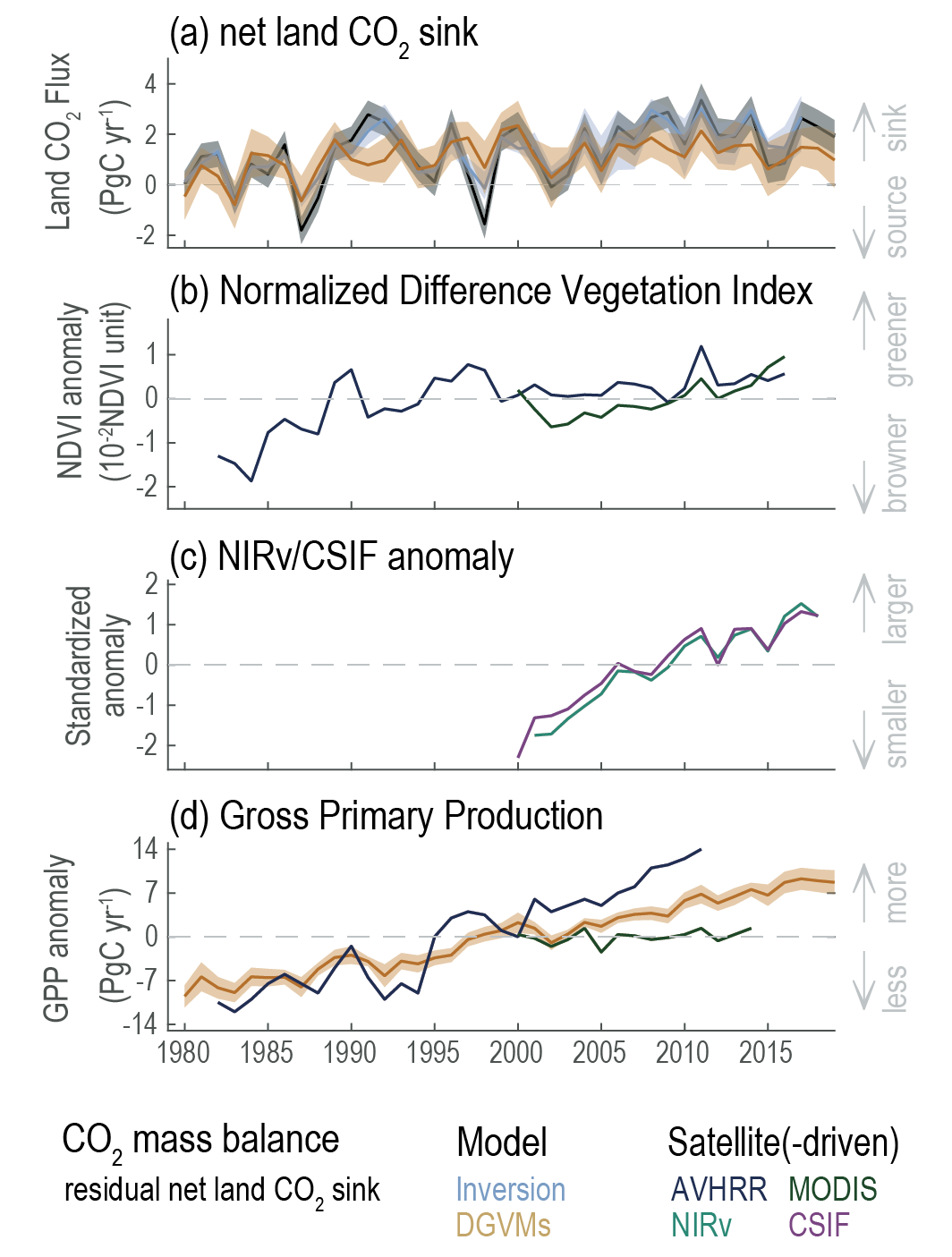 Figure 5.10 | Trends of the net land CO2 sink and related vegetation observations during 1980–2019. (a) Net land CO2 sink. The residual net land CO2 sink is estimated from the global CO2 mass balance (fossil fuel emissions minus atmospheric CO2 growth rate and ocean CO2 sink). Inversions indicate the net land CO2 sink estimated by an ensemble of four atmospheric inversions. Dynamic Global Vegetation Models (DGVMs) indicate the mean net land CO2 sink estimated by 17 dynamic global vegetation models driven by climate change, rising atmospheric CO2, land-use change and nitrogen deposition change (for carbon-nitrogen models). The positive values indicate net CO2 uptake from the atmosphere. (b) Normalized difference vegetation index (NDVI). The anomaly of global area-weighted NDVI observed by Advanced Very High Resolution Radiometer (AVHRR) and MODIS satellite sensors. AVHRR data are accessible during 1982–2016 and MODIS data are accessible during 2000–2018. (c) Near-infrared reflectance of vegetation (NIRv) and contiguous solar-induced chlorophyll fluorescence (CSIF). The standardized anomaly of area-weighted NIRv during 2001–2018 (Badgley et al., 2017) and CSIF during 2000–2018 (Zhang et al., 2018). (d) Gross primary production (GPP). The GPP from Cheng et al. (2017), DGVMs and MODIS GPP product (MOD17A3). GPP from Cheng et al. (2017) is based on an analytical model driven by climate change, rising atmospheric CO2, AVHRR leaf area index datasets and evapotranspiration datasets. GPP from DGVMs is the ensemble mean global GPP estimated by the same 17 DGVMs that provide the net land CO2 sink estimates. Shaded area indicates 1–σ inter-model spread except for atmospheric inversions, whose ranges were used due to limited number of models. Further details on data sources and processing are available in the chapter data table (Table 5.SM.6).
 Carbon uptake by vegetation photosynthesis exerts a first-order control over the net land CO2 sink. Several lines of evidence show enhanced vegetation photosynthesis over the past decades (medium to high confidence) (Figure 5.10), including increasing satellite-derived vegetation greenness (e.g., see Chapter 2; Mao et al., 2016; Zhu et al., 2016; Jia et al., 2019) and satellite-derived photosynthesis indicators (e.g., Badgley et al., 2017; Zhang et al., 2018), change in atmospheric concentration of carbonyl sulphide (Campbell et al., 2017), enhanced seasonal CO2 amplitude (Graven et al., 2013; Forkel et al., 2016), observation-driven inference of increasing photosynthesis CO2 uptake based mostly on enhanced water use efficiency (Cheng et al., 2017), and DGVM simulated increase of photosynthesis CO2 uptake (Anav et al., 2015).
Substantial progress has been made since AR5 on attributing change of the global net land CO2 sink. Increasing global net land CO2 sink since the 1980s is mainly driven by the fertilization effect from rising atmospheric CO2 concentrations (Schimel et al., 2015; Sitch et al., 2015; Fernández-Martínez et al., 2019; O’Sullivan et al., 2019; Tagesson et al., 2020; Walker et al., 2021) (medium confidence). Increasing nitrogen deposition (de Vries et al., 2009; Devaraju et al., 2016; Huntzinger et al., 2017) or the synergy between increasing nitrogen deposition and atmospheric CO2 concentration (O’Sullivan et al., 2019) could have also contributed to the increasing global net land CO2 sink. The effects of climate change alone on the global net land CO2 sink is so divergent that even the signs (directions) of the effects are not the same across DGVMs (e.g., Huntzinger et al., 2017).
Lower fire emissions of CO2 and enhanced vegetation carbon uptake due to reduced global burned area have contributed to the increasing global net land CO2 sink in the recent decade (Arora and Melton, 2018; Yin et al., 2020) (low to medium confidence). Satellite observations reveal a declining trend in global burned area by about 20% over past two decades (Andela et al., 2017; Earl and Simmonds, 2018; Forkel et al., 2019), a trend most pronounced in regions like northern Africa (Forkel et al., 2019; Zubkova et al., 2019; Bowman et al., 2020) and Mediterranean Europe (Turco et al., 2016). However, burned area trends are highly heterogeneous regionally with increasing trends reported in regions like western United States (Holden et al., 2018; Abatzoglou et al., 2019). Some regions (e.g., Amazon basin and Australia) experienced record-breaking fire events in 2019 and 2020 (e.g., Boer et al., 2020), whose effects on burned area trends remain to be explored. The burned area trends were primarily attributed to both human-induced climate change and human activities (Jolly et al., 2015; Andela et al., 2017; Holden et al., 2018; Turco et al., 2018; Teckentrup et al., 2019; Bowman et al., 2020), as well as changing frequency of lightning in the boreal region (Veraverbeke et al., 2017). In addition to changes in the burned area, fire dynamics could affect the trend in land-atmosphere CO2 exchange indirectly through increasing concentration of air pollutants (see Section 6.3.4 for impacts of ozone and aerosol on the carbon cycle; Yue and Unger, 2018; Lasslop et al., 2019).
Significant uncertainties remain for the land CO2 sink partition of processes due to challenges in reconciling multiple-scale evidence from experiments to the globe (Fatichi et al., 2019; Walker et al., 2021), due to large spatial and inter-model differences in diagnosing dominant driving factors affecting the net land CO2 sink (Huntzinger et al., 2017; Fernández-Martínez et al., 2019), and due to model deficiency in process representations (He et al., 2016). Nitrogen dynamics, a major gap in DGVMs identified in AR5, have now been incorporated in about half of the DGVMs contributing to the carbon budget of the Global Carbon Project (GCP) (see Le Quéré et al. (2018a) for model characteristics) and a growing number of ESMs (Arora et al., 2020). However, as the representations of carbon–nitrogen interactions vary greatly among models, large uncertainties remain on how nitrogen cycling regulates the response of ecosystem carbon uptake to higher atmospheric CO2 (Walker et al., 2015; Wieder et al., 2019; Davies-Barnard et al., 2020; Meyerholt et al., 2020; see Section 5.4.1). Fire modules have been incorporated into 10 of 16 DGVMs contributing to the global carbon budget (Le Quéré et al., 2018a), and a growing number of models have representations of human ignitions and fire suppression processes (Rabin et al., 2017; Teckentrup et al., 2019). There are also growing DGVM developments to include management practices (Pongratz et al., 2018) and the effects of secondary forest regrowth (Pugh et al., 2019), though models still under-represent intensively managed ecosystems, such as croplands and managed forests (Guanter et al., 2014; Thurner et al., 2017). Processes that have not yet played a significant role in the land CO2 sink of the past decades but can grow in importance, include permafrost (Box 5.1) and peatlands dynamics (Dargie et al., 2017; Gibson et al., 2019), have also been incorporated in some DGVMs (Koven et al., 2015b; Burke et al., 2017a; Guimberteau et al., 2018). Growing numbers and varieties of Earth observations are being jointly used to drive and benchmark models, helping to further identify missing key processes or mechanisms that are poorly represented in the current generation of DGVMs (e.g., Collier et al., 2018).
5.2.1.4.2 Interannual variability in land–atmosphere CO2 exchange
The AR5 stated that the interannual variability of the atmospheric CO2 growth rate is dominated by tropical land ecosystems. A set of new satellite measurements applied to assess the variability of the tropical land carbon balance since AR5 (Ciais et al., 2013) confirm this statement, including satellite column CO2 measurements, estimating the recent anomalous land–atmosphere CO2 exchange induced by El Niño at continental scale (e.g., J. Liu et al., 2017; Palmer et al., 2019), and L-band vegetation optical depth, estimating tropical above-ground biomass carbon stock changes (Fan et al., 2019). In addition, based onmedium evidence and medium agreement between studies with DGVMs and atmospheric inversions, semi-arid ecosystems over the tropical zones have a larger contribution to interannual variability in global land–atmosphere CO2 exchange than moist tropical forest ecosystems (low to medium confidence) (Poulter et al., 2014; Ahlstrom et al., 2015; Piao et al., 2020).
Understanding the mechanisms driving interannual variability in the carbon cycle has the potential to provide insights into whether and to what extent the carbon cycle can affect the climate (carbon–climate feedback), with particular interests over the highly climate-sensitive tropical carbon cycle (e.g., Cox et al., 2013; X. Wang et al., 2014; Fang et al., 2017; Jung et al., 2017; Humphrey et al., 2018; Malhi et al., 2018; see Section 5.4). Consistent findings from studies with atmospheric inversions, satellite observations and DGVMs (e.g., Malhi et al., 2018; Rödenbeck et al., 2018) lead to high confidence that the tropical net land CO2 sink is reduced under warmer and drier conditions, particularly during El Niño events. Interannual variations in tropical land-atmosphere CO2 exchange are significantly correlated with anomalies of tropical temperature, water availability and terrestrial water storage (X. Wang et al., 2014; Jung et al., 2017; Humphrey et al., 2018; Piao et al., 2020), whose relative contribution are difficult to separate due to covariations between these climatic factors. At continental scale, the dominant climatic driver of interannual variations of tropical land-atmosphere CO2 exchange was temperature variations (Figure 5.11; Piao et al., 2020), which could partly result from the spatial compensation of the water availability effects on land-atmospheric CO2 exchange (Jung et al., 2017).
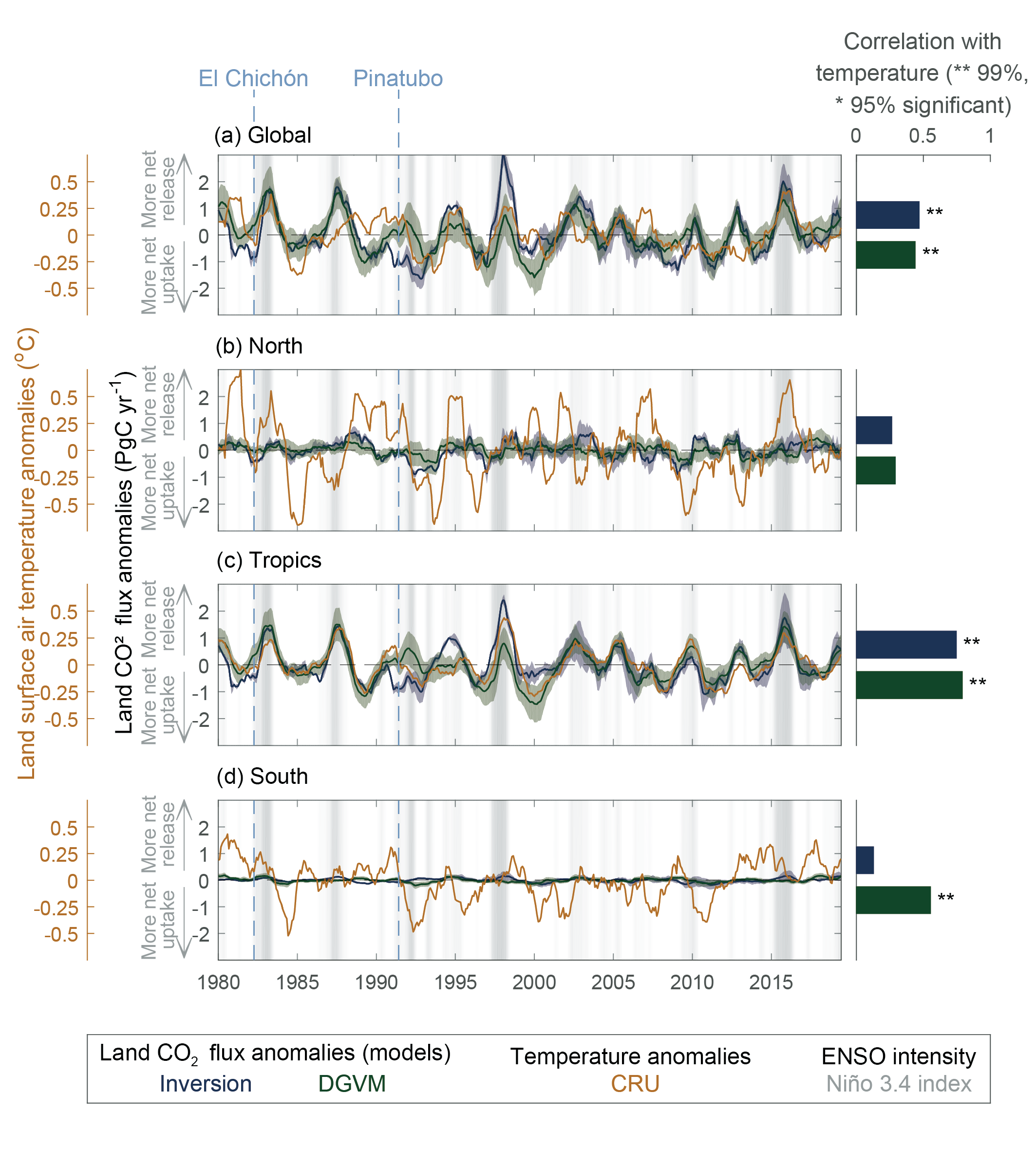 Figure 5.11 | Interannual variation in detrended anomalies of the net land CO2 sink and land surface air temperature during 1980–2019. Correlation coefficients between the net land CO2 sink anomalies and temperature anomalies are show on the right bar plots. The net land CO2 sink is estimated by four atmospheric inversions (blue) and 15 Dynamic Global Vegetation Models (DGVMs) (green), respectively (Friedlingstein et al., 2020). Solid blue and green lines show model mean detrended anomalies of the net land CO2 sink. The ensemble mean of DGVMs is bounded by the 1–σ inter-model spread in each large latitude band (North 30°N–90°N, Tropics 30°S–30°N, South 90°S–30°S) and the globe. The ensemble mean of atmospheric inversions is bounded by model spread. For each latitudinal band, the anomalies of the net land CO2 sink and temperature (orange) were obtained by removing the long-term trend and seasonal cycle. A 12-month running mean was taken to reduce high-frequency noise. The bars in the right panels show correlation coefficients between the net land CO2 sink anomalies and temperature anomalies for each region. ** indicates P<0.01; * indicates P<0.05. The grey shaded area shows the intensity of El Niño–Southern Oscillation (ENSO) as defined by the Niño 3.4 index. Two volcanic eruptions (El Chichón and Mount Pinatubo) are indicated with light blue dashed lines. Temperature data are from the Climatic Research Unit (CRU), University of East Anglia (Harris et al., 2014). Anomalies were calculated following Patra et al. (2005), but using a 12-month low-pass filter and detrended to obtain interannual variations. Further details on data sources and processing are available in the chapter data table (Table 5.SM.6).
 Cross-Chapter Box 5.1 | Interactions Between the Carbon and Water Cycles, Particularly Under Drought Conditions
Contributors: Josep G. Canadell (Australia), Philippe Ciais (France), Hervé Douville (France), Sabine Fuss (Germany), Robert Jackson (United States of America), Annalea Lohila (Finland), Shilong Piao (China), Sonia I. Seneviratne (Switzerland), Sergio M. Vicente-Serrano (Spain), Sönke Zaehle (Germany)
This box presents an assessment of interactions between the carbon and water cycles that influence the dynamics of the biosphere and its interaction with the climate system. It also highlights carbon–water trade-offs arising from the use of land-based climate change mitigation options. Individual aspects of the interactions between the carbon and water cycles are addressed in separate chapters (Sections 5.2.1, 5.4.1, 8.2.3, 8.3.1, 8.4.1 and 11.6). The influence of wetlands and dams on methane emissions is assessed elsewhere (Sections 5.2.2, 5.4.7 and 8.3.1), as well as the consequences of permafrost thawing (Section 9.5.2 and Box 5.1) and/or increased flooding (Sections 8.4.1, 11.5 and 12.4) on wetland extent in the northern high latitudes and wet tropics.
Does elevated CO2 alleviate the impacts of drought?
Increasing atmospheric CO2 concentration enhances leaf photosynthesis and drives a partial closure of leaf stomata, leading to higher water-use efficiency (WUE) at the leaf canopy and ecosystem scales (Norby and Zak, 2011; De Kauwe et al., 2013; Fatichi et al., 2016; Knauer et al., 2017; Mastrotheodoros et al., 2017). Since AR5 (Box 6.3), a growing body of evidence from tree-ring and carbon isotopes further confirms an increase of plant water-use efficiency over decadal to centennial time scales, with some evidence for a stronger enhancement of photosynthesis compared to stomatal reductions (Frank et al., 2015; Guerrieri et al., 2019; Adams et al., 2020).
Multiple lines of evidence suggest that WUE has increased in near proportionality to atmospheric CO2 (high confidence) at a rate generally consistent with Earth system models (ESMs), despite variation in the WUE response to CO2 (De Kauwe et al., 2013; Frank et al., 2015; Keeling et al., 2017; Lavergne et al., 2019; Walker et al., 2021). Both field-scale CO2 enrichment experiments and process models show the effect of physiologically induced water savings, particularly under water-limiting conditions (De Kauwe et al., 2013; Farrior et al., 2015; Lu et al., 2016; Roy et al., 2016). Plants can also benefit from reduced drought stress due to enhanced CO2 without ecosystem-scale water savings (Jiang et al., 2021). To some extent, this increased WUE offsets the effects of enhanced vapour pressure deficit (VPD) on plant transpiration (Bobich et al., 2010; Creese et al., 2014; Jiao et al., 2019), but will have limited effect on ameliorating plant water stress during extreme drought events (Xu et al., 2016; Menezes-Silva et al., 2019; L. Liu et al., 2020), when leaf stomata are governed primarily by soil moisture (Roy et al., 2016).
Leaf stomata closure can have large effects on land freshwater availability because of reduced plant transpiration, leading in some regions to higher soil moisture and runoff (Roderick et al., 2015; Milly and Dunne, 2016; Y. Yang et al., 2019). However, increased water availability is often not realized because other CO2 physiological effects that enhance ecosystem evapotranspiration might offset the gains. These effects include plant growth and leaf area expansion (Ainsworth and Long, 2005; Ukkola et al., 2016; McDermid et al., 2021), lengthening of the vegetative growing season (Frank et al., 2015; Lian et al., 2021), and the effects of stomatal closure on near-surface atmosphere that leads to increased air temperature and VPDs (Berg et al., 2016; Vogel et al., 2018; Zhou et al., 2019; Grossiord et al., 2020).
ESMs show no consensus about the net hydrological response to physiological CO2 effects. Some studies show water savings as a consequence of the CO2 effects on leaf stomata closure (Swann et al., 2016; Lemordant et al., 2018), while other studies show that increased leaf area offsets the gains from increased WUE (Mankin et al., 2019). However, these projections are subject to ESM uncertainties to quantify transpiration (Lian et al., 2021), among them the correct representations of plant hydraulic architecture such as changes in xylem anatomical properties and deep rooting (Nie et al., 2013; L. Liu et al., 2020).
In conclusion, it is very likely that elevated CO2 leads to increased WUE at the leaf level, concurrent with enhanced photosynthesis. Increased CO2 concentrations alleviate the effects of water deficits on plant productivity (medium confidence) but there is low confidence for its role under extreme drought conditions. There is low confidence that increased WUE by vegetation will substantially reduce global plant transpiration and diminish the frequency and severity of soil moisture and streamflow deficits associated with the radiative effect of higher CO2 concentrations.
How does drought affect the terrestrial CO2 sink?
Water availability controls the spatial distribution of photosynthesis – gross primary productivity (GPP) – over a larger part of the globe (Beer et al., 2010) and, at local scale, drought decreases GPP more than respiration (Schwalm et al., 2012) over most ecosystem types. This makes water availability a major climatic driver of variability in net ecosystem exchange (Jung et al., 2017; Humphrey et al., 2018). In addition to suppressing photosynthesis, field evidence suggests that droughts reduce the land CO2 sink, also through increasing forest mortality and promoting wildfire (Allen et al., 2015; Brando et al., 2019; Abram et al., 2021).
At the global scale, interannual variability in the atmospheric CO2 growth rate and global-scale terrestrial water storage from satellite show that a lower global net land CO2 sink is associated with below-average terrestrial water storage (Humphrey et al., 2018). Atmospheric inversions based on surface and satellite column CO2 measurements show significant carbon release during drought events in pan-tropic areas (Phillips et al., 2009; Gatti et al., 2014; J. Liu et al., 2017; Palmer et al., 2019). Regional extreme droughts in the mid-latitudes also decrease GPP and land CO2 sink (Ciais et al., 2005; Wolf et al., 2016; W. Peters et al., 2020; Flach et al., 2021). Droughts are not compensated by equivalent wet anomalies because of the non-linear response of the terrestrial carbon uptake to soil moisture (Green et al., 2019).
Uncertainties remain on the magnitude of sensitivity of the land carbon fluxes to droughts. Global studies indicate stronger control of soil moisture to variations in satellite proxies of GPP than VPD (Stocker et al., 2019; L. Liu et al., 2020). However, given that VPD increases exponentially with atmospheric warming, some studies suggest that VPD in stomatal regulation will become increasingly more important under a warmer climate (Novick et al., 2016; Grossiord et al., 2020). It is difficult to isolate the relative contributions of warmer temperature, higher VPD and lower soil moisture. This is because land-atmosphere feedbacks cause a simultaneous increase of plant evaporative demand and of root zone water deficit impairing plant root uptake (Berg et al., 2016). These physiological responses can be further compounded by drought legacies (Anderegg et al., 2015), changes in structure and population dynamics due to forest mortality (McDowell et al., 2020), disturbances associated with drought (fire, insects damage; Anderegg et al., 2020) and possible trade-offs between resistance and resilience (X. Li et al., 2020). Nonetheless, ESMs suggest that increased drought effects under very high levels of global warming (about 4°C at the end of the 21st century) contribute to the reduced efficiency of the land sink (Green et al., 2019).
In conclusion, there is high confidence that the global net land CO2 sink is reduced on interannual scale when regional-scale reductions in water availability associated with droughts occur, particularly in tropical regions. There is also high confidence that the global land sink will become less efficient due to soil moisture limitations and associated drought conditions in some regions for high-emissions scenarios, specially under global warming above 4°C. However, there is low confidence on how these water cycle feedbacks will play out in lower emissions scenarios (at 2°C global warming or lower) due to uncertainties in regional rainfall changes and the balance between the CO2 fertilization effect, through WUE, and the radiative impacts of greenhouse gases.
What are the limits of carbon dioxide removal from a water cycle perspective?
Carbon dioxide removal (CDR) options based on terrestrial carbon sinks will require the appropriation of significant amounts of water at the landscape level. Most mitigation pathways that seek to limit global warming to 1.5°C or less than 2°C require the removal of about 30 to 300 GtC from the atmosphere by 2100 (Rogelj et al., 2018b). Bioenergy with carbon capture and storage (BECCS), and afforestation/reforestation are the dominant CDR options used in climate stabilization scenarios, implying large requirements for land and water (Section 5.6; Beringer et al., 2011; Boysen et al., 2017b; Fajardy and Mac Dowell, 2017; Jans et al., 2018; Séférian et al., 2018b; Yamagata et al., 2018; Stenzel et al., 2019). A review of freshwater requirements for irrigating biomass plantations shows a range between 15 and 1250 km3 per GtC of biomass harvest. This is equivalent to a water requirement of 99–8250 km3 for the median BECCS deployment of around 3.3 GtC yr−1 (Smith et al., 2016) in <2°C-scenarios (Stenzel et al., 2021), assuming that biomass is converted to electricity, which is substantially less efficient than converting biomass to heat. These large ranges are the result of different assumptions about the type of biomass and yield improvements, management, and land availability. The use of alternative feedstocks, such as wastes, residues and algae, would lead to smaller water requirements (Smith et al., 2019).
Most of the water consumed in BECCS is used to grow the feedstock, with carbon capture and storage constituting a smaller portion across all crops (Rosa et al., 2020), with an estimated evaporative loss of 260 km3yr−1 for 3.3 GtC yr−1 (Smith et al., 2016). The same authors also estimate water use for CDR through afforestation at 1040 km3yr−1 for 3.3 GtC yr−1, including interception and transpiration, adjusted for the original land cover’s water use.
The impacts of different CDR options on the water cycle depend crucially on regional climate, prior land cover, and scale of deployment (Trabucco et al., 2008). Extensive irrigation for afforestation in drier areas will have larger downstream impacts than in wetter regions, with the difference in water use between the afforested landscapes and its previous vegetation determining the level of potential impacts on evapotranspiration and runoff (Jackson et al., 2005; Teuling et al., 2017). Afforestation and reforestation sometimes enhances precipitation through atmospheric feedbacks such as increased convection, at least in the tropics (Ellison et al., 2017) and the increase in precipitation can, in some regions, even cancel out the increased evapotranspiration (Li et al., 2018).
In conclusion, extensive deployment of BECCS and afforestation/reforestation will require larger amounts of freshwater resources than used by the previous vegetation, altering the water cycle at regional scales (high confidence). Consequences of high water consumption on downstream uses, biodiversity, and regional climate depend on prior land cover, background climate conditions, and scale of deployment (high confidence). Therefore, a regional approach is required to determine the efficacy and sustainability of CDR projects.
5.2.1.5 CO2 Budget
The global CO2 budget (Figure 5.12) encompasses all natural and anthropogenic CO2 sources and sinks. Table 5.1 shows the perturbation of the global carbon mass balance between reservoirs since the beginning of the industrial era, circa 1750.
1750–2019 Cumulative (PgC) | 1850–2019 Cumulative (PgC) | 1980–1989 Mean Annual Growth Rate (PgC yr–1) | 1990–1999 Mean Annual Growth Rate (PgC yr–1) | 2000–2009 Mean Annual Growth Rate (PgC yr–1) | 2010–2019 Mean Annual Growth Rate (PgC yr–1) | |
Emissions | ||||||
Fossil fuel combustion and cement production | 445 ± 20 | 445 ± 20 | 5.4 ± 0.3 | 6.3 ± 0.3 | 7.7 ± 0.4 | 9.4 ± 0.5 |
Net land-use change | 240 ± 70 | 210 ± 60 | 1.3 ± 0.7 | 1.4 ± 0.7 | 1.4 ± 0.7 | 1.6 ± 0.7 |
Total emissions | 685 ± 75 | 655 ± 65 | 6.7 ± 0.8 | 7.7 ± 0.8 | 9.1 ± 0.8 | 10.9 ± 0.9 |
Partition | ||||||
Atmospheric increase | 285 ± 5 | 265 ± 5 | 3.4 ± 0.02 | 3.2 ± 0.02 | 4.1 ± 0.02 | 5.1 ± 0.02 |
Ocean sink | 170 ± 20 | 160 ± 20 | 1.7 ± 0.4 | 2.0 ± 0.5 | 2.1 ± 0.5 | 2.5 ± 0.6 |
Terrestrial sink | 230 ± 60 | 210 ± 55 | 2.0 ± 0.7 | 2.6 ± 0.7 | 2.9 ± 0.8 | 3.4 ± 0.9 |
Budget imbalance | 0 | 20 | –0.4 | –0.1 | 0 | –0.1 |
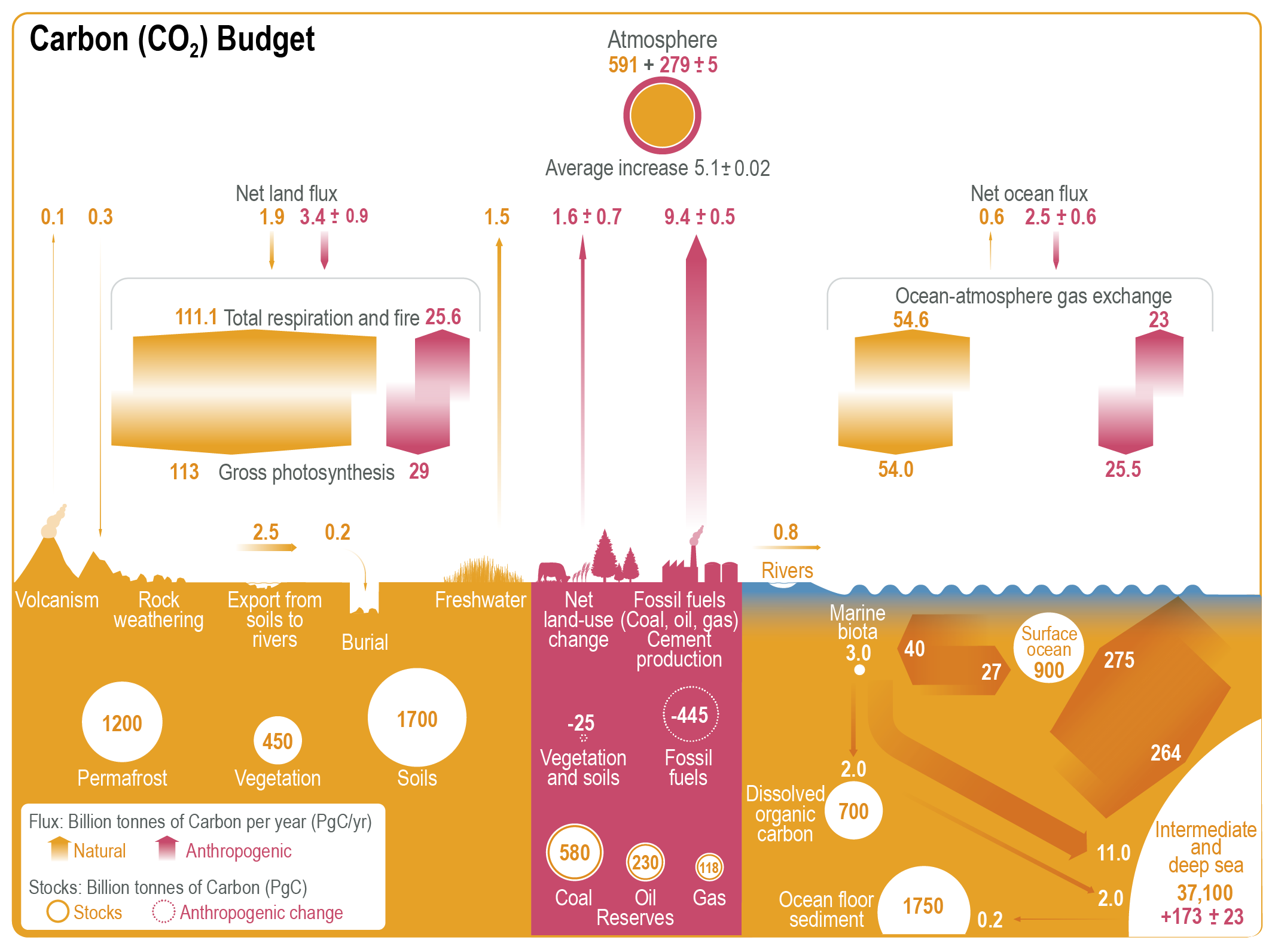 Figure 5.12 | Global carbon (CO2 ) budget (2010–2019). Yellow arrows represent annual carbon fluxes (in PgC yr–1) associated with the natural carbon cycle, estimated for the time prior to the industrial era, around 1750. Pink arrows represent anthropogenic fluxes averaged over the period 2010–2019. The rate of carbon accumulation in the atmosphere is equal to net land-use change emissions, including land management (called LULUCF in the main text) plus fossil fuel emissions, minus land and ocean net sinks (plus a small budget imbalance, Table 5.1). Circles with yellow numbers represent pre-industrial carbon stocks in PgC. Circles with pink numbers represent anthropogenic changes to these stocks (cumulative anthropogenic fluxes) since 1750. Anthropogenic net fluxes are reproduced from Friedlingstein et al. (2020). The relative change of gross photosynthesis since pre-industrial times is based on 15 DGVMs used in Friedlingstein et al. (2020). The corresponding emissions by total respiration and fire are those required to match the net land flux, exclusive of net land-use change emissions which are accounted for separately. The cumulative change of anthropogenic carbon in the terrestrial reservoir is the sum of carbon cumulatively lost by net land-use change emissions, and net carbon accumulated since 1750 in response to environmental drivers (warming, rising CO2, nitrogen deposition). The adjusted gross natural ocean–atmosphere CO2 flux was derived by rescaling the value in Figure 1 of Sarmiento and Gruber (2002) of 70 PgC yr–1by the revised estimate of the bomb radiocarbon (14C) inventory in the ocean. The original bomb14C inventory yielded an average global gas transfer velocity of 22 cm hr–1; the revised estimate is 17cm hr–1leading to 17/22*70=54. Dissolved organic carbon reservoir and fluxes from Hansell et al. (2009). Dissolved inorganic carbon exchanges between surface and deep ocean, subduction and obduction from Levy et al. (2013). Export production and flux from (Boyd et al., 2019). Net primary production (NPP) and remineralization in surface layer of the ocean from Kwiatkowski et al. (2020); Séférian et al. (2020). Deep ocean reservoir from Keppler et al. (2020). Anthropogenic carbon reservoir in the ocean is from Gruber et al. (2019b) extrapolated to 2015. Fossil fuel reserves are from BGR (2020); fossil fuel resources are 11,490 PgC for coal, 6,780 PgC for oil and 365 PgC for natural gas. Permafrost region stores are from Hugelius et al. (2014); Strauss et al. (2017); Mishra et al. (2021) (see also Box 5.1) and soil carbon stocks outside of permafrost region from Batjes (2016); Jackson et al. (2017). Biomass stocks (range of seven estimates) are from Erb et al. (2018). Sources for the fluxes of the land–ocean continuum are provided in main text and adjusted within the ranges of the various assessment to balance the budget (Section 5.2.1.5).
 Since AR5 (Ciais et al., 2013), a number of improvements have led to the more constrained carbon budget presented here. Some new additions include: (i) the use of independent estimates for the residual carbon sink on natural terrestrial ecosystems (Le Quéré et al., 2018a); (ii) improvements in the estimates of emissions from cement production (Andrew, 2019) and the sink associated with cement carbonation (Cao et al., 2020); (iii) improved and new emissions estimates from forestry and other land use (Hansis et al., 2015; Gasser et al., 2020); (iv) the use of ocean observation-based sink estimates and a revised river flux partition between hemispheres (Friedlingstein et al., 2020); and (v) the expansion of constraints from atmospheric inversions, based on surface networks and the use of satellite retrievals.
The budget, based on the annual assessment by the GCP (Friedlingstein et al., 2020), uses independent estimates of all major flux components: fossil fuel and carbonate emissions (EFOS), CO2 fluxes from land use, land-use change, and forestry (ELULUCF), the growth rate of CO2 in the atmosphere (Gatm), and the ocean (Socean) and natural land (Sland) CO2 sinks. An imbalance term (BImb) is required to ensure mass balance of the source and sinks that have been independently estimated: EFOS+ ELULUCF= Gatm+ Socean+ Sland. + BImb. All estimates are reported with 1 standard deviation (±1σ, 1 sigma) representing a likelihood of 68%.
Over the past decade (2010–2019), 10.9 ± 0.9 PgC yr–1 were emitted from human activities, which were distributed between three Earth system components: 46% accumulated in the atmosphere (5.1 ± 0.02 PgC yr–1), 23% was taken up by the ocean (2.5 ± 0.6 PgC yr–1) and 31% was stored by vegetation in terrestrial ecosystems (3.4 ± 0.9 PgC yr–1) (Table 5.1). There is a budget imbalance of 0.1 PgCyr–1 which is within the uncertainties of the other terms. Over the industrial era (1750–2019), the total cumulative CO2 fossil fuel and industry emissions were 445 ± 20 PgC, and the LULUCF flux (= net land-use change in Figure 5.12) was 240 ± 70 PgC (medium confidence). The equivalent total emissions (685 ± 75 PgC) was distributed between the atmosphere (285 ± 5 PgC), oceans (170 ± 20 PgC) and land (230 ± 60 PgC; Table 5.1), with a budget imbalance of 20 PgC. This budget (Table 5.1) does not explicitly account for source/sink dynamics due to carbon cycling in the land–ocean aquatic continuum comprising freshwaters, estuaries, and coastal areas. Natural and anthropogenic transfers of carbon from soils to freshwater systems are significant (2.4–5.1 PgC yr–1) (Regnier et al., 2013; Drake et al., 2018). Some of the carbon is buried in freshwater bodies (0.15 PgC) (Mendonça et al., 2017), and a significant proportion returns to the atmosphere via outgassing from lakes, rivers and estuaries (Raymond et al., 2013; Regnier et al., 2013; Lauerwald et al., 2015). The net export of carbon from the terrestrial domain to the open oceans is estimated to be 0.80 PgC yr–1 (medium confidence), based on the average of (Jacobson et al., 2007; Resplandy et al., 2018) and corrected to account for 0.2 PgC buried in ocean floor sediments. These terms are included in Figure 5.12. Inclusion of other smaller fluxes could further constrain the carbon budget (Ito, 2019; Friedlingstein et al., 2020).
5.2.2 Methane (CH4): Trends, Variability and Budget
Methane is a much more powerful greenhouse gas than CO2 (Chapter 7) and participates in tropospheric chemistry (Chapter 6). The CH4 variability in the atmosphere is mainly the result of the net balance between the sources and sinks on the Earth’s surface and chemical losses in the atmosphere. Atmospheric transport evens out the regional CH4 differences between different parts of the Earth’s atmosphere. The steady-state lifetime is estimated to be 9.1 ± 0.9 years (Section 6.3.1 and Table 6.2). About 90% of the loss of atmospheric CH4 occurs in the troposphere by reaction with hydroxyl radical (OH), 5% by bacterial soil oxidation, and the rest 5% by chemical reactions with OH, excited state oxygen (O1D), and atomic chlorine (Cl) in the stratosphere (Saunois et al., 2020). Methane has large emissions from natural and anthropogenic origins, but a clear demarcation of their nature is difficult because of the use and conversions of the natural ecosystem for human activities. The largest natural sources are from wetlands, freshwater and geological process, while the largest anthropogenic emissions are from enteric fermentation and manure treatment, landfills and waste treatment, rice cultivation and fossil fuel exploitation (Table 5.2). In the past two centuries, CH4 emissions have nearly doubled, predominantly human driven since 1900, and persistently exceeded the losses (virtually certain), thereby increasing the atmospheric abundance as evidenced from the ice core and firn air measurements (Ferretti et al., 2005; Ghosh et al., 2015).
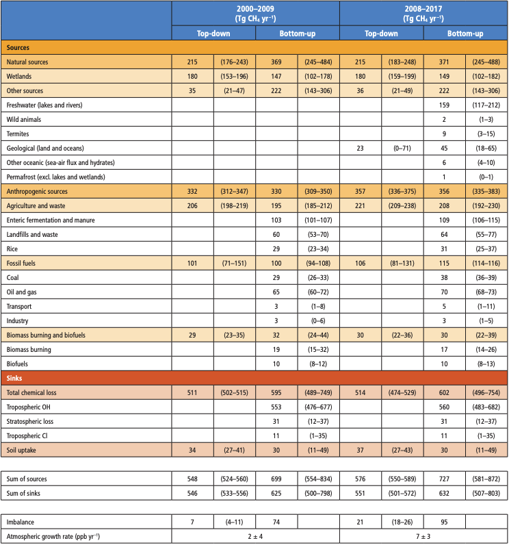
This section discusses both bottom-up and top-down estimates of emissions and sinks. Bottom-up estimates are based on empirical upscaling of point measurements, emissions inventories and dynamical model simulations, while top-down estimates refer to those constrained by atmospheric measurements and chemistry-transport models in inversion systems. Since AR5, a larger suite of atmospheric inversions using both in situ and remote sensing measurement have led to better understanding of the regional CH4 sources (Cross-Chapter Box 5.2). New ice core measurements of14C-CH4 are used for estimating the geological sources of CH4 (Table 5.2). Compared to the SRCCL (IPCC, 2019a; Jia et al., 2019), we provide a whole atmospheric sources-sinks budget consisting of all emissions and losses.
5.2.2.1 Atmosphere
Since the start of direct measurements of CH4 in the atmosphere in the 1970s (Figure 5.13), the highest growth rate was observed from 1977 to 1986 at 18 ± 4 ppb yr–1 (multi-year mean and 1 standard deviation) (Rice et al., 2016). This rapid CH4 growth followed the green revolution with increased crop production and a fast rate of industrialization that caused rapid increases in CH4 emissions from ruminant animals, rice cultivation, landfills, oil and gas industry and coal mining (Ferretti et al., 2005; Ghosh et al., 2015; Crippa et al., 2020). Due to increases in oil prices in the early 1980s, emissions from gas flaring declined significantly (Stern and Kaufmann, 1996). This explains the first reduction in CH4 growth rates from 1985 to 1990 (Steele et al., 1992; Chandra et al., 2021). Further emissions reductions occurred following the Mt Pinatubo eruption in 1991 that triggered a reduction in CH4 growth rate through a decrease in wetland emissions driven by lower surface temperatures due to the light scattering by aerosols (Bândă et al., 2016; Chandra et al., 2021). In the late 1990s through to 2006 there was a temporary pause in the CH4 growth rate, with higher confidence on its causes than in AR5: emissions from the oil and gas sectors declined by about 10 Tg yr–1through the 1990s, and atmospheric CH4 loss steadily increased (Dlugokencky et al., 2003; Simpson et al., 2012; Crippa et al., 2020; Höglund-Isaksson et al., 2020; Chandra et al., 2021). The methane growth rate began to increase again at 7 ± 3 ppb yr–1 during 2007–2016, the causes of which are highly debated since AR5 (Rigby et al., 2008; Dlugokencky et al., 2011; Dalsøren et al., 2016; Nisbet et al., 2016; Patra et al., 2016; Schaefer et al., 2016; Schwietzke et al., 2016; Turner et al., 2017; Worden et al., 2017; He et al., 2020); studies disagree on the relative contribution of thermogenic, pyrogenic and biogenic emission processes and variability in tropospheric OH concentration. The renewed CH4 increase is accompanied by a reversal of d13C trend to more negative values post 2007; opposite to what occurred in the 200 years prior (Ferretti et al., 2005; Ghosh et al., 2015; Schaefer et al., 2016; Schwietzke et al., 2016; Nisbet et al., 2019), suggesting an increasing contribution from animal farming, landfills and waste, and a slower increase in emissions from fossil fuel exploitation since the early 2000s (Patra et al., 2016; Jackson et al., 2020; Chandra et al., 2021). Atmospheric concentrations of CH4 reached 1866.3 ppb in 2019 (Figure 5.14). A comprehensive assessment of the CH4 growth rates over the past four decades is presented in Cross-Chapter Box 5.2.
 Figure 5.13 | Time series of CH4 concentrations, growth rates and isotopic composition. (a) CH4 concentrations; (b) CH4 growth rates; (c) d13-CH4. Data from selected site networks operated by the National Oceanic and Atmospheric Administration (NOAA; Dlugokencky et al., 2003), Advanced Global Atmospheric Gases Experiment (AGAGE; Prinn et al., 2018) and Portland Airport (PDX, Portland State University; Rice et al., 2016). To maintain clarity, data from many other measurement networks are not included here, and all measurements are shown in the World Metereological Organization X2004ACH4 global calibration standard. Global mean values of XCH4 (total-column), retrieved from radiation spectra measured by the Greenhouse Gases Observing Satellite (GOSAT) are shown in panels (a) and (b). Cape Grim Observatory (CGO; 41°S, 145°E) and Trinidad Head (THD; 41°N, 124°W) data are taken from the AGAGE network. NOAA global and northern hemispheric (NH) means for d13C are calculated from 10 and 6 sites, respectively. The PDX data adjusted to NH (period: 1977–2000) are merged with THD (period: 2001–2019) for CH4 concentration and growth rate analysis, and PDX and NOAA NH means of d13C data are used for joint interpretation of long-term trends analysis. The multivariate El Niño–Southern Oscillation (ENSO) index (MEI) is shown in panel (b). Further details on data sources and processing are available in the chapter data table (Table 5.SM.6).
 5.2.2.2 Anthropogenic Methane (CH4) Emissions
The positive gradient between CH4 at Cape Grim, Australia (41°S) and Trinidad Head, USA (41°N), and the bigger difference between Trinidad Head and global mean CH4 compared to that between global mean CH4 and Cape Grim, strongly suggest that the Northern Hemisphere is the dominant origin of anthropogenic CH4 emissions (Figure 5.13). The loss rate of CH4 in troposphere does not produce a large positive north–south hemispheric gradient in CH4 due to parity in hemispheric mean OH concentration (Patra et al., 2014), or in the case of greater OH concentrations in the northern rather than the Southern Hemisphere as simulated by the chemistry-climate models (Naik et al., 2013). Coal mining contributed about 35% of the total CH4 emissions from all fossil fuel-related sources. Top-down estimates of fossil fuel emissions (106 Tg yr–1) are smaller than bottom-up estimates (115 Tg yr–1) during 2008–2017 (Table 5.2). Inventory-based estimates suggest that CH4 emissions from coal mining increased by 17 Tg yr–1 between the periods 2002–2006 and 2008–2012, with a dominant contribution from China (Peng et al., 2016; Crippa et al., 2020; Höglund-Isaksson et al., 2020). Inventory-based estimates suggest that CH4 emissions from coal mining increased by 17 Tg yr–1 between the periods 2002–2006 and 2008–2012, with a dominant contribution from China (Peng et al., 2016; Crippa et al., 2020; Höglund-Isaksson et al., 2020). Recent country statistics and detailed inventory-based estimates show that CH4 emissions from coal mining in China declined between 2012 and 2016 (Sheng et al., 2019; Gao et al., 2020), while atmospheric-based estimates suggest a continuation of CH4 emissions growth but at a slower rate to the year 2015 (Miller et al., 2019) and 2016 (Chandra et al., 2021). Emissions from oil and gas extraction and use decreased in the 1980s and 1990s, but increased in the 2000s and 2010s (Dlugokencky et al., 1994; Stern and Kaufmann, 1996; Howarth, 2019; Crippa et al., 2020). The attribution to multiple CH4 sources using spatially aggregated atmospheric d13C data remained underdetermined to infer the global total emissions from the fossil fuel industry, biomass burning and agriculture (Rice et al., 2016; Schaefer et al., 2016; Schwietzke et al., 2016; Worden et al., 2017; Thompson et al., 2018).
In the agriculture and waste sectors (Table 5.2), livestock production has the largest emissions source (109 Tg yr–1 in 2008–2017) dominated by enteric fermentation by about 90%. Methane is formed during the storage of manure, when anoxic conditions are developed (Hristov et al., 2013). Emissions from enteric fermentation and manure have increased gradually from about 87 Tg yr–1 in 1990–1999 to 109 Tg yr–1 in 2008–2017 mainly due to the increase in global total animal numbers. Methane production in livestock rumens (cattle, goats, sheep, water buffalo) are affected by the type, amount and quality of feeds, energy consumption, animal size, health and growth rate, meat and milk production rate, and temperature (Broucek, 2014; S.R.O. Williams et al., 2020; SRCCLSection 5.4.3). Waste management and landfills produced 64 Tg yr–1 in 2008–2017, with global emissions increasing steadily since the 1970s and, despite significant declines in the USA, western Europe and Japan (Crippa et al., 2020; Höglund-Isaksson et al., 2020).
Emissions from rice cultivation decreased from about 45 Tg yr–1 in the 1980s to about 29 Tg yr–1 in the decade 2000–2009, but increased again slightly to 31 Tg yr–1 during 2008–2017, based on inventories data. However, ecosystem models showed a gradual increase with time due to climate change (limited evidence, low agreement) (Crippa et al., 2020; Höglund-Isaksson et al., 2020; Ito, 2020).
Biomass burning and biofuel consumption (including natural and anthropogenic processes) caused at least 30 Tg yr–1emissions during 2008–2017 and constituted up to about 5% of global anthropogenic CH4 emissions. Methane emissions from open biomass burning decreased during the past two decades mainly due to reduction of burning in savanna, grassland and shrubland (van der Werf et al., 2017; Worden et al., 2017). There is recent evidence from the tropics that fire occurrence is non-linearly related to precipitation, implying that severe droughts will increase CH4 emissions from fires, particularly from the degraded peatlands (Field et al., 2016).
5.2.2.3 Land Biospheric Emissions and Sinks
Freshwater wetlands are the single largest global natural source of CH4 in the atmosphere, accounting for about 26% of the total CH4 source (robust evidence, medium agreement). Progress has been made since AR5 (Ciais et al., 2013) in better constraining freshwater lake and river emissions and reducing double counting with wetland emissions. Bottom-up and top-down estimates for 2008–2017 are 149 and 180 Tg yr–1, respectively, with a top-down uncertainty range of 159–199 Tg yr–1 (Table 5.2). The large uncertainties stem from challenges in mapping wetland area and temporal dynamics to landscape estimates, and in scaling methane production, transport and consumption processes that are measured with small chambers or flux towers (Pham-Duc et al., 2017). Both the top-down and bottom-up estimates presented in Table 5.2 indicate little increase in wetland CH4 emissions during the last three decades, with the new estimates being slightly smaller than in AR5 due to updated wetland maps and ecosystem model simulations (Melton et al., 2013; Poulter et al., 2017). Wetland emissions show strong interannual variability due to the changes in inundated land area, air temperature and microbial activity (Bridgham et al., 2013). Present terrestrial ecosystem model simulated CH4 emissions variability does not produce strong correlation with the El Niño–Southern Oscillation (ENSO) cycle (Cross-Chapter Box 5.2, Figure 2), although observation evidence is emerging for lower CH4 emissions during El Niños and greater emissions during La Niña (Pandey et al., 2017).
Trees in upland and wetland forests contribute to CH4 emissions by abiotic production in the canopy, by the methanogenesis taking place in the stem, and by conducting CH4 from soil into the atmosphere (Covey and Megonigal, 2019). There is emerging evidence of the important role of trees in transporting and conducting CH4 from soils into the atmosphere, especially in tropics (Pangala et al., 2017), whereas direct production of CH44 by vegetation only has a minor contribution (limited evidence, high agreement) (Bruhn et al., 2012; Covey and Megonigal, 2019). The contribution of trees in transporting CH4 may further widen the gap between the bottom-up and top-down estimates in the global budget, particularly needing a re-assessment of emissions in the tropics and in forested wetlands of temperate and boreal regions (Pangala et al., 2017; Jeffrey et al., 2019; Welch et al., 2019; Sjögersten et al., 2020).
Microbial methane uptake by soil comprises up to 5% (30 Tg yr–1) of the total CH4 sink in 2008–2017 (Table 5.2). There is evidence from experimental and modelling studies of increasing soil microbial uptake due to increasing temperature (Yu et al., 2017), although evidence also exists for decreasing CH4 consumption, possibly linked to precipitation changes (Ni and Groffman, 2018). The estimate of global methane loss by microbial oxidation in upland soils has been lowered marginally by 4 Tg yr–1, compared to 34 Tg yr–1 in AR5, for the period 2000–2009. Termites, an infraorder of insects (Isoptera) found in almost all land masses, emitted about 9 Tg yr–1 of CH4 in 2000–2009. Increased emissions from insects and other anthropods are projected (Brune, 2018).
5.2.2.4 Ocean and Inland Water Emissions and Sinks
In AR5, the ocean CH4 emissions were reported together with geological emissions, summing up to 54 (33–75) Tg yr–1. Coastal oceans, fjords and mud volcanos are major sources of CH4 in the marine environment, but CH4 flux measurements are sparse. Saunois et al. (2020) estimate that the oceanic budget, including biogenic, geological and hydrate emissions from coastal and open ocean, is 6 (range 4–10) Tg yr–1 for the 2000s, which is in good agreement with an air–sea flux measurement-based estimate of 6–12 Tg yr–1 (Weber et al., 2019). When estuaries are included, the total oceanic budget is 9–22 Tg yr–1, with a mean value of 13 Tg yr–1. A recent synthesis suggests that CH4 emissions from shallow coastal ecosystems, particularly from mangroves, can be as high as 5–6 Tg yr–1 (Al-Haj and Fulweiler, 2020). The reservoir emissions, including coastal wetlands and tidal flats, contribute up to 13 Tg yr–1 (Borges and Abril, 2011; Deemer et al., 2016). Methane seepage from the Arctic shelf, possibly triggered by the loss of geological storage due to warming and thawing of permafrost and hydrate decomposition, has a wide estimated range of 0.0–17 Tg yr–1 (Shakhova et al., 2010, 2014, 2017; Berchet et al., 2016); advanced eddy covariance measurements put the best estimate at about 3 Tg yr–1 from the East Siberian Arctic shelf (Thornton et al., 2020). The current flux is expected to be a mix of pre-industrial and climate change-driven fluxes, CH4 seepage is anticipated to increase in a warmer world (Dean et al., 2018).
All geological sources around the world, including the coastal oceans and fjords, are estimated to emit CH4 in the range of 35–76 Tg yr–1 (Etiope et al., 2019). There is evidence that the ventilation of geological CH4 is likely to be smaller than 15 Tg yr–1 (Petrenko et al., 2017; Hmiel et al., 2020). A lower geological CH4 ventilation will reduce the gap between bottom-up and top-down estimates (Table 5.2), but widen the gap in the ratio of fossil fuel-derived sources to the biogenic sources for matching the D14C-CH4 observations.
Inland water (lakes, rivers, streams, ponds, estuaries) emissions are proportionally the largest source of uncertainty in the CH4 budget. Since AR5 (Ciais et al., 2013), the inland water CH4 source has been revised from 8–73 Tg yr–1 (1980s) to 117–212 Tg yr–1 (2000s) with the availability of more observational data and improved areal estimates (Bastviken et al., 2011; Deemer et al., 2016; Stanley et al., 2016; DelSontro et al., 2018; Saunois et al., 2020). However, it is difficult to estimate bottom-up CH4 emissions, due to the large spatial and temporal variation in lake and river CH4 fluxes (Wik et al., 2016; Crawford et al., 2017; Natchimuthu et al., 2017), uncertainties in their global area (Allen and Pavelsky, 2018), a relatively small number of observations, and varying measurement methods – for example, those neglecting ebullition, varying upscaling methods, and lack of appropriate processes (Sanches et al., 2019; Engram et al., 2020; L. Zhang et al., 2020). Accordingly, there is no clear accounting of inland waters in top-down budgets, which is the main reason for the large gap in bottom-up and top-down estimates of ‘other sources’ in the CH4 budget (Table 5.2). Despite recent progress in separating wetlands from inland waters, there is double-counting in the bottom-up estimates of their emissions (Thornton et al., 2016a). Although there is evidence that regional human activities and global warming both increase inland water CH4 emissions (Beaulieu et al., 2019), the increase in the decadal emissions since AR5 (Ciais et al., 2013) rather reflect improvements in the estimate (medium confidence), due to updates in the datasets and new upscaling approaches (Saunois et al., 2020).
5.2.2.5 Methane (CH4) Budget
A summary of top-down and bottom-up estimates of CH4 emissions and sinks for the period 2008–2017 is presented in Figure 5.14 (details in Table 5.2 and the associated text for the emissions). In addition to 483-682 Tg yr–1loss of CH4 in the troposphere by reaction with OH, 1–35 Tg yr–1 of CH4 loss is estimated to occur in the lower troposphere due to Cl but are not included in the top-down models as shown in Table 5.2 (Hossaini et al., 2016; Gromov et al., 2018; X. Wang et al., 2019). The decadal mean CH44 burden/imbalance increased at the rate of 30, 12, 7 and 21 Tg yr–1 in the 1980s (1980–1989), 1990s (1990–1999), 2000s (2000–2009) and the most recent decade (2008–2017), respectively (virtually certain), as can be estimated from observed atmospheric growth rate (Cross-Chapter Box 5.2, Figure 1).
Recent analysis using D14C-CH4 in ice samples suggest that CH4 emissions from fossil fuel exploitation are responsible for 30% of total CH4 emissions (Lassey et al., 2007; Hmiel et al., 2020), which is largely inconsistent with sectorial budgets where fossil fuel emissions add up to 20% only (Ciais et al., 2013). However, recent model simulations produce fairly consistent d13C-CH4 values and trends, as observed in the atmospheric samples using 20% fossil fuel emissions fraction (Ghosh et al., 2015; Warwick et al., 2016; Fujita et al., 2020; Strode et al., 2020). Further research is needed to clarify the relative roles of CH4 emissions from fossil fuel exploitation and freshwater components. A key challenge is to accommodate the higher estimated emissions from these two components without a major increase in the sinks, in order to be consistent with the observed changes in the carbon and hydrogen isotopes.
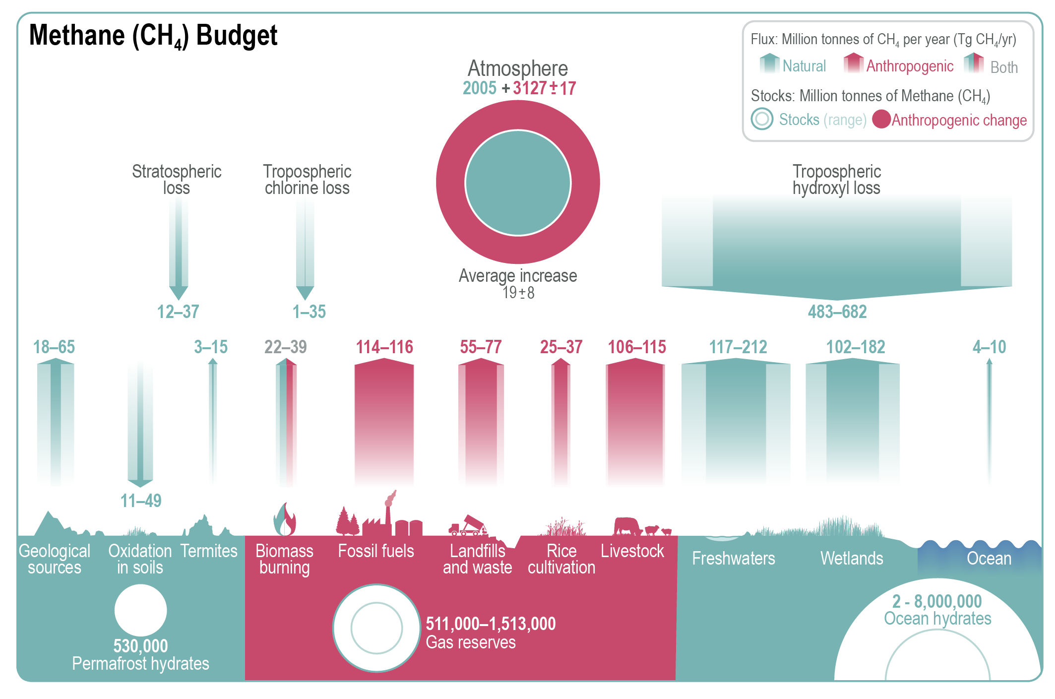 Figure 5.14 | Global methane (CH4 ) budget (2008–2017). Values and data sources as in Table 5.2 (in TgCH4). The atmospheric stock is calculated from mean CH4 concentration, multiplying a factor of 2.75 ± 0.015 Tg ppb–1, which accounts for the uncertainties in global mean CH4 (Chandra et al., 2021). Further details on data sources and processing are available in the chapter data table (Table 5.SM.6).
 Cross-Chapter Box 5.2 | Drivers of Atmospheric Methane Changes During 1980–2019
Contributors: Prabir K. Patra (Japan/India), Josep G. Canadell (Australia), Frank J. Dentener (European Union, The Netherlands), Xin Lan (United States of America/China), Vaishali Naik (United States of America)
The atmospheric methane (CH4) growth rate has varied widely over the past three decades, and the causes have been extensively studied since AR5. The mean growth rate decreased from 15 ± 5 ppb yr–1 in the 1980s to 0.48 ± 3.2 ppb yr–1 during 2000–2006 (the so-called quasi-equilibrium phase) and returned to an average rate of 7.6 ± 2.7 ppb yr–1 in the past decade (2010–2019) (based on data in Figure 5.14). Atmospheric CH4 grew faster (9.3 ± 2.4 ppb yr–1) over the last six years (2014–2019) – a period with prolonged El Niño conditions, which contributed to high CH4 growth rates consistent with behaviour during previous El Niño events (Figure 5.14b). Because of large uncertainties in both the emissions and sinks of CH4, it has been challenging to quantify accurately the methane budget and ascribe reasons for the growth over 1980–2019. In the context of CH4 emissions mitigation, it is critical to understand if the changes in growth rates are caused by emissions from human activities or by natural processes responding to changing climate. If CH4 continues to grow at rates similar to those observed over the past decade, it will contribute to decadal scale climate change and hinder the achievement of the long-term temperature goals of the Paris Agreement (Section 7.3.2.2; Nisbet et al., 2019).
Cross-Chapter Box 5.2, Figure 1 shows the decadal CH4 budget derived from the Global Carbon Project (GCP)-CH4 synthesis for 1980s, 1990s and 2000s (Kirschke et al., 2013), and for 2010–2017 (Saunois et al., 2020). The imbalance of the sources and sinks estimated by atmospheric inversions (dark blue bars) can be used to explain the changes in CH4 concentration increase rates between the decades (Table 5.2).
Since AR5, many studies have discussed the role of different source categories in explaining the increase in CH4 growth rate since 2007 and a coincident decrease of d13C–CH4 and dD–CH4 isotopes (Figure 5.13; Rice et al., 2016). Both13C and D are enriched in mass-weighted average source signatures for CH4 emissions from thermogenic sources (e.g., coal mining, oil and gas industry) and pyrogenic (biomass burning) sources, and depleted in biogenic (e.g., wetlands, rice paddies, enteric fermentation, landfill and waste) sources. Proposed hypotheses for CH4 growth (2007–2017) are inconclusive and vary from a concurrent decrease in thermogenic and increase in wetland and other biogenic emissions (Nisbet et al., 2016; Schwietzke et al., 2016), an increase in emissions from agriculture in the tropics (Schaefer et al., 2016), a concurrent reduction in pyrogenic emissions and an increase in thermogenic emissions (Worden et al., 2017), or an emissions increase from biogenic sources and a slower increase in emissions from thermogenic sources compared to inventory emissions (Patra et al., 2016; Thompson et al., 2018; Jackson et al., 2020; Chandra et al., 2021).

Cross-Chapter Box 5.2, Figure 1 | Methane sources and sinks for four decades from atmospheric inversions with the budget imbalance (source–sink; dark blue bars) (plotted on the left y-axis). Top-down analysis from Kirschke et al. (2013); Saunois et al. (2020). The global CH4 concentration seen in the black line (plotted on the right y-axis), representing National Oceanic and Atmospheric Administration (NOAA) observed global monthly mean atmospheric CH4 in dry-air mole fractions for 1983–2019 (Chapter 2, Annex V). Natural sources include emissions from natural wetlands, lakes and rivers, geological sources, wild animals, termites, wildfires, permafrost soils, and oceans. Anthropogenic sources include emissions from enteric fermentation and manure, landfills, waste and wastewater, rice cultivation, coal mining, oil and gas industry, biomass and biofuel burning. The top-down total sink is determined from global mass balance that includes chemical losses due to reactions with hydroxyl (OH), atomic chlorine (Cl), and excited atomic oxygen (O1D), and oxidation by bacteria in aerobic soils (Table 5.2). Further details on data sources and processing are available in the chapter data table (Table 5.SM.6).
A few studies emphasize the role of chemical destruction by hydroxyl (OH; the primary sink of methane), in driving changes in the growth of atmospheric methane abundance, in particular after 2006 (Rigby et al., 2017; Turner et al., 2017). Studies applying three-dimensional atmospheric inversion (McNorton et al., 2018), simple multi-species inversion (Thompson et al., 2018), as well as empirical methods using a variety of observational constraints based on OH chemistry (Nicely et al., 2018; Patra et al., 2021), do not find trends in OH large enough to explain the methane changes post-2006. On the contrary, global chemistry–climate models based on fundamental principles of atmospheric chemistry and known emissions trends of anthropogenic non-methane short-lived climate forcers simulate an increase in OH over this period (Zhao et al., 2019; Stevenson et al., 2020; see Section 6.2.3). These contrasting lines of evidence suggest that OH changes may have had a small moderating influence on methane growth since 2007 (low confidence).
Cross-Chapter Box 5.2 Figure 2 shows that modelled wetland emissions anomalies for all regions did not exhibit statistically significant trends (high agreement between models, medium evidence). Thus, the inter-decadal difference of total CH4 emissions derived from inversion models and wetland emissions, arises mainly from anthropogenic activities. The time series of regional emissions suggest that progress towards atmospheric CH4 quasi-equilibrium was primarily driven by reductions in anthropogenic (fossil fuel exploitation) emissions in Europe, Russia and temperate North America over 1988–2000. In the global totals, emissions equalled loss in the early 2000s. The growth since 2007 is driven by increasing agricultural emissions from East Asia (1997–2017), West Asia (2005–2017), Brazil (1988–2017) and Northern Africa (2005–2017), and fossil fuel exploitations in temperate North America (2010–2017; Lan et al., 2019; Crippa et al., 2020; Höglund-Isaksson et al., 2020; Jackson et al., 2020; Chandra et al., 2021).

Cross-Chapter Box 5.2, Figure 2 | Anomalies in global and regional methane (CH4) emissions for 1988–2017. The map in the centre shows mean CH4 emissions for 2010–2016. Multi-model mean (line) and 1-s standard deviations (shaded) for 2000–2017 are shown for 9 surface CH4 and 10 satellite XCH4 inversions, and 22 wetland models or model variants that participated in GCP-CH4 budget assessment (Saunois et al., 2020). The results for the period before 2000 are available from two inversions, one using 19 sites (Chandra et al., 2021; also used for the 2010–2016 mean emissions map) and one for global totals (Bousquet et al., 2006). The long-term mean values for 2010–2016 (common for all GCP–CH4 inversions), as indicated within each panel separately, are subtracted from the annual-mean time series for the calculation of anomalies for each region. Further details on data sources and processing are available in the chapter data table (Table 5.SM.6).
There is evidence from emissions inventories at country level and regional scale inverse modelling that CH4 growth rate variability between 1988 and 2017 is closely linked to anthropogenic activities (medium agreement). Isotopic composition observations and inventory data suggest that concurrent emissions changes from both fossil fuels and agriculture are playing roles in the resumed CH4 growth since 2007 (high confidence). Shorter-term decadal variability is predominantly driven by the influence of El Niño–Southern Oscillation on emissions from wetlands and biomass burning (Cross-Chapter Box 5.2, Figure 2), and loss due to OH variations (medium confidence), but lacking quantitative contribution from each of the sectors. By synthesizing all available information regionally from a priori (bottom-up) emissions, satellite and surface observations, including isotopic information, and inverse modelling (top-down), the capacity to track and explain changes in, and drivers of, natural and anthropogenic CH4 regional and global emissions has improved since AR5, but fundamental uncertainties related to OH variations remain unchanged.
5.2.3 N2O: Trends, Variability and Budget
In natural ecosystems, nitrous oxide (N2O) is primarily produced as a by-product during the remineralization of organic matter via the primary processes of nitrification and denitrification (Butterbach-Bahl et al., 2013; Voss et al., 2013). The net N2O production is highly sensitive to local environmental conditions such as temperature, oxygen concentrations, pH and the concentrations of ammonium and nitrate, among others, causing strong variability of N2O emissions in time and space, even at small scales. Changes in the atmospheric abundance of N2O result largely from the balance of the net N2O sources on land and ocean, and the photochemical destruction of N2O in the stratosphere.
Since AR5 (WGI, Section 6.4.3), improved understanding of N2O sources allows for a more comprehensive assessement of the global N2O budget (Table 5.3). This progress is based on extended atmospheric observations (Francey et al., 2003; Elkins et al., 2018; Prinn et al., 2018), improved atmospheric N2O inversions (Saikawa et al., 2014; Thompson et al., 2019), updated and expanded inventories of N2O sources (Winiwarter et al., 2018; Janssens-Maenhout et al., 2019), as well as improved bottom-up estimate of freshwater, ocean and terrestrial sources (Martinez-Rey et al., 2015; Landolfi et al., 2017; Buitenhuis et al., 2018; Lauerwald et al., 2019; Maavara et al., 2019; Tian et al., 2019).
The human perturbation of the natural nitrogen cycle through the use of synthetic fertilizers and manure, as well as nitrogen deposition resulting from land-based agriculture and fossil fuel burning has been the largest driver of the increase in atmospheric N2O of 31.0 ± 0.5 ppb (10%) between 1980 and 2019 (robust evidence, high agreement) (Tian et al., 2020). The long atmospheric lifetime of N2O implies that it will take more than a century before atmospheric abundances stabilize after the stabilization of global emissions. The rise of atmospheric N2O is of concern, not only because of its contribution to the anthropogenic radiative forcing (Chapter 7) but also because of the importance of N2O in stratospheric ozone loss (Ravishankara et al., 2009; Fleming et al., 2011; W. Wang et al., 2014).
5.2.3.1 Atmosphere
The tropospheric abundance of N2O was 332.1 ± 0.4 ppb in 2019 (Figure 5.15), which is 23% higher than pre-industrial levels of 270.1 ± 6.0 ppb (robust evidence, high agreement). Current estimates are based on atmospheric measurements with high accuracy and density (Francey et al., 2003; Elkins et al., 2018; Prinn et al., 2018), and pre-industrial estimates are based on multiple ice-core records Section 2.2.3.2.3). The average annual tropospheric growth rate was 0.85 ± 0.03 ppb yr–1 during the period 1995 to 2019 (Figure 5.15a). The atmospheric growth rate increased by about 20% between the decade 2000–2009 and the most recent decade of 2010–2019 (0.95 ± 0.04 ppb yr–1) (robust evidence, high agreement). The growth rate in 2010–2019 was also higher than during 1970–2000 (0.6–0.8 ppb yr–1; Ishijima et al., 2007) and the 30-year period prior to 2011 (0.73 ± 0.03 ppb yr–1), as reported by AR5. New evidence since AR5 (WGI, Section 6.4.3) confirms that, in the tropics and subtropics, large interannual variations in the atmospheric growth rate are negatively correlated with the multivariate ENSO index (MEI) and associated anomalies in land and ocean fluxes (Ji et al., 2019; Thompson et al., 2019; S. Yang et al., 2020) (Figure 5.15a).
 Figure 5.15 | Changes in atmospheric nitrous oxide (N2 O) and its isotopic composit ion since 1940. (a) Atmospheric N2O abundance (parts per billion, ppb) and growth rat (ppb yr–1); (b) δ15N of atmospheric N2O; and (c) alpha-site15N–N2O. Estimates are based on direct atmospheric measurements in the Advanced Global Atmospheric Gases Experiment (AGAGE), Commonwealth Scientific and Industrial Research Organisation (CSIRO), and National Oceanic and Atmospheric Administration (NOAA) networks (Prinn et al., 2000, 2018; Francey et al., 2003; Hall et al., 2007; Elkins et al., 2018), archived air samples from Cape Grim, Australia (Park et al., 2012), and firn air from the North Greenland Ice Core Project (NGRIP) Greenland and H72 Antarctica (Ishijima et al., 2007), Law Dome Antarctica (Park et al., 2012), as well as a collection of firn ice samples from Greenland (Prokopiou et al., 2017, 2018). Shading in (a) is based on the multivariate El Niño–Southern Oscillation (ENSO) index, with red indicating El Niño conditions (Wolter and Timlin, 1998). Further details on data sources and processing are available in the chapter data table (Table 5.SM.6).
 As assessed by SRCCL (IPCC, 2019a), combined firn, ice, air and atmospheric measurements show that the15N/14N isotope ratio (robust evidence, high agreement) and the predominant position of the15N atom in atmospheric N2O (limited evidence, low agreement) in N2O has changed since 1940 (Figure 5.15b, c) whereas they were relatively constant in the pre-industrial period (Ishijima et al., 2007; Park et al., 2012; Prokopiou et al., 2017, 2018). The SRCCL concluded that this change indicates a shift in the nitrogen-substrate available for denitrification, and the relative contribution of nitrification to the global N2O source (robust evidence, high agreement), which are associated with increased fertilizer use in agriculture (Park et al., 2012; Snider et al., 2015; Prokopiou et al., 2018).
Since AR5 (WGI, Section 6.4.3), the mean atmospheric lifetime of N2O has been revised to 116 ± 9 years (Prather et al., 2015). The small negative feedback of the N2O lifetime to increasing atmospheric N2O results in a slightly lower residence time (109 ± 10 years) of N2O perturbations compared with that assessed by AR5 (118–131 years) (Prather et al., 2015). The dominant N2O loss occurs through photolysis and oxidation by O(1D) radicals in the stratosphere and amounts to approximately 13.1 (12.4–13.6) TgN yr–1 (Minschwaner et al., 1993; Prather et al., 2015; Tian et al., 2020).
5.2.3.2 Anthropogenic N2O Emissions
The AR5 (WGI, Section 6.4.3) and SRCCL (Section 2.3.3) concluded that agriculture is the largest anthropogenic source of N2O emissions. Since SRCCL (2.3.3), a new synthesis of inventory-based and modelling studies shows that the widespread use of synthetic fertilizers and manure on cropland and pasture, manure management and aquaculture resulted in 3.8 (2.5–5.8) TgN yr–1 (average 2007–2016) (robust evidence, high agreement) (Table 5.3; Winiwarter et al., 2018; FAO, 2019; Janssens-Maenhout et al., 2019; Tian et al., 2020). Observations from field-measurements (Song et al., 2018), inventories (Wang et al., 2020) and atmospheric inversions (Thompson et al., 2019) further corroborate the assessment of SRCCL that there is a non-linear relationship between N2O emissions and nitrogen input, implying an increasing fraction of fertilizer lost as N2O with larger fertilizer excess (medium evidence, high agreement). Several studies using complementary methods indicate that agricultural N2O emissions have increased by more than 45% since the 1980s (high confidence) (Figure 5.16 and Table 5.3; Davidson, 2009; Winiwarter et al., 2018; Janssens-Maenhout et al., 2019; Tian et al., 2020), mainly due to the increased use of nitrogen fertilizer and manure. N2O emissions from aquaculture are among the fastest rising contributors of N2O emissions, but their overall magnitude is still small in the overall N2O budget (Tian et al., 2020).
 Figure 5.16 | Decadal mean nitrous oxide (N2 O) emissions for 2007–2016 and its change since 1850 based on process-model projections. The total effect, including that from anthropogenic nitrogen additions (atmospheric deposition, manure addition, fertilizer use and land-use), is evaluated against the background flux driven by changes in atmospheric carbon dioxide (CO2) concentration, and climate change. Fluxes are derived from the N2O model intercomparison project ensemble of terrestrial biosphere models (Tian et al., 2019) and three ocean biogeochemical models (Landolfi et al., 2017; Battaglia and Joos, 2018a; Buitenhuis et al., 2018). Further details on data sources and processing are available in the chapter data table (Table 5.SM.6).
 The principal non-agricultural anthropogenic sources of N2O are industry, specifically chemical processing, wastewater, and the combustion of fossil fuels (Table 5.3). Industrial emissions of N2O mainly due to nitric and adipic acid production have decreased in North America and Europe since the widespread installation of abatement technologies in the 1990s (Pérez-Ramίrez et al., 2003; Lee et al., 2011; Janssens-Maenhout et al., 2019). There is still considerable uncertainty in industrial emissions from other regions of the world with contrasting trends between inventories (Thompson et al., 2019). Globally, industrial emissions and emissions from fossil fuel combustion by stationary sources, such as power plants, as well as smaller emissions from mobile sources (e.g., road transport and aviation) have remained nearly constant between the 1980s and 2007–2016 (medium evidence, medium agreement) (Winiwarter et al., 2018; Janssens-Maenhout et al., 2019; Tian et al., 2020). Wastewater N2O emissions, including those from domestic and industrial sources, have increased from 0.2 (0.1–0.3) TgN yr–1 to 0.35 (0.2–0.5) TgN yr–1 between the 1980s and 2007–2016 (Tian et al., 2020).
Biomass burning from crop residue burning, grassland, savannah and forest fires, as well as biomass burnt in household stoves, releases N2O during the combustion of organic matter. Updated inventories since AR5 (WGI, Section 6.4.3) result in a lower range of the decadal mean emissions of 0.6 (0.5–0.8) TgN yr–1 (van der Werf et al., 2017; Tian et al., 2020). The attribution of grassland, savannah or forest fires to natural or anthropogenic origins is uncertain, preventing a separation of the biomass burning source into natural and anthropogenic.
5.2.3.3 Emissions from Ocean, Inland Water Bodies and Estuaries
Since AR5 (WGI, Section 6.4.3), new estimates of the global ocean N2O source derived from ocean biogeochemistry models are 3.4 (2.5–4.3) TgN yr–1 for the period 2007–2016 (Figure 5.16; Manizza et al., 2012; Suntharalingam et al., 2012; Martinez-Rey et al., 2015; Landolfi et al., 2017; Buitenhuis et al., 2018; Tian et al., 2020). This is slightly lower than climatological estimates from empirically based methods and surface ocean data syntheses (Bianchi et al., 2012; S. Yang et al., 2020). Nitrous oxide processes in coastal upwelling zones continue to be poorly represented in global estimates of marine N2O emissions (Kock et al., 2016), but may account for an additional 0.2–0.6 TgN yr–1 of the global ocean source (Seitzinger et al., 2000; Nevison et al., 2004).
In the oxic ocean (>97% of ocean volume), nitrification is believed to be the primary N2O source (Freing et al., 2012). In sub-oxic ocean zones (Section 5.3), where denitrification prevails, higher N2O yields and turnover rates make these regions potentially significant sources of N2O (Arévalo-Martínez et al., 2015; Babbin et al., 2015; Ji et al., 2015). The relative proportion of ocean N2O from oxygen-minimum zones is highly uncertain (Zamora et al., 2012). Estimates derived from in situ sampling, particularly in the eastern tropical Pacific, suggest significant fluxes from these regions, and potentially account for up to 50% of the global ocean source (Codispoti, 2010; Arévalo-Martínez et al., 2015; Babbin et al., 2015). However, recent global-scale analyses estimate lower contributions (4–7%, Battaglia and Joos, 2018b; Buitenhuis et al., 2018). Further investigation is required to reconcile these estimates and provide improved constraints on the N2O source from low-oxygen zones.
Atmospheric deposition of anthropogenic N on oceans can stimulate marine productivity and influence ocean emissions of N2O. New ocean model analyses since AR5 (WGI, 6.4.3), suggest a relatively modest global potential impact of 0.01–0.32 TgN yr–1 (pre-industrial to present-day) equivalent to 0.5–3.3% of the global ocean N2O source (Suntharalingam et al., 2012; Jickells et al., 2017; Landolfi et al., 2017). However, larger proportionate impacts are predicted in nitrogen-limited coastal and inland waters downwind of continental pollution outflow, such as the Northern Indian Ocean (Jickells et al., 2017; Suntharalingam et al., 2019).
Inland waters and estuaries are generally sources of N2O as a result of nitrification and denitrification of dissolved inorganic nitrogen, however, they can serve as N2O sinks in specific conditions (Webb et al., 2019). Since AR5 (WGI, 6.4.3), improved emissions factors, including their spatio-temporal scaling, and consideration of transport within the aquatic system allows for better constraint of these emissions (Murray et al., 2015; Hu et al., 2016; Lauerwald et al., 2019; Maavara et al., 2019; Kortelainen et al., 2020; Yao et al., 2020). Despite uncertainties because of the side effects of canals and reservoirs on nutrient cycling, these advances permit attribution of a fraction of inland water N2O emissions to anthropogenic sources (Tian et al., 2020), which contributes to the increased anthropogenic share of the global N2O source in this report compared to AR5 (Ciais et al., 2013). As an indirect consequence of agricultural nitrogen use and waste-water treatment, the anthropogenic emissions from inland waters have increased by about a quarter (0.1 TgN yr–1) between the 1980s and 2007–2016 (Tian et al., 2020).
5.2.3.4 Emissions and Sinks in Non-agricultural Land
Soils are the largest natural source of N2O, arising primarily from nitrogen processing associated with microbial nitrification and denitrification (Table 5.3; Butterbach-Bahl et al., 2013; Snider et al., 2015). Under some conditions, soils can also act as a net sink of N2O, but this effect is small compared to the overall source (Schlesinger, 2013). Since AR5 (WGI, Section 6.4.3), improved global process-based models (Tian et al., 2019) suggest a present-day source of 6.7 (5.3–8.1) TgN yr–1 (2007–2016 average), which is consistent with the estimate in AR5. Process-based models and inventory-based methods show that increased N deposition has enhanced terrestrial N2O emissions by 0.8 (0.4–1.4 TgN yr–1) relative to approximately pre-industrial times, and by 0.2 (0.1–0.2) TgN yr–1 between the 1980s and 2007–2016 (limited evidence, medium agreement) (Figure 5.16; Tian et al., 2019). This estimate is at the high end of the range reported in AR5 (WGI, Section 6.4.3). Model projections further show that global warming has led to increased soil N2O emissions of 0.8 (0.3–1.3) TgN yr–1 since approximately pre-industrial times, of which about half occurred since the 1980s (limited evidence, high agreement) (Tian et al., 2019, 2020).
The SRCCL assessed that deforestation and other forms of land-use change significantly alter terrestrial N2O emissions through emission pulses following conversions, generally resulting in long-term reduced emissions in unfertilized ecosystems (medium evidence, high agreement). This conclusion is supported by a recent study demonstrating that the deforestation-pulse effect is offset by the effect of reduced area of mature tropical forests (Tian et al., 2020).
Uncertainties remain in process-based models with respect to their ability to capture the complicated responses of terrestrial N2O emissions to rain pulses, freeze–thaw cycles and the net consequences of elevated levels of CO2 accurately (Tian et al., 2019). Emerging literature suggests that permafrost thaw may contribute significantly to arctic N2O emissions (Voigt et al., 2020), but these processes are not yet adequately represented in models and upscaling to large-scale remains a significant challenge.
5.2.3.5 N2O Budget
The synthesis of bottom-up estimates of N2O sources (Sections 5.2.3.2–5.2.3.4 and Figure 5.17) yields a global source of 17.0 (12.2 to 23.5) TgN yr–1 for the years 2007–2016 (Table 5.3). This estimate is comparable to AR5, but the uncertainty range has been reduced primarily due to improved estimates of ocean and anthropogenic N2O sources. Since AR5 (WGI, Section 6.4.3), improved capacity to estimate N2O sources from atmospheric N2O measurements by inverting models of atmospheric transport provides a new and independent constraint for the global N2O budget (Saikawa et al., 2014; Thompson et al., 2019; Tian et al., 2020). The decadal mean source derived from these inversions is remarkably consistent with the bottom-up global N2O budget for the same period, however, the split between land and ocean sources based on atmospheric inversions is less constrained, yielding a smaller land source of 11.3 (10.2 to 13.2) TgN yr–1 and a larger ocean source of 5.7 (3.4 to 7.2) TgN yr–1, respectively, compared to bottom-up estimates.
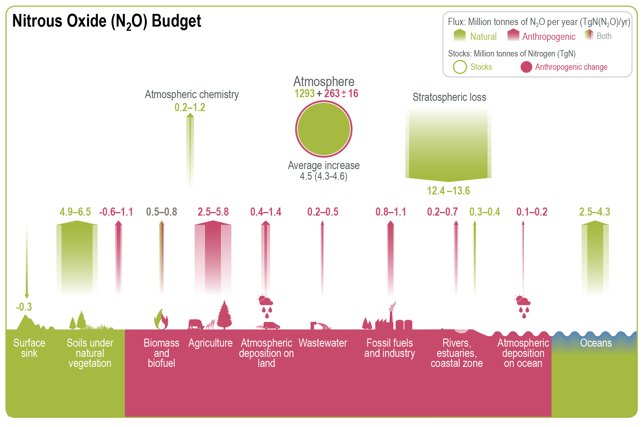 Figure 5.17 | Global nitrous oxide (N2 O) budget (2007–2016). Values and data sources as in Table 5.3. The atmospheric stock is calculated from mean N2O concentration, multiplying a factor of 4.79 ± 0.05 Tg ppb–1 (Prather et al., 2012). Pool sizes for the other reservoirs are largely unknown. Further details on data sources and processing are available in the chapter data table (Table 5.SM.6).
 Supported by multiple studies and extensive observational evidence (Sections 5.2.3.2–5.2.3.4 and Figure 5.17), anthropogenic emissions contributed about 40% (7.3; uncertainty range: 4.2 to 11.4 TgN yr–1) to the total N2O source in 2007–2016 (high confidence). This estimate is larger than in AR5 (WGI, 6.4.3) due to a larger estimated effect of nitrogen deposition on soil N2O emissions and the explicit consideration of the role of anthropogenic nitrogen in determining inland water and estuary emissions.
Based on bottom-up estimates, anthropogenic emissions from agricultural nitrogen use, industry and other indirect effects have increased by 1.7 (1.0 to 2.7) TgN yr–1 between the decades 1980–1989 and 2007–2016, and are the primary cause of the increase in the total N2O source (high confidence). Atmospheric inversions indicate that changes in surface emissions, rather than in the atmospheric transport or sink of N2O, are the cause for the increased atmospheric growth rate of N2O (robust evidence, high agreement) (Thompson et al., 2019). However, the increase of 1.6 (1.4 to 1.7) TgN yr–1 in global emissions between 2000–2005 and 2010–2015 based on atmospheric inversions is somewhat larger than bottom-up estimates over the same period, primarily because of differences in the estimates of land-based emissions.
AR6 1980–1989 (TgN yr–1) | AR6 1990–1999 (TgN yr–1) | AR6 2000–2009 (TgN yr–1) | AR6 (2007–2016) (TgN yr–1) | AR5 (2006–2011) (TgN yr–1) | ||
Bottom-up Budget | ||||||
Anthropogenic sources | ||||||
Fossil fuel combustion and Industry | 0.9 (0.8 to 1.1) | 0.9 (0.9 to 1.0) | 1.0 (0.8 to 1.0) | 1.0 (0.8 to 1.1) | 0.7 (0.2 to 1.8) | |
Agriculture (incl. aquaculture) | 2.6 (1.8 to 4.1) | 3.0 (2.1 to 4.8) | 3.4 (2.3 to 5.2) | 3.8 (2.5 to 5.8) | 4.1 (1.7 to 4.8) | |
Biomass and biofuel burning | 0.7 (0.7 to 0.7) | 0.7 (0.6 to 0.8) | 0.6 (0.6 to 0.6) | 0.6 (0.5 to 0.8) | 0.7 (0.2 to 1.0) | |
Wastewater | 0.2 (0.1 to 0.3) | 0.3 (0.2 to 0.4) | 0.3 (0.2 to 0.4) | 0.4 (0.2 to 0.5) | 0.2 (0.1 to 0.3) | |
Inland water, estuaries, coastal zones | 0.4 (0.2 to 0.5) | 0.4 (0.2 to 0.5) | 0.4 (0.2 to 0.6) | 0.5 (0.2 to 0.7) | ||
Atmospheric nitrogen deposition on ocean | 0.1 (0.1 to 0.2) | 0.1 (0.1 to 0.2) | 0.1 (0.1 to 0.2) | 0.1 (0.1 to 0.2) | 0.2 (0.1 to 0.4) | |
Atmospheric nitrogen deposition on land | 0.6 (0.3 to 1.2) | 0.7 (0.4 to 1.4) | 0.7 (0.4 to 1.3) | 0.8 (0.4 to 1.4) | 0.4 (0.3 to 0.9) | |
Other indirect effects from CO2, climate and land-use change | 0.1 (–0.4 to 0.7) | 0.1 (–0.5 to 0.7) | 0.2 (–0.4 to 0.9) | 0.2 (–0.6 to 1.1) | ||
Total anthropogenic | 5.6 (3.6 to 8.7) | 6.2 (3.9 to 9.6) | 6.7 (4.1 to 10.3) | 7.3 (4.2 to 11.4) | 6.3 (2.6 to 9.2) | |
Natural sources and sinks | ||||||
Rivers, estuaries, and coastal zones | 0.3 (0.3 to 0.4) | 0.3 (0.3 to 0.4) | 0.3 (0.3 to 0.4) | 0.3 (0.3 to 0.4) | 0.6 (0.1 to 2.9) | |
Open oceans | 3.6 (3.0 to 4.4) | 3.5 (2.8 to 4.4) | 3.5 (2.7 to 4.3) | 3.4 (2.5 to 4.3) | 3.8 (1.8 to 9.4) | |
Soils under natural vegetation | 5.6 (4.9 to 6.6) | 5.6 (4.9 to 6.5) | 5.6 (5.0 to 6.5) | 5.6 (4.9 to 6.5) | 6.6 (3.3 to 9.0) | |
Atmospheric chemistry | 0.4 (0.2 to 1.2) | 0.4 (0.2 to 1.2) | 0.4 (0.2 to 1.2) | 0.4 (0.2 to 1.2) | 0.6 (0.3 to 1.2) | |
Surface sink | –0.01 (–0.3 to 0) | –0.01 (–0.3 to 0) | –0.01 (–0.3 to 0) | –0.01 (–0.3 to 0) | –0.01 (–1 to 0) | |
Total natural | 9.9 (8.5–12.2) | 9.8 (8.3–12.1) | 9.8 (8.2–12.0) | 9.7 (8.0–12.0) | 11.6 (5.5–23.5) | |
Total bottom-up source | 15.5 (12.1 to 20.9) | 15.9 (12.2 to 21.7) | 16.4 (12.3 to 22.4) | 17.0 (12.2 to 23.5) | 17.9 (8.1 to 30.7) | |
Observed growth rate | 3.7 (3.7 to 3.7) | 4.5 (4.3 to 4.6) | 3.6 (3.5 to 3.8) | |||
Inferred stratospheric sink | 12.9 (12.2-13.5) | 13.1 (12.4–13.6) | 14.3 (4.3 to 28.7) | |||
Atmospheric inversion | ||||||
Atmospheric loss | 12.1 (11.4 to 13.3) | 12.4 (11.7 to 13.3) | ||||
Total source | 15.9 (15.1 to 16.9) | 16.9 (15.9 to 17.7) | ||||
Imbalance | 3.6 (2.2 to 5.7) | 4.2 (2.4 to 6.4) | ||||
5.2.4 The Relative Importance of CO2, CH4, and N2O
The total influence of anthropogenic greenhouse gases (GHGs) on the Earth’s radiative balance is driven by the combined effect of those gases, and the three most important – carbon dioxide (CO2), methane (CH4), nitrous oxide (N2O) – were discussed in the previous sections. This section compares the balance of the sources and sinks of these three gases and their regional net flux contributions to the radiative forcing. CO2 has multiple residence times in the atmosphere – from one year to many thousands of years (Box 6.1 in Ciais et al., 2013) – and N2O has a mean lifetime of 116 years. They are both long-lived GHGs, while CH4 has a lifetime of 9.1 years and is considered a short-lived GHG (see Chapter 2 for lifetime of GHGs, Chapter 6 for CH4 chemical lifetime, and Chapter 7 for effective radiative forcing of all GHGs).
Figure 5.18 shows the contribution to radiative forcing of CO2, CH4, N2O, and the halogenated species since the 1900s to more recent decades. For the period 1960–2019, the relative contribution to the total effective radiative forcing (ERF) was 63% for CO2, 11% for CH4, 6% for N2O, and 17% for the halogenated species (Chapter 7; Figure 5.18). The systematic decline in the relative contribution to ERF for CH4 since 1850 is caused by a slower increase rate of CH4 in the recent decades, at 6, 10 and 5 ppb yr–1 during 1850–2019, 1960–2019 and 2000–2019, respectively, in comparison with the increasing rate of CO2 (at 0.7, 1.6 and 2.2 ppm yr–1, respectively) and N2O (at 0.4, 0.7 and 0.9 ppb yr–1, respectively; Figure 5.4). Owing to the shorter lifetime of CH4, the effect of a reduction in the emissions increase rate on the ERF increase is evident at inter-decadal time scales.
 Figure 5.18 | Contributions of carbon dioxide (CO2 ), methane (CH4 ), nitrous oxide (N2 O) and halogenated species to the total effective radiative forcing (ERF) increases in 2019 since 1850, 1960 and 2000, respectively. ERF data are taken from Annex III (based on calculations from Chapter 7). Note that the sum of the ERFs exceeds 100% because there are negative ERFs due to aerosols and clouds. Further details on data sources and processing are available in the chapter data table (Table 5.SM.6).
 Atmospheric abundance of GHGs is proportional to their emissions-loss budgets in the Earth’s environment. There are multiple metrics to evaluate the relative importance of different GHGs for the global atmospheric radiation budget and the socio-economic impacts (Section 7.6). Metrics for weighting emissions are further developed in AR6 WGIII. Figure 5.19 shows the regional emissions of the three main GHGs. For North Asia, Europe, Temperate North America and West Asia, the most dominant GHG source is CO2 (high confidence) (Figure 5.19) while, for East Asia, South Asia, South East Asia, Tropical South America, Temperate North America and Central Africa, the source is CH4 (Figure 5.19). The N2O emissions are dominant in regions with intense use of nitrogen fertilizers in agriculture. Only boreal North America showed net sinks of CO2, while close to flux neutrality is observed for North Asia, Southern Africa, and Australasia. Persistent emissions of CO2 are observed for Tropical and South America, northern Africa, and South East Asia (medium confidence). The medium confidence arises from large uncertainties in the estimated non-fossil fuel CO2 fluxes over these regions due to the lack of high-quality atmospheric measurements.
 Figure 5.19 | Regional distributions of net fluxes of carbon dioxide (CO2), methane (CH4), nitrous oxide (N2O) on the Earth’s surface. The region divisions, shown as the shaded map, are made based on ecoclimatic characteristics of the land. The fluxes include those from anthropogenic activities and natural causes that result from responses to anthropogenic greenhouse gases and climate change (feedbacks) as in the three budgets shown in Sections 5.2.1.5, 5.2.2.5, and 5.2.3.5. The CH4and N2O emissions are weighted by arbitrary factors of 50 and 500, respectively, for depiction by common y-axes. Fluxes are shown as the mean of the inverse models as available from Thompsonet al. (2019); Friedlingsteinet al. (2020); Saunoiset al. (2020). Further details on data sources and processing are available in the chapter data Table (Table 5.SM.6).
 5.3 Ocean Acidification and Deoxygenation
The surface ocean has absorbed a quarter of all anthropogenic CO2 emissions, mainly through physical–chemical processes (McKinley et al., 2016; Gruber et al., 2019b; Friedlingstein et al., 2020). Once dissolved in seawater, CO2 reacts with water and forms carbonic acid, which in turn dissociates, leading to a decrease in the concentration of carbonate (CO3–2) ions, and increasing both bicarbonate (HCO3–) and hydrogen (H+) ion concentration. This process has caused a shift in the carbonate chemistry towards a less basic state, commonly referred to as ‘ocean acidification’ (Caldeira and Wickett, 2003; Orr et al., 2005; Doney et al., 2009). Although the societal concern regarding ocean acidification is relatively recent (about the last 20 years), the physical–chemical basis for the ocean absorption (sink) of atmospheric CO2 has been discussed much earlier by Revelle and Suess (1957). The AR5 and SROCC assessments were of robust evidence that the H+ion concentration is increasing in the surface ocean, thereby reducing seawater pH (= -log [H+]) (Section 2.3.4.1; Orr et al., 2005; Feely et al., 2009; Ciais et al., 2013; Bindoff et al., 2019), and there is high confidence that ocean acidification is impacting marine organisms (Bindoff et al., 2019).
Ocean oxygen decline, or deoxygenation, is driven by changes in ocean ventilation and solubility (Bindoff et al., 2019). It is virtually certain that anthropogenic forcing has made a substantial contribution to the ocean heat content increase over the historical period (Bindoff et al., 2019; IPCC, 2019c; Chapter 9, Section 2.3.3.1), strengthening upper water column stratification. Ocean warming decreases the solubility of dissolved oxygen in seawater, and it contributes to about 15% of the dissolved oxygen decrease in the oceans according to estimates based on solubility and the recent SROCC assessment (medium confidence), especially in sub-surface waters, between 100–600 m depth (Helm et al., 2011; Schmidtko et al., 2017; Breitburg et al., 2018; Oschlies et al., 2018; SROCC, Section 5.3.1). Stratification reduces the ventilation flux into the ocean interior, contributing to most of the remaining ocean deoxygenation (Schmidtko et al., 2017; Breitburg et al., 2018; Section 3.6.2). Deoxygenation may enhance emissions of nitrous oxide, especially from oxygen minimum zones (OMZs) or hypoxic coastal areas (Breitburg et al., 2018; Oschlies et al., 2018). Since SROCC (Bindoff et al., 2019), CMIP6 model simulation results agree with the reported 2% loss (4.8 ± 2.1 Pmoles O2) in total dissolved oxygen in the upper ocean layer (100–600 m) for the 1970–2010 period (Helm et al., 2011; Ito et al., 2017; Schmidtko et al., 2017; Kwiatkowski et al., 2020; Section 2.3.4.2). The response of marine organisms to the coupled effects of ocean warming, acidification and deoxygenation occur at different metabolic levels on different groups, and include respiratory stress and reduction of thermal tolerance (Gruber, 2011; Bindoff et al., 2019; IPCC, 2019c; Kawahata et al., 2019). An assessment of these effects on marine biota is found in WGII AR6 Chapter 2.
This section assesses past events of ocean acidification and deoxygenation (Section 5.3.1), the historical trends and spatial variability for the upper ocean (Section 5.3.2) and the ocean interior (Section 5.3.3). Future projections for ocean acidification and the drivers in the coastal ocean are assessed in Sections 5.3.4 and 5.3.5, respectively.
5.3.1 Paleoclimate Context
5.3.1.1 Paleocene–Eocene Thermal Maximum
The Paleocene–Eocene Thermal Maximum (PETM) was an episode of global warming exceeding pre-industrial temperatures by 4°C–8°C (McInerney and Wing, 2011; Dunkley Jones et al., 2013) that occurred 55.9–55.7 Ma. The PETM involved a large pulse of geologic CO2 released into the ocean–atmosphere system in 3–20 kyr (Zeebe et al., 2016; Gutjahr et al., 2017; Kirtland Turner et al., 2017; Kirtland Turner, 2018; Gingerich, 2019; Section 5.2.1.1). In response, observationally constrained model simulations report an increase in atmospheric CO2 concentrations ranging from about 900 ppm to >2000 ppm (Chapter 2; Gutjahr et al., 2017; Cui and Schubert, 2018; Anagnostou et al., 2020). The PETM thus provides a test for our understanding of the ocean’s response to the increase in carbon (and heat) emissions over geologically short time scales.
A limited number of independent proxy records indicate that the PETM was associated with a surface ocean pH decline ranging from 0.15 to 0.30 units (Penman et al., 2014; Gutjahr et al., 2017; Babila et al., 2018). It was also accompanied by a rapid (<10 ka) shallowing of the carbonate saturation horizon, resulting in the widespread dissolution of sedimentary carbonate, followed by a gradual (100 kyr) recovery (Zachos et al., 2005; Bralower et al., 2018). The remarkable similarity among sedimentary records spanning a wide range of ecosystems suggests with medium confidence that the perturbation in the ocean carbonate saturation was global (Babila et al., 2018) and directly resulted from elevated atmospheric CO2 levels. The degree of acidification is similar to the 0.4 pH unit decrease projected for the end of the 21st century under RCP8.5 (Gattuso et al., 2015) and is estimated to have occurred at a rate about one order of magnitude slower than the current rate of ocean acidification (Zeebe et al., 2016). There is low confidence in the inferred rates of ocean acidification inherent to the range of uncertainties affecting rates estimates based on marine sediments (Section 5.1.2.1).
Recent model outputs and globally distributed geochemical data reveal with medium confidence widespread ocean deoxygenation during the PETM (Dickson et al., 2012, 2014; Winguth et al., 2012; Chang et al., 2018; Remmelzwaal et al., 2019), with parts of the ocean potentially becoming drastically oxygen-depleted (anoxic; Yao et al., 2018; Clarkson et al., 2021). Deoxygenation affected the surface ocean globally (including the Arctic Ocean; Sluijs et al., 2006), due to vertical and lateral expansion of OMZs (Zhou et al., 2014) that resulted from warming and related changes in ocean stratification. Expansion of OMZs may have stimulated N2O production through water-column (de)nitrification (Junium et al., 2018). The degree to which N2O production impacted PETM warming, however, has not yet been established.
The feedbacks associated with recovery from the PETM are uncertain, yet could include drawdown associated with silicate weathering (Zachos et al., 2005) and regrowth of terrestrial and marine organic carbon stocks (Bowen and Zachos, 2010; Gutjahr et al., 2017).
5.3.1.2 Last Deglacial Transition
The Last Deglacial Transition (LDT) is the best documented climatic transition in the past associated with a substantial atmospheric CO2 rise ranging from 190 to 265 ppm between 18–11 ka (Marcott et al., 2014). The amplitude of the deglacial CO2 rise is thus on the same order of magnitude as the increase since the Industrial Revolution.
Boron isotope ( δ11B) data suggest a 0.15–0.05 unit decrease in sea surface pH (Hönisch and Hemming, 2005; Henehan et al., 2013) across the LDT, an average rate of decline of about 0.002 units per century compared with the current rate of more than 0.1 units per century (Bopp et al., 2013; Gattuso et al., 2015). Planktonic foraminiferal shell weights decreased by 40% to 50% (Barker and Elderfield, 2002), and coccolith mass decreased by about 25% (Beaufort et al., 2011) across the LDT. Independent proxy reconstructions thus highlight with high confidence that pH values decreased as atmospheric CO2 concentrations increased across the LDT. There is, however, low confidence in the inferred rate of ocean acidification owing to multiple sources of uncertainties affecting rates estimates based on marine sediments (Section 5.1.2.1).
Geochemical and micropaleontological evidence suggest that intermediate-depth OMZs almost vanished during the Last Glacial Maximum (LGM) (Jaccard et al., 2014). However, multiple lines of evidence suggest with medium confidence that the deep (>1500 m) ocean became depleted in O2 (concentrations were possibly lower than 50 μmol kg–1) globally (Jaccard and Galbraith, 2012; Hoogakker et al., 2015, 2018; Gottschalk et al., 2016, 2020a; Anderson et al., 2019) as a combined result of sluggish ventilation of the ocean subsurface (Gottschalk et al., 2016, 2020a; Skinner et al., 2017) and a generally more efficient marine biological carbon pump (Buchanan et al., 2016; Yamamoto et al., 2019; Galbraith and Skinner, 2020).
During the LDT, deep ocean ventilation increased as Antarctic Bottom Water (AABW) (Skinner et al., 2010; Gottschalk et al., 2016; Jaccard et al., 2016) and subsequently the Atlantic meridional overturning circulation (McManus et al., 2004; Lippold et al., 2016) resumed, transferring previously sequestered remineralized carbon from the ocean interior to the upper ocean, and eventually the atmosphere (Skinner et al., 2010; Galbraith and Jaccard, 2015; Gottschalk et al., 2016; Ronge et al., 2016, 2020; Sikes et al., 2016; Rae et al., 2018), contributing to the deglacial CO2 rise. Intermediate depths lost oxygen as a result of sluggish ventilation and increasing temperatures (decreasing saturation). As the world emerged from the last Glacial period, OMZs underwent a large volumetric increase at the beginning of the Bølling-Allerød (B/A), a northern-hemisphere wide warming event, 14.7 ka (Jaccard and Galbraith, 2012; Praetorius et al., 2015) with deleterious consequences for benthic ecosystems (e.g., Moffitt et al., 2015). These observations indicate with high confidence that the rate of warming, affecting the solubility of oxygen and upper water column stratification, coupled with changes in subsurface ocean ventilation, impose a direct control on the degree of ocean deoxygenation, implying a high sensitivity of ocean oxygen loss to warming. The expansion of OMZs contributed to a widespread increase in water column (de)nitrification (Galbraith and Kienast, 2013), which contributed substantially to enhanced marine N2O emissions. Nitrogen stable isotope measurements on N2O extracted from ice cores suggest that approximately one-third (of the order of 0.7 ± 0.3TgN yr–1) of thedeglacial increase in N2O emissions relates to oceanic sources (Schilt et al., 2014; H. Fischer et al., 2019).
5.3.2 Historical Trends and Spatial Characteristics in the Upper Ocean
5.3.2.1 Reconstructed Centennial Ocean Acidification Trends
Ocean pH time series are based on the reconstruction of coral boron isotope ratios ( δ11B). A majority of coral δ11B data have been generated from the western Pacific region with a few records from the Atlantic Ocean. Biweekly resolution paleo-pH records show monsoonal variation of about 0.5 pH unit in the South China Sea (Liu et al., 2014). Interannual ocean pH variability in the range of 0.07–0.16 pH unit characterizes southwest Pacific corals that are attributed to El Niño–Southern Oscillation (ENSO) (H.C. Wu et al., 2018) and river runoff (D’Olivo et al., 2015). Decadal (10-, 22- and 48-year) ocean pH variations in the south-west Pacific have been linked to the Inter-decadal Pacific Oscillation, causing variations of up to 0.30 pH unit in the Great Barrier Reef (Pelejero et al., 2005; Wei et al., 2009) but weaker (about 0.08 pH unit) in the open ocean (H.C. Wu et al., 2018). Decadal variations in the South China Sea pH changes of 0.10–0.20 have also been associated with the variation in the East Asian monsoon (Liu et al., 2014; Wei et al., 2015), as a weakening of the Asian winter monsoon leads to sluggish water circulation within the reefs, building up localised CO2 concentration in the water due to calcification and respiration.
Since the beginning of the industrial period in the mid-19th century, coral δ11B-derived ocean pH has decreased by 0.06–0.24 pH unit in the South China Sea (Liu et al., 2014; Wei et al., 2015) and 0.12 pH unit in the south-west Pacific (H.C. Wu et al., 2018). Since the mid-20th century, a distinct feature of coral δ11B records relates to ocean acidification trends, albeit having a wide range of values: 0.12–0.40 pH unit in the Great Barrier Reef (Wei et al., 2009; D’Olivo et al., 2015), 0.05–0.08 pH unit in the north-west Pacific (Shinjo et al., 2013) and 0.04–0.09 pH unit in the Atlantic Ocean (Goodkin et al., 2015; Fowell et al., 2018). Concurrent coral carbon isotopic ( δ13C) measurements infer ocean uptake of anthropogenic CO2 from the combustion of fossil fuel, based on the lower abundance of13C in fossil fuel carbon. Western Pacific coral records show depleted δ13C trends since the late 19th century that are more prominent since the mid-20th century (high confidence) (Pelejeroet al., 2005; Wei et al., 2009; Shinjo et al., 2013; Liu et al., 2014; Kubota et al., 2017; H.C. Wu et al., 2018).
Overall, many of the records show a highly variable seawater pH underlaying strong imprints of internal climate variability (high confidence) and, in most instances, superimposed on a decreasing δ11B trend that is indicative of anthropogenic ocean acidification in recent decades (medium confidence). The robustness of seawater pH reconstructions is currently limited by the uncertainty on the calibration of The δ11B proxy in different tropical coral species.
5.3.2.2 Observations of Ocean Acidification over Recent Decades
The SROCC (Section 5.2.2.3) indicated that it is virtually certain that the ocean has undergone acidification globally in response to ocean CO2 uptake, and concluded that pH in open ocean surface water has changed by avirtually certain range of –0.017 to –0.027 pH units per decade since the late 1980s. Since SROCC, evidence of the progress of acidification across all regions of the oceans has been further strengthened by continued observations of seawater carbonate chemistry at ocean time series stations, and compiled shipboard studies providing temporally resolved and methodologically consistent datasets (Jiang et al., 2019) (Figure 5.20; Supplementary Material Table 5.SM.3; Section 2.3.3.5).
 Figure 5.20 | Multi-decadal trends of pH (Total Scale) in surface layer at various sites of the oceans and a global distribution of annual mean pH adjusted to the year 2000. Time-series data of pH are from Dore et al. (2009), Olafsson et al. (2009), González-Dávila et al. (2010), Bates et al. (2014), Takahashi et al. (2014), Wakita et al. (2017), Merlivat et al. (2018), Ono et al. (2019), and Bates and Johnson (2020). Global distribution of annual mean pH have been evaluated from data of surface oceanpCO2 measurements (Bakker et al., 2016; Jiang et al., 2019). Acronyms in panels: KNOT and K2 – Western Pacific subarctic gyre time series; HOT – Hawaii Ocean Time-series; BATS – Bermuda Atlantic Time-series Study; DYFAMED – Dynamics of Atmospheric Fluxes in the Mediterranean Sea; ESTOC – European Station for Time-series in the Ocean Canary Islands; CARIACO – Carbon Retention in a Colored Ocean Time-series. Further details on data sources and processing are available in the chapter data table (Table 5.SM.6).
 In the subtropical open oceans, decreases in pH have been reported with avery likely rate range from –0.016 to –0.019 pH units per decade since 1980s, which equates to approximately 4 % increase in hydrogen ion concentration ([H+]) per decade. Accordingly, the saturation state Ω (=[Ca2+][CO32-]/Ksp) of seawater with respect to calcium carbonate mineral aragonite has been declining at rates ranging from –0.07 to –0.12 per decade (González-Dávila et al., 2010; Feely et al., 2012; Bates et al., 2014; Takahashi et al., 2014; Ono et al., 2019; Bates and Johnson, 2020; Supplementary Material Table 5.SM.3). These rates are consistent with the rates expected from the transient equilibration with increasing atmospheric CO2 concentrations, but the variability of rate in decadal time scale has also been detected with robust evidence (Ono et al., 2019; Bates and Johnson, 2020). In the tropical Pacific, its central and eastern upwelling zones exhibited a faster pH decline of –0.022 to –0.026 pH unit per decade due to increased upwelling of CO2 -rich sub-surface waters in addition to anthropogenic CO2 uptake (Sutton et al., 2014; Lauvset et al., 2015). By contrast, warm pools in the western tropical Pacific exhibited slower pH decline of –0.010 to –0.013 pH unit per decade (Supplementary Material Table 5.SM.3; Lauvsetet al., 2015; Ishii et al., 2020). Observational and modelling studies (Nakano et al., 2015; Ishii et al., 2020) consistently suggest that slower acidification in this region is attributable to the anthropogenic CO2 taken up in the extratropics around a decade ago and transported to the tropics via shallow meridional overturning circulations.
In open subpolar and polar zones, the very likely range (–0.003 to –0.026 pH unit per decade) and uncertainty (up to 0.010) observed in pH decline are larger than in the subtropics, reflecting the complex interplay between physical and biological forcing mechanisms (Olafsson et al., 2009; Midorikawa et al., 2012; Bates et al., 2014; Takahashi et al., 2014; Lauvset et al., 2015; Wakita et al., 2017; Merlivat et al., 2018). Nevertheless, the high agreement of pH decline among these available time-series studies leads to high confidence in the trend of acidification in these zones. In the Arctic Ocean, a temporally limited time series of carbonate chemistry measurements prevents drawing robust conclusions on ocean acidification trends. However, the carbonate saturation state (Ω) is generally low, and observational studies show with robust evidence that the recent extensive melting of sea ice leading to enhanced air–sea CO2 exchange, large freshwater inputs, together with river discharge and glacial drainage, as well as the degradation of terrestrial organic matter in seawater, result in the decline of Ω of aragonite to undersaturation (Bates et al., 2009; Chierici and Fransson, 2009; Yamamoto-Kawai et al., 2009; Azetsu-Scott et al., 2010; Robbins et al., 2013; Fransson et al., 2015; Semiletov et al., 2016; Anderson et al., 2017; Qi et al., 2017; Beaupré-Laperrière et al., 2020; Y. Zhang et al., 2020; SROCCSection 3.2.1.2.4, IPCC, 2019b). The low saturation state of aragonite (Ω about 1) has also been observed in surface waters of the Antarctic coastal zone associated with freshwater input from glaciers (Mattsdotter Björk et al., 2014) and upwelling of deep water (Hauri et al., 2015) as well as along eastern boundary upwelling systems (Feely et al., 2016).
Overall, in agreement with SROCC, it is virtually certain from these observational studies that ocean surface waters undergo acidification globally with the CO2 increase in the atmosphere. These sustained measurements over the past decades, and campaign studies of ocean carbonate chemistry, also highlight with robust evidence that trends of acidification have been modulated by the variability and changes in physical and chemical states of ocean, including those affected by the warming of the cryosphere, and need to be better understood.
5.3.3 Ocean Interior Change
5.3.3.1 Ocean Memory: Acidification in the Ocean Interior
Advances in observations and modelling for ocean physics and biogeochemistry and established knowledge of ocean carbonate chemistry show with very high confidence that anthropogenic CO2 taken up into the ocean surface layer is further spreading into the ocean interior through ventilation processes, including vertical mixing, diffusion, subduction and meridional overturning circulations (Sections 2.3.3.5, 5.2.1.3 and 9.2.2.3; Sallée et al., 2012; Bopp et al., 2015; Nakano et al., 2015; Iudicone et al., 2016; Toyama et al., 2017; Pérez et al., 2018; Gruber et al., 2019b) and is causing acidification in the ocean interior. The net change in oxygen consumption by aerobic respiration of marine organisms further influences acidification by releasing CO2 (Section 5.3.3.2; Chen et al., 2017; Breitburg et al., 2018; Robinson, 2019).
Observations over past decades of basin-wide and global syntheses of ocean interior carbon show that the extent of acidification due to anthropogenic CO2 invasion tends to diminish with depth (very high confidence) (Section 5.2.1.3.3 and Figure 5.21; Woosley et al., 2016; Carter et al., 2017; Lauvset et al., 2020). The regions of deep convection such as subpolar North Atlantic and Southern Ocean present the deepest acidification detections below 2000 m (medium confidence). Mid-latitudinal zones within the subtropical cells and tropical regions present a relatively deep and shallow detection, respectively. A pH decrease has also been observed on the Antarctic continental shelf (Hauck et al., 2010; Williams et al., 2015). Acidification is also underway in the subsurface to intermediate layers of the Arctic Ocean due to the inflow of ventilated waters from the North Atlantic and the North Pacific (Qi et al., 2017; Ulfsbo et al., 2018).
 Figure 5.21 | Spread of ocean acidification from the surface into the interior of ocean since pre-industrial times. (a) Map showing the three transects used to create the cross sections shown in (b) and (c); vertical sections of the changes in (b) pH and (c) saturation state of aragonite (Ωarag) between 1800–2002 due to anthropogenic CO2 invasion (colour). Contour lines are their contemporary values in 2002. The red transect begins in the Nordic Seas and then follows the GO-SHIP lines A16 southward in the Atlantic Ocean, SR04 and S04P westward in the Southern Ocean, and P16 northward in the Pacific Ocean. The purple line follows the GO-SHIP line I09 southward in the Indian Ocean. The green line on the smaller inset crosses the Arctic Ocean from the Bering Strait to North Pole along 175°W and from the North Pole to the Fram Strait along 5°E (Lauvset et al., 2020). Further details on data sources and processing are available in the chapter data table (Table 5.SM.6).
 A significant increase in acidification resulting from net metabolic CO2 release coupled with ocean circulation changes has been shown with high confidence in large swathes of intermediate waters in the Pacific and Atlantic oceans (Dore et al., 2009; Byrne et al., 2010; Ríos et al., 2015; Chu et al., 2016; Carter et al., 2017; Lauvset et al., 2020). For example, ocean circulation contributes a pH change of –0.013 ± 0.013 to the overall observed change of –0.029 ± 0.014 for 1993–2013 at depths around 1000 m at 30°S–40°S in the South Atlantic ocean (Ríos et al., 2015). Long-term repeated observations in the North Pacific show a decline in dissolved oxygen (–4.0 μmol kg−1 per decade at maximum) being sustained in the intermediate water since the 1980s (Takatani et al., 2012; Sasano et al., 2015). The amplification of acidification associated with the weakening ventilation is thought to have been occurring persistently. In contrast, for the North Pacific subtropical mode water, large decadal variability in pH and aragonite saturation state with amplitudes of about 0.02 and about 0.1, respectively, are superimposed on secular declining trends due to anthropogenic CO2 invasion (Oka et al., 2019). This is associated with the variability in ventilation due to the approximately 50% variation in the formation volume of the mode water that is forced remotely by the Pacific Decadal Oscillation (Qiu et al., 2013; Oka et al., 2015).
These trends of acidification in the ocean interior lead to high confidence in shoaling of the saturation horizons of calcium carbonate minerals where Ω = 1. In the Pacific Ocean where the aragonite saturation horizon is shallower (a few hundred metres to 1200 m; Figure 5.21c), the rate of its shoaling is in the order of 1–2 m yr–1 (Feely et al., 2012; Ross et al., 2020). In contrast, shoaling rates of 4 m yr–1 to 1710 m for 1984–2008 and of 10–15 m yr–1 to 2250 m for 1991–2016 have been observed in the Iceland sea and the Irminger sea, respectively (Olafsson et al., 2009; Pérez et al., 2018).
In summary, ocean acidification is spreading into the ocean interior. Its rates at depths are controlled by the ventilation of the ocean interior as well as anthropogenic CO2 uptake at the surface, thereby diminishing with depth (very high confidence) (Figure 5.21). Variability in ocean circulation modulates the trend of ocean acidification at depths through the changes in ventilation and their impacts on metabolic CO2 content. However, the large knowledge gap around ventilation changes leads to low confidence in their impacts in many ocean regions (Sections 5.3.3.2; 9.2.2.3 and 9.3.2).
5.3.3.2 Ocean Deoxygenation and its Implications for Greenhouse Gases
As summarized in SROCC (Section 5.2.2.4), there is a growing consensus that between 1970 and 2010 the open ocean has very likely lost 0.5–3.3% of its dissolved oxygen in the upper 1000 m depth (Section 2.3.3.6; Helm et al., 2011; Ito et al., 2017; Schmidtko et al., 2017; Bindoff et al., 2019). Regionally, the equatorial and North Pacific, the Southern Ocean and the South Atlantic have shown the greatest oxygen loss of up to 30 mol m–2 per decade (Schmidtko et al., 2017). Warming – via solubility reduction and circulation changes – mixing and respiration are considered the major drivers, with 50% of the oxygen loss for the upper 1000 m of the global oceans attributable to the solubility reduction (Schmidtko et al., 2017). Climate variability also modifies the oxygen loss on interannual and decadal time scales especially for the tropical ocean OMZs (Deutsch et al., 2011, 2014; Llanillo et al., 2013) and the North Pacific subarctic zone (Whitney et al., 2007; Sasano et al., 2018; Cummins and Ross, 2020). However, quantifying the oxygen decline and variability and attributing them to processes in different regions remains challenging (Levin, 2018; Oschlies et al., 2018). Earth system models (ESMs) in CMIP5 and CMIP6 corroborate the decline in ocean oxygen, and project a continuing and accelerating decline with a strong impact of natural climate variability under high-emissions scenarios (Bopp et al., 2013; Long et al., 2016; Kwiatkowski et al., 2020). However, CMIP5 models did not reproduce observed patterns for oxygen changes in the tropical thermocline, and generally simulated only about half the oxygen loss inferred from observations (Oschlies et al., 2018). CMIP6 models have a more realistic simulated mean state of ocean biogeochemistry than CMIP5 models due to improved ocean physical processes and better representation of biogeochemical processes (Séférian et al., 2020). Theyalso exhibit enhanced ocean warming as a result of an increase in the equilibrium climate sensitivity (ECS) of CMIP6 relative to CMIP5 models, which contributes to increased stratification and reduced subsurface ventilation (Sections 4.3.1, 4.3.4, 5.3.3.2, 7.4.2, 7.5.6, 9.2.1, and TS2.4). Consequently, CMIP6 model ensembles reproduce the ocean deoxygenation trend of −0.30 to −1.52 mmol m−3 per decade between 1970–2010 reported in SROCC (Section 5.2.2.4) with a verylikely range, and also project 32–71% greater subsurface (100–600 m) oxygen decline relative to their Representative Concentration Pathway (RCP) analogues in CMIP5, reaching to the likely range of decline of 6.4 ± 2.9 mmol m–3under SSP1–2.6 and 13.3 ± 5.3 mmol m–3under SSP5–8.5, from 1870–1899 to 2080–2099 (Kwiatkowski et al., 2020). It is concluded that the oxygen content of subsurface ocean is projected to transition to historically unprecedented condition with decline over the 21st century (medium confidence).
In oxygen-depleted waters, microbial processes (denitrification and anammox, i.e., anaerobic ammonium oxidation; Kuypers et al., 2005; Codispoti, 2007; Gruber and Galloway, 2008) remove fixed nitrogen, and when upwelled waters reach the photic zone, primary production becomes nitrogen-limited (Tyrrell and Lucas, 2002). However, in other oceanic regions, increased water-column stratification due to warming may reduce the amount of N2O reaching the surface and thereby decrease N2O flux to the atmosphere. Landolfi et al. (2017) suggest that, by 2100, under the RCP8.5 scenario, total N2O production in the ocean may decline by 5% and N2O emissions be reduced by 24% relative to the pre-industrial era due to decreased organic matter export and anthropogenic-driven changes in ocean circulation and atmospheric N2O concentrations. Projected oxygen loss in the ocean is thought to result in an ocean-climate feedback through changes in the natural emissions of GHGs (low confidence).
The areas with relatively rapid oxygen decrease include OMZs in the tropical oceans, where oxygen content has been decreasing at a rate of 0.9–3.4 µmol kg–1 per decade in the thermocline for the past five decades (Stramma et al., 2008). Low oxygen, low pH and shallow aragonite saturation horizons in the OMZs of the eastern boundary upwelling regions co-occur, affecting ecosystem structure (Chavez et al., 2008) and function in the water column, including the presently unbalanced nitrogen cycle (Paulmier and Ruiz-Pino, 2009). The coupling between upwelling, productivity, and oxygen depletion feeds back to biological productivity and the role of these regions as sinks or sources of climate active gases. When OMZ waters upwell and impinge on the euphotic zone, they release significant quantities of GHGs, including N2O (0.81–1.35 TgN yr–1), CH4 (0.27–0.38 TgCH4yr–1), and CO2 (yet to be quantified) to the atmosphere, exacerbating global warming (Paulmier et al., 2008; Naqvi et al., 2010; Kock et al., 2012; Arévalo-Martínez et al., 2015; Babbin et al., 2015; Farías et al., 2015). Modelling projectionssuggest a global decrease of 4–12% in oceanic N2O emissions (from 3.71–4.03 TgN yr–1 to 3.54–3.56 TgN yr–1) from 2005 to 2100 under RCP8.5, despite a tendency to increased N2O production in the OMZs, associated primarily with denitrification (Martinez-Rey et al., 2015). It is difficult to single out the contribution of nitrification and denitrification, which can occur simultaneously. A rigorous separation of these two processes would require more mechanistic parametrization, which has been hindered by the still large conceptual and parametric uncertainties (Babbin et al., 2015; Trimmer et al., 2016; Landolfi et al., 2017). Furthermore, the correlation between N2O and oxygen varies with microorganisms present, nutrient concentrations, and other environmental variables (Voss et al., 2013).
In summary, total oceanic N2O emissions were projected to decline by 4–12% from 2005–2100 (Martinez-Rey et al., 2015) and by 24% from the pre-industrial era to 2100 (Landolfi et al., 2017) under RCP8.5. However, there is low confidence in the reduction in N2O emissions to the atmosphere, because of large conceptual and parametric uncertainties, a limited number of modelling studies that explored this process, and greater oxygen losses simulated in CMIP6 models than in CMIP5 models (Kwiatkowski et al., 2020).
5.3.4 Future Projections for Ocean Acidification
5.3.4.1 Future Projections with Earth System Models (ESMs)
Projections with CMIP5 ESMs, reported in AR5 (Section 6.4.4) and SROCC (Section 5.2.2.3; IPCC, 2019b), showed changes in global mean surface ocean pH from 1870–1899 to 2080–2099 of –0.14 ± 0.001 (inter-model standard deviation) under RCP2.6 and –0.38 ± 0.005 under RCP8.5 with pronounced regional variability (Bopp et al., 2013; Hurd et al., 2018). They also projected faster pH declines in mode waters below seasonal mixed layers (Resplandy et al., 2013; Watanabe and Kawamiya, 2017) as has been observed in the Atlantic (Salt et al., 2015) and in the Pacific (Carter et al., 2019), because of the net CO2 release by respiration and lowering CO2 buffering capacity of seawater. In these CO2 concentration-driven simulations, the level of acidification in the surface ocean is primarily determined by atmospheric CO2 concentration and regional seawater carbonate chemistry, thereby providing consistent projections across models. New projections with CMIP6 ESMs show greater surface pH decline of –0.16 ± 0.002 under the SSP1-2.6 and –0.44 ± 0.005 under SSP5-8.5 from 1870–1899 to 2080–2099 (Section 4.3.2.5 and Cross-Chapter Box 5.3; Kwiatkowski et al., 2020). The greater pH declines in CMIP6 are primarily a consequence of higher atmospheric CO2 concentrations in SSPs than their CMIP5-RCP analogues (Kwiatkowski et al., 2020). Ocean acidification is also projected to occur with high confidence in the Abyssal Bottom Waters in regions such as the northern North Atlantic and the Southern Ocean (Sulpis et al., 2019), with the rates of global mean pH decline of –0.018 ± 0.001 under SSP1-2.6 and –0.030 ± 0.002 under SSP5-8.5 from 1870–1899 to 2080–2099 in CMIP6 (Kwiatkowski et al., 2020).
In surface ocean, changes in the amplitude of seasonal variations in pH are also projected to occur with high confidence. ESMs in CMIP6 show +73 ± 12% increase in the amplitude of seasonal variation in hydrogen ion concentration ([H+]) but 10 ± 5% decrease in the seasonal variation in pH (= -log [H+]) from 1995–2014 to 2080–2099 under SSP5-8.5. The simultaneous amplification of [H+] and attenuation of pH seasonal cycles is counterintuitive but is the consequence of a greater increase in the annual mean [H+] due to anthropogenic CO2 invasion than the corresponding increase in its seasonal amplitude. These changes are consistent with the amplification/attenuation of the seasonal variation of +81 ±16% for [H+] and –16 ± 7% for pH from 1990–1999 to 2090–2099 under RCP8.5 in CMIP5 (Kwiatkowski and Orr, 2018).
The signal of ocean acidification in surface ocean is large and is projected to emerge beyond the range of natural variability within the time scale of a decade in all ocean basins (Schlunegger et al., 2019). There is high agreement among modelling studies that the largest pH decline and large-scale undersaturation of aragonite in surface seawater start to occur first in polar oceans (Orr et al., 2005; Steinacher et al., 2009; Hurd et al., 2018; Jiang et al., 2019). Under SSP5-8.5, the largest surface pH decline, exceeding 0.45 between 1995–2014 and 2080–2099, occurs in the Arctic Ocean (Kwiatkowski et al., 2020). The freshwater input from sea ice melt is an additional factor leading to a faster decline of aragonite saturation level than expected from the anthropogenic CO2 uptake (Yamamoto et al., 2012). The increase in riverine and glacial discharges that provide terrigenous carbon, nutrients and alkalinity as well as freshwater are the other factors modifying the rate of acidification in the Arctic Ocean. However, their impacts have been projected in a limited number of studies with extensive knowledge gaps and model simplifications leading to low confidence in their impacts (Terhaar et al., 2019; Hopwood et al., 2020). In the Southern Ocean, the aragonite undersaturation starts in the 2030s in RCP8.5, and the area that experiences aragonite undersaturation for at least one month per year by 2100 is projected to be more than 95%. Under RCP2.6, short periods (less than one month) of aragonite undersaturation are expected to be found in less than 2% of the area during this century (Sasse et al., 2015; Hauri et al., 2016; Negrete-García et al., 2019). These long term projections are modified at interannual time scales by large-scale climate modes (Ríos et al., 2015) such as the ENSO and the Southern Annular Mode (Conrad and Lovenduski, 2015). In other regions, acidification trends are influenced by a range of processes such as changes in ocean circulation, temperature, salinity, carbon cycling, and the structure of the marine ecosystem. As, at present, models do not resolve fine-scale variability of these processes, current projections do not fully capture the changes that the marine environment will experience in the future (Takeshita et al., 2015; Turi et al., 2016).
Overall, with the rise of atmospheric CO2, the physics of CO2 transfer across the air–sea interface, the carbonate chemistry in seawater, the trends of ocean acidification being observed in the past decades (Section 5.3.3.2) and modelling studies described in this section, it is virtually certain that ocean acidification will continue to grow. However, the magnitude and sign (direction) of many of ocean carbon–climate feedbacks are still poorly constrained (Matear and Lenton, 2014, 2018), leading to low confidence in their significant and long-lasting impacts on ocean acidification.
5.3.4.2 Reversal of Ocean Acidification by Carbon Dioxide Removal
Reversing the increase in atmospheric CO2 concentrations through negative emissions (Section 5.6) will reverse ocean acidification at the sea surface (high confidence) but will not result in rapid amelioration of ocean acidification in the deeper ocean (Section 5.3.3.2). The ocean’s uptake of atmospheric CO2 will start to decrease as atmospheric CO2 decreases (Sections 5.4.5, 5.4.10 and 5.6.2.1; Mathesius et al., 2015; Tokarska and Zickfeld, 2015). However, because of the long time scales of the ocean turnover that transfers CO2 from the upper to the deep ocean, excess carbon will continue to accumulate in the deep ocean even after a decrease in atmospheric CO2 (Cao et al., 2014; Mathesius et al., 2015; Tokarska and Zickfeld, 2015; T. Li et al., 2020). There is thus high confidence that CO2 emissions leave a long-term legacy in ocean acidification, and are therefore irreversible at multi-human generational scales, even with aggressive atmospheric CO2 removal.
5.3.5 Coastal Ocean Acidification and Deoxygenation
The coastal ocean, from the shoreline to the isobath of 200 m, is highly heterogeneous due to the complex interplay between physical, biogeochemical and anthropogenic factors (Gattuso et al., 1998; Chen and Borges, 2009; Dürr et al., 2011; Laruelle et al., 2014; McCormack et al., 2016). These areas, according to SROCC (Bindoff et al., 2019) are, with high confidence, already affected by ocean acidification and deoxygenation. This section assesses the drivers and spatial variability of acidification and deoxygenation based on new observations and data products.
5.3.5.1 Drivers
Observations and data products including models (Astor et al., 2013; Bakker et al., 2016; Kosugi et al., 2016; Vargas et al., 2016; Laruelle et al., 2017, 2018; Orselli et al., 2018; Roobaert et al., 2019; Cai et al., 2020; H. Sun et al., 2020) confirm the strong spatial and temporal variability in the coastal ocean surface carbonate chemistry and sea-air CO2 fluxes (high agreement, robust evidence). The anthropogenic CO2 -induced acidification is either mitigated or enhanced through biological processes; primary production removes dissolved CO2 from the surface, and respiration adds CO2 and consumes oxygen in the subsurface layers. The relative intensity of these processes is controlled by natural or anthropogenic eutrophication. Other drivers of variability include biological community composition, freshwater input from rivers or melting ice, sea ice cover and calcium carbonate precipitation/dissolution dynamics, coastal upwelling and regional circulation, and seasonal surface cooling (Fransson et al., 2015, 2017; Feely et al., 2018; Roobaert et al., 2019; Cai et al., 2020; Hauri et al., 2020; Monteiro et al., 2020b; H. Sun et al., 2020). Near-shore surface waters are often supersaturated with CO2, regardless of the latitude, especially in highly populated areas receiving substantial amounts of domestic and industrial sewage (Chen and Borges, 2009). Nevertheless, thermal or haline-stratified eutrophic coastal areas may act as net atmospheric CO2 sinks (Chou et al., 2013; Cotovicz Jr. et al., 2015). Continental shelves, excluding near-shore areas, act as CO2 sinks at a rate of 0.2 ± 0.02 PgC yr–1 (Laruelle et al., 2014; Roobaert et al., 2019), considering ice-free areas only. Under increasing atmospheric CO2 and eutrophication, such ecosystems would be more vulnerable to ecological and seawater chemistry changes, impacting the local economy.
Since AR5, (Ciais et al., 2013) and in agreement with SROCC (IPCC, 2019b), there is now high agreement (robust evidence) that coastal ocean acidification, whether induced only by increasing atmospheric CO2 or exacerbated by eutrophication or upwelling, has negative effects on specific groups of marine organisms such as reef-building corals, crabs, pteropods, and sessile fauna (AR6 WGII, Chapter 3; Dupont et al., 2010; Bindoff et al., 2019; Bednaršek et al., 2020; Osborne et al., 2020), especially when combined with stressors such as temperature and deoxygenation, and potentially increased bioavailability of toxic elements such as arsenic and copper (Millero et al., 2009; Boyd et al., 2015; Breitburg et al., 2018).
Since SROCC (Bindoff et al., 2019), there is further evidence that anthropogenic eutrophication via continental runoff and atmospheric nutrient deposition, and ocean warming are very likely the main drivers of deoxygenation in coastal areas (Levin and Breitburg, 2015; Levin et al., 2015; Royer et al., 2016; Breitburg et al., 2018; Cocquempot et al., 2019; Fagundes et al., 2020; Limburg et al., 2020). Increasing intensity and frequency of wind-driven upwelling is responsible for longer and more intense coastal hypoxia, fuelled by organic matter degradation from primary production(medium to high agreement, medium evidence) (Rabalais et al., 2010; Bakun et al., 2015; Varela et al., 2015; Fennel and Testa, 2019; Limburg et al., 2020). Locally, submarine groundwater discharge may enhance the eutrophication state (low agreement, limited evidence, Luijendijk et al., 2020). Since AR5 (Ciais et al., 2013) and SROCC (Bindoff et al., 2019) new observations and model studies confirm the trends in increasing coastal hypoxia caused by eutrophication, ocean warming and changes in circulation (Claret et al., 2018; Dussin et al., 2019; Limburg et al., 2020), as well as the ubiquitous impacts on marine organisms and fisheries (AR6 WGII Chapter 3; Carstensen and Conley, 2019; Fennel and Testa, 2019; Osma et al., 2020). Following open ocean deoxygenation trends since the 1950s, more than 700 coastal regions are being reported as hypoxic (dissolved oxygen concentration <2 mg O2L–1) (Limburg et al., 2020). Additionally, deoxygenation or increasing severe hypoxic periods in coastal areas may enhance the sea-to-air fluxes of N2O and CH4 especially through microbial-mediated processes in the water column–sediment interface (medium agreement) (Middelburg and Levin, 2009; Naqvi et al., 2010; Farías et al., 2015; Limburg et al., 2020).
5.3.5.2 Spatial Characteristics
There is high agreement (robust evidence) that heterogeneity implies different responses of coastal regions to increasing atmospheric CO2, decreasing seawater pH and calcium carbonate saturation state, and deoxygenation (Duarte et al., 2013; Regnier et al., 2013; Breitburg et al., 2018; Laruelle et al., 2018; Carstensen and Duarte, 2019).
There is high agreement that long-time series of observations utilizing standard methods are needed to distinguish the climate change signal in seawater carbonate chemistry from the natural variability of coastal sites (Duarte et al., 2013; Salisbury and Jönsson, 2018; IOC, 2019; Sutton et al., 2019; Tilbrook et al., 2019; Turk et al., 2019). Despite the increasing availability of data and sea–air CO2 flux budgets for the coastal ocean (Sections 5.3.5.1 and 5.2.3.1), additional long-term observations are required to constrain the global time of emergence of coastal acidification. There is high agreement (medium evidence) that, for the coastal subtropical to temperate north-east Pacific and north-west Atlantic, the mean time of emergence for acidification is above two decades (Sutton et al., 2019; Turk et al., 2019).
Observations and models predict an expansion and intensification of low-pH deep water intrusions for the north-east Pacific coastal upwelling area (high agreement, robust evidence) (Hauri et al., 2013; Feely et al., 2016; Cai et al., 2020). Areas such as the California Current System are naturally exposed to intrusions of low‐pH, high pCO2sea deep waters from remineralization processes and anthropogenic CO2 intrusion (Feely et al., 2008, 2010, 2018; Chan et al., 2019; Lilly et al., 2019; Cai et al., 2020).The eastern Pacific coastal upwelling displays seasonality in subsurface aragonite undersaturation as a consequence of the interplay between anthropogenic CO2, respiration and intrusion of upwelling waters (Feely et al., 2008, 2010, 2016, 2018; Hauri et al., 2013; Vargas et al., 2016; Chan et al., 2019; Lilly et al., 2019). The coastal south-east Pacific upwelling combined with low-pH, low-alkalinity, organic matter-rich river inputs display extreme temporal variability in surface seawaterpCO2 and low aragonite saturation (Vargas et al., 2016; Osma et al., 2020).
Temperate, non-upwelling coastal areas along the north-west Atlantic display a trend of decreasing seawater pH, mainly attributed to the combined effects of eutrophication and decreasing seawater buffering capacity (high agreement, robust evidence). Observations show an increasing north to south gradient of aragonite saturation state (Sutton et al., 2016; Fennel et al., 2019; Cai et al., 2020). Low alkalinity and total inorganic carbon concentration, combined with an ocean signal of acidification, diminishes the buffering capacity along the decreasing salinity gradient from the ocean to the coast. Models suggest that, in this area, the aragonite saturation is seasonally controlled by nutrient availability and primary production, supporting the finding that eutrophication is the main driver for exacerbating acidification (Cai et al., 2017, 2020). The coastal Gulf of Mexico is facing a parallel increase in bottom water acidification and deoxygenation off the Mississippi Delta driven by eutrophication (Cai et al., 2011; Laurent et al., 2017; Fennel et al., 2019).
Many coastal tropical areas are under heavy anthropogenic eutrophication induced by the effluents from large cities, or receive large riverine inputs of freshwater, nutrients, and organic matter (such as Amazon, Mississippi, Orinoco, Congo, Mekong, or Changjiang rivers). Under strong eutrophication, often sub-surface and bottom waters present pH values lower than average surface open ocean (about 8.0) because increased respiration decreases pH (high agreement, robust evidence), despite a net atmospheric CO2 sink in shallow and vertically stratified coastal areas (Koné et al., 2009; Wallace et al., 2014; Cotovicz Jr. et al., 2015, 2018; Fennel and Testa, 2019; Lowe et al., 2019; Section 5.3.5.1).
There is medium evidence from observations and models that the coastal north-western Antarctic Peninsula (Southern Ocean) will experience calcium carbonate undersaturation by 2060, considering that anthropogenic emissions reach an atmospheric CO2 concentration of about 500 pm at that date (Lencina-Avila et al., 2018; Monteiro et al., 2020a). The synergies among warming, melt water, sea-air CO2 equilibrium and circulation may, to some extent, offset the coastal ocean acidification trends in Antarctica (Henley et al., 2020). In the coastal western Arctic Ocean, there is increasingrobust evidence that ocean acidification is driven by sea-air CO2 fluxes and sea-ice melt, and increasing intrusions since the 1990s of low-alkalinity Pacific water, lowering aragonite saturation state (Qi et al., 2017, 2020; Cross et al., 2018). The Bering Sea (north-eastern Pacific) shows decreasing trends in calcium carbonate saturation, associated to the increasing atmospheric CO2 uptake combined with riverine freshwater and carbon inputs (high agreement, robust evidence) (Pilcher et al., 2019; H. Sun et al., 2020).
The spatial distribution of hypoxic areas is highly heterogeneous in the coastal ocean, and there is high agreement, robust evidence that more severe hypoxia or anoxia is often associated with highly populated coastal areas,or local circulation and upwelling, and seasonal stratification leading to an accumulation of organic matter in subsurface waters (Ciais et al., 2013; Rabalais et al., 2014; M. Li et al., 2016; Breitburg et al., 2018; Bindoff et al., 2019; SROCC Chapter 5). The causes and trends of coastal deoxygenation can only be assessed by making available long-term time series combined with regional modelling (Fennel and Testa, 2019), as in the California current system (Wang et al., 2017), the East China Sea (Chen et al., 2007; Qian et al., 2017), the Namibian or along the north-western Atlantic shelves (Claret et al., 2018). Other coastal upwelling sites such as the Arabian Sea display seasonal hypoxia but no worsening trends (Gupta et al., 2016).
The Baltic Sea is the largest semi-enclosed sea where hypoxia is reported to have happened before the 1950s (Carstensen et al., 2014; Rabalais et al., 2014; Łukawska-Matuszewska et al., 2019). The frequency and volume of seawater inflow from the North Sea decreased after 1950, leading to an expansion of hypoxic areas from 40,000 to 60,000 km² in combination with increasing eutrophication (Carstensen et al., 2014). From the available observations, there is robust evidence that many areas in the Baltic Sea are experiencing deoxygenation despite efforts to reduce nutrient loads (Lennartz et al., 2014; Jokinen et al., 2018).
There is medium agreement (medium evidence) that simply reducing anthropogenic nutrient inputs may lead to less severe coastal hypoxic conditions, as observed in the coastal north-western Adriatic Sea (Djakovac et al., 2015). However, low-oxygen sediments may remain a long-term source of phosphorus and ammonium to the water column, and in this way fuelling primary production (Jokinen et al., 2018; Fennel and Testa, 2019; Limburg et al., 2020).
5.4 Biogeochemical Feedbacks on Climate Change
This section covers biogeochemical feedbacks on climate change, which represent one of the largest sources of uncertainty in climate change projections. The relevant processes are discussed (Sections 5.4.1 to 5.4.4), prior to discussing the simulation and projection of the carbon cycle in Earth system models (Section 5.4.5), emergent constraints on future projections (Section 5.4.6), non-CO2 feedbacks (Section 5.4.7), combined feedback assessment (Section 5.4.8), possible biogeochemical abrupt changes (Section 5.4.9), long-term carbon cycle projections (Section 5.4.10), and near-term prediction of ocean and land carbon sinks (5.4.11).
5.4.1 Direct CO2 Effect on Land Carbon Uptake
The AR5 (WGI, Box 6.3) and SRCCL (IPCC, 2019a) concluded with high confidence that rising atmospheric CO2 increases leaf-level photosynthesis. This effect is represented in all ESMs. New studies since AR5 add evidence that the leaf-level CO2 fertilization is modulated by acclimation of photosynthesis to long-term CO2 exposure, growth temperature, seasonal drought, and nutrient availability, but these effects are not yet routinely represented in ESMs (Smith and Dukes, 2013; Baig et al., 2015; Kelly et al., 2016; Drake et al., 2017; Jiang et al., 2020a). Cross-Chapter Box 5.1 assesses multiple lines of evidence, which suggest that the ratio of plant CO2 uptake to water loss – plant water-use efficiency (WUE) – increases in near proportionality to atmospheric CO2. Despite advances in the regional coverage of field experiments, observations of the consequences of CO2 fertilization at ecosystem level are still scarce, in particular from outside the temperate zone (Song et al., 2019). New syntheses since AR5 corroborate that the effect of elevated CO2 on plant growth and ecosystem carbon storage is generally positive (high confidence), but is modulated by temperature, water and nutrient availability (Reich et al., 2014; Obermeier et al., 2017; Peñuelas et al., 2017; Hovenden et al., 2019; Song et al., 2019). Plant carbon allocation, changes in plant community composition, disturbance, and natural plant mortality are important processes affecting the magnitude of the response, but are currently poorly represented in models (De Kauwe et al., 2014; Friend et al., 2014; Reich et al., 2018; A.P. Walker et al., 2019; K. Yu et al., 2019), and thus contribute strongly to uncertainty in ESM projections (Arora et al., 2020).
Field studies with elevated CO2 have demonstrated that the initial stimulation of above-ground growth may decline if insufficient nutrients such as nitrogen or phosphorus are available (Finzi et al., 2007; Norby et al., 2010; Hungate et al., 2013; Reich and Hobbie, 2013; Talhelm et al., 2014; Terrer et al., 2018). Model-data syntheses have demonstrated that capturing the observed long-term effect of elevated CO2 depends on the ability of models to predict the effect of vegetation on soil biogeochemistry (Zaehle et al., 2014; Koven et al., 2015b; Medlyn et al., 2015; Walker et al., 2015). Meta-analyses of CO2 manipulation experiments point to increased soil microbial activity and accelerated turnover of soil organic matter (van Groenigen et al., 2017) as a result of increased below-ground carbon allocation by plants (Song et al., 2019), and increased root exudation or mycorrhizal activity due to enhanced plant nutrient requirements under elevated CO2 (Drake et al., 2011; Terrer et al., 2016; Meier et al., 2017). These effects are not considered in most ESMs. One global model that attempts to represent these processes suggests that elevated CO2 -related carbon accumulation is reduced in soils but increased in vegetation relative to more conventional models (Sulman et al., 2019).
Our understanding of the effects of phosphorus limitation is less developed than for nitrogen, but a growing body of literature suggests that it is just as important, particularly in regions with highly weathered soils (Wang et al., 2018; Terrer et al., 2019; Du et al., 2020). CO2 experiments collectively show that soil phosphorus is an important constraint on the CO2 fertilization effect on plant biomass (Terrer et al., 2019; Jiang et al., 2020a). For example, despite increases in photosynthesis after four years of CO2 exposure, a free-air CO2 enrichment experiment in a phosphorus-limited mature forest ecosystem did not find an increase in biomass production (Jiang et al., 2020b). The lack of free-air CO2 enrichment experiments in phosphorus-limited tropical forests limits our understanding of the role of phosphorus availability in constraining the CO2 fertilization effect globally (Norby et al., 2016; Fleischer et al., 2019). Models accounting for the effects of phosphorus availability, in addition to nitrogen, generally show an even stronger reduction of the response of ecosystem carbon storage to elevated CO2 (Goll et al., 2012; Zhang et al., 2014; X. Yang et al., 2019). Insufficient data and uncertainties in the process formulation cause large uncertainty in the magnitude of this effect (Medlyn et al., 2016; Fleischer et al., 2019).
Consistent with AR5 (WGI, Section 6.4.2), the CO2 fertilization effect is the dominant cause for the projected increase in land carbon uptake between 1860 and 2100 in ESMs (Figures 5.26 and 5.27, and Table 5.5; Arora et al., 2020). In the CMIP6 ensemble, the increase of land carbon storage due to CO2 fertilization is a global phenomenon but is strongest in the tropics (Figure 5.26). The resulting increase of productivity is a key driver of increases in vegetation and soil carbon storage. However, consistent with earlier findings (Todd-Brown et al., 2013; Friend et al., 2014; Hajima et al., 2014), processes affecting vegetation carbon-use efficiency and turnover, such as allocation changes, mortality, and vegetation structural changes, as well as the pre-industrial soil carbon turnover time, also play an important role (Arora et al., 2020).
As a major advance since AR5 (WGI, Section 6.4.2), six out of 11 models in the C4MIP-CMIP6 ensemble account for nitrogen cycle dynamics over land (Table 5.4). On average, these models exhibit a 25–30% lower CO2 fertilization effect on land carbon storage, compared to models that do not account for nitrogen cycle dynamics (Figure 5.29 and Table 5.5). The only model in the C4MIP-CMIP6 ensemble that explicitly represents the effect of P availability on plant growth suggests the lowest carbon storage response to increasing CO2 (Arora et al., 2020). The lower CO2 effect due to decreased nutrient availability is generally consistent with analyses of the implicit nutrient limitation in CMIP5 simulations (Wieder et al., 2015; Zaehle et al., 2015) and independent assessments by stand-alone land models (Zaehle et al., 2010; Wårlind et al., 2014; Zhang et al., 2014; Goll et al., 2017; Meyerholt et al., 2020). The simulated effects are generally consistent with expectations based on independent observations (Walker et al., 2021). However, the magnitude of nutrient feedbacks in these models is poorly constrained by observations, owing to the limited geographic distribution of available observations and the uncertain scaling of results obtained from manipulation experiments to transient system dynamics (Song et al., 2019; Wieder et al., 2019; Meyerholt et al., 2020).
Our understanding of the various biological processes that affect the strength of the CO2 fertilization effect on photosynthesis and its impact on carbon storage in vegetation and soils, (in particular regarding the limitations imposed by nitrogen and phosphorus availability), has developed since AR5 (WGI, Box 6.2). Based on consistent behaviour across all CMIP6 ESMs, there is high confidence that CO2 fertilization of photosynthesis acts as an important negative feedback on anthropogenic climate change, by reducing the rate at which CO2 accumulates in the atmosphere. Since AR5 (WGI, Box 6.2), an increasing number of CMIP6 ESMs account for nutrient cycles. The consistent results found in their model projections suggests with high confidence that limited nutrient availability will limit the CO2 fertilization effect (Arora et al., 2020). The magnitude of the direct CO2 effect on land carbon uptake, and its limitation by nutrients, remains uncertain.
5.4.2 Direct CO2 Effects on Projected Ocean Carbon Uptake
In AR5 (WGI, Section 6.4.2) there was high agreement that CMIP5 ESMs project continued ocean CO2 uptake through to 2100, with higher uptake corresponding to higher concentration or emissions pathways. There has been no significant change in the magnitude of the sensitivity of ocean carbon uptake to increasing atmospheric CO2, or in the inter-model spread, between the CMIP5 and CMIP6 era (Arora et al., 2020). The analysis from emissions and concentration-driven CMIP5 model projections show that the ocean sink stops growing beyond 2050 across all emissions scenarios (Section 5.4.5.3). CMIP6 models also show a similar time evolution of global ocean CO2 uptake to CMIP5 models over the 21st century (Figure 5.25) with decreasing net ocean CO2 uptake ratio to anthropogenic CO2 emissions under SSP5-8.5.
The projected weakening of ocean carbon uptake is driven by a combination of decreasing carbonate buffering capacity and warming, which are positive feedbacks under weak to no mitigation scenarios (SSP4 and 5). In high mitigation scenarios (SSP1-2.6), weakening ocean carbon uptake is driven by decreasing emissions (Cross-Chapter Box 5.3). The detailed understanding of carbonate chemistry in seawater that has accumulated over more than half a century (e.g., Revelle and Suess, 1957; Egleston et al., 2010), provides high confidence that the excess CO2 dissolved in seawater leads to a non-linear reduction of the CO2 buffering capacity, that is smaller dissolved inorganic carbon (DIC) increase with respect to pCO2 increase along with the increase in cumulative ocean CO2 uptake. Recent studies (Katavouta et al., 2018; Jiang et al., 2019; Arora et al., 2020; Rodgers et al., 2020) suggest with medium confidence that the decrease in the ocean CO2 uptake ratio to anthropogenic CO2 emissions, under low to no mitigation scenarios over the 21st century, is predominantly attributable to the ocean carbon-concentration feedback through the reduction of the seawater CO2 buffering capacity, but with contributions from physical drivers such as warming and wind stress (medium confidence) and biological drivers (low confidence) (Sections 5.2.1.3.3 and 5.4.4).
Projected increases in ocean DIC due to anthropogenic CO2 uptake amplify the sensitivity of carbonate system variables to perturbations of DIC in the surface ocean, for example via the amplitude of the seasonal cycle of pCO2, which impacts the mean annual air–sea fluxes (Hauck et al., 2015; Fassbender et al., 2018; Landschützer et al., 2018; SROCC, Section 5.2.2.3). A larger amplification of the surface oceanpCO2 seasonality occurs in the subtropics where pCO2 seasonality is dominated by temperature seasonality, with the summer increase in the difference inpCO2 between surface water and the overlying atmosphere reaching 3μatm per decade between 1990 and 2030 under RCP8.5 (Schlunegger et al., 2019; Rodgers et al., 2020). In contrast, the impact of biological production on the seasonal cycle of pCO2 in summer in the Southern Ocean strengthens the drawdown of CO2 (Hauck et al., 2015).
Overall, there is medium confidence on three outcomes in the ocean from projected CO2 uptake under medium to high CO2 concentration scenarios: (i) a weakening of the buffering capacity, which impacts the airborne fraction via the reduction of the ocean CO2 buffering capacity due to cumulative ocean CO2 uptake, which reduces the net ocean CO2 uptake ratio to anthropogenic CO2 emissions (Katavouta et al., 2018; Arora et al., 2020; Rodgers et al., 2020); (ii) an amplification of the seasonal cycle of CO2 variables, which impacts both the ocean sink and ocean acidification (Hauck et al., 2015); (iii) a decrease in the aragonite and calcite saturation levels in the ocean, which negatively impacts the calcification rates of marine organisms (high confidence) and forms a negative feedback on the uptake of CO2 (McNeil and Sasse, 2016) (Cross-Chapter Box 5.3).
5.4.3 Climate Effect on Land Carbon Uptake
The AR5 assessed with medium confidence that future climate change will decrease land carbon uptake relative to the case with constant climate, but with a poorly constrained magnitude (AR5 WGI, Chapter 6, Executive Summary). Ongoing uncertainty in the magnitude and geographic pattern of the feedbacks (Section 5.4.5), continues to support amedium confidence assessment that future climate change will decrease land carbon uptake relative to the case with constant climate.
5.4.3.1 Plant Physiology
Plant productivity is highly dependent on local climate. In cold environments, warming has generally led to an earlier onset of the growing season, and with it an increase in early season vegetation productivity (e.g., Forkel et al., 2016). However, this trend is affected by the adverse effects of climate variability, and other emerging limitations on vegetation production by water, energy and nutrients, which may gradually reduce the effects of warming (Piao et al., 2017; Buermann et al., 2018; Liu et al., 2019). At centennial time scales, boreal forest expansion may act as a climate-driven carbon sink (Pugh et al., 2018).
In tropical and temperate environments, temperature simultaneously affects the metabolic rates of photosynthetic processes within leaf tissues, as well as the vapour pressure deficit that drives transpiration, its control by leaf stomata, and the resulting soil and plant tissue water content. Thus the direct effect of warming on photosynthesis can be positive, negative, or invariant depending on the environmental context (Lin et al., 2012; Yamori et al., 2014; Smith and Dukes, 2017; Grossiord et al., 2020). Observations and models suggest that the vapour pressure deficit effects are stronger than direct temperature effects on enzyme activities (Smith et al., 2020), and that acclimation of photosynthetic optimal temperature may mitigate productivity losses of tropical forests under climate change (Kattge and Knorr, 2007; Tan et al., 2017; Kumarathunge et al., 2019). Some models have begun to include these acclimation responses in photosynthesis and autotrophic respiration (Lombardozzi et al., 2015; Smith et al., 2015; Huntingford et al., 2017; Mercado et al., 2018).
5.4.3.2 Fire and Other Disturbances
The SRCCL assessed that climate change is playing an increasing role in determining wildfire regimes alongside human activity (medium confidence), with future climate variability expected to enhance the recurrence and severity of wildfires in many biomes, such as tropical rainforests (high confidence). Projections of increased fire weather in a warmer climate are widespread (Section 12.3.2.8) and may drive increased fire frequency and severity in several regions, including Arctic and boreal ecosystems (Gauthier et al., 2015; X.J. Walker et al., 2019), Mediterranean-type ecosystems (Turco et al., 2014; Jin et al., 2015), degraded tropical forests (Aragão et al., 2018), and tropical forest-savanna transition zones (Lehmann et al., 2014).
Wildfire is included in some CMIP6 ESMs (Table 5.4) and is thus only partially represented in estimates of carbon–climate feedbacks from these models. The CMIP5 ESMs that include fire project an 8–58% increase of fire carbon emissions under future scenarios, with higher emissions under higher warming scenarios; the ensemble spread is driven by differing factors such as population density, fire management, and other land-use processes (Kloster and Lasslop, 2017). Fire dynamics in CMIP6 models, as evaluated in land-only configurations of CMIP6-generation land surface models, also show large variations but better agreement with observations (Teckentrup et al., 2019; Hantson et al., 2020; Lasslop et al., 2020).
Climate change also drives changes to vegetation composition and ecosystem carbon storage through other disturbances such as forest dieback that lead to biome shifts in tropical forests (Cox et al., 2004; Jones et al., 2009; Brando et al., 2014; Le Page et al., 2017; Zemp et al., 2017), and temperate and boreal regions (Joos et al., 2001; Lucht et al., 2006; Scheffer et al., 2012; Lasslop et al., 2016). The AR5 assessed that large-scale loss of tropical forests due to climate change is unlikely (WGI, Section 6.4.9). Newer ecosystem modelling approaches that include a greater degree of ecosystem heterogeneity and diversity show a reduced sensitivity of such forest dieback-type changes (Levine et al., 2016; Sakschewski et al., 2016), supporting the AR5 assessment (Section 5.4.9). Beyond such biome shifts, observations of tropical forests also show that increasing tree mortality rates within tropical forests may reduce carbon turnover times and storage (Brienen et al., 2015), that increased tree mortality rates in tropical forests and elsewhere are expected with increased temperatures and vapour pressure deficit (Cross-Chapter Box 5.1; Allen et al., 2015; McDowell et al., 2018; Grossiord et al., 2020), and that these processes are not well represented in ESMs (Powell et al., 2013; Fisher et al., 2018). An ensemble of land models that includes ecological processes such as forest demography shows that changes to mortality may be a more important driver of carbon dynamics than changes to productivity (Friend et al., 2014).
Overall, climate change will force widespread increases in fire weather throughout the world (Section 12.3.2.8). Because of incomplete inclusion of fire in ESMs, a separate compilation of fire-driven carbon–climate feedback estimates is shown in Figure 5.29, based on results from Eliseev et al. (2014a) and Harrison et al. (2018). There is low agreement in magnitude and medium agreement in sign which leads to an assessment of medium confidence that fire represents a positive carbon–climate feedback, butvery low confidence in the magnitude of that feedback. Other disturbances such as tree mortality will increase across several ecosystems (medium agreement) with decreased vegetation carbon (medium confidence). However, the lack of model agreement and key process representation in ESMs leads to a low confidence assessment in the projected magnitude of this feedback.
5.4.3.3 Soil Carbon
Changes to soil carbon stocks in response to climate change are a potentially strong positive feedback (Cox et al., 2000). Since AR5 (WGI, Section 6.4.2), progress has been made in understanding soil carbon dynamics, and associated feedbacks. Advances include: (i) an increased understanding of and ability to quantify high-latitude soil carbon feedbacks (Box 5.1); (ii) increased understanding of the causes responsible for soil carbon persistence on long time scales, particularly the interactions between decomposers and soil organic matter and mineral assemblages (Kleber et al., 2007; Schmidt et al., 2011; Luo et al., 2016); and (iii) increased understanding of soil carbon dynamics in subsurface layers (Hicks Pries et al., 2017; Balesdent et al., 2018).
CMIP6 ESMs predict losses of soil carbon with warming, which are larger than climate-driven vegetation carbon losses (Arora et al., 2020). As in CMIP5 (Todd-Brown et al., 2013), there is also a large CMIP6 ensemble spread in climate-driven soil carbon changes, partially driven by a large spread in the current soil carbon stocks predicted by the models. In CMIP5 ESMs, much of the soil carbon losses with warming can be traced to decreased carbon inputs, with a weaker contribution from changing soil carbon lifetimes due to faster decomposition rates (Koven et al., 2015b), which may be an artefact of the lack of permafrost carbon (Box 5.1). Isotopic constraints suggest that CMIP5 ESMs systematically overestimated the transient sensitivity of soil14C responses to atmospheric14C changes, implying that the models respond too quickly to changes in either inputs or turnover times, and that therefore the soil contribution to all feedbacks may be weaker than currently projected (He et al., 2016). Using natural gradients of soil carbon turnover as a constraint on long-term responses to warming suggests that both CMIP5 and CMIP6 ESMs may systematically underestimate the temperature sensitivity at high latitudes, and may overestimate the temperature sensitivity in the tropics (Koven et al., 2017; Wieder et al., 2018; Varney et al., 2020), although experimental soil warming in tropical forests suggest high sensitivity of decomposition to warming in those regions as well (Nottingham et al., 2020).
Peat soils, where thick organic layers build up due to saturated and anoxic conditions, represent another possible source of carbon to the atmosphere. Peats could dry, and decompose or burn as a result of climate change in both high (Chaudhary et al., 2020) and tropical (Cobb et al., 2017) latitudes, and in combination with anthropogenic drainage of peatlands (Warren et al., 2017). Peat carbon dynamics are not included in the majority of CMIP6 ESMs. Soil microbial dynamics shift in response to temperature, giving rise to complex longer-term trophic effects that are more complex than the short-term sensitivity of decomposition to temperature. Such responses are observed in response to long-term warming experiments (Melillo et al., 2017). While most CMIP6 ESMs do not include microbial dynamics, simplified global soil models that do include such dynamics show greater uncertainty in projections of soil carbon changes, despite agreeing more closely with current observations, than the linear models used in most ESMs (Wieder et al., 2013; Guenet et al., 2018).
In nutrient-limited ecosystems, prolonged soil warming can induce a fertilization effect through increased decomposition, which increases nutrient availability and thereby vegetation productivity (Melillo et al., 2011). Models that include this process tend to show a weaker carbon–climate feedback than those that do not (Thornton et al., 2009; Zaehle et al., 2010; Wårlind et al., 2014; Meyerholt et al., 2020). In CMIP6, six out of 11 ESMs include a representation of the nitrogen cycle, and the mean of those models predicts a weaker carbon–climate feedback than the overall ensemble mean (Arora et al., 2020; Section 5.4.8). These models only partly account for the interactions of nutrient effects with other processes, such as shifts of vegetation zones under climate changes (Sakaguchi et al., 2016) leading to either changes in species composition or changes in plant tissue nutrient to carbon ratios (Thomas et al., 2015; Achat et al., 2016; Du et al., 2019).
The high agreement and multiple lines of evidence that warming increases decomposition rates lead to high confidence that warming will, overall, result in carbon losses relative to a constant climate and contribute to the positive carbon–climate feedback (Section 5.4.8). However, the wide spread in ESM projections and the lack of model representation of key processes that may amplify or mitigate soil carbon losses on longer time scales (including microbial dynamics, permafrost, peatlands, and nutrients) lead to low confidence in the magnitude of global soil carbon losses with warming.
Box 5.1 | Permafrost Carbon and Feedbacks to Climate
What is permafrost carbon and why should we be concerned about it?
Soils in the Arctic and other cold regions contain perennially frozen layers, known as permafrost. Soils in the northern permafrost region store a large amount of organic carbon, estimated at 1460–1600 PgC across surface soils and deeper deposits (Hugelius et al., 2014; Strauss et al., 2017; Mishra et al., 2021). Of that carbon, permafrost soils and deposits store 1070–1360 PgC, of which 300–400 PgC are in the first metre, and the rest at depth. The remaining 280–340 PgC are in permafrost-free soils within the permafrost region. These carbon deposits have accumulated over thousands of years due to the slow rates of organic matter decomposition in frozen and/or waterlogged soil layers, but these frozen soils are highly decomposable upon thaw (Schädel et al., 2014).
Is permafrost carbon already thawing and emitting greenhouse gases?
The permafrost region was a historic carbon sink over centuries to millennia (high confidence) (Loisel et al., 2014; Lindgren et al., 2018). Currently though, thawing soils due to anthropogenic warming are losing carbon from the decomposition of old frozen organic matter, as found via carbon 14 (14C) signature of respiration at sites undergoing rapid permafrost thaw (Hicks Pries et al., 2013), of dissolved organic carbon in rivers draining watersheds with permafrost thaw (Vonk et al., 2015; Wild et al., 2019), and of methane (CH4) produced in thawing lakes (Walter Anthony et al., 2016).
Despite accumulating evidence of increased carbon losses, it is difficult to scale up site- and ecosystem-level measurements to assess the net carbon balance over the entire permafrost region, due to the high spatial heterogeneity, the strong seasonal cycles, and the difficulty in monitoring these regions consistently across the year. The Special Report on Ocean and the Cryosphere in a Changing Climte (SROCC) assessed with high confidence that ecosystems in the permafrost region act as carbon sinks during the summer growing season, and that wintertime carbon losses are significant, consistent with a multi-decadal small increase in CO2 emissions during early winter at Barrow, Alaska (Sweeney et al., 2016; Webb et al., 2016; Meredith et al., 2019). These findings have been further strengthened by recent comprehensive synthesis of in-situ wintertime flux observations that show large carbon losses during the non-growing season (Natali et al., 2019). Increased autumn and winter respiration are a key large-scale fingerprint of top-down permafrost thaw predicted by ecosystem models (Parazoo et al., 2018). However, the length of these wintertime observational records is too short to unequivocally determine whether winter carbon losses are higher now than they used to be. One study inferred a multi-year net CO2 source for the tundra in Alaska (Commane et al., 2017), which is equivalent to 0.3 PgC yr–1 when scaled up to the northern permafrost region (low confidence) (Meredith et al., 2019).
Since AR5, evidence of a more active carbon cycle in the northern high-latitude regions has also been observed through the increased amplitude of CO2 seasonal cycles. However, the relative roles of local sources versus influence from mid-latitudes makes it difficult to infer changes to Arctic ecosystems from these observations (Graven et al., 2013; Forkel et al., 2016; Takata et al., 2017; Bruhwiler et al., 2021). Estimates of CO2 fluxes with atmospheric inversion models showed an enhanced seasonal cycle amplitude but no significant trends in annual total fluxes, in agreement with flux tower measurements over one decade (2004–2013) (Welp et al., 2016; Takata et al., 2017).
In addition to CO2, CH4 emissions from the northern permafrost region contribute to the global methane budget, but evidence as to whether these emissions have increased from thawing permafrost is mixed. The SROCC assigned low confidence to the degree of recent additional CH4 emissions from diverse sources throughout the permafrost region. These include observed regional lake area change, which suggest a 1.6–5 Tg CH4yr–1 increase over the last 50 years (Walter Anthony et al., 2016), ice-capped geological sources (Walter Anthony et al., 2012; Kohnert et al., 2017), and shallow Arctic Ocean shelves. The shallow subsea emissions are particularly uncertain due to the wide range of estimates (3 Tg CH4yr–1 (Thornton et al., 2016b) to 17 Tg CH4yr–1 (Shakhova et al., 2014)), and the lack of a baseline with which to infer any changes; however, the upper half of this range in flux estimates is inconsistent with the atmospheric inversions constrained by the pan-Arctic CH4 concentration measurements (Berchet et al., 2016).
Atmospheric measurements and inversions performed at the global and regional scales do not show any detectable trends in annual mean CH4 emissions from the permafrost region over the past 30 years (Jackson et al., 2020; Saunois et al., 2020; Bruhwiler et al., 2021), consistent with atmospheric measurements in Alaska that showed no significant annual trends, despite significant increase in air temperature (Sweeney et al., 2016). Atmospheric inversions and biospheric models do not show any clear trends in CH4 emissions for wetland regions of the high latitudes during the period 2000–2016 (Patra et al., 2016; Poulter et al., 2017; Jackson et al., 2020; Saunois et al., 2020). Large uncertainties on wetland extent and limited data constraints place low confidence in these modelling approaches.
The SROCC also assessed with high confidence that CH4 fluxes have been under-observed due to their high variability at multiple scales in both space and time, and that there is a persistent mismatch between top-down and bottom-up methane budgets, with emissions calculated by upscaling ground observations typically higher than emissions inferred from large-scale atmospheric observations (Thornton et al., 2016a; Saunois et al., 2020).
In conclusion, there is high confidence that the permafrost region has acted as a historic carbon sink over centuries to millennia, and high confidence that some permafrost regions are currently net sources of CO2. There is robust evidence that some CH4 emissions sources for some regions have increased over the past decades (medium confidence). For the northern permafrost-wide region, no multi-decadal trend has been detected on CO2 and CH4 fluxes but, given the low resolution and sparse observations of current observations and modelling sytems, we place low confidence in this statement.
Since AR5, there have been new studies showing that permafrost thaw also leads to nitrous oxide (N2O) release from soil (Abbott and Jones, 2015; Karelin et al., 2017; Wilkerson et al., 2019), a previously unaccounted source. However, this release is unquantified at the pan-Arctic scale.
What does the paleorecord tell us?
Large areas of Alaska and Siberia are underlain by frozen, glacial-age, ice- and carbon-rich deposits, and many of these areas show evidence of thermokarst processes during Holocene warm periods. Rapid warming of high northern latitudes contributed to permafrost thaw, liberating labile organic carbon tothe atmosphere (Köhler et al., 2014; Crichton et al., 2016; Winterfeld et al., 2018; Meyer et al., 2019), supporting the vulnerability of these areas to further warming (Strauss et al., 2013, 2017).
Radiogenic and stable isotopic measurements on CH4 trapped in Antarctic ice support the view that CH4 emissions from fossil carbon reservoirs, including permafrost and methane hydrates, remained small in response to the deglacial warming. Mass-balance calculations reveal that geological CH4 emissions have not exceeded 19 Tg yr–1, highlighting that the deglacial increase in CH4 emissions was predominantly related to contemporary CH4 emissions from tropical wetlands and seasonally inundated floodplains (Bock et al., 2017; Petrenko et al., 2017; Dyonisius et al., 2020). Isotopic constraints on CO2 losses from permafrost with warming after the Last Glacial Maximum (LGM) are weaker than for CH4. While the biosphere as a whole held less carbon during the LGM than the pre-industrial, that change in stocks was smaller than the change in plant productivity, and so carbon losses at high latitudes may have been offset by increased tropical productivity in response to warming during the Last Deglacial Transition (LDT; Ciais et al., 2012). There is also paleoclimate evidence for processes that mitigate carbon losses with warming on longer time scales, such as longer-term carbon accumulation in lake deposits following thermokarst thaw (Walter Anthony et al., 2014), and long-term accumulation of carbon in permafrost soils following LDT carbon loss (Lindgren et al., 2018), particularly in peatlands which accumulated carbon at a slow but persistent rate in warm paleoclimates (Treat et al., 2019).
In conclusion, several independent lines of evidence indicate that permafrost thaw did not release vast quantities of fossil CH4 associated with the transient warming events of the LDT. This suggests that large emissions of CH4 from old carbon sources will not occur in response to future warming (medium confidence).
What level of emissions do we expect in the future?
Near-surface permafrost is projected to decrease significantly under future global warming scenarios (high confidence) (Section 9.5.2), thus creating the potential for releasing CO2 and CH4 to the atmosphere, and act as a positive carbon–climate feedback.
The processes that govern permafrost carbon loss are grouped into gradual and abrupt mechanisms. Gradual processes include the deepening of the seasonally thawed active layer into perennially frozen permafrost layers and lengthening of the thawed season within the active layer, which increases the amount of organic carbon that is thawed and the duration of thaw. Abrupt thaw processes include ice-wedge polygon degradation, hillslope collapse, thermokarst lake expansion and draining, all of which are processes largely occurring in regions with very high soil carbon content (Olefeldt et al., 2016a, b). Abrupt thaw processes can contribute up to half of the total net greenhouse gas release from permafrost loss, the rest attributed to gradual thaw (Schneider von Deimling et al., 2015; Turetsky et al., 2020). Increased fire frequency and severity (Hu et al., 2010) also contributes to abrupt emissions and the removal of the insulating cover which leads to an acceleration of permafrost thaw (Genet et al., 2013). Ecological feedbacks can both mitigate and amplify carbon losses: nutrient release from increased organic matter decomposition can drive vegetation growth that partially offsets soil carbon losses (Salmon et al., 2016), but also lead to biophysical feedbacks that further amplify warming (Myers-Smith et al., 2011).
Through the Coupled Model Intercomparison Project Phase 5 (CMIP5), Earth system models (ESMs) had not included permafrost carbon dynamics. This remains largely true in Coupled Model Intercomparison Project Phase 6 (CMIP6), with most models not representing permafrost carbon processes, a small number representing the active-layer thickening effect on decomposition (Table 5.4), and no ESMs representing thermokarst or fire-permafrost-carbon interactions. The CMIP6 ensemble mean predicts a negative carbon–climate feedback in the permafrost region. However, those that do include permafrost carbon show a positive carbon–climate feedback in the permafrost region (Figure 5.27). Given the current limited ESM capacity to assess permafrost feedbacks, estimates in this report are based on published permafrost-enabled land surface model results.
The SROCC assessed that warming under a high-emissions scenario (RCP8.5 or similar) would result in a loss of permafrost carbon by 2100 of 10s to 100s of PgC, with a maximum estimate of 240 PgC and a best estimate of 92 ± 17 PgC (Meredith et al., 2019; SROCC, Figure 3.11). Under lower emissions scenarios, Schneider von Deimling et al. (2015) estimated permafrost feedbacks of 20–58 PgC of CO2 by 2100 under an RCP2.6 scenario, and 28–92 PgC of CO2 under an RCP4.5 scenario.
This new assessment, based on studies included in or published since SROCC (Schaefer et al., 2014; Koven et al., 2015c; Schneider von Deimling et al., 2015; Schuur et al., 2015; MacDougall and Knutti, 2016a; Gasser et al., 2018; Yokohata et al., 2020), estimates that the permafrost CO2 feedback per degree of global warming (Figure 5.29) is 18 [3.1 to 41, 5–95% range] PgC °C–1. The assessment is based on a wide range of scenarios evaluated at 2100, and an assessed estimate of the permafrost CH4-climate feedback at 2.8 [0.7 to 7.3] PgCeq °C–1 (Figure 5.29). This feedback affects the remaining carbon budgets for climate stabilization and is included in their assessment (Section 5.5.2).
Beyond 2100, models suggest that the magnitude of the permafrost carbon feedback strengthens considerably over the period 2100–2300 under a high-emissions scenario (Schneider von Deimling et al., 2015; McGuire et al., 2018). Schneider von Deimling et al. (2015) estimated that thawing permafrost could release 20–40 PgC of CO2 in the period from 2100 to 2300 under an RCP2.6 scenario, and 115–172 PgC of CO2 under an RCP8.5 scenario. The multi-model ensemble (McGuire et al., 2018) projects a much wider range of permafrost soil carbon losses of 81–642 PgC (mean 314 PgC) for an RCP8.5 scenario from 2100 to 2300, and of a gain of 14 PgC to a loss of 54 PgC (mean loss of 17 PgC) for an RCP4.5 scenario over the same period.
Methane release from permafrost thaw (including abrupt thaw) under a high-warming RCP8.5 scenario has been estimated at 836–2614 Tg CH4 over the 21st century and 2800–7400 Tg CH4 from 2100–2300 (Schneider von Deimling et al., 2015), and as 5300 Tg CH4 over the 21st century and 16,000 Tg CH4 from 2100–2300 (Turetsky et al., 2020). For RCP4.5, these numbers are 538–2356 Tg CH4 until 2100 and 2000–6100 Tg CH4 from 2100–2300 (Schneider von Deimling et al., 2015), and 4100 Tg CH4 until 2100 and 10,000 Tg CH4 from 2100–2300 (Turetsky et al., 2020).
A key uncertainty is whether permafrost carbon feedbacks scale roughly linearly with warming (Koven et al., 2015c), or instead scale at a greater (MacDougall and Knutti, 2016b; McGuire et al., 2018) or smaller rate (e.g., CH4 emissions estimated by Turetsky et al., 2020). It alsoremains unclear whether the permafrost carbon pool represents a coherent global tipping element of the Earth system with a single abrupt threshold (Drijfhout et al., 2015) at a given level of global warming, or a local scale tipping point without abrupt thresholds when aggregated across the pan-Arctic region, as is suggested by recent model results (e.g., Koven et al., 2015a; McGuire et al., 2018).
In conclusion, thawing terrestrial permafrost will lead to carbon release under a warmer world (high confidence). However, there is low confidence on the timing, magnitude and linearity of the permafrost climate feedback owing to the wide range of published estimates and the incomplete knowledge and representation in models of drivers and relationships. It is projected that CO2 released from permafrost will be 18 (3.1–41) PgC °C–1by 2100, with the relative contribution of CO2 vs CH4 remaining poorly constrained. Permafrost carbon feedbacks are included among the under-represented feedbacks quantified in Figure 5.29.
5.4.4 Climate Effects on Future Ocean Carbon Uptake
5.4.4.1 Physical Drivers of Future Ocean Carbon Uptake and Storage
The principal contribution to increasing global ocean carbon is the air–sea flux of CO2, which changes the dissolved inorganic carbon (DIC) inventory (Section 5.4.2; Arora et al., 2020). The processes that influence the variability and trends of the ocean carbon–heat nexus are assessed in Cross-Chapter Box 5.3. Climate has three important impacts on the ocean uptake of anthropogenic CO2 : (i) ocean warming reduces the solubility of CO2, which increases pCO2 and increases the stratification of the mixed layer, both acting as positive feedbacks weakening the ocean sink (Section 9.2.1 and Cross-Chapter Box 5.3; Arora et al., 2020); (ii) changing the temporal and spatial characteristics of wind stress and storms alters mixing – entrainment in, and across the bottom of, the mixed layer (Bronselaer et al., 2018); and (iii) warming and wind stress influence the large-scale meridional overturning circulation (MOC) circulation, which modifies the rate of ventilation, storage or outgassing of ocean carbon in the ocean interior (Section 5.2.3.1; Gruber et al., 2019b; Arora et al., 2020). The land-to-ocean riverine flux and the carbon burial in ocean sediments play a minor role (low confidence) (Arora et al., 2020). Based on high agreement of projections by coupled climate models, there is high confidence that the resultant climate–carbon cycle feedbacks are positive, but the extent of the ocean sink weakening is scenario dependent (Arora et al., 2020).
Regionally, the Southern Ocean is a major sink of anthropogenic CO2 (Figure 5.8a), although challenges in modelling its circulation and Antarctic sea ice transport (Sections 3.4.1.2, 9.2.3.2 and 9.3.2) generate uncertainty in the response of its sink to future carbon–climate feedbacks. Increased freshwater input may cause a slowdown of the lower overturning circulation, leading to increased Southern Ocean biological carbon storage (Ito et al., 2015); alternatively, increased winds may intensify the overturning circulation, reducing the net CO2 sink in the Southern Ocean (Bronselaer et al., 2018; Saunders et al., 2018). On centennial time scales, there is thus low confidence in the overall effect of intensifying winds in the Southern Ocean on CO2 uptake.
5.4.4.2 Biological Drivers of Future Ocean Carbon Uptake
While physical drivers control the present-day anthropogenic carbon sink, biological processes are responsible for the majority of the vertical gradient in DIC (natural carbon storage). A small fraction of the organic carbon fixed by primary production (PP) reaches the sea floor, where it can be stored in sediments on geological time scales, making the biological carbon pump (BCP) an important mechanism for very long-term CO2 storage. Projected reductions in ocean ventilation (Section 9.2.1.4) would lengthen residence time and lead to DIC accumulating in the deep ocean due to organic carbon remineralization.
Since AR5 (Section 6.3.2.5.6), progress has been made in understanding the biological drivers of ocean carbon uptake in both coupled climate models and observations (SROCC, Section 5.2.2.6). Here we focus on potential feedbacks between biological processes and climate. In CMIP5 models, the direction of modelled PP in response to increased atmospheric CO2 concentration and climate warming wasunclear (Taucher and Oschlies, 2011; Laufkötter et al., 2015). This remains the case in the CMIP6 models; inter-model uncertainty has increased in CMIP6 models, compared to CMIP5. The projected global multi-model mean change in PP in 13 models run under the SSP5−8.5 scenario is −3 ± 9% (2080–2099 mean values relative to 1870–1899 ± the inter-model standard deviation; Kwiatkowski et al., 2020). Under the low-emissions, high-mitigation scenario SSP1−2.6, the global change in PP is −0.56 ± 4%. Observations in the contemporary period provide little direct constraint on the modelled responses of PP to climate change, partly due to insufficiently long records (Henson et al., 2016). However, there is some indication of an emergent constraint on changes in tropical PP based on interannual variability derived from remote sensing (Section 5.4.6; Kwiatkowski et al., 2017).
In CMIP5 models run under RCP8.5, particulate organic carbon (POC) export flux is projected to decline by 1–12% by 2100 (Taucher and Oschlies, 2011; Laufkoetter et al., 2015). Similar values are predicted in 18 CMIP6 models, with declines of 2.5–21.5% (median –14%) or 0.2–2 GtC (median –0.8 GtC) between 1900 and 2100 under the SSP5-8.5 scenario. The mechanisms driving these changes vary widely between models due to differences in parametrization of particle formation, remineralization and plankton community structure.
Ocean warming reduces the vertical supply of nutrients to the upper ocean due to increasing stratification (Section 9.2.1.4) but may also act to alleviate seasonal light limitation. The projected effect is to decrease PP at low latitudes and increase PP at high latitudes (Kwiatkowski et al., 2020). Future changes to dust deposition due to desertification (Mahowald et al., 2017), alterations to the nitrogen cycle (Section 5.3.3.2; SROCC, Section 5.2.3.1.2), and reducing sea ice cover (Ardyna and Arrigo, 2020) all have the potential to alter PP regionally. Higher ocean temperatures tend to result in higher metabolic rates, although respiration may increase more rapidly than PP (Boscolo-Galazzo et al., 2018; Brewer, 2019; Cavan et al., 2019). Ocean warming and reduced PP are expected to result in lower zooplankton abundance, and the expansion of oxygen minimum zones (OMZs) may reduce the ability of zooplankton to remineralize POC, thus increasing the efficiency of the BCP and forming a negative climate feedback (Cavan et al., 2017). Increased microbial respiration due to warming may result in greater quantities of organic carbon transferred into the dissolved organic carbon pool (Jiao et al., 2014; Legendre et al., 2015; Roshan and DeVries, 2017) which, while increasing the residence time of carbon in the ocean, would ultimately reduce the sedimentary burial, and hence sequestration on geologic time scales (Olivarez Lyle and Lyle, 2006).
Most models project that smaller phytoplankton are favoured in future ocean conditions (medium confidence; Cabré et al., 2015; Fu et al., 2016; Flombaum et al., 2020) driven by warming water and/or changing nutrient availability, which would alter the magnitude and efficiency of the BCP by altering the sinking speed, respiration rate and aggregation/fragmentation of sinking particles. There is low confidence in the sign of the resulting feedback: regions in which small phytoplankton dominate may have a more efficient pump, although the total amount of organic carbon reaching the sea floor is lower (Herndl and Reinthaler, 2013; Bach et al., 2016; Richardson, 2019). Alternatively, an increase in small phytoplankton could result in a less efficient pump, due either to a greater fraction of PP being processed through the upper ocean microbial loop (Jiao et al., 2014) or generation of slower sinking particles (Guidi et al., 2009; Leung et al., 2021). Variable phytoplankton stoichiometry is predicted to increase the amount of carbon stored via the BCP relative to the amount of PP, so that fixed stoichiometry models (as in CMIP5) may underestimate cumulative ocean carbon uptake to 2100 by 0.5–3.5% (2–15 PgC; RCP8.5 scenario; Kwiatkowski et al., 2020). Other climate effects such as deoxygenation or ocean acidification could also result in alterations to the magnitude and efficiency of the BCP (Krumhardt et al., 2019; Raven et al., 2021; Taucher et al., 2021).
Based on high agreement across multiple lines of evidence and physical understanding there is high confidence that feedbacks to climate will arise from alterations to the magnitude and efficiency of the BCP changing PP, and the depth of remineralization. However, the complexity of the mechanisms involved in the export and remineralization of POC result in low confidence in the magnitude and sign of biological feedbacks to climate. Nevertheless, improved model representation of PP and the BCP is required (which requires better observational constraints), as the contribution of biological processes to CO2 uptake is expected to become more significant with continued climate change (Hauck et al., 2015).
5.4.5 Carbon Cycle Projections in Earth System Models
This section summarizes future projections of land and ocean carbon sinks from the latest ESMs. ESMs are the basis for century time-scale projections (Chapter 4), and for detection and attribution studies (Chapter 3). These models aim to simulate the evolution of the carbon sources and sinks on land and in the ocean, in addition to the physical components of the climate system. ESMs include interactions between many of the processes and feedbacks described in Sections 5.4.1 to 5.4.4.
ESMs are now integral to the Coupled Model Intercomparison Project. Model output data from CMIP5 was analysed in AR5, while data from CMIP6 forms the basis for the analysis presented in this subsection. The CMIP5 ESMs discussed in AR5 (WGI, Section 6.4.2) produced a wide range of projections of future CO2 (Friedlingstein et al., 2014b) primarily associated with different magnitudes of carbon–climate and carbon-concentration feedbacks (Arora et al., 2013), but also exacerbated by differences in the simulation of the net carbon release from land-use change (Brovkin et al., 2013). A key deficiency of almost all CMIP5 ESMs was the neglect of nutrient limitations on CO2-fertilization of land plant photosynthesis (Section 5.4.1; Zaehle et al., 2015).
Some CMIP6 models considered in this report now include nitrogen limitations on land vegetation growth, along with many other added processes compared to CMIP5. Table 5.4 summarizes characteristics of the land and ocean carbon cycle models used in CMIP6 ESMs (Arora et al., 2020). In CMIP6, most ocean carbon cycle models (8 of 11) track three or more limiting nutrients (most often nitrogen, phosphorus, silicon, iron), and include two or more phytoplankton types. More than half of the land carbon cycle models (6 of 11) now include an interactive nitrogen cycle, and almost half (5 of 11) represent forest fires. However, even for CMIP6, very few models explicitly represent vegetation dynamics (3 of 11) or permafrost carbon (2 of 11). Despite these remaining limitations, the carbon cycle components of CMIP6 represent an advance on those in CMIP5, as they represent additional important processes (e.g., nitrogen limitations on the land carbon sink, and iron limitations on ocean ecosystems).
ESMs can be driven by anthropogenic CO2 emissions (‘emissions-driven’ runs), in which case atmospheric CO2 concentration is a predicted variable; or by prescribed time-varying atmospheric concentrations (‘concentration-driven’ runs). In concentration-driven runs, simulated land and ocean carbon sinks respond to the prescribed atmospheric CO2 and resulting changes in climate, but do not feed back through changes in the atmospheric CO2 concentration. Concentration-driven runs are used to diagnose the carbon emissions consistent with the Shared Socio-economic Pathways (SSPs) and other prescribed concentration scenarios (Section 5.5). In this subsection we specifically analyse results from concentration-driven ESM projections.
5.4.5.1 Evaluation of the Contemporary Carbon Cycle in Concentration-driven Runs
To give confidence in their projections, models need to be compared to the widest possible array of observational benchmarks. This is particularly the case for highly uncertain land carbon cycle feedbacks (Arora et al., 2013; Friedlingstein et al., 2014b). Land models within ESMs can be compared to multiple different datasets that test different aspects of the models. These include fluxes, such as gross carbon uptake, and states, such as leaf area and carbon stocks, which influence carbon fluxes and are diagnostic of carbon turnover times. Comparisons can also be made between between carbon and water cycles and other aspects of the terrestrial carbon cycle. To provide these multiple orthogonal constraints, a model benchmarking system – the international land model benchmarking (ILAMB) – has been developed (Collier et al., 2018).
Figure 5.22 shows an overview set of land (Figure 5.22a) and ocean (Figure 5.22b) benchmarks applied to both the CMIP5 and CMIP6 historical simulations. There is good evidence of an improvement in model performance from CMIP5 (in yellow) to CMIP6 (in green), in both the land and ocean, based on these benchmarks. The mean of the CMIP6 land models outperforms or performs equivalently to the mean of the CMIP5 land models on all available metrics.
 Figure 5.22 | Overview scores for CMIP5 (left-hand side of table) and CMIP6 (right-hand side of table) Earth system models (ESMs), for multiple benchmarks against different datasets. (a) Benchmarking of ESM land models; (b) benchmarking of ocean models. Scores are relative to other models within each benchmark row, with positive scores indicating a better agreement with observations. Models included are only those from institutions that participated in both CMIP5 and CMIP6 carbon cycle experiments, in order to trace changes from one ensemble to the next. CMIP5 models are labels in blue and CMIP6 in red. Further details on data sources and processing are available in the chapter data table (Table 5.SM.6).
 Modelling Group | CSIRO | BCC | CCCma | CESM | CNRM | GFDL | IPSL | JAMSTEC | MPI | NorESM2-LM | UK |
ESM | ACCESS-ESM1.5 | BCC-CSM2-MR | CanESM5 | CESM2 | CNRM-ESM2-1 | GFDL-ESM4 | IPSL-CM6A-LR | MIROC-ES2L | MPI-ESM1.2-LR | NorESM2-LM | UKESM1-0-LL |
Land carbon/biogeochemistry component | |||||||||||
Model name | CABLE2.4 CASA-CNP | BCC-AVIM2 | CLASS-CTEM | CLM5 | ISBA-CTRIP | LM4p1 | ORCHIDEE ( 2) | MATSIRO (phys) VISIT-e (BGC) | JSBACH3.2 | CLM5 | JULES-ES-1.0 |
Veg C pools | 3 | 3 | 3 | 22 | 6 | 6 | 8 | 3 | 3 | 3 | 3 |
Dead C pools | 6 | 8 | 2 | 7 | 7 | 4 | 3 | 6 | 18 | 7 | 4 |
PFTS | 13 | 16 | 9 | 22 | 16 | 6 | 15 | 13 | 12 | 21 | 13 |
Fire | No | No | No | Yes | Yes | Yes | No | No | Yes | Yes | No |
Dynamic Veg | No | No | No | No | No | Yes | No | No | Yes | No | Yes |
Permafrost C | No | No | No | Yes | No | No | No | No | No | Yes | No |
Nitrogen cycle | Yes | No | No | Yes | No | No | No | Yes | Yes | Yes | Yes |
Ocean carbon/biogeochemistry component | |||||||||||
Model name | WOMBAT | MOM4_L40 | CMOC (biol) | MARBL | PISCESv2-gas | COBALTv2 | PISCES-v2 | OECO2 | HAMOCC6 | HAMOCC5.1 | MEDUSA-2.1 |
Phytoplankton | 1 | 0 | 1 | 3 | 2 | 3 | 2 | 2 | 2 | 1 | 2 |
Zooplankton | 1 | 0 | 1 | 1 | 2 | 3 | 2 | 1 | 1 | 1 | 2 |
Limiting nutrients | P, Fe | P | N | N, P, Si, Fe | N, P, Si, Fe | N, P, Si, Fe | N, P, Si, Fe | N, P, Fe | N, P, Si, FE | N, P, Si, Fe | N, Si, Fe |
5.4.5.2 Evaluation of Historical Carbon Cycle Simulations in Concentration-driven Runs
This section evaluates concentration-driven historical simulations of changes in land and ocean cumulative carbon uptake, against observation-based estimates from the Global Carbon Project (GCP; Le Quéré et al., 2018a). For each model, common historical land-use changes were prescribed (Jones et al., 2016a).
Figure 5.23 shows global annual mean values from CMIP6 concentration-driven runs for 1850 to 2014. The ocean carbon cycle models reproduce historical carbon uptake well, with the model range for the global ocean carbon sink in 2014 (2.3–2.7 GtC yr–1) clustering around the central GCP estimate of 2.6 ± 0.5 GtC yr–1. Simulated cumulative ocean carbon uptake (1850–2014) ranges from 110 to 166 GtC, with a model mean of 131 ± 17 PgC, which is lower than the GCP estimate of 150 ± 25 GtC (Figure 5.23a). This suggests that CMIP6 models may slightly underestimate historical ocean carbon uptake (Watson et al., 2020).
 Figure 5.23 | CMIP6 Earth system model (ESM) concentration-driven historical simulations for 1850 to 2014, compared to observation-based estimates from the global carbon project (GCP). (a) Cumulative ocean carbon uptake from 1850 (PgC); (b) cumulative land carbon uptake from 1850 (PgC). Only models that simulate both land and ocean carbon fluxes are shown here. Further details on data sources and processing are available in the chapter data table (Table 5.SM.6).
 The land carbon cycle components of historical ESM simulations show a larger range, with simulated cumulative land carbon uptake (1850–2014) spanning the range from –47 to +21 GtC, compared to the GCP estimate of –12 ± 50 GtC (Figure 5.23b). This range is due in part to the complications of simulating the difference between carbon uptake by intact ecosystems and the direct release of carbon due to land-use change (Hajima et al., 2020a). There is high confidence that the land continues to dominate the overall uncertainty in the projected response of the global carbon cycle to climate change.
5.4.5.3 Evaluation of Latitudinal Distribution of Simulated Carbon Sinks
This distinction between the relatively high fidelity with which the ocean carbon sink is simulated, and the much wider range of simulations of the land carbon sink, is also evident in the zonal distribution of the sinks (Figure 5.24). We compare the ESM simulations to estimates from three atmospheric inversion models: Copernicus Atmosphere Monitoring Service (CAMS; Chevallier et al., 2005), Carbon Tracker 2017 (Peters et al., 2007) and Model for Interdisciplinary Research on Climate Atmospheric Transport Model (MIROC-ATM4; Saeki and Patra, 2017). The ocean carbon cycle components of CMIP6 ESMs are able to simulate the tropical CO2 source and mid-latitude CO2 sink, with relatively small model spread (Figure 5.24a). The CMIP6 ensemble (red wedge) simulates a larger ocean carbon sink at 50°N and a weaker sink in the Southern Ocean, than the inversion estimate, but with some evidence of a reduction in these residual errors compared to CMIP5 (blue wedge). The spread in inversion fluxes arises primarily from differences in the atmospheric CO2 measurement networks and from transport model uncertainties.
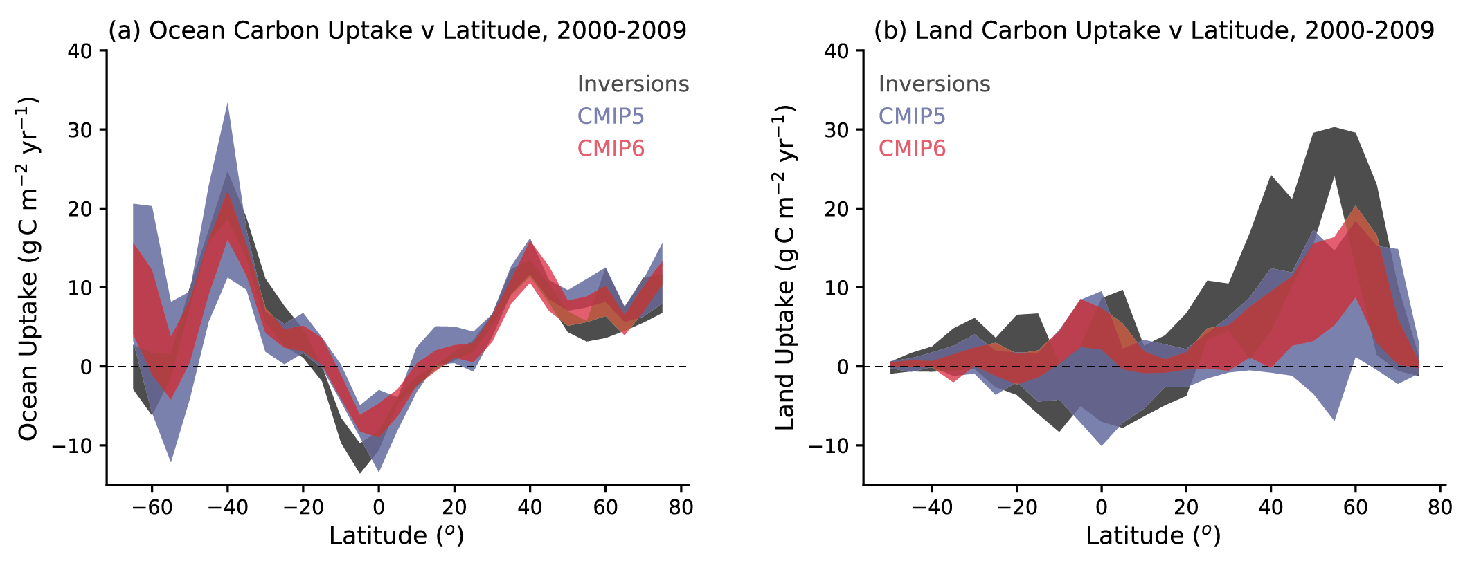 Figure 5.24 | Comparison of modelled zonal distribution of contemporary carbon sinks against atmospheric inversion estimates for 2000–2009: (a) ocean carbon uptake; (b) net land uptake. Latitude runs from 90°S (i.e., –90°N) to 90°N. Positive uptake represents a carbon sink to ocean/land while negative uptake represents a carbon source. The land uptake is taken as net biome productivity (NBP) and so includes net land-use change emissions. The bands show the mean ±1 standard deviation across the available inversions (black bands, 3 models), CMIP5 Earth system models (ESMs) (blue bands, 12 models for the ocean, 12 models for the land), and CMIP6 ESMs (red bands, 11 models for ocean, 10 models for land). Further details on data sources and processing are available in the chapter data table (Table 5.SM.6).
 It has been previously noted that AR5 models tended to overestimate land uptake in the tropics and underestimate uptake in the northern mid-latitudes, compared to inversion estimates. The inclusion of nitrogen limitations on CO2 -fertilization within CMIP6 models was expected to reduce this discrepancy (Anav et al., 2013). There is indeed some evidence that the CMIP6 ensemble (red wedge in Figure 5.24b) captures the northern land carbon sink more clearly than CMIP5 (blue wedge in Figure 5.24b), but there remains a tendency for the ESMs to place more of the global land carbon sink in the tropics than the mid-latitudes, compared to the inversion estimates. Based on a consistent signal across CMIP6 ESMs, there is medium confidence that land carbon cycle models continue to underestimate the Northern Hemisphere land carbon sink, when compared to estimates from atmospheric inversion (Ciais et al., 2019).
5.4.5.4 Coupled Climate–Carbon Cycle Projections
Land and ocean carbon uptake are driven primarily by increases in atmospheric CO2 (Figure 5.25). As a result, the evolution of land and ocean carbon sinks differs significantly between the SSP scenarios. Under scenarios that have greater increases in atmospheric CO2 (such as SSP5-8.5 and SSP3-7.0) the absolute values of the sinks are larger, but the fraction of implied emissions taken up by the sinks declines through the 21st century. By contrast, scenarios that assume CO2 stabilization in the 21st century (such as SSP1-2.6 or SSP2-4.5), have smaller absolute sinks, but these sinks take up an increasing fraction of the implied emissions (Figure 5.25d). These general principles apply to the ocean and land carbon sinks.
The concentration-driven CMIP6 ESMs agree well on the evolution of the global ocean carbon sink through the 21st century for four SSP scenarios (Figure 5.25). The five-year ensemble mean ocean sink declines to 0.6 ± 0.2 GtC yr–1by 2100 under SSP1-2.6, and peaks around 2080 at 5.4 ± 0.4 GtC yr–1under SSP5-8.5. Cumulative ocean carbon uptake from 1850 is projected to saturate at approximately 290 ± 30 GtC under SSP1-2.6, and to reach 520 ± 40 GtC by 2100 under SSP5-8.5 (Figure 5.25e).
The ensemble mean changes in land and ocean sinks are qualitatively similar, but the land shows much higher interannual variability in carbon uptake (Figure 5.25c) and also a much larger spread in the model projections of cumulative land carbon uptake (Figure 5.25f). The five-year ensemble mean net land carbon sink is projected to decline to 0.4 ± 1.0 GtC yr–1by 2100 under SSP1-2.6, and to reach around 5.6 ± 3.7 GtC yr–1under SSP5-8.5 (Figure 5.25c). Cumulative net land carbon uptake from 1850 is projected to saturate at approximately 150 ± 35 GtC under SSP1-2.6, and to reach 310 ± 130 GtC by 2100 under SSP5-8.5. Significant uncertainty remains in the future of the global land carbon sink, but there has been a notable reduction in the model spread from CMIP5 to CMIP6.
 Figure 5.25 | Modelled evolution of the global land and ocean carbon sinks for 1900 to 2100 in concentration-driven CMIP6 Earth system model (ESM) scenario runs. (SSP1-2.6: blue; SSP2-4.5: orange; SSP3-7.0: red; SSP5-8.5: brown): (a) prescribed atmospheric CO2 concentrations; (b) five-year running mean ocean carbon sink (GtC yr–1); (c) five-year running mean net land carbon sink (GtC yr–1); (d) inferred cumulative sink fraction of emissions from 1850; (e) change in ocean carbon storage from 1850 (GtC); (f) change in land carbon storage from 1850 (GtC). Thick lines represent the ensemble mean of the listed ESM runs, and the error bars represents ± 1 standard deviation about that mean. The grey wedges represent estimates from the global carbon project (GCP), assuming uncertainties in the annual mean ocean and net land carbon sinks of 0.5 GtC yr–1 and 1 GtC yr–1 respectively, and uncertainties in the changes in carbon stores (ocean, land and cumulative total emissions) of 25 GtC. The net land carbon sink is taken as net biome productivity (NBP) and so includes any modelled net land-use change emissions. Further details on data sources and processing are available in the chapter data table (Table 5.SM.6).
 Geographical patterns of carbon changes for four SSP scenarios are shown in Figure 5.26, with cleared areas (no diagonal lines) showing agreement on the sign of the change by at least 80% of the models. In all scenarios the ocean sink is strongest in the Southern Ocean and North Atlantic. The land carbon sink occurs primarily where there are present-day forests. In the mid- and high-northern latitudes, a carbon sink is projected as a result of the combined impacts of increasing CO2 and warming (Section 5.4.5.5). Changes in land carbon storage in the tropics also depend strongly on the assumed rate of deforestation which varies in magnitude across the SSPs, from relatively low rates in SSP1-2.6 to relatively high rates in SSP3-7.0.
 Figure 5.26 | Maps of net carbon changes under four Shared Socio-economic Pathway (SSP) scenarios, as evaluated from nine CMIP6 Earth system models. Uncertainty is represented using the simple approach (see Cross-Chapter Box Atlas.1 for more information). No overlay indicates regions with high model agreement, where ≥80% of models agree with the ensemble mean on the sign of change. Diagonal lines indicate regions with low model agreement, where <80% of models agree with the ensemble mean on the sign of change. On land, this is calculated as the time integral of net biome productivity (NBP), for the ocean it is the time-integral of air–sea carbon dioxide (CO2) gas flux anomalies relative to the pre-industrial. Further details on data sources and processing are available in the chapter data table (Table 5.SM.6).
 In summary, oceanic and terrestrial carbon sinks are projected to continue to grow with increasing atmospheric concentrations of CO2, but the fraction of emissions taken up by land and ocean is expected to decline as the CO2 concentration increases (high confidence). In the ensemble mean, ESMs suggest approximately equal global land and ocean carbon uptake for each of the SSP scenarios. However, the range of model projections is much larger for the land carbon sink. Despite the wide range of model responses, uncertainty in atmospheric CO2 by 2100 is dominated by future anthropogenic emissions rather than carbon–climate feedbacks (high confidence).
5.4.5.5 Linear Feedback Analysis
To diagnose the causes of the varying time-evolution of carbon sinks, the traditional linear feedback approach is adopted (Friedlingstein et al., 2003), as used previously to analyse C4MIP (Friedlingstein et al., 2006) and CMIP5 models (Arora et al., 2013). Changes in land carbon storage (ΔCL) and changes in ocean carbon storage (ΔCo) are decomposed into contributions arising from warming (ΔT) and increases in CO2 (ΔCO2):

whereβL (βo) and γ L (γ o) are coefficients that represent the sensitivity of land (ocean) carbon storage to changes in CO2 and global mean temperature respectively. This feedback formalism is one of several that have been proposed for analysing climate–carbon cycle feedbacks (Lade et al., 2018).
This quasi-equilibrium framework is scenario dependent because of the time scales associated with land and ocean carbon uptake, as discussed in AR5 (WGI, Box 6.4). However, it is retained here for traceability with AR5. This approach has been used to define a number of emergent constraints on carbon cycle feedbacks (Section 5.4.6) and to reconstruct the transient climate response to cumulative CO2 emissions (TCRE) (Jones and Friedlingstein, 2020), as in Section 5.5. To minimize the confounding effect of the scenario dependence, β and γvalues are diagnosed from idealized runs in which a 1% per year increase in atmospheric CO2 concentration is prescribed, as for AR5 (WGI, Box 6.4; Arora et al., 2013). Values ofβare calculated from ‘biogeochemical’ runs in which the prescribed CO2 increases do not affect climate, and these are then used to isolateγvalues in fully coupled runs where both climate and CO2 change (Friedlingstein et al., 2003).
Table 5.5 shows the global land and global ocean values ofβ and γ for each of the CMIP6 ESMs (Arora et al., 2020). The last two rows show the ensemble means and standard deviation across the ensemble for CMIP6 and CMIP5. In both ensembles, the largest uncertainties are in the sensitivity of land carbon storage to CO2 (βL) and the sensitivity of land carbon storage to temperature (γ L). The more widespread modelling of nitrogen limitations in CMIP6 was expected to lead to reductions in both of these feedback parameters. There is some evidence for that, with ensemble meanγ L moving from –58 ± 38 GtC K–1 to –33 ± 33 GtC K–1. Between CMIP5 and CMIP6, there are also reductions in ensemble meanβo (0.82 to 0.77 GtC ppm–1), βL (0.93 to 0.89 GtC ppm–1) and γ o (–17.3 to –16.9 GtC K–1), but these are progressively less significant compared to the model spread in each case.
Land Feedback Factors | Ocean Feedback Factors | |||
Model Name | βL(PgC ppm–1) | γ L(PgC K–1) | βo(PgC p_uo c;hnjppm–1) | γ o(PgC K–1) |
ACCESS-ESM1.5 | 0.37 | –21.1 | 0.90 | –23.8 |
CanESM5 | 1.28 | 16.0 | 0.77 | –14.7 |
CESM2 | 0.90 | –21.6 | 0.71 | –10.9 |
CNRM-ESM2-1 | 1.36 | –83.1 | 0.70 | –9.4 |
IPSL-CM6A-LR | 0.62 | –8.7 | 0.76 | –13.0 |
MIROC-ES2L | 1.12 | –69.6 | 0.73 | –22.3 |
MPI-ESM1.2-LR | 0.71 | –5.2 | 0.77 | –20.1 |
NOAA-GFDL-ESM4 | 0.93 | –80.1 | 0.84 | –21.7 |
NorESM2-LM | 0.85 | –21.0 | 0.78 | –19.6 |
UKESM1-0-LL | 0.75 | –38.4 | 0.75 | –14.1 |
CMIP6 Model Mean | 0.89±0.30 | –33.3±33.8 | 0.77±0.06 | –16.9±5.1 |
CMIP5 Model Mean | 0.93±0.49 | –57.9±38.2 | 0.82±0.07 | –17.3±3.8 |
In these idealized 1% per year CO2 runs, the CMIP6 models show reasonable agreement on the patterns of carbon uptake and also on the separate impacts of CO2 increase and climate change (Figure 5.27). For the ensemble mean, increasing atmospheric CO2 increases carbon uptake by the oceans, especially in the Southern Ocean and the North Atlantic Ocean, and on the land, especially in tropical and boreal forests (β, Figure 5.27a). Climate change further enhances land carbon storage in the boreal zone, but has a compensating negative impact on the carbon sink in tropical and subtropical lands, and in the North Atlantic Ocean (γ , Figure 5.27b). Overall, the ensemble mean of the CMIP6 ESMs model indicates increasing carbon storage with CO2 in almost all locations (Figure 5.27c).
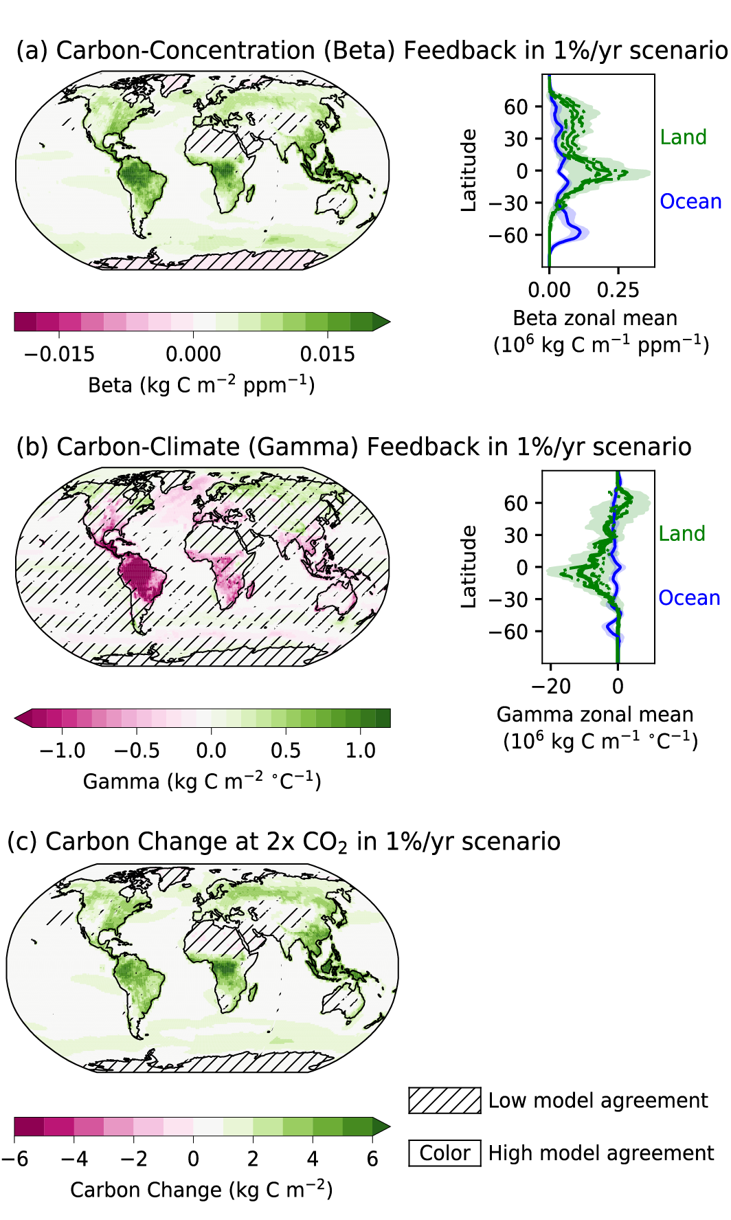 Figure 5.27 | Maps of carbon-concentration and carbon–climate feedback terms, as well as net carbon changes under the idealized 1% per year carbon dioxide (CO2 ) scenario, as evaluated from CMIP6 Earth system models (ESMs). Shown are the model means from nine CMIP6 ESMs. Uncertainty is represented using the simple approach (see Cross-Chapter Box Atlas.1 for more information): No overlay indicates regions with high model agreement, where ≥80% of models agree with the ensemble mean on the sign of change; diagonal lines indicate regions with low model agreement, where <80% of models agree with the ensemble mean on the sign of change. Also shown are zonal-mean latitude profiles of land (green) and ocean (blue) feedbacks. On the land, the zonal mean feedback for the mean of the ensemble of models that include nitrogen is shown as dashed lines, and for carbon-only models as dash-dotted lines, and the carbon–climate feedback from one permafrost-carbon enabled ESM is shown as a dotted line. Carbon changes are calculated as the difference between carbon stocks at different times on land and for the ocean as the time integral of atmosphere–ocean CO2 flux anomalies relative to the pre-industrial. The denominator for gamma here is the global mean surface air temperature. Further details on data sources and processing are available in the chapter data table (Table 5.SM.6).
 5.4.6 Emergent Constraints to Reduce Uncertainties in Projections
Emergent constraints are based on relationships between observable aspects of the current or past climate (such as trends or variability), and uncertain aspects of future climate change (such as the strength of particular feedbacks). These relationships are evident across an ensemble of models. When combined with an observational estimate of the trend or variability in the real climate, such emergent relationships can yield ‘emergent constraints’ on future climate change (Hall et al., 2019). At the time of AR5 (WGI, Section 9.8.3), there had been relatively few applications of the technique to constrain carbon cycle sensitivities, but there have been many studies published since (e.g., the summary in Cox, 2019). Figure 5.28 shows some key published emergent constraints on the carbon cycle in ESMs.
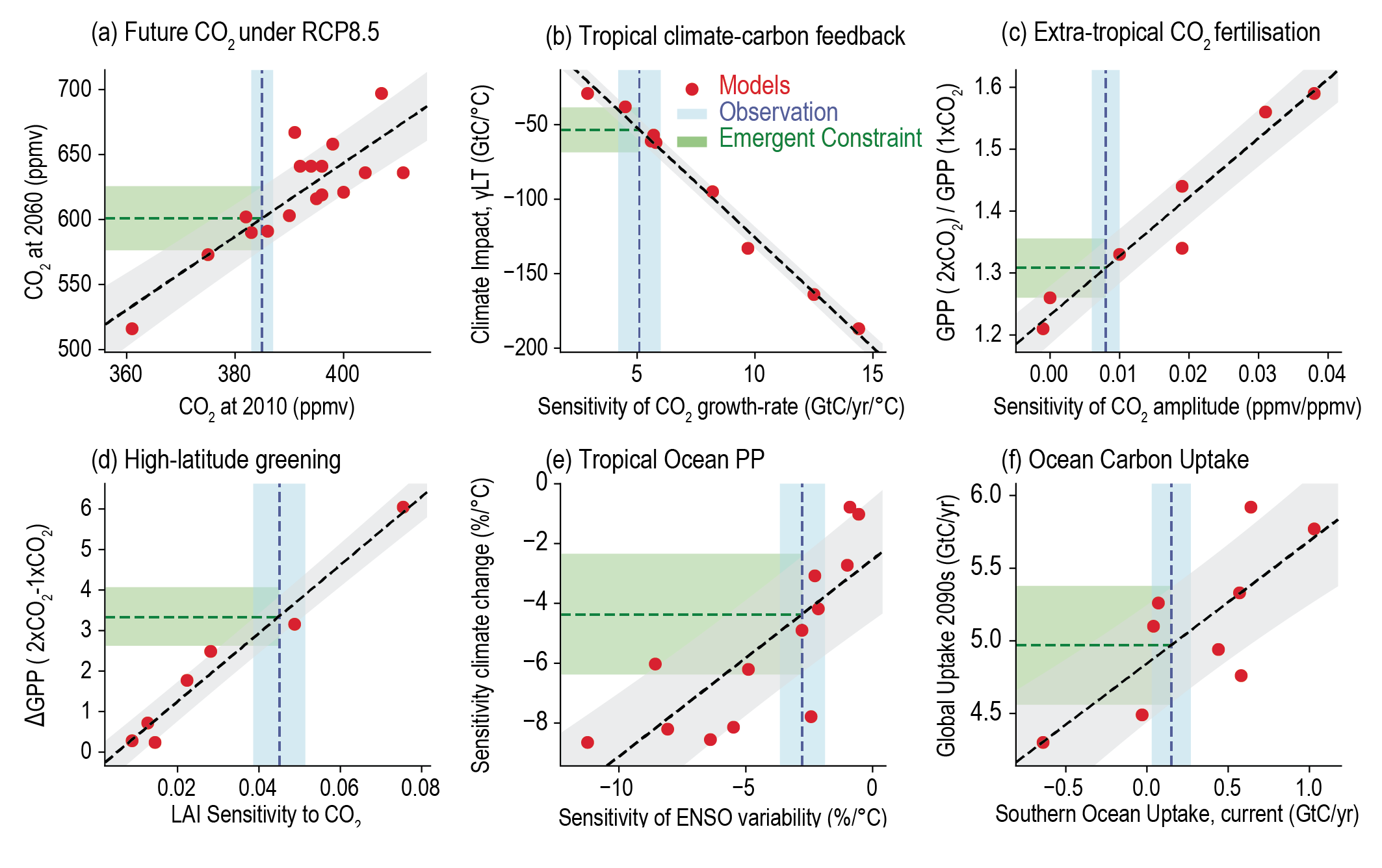 Figure 5.28 | Examples of emergent constraints on the carbon cycle in Earth system models (ESMs), reproduced from previously published studies: (a) projected global mean atmospheric carbon dioxide (CO2) concentration by 2060 under the RCP8. 5 emissions scenario against the simulated CO2 in 2010 (Friedlingstein et al., 2014b; Hoffman et al., 2014); (b) sensitivity of tropical land carbon to warming (γ LT) against the sensitivity of the atmospheric CO2 growth-rate to tropical temperature variability (Cox et al., 2013; Wenzel et al., 2014); (c) sensitivity of extratropical (30°N–90°N) gross primary production to a doubling of atmospheric CO2 against the sensitivity of the amplitude of the CO2 seasonal cycle at Kumkahi, Hawaii to global atmospheric CO2 concentration (Wenzel et al., 2016); (d) change in high-latitude (30°N–90°N) gross primary production versus trend in high-latitude leaf area index or ‘greenness’ (Winkler et al., 2019); (e) sensitivity of the primary production of the Tropical Ocean to climate change versus its sensitivity to El Niño–Southern Oscillation (ENSO)-driven temperature variability (Kwiatkowski et al., 2017); (f) global ocean carbon sink in the 2090s versus the current-day carbon sink in the Southern Ocean. In each case, a red dot represents a single ESM projection, the grey bar represents the emergent relationship between the y-variable and the x-variable, the blue bar represents the observational estimate of the x-axis variable, and the green bar represents the resulting emergent constraint on the y-axis variable. The thicknesses represent ± one standard error in each case. Figure after Cox (2019). Further details on data sources and processing are available in the chapter data table (Table 5.SM.6).
 5.4.7 Climate Feedbacks from CH4 and N2O
Sources and sinks of CH4 and N2O respond both directly and indirectly to atmospheric CO2 concentration and climate change, and thereby give rise to additional biogeochemical feedbacks in the climate system, which may amplify or attenuate climate–carbon cycle feedbacks (Gasser et al., 2017; Lade et al., 2018; Denisov et al., 2019). Many of these of feedbacks are only partially understood, and thus were only partially addressed in AR5 (WGI, Sections 6.3.3, 6.3.4 and 6.4.7). Since AR5, a growing body of estimates from ESMs, as well as independent modelling and observation-based studies, enable improved estimates of the associated feedbacks.
The goal of this section is to assess the climate feedback parameters α , as it is defined in Section 7.4.1.1, for CH4 and N2O biogeochemical feedbacks. The strength of the feedbacks is estimated in a linear framework (Gregory et al., 2009), using the radiative forcing equations for CO2, CH4 and N2O (Etminan et al., 2016). In addition to estimates from ESMs, the feedback parameter α is estimated from independent estimates of surface emission climate sensitivities and atmospheric box models, following (Arneth et al., 2010; Thornhill et al., 2021). These assessed feedback parameters are used in Section 7.4.2.5.
The CH4 feedbacks may arise from changing wetland emissions (including rice farming) and from sources that are expected to grow under climate change (e.g., related to permafrost thaw, fires, and freshwater bodies). CH4 emissions from wetlands and landfills generally increase with warming due to enhanced decomposition with higher temperatures, thereby potentially providing a positive CH4 feedback on climate (Dean et al., 2018). The contribution of wetlands to interannual variability of atmospheric CH4 is shaped by the different impacts of temperature and precipitation anomalies on wetland emissions (e.g., during El Niño episodes) and therefore the relationship between climate anomalies and the wetland contribution to the CH4 growth rate is complex (Pison et al., 2013; Nisbet et al., 2016; X. Zhang et al., 2020). As assessed by SROCC (IPCC, 2019b), there is high agreement across model simulations that wetlands CH4 emissions will increase in the 21st century, butlow agreement in the magnitude of the change (Denisov et al., 2013; Shindell et al., 2013; B.D. Stocker et al., 2013; Zhang et al., 2017; Koffi et al., 2020). Climate change increases wetland emissions (Gedney et al., 2004, 2019; Volodin, 2008; Ringeval et al., 2011; Denisov et al., 2013; Shindell et al., 2013) and gives rise to an estimated wetland CH4–climate feedback of 0.03 ± 0.01 W m–2°C–1 (mean ± 1 standard deviation; limited evidence, high agreement) (Arneth et al., 2010; Shindell et al., 2013; B.D. Stocker et al., 2013; Zhang et al., 2017). The effect of rising CO2 on productivity, and therefore on the substrate for methanogenesis, can further increase the projected increase in wetland CH4 emissions (Ringeval et al., 2011; Melton et al., 2013). Model projections accounting for the combined effects of CO2 and climate change suggest a potentially larger climate feedback (0.01–0.16 W m–2°C–1) (limited evidence, low agreement) (Gedney et al., 2019; Thornhill et al., 2021). Methane release from wetlands depends on the nutrient availability for methanogenic and methanotrophic microorganisms that can further modify this feedback (Stepanenko et al., 2016; Donis et al., 2017; Beaulieu et al., 2019). Methane emissions from thermokarst ponds and wetlands resulting from permafrost thaw are estimated to contribute an additional CH4-climate feedback of 0.01 [0.003 to 0.04, 5–95% range] W m–2°C–1 (limited evidence, low agreement).
Methane release from wildfires may increase by up to a factor of 1.5 during the 21st century (Eliseev et al., 2014a, b; Kloster and Lasslop, 2017). However, given the contemporary estimate for CH4 from wildfires of no more than 16 TgCH4yr–1 (van der Werf et al., 2017; Saunois et al., 2020), this feedback is small, adding no more than 40 ppb to the atmospheric CH44 by the end of the 21st century (medium confidence). Methane emissions from pan-Arctic freshwater bodies is also estimated to increase by 16 TgCH4yr–1 in the 21st century (Tan and Zhuang, 2015). Emissions from subsea and permafrost methane hydrates are not expected to change substantially in the 21st century (Section 5.4.9.1.3).
Land biosphere models show high agreement that long-term warming will increase N2O release from terrestrial ecosystems (Xu-Ri et al., 2012; B.D. Stocker et al., 2013; Zaehle, 2013; Tian et al., 2019). A positive land N2O climate feedback is consistent with paleo-evidence based on reconstructed and modelled emissions during the last deglacial period (Schilt et al., 2014; H. Fischer et al., 2019; Joos et al., 2020). The response of terrestrial N2O emissions to atmospheric CO2 increase and associated warming is dependent on nitrogen availability (van Groenigen et al., 2011; Butterbach-Bahl et al., 2013; Tian et al., 2019). Model-based estimates do not account for the potentially strong emissions increases in boreal and arctic ecosystems associated with future warming and permafrost thaw (Elberling et al., 2010; Voigt et al., 2017). There is medium confidence that the land N2O climate feedback is positive, but low confidence in the magnitude (0.02 ± 0.01 W m–2°C–1).
Climate change will also affect N2O production in the ocean (Codispoti, 2010; Freing et al., 2012; Bopp et al., 2013; Rees et al., 2016; Breider et al., 2019). Model projections in the 21st century show a 4–12% decrease in ocean N2O emissions under RCP8.5 due to a combination of factors, including increased ocean stratification, decreased ocean productivity, and the impact of increasing atmospheric N2O abundance on the air–sea flux, corresponding to an ocean N2O climate feedback of –0.008 ± 0.002 W m–2°C–1 (limited evidence, high agreement) (Martinez-Rey et al., 2015; Landolfi et al., 2017; Battaglia and Joos, 2018b). On millennial time scales, the ocean N2O climate feedback may be positive, owing to ocean deoxygenation and long-term increases in remineralization (Battaglia and Joos, 2018b).
Based-on these studies, there is medium confidence that the combined climate feedback parameter for CH4 and N2O is positive, but there is low confidence in the magnitude of the estimate (0.05 [0.02 to 0.09] W m–2°C–1, 5–95% range).
5.4.8 Combined Biogeochemical Climate Feedback
This section assesses the magnitude of the combined biogeochemical feedback in the climate system (Figure 5.29) by integrating evidence from: carbon-cycle projections represented in Earth system models (Section 5.4.5.5), independent estimates of CO2 emissions due to permafrost thaw (Box 5.1) and fire (Section 5.4.3.2), natural CH4 and N2O emissions (Section 5.4.7), and aerosol and atmospheric chemistry (Section 6.3.6). We derive a physical climate feedback parameter α , as defined in Section 7.4.1.1, for CO2 -based feedbacks using the linear framework proposed by Gregory et al. (2009), using the radiative forcing equations for CO2 (Etminan et al., 2016).
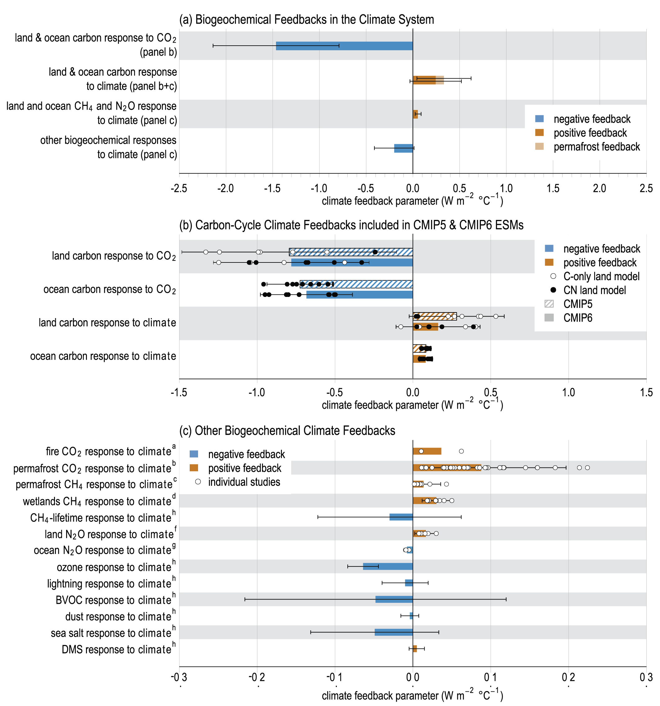 Figure 5.29 | Estimates of the biogeochemical climate feedback parameter ( α ). The parameter α (W m−2°C−1) for a feedback variable x is defined as
 The climate feedback parameter for CO2 (–1.13 ± 0.45 W m–2°C–1, mean and 1 standard-deviation range) is dominated by the contribution of the CO2 -induced increase of ocean and land carbon storage (–1.46 ± 0.41 W m–2°C–1, corresponding to aβL+O of 1.66 ± 0.31 PgC ppm–1), with smaller contributions from the carbon cycle’s response to climate (0.24 ± 0.17 W m–2°C–1, corresponding toγ L+O of –50 ± 34 PgC °C–1), and emissions from permafrost thaw (0.09 [0.02 to 0.20] W m–2°C–1, corresponding toγof –18 [3 to 41] PgC °C–1, mean and 5–95% range) (Figure 5.29a). This estimate does not include an estimate of the fire-related CO2 feedback (range: 0.01–0.06 W m–2°C–1), as onlylimited evidence was available to inform its assessment. The sum (mean and 5–95th percentile range) of feedbacks from natural emissions of CH4 including permafrost thaw, and N2O (0.05 [0.02 to 0.09] W m–2°C–1), and feedbacks from aerosol and atmospheric chemistry (–0.20 [–0.41 to 0.01] W m–2°C–1) leads to an estimate of the non-CO2 biogeochemical feedback parameter of –0.15 [–0.36 to +0.06] W m–2°C–1. There is low confidence in the estimate of the non-CO2 biogeochemical feedbacks, due to the large range in the estimates of α for some individual feedbacks (Figure 5.29c), which can be attributed to the diversity in how models account for these feedbacks, limited process-level understanding, and the existence of known feedbacks where there is insufficient evidence to assess the feedback strength.
CO2 and non-CO2 biogeochemical feedbacks are an important component of the assessment of TCRE and the remaining carbon budget (Section 5.5). The feedbacks of the carbon cycle of CO2 and climate are implicitly taken account in the TCRE assessment, because they are represented in the various underlying lines of evidence. Other feedback contributions, such as the non-CO2 biogeochemical feedback, can be converted into a carbon-equivalent feedback term (γ; Section 5.4.5.5, 7.6) by reverse application of the linear feedback approximation (Gregory et al., 2009). The contributions of non-CO2 biogeochemical feedbacks combine to a linear feedback term of 30 ± 27 PgCeq °C–1 (1 standard deviation range, 111 ± 98 Gt CO2- eq °C–1), including a feedback term of –11 [–18 to –5] PgCeq °C–1 (5–95% range, –40 [–62 to –18] Gt CO2- eq °C–1) from natural CH4 and N2O sources. The biogeochemical feedback from permafrost thaw leads to a combined linear feedback term of –21 ± 12 PgCeq °C–1 (1 standard deviation range –77 ± 44 Gt CO2- eq °C–1). For the integration of these feedbacks in the assessment of the remaining carbon budget (Section 5.5.2), two individual non-CO2 feedbacks (tropospheric ozone, and methane lifetime) are captured in the AR6-calibrated emulators (Box 7.1). Excluding those two contributions, the resulting combined linear feedback term for application in Section 5.5.2 is assessed at a reduction of 7 ± 27 PgCeq °C–1 (1 standard deviation range, –26 ± 97 PgCeq °C–1). For the same reasons as for the feedback terms expressed in W m–2°C–1 (see above), there is overall low confidence in the magnitude of these feedbacks.
5.4.9 Abrupt Changes and Tipping Points
The applicability of the linear feedback framework (Section 5.4.5.5) suggests that large-scale biogeochemical feedbacks are approximately linear in the forcing from changes in CO2 and climate. Nevertheless, regionally the biosphere is known to be capable of producing abrupt changes or even ‘tipping points’ (Higgins and Scheiter, 2012; Lasslop et al., 2016). Abrupt change is defined as a change in the system that is substantially faster than the typical rate of the changes in its history (Section 1.4.5). A related matter is a tipping point: a critical threshold beyond which a system reorganizes, often abruptly and/or irreversibly. Possible abrupt changes in the Earth system include those related to ecosystems and biogeochemistry (Lenton et al., 2008; Steffen et al., 2018): tropical and boreal forest dieback; and release of greenhouse gases (GHGs) from permafrost and methane clathrates (Table 5.6). In this section we therefore focus on estimating upper limits on the possible impact of abrupt changes on the evolution of atmospheric GHGs out to 2100, for comparison to the impact of direct anthropogenic emissions.
Abrupt Change/Tipping Point | Key Region(s) | Probability to Occur in the 21st Century | Maximum CO2or CH4Release in the 21st Century | Principal Development Time Scale | Maximum CO2or CH4Rate of Change Over the 21st Century | (Ir)reversibility |
Tropical forests dieback (Section 5.4.9.1.1) | Amazon watershed | Low | <200 PgC as CO2 (Section 5.4.9.1.1; medium confidence) | Multi-decadal | CO2 : <0.5 ppm yr–1 | Irreversible at multi-decadal scale (medium confidence) |
Boreal forests dieback (Sections 5.4.9.1.1, 5.4.3.2) | Boreal Eurasia and North America | Low | <27 Pg (Section 5.4.9.1.2; medium confidence) | Multi-decadal | Small (low confidence) | Irreversible at multi-decadal scale (medium confidence) |
Biogenic emissions from permafrost thaw (Section 5.4.9.1.2) | Pan-Arctic | High | up to 240 PgC of CO2 and up to 5300 Tg of CH4Section 5.4.8.1.2; low confidence) | Multi-decadal | CO2 : ≤1 ppm yr–1 CH4: ≤10 ppb yr–1 | Irreversible at centennial time scales (high confidence) |
Methane release from clathrates (Section 5.4.9.1.3) | Oceanic shelf | Very low | very likely small (Section 5.4.9.1.3) | Multi-millennium | CH4: ≤0.2 ppb yr–1 | Irreversible at multi-millennium time scales (medium confidence) |
5.4.9.1 Assessment of Biogeochemical Tipping Points
5.4.9.1.1 Forest dieback
Published examples of abrupt biogeochemical changes in models include tropical rain forest dieback (Cox et al., 2004; Jones et al., 2009; Brando et al., 2014; Le Page et al., 2017; Zemp et al., 2017), and temperate and boreal forest dieback (Joos et al., 2001; Lucht et al., 2006; Scheffer et al., 2012; Lasslop et al., 2016; Section 5.4.3). Such transitions may be related to: (i) large-scale changes in mean climate conditions crossing particular climate thresholds (Joos et al., 2001; Cox et al., 2004; Lucht et al., 2006; Hirota et al., 2011; Scheffer et al., 2012; Le Page et al., 2017; Zemp et al., 2017); (ii) temperature and precipitation extremes (Staver et al., 2011; Higgins and Scheiter, 2012; Scheffer et al., 2012; Pavlov, 2015; Zemp et al., 2017); or (iii) possible enhancement and intermittency in fire activity (Staver et al., 2011; Higgins and Scheiter, 2012; Lasslop et al., 2016; Brando et al., 2020). Simulated changes in forest cover are a combination of the effects of CO2 on photosynthesis and water-use efficiency (Section 5.4.1), and the effects of climate change on photosynthesis, respiration and disturbance (Section 5.4.3). In ESMs, direct CO2 effects tend to enhance forest growth, but the impacts of climate change vary between being predominantly negative in the tropics and predominantly positive in the boreal zone (Figure 5.27).
Most ESMs project continuing carbon accumulation in tropical forests as a result of direct CO2 effects overwhelming the negative effects of climate change (Huntingford et al., 2013; Drijfhout et al., 2015; Boulton et al., 2017). In the real world, forests may be less vulnerable to climate changes than those modelled in ESMs because of the greater plant trait diversity, which confers additional resilience (Reyer et al., 2015; Levine et al., 2016; Sakschewski et al., 2016), and because of possible acclimation of vegetation to warming (Good et al., 2011, 2013; Lloret et al., 2012; Mercado et al., 2018). On the contrary, forests may be more vulnerable in the real world due to indirect climate change effects such as insect outbreaks and diseases not considered here (Section 5.4.3.2) or model limitations in representing the effects disturbances such as wildfire and droughts. In general, forests are most vulnerable when climate change is combined with increased rates of direct deforestation (Nobre et al., 2016; Le Page et al., 2017).
To estimate an upper limit on the impact of Amazon forest dieback on atmospheric CO2, we consider the very unlikely limiting case of negligible direct-CO2 effects (Section 5.4.1). Emergent constraint approaches (Section 5.4.6) may be used to estimate an overall loss of tropical land carbon due to climate change alone, of around 50 PgC per °C of tropical warming (Cox et al., 2013; Wenzel et al., 2014). This implies an upper limit to the release of tropical land carbon of <200 PgC over the 21st century (assuming tropical warming of <4°C, and no CO2 -fertilization), which translates to dCO2 /dt <0.5 ppm yr–1.
Boreal forest dieback is not expected to change the atmospheric CO2 concentration substantially because forest loss at the south is partly compensated by: (i) temperate forest invasion into previously boreal areas; and (ii) boreal forest gain at the north (Friend et al., 2014; Kicklighter et al., 2014; Schaphoff et al., 2016) (medium confidence). An upper estimate of this magnitude, based on statistical modelling of climate change alone, is of 27 Pg vegetation carbon loss in the southern boreal forest, which is roughly balanced by gains in the northern zone (Koven, 2013). Carbon release from vegetation and soil due to wildfires in boreal regions (Eliseev et al., 2014b; Turetsky et al., 2015; X.J. Walker et al., 2019) is also not expected to change this estimate substantially because of its small present-day value of about 0.2 PgC yr–1 (van der Werf et al., 2017), and because of likely increases in precipitation in boreal regions (Section 4.5.1).
5.4.9.1.2 Biogenic emissions following permafrost thaw
There is large uncertainty in release of GHGs from permafrost in the 21st century. The largest of these estimates implies tens to hundreds of gigatons of carbon released in the form of CO2 (Box 5.1) and CH4 emissions up to 100 TgCH4yr–1 (Box 5.1). A carbon dioxide release of such magnitude would lead to an increase in the CO2 accumulation rate in the atmosphere of ≤1 ppm yr–1. These emissions develop at a multi-decadal time scale. Assuming a CH4 lifetime in the atmosphere of the order of 10 years and the associated feedback parameter of 1.34 ± 0.04 (Section 6.2.2.1), this would increase the atmospheric CH4 content by about 500 ppb over the century, corresponding to a rate of ≤10 ppb yr–1. Irrespective of its origin, additional CH4 accumulation of such a magnitude is not expected to modify the temperature response to anthropogenic emissions by more than a few tenths of a °C (Gedney et al., 2004; Eliseev et al., 2008; Denisov et al., 2013). Emissions from permafrost thawing are assessed in Box 5.1.
5.4.9.1.3 Methane release from clathrates
The total global clathrate reservoir is estimated to contain 1500–2000 PgC (Archer et al., 2009; Ruppel and Kessler, 2017), held predominantly in ocean sediments, with only an estimated 20 PgC in and under permafrost (Ruppel, 2015). The present-day CH4 release from shelf clathrates is <10 TgCH4yr–1 (Kretschmer et al., 2015; Saunois et al., 2020). Despite polar amplification (Chapter 7), substantial releases from the permafrost-embedded subsea clathrates is very unlikely (Minshull et al., 2016; Malakhova and Eliseev, 2017, 2020). This is consistent with an overall small release of CH4 from the shelf clathrates during the last deglacial transition, despite large reorganizations in climate state (Bock et al., 2017; Petrenko et al., 2017; Dyonisius et al., 2020). The long time scales associated with clathrate destabilization makes itunlikely that CH4 release from the ocean to the atmosphere will deviate markedly from the present-day value through the 21st century (Hunter et al., 2013), corresponding to no more than additional 20 ppb of atmospheric CH4 (i.e., <0.2 ppb yr–1). Another possible source of CH4 is gas clathrates in deeper terrestrial permafrost and below it (Buldovicz et al., 2018; Chuvilin et al., 2018), which may have caused recent craters in the north of Russia (Arzhanov et al., 2016, 2020; Arzhanov and Mokhov, 2017; Kizyakov et al., 2017, 2018). Land clathrates are formed at depths greater than 200 m (Ruppel and Kessler, 2017; Malakhova and Eliseev, 2020), which precludes a substantial response to global warming over the next few centuries and associated emissions.
Thus, it is very unlikely that CH4 emissions from clathrates will substantially warm the climate system over the next few centuries.
5.4.9.2 Abrupt Changes Detected in Earth System Model Projections
Projecting abrupt changes is intrinsically difficult, because by definition abrupt changes occur in a small region of the parameter and/or forcing space. At the time of AR5 there was no available systematic study of abrupt changes or tipping points in ESMs. An analysis of ESMs since AR5 has identified a number of abrupt changes in the CMIP5 ensemble (Drijfhout et al., 2015; Bathiany et al., 2020). These include abrupt changes in tropical forests and high-latitude greening, permafrost thaw, and vegetation composition change (Bathiany et al., 2020). Most modelled abrupt changes were detected in boreal and tundra regions, with few models showing Amazon forest dieback (Bathiany et al., 2020).
Based on the evidence presented in this section, we conclude that abrupt changes and tipping points in the biogeochemical cycles lead to additional uncertainty in 21st century GHG concentrations changes. However, these are very likely to be small compared to the uncertainty associated with future anthropogenic emissions (high confidence).
5.4.10 Long-term Response Past 2100
The AR5 assessed with very high confidence that the carbon cycle in the ocean and on land will continue to respond to climate change and rising atmospheric CO2 concentrations created during the 21st century (WGI, Chapter 6, Executive Summary). Since AR5, experiments with the Community Earth System Model version 1 (CESM1) under the RCP8.5 extension scenario to 2300, suggest that both land and ocean carbon–climate feedbacks strengthen in time, land and ocean carbon-concentration feedbacks weaken, and the relative importance of ocean sinks versus land sinks increases (Randerson et al., 2015). Under high emissions scenarios, this relative strengthening of land carbon–climate feedbacks leads the terrestrial biosphere to shift from sink to source at some point after 2100 in all of the CMIP5 ESMs and CMIP5-era Earth system models of intermediate complexity (EMICs) (Tokarska et al., 2016). The strengthening of land and ocean carbon–climate feedbacks projected beyond 2100 under high emissions scenarios offsets the declining climate sensitivity to incremental increases of CO2, leading to a net strengthening of carbon cycle feedbacks, as measured by the gain parameter, from one century to the next (Randerson et al., 2015).
Figure 5.30 shows carbon cycle changes to 2300 under three SSP scenarios with long-term extensions: SSP5-8.5, SSP5-3.4-overshoot, and SSP1-2.6, for four CMIP6 ESMs and one EMIC. Under all three scenarios, all five models project a reversal of the terrestrial carbon cycle from a sink to a source. However, the reasons for these reversals under very high emissions and low/negative emissions are very different. Under the SSP5-8.5 scenario, the terrestrial carbon–climate feedback is projected to strengthen, while the carbon-concentration feedbacks weaken after emissions peak at 2100, which together drives the land to become a net carbon source after 2100 (Tokarska et al., 2016). The difference in both timing and magnitude of this transition across the ensemble, leads to an assessment of medium confidence in the likelihood and low confidence in the timing and strength, of the land transitioning from a net sink to a net source under such a scenario. Based on high agreement across all available models, we assess with high confidence that the ocean sink strength would weaken but not reverse under a long-term high emissions scenario. In the SSP5-3.4-overshoot scenario, both the terrestrial and ocean reservoirs act as transient carbon sources during the overshoot period, when net anthropogenic CO2 emissions are negative and CO2 concentrations are falling, and then revert to near-zero (land) or weak sink (ocean) fluxes after stabilization of atmospheric CO2. The SSP1-2.6 scenario, characterized by lower peak CO2 concentrations, a smaller overshoot, and much less carbon loss from land-use change, shows instead a relaxation towards a neutral biosphere on land, and a sustained weak sink in the ocean (see also Section 5.6.2.2.1.2).
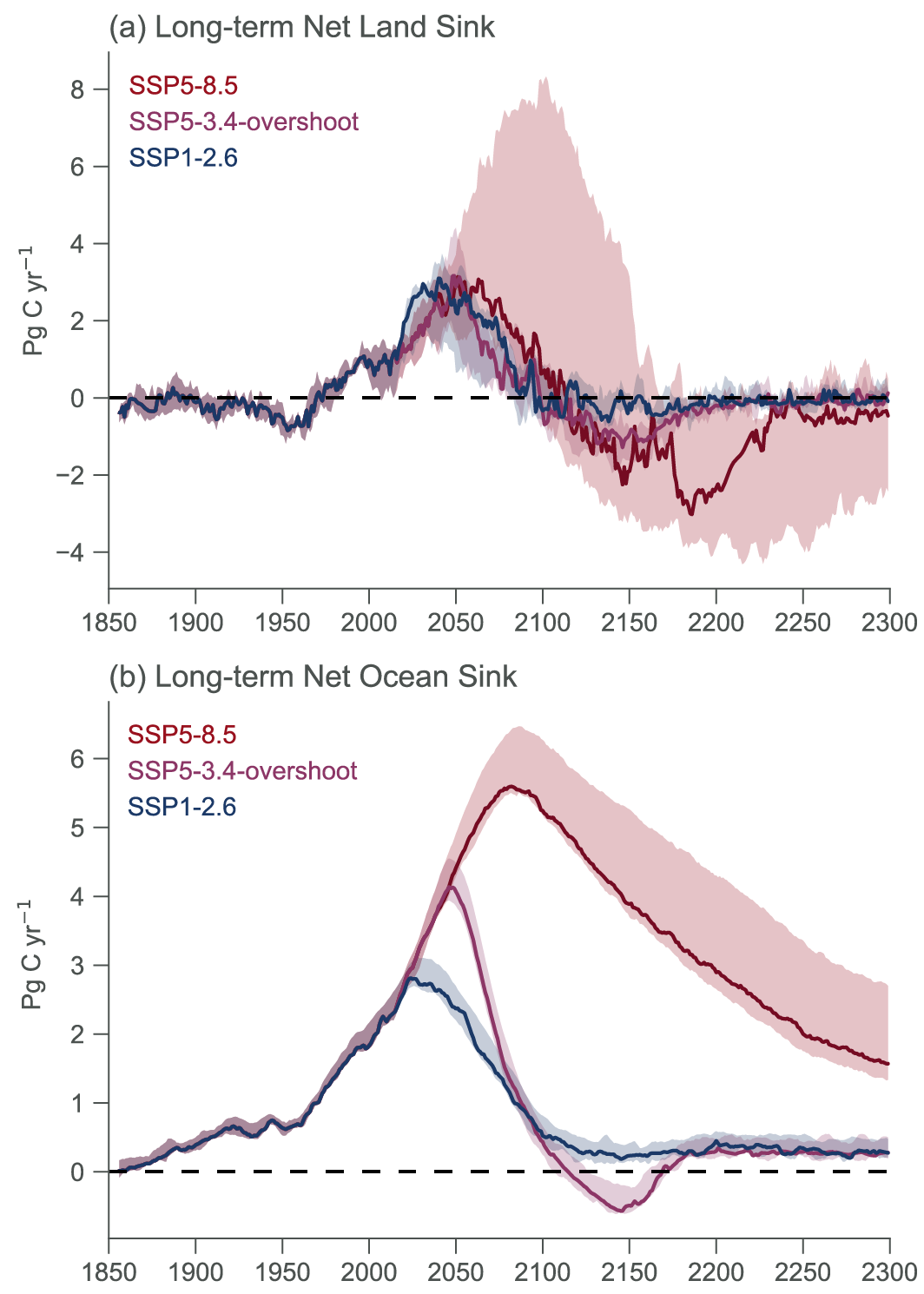 Figure 5.30 | Trajectories of carbon cycle dynamics for models beyond 2100. Shown are three scenarios: SSP5-8.5; SSP5-3.4-overshoot; and SSP1-2.6, from four ESMs (CanESM5, UKESM1, CESM2-WACCM, IPSL-CM6a-LR) and one EMIC (UVIC-ESCM, Mengis et al., 2020) for which extensions beyond 2100 are available. Solid lines represent the median flux value across the ensemble, and shading represents 15th–85th percentiles across the ensemble. Further details on data sources and processing are available in the chapter data table (Table 5.SM.6).
 5.4.11 Near-term Prediction of Ocean and Land Carbon Sinks
The AR5 (WGI, Section 11.3.2) assessed near-term climate predictability based on ESMs initialized from the observed climate state. Since AR5, a growing number of prediction systems have been developed based on ESMs that include the ocean and land carbon cycle components. Predictability of key physical climate variables (assessed in Chapter 4) provides a platform to establish predictive skill for interannual variations in the strength of the natural carbon sinks in response to internal climate variability. In most systems the carbon cycle components are only indirectly initialized and respond to the initialized climate variations (Li et al., 2019). This subsection synthesizes information on predictability of the land and ocean carbon sinks using both the idealized potential predictability and the actual predictability skill measures.
Longer-term memory residing in the ocean enables predictability of the ocean carbon sink (McKinley et al., 2017; Li and Ilyina, 2018). The predictive horizon of the globally integrated air–sea CO2 fluxes has been assessed in perfect-model frameworks that are based on an idealized ensemble of simulations in which each ensemble member serves as a verification, while no observations are assessed. Perfect-model studies provide an estimate of the upper range of potential predictability for the integrated air–sea CO2 fluxes of about two years globally and up to a decade in some regions (Séférian et al., 2018a; Spring and Ilyina, 2020). Evidence is also emerging for predictive skill of the global air–sea CO2 fluxes of up to six years based on prediction systems initialized with observed physical climate states (Ilyina et al., 2021), with a potential for even longer-term regional predictability in some regions, including the North Atlantic and subpolar Southern Ocean (H. Li et al., 2016; Lovenduski et al., 2019a).
Models suggest that predictability of the air–sea CO2 flux is related to predictability of ocean biogeochemical state variables such as dissolved inorganic carbon (DIC) and total alkalinity (TA; Lovenduski et al., 2019a), as well as the mixed layer depth (H. Li et al., 2016). Temperature variations largely control shorter-term predictability of the ocean carbon sink, while longer-term predictability is related to non-thermal drivers such as ocean circulation and biology (Li et al., 2019). Although there is a substantial spatial heterogeneity, initialized predictions suggest stronger multi-year variations of the air–sea CO2 flux and generally tend to outperform uninitialized simulations on the global scale (Li et al., 2019). The predictive skill of air–sea CO2 flux shows a consistent spatial pattern in different models, despite the wide range of techniques used to assimilate observational information (Regnier et al., 2013). ESM-based prediction systems also demonstrate predictability of other marine biogeochemical properties such as net primary production (Séférian et al., 2014; Yeager et al., 2018; Park et al., 2019) and seawater pH (Brady et al., 2020).
Seasonal predictability of air-land CO2 flux up to 6–8 months is driven by the state of El Niño–Southern Oscillation (ENSO) (Zeng et al., 2008; Betts et al., 2018). Fewer land carbon initialized predictions are available from decadal prediction systems, yet they tend to outperform the uninitialized simulations in capturing the major year-to-year variations, as indicated by higher correlations with the global carbon budget estimates. There is growing evidence that the potential predictive skill of air-land CO2 flux is maintained out to a lead-time of two years (Lovenduski et al., 2019b); this predictability horizon is also supported by perfect model studies (Séférian et al., 2018a; Spring and Ilyina, 2020). The origins of this interannual predictability are not yet fully understood. However, they seem to be associated with the oscillatory behaviour of ENSO (Séférian et al., 2014) and the drivers of terrestrial carbon flux predictability, such as ecosystem respiration and gross primary production (Lovenduski et al., 2019a). Initialized simulations suggest that observed variability in the land carbon sink is improved through initialization of prediction systems with the observed state of the physical climate.
The predictability horizon of variations in atmospheric CO2 growth rate is not yet fully established in the literature. However, predictive skill of the land and ocean carbon sinks show a potential to establish predictability of variations in atmospheric CO2 up to two years in advance in the initialized prediction systems, with an upper bound of up to three years in a perfect-model study (Spring and Ilyina, 2020); this skill is primarily limited by the terrestrial carbon sink predictability.
5.5 Remaining Carbon Budgets
Science at the time of AR5 established a near-linear relationship between cumulative emissions of CO2 and the resulting global warming (Allen et al., 2009; Matthews et al., 2009; Meinshausen et al., 2009; Zickfeld et al., 2009; T.F. Stocker et al., 2013). The amount of global warming per unit of cumulated carbon dioxide emissions is called the transient climate response to cumulative CO2 emissions (TCRE). This TCRE relationship is now used to estimate the amount of CO2 emissions that would be consistent with limiting global warming to specific levels (Allen et al., 2009; Matthews et al., 2009, 2012; Meinshausen et al., 2009; Zickfeld et al., 2009; M. Collins et al., 2013; T.F. Stocker et al., 2013; Knutti and Rogelj, 2015; Rogelj et al., 2016, 2019; Goodwin et al., 2018). The remainder of CO2 emissions that would be in line with limiting global warming to a specific temperature level (while accounting for all other factors affecting global warming) can be estimated with the help of the TCRE and is referred to as the remaining carbon budget (Rogelj et al., 2019; Matthews et al., 2020). Section 5.5.1 first assesses the TCRE as one of the core concepts underlying the notion of a remaining carbon budget, and Section 5.5.2 then integrates this with other contributing factors from across this assessment to provide a consolidated assessment following the approach of the Special Report on Global Warming of 1.5°C (SR1.5) (Rogelj et al., 2018b). The historical carbon budget of CO2 already emitted is assessed in Section 5.2.1.5.
5.5.1 Transient Climate Response to Cumulative Emissions of Carbon Dioxide (TCRE)
5.5.1.1 Contributing Physical Processes and Theoretical Frameworks
The processes that translate emissions of CO2 into a change in global temperature (terrestrial and oceanic carbon uptake, radiative forcing from CO2, and ocean heat uptake) are governed by complex mechanisms that all evolve in time (Sections 3.5, 4.3, 4.5, 5.4, and 7.3, and Cross-Chapter Box 5.3; Gregory et al., 2009). Starting with an initial description in AR5 (M. Collins et al., 2013; T.F. Stocker et al., 2013), a body of literature has since expanded the understanding of physical mechanisms from which a simple proportional relationship between cumulative emissions of CO2 and change in global temperature arises – expressed in either global mean surface temperature (GMST) or global surface air temperature (GSAT).
Studies have focused on two key features of the transient climate response to cumulative CO2 emissions (TCRE) relationship: (i) why the relationship is nearly constant in time (Goodwin et al., 2015; MacDougall and Friedlingstein, 2015; Williams et al., 2016; Ehlert et al., 2017; Katavouta et al., 2018); and (ii) why, and under which conditions, the relationship is independent of the historical rate (or pathway) of CO2 emissions (MacDougall, 2017; Seshadri, 2017).
There is increased confidence in the near-constancy of TCRE because of the variety of methods that have been used to examine this relationship: sensitivity studies with Earth system models of intermediate complexity (EMICs; Herrington and Zickfeld, 2014; Ehlert et al., 2017); theory-based equations used to examine ESM and EMIC output (Goodwin et al., 2015; R.G. Williams et al., 2016, 2017b); and simple analytical models that capture aspects of the TCRE relationship (MacDougall and Friedlingstein, 2015). All studies agree that the near-constancy of the TCRE arises from compensation between the diminishing sensitivity of radiative forcing to CO2 at higher atmospheric concentration and the diminishing ability of the ocean to take up heat and carbon at higher cumulative emissions (Allen et al., 2009; Matthews et al., 2009; Frölicher and Paynter, 2015; Goodwin et al., 2015; Gregory et al., 2015; MacDougall and Friedlingstein, 2015; MacDougall, 2016; Tokarska et al., 2016; Ehlert et al., 2017).
The question of whether, and under which conditions, the TCRE relationship is independent of the historical rate of CO2 emissions (also referred to as ‘pathway independence of TCRE’) has been examined by using simple mathematically tractable models (MacDougall, 2017; Seshadri, 2017). Based on the assumption that the cumulative fraction of carbon taken up by the terrestrial biosphere is constant, and that the climate feedback parameter and ocean heat uptake efficacy do not change in time, both studies agree that pathway independence is sensitive to the rate of CO2 emissions, such that pathway independence is expected to break down at both very high and very low absolute CO2 emissions rates (MacDougall, 2017; Seshadri, 2017). Note that, in pathways with strongly declining emissions, the cumulative sink fraction by the combined terrestrial biosphere and ocean is expected to increase (Figure 5.25). The studies also agree that no similar relationship analogous to TCRE can be expected for short-lived non-CO2 forcers, for which the annual emissions are a closer proxy for the implied warming (M. Collins et al., 2013; Sections 6.4, 7.6). MacDougall (2017) suggests that two additional constraints are required to create pathway independence: first, the transport of heat and carbon into the deep ocean should be governed by processes with similar time scales; and second, the ratio of the net change in the atmospheric carbon pool to the net change in the ocean carbon pool should be close to the ratio of the enhanced longwave radiation to space (i.e., the radiative response of the surface) to ocean heat uptake. If these ratios are identical, then TCRE would be completely path independent (MacDougall, 2017). If the ratios are close but not identical, TCRE would be only approximately path independent over a wide range of cumulative emissions (Cross-Chapter Box 5.3; MacDougall, 2017).
The land carbon cycle does not appear to play a fundamental role in the origin of the linearity and path-independence of TCRE (Goodwin et al., 2015; MacDougall and Friedlingstein, 2015; Ehlert et al., 2017) but, in contrast to the ocean sink, dominates the uncertainty in the magnitude of TCRE by modulating the cumulative airborne fraction of carbon (Goodwin et al., 2015; Williams et al., 2016; Katavouta et al., 2018; Jones and Friedlingstein, 2020). Some terrestrial carbon cycle feedbacks (such as the permafrost carbon feedback; Section 5.4.8, Box 5.1) have the potential to alter both the linearity and pathway independence of TCRE, if such feedbacks significantly contribute carbon to the atmosphere (Sections 5.5.1.2.3 and 5.4.8, and Box 5.1; MacDougall and Friedlingstein, 2015). A recent study also shows how the value of TCRE can depend on the effect of ocean ventilation modulating ocean heat uptake (Katavouta et al., 2019).
5.5.1.2 Assessment of Limits of the TCRE Concept
5.5.1.2.1 Sensitivity to amount of cumulative CO2 emissions
The AR5 indicated that the concept of a constant ratio of cumulative emissions of CO2 to temperature was applicable to scenarios with increasing cumulative CO2 emissions up to 2000 PgC (M. Collins et al., 2013). Recent analyses added confidence to this insight (Herrington and Zickfeld, 2014; Steinacher and Joos, 2016) and showed some evidence of a potentially larger window of constant TCRE (Leduc et al., 2015; Tokarska et al., 2016). Using an analytical approach, MacDougall and Friedlingstein (2015) quantified a window of constant TCRE – defined as the range in cumulative emissions over which the TCRE remains within 95% of its maximum value – as between 360 to 1560 PgC. However, models with a more sophisticated ocean representation suggest that TCRE could also remain constant for considerably larger quantities of cumulative emissions, up to at least 3000 PgC (Leduc et al., 2015; Tokarska et al., 2016). Beyond this upper limit, studies are inconclusive, with some suggesting that TCRE will decrease (Leduc et al., 2015) and others indicating that the linearity would hold up to as much as 5000 PgC (Tokarska et al., 2016).
As cumulative emissions increase, weakening land and ocean carbon sinks increase the airborne fraction of CO2 emissions (see Figure 5.25), but each unit increase in atmospheric CO2 has a smaller effect on global temperature owing to the logarithmic relationship between CO2 and its radiative forcing (Matthews et al., 2009; Etminan et al., 2016). At high values of cumulative emissions, some models simulate less warming per unit CO2 emitted, suggesting that the saturation of CO2 radiative forcing becomes more important than the effect of weakened carbon sinks (Herrington and Zickfeld, 2014; Leduc et al., 2015). The behaviour of carbon sinks at high emissions levels remains uncertain, as models used to assess the limits of the TCRE show a large spread in net land carbon balance (Section 5.4.5), and most estimates did not include the effect of permafrost carbon feedbacks (Sections 5.5.1.2.3 and 5.4). The latter would tend to further increase the airborne fraction at high cumulative emissions levels, and could therefore extend the window of linearity to higher total amounts of emissions (MacDougall et al., 2015). Leduc et al. (2016) suggested further that a declining strength of snow and sea ice feedbacks in a warmer world would also contribute to a smaller TCRE at high amounts of cumulative emissions. However, Tokarska et al. (2016) suggested that a large decrease in TCRE for high cumulative emissions is only associated with some EMICs; in the four ESMs analysed in their study, the TCRE remained approximately constant up to 5000 PgC, owing to stronger declines in the efficiency of ocean heat uptake in ESMs compared to EMICs.
Overall, there is high agreement between multiple lines of evidence (robust evidence) resulting in high confidence that TCRE remains constant for the domain of increasing cumulative CO2 emissions until at least 1500 PgC, with medium confidence of it remaining constant up to 3000 PgC because of less agreement across available lines of evidence.
5.5.1.2.2 Sensitivity to the rate of CO2 emissions
Global average temperature increase responds over a time scale of about 10 years following the emission of a 100 PgC pulse of CO2 (Joos et al., 2013; Ricke and Caldeira, 2014), with larger emission pulses associated with longer time scales and smaller pulses with shorter ones (Joos et al., 2013; Matthews and Solomon, 2013; Zickfeld and Herrington, 2015). This behaviour is confirmed in other studies, including those that calculate the temperature response to an instantaneous doubling or quadrupling of atmospheric CO2 (Matthews et al., 2009; Gillett et al., 2013; Herrington and Zickfeld, 2014; Leduc et al., 2015; Hajima et al., 2020b). These findings suggest that the TCRE is sensitive to the rate of emissions, but studies assessing this sensitivity have found diverging results. For example, an increase in TCRE and its surrounding uncertainty was reported for experiments that imply a gradual decline in annual CO2 emissions (Tachiiri et al., 2019). These studies suggest that, in most cases, TCRE would be expected to increase in scenarios with decreasing annual emissions rates. This increase in TCRE for annual CO2 emissions declining towards zero can be the result of the zero emissions commitment (ZEC) which is the amount of warming projected to occur following a complete cessation of emissions (see Section 4.7.1.1 for its assessment), as well as Earth system processes that are unrepresented in current TCRE estimates (Section 5.5.2.2.4) and other factors. When using TCRE to estimate CO2 emissions consistent with a specific maximum warming level, these factors have to be taken into account (see Figure 5.31). Combined with recent literature on the ZEC (MacDougall et al., 2020) and emissions pathways (Huppmann et al., 2018) and noting the lack of literature that disentangles these various contributions, there is medium evidence and high agreement resulting inmedium confidence that the TCRE remains a good predictor of CO2 -induced warming when applied in the context of emissions reduction pathways, provided that ZEC and long-term Earth system feedbacks are adequately accounted for when emissions decline towards zero (see also Section 5.5.1.2.3).
5.5.1.2.3 Reversibility and Earth system feedbacks
There are relatively few studies that have assessed how the TCRE is expected to change in scenarios of declining emissions followed by net negative annual CO2 emissions. Conceptually, the literature suggests that the small lag of about a decade between CO2 emissions and temperature change (Ricke and Caldeira, 2014; Zickfeld and Herrington, 2015) would result in more warming at a given amount of cumulative emissions in a scenario where that emissions level is first exceeded and then returned to by deploying negative emissions (referred to as an ‘overshoot’, as is often the case in scenarios that aim to limit radiative forcing in 2100 to 2.6 or 1.9 W m–2 (Riahi et al., 2017; Rogelj et al., 2018a). Zickfeld et al. (2016) showed this to hold across a range of scenarios, with positive emissions followed by negative emissions, whereby the TCRE increased by about 10% across the transition from positive to negative emissions as a result of the thermal and carbon inertia of the deep ocean. However, CMIP6 results for the SSP5-3.4-overshoot scenario show diverging trends across various ESMs (Figure 5.30). In an idealized CO2 -concentration-driven setting, Tachiiri et al. (2019) also reported an increase in TCRE. Exploring pathways with emissions rates and overshoots closer to mitigation pathways considered over the 21st century (in this case up to about 300 PgC), a recent emissions-driven EMIC experiment showed pathway independence of TCRE (Tokarska et al., 2019a). Furthermore, also in absence of net negative emissions, warming would not necessarily remain perfectly constant on time scales of centuries and millennia, but could decrease or increase (Frölicher and Paynter, 2015; R.G. Williams et al., 2017a; Hajima et al., 2020b). These additional changes in global mean temperature increase at various time scales are known as the ZEC (C.D. Jones et al., 2019; MacDougall et al., 2020), assessed in Section 4.7.1.1, and have to be integrated when using TCRE to estimate warming or remaining carbon budgets in overshoot scenarios.
The AR5-assessed (W.J. Collins et al., 2013) TCRE range was based in part on the ESMs available at the time, which did not include some potentially important Earth system feedbacks. Since then, a number of studies have assessed the importance of permafrost carbon feedbacks, in particular on remaining carbon budgets (MacDougall and Friedlingstein, 2015; MacDougall et al., 2015; Burke et al., 2017b; Gasser et al., 2018; Lowe and Bernie, 2018), a development highlighted and assessed in the IPCC Special Report on Global Warming of 1.5°C (Rogelj et al., 2018b). MacDougall and Friedlingstein (2015) reported a TCRE increase of about 15% when including permafrost carbon feedbacks. The overall linearity of the TCRE during the 21st century was not affected, but they also found that permafrost carbon feedbacks caused an increase in TCRE on multi-century time scales under declining CO2 emissions rates. In addition, other processes that are not regarded, or are only partially considered in individual or all ESMs, could cause a further increase or decrease of TCRE (Matthews et al., 2020). These are discussed in detail in Section 5.4, but their quantitative effects on TCRE have not yet been explored by the literature.
Whether TCRE remains an accurate predictor of CO2 -induced warming when annual CO2 emissions reach zero and are followed by net carbon dioxide removal (also referred to as TCRE reversibility) therefore hinges on contributions of slow components of the climate system that cause unrealized warming from past CO2 emissions. Such slow components can arise from either physical climate (i.e., ocean heat uptake) or carbon cycle (i.e., ocean carbon uptake and permafrost carbon release) processes. The combined effect of these processes determines the magnitude and sign of the ZEC (MacDougall et al., 2020), which in turn impacts TCRE reversibility. As discussed in Section 4.7.1.1, recent model estimates of the ZEC suggest a range of ±0.19°C centred on zero (MacDougall et al., 2020). This suggests low agreement among models as to the reversibility of the TCRE in response to net-negative CO2 emissions. Furthermore, most models used for ZEC assessments to date do not represent permafrost carbon processes, although understanding their contribution is essential to quantify the TCRE contribution. There is therefore limited evidence that quantifies the impact of permafrost carbon feedbacks on the reversibility of TCRE, leading to low confidence that the TCRE remains an accurate predictor of temperature changes in scenarios of net-negative CO2 emissions on time scales of more than a half a century.
5.5.1.3 Estimates of TCRE
The AR5 (M. Collins et al., 2013) assessed that the TCRE is likely to fall in the range of 0.8°C –2.5°C per 1000 PgC (or per exagrams of carbon, EgC–1) for cumulative emissions up to 2000 PgC, based on multiple lines of evidence. These include estimates based on ESMs of varying complexity (Matthews et al., 2009; Gillett et al., 2013; Zickfeld et al., 2013), simple climate modelling approaches (Allen et al., 2009; Rogelj et al., 2012) or observational constraints and attributable warming (Gillett et al., 2013).
Since AR5, new studies have further expanded the evidence base for estimating the value of TCRE. These studies rely on ESMs or EMICs, observational constraints and concepts of attributable warming, or theoretically derived equations (see Table 5.7 for an overview). Several studies have endeavoured to partition the uncertainty in the value of TCRE into constituent sources. For example, TCRE can be decomposed into terms of TCR and the airborne fraction of anthropogenic CO2 emissions over time (Allen et al., 2009; Matthews et al., 2009). These two terms are assessed individually (see Section 5.4 and Chapter 7, respectively) and allow the integration of evidence assessed elsewhere in the report into the assessment of TCRE (Section 5.5.1.4). Further studies use a variety of methods, including analysing the outputs from CMIP5 (R.G. Williams et al., 2017b) or CMIP6 (Arora et al., 2020; Jones and Friedlingstein, 2020), conducting perturbed parameter experiments with a single model (MacDougall et al., 2017), Monte-Carlo methods applied to a simple climate model (Spafford and Macdougall, 2020), or observations and estimates of the contribution of CO2 and non-CO2 forcers (Matthews et al., 2021). All of the studies agree that uncertainty in climate sensitivity – either equilibrium climate sensitivity (ECS) or transient climate response (TCR) – is among the most important contribution to uncertainty in TCRE, with uncertainty in the strength of the land carbon feedback and ocean heat uptake or ventilation having also been identified as crucial to uncertainty in TCRE (Matthews et al., 2009; Gillett et al., 2013; Ehlert et al., 2017; MacDougall et al., 2017; R.G. Williams et al., 2017a, 2020; Katavouta et al., 2019; Arora et al., 2020; Jones and Friedlingstein, 2020; Spafford and Macdougall, 2020). Finally, internal variability has been shown to affect the maximum accuracy of TCRE estimates by ±0.1°C per 1000 PgC (5–95% range; Tokarska et al., 2020).
Study | TCRE Range (°C per 1000 PgC) | Notes |
Studies available at the t ime of IPCC AR5 | ||
1–2.1 | 5–95% range; GSAT; C4MIP model range | |
1.4–2.5 | 5–95% range; blended global mean SAT and SSTs (no infilling of coverage gaps); simple model | |
1.5 | Best estimate; GSAT, EMIC | |
0.8–1.9 | Range consistent with 2°C to 4.5°C ECS; GSAT | |
About 1–2 | 5–95% range; historical constraint on GMST increase, but other constraints on GSAT increase MAGICC model calibrated to C4MIP model range and 2°C–4.5°Clikely ECS | |
1.4–2.5; mean: 1.9 | Model range; GSAT, EMICs | |
1.1–2.1; mean: 1.6 | Model range; GSAT, EMICs | |
0.8–2.4 | Model range; GSAT, CMIP5 ESMs | |
0.7–2.0 | 5–95% range; blended global mean SAT and SSTs; observationally constrained estimates of historical warming and emissions | |
IPCC AR5 M. Collins et al. (2013) | 0.8–2.5 | Assessed likely range; multiple lines of evidence; mixed definition of global average temperature increase |
Studies publishedsince IPCC AR5 | ||
0.3–2.4 | 5–95% range; blended global mean SAT and SSTs; JUMP-LCM model perturbed physics ensemble (EMIC) | |
1.1–1.7 | 5–95% range; blended global mean SAT and SSTs; observationally constrained JUMP-LCM perturbed physics ensemble | |
1.1 ± 0.5 | 5–95% range; theoretically derived TCRE equation constrained by surface warming, radiative forcing, and historic ocean and land carbon uptake from IPCC AR5 | |
1.0–2.5 | 5 to 95% range; blended global mean SAT and SSTs (HadCRUT4); observationally constrained probabilistic setup of simple climate model | |
1.0–2.7; median: 1.7 | 5–95% range; GSAT, observationally constrained BERN3D-LPJ EMIC | |
0.9–2.5; mean: 1.7 | 5–95% range; GSAT, emulation of 23 CMIP5 ESMs | |
1.2–2.1 | Model range; GSAT, UVIC EMIC with varying ocean mixing parameters | |
1.4–2.1; mean: 1.8 | 1-sigma range; GSAT, diagnosed from 10 CMIP5 ESMs | |
0.9–2.6; best estimate: 1.3 | 5–95% range; blended global mean SAT and SSTs (Cowtan and Way, 2014); detection attribution with observational constraints | |
Best estimate: 1.5 | Blended global mean SAT and SSTs (Berkeley Earth); detection attribution with observational constraints | |
Best estimate: 1.2 | Blended global mean SAT and SSTs (Cowtan and Way, 2014); detection attribution with observational constraints, with updated historical CO2 emissions (Le Quéré et al., 2018b) | |
C.J. Smith et al. (2018) | 1.0–2.2 | 5–95% range; blended global mean SAT and SSTs (Cowtan and Way, 2014); observationally constrained probabilistic setup of simple climate model |
1.0–2.2; median: 1.5 | 5–95% range; blended global mean SAT and SSTs; human-induced warming (Haustein et al., 2017) based on an average of three full coverage datasets; observationally constrained estimate using the current non-CO2 fraction of total anthropogenic forcing | |
1.3–2.4; mean: 1.8; median: 1.65 | Model range; GSAT, diagnosed CO2 emissions in CMIP6 ESMs | |
1.2–2.1; mean: 1.6 | 1-sigma range; GSAT, diagnosed CO2 emissions in 9 CMIP6 ESMs | |
1.2–2.7; median: 1.8 | 5–95% range; GSAT; estimate based on decomposition presented in (Jones and Friedlingstein, 2020) with ranges of carbon cycle feedback parameters from CMIP6 (Arora et al., 2020), see Section 5.4. | |
1.1–2.9; mean: 1.9; median: 1.8 | 5–95% range; ratio of land SAT and SST; probabilistic assessment of with a zero-dimensional ocean diffusive model | |
Cross-AR6 lines of evidence | ||
Transient Climate Response (TCR) and Airborne Fraction (AF) | 1.0–2.3; median: 1.6 | 5–95% range; GSAT; TCR–AF decomposition-based estimate using the assessed range of TCR (Section 7.5, 1.8°C median with 0.4°C 1-sigma range) and an airborne fraction of 53 ± 6% (1-sigma range) |
Overall assessment | ||
IPCC AR6 | 1.0–2.3; best estimate: 1.65 | Likely range; GSAT; based on combination of cross-AR6 lines of evidence (Section 5.5.1.4); normally distributed |
5.5.1.4 Combined Assessment of TCRE
Studies differ in how they define TCRE, in the methods they use, and their assumptions, such as the assumed climate sensitivity distribution or the choice of metrics of global temperature change (e.g., GMST or GSAT, see Table 5.7). This makes TCRE estimates from individual studies difficult to compare. The combined assessment of TCRE therefore takes advantage of the well-established decomposition of TCRE in two factors: the TCR and the AF (Section 5.5.1.3). This provides a TCRE assessment range for CO2 -induced warming at the time of doubling CO2 concentrations that builds on the broader Working Group 1 assessment. Expert judgement based on the airborne fraction range found in CMIP6 models (Arora et al., 2020; Jones and Friedlingstein, 2020) suggest a value of 53% with a 1-sigma range of ±6%, which is double the sigma range based on the spread of CMIP6 models only. Combining this range with the AR6 TCR assessment (Section 7.5, best estimate 1.8°C, 1.4°C–2.2°Clikely and 1.2°C–2.4°Cvery likely range) results in a 5–95% range of 1.0–2.3°C per 1000 PgC (0.27°C–0.63°C per 1000 GtCO2). Based on expert judgement that accounts for the incomplete coverage of all Earth system components, this results in a consolidated assessment that TCRE would fall likely in the range of 1.0–2.3°C per 1000 PgC, with a best estimate of 1.65°C per 1000 PgC (0.45°C per 1000 GtCO2). Warming here reflects the human-induced GSAT increase and assumes a normal distribution. Some studies using observational constraints support a lognormal shape for the TCRE distribution (Spafford and Macdougall, 2020), but such a distribution is currently not supported by the combined assessment of TCR and airborne fraction. Finally, this assessed TCRE range needs to be considered in combination with the ZEC (Section 4.7.1.1) when estimating the CO2 -induced warming of low-emissions scenarios.
Cross-Chapter Box 5.3 | The Ocean Carbon–Heat Nexus and Climate Change Commitment
Contributors: Pedro M.S. Monteiro (South Africa), Jean-Baptiste Sallée (France), Piers Foster (United Kingdom), Baylor Fox-Kemper (United States of America), Helen T. Hewitt (United Kingdom), Masao Ishii (Japan), Joeri Rogelj (United Kingdom/Belgium), Kirsten Zickfeld (Canada/Germany)
Context
In the past 60 years, the ocean has taken up and stored 23 ± 5% of anthropogenic carbon emissions (medium confidence) (Section 5.2.1.3) as well as more than 90% of the heat that has accumulated in the Earth system (referred to as excess heat) since the 1970s (Sections 7.2.2, 9.2.2 and 9.2.3, and Box 7.2; Frölicher et al., 2015; Talley et al., 2016; Gruber et al., 2019b; Hauck et al., 2020). The interplay between heat and CO2 uptake by the ocean has played a major role in slowing the rate of global warming, and also provides a first order influence in determining the unique properties of a metric of the coupled climate–carbon cycle response – transient climate response to cumulative CO2 emissions (TCRE) – which is critical to setting the future remaining carbon emissions budget (Sections 5.5.1.3 and 5.5.4). This role of the ocean in the uptake of heat and anthropogenic CO2 and related feedbacks is what we term the ‘ocean carbon–heat nexus’. The ocean processes behind this nexus are important in shaping and understanding the near-linear relationship between cumulative CO2 emissions and global warming (TCRE) as well as the uncertainties in future projections of TCRE properties (Zickfeld et al., 2016; Bronselaer and Zanna, 2020; Jones and Friedlingstein, 2020), its path independence (MacDougall, 2017), and the warming commitment after cessation of greenhouse gas emissions – the zero emissions commitment (ZEC; Section 5.5.2; Zickfeld et al., 2016; Ehlert and Zickfeld, 2017). In this box, we assess the role of the ocean and its physical and chemical thermodynamic processes that shape these striking characteristics.
The role of the ocean in setting the coupled climate–carbon cycle response is threefold. First, the ocean and land carbon sinks together set the airborne fraction (AF) of CO2 in the atmosphere, which sets the radiative forcing that drives the additional heat in the atmosphere, most of which is taken up by the ocean (Sections 7.2 and 9.2; Katavouta et al., 2019; Williams et al., 2019). the land carbon sink does not appear to play an important role in determining the linearity and path-independence of TCRE (Section 5.5.1.1; Goodwin et al., 2015; MacDougall and Friedlingstein, 2015; Ehlert et al., 2017). Second, the ocean sets the thermal response through ocean heat uptake (Section 9.2; Frölicher et al., 2015; Bronselaer and Zanna, 2020). Third, there is a feedback within the ocean carbon–heat nexus as ocean warming, particularly under low or no mitigation scenarios, weakens the ocean sink of CO2, which influences the AF, and hence the radiative forcing (Box 7.1; Williams et al., 2019). The near-linear relationship between cumulative CO2 emissions and global warming (TCRE) is thought to arise, to a large extent, from the compensation between the decreasing ability of the ocean to take up heat and CO2 at higher cumulative CO2 emissions, pointing to similar processes that determine ocean uptake of heat and carbon (Section 5.5.1.1; Goodwin et al., 2015; MacDougall and Friedlingstein, 2015; Williams et al., 2016; Zickfeld et al., 2016; Ehlert et al., 2017).
Processes that drive the ocean carbon–heat nexus and its change
The air–sea flux of heat and all gases across the ocean interface is driven by a common set of complex and turbulent diffusion and mixing processes that are difficult to observe (Sections 5.2.1.3 and 9.2.1.2; Wanninkhof et al., 2009; Wanninkhof, 2014; Cronin et al., 2019; Watson et al., 2020). These processes are typically simplified into widely verified expressions that link the flux to wind stress, the solubility and the gradient across the air–sea interface (medium confidence). Because the ocean has a higher heat capacity than the atmosphere (the heat capacity of the upper 100 m of the ocean is about 30 times larger than the heat capacity of the atmosphere), the partitioning of heat between the atmosphere and the ocean is primarily influenced by the temperature differences between air and seawater. Similarly, the unique seawater carbonate buffering capacity enables CO2 to be stored in the ocean as dissolved salts, rather than just as dissolved gas; this increases the capacity of seawater to store CO2 by two orders of magnitude beyond the solubility of CO2 gas and approximates the partitioning ratio of heat between the atmosphere and the ocean (Section 9.2.2.1; Zeebe and Wolf-Gladrow, 2009; Bronselaer and Zanna, 2020). The role of the biological carbon pump in influencing the ocean sink of anthropogenic carbon into the ocean interior is assessed to be minimal during the historical period, but this may change, particularly in regional contexts, by 2100 (medium confidence) (Laufkötter et al., 2015; Kwiatkowski et al., 2020). Its role is important in the natural or pre-industrial carbon cycle (medium confidence) (Henson et al., 2016).
Under climate change, the buffering capacity of the ocean decreases (increasing Revelle Factor), which reflects a decreasing capacity for the ocean to take up additional anthropogenic CO2 and store it in the dissolved inorganic carbon reservoir (Egleston et al., 2010). In contrast to CO2, there is no physical limitation that would reduce the ability of surface ocean temperature to equilibrate with the atmospheric temperature. However, both carbon and heat fluxes depend on air–sea heat fluxes that in turn depend on gradients of characteristics at the air–sea interface. These gradients at the air–sea interface respond to ocean dynamics, such as the volume of the surface mixed-layer that equilibrates with the atmosphere, and ocean circulation that can flush the surface layer with water masses that have not equilibrated with the atmosphere for a long time. Limited recent evidence suggests that the effect of small-scale dynamics absent in climate and Earth system models might be locally important (Bachman and Klocker, 2020). In summary, changes in heat and carbon uptake by the ocean rely on a combination of unique chemical and shared physical processes, any of which have the potential to disrupt the coherence of heat and CO2 change in the ocean.
Spatial pattern of air–sea fluxes and storage
Large-scale regional and global ocean circulation shape the spatial pattern of the uptake and storage of both CO2 and heat (see Figure 5.8 for carbon; Figure 9.6 for heat observations; Section 9.2; Frölicher et al., 2015; Bronselaer and Zanna, 2020). This coherence of spatial patterns driven by the large-scale ocean circulation has three aspects. First, notwithstanding interannual-decadal variability in heat and CO2 uptake, there is a spatial coherence of the temporally integrated uptake at the air–sea boundary, particularly in the Southern Ocean (Cross-Chapter Box 5.3, Figure 1; Talley et al., 2016; Keppler and Landschützer, 2019; Auger et al., 2021). Second, the importance of the meridional overturning circulation in the subsequent storage of both heat and CO2 in mode, intermediate and deep waters of the ocean interior (Section 9.2). Third, of particular note, the roles of the North Atlantic Ocean (Section 9.2.3.1) and the Southern Ocean (Section 9.2.3.2) in linking the spatial pattern of air–sea fluxes, the storage of heat and carbon, and ultimately in understanding and predicting the sensitivity of the carbon-heat nexus to climate change (Frölicher et al., 2015; Thomas et al., 2018; Wu et al., 2019).

Cross-Chapter Box 5.3, Figure 1 | CMIP6 multi-model mean of changes in zonally integrated (a) heat and (b) carbon storage in the ocean between the pre-industrial and the modern period. Carbon corresponds to dissolved in organic carbon. Data are shown for the upper 2000 m. The modern period is 1995–2014. Adapted from Frölicher et al. (2015).
The role of the large-scale circulation in shaping these fluxes is to: (i) flush the ocean surface layer with deep waters that are relatively cold and with weak or no anthropogenic CO2 and heat content because they have been isolated from the atmosphere for centuries; and (ii) transport the anthropogenic CO2 and heat at depth, away from the atmosphere (Frölicher et al., 2015; Marshall et al., 2015; Armour et al., 2016). For instance, in the Southern Ocean, upwelled water masses take up a large amount of anthropogenic CO2 and heat (Cross-Chapter Box 5.3, Figure 1), which are then exported northward by the circulation to be stored at depth in the Southern Hemisphere subtropical gyres (Cross-Chapter Box 5.3, Figure 1; Figure 9.7). In the North Atlantic, the signature of the Atlantic meridional overturning circulation (AMOC) is also clearly visible, with large amounts of heat and carbon being stored beneath the North Atlantic subtropical gyre at 1 km depth (Cross-Chapter Box 5.3, Figure 1). In summary, the net air–sea fluxes of anthropogenic CO2 and heat depend on large-scale circulation, which is associated with upper ocean stratification, mixed-layer depth, and water-mass formation, transport and mixing (Sections 9.1–9.3).
Changes in ocean processes and impact on the ocean carbon–heat nexus
Future projections of the ocean carbon–heat nexus in the second half of the 21st century, particularly those under weak or no mitigation scenarios, are characterized by the strengthening of the two largest positive feedbacks: weakening surface ocean CO2 buffering capacity (increasing Revelle Factor) and warming that further reduces CO2 solubility and strengthens ocean stratification, which reduces exchange between the ocean surface and interior (Jiang et al., 2019; Bronselaer and Zanna, 2020). These are offset by a growing but scenario-dependent negative feedback from increasing carbon and heat air–sea fluxes towards the ocean, due to increased atmospheric temperature and CO2 concentrations (Talley et al., 2016; Jiang et al., 2019; McKinley et al., 2020). The Southern Ocean in particular is one of the regions where the projected feedback can be largest and where inter-model differences are strongest (Roy et al., 2011; Frölicher et al., 2015; Hewitt et al., 2016; Mongwe et al., 2018). These projected trends in ocean carbonate chemistry (Section 5.4.2), together with surface ocean warming (Section 9.2.1.1), explain the slow down and long-term reduction of the ocean sink for anthropogenic CO2 even as emissions continue to rise beyond 2050 under weak-to-no-mitigation scenarios (Figures 2.7.1 and 5.25, and Technical Summary TS Box 7). Projected change in the North Atlantic and Southern Ocean overturning circulation also impact air–sea fluxes of heat and carbon. The very likely decline in AMOC in the 21st century for all shared socio-economic pathways (SSP) scenarios (Section 9.2.3.1) tends to reduce heat and carbon uptake, resulting in a positive feedback. In contrast, in the Southern Ocean, the future 21st century projected increase in upper ocean overturning circulation (low confidence) – due to increasing wind forcing projected for all scenarios, except those with large mitigation (SSP1-2.6) – produces a negative feedback, with increasing heat and carbon uptake and storage despite the increasing stratification and outgassing of natural CO2 in the upwelling zone (Sections 9.2.3.2 and 5.2.1.3).
In summary, a combination of unique chemical properties of seawater carbonate combined with shared physical ocean processes explain the coherence and scaling in the uptake and storage of both CO2 and heat in the ocean, which is the basis for the carbon–heat nexus (high confidence). In this way, the processes of the ocean carbon-heat nexus help understand the quasi-linear and path independence of properties of TCRE, which forms the basis for the zero emissions commitment (ZEC; Section 5.5) (medium confidence). Future projections under low or no mitigation indicate with high confidence that carbon chemistry and warming will strengthen the positive feedback to climate change by reducing ocean carbon uptake, and medium confidence that ocean circulation may partially compensate that positive feedback by slightly increasing anthropogenic carbon storage. Increasing ocean warming and stratification may decrease exchanges between the surface and subsurface ocean, which could reduce the path independence of TCRE, though this effect can be partially counterbalanced regionally by increasing circulation associated with increasing winds (low confidence).
5.5.2 Remaining Carbon Budget Assessment
Estimates of remaining carbon budgets consistent with holding global warming below a specific temperature threshold depend on a range of factors which are increasingly being studied and quantified. These factors include: (i) well-understood methodological and definitional choices (Sections 5.5.2.1 and 5.5.2.2; Friedlingstein et al., 2014a; Rogelj et al., 2016, 2018b); and (ii) a set of contributing factors such as historical warming, the TCRE and its limitations, the ZEC (the amount of warming projected to occur following a complete cessation of emissions; see Section 4.7.1.1), as well as contributions of non-CO2 climate forcers (Section 5.5.2.2; MacDougall and Friedlingstein, 2015; Rogelj et al., 2015a, b; MacDougall, 2016; Simmons and Matthews, 2016; Ehlert et al., 2017; Matthews et al., 2017, 2021; Millar et al., 2017b; Goodwin et al., 2018; Mengis et al., 2018; Pfleiderer et al., 2018; Tokarska et al., 2018; Cain et al., 2019). These contributing factors are integrated in an overarching assessment of remaining carbon budgets for limiting global average warming to levels ranging from 1.5°C to 2.5°C relative to pre-industrial levels provided in Section 5.5.2.3. Box 5.2 provides an overview of the methodological advances since AR5 (W.J. Collins et al., 2013).
5.5.2.1 Framework and Earlier Approaches
The AR6 Glossary (Annex VII) defines remaining carbon budgets as the maximum amount of cumulative net global anthropogenic CO2 emissions expressed from a recent specified date that would result in limiting global warming to a given level with a given probability, taking into account the effect of other anthropogenic climate forcers, consistent with the definition used inSR1.5 (Rogelj et al., 2018b). Studies, however, apply a variety of definitions that result in published remaining carbon budget estimates informing to cumulative emissions at the time when global-mean temperature increase would reach, exceed, avoid, or peak at a given warming level with a given probability (M. Collins et al., 2013; T.F. Stocker et al., 2013; Clarke et al., 2014; Friedlingstein et al., 2014a; IPCC, 2014; Rogelj et al., 2016; Millar et al., 2017b).
This section provides an assessment of remaining carbon budgets consistent with the AR6 Glossary definition (Annex VII). Given that some feedbacks are time dependent, the values in this section apply to limiting warming over the 21st century, consistent with recent studies highlighting the usefulness of time-limited carbon budgets (Sanderson, 2020). Irrespective of the exact definition of the remaining carbon budget, the finding that higher cumulative CO2 emissions lead to higher temperatures implies that annual net CO2 emissions have to decline to close to zero in order to halt global warming, whether at 1.5°C, 2°C or another level (Allen et al., 2018).
Two approaches were used in AR5 to determine carbon budgets (M. Collins et al., 2013; T.F. Stocker et al., 2013; Clarke et al., 2014; IPCC, 2014; Rogelj et al., 2016). Working Group I (WGI) reported threshold exceedance budgets (TEB) that correspond to the amount of cumulative CO2 emissions at the time a specific temperature threshold is exceeded, with a given probability in a particular greenhouse-gas and aerosol (pre-cursor) emissions scenario (M. Collins et al., 2013; IPCC, 2013b; T.F. Stocker et al., 2013). WGI also reported TEBs for the hypothetical case that only CO2 would be emitted by human activities (M. Collins et al., 2013; IPCC, 2013b; T.F. Stocker et al., 2013). The AR5 Working Group III used threshold avoidance budgets (TAB) that correspond to the cumulative CO2 emissions over a given time period of a subset of greenhouse-gas and aerosol (precursor) emissions scenarios in which global-mean temperature increase stays below a specific temperature threshold with at least a given probability (Clarke et al., 2014). The AR5 synthesis report used TABs defined until the time of peak warming over the 21st century (IPCC, 2014). Drawbacks have been identified for TEBs and TABs (Rogelj et al., 2016). TABs provide an estimate of the cumulative CO2 emissions under pathways that have as a common characteristic the fact that they do not exceed a specific global warming threshold. However, the actual level of maximum warming can vary between pathways, leading to an unnecessary and poorly constrained spread in TAB estimates (Rogelj et al., 2016). Therefore, the TAB approach typically does not result in accurate projections of the remaining carbon budget. One drawback of TEBs is that they provide an estimate of the cumulative CO2 emissions at the time global warming crosses a given threshold of interest in a specific emissions scenario – for example, most of the standard scenarios used in climate change research, such as the Representative Concentration Pathways (RCPs) or Shared Socio-economic Pathways (SSPs), exceed global warming of 1.5°C or 2°C (see Cross-Chapter Box 1.5) (M. Collins et al., 2013; T.F. Stocker et al., 2013; Friedlingstein et al., 2014a; Millar et al., 2017b). Because of potential variations in non-CO2 warming at that point in time, or potential lags of about a decade in CO2 warming (Joos et al., 2013; Ricke and Caldeira, 2014; Rogelj et al., 2015a, 2016, 2018b; Zickfeld and Herrington, 2015) TEBs also do not provide a precise estimate of the remaining carbon budget for limiting warming to a specific level.
Since the publication of AR5 (M. Collins et al., 2013), several new approaches have been proposed that provide a solution to the identified limitations of TABs and TEBs. Most of these approaches indirectly rely on the concept of TCRE (Section 5.5.1), for example, because they estimate modelled cumulative CO2 emissions until a temperature threshold is crossed and use this budget to infer insights for pathways that attempt to limit warming to below this threshold and thus need to follow a different path (Friedlingstein et al., 2014a; Matthews et al., 2017; Millar et al., 2017b; Goodwin et al., 2018; Tokarska and Gillett, 2018). In this report, the assessment framework of SR1.5 for remaining carbon budgets is applied (Rogelj et al., 2018b, 2019). This framework allows integration of multiple lines of evidence to assess the contributions of five components that together result in a consolidated assessment of the remaining carbon budget (TCRE, historical human-induced warming, non-CO2 warming, the ZEC, and adjustments due to additional Earth system feedbacks, see Section 5.5.2.2). It builds on the advances in estimating remaining carbon budgets or related quantities that have been published since AR5 (Rogelj et al., 2015a; Haustein et al., 2017; Matthews et al., 2017, 2021;Millar et al., 2017b; Gasser et al., 2018; Lowe and Bernie, 2018; Tokarska et al., 2018; Nicholls et al., 2020).
Recent studies suggest further changes to this framework by including non-linear adjustments to the TCRE contribution (Nicholls et al., 2020), or including non-CO2 forcers in different ways by accounting for their different forcing effects (Matthews et al., 2021). Figure 5.31 provides a conceptual schematic of how the various individually assessed contributions are combined into a consolidated assessment of the remaining carbon budget. Together with estimates of historical CO2 emissions to date (Section 5.2.1), these remaining carbon budgets provide the overall amount of cumulative CO2 emissions consistent with limiting global warming to specific levels. A comparison with the approach applied in AR5 (M. Collins et al., 2013; Clarke et al., 2014) is available in SR1.5Section 2.2.2 (Rogelj et al., 2018b) as well as Box 5.2.
 Figure 5.31 | Illustration of relationship between cumulative emissions of carbon dioxide (CO2 ) and global mean surface air temperature (GSAT) increase (left) and conceptual schematic of the assessment of the remaining carbon budget from its constituting components (right). Carbon budgets consistent with various levels of additional warming are provided in Table 5.8 and should not be read from the illustrations in either panel. Left-hand panel: Historical data (thin black line data) shows historical CO2 emissions as reported in Friedlingstein et al. (2020) together with the assessed global mean surface air temperature increase from 1850–1900 as assessed in Chapter 2 (Box 2.3, GSAT). The orange-brown range with its central line shows the estimated human-induced share of historical warming (Haustein et al., 2017). The vertical orange-brown line shows the assessed range of historical human-induced warming for the 2010–2019 period relative to 1850–1900 (Chapter 3). The grey cone shows the assessed range for the transient climate response to cumulative CO2 emissions (TCRE) assessed to fall likely in the 1.0°C–2.3°C per 1000 PgC range (Section 5.5.1.4), starting from 2015. Thin coloured lines show CMIP6 simulations for the five scenarios of the AR6 core set (SSP1-1.9, sky blue; SSP1-2.6, dark blue; SSP2-4.5, yellow; SSP3-7.0, red; SSP5-8.5, maroon), starting from 2015. Diagnosed carbon emissions (Arora et al., 2020) are complemented with estimated land-use change emissions for each respective scenario (Gidden et al., 2019). Coloured areas show the Chapter 4 assessed very likely range of GSAT projections and thick coloured central lines the median estimate, for each respective scenario. These projections are expressed relative to the cumulative CO2 emissions that are available for emissions-driven CMIP6 ScenarioMIP experiments for each respective scenario (Riahi et al., 2017; Rogelj et al., 2018a; Gidden et al., 2019). Right-hand panel: schematic illustration of assessment of remaining carbon budget based on multiple lines of evidence. The remaining allowable warming is estimated by combining the global warming limit of interest with the assessed historical human induced warming (Section 5.5.2.2.2), the assessed future potential non-CO2 warming contribution (Section 5.5.2.2.3) and the zero emissions commitment (Section 5.5.2.2.4). Note that contributions in the right-hand panel are illustrative and contributions are not to scale. For example, the central ZEC estimate was assessed to be zero. The remaining allowable warming (vertical blue bar) is subsequently combined with the assessed TCRE (Sections 5.5.1.4 and 5.5.2.2.1) and contribution of unrepresented Earth system feedbacks in models used to estimate ZEC and TCRE (Section 5.5.2.2.5) to provide an assessed estimate of the remaining carbon budget (horizontal blue bar; see Table 5.8). Further details on data sources and processing are available in the chapter data table (Table 5.SM.6).
 5.5.2.2 Assessment of Individual Components
Remaining carbon budgets are assessed through the combination of five separate components (Forster et al., 2018; Rogelj et al., 2018b). Each component is discussed and assessed separately in the sections below, based on all available lines of evidence. Box 5.1 details the differences compared to AR5 and SR1.5 estimates(W.J. Collins et al., 2013; Rogelj et al., 2018b).
5.5.2.2.1 TCRE
The first and central component for estimating remaining carbon budgets is the TCRE. Based on the assessment in Section 5.5.1.4, an assessed likely range for TCRE of 1.0°C–2.3°C per 1000 PgC with a normal distribution is used.
5.5.2.2.2 Historical warming
Advances in methods to estimate remaining carbon budgets have shown the importance of applying an estimate of historical warming to date that is as accurate as possible (Millar et al., 2017b; Tokarska and Gillett, 2018). This becomes particularly important when assessing remaining carbon budgets for global warming levels that are relatively close to present-day warming, such as a 1.5°C or 2°C levels (Rogelj et al., 2018b). Also shown to be important is the definition of global average temperature by which historical warming is estimated (Cross-Chapter Box 2.3; Cowtan and Way, 2014; Allen et al., 2018; Pfleiderer et al., 2018; Richardson et al., 2018; Tokarska et al., 2019b), as is the correct isolation of human-induced global warming (Haustein et al., 2017; Allen et al., 2018) to remove the effect of internal variability. Based on the assessment in Section 3.3 (Table 3.1), here we apply an assessedbest-estimate of historical warming expressed as an increase in GSAT of 1.07°C (0.8–1.3°C, likely range) between 1850–1900 and 2010–2019. This choice implies global coverage and is consistent with AR5 where carbon budgets were reported in GSAT (M. Collins et al., 2013; T.F. Stocker et al., 2013), SR1.5 where GSAT was the central metric for remaining carbon budgets (Rogelj et al., 2018b), and recent studies that highlight how GSAT enables an easy translation with AR5 (Tokarska et al., 2019b). The use of other historical reference periods (Cross-Chapter Box 1.2) or temperature metrics and updated data products (Cross-Chapter Box 2.3) can result in a different estimated historical warming and thus a changed remaining carbon budget.
5.5.2.2.3 Non-CO2 warming contribution
Non-CO2 emissions contribute either cumulatively (N2O, and other long-lived climate forcers) or in proportion to their annual emissions (CH4 and other short-lived climate forcers) to global warming, and thus also affect estimates of remaining carbon budgets by reducing the amount of warming that could still result from CO2 emissions (Meinshausen et al., 2009; Friedlingstein et al., 2014a; Knutti and Rogelj, 2015; Rogelj et al., 2015a, 2016; R.G. Williams et al., 2016, 2017b; Matthews et al., 2017; Collins et al., 2018; Mengis et al., 2018; Tokarska et al., 2018; Zickfeld et al., 2021). The size of this contribution has been estimated both implicitly (Meinshausen et al., 2009; Friedlingstein et al., 2014a; Rogelj et al., 2016; Matthews et al., 2017; Mengis et al., 2018; Tokarska et al., 2018) and explicitly (Rogelj et al., 2015a, 2018b; Collins et al., 2018; Matthews et al., 2021) by varying the assumptions of non-CO2 emissions and associated warming. Internally consistent evolutions of future CO2 and non-CO2 emissions allow for derivation of non-CO2 warming contributions consistent with global CO2 emissions reaching net zero levels, and therewith capping maximum future CO2 emissions (Smith and Mizrahi, 2013; Clarke et al., 2014; Huppmann et al., 2018; Rogelj et al., 2018b; Matthews et al., 2021). Pathways that reflect such development typically show a stabilization or decline in non-CO2 radiative forcing and warming at, and after the time of, global CO2 emissions reaching net zero levels, as illustrated in the scenario database underlying SR1.5 (Huppmann et al., 2018; Rogelj et al., 2018b).
The impact of non-CO2 emissions on remaining carbon budgets is assessed with emulators (Meinshausen et al., 2009; Millar et al., 2017b; Gasser et al., 2018; Goodwin et al., 2018; Rogelj et al., 2018b; C.J. Smith et al., 2018; Matthews et al., 2021) that incorporate synthesized climate and carbon-cycle knowledge (Cross-Chapter Box 7.1). The estimated implied non-CO2 warming can subsequently be applied to reduce the remaining allowable warming for estimating the remaining carbon budget (Figure 5.31; Rogelj et al., 2018b, 2019). Alternative methods estimate the non-CO2 fraction of total anthropogenic forcing (Matthews et al., 2021), or do not correct for non-CO2 warming directly. The latter methods instead consider CO2 and non-CO2 warming together to define a CO2 -forcing equivalent carbon budget from which eventual non-CO2 contributions expressed in CO2 -forcing-equivalent emissions have to be subtracted to obtain a remaining carbon budget (Jenkins et al., 2018; Matthews et al., 2020). These studies also use emulators to invert a specified evolution of non-CO2 forcing to a corresponding amount of equivalent CO2 emissions (Matthews et al., 2020), or alternatively use empirical relationships linking changes in non-CO2 greenhouse gas emissions to warming (Cain et al., 2019). Methods to express non-CO2 emissions in CO2 equivalence are assessed in Section 7.6, yet their applicability and related uncertainties for remaining carbon budgets have not yet been covered in-depth in the literature.
Application of the SR1.5 method (Forster et al., 2018; Rogelj et al., 2018b) with AR6-calibrated emulators (Box 7.1) suggests a median additional non-CO2 warming contribution at the time global CO2 emissions reach net zero levels of about 0.1°C–0.2°C relative to 2010–2019. Uncertainty surrounding this range due to geophysical uncertainties such as non-CO2 -forcing uncertainties and TCR is of the order of ±0.1°C. Differences in the choices of mitigation strategies considered in low-emissions scenarios (Huppmann et al., 2018) result in a potential additional variation around the central range of at least ±0.1°C (spread across scenarios, referred to as non-CO2 scenario uncertainty in Table 5.8).
Additional Warming Since 2010–2019a | Warming Since 1850–1900a | Remaining Carbon Budgetbstarting from 1 January 2020 and subject to variations and uncertainties quantified in the columns on the right | Scenario Variation | Geophysical Uncertainties | |||||||
°C | °C | Percentiles of TCREc,dPgC (GtCO2) | Non-CO2 scenario variatione | Non-CO2 forcing and response uncertaintyf | Historical temperature uncertaintya | Zero emissions commitment (ZEC)uncertaintyg | Recent emissions uncertaintyh | ||||
17th | 33rd | 50th | 67th | 83rd | PgC (GtCO2) | PgC (GtCO2) | PgC (GtCO2) | PgC (GtCO2) | PgC (GtCO2) | ||
0.23 | 1.3 | 100 (400) | 60 (250) | 40 (150) | 30 (100) | 10 (50) | Values can vary by at least ±60 PgC (±220 GtCO2) due to choices related to non-CO2 emissions mitigation | Values can vary by at least ±60 PgC (±220 GtCO2) due to uncertainty in the warming reponse to future non-CO2 emissions | ±150 PgC (±550 GtCO2) | ±115 PgC (±420 GtCO2) | ±6 PgC (±20 GtCO2) |
0.33 | 1.4 | 180 (650) | 120 (450) | 90 (350) | 70 (250) | 50 (200) | |||||
0.43 | 1.5 | 250 (900) | 180 (650) | 140 (500) | 110 (400) | 80 (300) | |||||
0.53 | 1.6 | 330 (1200) | 230 (850) | 180 (650) | 150 (550) | 110 (400) | |||||
0.63 | 1.7 | 400 (1450) | 290 (1050) | 230 (850) | 190 (700) | 150 (550) | |||||
0.73 | 1.8 | 470 (1750) | 350 (1250) | 280 (1000) | 230 (850) | 180 (650) | |||||
0.83 | 1.9 | 550 (2000) | 400 (1450) | 320 (1200) | 270 (1000) | 210 (800) | |||||
0.93 | 2 | 620 (2300) | 460 (1700) | 370 (1350) | 310 (1150) | 250 (900) | |||||
1.03 | 2.1 | 700 (2550) | 510 (1900) | 420 (1500) | 350 (1250) | 280 (1050) | |||||
1.13 | 2.2 | 770 (2850) | 570 (2100) | 460 (1700) | 390 (1400) | 310 (1150) | |||||
1.23 | 2.3 | 850 (3100) | 630 (2300) | 510 (1850) | 430 (1550) | 350 (1250) | |||||
1.33 | 2.4 | 920 (3350) | 680 (2500) | 550 (2050) | 470 (1700) | 380 (1400) | |||||
aHuman-induced global surface air temperature increase between 1850–1900 and 2010–2019 is assessed at 0.8–1.3°C (likely range; Chapter 3) with a best estimate of 1.07°C. Warming reflects changes in GSAT, as TCRE and other estimates are GSAT-based. Combined with a central estimate of TCRE (1.65°C EgC–1) the uncertainty in historical human-induced GSAT warming results in a potential variation of remaining carbon budgets of ±150 PgC or ±550 GtCO2.
bHistorical CO2 emissions between 1850 and 2019 have been estimated at about 655 ± 65 PgC (likely range, or 2390 ± 240 GtCO2, see Table 5.1). Note that 57 PgC (210 GtCO2) have been emitted from the middle of the 2010–2019 reference period (2015) until the end of 2019 (Friedlingstein et al., 2020).
cTCRE: transient climate response to cumulative CO2 emissions, assessed to fall likely between 1.0–2.3°C EgC–1 with a normal distribution. PgC values are rounded to the nearest 10; GtCO2 values to the nearest 50. For comparison, assuming a lognormal distribution with a 1.0–2.3°C EgC–1central 66% range instead of a normal distribution would increase remaining carbon budgets at the 17th, 33rd, 50th, 67th, and 83rd percentile with 3%, 10%, 12%, 9%, 2%, respectively. Future non-CO2 contributions in these remaining carbon budget estimates are based on the scenarios assessed in the SR1.5 report and estimated as the median quantile regression of non-CO2 warming since 2010–2019 relative to total additional warming since 2010–2019 at the time scenarios reach net-zero CO2 emissions (Forster et al., 2018; Huppmann et al., 2018; Rogelj et al., 2018b).
dAdditional Earth system feedbacks are included in the remaining carbon budget estimates as discussed in Section 5.5.2.2.5. The tropospheric ozone and methane lifetime contributions are included through the non-CO2 warming projections by the AR6-calibrated Model for the Assessment of Greenhouse Gas Induced Climate Change (MAGICC) emulator, while the remaining feedbacks are assessed totalling a combined feedback of magnitude 7 ± 27 PgC K–1 (1-sigma range, or 26 ± 97 GtCO2 °C–1).
eVariations due to different scenario assumptions related to the future evolution of non-CO2 emissions in mitigation scenarios reaching net zero CO2 emissions (Huppmann et al., 2018; Rogelj et al., 2018b) of at least ±0.1°C (spread across scenarios). Combined with a central estimate of TCRE (1.65°C EgC–1) this results in at least ±60 PgC or ±220 GtCO2. This spread reflects the variation in the underlying scenario ensemble but is not a formal likelihood. WGIII will re-assess the potential for non-CO2 mitigation based on literature since SR1.5.
f Remaining carbon budget variation due to geophysical uncertainty in forcing and temperature response of non-CO2 emissions of the order of ±0.1°C, very likely range (5–95%) of non-CO2 response (Section 5.5.2.2.3). Combined with a central estimate of TCRE (1.65°C EgC–1) this results in at least ±60 PgC or ±220 GtCO2.
g The variation due to the ZEC is estimated for a central TCRE value of 1.65°C EgC–1 and a 1-sigma ZEC range of 0.19°C. In real-world pathways, the magnitude of this effect will depend on the pace of CO2 emissions reductions to net zero.
hHistorical emissions uncertainty reflects the ±10% uncertainty in the historical emissions estimate since 1 January 2015.
5.5.2.2.4 Adjustments due to the zero emissions commitment
Use of TCRE for estimating remaining carbon budgets needs to consider the zero emissions commitment (ZEC), the potential additional warming after a complete cessation of net CO2 emissions. Based on the ZEC assessment presented in Section 4.7.1.1, the ZEC’s central value is taken to be zero with a likely range of ±0.19°C, noting that it might either increase or decrease after half a century. ZEC uncertainty is assessed for a time frame of half a century, as this most appropriately reflects the time between stringent mitigation pathways reaching net zero CO2 emissions and the end of the century. For shorter time horizons, a similar central zero value applies, but with a smaller range (MacDougall et al., 2020). Experiments that ramped up and down emissions following a bell-shaped trajectory (MacDougall and Knutti, 2016a) show that when annual CO2 emissions decline to zero at a pace consistent with those currently assumed in mitigation scenarios (Huppmann et al., 2018; Rogelj et al., 2018b), the ZEC will already be realized to a large degree at the time of reaching net zero CO2 emissions (MacDougall et al., 2020).
5.5.2.2.5 Adjustments for additional Earth system feedbacks
(Section 5.5.1.2 highlighted recent literature describing potential impacts of Earth system feedbacks that have typically not been included in standard ESMs (MacDougall and Friedlingstein, 2015; Schneider von Deimling et al., 2015; Schädel et al., 2016; Burke et al., 2017b; Mahowald et al., 2017; Comyn-Platt et al., 2018; Gasser et al., 2018; Lowe and Bernie, 2018), the most important of which is carbon release from thawing permafrost. The SR1.5 estimated unrepresented Earth system processes to result in a reduction of remaining carbon budgets of up to 100 GtCO2 over the course of this century, and more thereafter (Rogelj et al., 2018b). Here this assessment is updated based on the Earth system feedback assessment of (Section 5.4.8 and synthesized in Figure 5.29 by applying the reverse method by Gregory et al. (2009).
The assessment in Section 5.4 and Box 5.1 highlights the different nature, magnitude and uncertainties surrounding additional Earth system feedback. The remaining carbon budgets reported in Table 5.8 account for these feedbacks, including corrections due to permafrost CO2 and CH4 feedbacks as well as those due to aerosol and atmospheric chemistry (Section 5.4.8). Two of these additional feedbacks (tropospheric ozone and methane lifetime feedbacks) are included in the projections of non-CO2 warming carried out with AR6-calibrated emulators (Box 7.1). The remainder of these independent Earth system feedbacks combine to a feedback of about 7 ± 27 PgC K–1 (1-sigma range, or 26 ± 97 GtCO2 °C–1). Overall, Section 5.4.8 assessed there to be low confidence in the exact magnitude of these feedbacks and they represent identified additional amplifying factors that scale with additional warming, and mostly increase the challenge of limiting global warming to or below specific temperature levels.
5.5.2.3 Remaining Carbon Budget
The combination of the five components assessed in Sections 5.5.2.2.1–5.5.2.2.5 allows for an overall assessment of the remaining carbon budget in line with different levels of global average warming, as documented in SR1.5 (Rogelj et al., 2018b). The overall assessment of remaining carbon budgets (Table 5.8) reflects the uncertainty in TCRE quantification and provides estimates of the uncertainties surrounding the contributions of each of the respective further components. A formal combination of all uncertainties is not possible because they are not all independent, or because they represent choices rather than probabilistic uncertainties (Matthews et al., 2021). In light of all uncertainties related to TCRE, non-CO2 forcing and response, the level of non-CO2 mitigation, and historical warming, there is a small probability that the remaining carbon budget for limiting warming to 1.5°C since the 1850–1900 period is effectively zero. However, applying best estimate values for all but uncertainties in Earth system feedbacks and TCRE, the remaining carbon budgets in line with the Paris Agreement are generally small yet not zero (see Table 5.8).
There is robust evidence supporting the concept of TCRE as well as high confidence in the range of historical human-induced warming. Combined with the assessed uncertainties in the Earth system’s response to non-CO2 emissions and less well-established quantification of some of the effect of non-linear Earth system feedbacks, this leads to medium confidence being assigned to the assessed remaining carbon budget estimates while noting the identified and assessed uncertainties and potential variations. The reported values are applicable to warming and cumulative emissions over the 21st century. For climate stabilization beyond the 21st century, this confidence would decline to very low confidence due to uncertainties in Earth system feedbacks and the ZEC. For estimates of total carbon budgets in line with limiting global warming to a specific level, an estimate of historical CO2 emissions should be added to the remaining carbon budget values reported in Table 5.8. Historical CO2 emissions between 1850 and 2019 have been estimated at about 655 ± 65 PgC (1-sigma range, or 2390 ± 240 GtCO2, see Table 5.1), while since 1 January 2015, an additional 57 PgC (210 GtCO2) has been emitted until the end of 2019 (Friedlingstein et al., 2020).
Box 5.2 | Implications of Methodological Advancements in Estimating the Remaining Carbon Budget since the IPCC’s Fifth Assessment Report (AR5)
Methodological advancements since AR5 (M. Collins et al., 2013; IPCC, 2013b, 2014; T.F. Stocker et al., 2013; Clarke et al., 2014) result in an updated and strengthened assessment of remaining carbon budgets. Methods and approaches at the time of AR5 are described in Section 5.5.2.1. Since AR5, strengths and weaknesses of various approaches have been more clearly articulated in the literature (e.g., in Rogelj et al., 2016; Millar et al., 2017b; Tokarska and Gillett, 2018; Matthews et al., 2020), resulting in a new consolidated framework applied in SR1.5 (Rogelj et al., 2018b, 2019) that is also used in AR6. This framework incorporates five methodological advancements compared to AR5, the implications of which are discussed in this box.
First, publications since AR5 applied methods that limit the effect of uncertainties in historical, diagnosed emissions in coupled Earth system models (ESMs) on estimates of the remaining carbon budget (Millar et al., 2017b; Tokarska and Gillett, 2018). These new methods express remaining carbon budget estimates relative to a recent reference period instead of relative to the pre-industrial period (Millar et al., 2017b; Tokarska et al., 2019b). Estimates of the full carbon budget since the pre-industrial period can still be obtained by adding estimates of historical CO2 emissions (Table 5.1) to the estimates in Table 5.8. This methodological update resulted, all other aspects being equal, in median estimates of remaining carbon budgets being about 350–450 GtCO2 larger compared to AR5 (IPCC, 2014; Millar et al., 2017b).
At the time of AR5, Coupled Model Intercomparison Project Phase 5 (CMIP5; Taylor et al., 2012) provided global surface air temperature (GSAT) projections for the representative concentration pathways (Meinshausen et al., 2011c), which were used to determine carbon budgets while taking into account the effects of non-CO2 forcers (T.F. Stocker et al., 2013). Their use came with two recognized limitations: first, the model spread of the CMIP5 represents an ensemble of opportunity with limited statistical value (Tebaldi and Knutti, 2007); and second, the evolution of non-CO2 emissions as a function of cumulative CO2 emissions can differ markedly between high and low emissions pathways (Meinshausen et al., 2011c; Friedlingstein et al., 2014a; Rogelj et al., 2016; Matthews et al., 2017). Solutions to these two limitations have been published since AR5 and represent the second and third methodological improvement compared to AR5.
The reliance on an ensemble of opportunity (i.e., a serendipitous collection of scenario data from a variety of sources and studies) is avoided by methodologically separating the assessment of future warming contributions of non-CO2 emissions from the spread in transient climate response to cumulative CO2 emissions (TCRE; Section 5.5.2; Rogelj et al., 2018b, 2019). This facilitates the explicit representation of TCRE uncertainty by a formal distribution, in this case a normal distribution with a 1.0–2.3°C 1000 PgC–11–sigma range (Section 5.5.1.4). The effect of this methodological advance can be estimated from a direct comparison of the frequency distribution of TCRE in CMIP5 models that were used in AR5, and the formal TCRE distribution used in AR6, but is limited in precision. For estimates of the remaining carbon budget in line with limiting warming to 1.5°C or 2°C relative to pre-industrial levels, this improvement is estimated to lead to a reduction of budgets of the order of about 100 GtCO2 between AR5 and AR6.
The third methodological improvement is a more direct estimation of the warming contribution of non-CO2 emissions, consistent with pathways that bring global CO2 emissions down to net zero. Instead of deriving this contribution implicitly from the CMIP5 ensemble, climate emulators (Meinshausen et al., 2011b; C.J. Smith et al., 2018; Schwarber et al., 2019) that are calibrated to the combined AR6 assessment (Cross-Chapter Box 7.1) are used to estimate the non-CO2 contribution across a wide variety of stringent mitigation scenarios (Huppmann et al., 2018). The specific relative effect of this advance compared to AR5 is not calculable because CMIP5 data does not isolate non-CO2 from CO2 -induced warming.
The fourth and fifth methodological advancements are to explicitly account for the zero emissions commitment (ZEC; Section 5.5.2.2.4) and adjust estimates for Earth system feedbacks that are typically not represented in Earth system models (ESMs; Section 5.5.2.2.5). The central estimate of the assessed ZEC used in SR1.5 and AR6 is zero (Section 4.7.1.1). ZEC uncertainties are reported separately (Table 5.8), and the additional consideration of ZEC therefore does result in a better understanding but not in a net shift of central estimates of the remaining carbon budget compared to AR5. Furthermore, AR5 did not explicitly account for Earth system feedbacks not represented in ESMs. The SR1.5 assessed that they could reduce the remaining carbon budgets by about 100 GtCO2 over centennial time scales. This assessment has been updated in AR6, including a wider range of biogeochemical feedbacks and new evidence (Section 5.5.2.2.5). Some of these feedbacks are captured in the estimation of non-CO2 warming (see below), while the combined effect of remaining positive and negative feedbacks is assessed to reduce the remaining carbon budget estimates by 7 ± 27 PgC K–1 (1-sigma range, or 26 ± 97 GtCO2 °C–1) compared to AR5.
Between SR1.5 and AR6, each of the five components described in Section 5.5.2.1 and Figure 5.31 have been re-assessed (see Sections 5.5.2.2.1–5.5.2.2.5). Their updated assessments in turn affect the assessment of the remaining carbon budget. The new and narrower assessment of TCRE in AR6 compared to SR1.5 (likely range of 1.0°C–2.3°C EgC–1compared to 0.8°C–2.5°C EgC–1, respectively, with the same central estimate) leads to no change in median estimates and about a 50 and 100 GtCO2 increase in remaining carbon budgets estimates at the 67th percentile in AR6 compared to SR1.5 for 1.5°C and 2°C of global warming, respectively.
For historical warming, SR1.5 used GSAT increase between 1850–1900 and 2006–2015 of 0.97°C as its main starting point, while also providing values for other temperature metrics. Remaining carbon budgets were expressed starting from 1 January 2018 by accounting for historical emissions emitted from 1 January 2011 until the end of 2017. AR6 uses anthropogenic (human-induced) warming until the 2010–2019 period, which is assessed at the 0.8-1.3°C range, with a best estimate of 1.07°C (Table 3.1), and subsequently accounts for historical emissions from 1 January 2015 until the end of 2019 to express remaining carbon budget estimates from 1 January 2020 onwards. The human-induced warming between the 1850–1900 and 2006–2015 periods used in SR1.5 was assessed by AR6 at 0.97°C (Table 3.1). In a like-with-like comparison, the combined effect of data and methodological updates in historical warming estimates thus results in no shift in estimated remaining carbon budgets between SR1.5 and AR6. However, the emissions of the years passed since SR1.5 reduce the remaining carbon budget by about 85 GtCO2. Note that AR6 also updated its GSAT assessment for total warming between the 1850–1900 and 2006–2015 periods, reporting 0.94°C of warming. On a like-with-like basis, this would have resulted in slightly larger remaining carbon budgets compared to SR1.5 (Cross-Chapter Box 2.3).
The non-CO2 contribution to future warming in emissions scenarios (Huppmann et al., 2018) is re-assessed with AR6-calibrated emulators, in this case MAGICC7 (Cross-Chapter Box 7.1; Meinshausen et al., 2009, 2011a, 2020). The re-assessment of non-CO2 warming with MAGICC7 results in a relationship that closely matches the average relationship applied in SR1.5 (shown in Section 2.SM.1.1.2 in Forster et al., 2018), and therefore does not change estimates of the remaining carbon budget relative to SR1.5. The median ZEC assessment remained the same between SR1.5 and AR6, and therefore does not change the median remaining carbon budget estimates. Finally, as indicated above, AR6 expanded the assessment of Earth system feedbacks compared to SR1.5 and included it in its central remaining carbon budget estimates. Some feedbacks are accounted for through the non-CO2 warming estimate (Section 5.5.2.2.5), while the remainder combines to reduce the median remaining carbon budget estimates for 1.5°C and 2°C of warming by about 10 to 20 GtCO2, respectively, compared to SR1.5.
All methodological improvements and new evidence combined result in median and 67th percentile remaining carbon budget estimates for limiting warming to 1.5°C being about 300–350 GtCO2 larger compared to an assessment that would use the evidence and methods available at the time of the AR5. For limiting warming to 2°C, the difference is about 400–500 GtCO2. Since SR1.5, fewer key advancements had to be integrated. In a like-with-like comparison, the combined effects of all AR6 updates result in median remaining carbon budget estimates for limiting warming to 1.5°C and 2°C being the same and about 60 GtCO2 smaller, respectively, in AR6 compared to SR1.5. At the 67th percentile, remaining carbon budget estimates for limiting warming to 1.5°C and 2°C are about 40 to 60 GtCO2 larger, respectively, mainly as a result of a narrower assessed TCRE range.
5.6 Biogeochemical Implications of Carbon Dioxide Removal and Solar Radiation Modification
5.6.1 Introduction
Carbon dioxide removal (CDR) refers to anthropogenic activities that seek to remove CO2 from the atmosphere and durably store it in geological, terrestrial or ocean reservoirs, or in products (Glossary). CO2 is removed from the atmosphere by enhancing biological or geochemical carbon sinks or by direct capture of CO2 from air and storage. Solar radiation modification (SRM) refers to the intentional, planetary-scale modification of the Earth’s radiative budget with the aim of limiting global warming. Most proposed SRM methods involve reducing the amount of incoming solar radiation reaching the surface, but others also act on the longwave radiation budget by reducing optical thickness and cloud lifetime (Glossary). SRM does not fall within the IPCC definitions of mitigation and adaptation (Glossary). CDR and SRM are referred to as ‘geoengineering’ in some of the literature, and are considered separately in this report.
This section assesses the implications of CDR and SRM for biogeochemical cycles. CDR has received growing interest as an important mitigation option in emissions scenarios consistent with meeting the Paris Agreement climate goals (SR1.5, SRCCL). The climate effects of CDR and SRM are assessed in Chapter 4, and a detailed assessment of the socio-economic dimensions of these options is presented in AR6 WGIII, Chapters 7 and 12.
5.6.2 Biogeochemical Responses to Carbon Dioxide Removal (CDR)
The scope of this section is to assess the general and methods-specific effects of CDR on the global carbon cycle and other biogeochemical cycles. The focus is on Earth system feedbacks that either amplify or reduce carbon sequestration potentials of specific CDR methods, and determine their effectiveness in reducing atmospheric CO2 and mitigating climate change. Technical carbon sequestration potentials of CDR methods are assessed on a qualitative scale; a comprehensive quantitative assessment is left to the AR6 Working Group III Report (Chapters 7 and 12). Biogeochemical and biophysical side effects of CDR methods are assessed here, while the co-benefits and trade-offs for biodiversity, water and food production are briefly discussed for completeness, but a comprehensive assessment is left to WGII (Chapters 2 and 5) and WGIII (Chapters 7 and 12). The assessment in this chapter emphasizes literature published since the AR5 WGI report (Chapter 6) for the assessment of the global carbon cycle response to CDR, and literature published since SR1.5 (Chapter 4; IPCC, 2018), SRCCL (Chapter 6, IPCC, 2019a) and SROCC (Bindoff et al., 2019) for the assessment of potentials and side effects of specific CDR methods. Emerging literature on deliberate methane removal is also briefly discussed.
In this chapter, CDR methods are categorised by the carbon cycle processes that result in CO2 removal: (i) enhanced net biological production and storage by land ecosystems; (ii) enhanced net biological production and storage in the open and coastal ocean; (iii) enhanced geochemical processes on land and in the ocean; and (iv) direct air capture and storage by chemical processes. A subset of CDR methods that restore or sustainably manage natural or modified ecosystems while providing human well-being and biodiversity benefits are also referred to as natural or nature-based solutions (Glossary; Griscom et al., 2017, 2020; Fargione et al., 2018). CDR methods commonly discussed in the literature are summarized in Table 5.9. Other CDR options have been suggested, but there is insufficient literature for an assessment. These include ocean biomass burial, ocean downwelling, removal of CO2 from seawater with storage, and cloud alkalinization (Keller et al., 2018a; GESAMP, 2019).
Category | Methods (Section Where the Method is Assessed) | Nature of CO2Removal Process/Storage Form | Description | Time Scale of Carbon Storage | Factors that Affect Carbon Storage Time Scale | Termination Effects |
Enhanced biological production and storage on land (in vegetation, soils or geologic formations) | Afforestation, reforestation and forest management (5.6.2.2.1) | Biological/organic | Store carbon in trees and soils by planting, restoring or managing forests | Decades to centuries (Cooper, 1983) | Disturbances (e.g., fires, pests), extreme weather | None |
Soil carbon sequestration (5.6.2.2.1) | Biological/organic | Use agricultural management practices to improve soil carbon storage | Decades to centuries | Soil and crop management | None | |
Biochar (5.6.2.2.1) | Biological/organic | Burn biomass at high temperature under anoxic conditions to form biochar and add to soils | Decades to centuries (Campbell et al., 2018) | Fire | None | |
Peatland restoration (5.6.2.2.1) | Biological/organic | Store carbon in soil by creating or restoring peatlands | Decades to centuries | Peatland drainage, fire, drought, land-use change | None | |
Bioenergy with carbon capture and storage (BECCS) (5.6.2.2.1) | Biological/inorganic | Production of energy from plant biomass combined with carbon capture and storage | Potentially permanent – analogous to direct air carbon capture with carbon storage (DACCS) (Szulczewski et al., 2012) | Leakage | None | |
Enhanced biological production and storage in coastal and open ocean | Ocean fertilization (5.6.2.2.2) | Biological/organic | Fertilize upper ocean with micro (Fe) and macronutrients (N, P) to increase phytoplankton photosynthesis and biomass and deep ocean carbon storage through the biological pump | Decades to millennia | Ocean stratification and circulation (Robinson et al., 2014); efficiency of carbon sequestration in deep ocean (Yoon et al., 2018) | Uncertain (Keller et al., 2014) |
Artificial ocean upwelling (5.6.2.2.2) | Biological/organic | Pump nutrient-rich deep ocean water to the surface to increase carbon uptake and storage through the biological pump. | Centuries to millennia (Oschlies et al., 2010b) | Ocean circulation; dissolved inorganic carbon content of upwelled waters (Oschlies et al., 2010b) | Warming beyond temperatures experienced if artificial ocean upwelling had not been deployed (Keller et al., 2014) | |
Restoration of vegetated coastal ecosystems (“blue carbon”) (5.6.2.2.2) | Biological/organic | Manage coastal ecosystems to increase net primary production and store carbon in sediments | Decades to centuries if functional integrity of ecosystem maintained (Mcleod et al., 2011) | Land-use change of coastal ecosystems; extreme weather (e.g., heatwaves); sea level change (NASEM, 2019) | None | |
Enhanced geochemical processes on land and in ocean | Enhanced weathering (5.6.2.2.3) | Geochemical/inorganic | Spread alkaline minerals on land to chemically remove atmospheric CO2 in reactions that form solid minerals (carbonates and silicates) that are stored in soils or in the ocean | 10,000 to 106years (Fuss et al., 2018) | Storage in soils or ocean (Fuss et al., 2018) | None |
Ocean alkalinization (5.6.2.2.3) | Geochemical/inorganic | Increased CO2 uptake via increased alkalinity by deposition of alkaline minerals (e.g., olivine). | 10,000 to 100,000 years (Keller, 2019) | Carbonate chemistry; ocean stratification and circulation (Keller, 2019) | Higher rates of warming and acidification than if alkalinization had not begun (under a high emissions scenario) (González et al., 2018) | |
Chemical | Direct air carbon capture with storage (DACCS) (5.6.2.2.4) | Chemical/inorganic | Direct removal of CO2 from air through chemical adsorption, absorption or mineralization, and storage underground, in deep ocean or in long-lasting usable materials | Potentially permanent | Leakage | None |
5.6.2.1 Global Carbon Cycle Responses to CDR
This subsection assesses evidence about the response of the global carbon cycle to CDR from idealized model simulations which assume that CO2 is removed from the atmosphere directly and stored permanently in the geologic reservoir, which is analogous to direct air carbon capture with carbon storage (DACCS) (Table 5.9). The carbon cycle response to specific land and ocean-based CDR methods is assessed in Section 5.6.2.2.2. At the time of AR5 there were very few studies about the global carbon cycle response to CDR. Based on these studies and general understanding of the carbon cycle, AR5 WGI Chapter 6 assessed that it is virtually certain that deliberate removal of CO2 from the atmosphere will be partially offset by outgassing of CO2 from the ocean and land carbon sinks. Low confidence was placed on any quantification of effects. Since AR5 WGI Chapter 6, several studies have investigated the carbon cycle response to CDR in idealized ‘pulse’ removal simulations, whereby a specified amount of CO2 is removed instantly from the atmosphere, and scenario simulations with CO2 emissions and removals following a plausible trajectory. In addition, a dedicated carbon dioxide removal model intercomparison project was initiated (CDRMIP; Keller et al., 2018b) which includes a range of CDR experiments from idealized simulations to simulations of deployment of specific CDR methods (afforestation and ocean alkalinization).
This subsection assesses three aspects of the climate–carbon cycle response to CDR: the time-dependent behaviour of CO2 fluxes in scenarios with CDR, the effectiveness of CDR in drawing down atmospheric CO2 and cooling global mean temperature, and the symmetry of the climate–carbon cycle response to positive and negative CO2 emissions.
5.6.2.1.1 Carbon cycle response to instantaneous CDR
Idealized ‘pulse’ removal Earth system model simulations are useful for understanding the carbon cycle response to CDR. Figure 5.32 illustrates the response of atmospheric CO2, land and ocean carbon sinks to an instantaneous CO2 removal applied from a pre-industrial equilibrium state. Following CO2 removal from the atmosphere, the atmospheric CO2 concentration declines rapidly at first and then rebounds (Figure 5.32a). This rebound is due to CO2 release by the terrestrial biosphere and the ocean in response to declining atmospheric CO2 levels (Figure 5.32b,c; M. Collins et al., 2013). For the model simulations shown in Figure 5.32, 23 ± 6% (mean ± 1 standard deviation) of the 100 PgC removed remains out of the atmosphere 80–100 years after the instantaneous removal. The remainder is offset by CO2 outgassing from the land (49 ± 12%) and ocean (29 ± 7%). While the direction of the CO2 flux is robust across models, the relative contribution of the outgassing from land and ocean reservoirs to the atmospheric CO2 rebound after removal varies. These results corroborate the high confidence placed by AR5 WGI (Chapter 6) on the partial compensation of CO2 removal from the atmosphere by CO2 outgassing from the land and ocean. Due to disagreement between models, the magnitude of this outgassing and the relative contribution of land and ocean fluxes remains low confidence.
 Figure 5.32 | Carbon cycle response to instantaneous carbon dioxide (CO2 ) removal from the atmosphere. (a) Atmospheric CO2 concentration; (b) change in land carbon reservoir; (c) change in ocean carbon reservoir. Results are shown for simulations with seven CMIP6 Earth system models and the University of Victoria Earth System Climate Model (UVic ESCM) of intermediate complexity forced with 100 PgC instantaneously removed from the atmosphere. The ‘pulse’ removal is applied from a model state in equilibrium with a pre-industrial atmospheric CO2 concentration (CDRMIP experiment CDR-pi-pulse; Keller et al., 2018b). Changes in land and ocean carbon reservoirs are calculated relative to a pre-industrial control simulation. Data for the UVic ESCM is from Zickfeld et al. (2021). Further details on data sources and processing are available in the chapter data table (Table 5.SM.6).
 5.6.2.1.2 Carbon cycle response over time in scenarios with CDR
Since AR5 WGI (Chapter 6), studies with ESMs have explored the land and ocean carbon sink response to scenarios with CO2 emissions gradually declining during the 21st century. As CDR and other mitigation activities are ramped up, CO2 emissions in these scenarios reach net zero and, as removals exceed emissions, become net negative. Studies exploring the carbon sink response to such scenarios (e.g., RCP2.6, SSP1-2.6) show that, when net CO2 emissions are positive but start to decline, uptake of CO2 by the land and ocean begins to weaken (compare land and ocean CO2 fluxes in panels a and b of Figure 5.33; Tokarska and Zickfeld, 2015; Jones et al., 2016b). During the first decades after CO2 emissions become net negative, both the ocean and land carbon sinks continue to take up CO2, albeit at a lower rate. For the land carbon sink, the sink-to-source transition occurs decades to a century after CO2 emissions become net negative (Figure 5.33c). The ocean remains a sink of CO2 for centuries after emissions become net negative (Figure 5.33c–e; Section 5.4.9; Figure 5.30). Whether the transition to source occurs at all, the timing of the transition and the magnitude of the CO2 source are determined by the magnitude of the removal and the rate and amount of net CO2 emissions prior to emissions becoming net negative (medium confidence) (Tokarska and Zickfeld, 2015; Jones et al., 2016b). For scenarios with large amounts of CO2 removal, such as SSP5-3.4-overshoot, the land source is larger than for SSP1-2.6 and the ocean also turns into a source (Section 5.4.10, Figure 5.30). While the qualitative response to scenarios with net-negative emissions is largely robust across models, the timing of the sink-to-source transition and the magnitude of the CO2 source vary between models, particularly for the land sink. Due to low agreement between models, there is low confidence in the timing of the sink-to-source transition and the magnitude of the CO2 source in scenarios with net-negative CO2 emissions.
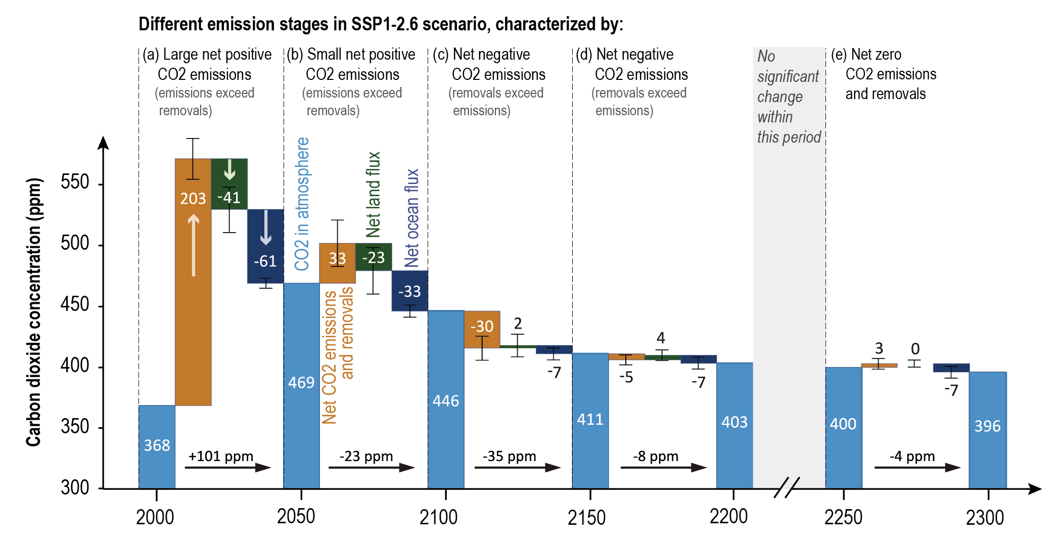 Figure 5.33 | Carbon sink response in a scenario with net carbon dioxide (CO2 ) removal from the atmosphere. Shown are CO2 flux components from concentration-driven Earth system model (ESM) simulations during different emissions stages of SSP1-2.6 and its long-term extension: (a) Large net positive CO2 emissions; (b) small net positive CO2 emissions; (c), (d) net negative CO2 emissions; (e) net zero CO2 emissions. Positive flux components act to raise the atmospheric CO2 concentration, whereas negative components act to lower the CO2 concentration. Net CO2 emissions, land and ocean CO2 fluxes represent the multi-model mean and standard deviation (error bar) of four ESMs (CanESM5, UKESM1, CESM2-WACCM, IPSL-CM6a-LR) and one Earth system model of intermediate complexity (UVic ESCM; Mengis et al., 2020). Net CO2 emissions are calculated from concentration-driven ESM simulations as the residual from the rate of increase in atmospheric CO2 and land and ocean CO2 fluxes. Fluxes are accumulated over each 50-year period and converted to concentration units (ppm). Further details on data sources and processing are available in the chapter data table (Table 5.SM.6).
 5.6.2.1.3 Removal effectiveness of CDR
It is well understood that land and ocean carbon fluxes are sensitive to the level of atmospheric CO2 and climate change and differ under varied future scenarios (Section 5.4). It is therefore important to establish to what extent the removal effectiveness of CDR – here defined as the fraction of total CO2 removed that remains out of the atmosphere – is dependent on the scenario in which CDR is applied. Different metrics have been proposed to quantify the removal effectiveness of CDR (Tokarska and Zickfeld, 2015; Jones et al., 2016b; Zickfeld et al., 2016). One is the airborne fraction (AF) of cumulative CO2 emissions, defined in the same way as for positive emissions (i.e., as the fraction of total CO2 emissions remaining in the atmosphere), with its use extended to periods of declining and net negative CO2 emissions. This metric, however, has not proven to be useful to quantify the removal effectiveness of CDR in simulations where CDR is applied from a trajectory of increasing atmospheric CO2 concentration. This is because it measures the carbon cycle response to CDR as well as to the prior atmospheric CO2 trajectory (Tokarska and Zickfeld, 2015; Jones et al., 2016b). A more useful metric is the perturbation airborne fraction (PAF; Jones et al., 2016b), which measures the AF of the perturbation (in this case the CO2 removal) relative to a reference scenario (Tokarska and Zickfeld, 2015; Jones et al., 2016b). The advantage of this metric is that it isolates the response to a CO2 removal from the response to atmospheric CO2 prior to when the removal is applied. A disadvantage is that the PAF cannot be calculated from a single model simulation, but instead requires a reference simulation to evaluate the effect of the CO2 removal. When CDR is applied from an equilibrium state, the PAF and AF are equivalent measures.
In scenario simulations and idealized simulations with instantaneous CO2 removals applied from an equilibrium state, the removal effectiveness of CDR is found to be slightly dependent on the rate and amount of CDR (Tokarska and Zickfeld, 2015; Jones et al., 2016b; Zickfeld et al., 2021), and to be strongly dependent on the emissions scenario from which CDR is applied (Jones et al., 2016b; Zickfeld et al., 2021). The fraction of CO2 removed remaining out of the atmosphere decreases slightly for larger removals and decreases strongly when CDR is applied from a lower background atmospheric CO2 concentration (Figure 5.34), due to state dependencies and climate–carbon cycle feedbacks that lead to a stronger overall response to CO2 removal (Zickfeld et al., 2021). Based on the high agreement between studies, we assess with medium confidence that the removal effectiveness of CDR is only slightly dependent on the rate and magnitude of removal and is smaller at lower background atmospheric CO2 concentrations. Simulations with Earth system models of intermediate complexity (EMIC) with instantaneous CO2 removal from different equilibrium initial states suggest that the smaller removal effectiveness of CDR at lower background CO2 levels results in greater cooling per unit CO2 removed (Zickfeld et al., 2021). However, there is low confidence in the robustness of this result as climate sensitivity has been shown to exhibit opposite state dependence in EMICs and ESMs (Section 7.4.3.1).
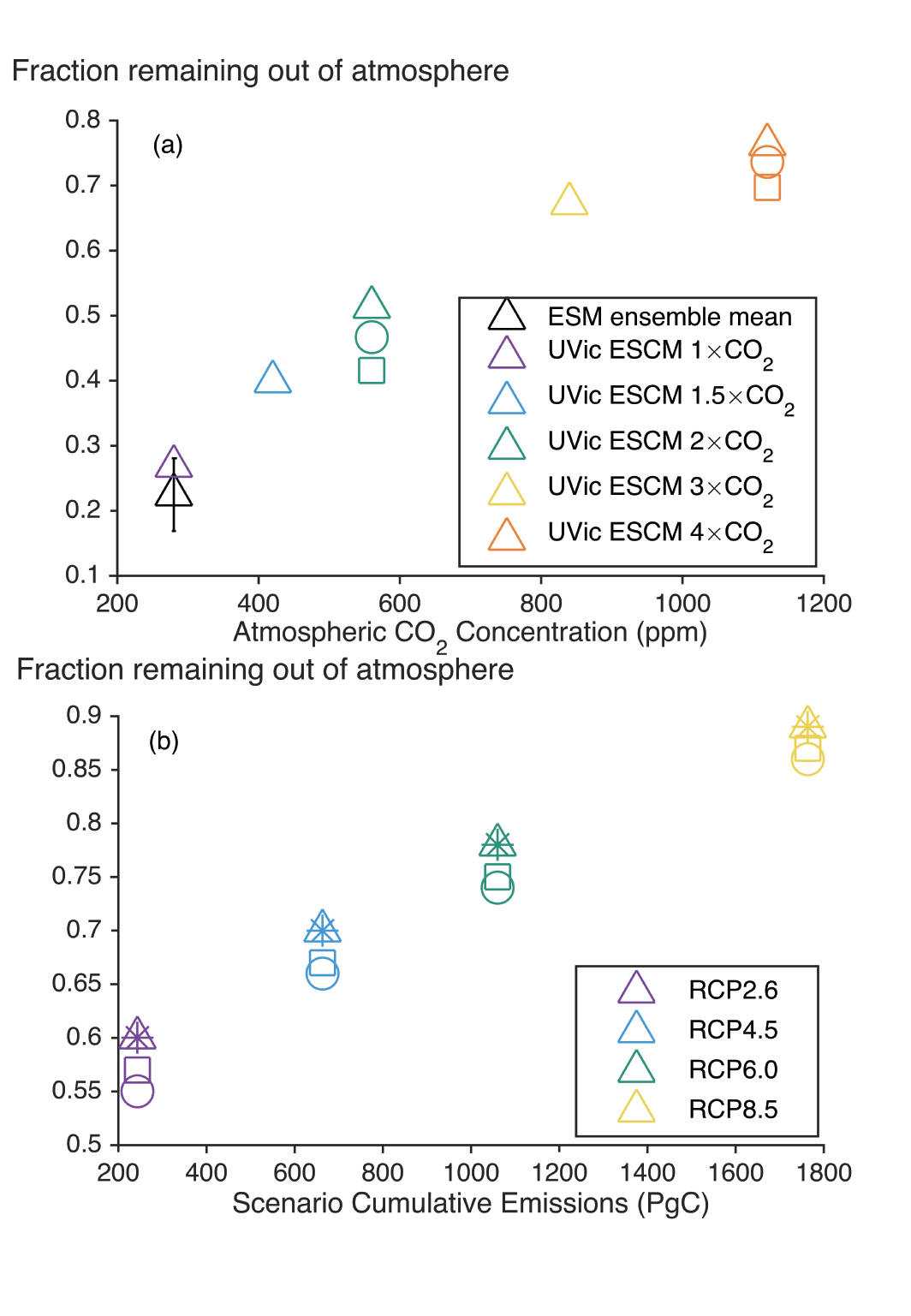 Figure 5.34 | Removal effectiveness of carbon dioxide removal (CDR). (a) Fraction of carbon dioxide (CO2) remaining out of the atmosphere for idealized model simulations with CDR applied instantly (pulse removals) from climate states in equilibrium with different atmospheric CO2 concentration levels (one to four times the pre-industrial atmospheric CO2 concentration; shown on the horizontal axis). The fraction is calculated 100 years after pulse removal. The black triangle and error bar indicate the multi-model mean and standard deviation for the seven Earth system models shown in Figure 5.32 forced with a 100 PgC pulse removal. Other symbols illustrate results with the UVic ESCM model of intermediate complexity for different magnitudes of pulse removals (triangles: –100 PgC; circles: –500 PgC; squares: –1000 PgC). Data for the UVic ESCM is from Zickfeld et al. (2021). (b) Perturbation airborne fraction (see text for definition) for model simulations where CDR is applied from four Representative Concentration Pathways (RCPs) (shown on the horizontal axis in terms of their cumulative CO2 emissions during 2020–2099). Symbols indicate results for four CDR scenarios, which differ in terms of the magnitude and rate of CDR (see Jones et al. (2016b) for details). Results are based on simulations with the Hadley Centre Simple Climate-Carbon Model and are shown for the year 2100. Data from Jones et al. (2016b). Further details on data sources and processing are available in the chapter data table (Table 5.SM.6).
 5.6.2.1.4 Symmetry of carbon cycle response to positive and negative CO2 emissions
It is commonly assumed that the climate–carbon cycle response to a negative CO2 emission (i.e., removal from the atmosphere) is equal in magnitude and opposite in sign to the response to a positive CO2 emission of equal magnitude – that is, symmetric. If the response were symmetric, a positive CO2 emission could be offset by a negative emission of equal magnitude. This subsection assesses the symmetry in the coupled climate–carbon cycle response in model simulations with positive and negative CO2 emission pulses applied from a pre-industrial climate state. Simulations with seven CMIP6 ESMs and the UVic Earth System Climate Model (ESCM) of intermediate complexity suggest that the carbon cycle response is asymmetric for pulse emissions/removals of ±100 PgC (Figure 5.35). For all models, the fraction of CO2 remaining in the atmosphere after an emission is larger than the fraction of CO2 remaining out of the atmosphere after a removal (by 4 ± 3%; mean ± standard deviation). In other words, an emission of CO2 into the atmosphere is more effective at raising atmospheric CO2 than an equivalent CO2 removal is at lowering it. Sensitivity experiments with the UVic ESCM suggest that the asymmetry increases for larger amounts of emissions/removals and is insensitive to the background atmospheric CO2 concentration from which the emissions/removals are applied (Figure 5.35). This asymmetry in the atmospheric CO2 response originates from asymmetries in the land and ocean carbon fluxes due to non-linearities in the carbon cycle response to CO2 and temperature (Section 5.4) (Zickfeld et al., 2021). Givenmedium evidence and high agreement, there is medium confidence in the sign of the asymmetry of the carbon cycle response to positive and negative CO2 emissions. The sign of the symmetry of the temperature response differs between models, with three out of seven examined ESMs showing a smaller temperature response to a 100 PgC emission than to an equivalent CO2 removal. Therefore, there is low confidence in the sign of the asymmetry of the temperature response to positive and negative CO2 emissions.
 Figure 5.35 | Asymmetry in the atmospheric carbon dioxide (CO2 ) response to CO2 emissions and removals. Shown are the fractions of total CO2 emissions remaining in the atmosphere (right-hand side) and CO2 removals remaining out of the atmosphere (left-hand side) 80–100 after a pulse emission/removal. Triangles and green circles denote results for seven Earth system models (ESMs) and the UVic ESCM model of intermediate complexity forced with ±100 PgC pulses applied from a pre-industrial state (1 × CO2) (Carbon Dioxide Removal Model Intercomparison Project (CDRMIP) experiment CDR-pi-pulse; Keller et al., 2018b). Yellow circles and diamonds indicate UVic ESCM results for CO2 emissions/removals applied at 1.5 times (1.5 × CO2) and 2 times (2 × CO2) the pre-industrial CO2 concentration, respectively. Pulses applied from a 2 × CO2 state span the magnitude ±100 PgC to ±500 PgC. UVic ESCM data is from Zickfeld et al. (2021). Further details on data sources and processing are available in the chapter data table (Table 5.SM.6).
 Box 5.3 | Carbon Cycle Response to CO2 Removal fromthe Atmosphere
During the industrial era, CO2 emitted by the combustion of fossil fuels and land-use change has been redistributed between atmosphere, land, and ocean carbon reservoirs due to carbon cycle processes (Box 5.3, Figure 1b and Figure 5.13). Over the past decade (2010–2019), 46% of the emitted CO2 remained in the atmosphere, 23% was taken up by the ocean, and 31% by the terrestrial biosphere (Section 5.2.1.5). When carbon dioxide removal (CDR) is applied during periods in which human activities are net CO2 sources to the atmosphere, and the amount of emissions removed by CDR is smaller than the net source (net positive CO2 emissions), CDR acts to reduce the net emissions (Box 5.3 Figure 1c). In this scenario, part of the CO2 emissions in the atmosphere are removed by the land and ocean sinks, as has been the case historically.

Box 5.3, Figure 1 | Schematic representation of carbon fluxes between atmosphere, land, ocean and geological reservoirs. Different system conditions are shown: (a) an unperturbed Earth system; and changes in carbon fluxes for (b) an Earth system perturbed by fossil fuel carbon dioxide (CO2) emissions; (c) an Earth system in which fossil fuel CO2 emissions are partially offset by carbon dioxide removal (CDR); (d) an Earth system in which CDR exceeds CO2 emissions from fossil fuels (‘net negative’ CO2 emissions). Carbon fluxes depicted in (a) (solid and dashed black lines) also occur in (b–d). The question mark in the land-to-ocean carbon flux perturbation in (c) and (d) indicates that the effect of CDR on this flux is unknown. Note that box sizes do not scale with the size of carbon reservoirs. Adapted from Keller et al. (2018a) . Further details on data sources and processing are available in the chapter data table (Table 5.SM.6).
When CDR removes more CO2 emissions than human activities emit (net negative CO2 emissions), and atmospheric CO2 declines, the land and ocean sinks initially continue to take up CO2 from the atmosphere. This is because carbon sinks, particularly the ocean, exhibit inertia and continue to respond to the prior trajectory of rising atmospheric CO2 concentration. After some time, which is determined by the magnitude of the removal and the rate and amount of CO2 emissions prior to the CDR application, land and ocean carbon reservoirs begin to release CO2 into the atmosphere, making CDR less effective (Box 5.3, Figure 1d).
5.6.2.2 Effects of Specific CDR Methods on Biogeochemical Cycles and Climate
The AR5 WGI (Chapter 6) discussed the CDR methods, their implications and unintended side effects on carbon cycle and climate, including their time scales and potentials. Since then, three IPCC special reports (SR) have been published. First, SR1.5 (Chapter 4 (IPCC, 2018) assessed the potentials and current understanding, including the side effects, of bioenergy with carbon capture and storage (BECCS), afforestation/reforestation, soil carbon sequestration, biochar, enhanced weathering, ocean alkalinization, direct air carbon capture with storage (DACCS) and ocean fertilization. Second, SRCCL (Chapter 6 (IPCC, 2019a) assessed the potentials, co-benefits and trade-offs of land-based mitigation options. It assessed with high confidence that land-based CDR options do not sequester carbon indefinitely, except for peatland restoration. Multiple co-benefits were identified in the deployment of CDR options, many of them with a potential to make positive contributions to sustainable development, enhancement of ecosystem functions and services and other societal goals. However, their potential was concluded to be context specific, and limits were identified in their contribution to global mitigation, such as competition for land. The third report, the Special Report on Ocean and the Cryosphere in a Changing Climate (SROCC) Chapter 5 (IPCC, 2019b), assessed the potential of marine options for climate change mitigation. It concluded that the feasibility of open ocean fertilization and alkalinization approaches were negligible, due to their inconclusive influence on ocean carbon storage on long time scales, due to the unintended side effects on marine ecosystems, and the associated governance challenges. The assessment of blue carbon ecosystems concluded that they could contribute only minimally to atmospheric CO2 reduction globally, but emphasized that the benefits of protecting and restoring coastal blue carbon extend beyond climate change mitigation (SROCC (Section 5.5.12).
5.6.2.2.1 Land-based biological CDR methods
Biological CDR methods, introduced in Table 5.9, seek to increase carbon storage on land by enhancing net primary productivity and/or reducing CO2 sources to the atmosphere.
Forest-based methods include afforestation, reforestation, and forest management (Table 5.9). Building on previous work that emphasized the global potentials of various options, more recent advances have focused on the limits of those global potentials in light of ecological and climate risks that can threaten the long-term permanence of carbon stocks (Boysen et al., 2017b; Anderegg et al., 2020). Some of those risks arise from droughts, fires, insect outbreaks, diseases, erosion, and other disturbances (Thompson et al., 2009).
Sustainable forest management can help to manage some of these vulnerabilities, while in some cases it can increase and maintain forest sinks through harvest, transfer of carbon to wood products and their use to store carbon and substitute emissions-intensive construction materials (Churkina et al., 2020). Forest genomics techniques can increase the success of both reforestation and conservation initiatives, accelerating breeding for tree health and productivity (Isabel et al., 2020).
In response to increasing risks to permanence of carbon stocks of some types of afforestation practices and the competition for land, there has been an increasing recognition that secondary forest regrowth and restoration of degraded forests and non-forest ecosystems can play a large role in carbon sequestration (high confidence). The rational for this focus builds on their high carbon stocks and rates of sequestration (Griscom et al., 2017; Lewis et al., 2019; Maxwell et al., 2019; Pugh et al., 2019), high resilience to disturbances (Dymond et al., 2014; Messier et al., 2019), and additional benefits such as enhanced biodiversity (Strassburg et al., 2020).
The global sequestration potential of forestation varies substantially depending on the scenario-assumptions of available land and of background climate (AR6 WGIII, Section 7.5). Afforestation of native grasslands, savannas, and open-canopy woodlands leads to the undesirable loss of unique natural ecosystems with rich biodiversity, carbon storage and other ecosystem services (Veldman et al., 2015; IPBES, 2018). Comprehensive approaches to assess the effectiveness of land-based carbon removal options need to be based on the whole carbon cycle, covering both carbon stocks and flows, and establishing the links between human activities and their impacts on the biosphere and atmosphere (Keith et al., 2021).
A range of mechanisms could enhance CO2 sequestration of forest-based methods under future scenarios, including CO2 fertilization, soil carbon enrichment due to enhanced litter input, or the northward shift of the tree line in future climate projection (Bathiany et al., 2010; Sonntag et al., 2016; Boysen et al., 2017b; Harper et al., 2018). There is low confidence in the net direction of feedbacks of afforestation on global mean temperature. The feedbacks are highly region dependent. For instance, afforestation at high latitudes would decrease albedo and increase local warming, while at low latitudes, the cooling effect of enhanced evapotranspiration could exceed the warming effect due to albedo decrease (Pearson et al., 2013; W. Zhang et al., 2013; Jia et al., 2019, SRCCL, Section 2.6.1). Both afforestation and reforestation affect the hydrological cycle through increased volatile organic compound (VOC) emissions and cloud albedo (Teuling et al., 2017; Kalliokoski et al., 2020), enhanced precipitation (Ellison et al., 2017) and increased transpiration, with potential effects on runoff and, especially in dry regions, on water supply (Figure 5.36 and Cross-Chapter Box 5.1; Farley et al., 2005; Smith et al., 2016; Krause et al., 2017; Teuling et al., 2019). Forest-based methods can either raise or lower N2O emissions, depending on tree species, previous land use, soil type and climatic factors (low confidence) (Figure 5.36 and Supplementary Materials, Table 5.SM.4; Benanti et al., 2014; Chen et al., 2019; McDaniel et al., 2019). Afforestation will decrease biodiversity if native species are replaced by monocultures (high confidence), while there is medium confidence that biodiversity is improved when forests are introduced into land areas with degraded soils or intensive monocultures, or where native species are re-introduced into managed land (Figure 5.36, Supplementary Materials Table 5.SM.4; Hua et al., 2016; Williamson and Bodle, 2016; P. Smith et al., 2018; Holl and Brancalion, 2020).
Soil carbon losses from human agriculture accounted for about 116 PgC in the last 12,000 years (Section 5.2.1.2; Sanderman et al., 2017). With best management practices, two-thirds of these losses may be recoverable, setting a theoretical maximum of 77 PgC that can be sequestered in soils. Methods to increase soil carbon content may be applied to the restoration of marginal or degraded land (Paustian et al., 2016; Smith, 2016), but may also be used in traditional agricultural lands. A simple practice is to increase the input of carbon to the soil by selecting appropriate varieties or species with greater root mass (Kell, 2011) or higher yields and net primary production (NPP) (Burney et al., 2010). In addition, improved agricultural practices also increase soil carbon content. These include using crop rotation cycles, increasing the amount of crop residues, using crop cover to prevent periods of bare soil (Poeplau and Don, 2015; Griscom et al., 2017), optimizing grazing (Henderson et al., 2015) and residue management (Wilhelm et al., 2004), using irrigation (Campos et al., 2020), employment of low-tillage or no-tillage (W. Sun et al., 2020), agroforestry, cropland nutrient recycling, and avoiding grassland conversion (Paustian et al., 2016; Fargione et al., 2018). With medium confidence, methods that seek soil carbon sequestration will diminish nitrous oxide (N2O) emissions and nutrient leaching, and improve soil fertility and biological activity (Figure 5.36; Tonitto et al., 2006; Fornara et al., 2011; Paustian et al., 2016; Smith et al., 2016; SRCCL, Section 2.6.1.3, IPCC, 2019a). However, if improved soil carbon sequestration practices involve higher fertilization rates, N2O emissions would increase (Gu et al., 2017). Some soil carbon sequestration methods, such as cover crops and crop diversity, can increase biodiversity (medium confidence) (Paustian et al., 2016; P. Smith et al., 2018).
Biochar is produced by burning biomass at high temperatures under anoxic conditions (pyrolysis) and, when added to soils, can increase soil carbon stocks and fertility for decades to centuries (Woolf et al., 2010; Lehmann et al., 2015). Biochar application improves many soil qualities and increases crop yield (medium confidence) (Ye et al., 2020; SRCCL, Chapter 4.9.5), particularly in already degraded or weathered soils (Woolf et al., 2010; Lorenz and Lal, 2014; Jeffery et al., 2016), increases soil water holding capacity (medium confidence) (Karhu et al., 2011; Liu et al., 2016; B.M.C. Fischer et al., 2019; Verheijen et al., 2019) and evapotranspiration (low confidence)(B.M.C. Fischer et al., 2019). The use of biochar reduces nutrient losses (low confidence) (Woolf et al., 2010), enhances fertilizer nitrogen use efficiency and improves the bioavailability of phosphorus (Figure 5.36; Clough et al., 2013; Shen et al., 2016; Z. Liu et al., 2017). Biochar addition may decrease methane (CH4) emissions in inundated and acid soils such as rice fields (low confidence)(Jeffery et al., 2016; Huang et al., 2019; Wang et al., 2019; Yang et al., 2019). In non-inundated, neutral soils, CH4 uptake from the atmosphere is suppressed after biochar application (low confidence) (Jeffery et al., 2016), and soil N2O emissions decline (medium confidence) (Cayuela et al., 2014; Kammann et al., 2017). The potential risks of introducing harmful contaminants into the soil environment are not well understood (Lorenz and Lal, 2014). With low confidence, application of biochar can have co-benefits for soil microbial biodiversity (P. Smith et al., 2018), while the potential trade-offs for biodiversity are due to land requirements (Tisserant and Cherubini, 2019).
Peatlands are less extensive than forests, croplands and grazing lands, yet per unit area, they hold high carbon stocks (Griscom et al., 2017). Peatland restoration relies on back-conversion or building of high-carbon-density soils through flooding – that is, rewetting (Leifeld et al., 2019). High water level and anoxic conditions are prerequisites for restoring by returning drained and/or degraded peatlands back to their natural state as CO2 sinks, but restoration also results in enhanced CH4 emissions which are similar to or higher than the pre-drainage fluxes (high confidence) (Koskinen et al., 2016; Wilson et al., 2016a; Hemes et al., 2019; Renou-Wilson et al., 2019; Holl et al., 2020). In a multi-decadal time frame, the reduction in CO2 emissions from rewetting more than compensates for the initial increase in radiative forcing due to enhanced CH4 emissions (Günther et al., 2020). Rewetting drained peatlands will decrease N2O emissions (medium confidence) (Wilson et al., 2016b; H. Liu et al., 2020; Tiemeyer et al., 2020). Restored wetlands and peatlands act as buffer zones that provide infiltration and nutrient retention and offer protection to water quality (Daneshvar et al., 2017; Lundin et al., 2017), particularly in nutrient-loaded agricultural catchments. Peatland restoration can also recover much of the original biodiversity (medium confidence) (Meli et al., 2014; P. Smith et al., 2018).
The concept of BECCS rests on the premise that bioenergy production is carbon neutral – that is, as much CO2 is sequestered when growing biomass as feedstock as is released by its combustion. If these emissions are also captured and stored, the net effect is removal of CO2 from the atmosphere (Fuss et al., 2018). Sequestration potentials from BECCS depend strongly on the feedstock, climate, and management practices (Beringer et al., 2011; Kato and Yamagata, 2014; Heck et al., 2016; Smith et al., 2016; Krause et al., 2017). If woody bioenergy plants replace marginal land, net carbon uptake increases, enriching soil carbon (Don et al., 2012; Heck et al., 2016; Boysen et al., 2017a, b). However, replacing carbon-rich ecosystems with herbaceous bioenergy plants could deplete soil-carbon stocks and reduce the additional sink capacity of standing forests (Don et al., 2012; Harper et al., 2018). Furthermore, wood-based BECCS may not be carbon negative in the first decades, initially emitting more CO2 than sequestering (Sterman et al., 2018). BECCS has several trade-offs to deal with, including possible threats to water supply and soil nutrient deficiencies (medium confidence) (SRCCL Chapters 2 and 6, and Cross-Chapter Box 5.1; Smith et al., 2016; Krause et al., 2017; de Coninck et al., 2018; Heck et al., 2018; Roy et al., 2018). Deployment of BECCS at the scales envisioned by many 1.5°C–2.0°C mitigation scenarios could threaten biodiversity and require large land areas, competing with afforestation, reforestation and food security (Anderson and Peters, 2016; P. Smith et al., 2018). Additional risks and side effects are related to geologic carbon storage (Fuss et al., 2018; see also Section 5.6.2.2.4).
In conclusion, land-based CDR methods that rely on enhanced net biological uptake and storage of carbon, have a wide range of biogeochemical and biophysical side effects. These side effects can (directly or indirectly) strengthen or weaken the climate change mitigation effect of a given method, or affect water quality and quantity, food supply and biodiversity (Figure 5.36). With the exception of weakened ocean carbon sequestration, there is low confidence in the Earth system feedbacks of these methods. Most methods are associated with a range of biogeochemical and biophysical side effects and co-benefits and trade-offs, but these are often highly dependent on local context, management regime, prior land use, and scale (high confidence). Highest co-benefits are obtained with methods that seek to restore natural ecosystems and improve soil carbon sequestration (Figure 5.36) while highest trade-off possibilities (symmetry with the highest co-benefits) occur for reforestation or afforestation with monocultures and BECCS, again with strong dependence on scale and context (medium confidence).
5.6.2.2.2 Ocean-based biological CDR methods
Both ocean biological and physical processes drive the CO2 exchange between the ocean and atmosphere. However, the ocean physical processes that remove CO2 from the atmosphere, such as large-scale circulation, cannot be feasibly altered, so ocean CDR methods focus on increasing the productivity of ocean ecosystems, and subsequent sequestration of carbon (GESAMP, 2019). There has been no change to the assessment of SROCC (SROCCSection 5.5.1): there is low confidence that nutrient addition to the open ocean, either through artificial ocean upwelling or iron fertilization, could contribute to climate change mitigation, due to its inconclusive effect on carbon sequestration and risks of adverse side effects on marine ecosystems (Figure 5.36, Table 5.9; Supplementary Materials Text 5.SM.3 and Table 5.SM.4; AR6 WGIII Chapter 12; Gattuso et al., 2018; Boyd and Vivian, 2019; Feng et al., 2020). In addition, ocean fertilization is currently prohibited by the LondonProtocol (Dixon et al., 2014; GESAMP, 2019).
Restoration of vegetated coastal ecosystems (sometimes referred to as ‘blue carbon’ – see Glossary) refers to the potential for increasing carbon sequestration by plant growth and burial of organic carbon in the soil of coastal wetlands (including salt marshes and mangroves) and seagrass ecosystems. Wider usage of the term blue carbon occurs in the literature, for example, including seaweeds (macroalgae), shelf sea sediments and open ocean carbon exchanges. However, such systems are less amenable to management, with many uncertainties relating to the permanence of their carbon stores (Windham-Myers et al., 2018; Lovelock and Duarte, 2019; SROCC, Section 5.5.1.1).
Coastal wetlands and seagrass meadows store significant amounts of carbon and are among the most productive ecosystems per unit area (Griscom et al., 2017, 2020; Ortega et al., 2019; Serrano et al., 2019). These rates could be reduced in the future, since these habitats are vulnerable to changing conditions, such as temperature, salinity, sediment supply, storm severity and continued coastal development (Bindoff et al., 2019; NASEM, 2019). These ecosystems are under threat from anthropogenic conversion and degradation and are being lost at rates between 0.7% and 7% per annum with consequent CO2 emissions (e.g., Atwood et al., 2017; Howard et al., 2017; Hamilton and Friess, 2018; Sasmito et al., 2019). Although sea level rise might lead to greater carbon sequestration in coastal wetlands (Rogers et al., 2019), there is high confidence that the frequency and intensity of marine heatwaves will increase (Cross-Chapter Box 9.1; Frölicher and Laufkötter, 2018; Laufkötter et al., 2020),which poses a more immediate threat to the integrity of coastal carbon stocks (Smale et al., 2019). Blue carbon restoration seeks to increase the rate of carbon sequestration, although restoration may be challenging, because of ongoing use of coastal land for human settlement, conversion to agriculture and aquaculture, shoreline hardening and port development.
Biogeochemical factors affecting reliable quantification of the climatic benefits of coastal vegetation include the variable production of CH4 and N2O by such ecosystems (Adams et al., 2012; Keller, 2018; Rosentreter et al., 2018), uncertainties regarding the provenance of the carbon that they accumulate (Macreadie et al., 2019), and the release of CO2 by biogenic carbonate formation in seagrass ecosystems (Kennedy et al., 2018). While coastal habitat restoration potentially provides significant mitigation of national emissions for some countries (Taillardat et al., 2018; Serrano et al., 2019), the global sequestration potential of blue carbon approaches is <0.02 PgC yr–1 (medium confidence) (Figure 5.36; SROCC, Section 5.5.1.2; Griscom et al., 2017; Gattuso et al., 2018; GESAMP, 2019; NASEM, 2019).
5.6.2.2.3 Geochemical CDR methods
Enhanced weathering (EW) is based on naturally occurring weathering processes of silicate and carbonate rocks, removing CO2 from the atmosphere. Weathering is accelerated by spreading ground rocks on soils, coasts or oceans. EW increases the alkalinity and pH of natural waters, helps dampen ocean acidification and increases ocean carbon uptake (Beerling et al., 2018). The dissolution of minerals stimulates biological productivity of croplands (Hartmann et al., 2013; Beerling et al., 2018), but can also liberate toxic trace metals (such as nickel, chromium, copper) into soil or water bodies (Keller et al., 2018a; Strefler et al., 2018). EW can also contribute to freshwater salinization as a result of increased salt inputs and cation exchange in watersheds, and so adversely affecting drinking water quality (low confidence) (Kaushal et al., 2018). With amedium confidence, amendment of soils with minerals will have lower N2O emissions (Kantola et al., 2017; Blanc-Betes et al., 2020) but will not have a marked effect on evapotranspiration or albedo (Fuss et al., 2018; de Oliveira Garcia et al., 2020). The mining of minerals can cause adverse impacts on biodiversity, however, the use of waste materials such as concrete demolition or steel slags for EW can reduce the need for mining (Renforth, 2019). The spreading of minerals on land has a neutral impact on biodiversity (P. Smith et al., 2018).
Ocean alkalinization, via the deposition of alkaline minerals (e.g., olivine) or their dissociation products (e.g., quicklime) at the ocean surface, can increase surface total alkalinity and thus increase CO2 uptake and storage (Glossary; Supplementary Material Text 5.SM.3; AR6 WGIII Chapter 12; GESAMP, 2019; Keller, 2019). Ocean alkalinization ameliorates surface ocean acidification (high confidence) (Hauck et al., 2016; Tran et al., 2020), but there are also negative side effects on the marine ecosystem, most of which are poorly understood or quantified (Figure 5.36 and Supplementary Materials Table 5.SM.4; Bach et al., 2019). Although ocean alkalinization could potentially sequester large amounts of carbon (≥1 PgC yr–1; Figure 5.36; and Supplementary Materials Table 5.SM.5) there is no new evidence to revisit the SROCC (SROCCSection 5.5.1.2.4) conclusion that there is low confidence that ocean alkalinization is a viable climate change mitigation approach.
5.6.2.2.4 Chemical CDR methods
Direct air carbon capture with carbon storage (DACCS) is a combination of two techniques, direct capture of CO2 from ambient air (DAC) and carbon storage. DAC entails contacting the air, capturing the CO2 on a liquid solvent or solid sorbent, and regenerating the solvent or sorbent. Different DAC methods have been proposed, which differ by the chemical process used to capture the CO2 and to recover it from the sorbent or solvent (NASEM, 2019). The captured CO2 may be either stored geologically as a high-pressure gas or sequestered by a mineral carbonation process. Storage is potentially permanent in both pressurised gas and mineral form (Fuss et al., 2018). DACCS has significant requirements of energy and, (depending on the type of technology), water and materials (Smith et al., 2016; NASEM, 2019). Compared to other CDR methods, it has a small land footprint (Smith et al., 2016; NASEM, 2019). Side effects of DACCS include CO2 -depleted air leaving the air contactor, which could have adverse effects on crop and ecosystem productivity, and VOC emissions (NASEM, 2019). Additional risks and side effects are related to the high pressure at which CO2 is stored in geologic formations (Fuss et al., 2018). DACCS is assessed in detail in WGIII Chapter 12.
5.6.2.2.5 Methane removal
Proposals to remove CH4 from the atmosphere are emerging (de Richter et al., 2017; Jackson et al., 2019). CH4 removal methods seek to capture CH4 directly from ambient air, similarly to DACCS for CO2 using, for example, zeolite trapping, but instead of storing it, CH4 would be chemically oxidized to CO2 (Jackson et al., 2019). Methane can be also removed microbially by supporting naturally occurring processes, such as by enhancing the soil microbial uptake through afforestation (J. Wu et al., 2018) or by directing the venting air from a cow barn into the soil bed of a nearby greenhouse, utilizing microbial CH4 oxidation (Nisbet et al., 2020). Microbial CH4 oxidation could also be used for removal of CH4 leaked from point sources by building biocatalytic polymers which include methane-oxidizing enzymes (Blanchette et al., 2016). Methane removal is, however, still in its infancy and the available literature is insufficient for an assessment.
 Figure 5.36 | Characteristics of carbon dioxide removal (CDR) methods, ordered according to the time scale of carbon storage. The first column shows biogeophysical (for open-ocean methods) or technical (for all other methods) sequestration potentials (i.e., the sequestration potentials constrained by biological, geophysical, geochemical limits and thermodynamics and, for technical potentials, availability of technologies and practices; technical potentials for some methods also consider social or environmental factors if these represent strong barriers for deployment; see Glossary, Annex VII), classified into low (<0.3 GtCO2 yr–1), moderate (0.3−3 GtCO2 yr–1) and large (>3 GtCO2 yr–1) (details underlying this classification are provided in Supplementary Materials Table 5.SM.5). The other columns show Earth system feedbacks that deployment of a given CDR method would have on carbon sequestration and climate, along with biogeochemical, biophysical, and other side effects of a given method. Earth system feedbacks do not include the direct effect of CO2 sequestration on atmospheric CO2, only secondary effects. For Earth system feedbacks, the colours indicate whether the feedbacks strengthen or weaken carbon sequestration and the climate cooling effect of a given CDR method. For biogeochemical and biophysical side effects the colours indicate whether the deployment of a CDR method increases or decreases the magnitude of the effect, whereas for co-benefits and trade-offs the colour indicates whether deployment of a CDR method results in beneficial (co-benefits) or adverse side effects (trade-offs) for water quality and quantity, food production and biodiversity. The details and references underlying the Earth system feedback and side effect assessment are provided in Supplementary Materials Table 5.SM.4. Further details on data sources and processing are available in the chapter data table (Table 5.SM.6).
 5.6.3 Biogeochemical Responses to Solar Radiation Modification (SRM)
This section assesses the possible consequences of solar radiation modification (SRM) on the biosphere and global biogeochemical cycles. The SRM options and the physical climate response to SRM is assessed in detail in Section 4.6.3 and Table 4.7. Section 6.3.6 assesses the potential effective radiative forcing of aerosol-based SRM options and Section 8.6.3 assesses the abrupt water cycle changes in response to initiation or termination of SRM. Most literature on the biogeochemical responses to SRM focuses on stratospheric aerosol injection (SAI), and only a few studies have investigated the biogeochemical responses to marine cloud brightening (MCB) and cirrus cloud thinning (CCT). At the time of AR5, there were only a few studies on the biogeochemical responses to SRM. The main assessment of AR5 (Ciais et al., 2013) was that SRM will not interfere with the direct biogeochemical effects of increased CO2, such as ocean acidification and CO2 fertilization, but could affect the carbon cycle through climate–carbon feedbacks. Overall, AR5 concluded that the level of confidence on the effects of SRM on carbon and other biogeochemical cycles is very low (Ciais et al., 2013). Since AR5, more modelling work has been conducted to examine various aspects of the global biogeochemical cycle responses to SRM.
 Figure 5.37 | Cumulative carbon dioxide (CO2 ) uptake by land and ocean carbon sinks in response to stratospheric sulphur dioxide (SO2) injection. Results are shown for a scenario with 50-year (2020−2069) continuous stratospheric SO2 injection at a rate of 5 Tg yr–1appplied to a RCP4.5 baseline scenario (GeoMIP experiment G4; Kravitz et al., 2011), followed by termination in year 2070. Anomalies are shown relative to RCP4.5 for the multi-model ensemble mean and for each of six Earth system models (ESMs) over the 50-year period of stratospheric SO2 injection (left-hand side), and over 20 years after termination of SO2 injection (right-hand side). Adapted from Plazzotta et al. (2019). Further details on data sources and processing are available in the chapter data table (Table 5.SM.6).
 5.6.3.1 Effects of SRM on the Carbon Cycle
Relative to a high-greenhouse gas (GHG) world without solar radiation modification (SRM), SRM would affect the carbon cycles through changes in sunlight, climate (e.g., temperature, precipitation, soil moisture, ocean circulation), and atmospheric chemistry (e.g., ozone; Section 4.6.3.3; Cao, 2018). Net SRM effects on the carbon cycle, relative to a world without SRM, depend on the change of individual factors, and interactions among them.
SRM-mediated sunlight changes directly affect the carbon cycle. In particular, SAI would reduce the sunlight reaching the Earth’s surface, but also increase the fraction of sunlight that is diffuse. These changes in the quantity and quality of the sunlight have opposing effects on the photosynthesis of land plants. On their own, reductions in photosynthetically active radiation (PAR) will reduce photosynthesis. However, diffuse light is more effective than direct light in accessing the light-limited leaves within plant canopies, leading to the so-called ‘diffuse-radiation’ fertilization effect (Mercado et al., 2009). The estimated balance between the negative impacts of reducing PAR and the positive impacts of increasing diffuse fraction differ between models (Kalidindi et al., 2015; Xia et al., 2016; C.-E. Yang et al., 2020) and across different ecosystems. The change in the absolute amount of direct and diffuse radiation could also depend on the height of the additional sulphate aerosol layer in the stratosphere and the hygroscopic growth of aerosols (Krishnamohan et al., 2019, 2020).
SRM-mediated cooling also affects the terrestrial carbon cycle. Relative to a high-GHG world without SRM, the simulated responses of net primary production (NPP) to SRM differ widely between models, such that even the sign of global mean change is uncertain (Glienke et al., 2015). SRM-induced cooling would decrease NPP at high latitudes by reducing the length of the growing season (Glienke et al., 2015). At low latitudes, the NPP response to SRM-induced cooling is sensitive to the effect of nitrogen limitation (Glienke et al., 2015; Duan et al., 2020). SRM-induced cooling tends to increase NPP in models without the nitrogen cycle because of reduced heat stress. However, in models including the nitrogen cycle, this is counteracted by reductions in NPP because of reductions in nitrogen mineralization and nitrogen availability (Glienke et al., 2015). SRM-induced changes in the hydrological cycle (Section 8.6.3), including changes in evapotranspiration, precipitation, and soil moisture, also pose strong constraints on the vegetation response (Dagon and Schrag, 2019). For the same amount of global mean cooling, different SRM options, such as SAI, MCB, and CCT, would have different effects on gross primary production (GPP) and NPP because of different spatial patterns of temperature, available sunlight and hydrological cycle changes (Section 4.6.3.3) (Duan et al., 2020). Modelling studies show that SRM-induced cooling would reduce plant and soil respiration (Tjiputra et al., 2016; Cao and Jiang, 2017; Muri et al., 2018; C.-E. Yang et al., 2020). Despite the large uncertainty in modelled NPP response, existing modelling studies consistently show that SRM would increase the global land carbon sink relative to a high-CO2 world without SRM (high confidence).
Based on available evidence, SRM with elevated CO2 would increase global mean NPP and carbon storage on land relative to an unperturbed climate, mainly because of CO2 fertilization of photosynthesis (high confidence) (Glienke et al., 2015; Tjiputra et al., 2016; Dagon and Schrag, 2019; Duan et al., 2020; C.-E. Yang et al., 2020). However, the amount of increase is uncertain as it depends on the extent to which CO2 fertilization of land plants is limited by nutrient availability.
Relative to a high-CO2 world without SRM, SRM would also have compensating effects on crop yields. SRM is expected to have a positive impact on crop yields by diminishing heat stress (Pongratz et al., 2012). However, reductions in light availability will produce a counteracting reduction in crop yields, especially if the crop type does not benefit appreciably from diffuse-light fertilization (Proctor et al., 2018). The balance between these effects varies markedly across crop types and regions, from projected increases in maize production in China (Xia et al., 2014) to reductions in groundnut yields in parts of India (Yang et al., 2016). Because of these diverging results from a limited set of studies, there is overall low confidence in the effect of SRM on crop yields.
Consistent with the AR5 assessment, there is high confidence that SRM would not mitigate CO2 -induced ocean acidification (Ciais et al., 2013). Some studies even suggest an acceleration of deep-ocean acidification as a result of ocean circulation change (Tjiputra et al., 2016; Lauvset et al., 2017). There are large differences in the simulated spatial pattern of ocean NPP change in response to SRM, which depends strongly on the SRM method that is considered (Partanen et al., 2016; Lauvset et al., 2017).
5.6.3.2 Consequences of SRM and its Termination on Atmospheric CO2 burden
Modelling studies consistently show that, relative to a high-CO2 world without SRM, SRM-induced cooling (Section 4.6.3.3) would reduce plant and soil respiration, and also reduce the negative effects of warming on ocean carbon uptake (Tjiputra et al., 2016; Xia et al., 2016; Cao and Jiang, 2017; Jiang et al., 2018; Muri et al., 2018; Sonntag et al., 2018; Plazzotta et al., 2019; C.-E. Yang et al., 2020). A multi-model study (Plazzotta et al., 2019) indicates that, relative to a high-CO2 concentration world without SRM, stratospheric sulphur dioxide (SO2) injection increases the allowable CO2 emissions by enhancing CO2 uptake by both land and ocean (Figure 5.37). As a result of enhanced global carbon uptake, SRM would reduce the burden of atmospheric CO2 (high confidence). However, the amount of SRM-induced reduction in atmospheric CO2 depends on the future emissions scenario and modelled oceanic and terrestrial carbon sinks, which differ widely between models (Tjiputra et al., 2016; Xia et al., 2016; Cao and Jiang, 2017; Muri et al., 2018). Models that include the terrestrial nitrogen cycle usually report a much smaller reduction of atmospheric CO2 in response to SRM than models without the nitrogen cycle, mainly because nitrogen limitation leads to a weaker terrestrial carbon sink (Tjiputra et al., 2016; Muri et al., 2018; C.-E. Yang et al., 2020). Large-scale application of SAI is found to reduce the rate of release of CO2 and CH4 from permafrost thaw (Lee et al., 2019; Chen et al., 2020).
A hypothetical sudden and sustained termination of SRM would cause a rapid increase in global warming that would pose great risks to biodiversity (A. Jones et al., 2013; McCusker et al., 2014; Trisos et al., 2018) (Section 4.6.3.3). It would also weaken carbon sinks, accelerating atmospheric CO2 accumulation and inducing further warming (Figure 5.37; Matthews and Caldeira, 2007; Tjiputra et al., 2016; Muri et al., 2018; Plazzotta et al., 2019). However, a scenario with gradual phase-out of SRM under emissions reduction could reduce the large negative effect of sudden SRM termination (MacMartin et al., 2014; Keith and MacMartin, 2015; Tilmes et al., 2016),though this would be limited by how rapidly emissions reductions can be scaled-up (Ekholm and Korhonen, 2016).
5.6.3.3 Consequences of SRM on other Biogeochemical Cycles
SAI is found to reduce global average surface ozone concentration (Xia et al., 2017) mainly as a result of aerosol-induced reduction in stratospheric ozone at polar regions, resulting in reduced transport of ozone from the stratosphere (Pitari et al., 2014; Tilmes et al., 2018). The reduction in surface ozone, together with alteration to ultraviolet (UV) radiation, would have important implications for vegetation response (Xia et al., 2017). A modelling study shows that sea salt aerosol injection for MCB would reduce hydroxyl (OH) concentration and increase CH4 lifetime, and hence, have potential implications for surface ozone pollution (Horowitz et al., 2020). It has also been reported that the use of SAI to limit global mean warming from 2°C to 1.5°C would reduce fire weather in many areas (Burton et al., 2018).
5.6.3.4 Synthesis of Biogeochemical Responses to SRM
SRM would alter the global carbon cycle through SRM-induced climate effect, such as changes in sunlight, temperature, precipitation, and ocean circulation. Compared to a high-CO2 world without SRM, SRM would enhance the net uptake of CO2 by the terrestrial biosphere and ocean, thus acting to reduce atmospheric CO2 (high confidence). SRM would also affect surface ozone, UV radiation, and atmospheric chemistry. Due to complex interplays between SRM-induced changes in direct and diffuse sunlight, temperature, the coupling of water-carbon-nitrogen cycles, and atmospheric chemistry, there is large uncertainty in the overall response of the terrestrial biosphere response to SRM. Thus, the level of confidence on the effect of SRM on carbon and other biogeochemical cycles is low.
5.7 Final Remarks
Key research developments to further strengthen the confidence levels in AR7 include the following:
Contemporary Greenhouse Gases (GHGs) Trends and Attribution
- Further constrain the CO2, CH4 and N2O fluxes from land use, land-use change and forestry (including gross fluxes), and fossil fuels. Improving spatial resolution and representations of land management, such as forestry, grazing and cropping.
- Improve representation of the variability and trends in the transport of carbon through the land–ocean continuum, which has implications for partitioning the land and ocean CO2 sinks.
- Improve understanding of the controls over the airborne franction and sinks rates, their trends, and future dynamics.
- Fill gaps in space and time for ocean CO2 and ancillary physical and biogeochemical observations at the ocean surface and interior to reduce the biases and uncertainties in the variability and trends for air–sea fluxes and inventory changes, particularly for the Arctic and the Southern Ocean.
- Reduce uncertainties of CH4 emissions from wetlands and inland waters, which are the largest source term in the global CH4 budget and proportionally have the largest uncertainty, to better understand future CH4-climate feedbacks.
- Reduce uncertainties in atmospheric transport models used to estimate regional sources and sinks of GHGs as independent evidence from that of ground and inventory estimates.
Ocean Acidification and Deoxygenation
- Improve observations for the interplay between carbonate chemistry and a variety of biogeochemical and physical processes, including eutrophication and freshwater inflow in coastal zones to increase the robustness of future assessments of ocean acidification.
- Improve our understanding of changes in water mass ventilation associated with climate change and variability to gain further insights into future trends in ocean acidification and deoxygenation in the ocean interior.
Biogeochemical Feedbacks on Climate Change
- Improve understanding and representation in Earth system models of changes in land carbon storage and associated carbon–climate feedbacks including: better treatment of the CO2 fertilization, nutrient-limitations, soil organic matter stabilization and turnover; land-use change; large-scale and fine-scale permafrost carbon; plant growth, mortality, and competition dynamics; plant hydraulics; and disturbance processes.
- Improve observations and process understanding of CH4 and N2O source responses to climate, specifically from wetlands and permafrost thaw.
- Improve observations and process understanding of ocean N2O source responses to oxygen loss and climate, particularly in the oxygen minimum zones of the tropical oceans and eastern boundary upwelling regions.
- Improve understanding of the sensitivity of ocean carbon–climate feedbacks to physical processes that are not yet resolved by the ocean domain in ESMs.
- Improve understanding of the processes affecting the efficiency, climate sensitivity and emerging feedbacks in the ocean carbon cycle via the biological carbon pump to constrain future global ocean feedbacks.
Remaining Carbon Budget to Climate Stabilization
- Improve understanding of the sign and magnitude of a possible zero emissions commitment (ZEC). The ZEC affects estimates of carbon budgets derived from the transient climate response to cumulative emissions of CO2 (TCRE), but not TCRE itself. ZEC is particularly relevant once global CO2 emissions decline towards net zero.
- Better constraint of the airborne fraction to reduce the spread in TCRE assessment.
- Account for time scales of Earth system feedbacks over time for increased accuracy of mitigation needs once global CO2 emissions reach near-zero levels.
Carbon Dioxide Removal (CDR) and Solar Radiation Modification (SRM)
- Run large-scale and long-term experiments and assessments to explore: the regional feasibility of CDR methods; whether they present an actual and verifiable negative regional carbon balance; and whether they result in adverse unintended consequences.
- Improve understanding of the effectiveness of CDR methods to lower atmospheric CO2 and reduce warming, taking into account Earth system feedbacks.
Frequently Asked Questions
FAQ 5.1 | Is the Natural Removal of Carbon From the Atmosphere Weakening?
For decades, about half of the carbon dioxide (CO2 ) that human activities have emitted to the atmosphere has been taken up by natural carbon sinks in vegetation, soils and oceans. These natural sinks of CO2 have thus roughly halved the rate at which atmospheric CO2 concentrations have increased, and therefore slowed down global warming. However, observations show that the processes underlying this uptake are beginning to respond to increasing CO2 in the atmosphere and climate change in a way that will weaken nature’s capacity to take up CO2 in the future. Understanding of the magnitude of this change is essential for projecting how the climate system will respond to future emissions and emissions reduction efforts.
Direct observations of CO2 concentrations in the atmosphere, which began in 1958, show that the atmosphere has only retained roughly half of the CO2 emitted by human activities, due to the combustion of fossil fuels and land-use change such as deforestation (FAQ 5.1, Figure 1). Natural carbon cycle processes on land and in the oceans have taken up the remainder of these emissions. These land and ocean removals or ‘sinks’ have grown largely in proportion to the increase in CO2 emissions, taking up 31% (land) and 23% (ocean) of the emissions in 2010–2019, respectively (FAQ 5.1, Figure 1). Therefore, the average proportion of yearly CO2 emissions staying in the atmosphere has remained roughly stable at 44% over the last six decades, despite continuously increasing CO2 emissions from human activities.
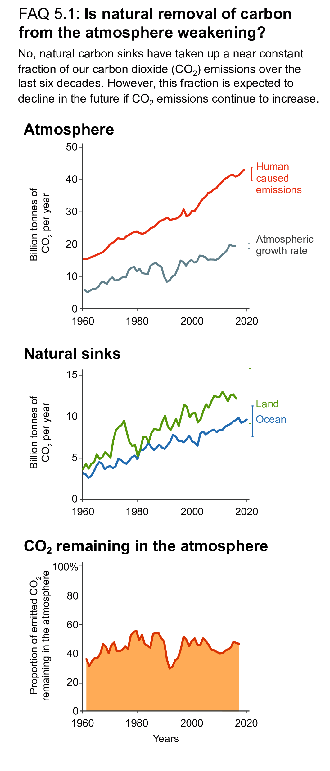
FAQ5.1, Figure 1 | Atmospheric carbon dioxide (CO2) and natural carbon sinks. (Top) Global emissions of CO2 from human activities and the growth rate of CO2 in the atmosphere; (middle) the net land and ocean CO2 removal (natural sinks); and (bottom) the fraction of CO2 emitted by human activities remaining in atmosphere from 1960 to 2019. Lines are the five years running mean, error bars denote the uncertainty of the mean estimate. See Table 5.SM.6 for more information on the data underlying this figure.
On land, it is mainly the vegetation that captures CO2 from the atmosphere through plant photosynthesis, which ultimately accumulates both in vegetation and soils. As more CO2 accumulates in the atmosphere, plant carbon capture increases through the CO2fertilization effect in regions where plant growth is not limited by, for instance, nutrient availability. Climate change affects the processes responsible for the uptake and release of CO2 on land in multiple ways. Land CO2 uptake is generally increased by longer growing seasons due to global warming in cold regions and by nitrogen deposition in nitrogen-limited regions. Respiration by plants and soil organisms, natural disturbances such as fires, and human activities such as deforestation all release CO2 back into the atmosphere. The combined effect of climate change on these processes is to weaken the future land sink. In particular, extreme temperatures and droughts as well as permafrost thaw (see FAQ 5.2) tend to reduce the land sink regionally. In the ocean, several factors control how much CO2 is captured: the difference in CO2 partial pressure between the atmosphere and the surface ocean; wind speeds at the ocean surface; the chemical composition of seawater (that is, its buffering capacity), which affects how much CO2 can be taken up; and the use of CO2 in photosynthesis by seawater microalgae. The CO2 -enriched surface ocean water is transported to the deep ocean in specific zones around the globe (such as the Northern Atlantic and the Southern Ocean), effectively storing the CO2 away from the atmosphere for many decades to centuries. The combined effect of warmer surface ocean temperatures on these processes is to weaken the future ocean CO2 sink.
The ocean carbon sink is better quantified than the land sink, thanks to direct ocean and atmospheric carbon observations. The land carbon sink is more challenging to monitor globally, because it varies widely, even regionally. There is currently no direct evidence that the natural sinks are slowing down, because observable changes in the fraction of human emissions stored on land or in oceans are small compared to year-to-year and decadal variations of these sinks. Nevertheless, it is becoming more obvious that atmospheric and climate changes are affecting the processes controlling the land and ocean sinks.
Since the land and ocean sinks respond to the rise in atmospheric CO2 and to human-induced global warming, the absolute amount of CO2 taken up by land and ocean will be affected by future CO2 emissions. This also implies that, if countries manage to strongly reduce global CO2 emissions, or even remove CO2 from the atmosphere, these sinks will take up less CO2 because of the reduced human perturbation of the carbon cycle. Under future high-warming scenarios, it is expected that the global ocean and land sinks will stop growing in the second half of the century as climate change increasingly affects them. Thus, the total amount of CO2 emitted to the atmosphere and the responses of the natural CO2 sinks will both determine what efforts are required to limit global warming to a certain level (see FAQ 5.4), underscoring how important it is to understand the evolution of these natural CO2 sinks.
FAQ 5.2 | Can Thawing Permafrost Substantially Increase Global Warming?
In the Arctic, large amounts of organic carbon are stored in permafrost – ground that remains frozen throughout the year. If significant areas of permafrost thaw as the climate warms, some of that carbon may be released into the atmosphere in the form of carbon dioxide or methane, resulting in additional warming. Projections from models of permafrost ecosystems suggest that future permafrost thaw will lead to some additional warming – enough to be important, but not enough to lead to a ‘runaway warming’ situation, where permafrost thaw leads to a dramatic, self-reinforcing acceleration ofglobal warming.
The Arctic is the biggest climate-sensitive carbon pool on Earth, storing twice as much carbon in its frozen soils, orpermafrost, than is currently stored in the atmosphere. As the Arctic region warms faster than anywhere else on Earth, there are concerns that this warming could release greenhouse gases to the atmosphere and therefore significantly amplify climate change.
The carbon in the permafrost has built up over thousands of years, as dead plants have been buried and accumulated within layers of frozen soil, where the cold prevents the organic material from decomposing. As the Arctic warms and soils thaw, the organic matter in these soils begins to decompose rapidly and return to the atmosphere as either carbon dioxide or methane, which are both important greenhouse gases. Permafrost can also thaw abruptly in a given place, due to melting ice in the ground reshaping Arctic landscapes, lakes growing and draining, and fires burning away insulating surface soil layers. Thawing of permafrost carbon has already been observed in the Arctic, and climate models project that much of the shallow permafrost (<3 m depth) throughout the Arctic would thaw under moderate to high amounts of global warming (2°C–4°C).
While permafrost processes are complex, they are beginning to be included in models that represent the interactions between the climate and the carbon cycle. The projections from these permafrost carbon models show a wide range in the estimated strength of a carbon–climate vicious circle, from both carbon dioxide and methane, equivalent to 14–175 billion tonnes of carbon dioxide released per 1°C of global warming. By comparison, in 2019, human activities have released about 40 billion tonnes of carbon dioxide into the atmosphere. This has two implications. First, the extra warming caused by permafrost thawing is strong enough that it must be considered when estimating the total amount of remaining emissions permitted to stabilize the climate at a given level of global warming (i.e., the remaining carbon budget, see FAQ 5.4). Second, the models do not identify any one amount of warming at which permafrost thaw becomes a ‘tipping point’ or threshold in the climate system that would lead to a runaway global warming. However, models do project that emissions would continuously increase with warming, and that this trend could last for hundreds of years.
Permafrost can also be found in other cold places (e.g., mountain ranges), but those places contain much less carbon than in the Arctic. For instance, the Tibetan plateau contains about 3% as much carbon as is stored in the Arctic. There is also concern about carbon frozen in shallow ocean sediments. These deposits are known as methane hydratesorclathrates, which are methane molecules locked within a cage of ice molecules. They formed as frozen soils that were flooded when sea levels rose after the last ice age. If these hydrates thaw, they may release methane that can bubble up to the surface. The total amount of carbon in permafrost-associated methane hydrates is much less than the carbon in permafrost soils. Global warming takes millennia to penetrate into the sediments beneath the ocean, which is why these hydrates are still responding to the last deglaciation. As a result, only a small fraction of the existing hydrates could be destabilised during the coming century. Even when methane is released from hydrates, most of it is expected to be consumed and oxidised into carbon dioxide in the ocean before reaching the atmosphere. The most complete modelling of these processes to date suggests a release to the atmosphere at a rate of less than 2% of current human-induced methane emissions.
Overall, thawing permafrost in the Arctic appears to be an important additional source of heat-trapping gases to the atmosphere, more so than undersea hydrates. Climate and carbon cycle models are beginning to consider permafrost processes. While these models disagree on the exact amount of the heat-trapping gases that will be released into the atmosphere, they agree that: (i) the amount of such gases released from permafrost will increase with the amount of global warming; and (ii) the warming effect of thawing permafrost is significant enough to be considered in estimates of the remaining carbon budgets for limiting future warming.
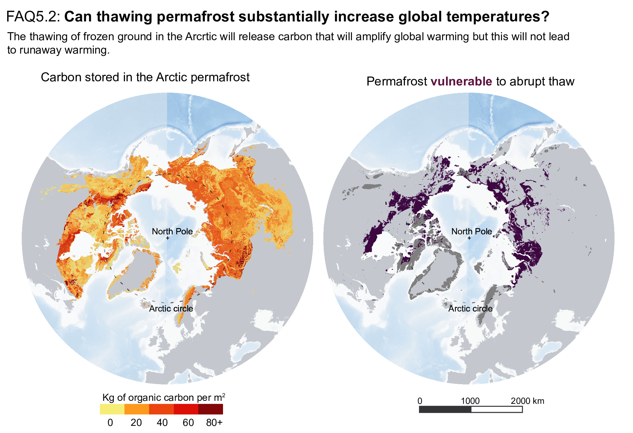 FAQ 5.2, Figure 1 | The Arctic permafrost is a big pool of carbon that is sensitive to climate change. (Left) Quantity of carbon stored in the permafrost, to 3 m depth (NCSCDv2 dataset) and (right) area of permafrost vulnerable to abrupt thaw (Circumpolar Thermokarst Landscapes dataset).
FAQ 5.3 | Could Climate Change Be Reversed By Removing Carbon Dioxide Fromthe Atmosphere?
Deliberate removal of carbon dioxide (CO2 ) from the atmospherecould reverse (i.e., change the direction of) some aspects of climate change. However, this will only happen if it results in a net reduction in the total amount of CO2 in the atmosphere, that is, if deliberate removals are larger than emissions. Some climate change trends, such as the increase in global surface temperature, would start to reverse within a few years. Other aspects of climate change would take decades (e.g., permafrost thawing) or centuries (e.g., acidification of the deep ocean) to reverse, and some, such as sea level rise, would take centuries to millennia to change direction.
The termnegative carbon dioxide (CO2 ) emissionsrefers to the removal of CO2 from the atmosphere by deliberate human activities, in addition to removals that occur naturally, and is often used as synonymous with carbon dioxide removal. Negative CO2 emissions can compensate for the release of CO2 into the atmosphere by human activities. They could be achieved by strengthening natural CO2 sequestration processes on land (e.g., by planting trees or through agricultural practices that increase the carbon content of soils) and/or in the ocean (e.g., by restoration of coastal ecosystems) or by removing CO2 directly from the atmosphere. If CO2 removals are greater than human-caused CO2 emissions globally, emissions are said to be net negative. It should be noted that CO2 removal technologies are unable, or not yet ready, to achieve the scale of removal that would be required to compensate for current levels of emissions, and most have undesired side effects.
In the absence of deliberate CO2 removal, the CO2 concentration in the atmosphere (a measure of the amount of CO2 in the atmosphere) results from a balance between human-caused CO2 release and the removal of CO2 by natural processes on land and in the ocean (natural ‘carbon sinks’; see FAQ 5.1). If CO2 release exceeds removal by carbon sinks, the CO2 concentration in the atmosphere would increase; if CO2 release equals removal, the atmospheric CO2 concentration would stabilize; and if CO2 removal exceeds release, the CO2 concentration would decline. This applies in the same way tonetCO2 emissions – that is, the sum of human-caused releases and deliberate removals.
If the CO2 concentration in the atmosphere starts to go down, the Earth’s climate would respond to this change (FAQ 5.3, Figure 1). Some parts of the climate system take time to react to a change in CO2 concentration, so a decline in atmospheric CO2 as a result of net negative emissions would not lead to immediate reversal of all climate change trends. Recent studies have shown that global surface temperature starts to decline within a few years following a decline in atmospheric CO2, although the decline would not be detectable for decades due to natural climate variability (see FAQ 4.2). Other consequences of human-induced climate change, such as reduction in permafrost area, would take decades; yet others, such as warming, acidification and oxygen loss of the deep ocean, would take centuries to reverse following a decline in the atmospheric CO2 concentration. Sea level would continue to rise for many centuries to millennia, even if large deliberate CO2 removals were successfully implemented.
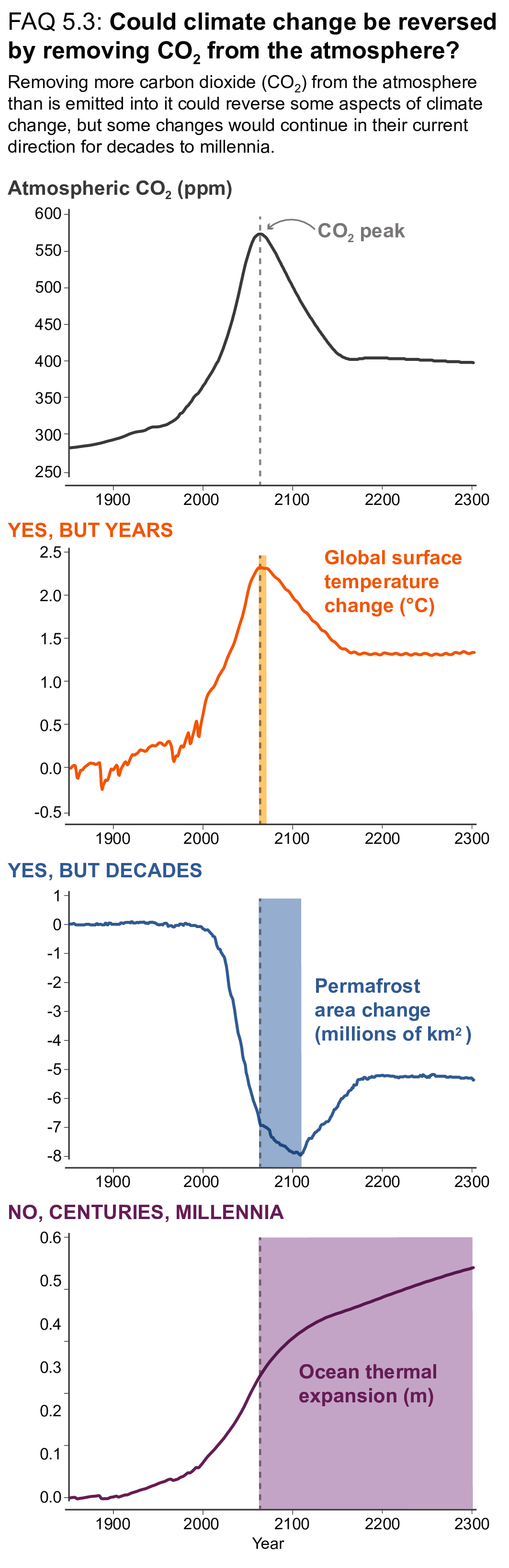
FAQ 5.3, Figure 1 | Changes in aspects of climate change in response to a peak and decline in the atmospheric CO2 concentration(top panel). The vertical grey dashed line indicates the time of peak CO2 concentration in all panels. It shows that the reversal of global surface warming lags the decrease in the atmospheric CO2 concentration by a few years, the reversal of permafrost area decline lags the decrease in atmospheric CO2 by decades, and ocean thermal expansion continues for several centuries. The quantitative information in the figure (i.e., numbers on vertical axes) is not to be emphasized as it results from simulations with just one model and will be different for other models. The qualitative behaviour, however, can be expected to be largely model independent.
‘Overshoot’ scenarios are a class of future scenarios that are receiving increasing attention, particularly in the context of ambitious climate goals, such as the global warming limits of 1.5°C or 2°C included in the Paris Agreement. In these scenarios, a slow rate of reduction in emissions in the near term is compensated by net negative CO2 emissions in the later part of this century, which results in a temporary breach or ‘overshoot’ of a given warming level. Due to the delayed reaction of several climate system components, it follows that the temporary overshoot would result in additional climate changes compared to a scenario that reaches the goal without overshoot. These changes would take decades to many centuries to reverse, with the reversal taking longer for scenarios with larger overshoot.
Removing more CO2 from the atmosphere than is emitted into it would indeed begin to reverse some aspects of climate change, but some changes would still continue in their current direction for decades to millennia. Approaches capable of large-scale removal of CO2 are still in the state of research and development or unproven at the scales of deployment necessary to achieve a net reduction in atmospheric CO2 levels. CO2 removal approaches, particularly those deployed on land, can have undesired side effects on water, food production and biodiversity.
FAQ 5.4 | What Are Carbon Budgets?
There are several types of carbon budgets. Most often, the term refers to the total net amount of carbon dioxide (CO2) that can still be emitted by human activities while limiting global warming to a specified level (e.g., 1.5°C or 2°C above pre-industrial levels). This is referred to as the ‘remaining carbon budget’. Several choices and value judgements have to be made before it can be unambiguously estimated. When the remaining carbon budget is combined with all past CO2 emissions to date, a ‘total carbon budget’ compatible with a specific global warming limit can also be defined. A third type of carbon budget is the ‘historical carbon budget’, which is a scientific way to describe all past and present sources and sinks of CO2.
The termremaining carbon budget is used to describe the total net amount of CO2 that human activities can still release into the atmosphere while keeping global warming to a specified level, like 1.5°C or 2°C relative to pre-industrial temperatures. Emissions of CO2 from human activities are the main cause of global warming. A remaining carbon budget can be defined because of the specific way CO2 behaves in the Earth system. That is, global warming is roughly linearly proportional to the total net amount of CO2 emissions that are released into the atmosphere by human activities – also referred to as cumulative anthropogenic CO2 emissions. Other greenhouse gases behave differently and have to be accounted for separately.
The concept of a remaining carbon budget implies that, to stabilize global warming at any particular level, global emissions of CO2 need to be reduced to net zero levels at some point. ‘Net zero CO2 emissions’ describes a situation where all the anthropogenic emissions of CO2 are counterbalanced by deliberate anthropogenic removals so that, on average, no CO2 is added or removed from the atmosphere by human activities. Atmospheric CO2 concentrations in such a situation would gradually decline to a long-term stable level as excess CO2 in the atmosphere is taken up by ocean and land sinks (see FAQ 5.1). The concept of a remaining carbon budget also means that, if CO2 emissions reductions are delayed, deeper and faster reductions are needed later to stay within the same budget. If the remaining carbon budget is exceeded, this will result in either higher global warming or a need to actively remove CO2 from the atmosphere to reduce global temperatures back down to the desired level (see FAQ 5.3).
Estimating the size of remaining carbon budgets depends on a set of choices. These choices include: (1) the global warming level that is chosen as a limit (for example, 1.5°C or 2°C relative to pre-industrial levels); (2) the probability with which we want to ensure that warming is held below that limit (for example, a one-in-two, two-in-three, or higher chance), and (3) how successful we are in limiting emissions of other greenhouse gases that affect the climate, such as methane or nitrous oxide. These choices can be informed by science, but ultimately represent subjective choices. Once these choices have been made, to estimate the remaining carbon budget for a given temperature goal, we can combine knowledge about: how much our planet has warmed already; the amount of warming per cumulative tonne of CO2 ; and the amount of warming that is still expected once global net CO2 emissions are brought down to zero. For example, to limit global warming to 1.5°C above pre-industrial levels with either a one-in-two (50%) or two-in-three (67%) chance, the remaining carbon budgets amount to 500 and 400 billion tonnes of CO2, respectively, from 1 January 2020 onward (FAQ 5.4, Figure 1). Currently, human activities are emitting around 40 billion tonnes of CO2 into the atmosphere in a single year.
The remaining carbon budget depends on how much the world has already warmed to date. This past warming is caused by historical emissions, which are estimated by looking at the historical carbon budget– a scientific way to describe all past and present sources and sinks of CO2. It describes how the CO2 emissions from human activities have redistributed across the various CO2 reservoirs of the Earth system. These reservoirs are the ocean, the land vegetation, and the atmosphere (into which CO2 was emitted). The share of CO2 that is not taken up by the ocean or the land, and that thus increases the concentration of CO2 in the atmosphere, causes global warming. The historical carbon budget tells us that, of the about 2560 billion tonnes of CO2 that were released into the atmosphere by human activities between the years 1750 and 2019, about a quarter were absorbed by the ocean (causing ocean acidification) and about a third by the land vegetation. About 45% of these emissions remain in the atmosphere (see FAQ 5.1). Adding these historical CO2 emissions to estimates of remaining carbon budgets allows an estimate of the total carbon budget consistent with a specific global warming level.
In summary, determining a remaining carbon budget – that is, how much CO2 can be released into the atmosphere while stabilizing global temperature below a chosen level – is well understood but relies on a set of choices. However, it is clear that, for limiting warming below 1.5°C or 2°C, the remaining carbon budget from 2020 onwards is much smaller than the total CO2 emissions released to date.

FAQ 5.4, Figure 1 | Various types of carbon budgets. Historical cumulative carbon dioxide (CO2) emissions determine to a large degree how much the world has warmed to date, while the remaining carbon budget indicates how much CO2 could still be emitted while keeping warming below specific temperature thresholds. Several factors limit the precision with which the remaining carbon budget can be estimated. Therefore, estimates need to specify the probability with which they aim at limiting warming to the intended target level (e.g., limiting warming to 1.5°C with a 67% probability).
References
Abatzoglou, J.T., A.P. Williams, and R. Barbero, 2019: Global Emergence of Anthropogenic Climate Change in Fire Weather Indices. Geophysical Research Letters, 46(1), 326–336, doi: 10.1029/2018gl080959.
Abbott, B.W. and J.B. Jones, 2015: Permafrost collapse alters soil carbon stocks, respiration, CH4, and N2O in upland tundra. Global Change Biology, 21(12), 4570–4587, doi: 10. 1111/gcb.13069.
Abram, N.J. et al., 2021: Connections of climate change and variability to large and extreme forest fires in southeast Australia. Communications Earth & Environment, 2(1), 8, doi: 10.1038/s43247-020-00065-8.
Achat, D.L., L. Augusto, A. Gallet-Budynek, and D. Loustau, 2016: Future challenges in coupled C–N–P cycle models for terrestrial ecosystems under global change: a review. Biogeochemistry, 131(1–2), 173–202, doi: 10.1007/s10533-016-0274-9.
Adams, C.A., J.E. Andrews, and T. Jickells, 2012: Nitrous oxide and methane fluxes vs. carbon, nitrogen and phosphorous burial in new intertidal and saltmarsh sediments. Science of The Total Environment, 434, 240–251, doi: 10.1016/j.scitotenv.2011.11.058.
Adams, M.A., T.N. Buckley, and T.L. Turnbull, 2020: Diminishing CO2 -driven gains in water-use efficiency of global forests. Nature Climate Change, 10(5), 466–471, doi: 10.1038/s41558-020-0747-7.
Ahlstrom, A. et al., 2015: The dominant role of semi-arid ecosystems in the trend and variability of the land CO2 sink. Science, 348(6237), 895–899, doi: 10.1126/science.aaa1668.
Ahn, J. and E.J. Brook, 2014: Siple Dome ice reveals two modes of millennial CO2 change during the last ice age. Nature Communications, 5(1), 3723, doi: 10.1038/ncomms4723.
Ainsworth, E.A. and S.P. Long, 2005: What have we learned from 15 years of free-air CO2 enrichment (FACE)? A meta-analytic review of the responses of photosynthesis, canopy properties and plant production to rising CO2. New Phytologist, 165(2), 351–372, doi: 10.1111/j.1469-8137.2004.01224.x.
Ajayi, S. et al., 2020: Evaluation of Paleocene–Eocene Thermal Maximum Carbon Isotope Record Completeness – An Illustration of the Potential of Dynamic Time Warping in Aligning Paleo-Proxy Records. Geochemistry, Geophysics, Geosystems, 21(3), e2019GC008620, doi: 10.1029/2019gc008620.
Al-Haj, A.N. and R.W. Fulweiler, 2020: A synthesis of methane emissions from shallow vegetated coastal ecosystems. Global Change Biology, 26(5), 2988–3005, doi: 10. 1111/gcb.15046.
Allen, C.D., D.D. Breshears, and N.G. McDowell, 2015: On underestimation of global vulnerability to tree mortality and forest die-off from hotter drought in the Anthropocene. Ecosphere, 6(8), art129, doi: 10.1890/es15-00203.1.
Allen, G.H. and T.M. Pavelsky, 2018: Global extent of rivers and streams. Science, 361(6402), 585–588, doi: 10.1126/science.aat0636.
Allen, M.R. et al., 2009: Warming caused by cumulative carbon emissions towards the trillionth tonne. Nature, 458(7242), 1163–1166, doi: 10.1038/nature08019.
Allen, M.R. et al., 2018: Framing and Context. In: Global Warming of 1.5°C. An IPCC Special Report on the impacts of global warming of 1.5°C above pre-industrial levels and related global greenhouse gas emission pathways, in the context of strengthening the global response to the threat of climate change, sustainable development, and efforts to eradicate poverty[Masson-Delmotte, V., P. Zhai, H.-O. Pörtner, D. Roberts, J. Skea, P.R. Shukla, A. Pirani, W. Moufouma-Okia, C. Péan, R. Pidcock, S. Connors, J.B.R. Matthews, Y. Chen, X. Zhou, M.I. Gomis, E. Lonnoy, T. Maycock, M. Tignor, and T. Waterfield (eds.)]. In Press, pp. 49–92, www.ipcc.ch/sr15/chapter/chapter-1.
Anagnostou, E. et al., 2016: Changing atmospheric CO2 concentration was the primary driver of early Cenozoic climate. Nature, 533(7603), 380–384, doi: 10.1038/nature17423.
Anagnostou, E. et al., 2020: Proxy evidence for state-dependence of climate sensitivity in the Eocene greenhouse. Nature Communications, 11(1), 4436, doi: 10.1038/s41467-020-17887-x.
Andela, N. et al., 2017: A human-driven decline in global burned area. Science, 1356, 1356–1362, doi: 10.1126/science.aal4108.
Anderegg, W.R.L. et al., 2015: Tropical nighttime warming as a dominant driver of variability in the terrestrial carbon sink. Proceedings of the National Academy of Sciences, 112(51), 201521479, doi: 10.1073/pnas.1521479112.
Anderegg, W.R.L. et al., 2020: Climate-driven risks to the climate mitigation potential of forests. Science, 368(6497), eaaz7005, doi: 10.1126/science.aaz7005.
Anderson, K. and G. Peters, 2016: The trouble with negative emissions. Science, 354(6309), 182–183, doi: 10.1126/science.aah4567.
Anderson, L.G. et al., 2017: Export of calcium carbonate corrosive waters from the East Siberian Sea. Biogeosciences, 14(7), 1811–1823, doi: 10.5194/bg-14-1811-2017.
Anderson, R.F. et al., 2019: Deep-Sea Oxygen Depletion and Ocean Carbon Sequestration During the Last Ice Age. Global Biogeochemical Cycles, 33(3), 301–317, doi: 10.1029/2018gb006049.
Andrew, R.M., 2018: Global CO2 emissions from cement production. Earth System Science Data, 10(1), 195–217, doi: 10.5194/essd-10-195-2018.
Andrew, R.M., 2019: Global CO2 emissions from cement production, 1928–2018. Earth System Science Data, 11(4), 1675–1710, doi: 10.5194/essd-11-1675-2019.
Andrew, R.M., 2020: A comparison of estimates of global carbon dioxide emissions from fossil carbon sources. Earth System Science Data, 12(2), 1437–1465, doi: 10.5194/essd-12-1437-2020.
Aragão, L.E.O.C. et al., 2018: 21st Century drought-related fires counteract the decline of Amazon deforestation carbon emissions. Nature Communications, 9(1), 536, doi: 10.1038/s41467-017-02771-y.
Archer, D., B. Buffett, and V. Brovkin, 2009: Ocean methane hydrates as a slow tipping point in the global carbon cycle. Proceedings of the National Academy of Sciences, 106(49), 20596–20601, doi: 10.1073/pnas.0800885105.
Ardyna, M. and K.R. Arrigo, 2020: Phytoplankton dynamics in a changing Arctic Ocean. Nature Climate Change, 10(10), 892–903, doi: 10.1038/s41558-020-0905-y.
Arévalo-Martínez, D.L., A. Kock, C.R. Löscher, R.A. Schmitz, and H.W. Bange, 2015: Massive nitrous oxide emissions from the tropical South Pacific Ocean. Nature Geoscience, 8(7), 530–533, doi: 10.1038/ngeo2469.
Armour, K.C., J. Marshall, J.R. Scott, A. Donohoe, and E.R. Newsom, 2016: Southern Ocean warming delayed by circumpolar upwelling and equatorward transport. Nature Geoscience, 9(7), 549–554, doi: 10.1038/ngeo2731.
Armstrong McKay, D.I. and T.M. Lenton, 2018: Reduced carbon cycle resilience across the Palaeocene–Eocene Thermal Maximum. Climate of the Past, 14(10), 1515–1527, doi: 10.5194/cp-14-1515-2018.
Arneth, A. et al., 2010: Terrestrial biogeochemical feedbacks in the climate system. Nature Geoscience, 3(8), 525–532, doi: 10.1038/ngeo905.
Arneth, A. et al., 2017: Historical carbon dioxide emissions caused by land-use changes are possibly larger than assumed. Nature Geoscience, 10(2), 79–84, doi: 10.1038/ngeo2882.
Arora, V.K. and J.R. Melton, 2018: Reduction in global area burned and wildfire emissions since 1930s enhances carbon uptake by land. Nature Communications, 9(1), 1326, doi: 10.1038/s41467-018-03838-0.
Arora, V.K. et al., 2013: Carbon–concentration and carbon–climate feedbacks in CMIP5 Earth system models. Journal of Climate, 26(15), 5289–5314, doi: 10.1175/jcli-d-12-00494.1.
Arora, V.K. et al., 2020: Carbon–concentration and carbon–climate feedbacks in CMIP6 models and their comparison to CMIP5 models. Biogeosciences, 17(16), 4173–4222, doi: 10.5194/bg-17-4173-2020.
Arzhanov, M.M. and I.I. Mokhov, 2017: Stability of continental relic methane hydrates for the holocene climatic optimum and for contemporary conditions. Doklady Earth Sciences, 476(2), 1163–1167, doi: 10.1134/s1028334x17100026.
Arzhanov, M.M., I.I. Mokhov, and S.N. Denisov, 2016: Impact of regional climatic change on the stability of relic gas hydrates. Doklady Earth Sciences, 468(2), 616–618, doi: 10.1134/s1028334x1606009x.
Arzhanov, M.M., V. Malakhova, and I.I. Mokhov, 2020: Modeling thermal regime and evolution of the methane hydrate stability zone of the Yamal peninsula permafrost. Permafrost and Periglacial Processes, 31(4), 487–496, doi: 10.1002/ppp.2074.
Astor, Y.M. et al., 2013: Interannual variability in sea surface temperature and fCO2 changes in the Cariaco Basin. Deep Sea Research Part II: Topical Studies in Oceanography, 93, 33–43, doi: 10.1016/j.dsr2.2013.01.002.
Atwood, T.B. et al., 2017: Global patterns in mangrove soil carbon stocks and losses. Nature Climate Change, 7(7), 523–528, doi: 10.1038/nclimate3326.
Auger, M., R. Morrow, E. Kestenare, J.-B. Sallée, and R. Cowley, 2021: Southern Ocean in-situ temperature trends over 25 years emerge from interannual variability. Nature Communications, 12(1), 514, doi: 10.1038/s41467-020-20781-1.
Azetsu-Scott, K. et al., 2010: Calcium carbonate saturation states in the waters of the Canadian Arctic Archipelago and the Labrador Sea. Journal of Geophysical Research: Oceans, 115(C11), C11021, doi: 10.1029/2009jc005917.
Babbin, A.R., D. Bianchi, A. Jayakumar, and B.B. Ward, 2015: Rapid nitrous oxide cycling in the suboxic ocean. Science, 348(6239), 1127–1129, doi: 10.1126/science.aaa8380.
Babila, T.L. et al., 2018: Capturing the global signature of surface ocean acidification during the Palaeocene–Eocene Thermal Maximum. Philosophical Transactions of the Royal Society A: Mathematical, Physical and Engineering Sciences, 376(2130), 20170072, doi: 10.1098/rsta.2017.0072.
Bacastow, R.B. et al., 1980: Atmospheric carbon dioxide, the Southern oscillation, and the weak 1975 El Niño. Science, 210(4465), 66–68, doi: 10.1126/science.210.4465.66.
Bach, L.T., S.J. Gill, R.E.M. Rickaby, S. Gore, and P. Renforth, 2019: CO2 Removal With Enhanced Weathering and Ocean Alkalinity Enhancement: Potential Risks and Co-benefits for Marine Pelagic Ecosystems. Frontiers in Climate, 1, 7, doi: 10.3389/fclim.2019.00007.
Bach, L.T. et al., 2016: Influence of plankton community structure on the sinking velocity of marine aggregates. Global Biogeochemical Cycles, 30(8), 1145–1165, doi: 10.1002/2016gb005372.
Bachman, S.D. and A. Klocker, 2020: Interaction of jets and submesoscale dynamics leads to rapid ocean ventilation. Journal of Physical Oceanography, 50(10), 2873–2883, doi: 10.1175/jpo-d-20-0117.1.
Badgley, G., C.B. Field, and J.A. Berry, 2017: Canopy near-infrared reflectance and terrestrial photosynthesis. Science Advances, 3(3), e1602244, doi: 10.1126/sciadv.1602244.
Baggenstos, D. et al., 2019: Earth’s radiative imbalance from the Last Glacial Maximum to the present. Proceedings of the National Academy of Sciences, 116(30), 14881–14886, doi: 10.1073/pnas.1905447116.
Baig, S., B.E. Medlyn, L.M. Mercado, and S. Zaehle, 2015: Does the growth response of woody plants to elevated CO2 increase with temperature? A model-oriented meta-analysis. Global Change Biology, 21(12), 4303–4319, doi: 10. 1111/gcb.12962.
Bakker, D.C.E. et al., 2016: A multi-decade record of high-quality fCO2 data in version 3 of the Surface Ocean CO2 (Atlas (SOCAT). Earth System Science Data, 8(2), 383–413, doi: 10.5194/essd-8-383-2016.
Bakun, A. et al., 2015: Anticipated Effects of Climate Change on Coastal Upwelling Ecosystems. Current Climate Change Reports, 1(2), 85–93, doi: 10.1007/s40641-015-0008-4.
Balesdent, J. et al., 2018: Atmosphere–soil carbon transfer as a function of soil depth. Nature, 559(7715), 599–602, doi: 10.1038/s41586-018-0328-3.
Ballantyne, A. et al., 2017: Accelerating net terrestrial carbon uptake during the warming hiatus due to reduced respiration. Nature Climate Change, 7(2), 148–152, doi: 10.1038/nclimate3204.
Ballantyne, A.P., C.B. Alden, J.B. Miller, P.P. Tans, and J.W.C. White, 2012: Increase in observed net carbon dioxide uptake by land and oceans during the past 50 years. Nature, 488(7409), 70–72, doi: 10.1038/nature11299.
Bândă, N. et al., 2016: Can we explain the observed methane variability after the Mount Pinatubo eruption?Atmospheric Chemistry and Physics, 16(1), 195–214, doi: 10.5194/acp-16-195-2016.
Barker, S. and H. Elderfield, 2002: Foraminiferal Calcification Response to Glacial-Interglacial Changes in Atmospheric CO2. Science, 297(5582), 833–836, doi: 10.1126/science.1072815.
Bastviken, D., L.J. Tranvik, J.A. Downing, P.M. Crill, and A. Enrich-Prast, 2011: Freshwater Methane Emissions Offset the Continental Carbon Sink. Science, 331(6013), 50–50, doi: 10.1126/science.1196808.
Bates, N.R. and R.J. Johnson, 2020: Acceleration of ocean warming, salinification, deoxygenation and acidification in the surface subtropical North Atlantic Ocean. Communications Earth & Environment, 1(1), 33, doi: 10.1038/s43247-020-00030-5.
Bates, N.R., J.T. Mathis, and L.W. Cooper, 2009: Ocean acidification and biologically induced seasonality of carbonate mineral saturation states in the western Arctic Ocean. Journal of Geophysical Research: Oceans, 114(C11), C11007, doi: 10.1029/2008jc004862.
Bates, N.R. et al., 2014: A Time-Series View of Changing Ocean Chemistry Due to Ocean Uptake of Anthropogenic CO2 and Ocean Acidification. Oceanography, 27(1), 126–141, doi: 10.5670/oceanog.2014.16.
Bathiany, S., J. Hidding, and M. Scheffer, 2020: Edge Detection Reveals Abrupt and Extreme Climate Events. Journal of Climate, 33(15), 6399–6421, doi: 10.1175/jcli-d-19-0449.1.
Bathiany, S., M. Claussen, V. Brovkin, T. Raddatz, and V. Gayler, 2010: Combined biogeophysical and biogeochemical effects of large-scale forest cover changes in the MPI earth system model. Biogeosciences, 7(5), 1383–1399, doi: 10.5194/bg-7-1383-2010.
Batjes, N.H., 2016: Harmonized soil property values for broad-scale modelling (WISE30sec) with estimates of global soil carbon stocks. Geoderma, 269, 61–68, doi: 10.1016/j.geoderma.2016.01.034.
Battaglia, G. and F. Joos, 2018a: Hazards of decreasing marine oxygen: the near-term and millennial-scale benefits of meeting the Paris climate targets. Earth System Dynamics, 9(2), 797–816, doi: 10.5194/esd-9-797-2018.
Battaglia, G. and F. Joos, 2018b: Marine N2O Emissions From Nitrification and Denitrification Constrained by Modern Observations and Projected in Multimillennial Global Warming Simulations. Global Biogeochemical Cycles, 32(1), 92–121, doi: 10.1002/2017gb005671.
Baumgartner, M. et al., 2014: NGRIP CH4 concentration from 120 to 10 kyr before present and its relation to a δ15N temperature reconstruction from the same ice core. Climate of the Past, 10(2), 903–920, doi: 10.5194/cp-10-903-2014.
Bauska, T.K. et al., 2018: Controls on Millennial-Scale Atmospheric CO2 Variability During the Last Glacial Period. Geophysical Research Letters, 45(15), 7731–7740, doi: 10.1029/2018gl077881.
Beaufort, L. et al., 2011: Sensitivity of coccolithophores to carbonate chemistry and ocean acidification. Nature, 476(7358), 80–83, doi: 10.1038/nature10295.
Beaulieu, J.J., T. DelSontro, and J.A. Downing, 2019: Eutrophication will increase methane emissions from lakes and impoundments during the 21st century. Nature Communications, 10(1), 1375, doi: 10.1038/s41467-019-09100-5.
Beaupré-Laperrière, A., A. Mucci, and H. Thomas, 2020: The recent state and variability of the carbonate system of the Canadian Arctic Archipelago and adjacent basins in the context of ocean acidification. Biogeosciences, 17(14), 3923–3942, doi: 10.5194/bg-17-3923-2020.
Beck, J. et al., 2018: Bipolar carbon and hydrogen isotope constraints on the Holocene methane budget. Biogeosciences, 15(23), 7155–7175, doi: 10.5194/bg-15-7155-2018.
Bednaršek, N. et al., 2020: Exoskeleton dissolution with mechanoreceptor damage in larval Dungeness crab related to severity of present-day ocean acidification vertical gradients. Science of The Total Environment, 716, 136610, doi: 10.1016/j.scitotenv.2020.136610.
Beer, C. et al., 2010: Terrestrial Gross Carbon Dioxide Uptake: Global Distribution and Covariation with Climate. Science, 329(5993), 834–838, doi: 10.1126/science.1184984.
Beerling, D.J. et al., 2018: Farming with crops and rocks to address global climate, food and soil security. Nature Plants, 4(3), 138–147, doi: 10.1038/s41477-018-0108-y.
Benanti, G., M. Saunders, B. Tobin, and B. Osborne, 2014: Contrasting impacts of afforestation on nitrous oxide and methane emissions. Agricultural and Forest Meteorology, 198–199, 82–93, doi: 10.1016/j.agrformet.2014.07.014.
Bennedsen, M., E. Hillebrand, and S. Jan Koopman, 2019: Trend analysis of the airborne fraction and sink rate of anthropogenically released CO2. Biogeosciences, 16(18), 3651–3663, doi: 10.5194/bg-16-3651-2019.
Berchet, A. et al., 2016: Atmospheric constraints on the methane emissions from the East Siberian Shelf. Atmospheric Chemistry and Physics, 16(6), 4147–4157, doi: 10.5194/acp-16-4147-2016.
Bereiter, B., S. Shackleton, D. Baggenstos, K. Kawamura, and J. Severinghaus, 2018: Mean global ocean temperatures during the last glacial transition. Nature, 553(7686), 39–44, doi: 10.1038/nature25152.
Berg, A. et al., 2016: Land–atmosphere feedbacks amplify aridity increase over land under global warming. Nature Climate Change, 6(9), 869–874, doi: 10.1038/nclimate3029.
Beringer, T., W. Lucht, and S. Schaphoff, 2011: Bioenergy production potential of global biomass plantations under environmental and agricultural constraints. GCB Bioenergy, 3(4), 299–312, doi: 10.1111/j.1757-1707.2010.01088.x.
Betts, R.A. et al., 2018: A successful prediction of the record CO2 rise associated with the 2015/2016 El Niño. Philosophical Transactions of the Royal Society B: Biological Sciences, 373(1760), 20170301, doi: 10.1098/rstb.2017.0301.
BGR, 2020: BGR Energy Study 2019 – Data and Developments Concerning German and Global Energy Supplies. 200 pp., www.bgr.bund.de/EN/Themen/Energie/Produkte/energy_study_2019_summary_en.html.
Bianchi, D., J.P. Dunne, J.L. Sarmiento, and E.D. Galbraith, 2012: Data-based estimates of suboxia, denitrification, and N2O production in the ocean and their sensitivities to dissolved O2. Global Biogeochemical Cycles, 26(2), GB2009, doi: 10.1029/2011gb004209.
Bindoff, N.L. et al., 2019: Changing Ocean, Marine Ecosystems, and Dependent Communities. In: IPCC Special Report on the Ocean and Cryosphere in a Changing Climate[Pörtner, H.-O., D.C. Roberts, V. Masson-Delmotte, P. Zhai, M. Tignor, E. Poloczanska, K. Mintenbeck, A. Alegría, M. Nicolai, A. Okem, J. Petzold, B. Rama, and N.M. Weyer (eds.)]. In Press, pp. 447–588, www.ipcc.ch/srocc/chapter/chapter-5.
Blanc-Betes, E. et al., 2020: In silico assessment of the potential of basalt amendments to reduce N2O emissions from bioenergy crops. GCB Bioenergy, 13(1), 224–241, doi: 10.1111/gcbb.12757.
Blanchette, C.D. et al., 2016: Printable enzyme-embedded materials for methane to methanol conversion. Nature Communications, 7(1), 11900, doi: 10.1038/ncomms11900.
Bobich, E.G., G.A. Barron-Gafford, K.G. Rascher, and R. Murthy, 2010: Effects of drought and changes in vapour pressure deficit on water relations ofPopulus deltoidesgrowing in ambient and elevated CO2. Tree Physiology, 30(7), 866–875, doi: 10.1093/t reephys/tpq036.
Bock, M. et al., 2010: Hydrogen isotopes preclude marine hydrate CH4 emissions at the onset of Dansgaard-Oeschger events. Science, 328(5986), 1686–9, doi: 10.1126/science.1187651.
Bock, M. et al., 2017: Glacial/interglacial wetland, biomass burning, and geologic methane emissions constrained by dual stable isotopic CH4 ice core records. Proceedings of the National Academy of Sciences, 114(29), E5778–E5786, doi: 10.1073/pnas.1613883114.
Boden, T.A., G. Marland, and R.J. Andres, 2017: Global, Regional, and National Fossil-Fuel CO2 Emissions (1751–2014) (V. 2017). Carbon Dioxide Information Analysis Center (CDIAC), Oak Ridge National Laboratory (ORNL), Oak Ridge, TN, USA. Retrieved from: https://cdiac.ess-dive.lbl.gov/trends/emis/overview.html.
Boer, M.M., V. Resco de Dios, and R.A. Bradstock, 2020: Unprecedented burn area of Australian mega forest fires. Nature Climate Change, 10(3), 171–172, doi: 10.1038/s41558-020-0716-1.
Bopp, L., M. Lévy, L. Resplandy, and J.B. Sallée, 2015: Pathways of anthropogenic carbon subduction in the global ocean. Geophysical Research Letters, 42(15), 6416–6423, doi: 10.1002/2015gl065073.
Bopp, L. et al., 2013: Multiple stressors of ocean ecosystems in the 21st century: projections with CMIP5 models. Biogeosciences, 10(10), 6225–6245, doi: 10.5194/bg-10-6225-2013.
Borges, A.V. and G. Abril, 2011: Carbon Dioxide and Methane Dynamics in Estuaries. In: Treatise on Estuarine and Coastal Science[Wolanski, E. and D. McLusky (eds.)]. Academic Press, Waltham, MA, USA, pp. 119–161, doi: 10.1016/b978-0-12-374711-2.00504-0.
Boscolo-Galazzo, F., K.A. Crichton, S. Barker, and P.N. Pearson, 2018: Temperature dependency of metabolic rates in the upper ocean: A positive feedback to global climate change?Global and Planetary Change, 170, 201–212, doi: 10.1016/j.gloplacha.2018.08.017.
Boulton, C.A., B.B.B. Booth, and P. Good, 2017: Exploring uncertainty of Amazon dieback in a perturbed parameter Earth system ensemble. Global Change Biology, 23(12), 5032–5044, doi: 10. 1111/gcb.13733.
Bousquet, P. et al., 2006: Contribution of anthropogenic and natural sources to atmospheric methane variability. Nature, 443(7110), 439–443, doi: 10.1038/nature05132.
Bowen, G.J. and J.C. Zachos, 2010: Rapid carbon sequestration at the termination of the Palaeocene–Eocene Thermal Maximum. Nature Geoscience, 3(12), 866–869, doi: 10.1038/ngeo1014.
Bowman, D.M.J.S. et al., 2020: Vegetation fires in the Anthropocene. Nature Reviews Earth & Environment, 1(10), 500–515, doi: 10.1038/s43017-020-0085-3.
Boyd, P.W. and C. Vivian, 2019: Should we fertilize oceans or seed clouds? No one knows. Nature, 570(7760), 155–157, doi: 10.1038/d41586-019-01790-7.
Boyd, P.W., S.T. Lennartz, D.M. Glover, and S.C. Doney, 2015: Biological ramifications of climate-change-mediated oceanic multi-stressors. Nature Climate Change, 5(1), 71–79, doi: 10.1038/nclimate2441.
Boyd, P.W., H. Claustre, M. Levy, D.A. Siegel, and T. Weber, 2019: Multi-faceted particle pumps drive carbon sequestration in the ocean. Nature, 568(7752), 327–335, doi: 10.1038/s41586-019-1098-2.
Boysen, L.R., W. Lucht, and D. Gerten, 2017a: Trade-offs for food production, nature conservation and climate limit the terrestrial carbon dioxide removal potential. Global Change Biology, 23(10), 4303–4317, doi: 10. 1111/gcb.13745.
Boysen, L.R. et al., 2017b: The limits to global-warming mitigation by terrestrial carbon removal. Earth’s Future, 5(5), 463–474, doi: 10.1002/2016ef000469.
BP, 2018: BP Statistical Review of World Energy June 2018. BP, London, UK, 53 pp., www.bp.com/content/dam/bp/business-sites/en/global/corporate/pdfs/energy-economics/statistical-review/bp-stats-review-2018-f ull-report.pdf .
Brady, R.X., N.S. Lovenduski, S.G. Yeager, M.C. Long, and K. Lindsay, 2020: Skillful multiyear predictions of ocean acidification in the California Current System. Nature Communications, 11(1), 2166, doi: 10.1038/s41467-020-15722-x.
Bralower, T.J. et al., 2018: Evidence for shelf acidification during the onset of the Paleocene-Eocene thermal maximum. Paleoceanography and Paleoclimatology, 33(12), 1408–1426, doi: 10.1029/2018pa003382.
Brando, P.M. et al., 2014: Abrupt increases in Amazonian tree mortality due to drought–fire interactions. Proceedings of the National Academy of Sciences, 111(17), 6347–6352, doi: 10.1073/pnas.1305499111.
Brando, P.M. et al., 2019: Droughts, Wildfires, and Forest Carbon Cycling: A Pantropical Synthesis. Annual Review of Earth and Planetary Sciences, 47, 555–581, doi: 10.1146/annurev-earth-082517-010235.
Brando, P.M. et al., 2020: The gathering firestorm in southern Amazonia. Science Advances, 6(2), eaay1632, doi: 10.1126/sciadv.aay1632.
Breider, F. et al., 2019: Response of N2O production rate to ocean acidification in the western North Pacific. Nature Climate Change, 9(12), 954–958, doi: 10.1038/s41558-019-0605-7.
Breitburg, D. et al., 2018: Declining oxygen in the global ocean and coastal waters. Science, 359(6371), eaam7240, doi: 10.1126/science.aam7240.
Brewer, P.G., 2019: The Molecular Basis for Understanding the Impacts of Ocean Warming. Reviews of Geophysics, 57(3), 1112–1123, doi: 10.1029/2018rg000620.
Bridgham, S.D., H. Cadillo-Quiroz, J.K. Keller, and Q. Zhuang, 2013: Methane emissions from wetlands: biogeochemical, microbial, and modeling perspectives from local to global scales. Global Change Biology, 19(5), 1325–1346, doi: 10. 1111/gcb.12131.
Brienen, R.J.W. et al., 2015: Long-term decline of the Amazon carbon sink. Nature, 519(7543), 344–348, doi: 10.1038/nature14283.
Bronselaer, B. and L. Zanna, 2020: Heat and carbon coupling reveals ocean warming due to circulation changes. Nature, 584(7820), 227–233, doi: 10.1038/s41586-020-2573-5.
Bronselaer, B., L. Zanna, D.R. Munday, and J. Lowe, 2018: Southern Ocean carbon–wind stress feedback. Climate Dynamics, 51(7–8), 2743–2757, doi: 10.1007/s00382-017-4041-y.
Broucek, J., 2014: Production of Methane Emissions from Ruminant Husbandry: A Review. Journal of Environmental Protection, 5(15), 1482–1493, doi: 10.4236/jep.2014.515141.
Brovkin, V. et al., 2013: Effect of anthropogenic land-use and land-cover changes on climate and land carbon storage in CMIP5 projections for the twenty-first century. Journal of Climate, 26(18), 6859–6881, doi: 10.1175/jcli-d-12-00623.1.
Brovkin, V. et al., 2016: Comparative carbon cycle dynamics of the present and last interglacial. Quaternary Science Reviews, 137, 15–32, doi: 10.1016/j.quascirev.2016.01.028.
Brovkin, V. et al., 2019: What was the source of the atmospheric CO2 increase during the Holocene?Biogeosciences, 16(13), 2543–2555, doi: 10.5194/bg-16-2543-2019.
Bruhn, D., I.M. Møller, T.N. Mikkelsen, and P. Ambus, 2012: Terrestrial plant methane production and emission. Physiologia Plantarum, 144(3), 201–209, doi: 10.1111/j.1399-3054.2011.01551.x.
Bruhwiler, L., F.J.W. Parmentier, P. Crill, M. Leonard, and P.I. Palmer, 2021: The Arctic Carbon Cycle and Its Response to Changing Climate. Current Climate Change Reports, 7, 14–34, doi: 10.1007/s40641-020-00169-5.
Brune, A., 2018: Methanogenesis in the Digestive Tracts of Insects and Other Arthropods. In: Biogenesis of Hydrocarbons[Stams, A. and D. Sousa (eds.)]. Springer, Cham, Switzerland, pp. 1–32, doi: 10.1007/978-3-319-53114-4_13-1.
Buchanan, P.J. et al., 2016: The simulated climate of the Last Glacial Maximum and insights into the global marine carbon cycle. Climate of the Past, 12(12), 2271–2295, doi: 10.5194/cp-12-2271-2016.
Buermann, W. et al., 2018: Widespread seasonal compensation effects of spring warming on northern plant productivity. Nature, 562(7725), 110–114, doi: 10.1038/s41586-018-0555-7.
Buitenhuis, E.T., P. Suntharalingam, and C. Le Quéré, 2018: Constraints on global oceanic emissions of N2O from observations and models. Biogeosciences, 15(7), 2161–2175, doi: 10.5194/bg-15-2161-2018.
Buldovicz, S.N. et al., 2018: Cryovolcanism on the Earth: Origin of a Spectacular Crater in the Yamal Peninsula (Russia). Scientific Reports, 8(1), 13534, doi: 10.1038/s41598-018-31858-9.
Burke, E.J., C.D. Jones, and C.D. Koven, 2013: Estimating the permafrost-carbon climate response in the CMIP5 climate models using a simplified approach. Journal of Climate, 26(14), 4897–4909, doi: 10.1175/jcli-d-12-00550.1.
Burke, E.J., S.E. Chadburn, and A. Ekici, 2017a: A vertical representation of soil carbon in the JULES land surface scheme (vn4.3_permafrost) with a focus on permafrost regions. Geoscientific Model Development, 10(2), 959–975, doi: 10.5194/gmd-10-959-2017.
Burke, E.J. et al., 2017b: Quantifying uncertainties of permafrost carbon–climate feedbacks. Biogeosciences, 14(12), 3051–3066, doi: 10.5194/bg-14-3051-2017.
Burls, N.J. et al., 2017: Active Pacific meridional overturning circulation (PMOC) during the warm Pliocene. Science Advances, 3(9), e1700156, doi: 10.1126/sciadv.1700156.
Burney, J.A., S.J. Davis, and D.B. Lobell, 2010: Greenhouse gas mitigation by agricultural intensification. Proceedings of the National Academy of Sciences, 107(26), 12052–12057, doi: 10.1073/pnas.0914216107.
Burton, C., R.A. Betts, C.D. Jones, and K. Williams, 2018: Will Fire Danger Be Reduced by Using Solar Radiation Management to Limit Global Warming to 1.5°C Compared to 2.0°C?Geophysical Research Letters, 45(8), 3644–3652, doi: 10.1002/2018gl077848.
Bushinsky, S.M. et al., 2019: Reassessing Southern Ocean Air-Sea CO2 Flux Estimates With the Addition of Biogeochemical Float Observations. Global Biogeochemical Cycles, 33(11), 1370–1388, doi: 10.1029/2019gb006176.
Butterbach-Bahl, K., E.M. Baggs, M. Dannenmann, R. Kiese, and S. Zechmeister-Boltenstern, 2013: Nitrous oxide emissions from soils: how well do we understand the processes and their controls?Philosophical Transactions of the Royal Society B: Biological Sciences, 368(1621), 20130122–20130122, doi: 10.1098/rstb.2013.0122.
Byrne, R.H., S. Mecking, R.A. Feely, and X. Liu, 2010: Direct observations of basin-wide acidification of the North Pacific Ocean. Geophysical Research Letters, 37(2), L02601, doi: 10.1029/2009gl040999.
Cabré, A., I. Marinov, and S. Leung, 2015: Consistent global responses of marine ecosystems to future climate change across the IPCC AR5 earth system models. Climate Dynamics, 45(5–6), 1253–1280, doi: 10.1007/s00382-014-2374-3.
Cai, W.-J. et al., 2011: Acidification of subsurface coastal waters enhanced by eutrophication. Nature Geoscience, 4(11), 766–770, doi: 10.1038/ngeo1297.
Cai, W.-J. et al., 2017: Redox reactions and weak buffering capacity lead to acidification in the Chesapeake Bay. Nature Communications, 8(1), 369, doi: 10.1038/s41467-017-00417-7.
Cai, W.-J. et al., 2020: Controls on surface water carbonate chemistry along North American ocean margins. Nature Communications, 11(1), 2691, doi: 10.1038/s41467-020-16530-z.
Cain, M. et al., 2019: Improved calculation of warming-equivalent emissions for short-lived climate pollutants. npj Climate and Atmospheric Science, 2, 29, doi: 10.1038/s41612-019-0086-4.
Caldeira, K. and M.E. Wickett, 2003: Anthropogenic carbon and ocean pH. Nature, 425(6956), 365–365, doi: 10.1038/425365a.
Campbell, J.E. et al., 2017: Large historical growth in global terrestrial gross primary production. Nature, 544(7648), 84–87, doi: 10.1038/nature22030.
Campbell, J.L., J. Sessions, D. Smith, and K. Trippe, 2018: Potential carbon storage in biochar made from logging residue: Basic principles and Southern Oregon case studies. PLOS ONE, 13(9), e0203475, doi: 10.1371/journal.pone.0203475.
Campos, R., G.F. Pires, and M.H. Costa, 2020: Soil Carbon Sequestration in Rainfed and Irrigated Production Systems in a New Brazilian Agricultural Frontier. Agriculture, 10(5), 156, doi: 10.3390/agriculture10050156.
Cao, L., 2018: The Effects of Solar Radiation Management on the Carbon Cycle. Current Climate Change Reports, 4(1), 41–50, doi: 10.1007/s40641-018-0088-z.
Cao, L. and J. Jiang, 2017: Simulated Effect of Carbon Cycle Feedback on Climate Response to Solar Geoengineering. Geophysical Research Letters, 44(24), 12484–12491, doi: 10.1002/2017gl076546.
Cao, L., H. Zhang, M. Zheng, and S. Wang, 2014: Response of ocean acidification to a gradual increase and decrease of atmospheric CO2. Environmental Research Letters, 9(2), 024012, doi: 10.1088/1748-9326/9/2/024012.
Cao, Z. et al., 2020: The sponge effect and carbon emission mitigation potentials of the global cement cycle. Nature Communications, 11(1), 1–9, doi: 10.1038/s41467-020-17583-w.
Carstensen, J. and D.J. Conley, 2019: Baltic Sea Hypoxia Takes Many Shapes and Sizes. Limnology and Oceanography Bulletin, 28(4), 125–129, doi: 10. 1002/lob.10350.
Carstensen, J. and C.M. Duarte, 2019: Drivers of pH variability in coastal ecosystems. Environmental Science & Technology, 53(8), 4020–4029, doi: 10.1021/acs.est.8b03655.
Carstensen, J., J.H. Andersen, B.G. Gustafsson, and D.J. Conley, 2014: Deoxygenation of the Baltic Sea during the last century. Proceedings of the National Academy of Sciences, 111(15), 5628–5633, doi: 10.1073/pnas.1323156111.
Cartapanis, O., E.D. Galbraith, D. Bianchi, and S.L. Jaccard, 2018: Carbon burial in deep-sea sediment and implications for oceanic inventories of carbon and alkalinity over the last glacial cycle. Climate of the Past, 14(11), 1819–1850, doi: 10.5194/cp-14-1819-2018.
Carter, B.R. et al., 2017: Two decades of Pacific anthropogenic carbon storage and ocean acidification along Global Ocean Ship-based Hydrographic Investigations Program sections P16 and P02. Global Biogeochemical Cycles, 31(2), 306–327, doi: 10.1002/2016gb005485.
Carter, B.R. et al., 2019: Pacific anthropogenic carbon between 1991 and 2017. Global Biogeochemical Cycles, 33(5), 597–617, doi: 10.1029/2018gb006154.
Cavan, E.L., S.A. Henson, and P.W. Boyd, 2019: The Sensitivity of Subsurface Microbes to Ocean Warming Accentuates Future Declines in Particulate Carbon Export. Frontiers in Ecology and Evolution, 6, 230, doi: 10.3389/f evo.2018.00230.
Cavan, E.L., S.A. Henson, A. Belcher, and R. Sanders, 2017: Role of zooplankton in determining the efficiency of the biological carbon pump. Biogeosciences, 14(1), 177–186, doi: 10.5194/bg-14-177-2017.
Cayuela, M.L. et al., 2014: Biochar’s role in mitigating soil nitrous oxide emissions: A review and meta-analysis. Agriculture, Ecosystems & Environment, 191, 5–16, doi: 10.1016/j.agee.2013.10.009.
Chan, F., J. Barth, K. Kroeker, J. Lubchenco, and B. Menge, 2019: The dynamics and impact of ocean acidification and hypoxia: insights from sustained investigations in the northern California current large marine ecosystem. Oceanography, 32(3), 62–71, doi: 10.5670/oceanog.2019.312.
Chandra, N. et al., 2021: Emissions from the Oil and Gas Sectors, Coal Mining and Ruminant Farming Drive Methane Growth over the Past Three Decades. Journal of the Meteorological Society of Japan. Series II, 99(2), 309–337, doi: 10.2151/jmsj.2021-015.
Chang, L. et al., 2018: Coupled microbial bloom and oxygenation decline recorded by magnetofossils during the Palaeocene–Eocene Thermal Maximum. Nature Communications, 9(1), 1–9, doi: 10.1038/s41467-018-06472-y.
Chaudhary, N. et al., 2020: Modelling past and future peatland carbon dynamics across the pan-Arctic. Global Change Biology, 26(7), 4119–4133, doi: 10. 1111/gcb.15099.
Chavez, F.P., A. Bertrand, R. Guevara-Carrasco, P. Soler, and J. Csirke, 2008: The northern Humboldt Current System: Brief history, present status and a view towards the future. Progress in Oceanography, 79(2–4), 95–105, doi: 10.1016/j.pocean.2008.10.012.
Chen, C.-C., G.-C. Gong, and F.-K. Shiah, 2007: Hypoxia in the East China Sea: One of the largest coastal low-oxygen areas in the world. Marine Environmental Research, 64(4), 399–408, doi: 10.1016/j.marenvres.2007.01.007.
Chen, C.-T.A. and A.V. Borges, 2009: Reconciling opposing views on carbon cycling in the coastal ocean: Continental shelves as sinks and near-shore ecosystems as sources of atmospheric CO2. Deep Sea Research Part II: Topical Studies in Oceanography, 56(8–10), 578–590, doi: 10.1016/j.dsr2.2009.01.001.
Chen, C.-T.A. et al., 2017: Deep oceans may acidify faster than anticipated due to global warming. Nature Climate Change, 7(12), 890–894, doi: 10.1038/s41558-017-0003-y.
Chen, P. et al., 2019: Effects of afforestation on soil CH4 and N2O fluxes in a subtropical karst landscape. Science of The Total Environment, 705, 135974, doi: 10.1016/j.scitotenv.2019.135974.
Chen, Y., A. Liu, and J.C. Moore, 2020: Mitigation of Arctic permafrost carbon loss through stratospheric aerosol geoengineering. Nature Communications, 11(1), 2430, doi: 10.1038/s41467-020-16357-8.
Cheng, L. et al., 2017: Recent increases in terrestrial carbon uptake at little cost to the water cycle. Nature Communications, 8(1), 110, doi: 10.1038/s41467-017-00114-5.
Chevallier, F. et al., 2005: Inferring CO2 sources and sinks from satellite observations: Method and application to TOVS data. Journal of Geophysical Research: Atmospheres, 110(D24), D24309, doi: 10.1029/2005jd006390.
Chierici, M. and A. Fransson, 2009: Calcium carbonate saturation in the surface water of the Arctic Ocean: undersaturation in freshwater influenced shelves. Biogeosciences, 6(11), 2421–2431, doi: 10.5194/bg-6-2421-2009.
Chou, W.-C., G.-C. Gong, W.-J. Cai, and C.-M. Tseng, 2013: Seasonality of CO2 in coastal oceans altered by increasing anthropogenic nutrient delivery from large rivers: evidence from the Changjiang–East China Sea system. Biogeosciences, 10(6), 3889–3899, doi: 10.5194/bg-10-3889-2013.
Chowdhry Beeman, J. et al., 2019: Antarctic temperature and CO2 : Near-synchrony yet variable phasing during the last deglaciation. Climate of the Past, 15(3), 913–926, doi: 10.5194/cp-15-913-2019.
Chu, S.N., Z.A. Wang, S.C. Doney, G.L. Lawson, and K.A. Hoering, 2016: Changes in anthropogenic carbon storage in the Northeast Pacific in the last decade. Journal of Geophysical Research: Oceans, 121(7), 4618–4632, doi: 10.1002/2016jc011775.
Churkina, G. et al., 2020: Buildings as a global carbon sink. Nature Sustainability, 3(4), 269–276, doi: 10.1038/s41893-019-0462-4.
Chuvilin, E., B. Bukhanov, D. Davletshina, S. Grebenkin, and V. Istomin, 2018: Dissociation and self-preservation of gas hydrates in permafrost. Geosciences, 8(12), 431, doi: 10.3390/geosciences8120431.
Ciais, P. et al., 2005: Europe-wide reduction in primary productivity caused by the heat and drought in 2003. Nature, 437(7058), 529–533, doi: 10.1038/nature03972.
Ciais, P. et al., 2012: Large inert carbon pool in the terrestrial biosphere during the Last Glacial Maximum. Nature Geoscience, 5(1), 74–79, doi: 10.1038/ngeo1324.
Ciais, P. et al., 2013: Carbon and Other Biogeochemical Cycles. In: Climate Change 2013: The Physical Science Basis. Contribution of Working Group I to the Fifth Assessment Report of the Intergovernmental Panel on Climate Change[Stocker, T.F., D. Qin, G.-K. Plattner, M. Tignor, S.K. Allen, J. Boschung, A. Nauels, Y. Xia, V. Bex, and P.M. Midgley (eds.)]. Cambridge University Press, Cambridge, United Kingdom and New York, NY, USA, pp. 465–570, doi: 10.1017/cbo9781107415324.015.
Ciais, P. et al., 2019: Five decades of northern land carbon uptake revealed by the interhemispheric CO2 gradient. Nature, 568(7751), 221–225, doi: 10.1038/s41586-019-1078-6.
Claret, M. et al., 2018: Rapid coastal deoxygenation due to ocean circulation shift in the northwest Atlantic. Nature Climate Change, 8(10), 868–872, doi: 10.1038/s41558-018-0263-1.
Clarke, L. et al., 2014: Assessing transformation pathways. In: Climate Change 2014: Mitigation of Climate Change. Contribution of Working Group III to the Fifth Assessment Report of the Intergovernmental Panel on Climate Change[Edenhofer, O., R. Pichs-Madruga, Y. Sokona, E. Farahani, S. Kadner, K. Seyboth, A. Adler, I. Baum, S. Brunner, P. Eickemeier, B. Kriemann, J. Savolainen, S. Schlömer, C. von Stechow, T. Zwickel, and J.C. Minx (eds.)]. Cambridge University Press, Cambridge, United Kingdom and New York, NY, USA, pp. 413–510, doi: 10.1017/cbo9781107415416.012.
Clarkson, M.O. et al., 2021: Upper limits on the extent of seafloor anoxia during the PETM from uranium isotopes. Nature Communications, 12(1), 399, doi: 10.1038/s41467-020-20486-5.
Clough, T., L. Condron, C. Kammann, and C. Müller, 2013: A review of biochar and soil nitrogen dynamics. Agronomy, 3(2), 275–293, doi: 10.3390/agronomy3020275.
Cobb, A.R. et al., 2017: How temporal patterns in rainfall determine the geomorphology and carbon fluxes of tropical peatlands. Proceedings of the National Academy of Sciences, 114(26), E5187–E5196, doi: 10.1073/pnas.1701090114.
Cocquempot, L. et al., 2019: Coastal Ocean and Nearshore Observation: A French Case Study. Frontiers in Marine Science, 6, 324, doi: 10.3389/fmars.2019.00324.
Codispoti, L.A., 2007: An oceanic fixed nitrogen sink exceeding 400 Tg N a–1vs the concept of homeostasis in the fixed-nitrogen inventory. Biogeosciences, 4(2), 233–253, doi: 10.5194/bg-4-233-2007.
Codispoti, L.A., 2010: Interesting Times for Marine N2O. Science, 327(5971), 1339–1340, doi: 10.1126/science.1184945.
Collier, N. et al., 2018: The International Land Model Benchmarking (ILAMB) System: Design, Theory, and Implementation. Journal of Advances in Modeling Earth Systems, 10(11), 2731–2754, doi: 10.1029/2018ms001354.
Collins, M. et al., 2013: Long-term Climate Change: Projections, Commitments and Irreversibility. In: Climate Change 2013: The Physical Science Basis. Contribution of Working Group I to the Fifth Assessment Report of the Intergovernmental Panel on Climate Change[Stocker, T.F., D. Qin, G.-K. Plattner, M. Tignor, S.K. Allen, J. Boschung, A. Nauels, Y. Xia, V. Bex, and P.M. Midgley (eds.)]. Cambridge University Press, Cambridge, United Kingdom and New York, NY, USA, pp. 1029–1136, doi: 10.1017/cbo9781107415324.024.
Collins, W.J. et al., 2013: Global and regional temperature-change potentials for near-term climate forcers. Atmospheric Chemistry and Physics, 13(5), 2471–2485, doi: 10.5194/acp-13-2471-2013.
Collins, W.J. et al., 2018: Increased importance of methane reduction for a 1.5 degree target. Environmental Research Letters, 13(5), 054003, doi: 10.1088/1748-9326/aab89c.
Commane, R. et al., 2017: Carbon dioxide sources from Alaska driven by increasing early winter respiration from Arctic tundra. Proceedings of the National Academy of Sciences, 114(21), 5361–5366, doi: 10.1073/pnas.1618567114.
Comyn-Platt, E. et al., 2018: Carbon budgets for 1.5 and 2°C targets lowered by natural wetland and permafrost feedbacks. Nature Geoscience, 11(8), 568–573, doi: 10.1038/s41561-018-0174-9.
Conrad, C.J. and N.S. Lovenduski, 2015: Climate-driven variability in the Southern Ocean carbonate system. Journal of Climate, 28(13), 5335–5350, doi: 10.1175/jcli-d-14-00481.1.
Conway, T.J. et al., 1994: Evidence for interannual variability of the carbon cycle from the National Oceanic and Atmospheric Administration/Climate Monitoring and Diagnostics Laboratory Global Air Sampling Network. Journal of Geophysical Research: Atmospheres, 99(D11), 22831, doi: 10. 1029/94jd01951.
Cooper, C.F., 1983: Carbon storage in managed forests. Canadian Journal of Forest Research, 13(1), 155–166, doi: 10.1139/x83-022.
Cotovicz Jr., L.C., B.A. Knoppers, N. Brandini, S.J. Costa Santos, and G. Abril, 2015: A strong CO2 sink enhanced by eutrophication in a tropical coastal embayment (Guanabara Bay, Rio de Janeiro, Brazil). Biogeosciences, 12(20), 6125–6146, doi: 10.5194/bg-12-6125-2015.
Cotovicz Jr., L.C. et al., 2018: Predominance of phytoplankton-derived dissolved and particulate organic carbon in a highly eutrophic tropical coastal embayment (Guanabara Bay, Rio de Janeiro, Brazil). Biogeochemistry, 137(1–2), 1–14, doi: 10.1007/s10533-017-0405-y.
Covey, K.R. and J.P. Megonigal, 2019: Methane production and emissions in trees and forests. New Phytologist, 222(1), 35–51, doi: 10. 1111/nph.15624.
Cowtan, K. and R.G. Way, 2014: Coverage bias in the HadCRUT4 temperature series and its impact on recent temperature trends. Quarterly Journal of the Royal Meteorological Society, 140(683), 1935–1944, doi: 10.1002/qj.2297.
Cox, P.M., 2019: Emergent Constraints on Climate–Carbon Cycle Feedbacks. Current Climate Change Reports, 5(4), 275–281, doi: 10.1007/s40641-019-00141-y.
Cox, P.M., R.A. Betts, C.D. Jones, S.A. Spall, and I.J. Totterdell, 2000: Acceleration of global warming due to carbon-cycle feedbacks in a coupled climate model. Nature, 408(6809), 184–187, doi: 10.1038/35041539.
Cox, P.M. et al., 2004: Amazonian forest dieback under climate-carbon cycle projections for the 21st century. Theoretical and Applied Climatology, 78(1–3), 137–156, doi: 10.1007/s00704-004-0049-4.
Cox, P.M. et al., 2013: Sensitivity of tropical carbon to climate change constrained by carbon dioxide variability. Nature, 494(7437), 341–344, doi: 10.1038/nature11882.
Crawford, J.T. et al., 2017: Spatial heterogeneity of within-stream methane concentrations. Journal of Geophysical Research: Biogeosciences, 122(5), 1036–1048, doi: 10.1002/2016jg003698.
Creese, C., S. Oberbauer, P. Rundel, and L. Sack, 2014: Are fern stomatal responses to different stimuli coordinated? Testing responses to light, vapor pressure deficit, and CO2 for diverse species grown under contrasting irradiances. New Phytologist, 204(1), 92–104, doi: 10. 1111/nph.12922.
Crichton, K.A., N. Bouttes, D.M. Roche, J. Chappellaz, and G. Krinner, 2016: Permafrost carbon as a missing link to explain CO2 changes during the last deglaciation. Nature Geoscience, 9(9), 683–686, doi: 10.1038/ngeo2793.
Crippa, M. et al., 2020: High resolution temporal profiles in the Emissions Database for Global Atmospheric Research. Scientific Data, 7(1), 121, doi: 10.1038/s41597-020-0462-2.
Cronin, M.F. et al., 2019: Air–sea fluxes with a focus on heat and momentum. Frontiers in Marine Science, 6, 430, doi: 10.3389/fmars.2019.00430.
Cross, J.N., J.T. Mathis, R.S. Pickart, and N.R. Bates, 2018: Formation and transport of corrosive water in the Pacific Arctic region. Deep Sea Research Part II: Topical Studies in Oceanography, 152, 67–81, doi: 10.1016/j.dsr2.2018.05.020.
Crowley, J.W., R.F. Katz, P. Huybers, C.H. Langmuir, and S.-H. Park, 2015: Glacial cycles drive variations in the production of oceanic crust. Science, 347(6227), 1237–1240, doi: 10.1126/science.1261508.
Cui, Y. and B.A. Schubert, 2018: Towards determination of the source and magnitude of atmospheric pCO2 change across the early Paleogene hyperthermals. Global and Planetary Change, 170, 120–125, doi: 10.1016/j.gloplacha.2018.08.011.
Cui, Y. et al., 2011: Slow release of fossil carbon during the Palaeocene–Eocene Thermal Maximum. Nature Geoscience, 4(7), 481–485, doi: 10.1038/ngeo1179.
Cummins, P.F. and T. Ross, 2020: Secular trends in water properties at Station P in the northeast Pacific: An updated analysis. Progress in Oceanography, 186, 102329, doi: 10.1016/j.pocean.2020.102329.
D’Olivo, J.P., M.T. McCulloch, S.M. Eggins, and J. Trotter, 2015: Coral records of reef-water pH across the central Great Barrier Reef, Australia: assessing the influence of river runoff on inshore reefs. Biogeosciences, 12(4), 1223–1236, doi: 10.5194/bg-12-1223-2015.
Dagon, K. and D.P. Schrag, 2019: Quantifying the effects of solar geoengineering on vegetation. Climatic Change, 153(1–2), 235–251, doi: 10.1007/s10584-019-02387-9.
Dalsøren, S.B. et al., 2016: Atmospheric methane evolution the last 40 years. Atmospheric Chemistry and Physics, 16(5), 3099–3126, doi: 10.5194/acp-16-3099-2016.
Daneshvar, F. et al., 2017: Evaluating the significance of wetland restoration scenarios on phosphorus removal. Journal of Environmental Management, 192, 184–196, doi: 10.1016/j.jenvman.2017.01.059.
Dargie, G.C. et al., 2017: Age, extent and carbon storage of the central Congo Basin peatland complex. Nature, 542(7639), doi: 10.1038/nature21048.
Davidson, E.A., 2009: The contribution of manure and fertilizer nitrogen to atmospheric nitrous oxide since 1860. Nature Geoscience, 2(9), 659–662, doi: 10.1038/ngeo608.
Davies-Barnard, T. et al., 2020: Nitrogen cycling in CMIP6 land surface models: progress and limitations. Biogeosciences, 17(20), 5129–5148, doi: 10.5194/bg-17-5129-2020.
de Coninck, H. et al., 2018: Strengthening and Implementing the Global Response. In: Global Warming of 1.5°C. An IPCC Special Report on the impacts of global warming of 1.5°C above pre-industrial levels and related global greenhouse gas emission pathways, in the context of strengthening the global response to the threat of climate change, sustainable development, and efforts to eradicate poverty[Masson-Delmotte, V., P. Zhai, H.-O. Pörtner, D. Roberts, J. Skea, P.R. Shukla, A. Pirani, W. Moufouma-Okia, C. Péan, R. Pidcock, S. Connors, J.B.R. Matthews, Y. Chen, X. Zhou, M.I. Gomis, E. Lonnoy, T. Maycock, M. Tignor, and T. Waterfield (eds.)]. In Press, pp. 313–444, www.ipcc.ch/sr15/chapter/chapter-4.
De Kauwe, M.G. et al., 2013: Forest water use and water use efficiency at elevated CO2 : a model-data intercomparison at two contrasting temperate forest FACE sites. Global Change Biology, 19(6), 1759–1779, doi: 10. 1111/gcb.12164.
De Kauwe, M.G. et al., 2014: Where does the carbon go? A model-data intercomparison of vegetation carbon allocation and turnover processes at two temperate forest free-air CO2 enrichment sites. New Phytologist, 203(3), 883–899, doi: 10. 1111/nph.12847.
de la Vega, E., T.B. Chalk, P.A. Wilson, R.P. Bysani, and G.L. Foster, 2020: Atmospheric CO2 during the Mid-Piacenzian Warm Period and the M2 glaciation. Scientific Reports, 10(1), 11002, doi: 10.1038/s41598-020-67154-8.
de Oliveira Garcia, W. et al., 2020: Impacts of enhanced weathering on biomass production for negative emission technologies and soil hydrology. Biogeosciences, 17(7), 2107–2133, doi: 10.5194/bg-17-2107-2020.
de Richter, R., T. Ming, P. Davies, W. Liu, and S. Caillol, 2017: Removal of non-CO2 greenhouse gases by large-scale atmospheric solar photocatalysis. Progress in Energy and Combustion Science, 60, 68–96, doi: 10.1016/j.pecs.2017.01.001.
de Vries, W. et al., 2009: The impact of nitrogen deposition on carbon sequestration by European forests and heathlands. Forest Ecology and Management, 258(8), 1814–1823, doi: 10.1016/j.foreco.2009.02.034.
Dean, J.F. et al., 2018: Methane feedbacks to the global climate system in a warmer world. Reviews of Geophysics, 56(1), 207–250, doi: 10.1002/2017rg000559.
DeConto, R.M. et al., 2008: Thresholds for Cenozoic bipolar glaciation. Nature, 455(7213), 652–656, doi: 10.1038/nature07337.
Deemer, B.R. et al., 2016: Greenhouse Gas Emissions from Reservoir Water Surfaces: A New Global Synthesis. BioScience, 66(11), 949–964, doi: 10.1093/biosci/biw117.
DelSontro, T., J.J. Beaulieu, and J.A. Downing, 2018: Greenhouse gas emissions from lakes and impoundments: Upscaling in the face of global change. Limnology and Oceanography Letters, 3(3), 64–75, doi: 10.1002/lol2.10073.
Denisov, S.N., A. Eliseev, and I.I. Mokhov, 2013: Climate change in IAP RAS global model taking account of interaction with methane cycle under anthropogenic scenarios of RCP family. Russian Meteorology and Hydrology, 38(11), 741–749, doi: 10.3103/s1068373913110034.
Denisov, S.N., A. Eliseev, and I.I. Mokhov, 2019: Contribution of Natural and Anthropogenic Emissions of CO2 and CH4 to the Atmosphere from the Territory of Russia to Global Climate Changes in the Twenty-first Century. Doklady Earth Sciences, 488(1), 1066–1071, doi: 10.1134/s1028334x19090010.
Denman, K.L. et al., 2007: Couplings Between Changes in the Climate System and Biogeochemistry. In: Climate Change 2007: The Physical Science Basis. Contribution of Working Group I to the Fourth Assessment Report of the Intergovernmental Panel on Climate Change[Solomon, S., D. Qin, M. Manning, Z. Chen, M. Marquis, K.B. Averyt, M. Tignor, and H.L. Miller (eds.)]. Cambridge University Press, Cambridge, United Kingdom and New York, NY, USA, pp. 499–588, www.ipcc.ch/report/ar4/wg1.
Denvil-Sommer, A., M. Gehlen, M. Vrac, and C. Mejia, 2019: LSCE-FFNN-v1: a two-step neural network model for the reconstruction of surface ocean pCO2 over the global ocean. Geoscientific Model Development, 12(5), 2091–2105, doi: 10.5194/gmd-12-2091-2019.
Deutsch, C., H. Brix, T. Ito, H. Frenzel, and L.A. Thompson, 2011: Climate-Forced Variability of Ocean Hypoxia. Science, 333(6040), 336–339, doi: 10.1126/science.1202422.
Deutsch, C. et al., 2014: Centennial changes in North Pacific anoxia linked to tropical trade winds. Science, 345(6197), 665–668, doi: 10.1126/science.1252332.
Devaraju, N., G. Bala, K. Caldeira, and R. Nemani, 2016: A model based investigation of the relative importance of CO2 -fertilization, climate warming, nitrogen deposition and land use change on the global terrestrial carbon uptake in the historical period. Climate Dynamics, 47(1–2), 173–190, doi: 10.1007/s00382-015-2830-8.
DeVries, T., 2014: The oceanic anthropogenic CO2 sink: Storage, air-sea fluxes, and transports over the industrial era. Global Biogeochemical Cycles, 28(7), 631–647, doi: 10.1002/2013gb004739.
DeVries, T., M. Holzer, and F. Primeau, 2017: Recent increase in oceanic carbon uptake driven by weaker upper-ocean overturning. Nature, 542(7640), 215–218, doi: 10.1038/nature21068.
DeVries, T. et al., 2019: Decadal trends in the ocean carbon sink. Proceedings of the National Academy of Sciences, 116(24), 201900371, doi: 10.1073/pnas.1900371116.
Dickson, A.J., A.S. Cohen, and A.L. Coe, 2012: Seawater oxygenation during the Paleocene–Eocene Thermal Maximum. Geology, 40(7), 639–642, doi: 10.1130/g32977.1.
Dickson, A.J. et al., 2014: The spread of marine anoxia on the northern Tethys margin during the Paleocene–Eocene Thermal Maximum. Paleoceanography, 29(6), 471–488, doi: 10.1002/2014pa002629.
Dignac, M.F. et al., 2017: Increasing soil carbon storage: mechanisms, effects of agricultural practices and proxies. A review. Agronomy for Sustainable Development, 37, 14, doi: 10.1007/s13593-017-0421-2.
Dixon, T., J. Garrett, and E. Kleverlaan, 2014: Update on the London Protocol – Developments on Transboundary CCS and on Geoengineering. Energy Procedia, 63, 6623–6628, doi: 10.1016/j.egypro.2014.11.698.
Djakovac, T., N. Supić, F. Bernardi Aubry, D. Degobbis, and M. Giani, 2015: Mechanisms of hypoxia frequency changes in the northern Adriatic Sea during the period 1972–2012. Journal of Marine Systems, 141, 179–189, doi: 10.1016/j.jmarsys.2014.08.001.
Dlugokencky, E.J. and P. Tans, 2019: Trends in atmospheric carbon dioxide. National Oceanic and Atmospheric Administration Earth System Research Laboratory (NOAA/ESRL). Retrieved from: www.esrl.noaa.gov/gmd/ccgg/trends/global.html.
Dlugokencky, E.J., E.G. Nisbet, R. Fisher, and D. Lowry, 2011: Global atmospheric methane: budget, changes and dangers. Philosophical Transactions of the Royal Society A: Mathematical, Physical and Engineering Sciences, 369(1943), 2058–2072, doi: 10.1098/rsta.2010.0341.
Dlugokencky, E.J. et al., 1994: A dramatic decrease in the growth rate of atmospheric methane in the northern hemisphere during 1992. Geophysical Research Letters, 21(1), 45–48, doi: 10. 1029/93gl03070.
Dlugokencky, E.J. et al., 2003: Atmospheric methane levels off: Temporary pause or a new steady-state?Geophysical Research Letters, 30(19), 1992, doi: 10.1029/2003gl018126.
Don, A. et al., 2012: Land-use change to bioenergy production in Europe: implications for the greenhouse gas balance and soil carbon. GCB Bioenergy, 4(4), 372–391, doi: 10.1111/j.1757-1707.2011.01116.x.
Doney, S.C. et al., 2009: Mechanisms governing interannual variability in upper-ocean inorganic carbon system and air–sea CO2 fluxes: Physical climate and atmospheric dust. Deep Sea Research Part II: Topical Studies in Oceanography, 56(8–10), 640–655, doi: 10.1016/j.dsr2.2008.12.006.
Donis, D. et al., 2017: Full-scale evaluation of methane production under oxic conditions in a mesotrophic lake. Nature Communications, 8(1), 1661, doi: 10.1038/s41467-017-01648-4.
Dore, J.E., R. Lukas, D.W. Sadler, M.J. Church, and D.M. Karl, 2009: Physical and biogeochemical modulation of ocean acidification in the central North Pacific. Proceedings of the National Academy of Sciences, 106(30), 12235–12240, doi: 10.1073/pnas.0906044106.
Drake, B.L., D.T. Hanson, T.K. Lowrey, and Z.D. Sharp, 2017: The carbon fertilization effect over a century of anthropogenic CO2 emissions: higher intracellular CO2 and more drought resistance among invasive and native grass species contrasts with increased water use efficiency for woody plants in the US Southwest. Global Change Biology, 23(2), 782–792, doi: 10. 1111/gcb.13449.
Drake, J.E. et al., 2011: Increases in the flux of carbon belowground stimulate nitrogen uptake and sustain the long-term enhancement of forest productivity under elevated CO2. Ecology Letters, 14(4), 349–357, doi: 10.1111/j.1461-0248.2011.01593.x.
Drake, J.E. et al., 2018: Three years of soil respiration in a mature eucalypt woodland exposed to atmospheric CO2 enrichment. Biogeochemistry, 139(1), 85–101, doi: 10.1007/s10533-018-0457-7.
Drijfhout, S. et al., 2015: Catalogue of abrupt shifts in Intergovernmental Panel on Climate Change climate models. Proceedings of the National Academy of Sciences, 112(43), E5777–E5786, doi: 10.1073/pnas.1511451112.
Du, C., X. Wang, M. Zhang, J. Jing, and Y. Gao, 2019: Effects of elevated CO2 on plant C–N–P stoichiometry in terrestrial ecosystems: A meta-analysis. Science of The Total Environment, 650, 697–708, doi: 10.1016/j.scitotenv.2018.09.051.
Du, E. et al., 2020: Global patterns of terrestrial nitrogen and phosphorus limitation. Nature Geoscience, 13(3), 221–226, doi: 10.1038/s41561- 019-0530-4.
Duan, L., L. Cao, G. Bala, and K. Caldeira, 2020: A Model-Based Investigation of Terrestrial Plant Carbon Uptake Response to Four Radiation Modification Approaches. Journal of Geophysical Research: Atmospheres, 125(9), e2019JD031883, doi: 10.1029/2019jd031883.
Duarte, C.M. et al., 2013: Is Ocean Acidification an Open-Ocean Syndrome? Understanding Anthropogenic Impacts on Seawater pH. Estuaries and Coasts, 36(2), 221–236, doi: 10.1007/s12237-013-9594-3.
Dunkley Jones, T. et al., 2013: Climate model and proxy data constraints on ocean warming across the Paleocene–Eocene Thermal Maximum. Earth-Science Reviews, 125, 123–145, doi: 10.1016/j.earscirev.2013.07.004.
Dupont, S., N. Dorey, and M. Thorndyke, 2010: What meta-analysis can tell us about vulnerability of marine biodiversity to ocean acidification?Estuarine, Coastal and Shelf Science, 89(2), 182–185, doi: 10.1016/j.ecss.2010.06.013.
Dürr, H.H. et al., 2011: Worldwide typology of nearshore coastal systems: defining the estuarine filter of river inputs to the oceans. Estuaries and Coasts, 34(3), 441–458, doi: 10.1007/s12237-011-9381-y.
Dussin, R., E.N. Curchitser, C.A. Stock, and N. Van Oostende, 2019: Biogeochemical drivers of changing hypoxia in the California Current Ecosystem. Deep Sea Research Part II: Topical Studies in Oceanography, 169–170, 104590, doi: 10.1016/j.dsr2.2019.05.013.
Dymond, C.C. et al., 2014: Diversifying managed forests to increase resilience. Canadian Journal of Forest Research, 44(10), 1196–1205, doi: 10.1139/cjfr-2014-0146.
Dyonisius, M.N. et al., 2020: Old carbon reservoirs were not important in the deglacial methane budget. Science, 367(6480), 907–910, doi: 10.1126/science.aax0504.
Earl, N. and I. Simmonds, 2018: Spatial and Temporal Variability and Trends in 2001–2016 Global Fire Activity. Journal of Geophysical Research: Atmospheres, 123(5), 2524–2536, doi: 10.1002/2017jd027749.
Eby, M. et al., 2013: Historical and idealized climate model experiments: an intercomparison of Earth system models of intermediate complexity. Climate of the Past, 9(3), 1111–1140, doi: 10.5194/cp-9-1111-2013.
Egleston, E.S., C.L. Sabine, and F.M.M. Morel, 2010: Revelle revisited: Buffer factors that quantify the response of ocean chemistry to changes in DIC and alkalinity. Global Biogeochemical Cycles, 24(1), doi: 10.1029/2008gb003407.
Ehlert, D. and K. Zickfeld, 2017: What determines the warming commitment after cessation of CO2 emissions?Environmental Research Letters, 12(1), 015002, doi: 10.1088/1748-9326/aa564a.
Ehlert, D., K. Zickfeld, M. Eby, and N. Gillett, 2017: The sensitivity of the proportionality between temperature change and cumulative CO2 emissions to ocean mixing. Journal of Climate, 30(8), 2921–2935, doi: 10.1175/jcli-d-16-0247.1.
Ekholm, T. and H. Korhonen, 2016: Climate change mitigation strategy under an uncertain Solar Radiation Management possibility. Climatic Change, 139(3), 503–515, doi: 10.1007/s10584-016-1828-5.
Elberling, B., H.H. Christiansen, and B.U. Hansen, 2010: High nitrous oxide production from thawing permafrost. Nature Geoscience, 3(5), 332–335, doi: 10.1038/ngeo803.
Eliseev, A., I.I. Mokhov, and A. Chernokulsky, 2014a: An ensemble approach to simulate CO2 emissions from natural fires. Biogeosciences, 11(12), 3205–3223, doi: 10.5194/bg-11-3205-2014.
Eliseev, A., I.I. Mokhov, and A. Chernokulsky, 2014b: Influence of ground and peat fires on CO2 emissions into the atmosphere. Doklady Earth Sciences, 459(2), 1565–1569, doi: 10.1134/s1028334x14120034.
Eliseev, A., I.I. Mokhov, M.M. Arzhanov, P.F. Demchenko, and S.N. Denisov, 2008: Interaction of the methane cycle and processes in wetland ecosystems in a climate model of intermediate complexity. Izvestiya, Atmospheric and Oceanic Physics, 44(2), 139–152, doi: 10.1134/s0001433808020011.
Elkins, J.W. et al., 2018: Combined Nitrous Oxide data from the NOAA/ESRL Global Monitoring Division. National Oceanic and Atmospheric Administration Earth System Research Laboratory (NOAA/ESRL). Retrieved from: www.esrl.noaa.gov/gmd/hats/combined/n2o.html.
Elling, F.J. et al., 2019: Archaeal lipid biomarker constraints on the Paleocene-Eocene carbon isotope excursion. Nature Communications, 10(1), 1–10, doi: 10.1038/s41467-019-12553-3.
Ellison, D. et al., 2017: Trees, forests and water: Cool insights for a hot world. Global Environmental Change, 43, 51–61, doi: 10.1016/j.gloenvcha. 2017.01.002.
Elsig, J. et al., 2009: Stable isotope constraints on Holocene carbon cycle changes from an Antarctic ice core. Nature, 461(7263), 507–510, doi: 10.1038/nature08393.
Engram, M. et al., 2020: Remote sensing northern lake methane ebullition. Nature Climate Change, 10(6), 511–517, doi: 10.1038/s41558-020-0762-8.
Erb, K.-H. et al., 2018: Unexpectedly large impact of forest management and grazing on global vegetation biomass. Nature, 553(7686), 73–76, doi: 10.1038/nature25138.
Etiope, G., G. Ciotoli, S. Schwietzke, and M. Schoell, 2019: Gridded maps of geological methane emissions and their isotopic signature. Earth System Science Data, 11(1), 1–22, doi: 10.5194/essd-11-1-2019.
Etminan, M., G. Myhre, E.J.J. Highwood, and K.P.P. Shine, 2016: Radiative forcing of carbon dioxide, methane, and nitrous oxide: A significant revision of the methane radiative forcing. Geophysical Research Letters, 43(24), 12614–12623, doi: 10.1002/2016gl071930.
Fagundes, M. et al., 2020: Downscaling global ocean climate models improves estimates of exposure regimes in coastal environments. Scientific Reports, 10(1), 14227, doi: 10.1038/s41598-020-71169-6.
Fajardy, M. and N. Mac Dowell, 2017: Can BECCS deliver sustainable and resource efficient negative emissions?Energy and Environmental Science, 10(6), 1389–1426, doi: 10.1039/c7ee00465f .
Fan, L. et al., 2019: Satellite-observed pantropical carbon dynamics. Nature Plants, 5(9), 944–951, doi: 10.1038/s41477-019-0478-9.
Fang, Y. et al., 2017: Global land carbon sink response to temperature and precipitation varies with ENSO phase. Environmental Research Letters, 12(6), 064007, doi: 10.1088/1748-9326/aa6e8e.
FAO, 2019: FAOSTAT: Emissions – Agriculture, Emissions – Land Use, Trade (Crops and livestock products), Population, Agri-Environmental Indicators (Livestock Manure). The Food and Agriculture Organization of the United Nations (FAO), Rome, Italy. Retrieved from: www.fao.org/faostat/en/#data.
Fargione, J.E. et al., 2018: Natural climate solutions for the United States. Science Advances, 4(11), eaat1869, doi: 10.1126/sciadv.aat1869.
Farías, L., V. Besoain, and S. García-Loyola, 2015: Presence of nitrous oxide hotspots in the coastal upwelling area off central Chile: an analysis of temporal variability based on ten years of a biogeochemical time series. Environmental Research Letters, 10(4), 044017, doi: 10.1088/1748-9326/10/4/044017.
Farley, K.A., E.G. Jobbagy, and R.B. Jackson, 2005: Effects of afforestation on water yield: a global synthesis with implications for policy. Global Change Biology, 11(10), 1565–1576, doi: 10.1111/j.1365-2486.2005.01011.x.
Farrior, C.E., I. Rodriguez-Iturbe, R. Dybzinski, S.A. Levin, and S.W. Pacala, 2015: Decreased water limitation under elevated CO2 amplifies potential for forest carbon sinks. Proceedings of the National Academy of Sciences, 112(23), 7213–7218, doi: 10.1073/pnas.1506262112.
Fassbender, A.J., C.L. Sabine, and H.I. Palevsky, 2017: Nonuniform ocean acidification and attenuation of the ocean carbon sink. Geophysical Research Letters, 44(16), 8404–8413, doi: 10.1002/2017gl074389.
Fassbender, A.J. et al., 2018: Seasonal carbonate chemistry variability in marine surface waters of the US Pacific Northwest. Earth System Science Data, 10(3), 1367–1401, doi: 10.5194/essd-10-1367-2018.
Fatichi, S., C. Pappas, J. Zscheischler, and S. Leuzinger, 2019: Modelling carbon sources and sinks in terrestrial vegetation. New Phytologist, 221(2), 652–668, doi: 10. 1111/nph.15451.
Fatichi, S. et al., 2016: Partitioning direct and indirect effects reveals the response of water-limited ecosystems to elevated CO2. Proceedings of the National Academy of Sciences, 113(45), 12757–12762, doi: 10.1073/pnas.1605036113.
Fay, A.R. and G.A. McKinley, 2014: Global open-ocean biomes: mean and temporal variability. Earth System Science Data, 6(2), 273–284, doi: 10.5194/essd-6-273-2014.
Feely, R.A., S. Doney, and S. Cooley, 2009: Ocean Acidification: Present Conditions and Future Changes in a High-CO2 World. Oceanography, 22(4), 36–47, doi: 10.5670/oceanog.2009.95.
Feely, R.A., C.L. Sabine, J.M. Hernandez-Ayon, D. Ianson, and B. Hales, 2008: Evidence for upwelling of corrosive “acidified” water onto the continental shelf. Science, 320(5882), 1490–1492, doi: 10.1126/science.1155676.
Feely, R.A. et al., 2010: The combined effects of ocean acidification, mixing, and respiration on pH and carbonate saturation in an urbanized estuary. Estuarine, Coastal and Shelf Science, 88(4), 442–449, doi: 10.1016/j.ecss.2010.05.004.
Feely, R.A. et al., 2012: Decadal changes in the aragonite and calcite saturation state of the Pacific Ocean. Global Biogeochemical Cycles, 26(3), 2011GB004157, doi: 10.1029/2011gb004157.
Feely, R.A. et al., 2016: Chemical and biological impacts of ocean acidification along the west coast of North America. Estuarine, Coastal and Shelf Science, 183, 260–270, doi: 10.1016/j.ecss.2016.08.043.
Feely, R.A. et al., 2018: The combined effects of acidification and hypoxia on pH and aragonite saturation in the coastal waters of the California current ecosystem and the northern Gulf of Mexico. Continental Shelf Research, 152, 50–60, doi: 10.1016/j.csr.2017.11.002.
Feng, E.Y., B. Su, and A. Oschlies, 2020: Geoengineered Ocean Vertical Water Exchange Can Accelerate Global Deoxygenation. Geophysical Research Letters, 47(16), e2020GL088263, doi: 10.1029/2020gl088263.
Fennel, K. and J.M. Testa, 2019: Biogeochemical controls on coastal hypoxia. Annual Review of Marine Science, 11(1), 105–130, doi: 10.1146/annurev-marine-010318-095138.
Fennel, K. et al., 2019: Carbon cycling in the North American coastal ocean: a synthesis. Biogeosciences, 16(6), 1281–1304, doi: 10.5194/bg-16-1281-2019.
Fernández-Martínez, M. et al., 2019: Global trends in carbon sinks and their relationships with CO2 and temperature. Nature Climate Change, 9(1), 73–79, doi: 10.1038/s41558-018-0367-7.
Ferrari, R. et al., 2014: Antarctic sea ice control on ocean circulation in present and glacial climates. Proceedings of the National Academy of Sciences, 111(24), 8753–8758, doi: 10.1073/pnas.1323922111.
Ferretti, D.F. et al., 2005: Unexpected Changes to the Global Methane Budget over the Past 2000 Years. Science, 309(5741), 1714–1717, doi: 10.1126/science.1115193.
Field, R.D. et al., 2016: Indonesian fire activity and smoke pollution in 2015 show persistent nonlinear sensitivity to El Niño-induced drought. Proceedings of the National Academy of Sciences, 113(33), 9204–9209, doi: 10.1073/pnas.1524888113.
Finzi, A.C. et al., 2007: Increases in nitrogen uptake rather than nitrogen-use efficiency support higher rates of temperate forest productivity under elevated CO2. Proceedings of the National Academy of Sciences, 104(35), 14014–14019, doi: 10.1073/pnas.0706518104.
Fischer, B.M.C. et al., 2019: Improving agricultural water use efficiency with biochar – A synthesis of biochar effects on water storage and fluxes across scales. Science of The Total Environment, 657, 853–862, doi: 10.1016/j.scitotenv.2018.11.312.
Fischer, H. et al., 2019: N2O changes from the Last Glacial Maximum to the preindustrial – Part 1: Quantitative reconstruction of terrestrial and marine emissions using N2O stable isotopes in ice cores. Biogeosciences, 16(20), 3997–4021, doi: 10.5194/bg-16-3997-2019.
Fisher, R.A. et al., 2018: Vegetation demographics in Earth System Models: A review of progress and priorities. Global Change Biology, 24(1), 35–54, doi: 10. 1111/gcb.13910.
Flach, M. et al., 2021: Vegetation modulates the impact of climate extremes on gross primary production. Biogeosciences, 18(1), 39–53, doi: 10.5194/bg-18-39-2021.
Fleischer, K. et al., 2019: Amazon forest response to CO2 fertilization dependent on plant phosphorus acquisition. Nature Geoscience, 12(9), 736–741, doi: 10.1038/s41561-019-0404-9.
Fleming, E.L., C.H. Jackman, R.S. Stolarski, and A.R. Douglass, 2011: A model study of the impact of source gas changes on the stratosphere for 1850–2100. Atmospheric Chemistry and Physics, 11(16), 8515–8541, doi: 10.5194/acp-11-8515-2011.
Flombaum, P., W.-L. Wang, F.W. Primeau, and A.C. Martiny, 2020: Global picophytoplankton niche partitioning predicts overall positive response to ocean warming. Nature Geoscience, 13(2), 116–120, doi: 10.1038/s41561-019-0524-2.
Forkel, M. et al., 2016: Enhanced seasonal CO2 exchange caused by amplified plant productivity in northern ecosystems. Science, 351(6274), 696–699, doi: 10.1126/science.aac4971.
Forkel, M. et al., 2019: Recent global and regional trends in burned area and their compensating environmental controls. Environmental Research Communications, 1(5), 051005, doi: 10.1088/2515-7620/ab25d2.
Fornara, D.A. et al., 2011: Increases in soil organic carbon sequestration can reduce the global warming potential of long-term liming to permanent grassland. Global Change Biology, 17(5), 1925–1934, doi: 10.1111/j.1365-2486.2010.02328.x.
Forster, P. et al., 2018: Mitigation Pathways Compatible with 1.5°C in the Context of Sustainable Development Supplementary Material. In: Global Warming of 1.5°C. An IPCC Special Report on the impacts of global warming of 1.5°C above pre-industrial levels and related global greenhouse gas emission pathways, in the context of strengthening the global response to the threat of climate change, sustainable development, and efforts to eradicate poverty[Masson-Delmotte, V., P. Zhai, H.-O. Pörtner, D. Roberts, J. Skea, P.R. Shukla, A. Pirani, W. Moufouma-Okia, C. Péan, R. Pidcock, S. Connors, J.B.R. Matthews, Y. Chen, X. Zhou, M.I. Gomis, E. Lonnoy, T. Maycock, M. Tignor, and T. Waterfield (eds.)]. In Press, pp. 2SM: 1–50, www.ipcc.ch/sr15/download.
Forster, P.M. et al., 2020: Current and future global climate impacts resulting from COVID-19. Nature Climate Change, 10(10), 913–919, doi: 10.1038/s41558-020-0883-0.
Forzieri, G., R. Alkama, D.G. Miralles, and A. Cescatti, 2017: Satellites reveal contrasting responses of regional climate to the widespread greening of Earth. Science, 356(6343), 1180–1184, doi: 10.1126/science.aal1727.
Foster, G.L., D.L. Royer, and D.J. Lunt, 2017: Future climate forcing potentially without precedent in the last 420 million years. Nature Communications, 8, 14845, doi: 10.1038/ncomms14845.
Fowell, S.E. et al., 2018: Historical Trends in pH and Carbonate Biogeochemistry on the Belize Mesoamerican Barrier Reef System. Geophysical Research Letters, 45(7), 3228–3237, doi: 10.1002/2017gl076496.
Francey, R.J. et al., 2003: The CSIRO (Australia) measurement of greenhouse gases in the global atmosphere. In: Report of the eleventh WMO/IAEA Meeting of Experts on Carbon Dioxide Concentration and Related Tracer Measurement Techniques[Toru, S. and S. Kazuto (eds.)]. WMO TD No. 1138, World Meteorological Organization (WMO), Geneva, Switzerland, pp. 97–111, https://library.wmo.int/index.php?lvl=notice_display&id=11080#.YHA_RtV1DIU.
Frank, D.C. et al., 2015: Water-use efficiency and transpiration across European forests during the Anthropocene. Nature Climate Change, 5(6), 579–583, doi: 10.1038/nclimate2614.
Fransson, A. et al., 2015: Effect of glacial drainage water on the CO2 system and ocean acidification state in an Arctic tidewater-glacier fjord during two contrasting years. Journal of Geophysical Research: Oceans, 120(4), 2413–2429, doi: 10.1002/2014jc010320.
Fransson, A. et al., 2017: Effects of sea-ice and biogeochemical processes and storms on under-ice water fCO2 during the winter-spring transition in the high Arctic Ocean: Implications for sea-air CO2 fluxes. Journal of Geophysical Research: Oceans, 122(7), 5566–5587, doi: 10.1002/2016jc012478.
Freing, A., D.W.R. Wallace, and H.W. Bange, 2012: Global oceanic production of nitrous oxide. Philosophical Transactions of the Royal Society B: Biological Sciences, 367(1593), 1245–1255, doi: 10.1098/rstb.2011.0360.
Friedlingstein, P., J.-L. Dufresne, P.M. Cox, and P. Rayner, 2003: How positive is the feedback between climate change and the carbon cycle?Tellus B, 55(2), 692–700, doi: 10.1034/j.1600-0889.2003.01461.x.
Friedlingstein, P. et al., 2006: Climate–Carbon Cycle Feedback Analysis: Results from the C4MIP Model Intercomparison. Journal of Climate, 19(14), 3337–3353, doi: 10.1175/jcli3800.1.
Friedlingstein, P. et al., 2014a: Persistent growth of CO2 emissions and implications for reaching climate targets. Nature Geoscience, 7(10), 709–715, doi: 10.1038/ngeo2248.
Friedlingstein, P. et al., 2014b: Uncertainties in CMIP5 climate projections due to carbon cycle feedbacks. Journal of Climate, 27(2), 511–526, doi: 10.1175/jcli-d-12-00579.1.
Friedlingstein, P. et al., 2019: Global Carbon Budget 2019. Earth System Science Data, 11(4), 1783–1838, doi: 10.5194/essd-11-1783-2019.
Friedlingstein, P. et al., 2020: Global Carbon Budget 2020. Earth System Science Data, 12(4), 3269–3340, doi: 10.5194/essd-12-3269-2020.
Friend, A.D. et al., 2014: Carbon residence time dominates uncertainty in terrestrial vegetation responses to future climate and atmospheric CO2. Proceedings of the National Academy of Sciences, 111(9), 3280–3285, doi: 10.1073/pnas.1222477110.
Frölicher, T.L. and D.J. Paynter, 2015: Extending the relationship between global warming and cumulative carbon emissions to multi-millennial timescales. Environmental Research Letters, 10(7), 075002, doi: 10.1088/1748-9326/10/7/075002.
Frölicher, T.L. and C. Laufkötter, 2018: Emerging risks from marine heat waves. Nature Communications, 9(1), 650, doi: 10.1038/s41467-018-03163-6.
Frölicher, T.L., F. Joos, C.C. Raible, and J.L. Sarmiento, 2013: Atmospheric CO2 response to volcanic eruptions: The role of ENSO, season, and variability. Global Biogeochemical Cycles, 27(1), 239–251, doi: 10. 1002/gbc.20028.
Frölicher, T.L. et al., 2015: Dominance of the Southern Ocean in Anthropogenic Carbon and Heat Uptake in CMIP5 Models. Journal of Climate, 28(2), 862–886, doi: 10.1175/jcli-d-14-00117.1.
Fu, W., J.T. Randerson, and J.K. Moore, 2016: Climate change impacts on net primary production (NPP) and export production (EP) regulated by increasing stratification and phytoplankton community structure in the CMIP5 models. Biogeosciences, 13(18), 5151–5170, doi: 10.5194/bg-13-5151-2016.
Fujita, R. et al., 2020: Global and Regional CH4 emissions for 1995–2013 Derived From Atmospheric CH4, δ13C-CH4, and δD-CH4Observations and a Chemical Transport Model. Journal of Geophysical Research: Atmospheres, 125(14), e2020JD032903, doi: 10.1029/2020jd032903.
Fuss, S. et al., 2018: Negative emissions – Part 2: Costs, potentials and side effects. Environmental Research Letters, 13(6), 063002, doi: 10.1088/1748-9326/aabf9f .
Galbraith, E.D. and M. Kienast, 2013: The acceleration of oceanic denitrification during deglacial warming. Nature Geoscience, 6(7), 579–584, doi: 10.1038/ngeo1832.
Galbraith, E.D. and S.L. Jaccard, 2015: Deglacial weakening of the oceanic soft tissue pump: global constraints from sedimentary nitrogen isotopes and oxygenation proxies. Quaternary Science Reviews, 109, 38–48, doi: 10.1016/j.quascirev.2014.11.012.
Galbraith, E.D. and L.C. Skinner, 2020: The biological pump during the Last Glacial Maximum. Annual Review of Marine Science, 12(1), 559–586, doi: 10.1146/annurev-marine-010419-010906.
Ganopolski, A. and V. Brovkin, 2017: Simulation of climate, ice sheets and CO2 evolution during the last four glacial cycles with an Earth system model of intermediate complexity. Climate of the Past, 13(12), 1695–1716, doi: 10.5194/cp-13-1695-2017.
Gao, J., C.H. Guan, and B. Zhang, 2020: China’s CH4 emissions from coal mining: A review of current bottom-up inventories. Science of the Total Environment, 725, 138295, doi: 10.1016/j.scitotenv.2020.138295.
Gasser, T. et al., 2017: Accounting for the climate–carbon feedback in emission metrics. Earth System Dynamics, 8(2), 235–253, doi: 10.5194/esd-8-235-2017.
Gasser, T. et al., 2018: Path-dependent reductions in CO2 emission budgets caused by permafrost carbon release. Nature Geoscience, 11(11), 830–835, doi: 10.1038/s41561-018-0227-0.
Gasser, T. et al., 2020: Historical CO2 emissions from land use and land cover change and their uncertainty. Biogeosciences, 17(15), 4075–4101, doi: 10.5194/bg-17-4075-2020.
Gatti, L. et al., 2014: Drought sensitivity of Amazonian carbon balance revealed by atmospheric measurements. Nature, 506(7486), 76–80, doi: 10.1038/nature12957.
Gattuso, J.-P., M. Frankignoulle, and R. Wollast, 1998: Carbon and carbonate metabolism in coastal aquatic ecosystems. Annual Review of Ecology and Systematics, 29(1), 405–434, doi: 10.1146/annurev.ecolsys.29.1.405.
Gattuso, J.-P. et al., 2015: Contrasting futures for ocean and society from different anthropogenic CO2 emissions scenarios. Science, 349(6243), aac4722, doi: 10.1126/science.aac4722.
Gattuso, J.-P. et al., 2018: Ocean Solutions to Address Climate Change and Its Effects on Marine Ecosystems. Frontiers in Marine Science, 5, 337, doi: 10.3389/fmars.2018.00337.
Gauthier, S., P. Bernier, T. Kuuluvainen, A.Z. Shvidenko, and D.G. Schepaschenko, 2015: Boreal forest health and global change. Science, 349(6250), 819–822, doi: 10.1126/science.aaa9092.
Gedney, N., P.M. Cox, and C. Huntingford, 2004: Climate feedback from wetland methane emissions. Geophysical Research Letters, 31(20), L20503, doi: 10.1029/2004gl020919.
Gedney, N., C. Huntingford, E. Comyn-Platt, and A. Wiltshire, 2019: Significant feedbacks of wetland methane release on climate change and the causes of their uncertainty. Environmental Research Letters, 14(8), 84027, doi: 10.1088/1748-9326/ab2726.
Genet, H. et al., 2013: Modeling the effects of fire severity and climate warming on active layer thickness and soil carbon storage of black spruce forests across the landscape in interior Alaska. Environmental Research Letters, 8(4), 45016, doi: 10.1088/1748-9326/8/4/045016.
GESAMP, 2019: High Level Review of a Wide Range of Proposed Marine Geoengineering Techniques[Boyd, P.W. and C.M.G. Vivian (eds.)]. IMO/FAO/UNESCO-IOC/UNIDO/WMO/IAEA/UN/UN Environment/UNDP/ISA Joint Group of Experts on the Scientific Aspects of Marine Environmental Protection, pp. 144, www.gesamp.org/publications/high-level-review-of-a-wide-range-of-proposed-marine-geoengineering-techniques.
Ghosh, A. et al., 2015: Variations in global methane sources and sinks during 1910–2010. Atmospheric Chemistry and Physics, 15(5), 2595–2612, doi: 10.5194/acp-15-2595-2015.
Gibson, C.M., C. Estop-Aragonés, M. Flannigan, D.K. Thompson, and D. Olefeldt, 2019: Increased deep soil respiration detected despite reduced overall respiration in permafrost peat plateaus following wildfire. Environmental Research Letters, 14(12), 125001, doi: 10.1088/1748-9326/ab4f8d.
Gidden, M.J. et al., 2019: Global emissions pathways under different socioeconomic scenarios for use in CMIP6: a dataset of harmonized emissions trajectories through the end of the century. Geoscientific Model Development, 12(4), 1443–1475, doi: 10.5194/gmd-12-1443-2019.
Gillett, N.P., V.K. Arora, D. Matthews, and M.R. Allen, 2013: Constraining the ratio of global warming to cumulative CO2 emissions using CMIP5 simulations. Journal of Climate, 26(18), 6844–6858, doi: 10.1175/jcli-d-12-00476.1.
Gingerich, P.D., 2019: Temporal Scaling of Carbon Emission and Accumulation Rates: Modern Anthropogenic Emissions Compared to Estimates of PETM Onset Accumulation. Paleoceanography and Paleoclimatology, 34(3), 329–335, doi: 10.1029/2018pa003379.
Gitz, V. and P. Ciais, 2003: Amplifying effects of land-use change on future atmospheric CO2 levels. Global Biogeochemical Cycles, 17(1), 1–15, doi: 10.1029/2002gb001963.
Glienke, S., P.J. Irvine, and M.G. Lawrence, 2015: The impact of geoengineering on vegetation in experiment G1 of the GeoMIP. Journal of Geophysical Research: Atmospheres, 120(19), 10196–10213, doi: 10.1002/2015jd024202.
Gloege, L. et al., 2021: Quantifying Errors in Observationally Based Estimates of Ocean Carbon Sink Variability. Global Biogeochemical Cycles, 35(4), e2020GB006788, doi: 10.1029/2020gb006788.
Gloor, M., J.L. Sarmiento, and N. Gruber, 2010: What can be learned about carbon cycle climate feedbacks from the CO2 airborne fraction?Atmospheric Chemistry and Physics, 10(16), 7739–7751, doi: 10.5194/acp-10-7739-2010.
Goll, D.S. et al., 2012: Nutrient limitation reduces land carbon uptake in simulations with a model of combined carbon, nitrogen and phosphorus cycling. Biogeosciences, 9(9), 3547–3569, doi: 10.5194/bg-9-3547-2012.
Goll, D.S. et al., 2017: Carbon–nitrogen interactions in idealized simulations with JSBACH (version 3.10). Geoscientific Model Development, 10(5), 2009–2030, doi: 10.5194/gmd-10-2009-2017.
González, M.F., T. Ilyina, S. Sonntag, and H. Schmidt, 2018: Enhanced rates of regional warming and ocean acidification after termination of large-scale ocean alkalinization. Geophysical Research Letters, 45(14), 7120–7129, doi: 10.1029/2018gl077847.
González-Dávila, M., J.M. Santana-Casiano, M.J. Rueda, and O. Llinás, 2010: The water column distribution of carbonate system variables at the ESTOC site from 1995 to 2004. Biogeosciences, 7(10), 3067–3081, doi: 10.5194/bg-7-3067-2010.
Good, P., C. Jones, J. Lowe, R. Betts, and N. Gedney, 2013: Comparing tropical forest projections from two denerations of Hadley Centre Earth System Models, HadGEM2-ES and HadCM3LC. Journal of Climate, 26(2), 495–511, doi: 10.1175/jcli-d-11-00366.1.
Good, P. et al., 2011: Quantifying environmental drivers of future tropical forest extent. Journal of Climate, 24(5), 1337–1349, doi: 10.1175/2010jcli3865.1.
Goodkin, N.F. et al., 2015: Ocean circulation and biogeochemistry moderate interannual and decadal surface water pH changes in the Sargasso Sea. Geophysical Research Letters, 42(12), 4931–4939, doi: 10.1002/2015gl064431.
Goodwin, P., R.G. Williams, and A. Ridgwell, 2015: Sensitivity of climate to cumulative carbon emissions due to compensation of ocean heat and carbon uptake. Nature Geoscience, 8(1), 29–34, doi: 10.1038/ngeo2304.
Goodwin, P. et al., 2018: Pathways to 1.5°C and 2°C warming based on observational and geological constraints. Nature Geoscience, 11(2), 102–107, doi: 10.1038/s41561-017-0054-8.
Gottschalk, J. et al., 2016: Biological and physical controls in the Southern Ocean on past millennial-scale atmospheric CO2 changes. Nature Communications, 7(1), 11539, doi: 10.1038/ncomms11539.
Gottschalk, J. et al., 2019: Mechanisms of millennial-scale atmospheric CO2 change in numerical model simulations. Quaternary Science Reviews, 220, 30–74, doi: 10.1016/j.quascirev.2019.05.013.
Gottschalk, J. et al., 2020a: Glacial heterogeneity in Southern Ocean carbon storage abated by fast South Indian deglacial carbon release. Nature Communications, 11(1), 6192, doi: 10.1038/s41467-020-20034-1.
Gottschalk, J. et al., 2020b: Southern Ocean link between changes in atmospheric CO2 levels and northern-hemisphere climate anomalies during the last two glacial periods. Quaternary Science Reviews, 230, 106067, doi: 10.1016/j.quascirev.2019.106067.
Grassi, G. et al., 2018: Reconciling global-model estimates and country reporting of anthropogenic forest CO2 sinks. Nature Climate Change, 8(10), 914–920, doi: 10.1038/s41558-018-0283-x.
Graven, H.D. et al., 2013: Enhanced Seasonal Exchange of CO2 by Northern Ecosystems Since 1960. Science, 341(6150), 1085–1089, doi: 10.1126/science.1239207.
Graven, H.D. et al., 2017: Compiled records of carbon isotopes in atmospheric CO2 for historical simulations in CMIP6. Geoscientific Model Development, 10(12), 4405–4417, doi: 10.5194/gmd-10-4405-2017.
Green, J.K. et al., 2019: Large influence of soil moisture on long-term terrestrial carbon uptake. Nature, 565(7740), 476–479, doi: 10.1038/s41586-018-0848-x.
Gregor, L., S. Kok, and P.M.S. Monteiro, 2018: Interannual drivers of the seasonal cycle of CO2 in the Southern Ocean. Biogeosciences, 15(8), 2361–2378, doi: 10.5194/bg-15-2361-2018.
Gregor, L., A.D. Lebehot, S. Kok, and P.M. Scheel Monteiro, 2019: A comparative assessment of the uncertainties of global surface ocean CO2 estimates using a machine-learning ensemble (CSIR-ML6 version 2019a) – have we hit the wall?Geoscientific Model Development, 12(12), 5113–5136, doi: 10.5194/gmd-12-5113-2019.
Gregory, J.M., T. Andrews, and P. Good, 2015: The inconstancy of the transient climate response parameter under increasing CO2. Philosophical Transactions of the Royal Society A: Mathematical, Physical and Engineering Sciences, 373(2054), 20140417, doi: 10.1098/rsta.2014.0417.
Gregory, J.M., C.D. Jones, P. Cadule, and P. Friedlingstein, 2009: Quantifying Carbon Cycle Feedbacks. Journal of Climate, 22(19), 5232–5250, doi: 10.1175/2009jcli2949.1.
Griscom, B.W. et al., 2017: Natural climate solutions. Proceedings of the National Academy of Sciences, 114(44), 11645–11650, doi: 10.1073/pnas.1710465114.
Griscom, B.W. et al., 2020: National mitigation potential from natural climate solutions in the tropics. Philosophical Transactions of the Royal Society B: Biological Sciences, 375(1794), 20190126, doi: 10.1098/rstb.2019.0126.
Gromov, S., C.A.M. Brenninkmeijer, and P. Jöckel, 2018: A very limited role of tropospheric chlorine as a sink of the greenhouse gas methane. Atmospheric Chemistry and Physics, 18(13), 9831–9843, doi: 10.5194/acp-18-9831-2018.
Grossiord, C. et al., 2020: Plant responses to rising vapor pressure deficit. New Phytologist, 226(6), 1550–1566, doi: 10. 1111/nph.16485.
Gruber, N., 2011: Warming up, turning sour, losing breath: ocean biogeochemistry under global change. Philosophical Transactions of the Royal Society A: Mathematical, Physical and Engineering Sciences, 369(1943), 1980–1996, doi: 10.1098/rsta.2011.0003.
Gruber, N. and J.N. Galloway, 2008: An Earth-system perspective of the global nitrogen cycle. Nature, 451(7176), 293–296, doi: 10.1038/nature06592.
Gruber, N., P. Landschützer, and N.S. Lovenduski, 2019a: The variable Southern Ocean carbon sink. Annual Review of Marine Science, 11(1), 159–186, doi: 10.1146/annurev-marine-121916-063407.
Gruber, N. et al., 2019b: The oceanic sink for anthropogenic CO2 from 1994 to 2007. Science, 363(6432), 1193–1199, doi: 10.1126/science.aau5153.
Gu, J. et al., 2017: Trade-off between soil organic carbon sequestration and nitrous oxide emissions from winter wheat-summer maize rotations: Implications of a 25-year fertilization experiment in Northwestern China. Science of The Total Environment, 595, 371–379, doi: 10.1016/j.scitotenv.2017.03.280.
Guanter, L. et al., 2014: Global and time-resolved monitoring of crop photosynthesis with chlorophyll fluorescence. Proceedings of the National Academy of Sciences, 111(14), E1327–E1333, doi: 10.1073/pnas.1320008111.
Guenet, B. et al., 2018: Impact of priming on global soil carbon stocks. Global Change Biology, 24(5), 1873–1883, doi: 10. 1111/gcb.14069.
Guerrieri, R. et al., 2019: Disentangling the role of photosynthesis and stomatal conductance on rising forest water-use efficiency. Proceedings of the National Academy of Sciences, 116(34), 16909–16914, doi: 10.1073/pnas.1905912116.
Guidi, L. et al., 2009: Effects of phytoplankton community on production, size, and export of large aggregates: A world-ocean analysis. Limnology and Oceanography, 54(6), 1951–1963, doi: 10.4319/lo. 2009.54.6.1951.
Guimberteau, M. et al., 2018: ORCHIDEE-MICT (v8.4.1), a land surface model for the high latitudes: model description and validation. Geoscientific Model Development, 11(1), 121–163, doi: 10.5194/gmd-11-121-2018.
Günther, A. et al., 2020: Prompt rewetting of drained peatlands reduces climate warming despite methane emissions. Nature Communications, 11(1), 1644, doi: 10.1038/s41467-020-15499-z.
Gupta, G.V.M. et al., 2016: Evolution to decay of upwelling and associated biogeochemistry over the southeastern Arabian Sea shelf. Journal of Geophysical Research: Biogeosciences, 121(1), 159–175, doi: 10.1002/2015jg003163.
Gutjahr, M. et al., 2017: Very large release of mostly volcanic carbon during the Palaeocene–Eocene Thermal Maximum. Nature, 548(7669), 573–577, doi: 10.1038/nature23646.
Hain, M.P., D.M. Sigman, and G.H. Haug, 2010: Carbon dioxide effects of Antarctic stratification, North Atlantic Intermediate Water formation, and subantarctic nutrient drawdown during the last ice age: Diagnosis and synthesis in a geochemical box model. Global Biogeochemical Cycles, 24(4), GB4023, doi: 10.1029/2010gb003790.
Hajima, T., K. Tachiiri, A. Ito, and M. Kawamiya, 2014: Uncertainty of concentration–terrestrial carbon feedback in Earth System Models. Journal of Climate, 27(9), 3425–3445, doi: 10.1175/jcli-d-13-00177.1.
Hajima, T. et al., 2020a: Development of the MIROC-ES2L Earth system model and the evaluation of biogeochemical processes and feedbacks. Geoscientific Model Development, 13(5), 2197–2244, doi: 10.5194/gmd-13-2197-2020.
Hajima, T. et al., 2020b: Millennium time-scale experiments on climate-carbon cycle with doubled CO2 concentration. Progress in Earth and Planetary Science, 7(1), 1–19, doi: 10.1186/s40645-020-00350-2.
Hall, A., P. Cox, C. Huntingford, and S. Klein, 2019: Progressing emergent constraints on future climate change. Nature Climate Change, 9(4), 269–278, doi: 10.1038/s41558-019-0436-6.
Hall, B.D., G.S. Dutton, and J.W. Elkins, 2007: The NOAA nitrous oxide standard scale for atmospheric observations. Journal of Geophysical Research: Atmospheres, 112(D9), D09305, doi: 10.1029/2006jd007954.
Hamilton, S.E. and D.A. Friess, 2018: Global carbon stocks and potential emissions due to mangrove deforestation from 2000 to 2012. Nature Climate Change, 8(3), 240–244, doi: 10.1038/s41558-018-0090-4.
Hansell, D.A., C.A. Carlson, D.J. Repeta, and R. Schlitzer, 2009: Dissolved Organic Matter in the Ocean: A Controversy Stimulates New Insights. Oceanography, 22(4), 202–211, doi: 10.5670/oceanog.2009.109.
Hansis, E., S.J. Davis, and J. Pongratz, 2015: Relevance of methodological choices for accounting of land use change carbon fluxes. Global Biogeochemical Cycles, 29(8), 1230–1246, doi: 10.1002/2014gb004997.
Hantson, S. et al., 2020: Quantitative assessment of fire and vegetation properties in simulations with fire-enabled vegetation models from the Fire Model Intercomparison Project. Geoscientific Model Development, 13(7), 3299–3318, doi: 10.5194/gmd-13-3299-2020.
Harenda, K.M., M. Lamentowicz, M. Samson, and B.H. Chojnicki, 2018: The role of peatlands and their carbon storage function in the context of climate change. In: Interdisciplinary Approaches for Sustainable Development Goals: Economic Growth, Social Inclusion and Environmental Protection[Zielinski, T., I. Sagan, and W. Surosz (eds.)]. Springer, Cham, Switzerland, pp. 169–187, doi: 10.1007/978-3-319-71788-3_12.
Harper, A.B. et al., 2018: Land-use emissions play a critical role in land-based mitigation for Paris climate targets. Nature Communications, 9(1), 2938, doi: 10.1038/s41467-018-05340-z.
Harris, I., P.D. Jones, T.J. Osborn, and D.H. Lister, 2014: Updated high-resolution grids of monthly climatic observations – the CRU TS3.10 Dataset. International Journal of Climatology, 34(3), 623–642, doi: 10.1002/joc.3711.
Harrison, S.P. et al., 2018: The biomass burning contribution to climate–carbon-cycle feedback. Earth System Dynamics, 9(2), 663–677, doi: 10.5194/esd-9-663-2018.
Hartmann, J. et al., 2013: Enhanced chemical weathering as a geoengineering strategy to reduce atmospheric carbon dioxide, supply nutrients, and mitigate ocean acidification. Reviews of Geophysics, 51(2), 113–149, doi: 10. 1002/rog.20004.
Hasenclever, J. et al., 2017: Sea level fall during glaciation stabilized atmospheric CO2 by enhanced volcanic degassing. Nature Communications, 8(1), 15867, doi: 10.1038/ncomms15867.
Hauck, J. and C. Völker, 2015: Rising atmospheric CO2 leads to large impact of biology on Southern Ocean CO2 uptake via changes of the Revelle factor. Geophysical Research Letters, 42(5), 1459–1464, doi: 10.1002/2015gl063070.
Hauck, J., P. Köhler, D. Wolf-Gladrow, and C. Völker, 2016: Iron fertilisation and century-scale effects of open ocean dissolution of olivine in a simulated CO2 removal experiment. Environmental Research Letters, 11(2), 024007, doi: 10.1088/1748-9326/11/2/024007.
Hauck, J., M. Hoppema, R.G.J. Bellerby, C. Völker, and D. Wolf-Gladrow, 2010: Data-based estimation of anthropogenic carbon and acidification in the Weddell Sea on a decadal timescale. Journal of Geophysical Research: Oceans, 115(C3), C03004, doi: 10.1029/2009jc005479.
Hauck, J. et al., 2015: On the Southern Ocean CO2 uptake and the role of the biological carbon pump in the 21st century. Global Biogeochemical Cycles, 29(9), 1451–1470, doi: 10.1002/2015gb005140.
Hauck, J. et al., 2020: Consistency and Challenges in the Ocean Carbon Sink Estimate for the Global Carbon Budget. Frontiers in Marine Science, 7, 852, doi: 10.3389/fmars.2020.571720.
Hauri, C., T. Friedrich, and A. Timmermann, 2016: Abrupt onset and prolongation of aragonite undersaturation events in the Southern Ocean. Nature Climate Change, 6(2), 172–176, doi: 10.1038/nclimate2844.
Hauri, C. et al., 2013: Spatiotemporal variability and long-term trends of ocean acidification in the California Current System. Biogeosciences, 10(1), 193–216, doi: 10.5194/bg-10-193-2013.
Hauri, C. et al., 2015: Two decades of inorganic carbon dynamics along the West Antarctic Peninsula. Biogeosciences, 12(22), 6761–6779, doi: 10.5194/bg-12-6761-2015.
Hauri, C. et al., 2020: A regional hindcast model simulating ecosystem dynamics, inorganic carbon chemistry, and ocean acidification in the Gulf of Alaska. Biogeosciences, 17(14), 3837–3857, doi: 10.5194/bg-17-3837-2020.
Haustein, K. et al., 2017: A real-time Global Warming Index. Scientific Reports, 7(1), 15417, doi: 10.1038/s41598-017-14828-5.
Haynes, L.L. and B. Hönisch, 2020: The seawater carbon inventory at the Paleocene–Eocene Thermal Maximum. Proceedings of the National Academy of Sciences, 117(39), 24088–24095, doi: 10.1073/pnas.2003197117.
He, J., V. Naik, L.W. Horowitz, E. Dlugokencky, and K. Thoning, 2020: Investigation of the global methane budget over 1980–2017 using GFDL-AM4.1. Atmospheric Chemistry and Physics, 20(2), 805–827, doi: 10.5194/acp-20-805-2020.
He, Y. et al., 2016: Radiocarbon constraints imply reduced carbon uptake by soils during the 21st century. Science, 353(6306), 1419–1424, doi: 10.1126/science.aad4273.
Heck, V., D. Gerten, W. Lucht, and L.R. Boysen, 2016: Is extensive terrestrial carbon dioxide removal a ‘green’ form of geoengineering? A global modelling study. Global and Planetary Change, 137, 123–130, doi: 10.1016/j.gloplacha.2015.12.008.
Heck, V., D. Gerten, W. Lucht, and A. Popp, 2018: Biomass-based negative emissions difficult to reconcile with planetary boundaries. Nature Climate Change, 8(2), 151–155, doi: 10.1038/s41558-017-0064-y.
Helm, K.P., N.L. Bindoff, and J.A. Church, 2011: Observed decreases in oxygen content of the global ocean. Geophysical Research Letters, 38(23), L23602, doi: 10.1029/2011gl049513.
Hemes, K.S. et al., 2019: Assessing the carbon and climate benefit of restoring degraded agricultural peat soils to managed wetlands. Agricultural and Forest Meteorology, 268, 202–214, doi: 10.1016/j.agrformet.2019.01.017.
Henderson, B.B. et al., 2015: Greenhouse gas mitigation potential of the world’s grazing lands: Modeling soil carbon and nitrogen fluxes of mitigation practices. Agriculture, Ecosystems & Environment, 207, 91–100, doi: 10.1016/j.agee.2015.03.029.
Henehan, M.J. et al., 2013: Calibration of the boron isotope proxy in the planktonic foraminiferaGlobigerinoides ruber for use in palaeo-CO2 reconstruction. Earth and Planetary Science Letters, 364(0), 111–122, doi: 10.1016/j.epsl.2012.12.029.
Henley, S.F. et al., 2020: Changing Biogeochemistry of the Southern Ocean and Its Ecosystem Implications. Frontiers in Marine Science, 7, 581, doi: 10.3389/fmars.2020.00581.
Henson, S.A., C. Beaulieu, and R. Lampitt, 2016: Observing climate change trends in ocean biogeochemistry: when and where. Global Change Biology, 22(4), 1561–1571, doi: 10. 1111/gcb.13152.
Herndl, G.J. and T. Reinthaler, 2013: Microbial control of the dark end of the biological pump. Nature Geoscience, 6(9), 718–724, doi: 10.1038/ngeo1921.
Herrington, T. and K. Zickfeld, 2014: Path independence of climate and carbon cycle response over a broad range of cumulative carbon emissions. Earth System Dynamics, 5(2), 409–422, doi: 10.5194/esd-5-409-2014.
Hewitt, H.T. et al., 2016: The impact of resolving the Rossby radius at mid-latitudes in the ocean: Results from a high-resolution version of the Met Office GC2 coupled model. Geoscientific Model Development, 9(10), 3655–3670, doi: 10.5194/gmd-9-3655-2016.
Hicks Pries, C.E., E.A.G. Schuur, and K.G. Crummer, 2013: Thawing permafrost increases old soil and autotrophic respiration in tundra: Partitioning ecosystem respiration using δ13C and ∆14C. Global Change Biology, 19(2), 649–661, doi: 10. 1111/gcb.12058.
Hicks Pries, C.E., C. Castanha, R.C. Porras, and M.S. Torn, 2017: The whole-soil carbon flux in response to warming. Science, 355(6332), 1420–1423, doi: 10.1126/science.aal1319.
Higgins, S.I. and S. Scheiter, 2012: Atmospheric CO2 forces abrupt vegetation shifts locally, but not globally. Nature, 488(7410), 209–212, doi: 10.1038/nature11238.
Hirota, M., M. Holmgren, E.H. Van Nes, and M. Scheffer, 2011: Global resilience of tropical forest and savanna to critical transitions. Science, 334(6053), 232–235, doi: 10.1126/science.1210657.
Hmiel, B. et al., 2020: Preindustrial14CH4 indicates greater anthropogenic fossil CH4 emissions. Nature, 578(7795), 409–412, doi: 10.1038/s41586-020-1991-8.
Hoffman, F.M. et al., 2014: Causes and implications of persistent atmospheric carbon dioxide biases in Earth System Models. Journal of Geophysical Research: Biogeosciences, 119(2), 141–162, doi: 10.1002/2013jg002381.
Höglund-Isaksson, L., A. Gómez-Sanabria, Z. Klimont, P. Rafaj, and W. Schöpp, 2020: Technical potentials and costs for reducing global anthropogenic methane emissions in the 2050 timeframe – results from the GAINS model. Environmental Research Communications, 2(2), 025004, doi: 10.1088/2515-7620/ab7457.
Holden, Z.A. et al., 2018: Decreasing fire season precipitation increased recent western US forest wildfire activity. Proceedings of the National Academy of Sciences, 115(36), E8349–E8357, doi: 10.1073/pnas.1802316115.
Holl, D., E.-M. Pfeiffer, and L. Kutzbach, 2020: Comparison of eddy covariance CO2 and CH4 fluxes from mined and recently rewetted sections in a northwestern German cutover bog. Biogeosciences, 17(10), 2853–2874, doi: 10.5194/bg-17-2853-2020.
Holl, K.D. and P.H.S. Brancalion, 2020: Tree planting is not a simple solution. Science, 368(6491), 580–581, doi: 10.1126/science.aba8232.
Hönisch, B. and N.G. Hemming, 2005: Surface ocean pH response to variations in pCO2 through two full glacial cycles. Earth and Planetary Science Letters, 236(1–2), 305–314, doi: 10.1016/j.epsl.2005.04.027.
Hoogakker, B.A.A., H. Elderfield, G. Schmiedl, I.N. McCave, and R.E.M. Rickaby, 2015: Glacial–interglacial changes in bottom-water oxygen content on the Portuguesemargin. Nature Geoscience, 8(1), 40–43, doi: 10.1038/ngeo2317.
Hoogakker, B.A.A. et al., 2018: Glacial expansion of oxygen-depleted seawater in the eastern tropical Pacific. Nature, 562(7727), 410–413, doi: 10.1038/s41586-018-0589-x.
Hopcroft, P.O., P.J. Valdes, F.M. O’Connor, J.O. Kaplan, and D.J. Beerling, 2017: Understanding the glacial methane cycle. Nature Communications, 8, 14383, doi: 10.1038/ncomms14383.
Hopwood, M.J. et al., 2020: Review article: How does glacier discharge affect marine biogeochemistry and primary production in the Arctic?The Cryosphere, 14(4), 1347–1383, doi: 10.5194/t c-14-1347-2020.
Horowitz, H.M. et al., 2020: Effects of Sea Salt Aerosol Emissions for Marine Cloud Brightening on Atmospheric Chemistry: Implications for Radiative Forcing. Geophysical Research Letters, 47(4), e2019GL085838, doi: 10.1029/2019gl085838.
Hossaini, R. et al., 2016: A global model of tropospheric chlorine chemistry: Organic versus inorganic sources and impact on methane oxidation. Journal of Geophysical Research: Atmospheres, 121(23), 14271–14297, doi: 10.1002/2016jd025756.
Houghton, R.A., 2013: Keeping management effects separate from environmental effects in terrestrial carbon accounting. Global Change Biology, 19(9), 2609–2612, doi: 10. 1111/gcb.12233.
Houghton, R.A. and A.A. Nassikas, 2017: Global and regional fluxes of carbon from land use and land cover change 1850–2015. Global Biogeochemical Cycles, 31(3), 456–472, doi: 10.1002/2016gb005546.
Houweling, S. et al., 2015: An intercomparison of inverse models for estimating sources and sinks of CO2 using GOSAT measurements. Journal of Geophysical Research: Atmospheres, 120(10), 5253–5266, doi: 10.1002/2014jd022962.
Hovenden, M.J. et al., 2019: Globally consistent influences of seasonal precipitation limit grassland biomass response to elevated CO2. Nature Plants, 5(2), 167–173, doi: 10.1038/s41477-018-0356-x.
Howard, J. et al., 2017: The potential to integrate blue carbon into MPA design and management. Aquatic Conservation: Marine and Freshwater Ecosystems, 27, 100–115, doi: 10.1002/aqc.2809.
Howarth, R.W., 2019: Ideas and perspectives: is shale gas a major driver of recent increase in global atmospheric methane?Biogeosciences, 16(15), 3033–3046, doi: 10.5194/bg-16-3033-2019.
Hristov, A.N. et al., 2013: Mitigation of methane and nitrous oxide emissions from animal operations: I. A review of enteric methane mitigation options. Journal of Animal Science, 91(11), 5045–5069, doi: 10.2527/jas.2013-6583.
Hu, F.S. et al., 2010: Tundra burning in Alaska: Linkages to climatic change and sea ice retreat. Journal of Geophysical Research: Biogeosciences, 115(G4), G04002, doi: 10.1029/2009jg001270.
Hu, M., D. Chen, and R.A. Dahlgren, 2016: Modeling nitrous oxide emission from rivers: a global assessment. Global Change Biology, 22(11), 3566–3582, doi: 10. 1111/gcb.13351.
Hua, F. et al., 2016: Opportunities for biodiversity gains under the world’s largest reforestation programme. Nature Communications, 7(1), 12717, doi: 10.1038/ncomms12717.
Huang, Y. et al., 2019: Methane and Nitrous Oxide Flux after Biochar Application in Subtropical Acidic Paddy Soils under Tobacco-Rice Rotation. Scientific Reports, 9(1), 17277, doi: 10.1038/s41598-019-53044-1.
Hugelius, G. et al., 2014: Estimated stocks of circumpolar permafrost carbon with quantified uncertainty ranges and identified data gaps. Biogeosciences, 11(23), 6573–6593, doi: 10.5194/bg-11-6573-2014.
Humphrey, V. et al., 2018: Sensitivity of atmospheric CO2 growth rate to observed changes in terrestrial water storage. Nature, 560(7720), 628–631, doi: 10.1038/s41586-018-0424-4.
Hungate, B.A. et al., 2013: Cumulative response of ecosystem carbon and nitrogen stocks to chronic CO2 exposure in a subtropical oak woodland. New Phytologist, 200(3), 753–766, doi: 10. 1111/nph.12333.
Hunter, S.J., D.S. Goldobin, A.M. Haywood, A. Ridgwell, and J.G. Rees, 2013: Sensitivity of the global submarine hydrate inventory to scenarios of future climate change. Earth and Planetary Science Letters, 367, 105–115, doi: 10.1016/j.epsl.2013.02.017.
Huntingford, C. et al., 2013: Simulated resilience of tropical rainforests to CO2 -induced climate change. Nature Geoscience, 6(4), 268–273, doi: 10.1038/ngeo1741.
Huntingford, C. et al., 2017: Implications of improved representations of plant respiration in a changing climate. Nature Communications, 8(1), 1602, doi: 10.1038/s41467-017-01774-z.
Huntzinger, D.N. et al., 2017: Uncertainty in the response of terrestrial carbon sink to environmental drivers undermines carbon–climate feedback predictions. Scientific Reports, 7(1), 4765, doi: 10.1038/s41598-017-03818-2.
Hupp, B. and D.C. Kelly, 2020: Delays, Discrepancies, and Distortions: Size-Dependent Sediment Mixing and the Deep-Sea Record of the Paleocene-Eocene Thermal Maximum From ODP Site 690 (Weddell Sea). Paleoceanography and Paleoclimatology, 35(11), e2020PA004018, doi: 10.1029/2020pa004018.
Huppmann, D., J. Rogelj, E. Kriegler, V. Krey, and K. Riahi, 2018: A new scenario resource for integrated 1.5°C research. Nature Climate Change, 8(12), 1027–1030, doi: 10.1038/s41558-018-0317-4.
Hurd, C.L., A. Lenton, B. Tilbrook, and P.W. Boyd, 2018: Current understanding and challenges for oceans in a higher-CO2 world. Nature Climate Change, 8(8), 686–694, doi: 10.1038/s41558-018-0211-0.
Hurtt, G.C. et al., 2020: Harmonization of global land use change and management for the period 850–2100 (LUH2) for CMIP6. Geoscientific Model Development, 13(11), 5425–5464, doi: 10.5194/gmd-13-5425-2020.
Huybers, P. and C.H. Langmuir, 2017: Delayed CO2 emissions from mid-ocean ridge volcanism as a possible cause of late-Pleistocene glacial cycles. Earth and Planetary Science Letters, 457, 238–249, doi: 10.1016/j.epsl.2016.09.021.
IEA, 2017: CO2Emissions from Fuel Combustion 2017. International Energy Agency (IEA), Paris, France, 529 pp., doi: 10.1787/co2_fuel-2017-en.
Iida, Y., Y. Takatani, A. Kojima, and M. Ishii, 2021: Global trends of ocean CO2 sink and ocean acidification: an observation-based reconstruction of surface ocean inorganic carbon variables. Journal of Oceanography, 77(2), 323–358, doi: 10.1007/s10872-020-00571-5.
Ilyina, T. et al., 2021: Predictable Variations of the Carbon Sinks and Atmospheric CO2 Growth in a Multi-Model Framework. Geophysical Research Letters, 48(6), e2020GL090695, doi: 10.1029/2020gl090695.
IOC, 2019: Indicator Methodology for 14.3.1. Intergovernmental Oceanographic Commission (IOC), Paris, France, 17 pp., http://goa-on.org/resources/sdg_14.3.1_indicator.php.
IPBES, 2018: The IPBES assessment report on land degradation and restoration[Montanarella, L., R. Scholes, and A. Brainich (eds.)]. Secretariat of the Intergovernmental Science-Policy Platform on Biodiversity and Ecosystem Services (IPBES), Bonn, Germany, pp. 744, doi: 10.5281/zenodo.3237392.
IPCC, 2013a: Climate Change 2013: The Physical Science Basis. Contribution of Working Group I to the Fifth Assessment Report of the Intergovernmental Panel on Climate Change [Stocker, T.F., D. Qin, G.-K. Plattner, M. Tignor, S.K. Allen, J. Boschung, A. Nauels, Y. Xia, V. Bex, and P.M. Midgley (eds.)]. Cambridge University Press, Cambridge, United Kingdom and New York, NY, USA, 1535 pp., doi: 10.1017/cbo9781107415324.004.
IPCC, 2013b: Summary for Policymakers. In: Climate Change 2013: The Physical Science Basis. Contribution of Working Group I to the Fifth Assessment Report of the Intergovernmental Panel on Climate Change[Stocker, T.F., D. Qin, G.-K. Plattner, M. Tignor, S.K. Allen, J. Boschung, A. Nauels, Y. Xia, V. Bex, and P.M. Midgley (eds.)]. Cambridge University Press, Cambridge, United Kingdom and New York, NY, USA, pp. 3–29, doi: 10.1017/cbo9781107415324.004.
IPCC, 2014: Climate Change 2014: Synthesis Report. Contribution of Working Groups I, II and III to the Fifth Assessment Report of the Intergovernmental Panel on Climate Change [Core Writing Team, R.K. Pachauri, and L.A. Meyer (eds.)]. IPCC, Geneva, Switzerland, 151 pp., www.ipcc.ch/report/ar5/syr.
IPCC, 2018: Global Warming of 1.5°C. An IPCC Special Report on the impacts of global warming of 1.5°C above pre-industrial levels and related global greenhouse gas emission pathways, in the context of strengthening the global response to the threat of climate change, [Masson-Delmotte, V., P. Zhai, H.-O. Pörtner, D. Roberts, J. Skea, P.R. Shukla, A. Pirani, W. Moufouma-Okia, C. Péan, R. Pidcock, S. Connors, J.B.R. Matthews, Y. Chen, X. Zhou, M.I. Gomis, E. Lonnoy, T. Maycock, M. Tignor, and T. Waterfield (eds.)]. In Press, 616 pp., ww w.ipcc.ch/sr15.
IPCC, 2019a: Climate Change and Land: an IPCC special report on climate change, desertification, land degradation, sustainable land management, food security, and greenhouse gas fluxes in terrestrial ecosystems [Shukla, P.R., J. Skea, E.C. Buendia, V. Masson-Delmotte, H.-O. Pörtner, D.C. Roberts, P. Zhai, R. Slade, S. Connors, R. Diemen, M. Ferrat, E. Haughey, S. Luz, S. Neogi, M. Pathak, J. Petzold, J.P. Pereira, P. Vyas, E. Huntley, K. Kissick, M. Belkacemi, and J. Malley (eds.)]. In Press, 896 pp., www.ipcc.ch/srccl.
IPCC, 2019b: IPCC Special Report on the Ocean and Cryosphere in a Changing Climate [Pörtner, H.-O., D.C. Roberts, V. Masson-Delmotte, P. Zhai, M. Tignor, E. Poloczanska, K. Mintenbeck, A. Alegría, M. Nicolai, A. Okem, J. Petzold, B. Rama, and N.M. Weyer (eds.)]. In Press, 755 pp., www.ipcc.ch/report/srocc.
IPCC, 2019c: Summary for Policymakers. In: IPCC Special Report on the Ocean and Cryosphere in a Changing Climate[Pörtner, H.-O., D.C. Roberts, V. Masson-Delmotte, P. Zhai, M. Tignor, E. Poloczanska, K. Mintenbeck, M. Nicolai, A. Okem, J. Petzold, B. Rama, and N. Weyer (eds.)]. In Press, pp. 3–35, www.ipcc.ch/srocc/chapter/summary-for-policymakers.
Isabel, N., J.A. Holliday, and S.N. Aitken, 2020: Forest genomics: Advancing climate adaptation, forest health, productivity, and conservation. Evolutionary Applications, 13(1), 3–10, doi: 10. 1111/eva.12902.
Ishidoya, S. et al., 2012: Time and space variations of the O2/N2 ratio in the troposphere over Japan and estimation of the global CO2 budget for the period 2000–2010. Tellus B: Chemical and Physical Meteorology, 64(1), 18964, doi: 10.3402/tellusb.v64i0.18964.
Ishii, M. et al., 2020: Ocean Acidification From Below in the Tropical Pacific. Global Biogeochemical Cycles, 34(8), e2019GB006368, doi: 10.1029/2019gb006368.
Ishijima, K. et al., 2007: Temporal variations of the atmospheric nitrous oxide concentration and its δ15N and δ18O for the latter half of the 20th century reconstructed from firn air analyses. Journal of Geophysical Research: Atmospheres, 112(D3), D03305, doi: 10.1029/2006jd007208.
Ito, A., 2019: Disequilibrium of terrestrial ecosystem CO2 budget caused by disturbance-induced emissions and non-CO2 carbon export flows: A global model assessment. Earth System Dynamics, 10(4), 685–709, doi: 10.5194/esd-10-685-2019.
Ito, A., 2020: Bottom-up evaluation of the regional methane budget of northern lands from 1980 to 2015. Polar Science, 27, 100558, doi: 10.1016/j.polar.2020.100558.
Ito, T., S. Minobe, M.C. Long, and C. Deutsch, 2017: Upper ocean O2 trends: 1958–2015. Geophysical Research Letters, 44(9), 4214–4223, doi: 10.1002/2017gl073613.
Ito, T. et al., 2015: Sustained growth of the Southern Ocean carbon storage in a warming climate. Geophysical Research Letters, 42(11), 4516–4522, doi: 10.1002/2015gl064320.
Iudicone, D. et al., 2016: The formation of the ocean’s anthropogenic carbon reservoir. Scientific Reports, 6(1), 35473, doi: 10. 1038/srep35473.
Jaccard, S.L. and E.D. Galbraith, 2012: Large climate-driven changes of oceanic oxygen concentrations during the last deglaciation. Nature Geoscience, 5(2), 151–156, doi: 10.1038/ngeo1352.
Jaccard, S.L., E.D. Galbraith, T.L. Frölicher, and N. Gruber, 2014: Ocean (de)oxygenation across the last deglaciation: insights for the future. Oceanography, 27(1), 26–35, doi: 10.5670/oceanog.2014.05.
Jaccard, S.L., E.D. Galbraith, A. Martínez-García, and R.F. Anderson, 2016: Covariation of deep Southern Ocean oxygenation and atmospheric CO2 through the last ice age. Nature, 530(7589), 207–210, doi: 10.1038/nature16514.
Jackson, R.B., E.I. Solomon, J.G. Canadell, M. Cargnello, and C.B. Field, 2019: Methane removal and atmospheric restoration. Nature Sustainability, 2(6), 436–438, doi: 10.1038/s41893-019-0299-x.
Jackson, R.B. et al., 2005: Atmospheric science: Trading water for carbon with biological carbon sequestration. Science, 310(5756), 1944–1947, doi: 10.1126/science.1119282.
Jackson, R.B. et al., 2017: The ecology of soil carbon: pools, vulnerabilities, and biotic and abiotic controls. Annual Review of Ecology, Evolution, and Systematics, 48(1), 419–445, doi: 10.1146/annurev-ecolsys-112414-054234.
Jackson, R.B. et al., 2020: Increasing anthropogenic methane emissions arise equally from agricultural and fossil fuel sources. Environmental Research Letters, 15(7), 071002, doi: 10.1088/1748-9326/ab9ed2.
Jacobson, A.R., S.E. Mikaloff Fletcher, N. Gruber, J.L. Sarmiento, and M. Gloor, 2007: A joint atmosphere–ocean inversion for surface fluxes of carbon dioxide: 1. Methods and global-scale fluxes. Global Biogeochemical Cycles, 21(1), GB1019, doi: 10.1029/2005gb002556.
Jans, Y., G. Berndes, J. Heinke, W. Lucht, and D. Gerten, 2018: Biomass production in plantations: Land constraints increase dependency on irrigation water. GCB Bioenergy, 10(9), 628–644, doi: 10.1111/gcbb.12530.
Janssens-Maenhout, G. et al., 2019: EDGAR v4.3.2 Global (Atlas of the three major greenhouse gas emissions for the period 1970–2012. Earth System Science Data, 11(3), 959–1002, doi: 10.5194/essd-11-959-2019.
Jeffery, S., F.G.A. Verheijen, C. Kammann, and D. Abalos, 2016: Biochar effects on methane emissions from soils: A meta-analysis. Soil Biology and Biochemistry, 101, 251–258, doi: 10.1016/j.soilbio.2016.07.021.
Jeffrey, L.C. et al., 2019: Are methane emissions from mangrove stems a cryptic carbon loss pathway? Insights from a catastrophic forest mortality. New Phytologist, 224(1), 146–154, doi: 10. 1111/nph.15995.
Jeltsch-Thömmes, A., G. Battaglia, O. Cartapanis, S.L. Jaccard, and F. Joos, 2019: Low terrestrial carbon storage at the Last Glacial Maximum: constraints from multi-proxy data. Climate of the Past, 15(2), 849–879, doi: 10.5194/cp-15-849-2019.
Jenkins, S., R.J. Millar, N. Leach, and M.R. Allen, 2018: Framing Climate Goals in Terms of Cumulative CO2 -Forcing-Equivalent Emissions. Geophysical Research Letters, 45(6), 2795–2804, doi: 10.1002/2017gl076173.
Ji, Q., A.R. Babbin, A. Jayakumar, S. Oleynik, and B.B. Ward, 2015: Nitrous oxide production by nitrification and denitrification in the Eastern Tropical South Pacific oxygen minimum zone. Geophysical Research Letters, 42(24), 10755–10764, doi: 10.1002/2015gl066853.
Ji, Q. et al., 2019: Investigating the effect of El Niño on nitrous oxide distribution in the eastern tropical South Pacific. Biogeosciences, 16(9), 2079–2093, doi: 10.5194/bg-16-2079-2019.
Jia, G. et al., 2019: Land–climate interactions. In: Climate Change and Land: an IPCC special report on climate change, desertification, land degradation, sustainable land management, food security, and greenhouse gas fluxes in terrestrial ecosystems. [Shukla, P.R., J. Skea, E.C. Buendia, V. Masson-Delmotte, H.-O. Pörtner, D.C. Roberts, P. Zhai, R. Slade, S. Connors, R. Diemen, M. Ferrat, E. Haughey, S. Luz, S. Neogi, M. Pathak, J. Petzold, J.P. Pereira, P. Vyas, E. Huntley, K. Kissick, M. Belkacemi, and J. Malley (eds.)]. In Press, pp. 131–248, www.ipcc.ch/srccl/chapter/chapter-2.
Jiang, J., H. Zhang, and L. Cao, 2018: Simulated effect of sunshade solar geoengineering on the global carbon cycle. Science China Earth Sciences, 61(9), 1306–1315, doi: 10.1007/s11430-017-9210-0.
Jiang, L.-Q., B.R. Carter, R.A. Feely, S.K. Lauvset, and A. Olsen, 2019: Surface ocean pH and buffer capacity: past, present and future. Scientific Reports, 9(1), 18624, doi: 10.1038/s41598-019-55039-4.
Jiang, M., J.W.G. Kelly, B.J. Atwell, D.T. Tissue, and B.E. Medlyn, 2021: Drought by CO2 interactions in trees: a test of the water savings mechanism. New Phytologist, doi: 10. 1111/nph.17233.
Jiang, M. et al., 2020a: Low phosphorus supply constrains plant responses to elevated CO2 : A meta-analysis. Global Change Biology, 26(10), 5856–5873, doi: 10. 1111/gcb.15277.
Jiang, M. et al., 2020b: The fate of carbon in a mature forest under carbon dioxide enrichment. Nature, 580(7802), 227–231, doi: 10.1038/s41586-020-2128-9.
Jiao, N. et al., 2014: Mechanisms of microbial carbon sequestration in the ocean – future research directions. Biogeosciences, 11(19), 5285–5306, doi: 10.5194/bg-11-5285-2014.
Jiao, X.C., X.M. Song, D.L. Zhang, Q.J. Du, and J.M. Li, 2019: Coordination between vapor pressure deficit and CO2 on the regulation of photosynthesis and productivity in greenhouse tomato production. Scientific Reports, 9(1), 1–10, doi: 10.1038/s41598-019-45232-w.
Jickells, T.D. et al., 2017: A reevaluation of the magnitude and impacts of anthropogenic atmospheric nitrogen inputs on the ocean. Global Biogeochemical Cycles, 31(2), 289–305, doi: 10.1002/2016gb005586.
Jin, Y. et al., 2015: Identification of two distinct fire regimes in Southern California: implications for economic impact and future change. Environmental Research Letters, 10(9), 94005, doi: 10.1088/1748-9326/10/9/094005.
Jokinen, S.A. et al., 2018: A 1500-year multiproxy record of coastal hypoxia from the northern Baltic Sea indicates unprecedented deoxygenation over the 20th century. Biogeosciences, 15(13), 3975–4001, doi: 10.5194/bg-15-3975-2018.
Jolly, W.M. et al., 2015: Climate-induced variations in global wildfire danger from 1979 to 2013. Nature Communications, doi: 10.1038/ncomms8537.
Jones, A. et al., 2013: The impact of abrupt suspension of solar radiation management (termination effect) in experiment G2 of the Geoengineering Model Intercomparison Project (GeoMIP). Journal of Geophysical Research: Atmospheres, 118(17), 9743–9752, doi: 10.1002/jgrd.50762.
Jones, C.D. and P. Friedlingstein, 2020: Quantifying process-level uncertainty contributions to TCRE and carbon budgets for meeting Paris Agreement climate targets. Environmental Research Letters, 15(7), 074019, doi: 10.1088/1748-9326/ab858a.
Jones, C.D., J. Lowe, S. Liddicoat, and R. Betts, 2009: Committed terrestrial ecosystem changes due to climate change. Nature Geoscience, 2(7), 484–487, doi: 10.1038/ngeo555.
Jones, C.D. et al., 2013: Twenty-First-Century Compatible CO2 Emissions and Airborne Fraction Simulated by CMIP5 Earth System Models under Four Representative Concentration Pathways. Journal of Climate, 26(13), 4398–4413, doi: 10.1175/jcli-d-12-00554.1.
Jones, C.D. et al., 2016a: C4MIP – The Coupled Climate–Carbon Cycle Model Intercomparison Project: experimental protocol for CMIP6. Geoscientific Model Development, 9(8), 2853–2880, doi: 10.5194/gmd-9-2853-2016.
Jones, C.D. et al., 2016b: Simulating the earth system response to negative emissions. Environmental Research Letters, 11(9), 095012, doi: 10.1088/1748-9326/11/9/095012.
Jones, C.D. et al., 2019: The Zero Emissions Commitment Model Intercomparison Project (ZECMIP) contribution to C4MIP: quantifying committed climate changes following zero carbon emissions. Geoscientific Model Development, 12(10), 4375–4385, doi: 10.5194/gmd-12-4375-2019.
Jones, S.M., M. Hoggett, S.E. Greene, and T. Dunkley Jones, 2019: Large Igneous Province thermogenic greenhouse gas flux could have initiated Paleocene–Eocene Thermal Maximum climate change. Nature Communications, 10(1), 5547, doi: 10.1038/s41467-019-12957-1.
Joos, F. et al., 2001: Global warming feedbacks on terrestrial carbon uptake under the Intergovernmental Panel on Climate Change (IPCC) emission scenarios. Global Biogeochemical Cycles, 15(4), 891–907, doi: 10.1029/2000gb001375.
Joos, F. et al., 2013: Carbon dioxide and climate impulse response functions for the computation of greenhouse gas metrics: a multi-model analysis. Atmospheric Chemistry and Physics, 13(5), 2793–2825, doi: 10.5194/acp-13-2793-2013.
Joos, F. et al., 2020: N2O changes from the Last Glacial Maximum to the preindustrial – Part 2: terrestrial N2O emissions and carbon–nitrogen cycle interactions. Biogeosciences, 17(13), 3511–3543, doi: 10.5194/bg-17-3511-2020.
Jung, M. et al., 2017: Compensatory water effects link yearly global land CO2 sink changes to temperature. Nature, 541(7638), 516–520, doi: 10.1038/nature20780.
Junium, C.K., A.J. Dickson, and B.T. Uveges, 2018: Perturbation to the nitrogen cycle during rapid Early Eocene global warming. Nature Communications, 9(1), 3186, doi: 10.1038/s41467-018-05486-w.
Kalidindi, S., G. Bala, A. Modak, and K. Caldeira, 2015: Modeling of solar radiation management: a comparison of simulations using reduced solar constant and stratospheric sulphate aerosols. Climate Dynamics, 44(9–10), 2909–2925, doi: 10.1007/s00382-014-2240-3.
Kalliokoski, T. et al., 2020: Mitigation Impact of Different Harvest Scenarios of Finnish Forests That Account for Albedo, Aerosols, and Trade-Offs of Carbon Sequestration and Avoided Emissions. Frontiers in Forests and Global Change, 3, 112, doi: 10.3389/ff gc.2020.562044.
Kammann, C. et al., 2017: Biochar as a Tool to Reduce the Agricultural Greenhouse-gas Burden – Knowns, Unknowns and Future Research Needs. Journal of Environmental Engineering and Landscape Management, 25(2), 114–139, doi: 10.3846/16486897.2017.1319375.
Kantola, I.B., M.D. Masters, D.J. Beerling, S.P. Long, and E.H. DeLucia, 2017: Potential of global croplands and bioenergy crops for climate change mitigation through deployment for enhanced weathering. Biology Letters, 13(4), 20160714, doi: 10.1098/rsbl.2016.0714.
Karelin, D. et al., 2017: Human footprints on greenhouse gas fluxes in cryogenic ecosystems. Doklady Earth Sciences, 477(2), 1467–1469, doi: 10.1134/s1028334x17120133.
Karhu, K., T. Mattila, I. Bergström, and K. Regina, 2011: Biochar addition to agricultural soil increased CH4 uptake and water holding capacity – Results from a short-term pilot field study. Agriculture, Ecosystems & Environment, 140(1), 309–313, doi: 10.1016/j.agee.2010.12.005.
Katavouta, A., R.G. Williams, and P. Goodwin, 2019: The Effect of Ocean Ventilation on the Transient Climate Response to Emissions. Journal of Climate, 32(16), 5085–5105, doi: 10.1175/jcli-d-18-0829.1.
Katavouta, A., R.G. Williams, P. Goodwin, and V. Roussenov, 2018: Reconciling Atmospheric and Oceanic Views of the Transient Climate Response to Emissions. Geophysical Research Letters, 45(12), 6205–6214, doi: 10.1029/2018gl077849.
Kato, E. and Y. Yamagata, 2014: BECCS capability of dedicated bioenergy crops under a future land-use scenario targeting net negative carbon emissions. Earth’s Future, 2(9), 421–439, doi: 10.1002/2014ef000249.
Kattge, J. and W. Knorr, 2007: Temperature acclimation in a biochemical model of photosynthesis: a reanalysis of data from 36 species. Plant, Cell & Environment, 30(9), 1176–1190, doi: 10.1111/j.1365-3040.2007.01690.x.
Kaushal, S.S. et al., 2018: Freshwater salinization syndrome on a continental scale. Proceedings of the National Academy of Sciences, 115(4), E574–E583, doi: 10.1073/pnas.1711234115.
Kawahata, H. et al., 2019: Perspective on the response of marine calcifiers to global warming and ocean acidification – Behavior of corals and foraminifera in a high CO2 world “hot house”. Progress in Earth and Planetary Science, 6(1), 5, doi: 10.1186/s40645-018-0239-9.
Keeling, C.D., 1960: The Concentration and Isotopic Abundances of Carbon Dioxide in the Atmosphere. Tellus, 12(2), 200–203, doi: 10.1111/j.2153-3490. 1960.tb01300.x.
Keeling, C.D., T.P. Whorf, M. Wahlen, and J. van der Plicht, 2001: Exchanges of Atmospheric CO2 and 13CO2 with the Terrestrial Biosphere and Oceans from 1978 to 2000. I. Global Aspects. SIO Reference No. 01–06, Scripps Institution of Oceanography, University of California San Diego, San Diego, CA, USA, 28 pp., https://escholarship.org/uc/item/09v319r9.
Keeling, R.F. and A.C. Manning, 2014: Studies of Recent Changes in Atmospheric O2 content. In: Treatise on Geochemistry (Second Edition)[Holland, H.D. and K.K. Turekian (eds.)]. Elsevier, pp. 385–404, doi: 10.1016/b978-0-08-095975-7.00420-4.
Keeling, R.F. et al., 2017: Atmospheric evidence for a global secular increase in carbon isotopic discrimination of land photosynthesis. Proceedings of the National Academy of Sciences, 114(39), 10361–10366, doi: 10.1073/pnas.1619240114.
Keith, D.W. and D.G. MacMartin, 2015: A temporary, moderate and responsive scenario for solar geoengineering. Nature Climate Change, 5(3), 201–206, doi: 10.1038/nclimate2493.
Keith, H. et al., 2021: Evaluating nature-based solutions for climate mitigation and conservation requires comprehensive carbon accounting. Science of the Total Environment, 769, 144341, doi: 10.1016/j.scitotenv.2020.144341.
Kell, D.B., 2011: Breeding crop plants with deep roots: their role in sustainable carbon, nutrient and water sequestration. Annals of Botany, 108(3), 407–418, doi: 10.1093/aob/mcr175.
Keller, D.P., 2019: Marine climate engineering. In: Handbook on Marine Environment Protection: Science, Impacts and Sustainable Management[Salomon, M. and T. Markus (eds.)]. Springer, Cham, Switzerland, pp. 261–276, doi: 10.1007/978-3-319-60156-4_13.
Keller, D.P., E.Y. Feng, and A. Oschlies, 2014: Potential climate engineering effectiveness and side effects during a high carbon dioxide-emission scenario. Nature Communications, 5(1), 3304, doi: 10.1038/ncomms4304.
Keller, D.P. et al., 2018a: The Effects of Carbon Dioxide Removal on the Carbon Cycle. Current Climate Change Reports, 4(3), 250–265, doi: 10.1007/s40641-018-0104-3.
Keller, D.P. et al., 2018b: The Carbon Dioxide Removal Model Intercomparison Project (CDRMIP): rationale and experimental protocol for CMIP6. Geoscientific Model Development, 11(3), 1133–1160, doi: 10.5194/gmd-11-1133-2018.
Keller, J.K., 2018: Greenhouse gases. In: A Blue Carbon Primer: The State of Coastal Wetland Carbon Science, Practice and Policy[Windham-Myers, L., S. Crooks, and Troxler (eds.)]. CRC Press, Boca Raton, FL, USA, pp. 93–106, doi: 10.1201/9780429435362.
Kelly, J.W.G., R.A. Duursma, B.J. Atwell, D.T. Tissue, and B.E. Medlyn, 2016: Drought × CO2 interactions in trees: a test of the low-intercellular CO2 concentration (Ci) mechanism. New Phytologist, 209(4), 1600–1612, doi: 10. 1111/nph.13715.
Kemp, D.B., K. Eichenseer, and W. Kiessling, 2015: Maximum rates of climate change are systematically underestimated in the geological record. Nature Communications, 6(1), 8890, doi: 10.1038/ncomms9890.
Kennedy, H., J. Fourqueran, and S. Papadimitriou, 2018: The calcium carbonate cycle in seagrass ecosystems. In: A Blue Carbon Primer: The State of Coastal Wetland Carbon Science, Practice and Policy[Windham-Myers, L., S. Crooks, and T. Troxler (eds.)]. CRC Press, Boca Raton, FL, USA, pp. 107–119, doi: 10.1201/9780429435362.
Keppler, L. and P. Landschützer, 2019: Regional Wind Variability Modulates the Southern Ocean Carbon Sink. Scientific Reports, 9(1), 7384, doi: 10.1038/s41598-019-43826-y.
Keppler, L., P. Landschützer, N. Gruber, S.K. Lauvset, and I. Stemmler, 2020: Seasonal Carbon Dynamics in the Near-Global Ocean. Global Biogeochemical Cycles, 34(12), e2020GB006571, doi: 10.1029/2020gb006571.
Khatiwala, S., A. Schmittner, and J. Muglia, 2019: Air–sea disequilibrium enhances ocean carbon storage during glacial periods. Science Advances, 5(6), eaaw4981, doi: 10.1126/sciadv.aaw4981.
Kicklighter, D.W. et al., 2014: Potential influence of climate-induced vegetation shifts on future land use and associated land carbon fluxes in Northern Eurasia. Environmental Research Letters, 9(3), 35004, doi: 10.1088/1748-9326/9/3/035004.
Kirschke, S. et al., 2013: Three decades of global methane sources and sinks. Nature Geoscience, 6(10), 813–823, doi: 10.1038/ngeo1955.
Kirtland Turner, S., 2018: Constraints on the onset duration of the Paleocene–Eocene Thermal Maximum. Philosophical Transactions of the Royal Society A: Mathematical, Physical and Engineering Sciences, 376(2130), 20170082, doi: 10.1098/rsta.2017.0082.
Kirtland Turner, S., P.M. Hull, L.R. Kump, and A. Ridgwell, 2017: A probabilistic assessment of the rapidity of PETM onset. Nature Communications, 8(1), 353, doi: 10.1038/s41467-017-00292-2.
Kizyakov, A. et al., 2017: Comparison of gas emission crater geomorphodynamics on Yamal and Gydan Peninsulas (Russia), based on repeat very-high-resolution stereopairs. Remote Sensing, 9(10), 1023, doi: 10. 3390/rs9101023.
Kizyakov, A. et al., 2018: Microrelief associated with gas emission craters: remote-sensing and field-based study. Remote Sensing, 10(5), 677, doi: 10.3390/rs10050677.
Kleber, M., P. Sollins, and R. Sutton, 2007: A conceptual model of organo-mineral interactions in soils: self-assembly of organic molecular fragments into zonal structures on mineral surfaces. Biogeochemistry, 85(1), 9–24, doi: 10.1007/s10533-007-9103-5.
Klein Goldewijk, K., A. Beusen, J. Doelman, and E. Stehfest, 2017: Anthropogenic land use estimates for the Holocene – HYDE 3.2. Earth System Science Data, 9(2), 927–953, doi: 10.5194/essd-9-927-2017.
Kleinen, T. and V. Brovkin, 2018: Pathway-dependent fate of permafrost region carbon. Environmental Research Letters, 13(9), 094001, doi: 10.1088/1748-9326/aad824.
Kleinen, T., U. Mikolajewicz, and V. Brovkin, 2020: Terrestrial methane emissions from the Last Glacial Maximum to the preindustrial period. Climate of the Past, 16(2), 575–595, doi: 10.5194/cp-16-575-2020.
Kloster, S. and G. Lasslop, 2017: Historical and future fire occurrence (1850 to 2100) simulated in CMIP5 Earth System Models. Global and Planetary Change, 150, 58–69, doi: 10.1016/j.gloplacha.2016.12.017.
Knauer, J. et al., 2017: The response of ecosystem water-use efficiency to rising atmospheric CO2 concentrations: sensitivity and large-scale biogeochemical implications. New Phytologist, 213(4), 1654–1666, doi: 10. 1111/nph.14288.
Knutti, R. and J. Rogelj, 2015: The legacy of our CO2 emissions: a clash of scientific facts, politics and ethics. Climatic Change, 133(3), 361–373, doi: 10.1007/s10584-015-1340-3.
Kock, A., D.L. Arévalo-Martínez, C.R. Löscher, and H.W. Bange, 2016: Extreme N2O accumulation in the coastal oxygen minimum zone off Peru. Biogeosciences, 13(3), 827–840, doi: 10.5194/bg-13-827-2016.
Kock, A., J. Schafstall, M. Dengler, P. Brandt, and H.W. Bange, 2012: Sea-to-air and diapycnal nitrous oxide fluxes in the eastern tropical North Atlantic Ocean. Biogeosciences, 9(3), 957–964, doi: 10.5194/bg-9-957-2012.
Koffi, E.N., P. Bergamaschi, R. Alkama, and A. Cescatti, 2020: An observation-constrained assessment of the climate sensitivity and future trajectories of wetland methane emissions. Science Advances, 6(15), eaay4444, doi: 10.1126/sciadv.aay4444.
Köhler, P., G. Knorr, and E. Bard, 2014: Permafrost thawing as a possible source of abrupt carbon release at the onset of the Bølling/Allerød. Nature Communications, 5(1), 5520, doi: 10.1038/ncomms6520.
Kohnert, K., A. Serafimovich, S. Metzger, J. Hartmann, and T. Sachs, 2017: Strong geologic methane emissions from discontinuous terrestrial permafrost in the Mackenzie Delta, Canada. Scientific Reports, 7(1), 5828, doi: 10.1038/s41598-017-05783-2.
Koné, Y.J.M., G. Abril, K.N. Kouadio, B. Delille, and A. Borges, 2009: Seasonal Variability of Carbon Dioxide in the Rivers and Lagoons of Ivory Coast (West Africa). Estuaries and Coasts, 32(2), 246–260, doi: 10.1007/s12237-008-9121-0.
Kortelainen, P. et al., 2020: Lakes as nitrous oxide sources in the boreal landscape. Global Change Biology, 26(3), 1432–1445, doi: 10. 1111/gcb.14928.
Koskinen, M., L. Maanavilja, M. Nieminen, K. Minkkinen, and E. Tuittila, 2016: High methane emissions from restored Norway spruce swamps in southern Finland over one growing season. Mires and Peat, 17(02), 1–13, doi: 10.19189/map.2015.omb.202.
Kosugi, N., D. Sasano, M. Ishii, K. Enyo, and S. Saito, 2016: Autumn CO2 chemistry in the Japan Sea and the impact of discharges from the Changjiang River. Journal of Geophysical Research: Oceans, 121(8), 6536–6549, doi: 10.1002/2016jc011838.
Koven, C.D., 2013: Boreal carbon loss due to poleward shift in low-carbon ecosystems. Nature Geoscience, 6(6), 452–456, doi: 10.1038/ngeo1801.
Koven, C.D., D.M. Lawrence, and W.J. Riley, 2015a: Permafrost carbon–climate feedback is sensitive to deep soil carbon decomposability but not deep soil nitrogen dynamics. Proceedings of the National Academy of Sciences, 112(12), 3752-3757, doi: 10.1073/pnas.1415123112.
Koven, C.D., G. Hugelius, D.M. Lawrence, and W.R. Wieder, 2017: Higher climatological temperature sensitivity of soil carbon in cold than warm climates. Nature Climate Change, 7(11), 817–822, doi: 10.1038/nclimate3421.
Koven, C.D. et al., 2015b: Controls on terrestrial carbon feedbacks by productivity versus turnover in the CMIP5 Earth System Models. Biogeosciences, 12(17), 5211–5228, doi: 10.5194/bg-12-5211-2015.
Koven, C.D. et al., 2015c: A simplified, data-constrained approach to estimate the permafrost carbon–climate feedback. Philosophical Transactions of the Royal Society A: Mathematical, Physical and Engineering Sciences, 373(2054), 20140423, doi: 10.1098/rsta.2014.0423.
Krause, A. et al., 2017: Global consequences of afforestation and bioenergy cultivation on ecosystem service indicators. Biogeosciences, 14(21), 4829–4850, doi: 10.5194/bg-14-4829-2017.
Kravitz, B. et al., 2011: The Geoengineering Model Intercomparison Project (GeoMIP). Atmospheric Science Letters, 12(2), 162–167, doi: 10.1002/asl.316.
Kretschmer, K., A. Biastoch, L. Rüpke, and E. Burwicz, 2015: Modeling the fate of methane hydrates under global warming. Global Biogeochemical Cycles, 29(5), 610–625, doi: 10.1002/2014gb005011.
Krishnamohan, K.-P.S.-P., G. Bala, L. Cao, L. Duan, and K. Caldeira, 2019: Climate system response to stratospheric sulfate aerosols: sensitivity to altitude of aerosol layer. Earth System Dynamics, 10(4), 885–900, doi: 10.5194/esd-10-885-2019.
Krishnamohan, K.-P.S.-P., G. Bala, L. Cao, L. Duan, and K. Caldeira, 2020: The Climatic Effects of Hygroscopic Growth of Sulfate Aerosols in the Stratosphere. Earth’s Future, 8(2), e2019EF001326, doi: 10.1029/2019ef001326.
Krumhardt, K.M. et al., 2019: Coccolithophore Growth and Calcification in an Acidified Ocean: Insights From Community Earth System Model Simulations. Journal of Advances in Modeling Earth Systems, 11(5), 1418–1437, doi: 10.1029/2018ms001483.
Kubota, K., Y. Yokoyama, T. Ishikawa, A. Suzuki, and M. Ishii, 2017: Rapid decline in pH of coral calcification fluid due to incorporation of anthropogenic CO2. Scientific Reports, 7(1), 7694, doi: 10.1038/s41598-017-07680-0.
Kumarathunge, D.P. et al., 2019: Acclimation and adaptation components of the temperature dependence of plant photosynthesis at the global scale. New Phytologist, 222(2), 768–784, doi: 10. 1111/nph.15668.
Kuypers, M.M.M. et al., 2005: Massive nitrogen loss from the Benguela upwelling system through anaerobic ammonium oxidation. Proceedings of the National Academy of Sciences, 102(18), 6478–6483, doi: 10.1073/pnas.0502088102.
Kwiatkowski, L. and J.C. Orr, 2018: Diverging seasonal extremes for ocean acidification during the twenty-first century. Nature Climate Change, 8(2), 141–145, doi: 10.1038/s41558-017-0054-0.
Kwiatkowski, L. et al., 2017: Emergent constraints on projections of declining primary production in the tropical oceans. Nature Climate Change, 7(5), 355–358, doi: 10.1038/nclimate3265.
Kwiatkowski, L. et al., 2020: Twenty-first century ocean warming, acidification, deoxygenation, and upper-ocean nutrient and primary production decline from CMIP6 model projections. Biogeosciences, 17(13), 3439–3470, doi: 10.5194/bg-17-3439-2020.
Lade, S.J. et al., 2018: Analytically tractable climate–carbon cycle feedbacks under 21st century anthropogenic forcing. Earth System Dynamics, 9(2), 507–523, doi: 10.5194/esd-9-507-2018.
Lamarche-Gagnon, G. et al., 2019: Greenland melt drives continuous export of methane from the ice-sheet bed. Nature, 565(7737), 73–77, doi: 10.1038/s41586-018-0800-0.
Lambert, F. et al., 2021: Regional patterns and temporal evolution of ocean iron fertilization and CO2 drawdown during the last glacial termination. Earth and Planetary Science Letters, 554, 116675, doi: 10.1016/j.epsl.2020.116675.
Lan, X. et al., 2019: Long-Term Measurements Show Little Evidence for Large Increases in Total U.S. Methane Emissions Over the Past Decade. Geophysical Research Letters, 46(9), 4991–4999, doi: 10.1029/2018gl081731.
Landolfi, A., C.J. Somes, W. Koeve, L.M. Zamora, and A. Oschlies, 2017: Oceanic nitrogen cycling and N2 flux perturbations in the Anthropocene. Global Biogeochemical Cycles, 31(8), 1236–1255, doi: 10.1002/2017gb005633.
Landschützer, P., N. Gruber, and D.C.E. Bakker, 2016: Decadal variations and trends of the global ocean carbon sink. Global Biogeochemical Cycles, 30(10), 1396–1417, doi: 10.1002/2015gb005359.
Landschützer, P., T. Ilyina, and N.S. Lovenduski, 2019: Detecting Regional Modes of Variability in Observation-Based Surface Ocean pCO2. Geophysical Research Letters, 46(5), 2670–2679, doi: 10.1029/2018gl081756.
Landschützer, P., N. Gruber, D.C.E. Bakker, and U. Schuster, 2014: Recent variability of the global ocean carbon sink. Global Biogeochemical Cycles, 28(9), 927–949, doi: 10.1002/2014gb004853.
Landschützer, P., G.G. Laruelle, A. Roobaert, and P. Regnier, 2020: A uniform pCO2 climatology combining open and coastal oceans. Earth System Science Data, 12(4), 2537–2553, doi: 10.5194/essd-12-2537-2020.
Landschützer, P., N. Gruber, D.C.E. Bakker, I. Stemmler, and K.D. Six, 2018: Strengthening seasonal marine CO2 variations due to increasing atmospheric CO2. Nature Climate Change, 8(2), 146–150, doi: 10.1038/s41558-017-0057-x.
Landschützer, P. et al., 2015: The reinvigoration of the Southern Ocean carbon sink. Science, 349(6253), 1221–1224, doi: 10.1126/science.aab2620.
Laruelle, G.G., R. Lauerwald, B. Pfeil, and P. Regnier, 2014: Regionalized global budget of the CO2 exchange at the air-water interface in continental shelf seas. Global Biogeochemical Cycles, 28(11), 1199–1214, doi: 10.1002/2014gb004832.
Laruelle, G.G. et al., 2017: Global high-resolution monthly CO2 climatology for the coastal ocean derived from neural network interpolation. Biogeosciences, 14(19), 4545–4561, doi: 10.5194/bg-14-4545-2017.
Laruelle, G.G. et al., 2018: Continental shelves as a variable but increasing global sink for atmospheric carbon dioxide. Nature Communications, 9(1), 454, doi: 10.1038/s41467-017-02738-z.
Lassey, K.R., D.M. Etheridge, D.C. Lowe, A.M. Smith, and D.F. Ferretti, 2007: Centennial evolution of the atmospheric methane budget: what do the carbon isotopes tell us?Atmospheric Chemistry and Physics, 7(8), 2119–2139, doi: 10.5194/acp-7-2119-2007.
Lasslop, G., V. Brovkin, C.H. Reick, S. Bathiany, and S. Kloster, 2016: Multiple stable states of tree cover in a global land surface model due to a fire-vegetation feedback. Geophysical Research Letters, 43(12), 6324–6331, doi: 10.1002/2016gl069365.
Lasslop, G., A.I. Coppola, A. Voulgarakis, C. Yue, and S. Veraverbeke, 2019: Influence of Fire on the Carbon Cycle and Climate. Current Climate Change Reports, 5(2), 112–123, doi: 10.1007/s40641-019-00128-9.
Lasslop, G. et al., 2020: Global ecosystems and fire: Multi-model assessment of fire-induced tree-cover and carbon storage reduction. Global Change Biology, 26(9), 5027–5041, doi: 10. 1111/gcb.15160.
Lauerwald, R., G.G. Laruelle, J. Hartmann, P. Ciais, and P.A.G. Regnier, 2015: Spatial patterns in CO2 evasion from the global river network. Global Biogeochemical Cycles, 29(5), 534–554, doi: 10.1002/2014gb004941.
Lauerwald, R. et al., 2019: Natural Lakes Are a Minor Global Source of N2O to the Atmosphere. Global Biogeochemical Cycles, 33(12), 1564–1581, doi: 10.1029/2019gb006261.
Laufkoetter, C. et al., 2015: Drivers and uncertainties of future global marine primary production in marine ecosystem models. Biogeosciences, 12(23), 6955–6984, doi: 10.5194/bg-12-6955-2015.
Laufkötter, C., J. Zscheischler, and T. Frölicher, 2020: High-impact marine heatwaves attributable to human-induced global warming. Science, 369(6511), 1621–1625, doi: 10.1126/science.aba0690.
Laufkötter, C. et al., 2015: Drivers and uncertainties of future global marine primary production in marine ecosystem models. Biogeosciences, 12(23), 6955–6984, doi: 10.5194/bg-12-6955-2015.
Laurent, A. et al., 2017: Eutrophication-induced acidification of coastal waters in the northern Gulf of Mexico: Insights into origin and processes from a coupled physical–biogeochemical model. Geophysical Research Letters, 44(2), 946–956, doi: 10.1002/2016gl071881.
Lauvset, S.K., J. Tjiputra, and H. Muri, 2017: Climate engineering and the ocean: effects on biogeochemistry and primary production. Biogeosciences, 14(24), 5675–5691, doi: 10.5194/bg-14-5675-2017.
Lauvset, S.K., N. Gruber, P. Landschützer, A. Olsen, and J. Tjiputra, 2015: Trends and drivers in global surface ocean pH over the past 3 decades. Biogeosciences, 12(5), 1285–1298, doi: 10.5194/bg-12-1285-2015.
Lauvset, S.K. et al., 2020: Processes Driving Global Interior Ocean pH Distribution. Global Biogeochemical Cycles, 34(1), 2019GB006229, doi: 10.1029/2019gb006229.
Lavergne, A. et al., 2019: Observed and modelled historical trends in the water-use efficiency of plants and ecosystems. Global Change Biology, 25(7), 2242–2257, doi: 10. 1111/gcb.14634.
Le Page, Y. et al., 2017: Synergy between land use and climate change increases future fire risk in Amazon forests. Earth System Dynamics, 8(4), 1237–1246, doi: 10.5194/esd-8-1237-2017.
Le Quéré, C. et al., 2018a: Global Carbon Budget 2018. Earth System Science Data, 10(4), 2141–2194, doi: 10.5194/essd-10-2141-2018.
Le Quéré, C. et al., 2018b: Global Carbon Budget 2017. Earth System Science Data, 10(1), 405–448, doi: 10.5194/essd-10-405-2018.
Le Quéré, C. et al., 2020: Temporary reduction in daily global CO2 emissions during the COVID-19 forced confinement. Nature Climate Change, 10(7), 647–653, doi: 10.1038/s41558-020-0797-x.
Leduc, M., H.D. Matthews, and R. de Elía, 2015: Quantifying the limits of a linear temperature response to cumulative CO2 emissions. Journal of Climate, 28(24), 9955–9968, doi: 10.1175/jcli-d-14-00500.1.
Leduc, M., H.D. Matthews, and R. de Elía, 2016: Regional estimates of the transient climate response to cumulative CO2 emissions. Nature Climate Change, 6(5), 474–478, doi: 10.1038/nclimate2913.
Lee, H. et al., 2019: The Response of Permafrost and High-Latitude Ecosystems Under Large-Scale Stratospheric Aerosol Injection and Its Termination. Earth’s Future, 7(6), 605–614, doi: 10.1029/2018ef001146.
Lee, S.-J., I.-S. Ryu, B.-M. Kim, and S.-H. Moon, 2011: A review of the current application of N2O emission reduction in CDM projects. International Journal of Greenhouse Gas Control, 5(1), 167–176, doi: 10.1016/j.ijggc.2010.07.001.
Legendre, L., R.B. Rivkin, M.G. Weinbauer, L. Guidi, and J. Uitz, 2015: The microbial carbon pump concept: Potential biogeochemical significance in the globally changing ocean. Progress in Oceanography, 134, 432–450, doi: 10.1016/j.pocean.2015.01.008.
Lehmann, C.E.R. et al., 2014: Savanna Vegetation–Fire–Climate Relationships Differ Among Continents. Science, 343(6170), 548–552, doi: 10.1126/science.1247355.
Lehmann, J. et al., 2015: Persistence of biochar in soil. In: Biochar for Environmental Management: Science, Technology and Implementation (Second Edition)[Lehmann, J. and S. Joseph (eds.)]. Routledge, London, UK, pp. 233––80, doi: 10.4324/9780203762264.
Leifeld, J., C. Wüst-Galley, and S. Page, 2019: Intact and managed peatland soils as a source and sink of GHGs from 1850 to 2100. Nature Climate Change, 9(12), 945–947, doi: 10.1038/s41558-019-0615-5.
Lemordant, L., P. Gentine, A.S. Swann, B.I. Cook, and J. Scheff, 2018: Critical impact of vegetation physiology on the continental hydrologic cycle in response to increasing CO2. Proceedings of the National Academy of Sciences, 115(16), 4093–4098, doi: 10.1073/pnas.1720712115.
Lencina-Avila, J.M. et al., 2018: Past and future evolution of the marine carbonate system in a coastal zone of the Northern Antarctic Peninsula. Deep Sea Research Part II: Topical Studies in Oceanography, 149(SI), 193–205, doi: 10.1016/j.dsr2.2017.10.018.
Lennartz, S.T. et al., 2014: Long-term trends at the Boknis Eck time series station (Baltic Sea), 1957–2013: does climate change counteract the decline in eutrophication?Biogeosciences, 11(22), 6323–6339, doi: 10.5194/bg-11-6323-2014.
Lenton, T.M. et al., 2008: Tipping elements in the Earth’s climate system. Proceedings of the National Academy of Sciences, 105(6), 1786–1793, doi: 10.1073/pnas.0705414105.
Leung, S.W., T. Weber, J.A. Cram, and C. Deutsch, 2021: Variable particle size distributions reduce the sensitivity of global export flux to climate change. Biogeosciences, 18(1), 229–250, doi: 10.5194/bg-18-229-2021.
Leutert, T.J., A. Auderset, A. Martínez-García, S. Modestou, and A.N. Meckler, 2020: Coupled Southern Ocean cooling and Antarctic ice sheet expansion during the middle Miocene. Nature Geoscience, 13(9), 634–639, doi: 10.1038/s41561-020-0623-0.
Levin, I. et al., 2010: Observations and modelling of the global distribution and long-term trend of atmospheric14CO2. Tellus B: Chemical and Physical Meteorology, 62(1), 26–46, doi: 10.1111/j.1600-0889.2009.00446.x.
Levin, L.A., 2018: Manifestation, Drivers, and Emergence of Open Ocean Deoxygenation. Annual Review of Marine Science, 10(1), 229–260, doi: 10.1146/annurev-marine-121916-063359.
Levin, L.A. and D.L. Breitburg, 2015: Linking coasts and seas to address ocean deoxygenation. Nature Climate Change, 5(5), 401–403, doi: 10.1038/nclimate2595.
Levin, L.A. et al., 2015: Comparative biogeochemistry–ecosystem–human interactions on dynamic continental margins. Journal of Marine Systems, 141, 3–17, doi: 10.1016/j.jmarsys.2014.04.016.
Levine, N.M. et al., 2016: Ecosystem heterogeneity determines the ecological resilience of the Amazon to climate change. Proceedings of the National Academy of Sciences, 113(3), 793–797, doi: 10.1073/pnas.1511344112.
Levy, M. et al., 2013: Physical pathways for carbon transfers between the surface mixed layer and the ocean interior. Global Biogeochemical Cycles, 27(4), 1001–1012, doi: 10. 1002/gbc.20092.
Lewis, S.L., C.E. Wheeler, E.T.A. Mitchard, and A. Koch, 2019: Regenerate natural forest to store carbon. Nature, 568(7750), 25–28, doi: 10.1038/d41586-019-01026-8.
Li, H. and T. Ilyina, 2018: Current and future decadal trends in the oceanic carbon uptake are dominated by internal variability. Geophysical Research Letters, 45(2), 916–925, doi: 10.1002/2017gl075370.
Li, H., T. Ilyina, W.A. Müller, and F. Sienz, 2016: Decadal predictions of the North Atlantic CO2 uptake. Nature Communications, 7(1), 11076, doi: 10.1038/ncomms11076.
Li, H., T. Ilyina, W.A. Müller, and P. Landschützer, 2019: Predicting the variable ocean carbon sink. Science Advances, 5(4), eaav6471, doi: 10.1126/sciadv.aav6471.
Li, M. et al., 2016: What drives interannual variability of hypoxia in Chesapeake Bay: Climate forcing versus nutrient loading?Geophysical Research Letters, 43(5), 2127–2134, doi: 10.1002/2015gl067334.
Li, T. et al., 2020: Rapid shifts in circulation and biogeochemistry of the Southern Ocean during deglacial carbon cycle events. Science Advances, 6(42), 1–10, doi: 10.1126/sciadv.abb3807.
Li, W. et al., 2016: Reducing uncertainties in decadal variability of the global carbon budget with multiple datasets. Proceedings of the National Academy of Sciences, 113(46), 13104–13108, doi: 10.1073/pnas.1603956113.
Li, W. et al., 2018: Temporal response of soil organic carbon after grassland-related land-use change. Global Change Biology, 24(10), 4731–4746, doi: 10. 1111/gcb.14328.
Li, X. et al., 2020: Temporal trade-off between gymnosperm resistance and resilience increases forest sensitivity to extreme drought. Nature Ecology & Evolution, 4(8), 1075–1083, doi: 10.1038/s41559-020-1217-3.
Lian, X. et al., 2021: Multifaceted characteristics of dryland aridity changes in a warming world. Nature Reviews Earth & Environment, 2(4), 232–250, doi: 10.1038/s43017-021-00144-0.
Lilly, L.E. et al., 2019: Biogeochemical Anomalies at Two Southern California Current System Moorings During the 2014–2016 Warm Anomaly-El Niño Sequence. Journal of Geophysical Research: Oceans, 124(10), 6886–6903, doi: 10.1029/2019jc015255.
Limburg, K.E., D. Breitburg, D.P. Swaney, and G. Jacinto, 2020: Ocean Deoxygenation: A Primer. One Earth, 2(1), 24–29, doi: 10.1016/j.oneear.2020.01.001.
Lin, Y.-S., B.E. Medlyn, and D.S. Ellsworth, 2012: Temperature responses of leaf net photosynthesis: the role of component processes. Tree Physiology, 32(2), 219–231, doi: 10.1093/t reephys/tpr141.
Lindgren, A., G. Hugelius, and P. Kuhry, 2018: Extensive loss of past permafrost carbon but a net accumulation into present-day soils. Nature, 560(7717), 219–222, doi: 10.1038/s41586-018-0371-0.
Lippold, J. et al., 2016: Deep water provenance and dynamics of the (de)glacial Atlantic meridional overturning circulation. Earth and Planetary Science Letters, 445, 68–78, doi: 10.1016/j.epsl.2016.04.013.
Liu, C. et al., 2016: Biochar increased water holding capacity but accelerated organic carbon leaching from a sloping farmland soil in China. Environmental Science and Pollution Research, 23(2), 995–1006, doi: 10.1007/s11356-015-4885-9.
Liu, H., N. Wrage-Mönnig, and B. Lennartz, 2020: Rewetting strategies to reduce nitrous oxide emissions from European peatlands. Communications Earth & Environment, 1(1), 17, doi: 10.1038/s43247-020-00017-2.
Liu, J. et al., 2017: Contrasting carbon cycle responses of the tropical continents to the 2015–2016 El Niño. Science, 358(6360), eaam5690, doi: 10.1126/science.aam5690.
Liu, L. et al., 2020: Soil moisture dominates dryness stress on ecosystem production globally. Nature Communications, 11(1), 4892, doi: 10.1038/s41467-020-18631-1.
Liu, Y. et al., 2014: Acceleration of modern acidification in the South China Sea driven by anthropogenic CO2. Scientific Reports, 4(1), 5148, doi: 10. 1038/srep05148.
Liu, Z. et al., 2017: Effects of biochar application on nitrogen leaching, ammonia volatilization and nitrogen use efficiency in two distinct soils. Journal of soil science and plant nutrition, 17(2), 515–528, doi: 10.4067/s0718-95162017005000037.
Liu, Z. et al., 2019: Global divergent responses of primary productivity to water, energy, and CO2. Environmental Research Letters, 14(12), 124044, doi: 10.1088/1748-9326/ab57c5.
Liu, Z. et al., 2020: Near-real-time monitoring of global CO2 emissions reveals the effects of the COVID-19 pandemic. Nature Communications, 11(1), 5172, doi: 10.1038/s41467-020-18922-7.
Llanillo, P.J., J. Karstensen, J.L. Pelegrí, and L. Stramma, 2013: Physical and biogeochemical forcing of oxygen and nitrate changes during El Niño/El Viejo and La Niña/La Vieja upper-ocean phases in the tropical eastern South Pacific along 86°W. Biogeosciences, 10(10), 6339–6355, doi: 10.5194/bg-10-6339-2013.
Lloret, F., A. Escudero, J.M. Iriondo, J. Martínez-Vilalta, and F. Valladares, 2012: Extreme climatic events and vegetation: the role of stabilizing processes. Global Change Biology, 18(3), 797–805, doi: 10.1111/j.1365-2486.2011.02624.x.
Loisel, J. et al., 2014: A database and synthesis of northern peatland soil properties and Holocene carbon and nitrogen accumulation. The Holocene, 24(9), 1028–1042, doi: 10.1177/0959683614538073.
Lombardozzi, D.L., G.B. Bonan, N.G. Smith, J.S. Dukes, and R.A. Fisher, 2015: Temperature acclimation of photosynthesis and respiration: A key uncertainty in the carbon cycle–climate feedback. Geophysical Research Letters, 42(20), 8624–8631, doi: 10.1002/2015gl065934.
Long, M.C., C. Deutsch, and T. Ito, 2016: Finding forced trends in oceanic oxygen. Global Biogeochemical Cycles, 30(2), 381–397, doi: 10.1002/2015gb005310.
Lorenz, K. and R. Lal, 2014: Biochar application to soil for climate change mitigation by soil organic carbon sequestration. Journal of Plant Nutrition and Soil Science, 177(5), 651–670, doi: 10.1002/jpln.201400058.
Loulergue, L. et al., 2008: Orbital and millennial-scale features of atmospheric CH4 over the past 800,000 years. Nature, 453(7193), 383–386, doi: 10.1038/nature06950.
Lovelock, C.E. and C.M. Duarte, 2019: Dimensions of Blue Carbon and emerging perspectives. Biology Letters, 15(3), 20180781, doi: 10.1098/rsbl.2018.0781.
Lovenduski, N.S., S.G. Yeager, K. Lindsay, and M.C. Long, 2019a: Predicting near-term variability in ocean carbon uptake. Earth System Dynamics, 10(1), 45–57, doi: 10.5194/esd-10-45-2019.
Lovenduski, N.S., G.B. Bonan, S.G. Yeager, K. Lindsay, and D.L. Lombardozzi, 2019b: High predictability of terrestrial carbon fluxes from an initialized decadal prediction system. Environmental Research Letters, 14(12), 124074, doi: 10.1088/1748-9326/ab5c55.
Lowe, A.T., J. Bos, and J. Ruesink, 2019: Ecosystem metabolism drives pH variability and modulates long-term ocean acidification in the Northeast Pacific coastal ocean. Scientific Reports, 9(1), 963, doi: 10.1038/s41598-018-37764-4.
Lowe, J.A. and D. Bernie, 2018: The impact of Earth system feedbacks on carbon budgets and climate response. Philosophical Transactions of the Royal Society A: Mathematical, Physical and Engineering Sciences, 376(2119), 20170263, doi: 10.1098/rsta.2017.0263.
Lu, X., L. Wang, and M.F. McCabe, 2016: Elevated CO2 as a driver of global dryland greening. Scientific Reports, 6, 1–7, doi: 10. 1038/srep20716.
Lucht, W., S. Schaphoff, T. Erbrecht, U. Heyder, and W. Cramer, 2006: Terrestrial vegetation redistribution and carbon balance under climate change. Carbon Balance and Management, 1(1), 6, doi: 10.1186/1750-0680-1-6.
Luijendijk, E., T. Gleeson, and N. Moosdorf, 2020: Fresh groundwater discharge insignificant for the world’s oceans but important for coastal ecosystems. Nature Communications, 11(1), 1260, doi: 10.1038/s41467-020-15064-8.
Łukawska-Matuszewska, K., B. Graca, O. Brocławik, and T. Zalewska, 2019: The impact of declining oxygen conditions on pyrite accumulation in shelf sediments (Baltic Sea). Biogeochemistry, 142(2), 209–230, doi: 10.1007/s10533-018-0530-2.
Lund, D.C. et al., 2016: Enhanced East Pacific Rise hydrothermal activity during the last two glacial terminations. Science, 351(6272), 478–482, doi: 10.1126/science.aad4296.
Lundin, L., T. Nilsson, S. Jordan, E. Lode, and M. Strömgren, 2017: Impacts of rewetting on peat, hydrology and water chemical composition over 15 years in two finished peat extraction areas in Sweden. Wetlands Ecology and Management, 25(4), 405–419, doi: 10.1007/s11273-016-9524-9.
Lunt, D.J. et al., 2011: A model for orbital pacing of methane hydrate destabilization during the Palaeogene. Nature Geoscience, 4(11), 775–778, doi: 10.1038/ngeo1266.
Luo, Y. et al., 2016: Toward more realistic projections of soil carbon dynamics by Earth system models. Global Biogeochemical Cycles, 30(1), 40–56, doi: 10.1002/2015gb005239.
Lüthi, D. et al., 2008: High-resolution carbon dioxide concentration record 650,000–800,000 years before present. Nature, 453(7193), 379–382, doi: 10.1038/nature06949.
Lyons, S.L. et al., 2019: Palaeocene–Eocene Thermal Maximum prolonged by fossil carbon oxidation. Nature Geoscience, 12(1), 54–60, doi: 10.1038/s41561-018-0277-3.
Maavara, T. et al., 2019: Nitrous oxide emissions from inland waters: Are IPCC estimates too high?Global Change Biology, 25(2), 473–488, doi: 10. 1111/gcb.14504.
MacDougall, A.H., 2016: The Transient Response to Cumulative CO2 Emissions: a Review. Current Climate Change Reports, 2(1), 39–47, doi: 10.1007/s40641-015-0030-6.
MacDougall, A.H., 2017: The oceanic origin of path-independent carbon budgets. Scientific Reports, 7(1), 10373, doi: 10.1038/s41598-017-10557-x.
MacDougall, A.H. and P. Friedlingstein, 2015: The origin and limits of the near proportionality between climate warming and cumulative CO2 emissions. Journal of Climate, 28(10), 4217–4230, doi: 10.1175/jcli-d-14-00036.1.
MacDougall, A.H. and R. Knutti, 2016a: Enhancement of non-CO2 radiative forcing via intensified carbon cycle feedbacks. Geophysical Research Letters, 43(11), 5833–5840, doi: 10.1002/2016gl068964.
MacDougall, A.H. and R. Knutti, 2016b: Projecting the release of carbon from permafrost soils using a perturbed parameter ensemble modelling approach. Biogeosciences, 13(7), 2123–2136, doi: 10.5194/bg-13-2123-2016.
MacDougall, A.H., N.C. Swart, and R. Knutti, 2017: The uncertainty in the transient climate response to cumulative CO2 emissions arising from the uncertainty in physical climate parameters. Journal of Climate, 30(2), 813–827, doi: 10.1175/jcli-d-16-0205.1.
MacDougall, A.H., K. Zickfeld, R. Knutti, and H.D. Matthews, 2015: Sensitivity of carbon budgets to permafrost carbon feedbacks and non-CO2 forcings. Environmental Research Letters, 10(12), 125003, doi: 10.1088/1748-9326/10/12/125003.
MacDougall, A.H. et al., 2020: Is there warming in the pipeline? A multi-model analysis of the Zero Emissions Commitment from CO2. Biogeosciences, 17(11), 2987–3016, doi: 10.5194/bg-17-2987-2020.
MacFarling Meure, C. et al., 2006: Law Dome CO2, CH4 and N2O ice core records extended to 2000 years BP. Geophysical Research Letters, 33(14), L14810, doi: 10.1029/2006gl026152.
MacMartin, D.G., K. Caldeira, and D.W. Keith, 2014: Solar geoengineering to limit the rate of temperature change. Philosophical Transactions of the Royal Society A: Mathematical, Physical and Engineering Sciences, 372(2031), 20140134, doi: 10.1098/rsta.2014.0134.
Macreadie, P.I. et al., 2019: The future of Blue Carbon science. Nature Communications, 10(1), 3998, doi: 10.1038/s41467-019-11693-w.
Mahowald, N.M. et al., 2017: Aerosol deposition impacts on land and ocean carbon cycles. Current Climate Change Reports, 3(1), 16–31, doi: 10.1007/s40641-017-0056-z.
Malakhova, V. and A. Eliseev, 2017: The role of heat transfer time scale in the evolution of the subsea permafrost and associated methane hydrates stability zone during glacial cycles. Global and Planetary Change, 157, 18–25, doi: 10.1016/j.gloplacha.2017.08.007.
Malakhova, V. and A. Eliseev, 2020: Uncertainty in temperature and sea level datasets for the Pleistocene glacial cycles: Implications for thermal state of the subsea sediments. Global and Planetary Change, 192, 103249, doi: 10.1016/j.gloplacha.2020.103249.
Malhi, Y., L. Rowland, L.E.O.C. Aragão, and R.A. Fisher, 2018: New insights into the variability of the tropical land carbon cycle from the El Niño of 2015/2016. Philosophical Transactions of the Royal Society B: Biological Sciences, 373(1760), 20170298, doi: 10.1098/rstb.2017.0298.
Manizza, M., R.F. Keeling, and C.D. Nevison, 2012: On the processes controlling the seasonal cycles of the air–sea fluxes of O2 and N2O: A modelling study. Tellus B: Chemical and Physical Meteorology, 64(1), 18429, doi: 10.3402/tellusb.v64i0.18429.
Mankin, J.S., R. Seager, J.E. Smerdon, B.I. Cook, and A.P. Williams, 2019: Mid-latitude freshwater availability reduced by projected vegetation responses to climate change. Nature Geoscience, 12(12), 983–988, doi: 10.1038/s41561-019-0480-x.
Mao, J. et al., 2016: Human-induced greening of the northern extratropical land surface. Nature Climate Change, 6(10), 959–963, doi: 10.1038/nclimate3056.
Marcott, S.A. et al., 2014: Centennial-scale changes in the global carbon cycle during the last deglaciation. Nature, 514(7524), 616–619, doi: 10.1038/nature13799.
Marshall, J. et al., 2015: The ocean’s role in the transient response of climate to abrupt greenhouse gas forcing. Climate Dynamics, 44(7–8), 2287–2299, doi: 10.1007/s00382-014-2308-0.
Martínez-Botí, M.A. et al., 2015a: Plio-Pleistocene climate sensitivity evaluated using high-resolution CO2 records. Nature, 518(7537), 49–54, doi: 10.1038/nature14145.
Martínez-Botí, M.A. et al., 2015b: Boron isotope evidence for oceanic carbon dioxide leakage during the last deglaciation. Nature, 518(7538), 219–222, doi: 10.1038/nature14155.
Martínez-García, A. et al., 2014: Iron Fertilization of the Subantarctic Ocean During the Last Ice Age. Science, 343(6177), 1347–1350, doi: 10.1126/science.1246848.
Martinez-Rey, J., L. Bopp, M. Gehlen, A. Tagliabue, and N. Gruber, 2015: Projections of oceanic N2O emissions in the 21st century using the IPSL Earth system model. Biogeosciences, 12(13), 4133–4148, doi: 10.5194/bg-12-4133-2015.
Mastrotheodoros, T. et al., 2017: Linking plant functional trait plasticity and the large increase in forest water use efficiency. Journal of Geophysical Research: Biogeosciences, 122(9), 2393–2408, doi: 10.1002/2017jg003890.
Matear, R.J. and A. Lenton, 2014: Quantifying the impact of ocean acidification on our future climate. Biogeosciences, 11(14), 3965–3983, doi: 10.5194/bg-11-3965-2014.
Matear, R.J. and A. Lenton, 2018: Carbon–climate feedbacks accelerate ocean acidification. Biogeosciences, 15(6), 1721–1732, doi: 10.5194/bg-15-1721-2018.
Mathesius, S., M. Hofmann, K. Caldeira, and H.J. Schellnhuber, 2015: Long-term response of oceans to CO2 removal from the atmosphere. Nature Climate Change, 5(12), 1107–1113, doi: 10.1038/nclimate2729.
Matthews, H.D. and K. Caldeira, 2007: Transient climate carbon simulations of planetary geoengineering. Proceedings of the National Academy of Sciences, 104(24), 9949–9954, doi: 10.1073/pnas.0700419104.
Matthews, H.D. and S. Solomon, 2013: Irreversible does not mean unavoidable. Science, 340(6131), 438–439, doi: 10.1126/science.1236372.
Matthews, H.D., S. Solomon, and R. Pierrehumbert, 2012: Cumulative carbon as a policy framework for achieving climate stabilization. Philosophical Transactions of the Royal Society A: Mathematical, Physical and Engineering Sciences, 370(1974), 4365–4379, doi: 10.1098/rsta.2012.0064.
Matthews, H.D., N.P. Gillett, P.A. Stott, and K. Zickfeld, 2009: The proportionality of global warming to cumulative carbon emissions. Nature, 459(7248), 829–832, doi: 10.1038/nature08047.
Matthews, H.D. et al., 2017: Estimating carbon budgets for ambitious climate targets. Current Climate Change Reports, 3(1), 69–77, doi: 10.1007/s40641-017-0055-0.
Matthews, H.D. et al., 2020: Opportunities and challenges in using remaining carbon budgets to guide climate policy. Nature Geoscience, 13(12), 769-779, doi: 10.1038/s41561-020-00663-3.
Matthews, H.D. et al., 2021: An integrated approach to quantifying uncertainties in the remaining carbon budget. Communications Earth & Environment, 2(1), 1–11, doi: 10.1038/s43247-020-00064-9.
Mattsdotter Björk, M., A. Fransson, A. Torstensson, and M. Chierici, 2014: Ocean acidification state in western Antarctic surface waters: controls and interannual variability. Biogeosciences, 11(1), 57–73, doi: 10.5194/bg-11-57-2014.
Maxwell, S.L. et al., 2019: Degradation and forgone removals increase the carbon impact of intact forest loss by 626%. Science Advances, 5(10), eaax2546, doi: 10.1126/sciadv.aax2546.
McCormack, C.G. et al., 2016: Key impacts of climate engineering on biodiversity and ecosystems, with priorities for future research. Journal of Integrative Environmental Sciences, 13(2–4), 1–26, doi: 10.1080/1943815x.2016.1159578.
McCusker, K.E., K.C. Armour, C.M. Bitz, and D.S. Battisti, 2014: Rapid and extensive warming following cessation of solar radiation management. Environmental Research Letters, 9(2), 024005, doi: 10.1088/1748-9326/9/2/024005.
McDaniel, M.D., D. Saha, M.G. Dumont, M. Hernández, and M.A. Adams, 2019: The effect of land-use change on soil CH4 and N2O fluxes: a global meta-analysis. Ecosystems, 22(6), 1424–1443, doi: 10.1007/s10021-019-00347-z.
McDermid, S.S. et al., 2021: Disentangling the Regional Climate Impacts of Competing Vegetation Responses to Elevated Atmospheric CO2. Journal of Geophysical Research: Atmospheres, 126(5), e2020JD034108, doi: 10.1029/2020jd034108.
McDowell, N. et al., 2018: Drivers and mechanisms of tree mortality in moist tropical forests. New Phytologist, 219(3), 851–869, doi: 10. 1111/nph.15027.
McGuire, A.D. et al., 2018: Dependence of the evolution of carbon dynamics in the northern permafrost region on the trajectory of climate change. Proceedings of the National Academy of Sciences, 115(15), 3882–3887, doi: 10.1073/pnas.1719903115.
McInerney, F.A. and S.L. Wing, 2011: The Paleocene-Eocene Thermal Maximum: A Perturbation of Carbon Cycle, Climate, and Biosphere with Implications for the Future. Annual Review of Earth and Planetary Sciences, 39(1), 489–516, doi: 10.1146/annurev-earth-040610-133431.
McKinley, G.A., A.R. Fay, N.S. Lovenduski, and D.J. Pilcher, 2017: Natural Variability and Anthropogenic Trends in the Ocean Carbon Sink. Annual Review of Marine Science, 9(1), 125–150, doi: 10.1146/annurev-marine-010816-060529.
McKinley, G.A., A.R. Fay, Y.A. Eddebbar, L. Gloege, and N.S. Lovenduski, 2020: External Forcing Explains Recent Decadal Variability of the Ocean Carbon Sink. AGU Advances, 1(2), e2019AV000149, doi: 10.1029/2019av000149.
McKinley, G.A. et al., 2016: Timescales for detection of trends in the ocean carbon sink. Nature, 530(7591), 469–472, doi: 10.1038/nature16958.
Mcleod, E. et al., 2011: A blueprint for blue carbon: toward an improved understanding of the role of vegetated coastal habitats in sequestering CO2. Frontiers in Ecology and the Environment, 9(10), 552–560, doi: 10.1890/110004.
McManus, J.F., R. Francois, J.-M. Gherardi, L.D. Keigwin, and S. Brown-Leger, 2004: Collapse and rapid resumption of Atlantic meridional circulation linked to deglacial climate changes. Nature, 428(6985), 834–837, doi: 10.1038/nature02494.
McNeil, B.I. and T.P. Sasse, 2016: Future ocean hypercapnia driven by anthropogenic amplification of the natural CO2 cycle. Nature, 529(7586), 383–386, doi: 10.1038/nature16156.
McNorton, J. et al., 2018: Attribution of recent increases in atmospheric methane through 3-D inverse modelling. Atmospheric Chemistry and Physics, 18(24), 18149–18168, doi: 10.5194/acp-18-18149-2018.
Medlyn, B.E. et al., 2015: Using ecosystem experiments to improve vegetation models. Nature Climate Change, 5(6), 528–534, doi: 10.1038/nclimate2621.
Medlyn, B.E. et al., 2016: Using models to guide field experiments: a priori predictions for the CO2 response of a nutrient- and water-limited native Eucalypt woodland. Global Change Biology, 22(8), 2834–2851, doi: 10. 1111/gcb.13268.
Meier, I.C., A.C. Finzi, and R.P. Phillips, 2017: Root exudates increase N availability by stimulating microbial turnover of fast-cycling N pools. Soil Biology and Biochemistry, 106, 119–128, doi: 10.1016/j.soilbio.2016.12.004.
Meinshausen, M., S.C.B. Raper, and T.M.L. Wigley, 2011a: Emulating coupled atmosphere-ocean and carbon cycle models with a simpler model, MAGICC6 – Part 1: Model description and calibration. Atmospheric Chemistry and Physics, 11(4), 1417–1456, doi: 10.5194/acp-11-1417-2011.
Meinshausen, M., T.M.L. Wigley, and S.C.B. Raper, 2011b: Emulating atmosphere–ocean and carbon cycle models with a simpler model, MAGICC6 – Part 2: Applications. Atmospheric Chemistry and Physics, 11(4), 1457–1471, doi: 10.5194/acp-11-1457-2011.
Meinshausen, M. et al., 2009: Greenhouse-gas emission targets for limiting global warming to 2°C. Nature, 458(7242), 1158–1162, doi: 10.1038/nature08017.
Meinshausen, M. et al., 2011c: The RCP greenhouse gas concentrations and their extensions from 1765 to 2300. Climatic Change, 109(1–2), 213–241, doi: 10.1007/s10584-011-0156-z.
Meinshausen, M. et al., 2017: Historical greenhouse gas concentrations for climate modelling (CMIP6). Geoscientific Model Development, 10(5), 2057–2116, doi: 10.5194/gmd-10-2057-2017.
Meinshausen, M. et al., 2020: The shared socio-economic pathway (SSP) greenhouse gas concentrations and their extensions to 2500. Geoscientific Model Development, 13(8), 3571–3605, doi: 10.5194/gmd-13-3571-2020.
Meli, P., J.M. Rey Benayas, P. Balvanera, and M. Martínez Ramos, 2014: Restoration enhances wetland biodiversity and ecosystem service supply, but results are context-dependent: a meta-analysis. PLOS ONE, 9(4), e93507, doi: 10.1371/journal.pone.0093507.
Melillo, J.M. et al., 2011: Soil warming, carbon–nitrogen interactions, and forest carbon budgets. Proceedings of the National Academy of Sciences, 108(23), 9508–9512, doi: 10.1073/pnas.1018189108.
Melillo, J.M. et al., 2017: Long-term pattern and magnitude of soil carbon feedback to the climate system in a warming world. Science, 358(6359), 101–105, doi: 10.1126/science.aan2874.
Melton, J.R. et al., 2013: Present state of global wetland extent and wetland methane modelling: conclusions from a model inter-comparison project (WETCHIMP). Biogeosciences, 10(2), 753–788, doi: 10.5194/bg-10-753-2013.
Mendonça, R. et al., 2017: Organic carbon burial in global lakes and reservoirs. Nature Communications, 8(1), 1–6, doi: 10.1038/s41467-017-01789-6.
Menezes-Silva, P.E. et al., 2019: Different ways to die in a changing world: Consequences of climate change for tree species performance and survival through an ecophysiological perspective. Ecology and Evolution, 9(20), 11979–11999, doi: 10. 1002/ece3.5663.
Mengis, N., A.-I. Partanen, J. Jalbert, and H.D. Matthews, 2018: 1.5°C carbon budget dependent on carbon cycle uncertainty and future non-CO2 forcing. Scientific Reports, 8(1), 5831, doi: 10.1038/s41598-018-24241-1.
Mengis, N. et al., 2020: Evaluation of the University of Victoria Earth System Climate Model version 2.10 (UVic ESCM 2.10). Geoscientific Model Development, 13(9), 4183–4204, doi: 10.5194/gmd-13-4183-2020.
Menviel, L. and F. Joos, 2012: Toward explaining the Holocene carbon dioxide and carbon isotope records: Results from transient ocean carbon cycle–climate simulations. Paleoceanography, 27(1), PA1207, doi: 10.1029/2011pa002224.
Mercado, L.M. et al., 2009: Impact of changes in diffuse radiation on the global land carbon sink. Nature, 458(7241), 1014–1017, doi: 10.1038/nature07949.
Mercado, L.M. et al., 2018: Large sensitivity in land carbon storage due to geographical and temporal variation in the thermal response of photosynthetic capacity. New Phytologist, 218(4), 1462–1477, doi: 10. 1111/nph.15100.
Meredith, M. et al., 2019: Polar Regions. In: IPCC Special Report on the Ocean and Cryosphere in a Changing Climate[Pörtner, H.-O., D.C. Roberts, V. Masson-Delmotte, P. Zhai, M. Tignor, E. Poloczanska, K. Mintenbeck, A. Alegría, M. Nicolai, A. Okem, J. Petzold, B. Rama, and N.M. Weyer (eds.)]. In Press, pp. 203–320, www.ipcc.ch/srocc/chapt er/chapter-3-2.
Merlivat, L. et al., 2018: Increase of dissolved inorganic carbon and decrease in pH in near-surface waters in the Mediterranean Sea during the past two decades. Biogeosciences, 15(18), 5653–5662, doi: 10.5194/bg-15-5653-2018.
Messier, C. et al., 2019: The functional complex network approach to foster forest resilience to global changes. Forest Ecosystems, 6(1), 21, doi: 10.1186/s40663-019-0166-2.
Meyer, V.D. et al., 2019: Permafrost-carbon mobilization in Beringia caused by deglacial meltwater runoff, sea-level rise and warming. Environmental Research Letters, 14(8), 085003, doi: 10.1088/1748-9326/ab2653.
Meyerholt, J., K. Sickel, and S. Zaehle, 2020: Ensemble projections elucidate effects of uncertainty in terrestrial nitrogen limitation on future carbon uptake. Global Change Biology, 26(7), 3978–3996, doi: 10. 1111/gcb.15114.
Middelburg, J.J. and L.A. Levin, 2009: Coastal hypoxia and sediment biogeochemistry. Biogeosciences, 6(7), 1273–1293, doi: 10.5194/bg-6-1273-2009.
Midorikawa, T. et al., 2012: Decreasing pH trend estimated from 35-year time series of carbonate parameters in the Pacific sector of the Southern Ocean in summer. Deep Sea Research Part I: Oceanographic Research Papers, 61, 131–139, doi: 10.1016/j.dsr.2011.12.003.
Millar, R.J. and P. Friedlingstein, 2018: The utility of the historical record for assessing the transient climate response to cumulative emissions. Philosophical Transactions of the Royal Society A: Mathematical, Physical and Engineering Sciences, 376(2119), 20160449, doi: 10.1098/rsta.2016.0449.
Millar, R.J., Z.R. Nicholls, P. Friedlingstein, and M.R. Allen, 2017a: A modified impulse-response representation of the global near-surface air temperature and atmospheric concentration response to carbon dioxide emissions. Atmospheric Chemistry and Physics, 17(11), 7213–7228, doi: 10.5194/acp-17-7213-2017.
Millar, R.J. et al., 2017b: Emission budgets and pathways consistent with limiting warming to 1.5°C. Nature Geoscience, 10(10), 741–747, doi: 10.1038/ngeo3031.
Miller, S.M. et al., 2019: China’s coal mine methane regulations have not curbed growing emissions. Nature Communications, 10(1), 303, doi: 10.1038/s41467-018-07891-7.
Millero, F., R. Woosley, B. DiTrolio, and J. Waters, 2009: Effect of Ocean Acidification on the Speciation of Metals in Seawater. Oceanography, 22(4), 72–85, doi: 10.5670/oceanog.2009.98.
Milly, P.C.D. and K.A. Dunne, 2016: Potential evapotranspiration and continental drying. Nature Climate Change, 6(10), 946–949, doi: 10.1038/nclimate3046.
Minschwaner, K., R.J. Salawitch, and M.B. McElroy, 1993: Absorption of solar radiation by O2: Implications for O3 and lifetimes of N2O, CFCl3, and CF2 cl2. Journal of Geophysical Research: Atmospheres, 98(D6), 10543, doi: 10. 1029/93jd00223.
Minshull, T.A., H. Marín-Moreno, D.I. Armstrong McKay, and P.A. Wilson, 2016: Mechanistic insights into a hydrate contribution to the Paleocene-Eocene carbon cycle perturbation from coupled thermohydraulic simulations. Geophysical Research Letters, 43(16), 8637–8644, doi: 10.1002/2016gl069676.
Mishra, U. et al., 2021: Spatial heterogeneity and environmental predictors of permafrost region soil organic carbon stocks. Science Advances, 7(9), eaaz5236, doi: 10.1126/sciadv.aaz5236.
Moffitt, S.E., T.M. Hill, P.D. Roopnarine, and J.P. Kennett, 2015: Response of seafloor ecosystems to abrupt global climate change. Proceedings of the National Academy of Sciences, 112(15), 4684–4689, doi: 10.1073/pnas.1417130112.
Mongwe, N.P., M. Vichi, and P.M.S. Monteiro, 2018: The seasonal cycle of pCO2 and CO2 fluxes in the Southern Ocean: diagnosing anomalies in CMIP5 Earth system models. Biogeosciences, 15(9), 2851–2872, doi: 10.5194/bg-15-2851-2018.
Monnin, E., 2001: Atmospheric CO2 Concentrations over the Last Glacial Termination. Science, 291(5501), 112–114, doi: 10.1126/science.291.5501.112.
Monteiro, T., R. Kerr, and E.C. Machado, 2020a: Seasonal variability of net sea–air CO2 fluxes in a coastal region of the northern Antarctic Peninsula. Scientific Reports, 10(1), 14875, doi: 10.1038/s41598-020-71814-0.
Monteiro, T., R. Kerr, I.B.M. Orselli, and J.M. Lencina-Avila, 2020b: Towards an intensified summer CO2 sink behaviour in the Southern Ocean coastal regions. Progress in Oceanography, 183, 102267, doi: 10.1016/j.pocean.2020.102267.
Moy, A.D. et al., 2019: Varied contribution of the Southern Ocean to deglacial atmospheric CO2 rise. Nature Geoscience, 12(12), 1006–1011, doi: 10.1038/s41561-019-0473-9.
Muri, H. et al., 2018: Climate response to aerosol geoengineering: A multimethod comparison. Journal of Climate, 31(16), 6319–6340, doi: 10.1175/jcli-d-17-0620.1.
Murray, R.H., D. Erler, and B.D. Eyre, 2015: Nitrous oxide fluxes in estuarine environments: response to global change. Global Change Biology, 21(9), 3219–3245, doi: 10. 1111/gcb.12923.
Myers-Smith, I.H. et al., 2011: Shrub expansion in tundra ecosystems: dynamics, impacts and research priorities. Environmental Research Letters, 6(4), 45509, doi: 10.1088/1748-9326/6/4/045509.
Naik, V. et al., 2013: Preindustrial to present-day changes in tropospheric hydroxyl radical and methane lifetime from the Atmospheric Chemistry and Climate Model Intercomparison Project (ACCMIP). Atmospheric Chemistry and Physics, 13(10), 5277–5298, doi: 10.5194/acp-13-5277-2013.
Nakano, H., M. Ishii, K.B. Rodgers, H. Tsujino, and G. Yamanaka, 2015: Anthropogenic CO2 uptake, transport, storage, and dynamical controls in the ocean imposed by the meridional overturning circulation: A modeling study. Global Biogeochemical Cycles, 29(10), 1706–1724, doi: 10.1002/2015gb005128.
Nakazawa, T., S. Morimoto, S. Aoki, and M. Tanaka, 1997: Temporal and spatial variations of the carbon isotopic ratio of atmospheric carbon dioxide in the western Pacific region. Journal of Geophysical Research: Atmospheres, 102(D1), 1271–1285, doi: 10. 1029/96jd02720.
Naqvi, S.W.A. et al., 2010: Marine hypoxia/anoxia as a source of CH4 and N2O. Biogeosciences, 7(7), 2159–2190, doi: 10.5194/bg-7-2159-2010.
NASEM, 2019: Negative Emissions Technologies and Reliable Sequestration: A Research Agenda. National Academies of Sciences, Engineering, and Medicine (NASEM). The National Academies Press, Washington, DC, USA, 510 pp., doi: 10.17226/25259.
Natali, S.M. et al., 2019: Large loss of CO2 in winter observed across the northern permafrost region. Nature Climate Change, 9(11), 852–857, doi: 10.1038/s41558-019-0592-8.
Natchimuthu, S., M.B. Wallin, L. Klemedtsson, and D. Bastviken, 2017: Spatio-temporal patterns of stream methane and carbon dioxide emissions in a hemiboreal catchment in Southwest Sweden. Scientific Reports, 7(1), 39729, doi: 10. 1038/srep39729.
Negrete-García, G., N.S. Lovenduski, C. Hauri, K.M. Krumhardt, and S.K. Lauvset, 2019: Sudden emergence of a shallow aragonite saturation horizon in the Southern Ocean. Nature Climate Change, 9(4), 313–317, doi: 10.1038/s41558-019-0418-8.
Nehrbass-Ahles, C. et al., 2020: Abrupt CO2 release to the atmosphere under glacia and early interglacial climate conditions. Science, 369(6506), 1000–1005, doi: 10.1126/science.aay8178.
Nevison, C.D., T.J. Lueker, and R.F. Weiss, 2004: Quantifying the nitrous oxide source from coastal upwelling. Global Biogeochemical Cycles, 18(1), GB1018, doi: 10.1029/2003gb002110.
Nevison, C.D. et al., 2020: Southern Annular Mode Influence on Wintertime Ventilation of the Southern Ocean Detected in Atmospheric O2 and CO2 Measurements. Geophysical Research Letters, 47(4), e2019GL085667, doi: 10.1029/2019gl085667.
Ni, X. and P.M. Groffman, 2018: Declines in methane uptake in forest soils. Proceedings of the National Academy of Sciences, 115(34), 8587–8590, doi: 10.1073/pnas.1807377115.
Nicely, J.M. et al., 2018: Changes in global tropospheric OH expected as a result of climate change over the last several decades. Journal of Geophysical Research: Atmospheres, 123(18), 10774–10795, doi: 10.1029/2018jd028388.
Nicholls, Z.R.J., R. Gieseke, J. Lewis, A. Nauels, and M. Meinshausen, 2020: Implications of non-linearities between cumulative CO2 emissions and CO2 -induced warming for assessing the remaining carbon budget. Environmental Research Letters, 15(7), 074017, doi: 10.1088/1748-9326/ab83af .
Nichols, J.E. and D.M. Peteet, 2019: Rapid expansion of northern peatlands and doubled estimate of carbon storage. Nature Geoscience, 12(11), 917–921, doi: 10.1038/s41561-019-0454-z.
Nie, M., M. Lu, J. Bell, S. Raut, and E. Pendall, 2013: Altered root traits due to elevated CO2 : A meta-analysis. Global Ecology and Biogeography, 22(10), 1095–1105, doi: 10. 1111/geb.12062.
Nisbet, E.G. et al., 2016: Rising atmospheric methane: 2007–2014 growth and isotopic shift. Global Biogeochemical Cycles, 30(9), 1356–1370, doi: 10.1002/2016gb005406.
Nisbet, E.G. et al., 2019: Very strong atmospheric methane growth in the 4 years 2014–2017: implications for the Paris Agreement. Global Biogeochemical Cycles, 33, 2018GB006009, doi: 10.1029/2018gb006009.
Nisbet, E.G. et al., 2020: Methane Mitigation: Methods to Reduce Emissions, on the Path to the Paris Agreement. Reviews of Geophysics, 58(1), e2019RG000675, doi: 10.1029/2019rg000675.
Nobre, C.A. et al., 2016: Land-use and climate change risks in the Amazon and the need of a novel sustainable development paradigm. Proceedings of the National Academy of Sciences, 113(39), 10759–10768, doi: 10.1073/pnas.1605516113.
Norby, R.J. and D.R. Zak, 2011: Ecological Lessons from Free-Air CO2 Enrichment (FACE) Experiments. Annual Review of Ecology, Evolution, and Systematics, 42(1), 181–203, doi: 10.1146/annurev-ecolsys-102209-144647.
Norby, R.J., J.M. Warren, C.M. Iversen, B.E. Medlyn, and R.E. McMurtrie, 2010: CO2 enhancement of forest productivity constrained by limited nitrogen availability. Proceedings of the National Academy of Sciences, 107(45), 19368–19373, doi: 10.1073/pnas.1006463107.
Norby, R.J. et al., 2016: Model–data synthesis for the next generation of forest free-air CO2 enrichment (FACE) experiments. New Phytologist, 209(1), 17–28, doi: 10. 1111/nph.13593.
Nottingham, A.T., P. Meir, E. Velasquez, and B.L. Turner, 2020: Soil carbon loss by experimental warming in a tropical forest. Nature, 584(7820), 234–237, doi: 10.1038/s41586-020-2566-4.
Novick, K.A., C.F. Miniat, and J.M. Vose, 2016: Drought limitations to leaf-level gas exchange: Results from a model linking stomatal optimization and cohesion–tension theory. Plant, Cell & Environment, 39(3), 583–596, doi: 10. 1111/pce.12657.
O’Dell, C.W. et al., 2018: Improved retrievals of carbon dioxide from Orbiting Carbon Observatory-2 with the version 8 ACOS algorithm. Atmospheric Measurement Techniques, 11(12), 6539–6576, doi: 10.5194/amt-11-6539-2018.
O’Sullivan, M. et al., 2019: Have synergies between nitrogen deposition and atmospheric CO2 driven the recent enhancement of the terrestrial carbon sink?Global Biogeochemical Cycles, 33(2), 163–180, doi: 10.1029/2018gb005922.
Obermeier, W.A. et al., 2017: Reduced CO2 fertilization effect in temperate C3 grasslands under more extreme weather conditions. Nature Climate Change, 7(2), 137–141, doi: 10.1038/nclimate3191.
Oka, E. et al., 2015: Decadal variability of Subtropical Mode Water subduction and its impact on biogeochemistry. Journal of Oceanography, 71(4), 389–400, doi: 10.1007/s10872-015-0300-x.
Oka, E. et al., 2019: Remotely forced decadal physical and biogeochemical variability of North Pacific Subtropical Mode Water over the last 40 years. Geophysical Research Letters, 46(3), 1555–1561, doi: 10.1029/2018gl081330.
Olafsson, J. et al., 2009: Rate of Iceland Sea acidification from time series measurements. Biogeosciences, 6(11), 2661–2668, doi: 10.5194/bg-6-2661-2009.
Olefeldt, D. et al., 2016a: Circumpolar distribution and carbon storage of thermokarst landscapes. Nature Communications, 7(1), 13043, doi: 10.1038/ncomms13043.
Olefeldt, D. et al., 2016b: Arctic Circumpolar Distribution and Soil Carbon of Thermokarst Landscapes, 2015. ORNL Distributed Active Archive Center, Oak Ridge, TN, USA. Retrieved from: http://daac.ornl.gov/cgi-bin/dsviewer.pl?ds_id=1332.
Olivarez Lyle, A. and M.W. Lyle, 2006: Missing organic carbon in Eocene marine sediments: Is metabolism the biological feedback that maintains end-member climates?Paleoceanography, 21(2), PA2007, doi: 10.1029/2005pa001230.
Olsen, A. et al., 2020: An updated version of the global interior ocean biogeochemical data product, GLODAPv2.2020. Earth System Science Data, 12(4), 3653–3678, doi: 10.5194/essd-12-3653-2020.
Ono, H. et al., 2019: Acceleration of Ocean Acidification in the Western North Pacific. Geophysical Research Letters, 46(22), 13161–13169, doi: 10.1029/2019gl085121.
Orr, J.C. et al., 2005: Anthropogenic ocean acidification over the twenty-first century and its impact on calcifying organisms. Nature, 437(7059), 681–686, doi: 10.1038/nature04095.
Orselli, I.B.M. et al., 2018: How fast is the Patagonian shelf-break acidifying?Journal of Marine Systems, 178, 1–14, doi: 10.1016/j.jmarsys.2017.10.007.
Ortega, A. et al., 2019: Important contribution of macroalgae to oceanic carbon sequestration. Nature Geoscience, 12(9), 748–754, doi: 10.1038/s41561-019-0421-8.
Osborne, E.B., R.C. Thunell, N. Gruber, R.A. Feely, and C.R. Benitez-Nelson, 2020: Decadal variability in twentieth-century ocean acidification in the California Current Ecosystem. Nature Geoscience, 13(1), 43–49, doi: 10.1038/s41561-019-0499-z.
Oschlies, A., W. Koeve, W. Rickels, and K. Rehdanz, 2010a: Side effects and accounting aspects of hypothetical large-scale Southern Ocean iron fertilization. Biogeosciences, 7(12), 4017–4035, doi: 10.5194/bg-7-4017-2010.
Oschlies, A., M. Pahlow, A. Yool, and R.J. Matear, 2010b: Climate engineering by artificial ocean upwelling: Channelling the sorcerer’s apprentice. Geophysical Research Letters, 37(4), L04701, doi: 10.1029/2009gl041961.
Oschlies, A., P. Brandt, L. Stramma, and S. Schmidtko, 2018: Drivers and mechanisms of ocean deoxygenation. Nature Geoscience, 11(7), 467–473, doi: 10.1038/s41561-018-0152-2.
Osma, N. et al., 2020: Response of Phytoplankton Assemblages From Naturally Acidic Coastal Ecosystems to Elevated pCO2. Frontiers in Marine Science, 7, 323, doi: 10.3389/fmars.2020.00323.
Palmer, P.I. et al., 2019: Net carbon emissions from African biosphere dominate pan-tropical atmospheric CO2 signal. Nature Communications, 10(1), 3344, doi: 10.1038/s41467-019-11097-w.
Pandey, S. et al., 2017: Enhanced methane emissions from tropical wetlands during the 2011 La Niña. Scientific Reports, 7(1), 45759, doi: 10. 1038/srep45759.
Pangala, S.R. et al., 2017: Large emissions from floodplain trees close the Amazon methane budget. Nature, 552(7684), 230–234, doi: 10.1038/nature24639.
Parazoo, N.C., C.D. Koven, D.M. Lawrence, V. Romanovsky, and C.E. Miller, 2018: Detecting the permafrost carbon feedback: talik formation and increased cold-season respiration as precursors to sink-to-source transitions. The Cryosphere, 12(1), 123–144, doi: 10.5194/tc-12-123-2018.
Park, J.-Y., C.A. Stock, J.P. Dunne, X. Yang, and A. Rosati, 2019: Seasonal to multiannual marine ecosystem prediction with a global Earth system model. Science, 365(6450), 284–288, doi: 10.1126/science.aav6634.
Park, S. et al., 2012: Trends and seasonal cycles in the isotopic composition of nitrous oxide since 1940. Nature Geoscience, 5(4), 261–265, doi: 10.1038/ngeo1421.
Partanen, A.-I., D.P. Keller, H. Korhonen, and H.D. Matthews, 2016: Impacts of sea spray geoengineering on ocean biogeochemistry. Geophysical Research Letters, 43(14), 7600–7608, doi: 10.1002/2016gl070111.
Patra, P.K., M. Ishizawa, S. Maksyutov, T. Nakazawa, and G. Inoue, 2005: Role of biomass burning and climate anomalies for land–atmosphere carbon fluxes based on inverse modeling of atmospheric CO2. Global Biogeochemical Cycles, 19(3), GB3005, doi: 10.1029/2004gb002258.
Patra, P.K. et al., 2014: Observational evidence for interhemispheric hydroxyl-radical parity. Nature, 513(7517), 219–223, doi: 10.1038/nature13721.
Patra, P.K. et al., 2016: Regional methane emission estimation based on observed atmospheric concentrations (2002–2012). Journal of the Meteorological Society of Japan. Series II, 94(1), 91–113, doi: 10.2151/jmsj.2016-006.
Patra, P.K. et al., 2021: Methyl Chloroform continues to constrain the hydroxyl (OH) variability in the troposphere. Journal of Geophysical Research: Atmospheres, 126(4), e2020JD033862, doi: 10.1029/2020jd033862.
Paulmier, A. and D. Ruiz-Pino, 2009: Oxygen minimum zones (OMZs) in the modern ocean. Progress in Oceanography, 80(3–4), 113–128, doi: 10.1016/j.pocean.2008.08.001.
Paulmier, A., D. Ruiz-Pino, and V. Garcon, 2008: The oxygen minimum zone (OMZ) off Chile as intense source of CO2 and N2O. Continental Shelf Research, 28(20), 2746–2756, doi: 10.1016/j.csr.2008.09.012.
Paustian, K. et al., 2016: Climate-smart soils. Nature, 532(7597), 49–57, doi: 10.1038/nature17174.
Pavlov, I.N., 2015: Biotic and abiotic factors as causes of coniferous forests dieback in Siberia and Far East. Contemporary Problems of Ecology, 8(4), 440–456, doi: 10.1134/s1995425515040125.
Pearson, R.G. et al., 2013: Shifts in Arctic vegetation and associated feedbacks under climate change. Nature Climate Change, 3(7), 673–677, doi: 10.1038/nclimate1858.
Pelejero, C. et al., 2005: Preindustrial to Modern Interdecadal Variability in Coral Reef pH. Science, 309(5744), 2204–2207, doi: 10.1126/science.1113692.
Peng, S. et al., 2016: Inventory of anthropogenic methane emissions in mainland China from 1980 to 2010. Atmospheric Chemistry and Physics, 16(22), 14545–14562, doi: 10.5194/acp-16-14545-2016.
Penman, D.E., B. Hönisch, R.E. Zeebe, E. Thomas, and J.C. Zachos, 2014: Rapid and sustained surface ocean acidification during the Paleocene–Eocene Thermal Maximum. Paleoceanography, 29(5), 357–369, doi: 10.1002/2014pa002621.
Peñuelas, J. et al., 2017: Shifting from a fertilization-dominated to a warming-dominated period. Nature Ecology & Evolution, 1(10), 1438–1445, doi: 10.1038/s41559-017-0274-8.
Pépin, L., D. Raynaud, J.-M. Barnola, and M.F. Loutre, 2001: Hemispheric roles of climate forcings during glacial–interglacial transitions as deduced from the Vostok record and LLN-2D model experiments. Journal of Geophysical Research: Atmospheres, 106(D23), 31885–31892, doi: 10.1029/2001jd900117.
Pérez, F.F. et al., 2013: Atlantic Ocean CO2 uptake reduced by weakening of the meridional overturning circulation. Nature Geoscience, 6(2), 146–152, doi: 10.1038/ngeo1680.
Pérez, F.F. et al., 2018: Meridional overturning circulation conveys fast acidification to the deep Atlantic Ocean. Nature, 554(7693), 515–518, doi: 10.1038/nature25493.
Pérez-Ramı́rez, J., F. Kapteijn, K. Schöffel, and J.A. Moulijn, 2003: Formation and control of N2O in nitric acid production. Applied Catalysis B: Environmental, 44(2), 117–151, doi: 10.1016/s0926-3373(03)00026-2.
Peters, G.P. et al., 2012: Rapid growth in CO2 emissions after the 2008–2009 global financial crisis. Nature Climate Change, 2(1), 2–4, doi: 10.1038/nclimate1332.
Peters, G.P. et al., 2020: Carbon dioxide emissions continue to grow amidst slowly emerging climate policies. Nature Climate Change, 10(1), 3–6, doi: 10.1038/s41558-019-0659-6.
Peters, W., A. Bastos, P. Ciais, and A. Vermeulen, 2020: A historical, geographical and ecological perspective on the 2018 European summer drought. Philosophical Transactions of the Royal Society B: Biological Sciences, 375(1810), 20190505, doi: 10.1098/rstb.2019.0505.
Peters, W. et al., 2007: An atmospheric perspective on North American carbon dioxide exchange: CarbonTracker. Proceedings of the National Academy of Sciences, 104(48), 18925–18930, doi: 10.1073/pnas.0708986104.
Peterson, C.D., L.E. Lisiecki, and J. Stern, 2014: Deglacial whole-ocean δ13C change estimated from 480 benthic foraminiferal records. Paleoceanography, 29(6), 549–563, doi: 10.1002/2013pa002552.
Petit, J.R. et al., 1999: Climate and atmospheric history of the past 420,000 years from the Vostok ice core, Antarctica. Nature, 399(6735), 429–436, doi: 10.1038/20859.
Petrenko, V. et al., 2017: Minimal geological methane emissions during the Younger Dryas–Preboreal abrupt warming event. Nature, 548(7668), 443–446, doi: 10.1038/nature23316.
Petrescu, A.M.R. et al., 2020: European anthropogenic AFOLU greenhouse gas emissions: a review and benchmark data. Earth System Science Data, 12(2), 961–1001, doi: 10.5194/essd-12-961-2020.
Peylin, P. et al., 2013: Global atmospheric carbon budget: results from an ensemble of atmospheric CO2 inversions. Biogeosciences, 10(10), 6699–6720, doi: 10.5194/bg-10-6699-2013.
Pfleiderer, P., C.-F. Schleussner, M. Mengel, and J. Rogelj, 2018: Global mean temperature indicators linked to warming levels avoiding climate risks. Environmental Research Letters, 13(6), 064015, doi: 10.1088/1748-9326/aac319.
Pham-Duc, B., C. Prigent, F. Aires, and F. Papa, 2017: Comparisons of global terrestrial surface water datasets over 15 years. Journal of Hydrometeorology, 18(4), 993–1007, doi: 10.1175/jhm-d-16-0206.1.
Phillips, O.L. et al., 2009: Drought Sensitivity of the Amazon Rainforest. Science, 323(5919), 1344–1347, doi: 10.1126/science.1164033.
Piao, S. et al., 2017: Weakening temperature control on the interannual variations of spring carbon uptake across northern lands. Nature Climate Change, 7(5), 359–363, doi: 10.1038/nclimate3277.
Piao, S. et al., 2020: Interannual variation of terrestrial carbon cycle: Issues and perspectives. Global Change Biology, 26(1), 300–318, doi: 10. 1111/gcb.14884.
Pilcher, D.J. et al., 2019: Modeled Effect of Coastal Biogeochemical Processes, Climate Variability, and Ocean Acidification on Aragonite Saturation State in the Bering Sea. Frontiers in Marine Science, 5, 508, doi: 10.3389/fmars.2018.00508.
Pison, I., B. Ringeval, P. Bousquet, C. Prigent, and F. Papa, 2013: Stable atmospheric methane in the 2000s: key-role of emissions from natural wetlands. Atmospheric Chemistry and Physics, 13(23), 11609–11623, doi: 10.5194/acp-13-11609-2013.
Pitari, G. et al., 2014: Stratospheric ozone response to sulfate geoengineering: Results from the Geoengineering Model Intercomparison Project (GeoMIP). Journal of Geophysical Research: Atmospheres, 119(5), 2629–2653, doi: 10.1002/2013jd020566.
Plazzotta, M., R. Séférian, and H. Douville, 2019: Impact of solar radiation modification on allowable CO2 emissions: what can we learn from multimodel simulations?Earth’s Future, 7(6), 664–676, doi: 10.1029/2019ef001165.
Poeplau, C. and A. Don, 2015: Carbon sequestration in agricultural soils via cultivation of cover crops – A meta-analysis. Agriculture, Ecosystems & Environment, 200, 33–41, doi: 10.1016/j.agee.2014.10.024.
Pongratz, J., D.B. Lobell, L. Cao, and K. Caldeira, 2012: Crop yields in a geoengineered climate. Nature Climate Change, 2(2), 101–105, doi: 10.1038/nclimate1373.
Pongratz, J., C.H. Reick, R.A. Houghton, and J.I. House, 2014: Terminology as a key uncertainty in net land use and land cover change carbon flux estimates. Earth System Dynamics, 5(1), 177–195, doi: 10.5194/esd-5-177-2014.
Pongratz, J. et al., 2018: Models meet data: Challenges and opportunities in implementing land management in Earth system models. Global Change Biology, 24(4), 1470–1487, doi: 10. 1111/gcb.13988.
Poulter, B. et al., 2014: Contribution of semi-arid ecosystems to interannual variability of the global carbon cycle. Nature, 509(7502), 600–603, doi: 10.1038/nature13376.
Poulter, B. et al., 2017: Global wetland contribution to 2000–2012 atmospheric methane growth rate dynamics. Environmental Research Letters, 12(9), 094013, doi: 10.1088/1748-9326/aa8391.
Powell, T.L. et al., 2013: Confronting model predictions of carbon fluxes with measurements of Amazon forests subjected to experimental drought. New Phytologist, 200(2), 350–365, doi: 10. 1111/nph.12390.
Praetorius, S.K. et al., 2015: North Pacific deglacial hypoxic events linked to abrupt ocean warming. Nature, 527(7578), 362–366, doi: 10.1038/nature15753.
Prather, M.J., C.D. Holmes, and J. Hsu, 2012: Reactive greenhouse gas scenarios: Systematic exploration of uncertainties and the role of atmospheric chemistry. Geophysical Research Letters, 39(9), L09803, doi: 10.1029/2012gl051440.
Prather, M.J. et al., 2015: Measuring and modeling the lifetime of nitrous oxide including its variability. Journal of Geophysical Research: Atmospheres, 120(11), 5693–5705, doi: 10.1002/2015jd023267.
Prinn, R.G. et al., 2000: A history of chemically and radiatively important gases in air deduced from ALE/GAGE/AGAGE. Journal of Geophysical Research: Atmospheres, 105(D14), 17751–17792, doi: 10.1029/2000jd900141.
Prinn, R.G. et al., 2018: History of chemically and radiatively important atmospheric gases from the Advanced Global Atmospheric Gases Experiment (AGAGE). Earth System Science Data, 10(2), 985–1018, doi: 10.5194/essd-10-985-2018.
Proctor, J., S. Hsiang, J. Burney, M. Burke, and W. Schlenker, 2018: Estimating global agricultural effects of geoengineering using volcanic eruptions. Nature, 560(7719), 480–483, doi: 10.1038/s41586-018-0417-3.
Prokopiou, M. et al., 2017: Constraining N2O emissions since 1940 using firn air isotope measurements in both hemispheres. Atmospheric Chemistry and Physics, 17(7), 4539–4564, doi: 10.5194/acp-17-4539-2017.
Prokopiou, M. et al., 2018: Changes in the Isotopic Signature of Atmospheric Nitrous Oxide and Its Global Average Source During the Last Three Millennia. Journal of Geophysical Research: Atmospheres, 123(18), 10757–10773, doi: 10.1029/2018jd029008.
Pugh, T.A.M. et al., 2018: A Large Committed Long-Term Sink of Carbon due to Vegetation Dynamics. Earth’s Future, 6(10), 1413–1432, doi: 10.1029/2018ef000935.
Pugh, T.A.M. et al., 2019: Role of forest regrowth in global carbon sink dynamics. Proceedings of the National Academy of Sciences, 116(10), 4382–4387, doi: 10.1073/pnas.1810512116.
Qi, D. et al., 2017: Increase in acidifying water in the western Arctic Ocean. Nature Climate Change, 7(3), 195–199, doi: 10.1038/nclimate3228.
Qi, D. et al., 2020: Coastal acidification induced by biogeochemical processes driven by sea-ice melt in the western Arctic ocean. Polar Science, 23, 100504, doi: 10.1016/j.polar.2020.100504.
Qian, W. et al., 2017: Non-local drivers of the summer hypoxia in the East China Sea off the Changjiang Estuary. Estuarine, Coastal and Shelf Science, 198, 393–399, doi: 10.1016/j.ecss.2016.08.032.
Qiu, B., S. Chen, N. Schneider, and B. Taguchi, 2013: A Coupled Decadal Prediction of the Dynamic State of the Kuroshio Extension System. Journal of Climate, 27(4), 1751–1764, doi: 10.1175/jcli-d-13-00318.1.
Rabalais, N.N. et al., 2010: Dynamics and distribution of natural and human-caused hypoxia. Biogeosciences, 7(2), 585–619, doi: 10.5194/bg-7-585-2010.
Rabalais, N.N. et al., 2014: Eutrophication-Driven Deoxygenation in the Coastal Ocean. Oceanography, 27(1), 172–183, doi: 10.5670/oceanog.2014.21.
Rabin, S.S. et al., 2017: The Fire Modeling Intercomparison Project (FireMIP), phase 1: experimental and analytical protocols with detailed model descriptions. Geoscientific Model Development, 10(3), 1175–1197, doi: 10.5194/gmd-10-1175-2017.
Rae, J.W.B. et al., 2018: CO2 storage and release in the deep Southern Ocean on millennial to centennial timescales. Nature, 562(7728), 569–573, doi: 10.1038/s41586-018-0614-0.
Rafter, P.A. et al., 2019: Anomalous > 2000-Year-Old Surface Ocean Radiocarbon Age as Evidence for Deglacial Geologic Carbon Release. Geophysical Research Letters, 46(23), 13950–13960, doi: 10.1029/2019gl085102.
Randerson, J.T. et al., 2015: Multicentury changes in ocean and land contributions to the climate–carbon feedback. Global Biogeochemical Cycles, 29(6), 744–759, doi: 10.1002/2014gb005079.
Raupach, M.R. et al., 2014: The declining uptake rate of atmospheric CO2 by land and ocean sinks. Biogeosciences, 11(13), 3453–3475, doi: 10.5194/bg-11-3453-2014.
Raven, M.R., R.G. Keil, and S.M. Webb, 2021: Microbial sulfate reduction and organic sulfur formation in sinking marine particles. Science, 371(6525), 178–181, doi: 10.1126/science.abc6035.
Ravishankara, A.R., J.S. Daniel, and R.W. Portmann, 2009: Nitrous Oxide (N2O): The Dominant Ozone-Depleting Substance Emitted in the 21st Century. Science, 326(5949), 123–125, doi: 10.1126/science.1176985.
Raymond, P.A. et al., 2013: Global carbon dioxide emissions from inland waters. Nature, 503(7476), 355–359, doi: 10.1038/nature12760.
Raynaud, D. et al., 2005: The record for marine isotopic stage 11. Nature, 436(7047), 39–40, doi: 10.1038/43639b.
Rees, A.P., I.J. Brown, A. Jayakumar, and B.B. Ward, 2016: The inhibition of N2O production by ocean acidification in cold temperate and polar waters. Deep Sea Research Part II: Topical Studies in Oceanography, 127, 93–101, doi: 10.1016/j.dsr2.2015.12.006.
Regnier, P. et al., 2013: Anthropogenic perturbation of the carbon fluxes from land to ocean. Nature Geoscience, 6(8), 597–607, doi: 10.1038/ngeo1830.
Reich, P.B. and S.E. Hobbie, 2013: Decade-long soil nitrogen constraint on the CO2 fertilization of plant biomass. Nature Climate Change, 3(3), 278–282, doi: 10.1038/nclimate1694.
Reich, P.B., S.E. Hobbie, and T.D. Lee, 2014: Plant growth enhancement by elevated CO2 eliminated by joint water and nitrogen limitation. Nature Geoscience, 7(12), 920–924, doi: 10.1038/ngeo2284.
Reich, P.B., S.E. Hobbie, T.D. Lee, and M.A. Pastore, 2018: Unexpected reversal of C3 versus C4 grass response to elevated CO2 during a 20-year field experiment. Science, 360(6386), 317–320, doi: 10.1126/science.aas9313.
Remmelzwaal, S.R.C. et al., 2019: Investigating Ocean Deoxygenation During the PETM Through the Cr Isotopic Signature of Foraminifera. Paleoceanography and Paleoclimatology, 34(6), 917–929, doi: 10.1029/2018pa003372.
Renforth, P., 2019: The negative emission potential of alkaline materials. Nature Communications, 10(1), 1401, doi: 10.1038/s41467-019-09475-5.
Renou-Wilson, F. et al., 2019: Rewetting degraded peatlands for climate and biodiversity benefits: Results from two raised bogs. Ecological Engineering, 127, 547–560, doi: 10.1016/j.ecoleng.2018.02.014.
Resplandy, L., L. Bopp, J.C. Orr, and J.P. Dunne, 2013: Role of mode and intermediate waters in future ocean acidification: Analysis of CMIP5 models. Geophysical Research Letters, 40(12), 3091–3095, doi: 10. 1002/grl.50414.
Resplandy, L. et al., 2018: Revision of global carbon fluxes based on a reassessment of oceanic and riverine carbon transport. Nature Geoscience, 11(7), 504–509, doi: 10.1038/s41561-018-0151-3.
Reuter, M. et al., 2017: How Much CO2 Is Taken Up by the European Terrestrial Biosphere?Bulletin of the American Meteorological Society, 98(4), 665–671, doi: 10.1175/bams-d-15-00310.1.
Revelle, R. and H.E. Suess, 1957: Carbon Dioxide Exchange Between Atmosphere and Ocean and the Question of an Increase of Atmospheric CO2 during the Past Decades. Tellus, 9(1), 18–27, doi: 10.1111/j.2153-3490. 1957.tb01849.x.
Reyer, C.P.O. et al., 2015: Forest resilience and tipping points at different spatio-temporal scales: Approaches and challenges. Journal of Ecology, 103(1), 5–15, doi: 10.1111/1365-2745.12337.
Rhodes, R.H. et al., 2017: Atmospheric methane variability: Centennial-scale signals in the Last Glacial Period. Global Biogeochemical Cycles, 31, 575–590, doi: 10.1002/2016gb005570.
Riahi, K. et al., 2017: The Shared Socioeconomic Pathways and their energy, land use, and greenhouse gas emissions implications: An overview. Global Environmental Change, 42, 153–168, doi: 10.1016/j.gloenvcha.2016.05.009.
Rice, A.L. et al., 2016: Atmospheric methane isotopic record favors fossil sources flat in 1980s and 1990s with recent increase. Proceedings of the National Academy of Sciences, 113(39), 10791–10796, doi: 10.1073/pnas.1522923113.
Richardson, M., K. Cowtan, and R.J. Millar, 2018: Global temperature definition affects achievement of long-term climate goals. Environmental Research Letters, 13(5), 054004, doi: 10.1088/1748-9326/aab305.
Richardson, T.L., 2019: Mechanisms and Pathways of Small-Phytoplankton Export from the Surface Ocean. Annual Review of Marine Science, 11(1), 57–74, doi: 10.1146/annurev-marine-121916-063627.
Ricke, K.L. and K. Caldeira, 2014: Maximum warming occurs about one decade after a carbon dioxide emission. Environmental Research Letters, 9(12), 124002, doi: 10.1088/1748-9326/9/12/124002.
Rigby, M. et al., 2008: Renewed growth of atmospheric methane. Geophysical Research Letters, 35(22), L22805, doi: 10.1029/2008gl036037.
Rigby, M. et al., 2017: Role of atmospheric oxidation in recent methane growth. Proceedings of the National Academy of Sciences, 114(21), 5373–5377, doi: 10.1073/pnas.1616426114.
Ringeval, B. et al., 2011: Climate–CH4 feedback from wetlands and its interaction with the climate–CO2 feedback. Biogeosciences, 8(8), 2137–2157, doi: 10.5194/bg-8-2137-2011.
Ríos, A.F. et al., 2015: Decadal acidification in the water masses of the Atlantic Ocean. Proceedings of the National Academy of Sciences, 112(32), 9950–9955, doi: 10.1073/pnas.1504613112.
Robbins, L.L. et al., 2013: Baseline Monitoring of the Western Arctic Ocean Estimates 20% of Canadian Basin Surface Waters Are Undersaturated with Respect to Aragonite. PLOS ONE, 8(9), e73796, doi: 10.1371/journal.pone.0073796.
Robinson, C., 2019: Microbial respiration, the engine of ocean deoxygenation. Frontiers in Marine Science, 5, 533, doi: 10.3389/fmars.2018.00533.
Robinson, J. et al., 2014: How deep is deep enough? Ocean iron fertilization and carbon sequestration in the Southern Ocean. Geophysical Research Letters, 41(7), 2489–2495, doi: 10.1002/2013gl058799.
Rödenbeck, C., S. Zaehle, R. Keeling, and M. Heimann, 2018: History of El Niño impacts on the global carbon cycle 1957–2017: a quantification from atmospheric CO2 data. Philosophical Transactions of the Royal Society B: Biological Sciences, 373(1760), 20170303, doi: 10.1098/rstb.2017.0303.
Rödenbeck, C. et al., 2014: Interannual sea–air CO2 flux variability from an observation-driven ocean mixed-layer scheme. Biogeosciences, 11(17), 4599–4613, doi: 10.5194/bg-11-4599-2014.
Rödenbeck, C. et al., 2015: Data-based estimates of the ocean carbon sink variability – first results of the Surface Ocean pCO2 Mapping intercomparison (SOCOM). Biogeosciences, 12(23), 7251–7278, doi: 10.5194/bg-12-7251-2015.
Roderick, M.L., P. Greve, and G.D. Farquhar, 2015: On the assessment of aridity with changes in atmospheric CO2. Water Resources Research, 51(7), 5450–5463, doi: 10.1002/2015wr017031.
Rodgers, K.B. et al., 2020: Reemergence of Anthropogenic Carbon Into the Ocean’s Mixed Layer Strongly Amplifies Transient Climate Sensitivity. Geophysical Research Letters, 47(18), doi: 10.1029/2020gl089275.
Rogelj, J., M. Meinshausen, and R. Knutti, 2012: Global warming under old and new scenarios using IPCC climate sensitivity range estimates. Nature Climate Change, 2(4), 248–253, doi: 10.1038/nclimate1385.
Rogelj, J., M. Meinshausen, M. Schaeffer, R. Knutti, and K. Riahi, 2015a: Impact of short-lived non-CO2 mitigation on carbon budgets for stabilizing global warming. Environmental Research Letters, 10(7), 075001, doi: 10.1088/1748-9326/10/7/075001.
Rogelj, J., P.M. Forster, E. Kriegler, C.J. Smith, and R. Séférian, 2019: Estimating and tracking the remaining carbon budget for stringent climate targets. Nature, 571(7765), 335–342, doi: 10.1038/s41586-019-1368-z.
Rogelj, J. et al., 2015b: Mitigation choices impact carbon budget size compatible with low temperature goals. Environmental Research Letters, 10(7), 075003, doi: 10.1088/1748-9326/10/7/075003.
Rogelj, J. et al., 2016: Differences between carbon budget estimates unravelled. Nature Climate Change, 6(3), 245–252, doi: 10.1038/nclimate2868.
Rogelj, J. et al., 2018a: Scenarios towards limiting global mean temperature increase below 1.5°C. Nature Climate Change, 8(4), 325–332, doi: 10.1038/s41558-018-0091-3.
Rogelj, J. et al., 2018b: Mitigation Pathways Compatible with 1.5°C in the Context of Sustainable Development. In: Global Warming of 1.5°C. An IPCC Special Report on the impacts of global warming of 1.5°C above pre-industrial levels and related global greenhouse gas emission pathways, in the context of strengthening the global response to the threat of climate change, sustainable development, and efforts to eradicate poverty[Masson-Delmotte, V., P. Zhai, H.-O. Pörtner, D. Roberts, J. Skea, P.R. Shukla, A. Pirani, W. Moufouma-Okia, C. Péan, R. Pidcock, S. Connors, J.B.R. Matthews, Y. Chen, X. Zhou, M.I. Gomis, E. Lonnoy, T. Maycock, M. Tignor, and T. Waterfield (eds.)]. In Press, pp. 93–174, www.ipcc.ch/sr15/chapter/chapter-2.
Rogers, K. et al., 2019: Wetland carbon storage controlled by millennial-scale variation in relative sea-level rise. Nature, 567(7746), 91–95, doi: 10.1038/s41586-019-0951-7.
Ronge, T.A. et al., 2016: Radiocarbon constraints on the extent and evolution of the South Pacific glacial carbon pool. Nature Communications, 7(1), 11487, doi: 10.1038/ncomms11487.
Ronge, T.A. et al., 2020: Radiocarbon Evidence for the Contribution of the Southern Indian Ocean to the Evolution of Atmospheric CO2 Over the Last 32,000 Years. Paleoceanography and Paleoclimatology, 35(3), e2019PA003733, doi: 10.1029/2019pa003733.
Roobaert, A., G.G. Laruelle, P. Landschützer, and P. Regnier, 2018: Uncertainty in the global oceanic CO2 uptake induced by wind forcing: quantification and spatial analysis. Biogeosciences, 15(6), 1701–1720, doi: 10.5194/bg-15-1701-2018.
Roobaert, A. et al., 2019: The spatiotemporal dynamics of the sources and sinks of CO2 in the global coastal ocean. Global Biogeochemical Cycles, 33(12), 2019GB006239, doi: 10.1029/2019gb006239.
Rosa, L., J.A. Reimer, M.S. Went, and P. D’Odorico, 2020: Hydrological limits to carbon capture and storage. Nature Sustainability, 3(8), 658–666, doi: 10.1038/s41893-020-0532-7.
Rosentreter, J.A., D.T. Maher, D. Erler, R.H. Murray, and B.D. Eyre, 2018: Methane emissions partially offset “blue carbon” burial in mangroves. Science Advances, 4(6), eaao4985, doi: 10.1126/sciadv.aao4985.
Roshan, S. and T. DeVries, 2017: Efficient dissolved organic carbon production and export in the oligotrophic ocean. Nature Communications, 8(1), 2036, doi: 10.1038/s41467-017-02227-3.
Ross, T., C. Du Preez, and D. Ianson, 2020: Rapid deep ocean deoxygenation and acidification threaten life on Northeast Pacific seamounts. Global Change Biology, 26(11), 6424–6444, doi: 10. 1111/gcb.15307.
Roth, R. and F. Joos, 2012: Model limits on the role of volcanic carbon emissions in regulating glacial–interglacial CO2 variations. Earth and Planetary Science Letters, 329–330, 141–149, doi: 10.1016/j.epsl.2012.02.019.
Roy, J. et al., 2016: Elevated CO2 maintains grassland net carbon uptake under a future heat and drought extreme. Proceedings of the National Academy of Sciences, 113(22), 6224–6229, doi: 10.1073/pnas.1524527113.
Roy, J. et al., 2018: Sustainable Development, Poverty Eradication and Reducing Inequalities. In: Global Warming of 1.5°C. An IPCC Special Report on the impacts of global warming of 1.5°C above pre-industrial levels and related global greenhouse gas emission pathways, in the context of strengthening the global response to the threat of climate change, sustainable development, and efforts to eradicate poverty[Masson-Delmotte, V., P. Zhai, H.-O. Pörtner, D. Roberts, J. Skea, P.R. Shukla, A. Pirani, W. Moufouma-Okia, C. Péan, R. Pidcock, S. Connors, J.B.R. Matthews, Y. Chen, X. Zhou, M.I. Gomis, E. Lonnoy, T. Maycock, M. Tignor, and T. Waterfield (eds.)]. In Press, pp. 445–538, www.ipcc.ch/sr15/chapter/chapter-5.
Roy, T. et al., 2011: Regional impacts of climate change and atmospheric CO2 on future ocean carbon uptake: A multimodel linear feedback analysis. Journal of Climate, 24(9), 2300–2318, doi: 10.1175/2010jcli3787.1.
Royer, S.-J. et al., 2016: A high-resolution time-depth view of dimethylsulphide cycling in the surface sea. Scientific Reports, 6, 32325, doi: 10. 1038/srep32325.
Rubino, M. et al., 2013: A revised 1000 year atmospheric δ13C-CO2 record from Law Dome and South Pole, Antarctica. Journal of Geophysical Research: Atmospheres, 118(15), 8482–8499, doi: 10.1002/jgrd.50668.
Ruddiman, W.F. et al., 2016: Late Holocene climate: Natural or anthropogenic?Reviews of Geophysics, 54(1), 93–118, doi: 10.1002/2015rg000503.
Ruppel, C.D., 2015: Permafrost-Associated Gas Hydrate: Is It Really Approximately 1% of the Global System?Journal of Chemical & Engineering Data, 60(2), 429–436, doi: 10. 1021/je500770m.
Ruppel, C.D. and J.D. Kessler, 2017: The interaction of climate change and methane hydrates. Reviews of Geophysics, 55(1), 126–168, doi: 10.1002/2016rg000534.
Sabine, C.L. et al., 2004: The Oceanic Sink for Anthropogenic CO2. Science, 305(5682), 367–371, doi: 10.1126/science.1097403.
Saeki, T. and P.K. Patra, 2017: Implications of overestimated anthropogenic CO2 emissions on East Asian and global land CO2 flux inversion. Geoscience Letters, 4(1), 9, doi: 10.1186/s40562-017-0074-7.
Saikawa, E. et al., 2014: Global and regional emissions estimates for N2O. Atmospheric Chemistry and Physics, 14(9), 4617–4641, doi: 10.5194/acp-14-4617-2014.
Sakaguchi, K., X. Zeng, L.R. Leung, and P. Shao, 2016: Influence of dynamic vegetation on carbon–nitrogen cycle feedback in the Community Land Model (CLM4). Environmental Research Letters, 11(12), 124029, doi: 10.1088/1748-9326/aa51d9.
Sakschewski, B. et al., 2016: Resilience of Amazon forests emerges from plant trait diversity. Nature Climate Change, 6(11), 1032–1036, doi: 10.1038/nclimate3109.
Salisbury, J.E. and B.F. Jönsson, 2018: Rapid warming and salinity changes in the Gulf of Maine alter surface ocean carbonate parameters and hide ocean acidification. Biogeochemistry, 141(3), 401–418, doi: 10.1007/s10533-018-0505-3.
Sallée, J.-B., R.J. Matear, S.R. Rintoul, and A. Lenton, 2012: Localized subduction of anthropogenic carbon dioxide in the Southern Hemisphere oceans. Nature Geoscience, 5(8), 579–584, doi: 10.1038/ngeo1523.
Salmon, V.G. et al., 2016: Nitrogen availability increases in a tundra ecosystem during five years of experimental permafrost thaw. Global Change Biology, 22(5), 1927–1941, doi: 10. 1111/gcb.13204.
Salt, L.A., S.M.A.C. van Heuven, M.E. Claus, E.M. Jones, and H.J.W. de Baar, 2015: Rapid acidification of mode and intermediate waters in the southwestern Atlantic Ocean. Biogeosciences, 12(5), 1387–1401, doi: 10.5194/bg-12-1387-2015.
Sanches, L.F., B. Guenet, C.C. Marinho, N. Barros, and F. de Assis Esteves, 2019: Global regulation of methane emission from natural lakes. Scientific Reports, 9(1), 255, doi: 10.1038/s41598-018-36519-5.
Sanderman, J., T. Hengl, and G.J. Fiske, 2017: Soil carbon debt of 12,000 years of human land use. Proceedings of the National Academy of Sciences, 114(36), 9575–9580, doi: 10.1073/pnas.1706103114.
Sanderson, B., 2020: The role of prior assumptions in carbon budget calculations. Earth System Dynamics, 11(2), 563–577, doi: 10.5194/esd-11-563-2020.
Sarmiento, J.L. and N. Gruber, 2002: Sinks for Anthropogenic Carbon. Physics Today, 55(8), 30–36, doi: 10. 1063/1.1510279.
Sarmiento, J.L. et al., 2010: Trends and regional distributions of land and ocean carbon sinks. Biogeosciences, 7(8), 2351–2367, doi: 10.5194/bg-7-2351-2010.
Sasano, D. et al., 2015: Multidecadal trends of oxygen and their controlling factors in the western North Pacific. Global Biogeochemical Cycles, 29(7), 935–956, doi: 10.1002/2014gb005065.
Sasano, D. et al., 2018: Decline and Bidecadal Oscillations of Dissolved Oxygen in the Oyashio Region and Their Propagation to the Western North Pacific. Global Biogeochemical Cycles, 32(6), 909–931, doi: 10.1029/2017gb005876.
Sasmito, S.D. et al., 2019: Effect of land-use and land-cover change on mangrove blue carbon: A systematic review. Global Change Biology, 25(12), 4291–4302, doi: 10. 1111/gcb.14774.
Sasse, T.P., B.I. McNeil, R.J. Matear, and A. Lenton, 2015: Quantifying the influence of CO2 seasonality on future aragonite undersaturation onset. Biogeosciences, 12(20), 6017–6031, doi: 10.5194/bg-12-6017-2015.
Saunders, K.M. et al., 2018: Holocene dynamics of the Southern Hemisphere westerly winds and possible links to CO2 outgassing. Nature Geoscience, 11(9), 650–655, doi: 10.1038/s41561-018-0186-5.
Saunois, M. et al., 2020: The Global Methane Budget 2000–2017. Earth System Science Data, 12(3), 1561–1623, doi: 10.5194/essd-12-1561-2020.
Schädel, C. et al., 2014: Circumpolar assessment of permafrost C quality and its vulnerability over time using long-term incubation data. Global Change Biology, 20(2), 641–652, doi: 10. 1111/gcb.12417.
Schädel, C. et al., 2016: Potential carbon emissions dominated by carbon dioxide from thawed permafrost soils. Nature Climate Change, 6(10), 950–953, doi: 10.1038/nclimate3054.
Schaefer, H. et al., 2016: A 21st-century shift from fossil-fuel to biogenic methane emissions indicated by13CH4. Science, 352(6281), 80–84, doi: 10.1126/science.aad2705.
Schaefer, K., H. Lantuit, V.E. Romanovsky, E.A.G. Schuur, and R. Witt, 2014: The impact of the permafrost carbon feedback on global climate. Environmental Research Letters, 9(8), 85003, doi: 10.1088/1748-9326/9/8/085003.
Schaphoff, S., C.P.O. Reyer, D. Schepaschenko, D. Gerten, and A. Shvidenko, 2016: Tamm Review: Observed and projected climate change impacts on Russia’s forests and its carbon balance. Forest Ecology and Management, 361, 432–444, doi: 10.1016/j.foreco.2015.11.043.
Scheffer, M., M. Hirota, M. Holmgren, E.H. Van Nes, and F.S. Chapin, 2012: Thresholds for boreal biome transitions. Proceedings of the National Academy of Sciences, 109(52), 21384–21389, doi: 10.1073/pnas.1219844110.
Schilt, A. et al., 2010a: Glacial–interglacial and millennial-scale variations in the atmospheric nitrous oxide concentration during the last 800,000 years. Quaternary Science Reviews, 29(1–2), 182–192, doi: 10.1016/j.quascirev.2009.03.011.
Schilt, A. et al., 2010b: Atmospheric nitrous oxide during the last 140,000 years. Earth and Planetary Science Letters, 300(1–2), 33–43, doi: 10.1016/j.epsl.2010.09.027.
Schilt, A. et al., 2014: Isotopic constraints on marine and terrestrial N2O emissions during the last deglaciation. Nature, 516(7530), 234–237, doi: 10.1038/nature13971.
Schimel, D., B.B. Stephens, and J.B. Fisher, 2015: Effect of increasing CO2 on the terrestrial carbon cycle. Proceedings of the National Academy of Sciences, 112(2), 436–441, doi: 10.1073/pnas.1407302112.
Schlesinger, W.H., 2013: An estimate of the global sink for nitrous oxide in soils. Global Change Biology, 19(10), 2929–2931, doi: 10. 1111/gcb.12239.
Schlunegger, S. et al., 2019: Emergence of anthropogenic signals in the ocean carbon cycle. Nature Climate Change, 9(9), 719–725, doi: 10.1038/s41558-019-0553-2.
Schmidt, M.W.I. et al., 2011: Persistence of soil organic matter as an ecosystem property. Nature, 478(7367), 49–56, doi: 10.1038/nature10386.
Schmidtko, S., L. Stramma, and M. Visbeck, 2017: Decline in global oceanic oxygen content during the past five decades. Nature, 542(7641), 335–339, doi: 10.1038/nature21399.
Schmitt, J. et al., 2012: Carbon Isotope Constraints on the Deglacial CO2 Rise from Ice Cores. Science, 336(6082), 711–714, doi: 10.1126/science.1217161.
Schneider von Deimling, T. et al., 2012: Estimating the near-surface permafrost-carbon feedback on global warming. Biogeosciences, 9(2), 649–665, doi: 10.5194/bg-9-649-2012.
Schneider von Deimling, T. et al., 2015: Observation-based modelling of permafrost carbon fluxes with accounting for deep carbon deposits and thermokarst activity. Biogeosciences, 12(11), 3469–3488, doi: 10.5194/bg-12-3469-2015.
Schuur, E.A.G. et al., 2015: Climate change and the permafrost carbon feedback. Nature, 520(7546), 171–179, doi: 10.1038/nature14338.
Schwalm, C.R. et al., 2012: Reduction in carbon uptake during turn of the century drought in western North America. Nature Geoscience, 5(8), 551–556, doi: 10.1038/ngeo1529.
Schwarber, A.K., S.J. Smith, C.A. Hartin, B.A. Vega-Westhoff, and R. Sriver, 2019: Evaluating climate emulation: fundamental impulse testing of simple climate models. Earth System Dynamics, 10(4), 729–739, doi: 10.5194/esd-10-729-2019.
Schwietzke, S. et al., 2016: Upward revision of global fossil fuel methane emissions based on isotope database. Nature, 538(7623), 88–91, doi: 10.1038/nature19797.
Schwinger, J. et al., 2014: Nonlinearity of Ocean Carbon Cycle Feedbacks in CMIP5 Earth System Models. Journal of Climate, 27(11), 3869–3888, doi: 10.1175/jcli-d-13-00452.1.
Séférian, R., S. Berthet, and M. Chevallier, 2018a: Assessing the decadal predictability of land and ocean carbon uptake. Geophysical Research Letters, 45(5), 2455–2466, doi: 10.1002/2017gl076092.
Séférian, R., M. Rocher, C. Guivarch, and J. Colin, 2018b: Constraints on biomass energy deployment in mitigation pathways: The case of water scarcity. Environmental Research Letters, 13(5), 054011, doi: 10.1088/1748-9326/aabcd7.
Séférian, R. et al., 2014: Multiyear predictability of tropical marine productivity. Proceedings of the National Academy of Sciences, 111(32), 11646–11651, doi: 10.1073/pnas.1315855111.
Séférian, R. et al., 2020: Tracking Improvement in Simulated Marine Biogeochemistry Between CMIP5 and CMIP6. Current Climate Change Reports, 6(3), 95–119, doi: 10.1007/s40641-020-00160-0.
Seitzinger, S.P., C. Kroeze, and R. Styles, 2000: Global distribution of N2O emissions from aquatic systems: natural emissions and anthropogenic effects. Chemosphere - Global Change Science, 2(3–4), 267–279, doi: 10.1016/s1465-9972(00)00015-5.
Semiletov, I. et al., 2016: Acidification of East Siberian Arctic Shelf waters through addition of freshwater and terrestrial carbon. Nature Geoscience, 9(5), 361–365, doi: 10.1038/ngeo2695.
Serrano, O. et al., 2019: Australian vegetated coastal ecosystems as global hotspots for climate change mitigation. Nature Communications, 10(1), 4313, doi: 10.1038/s41467-019-12176-8.
Seshadri, A.K., 2017: Origin of path independence between cumulative CO2 emissions and global warming. Climate Dynamics, 49(9–10), 3383–3401, doi: 10.1007/s00382-016-3519-3.
Shakhova, N. et al., 2010: Extensive methane venting to the atmosphere from sediments of the East Siberian Arctic shelf. Science, 327(5970), 1246–1250, doi: 10.1126/science.1182221.
Shakhova, N. et al., 2014: Ebullition and storm-induced methane release from the East Siberian Arctic Shelf. Nature Geoscience, 7(1), 64–70, doi: 10.1038/ngeo2007.
Shakhova, N. et al., 2017: Current rates and mechanisms of subsea permafrost degradation in the East Siberian Arctic Shelf. Nature Communications, 8, 15872, doi: 10.1038/ncomms15872.
Shakun, J.D. et al., 2012: Global warming preceded by increasing carbon dioxide concentrations during the last deglaciation. Nature, 484(7392), 49–54, doi: 10.1038/nature10915.
Shao, J. et al., 2019: Atmosphere–Ocean CO2 Exchange Across the Last Deglaciation From the Boron Isotope Proxy. Paleoceanography and Paleoclimatology, 34(10), 1650–1670, doi: 10.1029/2018pa003498.
Shen, Q., M. Hedley, M. Camps Arbestain, and M.U.F. Kirschbaum, 2016: Can biochar increase the bioavailability of phosphorus?Journal of Soil Science and Plant Nutrition, 16(2), 268–286, doi: 10.4067/s0718-95162016005000022.
Sheng, J., S. Song, Y. Zhang, R.G. Prinn, and G. Janssens-Maenhout, 2019: Bottom-Up Estimates of Coal Mine Methane Emissions in China: A Gridded Inventory, Emission Factors, and Trends. Environmental Science and Technology Letters, 6(8), 473–478, doi: 10.1021/acs.estlett.9b00294.
Shindell, D.T. et al., 2013: Interactive ozone and methane chemistry in GISS-E2 historical and future climate simulations. Atmospheric Chemistry and Physics, 13(5), 2653–2689, doi: 10.5194/acp-13-2653-2013.
Shinjo, R., R. Asami, K.-F. Huang, C.-F. You, and Y. Iryu, 2013: Ocean acidification trend in the tropical North Pacific since the mid-20th century reconstructed from a coral archive. Marine Geology, 342, 58–64, doi: 10.1016/j.margeo.2013.06.002.
Shuttleworth, R. et al., 2021: Early deglacial CO2 release from the Sub-Antarctic Atlantic and Pacific oceans. Earth and Planetary Science Letters, 554, 116649, doi: 10.1016/j.epsl.2020.116649.
Siegenthaler, U. et al., 2005: EPICA Dome C carbon dioxide concentrations from 650 to 391 kyr BP. PANGAEA. Retrieved from: https://doi.pangaea.de/10.1594/pangaea.728136.
Sigman, D.M., S.L. Jaccard, and G.H. Haug, 2004: Polar ocean stratification in a cold climate. Nature, 428(6978), 59–63, doi: 10.1038/nature02357.
Sikes, E.L., M.S. Cook, and T.P. Guilderson, 2016: Reduced deep ocean ventilation in the Southern Pacific Ocean during the last glaciation persisted into the deglaciation. Earth and Planetary Science Letters, 438, 130–138, doi: 10.1016/j.epsl.2015.12.039.
Simmons, C.T. and H.D. Matthews, 2016: Assessing the implications of human land-use change for the transient climate response to cumulative carbon emissions. Environmental Research Letters, 11(3), 035001, doi: 10.1088/1748-9326/11/3/035001.
Simpson, I.J. et al., 2012: Long-term decline of global atmospheric ethane concentrations and implications for methane. Nature, 488(7412), 490–494, doi: 10.1038/nature11342.
Singarayer, J.S., P.J. Valdes, P. Friedlingstein, S. Nelson, and D.J. Beerling, 2011: Late Holocene methane rise caused by orbitally controlled increase in tropical sources. Nature, 470(7332), 82–86, doi: 10.1038/nature09739.
Sitch, S. et al., 2015: Recent trends and drivers of regional sources and sinks of carbon dioxide. Biogeosciences, 12(3), 653–679, doi: 10.5194/bg-12-653-2015.
Sjögersten, S. et al., 2020: Methane emissions from tree stems in neotropical peatlands. New Phytologist, 225(2), 769–781, doi: 10. 1111/nph.16178.
Skinner, L.C., S. Fallon, C. Waelbroeck, E. Michel, and S. Barker, 2010: Ventilation of the Deep Southern Ocean and Deglacial CO2 Rise. Science, 328(5982), 1147–1151, doi: 10.1126/science.1183627.
Skinner, L.C. et al., 2015: Reduced ventilation and enhanced magnitude of the deep Pacific carbon pool during the last glacial period. Earth and Planetary Science Letters, 411, 45–52, doi: 10.1016/j.epsl.2014.11.024.
Skinner, L.C. et al., 2017: Radiocarbon constraints on the glacial ocean circulation and its impact on atmospheric CO2. Nature Communications, 8, 16010, doi: 10.1038/ncomms16010.
Sluijs, A. et al., 2006: Subtropical Arctic Ocean temperatures during the Palaeocene/Eocene thermal maximum. Nature, 441(7093), 610–613, doi: 10.1038/nature04668.
Smale, D.A. et al., 2019: Marine heatwaves threaten global biodiversity and the provision of ecosystem services. Nature Climate Change, 9(4), 306–312, doi: 10.1038/s41558-019-0412-1.
Smith, C.J. et al., 2018: FAIR v1.3: a simple emissions-based impulse response and carbon cycle model. Geoscientific Model Development, 11(6), 2273–2297, doi: 10.5194/gmd-11-2273-2018.
Smith, M.N. et al., 2020: Empirical evidence for resilience of tropical forest photosynthesis in a warmer world. Nature Plants, 6(10), 1225–1230, doi: 10.1038/s41477-020-00780-2.
Smith, N.G. and J.S. Dukes, 2013: Plant respiration and photosynthesis in global-scale models: incorporating acclimation to temperature and CO2. Global Change Biology, 19(1), 45–63, doi: 10.1111/j.1365-2486.2012.02797.x.
Smith, N.G. and J.S. Dukes, 2017: Short-term acclimation to warmer temperatures accelerates leaf carbon exchange processes across plant types. Global Change Biology, 23(11), 4840–4853, doi: 10. 1111/gcb.13735.
Smith, N.G., S.L. Malyshev, E. Shevliakova, J. Kattge, and J.S. Dukes, 2015: Foliar temperature acclimation reduces simulated carbon sensitivity to climate. Nature Climate Change, 6, 407, doi: 10.1038/nclimate2878.
Smith, P., 2016: Soil carbon sequestration and biochar as negative emission technologies. Global Change Biology, 22(3), 1315–1324, doi: 10. 1111/gcb.13178.
Smith, P., J. Price, A. Molotoks, R. Warren, and Y. Malhi, 2018: Impacts on terrestrial biodiversity of moving from a 2°C to a 1.5°C target. Philosophical Transactions of the Royal Society A: Mathematical, Physical and Engineering Sciences, 376(2119), 20160456, doi: 10.1098/rsta.2016.0456.
Smith, P. et al., 2016: Biophysical and economic limits to negative CO2 emissions. Nature Climate Change, 6(1), 42–50, doi: 10.1038/nclimate2870.
Smith, P. et al., 2019: Land-Management Options for Greenhouse Gas Removal and Their Impacts on Ecosystem Services and the Sustainable Development Goals. Annual Review of Environment and Resources, 44(1), 255–286, doi: 10.1146/annurev-environ-101718-033129.
Smith, S.J. and A. Mizrahi, 2013: Near-term climate mitigation by short-lived forcers. Proceedings of the National Academy of Sciences, 110(35), 14202–14206, doi: 10.1073/pnas.1308470110.
Snider, D.M., J.J. Venkiteswaran, S.L. Schiff, and J. Spoelstra, 2015: From the Ground Up: Global Nitrous Oxide Sources are Constrained by Stable Isotope Values. PLOS ONE, 10(3), e0118954, doi: 10.1371/journal.pone.0118954.
Song, J. et al., 2019: A meta-analysis of 1,119 manipulative experiments on terrestrial carbon-cycling responses to global change. Nature Ecology & Evolution, 3(9), 1309–1320, doi: 10.1038/s41559-019-0958-3.
Song, X. et al., 2018: Nitrous Oxide Emissions Increase Exponentially When Optimum Nitrogen Fertilizer Rates Are Exceeded in the North China Plain. Environmental Science & Technology, 52(21), 12504–12513, doi: 10.1021/acs.est.8b03931.
Sonntag, S., J. Pongratz, C.H. Reick, and H. Schmidt, 2016: Reforestation in a high-CO2 world-Higher mitigation potential than expected, lower adaptation potential than hoped for. Geophysical Research Letters, 43(12), 6546–6553, doi: 10.1002/2016gl068824.
Sonntag, S. et al., 2018: Quantifying and Comparing Effects of Climate Engineering Methods on the Earth System. Earth’s Future, 6(2), 149–168, doi: 10.1002/2017ef000620.
Spafford, L. and A.H. Macdougall, 2020: Quantifying the probability distribution function of the transient climate response to cumulative CO2 emissions. Environmental Research Letters, 15(3), 034044, doi: 10.1088/1748-9326/ab6d7b.
Spring, A. and T. Ilyina, 2020: Predictability Horizons in the Global Carbon Cycle Inferred From a Perfect-Model Framework. Geophysical Research Letters, 47(9), e2019GL085311, doi: 10.1029/2019gl085311.
Stanley, E.H. et al., 2016: The ecology of methane in streams and rivers: patterns, controls, and global significance. Ecological Monographs, 86(2), 146–171, doi: 10.1890/15-1027.
Staver, A.C., S. Archibald, and S.A. Levin, 2011: The global extent and determinants of savanna and forest as alternative biome states. Science, 334(6053), 230–232, doi: 10.1126/science.1210465.
Steele, L.P. et al., 1992: Slowing down of the global accumulation of atmospheric methane during the 1980s. Nature, 358(6384), 313–316, doi: 10.1038/358313a0.
Steffen, W. et al., 2018: Trajectories of the Earth System in the Anthropocene. Proceedings of the National Academy of Sciences, 115(33), 8252–8259, doi: 10.1073/pnas.1810141115.
Steinacher, M. and F. Joos, 2016: Transient Earth system responses to cumulative carbon dioxide emissions: linearities, uncertainties, and probabilities in an observation-constrained model ensemble. Biogeosciences, 13(4), 1071–1103, doi: 10.5194/bg-13-1071-2016.
Steinacher, M., F. Joos, T.L. Frölicher, G.-K. Plattner, and S.C. Doney, 2009: Imminent ocean acidification in the Arctic projected with the NCAR global coupled carbon cycle–climate model. Biogeosciences, 6(4), 515–533, doi: 10.5194/bg-6-515-2009.
Stenzel, F., D. Gerten, C. Werner, and J. Jägermeyr, 2019: Freshwater requirements of large-scale bioenergy plantations for limiting global warming to 1.5°C. Environmental Research Letters, 14(8), 084001, doi: 10.1088/1748-9326/ab2b4b.
Stenzel, F. et al., 2021: Irrigation of biomass plantations may globally increase water stress more than climate change. Nature Communications, 12(1), 1512, doi: 10.1038/s41467-021-21640-3.
Stepanenko, V. et al., 2016: LAKE 2.0: a model for temperature, methane, carbon dioxide and oxygen dynamics in lakes. Geoscientific Model Development, 9(5), 1977–2006, doi: 10.5194/gmd-9-1977-2016.
Sterman, J.D., L. Siegel, and J.N. Rooney-Varga, 2018: Does replacing coal with wood lower CO2 emissions? Dynamic lifecycle analysis of wood bioenergy. Environmental Research Letters, 13(1), 15007, doi: 10.1088/1748-9326/aaa512.
Stern, D.I. and R.K. Kaufmann, 1996: Estimates of global anthropogenic methane emissions 1860–1993. Chemosphere, 33(1), 159–176, doi: 10.1016/0045-6535(96)00157-9.
Stevenson, D.S. et al., 2020: Trends in global tropospheric hydroxyl radical and methane lifetime since 1850 from AerChemMIP. Atmospheric Chemistry and Physics, 20(21), 12905–12920, doi: 10.5194/acp-20-12905-2020.
Stocker, B.D. and F. Joos, 2015: Quantifying differences in land use emission estimates implied by definition discrepancies. Earth System Dynamics, 6(2), 731–744, doi: 10.5194/esd-6-731-2015.
Stocker, B.D., Z. Yu, C. Massa, and F. Joos, 2017: Holocene peatland and ice-core data constraints on the timing and magnitude of CO2 emissions from past land use. Proceedings of the National Academy of Sciences, 114(7), 1492–1497, doi: 10.1073/pnas.1613889114.
Stocker, B.D. et al., 2013: Multiple greenhouse-gas feedbacks from the land biosphere under future climate change scenarios. Nature Climate Change, 3(7), 666–672, doi: 10.1038/nclimate1864.
Stocker, B.D. et al., 2019: Drought impacts on terrestrial primary production underestimated by satellite monitoring. Nature Geoscience, 12(4), 264–270, doi: 10.1038/s41561-019-0318-6.
Stocker, T.F. et al., 2013: Technical Summary. In: Climate Change 2013: The Physical Science Basis. Contribution of Working Group I to the Fifth Assessment Report of the Intergovernmental Panel on Climate Change[Stocker, T.F., D. Qin, G.-K. Plattner, M. Tignor, S.K. Allen, A. Boschung, A. Nauels, Y. Xia, V. Bex, and P.M. Midgley (eds.)]. Cambridge University Press, Cambridge, United Kingdom and New York, NY, USA, pp. 33–115, doi: 10.1017/cbo9781107415324.005.
Stott, L.D., K.M. Harazin, and N.B. Quintana Krupinski, 2019a: Hydrothermal carbon release to the ocean and atmosphere from the eastern equatorial Pacific during the last glacial termination. Environmental Research Letters, 14(2), 025007, doi: 10.1088/1748-9326/aafe28.
Stott, L.D. et al., 2019b: CO2 Release From Pockmarks on the Chatham Rise-Bounty Trough at the Glacial Termination. Paleoceanography and Paleoclimatology, 34(11), 1726–1743, doi: 10.1029/2019pa003674.
Stramma, L., G.C. Johnson, J. Sprintall, and V. Mohrholz, 2008: Expanding oxygen-minimum zones in the tropical oceans. Science, 320(5876), 655–658, doi: 10.1126/science.1153847.
Strassburg, B.B.N. et al., 2020: Global priority areas for ecosystem restoration. Nature, 586(7831), 724–729, doi: 10.1038/s41586-020-2784-9.
Strauss, J. et al., 2013: The deep permafrost carbon pool of the Yedoma region in Siberia and Alaska. Geophysical Research Letters, 40(23), 6165–6170, doi: 10.1002/2013gl058088.
Strauss, J. et al., 2017: Deep Yedoma permafrost: A synthesis of depositional characteristics and carbon vulnerability. Earth-Science Reviews, 172, 75–86, doi: 10.1016/j.earscirev.2017.07.007.
Strefler, J., T. Amann, N. Bauer, E. Kriegler, and J. Hartmann, 2018: Potential and costs of carbon dioxide removal by enhanced weathering of rocks. Environmental Research Letters, 13(3), 34010, doi: 10.1088/1748-9326/aaa9c4.
Strode, S.A. et al., 2020: Strong sensitivity of the isotopic composition of methane to the plausible range of tropospheric chlorine. Atmospheric Chemistry and Physics, 20(14), 8405–8419, doi: 10.5194/acp-20-8405-2020.
Studer, A.S. et al., 2018: Increased nutrient supply to the Southern Ocean during the Holocene and its implications for the pre-industrial atmospheric CO2 rise. Nature Geoscience, 11(10), 756–760, doi: 10.1038/s41561-018-0191-8.
Suess, H.E., 1955: Radiocarbon Concentration in Modern Wood. Science, 122(3166), 415–417, doi: 10.1126/science. 122.3166.415.b.
Sulman, B.N. et al., 2019: Diverse mycorrhizal associations enhance terrestrial C storage in a global model. Global Biogeochemical Cycles, 33(4), 501–523, doi: 10.1029/2018gb005973.
Sulpis, O. et al., 2019: Reduced CaCO3Flux to the Seafloor and Weaker Bottom Current Speeds Curtail Benthic CaCO3 Dissolution Over the 21st Century. Global Biogeochemical Cycles, 33(12), 1654–1673, doi: 10.1029/2019gb006230.
Sun, H. et al., 2020: Surface seawater partial pressure of CO2 variability and air–sea CO2 fluxes in the Bering Sea in July 2010. Continental Shelf Research, 193, 104031, doi: 10.1016/j.csr.2019.104031.
Sun, W. et al., 2020: Climate drives global soil carbon sequestration and crop yield changes under conservation agriculture. Global Change Biology, 26(6), 3325–3335, doi: 10. 1111/gcb.15001.
Suntharalingam, P. et al., 2012: Quantifying the impact of anthropogenic nitrogen deposition on oceanic nitrous oxide. Geophysical Research Letters, 39(7), L07605, doi: 10.1029/2011gl050778.
Suntharalingam, P. et al., 2019: Anthropogenic nitrogen inputs and impacts on oceanic N2O fluxes in the northern Indian Ocean: The need for an integrated observation and modelling approach. Deep Sea Research Part II: Topical Studies in Oceanography, 166, 104–113, doi: 10.1016/j.dsr2.2019.03.007.
Sutton, A.J. et al., 2014: Natural variability and anthropogenic change in equatorial Pacific surface ocean pCO2 and pH. Global Biogeochemical Cycles, 28(2), 131–145, doi: 10.1002/2013gb004679.
Sutton, A.J. et al., 2016: Using present-day observations to detect when anthropogenic change forces surface ocean carbonate chemistry outside preindustrial bounds. Biogeosciences, 13(17), 5065–5083, doi: 10.5194/bg-13-5065-2016.
Sutton, A.J. et al., 2019: Autonomous seawater CO2 and pH time series from 40 surface buoys and the emergence of anthropogenic trends. Earth System Science Data, 11(1), 421–439, doi: 10.5194/essd-11-421-2019.
Swann, A.L.S., F.M. Hoffman, C.D. Koven, and J.T. Randerson, 2016: Plant responses to increasing CO2 reduce estimates of climate impacts on drought severity. Proceedings of the National Academy of Sciences, 113(36), 10019–10024, doi: 10.1073/pnas.1604581113.
Sweeney, C. et al., 2016: No significant increase in long-term CH4 emissions on North Slope of Alaska despite significant increase in air temperature. Geophysical Research Letters, 43(12), 6604–6611, doi: 10.1002/2016gl069292.
Szulczewski, M.L., C.W. MacMinn, H.J. Herzog, and R. Juanes, 2012: Lifetime of carbon capture and storage as a climate-change mitigation technology. Proceedings of the National Academy of Sciences, 109(14), 5185–5189, doi: 10.1073/pnas.1115347109.
Tachiiri, K., T. Hajima, and M. Kawamiya, 2015: Increase of uncertainty in transient climate response to cumulative carbon emissions after stabilization of atmospheric CO2 concentration. Environmental Research Letters, 10(12), 125018, doi: 10.1088/1748-9326/10/12/125018.
Tachiiri, K., T. Hajima, and M. Kawamiya, 2019: Increase of the transient climate response to cumulative carbon emissions with decreasing CO2 concentration scenarios. Environmental Research Letters, 14(12), 124067, doi: 10.1088/1748-9326/ab57d3.
Tagesson, T. et al., 2020: Recent divergence in the contributions of tropical and boreal forests to the terrestrial carbon sink. Nature Ecology & Evolution, 4(2), 202–209, doi: 10.1038/s41559-019-1090-0.
Taillardat, P., D.A. Friess, and M. Lupascu, 2018: Mangrove blue carbon strategies for climate change mitigation are most effective at the national scale. Biology Letters, 14(10), 20180251, doi: 10.1098/rsbl.2018.0251.
Takahashi, T. et al., 2014: Climatological distributions of pH, pCO2, total CO2, alkalinity, and CaCO3 saturation in the global surface ocean, and temporal changes at selected locations. Marine Chemistry, 164, 95–125, doi: 10.1016/j.marchem.2014.06.004.
Takata, K. et al., 2017: Reconciliation of top-down and bottom-up CO2 fluxes in Siberian larch forest. Environmental Research Letters, 12(12), 125012, doi: 10.1088/1748-9326/aa926d.
Takatani, Y., D. Sasano, T. Nakano, T. Midorikawa, and M. Ishii, 2012: Decrease of dissolved oxygen after the mid-1980s in the western North Pacific subtropical gyre along the 137°E repeat section. Global Biogeochemical Cycles, 26(2), GB2013, doi: 10.1029/2011gb004227.
Takeshita, Y. et al., 2015: Including high-frequency variability in coastal ocean acidification projections. Biogeosciences, 12(19), 5853–5870, doi: 10.5194/bg-12-5853-2015.
Talhelm, A.F. et al., 2014: Elevated carbon dioxide and ozone alter productivity and ecosystem carbon content in northern temperate forests. Global Change Biology, 20(8), 2492–2504, doi: 10. 1111/gcb.12564.
Talley, L.D. et al., 2016: Changes in Ocean Heat, Carbon Content, and Ventilation: A Review of the First Decade of GO-SHIP Global Repeat Hydrography. Annual Review of Marine Science, 8(1), 185–215, doi: 10.1146/annurev-marine-052915-100829.
Tan, Z. and Q. Zhuang, 2015: Arctic lakes are continuous methane sources to the atmosphere under warming conditions. Environmental Research Letters, 10(5), 054016, doi: 10.1088/1748-9326/10/5/054016.
Tan, Z.-H. et al., 2017: Optimum air temperature for tropical forest photosynthesis: mechanisms involved and implications for climate warming. Environmental Research Letters, 12(5), 054022, doi: 10.1088/1748-9326/aa6f97.
Tanhua, T. et al., 2017: Temporal changes in ventilation and the carbonate system in the Atlantic sector of the Southern Ocean. Deep Sea Research Part II: Topical Studies in Oceanography, 138, 26–38, doi: 10.1016/j.dsr2.2016.10.004.
Taucher, J. and A. Oschlies, 2011: Can we predict the direction of marine primary production change under global warming?Geophysical Research Letters, 38(2), L02603, doi: 10.1029/2010gl045934.
Taucher, J. et al., 2021: Changing carbon-to-nitrogen ratios of organic-matter export under ocean acidification. Nature Climate Change, 11(1), 52–57, doi: 10.1038/s41558-020-00915-5.
Taylor, K.E., R.J. Stouffer, and G.A. Meehl, 2012: An Overview of CMIP5 and the Experiment Design. Bulletin of the American Meteorological Society, 93(4), 485–498, doi: 10.1175/bams-d-11-00094.1.
Tebaldi, C. and R. Knutti, 2007: The use of the multi-model ensemble in probabilistic climate projections. Philosophical Transactions of the Royal Society A: Mathematical, Physical and Engineering Sciences, 365(1857), 2053–2075, doi: 10.1098/rsta.2007.2076.
Teckentrup, L. et al., 2019: Response of simulated burned area to historical changes in environmental and anthropogenic factors: a comparison of seven fire models. Biogeosciences, 16(19), 3883–3910, doi: 10.5194/bg-16-3883-2019.
Terhaar, J., J.C. Orr, C. Ethé, P. Regnier, and L. Bopp, 2019: Simulated Arctic Ocean Response to Doubling of Riverine Carbon and Nutrient Delivery. Global Biogeochemical Cycles, 33(8), 1048–1070, doi: 10.1029/2019gb006200.
Terrer, C., S. Vicca, B.A. Hungate, R.P. Phillips, and I.C. Prentice, 2016: Mycorrhizal association as a primary control of the CO2 fertilization effect. Science, 353(6294), 72–74, doi: 10.1126/science.aaf4610.
Terrer, C. et al., 2018: Ecosystem responses to elevated CO2 governed by plant–soil interactions and the cost of nitrogen acquisition. New Phytologist, 217(2), 507–522, doi: 10. 1111/nph.14872.
Terrer, C. et al., 2019: Nitrogen and phosphorus constrain the CO2 fertilization of global plant biomass. Nature Climate Change, 9(9), 684–689, doi: 10.1038/s41558-019-0545-2.
Teuling, A.J. et al., 2017: Observational evidence for cloud cover enhancement over western European forests. Nature Communications, 8(1), 14065, doi: 10.1038/ncomms14065.
Teuling, A.J. et al., 2019: Climate change, reforestation/afforestation, and urbanization impacts on evapotranspiration and streamflow in Europe. Hydrology and Earth System Sciences, 23(9), 3631–3652, doi: 10.5194/hess-23-3631-2019.
Thomas, J., D. Waugh, and A. Gnanadesikan, 2018: Relationship between ocean carbon and heat multidecadal variability. Journal of Climate, 31(4), 1467–1482, doi: 10.1175/jcli-d-17-0134.1.
Thomas, R.Q., E.N.J. Brookshire, and S. Gerber, 2015: Nitrogen limitation on land: how can it occur in Earth system models?Global Change Biology, 21(5), 1777–1793, doi: 10. 1111/gcb.12813.
Thompson, I., B. Mackey, S. Mcnulty, and A. Mosseler, 2009: Forest Resilience, Biodiversity, and Climate Change. A Synthesis of the Biodiversity/Resilience/Stability Relationship in Forest Ecosystems. Technical Series no. 43, Secretariat of the Convention on Biological Diversity, Montreal, QC, Canada, 67 pp., www.cbd.int/doc/publications/cbd-ts-43-en.pdf .
Thompson, R.L. et al., 2018: Variability in Atmospheric Methane From Fossil Fuel and Microbial Sources Over the Last Three Decades. Geophysical Research Letters, 45(20), 11499–11508, doi: 10.1029/2018gl078127.
Thompson, R.L. et al., 2019: Acceleration of global N2O emissions seen from two decades of atmospheric inversion. Nature Climate Change, 9(12), 993–998, doi: 10.1038/s41558-019-0613-7.
Thornhill, G. et al., 2021: Climate-driven chemistry and aerosol feedbacks in CMIP6 Earth system models. Atmospheric Chemistry and Physics, 21(2), 1105–1126, doi: 10.5194/acp-21-1105-2021.
Thornton, B.F., M. Wik, and P.M. Crill, 2016a: Double-counting challenges the accuracy of high-latitude methane inventories. Geophysical Research Letters, 43(24), 12569–12577, doi: 10.1002/2016gl071772.
Thornton, B.F., M.C. Geibel, P.M. Crill, C. Humborg, and C.-M. Mörth, 2016b: Methane fluxes from the sea to the atmosphere across the Siberian shelf seas. Geophysical Research Letters, 43(11), 5869–5877, doi: 10.1002/2016gl068977.
Thornton, B.F. et al., 2020: Shipborne eddy covariance observations of methane fluxes constrain Arctic sea emissions. Science Advances, 6(5), eaay7934, doi: 10.1126/sciadv.aay7934.
Thornton, P.E. et al., 2009: Carbon-nitrogen interactions regulate climate-carbon cycle feedbacks: results from an atmosphere–ocean general circulation model. Biogeosciences, 6(10), 2099–2120, doi: 10.5194/bg-6-2099-2009.
Thurner, M. et al., 2017: Evaluation of climate-related carbon turnover processes in global vegetation models for boreal and temperate forests. Global Change Biology, 23(8), 3076–3091, doi: 10. 1111/gcb.13660.
Tian, H. et al., 2019: Global soil nitrous oxide emissions since the preindustrial era estimated by an ensemble of terrestrial biosphere models: Magnitude, attribution, and uncertainty. Global Change Biology, 25(2), 640–659, doi: 10. 1111/gcb.14514.
Tian, H. et al., 2020: A comprehensive quantification of global nitrous oxide sources and sinks. Nature, 586(7828), 248–256, doi: 10.1038/s41586-020-2780-0.
Tiemeyer, B. et al., 2020: A new methodology for organic soils in national greenhouse gas inventories: Data synthesis, derivation and application. Ecological Indicators, 109, 105838, doi: 10.1016/j.ecolind.2019.105838.
Tierney, J.E. et al., 2020: Past climates inform our future. Science, 370(6517), eaay3701, doi: 10.1126/science.aay3701.
Tilbrook, B. et al., 2019: An Enhanced Ocean Acidification Observing Network: From People to Technology to Data Synthesis and Information Exchange. Frontiers in Marine Science, 6, 337, doi: 10.3389/fmars.2019.00337.
Tilmes, S., B.M. Sanderson, and B.C. O’Neill, 2016: Climate impacts of geoengineering in a delayed mitigation scenario. Geophysical Research Letters, 43(15), 8222–8229, doi: 10.1002/2016gl070122.
Tilmes, S. et al., 2018: Effects of Different Stratospheric SO2 injection Altitudes on Stratospheric Chemistry and Dynamics. Journal of Geophysical Research: Atmospheres, 123(9), 4654–4673, doi: 10.1002/2017jd028146.
Tisserant, A. and F. Cherubini, 2019: Potentials, Limitations, Co-Benefits, and Trade-Offs of Biochar Applications to Soils for Climate Change Mitigation. Land, 8(12), 179, doi: 10.3390/land8120179.
Tjiputra, J.F., A. Grini, and H. Lee, 2016: Impact of idealized future stratospheric aerosol injection on the large-scale ocean and land carbon cycles. Journal of Geophysical Research: Biogeosciences, 121(1), 2–27, doi: 10.1002/2015jg003045.
Todd-Brown, K.E.O. et al., 2013: Causes of variation in soil carbon simulations from CMIP5 Earth system models and comparison with observations. Biogeosciences, 10(3), 1717–1736, doi: 10.5194/bg-10-1717-2013.
Tohjima, Y., H. Mukai, T. Machida, Y. Hoshina, and S.-I. Nakaoka, 2019: Global carbon budgets estimated from atmospheric O2/N2 and CO2 observations in the western Pacific region over a 15-year period. Atmospheric Chemistry and Physics, 19(14), 9269–9285, doi: 10.5194/acp-19-9269-2019.
Tokarska, K.B. and K. Zickfeld, 2015: The effectiveness of net negative carbon dioxide emissions in reversing anthropogenic climate change. Environmental Research Letters, 10(9), 094013, doi: 10.1088/1748-9326/10/9/094013.
Tokarska, K.B. and N.P. Gillett, 2018: Cumulative carbon emissions budgets consistent with 1.5°C global warming. Nature Climate Change, 8(4), 296–299, doi: 10.1038/s41558-018-0118-9.
Tokarska, K.B., K. Zickfeld, and J. Rogelj, 2019a: Path Independence of Carbon Budgets When Meeting a Stringent Global Mean Temperature Target After an Overshoot. Earth’s Future, 7(12), 1283–1295, doi: 10.1029/2019ef001312.
Tokarska, K.B., N.P. Gillett, A.J. Weaver, V.K. Arora, and M. Eby, 2016: The climate response to five trillion tonnes of carbon. Nature Climate Change, 6(9), 851–855, doi: 10.1038/nclimate3036.
Tokarska, K.B., N.P. Gillett, V.K. Arora, W.G. Lee, and K. Zickfeld, 2018: The influence of non-CO2 forcings on cumulative carbon emissions budgets. Environmental Research Letters, 13(3), 034039, doi: 10.1088/1748-9326/aaafdd.
Tokarska, K.B. et al., 2019b: Recommended temperature metrics for carbon budget estimates, model evaluation and climate policy. Nature Geoscience, 12(12), 964–971, doi: 10.1038/s41561-019-0493-5.
Tokarska, K.B. et al., 2020: Uncertainty in carbon budget estimates due to internal climate variability. Environmental Research Letters, 15(10), 104064, doi: 10.1088/1748-9326/abaf1b.
Tonitto, C., M.B. David, and L.E. Drinkwater, 2006: Replacing bare fallows with cover crops in fertilizer-intensive cropping systems: A meta-analysis of crop yield and N dynamics. Agriculture, Ecosystems & Environment, 112(1), 58–72, doi: 10.1016/j.agee.2005.07.003.
Toyama, K. et al., 2017: Large reemergence of anthropogenic carbon into the ocean’s surface mixed layer sustained by the ocean’s overturning circulation. Journal of Climate, 30(21), 8615–8631, doi: 10.1175/jcli-d-16-0725.1.
Trabucco, A., R.J. Zomer, D.A. Bossio, O. van Straaten, and L. Verchot, 2008: Climate change mitigation through afforestation/reforestation: A global analysis of hydrologic impacts with four case studies. Agriculture, Ecosystems & Environment, 126(1–2), 81–97, doi: 10.1016/j.agee.2008.01.015.
Tran, G.T., A. Oschlies, and D.P. Keller, 2020: Comparative Assessment of Climate Engineering Scenarios in the Presence of Parametric Uncertainty. Journal of Advances in Modeling Earth Systems, 12(4), doi: 10.1029/2019ms001787.
Treat, C.C. et al., 2019: Widespread global peatland establishment and persistence over the last 130,000 y. Proceedings of the National Academy of Sciences, 116(11), 4822–4827, doi: 10.1073/pnas.1813305116.
Trimmer, M. et al., 2016: Nitrous oxide as a function of oxygen and archaeal gene abundance in the North Pacific. Nature Communications, 7(1), 13451, doi: 10.1038/ncomms13451.
Trisos, C.H. et al., 2018: Potentially dangerous consequences for biodiversity of solar geoengineering implementation and termination. Nature Ecology & Evolution, 2(3), 475–482, doi: 10.1038/s41559-017-0431-0.
Tubiello, F.N. et al., 2021: Carbon emissions and removals from forests: new estimates, 1990–2020. Earth System Science Data, 13(4), 1681–1691, doi: 10.5194/essd-13-1681-2021.
Turco, M., M.-C. Llasat, J. von Hardenberg, and A. Provenzale, 2014: Climate change impacts on wildfires in a Mediterranean environment. Climatic Change, 125(3), 369–380, doi: 10.1007/s10584-014-1183-3.
Turco, M. et al., 2016: Decreasing Fires in Mediterranean Europe. PLOS ONE, 11(3), e0150663, doi: 10.1371/journal.pone.0150663.
Turco, M. et al., 2018: Exacerbated fires in Mediterranean Europe due to anthropogenic warming projected with non-stationary climate–fire models. Nature Communications, 9(1), 3821, doi: 10.1038/s41467-018-06358-z.
Turetsky, M.R. et al., 2015: Global vulnerability of peatlands to fire and carbon loss. Nature Geoscience, 8(1), 11–14, doi: 10.1038/ngeo2325.
Turetsky, M.R. et al., 2020: Carbon release through abrupt permafrost thaw. Nature Geoscience, 13(2), 138–143, doi: 10.1038/s41561-019-0526-0.
Turi, G., Z. Lachkar, N. Gruber, and M. Münnich, 2016: Climatic modulation of recent trends in ocean acidification in the California Current System. Environmental Research Letters, 11(1), 014007, doi: 10.1088/1748-9326/11/1/014007.
Turk, D. et al., 2019: Time of Emergence of Surface Ocean Carbon Dioxide Trends in the North American Coastal Margins in Support of Ocean Acidification Observing System Design. Frontiers in Marine Science, 6, 91, doi: 10.3389/fmars.2019.00091.
Turnbull, J.C. et al., 2017: Sixty years of radiocarbon dioxide measurements at Wellington, New Zealand: 1954–2014. Atmospheric Chemistry and Physics, 17(23), 14771–14784, doi: 10.5194/acp-17-14771-2017.
Turner, A.J., C. Frankenberg, P.O. Wennberg, and D.J. Jacob, 2017: Ambiguity in the causes for decadal trends in atmospheric methane and hydroxyl. Proceedings of the National Academy of Sciences, 114(21), 5367–5372, doi: 10.1073/pnas.1616020114.
Tyrrell, T. and M.I. Lucas, 2002: Geochemical evidence of denitrification in the Benguela upwelling system. Continental Shelf Research, 22(17), 2497–2511, doi: 10.1016/s0278-4343(02)00077-8.
Ukkola, A.M. et al., 2016: Reduced streamflow in water-stressed climates consistent with CO2 effects on vegetation. Nature Climate Change, 6(1), 75–78, doi: 10.1038/nclimate2831.
Ulfsbo, A. et al., 2018: Rapid Changes in Anthropogenic Carbon Storage and Ocean Acidification in the Intermediate Layers of the Eurasian Arctic Ocean: 1996–2015. Global Biogeochemical Cycles, 32(9), 1254–1275, doi: 10.1029/2017gb005738.
US EPA, 2019: Global Non-CO2Greenhouse Gas Emission Projections & Mitigation Potential: 2015–2050. EPA-430-R-19-010, United States Environmental Protection Agency (US EPA), Office of Atmospheric Programs (6207A), Washington DC, USA, 78 pp., www.epa.gov/global-mitigation-non-co2-greenhouse-gases.
Valdes, P.J., D.J. Beerling, and C.E. Johnson, 2005: The ice age methane budget. Geophysical Research Letters, 32(2), L02704, doi: 10.1029/2004gl021004.
van der Werf, G.R. et al., 2017: Global fire emissions estimates during 1997–2016. Earth System Science Data, 9(2), 697–720, doi: 10.5194/essd-9-697-2017.
van Groenigen, K.J., C.W. Osenberg, and B.A. Hungate, 2011: Increased soil emissions of potent greenhouse gases under increased atmospheric CO2. Nature, 475(7355), 214–216, doi: 10.1038/nature10176.
van Groenigen, K.J. et al., 2017: Faster turnover of new soil carbon inputs under increased atmospheric CO2. Global Change Biology, 23(10), 4420–4429, doi: 10. 1111/gcb.13752.
Varela, R., I. Álvarez, F. Santos, M. DeCastro, and M. Gómez-Gesteira, 2015: Has upwelling strengthened along worldwide coasts over 1982–2010?Scientific Reports, 5, 10016, doi: 10. 1038/srep10016.
Vargas, C.A. et al., 2016: Influences of riverine and upwelling waters on the coastal carbonate system off Central Chile and their ocean acidification implications. Journal of Geophysical Research: Biogeosciences, 121(6), 1468–1483, doi: 10.1002/2015jg003213.
Varney, R.M. et al., 2020: A spatial emergent constraint on the sensitivity of soil carbon turnover to global warming. Nature Communications, 11(1), 5544, doi: 10.1038/s41467-020-19208-8.
Veldman, J.W. et al., 2015: Where tree planting and forest expansion are bad for biodiversity and ecosystem services. BioScience, 65(10), 1011–1018, doi: 10.1093/biosci/biv118.
Veraverbeke, S. et al., 2017: Lightning as a major driver of recent large fire years in North American boreal forests. Nature Climate Change, 7(7), 529–534, doi: 10.1038/nclimate3329.
Verheijen, F.G.A. et al., 2019: The influence of biochar particle size and concentration on bulk density and maximum water holding capacity of sandy vs sandy loam soil in a column experiment. Geoderma, 347, 194–202, doi: 10.1016/j.geoderma.2019.03.044.
Vogel, M.M., J. Zscheischler, and S.I. Seneviratne, 2018: Varying soil moisture–atmosphere feedbacks explain divergent temperature extremes and precipitation projections in central Europe. Earth System Dynamics, 9(3), 1107–1125, doi: 10.5194/esd-9-1107-2018.
Voigt, C. et al., 2017: Increased nitrous oxide emissions from Arctic peatlands after permafrost thaw. Proceedings of the National Academy of Sciences, 114(24), 6238–6243, doi: 10.1073/pnas.1702902114.
Voigt, C. et al., 2020: Nitrous oxide emissions from permafrost-affected soils. Nature Reviews Earth & Environment, 1(8), 420–434, doi: 10.1038/s43017-020-0063-9.
Volodin, E.M., 2008: Methane cycle in the INM RAS climate model. Izvestiya, Atmospheric and Oceanic Physics, 44(2), 153–159, doi: 10.1134/s0001433808020023.
Vonk, J.E. et al., 2015: Reviews and syntheses: Effects of permafrost thaw on Arctic aquatic ecosystems. Biogeosciences, 12(23), 7129–7167, doi: 10.5194/bg-12-7129-2015.
Voss, M. et al., 2013: The marine nitrogen cycle: recent discoveries, uncertainties and the potential relevance of climate change. Philosophical Transactions of the Royal Society B: Biological Sciences, 368(1621), 20130121, doi: 10.1098/rstb.2013.0121.
Wakita, M., A. Nagano, T. Fujiki, and S. Watanabe, 2017: Slow acidification of the winter mixed layer in the subarctic western North Pacific. Journal of Geophysical Research: Oceans, 122(8), 6923–6935, doi: 10.1002/2017jc013002.
Walker, A.P. et al., 2015: Predicting long-term carbon sequestration in response to CO2 enrichment: How and why do current ecosystem models differ?Global Biogeochemical Cycles, 29(4), 476–495, doi: 10.1002/2014gb004995.
Walker, A.P. et al., 2019: Decadal biomass increment in early secondary succession woody ecosystems is increased by CO2 enrichment. Nature Communications, 10(1), 454, doi: 10.1038/s41467-019-08348-1.
Walker, A.P. et al., 2021: Integrating the evidence for a terrestrial carbon sink caused by increasing atmospheric CO2. New Phytologist, 229(5), 2413–2445, doi: 10. 1111/nph.16866.
Walker, X.J. et al., 2019: Increasing wildfires threaten historic carbon sink of boreal forest soils. Nature, 572(7770), 520–523, doi: 10.1038/s41586-019-1474-y.
Wallace, R.B., H. Baumann, J.S. Grear, R.C. Aller, and C.J. Gobler, 2014: Coastal ocean acidification: The other eutrophication problem. Estuarine, Coastal and Shelf Science, 148(0), 1–13, doi: 10.1016/j.ecss.2014.05.027.
Walter Anthony, K.M., P. Anthony, G. Grosse, and J. Chanton, 2012: Geologic methane seeps along boundaries of Arctic permafrost thaw and melting glaciers. Nature Geoscience, 5(6), 419–426, doi: 10.1038/ngeo1480.
Walter Anthony, K.M. et al., 2014: A shift of thermokarst lakes from carbon sources to sinks during the Holocene epoch. Nature, 511(7510), 452–456, doi: 10.1038/nature13560.
Walter Anthony, K.M. et al., 2016: Methane emissions proportional to permafrost carbon thawed in Arctic lakes since the 1950s. Nature Geoscience, 9(9), 679–682, doi: 10.1038/ngeo2795.
Wang, Q. et al., 2020: Data-driven estimates of global nitrous oxide emissions from croplands. National Science Review, 7(2), 441–452, doi: 10.1093/nsr/nwz087.
Wang, S. et al., 2019: A 2-year study on the effect of biochar on methane and nitrous oxide emissions in an intensive rice–wheat cropping system. Biochar, 1(2), 177–186, doi: 10.1007/s42773-019-00011-8.
Wang, W. et al., 2014: Stratospheric ozone depletion from future nitrous oxide increases. Atmospheric Chemistry and Physics, 14(23), 12967–12982, doi: 10.5194/acp-14-12967-2014.
Wang, X. et al., 2014: A two-fold increase of carbon cycle sensitivity to tropical temperature variations. Nature, 506(7487), 212–215, doi: 10.1038/nature12915.
Wang, X. et al., 2019: The role of chlorine in global tropospheric chemistry. Atmospheric Chemistry and Physics, 19(6), 3981–4003, doi: 10.5194/acp-19-3981-2019.
Wang, Y., I. Hendy, and T.J. Napier, 2017: Climate and Anthropogenic Controls of Coastal Deoxygenation on Interannual to Centennial Timescales. Geophysical Research Letters, 44(22), 11528–11536, doi: 10.1002/2017gl075443.
Wang, Y. et al., 2018: GOLUM-CNP v1.0: a data-driven modeling of carbon, nitrogen and phosphorus cycles in major terrestrial biomes. Geoscientific Model Development, 11(9), 3903–3928, doi: 10.5194/gmd-11-3903-2018.
Wanninkhof, R., 2014: Relationship between wind speed and gas exchange over the ocean revisited. Limnology and Oceanography: Methods, 12(6), 351–362, doi: 10.4319/lom.2014.12.351.
Wanninkhof, R., W.E. Asher, D.T. Ho, C. Sweeney, and W.R. McGillis, 2009: Advances in Quantifying Air–Sea Gas Exchange and Environmental Forcing. Annual Review of Marine Science, 1(1), 213–244, doi: 10.1146/annurev.marine.010908.163742.
Wanninkhof, R. et al., 2010: Detecting anthropogenic CO2 changes in the interior Atlantic Ocean between 1989 and 2005. Journal of Geophysical Research: Oceans, 115(C11), C11028, doi: 10.1029/2010jc006251.
Wårlind, D., B. Smith, T. Hickler, and A. Arneth, 2014: Nitrogen feedbacks increase future terrestrial ecosystem carbon uptake in an individual-based dynamic vegetation model. Biogeosciences, 11(21), 6131–6146, doi: 10.5194/bg-11-6131-2014.
Warren, M., S. Frolking, Z. Dai, and S. Kurnianto, 2017: Impacts of land use, restoration, and climate change on tropical peat carbon stocks in the twenty-first century: implications for climate mitigation. Mitigation and Adaptation Strategies for Global Change, 22(7), 1041–1061, doi: 10.1007/s11027-016-9712-1.
Warwick, N.J. et al., 2016: Using δ13C-CH4 and δD-CH4 to constrain Arctic methane emissions. Atmospheric Chemistry and Physics, 16(23), 14891–14908, doi: 10.5194/acp-16-14891-2016.
Watanabe, M. and M. Kawamiya, 2017: Remote effects of mixed layer development on ocean acidification in the subsurface layers of the North Pacific. Journal of Oceanography, 73(6), 771–784, doi: 10.1007/s10872-017-0431-3.
Watson, A.J. et al., 2020: Revised estimates of ocean-atmosphere CO2 flux are consistent with ocean carbon inventory. Nature Communications, 11(1), 4422, doi: 10.1038/s41467-020-18203-3.
Webb, E.E. et al., 2016: Increased wintertime CO2 loss as a result of sustained tundra warming. Journal of Geophysical Research: Biogeosciences, 121(2), 249–265, doi: 10.1002/2014jg002795.
Webb, J.R. et al., 2019: Widespread nitrous oxide undersaturation in farm waterbodies creates an unexpected greenhouse gas sink. Proceedings of the National Academy of Sciences, 116(20), 9814–9819, doi: 10.1073/pnas.1820389116.
Weber, T., N.A. Wiseman, and A. Kock, 2019: Global ocean methane emissions dominated by shallow coastal waters. Nature Communications, 10(1), 4584, doi: 10.1038/s41467-019-12541-7.
Wei, G., M.T. McCulloch, G. Mortimer, W. Deng, and L. Xie, 2009: Evidence for ocean acidification in the Great Barrier Reef of Australia. Geochimica et Cosmochimica Acta, 73(8), 2332–2346, doi: 10.1016/j.gca.2009.02.009.
Wei, G. et al., 2015: Decadal variability in seawater pH in the West Pacific: Evidence from coral δ11B records. Journal of Geophysical Research: Oceans, 120(11), 7166–7181, doi: 10.1002/2015jc011066.
Welch, B., V. Gauci, and E.J. Sayer, 2019: Tree stem bases are sources of CH4 and N2O in a tropical forest on upland soil during the dry to wet season transition. Global Change Biology, 25(1), 361–372, doi: 10. 1111/gcb.14498.
Welp, L.R. et al., 2016: Increasing summer net CO2 uptake in high northern ecosystems inferred from atmospheric inversions and comparisons to remote-sensing NDVI. Atmospheric Chemistry and Physics, 16(14), 9047–9066, doi: 10.5194/acp-16-9047-2016.
Wenzel, S., P.M. Cox, V. Eyring, and P. Friedlingstein, 2014: Emergent constraints on climate–carbon cycle feedbacks in the CMIP5 Earth system models. Journal of Geophysical Research: Biogeosciences, 119(5), 794–807, doi: 10.1002/2013jg002591.
Wenzel, S., P.M. Cox, V. Eyring, and P. Friedlingstein, 2016: Projected land photosynthesis constrained by changes in the seasonal cycle of atmospheric CO2. Nature, 538(7626), 499–501, doi: 10.1038/nature19772.
Whitney, F.A., H.J. Freeland, and M. Robert, 2007: Persistently declining oxygen levels in the interior waters of the eastern subarctic Pacific. Progress in Oceanography, 75(2), 179–199, doi: 10.1016/j.pocean.2007.08.007.
Wieder, W.R., G.B. Bonan, and S.D. Allison, 2013: Global soil carbon projections are improved by modelling microbial processes. Nature Climate Change, 3(10), 909–912, doi: 10.1038/nclimate1951.
Wieder, W.R., C.C. Cleveland, W.K. Smith, and K. Todd-Brown, 2015: Future productivity and carbon storage limited by terrestrial nutrient availability. Nature Geoscience, 8(6), 441–444, doi: 10.1038/ngeo2413.
Wieder, W.R. et al., 2018: Carbon cycle confidence and uncertainty: Exploring variation among soil biogeochemical models. Global Change Biology, 24(4), 1563–1579, doi: 10. 1111/gcb.13979.
Wieder, W.R. et al., 2019: Beyond Static Benchmarking: Using Experimental Manipulations to Evaluate Land Model Assumptions. Global Biogeochemical Cycles, 33(10), 1289–1309, doi: 10.1029/2018gb006141.
Wik, M., R.K. Varner, K.W. Anthony, S. MacIntyre, and D. Bastviken, 2016: Climate-sensitive northern lakes and ponds are critical components of methane release. Nature Geoscience, 9(2), 99–105, doi: 10.1038/ngeo2578.
Wild, B. et al., 2019: Rivers across the Siberian Arctic unearth the patterns of carbon release from thawing permafrost. Proceedings of the National Academy of Sciences, 116(21), 10280–10285, doi: 10.1073/pnas.1811797116.
Wilhelm, W.W., J.M.F. Johnson, J.L. Hatfield, W.B. Voorhees, and D.R. Linden, 2004: Crop and Soil Productivity Response to Corn Residue Removal. Agronomy Journal, 96(1), 1–17, doi: 10.2134/agronj2004.1000.
Wilkerson, J. et al., 2019: Permafrost nitrous oxide emissions observed on a landscape scale using the airborne eddy-covariance method. Atmospheric Chemistry and Physics, 19(7), 4257–4268, doi: 10.5194/acp-19-4257-2019.
Williams, N.L. et al., 2015: Quantifying anthropogenic carbon inventory changes in the Pacific sector of the Southern Ocean. Marine Chemistry, 174, 147–160, doi: 10.1016/j.marchem.2015.06.015.
Williams, N.L. et al., 2017: Calculating surface ocean pCO2 from biogeochemical Argo floats equipped with pH: An uncertainty analysis. Global Biogeochemical Cycles, 31(3), 591–604, doi: 10.1002/2016gb005541.
Williams, R.G., A. Katavouta, and P. Goodwin, 2019: Carbon-Cycle Feedbacks Operating in the Climate System. Current Climate Change Reports, 5(4), 282–295, doi: 10.1007/s40641-019-00144-9.
Williams, R.G., P. Ceppi, and A. Katavouta, 2020: Controls of the transient climate response to emissions by physical feedbacks, heat uptake and carbon cycling. Environmental Research Letters, 15(9), 0940c1, doi: 10.1088/1748-9326/ab97c9.
Williams, R.G., P. Goodwin, A. Ridgwell, and P.L. Woodworth, 2012: How warming and steric sea level rise relate to cumulative carbon emissions. Geophysical Research Letters, 39(19), L19715, doi: 10.1029/2012gl052771.
Williams, R.G., P. Goodwin, V.M. Roussenov, and L. Bopp, 2016: A framework to understand the transient climate response to emissions. Environmental Research Letters, 11(1), 015003, doi: 10.1088/1748-9326/11/1/015003.
Williams, R.G., V. Roussenov, T.L. Frölicher, and P. Goodwin, 2017a: Drivers of continued surface warming after cessation of carbon emissions. Geophysical Research Letters, 44(20), 10633–10642, doi: 10.1002/2017gl075080.
Williams, R.G., V. Roussenov, P. Goodwin, L. Resplandy, and L. Bopp, 2017b: Sensitivity of Global Warming to Carbon Emissions: Effects of Heat and Carbon Uptake in a Suite of Earth System Models. Journal of Climate, 30(23), 9343–9363, doi: 10.1175/jcli-d-16-0468.1.
Williams, S.R.O., M.C. Hannah, R.J. Eckard, W.J. Wales, and P.J. Moate, 2020: Supplementing the diet of dairy cows with fat or tannin reduces methane yield, and additively when fed in combination. Animal, 14, s464–s472, doi: 10.1017/s1751731120001032.
Williamson, P. and R. Bodle, 2016: Update on Climate Geoengineering in Relation to the Convention on Biological Diversity: Potential Impacts and Regulatory Framework. Secretariat of the Convention on Biological Diversity, Montreal, QC, Canada, 158 pp., www.cbd.int/doc/publications/cbd-ts-84-en.pdf .
Wilson, D. et al., 2016a: Greenhouse gas emission factors associated with rewetting of organic soils. Mires and Peat, 17(4), 1–28, doi: 10.19189/map.2016.omb.222.
Wilson, D. et al., 2016b: Multiyear greenhouse gas balances at a rewetted temperate peatland. Global Change Biology, 22(12), 4080–4095, doi: 10. 1111/gcb.13325.
Windham-Myers, L., S. Crooks, and T. Troxler (eds.), 2018: A Blue Carbon Primer: The State of Coastal Wetland Carbon Science, Practice and Policy. CRC Press, Boca Raton, FL, USA, 507 pp., doi: 10.1201/9780429435362.
Winguth, A.M.E., E. Thomas, and C. Winguth, 2012: Global decline in ocean ventilation, oxygenation, and productivity during the Paleocene–Eocene Thermal Maximum: Implications for the benthic extinction. Geology, 40(3), 263–266, doi: 10.1130/g32529.1.
Winiwarter, W., L. Höglund-Isaksson, Z. Klimont, W. Schöpp, and M. Amann, 2018: Technical opportunities to reduce global anthropogenic emissions of nitrous oxide. Environmental Research Letters, 13(1), 014011, doi: 10.1088/1748-9326/aa9ec9.
Winkler, A.J., R.B. Myneni, G.A. Alexandrov, and V. Brovkin, 2019: Earth system models underestimate carbon fixation by plants in the high latitudes. Nature Communications, 10(1), 885, doi: 10.1038/s41467-019-08633-z.
Winterfeld, M. et al., 2018: Deglacial mobilization of pre-aged terrestrial carbon from degrading permafrost. Nature Communications, 9(1), 3666, doi: 10.1038/s41467-018-06080-w.
Wolf, S. et al., 2016: Warm spring reduced carbon cycle impact of the 2012 US summer drought. Proceedings of the National Academy of Sciences, 113(21), 5880–5885, doi: 10.1073/pnas.1519620113.
Wolter, K. and M.S. Timlin, 1998: Measuring the strength of ENSO events: How does 1997/98 rank?Weather, 53(9), 315–324, doi: 10.1002/j.1477-8696. 1998.tb06408.x.
Woolf, D., J.E. Amonette, F.A. Street-Perrott, J. Lehmann, and S. Joseph, 2010: Sustainable biochar to mitigate global climate change. Nature Communications, 1(1), 56, doi: 10.1038/ncomms1053.
Woosley, R.J., F.J. Millero, and R. Wanninkhof, 2016: Rapid anthropogenic changes in CO2 and pH in the Atlantic Ocean: 2003–2014. Global Biogeochemical Cycles, 30(1), 70–90, doi: 10.1002/2015gb005248.
Worden, J.R. et al., 2017: Reduced biomass burning emissions reconcile conflicting estimates of the post-2006 atmospheric methane budget. Nature Communications, 8(1), 2227, doi: 10.1038/s41467-017-02246-0.
Wu, H.C. et al., 2018: Surface ocean pH variations since 1689 CE and recent ocean acidification in the tropical South Pacific. Nature Communications, 9(1), 2543, doi: 10.1038/s41467-018-04922-1.
Wu, J. et al., 2018: Afforestation enhanced soil CH4 uptake rate in subtropical China: Evidence from carbon stable isotope experiments. Soil Biology and Biochemistry, 118, 199–206, doi: 10.1016/j.soilbio.2017.12.017.
Wu, Y., M.P. Hain, M.P. Humphreys, S. Hartman, and T. Tyrrell, 2019: What drives the latitudinal gradient in open-ocean surface dissolved inorganic carbon concentration?Biogeosciences, 16(13), 2661–2681, doi: 10.5194/bg-16-2661-2019.
Xia, L., A. Robock, S. Tilmes, and R.R. Neely III, 2016: Stratospheric sulfate geoengineering could enhance the terrestrial photosynthesis rate. Atmospheric Chemistry and Physics, 16(3), 1479–1489, doi: 10.5194/acp-16-1479-2016.
Xia, L., P.J. Nowack, S. Tilmes, and A. Robock, 2017: Impacts of stratospheric sulfate geoengineering on tropospheric ozone. Atmospheric Chemistry and Physics, 17(19), 11913–11928, doi: 10.5194/acp-17-11913-2017.
Xia, L. et al., 2014: Solar radiation management impacts on agriculture in China: A case study in the Geoengineering Model Intercomparison Project (GeoMIP). Journal of Geophysical Research: Atmospheres, 119(14), 8695–8711, doi: 10.1002/2013jd020630.
Xu, Z., Y. Jiang, B. Jia, and G. Zhou, 2016: Elevated-CO2 response of stomata and its dependence on environmental factors. Frontiers in Plant Science, 7, 1–15, doi: 10.3389/f pls.2016.00657.
Xu-Ri, I.C. Prentice, R. Spahni, and H.S. Niu, 2012: Modelling terrestrial nitrous oxide emissions and implications for climate feedback. New Phytologist, 196(2), 472–488, doi: 10.1111/j.1469-8137.2012.04269.x.
Yamagata, Y. et al., 2018: Estimating water–food–ecosystem trade-offs for the global negative emission scenario (IPCC-RCP2.6). Sustainability Science, 13(2), 301–313, doi: 10.1007/s11625-017-0522-5.
Yamamoto, A., M. Kawamiya, A. Ishida, Y. Yamanaka, and S. Watanabe, 2012: Impact of rapid sea-ice reduction in the Arctic Ocean on the rate of ocean acidification. Biogeosciences, 9(6), 2365–2375, doi: 10.5194/bg-9-2365-2012.
Yamamoto, A., A. Abe-Ouchi, R. Ohgaito, A. Ito, and A. Oka, 2019: Glacial CO2 decrease and deep-water deoxygenation by iron fertilization from glaciogenic dust. Climate of the Past, 15(3), 981–996, doi: 10.5194/cp-15-981-2019.
Yamamoto-Kawai, M., F.A. McLaughlin, E.C. Carmack, S. Nishino, and K. Shimada, 2009: Aragonite undersaturation in the Arctic ocean: effects of ocean acidification and sea ice melt. Science, 326(5956), 1098–1100, doi: 10.1126/science.1174190.
Yamori, W., K. Hikosaka, and D.A. Way, 2014: Temperature response of photosynthesis in C3, C4, and CAM plants: temperature acclimation and temperature adaptation. Photosynthesis Research, 119(1), 101–117, doi: 10.1007/s11120-013-9874-6.
Yang, C.-E. et al., 2020: Assessing terrestrial biogeochemical feedbacks in a strategically geoengineered climate. Environmental Research Letters, 15(10), 104043, doi: 10.1088/1748-9326/abacf7.
Yang, H. et al., 2016: Potential negative consequences of geoengineering on crop production: A study of Indian groundnut. Geophysical Research Letters, 43(22), 11786–11795, doi: 10.1002/2016gl071209.
Yang, J.-W., J. Ahn, E.J. Brook, and Y. Ryu, 2017: Atmospheric methane control mechanisms during the early Holocene. Climate of the Past, 13(9), 1227–1242, doi: 10.5194/cp-13-1227-2017.
Yang, S. et al., 2019: Biochar improved rice yield and mitigated CH4 and N2O emissions from paddy field under controlled irrigation in the Taihu Lake Region of China. Atmospheric Environment, 200, 69–77, doi: 10.1016/j.atmosenv.2018.12.003.
Yang, S. et al., 2020: Global reconstruction reduces the uncertainty of oceanic nitrous oxide emissions and reveals a vigorous seasonal cycle. Proceedings of the National Academy of Sciences, 117(22), 11954–11960, doi: 10.1073/pnas.1921914117.
Yang, X. et al., 2019: The Effects of Phosphorus Cycle Dynamics on Carbon Sources and Sinks in the Amazon Region: A Modeling Study Using ELM v1. Journal of Geophysical Research: Biogeosciences, 124(12), 3686–3698, doi: 10.1029/2019jg005082.
Yang, Y., M.L. Roderick, S. Zhang, T.R. McVicar, and R.J. Donohue, 2019: Hydrologic implications of vegetation response to elevated CO2 in climate projections. Nature Climate Change, 9(1), 44–48, doi: 10.1038/s41558-018-0361-0.
Yao, W., A. Paytan, and U.G. Wortmann, 2018: Large-scale ocean deoxygenation during the Paleocene–Eocene Thermal Maximum. Science, 361(6404), 804–806, doi: 10.1126/science.aar8658.
Yao, Y. et al., 2020: Increased global nitrous oxide emissions from streams and rivers in the Anthropocene. Nature Climate Change, 10(2), 138–142, doi: 10.1038/s41558-019-0665-8.
Ye, L. et al., 2020: Biochar effects on crop yields with and without fertilizer: A meta-analysis of field studies using separate controls. Soil Use and Management, 36(1), 2–18, doi: 10. 1111/sum.12546.
Yeager, S.G. et al., 2018: Predicting near-term changes in the Earth system: a large ensemble of initialized decadal prediction simulations using the community Earth system model. Bulletin of the American Meteorological Society, 99(9), 1867–1886, doi: 10.1175/bams-d-17-0098.1.
Yin, Y. et al., 2020: Fire decline in dry tropical ecosystems enhances decadal land carbon sink. Nature Communications, 11(1), 1900, doi: 10.1038/s41467-020-15852-2.
Yokohata, T. et al., 2020: Future projection of greenhouse gas emissions due to permafrost degradation using a simple numerical scheme with a global land surface model. Progress in Earth and Planetary Science, 7(1), 56, doi: 10.1186/s40645-020-00366-8.
Yoon, J.-E. et al., 2018: Reviews and syntheses: Ocean iron fertilization experiments – past, present, and future looking to a future Korean Iron Fertilization Experiment in the Southern Ocean (KIFES) project. Biogeosciences, 15(19), 5847–5889, doi: 10.5194/bg-15-5847-2018.
Yoshida, Y. et al., 2013: Improvement of the retrieval algorithm for GOSAT SWIR XCO2 and XCH4 and their validation using TCCON data. Atmospheric Measurement Techniques, 6(6), 1533–1547, doi: 10.5194/amt-6-1533-2013.
Yu, J. et al., 2010: Loss of carbon from the Deep Sea since the last glacial maximum. Science, 330(6007), 1084–1087, doi: 10.1126/science.1193221.
Yu, J. et al., 2019: More efficient North Atlantic carbon pump during the Last Glacial Maximum. Nature Communications, 10(1), 1–11, doi: 10.1038/s41467-019-10028-z.
Yu, K. et al., 2019: Pervasive decreases in living vegetation carbon turnover time across forest climate zones. Proceedings of the National Academy of Sciences, 116(49), 24662–24667, doi: 10.1073/pnas.1821387116.
Yu, L., Y. Huang, W. Zhang, T. Li, and W. Sun, 2017: Methane uptake in global forest and grassland soils from 1981 to 2010. Science of The Total Environment, 607–608, 1163–1172, doi: 10.1016/j.scitotenv.2017.07.082.
Yue, X. and N. Unger, 2018: Fire air pollution reduces global terrestrial productivity. Nature Communications, 9(1), 5413, doi: 10.1038/s41467-018-07921-4.
Zachos, J.C. et al., 2005: Rapid Acidification of the Ocean During the Paleocene–Eocene Thermal Maximum. Science, 308(5728), 1611–1615, doi: 10.1126/science.1109004.
Zaehle, S., 2013: Terrestrial nitrogen–carbon cycle interactions at the global scale. Philosophical Transactions of the Royal Society B: Biological Sciences, 368(1621), 20130125, doi: 10.1098/rstb.2013.0125.
Zaehle, S., P. Friedlingstein, and A.D. Friend, 2010: Terrestrial nitrogen feedbacks may accelerate future climate change. Geophysical Research Letters, 37(1), L01401, doi: 10.1029/2009gl041345.
Zaehle, S., C.D. Jones, B. Houlton, J.-F. Lamarque, and E. Robertson, 2015: Nitrogen Availability Reduces CMIP5 Projections of Twenty-First-Century Land Carbon Uptake. Journal of Climate, 28(6), 2494–2511, doi: 10.1175/jcli-d-13-00776.1.
Zaehle, S. et al., 2014: Evaluation of 11 terrestrial carbon–nitrogen cycle models against observations from two temperate free-air CO2 Enrichment studies. New Phytologist, 202(3), 803–822, doi: 10. 1111/nph.12697.
Zamora, L.M. et al., 2012: Nitrous oxide dynamics in low oxygen regions of the Pacific: insights from the MEMENTO database. Biogeosciences, 9(12), 5007–5022, doi: 10.5194/bg-9-5007-2012.
Zeebe, R.E. and D.A. Wolf-Gladrow, 2009: Carbon Dioxide, Dissolved (Ocean). In: Encyclopedia of Paleoclimatology and Ancient Environments[Gornitz, V. (ed.)]. Encyclopedia of Earth Sciences Series, Springer, Dordrecht, The Netherlands, pp. 1037–1039, doi: 10.1007/978-1-4020-4411-3_30.
Zeebe, R.E., J.C. Zachos, and G.R. Dickens, 2009: Carbon dioxide forcing alone insufficient to explain Palaeocene–Eocene Thermal Maximum warming. Nature Geoscience, 2(8), 576–580, doi: 10.1038/ngeo578.
Zeebe, R.E., A. Ridgwell, and J.C. Zachos, 2016: Anthropogenic carbon release rate unprecedented during the past 66 million years. Nature Geoscience, 9(4), 325–329, doi: 10.1038/ngeo2681.
Zemp, D.C. et al., 2017: Self-amplified Amazon forest loss due to vegetation–atmosphere feedbacks. Nature Communications, 8, 14681, doi: 10.1038/ncomms14681.
Zeng, J., Y. Nojiri, P. Landschützer, M. Telszewski, and S. Nakaoka, 2014: A Global Surface Ocean fCO2 Climatology Based on a Feed-Forward Neural Network. Journal of Atmospheric and Oceanic Technology, 31(8), 1838–1849, doi: 10.1175/jtech-d-13-00137.1.
Zeng, N. et al., 2008: Dynamical prediction of terrestrial ecosystems and the global carbon cycle: A 25-year hindcast experiment. Global Biogeochemical Cycles, 22(4), GB4015, doi: 10.1029/2008gb003183.
Zhang, L. et al., 2020: Significant methane ebullition from alpine permafrost rivers on the East Qinghai–Tibet Plateau. Nature Geoscience, 13(5), 349–354, doi: 10.1038/s41561-020-0571-8.
Zhang, Q., Y.P. Wang, R.J. Matear, A.J. Pitman, and Y.J. Dai, 2014: Nitrogen and phosphorous limitations significantly reduce future allowable CO2 emissions. Geophysical Research Letters, 41(2), 632–637, doi: 10.1002/2013gl058352.
Zhang, W. et al., 2013: Tundra shrubification and tree-line advance amplify arctic climate warming: results from an individual-based dynamic vegetation model. Environmental Research Letters, 8(3), 34023, doi: 10.1088/1748-9326/8/3/034023.
Zhang, X., X. Xu, G. Jia, B. Poulter, and Z. Zhang, 2020: Hiatus of wetland methane emissions associated with recent La Niña episodes in the Asian monsoon region. Climate Dynamics, 54(9), 4095–4107, doi: 10.1007/s00382-020-05219-0.
Zhang, Y., M. Yamamoto-Kawai, and W.J. Williams, 2020: Two Decades of Ocean Acidification in the Surface Waters of the Beaufort Gyre, Arctic Ocean: Effects of Sea Ice Melt and Retreat From 1997–2016. Geophysical Research Letters, 47(3), e60119, doi: 10.1029/2019gl086421.
Zhang, Y., J. Joiner, S. Hamed Alemohammad, S. Zhou, and P. Gentine, 2018: A global spatially contiguous solar-induced fluorescence (CSIF) dataset using neural networks. Biogeosciences, 15(19), 5779–5800, doi: 10.5194/bg-15-5779-2018.
Zhang, Y.G., M. Pagani, Z. Liu, S.M. Bohaty, and R. DeConto, 2013: A 40-million-year history of atmospheric CO2. Philosophical Transactions of the Royal Society A: Mathematical, Physical and Engineering Sciences, 371(2001), 20130096, doi: 10.1098/rsta.2013.0096.
Zhang, Z. et al., 2017: Emerging role of wetland methane emissions in driving 21st century climate change. Proceedings of the National Academy of Sciences, 114(36), 9647–9652, doi: 10.1073/pnas.1618765114.
Zhao, Y. et al., 2019: Inter-model comparison of global hydroxyl radical (OH) distributions and their impact on atmospheric methane over the 2000–2016 period. Atmospheric Chemistry and Physics, 19(21), 13701–13723, doi: 10.5194/acp-19-13701-2019.
Zhou, S. et al., 2019: Land–atmosphere feedbacks exacerbate concurrent soil drought and atmospheric aridity. Proceedings of the National Academy of Sciences, 116(38), 18848–18853, doi: 10.1073/pnas.1904955116.
Zhou, X., E. Thomas, R.E.M. Rickaby, A.M.E. Winguth, and Z. Lu, 2014: I/Ca evidence for upper ocean deoxygenation during the PETM. Paleoceanography, 29(10), 964–975, doi: 10.1002/2014pa002702.
Zhu, Z. et al., 2016: Greening of the Earth and its drivers. Nature Climate Change, 6(8), 791–795, doi: 10.1038/nclimate3004.
Zickfeld, K. and T. Herrington, 2015: The time lag between a carbon dioxide emission and maximum warming increases with the size of the emission. Environmental Research Letters, 10(3), 031001, doi: 10.1088/1748-9326/10/3/031001.
Zickfeld, K., A.H. MacDougall, and H.D. Matthews, 2016: On the proportionality between global temperature change and cumulative CO2 emissions during periods of net negative CO2 emissions. Environmental Research Letters, 11(5), 055006, doi: 10.1088/1748-9326/11/5/055006.
Zickfeld, K., M. Eby, H.D. Matthews, and A.J. Weaver, 2009: Setting cumulative emissions targets to reduce the risk of dangerous climate change. Proceedings of the National Academy of Sciences, 106(38), 16129–16134, doi: 10.1073/pnas.0805800106.
Zickfeld, K., D. Azevedo, S. Mathesius, and H.D. Matthews, 2021: Asymmetry in the climate–carbon cycle response to positive and negative CO2 emissions. Nature Climate Change, 11(7), 613–617, doi: 10.1038/s41558-021-01061-2.
Zickfeld, K. et al., 2013: Long-term climate change commitment and reversibility: An EMIC intercomparison. Journal of Climate, 26(16), 5782–5809, doi: 10.1175/jcli-d-12-00584.1.
Zubkova, M., L. Boschetti, J.T. Abatzoglou, and L. Giglio, 2019: Changes in Fire Activity in Africa from 2002 to 2016 and Their Potential Drivers. Geophysical Research Letters, 46(13), 7643–7653, doi: 10.1029/2019gl083469.


